4 CONTROLLED SOLIDIFICATION IN CONTINUOUS

Contribution to Quality and Process Optimisation in Continuous Casting Using Mathematical Modelling

Von der Fakultät für Maschinenbau, Verfahrens- und Energietechnik

der Technischen Universität Bergakademie Freiberg

eingereichte

DISSERTATION

zur Erlangung des akademischen Grades

Doktor-Ingenieur (Dr.-Ing.)

vorgelegt von M.Sc. Eng. Salah Bouhouche

geboren am 26.Oktober 1960 in Collo/Skikda (Algerien)

Gutachter: Prof. Dr.-Ing. habil. J. Bast

Prof. Dr.-Ing. habil.Dr.h.c. D. Janke

Dr.-Ing.habil. H.-J. Hartmann

Freiberg, den 18. Dezember 2002

2

CONTENT

1 INTRODUCTION 11 1.1 Description of main steelmaking processes 12

1.2 Problem statement and objectives 14

1.3 Process parameter analysis and control 17 2 MATHEMATICAL MODELLING 19

2.1. Conventional modelling 19

2.1.1 Identification models 21

2.1.2 Process control 23

2.2 Neural network modelling 23

2.2.1 Neural network identification and modelling 24

2.2.1.1 Problem formulation and back-propagation learning 24

2.2.1.2 Learning algorithm 26

2.2.2 Neural process control 27

2.2.3 Neural process optimisation and monitoring 29

3 MODELLING OF LADLE METALLURGICAL 30

TREATMENT PROCESSES

3.1 Introduction 30

3.2 Process description 32

3.3 Process modelling and identification 34

3.3.1 Linear model 34

3.3.2 Neural network model 35

3.4 Application 41

3.5 Results and analysis 44

4 CONTROLLED SOLIDIFICATION IN CONTINUOUS

CASTING MOULDS 46 4.1 Control and monitoring of solidification in the mould 47

4.2 Analysis of breakout phenomena 48

Content Salah Bouhouche PhD thesis 2002

3

4.2.1 Breakout propagation process 48

4.2.2 Breakout effect in the mould temperature field 49

4.3 Breakout prediction and detection 50

4.3.1 Mould instrumentation and measurement of thermal profiles 51

4.3.2 Conventional methods 53

4.3.3 Advanced methods using neural network modelling 55

4.3.3.1 Upper processing unit 55

4.3.3.1.1 Time series model 55

4.3.3.1.2 Spatial model 59

4.3.3.2 Lower processing unit 60

4.3.3.2.1 Time series model 60

4.3.3.2.2 Spatial model 62

4.3.4 Application 63

4.3.4.1 Application to real breakout prediction 64

4.3.4.2 Application to false breakout prediction 72

4.3.5 Results and analysis 77

5 CONTROL OF HEAT TRANSFER IN SECONDARY

COOLING 79 5.1 Introduction 79

5.2 Simplified heat transfer control model 80

5.3 Measurement and experimental data analysis 83

5.4 Conventional control 87

5.4.1 Feed forward control 87

5.4.2 Proportional, integral and derivative digital control 89

5.5 Neural network control 94

5.5.1 Overall structure of the neural networks control 94

5.5.2 Control using neural networks 95

5.6 Results of simulation 98

Content Salah Bouhouche PhD thesis2002

4

6 FAULT AND QUALITY PREDICTION BY DATABASE

MODELLING 99

6.1 Breakout alarm and quality monitoring in continuous casting 99

6.1.1 Position of the problem 99

6.1.2 Alarm, breakout and quality monitoring 100

6.1.2.1 Classification 101

6.1.2.2 Modelling 102

6.2 Process monitoring and fault detection of casting speed 102

6.2.1 Position of the problem 104

6.2.2 Process analysis and diagnosis 105

6.2.3 Fault detection and modelling 107

6.2.4 Application 109

6.2.5 Results 109

7 CONCLUSION AND OUTLOOK 113-115

8 REFERENCES 116-125

Content Salah Bouhouche PhD thesis 2002

5

To my mother “Cherifa”

To my wife ”Mounira”

To my children “Abir and Mohammed-Nadjib”

Dedication Salah Bouhouche PhD thesis2002

6

ACKNOWLEDGEMENT

The author would like to thank Prof. Dr.-Ing. habil. J. Bast of the Department Metallurgical,

Foundry and Forming Machines (HGUM) at the TU Bergakademie Freiberg for his guidance

and helpful advice. I am indebted to him for his direct and careful supervision of this thesis

from its development to completion and for his constant encouragement as well as his

financial and logistic support at the various stages of this work.

I would like to give special thanks to Prof. Dr.-Ing. habil.Dr.h.c. D. Janke of the Institute of

Iron and Steel Technology and Prof. Dr.-Ing.habil. P. Löber of the Institute of Automation at

the TU Bergakademie Freiberg for reading the initial manuscript and critical comments.

Special thanks go to Dr.-Ing.habil. H.-J. Hartmann of the Research and Quality Centre

(Forschungs- und Qualitäts Zentrum, �FQZ� Brandenburg) for his critical evaluation of this

work.

I am very grateful to the staff and colleagues Dr. M. Lahreche and Dipl.-Ing. H. Meradi of the

Steel Department at the SIDER-Applied Research Unit (DRA) Algeria for their help and

encouragement. Special thanks go to Dr. M. Lahreche for his kindness and discussion on the

field of the metallurgical and technical aspects.

My thanks go to Dr.-Ing.habil. H.-J. Hartmann, Dipl.-Ing. J.Gellert and Dipl.-Ing. J.Robert of

the FQZ for their assistance for temperature measurement in secondary cooling and breakout

data acquisition from process computers.

I am very grateful Dr.-Ing. D. Herrwig, Prof. Dr.-Ing. habil. R. Hartmann and Prof.Dr.-

Ing.habil. H.-P. Lüpfert for their lectures in the field of Mechanical Engineering.

My thanks go to Dipl.-Math. D. Renker, Dipl.-Ing. M. Aitsurade, Dipl.-Chem. (FH). A.

Müller and Dipl.-Ing. M. Ruffert of the Department Metallurgical, Foundry and Forming

Machines (HGUM), TU Bergakademie Freiberg for their help.

I am very grateful to the Dr.-Ing. M.S. Boucherit of the Algerian Institute of Technology for

his lectures in the field of Control Engineering.

Acknowledgement Salah Bouhouche PhD thesis2002

7

I am grateful to Dr A.Edet of the University of Calabar, Nigeria for reading and correcting the

manuscript.

The data for my work were kindly provided by Dipl.-Ing. A. Kahit and Dipl.-Ing. R.

Benslama from SIDER Steelworks Algeria. To all I acknowledge their kindness.

I wish to express my sincere thanks to all workers in continuous casting process in Algeria

(SIDER ) and in Germany (EKO STAHL and FQZ) for their help of providing data during my

study.

I am deeply grateful to the Deutscher Akademischer Austauschdienst (DAAD) and the

Deutsche Gesellschaft für Technische Zusammenarbeit (GTZ) for financing my doctoral

work.

The main work of this thesis has been carried out between 1996 and 2000 in the field of Steel

Research & Development as a result of technical cooperation between Algeria (SIDER,

Applied Research Unit) and Germany (TU Bergakademie Freiberg) and financed by GTZ.

Acknowledgement Salah Bouhouche PhD thesis2002

Information about the AuthorInformation about the AuthorInformation about the AuthorInformation about the Author

Bouhouche Salah was born on the 26th October 1960 in Collo/ Skikda, in Algeria.

Between 1977 and 1980 he attended the secondary school in Skikda/ Algeria. From

1980 to 1985 he obtained his diploma in Engineering (Automation) from the Algerian

Institute of Hydrocarbons and Chemistry, (Institut National des Hydrocarbures et de

la Chimie) –Boumerdes, Algeria. During the period (1986-1988) he did his military

service in Algerian forces. From 1988-1991, he worked as a research engineer at the

applied research unit in the Algerian steel industry, (DRA-SIDER Group.Spa). In the

year 1995 he obtained a Master degree (Magister thesis) in Control Engineering from

the Algerian Institute of Technology (Ecole Nationale Polytechnique). From 1996 he

worked in the field of the mathematical modelling in steel industry and as a candidate

to PhD thesis.

He speaks Arabic (native language), French, English and German. His hobbies are

footing and reading.

The address of the author is: PO BOX 196; 23300, Annaba, Algeria

E-mail:[email protected]

Tel(Private):00 213 38 87 68 98

Information about the Author Salah Bouhouche PhD thesis2002

8

9

SYMBOLS

AND :Logic function AND

A(q-1) :Output polynomial coefficients of q-1

α :Momentum (see neural networks software)

B(q-1) :Input polynomial coefficients of q-1

BP :Back-Propagation

βi, λ i :Pole coefficients for reference model

C(q-1) :Disturbance polynomial coefficients of q-1

CPi :Slab specific heat [Cal/ kg °C]

CPe :Water specific heat [Cal/ kg °C]

d :Desired values

d(t) :Desired values (dynamic)

Dynschell :Mathematical model for the strand temperature calculation

∆qE :Variations of mass or energy quantity

∆TU-L :Mould upper and lower temperature difference [°C]

∆t :Sampling time [min]

∆W :NN weight variation

EAF :Electrical arc furnace

Ep :Learning quadratic index

ei :Modelling error

eu(t) :Tracking error

IR :Infra- Red

I(t) :Motor current

J :Criterion

KRi :Proportional action

L,h,li :Strand geometrical dimensions [m]

λ(t) :Forgetting factor

NN :Neural Network

η :Learning rate

MTM :Mould Thermal Monitoring

mi :Mass of zone(i) [kg]

OR :Logic function OR

List of the main symbols Salah Bouhouche PhD thesis2002

10

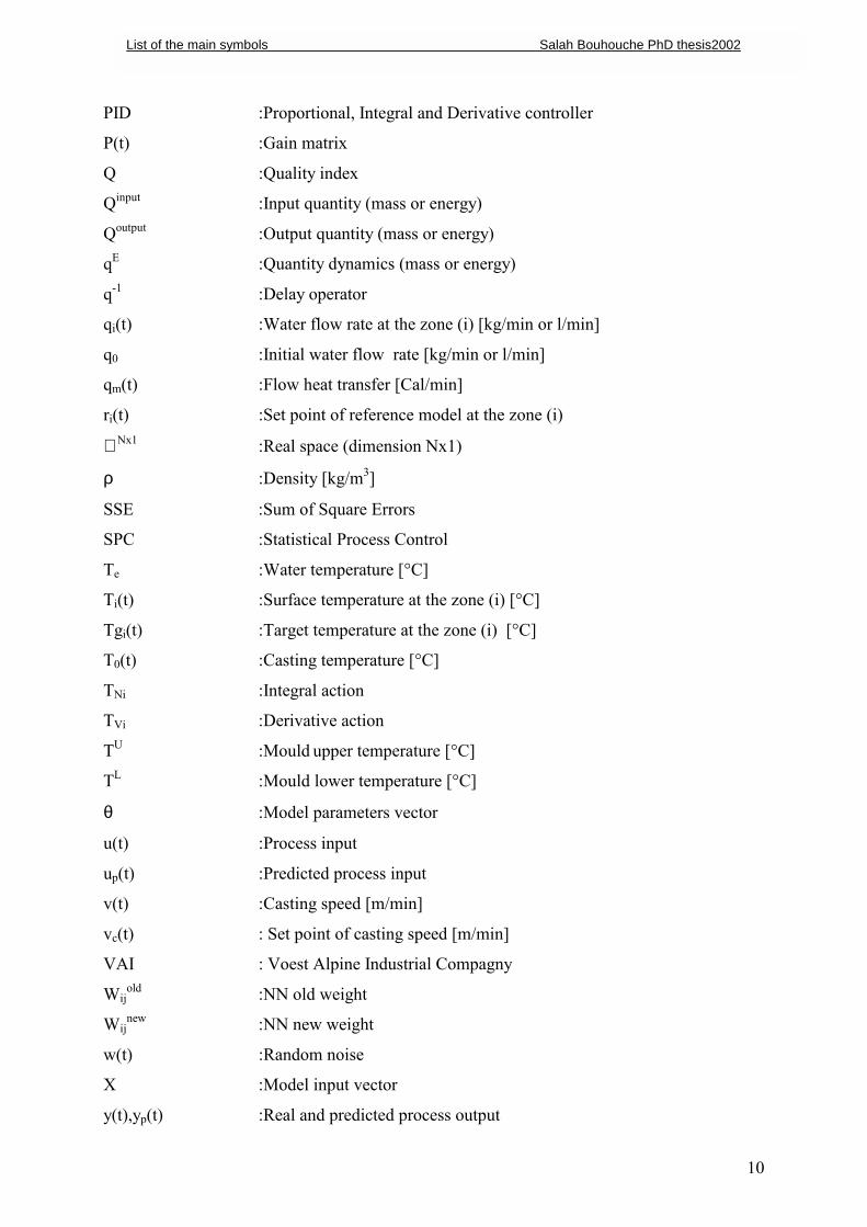
PID :Proportional, Integral and Derivative controller

P(t) :Gain matrix

Q :Quality index

Qinput :Input quantity (mass or energy)

Qoutput :Output quantity (mass or energy)

qE :Quantity dynamics (mass or energy)

q-1 :Delay operator

qi(t) :Water flow rate at the zone (i) [kg/min or l/min]

q0 :Initial water flow rate [kg/min or l/min]

qm(t) :Flow heat transfer [Cal/min]

ri(t) :Set point of reference model at the zone (i)

ℜ Nx1 :Real space (dimension Nx1)

ρ :Density [kg/m3]

SSE :Sum of Square Errors

SPC :Statistical Process Control

Te :Water temperature [°C]

Ti(t) :Surface temperature at the zone (i) [°C]

Tgi(t) :Target temperature at the zone (i) [°C]

T0(t) :Casting temperature [°C]

TNi :Integral action

TVi :Derivative action

TU :Mould upper temperature [°C]

TL :Mould lower temperature [°C]

θ :Model parameters vector

u(t) :Process input

up(t) :Predicted process input

v(t) :Casting speed [m/min]

vc(t) : Set point of casting speed [m/min]

VAI : Voest Alpine Industrial Compagny

Wijold :NN old weight

Wijnew :NN new weight

w(t) :Random noise

X :Model input vector

y(t),yp(t) :Real and predicted process output

List of the main symbols Salah Bouhouche PhD thesis2002

11

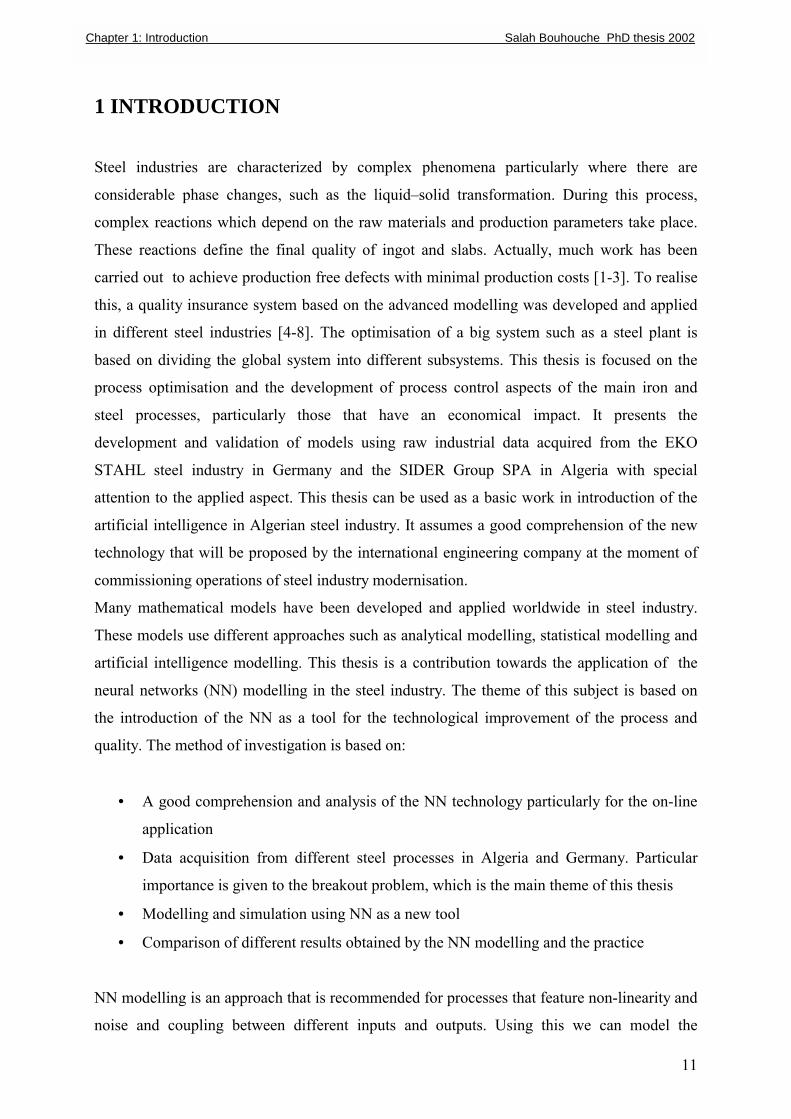
1 INTRODUCTION

Steel industries are characterized by complex phenomena particularly where there are

considerable phase changes, such as the liquid�solid transformation. During this process,

complex reactions which depend on the raw materials and production parameters take place.

These reactions define the final quality of ingot and slabs. Actually, much work has been

carried out to achieve production free defects with minimal production costs [1-3]. To realise

this, a quality insurance system based on the advanced modelling was developed and applied

in different steel industries [4-8]. The optimisation of a big system such as a steel plant is

based on dividing the global system into different subsystems. This thesis is focused on the

process optimisation and the development of process control aspects of the main iron and

steel processes, particularly those that have an economical impact. It presents the

development and validation of models using raw industrial data acquired from the EKO

STAHL steel industry in Germany and the SIDER Group SPA in Algeria with special

attention to the applied aspect. This thesis can be used as a basic work in introduction of the

artificial intelligence in Algerian steel industry. It assumes a good comprehension of the new

technology that will be proposed by the international engineering company at the moment of

commissioning operations of steel industry modernisation.

Many mathematical models have been developed and applied worldwide in steel industry.

These models use different approaches such as analytical modelling, statistical modelling and

artificial intelligence modelling. This thesis is a contribution towards the application of the

neural networks (NN) modelling in the steel industry. The theme of this subject is based on

the introduction of the NN as a tool for the technological improvement of the process and

quality. The method of investigation is based on:

• A good comprehension and analysis of the NN technology particularly for the on-line

application

• Data acquisition from different steel processes in Algeria and Germany. Particular

importance is given to the breakout problem, which is the main theme of this thesis

• Modelling and simulation using NN as a new tool

• Comparison of different results obtained by the NN modelling and the practice

NN modelling is an approach that is recommended for processes that feature non-linearity and

noise and coupling between different inputs and outputs. Using this we can model the

Chapter 1: Introduction Salah Bouhouche PhD thesis 2002

12

analytical and logical law together. This is very complex to achieve using other modelling

approaches such as statistical or physical methods.

In practice, generally a complete package of models called hybrid models is used. This

involves a combination of many approaches for each situation. In this thesis the application of

NN modelling to the breakout prediction is relatively new. This model is the basis for a

software development equivalent to the ones developed by different companies in Asia and

Europe such as Nippon Steel. More details will be given in chapter 4. The introduction of the

computerised process monitoring and fault detection is a new approach for SIDER Group,

Algeria. This approach allows to detect rapidly the source of defects which are monitored in

real-time. The implementation of this approach is of great importance for the maintenance

service that uses this as a tool of investigation.

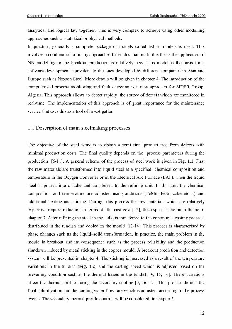
1.1 Description of main steelmaking processes

The objective of the steel work is to obtain a semi final product free from defects with

minimal production costs. The final quality depends on the process parameters during the

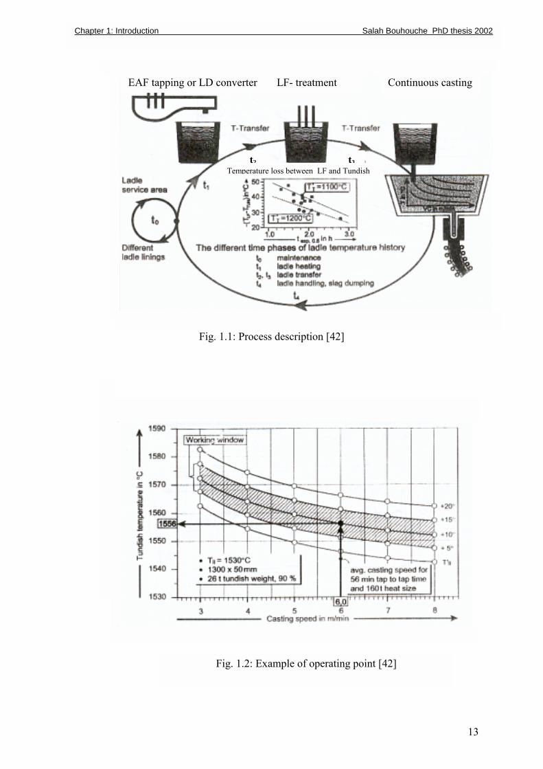
production [6-11]. A general scheme of the process of steel work is given in Fig. 1.1. First

the raw materials are transformed into liquid steel at a specified chemical composition and

temperature in the Oxygen Converter or in the Electrical Arc Furnace (EAF). Then the liquid

steel is poured into a ladle and transferred to the refining unit. In this unit the chemical

composition and temperature are adjusted using additions (FeMn, FeSi, coke etc�) and

additional heating and stirring. During this process the raw materials which are relatively

expensive require reduction in terms of the cast cost [12], this aspect is the main theme of

chapter 3. After refining the steel in the ladle is transferred to the continuous casting process,

distributed in the tundish and cooled in the mould [12-14]. This process is characterised by

phase changes such as the liquid�solid transformation. In practice, the main problem in the

mould is breakout and its consequence such as the process reliability and the production

shutdown induced by metal sticking in the copper mould. A breakout prediction and detection

system will be presented in chapter 4. The sticking is increased as a result of the temperature

variations in the tundish (Fig. 1.2) and the casting speed which is adjusted based on the

prevailing condition such as the thermal losses in the tundish [9, 15, 16]. These variations

affect the thermal profile during the secondary cooling [9, 16, 17]. This process defines the

final solidification and the cooling water flow rate which is adjusted according to the process

events. The secondary thermal profile control will be considered in chapter 5.



Fig. 1.1: Process description [42]

EAF tapping or LD converter Continuous castingLF- treatment

F

Temperature loss between LF and Tundisht2 t3

ig. 1.
2: Example of operatin
13

g point [42]

14

The monitoring of defects in slab and ingot due to variations of process parameters is an

important tool in reducing the management cost and a guarantee of the product quality [18,

19, 20]. Chapter 6 presents an application of Neural Network (NN) to predict fault detection

on the power control equipment of casting speed. This problem has led to many shutdowns in

order to find out the cause of the defects. The problem was solved using real-time data for

monitoring and process diagnosis methods. An alarm model has been developed and

implemented to predict the similar fault.

1.2 Problem statement and objectives

The objective of this study was to investigate the possibilities to improve the practical

operating conditions in steel works using mathematical models. As defined in section 1.1,

steelmaking is a complex process and it is necessary to develop some tools to optimise the

process with respect to chemical composition and temperature in the refining unit, controlled

solidification in the mould, secondary cooling and final quality monitoring and defect

detection. Many mathematical models have been developed in the field of steelmaking. These

models are based generally on the theoretical aspects and calibrated using experimental data

[1, 2, 9, 14, 21-23]. Thus modelling approach is generally oriented in the field of the design

and off-line simulation. From the on-line and real-time implementation point of view, this

modelling approach is considered to be long. Sometimes for achieving this, it is necessary to

synchronise the computer and units to reduce the computing time [24-25]. Another type of the

modelling today expended in the steel industry is based on neural networks [26-45].

Most models for processing steel in the steel industry are to predict the process output

parameters such as tapping temperature and chemical composition as a function of other

parameters. Unfortunately the �conventional� approach, based on energy and mass balances

by solving the physical and chemical equations, is very difficult, mainly because it does not

consider some parameters (raw materials characteristics etc.), and the non�linear interactions

between inputs and outputs. The use of neural networks for modelling can solve this problem

[46-50]. First, only the phenomena at the end of the process were modelled. The dynamic

follow up of the process is performed by a series of interconnected multi-layer perceptions,

which are �activated� at predefined moments during the process elaboration. This work seeks

to develop an approach to optimise different processes using mathematical modelling based

particularly on a new modelling strategy such as neural networks and its applications to the

modelling and optimisation using the appropriate data base [50-64]. In the ladle treatment


15

process, it considers the modelling and the optimisation of additions because the inputs are

generally costly. This process permits to obtain the target chemical composition and

temperature at minimal cost. The monitoring of the first solidification in the mould is

achieved by the development of new breakout detection and prediction system and the

breakout problem is modelled using neural networks [37, 42, 65-68]. This approach based on

the use of a real breakout database from EKO STAHL reduces the false alarm number

comparatively to the conventional system [37, 42, 68]. An optimal modelling and detection of

this phenomenon reduces the shutdown time and the cost of maintaining the equipment. A

neural closed loop control model is considered to achieve a stable surface temperature of the

secondary cooling profile according to the casting events such as variations of casting speed,

tundish temperature and its influence on heat transfer and slab quality particularly for

sensitive steel grades [1, 9, 15-16, 18, 24, 42, 69]. Prediction and monitoring of the product

quality has an important influence on the global production cost. A soft sensor using the steel

work database was developed [42, 70-74]. Particular importance is given to the analysis of the

relationship between the dynamics of process parameters and the defect apparition on the final

product. The analysis and modelling of the main data bank assumes the prediction and the

monitoring of the faults and their effect on the slab quality. Alarms are set forth when a fault

or defect is predicted and the necessary correction and adaptation will be achieved [68, 73,

75-76].

In this thesis the followings aspects have been developed:

• Prediction of final chemical composition and the temperature of liquid steel in the

ladle as a function of additions, this constitutes a soft sensor. Prediction using neural

networks model achieves good results comparatively to the conventional model based

on analytical and statistical approach. This prediction is an important tool for

optimising the mass of additions and the temperature. Non-linearities, thermal losses

and noise are taken into account.

• Improvement of the breakout prediction system using neural networks is clearly

proven in chapter 4 using the EKO STAHL breakout database. False alarms generated

by the fluctuating temperatures in the copper mould are cancelled. These results are

obtained by experience from earlier databases based on real and false alarms. This

model takes into account breakout propagation in the space of the mould and in the

time according to the temperature variation.


16

• Closed loop stabilisation of surface temperature using conventional PID and neural

networks control algorithms are developed in chapter 5. This new closed loop control

achieves a stable surface temeprature. The control algorithm can be connected to the

different existing heat conduction models. Simulation results are carried out by a

simplified heat transfer model. The robustness of the control algorithm is tested using

some changes in the process parameters such as casting speed and water temperature.

• Quality monitoring and classification is developed in chapter 6 on the basis of the

importance of breakouts which is connected to the breakout detection system. This

technique achieves a classification of different defects according to different alarms

given by the breakout prediction system. For example a breakout detected by many

alarms achieves an important defect as compared to that detected only by one alarm.

This constitutes a guide tool for the quality classification. Fault detection is also

developed using a neural networks model. Conventional modelling cannot establish a

complex non-linear relationship between alarm state (0-1) and historical dynamic

process parameters such as casting speed and motor current. This technique has been

applied at SIDER Group in Algeria. This allows to find out as soon as possible the

equipment defect using a real-time data acquisition system. The model is implemented

on the process computer using graphical programming by �Labview� software.


17

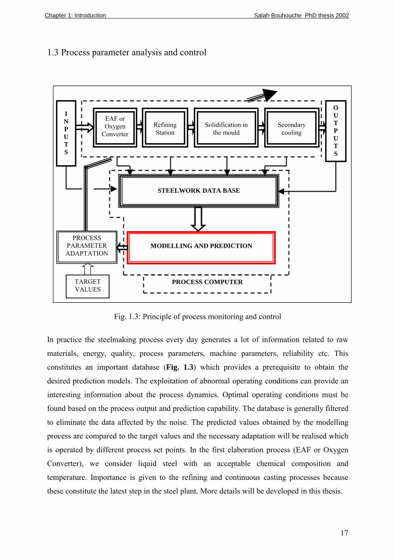
1.3 Process parameter analysis and control

Fig. 1.3: Principle of process monitoring and control

In practice the steelmaking process every day generates a lot of information related to raw

materials, energy, quality, process parameters, machine parameters, reliability etc. This

constitutes an important database (Fig. 1.3) which provides a prerequisite to obtain the

desired prediction models. The exploitation of abnormal operating conditions can provide an

interesting information about the process dynamics. Optimal operating conditions must be

found based on the process output and prediction capability. The database is generally filtered

to eliminate the data affected by the noise. The predicted values obtained by the modelling

process are compared to the target values and the necessary adaptation will be realised which

is operated by different process set points. In the first elaboration process (EAF or Oxygen

Converter), we consider liquid steel with an acceptable chemical composition and

temperature. Importance is given to the refining and continuous casting processes because

these constitute the latest step in the steel plant. More details will be developed in this thesis.


STEELWORK DATA BASE

MODELLING AND PREDICTION

PROCESS PARAMETER ADAPTATION

EAF or Oxygen

Converter

Refining Station

Solidification in

the mould

Secondary

cooling

TARGET VALUES

I N P U T S

OUTPUTS

PROCESS COMPUTER

18

Computer aided production management is an important skill today. In the major production

process, computerised management and control constitute an important tool to optimise

production and quality. The development of communication network has eased the expansion

of computerised production and optimisation, particularly for comprehensive systems where it

is necessary to undertake a distributed data processing [75-77]. The global process is divided

into many subsystems. Each sub-system is processed by its own algorithm and computer. The

data bank exchange between different sub-systems is carried out by the communication

network. Today, computer performance achieves real-time data processing and executes the

optimisation algorithm to reduce the production cost. The modelling of the input-output

interactions is an important tool for the research of the optimisation algorithm. This algorithm

allows an optimal adaptation of the control parameters to achieve the optimisation objective.

When the model for the inputs�outputs is defined around the operating point, the optimal

decision will be achieved by a closed loop called: �Loop of continuous amelioration�. The

continuous amelioration closed loop is a unified approach that may be applied to any system

or process. The computerised implementation seeks to implement this principle as a numerical

and logical model. The data processing can be realised in real-time or in off-line operation,

this depends on the calculation and the sampling time. Sometimes, different processes are

geographically dispatched, in this case the communication network is used to transfer data.

The process monitoring of critical parameters which has an important impact on the

production uses different methods of modelling such as neural networks. The data acquisition

is obtained by an analog to digital device for the measured process parameters and by the

specified terminal for other types of data and information. The local processing unit executes

the limited computing task such as the execution of the regulation algorithm (PI; PID) around

the set point. It is also considered in this part of sequential task. This doesn�t allow a long

computing time. The local processing considers the algorithm in the field of the binary and

sequential control and stabilisation of the process. The objective is to assume a stable control

loop. The host process computer that executes the optimisation algorithm gives the set points

with optimal values. In this case the local information is transferred to the host computer,

which has a sufficient computing capability. The production management computer, the

process computer and the local processing units are connected via network for exchange of

information. The network has a high transmission rate and noise rejection. All processing

units and terminals are inter-connected. Generally, the mathematical models are executed by

the process computer [14-15, 77-78].


19

2 MATHEMATICAL MODELLING

System and process are characterised by the complex interactions between the input and

output variables. There are many mathematical modelling approaches. In this thesis, particular

models are developed for easy application in the on-line control and optimisation.

Unfortunately, these systems are very complex by their structural and parameter changes such

as non-linearity and unsteady state behaviour [34, 44, 67, 79]. In these operating conditions,

conventional models such as linear modelling appear limited to achieve a high performance

for these processes. Hence, on-line adaptation according to the process parameter changes

must be performed [79-87]. Another aspect related to models validation must be considered

since physico-chemical models based on energy and mass balances feature some difficulties

on the validation using the measurement data. Sometimes, it is difficult to find the optimal

values of the physical parameters assuming a minimal error between the model and the

measurement; this reduces the precision of modelling. Models based on the identification

techniques particularly those using neural networks improve the prediction by reducing the

modelling error. This approach uses direct raw data. This process allows us to define inputs

and outputs of the model. Multilayered neural networks fit the non-linear Multi-Input and

Multi-Output Process (MIMO). Process interactions are taken into account by the

interconnectivity of the neurones between different hidden layers [87-97]. The aim of this

section is to review the different modelling methods and control using mathematical

modelling. Particular importance is given to the NN approach.

2.1 Conventional modelling

The importance of conventional modelling is particularly its use for the design and off-line

simulation. On-line implementation of this modelling approach is particularly limited by its

long computing time. To reduce this, it is sometimes necessary to use special computing

techniques.

Generally, the conventional modelling is based on energy and mass balances. The steady state

balance can be obtained by the following equation: output

iinput

i tQtQ )()( = (2.1)

and the dynamic equilibrium conditions can be written as: output

iinput

iEi tQtQtq )()()( −=∆ (2.2)

Chapter 2: Mathematical modelling Salah Bouhouche PhD thesis 2002

20

Equations (2.1) and (2.2) are valid for the mass and energy balances.

)...)(),(),...,(),(,()( 1 ttytyttututftQ iiiiiinput

i ∆−∆−= (2.3)

)...)(),(),...,(),(,()( 2 ttytyttututftQ iiiiioutput

i ∆−∆−= (2.4)

)...)(),(),(),(,()( 3 ttytyttututftq iiiiiEi ∆−∆−= (2.5)

The differential analysis of different equations gives a non-linear differential system. In the

linear case, these equations will be linearised around the operating point of each variable. The

linearisation process induces inevitably model precision losses. The numerical

implementation is obtained by a discretisation of the differential operator defined by the

following approximation

)()()( ttqtqtq Ei

Ei

Ei ∆−−≈∆ (2.6)

∆t is the sampling time. After transformation we obtain a recurrent model defined by:

0)....)(),(),...,(),(,( =∆−∆− ttytyttututF iiii (2.7)

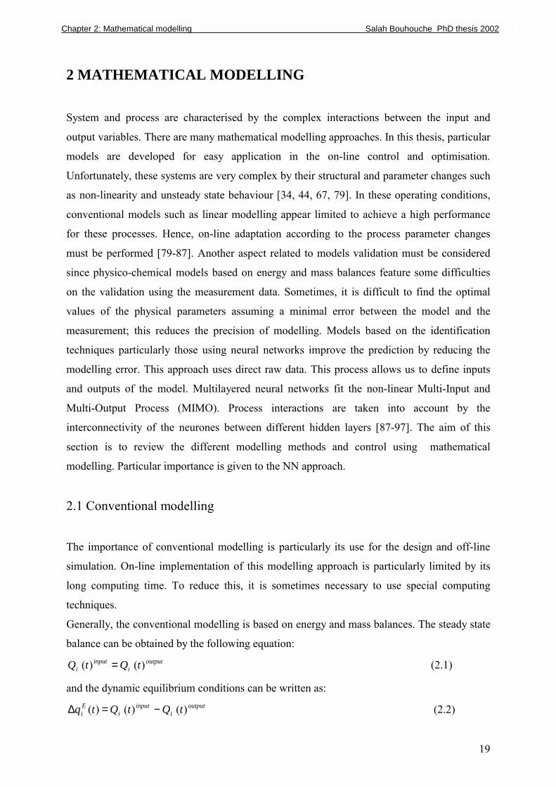
Fig. 2.1 defines the structure and the interactions between different process variables.

Fig. 2.1: Process model structure

t, ui(t), wi(t) and yi(t) are the time, process inputs, disturbance and process outputs

respectively, wi(t) is a random perturbation.

Process Model ui(t) yi(t)

wi(t)


2.1.1 Identification models [48, 88, 98-100]

The conventional identification technique permits to find the process parameter vector using

the minimum least square error between the process output and model output according to the

dynamical data. We consider a process with dynamic output and exogenous input; this model

is called Autoregressive Moving Average with eXogenous inputs (ARMAX). Each predicted

output can be written as:

)()()()()()( 111 twqCtuqBtyqA −−− += (2.8) n

n qaqaqaqA −−−− ++++= ...)1)( 22

11

1 (2.9)

mmqbqbqbbqB −−−− ++++= ...)( 2

21

101 (2.10)

p

p qcqcqccqC −−−− ++++= ...))( 22

110

1 (2.11)

n, m and p is the differentiation order for the output, the input and the exogenous input

respectively which are defined according to the process dynamics.

The objective is to find optimal values of the process parameters using a least square

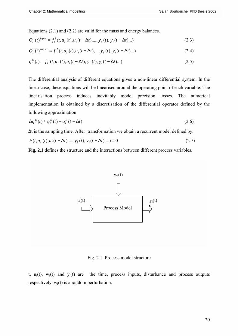
algorithm. The principle of identification is given by the scheme below (Fig. 2.2).

Fig. 2.2: Model identification principle

From equation (2.8 ), the model output can be written as:

Real Process

Process Model

yp(t)

y(t)


Error e(t)

u(t)

w(t)

21

22

)1()()( −= ttXty T θ (2.12)

with: TptwtwmtutuntytytytX )](),...,1(),(),...,1(),(),...,2(),1([)( −−−−−−−= (2.13)

Tpmn cccbbaaat ],...,,,,...,,,...,,[)( 21121=θ (2.14)

The prediction error can be defined as:

)1()()()( −−= ttXtyte Tp θ (2.15)

The identification objective is to find the process parameters that minimise the sum of errors

e(t).

optimal

t

ktkeJMin )(})({}{

0θ⇒= ∑

=

(2.16)

The following form gives the recursive estimation of vector parameters:

)()()()1()( tetXtPtt +−=θθ (2.17)

where:

−+

−−−−=)()1()()()1()()()1()1(

)(1)(

tXtPtXttPtXtXtPtP

ttP T

T

λλ (2.18)

The forgetting factor λ(t) is usually computed according to the rule

λ(t)=λ0λ(t-1)+1-λ0 (2.19)

P(0)=I/α, α<<1 (2.20)

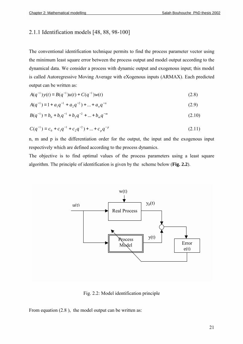
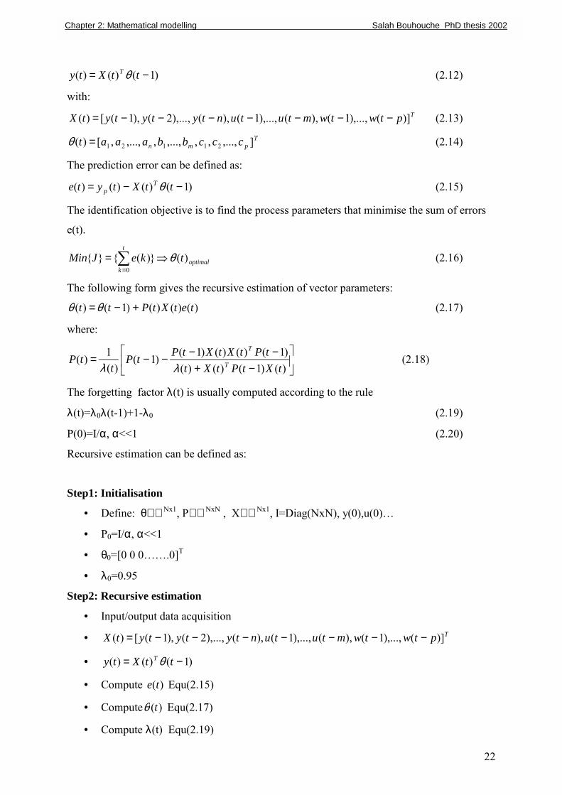
Recursive estimation can be defined as:

Step1: Initialisation

• Define: θ∈ℜ Nx1, P∈ℜ NxN , X∈ℜ Nx1, I=Diag(NxN), y(0),u(0)�

• P0=I/α, α<<1

• θ0=[0 0 0��.0]T

• λ 0=0.95

Step2: Recursive estimation

• Input/output data acquisition

• TptwtwmtutuntytytytX )](),...,1(),(),...,1(),(),...,2(),1([)( −−−−−−−=

• )1()()( −= ttXty T θ

• Compute )(te Equ(2.15)

• Compute )(tθ Equ(2.17)

• Compute λ(t) Equ(2.19)


23

• Compute )(tP Equ(2.18)

• Assign w(t)=e(t)

• If t=tmax: Go to step 3

• Else t=t+1 and Go to step 2

Step3: END

After the convergence of the identification algorithm, the estimated process parameters

θ(t)=θ0 are used to synthesise the control law, i. e, the PID tuning values.

2.1.2 Process control

Conventional or classic closed loop control is used for the process output stabilisation around

the set point. In the industry, generally, the Proportional Integral and Derivative (PID)

algorithm is used.

The identification results are used only for tuning the PID controller parameters in off-line.

Many conventional process control approaches based on linear modelling have been applied,

but they remain limited and don´t assume the necessary optimisation particularly for complex

processes with regard to:

• time variant process parameters

• models with high non-linearities

• It is more important when the optimisation objective is based on the prediction of the

product characteristics that are not directly measured by sensors but determined by

quality classification (defect, type and importance of the defects). In this situation

advanced approach of the production database analysis and modelling must be

considered.

2.2 Neural network modelling [48, 90-102]

Advanced process control and monitoring require accurate process models. The development

of analytical models from the relevant physical and chemical knowledge, especially complex

processes with phase changes, can be too costly or even impossible. For such process models

based on process production operational data should be capitalised. Many industrial processes

exhibit non-linear dynamic behaviour and non-linear models should be developed. Neural


networks have been shown to be able to approximate continuous non-linearity and have been

applied to non-linear and complex process modelling. Network training results in a �Black

Box� representation in which the model developed can be difficult to be analysed. The

complexity is due to the large number of network weights. In practice, many non-linear

processes are approximated by reduced order models, possibly linear, which are clearly

related to the underlying process characteristics.

2.2.1 Neural network identification and modelling

2.2.1.1 Problem formulation and back-propagation learning

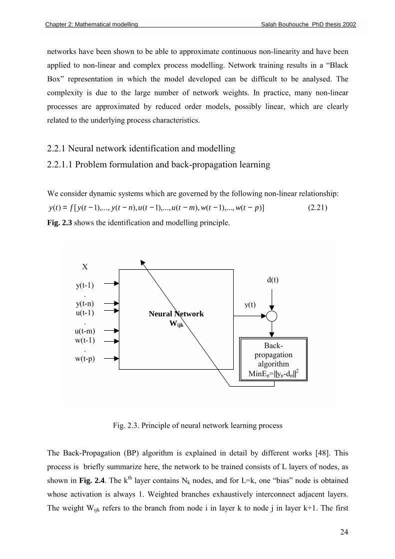
We consider dynamic systems which are governed by the following non-linear relationship:

)](),...,1(),(),...,1(),(),...,1([)( ptwtwmtutuntytyfty −−−−−−= (2.21)

Fig. 2.3 shows the identification and modelling principle.

Fig. 2.3. Principle of neural network learning p

The Back-Propagation (BP) algorithm is explained in detail by

process is briefly summarize here, the network to be trained cons

shown in Fig. 2.4. The kth layer contains Nk nodes, and for L=k, o

whose activation is always 1. Weighted branches exhaustively in

The weight Wijk refers to the branch from node i in layer k to no

Neural Network

Wijk

pra

Min

y

yu

u w

w

d(t)


Back-opagation lgorithm Ep=||yp-dp||2

X

(t-1) .

(t-n) (t-1)

. (t-m)(t-1) .

(t-p)

y(t)

24

rocess

different works [48]. This

ists of L layers of nodes, as

ne �bias� node is obtained

terconnect adjacent layers.

de j in layer k+1. The first

25

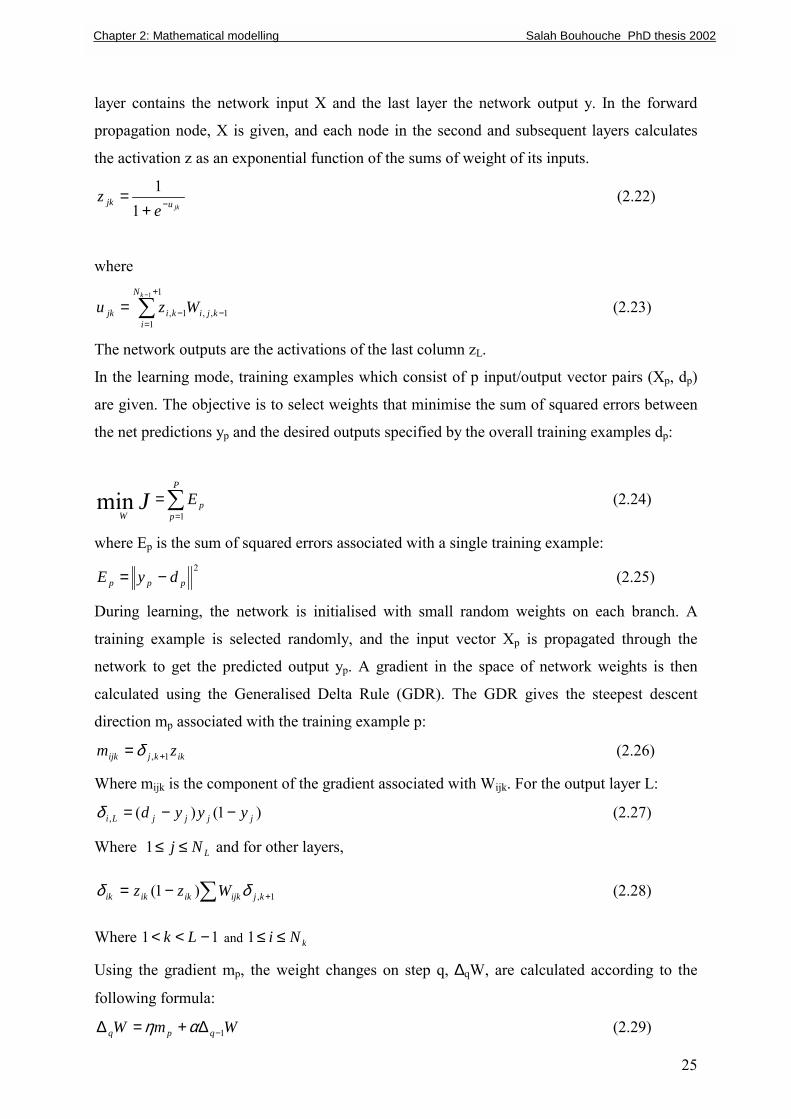
layer contains the network input X and the last layer the network output y. In the forward

propagation node, X is given, and each node in the second and subsequent layers calculates

the activation z as an exponential function of the sums of weight of its inputs.

jkujke

z −+=

11

(2.22)

where

∑+

=−−

−

=1

11,,1,

1kN

ikjikijk Wzu (2.23)

The network outputs are the activations of the last column zL.

In the learning mode, training examples which consist of p input/output vector pairs (Xp, dp)

are given. The objective is to select weights that minimise the sum of squared errors between

the net predictions yp and the desired outputs specified by the overall training examples dp:

∑=

=P

pp

WEJ

1min (2.24)

where Ep is the sum of squared errors associated with a single training example: 2

ppp dyE −= (2.25)

During learning, the network is initialised with small random weights on each branch. A

training example is selected randomly, and the input vector Xp is propagated through the

network to get the predicted output yp. A gradient in the space of network weights is then

calculated using the Generalised Delta Rule (GDR). The GDR gives the steepest descent

direction mp associated with the training example p:

ikkjijk zm 1, +=δ (2.26)

Where mijk is the component of the gradient associated with Wijk. For the output layer L:

)1()(, jjjjLi yyyd −−=δ (2.27)

Where LNj ≤≤1 and for other layers,

∑ +−= 1,)1( kjijkikikik Wzz δδ (2.28)

Where 11 −<< Lk and kNi ≤≤1

Using the gradient mp, the weight changes on step q, ∆qW, are calculated according to the

following formula:

WmW qpq 1−∆+=∆ αη (2.29)


26

In this expression two constants appear, η called the learning rate which is equivalent to a step

size, and α which acts as a momentum term to keep the direction of descent from changing

too rapidly from step to step. After the weights have been updated, a new training example is

selected and the procedure is repeated until satisfactory reduction of the objective function is

achieved.

Fig. 2.4: Neural network architecture and weight indexing

2.2.1.2 Learning algorithm

The following computing steps constitute the learning algorithm:

Step1: Initialisation of the network weights

Step2: Learning process

• Acquisition of inputs/outputs

• Compute the model output equ(2.22, 2.23)

• Compute the errors equ(2.26, 2.27, 2.28)

• If Ep<<1, save weights go to step3

• Else adapt the network weights equ(2.29) and go to step2

step3: END


2.2.2 Neural process control

Neural network is a tool used to describe the input/output relationship and the first step is to

use the NN to identify the process model. Many techniques were developed for application in

the field of control and optimisation design. The objective is to obtain optimal control inputs

that minimise the sum of quadratic error between the desired outputs on the one hand and

predicted output on the other hand. Several training and control methods have been developed

[48, 101-108]. Assuming that the system to be controlled can be described by equation (2.21),

the desired network is the one that isolates the most recent control input u(t),

)]1(),...,(),1(),...,1(),1(),...,1([)( 1 +−+−−+−+= − ptwtwmtutuntytyftu pp (2.30)

and can be used for controlling the process by substituting the output at time t+1 by the

desired output r(t+1).

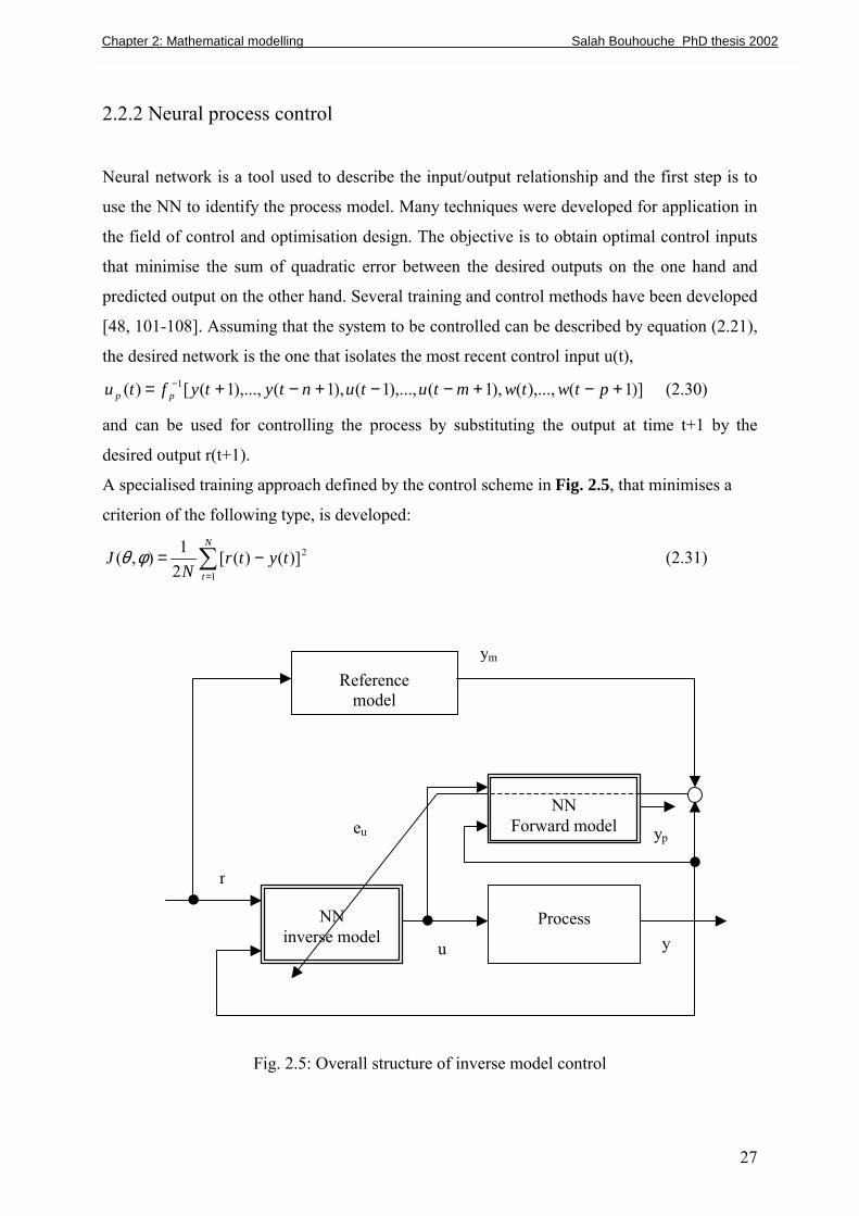
A specialised training approach defined by the control scheme in Fig. 2.5, that minimises a

criterion of the following type, is developed:

∑=

−=N

ttytr

NJ

1

2)]()([21),( φθ (2.31)

Fig. 2.5: Overall

Refem

NN

inverse mod

r

eu

m


rence

odel

NN

Forward model yp

structure

Process

el y
u
of inv

y

27

erse model control

28

Inspired by the recursive training algorithms the network might alternatively be trained to

minimise the relation 2

1 )]()([)1(,())(,( tytrtJtJ tt −+−= − φθφθ (2.32)

This is an on-line approach and therefore the scheme constitutes an adaptive controller. By

way of introduction, a recursive gradient method is considered. Assuming that Jt-1 has already

been minimised, the weights are adjusted at time t according to the following formula:

θµθθ

dtdett )()1()(

2

−−= , (2.33)

where e(t)=ym(t)-y(t), ym(t) is the reference model output [48] and

)()()(2

ted

tdyd

tdeθθ

−= (2.34)

By application of the chain rule the gradient θdtdy )(

can be calculated as

θθ dtdu

tuty

dtdy )1(

)1()()( −

−∂∂= (2.35)

−−∂−∂+−

−∂−∂+

∂−∂

−∂∂= ∑∑

== θθθ ditdu

itutu

ditdy

itytutu

tuty m

i

n

i

)()()1()(

)()1()1(

)1()(

21 (2.36)

It appears that the Jacobeans [48] of the system, θ∂

∂ )(ty, are required. These are generally

unknown since the system is unknown. To overcome this problem an estimation is given as

follows:

)1()(

)1()(

−∂∂

≅−∂

∂tu

tytu

ty p (2.37)

The (simplified) specialised training can easily be implemented with the back-propagation

algorithm. The back-propagation algorithm is used in the inverse model by assuming the

following �virtual� error of the output of the controller:

)()1(

)()( te

tuty

te pu −∂

∂= (2.38)

The on-line specialised control algorithm is summarised by the followings steps:

Step1: Data acquisition

• Read input/output data from the process

Step2: Control law computing

• Calculate the tracking error

• Calculate the virtual error


• Update weights with recursive form equ(2.29)

Step3: Go to step1

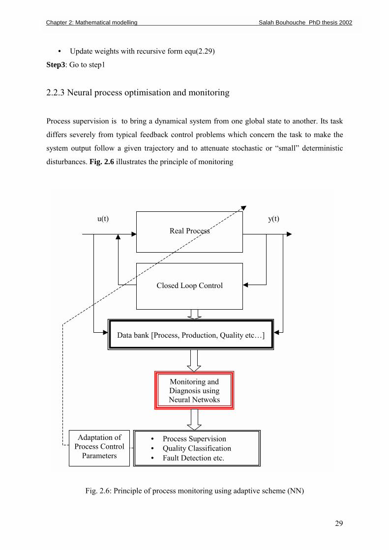
2.2.3 Neural process optimisation and monitoring

Process supervision is to bring a dynamical system from one global state to another. Its task

differs severely from typical feedback control problems which concern the task to make the

system output follow a given trajectory and to attenuate stochastic or �small� deterministic

disturbances. Fig. 2.6 illustrates the principle of monitoring

Fig. 2.6: Principle of proc

Real Process

Closed Loop Control

Data bank [Process, Production, Quality etc�]

• P• Q• F

u(t) y(t)

Adaptation of Process Control

Parameters


Monitoring and Diagnosis using Neural Netwoks

29

ess monitoring using adaptive scheme (NN)

rocess Supervision uality Classification ault Detection etc.

3 MODELLING OF LADLE METALLURGICAL

TREATMENT PROCESSES

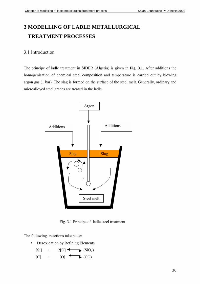
3.1 Introduction

The principe of ladle treatment in SIDER (Algeria) is given in Fig. 3.1. After additions the

homogenisation of chemical steel composition and temperature is carried out by blowing

argon gas (1 bar). The slag is formed on the surface of the steel melt. Generally, ordinary and

microalloyed steel grades are treated in the ladle.

The following

• Desox

[Si]

[C]

Chapter 3: Modelling of ladle metallurgical treatment process Salah Bouhouche PhD thesis 2002

Additions

Argon

Additions

30

Fig. 3.1 Principe of ladle steel treatment

s reactions take place:

idation by Refining Elements

+ 2[O] (SiO2)

+ [O] (CO)

Slag Slag

Steel melt

31

2[Al] + 3[O] (Al2O3)

• Separation of Oxide Inclusions

Al2O3(Steel) Al2O3(Slag)

[Mn] + [S] (MnS)

[Ca] + [S] (CaS)

In steel industry, the refining process adjusts the final chemical composition and temperature

of liquid steel by adding the optimal quantity of additions and energy. Generally a

conventional charge calculation based on mathematical and thermodynamic models that

provide considerable help is used, but it is difficult to model the highly complex nature of the

interactions between process variables such as thermal losses and the dynamics of non-linear

chemical reactions. Neural networks are able to identify internal relationships through training

examples.

In this work, the application of identification models using linear approach and (NN) to

predict the final chemical composition and temperature of the refining process is considered

[48, 90, 100, 102]. Using an industrial process database, dynamics of complex reactions is

modelled using the back propagation-learning algorithm. This model is used as a charge

calculation to predict the final process parameters. The performance of the model is evaluated

from new inputs and outputs. Production and quality cost management is reduced by an

optimal control of the input variables such as the mass of additions (FeMn, FeSi and coke)

and heating energy.

The aim of this section is to predict the process output for an optimal control of the process.

This constitutes an important tool particularly for SIDER Group in Algeria where there are

some problems with chemical analysis. Our investigation is based on the modelling and

analysis of the database generated by this process. The main chemical reactions are the

oxidation of the iron and the adjustement of manganese (Mn), silicon (Si) and carbon (C)

contents in the liquid steel. Reactions are complex and depend particularly on the

thermodynamic parameters. The final chemical composition of steel is adjusted by an optimal

control of different input variables. In practice, sometimes the chemical reactions have not

reached equilibrum and further operations are required to obtain the desired contents and

temperature. These manipulations induce excess costs by an excess consumption of different

additions and energy. Conventional charge calculations don´t take into account different non-

linear and random process changes. In this work an approach is considered based on NN to

model the complex input and output relationships. Modelling of real process databases


considers different noise measurements, non-linearity of process and other complex properties

[48, 109-112]. High prediction ability of the NN model improves the casting cycle and

reduces the cost quality analysis and management in the steel plant. Thus the model can be

used as a soft sensor. In our case the process inputs and outputs are defined as:

Input parameters:

• Different masses of additions (coke, FeMn, FeSi)

• Thermodynamic parameters (steel temperature)

• Initial chemical composition of liquid steel

Output parameters:

• Final liquid steel temperature or liquid steel temperature variation

• Final chemical composition or variation of chemical composition

All input and output data are used to define the NN parameters using the back-propagation

algorithm that reduces the error between the target values and NN outputs. After convergence,

the NN is used to predict the outputs using a new input database. The obtained model is used

to compute the input according to the target outputs, i .e, liquid steel temperature and the final

chemical composition.

3.2 Process description

FeMn

FeSi

Energy

Coke

Opt

CS


Inputs imisation

Neural networks prediction model C0, Mn0,

Si0, T0

, Mn, i, T

e

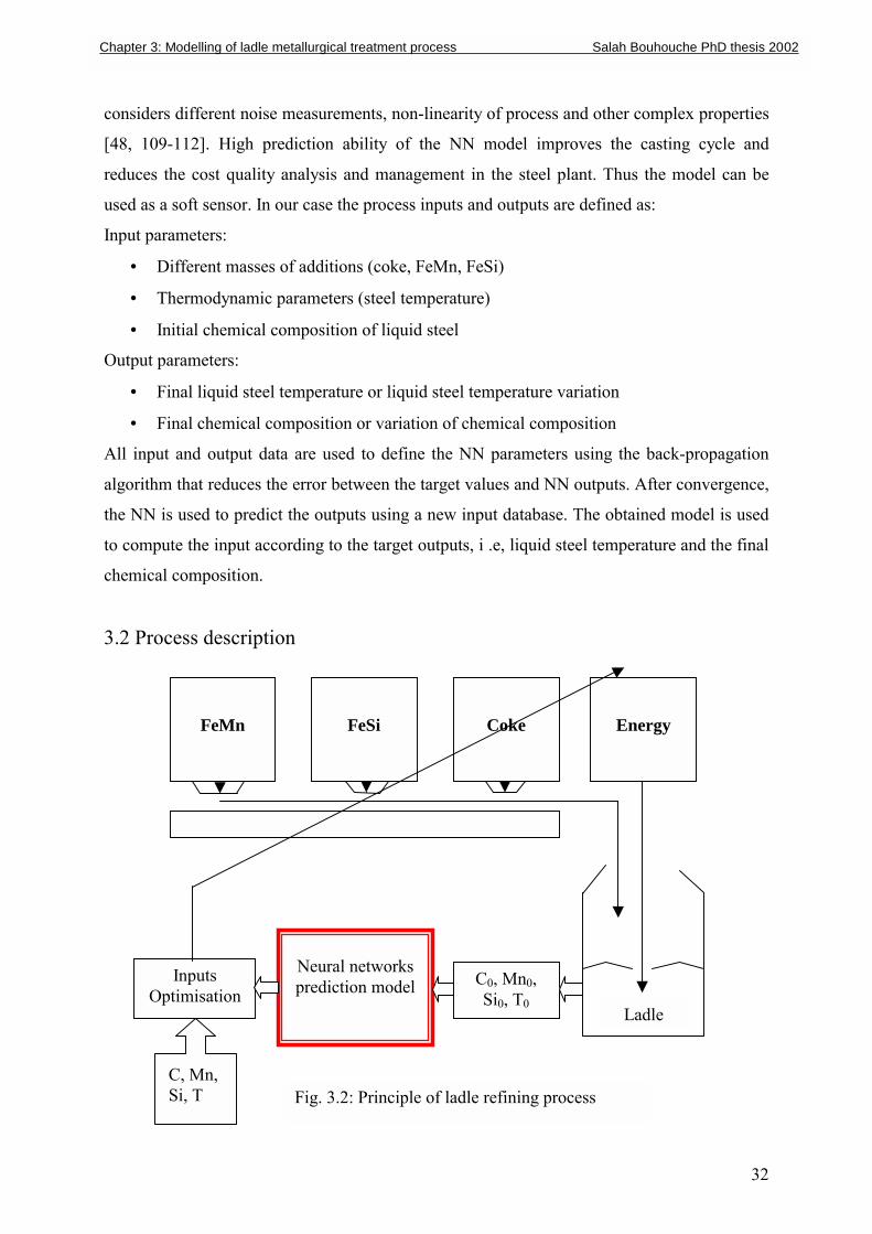
Fig. 3.2: Principle of ladle refining process

Ladl

32

33

The principle of the refining process is given in Fig. 3.2. The ladle with liquid steel arrives in

the refining station with the initial chemical composition and temperature. According to these

initial values and the desired chemical composition and temperature, optimal quantities of

additions (coke, FeMn, FeSi) are applied.

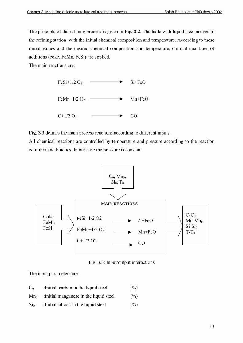
The main reactions are:

FeSi+1/2 O2 Si+FeO

FeMn+1/2 O2 Mn+FeO

C+1/2 O2 CO

Fig. 3.3 defines the main process reactions according to different inputs.

All chemical reactions are controlled by temperature and pressure according to the reaction

equilibra and kinetics. In our case the pressure is constant.

Fig. 3.3: Input/output interactions

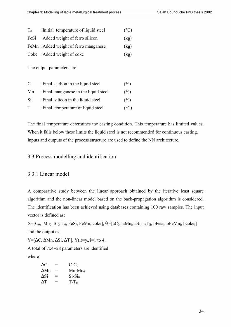
The input parameters are:

C0 :Initial carbon in the liquid steel (%)

Mn0 :Initial manganese in the liquid steel (%)

Si0 :Initial silicon in the liquid steel (%)

MAIN REACTIONS FeSi+1/2 O2 FeMn+1/2 O2 C+1/2 O2

Coke FeMn FeSi

C-C0 Mn-Mn0 Si-Si0 T-T0

C0, Mn0, Si0, T0

Si+FeO Mn+FeO CO


34

T0 :Initial temperature of liquid steel (°C)

FeSi :Added weight of ferro silicon (kg)

FeMn :Added weight of ferro manganese (kg)

Coke :Added weight of coke (kg)

The output parameters are:

C :Final carbon in the liquid steel (%)

Mn :Final manganese in the liquid steel (%)

Si :Final silicon in the liquid steel (%)

T :Final temperature of liquid steel (°C)

The final temperature determines the casting condition. This temperature has limited values.

When it falls below these limits the liquid steel is not recommended for continuous casting.

Inputs and outputs of the process structure are used to define the NN architecture.

3.3 Process modelling and identification

3.3.1 Linear model

A comparative study between the linear approach obtained by the iterative least square

algorithm and the non-linear model based on the back-propagation algorithm is considered.

The identification has been achieved using databases containing 100 raw samples. The input

vector is defined as:

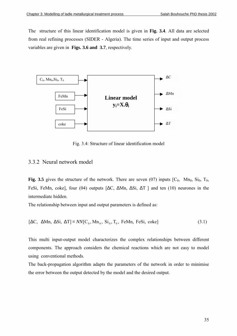
X=[C0, Mn0, Si0, T0, FeSi, FeMn, coke], θi=[aC0i, aMni, aSii, aT0i, bFesii, bFeMni, bcokei]

and the output as

Y=[∆C, ∆Mn, ∆Si, ∆T ], Y(i)=yi, i=1 to 4.

A total of 7x4=28 parameters are identified

where

∆C = C-C0 ∆Mn = Mn-Mn0 ∆Si = Si-Si0 ∆T = T-T0


35

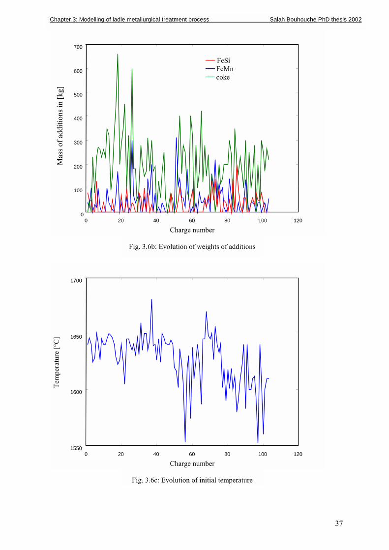
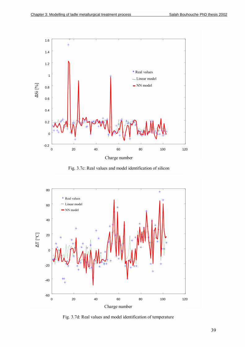
The structure of this linear identification model is given in Fig. 3.4. All data are selected

from real refining processes (SIDER - Algeria). The time series of input and output process

variables are given in Figs. 3.6 and 3.7, respectively.

Fig. 3.4: Structure of linear identification model

3.3.2 Neural network model

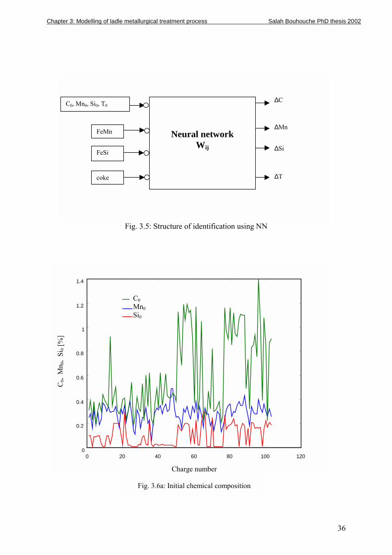
Fig. 3.5 gives the structure of the network. There are seven (07) inputs [C0, Mn0, Si0, T0,

FeSi, FeMn, coke], four (04) outputs [∆C, ∆Mn, ∆Si, ∆T ] and ten (10) neurones in the

intermediate hidden.

The relationship between input and output parameters is defined as:

coke] FeSi, FeMn, ,T ,Si ,Mn ,C[T] Si, Mn, C,[ 0000NN=∆∆∆∆ (3.1)

This multi input-output model characterizes the complex relationships between different

components. The approach considers the chemical reactions which are not easy to model

using conventional methods.

The back-propagation algorithm adapts the parameters of the network in order to minimise

the error between the output detected by the model and the desired output.

Linear model yi=X.θθθθi

C0, Mn0,Si0, T0

FeMn

FeSi

coke

∆C

∆Mn

∆Si

∆T


36

Fig. 3.5: Structure of identification using NN

Neural network Wij

C0, Mn0, Si0, T0

FeMn

FeSi

coke

∆C

∆Mn

∆Si

∆T

0 20 40 60 80 100 120 0

0.2

0.4

0.6

0.8

1

1.2

1.4

C0,

Mn 0

, Si

0 [%

]

Charge number

Fig. 3.6a: Initial chemical composition

C0 Mn0 Si0


37

0 20 40 60 80 100 120 0

100

200

300

400

500

600

700

FeSi FeMn coke

Charge number

Fig. 3.6b: Evolution of weights of additions

Mas

s of a

dditi

ons i

n [k

g]

0 20 40 60 80 100 120 1550

1600

1650

1700

Charge number

Fig. 3.6c: Evolution of initial temperature

Tem

pera

ture

[°C

]


38

0 20 40 60 80 100 120 -0.2

-0.15

-0.1

-0.05

0

0.05

0.1

0.15

0.2

0.25

0.3 ∆C

[%]

Charge number

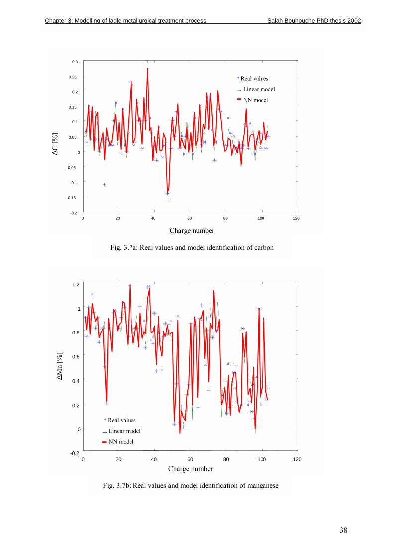
Fig. 3.7a: Real values and model identification of carbon

* Real values

Linear model

NN model

0 20 40 60 80 100 120 -0.2

0

0.2

0.4

0.6

0.8

1

1.2

∆Mn

[%]

Charge number

Fig. 3.7b: Real values and model identification of manganese

* Real values

Linear model

NN model


39

0 20 40 60 80 100 120 -0.2

0

0.2

0.4

0.6

0.8

1

1.2

1.4

1.6

Charge number

Fig. 3.7c: Real values and model identification of silicon

∆Si [

%]

* Real values

Linear model

NN model

0 20 40 60 80 100 120 -60

-40

-20

0

20

40

60

80

∆T [°

C]

Charge number

Fig. 3.7d: Real values and model identification of temperature

* Real values

Linear model

NN model


40

0 20 40 60 80 100 120 -0.2

-0.15

-0.1

-0.05

0

0.05

0.1

0.15

C

arbo

n er

ror [

%]

Charge number

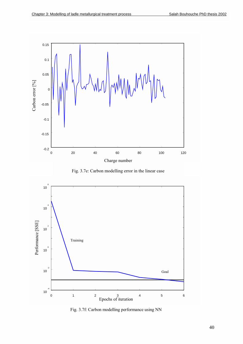
Fig. 3.7e: Carbon modelling error in the linear case

0 1 2 3 4 5 6 10

-4

10 -2

10 0

10 2

10 4

10 6

Epochs of iteration

Fig. 3.7f: Carbon modelling performance using NN

Perf

orm

ance

[SSE

]

Training

Goal


41

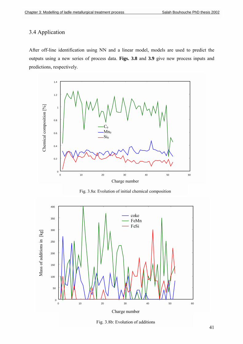
3.4 Application

After off-line identification using NN and a linear model, models are used to predict the

outputs using a new series of process data. Figs. 3.8 and 3.9 give new process inputs and

predictions, respectively.

0 10 20 30 40 50 60 0

0.2

0.4

0.6

0.8

1

1.2

1.4

C0

Mn0 Si0

Chem

ical

com

posi

tion

[%]

Charge number

Fig. 3.8a: Evolution of initial chemical composition

0 10 20 30 40 50 60 0

50

100

150

200

250

300

350

400

coke FeMn FeSi

Mas

s of a

dditi

ons i

n [k

g]

Charge number

Fig. 3.8b: Evolution of additions


42

0 10 20 30 40 50 60 -0.2

-0.15

-0.1

-0.05

0

0.05

0.1

0.15

∆C [%

]

Charge number

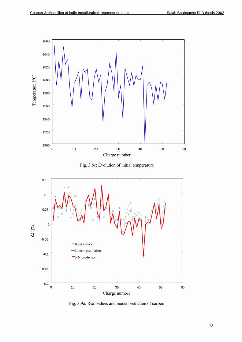
Fig. 3.9a: Real values and model prediction of carbon

* Real values

Linear prediction

NN prediction

0 10 20 30 40 50 60 1500

1520

1540

1560

1580

1600

1620

1640

1660

Charge number

Fig. 3.8c: Evolution of initial temperature

Tem

pera

ture

[°C

]


43

0 10 20 30 40 50 60 -0.2

0

0.2

0.4

0.6

0.8

1

1.2 ∆M

n [%

]

Charge number

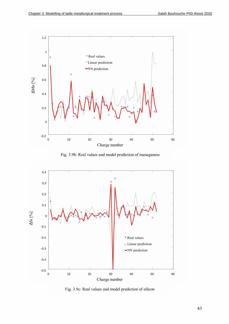
Fig. 3.9b: Real values and model prediction of managanese

* Real values

Linear prediction

NN prediction

0 10 20 30 40 50 60 -0.5

-0.4

-0.3

-0.2

-0.1

0

0.1

0.2

0.3

0.4

∆Si [

%]

Charge number

Fig. 3.9c: Real values and model prediction of silicon

* Real values

Linear prediction

NN prediction


44

0 10 20 30 40 50 60 -20

0

20

40

60

80

100

120

∆T [°

C]

Charge number

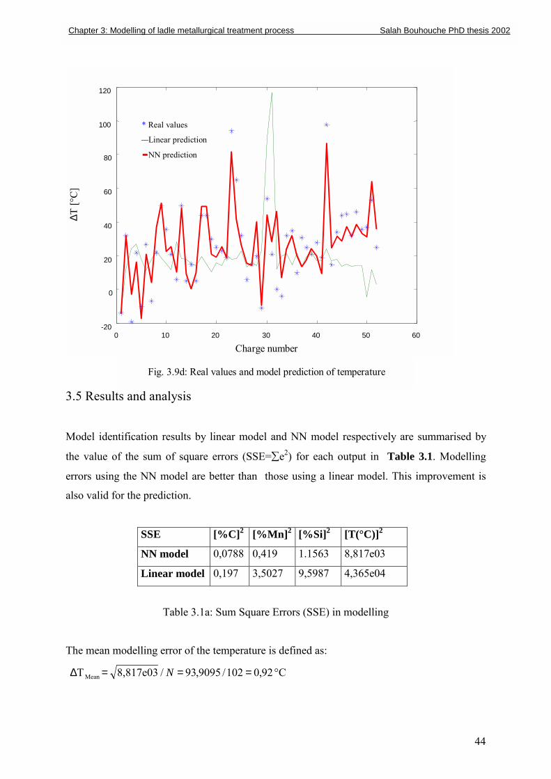
Fig. 3.9d: Real values and model prediction of temperature

* Real values

Linear prediction

NN prediction

3.5 Results and analysis

Model identification results by linear model and NN model respectively are summarised by

the value of the sum of square errors (SSE=∑e2) for each output in Table 3.1. Modelling

errors using the NN model are better than those using a linear model. This improvement is

also valid for the prediction.

SSE [%C]2 [%Mn]2 [%Si]2 [T(°C)]2

NN model 0,0788 0,419 1.1563 8,817e03

Linear model 0,197 3,5027 9,5987 4,365e04

Table 3.1a: Sum Square Errors (SSE) in modelling

The mean modelling error of the temperature is defined as:

92,0102/9095,93/8,817e03T Mean ===∆ N °C


45

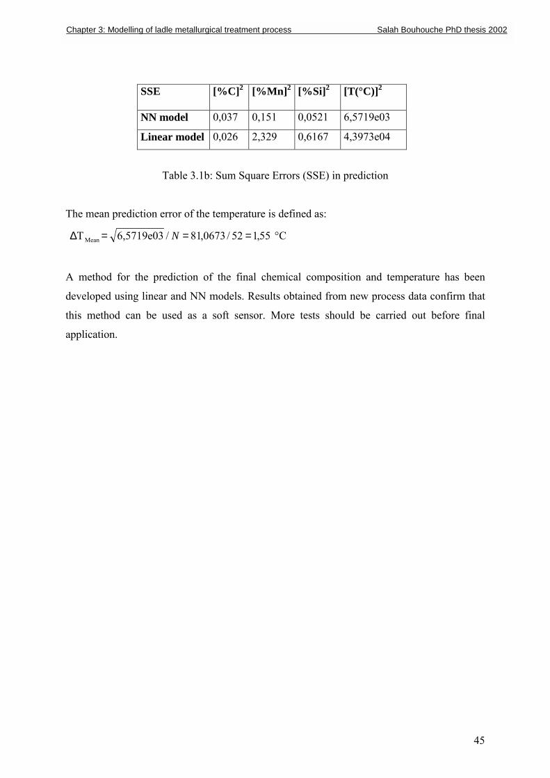
SSE [%C]2 [%Mn]2 [%Si]2 [T(°C)]2

NN model 0,037 0,151 0,0521 6,5719e03

Linear model 0,026 2,329 0,6167 4,3973e04

Table 3.1b: Sum Square Errors (SSE) in prediction

The mean prediction error of the temperature is defined as:

55,152/0673,81/6,5719e03T Mean ===∆ N °C

A method for the prediction of the final chemical composition and temperature has been

developed using linear and NN models. Results obtained from new process data confirm that

this method can be used as a soft sensor. More tests should be carried out before final

application.


4

T

p

T

Chapter 4: Controlled solidification in continuous casting moulds Salah Bouhouche PhD thesis 2002

46

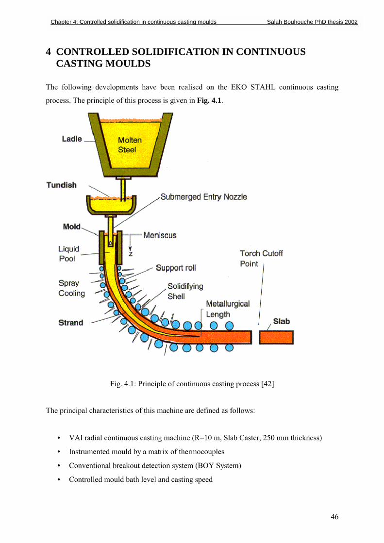
CONTROLLED SOLIDIFICATION IN CONTINUOUS CASTING MOULDS

he following developments have been realised on the EKO STAHL continuous casting

rocess. The principle of this process is given in Fig. 4.1.

Fig. 4.1: Principle of continuous casting process [42]

he principal characteristics of this machine are defined as follows:

• VAI radial continuous casting machine (R=10 m, Slab Caster, 250 mm thickness)

• Instrumented mould by a matrix of thermocouples

• Conventional breakout detection system (BOY System)

• Controlled mould bath level and casting speed

47

• Six secondary cooling zones

• Compensation of casting speed effect on strand surface temperature by a feedforward

using �Dynschell� model

• Format 850-1800 mm

• Casting speed (0 � 1.5 m/min)

• Slab thickness 250 mm

• Ordinary and microalloyed steel grades

• Contactless measurement of the slab width and temperature after cutting

4.1 Control and monitoring of solidification in the mould

In the present study, Mould Thermal Monitoring (MTM) technology in continuous casting

has been investigated in order to optimize casting control. The mould is the location of

complex metallurgical reactions characterising the liquid�solid transformation forming the

first crystals of solidification. Continuous measurements of the thermal profile are obtained

by a matrix of thermocouples. In such a way, real-time monitoring and control of the process

are considered. The control algorithm predicts solidification defects using mathematical

models. In this work, a new approach for a breakout detection system has been developed by

means of NN . A process database is used for training the NN using a back-propagation

algorithm. The learning process uses modelled data samples related to the real alarm

situations. After training the NN predicts new breakouts. Using this approach the number of

false alarms will be considerably reduced comparatively to the conventional system.

In continuous casting, the phenomenon of the breakout is generally caused by rupture of the

solid crust due to an increase in temperature at various points of the mould. Both peak and

temperature oscillations have a direct influence on the quality resulting from solidification

[31, 36, 42]. These phenomena appear at the time of slag incrustation, formation or

propagation of cracks and in the case of poor friction and generally at the time of an

imbalance of distributed thermal reactions in the mould. In this study, the monitoring and the

detection of abnormal phenomena affecting thermal conditions in the mould have been

developed using NN [48]. The structure and training process of the breakout prediction NN

model are obtain as a result of temperature measurements that have been obtained from

thermocouples fixed at the copper plates of the mould. The input of the time series network is

formed by the measured temperature samples, while the output is formed by alarm defining

the importance of defects. A new spatial network considers the combination of different time


48

series models alarm. The training has been carried out by the exploitation of databases

characterising the normal and deteriorated operating conditions of solidification process. Such

databases contain information on the dynamics of process parameters and the operating state

of the process (alarms, shutdown of production,). In the following training, the simulation

tests based on cases of real defects are applied to estimate the model detection ability.

4.2 Analysis of breakout phenomena

4.2.1 Breakout propagation process [31, 42, 63, 69]

The mechanism for the original sticking can be explained by the existing conditions at the

meniscus such as variations of casting speed, mould bath level of liquid steel, steel

temperature and lubrification. Changes of casting speed have an important influence.

Procedures for start-up and speed changes have been altered to slowly ramp up the speed.

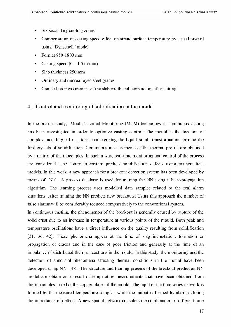
A breakout appears generally during metal sticking on the copper plate of the mould followed

by perforation of the solid shell due to a solidification disturbance. Sticking breakout is

propagated with various speeds in various directions and particularly in casting direction. Fig.

4.2 shows an example of breakout propagation and Fig. 4.2a a little crack which has been

developed in a breakout affecting the slab quality (see Fig. 4.2b).

Fig. 4.2: Example of breakout propagation [31]


49

In this complex situation, it is practically impossible to describe the development of a

breakout in the geometrical space of the mould using an analytical model based on heat

transfer, solidification and the mechanical laws. The measurement and acquisition of

temperature in different points at the mould surface constitute a tool for analysis and

comprehension of the phenomenon. This experimental approach is also used for the

development of a reliable system.

The technique is the basis of the MTM system that considers the mould as a thermal reactor

and the appearance of breakout is a result of an imbalance of the distributed thermal reactions.

The dynamics of process data that have generated a breakout are affected by these random

terms.

4.2.2 Breakout effect in the mould temperature field

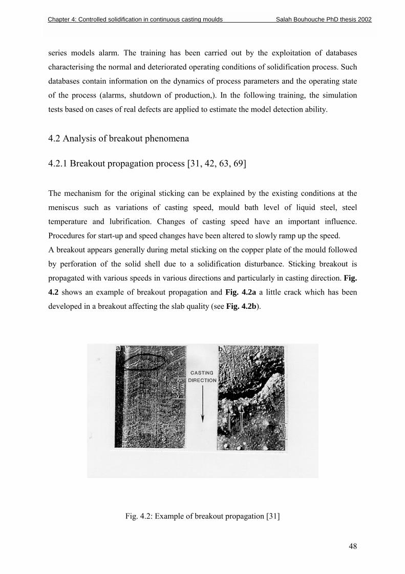
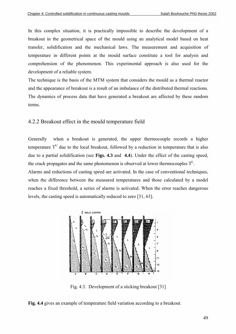
Generally when a breakout is generated, the upper thermocouple records a higher

temperature TU due to the local breakout, followed by a reduction in temperature that is also

due to a partial solidification (see Figs. 4.3 and 4.4). Under the effect of the casting speed,

the crack propagates and the same phenomenon is observed at lower thermocouples TL.

Alarms and reductions of casting speed are activated. In the case of conventional techniques,

when the difference between the measured temperatures and those calculated by a model

reaches a fixed threshold, a series of alarms is activated. When the error reaches dangerous

levels, the casting speed is automatically reduced to zero [31, 63].

Fig. 4.3. Development of a sticking breakout [31]

Fig. 4.4 gives an example of temperature field variation according to a breakout.


50

0 100 200 300 400 500 600 0

50

100

150

200

250

upper thermocouples

lower thermocouples

Upper and lower temperature field variations Te

mpe

ratu

re [°

C]

Sampling number

alarm activation

thermocouples at mould faces thermocouples not used

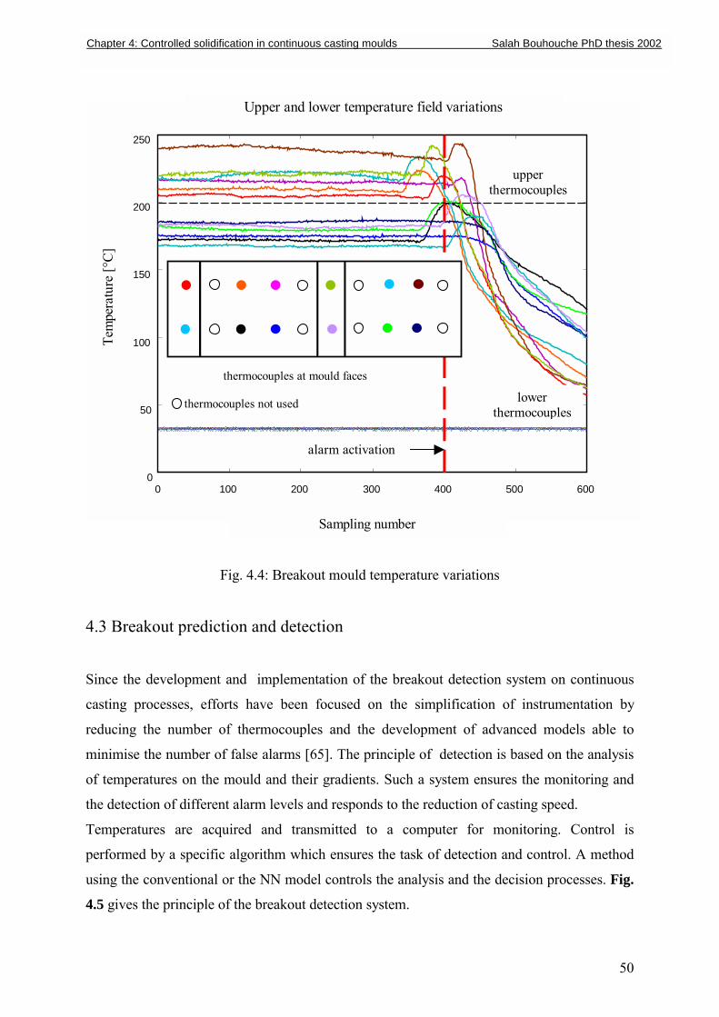
Fig. 4.4: Breakout mould temperature variations

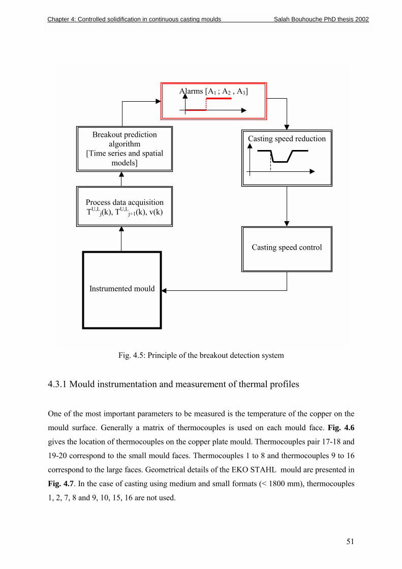
4.3 Breakout prediction and detection

Since the development and implementation of the breakout detection system on continuous

casting processes, efforts have been focused on the simplification of instrumentation by

reducing the number of thermocouples and the development of advanced models able to

minimise the number of false alarms [65]. The principle of detection is based on the analysis

of temperatures on the mould and their gradients. Such a system ensures the monitoring and

the detection of different alarm levels and responds to the reduction of casting speed.

Temperatures are acquired and transmitted to a computer for monitoring. Control is

performed by a specific algorithm which ensures the task of detection and control. A method

using the conventional or the NN model controls the analysis and the decision processes. Fig.

4.5 gives the principle of the breakout detection system.


51

Fig. 4.5: Principle of the breakout detection system

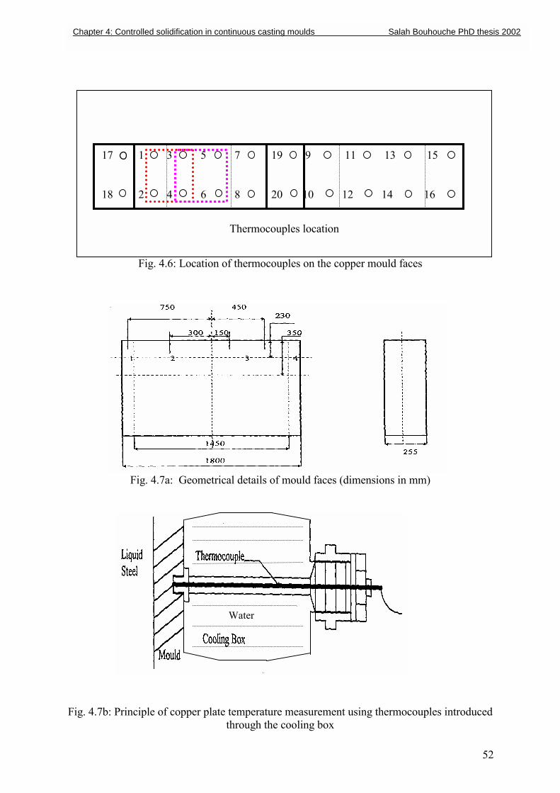
4.3.1 Mould instrumentation and measurement of thermal profiles

One of the most important parameters to be measured is the temperature of the copper on the

mould surface. Generally a matrix of thermocouples is used on each mould face. Fig. 4.6

gives the location of thermocouples on the copper plate mould. Thermocouples pair 17-18 and

19-20 correspond to the small mould faces. Thermocouples 1 to 8 and thermocouples 9 to 16

correspond to the large faces. Geometrical details of the EKO STAHL mould are presented in

Fig. 4.7. In the case of casting using medium and small formats (< 1800 mm), thermocouples

1, 2, 7, 8 and 9, 10, 15, 16 are not used.

Process data acquisition TU,L

j(k), TU,Lj+1(k), v(k)

Breakout prediction algorithm

[Time series and spatial models]

Alarms [A1 ; A2 , A3]

Casting speed reduction

Casting speed control

Instrumented mould


Fig

11 13 15

12 14 16


Thermocouples location

17 1 3 5 7 19 9 18 2 4 6 8 20 10

52

Fig. 4.6: Location of thermocouples on the copper mould faces

Fig. 4.7a: Geometrical details of mould faces (dimensions in mm)

. 4.7b: Principle of copper plate temperature measurement using thermocouples introduced through the cooling box

Water

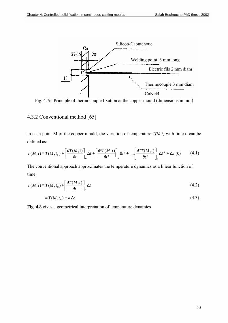
Fig. 4.7c: Principle of thermocouple fixatio

4.3.2 Conventional method [65]

In each point M of the copper mould, the vari

defined as:

²,(²),(),(),(

00 t

tMTtt

tMTtMTtMT

∂∂+∆

∂∂+=

The conventional approach approximates the te

time:

tt

tMTtMTtMT ∆

∂∂+=

00

),(),(),(

tatMT ∆+= .),( 0

Fig. 4.8 gives a geometrical interpretation of te

c


Silicon-Caoutchou

n at the copper m

ation of temperatu

(.....²)

0 tMTt

n

∂

∂+∆

mperature dynam

mperature dynami

Welding point 3 mm long

C

Electric fils 2 mm diam

Thermocouple 3 mm diam

53

ould (dimensions in mm)

re T(M,t) with time t, can be

)0(),

0

Ttt nn ∆+∆

(4.1)

ics as a linear function of

(4.2)

(4.3)

cs

uNi44

54

0 100 200 300 400 500 600 60

80

100

120

140

160

180

200

220

240

t0 t1

dt

TU(t1)

TL(t0)

TL(t1)

TU(t0)

Upper and lower temperature characteristics Te

mpe

ratu

re [°

C]

Sampling number

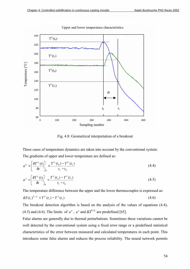
Fig. 4.8: Geometrical interpretation of a breakout

Three cases of temperature dynamics are taken into account by the conventional system:

The gradients of upper and lower temperature are defined as:

01

10

0

)()()(tt

tTtTt

tTaUUU

U

−−

=

∂

∂= (4.4)

01

10

0

)()()(tt

tTtTt

tTaLLL

L

−−

=

∂

∂= (4.5)

The temperature difference between the upper and the lower thermocouples is expressed as:

)()()( 111 tTtTtT LULU −=∆ − (4.6)

The breakout detection algorithm is based on the analysis of the values of equations (4.4),

(4.5) and (4.6). The limits of Ua , La and ∆TU-L are predefined [65].

False alarms are generally due to thermal perturbations. Sometimes these variations cannot be

well detected by the conventional system using a fixed error range or a predefined statistical

characteristics of the error between measured and calculated temperatures in each point. This

introduces some false alarms and reduces the process reliability. The neural network permits


55

to solve the problem by the learning process using the breakout data base related to the real

and false alarm situation, respectively.

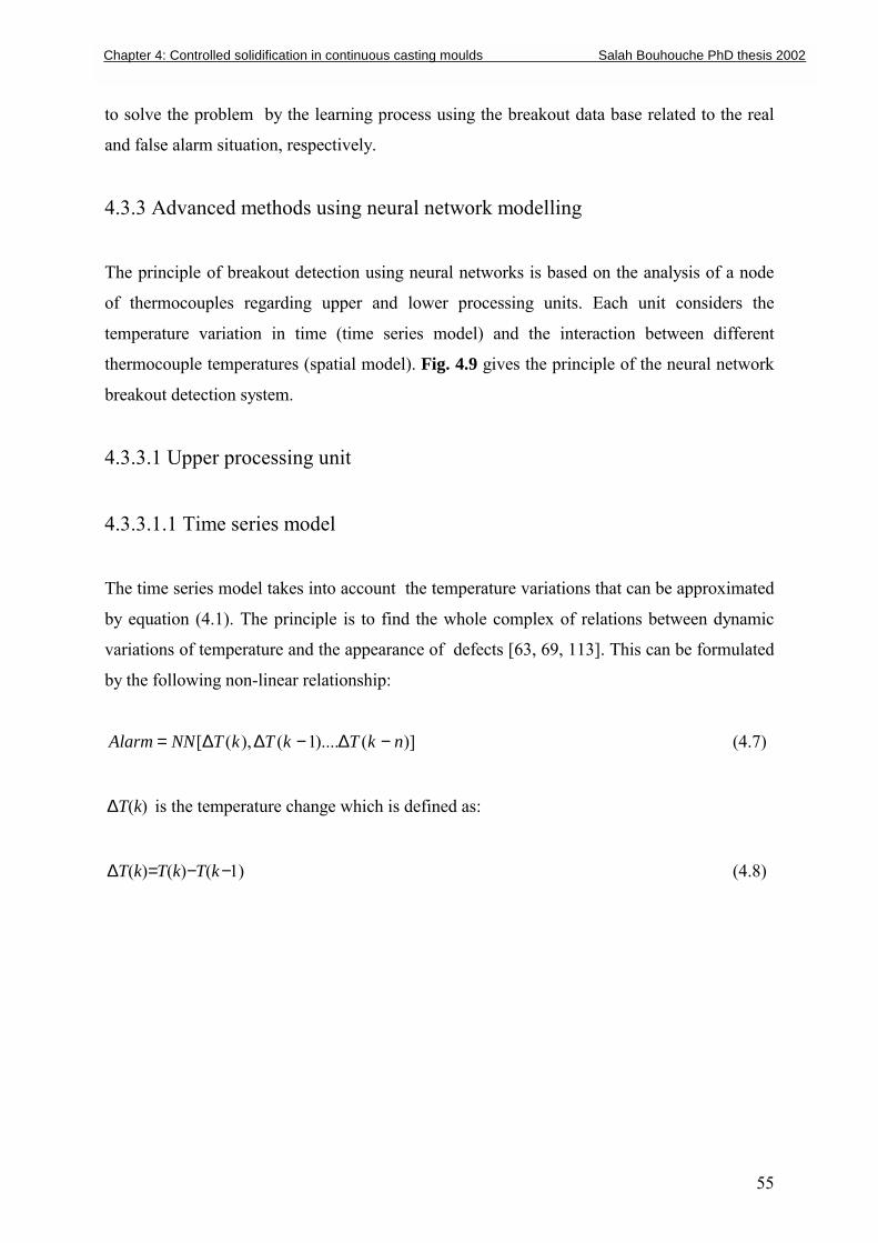
4.3.3 Advanced methods using neural network modelling

The principle of breakout detection using neural networks is based on the analysis of a node

of thermocouples regarding upper and lower processing units. Each unit considers the

temperature variation in time (time series model) and the interaction between different

thermocouple temperatures (spatial model). Fig. 4.9 gives the principle of the neural network

breakout detection system.

4.3.3.1 Upper processing unit

4.3.3.1.1 Time series model

The time series model takes into account the temperature variations that can be approximated

by equation (4.1). The principle is to find the whole complex of relations between dynamic

variations of temperature and the appearance of defects [63, 69, 113]. This can be formulated

by the following non-linear relationship:

)]()....1(),([ nkTkTkTNNAlarm −∆−∆∆= (4.7)

)(kT∆ is the temperature change which is defined as:

)1()()( −−=∆ kTkTkT (4.8)


Time series

model

Time series

model

Time series

model

Time series

model (TU-TL)

Spatial model

Spatial model

Spatial model

Upper thermocouples Lower thermocouples

Time series

model

Lower processing unit

Upper processing unit

O2

O3

O4

O5

A1

A2

Alarm0-1


Fig. 4.9: Principle of breako

O1

ut detection using the NN mod

A3

56

el

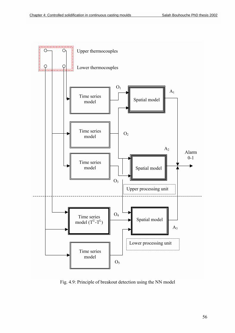
The model is obtained by the learning process using the back-propagation algorithm and the

characteristics of breakout temperature. Fig. 4.10 gives the learning principle of the time

series model.

Fig. 4.10: Principle of lea

After several trials an optimal neural network with

first layer and one node in the output layer that co

been chosen.

After the convergence, network weights Wijk are col

to other thermal profile breakout detections.

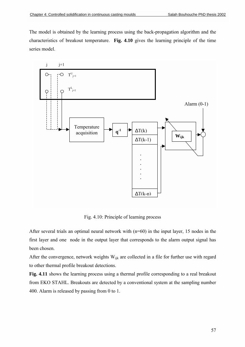
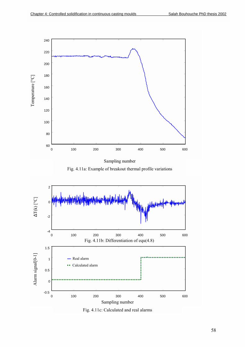
Fig. 4.11 shows the learning process using a therma

from EKO STAHL. Breakouts are detected by a con

400. Alarm is released by passing from 0 to 1.

j j+1

Temperature acquisition

q-1

TUj+1

TL

j+1

Alarm (0-1)


∆T(k)

∆T(k-1) Wijk

∆T(k-n)

rn

(n=

rr

lec

l p

ve

.

.

.

.

.

.

57

ing process

60) in the input layer, 15 nodes in the

esponds to the alarm output signal has

ted in a file for further use with regard

rofile corresponding to a real breakout

ntional system at the sampling number

58

0 100 200 300 400 500 600 60

80

100

120

140

160

180

200

220

240

Sampling number

Fig. 4.11a: Example of breakout thermal profile variations

Tem

pera

ture

[°C

]

0 100 200 300 400 500 600 -4

-2

0

2

0 100 200 300 400 500 600 -0.5

0

0.5

1

1.5

∆T(k

) [°C

]

Fig. 4.11b: Differentiation of equ(4.8)

Ala

rm si

gnal

[0-1

]

Sampling number

Fig. 4.11c: Calculated and real alarms

Real alarm

Calculated alarm


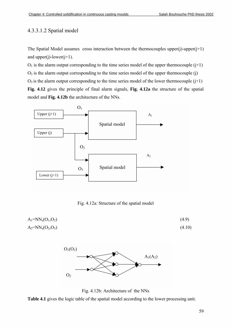
4.3.3.1.2 Spatial model

The Spatial Model assumes cross interaction between the thermocouples upper(j)-upper(j+1)

and upper(j)-lower(j+1).

O1 is the alarm output corresponding to the time series model of the upper thermocouple (j+1)

O2 is the alarm output corresponding to the time series model of the upper thermocouple (j)

O3 is the alarm output corresponding to the time series model of the lower thermocouple (j+1)

Fig. 4.12 gives the principle of final alarm signals, Fig. 4.12a the structure of the spatial

model and Fig. 4.12b the architecture of the NNs.

Fig. 4.12a: Structure of the spatial model

A1=NNs(O1,O2) (4.9)

A2=NNs(O2,O3) (4.10)

Table 4.1 gives the

Spatial model

Spatial model

O1

O2

O3

Upper (j+1)

Upper (j)

Lower (j+1)

A1

A2

O1(O3) )


O2

Fig. 4.12b: Architecture of the N

logic table of the spatial model according

A1(A2

59

Ns

to the lower processing unit.

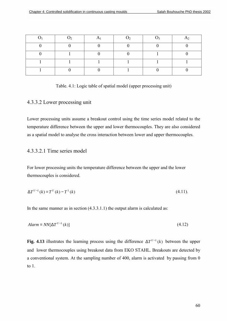
60

O1 O2 A1 O2 O3 A2

0 0 0 0 0 0

0 1 0 0 1 0

1 1 1 1 1 1

1 0 0 1 0 0

Table. 4.1: Logic table of spatial model (upper processing unit)

4.3.3.2 Lower processing unit

Lower processing units assume a breakout control using the time series model related to the

temperature difference between the upper and lower thermocouples. They are also considered

as a spatial model to analyse the cross interaction between lower and upper thermocouples.

4.3.3.2.1 Time series model

For lower processing units the temperature difference between the upper and the lower

thermocouples is considered.

)()()( kTkTkT LULU −=∆ − (4.11).

In the same manner as in section (4.3.3.1.1) the output alarm is calculated as:

)]([ kTNNAlarm LU −∆= (4.12)

Fig. 4.13 illustrates the learning process using the difference )(kT LU −∆ between the upper

and lower thermocouples using breakout data from EKO STAHL. Breakouts are detected by

a conventional system. At the sampling number of 400, alarm is activated by passing from 0

to 1.


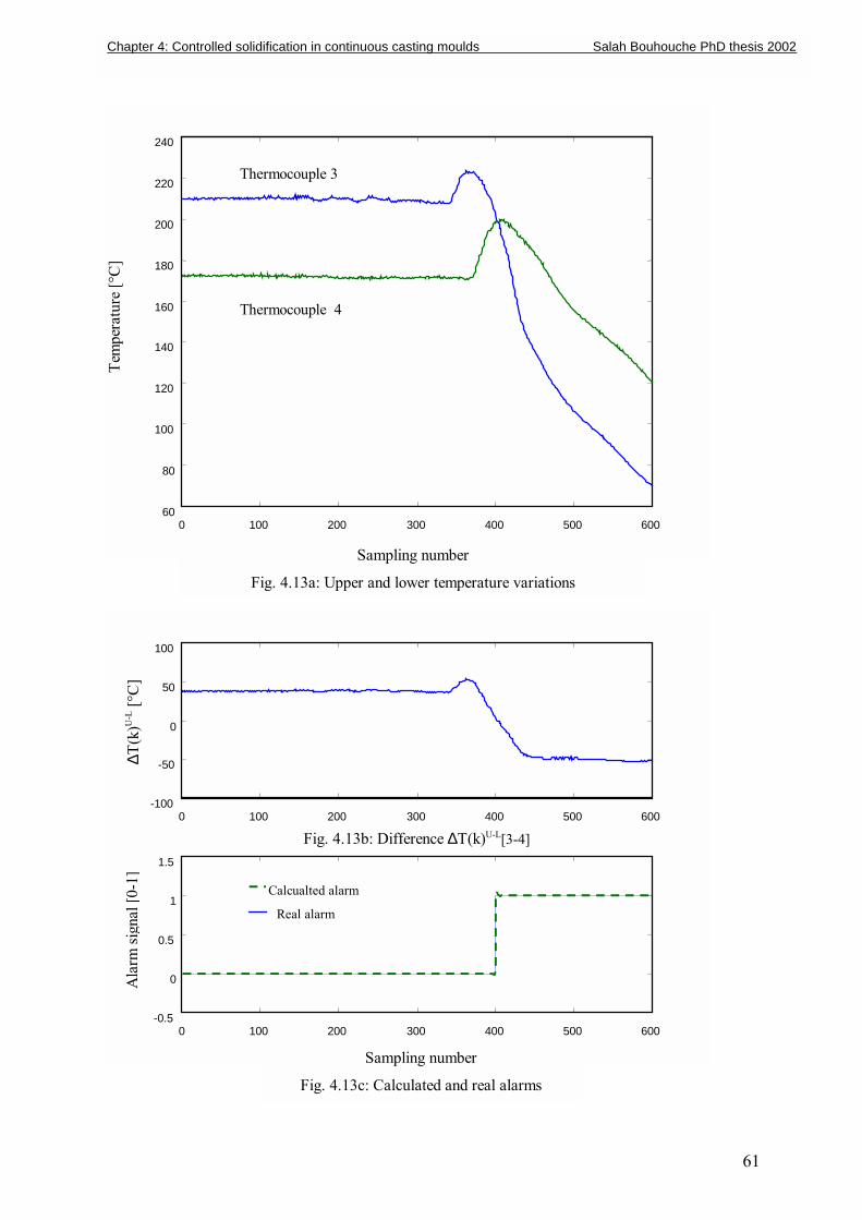
61

0 100 200 300 400 500 600 60

80

100

120

140

160

180

200

220

240

Sampling number

Fig. 4.13a: Upper and lower temperature variations

Tem

pera

ture

[°C

]

Thermocouple 3

Thermocouple 4

0 100 200 300 400 500 600 -100

-50

0

50

100

0 100 200 300 400 500 600 -0.5

0

0.5

1

1.5

∆T(k

)U-L

[°C

]

Fig. 4.13b: Difference ∆T(k)U-L[3-4]

Ala

rm si

gnal

[0-1

]

Sampling number


Calcualted alarm

Real alarm


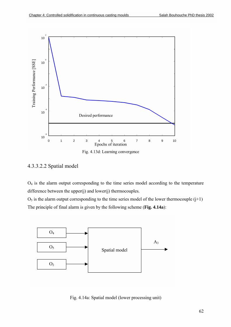
62

0 1 2 3 4 5 6 7 8 9 10 10

-6

10 -4

10 -2

10 0

10 2

Epochs of iteration

Fig. 4.13d: Learning convergence

Trai

ning

Per

form

ance

[SSE

]

Desired performance

4.3.3.2.2 Spatial model

O4 is the alarm output corresponding to the time series model according to the temperature

difference between the upper(j) and lower(j) thermocouples.

O5 is the alarm output corresponding to the time series model of the lower thermocouple (j+1)

The principle of final alarm is given by the following scheme (Fig. 4.14a):

Fig. 4.14a: Spatial model (lower processing unit)

Spatial model

O4

O5

O2

A3


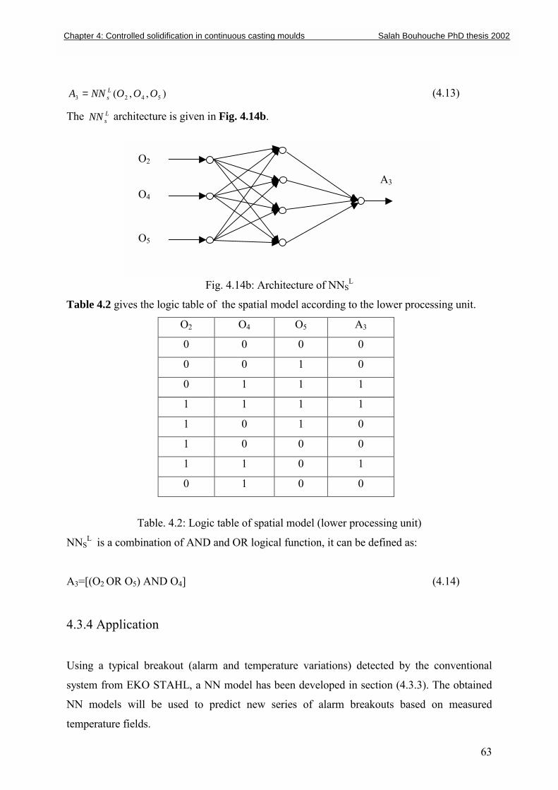
63

),,( 5423 OOONNA Ls= (4.13)

The LsNN architecture is given in Fig. 4.14b.

Fig. 4.14b: Architecture of NNSL

Table 4.2 gives the logic table of the spatial model according to the lower processing unit.

O2 O4 O5 A3

0 0 0 0

0 0 1 0

0 1 1 1

1 1 1 1

1 0 1 0

1 0 0 0

1 1 0 1

0 1 0 0

Table. 4.2: Logic table of spatial model (lower processing unit)

NNSL is a combination of AND and OR logical function, it can be defined as:

A3=[(O2 OR O5) AND O4] (4.14)

4.3.4 Application

Using a typical breakout (alarm and temperature variations) detected by the conventional

system from EKO STAHL, a NN model has been developed in section (4.3.3). The obtained

NN models will be used to predict new series of alarm breakouts based on measured

temperature fields.

O2

O4

O5

A3


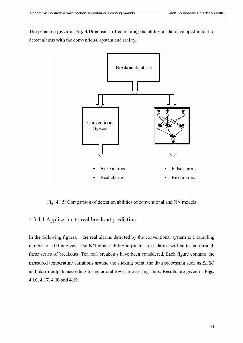
The principle given in Fig. 4.15 consists of comparing the ability of the developed model to

detect alarms with the conventional system and reality.

Fig. 4.15: Comparison of dete

4.3.4.1 Application to real breako

In the following figures, the real alar

number of 400 is given. The NN mod

these series of breakouts. Ten real bre

measured temperature variations aroun

and alarm outputs according to upper

4.16, 4.17, 4.18 and 4.19.

Breakout database

ConventionalSystem

• Fa

• Re

• Fa

• Re


lse alarms

al alarms

ction abilities of conventional and N

ut prediction

ms detected by the conventional sy

el ability to predict real alarms wil

akouts have been considered. Each

d the sticking point, the data proces

and lower processing units. Results

lse alarms

al alarms

64

N models

stem at a sampling

l be tested through

figure contains the

sing such as ∆T(k)

are given in Figs.

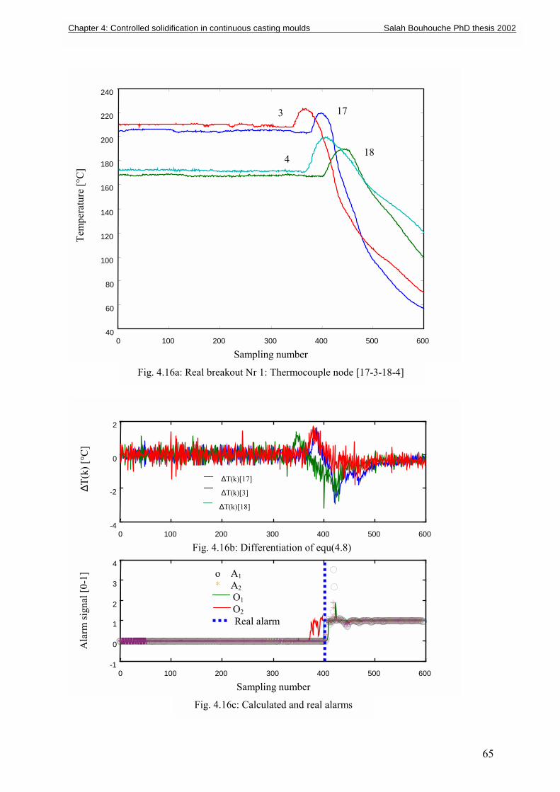
65

0 100 200 300 400 500 600 40

60

80

100

120

140

160

180

200

220

240 Te

mpe

ratu

re [°

C]

Sampling number

Fig. 4.16a: Real breakout Nr 1: Thermocouple node [17-3-18-4]

173

184


0 100 200 300 400 500 600 -4

-2

0

2

0 100 200 300 400 500 600 -1

0

1

2

3

4

∆T(k

) [°C

]


Ala

rm si

gnal

[0-1

]

Sampling number


∆T(k)[17]

∆T(k)[3]

∆T(k)[18]

o A1 * A2 O1 O2

Real alarm

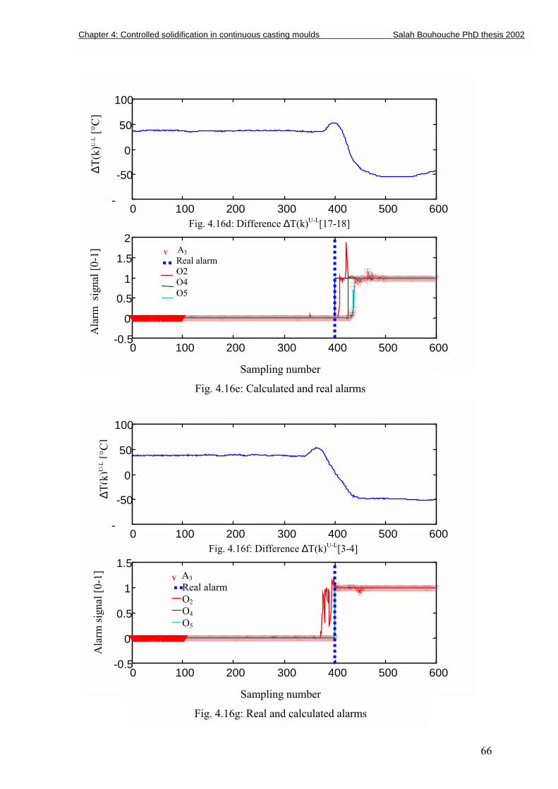
66

0 100 200 300 400 500 600-

-50

0

50

100

0 100 200 300 400 500 600-0.5

0

0.5

1

1.5

2

∆T(k

)U-L

[°C

]

Fig. 4.16d: Difference ∆T(k)U-L[17-18]

Ala

rm s

igna

l [0-

1] V A3

Real alarm O2 O4 O5

Sampling number

Fig. 4.16e: Calculated and real alarms

0 100 200 300 400 500 600-

-50

0

50

100

0 100 200 300 400 500 600-0.5

0

0.5

1

1.5

∆T(k

)U-L

[°C

]

Fig. 4.16f: Difference ∆T(k)U-L[3-4]

Ala

rm si

gnal

[0-1

]

Sampling number

Fig. 4.16g: Real and calculated alarms

V A3 Real alarm O2 O4 O5


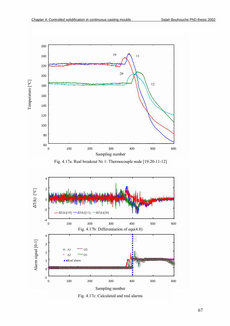
67

0 100 200 300 400 500 600 60

80

100

120

140

160

180

200

220

240

260

Tem

pera

ture

[°C

]

Sampling number


19 11

20

12

0 100 200 300 400 500 600 -4

-2

0

2

4

0 100 200 300 400 500 600 -1

0

1

2

3

4

∆T(k

) [°

C]


Ala

rm si

gnal

[0-1

]

Sampling number


∆T(k)[19]; ∆T(k)[11]; ∆T(k)[20]

O A1 O2

* A2 O1

Real alarm


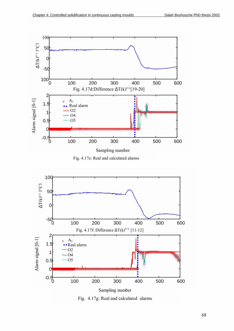
68

0 100 200 300 400 500 600 100

-50

0

50

100

0 100 200 300 400 500 600 -0.5

0

0.5

1

1.5

2

∆T(k

)U-L

[°C

]

Fig. 4.17d:Difference ∆T(k)U-L[19-20]

Sampling number Fig. 4.17e: Real and calculated alarms

Ala

rm si

gnal

[0-1

]


0 100 200 300 400 500 600-50

0

50

100

0 100 200 300 400 500 600-0.5

0

0.5

1

1.5

2

∆T(k

)U-L [°

C]

Fig. 4.17f: Difference ∆T(k)U-L [11-12]

Sampling number

Fig. 4.17g: Real and calculated alarms


Ala

rm si

gnal

[0-1

]


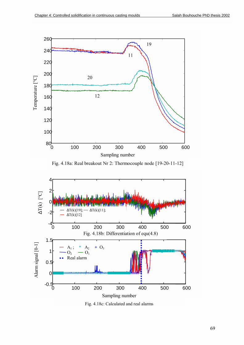
69

0 100 200 300 400 500 60080

100

120

140

160

180

200

220

240

26019

11

20

12

Tem

pera

ture

[°C

]

Sampling number


0 100 200 300 400 500 600-4

-2

0

2

4

0 100 200 300 400 500 600-0.5

0

0.5

1

1.5

∆T(k

) [°

C]

∆T(k)[19]; ∆T(k)[11]; ∆T(k)[12]


Ala

rm si

gnal

[0-1

]

Sampling number Fig. 4.18c: Calculated and real alarms

A1 ; * A2 + O3 O2 O1 Real alarm


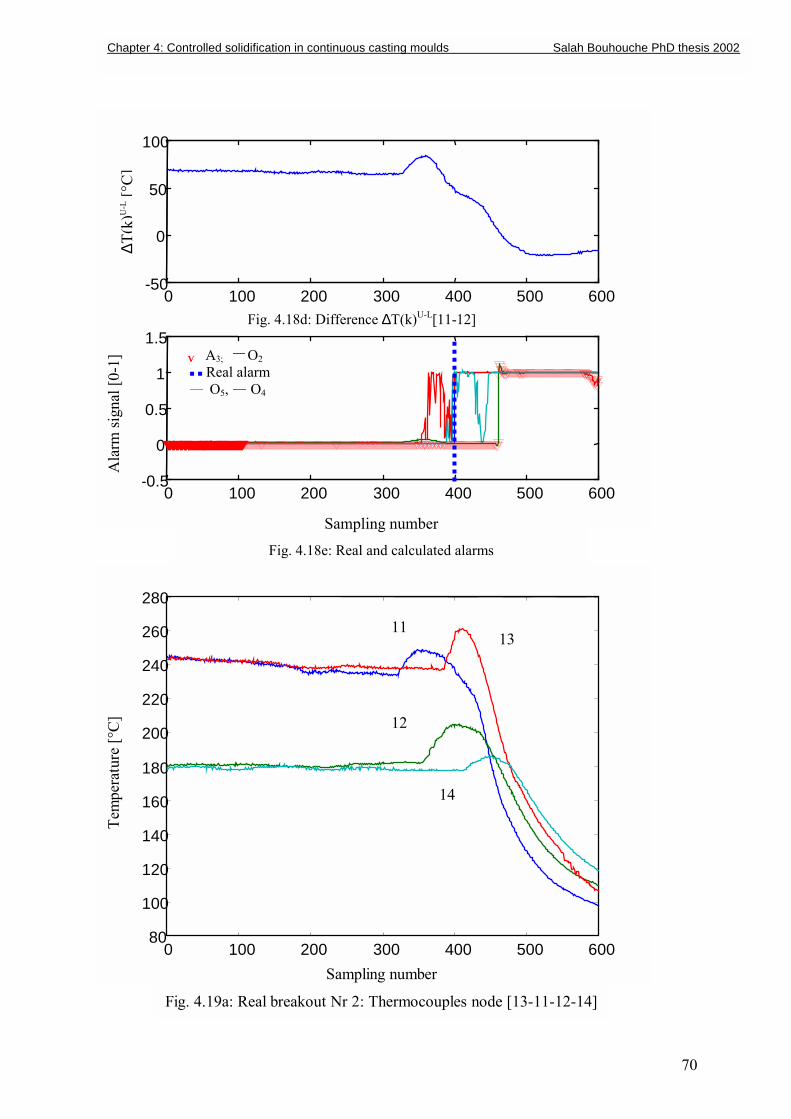
70

0 100 200 300 400 500 600-50

0

50

100

0 100 200 300 400 500 600-0.5

0

0.5

1

1.5

∆T(k

)U-L

[°C

]


Ala

rm si

gnal

[0-1

] V A3; O2 Real alarm O5, O4

Sampling number

Fig. 4.18e: Real and calculated alarms

0 100 200 300 400 500 60080

100

120

140

160

180

200

220

240

260

280

11 13

12

14

Tem

pera

ture

[°C

]

Sampling number

Fig. 4.19a: Real breakout Nr 2: Thermocouples node [13-11-12-14]


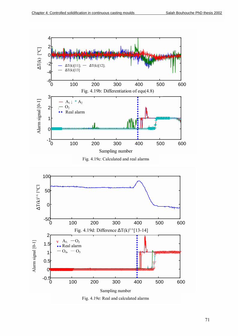
71

0 100 200 300 400 500 600-6

-4

-2

0

2

4

0 100 200 300 400 500 600-1

0

1

2

3

∆T(k

) [°

C]


Ala

rm si

gnal

[0-1

]


A1 ; * A2 ; O2 Real alarm

∆T(k)[11]; ∆T(k)[12]; ∆T(k)[13]

0 100 200 300 400 500 600-50

0

50

100

0 100 200 300 400 500 600-0.5

0

0.5

1

1.5

2

∆T(k

)U-L

[°C

]


Ala

rm si

gnal

[0-1

] V A3; O2 Real alarm O4, O5

Sampling number



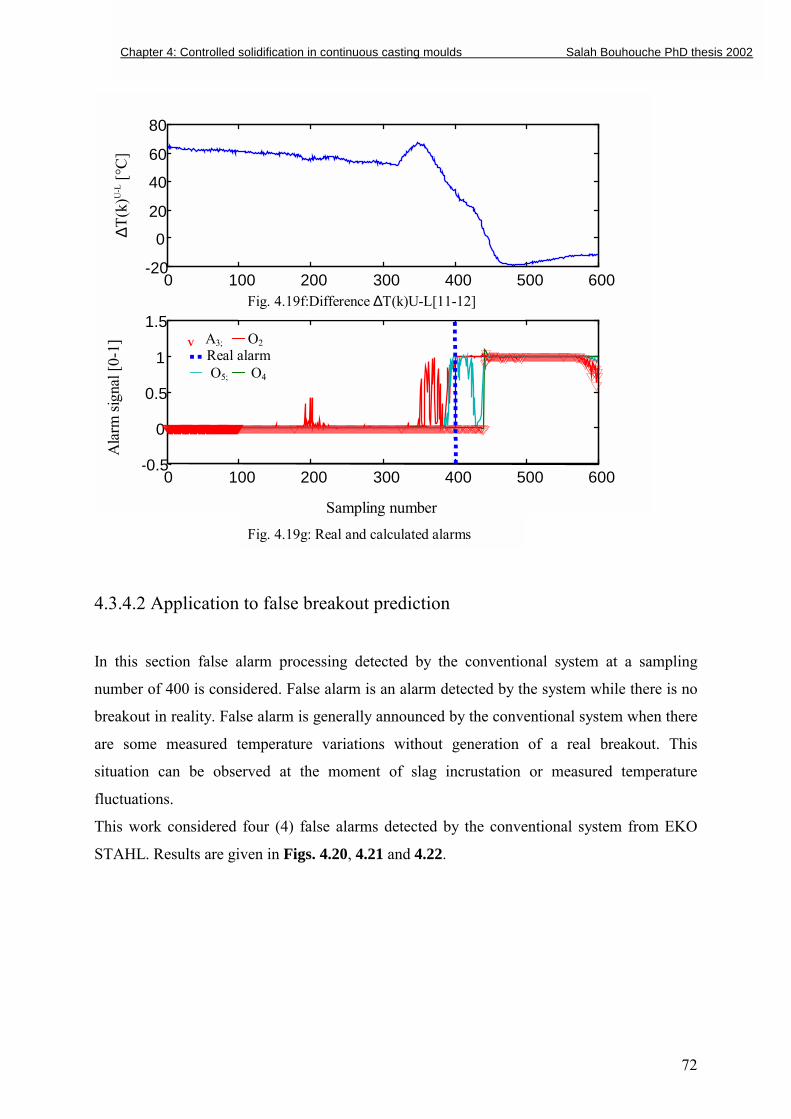
72

4.3.4.2 Application to false breakout prediction

In this section false alarm processing detected by the conventional system at a sampling

number of 400 is considered. False alarm is an alarm detected by the system while there is no

breakout in reality. False alarm is generally announced by the conventional system when there

are some measured temperature variations without generation of a real breakout. This

situation can be observed at the moment of slag incrustation or measured temperature

fluctuations.

This work considered four (4) false alarms detected by the conventional system from EKO

STAHL. Results are given in Figs. 4.20, 4.21 and 4.22.

0 100 200 300 400 500 600-20

0

20

40

60

80

0 100 200 300 400 500 600-0.5

0

0.5

1

1.5

∆T(k

)U-L [°

C]

Fig. 4.19f:Difference ∆T(k)U-L[11-12]

V A3; O2 Real alarm O5; O4

Ala

rm si

gnal

[0-1

]

Sampling number Fig. 4.19g: Real and calculated alarms


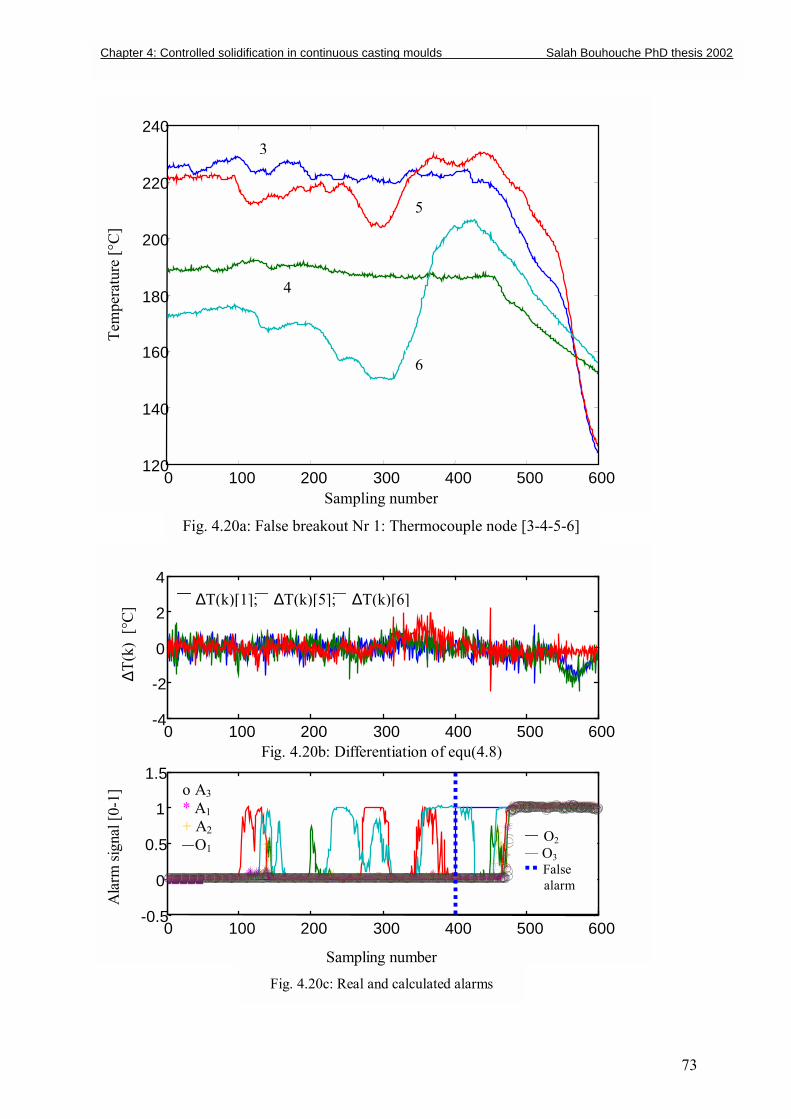
73

0 100 200 300 400 500 600120

140

160

180

200

220

2403

4

5

6

Tem

pera

ture

[°C

]

Sampling number

Fig. 4.20a: False breakout Nr 1: Thermocouple node [3-4-5-6]

0 100 200 300 400 500 600-4

-2

0

2

4

0 100 200 300 400 500 600-0.5

0

0.5

1

1.5

∆T(k

) [°

C]


Ala

rm si

gnal

[0-1

] o A3 * A1 + A2 O1

∆T(k)[1]; ∆T(k)[5]; ∆T(k)[6]

O2 O3

False alarm

Sampling number Fig. 4.20c: Real and calculated alarms


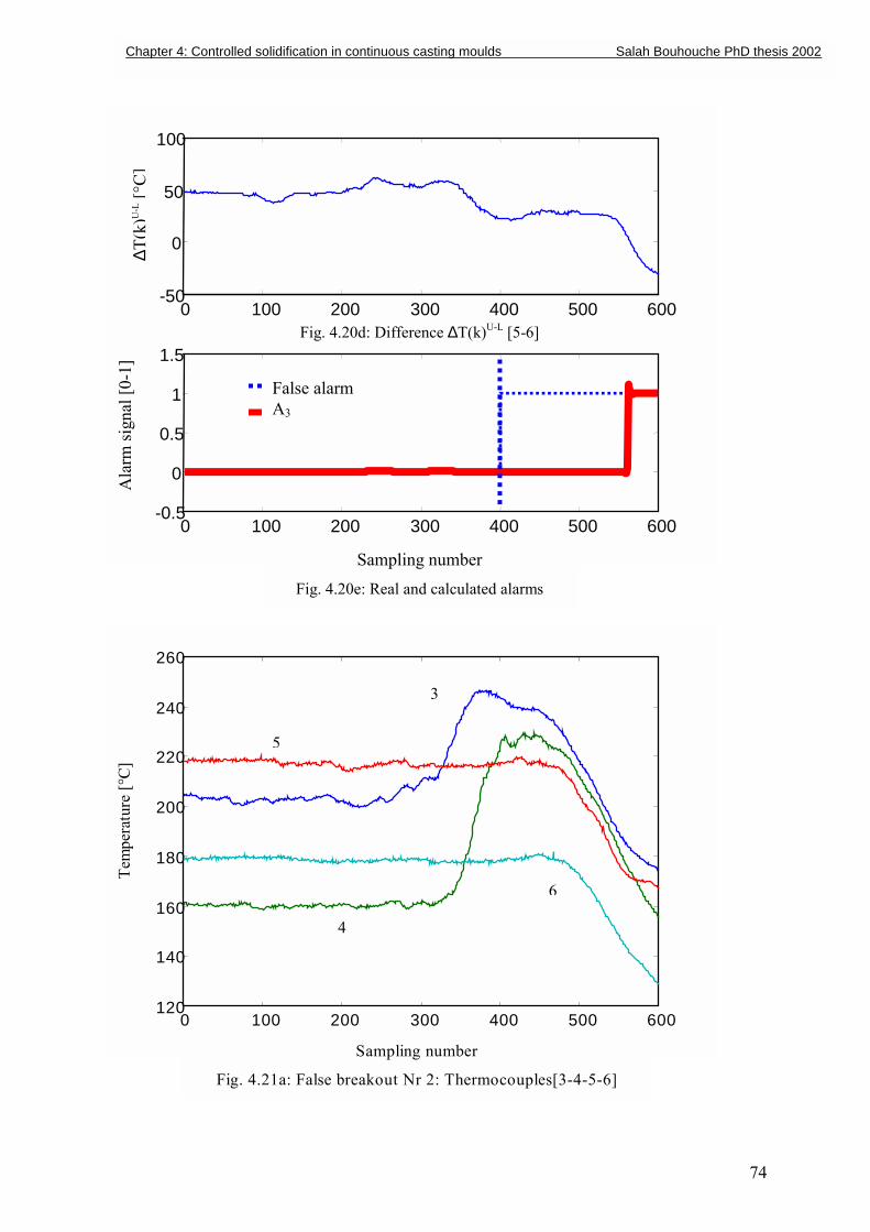
74

0 100 200 300 400 500 600-50

0

50

100

0 100 200 300 400 500 600-0.5

0

0.5

1

1.5

∆T(k

)U-L

[°C

]

Fig. 4.20d: Difference ∆T(k)U-L [5-6]

Ala

rm si

gnal

[0-1

]

False alarm A3

Sampling number Fig. 4.20e: Real and calculated alarms

0 100 200 300 400 500 600120

140

160

180

200

220

240

260

Tem

pera

ture

[°C

]

Sampling number

Fig. 4.21a: False breakout Nr 2: Thermocouples[3-4-5-6]

3

5

4

6


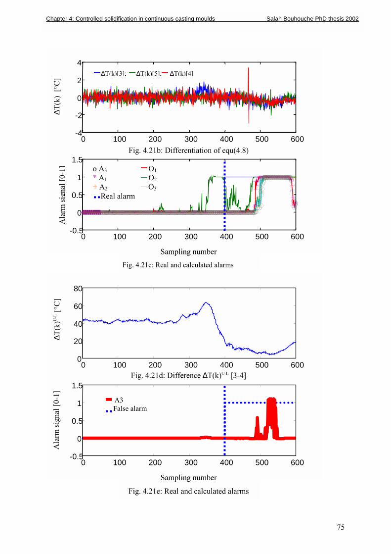
75

0 100 200 300 400 500 600-4

-2

0

2

4

0 100 200 300 400 500 600-0.5

0

0.5

1

1.5

∆T(k

) [°

C] ∆T(k)[3]; ∆T(k)[5]; ∆T(k)[4]


Ala

rm si

gnal

[0-1

]

Sampling number

Fig. 4.21c: Real and calculated alarms

o A3 O1 * A1 O2 + A2 O3 Real alarm

0 100 200 300 400 500 6000

20

40

60

80

0 100 200 300 400 500 600-0.5

0

0.5

1

1.5

∆T(k

)U-L

[°C

]

Fig. 4.21d: Difference ∆T(k)U-L [3-4]

Ala

rm si

gnal

[0-1

]

Sampling number


A3 False alarm


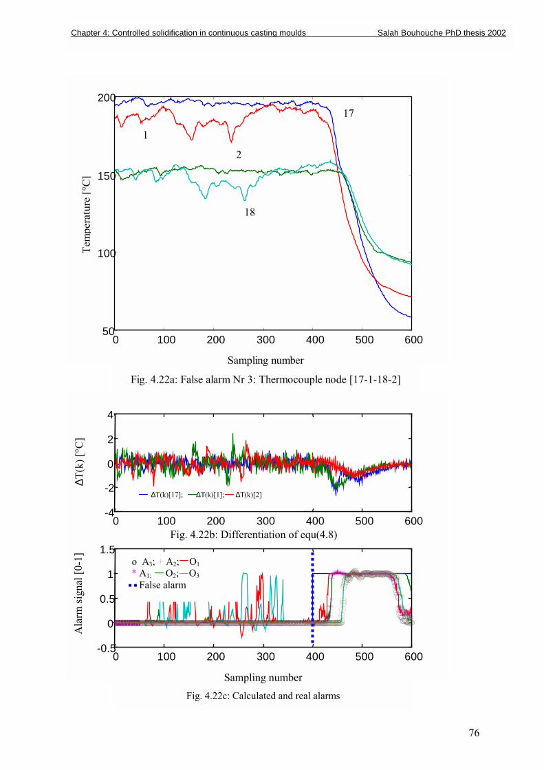
76

0 100 200 300 400 500 60050

100

150

20017

1

2

18

Tem

pera

ture

[°C

]

Sampling number

Fig. 4.22a: False alarm Nr 3: Thermocouple node [17-1-18-2]

0 100 200 300 400 500 600-4

-2

0

2

4

0 100 200 300 400 500 600-0.5

0

0.5

1

1.5

∆T(k

) [°C

]

∆T(k)[17]; ∆T(k)[1]; ∆T(k)[2]


Ala

rm si

gnal

[0-1

]


o A3; + A2; O1 * A1; O2; O3 False alarm


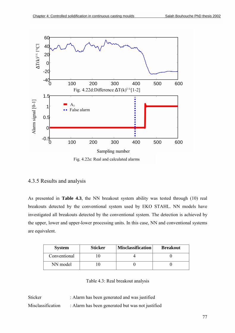
77

0 100 200 300 400 500 600-40

-20

0

20

40

60

0 100 200 300 400 500 600-0.5

0

0.5

1

1.5

∆T(k

)U-L

[°C

]

Fig. 4.22d:Difference ∆T(k)U-L[1-2]

Ala

rm si

gnal

[0-1

]

A3 False alarm

Sampling number


4.3.5 Results and analysis

As presented in Table 4.3, the NN breakout system ability was tested through (10) real

breakouts detected by the conventional system used by EKO STAHL. NN models have

investigated all breakouts detected by the conventional system. The detection is achieved by

the upper, lower and upper-lower processing units. In this case, NN and conventional systems

are equivalent.

System Sticker Misclassification Breakout

Conventional 10 4 0

NN model 10 0 0

Table 4.3: Real breakout analysis

Sticker : Alarm has been generated and was justified

Misclassification : Alarm has been generated but was not justified


78

Breakout : A breakout occurred but no alarm has been generated

In the case of false breakout detection by the conventional system (misclassification), the NN

model has been tested through four (4) false breakouts detected by the EKO STAHL

conventional system. The NN model has not detected all false alarms. In this case the NN

model has a greater ability not to take into account the field temperature variations that do

not generate a breakout.

As presented in Table 4.3, the objective of reducing the false alarm rate has been achieved.

The NN breakout detection system has been tested through real data. The obtained results

confirm an improvement.


79

5 CONTROL OF HEAT TRANSFER IN SECONDARY

COOLING

5.1 Introduction

In continuous casting, the cooling�solidification process is based on the adaptation of heat

transfer which is directly connected to casting speed. In practice, the casting speed is

continuously changed by the casting operator on the basis of thermal loss and chemical

composition of steel in the tundish. Most of the control schemes are based on the static

relation between casting speed and water flow rate in each cooling zone. This constitutes an

open loop that does not consider surface temperature variation which is an important

parameter for slab quality. In steelmaking, changes in the casting speed affect the entire heat

transfer. An optimal operation requires an adjustment of the process variables, i. e., global

heat transfer that depends on the operating point, steel grades, water flow rate and most

importantly the casting speed. A learning NN allows the identification and the control of a

non-linear heat transfer model in the continuous casting process. A heat transfer model was

developed using the dynamic heat balance. A comparison between the experimental open

loop results and those of the model simulation is considered. From the adaptation, the model

is used for controlling the slab surface temperature in the closed loop using NN technology

and PID controllers. Temperature stability is very important especially for casting crack

sensitive steel grades. Such performance cannot be achieved without the NN technology, as

the process features an important non-linearity and disturbances in casting speed, water

temperature and specific heat coefficients.

In the steel industry, the continuous casting process results in the formation of steel strands

obtained by the passage of liquid steel through several cooling zones. In this phase, the liquid

steel is poured into the mould, cooled by water, and transfered through the cooling zones at a

constant casting speed and a constant water flow rate. The final quality of the solidified strand

depends on its thermal history within the different cooling zones. It is, therefore, necessary to

control the cooling based on the casting events, variations of thermal loss, casting speed and

different heat dissipation. In most industrial applications, the appropriate cooling rate is

adjusted on the basis of the casting speed by linear correlation and the anticipated casting

speed effect on the temperature in the cooling zones [1-3]. This control approach is inefficient

in transient response as the thermal diffusion and the relation between water flow rate and

Chapter 5:Control of heat transfer in secondary cooling Salah Bouhouche PhD thesis 2002

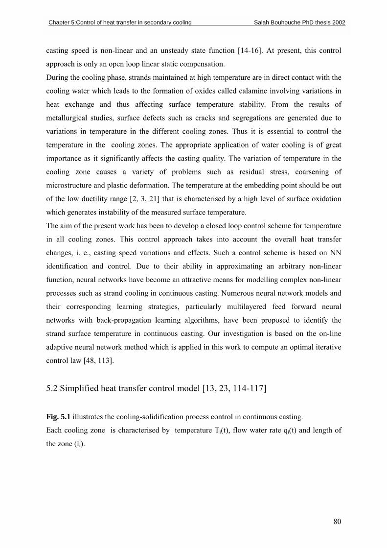
80

casting speed is non-linear and an unsteady state function [14-16]. At present, this control

approach is only an open loop linear static compensation.

During the cooling phase, strands maintained at high temperature are in direct contact with the

cooling water which leads to the formation of oxides called calamine involving variations in

heat exchange and thus affecting surface temperature stability. From the results of

metallurgical studies, surface defects such as cracks and segregations are generated due to

variations in temperature in the different cooling zones. Thus it is essential to control the

temperature in the cooling zones. The appropriate application of water cooling is of great

importance as it significantly affects the casting quality. The variation of temperature in the

cooling zone causes a variety of problems such as residual stress, coarsening of

microstructure and plastic deformation. The temperature at the embedding point should be out

of the low ductility range [2, 3, 21] that is characterised by a high level of surface oxidation

which generates instability of the measured surface temperature.

The aim of the present work has been to develop a closed loop control scheme for temperature

in all cooling zones. This control approach takes into account the overall heat transfer

changes, i. e., casting speed variations and effects. Such a control scheme is based on NN

identification and control. Due to their ability in approximating an arbitrary non-linear

function, neural networks have become an attractive means for modelling complex non-linear

processes such as strand cooling in continuous casting. Numerous neural network models and

their corresponding learning strategies, particularly multilayered feed forward neural

networks with back-propagation learning algorithms, have been proposed to identify the

strand surface temperature in continuous casting. Our investigation is based on the on-line

adaptive neural network method which is applied in this work to compute an optimal iterative

control law [48, 113].

5.2 Simplified heat transfer control model [13, 23, 114-117]

Fig. 5.1 illustrates the cooling-solidification process control in continuous casting.

Each cooling zone is characterised by temperature Ti(t), flow water rate qi(t) and length of

the zone (li).


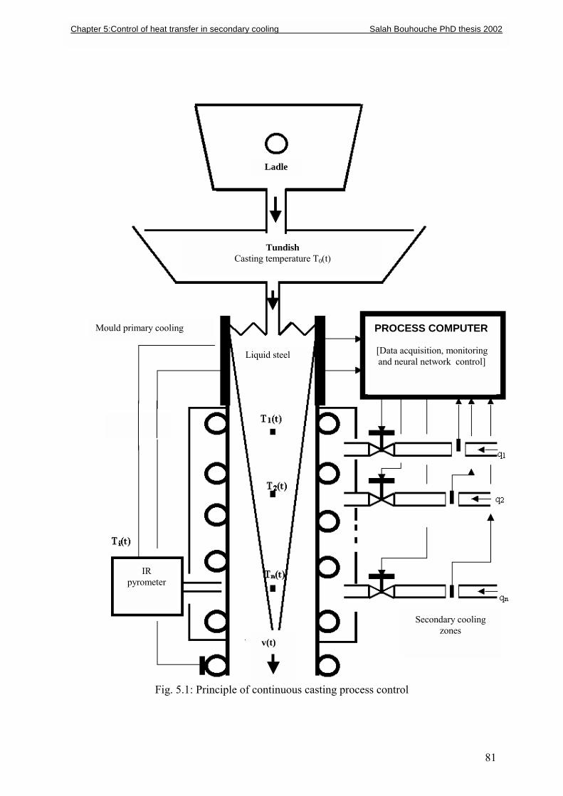
81

Fig. 5.1: Principle of continuous casting process control

Secondary cooling zones

v(t)

IR pyrometer

Mould primary cooling PROCESS COMPUTER

[Data acquisition, monitoring and neural network control]

Liquid steel

Tundish Casting temperature T0(t)

Ladle


82

Steel flows into the mould at a temperature T0(t), called casting temperature, and at a casting

speed v(t).

The solidified strand is characterised by:

- Strand density (ρ)

- Strand specific heat (Cpi)

- Geometrical characteristics (L, h see Fig. 5.3)

The cooling changes are characterised by:

- Water specific heat (CPe)

- Water temperature (Te)

The thermal balance in the dynamic regime for every zone is given as:

)T(t)(T(t)Cq(t))T(t)(T(t)Cqdt

(t)dTCm eiPeii1iPimi

Pii −−−= − (5.1)

where

iLhlρmi = , ρLhv(t))(q m =t

We consider Cpi, Cpe, mi, ρ and Te constant.

A second order variation of the equation (5.1) is written as:

)dt

(t)dTdt

(t)dT(CmρLhv(t)C

dtdv(t)Lh(t))T(t)(T

CmC

dt(t)Td i1i

Pii

Pii1i

Pii

Pi2i

2

−+−= −− ρ

dt

(t)dTCm

(t)Cqdt

(t)dq)T(t)(T

CmC i

Pii

Peiiei

Pii

Pe −−− (5.2)

tt)-(tT(t)T

dt(t)dT iii

∆∆−≈ (5.3)

where ∆t is the sampling time (the sampling number is a multiple of the sampling time).

After transformation we obtain:

F)1)(kET(k)DT2)(kCT1)-(k(BTA(k)T 1i1iii-1i +−++−+= −− (5.4)

where,


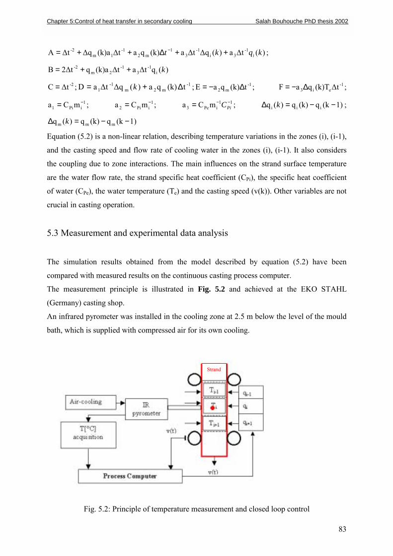
83

)(∆ta)(∆q∆ta(k)qa∆t(k)a∆q∆tA -13i

-13

1m2

-11m

-2 kqkt i++∆++= − ;

)(q∆ta∆t(k)aq∆t2B i-1

3-1

2m-2 k++=

-2∆tC = ; -1m2m

-11 t(k)qa)(∆q∆taD ∆+= k ; -1

m2 t(k)qaE ∆−= ; -1ei3 ∆t(k)TqaF ∆−= ;

1iPi1 mCa −= ; 1

iPi2 mCa −= ; 11iPe3 mCa −−= PiC ; 1)(kq(k)q)(q iii −−=∆ k ;

1)(kq(k)q)(q mmm −−=∆ k

Equation (5.2) is a non-linear relation, describing temperature variations in the zones (i), (i-1),

and the casting speed and flow rate of cooling water in the zones (i), (i-1). It also considers

the coupling due to zone interactions. The main influences on the strand surface temperature

are the water flow rate, the strand specific heat coefficient (CPi), the specific heat coefficient

of water (CPe), the water temperature (Te) and the casting speed (v(k)). Other variables are not

crucial in casting operation.

5.3 Measurement and experimental data analysis

The simulation results obtained from the model described by equation (5.2) have been

compared with measured results on the continuous casting process computer.

The measurement principle is illustrated in Fig. 5.2 and achieved at the EKO STAHL

(Germany) casting shop.

An infrared pyrometer was installed in the cooling zone at 2.5 m below the level of the mould

bath, which is supplied with compressed air for its own cooling.

Fig. 5.2: Principle of temperature measurement and closed loop control

Strand


84

The measured signals of the pyrometer range from 4 to 20 mA corresponding to a

temperature range of 900 � 1300 °C.

The sampling time for all process variables is equal to 8 s.

The constants and structure of the model are shown in Fig. 5.3. The calculated and measured

temperatures obtained by the model are shown in Fig. 5.4. Process dynamics described in Fig.

5.4 have been used for testing the model temperature response. It has been noticed that an

adequate choice of initial conditions for the model described by equation (5.2) results in a

static error approximately equal to zero. In the present case, the initial value of the casting

temperature was equivalent to 1532°C. The complex metallurgical reactions such as strand

surface oxidation disturb the temperature measurement due to the variation of the specific

heat coefficient (CPi) of the steel.

The change in water quality affects the specific heat coefficient (CPe) of the water. The casting

temperature variation (T0(t)) has a considerable effect on the internal stress and defects of the

solidified strand, but it has a negligible influence on the strand surface temperature [3, 9]. As

shown in Fig. 5.4, temperature variation of the sampling number 520 approximately is

generated by a reduction of casting speed according to a casting incident.


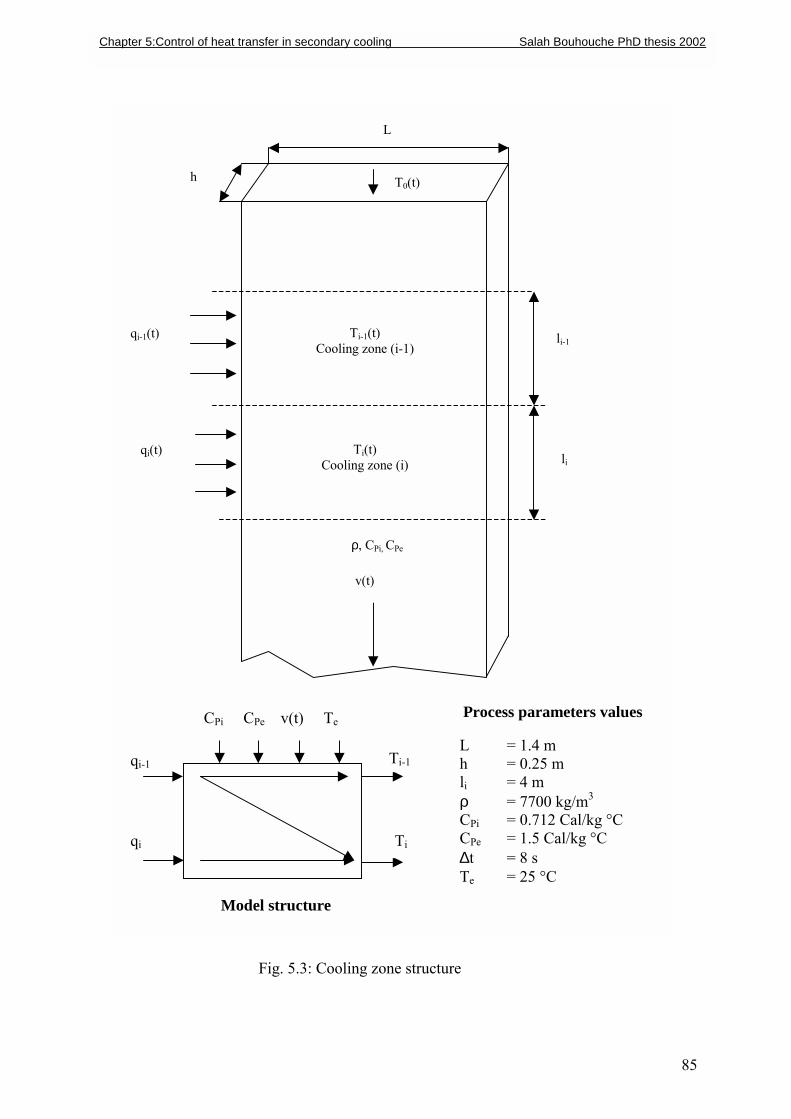
L

h

li-1

li

qi-1(t)

qi(t)

Ti-1(t) Cooling zone (i-1)

Ti(t) Cooling zone (i)

v(t)

CPi CPe v(t) Te

Process parameters values L = 1.4 m h = 0.25 m

T0(t)

ρ, CPi, CPe


qi-1

Fig. 5.3: Cooling zo

qi

Model structure

Ti-1

85

ne structure

Ti

li = 4 m ρ = 7700 kg/m3

CPi = 0.712 Cal/kg °C CPe = 1.5 Cal/kg °C ∆t = 8 s Te = 25 °C

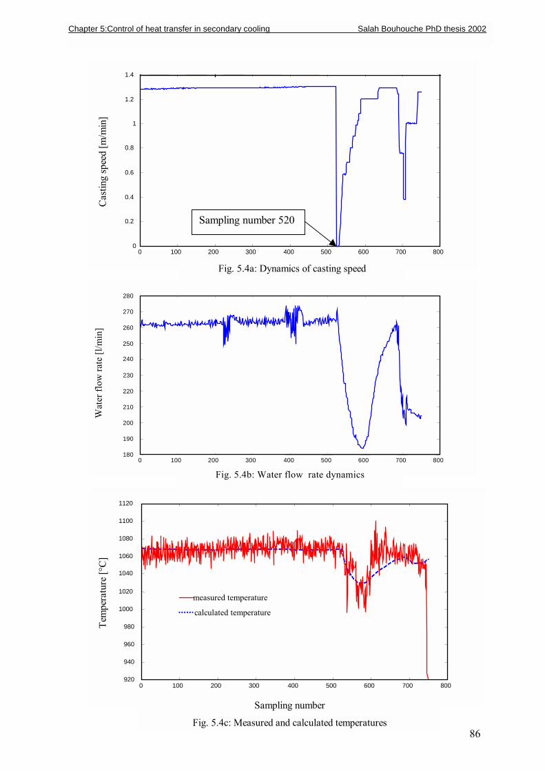
86

0 100 200 300 400 500 600 700 800 0

0.2

0.4

0.6

0.8

1

1.2

1.4

Cas

ting

spee

d [m

/min

]

Fig. 5.4a: Dynamics of casting speed

Sampling number 520

0 100 200 300 400 500 600 700 800 180 190 200 210 220 230 240 250 260 270 280

Wat

er fl

ow ra

te [l

/min

]

Fig. 5.4b: Water flow rate dynamics

0 100 200 300 400 500 600 700 800920 940 960 980

1000 1020

1040 1060 1080 1100 1120

measured temperature

calculated temperature

Tem

pera

ture

[°C

]

Sampling number

Fig. 5.4c: Measured and calculated temperatures


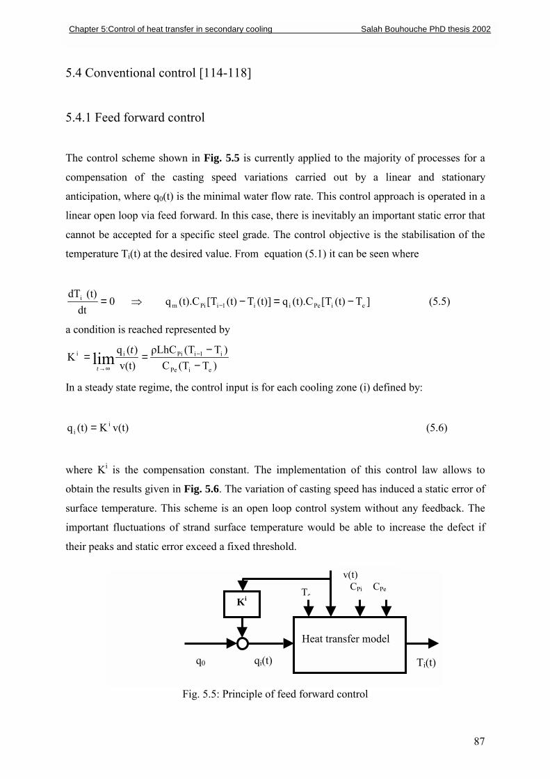
5.4 Conventional control [114-118]

5.4.1 Feed forward control

The control scheme shown in Fig. 5.5 is currently applied to the majority of processes for a

compensation of the casting speed variations carried out by a linear and stationary

anticipation, where q0(t) is the minimal water flow rate. This control approach is operated in a

linear open loop via feed forward. In this case, there is inevitably an important static error that

cannot be accepted for a specific steel grade. The control objective is the stabilisation of the

temperature Ti(t) at the desired value. From equation (5.1) it can be seen where

0dt

(t)dTi = ⇒ ]T(t)[T(t).Cq(t)]T(t)[T(t).Cq eiPeii1iPim −=−− (5.5)

a condition is reached represented by

)T(TC)T(TρLhC

v(t))(q

KeiPe

i1iPiii lim −−

== −

∞→

tt

In a steady state regime, the control input is for each cooling zone (i) defined by:

v(t)K(t)q ii = (5.6)

where Ki is the compensation constant. The implementation of this control law allows to

obtain the results given in Fig. 5.6. The variation of casting speed has induced a static error of

surface temperature. This scheme is an open loop control system without any feedback. The

important fluctuations of strand surface temperature would be able to increase the defect if

their peaks and static error exceed a fixed threshold.

Fig. 5.5: Principle of fee

Ki

q0 qi(t)

v(t) CPi CPe

e


T

87

d forward control

Heat transfer model

Ti(t)

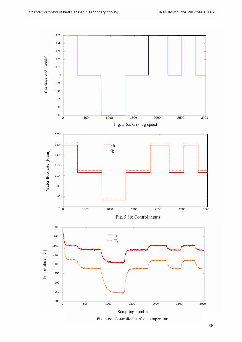
88

0 500 1000 1500 2000 2500 300040

60

80

100

120

140

160

180

q1 q2

Wat

er fl

ow ra

te [l

/min

]

Fig. 5.6b: Control inputs

0 500 1000 1500 2000 2500 30000.5

0.6

0.7

0.8

0.9

1

1.1

1.2

1.3

1.4

1.5

Cas

ting

spee

d [m

/min

]

Fig. 5.6a: Casting speed

0 500 1000 1500 2000 2500 3000800

850

900

950

1000

1050

1100

1150

1200

Tem

pera

ture

[°C

]

T1 T2

Sampling number

Fig. 5.6c: Controlled surface temperature


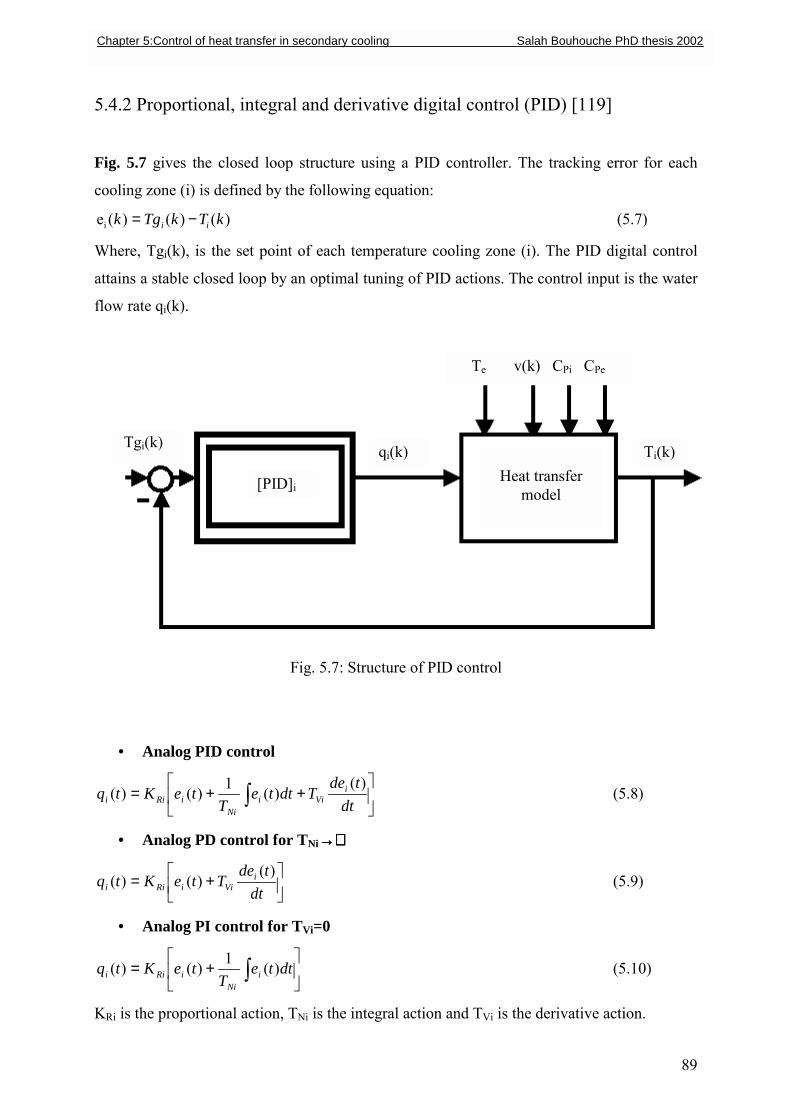
89

5.4.2 Proportional, integral and derivative digital control (PID) [119]

Fig. 5.7 gives the closed loop structure using a PID controller. The tracking error for each

cooling zone (i) is defined by the following equation:

)()()(ei kTkTgk ii −= (5.7)

Where, Tgi(k), is the set point of each temperature cooling zone (i). The PID digital control

attains a stable closed loop by an optimal tuning of PID actions. The control input is the water

flow rate qi(k).

Fig. 5.7: Structure of PID control

• Analog PID control

++= ∫ dt

tdeTdtte

TteKtq i

ViiNi

iRii)(

)(1)()( (5.8)

• Analog PD control for TNi→→→→∝∝∝∝

+=

dttdeTteKtq i

ViiRii)(

)()( (5.9)

• Analog PI control for TVi=0

+= ∫ dtte

TteKtq i

NiiRii )(1)()( (5.10)

KRi is the proportional action, TNi is the integral action and TVi is the derivative action.

Te v(k) CPi CPe

Ti(k)qi(k) Tgi(k)

[PID]i

Heat transfer model


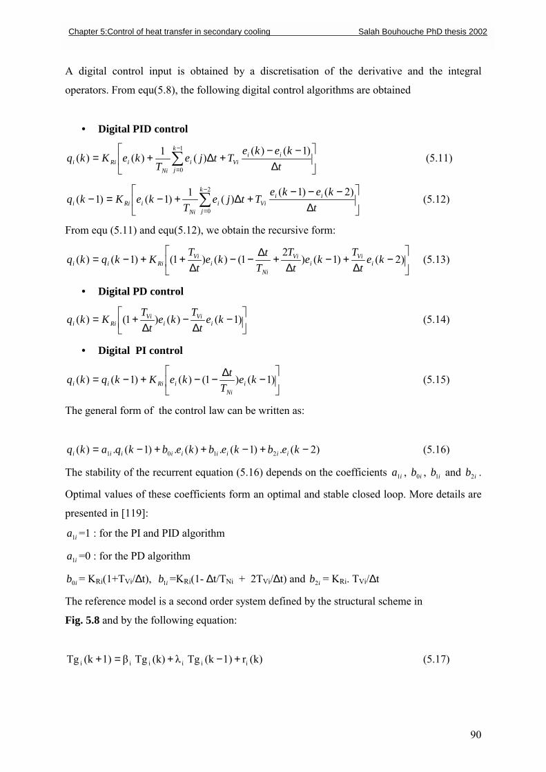
90

A digital control input is obtained by a discretisation of the derivative and the integral

operators. From equ(5.8), the following digital control algorithms are obtained

• Digital PID control

∆

−−+∆+= ∑

−

=

1

0

)1()()(1)()(

k

j

iiVii

NiiRii t

kekeTtje

TkeKkq (5.11)

∆

−−−+∆+−=− ∑

−

=

2

0

)2()1()(1)1()1(

k

j

iiVii

NiiRii t

kekeTtje

TkeKkq (5.12)

From equ (5.11) and equ(5.12), we obtain the recursive form:

−

∆+−

∆+∆−−

∆++−= )2()1()

21()()1()1()( ke

tT

ket

TT

tket

TKkqkq i

Vii

Vi

Nii

ViRiii (5.13)

• Digital PD control

−

∆−

∆+= )1()()1()( ke

tTke

tTKkq i

Vii

ViRii (5.14)

• Digital PI control

−∆−−+−= )1()1()()1()( ke

TtkeKkqkq i

NiiRiii (5.15)

The general form of the control law can be written as:

)2(.)1(.)(.)1(.)( 2101 −+−++−= kebkebkebkqakq iiiiiiiii (5.16)

The stability of the recurrent equation (5.16) depends on the coefficients ia1 , ib0 , ib1 and ib2 .

Optimal values of these coefficients form an optimal and stable closed loop. More details are

presented in [119]:

ia1 =1 : for the PI and PID algorithm

ia1 =0 : for the PD algorithm

ib0 = KRi(1+TVi/∆t), ib1 =KRi(1- ∆t/TNi + 2TVi/∆t) and ib2 = KRi. TVi/∆t

The reference model is a second order system defined by the structural scheme in

Fig. 5.8 and by the following equation:

(k)r1)(kTg λ(k)Tg β1)(kTg iiiiii +−+=+ (5.17)


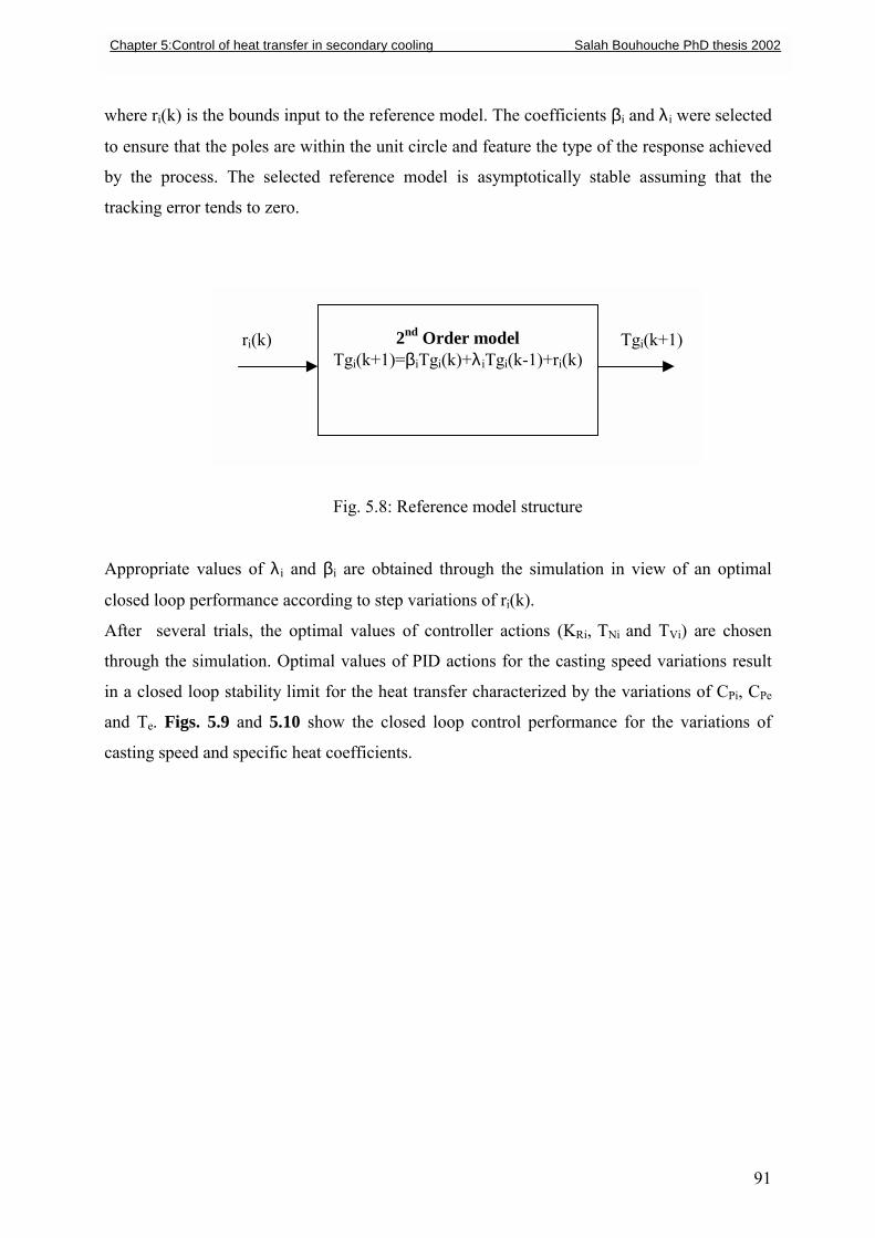
91

where ri(k) is the bounds input to the reference model. The coefficients βi and λ i were selected

to ensure that the poles are within the unit circle and feature the type of the response achieved

by the process. The selected reference model is asymptotically stable assuming that the

tracking error tends to zero.

Fig. 5.8: Reference model structure

Appropriate values of λ i and βi are obtained through the simulation in view of an optimal

closed loop performance according to step variations of ri(k).

After several trials, the optimal values of controller actions (KRi, TNi and TVi) are chosen

through the simulation. Optimal values of PID actions for the casting speed variations result

in a closed loop stability limit for the heat transfer characterized by the variations of CPi, CPe

and Te. Figs. 5.9 and 5.10 show the closed loop control performance for the variations of

casting speed and specific heat coefficients.

2nd Order model Tgi(k+1)=βiTgi(k)+λ iTgi(k-1)+ri(k)

ri(k) Tgi(k+1)


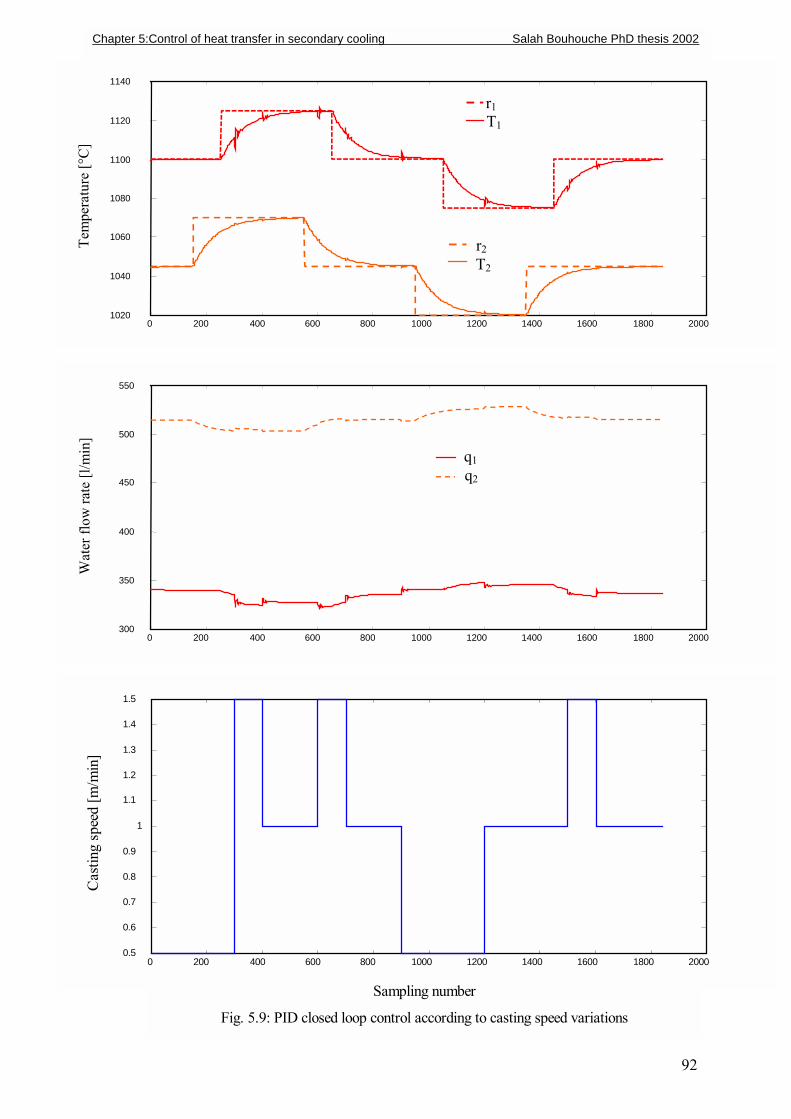
92

0 200 400 600 800 1000 1200 1400 1600 1800 20001020

1040

1060

1080

1100

1120

1140 Te

mpe

ratu

re [°

C]

r1 T1

r2 T2

0 200 400 600 800 1000 1200 1400 1600 1800 2000300

350

400

450

500

550

Wat

er fl

ow ra

te [l

/min

]

q1 q2

0 200 400 600 800 1000 1200 1400 1600 1800 20000.5 0.6 0.7 0.8 0.9

1 1.1 1.2 1.3 1.4 1.5

Sampling number

Fig. 5.9: PID closed loop control according to casting speed variations

Cas

ting

spee

d [m

/min

]


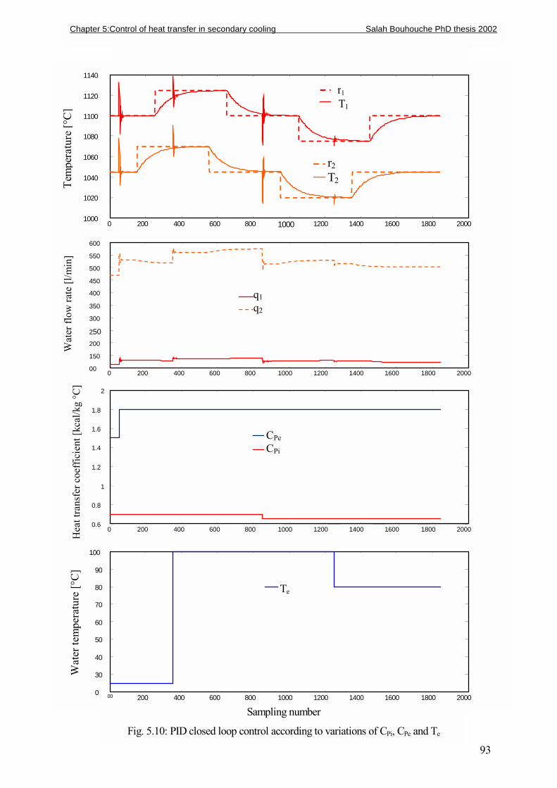
93

0 200 400 600 800 1000 1200 1400 1600 1800 2000 1000

1020

1040

1060

1080

1100

1120

1140

r1

T1

Tem

pera

ture

[°C

]

r2 T2

0 200 400 600 800 1000 1200 1400 1600 1800 200000

150

200

250

300

350

400

450

500

550

600

Wat

er fl

ow ra

te [l

/min

]

q1 q2

0 200 400 600 800 1000 1200 1400 1600 1800 20000.6

0.8

1

1.2

1.4

1.6

1.8

2

CPe CPi

Hea

t tra

nsfe

r coe

ffic

ient

[kca

l/kg

°C]

00 200 400 600 800 1000 1200 1400 1600 1800 2000 0

30

40

50

60

70

80

90

100

Wat

er te

mpe

ratu

re [°

C]

Sampling number

Fig. 5.10: PID closed loop control according to variations of CPi, CPe and Te

Te


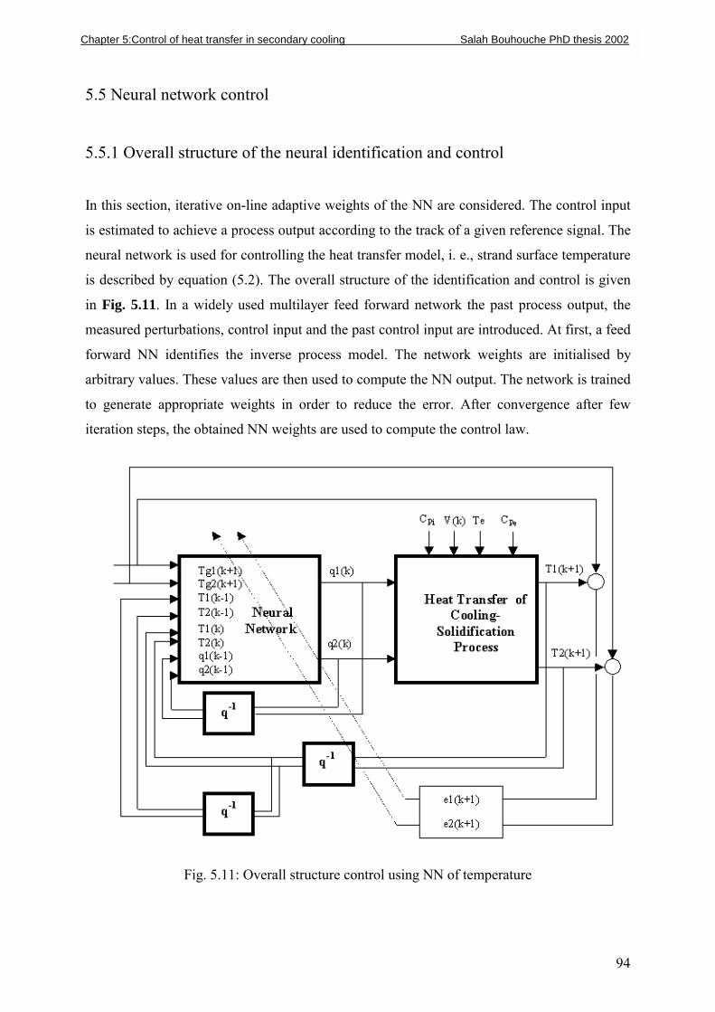
94

5.5 Neural network control

5.5.1 Overall structure of the neural identification and control

In this section, iterative on-line adaptive weights of the NN are considered. The control input

is estimated to achieve a process output according to the track of a given reference signal. The

neural network is used for controlling the heat transfer model, i. e., strand surface temperature

is described by equation (5.2). The overall structure of the identification and control is given

in Fig. 5.11. In a widely used multilayer feed forward network the past process output, the

measured perturbations, control input and the past control input are introduced. At first, a feed

forward NN identifies the inverse process model. The network weights are initialised by

arbitrary values. These values are then used to compute the NN output. The network is trained

to generate appropriate weights in order to reduce the error. After convergence after few

iteration steps, the obtained NN weights are used to compute the control law.

Fig. 5.11: Overall structure control using NN of temperature


95

For each secondary cooling zone, the inputs of the network are [Ti(k-1), Ti(k-2), qi(k-1),

qi(k-2),v(k-1), v(k-2)] and the output is Ti(k).

5.5.2 Control using neural networks

The objective of the control system is to track the strand surface temperature at the desired

values as defined by the optimal operating conditions. The reference model through the

trajectory selects the set point dynamics.

The control scheme (Fig. 5.11) is used to compute the control law using the weights from the

identification process. For each controlled temperature zone, the control law minimises the

tracking error.

To ensure that the error signal is equal to zero, the control inputs are inversely estimated by

trained NN as:

)]1(),1(),1(),1(),(),(),1(),1([)( 1111 −−−−++= −−−− kqkqkTkTkTkTkTgkTgNNkq iiiiiiiii (5.18)

Figs. 5.12 and 5.13 show the NN closed loop performance for the variation of casting speed,

water temperature (Te) and specific heat coefficients (CPi, CPe).

The on-line control algorithm can be summarised as follows:

Step 0: Initialise the network weight (-0.5 to +0.5)

Step 1: Identification

• Acquisition of inputs/outputs

• For each cooling zone (i), calculate the tracking error (k)(k)(k)e ii TTg i −=

• If 0(k)ei ≅ , oldijW=new

ijW

• Else, adjust NN weights using the BP algorithm section (2.2.1.2)

Step 2: Control

• Using newijW , compute the new control inputs (k)qi , equation (5.18)

• Next step time k=k+1

• Go to step 1


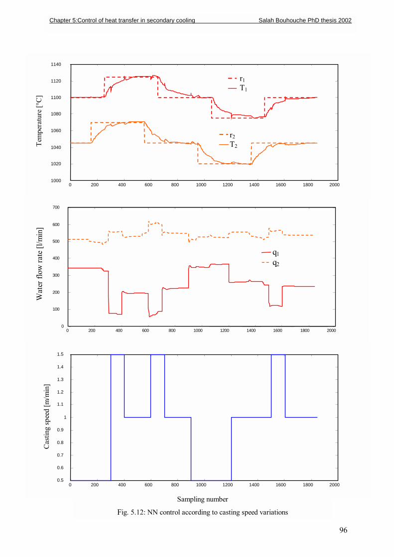
96

0 200 400 600 800 1000 1200 1400 1600 1800 20001000

1020

1040

1060

1080

1100

1120

1140

r1 T1

r2 T2 Te

mpe

ratu

re [°

C]

0 200 400 600 800 1000 1200 1400 1600 1800 20000

100

200

300

400

500

600

700

q1 q2

Wat

er fl

ow ra

te [l

/min

]

0 200 400 600 800 1000 1200 1400 1600 1800 20000.5 0.6 0.7 0.8 0.9

1

1.1 1.2 1.3 1.4 1.5

Cas

ting

spee

d [m

/min

]

Sampling number

Fig. 5.12: NN control according to casting speed variations


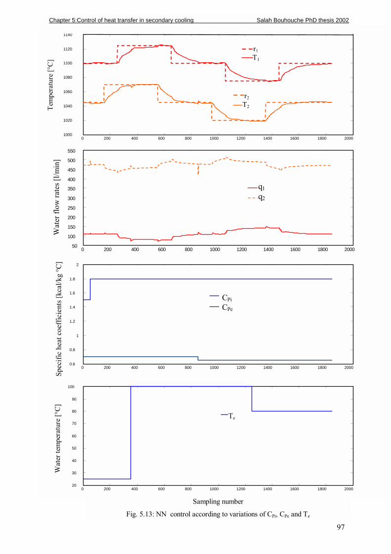
97

0 200 400 600 800 1000 1200 1400 1600 1800 20001000

1020

1040

1060

1080

1100

1120

1140

r1 T1

r2 T2 Te

mpe

ratu

re [°

C]

0 200 400 600 800 1000 1200 1400 1600 1800 200050

100

150

200

250

300

350

400

450

500

550

Wat

er fl

ow ra

tes [

l/min

]

q1 q2

0 200 400 600 800 1000 1200 1400 1600 1800 20000.6

0.8

1

1.2

1.4

1.6

1.8

2

Spec

ific

heat

coe

ffic

ient

s [kc

al/k

g °C

]

CPi CPe

0 200 400 600 800 1000 1200 1400 1600 1800 200020 30 40 50 60 70 80 90

100

Wat

er te

mpe

ratu

re [°

C]

Sampling number

Fig. 5.13: NN control according to variations of CPi, CPe and Te

Te


98

5.6 Results of Simulation

The analysis of the heat transfer dynamic model shows the existence of coupling between

cooling zones (i) and (i-1). A multivariable structure with two inputs and two outputs has

therefore been selected. The set points r1(k) and r2(k) are filtered by a second-order model that

defines stable closed loop dynamics which reduces the output temperature oscillations Ti(k)

and limits the control saturation of water flow rate qi(k). In the present NN controller, there

are 8 nodes, yr1(k+1), yr2(k+1), T1(k), T2(k), T1(k-1), T2(k-1), q1(k-1) and q2(k-1), in the input

layer. These include 3 in the first hidden layer and 2 in the second hidden layer and 2 NN

outputs q1(k) and q2(k) are chosen to learn the controller dynamics equation (5.18). A learning

rate (η ) of 0.01 and a momentum (α ) of 0.01 were used. The closed loops dynamics must

track the second order system equation (5.17) with (λ1, λ2) of 0.5 and (β1, β2) of 0.4. For the

same variations of casting speed, water temperature and specific heat coefficients, the closed

loop performance for the PID and the NN controllers were different. NN control gives an

improvement of the surface temperature dynamics compared to PID with reduced tracking

error. After several simulations, an optimally tuned PID controller based on the variations of

the casting speed has been found, while for other variables (Te, CPi and CPe), the surface

temperature behaviour is yet to be improved. This was expected due to the large variations of

process parameters and the model non-linearities with some oscillations due mainly to the

variations of Te, CPi and CPe. In practice, at normal operating conditions, the maximum

variation of casting speed (| )1()( −− kvkv |) is limited to 0.3 m/min which doesn�t affect the

surface temperature stability and reduces the inputs oscillations for NN and PID control. The

present performance was obtained by iterative adaption of NN weights using the tracking

error.

A closed loop control model has been developed. As shown in the different figures (Figs. 5.9,

5.10, 5.12 and 5.13), the closed loop is stable. NN identification and control strategy achieve a

robust and stable temperature closed loop control comparatively to the conventional PID.


99

6 FAULT AND QUALITY MONITORING BY DATABASE MODELLING

In continuous casting, on-line quality control systems and process fault detections are

generally based on the implementation of mathematical models using the process database. It

is usually possible to find a complex relation between the quality or fault and the process

parameter variations. Statistical Process Control (SPC) is applied in different steel plants as a

tool for process monitoring. SPC is used to obtain the monitoring process parameters which

are controlled between a low and high limit defined by the optimal operating conditions using

their statistical properties. NN�s permit to obtain complex non-linear relationships between

quality or defect classification and process parameters [33, 34, 120, 121, 122]. This

constitutes an important tool for the optimisation of quality control and fault detection.

Quality defects have many origins such as important process parameter deviations and faults

due to equipment. In practice, it is sometimes very difficult to find the cause of a fault in the

equipment without a real-time machine and equipment monitoring and analysis. Two

applications are considered in this chapter, the first is related to breakout alarms and their

effect on strand defects and the second is an application of real-time monitoring of casting

speed control equipment parameters. This approach of monitoring has been used to find the

cause of faults. The aim of this section is the following

• Monitoring of strand defects on the basis of the alarm number detected by the

breakout system.

• Real-time monitoring and diagnosis using computerised methods as a tool of fault

investigation (data acquisition and modelling using neural networks).

6.1 Breakout alarm and quality monitoring in continuous casting

6.1.1 Position of the problem

In chapter 4 a breakout detection system based on temperature field changes using breakout

events was developed. It is shown that a breakout can be detected by several alarms together

or by individual ones. False alarms are caused by temperature field changes and can be

cancelled by advanced modelling. In this section, the relationship between breakout alarms

and the importance of defects on the strand surface is considered. Using upper and lower

processing units of breakout it is possible to find a complex relation between alarms generated

Chapter 6 : Fault and quality monitoring by database modelling Salah Bouhouche PhD thesis 2002

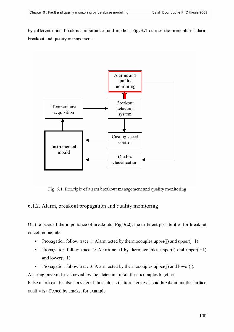
100

by different units, breakout importances and models. Fig. 6.1 defines the principle of alarm

breakout and quality management.

Fig. 6.1. Principle of alarm breakout management and quality monitoring

6.1.2. Alarm, breakout propagation and quality monitoring

On the basis of the importance of breakouts (Fig. 6.2), the different possibilities for breakout

detection include:

• Propagation follow trace 1: Alarm acted by thermocouples upper(j) and upper(j+1)

• Propagation follow trace 2: Alarm acted by thermocouples upper(j) and upper(j+1)

and lower(j+1)

• Propagation follow trace 3: Alarm acted by thermocouples upper(j) and lower(j).

A strong breakout is achieved by the detection of all thermocouples together.

False alarm can be also considered. In such a situation there exists no breakout but the surface

quality is affected by cracks, for example.

Temperature acquisition

Breakout detection system

Casting speed control

Alarms and quality

monitoring

Quality classification

Instrumented mould


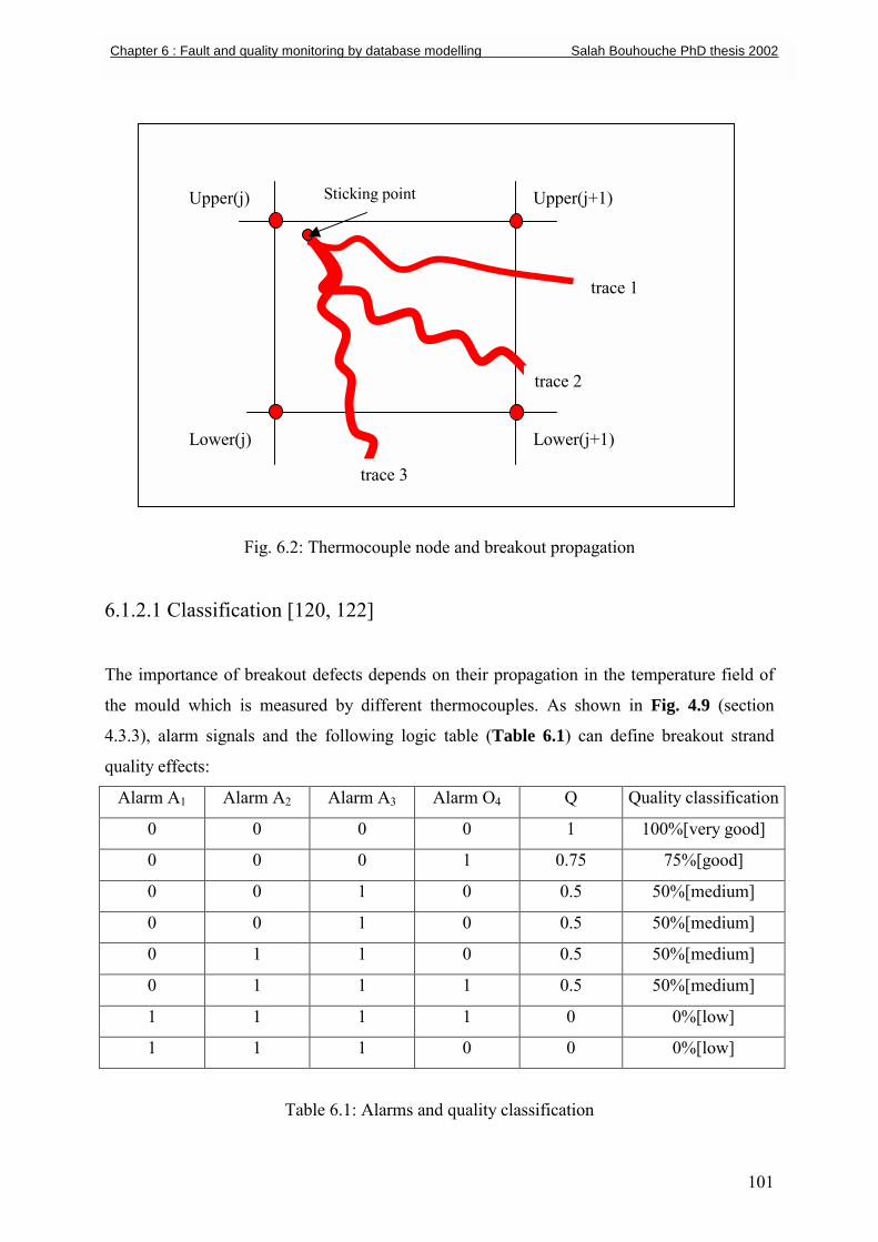
Fig. 6.2: Thermocouple node and breako

6.1.2.1 Classification [120, 122]

The importance of breakout defects depends on their prop

the mould which is measured by different thermocouple

4.3.3), alarm signals and the following logic table (Tabl

quality effects:

Alarm A1 Alarm A2 Alarm A3 Alarm O4

0 0 0 0

0 0 0 1

0 0 1 0

0 0 1 0

0 1 1 0

0 1 1 1

1 1 1 1

1 1 1 0

Table 6.1: Alarms and quality clas

Upper(j) Upper(j+1)

Lower(j)

trace 1

2

trace 3

Sticking point


trace

101

ut propagation

agation in the temperature field of

s. As shown in Fig. 4.9 (section

e 6.1) can define breakout strand

Q Quality classification

1 100%[very good]

0.75 75%[good]

0.5 50%[medium]

0.5 50%[medium]

0.5 50%[medium]

0.5 50%[medium]

0 0%[low]

0 0%[low]

sification

Lower(j+1)

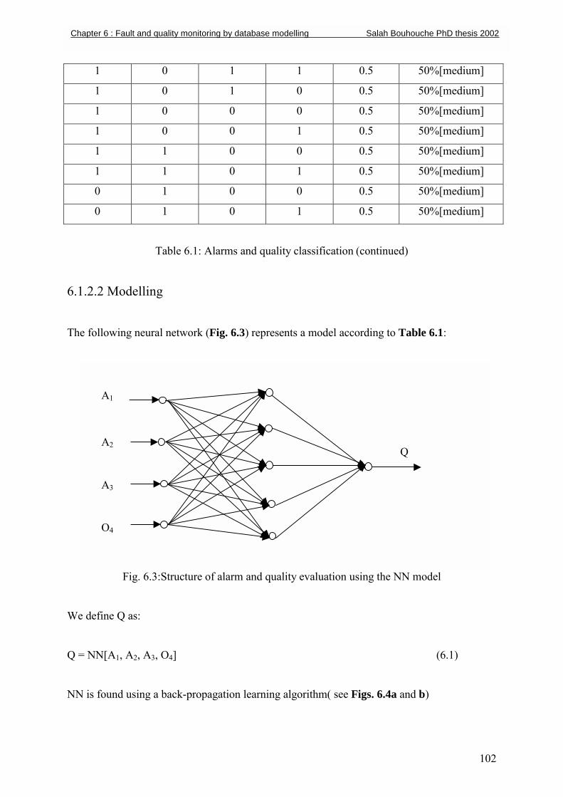
Table 6.1: Alarms and quality classification (continued)

6.1.2.2 Modelling

The following neural network (Fig. 6.3) represents a model according to Table 6.1:

Fig. 6.3:Structure of alarm and quality evaluation using the N

We define Q as:

Q = NN[A1, A2, A3, O4]

NN is found using a back-propagation learning algorithm( see Figs. 6.4a

1 0 1 1 0.5 50%[medium]

1 0 1 0 0.5 50%[medium]

1 0 0 0 0.5 50%[medium]

1 0 0 1 0.5 50%[medium]

1 1 0 0 0.5 50%[medium]

1 1 0 1 0.5 50%[medium]

0 1 0 0 0.5 50%[medium]

0 1 0 1 0.5 50%[medium]

A1

A2

A3

O4


Q

102

N model

(6.1)

and b)

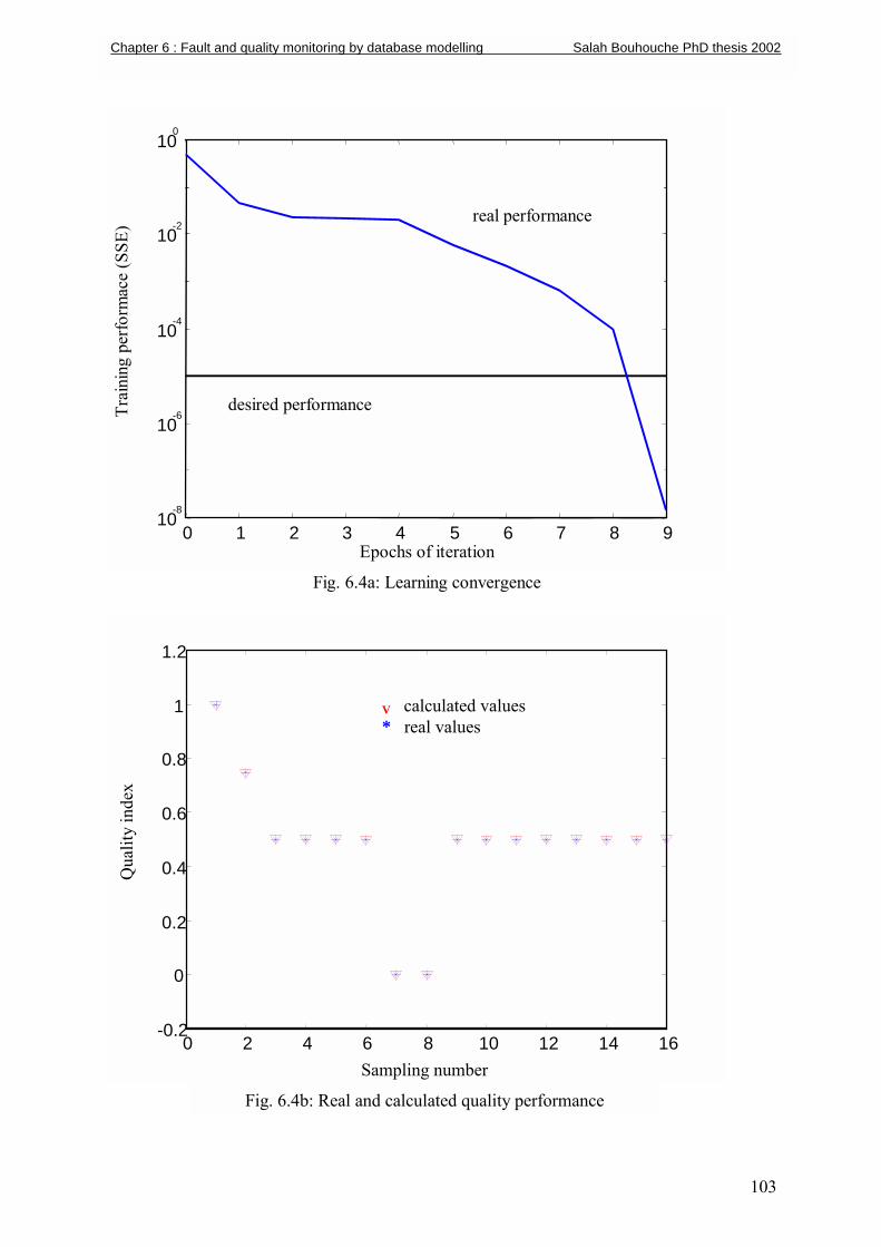
103

0 1 2 3 4 5 6 7 8 9 10

-8

10 -6

10 -4

10 -2

10 0

Epochs of iteration

Fig. 6.4a: Learning convergence

Trai

ning

per

form

ace

(SSE

)

desired performance

real performance

0 2 4 6 8 10 12 14 16 -0.2

0

0.2

0.4

0.6

0.8

1

1.2

Qua

lity

inde

x

Sampling number

Fig. 6.4b: Real and calculated quality performance

V calculated values * real values


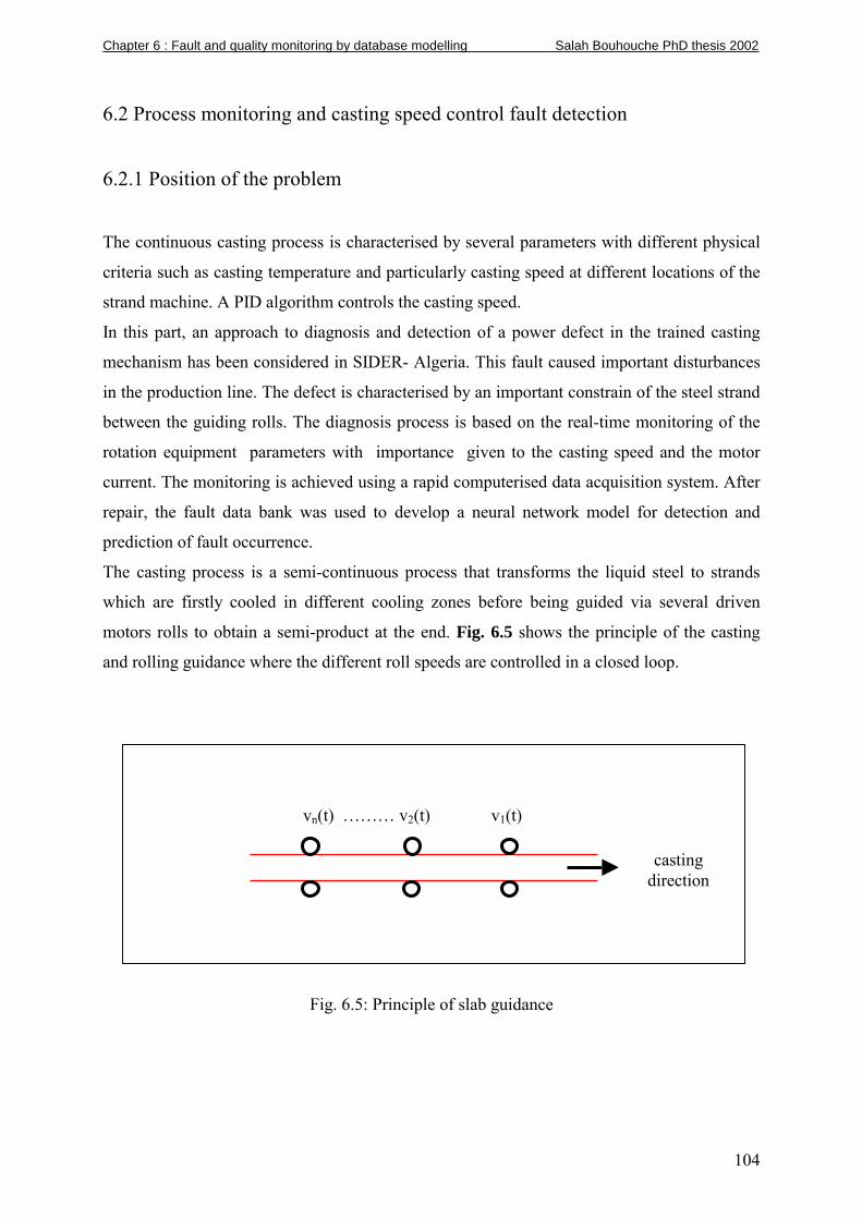
6.2 Process monitoring and casting speed control fault detection

6.2.1 Position of the problem

The continuous casting process is characterised by several parameters with different physical

criteria such as casting temperature and particularly casting speed at different locations of the

strand machine. A PID algorithm controls the casting speed.

In this part, an approach to diagnosis and detection of a power defect in the trained casting

mechanism has been considered in SIDER- Algeria. This fault caused important disturbances

in the production line. The defect is characterised by an important constrain of the steel strand

between the guiding rolls. The diagnosis process is based on the real-time monitoring of the

rotation equipment parameters with importance given to the casting speed and the motor

current. The monitoring is achieved using a rapid computerised data acquisition system. After

repair, the fault data bank was used to develop a neural network model for detection and

prediction of fault occurrence.

The casting process is a semi-continuous process that transforms the liquid steel to strands

which are firstly cooled in different cooling zones before being guided via several driven

motors rolls to obtain a semi-product at the end. Fig. 6.5 shows the principle of the casting

and rolling guidance where the different roll speeds are controlled in a closed loop.

)


vn(t) �� v2(t) v1(t

104

Fig. 6.5: Principle of slab guidance

casting direction

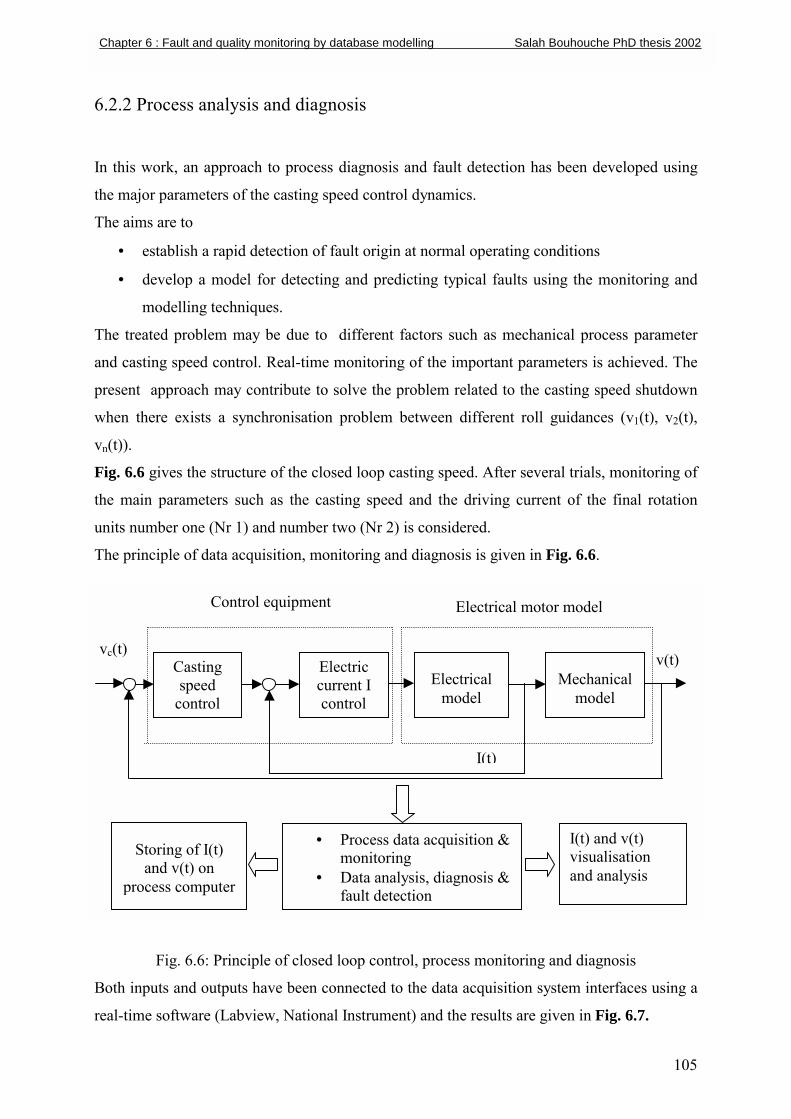
6.2.2 Process analysis and diagnosis

In this work, an approach to process diagnosis and fault detection has been developed using

the major parameters of the casting speed control dynamics.

The aims are to

• establish a rapid detection of fault origin at normal operating conditions

• develop a model for detecting and predicting typical faults using the monitoring and

modelling techniques.

The treated problem may be due to different factors such as mechanical process parameter

and casting speed control. Real-time monitoring of the important parameters is achieved. The

present approach may contribute to solve the problem related to the casting speed shutdown

when there exists a synchronisation problem between different roll guidances (v1(t), v2(t),

vn(t)).

Fig. 6.6 gives the structure of the closed loop casting speed. After several trials, monitoring of

the main parameters such as the casting speed and the driving current of the final rotation

units number one (Nr 1) and number two (Nr 2) is considered.

The principle of data acquisition, monitoring and diagnosis is given in Fig. 6.6.

Fig. 6.6: Principle of clo

Both inputs and outputs have been

real-time software (Labview, Natio

Mechanical

model

Electrical

model

v(t)vc(t)

Electrical motor model Control equipment

Storing of I(t)

and v(t) on process computer


Electric current I control

Casting speed

control

sed loop control, process

connected to the data a

nal Instrument) and the

)

• Promo

• Dafau

I(t

I(t) and v(t) visualisation and analysis

cess data acquisition & nitoring ta analysis, diagnosis & lt detection

105

monitoring and diagnosis

cquisition system interfaces using a

results are given in Fig. 6.7.

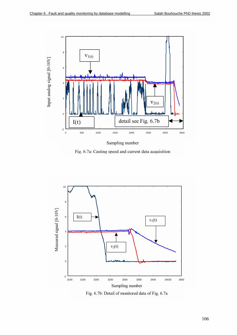
106

0 500 1000 1500 2000 2500 3000 3500 -2

0

2

4

6

8

10

v1(t)

Sampling number

Fig. 6.7a: Casting speed and current data acquisition

Inpu

t ana

log

sign

al [0

-10V

]

I(t)

v2(t)

detail see Fig. 6.7b

3100 3150 3200 3250 3300 3350 3400 34530 3500 -2

0

2

4

6

8

10

v1(t)

Sampling number

Fig. 6.7b: Detail of monitored data of Fig. 6.7a

Mea

sure

d sig

nal [

0-10

V]

I(t)

v2(t)


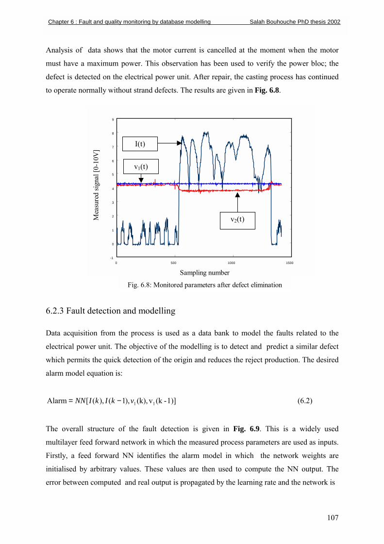
107

Analysis of data shows that the motor current is cancelled at the moment when the motor

must have a maximum power. This observation has been used to verify the power bloc; the

defect is detected on the electrical power unit. After repair, the casting process has continued

to operate normally without strand defects. The results are given in Fig. 6.8.

6.2.3 Fault detection and modelling Data acquisition from the process is used as a data bank to model the faults related to the

electrical power unit. The objective of the modelling is to detect and predict a similar defect

which permits the quick detection of the origin and reduces the reject production. The desired

alarm model equation is:

1)]-(kv(k),),1(),([Alarm 11vkIkINN −= (6.2)

The overall structure of the fault detection is given in Fig. 6.9. This is a widely used

multilayer feed forward network in which the measured process parameters are used as inputs.

Firstly, a feed forward NN identifies the alarm model in which the network weights are

initialised by arbitrary values. These values are then used to compute the NN output. The

error between computed and real output is propagated by the learning rate and the network is

0 500 1000 1500 -1

0

1

2

3

4

5

6

7

8

9

I(t)

Sampling number

Fig. 6.8: Monitored parameters after defect elimination

Mea

sure

d sig

nal [

0-10

V]

v2(t)

v1(t)


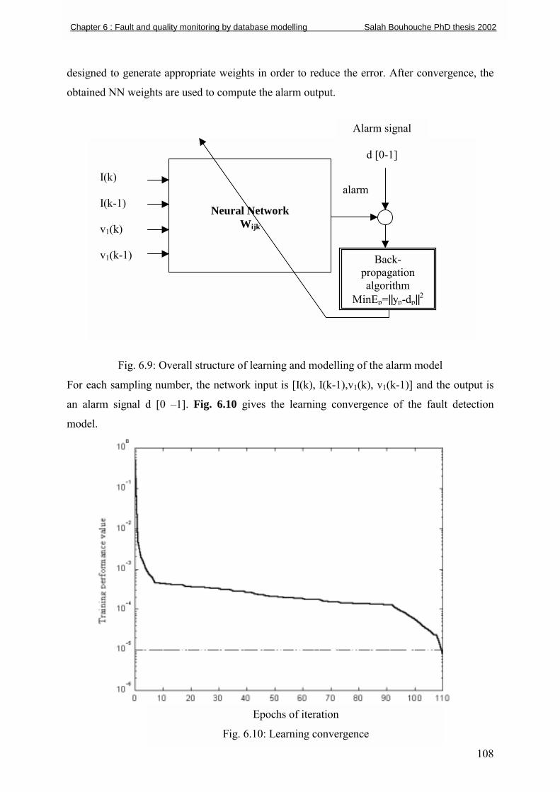
designed to generate appropriate weights in order to reduce the error. After convergence, the

obtained NN weights are used to compute the alarm output.

Fig. 6.9: Overall structure of learning and modelling of the alarm model

For each sampling number, the network input is [I(k), I(k-1),v1(k), v1(k-1)] and the output is

an alarm signal d [0 �1]. Fig. 6.10 gives the learning convergence of the fault detection

model.

Fig. 6

Neural Network

Wijk

pra

Min

I(k) I(k-1) v1(k) v1(k-1)

Alarm signal

d [0-1]


Epochs of iteration

.10: Learning convergence

Back-opagation lgorithm Ep=||yp-dp||2

alarm

108

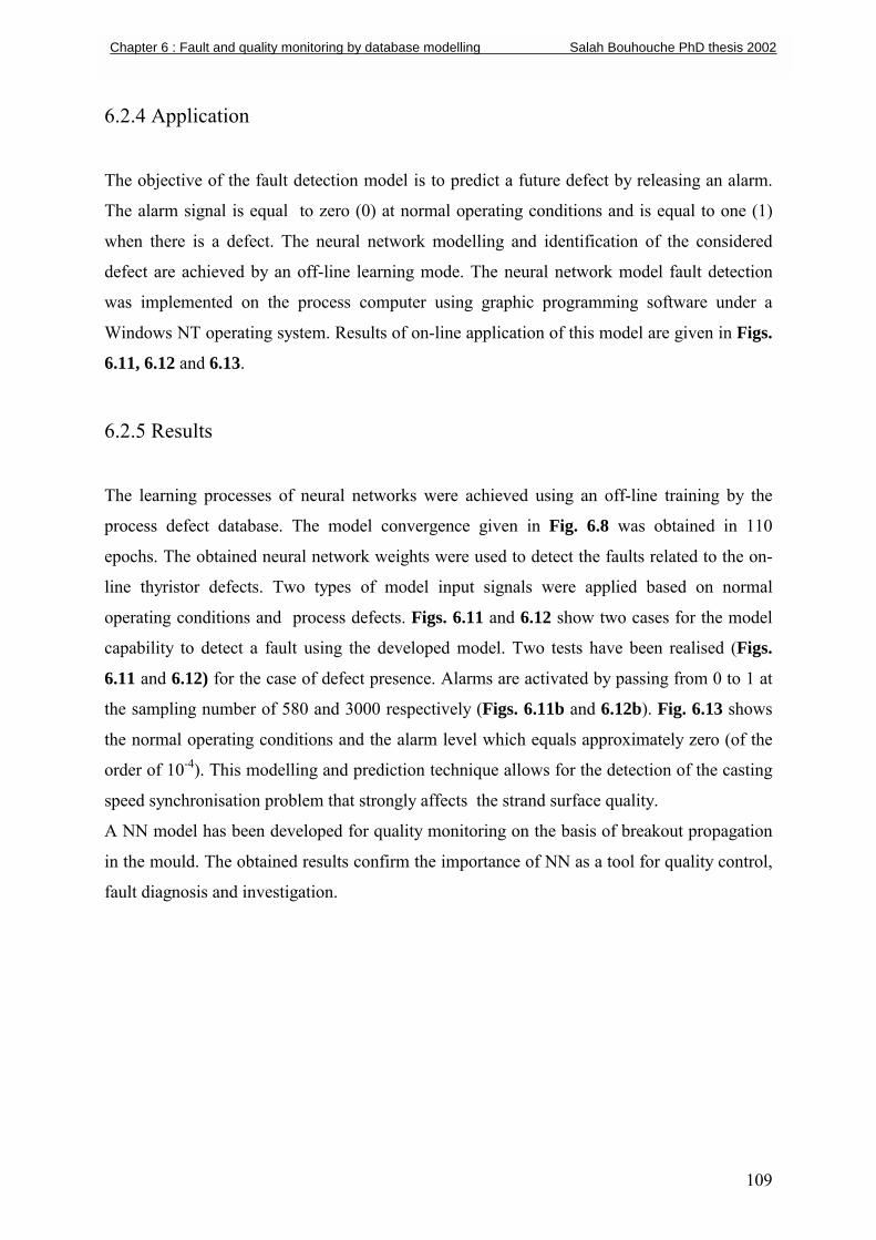
109

6.2.4 Application

The objective of the fault detection model is to predict a future defect by releasing an alarm.

The alarm signal is equal to zero (0) at normal operating conditions and is equal to one (1)

when there is a defect. The neural network modelling and identification of the considered

defect are achieved by an off-line learning mode. The neural network model fault detection

was implemented on the process computer using graphic programming software under a

Windows NT operating system. Results of on-line application of this model are given in Figs.

6.11, 6.12 and 6.13.

6.2.5 Results

The learning processes of neural networks were achieved using an off-line training by the

process defect database. The model convergence given in Fig. 6.8 was obtained in 110

epochs. The obtained neural network weights were used to detect the faults related to the on-

line thyristor defects. Two types of model input signals were applied based on normal

operating conditions and process defects. Figs. 6.11 and 6.12 show two cases for the model

capability to detect a fault using the developed model. Two tests have been realised (Figs.

6.11 and 6.12) for the case of defect presence. Alarms are activated by passing from 0 to 1 at

the sampling number of 580 and 3000 respectively (Figs. 6.11b and 6.12b). Fig. 6.13 shows

the normal operating conditions and the alarm level which equals approximately zero (of the

order of 10-4). This modelling and prediction technique allows for the detection of the casting

speed synchronisation problem that strongly affects the strand surface quality.

A NN model has been developed for quality monitoring on the basis of breakout propagation

in the mould. The obtained results confirm the importance of NN as a tool for quality control,

fault diagnosis and investigation.


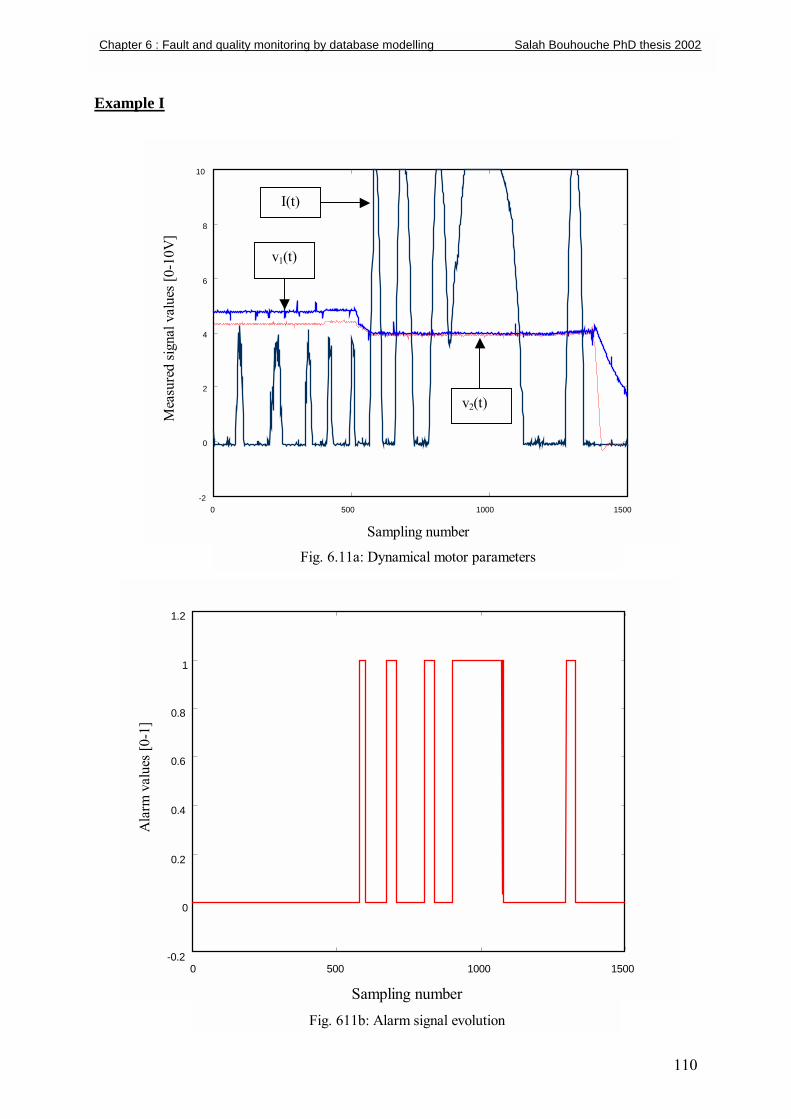
110

Example I

0 500 1000 1500 -2

0

2

4

6

8

10

Sampling number

Fig. 6.11a: Dynamical motor parameters

Mea

sure

d sig

nal v

alue

s [0-

10V

]

I(t)

v2(t)

v1(t)

0 500 1000 1500 -0.2

0

0.2

0.4

0.6

0.8

1

1.2

Ala

rm v

alue

s [0-

1]

Sampling number Fig. 611b: Alarm signal evolution


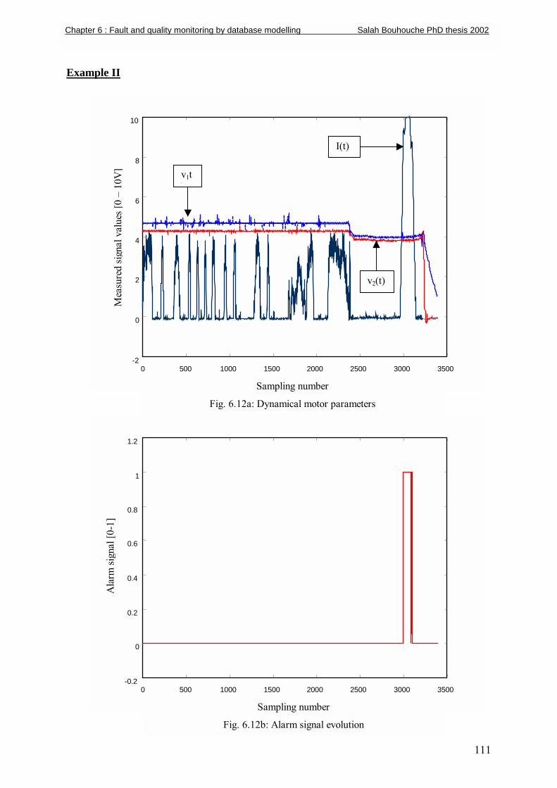
111

Example II

0 500 1000 1500 2000 2500 3000 3500 -2

0

2

4

6

8

10

I(t)

Sampling number


Mea

sure

d sig

nal v

alue

s [0

� 10

V]

v2(t)

v1t)

0 500 1000 1500 2000 2500 3000 3500 -0.2

0

0.2

0.4

0.6

0.8

1

1.2

Sampling number

Fig. 6.12b: Alarm signal evolution

Ala

rm si

gnal

[0-1

]


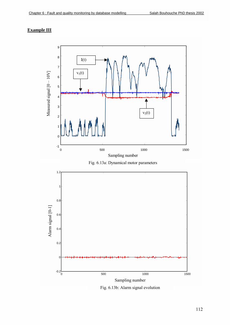
112

Example III

0 500 1000 1500-0.2

0

0.2

0.4

0.6

0.8

1

1.2

Sampling number

Fig. 6.13b: Alarm signal evolution

Ala

rm si

gnal

[0-1

]

0 500 1000 1500 -1

0

1

2

3

4

5

6

7

8

9

I(t)

Sampling number


Mea

sure

d sig

nal [

0 �

10V

]

v2(t)

v1(t)


113

7 CONCLUSION AND OUTLOOK

In this thesis work, a contribution to process and quality optimisation in ladle refining and

continuous casting of steel has been developed. The advanced tools based on neural networks

modelling have been applied to different process stages in steel production. Particular

attention has been given to the development of a reliable breakout prediction system in

continuous casting. The ability of this new system has been tested using breakout alarm

databases from EKO STAHL, Eisenhüttenstadt, Germany.

The NN breakout system based on the instrumentation of the mould by a matrix of

thermocouples using a model of prediction by NN was developed, implemented and tested.

The training of the model and tests of detection were carried out using real and false breakout

data. In the case of real alarm, the results do not detect the presence of false alarms. The

developed algorithm detected the dynamic behaviour of temperature profiles having generated

real breakouts. In the case of false alarms, the developed model does not detect false

breakouts.

The ability of the NN to detect complex processes by noise signals makes these a valuable

tool in almost all fault detections and helps in increasing the production quality standards.

This work is an example for a NN based system which has been acquired using earlier data

and can improve continuously by learning from experiences gathered during on-line

operation. The capability of the neural breakout detection system can be summarised by the

following items:

• Reliable detection of stickers in the continuous casting process

• Avoidance of the misclassification of conventional alarm systems

• Invariance with respect to variations in steel quality

• Robustness based on the variations of casting conditions

• Robustness on the basis of bath level and steel temperature variations

The results of the off-line evaluation have been fully confirmed. All real alarms have been

detected by both systems. However, the alarms from the NN detection system occur earlier

compared to those of the conventional system.

Chapter 7 : Conclusion and outlook Salah Bouhouche PhD thesis 2002

Fu

pa

In

pr

pe

be

pr

th

Al

th

pr

ap

A

de

an

pa

tem

er

co

co

di

sit

In

co

re

be

m

sy

im


114

rther developments seem to be necessary for a better optimisation of the structure and

rameters of the model.

chapter 3, a NN predictor was designed and tested through simulation and practice. The

evious NN model based on the back-propagation learning algorithm has a good prediction

rformance. Because the casting cycle is long, the learning process is easily achieved

tween the actual and the next charge. The prediction ability using NN improves the

ediction capacity. Large-scale industrial tests, on-line implementation in steelmaking and

e development of a software package are currently being investigated at SIDER Group

geria. In specific situations of steel refining processes, where there are problems related to

e timing and the chemical analysis equipment, this model can be used as a soft sensor to

edict the final chemical composition without waiting for laboratory analysis results. This

proach can be expanded without difficulties to other typical processes.

NN closed loop control scheme of heat transfer in the continuous casting process was

signed and tested through simulation in chapter 5. The neural network controller based on

inverse model seems to have a good control performance for changes of heat transfer

rameters, casting speed variations and set point changes. The changes in strand surface

perature are smaller than in conventional control where there exists an important tracking

ror. Coupling effects are also cancelled. The implementation of on-line control in the

ntinuous casting process is currently being investigated. Feedback control requires a

ntinuous measurement of surface temperature in the cooling zones. This constitutes a

sadvantage. In practice it is recommended that this approach should be used only in specific

uations with regard to sensitive steel grades.

chapter 6, systems for fault diagnosis, detection of cracks and repair were realised in the

ntinuous casting process using real-time monitoring of the major process parameters. The

al-time monitoring of the process parameters is an important tool for detecting and repair

cause it reduces the defect searching time. Fault databases were used to develop a fault

odel that predicts future defects by the electrical power unit using dynamics of the rotation

stem parameters such as rolling speed and electrical current. This model is actually

plemented on the process computer in the continuous casting process.

Th

re

ala

us

Th

su

T

su

A

sc

re

wh

pr

pr

of


115

e NN quality monitoring is a non-linear classifier which is obtained by a combination of

levant variables that have been considered by the breakout detection system. Breakout

rm monitoring using the NN model is an important tool to quality classification. It can be

ed to guide quality inspection services.

e breakout alarm management and quality monitoring remains open for other developments

ch as neuro-fuzzy application to a number of alarms and breakout defects.

he application of this technology for the prediction of other types of defects will be the

bject of future research and development work.

contribution to the improvement of main processes in steelmaking has been achieved. The

ientific importance given through the NN model implementation and on-line control

presents a highlight. Particular importance has been given to the breakout detection system

ich is of great economical impact. Mathematical modelling does not completely solve

oblems in steelmaking but in the majority of cases it leads to an improvement. Parallel

ocess computing approaches can be used as a means for future development and application

mathematical modelling in the main processes of the steel industry.

116

8 REFERENCES

[1] K.Mörwald et al., Dynacs: Cooling system�features and operational results, Ironmaking

and Steelmaking,!25(4), pp 323-327, 1998.!

[2] MmeEtiene, Reflexion sur le contrôle du refroidissement secondaire des installations de

coulée continue, rapport de la commission coulée continue, Centre de Recherche

Métallurgique de Liège, 1977.

[3] MmeEtiene, Contrôle métallurgique d'une machine de coulée continue à brames, Rapport

final convention CCE/Centre de Recherche Métallurgique de Liège, Belgique Nr 7210,

CA/204, 1977.

[4] J.P.Birat, Modelling and process control in steel industry, Révue de Métallugie, CIT (11),

pp 1348-1367, 1997.

[5] A.J.Morris and E.B.Martin, Neural networks�Panacea or pragmatic solution, European

Commission for Technical Steel Research, ECSC Workshop, Proceedings of Application

of Artificial Neural Network Systems in the Steel Industry, Brussels 22-23 January, pp 9-

41, 1998.

[6] M.Sanarico, Neural networks: The ideal and the commercially avaible tools, European


of Artificial Neural Network Systems in the Steel Industry, Brussels 22-23 January, pp

45-50, 1998.

[7] J.Frigière, L.Bertrand, M.Chouvet, M.Lallier and R.Perisse, The state of the art of neural

network application in the iron and steel industry outside of Europe, European


of Artificial Neural Network Systems in the Steel Industry, Brussels 22-23 January, pp

53-62, 1998.

[8] M.Falzetti, J.Mochon and S.Kumar, Results and perspectives of using artificial

intelligence techniques in blast furnaces: The FANCIM project, European Commission

for Technical Steel Research, ECSC Workshop, Proceedings of Application of Artificial

Neural Network Systems in the Steel Industry, Brussels 22-23 January, pp 95-104, 1998.

[9] K.Harste et al., Optimisation of casting and cooling strategies in continuous casting with

help of mathematical modelling, 10th PTD Conference Toronto Canada, (10), pp 305-

316, 1992. !

[10] H.Whittker, M.Hartwig, M.Poschmann and A.Seeliger, The use of neural networks in

Chapter 8: References Salah Bouhouche PhD thesis 2002

117

BOS Process Modelling, European Commission for Technical Steel Research, ECSC

Workshop, Proceedings of Application of Artificial Neural Network Systems in the

Steel Industry, Brussels 22-23 January, pp 135-144, 1998.

[11] M.Hormel and M.Schwartz, Breakout prediction in continuous casting by artificial

neural networks, European Commission for Technical Steel Research, ECSC


Steel Industry, Brussels 22-23 January, pp159-167, 1998.

[12] S.Li, X.Gao, J.Chai and X.Wang, Neural network techniques and its applications in

ladle furnace burden, Proceedings of IFAC Automation in Steel Industry: Current

Practice and Future Developments, pp 165-168, 1997.

[13] J.Bast und S.Bouhouche, Mathematishe Modellierung einer Strangießanlage, Freiberger

Forschungshefte, Automatisierung in der Montanindustrie Freiberg Germany A839, pp

37-50, 1997.

[14] C.Barlocco, Projet dún système dáutomatisation du refroidissement secondaire en

coulée continue, Révue de Métallurgie, CIT (12), pp 947-951, 1983.

[15] B.Stefano et al., Computer control and optimisation of secondary cooling during

continuous casting, Iron and Steel Engineer!(11), pp 21-26, 1986.

[16] K.Harste et al., Process Control and strand condition monitoring at Dillinger

Hüttenwerke, Révue de Métallurgie, CIT (4), pp 1241-1247, 1996.

[17] B.Holger, Computersimulation thermischer und mechanischer Vorgänge beim

Brammenstranggießen von Stahl, Dissertation Dr.-Ing Nr 94.10186/3, TU

Bergakademie Freiberg 1994.

[18] K.H. Spitzer et al., Mathematical model for thermal tracking and on-line control in

continuous casting, ISIJ International, 32 (7), pp 848-856, 1992.

[19] M.Sergio, S.E.Alice and B.Bopaya, Neural predictive quality model for slip casting

using categorical metrics, Proceedings of the 2nd Industrial Engineering Research

Conference, pp 265-269, 1993.

[20] F.Angela and L.Marcel, Quality control in die casting with neural networks, Proceedings

of 1st International Symposium on Neuro-Fuzzy Systems, pp 1-7, 1996.

[21] E.Laitinen. and P.Neittaanmaki, On numerical simulation of the problem connected

with the control of the secondary cooling in the continuous casting process, CTAT

14(3), pp 284-305, 1988.

[22] M.Larrecq, C.Saguez et M.Wanin, Modèle mathématique de la solidification en coulée


118

continue tenant compte de la convection à línterface solide-liquide, ! Révue de

Métallurgie, CIT (6), pp 337-352, 1978.!

[23] B.Lally, L.Biegler and H.Henein, Finite difference heat transfer modelling for continuous

casting, Metallurgical Transactions B21 (4), pp 761-770, 1990.!

[24] S.Louhenkilpi, E.Laitinen and R.Nieminen, Real-time simulation of heat transfer in

continuous casting, Metallurgical Transactions B (24), pp 685-693, 1993.

[25] I.F.Taylor, G.J.Thornton and R.J.Batterham, Process control models for real-time

applications, Ironmaking and Steelmaking 17, (6), pp 438-442, 1990

[26] G.Brunnbaner, B.Rummer and J.Marhart, The fully automatic blast furnace only a

vision, Révue de Métallugie, (6), pp 542-552, 2001.

[27] R.Capotosti, F.Macci and A.Spaccarotella, Computerised surface quality prediction in

the continuous casting of stainless steel slabs, AISE Spring Convention, Salt Lake City,

pp 61 � 71, 1995.

[28] D.Lee, J.S.Lee and T.Kang, Adaptive fuzzy control of the molten steel level in a strip

casting process, Control Engineering Practices, 4, (11), pp 1511-1520 , 1996.

[29] L.Brimacombe, C.Jackson and N.Schofield, Artificial intelligence expert system for

steelworks pollution control, Révue de Métallugie,CIT (1), pp 111-116, 2001.

[30] C.Harris, M.Brown, K.M.Bossley, D.J.Mills and F.Ming, Advances in neuro-fuzzy

algorithms for real-time modelling and control, Engineering Application of Artificial

Intelligence, 9, (1), pp 1-16, 1996.

[31] K.E.Blazek and I.G.Saucedo, Recovery of sticker type breakouts, Proceedings of

Steelmaking Conference, pp 99-107, 1989.!

[32] J.H.Zietsman, S.Kumar, J.A.Meech, I.V.Samarasekera and J.K.Brimacombe, Taper

design in continuous billet casting using neural networks, Ironmaking and Steelmaking

25 (6), pp 476-483, 1998.!

[33] P.Bellomo, M.Milone, A.Spaccarotella, F.Vicino and M.Sanarico, Stainless steel slab

surface quality prediction by means of artificial neural networks, European Commission

for Technical Steel Research, ECSC Workshop, Proceedings of Application of Artificial

Neural Network Systems in the Steel Industry, Brussels 22-23 January, pp 181-193,

1998.

[34] L.G.Lock, A.R.Mc.Namara, K.C.The, H.M.Lie, B.J.Orenstein and D.J.H.Brown, Rapid

prototyping tools for real-time expert systems in the steel industry, ISIJ International,

30, pp 90-97, 1990.


119

[35] N.Link and N.Holzkhecht, Quality prediction by data based methods, European

Commission for Technical Steel Research, ECSC Workshop, Proceedings of

Application of Artificial Neural Network Systems in the Steel Industry, Brussels 22-23

January, pp 171-178, 1998.

[36] N.Chakraborti and A.Mukherjee, Optimisation of continuous casting mould parameters

using genetic algorithms and other allied techniques, Ironmaking and Steelmaking, 27,

(3), pp 243-247, 2000

[37] S.Bouhouche, M.S.Boucherit and M.Lahreche, Improvement of breakout detection

system in continuous casting process using neural networks, IEEE Proceedings on

Advanced Process Control Applications for Industry Workshop, Vancouver, Canada,

pp 53-63, 2001, (Site Internet www.ieee-ias.org /apc2001).

[38] N.Ramaseder and J.Heiss, VAI-CONR Temp: Continuous temperature monitoring in

metallurgical vessels, Révue de Métallugie, CIT (6), pp 562-569, 2001.

[39] P.N.Hewih, A.Robson, A.S.Normanton, N.S.Hunter and A.Scholes, Continuous casting

development at British steel, Révue de Métallugie, CIT (6), pp 765-776, 1998.

[40] H. Kominami et al., Neural networks system for breakout prediction in continuous

casting process, Nippon Steel Technical Report, (49), pp 34-38, 1991.

[41] S.B.Singh, H.K.D.H.Bhadeshia, D.S.C.Mackay, H.Creyand and I.Martin, Neural

network analysis of steel plate processing, Ironmaking and Steelmaking, 25, (5), pp

355-365, 1998.

[42] P.Hemy, R.Smylie and C.Srinivasan, Analysing casting problem by the on-line

monitoring of continuous casting mold temperatures, JOM-e, 2002,

www.umc.tms.org/pubs/journals/JOM/021/Hemy/Hemy-0201.html

[43] J.T.Niu, L.J.Sun and P.Karjalainen, A neural network-based model for prediction of hot-

rolling austenite grain size and flow stress in microalloy steel, Acta Metallurgica Sinica

(English letters), 13, (2), pp 521-530, 2000.

[44] F.H.R.Sesselmann, Improving EAF energy utilisation with electrode controllers based

on neural networks, Proceedings of IFAC Automation in Mining, Mineral and Metal

Processing, pp 61-67, 1998.

[45] S.Z.Suo, L.Yuon and S.Kang, The AGC-ASC synthetic artificial neural networks

controllers, Proceedings of IFAC Automation in Mining, Mineral and Metal



http://www.umc.tms.org/pubs)journals/JOM/021/Hemy/Hemy-0201.html

120

[46] N.Bhat, P.Minderman and P.Mc.Avoy, Use of neural nets for modelling of chemical

process systems, IFAC Symposium, pp 21-23, 1989.

[47] Di.Psaltis, A.Sideris and A.Yamamura, A multilayered neural network controller, IEEE

Control System Magazine, pp 17-21, 1988.

[48] M.Norgaard, O.Ravn, N.K.Poulsen and L.K.Hansen, Neural networks for modelling and

control of dynmic systems, Springer, ISBN 1-85233-227, 2000.

[49] M.Jansen, E.Broese, B.Feldkeller, O.Gramckown, T.proppe, M.Schlang and G.Sorgel,

Application of neural networks to process control in steel industry, Proceedings of

IFAC Automation in Mining, Mineral and Metal Processing, pp 177-182, 1998.

[50] M.Waller and H.Saxén, Time-varying Fir-models for short-term prediction of pig silicon

content, Proceedings of IFAC Automation in Mining, Mineral and Metal Processing,

pp 227-232, 1998.

[51] M.Hadjiski, I.Kalaykov and S.Mollov, Neural network modelling and control of

parameter depending metallurgical plants, Proceedings of IFAC Automation in Mining,

Mineral and Metal Processing, pp 375-380, 1998.

[52] G.C.Goodwin and R.Middleron, Advanced control applications in the steel industry,

Proceedings of IFAC Automation in Steel Industry: Current Practice and Future

Developments, pp 13-18, 1997.

[53] Y.I.Kim, K.C.Moon, B.S.Kang, C.Han and K.S.Chang, Application of Neural network

to supervisory control of reheating furnace in steel industry, Proceedings of IFAC

Automation in Steel Industry: Current Practice and Future Developments, pp 33-38,

1997.

[54] H.Ingason and G.R.Jonsson, On the control of silicon ratio in ferrosilicon production,

Proceedings of IFAC Automation in Steel Industry: Current Practice and Future

Developments, pp 73-78, 1997.

[55] Y.Kueon and S.Y.Yoo, Mold level control in continuous caster via non-linear control

technique, Proceedings of IFAC Automation in Steel Industry: Current Practice and

Future Developments, pp 169-173, 1997.

[56] X.G.Shujiangli, T.Chai and X.Wang, Intelligent compound control of direct current

electric arc furnace, Proceedings of IFAC Automation in Steel Industry: Current

Practice and Future Developments, pp 135-140, 1997.

[57] J.S.Choi, H.Kim and Y.J.Moon, Identification and adaptive control of dynamic systems

using self-organised distributed networks, Proceedings of IFAC Automation in Steel

Industry: Current Practice and Future Developments, pp 91-96, 1997.


121

[58] D.Y.Seok and J.S.Lee, Adaptive inverse control for non-linear plants, Proceedings of

IFAC Automation in Steel Industry: Current Practice and Future Developments, pp 199-

204, 1997.

[59] S.Johnstone and A.G.Taylor, Application of multivariate statistical methods to blast

furnace hearth temperatures, European Commission for Technical Steel Research,

ECSC Workshop, Proceedings of Application of Artificial Neural Network Systems in

the Steel Industry, Brussels 22-23 January, pp 69-91, 1998.

[60] K.S.Yoon and M.H.Lee, On the design of self�tuning controller using generalised

predictive control, Proceedings of IFAC Automation in Steel Industry: Current Practice

and Future Developments, pp 85-90, 1997.

[61] M.L.Goc and C.C.Thirion, The SACHEM experience on artificial neural networks

application, European Commission for Technical Steel Research, ECSC Workshop,

Proceedings of Application of Artificial Neural Network Systems in the Steel Industry,

Brussels 22-23 January, pp107-131, 1998.

[62] C.D.I.Massimo, G.A.Montague, M.J.Willis, M.T.Tham and A.J.Morris, Towars

improved penicillin fermentation via artificial neural networks, Computer in Chemical

Engineering, 16, (4), pp 283-291, 1992.

[63] S.Kumar et al., Development of intelligent mould for on-line detection defects in steel

billets, Ironmaking and Steelmaking, 26(4), pp 269-284, 1999.

[64] M.Konishi , Development of intelligent processes in iron and steel industry, Metal and

Technology (Japan), 63, (2), pp 11-15, 1993.

[65] J.D.Madill, Application of mould thermal monitoring to Avesta Sheffield´s SMACC

slab caster, Ironmaking and Steelmaking, 23, (3), pp 228-234, 1996.

[66] S.Bouhouche, M.Lahreche and J.Bast, Mould thermal monitoring and control in

continuous casting process, Proceedings of 6th Arab Congress on Iron and Steel

Industry, Alexandria-Egypt, October 2000.

[67] P.Albertos, J.Picδ, J.L.Nnavado and A.Crespo, Some issues on artificial intelligence

techniques in real-time process control, Proceedings of IFAC Automation in Steel

Industry: Current Practice and Future Developments, pp 1-12, 1997.

[68] A.Heinrich and S.Roman, Latest development for control of high quality processed steel

strips, Proceedings of IFAC Automation in Mining, Mineral and Metal Processing, pp

393-398, 1998.

[69] C.A.M.Pinheiro, I.V.S.Samarasekera, J.K.Brimacombe, B.Howes and O.Gussias, Mould


122

heat transfer and continuously cast billet quality with mould flux lubrification Part2:

Quality issues, Ironmaking Steelmaking, 27, (2), pp 144-159, 2000

[70] J.Lunze, Process supervision by means of qualitative models, Proceedings of IFAC

Automation in Mining, Mineral and Metal Processing, pp 105-118, 1998.

[71] D.Meyer and S.Heinkel, An information system for quality data in industrial production

processes, Proceedings of IFAC Automation in Mining, Mineral and Metal Processing,

pp 165-169, 1998.

[72] S.Burkhardt and U.Stein, Automatic surface inspection and quality control-A survey,

Proceedings of IFAC Automation in Mining, Mineral and Metal Processing, pp 183-

186, 1998.

[73] T.Kim and S.R.T.Kumara, Boundary defect recognition using neural networks,

International Journal of Production Research, 35, (9), pp 2397-2412, 1997.

[74] W.R.Irving, Online quality control for continuously cast semis, Ironmaking and

Steelmaking, 17, (3), pp 197-202; 1990

[75] D.Widlund, A.Medvedev and R.Gyllenram, Towards model-based closed-loop control

of the basic oxygen steelmaking process, Proceedings of IFAC Automation in Mining,


[76] O.Reisch, R.Weller and T.Pirron, TOPAZ-Decentralised cooperative production

management, Proceedings of IFAC Automation in Mining, Mineral and Metal


[77] H.Albrecht and B.Peters, Communication in process control, Proceedings of IFAC


[78] B.lodin, T.K.Lovborg-Laustsen, A.Kjaer, J.weiss, H.Preissl and P.Juza, Slab caster

automation upgrade at Dansteel Denmark, Révue de Métallurgie, CIT (6), pp 753-761,

2000.

[79] G.Sorgrl, T.Poppe and M.schlang, Real-time control with neural networks in steel

processing, European Commission for Technical Steel Research, ECSC Workshop,

Proceedings of Application of Artificial Neural Network Systems in the Steel Industry,

Brussels 22-23 January, pp 209-225, 1998.

[80] C.Foulard, S.Gentil and J.P.Sandraz, Commande et régulation par calculateur numérique

Cinquième Edition Eyrolles, 1987.

[81] M.Najim, Identification et modélisation en traitement de signal, Edition Masson, 1988.

[82] M.Cabarrere, J.P.Krief et B.Gimonet, Le filtrage et ses applications, Cepaques Editions,

1982.


123

[83] K.Najim, Commande adaptative des procédés industriels, Edition Masson, 1982.

[84] I.D.Landau et al., Commande adaptative aspects théoriques et pratiques, Edition

Masson,1986.

[85] L.Praly, Introduction à la théorie de la commande adaptative des systèmes linéaires, Ecole

Supérieure des Mines de Paris, Centre Automatique et Systèmes, Fevrier 1992.

[86] K.Najim et G.Murat, Optimisation et commande en génie des procédés, Edition Masson,

1987.

[87] C.A.Bazzo, Le filtrage optimal et ces applications aux problèmes de poursuite, Tome 2,

Edition Lavoisier, 1983

[88] S.Chen and S.A.Billing, Neural networks for non-linear dynamic system modelling and

identification, International Journal of Control 56 (2), pp 319-346, 1992.

[89] S.Weerasooriya and M.A.Sharkawi, Identification and Control of a DC Motor using

back�propagation neural networks, IEEE Transactions On Energy Conversion!6(4),

pp 663-670, 1991.!

[90] E.Yurio et al., Feedforward control of thermal plants using neural networks, Research

Reports on Information Science and Electrical Engineering of Kyushu University, 03

(1), pp 13-21, 1998.

[91] A.P.Loh, K.O.Looi and K.F.Fong, Neural network modelling and control strategies for

a pH process, Journal of Process Control, 15 (6), pp 355-362, 1995.!

[92] W.Zhenni, D.Christine, T.Ming and J.A.Morris, A procedure for determining the

topology of multilayer feedforward neural networks, Neural Networks, 7, (2), pp 291-

300, 1994.

[93] D.Pham and X.Liu, State space identification of dynamic systems using neural

networks, Engineering Application in Artificial Intelligence, (3), pp 198-203, 1990.

[94] L.Jin, P.N.Nikiforuk and M.M.Gupta, Direct adaptive output tracking control using

multilayered neural networks, IEE, Control Theory Application, (140), pp 393-398,

1993.

[95] K.S.Narenda and K.Parthasarathy, Identification and control of dynamical systems

using neural networks, IEEE Trans Neural Networks, 1, (1), pp 4-27, 1990

[96] H.B.Ronald, L.R.Timothy and F.Xin, On identification of partially known dynamic

non-linear systems with neural networks, Proceedings of the International Symposium

on Intelligent Control, pp 499-504, 1993.


124

[97] J.Zhang, Developing robust neural network models by using both dynamic and static

process operating data, Industrial Engineering Research, (40), pp 234-241, 2001.

[98] J.P.Pelletier, Techniques numériques appliquées au calcul scientifique, Edition Masson,

1982.

[99] J.Legaras, Algorithmes et programmes d'optimisation non linéaire avec contraintes:

Application au contrôle optimal, Edition Masson, 1982.

[100] S.Kumpati, N.Arenda and K.Parthasarathy, Identification and control of dynamical

systems using neural networks, IEEE Trans on Neural Networks, 1, (1), pp 4-27,

1990.

[101] J.Leonard and M.A.Kramer, Improvement of the back-propagation algorithm for

training neural networks,, Computer Chemical Engineering, 14, (3), pp 337-341, 1990.

[102] Y.Liguni, H.Sakai and H.Tokumaru, Real-time learning algorithm for multilayered

neural network based on the extended Kalman filter, IEEE Trans on Signal Processing,

40, (4), pp 959-966, 1992.

[103] M.S.Ahmed and I.A.Tasadduq, Neural net controller for non-linear plants: Design

approach through linearisation, IEE, Control Theory Application, 141, (5), pp 315-

322, 1994.

[104] J.Abonyi, R.Babuska, M.Y.Botto, F.Szeifert and L.Nagy, Identification and control of

non-linear systems using fuzzy Hammerstein models, Industrial Chemical Engineering

Research, (39), pp 4302-4314, 2000.

[105] F.Gao, F.Wangand and M.Li, A neural network based non-linear controller using an

extended Kalman filter, Industrial Chemical Engineering Research 38, pp 2345-2349,

1999.!

[106] A.F.MacAlister, P.J.Reeve and P.Smith, Predictive control of temperatre and width for

heat strip Mills, Proceedings of IFAC Automation in Mining, Mineral and Metal


[107] H.Frank, R.Pichler, M.Schoisswohl and W.Staufer, Improved rolling-Mill Automation

by means of advanced control techniques and process models, Proceedings of IFAC


[108] D.Sbarbaro-Hofer, D.Neumerkel and K.Hunt, Neural control of a steel rolling mill,

IEEE Control Systems (6), pp 69-75, 1993.

[109] H.K.D.H.Bhadeshia, Neural networks in materials science, ISIJ International, 39, (10),

pp 966-979, 1999.

[110] S.Datta, J.Sil and M.K.Banerjee, Petri neural network model for the effect of controlled


125

thermomechanical process parameters on the mechanical properties of HSLA steels,

ISIJ International, 39, (10), pp 986-979, 1999.

[111] Y.Otsuka, M. Konishi, K.Hanaoka and T.Mak, Forecasting heat levels in blast furnaces

using a neural network model, ISIJ International, 39, (10), pp 1047-1052, 1999.

[112] W.Chen, G.Duan and C.Ou, Neural network applied to predicting molten steel

temperature profile from converter to continuous casting, Iron and Steel (CHINA), 32,

(8), pp 30-32, 1997.

[113] H.T.Ngyena and M.Sugeno, Fuzzy systems: Modelling and control, Kluwer Academic

Publishers, ISBN 0-7923-8112-2, 1998.

[114] S.K.Das, Numerical formalism for solving heat transfer in continuous casting process

by nonorthogonal co-ordinate transformation strategy, Scandinavian Journal of

Metallurgy, (22), pp198-202, 1993.

[115] F.R.Camisani-Calzolari, I.K.Graig and P.C.Pistorius, On the control of the secondary

cooling zone in continuous casting, Proceedings of IFAC Automation in Mining,


[116] S.Guan, X.Wang, T.Chai and X.Wang, The slab accelerating cooling system control

model and its application study, Proceedings of IFAC Automation in Steel Industry:

Current Practice and Future Developments, pp 219-224, 1997.

[117] M.El-Bealy, N.Leskinen and H.Fredriksson, Simulation of cooling conditions in

secondary cooling zones in continuous casting process, Ironmaking and Steelmaking

22, (3), pp 246-255, 1995:

[118] K.Sigeru et al., On the secondary cooling control technology for the continuous

casting-direct rolling processes, Nippon Steel Technical Report (23), pp 69-79, 1984.

[119] P.Löber, Industrielle Steurungstechnik, Institut für Automatisierungstechnik, TU

Bergakademie Freiberg 01.01.2000.

[120] J.Laine, Analysis and monitoring of continuous casting mould with the self-

organisation map, European Commission for Technical Steel Research, ECSC


Steel Industry, Brussels 22-23 January, pp 151-155, 1998.

[121] U.Dilthey and J.Heidrich, Using AI-methods for parameter scheduling, quality control

and weld geometry determination in GMA-welding, ISIJ International, 39, (10), pp

1067-1074, 1999.

[122] H.Nazaki, T.Iwatani, K.Omura, Y.Otsuka and M.Konishi, An AI tool and its

applications to diagnosis problems, ISIJ International, 30, (2), pp 98-104, 1990.


Documents

4 CONTROLLED SOLIDIFICATION IN CONTINUOUS