Embed Size (px)
Citation preview

Diplomarbeit
FB3 Mathematik und Informatik
A Framework for Sparse, Non-Linear Least Squares Problems
on Manifolds
Ein Rahmen für dünnbesetzte, nichtlineare quadratische Ausgleichsrechnung
auf Mannigfaltigkeiten
Gutachter: Prof. Dr.-Ing. Udo FresePD Dr. Lutz Schröder
vorgelegt durch: Christoph HertzbergUniversität BremenNovember 2008

Acknowledgements
First of all I would like to thank Udo Frese for o�ering me this complex but also interesting andexiting topic, for the constructive discussions, the many useful suggestions and informations,as well as for providing me with several data sets needed to evaluate this thesis.I like to thank Jörg Kurlbaum for implementing an early example using this framework, and
his feedback which led to many interface improvements.Furthermore I thank Lutz Schröder for volunteering to be the second reviewer for this thesis.Finally I thank my family for supporting me during my studies and during my whole life.
Bremen, November 2008
Christoph Hertzberg

Contents iii
Contents
0 Introduction 1
0.1 Goals of the Thesis . . . . . . . . . . . . . . . . . . . . . . . . . . . . . . . . . . 1
0.2 Guide to the Thesis . . . . . . . . . . . . . . . . . . . . . . . . . . . . . . . . . . 2
0.3 Acronyms . . . . . . . . . . . . . . . . . . . . . . . . . . . . . . . . . . . . . . . 2
1 Manifolds 3
1.1 Motivation . . . . . . . . . . . . . . . . . . . . . . . . . . . . . . . . . . . . . . . 3
1.2 De�nition . . . . . . . . . . . . . . . . . . . . . . . . . . . . . . . . . . . . . . . 4
1.3 Encapsulation . . . . . . . . . . . . . . . . . . . . . . . . . . . . . . . . . . . . . 5
1.3.1 Generic De�nition . . . . . . . . . . . . . . . . . . . . . . . . . . . . . . 6
1.3.2 Encapsulation for Lie-Groups . . . . . . . . . . . . . . . . . . . . . . . . 6
1.4 Cartesian Product . . . . . . . . . . . . . . . . . . . . . . . . . . . . . . . . . . 7
1.5 Examples . . . . . . . . . . . . . . . . . . . . . . . . . . . . . . . . . . . . . . . 7
1.5.1 SO(2) . . . . . . . . . . . . . . . . . . . . . . . . . . . . . . . . . . . . . 7
1.5.2 SO(3) . . . . . . . . . . . . . . . . . . . . . . . . . . . . . . . . . . . . . 8
1.5.3 S2 . . . . . . . . . . . . . . . . . . . . . . . . . . . . . . . . . . . . . . . 9
2 Least Squares Problems 11
2.1 Modeling Least Squares Problems . . . . . . . . . . . . . . . . . . . . . . . . . . 11
2.2 Normalization . . . . . . . . . . . . . . . . . . . . . . . . . . . . . . . . . . . . . 12
2.3 Linear Least Squares Problems . . . . . . . . . . . . . . . . . . . . . . . . . . . 13
2.4 Non-Linear Least Squares Problems . . . . . . . . . . . . . . . . . . . . . . . . 14
2.4.1 Gradient Descent . . . . . . . . . . . . . . . . . . . . . . . . . . . . . . . 15
2.4.2 Newton's Method . . . . . . . . . . . . . . . . . . . . . . . . . . . . . . . 16
2.4.3 Gauss-Newton Method . . . . . . . . . . . . . . . . . . . . . . . . . . . . 16
2.4.4 Levenberg-Marquardt Algorithm . . . . . . . . . . . . . . . . . . . . . . 17
3 Sparse Matrices 19
3.1 Motivation . . . . . . . . . . . . . . . . . . . . . . . . . . . . . . . . . . . . . . . 19
3.2 Sparsity of Least Square Problems . . . . . . . . . . . . . . . . . . . . . . . . . 20
3.2.1 Sparsity of the Jacobian . . . . . . . . . . . . . . . . . . . . . . . . . . . 20
3.2.2 Sparsity and Calculation of J>J . . . . . . . . . . . . . . . . . . . . . . 21
3.2.3 Solving Sparse Systems . . . . . . . . . . . . . . . . . . . . . . . . . . . 22
4 Framework 23
4.1 Basic Types . . . . . . . . . . . . . . . . . . . . . . . . . . . . . . . . . . . . . . 23
iv Contents
4.2 Cartesian Product of Manifolds . . . . . . . . . . . . . . . . . . . . . . . . . . . 244.3 Data holding . . . . . . . . . . . . . . . . . . . . . . . . . . . . . . . . . . . . . 244.4 Evaluation of Jacobian . . . . . . . . . . . . . . . . . . . . . . . . . . . . . . . . 244.5 Building Measurements . . . . . . . . . . . . . . . . . . . . . . . . . . . . . . . 25
5 Implementation 27
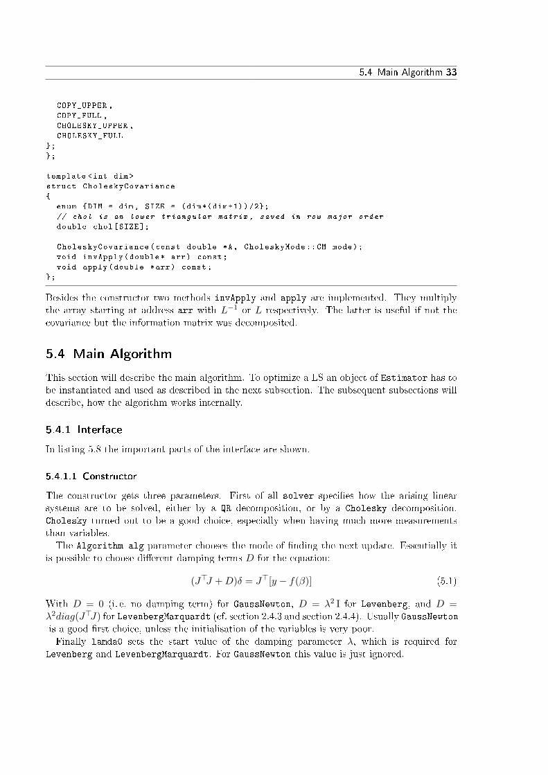
5.1 Basic Types . . . . . . . . . . . . . . . . . . . . . . . . . . . . . . . . . . . . . . 275.1.1 Manifolds . . . . . . . . . . . . . . . . . . . . . . . . . . . . . . . . . . . 275.1.2 Random Variables . . . . . . . . . . . . . . . . . . . . . . . . . . . . . . 28
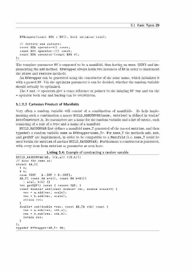
5.1.2.1 Interface . . . . . . . . . . . . . . . . . . . . . . . . . . . . . . 285.1.2.2 Implementation . . . . . . . . . . . . . . . . . . . . . . . . . . 285.1.2.3 Cartesian Product of Manifolds . . . . . . . . . . . . . . . . . . 29
5.1.3 Measurements . . . . . . . . . . . . . . . . . . . . . . . . . . . . . . . . . 305.2 Manifolds . . . . . . . . . . . . . . . . . . . . . . . . . . . . . . . . . . . . . . . 31
5.2.1 Vector . . . . . . . . . . . . . . . . . . . . . . . . . . . . . . . . . . . . . 315.2.2 SO(2) . . . . . . . . . . . . . . . . . . . . . . . . . . . . . . . . . . . . . 315.2.3 SO(3) . . . . . . . . . . . . . . . . . . . . . . . . . . . . . . . . . . . . . 325.2.4 MakePose . . . . . . . . . . . . . . . . . . . . . . . . . . . . . . . . . . . 32
5.3 Helper Classes . . . . . . . . . . . . . . . . . . . . . . . . . . . . . . . . . . . . 325.4 Main Algorithm . . . . . . . . . . . . . . . . . . . . . . . . . . . . . . . . . . . . 33
5.4.1 Interface . . . . . . . . . . . . . . . . . . . . . . . . . . . . . . . . . . . . 335.4.1.1 Constructor . . . . . . . . . . . . . . . . . . . . . . . . . . . . . 335.4.1.2 Inserting Random Variables and Measurements . . . . . . . . . 355.4.1.3 Initializing and Optimizing . . . . . . . . . . . . . . . . . . . . 35
6 Results 37
6.1 Syntetic Data Set . . . . . . . . . . . . . . . . . . . . . . . . . . . . . . . . . . . 376.2 DLR Data Set . . . . . . . . . . . . . . . . . . . . . . . . . . . . . . . . . . . . . 39
6.2.1 Preparations . . . . . . . . . . . . . . . . . . . . . . . . . . . . . . . . . 396.2.2 Data Initialization . . . . . . . . . . . . . . . . . . . . . . . . . . . . . . 396.2.3 Optimization Result . . . . . . . . . . . . . . . . . . . . . . . . . . . . . 416.2.4 Partial Optimization . . . . . . . . . . . . . . . . . . . . . . . . . . . . . 436.2.5 Calibration Problems . . . . . . . . . . . . . . . . . . . . . . . . . . . . . 43
7 Conclusion 47
7.1 Achieve Goals . . . . . . . . . . . . . . . . . . . . . . . . . . . . . . . . . . . . . 477.2 Outlook . . . . . . . . . . . . . . . . . . . . . . . . . . . . . . . . . . . . . . . . 47
Bibliography 49
Chapter 0 Introduction 1
There is always a well-known solution to every human problem � neat,
plausible, and wrong.
H. L. Mencken (1880-1956)
0Introduction
This thesis provides a framework for sparse, non-linear least square problems on manifolds.
Least square problems appear in many areas of computer science today. A well-knownexample in robotics is the SLAM-problem [TBF05].
The motivation for this topic arose due to the fact, that today there exist many least squaresalgorithms, which all usually make some approximations and trade-o�s, to keep their runningtime reasonable or to reduce their memory load. The goal of this thesis however is to �ndthe �best possible� solution to any given least squares problem. This is useful when evaluatingother algorithms to determine how good their approximation is.
In some areas in computer science like visual-SLAM there are already e�orts to �nd bestpossible solutions as a �nal step, after performing an approximate algorithms. There themethod is known as �bundle adjustment� and there already exist some specialized methods forthat [HZ03].
The term manifold in combination with least squares problems often appears when trying toestimate orientations in 3D. It is known, that there is no way to represent an orientation withjust three parameters, which doesn't get problems at some point.
0.1 Goals of the Thesis
The main goal of this thesis is to provide a framework which makes it easy to solve arbitraryleast square problems. The framework will be a big support when solving problems which arealready solved in an approximated way, and it o�ers a possibility to solve calibration problems.
This thesis does not provide an e�cient online-SLAM algorithm, although it is useable asone theoretically. Furthermore doesn't it solve data association problems, which often arisesimultaneously with least squares problem. And as this is only a framework it doesn't provideany application speci�c code, like sensor or motion models.
2 Chapter 0 Introduction
0.2 Guide to the Thesis
The �rst four chapters mainly describe the terms of the title in reverse direction.The �rst chapter will give an introduction to manifolds, which are necessary to model non-
euclidean variables. It requires some basic knowledge in topology.The second chapter will describe least squares problems and will give some algorithms to
solve them.The third chapter will deal with sparse matrices (matrices which consist mainly of zero
entries), and explain their importance.The fourth chapter explains the general design of the framework and explains some design
decissions.Afterwards, the �fth chapter deals with the actual implementation, the sixth chapter presents
some example usages of the framework and evaluates their results.Finally the seventh chapter draws a conclusion over the thesis.
0.3 Acronyms
CRTP Curiously Recurring Template Pattern, see [Cop95]
DOF degrees of freedom, see de�nition 1.1.
LM Levenberg-Marquardt algorithm, see section 2.4.4.
LS Least Squares problem, see ??.
RSS residual sum of squares
SLAM Simultaneos Localisation And Mapping
Chapter 1 Manifolds 3
We must maintain that mathematical geometry is not a science of space
insofar as we understand by space a visual structure that can be �lled
with objects � it is a pure theory of manifolds.
Hans Reichenbach
1Manifolds
1.1 Motivation
Most standard estimation algorithms work properly only on euclidean vector spaces (i. e. spacesisomorphic to Rn). But sometimes variables to be estimated do not form a euclidean vectorspace.A simple example are the orientations in R2, more formally called SO(2). They can be
represented using a single angle α with α ∈ [−π, π). Adding small changes to α is no problem,as α can be �renormalized� if it gets out of [−π, π) by simply adding or subtracting 2π.But a problem arises when comparing two angles which are near −π and π respectively.
Their di�erence is almost 2π although they are actually very close. Some algorithms solve thismanually by normalizing this di�erence to [−π, π).Another frequent example in practice is SO(3), the group of rotations in R3. To handle
SO(3) there exist basically two suboptimal approaches.One approach is to use a representation with three parameters (like e. g. Euler Angles). The
problem arises that there exist no parameterization of SO(3) with three parameters which hasno singularities (cf. [FS]). Singularities cause problems called �gimbal lock�. When the variableto be estimated approaches such a singularity the inverse of the parameterization becomesdiscontinuous, which means that some small changes of the variable require big changes inits representation. Some algorithms using this approach avoid this problem by changing theparameterization if the variable gets to close to a singularity.Another approach is to �overparameterize� the variable (for SO(3) e. g. by using quaternions,
which have four values) and normalize the parameterization in some way [MYB+01, WI95].But this usually causes signi�cant problems:As standard estimation algorithms expect their variables to be from euclidean vector spaces
they are not aware of the inner constraints between the parameters. Therefore they are op-timizing some degrees of freedom (DOF) which actually do not exist. This is obvisously aproblem when the parameterization of the variable has more parameters than the dimension
4 Chapter 1 Manifolds
of the measurement space, as there can't exist a unique result then (ignoring the constraints).But even otherwise the result has unde�ned DOF and any modi�cation tends to denormal-ize the representation, which therefore has to be renormalized. Another related problem isthat the parameterization sometimes behaves non-euclidean. That means changes of the samemagnitude to di�erent parameters yield to changes of the variable of quite di�erent magnitude.To solve these problems a combination of both approaches can be used. The variable is glob-
ally overparameterized, but local changes are represented with a minimal representation, whichideally behaves like a euclidean space as much as possible, for small values. A formalization ofthis idea leads to the theory of manifolds.So informally a manifold can be seen as a space, which locally behaves like a euclidean space,
but in general does not globally.
1.2 De�nition
This section will give a more formal description of manifolds. The de�nition in this section isnot the broadest possible, but it will su�ce for this thesis. For a more general de�nition anddeeper introduction see [Lee03].As a general note, the actual de�nition of smooth in this whole chapter will depend on its
context, but will generally mean Ck-di�erentiable, with k being constant within each de�nitionor theorem.
De�nition 1.1 (Manifold). LetM ⊂ Rn be connected, and F = (Uα, ϕα)α∈A be a family suchthat for a given d ∈ N:
1. ∀α∈A : Uα is an open subset of M (open in M means there is an open set U ⊂ Rn, suchthat U = M ∩ U), and M =
⋃α∈A Uα.
2. ϕα : Uα → Vα is a homeomorphism to an open subset Vα ⊂ Rd.
3. If Uα ∩ Uβ 6= ∅, the transition map
ϕα ◦ ϕ−1β : ϕβ(Uα ∩ Uβ)→ ϕα(Uα ∩ Uβ) (1.1)
is a Ck di�eomorphism.
Then (M,F) (or just M) is called a (Ck-) manifold. The tuples (Uα, ϕα) are called charts, andthe family F is called atlas of M . The number d is called the dimension, or degrees of freedomof M .
The �rst condition ensures thatM is completely covered by open sets. The second conditionmakes sure that the charts are continous. Intuitively that means that the chart has no holesor gaps. The last condition ensures that the charts are smoothly compatible. This is neededwhen de�ning smooth functions on M .
De�nition 1.2 (Smooth Function). Let (M, (Uα, ϕα)), (N, (Wβ, ψβ)) be Ck-manifolds. Afunction f : M → N is called Ck-di�erentiable in x ∈M i� for x ∈ Uα and f(x) ∈Wβ :
fβα :ϕα(Uα)→ψβ(Wβ)x 7→ψβ(f(ϕ−1
α (x)))(1.2)

1.3 Encapsulation 5
is Ck-di�erentiable in ϕα(x). [Note that ϕα(Uα) ⊂ Rd, so the usual de�nition for smoothnessis applicable.] f is called Ck-di�erentiable i� it is Ck-di�erentiable in every point x ∈M .
Due to the third condition of de�nition 1.1 the smoothness of f does not depend on theparticular choices of ϕα and ψβ :
Proof. Let x ∈ Uα ∩ Uα′ , f(x) ∈Wβ ∩Wβ′ and fβα be smooth in ϕα(x), then:
fβ′
α′ = (ψβ′ ◦ ψ−1β ) ◦ fβα ◦ (ϕα ◦ ϕ−1
α′ ) (1.3)
is smooth in ϕα′(x), because (ϕα ◦ ϕ−1α′ )(ϕα′(x)) = ϕα(x) and the composition of smooth
functions is smooth.
1.3 Encapsulation
When using manifolds in standard algorithms (like Kalman �lters), it would be very impracticalif the main algorithm had to care about charts and applying homeomorphisms. To avoid thisthe entire handling of manifolds can be encapsulated, with an approach proposed in [FS].The general idea is that an estimation algorithm handles the manifold as a �black box�. The
algorithm has only two possibilities to access the manifold.The �rst is to add small changes to the manifold:
� : M × Rm →M (1.4)
where δ 7→ x � δ is a homeomorphism from a neighborhood of 0 ∈ Rm to a neighborhood ofx ∈M . The other possibility is to �nd the di�erence between two elements in M :
� : M ×M → Rm, (1.5)
where y 7→ y � x is the inverse of �, or formally for all x, y ∈M :
x� (y � x) = y (1.6)
As δ 7→ x�δ is supposed to be a homeomorphism, the dimension ofM has to bem. Furthermoreas the domain of the homeomorphism is a neighborhood of 0, it follows that x� 0 = x.This approach has some quite remarkable advantages. Most standard algorithms working
on Rm now work essentially the same way on M , after replacing + with � when adding smallupdates to the state, and − with � when calculating the di�erence between two states.In particular they do not have to deal with singularities or denormalized overparameteriza-
tions. And, after adapting an algorithm, no further adaptions are needed, if other manifolds areprocessed (or the internal representation of the manifold changes), as long as these manifoldsimplement both these operators.Note that � might often be de�ned only for �small� δ and that � might behave uncontinous
or become unde�ned if minuend and subtrahend are �far apart�. Within this thesis it is alwaysassumed that this doesn't happen. In practice adding too big di�erences should be avoidedanyway, especially if non-linear functions are linearized by their derivation.
6 Chapter 1 Manifolds
1.3.1 Generic De�nition
One way to de�ne x� δ is to choose a chart including x, within which a vector x can be added,and project the result back toM . y�x essentially does the inverse of this operation, i. e. it �ndsthe value y in a chart including x and subtracts their coordinates. To make these functionsunique, the choice of the chart has to be determined by x.More formally with ϕx describing the chosen chart around x, one can de�ne:
x� δ := ϕ−1x (ϕx(x) + δ) (1.7)
y � x := ϕx(y)− ϕx(x) (1.8)
One can easily verify, that (1.6) holds for this de�nition:
Proof.
x� (y � x) = x�(ϕx(y)− ϕx(x)
)(1.9)
= ϕ−1x
(ϕx(y) + ϕx(y)− ϕx(x)
)(1.10)
= ϕ−1x
(ϕx(y)
)= y
One can also prove, that using aboves de�nitions � and � propagate smoothness:
Proposition 1.1. Let M , N be smooth manifolds, and f : M → N be smooth. Then
g(δ) := f(x� δ) � f(x) (1.11)
is smooth in δ.
Proof.g(δ) = f(x� δ) � f(x) = ψf(x)(f(ϕ−1
x (ϕx(x) + δ)))− ψf(x)(f(x)), (1.12)
and ψf(x) ◦ f ◦ ϕ−1x is smooth by de�nition, whereas ϕx(x) and ψf(x)(f(x)) are constant with
regard to δ.
1.3.2 Encapsulation for Lie-Groups
M is called Lie-Group, if it is a manifold and has a group structure.If M is a Lie-Group one can use a simpler de�nition, needing only a single chart around the
unit element id ∈M with ϕ(id) = 0. Using the group's · and −1 operators, one can then de�ne:
x� δ := x · ϕ−1(δ) (1.13)
y � x := ϕ(x−1 · y) (1.14)
or alternatively (but not necessarily equivalent):
x� δ := ϕ−1(δ) · x (1.15)
y � x := ϕ(y · x−1) (1.16)
Note that this de�nition is still a special case of the generic de�nition, as it is possible torecalculate ϕx from �, which satis�es (1.7) and (1.8):
ϕx(y) := y � x, (1.17)
where ϕid 6= ϕ in general.

1.4 Cartesian Product 7
1.4 Cartesian Product
One can show, that with M1, M2 being manifolds with dimensions d1 and d2, their cartesianproduct M := M1 ×M2 is a manifold as well, having dimension d := d1 + d2 [Lee03, p. 8].Intuitively this means just writing elements x of M as a tupel (x1, x2) with xi ∈Mi. It is nowpossible to extend the de�nition of � and � to M in the obvious way:
� : M × Rd →M((x1, x2),
[δ1δ2
])7→ (x1 � δ1, x2 � δ2)
(1.18)
� : M ×M →Rd
((x1, x2), (y1, y2)) 7→[x1�y1x2�y2
],
(1.19)
with x� (y�x) = y and x�0 = x still holding, as they hold by component. This can of coursebe extended to any �nite number of manifolds.
Analog to that a set of functions can be combined to a single function. For f1 : N1×N2 →M1
and f2 : N2 × N3 → M2 one can de�ne a function f := f1 × f2 from N := N1 × N2 × N3 toM := M1 ×M2 as follows:
f : N →M(x1, x2, x3) 7→ (f1(x1, x2), f2(x2, x3)),
(1.20)
which of course can also be extended to any �nite number of functions. Note that the smooth-ness of f is determined by the least smoothest function fi, as di�erent subfunctions do nota�ect the smoothness of others.
1.5 Examples
This section will give some examples for manifolds and prove their smoothness. The actualimplementation will be handled in section 5.2.
The most trivial example would be Rd itself. As one can easily verify, replacing �, � bytheir vector space equivalents +, − complies with (1.6).
This shows that restricting a variable to be from a manifold doesn't let it lose its generality.In the following there will be given some other useful examples, which justify the e�ort ofintroducing manifolds.
1.5.1 SO(2)
A still simple example is the special orthogonal group of degree 2, which is informally thegroup of rotations in the plane (or angles with periodicity). Formally it can be described asthe following set of matrices:
SO(2) :={Q ∈ R2×2; Q>Q = I2 = QQ> ∧ detQ = 1
}(1.21)
8 Chapter 1 Manifolds
which is a subgroup of the general linear group (the invertable matrices) using the standardmatrix multiplication. One can verify, that SO(2) has one DOF1 and in fact it can be param-eterized with one variable:
SO(2) ={[
cosα − sinαsinα cosα
]; α ∈ R
}. (1.22)
So a simple parameterization is to just store a single angle α and de�ne α � δ := α + δ.When de�ning α � β care has to be taken that α + 2πk, for integer k all represent the same
rotation. So simply de�ning α � β?
:= α − β won't work. A working solution is to normalizethis di�erence to the intervall (−π, π), e. g. with ϕ(δ) := δ − 2πb δ+π2π c, de�ning:
α� β := ϕ(α− β). (1.23)
Note that this directly corresponds to the encapsulation of Lie groups proposed in section 1.3.2with + and − as group operations.
This is a procedure which is often done �manually� in algorithms not using a manifold ap-proach.
1.5.2 SO(3)
A more important application for manifolds is the representation of rotations in 3D-space,formally the special orthogonal group of degree 3. Its matrix representation is similar to thatof SO(2):
SO(3) :={Q ∈ R3×3; Q>Q = I3 = QQ> ∧ detQ = 1
}, (1.24)
but in contrast it does not have a singularity free covering with only three parameters [FS].
However a covering with with four parameters is possible, namely using quaternions. AsSO(3) is a Lie group, it is only necessary to provide a homeomorphism from a neighborhoodof the identity id ∈ SO(3) to R3 in order to de�ne � and �. A possible homeomorphism isgiven by the quaternion logarithm ϕ(q) := log(q). For q = (w, u), with w ∈ R, u ∈ R3 andw2 + ‖u‖2 = 1 it is de�ned as:
log :SO(3)→R3
q 7→
{u‖u‖ arccosw u 6= 0
0 u = 0,(1.25)
the inverse is given by the exponential map ϕ−1(δ) = exp δ, with
exp : R3→SO(3)δ 7→ (cos ‖δ‖ , δ · sinc ‖δ‖). (1.26)
A derivation for these formulas can be found in [Ude99]. A more general introduction toquaternions can be found in [Vic01].
1Viewed as matrix it has 4 variables and the equation Q>Q = I2 gives 3 constraints.
1.5 Examples 9
1.5.3 S2
Sn is the unit sphere in Rn+1, that is
Sn :={x ∈ Rn+1; ‖x‖2 = 1
}. (1.27)
As this parameterisation has n + 1 components and 1 constraint, it has n DOF. For n = 0S0 = −1, 1 is a two point set, which is not connected and therefore not a smooth manifold. Forn = 1 it is essentially the same as SO(2), using the parameterisation S1 = {[ cosα
sinα ] ; α ∈ R},which can be mapped to SO(2) isomorphically.Furthermore one can see that S3 is a cover of SO(3) (the unit quaternions are isomorphic to
S3 and a cover of SO(3) as seen previously).The 2-sphere S2 (the surface of the globe or the directions in R3) is another manifold and one
example which does not have a group structure.2 It can be parameterized by 2 angles latitudeand longitude (like the earth's surface) but this leads to singularities at the poles as they havearbitrary longitude.A common way to parameterize S2 is to store it using its 3 coordinates in R3 and use
stereographic projection [Wikb] to map it to R2. For U := S2 \ [0, 0, 1]> the following de�nitionfor ϕ is a homeomorphism:
ϕ :U → R2 (1.28)
ϕ([x, y, z]>) =1
1− z[ xy ] (1.29)
with the inverse
ϕ−1([a, b]>) =1
1 + a2 + b2
[ 2a2b
−1+a2+b2
](1.30)
To get a complete cover of S2 one can use the sets U±i := S2 \ ±ei, 1 ≤ i ≤ 3 and ei being theith unit vector, thus U = U3 and de�ne ϕ±i analogously to ϕ.When de�ning � and � one can use the generic de�nitions (1.7) and (1.8) with ϕ[x,y,z] chosen
such that [x, y, z]> has the biggest distance to ±ei (with an arbitrary but de�ned strategy forties). Due to the fact that ϕ : R3 \ e3 → R2 is smooth and ϕ−1 : R2 → R3 as well, it iseasy to see that any transistion map ϕ±i ◦ ϕ
−1±j is smooth as well thus holding condition 3 of
de�nition 1.1.This is however an example where x� δ is not smooth in x (and not even continuous), but
it is in δ, as required.
2This is a consequence of the so-called �Hairy Ball Theorem� [Wika].

10 Chapter 1 Manifolds
Chapter 2 Least Squares Problems 11
It is better to be approximately right than exactly wrong.
Old adage
2Least Squares Problems
The problem to be solved in this chapter is to determine the distribution of a random variableX ∈ N , given a noisy measurement Z ∈ M and a measurement function f describing therelation between them.Before giving di�erent solutions to that problem, it is discussed how exactly noise can be
modeled into this relation. Afterwards a method to normalize Least Squares problems (LSs)on manifolds is introduced, which is then used to apply standard least squares solvers to theproblem.
2.1 Modeling Least Squares Problems
For M = Rm a common way to describe a measurement with noise ε ∼ N (0, Σ) and knowncovariance Σ is the following equation:
Z = f(X) + ε, (2.1)
which is equivalent to:
Z + (−ε) = f(X). (2.2)
Note that ε ∼ N (0, Σ) is often just an approximation, which usually doesn't hold exactlyespecially when f is non-linear.For M being an arbitrary manifold one can write analogously:
Z = f(X) � ε1, (2.3)
or:
Z � ε2 = f(X). (2.4)
12 Chapter 2 Least Squares Problems
Since Z � f(X) 6= −(f(X) � Z) in general, these equations are no longer equivalent to eachother as (2.1) and (2.2).On the �rst view (2.3) makes more sense: After applying the measurement function f on
X noise ε1 is added and the �noisy� result Z is measured. But this has a big drawback: Asthe actual value of ε1 can depend discontinuously on the unknown value of f(X) it is hard todetermine Σ = Cov(ε1) in general.When using (2.4) instead, the actual value of ε2 depends smoothly on f(X) and discontinu-
ously only on the known value of Z. In fact with known Z = z one can de�ne:
f(X) := f(X) � z = ε2 ∼ N (0, Σ) , (2.5)
so for now it is assumed thatf(X) = Z � ε, (2.6)
with ε ∼ N (0, Σ), known Σ and known Z = z.
2.2 Normalization
In order to simplify algorithms this section develops a method to normalize a Gaussian distri-bution, such that the problem will simplify to
f(X) ∼ N (0, Im) . (2.7)
First of all lemma 2.1 shows that Gaussian distributions are closed under linear transforma-tions. It is usually proven in stochastics.
Lemma 2.1. Let µ ∈ Rm, Σ ∈ Rm×m. Furthermore let C ∈ Rn×m with C having full rankand b ∈ Rn, then for X ∼ N (µ, Σ):
Z = CX + b ∼ N(Cµ+ b, CΣC>
)(2.8)
Using this lemma, one can always normalize a normally distributed variable:
Proposition 2.1. If Rm 3 Z ∼ N (µ, Σ) and LL> is the Cholesky decomposition of Σ, then
Y := L−1(Z − µ) ∼ N (0, Im) . (2.9)
Proof.
L−1(Z − µ) ∼ N(L−1(µ− µ), L−1ΣL−>
)= N
(0, L−1(LL>)L−>
)(2.10)
= N (0, Im)
This can be used to normalize f(X) as in (2.6), by setting
f(X) := L−1(f(X) � z) ∼ L−1(N (0, Σ)) (2.11)
∼ N (0, Im) , (2.12)
using (2.5) and proposition 2.1.For the rest of this chapter it is assumed without loss of generality, that f(X) is normalized
as above.Also note that if f is the cartesian product of smaller functions as shown in section 1.4, the
normalization can be done function-wise.
2.3 Linear Least Squares Problems 13
2.3 Linear Least Squares Problems
The next goal is to determine X for di�erent kinds of f . For linear f : Rn → Rm, the followingtheorem gives an exact solution. It is assumed that A ∈ Rm×n has maximal rank (thereforeA>A is invertable).
Theorem 2.1. Let f(X) = AX + b = Z ∼ N (0, I), then
X ∼ N(
(A>A)−1A>(−b), (A>A)−1)
(2.13)
Proof. Using lemma 2.1 with h(Z) = (A>A)−1A>(Z − b) it follows:
X = (A>A)−1A>(AX + b− b) = h(AX + b) (2.14)
= h(Z) ∼ N(
(A>A)−1A>(−b), (A>A)−1)
To justify the term �least squares� the following theorem shows, that the expectation valuefrom (2.13) also has the smallest squared residual:
Theorem 2.2. Let f(X) = AX + b, then
(A>A)−1A>(−b) = argminx‖f(x)‖2 . (2.15)
Proof. Let F (x) := ‖f(x)‖2. The minimum is determined by �nding the root of ∂∂xF (x):
0 !=∂
∂xF (x) = 2f(x)>f ′(x) = 2(x>A>A+ b>A) = 2(A>Ax+A>b)> (2.16)
⇔ A>Ax = −A>b (2.17)
⇔ x = −(A>A)−1A>b (2.18)
Since this is the only root and F (x) ≥ 0, this has to be a minimum.
When computing x it is usually very ine�cient to actually compute (A>A)−1, unless onereally needs the complete covariance matrix. Instead x can be calculated by solving the linearsystem (2.17). Since A>A is symmetric and positive-de�nite, (2.17) can be solved using theCholesky decomposition of A>A.Another, sometimes faster, method to solve (2.17) is to use the QR decomposition of A:
Theorem 2.3. If A = QR is the QR decomposition of A with R =[R 0
]>, solving (2.17) is
equivalent to solving:Rx = −
[In 0
]Q>b. (2.19)
(Note that multiplying by[In 0
]essentially means only to consider the �rst n entries Q>b.)
Proof. Substituting A = QR in (2.18) leads to:
x = −(R>Q>QR)−1R>Q>b = −(R>[In 0
] [In0
]R
)−1
R>[In 0
]Q>b (2.20)
= −(R>R)−1R>[In 0
]Q>b = −R−1R−>R>
[In 0
]Q>b = −R−1
[In 0
]Q>b
(2.21)
⇔ Rx = −[In 0
]Q>b
14 Chapter 2 Least Squares Problems
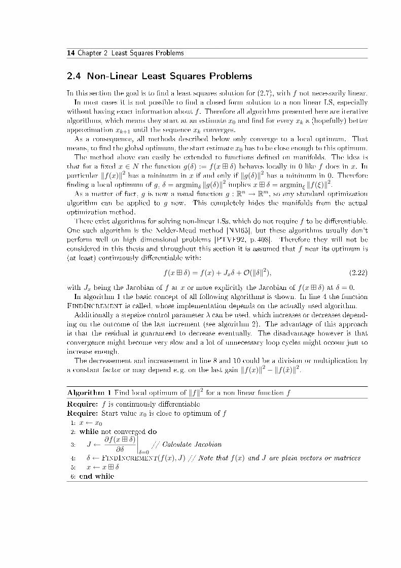
2.4 Non-Linear Least Squares Problems
In this section the goal is to �nd a least squares solution for (2.7), with f not necessarily linear.In most cases it is not possible to �nd a closed form solution to a non-linear LS, especially
without having exact information about f . Therefore all algorithms presented here are iterativealgorithms, which means they start at an estimate x0 and �nd for every xk a (hopefully) betterapproximation xk+1 until the sequence xk converges.As a consequence, all methods described below only converge to a local optimum. That
means, to �nd the global optimum, the start estimate x0 has to be close enough to this optimum.The method above can easily be extended to functions de�ned on manifolds. The idea is
that for a �xed x ∈ N the function g(δ) := f(x � δ) behaves locally in 0 like f does in x. Inparticular ‖f(x)‖2 has a minimum in x if and only if ‖g(δ)‖2 has a minimum in 0. Therefore�nding a local optimum of g, δ = argminδ ‖g(δ)‖2 implies x� δ = argminξ ‖f(ξ)‖2.As a matter of fact, g is now a usual function g : Rn → Rm, so any standard optimization
algorithm can be applied to g now. This completely hides the manifolds from the actualoptimization method.There exist algorithms for solving non-linear LSs, which do not require f to be di�erentiable.
One such algorithm is the Nelder-Mead method [NM65], but these algorithms usually don'tperform well on high dimensional problems [PTVF92, p. 408]. Therefore they will not beconsidered in this thesis and throughout this section it is assumed that f near its optimum is(at least) continuously di�erentiable with:
f(x� δ) = f(x) + Jxδ +O(‖δ‖2), (2.22)
with Jx being the Jacobian of f at x or more explicitly the Jacobian of f(x� δ) at δ = 0.In algorithm 1 the basic concept of all following algorithms is shown. In line 4 the function
FindIncrement is called, whose implementation depends on the actually used algorithm.Additionally a stepsize control parameter λ can be used, which increases or decreases depend-
ing on the outcome of the last increment (see algorithm 2). The advantage of this approachis that the residual is guaranteed to decrease eventually. The disadvantage however is thatconvergence might become very slow and a lot of unnecessary loop cycles might occour just toincrease enough.The decreasement and increasement in line 8 and 10 could be a division or multiplication by
a constant factor or may depend e. g. on the last gain ‖f(x)‖2 − ‖f(x)‖2.
Algorithm 1 Find local optimum of ‖f‖2 for a non-linear function f
Require: f is continuously di�erentiableRequire: Start value x0 is close to optimum of f1: x← x0
2: while not converged do
3: J ← ∂f(x� δ)∂δ
∣∣∣∣δ=0
// Calculate Jacobian
4: δ ← FindIncrement(f(x), J) // Note that f(x) and J are plain vectors or matrices5: x← x� δ6: end while
2.4 Non-Linear Least Squares Problems 15
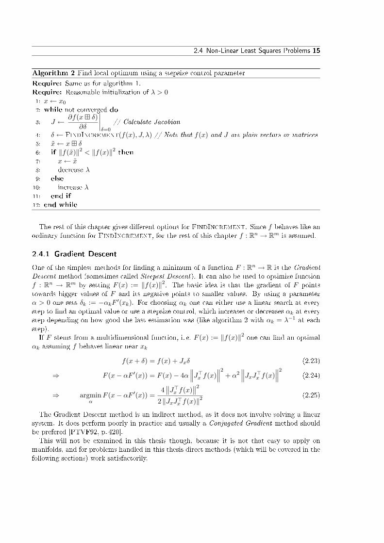
Algorithm 2 Find local optimum using a stepsize control parameter
Require: Same as for algorithm 1.Require: Reasonable initialization of λ > 01: x← x0
2: while not converged do
3: J ← ∂f(x� δ)∂δ
∣∣∣∣δ=0
// Calculate Jacobian
4: δ ← FindIncrement(f(x), J, λ) // Note that f(x) and J are plain vectors or matrices5: x← x� δ6: if ‖f(x)‖2 < ‖f(x)‖2 then7: x← x8: decrease λ9: else
10: increase λ11: end if
12: end while
The rest of this chapter gives di�erent options for FindIncrement. Since f behaves like anordinary function for FindIncrement, for the rest of this chapter f : Rn → Rm is assumed.
2.4.1 Gradient Descent
One of the simplest methods for �nding a minimum of a function F : Rn → R is the GradientDescent method (sometimes called Steepest Descent). It can also be used to optimize functionf : Rn → Rm by setting F (x) := ‖f(x)‖2. The basic idea is that the gradient of F pointstowards bigger values of F and its negative points to smaller values. By using a parameterα > 0 one sets δk := −αkF ′(xk). For choosing αk one can either use a linear search at everystep to �nd an optimal value or use a stepsize control, which increases or decreases αk at everystep depending on how good the last estimation was (like algorithm 2 with αk = λ−1 at eachstep).If F stems from a multidimensional function, i. e. F (x) := ‖f(x)‖2 one can �nd an optimal
αk assuming f behaves linear near xk
f(x+ δ) = f(x) + Jxδ (2.23)
⇒ F (x− αF ′(x)) = F (x)− 4α∥∥∥J>x f(x)
∥∥∥2+ α2
∥∥∥JxJ>x f(x)∥∥∥2
(2.24)
⇒ argminα
F (x− αF ′(x)) =4∥∥J>x f(x)
∥∥2
2 ‖JxJ>x f(x)‖2(2.25)
The Gradient Descent method is an indirect method, as it does not involve solving a linearsystem. It does perform poorly in practice and usually a Conjugated Gradient method shouldbe prefered [PTVF92, p. 420].This will not be examined in this thesis though, because it is not that easy to apply on
manifolds, and for problems handled in this thesis direct methods (which will be covered in thefollowing sections) work satisfactorily.
16 Chapter 2 Least Squares Problems
2.4.2 Newton's Method
Newton's method usually is a method to �nd roots of a function g : Rn → Rn, but can alsobe used to �nd local extrema of a function F like given above, provided that F is twice-di�erentiable. The general idea is to �nd the roots of F ′ using Newton's method.
Assuming F (x) has the gradient F ′(x) and Hessian F ′′(x) and higher order derivations areneglectible one can write:
F (x+ δ) = F (x) + F ′(x)δ +12δ>F ′′(x)δ (2.26)
⇒ F ′(x+ δ) = F ′(x) + δ>F ′′(x) != 0 (2.27)
⇔ F ′′(x)δ = −F ′(x)>, (2.28)
which can be solved for δ.
For F = ‖f‖2 the Jacobian of F calculates as F ′(x)> = 2J>x f(x). The Hessian calculates asfollows:
(F ′′(x))ij =∂
∂xi(F ′(x))j = 2
m∑k=1
∂
∂xi
(fk(x)
∂
∂xjfk(x)
)(2.29)
= 2m∑k=1
(∂
∂xifk(x)
∂
∂xjfk(x) + fk(x)
∂
∂xi
∂
∂xjfk(x)
), (2.30)
therefore:
F ′′(x) = 2
(J>x Jx +
m∑k=1
fk(x)f ′′k (x)
)(2.31)
In most practical cases Newton's method converges locally quadratic. A downside of Newton'smethod is that it requires the second order derivation of F (or f), which sometimes doesn'texist or is di�cult to obtain, especially if it has to be calculated numerically.
2.4.3 Gauss-Newton Method
The Gauss-Newton method can be seen as a simpli�cation of Newton's method, neglectingsecond order derivations of f . Equivalently it can be derived by iteratively applying linear leastsquares methods to f linearized at xk (cf. theorem 2.1). With Jx being the Jacobian of f bothlead to the same update formula:
(J>x Jx)δ = −J>x f(x), (2.32)
which has to be solved for δ. Unlike Newton's method the Gauss-Newton algorithm is not guar-anteed to converge. Especially if f is highly non-linear (i. e. has big higher order derivations).
2.4 Non-Linear Least Squares Problems 17
2.4.4 Levenberg-Marquardt Algorithm
A quite popular algorithm for LSs is the Levenberg-Marquardt algorithm (LM) [PTVF92,p. 683]. It can be seen as a combination of the Gauss-Newton algorithm and gradient descent.It uses a control parameter as in algorithm 2 and its update formula is:
(J>x Jx + λD)δ = −J>x f(x), (2.33)
with D being a positive de�nite diagonal matrix. Common choices for D are D = I (the originalproposal of Levenberg [Lev44]) or Dii = (J>x Jx)ii as proposed by Marquardt [Mar63].The big advantage of LM is, that due to its control parameter it can't diverge and it almost
always converges eventually, as for increased λ it behaves like gradient descent. Furthermorelocally λ usually gets small, thus behaving much like the Gauss-Newton method, with nearlyquadratic convergence.A downside however is that it sometimes converges really slow especially with a highly non-
linear f , as it then has to avoid increasing the residual by choosing a very big λ, which makesthe update step δ very small.

18 Chapter 2 Least Squares Problems
Chapter 3 Sparse Matrices 19
3Sparse Matrices
In many LSs that arise in practice one has a (probably big) set of random variables, eachhaving a low dimension. Furthermore there is a (most likely even bigger) set of independentmeasurements, from which each depends only on a few variables.One common example would be the Simultaneos Localisation And Mapping (SLAM) prob-
lem, where one has a set of poses and landmarks (the random variables) and a set of measure-ments (usually odometry and some kind of relation between the poses and the landmarks).This chapter will deal with how this �sparseness� can be utilized and why it is crucial to
do so. There will be no deep insight in how the actual matrix algorithms work, as for theimplementation of this thesis CSparse [Dav] is used, which is described thoroughly in [Dav06].
3.1 Motivation
The straight-forward solution to solve problems as above is to stack all variables together andalso all functions, as shown in section 1.4. Then there is one big function, which depends onone big random variable. For real life problems the dimension of the random variable can easilyreach n = 20000, and for the function say m = 50000.Storing the Jacobian J of f alone would take 8nm = 8 · 109 bytes (when using doubles),
which would not be storable on a 32bit architecture. Calculating J>J would require aboutn2m = 20 · 1012 FLOPS, which alone would take about 1000 s on a 20 GFLOPS CPU in eachiteration. For the above problem this could easily lead to execution times of an hour or moreeven on state-of-the-art hardware.As it will be shown later in this chapter, a big proportion of J and J>J consists only of zero
entries making these matrices sparse. There is no exact de�nition of a sparse matrix, but acommonly used is the following, �rst given by J. H. Wilkinson:
De�nition 3.1 (Sparse Matrix). �The matrix may be sparse, either with the non-zero ele-ments concentrated on a narrow band centered on the diagonal or alternatively they may be

20 Chapter 3 Sparse Matrices
distributed in a less systematic manner. We shall refer to a matrix as dense if the percentageof zero elements or its distribution is such as to make it uneconomic to take advantage of theirpresence.�[WR71]
It is clear, that by simply saying a matrix is sparse, if only its non-zero entries are stored,every matrix would be sparse. The above de�nition will surely depend on the methods howa sparse matrix is stored and on the e�ciency of algorithms exploiting it. However, sparsematrices in practice are likely to give bene�ts in order of magnitude, even with o�-the-shelfsparse algorithms, so the de�nition will be su�cient for this thesis.
3.2 Sparsity of Least Square Problems
First of all in this section it will be shown that the Jacobian J that arises in a LS is sparse andthat the matrix J>J is sparse as well. At the end some methods for solving sparse systems arementioned.
3.2.1 Sparsity of the Jacobian
The measurement function f is assumed to be the combination of several smaller normalizedsubfunctions, that depends on a big vector x ∈ N , with N = N1 × . . . × Nn, but with eachsubfunction fi depending only on a few components of x = (x1, . . . , xn). Since all fi are normal-ized their individual components are independent, so every fi can be split into its components.Therefore it is assumed in the rest of the chapter that every fi is single dimensional with:
fi :N→Rx 7→ fi(xi1 , . . . , xiK )
(3.1)
The gradient of f in x is now de�ned as the gradient of gi(δ) := fi(x � δ) (cf. algorithm 1,line 3).
Let Xi be the set of indexes that correspond to xi in δ, that means with di being the dimensionof Ni:
X1 := {1, . . . , d1}, (3.2)
X2 := {d1 + 1, . . . , d1 + d2} (3.3)
...
Xn :={
1 +∑n−1
i=1 di, . . . ,∑n
i=1 di
}. (3.4)
By using the de�nition of � in section 1.4 one can see, that values of δ in positions which donot a�ect any xik don't a�ect gi(δ) either. Therefore the gradient of gi can be non-zero onlyat positions that a�ect any xik . That means ∂
∂δgi(δ) can be non-zero only at⋃Kk=1Xik =: Fi.
The Jacobian J now only consists of the lines gi, i. e. Ji• = gi. This sums up to the followingconclusion:
Proposition 3.1. With J de�ned as above Jij 6= 0 only if j ∈ Fi.

3.2 Sparsity of Least Square Problems 21
Going back to the introducing example from section 3.1 the space required for storing theentries of J now drops to mk entries assuming that each measurement depends on variableswith a total dimension of k. For a typical case of 2D-SLAM this would be like 6 (a measurementbetween two poses) or 5 (a measurement between a pose and a landmark), requirering now only2.4·106 bytes. Of course additional memory is needed to store the structure of J , but this isonly a factor of about 1.5 asymptotically. What matters is that the space consumption nowonly grows linear in m (in the dense case n would usually grow linear with m as well, becausein SLAM new measurements usually introduce new variables, and therefore letting the matrixgrow quadratically.)
3.2.2 Sparsity and Calculation of J>J
The product of two sparse matrices is not necessarily sparse. The simplest counter-examplewould be a matrix J ∈ Rn×n with only the �rst row �lled with ones. Now the product J>Jwould also be a matrix in Rn×n but completely �lled with ones, which surely can't be consideredas sparse anymore.
However this will generally not happen for LSs if every sub-function depends only on a fewvariables. To see whether (J>J)ij is non-zero one has to look at the de�nition of the product:
(J>J)ij =m∑k=1
JkiJkj , (3.5)
which is non-zero only if there is a function fk with {i, j} ⊂ Fk.It is now possible to �nd an upper bound for the density of J>J for the introducing example.
Suppose again every function depends on two variables having a dimension of 3. The diagonalblocks of J>J are set as soon as one function depends on the corresponding variable.1
Now a measurement depending on Ni and Nj sets the blocks Xi×Xj and Xj×Xi which adds2 · 3 · 3 = 18 elements to J>J . Therefore J>J in this example has a maximum of 9 · n+ 18 ·mentries, which can be reduced to its half by only saving the upper half of J>J as it is symmetric.But again, most important here is that the number of non-zeroes grows only linear with m.
The number of FLOPS to calculate J>J can be estimated by looking at another way toexpress this product:
J>J =m∑k=1
Jk•J>k•, (3.6)
with Jk• having 6 entries so each summand requires 6·(6+1)2 = 21 multiplications and the same
amount of additions (taking advantage of the symmetry). This leads to a total sum of about42m FLOPS needing only 2.1·106 FLOPS instead of 20·1012 FLOPS for the naïve approach,which makes a tremendous di�erence needing on the same CPU only about 0.1ms instead of1000 s. This is of course a gain that can't be achieved in practice as for the sparse matrixmultiplication some additional overhead appears. But again, what's crucial, is that the numberof FLOPS grows only linear with m.
1Which should be the case, because otherwise there would be no way to estimate the variable anyway.
22 Chapter 3 Sparse Matrices
3.2.3 Solving Sparse Systems
In section 2.3 two methods were given for solving an equation like
(J>J)δ = J>z, (3.7)
which is needed to calculate a new increment δ.One possibility is to calculate the Cholesky decomposition L of J>J and then solve the
systems
Lδ = J>z and (3.8)
L>δ = δ. (3.9)
The other possibility is to calculate the QR decomposition of J = QR and then solve thelinear system (cf. theorem 2.3):
Rδ = Q>z. (3.10)
Although the latter looks like needing far less operations, this isn't always the case. Forexample for m much bigger than n the QR decomposition of J ∈ Rm×n usually takes muchmore e�ort than the cholesky decomposition of J>J ∈ Rn×n, which can compensate for theextra work to calculate J>J and J>z and the extra linear system to be solved.Also and more important is the amount of �ll-in which occours when computing a matrix
decomposition of a sparse matrix.When the decomposition of a sparse matrix is calculated, ideally the factors (either L, or
Q and R) would have the same sparsity pattern as the original matrix. Unfortunately this isonly the case in some special cases. For most matrices additional entries called ��ll-in� have tobe introduced. To determine how much �ll-in is needed and what possibilities exist to reduce�ll-in is a rather complex task and will not be covered in this thesis. An in-depth analysis of itcan be found in [Dav06].

Chapter 4 Framework 23
4Framework
A main objective of this thesis is to provide a framework, which makes it easy to implementand optimize arbitrary least square problems. Several design decisions had to be made to keepit reasonably fast, without increasing the complexity of implementation unreasonably.
This chapter will only describe the design decisions not the actual implementation, whichwill be covered in the next chapter.
4.1 Basic Types
Besides the main class Estimator the framework distuinguishes between three basic types:
� A Manifold represents just a simple manifold.
� A RandomVariable represents a random variable, which is to be optimized. It containsa manifold which represents the current value (the currently best approximation) of therandom variable.
� A Measurement is a function which describes the relation between several RandomVariables.The function has to be normalized as described in section 2.2.
There are several basic requirements for each type.
A Manifold has to implement the � and � operators, and its DOF have to be known.Additionally it can have several access methods to enable user code to initialize it and tocalculate with it, but these are irrelevant for the main algorithm.
In order to evaluate a Measurement it has to hold references to the variables it depends on. Inorder to be normalized it needs to hold its value of expectation and covariance.1 Additionallythe framework needs to know the dimension of each measurement.
1They can be given implizit, e. g. if they are known to be 0 or I, respectively.
24 Chapter 4 Framework
A RandomVariable needs to propagate the dimension of its inherent manifold and its �operator.2 It also has to give read access to its manifold to make it possible for functions to beevaluated, and it must be possible to initialize it (usually via a manifold).During the next section additional requirements will arise.
4.2 Cartesian Product of Manifolds
As shown in section 1.4 manifolds can be combined to bigger manifolds by forming their carte-sian product. A user could do this manually by implementing �, � and the DOF of a combinedmanifold, but this would be error-prone and cumbersome. Therefore the framework provides amacro BUILD_RANDOMVAR which does the necessary work. It will be described in section 5.1.2.3.
4.3 Data holding
The main class needs to hold references or pointers to each variable which has to be optimized,and to each measurement function which describes the relation between the variables. Variablesand measuremts are stored into a single container each.When evaluating the whole function each subfunction can be evaluated by iterating the
measurement container and writing the results into some array consecutively.At some points it is however not necessary to evaluate the complete function, but only parts
of it. In order to do so it is mandatory to know the index of the subfunction in the �bigfunction�. To simplify matters this is achieved by simply storing the index of the function intothe corresponding Measurement object, as soon as it gets registered to the algorithm.
4.4 Evaluation of Jacobian
One of the main tasks for the framework is to calculate the Jacobian of the complete mea-surement function. In this framework this is always done numerically, as there isn't always apractical way to do so symbolically.There are two common ways to compute a Jacobian numerically:
J•j = 1df(X � dej)− f(X), (4.1)
or J•j = 12d(f(X � dej)− f(X �−dej)), (4.2)
with d > 0 being a small scalar value and ej being the jth unit vector. The �rst variant needsless function evaluations because f(x) has to be calculated only once. The second varianthowever usually approximates the exact Jacobian better and it also has some advantages whenthe Jacobian is sparse.The naïve way to evaluate the Jacobian would be to consecutively evaluate f(X � dej) and
subtract f(X) (or evaluate f(x � −dej) and subtract this). As observed in chapter 3, it iscrucial to exploit the sparseness of J , therefore zero values have to be dropped then.It is however possible to exploit the sparseness of J already when evaluating it. As observed
in section 3.2.1 entry Jij can be non-zero only if the ith subfunction depends on the variable
2Note that � is only needed to normalize functions, which hold their expectation value as a manifold.
4.5 Building Measurements 25
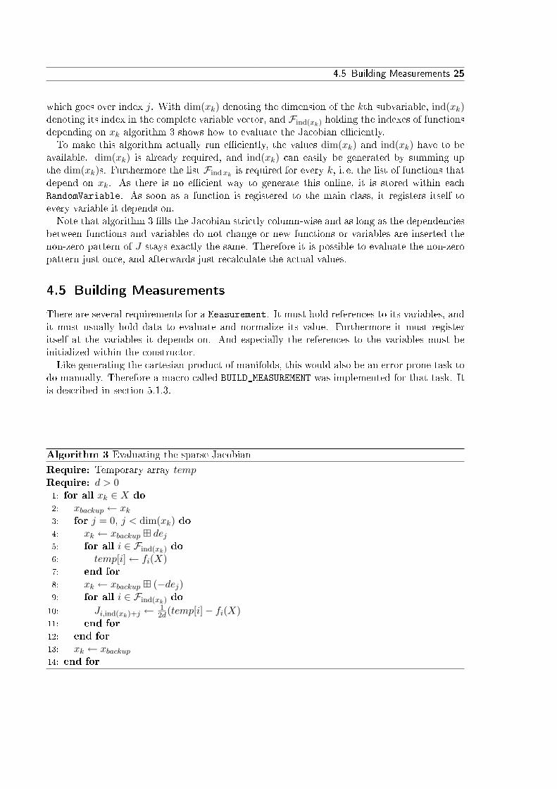
which goes over index j. With dim(xk) denoting the dimension of the kth subvariable, ind(xk)denoting its index in the complete variable vector, and Find(xk) holding the indexes of functionsdepending on xk algorithm 3 shows how to evaluate the Jacobian e�ciently.To make this algorithm actually run e�ciently, the values dim(xk) and ind(xk) have to be
available. dim(xk) is already required, and ind(xk) can easily be generated by summing upthe dim(xk)s. Furthermore the list Findxk
is required for every k, i. e. the list of functions thatdepend on xk. As there is no e�cient way to generate this online, it is stored within eachRandomVariable. As soon as a function is registered to the main class, it registers itself toevery variable it depends on.Note that algorithm 3 �lls the Jacobian strictly column-wise and as long as the dependencies
between functions and variables do not change or new functions or variables are inserted thenon-zero pattern of J stays exactly the same. Therefore it is possible to evaluate the non-zeropattern just once, and afterwards just recalculate the actual values.
4.5 Building Measurements
There are several requirements for a Measurement. It must hold references to its variables, andit must usually hold data to evaluate and normalize its value. Furthermore it must registeritself at the variables it depends on. And especially the references to the variables must beinitialized within the constructor.Like generating the cartesian product of manifolds, this would also be an error-prone task to
do manually. Therefore a macro called BUILD_MEASUREMENT was implemented for that task. Itis described in section 5.1.3.
Algorithm 3 Evaluating the sparse Jacobian
Require: Temporary array tempRequire: d > 01: for all xk ∈ X do
2: xbackup ← xk3: for j = 0, j < dim(xk) do4: xk ← xbackup � dej5: for all i ∈ Find(xk) do
6: temp[i]← fi(X)7: end for
8: xk ← xbackup � (−dej)9: for all i ∈ Find(xk) do
10: Ji,ind(xk)+j ← 12d(temp[i]− fi(X)
11: end for
12: end for
13: xk ← xbackup14: end for

26 Chapter 4 Framework
Chapter 5 Implementation 27
5Implementation
This chapter will deal with the actual implementation of the algorithms described and explainsome internal design decisions. A major design goal was to avoid virtual polymorphism asmuch as possible by using static polymorphism.
5.1 Basic Types
This section will describe the interfaces of the basic types for describing manifolds, randomvariables, and measurement functions.
5.1.1 Manifolds
Manifolds are completely de�ned using only static polymorphism. To be a Manifold a classneeds to have a public enum {DOF} describing its DOF, and must implement a � and � method(see section 1.3). These methods are called add and sub and have the following interface:
Listing 5.1: Manifold interface
const double * add(const double *vec , double scale =1);
double * sub(double *res , const Derived& oth) const;
m.add(vec, scale) lets m← m� scale · vec, where vec is handled as standard C array. Itreturns the address of the �rst element after the vector, i. e. vec+DOF.
m.sub(res, oth) lets res ← m � oth and returns the address of the �rst element of res,that isn't used, i. e. res+DOF.
The templated struct Manifold de�ned in types/Manifold.h implements add and sub
and de�nes DOF, when given a baseclass, that implements add_ and sub_ which have thesame interfaces but do not return a value. Manifold uses the Curiously Recurring TemplatePattern (CRTP) to do this without virtual inheritence.

28 Chapter 5 Implementation
The idea of letting add and sub return the next adress is to make the cartesian productof manifolds be easier to implement (see section 1.4). When combining a list of manifolds tosingle manifold, one has to make sure that the resulting manifold has a DOF set to the sum ofDOFs of its members, and that add and sub call the corresponding methods of the membersin a de�ned order. This can be done automatically by the macro BUILD_RANDOMVAR(name,
entries), described in section 5.1.2.3.
5.1.2 Random Variables
Random variables are modeled using a virtual interface, since using static polymorphismwould be too complicated for this purpose, as the main algorithm must be able to han-dle arbitrary random variables registered in any order. Random variables are de�ned intypes/RandomVariable.h.
5.1.2.1 Interface
The interface of a random variable is:
Listing 5.2: Random Variable interface
struct IRVWrapper : public std::deque <const IMeasurement *>{
virtual int getDOF () const = 0;
virtual const double* add(const double* vec , double scale =1) = 0;
virtual void store() = 0;
virtual void restore () = 0;
int registerMeasurement(const IMeasurement* m);
};
The IRVWrapper interface provides (basically) everything the main algorithm needs to knowabout a random variable. Via getDOF() it can determine its DOF, using add it can modify therandom variable (note that the main algorithm itself only needs the � operator but not �).Via store and restore it can store and restore values of random variables (to do so internallyevery variable holds a backup of itself), which is needed when modifying variables temporarlye. g. to numerically calculate a Jacobian, or when reverting unsuccessful optimization steps.The registerMeasurement method �nally lets each variable keep track what measurements
depend on it. This is necessary to e�ciently calculate the Jacobian.
5.1.2.2 Implementation
To implement the interface from the previous section there is a templated wrapper classRVWrapper. Besides implementing the virtual functions of IRVWrapper it has some methods foruser access:
Listing 5.3: RVWrapper class
template <typename RV>
class RVWrapper : public IRVWrapper{
RV var;
RV backup;
public:
enum {DOF = RV::DOF};
5.1 Basic Types 29
RVWrapper(const RV& v=RV(), bool optimize=true);
// Getters and setters:
const RV& operator *() const;
const RV* operator ->() const;
const RV& operator =( const RV& v);
};
The template parameter RV is supposed to be a manifold, thus having an enum {DOF} and im-plementing the add method. RVWrapper always holds two instances of RV in order to implementthe store and restore methods.An RVWrapper can be generated using the constructor of the same name, which initializes it
with a passed RV. Via the optimize parameter it can be decided, whether the random variableshould actually be optimized.The * and -> operators give a const reference or pointer to the inlaying RV var and via the
= operator both var and backup can be overwritten.
5.1.2.3 Cartesian Product of Manifolds
Very often a random variable will consist of a combination of manifolds. To help imple-menting such a combination a macro BUILD_RANDOMVAR(name, entries) is de�ned in tools/
AutoConstruct.h. Its parameters are a name for the random variable and a list of entries, eachconsisting of a pair of a type and a name of a manifold.BUILD_RANDOMVAR �rst de�nes a manifold name_T generated of the passed entries, and then
typedefs a random variable name as RVWrapper<name_T>. For name_T the methods add, sub,and getDOF are implemented, in order to be compatible to a Manifold (i. e. name_T could beused within the entries of another BUILD_RANDOMVAR). Furthermore a constructor is generated,with every item from entries as parameter as seen here:
Listing 5.4: Example of constructing a random variable
BUILD_RANDOMVAR(AB, ((A,a)) ((B,b)))
// does the same as:
struct AB_T{
A a;
B b;
enum {DOF = A::DOF + B::DOF};
AB_T( const A& a=A(), const B& b=B())
: a(a), b(b) {}
int getDOF () const { return DOF; }
const double* add(const double* vec , double scale =1) {
vec = a.add(vec , scale);
vec = b.add(vec , scale);
return vec;
}
double* sub(double *res , const AB_T& oth) const {
res = a.sub(res , oth.a);
res = b.sub(res , oth.b);
return res;
}
};
typedef RVWrapper <AB_T > AB;
30 Chapter 5 Implementation
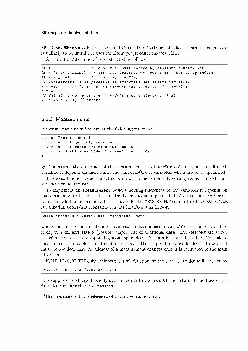
BUILD_RANDOMVAR is able to process up to 255 entries (although this hasn't been tested yet andis unlikely to be useful). It uses the Boost preprocessor macros [KM].
An object of AB can now be constructed as follows:
AB x; // x.a, x.b, initialised by standard constructor
AB y(AB_T(), false); // also std constructor , but y will not be optimized
AB z(AB_T(a)); // z.a = a, z.b=B();
// Furthermore it is possible to overwrite the entire variable:
x = *z; // Note that *z returns the value of z's variable
z = AB_T();
// But it is not possible to modify single elements of AB:
// x->a = y->a; // error!
5.1.3 Measurements
A measurement must implement the following interface:
struct IMeasurement {
virtual int getDim () const = 0;
virtual int registerVariables () const = 0;
virtual double* eval(double* res) const = 0;
};
getDim returns the dimension of the measurement. registerVariables registers itself at allvariables it depends on and returns the sum of DOFs of variables, which are to be optimized.
The eval function does the actual work of the measurement, writing its normalized mea-surement value into res.
To implement an IMeasurement besides holding references to the variables it depends onand optionally further data these methods have to be implemented. As this is an error-prone(and somewhat cumbersome) a helper macro BUILD_MEASUREMENT similar to BUILD_RANDOMVAR
is de�ned in tools/AutoConstruct.h. Its interface is as follows:
BUILD_MEASUREMENT(name , dim , variables , data)
where name is the name of the measurement, dim its dimension, variables the list of variablesit depends on, and data a (possibly empty) list of additional data. The variables are storedas references to the corresponding RVWrapper class, the data is stored by value. To make ameasurement storeable in std container classes, the = operator is overloaded.1 However itmust be avoided, that the address of a measurement changes once it is registered to the mainalgorithm.
BUILD_MEASUREMENT only declares the eval function, so the user has to de�ne it later on as
double* name::eval(double* res);
It is supposed to changed exactly dim values starting at res[0] and return the address of the�rst element after that, i. e. res+dim.
1This is necessary as it holds references, which can't be assigned directly.
5.2 Manifolds 31
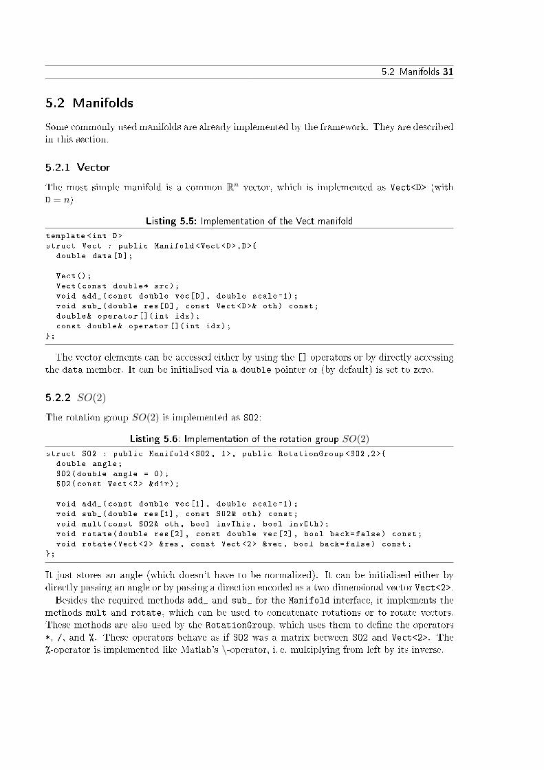
5.2 Manifolds
Some commonly used manifolds are already implemented by the framework. They are describedin this section.
5.2.1 Vector
The most simple manifold is a common Rn vector, which is implemented as Vect<D> (withD = n)
Listing 5.5: Implementation of the Vect manifold
template <int D>
struct Vect : public Manifold <Vect <D>,D>{
double data[D];
Vect();
Vect(const double* src);
void add_(const double vec[D], double scale =1);
void sub_(double res[D], const Vect <D>& oth) const;
double& operator []( int idx);
const double& operator []( int idx);
};
The vector elements can be accessed either by using the [] operators or by directly accessingthe data member. It can be initialised via a double pointer or (by default) is set to zero.
5.2.2 SO(2)
The rotation group SO(2) is implemented as SO2:
Listing 5.6: Implementation of the rotation group SO(2)struct SO2 : public Manifold <SO2 , 1>, public RotationGroup <SO2 ,2>{
double angle;
SO2(double angle = 0);
SO2(const Vect <2> &dir);
void add_(const double vec[1], double scale =1);
void sub_(double res[1], const SO2& oth) const;
void mult(const SO2& oth , bool invThis , bool invOth);
void rotate(double res[2], const double vec[2], bool back=false) const;
void rotate(Vect <2> &res , const Vect <2> &vec , bool back=false) const;
};
It just stores an angle (which doesn't have to be normalized). It can be initialised either bydirectly passing an angle or by passing a direction encoded as a two-dimensional vector Vect<2>.
Besides the required methods add_ and sub_ for the Manifold interface, it implements themethods mult and rotate, which can be used to concatenate rotations or to rotate vectors.These methods are also used by the RotationGroup, which uses them to de�ne the operators*, /, and %. These operators behave as if SO2 was a matrix between SO2 and Vect<2>. The%-operator is implemented like Matlab's \-operator, i. e. multiplying from left by its inverse.
32 Chapter 5 Implementation
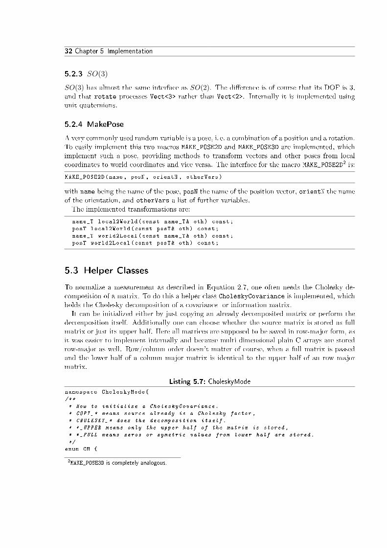
5.2.3 SO(3)
SO(3) has almost the same interface as SO(2). The di�erence is of course that its DOF is 3,and that rotate processes Vect<3> rather than Vect<2>. Internally it is implemented usingunit quaternions.
5.2.4 MakePose
A very commonly used random variable is a pose, i. e. a combination of a position and a rotation.To easily implement this two macros MAKE_POSE2D and MAKE_POSE3D are implemented, whichimplement such a pose, providing methods to transform vectors and other poses from localcoordinates to world coordinates and vice versa. The interface for the macro MAKE_POSE2D2 is:
MAKE_POSE2D(name , posN , orientN , otherVars)
with name being the name of the pose, posN the name of the position vector, orientN the nameof the orientation, and otherVars a list of further variables.The implemented transformations are:
name_T local2World(const name_T& oth) const;
posT local2World(const posT& oth) const;
name_T world2Local(const name_T& oth) const;
posT world2Local(const posT& oth) const;
5.3 Helper Classes
To normalize a measurement as described in Equation 2.7, one often needs the Cholesky de-composition of a matrix. To do this a helper class CholeskyCovariance is implemented, whichholds the Cholesky decomposition of a covariance- or information-matrix.It can be initialized either by just copying an already decomposited matrix or perform the
decomposition itself. Additionally one can choose whether the source matrix is stored as fullmatrix or just its upper half. Here all matrices are supposed to be saved in row-major form, asit was easier to implement internally and because multi dimensional plain C arrays are storedrow-major as well. Row/column order doesn't matter of course, when a full matrix is passedand the lower half of a column major matrix is identical to the upper half of an row majormatrix.
Listing 5.7: CholeskyMode
namespace CholeskyMode{
/**
* How to initialize a CholeskyCovariance.
* COPY_* means source already is a Cholesky factor ,
* CHOLESKY_* does the decomposition itself.
* *_UPPER means only the upper half of the matrix is stored ,
* *_FULL means zeros or symetric values from lower half are stored.
*/
enum CM {
2MAKE_POSE3D is completely analogous.
5.4 Main Algorithm 33
COPY_UPPER ,
COPY_FULL ,
CHOLESKY_UPPER ,
CHOLESKY_FULL
};
};
template <int dim >
struct CholeskyCovariance
{
enum {DIM = dim , SIZE = (dim*(dim +1))/2};
// chol is an lower triangular matrix , saved in row major order
double chol[SIZE];
CholeskyCovariance(const double *A, CholeskyMode ::CM mode);
void invApply(double* arr) const;
void apply(double *arr) const;
};
Besides the constructor two methods invApply and apply are implemented. They multiplythe array starting at address arr with L−1 or L respectively. The latter is useful if not thecovariance but the information matrix was decomposited.
5.4 Main Algorithm
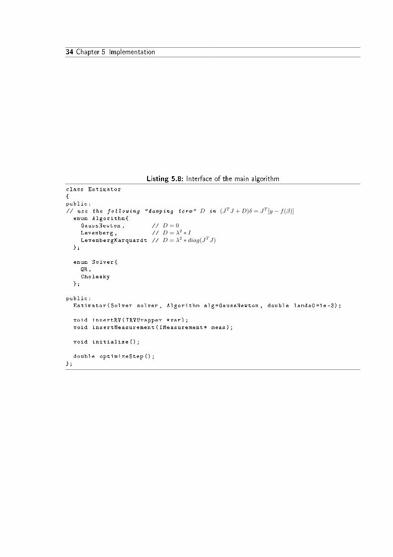
This section will describe the main algorithm. To optimize a LS an object of Estimator has tobe instantiated and used as described in the next subsection. The subsequent subsections willdescribe, how the algorithm works internally.
5.4.1 Interface
In listing 5.8 the important parts of the interface are shown.
5.4.1.1 Constructor
The constructor gets three parameters. First of all solver speci�es how the arising linearsystems are to be solved, either by a QR decomposition, or by a Cholesky decomposition.Cholesky turned out to be a good choice, especially when having much more measurementsthan variables.
The Algorithm alg parameter chooses the mode of �nding the next update. Essentially itis possible to choose di�erent damping terms D for the equation:
(J>J +D)δ = J>[y − f(β)] (5.1)
With D = 0 (i. e. no damping term) for GaussNewton, D = λ2 I for Levenberg, and D =λ2diag(J>J) for LevenbergMarquardt (cf. section 2.4.3 and section 2.4.4). Usually GaussNewtonis a good �rst choice, unless the initialisation of the variables is very poor.
Finally lamda0 sets the start value of the damping parameter λ, which is required forLevenberg and LevenbergMarquardt. For GaussNewton this value is just ignored.
34 Chapter 5 Implementation
Listing 5.8: Interface of the main algorithm
class Estimator
{
public:
// use the following "damping term" D in (JTJ +D)δ = JT [y − f(β)]enum Algorithm{
GaussNewton , // D = 0Levenberg , // D = λ2 ∗ ILevenbergMarquardt // D = λ2 ∗ diag(JTJ)
};
enum Solver{
QR ,
Cholesky
};
public:
Estimator(Solver solver , Algorithm alg=GaussNewton , double lamda0 =1e-3);
void insertRV(IRVWrapper *var);
void insertMeasurement(IMeasurement* meas);
void initialize ();
double optimizeStep ();
};
5.4 Main Algorithm 35
5.4.1.2 Inserting Random Variables and Measurements
After constructing an Estimator random variables and measurements have to be inserted (or�registered�). This is done via the insertRV and insertMeasurement methods, which requirea pointer to an IRVWrapper or IMeasurement respectively.Two things are very important here. The address of the variables and measurements isn't
allowed to change after they have been inserted.3
Furthermore variables always have to be inserted before any measurements, that depend onthem. Apart from that the order in which variables are inserted doesn't matter.
5.4.1.3 Initializing and Optimizing
After all variables and measurements are registered the algorithms has to be initialized, via themethod initialize(). Within this method memory is allocated and the sparsity structure ofthe Jacobian is precalculated.Finally via optimizeStep() the problem can be optimized successively. The method directly
modi�es the registered random variables. It returns the last optimization gain i. e.
gain :=‖f(xk)‖2 − ‖f(xk+1)‖2
‖f(xk+1)‖2. (5.2)
The user then has to decide whether he wants to continue optimizing or not.
3That means when storing variables or measurements in a std::vector it has to be su�ciently preallocated.

36 Chapter 5 Implementation
Chapter 6 Results 37
6Results
The framework was successfully tested with several data sets, from which two are presentedin this chapter, with various variations. This chapter demonstrates the simplicity in which LScan be implemented and also shows the enormous convergence speed of the algorithm.
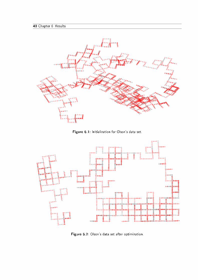
The �rst data set is a syntetic data set provided by Edwin Olson [OLT06]. It consists of 2Dposes and relations between them.
The second data set is Udo Frese's DLR-dataset [Fre], which contains odometry and landmarkmeasurements (with known data association). For this data set some experiments were madelike optimizing a calibration problem or just optimizing poses while keeping the landmarks �xed.The former is useful especially in real-life problems where it is often not possible to perfectlycalibrate sensors. The latter is useful, e. g. when evaluating the results of other algorithmswhich only output landmarks.
6.1 Syntetic Data Set
Edwin Olson's simulated data set consists of poses moving along a grid-world path, whichmakes it easy to visually rate the obtained result, as only orthogonal corners appear and pathsfrequently overlap.
This data set consists only of poses and measurements between them, therefore only one typeof random variable and one type of measurement had to be implemented (see listing 6.1). Theodometry measurement transforms the endpose t1 in the local coordinate system of the startpose t0 and then subtracts the measured odometry (using sub, which corresponds to the �operator). Afterwards the result is normalized by multiplying with the inverse Cholesky factorof the covariance.
In the main routine a log�le is read and for each relation an Odo object is created and stored.Furthermore whenever a new frameID is encountered a new Pose is created, which is initializedby the inverse odometry model (see listing 6.2).
38 Chapter 6 Results
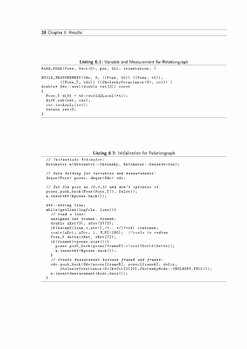
Listing 6.1: Variable and Measurement for Relationgraph
MAKE_POSE(Pose , Vect <2>, pos , SO2 , orientation , )
BUILD_MEASUREMENT(Odo , 3, ((Pose , t0)) ((Pose , t1)),
((Pose_T , odo)) (( CholeskyCovariance <3>, cov)) )
double* Odo::eval(double ret [3]) const
{
Pose_T diff = t0 ->world2Local (*t1);
diff.sub(ret , odo);
cov.invApply(ret);
return ret+3;
}
Listing 6.2: Initialization for Relationgraph
// Instantiate Estimator:
Estimator e(Estimator ::Cholesky , Estimator :: GaussNewton);
// Data holding for variables and measurements:
deque <Pose > poses; deque <Odo > odo;
// Set 0th pose as (0,0,0) and don't optimize it
poses.push_back(Pose(Pose_T (), false));
e.insertRV (&poses.back());
std:: string line;
while(getline(logfile , line)){
// read a line:
unsigned int frameA , frameB;
double xEst[3], xCov [3][3];
if(sscanf(line.c_str(),/*...*/)!=14) continue;
scale(xEst , xCov , 1, M_PI /180); //scale to radian
Pose_T delta(xEst , xEst [2]);
if(frameA >=poses.size()){
poses.push_back(poses[frameB]->local2World(delta));
e.insertRV (&poses.back());
}
// Create Measurement between frameB and frameA:
odo.push_back(Odo(poses[frameB], poses[frameA], delta ,
CholeskyCovariance <3>(& xCov [0][0] , CholeskyMode :: CHOLESKY_FULL)));
e.insertMeasurement (&odo.back());
}

6.2 DLR Data Set 39
After initializing the variables and measurements, the Estimator itself has to be initial-ized (allocating workspace and precalculating the structure of the Jacobian) by calling itsinitialize() method. Afterwards the method optimizeStep() is called several times untilthe gain drops below a certain level (10−9). Between optimization steps an intermediate resultis stored in an output �le. The optimization loop is shown in listing 6.3.
The residual sum of squares (RSS) drops from 1.13 ·108 after initialization to 6415.57 in foursteps, afterwards it slowly drops further to 6413.96, where the optimization converges after atotal of seven steps. The data set has 3500 poses and about 5600 measurements between them.The total optimization time (excluding data output) was about 0.95 s on a 1.86GHz CPU. Theinitialization and �nal graph can be seen in �gure 6.1 and �gure 6.2.
6.2 DLR Data Set
The second data set was provided by Udo Frese [Fre]. The data set consists of odometryand landmark measurements. Both measurements are given in relative coordinates and withcovariance information.
6.2.1 Preparations
Like in previous example, �rst of all the variables and measurements have to be de�ned. ThePose and the Odo types are implemented the same way as in listing 6.1. This example addslandmarks, which can be modeled as a Vect<2>. The landmark measurement is implementedsimilar to the odometry measurement by transforming the landmark from world coordinates intothe local coordinate system of the pose. Afterwards the di�erence to the measured landmarkis calculated and normalized by the inverse covariance (see listing 6.4).
6.2.2 Data Initialization
As the parser for this data set is a bit more complex, only the pure data initialization isdemonstrated here. The landmarks do not necessarily come in order, therefore they are stored
Listing 6.3: Optimization Loop for Relationgraph
// Initialize Estimator:
e.initialize ();
int kMax = 20; // limit nr of iterations
for(int k=0; k<kMax; k++){
// optimize:
double gain=e.optimizeStep ();
// Output intermediate result:
outputPoses(poses , make_filename("output",k,".pos").c_str());
// break if gain < 1e-9:
if(0<=gain && gain < 1e-9) break;
}
40 Chapter 6 Results
Figure 6.1: Initialization for Olson's data set.
Figure 6.2: Olson's data set after optimization.
6.2 DLR Data Set 41
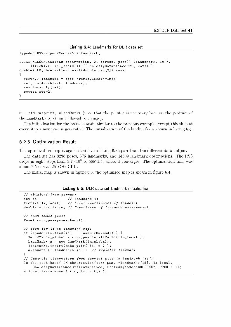
Listing 6.4: Landmarks for DLR data set
typedef RVWrapper <Vect <2> > LandMark;
BUILD_MEASUREMENT(LM_observation , 2, ((Pose , pose)) ((LandMark , lm)),
((Vect <2>, rel_coord )) (( CholeskyCovariance <2>, cov)) )
double* LM_observation ::eval(double ret [2]) const
{
Vect <2> landmark = pose ->world2Local (*lm);
rel_coord.sub(ret , landmark);
cov.invApply(ret);
return ret+2;
}
in a std::map<int, *LandMark> (note that the pointer is necessary because the position ofthe LandMark object isn't allowed to change).
The initialization for the poses is again similar to the previous example, except this time atevery step a new pose is generated. The initialization of the landmarks is shown in listing 6.5.
6.2.3 Optimization Result
The optimization loop is again identical to listing 6.3 apart from the di�erent data output.
The data set has 3298 poses, 576 landmarks, and 14309 landmark observations. The RSSdrops in eight steps from 3.7 · 108 to 56871.5, where it converges. The optimization time wasabout 2.5 s on a 1.86GHz CPU.
The initial map is shown in �gure 6.3, the optimized map is shown in �gure 6.4.
Listing 6.5: DLR data set landmark initialisation
// obtained from parser:
int id; // Landmark id
Vect <2> lm_local; // Local coordinates of landmark
double *covariance; // Covariance of landmark measurement
// Last added pose:
Pose& curr_pos=poses.back();
// Look for id in landmark map:
if (landmarks.find(id) == landmarks.end() ) {
Vect <2> lm_global = curr_pos.local2World( lm_local );
LandMark* n = new LandMark(lm_global);
landmarks.insert(make_pair( id , n ) );
e.insertRV( landmarks[id]); // register landmark
}
// Generate observation from current pose to landmark "id":
lm_obs.push_back( LM_observation(curr_pos , *landmarks[id], lm_local ,
CholeskyCovariance <2>(covariance , CholeskyMode :: CHOLESKY_UPPER ) ));
e.insertMeasurement( &lm_obs.back() );
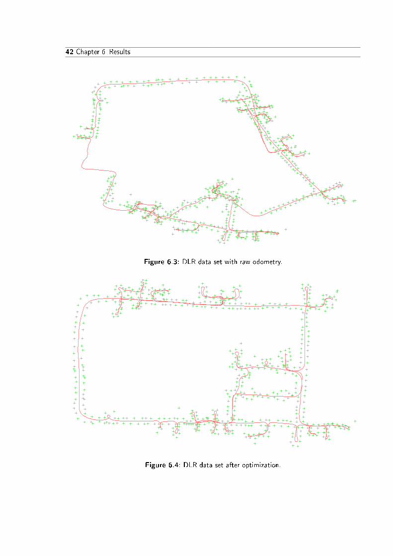
42 Chapter 6 Results
Figure 6.3: DLR data set with raw odometry.
Figure 6.4: DLR data set after optimization.
6.2 DLR Data Set 43
6.2.4 Partial Optimization
A nice feature of the framework is to optimize only parts of a data set. A possible use case forthis is the evaluation of algorithms which perform some kind of data reduction, e. g. combinelocal sub maps and lose the pose information therein before doing a global optimization.
If the result of such an algorithm shall be compared with the optimal solution, one has toreestimate the poses afterwards. This can be done by the framework, by inserting the landmarksas �xed variables into the algorithm:1
int id;
Vect <2> data; // read from logfile
// Do not optimize n:
LandMark* n=new LandMark(data , false);
// store and register to algorithm
landmarks.insert(make_pair( id , n ) );
e.insertRV(n);
This was done for several data sets. The optimization time was slightly faster than the fulloptimization. The RSS was not surprisingly always bigger than the optimal result. The actualresults are not that important within this thesis.
6.2.5 Calibration Problems
A class of problems which can't be solved by standard SLAM algorithms are calibration prob-lems. When miscalibrated sensors are used, they can be calibrated simultaneously with opti-mizing the SLAM problem, using this framework.
Suppose for example, the odometry has an unknown scale factor for each component, i. e. forthe measured odometry u = [x, y, α]>, the real odometry would be (neglecting noise):
u = [c0x, c1y, c2α]>. (6.1)
This can easily be modelled in the framework by introducing a new variable Calibration
which holds a Vect<3>, and adapting the Odo measurement as shown in listing 6.6.
During initialization this time a Calibration object has to be instantiated and registered tothe framework. This object has then to be passed to every odometry measurement, as shownin listing 6.7.
The initialization of landmarks and the optimization is still the same. Amazingly the RSS ofthe optimized problem dropped signi�cantly from 56871.5 to 42933.1 using the original data.
After optimizing, the values from calib were displayed:
c0 = 1.05704 c1 = 0.924149 c3 = 1.00269, (6.2)
which means that there might be a systematic error of over 5% in the translation, and 0.2% inthe orientation. However this can't be said for sure, as the error theoretically might be causedby miscalibrated landmark measurements as well. Note that simultaneously applying the same
1This has to be done before the �other� initialization. Note that the later initialization does not overwrite thelandmarks.
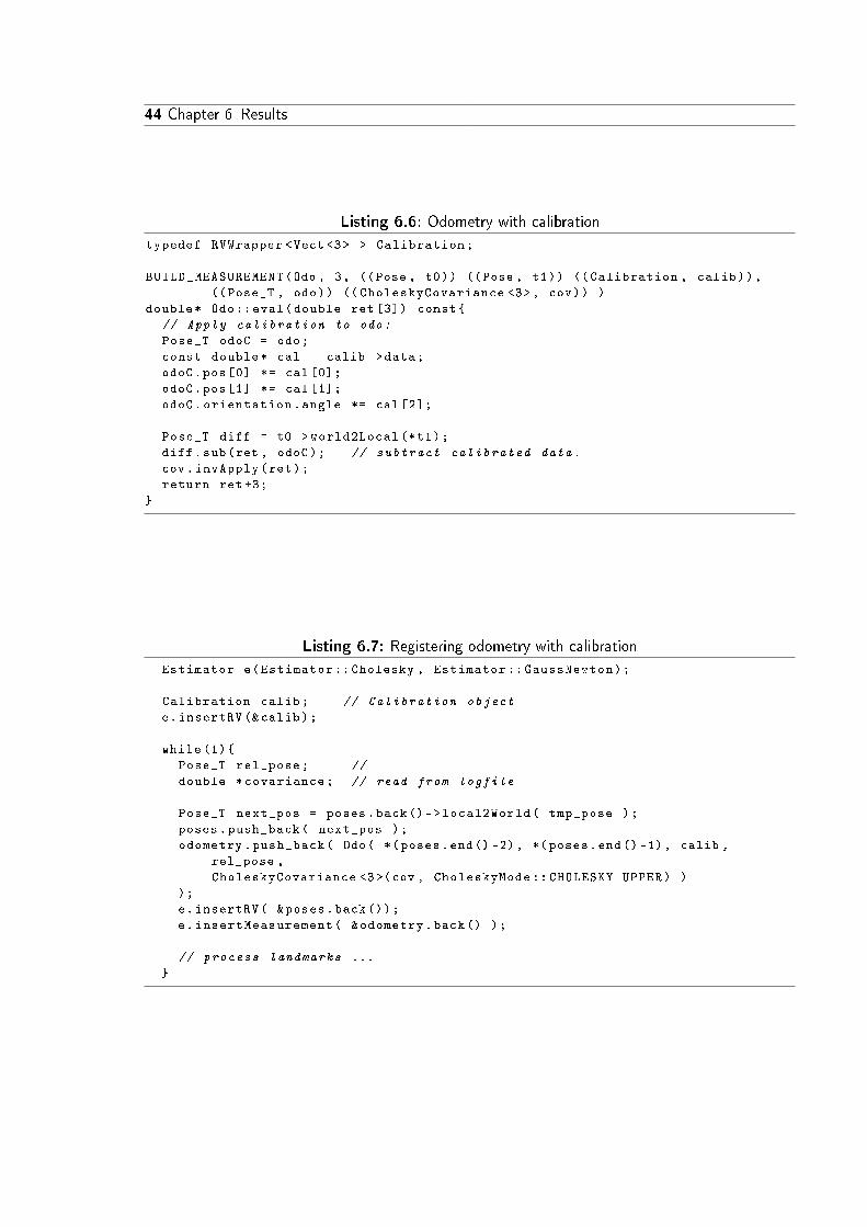
44 Chapter 6 Results
Listing 6.6: Odometry with calibration
typedef RVWrapper <Vect <3> > Calibration;
BUILD_MEASUREMENT(Odo , 3, ((Pose , t0)) ((Pose , t1)) (( Calibration , calib)),
((Pose_T , odo)) (( CholeskyCovariance <3>, cov)) )
double* Odo::eval(double ret [3]) const{
// Apply calibration to odo:
Pose_T odoC = odo;
const double* cal = calib ->data;
odoC.pos[0] *= cal [0];
odoC.pos[1] *= cal [1];
odoC.orientation.angle *= cal [2];
Pose_T diff = t0 ->world2Local (*t1);
diff.sub(ret , odoC); // subtract calibrated data.
cov.invApply(ret);
return ret+3;
}
Listing 6.7: Registering odometry with calibration
Estimator e(Estimator ::Cholesky , Estimator :: GaussNewton);
Calibration calib; // Calibration object
e.insertRV (&calib);
while (1){
Pose_T rel_pose; //
double *covariance; // read from logfile
Pose_T next_pos = poses.back()->local2World( tmp_pose );
poses.push_back( next_pos );
odometry.push_back( Odo( *( poses.end() -2), *( poses.end() -1), calib ,
rel_pose ,
CholeskyCovariance <3>(cov , CholeskyMode :: CHOLESKY_UPPER) )
);
e.insertRV( &poses.back());
e.insertMeasurement( &odometry.back() );
// process landmarks ...
}

6.2 DLR Data Set 45
calibration strategy to the landmarks will not give meaningful results, as this gives the wholesystem at least one unde�ned DOF namely an over all scale factor.2
The calibration problem was repeated by intentionally scaling each odometry value afterreading it from the log�le. For the translational scale quite arbitrary factors could be used,while still obtaining the same results (when scaled by the same factor). For the orientationalpart however too big errors could not be compensated and let the algorithm get stuck in localminima.
2In that case the optimal result would be to set every factor to 0.

46 Chapter 6 Results
Chapter 7 Conclusion 47
7Conclusion
7.1 Achieve Goals
This thesis provided a formalization of manifolds and the encapsulation operators �, � proposedin [FS].It was shown that using these encapsulation operators functions between manifolds can be
normalized such that they behave like general functions locally and standard optimizationalgorithms can be applied.This was used this to solve arbitrary least squares problems on manifolds, �rst theoretically,
and later in practice.Exploiting the sparseness of the least squares problem and using a sparse library package for
direct methods leads to rather fast optimization times, which even outperforms some specializedo�ine SLAM algorithms.It was showed that using this framework it is possible to
� solve an o�ine SLAM problem with very little implementation necessary.
� just partly optimize problems (e. g. keep some variables �xed).
� solve calibration problems (which is hard to do with standard SLAM algorithms).
� test the accuracy of other LS algorithms.
7.2 Outlook
Unfortunately it wasn't possible in the end to implement a good 3D example, which wouldhave demonstrated the usefulness of manifolds better.Some possibilities for further research arose during the development of this thesis:
� Give the framework the possibility to handle online problems better

48 Chapter 7 Conclusion
� Make it possible to change correspondences between variables and measurements betweenoptimizations
� maybe use another backend like Treemap [Fre07] for the optimization.
49
Bibliography
[Cop95] Coplien, James O.: Curiously recurring template patterns. In: C++ Rep. 7(1995), Nr. 2, S. 24�27. � ISSN 1040�6042
[Dav] Davis, Timothy A.: Direct Methods for Sparse Linear Systems, and the CSparsePackage. http://www.cise.ufl.edu/research/sparse/CSparse/, Last checked:2008-11-01
[Dav06] Davis, Timothy A.: Direct Methods for Sparse Linear Systems. Philadelphia :siam, 2006 (Fundamentals of Algorithms)
[Fre] Frese, Udo: Deutsches Zentrum für Luft- und Raumfahrt (DLR) dataset. http://www.sfbtr8.spatial-cognition.de/insidedataassociation/data.html,Last checked: 2008-11-01
[Fre07] Frese, U.: E�cient 6-DOF SLAM with Treemap as a Generic Backend. In:Procedings of International Conference on Robotics and Automation, Rome, 2007
[FS] Frese, Udo ; Schröder, Lutz: Theorie der Sensorfusion Skript 2006. http://
www.informatik.uni-bremen.de/agebv/de/VeranstaltungTDS06, Last checked:2008-11-01
[HZ03] Hartley, Richard ; Zisserman, Andrew: Multiple View Geometry in ComputerVision. Cambridge University Press, 2003. � ISBN 0521540518
[KM] Karvonen, Vesa ; Mensonides, Paul: The Boost Library, Preprocessor Subsetfor C/C++. http://www.boost.org/doc/libs/1_36_0/libs/preprocessor/
doc/index.html, Last checked: 2008-11-01
[Lee03] Lee, John M.: Introduction to Smooth Manifolds. Springer Verlag, 2003
[Lev44] Levenberg, Kenneth: A Method for the Solution of Certain Non-Linear Prob-lems in Least Squares. In: The Quarterly of Applied Mathematics (1944), Nr. 2,S. 164�168
[Mar63] Marquardt, D. W.: An Algorithm for Least-Squares Estimation of NonlinearParameters. In: Journal of the Society for Industrial and Applied Mathematics(1963)
[MYB+01] Marins, João L. ; Yun, Xiaoping ; Bachmann, Eric R. ; Mcghee, Robert B. ;Zyda, Michael J.: An extended Kalman �lter for quaternion-based orientation es-timation using MARG sensors. In: Engineer's Thesis, Naval Postgraduate School,2001, 2003�2011
50 Bibliography
[NM65] Nelder, J. A. ; Mead, R.: A Simplex Method for Function Minimization. In:The Computer Journal 7 (1965), January, Nr. 4, S. 308�313
[OLT06] Olson, Edwin ; Leonard, John ; Teller, Seth: Fast Iterative Optimization ofPose Graphs with Poor Initial Estimates, 2006, S. 2262�2269
[PTVF92] Press, William ; Teukolsky, Saul ; Vetterling, William ; Flannery, Brian:Numerical Recipes in C. 2nd. Cambridge, UK : Cambridge University Press, 1992
[TBF05] Thrun, S. ; Burgard, W. ; Fox, D.: Probabilistic Robotics. MIT Press, 2005
[Ude99] Ude, Ale�s: Filtering in a unit quaternion space for model-based object tracking.In: Robotics and Autonomous Systems 28 (1999), August, Nr. 2-3, S. 163�172
[Vic01] Vicci, L.: Quaternions and Rotations in 3-Space: The Algebra and its Geomet-ric Interpretation / Dept. of Computer Science, University of North Carolina atChapel Hill. 2001 (TR01-014). � Technical Report
[WI95] Wheeler, Mark D. ; Ikeuchi, Katsushi: Iterative estimation of rotation andtranslation using the quaternion / Carnegie Mellon University, Pittsburgh, PA.Version: 1995. http://dx.doi.org/10.1.1.71.6291. 1995. � Forschungsbericht
[Wika] Wikipedia: Hairy Ball Theorem. http://en.wikipedia.org/wiki/Hairy_ball_theorem, Last checked: 2008-11-01
[Wikb] Wikipedia: Stereographic Projection. http://en.wikipedia.org/wiki/
Stereographic_projection, Last checked: 2008-11-01
[WR71] Wilkinson, James H. ; Reinsch, Christian: Handbook for Automatic Compu-tation. Vol. II: Linear Algebra. Springer-Verlag, 1971. � Source of this quote:http://www.netlib.org/na-digest-html/07/v07n12.html#1


![Singularities in cosmological Bianchi class A models...have also been considered by [Wal83] and [Ren95]. The case of Bianchi type Ican be integrated explicitely. Using assumptions](https://img.pdfslide.org/doc/110x75/612d99ae1ecc515869424a4c/singularities-in-cosmological-bianchi-class-a-models-have-also-been-considered.jpg)