A Tool Chain for a Lightweight, Robust andUncertainty-based Context Classification System (CCS)Henning Günther, Firas El Simrany, Martin Berchtold and Michael BeiglInstitut für Betriebssysteme und Rechnerverbund, Technische Universität Braunschweig

AbstractIn this paper we present a tool chain developed to support a Context Classification System (CCS). The CCS is especiallydesigned to run even on lightweight commodity phones with a high detection rate and low calculation effort. The maindesign aspect considered while building the tool chain was the support for most common users and not only developers.Moreover, the CCS we are using proves to be a robust context recognition method, which supports the gain of both contextclasses and a fuzzy uncertainty value describing the confidence of their classification.

1 Introduction

Context-awareness has been a research topic for manyyears now. There has been a lot of progress since first ap-pliances [1], “smart” environments [2] and very rudimen-tary “smart” devices [3], compared to nowadays context-aware systems [4] and activity recognition [5]. Thisprogress was facilitated through a growing number oftoolkits to visualize, transform, interpret and/or classifysensor data.The Common Sense ToolKit (CSTK) [6][7] was an earlytoolkit which was mainly focusing on the data transfor-mation and visualization. The CSTK is a collection oftools, written mostly in C++, that assist in the communi-cation, abstraction, visualisation, and processing of sen-sor data. CSTK’s core qualities are its real- time facilitiesand embedded systems-friendly implementation, provid-ing ready-to-use modules for the prototyping and construc-tion of sensor-based applications. Although it can be usedfor offline analysis (i.e., using recorded data files), CSTKis mainly envisioned as a tool to be applied in online fash-ion (i.e., using the sensor data as it comes streaming in).A well known and also a very early toolkit for process-ing sensor data is the Context Toolkit [8]. The aim ofthis toolkit is to make it easy to build context-aware ap-plications. They claim that context is difficult to use be-cause, unlike other forms of user input, there is no com-mon, reusable way to handle it. We are disagreeing withthis proposition, because our approach presents mecha-nisms to build context classifiers which are reusable dueto their simple and flexible design.In [9] a GUI-based C++ toolbox is presented that allowsthe building of distributed, multi-modal context recogni-tion systems by plugging together reusable, parameteriz-able components. The goals of this toolbox are to simplifythe steps from prototypes to online implementations onlow-power mobile devices, facilitate portability between

platforms and foster easy adaptation and extensibility. Ourapproach differs in the level the online system gets dis-tributed. We try to do the classifications on the device andthen infer further context knowledge in a distributed way,whereas in this paper, we do not present a reasoning. Thereasoning is part of our future work.Compared to the named toolkits, this work is focusingonly on one strain of sensor data processing, which startsat the data collection, over to the annotation, the systemidentification and ends in a Context Classifying System(CCS) that runs even on lightweight commodity phones asthe OpenMoko platform. Also, the focus of the proposedtoolkit is not the diversity of algorithms, but the simplicityof identifying a CCS. The diversity that can be coveredthough, lies in the platforms which are supported by theCCS.

The paper is structured as follows: In Sect. 2, we introducethe tool chain with it’s different components from data col-lection to CCS. In sect. 3. the Context Classification Sys-tem CCS is introduced. Sect. 4 is about the process oftraining context classifiers out of real life data using thetool chain and the CCS. The description of the Data Col-lection Tool (DCT) can be found in sect. 5 followed by thedescription of the Context Annotator Tool (CAT) in sect.6. In sect. 7 we present th performance evaluations of theCCS, whereas between different implementations is com-pared. In the last section we conclude and show some fu-ture activities.

2 The Tool ChainThe tool chain consists of several tools, algorithms, inter-faces and databases, all for one purpose, to most simplyas possible identify a CCS. All links of the tool chain andtheir interconnections are displayed in figure 1.

Gath-Geva

Clustering

Training Data

Check Data

Subtractive

Clustering

Genetic Algorithm

Selection of best combination of initial

cluster centresLeast

Squares

Regression

Calculation

of new dim.

on output

Calculation

of Fitness

(Q. Error)

Fitness Value

Output Vector

Stop

Criteria Check

Repeat until stop criteria

RFIS

12 2

22

3 4 5

Offline CCS Identification Algorithm

Context Classification

System (CCS)

Context Annotator Tool (CAT)

Data Collector Tool

(DCT)Context Data

Base (CDB)

Figure 1: Tool Chain

2.1 Context Classification System (CCS)Identifying the Context Classification System (CCS) is thesole purpose of the proposed tool chain. We chose a Re-cursive Fuzzy Inference System (RFIS) as the the mappingfunction from the features onto a classifiable linear set. Itsaccuracy compared to other methods (HMM, GMM, NN,etc.) is really high, it delivers a fuzzy uncertainty valuewith every classification and the calculation time rises lin-ear with every new rule added to the RFIS.The decision to use a RFIS mapping function in the CCS isfounded, but there are other methods of mapping which arealso suited. We decided to solely use the RFIS mapping,because a choice of different mapping methods would onlyconfuse the user. So, having lots of choice in the mappingmethods contradicts our conception of a simple to use toolchain and CCS, especially if the user is no expert.

2.2 CCS Identification AlgorithmThe CCS identification algorithm consists of a combina-tion of clustering, least squares and genetic algorithm. Ac-cording to a training data set, a combination of subtractiveand Gath-Geva clustering identifies the rules of the RFISmapping function used in the CCS. The consequences ofthe rules are calculated with a least squares method. A ge-netic algorithm helps optimizing the cluster selection usedin the RFIS mapping.Here, we decided to develop our own identification algo-rithm, instead of using a well known approach such asthe ANFIS (Adaptive Network-based Fuzzy Inference Sys-tem) [10] one. One main aspect is, that the calculationtime for a hybrid training (gradient decent) of the ANFISis much higher than for our algorithm. Secondly, there isno easy way to include recurrence in the ANFIS approach,whereas the recurrence in our algorithm is a simple shiftoperation. Also, the accuracy of a trained multivariateANFIS is lower than our used covariate RFIS. Since we

use highly correlated sensor data (accelerometer axis), weneed covariant cluster shapes, which are not supported inthe ANFIS approach.

2.3 Data Collector Tool (DCT)

In order to get different contextual training data for theCCS (section 3) a simple Python application, the Data Col-lector Tool (DCT), allows to gather sensor data from thesensors on the Neo Freerunner (future support for otherplatforms, e.g. iPhone, Android, Maemo, etc.) which isequipped with one audio and two acceleration sensors. TheDCT would be extended to gather data from other sensoryinputs when needed. However the data produced shouldbe first processed with the CAT, see section 4.1 before itbecomes suitable for training. More on the DCT in section5.

2.4 Context Annotator Tool (CAT)

The next step is the contextual annotation, and conversioninto training data, of the collected raw data. The ContextAnnotation Tool (CAT), is a user friendly tool allowing vi-sualization of different data sources and to easily associatesuitable recognized context information. Then convertingit into the training data, in a format suitable for the CCS.More on the CAT is shown in section 6.

2.5 Context Data Base (CDB)

All previously intoduced tools produce, consume orchange data and classifiers. To manage the data, usuallya stream pipes the data from one modul to the next one.Since we not only have one device producing sensor dataor running a CCS, we need a more flexible approach tomanage the data. We decided to use a data base, to storethe raw sensor data, the annotated data, the preprocesseddata and the trained classifiers.

The Contex Data Bases (CDB) purpose is to collect datafrom different users and devices (OpenMoko, iPhone, Mo-torola Milstone, Nokia N900, etc.) over a indefinite spanof time. Also, all the trained CCS are not only stored, butalso the training and check data are linked through a SQLstring. With this SQL string the identification of each CCScan be reconstructed and therefore providing total visibil-ity. The access to the CDB is done via command line orthe Context Web Interface (CWI). Also, the CAT will beextended to allow direct loading and saving from and tothe database. The implementation of the CDB is currentlyin progress, thats why we do not take a closer look into thismodule.

FFT

mean/variance

Accelerometer

Microphone

Recurrent Fuzzy

Inference System

(RFIS) Fuzzy Numbers ( )

()

( )

Feature Extraction Mapping Function Fuzzy ClassificationSensoryReal World

Sampled

SignalFeature

Vector

Mapping

Value

Class

Identifier /

Uncertainty

Value

Signal

Recurrent Edge

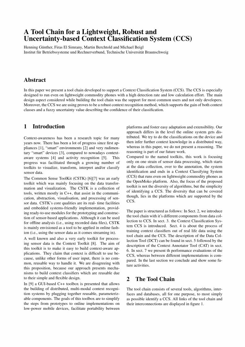
Figure 2: Online system architecture for classification and fuzzy uncertainty.

3 Context Classification System(CCS)

In our implementation we use the Context ClassificationSystem (CCS) for context recognition, which was intro-duced in [11] (there its called ORFC). The CCS uses a Re-current Fuzzy Inference System (RFIS) for mapping thefeature vectors on a classifiable linear set. All steps arediagrammed in figure 2.

3.1 Feature Extraction

For the application in this paper, we used audio and ac-celeration sensors. We segment the sensor streams intoframes of 64 milliseconds length for audio and 80 mil-liseconds for acceleration. This frame lengths result in512 samples (8kHz sampling rate) for audio and 8 sam-ples (∼100Hz sampling rate) for acceleration. The fea-tures used for activity recognition with acceleration mea-surements are mostly variance and mean values, since theycan be calculated with low resource consumption and givegood classification results. These features were used topre-process the accelerometer data, where the two 3-axisaccelerometer sensors lead to a twelve-dimensional fea-ture vector −→v acc

t = (v1, .., v12). For audio data, we use“ Fast Fourier Transformation (FFT)” to extract frequencyfeatures for the audio classification. Since the dimension-ality after the FFT (e.g. 512 spectra) is too high to be usedas input for a classifier, mean, variance and frequency cen-troid are calculated over the two halves of the frequencyspectrum. This leads to a six dimensional feature vector−→v snd

t = (v1, .., v6).

3.2 Recurrent FIS Mapping

Takagi, Sugeno and Kang [12][13] (TSK) fuzzy inferencesystems are fuzzy rule-based structures, which are espe-cially suited for automated construction. The TSK-FISalso maps unknown data to zero, making it especially suit-able for partially incomplete training sets. In TSK-FIS theconsequence of the implication is not a functional mem-bership to a fuzzy set but a constant or linear function. The

consequence of the rule j depends on the input of the FIS:

fj(−→v t) := a1jv1 + ..anjvn + a(n+1)j

=

n∑i=1

aijvi + a(n+1)j

The linguistic equivalent of a rule with Gaussian member-ship functions in the antecedence part is formulated ac-cordingly:

IF µ1j(v1) AND µ2j(v2) AND .. AND µnj(vn) THEN fj(−→v t)

Since in activity recognition we deal with highly corre-lated features, especially when accelerometers are used,we use a slight variation of the rule above, which includescovariant Gaussian functions. The linguistic rule with acovariant antecedence is formulated accordingly:

IF µj(−→v t) THEN fj(

−→v t) (1)

The covariant Gaussian MF, depending on the covariancematrix Σj and the mean vector−→mj , is defined accordingly:

µj(−→v t) := e−

12 (−→v t−−→m j)Σ−1

j (−→v t−−→m j)T (2)

The whole antecedent part of each rule was multiplied withthe usual TSK-FIS to get the respective weight, but withthe covariant MF’s the function is already the weight. Theresulting formula for the covariant TSK-FIS is defined, asfollows:

S(−→v t) :=

∑mj=1 µj(

−→v t)fj(−→v t)∑m

j=1 µj(−→v t)

(3)

The outcome of the mapping at time t is fed back as addi-tional input dimension for the TSK-FIS mapping at t + 1.The recurrence not only delivers the desired uncertaintylevel, but also stabilizes and improves the mapping accu-racy.

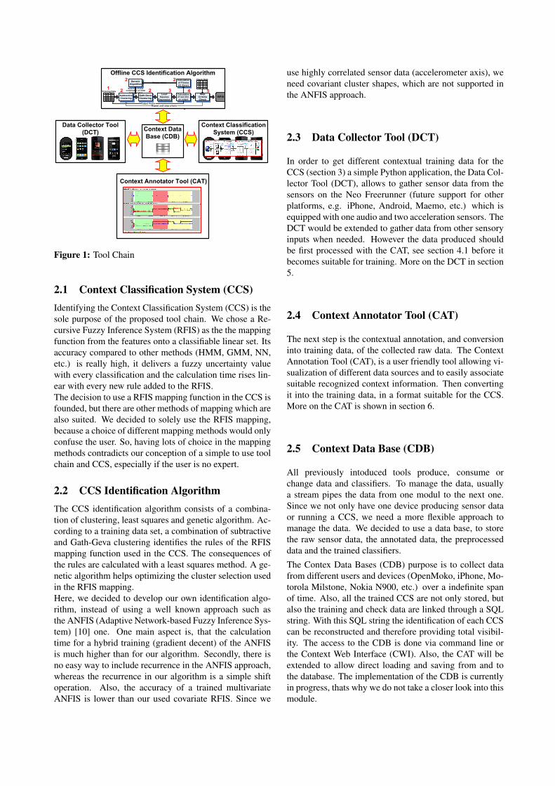
3.3 Fuzzy ClassificationThe outcome of the TSK-FIS mapping needs to be as-signed to one of the classes that the projection should resultin. This assignment is done fuzzily, so the result is not onlya class identifier, but also a membership, identifying thefuzzy uncertainty of the classification process. Each class

identifier is interpreted as a triangular shaped fuzzy num-ber (fig. 3). The mean of the fuzzy number is the identifieritself, with the highest membership of one. An example forfour classes is shown in Fig. 3. The crisp decision (whichidentifier is the mapping outcome) is carried out based onthe highest degree of membership to one of the class iden-tifiers. The overall output of the RFIS mapping is a fuzzyclassification, that is, a pair (CA, µA) of a class identifierand a degree of membership.

1 2 3 40

−1 1 2 3 40

−1

1

0 0

1

Figure 3: Fuzzy numbers identifying class membershipand fuzzy uncertainty level.

3.4 Fuzzy Uncertainty FilterThe classifications vary strongly with respect to fuzzinessand therefore in the reliability of the RFIS mapping. Sincemany more classifications are made than needed for mostapplications, a filter upon the fuzzy uncertainty can im-prove reliability, but also reduces the number of classi-fications. In order to determine the threshold values forfiltering, we used the “‘Receiver Operator Characteristic(ROC)” described in [14].

3.5 ImplementationThe first implementation of the CCS was done on the NeoFreerunner phone, developed by the OpenMoko project[15].

3.5.1 Python

The Python implementation was done first to provide aproof-of-concept implementation to show that the systemcould deliver certain recognition levels. The implementa-tion consist of three parts:

1. A rule parser

2. A rule engine

3. An input processing module

The rule parser uses the INI file format to load rules intothe system. Each rule file starts with a default section inwhich the rule count as well as the dimensions of the rulesare specified:

[DEFAULT]dimensions = 13rules = 4

Even though this information is redundant, it can be usedfor error checking or making the parsing process mucheasier. Following this header, each rule is given as aseparate section. Each rule j is defined through the co-variance matrix (sigma =̂ Σj), the mean vector (mean =̂−→mj), the consequence parameter vector (consequence =̂−→a j = (a1j , ..., a(n+1)j) and the bit masking vector (bitvec

=̂−→b j for example

−→b j = (0000111010101)):

[RULE1]sigma = 2.502186e-02 -1.515808e-02 ...mean = -8.953875e+02 -4.980525e+02 ...consequence = 3.532613e-03 ...bitvec = 0 0 0 0 1 1 1 0 1 0 1 0 1

With the bit masking vector−→b j the rule j of the CCS can

be changed without destroying the original rule. The bitmasking vector therefore gives the possibility to adapt theCCS to changed conditions or users. More details on thebit vector masking can be found in [16].The rule engine essentially implements the algorithm de-scribed in section 3. All matrix-/vector-operations are im-plemented using the numpy-package [17], which providesoptimized numerical functions. A class diagram of the ruleengine can be seen in figure 4.

Figure 4: Class diagram of the python rule engine

The input processing module is responsible for fetchingdata from the sensor hardware of the phone and for prepro-cessing it according to section 3.1. Audio data is fetchedusing the ALSA (Advanced Linux Sound Architecture),which provides a clean API for setting the necessary pa-rameters (sample rate, sample width, etc. . . ). Preprocess-ing is done using numpy routines, except for the cen-troid calculation, which had to be implemented in python.Movement data is collected using the exposed sysfs API ofthe OpenMoko operating system.

3.5.2 Native (C)

The C implementation was conceived to address the mainproblem with the python implementation: performance.As we will show in section 7, the python implementa-tion wasn’t able to achieve real-time performance on theFreerunner phone.

To make the implementation as lightweight and portableas possible, as few as possible external libraries were used.The fourier transformation necessary for the audio pre-processing was implemented using the FFTW-library [18].Everything else, including vector-/matrix-operations werehand-coded to avoid dependencies.

4 CCS IdentificationIn this section we show how to use the tools collectingtraining data and how the algorithm for identifying theCCS works upon the data.

4.1 Obtaining Training DataReal life data collection, both from audio and accelerationsensors, was conceived in a way that, at the end of the toolchain, would produce a specific set of feature vectors asdescribed in 3.1.Contexts in real life are correlated, have intersections andcan occur simultaneously. However we needed to definecontext classes which are simple and flexible enough to en-sure re-usability and to avoid overlapping. E.g., it makesno sense to train a CCS (RFIS) with both acceleration andaudio data. It leads to lower context recognition ratios andis semantically incorrect. Combining other kinds of sen-sor inputs, like video and audio or GPS and acceleration,would be more plausible. Consequent we choose to traincontexts with one sensor type data at a time. Once the setof context classes, we wanted to collect data for, is defined,data is collected according to the following procedure:

1. Collecting raw data using Data Collection Tool DCT(section 5): Both from audio and acceleration sen-sors, using the DCT, we can collect annotated andnon annotated data. Non annotated data is mere sen-sor data. Annotated data, is sensor data that was di-rectly associated to a specific context class and thenbundled into a tar file format. The tar file can be di-rectly imported in the Context Annotation Tool CAT(section 6).

2. Processing the data using the CAT: Non annotateddata will be annotated then converted into raw train-ing data. Annotated data can be edited or directlyconverted.

3. Feature extraction according to section 3.1 producesready to use training and check data.

All above described steps are visualized in figure 5.

1

Training Data

Real Life Manual

Annotation

CAT

Conversion

CAT

2 2Annotated Raw

Data

Not Annotated

Raw Data

0

Recording/

Gathering

DCT

FFT for

Audio Data

Mean/

Variance for

Acceleration

Data

3

Figure 5: Training Data Gain using DCT, CAT and Fea-ture Extraction

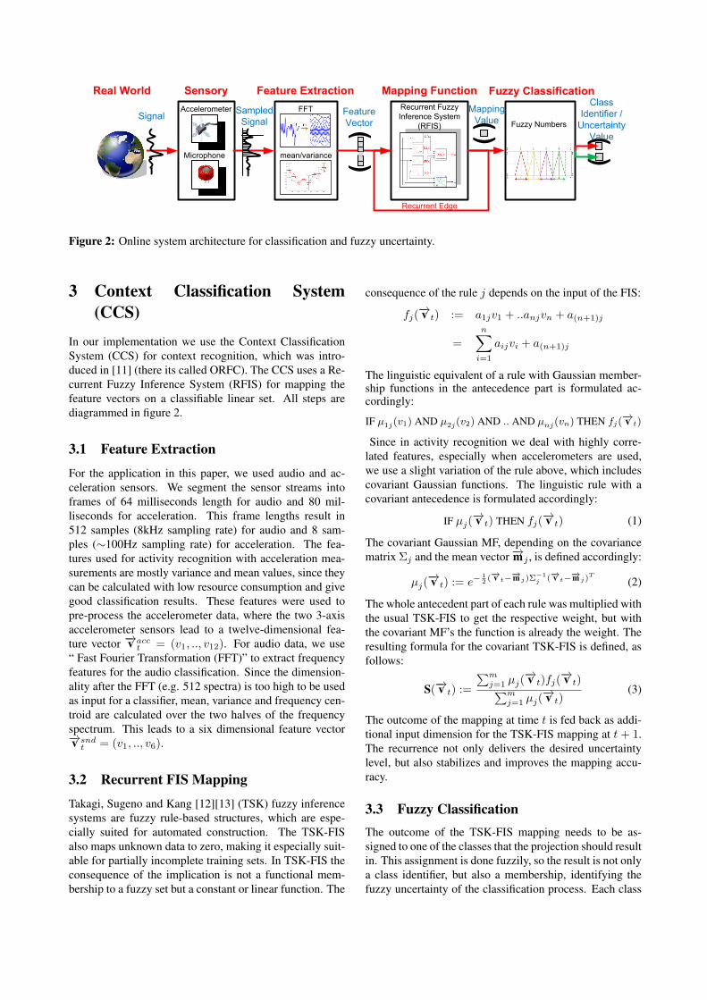
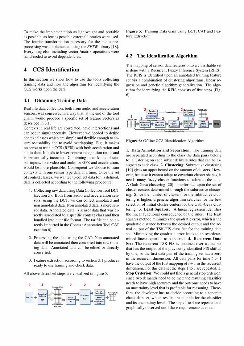
4.2 The Identification Algorithm

The mapping of sensor data features onto a classifiable setis done with a Recurrent Fuzzy Inference System (RFIS).The RFIS is identified upon an annotated training featureset via a combination of clustering algorithms, linear re-gression and genetic algorithm generalization. The algo-rithm for identifying the RFIS consists of five steps (Fig.6).

Gath-Geva

Clustering

Training Data

Check Data

Subtractive

Clustering

Genetic

Algorithm

Selection of best

combination of initial

cluster centresLeast

Squares

Regression

Calculation

of new dim.

on output

Calculation

of Fitness

(Q. Error)

Fitness Value

Output Vector

Stop

Criteria

Check

Repeat until stop criteria

RFIS

12 2

22

3 4 5

Figure 6: Offline CCS Identification Algorithm

1. Data Annotation and Separation: The training dataare separated according to the class the data pairs belongto. Clustering on each subset delivers rules that can be as-signed to each class. 2. Clustering: Subtractive clustering[19] gives an upper bound on the amount of clusters. How-ever, because it cannot adapt to covariant cluster shapes, itneeds many fuzzy cluster functions to adapt to the data.A Gath-Geva clustering [20] is performed upon the set ofcluster centers determined through the subtractive cluster-ing. Since the number of clusters for the subtractive clus-tering is higher, a genetic algorithm searches for the bestselection of initial cluster centers for the Gath-Geva clus-tering. 3. Least Squares: A linear regression identifiesthe linear functional consequence of the rules. The leastsquares method minimizes the quadratic error, which is thequadratic distance between the desired output and the ac-tual output of the TSK-FIS classifier for the training dataset. Minimizing the quadratic error leads to an overdeter-mined linear equation to be solved. 4. Recurrent DataSet: The recurrent TSK-FIS is obtained over a data setthat has the output of the previously identified FIS shiftedby one, so the first data pair of the training set has a zeroin the recurrent dimension. All data pairs for time t > 1have the output of the FIS mapping of t+1 in the recurrentdimension. For this data set the steps 1 to 3 are repeated. 5.Stop Criterion: We could not find a general stop criterion,since two demands need to be met: the resulting classifierneeds to have high accuracy and the outcome needs to havean uncertainty level that is profitable for reasoning. There-fore, the developer has to decide according to a separatecheck data set, which results are suitable for the classifierand its uncertainty levels. The steps 1 to 4 are repeated andgraphically observed until these requirements are met.

4.3 Implementation

The CCS identification algorithm is currently implementedin Matlab. The implementation consists of different scriptsfor the clustering, the linear regression and the genetic al-gorithm. In future we want to translate the Matlab scriptsinto python, so not only users with a Matlab license canuse the algorithm.

5 Data Collection Tool (DCT)

The Data Collection Tool is a simple Python applicationthat gathers audio and acceleration data on the Freerun-ner phone. Upon startup, it fires up two threads: The au-dio thread records audio samples of the required frequency(8000Hz) and saves them as an audio file on the disk (eitherin WAV- or, to conserve space, FLAC-format). The record-ing time of the audio sample is given in the filename toease the finding of previous recordings. The second threadreads acceleration data from the two acceleration sensorsof the phone and writes them with their correspondingtimestamp into a simple text file. The DCT also allowsthe user to associate contexts from a list of contexts to thegathered data. The user can whenever he wants changethe current context annotation. The resulting gathered dataand the the list of annotations is saved in the annotationpackage format, described in the following section 5.1.

5.1 Annotation Package Format

To provide easy data exchange between the tools that col-lect and manipulate context annotated sensor data, a newfile format (fig. 7) was designed. The idea is to couple theannotation data with the actual sensor data it relates to.An annotation package is a file that combines sensor datafrom multiple sources with annotation data. The outerlayer of the file is a tarball-archive. It always contains anindex file that specifies the content.

Figure 7: Annotation Package structure

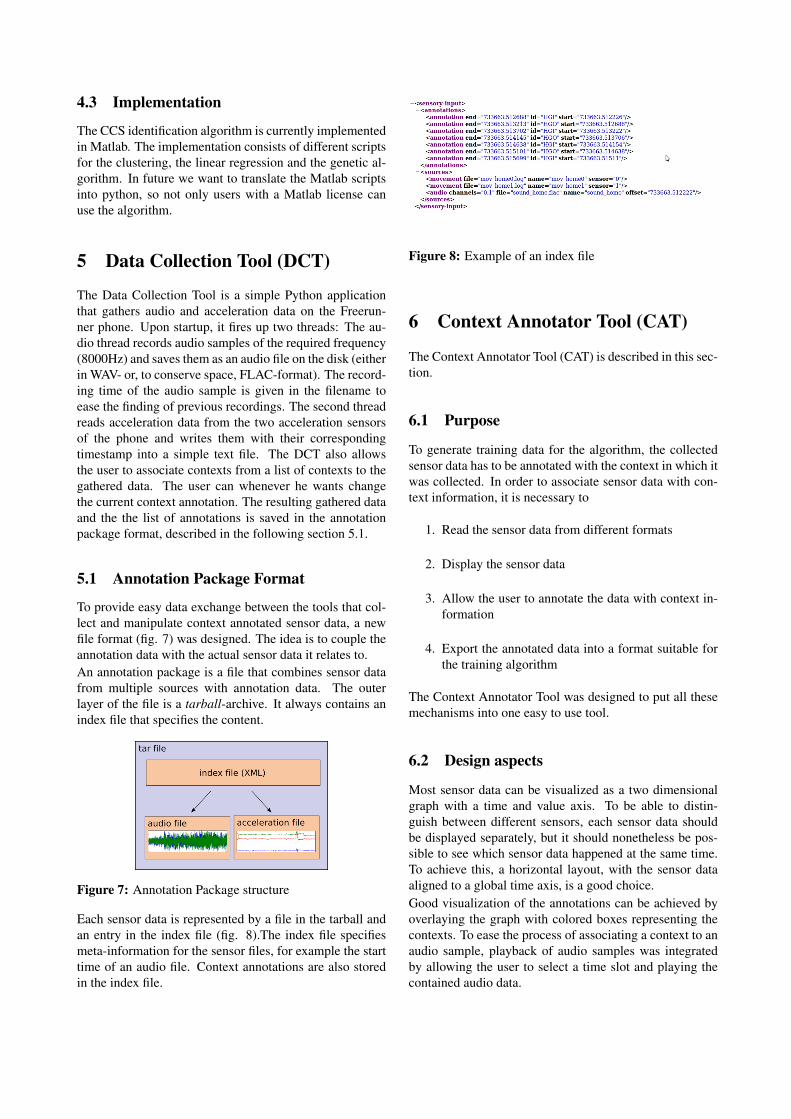
Each sensor data is represented by a file in the tarball andan entry in the index file (fig. 8).The index file specifiesmeta-information for the sensor files, for example the starttime of an audio file. Context annotations are also storedin the index file.

Figure 8: Example of an index file

6 Context Annotator Tool (CAT)

The Context Annotator Tool (CAT) is described in this sec-tion.

6.1 Purpose

To generate training data for the algorithm, the collectedsensor data has to be annotated with the context in which itwas collected. In order to associate sensor data with con-text information, it is necessary to

1. Read the sensor data from different formats

2. Display the sensor data

3. Allow the user to annotate the data with context in-formation

4. Export the annotated data into a format suitable forthe training algorithm

The Context Annotator Tool was designed to put all thesemechanisms into one easy to use tool.

6.2 Design aspects

Most sensor data can be visualized as a two dimensionalgraph with a time and value axis. To be able to distin-guish between different sensors, each sensor data shouldbe displayed separately, but it should nonetheless be pos-sible to see which sensor data happened at the same time.To achieve this, a horizontal layout, with the sensor dataaligned to a global time axis, is a good choice.Good visualization of the annotations can be achieved byoverlaying the graph with colored boxes representing thecontexts. To ease the process of associating a context to anaudio sample, playback of audio samples was integratedby allowing the user to select a time slot and playing thecontained audio data.

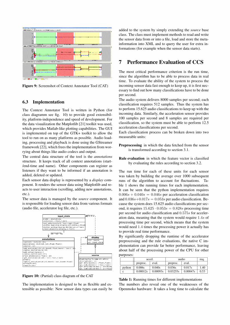
Figure 9: Screenshot of Context Annotator Tool (CAT)

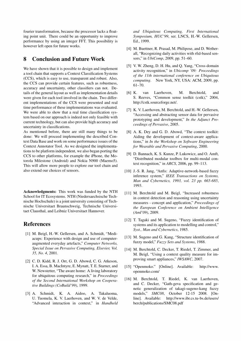
6.3 Implementation

The Context Annotator Tool is written in Python (forclass diagramm see fig. 10) to provide good extensibil-ity, platform-independence and speed of development. Forthe data visualization the Matplotlib [21] toolkit was used,which provides Matlab-like plotting capabilities. The GUIis implemented on top of the GTK+ toolkit to allow thetool to run on as many platforms as possible. Audio load-ing, processing and playback is done using the GStreamerframework [22], which frees the implementation from wor-rying about things like audio codecs and output.The central data structure of the tool is the annotationsstructure. It keeps track of all context annotations (start-/end-time and name). Other components can register aslisteners if they want to be informed if an annotation isadded, deleted or updated.Each sensor data display is represented by a display com-ponent. It renders the sensor data using Matplotlib and re-acts to user interaction (scrolling, adding new annotations,etc.).The sensor data is managed by the source component. Itis responsible for loading sensor data from various formats(audio file, accelerator log file, etc.).

Figure 10: (Partial) class diagram of the CAT

The implementation is designed to be as flexible and ex-tensible as possible: New sensor data types can easily be

added to the system by simply extending the source baseclass. The class must implement methods to read and writethe sensor data from or into a file, load and store the meta-information into XML and to query the user for extra in-formations (for example when the sensor data starts).

7 Performance Evaluation of CCS

The most critical performance criterion is the run time,since the algorithm has to be able to process data in realtime. To evaluate the ability of the system to process theincoming sensor data fast enough to keep up, it is first nec-essary to find out how many classifications have to be doneper second.The audio system delivers 8000 samples per second; eachclassification requires 512 samples. Thus the system hasto perform 15.625 audio classifications to keep up with theincoming data. Similarly, the acceleration sensor provides100 samples per second and 8 samples are required perclassification, so the system must be able to perform 12.5acceleration classifications per second.Each classification process can be broken down into twomeasurable units:

Preprocessing in which the data fetched from the sensoris transformed according to section 3.1.

Rule evaluation in which the feature vector is classifiedby evaluating the rules according to section 3.2.

The run time for each of these units for each sensorwas taken by building the average over 1000 subsequentruns of the algorithm to account for fluctuations. Ta-ble 1 shows the running times for each implementation.It can be seen that the python implementation requires0.006s + 0.040s = 0.046s per acceleration classificationand 0.036s+0.017s = 0.053s per audio classification. Be-cause the system does 15.625 audio classifications per sec-ond, it requires 15.625 · 0.053s = 0.828s processing timeper second for audio classification and 0.575s for acceler-ation data, meaning that the system would require 1.4s ofprocessing time per second, which means that the systemwould need 1.4 times the processing power it actually hasto provide real time performance.By significantly dropping the runtime of the acceleratorpreprocessing and the rule evaluations, the native C im-plementation can provide far better performance, leavingabout half of the processing power of the CPU for otherpurposes:

accel. audio req.preproc. eval. preproc. eval.

python 0.006s 0.040s 0.036s 0.017s 1.40c 0.00012s 0.00093s 0.03255s 0.00047s 0.53

Table 1: Running times for different implementationsThe numbers also reveal one of the weaknesses of theOpenmoko hardware: It takes a long time to calculate the

fourier transformation, because the processor lacks a float-ing point unit. There could be an opportunity to improveperformance by using an integer FFT. This possibility ishowever left open for future works.

8 Conclusion and Future WorkWe have shown that it is possible to design and implementa tool chain that supports a Context Classification Systems(CCS), which is easy to use, transparent and robust. Also,the CCS can provide certain features, such as robustness,accuracy and uncertainty, other classifiers can not. De-tails of the general layout as well as implementation detailswere given for each tool involved in the chain. Two differ-ent implementations of the CCS were presented and realtime performance of these implementations was evaluated.We were able to show that a real time classification sys-tem based on our approach is indeed not only feasible withcurrent technology, but can also provide high accuracy anduncertainty in classifications.As mentioned before, there are still many things to bedone: We will proceed implementing the described Con-text Data Base and work on some performance issues of theContext Annotator Tool. As we designed the implementa-tions to be platform independent, we also began porting theCCS to other platforms, for example the iPhone, the Mo-torola Milestone (Android) and Nokia N900 (Maemo5).This will allow more people to explore our tool chain andalso extend our choices of sensors.

Acknowledgments: This work was funded by the NTHSchool for IT Ecosystems. NTH (Niedersaechsische Tech-nische Hochschule) is a joint university consisting of Tech-nische Universitaet Braunschweig, Technische Universi-taet Clausthal, and Leibniz Universitaet Hannover.

References[1] M. Beigl, H.-W. Gellersen, and A. Schmidt, “Medi-

acups: Experience with design and use of computer-augmented everyday artefacts,” Computer Networks,Special Issue on Pervasive Computing, Elsevier, Vol.35, No. 4, 2001.

[2] C. D. Kidd, R. J. Orr, G. D. Abowd, C. G. Atkeson,I. A. Essa, B. MacIntyre, E. Mynatt, T. E. Starner, andW. Newstetter, “The aware home: A living laboratoryfor ubiquitous computing research,” in Proceedingsof the Second International Workshop on Coopera-tive Buildings (CoBuild’99), 1999.

[3] A. Schmidt, K. A. Aidoo, A. Takaluoma,U. Tuomela, K. V. Laerhoven, and W. V. de Velde,“Advanced interaction in context,” in Handheld

and Ubiquitous Computing, First InternationalSymposium, HUC’99, ser. LNCS, H.-W. Gellersen,Ed., 1999.

[4] M. Buettner, R. Prasad, M. Philipose, and D. Wether-all, “Recognizing daily activities with rfid-based sen-sors,” in UbiComp, 2009, pp. 51–60.

[5] V. W. Zheng, D. H. Hu, and Q. Yang, “Cross-domainactivity recognition,” in Ubicomp ’09: Proceedingsof the 11th international conference on Ubiquitouscomputing. New York, NY, USA: ACM, 2009, pp.61–70.

[6] K. van Laerhoven, M. Berchtold, andS. Reeves, “Common sense toolkit (cstk),” 2004,http://cstk.sourceforge.net/.

[7] K. V. Laerhoven, M. Berchtold, and H.-W. Gellersen,“Accessing and abstracting sensor data for pervasiveprototyping and development,” In the Adjunct Pro-ceedings of Pervasive, 2005.

[8] A. K. Dey and G. D. Abowd, “The context toolkit:Aiding the development of context-aware applica-tions,” in In the Workshop on Software Engineeringfor Wearable and Pervasive Computing, 2000.

[9] D. Bannach, K. S. Kunze, P. Lukowicz, and O. Amft,“Distributed modular toolbox for multi-modal con-text recognition,” in ARCS, 2006, pp. 99–113.

[10] J.-S. R. Jang, “Anfis: Adaptive-network-based fuzzyinference system,” IEEE Transactions on Systems,Man and Cybernetics, 1993, vol. 23 pp. 665-685,1993.

[11] M. Berchtold and M. Beigl, “Increased robustnessin context detection and reasoning using uncertaintymeasures - concept and application,” Proceedings ofthe European Conference on Ambient Intelligence(AmI’09), 2009.

[12] T. Tagaki and M. Sugeno, “Fuzzy identification ofsystems and its application to modelling and control,”Syst., Man and Cybernetics, 1985.

[13] M. Sugeno and G. Kang, “Structure identification offuzzy model,” Fuzzy Sets and Systems, 1988.

[14] M. Berchtold, C. Decker, T. Riedel, T. Zimmer, andM. Beigl, “Using a context quality measure for im-proving smart appliances,” IWSAWC, 2007.

[15] “Openmoko.” [Online]. Available: http://www.openmoko.com/

[16] M. Berchtold, T. Riedel, K. van Laerhoven,and C. Decker, “Gath-geva specification and ge-netic generalization of takagi-sugeno-kang fuzzymodels,” SMC08, October 12-15 2008. [On-line]. Available: http://www.ibr.cs.tu-bs.de/users/berch/publications/SMC08.pdf

[17] E. Jones, T. Oliphant, P. Peterson et al., “SciPy:Open source scientific tools for Python,” 2001–.[Online]. Available: http://www.scipy.org/

[18] M. Frigo and S. G. Johnson, “The fastest Fouriertransform in the West,” Massachusetts Institute ofTechnology, Tech. Rep. MIT-LCS-TR-728, Septem-ber 1997.

[19] S. Chiu, “Method and software for extracting fuzzyclassification rules by subtractive clustering,” IEEEControl Systems Magazine, pp. 461–465, 1996.

[20] I. Gath and A. B. Geva, “Unsupervised optimal fuzzyclustering,” IEEE Transactions on Pattern Analysisand Machine Intelligence, vol 11(7), pp 773-781,1989.

[21] J. D. Hunter, “Matplotlib: A 2d graphics envi-ronment,” Computing in Science and Engineering,vol. 9, pp. 90–95, 2007.

[22] “GStreamer – open source multimedia framework.”[Online]. Available: http://www.gstreamer.net/