Embed Size (px)
Citation preview
Adaptive Terrain Rendering using
DirectX 11 Shader Pipeline
Bachelor Thesis
Studiengang Medieninformatik Bachelor
Hochschule der Medien Stuttgart
Markus Rapp
Erstprüfer: Prof. Dr. Jens-Uwe Hahn
Zweitprüfer: Prof. Walter Kriha
Stuttgart, 4. April 2011
Adaptive Terrain Rendering using DirectX 11 Shader Pipeline Abstract
i
A b s t r a c t
This thesis is about the development of a terrain rendering algorithm that uses the
DirectX 11 shader pipeline for rendering and the ability of DirectX 11 to render a
view-dependent level of detail system. The basics of terrain rendering and level of detail
systems are described and previous work that has been done on the subject of adaptive
terrain rendering is discussed. In addition, an explanation of the DirectX 11 shader
pipeline is provided. This shows how the new shader stages of the pipeline are
integrated to support hardware tessellation. Accordingly the developed algorithm will
be described and its usefulness for terrain rendering will be explored. Finally the
difficulties of the development will be mentioned and the future work will be discussed.
Keywords: thesis, terrain, view-dependent level of detail, tessellation, DirectX 11,
refinement, adaptive, hull shader, tessellator, domain shader

Adaptive Terrain Rendering using DirectX 11 Shader Pipeline Declaration of originality
ii
D e c l a r a t i o n o f o r i g i n a l i t y
I hereby certify that I am the sole author of this thesis and that no part of this thesis has
been published or submitted for publication.
I certify that, to the best of my knowledge, my thesis does not infringe upon anyone’s
Copyright nor violate any proprietary rights and that any ideas, techniques, quotations,
or any other material from the work of other people included in my thesis, published or
otherwise, are fully acknowledged in accordance with the standard referencing
practices.
Markus Rapp, April 4, 2011

Adaptive Terrain Rendering using DirectX 11 Shader Pipeline Acknowledgements
iii
A c k n o w l e d g e m e n t s
I want to say thank you very much for all people that supported me while I was writing
this thesis. A special thanks goes to my brother Daniel Rapp who supported me at the
last weeks of my thesis and gave me good advices so I could finish my work in time.
Also thank you very much for Michael Steele and Brigitte Bauer for supporting me with
their English skills. I would also like to say thank you to my parents who supported me
financially over my whole study time and helped me a lot so I could focus on my thesis.
Finally I want to say thank you to all professors and employees of “Hochschule der
Medien Stuttgart” that taught me a lot at my studies. Without the knowledge I got from
the lectures, making this thesis would not have been possible.
Adaptive Terrain Rendering using DirectX 11 Shader Pipeline Contents
iv
C o n t e n t s
Abstract .............................................................................................................................. i
Declaration of originality ................................................................................................ ii
Acknowledgements .......................................................................................................... iii
Contents ........................................................................................................................... iv
List of Figures ................................................................................................................. vi
1. Introduction .................................................................................................................. 1
2. Basics ............................................................................................................................ 3
2.1. Coordinate System ........................................................................................................... 3
2.2. Terrain Structure ............................................................................................................. 3
2.2.1. Triangulated Irregular Networks ............................................................................................... 3
2.2.2. Regular Grid .............................................................................................................................. 4
2.2.3. Height Map ............................................................................................................................... 5
2.3. Level of Detail ................................................................................................................... 7
2.3.1. Discrete Level of Detail ............................................................................................................ 8
2.3.2. Continuous Level of Detail ....................................................................................................... 9
2.3.3. Distance-Dependent Level of Detail ....................................................................................... 11
2.3.4. View-Dependent Level of Detail ............................................................................................ 12
2.4. T-Junctions and Cracks ................................................................................................. 16
3. Previous Work ............................................................................................................ 17
3.1. ROAM ............................................................................................................................. 17
3.2. Smooth View-Dependent Level-of-Detail Control and its Application to Terrain
Rendering ............................................................................................................................... 21
3.3. Geometry Clipmaps ....................................................................................................... 26
4. DirectX 11 Shader Pipeline ....................................................................................... 31
4.1. Input Assembler ............................................................................................................. 34
4.2. Vertex Shader ................................................................................................................. 35
4.3. Hull Shader ..................................................................................................................... 36
4.4. Tessellator ....................................................................................................................... 37
4.5. Domain Shader ............................................................................................................... 40
4.6. Geometry Shader ........................................................................................................... 41
4.7. Pixel Shader .................................................................................................................... 42

Adaptive Terrain Rendering using DirectX 11 Shader Pipeline Contents
v
5. Terrain Rendering with DirectX 11 .......................................................................... 43
5.1. Architecture of Terrain Engine .................................................................................... 43
5.2. Implementation of View-Dependent Tessellation........................................................ 48
5.2.1. Grid Construction .................................................................................................................... 48
5.2.2. Normal calculation .................................................................................................................. 49
5.2.3. Density Map Creation ............................................................................................................. 50
5.2.4. Shader Pipeline ....................................................................................................................... 52
6. Conclusion .................................................................................................................. 58
6.1. Future Work ................................................................................................................... 59
References ...................................................................................................................... 62
Adaptive Terrain Rendering using DirectX 11 Shader Pipeline List of Figures
vi
L i s t o f F i g u r e s
Figure 2-1: Left-handed and right-handed Cartesian coordinate systems .................................................... 3
Figure 2-2: TIN representation [Gar95] ....................................................................................................... 4
Figure 2-3: Regular grid [Lue03] ................................................................................................................. 5
Figure 2-4: Gray scale height map with resolution 256 x 256 [AMD09] .................................................... 6
Figure 2-5: Color height map [Wig10] ........................................................................................................ 7
Figure 2-6: Different LODs of Stanford Bunny [Lue03] ............................................................................. 8
Figure 2-7: Different LODs of a quad [Lue03] ............................................................................................ 9
Figure 2-8: Shows edge collapse (ecol) and vertex split (vsplit) [Hop96] ................................................. 10
Figure 2-9: Progressive mesh [Hop96] ...................................................................................................... 10
Figure 2-10: Distance selection of Stanford Bunny LODs [Lue03] .......................................................... 11
Figure 2-11: Vertex hierarchy [Hop97] ..................................................................................................... 13
Figure 2-12: Shows modified edge collapse (ecol) and vertex split (vsplit) [Hop97] ............................... 14
Figure 2-13: Preconditions and effects of vertex split and edge collapse [Hop97] .................................... 14
Figure 2-14: Illustration of MA, M
B and M
G [Hop97] ................................................................................ 15
Figure 2-15: View-dependent refinement example of Stanford Bunny [Hop97] ....................................... 16
Figure 2-16: Shows cracks and t-junctions [Lue03] .................................................................................. 16
Figure 3-1: Levels 0-5 of triangle binary tree [Duc97] .............................................................................. 17
Figure 3-2: Split and merge operation [Duc97] ......................................................................................... 18
Figure 3-3: Forced split of triangle T [Duc97]........................................................................................... 19
Figure 3-4: Construction of nested wedgies [Duc97] ................................................................................ 20
Figure 3-5: Changes to active mesh during forward motion of viewer [Hop98] ....................................... 22
Figure 3-6: Shows geomorph refinement [Hop981] .................................................................................. 23
Figure 3-7: Accurate approximation error [Hop98] ................................................................................... 23
Figure 3-8: Hierarchical block-based simplification [Hop98] ................................................................... 24
Figure 3-9: Result of the hierarchical construction process [Hop98] ........................................................ 25
Figure 3-10: Mesh with an average error of 2.1 pixels, which has 6.096 vertices [Hop98] ...................... 25
Figure 3-11: How geometry clip maps work [Asi05] ................................................................................ 26
Figure 3-12: Terrain rendering using a coarse geometry clipmap [Asi05] ................................................ 27
Figure 3-13: Terrain rendering using a geometry clipmap with transition regions [Asi05] ....................... 28
Figure 3-14: Illustration of triangle strip generation within a renderer region. [Los041] .......................... 29
Adaptive Terrain Rendering using DirectX 11 Shader Pipeline List of Figures
vii
Figure 4-1: Authoring pipeline of the past [NiT09] ................................................................................... 31
Figure 4-2: Real-time tessellation rendering [NiT09] ................................................................................ 32
Figure 4-3: Shader pipeline DirectX 11 ................................................................................................... 33
Figure 4-4: Input assembler ....................................................................................................................... 34
Figure 4-5: Vertex shader .......................................................................................................................... 35
Figure 4-6: Hull shader .............................................................................................................................. 36
Figure 4-7: Tessellator ............................................................................................................................... 37
Figure 4-8: Tessellation of a quad with tessellation factor 2.5 ................................................................. 38
Figure 4-9: Quads with different tessellation factors ................................................................................ 39
Figure 4-10: Domain shader ...................................................................................................................... 40
Figure 4-11: Geometry shader ................................................................................................................... 41
Figure 4-12: Pixel shader ........................................................................................................................... 42
Figure 5-1: Class diagram of terrain engine .............................................................................................. 43
Figure 5-2: Class diagram of CSystem ..................................................................................................... 43
Figure 5-3: Class diagram of CRenderer .................................................................................................. 45
Figure 5-4: Class diagram of CRenderable ............................................................................................... 46
Figure 5-5: How to create two triangles out of one quad ........................................................................... 49
Figure 5-6: Normal calculation .................................................................................................................. 49
Figure 5-7: Pixel selection and variation calculation for density map creation ......................................... 50
Figure 5-8: Calculation of variation .......................................................................................................... 51
Figure 5-9: Input and output of vertex shader ........................................................................................... 52
Figure 5-10: Vertex shader ....................................................................................................................... 52
Figure 5-11: Hull shader constant data, hull shader main function output and hull shader main function 53
Figure 5-12: Phong tessellation principle [Bou08] .................................................................................... 54
Figure 5-13: Domain shader ..................................................................................................................... 55
Figure 5-14: Terrain without tessellation ................................................................................................... 57
Figure 5-15: Terrain with tessellation ........................................................................................................ 57
Figure 6-1: Frame rate comparison with 256-to-256 height map (frame rate [rendered triangles]) .......... 58
Figure 6-2: Crack in terrain........................................................................................................................ 59
Adaptive Terrain Rendering using DirectX 11 Shader Pipeline 1. Introduction
1
1 . I n t r o d u c t i o n
Terrain rendering has a wide application area. It has been used for virtual tourism,
education in subjects such as geography, for weather visualization, and to calculate the
most efficient positioning of radio, TV or cellular transmitter. Large companies such as
Google use terrain rendering for products like Google Earth.
Especially in the video games industry terrain rendering plays a big role as main
geometry for outdoor scenes. Open world games like Grand Theft Auto 4 or Mafia 2
were not be possible without a good terrain system. Also, for first person shooters
terrain is the main geometry for outdoor scenes. Game engines like Unreal Engine 3 and
Cry Engine 3 have their own terrain systems. Racing games use terrains for making the
tracks. Even dynamic terrain was used in games. One example is Sega Rally Revo
which was released in 2007 for PC, Xbox 360 and PS3. It uses a deformable terrain
system, which changes the course each lap. 1
What qualities and capabilities do we look for in a terrain renderer? A perfect terrain
would be a single continuous mesh from the foreground to the horizon with no cracks or
holes. A perfect terrain renderer would allow us to see a wide area over a large range of
detail. We want to walk on the terrain or fly over the terrain in real-time. To achieve
these requirements a rendering terrain algorithm has to be developed that has the ability
to blend out detail that is not seen or distant. This is done to save computing resources
to be able to show as much detail near the viewport as possible.
The first terrain renderer had a static geometry. Because of lack of these algorithms to
adapt geometry dependent on changing scene conditions it has always been necessary to
find a balance between small terrain with large detail and large terrain with less detail.
Since the 90’s a lot of research has been done about terrain rendering that supported a
greater level of detail (LOD). The main focus on development of these algorithms has
been to render a terrain in real-time that is as large as possible and has as much close up
detail as possible. 2
The first rendering algorithms that tried to achieve this target were CPU bound. The
final geometry was calculated on the CPU and send to the GPU for rendering. The GPU
only got the final data, which it had to render.
With the rapid development of graphics hardware the algorithms moved increasingly to
GPU. Therefore the algorithms had to be adapted to the specialized hardware to be
massively parallel.
1 cf. http://www.gametrailers.com/video/preview-hd-sega-rally/26005 (accessed March 2011)
2 cf. [Vir10], http://www.vterrain.org/LOD/Papers/ (accessed March 2011)
Adaptive Terrain Rendering using DirectX 11 Shader Pipeline 1. Introduction
2
In 2005 ATI was the first company to integrate a hardware tessellator in their graphics
cards. With this tessellator it has been possible to refine the geometry entirely on the
GPU. ATI published a Tessellation SDK which made it possible to use the tessellator
together with DirectX9. 3
Two years later Microsoft released DirectX10 with Shader Model 4.0 which included
the new geometry shader. This made geometry refinement possible on all GPUs that
support DirectX 10.
The big break-through of hardware tessellation came with the introduction of
DirectX 11, which Microsoft released together with Windows 7 in 2009. DirectX 11
sets a standard for hardware tessellation with the new hull shader, tessellator and
domain shader. With this development, NVIDIA also decided to develop graphics cards
that are capable of tessellation.
The goal of this thesis is to develop a view-dependent LOD system. The main focus is
to develop a LOD system that is not visible for the user. It should show as much detail
as possible. Additionally an adaption of the detail should be possible in order that faster
hardware will show more detail than slower hardware. At the same time, the
development of the program should allow backward compatibility to older approaches.
This backward compatibility allows the use of old data. Terrain can also be rendered on
graphics cards that do not have a hardware tessellator integrated. The amount of visual
quality would be reduced, but the application could still run on older hardware.
In the end result it should also be possible to use a collision detection system or a
physics engine for the terrain. This would make it possible to walk over the terrain. All
this should be accomplished in real-time. For a fluid application it is important to have
at least 60 frames per second. In most applications terrain is only the base geometry.
Thus it would be better when a higher frame rate than 60 frames per seconds would be
achieved. Finally it should be developed a terrain editor that gives artists the ability to
model a terrain that uses the developed terrain rendering algorithm.
These goals will be attempted using the DirectX 11 shader pipeline with Shader Model
5.0. The hardware that is used for development is an AMD Radeon HD 6870.
The second chapter of the thesis will describe the basics of terrain rendering and level of
detail systems. In section 3 previous approaches to the topic will be discussed. The
following section is about the DirectX11 shader pipeline. Shader stages will be
explained. Section 5 will be shown the new developed tessellation terrain rendering
system. The final section will deal with the results of the new rendering system and
possible work for the future.
3 cf. http://developer.amd.com/gpu/radeon/Tessellation/Pages/default.aspx (accessed March 2011)
Adaptive Terrain Rendering using DirectX 11 Shader Pipeline 2. Basics
3
2 . B a s i c s
In this section you’ll find some basic terms and definitions about terrain rendering.
Additionally you’ll read what exactly a LOD system is and which types of LODs exist.
2.1. Coordinate System
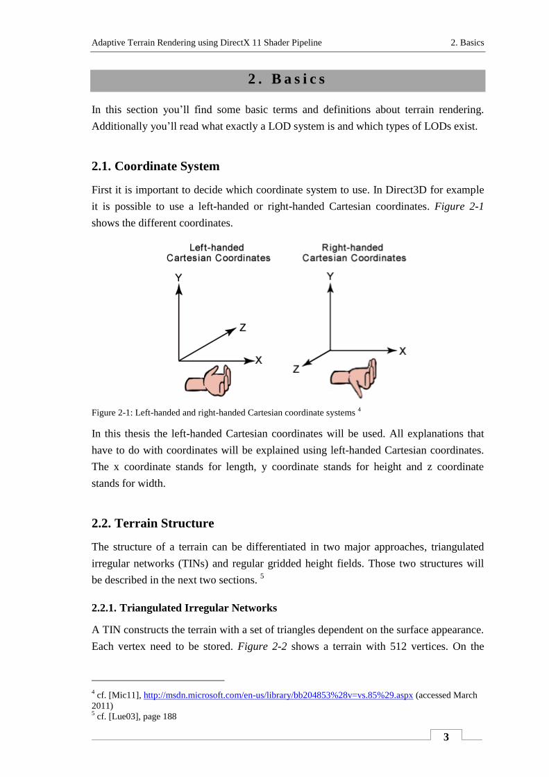
First it is important to decide which coordinate system to use. In Direct3D for example
it is possible to use a left-handed or right-handed Cartesian coordinates. Figure 2-1
shows the different coordinates.
Figure 2-1: Left-handed and right-handed Cartesian coordinate systems
4
In this thesis the left-handed Cartesian coordinates will be used. All explanations that
have to do with coordinates will be explained using left-handed Cartesian coordinates.
The x coordinate stands for length, y coordinate stands for height and z coordinate
stands for width.
2.2. Terrain Structure
The structure of a terrain can be differentiated in two major approaches, triangulated
irregular networks (TINs) and regular gridded height fields. Those two structures will
be described in the next two sections. 5
2.2.1. Triangulated Irregular Networks
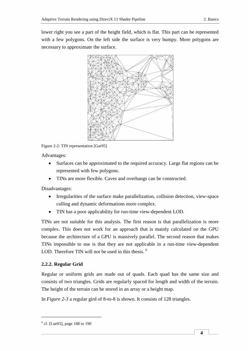
A TIN constructs the terrain with a set of triangles dependent on the surface appearance.
Each vertex need to be stored. Figure 2-2 shows a terrain with 512 vertices. On the
4 cf. [Mic11], http://msdn.microsoft.com/en-us/library/bb204853%28v=vs.85%29.aspx (accessed March
2011) 5 cf. [Lue03], page 188
Adaptive Terrain Rendering using DirectX 11 Shader Pipeline 2. Basics
4
lower right you see a part of the height field, which is flat. This part can be represented
with a few polygons. On the left side the surface is very bumpy. More polygons are
necessary to approximate the surface.
Figure 2-2: TIN representation [Gar95]
Advantages:
Surfaces can be approximated to the required accuracy. Large flat regions can be
represented with few polygons.
TINs are more flexible. Caves and overhangs can be constructed.
Disadvantages:
Irregularities of the surface make parallelization, collision detection, view-space
culling and dynamic deformations more complex.
TIN has a poor applicability for run-time view-dependent LOD.
TINs are not suitable for this analysis. The first reason is that parallelization is more
complex. This does not work for an approach that is mainly calculated on the GPU
because the architecture of a GPU is massively parallel. The second reason that makes
TINs impossible to use is that they are not applicable in a run-time view-dependent
LOD. Therefore TIN will not be used in this thesis. 6
2.2.2. Regular Grid
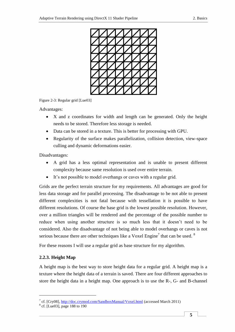
Regular or uniform grids are made out of quads. Each quad has the same size and
consists of two triangles. Grids are regularly spaced for length and width of the terrain.
The height of the terrain can be stored in an array or a height map.
In Figure 2-3 a regular gird of 8-to-8 is shown. It consists of 128 triangles.
6 cf. [Lue03], page 188 to 190
Adaptive Terrain Rendering using DirectX 11 Shader Pipeline 2. Basics
5
Figure 2-3: Regular grid [Lue03]
Advantages:
X and z coordinates for width and length can be generated. Only the height
needs to be stored. Therefore less storage is needed.
Data can be stored in a texture. This is better for processing with GPU.
Regularity of the surface makes parallelization, collision detection, view-space
culling and dynamic deformations easier.
Disadvantages:
A grid has a less optimal representation and is unable to present different
complexity because same resolution is used over entire terrain.
It’s not possible to model overhangs or caves with a regular grid.
Grids are the perfect terrain structure for my requirements. All advantages are good for
less data storage and for parallel processing. The disadvantage to be not able to present
different complexities is not fatal because with tessellation it is possible to have
different resolutions. Of course the base grid is the lowest possible resolution. However,
over a million triangles will be rendered and the percentage of the possible number to
reduce when using another structure is so much less that it doesn’t need to be
considered. Also the disadvantage of not being able to model overhangs or caves is not
serious because there are other techniques like a Voxel Engine7 that can be used.
8
For these reasons I will use a regular grid as base structure for my algorithm.
2.2.3. Height Map
A height map is the best way to store height data for a regular grid. A height map is a
texture where the height data of a terrain is saved. There are four different approaches to
store the height data in a height map. One approach is to use the R-, G- and B-channel
7 cf. [Cry08], http://doc.crymod.com/SandboxManual/Voxel.html (accessed March 2011)
8 cf. [Lue03], page 188 to 190
Adaptive Terrain Rendering using DirectX 11 Shader Pipeline 2. Basics
6
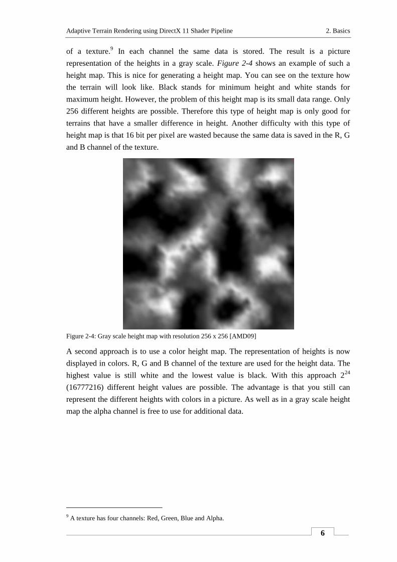
of a texture.9 In each channel the same data is stored. The result is a picture
representation of the heights in a gray scale. Figure 2-4 shows an example of such a
height map. This is nice for generating a height map. You can see on the texture how
the terrain will look like. Black stands for minimum height and white stands for
maximum height. However, the problem of this height map is its small data range. Only
256 different heights are possible. Therefore this type of height map is only good for
terrains that have a smaller difference in height. Another difficulty with this type of
height map is that 16 bit per pixel are wasted because the same data is saved in the R, G
and B channel of the texture.
Figure 2-4: Gray scale height map with resolution 256 x 256 [AMD09]
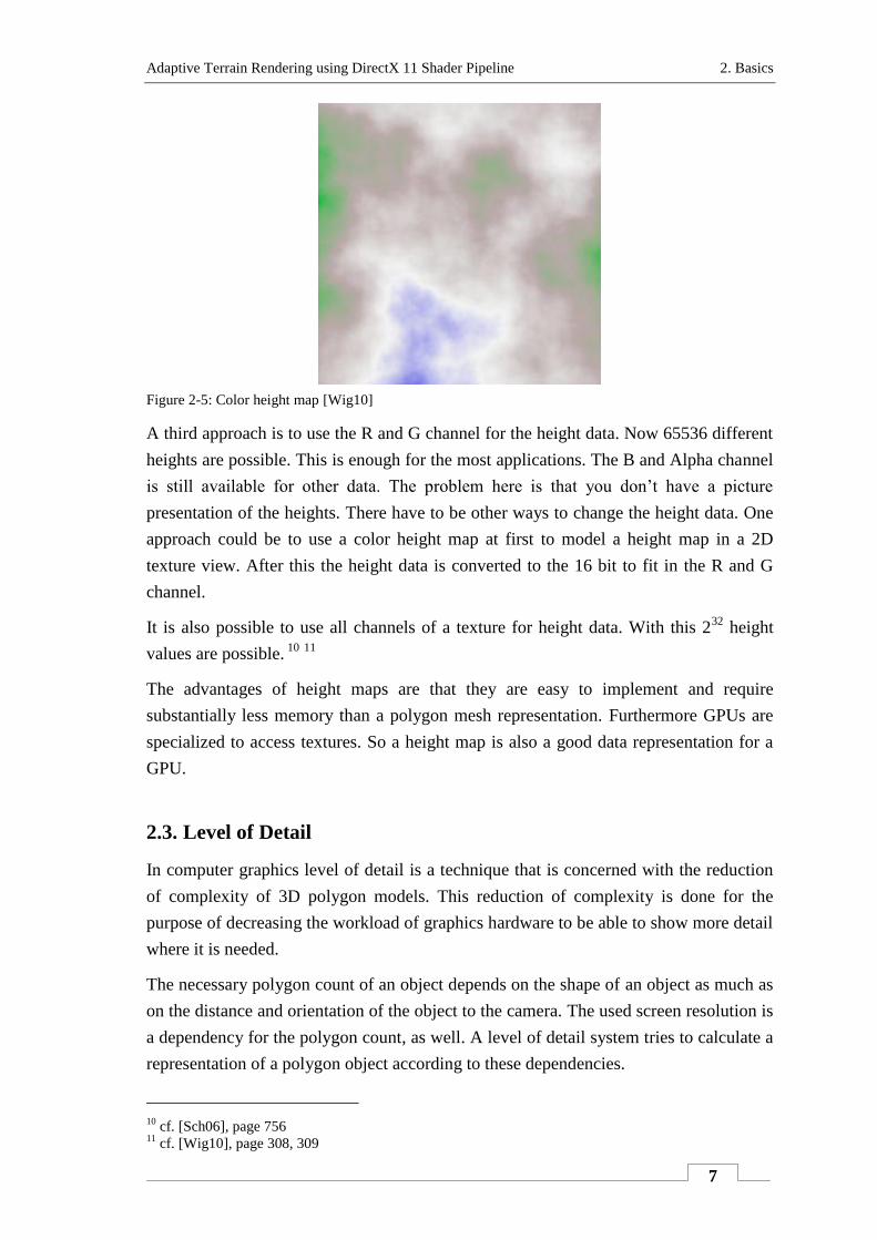
A second approach is to use a color height map. The representation of heights is now
displayed in colors. R, G and B channel of the texture are used for the height data. The
highest value is still white and the lowest value is black. With this approach 224
(16777216) different height values are possible. The advantage is that you still can
represent the different heights with colors in a picture. As well as in a gray scale height
map the alpha channel is free to use for additional data.
9 A texture has four channels: Red, Green, Blue and Alpha.
Adaptive Terrain Rendering using DirectX 11 Shader Pipeline 2. Basics
7
Figure 2-5: Color height map [Wig10]
A third approach is to use the R and G channel for the height data. Now 65536 different
heights are possible. This is enough for the most applications. The B and Alpha channel
is still available for other data. The problem here is that you don’t have a picture
presentation of the heights. There have to be other ways to change the height data. One
approach could be to use a color height map at first to model a height map in a 2D
texture view. After this the height data is converted to the 16 bit to fit in the R and G
channel.
It is also possible to use all channels of a texture for height data. With this 232
height
values are possible. 10
11
The advantages of height maps are that they are easy to implement and require
substantially less memory than a polygon mesh representation. Furthermore GPUs are
specialized to access textures. So a height map is also a good data representation for a
GPU.
2.3. Level of Detail
In computer graphics level of detail is a technique that is concerned with the reduction
of complexity of 3D polygon models. This reduction of complexity is done for the
purpose of decreasing the workload of graphics hardware to be able to show more detail
where it is needed.
The necessary polygon count of an object depends on the shape of an object as much as
on the distance and orientation of the object to the camera. The used screen resolution is
a dependency for the polygon count, as well. A level of detail system tries to calculate a
representation of a polygon object according to these dependencies.
10
cf. [Sch06], page 756 11
cf. [Wig10], page 308, 309
Adaptive Terrain Rendering using DirectX 11 Shader Pipeline 2. Basics
8
There are several different approaches of level of detail systems.
2.3.1. Discrete Level of Detail
Discrete LOD is a scheme where several discrete models with fewer triangles are
calculated or modeled for a complex model. The different models are precomputed
offline and can then be used inside the application when they are needed. At run-time
the application chooses which representation of the model is best suited to the scene
conditions and should be rendered.
Discrete LOD is also called view-independent LOD. When the LODs are computed it
can’t be predicted in which direction the camera shows.
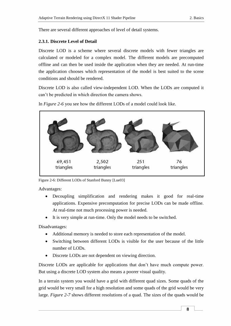
In Figure 2-6 you see how the different LODs of a model could look like.
Figure 2-6: Different LODs of Stanford Bunny [Lue03]
Advantages:
Decoupling simplification and rendering makes it good for real-time
applications. Expensive precomputation for precise LODs can be made offline.
At real-time not much processing power is needed.
It is very simple at run-time. Only the model needs to be switched.
Disadvantages:
Additional memory is needed to store each representation of the model.
Switching between different LODs is visible for the user because of the little
number of LODs.
Discrete LODs are not dependent on viewing direction.
Discrete LODs are applicable for applications that don’t have much compute power.
But using a discrete LOD system also means a poorer visual quality.
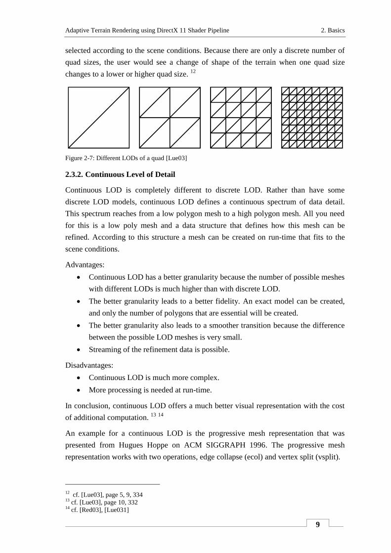
In a terrain system you would have a grid with different quad sizes. Some quads of the
grid would be very small for a high resolution and some quads of the grid would be very
large. Figure 2-7 shows different resolutions of a quad. The sizes of the quads would be
Adaptive Terrain Rendering using DirectX 11 Shader Pipeline 2. Basics
9
selected according to the scene conditions. Because there are only a discrete number of
quad sizes, the user would see a change of shape of the terrain when one quad size
changes to a lower or higher quad size. 12
Figure 2-7: Different LODs of a quad [Lue03]
2.3.2. Continuous Level of Detail
Continuous LOD is completely different to discrete LOD. Rather than have some
discrete LOD models, continuous LOD defines a continuous spectrum of data detail.
This spectrum reaches from a low polygon mesh to a high polygon mesh. All you need
for this is a low poly mesh and a data structure that defines how this mesh can be
refined. According to this structure a mesh can be created on run-time that fits to the
scene conditions.
Advantages:
Continuous LOD has a better granularity because the number of possible meshes
with different LODs is much higher than with discrete LOD.
The better granularity leads to a better fidelity. An exact model can be created,
and only the number of polygons that are essential will be created.
The better granularity also leads to a smoother transition because the difference
between the possible LOD meshes is very small.
Streaming of the refinement data is possible.
Disadvantages:
Continuous LOD is much more complex.
More processing is needed at run-time.
In conclusion, continuous LOD offers a much better visual representation with the cost
of additional computation. 13
14
An example for a continuous LOD is the progressive mesh representation that was
presented from Hugues Hoppe on ACM SIGGRAPH 1996. The progressive mesh
representation works with two operations, edge collapse (ecol) and vertex split (vsplit).
12
cf. [Lue03], page 5, 9, 334 13
cf. [Lue03], page 10, 332 14
cf. [Red03], [Lue031]
Adaptive Terrain Rendering using DirectX 11 Shader Pipeline 2. Basics
10
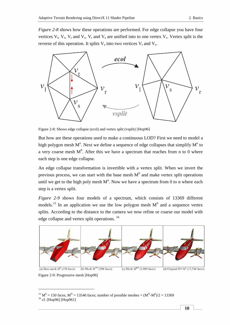
Figure 2-8 shows how these operations are performed. For edge collapse you have four
vertices Vl, Vr, Vt and Vs. Vt and Vs are unified into to one vertex Vs. Vertex split is the
reverse of this operation. It splits Vs into two vertices Vt and Vs.
Figure 2-8: Shows edge collapse (ecol) and vertex split (vsplit) [Hop96]
But how are these operations used to make a continuous LOD? First we need to model a
high polygon mesh Mn. Next we define a sequence of edge collapses that simplify M
n to
a very coarse mesh M0. After this we have a spectrum that reaches from n to 0 where
each step is one edge collapse.
An edge collapse transformation is invertible with a vertex split. When we invert the
previous process, we can start with the base mesh M0 and make vertex split operations
until we get to the high poly mesh Mn. Now we have a spectrum from 0 to n where each
step is a vertex split.
Figure 2-9 shows four models of a spectrum, which consists of 13369 different
models.15
In an application we use the low polygon mesh M0 and a sequence vertex
splits. According to the distance to the camera we now refine or coarse our model with
edge collapse and vertex split operations. 16
Figure 2-9: Progressive mesh [Hop96]
15
M0 = 150 faces, M
N = 13546 faces; number of possible meshes = (M
N-M
0)/2 = 13369
16 cf. [Hop96] [Hop961]
Adaptive Terrain Rendering using DirectX 11 Shader Pipeline 2. Basics
11
Progressive meshes alone are not applicable for a terrain system. Because we have only
one refinement sequence, the terrain only can be refined at one part of its surface. One
sequence is enough for a small mesh but for a big terrain it is insufficient.
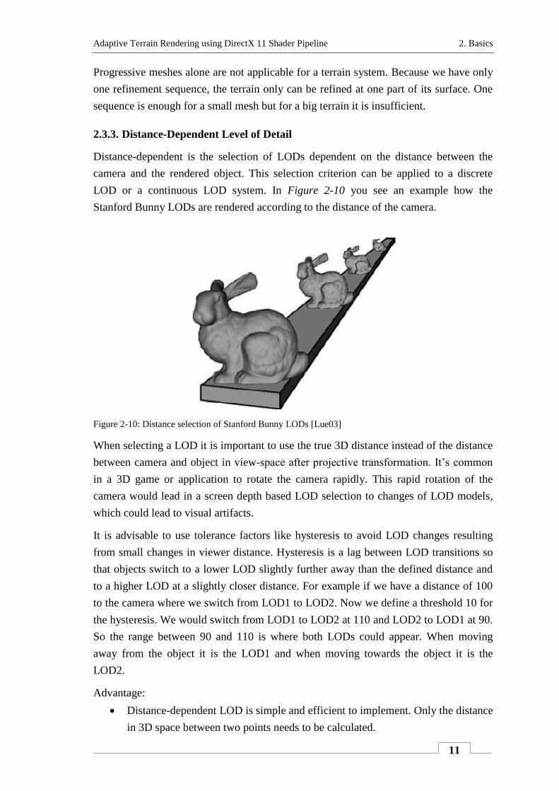
2.3.3. Distance-Dependent Level of Detail
Distance-dependent is the selection of LODs dependent on the distance between the
camera and the rendered object. This selection criterion can be applied to a discrete
LOD or a continuous LOD system. In Figure 2-10 you see an example how the
Stanford Bunny LODs are rendered according to the distance of the camera.
Figure 2-10: Distance selection of Stanford Bunny LODs [Lue03]
When selecting a LOD it is important to use the true 3D distance instead of the distance
between camera and object in view-space after projective transformation. It’s common
in a 3D game or application to rotate the camera rapidly. This rapid rotation of the
camera would lead in a screen depth based LOD selection to changes of LOD models,
which could lead to visual artifacts.
It is advisable to use tolerance factors like hysteresis to avoid LOD changes resulting
from small changes in viewer distance. Hysteresis is a lag between LOD transitions so
that objects switch to a lower LOD slightly further away than the defined distance and
to a higher LOD at a slightly closer distance. For example if we have a distance of 100
to the camera where we switch from LOD1 to LOD2. Now we define a threshold 10 for
the hysteresis. We would switch from LOD1 to LOD2 at 110 and LOD2 to LOD1 at 90.
So the range between 90 and 110 is where both LODs could appear. When moving
away from the object it is the LOD1 and when moving towards the object it is the
LOD2.
Advantage:
Distance-dependent LOD is simple and efficient to implement. Only the distance
in 3D space between two points needs to be calculated.
Adaptive Terrain Rendering using DirectX 11 Shader Pipeline 2. Basics
12
Disadvantages:
Only using the distance for LOD selection is inaccurate because shape or
orientation of the mesh to the camera are not considered.
View-distance conditions can change when scaling a mesh or using different
display resolutions.
In conclusion, distance-dependent LOD is the best selection for discrete LOD and
continuous LOD because the different LODs of the schemes only depend on the
distance to the camera. 17
In section 3.3 a terrain rendering approach is described that uses distance-dependent
LOD for its LOD selection.
2.3.4. View-Dependent Level of Detail
View-dependent LOD is an extension of continuous LOD. The selection of LOD is
done with view-dependent selection criteria such as screen resolution, orientation of the
camera and shape of a polygon mesh. Meshes that are near to the camera have a higher
detail than meshes that are far away.
The human visual system is sensitive to edges. Therefore a view-dependent LOD
system also provides to have a higher detail on silhouette regions and less detail on the
interior regions of a mesh.
One major problem of continuous LOD is that either we have a very detailed mesh or a
very coarse mesh. A view-dependent LOD provides the ability to have a mesh that on
the one hand has very detailed parts like silhouette of the mesh or parts that are really
near to the camera. On the other hand the same mesh could also have some regions of
the mesh that are not that detailed. These parts are in the interior region of the mesh or
parts that are not that close to the camera. There are also some parts of the mesh that are
not seen from the user such as faces oriented to the rear or parts that are outside the
view frustum. These parts that are not seen should not be rendered.
Advantages:
A view-dependent LOD system provides even better granularity than a
continuous LOD system. The outcome of the better granularity is a higher
fidelity. As a result polygons are allocated exactly where they are needed.
View-dependent LOD provides smoother transition between LODs. This leads
to a reduction of popping effects18
that plague discrete LOD.
Drastic simplification of very large objects is possible.
17
cf. [Lue03], page 88-90, 93-94, 180 18
Popping effect is the noticeable flicker that can occur when the graphics system switches between
different LODS. cf. [Lue03], page 342
Adaptive Terrain Rendering using DirectX 11 Shader Pipeline 2. Basics
13
Disadvantage:
Relatively high computational cost at run-time.
View-dependent LOD seems to be the perfect approach to have the best visual quality
with fewest polygons. The only problem is the high computational cost at run-time that
comes with view-dependent LOD. 19
20
An example for a view-dependent LOD is “View-Dependent Refinement of Progressive
Meshes”. This is a further development of progressive meshes and was developed by
Hugues Hoppe. With this approach different LODs can coexist on one mesh. Regions
that are outside the view frustum, distant or facing away from the camera are coarsened.
With progressive meshes vertex split and edge collapse operations are only possible in a
defined sequence. Therefore it is not possible with this technique to have different
LODs on one mesh. To define different LODs on one mesh we need to be able to make
vertex split and edge collapse operations on several parts of the mesh. The first thing we
need to be aware of is that a vertex split transformation defines a parent-child
relationship between the vertex Vs that gets split and the new created vertices Vt and Vu.
This parent-child relation can be applied to a binary tree.
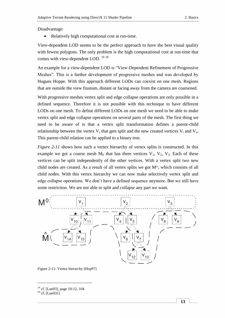
Figure 2-11 shows how such a vertex hierarchy of vertex splits is constructed. In this
example we got a coarse mesh M0 that has three vertices V1, V2, V3. Each of these
vertices can be split independently of the other vertices. With a vertex split two new
child nodes are created. As a result of all vertex splits we got M^, which consists of all
child nodes. With this vertex hierarchy we can now make selectively vertex split and
edge collapse operations. We don’t have a defined sequence anymore. But we still have
some restriction. We are not able to split and collapse any part we want.
Figure 2-11: Vertex hierarchy [Hop97]
19
cf. [Lue03], page 10-12, 104 20
cf. [Lue031]
Adaptive Terrain Rendering using DirectX 11 Shader Pipeline 2. Basics
14
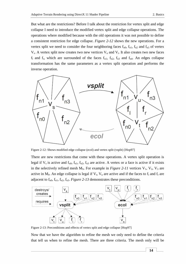
But what are the restrictions? Before I talk about the restriction for vertex split and edge
collapse I need to introduce the modified vertex split and edge collapse operations. The
operations where modified because with the old operations it was not possible to define
a consistent restriction for edge collapse. Figure 2-12 shows the new operations. For a
vertex split we need to consider the four neighboring faces fn0, fn1, fn2 and fn3 of vertex
Vs. A vertex split now creates two new vertices Vu and Vt. It also creates two new faces
fl and fr, which are surrounded of the faces fn1, fn2, fn3 and fn4. An edges collapse
transformation has the same parameters as a vertex split operation and performs the
inverse operation.
Figure 2-12: Shows modified edge collapse (ecol) and vertex split (vsplit) [Hop97]
There are new restrictions that come with these operations. A vertex split operation is
legal if Vs is active and fn0, fn1, fn2, fn3 are active. A vertex or a face is active if it exists
in the selectively refined mesh MS. For example in Figure 2-11 vertices V1, V2, V3 are
active in M0. An edge collapse is legal if Vt, Vu are active and if the faces to fi and fr are
adjacent to fn0, fn1, fn2, fn3. Figure 2-13 demonstrates these preconditions.
Figure 2-13: Preconditions and effects of vertex split and edge collapse [Hop97]
Now that we have the algorithm to refine the mesh we only need to define the criteria
that tell us when to refine the mesh. There are three criteria. The mesh only will be
Adaptive Terrain Rendering using DirectX 11 Shader Pipeline 2. Basics
15
refined if the surface is inside the view frustum, faces the viewer or if screen-space
geometric error exceeds screen-space tolerance τ. The screen-space tolerance can be
adapted according to refinement level that wants to be achieved. A byproduct of the
screen-space geometric error is that the refinement is denser near the silhouettes and the
mesh is coarser the farther it is from the viewpoint.
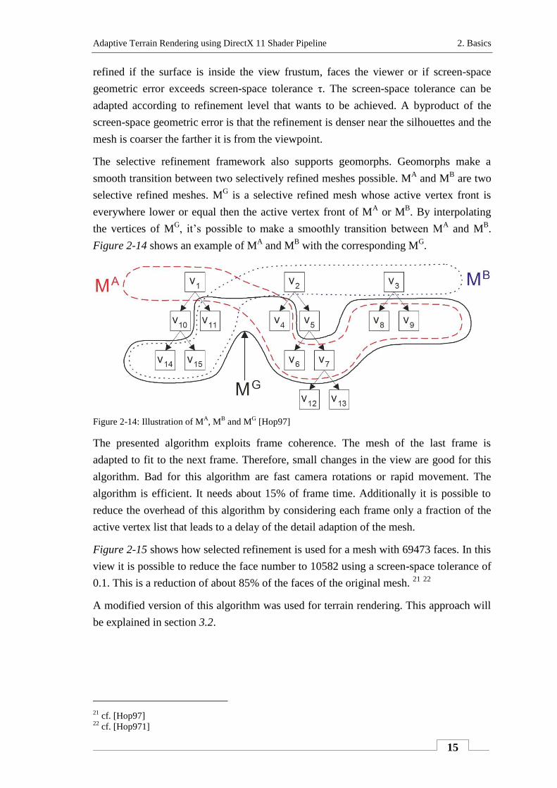
The selective refinement framework also supports geomorphs. Geomorphs make a
smooth transition between two selectively refined meshes possible. MA and M
B are two
selective refined meshes. MG is a selective refined mesh whose active vertex front is
everywhere lower or equal then the active vertex front of MA or M
B. By interpolating
the vertices of MG, it’s possible to make a smoothly transition between M
A and M
B.
Figure 2-14 shows an example of MA and M
B with the corresponding M
G.
Figure 2-14: Illustration of M
A, M
B and M
G [Hop97]
The presented algorithm exploits frame coherence. The mesh of the last frame is
adapted to fit to the next frame. Therefore, small changes in the view are good for this
algorithm. Bad for this algorithm are fast camera rotations or rapid movement. The
algorithm is efficient. It needs about 15% of frame time. Additionally it is possible to
reduce the overhead of this algorithm by considering each frame only a fraction of the
active vertex list that leads to a delay of the detail adaption of the mesh.
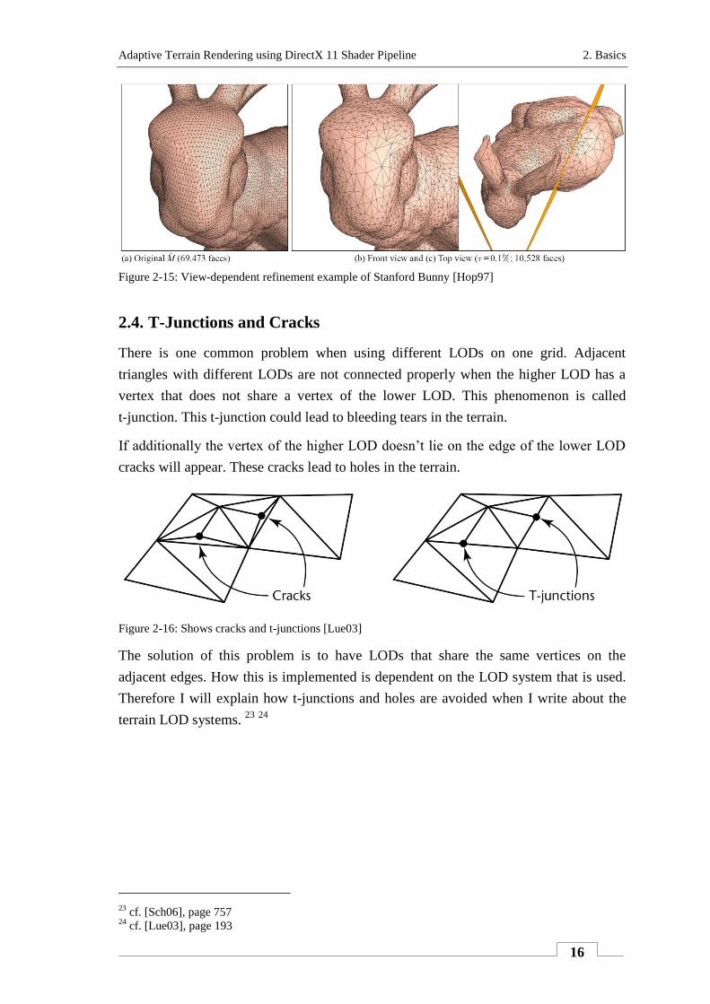
Figure 2-15 shows how selected refinement is used for a mesh with 69473 faces. In this
view it is possible to reduce the face number to 10582 using a screen-space tolerance of
0.1. This is a reduction of about 85% of the faces of the original mesh. 21
22
A modified version of this algorithm was used for terrain rendering. This approach will
be explained in section 3.2.
21
cf. [Hop97] 22
cf. [Hop971]
Adaptive Terrain Rendering using DirectX 11 Shader Pipeline 2. Basics
16
Figure 2-15: View-dependent refinement example of Stanford Bunny [Hop97]
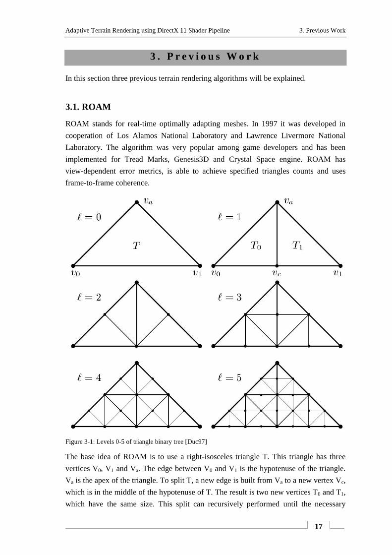
2.4. T-Junctions and Cracks
There is one common problem when using different LODs on one grid. Adjacent
triangles with different LODs are not connected properly when the higher LOD has a
vertex that does not share a vertex of the lower LOD. This phenomenon is called
t-junction. This t-junction could lead to bleeding tears in the terrain.
If additionally the vertex of the higher LOD doesn’t lie on the edge of the lower LOD
cracks will appear. These cracks lead to holes in the terrain.
Figure 2-16: Shows cracks and t-junctions [Lue03]
The solution of this problem is to have LODs that share the same vertices on the
adjacent edges. How this is implemented is dependent on the LOD system that is used.
Therefore I will explain how t-junctions and holes are avoided when I write about the
terrain LOD systems. 23
24
23
cf. [Sch06], page 757 24
cf. [Lue03], page 193
Adaptive Terrain Rendering using DirectX 11 Shader Pipeline 3. Previous Work
17
3 . P r e v i o u s W o r k
In this section three previous terrain rendering algorithms will be explained.
3.1. ROAM
ROAM stands for real-time optimally adapting meshes. In 1997 it was developed in
cooperation of Los Alamos National Laboratory and Lawrence Livermore National
Laboratory. The algorithm was very popular among game developers and has been
implemented for Tread Marks, Genesis3D and Crystal Space engine. ROAM has
view-dependent error metrics, is able to achieve specified triangles counts and uses
frame-to-frame coherence.
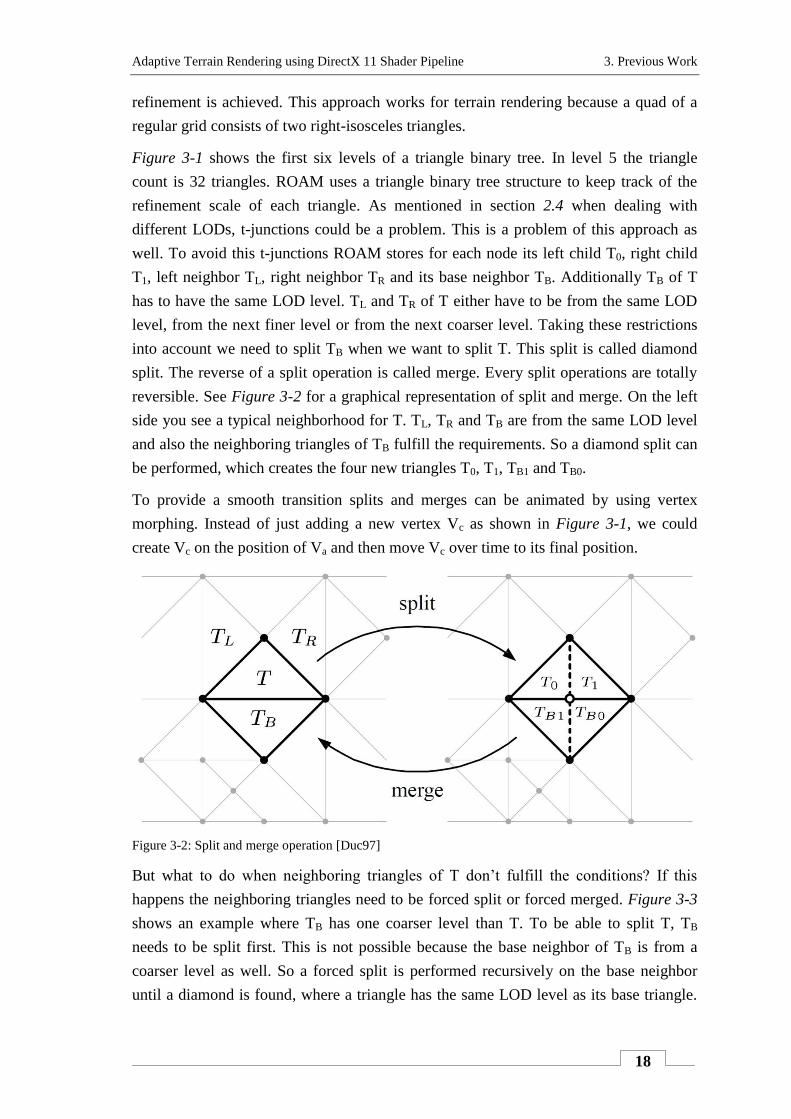
Figure 3-1: Levels 0-5 of triangle binary tree [Duc97]
The base idea of ROAM is to use a right-isosceles triangle T. This triangle has three
vertices V0, V1 and Va. The edge between V0 and V1 is the hypotenuse of the triangle.
Va is the apex of the triangle. To split T, a new edge is built from Va to a new vertex Vc,
which is in the middle of the hypotenuse of T. The result is two new vertices T0 and T1,
which have the same size. This split can recursively performed until the necessary
Adaptive Terrain Rendering using DirectX 11 Shader Pipeline 3. Previous Work
18
refinement is achieved. This approach works for terrain rendering because a quad of a
regular grid consists of two right-isosceles triangles.
Figure 3-1 shows the first six levels of a triangle binary tree. In level 5 the triangle
count is 32 triangles. ROAM uses a triangle binary tree structure to keep track of the
refinement scale of each triangle. As mentioned in section 2.4 when dealing with
different LODs, t-junctions could be a problem. This is a problem of this approach as
well. To avoid this t-junctions ROAM stores for each node its left child T0, right child
T1, left neighbor TL, right neighbor TR and its base neighbor TB. Additionally TB of T
has to have the same LOD level. TL and TR of T either have to be from the same LOD
level, from the next finer level or from the next coarser level. Taking these restrictions
into account we need to split TB when we want to split T. This split is called diamond
split. The reverse of a split operation is called merge. Every split operations are totally
reversible. See Figure 3-2 for a graphical representation of split and merge. On the left
side you see a typical neighborhood for T. TL, TR and TB are from the same LOD level
and also the neighboring triangles of TB fulfill the requirements. So a diamond split can
be performed, which creates the four new triangles T0, T1, TB1 and TB0.
To provide a smooth transition splits and merges can be animated by using vertex
morphing. Instead of just adding a new vertex Vc as shown in Figure 3-1, we could
create Vc on the position of Va and then move Vc over time to its final position.
Figure 3-2: Split and merge operation [Duc97]
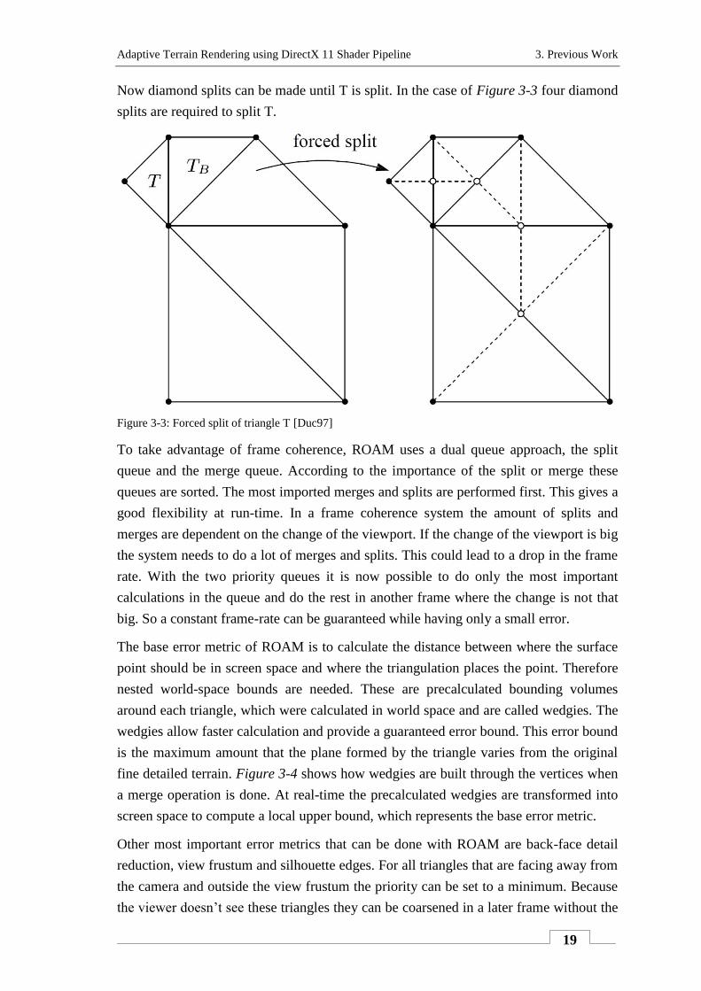
But what to do when neighboring triangles of T don’t fulfill the conditions? If this
happens the neighboring triangles need to be forced split or forced merged. Figure 3-3
shows an example where TB has one coarser level than T. To be able to split T, TB
needs to be split first. This is not possible because the base neighbor of TB is from a
coarser level as well. So a forced split is performed recursively on the base neighbor
until a diamond is found, where a triangle has the same LOD level as its base triangle.
Adaptive Terrain Rendering using DirectX 11 Shader Pipeline 3. Previous Work
19
Now diamond splits can be made until T is split. In the case of Figure 3-3 four diamond
splits are required to split T.
Figure 3-3: Forced split of triangle T [Duc97]
To take advantage of frame coherence, ROAM uses a dual queue approach, the split
queue and the merge queue. According to the importance of the split or merge these
queues are sorted. The most imported merges and splits are performed first. This gives a
good flexibility at run-time. In a frame coherence system the amount of splits and
merges are dependent on the change of the viewport. If the change of the viewport is big
the system needs to do a lot of merges and splits. This could lead to a drop in the frame
rate. With the two priority queues it is now possible to do only the most important
calculations in the queue and do the rest in another frame where the change is not that
big. So a constant frame-rate can be guaranteed while having only a small error.
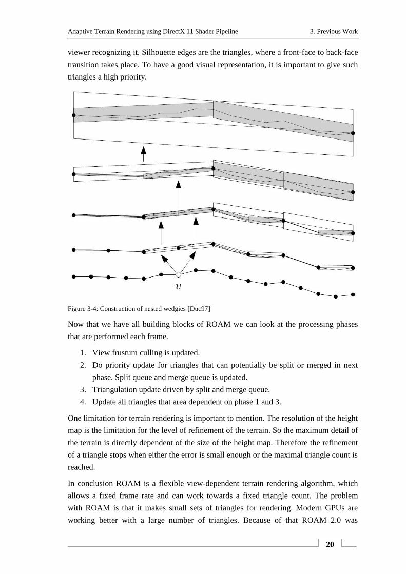
The base error metric of ROAM is to calculate the distance between where the surface
point should be in screen space and where the triangulation places the point. Therefore
nested world-space bounds are needed. These are precalculated bounding volumes
around each triangle, which were calculated in world space and are called wedgies. The
wedgies allow faster calculation and provide a guaranteed error bound. This error bound
is the maximum amount that the plane formed by the triangle varies from the original
fine detailed terrain. Figure 3-4 shows how wedgies are built through the vertices when
a merge operation is done. At real-time the precalculated wedgies are transformed into
screen space to compute a local upper bound, which represents the base error metric.
Other most important error metrics that can be done with ROAM are back-face detail
reduction, view frustum and silhouette edges. For all triangles that are facing away from
the camera and outside the view frustum the priority can be set to a minimum. Because
the viewer doesn’t see these triangles they can be coarsened in a later frame without the
Adaptive Terrain Rendering using DirectX 11 Shader Pipeline 3. Previous Work
20
viewer recognizing it. Silhouette edges are the triangles, where a front-face to back-face
transition takes place. To have a good visual representation, it is important to give such
triangles a high priority.
Figure 3-4: Construction of nested wedgies [Duc97]
Now that we have all building blocks of ROAM we can look at the processing phases
that are performed each frame.
1. View frustum culling is updated.
2. Do priority update for triangles that can potentially be split or merged in next
phase. Split queue and merge queue is updated.
3. Triangulation update driven by split and merge queue.
4. Update all triangles that area dependent on phase 1 and 3.
One limitation for terrain rendering is important to mention. The resolution of the height
map is the limitation for the level of refinement of the terrain. So the maximum detail of
the terrain is directly dependent of the size of the height map. Therefore the refinement
of a triangle stops when either the error is small enough or the maximal triangle count is
reached.
In conclusion ROAM is a flexible view-dependent terrain rendering algorithm, which
allows a fixed frame rate and can work towards a fixed triangle count. The problem
with ROAM is that it makes small sets of triangles for rendering. Modern GPUs are
working better with a large number of triangles. Because of that ROAM 2.0 was
Adaptive Terrain Rendering using DirectX 11 Shader Pipeline 3. Previous Work
21
developed which mixes the continuous LOD approach of ROAM with a discrete LOD
system. 25
26
The original ROAM algorithm has been modified and improved by a number of
researchers and game developers. One example is the implementation of Bryan Turner.
He implemented a simplified version of ROAM. In his approach he uses a split only
approach where the terrain is refined from scratch in each frame. Therefore he uses a
variance binary tree, which stores geometric error. The variance tree is updated every
frame according to the change of the scene. The terrain is then tessellated according to
the variance binary tree. 27
ROAM is also able to deal with dynamic terrain. Yefei He developed a real-time
dynamic terrain for an off-road ground vehicle simulation, in which a vehicle can
deform the terrain. So it’s possible to form skid marks of the car into the terrain. The
system is called DEXTER (Dynamic EXTEnsion of Resolution). 28
3.2. Smooth View-Dependent Level-of-Detail Control and its
Application to Terrain Rendering
Hugues Hoppe developed the terrain algorithm in 1998. The representation uses as base
view-dependent progressive meshes that were introduced in section 2.3.4. The target of
this terrain rendering systems was to render the Grand Canyon data in real-time, which
has about 16.7 million triangles. To be able to render this data the complexity of the
terrain needed to be reduced to 20000 triangles. This was the number of polygons,
which graphics hardware was able to render in 1997. To achieve this target they would
like to adapt the mesh complexity according to the screen-space projected error, which
makes a view-dependent LOD system. So the terrain is refined more densely near the
viewer, while distance and regions outside the view frustum are kept coarser. It was also
the goal to make a terrain rendering system with improved approximation error and that
provides scalability. Two important factors for a good terrain system they also tried to
achieve were a constant frame rate and the absence of popping artifacts.
To avoid popping artifacts the screen-space error value needs to be near 1 pixel. When
the screen-space error is near 1 pixel the change of resolution can’t be seen by the
viewer. The problem of a constant error tolerance is that the number of faces depends
directly on the terrain complexity near the viewpoint. This leads to a non-uniform frame
rate because the frame rate is dependent on the number of triangles that need to be
25
cf. [Duc97] 26
cf. [Lue03], page 202-206 27
cf. [Tur00] 28
cf. [HeY00]
Adaptive Terrain Rendering using DirectX 11 Shader Pipeline 3. Previous Work
22
rendered, and these are not constant in this approach. For a constant frame rate, the
screen-space error needs to be adjusted. But this leads to popping artifacts. To hide the
popping artifacts they use geomorphs. At run-time the triangles of the terrain need to be
split or refined to get the needed resolution. Instead of doing the refine and split in one
frame they morph it over several frames.
When do we need to use this geomorphing in a terrain rendering system? There are two
different situations we need to consider. One is forward moving the other is backward
moving.
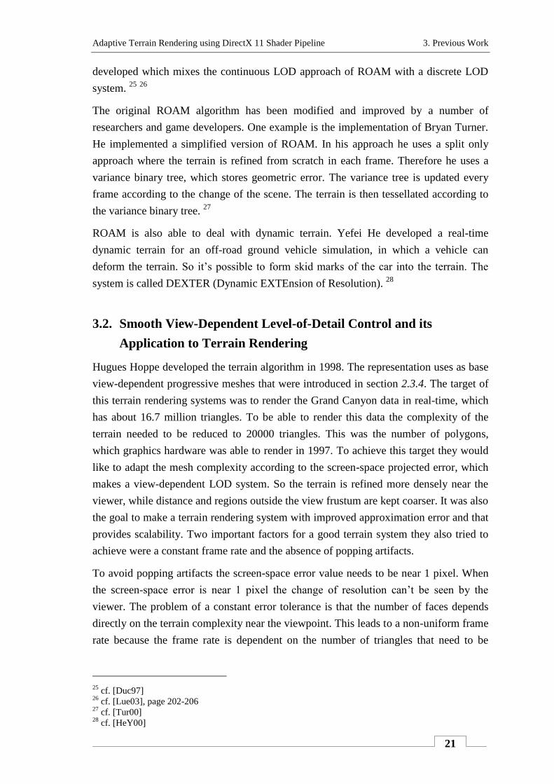
When we move forward we use geomorph refinement. In Figure 3-5 we see how the
view port changes when we move forward and turn left at the same time. We get three
different regions. All parts that are new in the view frustum are instantaneous refined,
all parts that are outside the view frustum are instantaneous coarsened and all parts that
were visible in the frame before, we need to do geomorph refinement.
Figure 3-5: Changes to active mesh during forward motion of viewer [Hop98]
Figure 3-6 shows how a geomorph refinement is done. At first we do a split operation.
But instead of placing the new created vertex directly on its final position we spawn the
vertex on the old vertex. After this we move the new vertex over several frames to his
new position. How long this morphing takes, depends on a user specified time, which is
called gtime. With a frame rate between 30 to 72 fps the gtime is set to 1 second. A nice
thing about geomorph refinement is that while a new vertex is morphing it can be split
already. So we’re able to do several geomorph refinements at the same time.
Adaptive Terrain Rendering using DirectX 11 Shader Pipeline 3. Previous Work
23
Figure 3-6: Shows geomorph refinement [Hop981]
We use geomorph coarsening for moving backward. When we move backward and turn
right at the same time we get three different regions as well. All parts that are new in the
view frustum are instantaneous refined, all parts that are outside the view frustum are
instantaneous coarsened and all parts that were visible in the frame before, we need to
do geomorph coarsening. Geomorph coarsening is more complex than geomorph
refinement. It is just the reverse as shown in Figure 3-6. We gradually move the vertex
to its parent position. Only when the vertex is at its parents position the mesh
connectivity can be updated, which means to merge the vertex with its parent vertex.
Only one geomorph coarsening is possible at a time. Therefore gtime is reduced to the
half. Fortunately geomorph coarsening is only required when the user moves backward,
which doesn’t happen that often.
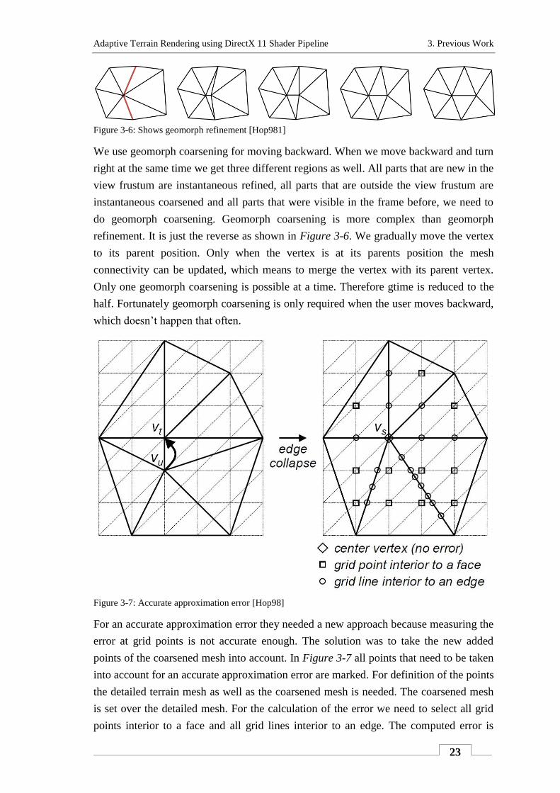
Figure 3-7: Accurate approximation error [Hop98]
For an accurate approximation error they needed a new approach because measuring the
error at grid points is not accurate enough. The solution was to take the new added
points of the coarsened mesh into account. In Figure 3-7 all points that need to be taken
into account for an accurate approximation error are marked. For definition of the points
the detailed terrain mesh as well as the coarsened mesh is needed. The coarsened mesh
is set over the detailed mesh. For the calculation of the error we need to select all grid
points interior to a face and all grid lines interior to an edge. The computed error is
Adaptive Terrain Rendering using DirectX 11 Shader Pipeline 3. Previous Work
24
exact because it is possible to compute it with respect to the original fully detailed
mesh. Additionally the error can be precalculated. Therefore this operation is not time
critical.
Now let’s see how they wanted to achieve scalability. Scalability is very important
when you have the target to render a mesh with more than 16.7 million triangles in
real-time. To achieve scalability they used a hierarchical approach, which decomposes
the mesh into blocks. The difficulty is to preserve spatial continuity. Without spatial
continuity cracks or holes could appear which is really bad for a terrain rendering
system.
To achieve scalability they developed a hierarchical progressive mesh construction.
Their approach is motivated by three considerations. The first is that simplification is
memory intensive because it starts from the detailed mesh. The second is that for larger
objects even the pre-simplified mesh could be too large to fit into main memory. And
the last is that the associated texture image may be too large for memory as well.
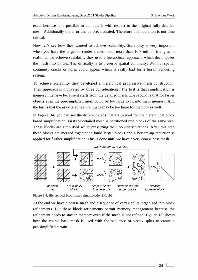
In Figure 3-8 you can see the different steps that are needed for the hierarchical block
based simplification. First the detailed mesh is partitioned into blocks of the same size.
These blocks are simplified while preserving their boundary vertices. After this step
these blocks are merged together to build larger blocks and a bottom-up recursion is
applied for further simplification. This is done until we have a very coarse base mesh.
Figure 3-8: Hierarchical block-based simplification [Hop98]
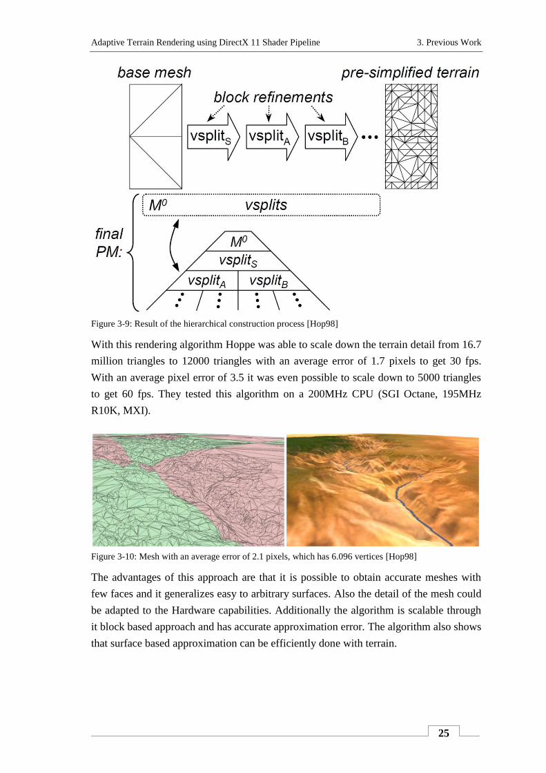
At the end we have a coarse mesh and a sequence of vertex splits, organized into block
refinements. But these block refinements permit memory management because the
refinement needs to stay in memory even if the mesh is not refined. Figure 3-9 shows
how the coarse base mesh is used with the sequence of vertex splits to create a
pre-simplified terrain.
Adaptive Terrain Rendering using DirectX 11 Shader Pipeline 3. Previous Work
25
Figure 3-9: Result of the hierarchical construction process [Hop98]
With this rendering algorithm Hoppe was able to scale down the terrain detail from 16.7
million triangles to 12000 triangles with an average error of 1.7 pixels to get 30 fps.
With an average pixel error of 3.5 it was even possible to scale down to 5000 triangles
to get 60 fps. They tested this algorithm on a 200MHz CPU (SGI Octane, 195MHz
R10K, MXI).
Figure 3-10: Mesh with an average error of 2.1 pixels, which has 6.096 vertices [Hop98]
The advantages of this approach are that it is possible to obtain accurate meshes with
few faces and it generalizes easy to arbitrary surfaces. Also the detail of the mesh could
be adapted to the Hardware capabilities. Additionally the algorithm is scalable through
it block based approach and has accurate approximation error. The algorithm also shows
that surface based approximation can be efficiently done with terrain.
Adaptive Terrain Rendering using DirectX 11 Shader Pipeline 3. Previous Work
26
The problem of this approach is that the detail is limited by the original terrain
resolution. The detail could for example be enhanced through randomly build detail
through a noise algorithm. 29
3.3. Geometry Clipmaps
Geometry clipmaps were developed by Frank Losasso (Stanford University &
Microsoft Research) and Hugues Hoppe (Microsoft Research) in 2004. They wanted to
master several challenges with their terrain rendering algorithm. One was to be able to
store, manipulate and render a large number of samples. So as primary data set they
used a 40 GB large height map of the United States. They wanted to render this data set
in real-time with a constant frame rate of 60 frames per second. They wanted to have a
concise storage and visual continuity. Concise storage means that they didn’t want to
have loading times during the real-time application or lags because they needed to read
data from disk. With visual continuity they wanted to achieve a terrain representation
without cracks or popping artifacts. They also wanted to develop a terrain algorithm that
is more GPU based and therefore decreases the workload of the CPU.
Former terrain algorithms were view-dependent LOD algorithms. The terrain was
adaptively refined and coarsened according to a screen-space geometry error. The
screen-space geometric error was dependent on the viewer distance, the surface
orientation and the surface geometry. So the geometry was only refined where it was
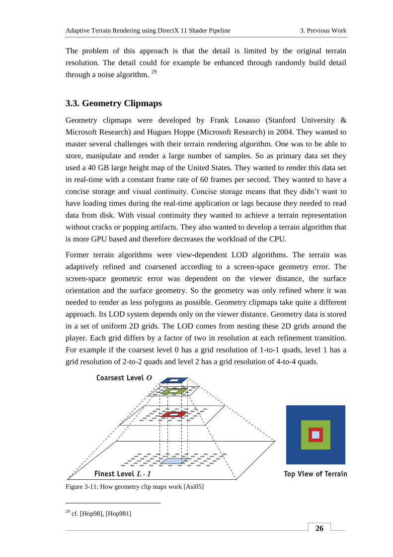
needed to render as less polygons as possible. Geometry clipmaps take quite a different
approach. Its LOD system depends only on the viewer distance. Geometry data is stored
in a set of uniform 2D grids. The LOD comes from nesting these 2D grids around the
player. Each grid differs by a factor of two in resolution at each refinement transition.
For example if the coarsest level 0 has a grid resolution of 1-to-1 quads, level 1 has a
grid resolution of 2-to-2 quads and level 2 has a grid resolution of 4-to-4 quads.
Figure 3-11: How geometry clip maps work [Asi05]
29
cf. [Hop98], [Hop981]
Adaptive Terrain Rendering using DirectX 11 Shader Pipeline 3. Previous Work
27
Figure 3-11 shows how the geometry clip map hierarchy can be illustrated. It can be
compared to a mipmap30
pyramid. The full hierarchy is a prefiltered sequence of all
possible grid resolutions, where the finest level contains the whole terrain at the finest
resolution. The coarsest level has the size of the active region. The active region is the
region that is rendered into screen-space. Its size is calculated according to the windows
size W, the field of view φ and the screen-space triangle size s. With W=640 pixels,
φ=90° and s=3 pixels we got an active region of 255-to-255.
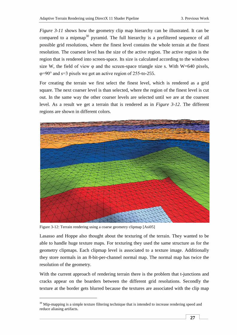
For creating the terrain we first select the finest level, which is rendered as a grid
square. The next coarser level is than selected, where the region of the finest level is cut
out. In the same way the other coarser levels are selected until we are at the coarsest
level. As a result we get a terrain that is rendered as in Figure 3-12. The different
regions are shown in different colors.
Figure 3-12: Terrain rendering using a coarse geometry clipmap [Asi05]
Lasasso and Hoppe also thought about the texturing of the terrain. They wanted to be
able to handle huge texture maps. For texturing they used the same structure as for the
geometry clipmaps. Each clipmap level is associated to a texture image. Additionally
they store normals in an 8-bit-per-channel normal map. The normal map has twice the
resolution of the geometry.
With the current approach of rendering terrain there is the problem that t-junctions and
cracks appear on the boarders between the different grid resolutions. Secondly the
texture at the border gets blurred because the textures are associated with the clip map
30
Mip-mapping is a simple texture filtering technique that is intended to increase rendering speed and
reduce aliasing artifacts.
Adaptive Terrain Rendering using DirectX 11 Shader Pipeline 3. Previous Work
28
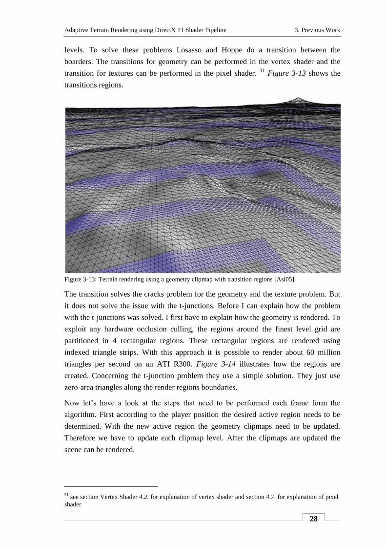
levels. To solve these problems Losasso and Hoppe do a transition between the
boarders. The transitions for geometry can be performed in the vertex shader and the
transition for textures can be performed in the pixel shader. 31
Figure 3-13 shows the
transitions regions.
Figure 3-13: Terrain rendering using a geometry clipmap with transition regions [Asi05]
The transition solves the cracks problem for the geometry and the texture problem. But
it does not solve the issue with the t-junctions. Before I can explain how the problem
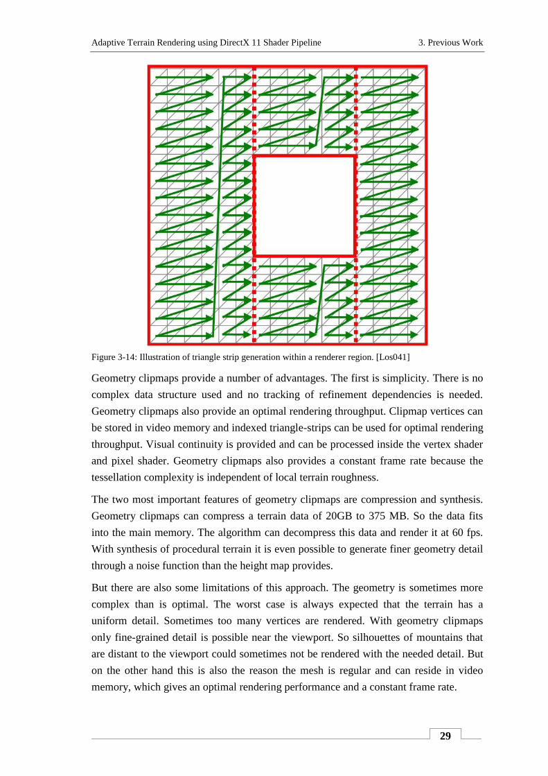
with the t-junctions was solved. I first have to explain how the geometry is rendered. To
exploit any hardware occlusion culling, the regions around the finest level grid are
partitioned in 4 rectangular regions. These rectangular regions are rendered using
indexed triangle strips. With this approach it is possible to render about 60 million
triangles per second on an ATI R300. Figure 3-14 illustrates how the regions are
created. Concerning the t-junction problem they use a simple solution. They just use
zero-area triangles along the render regions boundaries.
Now let’s have a look at the steps that need to be performed each frame form the
algorithm. First according to the player position the desired active region needs to be
determined. With the new active region the geometry clipmaps need to be updated.
Therefore we have to update each clipmap level. After the clipmaps are updated the
scene can be rendered.
31
see section Vertex Shader 4.2. for explanation of vertex shader and section 4.7. for explanation of pixel
shader
Adaptive Terrain Rendering using DirectX 11 Shader Pipeline 3. Previous Work
29
Figure 3-14: Illustration of triangle strip generation within a renderer region. [Los041]
Geometry clipmaps provide a number of advantages. The first is simplicity. There is no
complex data structure used and no tracking of refinement dependencies is needed.
Geometry clipmaps also provide an optimal rendering throughput. Clipmap vertices can
be stored in video memory and indexed triangle-strips can be used for optimal rendering
throughput. Visual continuity is provided and can be processed inside the vertex shader
and pixel shader. Geometry clipmaps also provides a constant frame rate because the
tessellation complexity is independent of local terrain roughness.
The two most important features of geometry clipmaps are compression and synthesis.
Geometry clipmaps can compress a terrain data of 20GB to 375 MB. So the data fits
into the main memory. The algorithm can decompress this data and render it at 60 fps.
With synthesis of procedural terrain it is even possible to generate finer geometry detail
through a noise function than the height map provides.
But there are also some limitations of this approach. The geometry is sometimes more
complex than is optimal. The worst case is always expected that the terrain has a
uniform detail. Sometimes too many vertices are rendered. With geometry clipmaps
only fine-grained detail is possible near the viewport. So silhouettes of mountains that
are distant to the viewport could sometimes not be rendered with the needed detail. But
on the other hand this is also the reason the mesh is regular and can reside in video
memory, which gives an optimal rendering performance and a constant frame rate.

Adaptive Terrain Rendering using DirectX 11 Shader Pipeline 3. Previous Work
30
Hugues Hoppe and Arul Sirvatham (Microsoft Research) improved geometry clipmaps
to make it more GPU-based. They achieved that everything except of the
decompression could be done on the GPU. With the GPU based approach they are able
to render the terrain at around 90 fps what gives a performance gain of about 50%. 32
32
cf. [Los04], [Los041], [Asi05]
Adaptive Terrain Rendering using DirectX 11 Shader Pipeline 4. DirectX 11 Shader Pipeline
31
4 . D i r e c t X 1 1 S h a d e r P i p e l i n e
In the past rendering of highly detailed models were not possible in real-time. The main
limitation for the number of polygons to render was the bus bandwidth between CPU
and GPU. Every highly detailed polygon mesh needed to be transferred over that bus.
An additional limitation was the main memory of the graphics hardware. Even when it
was managed to transfer the data, it couldn’t be stored on the memory of the graphics
card. To be able to render a high number of polygons on the graphics hardware, the way
of how to render high polygon meshes needed to be rethought.
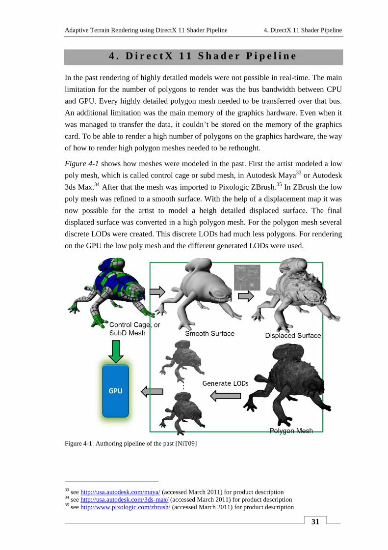
Figure 4-1 shows how meshes were modeled in the past. First the artist modeled a low
poly mesh, which is called control cage or subd mesh, in Autodesk Maya33
or Autodesk
3ds Max.34
After that the mesh was imported to Pixologic ZBrush.35
In ZBrush the low
poly mesh was refined to a smooth surface. With the help of a displacement map it was
now possible for the artist to model a heigh detailed displaced surface. The final
displaced surface was converted in a high polygon mesh. For the polygon mesh several
discrete LODs were created. This discrete LODs had much less polygons. For rendering
on the GPU the low poly mesh and the different generated LODs were used.
Figure 4-1: Authoring pipeline of the past [NiT09]
33
see http://usa.autodesk.com/maya/ (accessed March 2011) for product description 34
see http://usa.autodesk.com/3ds-max/ (accessed March 2011) for product description 35
see http://www.pixologic.com/zbrush/ (accessed March 2011) for product description
Adaptive Terrain Rendering using DirectX 11 Shader Pipeline 4. DirectX 11 Shader Pipeline
32
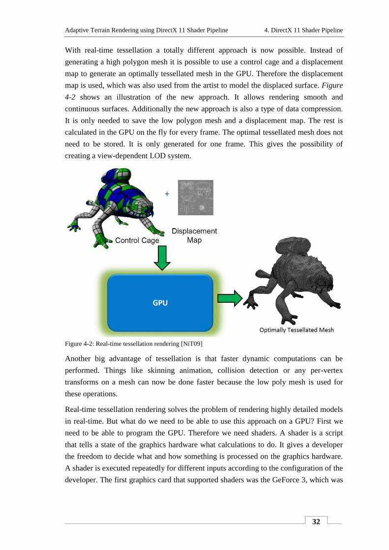
With real-time tessellation a totally different approach is now possible. Instead of
generating a high polygon mesh it is possible to use a control cage and a displacement
map to generate an optimally tessellated mesh in the GPU. Therefore the displacement
map is used, which was also used from the artist to model the displaced surface. Figure
4-2 shows an illustration of the new approach. It allows rendering smooth and
continuous surfaces. Additionally the new approach is also a type of data compression.
It is only needed to save the low polygon mesh and a displacement map. The rest is
calculated in the GPU on the fly for every frame. The optimal tessellated mesh does not
need to be stored. It is only generated for one frame. This gives the possibility of
creating a view-dependent LOD system.
Figure 4-2: Real-time tessellation rendering [NiT09]
Another big advantage of tessellation is that faster dynamic computations can be
performed. Things like skinning animation, collision detection or any per-vertex
transforms on a mesh can now be done faster because the low poly mesh is used for
these operations.
Real-time tessellation rendering solves the problem of rendering highly detailed models
in real-time. But what do we need to be able to use this approach on a GPU? First we
need to be able to program the GPU. Therefore we need shaders. A shader is a script
that tells a state of the graphics hardware what calculations to do. It gives a developer
the freedom to decide what and how something is processed on the graphics hardware.
A shader is executed repeatedly for different inputs according to the configuration of the
developer. The first graphics card that supported shaders was the GeForce 3, which was
Adaptive Terrain Rendering using DirectX 11 Shader Pipeline 4. DirectX 11 Shader Pipeline
33
created by NVIDIA.36
It was released in 2001 and supported shader model 1.1. The first
version of the shader model gave the developers only a little possibility to program the
GPU. Over the years, shader model was more and more extended.
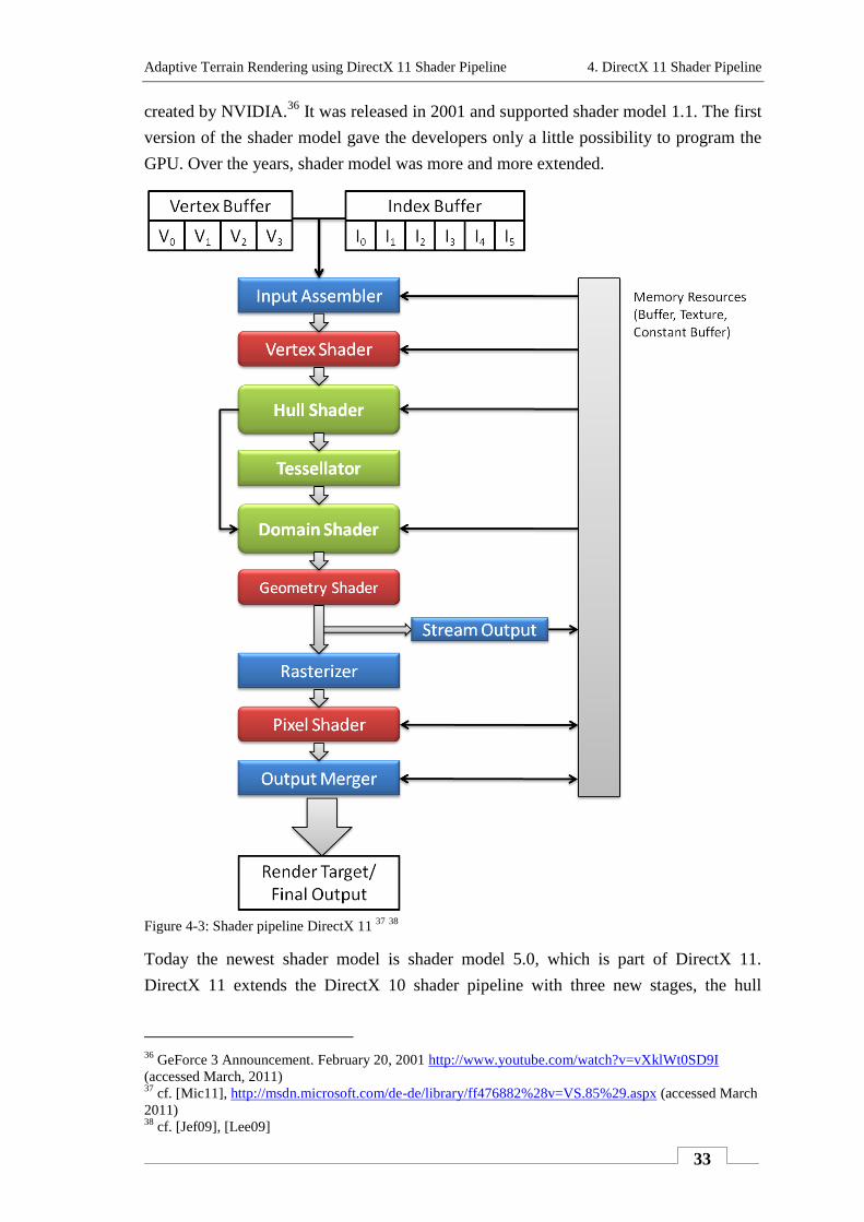
Figure 4-3: Shader pipeline DirectX 11
37 38
Today the newest shader model is shader model 5.0, which is part of DirectX 11.
DirectX 11 extends the DirectX 10 shader pipeline with three new stages, the hull
36
GeForce 3 Announcement. February 20, 2001 http://www.youtube.com/watch?v=vXklWt0SD9I
(accessed March, 2011) 37
cf. [Mic11], http://msdn.microsoft.com/de-de/library/ff476882%28v=VS.85%29.aspx (accessed March
2011) 38
cf. [Jef09], [Lee09]
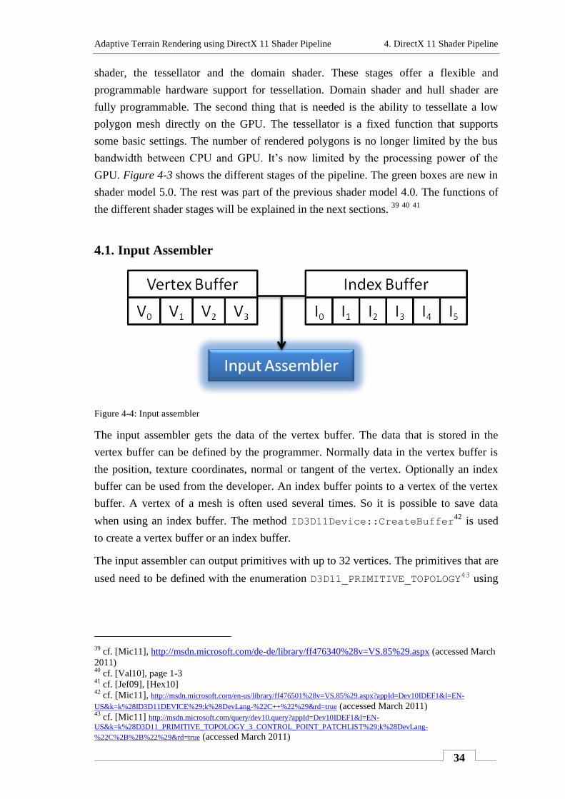
Adaptive Terrain Rendering using DirectX 11 Shader Pipeline 4. DirectX 11 Shader Pipeline
34
shader, the tessellator and the domain shader. These stages offer a flexible and
programmable hardware support for tessellation. Domain shader and hull shader are
fully programmable. The second thing that is needed is the ability to tessellate a low
polygon mesh directly on the GPU. The tessellator is a fixed function that supports
some basic settings. The number of rendered polygons is no longer limited by the bus
bandwidth between CPU and GPU. It’s now limited by the processing power of the
GPU. Figure 4-3 shows the different stages of the pipeline. The green boxes are new in
shader model 5.0. The rest was part of the previous shader model 4.0. The functions of
the different shader stages will be explained in the next sections. 39
40
41
4.1. Input Assembler
Figure 4-4: Input assembler
The input assembler gets the data of the vertex buffer. The data that is stored in the
vertex buffer can be defined by the programmer. Normally data in the vertex buffer is
the position, texture coordinates, normal or tangent of the vertex. Optionally an index
buffer can be used from the developer. An index buffer points to a vertex of the vertex
buffer. A vertex of a mesh is often used several times. So it is possible to save data
when using an index buffer. The method ID3D11Device::CreateBuffer42
is used
to create a vertex buffer or an index buffer.
The input assembler can output primitives with up to 32 vertices. The primitives that are
used need to be defined with the enumeration D3D11_PRIMITIVE_TOPOLOGY43 using
39
cf. [Mic11], http://msdn.microsoft.com/de-de/library/ff476340%28v=VS.85%29.aspx (accessed March
2011) 40
cf. [Val10], page 1-3 41
cf. [Jef09], [Hex10] 42
cf. [Mic11], http://msdn.microsoft.com/en-us/library/ff476501%28v=VS.85%29.aspx?appId=Dev10IDEF1&l=EN-
US&k=k%28ID3D11DEVICE%29;k%28DevLang-%22C++%22%29&rd=true (accessed March 2011) 43
cf. [Mic11] http://msdn.microsoft.com/query/dev10.query?appId=Dev10IDEF1&l=EN-
US&k=k%28D3D11_PRIMITIVE_TOPOLOGY_3_CONTROL_POINT_PATCHLIST%29;k%28DevLang-
%22C%2B%2B%22%29&rd=true (accessed March 2011)
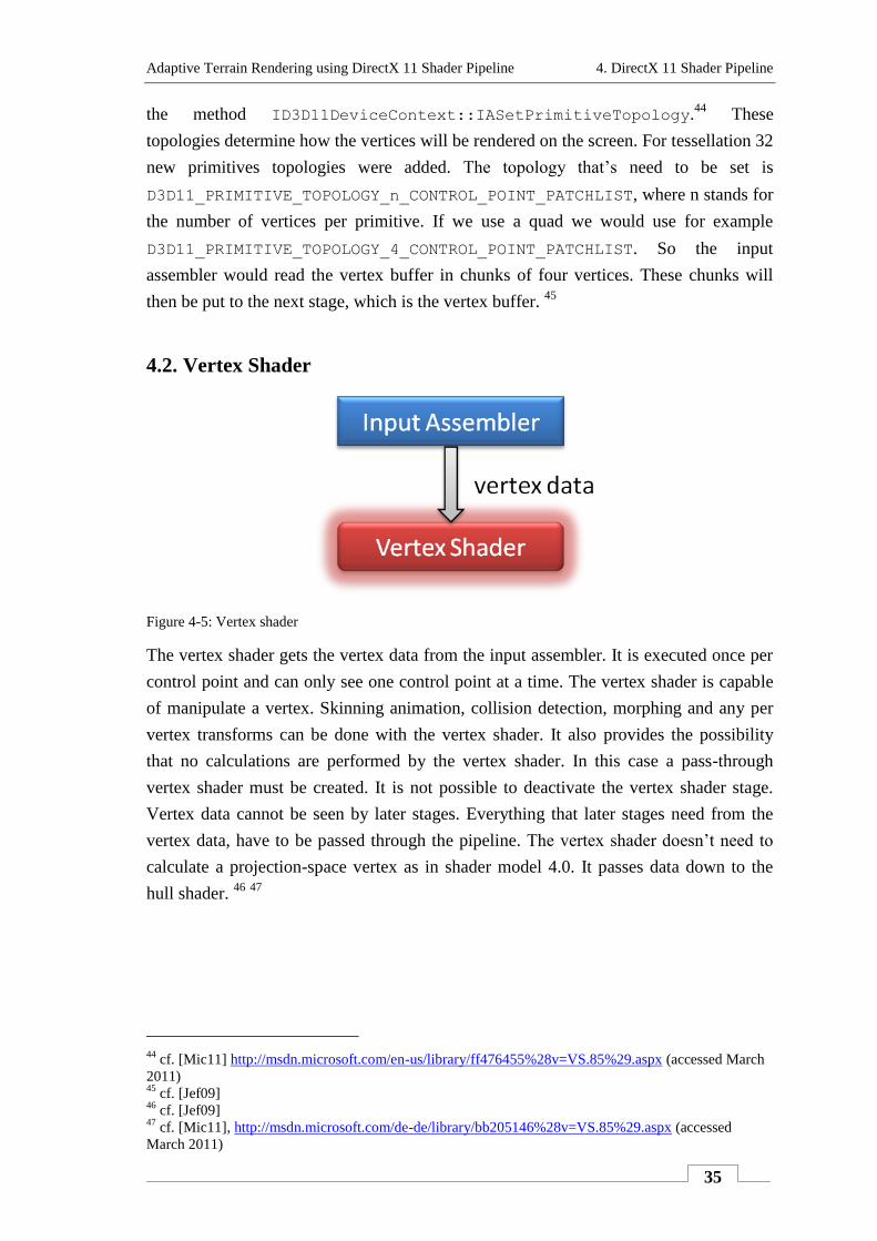
Adaptive Terrain Rendering using DirectX 11 Shader Pipeline 4. DirectX 11 Shader Pipeline
35
the method ID3D11DeviceContext::IASetPrimitiveTopology.44
These
topologies determine how the vertices will be rendered on the screen. For tessellation 32
new primitives topologies were added. The topology that’s need to be set is
D3D11_PRIMITIVE_TOPOLOGY_n_CONTROL_POINT_PATCHLIST, where n stands for
the number of vertices per primitive. If we use a quad we would use for example
D3D11_PRIMITIVE_TOPOLOGY_4_CONTROL_POINT_PATCHLIST. So the input
assembler would read the vertex buffer in chunks of four vertices. These chunks will
then be put to the next stage, which is the vertex buffer. 45
4.2. Vertex Shader
Figure 4-5: Vertex shader
The vertex shader gets the vertex data from the input assembler. It is executed once per
control point and can only see one control point at a time. The vertex shader is capable
of manipulate a vertex. Skinning animation, collision detection, morphing and any per
vertex transforms can be done with the vertex shader. It also provides the possibility
that no calculations are performed by the vertex shader. In this case a pass-through
vertex shader must be created. It is not possible to deactivate the vertex shader stage.
Vertex data cannot be seen by later stages. Everything that later stages need from the
vertex data, have to be passed through the pipeline. The vertex shader doesn’t need to
calculate a projection-space vertex as in shader model 4.0. It passes data down to the
hull shader. 46
47
44
cf. [Mic11] http://msdn.microsoft.com/en-us/library/ff476455%28v=VS.85%29.aspx (accessed March
2011) 45
cf. [Jef09] 46
cf. [Jef09] 47
cf. [Mic11], http://msdn.microsoft.com/de-de/library/bb205146%28v=VS.85%29.aspx (accessed
March 2011)
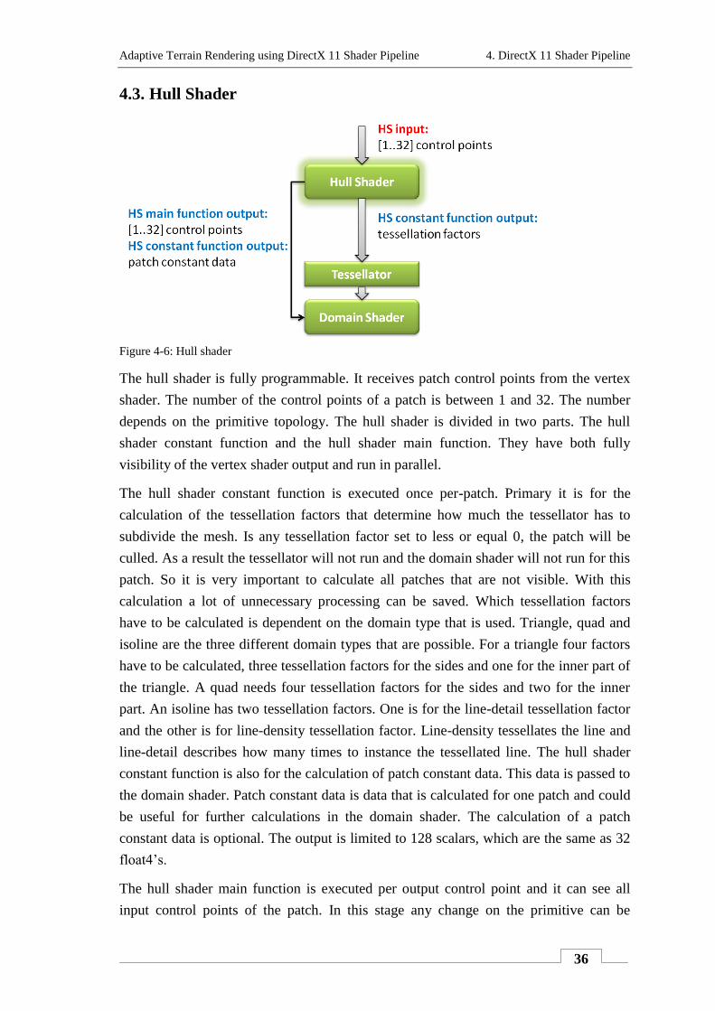
Adaptive Terrain Rendering using DirectX 11 Shader Pipeline 4. DirectX 11 Shader Pipeline
36
4.3. Hull Shader
Figure 4-6: Hull shader
The hull shader is fully programmable. It receives patch control points from the vertex
shader. The number of the control points of a patch is between 1 and 32. The number
depends on the primitive topology. The hull shader is divided in two parts. The hull
shader constant function and the hull shader main function. They have both fully
visibility of the vertex shader output and run in parallel.
The hull shader constant function is executed once per-patch. Primary it is for the
calculation of the tessellation factors that determine how much the tessellator has to
subdivide the mesh. Is any tessellation factor set to less or equal 0, the patch will be
culled. As a result the tessellator will not run and the domain shader will not run for this
patch. So it is very important to calculate all patches that are not visible. With this
calculation a lot of unnecessary processing can be saved. Which tessellation factors
have to be calculated is dependent on the domain type that is used. Triangle, quad and
isoline are the three different domain types that are possible. For a triangle four factors
have to be calculated, three tessellation factors for the sides and one for the inner part of
the triangle. A quad needs four tessellation factors for the sides and two for the inner
part. An isoline has two tessellation factors. One is for the line-detail tessellation factor
and the other is for line-density tessellation factor. Line-density tessellates the line and
line-detail describes how many times to instance the tessellated line. The hull shader
constant function is also for the calculation of patch constant data. This data is passed to
the domain shader. Patch constant data is data that is calculated for one patch and could
be useful for further calculations in the domain shader. The calculation of a patch
constant data is optional. The output is limited to 128 scalars, which are the same as 32
float4’s.
The hull shader main function is executed per output control point and it can see all
input control points of the patch. In this stage any change on the primitive can be
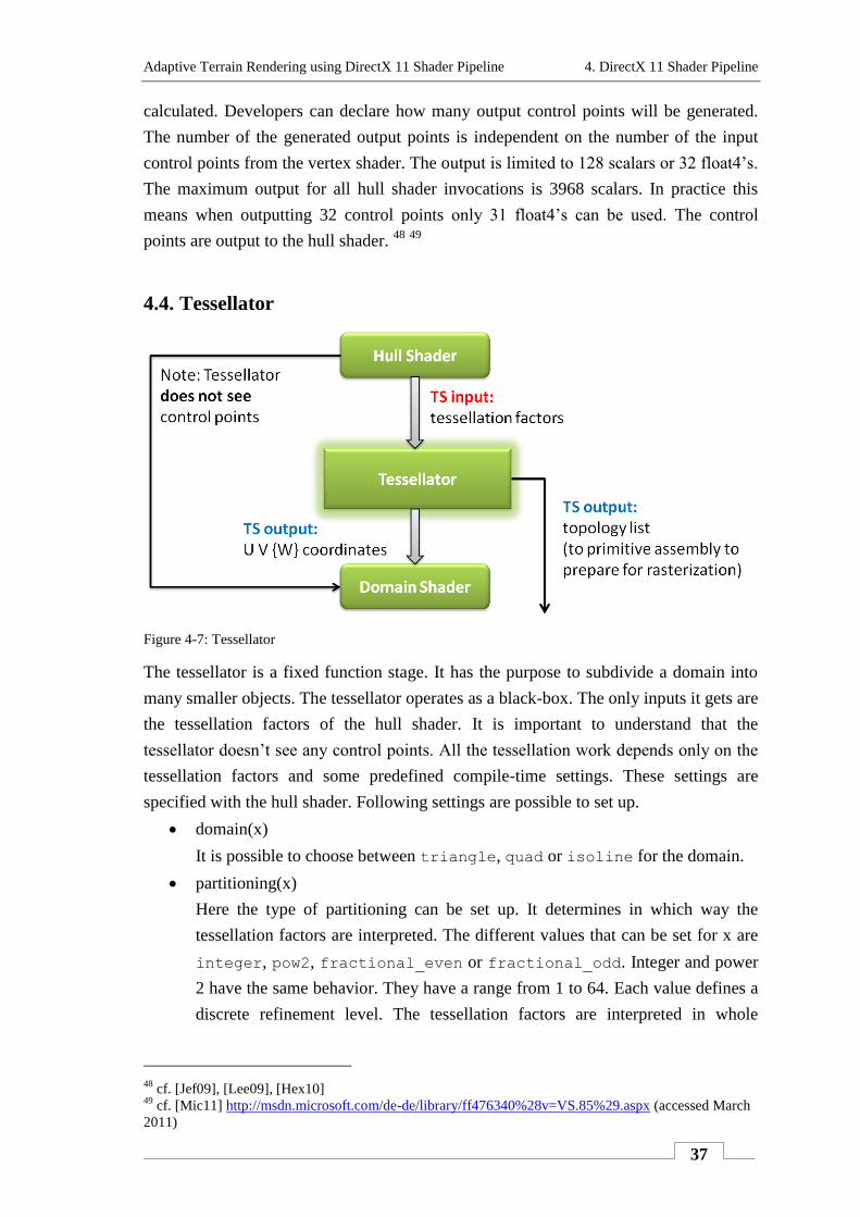
Adaptive Terrain Rendering using DirectX 11 Shader Pipeline 4. DirectX 11 Shader Pipeline
37
calculated. Developers can declare how many output control points will be generated.
The number of the generated output points is independent on the number of the input
control points from the vertex shader. The output is limited to 128 scalars or 32 float4’s.
The maximum output for all hull shader invocations is 3968 scalars. In practice this
means when outputting 32 control points only 31 float4’s can be used. The control
points are output to the hull shader. 48
49
4.4. Tessellator
Figure 4-7: Tessellator
The tessellator is a fixed function stage. It has the purpose to subdivide a domain into
many smaller objects. The tessellator operates as a black-box. The only inputs it gets are
the tessellation factors of the hull shader. It is important to understand that the
tessellator doesn’t see any control points. All the tessellation work depends only on the
tessellation factors and some predefined compile-time settings. These settings are
specified with the hull shader. Following settings are possible to set up.
domain(x)
It is possible to choose between triangle, quad or isoline for the domain.
partitioning(x)
Here the type of partitioning can be set up. It determines in which way the
tessellation factors are interpreted. The different values that can be set for x are
integer, pow2, fractional_even or fractional_odd. Integer and power
2 have the same behavior. They have a range from 1 to 64. Each value defines a
discrete refinement level. The tessellation factors are interpreted in whole
48
cf. [Jef09], [Lee09], [Hex10] 49
cf. [Mic11] http://msdn.microsoft.com/de-de/library/ff476340%28v=VS.85%29.aspx (accessed March
2011)
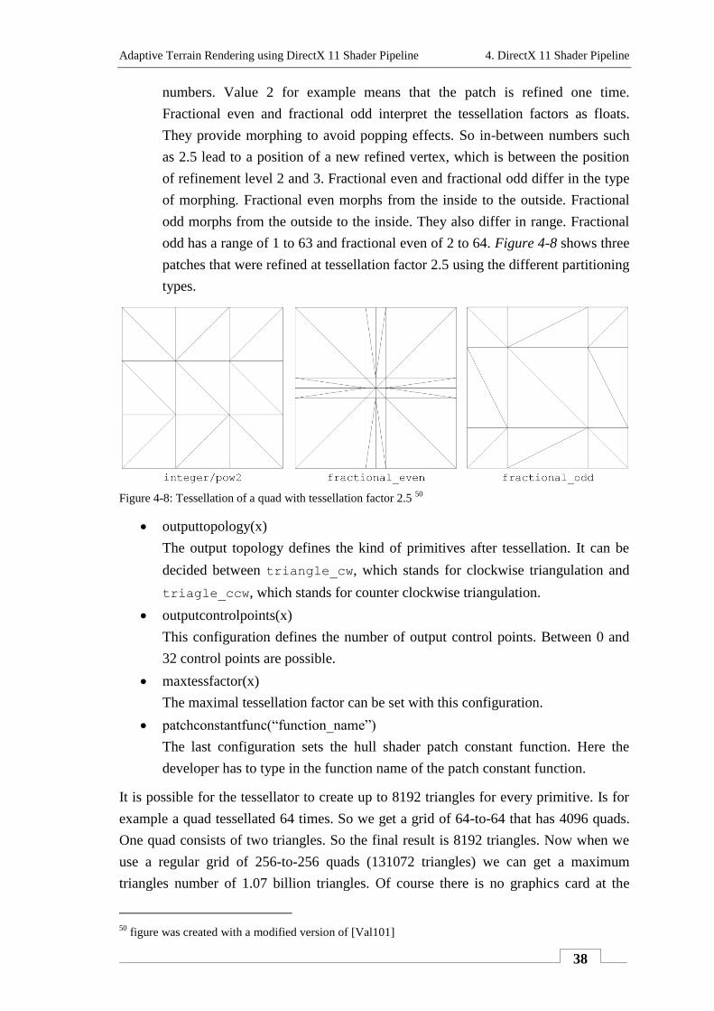
Adaptive Terrain Rendering using DirectX 11 Shader Pipeline 4. DirectX 11 Shader Pipeline
38
numbers. Value 2 for example means that the patch is refined one time.
Fractional even and fractional odd interpret the tessellation factors as floats.
They provide morphing to avoid popping effects. So in-between numbers such
as 2.5 lead to a position of a new refined vertex, which is between the position
of refinement level 2 and 3. Fractional even and fractional odd differ in the type
of morphing. Fractional even morphs from the inside to the outside. Fractional
odd morphs from the outside to the inside. They also differ in range. Fractional
odd has a range of 1 to 63 and fractional even of 2 to 64. Figure 4-8 shows three
patches that were refined at tessellation factor 2.5 using the different partitioning
types.
Figure 4-8: Tessellation of a quad with tessellation factor 2.5
50
outputtopology(x)
The output topology defines the kind of primitives after tessellation. It can be
decided between triangle_cw, which stands for clockwise triangulation and
triagle_ccw, which stands for counter clockwise triangulation.
outputcontrolpoints(x)
This configuration defines the number of output control points. Between 0 and
32 control points are possible.
maxtessfactor(x)
The maximal tessellation factor can be set with this configuration.
patchconstantfunc(“function_name”)
The last configuration sets the hull shader patch constant function. Here the
developer has to type in the function name of the patch constant function.
It is possible for the tessellator to create up to 8192 triangles for every primitive. Is for
example a quad tessellated 64 times. So we get a grid of 64-to-64 that has 4096 quads.
One quad consists of two triangles. So the final result is 8192 triangles. Now when we
use a regular grid of 256-to-256 quads (131072 triangles) we can get a maximum
triangles number of 1.07 billion triangles. Of course there is no graphics card at the
50
figure was created with a modified version of [Val101]
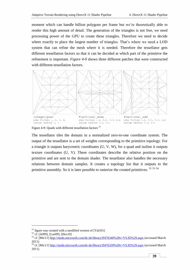
Adaptive Terrain Rendering using DirectX 11 Shader Pipeline 4. DirectX 11 Shader Pipeline
39
moment which can handle billion polygons per frame but we’re theoretically able to
render this high amount of detail. The generation of the triangles is not free, we need
processing power of the GPU to create these triangles. Therefore we need to decide
where exactly to place the largest number of triangles. That’s where we need a LOD
system that can refine the mesh where it is needed. Therefore the tessellator gets
different tessellation factors so that it can be decided at which part of the primitive the
refinement is important. Figure 4-9 shows three different patches that were constructed
with different tessellation factors.
Figure 4-9: Quads with different tessellation factors
51
The tessellator tiles the domain in a normalized zero-to-one coordinate system. The
output of the tessellator is a set of weights corresponding to the primitive topology. For
a triangle it outputs barycentric coordinates (U, V, W), for a quad and isoline it outputs
texture coordinates (U, V). These coordinates describe the relative position on the
primitive and are sent to the domain shader. The tessellator also handles the necessary
relations between domain samples. It creates a topology list that it outputs to the
primitive assembly. So it is later possible to rasterize the created primitives. 52
53
54
51
figure was created with a modified version of [Val101] 52
cf. [Jef09], [Lee09], [Hex10] 53
cf. [Mic11] http://msdn.microsoft.com/de-de/library/ff476340%28v=VS.85%29.aspx (accessed March
2011) 54
cf. [Mic11] http://msdn.microsoft.com/de-de/library/ff476339%28v=VS.85%29.aspx (accessed March
2011)
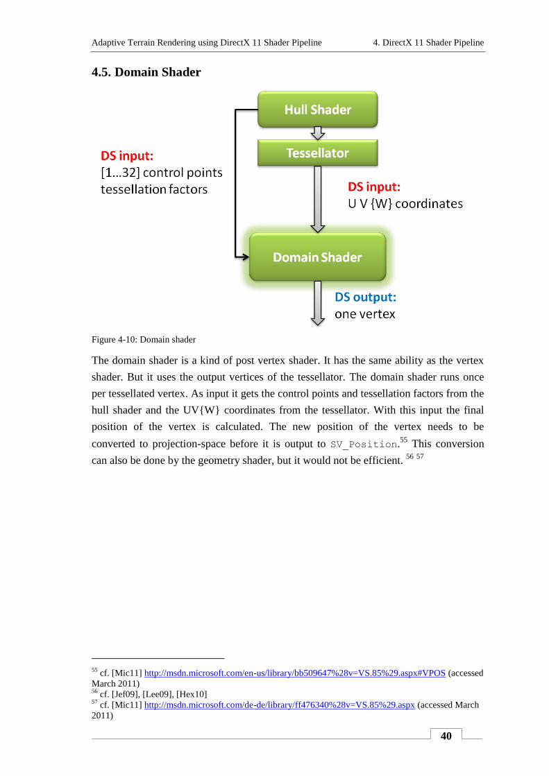
Adaptive Terrain Rendering using DirectX 11 Shader Pipeline 4. DirectX 11 Shader Pipeline
40
4.5. Domain Shader
Figure 4-10: Domain shader
The domain shader is a kind of post vertex shader. It has the same ability as the vertex
shader. But it uses the output vertices of the tessellator. The domain shader runs once
per tessellated vertex. As input it gets the control points and tessellation factors from the
hull shader and the UV{W} coordinates from the tessellator. With this input the final
position of the vertex is calculated. The new position of the vertex needs to be
converted to projection-space before it is output to SV_Position.55
This conversion
can also be done by the geometry shader, but it would not be efficient. 56
57
55
cf. [Mic11] http://msdn.microsoft.com/en-us/library/bb509647%28v=VS.85%29.aspx#VPOS (accessed
March 2011) 56
cf. [Jef09], [Lee09], [Hex10] 57
cf. [Mic11] http://msdn.microsoft.com/de-de/library/ff476340%28v=VS.85%29.aspx (accessed March
2011)
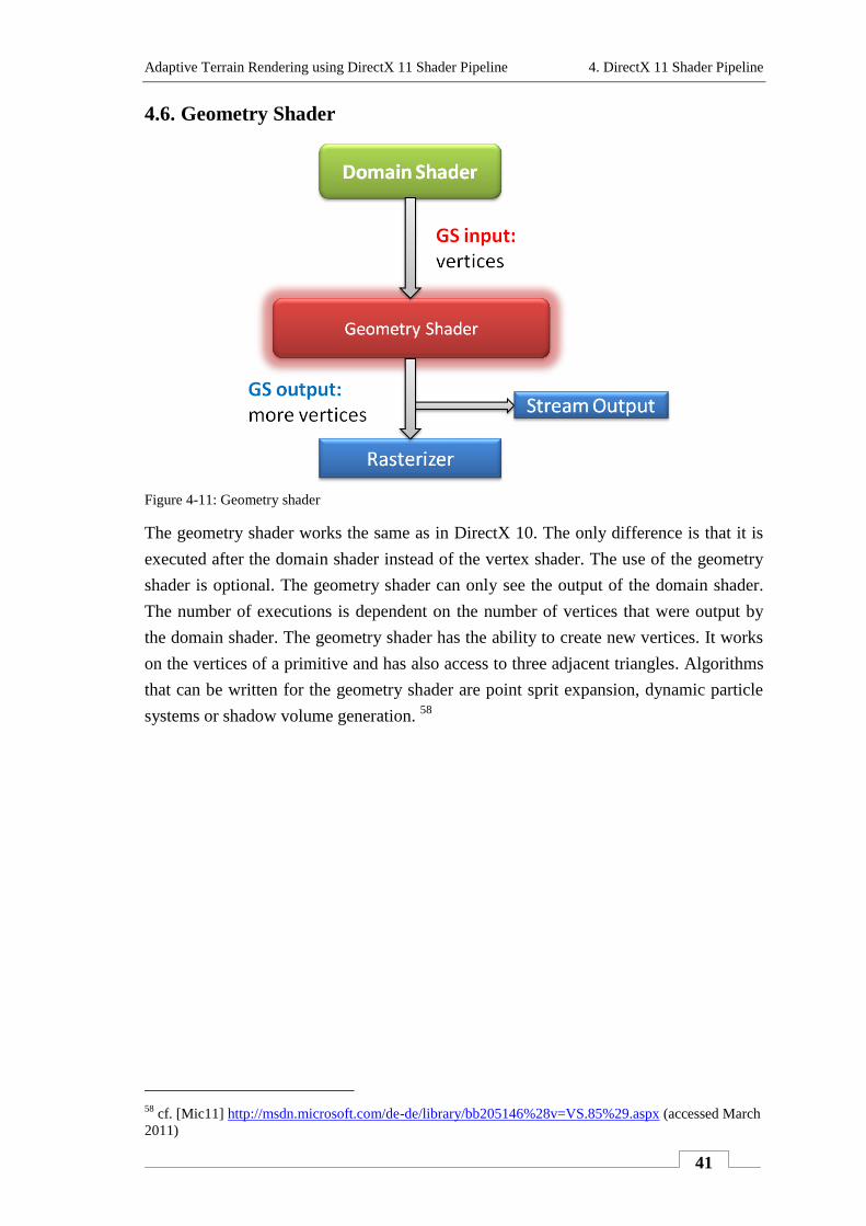
Adaptive Terrain Rendering using DirectX 11 Shader Pipeline 4. DirectX 11 Shader Pipeline
41
4.6. Geometry Shader
Figure 4-11: Geometry shader
The geometry shader works the same as in DirectX 10. The only difference is that it is
executed after the domain shader instead of the vertex shader. The use of the geometry
shader is optional. The geometry shader can only see the output of the domain shader.
The number of executions is dependent on the number of vertices that were output by
the domain shader. The geometry shader has the ability to create new vertices. It works
on the vertices of a primitive and has also access to three adjacent triangles. Algorithms
that can be written for the geometry shader are point sprit expansion, dynamic particle
systems or shadow volume generation. 58
58
cf. [Mic11] http://msdn.microsoft.com/de-de/library/bb205146%28v=VS.85%29.aspx (accessed March
2011)
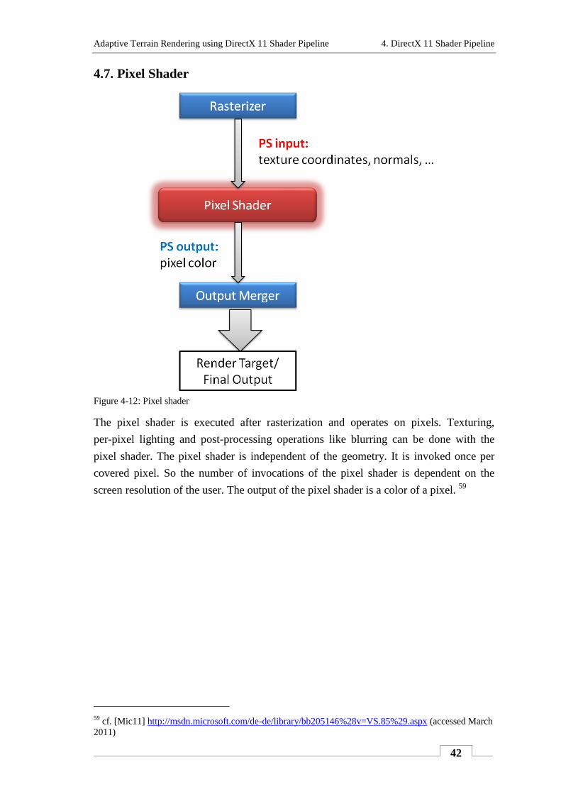
Adaptive Terrain Rendering using DirectX 11 Shader Pipeline 4. DirectX 11 Shader Pipeline
42
4.7. Pixel Shader
Figure 4-12: Pixel shader
The pixel shader is executed after rasterization and operates on pixels. Texturing,
per-pixel lighting and post-processing operations like blurring can be done with the
pixel shader. The pixel shader is independent of the geometry. It is invoked once per
covered pixel. So the number of invocations of the pixel shader is dependent on the
screen resolution of the user. The output of the pixel shader is a color of a pixel. 59
59
cf. [Mic11] http://msdn.microsoft.com/de-de/library/bb205146%28v=VS.85%29.aspx (accessed March
2011)
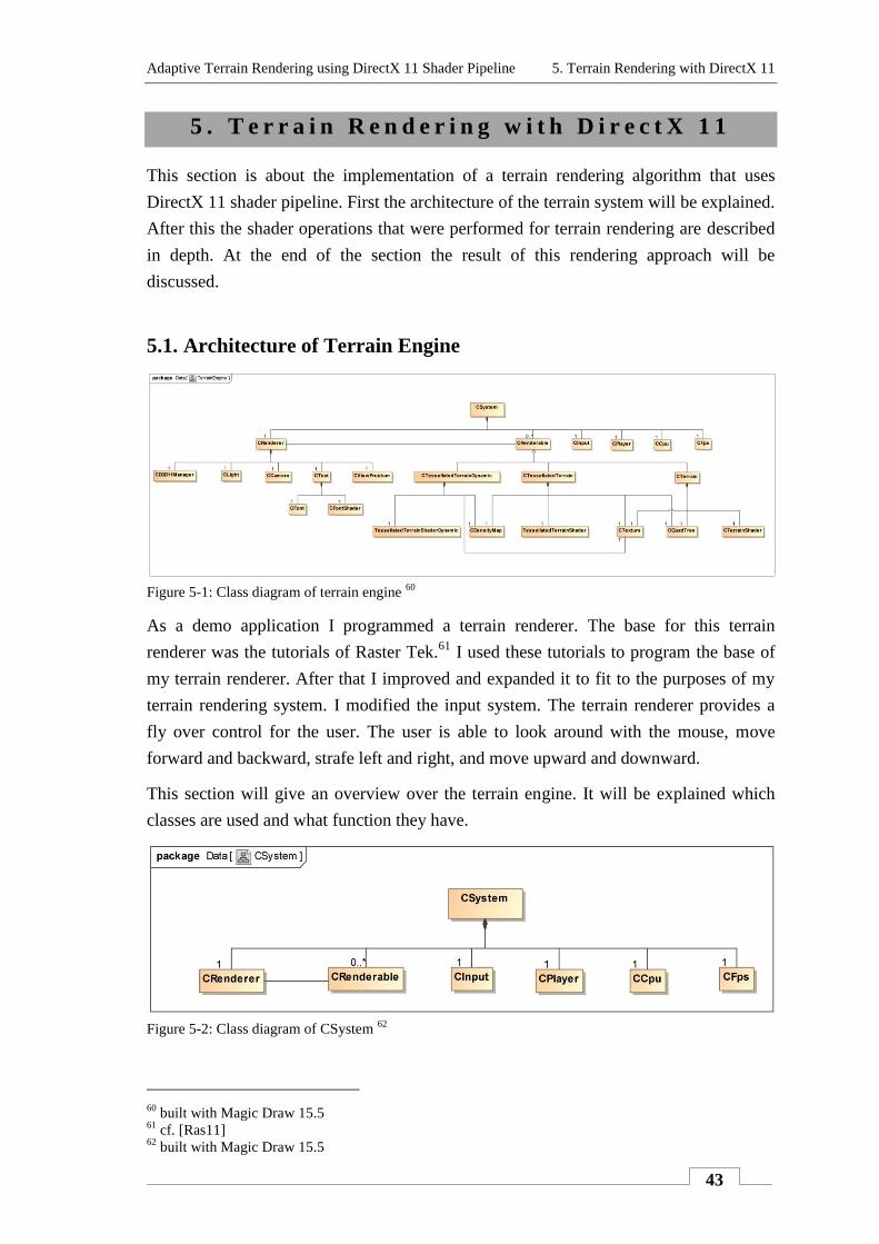
Adaptive Terrain Rendering using DirectX 11 Shader Pipeline 5. Terrain Rendering with DirectX 11
43
5 . T e r r a i n R e n d e r i n g w i t h D i r e c t X 1 1
This section is about the implementation of a terrain rendering algorithm that uses
DirectX 11 shader pipeline. First the architecture of the terrain system will be explained.
After this the shader operations that were performed for terrain rendering are described
in depth. At the end of the section the result of this rendering approach will be
discussed.
5.1. Architecture of Terrain Engine
Figure 5-1: Class diagram of terrain engine
60
As a demo application I programmed a terrain renderer. The base for this terrain
renderer was the tutorials of Raster Tek.61
I used these tutorials to program the base of
my terrain renderer. After that I improved and expanded it to fit to the purposes of my
terrain rendering system. I modified the input system. The terrain renderer provides a
fly over control for the user. The user is able to look around with the mouse, move
forward and backward, strafe left and right, and move upward and downward.
This section will give an overview over the terrain engine. It will be explained which
classes are used and what function they have.
Figure 5-2: Class diagram of CSystem
62
60
built with Magic Draw 15.5 61
cf. [Ras11] 62
built with Magic Draw 15.5
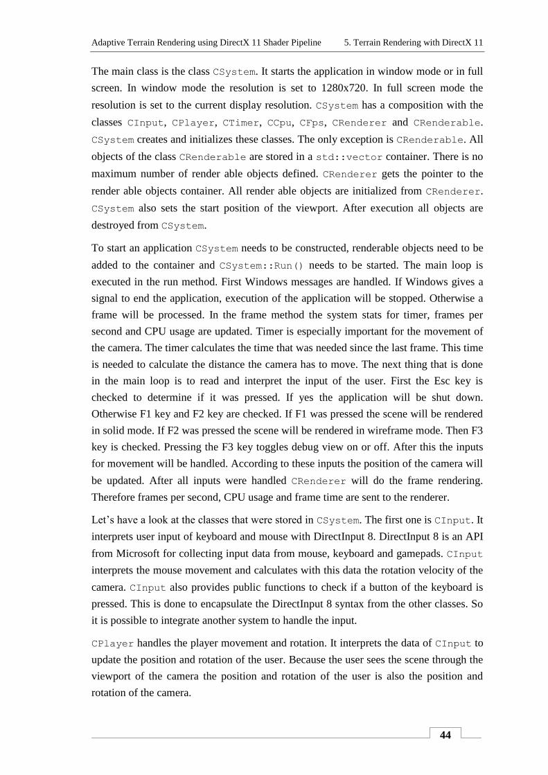
Adaptive Terrain Rendering using DirectX 11 Shader Pipeline 5. Terrain Rendering with DirectX 11
44
The main class is the class CSystem. It starts the application in window mode or in full
screen. In window mode the resolution is set to 1280x720. In full screen mode the
resolution is set to the current display resolution. CSystem has a composition with the
classes CInput, CPlayer, CTimer, CCpu, CFps, CRenderer and CRenderable.
CSystem creates and initializes these classes. The only exception is CRenderable. All
objects of the class CRenderable are stored in a std::vector container. There is no
maximum number of render able objects defined. CRenderer gets the pointer to the
render able objects container. All render able objects are initialized from CRenderer.
CSystem also sets the start position of the viewport. After execution all objects are
destroyed from CSystem.
To start an application CSystem needs to be constructed, renderable objects need to be
added to the container and CSystem::Run() needs to be started. The main loop is
executed in the run method. First Windows messages are handled. If Windows gives a
signal to end the application, execution of the application will be stopped. Otherwise a
frame will be processed. In the frame method the system stats for timer, frames per
second and CPU usage are updated. Timer is especially important for the movement of
the camera. The timer calculates the time that was needed since the last frame. This time
is needed to calculate the distance the camera has to move. The next thing that is done
in the main loop is to read and interpret the input of the user. First the Esc key is
checked to determine if it was pressed. If yes the application will be shut down.
Otherwise F1 key and F2 key are checked. If F1 was pressed the scene will be rendered
in solid mode. If F2 was pressed the scene will be rendered in wireframe mode. Then F3
key is checked. Pressing the F3 key toggles debug view on or off. After this the inputs
for movement will be handled. According to these inputs the position of the camera will
be updated. After all inputs were handled CRenderer will do the frame rendering.
Therefore frames per second, CPU usage and frame time are sent to the renderer.
Let’s have a look at the classes that were stored in CSystem. The first one is CInput. It
interprets user input of keyboard and mouse with DirectInput 8. DirectInput 8 is an API
from Microsoft for collecting input data from mouse, keyboard and gamepads. CInput
interprets the mouse movement and calculates with this data the rotation velocity of the
camera. CInput also provides public functions to check if a button of the keyboard is
pressed. This is done to encapsulate the DirectInput 8 syntax from the other classes. So
it is possible to integrate another system to handle the input.
CPlayer handles the player movement and rotation. It interprets the data of CInput to
update the position and rotation of the user. Because the user sees the scene through the
viewport of the camera the position and rotation of the user is also the position and
rotation of the camera.
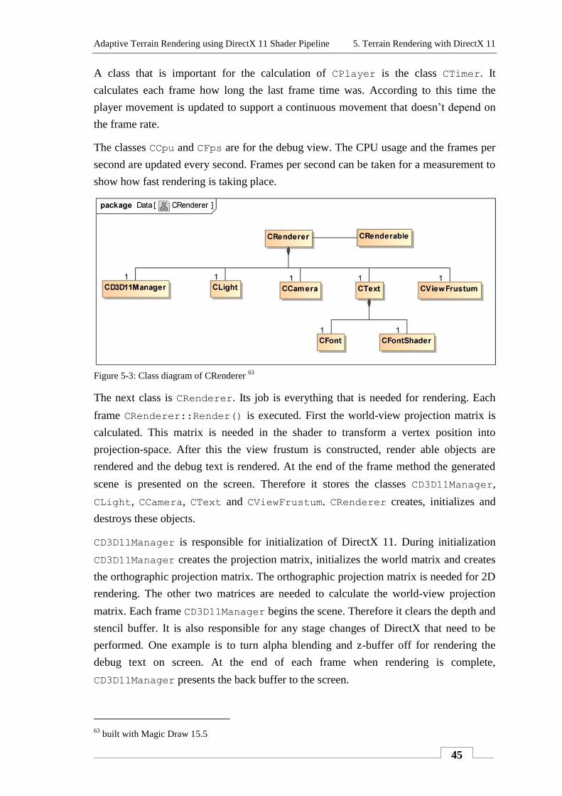
Adaptive Terrain Rendering using DirectX 11 Shader Pipeline 5. Terrain Rendering with DirectX 11
45
A class that is important for the calculation of CPlayer is the class CTimer. It
calculates each frame how long the last frame time was. According to this time the
player movement is updated to support a continuous movement that doesn’t depend on
the frame rate.
The classes CCpu and CFps are for the debug view. The CPU usage and the frames per
second are updated every second. Frames per second can be taken for a measurement to
show how fast rendering is taking place.
Figure 5-3: Class diagram of CRenderer
63
The next class is CRenderer. Its job is everything that is needed for rendering. Each
frame CRenderer::Render() is executed. First the world-view projection matrix is
calculated. This matrix is needed in the shader to transform a vertex position into
projection-space. After this the view frustum is constructed, render able objects are
rendered and the debug text is rendered. At the end of the frame method the generated
scene is presented on the screen. Therefore it stores the classes CD3D11Manager,
CLight, CCamera, CText and CViewFrustum. CRenderer creates, initializes and
destroys these objects.
CD3D11Manager is responsible for initialization of DirectX 11. During initialization
CD3D11Manager creates the projection matrix, initializes the world matrix and creates
the orthographic projection matrix. The orthographic projection matrix is needed for 2D
rendering. The other two matrices are needed to calculate the world-view projection
matrix. Each frame CD3D11Manager begins the scene. Therefore it clears the depth and
stencil buffer. It is also responsible for any stage changes of DirectX that need to be
performed. One example is to turn alpha blending and z-buffer off for rendering the
debug text on screen. At the end of each frame when rendering is complete,
CD3D11Manager presents the back buffer to the screen.
63
built with Magic Draw 15.5
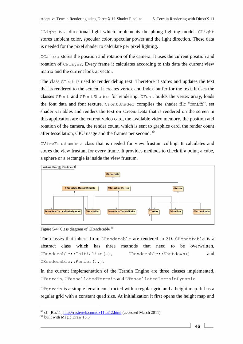
Adaptive Terrain Rendering using DirectX 11 Shader Pipeline 5. Terrain Rendering with DirectX 11
46
CLight is a directional light which implements the phong lighting model. CLight
stores ambient color, specular color, specular power and the light direction. These data
is needed for the pixel shader to calculate per pixel lighting.
CCamera stores the position and rotation of the camera. It uses the current position and
rotation of CPlayer. Every frame it calculates according to this data the current view
matrix and the current look at vector.
The class CText is used to render debug text. Therefore it stores and updates the text
that is rendered to the screen. It creates vertex and index buffer for the text. It uses the
classes CFont and CFontShader for rendering. CFont builds the vertex array, loads
the font data and font texture. CFontShader compiles the shader file “font.fx”, set
shader variables and renders the text on screen. Data that is rendered on the screen in
this application are the current video card, the available video memory, the position and
rotation of the camera, the render count, which is sent to graphics card, the render count
after tessellation, CPU usage and the frames per second. 64
CViewFrustum is a class that is needed for view frustum culling. It calculates and
stores the view frustum for every frame. It provides methods to check if a point, a cube,
a sphere or a rectangle is inside the view frustum.
Figure 5-4: Class diagram of CRenderable
65
The classes that inherit from CRenderable are rendered in 3D. CRenderable is a
abstract class which has three methods that need to be overwritten,
CRenderable::Initialize(…), CRenderable::Shutdown() and
CRenderable::Render(..).
In the current implementation of the Terrain Engine are three classes implemented,
CTerrain, CTessellatedTerrain and CTessellatedTerrainDynamic.
CTerrain is a simple terrain constructed with a regular grid and a height map. It has a
regular grid with a constant quad size. At initialization it first opens the height map and
64
cf. [Ras11] http://rastertek.com/dx11tut12.html (accessed March 2011) 65
built with Magic Draw 15.5
Adaptive Terrain Rendering using DirectX 11 Shader Pipeline 5. Terrain Rendering with DirectX 11
47
reads in the data. According to the height map data a grid is constructed and
corresponding normals and texture coordinates are calculated. It also loads the texture
for terrain. The used primitive is D3D11_PRIMITIVE_TOPOLOGY_TRIANGLELIST.
CTerrain uses three classes CTexture, CQuadTree and CTerrainShader.
CTexture is used to load the texture and create a shader resource view. CQuadTree
uses a quad tree to separate the grid in parts according to a predefined vertex count. For
each child the quad tree creates a vertex buffer and index buffer. Which node of the
quad tree will be rendered is decided on run-time dependent on the view frustum
position. CTerrainShader compiles the corresponding shader file “terrain.fx”. It also
defines the used polygon layout, sets the shader variables and renders the terrain. Data
that is used for each vertex is the position, a texture coordinate and a normal. The
shader variables are the world matrix, the view matrix, the projection matrix, the
world-view projection matrix, the terrain texture, ambient color, diffuse color and light
direction. 66
CTessellatedTerrain and CTessellatedTerrainDynamic use a
view-dependent LOD for tessellation. The refinement of the terrain depends on the
screen resolution, the position of the camera, the shape of the terrain and the desired
triangle size that wants to be achieved. The used domain for tessellation is a triangle.
CTessellatedTerrain creates the grid and calculates the normals on the same way
as CTerrain. CTessellatedTerrain also uses a CQuadTree to separate the grid.
The first thing that is different from CTerrain is that it uses the primitive topology
D3D11_PRIMITIVE_TOPOLOGY_3_CONTROL_POINT_PATCHLIST. This topology is
needed to be able to tessellate the terrain. It uses a triangle as input.
CTessellatedTerrain uses the class CDensityMap to define the tessellation factors
of a triangle. This class calculates a density map according to the height map data. The
density map describes at which places the terrain needs to be refined and at which
places refinement is not needed. Where the height doesn’t change there is a flat surface.
So there is no refinement needed. From the density map a density buffer is created. In
the density buffer for each patch are the tessellation factors stored. This buffer can be
read from the shader to set the tessellation factors. How the density map works in detail
will be explained in section 5.2.3. It is important for the use of the quad tree with this
approach that for each node of the quad tree a density buffer is created.
CTessellatedTerrain uses its own shader class CTessellatedTerrainShader.
This class compiles the shader file “tessellatedterrain.fx”. It sets the same shader
variables as CTerrianShader. Additionally it sets the shader variables which are
needed for tessellation.
66
cf. [Ras11], http://rastertek.com/tutindex.html DirectX 10 Terrain Tutorials (accessed March 2011)
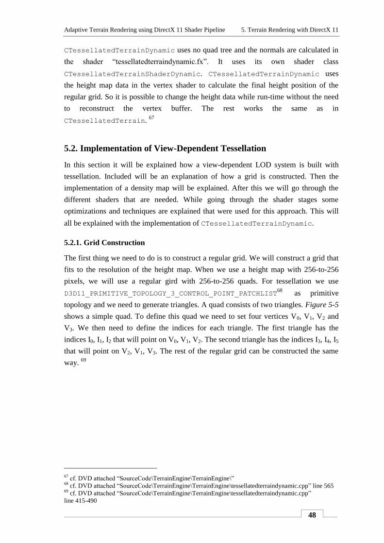
Adaptive Terrain Rendering using DirectX 11 Shader Pipeline 5. Terrain Rendering with DirectX 11
48
CTessellatedTerrainDynamic uses no quad tree and the normals are calculated in
the shader “tessellatedterraindynamic.fx”. It uses its own shader class
CTessellatedTerrainShaderDynamic. CTessellatedTerrainDynamic uses
the height map data in the vertex shader to calculate the final height position of the
regular grid. So it is possible to change the height data while run-time without the need
to reconstruct the vertex buffer. The rest works the same as in
CTessellatedTerrain. 67
5.2. Implementation of View-Dependent Tessellation
In this section it will be explained how a view-dependent LOD system is built with
tessellation. Included will be an explanation of how a grid is constructed. Then the
implementation of a density map will be explained. After this we will go through the
different shaders that are needed. While going through the shader stages some
optimizations and techniques are explained that were used for this approach. This will
all be explained with the implementation of CTessellatedTerrainDynamic.
5.2.1. Grid Construction
The first thing we need to do is to construct a regular grid. We will construct a grid that
fits to the resolution of the height map. When we use a height map with 256-to-256
pixels, we will use a regular gird with 256-to-256 quads. For tessellation we use
D3D11_PRIMITIVE_TOPOLOGY_3_CONTROL_POINT_PATCHLIST68 as primitive
topology and we need to generate triangles. A quad consists of two triangles. Figure 5-5
shows a simple quad. To define this quad we need to set four vertices V0, V1, V2 and
V3. We then need to define the indices for each triangle. The first triangle has the
indices I0, I1, I2 that will point on V0, V1, V2. The second triangle has the indices I3, I4, I5
that will point on V2, V1, V3. The rest of the regular grid can be constructed the same
way. 69
67
cf. DVD attached “SourceCode\TerrainEngine\TerrainEngine\” 68
cf. DVD attached “SourceCode\TerrainEngine\TerrainEngine\tessellatedterraindynamic.cpp” line 565 69
cf. DVD attached “SourceCode\TerrainEngine\TerrainEngine\tessellatedterraindynamic.cpp”
line 415-490
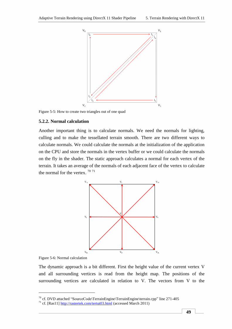
Adaptive Terrain Rendering using DirectX 11 Shader Pipeline 5. Terrain Rendering with DirectX 11
49
Figure 5-5: How to create two triangles out of one quad
5.2.2. Normal calculation
Another important thing is to calculate normals. We need the normals for lighting,
culling and to make the tessellated terrain smooth. There are two different ways to
calculate normals. We could calculate the normals at the initialization of the application
on the CPU and store the normals in the vertex buffer or we could calculate the normals
on the fly in the shader. The static approach calculates a normal for each vertex of the
terrain. It takes an average of the normals of each adjacent face of the vertex to calculate
the normal for the vertex. 70
71
Figure 5-6: Normal calculation
The dynamic approach is a bit different. First the height value of the current vertex V
and all surrounding vertices is read from the height map. The positions of the
surrounding vertices are calculated in relation to V. The vectors from V to the
70
cf. DVD attached “SourceCode\TerrainEngine\TerrainEngine\terrain.cpp” line 271-405 71
cf. [Ras11] http://rastertek.com/tertut03.html (accessed March 2011)
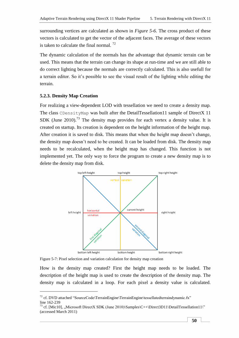
Adaptive Terrain Rendering using DirectX 11 Shader Pipeline 5. Terrain Rendering with DirectX 11
50
surrounding vertices are calculated as shown in Figure 5-6. The cross product of these
vectors is calculated to get the vector of the adjacent faces. The average of these vectors
is taken to calculate the final normal. 72
The dynamic calculation of the normals has the advantage that dynamic terrain can be
used. This means that the terrain can change its shape at run-time and we are still able to
do correct lighting because the normals are correctly calculated. This is also usefull for
a terrain editor. So it’s possible to see the visual result of the lighting while editing the
terrain.
5.2.3. Density Map Creation
For realizing a view-dependent LOD with tessellation we need to create a density map.
The class CDensityMap was built after the DetailTessellation11 sample of DirectX 11
SDK (June 2010).73
The density map provides for each vertex a density value. It is
created on startup. Its creation is dependent on the height information of the height map.
After creation it is saved to disk. This means that when the height map doesn’t change,
the density map doesn’t need to be created. It can be loaded from disk. The density map
needs to be recalculated, when the height map has changed. This function is not
implemented yet. The only way to force the program to create a new density map is to
delete the density map from disk.
Figure 5-7: Pixel selection and variation calculation for density map creation
How is the density map created? First the height map needs to be loaded. The
description of the height map is used to create the description of the density map. The
density map is calculated in a loop. For each pixel a density value is calculated.
72
cf. DVD attached “SourceCode\TerrainEngine\TerrainEngine\tessellatedterraindynamic.fx”
line 162-239 73
cf. [Mic10], „Microsoft DirectX SDK (June 2010)\Samples\C++\Direct3D11\DetailTessellation11\”
(accessed March 2011)
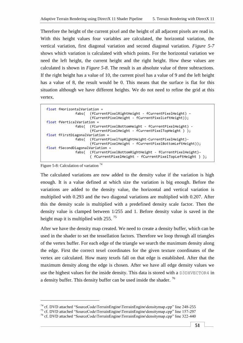
Adaptive Terrain Rendering using DirectX 11 Shader Pipeline 5. Terrain Rendering with DirectX 11
51
Therefore the height of the current pixel and the height of all adjacent pixels are read in.
With this height values four variables are calculated, the horizontal variation, the
vertical variation, first diagonal variation and second diagonal variation. Figure 5-7
shows which variation is calculated with which points. For the horizontal variation we
need the left height, the current height and the right height. How these values are
calculated is shown in Figure 5-8. The result is an absolute value of three subtractions.
If the right height has a value of 10, the current pixel has a value of 9 and the left height
has a value of 8, the result would be 0. This means that the surface is flat for this
situation although we have different heights. We do not need to refine the grid at this
vertex.
float fHorizontalVariation = fabs( (fCurrentPixelRightHeight - fCurrentPixelHeight) –
(fCurrentPixelHeight - fCurrentPixelLeftHeight)); float fVerticalVariation =
fabs( (fCurrentPixelBottomHeight - fCurrentPixelHeight) - (fCurrentPixelHeight - fCurrentPixelTopHeight ) );
float fFirstDiagonalVariation = fabs( (fCurrentPixelTopRightHeight-CurrentPixelHeight)-
(fCurrentPixelHeight - fCurrentPixelBottomLeftHeight)); float fSecondDiagonalVariation =
fabs( (fCurrentPixelBottomRightHeight - fCurrentPixelHeight)– ( fCurrentPixelHeight - fCurrentPixelTopLeftHeight ) );
Figure 5-8: Calculation of variation 74
The calculated variations are now added to the density value if the variation is high
enough. It is a value defined at which size the variation is big enough. Before the
variations are added to the density value, the horizontal and vertical variation is
multiplied with 0.293 and the two diagonal variations are multiplied with 0.207. After
this the density scale is multiplied with a predefined density scale factor. Then the
density value is clamped between 1/255 and 1. Before density value is saved in the
height map it is multiplied with 255. 75
After we have the density map created. We need to create a density buffer, which can be
used in the shader to set the tessellation factors. Therefore we loop through all triangles
of the vertex buffer. For each edge of the triangle we search the maximum density along
the edge. First the correct texel coordinates for the given texture coordinates of the
vertex are calculated. How many texels fall on that edge is established. After that the
maximum density along the edge is chosen. After we have all edge density values we
use the highest values for the inside density. This data is stored with a D3DXVECTOR4 in
a density buffer. This density buffer can be used inside the shader. 76
74
cf. DVD attached “SourceCode\TerrainEngine\TerrainEngine\densitymap.cpp” line 248-255 75
cf. DVD attached “SourceCode\TerrainEngine\TerrainEngine\densitymap.cpp” line 157-297 76
cf. DVD attached “SourceCode\TerrainEngine\TerrainEngine\densitymap.cpp” line 322-440
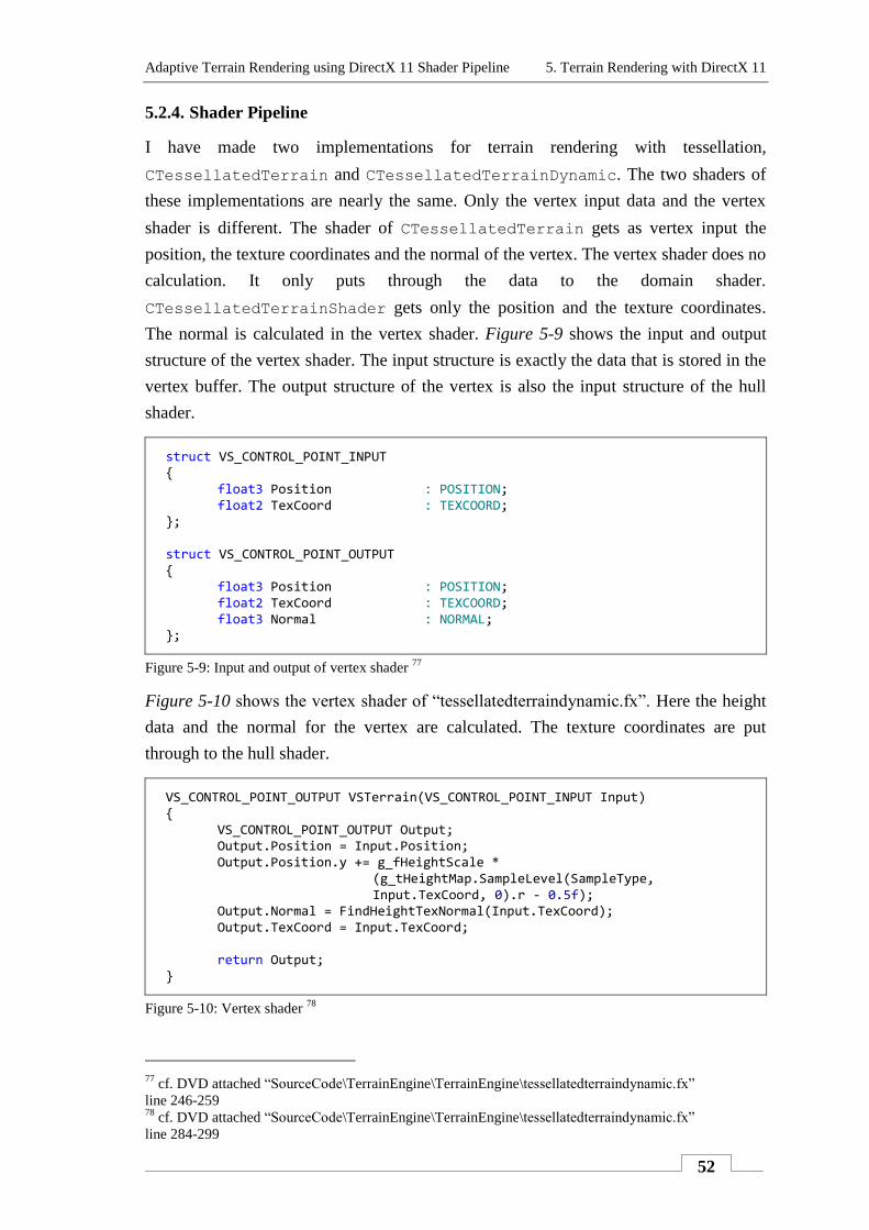
Adaptive Terrain Rendering using DirectX 11 Shader Pipeline 5. Terrain Rendering with DirectX 11
52
5.2.4. Shader Pipeline
I have made two implementations for terrain rendering with tessellation,
CTessellatedTerrain and CTessellatedTerrainDynamic. The two shaders of
these implementations are nearly the same. Only the vertex input data and the vertex
shader is different. The shader of CTessellatedTerrain gets as vertex input the
position, the texture coordinates and the normal of the vertex. The vertex shader does no
calculation. It only puts through the data to the domain shader.
CTessellatedTerrainShader gets only the position and the texture coordinates.
The normal is calculated in the vertex shader. Figure 5-9 shows the input and output
structure of the vertex shader. The input structure is exactly the data that is stored in the
vertex buffer. The output structure of the vertex is also the input structure of the hull
shader.
struct VS_CONTROL_POINT_INPUT { float3 Position : POSITION; float2 TexCoord : TEXCOORD; }; struct VS_CONTROL_POINT_OUTPUT { float3 Position : POSITION; float2 TexCoord : TEXCOORD; float3 Normal : NORMAL; };
Figure 5-9: Input and output of vertex shader 77
Figure 5-10 shows the vertex shader of “tessellatedterraindynamic.fx”. Here the height
data and the normal for the vertex are calculated. The texture coordinates are put
through to the hull shader.
VS_CONTROL_POINT_OUTPUT VSTerrain(VS_CONTROL_POINT_INPUT Input) { VS_CONTROL_POINT_OUTPUT Output; Output.Position = Input.Position; Output.Position.y += g_fHeightScale * (g_tHeightMap.SampleLevel(SampleType, Input.TexCoord, 0).r - 0.5f); Output.Normal = FindHeightTexNormal(Input.TexCoord); Output.TexCoord = Input.TexCoord; return Output; }
Figure 5-10: Vertex shader 78
77
cf. DVD attached “SourceCode\TerrainEngine\TerrainEngine\tessellatedterraindynamic.fx”
line 246-259 78
cf. DVD attached “SourceCode\TerrainEngine\TerrainEngine\tessellatedterraindynamic.fx”
line 284-299
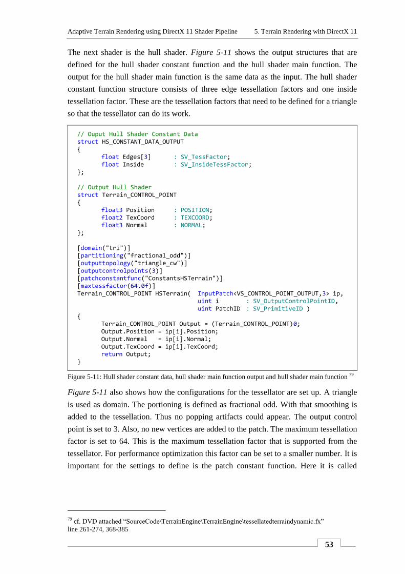
Adaptive Terrain Rendering using DirectX 11 Shader Pipeline 5. Terrain Rendering with DirectX 11
53
The next shader is the hull shader. Figure 5-11 shows the output structures that are
defined for the hull shader constant function and the hull shader main function. The
output for the hull shader main function is the same data as the input. The hull shader
constant function structure consists of three edge tessellation factors and one inside
tessellation factor. These are the tessellation factors that need to be defined for a triangle
so that the tessellator can do its work.
// Ouput Hull Shader Constant Data struct HS_CONSTANT_DATA_OUTPUT { float Edges[3] : SV_TessFactor; float Inside : SV_InsideTessFactor; }; // Output Hull Shader struct Terrain_CONTROL_POINT { float3 Position : POSITION; float2 TexCoord : TEXCOORD; float3 Normal : NORMAL; }; [domain("tri")] [partitioning("fractional_odd")] [outputtopology("triangle_cw")] [outputcontrolpoints(3)] [patchconstantfunc("ConstantsHSTerrain")] [maxtessfactor(64.0f)] Terrain_CONTROL_POINT HSTerrain( InputPatch<VS_CONTROL_POINT_OUTPUT,3> ip, uint i : SV_OutputControlPointID, uint PatchID : SV_PrimitiveID ) { Terrain_CONTROL_POINT Output = (Terrain_CONTROL_POINT)0; Output.Position = ip[i].Position; Output.Normal = ip[i].Normal; Output.TexCoord = ip[i].TexCoord; return Output; }
Figure 5-11: Hull shader constant data, hull shader main function output and hull shader main function 79
Figure 5-11 also shows how the configurations for the tessellator are set up. A triangle
is used as domain. The portioning is defined as fractional odd. With that smoothing is
added to the tessellation. Thus no popping artifacts could appear. The output control
point is set to 3. Also, no new vertices are added to the patch. The maximum tessellation
factor is set to 64. This is the maximum tessellation factor that is supported from the
tessellator. For performance optimization this factor can be set to a smaller number. It is
important for the settings to define is the patch constant function. Here it is called
79
cf. DVD attached “SourceCode\TerrainEngine\TerrainEngine\tessellatedterraindynamic.fx”
line 261-274, 368-385
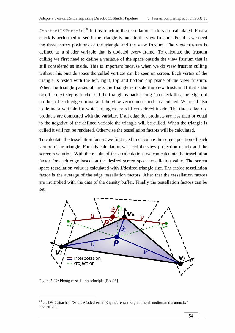
Adaptive Terrain Rendering using DirectX 11 Shader Pipeline 5. Terrain Rendering with DirectX 11
54
ConstantHSTerrain.80
In this function the tessellation factors are calculated. First a
check is performed to see if the triangle is outside the view frustum. For this we need
the three vertex positions of the triangle and the view frustum. The view frustum is
defined as a shader variable that is updated every frame. To calculate the frustum
culling we first need to define a variable of the space outside the view frustum that is
still considered as inside. This is important because when we do view frustum culling
without this outside space the culled vertices can be seen on screen. Each vertex of the
triangle is tested with the left, right, top and bottom clip plane of the view frustum.
When the triangle passes all tests the triangle is inside the view frustum. If that’s the
case the next step is to check if the triangle is back facing. To check this, the edge dot
product of each edge normal and the view vector needs to be calculated. We need also
to define a variable for which triangles are still considered inside. The three edge dot
products are compared with the variable. If all edge dot products are less than or equal
to the negative of the defined variable the triangle will be culled. When the triangle is
culled it will not be rendered. Otherwise the tessellation factors will be calculated.
To calculate the tessellation factors we first need to calculate the screen position of each
vertex of the triangle. For this calculation we need the view-projection matrix and the
screen resolution. With the results of these calculations we can calculate the tessellation
factor for each edge based on the desired screen space tessellation value. The screen
space tessellation value is calculated with 1/desired triangle size. The inside tessellation
factor is the average of the edge tessellation factors. After that the tessellation factors
are multiplied with the data of the density buffer. Finally the tessellation factors can be
set.
Figure 5-12: Phong tessellation principle [Bou08]
80
cf. DVD attached “SourceCode\TerrainEngine\TerrainEngine\tessellatedterraindynamic.fx”
line 301-365
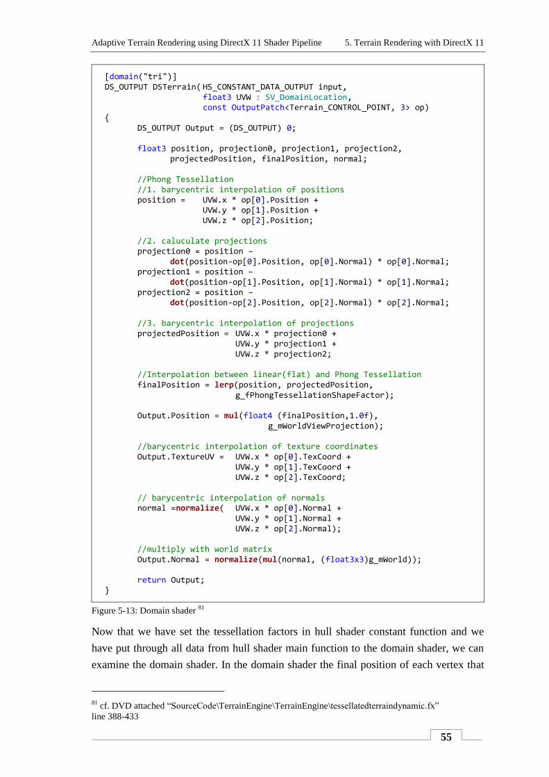
Adaptive Terrain Rendering using DirectX 11 Shader Pipeline 5. Terrain Rendering with DirectX 11
55
[domain("tri")] DS_OUTPUT DSTerrain( HS_CONSTANT_DATA_OUTPUT input, float3 UVW : SV_DomainLocation, const OutputPatch<Terrain_CONTROL_POINT, 3> op) { DS_OUTPUT Output = (DS_OUTPUT) 0; float3 position, projection0, projection1, projection2, projectedPosition, finalPosition, normal; //Phong Tessellation //1. barycentric interpolation of positions position = UVW.x * op[0].Position + UVW.y * op[1].Position + UVW.z * op[2].Position; //2. caluculate projections projection0 = position – dot(position-op[0].Position, op[0].Normal) * op[0].Normal; projection1 = position – dot(position-op[1].Position, op[1].Normal) * op[1].Normal; projection2 = position – dot(position-op[2].Position, op[2].Normal) * op[2].Normal; //3. barycentric interpolation of projections projectedPosition = UVW.x * projection0 + UVW.y * projection1 + UVW.z * projection2; //Interpolation between linear(flat) and Phong Tessellation finalPosition = lerp(position, projectedPosition, g_fPhongTessellationShapeFactor); Output.Position = mul(float4 (finalPosition,1.0f), g_mWorldViewProjection); //barycentric interpolation of texture coordinates Output.TextureUV = UVW.x * op[0].TexCoord + UVW.y * op[1].TexCoord + UVW.z * op[2].TexCoord; // barycentric interpolation of normals normal =normalize( UVW.x * op[0].Normal + UVW.y * op[1].Normal + UVW.z * op[2].Normal); //multiply with world matrix Output.Normal = normalize(mul(normal, (float3x3)g_mWorld)); return Output; }
Figure 5-13: Domain shader 81
Now that we have set the tessellation factors in hull shader constant function and we
have put through all data from hull shader main function to the domain shader, we can
examine the domain shader. In the domain shader the final position of each vertex that
81
cf. DVD attached “SourceCode\TerrainEngine\TerrainEngine\tessellatedterraindynamic.fx”
line 388-433
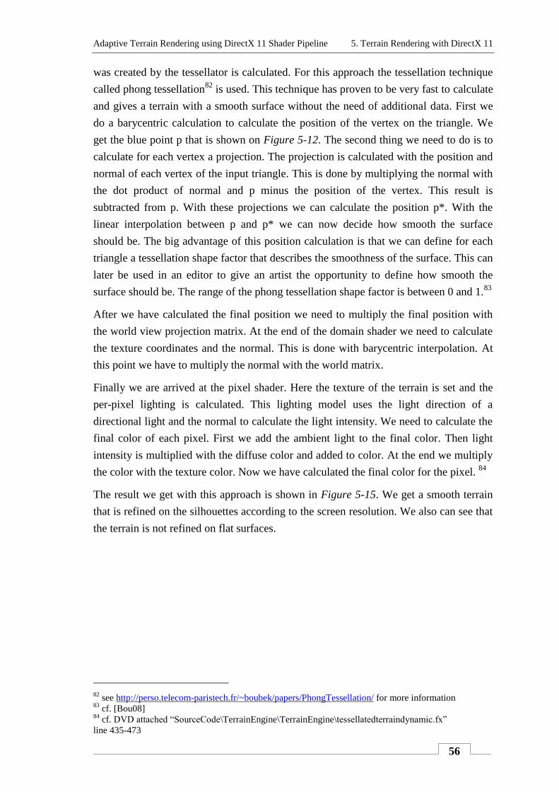
Adaptive Terrain Rendering using DirectX 11 Shader Pipeline 5. Terrain Rendering with DirectX 11
56
was created by the tessellator is calculated. For this approach the tessellation technique
called phong tessellation82
is used. This technique has proven to be very fast to calculate
and gives a terrain with a smooth surface without the need of additional data. First we
do a barycentric calculation to calculate the position of the vertex on the triangle. We
get the blue point p that is shown on Figure 5-12. The second thing we need to do is to
calculate for each vertex a projection. The projection is calculated with the position and
normal of each vertex of the input triangle. This is done by multiplying the normal with
the dot product of normal and p minus the position of the vertex. This result is
subtracted from p. With these projections we can calculate the position p*. With the
linear interpolation between p and p* we can now decide how smooth the surface
should be. The big advantage of this position calculation is that we can define for each
triangle a tessellation shape factor that describes the smoothness of the surface. This can
later be used in an editor to give an artist the opportunity to define how smooth the
surface should be. The range of the phong tessellation shape factor is between 0 and 1.83
After we have calculated the final position we need to multiply the final position with
the world view projection matrix. At the end of the domain shader we need to calculate
the texture coordinates and the normal. This is done with barycentric interpolation. At
this point we have to multiply the normal with the world matrix.
Finally we are arrived at the pixel shader. Here the texture of the terrain is set and the
per-pixel lighting is calculated. This lighting model uses the light direction of a
directional light and the normal to calculate the light intensity. We need to calculate the
final color of each pixel. First we add the ambient light to the final color. Then light
intensity is multiplied with the diffuse color and added to color. At the end we multiply
the color with the texture color. Now we have calculated the final color for the pixel. 84
The result we get with this approach is shown in Figure 5-15. We get a smooth terrain
that is refined on the silhouettes according to the screen resolution. We also can see that
the terrain is not refined on flat surfaces.
82
see http://perso.telecom-paristech.fr/~boubek/papers/PhongTessellation/ for more information 83
cf. [Bou08] 84
cf. DVD attached “SourceCode\TerrainEngine\TerrainEngine\tessellatedterraindynamic.fx”
line 435-473
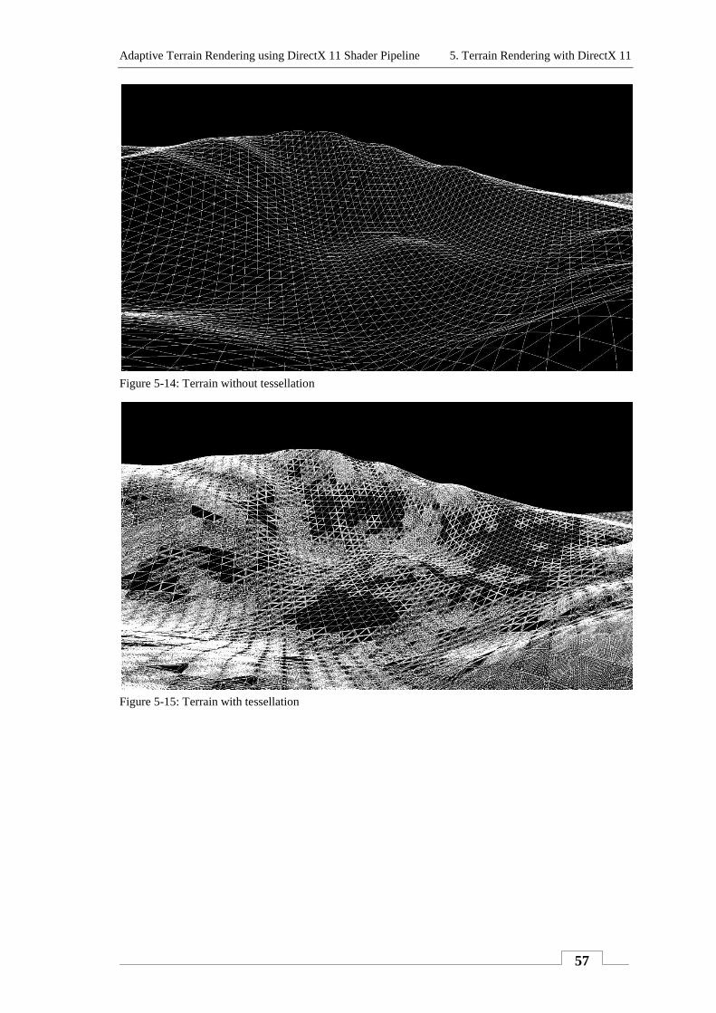
Adaptive Terrain Rendering using DirectX 11 Shader Pipeline 5. Terrain Rendering with DirectX 11
57
Figure 5-14: Terrain without tessellation
Figure 5-15: Terrain with tessellation
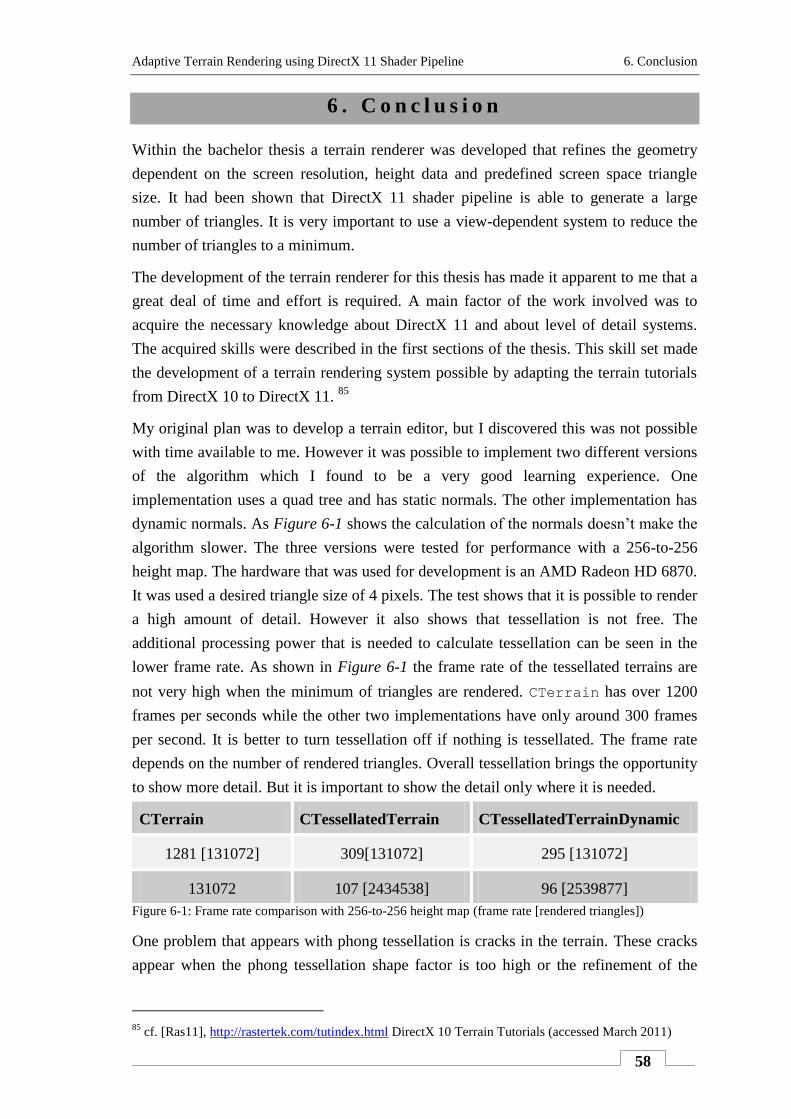
Adaptive Terrain Rendering using DirectX 11 Shader Pipeline 6. Conclusion
58
6 . C o n c l u s i o n
Within the bachelor thesis a terrain renderer was developed that refines the geometry
dependent on the screen resolution, height data and predefined screen space triangle
size. It had been shown that DirectX 11 shader pipeline is able to generate a large
number of triangles. It is very important to use a view-dependent system to reduce the
number of triangles to a minimum.
The development of the terrain renderer for this thesis has made it apparent to me that a
great deal of time and effort is required. A main factor of the work involved was to
acquire the necessary knowledge about DirectX 11 and about level of detail systems.
The acquired skills were described in the first sections of the thesis. This skill set made
the development of a terrain rendering system possible by adapting the terrain tutorials
from DirectX 10 to DirectX 11. 85
My original plan was to develop a terrain editor, but I discovered this was not possible
with time available to me. However it was possible to implement two different versions
of the algorithm which I found to be a very good learning experience. One
implementation uses a quad tree and has static normals. The other implementation has
dynamic normals. As Figure 6-1 shows the calculation of the normals doesn’t make the
algorithm slower. The three versions were tested for performance with a 256-to-256
height map. The hardware that was used for development is an AMD Radeon HD 6870.
It was used a desired triangle size of 4 pixels. The test shows that it is possible to render
a high amount of detail. However it also shows that tessellation is not free. The
additional processing power that is needed to calculate tessellation can be seen in the
lower frame rate. As shown in Figure 6-1 the frame rate of the tessellated terrains are
not very high when the minimum of triangles are rendered. CTerrain has over 1200
frames per seconds while the other two implementations have only around 300 frames
per second. It is better to turn tessellation off if nothing is tessellated. The frame rate
depends on the number of rendered triangles. Overall tessellation brings the opportunity
to show more detail. But it is important to show the detail only where it is needed.
CTerrain CTessellatedTerrain CTessellatedTerrainDynamic
1281 [131072] 309[131072] 295 [131072]
131072 107 [2434538] 96 [2539877]
Figure 6-1: Frame rate comparison with 256-to-256 height map (frame rate [rendered triangles])
One problem that appears with phong tessellation is cracks in the terrain. These cracks
appear when the phong tessellation shape factor is too high or the refinement of the
85
cf. [Ras11], http://rastertek.com/tutindex.html DirectX 10 Terrain Tutorials (accessed March 2011)
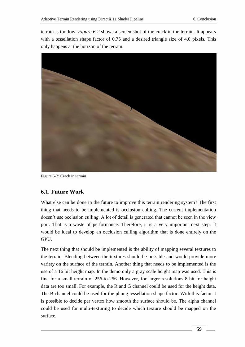
Adaptive Terrain Rendering using DirectX 11 Shader Pipeline 6. Conclusion
59
terrain is too low. Figure 6-2 shows a screen shot of the crack in the terrain. It appears
with a tessellation shape factor of 0.75 and a desired triangle size of 4.0 pixels. This
only happens at the horizon of the terrain.
Figure 6-2: Crack in terrain
6.1. Future Work
What else can be done in the future to improve this terrain rendering system? The first
thing that needs to be implemented is occlusion culling. The current implementation
doesn’t use occlusion culling. A lot of detail is generated that cannot be seen in the view
port. That is a waste of performance. Therefore, it is a very important next step. It
would be ideal to develop an occlusion culling algorithm that is done entirely on the
GPU.
The next thing that should be implemented is the ability of mapping several textures to
the terrain. Blending between the textures should be possible and would provide more
variety on the surface of the terrain. Another thing that needs to be implemented is the
use of a 16 bit height map. In the demo only a gray scale height map was used. This is
fine for a small terrain of 256-to-256. However, for larger resolutions 8 bit for height
data are too small. For example, the R and G channel could be used for the height data.
The B channel could be used for the phong tessellation shape factor. With this factor it
is possible to decide per vertex how smooth the surface should be. The alpha channel
could be used for multi-texturing to decide which texture should be mapped on the
surface.
Adaptive Terrain Rendering using DirectX 11 Shader Pipeline 6. Conclusion
60
To provide a fine-grained detail displacement maps should be supported. Displacement
maps could provide the textures of the terrain with geometry detail. In this way, it
would be possible to adapt the geometry to the texture. In a displacement map a normal
and height is stored for each texel. The problem of supporting displacement maps is the
change of density of the surface. It needs to be explored how the density data of the
height map and the density data of the displacement map can be combined to calculate
the correct density map. An additional problem is that the transition between different
displacement maps needs to be handled to avoid cracks and holes in the terrain.
Another way to add detail to the terrain is to make use of generation of detail with a
noise function. The detail is generated on the fly and needs no additional data. This
approach works well in a distance-dependent LOD system that has constant vertex
count. In a view-dependent approach this is more difficult because the density map
needs to be adapted according to the generated noise.
To support a good visual quality it is also important to provide a good lighting. The
lighting of the demo is not sufficiently detailed. It only simulates indirect lighting with a
constant ambient light factor. A better lighting model would significantly improve the
visual quality.
To provide the ability to walk over the terrain it is important to have a collision
detection system or a physics engine. One example for an integration of a physics
engine would be to integrate the Havok Physics.86
The engine can be integrated at no
charge for non-commercial use. The base regular grid could be taken as collision
volume. This provides a fast calculation. Of course it could lead to overlapping
geometry when the refined terrain differs too much from the base grid. If the error is too
large it could also be used a regular grid as collision volume with a higher resolution
than the base grid.
For the implementation of an editor it would be helpful to first create a height map with
a graphic editor. In the graphic editor an artist can paint a height map. At the same time
the artist should be able to see the result of the painted height map in a 3D view.
Additionally different noise functions should be supported to be able to model detail
quickly. The height should also be changeable in the 3D view. It should be possible to
point at the position where the height of the terrain needs to be changed. By clicking
Ctrl and left mouse button it should be possible to raise the terrain. By clicking Ctrl and
right mouse button it should be possible to lower the terrain. Flat surfaces should be
easy to model. Therefore the artist should be able to define a constant height. This
height should be set on all places of the terrain that the artist has defined. A function to
86
see http://www.havok.com/index.php?page=havok-physics for product information (accessed March
2011)

Adaptive Terrain Rendering using DirectX 11 Shader Pipeline 6. Conclusion
61
smooth the terrain heights is needed as well. This function could be combined with the
phong tessellation shape factor. It should also be possible for the artist to manipulate the
density map. The artist can decide which parts of the terrain need a higher density.
Finally it should also be provided a button to generate a new density map for the current
height map.
In conclusion there is still much to be done to improve this terrain rendering system.
However, it does show that today it is possible to render fine-grained detail on current
hardware and support at the same time a view-dependent LOD system. The biggest
challenge for the future will be to support a view-dependent LOD system and still
provide a constant frame rate. Distance-dependent LODs can easily provide a constant
frame rate. But these LODs lack of the ability to show detailed silhouettes of the terrain
that are distant. So for a finer detail that is also depended on the screen resolution it will
be no alternative for view-dependent LOD.
While working on the thesis I learned a lot about terrain rendering. I also discovered I
would benefit from a better understanding of terrain editors and how they work.
Definitely the skills I acquired in the process of researching and writing this thesis will
be important for my future work or for continuing my studies. I did not achieve my
original target because I underestimated the amount of time and work involved to learn
DirectX 11 fully, and to develop both a terrain rendering system and an editor.
Adaptive Terrain Rendering using DirectX 11 Shader Pipeline References
62
R e f e r e n c e s
[Vir10] „Virtual Terrain Project“
http://www.vterrain.org/ (accessed March 2010)
[Ras11] „Raster Tek.“
http://rastertek.com/ (accessed March 2011)
[AMD09] AMD, Inc. „Direct3D 9 Tessellation Samples - Tutorial.“ 2009.
http://developer.amd.com/media/gpu_assets/TessellationTutorial-
v1.16.zip (accessed March 2011)
[Asi05] Asirvatham, A. & Hoppe, H. „Terrain Rendering Using GPU-Based
Geometry Clipmaps.“ March 2005.
http://research.microsoft.com/en-us/um/people/hoppe/gpugcm.pdf
(accessed March 2011)
[Bou08] „Phong Tessellation Paper.“ Herausgeber Tamy Boubekeur & Marc
Alexa. 2008.
http://perso.telecom-paristech.fr/~boubek/papers/PhongTessellation/PhongTessellation.pdf
(accessed March 2011)
[Cry08] Crytek „CryENGINE® 2 Manuals“ 2008.
http://doc.crymod.com/ (accessed March 2011)
[Duc97] Duchaineau, M. , Wolinsky, M. , Sigeti, D. , Miller, M. C. , Aldrich,
C. & Mineev-Weinstein, M. B. „ROAMing Terrain: Real-time
Optimally Adpating Meshes.“ October 19, 1997.
http://www.llnl.gov/graphics/ROAM/roam.pdf (accessed March 2011)
[Gar95] Garland, M. & Heckbert, P. S. „Fast Polygonal Approximation of
Terrains and Height Fields.“ Septembre 1995.
http://mgarland.org/files/papers/scape.pdf (accessed March 2011)
[HeY00] He, Y. „Real-Time Visualization of Dynamic Terrain for Ground Vehicle
Simulation.“ December 2000.
http://citeseerx.ist.psu.edu/viewdoc/download?doi=10.1.1.112.9272&rep
=rep1&type=pdf (accessed March 2011)
[Hex10] Hexadecimal, „D3D11 tessellation, in depth“ GPU Experiments Blog.
February 6, 2010.
http://gpuexperiments.blogspot.com/2010/02/d3d11-tessellation-in-
depth.html (accessed March 2011)
Adaptive Terrain Rendering using DirectX 11 Shader Pipeline References
63
[Hop961] Hoppe, H. „Progressive Meshes SIGGRAPH Presentation.“ 1996.
http://research.microsoft.com/en-us/um/people/hoppe/pm.ppt (accessed
March 2011)
[Hop96] Hoppe, H. „Pogressive Meshes Paper.“ 1996.
http://research.microsoft.com/en-us/um/people/hoppe/pm.pdf (accessed
March 2011)
[Hop97] Hoppe, H. „View-Dependent Refinement of Progressive Meshes Paper.“
1997.
http://research.microsoft.com/en-us/um/people/hoppe/vdrpm.pdf
(accessed March 2011)
[Hop971] Hoppe, H. „View-Dependent Refinement of Progressive Meshes
SIGGRAPH Presentation.“ 1997.
http://research.microsoft.com/en-us/um/people/hoppe/vdrpm.ppt
(accessed March 2011)
[Hop98] Hoppe, H. „Smooth View-Dependent Level-of-Detail Control and its
Application to Terrain Rendering Paper.“ 1998.
http://research.microsoft.com/en-us/um/people/hoppe/svdlod.pdf
(accessed March 2011)
[Hop981] Hoppe, H. „Smooth View-Dependent Level-of-Detail Control and its
Application to Terrain Rendering Presentation.“ 1998.
http://research.microsoft.com/en-us/um/people/hoppe/svdlod.ppt
(accessed March 2011)
[Jef09] Jeffers, J „Detailed flow through the Direct3D 11 Pipeline“ March 21,
2009.
http://www.gamedev.net/blog/272/entry-1917722-detailed-flow-through-
the-direct3d-11-pipeline/ (accessed March 2011)
[Lee09] Lee, M. „GDC 2009: Direct3D 11 Tessellation Deep Dive.“ 2009.
http://www.microsoft.com/downloads/en/confirmation.aspx?FamilyID=E
D3C85F3-CBE5-4BCA-B594-606914741884&%3Bdisplaylang=en
(accessed March 2011)
[Los04] Losasso, F. & Hoppe, H. „Geometry Clipmaps: Terrain Rendering
Using Nested Regular Grids Paper.“ 2004.
http://research.microsoft.com/en-us/um/people/hoppe/geomclipmap.pdf
(accessed March 2011)
Adaptive Terrain Rendering using DirectX 11 Shader Pipeline References
64
[Los041] Losasso, F. & Hoppe, H. „Geometry Clipmaps: Terrain Rendering
Using Nested Regular Grids Presentation.“ 2004.
http://research.microsoft.com/en-us/um/people/hoppe/geomclipmap.ppt
(accessed March 2011)
[Lue031] Luebke, D. „Level of Detail Management for Games - View-Dependent
LOD.“ 2003.
http://lodbook.com/course/2003/Luebke_ViewDepSimp.ppt (accessed
March 2011)
[Lue03] Luebke, David , Reddy, Martin , Cohen, Jonathan D. , Varshney,
Amitabh , Watson, Benjamin & Huebner, Robert „Level of Detail for
3D Graphics.“ San Fransisco, Morgan Kaufmann Publishers, 2003. ISBN
1-55860-838-9
[Mic11] Microsoft „MSDN - Windows DirectX Graphic Documentation“
http://msdn.microsoft.com/de-
de/library/ee663301%28v=VS.85%29.aspx (accessed March 2011)
[Mic10] Microsoft „DirectX Software Development Kit June 2010.“ June 2010.
http://www.microsoft.com/downloads/en/details.aspx?displaylang=en&F
amilyID=3021d52b-514e-41d3-ad02-438a3ba730ba (accessed March
2011)
[NiT09] Ni, T. „SIGGRAPH 2009: Efficient Substitutes for Subdivision Surfaces -
Implementation.“ August 5, 2009.
http://www.nitianyun.com/TianyunNi_ch4.pdf (accessed March 2011)
[Red03] Reddy, M. „Level of Detail Management for 3D Games - Run-Time
Management for LOD.“ 2003.
http://lodbook.com/course/2003/Reddy_RunTime.ppt (accessed March
2011)
[Sch06] Scherfgen, David „3D-Spieleprogrammierung mit DirectX9 und C++ 3.
aktualiserte Auflage.“ München, Carl Hanser Verlag, 2006. ISBN 978-3-
446-40596-7
[Tur00] Turner, B. „Real-Time Dynamic Level of Detail Terrain Rendering with
ROAM.“ April 3, 2000.
http://www.gamasutra.com/view/feature/3188/realtime_dynamic_level_o
f_detail_.php?page=1 (accessed March 2011)
Adaptive Terrain Rendering using DirectX 11 Shader Pipeline References
65
[Val101] Valdetaro, A. , Nunes, G. , Rapaso, A. & Feijó, B. „DirectX 11
Tessellator Tutorial Samples.“ November 2010.
http://xtunt.com/wp-
content/uploads/2010/11/DX11TessellatorTutorialwww.xtunt_.com_.zip
(accessed March 2011)
[Val10] Valdetaro, A. , Nunes, G. , Raposo, A. & Feijó, B. „Understanding
Shader Model 5.0 with DirectX 11.“ November 2010.
http://xtunt.com/wp-
content/uploads/2010/11/Understanding_Shader_Model_5-
format_rev4_web.pdf (accessed March 2011)
[Wig10] Wigard, Susanne „Spieleprogrammierung mit DirectX 11 und C++.“
Heidelberg, Verlagsgruppe Hüthig Jehle Rehm GmbH, 2010. ISBN 978-
3-8266-5953-9