Embed Size (px)
Citation preview
Affine nilTemperley-Lieb Algebrasand Generalized Weyl Algebras:
Combinatoricsand
Representation Theory
Dissertation
zur Erlangung des Doktorgrades (Dr. rer. nat.)
der
Mathematisch-Naturwissenschaftlichen Fakultat
der
Rheinischen Friedrich-Wilhelms-Universitat Bonn
vorgelegt von
Joanna Meinel
ausBonn-Duisdorf
Bonn, Marz 2016

Angefertigt mit Genehmigung der Mathematisch-Naturwissenschaftlichen Fakultat der
Rheinischen Friedrich-Wilhelms-Universitat Bonn
1. Gutachter: Prof. Dr. Catharina Stroppel
2. Gutachter: Prof. Dr. Henning Haahr Andersen
Tag der Promotion: 29.07.2016
Erscheinungsjahr: 2016

Contents
Summary 9
Introduction 11
I Particle configurations and crystals 27
I.1 Crystal bases and particle configurations 29
I.1.1 Quantum groups and crystal bases of type An and An . . . . . . . . . . . 29
I.1.1.1 Finite case . . . . . . . . . . . . . . . . . . . . . . . . . . . . . . . . 29
I.1.1.2 Affine case . . . . . . . . . . . . . . . . . . . . . . . . . . . . . . . . 38
I.1.2 Combinatorics of particle configurations . . . . . . . . . . . . . . . . . . . 43
I.2 The affine nilTemperley–Lieb algebra 47
I.2.1 Notation . . . . . . . . . . . . . . . . . . . . . . . . . . . . . . . . . . . . . . 47
I.2.2 Related algebras . . . . . . . . . . . . . . . . . . . . . . . . . . . . . . . . . 49
I.2.2.1 The affine nilCoxeter algebra . . . . . . . . . . . . . . . . . . . . . 49
I.2.2.2 The universal enveloping algebra of the Lie algebra of affine type A 52
I.2.2.3 The affine plactic algebra . . . . . . . . . . . . . . . . . . . . . . . 52
I.2.2.4 Combinatorial actions . . . . . . . . . . . . . . . . . . . . . . . . . 53
I.2.2.5 The creation/annihilation algebra . . . . . . . . . . . . . . . . . . 54
I.2.2.6 The affine Temperley–Lieb algebra . . . . . . . . . . . . . . . . . . 55
I.2.3 Gradings . . . . . . . . . . . . . . . . . . . . . . . . . . . . . . . . . . . . . . 58
I.2.4 The graphical representation of the affine nilTemperley–Lieb algebra . . 59
I.2.5 A normal form of monomials in the affine nilTemperley–Lieb algebra . . 62
I.2.6 Faithfulness of the graphical representation . . . . . . . . . . . . . . . . . 68
I.2.6.1 Labelling of basis elements . . . . . . . . . . . . . . . . . . . . . . 68
I.2.6.2 Description and linear independence of the matrices . . . . . . . 74
I.2.7 Projectors . . . . . . . . . . . . . . . . . . . . . . . . . . . . . . . . . . . . . 76
I.2.8 Description of the center . . . . . . . . . . . . . . . . . . . . . . . . . . . . 79
I.2.9 The affine nilTemperley–Lieb algebra is finitely generated over its center 83
5
Contents
I.2.10 An alternative normal form using the center . . . . . . . . . . . . . . . . 85
I.2.11 Embeddings of affine nilTemperley–Lieb algebras . . . . . . . . . . . . . . 87
I.2.12 Classification of simple modules . . . . . . . . . . . . . . . . . . . . . . . . 89
I.2.13 The affine nilTemperley–Lieb algebra is not free over its center . . . . . 92
I.2.14 Affine cellularity of the affine nilTemperley–Lieb algebra . . . . . . . . . 93
I.3 The plactic and the partic algebra 99
I.3.1 The classical and the affine plactic algebra . . . . . . . . . . . . . . . . . 99
I.3.2 The partic algebra . . . . . . . . . . . . . . . . . . . . . . . . . . . . . . . . 101
I.3.3 A basis of the partic algebra . . . . . . . . . . . . . . . . . . . . . . . . . . 103
I.3.4 The action on bosonic particle configurations . . . . . . . . . . . . . . . . 107
I.3.5 The center of the partic algebra . . . . . . . . . . . . . . . . . . . . . . . . 111
I.3.6 The affine partic algebra . . . . . . . . . . . . . . . . . . . . . . . . . . . . 114
II Generalized Weyl algebras 119
II.1 A Duflo theorem for a class of generalized Weyl algebras 121
II.1.1 An overview of Duflo type theorems . . . . . . . . . . . . . . . . . . . . . 121
II.1.2 Generalized Weyl algebras and graded modules . . . . . . . . . . . . . . . 123
II.1.2.1 Definition of a GWA and first observations . . . . . . . . . . . . . 123
II.1.2.2 A special class of GWA’s . . . . . . . . . . . . . . . . . . . . . . . . 124
II.1.2.3 Weight modules . . . . . . . . . . . . . . . . . . . . . . . . . . . . . 125
II.1.2.4 A characterization of highest weight modules for special GWA’s 126
II.1.2.5 Side remark on generalized gradings . . . . . . . . . . . . . . . . . 127
II.1.3 Description of weight modules in terms of breaks . . . . . . . . . . . . . . 128
II.1.3.1 Grading of weight modules . . . . . . . . . . . . . . . . . . . . . . 128
II.1.3.2 Breaks and the submodule lemma . . . . . . . . . . . . . . . . . . 130
II.1.4 Primitive ideals of generalized Weyl algebras . . . . . . . . . . . . . . . . 132
II.1.4.1 The main result . . . . . . . . . . . . . . . . . . . . . . . . . . . . . 132
II.1.4.2 The result of [MB98] . . . . . . . . . . . . . . . . . . . . . . . . . . 134
II.1.4.3 The proof of Theorem II.1.4.1: Reduction to weight modules . . 136
II.1.4.4 The proof: The refinement . . . . . . . . . . . . . . . . . . . . . . 138
II.1.5 Examples . . . . . . . . . . . . . . . . . . . . . . . . . . . . . . . . . . . . . 139
II.1.5.1 The first Weyl algebra . . . . . . . . . . . . . . . . . . . . . . . . . 139
II.1.5.2 A rank 1 example with two breaks . . . . . . . . . . . . . . . . . . 140
II.1.5.3 A rank 2 example . . . . . . . . . . . . . . . . . . . . . . . . . . . . 142
6
Contents
Bibliography 145
7

Summary
This thesis lies at the crossroads of representation theory and combinatorics. It is sub-
divided into two parts, each of which is devoted to a particular combinatorial technique
in the study of weight modules.
In the first part, we start out by a short review of crystal bases for finite-dimensional
simple modules of the quantum group Uq(sln(C)) and for Kirillov–Reshetikhin modules
of the quantum affine algebra Uq(sln(C)). We identify crystal bases with combinatorially
defined particle configurations on a lattice. Such particle configurations consist of a finite
number of particles distributed along a line segment (the finite/classical case) or along a
circle (the affine case). There are two versions present: Fermionic configurations where
only one particle is allowed at each position, and bosonic configurations where arbitrarily
many particles are admissible. Under this identification, Kashiwara crystal operators
correspond to particle propagation operators, pushing particles from one position in the
lattice to another. These operators satisfy the plactic relations, and we want to describe
the algebras that act faithfully on the particle configurations.
It is known that the nilTemperley–Lieb algebra acts faithfully on fermionic particle
configurations on a line segment. For bosonic particle configurations on line segments,
we prove faithfulness of the action of the so-called partic algebra, which we define as
a quotient of the plactic algebra. We construct a basis of the partic algebra, and we
describe its center.
The question becomes substantially harder in the affine case. For fermionic particle
configurations on a circle it is the affine nilTemperley–Lieb algebra that acts faithfully.
This is an infinite dimensional algebra defined by generators and relations. Our main
results for the affine nilTemperley–Lieb algebras include different bases of the algebra, an
explicit description of its center, and a classification of its simple modules. Furthermore,
we define embeddings of the affine nilTemperley–Lieb algebra on N generators into the
affine nilTemperley–Lieb algebra on N + 1 generators.
For bosonic particle configurations on a circle we find an interesting family of additional
relations that are not obvious from the classical case.
9
Summary
The second part of the thesis exhibits a different combinatorial approach to weight
modules, namely that of discrete geometry applied to the support of a module. This time
we consider the representation theory of generalized Weyl algebras, a class of algebras
that generalizes the definition of the Weyl algebra, the algebra of differential operators
on a polynomial ring. Its weight modules allow a beautiful description in terms of lattice
points and hyperplanes.
We apply a theorem by Musson and Van den Bergh [MB98] to a special class of gener-
alized Weyl algebras, thereby proving a Duflo type theorem stating that the annihilator
of any simple module is in fact given by the annihilator of a simple highest weight
module.
10
Introduction
The interplay of representation theory and combinatorics builds on a long tradition. In
particular the study of algebras that admit a notion of highest weight modules has turned
out to be remarkably fruitful. Famous examples are provided by universal enveloping
algebras of Lie algebras, quantum groups and Weyl algebras. Within the usually un-
fathomable category of all modules over such an algebra, it is the subcategory of weight
modules that allows for neat combinatorial descriptions. Weight combinatorics have been
studied extensively over the past decades, and they continue to be a source of beautiful
results with many applications in algebra, geometry and mathematical physics.
In all of the examples above, the algebra is generated by a nice subalgebra whose rep-
resentation theory is well understood – e.g. a commutative subalgebra – together with
some additional generators that come in pairs (often called “positive” and “negative”
generators) so that the product or the commutator of each such pair lies in the nice
subalgebra. Weight modules are fully reducible modules over the nice subalgebra, the
irreducible summands are called the weight spaces of the module. The labelling set of the
isomorphism classes of simple modules over the nice subalgebra is called set of weights.
The positive and negative generators take weight spaces to weight spaces (or 0) in a
controlled way – ideally, each weight space is taken to one particular other weight space,
so one gets an action of the positive and negative generators on the set of weights.
The classical example is the simple Lie algebra sln(C) with its triangular decomposition
into upper and lower triangular matrices and the commutative subalgebra of diagonal
matrices h, together with its highest weight modules in category O with weights in h∗,
see [BGG76], [Hum08]. This can be generalized to a theory of Lie algebras with a
triangular decomposition as in [MP95, Sections 2.1, 2.2], [RCW82]. Also the notion of
category O can be extended to Lie algebras with a triangular decomposition [Kha15].
Some characterizations of simple highest weight modules carry over from the complex
semisimple Lie algebra case to more general Lie algebras with a triangular decomposition
[MZ13].
11
Introduction
An important result about highest weight modules for semisimple complex Lie algebras
is Duflo’s theorem [Duf77]. It states that inside the universal enveloping algebra, all the
annihilators of simple modules are given by the annihilators of simple highest weight
modules. In contrast, the simple modules themselves are far from being classified in
general. This theorem underlines the significance of highest weight modules inside the
category of all modules over a semisimple complex Lie algebra. There are some Duflo
type theorems for other families of algebras known, see Section II.1.1. One result of this
thesis is the proof of a Duflo type theorem for a class of generalized Weyl algebras.
The definition of weight modules opens many possibilities to apply combinatorics to
representation theoretic questions. Some of the tools that also appear in this thesis
include crystal bases, Young tableaux, and geometry of weight lattices. But also further
combinatorial techniques like gradings, central characters, diagrammatical calculus, and
(affine) cellular structures are present.
Certain crystal bases for highest weight modules of the quantum group Uq(sln(C)) and
the quantum affine algebra Uq(sln(C)) can be identified with particle configurations on
a lattice, so that the Kashiwara operators correspond to particle propagation opera-
tors. Such particle configurations were used in [KS10, Theorem 1.3] to describe the
sln(C)-Verlinde algebras, which in turn can be identified with a quotient of the quantum
cohomology ring of the Grassmannian, see e.g. [Buc03], [Pos05] and see [ST97] for a
presentation by generators and relations. An alternative combinatorial realisation in
terms of vicious and osculating walkers is given e.g. in [Kor14].
12
Introduction
Overview of the thesis
The thesis consists of two parts. The first part on “Particle configurations and crystals”
is split into three chapters, the second part on “Generalized Weyl algebras” contains
a single chapter. All chapters are independent from each other, although we include
cross-references to indicate connections among them.
Conventions and notation
In both parts of the thesis we use the following conventions unless stated otherwise:
By a module, we always mean a left module. All rings and algebras are associative and
unital.
We denote our ground field by k. If the ground field should satisfy any additional
properties (uncountable, algebraically closed and/or of characteristic 0) we indicate this
in the beginning of the chapter or section where it applies. In Chapter I.1 we work over
the complex numbers k = C. In most of Chapters I.2 and I.3 it suffices to assume that k
be a (commutative) ring, for details see Remark I.2.1.3.
We use δ to denote the Kronecker symbol, i.e. δxy = 1 if x = y and δxy = 0 if x ≠ y. The
symmetric group generated by m− 1 simple transpositions (i, i+ 1) is denoted by Sm.
Part I: Particle configurations and crystals
The first part of the thesis deals with the (classical and affine) plactic algebra, and
two interesting quotients: The affine nilTemperley–Lieb algebra, a quotient of the affine
local plactic algebra that has been known before, and the partic algebra, a quotient of
the classical local plactic algebra that we introduce in this thesis. These algebras are
defined by generators and relations over the ground field (or ground ring) k, and they
appear in the study of representation theory and crystal combinatorics of U(sln(C)) and
U(sln(C)).
Let us briefly introduce these algebras and explain where they come from and why they
are interesting. After that we give an overview of our results. For precise definitions and
statements see the cross-references.
13
Introduction
The classical (local) plactic algebra is generated by a1, . . . , aN−1 subject to the so-called
plactic relations
aiaj = ajai for ∣i − j∣ > 1,
aiai−1ai = aiaiai−1 for 2 ≤ i ≤ N − 1,
aiai+1ai = ai+1aiai for 1 ≤ i ≤ N − 2.
For the affine version of the plactic algebra, take generators a1, . . . , aN−1, a0 with “the
same” relations, except that the indices of the generators are now read modulo N .
In particular we have additional relations a0aN−1a0 = a0a0aN−1 and a0aN−1aN−1 =
aN−1a0aN−1, and the generators a0 and aN−1 are neighbours that do not commute (Def-
inition I.3.1.2).
The classical plactic algebra was studied in [FG98]. It is a quotient of the algebra over
the “monoide plaxique” defined by Lascoux and Schutzenberger [LS81]. These relations
are also known as 0-Serre relations from a specialisation of the negative or positive half
of Uq(slN(C)) to q = 0 (Remark I.1.1.9), and they are precisely the relations satisfied
in the Hall monoid from [Rei01], [Rei02] (classical type A) and [DD05] (affine type A).
Moreover, the Kashiwara operators on certain crystals of type A and A satisfy the above
relations (Section I.1.1). These are the crystals B(ωk) and B(kω1) associated with
the alternating representation Λk(CN) and the symmetric representation Symk(CN)
of slN(C), and in the affine case the corresponding Kirillov-Reshetikhin crystals, as
discussed in Chapter I.1.
In [KS10], the plactic algebra appears in the study of certain particle configurations. This
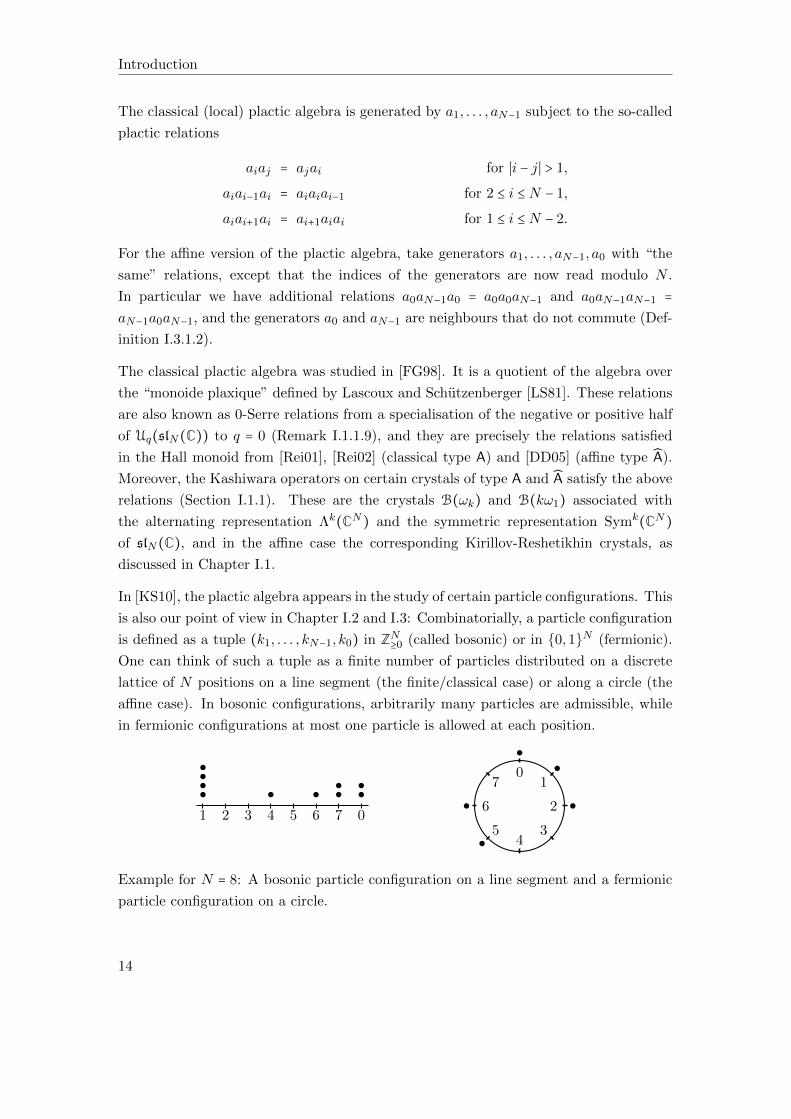
is also our point of view in Chapter I.2 and I.3: Combinatorially, a particle configuration
is defined as a tuple (k1, . . . , kN−1, k0) in ZN≥0 (called bosonic) or in 0,1N (fermionic).
One can think of such a tuple as a finite number of particles distributed on a discrete
lattice of N positions on a line segment (the finite/classical case) or along a circle (the
affine case). In bosonic configurations, arbitrarily many particles are admissible, while
in fermionic configurations at most one particle is allowed at each position.
1 2 3 4 5 6 7 0
01
2
34
5
6
7
Example for N = 8: A bosonic particle configuration on a line segment and a fermionic
particle configuration on a circle.
14
Introduction
The generators ai act on the particle configurations (or their k-span) by lowering ki
by 1 and increasing ki+1 by 1, if possible. If not possible, i.e. because ki = 0 or, in
the fermionic case, ki+1 = 1, the result is 0. In the picture this would correspond to
(clockwise) propagation of a particle from position i to i + 1 (Sections I.2.4 and I.3.4).
This action can be identified with the action of Kashiwara operators fi on crystals B(ωk)
and B(kω1) (Section I.1.2).
On affine particle configurations, the additional generator a0 takes a particle from po-
sition 0 and moves it to position 1. If we consider the k[q]-span instead of the k-span,
we can keep track of the application of a0 by multiplication with an additional factor q
(bosonic) or ±q (fermionic).
In Chapter I.2 we describe a quotient of the affine plactic algebra that acts faithfully
on the k[q]-span of fermionic particle configurations on a circle. This is the affine
nilTemperley–Lieb algebra nTLN : It is defined by the additional nil relation a2i = 0 for
all i. Together with the plactic relations we obtain immediately that also aiai±1ai = 0
for all i, where we take the indices modulo N . The subalgebra of nTLN generated by
a1, . . . , aN−1 is the (classical/finite) nilTemperley–Lieb algebra nTLN .
Chapter I.3 is devoted to the quotient of the classical plactic algebra that acts faithfully
on the k-span of the bosonic particle configurations on a line segment. The additional
defining relation is aiai−1ai+1ai = ai+1aiai−1ai for all 2 ≤ i ≤ N −2. We call this the partic
algebra because of its faithful action on the particle configurations. The corresponding
action of the affine plactic algebra on bosonic particle configurations on a circle is much
harder to describe: We encounter an infinite family of additional relations of the form
ami+1ami+2 . . . a
mi−2a
mi−1a
2mi ami+1a
mi+2 . . . a
mi−2a
mi−1
= amj+1amj+2 . . . a
mj−2a
mj−1a
2mj amj+1a
mj+2 . . . a
mj−2a
mj−1 for all i, j ∈ Z/NZ, m ∈ Z≥1,
and it is not yet clear whether these relations together with aiai−1ai+1ai = ai+1aiai−1ai
for all i ∈ Z/NZ suffice to produce a faithful action.
15
Introduction
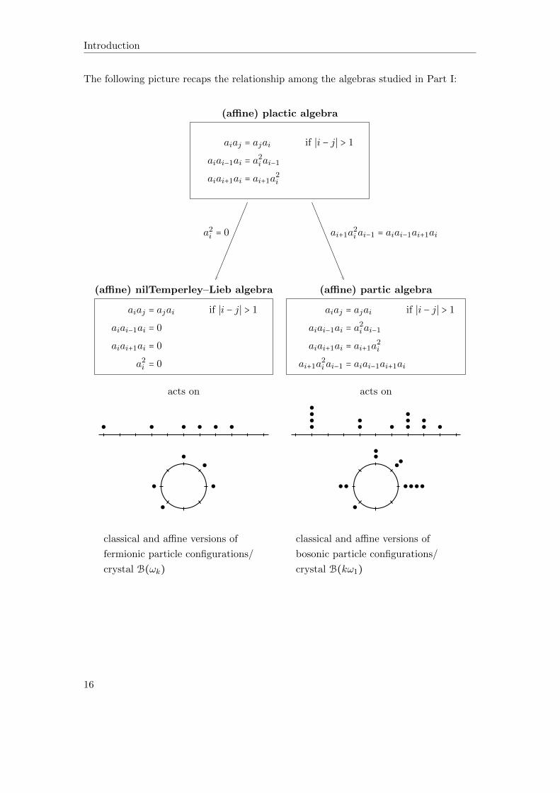
The following picture recaps the relationship among the algebras studied in Part I:
aiaj = ajai if ∣i − j∣ > 1
aiai−1ai = a2i ai−1
aiai+1ai = ai+1a2i
aiaj = ajai if ∣i − j∣ > 1
aiai−1ai = 0
aiai+1ai = 0
a2i = 0
aiaj = ajai if ∣i − j∣ > 1
aiai−1ai = a2i ai−1
aiai+1ai = ai+1a2i
ai+1a2i ai−1 = aiai−1ai+1ai
(affine) plactic algebra
(affine) partic algebra(affine) nilTemperley–Lieb algebra
a2i = 0 ai+1a
2i ai−1 = aiai−1ai+1ai
acts on acts on
classical and affine versions of
fermionic particle configurations/
crystal B(ωk)
classical and affine versions of
bosonic particle configurations/
crystal B(kω1)
16
Introduction
Chapter I.1: Crystal bases and particle configurations
The first chapter is mainly devoted to a review of crystals of classical type A and affine
type A. We briefly recall the basic definitions of quantum groups and quantum affine alge-
bras, their finite dimensional irreducible modules, and their crystal bases in Section I.1.1.
We consider the action of Kashiwara operators on the crystals B(ωk) and B(kω1) for
the simple Uq(slN(C))-modules Lq(ωk) and Lq(kω1), corresponding to the alternating
representation Λk(CN) and the symmetric representation Symk(CN) of U(slN(C)), re-
spectively. In affine type A we study the crystals of the Kirillov-Reshetikhin modules
W k,1 and W 1,k that are isomorphic to Lq(ωk) and Lq(kω1) as Uq(slN(C))-modules, re-
spectively. In this special case it is particularly easy to describe this operation. We make
the following two observations for classical type A, as well as the analogous observations
for Kirillov–Reshetikhin crystals in affine type A:
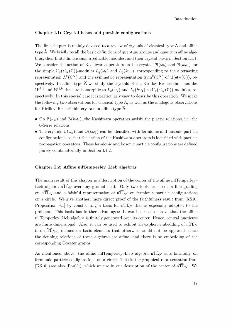
On B(ωk) and B(kω1), the Kashiwara operators satisfy the plactic relations, i.e. the
0-Serre relations.
The crystals B(ωk) and B(kω1) can be identified with fermionic and bosonic particle
configurations, so that the action of the Kashiwara operators is identified with particle
propagation operators. These fermionic and bosonic particle configurations are defined
purely combinatorially in Section I.1.2.
Chapter I.2: Affine nilTemperley–Lieb algebras
The main result of this chapter is a description of the center of the affine nilTemperley–
Lieb algebra nTLN over any ground field. Only two tools are used: a fine grading
on nTLN and a faithful representation of nTLN on fermionic particle configurations
on a circle. We give another, more direct proof of the faithfulness result from [KS10,
Proposition 9.1] by constructing a basis for nTLN that is especially adapted to the
problem. This basis has further advantages: It can be used to prove that the affine
nilTemperley–Lieb algebra is finitely generated over its center. Hence, central quotients
are finite dimensional. Also, it can be used to exhibit an explicit embedding of nTLN
into nTLN+1 defined on basis elements that otherwise would not be apparent, since
the defining relations of these algebras are affine, and there is no embedding of the
corresponding Coxeter graphs.
As mentioned above, the affine nilTemperley–Lieb algebra nTLN acts faithfully on
fermionic particle configurations on a circle. This is the graphical representation from
[KS10] (see also [Pos05]), which we use in our description of the center of nTLN . We
17
Introduction
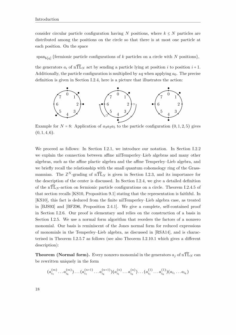
consider circular particle configuration having N positions, where k ≤ N particles are
distributed among the positions on the circle so that there is at most one particle at
each position. On the space
spank[q] fermionic particle configurations of k particles on a circle with N positions,
the generators ai of nTLN act by sending a particle lying at position i to position i + 1.
Additionally, the particle configuration is multiplied by ±q when applying a0. The precise
definition is given in Section I.2.4, here is a picture that illustrates the action:
01
2
34
5
6
70
1
2
34
5
6
70
1
2
34
5
6
7
Example for N = 8: Application of a3a2a5 to the particle configuration (0,1,2,5) gives
(0,1,4,6).
We proceed as follows: In Section I.2.1, we introduce our notation. In Section I.2.2
we explain the connection between affine nilTemperley–Lieb algebras and many other
algebras, such as the affine plactic algebra and the affine Temperley–Lieb algebra, and
we briefly recall the relationship with the small quantum cohomology ring of the Grass-
mannian. The ZN -grading of nTLN is given in Section I.2.3, and its importance for
the description of the center is discussed. In Section I.2.4, we give a detailed definition
of the nTLN -action on fermionic particle configurations on a circle. Theorem I.2.4.5 of
that section recalls [KS10, Proposition 9.1] stating that the representation is faithful. In
[KS10], this fact is deduced from the finite nilTemperley–Lieb algebra case, as treated
in [BJS93] and [BFZ96, Proposition 2.4.1]. We give a complete, self-contained proof
in Section I.2.6. Our proof is elementary and relies on the construction of a basis in
Section I.2.5. We use a normal form algorithm that reorders the factors of a nonzero
monomial. Our basis is reminiscent of the Jones normal form for reduced expressions
of monomials in the Temperley–Lieb algebra, as discussed in [RSA14], and is charac-
terised in Theorem I.2.5.7 as follows (see also Theorem I.2.10.1 which gives a different
description):
Theorem (Normal form). Every nonzero monomial in the generators aj of nTLN can
be rewritten uniquely in the form
(a(m)i1
. . . a(m)ik
) . . . (a(n+1)i1
. . . a(n+1)ik
)(a(n)i1
. . . a(n)ik
) . . . (a(1)i1. . . a
(1)ik
)(ai1 . . . aik)
18
Introduction
with a(n)i`
∈ 1, a0, a1, . . . , aN−1 for all 1 ≤ n ≤m, 1 ≤ ` ≤ k, such that
a(n+1)i`
∈
⎧⎪⎪⎪⎨⎪⎪⎪⎩
1 if a(n)i`
= 1,
1, aj+1 if a(n)i`
= aj .
The factors ai1 , . . . , aik are determined by the property that the generator ai`−1 does not
appear to the right of ai` in the original presentation of the monomial. Alternatively,
every nonzero monomial is uniquely determined by the following data from its action on
the graphical representation:
the input particle configuration with the minimal number of particles on which it acts
nontrivially,
the corresponding output particle configuration,
the power of q by which it acts.
For the proof of this result, we recall a characterisation of the nonzero monomials in
nTLN from [Gre02]. Al Harbat [Alh13] has recently described a normal form for fully
commutative elements of the affine Temperley–Lieb algebra, which differs from ours
when passing to nTLN .
In Section I.2.7 we define special monomials that serve as the projections onto a single
particle configuration (up to multiplication by ±q). Based on this, in Section I.2.8 we
state the main result (Theorem I.2.8.5) of the chapter:
Theorem. The center of nTLN is the subalgebra
CN = Cent(nTLN) = ⟨1, t1, . . . , tN−1⟩ ≅k[t1, . . . , tN−1]
(tkt` ∣ k ≠ `),
where the generator tk = (−1)k−1∑
∣I∣=ka(i) is the sum of monomials a(i) corresponding
to particle configurations given by increasing sequences i = 1 ≤ i1 < . . . < ik ≤ N of
length k. The monomial a(i) sends particle configurations with n ≠ k particles to 0 and
acts on a particle configuration with k particles by projecting onto i and multiplying by
(−1)k−1q. Hence, tk acts as multiplication by q on the configurations with k particles.
Our N − 1 central generators tk are essentially the N − 1 central elements constructed
by Postnikov. Lemma 9.4 of [Pos05] gives an alternative description of tk as product
of the k-th elementary symmetric polynomial (with factors cyclically ordered) with the
(N −k)-th complete homogeneous symmetric polynomial (with factors reverse cyclically
ordered) in the noncommuting generators of nTLN . The above theorem shows that in
19
Introduction
fact these elements generate the entire center of nTLN . In Section I.2.9, we establish that
nTLN is finitely generated over its center. In Section I.2.10 we describe an alternative
normal form for monomials in nTLN using the generators tk of the center. Using the
faithfulness of the graphical representation, we define monomials eij that move particles
from positions j = 1 ≤ j1 < . . . < jk ≤ N to i = 1 ≤ i1 < . . . < ik ≤ N so that the power
of q in this action is minimal. Then the main result is Theorem I.2.10.1:
Theorem. The set of monomials
1 ∪ t`keij ∣ ` ∈ Z≥0, 1 ≤ ∣i∣ = ∣j∣ = k ≤ N − 1, 1 ≤ k ≤ N − 1
defines a k-basis of the affine nilTemperley–Lieb algebra nTLN .
In Section I.2.11, we define yet another monomial basis for nTLN indexed by pairs of
particle configurations together with a natural number indicating how often the particles
have been moved around the circle. With this basis at hand, we obtain inclusions
nTLN ⊂ nTLN+1. The inclusions are not as obvious as those for the nilCoxeter algebra
nCN having underlying Coxeter graph of type AN−1, since one cannot deduce them from
embeddings of the affine Coxeter graphs. Our result, Theorem I.2.11.1, reads as follows:
Theorem. For all 0 ≤ m ≤ N − 1, there are unital algebra embeddings εm ∶ nTLN →
nTLN+1 given by
ai ↦ ai for 0 ≤ i ≤m − 1, am ↦ am+1am, ai ↦ ai+1 for m + 1 ≤ i ≤ N − 1.
In Section I.2.12 we turn towards the representation theory of nTLN : In this section
and the remainder of Chapter I.2 we have to assume that the ground field k of nTLN
is restricted to be an uncountable algebraically closed field (of arbitrary characteristic).
Let χ be an algebra homomorphism CN → k. Then with the help of localisations with
respect to central elements, we classify the simple modules over nTLN with central
character χ in Theorem I.2.12.3 as follows.
Theorem. Up to isomorphism, there is precisely one simple module of nTLN with
central character χ. The simple modules of nTLN are given up to isomorphism by
i) the trivial onedimensional module k with trivial central character,
ii) the (Nk)-dimensional module ⋀k kN with central character χ(tk) ∈ k∖0, χ(t`) = 0
for all ` ≠ k.
20
Introduction
The localisation with respect to multiplicative subsets of the center can be considered as
pseudo-commutative localisation since the Ore conditions are for free. In Section I.2.13
we use these localisations together with a rank argument to show that nTLN is not free
over its center.
In analogy to the affine Temperley–Lieb algebra one would expect that also the affine
nilTemperley–Lieb algebra can easily be equipped with the structure of an affine cellular
algebra in the sense of [KX12]. Then the classification of simple modules for nTLN would
follow from the general approach for affine cellular algebras. However, affine cellularity
does not pass in an obvious way to the nil-case. In Section I.2.14 we discuss three
approaches to identify nTLN as an affine cellular algebra.
Chapter I.3: The plactic and the partic algebra
Analogous to the results for the affine nilTemperley–Lieb algebra in Chapter I.2, our
main results in this chapter are a description of the center of the partic algebra and the
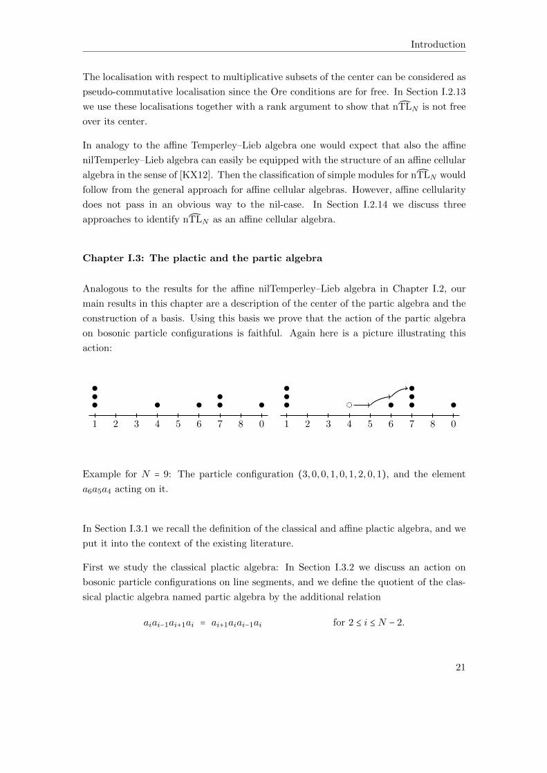
construction of a basis. Using this basis we prove that the action of the partic algebra
on bosonic particle configurations is faithful. Again here is a picture illustrating this
action:
1 2 3 4 5 6 7 8 0 1 2 3 4 5 6 7 8 0
Example for N = 9: The particle configuration (3,0,0,1,0,1,2,0,1), and the element
a6a5a4 acting on it.
In Section I.3.1 we recall the definition of the classical and affine plactic algebra, and we
put it into the context of the existing literature.
First we study the classical plactic algebra: In Section I.3.2 we discuss an action on
bosonic particle configurations on line segments, and we define the quotient of the clas-
sical plactic algebra named partic algebra by the additional relation
aiai−1ai+1ai = ai+1aiai−1ai for 2 ≤ i ≤ N − 2.
21
Introduction
Since these relations only involve permutations of the generators we can define two
gradings on the partic algebra, by the word length and by how often each generator
occurs, similar to the affine nilTemperley–Lieb algebra before.
In Section I.3.3 we construct a normal form of the monomials in the partic algebra. Our
main result of this section is Theorem I.3.3.1
Theorem. The partic algebra PpartN has a k-basis given by monomials of the form
adN−1N−1 . . . a
d22 a
k11 a
k22 . . . akN−1
N−1 ∣ di ≤ di−1 + ki−1 for all 3 ≤ i ≤ N − 1, d2 ≤ k1
where di, ki ∈ Z≥0 for all 1 ≤ i ≤ N − 1.
In Section I.3.4 we consider the action of the classical plactic and the partic algebra
on bosonic particle configurations, and we obtain the following faithfulness result in
Theorem I.3.4.2
Theorem. The action of the partic algebra PpartN on bosonic particle configurations is
faithful.
This allows us to define a labelling of the monomials in normal form. We get an alter-
native description of the basis from Theorem I.3.3.1 in Proposition I.3.4.5. If we write
aij = adN−1N−1 . . . a
d22 a
k11 a
k22 . . . akN−1
N−1 , it can be reformulated as follows:
Theorem. The set of monomials
1 ∪ aij ∣ j = (k1, k2, k3 . . . , kN−1,0), i = (0, k1 − d2, k2 + d2 − d3, . . . , kN−1 + dN−1)
with k1, . . . , kN−1 ∈ Z≥0 and di ≤ di−1 + ki−1 ∈ Z≥0 for all 3 ≤ i ≤ N − 1, d2 ≤ k1, defines a
k-basis of the partic algebra.
In Section I.3.5 we describe the center of the partic algebra:
Theorem. The center of the partic algebra PpartN is given by the k-span of the elements
arN−1arN−2 . . . a
r2ar1 ∣ r ≥ 0.
Finally, in Section I.3.6 we turn to the affine case. We define the affine partic algebra
and we consider its action on affine bosonic particle configurations. This is substantially
harder to understand than the classical case, in particular we find a new type of relations
of the form
ami+1ami+2 . . . a
mi−2a
mi−1a
2mi ami+1a
mi+2 . . . a
mi−2a
mi−1
= amj+1amj+2 . . . a
mj−2a
mj−1a
2mj amj+1a
mj+2 . . . a
mj−2a
mj−1 for all i, j ∈ Z/NZ, m ∈ Z≥1.
22
Introduction
We have not yet found a nice normal form for monomials for the affine partic algebra (and
neither for its quotient with respect to the new type of relations). For the construction
of the normal forms of the partic algebra and the affine nilTemperley–Lieb algebra, it
was helpful to know the faithful representations on particle configurations. The particle
configurations could be used for labelling sets of the basis elements. This approach fails
for the affine partic algebra since it does not act faithfully on affine bosonic particle
configurations. It is unclear whether faithfulness holds for the quotient with respect to
the new type of relations.
Part II: Generalized Weyl algebras
Generalized Weyl algebras (GWA’s) were introduced by Bavula in [Bav92]. A GWA is
defined over a unital associative commutative k-algebra R that is a noetherian domain,
where k is an algebraically closed ground field of characteristic 0. For any choice of n
nonzero elements t = (t1, . . . , tn) in R and n pairwise commuting algebra automorphisms
σ = (σ1, . . . , σn) in Aut(R) such that σi(tj) = tj for all i ≠ j the corresponding GWA
A = R(σ, t) is the k-algebra generated over R by 2n additional generators Xi, Yi, 1 ≤ i ≤ n,
with relations
Xir = σi(r)Xi, XiYi = σi(ti), [Xi,Xj] = 0,
Yir = σ−1i (r)Yi, YiXi = ti, [Yi, Yj] = 0,
[Xi, Yj] = 0
for all 1 ≤ i, j ≤ n with i ≠ j and all r ∈ R. It is a Zn-graded algebra with deg(Xi) = ei
and deg(Yi) = −ei where we denote by ei the i-th standard basis vector of Zn.
Chapter II.1: Duflo Theorem for a Class of Generalized Weyl Algebras
The main result of this chapter is a Duflo type theorem for a class of generalized Weyl
algebras (GWA’s).
For the universal enveloping algebra of a semisimple Lie algebra over k, Duflo’s Theorem
[Duf77] states that all its primitive ideals (i.e. the annihilators of simple modules) are
given by the annihilators of simple highest weight modules. In contrast, the simple
modules themselves are far from being classified in general.
Now it is possible to define highest weight modules for GWA’s and therefore natural to
ask whether an analogous statement holds. We prove a Duflo type theorem for a special
23
Introduction
class of GWA’s using a theorem by [MB98] that relates the annihilator of a simple weight
module to its support.
This chapter is subdivided as follows: In Section II.1.1 we provide a quick overview of
Duflo type theorems. In Section II.1.2 we review generalized Weyl algebras, and we
introduce our special class of GWA’s. In particular, our base ring is always a polynomial
ring R = k[T1, . . . , Tn] and the automorphisms are given by translations σi(Tj) = Tj−δijbi
as considered already in [Bav92]. We discuss highest weight modules and graded modules
over generalized Weyl algebras. We characterize moreover the highest weight modules
as those modules with a locally nilpotent action of the Xi.
In Section II.1.3 we prepare to apply the result from [MB98] to our class of GWA’s: We
recall the description of weight modules by their support which is given in terms of lattice
points and hyperplanes from [Bav92]. These hyperplanes “break” the weight lattice into
regions, and a weight module can be characterised by these regions and its defining
“breaks”. This is made precise in Definition II.1.3.3. We give a careful description of
the break conditions.
In Section II.1.4 we formulate and prove the main theorem of the chapter:
Theorem. Let A = R(σ, t) be a GWA of rank n as defined in Section II.1.2 where we
assume R = k[T1, . . . , Tn], σi(Tj) = Tj − δijbi for bi ∈ k∖0 and ti ∈ k[Ti] ⊂ k[T1, . . . , Tn],
ti ∉ k. Then all primitive ideals of A, i.e. the annihilator ideals of simple A-modules,
are given by the annihilators of simple highest weight A-modules L(m) of highest weight
m ∈ mspec(R).
The main tool is the Duflo type theorem from [MB98]. We show it applies to our
situation and improve it by showing that it is enough to consider the much smaller class
of highest weight modules (as in the classical Duflo theorem).
We provide a list of important examples of GWA’s to which the main theorem applies,
e.g. central quotients of the universal enveloping algebra U(sl2(C)) and its generalisa-
tions by [Smi90] as discussed in [Bav92, Example 1.2.(4)]. We include a discussion why
we require our assumptions on the special class of GWA’s.
In Section II.1.5 we conclude the chapter by some examples that illustrate the relation-
ship between the annihilator and the support of simple highest weight modules.
24
Introduction
Publications and Coauthorships
Parts of this thesis have been published or accepted for publication during the PhD
project: Most of Chapter I.2 as well as the corresponding parts of this introduction can
be found in the paper [BM16] with Georgia Benkart. Except for Lemma II.1.2.2, all of
Chapter II.1 is published in [Mei15].
Sections I.2.12 and I.2.13 grew out of discussions with Gwyn Bellamy and Uli Krahmer.
Acknowledgements
I am deeply thankful to my advisor Catharina Stroppel for sharing her deep insights and
her enthusiasm, for patiently standing me by and supporting me. It has been a huge
pleasure to work under her guidance, and I enjoyed every single hour during our many,
many discussions. From the first time that I heard about Lie algebras to our most recent
meeting she has been an inspiring teacher and a fantastic mentor, and I am grateful for
all the time we spent together in great working atmosphere.
During my PhD project I spent five months at QGM Aarhus and five more months at the
University of Uppsala. I would like to thank Henning Haahr Andersen and Volodymyr
Mazorchuk for generously hosting me, for giving me their time and for the numerous
interesting discussions that we had. I enjoyed my stays in Aarhus and in Uppsala a
lot, and I would like to thank the members of QGM Aarhus and the people at the
Department for Mathematics in Uppsala for their kind hospitality.
I am grateful to my coauthor Georgia Benkart for our collaboration, including long
discussions and exciting example computations. I thank the MSRI Berkeley for giving us
the opportunity to start this collaboration during the programme on “Noncommutative
Algebraic Geometry and Representation Theory”.
I would like to thank Gwyn Bellamy, Kenneth Brown, Christian Korff and Uli Krahmer
for kind advice and discussions about the affine nilTemperley–Lieb algebra during a short
visit to the University of Glasgow, and I am grateful to Jonas Hartwig for interesting
conversations about GWA’s.
I heartily thank the members of the representation theory working group in Bonn for
sharing their knowledge, giving me support and advice. I am particularly indebted to
Hanno Becker, Michael Ehrig, Deniz Kus, and Daniel Tubbenhauer for lots of feedback
and discussions about this thesis, for proofreading, and for bearing with my terrible
25
Introduction
puns. I thank Viktoriya Ozornova for comments on the thesis, and further thanks are
due to the referees for many improvements of the two articles underlying this thesis.
I gratefully acknowledge the support by the IMPRS programme of the Max Planck
Institute for Mathematics, the Hausdorff stipend of the Bonn International Graduate
School, and the scholarship of the Deutsche Telekom Stiftung. Their generous funding
and the extremely helpful administrative staff enabled me to carry out my work, and I
learned a lot from the exchange with the people I met thanks to these programmes.
My friends at the Mathematical Institutes in Bonn, Aarhus and Uppsala made my life
as a PhD student very pleasant. The list of reasons is long, and it includes many math-
ematical discussions, feedback, and reciprocal encouragement as well as common coffee
breaks, QGM lounge meetings, fika sessions, tea sessions, sushi dinners, Vietnamese din-
ners, cooking together in the tiny kitchen of the Mathematical Institute in Bonn, baking
delicious cookies, processing tons of chestnuts, hiking in California, Catalonia, Corsica,
Scotland and the Siebengebirge, cinema visits, shared rooms in strange hotels, shared
offices, and many non-mathematical discussions.
I am lucky to have a wonderful family and patient friends who supported me uncon-
ditionally during the past years, even when I was fully absorbed by my thesis. It is a
pleasure to thank them for giving me so much of their time and energy!
26
Part I.
Particle configurations and
crystals
27

I.1. Crystal bases and particle
configurations
In this chapter we discuss the relationship of particle configurations on a lattice with
crystal combinatorics in type A and A. It can be seen as a motivation for the definitions of
the affine nilTemperley-Lieb algebra, the plactic and the partic algebra that we discuss in
the following chapters. This chapter is otherwise independent of the following chapters.
In Section I.1.1 we review crystal bases for the quantum group Uq(sln(C)) and the
quantum affine algebra Uq(sln(C)), and we discuss relations among Kashiwara opera-
tors. In Section I.1.2 we describe particle configurations following [KS10] and we discuss
identifications of crystal and particle combinatorics.
Throughout the chapter we work over the complex numbers k = C for convenience. For
tensor products over C we write ⊗ instead of ⊗C. We write C(q) for the field of rational
functions in the variable q.
I.1.1. Quantum groups and crystal bases of type An and An
In this section we review crystal bases for the quantum groups Uq(sln(C)) and Uq(sln(C))
and fix our notation. We follow mainly [HK02] and [Jan96] unless otherwise stated. We
focus on type An and An, for more general statements see the references.
I.1.1.1. Finite case
Let sln(C) be the Lie algebra of traceless complex n × n-matrices with standard Cartan
subalgebra h consisting of the diagonal matrices generated by hi = eii − e(i+1)(i+1) for
1 ≤ i ≤ n − 1. Here eii denotes the elementary matrix where the (i, i)th entry is one and
all other entries are zero. The root decomposition of sln(C) with respect to the adjoint h-
action is given by sln(C) = ⊕α∈Φ
sln(C)α and simple roots αi = εi−εi+1 ∈ h∗. Here εi denotes
29
I.1. Crystal bases and particle configurations
the function on h that returns the ith diagonal entry, and Φ = spanZα1, . . . , αn−1 is the
root lattice of sln(C). In our notation we do not distinguish between linear functions on
h and linear functions on the diagonal matrices. The fundamental weights are given by
ωi = ε1 + . . . + εi. We denote the weight lattice by P = spanZ ω1, . . . , ωn−1. It contains
the dominant integral weights P + = spanZ≥0 ω1, . . . , ωn−1.
The finite dimensional simple sln(C)-modules L(λ) are labelled by their dominant in-
tegral highest weights λ ∈ P + ⊂ h∗ = spanC εi ∣ 1 ≤ i ≤ n/spanC ε1 + . . . + εn.
Such a dominant integral highest weight can be represented by an element of the form
λ = λ1ε1 + . . . + λn−1εn−1 with coefficients λ1 ≥ . . . ≥ λn−1 ∈ Z≥0. This in turn is identified
with partitions (λ1, . . . , λn−1) with n − 1 rows of length λi.
Now we turn to the quantum group:
I.1.1.1 Definition. The quantum group Uq(sln(C)) is the unital associative C(q)-
algebra generated by formal generators Ei, Fi,K±1i for 1 ≤ i ≤ n − 1 with relations
KiK−1i = 1 = K−1
i Ki for 1 ≤ i ≤ n − 1,
KjEi = qαi(hj)EiKj for 1 ≤ i, j ≤ n − 1,
KjFi = q−αi(hj)FiKj for 1 ≤ i, j ≤ n − 1,
[Ei, Fj] = δijKi −K
−1i
q − q−1for 1 ≤ i, j ≤ n − 1,
E2i Ei±1 − [2]qEiEi±1Ei +Ei±1E
2i = 0,
[Ei,Ej] = 0 for ∣i − j∣ > 1,
F 2i Fi±1 − [2]qFiFi±1Fi + Fi±1F
2i = 0,
[Fi, Fj] = 0 for ∣i − j∣ > 1,
where [n]q =qn−q−nq−q−1 is the usual notation for quantum integers, so [2]q = q + q
−1. It can
be equipped with a Hopf algebra structure where in particular the comultiplication ∆
applied to Fi is given by ∆(Fi) = Fi ⊗ 1 +Ki ⊗ Fi, the comultiplication applied to Ei is
∆(Ei) = Ei ⊗K−1i + 1⊗Ei, and the elements K±1
i are grouplike, for 1 ≤ i ≤ n − 1.
I.1.1.2 Remark. This is the adjoint form of Uq(sln(C)) in the sense of [BG02], where
the generators Ki correspond to the generators αi of the root lattice Φ of sln(C). Alterna-
tive forms of the quantum group Uq(sln(C)) can be defined for the (finer) weight lattice
or any other lattice lying in between those two, see [BG02, Section 1.6.3], [CP95a, Sec-
tion 9.1.A]. Furthermore, there is the Drinfeld-Jimbo quantum algebra whose elements
are formal power series in ei, fi and hi over the field C[[h]], see [CP95a, Definition 6.5.1],
[Kas95]. There is a map of Hopf algebras from the quantum group defined above into
30
I.1.1. Quantum groups and crystal bases of type An and An
the Drinfeld-Jimbo quantum group by q ↦ eh2 , K±1
i ↦ e±h2hi , Fi ↦ e−
h4 fi and Ei ↦ e
h4 ei,
see [Kas95, Proposition XVII.4.1] for n = 2. ◊
We are only interested in weight modules, i.e. Uq(sln(C))-modules with a weight space
decomposition with respect to the action of Ki, 1 ≤ i ≤ n−1, so that the Ki act by scalars
in C(q)× on the weight spaces. In particular, we consider weight modules with weights
of the form ±qµ for µ ∈ P ⊂ h∗, meaning that Ki acts by ±qµ(hi), for all 1 ≤ i ≤ n − 1.
All finite dimensional Uq(sln(C))-modules are completely reducible into simple highest
weight modules of highest weight ±qλ with λ ∈ P +, see [CP95a, Propositions 10.1.1, 10.1.2].
In other words, the finite dimensional highest weight modules are labelled by partitions
λ together with a choice of (n − 1) signs, so that Ki acts by ±qλi , for all 1 ≤ i ≤ n − 1.
One usually prefers the choice of all signs equal to +1 since the subcategory of these
so-called type 1 modules is closed under tensor products. The abelian subcategory of
finite dimensional Uq(sln(C))-modules with a fixed choice of signs is equivalent to the
abelian category of finite dimensional sln(C)-modules. For type 1, this is an equivalence
of monoidal categories.
Under this equivalence, the finite dimensional simple sln(C)-module L(λ) is mapped
to the simple Uq(sln(C))-module Lq(λ) of type 1 with the same character, see [BG02,
Section I.6.12]. Here and in the following we adopt the shorthand notation of writing λ
for +qλ.
Let us now recall the combinatorics of some special crystals for sln(C). We do not
introduce Kashiwara operators and crystal bases in detail. We refer to [Kas91], but also
e.g. to [HK02, Section 4] for the general statements and background material and to
[HK02, Sections 7.4, 8.2] for details about type An.
Let fi denote the Kashiwara operator on a Uq(sln(C))-module M associated with the
operator Fi ∈ Uq(sln(C)), i.e. fiu = ∑k F(k+1)i uk for a weight vector u ∈Mµ written in the
form u = ∑k F(k)i uk with uk ∈Mλ+kαi ∩ ker(Ei). Here F
(k)i = 1
[k]q !Fki is the notation for
divided powers. The Kashiwara operator ei associated with Ei is defined analogously.
By [Kas91] there exists a crystal basis (L(λ),B(λ)) for the simple Uq(sln(C))-module
Lq(λ). Here L(λ) denotes the crystal lattice, the minimal lattice over the rational
functions regular at 0 that contains a highest weight vector vλ of Lq(λ) and that is stable
under the action of the Kashiwara operators fi, ei. The subset B(λ) of L(λ)/qL(λ) is
given by all nonzero elements of the form fi1 . . . fir(vλ) + qL(λ).
31
I.1. Crystal bases and particle configurations
One defines the crystal graph to be an oriented graph with vertices B(λ) and edges
labelled by 1, . . . , n− 1, so that there is an i-labelled edge from b to b′ ∈ B(λ) if and only
if fi(b) = b′ modulo qL(λ). This is the case if and only if ei(b
′) = b modulo qL(λ). By
abuse of notation, the crystal graph is also denoted by B(λ).
Crystal bases are particularly suitable for the computation of tensor products. Given
Lq(λ) with crystal basis (L(λ),B(λ)) and Lq(λ′) with crystal basis (L(λ′),B(λ′)),
one can easily determine a crystal graph for L(λ) ⊗C(q) L(λ′) on the set of vertices
B(λ)⊗B(λ′) ∶= B(λ)×B(λ′). The tensor product rule prescribes on which tensor factor
the Kashiwara operator fi acts, see [HK02, Theorem 4.4.1].
In type An, for any simple Uq(sln(C))-module Lq(λ), the set B(λ) can be realized by
semistandard Young tableaux of shape λ with entries 1, . . . , n. The highest weight vector
vλ of Lq(λ) is represented by the “standard” semistandard Young tableau of shape λ
where all entries in the kth row are equal to k. In the crystal graph B(λ), if two
semistandard Young tableaux are connected by an i-labelled edge, then their entries are
the same except that in one box the entry i is replaced by i+1. Let us recall the details: In
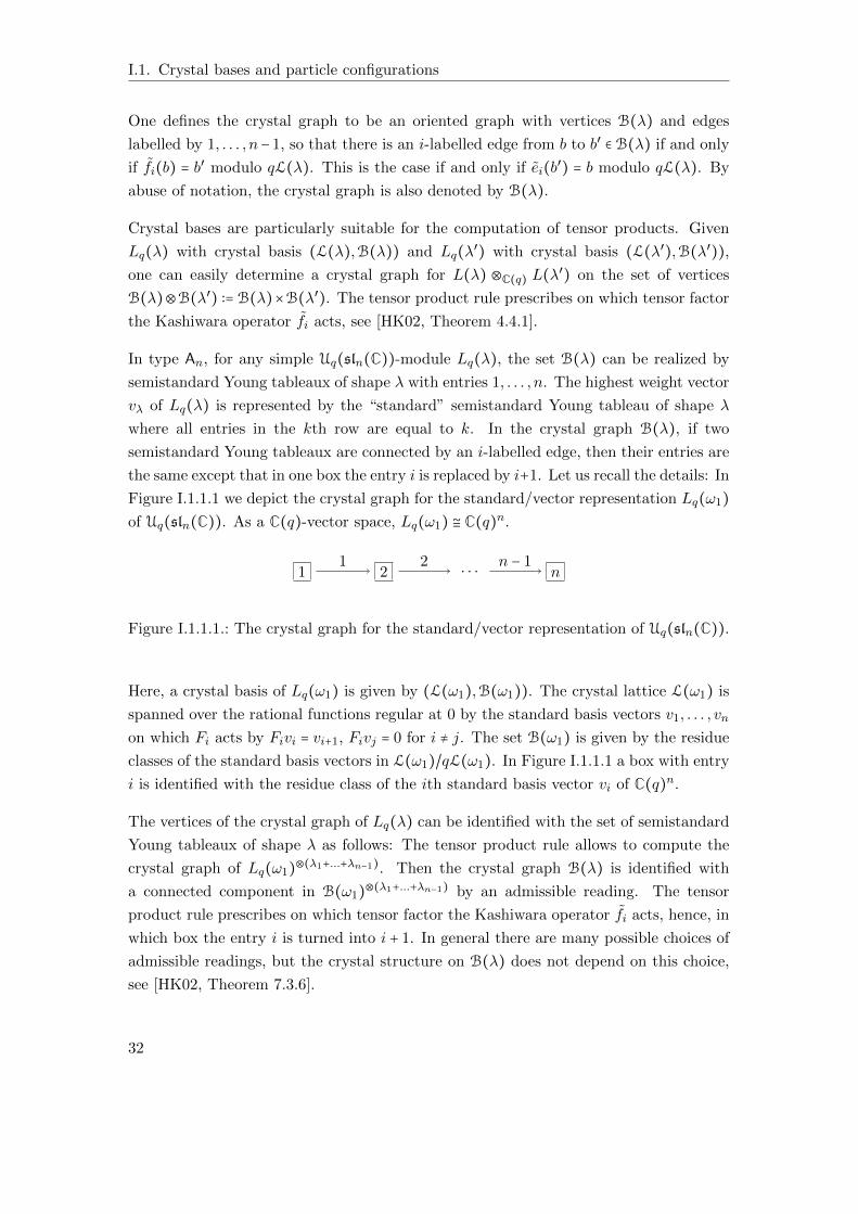
Figure I.1.1.1 we depict the crystal graph for the standard/vector representation Lq(ω1)
of Uq(sln(C)). As a C(q)-vector space, Lq(ω1) ≅ C(q)n.
1 2 . . . n1 2 n − 1
Figure I.1.1.1.: The crystal graph for the standard/vector representation of Uq(sln(C)).
Here, a crystal basis of Lq(ω1) is given by (L(ω1),B(ω1)). The crystal lattice L(ω1) is
spanned over the rational functions regular at 0 by the standard basis vectors v1, . . . , vn
on which Fi acts by Fivi = vi+1, Fivj = 0 for i ≠ j. The set B(ω1) is given by the residue
classes of the standard basis vectors in L(ω1)/qL(ω1). In Figure I.1.1.1 a box with entry
i is identified with the residue class of the ith standard basis vector vi of C(q)n.
The vertices of the crystal graph of Lq(λ) can be identified with the set of semistandard
Young tableaux of shape λ as follows: The tensor product rule allows to compute the
crystal graph of Lq(ω1)⊗(λ1+...+λn−1). Then the crystal graph B(λ) is identified with
a connected component in B(ω1)⊗(λ1+...+λn−1) by an admissible reading. The tensor
product rule prescribes on which tensor factor the Kashiwara operator fi acts, hence, in
which box the entry i is turned into i + 1. In general there are many possible choices of
admissible readings, but the crystal structure on B(λ) does not depend on this choice,
see [HK02, Theorem 7.3.6].
32
I.1.1. Quantum groups and crystal bases of type An and An
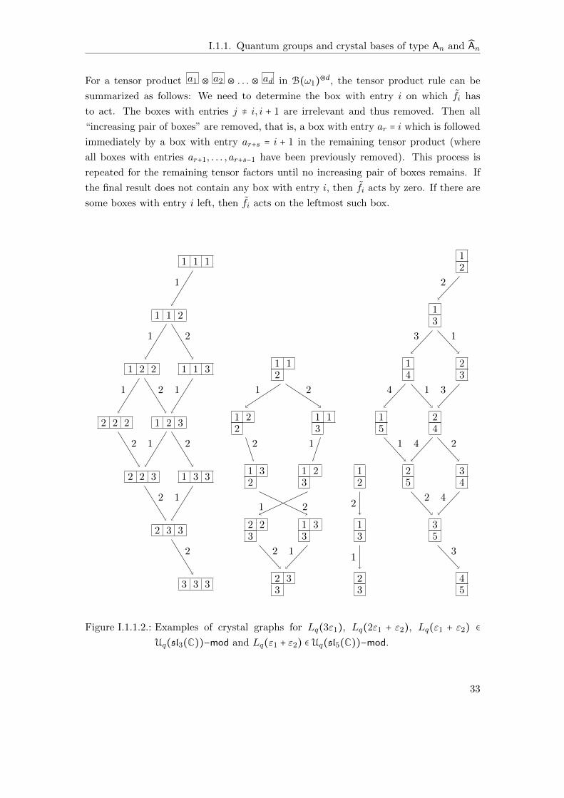
For a tensor product a1 ⊗ a2 ⊗ . . . ⊗ ad in B(ω1)⊗d, the tensor product rule can be
summarized as follows: We need to determine the box with entry i on which fi has
to act. The boxes with entries j ≠ i, i + 1 are irrelevant and thus removed. Then all
“increasing pair of boxes” are removed, that is, a box with entry ar = i which is followed
immediately by a box with entry ar+s = i + 1 in the remaining tensor product (where
all boxes with entries ar+1, . . . , ar+s−1 have been previously removed). This process is
repeated for the remaining tensor factors until no increasing pair of boxes remains. If
the final result does not contain any box with entry i, then fi acts by zero. If there are
some boxes with entry i left, then fi acts on the leftmost such box.
1 1 1
1 1 2
1 2 2 1 1 3
2 2 2 1 2 3
2 2 3 1 3 3
2 3 3
3 3 3
1
1 2
1 2 1
1 22
12
2
1 12
1 22
1 13
1 32
1 23
2 23
1 33
2 33
1 2
2 1
1 2
12
12
13
23
2
1
12
13
23
14
24
15
34
25
35
45
2
13
4 1 3
4 21
42
3
Figure I.1.1.2.: Examples of crystal graphs for Lq(3ε1), Lq(2ε1 + ε2), Lq(ε1 + ε2) ∈
Uq(sl3(C))−mod and Lq(ε1 + ε2) ∈ Uq(sl5(C))−mod.
33
I.1. Crystal bases and particle configurations
The examples in Figure I.1.1.2 illustrate the crystal graphs for the Uq(sl3(C))-modules
Lq(3ε1), Lq(2ε1 + ε2), Lq(ε1 + ε2), and for the Uq(sl5(C))-module Lq(ε1 + ε2). For
Lq(2ε1 + ε2) this is Example 7.4.3 from [HK02].
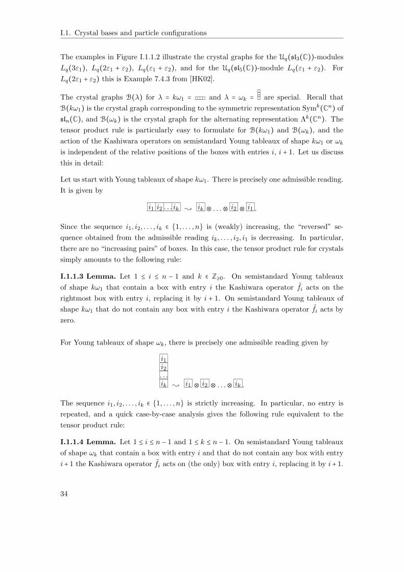
The crystal graphs B(λ) for λ = kω1 = and λ = ωk = are special. Recall that
B(kω1) is the crystal graph corresponding to the symmetric representation Symk(Cn) of
sln(C), and B(ωk) is the crystal graph for the alternating representation Λk(Cn). The
tensor product rule is particularly easy to formulate for B(kω1) and B(ωk), and the
action of the Kashiwara operators on semistandard Young tableaux of shape kω1 or ωk
is independent of the relative positions of the boxes with entries i, i + 1. Let us discuss
this in detail:
Let us start with Young tableaux of shape kω1. There is precisely one admissible reading.
It is given by
i1 i2 . . . ik ; ik ⊗ . . .⊗ i2 ⊗ i1 .
Since the sequence i1, i2, . . . , ik ∈ 1, . . . , n is (weakly) increasing, the “reversed” se-
quence obtained from the admissible reading ik, . . . , i2, i1 is decreasing. In particular,
there are no “increasing pairs” of boxes. In this case, the tensor product rule for crystals
simply amounts to the following rule:
I.1.1.3 Lemma. Let 1 ≤ i ≤ n − 1 and k ∈ Z≥0. On semistandard Young tableaux
of shape kω1 that contain a box with entry i the Kashiwara operator fi acts on the
rightmost box with entry i, replacing it by i + 1. On semistandard Young tableaux of
shape kω1 that do not contain any box with entry i the Kashiwara operator fi acts by
zero.
For Young tableaux of shape ωk, there is precisely one admissible reading given by
i1i2. . .ik ; i1 ⊗ i2 ⊗ . . .⊗ ik .
The sequence i1, i2, . . . , ik ∈ 1, . . . , n is strictly increasing. In particular, no entry is
repeated, and a quick case-by-case analysis gives the following rule equivalent to the
tensor product rule:
I.1.1.4 Lemma. Let 1 ≤ i ≤ n − 1 and 1 ≤ k ≤ n − 1. On semistandard Young tableaux
of shape ωk that contain a box with entry i and that do not contain any box with entry
i+ 1 the Kashiwara operator fi acts on (the only) box with entry i, replacing it by i+ 1.
34
I.1.1. Quantum groups and crystal bases of type An and An
On any other semistandard Young tableaux of shape ωk the Kashiwara operator fi acts
by zero.
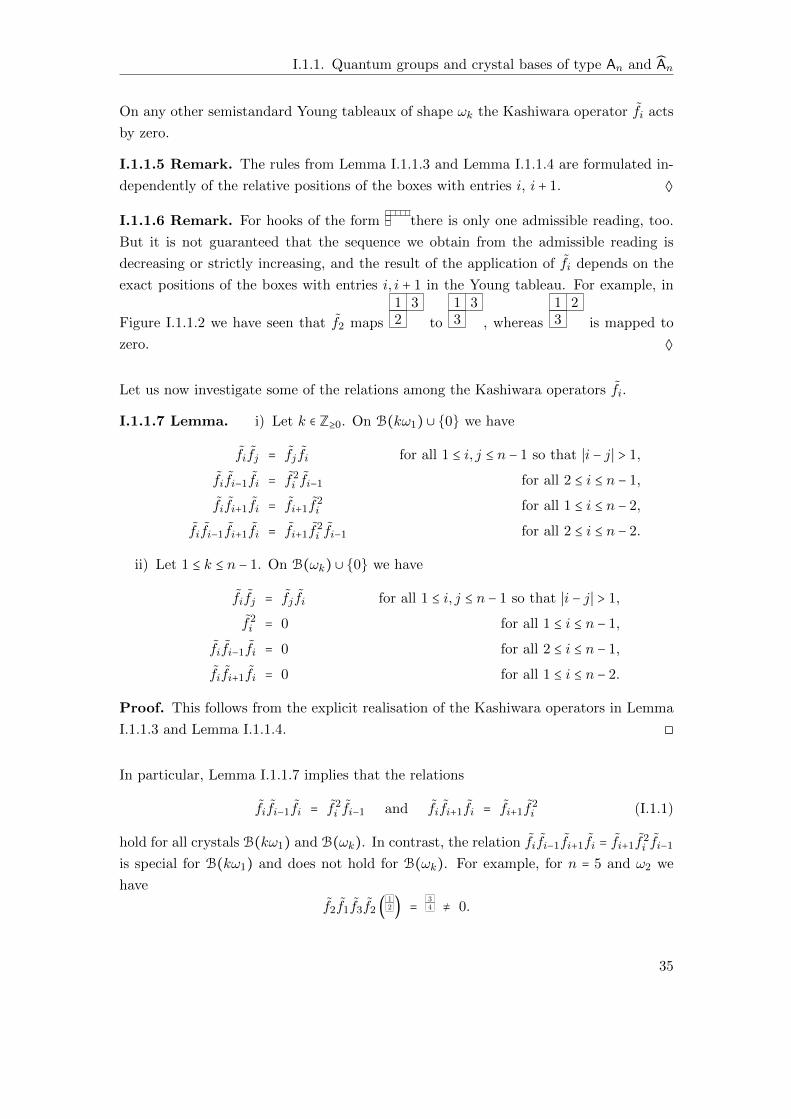
I.1.1.5 Remark. The rules from Lemma I.1.1.3 and Lemma I.1.1.4 are formulated in-
dependently of the relative positions of the boxes with entries i, i + 1. ◊
I.1.1.6 Remark. For hooks of the form there is only one admissible reading, too.
But it is not guaranteed that the sequence we obtain from the admissible reading is
decreasing or strictly increasing, and the result of the application of fi depends on the
exact positions of the boxes with entries i, i + 1 in the Young tableau. For example, in
Figure I.1.1.2 we have seen that f2 maps
1 32 to
1 33 , whereas
1 23 is mapped to
zero. ◊
Let us now investigate some of the relations among the Kashiwara operators fi.
I.1.1.7 Lemma. i) Let k ∈ Z≥0. On B(kω1) ∪ 0 we have
fifj = fj fi for all 1 ≤ i, j ≤ n − 1 so that ∣i − j∣ > 1,
fifi−1fi = f2i fi−1 for all 2 ≤ i ≤ n − 1,
fifi+1fi = fi+1f2i for all 1 ≤ i ≤ n − 2,
fifi−1fi+1fi = fi+1f2i fi−1 for all 2 ≤ i ≤ n − 2.
ii) Let 1 ≤ k ≤ n − 1. On B(ωk) ∪ 0 we have
fifj = fj fi for all 1 ≤ i, j ≤ n − 1 so that ∣i − j∣ > 1,
f2i = 0 for all 1 ≤ i ≤ n − 1,
fifi−1fi = 0 for all 2 ≤ i ≤ n − 1,
fifi+1fi = 0 for all 1 ≤ i ≤ n − 2.
Proof. This follows from the explicit realisation of the Kashiwara operators in Lemma
I.1.1.3 and Lemma I.1.1.4. ◻
In particular, Lemma I.1.1.7 implies that the relations
fifi−1fi = f2i fi−1 and fifi+1fi = fi+1f
2i (I.1.1)
hold for all crystals B(kω1) and B(ωk). In contrast, the relation fifi−1fi+1fi = fi+1f2i fi−1
is special for B(kω1) and does not hold for B(ωk). For example, for n = 5 and ω2 we
have
f2f1f3f2 (12 ) =
34 ≠ 0.
35
I.1. Crystal bases and particle configurations
The relations given in Lemma I.1.1.7 are not a complete list of relations, e.g. we have
in adddition fk+1i = 0 on B(kω1) ∪ 0.
One can also define abstract crystals in a purely combinatorial way as a set B together
with some maps, including operators B → B ∪ 0, that satisfy a list of axioms, see
[HK02, Definition 4.5.1]. These axioms are satisfied by crystal graphs and Kashiwara
operators obtained from integrable highest weight modules of quantum symmetrizable
Kac–Moody algebras, in particular from finite-dimensional Uq(sln(C))-modules.
For abstract crystals of simply laced finite and affine type, [Ste03] gives a list of relations
that hold if and only if the abstract crystal graph can be realized as a crystal graph of an
integrable highest weight representation. These relations are formulated using i-strings
in the crystal graph. An i-string is defined at a node x to be the path of maximum
(finite) length of the form
edi x Ð→ . . . Ð→ eix Ð→ x Ð→ fix Ð→ . . . Ð→ f ri x.
In this case, write ε(x, i) = r, where we adopt the notation from [Ste03].
A subset of these relations is equivalent to the abstract crystal axioms. The additional
relations are given by fifjx = fj fix or fif2j fix = fj f
2i fjx at nodes x of the crystal graph
where fi, fj are both defined, i.e. fix ≠ 0 and fix ≠ 0 (analogously for ei). Stembridge
gives precise conditions in terms of the i-strings to determine which of the two relations
must hold for a pair of Kashiwara operators fi, fj , see Relations (P5’), (P6’) in [Ste03].
These additional relations can be considered as crystal versions of the Serre relations.
For crystals of type A and hence for all crystals of finite-dimensional Uq(sln(C))-modules
this result implies
fifjx = fj fix for all i, j with ∣i − j∣ > 1,
fif2i+1fix = fi+1f
2i fi+1x if ε(x, i + 1) − ε(fix, i + 1) = −1 = ε(x, i) − ε(fi+1x, i)
at nodes x of the crystal graph where fi, fj (respectively fi, fi+1) are both defined.
Notice that fi, fi+1 cannot both be defined at a node x of the crystal B(ωk): For fi+1x ≠ 0
we need a box labelled i + 1 in the semistandard Young tableau corresponding to x, in
which case fix = 0.
For the crystals B(kω1), B(ωk) considered in Lemma I.1.1.7 one can deduce the relation
fif2i+1fix = fi+1f
2i fi+1x for all nodes x of the crystal graph from the relations (I.1.1).
One does not need the condition that fi, fi+1 have to be defined at x in this special case.
36
I.1.1. Quantum groups and crystal bases of type An and An
I.1.1.8 Remark. The relations from [Ste03] are necessary and sufficient to determine
the crystals of integrable highest weight representations, but they do not form a complete
list of relations. In particular, the relation
fifi−1fi+1fi = fi+1f2i fi−1
that holds for Kashiwara operators on B(kω1) does not appear in [Ste03]. Still it is
surprisingly similar to the Stembridge relation
fif2i+1fi = fi+1f
2i fi+1.
I.1.1.9 Remark. The theory of crystal bases and Kashiwara operators is often under-
stood as a theory of quantum groups “at q = 0”, see e.g. [HK02, Chapter 4.2]. There
are different approaches to define quantum groups “at q = 0”, but these approaches do
not necessarily give the same result.
In particular, one can only define specializations at q = 0 of the negative (or positive)
half of the quantum groups after desymmetrizing the quantum Serre relations so that
they can be rewritten without appearance of q−1. For this one uses a twisted version of
the quantum group Uq(sln(C)). The nonsymmetrised Euler form gives on simple roots
⟨αi, αi⟩ = 1, ⟨αi, αi−1⟩ = −1 and ⟨αi, αj⟩ = 0 for all j ≠ i, i−1. Then the twisted product in
the negative half of the quantum group Uq(sln(C)−) is defined by Fi ∗Fj = q−⟨αi,αj⟩FiFj .
From the q-Serre relations one computes new assymmetric relations of the form
Fi ∗ Fj − Fj ∗ Fi = 0, ∣i − j∣ > 1, (I.1.2)
Fi ∗ Fi ∗ Fi−1 − (1 + q2)Fi ∗ Fi−1 ∗ Fi + q2Fi−1 ∗ Fi ∗ Fi = 0, (I.1.3)
Fi ∗ Fi−1 ∗ Fi−1 − (1 + q2)Fi−1 ∗ Fi ∗ Fi−1 + q2Fi−1 ∗ Fi−1 ∗ Fi = 0. (I.1.4)
The twisted negative half of the quantum group Uq(sln(C)) is defined to be the Q[[q2]]-
subalgebra of (Uq(sln(C)),∗) generated by F1, . . . , Fn−1 with respect to the twisted mul-
tiplication ∗. In order to compare Hall algebra constructions and quantum groups one
needs to twist the usual multiplication in one of the algebras in question. In [Rei02]
it is proven that the twisted (positive) half of the quantum group specialized to q = 0
is isomorphic to the linearisation of the Hall monoid, see also Section I.3.1. The rela-
tions that are given by (I.1.2), (I.1.3) and (I.1.4) with q = 0 are known as (local) plactic
relations.
By Lemma I.1.1.7, the Kashiwara operators fi satisfy the plactic relations on crystals
B(kω1) and B(ωk), see in particular equation (I.1.1).
37
I.1. Crystal bases and particle configurations
In general, the Kashiwara operators fi cannot be identified with the operators Fi in the
above specialisation of the quantum group at q = 0. For example, while F2 ∗ F1 ∗ F1 =
F1 ∗ F2 ∗ F1 in the above specialisation, we can read off from the crystal graph of the
Uq(sl3(C))-module Lq(2ε1 + ε2) that f2f21 ≠ f1f2f1, see Figure I.1.1.2. ◊
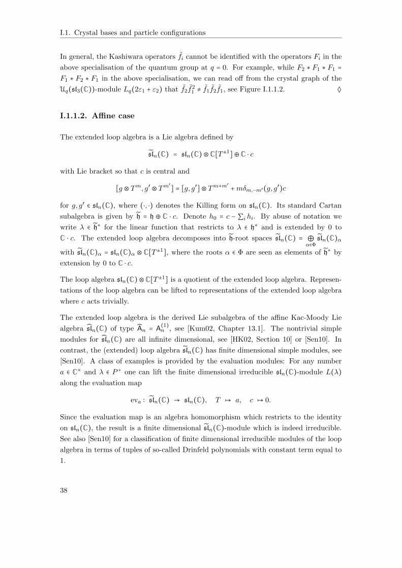
I.1.1.2. Affine case
The extended loop algebra is a Lie algebra defined by
sln(C) = sln(C)⊗C[T±1]⊕C ⋅ c
with Lie bracket so that c is central and
[g ⊗ Tm, g′ ⊗ Tm′] = [g, g′]⊗ Tm+m
′+mδm,−m′(g, g′)c
for g, g′ ∈ sln(C), where (⋅, ⋅) denotes the Killing form on sln(C). Its standard Cartan
subalgebra is given by h = h ⊕ C ⋅ c. Denote h0 = c − ∑i hi. By abuse of notation we
write λ ∈ h∗ for the linear function that restricts to λ ∈ h∗ and is extended by 0 to
C ⋅ c. The extended loop algebra decomposes into h-root spaces sln(C) = ⊕α∈Φ
sln(C)α
with sln(C)α = sln(C)α ⊗ C[T±1], where the roots α ∈ Φ are seen as elements of h∗ by
extension by 0 to C ⋅ c.
The loop algebra sln(C)⊗C[T±1] is a quotient of the extended loop algebra. Represen-
tations of the loop algebra can be lifted to representations of the extended loop algebra
where c acts trivially.
The extended loop algebra is the derived Lie subalgebra of the affine Kac-Moody Lie
algebra sln(C) of type An = A(1)n , see [Kum02, Chapter 13.1]. The nontrivial simple
modules for sln(C) are all infinite dimensional, see [HK02, Section 10] or [Sen10]. In
contrast, the (extended) loop algebra sln(C) has finite dimensional simple modules, see
[Sen10]. A class of examples is provided by the evaluation modules: For any number
a ∈ C× and λ ∈ P + one can lift the finite dimensional irreducible sln(C)-module L(λ)
along the evaluation map
eva ∶ sln(C) → sln(C), T ↦ a, c ↦ 0.
Since the evaluation map is an algebra homomorphism which restricts to the identity
on sln(C), the result is a finite dimensional sln(C)-module which is indeed irreducible.
See also [Sen10] for a classification of finite dimensional irreducible modules of the loop
algebra in terms of tuples of so-called Drinfeld polynomials with constant term equal to
1.
38
I.1.1. Quantum groups and crystal bases of type An and An
Let us now turn to the quantum affine algebra:
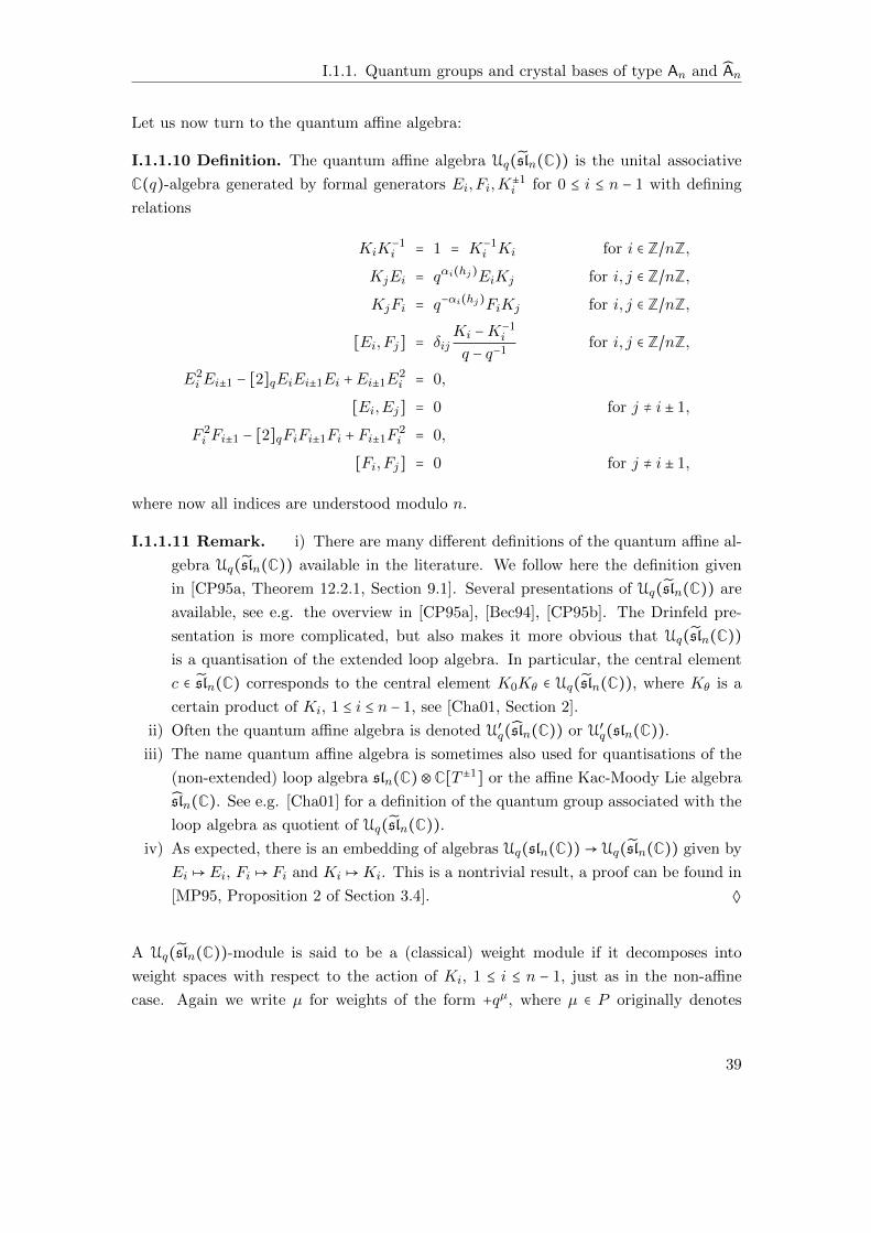
I.1.1.10 Definition. The quantum affine algebra Uq(sln(C)) is the unital associative
C(q)-algebra generated by formal generators Ei, Fi,K±1i for 0 ≤ i ≤ n − 1 with defining
relations
KiK−1i = 1 = K−1
i Ki for i ∈ Z/nZ,
KjEi = qαi(hj)EiKj for i, j ∈ Z/nZ,
KjFi = q−αi(hj)FiKj for i, j ∈ Z/nZ,
[Ei, Fj] = δijKi −K
−1i
q − q−1for i, j ∈ Z/nZ,
E2i Ei±1 − [2]qEiEi±1Ei +Ei±1E
2i = 0,
[Ei,Ej] = 0 for j ≠ i ± 1,
F 2i Fi±1 − [2]qFiFi±1Fi + Fi±1F
2i = 0,
[Fi, Fj] = 0 for j ≠ i ± 1,
where now all indices are understood modulo n.
I.1.1.11 Remark. i) There are many different definitions of the quantum affine al-
gebra Uq(sln(C)) available in the literature. We follow here the definition given
in [CP95a, Theorem 12.2.1, Section 9.1]. Several presentations of Uq(sln(C)) are
available, see e.g. the overview in [CP95a], [Bec94], [CP95b]. The Drinfeld pre-
sentation is more complicated, but also makes it more obvious that Uq(sln(C))
is a quantisation of the extended loop algebra. In particular, the central element
c ∈ sln(C) corresponds to the central element K0Kθ ∈ Uq(sln(C)), where Kθ is a
certain product of Ki, 1 ≤ i ≤ n − 1, see [Cha01, Section 2].
ii) Often the quantum affine algebra is denoted U′q(sln(C)) or U′
q(sln(C)).
iii) The name quantum affine algebra is sometimes also used for quantisations of the
(non-extended) loop algebra sln(C)⊗C[T±1] or the affine Kac-Moody Lie algebra
sln(C). See e.g. [Cha01] for a definition of the quantum group associated with the
loop algebra as quotient of Uq(sln(C)).
iv) As expected, there is an embedding of algebras Uq(sln(C))→ Uq(sln(C)) given by
Ei ↦ Ei, Fi ↦ Fi and Ki ↦Ki. This is a nontrivial result, a proof can be found in
[MP95, Proposition 2 of Section 3.4]. ◊
A Uq(sln(C))-module is said to be a (classical) weight module if it decomposes into
weight spaces with respect to the action of Ki, 1 ≤ i ≤ n − 1, just as in the non-affine
case. Again we write µ for weights of the form +qµ, where µ ∈ P originally denotes
39
I.1. Crystal bases and particle configurations
an integral weight of sln(C), see Section I.1.1.1. A Uq(sln(C))-module is called highest
weight module if it is highest weight as Uq(sln(C))-module, and the central element
K0K acts by 1.
The finite dimensional irreducible Uq(sln(C))-modules are all highest weight up to some
sign twist. By [CP95b, Theorem 3.3] the finite dimensional irreducible Uq(sln(C))-
modules (of type 1) are parametrized by (n − 1)-tuples of polynomials in one variable
with constant term 1, see also [CP91] (and note that the results from [CP91], [CP95b]
have been obtained for q = ε ∈ C× transcendental). In general it is difficult to describe
these modules explicitly. In the quantum case it is only possible in type A to construct
finite dimensional irreducible Uq(sln(C))-modules from Uq(sln(C))-modules via evalu-
ation homomorphisms, see [CP95b, Section 4.1] and [CP91, Proposition 4.1] for the
definition in case n = 2.
In general, an important class of finite dimensional irreducible Uq(sln(C))-modules is
given by Kirillov–Reshetikhin modules W i,r. The name originally refers to evaluation
modules of the Yangian developed in [KR87]. They are labelled by a node i of the
Dynkin diagram of classical type An−1 and a positive integer r ∈ Z>0. In [Cha01] a
definition of the Kirillov–Reshetikhin modules W i,r in terms of generators and relations
is given. They are constructed for the quantum loop algebra which is a quotient of
Uq(sln(C)), so the central element K0Kθ acts by zero on W i,r. Chari proved a decom-
position theorem for Kirillov–Reshetikhin modules as Uq(sln(C))-modules conjectured
in [Hat+02, Conjecture 2.1]. The Kirillov–Reshetikhin modules are minimal affinizations
in the sense of [CP95b, Section 6], see [CH10, Section 8]. In particular, for type A there
is an isomorphism W i,r ≅ Lq(rωi) as Uq(sln(C))-modules [CP96, Theorem 3.1].
Abstract crystals can be defined similarly to the finite case situation from Section I.1.1.1,
see e.g. [Kan+92]. It is proven in [Kan+92] that Kirillov–Reshetikhin modules admit
crystal (pseudo)bases. Previously, results for type A have been obtained in [MM90] and
[Jim+91], see furthermore [Shi02] and the overview in [Kus13], [Kus16]. In type A these
Kirillov-Reshetikhin crystals are perfect [Kan+92, Theorem 1.2.2], see also [Par12].
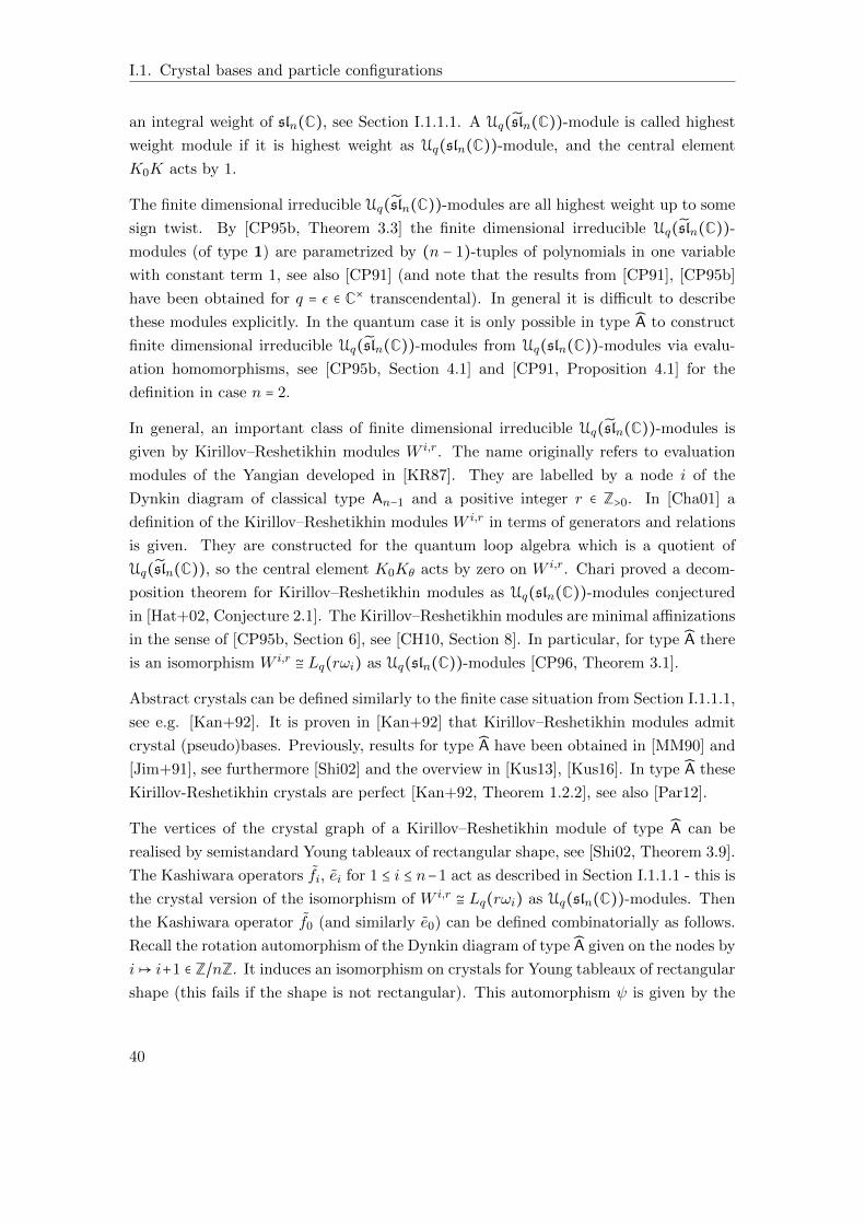
The vertices of the crystal graph of a Kirillov–Reshetikhin module of type A can be
realised by semistandard Young tableaux of rectangular shape, see [Shi02, Theorem 3.9].
The Kashiwara operators fi, ei for 1 ≤ i ≤ n−1 act as described in Section I.1.1.1 - this is
the crystal version of the isomorphism of W i,r ≅ Lq(rωi) as Uq(sln(C))-modules. Then
the Kashiwara operator f0 (and similarly e0) can be defined combinatorially as follows.
Recall the rotation automorphism of the Dynkin diagram of type A given on the nodes by
i↦ i+1 ∈ Z/nZ. It induces an isomorphism on crystals for Young tableaux of rectangular
shape (this fails if the shape is not rectangular). This automorphism ψ is given by the
40
I.1.1. Quantum groups and crystal bases of type An and An
Schutzenberger promotion operator realised in [Shi02, Proposition 3.15], according to
which, ψ is applied to a semistandard Young tableau by the following steps: (i) remove
all entries n, (ii) perform jeu-de-taquin to slide the remaining entries to the empty boxes,
(iii) add 1 to all entries, (iv) fill the vacated boxes by 1.
For general Young tableaux, jeu-de-taquin is defined by a combinatorial rule e.g. in
[Ful97, Section 1.2]. For Young tableaux of shape kω1 or ωk that consist of a single row
or column, respectively, it is simply given by sliding all entries to the left or downwards,
respectively.
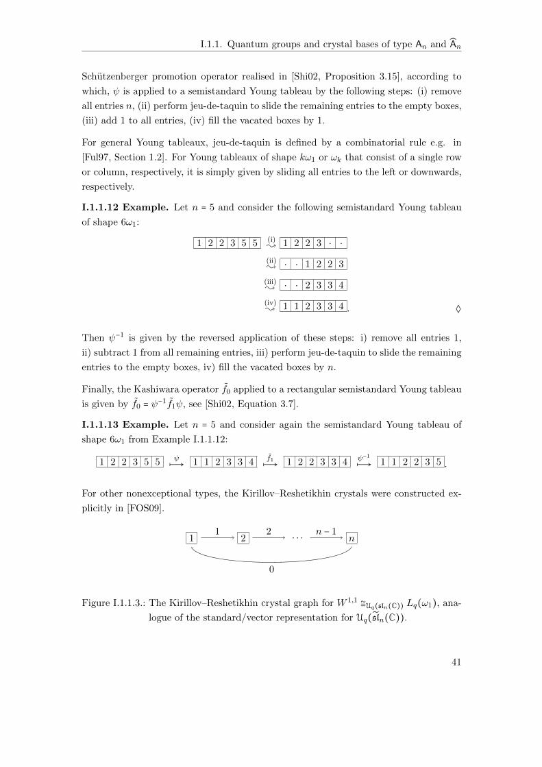
I.1.1.12 Example. Let n = 5 and consider the following semistandard Young tableau
of shape 6ω1:
1 2 2 3 5 5 (i); 1 2 2 3 ⋅ ⋅
(ii); ⋅ ⋅ 1 2 2 3
(iii); ⋅ ⋅ 2 3 3 4
(iv); 1 1 2 3 3 4 . ◊
Then ψ−1 is given by the reversed application of these steps: i) remove all entries 1,
ii) subtract 1 from all remaining entries, iii) perform jeu-de-taquin to slide the remaining
entries to the empty boxes, iv) fill the vacated boxes by n.
Finally, the Kashiwara operator f0 applied to a rectangular semistandard Young tableau
is given by f0 = ψ−1f1ψ, see [Shi02, Equation 3.7].
I.1.1.13 Example. Let n = 5 and consider again the semistandard Young tableau of
shape 6ω1 from Example I.1.1.12:
1 2 2 3 5 5 ψz→ 1 1 2 3 3 4 f1
z→ 1 2 2 3 3 4 ψ−1z→ 1 1 2 2 3 5 .
For other nonexceptional types, the Kirillov–Reshetikhin crystals were constructed ex-
plicitly in [FOS09].
1 2 . . . n1 2 n − 1
0
Figure I.1.1.3.: The Kirillov–Reshetikhin crystal graph for W 1,1 ≅Uq(sln(C)) Lq(ω1), ana-
logue of the standard/vector representation for Uq(sln(C)).
41
I.1. Crystal bases and particle configurations
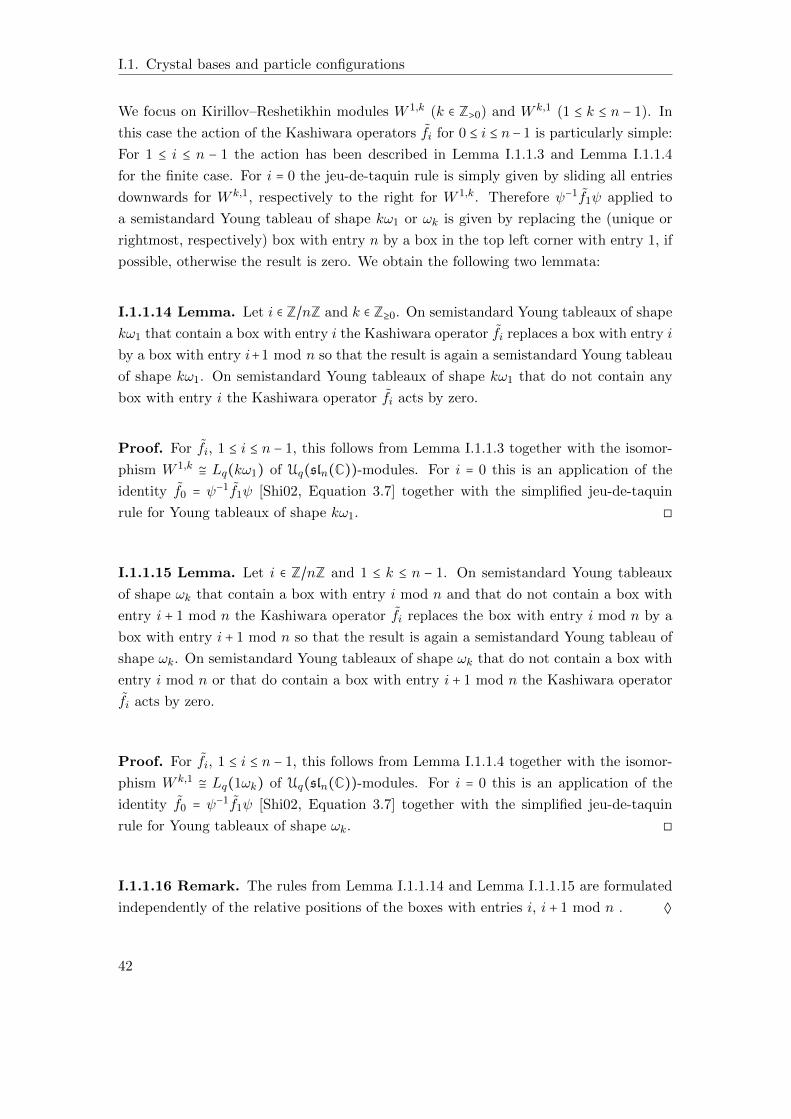
We focus on Kirillov–Reshetikhin modules W 1,k (k ∈ Z>0) and W k,1 (1 ≤ k ≤ n − 1). In
this case the action of the Kashiwara operators fi for 0 ≤ i ≤ n− 1 is particularly simple:
For 1 ≤ i ≤ n − 1 the action has been described in Lemma I.1.1.3 and Lemma I.1.1.4
for the finite case. For i = 0 the jeu-de-taquin rule is simply given by sliding all entries
downwards for W k,1, respectively to the right for W 1,k. Therefore ψ−1f1ψ applied to
a semistandard Young tableau of shape kω1 or ωk is given by replacing the (unique or
rightmost, respectively) box with entry n by a box in the top left corner with entry 1, if
possible, otherwise the result is zero. We obtain the following two lemmata:
I.1.1.14 Lemma. Let i ∈ Z/nZ and k ∈ Z≥0. On semistandard Young tableaux of shape
kω1 that contain a box with entry i the Kashiwara operator fi replaces a box with entry i
by a box with entry i+1 mod n so that the result is again a semistandard Young tableau
of shape kω1. On semistandard Young tableaux of shape kω1 that do not contain any
box with entry i the Kashiwara operator fi acts by zero.
Proof. For fi, 1 ≤ i ≤ n − 1, this follows from Lemma I.1.1.3 together with the isomor-
phism W 1,k ≅ Lq(kω1) of Uq(sln(C))-modules. For i = 0 this is an application of the
identity f0 = ψ−1f1ψ [Shi02, Equation 3.7] together with the simplified jeu-de-taquin
rule for Young tableaux of shape kω1. ◻
I.1.1.15 Lemma. Let i ∈ Z/nZ and 1 ≤ k ≤ n − 1. On semistandard Young tableaux
of shape ωk that contain a box with entry i mod n and that do not contain a box with
entry i + 1 mod n the Kashiwara operator fi replaces the box with entry i mod n by a
box with entry i + 1 mod n so that the result is again a semistandard Young tableau of
shape ωk. On semistandard Young tableaux of shape ωk that do not contain a box with
entry i mod n or that do contain a box with entry i + 1 mod n the Kashiwara operator
fi acts by zero.
Proof. For fi, 1 ≤ i ≤ n − 1, this follows from Lemma I.1.1.4 together with the isomor-
phism W k,1 ≅ Lq(1ωk) of Uq(sln(C))-modules. For i = 0 this is an application of the
identity f0 = ψ−1f1ψ [Shi02, Equation 3.7] together with the simplified jeu-de-taquin
rule for Young tableaux of shape ωk. ◻
I.1.1.16 Remark. The rules from Lemma I.1.1.14 and Lemma I.1.1.15 are formulated
independently of the relative positions of the boxes with entries i, i + 1 mod n . ◊
42
I.1.2. Combinatorics of particle configurations
12
13
23
14
24
15
34
25
35
45
2
13
4 1 3
4 21
42
3
;
12
13
23
14
24
15
34
25
35
45
2
13
4 1 3
4 21
42
3
0
0
0
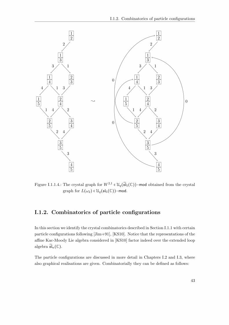
Figure I.1.1.4.: The crystal graph for W 2,1 ∈ Uq(sl5(C))−mod obtained from the crystal
graph for L(ω2) ∈ Uq(sl5(C))−mod.
I.1.2. Combinatorics of particle configurations
In this section we identify the crystal combinatorics described in Section I.1.1 with certain
particle configurations following [Jim+91], [KS10]. Notice that the representations of the
affine Kac-Moody Lie algebra considered in [KS10] factor indeed over the extended loop
algebra sln(C).
The particle configurations are discussed in more detail in Chapters I.2 and I.3, where
also graphical realisations are given. Combinatorially they can be defined as follows:
43
I.1. Crystal bases and particle configurations
I.1.2.1 Definition. i) For k ∈ Z>0, n ≥ 2, classical and affine bosonic particle con-
figurations of k particles on n positions are defined to be partitions of k with n
parts, i.e. tuples (k1, . . . , kn) ∈ Zn≥0 with ∑i ki = k. For classical bosonic particle
configurations, particle propagation operators ar are defined for 1 ≤ r ≤ n − 1 by
ar(k1, . . . , kr, kr+1, . . . , kn) = (k1, . . . , kr − 1, kr+1 + 1, . . . , kn) if kr > 0,
ar(k1, . . . , kr, kr+1, . . . , kn) = 0 else.
For affine bosonic particle configurations, the particle propagation operators are
defined for 1 ≤ r ≤ n − 1 in the same way. Additionally, there is a propagation
operator a0 given by
a0(k1, . . . , kn) = (k1 + 1, . . . , kn − 1) if kn > 0,
a0(k1, . . . , kn) = 0 else.
Similarly, a reversed particle propagation operator a∗r is defined for classical or
affine bosonic particle configurations (k1, . . . , kn) with 1 ≤ r ≤ n− 1 or 0 ≤ r ≤ n− 1,
respectively, by
a∗r(k1, . . . , kr, kr+1, . . . , kn) = (k1, . . . , kr + 1, kr+1 − 1, . . . , kn) if kr+1 > 0,
a∗r(k1, . . . , kr, kr+1, . . . , kn) = 0 else.
ii) For 1 ≤ k ≤ n − 1, n ≥ 2, classical and affine fermionic particle configurations of k
particles on n positions are defined to be tuples (i1, . . . , in) ∈ 0,1n with ∑r ir = k.
For classical fermionic particle configurations, particle propagation operators ar are
defined for 1 ≤ r ≤ n − 1 by
ar(k1, . . . , kr, kr+1, . . . , kn) = (k1, . . . , kr − 1, kr+1 + 1, . . . , kn) if kr = 1, kr+1 = 0,
ar(k1, . . . , kr, kr+1, . . . , kn) = 0 else.
For affine fermionic particle configurations, the particle propagation operators are
defined for 1 ≤ r ≤ n − 1 in the same way. Additionally, there is a propagation
operator a0 given by
a0(k1, . . . , kn) = (k1 + 1, . . . , kn − 1) if kn = 1, k1 = 0,
a0(k1, . . . , kn) = 0 else.
Similarly, define the reversed particle propagation operator a∗r for a classical or
affine fermionic particle configuration (k1, . . . , kn) with 1 ≤ r ≤ n−1 or 0 ≤ r ≤ n−1,
respectively, by
a∗r(k1, . . . , kr, kr+1, . . . , kn) = (k1, . . . , kr + 1, kr+1 − 1, . . . , kn) if kr+1 = 1, kr = 0,
a∗r(k1, . . . , kr, kr+1, . . . , kn) = 0 else.
44
I.1.2. Combinatorics of particle configurations
Hence, if ai(k′1, . . . , k
′n) = (k1, . . . , kn) ≠ 0, then we have a∗i (k1, . . . , kn) = (k′1, . . . , k
′n).
One can identify particle configurations and crystals as follows, see [KS10, Remark 5.9]:
I.1.2.2 Proposition. i) Let k ∈ Z>0. There are bijections of sets
semistandard Young tableaux of shape kω1 with entries 1, . . . , n
↔ classical bosonic particle configurations of k particles with n positions,
semistandard Young tableaux of shape kω1 with entries in Z/nZ
↔ affine bosonic particle configurations of k particles with n positions
that identify the unique semistandard Young tableaux of shape kω1 with entries
(i1, . . . , ik) so that kr ∶= #j ∣ 1 ≤ j ≤ k, ij = r with the particle configuration
(k1, . . . , kn). These bijections identify the Kashiwara operators fi with particle
propagation operators ai for 1 ≤ i ≤ n and i ∈ Z/nZ, respectively. The Kashiwara
operators ei are identified with particle propagation operators a∗i for 1 ≤ i ≤ n and
i ∈ Z/nZ, respectively.
ii) Let 1 ≤ k ≤ n − 1. There are bijections of sets
semistandard Young tableaux of shape ωk with entries 1, . . . , n
↔ classical fermionic particle configurations of k particles with n positions,
semistandard Young tableaux of shape ωk with entries in Z/nZ
↔ affine fermionic particle configurations of k particles with n positions
that identify the unique semistandard Young tableaux of shape ωk with entries
(i1, . . . , ik) so that kr ∶= #j ∣ 1 ≤ j ≤ k, ij = r with the particle configuration
(k1, . . . , kn). These bijections identify the Kashiwara operators fi with particle
propagation operators ai for 1 ≤ i ≤ n and i ∈ Z/nZ, respectively. The Kashiwara
operators ei are identified with particle propagation operators a∗i for 1 ≤ i ≤ n and
i ∈ Z/nZ, respectively.
Proof. For the bijections between semistandard Young tableaux and particle config-
urations it suffices to observe that semistandard Young tableaux of shape ωk or kω1
are uniquely determined by their entries without recording the precise position of each
entry. The identification of Kashiwara operators with particle propagation operators fol-
lows from Lemma I.1.1.3, Lemma I.1.1.14, Lemma I.1.1.4 and Lemma I.1.1.15 together
with the property of crystals graphs that there is an edge from node x to node x′ labelled
fi if and only if there is an edge from node x′ to x labelled ei. ◻
45
I.1. Crystal bases and particle configurations
I.1.2.3 Remark. By Proposition I.1.2.2 one can identify Kashiwara operators with
particle propagation operators. In Chapters I.2 and Chapter I.3 we see that one can
identify the particle propagation operators with generators of the (affine) plactic algebra.
The (affine) plactic algebra is isomorphic to the specialisation of one half of the (affine)
quantum group at q = 0 by desymmetrized Serre relations, see Remark I.1.1.9.
Thereby the two different approaches of specialisation of the quantum group at q = 0 – by
crystals and by desymmetrized Serre relations – are related in the special case of Young
diagrams of shape kω1, ωk. This fails for other crystals, see Remark I.1.1.9. It is special
about kω1 and ωk that the action of Kashiwara operators, particle propagation operators
and plactic operators is uniquely determined by the list of entries in the Young tableaux,
independently of the position of the entries. In general, the Kashiwara operators are
sensitive to the position of the entries, see Figure I.1.1.2 ◊
46
I.2. The affine nilTemperley–Lieb
algebra
This chapter is structured as follows: In Section I.2.1 we define the affine nilTemperley–
Lieb algebra nTLN and fix some notation. In Section I.2.2 we give an overview over
algebras related to the affine nilTemperley–Lieb algebra. In Section I.2.3 we discuss two
gradings of nTLN that are important tools when we compute the center of the algebra.
The second main tool for the computation of the center is the faithfulness of the action
on affine fermionic particle configurations: In Section I.2.4 we define this action, in
Section I.2.5 we describe a normal form for monomials and hence a basis of nTLN that
we use in Section I.2.6 to give an elementary proof of faithfulness.
In Section I.2.7 we define certain projectors inside nTLN that sum up to central elements.
Then in Section I.2.8 we show that the center of nTLN is in fact generated by these
special central elements. In Section I.2.9 we show that nTLN is finitely generated over
the center. In Section I.2.10 we describe another normal form for the monomials that
makes use of the center. At that moment we have collected enough information to
construct inclusions nTLN ⊂ nTLN+1 in Section I.2.11.
While all results so far hold over an arbitrary ground field k (see Remark I.2.1.3), we have
to assume that k is an uncountable algebraically closed field in the remaining sections. In
Section I.2.12 we compute localisations with respect to central elements and we classify
the simple modules over nTLN . In Section I.2.13 we use these localisations together
with a rank argument to show that nTLN is not free over its center. In Section I.2.14 we
discuss possible approaches to equip nTLN with an affine cellular structure in the sense
of [KX12] based on our knowledge of different normal forms for monomials in nTLN .
I.2.1. Notation
Let k be any field, denote by k[q] the polynomial ring in an indeterminate q, and assume
N is a positive integer. Throughout we will assume N ≥ 3.
47
I.2. The affine nilTemperley–Lieb algebra
I.2.1.1 Definition. The affine nilTemperley–Lieb algebra nTLN of rank N is the unital
associative k-algebra generated by elements a0, . . . , aN−1 subject to the relations
a2i = 0 for all 0 ≤ i ≤ N − 1,
aiaj = ajai for all i − j ≠ ±1 mod N,
aiai+1ai = ai+1aiai+1 = 0 for all 0 ≤ i ≤ N − 1,
where all indices are taken modulo N , so in particular aN−1a0aN−1 = a0aN−1a0 = 0.
The finite nilTemperley–Lieb algebra nTLN is the subalgebra of nTLN generated by
a1, . . . , aN−1. We adopt the convention that nTL1 = k1.
We fix the following notation for monomials in nTLN and nTLN : For an ordered index
sequence j = (j1, . . . , jm) with 0 ≤ j1, . . . , jm ≤ N − 1, we define the element
a(j) = aj1 . . . ajm
and we call it (ordered) monomial. Unless otherwise specified, we use the letters i, j for
indices from Z/NZ, in particular, we identify the indices 0 and N in this case.
I.2.1.2 Example. For N = 5, the monomial associated with the ordered index sequence
j = (1,3,2,0,1,4,3) is given by
a(j) = a(1,3,2,0,1,4,3) = a1a3a2a0a1a4a3.
I.2.1.3 Remark. Except for Sections I.2.12, I.2.13 and I.2.14, all of our results hold
over an arbitrary ground field k, even one of characteristic 2, simply by ignoring signs
in that case.
In fact, our arguments in Sections I.2.1 – I.2.7 work for any associative unital ground
ring R if we adapt our notation: We need to replace k-vector spaces and k-algebras with
free R-modules and R-algebras, respectively. In particular, the affine nilTemperley–Lieb
algebra over k is replaced by the R-algebra with the same generators and relations, and
the polynomial ring k[q] is replaced by R[q]. In addition, in Sections I.2.8 – I.2.11 we
have to assume in addition that R is commutative unless we modify our statements
slightly, e.g. replace R by its center in Proposition I.2.8.2 and Theorem I.2.8.5 and
assume that R is finitely generated over its center in Theorem I.2.9.1.
This is possible because our arguments mainly rely on investigating monomials in the
generators of nTLN . However, for simplicity we have chosen to assume k is a field
throughout the chapter. ◊
48
I.2.2. Related algebras
I.2.2. Related algebras
The affine nilTemperley–Lieb algebra appears in many different settings, some of which
we describe in this section.
I.2.2.1. The affine nilCoxeter algebra
nTLN is a quotient of the affine nilCoxeter algebra of type AN−1:
The affine nilCoxeter algebra nCN of type AN−1 over a field k is the unital associative
algebra generated by elements ui, 0 ≤ i ≤ N−1, satisfying the relations u2i = 0; uiuj = ujui
for i − j ≠ ±1 mod N ; and uiui+1ui = ui+1uiui+1 for 1 ≤ i ≤ N − 1, where the subscripts
are read modulo N . The algebra nTLN is isomorphic to the quotient of nCN obtained
by imposing the additional relations uiui+1ui = ui+1uiui+1 = 0 for 1 ≤ i ≤ N − 1.
The nilCoxeter algebra nCN has generators ui,1 ≤ i ≤ N − 1, which satisfy the same
relations as they do in nCN . It first appeared in work on the cohomology of flag varieties
[BGG73] and has played an essential role in studies on Schubert polynomials, Stanley
symmetric functions, and the geometry of flag varieties (see for example [LS89], [Mac91],
[KK86], [FS94]). The definition of nCN was inspired by the divided difference operators
∂i on polynomials in variables x = x1, . . . , xN defined by Demazure operators
∂i(f) =f(x) − f(σix)
xi − xi+1,
where the transposition σi fixes all the variables except for xi and xi+1, which it in-
terchanges. The operators ∂i satisfy the nilCoxeter relations above, and applications
of these relations enabled Fomin and Stanley [FS94] to recover known properties and
establish new properties of Schubert polynomials.
The algebra nCN belongs to a two-parameter family of algebras having generators ui,
1 ≤ i ≤ N −1, which satisfy the relations uiuj = ujui for ∣i−j∣ > 1 and uiui+1ui = ui+1uiui+1
for 1 ≤ i ≤ N−2 from above, together with the relation u2i = αui+β for all i, where α,β are
fixed parameters. In particular, the specialization α = β = 0 yields the nilCoxeter algebra;
α = 0, β = 1 gives the standard presentation of the group algebra of the symmetric group
kSN ; and α = q − 1, β = q gives the Hecke algebra HN(q) of type A.
Khovanov [Kho01] introduced restriction functors FD and induction functors FX corre-
sponding to the natural inclusion of algebras nCN nCN+1 on the direct sum C of the
categories CN of finite-dimensional nCN -modules. These functors categorify the Weyl
49
I.2. The affine nilTemperley–Lieb algebra
algebra of differential operators with polynomial coefficients in one variable and cor-
respond to the Weyl algebra generators ∂ and x (derivative and multiplication by x),
which satisfy the relation ∂x − x∂ = 1.
Brichard [Bri11] used a diagram calculus on cylinders to determine the dimension of the
center of nCN and to describe a basis of the center for which the multiplication is trivial.
In this diagram calculus on N strands, the generator ui corresponds to a crossing of the
strands i and i + 1. The nil relation u2i = 0 is represented by demanding that any two
strands may cross at most once; otherwise the diagram is identified with zero.
For convenience let us include an overview of the various 0- and nil-versions of Hecke
and Coxeter algebras of type A or A over the ground ring k (e.g. k = C(q)). Let ν ∈ k×
be a unit (e.g. ν = q).
i) The nilCoxeter algebra nCN of type A with its defining relations u2i = 0; uiuj = ujui
for ∣i − j∣ > 1; and uiui+1ui = ui+1uiui+1 for 1 ≤ i ≤ N − 2 is sometimes also called
nilHecke algebra [GR04]. See [Kha16] for generalizations of the nilCoxeter algebra.
ii) The (polynomial) affine nilHecke algebra of type A is the algebra generated by ui,
1 ≤ i ≤ N − 1, and Xi, 1 ≤ i ≤ N , with relations u2i = 0; uiuj = ujui for ∣i − j∣ > 1;
uiui+1ui = ui+1uiui+1 for 1 ≤ i ≤ N − 2; XiXj = XjXi for all i, j; and with mixed
relations Xjui = uiXj for all j ≠ i, i + 1 and
uiXi+1 = Xiui + 1, Xi+1ui = uiXi + 1.
It contains the nilCoxeter algebra nCN and the polynomial ring k[X1, . . . ,Xn] as
subalgebras. Many authors use the name nilHecke algebra for this algebra [KK86],
[KL09]. Because of this ambiguity we avoid to use the terminology “nilHecke
algebra”. In [KL09, Examples 2.2 3)] a graphical realisation for the affine nilHecke
algebra is given. Every monomial corresponds to a string diagram connecting N
points in the bottom with N points in the top of the diagram. The generator Xi
is given by the identity diagram with a dot on the i-th strand, while ui is given by
the crossing of the strands connecting i, i + 1.
iii) The (localised) affine nilHecke algebra of type A is the localisation of the affine
nilHecke algebra at all Xi, 1 ≤ i ≤ N .
iv) The Hecke algebra or Iwahori–Hecke algebra HN(ν) of type A is “the” Hecke alge-
bra defined by generators Ti, 1 ≤ i ≤ N−1, with defining relations (Ti−ν)(Ti+1) = 0;
TiTj = TjTi for ∣i−j∣ > 1; and TiTi+1Ti = Ti+1TiTi+1 for 1 ≤ i ≤ N−2. Since ν ∈ k× one
can deduce frome these relations in addition that there exists T−1i = ν−1(Ti + 1− ν)
for all 1 ≤ i ≤ N − 1.
50
I.2.2. Related algebras
v) The (polynomial) affine Hecke algebra of type A is given by generators Ti, 1 ≤ i ≤
N −1, and Xi, 1 ≤ i ≤ N , with relations (Ti−ν)(Ti+1) = 0; TiTj = TjTi for ∣i−j∣ > 1;
and TiTi+1Ti = Ti+1TiTi+1 for 1 ≤ i ≤ N −2; XiXj =XjXi for all i, j; and with mixed
relations TiXiTi = νXi+1 for 1 ≤ i ≤ N − 1 and TiXj = XjTi for j ≠ i, i + 1. One
can deduce frome these relations that there exists T−1i = ν−1(Ti + 1 − ν) for all
1 ≤ i ≤ N − 1, and furthermore
TiXi = Xi+1Ti +Xi+1 − νXi+1, XiTi = TiXi+1 +Xi+1 − νXi+1.
Although these relations have been deduced using ν ∈ k×, they also make sense
for ν = 0, so they will appear again in the definition of the affine 0-Hecke algebra
below.
vi) The (localised) affine Hecke algebra or extended Iwahori–Matsumoto Hecke algebra
of type A is equal to the polynomial affine Hecke algebra localised at Xi for all
1 ≤ i ≤ N [IM65], [MS16].
vii) The 0-Hecke algebra of type A is defined by generators Ti, 1 ≤ i ≤ N−1 and relations
T 2i = −Ti; TiTj = TjTi for ∣i − j∣ > 1; and TiTi+1Ti = Ti+1TiTi+1 for 1 ≤ i ≤ N − 2.
For alternative generators H i = Ti+1 the relations read H2i =H i; H iHj =HjH i for
∣i−j∣ > 1; and H iH i+1H i =H i+1H iH i+1 for 1 ≤ i ≤ N −2. Notice that some authors
call this algebra as well nilHecke algebra, see [Kha16] and references therein.
viii) Define the (polynomial) affine 0-Hecke algebra of type A as the algebra generated
by Ti, 1 ≤ i ≤ N − 1, and Xi, 1 ≤ i ≤ N , and relations T 2i = −Ti; TiTj = TjTi for
∣i− j∣ > 1; TiTi+1Ti = Ti+1TiTi+1 for 1 ≤ i ≤ N − 2; XiXj =XjXi for all i, j; and with
mixed relations TiXj =XjTi for j ≠ i, i + 1; and furthermore
TiXi = Xi+1Ti +Xi+1, XiTi = TiXi+1 +Xi+1.
From this it follows that TiXiTi = 0 for 1 ≤ i ≤ N − 1. For alternative generators
H i = Ti + 1 the relations read H2i = H i; H iHj = HjH i for ∣i − j∣ > 1; H iH i+1H i =
H i+1H iH i+1 for 1 ≤ i ≤ N − 2; XiXj = XjXi for all i, j; and with mixed relations
TiXiTi = 0 for 1 ≤ i ≤ N − 1 and H iXj =XjH i for j ≠ i, i + 1; and furthermore
H iXi = Xi+1H i +Xi, XiH i = H iXi+1 +Xi.
ix) The (localised) affine 0-Hecke algebra of type A is the localisation of the affine
0-Hecke algebra at all Xi, 1 ≤ i ≤ N .
x) We use the name cyclic affine Hecke algebra when we refer to the Hecke algebra
associated with the affine Coxeter group of type A. It is defined by generators Ti,
0 ≤ i ≤ N − 1, with relations (Ti − q)(Ti + 1) = 0; TiTj = TjTi for ∣i − j∣ > 1; and
TiTi+1Ti = Ti+1TiTi+1 for 0 ≤ i ≤ N − 1, where all indices are understood modulo N .
51
I.2. The affine nilTemperley–Lieb algebra
It is not immediate how these algebras defined by generators and relations are related.
One can check that there is an isomorphism between the (localised) affine nilHecke
algebra and the (localised) affine 0-Hecke algebra given by
(Localised) affine nilHecke algebra ≅ (Localised) affine 0-Hecke algebra
ui ↦ −X−1i H i
X±1i ↦ X±1
i .
Although the affine nilCoxeter algebra nCN of type A and the localised affine nilHecke
algebra of type A are defined in quite different ways, there is hope that they can be
related similarly to the group algebras of “cyclic” affine symmetric group C[SN ] and
the “extended” affine symmetric group C[SN ] ⋉ C[X±11 , . . . ,X±1
N ]. In fact, C[SN ] ⋉
C[X±11 , . . . ,X±1
N ] is isomorphic to the C-algebra defined by generators si, 1 ≤ i ≤ N ,
and τ , so that s2i = 1; sisj = sjsi for ∣i − j∣ > 1; sisi+1si = si+1sisi+1 for 1 ≤ i ≤ N − 2;
siτ = τsi+1 for all i; and all indices are understood modulo N , see [GJ11, Section 6.2].
Indeed, for the (localised) affine Hecke algebra it is known that the “cyclic” presentation
(x) and the “extended” presentation (vi) are equivalent, see [MS16, Lemma 3.2]. The
Bernstein and the Iwahori-Matsumoto presentation are related by [HP02].
I.2.2.2. The universal enveloping algebra of the Lie algebra of affine
type A
nTLN is a quotient of the negative part of the universal enveloping algebra of the affine
Kac–Moody Lie algebra slN :
The negative part U−(slN) of the universal enveloping algebra U(slN) of the affine Kac–
Moody Lie algebra slN has generators fi, 0 ≤ i ≤ N − 1, which satisfy the Serre relations
f2i fi+1 − 2fifi+1fi + fi+1f
2i = 0 = f2
i+1fi − 2fi+1fifi+1 + fif2i+1 and fifj = fjfi for i − j ≠
±1 mod N (all indices modulo N). Factoring U−(slN) by the ideal generated by the
elements f2i , 0 ≤ i ≤ N − 1, gives nTLN whenever the characteristic of k is different from
2.
I.2.2.3. The affine plactic algebra
The affine nilTemperley–Lieb algebra is a quotient of the affine plactic algebra and the
local affine plactic algebra that we encounter again in Chapter I.3. The local affine
plactic algebra PN is the unital associative k-algebra generated by a0, a1, . . . , aN−1 with
defining relations aiaj = ajai for i− j ≠ ±1 mod N ; aiai−1ai = aiaiai−1 for i, i−1 ∈ Z/NZ;
52
I.2.2. Related algebras
and aiai+1ai = ai+1aiai for i, i+1 ∈ Z/NZ. The name “local” refers to the commutativity
relation aiaj = ajai. See the discussion of the plactic algebra in Chapter I.3 for references
and more details about this algebra.
After we quotient out the additional relation a2i = 0 for all i, we obtain the affine
nilTemperley–Lieb algebra.
I.2.2.4. Combinatorial actions
nTLN acts on the small quantum cohomology ring of the Grassmannian:
As in [Pos05, Section 2] (see also [KS10]), consider the cohomology ring H(Gr(k,N))
with integer coefficients for the Grassmannian Gr(k,N) of k-dimensional subspaces of
kN . It has a basis given by the Schubert classes [Ωλ], where λ runs over all partitions
with k parts, the largest part having size N − k. By recording the k vertical and N − k
horizontal steps that identify the Young diagram of λ inside the northwest corner of
a k × (N − k) rectangle, such a partition corresponds to a (0,1)-sequence of length N
with k ones (respectively and N − k zeros) in the positions corresponding to the vertical
(respectively horizontal) steps.
As a Z[q]-module for an indeterminate q, the quantum cohomology ring of the Grassman-
nian is given by qH(Gr(k,N)) = Z[q]⊗ZH(Gr(k,N)) together with a q-multiplication,
[Buc03], [FGP97, Theorem 1.3] (see also [FGP97, Theorem 1.2] for an identification of
Schubert classes with quantum Schubert polynomials, analogously to [BGG73], and ref-
erences therein).
The nTLN -action can be defined combinatorially on
qH(Gr(k,N)) ≅ spanZ[q] (0,1)-sequences of length N with k ones
as described in the next item, and the multiplication of two Schubert classes [Ωλ] ⋅ [Ωµ]
is equal to sλ ⋅ [Ωµ] where sλ is a certain Schur polynomial in the noncommutative
generators of nTLN as defined in [Pos05, Corollary 8.3].
nTLN acts faithfully on fermionic particle configurations on a circle:
First, a (0,1)-sequence with k ones is identified with a circular particle configuration
having N positions, where the k particles are distributed at the position on the circle
53
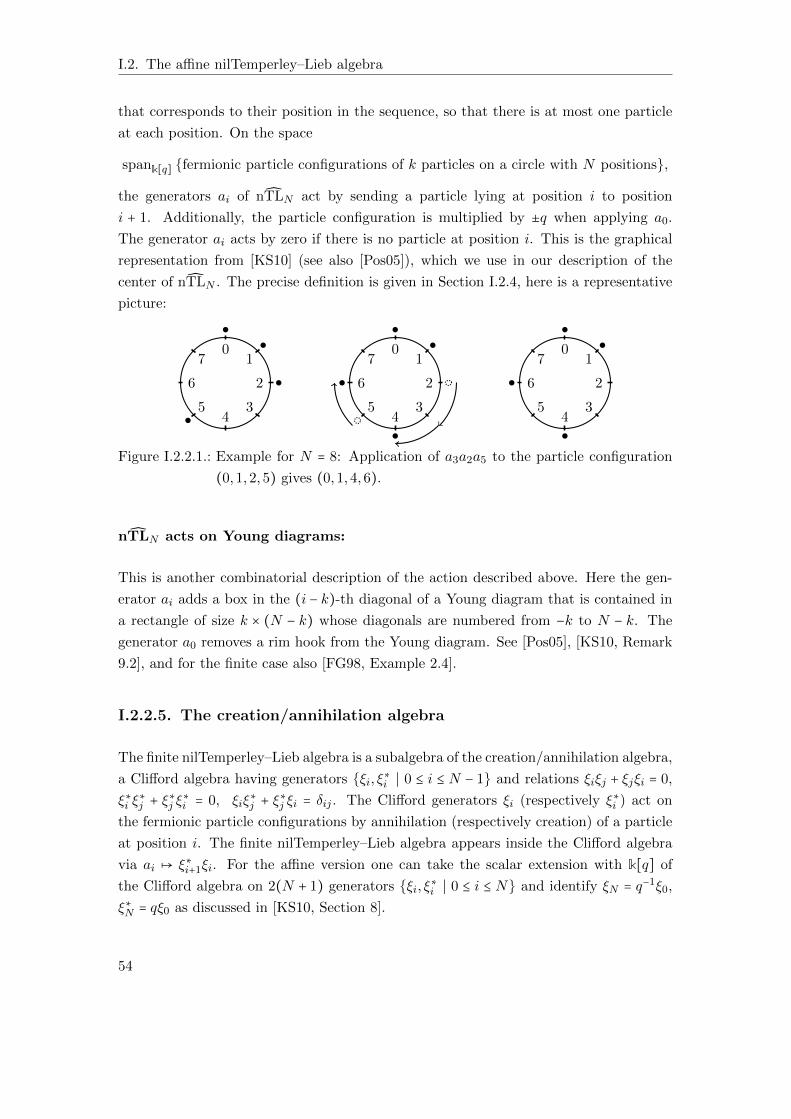
I.2. The affine nilTemperley–Lieb algebra
that corresponds to their position in the sequence, so that there is at most one particle
at each position. On the space
spank[q] fermionic particle configurations of k particles on a circle with N positions,
the generators ai of nTLN act by sending a particle lying at position i to position
i + 1. Additionally, the particle configuration is multiplied by ±q when applying a0.
The generator ai acts by zero if there is no particle at position i. This is the graphical
representation from [KS10] (see also [Pos05]), which we use in our description of the
center of nTLN . The precise definition is given in Section I.2.4, here is a representative
picture:
01
2
34
5
6
70
1
2
34
5
6
70
1
2
34
5
6
7
Figure I.2.2.1.: Example for N = 8: Application of a3a2a5 to the particle configuration
(0,1,2,5) gives (0,1,4,6).
nTLN acts on Young diagrams:
This is another combinatorial description of the action described above. Here the gen-
erator ai adds a box in the (i − k)-th diagonal of a Young diagram that is contained in
a rectangle of size k × (N − k) whose diagonals are numbered from −k to N − k. The
generator a0 removes a rim hook from the Young diagram. See [Pos05], [KS10, Remark
9.2], and for the finite case also [FG98, Example 2.4].
I.2.2.5. The creation/annihilation algebra
The finite nilTemperley–Lieb algebra is a subalgebra of the creation/annihilation algebra,
a Clifford algebra having generators ξi, ξ∗i ∣ 0 ≤ i ≤ N − 1 and relations ξiξj + ξjξi = 0,
ξ∗i ξ∗j + ξ
∗j ξ
∗i = 0, ξiξ
∗j + ξ
∗j ξi = δij . The Clifford generators ξi (respectively ξ∗i ) act on
the fermionic particle configurations by annihilation (respectively creation) of a particle
at position i. The finite nilTemperley–Lieb algebra appears inside the Clifford algebra
via ai ↦ ξ∗i+1ξi. For the affine version one can take the scalar extension with k[q] of
the Clifford algebra on 2(N + 1) generators ξi, ξ∗i ∣ 0 ≤ i ≤ N and identify ξN = q−1ξ0,
ξ∗N = qξ0 as discussed in [KS10, Section 8].
54
I.2.2. Related algebras
I.2.2.6. The affine Temperley–Lieb algebra
nTLN is the associated graded algebra of the affine Temperley–Lieb algebra:
The affine Temperley–Lieb algebra TLN(δ) generated by a0, . . . , aN−1 has the usual
commuting relations and the relations aiai±1ai = ai and a2i = δai for some parameter
δ ∈ k instead of the nil relations (where again all indices are mod N). It contains the
famous Temperley–Lieb algebra TLN(δ) as the subalgebra generated by a1, . . . , aN−1,
see [TL71], [Kau90]. Both are filtered algebras with `-th filtration space generated by
all monomials of length at most `. Since the associated graded algebra of TLN(δ) is
nTLN for any value of δ, elements of nTLN can be identified with reduced expressions
in TLN(δ).
The Temperley–Lieb algebra TLN(δ) is known for its diagrammatical realisation by
crossingless string diagrams in the plane that connect 2N points. Multiplication of
diagrams is given by connecting and smoothing the strands. Whenever the strands
form a circle, this is removed from the diagram at the expense of multiplying by the
parameter δ. This is an example for a diagram algebra, in the sense that it is a quotient
of an algebra with a presentation by generators and relations so that the generators
can be identified with string diagrams (possibly with labelled strands and additional
decoration, e.g. dots) inside [0,1] ×M, where M is a compact manifold. The strands in
such a diagram form closed loops or connect a finite number of end points in 0,1×M,
multiplication is given by stacking the diagrams on top of each other and connecting
the strands at the end points, and isotopy relations hold. See [Koe08] for an overview
of diagram algebras.
The diagram algebra structure of TLN(δ) is given by the same pictures as for the
Temperley–Lieb algebra, but now the diagrams are wrapped around the cylinder (see
e.g. [FG99], [KX12]). The top and bottom of the cylinder each have N nodes. Monomi-
als in the affine Temperley–Lieb algebra are represented by diagrams of N non-crossing
strands, each connecting a pair of those 2N nodes. Multiplication of two monomials is
realized by stacking the cylinders one on top of the other, and then proceeding as for
TLN(δ). The relation aiai±1ai = ai corresponds to the isotopy between a strand that
changes direction and a strand that is pulled straight.
In contrast, the affine nilTemperley–Lieb algebra is not a diagram algebra in this sense.
The relation aiai±1ai = 0 implies that isotopy would identify zero and nonzero elements.
Nevertheless, the diagram of a reduced expression in TLN may be considered as an
element of nTLN . Such a diagram consists of a number (possibly zero) of arcs that
connect two nodes on the top of the cylinder, the same number of arcs connecting two
55
I.2. The affine nilTemperley–Lieb algebra
nodes on the bottom, and arcs that connect a top node and a bottom one. The latter
arcs wrap around the cylinder either all in a strictly clockwise direction or all in a strictly
counterclockwise way. Since the multiplication of two such diagrams may give zero, we
will not use this diagrammatic realization here.
In quantum Schur-Weyl duality the Temperley–Lieb algebra appears as the quotient
of the Iwahori–Hecke algebra HN(q) that acts faithfully on tensor powers of the two-
dimensional simple module of Uq(sl2) of type 1. More precisely, the Temperley–Lieb
algebra TLN(δ) is the following quotient of the Iwahori–Hecke algebra HN(q) over Z[q±12 ]
of type (A) [Jon87, Section 11]:
HN(q)/(TiTi+1Ti + TiTi+1 + Ti+1Ti + Ti + Ti+1 + 1 ∣ 1 ≤ i ≤ N − 2) ≅ TLN(q12 + q−
12 )
Ti ↦ q12ai − 1.
The standard basis of HN (q) consists of monomials labelled by elements of SN , the
Coxeter group of type A. According to [Fan96, Proposition 1], the subset of monomials
labelled by 321-avoiding permutations is mapped under the quotient map to a basis of
TLN(q12 + q−
12 ) (see also [GL01] and the reference [Gra95, Theorem 6.2] therein). The
leading term in the image of a monomial Tw ∈ HN(q) for a 321-avoiding permutation
w = si1 . . . sir is the reduced monomial ai1 . . . air in the Temperley–Lieb algebra.
Likewise, the Kazhdan-Lusztig basis elements of HN(q) labelled by 321-avoiding permu-
tations are mapped to the canonical basis of TLN(q12 + q−
12 ), see [GL01, Lemma 2.2.1]
and [GL99] for the canonical basis of the Temperley–Lieb algebra. There are many
further bases known for TLN , see e.g. [Jon83, Aside 4.1.4], [Mur95], [RSA14], [Har99],
[Gob15] and references therein.
Also in the affine case, the affine Temperley–Lieb algebra TLN(q12 +q−
12 ) is a quotient of
the affine Hecke algebra HN(q) of type A, although by [GL98] the affine Temperley–Lieb
algebra defined in terms of diagrams on a cylinder is slightly larger than the quotient
of the affine Hecke algebra: The additional elements are given by so-called twists that
allow strands to wrap around the cylinder, see the picture in [GL98, p. 182].
One can define generalized Temperley–Lieb algebras as a quotient of the Hecke algebra
associated with a Coxeter group of any type. Then for any type, the subset of the
standard basis or the Kazhdan-Lusztig basis of the Hecke algebra that is labelled by
fully commutative elements induces a basis of the Temperley–Lieb quotient, see [GL01,
Proposition 2.1.3 and Lemma 2.2.1]. Fully commutative elements of a Coxeter group are
defined to be those elements for which any two words that represent this element differ
only by a sequence of transpositions applied to adjacent pairs of commuting generators
56
I.2.2. Related algebras
[Ste96]. Then one can identify the fully commutative elements (considered as equiva-
lence classes of words in the Coxeter group) with a basis of the corresponding generalized
Temperley–Lieb algebra. For certain types (in particular type A), the fully commutative
elements of the Coxeter group form a union of twosided Kazhdan–Lusztig cells. Equiva-
lently, the Kazhdan–Lusztig basis elements not labelled by fully commutative elements
are mapped to zero under the quotient map [GL01, Theorem 2.2.3].
In particular, the reduced expressions in the affine Temperley–Lieb algebra TLN(δ)
can be identified with fully commutative elements in the affine Coxeter group of type
AN−1 [Fan96], see also [FG99, Section 2.1]. This is similar to the finite case: The
monomials in the nilTemperley–Lieb algebra nTLN correspond to reduced monomials in
the Temperley–Lieb algebra TLN , which are also known to be labelled by 321-avoiding
permutations in the symmetric group [Fan96]. By [BJS93, Theorem 2.1], being 321-
avoiding is equivalent to being fully commutative for the words in the symmetric group.
In [HJ10] abacus diagrams are used in order to find a generating function for the num-
ber of fully commutative elements of a given Coxeter length in type A. This can be
interpreted as a graded dimension formula for the affine (nil)Temperley–Lieb algebra.
Descriptions in terms of heaps and generating functions can be found for any affine type
in [BJN15], together with an overview of the literature, see in particular [BJN15, Sec-
tion 2.6] for type A. More on the properties of the generating functions can be found
e.g. in [Nad15] Al Harbat [Alh13] has recently described a normal form for the fully
commutative elements of type A.
For the Temperley–Lieb algebra TLN(δ) there are several elements of the center known,
e.g. the Jones-Wenzl projectors, see [RSA14, Appendix A]. Some description of the
center of the affine Temperley–Lieb algebra TLN(δ) is available in [Vla04]. In [HMR09]
a commuting family of elements in the affine Temperley–Lieb algebra analogous to the
Jucys-Murphy elements is defined.
The (diagrammatically defined) affine Temperley–Lieb algebra is known to be affine
cellular in the sense of Koenig and Xi [KX12], see Proposition 2.5 therein. Affine cel-
lularity generalizes the notion of cellularity for finite dimensional algebras from [GL96].
The Temperley–Lieb algebra TLN(δ) is known for being cellular, even graded cellular
[PRH14] with grading induced from the grading on cyclotomic quiver Hecke algebras
[BK09]. Therefore it is very tempting to ask whether the affine nilTemperley–Lieb alge-
bra is affine cellular, too. This is far from being obvious, and we come back to this in
Section I.2.14.
57
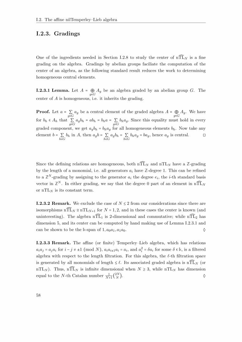
I.2. The affine nilTemperley–Lieb algebra
I.2.3. Gradings
One of the ingredients needed in Section I.2.8 to study the center of nTLN is a fine
grading on the algebra. Gradings by abelian groups faciliate the computation of the
center of an algebra, as the following standard result reduces the work to determining
homogeneous central elements.
I.2.3.1 Lemma. Let A = ⊕g∈G
Ag be an algebra graded by an abelian group G. The
center of A is homogeneous, i.e. it inherits the grading.
Proof. Let a = ∑g∈G
ag be a central element of the graded algebra A = ⊕g∈G
Ag. We have
for bh ∈ Ah that ∑g∈G
agbh = abh = bha = ∑g∈G
bhag. Since this equality must hold in every
graded component, we get agbh = bhag for all homogeneous elements bh. Now take any
element b = ∑h∈G
bh in A, then agb = ∑h∈G
agbh = ∑h∈G
bhag = bag, hence ag is central. ◻
Since the defining relations are homogeneous, both nTLN and nTLN have a Z-grading
by the length of a monomial, i.e. all generators ai have Z-degree 1. This can be refined
to a ZN -grading by assigning to the generator ai the degree ei, the i-th standard basis
vector in ZN . In either grading, we say that the degree 0 part of an element in nTLN
or nTLN is its constant term.
I.2.3.2 Remark. We exclude the case of N ≤ 2 from our considerations since there are
isomorphisms nTLN ≅ nTLN+1 for N = 1,2, and in these cases the center is known (and
uninteresting). The algebra nTL1 is 2-dimensional and commutative; while nTL2 has
dimension 5, and its center can be computed by hand making use of Lemma I.2.3.1 and
can be shown to be the k-span of 1, a0a1, a1a0. ◊
I.2.3.3 Remark. The affine (or finite) Temperley–Lieb algebra, which has relations
aiaj = ajai for i − j ≠ ±1 (mod N), aiai±1ai = ai, and a2i = δai for some δ ∈ k, is a filtered
algebra with respect to the length filtration. For this algebra, the `-th filtration space
is generated by all monomials of length ≤ `. Its associated graded algebra is nTLN (or
nTLN ). Thus, nTLN is infinite dimensional when N ≥ 3, while nTLN has dimension
equal to the N -th Catalan number 1N+1
(2NN
). ◊
58
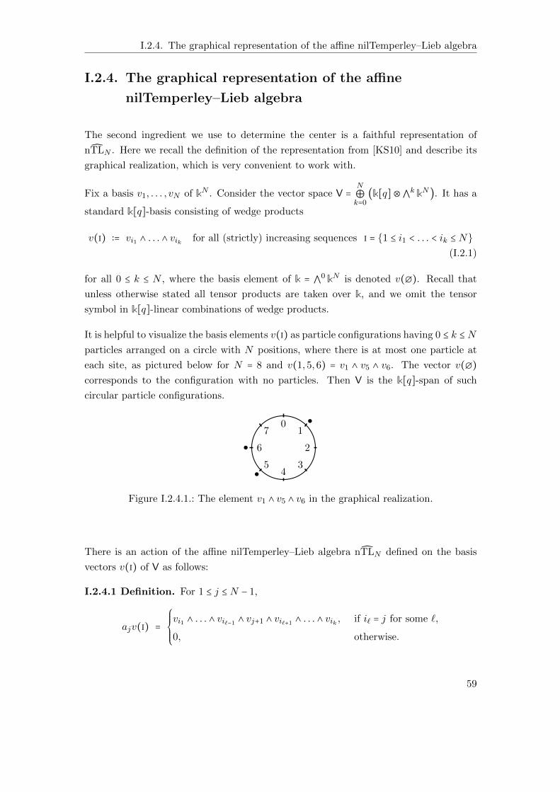
I.2.4. The graphical representation of the affine nilTemperley–Lieb algebra
I.2.4. The graphical representation of the affine
nilTemperley–Lieb algebra
The second ingredient we use to determine the center is a faithful representation of
nTLN . Here we recall the definition of the representation from [KS10] and describe its
graphical realization, which is very convenient to work with.
Fix a basis v1, . . . , vN of kN . Consider the vector space V =N
⊕k=0
(k[q]⊗⋀k kN). It has a
standard k[q]-basis consisting of wedge products
v(i) ∶= vi1 ∧ . . . ∧ vik for all (strictly) increasing sequences i = 1 ≤ i1 < . . . < ik ≤ N
(I.2.1)
for all 0 ≤ k ≤ N , where the basis element of k = ⋀0 kN is denoted v(∅). Recall that
unless otherwise stated all tensor products are taken over k, and we omit the tensor
symbol in k[q]-linear combinations of wedge products.
It is helpful to visualize the basis elements v(i) as particle configurations having 0 ≤ k ≤ N
particles arranged on a circle with N positions, where there is at most one particle at
each site, as pictured below for N = 8 and v(1,5,6) = v1 ∧ v5 ∧ v6. The vector v(∅)
corresponds to the configuration with no particles. Then V is the k[q]-span of such
circular particle configurations.
01
2
34
5
6
7
Figure I.2.4.1.: The element v1 ∧ v5 ∧ v6 in the graphical realization.
There is an action of the affine nilTemperley–Lieb algebra nTLN defined on the basis
vectors v(i) of V as follows:
I.2.4.1 Definition. For 1 ≤ j ≤ N − 1,
ajv(i) =
⎧⎪⎪⎪⎨⎪⎪⎪⎩
vi1 ∧ . . . ∧ vi`−1 ∧ vj+1 ∧ vi`+1 ∧ . . . ∧ vik , if i` = j for some `,
0, otherwise.
59
I.2. The affine nilTemperley–Lieb algebra
For the action of a0, note that vN appears in the basis element v(i) if and only if it
occurs in the last position, i.e. vik = vN , and define
a0v(i) =
⎧⎪⎪⎪⎨⎪⎪⎪⎩
q ⋅ vi1 ∧ . . . ∧ vik−1 ∧ v1, if ik = N,
0, otherwise;
=
⎧⎪⎪⎪⎨⎪⎪⎪⎩
(−1)k−1q ⋅ v1 ∧ vi1 ∧ . . . ∧ vik−1 , if ik = N,
0, otherwise.
I.2.4.2 Remark. The indices of the vectors vj can be interpreted modulo N , in the
sense that we make no distinction between v0 and vN and often use the two interchange-
ably. This does not affect the order of factors in the wedge basis. We identify e.g.
v1 ∧ v3 ∧ v4 ∧ v6 and v1 ∧ v3 ∧ v4 ∧ v0 for N = 6. ◊
I.2.4.3 Remark. It follows that ajv(i) = 0 if the sequence i contains j + 1 or if it does
not contain j. In other words, aj acts by replacing vj by vj+1. If this creates a wedge
expression with two factors equal to vj+1, the result is zero. Thus, for any monomial
a(j) there is a unique increasing sequence j = 1 ≤ j1 < . . . < jk ≤ N with k minimal
on which the monomial acts nontrivially. Under the identification of basis elements v(j)
with particle configurations, we refer to j as the minimal particle configuration on which
a(j) acts nontrivially. ◊
In the graphical description, aj moves a particle clockwise from position j to position
j + 1, and one records “passing position 0” by multiplying by ±q as illustrated by the
particle configurations below.
60
I.2.4. The graphical representation of the affine nilTemperley–Lieb algebra
01
2
34
5
6
7
(a) a6(v1∧v5∧v6) = v1∧v5∧v7
01
2
34
5
6
7
(b) a7a1a6(v1∧v5∧v6) = v2∧v5∧v0
01
2
34
5
6
7
⋅(−q)
(c) a0(v5 ∧ v0) = −q ⋅ v1 ∧ v5.
Figure I.2.4.2.: Examples for the action of nTLN on a particle configuration.
It is easy to verify that the defining relations for nTLN hold for this action, assuming
that N ≥ 3. Hence we obtain
I.2.4.4 Lemma. i) Definition I.2.4.1 gives a representation of nTLN on V.
ii) The number of wedge factors (i.e., the number of particles) remains constant under
the action of the generators ai, so that V =N
⊕k=0
(k[q]⊗⋀k kN) is a direct sum
decomposition of V as an nTLN -module.
The following crucial statement is taken from [KS10, Proposition 9.1.(2)], see also
[BFZ96, Proposition 2.4.1]. We will give a detailed proof adapted to our notation in
Section I.2.6.
I.2.4.5 Theorem. The action from Definition I.2.4.1 gives a faithful representation of
nTLN on V when N ≥ 3.
The spaces k[q] ⊗ ⋀0 kN and k[q] ⊗ ⋀N kN are trivial summands in V on which every
generator ai acts as 0, and so they are not needed for the faithfulness of the graphical
representation from Theorem I.2.4.5.
61
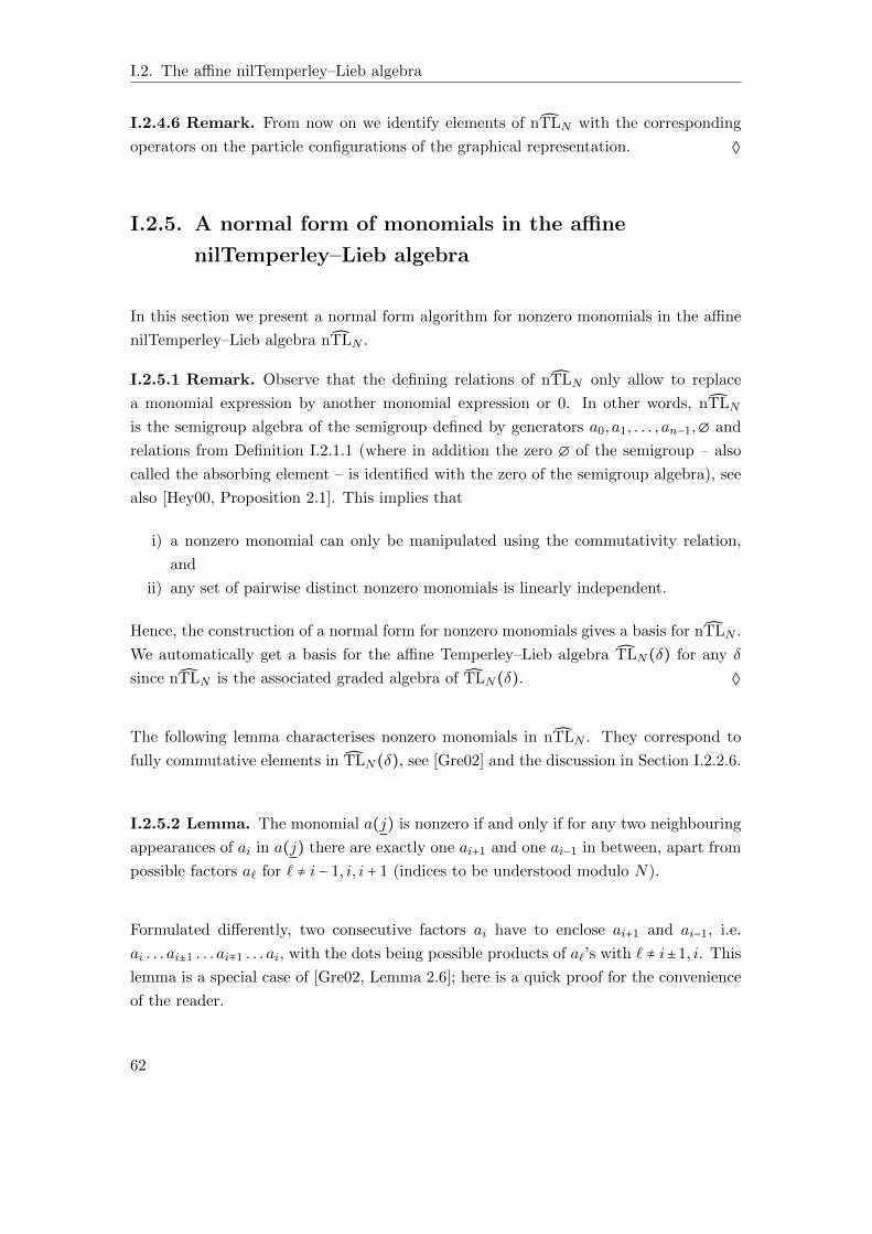
I.2. The affine nilTemperley–Lieb algebra
I.2.4.6 Remark. From now on we identify elements of nTLN with the corresponding
operators on the particle configurations of the graphical representation. ◊
I.2.5. A normal form of monomials in the affine
nilTemperley–Lieb algebra
In this section we present a normal form algorithm for nonzero monomials in the affine
nilTemperley–Lieb algebra nTLN .
I.2.5.1 Remark. Observe that the defining relations of nTLN only allow to replace
a monomial expression by another monomial expression or 0. In other words, nTLN
is the semigroup algebra of the semigroup defined by generators a0, a1, . . . , an−1,∅ and
relations from Definition I.2.1.1 (where in addition the zero ∅ of the semigroup – also
called the absorbing element – is identified with the zero of the semigroup algebra), see
also [Hey00, Proposition 2.1]. This implies that
i) a nonzero monomial can only be manipulated using the commutativity relation,
and
ii) any set of pairwise distinct nonzero monomials is linearly independent.
Hence, the construction of a normal form for nonzero monomials gives a basis for nTLN .
We automatically get a basis for the affine Temperley–Lieb algebra TLN(δ) for any δ
since nTLN is the associated graded algebra of TLN(δ). ◊
The following lemma characterises nonzero monomials in nTLN . They correspond to
fully commutative elements in TLN(δ), see [Gre02] and the discussion in Section I.2.2.6.
I.2.5.2 Lemma. The monomial a(j) is nonzero if and only if for any two neighbouring
appearances of ai in a(j) there are exactly one ai+1 and one ai−1 in between, apart from
possible factors a` for ` ≠ i − 1, i, i + 1 (indices to be understood modulo N).
Formulated differently, two consecutive factors ai have to enclose ai+1 and ai−1, i.e.
ai . . . ai±1 . . . ai∓1 . . . ai, with the dots being possible products of a`’s with ` ≠ i±1, i. This
lemma is a special case of [Gre02, Lemma 2.6]; here is a quick proof for the convenience
of the reader.
62
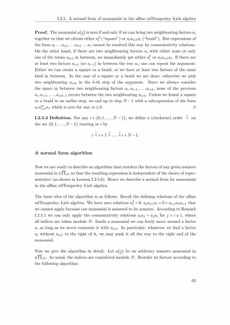
I.2.5. A normal form of monomials in the affine nilTemperley–Lieb algebra
Proof. The monomial a(j) is zero if and only if we can bring two neighbouring factors ai
together so that we obtain either a2i (“square”) or aiai±1ai (“braid”). But expressions of
the form ai . . . ai±1 . . . ai∓1 . . . ai cannot be resolved this way by commutativity relations.
On the other hand, if there are two neighbouring factors ai with either none or only
one of the terms ai±1 in between, we immediately get either a2i or aiai±1ai. If there are
at least two factors ai+1 (or ai−1) in between the two ai, one can repeat the argument:
Either we can create a square or a braid, or we have at least two factors of the same
kind in between. In the case of a square or a braid we are done; otherwise we pick
two neighbouring ai+k in the k-th step of the argument. Since we always consider
the space in between two neighbouring factors ai, ai+1, . . . , ai+k, none of the previous
ai, ai+1, . . . , ai+k−1 occurs between the two neighbouring ai+k. Unless we found a square
or a braid in an earlier step, we end up in step N − 1 with a subexpression of the form
aramr±1ar which is zero for any m ≥ 0. ◻
I.2.5.3 Definition. For any i ∈ 0,1, . . . ,N − 1, we define a (clockwise) orderi≺ on
the set 0,1, . . . ,N − 1 starting at i by
ii≺ i + 1
i≺ . . .
i≺ i +N − 1.
A normal form algorithm
Now we are ready to describe an algorithm that reorders the factors of any given nonzero
monomial in nTLN so that the resulting expression is independent of the choice of repre-
sentative (as shown in Lemma I.2.5.6). Hence we describe a normal form for monomials
in the affine nilTemperley–Lieb algebra.
The basic idea of the algorithm is as follows. Recall the defining relations of the affine
nilTemperley–Lieb algebra: We have zero relations a2i = 0, aiai+1ai = 0 = ai+1aiai+1 that
we cannot apply because our monomial is assumed to be nonzero. According to Remark
I.2.5.1 we can only apply the commutativity relations aiaj = ajai for j ≠ i ± 1, where
all indices are taken modulo N . Inside a monomial we can freely move around a factor
ai as long as we never commute it with ai±1. In particular, whenever we find a factor
ai without ai±1 to the right of it, we may push it all the way to the right end of the
monomial.
Now we give the algorithm in detail. Let a(j) be an arbitrary nonzero monomial in
nTLN . As usual, the indices are considered modulo N . Reorder its factors according to
the following algorithm:
63
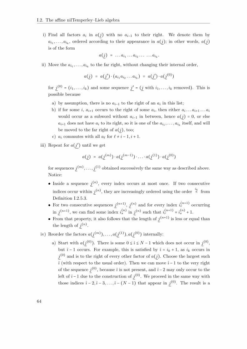
I.2. The affine nilTemperley–Lieb algebra
i) Find all factors ai in a(j) with no ai−1 to their right. We denote them by
ai1 , . . . , aik , ordered according to their appearance in a(j); in other words, a(j)
is of the form
a(j) = . . . ai1 . . . ai2 . . . . . . aik .
ii) Move the ai1 , . . . , aik to the far right, without changing their internal order,
a(j) = a(j′) ⋅ (ai1ai2 . . . aik) = a(j′) ⋅ a(j(0))
for j(0) = (i1, . . . , ik) and some sequence j′ = (j with i1, . . . , ik removed). This is
possible because
a) by assumption, there is no ai−1 to the right of an ai in this list;
b) if for some i, ai+1 occurs to the right of some ai, then either ai . . . ai+1 . . . ai
would occur as a subword without ai−1 in between, hence a(j) = 0, or else
ai+1 does not have ai to its right, so it is one of the ai1 , . . . , aik itself, and will
be moved to the far right of a(j), too;
c) ai commutes with all a` for ` ≠ i − 1, i + 1.
iii) Repeat for a(j′) until we get
a(j) = a(j(m)) ⋅ a(j(m−1)
) ⋅ . . . ⋅ a(j(1)) ⋅ a(j(0))
for sequences j(m), . . . , j(1) obtained successively the same way as described above.
Notice:
Inside a sequence j(n), every index occurs at most once. If two consecutive
indices occur within j(n), they are increasingly ordered using the orderik≺ from
Definition I.2.5.3.
For two consecutive sequences j(n+1), j(n) and for every index i(n+1)r occurring
in j(n+1), we can find some index i(n)s in j(n) such that i
(n+1)r = i
(n)s + 1.
From that property, it also follows that the length of j(n+1) is less or equal than
the length of j(n).
iv) Reorder the factors a(j(m)), . . . , a(j(1)), a(j(0)) internally:
a) Start with a(j(0)). There is some 0 ≤ ı ≤ N − 1 which does not occur in j(0),
but ı − 1 occurs. For example, this is satisfied by ı = ik + 1, as ik occurs in
j(0) and is to the right of every other factor of a(j). Choose the largest such
ı (with respect to the usual order). Then we can move ı − 1 to the very right
of the sequence j(0), because ı is not present, and ı− 2 may only occur to the
left of ı− 1 due to the construction of j(0). We proceed in the same way with
those indices ı − 2, ı − 3, . . . , ı − (N − 1) that appear in j(0). The result is a
64
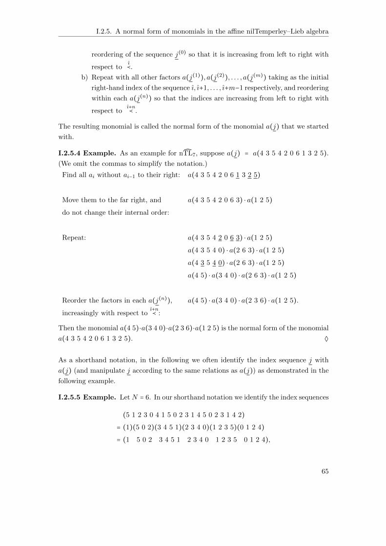
I.2.5. A normal form of monomials in the affine nilTemperley–Lieb algebra
reordering of the sequence j(0) so that it is increasing from left to right with
respect toı≺.
b) Repeat with all other factors a(j(1)), a(j(2)), . . . , a(j(m)) taking as the initial
right-hand index of the sequence ı, ı+1, . . . , ı+m−1 respectively, and reordering
within each a(j(n)) so that the indices are increasing from left to right with
respect toı+n≺ .
The resulting monomial is called the normal form of the monomial a(j) that we started
with.
I.2.5.4 Example. As an example for nTL7, suppose a(j) = a(4 3 5 4 2 0 6 1 3 2 5).
(We omit the commas to simplify the notation.)
Find all ai without ai−1 to their right: a(4 3 5 4 2 0 6 1 3 2 5)
Move them to the far right, and a(4 3 5 4 2 0 6 3) ⋅ a(1 2 5)
do not change their internal order:
Repeat: a(4 3 5 4 2 0 6 3) ⋅ a(1 2 5)
a(4 3 5 4 0) ⋅ a(2 6 3) ⋅ a(1 2 5)
a(4 3 5 4 0) ⋅ a(2 6 3) ⋅ a(1 2 5)
a(4 5) ⋅ a(3 4 0) ⋅ a(2 6 3) ⋅ a(1 2 5)
Reorder the factors in each a(j(n)), a(4 5) ⋅ a(3 4 0) ⋅ a(2 3 6) ⋅ a(1 2 5).
increasingly with respect toı+n≺ :
Then the monomial a(4 5)⋅a(3 4 0)⋅a(2 3 6)⋅a(1 2 5) is the normal form of the monomial
a(4 3 5 4 2 0 6 1 3 2 5). ◊
As a shorthand notation, in the following we often identify the index sequence j with
a(j) (and manipulate j according to the same relations as a(j)) as demonstrated in the
following example.
I.2.5.5 Example. LetN = 6. In our shorthand notation we identify the index sequences
(5 1 2 3 0 4 1 5 0 2 3 1 4 5 0 2 3 1 4 2)
= (1)(5 0 2)(3 4 5 1)(2 3 4 0)(1 2 3 5)(0 1 2 4)
= (1 5 0 2 3 4 5 1 2 3 4 0 1 2 3 5 0 1 2 4),
65
I.2. The affine nilTemperley–Lieb algebra
where we omit the commas to simplify the notation again. ◊
I.2.5.6 Lemma. Let a(j) be an arbitrary nonzero monomial in nTLN . We consider
the monomials a(j(m)), a(j(m−1)), . . . , a(j(1)), a(j(0)) constructed from a(j) by the al-
gorithm above.
i) The equality a(j) = a(j(m))a(j(m−1)) ⋯ a(j(1))a(j(0)) holds in nTLN .
ii) Given any two representatives a(j), a(j#) of the same element in nTLN , the above
algorithm creates the same representative a(j(m))a(j(m−1)) ⋯ a(j(1))a(j(0)) for
both a(j) and a(j#).
Proof. i) The algorithm only uses the defining relations of nTLN : It never inter-
changes the order of two factors ai, ai±1 with consecutive indices within a(j).
Hence, the reordering of the factors of a(j) uses only the commutativity relation
aiaj = ajai for i − j ≠ ±1 mod N of nTLN .
ii) Two nonzero monomials a(j), a(j#) in nTLN are equal if and only if they only
differ by applications of commutativity relations aiaj = ajai for i − j ≠ ±1 mod N ,
hence, if and only if they contain the same number of factors ai for each i and the
relative position of each ai and ai±1 is the same. Since the outcome of the algo-
rithm depends only on the relative positions of consecutive indices, the resulting
decomposition a(j(m))a(j(m−1)) ⋯ a(j(1))a(j(0)) is the same. ◻
Subsequently, whenever we refer to monomials in normal form, we assume the monomial
is nonzero and nonconstant, in particular the sequence j is nonempty.
I.2.5.7 Theorem. Assume N ≥ 3.
i) The algorithm above provides a normal form for nonzero monomials a(j) in the
generators ai of nTLN , or equivalently for nonzero fully commutative monomials
in TLN , so that
a(j) = (a(m)i1
. . . a(m)ik
) . . . (a(n+1)i1
. . . a(n+1)ik
)(a(n)i1
. . . a(n)ik
) . . . (a(1)i1. . . a
(1)ik
)(ai1 . . . aik),
where a(n)i`
∈ 1, a0, a1, . . . , aN−1 for all 1 ≤ n ≤m, 1 ≤ ` ≤ k, and
a(n+1)i`
∈
⎧⎪⎪⎪⎨⎪⎪⎪⎩
1 if a(n)i`
= 1,
1, aj+1 if a(n)i`
= aj .
The factors ai1 , . . . , aik are determined by the property that the generator ai`−1
does not appear to the right of ai` in the original presentation of the monomial.
The internal ordering of the factors is increasing with respect to the relationı≺
as in Definition I.2.5.3, where ı is the largest value in 0,1, . . . ,N − 1 such that
ı − 1 ∉ i1, . . . , ik, but ı ∈ i1, . . . , ik.
66
I.2.5. A normal form of monomials in the affine nilTemperley–Lieb algebra
ii) The set a(j) in normal form ∪ 1 is a k-basis of nTLN .
Proof. We have shown in Lemma (I.2.5.6.i) that any nonzero nonconstant monomial
can be rewritten by the algorithm as a monomial in normal form. By Lemma (I.2.5.6.ii)
these monomials are in pairwise distinct equivalence classes with respect to the defining
relations of nTLN . Then by Remark I.2.5.1, the set of monomials in normal form together
with 1 is linearly independent. ◻
I.2.5.8 Corollary. The set of monomials obtained by the normal form algorithm re-
garded as elements in TLN forms a k-basis of the positively graded part (TLN)>0 in
the filtration by length of monomials. In other words, a(j) in normal form ∪ 1 is a
k-basis of TLN .
Proof. Recall that the affine nilTemperley–Lieb algebra nTLN is the associated graded
algebra for the affine Temperley–Lieb algebra TLN with respect to the filtration by
length of monomials. A k-basis for nTLN is automatically a k-basis for TLN and vice
versa. ◻
I.2.5.9 Remark. We obtain a different normal form for monomials in nTLN if we
replace the steps
i) Find all factors ai in a(j) with no ai−1 to their right,
ii) Move them to the far right, without changing their internal order
in our algorithm by the alternative steps
i) Find all factors ai in a(j) with no ai+1 to their left,
ii) Move them to the far left, without changing their internal order.
After we fix some rule for the internal reordering of factors, we obtain the following two
versions of normal forms in Example I.2.5.5:
(5 1 2 3 0 4 1 5 0 2 3 1 4 5 0 2 3 1 4 2)
= (1)(5 0 2)(3 4 5 1)(2 3 4 0)(1 2 3 5)(0 1 2 4)
= (5 1 2 3)(4 0 1 2)(3 5 0 1)(2 4 5 0)(1 3 4)(2).
Here, the first expression is the given monomial, the second expression is the normal form
obtained by the original algorithm, and the third expression is the alternative normal
form. However, we do not use the alternative normal form in the following. ◊
67
I.2. The affine nilTemperley–Lieb algebra
I.2.6. Faithfulness of the graphical representation
In this section, we prove Theorem I.2.4.5 which we recall here:
Theorem. For N ≥ 3, V is a faithful nTLN -module with respect to the action described
in Definition I.2.4.1.
For the proof, we explicitly show the linear independence of the matrices representing
the monomials in nTLN . We proceed in two steps: First, we find a bijection between
the monomials in normal form constructed in Section I.2.5 and certain pairs of particle
configurations together with a power of q. In other words, we find a labelling for the
basis of nTLN from Theorem I.2.5.7. The final step is the description of the action of a
monomial on V using its matrix realization. The matrices representing the monomials
have a distinguished nonzero entry that is given in terms of the particle configurations
and the power of q from the bijection, and for most matrices, this is the only nonzero
entry. From this description it will quickly follow that all these matrices are linearly
independent.
I.2.6.1. Labelling of basis elements
In this section we use the following shorthand notation:
I.2.6.1 Definition. i) Given a tuple (n1, . . . , nr) ∈ Zr for some r > 0 we write m ∈
(n1, . . . , nr) if there exists some index 1 ≤ ` ≤ r so that m = n`. Similarly, for
(n1, . . . , nr) ∈ (Z/NZ)r we write m ∈ (n1, . . . , nr) if there exists some index 1 ≤ ` ≤ r
so that m = n` mod N .
ii) Given two tuples (n1, . . . , nr) ∈ Zr or (Z/NZ)r, and (n′1, . . . , n′r′) ∈ Zr
′or (Z/NZ)r
′,
we write
(n1, . . . , nr) ⋅ (n′1, . . . , n
′r′) = (n1, . . . , nr, n
′1, . . . , n
′r′) ∈ Zr+r
′
for their concatenation, where r, r′ > 0.
iii) For two tuples (n1, . . . , nr) ∈ Zr or (Z/NZ)r, and (n′1, . . . , n′r′) ∈ Zr
′or (Z/NZ)r
′,
with pairwise distinct elements n` ≠ nm and n′` ≠ n′m for ` ≠m, we write
(n1, . . . , nr) ⊂ (n′1, . . . , n′r′)
if there is an inclusion n1, . . . , nr ⊂ n′1, . . . , n′r′ of the underlying sets.
We need the following notion of blocks and strands of index sequences:
68

I.2.6. Faithfulness of the graphical representation
I.2.6.2 Definition. Let a(j) = a(j(m))a(j(m−1)) ⋯ a(j(1))a(j(0)) be a normal form
monomial.
i) We call j(`) the `-th block of j.
ii) A string of indices of maximal length of the form is ∈ j(0), is+1 ∈ j(1), is+2 ∈ j(2), . . .
(modulo N) is called the s-th strand of j.
I.2.6.3 Example. Let N = 6, and consider Example I.2.5.5 once again, where
j = (1 5 0 2 3 4 5 1 2 3 4 0 1 2 3 5 0 1 2 4).
The blocks are j(0) = (0124), j(1) = (1235), j(2) = (2340), j(3) = (3451), j(4) = (502), and
j(5) = (1). The strands are [3210], [54321], [105432] and [21054]. In particular, strands
(and blocks) can have different lengths, but the longest strand has length m = 6. ◊
Each monomial a(j) ∈ nTLN determines two sets iinj , ioutj and an integer `j ∈ Z≥0 as
follows:
iinj = i ∈ 0,1, . . . ,N − 1 ∣ no i − 1 to the right of i in j (I.2.2)
ioutj = i ∈ 0,1, . . . ,N − 1 ∣ no i + 1 to the left of i in j
`j = the number of zeros in j.
These are well defined because, as in the proof of Lemma I.2.5.6, any element of nTLN is
uniquely determined by the number of factors ai and the relative position of each ai and
ai±1, for all i. The set iinj equals the underlying set of j(0) in the normal form from the
algorithm above. All strands of j begin with an element in iinj and end with an element
from ioutj .
The goal of this subsection is to show
I.2.6.4 Proposition. The mapping
ψ ∶ a(j) ∈ nTLN in normal form → PN ×PN ×Z≥0 (I.2.3)
a(j) ↦ (iinj , ioutj , `j),
is injective, where PN is the power set of 0,1, . . . ,N − 1.
I.2.6.5 Remark. i) The map ψ is defined so that in the graphical description of
the representation V of nTLN , the set iinj equals the set of positions where a(j)
expects a particle to be. The set ioutj equals the set of positions where a(j) moves
the particles from iinj , but each one is translated by 1, that is,
a(j) applied to a particle at i ∈ iinj gives a particle at j + 1 for some j ∈ ioutj .
69
I.2. The affine nilTemperley–Lieb algebra
ii) The map ψ is far from being surjective. An obvious constraint is that ∣iinj ∣ = ∣ioutj ∣,
and furthermore, for some pairs (iinj , ioutj ), one can only obtain sufficiently large
values `j . ◊
We start by proving injectivity of the restriction ψ0 of ψ to those monomials a(j) in
normal form whose first element i1 of j(0) is 0. The proof itself will amount to counting
indices.
I.2.6.6 Proposition. The map
ψ0 ∶ a(j) ∈ nTLN in normal form, with i1 = 0 → PN ×PN ×Z≥0,
a(j) ↦ (iinj , ioutj , `j)
that sends a basis element in normal form with rightmost index i1 = 0 to the tuple
(iinj , ioutj , `j) defined in Equation I.2.2 is injective.
Before beginning the proof of this result, we note that for monomials a(j) with i1 = 0,
the inequality ik < N −1 must hold in iinj , since i1 = 0 implies that i1−1 = N −1 is not an
element of iinj . Consequently, the ordering of the indices in iinj agrees with the natural
ordering of Z, so we can regard (iinj ,<) as a subset of (Z,<) and replace the modular
index sequence j by an integral index sequence jZ such that jZ( mod N) = j.
I.2.6.7 Definition. Assume j = j(m) ⋅ . . . ⋅ j(1) ⋅ j(0) is a normal form sequence with
j(0) = 0 = i1 < . . . < ik < N − 1 and j(n) = (ih1 + n, . . . , ihk(n) + n) ⊆ (i1 + n, . . . , ik + n),
where indices in j(n) are modulo N and 1 ≤ k(n) ≤ k for all 1 ≤ n ≤ m. The integral
normal form sequence for j is
jZ= (j(m)
)Z⋅ . . . ⋅ (j(1))Z
⋅ j(0) where (j(n))Z∶= (ih1 + n, . . . , ihk(n) + n) ∈ Zk(n)
for n = 1, . . . ,m.
I.2.6.8 Example. We illustrate our notation with our running Example I.2.5.5 for N =
6.
If j = (1 5 0 2 3 4 5 1 2 3 4 0 1 2 3 5 0 1 2 4),
then jZ= (7 5 6 8 3 4 5 7 2 3 4 6 1 2 3 5 0 1 2 4). ◊
Our proof of Proposition I.2.6.6 will hinge upon the following technical lemma.
I.2.6.9 Lemma. Let jZ be the integral normal form sequence for j and let [is, . . . , is +
ns] for s = 1, . . . , k be the strands of jZ in the sense of Definition I.2.6.2. Assume i1 = 0.
Then
70
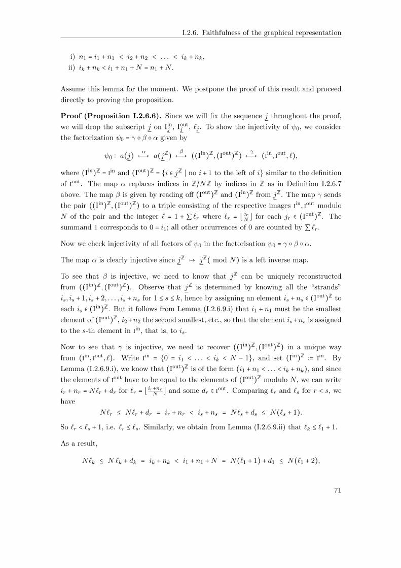
I.2.6. Faithfulness of the graphical representation
i) n1 = i1 + n1 < i2 + n2 < . . . < ik + nk,
ii) ik + nk < i1 + n1 +N = n1 +N .
Assume this lemma for the moment. We postpone the proof of this result and proceed
directly to proving the proposition.
Proof (Proposition I.2.6.6). Since we will fix the sequence j throughout the proof,
we will drop the subscript j on iinj , ioutj , `j . To show the injectivity of ψ0, we consider
the factorization ψ0 = γ β α given by
ψ0 ∶ a(j)αz→ a(jZ
)βz→ ((iin)Z, (iout
)Z)
γz→ (iin, iout, `),
where (iin)Z = iin and (iout)Z = i ∈ jZ ∣ no i+ 1 to the left of i similar to the definition
of iout. The map α replaces indices in Z/NZ by indices in Z as in Definition I.2.6.7
above. The map β is given by reading off (iout)Z and (iin)Z from jZ. The map γ sends
the pair ((iin)Z, (iout)Z) to a triple consisting of the respective images iin, iout modulo
N of the pair and the integer ` = 1 + ∑ `r where `r = ⌊jrN ⌋ for each jr ∈ (iout)Z. The
summand 1 corresponds to 0 = i1; all other occurrences of 0 are counted by ∑ `r.
Now we check injectivity of all factors of ψ0 in the factorisation ψ0 = γ β α.
The map α is clearly injective since jZ ↦ jZ( mod N) is a left inverse map.
To see that β is injective, we need to know that jZ can be uniquely reconstructed
from ((iin)Z, (iout)Z). Observe that jZ is determined by knowing all the “strands”
is, is + 1, is + 2, . . . , is +ns for 1 ≤ s ≤ k, hence by assigning an element is +ns ∈ (iout)Z to
each is ∈ (iin)Z. But it follows from Lemma (I.2.6.9.i) that i1 + n1 must be the smallest
element of (iout)Z, i2+n2 the second smallest, etc., so that the element is+ns is assigned
to the s-th element in iin, that is, to is.
Now to see that γ is injective, we need to recover ((iin)Z, (iout)Z) in a unique way
from (iin, iout, `). Write iin = 0 = i1 < . . . < ik < N − 1, and set (iin)Z ∶= iin. By
Lemma (I.2.6.9.i), we know that (iout)Z is of the form (i1 +n1 < . . . < ik +nk), and since
the elements of iout have to be equal to the elements of (iout)Z modulo N , we can write
ir + nr = N`r + dr for `r = ⌊ ir+nrN ⌋ and some dr ∈ iout. Comparing `r and `s for r < s, we
have
N`r ≤ N`r + dr = ir + nr < is + ns = N`s + ds ≤ N(`s + 1).
So `r < `s + 1, i.e. `r ≤ `s. Similarly, we obtain from Lemma (I.2.6.9.ii) that `k ≤ `1 + 1.
As a result,
N`k ≤ N `k + dk = ik + nk < i1 + n1 +N = N(`1 + 1) + d1 ≤ N(`1 + 2),
71
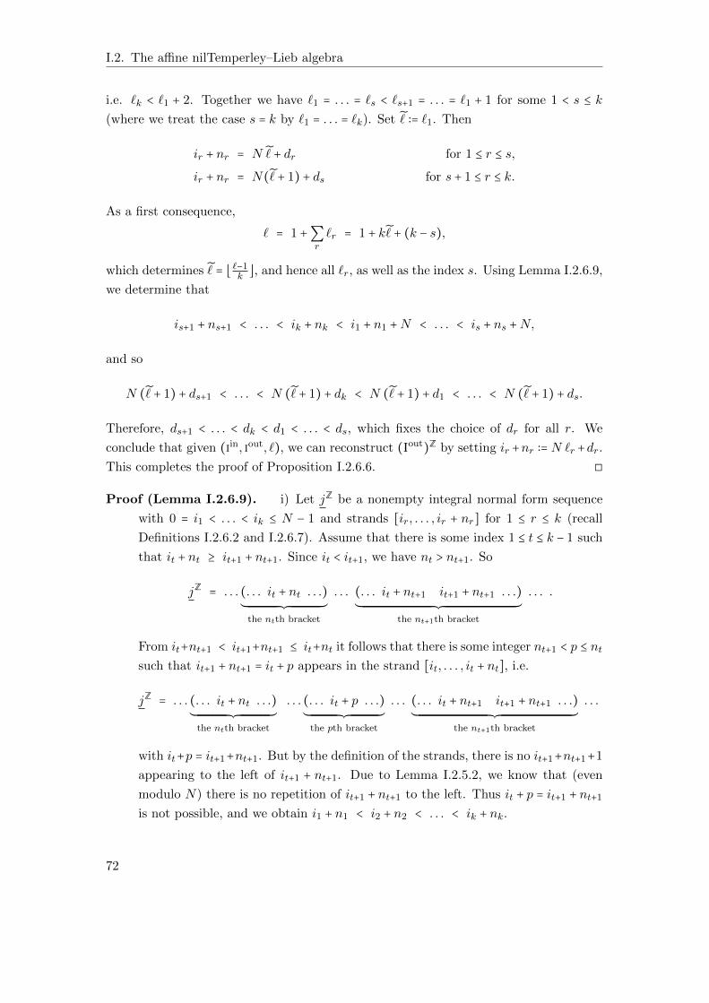
I.2. The affine nilTemperley–Lieb algebra
i.e. `k < `1 + 2. Together we have `1 = . . . = `s < `s+1 = . . . = `1 + 1 for some 1 < s ≤ k
(where we treat the case s = k by `1 = . . . = `k). Set ∶= `1. Then
ir + nr = N + dr for 1 ≤ r ≤ s,
ir + nr = N(+ 1) + ds for s + 1 ≤ r ≤ k.
As a first consequence,
` = 1 +∑r
`r = 1 + k+ (k − s),
which determines = ⌊ `−1k ⌋, and hence all `r, as well as the index s. Using Lemma I.2.6.9,
we determine that
is+1 + ns+1 < . . . < ik + nk < i1 + n1 +N < . . . < is + ns +N,
and so
N (+ 1) + ds+1 < . . . < N (+ 1) + dk < N (+ 1) + d1 < . . . < N (+ 1) + ds.
Therefore, ds+1 < . . . < dk < d1 < . . . < ds, which fixes the choice of dr for all r. We
conclude that given (iin, iout, `), we can reconstruct (iout)Z by setting ir +nr ∶= N `r +dr.
This completes the proof of Proposition I.2.6.6. ◻
Proof (Lemma I.2.6.9). i) Let jZ be a nonempty integral normal form sequence
with 0 = i1 < . . . < ik ≤ N − 1 and strands [ir, . . . , ir + nr] for 1 ≤ r ≤ k (recall
Definitions I.2.6.2 and I.2.6.7). Assume that there is some index 1 ≤ t ≤ k − 1 such
that it + nt ≥ it+1 + nt+1. Since it < it+1, we have nt > nt+1. So
jZ= . . . (. . . it + nt . . .)
´¹¹¹¹¹¹¹¹¹¹¹¹¹¹¹¹¹¹¹¹¹¹¹¹¹¹¹¹¹¹¹¹¹¹¹¹¹¹¹¹¹¸¹¹¹¹¹¹¹¹¹¹¹¹¹¹¹¹¹¹¹¹¹¹¹¹¹¹¹¹¹¹¹¹¹¹¹¹¹¹¹¹¹¶the ntth bracket
. . . (. . . it + nt+1 it+1 + nt+1 . . .)´¹¹¹¹¹¹¹¹¹¹¹¹¹¹¹¹¹¹¹¹¹¹¹¹¹¹¹¹¹¹¹¹¹¹¹¹¹¹¹¹¹¹¹¹¹¹¹¹¹¹¹¹¹¹¹¹¹¹¹¹¹¹¹¹¹¹¹¹¹¹¹¹¹¹¹¹¹¹¹¹¹¹¹¹¹¹¹¹¹¹¹¹¹¹¹¹¸¹¹¹¹¹¹¹¹¹¹¹¹¹¹¹¹¹¹¹¹¹¹¹¹¹¹¹¹¹¹¹¹¹¹¹¹¹¹¹¹¹¹¹¹¹¹¹¹¹¹¹¹¹¹¹¹¹¹¹¹¹¹¹¹¹¹¹¹¹¹¹¹¹¹¹¹¹¹¹¹¹¹¹¹¹¹¹¹¹¹¹¹¹¹¹¹¹
the nt+1th bracket
. . . .
From it+nt+1 < it+1+nt+1 ≤ it+nt it follows that there is some integer nt+1 < p ≤ nt
such that it+1 + nt+1 = it + p appears in the strand [it, . . . , it + nt], i.e.
jZ= . . . (. . . it + nt . . .)
´¹¹¹¹¹¹¹¹¹¹¹¹¹¹¹¹¹¹¹¹¹¹¹¹¹¹¹¹¹¹¹¹¹¹¹¹¹¹¹¹¹¸¹¹¹¹¹¹¹¹¹¹¹¹¹¹¹¹¹¹¹¹¹¹¹¹¹¹¹¹¹¹¹¹¹¹¹¹¹¹¹¹¹¶the ntth bracket
. . . (. . . it + p . . .)´¹¹¹¹¹¹¹¹¹¹¹¹¹¹¹¹¹¹¹¹¹¹¹¹¹¹¹¹¹¹¹¹¹¹¹¹¹¸¹¹¹¹¹¹¹¹¹¹¹¹¹¹¹¹¹¹¹¹¹¹¹¹¹¹¹¹¹¹¹¹¹¹¹¹¹¹
the pth bracket
. . . (. . . it + nt+1 it+1 + nt+1 . . .)´¹¹¹¹¹¹¹¹¹¹¹¹¹¹¹¹¹¹¹¹¹¹¹¹¹¹¹¹¹¹¹¹¹¹¹¹¹¹¹¹¹¹¹¹¹¹¹¹¹¹¹¹¹¹¹¹¹¹¹¹¹¹¹¹¹¹¹¹¹¹¹¹¹¹¹¹¹¹¹¹¹¹¹¹¹¹¹¹¹¹¹¹¹¹¹¹¸¹¹¹¹¹¹¹¹¹¹¹¹¹¹¹¹¹¹¹¹¹¹¹¹¹¹¹¹¹¹¹¹¹¹¹¹¹¹¹¹¹¹¹¹¹¹¹¹¹¹¹¹¹¹¹¹¹¹¹¹¹¹¹¹¹¹¹¹¹¹¹¹¹¹¹¹¹¹¹¹¹¹¹¹¹¹¹¹¹¹¹¹¹¹¹¹¹
the nt+1th bracket
. . .
with it+p = it+1+nt+1. But by the definition of the strands, there is no it+1+nt+1+1
appearing to the left of it+1 + nt+1. Due to Lemma I.2.5.2, we know that (even
modulo N) there is no repetition of it+1 + nt+1 to the left. Thus it + p = it+1 + nt+1
is not possible, and we obtain i1 + n1 < i2 + n2 < . . . < ik + nk.
72
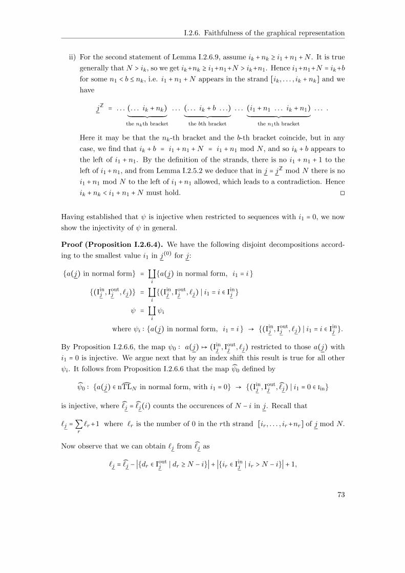
I.2.6. Faithfulness of the graphical representation
ii) For the second statement of Lemma I.2.6.9, assume ik +nk ≥ i1 +n1 +N . It is true
generally that N > ik, so we get ik+nk ≥ i1+n1+N > ik+n1. Hence i1+n1+N = ik+b
for some n1 < b ≤ nk, i.e. i1 + n1 +N appears in the strand [ik, . . . , ik + nk] and we
have
jZ= . . . (. . . ik + nk)
´¹¹¹¹¹¹¹¹¹¹¹¹¹¹¹¹¹¹¹¹¹¹¹¹¹¹¹¹¹¸¹¹¹¹¹¹¹¹¹¹¹¹¹¹¹¹¹¹¹¹¹¹¹¹¹¹¹¹¹¶the nkth bracket
. . . (. . . ik + b . . .)´¹¹¹¹¹¹¹¹¹¹¹¹¹¹¹¹¹¹¹¹¹¹¹¹¹¹¹¹¹¹¹¹¹¹¹¹¹¹¸¹¹¹¹¹¹¹¹¹¹¹¹¹¹¹¹¹¹¹¹¹¹¹¹¹¹¹¹¹¹¹¹¹¹¹¹¹¹
the bth bracket
. . . (i1 + n1 . . . ik + n1)
´¹¹¹¹¹¹¹¹¹¹¹¹¹¹¹¹¹¹¹¹¹¹¹¹¹¹¹¹¹¹¹¹¹¹¹¹¹¹¹¹¹¹¹¹¹¹¹¹¹¹¹¹¹¹¹¹¹¹¸¹¹¹¹¹¹¹¹¹¹¹¹¹¹¹¹¹¹¹¹¹¹¹¹¹¹¹¹¹¹¹¹¹¹¹¹¹¹¹¹¹¹¹¹¹¹¹¹¹¹¹¹¹¹¹¹¹¹¹¶the n1th bracket
. . . .
Here it may be that the nk-th bracket and the b-th bracket coincide, but in any
case, we find that ik + b = i1 + n1 +N = i1 + n1 mod N , and so ik + b appears to
the left of i1 + n1. By the definition of the strands, there is no i1 + n1 + 1 to the
left of i1+n1, and from Lemma I.2.5.2 we deduce that in j = jZ mod N there is no
i1 +n1 mod N to the left of i1 +n1 allowed, which leads to a contradiction. Hence
ik + nk < i1 + n1 +N must hold. ◻
Having established that ψ is injective when restricted to sequences with i1 = 0, we now
show the injectivity of ψ in general.
Proof (Proposition I.2.6.4). We have the following disjoint decompositions accord-
ing to the smallest value i1 in j(0) for j:
a(j) in normal form = ∐i
a(j) in normal form, i1 = i
(iinj , ioutj , `j) = ∐
i
(iinj , ioutj , `j) ∣ i1 = i ∈ iinj
ψ = ∐i
ψi
where ψi ∶ a(j) in normal form, i1 = i → (iinj , ioutj , `j) ∣ i1 = i ∈ iinj .
By Proposition I.2.6.6, the map ψ0 ∶ a(j) ↦ (iinj , ioutj , `j) restricted to those a(j) with
i1 = 0 is injective. We argue next that by an index shift this result is true for all other
ψi. It follows from Proposition I.2.6.6 that the map ψ0 defined by
ψ0 ∶ a(j) ∈ nTLN in normal form, with i1 = 0 → (iinj , ioutj , j) ∣ i1 = 0 ∈ iin
is injective, where j =
j(i) counts the occurences of N − i in j. Recall that
`j =∑r
`r+1 where `r is the number of 0 in the rth strand [ir, . . . , ir+nr] of j mod N.
Now observe that we can obtain `j from j as
`j = j − ∣dr ∈ iout
j ∣ dr ≥ N − i∣ + ∣ir ∈ iinj ∣ ir > N − i∣ + 1,
73
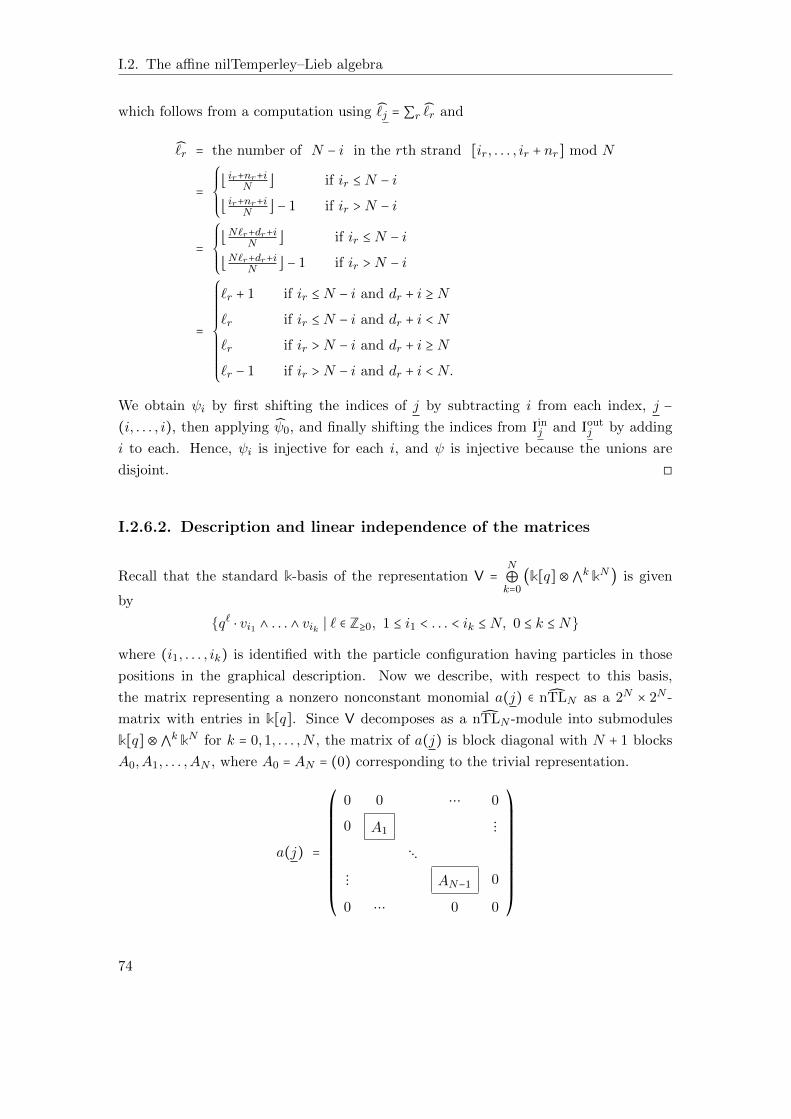
I.2. The affine nilTemperley–Lieb algebra
which follows from a computation using j = ∑r
r and
r = the number of N − i in the rth strand [ir, . . . , ir + nr] mod N
=
⎧⎪⎪⎪⎨⎪⎪⎪⎩
⌊ ir+nr+iN ⌋ if ir ≤ N − i
⌊ ir+nr+iN ⌋ − 1 if ir > N − i
=
⎧⎪⎪⎪⎨⎪⎪⎪⎩
⌊N`r+dr+iN ⌋ if ir ≤ N − i
⌊N`r+dr+iN ⌋ − 1 if ir > N − i
=
⎧⎪⎪⎪⎪⎪⎪⎪⎪⎪⎪⎨⎪⎪⎪⎪⎪⎪⎪⎪⎪⎪⎩
`r + 1 if ir ≤ N − i and dr + i ≥ N
`r if ir ≤ N − i and dr + i < N
`r if ir > N − i and dr + i ≥ N
`r − 1 if ir > N − i and dr + i < N.
We obtain ψi by first shifting the indices of j by subtracting i from each index, j −
(i, . . . , i), then applying ψ0, and finally shifting the indices from iinj and ioutj by adding
i to each. Hence, ψi is injective for each i, and ψ is injective because the unions are
disjoint. ◻
I.2.6.2. Description and linear independence of the matrices
Recall that the standard k-basis of the representation V =N
⊕k=0
(k[q]⊗⋀k kN) is given
by
q` ⋅ vi1 ∧ . . . ∧ vik ∣ ` ∈ Z≥0, 1 ≤ i1 < . . . < ik ≤ N, 0 ≤ k ≤ N
where (i1, . . . , ik) is identified with the particle configuration having particles in those
positions in the graphical description. Now we describe, with respect to this basis,
the matrix representing a nonzero nonconstant monomial a(j) ∈ nTLN as a 2N × 2N -
matrix with entries in k[q]. Since V decomposes as a nTLN -module into submodules
k[q] ⊗⋀k kN for k = 0,1, . . . ,N , the matrix of a(j) is block diagonal with N + 1 blocks
A0,A1, . . . ,AN , where A0 = AN = (0) corresponding to the trivial representation.
a(j) =
⎛⎜⎜⎜⎜⎜⎜⎜⎜⎜⎜⎜⎝
0 0 ⋯ 0
0 A1 ⋮
⋱
⋮ AN−1 0
0 ⋯ 0 0
⎞⎟⎟⎟⎟⎟⎟⎟⎟⎟⎟⎟⎠
74
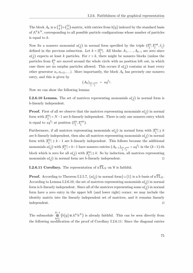
I.2.6. Faithfulness of the graphical representation
The block Ak is a (Nk)×(
Nk)-matrix, with entries from k[q] indexed by the standard basis
of ⋀k kN , corresponding to all possible particle configurations whose number of particles
is equal to k.
Now fix a nonzero monomial a(j) in normal form specified by the triple (iinj , ioutj , `j)
defined in the previous subsection. Let k = ∣iinj ∣. All blocks A1, . . . ,Ak−1 are zero since
a(j) expects at least k particles. For r > k, there might be nonzero blocks (unless the
particles from iinj are moved around the whole circle with no position left out, in which
case there are no surplus particles allowed. This occurs if a(j) contains at least every
other generator ai, ai+2, . . .). More importantly, the block Ak has precisely one nonzero
entry, and this is given by
(Ak)iinj ,ioutj
= ±q`j .
Now we can show the following lemma:
I.2.6.10 Lemma. The set of matrices representing monomials a(j) in normal form is
k-linearly independent.
Proof. First of all we observe that the matrices representing monomials a(j) in normal
form with ∣iinj ∣ = N −1 are k-linearly independent. There is only one nonzero entry which
is equal to ±q`j at position (iinj , ioutj ).
Furthermore, if all matrices representing monomials a(j) in normal form with ∣iinj ∣ ≥ k
are k-linearly independent, then also all matrices representing monomials a(j) in normal
form with ∣iinj ∣ ≥ k − 1 are k-linearly independent. This follows because the additional
monomials a(j) with ∣iinj ∣ = k−1 have nonzero entries (Ak−1)iinj ,ioutj
= ±q`j in the (k−1)-th
block which is zero for all a(j) with ∣iinj ∣ ≥ k. So by induction, all matrices representing
monomials a(j) in normal form are k-linearly independent. ◻
I.2.6.11 Corollary. The representation of nTLN on V is faithful.
Proof. According to Theorem I.2.5.7, a(j) in normal form∪1 is a k-basis of nTLN .
According to Lemma I.2.6.10, the set of matrices representing monomials a(j) in normal
form is k-linearly independent. Since all of the matrices representing some a(j) in normal
form have a zero entry in the upper left (and lower right) corner, we may include the
identity matrix into the linearly independent set of matrices, and it remains linearly
independent. ◻
The submoduleN−1
⊕k=1
(k[q]⊗⋀k kN) is already faithful. This can be seen directly from
the following modification of the proof of Corollary I.2.6.11: Since the diagonal entries
75
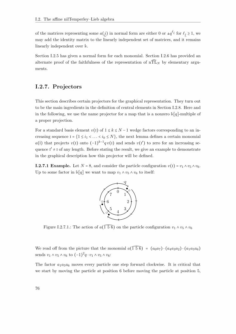
I.2. The affine nilTemperley–Lieb algebra
of the matrices representing some a(j) in normal form are either 0 or ±q`j for `j ≥ 1, we
may add the identity matrix to the linearly independent set of matrices, and it remains
linearly independent over k.
Section I.2.5 has given a normal form for each monomial. Section I.2.6 has provided an
alternate proof of the faithfulness of the representation of nTLN by elementary argu-
ments.
I.2.7. Projectors
This section describes certain projectors for the graphical representation. They turn out
to be the main ingredients in the definition of central elements in Section I.2.8. Here and
in the following, we use the name projector for a map that is a nonzero k[q]-multiple of
a proper projection.
For a standard basis element v(i) of 1 ≤ k ≤ N − 1 wedge factors corresponding to an in-
creasing sequence i = 1 ≤ i1 < . . . < ik ≤ N, the next lemma defines a certain monomial
a(i) that projects v(i) onto (−1)k−1q v(i) and sends v(i′) to zero for an increasing se-
quence i′ ≠ i of any length. Before stating the result, we give an example to demonstrate
in the graphical description how this projector will be defined.
I.2.7.1 Example. Let N = 8, and consider the particle configuration v(i) = v1 ∧ v5 ∧ v6.
Up to some factor in k[q] we want to map v1 ∧ v5 ∧ v6 to itself:
01
2
34
5
6
7
⋅q
Figure I.2.7.1.: The action of a(1 5 6) on the particle configuration v1 ∧ v5 ∧ v6
We read off from the picture that the monomial a(1 5 6) = (a0a7) ⋅ (a4a3a2) ⋅ (a1a5a6)
sends v1 ∧ v5 ∧ v6 to (−1)2q ⋅ v1 ∧ v5 ∧ v6:
The factor a1a5a6 moves every particle one step forward clockwise. It is critical that
we start by moving the particle at position 6 before moving the particle at position 5,
76
I.2.7. Projectors
as otherwise the result would be zero. But since there is a “gap” at position 7, we can
move the particle from site 6 to 7, and afterwards the particle from site 5 to 6, without
obtaining zero. The assumption that k < N ensures such a gap always exists.
After applying a1a5a6, the particles are at positions 2, 6, and 7. The particle previously
at position 5 is now at position 6, which is where we want a particle to be. The particle
currently at position 2 can be moved to position 5 by applying the product a4a3a2.
The particle now at position 7 can be moved by a0a7 to position 1. Hence, the result of
applying (a0a7) ⋅(a4a3a2) ⋅(a1a5a6) is the same particle configuration as the original one.
However, the answer must be multiplied by ±q, since applying a0a7 involves crossing the
zero position once. To determine the sign, note from Definition I.2.4.1 that (a0a7) ⋅
(a4a3a2) ⋅ (a1a5a6)(v1 ∧ v5 ∧ v6) = q ⋅ v5 ∧ v6 ∧ v1 = (−1)2q ⋅ v1 ∧ v5 ∧ v6, so the sign is +.◊
Now we describe the general procedure that defines the projector a(i):
I.2.7.2 Lemma. Assume v(i) is a particle configuration, where i = 1 ≤ i1 < . . . < ik ≤
N is an increasing sequence and 1 ≤ k ≤ N − 1. Then there exists an index ` such that
i` + 1 < i`+1 (or ik + 1 < i1), i.e. the sequence has a “gap” between i` and i`+1. Split the
sequence i into the two parts i1 < . . . < i` and i`+1 < . . . < ik. Set
a(i) ∶= (ai1−1ai1−2 . . . aik+2aik+1) ⋅k−1
∏s=1
(ais+1−1ais+1−2 . . . ais+2ais+1) (⋆)
⋅ (ai`+1ai`+2 . . . aik−1aik) ⋅ (ai1ai2 . . . ai`−1ai`),
where the indices are modulo N in the factor (ai1−1ai1−2 . . . aik+2aik+1). Then
a(i)v(i′) =
⎧⎪⎪⎪⎨⎪⎪⎪⎩
(−1)k−1q ⋅ v(i) if i′ = i,
0 for all i′ ≠ i (of any length),
and a(i) has ZN -degree (1,1, . . . ,1).
Proof. The assertions can be seen using the graphical realization of V. The terms in
the second line of equation (⋆) move a particle at site ij ∈ i one step forward to ij + 1
for each j, while the terms in the first line send the particle from ij + 1 to the original
position of ij+1.
Consider first a(i)v(i). By applying (ai`+1ai`+2 . . . aik−1aik) ⋅ (ai1ai2 . . . ai`−1ai`), every
particle is first moved clockwise by one position. By our choice of the index i`, we
avoid mapping the whole particle configuration to zero. After that step, every particle
is moved by one of the factors (ais+1−1ais+1−2 . . . ais+2ais+1) to the original position of its
successor in the sequence i, so the particle configuration remains the same. One of the
77
I.2. The affine nilTemperley–Lieb algebra
particles has passed the zero position, so we have to multiply by ±q. Definition I.2.4.1
tells us the appropriate sign is (−1)k−1.
Now consider a(i)v(i′) for i′ ≠ i. The term (ai`+1ai`+2 . . . aik−1aik) ⋅ (ai1ai2 . . . ai`−1ai`)
expects a particle at each of the sites i1, . . . , ik, so if any of these positions is empty in
v(i′), the result of applying a(i) is zero. If the positions i1, . . . , ik are already filled, and
there is an additional particle somewhere, multiplication by (ai`+1−1ai`+1−2 . . . ai`+2ai`+1)
will cause two particles to be at the same position, hence the result is again zero.
Since every aj appears in a(i) exactly once, the ZN -degree of a(i) is (1,1, . . . ,1). ◻
I.2.7.3 Example. In the previous example, N = 8, i = (1,5,6), and we may assume
the two subsequences are (1) and (5,6). Then the terms in the second line of (⋆)
are (a5a6) ⋅ (a1) = a1a5a6. The term corresponding to j = 1 in the product on the
first line of (⋆) is a4a3a2, and the expression corresponding to j = 2 is empty, hence
taken to be 1. The first factor on the first line is a0a7. Thus, for i = (1,5,6), a(i) =
(a0a7) ⋅ (a4a3a2) ⋅ (a1a5a6), as in Example I.2.7.1. If the gap between 6 and 0 is used
instead, the right-hand factor of the second line is a1a5a6 and the left-hand factor is 1.
The factors in the first line remain the same, and so one obtains the same expression for
a(i). ◊
I.2.7.4 Corollary. For i ≠ j the product a(i) ⋅ a(j) of two distinct projectors defined
in Lemma I.2.7.2 is zero. In particular, the subalgebra generated by the set of projectors
a(i) ∈ nTLN ∣ i increasing sequence
is commutative.
Proof. This follows from Lemma I.2.7.2 together with the faithfulness of the particle
configuration module V, see Theorem I.2.4.5. ◻
I.2.7.5 Remark. Because V is a faithful module (Theorem I.2.4.5), a(i) is, as an el-
ement in nTLN (i.e. up to reordering according to the defining relations), uniquely
determined by the increasing sequence i. One can read off i from a(i) as follows: In
the defining equation (⋆) of a(i), the factors in the first line are pairwise commuting.
The underlying subsequence (is+1 − 1, is+1 − 2, . . . , is + 2, is + 1) corresponding to the fac-
tor ais+1−1ais+1−2 . . . ais+2ais+1 of a(i) is a decreasing sequence. After all such decreasing
sequences are removed from a(i), what remains is a product of generators aj with an
increasing subsequence of indices or a product of two such subsequences corresponding
to the factors in the second line. This is i. Given any monomial a(r) of ZN -degree
(1, . . . ,1), one can rewrite it using the relations in nTLN so that it is of the form a(i) for
78
I.2.8. Description of the center
some increasing sequence i. Then v(i) is the unique standard basis element upon which
a(r) = a(i) acts by multiplication by ±q. ◊
I.2.8. Description of the center
In this section, we give an explicit description of the center CN of nTLN . We start with
the following initial characterisation of the central elements:
I.2.8.1 Lemma. Any central element c in nTLN with zero constant term is a linear
combination of monomials a(j) = aj1 ⋅ . . . ⋅ ajm where every generator ai, 0 ≤ i ≤ N − 1,
appears at least once. In particular, a homogeneous nonconstant central element c has
Z-degree at least N .
Proof. Assume c = ∑jcja(j), where cj ∈ k for all j. By Lemma I.2.3.1, we can assume c
is a homogeneous central element with respect to the ZN -grading. By our assumption,
c ∉ k. For all i, we need to show that ai occurs in each monomial a(j) appearing in c.
Without loss of generality, we show this for i = 0. Suppose some summand is missing
a0, then no summand contains a0 because c is homogeneous. Hence a0a(j) ≠ 0 and
a(j)a0 ≠ 0 for all j with cj ≠ 0, and since a0c = ca0, none of the a(j) can contain the
factor a1 either, as otherwise the factor a0 cannot pass through c from left to right (so
also aN−1 cannot be contained in the a(j)). Proceeding inductively, we see that all a(j)
must be a constant, contrary to our assumption. ◻
The next proposition states that on the standard wedge basis vector v(i) of V defined in
Equation I.2.1, any central element acts via multiplication by a polynomial pk ∈ k[q] that
only depends on the length k = ∣i∣ of the increasing sequence i = 1 ≤ i1 < . . . < ik ≤ N. In
other words, the decomposition of V into the summands k[q]⊗⋀k kN is a decomposition
with respect to different central characters (apart from the two trivial summands for
k ∈ 0,N).
I.2.8.2 Proposition. For any central element c ∈ nTLN and all increasing sequences i
with fixed length 0 ≤ k ≤ N , there is some element pk ∈ k[q] depending only on c and the
length k such that cv(i) = pk v(i).
Proof. By Lemma I.2.3.1 we may assume c is a ZN -homogeneous central element of
nTLN . If c is constant, then pk = c for any 0 ≤ k ≤ N , independently of i. Now assume
that c is nonconstant.
79
I.2. The affine nilTemperley–Lieb algebra
For k ∈ 0,N, the action of a generator ai on a monomial of length k is 0, so pk = 0 for
such values of k. Now consider 1 ≤ k ≤ N − 1, and suppose that i = 1 ≤ i1 < . . . < ik ≤ N
is an increasing sequence of length k. According to Lemma (I.2.4.4.ii), the number of
wedges in a vector remains constant under the action of the ai. Hence cv(i) = ∑∣I′∣=k
cI′ v(i′)
for some polynomials cI′ ∈ k[q]. We want to prove that cI′ = 0 for all i′ ≠ i.
We have shown in Lemma I.2.7.2 that to each increasing sequence j ⊂ 1, . . . ,N there
corresponds a monomial a(j) ∈ nTLN that allows us to select a single basis vector:
a(j)v(i) =
⎧⎪⎪⎪⎨⎪⎪⎪⎩
(−1)k−1qv(j) if i = j,
0 otherwise.
Thus, for j ≠ i, we see that
0 = c(a(j)v(i)) = a(j)(cv(i)) = a(j)⎛
⎝∑
∣I′∣=kcI′ v(i
′)⎞
⎠= cJ (−1)k−1qv(j),
implying cJ = 0 for j ≠ i. Hence, we may assume for each increasing sequence i that
cv(i) = pI v(i) for some polynomial pI ∈ k[q]. Now it is left to show that pI = pI′ for all i′
with ∣i′∣ = ∣i∣ = k. It is enough to verify this for i, i′ which differ in exactly one entry, i.e.
is = i, i′s = i + 1, and i` = i
′` for all ` ≠ s, for some 1 ≤ s ≤ k and i ∈ Z/NZ. If 1 ≤ i ≤ N − 1,
we have
pI′ v(i′) = cv(i′) = c(aiv(i)) = ai(cv(i)) = ai(pI v(i)) = pI v(i
′),
and if i = 0, we get
(−1)k−1qpI′ v(i′) = (−1)k−1qcv(i′) = c(a0v(i)) = a0(cv(i)) = a0(pI v(i))
= (−1)k−1qpI v(i′).
Hence, pI′ = pI, and this common polynomial is the desired polynomial pk. ◻
I.2.8.3 Corollary. Any central element in nTLN with constant term 0 acts on a stan-
dard basis vector v(i) ∈ V as multiplication by an element of qk[q].
Proof. According to Lemma I.2.8.1, each summand of such a central element must
contain the factor a0, and a0 acts on a wedge product by 0 or multiplication by ±q. ◻
Now we are ready to introduce nontrivial central elements in nTLN . For each 1 ≤ k ≤
N − 1, set
tk ∶= (−1)k−1∑∣i∣=k
a(i), (I.2.4)
where the monomials a(i) correspond to increasing sequences i = 1 ≤ i1 < . . . < ik ≤ N
of length k as defined in Lemma I.2.7.2.
80
I.2.8. Description of the center
I.2.8.4 Example. In nTL3 the elements t1, t2 look as follows:
t1 = a2a1a0 + a0a2a1 + a1a0a2,
t2 = −a0a1a2 − a1a2a0 − a2a0a1.
In nTL4 we have
t1 = a3a2a1a0 + a0a3a2a1 + a1a0a3a2 + a2a1a0a3,
t2 = −a0a3a1a2 − a0a2a1a3 − a3a2a0a1 − a1a0a2a3 − a1a3a0a2 − a2a1a3a0,
t3 = a0a1a2a3 + a1a2a3a0 + a2a3a0a1 + a3a0a1a2. ◊
In the graphical realization of V, tk acts by annihilating all particle configurations whose
number of particles is different from k. For particle configurations having k particles,
every particle is moved clockwise to the original site of the next particle. Hence, the
particle configuration itself remains fixed by the action of tk (and it is multiplied with
(−1)2(k−1)q = q, since a particle has been moved through position 0). All the tk have
ZN -degree equal to (1, . . . ,1) and Z-degree equal to N . Any monomial whose ZN -degree
is (1, . . . ,1) occurs as a summand in some central element (after possibly reordering the
factors), and the number of summands of tk equals (Nk) = dim(⋀
k kN), see Remark
I.2.7.5.
Now we formulate our main theorem of this section:
I.2.8.5 Theorem. Let nTLN be the affine nilTemperley–Lieb algebra for N ≥ 3.
i) The tk defined in Equation I.2.4 are central for all 1 ≤ k ≤ N − 1, and the center of
nTLN is generated by 1 and the tk, 1 ≤ k ≤ N − 1.
ii) The subalgebra generated by tk is isomorphic to the polynomial ring k[q] for all
1 ≤ k ≤ N − 1. Moreover tkt` = 0 for all k ≠ `. Hence the center of nTLN is the
subalgebra
CN = k⊕ (t1k[t1]⊕ . . .⊕ tN−1k[tN−1]) ≅k[t1, . . . , tN−1]
(tkt` ∣ k ≠ `).
Proof. i) The action of tk on V is the projection onto the nTLN -submodule k[q]⊗
⋀k kN followed by multiplication by q. This commutes with the action of every
other element of nTLN . Since V is a faithful module, tk commutes with any
element of nTLN . As we have seen in Proposition I.2.8.2, any central element c
without constant term acts on the summand k[q] ⊗ ⋀k kN via multiplication by
some polynomial pck ∈ qk[q]. Once again using the faithfulness of V, we get that
c =N−1
∑k=1
pck(tk).
81
I.2. The affine nilTemperley–Lieb algebra
ii) Note that k[q] ⊗⋀k kN is a free k[q]-module of rank (Nk). Since tk acts by mul-
tiplication with q on that module, the subalgebra of nTLN generated by tk must
be isomorphic to the polynomial ring k[q]. Since a(j)a(i) = 0 for all j ≠ i, in
particular for j, i of different length, we get tkt` = 0 for k ≠ `, as they consist of
pairwise different summands. ◻
Theorem I.2.8.5 enables us to describe the endomorphism algebra EndnTLN(W) of the
space of nontrivial particle configurations W ∶=N−1
⊕k=1
(k[q]⊗⋀k kN) ⊂ V. We first observe
that on W multiplication by q is given by the action of a central element in CN , therefore
it is justified to speak about k[q]-linearity of a nTLN -endomorphism of W.
I.2.8.6 Lemma. Any nTLN -module endomorphism ϕ of W is k[q]-linear, that is, we
have EndnTLN(W) ⊂ Endk[q](W).
Proof. Observe that ∑N−1k=1 tk ∈ nTLN acts by multiplication by q on every element in W.
Therefore multiplication by q commutes with the application of every ϕ ∈ EndnTLN(W).◻
I.2.8.7 Proposition. The endomorphism algebra EndnTLN(W) is isomorphic to a di-
rect sum of N − 1 polynomial algebras k[T1]⊕ . . .⊕ k[TN−1].
Proof. The proof is very similar to the one of Proposition I.2.8.2. First we show that
ϕ(v(i)) is a k[q]-linear multiple of v(i) for any ϕ ∈ EndnTLN(W) and any increas-
ing sequence i. This statement holds if and only if ±qϕ(v(i)) ∈ k[q] v(i). Indeed, by
Lemma I.2.7.2 and Lemma I.2.8.6 we get
±qϕ(v(i)) = ϕ(±qv(i)) = ϕ(a(i)v(i)) = a(i)ϕ(v(i)) ∈ k[q] v(i).
Therefore, we can write ϕ(v(i)) = pi ⋅ v(i) for some polynomial pi ∈ k[q]. Note that this
implies
EndnTLN(N−1
⊕k=1
(k[q]⊗⋀kkN)) =N−1
⊕k=1
(EndnTLN(k[q]⊗⋀kkN)) .
What remains is to show that these polynomials only depend on the number of particles
in i, in other words there exists pk ∈ k[q] so that pi = pk for all i with ∣i∣ = k. Again it
suffices to show this for two sequences i, i′ of length k which differ in exactly one entry.
So say is = i, i′s = i + 1, and i` = i
′` for all ` ≠ s, for some 1 ≤ s ≤ k and i ∈ Z/NZ. When
1 ≤ i ≤ N − 1,
pi′ v(i′) = ϕ(v(i′)) = ϕ(aiv(i)) = aiϕ(v(i)) = ai(pi v(i)) = pi v(i
′),
82
I.2.9. The affine nilTemperley–Lieb algebra is finitely generated over its center
and when i = 0,
(−1)k−1qpi′ v(i′) = (−1)k−1qϕ(v(i′)) = ϕ(a0v(i)) = a0ϕ(v(i)) = a0(pi v(i))
= (−1)k−1qpi v(i′).
Hence we can write ϕ = ∑N−1k=1 pkπk where πk is the projection onto k[q]⊗⋀k kN , and we
get that
EndnTLN(k[q]⊗⋀kkN) = k[Tk],
where Tk denotes the multiplication action of the central element tk, which is indeed a
nTLN -module endomorphism of W. Thus, EndnTLN(W) is isomorphic to a direct sum
of polynomial algebras as claimed. ◻
I.2.8.8 Remark. The arguments in the proof of Proposition I.2.8.7 remain valid even
if we specialize the indeterminate q to some element in k ∖ 0. In this case, we obtain
that the summands ⋀k kN are simple modules and
EndnTLN(N−1
⊕k=1
k
⋀kN) ≅ kN−1.
For q = 0, the situation is more complicated: If q is specialized to zero, the generator a0
acts by zero on the module. The action of nTLN factorizes over nTLN and the module
⋀k kN is no longer simple. Instead it has a one-dimensional head spanned by the particle
configuration v(1, . . . , k), and any endomorphism is given by choosing an image of this
top configuration. It is always possible to map it to itself and to the one-dimensional
socle spanned by v(N − k, . . . ,N), but in general there are more endomorphisms.
For example, in ⋀4 k8, the image of v(1,2,3,4) may be any linear combination of
v(1,2,3,4), v(2,3,4,8), v(3,4,7,8), v(4,6,7,8) and v(5,6,7,8), so that EndnTL8(⋀
4 k8)
is 5-dimensional.
In ⋀3 k8, the image of v(1,2,3) may be any linear combination of v(1,2,3), v(2,3,8),
v(3,7,8) and v(6,7,8), so its endomorphism algebra is 4-dimensional. ◊
I.2.9. The affine nilTemperley–Lieb algebra is finitely
generated over its center
In this section we prove that nTLN is finitely generated over its center (it is not free
over its center, as we will see in Section I.2.13). We show this using a basis of nTLN
83
I.2. The affine nilTemperley–Lieb algebra
that is adapted to the problem, but recall the normal form constructed in Section I.2.5
and the labelling thereof from Section I.2.6.
The affine nilTemperley–Lieb algebra is infinite dimensional when N ≥ 3; however, the
following finiteness result holds:
I.2.9.1 Theorem. The algebra nTLN is finitely generated over its center.
Proof. Given an arbitrary monomial a(j) ∈ nTLN , we first factor it as a(j′) ⋅ a(j(0)) in
the following way: Take the minimal particle configuration j = 1 ≤ j1 < . . . < jk ≤ N on
which the monomial a(j) acts nontrivially, in the sense of Remark I.2.4.3. The monomial
a(j) moves all of the particles by at least one step, because the particle configuration was
assumed to be minimal. Using the faithfulness of the representation, we know that we
may reorder the monomial a(j) so that first each particle is moved one step clockwise,
and afterwards the remaining particle moves are carried out. Hence, we may choose
some factorization a(j) = a(j′) ⋅ a(j(0)), where j(0) is a sequence obtained by permuting
j1, . . . , jk. The remaining particle moves are carried out by a(j′). In Section I.2.5, this
decomposition is explicitly constructed (not using the faithful representation). Next, we
want to find an expression of the form
a(j) = afin ⋅ tnk ⋅ a(j
(0)),
where afin is a monomial of some subalgebra inTLN of nTLN , tnk is in the center of
nTLN , and a(j(0)) is the above factor. Here
inTLN = ⟨a0, . . . , ai−1, ai+1, . . . , aN−1⟩ (I.2.5)
is a copy of the finite nilTemperley–Lieb algebra nTLN sitting in nTLN . To accomplish
this, we have to subdivide the action of a(j) on the particle configuration j = j1 < . . . <
jk one more time. There are two cases:
i) There is an index i not appearing in j′: In this case, a(j′) is an element of inTLN
and we are done.
ii) All indices appear at least n ≥ 1 times in j′: Let us investigate the action of a(j′)
on the particle configuration v(i) = a(j(0))v(j), where i = j1+1, . . . , jk +1. Note
that i is the minimal particle configuration for a(j′) in the sense of Remark I.2.4.3.
Each of the particles in i is moved by a(j′) to the position of the next particle in
the sequence i, because there is no index missing (a missing index is equivalent
to a particle being stopped before reaching the position of its successor), before
possibly continuing to move along the circle. Again invoking the faithfulness of the
representation, we can rewrite a(j′) = a(j′′) ⋅ a(i)n, with the monomial a(i) from
84
I.2.10. An alternative normal form using the center
Lemma I.2.7.2. For maximal n, the remaining factor a(j′′) is an element of inTLN
for some i. Observe that a(i)na(j(0)) = tnka(j(0)), which follows immediately from
the definition of tk and Lemma I.2.7.2.
Therefore, we have shown that
a(j) = a(j′) ⋅ a(j(0)) = afin ⋅ a(i)n⋅ a(j(0)) = afin ⋅ t
nk ⋅ a(j
(0)),
where n = 0 in the first case. Since there is only a finite number of monomials in0nTLN ,
1nTLN , . . . ,N−1nTLN and only finitely many monomials a(j(0)) such that every
index 0,1, . . . ,N−1 occurs at most once in the sequence j(0), the affine nilTemperley–Lieb
algebra is indeed finitely generated over its center. ◻
I.2.10. An alternative normal form using the center
Motivated by the proof of Theorem I.2.9.1 we introduce another basis of nTLN . In this
section we use faithfulness of the graphical representation V from Theorem I.2.4.5 and
our knowledge of the center CN of nTLN from Theorem I.2.8.5. Therefore the approach
given here is much simpler that the elementary but lengthy computation of a normal
form in Sections I.2.5 and I.2.6.
For any two particle configurations with the same number 1 ≤ k ≤ N − 1 of particles
corresponding to the increasing sequences i = 1 ≤ i1 < . . . < ik ≤ N and j = 1 ≤ j1 <
. . . < jk ≤ N, there is a monomial in nTLN moving particles at the positions j to the
positions i. We require that every particle from j is moved by at least one step, but
we do not prescribe explicitly which of the j’s is mapped to which of the i’s. For i ≠ j,
take eij to be the monomial such that the power of q in eijv(j) = ±q`v(i) is minimal
(under the assumption that every particle from j must be moved). By faithfulness of
the graphical representation, eij is uniquely determined. For i = j, we have eii = a(i),
the special monomial defined in Section I.2.7, hence eiiv(i) = ±qv(i). Observe that one
can write tk = ∑∣i∣=k eii, where the sum runs over all possible increasing sequences i of
length k, and that t`keij is a monomial, since all but one summand vanish for k = ∣i∣.
The condition that eij moves all particles from j by at least one step guarantees that it
acts by zero on all particle configurations with fewer particles than ∣i∣ = ∣j∣. For example,
when N = 7,
e(2)(1) = a1, e(0,2)(0,1) = a6a5a4a3a1a2a0a1.
(Note that a1 moves v(0,1) to v(0,2), but this does not satisfy the requisite property
that all the particles must be moved by at least one step.) If we apply the factorization
85
I.2. The affine nilTemperley–Lieb algebra
of monomials from Theorem I.2.9.1 to eij, the minimality condition implies that eij =
afin ⋅1 ⋅a(j(0)), where if j = j1 < . . . < jk, then j(0) is a sequence obtained by permuting
the elements of j.
I.2.10.1 Theorem. The set of monomials
1 ∪ t`keij ∣ ` ∈ Z≥0, 1 ≤ ∣i∣ = ∣j∣ = k ≤ N − 1, 1 ≤ k ≤ N − 1
defines a k-basis of the affine nilTemperley–Lieb algebra nTLN .
Proof. First, observe that t`keij is indeed a monomial since ∣i∣ = k. We show that
the elements t`keij act k-linearly independently on the graphical representation V =N
⊕k=0
(k[q]⊗⋀k kN). By definition, the monomial eij acts by zero on summands k[q] ⊗
⋀k′ kN for k′ < ∣i∣. On k[q]⊗⋀∣i∣ kN , the matrix representing the action of t`keij relative to
the standard basis has exactly one nonzero entry, and this one distinguishes all monomi-
als with the same minimal number of particles ∣i∣ = ∣j∣. From these two observations, the
linear independence follows. On the other hand, given any nonzero monomial in nTLN ,
there exists a minimal particle configuration j on which it acts nontrivially. Recording
the image particle configuration i and the power of q, we conclude that there is some ` so
that the element t`keij acts on the minimal particle configuration j in the same way as the
given monomial does. The action of a monomial on the minimal particle configuration
determines its action on the module V. Due to the faithfulness of this representation
(see Theorem I.2.4.5 or Section I.2.6), the proposition follows. ◻
The following proposition describes the multiplication of the monomials eij from the
k-basis in Theorem I.2.10.1.
I.2.10.2 Proposition. The product of basis elements eij and ekl for any particle con-
figurations given by i, j, k, l is given by
eij ⋅ ekl =
⎧⎪⎪⎪⎪⎪⎪⎨⎪⎪⎪⎪⎪⎪⎩
0 if ∃k ∈ k ∶ k ∉ j but k ∈ j(0) ∪ j(1) ∪ . . . ∪ j(m−1) ∪ i
0 if ∃j ∈ j ∶ j ∉ k but j ∈ l ∪ l(0) ∪ . . . ∪ l(n−2) ∪ l(n−1)
±tr∗
∣i∗∣ei∗l∗ else, where l∗ = l ∪ (j ∖ (j ∩ k)), i∗ = i ∪ (k ∖ (j ∩ k)),
where
v(j(s)) = a(j(s)) . . . a(j(1))a(j(0))v(j)
for eij = a(j(m))a(j(m−1)) . . . a(j(1))a(j(0)) in the normal form from Theorem I.2.5.7.
Similarly,
v(l(s)) = a(l(s)) . . . a(l(1))a(l(0))v(l)
for ekl = a(l(n))a(l(n−1)) . . . a(l(1))a(l(0)) in normal form. The power r∗ depends on
all particle configurations i, j, k and l.
86
I.2.11. Embeddings of affine nilTemperley–Lieb algebras
Proof. This can be seen using the graphical representation: The product eij ⋅ekl is zero
if and only if it acts by zero on the particle configuration l∗ = l ∪ (j ∖ (j ∩ k)). This is
the case if ekl acts by zero on l∗, or if eij acts by zero on
k ∪ j = k ∪ (j ∖ (j ∩ k)) = ekl applied to l∗, if nonzero.
Example I.2.10.3 illustrates the dependence of the power r∗ in the product
eij ⋅ ekl = tr∗
∣i∗∣ei∗l∗
from Proposition I.2.10.2 on the particle configurations i, j, k and l.
I.2.10.3 Example. Let N = 10. Let i = (8), j = k = (5) and l = (3). Then eij ⋅ekl = eil.
If we replace i by i′ = (4) we obtain ei′j ⋅ ekl = t11ei′l. For j′ = k′ = (1) we have
eij′ ⋅ ek′l = t11eil. ◊
I.2.10.4 Remark. The bases from Section I.2.10 and Section I.2.5 are both labelled by
pairs of particle configurations (pairs of increasing sequences) together with a natural
number `, see also Section I.2.6.1. The labelling sets agree up to an index shift in the
output configuration i and a shift of the natural number `. ◊
I.2.10.5 Remark. From a monomial eij, we can read off the sequences
j = i ∣ no ai−1 occurs to the right of ai in the monomial eij,
i = i ∣ no ai occurs to the left of ai−1 in the monomial eij ◊
I.2.11. Embeddings of affine nilTemperley–Lieb algebras
In this section we use the basis constructed in Section I.2.10 and construct embeddings
of affine nilTemperley–Lieb algebras nTLN ⊂ nTLN+1.
In the proof of Theorem I.2.9.1, we have used the N obvious embeddings of nTLN
into nTLN coming from the N different embeddings of the Coxeter graph AN−1 into
AN−1. For finite nilTemperley–Lieb algebras there are obvious embeddings of nTLN into
nTLN+1 coming from the embeddings of the Coxeter graphs AN−1 into AN .
Embeddings for affine nilTemperley–Lieb algebras cannot be defined in an obvious way.
There are no corresponding embeddings of Coxeter graphs. Instead our embeddings of
nTLN into nTLN+1 correspond to the subdivision of an edge of AN−1 by inserting a
vertex on the edge to obtain AN .
87
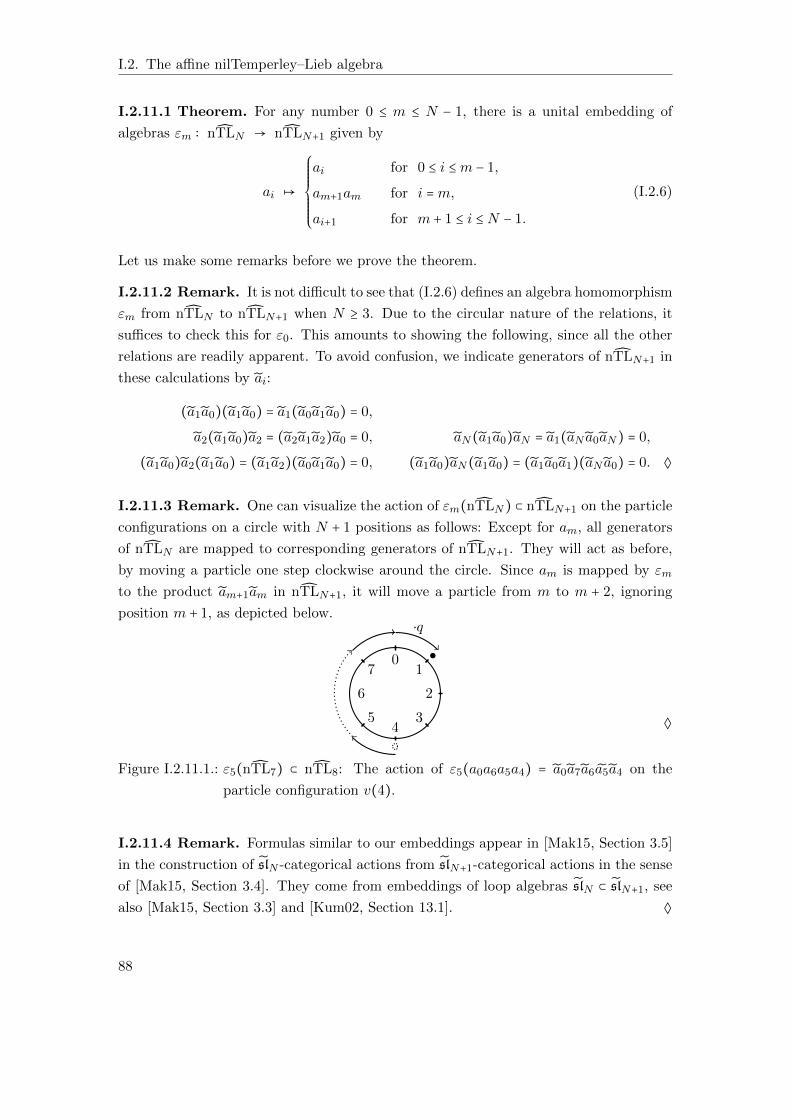
I.2. The affine nilTemperley–Lieb algebra
I.2.11.1 Theorem. For any number 0 ≤ m ≤ N − 1, there is a unital embedding of
algebras εm ∶ nTLN → nTLN+1 given by
ai ↦
⎧⎪⎪⎪⎪⎪⎪⎨⎪⎪⎪⎪⎪⎪⎩
ai for 0 ≤ i ≤m − 1,
am+1am for i =m,
ai+1 for m + 1 ≤ i ≤ N − 1.
(I.2.6)
Let us make some remarks before we prove the theorem.
I.2.11.2 Remark. It is not difficult to see that (I.2.6) defines an algebra homomorphism
εm from nTLN to nTLN+1 when N ≥ 3. Due to the circular nature of the relations, it
suffices to check this for ε0. This amounts to showing the following, since all the other
relations are readily apparent. To avoid confusion, we indicate generators of nTLN+1 in
these calculations by ai:
(a1a0)(a1a0) = a1(a0a1a0) = 0,
a2(a1a0)a2 = (a2a1a2)a0 = 0, aN(a1a0)aN = a1(aN a0aN) = 0,
(a1a0)a2(a1a0) = (a1a2)(a0a1a0) = 0, (a1a0)aN(a1a0) = (a1a0a1)(aN a0) = 0. ◊
I.2.11.3 Remark. One can visualize the action of εm(nTLN) ⊂ nTLN+1 on the particle
configurations on a circle with N + 1 positions as follows: Except for am, all generators
of nTLN are mapped to corresponding generators of nTLN+1. They will act as before,
by moving a particle one step clockwise around the circle. Since am is mapped by εm
to the product am+1am in nTLN+1, it will move a particle from m to m + 2, ignoring
position m + 1, as depicted below.
01
2
34
5
6
7
⋅q
◊
Figure I.2.11.1.: ε5(nTL7) ⊂ nTL8: The action of ε5(a0a6a5a4) = a0a7a6a5a4 on the
particle configuration v(4).
I.2.11.4 Remark. Formulas similar to our embeddings appear in [Mak15, Section 3.5]
in the construction of slN -categorical actions from slN+1-categorical actions in the sense
of [Mak15, Section 3.4]. They come from embeddings of loop algebras slN ⊂ slN+1, see
also [Mak15, Section 3.3] and [Kum02, Section 13.1]. ◊
88
I.2.12. Classification of simple modules
Proof (Theorem I.2.11.1). Recall the basis given by 1 ∪ t`keij ∣ ` ∈ Z≥0, 1 ≤
∣i∣ = ∣j∣ = k ≤ N − 1 defined in Section I.2.10. We have already noted in Remark
I.2.11.2 that εm is an algebra homomorphism. Using Remark I.2.11.3, observe that the
monomial eij ∈ nTLN is mapped to a monomial ei′j′ ∈ nTLN+1 (tilde again indicates in
nTLN+1), where the new index sets are obtained by i ↦ i for 0 ≤ i ≤m and i ↦ i + 1 for
m + 1 ≤ i ≤ N − 1. The injectivity follows since distinct basis elements (∑∣K∣=k eKK)`⋅ eij
of nTLN are mapped to distinct basis elements (∑∣K′∣=k eK′K′)`⋅ ei′j′ of nTLN+1. ◻
I.2.11.5 Remark. It is possible to verify this theorem on generators and relations in
the language of Section I.2.5 without using the graphical description. The idea is that
from a monomial eij, we can read off the sequences
j = i ∣ no ai−1 occurs to the right of ai in the monomial eij,
i = i ∣ no ai occurs to the left of ai−1 in the monomial eij
as in Remark I.2.10.5. Now using Lemma I.2.5.2 one checks that the image of eij under
εm is a nonzero monomial, which must be equal to the monomial ei′j′ determined by
i ∣ no ai−1 occurs to the right of ai in the monomial εm(eij) = j′,
i ∣ no ai occurs to the left of ai−1 in the monomial εm(eij) = i′. ◊
I.2.11.6 Remark. These embeddings work specifically for the affine nilTemperley–Lieb
algebras but fail for the ordinary Temperley–Lieb algebras. The relation that fails to
hold is the braid relation for Temperley–Lieb algebras, i.e. aiai±1ai = ai. Interestingly,
the relation a2i = δai is respected for δ = 1. ◊
I.2.12. Classification of simple modules
In this section we have to assume that the ground ring k of nTLN is restricted to be an
uncountable algebraically closed field of arbitrary characteristic.
The classification of simple modules for nTLN uses central characters.
I.2.12.1 Definition. Let A be a k-algebra over some field k. An A-module M has
central character χ ∶ C(A) → k if χ is an algebra homomorphism such that cv = χ(c)v
for all c ∈ C(A) and all v ∈M . In case χ is the central character of M we denote it by
χM .
Recall the following fact:
89
I.2. The affine nilTemperley–Lieb algebra
I.2.12.2 Proposition. Let k be an algebraically closed field and A be a k-algebra with
dim(A) < ∣k∣. Then every simple A-module has central character.
This is proven e.g. in [CG97, Corollary 8.1.2] for the affine Hecke algebra, and in
[Maz10, Theorem 4.7] for A = U(sl2), compare Section II.1.4. The general statement can
be proven analogously.
Let us now turn to the affine nilTemperley–Lieb algebra nTLN . From now on, the ground
ring k of nTLN is an uncountable algebraically closed field. Denote the category of left
nTLN -modules by nTLN−mod. We will use two main facts about nTLN to describe
its simple modules: The finiteness of nTLN over its center, and the explicit description
of the center CN ≅k[t1,...,tN−1](tkt`∣k≠`) . Observe that due to the relation tkt` = 0 in CN
the only nonzero algebra homomorphisms χ ∶ CN → k are given by the choice of some
χ(tk) = ζ ∈ k ∖ 0, χ(t`) = 0 for all ` ≠ k. The following theorem classifies all simple
nTLN -modules:
I.2.12.3 Theorem. Let k be an uncountable algebraically closed field of arbitrary char-
acteristic. Let χ be an algebra homomorphism CN → k. Then up to isomorphism there
is precisely one simple module of nTLN with central character χ.
The simple modules of nTLN are given up to isomorphism by
i) the trivial onedimensional module k with trivial central character,
ii) the (Nk)-dimensional module ⋀k kN with central character χ(tk) ∈ k∖0, χ(t`) = 0
for all ` ≠ k.
Proof. Thanks to our assumption that k is an uncountable algebraically closed field we
know that every simple module of nTLN has central character.
Let us first consider the case χ = 0. Given any simple nTLN -module M with χM = 0,
we have that M is simple as nTLN/⟨t1, . . . , tN−1⟩-module. This quotient algebra is
graded by the length of monomials (since CN ⊂ nTLN is homogeneously generated) and
furthermore finite dimensional by Theorem I.2.9.1. Its degree 0 component equals k.
Its Jacobson radical is given by all positively graded elements (nTLN/⟨t1, . . . , tN−1⟩)>0.
Since the simple modules over an algebra can be identified with the simple modules over
the quotient with respect to the Jacobson radical, we only need to determine all simple
modules of the quotient (nTLN/⟨t1, . . . , tN−1⟩) / (nTLN/⟨t1, . . . , tN−1⟩)>0, which is k. By
the Artin-Wedderburn Theorem [Lam01, Chapter 1.3] (or directly by the lack of nontriv-
ial maximal ideals in k), the only simple module of k and hence of nTLN/⟨t1, . . . , tN−1⟩
is the one-dimensional (trivial) module k.
90
I.2.12. Classification of simple modules
Now we turn to the case χ ≠ 0, i.e. χ is given by χ(tk) = ζ ∈ k ∖ 0, χ(t`) = 0
for all ` ≠ k. In this case we want to form the localisation nTLN [t−1k ]. There are
two possibilities to convince oneself that one can localise nTLN with respect to the
multiplicative subset generated by tk: Either one checks that localisation with respect
to a multiplicative subset for commutative rings as in [AM69, Chapter 3] can be easily
imitated for multiplicative central subsets in an arbitrary ring. Or one applies Ore
localisation as discussed in [Lam99, Chapter 4, Section 10] to the noncommutative ring
nTLN and the (right and left) denominator set 1, tk, t2k, . . ., where the Ore conditions
are automatically satisfied since 1, tk, t2k, . . . is central (see [Lam99, (10.15)]). The
resulting right and left ring of fractions is unique up to unique isomorphism. We denote
the localisation of nTLN with respect to the set 1, tk, t2k, . . . by nTLN [t−1
k ].
Now our goal is to show that the functor nTLN [t−1k ]⊗nTLN
− induces a bijection
simple nTLN -modules with tk acts by ζ ≠ 0/ ≅ (I.2.7)
1∶1←→ simple nTLN [t−1
k ]-modules with tk acts by ζ ≠ 0/ ≅
that preserves the k-dimensions of the simple modules. First of all, localisation is exact,
see [Lam99, Exercise 10.18] or [Mat89, Theorem 4.5] for the commutative version of the
statement. Therefore nTLN [t−1k ]⊗nTLN
L is a simple nTLN [t−1k ]-module for any simple
nTLN -module L.
Let L be a simple nTLN -module so that tk acts by ζ ≠ 0 on L. In this case the
dimension of L is preserved under localisation since L ≅ nTLN [t−1k ] ⊗nTLN
L even as
nTLN [t−1k ]-modules. The nTLN [t−1
k ]-action on L is given by letting t−1k act by ζ−1.
More precisely, by the universal property of localisation ([Lam99, Proposition 9.2]), any
ring homomorphism from nTLN that maps 1, tk, t2k, . . . into the units of the codomain
ring factors uniquely over nTLN [t−1k ]. In this way we can see a simple nTLN -module L
as nTLN [t−1k ]-module. The natural map L → nTLN [t−1
k ] ⊗nTLNL is injective since its
kernel is given by m ∈ L ∣ tnkm = ζnm = 0 for some n = 0. It is also surjective since
t−1k ⊗nTLN
m = 1⊗nTLNζ−1m for all m ∈ L.
Vice versa, any simple nTLN [t−1k ]-module L′ so that tk acts by ζ(≠ 0) on L′ is naturally
an nTLN -module. As such, L′ is simple: Let 0 → N ′ → L′ → M ′ → 0 be a short exact
sequence of nTLN -modules. The central element tk acts by ζ on N ′, L′ and M ′. Now
apply the exact functor nTLN [t−1k ] ⊗nTLN
−. We have 0 = nTLN [t−1k ] ⊗nTLN
N ′ ≅ N ′
or 0 = nTLN [t−1k ] ⊗nTLN
M ′ ≅ M ′, where we use again that the natural map is an
isomorphism.
These two maps are inverses of each other on isomorphism classes of simples, and we get
the bijection from Equation (I.2.7).
91
I.2. The affine nilTemperley–Lieb algebra
Next we show that nTLN [t−1k ] ≅ Endk (k[q±1]⊗⋀
k kN):
Consider the composition of the k-linear embedding of nTLN into the k[q]-algebra of
endomorphisms of its faithful module V =N
⊕k=0
(k[q]⊗⋀k kN) with the k-linear embedding
of Endk[q](V) Endk[q±1](k[q±1]⊗k[q] V). Then
nTLN Endk[q±1](k[q±1]⊗k[q] V)
is a k[tk]-linear map where tk acts on the affine nilTemperley–Lieb algebra nTLN by
(left) multiplication and on the endomorphism space Endk[q±1](k[q±1]⊗k[q] V) by mul-
tiplication with q times the projection map onto the summand k[q±1]⊗k ⋀k kN .
Localisation with respect to tk gives an embedding of nTLN [t−1k ] into the k[q±1]-algebra
of endomorphisms ofN
⊕k=0
(k[q±1]⊗⋀k kN). Since tk acts by zero on k[q±1] ⊗⋀
` kN for
all ` ≠ k, we obtain an embedding
nTLN [t−1k ] Endk (k[q±1
]⊗k
⋀kN) .
This map is an isomorphism – surjectivity follows from the fact that the basis element
eij is mapped to qm times the elementary matrix Eij, where i labels the basis element
v(i) of ⋀k kN and m equals the number of appearances of a0 in eij. In other words,
t−mk eij is mapped to the elementary matrix Eij.
Finally it suffices to observe that the only simple module of the k[q±1]-linear matrices
of size (Nk)× (
Nk) where qId acts by multiplication with ζ ≠ 0 is the vector representation
k(Nk). ◻
I.2.13. The affine nilTemperley–Lieb algebra is not free
over its center
In this section we have to assume that the ground ring k of nTLN is restricted to be an
uncountable algebraically closed field of arbitrary characteristic.
I.2.13.1 Theorem. The affine nilTemperley–Lieb algebra is not free (as a module) over
its center.
Proof. Recall that the algebra nTLN is finitely generated over its center by Theo-
rem I.2.9.1. If nTLN was freely generated over its center, its rank as a module over
the center would agree with its rank as a module over any localisation of the center
92
I.2.14. Affine cellularity of the affine nilTemperley–Lieb algebra
since localisation commutes with direct sums, see [Lam99, Exercise 10.18] or [Mat89,
Theorem 4.4] for the commutative algebra version of this statement. In particular, its
rank as a module over any localisation of the center would be constant. In the proof
of Theorem I.2.12.3 we have seen that the localisation with respect to tk is a matrix
algebra over C (nTLN) [t−1k ] = k[t±1
k ] of size (Nk) for 0 ≤ k ≤ N . Hence the rank is not
constant and nTLN is not freely generated over the center. ◻
I.2.14. Affine cellularity of the affine nilTemperley–Lieb
algebra
In this section we assume that the ground ring k of nTLN is restricted to be an uncount-
able algebraically closed field of arbitrary characteristic.
In [KX12] Koenig and Xi introduce the notion of affine cellular algebras generalizing the
concept of cellular algebras from [GL96]. One of the motivating examples is given by
affine Temperley–Lieb algebras that can be equipped with an affine cellular structure
[KX12, Proposition 2.5]. It would be interesting to know whether this is the case for the
affine nilTemperley–Lieb algebra nTLN as well. In this section we first recall the basic
properties of affine cellular algebras from [KX12]. Then we discuss possible approaches
to the construction of an affine cellular structure for nTLN (and their limitations).
By definition, a k-algebra A together with a k-linear anti-algebra involution i is called
affine cellular if
A ≅ J ′1 ⊕ . . .⊕ J′n as k-vector spaces (I.2.8)
for some J ′1, . . . , J′n stable under i so that Jk ∶=
k
⊕`=1J ′` is a twosided ideal of A, and n ≥ 1.
The subquotient Jk/Jk−1 is required to be an affine cell ideal in A/Jk−1 for 1 ≤ k ≤ n,
where J0 ∶= 0. This means that
Jk/Jk−1 ≅ Vk ⊗k Bk ⊗k Vk as (A/Jk−1 −A/Jk−1)-bimodules, (I.2.9)
where Bk is a quotient of a polynomial ring in finitely many variables and Vk is some
finite-dimensional k-vector space. The tensor product Vk ⊗k Bk is equipped with a
left A/Jk−1-action that commutes with the right multiplication with elements in Bk.
This also induces a right A/Jk−1-action on Bk ⊗k Vk by twisting with the anti-algebra
involution i (to be precise, i is identified with the induced map on the quotient A/Jk−1),
which commutes with the left multplication action of Bk. Under the identification (I.2.9),
the anti-algebra involution i is required to be of the form
i ∶ v ⊗ b⊗ v′ ↦ v′ ⊗ σk(b)⊗ v for v, v′ ∈ Vk, b ∈ Bk, (I.2.10)
93
I.2. The affine nilTemperley–Lieb algebra
where σk is some involution of Bk.
The monomial basis of nTLN from Section I.2.10 suggests that one can equip nTLN with
an affine cellular structure in the following natural way. Namely, one can decompose
nTLN ≅ J ′1 ⊕ . . .⊕ J′N as a k-vector space with
J ′k = t`N−keij ∣ ∣i∣ = ∣j∣ = N − k for 1 ≤ k ≤ N,
Jk = t`N−keij ∣ ∣i∣ = ∣j∣ ≥ N − k for 1 ≤ k ≤ N,
Vk = spank i ∣ ∣i∣ = N − k for 1 ≤ k ≤ N,
Bk = k[tN−k] for 1 ≤ k ≤ N,
so that there is an isomorphism of k-vector spaces Jk/Jk−1 ≅ Vk ⊗kBk ⊗k Vk given by
t`N−keij ↦ i⊗ t`N−k ⊗ j.
For k = N , we identify e∅∅ = t0 = 1, so we have J ′N ≅ k. An involution that matches
these definitions is given by
i ∶ nTLN → nTLN defined by t`keij ↦ t`keji.
A left nTLN/Jk−1-action on Vk ⊗k Bk can be given by tdN−keji(i ⊗ t`N−k) = j ⊗ t`+d+r∗
N−kfor N − k = ∣j∣ = ∣i∣ and r∗ is the power of tN−k from Proposition I.2.10.2. It naturally
commutes with the right Bk-action since Bk = k[tN−k] is central.
But there are several problems about this definition: The involution i fails to be an
anti-algebra homomorphism, as can be seen from the following example for N = 5, where
we have i(e43e32) = i(e42) = e24, but i(e32)i(e43) = e23e34 =
t11e24. Likewise, products do not obey the multiplication rule for affine cellular alge-
bras from [KX12, Proposition 2.2]: The power `′′ of tN−k in the product
(i⊗ t`N−k ⊗ j)(i′ ⊗ t`′N−k ⊗ j′) = i⊗ δji′t
`+`′+`′′N−k ⊗ j′ ∈ Vk ⊗Bk ⊗ Vk
depends on all of i, j = i′ and j, see Example I.2.10.3. According to the multiplication
rule for affine cellular algebras, an additional factor in Bk (apart from t`+`′
N−k) may only
depend on j and i′.
Let us discuss another approach to defining an affine cellular structure on nTLN , based
on the labelling set of monomials from Proposition I.2.6.4, see also Section I.2.5 and
Remark I.2.10.4. There we have seen that a monomial a(j) can be uniquely identified
by the triple (iinj , ioutj , `j) where
iinj = i ∈ 0,1, . . . ,N − 1 ∣ no i − 1 to the right of i in j
ioutj = i ∈ 0,1, . . . ,N − 1 ∣ no i + 1 to the left of i in j
`j = the number of zeros in j.
94
I.2.14. Affine cellularity of the affine nilTemperley–Lieb algebra
We define an affine cellular algebra by the following data (see [KX12, Proposition 2.3]):
Vk = spank i ∣ ∣i∣ = N − k for 1 ≤ k ≤ N − 1,
Bk = k[q] for 1 ≤ k ≤ N − 1,
VN = k,
BN = k,
A+ =N
⊕k=1
Vk ⊗Bk ⊗ Vk,
i ∶ i⊗ q` ⊗ j ↦ j⊗ q` ⊗ i.
The multiplication on A+ is defined for i, j ∈ Vk, i′, j′ ∈ Vk′ and `, `′ ∈ Z≥0 by
(i⊗ q` ⊗ j)(i′ ⊗ q`′⊗ j′) =
⎧⎪⎪⎪⎨⎪⎪⎪⎩
i∗ ⊗ q`+`′⊗ j∗ if eijei′j′ ≠ 0,
0 else,
where i∗, j∗ are defined precisely like in Proposition I.2.10.2 by
i∗ = i ∪ (i′ ∖ (j ∩ i′)), j∗ = j′ ∪ (j ∖ (j ∩ i′)).
In particular, the induced multiplication on the subquotient Vk ⊗Bk ⊗Vk of A+ is given
by
(i⊗ q` ⊗ j)(i′ ⊗ q`′⊗ j′) = i⊗ δji′q
`+`′⊗ j′. (I.2.11)
I.2.14.1 Lemma. There is a proper embedding of algebras
nTLN ⊂ A+, t`keij ↦ i⊗ q`+rij ⊗ j,
where rij is the number of generators a0 appearing in the basis monomial eij.
Proof. This map is a k-linear embedding of vector spaces. By definition of the multi-
plication, it is an algebra homomorphism. An element of the form i ⊗ qr ⊗ j ∈ A+ with
r < rij does not have a preimage in nTLN . ◻
In this approach, we find an affine cellular algebra A+, but the problem is that the
embedding nTLN ⊂ A+ is not surjective.
Let us now modify this approach slightly to obtain another affine cellular algebra A−:
As a k-vector space, we define A− = A+, and also the involution i remains the same. We
define a new multiplication on A− by
(i⊗ q` ⊗ j)(i′ ⊗ q`′⊗ j′) =
⎧⎪⎪⎪⎨⎪⎪⎪⎩
i∗ ⊗ q∣j∩i′∣+`+`′ ⊗ j∗ if eijei′j′ ≠ 0,
0 else,
95
I.2. The affine nilTemperley–Lieb algebra
where we use the notation from above. For the induced multiplication on the subquotient
Vk ⊗Bk ⊗ Vk of A− we obtain
(i⊗ q` ⊗ j)(i′ ⊗ q`′⊗ j′) = i⊗ (δji′q
N−k)q`+`
′⊗ j′, (I.2.12)
I.2.14.2 Lemma. There is a proper embedding of algebras
A− ⊂ nTLN , i⊗ q` ⊗ j ↦ t`+k−rijk eij,
where rij is the number of generators a0 appearing in the basis monomial eij.
Proof. This map is a k-linear embedding of vector spaces. By definition of the multi-
plication, it is an algebra homomorphism. A basis element of the form eij ∈ nTLN with
rij < k does not have a preimage in A−. ◻
We obtain that the affine nilTemperley–Lieb algebra is sandwiched between two affine
cellular algebras:
I.2.14.3 Corollary. There are proper inclusions of algebras
A− ⊂ nTLN ⊂ A+,
where A−, A+ are affine cellular algebras that are isomorphic as k-vector spaces.
Proof. This is precisely the statement of Lemma I.2.14.1 and Lemma I.2.14.2. ◻
The reason why we work in this section over an uncountable algebraically closed field
k (instead of an arbitrary field or commutative ring) is that we will now compare the
classifications of simple modules for the algebras A− and A+ with the classification of
simple modules of nTLN from Section I.2.12.
I.2.14.4 Proposition. The isomorphism classes of simple modules of the affine cellular
algebra A− are labelled by the set
(N,0) ∪ (k,m) ∣ 1 ≤ k ≤ N − 1, m ⊂ k[q] maximal ideal with q ∉ m.
The isomrphism classes of simple modules of the affine cellular algebra A+ are labelled
by the set
(N,0) ∪ (k,m) ∣ 1 ≤ k ≤ N − 1, m ⊂ k[q] maximal ideal.
96
I.2.14. Affine cellularity of the affine nilTemperley–Lieb algebra
Proof. This is an immediate consequence of [KX12, Theorem 3.12] together with the
multiplication laws (I.2.11), (I.2.12) for subquotients of A+ and A−. ◻
It is not clear yet whether the affine nilTemperley–Lieb algebra nTLN can be equipped
with an affine cellular structure or not. Nevertheless, nTLN contains a slightly smaller
affine cellular algebra, so that the classifications of simple modules for both algebras
agree:
I.2.14.5 Corollary. The labelling sets of the isomorphism classes of simple modules
agree for nTLN and the affine cellular algebra A−.
Proof. This follows from Proposition I.2.14.4 and Theorem I.2.12.3. ◻
97

I.3. The plactic and the partic algebra
This chapter is devoted to the plactic algebra and its action on bosonic particle configu-
rations. It turns out that this action factors over a quotient algebra that we call partic
algebra, whose induced action on bosonic particle configurations is faithful.
The chapter is subdivided as follows: In Section I.3.1 we recall the definition of the clas-
sical and affine plactic algebra, and we give a short overview over the literature so far.
We dedicate the following sections to the classical case: In Section I.3.2 we discuss the
action of the classical plactic algebra on classical bosonic particle configurations, and we
define a quotient of the classical plactic algebra named partic algebra. In Section I.3.3
we construct a normal form of the monomials in the partic algebra. In Section I.3.4 we
discuss the action of the classical plactic and the partic algebra on bosonic particle con-
figurations, and we prove faithfulness of the action of the partic algebra. In Section I.3.5
we describe the center of the partic algebra.
Finally, in Section I.3.6 we turn to the affine case. We define the affine partic algebra
and we consider its action on affine bosonic particle configurations. This is substan-
tially harder to understand than the classical case, in particular we find a new type of
relations.
I.3.1. The classical and the affine plactic algebra
Let k be a field. Similar to Chapter I.2 our results hold over an arbitrary unitary
associative ring, see the discussion in Remark I.2.1.3, but for simplicity we choose to
work over a field.
I.3.1.1 Definition. Define the (local) plactic algebra PN to be the unital associative
k-algebra generated by a1, . . . , aN−1 subject to the plactic relations
aiaj = ajai for ∣i − j∣ > 1, (I.3.1)
aiai−1ai = aiaiai−1 for 2 ≤ i ≤ N − 1, (I.3.2)
aiai+1ai = ai+1aiai for 1 ≤ i ≤ N − 2. (I.3.3)
99
I.3. The plactic and the partic algebra
In order to distinguish PN from the affine plactic algebra defined in Definition I.3.1.2 we
refer to it as classical plactic algebra.
An affine version of the plactic algebra can be obtained by a very similar construction,
except that the indices of the generators are now read modulo N .
I.3.1.2 Definition. Define the affine plactic algebra PN to be the unital associative
k-algebra generated by a0, a1, . . . , aN−1 subject to the plactic relations
aiaj = ajai for i − j ≠ ±1 mod N, (I.3.4)
aiai−1ai = aiaiai−1 for i, i − 1 ∈ Z/NZ, (I.3.5)
aiai+1ai = ai+1aiai for i, i + 1 ∈ Z/NZ. (I.3.6)
The plactic relations go back to Lascoux and Schutzenberger [LS81]. They study the
monoid defined by the “plaxic relations” (in the original, “plaxique” or “a placche”)
(I.3.2), (I.3.3) and the non-local Knuth relation, a slightly weaker commutativity relation
(aiaj)ak = (ajai)ak, ak(aiaj) = ak(ajai) for i < k < j (in particular for ∣i − j∣ > 1).
This monoid is isomorphic to the monoid of semistandard Young tableaux with entries
1, . . . ,N − 1 (and multiplication defined by row bumping) by reading off the entries of a
tableau from left to right and bottom to top, see [Ful97, Section 2.1] for the details.
The name local plactic algebra for the algebra defined by the relations (I.3.1), (I.3.2) and
(I.3.3) goes back to [FG98] due to the additional “local” commutativity relation (I.3.1).
Fomin and Greene develop a theory of Schur functions in noncommutative variables that
applies in particular to the (local) plactic algebra (and to the nilTemperley-Lieb algebra),
see [FG98, Example 2.6], including a generalized Littlewood-Richardson rule for Schur
functions defined over the plactic algebra. The plactic algebra acts on Young diagrams
by Schur operators, i.e. ai adds a box in the i-th column if possible, and otherwise maps
the diagram to zero [Fom95].
In [KS10], the plactic algebra appears in the study of bosonic particle configurations
in the finite as well as in the affine case that we discuss in Sections I.3.4 and I.3.6.
Schur functions in the generators of the affine plactic algebra are defined, using Bethe
Ansatz techniques to show that they are well-defined. One can identify bosonic particle
configurations with Young diagrams, then the operator ai acts by adding a box in the
(i+1)st row of the Young diagram. Up to an index shift and switching rows and columns,
in the finite case this is the same as the action on Young diagrams by Schur operators
from [FG98].
100
I.3.2. The partic algebra
The monoid defined by the plactic relations (I.3.1), (I.3.2), (I.3.3) appears as a Hall
monoid or “quantic monoid” of type AN−1 in [Rei01], [Rei02]: Reineke defines the
structure of a monoid on isomorphism classes of modules over kQ for an oriented
Dynkin quiver Q. The product of two isomorphism classes [M] and [M ′] is defined
by [M ∗M ′], the isomorphism class of the generic extension of M by M ′ in kQ −mod.
The generic extension is up to isomorphism uniquely determined to be the extension
with dimEndkQ(M ∗M ′) minimal among all possible extensions. Equivalently, the orbit
of the generic extension is dense in the subset of extensions of [M] and [M ′] inside
the representation variety of Q. In particular, Reineke shows that for Q = AN−1 (with
orientation given e.g. by i→ (i−1) for the vertices 2 ≤ i ≤ N −1 of Q), the k-linearisation
of the resulting monoid is isomorphic the plactic algebra as defined above, where the
isomorphism classes of the one-dimensional simple modules [Si] are mapped to the gen-
erators ai. This is furthermore identified with the positive half of the twisted quantum
group at q = 0, see Remark I.1.1.9. By Ringel’s theorem [Rin90] we know that the posi-
tive half of the twisted quantum group is isomorphic to the generic Hall algebra for any
Dynkin quiver Q. Hence, the specialisation of the generic Hall algebra at q = 0 gives the
Hall monoid. Different normal forms for monomials in the plactic algebra are given in
terms of enumerations of the roots [Rei02, Theorem 2.10].
In [DD05] a similar approach is taken for affine type AN−1. A normal form for monomials
in the affine plactic algebra is constructed using generic extensions of nilpotent represen-
tations of the quiver AN−1 with cyclic orientation. In [Wol07, Theorem 2.8] it is shown
that also for affine type AN−1, the specialisation of the generic Hall algebra at q = 0 gives
the Hall monoid of generic extensions. Schiffmann [Sch00] and Hubery [Hub05] describe
the center of the Hall algebra of nilpotent modules of the cyclic quiver.
I.3.2. The partic algebra
In this section we introduce a quotient of the classical plactic algebra:
I.3.2.1 Definition. Define the partic algebra PpartN to be the quotient of PN by the
additional relation
aiai−1ai+1ai = ai+1aiai−1ai for 2 ≤ i ≤ N − 2. (I.3.7)
Note that one can interpret relations (I.3.2), (I.3.3) as commutativity of the product
(ai+1ai) with the generators ai+1 and ai. Relation (I.3.7) together with (I.3.2) implies in
particular that (ai+1ai) and (aiai−1) commute.
101
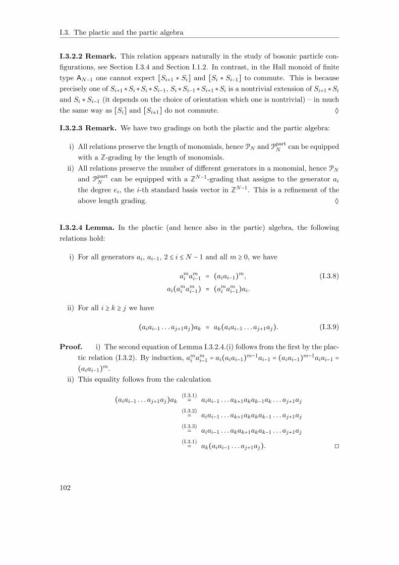
I.3. The plactic and the partic algebra
I.3.2.2 Remark. This relation appears naturally in the study of bosonic particle con-
figurations, see Section I.3.4 and Section I.1.2. In contrast, in the Hall monoid of finite
type AN−1 one cannot expect [Si+1 ∗ Si] and [Si ∗ Si−1] to commute. This is because
precisely one of Si+1∗Si∗Si∗Si−1, Si∗Si−1∗Si+1∗Si is a nontrivial extension of Si+1∗Si
and Si ∗Si−1 (it depends on the choice of orientation which one is nontrivial) – in much
the same way as [Si] and [Si±1] do not commute. ◊
I.3.2.3 Remark. We have two gradings on both the plactic and the partic algebra:
i) All relations preserve the length of monomials, hence PN and PpartN can be equipped
with a Z-grading by the length of monomials.
ii) All relations preserve the number of different generators in a monomial, hence PN
and PpartN can be equipped with a ZN−1-grading that assigns to the generator ai
the degree ei, the i-th standard basis vector in ZN−1. This is a refinement of the
above length grading. ◊
I.3.2.4 Lemma. In the plactic (and hence also in the partic) algebra, the following
relations hold:
i) For all generators ai, ai−1, 2 ≤ i ≤ N − 1 and all m ≥ 0, we have
ami ami−1 = (aiai−1)
m, (I.3.8)
ai(ami a
mi−1) = (ami a
mi−1)ai.
ii) For all i ≥ k ≥ j we have
(aiai−1 . . . aj+1aj)ak = ak(aiai−1 . . . aj+1aj). (I.3.9)
Proof. i) The second equation of Lemma I.3.2.4.(i) follows from the first by the plac-
tic relation (I.3.2). By induction, ami ami−1 = ai(aiai−1)
m−1ai−1 = (aiai−1)m−1aiai−1 =
(aiai−1)m.
ii) This equality follows from the calculation
(aiai−1 . . . aj+1aj)ak(I.3.1)= aiai−1 . . . ak+1akak−1ak . . . aj+1aj
(I.3.2)= aiai−1 . . . ak+1akakak−1 . . . aj+1aj
(I.3.3)= aiai−1 . . . akak+1akak−1 . . . aj+1aj
(I.3.1)= ak(aiai−1 . . . aj+1aj). ◻
102

I.3.3. A basis of the partic algebra
I.3.3. A basis of the partic algebra
In this section we formulate the following main theorem:
I.3.3.1 Theorem. The partic algebra PpartN has a basis given by monomials of the form
adN−1N−1 . . . a
d22 a
k11 a
k22 . . . akN−1
N−1 ∣ di ≤ di−1 + ki−1 for all 3 ≤ i ≤ N − 1, d2 ≤ k1 (I.3.10)
where di, ki ∈ Z≥0 for all 1 ≤ i ≤ N − 1.
The proof consists of two steps: Since the partic algebra is defined by monomial relations,
it suffices to construct a normal form for monomials to obtain a k-basis for the algebra.
This is similar to the affine nilTemperley–Lieb algebra, see Remark I.2.5.1. In this section
we show that every monomial in the partic algebra is equivalent to a monomial of the
form (I.3.10). In Section I.3.4 we observe that these monomials act pairwise differently
on the particle configuration module, and we conclude that they must have been distinct.
I.3.3.2 Proposition. Every monomial in the partic algebra PpartN is equivalent to a
monomial of the form (I.3.10), i.e. adN−1N−1 . . . a
d22 a
k11 a
k22 . . . akN−1
N−1 with di ≤ di−1+ki−1 for all
3 ≤ i ≤ N − 1 and d2 ≤ k1.
Proof. The proof works by induction on the length of monomials. If the length is equal
to 1, we have ai = akii for ki = 1, and the condition from (I.3.10) is preserved. For the
induction step our goal is to show that
ai ⋅ (adN−1N−1 . . . a
d22 a
k11 a
k22 . . . akN−1
N−1 ) = adN−1N−1 . . . a
d′ii . . . a
d22 a
k11 a
k22 . . . a
k′ii . . . a
kN−1N−1 , (I.3.11)
where d′i = di and k′i = ki + 1, or d′i = di + 1 and k′i = ki are such that the inequality
condition (I.3.10) is preserved. Since we can commute ai with all aj as long as j ≠ i ± 1,
we only need to consider
ai ⋅ (adi+1i+1 a
dii a
di−1i−1 . . . aki−1i−1 a
kii ) .
In order to prove that this can be rewritten as in (I.3.11), we have to show that either
we can pass ai through to the right hand side, increasing the exponent ki by one, or we
leave it at the left hand side, increasing di by one.
i) Case di+1 = di = di−1 = ki−1 = 0: Set k′i = ki + 1. The inequality condition (I.3.10)
is automatically satisfied if we increase one of the k’s, so there is nothing to
check. The equality (I.3.11) is obvious since we only apply the commutativity
relation (I.3.1).
103
I.3. The plactic and the partic algebra
ii) Case di+1 = di = di−1 = 0, ki−1 > 0: Set d′i = 1. The inequality condition (I.3.10) is
preserved since ki−1 ≥ 1, and again we only apply the commutativity relation (I.3.1).
iii) Case di+1 = di = 0, di−1 > 0, ki−1 arbitrary: Set d′i = 1. The inequality condi-
tion (I.3.10) is preserved since di−1 ≥ 1, and as before we only apply the commuta-
tivity relation (I.3.1).
iv) Case di+1 = 0, di > 0, di−1 and ki−1 arbitrary so that di ≤ di−1 + ki−1:
di < di−1 + ki−1: Set d′i = di + 1.
di = di−1 + ki−1: We cannot increase di, hence we have to show that we can com-
mute ai past adi−1i−1 and aki−1i−1 to increase ki. Indeed, we can apply equality (I.3.8)
from Lemma I.3.2.4.(i) to obtain
ai (adii a
di−1i−1 . . . aki−1i−1 a
kii ) = adi−1+ki−1+1
i adi−1i−1 . . . aki−1i−1 akii
= aki−1+1i (aiai−1)
di−1 . . . aki−1i−1 akii
= (aiai−1)di−1aki−1+1
i . . . aki−1i−1 akii
= (aiai−1)di−1 . . . aki−1+1
i aki−1i−1 akii
= (aiai−1)di−1 . . . ai(aiai−1)
ki−1akii
= (aiai−1)di−1 . . . (aiai−1)
ki−1aki+1i
= (aiai−1)di−1aki−1i . . . aki−1i−1 a
ki+1i
= adi−1+ki−1i adi−1i−1 . . . aki−1i−1 aki+1i .
v) Case di+1 > 0, di, ki and di−1, ki−1 arbitrary so that di+1 ≤ di + ki, di ≤ di−1 + ki−1:
We reduce to the previous cases by proving
aiadi+1i+1 ⋅ (adii a
di−1i−1 . . . aki−1i−1 a
kii ) = adi+1i+1 ai (a
dii a
di−1i−1 . . . aki−1i−1 a
kii ) .
di+1 > di: Here we can apply Lemma I.3.2.4.(i) to obtain
ai(adi+1i+1 a
dii ) = ai(ai+1ai)
di+1adi−di+1i = (ai+1ai)di+1adi−di+1i = adi+1i+1 aia
dii .
di+1 ≤ di: In this case we have ki ≥ di+1 − di > 0. It suffices to prove that
aiami+1a
di−1i−1 . . . aki−1i−1 a
mi = ami+1aia
di−1i−1 . . . aki−1i−1 a
mi
for any m > 0. Then the desired statement follows using equality (I.3.8) from
Lemma I.3.2.4.(i):
aiadi+1i+1 a
dii a
di−1i−1 . . . aki−1i−1 a
kii = (ai+1ai)
di (aiadi+1−dii+1 adi−1i−1 . . . aki−1i−1 a
di+1−dii )aki+di−di+1i
= (ai+1ai)di (adi+1−dii+1 aia
di−1i−1 . . . aki−1i−1 a
di+1−dii )aki+di−di+1i
= adi+1i+1 aiadii a
di−1i−1 . . . aki−1i−1 a
kii .
104
I.3.3. A basis of the partic algebra
Now for di−1, di−2, . . . , dj > 0 and dj−1 = 0 (possibly j = i, or j = 1), we applyequations (I.3.1), (I.3.7), (I.3.8) and (I.3.9) to pass the factor ai (distinguished bybold print) through the whole expression, thereby proving the desired equality.
aiaiaiami+1a
di−1i−1 a
di−2i−2 . . . a
djj a
dj−2j−2 . . . a
kj−2j−2 a
kj−1j−1 a
kjj . . . a
ki−1i−1 ami
(I.3.1)= aiaiaia
di−1i−1 a
di−2i−2 . . . a
djj a
dj−2j−2 . . . a
kj−2j−2 a
kj−1j−1 a
kjj . . . a
ki−1i−1 ami+1a
mi
(I.3.8)= aiaiaia
di−1i−1 a
di−2i−2 . . . a
djj a
dj−2j−2 . . . a
kj−2j−2 a
kj−1j−1 a
kjj . . . a
ki−1i−1 (ai+1ai)
m
= (aiaiaiai−1)adi−1−1i−1 a
di−2i−2 . . . a
djj a
dj−2j−2 . . . a
kj−2j−2 a
kj−1j−1 a
kjj . . . a
ki−1i−1 (ai+1ai)
m
(I.3.9)= a
di−1−1i−1 a
di−2−1i−2 . . . (aiaiaiai−1ai−2 . . . aj)a
dj−1j a
dj−2j−2 . . . a
kj−2j−2 a
kj−1j−1 a
kjj . . . a
ki−1i−1 (ai+1ai)
m
(I.3.9)= a
di−1−1i−1 a
di−2−1i−2 . . . a
dj−1j (aiaiaiai−1ai−2 . . . aj)a
dj−2j−2 . . . a
kj−2j−2 a
kj−1j−1 a
kjj . . . a
ki−1i−1 (ai+1ai)
m
(I.3.1)= a
di−1−1i−1 a
di−2−1i−2 . . . a
dj−1j a
dj−2j−2 . . . a
kj−2j−2 (aiaiaiai−1ai−2 . . . aj)a
kj−1j−1 a
kjj . . . a
ki−1i−1 (ai+1ai)
m
(I.3.9)= a
di−1−1i−1 a
di−2−1i−2 . . . a
dj−1j a
dj−2j−2 . . . a
kj−2j−2 a
kj−1−1j−1 (aiaiaiai−1ai−2 . . . ajaj−1)a
kjj . . . a
ki−1i−1 (ai+1ai)
m
(I.3.9)= a
di−1−1i−1 a
di−2−1i−2 . . . a
dj−1j a
dj−2j−2 . . . a
kj−2j−2 a
kj−1−1j−1 a
kjj . . . a
ki−1i−1 (aiaiaiai−1ai−2 . . . ajaj−1)(ai+1ai)
m
(I.3.1)= a
di−1−1i−1 a
di−2−1i−2 . . . a
dj−1j a
dj−2j−2 . . . a
kj−2j−2 a
kj−1−1j−1 a
kjj . . . a
ki−1i−1 (aiaiaiai−1)(ai+1ai)
m(ai−2 . . . ajaj−1)
(I.3.7)= a
di−1−1i−1 a
di−2−1i−2 . . . a
dj−1j a
dj−2j−2 . . . a
kj−2j−2 a
kj−1−1j−1 a
kjj . . . a
ki−1i−1 (ai+1ai)
m(aiaiaiai−1)(ai−2 . . . ajaj−1)
(I.3.8)= a
di−1−1i−1 a
di−2−1i−2 . . . a
dj−1j a
dj−2j−2 . . . a
kj−2j−2 a
kj−1−1j−1 a
kjj . . . a
ki−1i−1 ami+1a
mi (aiaiaiai−1)(ai−2 . . . ajaj−1)
(I.3.1)= ami+1a
di−1−1i−1 a
di−2−1i−2 . . . a
dj−1j a
dj−2j−2 . . . a
kj−2j−2 a
kj−1−1j−1 a
kjj . . . a
ki−1i−1 ami (aiaiaiai−1ai−2 . . . ajaj−1)
(I.3.9)= ami+1a
di−1−1i−1 a
di−2−1i−2 . . . a
dj−1j a
dj−2j−2 . . . a
kj−2j−2 (aiaiaiai−1ai−2 . . . ajaj−1)a
kj−1−1j−1 a
kjj . . . a
ki−1i−1 ami
= ami+1adi−1−1i−1 a
di−2−1i−2 . . . a
dj−1j a
dj−2j−2 . . . a
kj−2j−2 (aiaiaiai−1ai−2 . . . aj)a
kj−1j−1 a
kjj . . . a
ki−1i−1 ami
(I.3.1)= ami+1a
di−1−1i−1 a
di−2−1i−2 . . . a
dj−1j (aiaiaiai−1ai−2 . . . aj)a
dj−2j−2 . . . a
kj−2j−2 a
kj−1j−1 a
kjj . . . a
ki−1i−1 ami
(I.3.9)= ami+1a
di−1−1i−1 a
di−2−1i−2 . . . (aiaiaiai−1ai−2 . . . aj)a
dj−1j a
dj−2j−2 . . . a
kj−2j−2 a
kj−1j−1 a
kjj . . . a
ki−1i−1 ami
(I.3.9)= ami+1a
di−1−1i−1 (aiaiaiai−1ai−2)a
di−2−1i−2 . . . a
djj a
dj−2j−2 . . . a
kj−2j−2 a
kj−1j−1 a
kjj . . . a
ki−1i−1 ami
(I.3.9)= ami+1(aiaiaiai−1)a
di−1−1i−1 a
di−2i−2 . . . a
djj a
dj−2j−2 . . . a
kj−2j−2 a
kj−1j−1 a
kjj . . . a
ki−1i−1 ami
= ami+1aiaiaiadi−1i−1 a
di−2i−2 . . . a
djj a
dj−2j−2 . . . a
kj−2j−2 a
kj−1j−1 a
kjj . . . a
ki−1i−1 ami .
This concludes the proof of Proposition I.3.3.2. ◻
Note that the relation special for the partic algebra (I.3.7) was only used once in the
proof of Proposition I.3.3.2, namely in the long computation at the end. All other
steps have been carried out using only the commutativity relation (I.3.1) and the plactic
relations (I.3.2) and (I.3.3). The following corollary recaps what we obtained for the
multiplication in the partic algebra:
I.3.3.3 Corollary. Assume we are given a monomial adN−1N−1 . . . a
d22 a
k11 a
k22 . . . akN−1
N−1 of the
105
I.3. The plactic and the partic algebra
form (I.3.10) in the partic algebra. Then left multiplication with ai gives
ai ⋅ (adN−1N−1 . . . a
d22 a
k11 a
k22 . . . akN−1
N−1 ) (I.3.12)
=
⎧⎪⎪⎪⎨⎪⎪⎪⎩
adN−1N−1 . . . a
dii . . . a
d22 a
k11 a
k22 . . . aki+1
i . . . akN−1N−1 if di = di−1 + ki−1,
adN−1N−1 . . . a
di+1i . . . ad22 a
k11 a
k22 . . . akii . . . a
kN−1N−1 if di < di−1 + ki−1.
Right multiplication with ai gives
(adN−1N−1 . . . a
d22 a
k11 a
k22 . . . akN−1
N−1 ) ⋅ ai (I.3.13)
=
⎧⎪⎪⎪⎨⎪⎪⎪⎩
adN−1N−1 . . . a
dii a
di+1+1i+1 . . . ad22 a
k11 a
k22 . . . aki+1
i aki+1−1i+1 . . . akN−1
N−1 if ki+1 ≥ 1
adN−1N−1 . . . a
dii a
di+1i+1 . . . ad22 a
k11 a
k22 . . . aki+1
i a0i+1 . . . a
kN−1N−1 if ki+1 = 0,
with the result written again in the normal form (I.3.10).
Proof. For the left multiplication, equation (I.3.12) is contained in the proof of Propo-
sition I.3.3.2. For the right multiplication, equation (I.3.13) follows from the repeated
application of the rule for left multiplication of adN−1N−1 . . . a
d22 a
k11 a
k22 . . . akN−1
N−1 to ai. ◻
I.3.3.4 Example. The partic algebra has zero divisors, e.g. in Ppart3 ,
a2 ⋅ (a53a
82a
81a
32a
13 − a5
3a72a
81a
42a
13) = a5
3a82a
81a
42a
13 − a5
3a82a
81a
42a
13 = 0
(it follows from Theorem I.3.3.1 that a53a
82a
81a
32a
13 − a5
3a72a
81a
42a
13 ≠ 0). ◊
I.3.3.5 Remark. Let us compare our normal form with the monomial bases of the
plactic algebra from [Rei02]: The plactic algebra PN surjects onto the partic algebra
PpartN , mapping generators to generators and hence monomials to monomials. Given
a monomial of the normal form from Proposition I.3.3.2, finding the (finitely many)
preimages of basis monomials in the plactic algebra amounts to solving a system of linear
equations over the nonnegative integers, i.e. finding lattice points inside a polyhedron.
For example, consider the basis of the plactic algebra P5 from [Rei02, Theorem 2.10]
given by monomials
(a1)n1(a2a1)
n21(a2)n2(a3a2a1)
n321(a3a2)n32(a3)
n3(a4a3a2a1)n4321(a4a3a2)
n432(a4a3)n43(a4)
n4
where all ni ∈ Z≥0 and compare it with the basis of the partic algebra Ppart5 from Propo-
sition I.3.3.2
ad44 ad33 a
d22 a
k11 a
k22 a
k33 a
k44 ∣ all ki, di ∈ Z≥0, di ≤ di−1 + ki−1.
While a1a2a3a4 ∈ Ppart5 has only one preimage, namely (a1)
1(a2)1(a3)
1(a4)1 ∈ P5, we
find two preimages of a4a3a2a1a2 ∈ Ppart5 , namely (a2)
1(a4a3a2a1)1, (a2a1)
1(a4a3a2)1 ∈
P5. This corresponds to the number of possible applications of the additional partic
relation (I.3.7). ◊
106
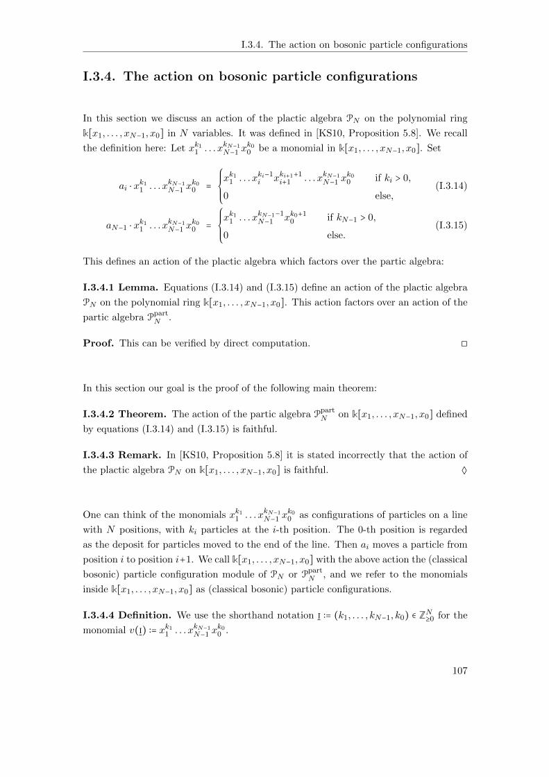
I.3.4. The action on bosonic particle configurations
I.3.4. The action on bosonic particle configurations
In this section we discuss an action of the plactic algebra PN on the polynomial ring
k[x1, . . . , xN−1, x0] in N variables. It was defined in [KS10, Proposition 5.8]. We recall
the definition here: Let xk11 . . . xkN−1N−1 x
k00 be a monomial in k[x1, . . . , xN−1, x0]. Set
ai ⋅ xk11 . . . xkN−1
N−1 xk00 =
⎧⎪⎪⎪⎨⎪⎪⎪⎩
xk11 . . . xki−1i xki+1+1
i+1 . . . xkN−1N−1 x
k00 if ki > 0,
0 else,(I.3.14)
aN−1 ⋅ xk11 . . . xkN−1
N−1 xk00 =
⎧⎪⎪⎪⎨⎪⎪⎪⎩
xk11 . . . xkN−1−1N−1 xk0+1
0 if kN−1 > 0,
0 else.(I.3.15)
This defines an action of the plactic algebra which factors over the partic algebra:
I.3.4.1 Lemma. Equations (I.3.14) and (I.3.15) define an action of the plactic algebra
PN on the polynomial ring k[x1, . . . , xN−1, x0]. This action factors over an action of the
partic algebra PpartN .
Proof. This can be verified by direct computation. ◻
In this section our goal is the proof of the following main theorem:
I.3.4.2 Theorem. The action of the partic algebra PpartN on k[x1, . . . , xN−1, x0] defined
by equations (I.3.14) and (I.3.15) is faithful.
I.3.4.3 Remark. In [KS10, Proposition 5.8] it is stated incorrectly that the action of
the plactic algebra PN on k[x1, . . . , xN−1, x0] is faithful. ◊
One can think of the monomials xk11 . . . xkN−1N−1 x
k00 as configurations of particles on a line
with N positions, with ki particles at the i-th position. The 0-th position is regarded
as the deposit for particles moved to the end of the line. Then ai moves a particle from
position i to position i+1. We call k[x1, . . . , xN−1, x0] with the above action the (classical
bosonic) particle configuration module of PN or PpartN , and we refer to the monomials
inside k[x1, . . . , xN−1, x0] as (classical bosonic) particle configurations.
I.3.4.4 Definition. We use the shorthand notation i ∶= (k1, . . . , kN−1, k0) ∈ ZN≥0 for the
monomial v(i) ∶= xk11 . . . xkN−1N−1 x
k00 .
107
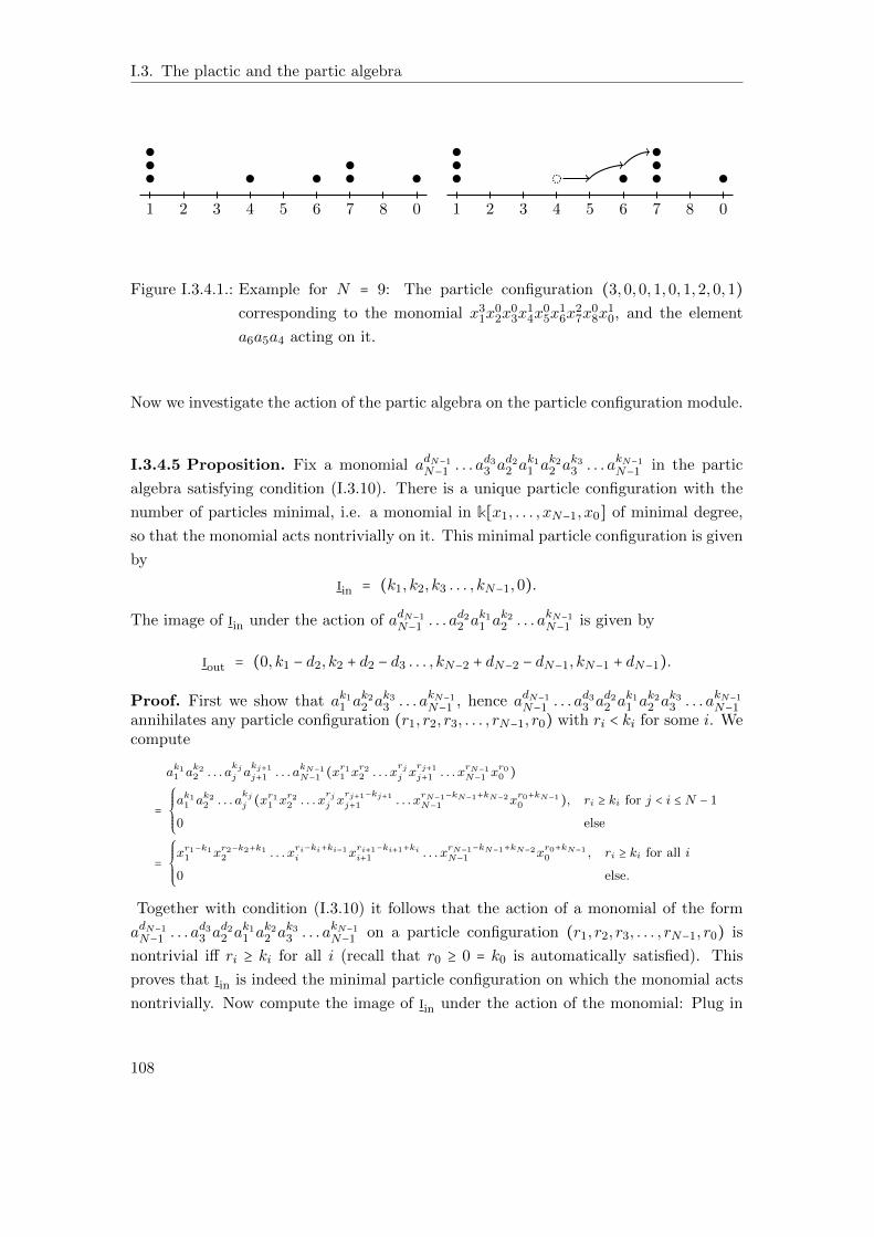
I.3. The plactic and the partic algebra
1 2 3 4 5 6 7 8 0 1 2 3 4 5 6 7 8 0
Figure I.3.4.1.: Example for N = 9: The particle configuration (3,0,0,1,0,1,2,0,1)
corresponding to the monomial x31x
02x
03x
14x
05x
16x
27x
08x
10, and the element
a6a5a4 acting on it.
Now we investigate the action of the partic algebra on the particle configuration module.
I.3.4.5 Proposition. Fix a monomial adN−1N−1 . . . a
d33 a
d22 a
k11 a
k22 a
k33 . . . akN−1
N−1 in the partic
algebra satisfying condition (I.3.10). There is a unique particle configuration with the
number of particles minimal, i.e. a monomial in k[x1, . . . , xN−1, x0] of minimal degree,
so that the monomial acts nontrivially on it. This minimal particle configuration is given
by
iin = (k1, k2, k3 . . . , kN−1,0).
The image of iin under the action of adN−1N−1 . . . a
d22 a
k11 a
k22 . . . akN−1
N−1 is given by
iout = (0, k1 − d2, k2 + d2 − d3 . . . , kN−2 + dN−2 − dN−1, kN−1 + dN−1).
Proof. First we show that ak11 ak22 a
k33 . . . akN−1
N−1 , hence adN−1N−1 . . . a
d33 a
d22 a
k11 a
k22 a
k33 . . . akN−1
N−1annihilates any particle configuration (r1, r2, r3, . . . , rN−1, r0) with ri < ki for some i. Wecompute
ak11 ak22 . . . akjj a
kj+1j+1 . . . a
kN−1N−1 (x
r11 xr22 . . . x
rjj x
rj+1j+1 . . . x
rN−1N−1 xr00 )
=
⎧⎪⎪⎪⎨⎪⎪⎪⎩
ak11 ak22 . . . akjj (x
r11 xr22 . . . x
rjj x
rj+1−kj+1j+1 . . . x
rN−1−kN−1+kN−2N−1 x
r0+kN−10 ), ri ≥ ki for j < i ≤ N − 1
0 else
=
⎧⎪⎪⎪⎨⎪⎪⎪⎩
xr1−k11 xr2−k2+k12 . . . xri−ki+ki−1i x
ri+1−ki+1+kii+1 . . . x
rN−1−kN−1+kN−2N−1 x
r0+kN−10 , ri ≥ ki for all i
0 else.
Together with condition (I.3.10) it follows that the action of a monomial of the form
adN−1N−1 . . . a
d33 a
d22 a
k11 a
k22 a
k33 . . . akN−1
N−1 on a particle configuration (r1, r2, r3, . . . , rN−1, r0) is
nontrivial iff ri ≥ ki for all i (recall that r0 ≥ 0 = k0 is automatically satisfied). This
proves that iin is indeed the minimal particle configuration on which the monomial acts
nontrivially. Now compute the image of iin under the action of the monomial: Plug in
108
I.3.4. The action on bosonic particle configurations
ri = ki for all i to see that
adN−1N−1 . . . a
d33 a
d22 a
k11 a
k22 a
k33 . . . akN−1
N−1 (iin) = adN−1N−1 . . . a
d33 a
d22 (x0
1xk12 . . . xkN−2
N−1 xkN−10 )
= iout.
This proves Proposition I.3.4.5. ◻
See also Remark I.2.4.3 for the notion of minimal (affine fermionic) particle configurations
for the affine nilTemperley–Lieb algebra.
Proof (of Theorem I.3.3.1). By Proposition I.3.3.2 any monomial in the partic alge-
bra is equivalent to one of the form (I.3.10). We have shown in Proposition I.3.4.5 that
the action on the particle configuration module distinguishes any two monomials of the
form (I.3.10), hence (I.3.10) describes a normal form for the monomials in the partic
algebra PpartN , hence a basis of Ppart
N . ◻
Now Theorem I.3.4.2 follows as a corollary from Proposition I.3.4.5:
Proof (of Theorem I.3.4.2). We have seen in Proposition I.3.4.5 that the normal
form monomials, hence the basis elements in PpartN act linearly independent on the par-
ticle configurations. In other words, the action of PpartN is faithful. ◻
I.3.4.6 Remark. The faithfulness of the action of the algebra PpartN on the particle
configuration module motivates us to give PpartN the name “partic” algebra. ◊
By Proposition I.3.3.2 and Proposition I.3.4.5, we can identify each monomial in the
partic algebra uniquely by the minimal particle configuration j ∈ ZN≥0 on which it acts
nontrivially and the output particle configuration i ∈ ZN≥0 that one gets back from the
action of the monomial on j. Hence the following is welldefined:
I.3.4.7 Definition. Given a monomial in normal form with di ≤ di−1 + ki−1 for all 3 ≤
i ≤ N − 1 and d2 ≤ k1, see Proposition I.3.4.5, we write
aij = adN−1N−1 . . . a
d22 a
k11 a
k22 . . . akN−1
N−1
for bosonic particle configurations i = (0, k1−d2, k2+d2−d3 . . . , kN−2+dN−2−dN−1, kN−1+
dN−1) and j = (k1, k2, k3 . . . , kN−1,0). The number of particles ∣i∣ = ∣j∣ = ∑i ki in i and j
is the same.
This labelling is made so that aij ⋅ v(j) = v(i) in the notation of Definition I.3.4.4.
109
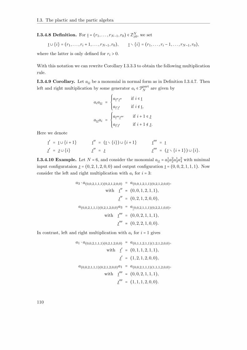
I.3. The plactic and the partic algebra
I.3.4.8 Definition. For i = (r1, . . . , rN−1, r0) ∈ ZN≥0, we set
i ∪ i = (r1, . . . , ri + 1, . . . , rN−1, r0), i ∖ i = (r1, . . . , ri − 1, . . . , rN−1, r0),
where the latter is only defined for ri > 0.
With this notation we can rewrite Corollary I.3.3.3 to obtain the following multiplication
rule.
I.3.4.9 Corollary. Let aij be a monomial in normal form as in Definition I.3.4.7. Then
left and right multiplication by some generator ai ∈ PpartN are given by
aiaij =
⎧⎪⎪⎪⎨⎪⎪⎪⎩
ai′′j′′ if i ∈ i
ai′j′ if i ∉ i,
aijai =
⎧⎪⎪⎪⎨⎪⎪⎪⎩
ai′′′j′′′ if i + 1 ∈ j
ai′j′ if i + 1 ∉ j.
Here we denote
i′ = i ∪ i + 1 i′′ = (i ∖ i) ∪ i + 1 i′′′ = i
j′ = j ∪ i j′′ = j j′′′ = (j ∖ i + 1) ∪ i.
I.3.4.10 Example. Let N = 6, and consider the monomial aij = a15a
22a
13a
24 with minimal
input configurataion j = (0,2,1,2,0,0) and output configuration i = (0,0,2,1,1,1). Now
consider the left and right multiplication with ai for i = 3:
a3 ⋅ a(0,0,2,1,1,1)(0,2,1,2,0,0) = a(0,0,1,2,1,1)(0,2,1,2,0,0),
with i′′ = (0,0,1,2,1,1),
j′′ = (0,2,1,2,0,0),
a(0,0,2,1,1,1)(0,2,1,2,0,0)a3 = a(0,0,2,1,1,1)(0,2,2,1,0,0),
with i′′′ = (0,0,2,1,1,1),
j′′′ = (0,2,2,1,0,0).
In contrast, left and right multiplication with ai for i = 1 gives
a1 ⋅ a(0,0,2,1,1,1)(0,2,1,2,0,0) = a(0,1,1,2,1,1)(1,2,1,2,0,0),
with i′ = (0,1,1,2,1,1),
j′ = (1,2,1,2,0,0),
a(0,0,2,1,1,1)(0,2,1,2,0,0)a1 = a(0,0,2,1,1,1)(1,1,1,2,0,0),
with i′′′ = (0,0,2,1,1,1),
j′′′ = (1,1,1,2,0,0).
110
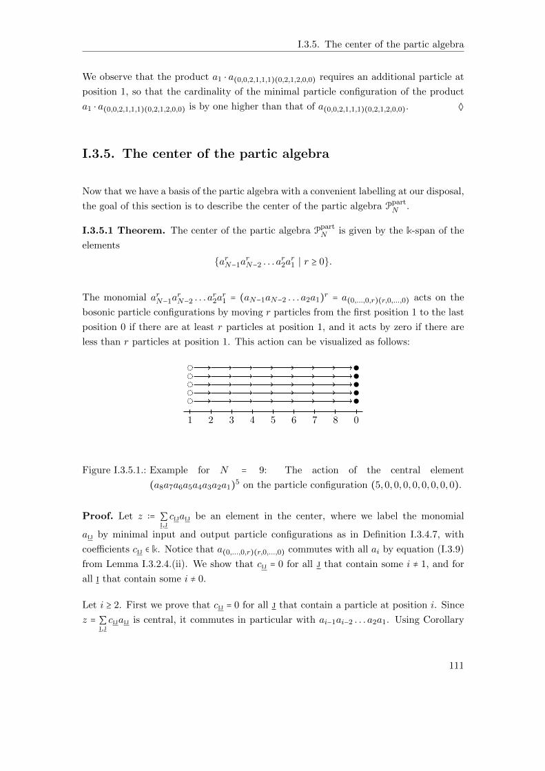
I.3.5. The center of the partic algebra
We observe that the product a1 ⋅ a(0,0,2,1,1,1)(0,2,1,2,0,0) requires an additional particle at
position 1, so that the cardinality of the minimal particle configuration of the product
a1 ⋅ a(0,0,2,1,1,1)(0,2,1,2,0,0) is by one higher than that of a(0,0,2,1,1,1)(0,2,1,2,0,0). ◊
I.3.5. The center of the partic algebra
Now that we have a basis of the partic algebra with a convenient labelling at our disposal,
the goal of this section is to describe the center of the partic algebra PpartN .
I.3.5.1 Theorem. The center of the partic algebra PpartN is given by the k-span of the
elements
arN−1arN−2 . . . a
r2ar1 ∣ r ≥ 0.
The monomial arN−1arN−2 . . . a
r2ar1 = (aN−1aN−2 . . . a2a1)
r = a(0,...,0,r)(r,0,...,0) acts on the
bosonic particle configurations by moving r particles from the first position 1 to the last
position 0 if there are at least r particles at position 1, and it acts by zero if there are
less than r particles at position 1. This action can be visualized as follows:
1 2 3 4 5 6 7 8 0
Figure I.3.5.1.: Example for N = 9: The action of the central element
(a8a7a6a5a4a3a2a1)5 on the particle configuration (5,0,0,0,0,0,0,0,0).
Proof. Let z ∶= ∑i,jcijaij be an element in the center, where we label the monomial
aij by minimal input and output particle configurations as in Definition I.3.4.7, with
coefficients cij ∈ k. Notice that a(0,...,0,r)(r,0,...,0) commutes with all ai by equation (I.3.9)
from Lemma I.3.2.4.(ii). We show that cij = 0 for all j that contain some i ≠ 1, and for
all i that contain some i ≠ 0.
Let i ≥ 2. First we prove that cij = 0 for all j that contain a particle at position i. Since
z = ∑i,jcijaij is central, it commutes in particular with ai−1ai−2 . . . a2a1. Using Corollary
111
I.3. The plactic and the partic algebra
I.3.4.9 we calculate
(ai−1ai−2 . . . a2a1)aij = a(i∪i)(j∪1),
aij(ai−1ai−2 . . . a2a1) =
⎧⎪⎪⎪⎨⎪⎪⎪⎩
a(i∪i)(j∪1) if i ∉ j,
ai((j∖i)∪1) if i ∈ j.
Therefore (ai−1ai−2 . . . a2a1)aij = aij(ai−1ai−2 . . . a2a1) for i ∉ j. This we use to deduce
that we have (ai−1ai−2 . . . a2a1)z = z(ai−1ai−2 . . . a2a1) if and only if
(ai−1ai−2 . . . a2a1)
⎛⎜⎜⎝
∑i, ji∉j
cijaij + ∑i, ji∈j
cijaij
⎞⎟⎟⎠
=
⎛⎜⎜⎝
∑i, ji∉j
cijaij + ∑i, ji∈j
cijaij
⎞⎟⎟⎠
(ai−1ai−2 . . . a2a1),
which holds if and only if
(ai−1ai−2 . . . a2a1)
⎛⎜⎜⎝
∑i, ji∈j
cijaij
⎞⎟⎟⎠
=
⎛⎜⎜⎝
∑i, ji∈j
cijaij
⎞⎟⎟⎠
(ai−1ai−2 . . . a2a1).
The latter is precisely the equality
∑i, ji∈j
cija(i∪i)(j∪1) = ∑i, ji∈j
cijai((j∖i)∪1). (I.3.16)
Observe on the other hand that for fixed i the set of monomials
ai((j∖i)∪1) ∣ i, j such that i ∈ j
is linearly independent since the sets ((j ∖ i) ∪ 1) are all distinct for distinct j.
Next, we show by induction on the number ki of particles at position i in j that all
coefficients cij are zero for ki ≥ 1:
For ki = 1, the set (j ∖ i) ∪ 1 does not contain any particle at position i any more.
Hence the monomial ai((j∖i)∪1) cannot appear in the left sum in equation (I.3.16),
and so its coefficient cij must have been zero. For the induction step, assume that the
coefficient cij is zero for all aij with at most ki particles at position i in the minimal
input particle configuration j. Consider some aij with ki + 1 particles at position i in j.
So the set (j ∖ i) ∪ 1 contains ki particles at position i in j, and so the monomial
ai((j∖i)∪1) cannot appear in the sum (I.3.16). Therefore we see that the coefficient cij
must have been zero.
We have shown that any central element in PpartN is of the form
z = ∑i, j
cijaij,
112
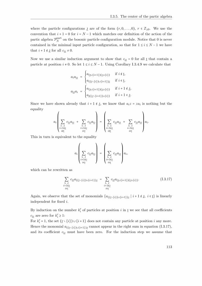
I.3.5. The center of the partic algebra
where the particle configurations j are of the form (r,0, . . . ,0), r ∈ Z≥0. We use the
convention that i + 1 = 0 for i = N − 1 which matches our definition of the action of the
partic algebra PpartN on the bosonic particle configuration module. Notice that 0 is never
contained in the minimal input particle configuration, so that for 1 ≤ i ≤ N − 1 we have
that i + 1 ∉ j for all cij ≠ 0.
Now we use a similar induction argument to show that cij = 0 for all i that contain a
particle at position i ≠ 0. So let 1 ≤ i ≤ N − 1. Using Corollary I.3.4.9 we calculate that
aiaij =
⎧⎪⎪⎪⎨⎪⎪⎪⎩
a(i∪i+1)(j∪i) if i ∉ i,
a((i∖i)∪i+1)j if i ∈ i,
aijai =
⎧⎪⎪⎪⎨⎪⎪⎪⎩
a(i∪i+1)(j∪i) if i + 1 ∉ j,
ai((j∖i+1)∪i) if i + 1 ∈ j.
Since we have shown already that i + 1 ∉ j, we know that aiz = zai is nothing but the
equality
ai
⎛⎜⎜⎜⎜⎜⎝
∑i, ji+1∉ji∉i
cijaij + ∑i, ji+1∉ji∈i
cijaij
⎞⎟⎟⎟⎟⎟⎠
=
⎛⎜⎜⎜⎜⎜⎝
∑i, ji+1∉ji∉i
cijaij + ∑i, ji+1∉ji∈i
cijaij
⎞⎟⎟⎟⎟⎟⎠
ai.
This in turn is equivalent to the equality
ai
⎛⎜⎜⎜⎜⎜⎝
∑i, ji+1∉ji∈i
cijaij
⎞⎟⎟⎟⎟⎟⎠
=
⎛⎜⎜⎜⎜⎜⎝
∑i, ji+1∉ji∈i
cijaij
⎞⎟⎟⎟⎟⎟⎠
ai,
which can be rewritten as
∑i, ji+1∉ji∈i
cija((i∖i)∪i+1)j = ∑i, ji+1∉ji∈i
cija(i∪i+1)(j∪i). (I.3.17)
Again, we observe that the set of monomials a((i∖i)∪i+1)j ∣ i + 1 ∉ j, i ∈ i is linearly
independent for fixed i.
By induction on the number k′i of particles at position i in i we see that all coefficients
cij are zero for k′i ≥ 1:
For k′i = 1, the set (i∖i)∪i+1 does not contain any particle at position i any more.
Hence the monomial a((i∖i)∪i+1)j cannot appear in the right sum in equation (I.3.17),
and its coefficient cij must have been zero. For the induction step we assume that
113
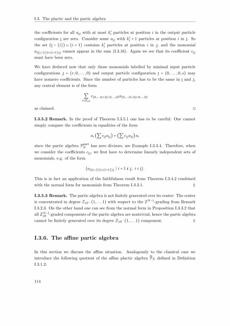
I.3. The plactic and the partic algebra
the coefficients for all aij with at most k′i particles at position i in the output particle
configuration i are zero. Consider some aij with k′i + 1 particles at position i in i. So
the set (i ∖ i) ∪ i + 1 contains k′i particles at position i in j, and the monomial
a((i∖i)∪i+1)j cannot appear in the sum (I.3.16). Again we see that its coefficient cij
must have been zero.
We have deduced now that only those monomials labelled by minimal input particle
configurations j = (r,0, . . . ,0) and output particle configuration i = (0, . . . ,0, s) may
have nonzero coefficients. Since the number of particles has to be the same in i and j,
any central element is of the form
∑r∈Z≥0
c(0,...,0,r)(r,0,...,0)a(0,...,0,r)(r,0,...,0)
as claimed. ◻
I.3.5.2 Remark. In the proof of Theorem I.3.5.1 one has to be careful: One cannot
simply compare the coefficients in equalities of the form
ai (∑ cijaij) = (∑ cijaij)ai
since the partic algebra PpartN has zero divisors, see Example I.3.3.4. Therefore, when
we consider the coefficients cij, we first have to determine linearly independent sets of
monomials, e.g. of the form
a((i∖i)∪i+1)j ∣ i + 1 ∉ j, i ∈ i.
This is in fact an application of the faithfulness result from Theorem I.3.4.2 combined
with the normal form for monomials from Theorem I.3.3.1. ◊
I.3.5.3 Remark. The partic algebra is not finitely generated over its center: The center
is concentrated in degree Z≥0 ⋅ (1, . . .1) with respect to the ZN−1-grading from Remark
I.3.2.3. On the other hand one can see from the normal form in Proposition I.3.3.2 that
all ZN−1≥0 -graded components of the partic algebra are nontrivial, hence the partic algebra
cannot be finitely generated over its degree Z≥0 ⋅ (1, . . .1) component. ◊
I.3.6. The affine partic algebra
In this section we discuss the affine situation. Analogously to the classical case we
introduce the following quotient of the affine plactic algebra PN defined in Definition
I.3.1.2:
114
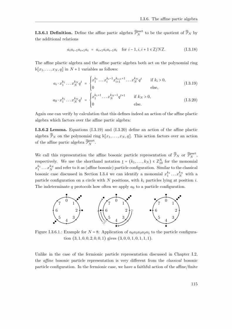
I.3.6. The affine partic algebra
I.3.6.1 Definition. Define the affine partic algebra PpartN to be the quotient of PN by
the additional relations
aiai−1ai+1ai = ai+1aiai−1ai for i − 1, i, i + 1 ∈ Z/NZ. (I.3.18)
The affine plactic algebra and the affine partic algebra both act on the polynomial ring
k[x1, . . . , xN , q] in N + 1 variables as follows:
ai ⋅ xk11 . . . xkNN qt =
⎧⎪⎪⎪⎨⎪⎪⎪⎩
xk11 . . . xki−1i xki+1+1
i+1 . . . xkNN qt if ki > 0,
0 else,(I.3.19)
a0 ⋅ xk11 . . . xkNN qt =
⎧⎪⎪⎪⎨⎪⎪⎪⎩
xk1+11 . . . xkN−1
N qt+1 if kN > 0,
0 else.(I.3.20)
Again one can verify by calculation that this defines indeed an action of the affine plactic
algebra which factors over the affine partic algebra:
I.3.6.2 Lemma. Equations (I.3.19) and (I.3.20) define an action of the affine plactic
algebra PN on the polynomial ring k[x1, . . . , xN , q]. This action factors over an action
of the affine partic algebra PpartN .
We call this representation the affine bosonic particle representation of PN or PpartN ,
respectively. We use the shorthand notation i = (k1, . . . , kN) ∈ ZN≥0 for the monomial
xk11 . . . xkNN and refer to it as (affine bosonic) particle configuration. Similar to the classical
bosonic case discussed in Section I.3.4 we can identify a monomial xk11 . . . xkNN with a
particle configuration on a circle with N positions, with ki particles lying at position i.
The indeterminate q protocols how often we apply a0 to a particle configuration.
01
2
34
5
6
70
1
2
34
5
6
70
1
2
34
5
6
7
Figure I.3.6.1.: Example for N = 8: Application of a6a5a3a2a5 to the particle configura-
tion (3,1,0,0,2,0,0,1) gives (3,0,0,1,0,1,1,1).
Unlike in the case of the fermionic particle representation discussed in Chapter I.2,
the affine bosonic particle representation is very different from the classical bosonic
particle configuration. In the fermionic case, we have a faithful action of the affine/finite
115
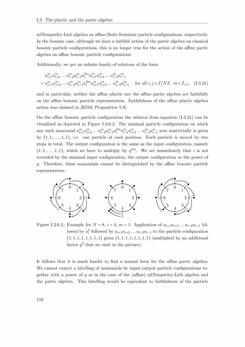
I.3. The plactic and the partic algebra
nilTemperley-Lieb algebra on affine/finite fermionic particle configurations, respectively.
In the bosonic case, although we have a faithful action of the partic algebra on classical
bosonic particle configurations, this is no longer true for the action of the affine partic
algebra on affine bosonic particle configurations:
Additionally, we get an infinite family of relations of the form
ami+1ami+2 . . . a
mi−2a
mi−1a
2mi ami+1a
mi+2 . . . a
mi−2a
mi−1
= amj+1amj+2 . . . a
mj−2a
mj−1a
2mj amj+1a
mj+2 . . . a
mj−2a
mj−1 for all i, j ∈ Z/NZ, m ∈ Z≥1, (I.3.21)
and in particular, neither the affine plactic nor the affine partic algebra act faithfully
on the affine bosonic particle representation. Faithfulness of the affine plactic algebra
action was claimed in [KS10, Proposition 5.8].
On the affine bosonic particle configuration the relation from equation (I.3.21) can be
visualized as depicted in Figure I.3.6.2: The minimal particle configuration on which
any such monomial ami+1ami+2 . . . a
mi−2a
mi−1a
2mi ami+1a
mi+2 . . . a
mi−2a
mi−1 acts nontrivially is given
by (1,1, . . . ,1,1), i.e. one particle at each position. Each particle is moved by two
steps in total. The output configuration is the same as the input configuration, namely
(1,1, . . . ,1,1), which we have to multiply by q2m. We see immediately that i is not
recorded by the minimal input configuration, the output configuration or the power of
q. Therefore, these monomials cannot be distinguished by the affine bosonic particle
representation.
01
2
34
5
6
70
1
2
34
5
6
70
1
2
34
5
6
7
Figure I.3.6.2.: Example for N = 8, i = 4, m = 1: Application of ai+1ai+2 . . . ai−2ai−1 fol-
lowed by a2i followed by ai+1ai+2 . . . ai−2ai−1 to the particle configuration
(1,1,1,1,1,1,1,1) gives (1,1,1,1,1,1,1,1) (multiplied by an additional
factor q2 that we omit in the picture).
It follows that it is much harder to find a normal form for the affine partic algebra:
We cannot expect a labelling of monomials by input/output particle configurations to-
gether with a power of q as in the case of the (affine) nilTemperley-Lieb algebra and
the partic algebra. This labelling would be equivalent to faithfulness of the particle
116
I.3.6. The affine partic algebra
representation. Such a labelling allowed us to reorder monomials so that the indices of
the rightmost factors correspond to the the minimal particle configuration on which the
monomial acts nontrivially, see Proposition I.3.4.5, Section I.2.6, and also compare with
Theorem I.2.10.1. The whole approach fails for the affine partic algebra:
The minimal particle configuration does not indicate a natural reordering of factors. For
example, consider the following monomials in Ppart5 :
a21a2a3a4a0, a
22a3a4a0a1, a
23a4a0a1a2, a
24a0a1a2a3, a
20a1a2a3a4.
All of these expect precisely one particle at each position 1,2,3,4,0 in the minimal
particle configuration, but none of them can be reordered in any way. Of course the
output configurations are all different, so these five different monomials could even be
distinguished by the affine particle representation. In fact one cannot expect a basis
labelled by tuples of a minimal input configuration, the output configuration, and some
power of q.
117

Part II.
Generalized Weyl algebras
119

II.1. A Duflo theorem for a class of
generalized Weyl algebras
II.1.1. An overview of Duflo type theorems
Let k be an algebraically closed field of characteristic 0. For the universal enveloping
algebra of a semisimple Lie algebra over k, Duflo’s Theorem [Duf77] states that all its
primitive ideals (i.e. the annihilators of simple modules) are given by the annihilators of
simple highest weight modules. In contrast, the simple modules themselves are far from
being classified in general. Fortunately, for several other classes of algebras the notion
of a highest weight module makes sense and the analogue of Duflo’s theorem holds:
In [Smi90], Smith introduced a family of algebras similar to U(sl2). These are C-algebras
generated by three elements E,F,H subject to the relations [H,E] = E, [H,F ] = −F
and [E,F ] = f(H) where f can be any polynomial. They share many properties with
U(sl2) (which is of course included in this family for f(H) = 2H). In particular it is
straightforward to generalize the notion of highest weight modules to these algebras
and indeed all primitive ideals are given by annihilators of highest weight modules (see
[Smi90, Theorem 3.3]).
For classical simple Lie superalgebras, Musson defines Z/2Z-graded highest weight mod-
ules depending on a choice of a triangular decomposition. Then all Z/2Z-graded primi-
tive ideals in the universal enveloping algebra of a classical simple Lie superalgebra are
given by the annihilators of Z/2Z-graded simple highest weight modules (see [Mus92,
Theorem 2.2]).
In [MB98], Musson and Van den Bergh introduce algebras that, roughly speaking, allow
a weight space decomposition with weight spaces cyclic over a commutative subalgebra.
This class of algebras is closed under taking certain graded subalgebras, tensor products
and central quotients. They show that (under some further assumptions, see Theo-
rem II.1.4.4 for details) all prime, hence all primitive ideals are given by the annihilators
of simple weight modules. In particular, this applies to localizations of Weyl algebras
121
II.1. A Duflo theorem for a class of generalized Weyl algebras
and their central subquotients (see [MB98, Chapter 6]). Note that for a classical Weyl
algebra, given by differential operators on a polynomial ring in n variables, the primitive
ideals are not very interesting: These algebras are simple, i.e. the only proper twosided
ideal is the zero ideal. Since an annihilator is always twosided, the only primitive ideal
of a classical Weyl algebra is the zero ideal.
Now it is natural to ask whether an analogous statement holds for generalized Weyl al-
gebras, a class of algebras that includes many interesting examples, in particular Smith’s
generalizations of U(sl2). These noncommutative algebras are generated by a commuta-
tive k-algebra R together with 2n elements X1, . . . ,Xn, Y1, . . . , Yn. For the relations see
Section II.1.2. They are Zn-graded by setting deg(Xi) = ei, deg(Yi) = −ei where ei de-
notes the i-th standard basis vector in Zn. Each graded component is a cyclic R-module.
In this situation, we can define highest weight modules and formulate a Duflo theorem.
We prove it for a special class of generalized Weyl algebras using a theorem by [MB98]
that relates the annihilator of a simple weight module to its support and obtain as main
result (see Theorem II.1.4.1):
Theorem. Let A = R(σ, t) be a GWA of rank n as defined in Section II.1.2 where we
assume R = k[T1, . . . , Tn], σi(Tj) = Tj − δijbi for bi ∈ k∖0 and ti ∈ k[Ti] ⊂ k[T1, . . . , Tn],
ti ∉ k. Then all primitive ideals of A, i.e. the annihilator ideals of simple A-modules,
are given by the annihilators of simple highest weight A-modules L(m) of highest weight
m ∈ mspec(R).
In Section II.1.2 we recall the definition of generalized Weyl algebras, define highest
weight modules and discuss graded modules over generalized Weyl algebras. We char-
acterize moreover the highest weight modules as those modules with a locally nilpotent
action of the Xi. In Section II.1.4 we formulate and prove the main theorem. The
principal tool is the Duflo type theorem using weight modules from [MB98]. We show
it applies to our situation and improve it by showing that it is enough to consider the
much smaller class of highest weight modules (as in the classical Duflo theorem). In
Section II.1.5 we finally give some examples to illustrate the relationship between the
annihilator and the support of simple highest weight modules.
122
II.1.2. Generalized Weyl algebras and graded modules
II.1.2. Generalized Weyl algebras and graded modules
II.1.2.1. Definition of a GWA and first observations
Fix a base field k = k of characteristic 0. Fix a unital associative commutative k-algebra
R that is a noetherian domain. Given n nonzero elements t = (t1, . . . , tn) in R and
n pairwise commuting algebra automorphisms σ = (σ1, . . . , σn) in Aut(R) such that
σi(tj) = tj for all i ≠ j, define the corresponding generalized Weyl algebra (GWA)
A = R(σ, t) of rank n as follows: It is the k-algebra generated over R by 2n generators
Xi, Yi, 1 ≤ i ≤ n with relations given by
Xir = σi(r)Xi, XiYi = σi(ti), [Xi,Xj] = 0,
Yir = σ−1i (r)Yi, YiXi = ti, [Yi, Yj] = 0,
[Xi, Yj] = 0
for all 1 ≤ i, j ≤ n with i ≠ j and all r ∈ R. It was introduced originally by Bavula in
[Bav92].
The GWA A = ⊕α∈Zn
R ⋅ aα is a left and right R-module with generators
aα = aα11 ⋅ . . . ⋅ aαnn , aαii =
⎧⎪⎪⎪⎨⎪⎪⎪⎩
Xαii for αi ≥ 0
Y∣αi∣i for αi < 0.
Denote Aα = R ⋅ aα. Since Aα ⋅ Aβ ∈ Aα+β, any GWA A is a Zn-graded algebra with
deg(Xi) = ei and deg(Yi) = −ei where we denote by ei the i-th standard basis vector of
Zn, see eg. [Bav92, Section 1.1]. The degree 0 part of A is given by A0 = R. Notice
that the σ1, . . . , σn from the defining data of a GWA A = R(σ, t) give a Zn-action on
R by ei ↦ σi. Write σα = σα11 ⋅ . . . ⋅ σαnn . The following lemma summarizes [Bav92,
Proposition 1.3 (1)] and [Bav92, p. 1.1], [BO09].
II.1.2.1 Lemma. Let A = R(σ, t) be a GWA of finite rank. Then A is left and right
noetherian, and the tensor product over R or k of two GWA’s is again a GWA.
We give a detailed proof of the following statement from [BB00, Proposition 1.3 (2)] or
[BO09, Lemma 2.3]:
II.1.2.2 Lemma. Let A = R(σ, t) be a GWA, in particular R is a domain, ti ≠ 0 for all
i and σi(tj) = tj for all i ≠ j. Then A = ⊕α∈Zn
R ⋅ aα is a free left and right R-module, and
A is a domain.
123
II.1. A Duflo theorem for a class of generalized Weyl algebras
Proof. First we show that A ≅ R ⊗ k[Z±11 , . . . , Z±1
n ] as k-vector spaces. This implies
R⋅aα ≅ R and freeness of A as a left R-module. Freeness as a right R-module follows since
σα is a ring automorphism of R. For the proof, construct the following representation
of A: Consider the semidirect product R ⋉ k[Z±11 , . . . , Z±1
n ] with respect ot the action
of k[Z±11 , . . . , Z±1
n ] on R given by Z±1i ⋅ r = σ±1
i (r). This is well defined since σi, σj are
pairwise commuting automorphisms of R for all i, j. Now define an A-module structure
on R ⋉ k[Z±11 , . . . , Z±1
n ] by
r(s, v) = (rs, v), Xi(s, v) = (σi(s), Ziv), Yi(s, v) = (σ−1i (s) ⋅ ti, Z
−1i v)
for (s, v) ∈ R ⋉ k[Z±11 , . . . , Z±1
n ]. One quickly checks that this defines indeed an A-
module structure because all defining GWA relations are satisfied. Here one needs again
that σiσj = σjσi, and additionally σi(tj) = tj for all i ≠ j. Next, one observes that
this is a faithful representation of A. Then a ↦ a(1,1) gives the desired isomorphism
A ≅ R⊗ k[Z±11 , . . . , Z±1
n ].
From R ⋅ aα ≅ R it follows that A is a domain, i.e. for any b, b′ ∈ A ∖ 0 their product
is nonzero: Write b = ∑α rαaα and b′ = ∑α′ r
′αa
α′ . By lexicographic ordering we can
compare the multiindices that appear, and we have bb′ = 0 if and only if rβaβ ⋅ rβ′a
β′ = 0
for rβ, rβ′ ≠ 0, where β > α for all α ≠ β with rα ≠ 0, α′ ≠ β′ with rα′ ≠ 0. Using
the defining relations of the GWA A we compute rβaβ ⋅ rβ′a
β′ = rβσβ(rβ′)sa
β+β′ , where
s = s1 . . . sn ∈ R is given by
si =
⎧⎪⎪⎪⎪⎪⎪⎪⎪⎪⎪⎪⎪⎪⎨⎪⎪⎪⎪⎪⎪⎪⎪⎪⎪⎪⎪⎪⎩
1 if βi, β′i have the same parity,
σβi−1i (ti) ⋅ . . . ⋅ σ
1i (ti) ⋅ ti if ∣βi∣ ≤ ∣β′i ∣ and βi ≥ 0, β′i < 0,
σβi+1i (ti) ⋅ . . . ⋅ σ
−1i (ti) if ∣βi∣ ≤ ∣β′i ∣ and βi < 0, β′i ≥ 0,
σβ′i−1i (ti) ⋅ . . . ⋅ σ
1i (ti) ⋅ ti if ∣β′i ∣ ≤ ∣βi∣ and β′i ≥ 0, βi < 0,
σβ′i+1i (ti) ⋅ . . . ⋅ σ
−1i (ti) if ∣β′i ∣ ≤ ∣βi∣ and β′i < 0, βi ≥ 0.
as shown in the proof for [BO09, Lemma 2.3]. By R ⋅ aα ≅ R, injectivity of σβ and since
R is a domain and ti ≠ 0 for all i, we get that rβaβ ⋅ rβ′a
β′ is nonzero if and only if
rβ, rβ′ ≠ 0. This concludes the proof. ◻
Observe that the condition σi(tj) = tj for all i ≠ j is essential for A being a domain: Oth-
erwise (σi(tj)− tj)Xi =XiYjXj −YjXjXi =XiYjXj −XiYjXj = 0 is a counterexample.
II.1.2.2. A special class of GWA’s
We confine ourselves to the study of GWA’s with base ring R = k[T1, . . . , Tn], automor-
phisms σi(Tj) = Tj − δijbi for bi ∈ k ∖ 0 and ti ∈ k[Ti] ⊂ k[T1, . . . , Tn], ti ∉ k. This is
124
II.1.2. Generalized Weyl algebras and graded modules
the tensor product of n GWA’s of rank 1 over the polynomial ring in one variable k[T ],
with σ ∈ Aut(k[T ]) of the form T ↦ T − b for some b ≠ 0 in k and a nonconstant element
t ∈ k[T ]. As k is algebraically closed, we can factorize t = (T − z1) ⋅ . . . ⋅ (T − zs) for some
z1, . . . , zs ∈ k (multiplying t by some nonzero scalar would give an isomorphic GWA, so
we can assume this scalar is 1).
II.1.2.3 Remark. With this choice of σ1, . . . , σn the Zn-action on R is free on R∖k (on
k the action is trivial). Additionally, the Zn-action on mspec(R) given by αm ∶= σα(m)
is free. As freeness is defined pointwise, every orbit σα(m) ∣ α ∈ Z is infinite. So we
only deal with pure translations, i.e. a = 1 in a general automorphism σ ∶ T ↦ aT − b,
a ≠ 0, of k[T ]. For the application of [MB98], we need to work with Z-lattices, and we
want to keep things easy. ◊
II.1.2.3. Weight modules
In this section, A = R(σ, t) can be any GWA. By a module, we always mean a left
module unless stated otherwise. Denote by mspec(R) the set of maximal ideals of R.
For m ∈ mspec(R) define the m-weight space of an A-module M to be
Mm = v ∈M ∣ m ⋅ v = 0
and say that M is a weight module if M decomposes as vector space into its weight
spaces M = ∑m∈mspec(R)Mm. Define the support of the weight module M to be
Supp (M) = m ∈ mspec(R) ∣ Mm ≠ 0.
Furthermore, for a weight A-module M we have Xi(Mm) ⊂ Mσi(m) and Yi(Mm) ⊂
Mσ−1i (m). In other words, Aα ⋅Mm ⊂Mσα(m) for α ∈ Zn. M is called a highest weight A-
module if it is generated as A-module by Mm and Xi ⋅Mm = 0 for all 1 ≤ i ≤ n. In particu-
lar, for the support of a highest weight module M we have Supp(M) ⊂ σα(m) ∣ α ∈ Zn≤0.
II.1.2.4 Lemma. Let A be a GWA of finite rank.
i) Let M be a weight A-module. Then M = ⊕m∈mspec(R)
Mm.
ii) Let M be a weight A-module, U ⊂M some A-submodule. Then U and hence M/U
inherit the weight decomposition from M , i.e. U is a homogeneous submodule.
iii) Let M,N be weight A-modules and f ∶M → N be a homomorphism of A-modules.
Then f(Mm) ⊂ Nm.
Proof. The proof uses standard arguments.
125
II.1. A Duflo theorem for a class of generalized Weyl algebras
i) Let v1 + . . . + vn = 0 with vi ∈ Mmi , i.e. mi ⋅ vi = 0, and assume mi ≠ mj for all
i ≠ j. In particular, ∏i≠j
mi /⊂ mj because mj is maximal and hence prime. Each vj
is zero: As ∏i≠j
mi ∋ r annihilates all vi, i ≠ j, we get 0 = r ⋅ (v1 + . . . + vn) = r ⋅ vj .
So vj is annihilated by ∏i≠j
mi and mj which generate the whole R. In particular
1 ⋅ vj = vj = 0 and the sum is direct.
ii) We have to check that U = ⊕m∈mspec(R)
Um with Um ∶= U ∩Mm. Decompose v ∈ U as
element of M into v = v1 + . . . + vn with nonzero vj ∈Mmj . We show by a diagonal
argument that vj ∈ U for all j. Take some element r ∶= ∏i≠jri, where the ri are some
nonzero elements of the maximal ideals mi. Hence r is nonzero, r ⋅vj ≠ 0 and r ∉ mj .
Thus there is some r′ ∈ R with r′r = 1 ∈ k ≅ R/mj . We get r′r ⋅ v = r′r ⋅ vj = vjbecause mj annihilates vj . Therefore vj ∈ U . It follows that M/U is isomorphic to
⊕m∈mspec(R)
Mm/Um.
iii) Since f is an A-module homomorphism, m ⋅ f(v) = f(m ⋅ v) for all v ∈ M . Hence
m ⋅ f(Mm) = 0, in other words, f(Mm) ⊂ Nm. ◻
From the lemma it follows that the weight A-modules together with A-module homomor-
phisms that preserve the weight spaces form a full abelian subcategory of the category
of left A-modules.
II.1.2.4. A characterization of highest weight modules for special
GWA’s
Here, A is a special GWA as defined in Section II.1.2.2. The following lemma character-
izes highest weight A-modules. A similar result for Lie algebras can be found in [MZ13].
II.1.2.5 Proposition. Let M be a simple left A-module. The following are equivalent:
i) M is a highest weight module.
ii) For all 1 ≤ i ≤ n, the action of Xi on M is locally nilpotent, i.e. for every v ∈ M
there exists a natural number ki such that Xkii ⋅ v = 0.
iii) There exists v ∈M such that Xi acts nilpotently on v for all 1 ≤ i ≤ n.
Proof. (i)⇒(ii): Let M be a highest weight module with highest weight m and weight
space decomposition M = ⊕α∈Zn≤0
Mσα(m). So any v ∈M decomposes as v = vα(1)+. . .+vα(r)
for weight vectors vα(j) ∈ Mσα(j)(m). In particular, X−α(j) ⋅ vα(j) = a−α(j) ⋅ vα(j) ∈ Mm,
126
II.1.2. Generalized Weyl algebras and graded modules
which is the highest weight space, hence X−α(j)i+1i ⋅ vα(j) = 0. Now choose ki ∈ Z such
that ki ≥ −α(j)i + 1 for all j. Then Xkii ⋅ vα(j) = 0 for all j and therefore Xki
i ⋅ v = 0.
(ii)⇒(iii): Clear.
(iii)⇒(i): Assume we have an element v ∈ M such that Xkii ⋅ v = 0 for some natural
numbers ki. We construct a nonzero element v′ in M that is annihilated by all Xi and
a maximal ideal m. Since M is simple, this suffices to prove that
M = A ⋅ v′ = ⊕α∈Zn≤0
Aαv′= ⊕
α∈Zn≤0Mσα(m)
is a highest weight module of highest weight m. Since the Xi commute, we can find for
all i a natural number βi such that 0 ≤ βi < ki and v ∶= Xβ11 . . .Xβn
n ⋅ v ≠ 0 but Xi ⋅ v = 0
for all i. Hence
ti ⋅ v = YiXi ⋅ v = 0.
Now according to our assumption ti ∈ k[Ti] is a polynomial, say ti = (Ti − a(i)1) . . . (Ti −
a(i)s(i)) for some s(i) ∈ Z>0 and a(i)r ∈ C. So there is a linear factor (Ti − a(i)r(i)) such
that
v(i) ∶= (Ti − a(i)r(i)+1) . . . (Ti − a(i)s(i))v ≠ 0, and
(Ti − a(i)r(i))(Ti − a(i)r(i)+1) . . . (Ti − a(i)s(i))v = 0.
In this way we construct successively nonzero elements v(1), . . . , v(n) in M that are
annihilated by all Xi since they differ from v only by multiplication with elements in
the base ring R. Furthermore, v′ ∶= v(n) is annihilated by the maximal ideal m ∶=
(T1 − a(1)r(1), . . . , Tn − a(n)r(n)). ◻
II.1.2.5. Side remark on generalized gradings
Theorem II.1.4.4 describes primitive ideals of graded algebras in terms of annihilators
of graded simple modules. Although GWA’s are Zn-graded, their weight modules are
not Zn-graded in general. Instead, weight modules M decompose into weight spaces Mm
indexed by mspec(R). It makes sense to think of a weight module as a graded module,
but instead of the usual notion of graded modules over a graded algebra, where both
objects are graded over the same additive group, one needs to generalize it as follows:
II.1.2.6 Definition. Let G be an abelian group and X be a set with G-action. Let
A = ⊕g∈G
Ag be a G-graded algebra. Then a (G X)-graded module (or a module with
127
II.1. A Duflo theorem for a class of generalized Weyl algebras
X-grading respecting the G-action) is an A-module M with a decomposition M = ⊕x∈X
Mx
such that Ag ⋅Mx ⊂Mgx.
This kind of graded modules was studied in [NRVO90], motivated by G-graded modules
over the group algebra k[G] of a group G: Take a k[G]-module graded by the group
G itself, but consider it now as k[H]-modules for a subgroup H ⊂ G. As a k[H]-
module, it is then naturally (H G)-graded. In [BD96] an equivalence of the category
of (G X)-graded modules with the module category over a smash product ring is
given.
Weight modules over a GWA A are naturally (Zn mspec(R))-graded because Aα ⋅
Mm ⊂Mσα(m). Nevertheless, for our special GWA’s it is enough to change the indexing
set of both the GWA A and the module M to find a common index set with group
structure, with respect to which M is a classically graded A-module, see Section II.1.3.1.
So we will work with the classical grading.
II.1.3. Description of weight modules in terms of breaks
II.1.3.1. Grading of weight modules
Let A be again a special GWA as introduced in Section II.1.2.2. Consider the left
A-module M(m) = A/Am. As R-module it decomposes into
M(m) = ⊕α∈Zn
Aα/Aαm,
and this decomposition is already a weight space decomposition because
Aα/Aαm ≅ m ∈ A ∣ σα(m) ⋅m ∈ Am ≅ m ∈M(m) ∣ σα(m) ⋅m = 0 = M(m)σα(m).
Here we use σα(m) ⋅Aα = Aα ⋅m and that A is graded, so that one can study whether
σα(m) ⋅m is an element of Am for homogeneous m. For m = ma and the shorthand
notation M(ma)a′ = M(ma)ma′ and α ⋅ β defined componentwise by (α ⋅ b)i = αi ⋅ bi, we
obtain
M(ma) = ⊕α∈Zn
M(ma)σα(ma) = ⊕α∈Zn
M(ma)a+α⋅b
(notice that indeed σi(ma) = ma+bi). This weight space decomposition turns M(ma) into
a graded A-module, but only after reindexing the grading of A: The decomposition of
M(ma) does not respect the usual Zn-grading of A = ⊕α∈Zn
Aα because Aα ⋅M(ma)a′ is
128
II.1.3. Description of weight modules in terms of breaks
a subset of M(ma)a′+α⋅b instead of M(ma)a′+α. We have to interpret the abstract Zn-
grading of the GWA A as a Zn ⋅ b-grading coming from the adjoint R-action as in (A1),
where we write Zn ⋅ b = α ⋅ b ∣ α ∈ Zn. Observe that
Aα = R ⋅ aα
= a ∈ A ∣ r ⋅ a = a ⋅ σ−α(r) ∀ r ∈ R
= a ∈ A ∣ Ti ⋅ a = a ⋅ (Ti + αibi) ∀ 1 ≤ i ≤ n
= a ∈ A ∣ [Ti, a] = αibi ⋅ a ∀ 1 ≤ i ≤ n
= Aα⋅b in the sense of (A1).
Then thanks to Aα⋅b ⋅Aα′⋅b ⊂ A(α+α′)⋅b,
A = ⊕τ∈kn
Aτ with Aτ = 0 for τ ≠ α ⋅ b
is a kn-grading of A. Of course we do not change the decomposition of A, we only choose
a concrete realization for the abstract Zn-grading and added some 0-summands to A.
With respect to this new grading M(m) is a kn-graded A-module.
Let us recall some further properties of M(m):
Since 1 ∈ A0/A0m = M(m)m, it follows that Aα ⋅M(m)m = M(m)σα(m) for all α ∈
Supp (A), therefore the support of M(m) is given by
Supp (M(ma)) = a + Supp (A) = a +Zn ⋅ b = a + α ⋅ b ∣ α ∈ Zn,
i.e. as subset of mspec(R), the support equals the whole orbit σα(m) ∣ α ∈ Z.
Every weight space of M(m) is one-dimensional since
M(m)σα(m) = Aα/Aαm ≅ R/σ−α(m) ≅ k
with Aαm = R ⋅ aα ⋅m = σ−α(m)Aα.
Every submodule of M(m) is homogeneous (see Lemma II.1.2.4).
M(m) has a unique simple top, denoted by L(m). It inherits the grading of M(m).
Its support is denoted by ⟨m⟩ ∶= Supp (L(m)). We usually consider ⟨m⟩ as subset of
kn.
Notice that although the modules M(m) seem to be very similar (as k-vector spaces
they are all isomorphic to ⊕α∈Zn
k), two modules M(m), M(m′) are only isomorphic iff
their simple tops L(m) and L(m′) are isomorphic, too, and the latter are isomorphic
iff they have the same support.
The weight space structure of the module M(m) = A/Am and the existence of its simple
top were discussed in [Bav92].
129
II.1. A Duflo theorem for a class of generalized Weyl algebras
II.1.3.2. Breaks and the submodule lemma
Now recall how the submodules of M(ma) can be described in terms of its support and
the breaks therein, see [Bav92] and [DGO96]. Later on we will see how this carries over
to the primitive ideals.
II.1.3.1 Definition. A maximal ideal m ∈ mspec(R) is called a break ideal in direction
i if ti ∈ m.
It deserves this name since the module M(ma) ‘breaks’ into submodules precisely be-
tween its weight spaces M(ma)m and M(ma)σi(m) for break ideals m:
II.1.3.2 Lemma. Let M =M(ma) for some ma ∈ mspec(R). Let m be in the support
of M . If ti ∈ m then Xi or Yi act by 0 between Mm and Mσi(m). Otherwise, Xi and Yi
act up to nonzero scalars as mutually inverse bijections between the weight spaces.
Proof. Every weight space of M(ma) is of the form M(ma)a+α⋅b of M(ma) and in
particular one-dimensional. Therefore,
Xi ⋅M(ma)a+α⋅b =
⎧⎪⎪⎪⎨⎪⎪⎪⎩
0, iff Xi ⋅ aα ∈ Aα+eima;
M(ma)a+(α+ei)⋅b, else.
For αi ≥ 0, we have Xiaα = aα+ei ∉ Aα+eima. For αi < 0, the defining relations of a GWA
give Xiaα = σi(ti)a
α+ei . So Xiaα ∈ Aα+eima = σα+ei(ma)Aα+ei iff σi(ti) ∈ σα+ei(ma)
(use that Aα is a free R-module), iff ti ∈ σα(ma). Similarly, we obtain for Yi that
Yi ⋅M(ma)a+α⋅b = 0 iff αi > 0 and ti ∈ σα−ei(ma). In other words:
Xi acts by zero on M(m)σα(m) iff αi < 0 and ti ∈ σα(m),
Yi acts by zero on M(m)σα(m) iff αi > 0 and ti ∈ σα−ei(m).
Together this proves the claim. ◻
Since σj(ti) = ti for i ≠ j, a maximal ideal m is a break ideal in direction i iff so is σj(m).
The break ideals that are in the same σj-orbits for j ≠ i lie on a common hyperplane.
II.1.3.3 Definition. We call a hyperplane in kn containing all σj-orbits of m for j ≠ i
a break in direction i.
Notice that every point inside a break is indeed a break ideal. If we identify once more
kn with mspec(R), the breaks correspond to hyperplanes parallel to the coordinate hy-
perplanes. From Lemma II.1.3.2 we know that breaks should be interpreted as ‘forward
breaks’. Examples will be given in Section II.1.5.
130
II.1.3. Description of weight modules in terms of breaks
II.1.3.4 Lemma. The module M(m) has at most 2
n
∏i=1
(1+number of zeroes of ti)submod-
ules. The subquotients occur with multiplicity 1. In particular, M(m) has finite length
bounded byn
∏i=1
(1 + number of zeroes of ti), independent of m.
Proof. Every submodule N inherits the weight space decomposition from M(m), and
because every weight space of M(m) is at most one-dimensional, we have
N = ⊕m′∈Supp (N)
M(m)m′ .
The submodules are therefore completely determined by their supports, in the sense that
N = N ′ iff Supp(N) = Supp(N ′). From the discussion of the breaks we know that Xi and
Yi act as mutually inverse (up to multiplication by elements in R) bijections between
the weight spaces, unless we encounter a weight space that belongs to a break. If a
weight between two successive breaks belongs to the support of N , all the other weights
between these two breaks do as well. The choice of a submodule is thus equivalent
to the choice of the breaks (or no breaks at all) for each coordinate direction i. The
polynomial ti is contained in the maximal ideal ma = (T1 − a1, . . . , Tn − an) iff ai is a
zero of ti. In particular, ti can only be contained in finitely many maximal ideals in the
orbit σαii (m) ∣ i ∈ Z. So there are only finitely many breaks in each direction i, and
they all occur at zeros of ti. Since there are #(zeroes of ti) breaks in the i-th coordinate
direction, the statement of the lemma follows. ◻
The breaks provide in particular a description of the support of the simple modules
L(ma): We have Supp (L(ma)) ⊂ Supp (M(ma)). In other words, ⟨ma⟩ ⊂ a + Zn ⋅ b, i.e.
the support consists of lattice points. Since 1 ∈ L(ma)a, we know that a ∈ ⟨ma⟩. Again,
Xi and Yi act (up to multiplication by elements in R) as mutually inverse bijections
between the weight spaces, unless we encounter a weight space that belongs to a break
ideal. So informally speaking ⟨ma⟩ is given by those weights that can be reached from a
without crossing a break.
More precisely: For every i, pick the largest γLOW
i < 0 with ti ∈ σγLOW
ii (ma) and the small-
est γUP
i > 0 with ti ∈ σγUP
i −eii (ma) (if they exist). Under the isomorphism mspec(R) ≅
kn, denote the i-th coordinate of the image of σγLOW
ii (ma) by g
LOW
i and the image of
σγUP
i −eii (ma) by g
UP
i (and set gLOW
i = −∞ resp. gUP
i = ∞ in case this does not exist).
Then as a subset of kn,
⟨ma⟩ = Supp (L(ma)) = (a +Zn ⋅ b) ∩ x ∈ kn ∣ gLOW
i < xi ≤ gUP
i for all i
= (a +Zn ⋅ b) ∩ x ∈ kn ∣ gLOW
i + bi ≤ xi ≤ gUP
i for all i.
131
II.1. A Duflo theorem for a class of generalized Weyl algebras
As these inequalities involve only one coordinate each, the support has the shape of a
rectangle with sides consisting of hyperplanes parallel to the coordinate hyperplanes, in
case there exist gUP
i and gLOW
i (otherwise drop the corresponding hyperplane from the
picture). Of course gLOW
i , gUP
i are just two zeroes of ti chosen such that gLOW
i < ai ≤ gUP
i
and there is no other zero of the polynomial ti between them in the lattice ai + Z ⋅ bi.
The choice of these zeroes depends on a (so we should really write agUP
i if it wasn’t too
much index notation).
II.1.4. Primitive ideals of generalized Weyl algebras
II.1.4.1. The main result
Let A be the special GWA described in Section II.1.2.2. Denote by AnnA(M) ∶= a ∈
A ∣ a ⋅M = 0 the annihilator of M . It is a twosided ideal of A. For a simple A-module
L, the annihilator AnnA(L) is called a primitive ideal. Then our main result reads as
follows:
II.1.4.1 Theorem. Let A be the GWA of rank n given by R = k[T1, . . . , Tn], σi(Tj) =
Tj−δijbi for some bi ∈ k∖0 and some ti ∈ k[Ti] ⊂ k[T1, . . . , Tn], ti ∉ k. Then all primitive
ideals of A are of the form AnnA(L(m)) for some simple highest weight A-module L(m)
of highest weight m ∈ mspec(R). In other words, there is a bijection
AnnA(L(m)) ∣ m ∈ mspec(R) such that L(m) is a highest weight module
↔ primitive ideals of A.
This theorem is analogous to the classical Duflo theorem from [Duf77] for the universal
enveloping algebra U(g) of a semisimple Lie algebra g, stating that its primitive ideals
are given by the annihilators of highest weight modules L(λ) where λ ∈ h∗ for a Cartan
subalgebra h ⊂ g. The proof is an application of Theorem II.1.4.4 from [MB98], which we
recall in Section II.1.4.2. In Section II.1.3.1 we will give more details about the simple
highest weight module L(m). The proof itself follows in Sections II.1.4.3 and II.1.4.4.
From the proof it follows that
II.1.4.2 Corollary. A as above has only finitely many different primitive ideals.
We give some important examples of the class of GWA’s to which Theorem II.1.4.1
applies:
132
II.1.4. Primitive ideals of generalized Weyl algebras
II.1.4.3 Example. i) The classical Weyl algebras An = k[x1, . . . , xn, ∂1, . . . , ∂n] (see
[Bav92, Example 1.2.(1)]). Since these algebras are simple, every primitive ideal
is zero.
ii) The universal enveloping algebra
U(sl2) = C⟨e, f, h⟩/ ([h, e] = 2e, [h, f] = −2f, [e, f] = h)
is not included in this class of algebras: It is isomorphic to the GWA C[C,H](σ, t)
with σ(H) =H − 2, σ(C) = C and t = 14(C −H(H + 2)). The isomorphism is given
by X ↦ e, Y ↦ f , H ↦ h and C ↦ c where c = h(h + 2) + 4fe denotes the Casimir
element in the universal enveloping algebra. Hence t is mapped to fe. However,
every simple sl2-module L has central character, so for every simple module L
there is some χ ∈ C such that c ⋅ v = χ ⋅ v for all v ∈ L. Hence we have
primitive ideals of U(sl2) = ⋃χ∈C
primitive ideals of U(sl2) that contain (c − χ)
↔ ⋃χ∈C
primitive ideals of U(sl2)/(c − χ).
But the central quotient U(sl2)/(c − χ) is isomorphic to the GWA C[H](σ ∶ H ↦
H + 2, t = 14(χ −H(H + 2)) (see [Bav92, Example 1.2.(3)]), to which our theorem
applies. Hence we recover the Duflo theorem in this case.
iii) More generally, for all k-algebras A with dim(A) < ∣k∣ it is true that every sim-
ple module has central character, see the argument in [CG97, Corollary 8.1.2] or
[Maz10, Theorem 4.7] (it is shown in [Maz10] that the Casimir element C of U(sl2)
acts by a scalar on any simple U(sl2)-module, but one can apply exactly the same
argument for a central element C ∈ A of any algebra with dim(A) < ∣k∣, eg. A with
countable dimension and k uncountable (and still algebraically closed!)). To obtain
a Duflo statement for A, it is enough to establish a Duflo theorem for all central
quotients A/(Z − χ(Z)), where Z denotes the center of A and χ ∈ Z∗ is a central
character - similarly to the U(sl2)-example. The primitive ideals in A/(Z −χ(Z))
can then be lifted to ideals in A, which are indeed primitive and exactly those
primitive ideals of A that contain (Z − χ(Z)) (all simple A-modules with central
character χ are lifts of the simple A/(Z −χ(Z))-modules). But notice that if some
Xi is central, a simple highest weight A/(Z − χ(Z))-module need not be highest
weight as A-module in the sense of the defintion given in Section II.1.2.3. However,
it seems to be adequate to adapt the notion of a highest weight module so that a
central Xi is not supposed to act by 0 on the ‘highest weight space’.
iv) More generally, Smith’s generalizations of U(sl2), defined in [Smi90], have central
quotients that are GWA’s in the special class we consider here. The realization
133
II.1. A Duflo theorem for a class of generalized Weyl algebras
as GWA is given in [Bav92, Example 1.2.(4)]. The primitive ideals were already
described in [Smi90, Section 3].
v) The class of GWA’s and all examples discussed in [Bav92, Section 1.2]: They agree
with our special GWA’s, except that the automorphism σ is given by translation
by 1 instead of any nonzero b. In [Bav92, Theorem 3.2, 3.8], a classification of
simple modules for these algebras is given. ◊
We confine ourselves to the special class of GWA’s because we want the following prop-
erties to hold, mainly for the application of Theorem II.1.4.4. Some of them could be
weakened slightly, but without greater insight and to the cost of additional technical
considerations (as illustrated in the enveloping algebra example).
The base ring R is in particular noetherian, hence by Lemma II.1.2.1 the GWA A is
noetherian, too. This is a requirement of Theorem II.1.4.4.
The base ring is the polynomial ring and not just a quotient of such since otherwise
we cannot guarantee that there are only finitely many ‘breaks’, see Section II.1.3.2.
But such a finiteness condition is needed in Theorem II.1.4.4.
To satisfy σi(tj) = tj for i ≠ j, it is convenient to consider only tensor products of rank
1 GWA’s.
The application of Theorem II.1.4.4 is only possible for a GWA where Zn acts freely
on R, i.e. σα = σβ iff α = β: This ensures that the graded components Aα are cyclic
over R, see (A2) below.
The grading should come from a weight space decomposition with respect to the
adjoint action of R on A. In this case, any twosided ideal inherits the grading of
A, and this is fundamental for Theorem II.1.4.4. Therefore in the rank 1 case, some
automorphism of the polynomial ring σ ∶ T ↦ aT −b must be of the form σ ∶ T ↦ T −b.
Furthermore, bi ≠ 0 because otherwise σi would be trivial. This contradicts the free
Zn-action on R.
II.1.4.2. The result of [MB98]
We would like to apply the following result of [MB98, Theorem 3.2.4], slightly reformu-
lated:
II.1.4.4 Theorem. Let k be an algebraically closed field of characteristic 0. Let A be
any unital associative k-algebra satisfying the following assumptions:
134
II.1.4. Primitive ideals of generalized Weyl algebras
(A1) A carries a grading ⊕τ∈kn
Aτ with A0 = R ∶= k[T1, . . . , Tn] commutative, where the
grading comes from the weight space decomposition of A with respect to the adjoint
action of spank T1, . . . , Tn,
Aτ = a ∈ A ∣ [Ti, a] = τia.
(A2) R↠ Aτ = R ⋅aτ for all τ , i.e. each nonzero Aτ is generated by one element over R.
(A3) A is graded left noetherian.
(A4) For a maximal ideal m ⊂ R, the A-module M(m) ∶= A/Am has uniformly bounded
length, independent of m.
(A5) The number of different Zariski closed sets ⟨m⟩ ⊂ kn is finite.
Here, the set ⟨m⟩ is defined as follows: For an algebra A satisfying (A1) and
(A2), the A-module M(m) has a weight space decomposition which turns it into
a kn-graded module with M(m)a ∶= M(m)ma and ma = (T1 − a1, . . . , Tn − an) is
the maximal ideal corresponding to a = (a1 . . . , an) ∈ kn: Indeed Aτ ⋅M(m)α ⊂
M(m)α+τ . It is easy to see that M(m) has a unique maximal submodule, because
a submodule is proper iff it does not contain 1 ∈ A/Am. Hence M(m) has simple
top, denoted L(m). It inherits the grading of M(m). Its support is denoted by
⟨m⟩ ∶= Supp (L(m)). We usually consider ⟨m⟩ as subset of kn.
(A6) For all mα ∈ mspec(R) and all τ ∈ Supp (A) we have
(τ + ⟨m⟩) ∩ ⟨m⟩ = (τ + ⟨m⟩) ∩ ⟨m⟩.
Then all prime ideals, hence all primitive ideals of A are of the form AnnA(L(m)) =∶ J(m)
for some m ∈ mspec(R), and
⟨m⟩ ∣ m ∈ mspec(R) ↔ J(m) ∣ m ∈ mspec(R) ↔ primitive ideals of A.
The first bijection is given by J(m) = A ⋅ I(⟨m⟩) ⋅A where I(⟨m⟩) = ⋂m′∈⟨m⟩
m′.
The formulation of the theorem is slightly modified: In [MB98] the subalgebra R can be
any finitely generated commutative subalgebra. We will obtain a slight refinement, by
finding the above correspondence for highest weight modules L(m).
As mentioned in Section II.1.3.1, the weight space structure of the module M(m) =
A/Am and the existence of its simple top were treated for GWA’s already in [Bav92].
But in fact they are a general consequence of conditions (A1) and (A2) (see [MB98,
Proposition 3.1.7]).
135
II.1. A Duflo theorem for a class of generalized Weyl algebras
II.1.4.3. The proof of Theorem II.1.4.1: Reduction to weight modules
We now check the conditions of Theorem II.1.4.4.
Condition (A1) is valid for any GWA (here we have to use the unusual grading as
described in Section II.1.3.1).
Condition (A2) holds for any GWA with free Zn-action on Aut(R). For σi given by
translations in coordinate direction i, it follows from σα = σβ that α = β, so the Zn-
action on Aut(R) is indeed free.
Condition (A3) holds for any GWA whose ground ring R is noetherian (Lemma II.1.2.1),
in particular in our case where R = k[T1, . . . , Tn] is the polynomial ring.
Condition (A4) is satisfied according to Lemma II.1.3.4, and the length is uniformly
bounded byn
∏i=1
(1 + number of zeroes of ti).
For the verification of (A5) and (A6), we first notice that there are only finitely many
breaks (i.e. hyperplanes consisting of those points in kn that correspond to maximal
ideals m ⊂ k[T1, . . . , Tn] containing one of the ti).
II.1.4.5 Remark. In case m is contained in an orbit without breaks, the support of
L(m) is the whole orbit ⟨m⟩ = Supp (A) ⋅ m. For our special choice of GWA’s A we
have Supp (A) ⋅m = Zn ⋅m which is dense in mspec(R), and therefore ⟨m⟩ = mspec(R).
So these closures give all the same contribution when we count the different closures to
verify (A5). Also, σα(⟨m⟩) = ⟨m⟩ for any σα ∈ Supp (A) and so (A6) is satisfied for those
m. ◊
For ma inside an orbit Zn ⋅ma containing a break, we can first translate the whole orbit
by −a to the origin. Then rescale in every coordinate direction by b−1i , so that the
orbit becomes the standard Z-lattice in kn. In particular, the breaks gi, di ∈ (ai + Z ⋅ bi)
become points in Z (to be precise, gUP
i ↦ gUP
i = b−1i (g
UP
i − ai), gLOW
i ↦ gLOW
i = b−1i (g
LOW
i −
ai)). Rescaling and translation are isomorphisms of varieties, so these manipulations are
allowed when computing the closure. Furthermore, we can compute the closure of ⟨m⟩
over Q since ⟨m⟩k = k ⊗Q ⟨m⟩Q. Use the following results from [MB98, Section 7.1]:
II.1.4.6 Proposition. Consider Zn ⊂ Qn.
136
II.1.4. Primitive ideals of generalized Weyl algebras
i) Given any λ1, . . . , λm ∈ (Qn)∗, there is a unique decomposition of the index
set T = 1, . . . ,m into two disjoint parts I∪J , such that there are e ∈ Qn, z =
(z1, . . . , zm) ∈ Qm with
m
∑i=1
ziλi = 0, and ⟨λi, e⟩ = λi(e) =
⎧⎪⎪⎪⎨⎪⎪⎪⎩
> 0, for i ∈ I
= 0, for i ∈ Jand zi =
⎧⎪⎪⎪⎨⎪⎪⎪⎩
= 0, for i ∈ I
> 0, for i ∈ J.
ii) Given furthermore q1, . . . , qm ∈ Q, define E = ⋂j∈J ker(λj) and
C = x ∈ Qn ∣ ⟨λi, x⟩ = λi(x) ≤ qi, ∀i ∈ T,
C ′= x ∈ Qn ∣ ⟨λj , x⟩ = λj(x) ≤ qj ∀j ∈ J,
then the Zariski closure of C ∩Zn equals C ∩Zn = C ′ ∩ (Zn +E) and C ′ ∩ (Zn +E)
is a finite union of translates of E.
iii) For x ∈ Zn, one has (x +C ∩Zn) ∩ (C ∩Zn) = (x +C ∩Zn) ∩ (C ∩Zn).
This proposition can be applied to the translated, rescaled support of L(m) given by
Zn ∩C with
C = x ∈ Qn ∣ gLOW
i + 1 ≤ xi ≤ gUP
i for all i
= x ∈ Qn ∣ − εi(x) ≤ −gLOW
i − 1, εi(x) ≤ gUP
i , 1 ≤ i ≤ n
= x ∈ Qn ∣ λk(x) ≤ qk, 1 ≤ k ≤ 2n
where εi denotes the i-th coordinate function, λk = εk, qk = gUP
k for 1 ≤ k ≤ n and
λk = −εk−n, qk = −gLOW
k−n − 1 for n+ 1 ≤ k ≤ 2n. Inequalities where gUP
i or gLOW
i are ±∞ are
dropped. In our easy situation, we can make the index set J ⊂ 1, . . . ,2n concrete:
J = i ∣ neither gUP
i nor gLOW
i = ±∞
(choose eg. e = (ek)k with ek = ek+n = 0 for those 1 ≤ k ≤ n with neither gUP
k nor gLOW
k
are ±∞, and ek = 1 resp. en+k = −1 otherwise. Similarly, z = (zk)k with zk = zk+n = 1 for
those 1 ≤ k ≤ n with neither gUP
k nor gLOW
k are ±∞, and zk = 0 otherwise). We get
C ∩Zn = x ∈ Qn ∣ gLOW
i + 1 ≤ xi ≤ gUP
i for all i st. gLOW
i and gUP
i ≠ ±∞ ∩ (Zn +Qn−J)
where we denote Qn−J = spanQ ei ∣ 1 ≤ i ≤ n and i ∉ J. Tensor with k and undo the
rescaling and translating, then we get
⟨m⟩ = x ∈ kn ∣ gLOW
i + bi ≤ xi ≤ gUP
i for all i ∈ J, i.e. gLOW
i and gUP
i ≠ ±∞
∩ (Zn ⋅ b + a + spank bi ∣ 1 ≤ i ≤ n and i ∉ J)
137
II.1. A Duflo theorem for a class of generalized Weyl algebras
(note here that the inequalities still make sense over an arbitrary field k because in the
i-th coordinate for i ∈ J , we work in a lattice). But because there are only finitely
many breaks, there are only finitely many possibilities to choose gUP
i and gLOW
i corre-
sponding to a break, as well as for J ⊂ 1, . . . , n. Therefore there are only finitely
many different Zariski closed sets ⟨m⟩, so (A5) holds. Finally, (A6) is the consequence
of Proposition (II.1.4.6.iii).
II.1.4.7 Remark. Of course in this easy case the closures can be computed by hands.
But this proposition indicates how to deal with (twisted) GWA’s where the breaks need
no longer be parallel to the coordinate hyperplanes (for twisted GWA’s, see [MT99]). ◊
II.1.4.4. The proof: The refinement
Given any primitive ideal a, Theorem II.1.4.4 assigns a simple weight module L(m) such
that AnnA(L(m)) = a. Now we show that it is possible to choose m′ to be highest weight
with AnnA(L(m′)) = a, under the assumption that none of the ti is a unit. In that case
the tensor factor Ai of A = A1 ⊗ . . . ⊗ An would be a commutative algebra and not of
interest. Once the theorem gave us m, there are two possibilities:
Either there are breaks σγUP
ii (m) for γ
UP
i > 0 in all coordinate directions i. This means
that σγUP−1(m) =∶ m′ is a highest weight (where 1 = (1, . . . ,1)), and since m′ lies in
the support of L(m), we have L(m) ≅ L(m′). Hence J(m) = J(m′).
Or we have some coordinate i for which gUP
i =∞, so in
⟨m⟩ = x ∈ kn ∣ gUP
i ≥ xi ≥ gLOW
i + bi for all i ∈ J, i.e. gUP
i and gLOW
i ≠ ±∞
∩ (Zn ⋅ b + a + spank bi ∣ 1 ≤ i ≤ n and i ∉ J),
there is no inequality restricting the coordinate xi of any element x ∈ ⟨m⟩. In other
words, ⟨m⟩ + k ⋅ ei = ⟨m⟩. We want to replace m by some other maximal ideal m′
so that their closures are the same, but L(m′) is a highest weight module. All we
need to do is to keep the inequalities and the index set J in the description of ⟨m⟩
unchanged. Replace for this purpose m = ma = (T1 − a1, . . . , Tn − an) by any other
maximal ideal of the form (T1 − a1, . . . , Ti − z, . . . , Tn − an) such that (Ti − z) is a root
of ti (recall that we assumed ti ∉ k). Assume that it is the smallest break in the orbit
σZi (T1 − a1, . . . , Ti − z, . . . , Tn − an). This is possible because ti has only finitely many
roots. Then σi(T1 − a1, . . . , Ti − z, . . . , Tn − an) =∶ m′ is a highest weight in the i-th
coordinate direction. Let us check that we preserved the closure ⟨m⟩ = ⟨m′⟩: Because
we chose the break to be smallest possible, we have gUP
i = z and gLOW
i = −∞, and in
the computation of the closure the corresponding i-th inequality will be dropped. The
138
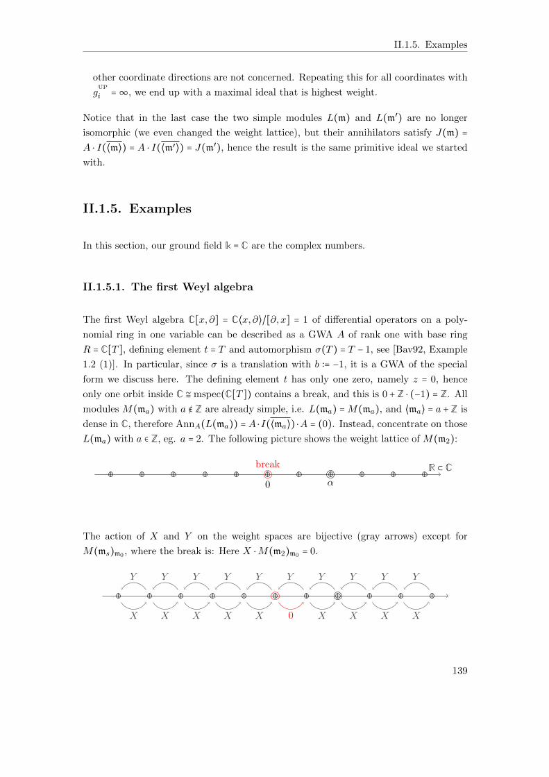
II.1.5. Examples
other coordinate directions are not concerned. Repeating this for all coordinates with
gUP
i =∞, we end up with a maximal ideal that is highest weight.
Notice that in the last case the two simple modules L(m) and L(m′) are no longer
isomorphic (we even changed the weight lattice), but their annihilators satisfy J(m) =
A ⋅ I(⟨m⟩) = A ⋅ I(⟨m′⟩) = J(m′), hence the result is the same primitive ideal we started
with.
II.1.5. Examples
In this section, our ground field k = C are the complex numbers.
II.1.5.1. The first Weyl algebra
The first Weyl algebra C[x, ∂] = C⟨x, ∂⟩/[∂, x] = 1 of differential operators on a poly-
nomial ring in one variable can be described as a GWA A of rank one with base ring
R = C[T ], defining element t = T and automorphism σ(T ) = T − 1, see [Bav92, Example
1.2 (1)]. In particular, since σ is a translation with b ∶= −1, it is a GWA of the special
form we discuss here. The defining element t has only one zero, namely z = 0, hence
only one orbit inside C ≅ mspec(C[T ]) contains a break, and this is 0 +Z ⋅ (−1) = Z. All
modules M(ma) with a ∉ Z are already simple, i.e. L(ma) =M(ma), and ⟨ma⟩ = a +Z is
dense in C, therefore AnnA(L(ma)) = A ⋅I(⟨ma⟩) ⋅A = (0). Instead, concentrate on those
L(ma) with a ∈ Z, eg. a = 2. The following picture shows the weight lattice of M(m2):
R ⊂ C
0
break
α
The action of X and Y on the weight spaces are bijective (gray arrows) except for
M(ms)m0 , where the break is: Here X ⋅M(m2)m0 = 0.
Y Y Y Y Y Y Y Y Y Y
X X X X X 0 X X X X
139
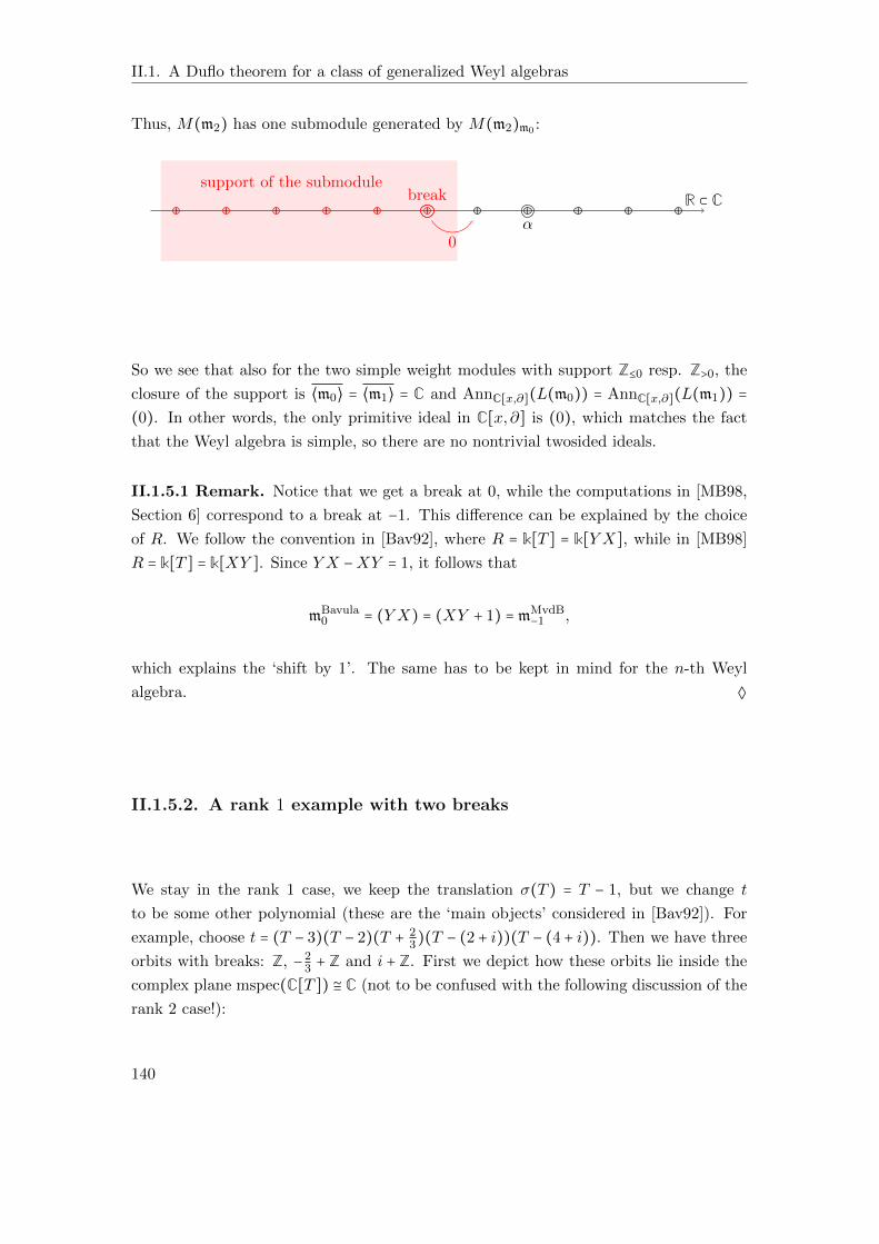
II.1. A Duflo theorem for a class of generalized Weyl algebras
Thus, M(m2) has one submodule generated by M(m2)m0 :
R ⊂ Csupport of the submodule
break
0α
So we see that also for the two simple weight modules with support Z≤0 resp. Z>0, the
closure of the support is ⟨m0⟩ = ⟨m1⟩ = C and AnnC[x,∂](L(m0)) = AnnC[x,∂](L(m1)) =
(0). In other words, the only primitive ideal in C[x, ∂] is (0), which matches the fact
that the Weyl algebra is simple, so there are no nontrivial twosided ideals.
II.1.5.1 Remark. Notice that we get a break at 0, while the computations in [MB98,
Section 6] correspond to a break at −1. This difference can be explained by the choice
of R. We follow the convention in [Bav92], where R = k[T ] = k[Y X], while in [MB98]
R = k[T ] = k[XY ]. Since Y X −XY = 1, it follows that
mBavula0 = (Y X) = (XY + 1) = mMvdB
−1 ,
which explains the ‘shift by 1’. The same has to be kept in mind for the n-th Weyl
algebra. ◊
II.1.5.2. A rank 1 example with two breaks
We stay in the rank 1 case, we keep the translation σ(T ) = T − 1, but we change t
to be some other polynomial (these are the ‘main objects’ considered in [Bav92]). For
example, choose t = (T − 3)(T − 2)(T + 23)(T − (2 + i))(T − (4 + i)). Then we have three
orbits with breaks: Z, −23 + Z and i + Z. First we depict how these orbits lie inside the
complex plane mspec(C[T ]) ≅ C (not to be confused with the following discussion of the
rank 2 case!):
140
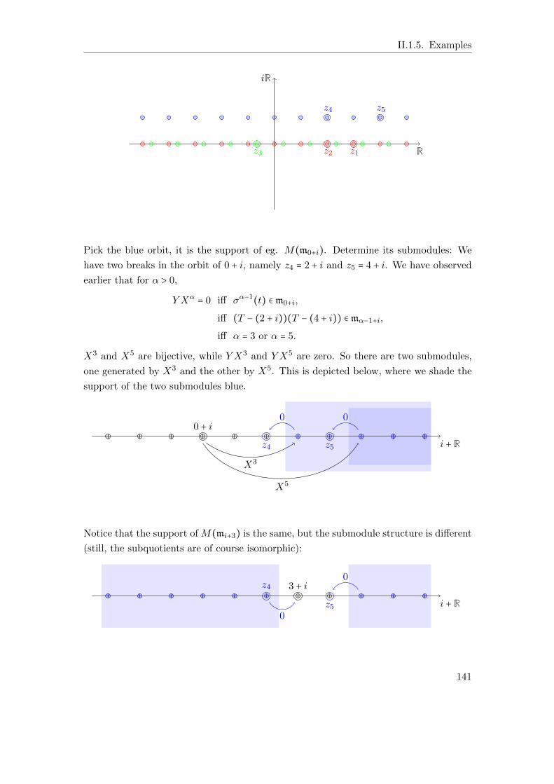
II.1.5. Examples
R
iR
z1z2z3
z4 z5
Pick the blue orbit, it is the support of eg. M(m0+i). Determine its submodules: We
have two breaks in the orbit of 0 + i, namely z4 = 2 + i and z5 = 4 + i. We have observed
earlier that for α > 0,
Y Xα= 0 iff σα−1
(t) ∈ m0+i,
iff (T − (2 + i))(T − (4 + i)) ∈ mα−1+i,
iff α = 3 or α = 5.
X3 and X5 are bijective, while Y X3 and Y X5 are zero. So there are two submodules,
one generated by X3 and the other by X5. This is depicted below, where we shade the
support of the two submodules blue.
i + Rz4 z5
0 0
X3
X5
0 + i
Notice that the support of M(mi+3) is the same, but the submodule structure is different
(still, the subquotients are of course isomorphic):
i + R
z4
z5
0
03 + i
141
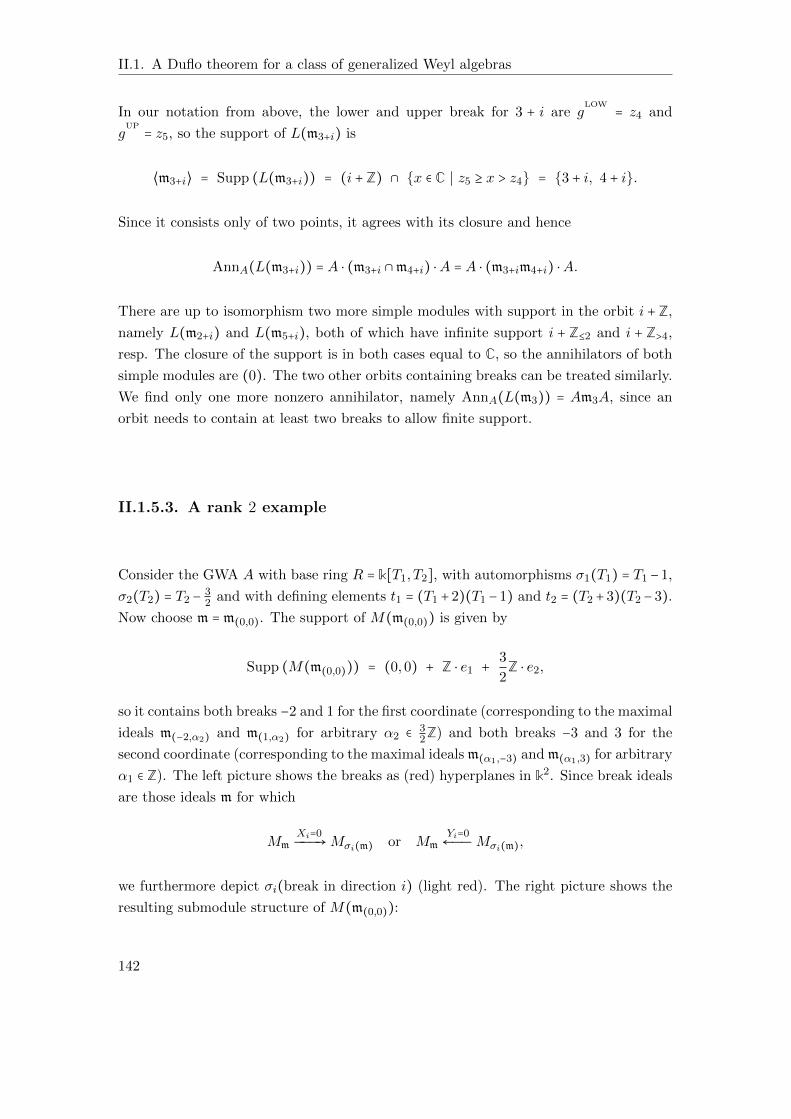
II.1. A Duflo theorem for a class of generalized Weyl algebras
In our notation from above, the lower and upper break for 3 + i are gLOW
= z4 and
gUP
= z5, so the support of L(m3+i) is
⟨m3+i⟩ = Supp (L(m3+i)) = (i +Z) ∩ x ∈ C ∣ z5 ≥ x > z4 = 3 + i, 4 + i.
Since it consists only of two points, it agrees with its closure and hence
AnnA(L(m3+i)) = A ⋅ (m3+i ∩m4+i) ⋅A = A ⋅ (m3+im4+i) ⋅A.
There are up to isomorphism two more simple modules with support in the orbit i + Z,
namely L(m2+i) and L(m5+i), both of which have infinite support i + Z≤2 and i + Z>4,
resp. The closure of the support is in both cases equal to C, so the annihilators of both
simple modules are (0). The two other orbits containing breaks can be treated similarly.
We find only one more nonzero annihilator, namely AnnA(L(m3)) = Am3A, since an
orbit needs to contain at least two breaks to allow finite support.
II.1.5.3. A rank 2 example
Consider the GWA A with base ring R = k[T1, T2], with automorphisms σ1(T1) = T1 −1,
σ2(T2) = T2 −32 and with defining elements t1 = (T1 + 2)(T1 − 1) and t2 = (T2 + 3)(T2 − 3).
Now choose m = m(0,0). The support of M(m(0,0)) is given by
Supp (M(m(0,0))) = (0,0) + Z ⋅ e1 +3
2Z ⋅ e2,
so it contains both breaks −2 and 1 for the first coordinate (corresponding to the maximal
ideals m(−2,α2) and m(1,α2) for arbitrary α2 ∈ 32Z) and both breaks −3 and 3 for the
second coordinate (corresponding to the maximal ideals m(α1,−3) and m(α1,3) for arbitrary
α1 ∈ Z). The left picture shows the breaks as (red) hyperplanes in k2. Since break ideals
are those ideals m for which
MmXi=0ÐÐÐ→Mσi(m) or Mm
Yi=0←ÐÐMσi(m),
we furthermore depict σi(break in direction i) (light red). The right picture shows the
resulting submodule structure of M(m(0,0)):
142
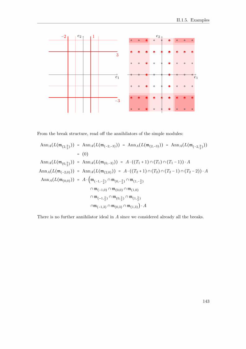
II.1.5. Examples
e1
e2−2 1
3
−3
e1
e2
From the break structure, read off the annihilators of the simple modules:
AnnA(L(m(2, 92))) = AnnA(L(m(−2,−3))) = AnnA(L(m(2,−3))) = AnnA(L(m(−2, 9
2)))
= (0)
AnnA(L(m(0, 92))) = AnnA(L(m(0,−3))) = A ⋅ ((T1 + 1) ∩ (T1) ∩ (T1 − 1)) ⋅A
AnnA(L(m(−2,0))) = AnnA(L(m(2,0))) = A ⋅ ((T2 + 1) ∩ (T2) ∩ (T2 − 1) ∩ (T2 − 2)) ⋅A
AnnA(L(m(0,0))) = A ⋅ (m(−1,− 32) ∩m(0,− 3
2) ∩m(1,− 3
2)
∩m(−1,0) ∩m(0,0) ∩m(1,0)
∩m(−1, 32) ∩m(0, 3
2) ∩m(1, 3
2)
∩m(−1,3) ∩m(0,3) ∩m(1,3)) ⋅A
There is no further annihilator ideal in A since we considered already all the breaks.
143

Bibliography
[Alh13] S. Alharbat. “A classification of affine fully commutative elements”. In:
arXiv (2013). eprint: arXiv/1311.7089.
[AM69] M. F. Atiyah and I. G. Macdonald. Introduction to commutative algebra.
Addison-Wesley Publishing Co., Reading, Mass.-London-Don Mills, Ont.,
1969, pp. ix+128.
[Bav92] V. V. Bavula. “Generalized Weyl algebras and their representations”. In:
Algebra i Analiz 4.1 (1992), pp. 75–97.
[BB00] V. V. Bavula and V. Bekkert. “Indecomposable representations of general-
ized Weyl algebras”. In: Comm. Algebra 28.11 (2000), pp. 5067–5100.
[BD96] M. Beattie and S. Dascalescu. “Categories of modules graded by G-sets.
Applications”. In: J. Pure Appl. Algebra 107.2-3 (1996). Contact Franco-
Belge en Algebre (Diepenbeek, 1993), pp. 129–139.
[Bec94] J. Beck. “Braid group action and quantum affine algebras”. In: Comm.
Math. Phys. 165.3 (1994), pp. 555–568.
[BM16] G. Benkart and J. Meinel. “The center of the affine nilTemperley–Lieb alge-
bra”. In: Math. Zeit. (2016). To appear. eprint: arXiv/math/1505.02544.
[BO09] G. Benkart and M. Ondrus. “Whittaker modules for generalized Weyl alge-
bras”. In: Represent. Theory 13 (2009), pp. 141–164.
[BFZ96] A. Berenstein, S. Fomin, and A. Zelevinsky. “Parametrizations of canonical
bases and totally positive matrices”. In: Adv. Math. 122.1 (1996), pp. 49–
149.
[BGG73] I. N. Bernstein, I. M. Gel′fand, and S. I. Gel′fand. “Schubert cells, and the
cohomology of the spaces G/P”. In: Uspehi Mat. Nauk 28.3(171) (1973),
pp. 3–26.
[BGG76] I. N. Bernstein, I. M. Gel′fand, and S. I. Gel′fand. “A certain category of
g-modules”. In: Funkcional. Anal. i Prilozen. 10.2 (1976), pp. 1–8.
145
Bibliography
[BJN15] R. Biagioli, F. Jouhet, and P. Nadeau. “Fully commutative elements in finite
and affine Coxeter groups”. In: Monatsh. Math. 178.1 (2015), pp. 1–37.
[BJS93] S. C. Billey, W. Jockusch, and R. P. Stanley. “Some combinatorial proper-
ties of Schubert polynomials”. In: J. Algebraic Combin. 2.4 (1993), pp. 345–
374.
[Bri11] J. Brichard. On Using Graphical Calculi: Centers, Zeroth Hochschild Ho-
mology and Possible Compositions of Induction and Restriction Functors
in Various Diagrammatical Algebras. Ph.D. Thesis – Columbia University.
ProQuest LLC, Ann Arbor, MI, 2011, p. 107.
[BG02] K. A. Brown and K. R. Goodearl. Lectures on algebraic quantum groups. Ad-
vanced Courses in Mathematics. CRM Barcelona. Birkhauser Verlag, Basel,
2002, pp. x+348.
[BK09] J. Brundan and A. Kleshchev. “Blocks of cyclotomic Hecke algebras and
Khovanov-Lauda algebras”. In: Invent. Math. 178.3 (2009), pp. 451–484.
[Buc03] A. S. Buch. “Quantum cohomology of Grassmannians”. In: Compositio
Math. 137.2 (2003), pp. 227–235.
[Cha01] V. Chari. “On the fermionic formula and the Kirillov-Reshetikhin conjec-
ture”. In: Internat. Math. Res. Notices 12 (2001), pp. 629–654.
[CH10] V. Chari and D. Hernandez. “Beyond Kirillov-Reshetikhin modules”. In:
Quantum affine algebras, extended affine Lie algebras, and their applica-
tions. Vol. 506. Contemp. Math. Amer. Math. Soc., Providence, RI, 2010,
pp. 49–81.
[CP91] V. Chari and A. Pressley. “Quantum affine algebras”. In: Comm. Math.
Phys. 142.2 (1991), pp. 261–283.
[CP95a] V. Chari and A. Pressley. A guide to quantum groups. Corrected reprint of
the 1994 original. Cambridge: Cambridge University Press, 1995, pp. xvi+651.
[CP95b] V. Chari and A. Pressley. “Quantum affine algebras and their representa-
tions”. In: Representations of groups (Banff, AB, 1994). Vol. 16. CMS Conf.
Proc. Amer. Math. Soc., Providence, RI, 1995, pp. 59–78.
[CP96] V. Chari and A. Pressley. “Minimal affinizations of representations of quan-
tum groups: the simply laced case”. In: J. Algebra 184.1 (1996), pp. 1–30.
[CG97] N. Chriss and V. Ginzburg. Representation theory and complex geometry.
Birkhauser Boston, Inc., Boston, MA, 1997, pp. x+495.
[DD05] B. Deng and J. Du. “Monomial bases for quantum affine sln”. In: Adv. Math.
191.2 (2005), pp. 276–304.
146
Bibliography
[DGO96] Yu. A. Drozd, B. L. Guzner, and S. A. Ovsienko. “Weight modules over
generalized Weyl algebras”. In: J. Algebra 184.2 (1996), pp. 491–504.
[Duf77] M. Duflo. “Sur la classification des ideaux primitifs dans l’algebre envelop-
pante d’une algebre de Lie semi-simple”. In: Ann. of Math. (2) 105.1 (1977),
pp. 107–120.
[Fan96] C. K. Fan. “A Hecke algebra quotient and some combinatorial applications”.
In: J. Algebraic Combin. 5.3 (1996), pp. 175–189.
[FG99] C. K. Fan and R. M. Green. “On the affine Temperley-Lieb algebras”. In:
J. London Math. Soc. (2) 60.2 (1999), pp. 366–380.
[Fom95] S. Fomin. “Schur operators and Knuth correspondences”. In: J. Combin.
Theory Ser. A 72.2 (1995), pp. 277–292.
[FGP97] S. Fomin, S. Gelfand, and A. Postnikov. “Quantum Schubert polynomials”.
In: J. Amer. Math. Soc. 10.3 (1997), pp. 565–596.
[FG98] S. Fomin and C. Greene. “Noncommutative Schur functions and their ap-
plications”. In: Discrete Math. 193.1-3 (1998). Selected papers in honor of
Adriano Garsia (Taormina, 1994), pp. 179–200.
[FS94] S. Fomin and R. P. Stanley. “Schubert polynomials and the nil-Coxeter
algebra”. In: Adv. Math. 103.2 (1994), pp. 196–207.
[FOS09] G. Fourier, M. Okado, and A. Schilling. “Kirillov-Reshetikhin crystals for
nonexceptional types”. In: Adv. Math. 222.3 (2009), pp. 1080–1116.
[Ful97] W. Fulton. Young tableaux. Vol. 35. London Mathematical Society Student
Texts. With applications to representation theory and geometry. Cambridge
University Press, Cambridge, 1997, pp. x+260.
[GJ11] M. Geck and N. Jacon. Representations of Hecke algebras at roots of unity.
Vol. 15. Algebra and Applications. Springer-Verlag London, Ltd., London,
2011, pp. xii+401.
[Gob15] T. Gobet. “Noncrossing partitions, fully commutative elements and bases
of the Temperley-Lieb algebra”. In: arXiv (2015). eprint: arXiv/arXiv:
1409.6500v2.
[Gra95] J. J. Graham. Modular representations of Hecke algebras and related alge-
bras. Ph.D. Thesis – University of Sydney. 1995.
[GL96] J. J. Graham and G. I. Lehrer. “Cellular algebras”. In: Invent. Math. 123.1
(1996), pp. 1–34.
[GL98] J. J. Graham and G. I. Lehrer. “The representation theory of affine Temperley-
Lieb algebras”. In: Enseign. Math. (2) 44.3-4 (1998), pp. 173–218.
147
Bibliography
[Gre02] R. M. Green. “On 321-avoiding permutations in affine Weyl groups”. In: J.
Algebraic Combin. 15.3 (2002), pp. 241–252.
[GL99] R. M. Green and J. Losonczy. “Canonical bases for Hecke algebra quotients”.
In: Math. Res. Lett. 6.2 (1999), pp. 213–222.
[GL01] R. M. Green and J. Losonczy. “Fully commutative Kazhdan-Lusztig cells”.
In: Ann. Inst. Fourier (Grenoble) 51.4 (2001), pp. 1025–1045.
[GR04] S. Griffeth and A. Ram. “Affine Hecke algebras and the Schubert calculus”.
In: European J. Combin. 25.8 (2004), pp. 1263–1283.
[HP02] T. J. Haines and A. Pettet. “Formulae relating the Bernstein and Iwahori-
Matsumoto presentations of an affine Hecke algebra”. In: J. Algebra 252.1
(2002), pp. 127–149.
[HMR09] T. Halverson, M. Mazzocco, and A. Ram. “Commuting families in Hecke
and Temperley-Lieb algebras”. In: Nagoya Math. J. 195 (2009), pp. 125–
152.
[HJ10] C. R. H. Hanusa and B. C. Jones. “The enumeration of fully commutative
affine permutations”. In: European J. Combin. 31.5 (2010), pp. 1342–1359.
[Har99] M. Harterich. “Murphy bases of generalized Temperley-Lieb algebras”. In:
Arch. Math. (Basel) 72.5 (1999), pp. 337–345.
[Hat+02] G. Hatayama et al. “Paths, crystals and fermionic formulae”. In: MathPhys
odyssey, 2001. Vol. 23. Prog. Math. Phys. Birkhauser Boston, Boston, MA,
2002, pp. 205–272.
[Hey00] A. Heyworth. “Rewriting as a special case of non-commutative Grobner
basis theory”. In: Computational and geometric aspects of modern algebra
(Edinburgh, 1998). Vol. 275. London Math. Soc. Lecture Note Ser. Cam-
bridge Univ. Press, Cambridge, 2000, pp. 101–105.
[HK02] J. Hong and S.-J. Kang. Introduction to quantum groups and crystal bases.
Vol. 42. Graduate Studies in Mathematics. Providence, RI: American Math-
ematical Society, 2002, pp. xviii+307.
[Hub05] A. Hubery. “Symmetric functions and the centre of the Ringel-Hall algebra
of a cyclic quiver”. In: Math. Z. 251.3 (2005), pp. 705–719.
[Hum08] J. E. Humphreys. Representations of semisimple Lie algebras in the BGG
category O. Vol. 94. Graduate Studies in Mathematics. American Mathe-
matical Society, Providence, RI, 2008, pp. xvi+289.
148
Bibliography
[IM65] N. Iwahori and H. Matsumoto. “On some Bruhat decomposition and the
structure of the Hecke rings of p-adic Chevalley groups”. In: Inst. Hautes
Etudes Sci. Publ. Math. 25 (1965), pp. 5–48.
[Jan96] J. C. Jantzen. Lectures on quantum groups. Vol. 6. Graduate Studies in
Mathematics. American Mathematical Society, Providence, RI, 1996, pp. viii+266.
[Jim+91] M. Jimbo et al. “Combinatorics of representations of Uq(gl(n)) at q = 0”.
In: Comm. Math. Phys. 136.3 (1991), pp. 543–566.
[Jon83] V. F. R. Jones. “Index for subfactors”. In: Invent. Math. 72.1 (1983), pp. 1–
25.
[Jon87] V. F. R. Jones. “Hecke algebra representations of braid groups and link
polynomials”. In: Ann. of Math. (2) 126.2 (1987), pp. 335–388.
[Kan+92] S.-J. Kang et al. “Perfect crystals of quantum affine Lie algebras”. In: Duke
Math. J. 68.3 (1992), pp. 499–607.
[Kas91] M. Kashiwara. “On crystal bases of the q-analogue of universal enveloping
algebras”. In: Duke Math. J. 63.2 (1991), pp. 465–516.
[Kas95] C. Kassel. Quantum groups. Vol. 155. Graduate Texts in Mathematics. New
York: Springer-Verlag, 1995, pp. xii+531.
[Kau90] L. H. Kauffman. “An invariant of regular isotopy”. In: Trans. Amer. Math.
Soc. 318.2 (1990), pp. 417–471.
[Kha15] A. Khare. “Axiomatic framework for the BGG category O”. In: arXiv (2015).
eprint: arXiv/math/1502.06706.
[Kha16] A. Khare. “On the classification of finite-dimensional nil-Coxeter algebras
over complex reflection groups”. In: arXiv (2016). eprint: arXiv:1601.
08231.
[Kho01] M. Khovanov. “Nilcoxeter algebras categorify the Weyl algebra”. In: Comm.
Algebra 29.11 (2001), pp. 5033–5052.
[KL09] M. Khovanov and A. D. Lauda. “A diagrammatic approach to categorifi-
cation of quantum groups. I”. In: Represent. Theory 13 (2009), pp. 309–
347.
[KR87] A. N. Kirillov and N. Yu. Reshetikhin. “Representations of Yangians and
multiplicities of the inclusion of the irreducible components of the tensor
product of representations of simple Lie algebras”. In: Zap. Nauchn. Sem.
Leningrad. Otdel. Mat. Inst. Steklov. (LOMI) 160.Anal. Teor. Chisel i Teor.
Funktsii. 8 (1987), pp. 211–221, 301.
149
Bibliography
[Koe08] S. Koenig. “A panorama of diagram algebras”. In: Trends in representation
theory of algebras and related topics. EMS Ser. Congr. Rep. Eur. Math. Soc.,
Zurich, 2008, pp. 491–540.
[KX12] S. Koenig and C. Xi. “Affine cellular algebras”. In: Adv. Math. 229.1 (2012),
pp. 139–182.
[Kor14] C. Korff. “Quantum cohomology via vicious and osculating walkers”. In:
Lett. Math. Phys. 104.7 (2014), pp. 771–810.
[KS10] C. Korff and C. Stroppel. “The sl(n)k-WZNW fusion ring: a combinatorial
construction and a realisation as quotient of quantum cohomology”. In: Adv.
Math. 225.1 (2010), pp. 200–268.
[KK86] B. Kostant and S. Kumar. “The nil Hecke ring and cohomology of G/P for
a Kac-Moody group G”. In: Adv. in Math. 62.3 (1986), pp. 187–237.
[Kum02] S. Kumar. Kac-Moody groups, their flag varieties and representation theory.
Vol. 204. Progress in Mathematics. Birkhauser Boston, Inc., Boston, MA,
2002, pp. xvi+606.
[Kus13] D. Kus. “Realization of affine type A Kirillov-Reshetikhin crystals via poly-
topes”. In: J. Combin. Theory Ser. A 120.8 (2013), pp. 2093–2117.
[Kus16] D. Kus. “Kirillov–Reshetikhin crystals, energy function and the combinato-
rial R-matrix”. In: J. Algebraic Combin. 43.1 (2016), pp. 45–74.
[Lam99] T. Y. Lam. Lectures on modules and rings. Vol. 189. Graduate Texts in
Mathematics. Springer-Verlag, New York, 1999, pp. xxiv+557.
[Lam01] T. Y. Lam. A first course in noncommutative rings. Second. Vol. 131. Grad-
uate Texts in Mathematics. Springer-Verlag, New York, 2001, pp. xx+385.
[LS81] A. Lascoux and M.-P. Schutzenberger. “Le mono¨−1de plaxique”. In: Non-
commutative structures in algebra and geometric combinatorics (Naples,
1978). Vol. 109. Quad. “Ricerca Sci.” CNR, Rome, 1981, pp. 129–156.
[LS89] A. Lascoux and M.-P. Schutzenberger. “Fonctorialite des polynomes de
Schubert”. In: Invariant theory (Denton, TX, 1986). Vol. 88. Contemp.
Math. Amer. Math. Soc., Providence, RI, 1989, pp. 585–598.
[Mac91] I. G. Macdonald. “Schubert polynomials”. In: Surveys in combinatorics,
1991 (Guildford, 1991). Vol. 166. London Math. Soc. Lecture Note Ser.
Cambridge Univ. Press, Cambridge, 1991, pp. 73–99.
[Mak15] R. Maksimau. “Categorical representations, KLR algebras and Koszul du-
ality”. In: arXiv (2015). eprint: arXiv/math/1512.04878.
150
Bibliography
[Mat89] H. Matsumura. Commutative ring theory. Second. Vol. 8. Cambridge Stud-
ies in Advanced Mathematics. Translated from the Japanese by M. Reid.
Cambridge University Press, Cambridge, 1989, pp. xiv+320.
[Maz10] V. Mazorchuk. Lectures on sl2(C)-modules. London: Imperial College Press,
2010, pp. x+263.
[MT99] V. Mazorchuk and L. Turowska. “Simple weight modules over twisted gen-
eralized Weyl algebras”. In: Comm. Algebra 27.6 (1999), pp. 2613–2625.
[MZ13] V. Mazorchuk and K. Zhao. “Characterization of simple highest weight mod-
ules”. In: Canad. Math. Bull. 56.3 (2013), pp. 606–614.
[Mei15] J. Meinel. “Duflo theorem for a class of generalized Weyl algebras”. In: J.
Algebra Appl. 14.10 (2015), pp. 1550147, 21.
[MS16] V. Miemietz and C. Stroppel. “Affine quiver Schur algebras and p-adic
GLn”. In: arXiv (2016). eprint: arXiv:1601.07323.
[MM90] K. Misra and T. Miwa. “Crystal base for the basic representation of Uq(sl(n))”.
In: Comm. Math. Phys. 134.1 (1990), pp. 79–88.
[MP95] R. V. Moody and A. Pianzola. Lie algebras with triangular decompositions.
Canadian Mathematical Society Series of Monographs and Advanced Texts.
A Wiley-Interscience Publication. John Wiley & Sons, Inc., New York, 1995,
pp. xxii+685.
[Mur95] G. E. Murphy. “The representations of Hecke algebras of type An”. In: J.
Algebra 173.1 (1995), pp. 97–121.
[Mus92] I. M. Musson. “A classification of primitive ideals in the enveloping algebra
of a classical simple Lie superalgebra”. In: Adv. Math. 91.2 (1992), pp. 252–
268.
[MB98] I. M. Musson and M. Van den Bergh. “Invariants under tori of rings of dif-
ferential operators and related topics”. In: Mem. Amer. Math. Soc. 136.650
(1998).
[Nad15] P. Nadeau. “On the length of fully commutative elements”. In: arXiv (2015).
eprint: arXiv:1511.08788v1.
[NRVO90] C. Nastasescu, S. Raianu, and F. Van Oystaeyen. “Modules graded by G-
sets”. In: Math. Z. 203.4 (1990), pp. 605–627.
[Par12] E. Park. “Quiver varieties and adjoint crystals of level ` for type A(1)n ”. In:
Comm. Algebra 40.12 (2012), pp. 4513–4539.
151
Bibliography
[PRH14] D. Plaza and S. Ryom-Hansen. “Graded cellular bases for Temperley-Lieb
algebras of type A and B”. In: J. Algebraic Combin. 40.1 (2014), pp. 137–
177.
[Pos05] A. Postnikov. “Affine approach to quantum Schubert calculus”. In: Duke
Math. J. 128.3 (2005), pp. 473–509.
[Rei01] M. Reineke. “Generic extensions and multiplicative bases of quantum groups
at q = 0”. In: Represent. Theory 5 (2001), 147–163 (electronic).
[Rei02] M. Reineke. “The quantic monoid and degenerate quantized enveloping al-
gebras”. In: arXiv (2002). eprint: arXiv/math/0206095.
[RSA14] D. Ridout and Y. Saint-Aubin. “Standard Modules, Induction and the
Temperley-Lieb Algebra”. In: Adv. Theor. Math. Phys. 18.5 (2014), pp. 957–
1041.
[Rin90] C. M. Ringel. “Hall algebras and quantum groups”. In: Invent. Math. 101.3
(1990), pp. 583–591.
[RCW82] A. Rocha-Caridi and N. R. Wallach. “Projective modules over graded Lie
algebras. I”. In: Math. Z. 180.2 (1982), pp. 151–177.
[Sch00] O. Schiffmann. “The Hall algebra of a cyclic quiver and canonical bases of
Fock spaces”. In: Internat. Math. Res. Notices 8 (2000), pp. 413–440.
[Sen10] P. Senesi. “Finite-dimensional representation theory of loop algebras: a sur-
vey”. In: Quantum affine algebras, extended affine Lie algebras, and their
applications. Vol. 506. Contemp. Math. Amer. Math. Soc., Providence, RI,
2010, pp. 263–283.
[Shi02] M. Shimozono. “Affine type A crystal structure on tensor products of rectan-
gles, Demazure characters, and nilpotent varieties”. In: J. Algebraic Combin.
15.2 (2002), pp. 151–187.
[ST97] B. Siebert and G. Tian. “On quantum cohomology rings of Fano manifolds
and a formula of Vafa and Intriligator”. In: Asian J. Math. 1.4 (1997),
pp. 679–695.
[Smi90] S. P. Smith. “A class of algebras similar to the enveloping algebra of sl2”.
In: Trans. Amer. Math. Soc. 322.1 (1990), pp. 285–314.
[Ste96] J. R. Stembridge. “On the fully commutative elements of Coxeter groups”.
In: J. Algebraic Combin. 5.4 (1996), pp. 353–385.
[Ste03] J. R. Stembridge. “A local characterization of simply-laced crystals”. In:
Trans. Amer. Math. Soc. 355.12 (2003), 4807–4823 (electronic).
152
Bibliography
[TL71] H. N. V. Temperley and E. H. Lieb. “Relations between the “percolation”
and “colouring” problem and other graph-theoretical problems associated
with regular planar lattices: some exact results for the “percolation” prob-
lem”. In: Proc. Roy. Soc. London Ser. A 322.1549 (1971), pp. 251–280.
[Vla04] M. Vlasenko. “Description of the center of the affine Temperley-Lieb algebra
of type AN”. In: arXiv (2004). eprint: arXiv/math/0408392.
[Wol07] S. Wolf. “The Hall algebra of a cyclic quiver at q = 0”. In: arXiv (2007).
eprint: arXiv:0709.4348.
153