Embed Size (px)
Citation preview
Algorithm-Based Fault Tolerance for MatrixOperations on Graphics Processing Units:Analysis and Extension to Autonomous
Operation
Von der Fakultät Informatik, Elektrotechnik und Informationstechnikund dem Stuttgart Research Centre for Simulation Technology
der Universität Stuttgartzur Erlangung der Würde eines
Doktors der Naturwissenschaften (Dr. rer. nat.)genehmigte Abhandlung
Vorgelegt von
Claus Braun
aus Reutlingen
Hauptberichter: Prof. Dr. Hans-Joachim WunderlichMitberichter: Prof. Matteo Sonza Reorda, PhD.
Tag der mündlichen Prüfung: 13. Juli 2015
Institut für Technische Informatikder Universität Stuttgart
2015


To my parents and my brother.

Contents
Acknowledgments xvii
Abstract xix
Zusammenfassung xxi
1 Introduction 11.1 Modern Scientific Computing and Simulation . . . . . . . . . . . . . . . 31.2 From Graphics to GPU Computing . . . . . . . . . . . . . . . . . . . . . 51.3 Reliability Requirements and Challenges . . . . . . . . . . . . . . . . . . 91.4 Reliability Threats . . . . . . . . . . . . . . . . . . . . . . . . . . . . . . . 101.5 ABFT for Reliable GPU Computing . . . . . . . . . . . . . . . . . . . . . 121.6 Objectives and Contributions of this Work . . . . . . . . . . . . . . . . 14
2 Formal Foundations and Background 172.1 Dependability Concepts and Terminology . . . . . . . . . . . . . . . . . 172.2 Fault Modeling . . . . . . . . . . . . . . . . . . . . . . . . . . . . . . . . . 202.3 Coding Theory . . . . . . . . . . . . . . . . . . . . . . . . . . . . . . . . . 212.4 Floating-Point Number Systems and Arithmetic . . . . . . . . . . . . . 23
3 GPU Architectures and Programming Models 273.1 Global GPU Architecture . . . . . . . . . . . . . . . . . . . . . . . . . . . 273.2 Streaming Multiprocessor Units . . . . . . . . . . . . . . . . . . . . . . . 293.3 Thread Organization and Scheduling . . . . . . . . . . . . . . . . . . . . 303.4 Memory Hierarchy . . . . . . . . . . . . . . . . . . . . . . . . . . . . . . . 323.5 CUDA Programming Model . . . . . . . . . . . . . . . . . . . . . . . . . 33
4 Fault Tolerance for Graphics Processing Units 394.1 Vulnerability Assessment . . . . . . . . . . . . . . . . . . . . . . . . . . . 404.2 Memory, ECC and ABFT . . . . . . . . . . . . . . . . . . . . . . . . . . . 434.3 Checkpointing . . . . . . . . . . . . . . . . . . . . . . . . . . . . . . . . . . 454.4 Software-Based Self-Test . . . . . . . . . . . . . . . . . . . . . . . . . . . 474.5 Redundant Hardware and Scheduling . . . . . . . . . . . . . . . . . . . 50
v
Contents
4.6 Discussion and Differentiation from ABFT . . . . . . . . . . . . . . . . 53
5 Algorithm-Based Fault Tolerance 555.1 Introduction to ABFT for Matrix Operations . . . . . . . . . . . . . . . 565.2 Weighted Checksum Codes . . . . . . . . . . . . . . . . . . . . . . . . . . 625.3 Partitioned Encoding . . . . . . . . . . . . . . . . . . . . . . . . . . . . . . 685.4 Handling of Rounding Errors . . . . . . . . . . . . . . . . . . . . . . . . . 715.5 Applicability to Graphics Processing Units . . . . . . . . . . . . . . . . 79
6 A-Abft: Autonomous Algorithm-Based Fault Tolerance 816.1 Overview of the Method . . . . . . . . . . . . . . . . . . . . . . . . . . . . 836.2 Probabilistic Rounding Error Analysis . . . . . . . . . . . . . . . . . . . 846.3 Reciprocal Probability Distribution . . . . . . . . . . . . . . . . . . . . . 866.4 Distribution, Expectation Value and Variance of the Significand’s Error 886.5 Expectation Value and Variance
of Rounding Errors . . . . . . . . . . . . . . . . . . . . . . . . . . . . . . . 926.6 Rounding Error Bounds for A-Abft Checksums . . . . . . . . . . . . . 946.7 Parallel Computation of Rounding Error Bounds . . . . . . . . . . . . . 97
7 Case Studies on the Application of A-ABFT 1037.1 A GPU-Accelerated QR Decomposition . . . . . . . . . . . . . . . . . . 103
7.1.1 QR Decomposition of Matrices . . . . . . . . . . . . . . . . . . . 1047.1.2 Householder Transformations . . . . . . . . . . . . . . . . . . . 1047.1.3 QR Decomposition with Householder Transformations . . . . 1057.1.4 Experimental Evaluation . . . . . . . . . . . . . . . . . . . . . . . 106
7.2 A GPU-Accelerated Linear Programming Solver . . . . . . . . . . . . . 1097.2.1 Linear Programming . . . . . . . . . . . . . . . . . . . . . . . . . 1097.2.2 Simplex and Revised Simplex Algorithm . . . . . . . . . . . . . 1107.2.3 Implementation . . . . . . . . . . . . . . . . . . . . . . . . . . . . 1137.2.4 Experimental Evaluation . . . . . . . . . . . . . . . . . . . . . . . 113
8 Experimental Evaluation 1218.1 Computational Performance . . . . . . . . . . . . . . . . . . . . . . . . . 123
8.1.1 Runtime of ABFT Encoding and Checking Kernels . . . . . . . 1248.1.2 Runtime of SEA and PEA Preprocessing Kernels . . . . . . . . 1258.1.3 Runtime of SEA and PEA ε-Determination Kernels . . . . . . . 126
vi
Contents
8.1.4 Overall Computational Performance . . . . . . . . . . . . . . . 1288.2 Quality of Rounding Error Bounds . . . . . . . . . . . . . . . . . . . . . 1308.3 Error Detection Capabilities . . . . . . . . . . . . . . . . . . . . . . . . . 1378.4 Discussion of Experimental Results . . . . . . . . . . . . . . . . . . . . . 140
9 Conclusions 143
Bibliography 147
A Abbreviations and Notation 177
B Dependability-related Definitions 181
C Definitions from Coding Theory 183
D Overview of the IEEE Standard 754™-2008 189
E Implementation Details 195
F Experimental Data 201F.1 Hardware and Software Configuration . . . . . . . . . . . . . . . . . . . 201F.2 Evaluation of Computational Performance . . . . . . . . . . . . . . . . 203
F.2.1 Runtime of ABFT Encoding and Checking Kernels . . . . . . . 203F.2.2 Runtime of SEA and PEA Preprocessing Kernels . . . . . . . . 205F.2.3 Runtime of SEA and PEA ε-Determination Kernels . . . . . . . 205F.2.4 Computational Performance for different weighted checksum
encodings across different ABFT encoding block sizes . . . . . 206F.3 Overall Computational Performance of A-Abft . . . . . . . . . . . . . 221F.4 Quality of Rounding Error Bounds . . . . . . . . . . . . . . . . . . . . . 222F.5 Error Detection . . . . . . . . . . . . . . . . . . . . . . . . . . . . . . . . . 226
Index 235
Curriculum Vitae of the Author 241
Publications of the Author 243
vii
List of Figures
Chapter 1
1.1 Algorithm-Based Fault Tolerance as part of a cross-layer reliability ap-proach. . . . . . . . . . . . . . . . . . . . . . . . . . . . . . . . . . . . . . . . . 14
Chapter 2
2.1 Dependability tree with concepts, threats and means. . . . . . . . . . . . . 202.2 Basic principle of block codes. . . . . . . . . . . . . . . . . . . . . . . . . . . 22
Chapter 3
3.1 NVIDIA GK 110 "Kepler" GPU architecture top-level block diagram. . . . 283.2 NVIDIA GK 110 streaming multiprocessor unit (SMX) block diagram. . . 293.3 NVIDIA GK 110 streaming processor unit (SP) block diagram. . . . . . . . 303.4 Scheduling of thread groups (warps) within multiprocessors. . . . . . . . 313.5 Memory hierarchy of the GK 100 GPU architecture. . . . . . . . . . . . . . 333.6 Structure of a CUDA C/C++ program. . . . . . . . . . . . . . . . . . . . . . . 353.7 Thread organization and memory access hierarchy. . . . . . . . . . . . . . 37
Chapter 5
5.1 Partitioned encoding for weighted column-checksum matrices. . . . . . . 695.2 Partitioned encoding for weighted row-checksum matrices. . . . . . . . . 70
Chapter 6
6.1 Check of candidate sets, p=3, no direct combinations. . . . . . . . . . . . . 996.2 Check of candidate sets, p=3, direct combinations. . . . . . . . . . . . . . . 100
Chapter 7
7.1 Maximum norms of the difference matrices DPEA2 and DSEA for 100fault injection experiments per matrix dimension. . . . . . . . . . . . . . . 108
viii
Figures
7.2 Comparison of impact of injected faults during QR decomposition for sim-plified error analysis SEA and probabilistic rounding error determinationPEA. . . . . . . . . . . . . . . . . . . . . . . . . . . . . . . . . . . . . . . . . . . 108
7.3 Comparison of LP solver performance of an unprotected multi-core CPUimplementation versus an A-Abft-protected GPU implementation. . . . 115
7.4 Absolute error in final result for problem ADLITTLE, comparison be-tween unprotected and A-abft protected variants with normal weightedchecksums. . . . . . . . . . . . . . . . . . . . . . . . . . . . . . . . . . . . . . . 116
7.5 Absolute error in final result for problem ADLITTLE, comparison be-tween different weighted checksums for PEA 2. . . . . . . . . . . . . . . . 116
7.6 Absolute error in final result for problem ADLITTLE, comparison be-tween different weighted checksums for SEA. . . . . . . . . . . . . . . . . . 117
7.7 Absolute error in final result for problem BANDM, comparison betweenunprotected and A-abft protected variants with normal weighted check-sums. . . . . . . . . . . . . . . . . . . . . . . . . . . . . . . . . . . . . . . . . . . 117
7.8 Absolute error in final result for problem BRANDY, comparison betweenunprotected andA-abft protected variants with normal +MDRweightedchecksums. . . . . . . . . . . . . . . . . . . . . . . . . . . . . . . . . . . . . . . 118
7.9 Absolute error in final result for problem STOCFOR2, comparison be-tween unprotected and A-abft protected variants with normal + linearweighted checksums. . . . . . . . . . . . . . . . . . . . . . . . . . . . . . . . . 118
Chapter 8
8.1 Kernel execution times for encoding and checking over different encodingblock sizes for matrix dimension 8192× 8192 with one and two weightedchecksums. . . . . . . . . . . . . . . . . . . . . . . . . . . . . . . . . . . . . . . 124
8.2 Kernel execution times for SEA and PEA preprocessing. . . . . . . . . . . 1268.3 Kernel execution times for SEA and PEA ε-determination. . . . . . . . . . 1278.4 Performance of SEA and PEA with one weighted checksum on Nvidia
Tesla K40c GPU compared to unprotected matrix multiplication onmulticore CPUs. . . . . . . . . . . . . . . . . . . . . . . . . . . . . . . . . . . . 128
8.5 Average relative rounding error λrel and determined relative roundingerror bounds, test data set Tpos(0,1000). . . . . . . . . . . . . . . . . . . . . . 133
ix
Figures
8.6 Histogram of rounding error bound quality, PEA 2 vs. SEA, test data setTpos. . . . . . . . . . . . . . . . . . . . . . . . . . . . . . . . . . . . . . . . . . . 134
8.7 Histogram of rounding error bound quality, PEA 2 vs. SEA, test data setTortho. . . . . . . . . . . . . . . . . . . . . . . . . . . . . . . . . . . . . . . . . . 134
8.8 Influence of ABFT encoding block size on determined absolute round-ing error bounds. Comparison of SEA and PEA 2 for normal weightedchecksums across the test data set Tortho(0, 2). . . . . . . . . . . . . . . . . 136
8.9 Absolute rounding error for different weighted checksum encodingswith ABFT encoding block size 32 × 32 over the three input data setsTpos(0, 1000), Tf ull(−1000, 1000) and Tortho(0, 2). . . . . . . . . . . . . . . 136
8.10 Comparison of the three different baselines for the classification of sig-nificant errors. Test data set Tortho(0,8192) with α = 0 and κ = 8192, fornormal weighted checksums. . . . . . . . . . . . . . . . . . . . . . . . . . . . 138
8.11 Detected significant errors (λprob) across different ABFT encoding blocksizes for normal + exponential weighted checksums and test data setTortho(0,65536). . . . . . . . . . . . . . . . . . . . . . . . . . . . . . . . . . . . . 139
Appendix D
D.1 Structure of IEEE-754 floating-point data formats. . . . . . . . . . . . . . . 191
Appendix F
F.1 Performance of SEA and PEA with one weighted checksum on NvidiaTesla K40c GPU compared to unprotected matrix multiplication onmulticore CPUs. . . . . . . . . . . . . . . . . . . . . . . . . . . . . . . . . . . . 221
F.2 Performance of SEA and PEA with two weighted checksums on NvidiaTesla K40c GPU compared to unprotected matrix multiplication onmulticore CPUs. . . . . . . . . . . . . . . . . . . . . . . . . . . . . . . . . . . . 221
F.3 Average relative rounding error λrel and determined relative roundingerror bounds, test data set Tf ull(−1000,1000). . . . . . . . . . . . . . . . . . . 222
F.4 Average relative rounding error λrel and determined relative roundingerror bounds, test data set Tortho(0,2). . . . . . . . . . . . . . . . . . . . . . . 223
F.5 Detected significant errors (λabs) across different ABFT encoding blocksizes for normal weighted checksums and test data set Tortho(0,65536). . . 226
x
Figures
F.6 Detected significant errors (λprob) across different ABFT encoding blocksizes for normal weighted checksums and test data set Tortho(0,65536). . . 226
F.7 Detected significant errors (λabs) across different ABFT encoding blocksizes for exponential weighted checksums and test data set Tortho(0,65536). 227
F.8 Detected significant errors (λprob) across different ABFT encoding blocksizes for exponential weighted checksums and test data set Tortho(0,65536). 227
F.9 Detected significant errors (λabs) across different ABFT encoding blocksizes for linear weighted checksums and test data set Tortho(0,65536). . . . 228
F.10 Detected significant errors (λprob) across different ABFT encoding blocksizes for linear weighted checksums and test data set Tortho(0,65536). . . . 228
F.11 Detected significant errors (λabs) across different ABFT encoding blocksizes for MDR weighted checksums and test data set Tortho(0,65536). . . . 229
F.12 Detected significant errors (λprob) across different ABFT encoding blocksizes for MDR weighted checksums and test data set Tortho(0,65536). . . . 229
F.13 Detected significant errors (λabs) across different ABFT encoding blocksizes for periodic weighted checksums and test data set Tortho(0,65536). . . 230
F.14 Detected significant errors (λprob) across different ABFT encoding blocksizes for periodic weighted checksums and test data set Tortho(0,65536). . . 230
F.15 Detected significant errors (λabs) across different ABFT encoding blocksizes for normal + exponential weighted checksums and test data setTortho(0,65536). . . . . . . . . . . . . . . . . . . . . . . . . . . . . . . . . . . . . 231
F.16 Detected significant errors (λprob) across different ABFT encoding blocksizes for normal + exponential weighted checksums and test data setTortho(0,65536). . . . . . . . . . . . . . . . . . . . . . . . . . . . . . . . . . . . . 231
F.17 Detected significant errors (λabs) across different ABFT encoding blocksizes for normal + linearweighted checksums and test data set Tortho(0,65536). 232
F.18 Detected significant errors (λprob) across different ABFT encoding blocksizes for normal + linearweighted checksums and test data set Tortho(0,65536). 232
F.19 Detected significant errors (λabs) across different ABFT encoding blocksizes for normal +MDRweighted checksums and test data set Tortho(0,65536). 233
F.20 Detected significant errors (λprob) across different ABFT encoding blocksizes for normal +MDRweighted checksums and test data set Tortho(0,65536). 233
xi
List of Tables
Chapter 7
7.1 Average Frobenius and Maximum norms of the difference matricesDNoABFT , DSEA and DPEA. . . . . . . . . . . . . . . . . . . . . . . . . . . . 107
7.2 Evaluated Linear Programming Problems from NetLib. . . . . . . . . . . . 114
Chapter 8
8.1 Types of evaluated weighted checksum codes. . . . . . . . . . . . . . . . . 1228.2 Average absolute rounding error and determined absolute rounding error
bounds for an ABFT encoding block size of 32× 32 and normal weightedchecksums over test data set Tortho(0,2). . . . . . . . . . . . . . . . . . . . . . 131
Appendix D
D.1 Parameters of the IEEE 754-2008 number and data formats. . . . . . . . . 192
Appendix F
F.1 Runtime of encoding and checking kernels on Nvidia Tesla K20c GPUfor a 512× 512 matrix using 1 weighted checksum and different ABFTencoding block sizes bs × bs. . . . . . . . . . . . . . . . . . . . . . . . . . . . 203
F.2 Runtime of encoding and checking kernels on Nvidia Tesla K20c GPUfor a 4096× 4096 matrix using 1 weighted checksum and different ABFTencoding block sizes bs × bs. . . . . . . . . . . . . . . . . . . . . . . . . . . . 203
F.3 Runtime of encoding and checking kernels on Nvidia Tesla K20c GPUfor a 8192× 8192 matrix using 1 weighted checksum and different ABFTencoding block sizes bs × bs. . . . . . . . . . . . . . . . . . . . . . . . . . . . 204
F.4 Runtime of encoding and checking kernels on Nvidia Tesla K20c GPUfor a 512× 512 matrix using 2 weighted checksums and different ABFTencoding block sizes bs × bs. . . . . . . . . . . . . . . . . . . . . . . . . . . . 204
xii
Tables
F.5 Runtime of encoding and checking kernels on Nvidia Tesla K20c GPUfor a 4096×4096 matrix using 2 weighted checksums and different ABFTencoding block sizes bs × bs. . . . . . . . . . . . . . . . . . . . . . . . . . . . 204
F.6 Runtime of encoding and checking kernels on Nvidia Tesla K20c GPUfor a 8192×8192 matrix using 2 weighted checksums and different ABFTencoding block sizes bs × bs. . . . . . . . . . . . . . . . . . . . . . . . . . . . 204
F.7 Kernel Execution Times for SEA and PEA Preprocessing separated forrows/columns. . . . . . . . . . . . . . . . . . . . . . . . . . . . . . . . . . . . . 205
F.8 Kernel Execution Times for SEA and PEA ε-determination, ABFT encod-ing block size 32× 32. . . . . . . . . . . . . . . . . . . . . . . . . . . . . . . . 205
F.9 Kernel Execution Times for SEA and PEA ε-determination, ABFT encod-ing block size 256× 256. . . . . . . . . . . . . . . . . . . . . . . . . . . . . . . 206
F.10 Performance on Nvidia Tesla K40c GPU with one Normal weightedchecksum and ABFT encoding block size 32× 32. . . . . . . . . . . . . . . 206
F.11 Performance on Nvidia Tesla K40c GPU with one Normal weightedchecksum and ABFT encoding block size 64× 64. . . . . . . . . . . . . . . 207
F.12 Performance on Nvidia Tesla K40c GPU with one Normal weightedchecksum and ABFT encoding block size 128× 128. . . . . . . . . . . . . . 207
F.13 Performance on Nvidia Tesla K40c GPU with one Normal weightedchecksum and ABFT encoding block size 256× 256. . . . . . . . . . . . . . 208
F.14 Performance on Nvidia Tesla K40c GPU with one Exponential weightedchecksum and ABFT encoding block size 32× 32. . . . . . . . . . . . . . . 208
F.15 Performance on Nvidia Tesla K40c GPU with one Exponential weightedchecksum and ABFT encoding block size 64× 64. . . . . . . . . . . . . . . 209
F.16 Performance on Nvidia Tesla K40c GPU with one Exponential weightedchecksum and ABFT encoding block size 128× 128. . . . . . . . . . . . . . 209
F.17 Performance on Nvidia Tesla K40c GPU with one Exponential weightedchecksum and ABFT encoding block size 256× 256. . . . . . . . . . . . . . 210
F.18 Performance on Nvidia Tesla K40c GPU with one Linear weightedchecksum and ABFT encoding block size 32× 32. . . . . . . . . . . . . . . 210
F.19 Performance on Nvidia Tesla K40c GPU with one Linear weightedchecksum and ABFT encoding block size 64× 64. . . . . . . . . . . . . . . 211
F.20 Performance on Nvidia Tesla K40c GPU with one Linear weightedchecksum and ABFT encoding block size 128× 128. . . . . . . . . . . . . . 211
xiii
Tables
F.21 Performance on Nvidia Tesla K40c GPU with one Linear weightedchecksum and ABFT encoding block size 256× 256. . . . . . . . . . . . . . 212
F.22 Performance on Nvidia Tesla K40c GPU with oneMDR weighted check-sum and ABFT encoding block size 32× 32. . . . . . . . . . . . . . . . . . . 212
F.23 Performance on Nvidia Tesla K40c GPU with oneMDR weighted check-sum and ABFT encoding block size 64× 64. . . . . . . . . . . . . . . . . . . 213
F.24 Performance on Nvidia Tesla K40c GPU with oneMDR weighted check-sum and ABFT encoding block size 128× 128. . . . . . . . . . . . . . . . . . 213
F.25 Performance on Nvidia Tesla K40c GPU with oneMDR weighted check-sum and ABFT encoding block size 256× 256. . . . . . . . . . . . . . . . . . 214
F.26 Performance on Nvidia Tesla K40c GPU with one Periodic weightedchecksum and ABFT encoding block size 32× 32. . . . . . . . . . . . . . . 214
F.27 Performance on Nvidia Tesla K40c GPU with one Periodic weightedchecksum and ABFT encoding block size 64× 64. . . . . . . . . . . . . . . 215
F.28 Performance on Nvidia Tesla K40c GPU with one Periodic weightedchecksum and ABFT encoding block size 128× 128. . . . . . . . . . . . . . 215
F.29 Performance on Nvidia Tesla K40c GPU with one Periodic weightedchecksum and ABFT encoding block size 256× 256. . . . . . . . . . . . . . 216
F.30 Performance on Nvidia Tesla K40c GPU with one Normal and oneLinear weighted checksum and ABFT encoding block size 32× 32. . . . . 216
F.31 Performance on Nvidia Tesla K40c GPU with one Normal and oneLinear weighted checksum and ABFT encoding block size 64× 64. . . . . 217
F.32 Performance on Nvidia Tesla K40c GPU with one Normal and oneLinear weighted checksum and ABFT encoding block size 128× 128. . . 217
F.33 Performance on Nvidia Tesla K40c GPU with one Normal and oneExponential weighted checksum and ABFT encoding block size 32× 32. . 218
F.34 Performance on Nvidia Tesla K40c GPU with one Normal and oneExponential weighted checksum and ABFT encoding block size 64× 64. . 218
F.35 Performance on Nvidia Tesla K40c GPU with one Normal and oneExponential weighted checksum and ABFT encoding block size 128× 128. 219
F.36 Performance on Nvidia Tesla K40c GPU with one Normal and oneMDRweighted checksum and ABFT encoding block size 32× 32. . . . . . . . . 219
F.37 Performance on Nvidia Tesla K40c GPU with one Normal and oneMDRweighted checksum and ABFT encoding block size 64× 64. . . . . . . . . 220
xiv
Chapter
F.38 Performance on Nvidia Tesla K40c GPU with one Normal and oneMDRweighted checksum and ABFT encoding block size 128× 128. . . . . . . . 220
F.39 Average relative rounding error and determined rounding error boundsfor an ABFT encoding block size of 32× 32 and normal weighted check-sums over test data set Tpos(0,1000). . . . . . . . . . . . . . . . . . . . . . . . 224
F.40 Average relative rounding error and determined rounding error boundsfor an ABFT encoding block size of 32× 32 and normal weighted check-sums over test data set Tf ull(−1000,1000). . . . . . . . . . . . . . . . . . . . . 224
F.41 Average relative rounding error and determined rounding error boundsfor an ABFT encoding block size of 32× 32 and normal weighted check-sums over test data set Tortho(0,2). . . . . . . . . . . . . . . . . . . . . . . . . 225
xv


Acknowledgments
It is my pleasure to thank everyone who supported me during the past years.
I’m very grateful to my parents, Leni and Sigfried Braun, and my brother Axel, whoconstantly supported me throughout my education and studies. Without them, I wouldnot have been able to even start with a work like this. I would like to thank Prof.Hans-Joachim Wunderlich for his professional supervision, his enduring support andfor sharing many interesting ideas in countless discussions. I would also like to thankProf. Matteo Sonza Reorda for his support and for accepting to be the second adviserof my thesis.
In addition, I would like to thank all my project partners within the SimTech Clusterof Excellence at the University of Stuttgart. In particular, I would like to thank Prof.Hans-Joachim Werner, Prof. Guido Schneider, Prof. Joachim Groß, and Dr. MarkusDaub for interesting and fruitful interdisciplinary collaborations.
I very much enjoyed the work with colleagues and students who were at some timeinvolved in my activities in Stuttgart. Sorry, I cannot list everyone here, you arenot forgotten! I’d like to acknowledge those with whom I spend a lot of time incollaborations or personally: Melanie Elm, Michael Kochte, Stefan Holst, Eric Schneider,Alexander Schöll, Rafał Baranowski, Laura Rodríguez Gómez, Chang Liu, MichaelImhof, Marcus Wagner, Dominik Ull, Alejandro Cook, Atefe Dalirsani, Nadereh Hatami,Lars Bauer, Hongyan Zhang, Abdullah Mumtaz, Abdul-Wahid Hakmi, Anusha Kakarala,and Christian Zöllin.
A work like this is not possible without administrative and technical assistance: Thankyou very much, Mirjam Breitling, Helmut Häfner, Lothar Hellmeier, and WolfgangMoser(d).
Stuttgart, July 2015
Claus Braun
xvii

Abstract
Scientific computing and computer-based simulation technology evolved to indis-pensable tools that enable solutions for major challenges in science and engineering.Applications in these domains are often dominated by compute-intensive mathematicaltasks like linear algebra matrix operations. The provision of correct and trustworthycomputational results is an essential prerequisite since these applications can havedirect impact on scientific, economic or political processes and decisions.
Graphics processing units (GPUs) are highly parallel many-core processor architecturesthat deliver tremendous floating-point compute performance at very low cost. Thismakes them particularly interesting for the substantial acceleration of complex applica-tions in science and engineering. However, like most nano-scaled CMOS devices, GPUsare facing a growing number of threats that jeopardize their reliability. This makes theintegration of fault tolerance measures mandatory.
Algorithm-Based Fault Tolerance (ABFT) allows the protection of essential mathematicaloperations, which are intensively used in scientific computing. It provides a high errorcoverage combined with a low computational overhead. However, the integration ofABFT into linear algebra matrix operations on GPUs is a non-trivial task, which requiresa thorough balance between fault tolerance, architectural constraints and performance.Moreover, ABFT for operations carried out in floating-point arithmetic has to cope witha reduced error detection and localization efficacy due to inevitable rounding errors.
This work provides an in-depth analysis of Algorithm-Based Fault Tolerance for matrixoperations on graphics processing units with respect to different types and combinationsof weighted checksum codes, partitioned encoding schemes and architecture-relatedexecution parameters. Moreover, a novel approach called A-Abft is introduced forthe efficient online determination of rounding error bounds, which improves the errordetection and localization capabilities of ABFT significantly.
Extensive experimental evaluations of the error detection capabilities, the quality of thedetermined rounding error bounds, as well as the achievable performance confirm thatthe proposed A-Abft method performs better than previous approaches. In addition,two case studies (QR decomposition and Linear Programming) emphasize the efficacyof A-Abft and its applicability to practical problems.
xix

Zusammenfassung
Wissenschaftliches Rechnen und rechnergestützte Simulationstechnik haben sich zuunentbehrlichen Werkzeugen entwickelt, die Lösungen für wichtige Probleme in Wis-senschaft und Technik ermöglichen. Anwendungen in diesen Bereichen werden häufigvon rechenaufwändigen mathematischen Operationen, wie zum Beispiel Matrixopera-tionen aus der linearen Algebra, dominiert. Die Bereitstellung korrekter und vertrau-enswürdiger Berechnungsergebnisse ist daher eine zentrale Grundvoraussetzung dadie genannten Anwendungen direkten Einfluss auf Prozesse und Entscheidungen inWissenschaft, Wirtschaft und Politik haben können.
Grafikprozessoren (GPUs) sind hochparallele Many-Core-Prozessorarchitekturen dieeine außergewöhnlich hohe Gleitkommarechenleistung bei sehr niedrigen Kosten er-möglichen. Dies macht sie besonders interessant für die deutliche Beschleunigung vonkomplexen Anwendungen in Wissenschaft und Technik. Wie die meisten nanoskalier-ten CMOS-Schaltkreise sehen sich auch GPUs einer wachsenden Zahl von Störfaktorengegenüber die ihre Zuverlässigkeit massiv beeinträchtigen. Dies macht die Integrationvon Fehlertoleranzmaßnahmen unabdingbar.
Algorithmenbasierte Fehlertoleranz (ABFT) erlaubt den Schutz wichtiger mathemati-scher Operationen die im wissenschaftlichen Rechnen zahlreiche Anwendung finden.ABFT bietet dabei eine hohe Fehlerabdeckung und verursacht nur einen geringenMehraufwand bei der Berechnung. Die Integration von ABFT in Matrixoperationen aufGrafikprozessoren ist jedoch sehr anspruchsvoll da sie die Balance zwischen Fehlertole-ranz, Prozessorarchitektur und Performanz erfordert. Darüber hinaus zeigt sich beimEinsatz von ABFT für Operationen die in Gleitkommaarithmetik ausgeführt werdenhäufig eine reduzierte Wirksamkeit der Fehlererkennung und -lokalisierung auf Grundvon unvermeidlich auftretenden Rundungsfehlern.
Die vorliegende Arbeit stellt eine umfangreiche Analyse von ABFT für Matrixopera-tionen auf Grafikprozessoren unter den Gesichtspunkten verschiedener gewichteterPrüfsummenkodes, partitionierte Kodierungsschemata und ausführungsrelevanter Ar-chitekturparameter bereit. Darüber hinaus wird mit A-Abft eine neuartige Methodefür die effiziente Bestimmung von Rundungsfehlerschranken zur Laufzeit vorgestellt,die die Fehlererkennung und -lokalisierung von ABFT deutlich verbessert.
xxi

Zusammenfassung
Umfangreiche experimentelle Untersuchungen der Fehlererkennung, der bestimm-ten Rundungsfehlerschranken, sowie der erzielbaren Performanz bestätigen, dass dievorgeschlagene A-Abft-Methode bessere Ergebnisse erzielt als bisherige Ansätze. Dar-über hinaus wird die Anwendbarkeit und Effektivität von A-Abft für praxisrelevanteProbleme anhand zweier Fallstudien (QR-Zerlegung und Lineare Optimierung) gezeigt.
xxii


Chapter
1Introduction
Scientific computing and computer-based simulation technology evolved to indispens-able and highly valuable tools that impel solutions for major challenges in scienceand engineering. Dominated by compute-intensive mathematical operations, the highcomputational requirements of these applications often necessitate the use of high-performance computing (HPC) systems. This in turn limits the access to such applica-tions and their benefits in many cases to national research laboratories, universities,governmental institutions and large corporations.
Graphics processing units (GPUs) developed within the last decade from highly spe-cialized ASICs to versatile parallel many-core processor architectures that delivertremendous floating-point compute performance at comparatively low cost. Contem-porary GPUs enable the substantial acceleration of scientific applications and complexsimulations outside of HPC compute centers, and open up an entirely new spectrum ofapplications. At the same time, graphics processing units are rapidly advancing intothe field of embedded systems, where they provide parallel compute power for mobiledevices and applications like realtime simulations or safety-critical image processingtasks in the automotive domain.
Besides high computational performance, reliability is of utmost importance for theseapplications to guarantee correct and trustworthy results, which can have considerableimpact on scientific, economic and political processes and decisions.
2 Chapter 1 ● Introduction
Fault tolerance and its effective and efficient integration are therefore key challengesfor allowing scientific computing and simulation technology to benefit in a reliable andsustainable way from many-core accelerator architectures like GPUs.
Fault tolerance enables systems to deliver their intended services even in presence ofhardware failures or software errors. It can be applied at very different levels, from thehardware up to the software and the algorithm. The respective techniques at the differentlevels are thereby often guided by similar principles. The concept of redundancy, forinstance, plays a fundamental role in most of them.
Hardware-based fault tolerance allows the effective protection against a variety ofpotential faults. The spectrum of techniques ranges from the hardening of single tran-sistors or logic gates to hardware-implemented information, structural or temporalredundancy. Error detecting and correcting codes, for instance, can be implemented forcommunication channels and memories with a high gain in reliability and a compara-tively low hardware overhead. Self-checkingmechanisms or pure structural redundancyare effective measures for the protection of logic blocks such as ALUs. However, thesetechniques can be associated with significant cost in terms of area overhead, increasedpower consumption, and sometimes even loss of performance. Moreover, for highlyparallel many-core graphics processing units, potential hardware-based fault tolerancemeasures may have to be implemented for structures that are placed a several hundredor thousand times on a single chip.
Software- and algorithm-based fault tolerance measures operate on top of the hard-ware. They can be integrated into firmware and hardware drivers, operating systemsand middleware layers, as well as top level applications. Such techniques allow theeffective and cost-efficient protection of processed data and the program control flow.In contrast to fixed hardware structures, software-based fault tolerance measures offera high flexibility since they can be adapted to changing operating conditions in thefield. As for hardware-based techniques, redundancy also plays an essential role forsoftware- and algorithm-based fault tolerance. Redundant computations and encodingfor the protection of data, and assertions or embedded signatures for the surveillanceof the control flow are common examples of software-based fault tolerance measures.However, software- and algorithm-based fault tolerance measures can only tackle faultswhich propagate to the upper system layers and which become visible as error. More-over, the integration of algorithm-based fault tolerance techniques often involves asignificant redesign of existing algorithms.
1.1 ● Modern Scientific Computing and Simulation 3
The choice of an appropriate fault tolerance measure can therefore be a highly complextask, especially when a good balance between benefit and cost has to be found. Moderncross-layer approaches to reliability therefore try to combine different measures atdifferent levels to achieve optimal fault tolerance.
This work addresses fault tolerance for essential mathematical matrix operations ongraphics processing units at the algorithmic level. It provides a comprehensive analysisand assessment of Algorithm-based Fault Tolerance (ABFT) schemes for such operationswith respect to their error detection, localization and correction capabilities, as wellas their performance impact. Moreover, this work identifies the handling of round-ing errors in state of the art ABFT schemes as a major weak point which hampersthe widespread practical application of ABFT in scientific computing and simulationtechnology. To solve this problem, a novel, autonomously operating ABFT scheme formatrix operations is introduced, which utilizes a probabilistic approach for the efficientdetermination of rounding error bounds. This A-Abft scheme is tailored to the parallelnature of graphics processing units and operates online with low performance impact.
The remainder of this chapter briefly introduces the reader to modern scientific com-puting and simulation technology. It emphasizes their growing importance and thechallenges in connection with GPU many-core processors. To motivate the applicationof fault tolerance, reliability requirements of scientific computations and simulationsare discussed and an overview of potential reliability threats is given.
The chapter then turns to Algorithm-based fault tolerance as a particularly promisingtechnique for improving the reliability of essential mathematical core operations likematrix multiplications in scientific applications. It shows that ABFT can be an excellentfit for modern cross-layer approaches to dependable scientific computing. Challengesand open research problems are presented regarding the integration of ABFT into linearalgebra matrix operations on GPUs, which motivate the in-depth analysis and extensionof ABFT for transparent and autonomous operation.
The chapter closes with the objectives and contributions of this work and outlines thestructure of the remaining chapters it is composed of.
1.1 Modern Scientific Computing and Simulation
Scientific computing and computer-based simulation technology made extraordinaryprogress within the last decades. They fundamentally changed the way how scientific
4 Chapter 1 ● Introduction
problems are tackled and how basic research is carried out today in many scientificdomains [Winsb10]. Computational science is thereby an interdisciplinary endeavorof numerical mathematics, computer science and the research areas that provide theconsidered models and data.
Scientific computing complements and enhances the research in natural sciences andengineering by adding numerical simulation as third pillar to the existing two of theoryand experiment. Computer-based simulations, so called in-silico experiments, are in-creasingly used to substitute practical experiments since they are often faster, cheaper,and—in many cases—more comprehensible. An important example for the large-scaleapplication of scientific computing and simulation technology are the internationalresearch efforts in the area of global climate change and weather forecast [Gent11].
In engineering, the role of scientific computing and simulation technology changedfrom a supporting one to a leading one [Oberk10]. Virtual prototyping and virtualtesting are just two synonyms for the application of both within development andevaluation processes of new products and systems. Well-known examples can be foundin the aerospace and automotive industries [Benne97, Zorri03], as well as in nano-electronics, where new products cannot be developed without massive use of scientificcomputations and simulations.
Applications in computational science are predominantly characterized by the followingmathematical problem classes:
• Systems of linear algebraic equations,• linear least square problems,• eigenvalue and singular value problems,• non-linear equations,• optimization problems,• interpolation and extrapolation,• numerical integration and differentiation,• ordinary and partial differential equations,• (Fast) Fourier transform and spectral analysis.
The corresponding methods for the numerical solution of these problems are typicallyassociated with high computational cost, which often grows rapidly with the problemsize and the complexity of the considered model. The interested reader can find acomprehensive overview and discussion of such methods in [Heath97] and [Press07].
1.2 ● From Graphics to GPU Computing 5
Linear algebra operations like the matrix multiplication play a central role in manysolution algorithms for the above listed problem classes. As a consequence, dedicatedsoftware libraries such as BLAS [The N14a], LINPACK [The N14d] and LAPACK [TheN14b] have grown over time, which allow the seamless integration of these operationsin a wide variety of scientific applications. Their widespread use and the considerablecomputational effort they require, make linear algebra operations particularly inter-esting and attractive for acceleration on modern graphics processing units. However,because they play such a central role and due to the fact that the reliability requirementsof the applications they will be used in can be very high, the simple parallelizationof these operations is not sufficient. They have to be provided in a way that they arefast and fault tolerant. Selected examples of scientific applications which benefit fromGPU-accelerated linear algebra operations, and the acceleration on GPUs in general,are presented in the next section.
1.2 From Graphics to GPU Computing
Development
The development of dedicated graphics hardware started in the early 1960s [Krull94,Suthe64]. Graphics display controllers (GDCs) and later graphics processing units (GPUs)evolved within thirty years to complex application-specific integrated circuits (ASICs)consisting of fixed-function pipelines. Their sole purpose was the transformation ofinternal, mathematical graphics representations into displayable pixel data [Hughe13].
With the spread of 3D graphics since the mid-1990s, the real-time performance require-ments for complex, high resolution 3D graphics at interactive frame rates increasedrapidly. GPU architectures therefore moved from fixed-function ASICs over microcodedprocessors to configurable and finally fully programmable, parallel many-core proces-sors [Nicko10]. These unified graphics architectures [Lindh08,Nicko10] of modern GPUsdiffer fundamentally from conventional central processing units (CPUs).
Architecture
Advanced CPUs are designed for high single-thread performance through latency-optimized instruction processing. They devote significant fractions of their design
6 Chapter 1 ● Introduction
to deep instruction pipelines, complex scheduling and control structures (e.g. out-of-order execution, branch prediction), as well as rather large cache memories forinstructions and data [Henne12]. Multi-core CPU architectures follow the multipleinstruction stream, multiple data stream (MIMD) paradigm [Flynn72]. They exploitinternal parallelism at different levels, from the instruction level over the thread levelto the core level. However, their multi-core parallelism increases comparatively slow(1→2→4→8→16→...) [Catan08a].
GPUs are designed for high computational throughput on data-parallel workloads. Theyfollow the single instruction stream, multiple data stream (SIMD) paradigm [Flynn72]and consist of large numbers of uniform stream processor cores that are tightly groupedinto multiprocessor units1. Stream processors share parts of the instruction issue andcontrol logic, as well as registers and local memories within a multiprocessor unit. Aspecial characteristic of GPU architectures is the waiver of overly complex instructionscheduling and control structures in favor of more arithmetic units, registers andembedded memories. Their memory system is explicitly exposed and comprises ofseveral thousands of registers, shared memories and caches within the multiprocessors,accompanied by global graphics memories. The memory bandwidth of contemporaryGPUs is more than ten times higher compared to CPUs2.
Since the year 2000, the transistor count of GPUs closely followedMoore’s Law [Moore65]and almost doubled every 18 months [Nicko10]. Within the same time, the number ofstream processors also doubled nearly every 18 months, leading to rapidly growingmany-core parallelism (128→240→512→1536→2880→...)3 and significant performanceimprovements.
Implications and Challenges
The massively parallel nature of modern many-core GPU architectures has strongimplications on their programmability, the design of algorithms and the integration of1 It should be noted at this point that the term core can be misleading for the comparison of CPU andGPU architectures. CPU cores are typically complete and almost independent processing units, whichare placed in multiple copies on the same chip-die, sharing resources like higher level caches or businterfaces. GPU stream processor cores are floating-point processing pipelines that require additional,shared infrastructure within a multiprocessor unit.
2 A contemporary desktop CPU like the Intel Core i7-4770 offers up to 25.6GB/s memory bandwidth [In-tel13], compared to up to 288GB/s of an NVIDIA GK110 GPU [NVIDI13]
3 Exemplarily the increase of processing cores of subsequent generations of NVIDIA GPUs from 1997(G80 architecture) to 2013 (GK110 architecture).
1.2 ● From Graphics to GPU Computing 7
fault tolerance measures. GPUs require large numbers of concurrent threads (many-threading) to achieve high performance on data-parallel workloads. This implies thatcomputational problems have to be decomposed in a way that they match this many-threading paradigm.
GPU memory architectures demand active management of available resources at eachlevel. The per-thread register usage has to be controlled and kept low to allow highparallelism. Shared memories have to be used to enable data reuse and fast localthread communication. The limited capacity and bank-wise organization of sharedmemories on GPUs can lead to access conflicts and loss of performance. The globalgraphics memories offer large capacities associated with high access latencies. Thisfavors aligned memory accesses, which can be combined by the hardware into singleoperations for improved bandwidth utilization, and necessitates the overlay of memorytransfers and computations.
Threads on GPUs are executed in groups on multiprocessor units. The control flowwithin multiprocessor units operates at the granularity of such groups. This has theconsequence that threads with a diverging control flow, e.g. caused by a differentlyevaluated comparison, lead to a serialized execution. Moreover, global synchronizationof threads on GPUs for consistency reasons is highly expensive since all threads haveto wait until the last finished.
The need for parallel workloads, the complex memory architecture and the control flowon GPUs, represent major challenges for the design and implementation of algorithmsand they complicate the integration of software- and algorithm-based fault tolerance.Chapter 3 provides the reader with a detailed introduction to a contemporary GPUarchitecture and the associated programming model, which form the hardware basis ofthis work.
Spectrum and Significance of GPU Computing
The acceleration of complex, non-graphical scientific applications and the conductingof in-silico experiments on graphics processing units is rapidly gaining importance. Thissection provides the reader with selected references to exemplary applications. Anextensive overview can be found in [Hwu11].
Computational biology, bioinformatics and the life sciences are among the domainswhich quickly adopted GPUs for the substantial acceleration of core applications.
8 Chapter 1 ● Introduction
Examples can be found in systems biology [Demat10], protein and genetic sequenc-ing [Manav08,Vouzi11], as well as in the investigation of biological networks [Zhou11]and communication processes [Braun12a]. In the life sciences, medical imaging appli-cations, in particular the reconstruction and analysis of images [Walte09,Agull11], aremapped to GPUs. In pharmacology, GPU-accelerated in-silico experiments are used tosupport and accelerate the design of new drugs [Sinko13].
Computational chemistry and related domains like thermodynamics and process technol-ogy exhibit numerous core methods with high potential for parallelization on GPUs.Particularly noteworthy are molecular dynamics (MD) [Yang07, Ander08, Stone10],molecular and quantum mechanics methods (MM/QM) [Ufimt08, Stone09], as wellas Markov-chain molecular Monte-Carlo simulations [Braun12b]. In general, relatedmethods such as parallel particle and n-body simulations on GPU are widely applied inother domains, for instance in astrophysics [Belle08,Hamad09].
The environmental and earth sciences such as climate research and meteorology, utilizeGPUs for the accelerated evaluation of large-scale models of atmospheric and oceano-graphic systems [Shimo10,Mieli12], as well as the modeling and analysis of geophysicaland seismic problems [Hollo05,Ehlig10,Abdel09,Okamo13].
In electronic design automation (EDA) both branches, the scientific research and theindustrial engineering exhibit a multitude of highly compute-intensive tasks withstrong demand for GPU acceleration [Croix13]. Design, validation and verification ofdigital circuits with billions of transistors benefit from GPU accelerated solvers, gate-level [Chatt09b,Chatt09a], register-transfer and system-level simulators [Nanju10]. Inaddition, key tasks like power analysis [Holst12] and fault simulation [Gulat08,Kocht10]are being adapted for GPUs.
In the classical engineering disciplines, GPUs are already being used in different fields,including computational structural mechanics (CSM) methods [Papad11] and compu-tational fluid dynamics (CFD) [Liu04, Kolb05, Tolke08], dealing with Navier-Stokesmodels and Lattice Boltzman methods. In addition, multi-grid solvers [Goodn05] andfinite-element methods (FEM) [Kiss12] are accelerated on graphics processing units.
A rather new domain with rapidly growing importance summarizes different methodsand applications under the term Big Data. Here, techniques such as machine learn-ing [Stein05,Catan08b], data mining and analytics [Ma09], searching [Soman10] andsorting [Sinto08, Satis09], as well as databases [Govin04, Govin06] are adapted andre-designed to utilize the compute power of GPUs. This domain also includes basic
1.3 ● Reliability Requirements and Challenges 9
techniques like parallel random number generators [Sussm06, Langd09,Phill11] andmap-reduce [He08, Stuar11].
The last application domain presented in this section is computational finance [Gaikw10,Pages12], where graphics processing units are increasingly used for the real-time anal-ysis of financial markets, the assessment of risk, and for fast option pricing [Gaikw09,Surko10].
1.3 Reliability Requirements and Challenges
"Computational results can affect public policy, the well-being of entire industries, and thedetermination of legal liability in the event of loss of life or environmental
damage." [Oberk10]
High-consequence applications [Oberk10] where scientific computations and simulationsare used to assess the reliability, robustness or safety of products and systems, or the riskof new technologies, pose extraordinary high reliability requirements. This is especiallytrue for applications which can have direct influence on decision making processes,like for instance simulations of the underground deposition of nuclear waste [Bourg04],carbon sequestration [Hollo05,Ehlig10] or climatic change [Jones95,Morio11]. Suchapplications are often characterized by the fact that they do not allow the validationand verification of computational results by experiments due to high complexity, largetimescales, high cost or risk.
The impact of scientific computing and simulation technology on research, economyand politics is directly related to the reliable provision of correct and trustworthy results.This in turn poses a hard challenge since modern scientific computing has to cope withuncertainties and reliability threats.
Uncertainty is a critical and often inevitable factor that affects scientific computingin mainly two different ways. First, uncertainty is introduced by the mathematicalmodeling when physical phenomena or other real-world processes are simplified andapproximated. Second, the data is often associated with uncertainty, for instance dueto low measurement precision or incompleteness. The handling and reduction ofuncertainty, as well as the validation and verification of scientific computations areimportant subjects of current research [Oberk02,Roy11], but not in the scope of thiswork.
10 Chapter 1 ● Introduction
Like most nano-scaled CMOS semiconductor devices, modern graphics processing unitsare increasingly prone to a number of reliability threats which can have significant im-pact on the underlying computations of scientific applications. The spectrum of threatsreaches from increasing variability in manufacturing processes over increasing suscepti-bility to transient events, to stress and aging-related effects. In the best case, the effectsof these threats are mitigated by fault tolerance measures or, at least, become visible aserrors. In the worst case, these effects remain undetected silent data corruptions andcause erroneous results with potentially far-reaching consequences. Since additionaluncertainty in computed results due to such errors cannot be tolerated, the integrationof appropriate fault tolerance measures has become mandatory. However, althoughGPUs have become highly attractive for parallel computing, their main purpose still isgraphics processing and they are designed for the mass market. This puts tight limitsto the integration of hardware-based fault tolerance due to the associated cost as wellas the lower reliability requirements in this market. Section 1.4 provides an overviewof the most important reliability threats for current semiconductor nano-electronics.
Challenges for the integration of algorithm-based fault tolerance arise from the hard-ware and the software. On the hardware side, GPUs and their implications on thedesign and implementation of algorithms (see Section 1.2) demand fault toleranceschemes which are closely tailored to their parallel architecture and the many-threadingparadigm to prevent substantial loss of performance. On the software side, scientificapplications and essential kernels like matrix operations are often highly optimizedand tuned for maximum performance. This leaves only small room for the integra-tion of fault tolerance measures. Only schemes with low computational overheadand low memory requirements can be considered for productive use. Moreover, theprojected, short mean times between failures in upcoming generations of computingsystems [Cappe09] demand fault tolerance schemes that operate online and with lowlatencies.
1.4 Reliability Threats
The unprecedented progress in Complementary Metal-Oxide-Semiconductor (CMOS)technology continues to drive the design and manufacturing of highly complex inte-grated circuits [ITRS13]. Semiconductor technology scaling [Moore65] enables latest
1.4 ● Reliability Threats 11
generation CPUs and GPUs with reduced power consumption and improved perfor-mance, comprising of billions of transistors.
However, this development does not only have beneficial effects, it also emphasizesexisting and introduces new threats to the reliability of sophisticated integrated semi-conductor circuits [Bol09,Nassi10, ITRS13]. These threats can be roughly categorizedinto manufacturing-related threats, life cycle or operation-related threats, and external,environmental threats.
Manufacturing
CMOSmanufacturing processes have to copewith physical and technological challengesamong which variability [Borka05,Kuhn11] is one of the most critical. Random andsystematic variations appear at different stages during the manufacturing process.Lithography variations [Owa04, Bensc08, ITRS13] cause amorphous structures andeffects like increased line edge roughness (LER) [Aseno03]. Distortions of the siliconcrystal structure, impurities and especially random dopant and implantation fluctuations(RDF) [Aseno98,Tang97] can lead to incomplete or defective structures, which causethreshold voltage fluctuations. The same applies to variations due to etching or chemicaland mechanical polishing [Stine98]. Variability within the manufacturing processcan cause altered electrical properties and potentially erroneous functional behavior.Production tests such as burn-in or packaging tests are used to filter out defectivedevices. However, test escapes are possible [Borka05] and more weak devices withlatent defects may come into productive use with reduced reliability and an increasedrisk of transient and intermittent faults or even early-life failures in the field.
Operation
During operation and over the life cycle of CMOS devices, dynamic variations liketemperature changes, crosstalk on signals or busses, and fluctuations in the power gridlike power droop [Bowma09] and IR drop [Nithi10], can lead to erroneous behavior.These effects are accompanied by stress and aging mechanisms such as negative-biasedtemperature instability (NBTI) [Huard06, Alam05], hot carrier injections (HCI) [Se-gur04, Chen99], time-dependent dielectric breakdown (TDDB) [Ogawa03, Segur04],and electromigration [Arnau11]. Negative-biased temperature instability is a phe-nomenon where positive charges (Si+) build up at Si/SiO2 channel interfaces within
12 Chapter 1 ● Introduction
PMOS transistors, leading to increased threshold voltages. Hot carrier injections occurwhen carriers are accelerated along conducting channels and resulting collisions withsubstrate atoms cause electron/hole pairs (oxide damage). Time-dependent dielectricbreakdown (TDDB) is a wear-out phenomenon where the insulating property of thedevice oxide is reduced. TDDB can lead to hard breakdowns when conductive channelsare formed by accumulated charge in the oxide. Electromigration describes the move-ment of metal atoms caused by electron flux and high temperatures, which can lead tovoids and cracks, as well as shorts and bridges.
Environment
Environmental reliability threats include different kinds of mechanical stress like vi-brations [Sony 10], as well as high ambient temperatures. In addition, single eventeffects (SEE) can be caused by radiation. Such effects occur when ionizing particleslike heavy ions, neutrons or alpha particles hit the substrate of a CMOS device andgenerate additional charges. If such charges are collected at junctions or contacts, theycan change logic states within a circuit. In [Nicol11], Heijmen distinguishes six types ofSEE based on their place of occurrence and impact. Single-bit (SBU) and multi-cell upsets(MCU) in memory cells and latches, multi-bit upsets (MBU) of two or more bits within amemory word, single-event transients (SET) causing voltage glitches that become biterrors when captured in a state element, and single-event latchups (SEL), which cancause permanent damage in a circuit. Almost all parts of modern CMOS circuits arevulnerable to single event effects, from latches and flip-flops to static and dynamicRAM, as well as the logic. However, the actual impact of SEEs on the system behaviordepends strongly on the used semiconductor material, the circuit design, the radiationintensity and potentially integrated fault tolerance measures.
All described mechanisms can cause performance degradations, reduced reliabilityduring operation or even complete failure.
1.5 Algorithm-Based Fault Tolerancefor Reliable GPU Computing
Algorithm-based fault tolerance (ABFT) is a fault tolerance technique introduced byHuang and Abraham in 1982 [Huang82,Huang84]. It is based on the idea of utilizing
1.5 ● ABFT for Reliable GPU Computing 13
block codes for the encoding of data before it is processed by modified algorithms,which in turn produce encoded output data. The information redundancy introduced bythe encoding is used to detect, localize and correct errors that occur during processingof the data. Algorithm-based fault tolerance can operate online and is characterized bya comparatively low overhead for the encoding and checking.
For certain application scenarios, algorithm-based fault tolerance can be less generalor flexible compared to conventional fault tolerance techniques such as n-modularredundancy or redundant computations. The design and integration of ABFT can alsobe a non-trivial and challenging task depending on the target algorithm. However,algorithm-based fault tolerance allows the efficient and effective protection of essentialmathematical operations, ranging from linear algebra matrix operations and decomposi-tions to spectral analyses based on fast Fourier transforms. These operations representextensively used core components within many scientific applications and can benefitsubstantially from acceleration on graphics processing units.
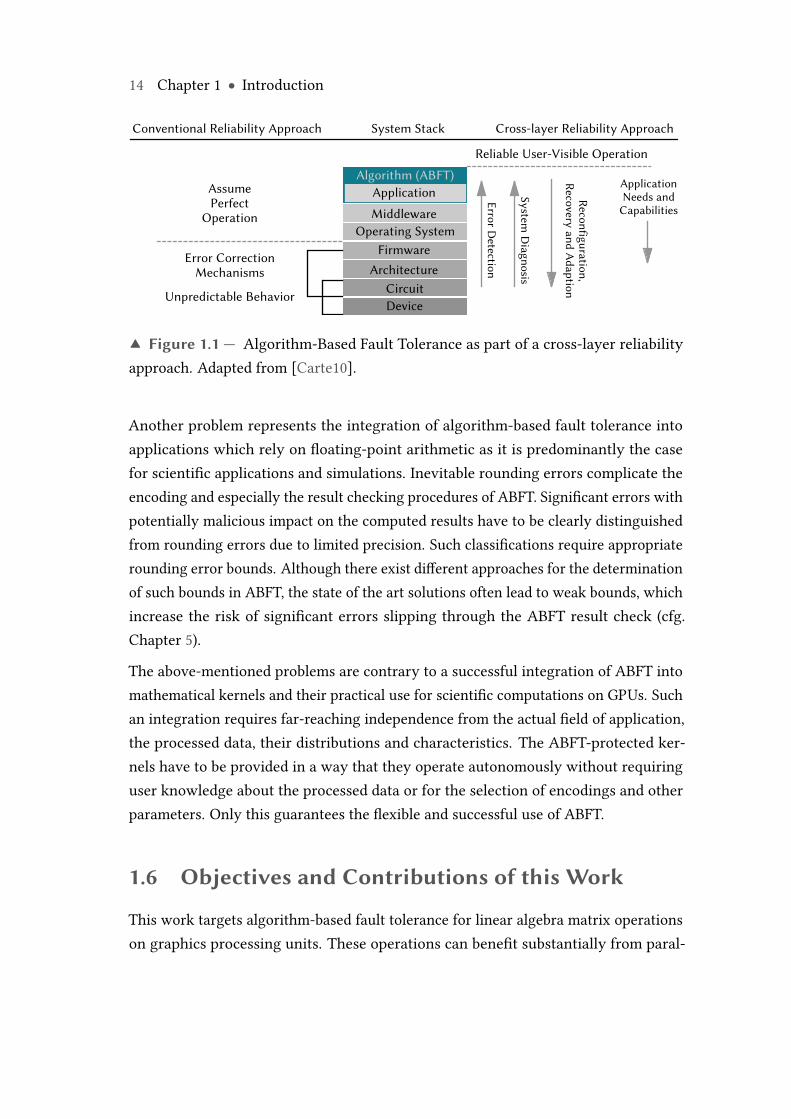
Cross-layer reliability approaches [DeHon10] leave the perspective of isolated faulttolerance measures at single, potentially lower levels and consider the whole systemstack for decentralized, cooperative fault tolerance. Appropriate measures for thedetection and mitigation of errors are implemented, matching the requirements ofeach layer optimally. Communication across the layers of the system stack allowsthe handling of errors at higher levels, which have not been detected or mitigatedat lower levels. Figure 1.1 shows the different perspectives of isolated, conventionalapproaches and modern cross-layer reliability. Algorithm-based fault tolerance directlycomplements such cross-layer reliability approaches and can act at the top level of thesystem stack.
However, although ABFT is a mature technique on which a substantial amount ofresearch has been conducted, several research questions and problems remain open andhamper the widespread, practical use of this technique: A broad spectrum of extensionsand different encoding schemes has been proposed for ABFT over the years. Theseapproaches unfold a considerable parameter space with a variety of options for theircombination. The impact of individual methods and their potential combinations onthe ability of ABFT to detect, localize and correct errors, as well as their impact on theperformance of the target operation have not yet been adequately studied with respectto the application on GPUs. The implications of these architectures (see Section 1.2)make the selection and implementation of appropriate solutions difficult.
14 Chapter 1 ● Introduction
ApplicationAlgorithm (ABFT)
DeviceCircuit
ArchitectureFirmware
Operating SystemMiddleware
System Stack
ApplicationNeeds and
Capabilities
Error Detection
System D
iagnosis
Reconfiguration,Recovery and A
daption
Cross-layer Reliability ApproachConventional Reliability Approach
Reliable User-Visible Operation
AssumePerfect
Operation
Error CorrectionMechanisms
Unpredictable Behavior
▲ Figure 1.1 — Algorithm-Based Fault Tolerance as part of a cross-layer reliabilityapproach. Adapted from [Carte10].
Another problem represents the integration of algorithm-based fault tolerance intoapplications which rely on floating-point arithmetic as it is predominantly the casefor scientific applications and simulations. Inevitable rounding errors complicate theencoding and especially the result checking procedures of ABFT. Significant errors withpotentially malicious impact on the computed results have to be clearly distinguishedfrom rounding errors due to limited precision. Such classifications require appropriaterounding error bounds. Although there exist different approaches for the determinationof such bounds in ABFT, the state of the art solutions often lead to weak bounds, whichincrease the risk of significant errors slipping through the ABFT result check (cfg.Chapter 5).
The above-mentioned problems are contrary to a successful integration of ABFT intomathematical kernels and their practical use for scientific computations on GPUs. Suchan integration requires far-reaching independence from the actual field of application,the processed data, their distributions and characteristics. The ABFT-protected ker-nels have to be provided in a way that they operate autonomously without requiringuser knowledge about the processed data or for the selection of encodings and otherparameters. Only this guarantees the flexible and successful use of ABFT.
1.6 Objectives and Contributions of this Work
This work targets algorithm-based fault tolerance for linear algebra matrix operationson graphics processing units. These operations can benefit substantially from paral-
1.6 ● Objectives and Contributions of this Work 15
lel acceleration and form an essential foundation of many scientific applications. Itprovides a comprehensive analysis and assessment of the most important ABFT en-coding approaches and the accompanying parameters with respect to error detection,localization, correction and performance impact on GPU architectures.
Furthermore, this work extends algorithm-based fault tolerance for matrix operationswith a new method for the determination of rounding error bounds. This extension isbased on a probabilistic model of floating-point arithmetic and enables ABFT-protectedoperations to determine rounding error bounds at runtime without requiring userknowledge or intervention. The developed method is tailored to modern GPU archi-tectures and reduces the number of false-negative error detections while maintaininghigh performance of the target matrix operations. In addition, the method can be usedto deliver detailed information on the rounding error that has to be expected for theperformed operation. This allows the provision of ABFT-protected matrix operationson graphics processing units which act as accelerated, fault tolerant building blocks forscientific applications and simulations.
Besides an in-depth evaluation of the developed method with respect to the quality ofthe determined error bounds, the achievable error detection rates and the associatedperformance overhead, two case studies are presented which show the application ofthe method and the benefit of fault tolerant, accelerated matrix operations on GPU inscientific applications.
The remainder of this work comprises the following chapters: Chapter 2 introducesthe reader to the formal foundations on which subsequent chapters build upon. Thisincludes definitions of essential terms and concepts from the fields of dependability,fault modeling, coding theory, and floating-point arithmetic.
Chapter 3 describes in detail the hardware architecture of a contemporary graphicsprocessing units, which also formed the hardware platform for the experimental evalua-tion parts of this work. In addition to the GPU architecture, the software programmingmodel is introduced to the reader.
Chapter 4 provides a concise summary of the state of the art for hardware-related faulttolerance measures with a special focus on fault tolerance for graphics processing units.
Chapter 5 introduces the reader in detail to the field of algorithm-based fault tolerance.A formal mathematical definition of ABFT for matrix operations is presented whichprovides the link to coding theory and which builds upon the foundations given in
16 Chapter 1 ● Introduction
Chapter 2. The chapter gives a brief overview of possible applications of ABFT and thenfocuses on relevant ABFT encoding techniques. The last part of the chapter presentsthe state of the art for the determination of error tolerances and rounding error boundsin ABFT.
Chapter 6 presents a novel ABFT approach calledA-Abft, which operates autonomouslyand utilizes a probabilisticmethod for the online determination of rounding error boundson graphics processing units. The reader is introduced to the mathematical backgroundand the algorithmic steps that are tailored to GPU architectures.
Chapter 7 presents two case studies which show the application of the developedprobabilistic A-Abft scheme for accelerated matrix multiplications on GPU. The firststudy considers a QR decomposition based on Householder reflections, which playsan important role in numerical mathematics for the solution of linear least squaresproblems and forms the basis of the QR algorithm for the solution of eigenvalueproblems. The second case study considers an accelerated linear programming solver,which represents an essential tool for the solution of optimization problems.
Chapter 8 presents the analysis and assessment of the most relevant ABFT encodingschemes, their associated parameters, as well as the developed probabilistic methodfor the online determination of rounding error bounds. Error detection capabilities areevaluated and the impact on the achievable performance on graphics processing unitsinvestigated.
Chapter 9 summarizes the findings of this work, discusses the achieved results andpoints out starting points for further research.
Abbreviations, notations and supplemental material, as well as extended experimentalresults can be found in the appendices.
Chapter
2Formal Foundations and
Background
This chapter introduces the formal foundations of this work comprising importantconcepts, definitions and terminology on which subsequent chapters build upon. Thisincludes the fields of dependability and fault modeling, coding theory, as well as floating-point computer arithmetic. In order to keep this introduction concise, potentiallyrequired basics from the fields of abstract and linear algebra, which can be found inliterature, are omitted. Dependability-related mathematical definitions are given inAppendix B and fundamental definitions from coding theory in Appendix C. Whereappropriate, references pointing to the corresponding literature are provided.
2.1 Dependability Concepts and Terminology
This section presents required definitions and concepts of dependability concerningthis work. It closely follows the definitions introduced by Avižienis et al. in [Avizi04].
18 Chapter 2 ● Formal Foundations and Background
Defects, Faults, Errors and Failures
Starting point for the following definitions is the notion of a system. A system can bedescribed as an entity which communicates and interacts with other systems. Theseother systems form the environment of the considered system, which is separated fromthis environment by its boundaries.
A system is determined by different properties among which its functionality is the mostimportant one. The steps performed by the system to realize its specified functionalityform its behavior. This behavior can be described as a sequence of states.
The system’s behavior, as it can be observed by other systems in its environment,represents the service it provides. This service is delivered via dedicated points at thesystem’s boundary, the so called service interfaces. The set of states that become visibleat the service interfaces form the system’s external state. The remaining states representits internal state. The provided service can be described as a sequence of such states.
A defect is a distortion of the physical structure of the system’s hardware. Variousdefect mechanisms, such as aging or radiation, can increase the probability of occurringdefects.
A fault is an abstraction to model and represent a defect at the structural level. Faultscan be categorized into permanent, intermittent and transient faults. A permanent faultoccurs and remains in the system until it is repaired or replaced. An intermittent faultoccurs repeatedly in regular or non-regular time intervals. A transient fault occursonce and typically disappears after a short period of time.
A correct service is delivered by a system as long as it provides its functionality accordingto the specifications. In cases where the service is not delivered or delivered deviatingfrom the specifications, a failure has occurred. Such a failure implies that a singleexternal state or a sequence of external states of the system differs from the correctsequence of states. This deviation is called an error. If the presence of such an error issignaled by the system, the error is referred to as detected error.
In the context of this work, a system consists of one or more graphics processing unitsand the matrix operations that are executed on these GPUs. The service interface isrepresented by software interfaces that allow to call software library routines.
2.1 ● Dependability Concepts and Terminology 19
Dependability, Reliability and Fault Tolerance
Dependability is not an isolated or stand-alone concept. It is a unification that integratesdifferent concepts and it can be characterized by these concepts, the threats it facesand the means that can be applied to achieve it. The concepts comprise availability,reliability, safety, integrity and maintainability. Dependability is also often extended bysecurity, which then adds confidentiality to the set of concepts. Availability describesthe readiness of a system, which means the fraction of time the system delivers itscorrect service during a given interval of time. Reliability describes the probability that asystem provides its correct service during a specified period of time (cfg. Definition B.4).Safety, in turn, implies that the operation of a system cannot have any dangerous orharmful effects on its environment. The concepts of integrity and confidentiality arealso related to security and imply that a system cannot be altered in a malicious wayand that information is not disclosed by a system unintentionally. The last concept,maintainability, describes the property that a system can be diagnosed and repaired inreasonable time. Mathematical definitions of availability and reliability are given inAppendix B.
The threats that potentially jeopardize the dependability of a system are defects, faults,errors and failures, as they have been introduced above. A dependable system triesto prevent and neutralize these threats by the application of the following groupsof countermeasures: Fault prevention and fault tolerance, which try to prevent faultsbefore they occur or try to ensure the correct service although faults have occurred.Fault prevention techniques target the design and implementation phase of a system,whereas fault tolerance techniques are intended to have effect during operation ofthe system. Fault tolerance includes the steps error detection and error recovery. Faultremoval techniques are intended to reduce the total number of faults and the severity oftheir impact. Fault removal can be performed during the design phase, for instance byapplication of formal methods for validation of the design, as well as during operation.Fault forecasting techniques try to predict the occurrence and impact of future faultsbased on current fault information.
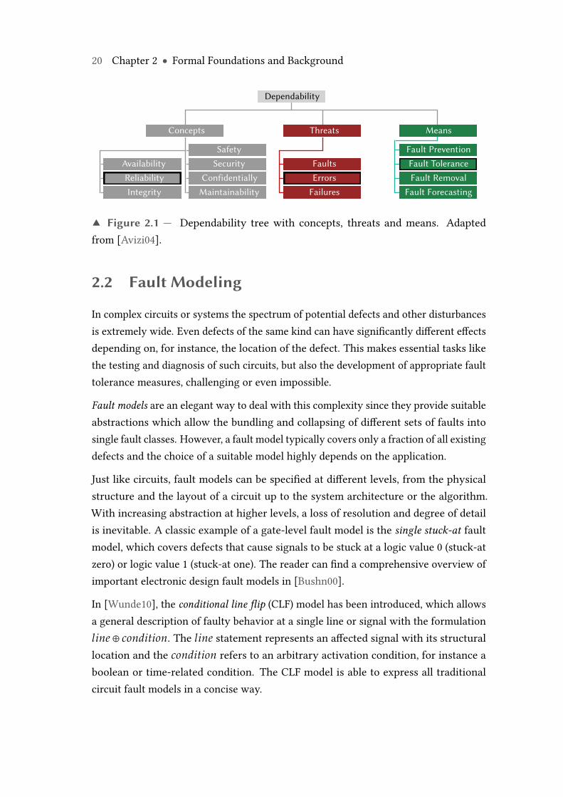
To contribute to the overall goal of dependable scientific computing on graphics process-ing units, this work is dedicated to improve the reliability of GPU matrix operations.This goal is achieved by applying means of fault tolerance that target errors whichmanifest themselves as faulty values. The dependability tree in Figure 2.1 summarizesthe characteristics of dependability and highlights the parts involved in this thesis.
20 Chapter 2 ● Formal Foundations and Background
Concepts
Availability SecuritySafety
ConfidentiallyIntegrity Maintainability
Faults
Threats
Failures
Fault Prevention
Means
Fault RemovalFault Forecasting
Reliability Errors
Dependability
Fault Tolerance
▲ Figure 2.1 — Dependability tree with concepts, threats and means. Adaptedfrom [Avizi04].
2.2 Fault Modeling
In complex circuits or systems the spectrum of potential defects and other disturbancesis extremely wide. Even defects of the same kind can have significantly different effectsdepending on, for instance, the location of the defect. This makes essential tasks likethe testing and diagnosis of such circuits, but also the development of appropriate faulttolerance measures, challenging or even impossible.
Fault models are an elegant way to deal with this complexity since they provide suitableabstractions which allow the bundling and collapsing of different sets of faults intosingle fault classes. However, a fault model typically covers only a fraction of all existingdefects and the choice of a suitable model highly depends on the application.
Just like circuits, fault models can be specified at different levels, from the physicalstructure and the layout of a circuit up to the system architecture or the algorithm.With increasing abstraction at higher levels, a loss of resolution and degree of detailis inevitable. A classic example of a gate-level fault model is the single stuck-at faultmodel, which covers defects that cause signals to be stuck at a logic value 0 (stuck-atzero) or logic value 1 (stuck-at one). The reader can find a comprehensive overview ofimportant electronic design fault models in [Bushn00].
In [Wunde10], the conditional line flip (CLF) model has been introduced, which allowsa general description of faulty behavior at a single line or signal with the formulationline⊕ condition. The line statement represents an affected signal with its structurallocation and the condition refers to an arbitrary activation condition, for instance aboolean or time-related condition. The CLF model is able to express all traditionalcircuit fault models in a concise way.
2.3 ● Coding Theory 21
Algorithm-based fault tolerance is a fault tolerance technique which acts at the level ofalgorithms and their respective implementations. Low level fault models such as thesingle stuck-at or the transition-delay fault model are therefore often of limited use anda higher level of abstraction is required. In [Huang84], a module level fault model hasbeen introduced which considers single computational units or complete processorswithin a multiprocessor system as abstract modules. Modules are able to communicatewith each other and they produce certain results that become visible at their serviceinterfaces. Furthermore, the following assumptions apply for the module level faultmodel: Within a given period of time, at most one module produces erroneous resultsand latent failures are detected by periodic testing of the modules. Communicationchannels and memories are protected, for instance, by error detecting and correctingcodes.
In this work, the module level fault model is refined and adapted for the application toarchitectures and execution paradigms of modern graphics processing units. Streamprocessing cores, which reside within multiprocessor units of GPUs (see Chapter 3), areconsidered as basic entities or modules in this model. Although the above-mentionedassumptions still apply, multiple modules are allowed to produce erroneous resultvalues as long as they are not located within the same multiprocessor unit. Thisassumption is justified by the fact that modern graphics processing units consist ofmultiple multiprocessor units. In addition, it is assumed that the algorithm-based faulttolerance scheme is always able to execute its basic phases, which comprise the encodingof input data, the payload computation of the target algorithm, and the decoding andchecking phase. This assumption, in turn, is justified by the fact that an ABFT schemecan be combined with additional software-based fault tolerance techniques for theprotection of the control flow, as well as hardware-based fault tolerance measures likededicated watchdog processors.
2.3 Coding Theory
Algorithm-based fault tolerance can be formulated and defined in terms of linear blockcodes. In ABFT, such linear block codes are applied at the word level instead of theclassic bit level. This section provides the reader with a short introduction to linearblock codes. Foundations and basic definitions from coding theory can be found inAppendix C.
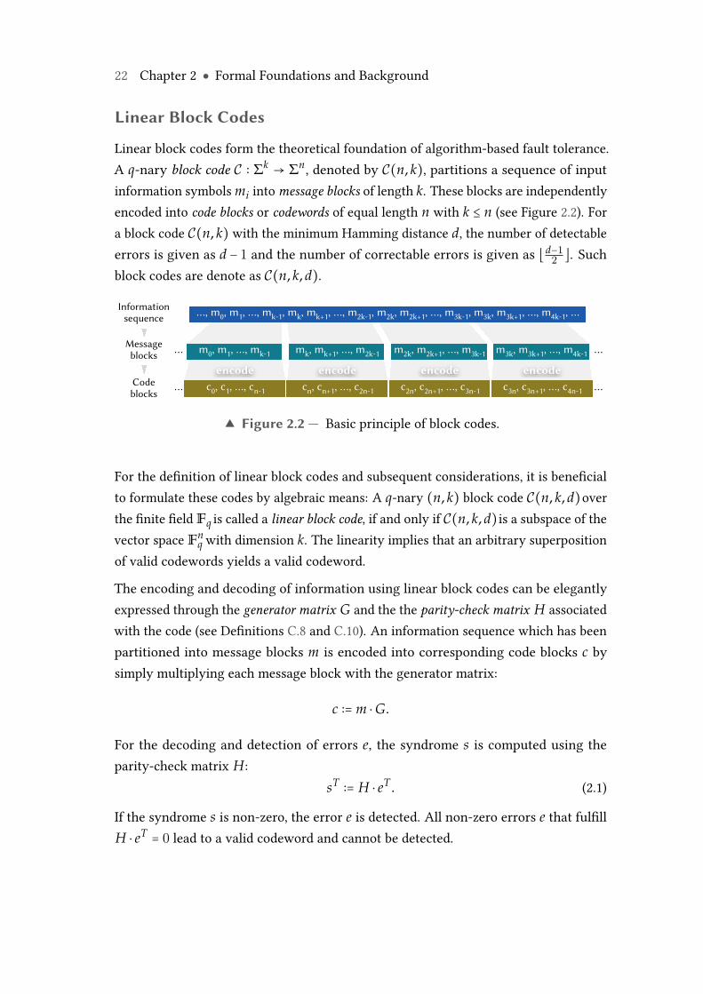
22 Chapter 2 ● Formal Foundations and Background
Linear Block Codes
Linear block codes form the theoretical foundation of algorithm-based fault tolerance.A q-nary block code C ∶ Σk → Σn, denoted by C(n, k), partitions a sequence of inputinformation symbols mi intomessage blocks of length k. These blocks are independentlyencoded into code blocks or codewords of equal length n with k ≤ n (see Figure 2.2). Fora block code C(n, k) with the minimum Hamming distance d, the number of detectableerrors is given as d − 1 and the number of correctable errors is given as ⌊d−1
2 ⌋. Suchblock codes are denote as C(n, k, d).
Informationsequence
Messageblocks
Codeblocks
…, m0, m1, …, mk-1, mk, mk+1, …, m2k-1, m2k, m2k+1, …, m3k-1, m3k, m3k+1, …, m4k-1, …
m3k, m3k+1, …, m4k-1m2k, m2k+1, …, m3k-1m0, m1, …, mk-1… …mk, mk+1, …, m2k-1
c3n, c3n+1, …, c4n-1c2n, c2n+1, …, c3n-1c0, c1, …, cn-1… …cn, cn+1, …, c2n-1
encode encodeencode encodeencode encodeencode encode
▲ Figure 2.2 — Basic principle of block codes.
For the definition of linear block codes and subsequent considerations, it is beneficialto formulate these codes by algebraic means: A q-nary (n, k) block code C(n, k, d)overthe finite field Fq is called a linear block code, if and only if C(n, k, d) is a subspace of thevector space Fn
q with dimension k. The linearity implies that an arbitrary superpositionof valid codewords yields a valid codeword.
The encoding and decoding of information using linear block codes can be elegantlyexpressed through the generator matrix G and the the parity-check matrix H associatedwith the code (see Definitions C.8 and C.10). An information sequence which has beenpartitioned into message blocks m is encoded into corresponding code blocks c bysimply multiplying each message block with the generator matrix:
c ∶= m ⋅G.
For the decoding and detection of errors e, the syndrome s is computed using theparity-check matrix H:
sT ∶= H ⋅ eT. (2.1)
If the syndrome s is non-zero, the error e is detected. All non-zero errors e that fulfillH ⋅ eT = 0 lead to a valid codeword and cannot be detected.
2.4 ● Floating-Point Number Systems and Arithmetic 23
In chapter 5, the formal definition of algorithm-based fault tolerance for matrix opera-tions will be introduced using the concepts described above.
2.4 Floating-Point Number Systems and Arithmetic
Being an infinite, continuous set of values, the real numbers pose a challenge for dig-ital computer systems, since these are limited to finite sets of binary values for therepresentation of information. This fact urged the development of suitable approx-imations which allow the mapping of at least a portion of the real numbers to thisfinite, discrete quantity of machine-representable values. A comprehensive overview ofdifferent number formats and representations that have been proposed over time, canbe found in [Mulle10]. Today, real numbers in scientific computing and engineering arepredominantly represented by floating-point numbers according to the IEEE Standard754™ for floating-point arithmetic [IEEE 08]. The following introduction is based onthis standard using base 2.
Floating-Point Numbers
The design of floating-point systems is a non-trivial task which requires the balancingof different, in parts conflicting, constraints like accuracy, performance, value ranges,portability and implementation complexity [Mulle10]. Floating-point arithmetic alsoexhibits certain characteristics and properties which have to be considered thoroughlyby the user and whose defiance or careless treatment can lead to serious errors.
A floating-point number is a compound consisting of a sign, a significand and an expo-nent. This compound is accompanied by a set of parameters like the radix or base uponwhich the number is defined, the precision and the value range of the exponent [Mulle10]:
• The radix or base β is an integer value with β ≥ 2. Unless indicated otherwise,radix β = 2 is used throughout this work.
• The precision p is an integer value with p ≥ 2. It defines the number of digitsdi in the significand.
• The sign s is an integer value with s ∈ {0, 1}.• The exponent limits emin and emax are integer values with emin ≤ 0 ≤ emax.These values represent the minimum and the maximum possible value of theexponent.
24 Chapter 2 ● Formal Foundations and Background
• The exponent e is an integer value with emin ≤ e ≤ emax.
• The normalized significand1 m is a number which is represented by a digitstring of the form d0 ● d1d2...dp−1, where di is an integer digit with 0 ≤ di < 2and therefore 0 ≤ m < 2.
This allows the formulation of a floating-point number a in the form
a = (−1)s ×m × 2e. (2.2)
With radix β = 2, normalization does not only guarantee the unique representationof floating-point numbers, it also allows the implicit storage of the digit on the leftof the radix point, which is always one. This yields an additional bit of precision forthe significand. However, with a normalized floating-point number format, zero canno longer be directly represented, which makes a separate encoding necessary (seeAppendix D).
Floating-point numbers whose exponent is e = emin and whose significand is ∣m∣ <1 do not fulfill the normalization condition and are called subnormal floating-pointnumbers2. Although subnormal numbers complicate the implementation of floating-point arithmetic, they do fill the gap between the smallest representable, normal floating-point number and zero, which allows for so called graceful underflow.
Rounding and Sources of Error
Floating-point numbers are a finite set of rational numbers which have a terminatingexpansion with respect to the radix β. In case of radix β = 2, rational numbers whosedenominator is a power of 2 can be represented exactly. Numbers without a terminatingexpansion have to be adjusted, which means that they are mapped to an appropriatefloating-point number nearby. This adjustment is called rounding and introduces aso-called rounding error .
The mapping of numbers without a terminating expansion to a floating-point numberis not always unambiguous. In cases where a candidate is located exactly in the middlebetween two numbers, distinct tie-breaking rules are required. Such rules, or rounding1 In this work, the significand of floating-point numbers is denoted by M or m, which is derived fromthe term mantissa and which is used to avoid confusion with the sign s of such numbers. The termsignificand was originally introduced by Forsythe and Moler [Forsy67].
2 Subnormal floating-point numbers are also often called denormal.
2.4 ● Floating-Point Number Systems and Arithmetic 25
modes, have to be applied in a consistent manner to achieve reproducible and predictableresults.
The IEEE Standard 754™ for floating-point arithmetic (see Appendix D) provides detailedguidelines and definitions of rounding algorithms for arithmetic operations such asaddition, multiplication or square root [Goldb91,Mulle10,IEEE 08]. The round-to-nearestrounding mode maps a real number a to RN(a), which is the floating-point numberclosest to a. In case that a is located exactly in the middle between two floating-pointnumbers, a so called tie-breaking rule is required. In IEEE-754(-2008), round-to-nearest-even is the default, whichmaps a to the floating-point number whose integral significandis even. Another option for tie-breaking is round-ties-away, where the floating-pointnumber whose magnitude is the larger one is chosen. The round-towards-zero roundingmode maps a to RZ(a), which is the floating-point number closest to a, but not greaterin magnitude than a. The round-towards-+∞ rounding mode maps a to RU(a), whichis the smallest floating-point number greater than or equal to a, possibly +∞. Theround-towards-−∞ rounding mode maps a to RD(a), which is the largest floating-pointnumber less than or equal to a, possibly −∞.
For the quantification of the rounding error that occurs in a floating-point computation,an appropriate measure can be beneficial. For any floating-point number system andaccompanying rounding procedure, the machine epsilon ϵM is therefore defined as thedifference between 1.0 and the next-nearest number that can be represented in thegiven floating-point number format3,4:
ϵM ∶= β−(p−1) (2.3)
In case of radix β = 2 and for the single and double precision IEEE 754 number formats,the machine epsilon is hence defined as
ϵM ∶= 2−23 ≈ 1, 1921 ⋅ 10−7 (single precision) (2.4)
ϵM ∶= 2−52 ≈ 2, 2205 ⋅ 10−16 (double precision). (2.5)
Besides the rounding error, floating-point arithmetic exhibits certain characteristicswhich can lead to considerable errors, if they are not treated carefully. This is especially3 It should be noted that the IEEE Standard 754™ for floating-point arithmetic [IEEE 08] does not providea definition for the term machine epsilon.
4 The term unit roundoff u can also be found in literature and is often used interchangeably with theterm machine epsilon.
26 Chapter 2 ● Formal Foundations and Background
true when software is designed with properties of the real numbers in mind that do notapply to floating-point numbers. In general, the addition and multiplication of floating-point numbers are neither associative nor distributive, which makes an importantdifference to the real numbers. Moreover, the phenomenon of subtractive cancellationcan lead to a loss of accuracy if floating-point numbers are subtracted which are almostequal. Additions and subtractions of floating-point numbers which differ significantlyin their magnitude can lead to a phenomenon called absorption, where the contributionof the smaller operand is lost. Similar problems arise with underflows in floating-pointcomputations.
Rounding errors and phenomena such as those described above can be regarded asmajor drawbacks of floating-point arithmetic. However, in this work, the oppositeperspective is taken and these phenomena are considered as inevitable properties offloating-point arithmetic which even provide a certain degree of inherent fault tolerance.This has particular implications for the design and implementation of fault tolerancetechniques such as ABFT. In the context of floating-point arithmetic, such fault tolerancetechniques must never be more accurate than the level of accuracy provided by thearithmetic system itself. This effectively means that errors can be tolerated as long asthey are in the order of magnitude of the performed operation’s expected rounding error.This in turn makes the derivation of rounding error information and the determinationof appropriate rounding error bounds an essential task.
Chapter
3GPU Architectures andProgramming Models
This chapter introduces modern graphics processing architectures and the accompa-nying programming models in detail. The basic principles are explained using theexample of the NVIDIA GK 110 GPU architecture [NVIDI12] and the Compute UnifiedDevice Architecture (CUDA) programming model. Since modern graphics processingunits and programming models exhibit strong similarities, the described principles aretransferable to other contemporary architectures. The largest currently available GPUbased on the described architecture consists of 7.1 ⋅ 109 transistors which reside ona 533 mm2 silicon die, manufactured in 28 nm CMOS technology. It comprises 2880processing cores and delivers a theoretical peak performance of 4.29 TFLOPS singleprecision and 1.43 TFLOPS double precision.
3.1 Global GPU Architecture
Advanced graphics processing units possess many-core stream architectures, whichfollow the Single Instruction stream, Multiple Data stream (SIMD) [Flynn72] paradigm.In principle, these architectures execute a single instruction stream, coming from asingle GPU program, by a large number of parallel threads on different data elements.
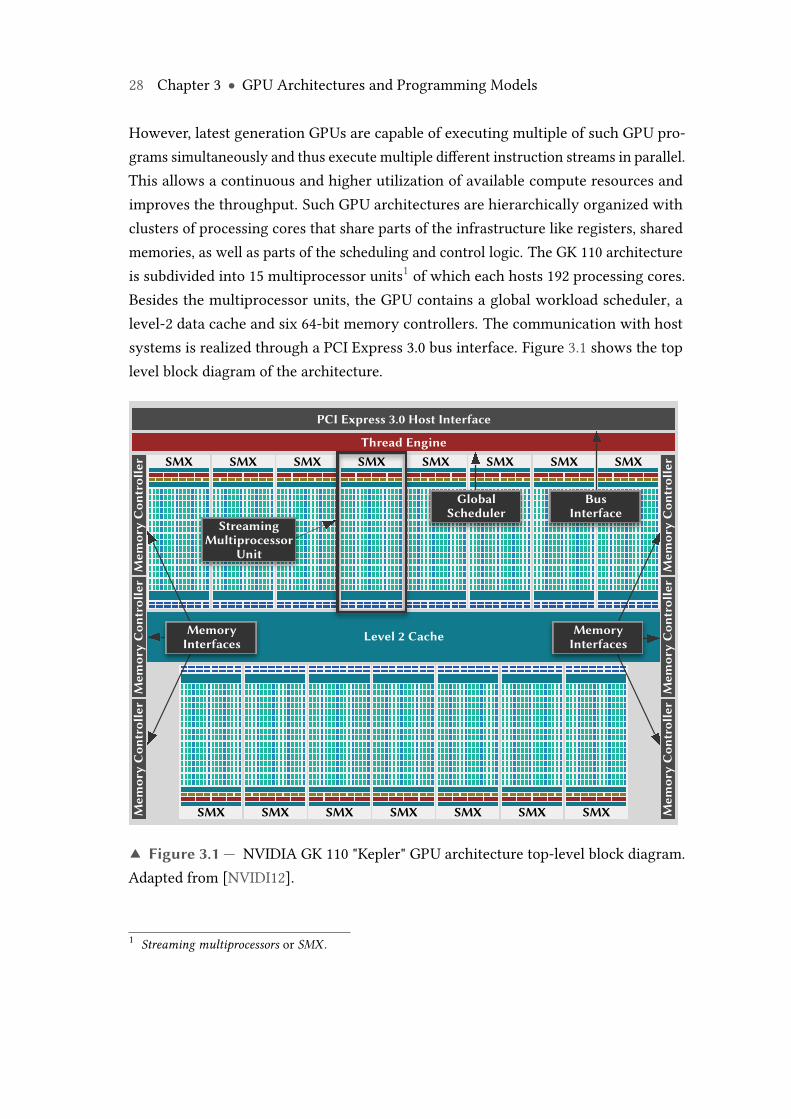
28 Chapter 3 ● GPU Architectures and Programming Models
However, latest generation GPUs are capable of executing multiple of such GPU pro-grams simultaneously and thus execute multiple different instruction streams in parallel.This allows a continuous and higher utilization of available compute resources andimproves the throughput. Such GPU architectures are hierarchically organized withclusters of processing cores that share parts of the infrastructure like registers, sharedmemories, as well as parts of the scheduling and control logic. The GK 110 architectureis subdivided into 15 multiprocessor units1 of which each hosts 192 processing cores.Besides the multiprocessor units, the GPU contains a global workload scheduler, alevel-2 data cache and six 64-bit memory controllers. The communication with hostsystems is realized through a PCI Express 3.0 bus interface. Figure 3.1 shows the toplevel block diagram of the architecture.
SMX
SMX SMX SMX SMX SMX SMX SMX
SMX SMX SMX SMX SMX SMX SMX
Mem
ory
Con
trol
ler
Mem
ory
Con
trol
ler
Mem
ory
Con
trol
ler
Mem
ory
Con
trol
ler
Mem
ory
Con
trol
ler
Mem
ory
Con
trol
ler
Level 2 Cache
Thread Engine
PCI Express 3.0 Host Interface
StreamingMultiprocessor
Unit
MemoryInterfaces
MemoryInterfaces
GlobalScheduler
BusInterface
▲ Figure 3.1 — NVIDIA GK 110 "Kepler" GPU architecture top-level block diagram.Adapted from [NVIDI12].
1 Streaming multiprocessors or SMX .
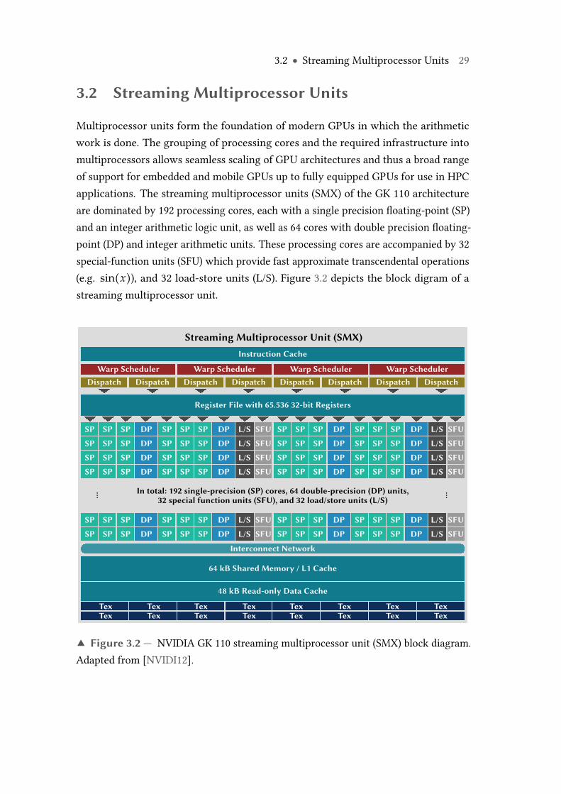
3.2 ● Streaming Multiprocessor Units 29
3.2 Streaming Multiprocessor Units
Multiprocessor units form the foundation of modern GPUs in which the arithmeticwork is done. The grouping of processing cores and the required infrastructure intomultiprocessors allows seamless scaling of GPU architectures and thus a broad rangeof support for embedded and mobile GPUs up to fully equipped GPUs for use in HPCapplications. The streaming multiprocessor units (SMX) of the GK 110 architectureare dominated by 192 processing cores, each with a single precision floating-point (SP)and an integer arithmetic logic unit, as well as 64 cores with double precision floating-point (DP) and integer arithmetic units. These processing cores are accompanied by 32special-function units (SFU) which provide fast approximate transcendental operations(e.g. sin(x)), and 32 load-store units (L/S). Figure 3.2 depicts the block digram of astreaming multiprocessor unit.
In total: 192 single-precision (SP) cores, 64 double-precision (DP) units,32 special function units (SFU), and 32 load/store units (L/S)… …
Instruction Cache
Warp Scheduler Warp Scheduler Warp Scheduler Warp SchedulerDispatch Dispatch Dispatch Dispatch Dispatch Dispatch Dispatch Dispatch
Register File with 65.536 32-bit Registers
SP SP SP SP SP SPDP DP L/S SFU SP SP SP SP SP SPDP DP L/S SFU
SP SP SP SP SP SPDP DP L/S SFU SP SP SP SP SP SPDP DP L/S SFU
SP SP SP SP SP SPDP DP L/S SFU SP SP SP SP SP SPDP DP L/S SFU
SP SP SP SP SP SPDP DP L/S SFU SP SP SP SP SP SPDP DP L/S SFU
SP SP SP SP SP SPDP DP L/S SFU SP SP SP SP SP SPDP DP L/S SFU
SP SP SP SP SP SPDP DP L/S SFU SP SP SP SP SP SPDP DP L/S SFU
Interconnect Network
64 kB Shared Memory / L1 Cache
48 kB Read-only Data Cache
Tex Tex Tex Tex Tex Tex Tex TexTex Tex Tex Tex Tex Tex Tex Tex
Streaming Multiprocessor Unit (SMX)
▲ Figure 3.2 — NVIDIA GK 110 streaming multiprocessor unit (SMX) block diagram.Adapted from [NVIDI12].
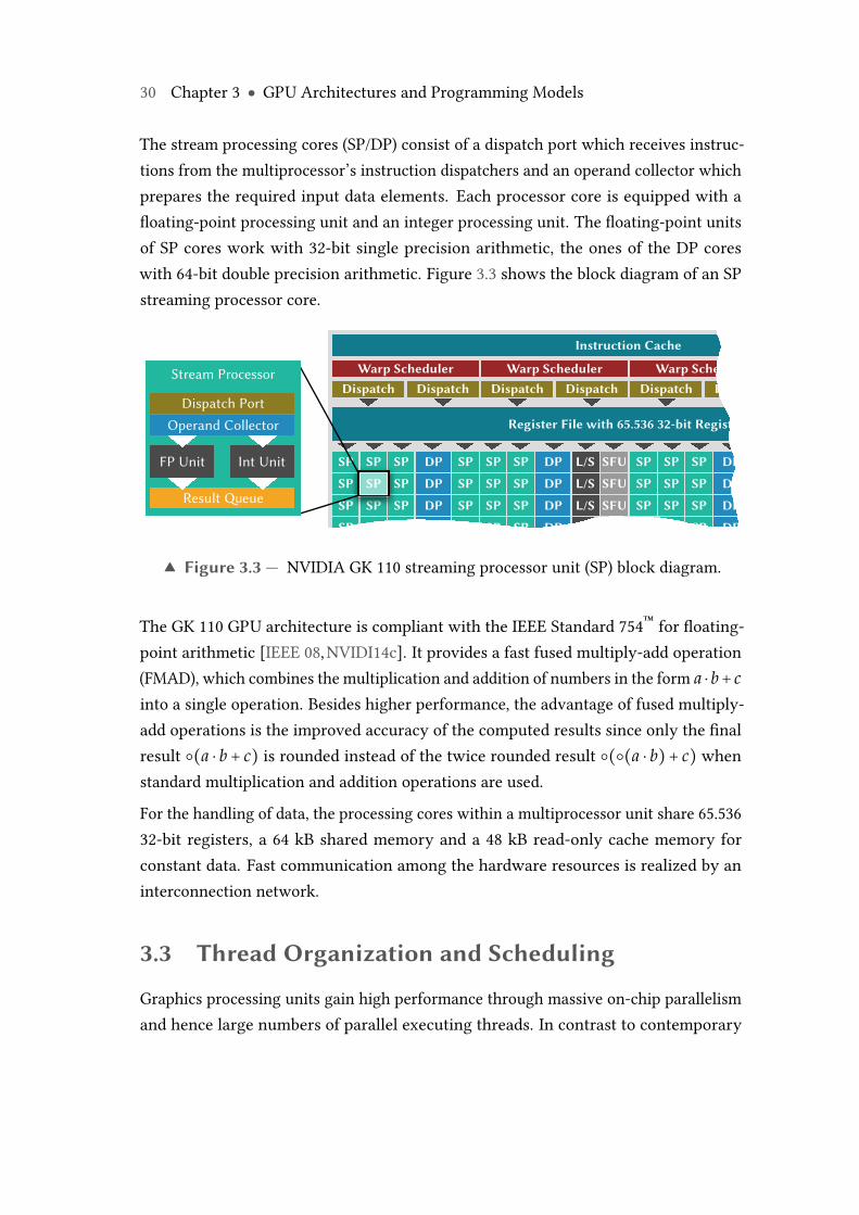
30 Chapter 3 ● GPU Architectures and Programming Models
The stream processing cores (SP/DP) consist of a dispatch port which receives instruc-tions from the multiprocessor’s instruction dispatchers and an operand collector whichprepares the required input data elements. Each processor core is equipped with afloating-point processing unit and an integer processing unit. The floating-point unitsof SP cores work with 32-bit single precision arithmetic, the ones of the DP coreswith 64-bit double precision arithmetic. Figure 3.3 shows the block diagram of an SPstreaming processor core.
Instruction Cache
Warp Scheduler Warp Scheduler Warp SchedulerDispatch Dispatch Dispatch Dispatch Dispatch Dispatch
Register File with 65.536 32-bit Registers
SP SP SP SP SP SPDP DP L/S SFU SP SP SP DP
SP SP SP SP SP SPDP DP L/S SFU SP SP SP DP
SP SP SP SP SP SPDP DP L/S SFU SP SP SP DP
SP SP SP DP SP DP
Stream Processor
Dispatch PortOperand Collector
Result Queue
FP Unit Int Unit
▲ Figure 3.3 — NVIDIA GK 110 streaming processor unit (SP) block diagram.
The GK 110 GPU architecture is compliant with the IEEE Standard 754™ for floating-point arithmetic [IEEE 08,NVIDI14c]. It provides a fast fused multiply-add operation(FMAD), which combines the multiplication and addition of numbers in the form a ⋅ b+ cinto a single operation. Besides higher performance, the advantage of fused multiply-add operations is the improved accuracy of the computed results since only the finalresult ○(a ⋅ b + c) is rounded instead of the twice rounded result ○(○(a ⋅ b)+ c) whenstandard multiplication and addition operations are used.
For the handling of data, the processing cores within a multiprocessor unit share 65.53632-bit registers, a 64 kB shared memory and a 48 kB read-only cache memory forconstant data. Fast communication among the hardware resources is realized by aninterconnection network.
3.3 Thread Organization and Scheduling
Graphics processing units gain high performance through massive on-chip parallelismand hence large numbers of parallel executing threads. In contrast to contemporary
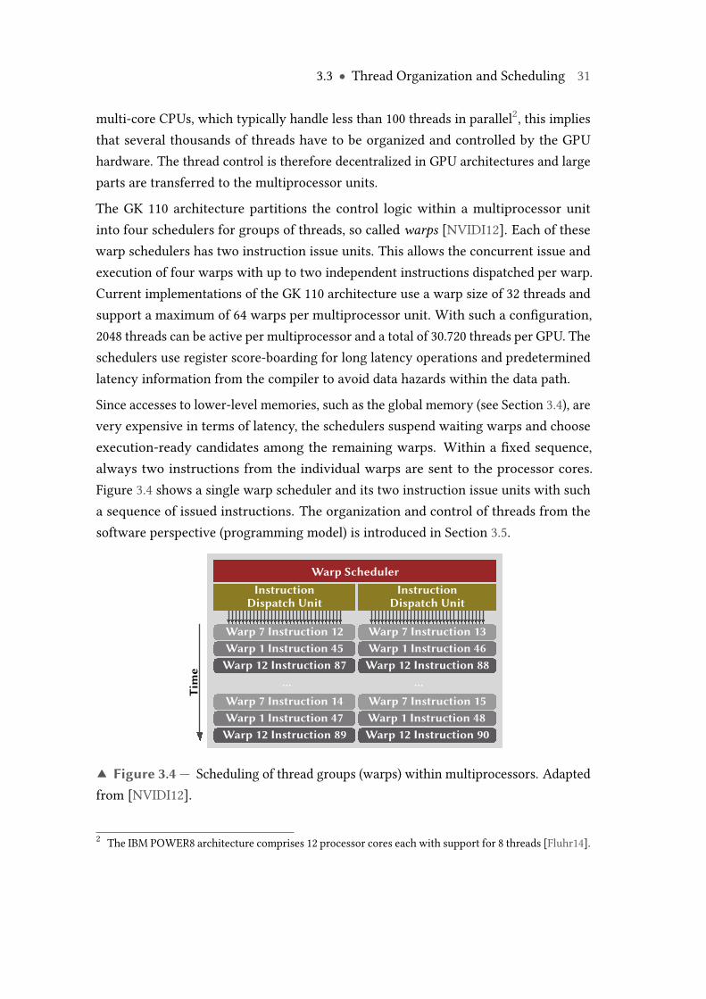
3.3 ● Thread Organization and Scheduling 31
multi-core CPUs, which typically handle less than 100 threads in parallel2, this impliesthat several thousands of threads have to be organized and controlled by the GPUhardware. The thread control is therefore decentralized in GPU architectures and largeparts are transferred to the multiprocessor units.
The GK 110 architecture partitions the control logic within a multiprocessor unitinto four schedulers for groups of threads, so called warps [NVIDI12]. Each of thesewarp schedulers has two instruction issue units. This allows the concurrent issue andexecution of four warps with up to two independent instructions dispatched per warp.Current implementations of the GK 110 architecture use a warp size of 32 threads andsupport a maximum of 64 warps per multiprocessor unit. With such a configuration,2048 threads can be active per multiprocessor and a total of 30.720 threads per GPU. Theschedulers use register score-boarding for long latency operations and predeterminedlatency information from the compiler to avoid data hazards within the data path.
Since accesses to lower-level memories, such as the global memory (see Section 3.4), arevery expensive in terms of latency, the schedulers suspend waiting warps and chooseexecution-ready candidates among the remaining warps. Within a fixed sequence,always two instructions from the individual warps are sent to the processor cores.Figure 3.4 shows a single warp scheduler and its two instruction issue units with sucha sequence of issued instructions. The organization and control of threads from thesoftware perspective (programming model) is introduced in Section 3.5.
Warp SchedulerInstruction
Dispatch UnitInstruction
Dispatch Unit
Warp 7 Instruction 12Warp 1 Instruction 45
Warp 12 Instruction 87
Warp 7 Instruction 14Warp 1 Instruction 47
Warp 12 Instruction 89
Warp 7 Instruction 13Warp 1 Instruction 46
Warp 12 Instruction 88
Warp 7 Instruction 15Warp 1 Instruction 48Warp 12 Instruction 90
Tim
e
… …
▲ Figure 3.4 — Scheduling of thread groups (warps) within multiprocessors. Adaptedfrom [NVIDI12].
2 The IBM POWER8 architecture comprises 12 processor cores each with support for 8 threads [Fluhr14].
32 Chapter 3 ● GPU Architectures and Programming Models
3.4 Memory Hierarchy
Modern graphics processing architectures feature rich memory hierarchies with differ-ent levels of embedded memories, which provide different capacities, access latenciesand access paths for threads. Recent GPU architectures, which target applicationsin high-performance computing, offer single-error correction, double-error detection(SECDED) ECC-protection for register files, shared memories and caches, as well as forthe global device memories. In addition, single-error correction through parity checksis available for certain caches.
The memory access granularity depends on the level of the memory resource. Registerscan be individually and directly accessed by threads. Accesses of multiple threads tolower level caches and global device memories are typically bundled by the hardwareinto single memory operations.
Within the GK 110 GPU architecture, each multiprocessor (SMX) comprises an ECC-protected register file with 65.536 32-bit registers. A single thread can address up to255 registers as private local storage. The registers are managed by the compiler.
The next lower level within the memory hierarchy is a local memory of 64 kB capacitywithin each multiprocessor unit. This memory can be partitioned into a shared memory,which is then fully managed by the software, and a level-1 data cache, which is managedby the hardware. The partitioning is possible in shared memory to cache ratios of 32kB:32 kB, 16 kB:48 kB and 48 kB:16 kB. The shared memory partition is accessible byall threads on a multiprocessor. The bandwidth of this memory for 64 bit and largerload operations is 256 B per core clock cycle, which yields up to 2.5 TB/s. This highbandwidth is achieved by internal partitioning of the shared memory into so calledbanks that can be accessed simultaneously. Memory read or write accesses to theshared memory with subsequent addresses that fall into different banks can thereforebe processed in parallel. However, if addresses refer to the same bank, a bank conflictarises and the accesses are serialized, leading to a reduced throughput.
Besides the shared memory and level-1 cache, each multiprocessor is equipped with aparity-protected read-only cache of 48 kB capacity. This cache can be either managedautomatically by the hardware or explicitly by the software.
In addition to the described memory resources, the GK 110 architecture provides a level-2 data cache of 1536 kB capacity. This cache is also ECC-protected and transparentlymanaged by the hardware. Its main purpose is the unification and communication of
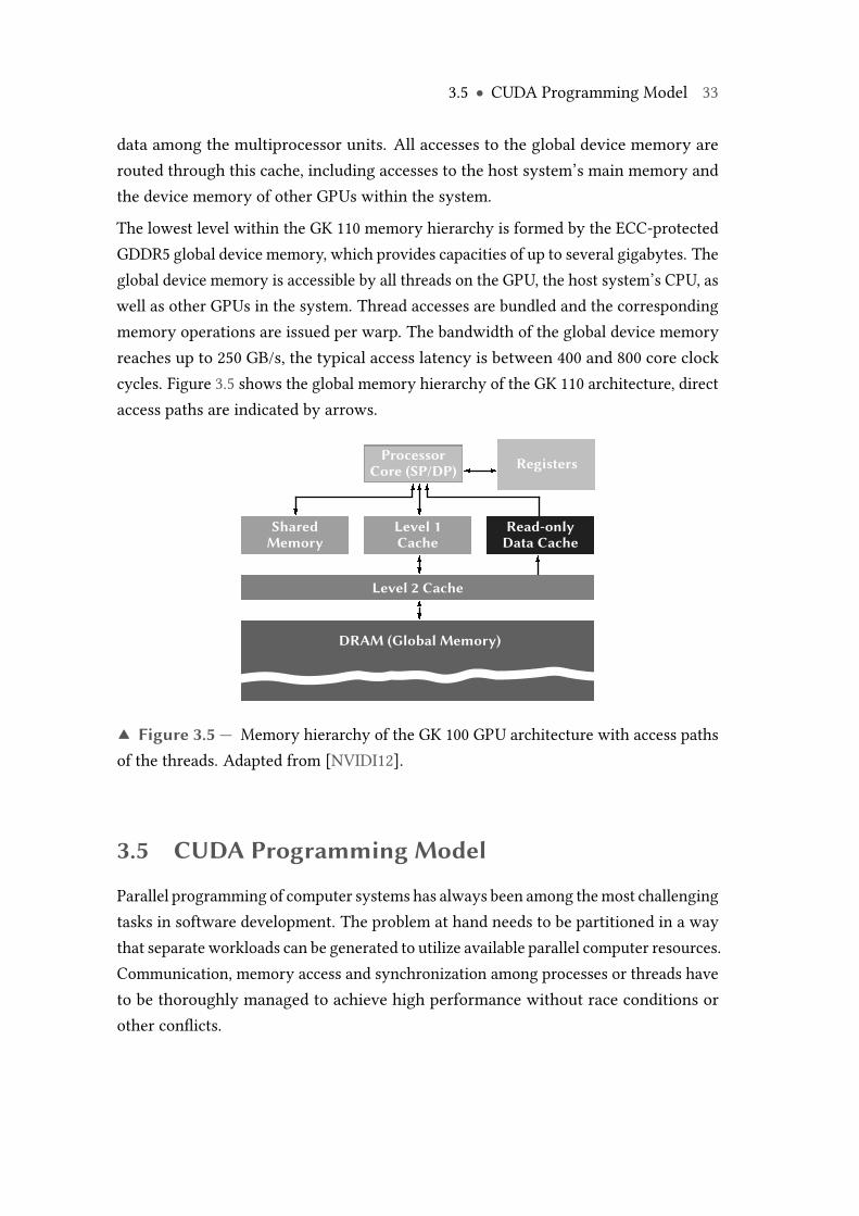
3.5 ● CUDA Programming Model 33
data among the multiprocessor units. All accesses to the global device memory arerouted through this cache, including accesses to the host system’s main memory andthe device memory of other GPUs within the system.
The lowest level within the GK 110 memory hierarchy is formed by the ECC-protectedGDDR5 global device memory, which provides capacities of up to several gigabytes. Theglobal device memory is accessible by all threads on the GPU, the host system’s CPU, aswell as other GPUs in the system. Thread accesses are bundled and the correspondingmemory operations are issued per warp. The bandwidth of the global device memoryreaches up to 250 GB/s, the typical access latency is between 400 and 800 core clockcycles. Figure 3.5 shows the global memory hierarchy of the GK 110 architecture, directaccess paths are indicated by arrows.
DRAM (Global Memory)
Level 2 Cache
SharedMemory
ProcessorCore (SP/DP) Registers
Level 1Cache
Read-onlyData Cache
▲ Figure 3.5 — Memory hierarchy of the GK 100 GPU architecture with access pathsof the threads. Adapted from [NVIDI12].
3.5 CUDA Programming Model
Parallel programming of computer systems has always been among themost challengingtasks in software development. The problem at hand needs to be partitioned in a waythat separate workloads can be generated to utilize available parallel computer resources.Communication, memory access and synchronization among processes or threads haveto be thoroughly managed to achieve high performance without race conditions orother conflicts.
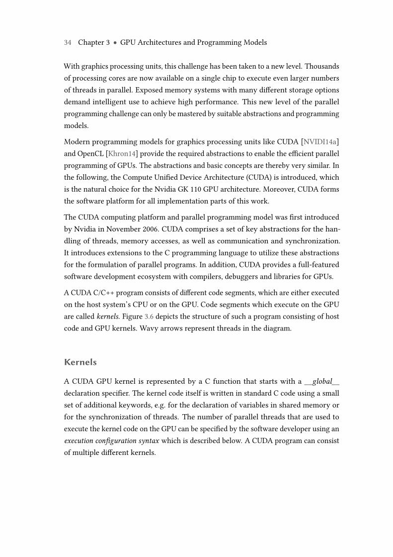
34 Chapter 3 ● GPU Architectures and Programming Models
With graphics processing units, this challenge has been taken to a new level. Thousandsof processing cores are now available on a single chip to execute even larger numbersof threads in parallel. Exposed memory systems with many different storage optionsdemand intelligent use to achieve high performance. This new level of the parallelprogramming challenge can only be mastered by suitable abstractions and programmingmodels.
Modern programming models for graphics processing units like CUDA [NVIDI14a]and OpenCL [Khron14] provide the required abstractions to enable the efficient parallelprogramming of GPUs. The abstractions and basic concepts are thereby very similar. Inthe following, the Compute Unified Device Architecture (CUDA) is introduced, whichis the natural choice for the Nvidia GK 110 GPU architecture. Moreover, CUDA formsthe software platform for all implementation parts of this work.
The CUDA computing platform and parallel programming model was first introducedby Nvidia in November 2006. CUDA comprises a set of key abstractions for the han-dling of threads, memory accesses, as well as communication and synchronization.It introduces extensions to the C programming language to utilize these abstractionsfor the formulation of parallel programs. In addition, CUDA provides a full-featuredsoftware development ecosystem with compilers, debuggers and libraries for GPUs.
A CUDA C/C++ program consists of different code segments, which are either executedon the host system’s CPU or on the GPU. Code segments which execute on the GPUare called kernels. Figure 3.6 depicts the structure of such a program consisting of hostcode and GPU kernels. Wavy arrows represent threads in the diagram.
Kernels
A CUDA GPU kernel is represented by a C function that starts with a __global__declaration specifier. The kernel code itself is written in standard C code using a smallset of additional keywords, e.g. for the declaration of variables in shared memory orfor the synchronization of threads. The number of parallel threads that are used toexecute the kernel code on the GPU can be specified by the software developer using anexecution configuration syntax which is described below. A CUDA program can consistof multiple different kernels.
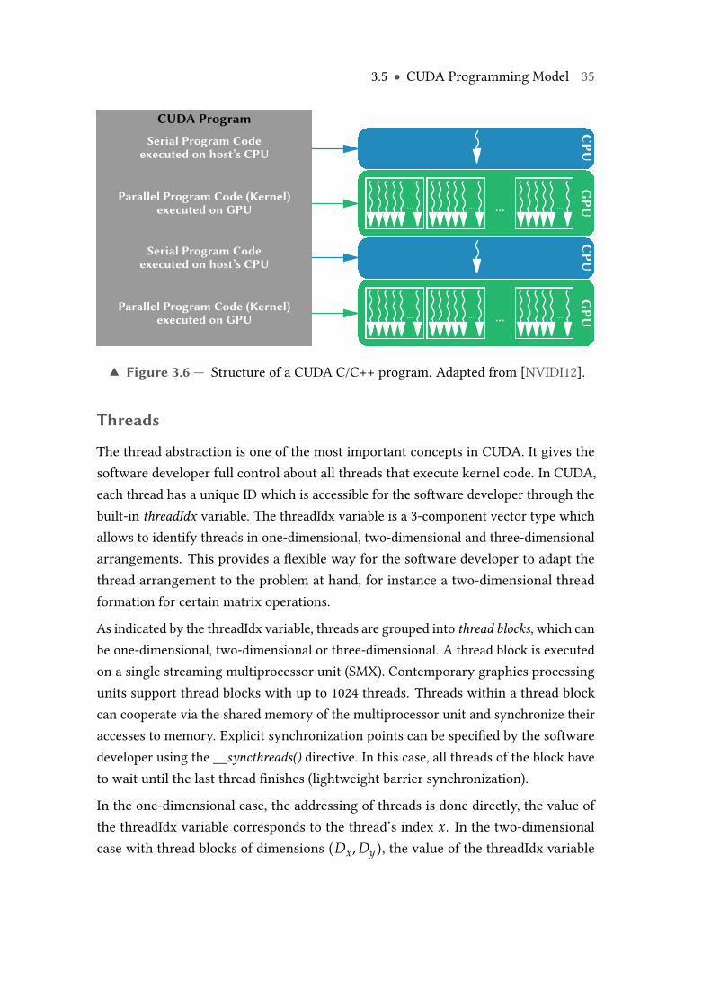
3.5 ● CUDA Programming Model 35
CUDA ProgramC
PUC
PUG
PUG
PU… … ……
… … ……
Serial Program Codeexecuted on host’s CPU
Parallel Program Code (Kernel)executed on GPU
Parallel Program Code (Kernel)executed on GPU
Serial Program Codeexecuted on host’s CPU
▲ Figure 3.6 — Structure of a CUDA C/C++ program. Adapted from [NVIDI12].
Threads
The thread abstraction is one of the most important concepts in CUDA. It gives thesoftware developer full control about all threads that execute kernel code. In CUDA,each thread has a unique ID which is accessible for the software developer through thebuilt-in threadIdx variable. The threadIdx variable is a 3-component vector type whichallows to identify threads in one-dimensional, two-dimensional and three-dimensionalarrangements. This provides a flexible way for the software developer to adapt thethread arrangement to the problem at hand, for instance a two-dimensional threadformation for certain matrix operations.
As indicated by the threadIdx variable, threads are grouped into thread blocks, which canbe one-dimensional, two-dimensional or three-dimensional. A thread block is executedon a single streaming multiprocessor unit (SMX). Contemporary graphics processingunits support thread blocks with up to 1024 threads. Threads within a thread blockcan cooperate via the shared memory of the multiprocessor unit and synchronize theiraccesses to memory. Explicit synchronization points can be specified by the softwaredeveloper using the __syncthreads() directive. In this case, all threads of the block haveto wait until the last thread finishes (lightweight barrier synchronization).
In the one-dimensional case, the addressing of threads is done directly, the value ofthe threadIdx variable corresponds to the thread’s index x. In the two-dimensionalcase with thread blocks of dimensions (Dx, Dy), the value of the threadIdx variable
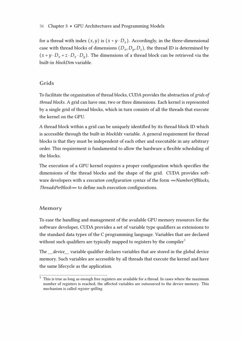
36 Chapter 3 ● GPU Architectures and Programming Models
for a thread with index (x, y) is (x + y ⋅Dx). Accordingly, in the three-dimensionalcase with thread blocks of dimensions (Dx, Dy, Dz), the thread ID is determined by(x + y ⋅Dx + z ⋅Dx ⋅Dy). The dimensions of a thread block can be retrieved via thebuilt-in blockDim variable.
Grids
To facilitate the organization of thread blocks, CUDA provides the abstraction of grids ofthread blocks. A grid can have one, two or three dimensions. Each kernel is representedby a single grid of thread blocks, which in turn consists of all the threads that executethe kernel on the GPU.
A thread block within a grid can be uniquely identified by its thread block ID whichis accessible through the built-in blockIdx variable. A general requirement for threadblocks is that they must be independent of each other and executable in any arbitraryorder. This requirement is fundamental to allow the hardware a flexible scheduling ofthe blocks.
The execution of a GPU kernel requires a proper configuration which specifies thedimensions of the thread blocks and the shape of the grid. CUDA provides soft-ware developers with a execution configuration syntax of the form <<<NumberOfBlocks,ThreadsPerBlock>>> to define such execution configurations.
Memory
To ease the handling and management of the available GPU memory resources for thesoftware developer, CUDA provides a set of variable type qualifiers as extensions tothe standard data types of the C programming language. Variables that are declaredwithout such qualifiers are typically mapped to registers by the compiler3
The __device__ variable qualifier declares variables that are stored in the global devicememory. Such variables are accessible by all threads that execute the kernel and havethe same lifecycle as the application.
3 This is true as long as enough free registers are available for a thread. In cases where the maximumnumber of registers is reached, the affected variables are outsourced to the device memory. Thismechanism is called register spilling.
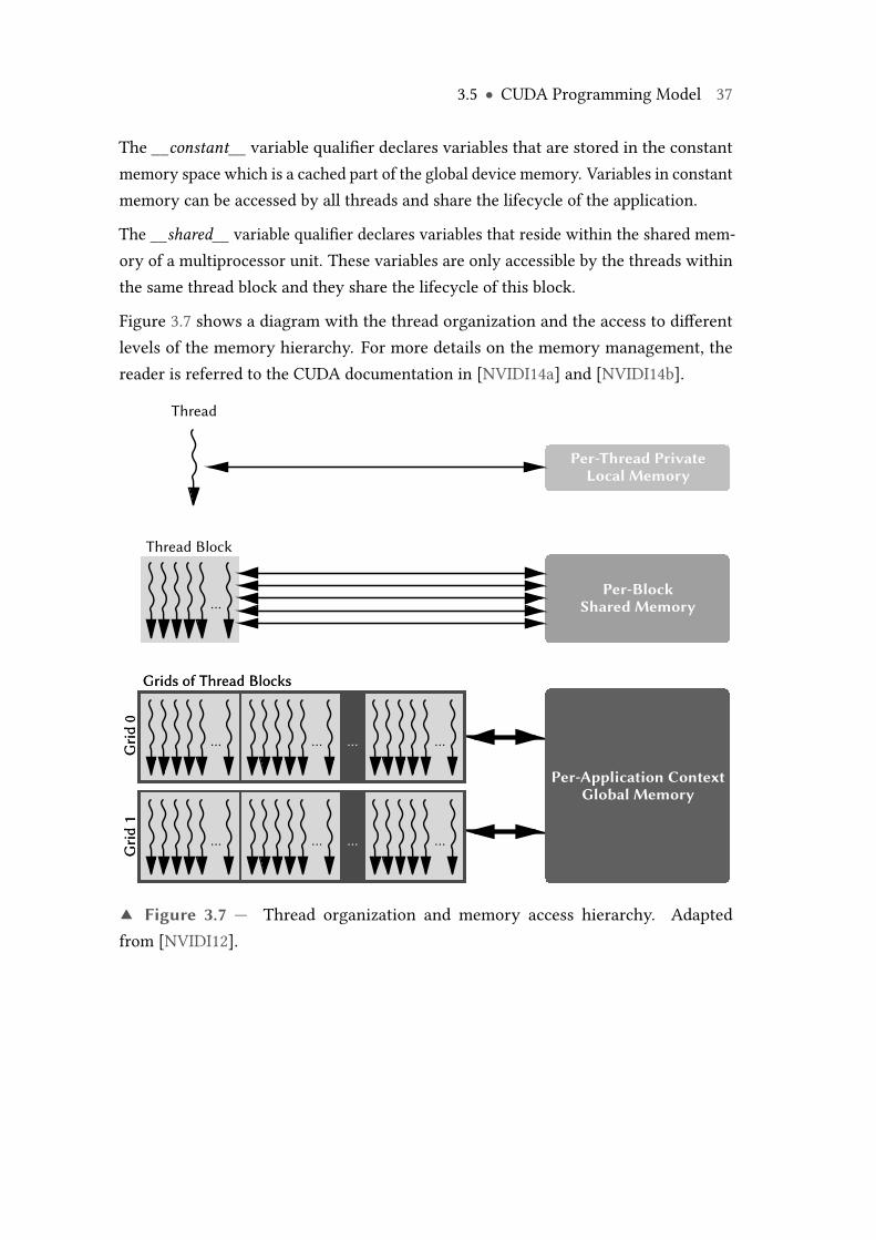
3.5 ● CUDA Programming Model 37
The __constant__ variable qualifier declares variables that are stored in the constantmemory space which is a cached part of the global device memory. Variables in constantmemory can be accessed by all threads and share the lifecycle of the application.
The __shared__ variable qualifier declares variables that reside within the shared mem-ory of a multiprocessor unit. These variables are only accessible by the threads withinthe same thread block and they share the lifecycle of this block.
Figure 3.7 shows a diagram with the thread organization and the access to differentlevels of the memory hierarchy. For more details on the memory management, thereader is referred to the CUDA documentation in [NVIDI14a] and [NVIDI14b].
…
Thread
Thread Block
Per-Thread PrivateLocal Memory
Per-BlockShared Memory
… … ……
… … ……
Grids of Thread Blocks
Gri
d 0
Gri
d 1
Per-Application ContextGlobal Memory
… … ……
… … ……
Grids of Thread Blocks
Gri
d 0
Gri
d 1
Per-Application ContextGlobal Memory
▲ Figure 3.7 — Thread organization and memory access hierarchy. Adaptedfrom [NVIDI12].

Chapter
4Fault Tolerance for Graphics
Processing Units
Modern graphics processing units do not only represent some of the most complex andmost sophisticated contemporary processor architectures, they also belong to the classof nano-scaled devices, which are typically manufactured in latest CMOS technology.As introduced in Chapter 1.3, graphics processing units are therefore increasinglyconfronted with a rapidly growing spectrum of very different factors that threaten theirreliability. This in turn makes the integration of fault tolerance mandatory.
Fault tolerance is a mature research area, which provides hardware and softwaresolutions to exploit and manage redundancy in order to improve the reliability ofsystems. For the sake of conciseness, a detailed introduction to fault tolerance is omittedat this point. Profound introductions to the design and the most important concepts andmethods of self-checking and fault tolerant systems can be found in [Koren07], [Lala01]and [Goess08].
The selection and combination of appropriate fault tolerance measures is often a non-trivial task, which requires detailed information about the vulnerability of the targetsystem. This chapter therefore starts with a brief overview of common methods for thevulnerability assessment of GPUs and presents recent results, which strongly motivatethe integration of fault tolerance measures. The chapter then puts its focus to faulttolerance measures that have been proposed for GPUs.
40 Chapter 4 ● Fault Tolerance for Graphics Processing Units
4.1 Vulnerability Assessment
Mainly three different options exist to assess the vulnerability of modern graphicsprocessing units, for instance to transient effects. The first option are analytical methodssuch as the Architectural Vulnerability Factor (AVF) [Mukhe08], which allows to identifyand distinguish components within a design by their susceptibility to soft errors. Thesecond option are simulation-based evaluations, which range from gate-level or RT-levellogic simulations combined with fault injections, up to system-level simulations. Thethird option are physical experiments such as the exposure of a circuit-under-test todifferent kinds of radiation.
Since floating-point processing is a core task of graphics processing units, a generalstructural hardware model and an integrated multi-level simulation environment havebeen developed in course of the preparations of this thesis. The hardware model isindependent of vendor-specific hardware information, it provides transferable soft errordata, and it offers large flexibility for the adaption to new hardware structures. Thesimulation environment utilizes gate-level logic simulation and fault injections to gaindetailed soft error data. The hardware basis for the model is a synthesized netlist ofan industry-grade floating-point unit (FPU), which complies with the IEEE Standard754™ for floating-point arithmetic. Fault injections are performed exhaustively, whichmeans that signal-line-flips or stuck-at-faults are injected into each gate of the FPUseparately and not only into the state elements. Given that the structural model ofthe FPU consists of ca. 22.000 logic gates, 22.000 fault injections are performed for thecharacterization of a single operation.
Although hardware structures for floating-point processing typically exhibit a certaininherent fault tolerance, soft error characterizations of the FPU’s four basic arithmeticoperations FADD, FSUB, FMUL and FDIV showed that between 27.5% (FDIV) and36.8% (FMUL) of all injected faults1 caused an error in the FPU’s internal state. Between14.5% (FADD, FSUB) and 24.4% (FMUL) of such internal state errors lead to erroneouscomputational results. Additional results of these experiments have been presentedin [Wunde13] and emphasize the vulnerability of floating-point processing logic.
In [Tan11], Tan et al. introduced GPGPU-SODA, a software framework for the softerror characterization of graphics processing units based on the GPU architecture
1 For the referenced soft error characterizations, the FPU processed random input data between 10−3
and 103.
4.1 ● Vulnerability Assessment 41
simulator GPGPU-Sim [Bakho09]. The framework allows the computation of Architec-tural Vulnerability Factors for components of the GPU microarchitecture like the warpscheduler, the processing cores, as well as the register file. The authors performed ex-haustive analyses across different workloads based on examples from the Nvidia CUDASDK [NVIDI15], the Rodinia Benchmark [Che09], and the Parboil Benchmark [Strat12].The experimental results showed that the AVF of the warp scheduler, the register fileand the processing cores achieved up to 76%, 95%, and 75%, respectively. Tan et al.concluded that the "majority structures in GPGPUs (e.g. warp scheduler, streaming pro-cessors, and register file) are highly vulnerable" and that "a comprehensive technique isneeded to protect them against soft error attacks".
In [Tselo13], Tselonis et al. evaluated the vulnerability of modern GPUs to permanentfaults in the registers. Based on the cycle-accurate GPU architecture simulator GPGPU-Sim [Bakho09], the authors performed extensive fault injection experiments, wherethey injected stuck-at-zero and stuck-at-one faults at different positions of randomlychosen registers. A vector addition (vadd) and a matrix multiplication with and withoutshared memory utilization (mmult-sm/mmult) formed the benchmarks. Across allexperiments, 33.98% (vadd), 34.98% (mmult-sm) and 39.94% (mmult) of the injectedfaults did not cause any error, which shows a rather high tolerance against permanentfaults in registers. However, 65.89% (vadd), 61.48% (mmult-sm) and 43.99% (mmult) ofthe injections caused erroneous computational results. Tselonis et al. also investigatedthe impact of permanent faults in registers on the overall performance of the GPU. Theirresults showed that, even with significantly increasing numbers of affected registers indifferent streaming multiprocessors, the GPU performance degraded only moderatelydue to high thread-level redundancy.
WithGPU-Qin [Fang14], Fang et al. introduced amethod for the vulnerability assessmentof GPU applications based on fault injections. The approach utilizes a GPU debuggerand performs the fault injections at assembly-language level of GPU applications.It allows to model faults at the granularity of individual instructions. The authorsselected 15 benchmark programs from the Nvidia CUDA SDK [NVIDI15] and theRodinia Benchmark [Che09], which also included the matrix multiplication and thematrix transpose. The experimental results showed crash rates, i.e. the application didnot finish execution, between 31% (matrix multiplication) and around 40% (matrixtranspose), as well as silent data corruption (SDC) rates between 22% (matrix transpose)and 25% (matrix multiplication).
42 Chapter 4 ● Fault Tolerance for Graphics Processing Units
In recent years, several works have been published on radiation-based experiments forthe vulnerability assessment of GPUs and GPU applications. In [Rech13] Rech et al.exposed graphics processing units (Nvidia GTX480) to different levels of neutron fluxbetween 4 ⋅ 104 n
cm2⋅sand 1 ⋅ 106 n
cm2⋅s, and evaluated the behavior of a matrix multiplica-
tion and a Fast-Fourier-Transform kernel. The authors reported cross sections2, which,in case of the matrix multiplication, represent the probability for a neutron that hitsthe GPU during the matrix multiplication to cause an output error. A FIT rate (failuresin time) of 2.81 ⋅ 104 was reported for the matrix multiplication and 5.17 ⋅ 105 for theFFT. For the matrix multiplication, a majority of 51.51% of the erroneous results wasaffected by multiple errors. Although the FIT rates appear low at first, the authorspointed out that such rates are intolerable for scientific calculations or even safety-critical applications. Extended experimental results for the Fast-Fourier-Transform canbe found in [Saben14b].
In [Saben14a], Sabena et al. used a similar experimental setup to evaluate the vulnera-bility of GPU caches and shared memories. The target hardware for the experimentswas an Nvidia Tegra 3 quad-core ARM9 CPU, which was equipped with an NvidiaQuadro 1000M GPU. The applied neutron flux was about 3.4 ⋅ 105 n
cm2⋅s. The authors
reported soft error cross sections ( cm2
device ) of 1.42 ⋅ 10−9, 2.48 ⋅ 10−9 and 1.35 ⋅ 10−8 forthe L1 cache, the shared memory and the L2 cache, respectively.
In [Olive14], Oliveira et al. carried out radiation-based experiments to assess the vul-nerability of the GPU main memory and the efficacy of error detecting and correctingcodes (ECC) (see Section 4.2). The devices-under-test in these experiments were anNvidia Tesla C2050 and an Nvidia K20 GPU, the neutron flux was about 1.0 ⋅ 106 n
cm2⋅s
and 4 ⋅ 104 ncm2⋅s. The authors used a matrix multiplication, a Fast-Fourier-Transform
and Hotspot [Che09] as benchmarks for the evaluations. The experimental resultsshowed silent data corruption (SDC) FIT rates of 3.46 ⋅ 104, 4.8 ⋅ 104 and 1.62 ⋅ 103 forthe matrix multiplications, the FFT and Hotspot, respectively. The authors also sum-marized all cases in which the GPU stopped responding and had to be reset underthe term functional interruption (FI). The reported FI FIT rates were 1.49 ⋅ 104 (matrixmultiplication), 1.17 ⋅ 104 (FFT) and 8.48 ⋅ 102 (Hotspot).
In summary, all vulnerability assessments that have been published so far, either beingbased on analytical methods, simulations or physical experiments, show that GPUs are2 The cross section for the matrix multiplication was obtained by dividing the number of observederrors per time unit by the flux.
4.2 ● Memory, ECC and ABFT 43
highly vulnerable to soft errors, but also to permanent faults. The integration of faulttolerance measures is therefore of utmost importance in order to ensure the reliableuse of graphics processing units in science and engineering, as well as safety-criticalapplications.
4.2 Memory, ECC and ABFT
Memory plays an essential role in modern GPU architectures, which typically incor-porate larger main or device memories, L2 caches, L1 caches and shared memories, aswell as large register files with several thousands of registers (cfg. Chapter 3). With ex-ception of the main memory, all memories are directly distributed across the GPU chip.Since GPU memories are susceptible to soft errors, different fault tolerance measureshave been proposed for their protection.
In [Maruy10], Maruyama et al. introduced a software framework that combines datacoding for the detection of bit-flip errors in the main memory and checkpointingfor the recovery. The approach targets GPUs without ECC-protected memories. Foreach 128-byte data block in memory, Maruyama et al. propose the application of amodified cross-parity code. Two words of parity bits from 32 words of protected dataare computed. One word for the data in the given order and one word for the rotatedwords of the same data. The first parity word allows the detection of one single-biterror in a word, whereas the second word ensures that double-bit errors within ablock are detectable. The encoding and checking of data words is intertwined with theGPU’s standard load and store operations. To minimize the cost of error correction, theauthors proposed to use a checkpointing scheme, which allows quick rollbacks in caseswhere errors are detected. The reported experimental results showed that the proposedapproach reached up to 86% of the target GPU’s unprotected data throughput. Likemost encoding-based protection mechanisms for memories, the method proposed byMaruyama et al. is not able to detect errors that occur during computations. This is asignificant difference to ABFT schemes like the A-Abft method proposed in this thesis.Moreover, with increasing hardware support for ECC-protected memories in modernGPUs, the potential benefits of this software-based ECC mechanism are diminishing.
Errors that occur in the computational logic of graphics processing units are typicallynot detected by memory protection mechanisms such as error detecting and correctingcodes. This increases the risk of silent data corruptions (SDCs). In [Yim11], Yim et al.
44 Chapter 4 ● Fault Tolerance for Graphics Processing Units
introducedHAUBERK, a lightweight method for the detection of SDCs in GPU programs.The authors propose two types of error detectors, namely, duplication and checksumvariables for non-loop portions of GPU kernels, and accumulation-based value rangechecking for the protection of loop portions. The authors report an average performanceoverhead of 15.3% for different benchmark GPU kernels equipped with HAUBERK. Forthe error detection coverage, 86.8% are reported, leaving a fraction of 13.2% of injectedfaults leading to SDCs. The error detectors proposed by Yim et al. are orthogonal tothe ABFT method proposed in this thesis. However, the HAUBERK mechanisms can beintegrated into such an ABFT scheme to protect the control part and to ensure that thedifferent ABFT phases (e.g. encoding, rounding error determination, result checking,etc.) are executed correctly.
In recent generations of professional graphics processing units targeting the high-performance computing (HPC) market, vendors like Nvidia started to integrate singleerror correction, double error detection (SECDED) memory protection. Accordingto [NVIDI12], ECC-protection can be activated for register files, shared memories, L1and L2 caches, as well as the GDDR main memory. Read-only caches are reported tobe protected by single error correction parity codes. Although no detailed technicalinformation on the ECC-protection is disclosed by the vendors, it is highly likely that(72,64)-Hamming SECDED codes [Koren07, Lala01] are implemented in these GPUs,which use 8 additional check bits for the protection of 64 data bits. In typical hardwareimplementations, memory lines are extended to hold 72 bits and the 8 check bits aretransparently computed by the memory controller. In [NVIDI13], Nvidia reports thatthe activation of the SECDED ECC-protection will cause a reduced overall performanceand a reduction of the available main memory by about 6.25%, which suggests a hybridhardware/software implementation of the memory protection.
Memory protection mechanisms based on SECDED ECC and Algorithm-Based FaultTolerance operate at very different layers of the system stack. ECC-protection formemories is typically implemented at lower hardware layers and operates transparentlyfor the user, independent of upper system layers. Algorithm-Based Fault Tolerancetechniques like the proposed A-Abft, in contrast, operate at the top layer of the systemstack. Nonetheless, both techniques share the basic principle of utilizing information re-dundancy by encoding the data they protect. Data integrity is their joint goal. However,ECC-protection schemes for memories can only detect and to a certain extent correcterrors that occur within the memory, for instance caused by a transient event. Errors
4.3 ● Checkpointing 45
that occur in the computational logic and propagate to the memory cannot be detected.Since ABFT schemes like A-Abft have more knowledge on the semantics of the datathey protect, they are able to detect and to certain extent correct computational errors,as well as memory errors3.
ECC-protection for memories is therefore no replacement for Algorithm-Based FaultTolerance schemes and vice versa. In contrast, both techniques have to be applied inconjunction to achieve a maximum level of protection. Latest experimental resultsfrom radiation-beam tests in [Olive14] clearly showed, that ECC-protection for GPUmemories is very effective and reduces the silent data corruption (SDC) rate by anorder of magnitude. The same experimental results also showed, that the integration ofAlgorithm-Based Fault Tolerance schemes, on top of ECC, enables a further reduction ofthe SDC rate by another order of magnitude. Especially the matrix multiplication thathas been equipped with ABFT showed an SDC rate of less then 2% of the unprotectedversion.
First works such as [Li13], present cooperative approaches, which closely integrate ECC-protection and Algorithm-Based Fault Tolerance, and which move into the direction ofmodern cross- or multi-layer approaches to dependability.
To enable a seamless realization of hybrid schemes using ECC-protection and ABFT, theused ABFT schemes have to be designed to operate autonomously and in a transparentmanner for the user—just like hardware-based ECC memory protection. The A-Abftmethod introduced in this thesis fulfills this requirement and is hence very well suitedfor such hybrid approaches.
4.3 Checkpointing
Checkpointing is a classic fault tolerance technique [Koren07], which is widely used,for instance, in scientific high-performance computing, to protect complex and long-running applications. The basic idea of checkpointing is to reduce the error correctionoverhead by taking snapshots of the system or application state in regular intervalsand storing them on a stable storage medium such as hard disk drives. In case of errors,an application does not have to be restarted from the beginning, it suffices to loadthe last checkpoint and continue execution from there. Depending on the application,3 Under the assumption that the encoding and checking procedures of an ABFT scheme are executedcorrectly.
46 Chapter 4 ● Fault Tolerance for Graphics Processing Units
checkpoints can be rather large, since they have to record all relevant information thatis required to restart from the saved state.
In [Takiz09], Takizawa et al. introduced CheCUDA, a software framework for NvidiaGPUs, which utilizes driver API calls in order to generate checkpoints from the GPUstate. CheCUDA copies all user data from the GPU main memory into the host’s (CPU)main memory. It then completely deletes all existing memory entries on the GPU. In asubsequent step, CheCUDA writes the current state of the GPU application, includingthe part running on the host, into a checkpoint file on the system’s hard disk drive.After the checkpoint has been written, CheCUDA re-initializes the GPU and recreatesthe context saved in the checkpoint by copying all data back to the GPU. By storing thecomplete GPU application state in the checkpoint file, CheCUDA does not only allowclassic checkpointing and restart, it also allows the migration of complete GPU tasks toother GPUs. Takizawa et al. implemented CheCUDA as add-on to the Berkeley LabsCheckpoint Restart (BLCR) package [Hargr06]. The provided experimental evaluationsof CheCUDA showed runtime overheads of up to almost 100%, especially in cases wheremany memory resources were allocated on the GPU.
Xu et al. proposed a hierarchical application-level checkpointing method called HiAL-Ckpt [Xu10], which is tailored for hybrid CPU-GPU systems. The proposed methodperforms classic checkpointing hierarchically and separately for the CPU and the GPU.The state of the CPU application is regularly recorded into checkpoints that are storedon the system’s hard disk drive. The state of the GPU application is saved in shorterintervals into checkpoints within the CPU main memory. HiAL-Ckpt provides compilerdirectives for the checkpointing that have to be placed manually by the developer, whoalso has to set the checkpointing intervals. Xu et al. provided an experimental evaluationof HiAL-Ckpt based on a single benchmark (SWIM) from the Spec200 benchmark suite.HiAL-Ckpt checkpointing directives have been placed into loops within the benchmark’ssource code. GPU checkpoints have been recorded every 100 loop iterations, whereasCPU checkpoints have been recorded every 500 iterations. The authors reported 2.5%execution time overhead for the checkpointing and 0.19% and 0.1% execution timeoverhead for the recovery after a CPU fault or a GPU fault, respectively.
In [Laoso11], Laosooksathit et al. proposed a two-phase checkpointing protocol forgraphics processing units, which utilizes latency-hiding features of modern GPUs, likeNvidia CUDA Streams [NVIDI14a]. CUDA Streams allows the overlapping of memorytransfers and computations, and hence reduces idle times. The basic principle of the
4.4 ● Software-Based Self-Test 47
proposed checkpointing protocol is similar to HiAL-Ckpt [Xu10], with the differencethat the GPU continues with the kernel execution, while the checkpoint informationis transferred to the host. Checkpoint data from the GPU is first kept in the host’smain memory and after completion of the GPU-to-CPU memory transfer written intoa checkpoint file on the system’s hard disk drive. Failures that occur during kernelexecution compromise and destroy the application context and the application data onthe GPU. To restore the application, the proposed protocol has to recreate the applicationcontext and to copy back the data from the checkpoint file. Laosooksathit et al. useda matrix addition for the experimental evaluation of their checkpointing protocol,and showed that it induces lower execution time overhead than a variant withoutoverlapping memory transfers. The overhead was especially for large problem sizessmaller. In comparison to the non-streamed checkpointing, the proposed protocolrequired between 0.2 ms and 44.0 ms less execution time using four streams, and 2.0ms to 48.5 ms less execution time using eight streams.
The applicability of the proposed GPU checkpointing techniques is more general thanthe applicability of Algorithm-Based Fault Tolerance schemes like A-Abft, since modi-fications of the target algorithm are not required. However, with sophisticated scientificapplications, the amount of data that has to be stored for each checkpoint can quicklygrow very large. This can be particularly important on GPUs, where computationsare typically favored over memory transfers, which means that the re-computationor correction of an erroneous result (e.g. ABFT) is often more attractive than a com-plete rollback that involves substantial memory transfers. However, for applicationsthat consist of ABFT-protectable and non-ABFT-protectable parts, combinations ofcheckpointing and ABFT schemes like A-Abft can be very attractive [Bosil15].
4.4 Software-Based Self-Test
The detection of errors is an essential prerequisite for all fault tolerance measures inorder to be effective. As summarized in Chapter 1.3, the reliability of modern graphicsprocessing units is not only threatened by transient events that cause soft errors, butalso by defects, latent faults, damages caused by the environment, and wear-out effects.
Hardware test methods [Bushn00] are therefore extensively used during and directlyafter the manufacturing process to identify defective and faulty parts. These test meth-ods typically apply sets of stimuli (test patterns) to a circuit-under-test and compare the
48 Chapter 4 ● Fault Tolerance for Graphics Processing Units
circuit’s test responses to a golden reference. The test of modern semiconductor devicesis a complex and challenging task, which requires appropriate test infrastructure onthe chip, as well as expensive external test hardware such as automated test equipment(ATE). In addition, hard constraints like a maximum fault coverage, a minimum testpower and a minimum test time often have to be met.
Software-Based Self-Test (SBST) [Shen98,Chen01,Chen03,Corno03,Gizop04,Bayra06,Singh06,Gurum06,Wen06,Zhou06,Psara10] represents a class of test methods, whichutilize the instruction set architecture (ISA) and other processor resources, such asinstructions, functional units and memories, to test microprocessors and associatedcomponents. The basic principle behind SBST is to map and transform test patternsinto executable software programs, which then apply these test patterns and check thetest responses. SBST is non-intrusive and it can be applied without requiring additionalhardware test infrastructure. SBST can be applied at-speed and it allows the periodiconline testing of hardware in the field [Pasch05, Sanch05,Krani06].
Software-based self-test methods evolved within the last decades from the test of singleinteger arithmetic units [Pasch05] and floating-point units [Xenou09], to the test ofcomplex systems-on-chip (SoC) and parallel multi-core processors [Corno03]. SBST istherefore particularly interesting for GPU fault tolerance measures since it allows togain required information on the health status of the GPU hardware. This information,in turn, can then be utilized by the fault tolerance measures.
In [Kalio14], Kaliorakis et al. performed in-depth analyses on the parallelization andapplication of SBST programs on massively parallel many-core architectures. Sinceevery processor core within such an architecture has to execute the test program andsince there is no communication required between the cores during the test, the paral-lelization of such SBST programs appears trivial. However, the experimental resultsshowed that a straight-forward parallelization of the test programs did not lead tosatisfactory speedups. The authors explained the poor performance with an overex-tension of the architecture’s memory system and on-chip interconnection network,since the test programs are highly memory-intensive. Based on their experimentalresults, Kaliorakis et al. proposed a new method for the parallelization of SBST pro-grams on many-core architectures, which focuses on the test preparation phase andthe utilization of fast inter-core communication channels. The method partitions theoverall test pattern set into as many subsets as processor cores exist. Each processorcore stores its fraction of test patterns in a fast local memory and starts the execution
4.4 ● Software-Based Self-Test 49
of the SBST program with these patterns. In a subsequent step, the remaining partsof the test pattern set are loaded via a fast inter-core communication channel fromthe other cores. Kaliorakis et al. reported speedups of up to 47.6% for SBST programsparallelized with the proposed method.
Di Carlo et al. [Di Ca13a] utilized software-based self-tests for the detection and lo-calization of hardware faults in Nvidia Fermi GPUs. The proposed method allowsa fine-grained fault detection by exploiting state-of-the-art and custom SBST meth-ods for all components within a streaming multiprocessor (SMX) of the GPU. TheSBST programs are realized as GPU kernels that are executed by parallel instanceson the GPU. Each component within the streaming multiprocessor unit (e.g. integerunits, floating-point units, special-function units, etc.) is covered by a single kernel.For each instance of a test kernel, the test responses are computed on the GPU andeach executing thread writes its unique ID into the test response. The computed testresponses are then transferred back to the CPU, where they are compared to precom-puted golden references. In cases of a mismatch, a hardware fault is detected andsubsequently localized by the thread ID and the ID of the streaming multiprocessorunit. For the test of the integer units, Di Carlo et al. use an SBST method proposedby Paschalis et al. [Pasch01], the floating-point units are covered by an SBST methodproposed by Xenoulis et al. [Xenou09]. The special-functional units that are used tocompute transcendental mathematical operations, are tested by a custom kernel whichexercises all supported operations on pseudo-random input patterns. Di Carlo et al.performed experimental evaluations of their SBST method based on fault injections.The reported percentages of detected faults range from 99.9% for the integer unit and99.8% for the floating-point unit to 93.16% for the special-function units.
Algorithm-Based Fault Tolerance methods like A-Abft and Software-Based Self Testmethods are orthogonal and not directly related. However, combinations of bothtechniques can be used to further improve the reliability of GPU-accelerated scientificcomputations. SBST-kernels that are scheduled regularly on the GPU in-betweenABFT-protected operations can, for instance, help to monitor the health state of thehardware.
50 Chapter 4 ● Fault Tolerance for Graphics Processing Units
4.5 Redundant Hardware and Scheduling
The exploitation of redundancy is a key characteristic of fault tolerance measures.In [Sheaf07], Sheaffer et al. investigated the scope of hardware redundancy that isrequired to enable fault tolerant computations onGPUs. The authors proposed hardwaremodifications, including comparison logic and new data-paths for the signaling of errors,which allow a dual-issue of thread blocks, exploiting temporal locality and data cacheeffects. The approach replicates incoming data elements and schedules thread blockstwice. The computational results of both runs are compared afterwards.
In [Dimit09], Dimitrov et al. evaluated different options for application-level redun-dant scheduling. The first technique (R-Naïve) uses duplication with comparison, andschedules GPU kernels twice, before the computational results are compared. Thesecond proposed scheduling (R-Scatter) tries to exploit unused instruction-level par-allelism within the GPU kernel code, whereas the third technique (R-Thread) utilizesavailable thread-level parallelism. While the R-Naïve scheduling can be applied with-out restrictions on all GPU architectures, the proposed R-Scatter method exploits freeinstruction slots due to data dependencies and places redundant instructions withinthese slots. This approach showed higher benefit on VLIW-like GPU architectures asthey are found in older AMD GPUs. With the R-Thread scheduling, each GPU threaddoes the same amount of work as in the original GPU kernel. However, the numberof allocated thread blocks per kernel is doubled. The extra thread blocks perform theredundant computations and are scheduled together with the thread blocks that executethe original code. If a GPU application does not fully utilize the GPU, the redundantlyscheduled thread blocks cause less overhead compared to the duplication approachR-Naïve. Dimitrov et al. experimentally evaluated the three scheduling approachesand reported execution times for R-Naïve, which are 199% of the original executiontimes. R-Scatter caused between 40% and 110% execution time overhead, and R-Threadcaused 97% overhead on average.
Inspired by simultaneous multi-threading, Backer and Karri [Backe12] proposed ascheduling scheme called Partial Warp Redundancy (PWR), which replicates threadsand assigns them to different stream processors of the GPU to be executed in lock-step. The method targets transient and permanent faults. Threads within a warp arereplaced by redundant threads from other thread blocks. In order to achieve a highcoverage, the authors proposed to replace half of the threads within a warp. To reduce
4.5 ● Redundant Hardware and Scheduling 51
the performance penalty, Backer and Karri introduced two different versions of theirscheduling, E-PWR and C-PWR, which use different time intervals after which thecomputed results are compared. Experimental evaluations based on examples fromthe Nvidia CUDA SDK [NVIDI15] have been performed using a GPU simulator. Forthe fault injection experiments, the authors reported 63.91% detected faults for PWRwith constant comparison of the results. For E-PWR, 33.92% and for C-PWR 44.95%detected faults are reported. Regarding the performance, overheads of up to 44.65%are reported.
Jeon et al. [Jeon12] investigated the utilization of threads within awarp for different GPUbenchmarks from the Nvidia CUDA SDK [NVIDI15], the Parboil Benchmark [Strat12]and the ERCBench benchmark suite [Chang10]. For the majority of evaluated GPUprograms, the authors reported that not all threads within a warp are fully utilized overthe runtime. Based on these findings, Jeon et al. proposed Warped-DMR, a lightweighterror detection method for graphics processing units, which opportunistically exploitsspatial and temporal redundancy. Warped-DMR comprises two different techniques,Intra-Warp DMR and Inter-Warp DMR, which enable the detection of errors within andbetween warps. The Intra-Warp DMR approach uses inactive threads within a warp toverify the computations of the active threads of the same warp. The technique imposesonly small performance overhead and requires only small hardware modifications toenable the comparison of the duplicated computational results. The second proposedtechnique, Inter-Warp DMR, is used when all threads within a warp are fully utilizedand a redundant execution within the warp is not possible. In this case, dual-modulartemporal redundancy is exploited by duplicate scheduling of each fully utilized warp.A hardware queue is used to buffer warps until they are scheduled. Thread shuffling isused to change the thread-to-core assignment, so that each redundant thread is executedby a different processor core, compared to the original thread. Jeon et al. evaluated theproposed Warped-DMR method with a GPU simulator and reported up to 96.43% errorcoverage and a worst case performance overhead of 16%.
In [Dweik14], Dweik et al. proposed Warped-Shield, an approach for tolerating per-manent hardware faults in streaming multiprocessor units of GPUs. The approachcomprises two techniques, thread shuffling and dynamic warp deformation, which aremotivated by potential under-utilizations of streaming multiprocessors. Based on a faultmap, which indicates faulty stream processors within a multiprocessor unit, and whichhas to be determined beforehand by an appropriate error detection technique, thread
52 Chapter 4 ● Fault Tolerance for Graphics Processing Units
shuffling reroutes threads, which are scheduled on faulty stream processors, to healthyprocessors. After execution, the threads are rerouted to the original processor coresin order to write their results to the correct register file banks. The proposed threadshuffling requires modifications of the hardware in form of two multiplexer stages.The first stage, called shuffling-MUXes, is introduced right after the instruction issueunit and before the stream processors. The second stage, called reshuffling-MUXes, isintroduced between the last execution stage and the write-back stage. Thread shufflingoperates intra-warp and relies on idle stream processors. In cases where the GPUprogram fully utilizes the warps, thread shuffling is not possible. In these cases, thedynamic warp formation technique is applied, which splits a given fully utilized warpinto a number of sub-warps with a reduced number of active threads. The sub-warpsare scheduled consecutively. After the last sub-warp finished execution, the originalwarp is reassembled and the results for all active threads are written back to the reg-ister file. The dynamic warp deformation requires a modified warp scheduler, whichutilizes the fault map information to generate the sub-warps. Dweik et al. evaluatedthe proposed Warped-Shield method using the GPU architecture simulator GPGPUSim and benchmarks from ISPASS [Bakho09], the Parboil Benchmark [Strat12] andthe Rodinia Benchmark [Che09]. In worst case expriments, where 75% of the streamprocessors were faulty, the proposed technique guaranteed the correct execution of thebenchmarks with an average performance overhead of 35.5%. In another scenario with50% faulty stream processors, an average performance overhead of 7% is reported.
In [Di Ca13b], Di Carlo et al. introduced a software-level fault mitigation strategyfor Nvidia GPUs, which targets permanent faults in the streaming multiprocessorunits. The technique relies on fault information (fault maps), which indicate faultymultiprocessors. The required fault map information is assumed to be gained byperiodically executed functional tests [Di Ca13a]. GPU kernels that are instrumentedwith the proposed method exploit the fault map to identify thread blocks that willbe scheduled to faulty multiprocessors. The execution of these thread blocks is thencancelled. The execution of a GPU kernel is considered to be correct, if every threadblock has been scheduled to a healthy multiprocessor unit. If there remains at least onethread block whose execution has been cancelled, the method creates several copiesof this thread block and re-schedules the copies. With more than one copy per threadblock, the method guarantees that each of the thread blocks is executed on at least onehealthy multiprocessor. The process of re-scheduling copies is repeated until no thread
4.6 ● Discussion and Differentiation from ABFT 53
blocks are left. The authors evaluated the proposed mitigation strategy for two GPUkernels from the Nvidia CUDA SDK [NVIDI15] (matrix multiplication and histogramcomputation) with different numbers of faulty multiprocessor units. The experimentalresults showed that the instrumented GPU kernels exhibited no performance overheadin case of zero faulty multiprocessors. Even with increasing numbers of up to 7 faultymultiprocessor units, the instrumented kernels delivered correct computational resultsand still outperformed a reference implementation on the CPU.
4.6 Discussion and Differentiation from ABFT
This chapter briefly reviewed methods for the vulnerability assessment of moderngraphics processing units and presented recent experimental results, which stronglyemphasize the need for efficient and effective fault tolerance measures for GPUs. Thechapter then introduced the most prominent non-ABFT fault tolerance techniques thathave been proposed for graphics processing units so far.
With the growing support of ECC-protection mechanisms for GPU memories, one ofthe most critical vulnerability issues of contemporary GPUs is increasingly addressed bythe major vendors. This renders techniques like the software-based ECC in [Maruy10]more and more obsolete, although computing systems built upon consumer-gradegraphics processing units without ECC might still benefit to a certain extent from them.As discussed in Section 4.2, ECC-based memory protection and the A-Abft methodproposed in this thesis do not conflict, in contrast, they supplement each other andcan be efficiently combined to achieve a stronger protection of data in memory. Faulttolerance techniques such asHAUBERK [Yim11], which try to protect the computationalportions of GPU kernels in order to reduce silent data corruptions can also be directlycombined with ABFT measures like A-Abft in a cooperative way.
Checkpointing techniques are typically realized at system- or application-level andoperate with another granularity than A-Abft. They are also often associated with asignificantly higher performance overhead. While ABFT is intended to protect singlemathematical tasks, checkpointing is often used to cover multiple such operations.Nonetheless, combinations of both techniques can be attractive to cover completeapplications, which might comprise non-ABFT-protectable parts.
Software-Based Self-Test methods are particularly important for the fault toleranceof graphics processing units since they can provide a link to the health status of the
54 Chapter 4 ● Fault Tolerance for Graphics Processing Units
hardware for ABFT in cross- or multi-layer approaches to dependability. Informationon faulty functional units or memories can be incorporated by ABFT schemes, forinstance to adapt encoding and checking procedures.
Approaches based on redundant scheduling typically induce a significantly higherperformance overhead compared to ABFT-based solutions like A-Abft. In addition,techniques for the utilization of unused instruction-level parallelism, as proposedin [Dimit09], are becoming increasingly less attractive with current generation graph-ics processing units. These GPU architectures offer sophisticated thread schedulingmechanisms that support the concurrent execution of multiple different kernels toachieve a significantly higher utilization of the parallel hardware. However, morerecent redundant scheduling approaches, which exploit the underutilization of warps,can be an attractive companion to A-Abft, especially for the encoding and checkingprocedures, where typically not all threads on the GPU are fully utilized.
Chapter
5Algorithm-Based Fault Tolerance
Algorithm-based Fault Tolerance (ABFT) is an algorithm-level fault tolerance techniqueoriginally introduced by Huang and Abraham in [Huang82] and [Huang84]. The basicidea of ABFT comprises three major aspects:
• First, the input data for the target algorithm is encoded before it is processed.
• Second, the target algorithm is modified to work on encoded input data and toproduce encoded output data.
• Third, the computational steps within the target algorithm are distributed amongthe available compute resources.
The encoding of input data is achieved by application of linear block codes. However,in contrast to the conventional application of such codes at the word- or bit-level, theencoding in ABFT takes place at the higher level of the target algorithm’s completeinput data set.
Although not as generally applicable as conventional fault tolerance techniques such astriple modular redundancy (TMR), Algorithm-based Fault Tolerance is able to signifi-cantly improve the reliability of essential mathematical operations with a comparativelylow overhead. This makes ABFT particularly attractive for the protection of linearalgebra matrix operations on graphics processing units.
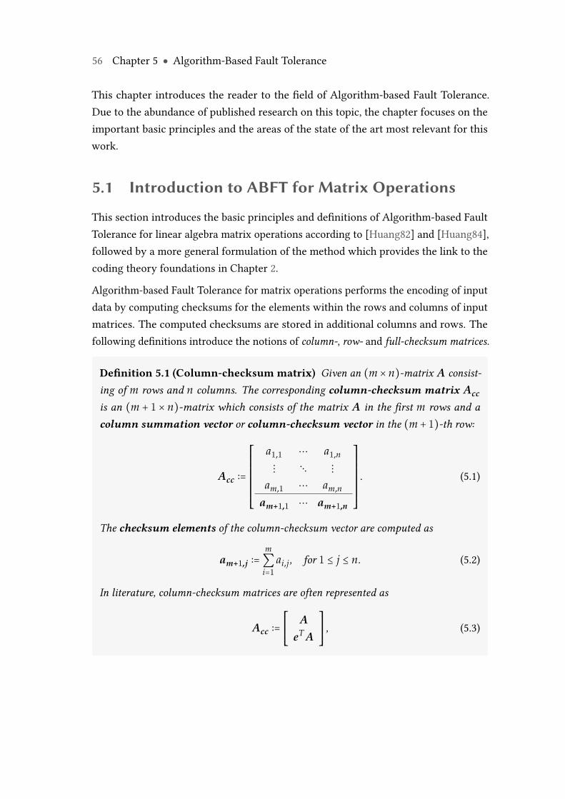
56 Chapter 5 ● Algorithm-Based Fault Tolerance
This chapter introduces the reader to the field of Algorithm-based Fault Tolerance.Due to the abundance of published research on this topic, the chapter focuses on theimportant basic principles and the areas of the state of the art most relevant for thiswork.
5.1 Introduction to ABFT for Matrix Operations
This section introduces the basic principles and definitions of Algorithm-based FaultTolerance for linear algebra matrix operations according to [Huang82] and [Huang84],followed by a more general formulation of the method which provides the link to thecoding theory foundations in Chapter 2.
Algorithm-based Fault Tolerance for matrix operations performs the encoding of inputdata by computing checksums for the elements within the rows and columns of inputmatrices. The computed checksums are stored in additional columns and rows. Thefollowing definitions introduce the notions of column-, row- and full-checksum matrices.
Definition 5.1 (Column-checksum matrix) Given an (m × n)-matrix A consist-ing of m rows and n columns. The corresponding column-checksum matrix Acc
is an (m + 1 × n)-matrix which consists of the matrix A in the first m rows and acolumn summation vector or column-checksum vector in the (m + 1)-th row:
Acc ∶=
⎡⎢⎢⎢⎢⎢⎢⎢⎢⎢⎣
a1,1 ⋯ a1,n
⋮ ⋱ ⋮am,1 ⋯ am,n
am+1,1 ⋯ am+1,n
⎤⎥⎥⎥⎥⎥⎥⎥⎥⎥⎦
. (5.1)
The checksum elements of the column-checksum vector are computed as
am+1,j ∶=m∑i=1
ai,j, for 1 ≤ j ≤ n. (5.2)
In literature, column-checksum matrices are often represented as
Acc ∶=⎡⎢⎢⎢⎢⎣
AeT A
⎤⎥⎥⎥⎥⎦, (5.3)
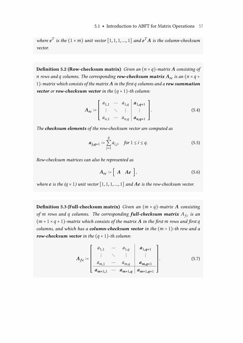
5.1 ● Introduction to ABFT for Matrix Operations 57
where eT is the (1 ×m) unit vector [1, 1, 1, ..., 1] and eT A is the column-checksumvector.
Definition 5.2 (Row-checksum matrix) Given an (n × q)-matrix A consisting ofn rows and q columns. The corresponding row-checksum matrix Arc is an (n × q +1)-matrix which consists of the matrix A in the first q columns and a row summationvector or row-checksum vector in the (q + 1)-th column:
Arc ∶=⎡⎢⎢⎢⎢⎢⎢⎣
a1,1 ⋯ a1,q a1,q+1
⋮ ⋱ ⋮ ⋮an,1 ⋯ an,q an,q+1
⎤⎥⎥⎥⎥⎥⎥⎦. (5.4)
The checksum elements of the row-checksum vector are computed as
aj,q+1 ∶=q
∑j=1
ai,j, for 1 ≤ i ≤ q. (5.5)
Row-checksum matrices can also be represented as
Arc ∶= [ A Ae ] , (5.6)
where e is the (q × 1) unit vector [1, 1, 1, ..., 1] and Ae is the row-checksum vector.
Definition 5.3 (Full-checksum matrix) Given an (m × q)-matrix A consistingof m rows and q columns. The corresponding full-checksum matrix A f c is an(m + 1× q + 1)-matrix which consists of the matrix A in the first m rows and first qcolumns, and which has a column-checksum vector in the (m + 1)-th row and arow-checksum vector in the (q + 1)-th column:
A f c ∶=
⎡⎢⎢⎢⎢⎢⎢⎢⎢⎢⎣
a1,1 ⋯ a1,q a1,q+1
⋮ ⋱ ⋮ ⋮am,1 ⋯ am,q am,q+1
am+1,1 ⋯ am+1,q am+1,q+1
⎤⎥⎥⎥⎥⎥⎥⎥⎥⎥⎦
. (5.7)
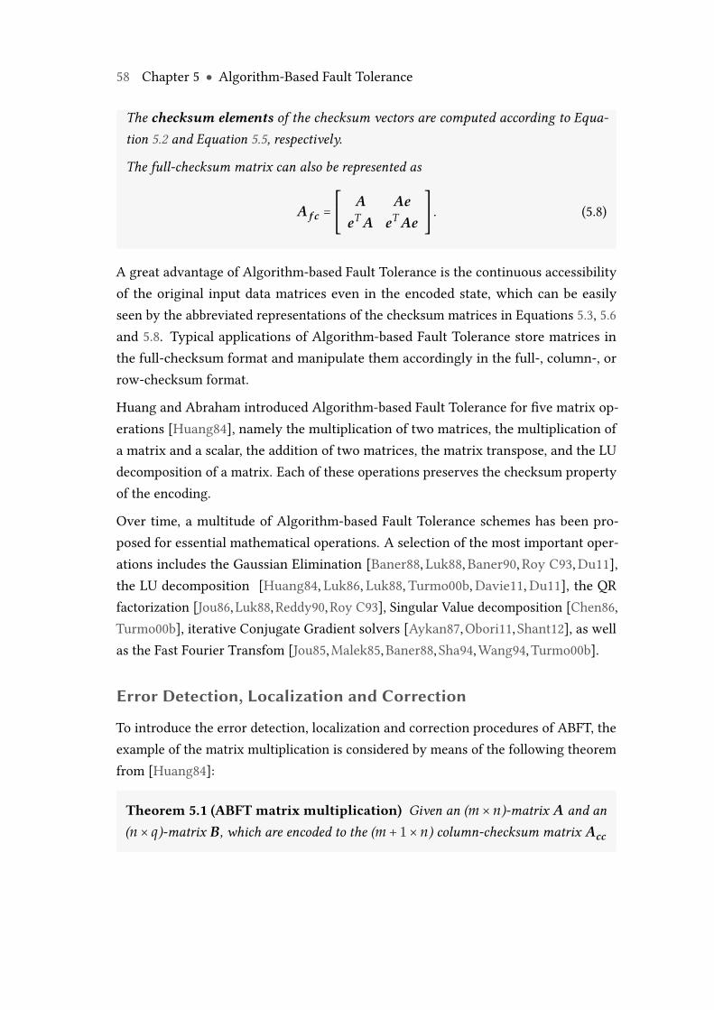
58 Chapter 5 ● Algorithm-Based Fault Tolerance
The checksum elements of the checksum vectors are computed according to Equa-tion 5.2 and Equation 5.5, respectively.
The full-checksum matrix can also be represented as
A f c =⎡⎢⎢⎢⎢⎣
A AeeT A eT Ae
⎤⎥⎥⎥⎥⎦. (5.8)
A great advantage of Algorithm-based Fault Tolerance is the continuous accessibilityof the original input data matrices even in the encoded state, which can be easilyseen by the abbreviated representations of the checksum matrices in Equations 5.3, 5.6and 5.8. Typical applications of Algorithm-based Fault Tolerance store matrices inthe full-checksum format and manipulate them accordingly in the full-, column-, orrow-checksum format.
Huang and Abraham introduced Algorithm-based Fault Tolerance for five matrix op-erations [Huang84], namely the multiplication of two matrices, the multiplication ofa matrix and a scalar, the addition of two matrices, the matrix transpose, and the LUdecomposition of a matrix. Each of these operations preserves the checksum propertyof the encoding.
Over time, a multitude of Algorithm-based Fault Tolerance schemes has been pro-posed for essential mathematical operations. A selection of the most important oper-ations includes the Gaussian Elimination [Baner88, Luk88, Baner90, Roy C93,Du11],the LU decomposition [Huang84, Luk86, Luk88, Turmo00b, Davie11, Du11], the QRfactorization [Jou86, Luk88,Reddy90,Roy C93], Singular Value decomposition [Chen86,Turmo00b], iterative Conjugate Gradient solvers [Aykan87,Obori11, Shant12], as wellas the Fast Fourier Transfom [Jou85,Malek85,Baner88, Sha94,Wang94,Turmo00b].
Error Detection, Localization and Correction
To introduce the error detection, localization and correction procedures of ABFT, theexample of the matrix multiplication is considered by means of the following theoremfrom [Huang84]:
Theorem 5.1 (ABFT matrix multiplication) Given an (m × n)-matrix A and an(n × q)-matrix B, which are encoded to the (m + 1× n) column-checksum matrix Acc
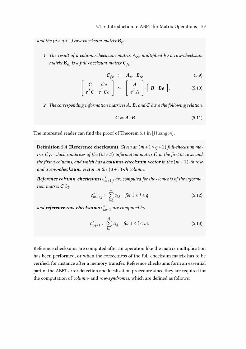
5.1 ● Introduction to ABFT for Matrix Operations 59
and the (n × q + 1) row-checksum matrix Brc.
1. The result of a column-checksum matrix Acc multiplied by a row-checksummatrix Brc is a full-checksum matrix C f c:
C f c ∶= Acc ⋅ Brc (5.9)⎡⎢⎢⎢⎢⎣
C CeeTC eTCe
⎤⎥⎥⎥⎥⎦∶=⎡⎢⎢⎢⎢⎣
AeT A
⎤⎥⎥⎥⎥⎦⋅ [ B Be ] . (5.10)
2. The corresponding information matrices A, B, and C have the following relation:
C ∶= A ⋅ B. (5.11)
The interested reader can find the proof of Theorem 5.1 in [Huang84].
Definition 5.4 (Reference checksum) Given an (m+1× q+1) full-checksumma-trix C f c which comprises of the (m × q) information matrix C in the first m rows andthe first q columns, and which has a column-checksum vector in the (m+ 1)-th rowand a row-checksum vector in the (q + 1)-th column.
Reference column-checksums c∗m+1,j are computed for the elements of the informa-tion matrix C by
c∗m+1,j ∶=m∑i=1
ci,j for 1 ≤ j ≤ q (5.12)
and reference row-checksums c∗i,q+1 are computed by
c∗i,q+1 ∶=q
∑j=1
ci,j for 1 ≤ i ≤ m. (5.13)
Reference checksums are computed after an operation like the matrix multiplicationhas been performed, or when the correctness of the full-checksum matrix has to beverified, for instance after a memory transfer. Reference checksums form an essentialpart of the ABFT error detection and localization procedure since they are required forthe computation of column- and row-syndromes, which are defined as follows:
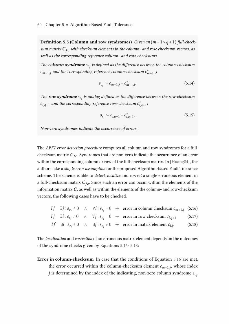
60 Chapter 5 ● Algorithm-Based Fault Tolerance
Definition 5.5 (Column and row syndromes) Given an (m+1×q+1) full-check-sum matrix C f c with checksum elements in the column- and row-checksum vectors, aswell as the corresponding reference column- and row-checksums.
The column syndrome scjis defined as the difference between the column-checksum
cm+1,j and the corresponding reference column-checksum c∗m+1,j:
scj∶= cm+1,j − c∗m+1,j. (5.14)
The row syndrome sriis analog defined as the difference between the row-checksum
ci,q+1 and the corresponding reference row-checksum c∗i,q+1:
sri∶= ci,q+1 − c∗i,q+1. (5.15)
Non-zero syndromes indicate the occurrence of errors.
The ABFT error detection procedure computes all column and row syndromes for a full-checksum matrix C f c. Syndromes that are non-zero indicate the occurrence of an errorwithin the corresponding column or row of the full-checksummatrix. In [Huang84], theauthors take a single error assumption for the proposed Algorithm-based Fault Tolerancescheme. The scheme is able to detect, localize and correct a single erroneous element ina full-checksum matrix C f c. Since such an error can occur within the elements of theinformation matrix C, as well as within the elements of the column- and row-checksumvectors, the following cases have to be checked:
I f ∃j ∶ scj≠ 0 ∧ ∀i ∶ sri
= 0 → error in column checksum cm+1,j (5.16)
I f ∃i ∶ sri≠ 0 ∧ ∀j ∶ scj
= 0 → error in row checksum ci,q+1 (5.17)
I f ∃i ∶ sri≠ 0 ∧ ∃j ∶ scj
≠ 0 → error in matrix element ci,j. (5.18)
The localization and correction of an erroneous matrix element depends on the outcomesof the syndrome checks given by Equations 5.16- 5.18:
Error in column-checksum In case that the conditions of Equation 5.16 are met,the error occurred within the column-checksum element cm+1,j, whose indexj is determined by the index of the indicating, non-zero column syndrome scj
.
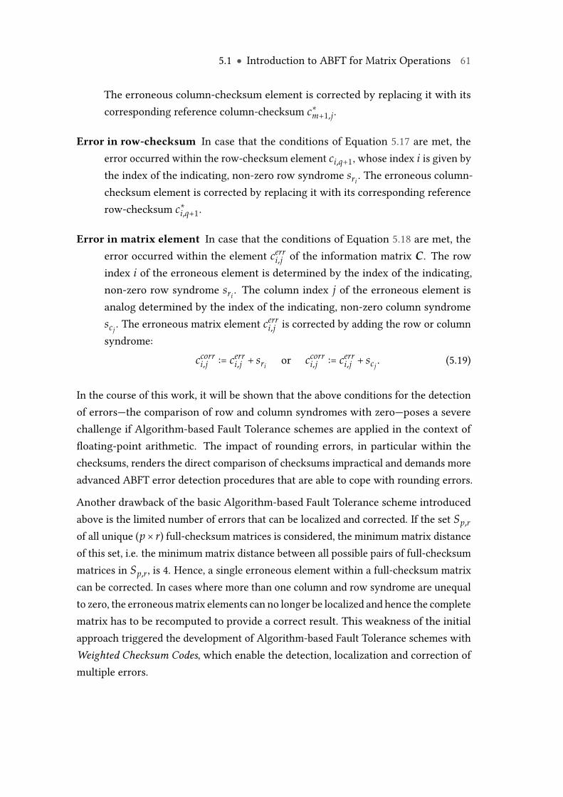
5.1 ● Introduction to ABFT for Matrix Operations 61
The erroneous column-checksum element is corrected by replacing it with itscorresponding reference column-checksum c∗m+1,j.
Error in row-checksum In case that the conditions of Equation 5.17 are met, theerror occurred within the row-checksum element ci,q+1, whose index i is given bythe index of the indicating, non-zero row syndrome sri
. The erroneous column-checksum element is corrected by replacing it with its corresponding referencerow-checksum c∗i,q+1.
Error in matrix element In case that the conditions of Equation 5.18 are met, theerror occurred within the element cerr
i,j of the information matrix C. The rowindex i of the erroneous element is determined by the index of the indicating,non-zero row syndrome sri
. The column index j of the erroneous element isanalog determined by the index of the indicating, non-zero column syndromescj
. The erroneous matrix element cerri,j is corrected by adding the row or column
syndrome:ccorr
i,j ∶= cerri,j + sri
or ccorri,j ∶= cerr
i,j + scj. (5.19)
In the course of this work, it will be shown that the above conditions for the detectionof errors—the comparison of row and column syndromes with zero—poses a severechallenge if Algorithm-based Fault Tolerance schemes are applied in the context offloating-point arithmetic. The impact of rounding errors, in particular within thechecksums, renders the direct comparison of checksums impractical and demands moreadvanced ABFT error detection procedures that are able to cope with rounding errors.
Another drawback of the basic Algorithm-based Fault Tolerance scheme introducedabove is the limited number of errors that can be localized and corrected. If the set Sp,r
of all unique (p× r) full-checksum matrices is considered, the minimum matrix distanceof this set, i.e. the minimum matrix distance between all possible pairs of full-checksummatrices in Sp,r, is 4. Hence, a single erroneous element within a full-checksum matrixcan be corrected. In cases where more than one column and row syndrome are unequalto zero, the erroneousmatrix elements can no longer be localized and hence the completematrix has to be recomputed to provide a correct result. This weakness of the initialapproach triggered the development of Algorithm-based Fault Tolerance schemes withWeighted Checksum Codes, which enable the detection, localization and correction ofmultiple errors.
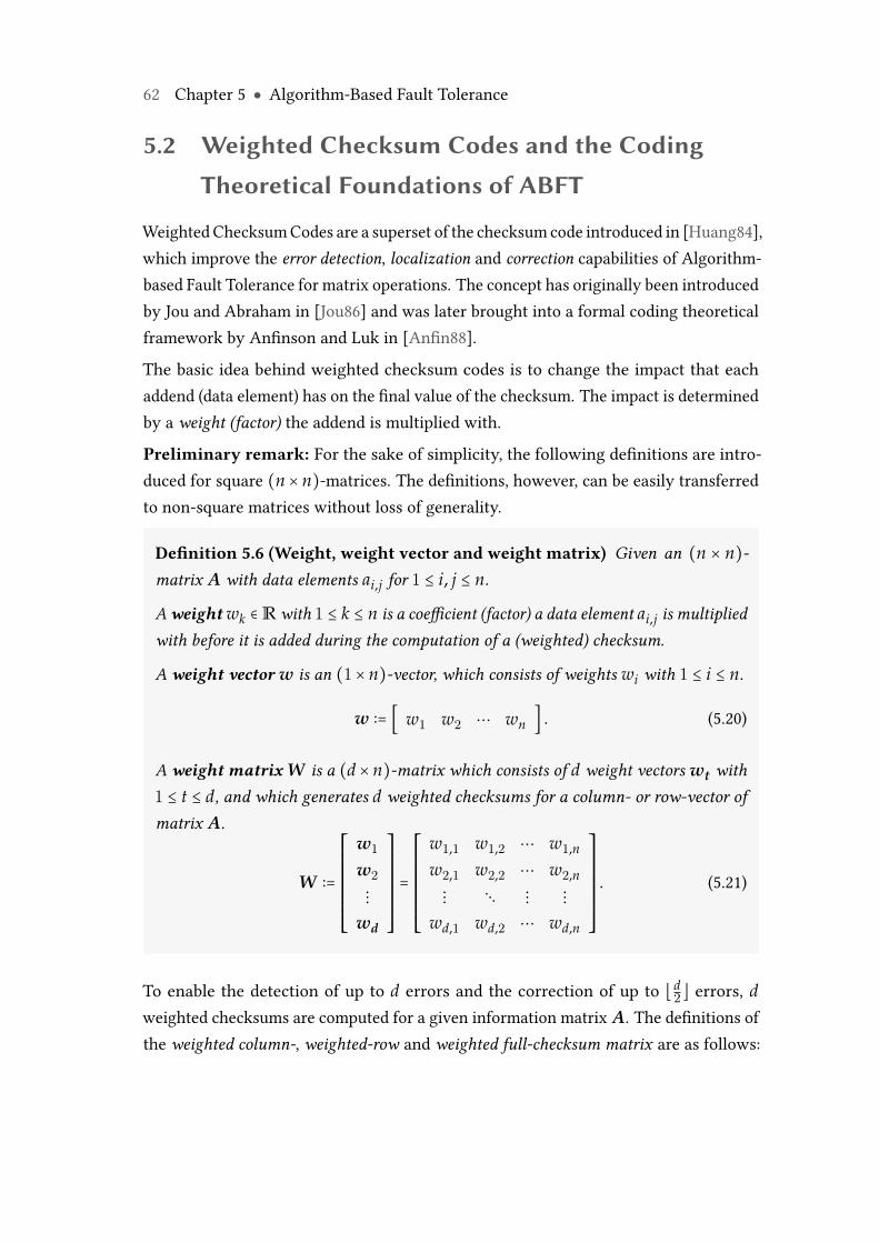
62 Chapter 5 ● Algorithm-Based Fault Tolerance
5.2 Weighted Checksum Codes and the CodingTheoretical Foundations of ABFT
Weighted ChecksumCodes are a superset of the checksum code introduced in [Huang84],which improve the error detection, localization and correction capabilities of Algorithm-based Fault Tolerance for matrix operations. The concept has originally been introducedby Jou and Abraham in [Jou86] and was later brought into a formal coding theoreticalframework by Anfinson and Luk in [Anfin88].
The basic idea behind weighted checksum codes is to change the impact that eachaddend (data element) has on the final value of the checksum. The impact is determinedby a weight (factor) the addend is multiplied with.
Preliminary remark: For the sake of simplicity, the following definitions are intro-duced for square (n × n)-matrices. The definitions, however, can be easily transferredto non-square matrices without loss of generality.
Definition 5.6 (Weight, weight vector and weight matrix) Given an (n × n)-matrix A with data elements ai,j for 1 ≤ i, j ≤ n.
Aweight wk ∈R with 1 ≤ k ≤ n is a coefficient (factor) a data element ai,j is multipliedwith before it is added during the computation of a (weighted) checksum.
A weight vector w is an (1× n)-vector, which consists of weights wi with 1 ≤ i ≤ n.
w ∶= [ w1 w2 ⋯ wn ] . (5.20)
A weight matrix W is a (d × n)-matrix which consists of d weight vectors wt with1 ≤ t ≤ d, and which generates d weighted checksums for a column- or row-vector ofmatrix A.
W ∶=
⎡⎢⎢⎢⎢⎢⎢⎢⎢⎢⎣
w1
w2
⋮wd
⎤⎥⎥⎥⎥⎥⎥⎥⎥⎥⎦
=
⎡⎢⎢⎢⎢⎢⎢⎢⎢⎢⎣
w1,1 w1,2 ⋯ w1,n
w2,1 w2,2 ⋯ w2,n
⋮ ⋱ ⋮ ⋮wd,1 wd,2 ⋯ wd,n
⎤⎥⎥⎥⎥⎥⎥⎥⎥⎥⎦
. (5.21)
To enable the detection of up to d errors and the correction of up to ⌊d2⌋ errors, d
weighted checksums are computed for a given information matrix A. The definitions ofthe weighted column-, weighted-row and weighted full-checksum matrix are as follows:
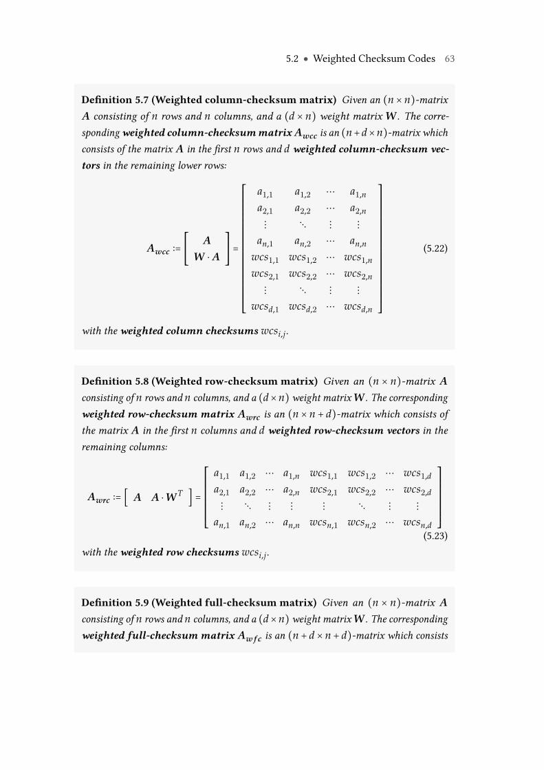
5.2 ● Weighted Checksum Codes 63
Definition 5.7 (Weighted column-checksum matrix) Given an (n × n)-matrixA consisting of n rows and n columns, and a (d × n) weight matrix W . The corre-spondingweighted column-checksummatrix Awcc is an (n+d×n)-matrix whichconsists of the matrix A in the first n rows and d weighted column-checksum vec-tors in the remaining lower rows:
Awcc ∶=⎡⎢⎢⎢⎢⎣
AW ⋅ A
⎤⎥⎥⎥⎥⎦=
⎡⎢⎢⎢⎢⎢⎢⎢⎢⎢⎢⎢⎢⎢⎢⎢⎢⎢⎢⎢⎢⎢⎣
a1,1 a1,2 ⋯ a1,n
a2,1 a2,2 ⋯ a2,n
⋮ ⋱ ⋮ ⋮an,1 an,2 ⋯ an,n
wcs1,1 wcs1,2 ⋯ wcs1,n
wcs2,1 wcs2,2 ⋯ wcs2,n
⋮ ⋱ ⋮ ⋮wcsd,1 wcsd,2 ⋯ wcsd,n
⎤⎥⎥⎥⎥⎥⎥⎥⎥⎥⎥⎥⎥⎥⎥⎥⎥⎥⎥⎥⎥⎥⎦
(5.22)
with the weighted column checksums wcsi,j.
Definition 5.8 (Weighted row-checksum matrix) Given an (n × n)-matrix Aconsisting of n rows and n columns, and a (d×n)weight matrix W . The correspondingweighted row-checksum matrix Awrc is an (n × n + d)-matrix which consists ofthe matrix A in the first n columns and d weighted row-checksum vectors in theremaining columns:
Awrc ∶= [ A A ⋅W T ] =
⎡⎢⎢⎢⎢⎢⎢⎢⎢⎢⎣
a1,1 a1,2 ⋯ a1,n wcs1,1 wcs1,2 ⋯ wcs1,d
a2,1 a2,2 ⋯ a2,n wcs2,1 wcs2,2 ⋯ wcs2,d
⋮ ⋱ ⋮ ⋮ ⋮ ⋱ ⋮ ⋮an,1 an,2 ⋯ an,n wcsn,1 wcsn,2 ⋯ wcsn,d
⎤⎥⎥⎥⎥⎥⎥⎥⎥⎥⎦(5.23)
with the weighted row checksums wcsi,j.
Definition 5.9 (Weighted full-checksum matrix) Given an (n × n)-matrix Aconsisting of n rows and n columns, and a (d×n)weight matrix W . The correspondingweighted full-checksum matrix Aw f c is an (n + d × n + d)-matrix which consists
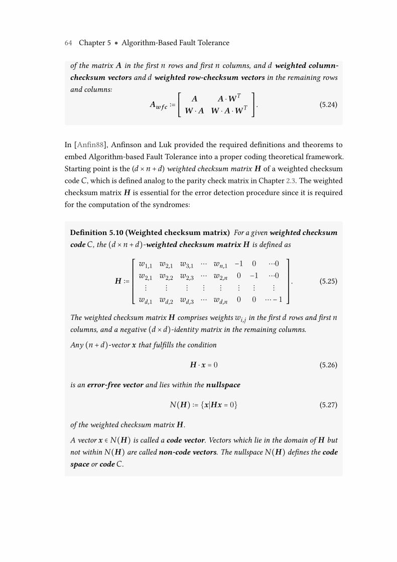
64 Chapter 5 ● Algorithm-Based Fault Tolerance
of the matrix A in the first n rows and first n columns, and d weighted column-checksum vectors and d weighted row-checksum vectors in the remaining rowsand columns:
Aw f c ∶=⎡⎢⎢⎢⎢⎣
A A ⋅W T
W ⋅ A W ⋅ A ⋅W T
⎤⎥⎥⎥⎥⎦. (5.24)
In [Anfin88], Anfinson and Luk provided the required definitions and theorems toembed Algorithm-based Fault Tolerance into a proper coding theoretical framework.Starting point is the (d × n + d) weighted checksum matrix H of a weighted checksumcode C, which is defined analog to the parity check matrix in Chapter 2.3. The weightedchecksum matrix H is essential for the error detection procedure since it is requiredfor the computation of the syndromes:
Definition 5.10 (Weighted checksum matrix) For a givenweighted checksumcode C, the (d × n + d)-weighted checksum matrix H is defined as
H ∶=
⎡⎢⎢⎢⎢⎢⎢⎢⎢⎢⎣
w1,1 w2,1 w3,1 ⋯ wn,1 −1 0 ⋯0w2,1 w2,2 w2,3 ⋯ w2,n 0 −1 ⋯0⋮ ⋮ ⋮ ⋮ ⋮ ⋮ ⋮ ⋮
wd,1 wd,2 wd,3 ⋯ wd,n 0 0 ⋯− 1
⎤⎥⎥⎥⎥⎥⎥⎥⎥⎥⎦
. (5.25)
The weighted checksum matrix H comprises weights wi,j in the first d rows and first ncolumns, and a negative (d × d)-identity matrix in the remaining columns.
Any (n + d)-vector x that fulfills the condition
H ⋅ x = 0 (5.26)
is an error-free vector and lies within the nullspace
N(H) ∶= {x∣Hx = 0} (5.27)
of the weighted checksum matrix H.
A vector x ∈ N(H) is called a code vector. Vectors which lie in the domain of H butnot within N(H) are called non-code vectors. The nullspace N(H) defines the codespace or code C.
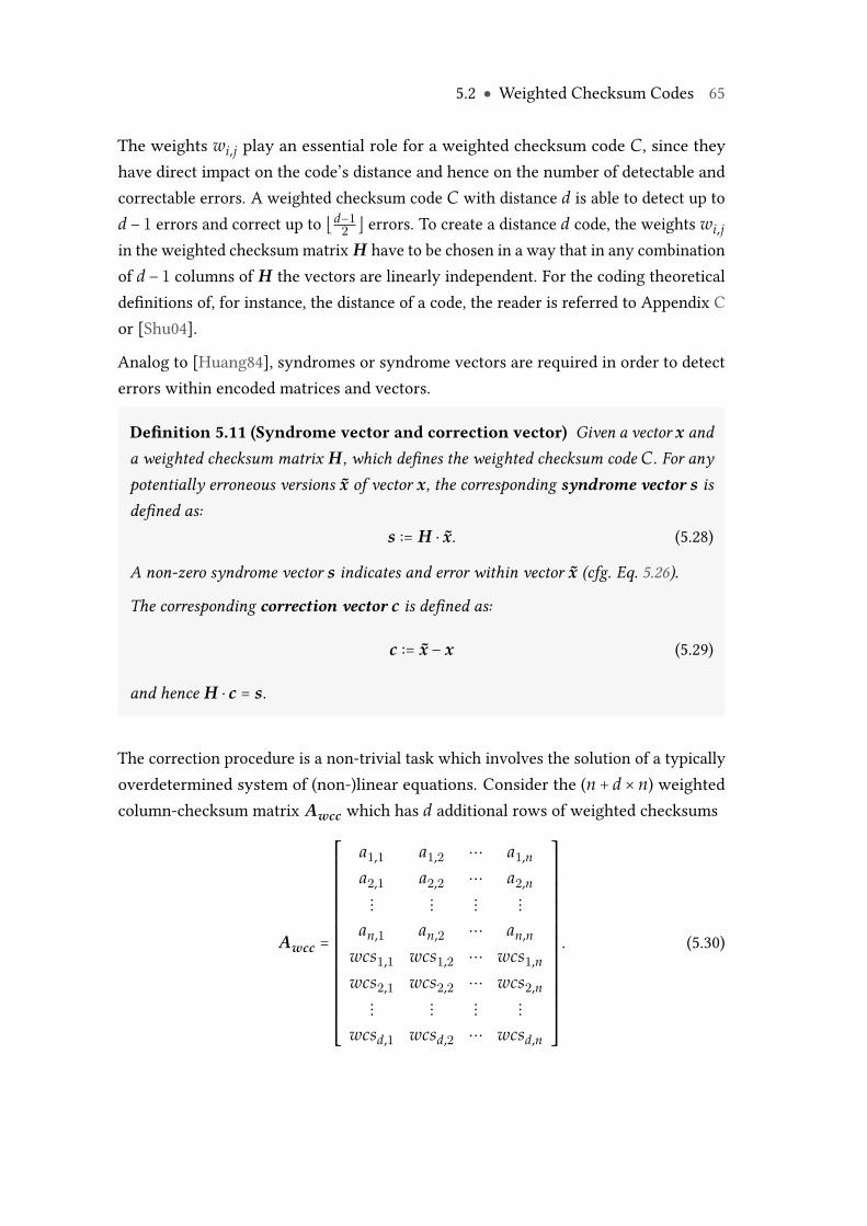
5.2 ● Weighted Checksum Codes 65
The weights wi,j play an essential role for a weighted checksum code C, since theyhave direct impact on the code’s distance and hence on the number of detectable andcorrectable errors. A weighted checksum code C with distance d is able to detect up tod − 1 errors and correct up to ⌊d−1
2 ⌋ errors. To create a distance d code, the weights wi,j
in the weighted checksummatrix H have to be chosen in a way that in any combinationof d − 1 columns of H the vectors are linearly independent. For the coding theoreticaldefinitions of, for instance, the distance of a code, the reader is referred to Appendix Cor [Shu04].
Analog to [Huang84], syndromes or syndrome vectors are required in order to detecterrors within encoded matrices and vectors.
Definition 5.11 (Syndrome vector and correction vector) Given a vector x anda weighted checksum matrix H , which defines the weighted checksum code C. For anypotentially erroneous versions x of vector x, the corresponding syndrome vector s isdefined as:
s ∶= H ⋅ x. (5.28)
A non-zero syndrome vector s indicates and error within vector x (cfg. Eq. 5.26).
The corresponding correction vector c is defined as:
c ∶= x − x (5.29)
and hence H ⋅ c = s.
The correction procedure is a non-trivial task which involves the solution of a typicallyoverdetermined system of (non-)linear equations. Consider the (n + d × n) weightedcolumn-checksum matrix Awcc which has d additional rows of weighted checksums
Awcc =
⎡⎢⎢⎢⎢⎢⎢⎢⎢⎢⎢⎢⎢⎢⎢⎢⎢⎢⎢⎢⎢⎢⎣
a1,1 a1,2 ⋯ a1,n
a2,1 a2,2 ⋯ a2,n
⋮ ⋮ ⋮ ⋮an,1 an,2 ⋯ an,n
wcs1,1 wcs1,2 ⋯ wcs1,n
wcs2,1 wcs2,2 ⋯ wcs2,n
⋮ ⋮ ⋮ ⋮wcsd,1 wcsd,2 ⋯ wcsd,n
⎤⎥⎥⎥⎥⎥⎥⎥⎥⎥⎥⎥⎥⎥⎥⎥⎥⎥⎥⎥⎥⎥⎦
. (5.30)
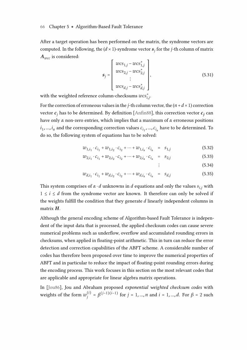
66 Chapter 5 ● Algorithm-Based Fault Tolerance
After a target operation has been performed on the matrix, the syndrome vectors arecomputed. In the following, the (d×1)-syndrome vector sj for the j-th column of matrixAwcc is considered:
sj =
⎡⎢⎢⎢⎢⎢⎢⎢⎢⎢⎢⎣
wcs1,j −wcs∗1,j
wcs2,j −wcs∗2,j
⋮wcsd,j −wcs∗d,j
⎤⎥⎥⎥⎥⎥⎥⎥⎥⎥⎥⎦
, (5.31)
with the weighted reference column-checksums wcs∗i,j.
For the correction of erroneous values in the j-th column vector, the (n+d×1) correctionvector cj has to be determined. By definition [Anfin88], this correction vector cj canhave only α non-zero entries, which implies that a maximum of α erroneous positionsi1, ..., iα and the corresponding correction values ci1 , ..., ciα have to be determined. Todo so, the following system of equations has to be solved:
w1,i1 ⋅ ci1 +w1,i2 ⋅ ci2 +⋯+w1,iα ⋅ ciα = s1,j (5.32)
w2,i1 ⋅ ci1 +w2,i2 ⋅ ci2 +⋯+w2,iα ⋅ ciα = s2,j (5.33)
⋮ (5.34)
wd,i1 ⋅ ci1 +wd,i2 ⋅ ci2 +⋯+wd,iα ⋅ ciα = sd,j (5.35)
This system comprises of α ⋅ d unknowns in d equations and only the values si,j with1 ≤ i ≤ d from the syndrome vector are known. It therefore can only be solved ifthe weights fulfill the condition that they generate d linearly independent columns inmatrix H.
Although the general encoding scheme of Algorithm-based Fault Tolerance is indepen-dent of the input data that is processed, the applied checksum codes can cause severenumerical problems such as underflow, overflow and accumulated rounding errors inchecksums, when applied in floating-point arithmetic. This in turn can reduce the errordetection and correction capabilities of the ABFT scheme. A considerable number ofcodes has therefore been proposed over time to improve the numerical properties ofABFT and in particular to reduce the impact of floating-point rounding errors duringthe encoding process. This work focuses in this section on the most relevant codes thatare applicable and appropriate for linear algebra matrix operations.
In [Jou86], Jou and Abraham proposed exponential weighted checksum codes withweights of the form w(i)j = β(j−1)(i−1) for j = 1, ..., n and i = 1, ..., d. For β = 2 such
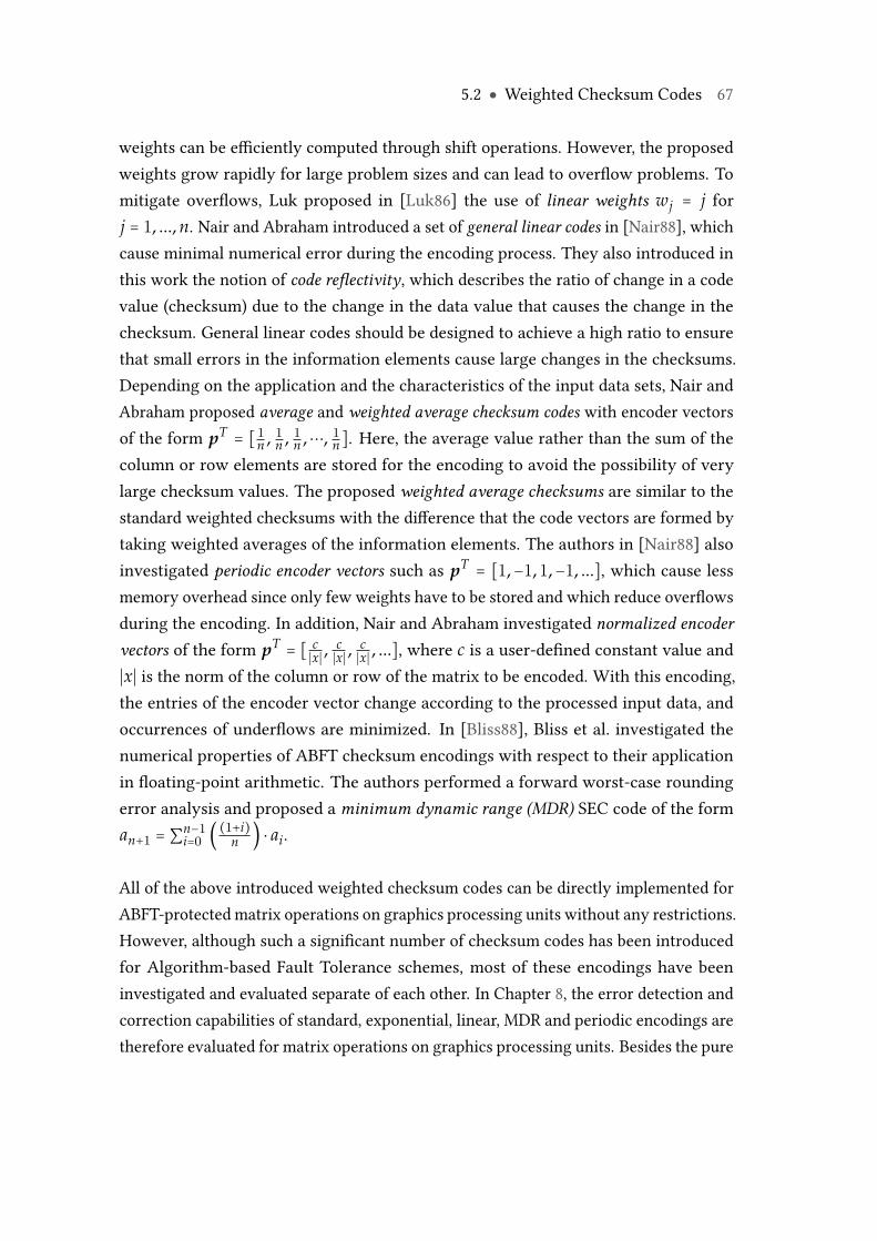
5.2 ● Weighted Checksum Codes 67
weights can be efficiently computed through shift operations. However, the proposedweights grow rapidly for large problem sizes and can lead to overflow problems. Tomitigate overflows, Luk proposed in [Luk86] the use of linear weights wj = j forj = 1, ..., n. Nair and Abraham introduced a set of general linear codes in [Nair88], whichcause minimal numerical error during the encoding process. They also introduced inthis work the notion of code reflectivity, which describes the ratio of change in a codevalue (checksum) due to the change in the data value that causes the change in thechecksum. General linear codes should be designed to achieve a high ratio to ensurethat small errors in the information elements cause large changes in the checksums.Depending on the application and the characteristics of the input data sets, Nair andAbraham proposed average and weighted average checksum codes with encoder vectorsof the form pT = [ 1n , 1
n , 1n ,⋯, 1
n]. Here, the average value rather than the sum of thecolumn or row elements are stored for the encoding to avoid the possibility of verylarge checksum values. The proposed weighted average checksums are similar to thestandard weighted checksums with the difference that the code vectors are formed bytaking weighted averages of the information elements. The authors in [Nair88] alsoinvestigated periodic encoder vectors such as pT = [1,−1, 1,−1, ...], which cause lessmemory overhead since only few weights have to be stored and which reduce overflowsduring the encoding. In addition, Nair and Abraham investigated normalized encodervectors of the form pT = [ c
∣x∣ ,c∣x∣ ,
c∣x∣ , ...], where c is a user-defined constant value and
∣x∣ is the norm of the column or row of the matrix to be encoded. With this encoding,the entries of the encoder vector change according to the processed input data, andoccurrences of underflows are minimized. In [Bliss88], Bliss et al. investigated thenumerical properties of ABFT checksum encodings with respect to their applicationin floating-point arithmetic. The authors performed a forward worst-case roundingerror analysis and proposed a minimum dynamic range (MDR) SEC code of the forman+1 = ∑n−1
i=0 ((1+i)
n ) ⋅ ai.
All of the above introduced weighted checksum codes can be directly implemented forABFT-protected matrix operations on graphics processing units without any restrictions.However, although such a significant number of checksum codes has been introducedfor Algorithm-based Fault Tolerance schemes, most of these encodings have beeninvestigated and evaluated separate of each other. In Chapter 8, the error detection andcorrection capabilities of standard, exponential, linear, MDR and periodic encodings aretherefore evaluated for matrix operations on graphics processing units. Besides the pure
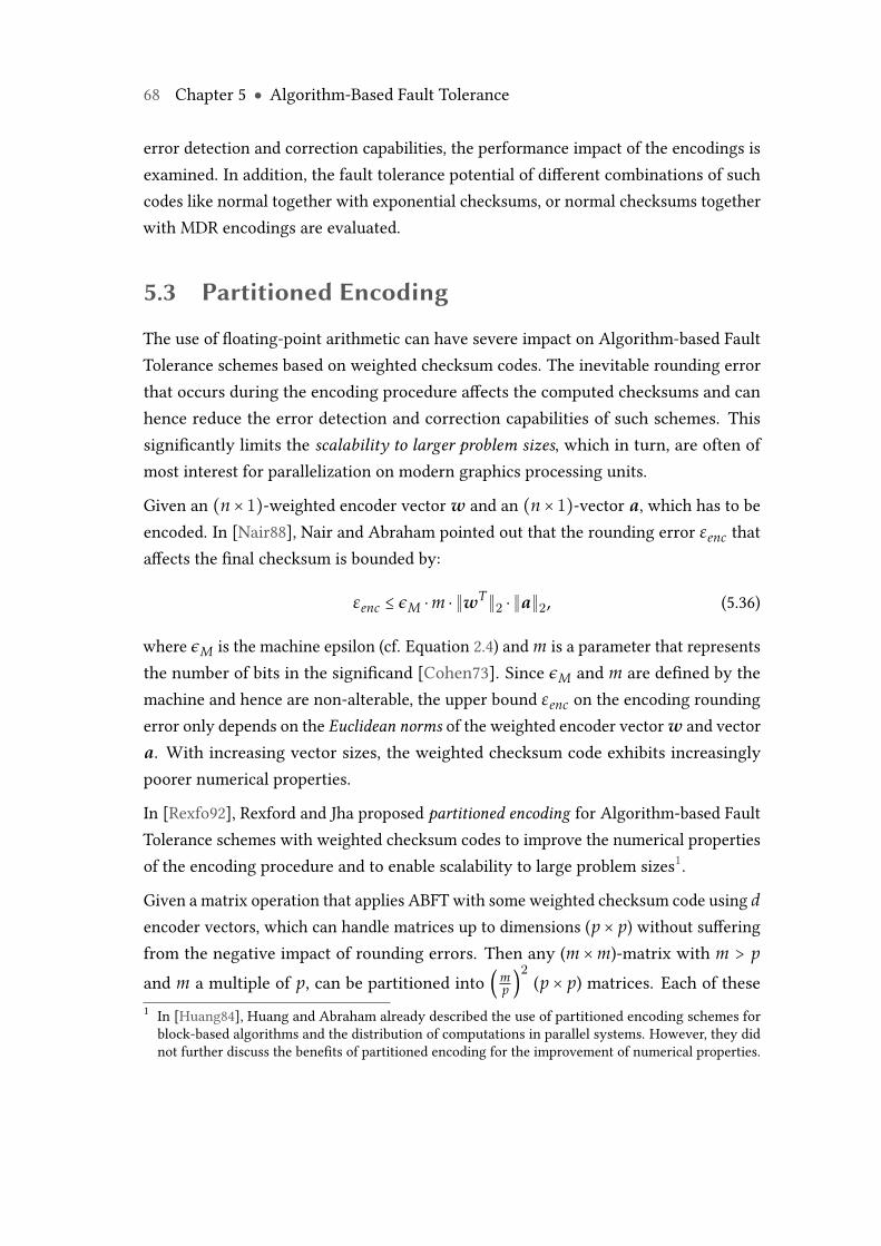
68 Chapter 5 ● Algorithm-Based Fault Tolerance
error detection and correction capabilities, the performance impact of the encodings isexamined. In addition, the fault tolerance potential of different combinations of suchcodes like normal together with exponential checksums, or normal checksums togetherwith MDR encodings are evaluated.
5.3 Partitioned Encoding
The use of floating-point arithmetic can have severe impact on Algorithm-based FaultTolerance schemes based on weighted checksum codes. The inevitable rounding errorthat occurs during the encoding procedure affects the computed checksums and canhence reduce the error detection and correction capabilities of such schemes. Thissignificantly limits the scalability to larger problem sizes, which in turn, are often ofmost interest for parallelization on modern graphics processing units.
Given an (n × 1)-weighted encoder vector w and an (n × 1)-vector a, which has to beencoded. In [Nair88], Nair and Abraham pointed out that the rounding error εenc thataffects the final checksum is bounded by:
εenc ≤ ϵM ⋅m ⋅ ∥wT∥2 ⋅ ∥a∥2, (5.36)
where ϵM is the machine epsilon (cf. Equation 2.4) and m is a parameter that representsthe number of bits in the significand [Cohen73]. Since ϵM and m are defined by themachine and hence are non-alterable, the upper bound εenc on the encoding roundingerror only depends on the Euclidean norms of the weighted encoder vector w and vectora. With increasing vector sizes, the weighted checksum code exhibits increasinglypoorer numerical properties.
In [Rexfo92], Rexford and Jha proposed partitioned encoding for Algorithm-based FaultTolerance schemes with weighted checksum codes to improve the numerical propertiesof the encoding procedure and to enable scalability to large problem sizes1.
Given a matrix operation that applies ABFT with some weighted checksum code using dencoder vectors, which can handle matrices up to dimensions (p × p) without sufferingfrom the negative impact of rounding errors. Then any (m ×m)-matrix with m > p
and m a multiple of p, can be partitioned into (mp )
2(p × p) matrices. Each of these
1 In [Huang84], Huang and Abraham already described the use of partitioned encoding schemes forblock-based algorithms and the distribution of computations in parallel systems. However, they didnot further discuss the benefits of partitioned encoding for the improvement of numerical properties.
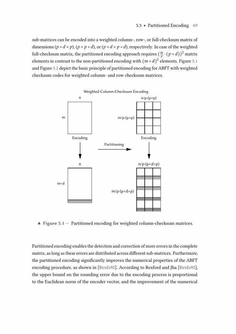
5.3 ● Partitioned Encoding 69
sub-matrices can be encoded into a weighted column-, row-, or full-checksum matrix ofdimensions (p+ d× p), (p× p+ d), or (p+ d× p+ d), respectively. In case of the weightedfull-checksum matrix, the partitioned encoding approach requires (m
p ⋅ (p+ d))2 matrixelements in contrast to the non-partitioned encoding with (m+ d)2 elements. Figure 5.1and Figure 5.2 depict the basic principle of partitioned encoding for ABFTwith weightedchecksum codes for weighted column- and row checksum matrices.
n
Partitioning
Weighted Column-Checksum Encoding
m m/p∙(p×p)
m/p∙(p+d×p)
m+d
n/p∙(p×p)
n n/p∙(p+d×p)
Encoding Encoding
Weighted Row-Checksum Encoding▲ Figure 5.1 — Partitioned encoding for weighted column-checksum matrices.
Partitioned encoding enables the detection and correction of more errors in the completematrix, as long as these errors are distributed across different sub-matrices. Furthermore,the partitioned encoding significantly improves the numerical properties of the ABFTencoding procedure, as shown in [Rexfo92]. According to Rexford and Jha [Rexfo92],the upper bound on the rounding error due to the encoding process is proportionalto the Euclidean norm of the encoder vector, and the improvement of the numerical
70 Chapter 5 ● Algorithm-Based Fault Tolerance
Weighted Row-Checksum Encoding
q
q+d
n n/p∙(p×p)
n/p∙(p×p+d)
q/p∙(p×p)
q/p∙(p×p+d)
n
Encoding EncodingPartitioning
▲ Figure 5.2 — Partitioned encoding for weighted row-checksum matrices.
properties can be quantified by the factor
γ ∶=∣∣wT
p ∣∣2∣∣wT
m∣∣2. (5.37)
The partitioned encoding checksum property is preserved by matrix operations like thematrix multiplication, the matrix addition, the multiplication of a matrix with a scalar,the matrix transpose, as well as the LU decomposition. Further matrix operations canbe adapted to support ABFT with partitioned encoding.
Moreover, partitioned encoding matches classic block-based matrix algorithms, forinstance, for the multiplication of matrices. It also provides a perfect match for theblock-based execution paradigm (thread blocks) on modern graphics processing units.In this context, the impact of the sub-matrix dimensions (p × p) on the encoding andhence on the error detection and correction capabilities of ABFT schemes, as well asthe potential impact on the GPU performance has not yet been investigated. Sincep represents an important design parameter for fault tolerant linear algebra matrixoperations on GPUs, Chapter 8 provides an in-depth analysis of relevant encodingblock sizes on GPUs.
5.4 ● Handling of Rounding Errors 71
5.4 Handling of Rounding Errors
In floating-point arithmetic systems, Algorithm-based Fault Tolerance schemes haveto cope with rounding errors during different phases. Rounding errors are introducedduring the initial encoding and during the computation of reference checksums in theresult checking procedure. Rounding errors are, of course, also introduced during thecomputations performed by the target algorithm. In Section 5.2, different codes havebeen introduced which improve the numerical properties of the encoding. In Section 5.3,partitioned encoding was introduced as a technique which also improves the numericalquality of the encoding, and which enables the seamless scaling of ABFT schemes tolarge problem sizes without affecting the encoding. Nevertheless, the rounding errorsthat affect the checksum comparison during the ABFT result checking procedure remaina hard challenge, since they render the direct comparison for equality of checksumsuseless.
Appropriate rounding error bounds (tolerances) are therefore required for the reliableonline classification of errors into inevitable rounding errors due to limited numericalprecision, tolerable compute errors in the magnitude of such rounding errors, and intocritical errors that are larger than those and not tolerable.
Up to date, different approaches have been proposed for the determination of roundingerror bounds, including experimental calibration-based approaches, schemes based onmantissa checks and approaches based on analytical rounding error bounds.
In [Baner88] and [Baner90], Banerjee et al. determined rounding error bounds basedon experimental calibrations. The authors expressed the norm of the error εcomp incomputations due to rounding as
∥εcomp∥ ∶= K ⋅ F(N) ⋅ 2−2t, (5.38)
where K is an application-dependent constant, F(N) is an application-dependent func-tion of the problem size, and t is the size of the significand in the used floating-pointrepresentation. The authors did not disclose any further details on the determination ofthe application-specific constant K or the function F(N). They only mentioned that forthe Fast Fourier Transform F(N) = log(N). In fault injection experiments performedby the authors, the problem size was kept fix and the norm of the error due to roundingwas substituted by a constant K′. This constant was chosen through calibration in away that the error coverage was maximized while keeping the number of false alarms
72 Chapter 5 ● Algorithm-Based Fault Tolerance
equal to zero. To achieve a suitable calibration, a large number of different data sets wasconsidered. The data sets were all of the same size and span approximately the samerange. The target computation was executed repeatedly on the data sets, starting witha rounding error bound equal to zero. Every time the fault tolerance scheme detectedan error (false alarm), the bound was increased. This procedure has been repeated untilno more false alarms occurred on the data sets.
The experimental calibration has massive drawbacks which make it impractical forthe online determination of rounding error bounds. First, the calibration requiresseveral runs before the intended target computation can be performed. Second, thedetermined rounding error bound is highly likely to produces false-positive and, evenworse, false-negative detections when the characteristics of the input data sets change.Third, the problem size is kept fix for the calibration and hence, every time the problemsize changes, the calibration has to be repeated.
Another group of approaches considers mantissa checks for floating-point results.In [Assad92], so called integer mantissa checks (IMC) have been proposed for matrixmultiplications. These checks treat the significands of floating-point elements in theinput matrices and the product matrix as integers and use the integer ALU to test forerrors in the results. The original approach was only able to apply integer mantissachecks for floating-point multiplications, the authors therefore proposed an additionalcheck for the floating-point additions and called the scheme a hybrid checksum test.In [Zhang94], extended mantissa checksums (EMC) have been introduced, which alsosplit the significands of elements in the product matrix into two parts, which are thenextended to the maximum length allowed by the system’s integer precision. Errorsare detected and corrected in both parts before the parts are merged in the end toyield a full-checksum result matrix. In [Dutt96], the authors extended their previouslyproposed integer mantissa checks and applied the hybrid checksum test to the LUdecomposition. They also described possible extensions of the hardware to supportinteger mantissa checks with less time overhead.
Approaches based on mantissa checks exhibit several issues which hinder their applica-tion. First, the checks are hybrid and only errors in floating-point multiplications can bedetected by these checks. Errors in the floating-point addition part can not be detectedsince this requires the alignment of significand products and hence a loss of precision.A second, non-mantissa check is therefore required for floating-point additions. An-other problem are potential overflows in the product of integer matrices, although this
5.4 ● Handling of Rounding Errors 73
has been addressed in parts by [Zhang94]. The extraction of the significands and therequired computation of the significand product introduce additional computationaland memory overhead.
The third group of proposed approaches for the determination of rounding error boundsis based on classic analytical rounding error bounds. Inter alia, such analytical boundscan be found for numerous linear algebra matrix operations in [Higha02] and [Golub12].
In [Turmo00a,Turmo00b] and [Turmo03], Turmon et al. derived and evaluated sets ofchecksum tests for a number of ABFT-protected linear algebra operations, including thematrix multiplication, to distinguish between intolerable errors and inevitable roundingerrors. The checksum tests are derived from classic analytical rounding error bounds,for instance for the multiplication of matrices A ∈Rm×k and B ∈Rk×n:
E ∶= P − A ⋅ B (5.39)
∣∣E∣∣∞ ≤ max (m, n, k) ⋅ ∣∣A∣∣∞ ⋅ ∣∣B∣∣∞ ⋅ εM, (5.40)
where E is the error matrix, P is the machine-computed matrix product and ϵM isthe machine epsilon (cf. Equation 2.4). The authors proposed an input-independentchecksum test of the form
d ∶= P ⋅w − A ⋅ B ⋅w. (5.41)
∣∣d∣∣∞∣∣A∣∣∞ ⋅ ∣∣B∣∣∞ ⋅ ∣∣w∣∣∞
> τ ⋅ ϵM Ô⇒ error (5.42)
∣∣d∣∣∞∣∣A∣∣∞ ⋅ ∣∣B∣∣∞ ⋅ ∣∣w∣∣∞
≤ τ ⋅ ϵM Ô⇒ rounding error, (5.43)
where w is an ABFT encoder vector2 and τ is defined as an input-independent thresholdvalue. If the discrepancy in Equation 5.42 is larger than τ ⋅ ϵM the approach signals anerror. Otherwise, the divergence is classified as rounding error (Equation 5.43).
The matrix norms required for the proposed checksum test are associated with con-siderable computational overhead. Turmon et al. therefore derived simplified tests.Instead of ∣∣A∣∣∞ ⋅ ∣∣B∣∣∞, they proposed to compute ∣∣P∣∣∞ which equals ∣∣A ⋅B∣∣∞ in theerror-free case. Since ∣∣A ⋅ B∣∣∞ ≤ ∣∣A∣∣∞ ⋅ ∣∣B∣∣∞, this bound underestimates the upperbound for the rounding error and increases the risk of false-positive detections. Tomitigate this problem, the authors suggested the application of an additional scalingfactor which can be absorbed in the factor τ. Following the same idea, ∣∣P ⋅w∣∣∞ could2 Turmon et al. used the basic encoder vector w = [1, 1, ..., 1].
74 Chapter 5 ● Algorithm-Based Fault Tolerance
be used as replacement for ∣∣A∣∣∞ ⋅ ∣∣B∣∣∞ ⋅ ∣∣w∣∣∞. However, this vector norm intensifiesthe risk of false alarms even more. Turmon et al. therefore suggested to computeλ ⋅ ∣∣w∣∣∞ + ∣∣Pw∣∣∞, using an application-dependent factor λ. In conclusion, the aboveintroduced substitutions yielded a set of checksum tests with different trade-offs be-tween error detection capability and computational overhead. The tests all follow fromthe indicated difference matrix ∆, which is never computed explicitly, by computa-tion of the norm δ = ∣∣∆ ⋅w∣∣∞, which is then scaled by a factor defined by the abovesubstitutions. The so called ideal test is then defined as
δ
∣∣A∣∣∞ ⋅ ∣∣B∣∣∞ ⋅ ∣∣w∣∣∞> τ ⋅ ϵM Ô⇒ error, (5.44)
the so called matrix test asδ
∣∣P∣∣∞ ⋅ ∣∣w∣∣∞> τ ⋅ ϵM Ô⇒ error (5.45)
and the so called vector test asδ
λ ⋅ ∣∣w∣∣∞ + ∣∣Pw∣∣∞> τ ⋅ ϵM Ô⇒ error. (5.46)
In [Gunne01], Gunnels et al. followed the general idea of the above introduced approachand proposed norm-based tests for the matrix multiplication, which allow the detectionof errors within the result matrix C, as well as in the two input matrices A ∈R(m×k)
and B ∈ R(k×n). They considered the norm of the difference vectors d and e for row-and column-checksums:
d ∶= Cw −Cw (5.47)
e ∶= vTC − vTC, (5.48)
where w and vT are ABFT encoder vectors and C is the machine-computed matrixproduct. The corresponding checksum tests were of the form
∣∣d∣∣∞ > τ ⋅ ∣∣A∣∣∞ ⋅ ∣∣B∣∣∞ (5.49)
∣∣eT ∣∣∞ > τ ⋅ ∣∣A∣∣∞ ⋅ ∣∣B∣∣∞, (5.50)
where τ =max (m, n, k) ⋅ εM with the machine epsilon ϵM (cf. Equation 2.4).
The norm-based approaches based on analytical rounding error bounds introduce,depending on the chosen checksum test, a considerable computational overhead. More-over, the different error detection and overhead trade-offs require user interaction for
5.4 ● Handling of Rounding Errors 75
the selection of the appropriate test. In [Turmo03], Turmon et al. summarize: "Thekey question for a fault tolerance practitioner is to set the threshold to achieve the righttradeoff between correct fault detections and false alarms. Because of the imprecisioninherent in the error bounds, theoretical results can only give an indication of how expectederror scales with algorithm inputs; the precise constants for best performance must ingeneral be determined empirically for a given algorithm implementation." This rendersthese approaches unattractive for Algorithm-based Fault Tolerance schemes whichare intended to operate in an autonomous manner, independent of the input data anduser-defined thresholds. Another point of criticism of the above described approaches,which is worth to be considered, is the fact that these methods determine roundingerror bounds for complete (sub-)matrices and not for individual checksums. Hence, theresolution or sharpness of these bounds can be rather low.
In [Roy C93], Roy-Chowdhury and Banerjee introduced a novel approach for thedetermination of rounding error bounds for individual checksums. Since their approachis based on the principles of classic analytical rounding error bounds, it is calledSimplified Error Analysis (SEA). The basic idea of this method is to keep track of theaccumulated rounding error in variables after each update of the variables.
Let vk be the value of a variable v after the k-th update, and let vk be the exact, error-freevalue of the variable. Roy-Chowdhury and Banerjee use EB(vk) as a bound on themagnitude of the rounding error accumulation in the computation of vk, where thefollowing relation holds between vk, vk and EB(vk):
∣vk∣ ≤ ∣vk∣+ EB(vk). (5.51)
The set of variables which are involved in the computations between the k-th and (k+1)-th update of v is denoted by Vk and the bound on the magnitude of the accumulatedrounding error associated with these variables is denoted by EBk(V). The boundEBk(V) of the accumulated rounding error is updated according to
EBk+1(v)←Ð Fk(Vk, EB(Vk), ϵM), (5.52)
where ϵM = 2−t is the machine epsilon and t is the number of mantissa bits.
If the computations that take place during the k-th and (k + 1)-th update are known,the function Fk can be derived by application of classic rounding error analysis for theperformed basic floating-point operations. However, this approach of analyzing and
76 Chapter 5 ● Algorithm-Based Fault Tolerance
tracking the accumulated rounding error is associated with considerable memory andtime overhead. Roy-Chowdhury and Banerjee therefore proposed the following threesimplifications:
1. The update function Fk is typically given as polynomial in εM. For a reduction ofthe computational overhead, the higher order error terms (O(ε2
M)) are omitted.
2. The introduction and tracking of a rounding error bound for each variable in-volved in a computation is very expensive. The Simplified Error Analysis thereforederives upper bounds on the total rounding error for groups of variables, forinstance the elements within a row or column of a matrix.
3. For certain algorithms the derived rounding error bound can grow exponentiallywith the execution time. This is reflected by an additional constant factor K ⋅EB(Vk), K > 1, in the update function Fk. In the Simplified Error Analysis, theconstant factor K is set to 1, which prevents exponential growth of the bound.
In [Roy C93], the Simplified Error Analysis (SEA) is introduced for the QR decomposition,the Gaussian Elimination and the matrix multiplication, which serves as example forthe following introduction of SEA.
Given two (n × n)-matrices A and B to be multiplied on a parallel computer systemwith p processors. The computation of the matrix multiplication is distributed amongthe p processors by sending an (m×n) row strip of matrix A and a full copy of matrix Bto each of the processors. The ABFT checksum encoding is done on these (m × n)-sub-matrices of A. Due to the described distribution of the computations, Roy-Chowdhuryand Banerjee considered the matrix-vector multiplication A(m×n) ⋅ b = c, instead of thefull matrix multiplication, to introduce the SEA rounding error bound for the ABFTchecksum comparison procedure. The rounding error bound consists of a combinationof basic analytical rounding error bounds for the product and sum of floating-pointnumbers, as well as the inner product of vectors. These bounds are briefly introducedin the following:
Definition 5.12 (Analytical rounding error bound for products) Given a set ofn real numbers xi ∈R. The product f l(∏n
i=1 xi) of the xi computed in floating-point
5.4 ● Handling of Rounding Errors 77
arithmetic is defined as
f l(n∏i=1
xi) ∶= (1+ E)n∏i=1
xi, (5.53)
where E is the upper bound on the rounding error with
∣E∣ < (n − 1) ⋅ ϵM, (5.54)
and with the machine epsilon ϵM.
Definition 5.13 (Analytical rounding error bound for summations) Given aset of n real numbers xi ∈R. The sum f l(∑n
i=1 xi) of the xi computed in floating-pointarithmetic is defined as
f l(n∑i=1
xi) ∶=n∑i=1
xi(1+ δi), (5.55)
where δi is the upper bound on the rounding error with
∣δ1∣ < (n − 1) ⋅ ϵM (5.56)
∣δi∣ < (n + 1− i) ⋅ ϵM, for i = 2, ..., n, (5.57)
and with the machine epsilon ϵM.
Definition 5.14 (Analytical rounding error bound for inner products) Giventwo vectors x and y with real number elements xi, yi ∈R. The inner product of the twovectors computed in floating-point arithmetic is defined as
f l(xTy) ∶= f l(n∑i=1
xiyi) =n∑i=1
xiyi(1+ δi), (5.58)
where δi is the upper bound on the rounding error with
∣δ1∣ < n ⋅ ϵM (5.59)
∣δi∣ < (n + 2− i) ⋅ ϵM, for i = 2, ..., n, (5.60)
and with the machine epsilon ϵM.
78 Chapter 5 ● Algorithm-Based Fault Tolerance
The rounding error bound can also be expressed as
∣ f l(xTy)− xTy∣ ≤ n ⋅ ϵM ⋅ ∥x∥2∥ ⋅ y∥2. (5.61)
Based on these basic rounding error bounds, Roy-Chowdhury and Banerjee introducedthe rounding error bound for the original checksum elements ci: Given the originalchecksum element c ∈ R and the accompanying original checksum element f l(c)computed in floating-point arithmetic. The rounding error that affects the originalchecksum element is bounded by
∣ f l(c)− c∣ < (m − 1) ⋅ ϵM ⋅m∑i=1∥ai∥2 ⋅ ∥b∥2 + n ⋅ ϵM∥s∥2 ⋅ ∥b∥2, (5.62)
where b is an (n × 1) column vector from matrix B, ai is the i-th row vector of the(m × n)-sub-matrix from matrix A, and s is the row vector consisting of the columnchecksums of this sub-matrix.
Analogously, they specified the rounding error bound for the reference checksums: Giventhe reference checksum element c∗ ∈ R and the accompanying original checksumelement f l(c∗) computed in floating-point arithmetic. The rounding error that affectsthe reference checksum element is bounded by
∣ f l(c∗)− c∗∣ < (n +m − 1) ⋅ ϵM ⋅ ∥b∥2 ⋅m∑i=1∥ai∥2, (5.63)
where ai is the i-th row vector of the (m × n)-sub-matrix from matrix A and s is therow vector consisting of the column checksums of this sub-matrix.
The final SEA rounding error bound for the matrix-vector multiplication using ABFTcolumn checksums is then given the difference between these two rounding errorbounds:
∣ f l(cn+1)− f l(c∗n+1)∣ < ((n + 2m − 2) ⋅ ∥b∥2 ⋅m∑i=1∥ai∥2
+ n ⋅ ∥am+1∥2 ⋅ ∥b∥2) ⋅ ϵM.
The SEA rounding error bound for row checksums is determined in an analogousmanner.
The Simplified Error Analysis represents amajor advance in the direction of autonomouslyoperating ABFT schemes, which do not require the setting of threshold values or any
5.5 ● Applicability to Graphics Processing Units 79
other user interaction. The required vector norms can be efficiently precomputed ongraphics processing units, which reduces the overall performance overhead. However,since the determined SEA rounding error bounds strongly depend on these vectornorms, a dependence on the problem size is introduced which can lead to roundingerror bounds that are too loose and therefore increase the risk of false-negative errordetections.
5.5 Applicability to Graphics Processing Units
This chapter provided a detailed introduction to Algorithm-Based Fault Tolerancefor matrix operations, including weighted checksum codes and partitioned encodingschemes. In addition, the most important methods for the handling of rounding errorsin ABFT schemes have been reviewed.
The weighted checksum codes, which have been introduced in Section 5.2, are all wellsuited for the application in ABFT schemes for the protection of matrix operations ongraphics processing units. The mathematical and numerical properties they exhibit,allow the efficient computation of these codes without any restrictions. The efficacy ofthe different weighted checksum codes is evaluated in-depth in Chapter 8.
Partitioned encoding schemes, as they were discussed in Section 5.3, not only improvethe numerical properties of the ABFT checksum encoding, they also match classic block-based matrix algorithms, for instance, for the multiplication of matrices. Moreover,the partitioned encoding matches the block-based organization of threads on moderngraphics processing units. The application of partitioned encoding schemes is thereforeparticularly attractive for ABFT schemes on GPUs.
As motivated in Section 5.4, floating-point rounding errors can have severe impacton the error detection and localization efficacy of Algorithm-Based Fault Toleranceschemes. Calibration-based approaches that have been proposed for the determinationof appropriate rounding error bounds, are inefficient and cause significant overhead, es-pecially if the problem sizes and the characteristics of the input data sets vary. Schemesthat utilize the separate encoding and checking of the mantissa- or significand-part offloating-point numbers are highly counter-intuitive for ABFT schemes on massively par-allel floating-point processors. In addition, the mantissa-preserving methods often haveto be realized as hybrid schemes with different tests for different arithmetic operations.The checks for input and result matrices, which have been proposed by Turmon et al.,
80 Chapter 5 ● Algorithm-Based Fault Tolerance
as well as by Gunnels et al., are rather coarse-grained, but showed a good efficiency.The methods are in large parts based on norms, which can be efficiently computed ongraphics processing units. However, the input-dependent threshold value τ, whichhas to be set by the developer or the user, renders these approaches less attractivefor implementations of autonomously operating ABFT schemes on GPUs. Analyticalmethods for the determination of rounding error bounds such as the Simplified ErrorAnalysis, allow the realization of autonomously operating ABFT schemes on graphicsprocessing units. The required vector and matrix norms can be efficiently precomputedon graphics processing units, which reduces the overall performance overhead. Thequality of the determined rounding error bound, however, may not be always goodenough to reliably distinguish between significant and insignificant errors.
Chapter
6A-Abft: Autonomous
Algorithm-Based Fault Tolerance
The computation and comparison of checksums are essential steps in ABFT-protectedoperations (see Chapter 5, equations 5.1, 5.4, 5.7). For ABFT matrix operations carriedout in integer arithmetic, conventional ABFT schemes use the direct comparison ofchecksums to detect errors in computed results. Diverging checksums lead to failingcomparisons for equality and indicate errors. In case of large checksum values, potentialoverflows are often prevented by the application of modulo arithmetic.
In scientific computing and computer-based simulation technology, a vast majorityof applications relies on floating-point arithmetic and computed results are thereforeoften prone to rounding errors. This creates a major challenge, because the impactof such rounding errors renders the direct comparison for equality of checksumsimpractical. As a consequence, the check conditions for the column and row syndromes(cf. Definition 5.5):
I f ∃j ∶ scj≠ 0 ∧ ∀i ∶ sri
= 0 → error in column checksum cm+1,j (6.1)
I f ∃i ∶ sri≠ 0 ∧ ∀j ∶ scj
= 0 → error in row checksum ci,q+1 (6.2)
I f ∃i ∶ sri≠ 0 ∧ ∃j ∶ scj
≠ 0 → error in matrix element ci,j. (6.3)
82 Chapter 6 ● A-Abft: Autonomous Algorithm-Based Fault Tolerance
now become
I f ∃j ∶ scj> ϵcj
∧ ∀i ∶ sri≤ ϵri
→ error in column checksum cm+1,j (6.4)
I f ∃i ∶ sri> ϵri
∧ ∀j ∶ scj≤ ϵcj
→ error in row checksum ci,q+1 (6.5)
I f ∃i ∶ sri> ϵri
∧ ∃j ∶ scj> ϵcj
→ error in matrix element ci,j, (6.6)
where ϵcjand ϵri
are rounding error bounds for the column and row checksums.
The application of this new kind of check conditions requires knowledge about therounding errors that occur during the computation of the respective checksums andit requires the determination of appropriate rounding error bounds ϵcj
and ϵri. The
precise determination of such bounds is essential, because bounds that are too large andhence too far away from the actual rounding error, increase the risk of false-negatives.In these cases, errors which can affect the final result negatively, may slip undetectedthrough the ABFT result checking procedure. Bounds that are too small, which meansthat they are in the magnitude of the actual rounding error or below, may increase therate of false-positives. Although false-positives do not affect the final result, they dohave a negative impact on the performance of the ABFT-protected operation since theytrigger unnecessary corrections.
In this work, the term quality of a rounding error bound is used to qualitatively describethe properties of determined rounding error bounds:
Definition 6.1 (Quality of a Rounding Error Bound) The quality of a round-ing error bound ϵcj
or ϵrifor a column or row checksum, is defined as the reciprocal of
the distance between the determined rounding error bound and the absolute roundingerror εabs that affects the checksum:
q ∶= 1∣εabs − ϵcj
∣ or q ∶= 1∣εabs − ϵri
∣ . (6.7)
The smaller the distance between the determined rounding error bound and the actualrounding error, the higher the quality of the bound.
The problem of rounding errors in ABFT checksums has been tackled before in differentways (see Chapter 5.4). However, state of the art approaches often generate non-negligible overhead or they yield rounding error bounds of minor quality and hencefavor false-negatives. In addition, some of the approaches proposed so far depend on the
6.1 ● Overview of the Method 83
problem size or the characteristics of the input data. This often leads to situations whereuser knowledge about the performed operation and user interaction are required. Thishampers the autonomous operation of ABFT schemes, which is an essential prerequisitefor the successful application of ABFT, for instance in fault tolerant matrix operationson GPU.
With A-Abft, this work contributes a new method for autonomously operating Algo-rithm-Based Fault Tolerance, which enables the efficient online determination of roundingerror bounds for ABFT matrix operations. The method is based on a probabilistic round-ing error analysis and designed for parallel ABFT matrix operations on GPUs. Themethod supports partitioned encoding schemes with different block sizes and works in-dependently of the chosen checksum encoding algorithm. It induces a low performanceoverhead and yields rounding error bounds which are up to two orders of magnitudecloser to the actual rounding error than comparable state of the art techniques. Theapplication of the method is shown for parallel ABFT-protected matrix multiplicationson graphics processing units.
6.1 Overview of the Method
The goal of A-Abft is the efficient online determination of rounding error bounds forthe ABFT result checking procedure. This goal is achieved by a probabilistic modelingand analysis of rounding errors that appear in floating-point computations and anefficient algorithm for the computation of rounding error bounds on graphics processingunits [Braun14].
A central task of the A-Abft method comprises the determination of an appropriateconfidence interval Iεc
for the rounding error εc that affects an ABFT checksum c. Theconfidence interval is defined as follows:
Definition 6.2 (Confidence Interval for Rounding Error) Given a column orrow checksum c, which is affected by the rounding error εc. The confidence intervalfor the rounding error εc that affects the checksum c is defined as
Iεc∶= [E(εc)−ω ⋅ σ(εc), E(εc)+ω ⋅ σ(εc)], (6.8)
84 Chapter 6 ● A-Abft: Autonomous Algorithm-Based Fault Tolerance
where E(εc) is the expectation value of the rounding error and σ(εc) is the standarddeviation of the rounding error, which is defined as
σ(εc) ∶=√
Var(εc), (6.9)
where Var(εc) is the variance of the rounding error, and ω is a scaling factor.
To enable the computation of these terms, a probability distribution for the significandsof the results of floating-point operations is required. As will be shown in this chapter, areciprocal distribution can be utilized for this task. Based on this reciprocal distribution,a probability distribution for the significand’s error will be deduced. This in turn allowsthe computation of the expectation value and the variance of the significand’s errorwith respect to different floating-point operations. In a subsequent step, these terms arethen used for the computation of the expectation value E(εc) and the variance Var(εc)of the A-Abft checksum’s rounding error εc.
Section 6.2 introduces the probabilistic modeling and analysis of rounding errors infloating-point arithmetic and the assumptions that are made. Section 6.3 provides theempirical and theoretical justification for the reciprocal probability distribution. Theformulas for the distribution, the expectation value and the variance of the significand’serror are introduced in Section 6.4. Section 6.6 then introduces the formulas for theexpectation value and the variance of the rounding error, and presents their applicationto the computation of inner products. The algorithm for the parallel computation ofthe rounding error bounds for A-Abft checksums, and its integration into an ABFTmatrix multiplication on graphics processing units, are described in Section 6.7.
The formal foundations are first introduced for a general system of floating-pointarithmetic based on a radix β. Where appropriate, formulas are then given for the binarycase with radix β = 2 which matches the IEEE Standard 754™-2008 for floating-pointarithmetic used by modern graphics processing units. The introduced A-Abft methodcan be directly applied to computations carried out in this floating-point standard.
6.2 Probabilistic Rounding Error Analysis
The probabilistic modeling and analysis of rounding errors in floating-point arithmetichas been introduced in [Barlo85a] and is described below. Basic arithmetic floating-point operations are considered at first to motivate and introduce the use of a reciprocal
6.2 ● Probabilistic Rounding Error Analysis 85
probability distribution for the significands of the results of such operations. A roundingalgorithm with symmetric tie-breaking is assumed, which complies with the IEEEStandard 754™ for floating-point arithmetic. Other rounding algorithms can be appliedas well and will lead to a second order difference in the computed expectation value ofthe rounding error.
Given a floating-point arithmetic system with radix β and two normalized, t-digitfloating-point numbers a and b of the form
a ∶= ma ⋅ βea and b ∶= mb ⋅ βeb . (6.10)
Let s denote the exact result of a floating-point operation ⊙ ∈ {+,−, ⋅, /} and s∗ thet-digit machine-computed result. Then
s ≡ a⊙ b ≡ s∗ + ε, (6.11)
where
ε ∶= s − s∗ (6.12)
is the rounding error that occurred during the computation. The results s and s∗ areassumed to have the same exponent. Cases where the exponents differ, arise witha probability of only O(β−t) and are not considered here. Hence, if s = ms ⋅ βe ands∗ = m∗s ⋅ βe, then ms, m∗s ∈ [ 1β , 1) are the significands and e is the exponent. Therounding error ε can now be expressed as
ε ∶= s − s∗ = ms ⋅ βe −m∗s ⋅ βe = (ms −m∗s )´¹¹¹¹¹¹¹¹¹¹¹¹¹¹¹¹¹¹¹¸¹¹¹¹¹¹¹¹¹¹¹¹¹¹¹¹¹¹¹¶=ϱ
⋅βe = ϱ ⋅ βe, (6.13)
where ϱ denotes the significand’s error .
In order to deal with the significand’s error and in order to be able to perform aprobabilistic rounding error analysis, an appropriate probability distribution is required.From the perspective of the integer numbers, a uniform distribution can be assumed,since these numbers can be seen as equally spaced points on a homogeneous, straightline. Floating-point numbers, however, are not equally spaced. In a floating-pointnumber system, the distance between the two largest representable numbers is verylarge, whereas the distance between the two smallest representable positive numbers iscomparatively small. A uniform probability distribution is therefore not suitable.
86 Chapter 6 ● A-Abft: Autonomous Algorithm-Based Fault Tolerance
According to [Hammi70] and [Barlo85a], a reciprocal probability distribution overthe interval [ 1β , 1) is therefore assumed for the approximation of the significands’distribution of results of floating-point operations ⊙ ∈ {+,−, ⋅, /}:
r(ms) =1
ms ⋅ ln βwith ms ∈ [
1β
, 1). (6.14)
Based on this distribution r(ms), the probability distribution for the significand’s errorϱ and the formulas for its expectation value E(ϱ) and variance Var(ϱ) with respectto different floating-point operations will be deduced in Section 6.4. However, theapplication of the reciprocal probability distribution has to be justified first.
6.3 Reciprocal Probability Distribution
In 1881, Newcomb observed during his studies, that the first pages of books with tablesof logarithms were worn out much more than the pages in the rear parts. In [Newco81],he stated "that the ten digits do not occur with equal frequency (...). The first significantfigure is oftener 1 than any other digit, and the frequency diminishes up to 9." Newcombfurther concluded: "The law of probability of the occurrence of numbers is such that allmantissæ of their logarithms are equally probable."
In 1938, Benford described the same observation [Benfo38]1 and presented additionalempirical evidence for the phenomenon which he gained through the examination ofmore than 20.000 first digits from various sources. He formulated the probability for afirst decimal digit D1, which became known as Benford’s Law:
Definition 6.3 (Probability of First Digit - Benford’s Law) A given set of num-bers satisfies Benford’s Law, when the first leading digit D1 appears with probability
Prob(D1 = d1) = log10 (1+1d1) , for all d1 = 1, 2, ..., 9. (6.15)
In 1995, Hill provided a more complete and more general form of Benford’s Law as astatement about the joint distribution of all digits (General Significant-Digit Law) [Hill95a]1 It seems that Benford was not aware of Newcomb’s work since he did not give any referenceto [Newco81].
6.3 ● Reciprocal Probability Distribution 87
for an arbitrary base β ≥ 2:
Prob ((D(β)1 , D(β)2 , ..., D(β)m , ) = (d1, d2, ..., dm)) = logβ
⎛⎜⎝1+⎛⎝
m∑j=1
βm−j ⋅ dj⎞⎠
−1⎞⎟⎠,
(6.16)where D(β)1 , D(β)2 , ..., D(β)m are the first, second, etc. significant digits in base β, andwhere therefore d1 is an integer in {1, 2, ..., β − 1}, and for j ≥ 2, dj is an integer in{0, 1, 2, ..., β − 1}. logβ denotes the logarithm to the base β, and m is a positive integer.
Benford’s Law finds application in numerous areas, e.g. for the evaluation and analysisof errors due to overflow and underflow [Felds82, Felds86] or rounding in floating-point computations [Barlo81,Knuth81, Barlo83, Barlo85b]. Moreover, its applicationhas been proposed for the design and evaluation of floating-point processing architec-tures [Hammi70,Knuth81, Schat81]. In the recent past, methods for the detection ofmanipulations and fraud in statistical data, as well as forensic financial accounting forthe analysis of corporate balances [Nigri97,Nigri12], have become an emerging field ofapplication.
Although not all possible sets of data show Benford characteristics, solid empiricalevidence for the appearance of Benford’s Law can be found in many different areas.In [Berge11], Berger and Hill summarize its appearance in the set of physical con-stants [Knuth81,Burke91], the results of scientific computations [Hammi70,Knuth81],geographical data [Benfo38], election results and census data, as well as financial ac-counting data [Nigri97, Nigri12]. Moreover, the authors mention the appearance ofBenford’ Law in solutions of ordinary and partial differential equations, products of inde-pendent, identically distributed random variables, in mixtures of random samples, andstochastic models like geometric Brownian motions, order statistics, random matrices,Lévy processes and Bayesian models [Leemi00,Engel03,Berge05,Mille08, Schur08].
Over time, numerous attempts have been made to prove Benford’s Law. Benford himselftried to prove the law as some "built-in characteristic of our number system" [Hill98] byconsidering the natural numbers N and their frequencies. Benford chose an integrationapproach and studied the non-continuous but directly connected intervals 10.000 −20.000, 20.000− 99.999 and 99.999− 100.000. He then stated that "the area under thecurve will be very closely 0.30103, where the entire area of the frame of coordinates has anarea 1."
Flehinger [Flehi66] followed a similar approach and applied a re-iterated-averaging
88 Chapter 6 ● A-Abft: Autonomous Algorithm-Based Fault Tolerance
technique (Cesàro summation) to define a generalized density which assigns the correctBenford value log10(2) to {D1 = 1} [Hill95a].
A major contribution to the explanation of Benford’s Law has been made by Pinkham,who introduced an invariance principle for the law’s characterization. In [Pinkh61], hereasoned that if there exists something like a universal law for the distribution of firstdigits, such a law has to be independent of units. Pinkham showed that the logarithmiclaw is scale-invariant and that it is the only law with this property. The basic ideaof invariance prepared the ground for further, more comprehensive explanations ofBenford’s Law.
Today, the most complete explanation of Benford’s Law is given by Hill who provides anextension of the invariance reasoning from scale- to base-invariance [Hill95b], and whoputs Benford’s Law into a proper, countably additive probability framework [Hill95a].The concept of base-invariance refers to the requirement that a universal law has to beindependent of the base used for the representation of numbers and the general idea ofHill’s approach is to think of data as being a mixture of random samples from differentprobability distributions.
An excellent introduction to Benford’s Law, the different approaches for its characteri-zation and explanations, as well as different applications can be found in [Berge11].
6.4 Distribution, Expectation Value and Variance ofthe Significand’s Error
This section introduces the expectation value E(ϱ) and the variance Var(ϱ) of thesignificand’s error ϱ (cf. Equation 6.13) with respect to the four basic arithmetic floating-point operations ⊙ ∈ {+,−, ⋅, /}.
As pointed out in Section 6.1, the derivation of a probability distribution for the signifi-cand’s error is based on the assumption of a reciprocal distribution of floating-pointsignificands (Equation 6.14), which has been justified by Benford’s Law in Section 6.3.To derive the distribution of the significand’s error ϱ and to compute its expectationvalue and variance, answers to the following questions are required: How are theprobability distributions of floating-point numbers combined and transformed, whenthe four basic arithmetic operations carried out? How do the intermediate and trailingdigits of floating-point numbers behave under these operations? The second question
6.4 ● Distribution, Expectation Value and Variance of the Significand’s Error 89
is particularly important because these digits are the parts of floating-point numbersthat are affected by the significand’s error and hence the rounding error.
In [Hammi70], Hamming showed for the first time how the distributions of floating-point numbers are combined when operations ⊙ ∈ {+,−, ⋅, /} are performed. He provedthat the reciprocal distribution persists under multiplication and division, which meansthat, if one of the factors in these operations comes from the reciprocal distribution andregardless of the distribution of the other factors, the result’s probability distributionwill be the reciprocal distribution. Turner [Turne82] also showed that for the resultsof arithmetic operations, for instance resulting from successive multiplications, theleading significant digits are not uniformly distributed, but follow the logarithmicdistribution. In [Turne84], he extended his results by showing, without any assumptionof scale-invariance, that the logarithmic distribution remains invariant under all furtherarithmetic operations–both multiplicative and additive. Barlow and Bareiss [Barlo85a]summarized the existing conditions and statements about the reciprocal distribution offloating-point significands, and they introduced a theorem for the justification of thisdistribution, which explicitly considers the impact of long sequences of multiplicationsand divisions on the distribution.
Feldstein and Goodman [Felds76] investigated the distribution of trailing digits inpositive floating-point numbers for arbitrary bases β and their analysis showed thatthe n-th digit (n ≥ 2) is approximately uniformly distributed. They also showedthat the approximation depends on the base β and n, and that it becomes better forn →∞. Bustoz et al. [Busto79] extended these investigations and presented additionalresults on the distribution of trailing digits for logarithmically distributed numbers andfor errors in floating-point multiplications. Based on this prior work and under theassumption that the significands m have a probability distribution whose density isLipschitz continuous, Barlow and Bareiss derived a distribution for the significand’serror ϱ = m−m∗, the k discarded digits after the application of the four basic arithmeticoperations ⊙ ∈ {+,−, ⋅, /}:
Theorem 6.1 (Probability Distribution of the Significand’s Error) Let m ⋅ βe
be a real number where m ∈ [ 1β , 1) follows a probability distribution F with continuous
90 Chapter 6 ● A-Abft: Autonomous Algorithm-Based Fault Tolerance
density f (m) = F′(m) satisfying
∣ f (m)− f (y)∣ ≤ K ⋅ ∣m − y∣ for all m ∈ [ 1β
, 1) (6.17)
for a fixed constant K. Let m∗ ⋅ βe be m ⋅ βe truncated to t digits and k be the numberof discarded digits, which are represented below by [.mt+1...mt+k]. Define
a ∶= ⌊(m −m∗) ⋅ β−t+k⌋ ⋅ β−k = [.mt+1...mt+k] (6.18)
and let Qtk(A) be the probability distribution of A = ϱ ⋅ βt. Then
limk→∞
Qtk(A) = U(A)+O(β−t) and (6.19)
limt→∞
Qtk(A) = U(A)+O(β−k), (6.20)
where
U(A) =
⎧⎪⎪⎪⎪⎪⎪⎨⎪⎪⎪⎪⎪⎪⎩
0 if A < 0
A if A ∈ [0, 1)1 if A ≥ 1.
(6.21)
The proof of this theorem is omitted and can be found in [Barlo85a] (pages 333-335).Since Barlow and Bareiss approximated the density function f by the reciprocal distri-bution, they only considered problems involving the values of k and t. For the modeledproblems, such as the inner product in Section 6.6, k is the number of digits discarded inthe operational error. In multiplications k = t and in divisions k =∞. For addition andsubtraction the number k of discarded digits is between 0 and the largest representablefloating-point number, but is frequently less than t. Thus, Barlow and Bareiss approxi-mate Qt
k(A) by U(A) when dealing with multiplications or divisions, but approximateQt
k by ⌊A ⋅ β−k⌋ ⋅ βk when dealing with errors from additions and subtractions.
Expectation Value and Variance of the Significand’s Errorfor Multiplications and Divisions
Based on the distribution of the significand’s error ϱ and the assumption of a sym-metric rounding algorithm, the expectation value E(ϱ) of the significand’s error formultiplications and divisions is derived as [Barlo85a] (page 336):
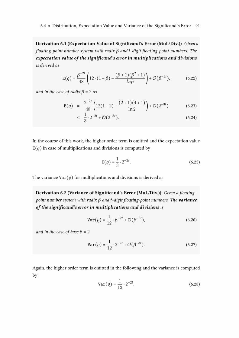
6.4 ● Distribution, Expectation Value and Variance of the Significand’s Error 91
Derivation 6.1 (Expectation Value of Significand’s Error (Mul./Div.)) Given afloating-point number system with radix β and t-digit floating-point numbers. Theexpectation value of the significand’s error in multiplications and divisionsis derived as
E(ϱ) = β−2t
48(12 ⋅ (1+ β)− (β + 1)(β2 + 1)
lnβ)+O(β−3t), (6.22)
and in the case of radix β = 2 as
E(ϱ) = 2−2t
48(12(1+ 2)− (2+ 1)(4+ 1)
ln 2)+O(2−3t) (6.23)
≤ 13⋅ 2−2t +O(2−3t). (6.24)
In the course of this work, the higher order term is omitted and the expectation valueE(ϱ) in case of multiplications and divisions is computed by
E(ϱ) = 13⋅ 2−2t. (6.25)
The variance Var(ϱ) for multiplications and divisions is derived as
Derivation 6.2 (Variance of Significand’s Error (Mul./Div.)) Given a floating-point number system with radix β and t-digit floating-point numbers. The varianceof the significand’s error in multiplications and divisions is
Var(ϱ) = 112⋅ β−2t +O(β−3t), (6.26)
and in the case of base β = 2
Var(ϱ) = 112⋅ 2−2t +O(β−3t). (6.27)
Again, the higher order term is omitted in the following and the variance is computedby
Var(ϱ) = 112⋅ 2−2t. (6.28)
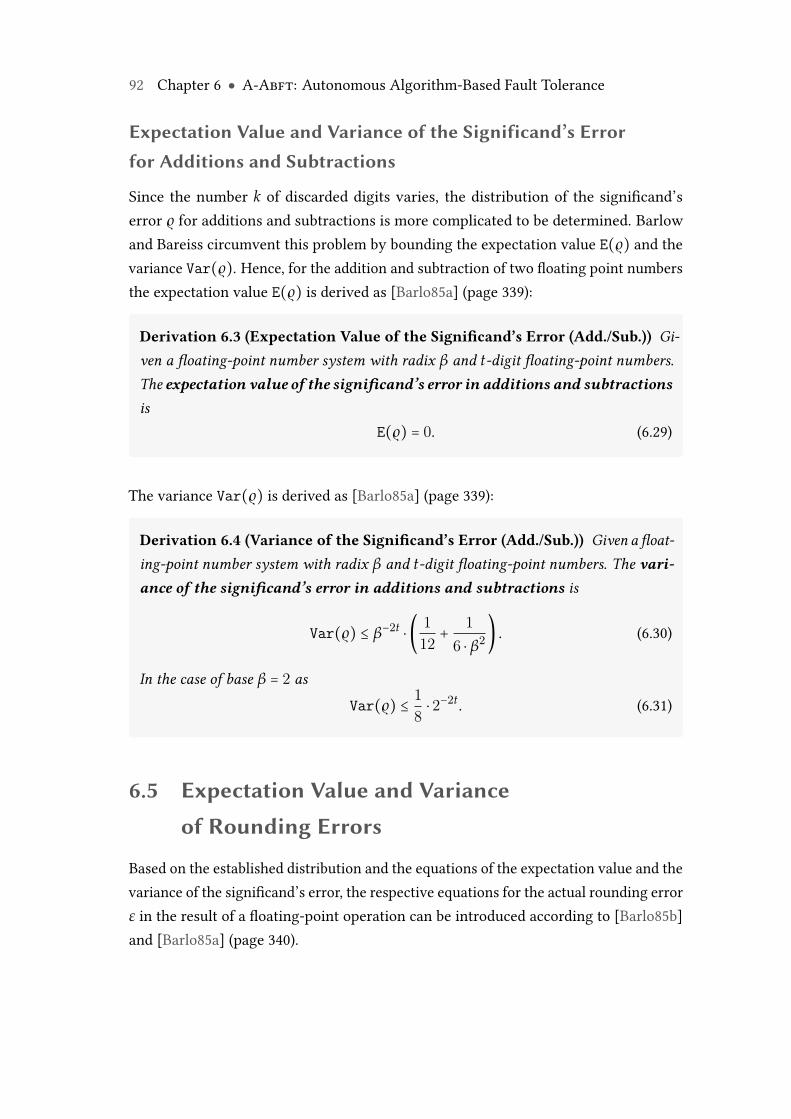
92 Chapter 6 ● A-Abft: Autonomous Algorithm-Based Fault Tolerance
Expectation Value and Variance of the Significand’s Errorfor Additions and Subtractions
Since the number k of discarded digits varies, the distribution of the significand’serror ϱ for additions and subtractions is more complicated to be determined. Barlowand Bareiss circumvent this problem by bounding the expectation value E(ϱ) and thevariance Var(ϱ). Hence, for the addition and subtraction of two floating point numbersthe expectation value E(ϱ) is derived as [Barlo85a] (page 339):
Derivation 6.3 (Expectation Value of the Significand’s Error (Add./Sub.)) Gi-ven a floating-point number system with radix β and t-digit floating-point numbers.The expectation value of the significand’s error in additions and subtractionsis
E(ϱ) = 0. (6.29)
The variance Var(ϱ) is derived as [Barlo85a] (page 339):
Derivation 6.4 (Variance of the Significand’s Error (Add./Sub.)) Given a float-ing-point number system with radix β and t-digit floating-point numbers. The vari-ance of the significand’s error in additions and subtractions is
Var(ϱ) ≤ β−2t ⋅ ( 112+ 1
6 ⋅ β2) . (6.30)
In the case of base β = 2 as
Var(ϱ) ≤ 18⋅ 2−2t. (6.31)
6.5 Expectation Value and Varianceof Rounding Errors
Based on the established distribution and the equations of the expectation value and thevariance of the significand’s error, the respective equations for the actual rounding errorε in the result of a floating-point operation can be introduced according to [Barlo85b]and [Barlo85a] (page 340).
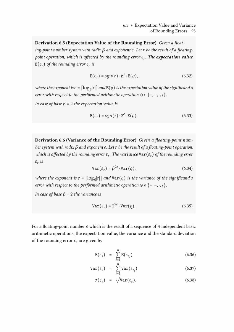
6.5 ● Expectation Value and Varianceof Rounding Errors 93
Derivation 6.5 (Expectation Value of the Rounding Error) Given a float-ing-point number system with radix β and exponent e. Let r be the result of a floating-point operation, which is affected by the rounding error εr. The expectation valueE(εr) of the rounding error εr is
E(εr) = sgn(r) ⋅ βe ⋅ E(ϱ), (6.32)
where the exponent is e = ⌈logβ∣r∣⌉ and E(ϱ) is the expectation value of the significand’serror with respect to the performed arithmetic operation ⊙ ∈ {+,−, ⋅, /}.
In case of base β = 2 the expectation value is
E(εr) = sgn(r) ⋅ 2e ⋅ E(ϱ). (6.33)
Derivation 6.6 (Variance of the Rounding Error) Given a floating-point num-ber system with radix β and exponent e. Let r be the result of a floating-point operation,which is affected by the rounding error εr. The variance Var(εr) of the rounding errorεr is
Var(εr) = β2e ⋅ Var(ϱ), (6.34)
where the exponent is e = ⌈logβ∣r∣⌉ and Var(ϱ) is the variance of the significand’serror with respect to the performed arithmetic operation ⊙ ∈ {+,−, ⋅, /}.
In case of base β = 2 the variance is
Var(εr) = 22e ⋅ Var(ϱ). (6.35)
For a floating-point number s which is the result of a sequence of n independent basicarithmetic operations, the expectation value, the variance and the standard deviationof the rounding error εs are given by
E(εs) =n∑i=1
E(εri) (6.36)
Var(εs) =n∑i=1
Var(εri) (6.37)
σ(εs) =√
Var(εs). (6.38)
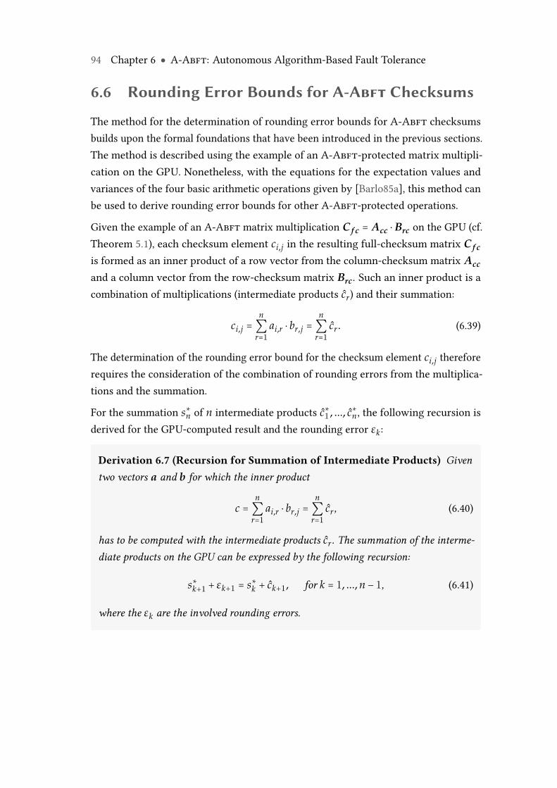
94 Chapter 6 ● A-Abft: Autonomous Algorithm-Based Fault Tolerance
6.6 Rounding Error Bounds for A-Abft Checksums
The method for the determination of rounding error bounds for A-Abft checksumsbuilds upon the formal foundations that have been introduced in the previous sections.The method is described using the example of an A-Abft-protected matrix multipli-cation on the GPU. Nonetheless, with the equations for the expectation values andvariances of the four basic arithmetic operations given by [Barlo85a], this method canbe used to derive rounding error bounds for other A-Abft-protected operations.
Given the example of an A-Abft matrix multiplication C f c = Acc ⋅ Brc on the GPU (cf.Theorem 5.1), each checksum element ci,j in the resulting full-checksum matrix C f c
is formed as an inner product of a row vector from the column-checksum matrix Acc
and a column vector from the row-checksum matrix Brc. Such an inner product is acombination of multiplications (intermediate products cr) and their summation:
ci,j =n∑r=1
ai,r ⋅ br,j =n∑r=1
cr. (6.39)
The determination of the rounding error bound for the checksum element ci,j thereforerequires the consideration of the combination of rounding errors from the multiplica-tions and the summation.
For the summation s∗n of n intermediate products c∗1 , ..., c∗n, the following recursion isderived for the GPU-computed result and the rounding error εk:
Derivation 6.7 (Recursion for Summation of Intermediate Products) Giventwo vectors a and b for which the inner product
c =n∑r=1
ai,r ⋅ br,j =n∑r=1
cr, (6.40)
has to be computed with the intermediate products cr. The summation of the interme-diate products on the GPU can be expressed by the following recursion:
s∗k+1 + εk+1 = s∗k + ck+1, for k = 1, ..., n − 1, (6.41)
where the εk are the involved rounding errors.
6.6 ● Rounding Error Bounds for A-Abft Checksums 95
Derivation 6.8 (Recursion for the Rounding Errors) The recursion for the dif-ference
∆sk = sk − s∗k (6.42)
between the exact result and the GPU-computed result, which represents the roundingerror, is
∆sk+1 = ∆sk + εk+1 (6.43)
and can be expressed as
∆sn =n∑k=2
εk. (6.44)
For the probabilistic determination of the rounding error within the sum sn, the confi-dence interval comprising the expectation value EΣ(∆sn) and the standard deviationσΣ =
√VarΣ(∆sn) has to be formed. According to Equations 6.36
EΣ(∆sn) =n∑k=2
E(εk) (6.45)
VarΣ(∆sn) =n∑k=2
Var(εk). (6.46)
With Equations 6.29 and 6.31 for the addition and subtraction of two floating-pointnumbers, the application of the Equation 6.32 yields
EΣ(∆sn) = 0 (6.47)
and
VarΣ(∆sn) =n∑k=2
Var(εk) (6.48)
≤n∑k=2
22ek ⋅ Var(ϱ) (6.49)
≤ 18⋅ 2−2t ⋅
n∑k=2
22ek (6.50)
where ek denotes the exponent of the intermediate result s∗k after the addition of thek-th addend. Since the terms in the sum are independent the variance is bound by
VarΣ(∆sn) ≤18⋅ 2−2t ⋅
n∑k=2(s∗k)2. (6.51)
96 Chapter 6 ● A-Abft: Autonomous Algorithm-Based Fault Tolerance
For an upper bound y with s∗k ≤ k ⋅ y, Equation 6.51 can be bounded by
VarΣ(∆sn) ≤18⋅ 2−2t ⋅
n∑k=2(k ⋅ y)2 (6.52)
≤ 18⋅ 2−2t ⋅ (n ⋅ (n + 1) ⋅ (2n + 1)
6) ⋅ y2. (6.53)
With the standard deviation σΣ(∆sn), the confidence interval is determined by
EΣ(∆sn) = 0 (6.54)
and
σΣ(∆sn) ≤√
n ⋅ (n + 1) ⋅ (2n + 1)48
⋅ y ⋅ 2−t (6.55)
To complete the derivation of the confidence interval for the rounding error in the innerproduct, the above considerations have to be extended with respect to the roundingerror αk caused by the multiplications ck = ai,k ⋅ bk,j, which is
c∗k + αk = ck. (6.56)
The recursion for the rounding error in the summation within the inner producttherefore changes to
∆sk+1 = ∆sk + εk + αk, (6.57)
which can be expressed as
∆sn =n∑k=2
εk +n∑k=1
αk. (6.58)
Analog to the Equations 6.45, the expectation value and the variance can be derived as
EΣΠ(∆sn) = EΣ(∆sn)+ EΠ(∆sn) (6.59)
=n∑k=2
E(εk)+n∑k=1
E(αk) (6.60)
and
VarΣΠ(∆sn) = VarΣ(∆sn)+ VarΠ(∆sn) (6.61)
=n∑k=2
Var(εk)+n∑k=1
Var(αk). (6.62)
With the Equations 6.25 and 6.28 the contribution of the rounding error variance afterk multiplications in the sum of all partial variances is
VarΠ(∆sn) =n∑k=1
Var(αk). (6.63)
6.7 ● Parallel Computation of Rounding Error Bounds 97
For y = ad ⋅ bd with d ∈ {1, ..., n}, where the variance Var(αd) is maximal, Equation 6.63can be bounded by
VarΠ(∆sn) ≤ n ⋅ Var(αd). (6.64)
The variance is maximal if the exponent e of the multiplication’s result is maximal
Var(αd) = 22ed ⋅ Var(ϱ) ≥ 22ek ⋅ Var(ϱ) = Var(αk). (6.65)
Using y as upper bound, the variance of the rounding error from the multiplications is
VarΠ(∆sn) ≤ n ⋅ Var(αy) (6.66)
≤ n ⋅ y2 ⋅ Var(ϱ) (6.67)
= 112⋅ n ⋅ 2−2t ⋅ y2. (6.68)
Analog, the expectation value is derived as
EΠ(∆sn) = n ⋅ y ⋅ E(ϱ) (6.69)
≤ 13⋅ n ⋅ 2−2t ⋅ y. (6.70)
With the expectation values and the variances from the summation and the multiplica-tions, the confidence interval for the rounding error in the final inner product can beformed using the standard deviation
σΣΠ(∆sn) =√
VarΣΠ(∆sn) (6.71)
=√
VarΣ(∆sn)+ VarΠ(∆sn) (6.72)
≤√
n ⋅ (n + 1) ⋅ (n + 12)+ 2n
24⋅ 2−t ⋅ y. (6.73)
6.7 Parallel Computation of Rounding Error Bounds
This section introduces into to the parallel determination of probabilistic rounding errorbounds on GPU. Taking the example of an A-Abft-protected matrix multiplication thatuses a partitioned encoding scheme, the typical problem sizes of interest for executionon GPUs imply that large numbers of checksums have to be processed during the A-Abft checking procedure. In order to keep the performance overhead low, the proposedmethod performs this step in parallel for all checksum elements.
As it has been shown in the foundations presented above, an appropriate upper boundy has to be identified before the respective equations for the expectation value, the
98 Chapter 6 ● A-Abft: Autonomous Algorithm-Based Fault Tolerance
variance and the standard deviation can be evaluated. This upper bound is essential,because it has direct influence on the quality of the final rounding error bound. Thesmaller the upper bound y can be chosen, the closer the rounding error bound willbe to the actual rounding error. An algorithm for the identification of such upperbounds y is therefore introduced before the complete algorithm for the efficient onlinedetermination of rounding error bounds for A-Abft checksums is presented.
Identification of Upper Bounds
For the A-Abft-protected matrix multiplication Acc ⋅ Brc = C f c, every element in thefull-checksum result matrix is formed as an inner product of a row vector ai from thecolumn-checksum matrix Acc and a column vector bj of the row-checksum matrix Brc.A trivial approach for the identification of an upper bound y would select the elementwith the largest absolute value from each of the vectors ai and bj, and then take theproduct of these two elements as y. Although this procedure always yields a validupper bound, this bound will be a worst-case bound, which is often too pessimistic. Thisis due to the fact that it is not guaranteed that exactly the two maximal elements areactually combined during the formation of the inner product.
The identification of an improved upper bound y depends on the position or, moreprecisely, the indices i and j of the vector elements. The proposed algorithm deter-mines two sets of candidate elements from both involved vectors and checks whethercombinations of elements from these two sets exist.
Definition 6.4 (Candidate Sets) Given a row vector ai from a column-checksummatrix Acc, and column vector bj form a row-checksum matrix Brc.
The candidate set Aidx of vector ai consists of the p vector elements from ai with thelargest absolute values and their index positions within the vector.
The candidate set Bidx of vector bj consists of the p vector elements from bj with thelargest absolute values and their index positions within the vector.
The candidate sets Aidx and Bidx are generated during a scan operation in whichthe absolute value of each vector element is computed. An element is added to thecandidate set if its absolute value is larger than the absolute value of the currentlysmallest element within the set. Besides the absolute value of the element, its index is
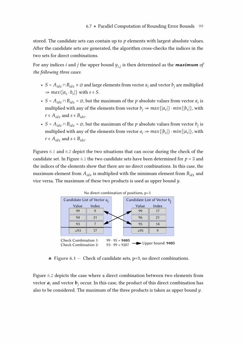
6.7 ● Parallel Computation of Rounding Error Bounds 99
stored. The candidate sets can contain up to p elements with largest absolute values.After the candidate sets are generated, the algorithm cross-checks the indices in thetwo sets for direct combinations.
For any indices i and j the upper bound yi,j is then determined as the maximum ofthe following three cases:
• S = Aidx ∩Bidx ≠ ∅ and large elements from vector ai and vector bj are multiplied⇒ max{∣as ⋅ bs∣} with s ∈ S.
• S = Aidx ∩ Bidx = ∅, but the maximum of the p absolute values from vector ai ismultiplied with any of the elements from vector bj ⇒ max{∣ar∣} ⋅min{∣bs∣}, withr ∈ Aidx and s ∈ Bidx.
• S = Aidx ∩ Bidx = ∅, but the maximum of the p absolute values from vector bj ismultiplied with any of the elements from vector ai ⇒ max{∣bs∣} ⋅min{∣ar∣}, withr ∈ Aidx and s ∈ Bidx.
Figures 6.1 and 6.2 depict the two situations that can occur during the check of thecandidate set. In Figure 6.1 the two candidate sets have been determined for p = 3 andthe indices of the elements show that there are no direct combinations. In this case, themaximum element from Aidx is multiplied with the minimum element from Bidx andvice versa. The maximum of these two products is used as upper bound y.
No direct combination of positions, p=3
ValueCandidate List of Vector ai
Index9
31
7
17
99
Check Combination 1: 99 · 95 = 9405Check Combination 2: 93 · 99 = 9207 Upper bound: 9405
94
93
≤93
ValueCandidate List of Vector bj
Index17
21
14
9
99
96
95
≤95
▲ Figure 6.1 — Check of candidate sets, p=3, no direct combinations.
Figure 6.2 depicts the case where a direct combination between two elements fromvector ai and vector bj occur. In this case, the product of this direct combination hasalso to be considered. The maximum of the three products is taken as upper bound y.
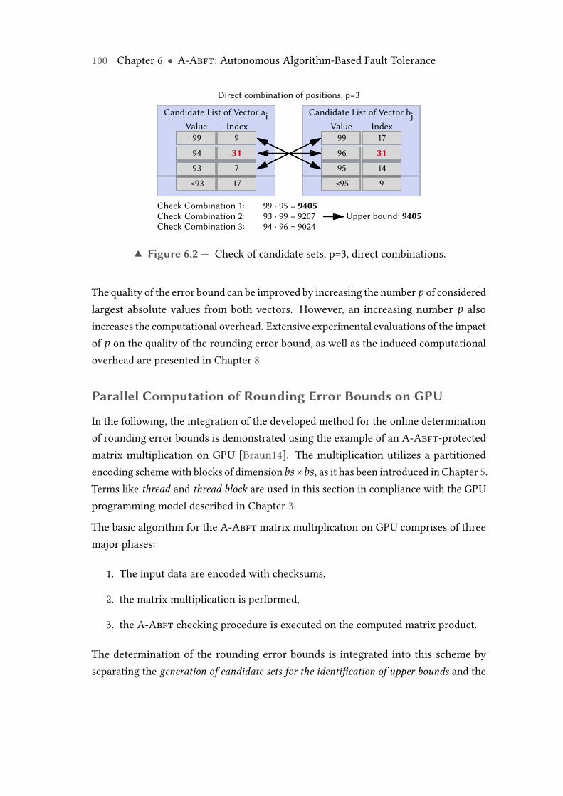
100 Chapter 6 ● A-Abft: Autonomous Algorithm-Based Fault Tolerance
Check Combination 1: 99 · 95 = 9405Check Combination 2: 93 · 99 = 9207Check Combination 3: 94 · 96 = 9024
Upper bound: 9405
Direct combination of positions, p=3
ValueCandidate List of Vector ai
Index9
317
17
99
94
93
≤93
ValueCandidate List of Vector bj
Index17
3114
9
99
96
95
≤95
▲ Figure 6.2 — Check of candidate sets, p=3, direct combinations.
The quality of the error bound can be improved by increasing the number p of consideredlargest absolute values from both vectors. However, an increasing number p alsoincreases the computational overhead. Extensive experimental evaluations of the impactof p on the quality of the rounding error bound, as well as the induced computationaloverhead are presented in Chapter 8.
Parallel Computation of Rounding Error Bounds on GPU
In the following, the integration of the developed method for the online determinationof rounding error bounds is demonstrated using the example of an A-Abft-protectedmatrix multiplication on GPU [Braun14]. The multiplication utilizes a partitionedencoding schemewith blocks of dimension bs×bs, as it has been introduced in Chapter 5.Terms like thread and thread block are used in this section in compliance with the GPUprogramming model described in Chapter 3.
The basic algorithm for the A-Abft matrix multiplication on GPU comprises of threemajor phases:
1. The input data are encoded with checksums,
2. the matrix multiplication is performed,
3. the A-Abft checking procedure is executed on the computed matrix product.
The determination of the rounding error bounds is integrated into this scheme byseparating the generation of candidate sets for the identification of upper bounds and the
6.7 ● Parallel Computation of Rounding Error Bounds 101
computation of the rounding error bounds. The generation of the candidate sets becomespart of the encoding phase (1) and the determination of the upper bounds y, as well asthe computation of the error bounds, becomes part of the result checking procedure inphase (3). This leads to the following algorithmic steps, which are encapsulated intoGPU kernels that are executed by thread blocks of dimension bs × 1:
1. GPU kernel for checksum encoding and candidate set generation.
a) Computation of the column checksums for the bs× bs sub-matrix Ai of Acc.
b) Generation of the candidate set Aidx,i with the p largest absolute valueelements in each sub-matrix Ai of matrix Acc.
c) Computation of the row checksums for the bs × bs sub-matrix Bi of Brc.
d) Generation of the candidate sets Bidx,i with the p largest absolute valueelements in each sub-matrix Bi of matrix Brc.
2. Computation of the matrix product.
3. GPU kernel for the reduction of the block-wise determined candidatesets Aidx,i and Bidx,i into the candidate sets Aidx and Bidx for the p globalelements with the largest absolute values per row/column vector.
4. GPUkernel for the determination of upper bounds, computation of round-ing error bounds and A-Abft checking procedure.
a) Computation of the rounding error bounds for the row and column check-sum elements of each bs × bs result sub-matrix Ci of the full checksummatrix C f c.
b) Computation of the reference row and column checksums for each bs × bsresult sub-matrix Ci of the full checksum matrix C f c.
c) Comparison of the original and the reference checksums using the computedrounding error bounds.
Kernel for checksum encoding and candidate set generation
This GPU kernel is launched in step 1) with thread blocks of dimension bs × 1, whereeach row or column of the sub-matrix is processes by a single thread. It combines thecomputation of A-Abft row or column checksums with the generation of the candidate
102 Chapter 6 ● A-Abft: Autonomous Algorithm-Based Fault Tolerance
sets for the p elements with the largest absolute values. The kernel reduces expensiveaccesses to the global GPU device memory by loading the elements of the processedsub-matrix into the shared memory. In a first step, the threads iterate over the elementsof a sub-matrix from top to bottom (column checksum case) or from left to right (rowchecksum case) and accumulate the elements into the respective checksum elements.After an element has been added, it is replaced in shared memory by its absolute value.In a subsequent step, the threads re-iterate over the sub-matrix elements to identifythe p elements with the largest absolute values and store the indices (positions) ofthese elements. Since the p elements with the largest absolute values are determinedwithin each sub-matrix, a total of m
bs ⋅ p such elements has been found at the end, wherembs is the number of sub-matrices. Hence, an additional reduction kernel (step 3) isexecuted in parallel to the matrix multiplication (step 2) to reduce the candidate sets tothe p global elements with the largest absolute values for each vector. Algorithm 1 inAppendix E describes all performed steps in detail.
Kernel for the determination of upper bounds, computation of rounding errorbounds and A-Abft checking procedure
The A-Abft-protected matrix multiplication is finalized by the invocation of this lastkernel which performs a sequence of four major tasks. First, the upper bounds y aredetermined based on the candidate sets which have been generated in step 1) andhave been reduced to global candidate sets for the vectors in parallel to the matrixmultiplication. The kernel checks these sets for index combinations and computes theupper bounds according to the rules introduced above. The upper bounds y are thenused in the second task for the evaluation of the equations of the expectation value andthe standard deviation of the rounding error to determine the rounding error bound ε.In a subsequent step, the reference checksums are computed and the comparison for theA-Abft check is performed. In the error-free case the result of the matrix multiplicationis returned. In case of errors, the corresponding correction procedures are invoked.Algorithm 2 in Appendix E shows the different steps for the column checksum casein detail. A first efficient implementation of the proposed method [Braun14] has beenintroduced in [Halde14].
Chapter
7Case Studies on the
Application of A-ABFT
In addition to the detailed experimental evaluation of the introduced A-Abftmethod inChapter 8, two case studies on the application of A-Abft in real world examples of highpractical relevance are presented in this chapter. First, a QR decomposition based onHouseholder transformations is realized usingA-Abft-protected matrix multiplicationson a GPU. Second, a linear programming solver based on the Revised Simplex algorithmis presented, which also utilizes A-Abft-protected GPU matrix multiplications.
7.1 A GPU-Accelerated QR Decomposition
The factorization or decomposition of matrices belongs to the most fundamental op-erations in linear algebra. The objective of a matrix decomposition is to represent agiven matrix A as product of two other matrices with some special characteristics. Avery common application of matrix decompositions is the solution of systems of linearequations. Depending on the actual application and the intended target decomposition,different factorization methods can be applied. Among the most important methodsare the LU decomposition, the Cholesky decomposition, as well as the QR decomposition.
104 Chapter 7 ● Case Studies on the Application of A-ABFT
The interested reader can find a comprehensive introduction to matrix factorizationsin [Golub12].
In this first case study, a QR decomposition based on Householder transformations hasbeen implemented, which utilizes ABFT-protected GPU matrix operations. The QRdecomposition serves as test bench for the further evaluation and comparison of theproposed A-Abft method and the SEA-ABFT approach. QR decompositions acrossdifferent matrix dimensions have been combined with fault injection experiments toinvestigate the efficiency and efficacy of both ABFT methods.
7.1.1 QR Decomposition of Matrices
The goal of a QR decomposition is to represent a given matrix A as product of twomatrices Q and R:
A = QR, (7.1)
where Q is an orthogonal matrix1 with QTQ = I and R is an upper right triangularmatrix. The above decomposition is given for the square case of A ∈ Rn×n. The QRdecomposition can also be defined for rectangular matrices A ∈Rm×n with m ≥ n as
A = QR = Q⎡⎢⎢⎢⎢⎣
R1
0
⎤⎥⎥⎥⎥⎦= [Q1 Q2]
⎡⎢⎢⎢⎢⎣
R1
0
⎤⎥⎥⎥⎥⎦= Q1R1, (7.2)
where R1 is a n × n upper right triangular matrix which is padded at the bottom with am− n× n matrix 0 consisting of zeros. Corresponding to the partitioning, Q1 is a m× nand Q2 a m ×m − n matrix. The partitioned representation of the QR decomposition inthe rectangular case is often called reduced or thin QR decomposition [Golub12].
In general, three options exist for the computation of a QR decomposition, includingthe Gram-Schmidt method, Givens rotations and Householder transformations. Since theQR decomposition with Householder transformations can be expressed in terms ofmatrix multiplications, it is particularly attractive for the integration of ABFT-protectedGPU matrix operations.
7.1.2 Householder Transformations
Householder transformations are linear transformations, introduced 1958 by AlstonScott Householder [House58], which reflect a given vector on a hyperplane through the1 In the complex case, Q is an unitary matrix with Q∗Q = I
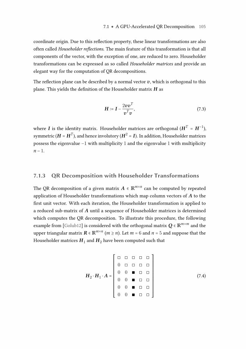
7.1 ● A GPU-Accelerated QR Decomposition 105
coordinate origin. Due to this reflection property, these linear transformations are alsooften called Householder reflections. The main feature of this transformation is that allcomponents of the vector, with the exception of one, are reduced to zero. Householdertransformations can be expressed as so called Householder matrices and provide anelegant way for the computation of QR decompositions.
The reflection plane can be described by a normal vector v, which is orthogonal to thisplane. This yields the definition of the Householder matrix H as
H ∶= I − 2vvT
vTv, (7.3)
where I is the identity matrix. Householder matrices are orthogonal (HT = H−1),symmetric (H = HT), and hence involutory (H2 = I). In addition, Householder matricespossess the eigenvalue −1 with multiplicity 1 and the eigenvalue 1 with multiplicityn − 1.
7.1.3 QR Decomposition with Householder Transformations
The QR decomposition of a given matrix A ∈ Rm×n can be computed by repeatedapplication of Householder transformations which map column vectors of A to thefirst unit vector. With each iteration, the Householder transformation is applied toa reduced sub-matrix of A until a sequence of Householder matrices is determinedwhich computes the QR decomposition. To illustrate this procedure, the followingexample from [Golub12] is considered with the orthogonal matrix Q ∈Rm×m and theupper triangular matrix R ∈ Rm×n (m ≥ n). Let m = 6 and n = 5 and suppose that theHouseholder matrices H1 and H2 have been computed such that
H2 ⋅H1 ⋅ A =
⎡⎢⎢⎢⎢⎢⎢⎢⎢⎢⎢⎢⎢⎢⎢⎢⎣
◻ ◻ ◻ ◻ ◻0 ◻ ◻ ◻ ◻0 0 ∎ ◻ ◻0 0 ∎ ◻ ◻0 0 ∎ ◻ ◻0 0 ∎ ◻ ◻
⎤⎥⎥⎥⎥⎥⎥⎥⎥⎥⎥⎥⎥⎥⎥⎥⎦
(7.4)
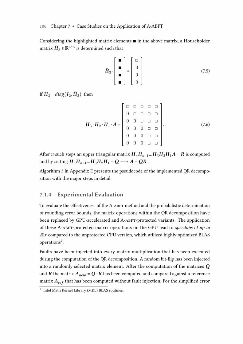
106 Chapter 7 ● Case Studies on the Application of A-ABFT
Considering the highlighted matrix elements ∎ in the above matrix, a Householdermatrix H3 ∈R4×4 is determined such that
H3 ⋅
⎡⎢⎢⎢⎢⎢⎢⎢⎢⎢⎣
∎∎∎∎
⎤⎥⎥⎥⎥⎥⎥⎥⎥⎥⎦
=
⎡⎢⎢⎢⎢⎢⎢⎢⎢⎢⎣
◻000
⎤⎥⎥⎥⎥⎥⎥⎥⎥⎥⎦
. (7.5)
If H3 = diag(I2, H3), then
H3 ⋅H2 ⋅H1 ⋅ A =
⎡⎢⎢⎢⎢⎢⎢⎢⎢⎢⎢⎢⎢⎢⎢⎢⎣
◻ ◻ ◻ ◻ ◻0 ◻ ◻ ◻ ◻0 0 ◻ ◻ ◻0 0 0 ◻ ◻0 0 0 ◻ ◻0 0 0 ◻ ◻
⎤⎥⎥⎥⎥⎥⎥⎥⎥⎥⎥⎥⎥⎥⎥⎥⎦
. (7.6)
After n such steps an upper triangular matrix HnHn−1...H3H2H1A = R is computedand by setting HnHn−1...H3H2H1 = QÔ⇒ A = QR.
Algorithm 3 in Appendix E presents the pseudocode of the implemented QR decompo-sition with the major steps in detail.
7.1.4 Experimental Evaluation
To evaluate the effectiveness of the A-abft method and the probabilistic determinationof rounding error bounds, the matrix operations within the QR decomposition havebeen replaced by GPU-accelerated and A-abft-protected variants. The applicationof these A-abft-protected matrix operations on the GPU lead to speedups of up to20x compared to the unprotected CPU version, which utilized highly optimized BLASoperations2.
Faults have been injected into every matrix multiplication that has been executedduring the computation of the QR decomposition. A random bit-flip has been injectedinto a randomly selected matrix element. After the computation of the matrices Qand R the matrix Anew = Q ⋅R has been computed and compared against a referencematrix Are f that has been computed without fault injection. For the simplified error2 Intel Math Kernel Library (MKL) BLAS routines.
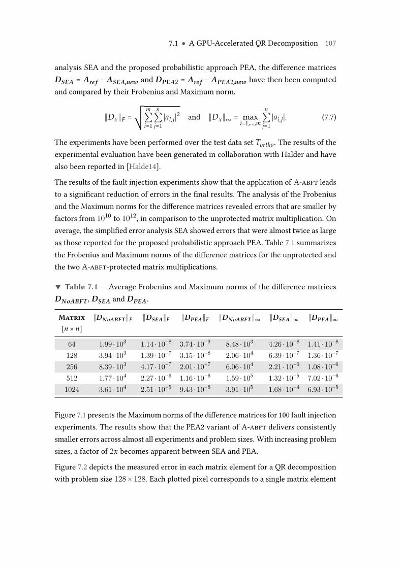
7.1 ● A GPU-Accelerated QR Decomposition 107
analysis SEA and the proposed probabilistic approach PEA, the difference matricesDSEA = Are f − ASEA,new and DPEA2 = Are f − APEA2,new have then been computedand compared by their Frobenius and Maximum norm.
∥Dx∥F =¿ÁÁÀ
m∑i=1
n∑j=1∣ai,j∣2 and ∥Dx∥∞ = max
i=1,...,m
n∑j=1∣ai,j∣. (7.7)
The experiments have been performed over the test data set Tortho. The results of theexperimental evaluation have been generated in collaboration with Halder and havealso been reported in [Halde14].
The results of the fault injection experiments show that the application of A-abft leadsto a significant reduction of errors in the final results. The analysis of the Frobeniusand the Maximum norms for the difference matrices revealed errors that are smaller byfactors from 1010 to 1012, in comparison to the unprotected matrix multiplication. Onaverage, the simplified error analysis SEA showed errors that were almost twice as largeas those reported for the proposed probabilistic approach PEA. Table 7.1 summarizesthe Frobenius and Maximum norms of the difference matrices for the unprotected andthe two A-abft-protected matrix multiplications.
▼ Table 7.1 — Average Frobenius and Maximum norms of the difference matricesDNoABFT , DSEA and DPEA.
Matrix ∥DNoABFT∥F ∥DSEA∥F ∥DPEA∥F ∥DNoABFT∥∞ ∥DSEA∥∞ ∥DPEA∥∞[n × n]
64 1.99 ⋅ 103 1.14 ⋅ 10−8 3.74 ⋅ 10−9 8.48 ⋅ 103 4.26 ⋅ 10−8 1.41 ⋅ 10−8
128 3.94 ⋅ 103 1.39 ⋅ 10−7 3.15 ⋅ 10−8 2.06 ⋅ 104 6.39 ⋅ 10−7 1.36 ⋅ 10−7
256 8.39 ⋅ 103 4.17 ⋅ 10−7 2.01 ⋅ 10−7 6.06 ⋅ 104 2.21 ⋅ 10−6 1.08 ⋅ 10−6
512 1.77 ⋅ 104 2.27 ⋅ 10−6 1.16 ⋅ 10−6 1.59 ⋅ 105 1.32 ⋅ 10−5 7.02 ⋅ 10−6
1024 3.61 ⋅ 104 2.51 ⋅ 10−5 9.43 ⋅ 10−6 3.91 ⋅ 105 1.68 ⋅ 10−4 6.93 ⋅ 10−5
Figure 7.1 presents the Maximum norms of the difference matrices for 100 fault injectionexperiments. The results show that the PEA2 variant of A-abft delivers consistentlysmaller errors across almost all experiments and problem sizes. With increasing problemsizes, a factor of 2x becomes apparent between SEA and PEA.
Figure 7.2 depicts the measured error in each matrix element for a QR decompositionwith problem size 128× 128. Each plotted pixel corresponds to a single matrix element
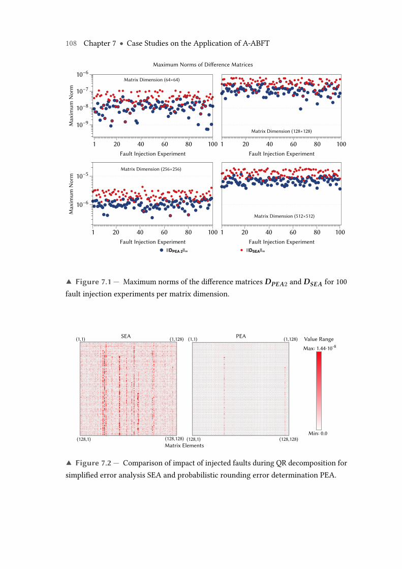
108 Chapter 7 ● Case Studies on the Application of A-ABFT
Matrix Dimension (64×64)
Matrix Dimension (128×128)
Max
imum
Nor
m
10−9
10−8
10−7
10−6
Fault Injection Experiment
1 20 40 60 80 100Fault Injection Experiment
1 20 40 60 80 100
Matrix Dimension (256×256)
Matrix Dimension (512×512)Max
imum
Nor
m
10−6
10−5
Fault Injection Experiment
1 20 40 60 80 100Fault Injection Experiment
1 20 40 60 80 100
||DPEA 2||∞ ||DSEA||∞
Maximum Norms of Difference Matrices
▲ Figure 7.1 — Maximum norms of the difference matrices DPEA2 and DSEA for 100fault injection experiments per matrix dimension.
SEA
Min: 0.0
Max: 1.44⋅10-8
PEA
Matrix Elements
(1,1) (1,1)(1,128) (1,128)
(128,1) (128,128) (128,1) (128,128)
Value Range
▲ Figure 7.2 — Comparison of impact of injected faults during QR decomposition forsimplified error analysis SEA and probabilistic rounding error determination PEA.
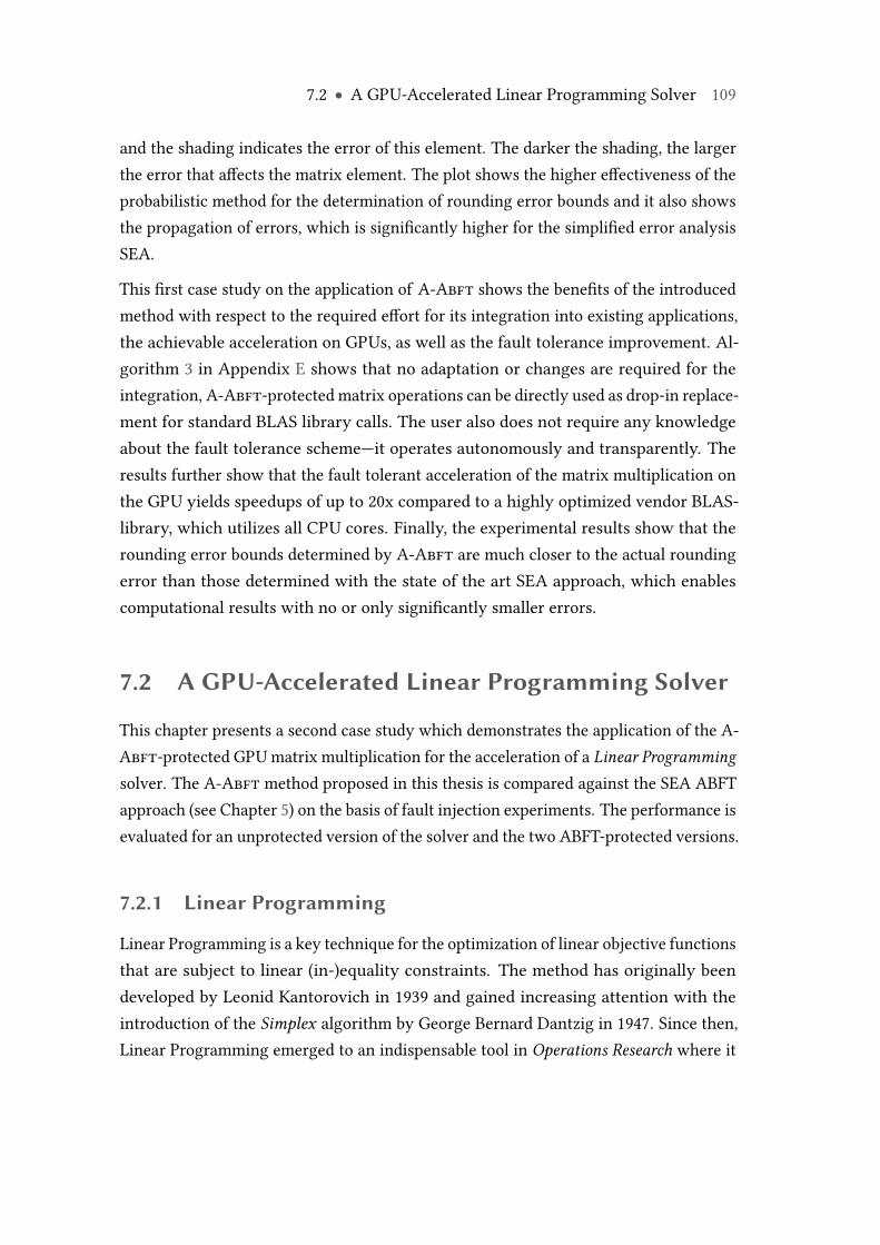
7.2 ● A GPU-Accelerated Linear Programming Solver 109
and the shading indicates the error of this element. The darker the shading, the largerthe error that affects the matrix element. The plot shows the higher effectiveness of theprobabilistic method for the determination of rounding error bounds and it also showsthe propagation of errors, which is significantly higher for the simplified error analysisSEA.
This first case study on the application of A-Abft shows the benefits of the introducedmethod with respect to the required effort for its integration into existing applications,the achievable acceleration on GPUs, as well as the fault tolerance improvement. Al-gorithm 3 in Appendix E shows that no adaptation or changes are required for theintegration, A-Abft-protected matrix operations can be directly used as drop-in replace-ment for standard BLAS library calls. The user also does not require any knowledgeabout the fault tolerance scheme—it operates autonomously and transparently. Theresults further show that the fault tolerant acceleration of the matrix multiplication onthe GPU yields speedups of up to 20x compared to a highly optimized vendor BLAS-library, which utilizes all CPU cores. Finally, the experimental results show that therounding error bounds determined by A-Abft are much closer to the actual roundingerror than those determined with the state of the art SEA approach, which enablescomputational results with no or only significantly smaller errors.
7.2 A GPU-Accelerated Linear Programming Solver
This chapter presents a second case study which demonstrates the application of the A-Abft-protected GPU matrix multiplication for the acceleration of a Linear Programmingsolver. The A-Abft method proposed in this thesis is compared against the SEA ABFTapproach (see Chapter 5) on the basis of fault injection experiments. The performance isevaluated for an unprotected version of the solver and the two ABFT-protected versions.
7.2.1 Linear Programming
Linear Programming is a key technique for the optimization of linear objective functionsthat are subject to linear (in-)equality constraints. The method has originally beendeveloped by Leonid Kantorovich in 1939 and gained increasing attention with theintroduction of the Simplex algorithm by George Bernard Dantzig in 1947. Since then,Linear Programming emerged to an indispensable tool in Operations Research where it
110 Chapter 7 ● Case Studies on the Application of A-ABFT
is used for the optimization of business processes, production planning and schedulingtasks, as well as the allocation of resources.
The optimization problem, called the linear program, is represented by the linearobjective function c ∶ Rn → R, a set of n variables x1, ..., xn with xi ∈ R and xi ≥ 0, aswell as m linear constraints a ∶Rn →R defined by the inequalities3
a1,1 ⋅ x1 + a1,2 ⋅ x2 +⋯+ a1,n ⋅ xn ≤ b1 (7.8)
⋮ (7.9)
am,1 ⋅ x1 + am,2 ⋅ x2 +⋯+ am,n ⋅ xn ≤ bm (7.10)
with bi ∈ R. Formulated as matrix A ∈ Rm×n and the two vectors b ∈ Rm and c ∈ Rn,the goal is to determine a vector x ∈Rn whose elements are non-negative and representa feasible solution for
A ⋅ x ≤ b (7.11)⎡⎢⎢⎢⎢⎢⎢⎣
a1,1 ⋯ a1,n
⋮ ⋱ ⋮am,1 ⋯ am,n
⎤⎥⎥⎥⎥⎥⎥⎦⋅⎡⎢⎢⎢⎢⎢⎢⎣
x1
⋮xn
⎤⎥⎥⎥⎥⎥⎥⎦≤⎡⎢⎢⎢⎢⎢⎢⎣
b1
⋮bm
⎤⎥⎥⎥⎥⎥⎥⎦(7.12)
such that the inner product
cTx = c1 ⋅ x1 + c2 ⋅ x2 +⋯+ cn ⋅ xn (7.13)
becomes maximal:max{cTx ∣ Ax ≤ b, xi ≥ 0}. (7.14)
7.2.2 Simplex and Revised Simplex Algorithm
The Simplex algorithm is a method for the solution of linear programs which has beenintroduced by George Bernard Dantzig [Dantz63] in 1947. The Simplex algorithm is ableto either determine an exact solution for the linear program in finite time, or to prove thatthe linear program has no solution. It has been shown that the Simplex algorithm andall its derivates exhibit an exponential worst-case runtime [Klee70]. However, in mostpractical applications, Simplex algorithms show a much better runtime behavior andoften outperform alternative methods like interior points algorithms [Karma84,Neste94]or the ellipsoid method [Khach80].3 Constraints can also be expressed as equations "=" and inequalities with "≥". Transformations into the"≤" representation exist.
7.2 ● A GPU-Accelerated Linear Programming Solver 111
The Simplex algorithm operates in two phases. In the first phase, an initial feasiblebasic solution is searched for the linear program. This is done by consideration of anauxiliary linear program based on the original program with additionally introducedartificial variables. The objective of the auxiliary linear program is to minimize thesum of the artificial variables. If such an optimal solution can be determined and ifthe auxiliary linear program also possesses a solution where all artificial variables areequal to zero, this latter solution can be taken as initial feasible solution for the originalprogram. If no such solution exits, the Simplex algorithm aborts.
In phase two, the Simplex algorithm starts with the initial feasible basic solutioncomputed in phase one, and iteratively tries to improve the value of the objectivefunction. Within each step, the current basis is changed and a new basic solution iscomputed. The change of the basis is achieved by pivot operations, where a currentbasic variable is selected and replaced with a non-basic variable. The basic variableis called the leaving variable, whereas the non-basic variable is called the enteringvariable. Different rules and criteria for the selection procedure have been proposedover time. One possibility will be to choose the non-basic variable which yields themaximum marginal improvement of the objective function’s value. The column vectorcorresponding to the selected entering variable is called the pivot column. In the nextstep, the leaving variable has to be determined. Therefore, the quotient of the pivotcolumn’s elements and the corresponding entries on the right-hand side of the tableauare computed. The minimum resulting quotient designates the leaving variable and theso called pivot row. Further details on the selection of entering and leaving variables,the remaining computational steps for the change of the basis, as well as an extensiveintroduction to Linear Programming and available solution methods can be foundin [Luenb08]. In conclusion, the Simplex algorithm continues to change the basisuntil no further improvement can be achieved or the linear program is proved to beunbounded.
The LP solver developed for this case study uses a so called Revised Simplex algo-rithm [Dantz53], which provides a higher computational and higher memory efficiency.A common characteristic of revised simplex algorithms is that they do not store the fullSimplex tableau. Instead, only a representation of the basis B of the matrix represent-ing the constraints is stored. These matrix-based methods, which are mathematicallyequivalent to the original Simplex algorithm, map the steps of the original algorithm tosequences of linear algebra operations. This makes them particularly attractive for ac-
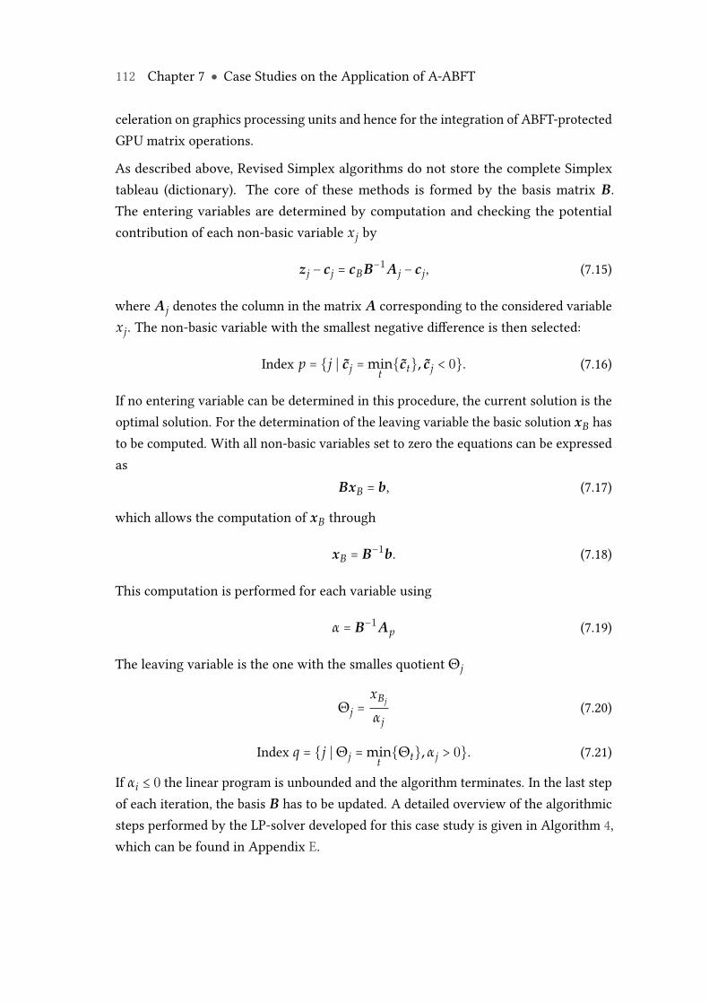
112 Chapter 7 ● Case Studies on the Application of A-ABFT
celeration on graphics processing units and hence for the integration of ABFT-protectedGPU matrix operations.
As described above, Revised Simplex algorithms do not store the complete Simplextableau (dictionary). The core of these methods is formed by the basis matrix B.The entering variables are determined by computation and checking the potentialcontribution of each non-basic variable xj by
zj − cj = cBB−1Aj − cj, (7.15)
where Aj denotes the column in the matrix A corresponding to the considered variablexj. The non-basic variable with the smallest negative difference is then selected:
Index p = {j ∣ cj =mint{ct}, cj < 0}. (7.16)
If no entering variable can be determined in this procedure, the current solution is theoptimal solution. For the determination of the leaving variable the basic solution xB hasto be computed. With all non-basic variables set to zero the equations can be expressedas
BxB = b, (7.17)
which allows the computation of xB through
xB = B−1b. (7.18)
This computation is performed for each variable using
α = B−1Ap (7.19)
The leaving variable is the one with the smalles quotient Θj
Θj =xBj
αj(7.20)
Index q = {j ∣ Θj =mint{Θt}, αj > 0}. (7.21)
If αi ≤ 0 the linear program is unbounded and the algorithm terminates. In the last stepof each iteration, the basis B has to be updated. A detailed overview of the algorithmicsteps performed by the LP-solver developed for this case study is given in Algorithm 4,which can be found in Appendix E.
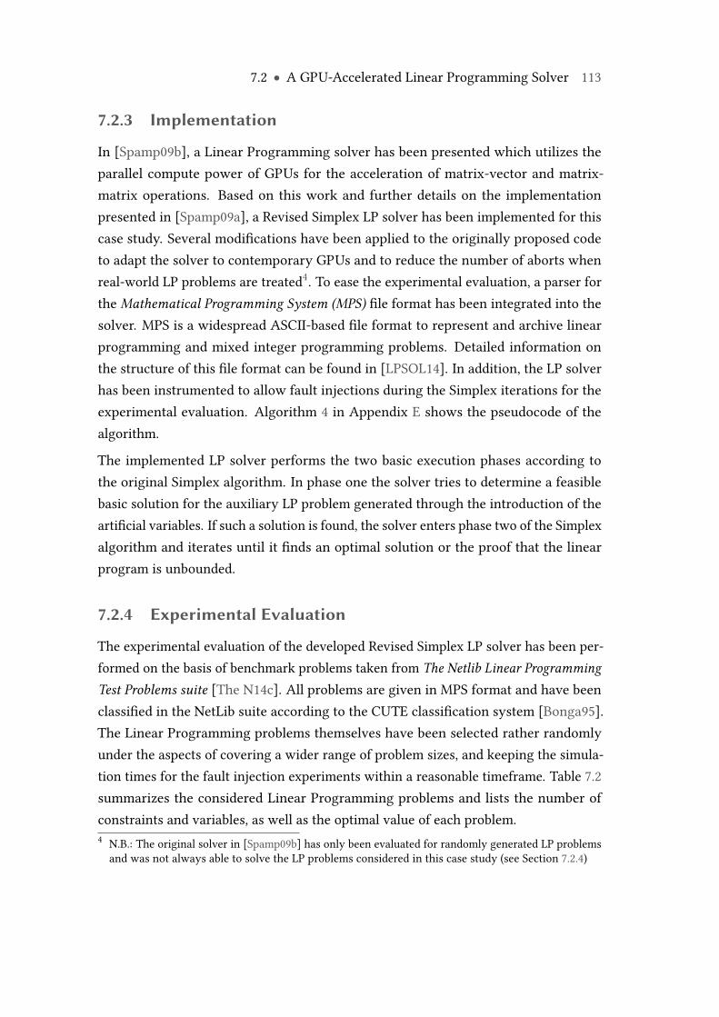
7.2 ● A GPU-Accelerated Linear Programming Solver 113
7.2.3 Implementation
In [Spamp09b], a Linear Programming solver has been presented which utilizes theparallel compute power of GPUs for the acceleration of matrix-vector and matrix-matrix operations. Based on this work and further details on the implementationpresented in [Spamp09a], a Revised Simplex LP solver has been implemented for thiscase study. Several modifications have been applied to the originally proposed codeto adapt the solver to contemporary GPUs and to reduce the number of aborts whenreal-world LP problems are treated4. To ease the experimental evaluation, a parser forthe Mathematical Programming System (MPS) file format has been integrated into thesolver. MPS is a widespread ASCII-based file format to represent and archive linearprogramming and mixed integer programming problems. Detailed information onthe structure of this file format can be found in [LPSOL14]. In addition, the LP solverhas been instrumented to allow fault injections during the Simplex iterations for theexperimental evaluation. Algorithm 4 in Appendix E shows the pseudocode of thealgorithm.
The implemented LP solver performs the two basic execution phases according tothe original Simplex algorithm. In phase one the solver tries to determine a feasiblebasic solution for the auxiliary LP problem generated through the introduction of theartificial variables. If such a solution is found, the solver enters phase two of the Simplexalgorithm and iterates until it finds an optimal solution or the proof that the linearprogram is unbounded.
7.2.4 Experimental Evaluation
The experimental evaluation of the developed Revised Simplex LP solver has been per-formed on the basis of benchmark problems taken from The Netlib Linear ProgrammingTest Problems suite [The N14c]. All problems are given in MPS format and have beenclassified in the NetLib suite according to the CUTE classification system [Bonga95].The Linear Programming problems themselves have been selected rather randomlyunder the aspects of covering a wider range of problem sizes, and keeping the simula-tion times for the fault injection experiments within a reasonable timeframe. Table 7.2summarizes the considered Linear Programming problems and lists the number ofconstraints and variables, as well as the optimal value of each problem.4 N.B.: The original solver in [Spamp09b] has only been evaluated for randomly generated LP problemsand was not always able to solve the LP problems considered in this case study (see Section 7.2.4)
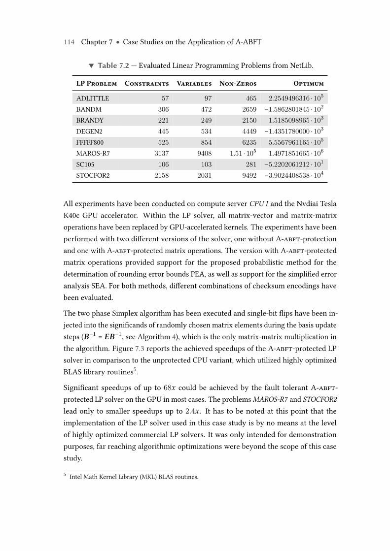
114 Chapter 7 ● Case Studies on the Application of A-ABFT
▼ Table 7.2 — Evaluated Linear Programming Problems from NetLib.
LP Problem Constraints Variables Non-Zeros Optimum
ADLITTLE 57 97 465 2.2549496316 ⋅ 105
BANDM 306 472 2659 −1.5862801845 ⋅ 102
BRANDY 221 249 2150 1.5185098965 ⋅ 103
DEGEN2 445 534 4449 −1.4351780000 ⋅ 103
FFFFF800 525 854 6235 5.5567961165 ⋅ 105
MAROS-R7 3137 9408 1.51 ⋅ 105 1.4971851665 ⋅ 106
SC105 106 103 281 −5.2202061212 ⋅ 101
STOCFOR2 2158 2031 9492 −3.9024408538 ⋅ 104
All experiments have been conducted on compute server CPU I and the Nvdiai TeslaK40c GPU accelerator. Within the LP solver, all matrix-vector and matrix-matrixoperations have been replaced by GPU-accelerated kernels. The experiments have beenperformed with two different versions of the solver, one without A-abft-protectionand one with A-abft-protected matrix operations. The version with A-abft-protectedmatrix operations provided support for the proposed probabilistic method for thedetermination of rounding error bounds PEA, as well as support for the simplified erroranalysis SEA. For both methods, different combinations of checksum encodings havebeen evaluated.
The two phase Simplex algorithm has been executed and single-bit flips have been in-jected into the significands of randomly chosen matrix elements during the basis updatesteps (B−1 = EB−1, see Algorithm 4), which is the only matrix-matrix multiplication inthe algorithm. Figure 7.3 reports the achieved speedups of the A-abft-protected LPsolver in comparison to the unprotected CPU variant, which utilized highly optimizedBLAS library routines5.
Significant speedups of up to 68x could be achieved by the fault tolerant A-abft-protected LP solver on the GPU in most cases. The problemsMAROS-R7 and STOCFOR2lead only to smaller speedups up to 2.4x. It has to be noted at this point that theimplementation of the LP solver used in this case study is by no means at the levelof highly optimized commercial LP solvers. It was only intended for demonstrationpurposes, far reaching algorithmic optimizations were beyond the scope of this casestudy.
5 Intel Math Kernel Library (MKL) BLAS routines.
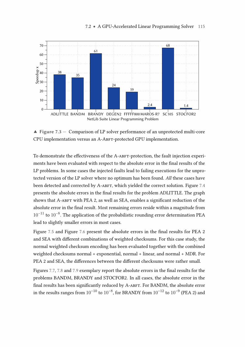
7.2 ● A GPU-Accelerated Linear Programming Solver 115
3835
61
2419
2.4
68
1.4
Spee
dup
x
0
10
20
30
40
50
60
70
NetLib Suite Linear Programming ProblemADLITTLE BANDM BRANDY DEGEN2 FFFFF800MAROS-R7 SC105 STOCFOR2
▲ Figure 7.3 — Comparison of LP solver performance of an unprotected multi-coreCPU implementation versus an A-Abft-protected GPU implementation.
To demonstrate the effectiveness of the A-abft-protection, the fault injection experi-ments have been evaluated with respect to the absolute error in the final results of theLP problems. In some cases the injected faults lead to failing executions for the unpro-tected version of the LP solver where no optimum has been found. All these cases havebeen detected and corrected by A-abft, which yielded the correct solution. Figure 7.4presents the absolute errors in the final results for the problem ADLITTLE. The graphshows that A-abft with PEA 2, as well as SEA, enables a significant reduction of theabsolute error in the final result. Most remaining errors reside within a magnitude from10−11 to 10−8. The application of the probabilistic rounding error determination PEAlead to slightly smaller errors in most cases.
Figure 7.5 and Figure 7.6 present the absolute errors in the final results for PEA 2and SEA with different combinations of weighted checksums. For this case study, thenormal weighted checksum encoding has been evaluated together with the combinedweighted checksums normal + exponential, normal + linear, and normal + MDR. ForPEA 2 and SEA, the differences between the different checksums were rather small.
Figures 7.7, 7.8 and 7.9 exemplary report the absolute errors in the final results for theproblems BANDM, BRANDY and STOCFOR2. In all cases, the absolute error in thefinal results has been significantly reduced by A-abft. For BANDM, the absolute errorin the results ranges from 10−10 to 10−8, for BRANDY from 10−12 to 10−9 (PEA 2) and
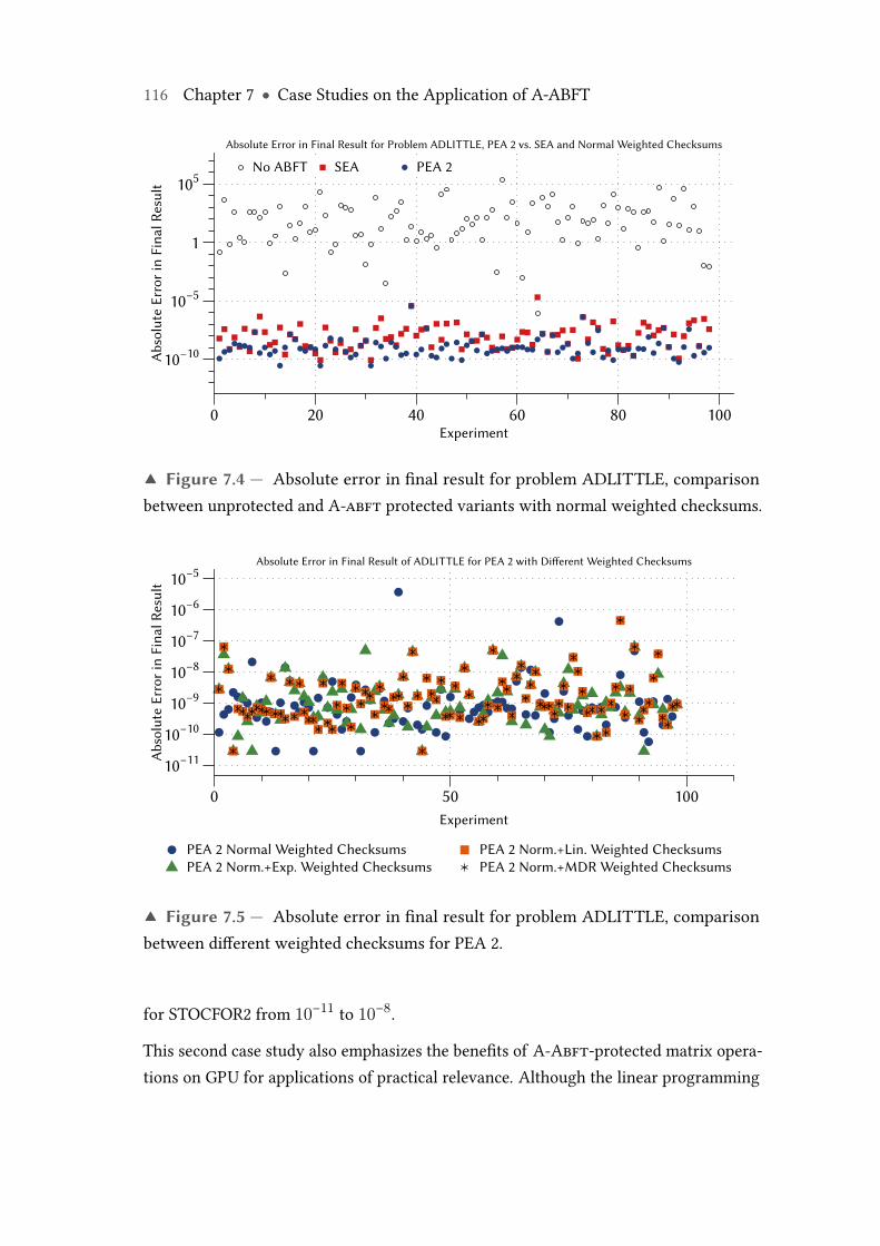
116 Chapter 7 ● Case Studies on the Application of A-ABFT
No ABFT SEA PEA 2A
bsol
ute
Erro
r in
Fina
l Res
ult
10−10
10−5
1
105
Experiment0 20 40 60 80 100
Absolute Error in Final Result for Problem ADLITTLE, PEA 2 vs. SEA and Normal Weighted Checksums
▲ Figure 7.4 — Absolute error in final result for problem ADLITTLE, comparisonbetween unprotected and A-abft protected variants with normal weighted checksums.
PEA 2 Normal Weighted ChecksumsPEA 2 Norm.+Exp. Weighted Checksums
PEA 2 Norm.+Lin. Weighted ChecksumsPEA 2 Norm.+MDR Weighted Checksums
Abs
olut
e Er
ror i
n Fi
nal R
esul
t
10−11
10−10
10−9
10−8
10−7
10−6
10−5
Experiment
0 50 100
Absolute Error in Final Result of ADLITTLE for PEA 2 with Different Weighted Checksums
▲ Figure 7.5 — Absolute error in final result for problem ADLITTLE, comparisonbetween different weighted checksums for PEA 2.
for STOCFOR2 from 10−11 to 10−8.
This second case study also emphasizes the benefits of A-Abft-protected matrix opera-tions on GPU for applications of practical relevance. Although the linear programming
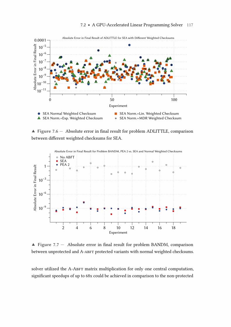
7.2 ● A GPU-Accelerated Linear Programming Solver 117
SEA Normal Weighted ChecksumSEA Norm.+Exp. Weighted Checksum
SEA Norm.+Lin. Weighted ChecksumSEA Norm.+MDR Weighted Checksum
Abs
olut
e Er
ror i
n Fi
nal R
esul
t
10−1110−1010−910−810−710−610−5
0.0001
Experiment
0 50 100
Absolute Error in Final Result of ADLITTLE for SEA with Different Weighted Checksums
▲ Figure 7.6 — Absolute error in final result for problem ADLITTLE, comparisonbetween different weighted checksums for SEA.
No ABFTSEAPEA 2
Abs
olut
e Er
ror i
n Fi
nal R
esul
t
10−9
10−6
10−3
1
Experiment2 4 6 8 10 12 14 16 18
Absolute Error in Final Result for Problem BANDM, PEA 2 vs. SEA and Normal Weighted Checksums
▲ Figure 7.7 — Absolute error in final result for problem BANDM, comparisonbetween unprotected and A-abft protected variants with normal weighted checksums.
solver utilized the A-Abft matrix multiplication for only one central computation,significant speedups of up to 68x could be achieved in comparison to the non-protected
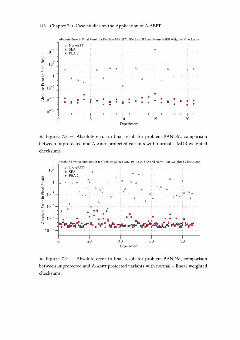
118 Chapter 7 ● Case Studies on the Application of A-ABFT
No ABFTSEAPEA 2
Abs
olut
e Er
ror i
n Fi
nal R
esul
t
10−15
10−10
10−5
1
105
1010
Experiment0 5 10 15 20
Absolute Error in Final Result for Problem BRANDY, PEA 2 vs. SEA and Norm.+MDR Weighted Checksums
▲ Figure 7.8 — Absolute error in final result for problem BANDM, comparisonbetween unprotected and A-abft protected variants with normal + MDR weightedchecksums.
No ABFTSEAPEA 2
Abs
olut
e Er
ror i
n Fi
nal R
esul
t
10−12
10−9
10−6
10−3
1
103
Experiment0 20 40 60 80
Absolute Error in Final Result for Problem STOCFOR2, PEA 2 vs. SEA and Norm.+Lin. Weighted Checksums
▲ Figure 7.9 — Absolute error in final result for problem BANDM, comparisonbetween unprotected and A-abft protected variants with normal + linear weightedchecksums.
7.2 ● A GPU-Accelerated Linear Programming Solver 119
variant of the solver, which used highly optimized BLAS routines on the CPU. Evenmore important are the results of the fault injection experiments, which show thatalmost all of the injected faults caused severe errors in the final solution or led to anon-terminating execution of the solver. As in the first case study, the introducedA-Abft method determined rounding error bounds that were almost always closer tothe actual rounding error than those determined by the state of the art SEA technique.

Chapter
8Experimental Evaluation
This chapter presents and discusses the main results of the detailed experimentalevaluation of the proposed A-Abft method for matrix operations on GPUs [Braun14].Using the example of the matrix multiplication, the novel probabilistic approach forthe determination of rounding error bounds (PEA) is compared against the state ofthe art simplified error analysis (SEA) [Roy C93]. In addition, an in-depth analysisof central ABFT design parameters such as different kinds of weighted checksumcodes and their combinations, as well as different block sizes for partitioned encodings,is performed. To demonstrate the advantages of A-Abft over the state of the art,the experimental evaluations consider three main aspects including the achievablecomputational throughput and performance, the quality of the determined roundingerror bounds and the error detection capabilities. In favor of a concise presentation ofthe experimental results, the most important findings are summarized in this chapter.Section 8.1 presents the evaluation results for the achievable computational performance.Section 8.2 gives the reader details on the quality of the determined rounding errorbounds and Section 8.3 summarizes the results of fault injection experiments for theevaluation of the error detection capabilities. Appendix F provides detailed supplementalresults on the performed experiments, which have been omitted in this chapter.
The experiments for the evaluation part of this work have been performed on two IntelXeon-based compute servers, hereinafter referred to as CPU I and CPU II, which were
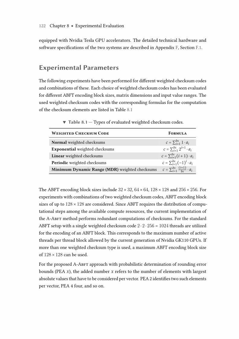
122 Chapter 8 ● Experimental Evaluation
equipped with Nvidia Tesla GPU accelerators. The detailed technical hardware andsoftware specifications of the two systems are described in Appendix F, Section F.1.
Experimental Parameters
The following experiments have been performed for different weighted checksum codesand combinations of these. Each choice of weighted checksum codes has been evaluatedfor different ABFT encoding block sizes, matrix dimensions and input value ranges. Theused weighted checksum codes with the corresponding formulas for the computationof the checksum elements are listed in Table 8.1
▼ Table 8.1 — Types of evaluated weighted checksum codes.
Weighted Checksum Code Formula
Normal weighted checksums c = ∑bsi=1 1 ⋅ ai
Exponential weighted checksums c = ∑bsi=1 2i+1
⋅ ai
Linear weighted checksums c = ∑bsi=1(i + 1) ⋅ ai
Periodic weighted checksums c = ∑bsi=1(−1)
i⋅ ai
Minimum Dynamic Range (MDR) weighted checksums c = ∑bsi=1(i+1)
bs ⋅ ai
The ABFT encoding block sizes include 32× 32, 64× 64, 128× 128 and 256× 256. Forexperiments with combinations of two weighted checksum codes, ABFT encoding blocksizes of up to 128× 128 are considered. Since ABFT requires the distribution of compu-tational steps among the available compute resources, the current implementation ofthe A-Abft method performs redundant computations of checksums. For the standardABFT setup with a single weighted checksum code 2 ⋅ 2 ⋅ 256 = 1024 threads are utilizedfor the encoding of an ABFT block. This corresponds to the maximum number of activethreads per thread block allowed by the current generation of Nvidia GK110 GPUs. Ifmore than one weighted checksum type is used, a maximum ABFT encoding block sizeof 128× 128 can be used.
For the proposed A-Abft approach with probabilistic determination of rounding errorbounds (PEA x), the added number x refers to the number of elements with largestabsolute values that have to be considered per vector. PEA 2 identifies two such elementsper vector, PEA 4 four, and so on.
8.1 ● Computational Performance 123
To cover a rather wide range of input data set sizes, the experiments are performed formatrices of the dimensions 512 × 512, 1024 × 1024, 2048 × 2048, 3072 × 3072, 4096 ×4096, 5120× 5120, 6144× 6144, 7168× 7168 and 8192× 8192.
The test data sets used for the experiments comprise three different types, including testmatrices of type Tpos with uniformly distributed numbers in the range of [0, 10i] withi ∈ {0, 1, 2, 3}, type Tf ull with uniformly distributed positive and negative numbers inthe range [−10i, 10i] with i ∈ {0, 1, 2, 3} and test matrices of type Tortho. The latter typecomprises randomized orthogonal matrices U and V with a higher dynamic range inthe input values, which are generated according to Turmonet al. [Turmo00a] by theformula
A = 10α ⋅U ⋅Dκ ⋅V T . (8.1)
"The random matrices U and V are the orthogonal factors in the QR factorization of twosquare matrices with normally distributed entries. The diagonal matrix Dκ is filled in bychoosing random singular values, such that the largest singular value is unity and thesmallest is 1
κ . These matrices all have 2-norm equal to unity; the overall scale is set by α
which is chosen uniformly at random between−8 and+8" [Turmo00a]. Experiments basedon the test data set Tortho have been performed with κ ∈ {2, 16, 128, 1024, 8192, 65536}.
8.1 Computational Performance
For the evaluation of the computational performance the execution times of the GPUkernels for the different ABFT phases have been measured. Section 8.1.1 presentsthe execution times for the ABFT checksum encoding of the matrices A and B, aswell as the ABFT result check of matrix C. These operations are independent of thechosen method for the determination of the required rounding error bounds (SEA andPEA). Section 8.1.2 analyzes the execution times of the GPU kernels required for thepreprocessing steps of SEA and PEA, followed by the analysis of the kernel executiontimes for the final determination of the rounding error bounds (ε-determination kernels)in Section 8.1.3. The overall computational performance and throughput of the A-Abft-protected matrix multiplications is evaluated in Section 8.1.4.
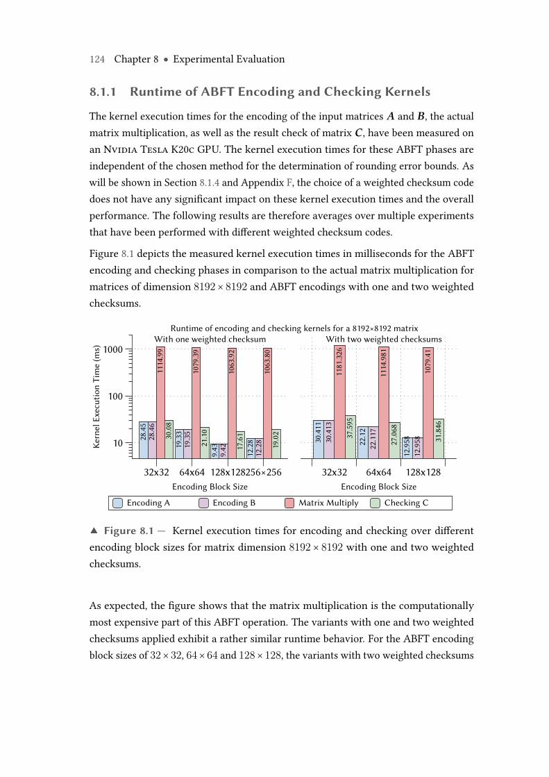
124 Chapter 8 ● Experimental Evaluation
8.1.1 Runtime of ABFT Encoding and Checking Kernels
The kernel execution times for the encoding of the input matrices A and B, the actualmatrix multiplication, as well as the result check of matrix C, have been measured onan Nvidia Tesla K20c GPU. The kernel execution times for these ABFT phases areindependent of the chosen method for the determination of rounding error bounds. Aswill be shown in Section 8.1.4 and Appendix F, the choice of a weighted checksum codedoes not have any significant impact on these kernel execution times and the overallperformance. The following results are therefore averages over multiple experimentsthat have been performed with different weighted checksum codes.
Figure 8.1 depicts the measured kernel execution times in milliseconds for the ABFTencoding and checking phases in comparison to the actual matrix multiplication formatrices of dimension 8192× 8192 and ABFT encodings with one and two weightedchecksums.
Encoding A Encoding B Matrix Multiply Checking C
28.4
5
19.3
3
9.43
12.2
828.4
6
19.3
5
9.42
12.2
8
1114
.99
1079
.39
1063
.92
1063
.80
30.0
8
21.1
0
17.6
1
19.0
2
30.4
11
22.1
2
12.9
5830.4
13
22.1
17
12.9
58
1181
.326
1114
.981
1079
.41
37.5
95
27.0
68
31.8
46
With one weighted checksum With two weighted checksums
Kern
el E
xecu
tion
Tim
e (m
s)
10
100
1000
Encoding Block Size
32x32 64x64 128x128256×256Encoding Block Size
32x32 64x64 128x128
Runtime of encoding and checking kernels for a 8192×8192 matrix
▲ Figure 8.1 — Kernel execution times for encoding and checking over differentencoding block sizes for matrix dimension 8192 × 8192 with one and two weightedchecksums.
As expected, the figure shows that the matrix multiplication is the computationallymost expensive part of this ABFT operation. The variants with one and two weightedchecksums applied exhibit a rather similar runtime behavior. For the ABFT encodingblock sizes of 32× 32, 64× 64 and 128× 128, the variants with two weighted checksums
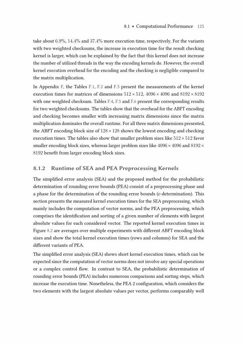
8.1 ● Computational Performance 125
take about 6.9%, 14.4% and 37.4% more execution time, respectively. For the variantswith two weighted checksums, the increase in execution time for the result checkingkernel is larger, which can be explained by the fact that this kernel does not increasethe number of utilized threads in the way the encoding kernels do. However, the overallkernel execution overhead for the encoding and the checking is negligible compared tothe matrix multiplication.
In Appendix F, the Tables F.1, F.2 and F.3 present the measurements of the kernelexecution times for matrices of dimensions 512 × 512, 4096 × 4096 and 8192 × 8192with one weighted checksum. Tables F.4, F.5 and F.6 present the corresponding resultsfor two weighted checksums. The tables show that the overhead for the ABFT encodingand checking becomes smaller with increasing matrix dimensions since the matrixmultiplication dominates the overall runtime. For all three matrix dimensions presented,the ABFT encoding block size of 128× 128 shows the lowest encoding and checkingexecution times. The tables also show that smaller problem sizes like 512× 512 favorsmaller encoding block sizes, whereas larger problem sizes like 4096× 4096 and 8192×8192 benefit from larger encoding block sizes.
8.1.2 Runtime of SEA and PEA Preprocessing Kernels
The simplified error analysis (SEA) and the proposed method for the probabilisticdetermination of rounding error bounds (PEA) consist of a preprocessing phase anda phase for the determination of the rounding error bounds (ε-determination). Thissection presents the measured kernel execution times for the SEA preprocessing, whichmainly includes the computation of vector norms, and the PEA preprocessing, whichcomprises the identification and sorting of a given number of elements with largestabsolute values for each considered vector. The reported kernel execution times inFigure 8.2 are averages over multiple experiments with different ABFT encoding blocksizes and show the total kernel execution times (rows and columns) for SEA and thedifferent variants of PEA.
The simplified error analysis (SEA) shows short kernel execution times, which can beexpected since the computation of vector norms does not involve any special operationsor a complex control flow. In contrast to SEA, the probabilistic determination ofrounding error bounds (PEA) includes numerous comparisons and sorting steps, whichincrease the execution time. Nonetheless, the PEA 2 configuration, which considers thetwo elements with the largest absolute values per vector, performs comparably well
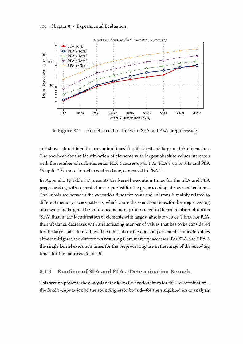
126 Chapter 8 ● Experimental Evaluation
SEA TotalPEA 2 TotalPEA 4 TotalPEA 8 TotalPEA 16 Total
Kern
el E
xecu
tion
Tim
e (m
s)
10
100
Matrix Dimension (n×n)512 1024 2048 3072 4096 5120 6144 7168 8192
Kernel Execution Times for SEA and PEA Preprocessing
▲ Figure 8.2 — Kernel execution times for SEA and PEA preprocessing.
and shows almost identical execution times for mid-sized and large matrix dimensions.The overhead for the identification of elements with largest absolute values increaseswith the number of such elements. PEA 4 causes up to 1.7x, PEA 8 up to 3.4x and PEA16 up to 7.7x more kernel execution time, compared to PEA 2.
In Appendix F, Table F.7 presents the kernel execution times for the SEA and PEApreprocessing with separate times reported for the preprocessing of rows and columns.The imbalance between the execution times for rows and columns is mainly related todifferent memory access patterns, which cause the execution times for the preprocessingof rows to be larger. The difference is more pronounced in the calculation of norms(SEA) than in the identification of elements with largest absolute values (PEA). For PEA,the imbalance decreases with an increasing number of values that has to be consideredfor the largest absolute values. The internal sorting and comparison of candidate valuesalmost mitigates the differences resulting from memory accesses. For SEA and PEA 2,the single kernel execution times for the preprocessing are in the range of the encodingtimes for the matrices A and B.
8.1.3 Runtime of SEA and PEA ε-Determination Kernels
This section presents the analysis of the kernel execution times for the ε-determination—the final computation of the rounding error bound—for the simplified error analysis
8.1 ● Computational Performance 127
(SEA) and the proposed probabilistic approach (PEA). The implementation of A-Abfttakes the ABFT encoding block size as one input parameter for the runtime configurationof the ε-determination GPU kernels. Both SEA and PEA therefore show different kernelexecution times for different encoding block sizes. Figure 8.3 depicts the executiontimes for all methods and an ABFT encoding block size of 32× 32. The graph includesthe execution times for SEA and PEA 2 with an ABFT encoding block size of 256× 256for comparison.
SEA (32×32)PEA 2 (32×32)PEA 4 (32×32)PEA 8 (32×32)
PEA 16 (32×32)SEA (256×256)PEA 2 (256×256)
Kern
el E
xecu
tion
Tim
e (m
s)
0.01
0.1
1
10
Matrix Dimension (n×n)512 1024 2048 3072 4096 5120 6144 7168 8192
Kernel Execution Times for SEA and PEA eps-Determination, ABFT encoding block size (32×32)
▲ Figure 8.3 — Kernel execution times for SEA and PEA ε-determination.
In Appendix F, Table F.8 shows the kernel execution times for setups with one weightedchecksum and an ABFT encoding block size of 32× 32. Table F.9 lists the correspondingexecution times for an ABFT encoding block size of 256 × 256. The simplified erroranalysis (SEA) exhibits short kernel execution times below 0.5 milliseconds across alltest data set sizes and ABFT encoding block sizes. The probabilistic rounding errordetermination PEA requires between 1.3x and 5.3x more execution time compared toSEA. However, all these kernel execution times are significantly lower than the requiredtimes for the encoding of the matrices or the preprocessing steps. Table F.9 also showsthat the kernel execution times of SEA and all variants of PEA benefit significantlyfrom larger ABFT encoding block sizes.
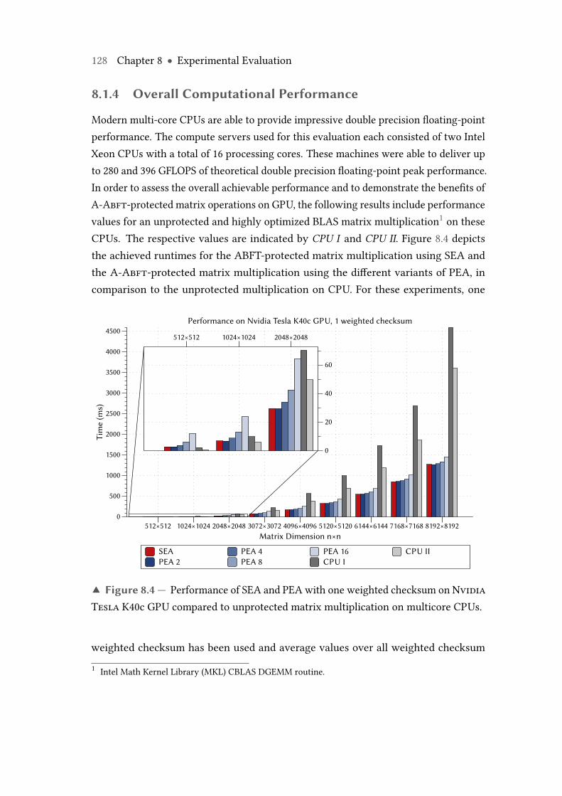
128 Chapter 8 ● Experimental Evaluation
8.1.4 Overall Computational Performance
Modern multi-core CPUs are able to provide impressive double precision floating-pointperformance. The compute servers used for this evaluation each consisted of two IntelXeon CPUs with a total of 16 processing cores. These machines were able to deliver upto 280 and 396 GFLOPS of theoretical double precision floating-point peak performance.In order to assess the overall achievable performance and to demonstrate the benefits ofA-Abft-protected matrix operations on GPU, the following results include performancevalues for an unprotected and highly optimized BLAS matrix multiplication1 on theseCPUs. The respective values are indicated by CPU I and CPU II. Figure 8.4 depictsthe achieved runtimes for the ABFT-protected matrix multiplication using SEA andthe A-Abft-protected matrix multiplication using the different variants of PEA, incomparison to the unprotected multiplication on CPU. For these experiments, one
SEAPEA 2
PEA 4PEA 8
PEA 16CPU I
CPU II
Tim
e (m
s)
0
500
1000
1500
2000
2500
3000
3500
4000
4500
Matrix Dimension n×n512×512 1024×1024 2048×2048 3072×3072 4096×4096 5120×5120 6144×6144 7168×7168 8192×8192
Performance on Nvidia Tesla K40c GPU, 1 weighted checksum
0
20
40
60
512×512 1024×1024 2048×2048
▲ Figure 8.4 — Performance of SEA and PEA with one weighted checksum on NvidiaTesla K40c GPU compared to unprotected matrix multiplication on multicore CPUs.
weighted checksum has been used and average values over all weighted checksum1 Intel Math Kernel Library (MKL) CBLAS DGEMM routine.
8.1 ● Computational Performance 129
types and encoding block sizes are reported. In Appendix F, Figures F.1 and F.2 comparethe overall computational performance for the experiments with one and two weightedchecksums. In addition, Tables F.10 to F.38 report the runtimes for the different weightedchecksum codes, encoding block sizes and problem sizes in detail.
The experimental results show that the unprotected matrix multiplication on CPU I andCPU II yields very high performance values. For a problem size of 7168× 7168, CPUI took 2698.9 ms and CPU II 1866.8 ms. This corresponds to 272.9 and 394.6 GFLOPS,which is equivalent to 97.5% and 99.6% of the CPUs’ theoretical floating-point peakperformance. These results are in good compliance with the observed system CPUutilization of up to 1596% during the experiments, which indicates that all 16 processorcores have been utilized on both machines.
Starting with problems of size 1024× 1024, the ABFT-protected matrix multiplicationson the graphics processing unit (SEA and PEA2) achieved shorter computation times andoutperformed the two multi-core CPUs. With growing problem sizes, the performanceof the ABFT-protected matrix multiplications on the GPU increased substantially. With1001.22 ms (PEA 2) and 1005.57 ms (SEA) for problems of size 8192× 8192, a maximumspeedup of 4.6× has been achieved over the highly optimized and unprotected matrixmultiplication on the twomulticore CPUs. The implementation of theA-Abft-protectedmatrix multiplication achieved up to 1127.2 GFLOPS (PEA 2) for problems of size 8192×8192, which corresponds to 80.5% of the used Nvidia Tesla K40c GPU’s theoreticaldouble precision floating-point peak performance of 1.4 TFLOPS. The implementationof ABFT with SEA achieved up to 1126.1 GFLOPS.
In order to assess the performance impact of the different ABFT design parameterssuch as the ABFT encoding block size, the types and combinations of applied weightedchecksum codes, as well as the different PEA variants, a large number of A-Abft-protected matrix multiplications has been performed across different problem sizes.Tables F.10 to F.38 in Appendix F report the performance results of these experimentsin detail.
In summary, the experimental results show that the different types of weighted check-sum codes, as well as their combinations, do not have a significant impact on the overallperformance. The achieved performance values are very similar across all codes.
The ABFT encoding block size, however, has more influence on the achievable perfor-mance. For experimental setups with one and combinations of two types of weighted
130 Chapter 8 ● Experimental Evaluation
checksum codes, the encoding block sizes of 64× 64 and 128× 128 yielded the highestperformance values for SEA and all PEA variants, across all problem sizes.
In comparison to the experimental setups with one weighted checksum type, thecombinations of two checksum codes increased the computation times by only 3.3%(SEA) and 3.5% (PEA 2) on average.
For the A-Abft method with its probabilistic determination of rounding error bounds(PEA), the number of elements with largest absolute values that have to be consid-ered has direct influence on the overall performance. As expected, PEA16 shows thelowest performance among the different PEA variants. In comparison of the averagecomputation times, PEA8 is up to 1.9×, PEA4 up to 3.2× and PEA2 up to 4.1× fasterfor problem size 512 × 512. However, the performance penalty for PEA16 decreasessignificantly with increasing problem sizes and becomes almost negligible. As will beshown in Sections 8.2 and 8.3, the quality of the determined rounding error bounds andhence the error detection capabilities of PEA2 are comparable to those of PEA16. Forpractical applications, PEA2 is therefore the PEA variant of choice, which yields thehighest computational performance.
8.2 Quality of Rounding Error Bounds
The quality of a determined rounding error bound, i.e. its distance from the actualrounding error, has direct impact on the error detection capability of an ABFT scheme.TheA-Abftmethod proposed in this work utilizes the probabilistic approach introducedin Chapter 6 to determine such rounding error bounds. This probabilistic PEA methodis evaluated and compared in this section against the state of the art simplified erroranalysis technique SEA from [Roy C93]. All experiments have been performed for theinput data sets Tpos, Tf ull and Tortho, across all problem sizes and ABFT encoding blocksizes.
To measure the quality of the rounding error bounds determined by both methods, alarge number of A-Abft-protected matrix multiplications has been performed. Foreach multiplication, the absolute rounding error that affects each checksum element ofthe result matrix has been computed together with the SEA and the different variantsof the PEA rounding error bound. For reference purposes, all computations of interesthave also been performed using a multi-precision floating-point data type with 100-bit precision provided by The GNU Multiple Precision Arithmetic Library (GMP) [The
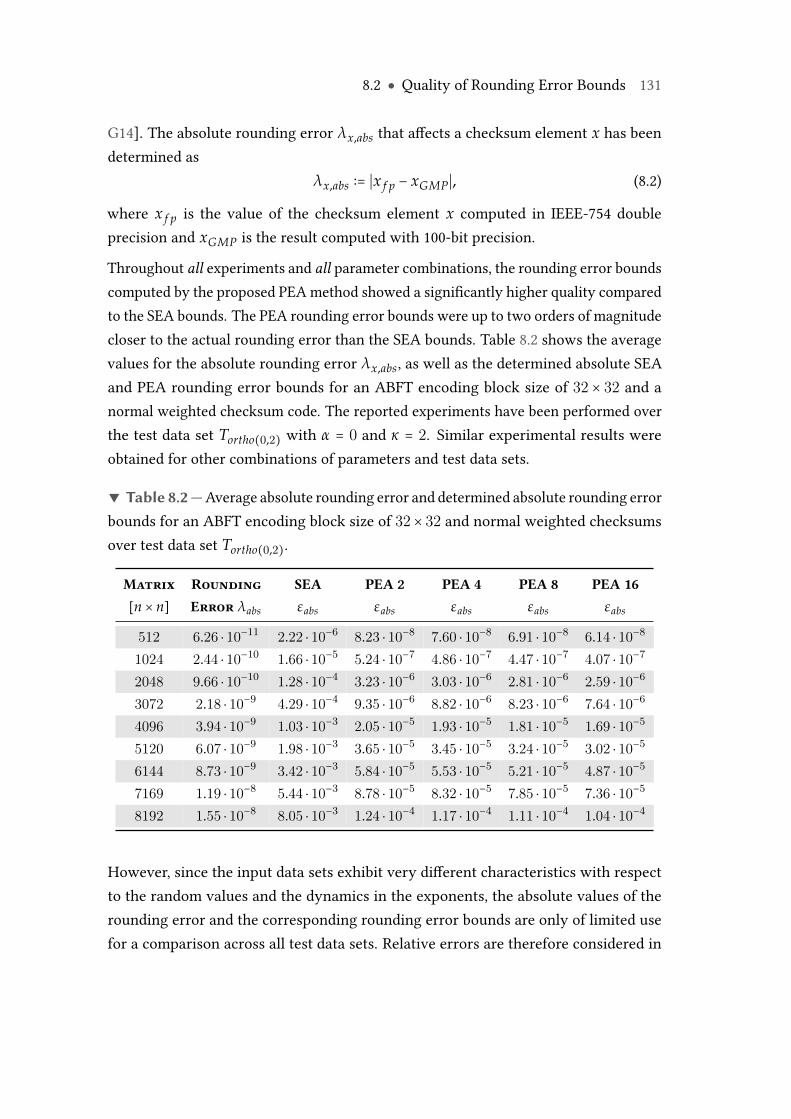
8.2 ● Quality of Rounding Error Bounds 131
G14]. The absolute rounding error λx,abs that affects a checksum element x has beendetermined as
λx,abs ∶= ∣x f p − xGMP∣, (8.2)
where x f p is the value of the checksum element x computed in IEEE-754 doubleprecision and xGMP is the result computed with 100-bit precision.
Throughout all experiments and all parameter combinations, the rounding error boundscomputed by the proposed PEA method showed a significantly higher quality comparedto the SEA bounds. The PEA rounding error bounds were up to two orders of magnitudecloser to the actual rounding error than the SEA bounds. Table 8.2 shows the averagevalues for the absolute rounding error λx,abs, as well as the determined absolute SEAand PEA rounding error bounds for an ABFT encoding block size of 32 × 32 and anormal weighted checksum code. The reported experiments have been performed overthe test data set Tortho(0,2) with α = 0 and κ = 2. Similar experimental results wereobtained for other combinations of parameters and test data sets.
▼ Table 8.2—Average absolute rounding error and determined absolute rounding errorbounds for an ABFT encoding block size of 32× 32 and normal weighted checksumsover test data set Tortho(0,2).
Matrix Rounding SEA PEA 2 PEA 4 PEA 8 PEA 16[n × n] Error λabs εabs εabs εabs εabs εabs
512 6.26 ⋅ 10−11 2.22 ⋅ 10−6 8.23 ⋅ 10−8 7.60 ⋅ 10−8 6.91 ⋅ 10−8 6.14 ⋅ 10−8
1024 2.44 ⋅ 10−10 1.66 ⋅ 10−5 5.24 ⋅ 10−7 4.86 ⋅ 10−7 4.47 ⋅ 10−7 4.07 ⋅ 10−7
2048 9.66 ⋅ 10−10 1.28 ⋅ 10−4 3.23 ⋅ 10−6 3.03 ⋅ 10−6 2.81 ⋅ 10−6 2.59 ⋅ 10−6
3072 2.18 ⋅ 10−9 4.29 ⋅ 10−4 9.35 ⋅ 10−6 8.82 ⋅ 10−6 8.23 ⋅ 10−6 7.64 ⋅ 10−6
4096 3.94 ⋅ 10−9 1.03 ⋅ 10−3 2.05 ⋅ 10−5 1.93 ⋅ 10−5 1.81 ⋅ 10−5 1.69 ⋅ 10−5
5120 6.07 ⋅ 10−9 1.98 ⋅ 10−3 3.65 ⋅ 10−5 3.45 ⋅ 10−5 3.24 ⋅ 10−5 3.02 ⋅ 10−5
6144 8.73 ⋅ 10−9 3.42 ⋅ 10−3 5.84 ⋅ 10−5 5.53 ⋅ 10−5 5.21 ⋅ 10−5 4.87 ⋅ 10−5
7169 1.19 ⋅ 10−8 5.44 ⋅ 10−3 8.78 ⋅ 10−5 8.32 ⋅ 10−5 7.85 ⋅ 10−5 7.36 ⋅ 10−5
8192 1.55 ⋅ 10−8 8.05 ⋅ 10−3 1.24 ⋅ 10−4 1.17 ⋅ 10−4 1.11 ⋅ 10−4 1.04 ⋅ 10−4
However, since the input data sets exhibit very different characteristics with respectto the random values and the dynamics in the exponents, the absolute values of therounding error and the corresponding rounding error bounds are only of limited usefor a comparison across all test data sets. Relative errors are therefore considered in
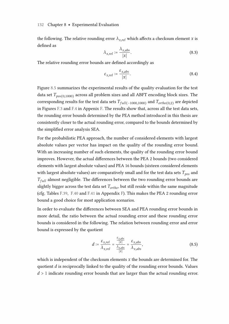
132 Chapter 8 ● Experimental Evaluation
the following. The relative rounding error λx,rel which affects a checksum element x isdefined as
λx,rel ∶=λx,abs
∣x∣ . (8.3)
The relative rounding error bounds are defined accordingly as
εx,rel ∶=εx,abs
∣x∣ . (8.4)
Figure 8.5 summarizes the experimental results of the quality evaluation for the testdata set Tpos(0,1000) across all problem sizes and all ABFT encoding block sizes. Thecorresponding results for the test data sets Tf ull(−1000,1000) and Tortho(0,2) are depictedin Figures F.3 and F.4 in Appenix F. The results show that, across all the test data sets,the rounding error bounds determined by the PEA method introduced in this thesis areconsistently closer to the actual rounding error, compared to the bounds determined bythe simplified error analysis SEA.
For the probabilistic PEA approach, the number of considered elements with largestabsolute values per vector has impact on the quality of the rounding error bound.With an increasing number of such elements, the quality of the rounding error boundimproves. However, the actual differences between the PEA 2 bounds (two consideredelements with largest absolute values) and PEA 16 bounds (sixteen considered elementswith largest absolute values) are comparatively small and for the test data sets Tpos andTf ull almost negligible. The differences between the two rounding error bounds areslightly bigger across the test data set Tortho, but still reside within the same magnitude(cfg. Tables F.39, F.40 and F.41 in Appendix F). This makes the PEA 2 rounding errorbound a good choice for most application scenarios.
In order to evaluate the differences between SEA and PEA rounding error bounds inmore detail, the ratio between the actual rounding error and these rounding errorbounds is considered in the following. The relation between rounding error and errorbound is expressed by the quotient
d ∶=εx,rel
λx,rel=
εx,abs∣x∣
λx,abs∣x∣
=εx,abs
λx,abs, (8.5)
which is independent of the checksum elements x the bounds are determined for. Thequotient d is reciprocally linked to the quality of the rounding error bounds. Valuesd > 1 indicate rounding error bounds that are larger than the actual rounding error.
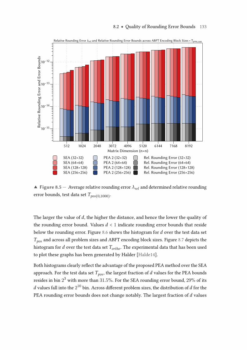
8.2 ● Quality of Rounding Error Bounds 133
SEA (32×32)SEA (64×64)SEA (128×128)SEA (256×256)
PEA 2 (32×32)PEA 2 (64×64)PEA 2 (128×128)PEA 2 (256×256)
Rel. Rounding Error (32×32)Rel. Rounding Error (64×64)Rel. Rounding Error (128×128)Rel. Rounding Error (256×256)
Rela
tive
Roun
ding
Err
or a
nd E
rror
Bou
nds
10−15
10−14
10−13
10−12
Matrix Dimension (n×n)512 1024 2048 3072 4096 5120 6144 7168 8192
Relative Rounding Error λrel and Relative Rounding Error Bounds across ABFT Encoding Block Sizes • Tpos0,1000
▲ Figure 8.5 — Average relative rounding error λrel and determined relative roundingerror bounds, test data set Tpos(0,1000).
The larger the value of d, the higher the distance, and hence the lower the quality ofthe rounding error bound. Values d < 1 indicate rounding error bounds that residebelow the rounding error. Figure 8.6 shows the histogram for d over the test data setTpos and across all problem sizes and ABFT encoding block sizes. Figure 8.7 depicts thehistogram for d over the test data set Tortho. The experimental data that has been usedto plot these graphs has been generated by Halder [Halde14].
Both histograms clearly reflect the advantage of the proposed PEAmethod over the SEAapproach. For the test data set Tpos, the largest fraction of d values for the PEA boundsresides in bin 23 with more than 31.5%. For the SEA rounding error bound, 29% of itsd values fall into the 210 bin. Across different problem sizes, the distribution of d for thePEA rounding error bounds does not change notably. The largest fraction of d values
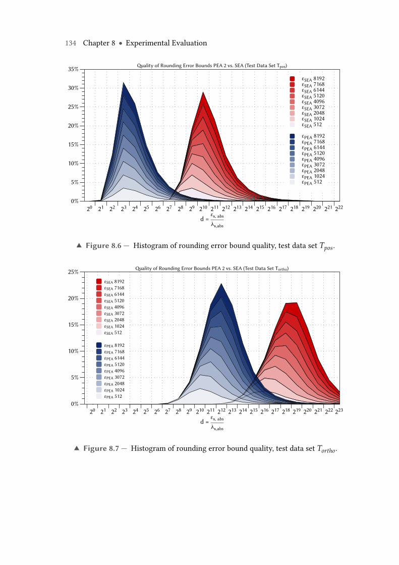
134 Chapter 8 ● Experimental Evaluation
εSEA 8192εSEA 7168εSEA 6144εSEA 5120εSEA 4096εSEA 3072εSEA 2048εSEA 1024εSEA 512 εPEA 8192εPEA 7168εPEA 6144εPEA 5120εPEA 4096εPEA 3072εPEA 2048εPEA 1024εPEA 512
0%
5%
10%
15%
20%
25%
30%
35%
d = εx, abs
λx,abs
20 21 22 23 24 25 26 27 28 29 210 211 212 213 214 215 216 217 218 219 220 221 222
Quality of Rounding Error Bounds PEA 2 vs. SEA (Test Data Set Tpos)
▲ Figure 8.6 — Histogram of rounding error bound quality, test data set Tpos.
εSEA 8192εSEA 7168εSEA 6144εSEA 5120εSEA 4096εSEA 3072εSEA 2048εSEA 1024εSEA 512 εPEA 8192εPEA 7168εPEA 6144εPEA 5120εPEA 4096εPEA 3072εPEA 2048εPEA 1024εPEA 512
0%
5%
10%
15%
20%
25%
d = εx, abs
λx,abs
20 21 22 23 24 25 26 27 28 29 210 211 212 213 214 215 216 217 218 219 220 221 222 223
Quality of Rounding Error Bounds PEA 2 vs. SEA (Test Data Set Tortho)
▲ Figure 8.7 — Histogram of rounding error bound quality, test data set Tortho.
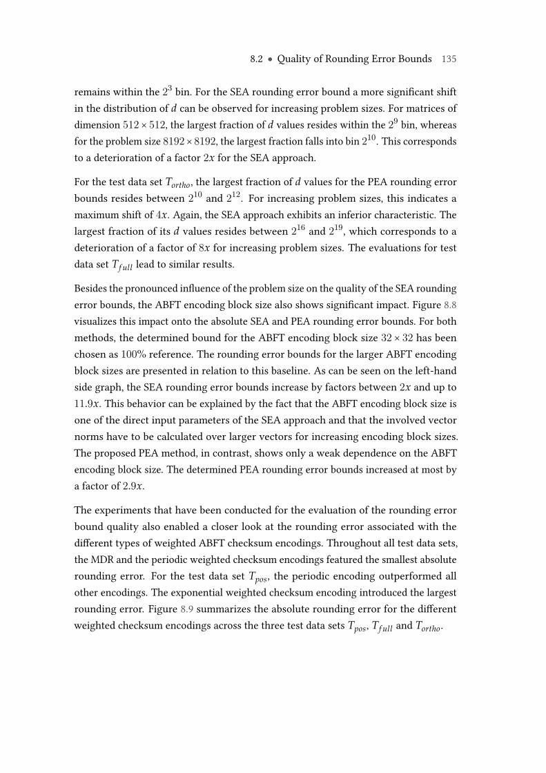
8.2 ● Quality of Rounding Error Bounds 135
remains within the 23 bin. For the SEA rounding error bound a more significant shiftin the distribution of d can be observed for increasing problem sizes. For matrices ofdimension 512× 512, the largest fraction of d values resides within the 29 bin, whereasfor the problem size 8192×8192, the largest fraction falls into bin 210. This correspondsto a deterioration of a factor 2x for the SEA approach.
For the test data set Tortho, the largest fraction of d values for the PEA rounding errorbounds resides between 210 and 212. For increasing problem sizes, this indicates amaximum shift of 4x. Again, the SEA approach exhibits an inferior characteristic. Thelargest fraction of its d values resides between 216 and 219, which corresponds to adeterioration of a factor of 8x for increasing problem sizes. The evaluations for testdata set Tf ull lead to similar results.
Besides the pronounced influence of the problem size on the quality of the SEA roundingerror bounds, the ABFT encoding block size also shows significant impact. Figure 8.8visualizes this impact onto the absolute SEA and PEA rounding error bounds. For bothmethods, the determined bound for the ABFT encoding block size 32 × 32 has beenchosen as 100% reference. The rounding error bounds for the larger ABFT encodingblock sizes are presented in relation to this baseline. As can be seen on the left-handside graph, the SEA rounding error bounds increase by factors between 2x and up to11.9x. This behavior can be explained by the fact that the ABFT encoding block size isone of the direct input parameters of the SEA approach and that the involved vectornorms have to be calculated over larger vectors for increasing encoding block sizes.The proposed PEA method, in contrast, shows only a weak dependence on the ABFTencoding block size. The determined PEA rounding error bounds increased at most bya factor of 2.9x.
The experiments that have been conducted for the evaluation of the rounding errorbound quality also enabled a closer look at the rounding error associated with thedifferent types of weighted ABFT checksum encodings. Throughout all test data sets,the MDR and the periodic weighted checksum encodings featured the smallest absoluterounding error. For the test data set Tpos, the periodic encoding outperformed allother encodings. The exponential weighted checksum encoding introduced the largestrounding error. Figure 8.9 summarizes the absolute rounding error for the differentweighted checksum encodings across the three test data sets Tpos, Tf ull and Tortho.
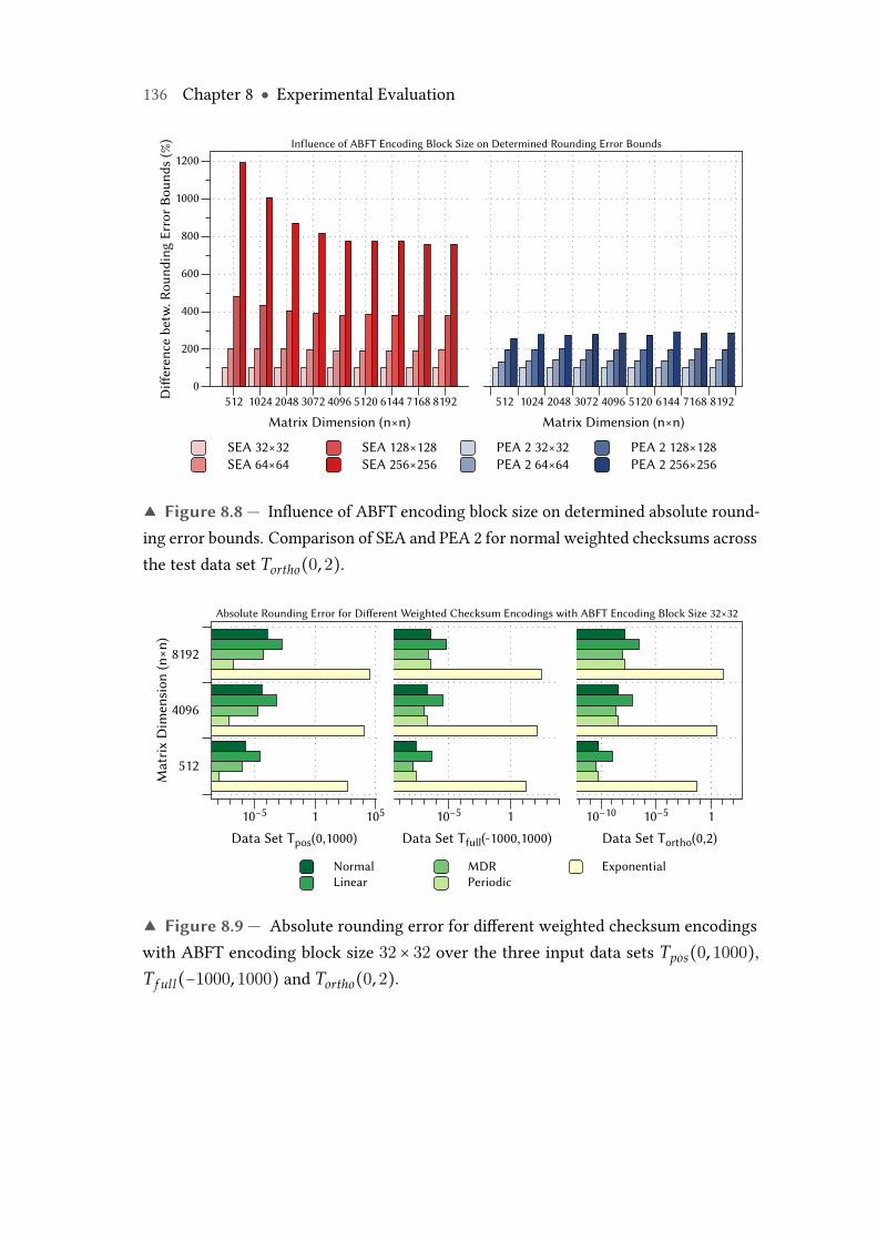
136 Chapter 8 ● Experimental Evaluation
SEA 32×32SEA 64×64
SEA 128×128SEA 256×256
PEA 2 32×32PEA 2 64×64
PEA 2 128×128PEA 2 256×256
Diff
eren
ce b
etw
. Rou
ndin
g Er
ror B
ound
s (%
)
0
200
400
600
800
1000
1200
Matrix Dimension (n×n)512 1024 2048 3072 4096 5120 6144 7168 8192
Matrix Dimension (n×n)512 1024 2048 3072 4096 5120 6144 7168 8192
Influence of ABFT Encoding Block Size on Determined Rounding Error Bounds
▲ Figure 8.8 — Influence of ABFT encoding block size on determined absolute round-ing error bounds. Comparison of SEA and PEA 2 for normal weighted checksums acrossthe test data set Tortho(0, 2).
NormalLinear
MDRPeriodic
Exponential
Mat
rix
Dim
ensi
on (n
×n)
512
4096
8192
Data Set Tpos(0,1000)10−5 1 105
Data Set Tfull(-1000,1000)10−5 1
Data Set Tortho(0,2)10−10 10−5 1
Absolute Rounding Error for Different Weighted Checksum Encodings with ABFT Encoding Block Size 32×32
▲ Figure 8.9 — Absolute rounding error for different weighted checksum encodingswith ABFT encoding block size 32 × 32 over the three input data sets Tpos(0, 1000),Tf ull(−1000, 1000) and Tortho(0, 2).
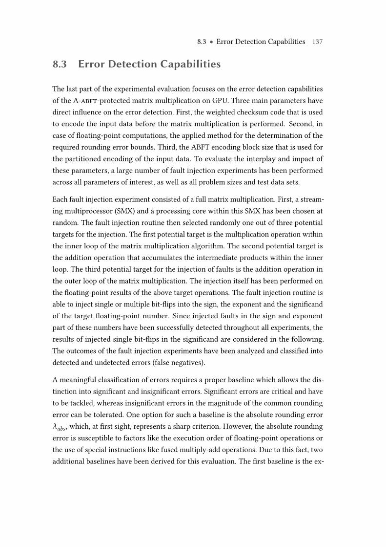
8.3 ● Error Detection Capabilities 137
8.3 Error Detection Capabilities
The last part of the experimental evaluation focuses on the error detection capabilitiesof the A-abft-protected matrix multiplication on GPU. Three main parameters havedirect influence on the error detection. First, the weighted checksum code that is usedto encode the input data before the matrix multiplication is performed. Second, incase of floating-point computations, the applied method for the determination of therequired rounding error bounds. Third, the ABFT encoding block size that is used forthe partitioned encoding of the input data. To evaluate the interplay and impact ofthese parameters, a large number of fault injection experiments has been performedacross all parameters of interest, as well as all problem sizes and test data sets.
Each fault injection experiment consisted of a full matrix multiplication. First, a stream-ing multiprocessor (SMX) and a processing core within this SMX has been chosen atrandom. The fault injection routine then selected randomly one out of three potentialtargets for the injection. The first potential target is the multiplication operation withinthe inner loop of the matrix multiplication algorithm. The second potential target isthe addition operation that accumulates the intermediate products within the innerloop. The third potential target for the injection of faults is the addition operation inthe outer loop of the matrix multiplication. The injection itself has been performed onthe floating-point results of the above target operations. The fault injection routine isable to inject single or multiple bit-flips into the sign, the exponent and the significandof the target floating-point number. Since injected faults in the sign and exponentpart of these numbers have been successfully detected throughout all experiments, theresults of injected single bit-flips in the significand are considered in the following.The outcomes of the fault injection experiments have been analyzed and classified intodetected and undetected errors (false negatives).
A meaningful classification of errors requires a proper baseline which allows the dis-tinction into significant and insignificant errors. Significant errors are critical and haveto be tackled, whereas insignificant errors in the magnitude of the common roundingerror can be tolerated. One option for such a baseline is the absolute rounding errorλabs, which, at first sight, represents a sharp criterion. However, the absolute roundingerror is susceptible to factors like the execution order of floating-point operations orthe use of special instructions like fused multiply-add operations. Due to this fact, twoadditional baselines have been derived for this evaluation. The first baseline is the ex-
138 Chapter 8 ● Experimental Evaluation
pected rounding error λexp, determined by the analysis of the squared sums during theformation of the inner product (see Equation 6.51). The second baseline is the expectedrounding error λprob, which is determined using the probabilistic method introducedin Chapter 6 (see Equation 6.52). The three baselines fulfill the following magnituderelation: λabs ≤ λexp ≤ λprob. Figure 8.10 depicts the three different baselines for thedetermination of significant errors in comparison. In the remainder of this chapter, theresults of the error detection evaluation are presented based on λprob.
71.56
64.30
57.52
77.11
68.94
62.12
94.03
93.75
90.81
62.68
51.59
45.20
67.55
55.31
48.82
82.37
75.22
71.36
72.92
67.02
66.16
77.26
72.60
71.38
93.37
94.10
92.64
65.09
57.69
53.99
68.96
62.49
58.25
83.35
81.00
75.61
74.24
69.93
67.30
78.20
75.02
72.10
95.12
94.37
94.71
66.75
60.40
57.55
70.31
64.80
61.65
85.52
81.51
80.98
SEA λprobSEA λexpSEA λabs
PEA 2 λprobPEA 2 λexpPEA 2 λabs
Mat
rix
Dim
ensi
on (n
×n)
512
4096
8192
Inner Loop Multiplication0% 100%
Inner Loop Addition0% 100%
Outer Loop Addition0% 100%
Percentage of Detected Significant Errors for Different Significance Classes (λX), ABFT Encoding Block Size 32×32
▲ Figure 8.10 — Comparison of the three different baselines for the classificationof significant errors. Test data set Tortho(0,8192) with α = 0 and κ = 8192, for normalweighted checksums.
The following results of the error detection evaluation are presented for the test dataset Tortho(0,65536) with α = 0 and κ = 65536. This is the most challenging test data setwith the highest diversity in the input values and the highest dynamic in the exponents.In order to allow the comparison of all weighted checksum encodings, results for theABFT encoding block sizes 32 × 32, 64 × 64 and 128 × 128 are reported. The resultsfor ABFT encoding blocks of size 256 × 256, which can only be used when a singleweighted checksum is applied, closely followed the trend which becomes visible forthe presented ABFT block sizes. The detection rates for the block size 256× 256 werethe lowest throughout all experiments. The results are reported in the following forthe problem sizes 512× 512, 4096× 4096 and 8192× 8192. The results for the problemsizes in between these sizes also closely followed the presented trend.
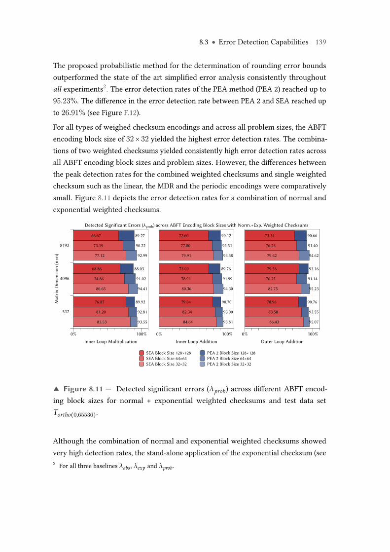
8.3 ● Error Detection Capabilities 139
The proposed probabilistic method for the determination of rounding error boundsoutperformed the state of the art simplified error analysis consistently throughoutall experiments2. The error detection rates of the PEA method (PEA 2) reached up to95.23%. The difference in the error detection rate between PEA 2 and SEA reached upto 26.91% (see Figure F.12).
For all types of weighed checksum encodings and across all problem sizes, the ABFTencoding block size of 32× 32 yielded the highest error detection rates. The combina-tions of two weighted checksums yielded consistently high error detection rates acrossall ABFT encoding block sizes and problem sizes. However, the differences betweenthe peak detection rates for the combined weighted checksums and single weightedchecksum such as the linear, the MDR and the periodic encodings were comparativelysmall. Figure 8.11 depicts the error detection rates for a combination of normal andexponential weighted checksums.
93.55
94.41
92.99
92.81
91.02
90.22
89.92
88.03
89.27
83.53
80.65
77.12
81.20
74.86
73.19
76.87
68.86
66.67
93.81
94.30
93.58
93.00
91.99
91.51
90.70
89.76
90.12
84.64
80.36
79.91
82.34
78.91
77.80
79.04
73.00
72.60
95.07
95.23
94.62
93.55
91.14
91.40
90.76
93.16
90.66
86.43
82.75
79.62
83.50
76.25
76.23
78.96
79.56
73.34
SEA Block Size 128×128SEA Block Size 64×64SEA Block Size 32×32
PEA 2 Block Size 128×128PEA 2 Block Size 64×64PEA 2 Block Size 32×32
Mat
rix
Dim
ensi
on (n
×n)
512
4096
8192
Inner Loop Multiplication0% 100%
Inner Loop Addition0% 100%
Outer Loop Addition0% 100%
Detected Significant Errors (λprob) across ABFT Encoding Block Sizes with Norm.+Exp. Weighted Checksums
▲ Figure 8.11 — Detected significant errors (λprob) across different ABFT encod-ing block sizes for normal + exponential weighted checksums and test data setTortho(0,65536).
Although the combination of normal and exponential weighted checksums showedvery high detection rates, the stand-alone application of the exponential checksum (see2 For all three baselines λabs, λexp and λprob.
140 Chapter 8 ● Experimental Evaluation
Figure F.8) is a conspicuous exception. It showed significantly worse error detectionrates and a particularly strong dependence on the ABFT encoding block sizes. Forthe encoding block size 32× 32, the exponential weighted checksum reached between69.51% and 74.32% error detection rates with PEA 2. For the simplified error analysisSEA, the error detection rates resided between 63.5% and 68.92%. For increasing ABFTencoding block sizes, the error detection rates dropped to 42.82% − 47.22% (ABFTencoding block size 64 × 64, problem size 512 × 512) and 22.95% − 27.07% (ABFTencoding block size 128× 128, problem size 512× 512). The lowest error detection rateswith 17.58%−19.91% became evident for the simplified error analysis SEA and problemsize 8192× 8192. The sole use of exponential weighted checksums can therefore not berecommended on the basis of these results.
Across all test data sets, the combination of normal and MDR weighted checksumsperformed very well. For the single weighted checksums the linear (up to 94.19%), theMDR (up to 94.04%) and the periodic (up to 94.57%) weighted checksum encodingsperformed very similar with high error detection rates. For the test data set Tpos, whichshows very homogeneous input values, the single weighted checksums linear, MDRand periodic outperformed the combined checksums. For test data set Tf ull , the singleweighted checksums linear and MDR yielded the highest error detection rates, followedby the periodic encoding. The normal checksum encoding and the combined weightedchecksums achieved in some cases significantly worse error detection rates.
In Appendix F, the Figures F.5 to F.20 present the detailed experimental results for theevaluation of the error detection capabilities for significance class λabs, as well as forλprob.
Based on these results, the linear, the MDR and in many cases the periodic weightedchecksum encodings can be universally recommended, especially for applications wherethe characteristics of the input data is unknown.
8.4 Discussion of Experimental Results
In summary, the results of the experimental evaluation with respect to the achievablecomputational performance, the quality of the rounding error bounds, as well as theerror detection capabilities, show that the introduced A-Abft method is superior tothe state of the art simplified error analysis method (SEA).
8.4 ● Discussion of Experimental Results 141
Although A-Abft involves more complex algorithmic steps in comparison to SEA, thehigh efficiency of the method enables a high computational performance. This perfor-mance gain, compared to modern multi-core CPUs, enables a substantial accelerationof sophisticated applications in science and engineering combined with an improvedfault tolerance.
The rounding error bounds determined by the A-Abft method (PEA) consistentlyshow a significant improvement over the state of the art, and are up to two orders ofmagnitude closer to the actual rounding error. The method thereby exhibits a muchlower dependence on the ABFT encoding block size and the problem size. High qualityrounding error bounds are an essential prerequisite for the reduction of false negativeerror detections in ABFT-protected floating-point applications.
The results of the fault injection experiments show that, independent of the appliedweighted checksum encoding, the problem size and the characteristics of the inputdata, the A-Abft method consistently achieves better error detection rates, enablingan efficient, effective and autonomously operating ABFT scheme on GPUs.

Chapter
9Conclusions
The rapid spread and growing importance of scientific computing and computer-basedsimulation technology fundamentally change the way how research is carried out andhow complex products are developed. Modern graphics processing units with theirtremendous floating-point compute performance and constantly increasing parallelismact as propellant charge and pave the way for completely new classes of applications. So-phisticated applications in scientific computing and simulation technology, which wereonly possible in large compute centers with high-performance computing equipment afew years ago, are no brought to the desktop using the power of GPUs.
However, with the spread of these applications and their growing influence on social,economical and political processes and decisions, the trustworthiness of the computedresults becomes crucial. Fault tolerance therefore becomes mandatory to improve thereliability and ensure the trustworthiness of such computations. Isolated fault tolerancemeasures are no longer sufficient. Cross-layer reliability requires fault tolerance at eachsystem layer, from the hardware up to the software and the algorithms.
Algorithm-Based Fault Tolerance is a mature fault tolerance technique that allows toimprove the reliability of essential mathematical tasks such as linear algebra matrixoperations. Algorithm-Based Fault Tolerance perfectly fits into the concept of cross-layer reliability and can be combined with other hardware- and software-based faulttolerance techniques.
144 Chapter 9 ● Conclusions
Linear algebra matrix operations like the matrix multiplication are essential componentsof many applications in scientific computing. The development and provision of faulttolerant GPU kernels for such operations will therefore help to significantly improvethe reliability. However, for computations performed in floating-point arithmetic,Algorithm-Based Fault Tolerance schemes often suffer from poor error detection ratesdue to rounding errors. Solutions like manually set rounding error thresholds orcalibration runs are impractical and hamper the application of Algorithm-Based FaultTolerance. State of the art methods for the analytical derivation of rounding errorbounds, such as the simplified error analysis SEA [Roy C93] often lead to weak bounds,which cause insufficient error detection.
In this work, a novel approach called Autonomous Algorithm-Based Fault Tolerance (A-abft) has been introduced for linear algebra matrix operations on GPUs. The approachutilizes a probabilistic model for the determination of rounding error bounds, which aresignificantly closer to the actual rounding error than state of the art approaches. Therequired algorithmic steps are designed in a way that the parallel compute capabilities ofmodern GPUs are utilized to keep the overhead as small as possible. Since the proposedA-abft method operates independently of the input data and does not require any userinteraction, an autonomous operation can be achieved. This eases the integration ofsuch fault tolerant GPU kernels into existing scientific applications.
In-depth experimental evaluations were performed to compare the introduced A-abftmethod against the state of the art simplified error analysis. For the computational per-formance, the experimental results showed that the A-abftmethod does not create anysignificant overhead compared to state of the art techniques. With peak performancevalues of 1127.2 GFLOPS, A-abft achieved up to 80% of the theoretical peak perfor-mance of the used GPU accelerators. The evaluation of the error detection capabilitiesrevealed error detection rates of up to 95.2% for A-abft, which corresponds to animprovement of the state of the art of up to 23%. Besides the evaluation with synthetictest data sets, two case studies were performed which demonstrated the effectivenessand efficiency of A-abft in real world applications.
Ongoing Research and Future Work
The ongoing research focuses on the integration of the probabilistic method for thedetermination of rounding error bounds into more linear algebra matrix operations onGPU to provide a library of fault tolerant, GPU-accelerated building blocks for scientific
145
applications. The research also focuses on further improvements of the rounding errorbounds. For the matrix multiplication, the consideration of block-based local andglobal average values has already been investigated for the probabilistic method byHalder [Halde14]. First results indicated improved rounding error bounds, although theperformance loss was significantly higher, compared to the proposed A-abft method.

Bibliography
[Abdel09] R. Abdelkhalek, H. Calandra, O. Coulaud, J. Roman, and G. Latu. FastSeismic Modeling and Reverse Time Migration on a GPU Cluster. InProceedings of the International Conference on High Performance ComputingSimulation (HPCS ’09), pages 36–43. June 2009. [page 8]
[Agull11] J. I. Agulleiro and J. J. Fernandez. Fast tomographic reconstructionon multicore computers. Bioinformatics, 27(4):582–583, 2011. URLhttp://bioinformatics.oxfordjournals.org/content/27/4/
582.abstract. [page 8]
[Alam05] M. Alam and S. Mahapatra. A comprehensive model of PMOSNBTI degradation. Microelectronics Reliability, 45(1):71 – 81,2005. URL http://www.sciencedirect.com/science/article/
pii/S0026271404001751. [page 11]
[Ander08] J. A. Anderson, C. D. Lorenz, and A. Travesset. General purposemolecular dynamics simulations fully implemented on graphics pro-cessing units. Journal of Computational Physics, 227(10):5342 – 5359,2008. URL http://www.sciencedirect.com/science/article/
pii/S0021999108000818. [page 8]
[Anfin88] C. J. Anfinson and F. T. Luk. A Linear Algebraic Model of Algorithm-BasedFault Tolerance. IEEE Transactions on Computers, 37(12):1599–1604, 1988.[pages 62, 64, and 66]
[Arnau11] L. Arnaud, P. Lamontagne, R. Galand, E. Petitprez, D. Ney, and P. Waltz.Electromigration Induced Void Kinetics In Cu Interconnects For AdvancedCMOS Nodes. In Proceedings of the IEEE International Reliability PhysicsSymposium (IRPS’11), pages 3E.1.1–3E.1.10. April 2011. [page 11]
148 Bibliography
[Aseno98] A. Asenov. Random Dopant Induced Threshold Voltage Lowering andFluctuations in Sub-0.1 µm MOSFET’s: A 3-D "Atomistic" SimulationStudy. IEEE Transactions on Electron Devices, 45(12):2505–2513, Dec 1998.[page 11]
[Aseno03] A. Asenov, S. Kaya, and A. R. Brown. Intrinsic Parameter Fluctuations inDecananometer MOSFETs Introduced by Gate Line Edge Roughness. IEEETransactions on Electron Devices, 50(5):1254–1260, May 2003. [page 11]
[Assad92] F. T. Assad and S. Dutt. More Robust Tests in Algorithm-Based Fault-Tolerant Matrix Multiplication. In Digest of Papers of the Twenty-SecondInternational Symposium on Fault-Tolerant Computing (FTCS-22), pages430–439. 1992. [page 72]
[Avizi04] A. Avižienis, J.-C. Laprie, B. Randell, and C. Landwehr. Basic Concepts andTaxonomy of Dependable and Secure Computing. IEEE Transactions onDependable and Secure Computing, 1(1):11–33, Jan 2004. [pages 17 and 20]
[Aykan87] C. Aykanat and F. Ozguner. A Concurrent Error Detecting ConjugateGradient Algorithm on a Hypercube Multiprocessor. In IEEE 17th Inter-national Symposium on Fault Tolerant Computing, pages 204–209. 1987.[page 58]
[Backe12] J. Backer and R. Karri. Balancing Performance and Fault Detection forGPGPU Workloads. In 30th IEEE International Conference on ComputerDesign (ICCD’12), pages 518–519. Sept 2012. [page 50]
[Bakho09] A. Bakhoda, G. Yuan, W. Fung, H. Wong, and T. Aamodt. Analyzing CUDAWorkloads Using a Detailed GPU Simulator. In Proceedings of the IEEEInternational Symposium on Performance Analysis of Systems and Software(ISPASS’09), pages 163–174. April 2009. [pages 41 and 52]
[Baner88] P. Banerjee and C. B. Stunkel. A Novel Approach to System-level FaultTolerance in Hypercube Multiprocessors. In Proceedings of the ThirdConference on Hypercube Concurrent Computers and Applications: Archi-tecture, Software, Computer Systems, and General Issues - Volume 1, pages307–311. ACM, New York, NY, USA, 1988. ISBN 0-89791-278-0. URLhttp://doi.acm.org/10.1145/62297.62330. [pages 58 and 71]
Bibliography 149
[Baner90] P. Banerjee, J. T. Rahmeh, C. Stunkel, V. S. Nair, K. Roy, V. Balasubramanian,and J. A. Abraham. Algorithm-Based Fault Tolerance on a HypercubeMultiprocessor. IEEE Transactions on Computers, 39(9):1132–1145, 1990.[pages 58 and 71]
[Barlo81] J. L. Barlow. Probabilistic Error Analysis of Floating Point and CRD Arith-metics. Ph.D. thesis, Evanston, IL, USA, 1981. AAI8124850. [page 87]
[Barlo83] J. L. Barlow. Fast a posteriori bounds for roundoff error in Gaussianelimination. Technical report, Technical Report No. CS-83-20, Departmentof Computer Science, The Pennsylvania State University, University Park,Pennsylvania (September 1983), 1983. [page 87]
[Barlo85a] J. L. Barlow and E. H. Bareiss. On Roundoff Error Distributions in Float-ing Point and Logarithmic Arithmetic. Computing, 34(4):325–347, 1985.[pages 84, 86, 89, 90, 92, and 94]
[Barlo85b] J. L. Barlow and E. H. Bareiss. Probabilistic Error Analysis of GaussianElimination in Floating Point and Logarithmic Arithmetic. Computing,34(4):349–364, 1985. URL http://dx.doi.org/10.1007/BF02251834.[pages 87 and 92]
[Bayra06] I. Bayraktaroglu, J. Hunt, and D. Watkins. Cache Resident FunctionalMicroprocessor Testing: Avoiding High Speed IO Issues. In Proceedingsof the IEEE International Test Conference (ITC’06), pages 1–7. Oct 2006.[page 48]
[Belle08] R. G. Belleman, J. Bédorf, and S. F. P. Zwart. High performancedirect gravitational N-body simulations on graphics processing unitsII: An implementation in CUDA. New Astronomy, 13(2):103 – 112,2008. URL http://www.sciencedirect.com/science/article/
pii/S1384107607000760. [page 8]
[Benfo38] F. Benford. The Law of Anomalous Numbers. Proceedings of the AmericanPhilosophical Society, 78(4):pp. 551–572, 1938. URL http://www.jstor.
org/stable/984802. [pages 86 and 87]
150 Bibliography
[Benne97] G. R. Bennett. The application of virtual prototyping in the develop-ment of complex aerospace products. Aircraft Engineering and AerospaceTechnology, 69(1):19–25, 1997. [page 4]
[Bensc08] J. Benschop, V. Banine, S. Lok, and E. Loopstra. Extreme ultravioletlithography: Status and prospects. Journal of Vacuum Science & TechnologyB, 26(6):2204–2207, 2008. [page 11]
[Berge05] A. Berger, L. Bunimovich, and T. Hill. One-Dimensional Dynamical Sys-tems and Benford’s Law. Transactions of the American MathematicalSociety, 357(1):197–219, 2005. [page 87]
[Berge11] A. Berger and T. P. Hill. A Basic Theory of Benford’s Law. ProbabilitySurveys, 8:1–126, 2011. [pages 87 and 88]
[Bliss88] W. G. Bliss, M. R. Lightner, and B. Friedlander. Numerical Properties OfAlgorithm-Based Fault-Tolerance For High Reliability Array Processors.In Twenty-Second Asilomar Conference on Signals, Systems and Computers,volume 2, pages 631–635. 1988. [page 67]
[Bol09] D. Bol, R. Ambroise, D. Flandre, and J.-D. Legat. Interests and Limita-tions of Technology Scaling for Subthreshold Logic. IEEE Transactions onVery Large Scale Integration (VLSI) Systems, 17(10):1508–1519, Oct 2009.[page 11]
[Bonga95] I. Bongartz, A. R. Conn, N. Gould, and P. L. Toint. CUTE: Constrained andUnconstrained Testing Environment. ACM Transactions on MathematicalSoftware, 21(1):123–160, March 1995. URL http://doi.acm.org/10.
1145/200979.201043. [page 113]
[Borka05] S. Borkar. Designing Reliable Systems from Unreliable Components: TheChallenges of Transistor Variability and Degradation. IEEEMicro, 25(6):10–16, Nov 2005. [page 11]
[Bosil15] G. Bosilca, A. Bouteiller, T. Herault, Y. Robert, and J. Dongarra. Compos-ing Resilience Techniques: ABFT, Periodic and Incremental Checkpoint-ing. International Journal of Networking and Computing, 5(1):2–25, 2015.[page 47]
Bibliography 151
[Bourg04] A. Bourgeat, M. Kern, S. Schumacher, and J. Talandier. The COUPLEX TestCases: Nuclear Waste Disposal Simulation. Computational Geosciences,8(2):83–98, 2004. [page 9]
[Bowma09] K. Bowman, J. Tschanz, C. Wilkerson, S.-L. Lu, T. Karnik, V. De, andS. Borkar. Circuit Techniques for Dynamic Variation Tolerance. In Pro-ceedings of the 46th Annual Design Automation Conference, DAC ’09, pages4–7. ACM, New York, NY, USA, 2009. ISBN 978-1-60558-497-3. URLhttp://doi.acm.org/10.1145/1629911.1629915. [page 11]
[Braun12a] C. Braun, M. Daub, A. Schöll, G. Schneider, and H.-J. Wunderlich. Paral-lel Simulation of Apoptotic Receptor-Clustering on GPGPU Many-CoreArchitectures. In IEEE International Conference on Bioinformatics andBiomedicine (BIBM’12), pages 1–6. 2012. [page 8]
[Braun12b] C. Braun, S. Holst, H.-J. Wunderlich, J. M. Castillo, and J. Gross. Ac-celeration of Monte-Carlo Molecular Simulations on Hybrid ComputingArchitectures. In IEEE 30th International Conference on Computer Design(ICCD’12), pages 207–212. 2012. [page 8]
[Braun14] C. Braun, S. Halder, and H.-J. Wunderlich. A-ABFT: AutonomousAlgorithm-Based Fault Tolerance for Matrix Multiplications on GraphicsProcessing Units. In Proceedings of the 44th Annual IEEE/IFIP Interna-tional Conference on Dependable Systems and Networks (DSN 2014). 2014.[pages 83, 100, 102, and 121]
[Burke91] J. Burke and E. Kincanon. Benford’s Law and Physical Constants: TheDistribution of Initial Digits. American Journal of Physics, 59(10):952–952,1991. [page 87]
[Bushn00] M. L. Bushnell and V. D. Agrawal. Essentials of Electronic Testing for Digital,Memory andMixed-Signal VLSI Circuits, volume 17 of Frontiers in ElectronicTesting. Springer, 2000. ISBN 978-0-7923-7991-1. [pages 20 and 47]
[Busto79] J. Bustoz, A. Feldstein, R. Goodman, and S. Linnainmaa. Improved TrailingDigits Estimates Applied to Optimal Computer Arithmetic. Journal ofthe ACM, 26(4):716–730, October 1979. URL http://doi.acm.org/10.
1145/322154.322162. [page 89]
152 Bibliography
[Cappe09] F. Cappello, A. Geist, B. Gropp, L. Kale, B. Kramer, and M. Snir. TowardExascale Resilience. International Journal of High Performance Comput-ing Applications, 23(4):374–388, 2009. URL http://hpc.sagepub.com/
content/23/4/374.abstract. [page 10]
[Carte10] N. P. Carter, H. Naeimi, and D. S. Gardner. Design Techniques for Cross-layer Resilience. In Proceedings of the Conference on Design, Automationand Test in Europe, DATE ’10, pages 1023–1028. European Design andAutomation Association, Leuven, Belgium, 2010. ISBN 978-3-9810801-6-2. URL http://dl.acm.org/citation.cfm?id=1870926.1871178.[page 14]
[Catan08a] B. Catanzaro, K. Keutzer, and B.-Y. Su. Parallelizing CAD: A TimelyResearch Agenda for EDA. In Proceedings of the 45th Annual DesignAutomation Conference (DAC’08), DAC ’08, pages 12–17. ACM, New York,NY, USA, 2008. ISBN 978-1-60558-115-6. URL http://doi.acm.org/
10.1145/1391469.1391475. [page 6]
[Catan08b] B. Catanzaro, N. Sundaram, and K. Keutzer. Fast Support Vector MachineTraining and Classification on Graphics Processors. In Proceedings ofthe 25th International Conference on Machine Learning, ICML ’08, pages104–111. ACM, New York, NY, USA, 2008. ISBN 978-1-60558-205-4. URLhttp://doi.acm.org/10.1145/1390156.1390170. [page 8]
[Chang10] D. Chang, C. Jenkins, P. Garcia, S. Gilani, P. Aguilera, A. Nagarajan, M. An-derson, M. Kenny, S. Bauer, M. Schulte, and K. Compton. ERCBench: AnOpen-Source Benchmark Suite for Embedded and Reconfigurable Comput-ing. In Proceedings of the International Conference on Field ProgrammableLogic and Applications (FPL’10), pages 408–413. Aug 2010. [page 51]
[Chatt09a] D. Chatterjee, A. DeOrio, and V. Bertacco. Event-driven Gate-level Sim-ulation with GP-GPUs. In Proceedings of the 46th Annual Design Au-tomation Conference (DAC’09), pages 557–562. ACM, New York, NY, USA,2009. ISBN 978-1-60558-497-3. URL http://doi.acm.org/10.1145/
1629911.1630056. [page 8]
[Chatt09b] D. Chatterjee, A. DeOrio, and V. Bertacco. GCS: High-performance Gate-level Simulation with GP-GPUs. In Proceedings of the Conference on Design,
Bibliography 153
Automation and Test in Europe (DATE’09), DATE ’09, pages 1332–1337.European Design and Automation Association, 3001 Leuven, Belgium,Belgium, 2009. ISBN 978-3-9810801-5-5. URL http://dl.acm.org/
citation.cfm?id=1874620.1874941. [page 8]
[Che09] S. Che, M. Boyer, J. Meng, D. Tarjan, J. W. Sheaffer, S.-H. Lee, andK. Skadron. Rodinia: A Benchmark Suite for Heterogeneous Computing.In Proceedings of the IEEE International Symposium on Workload Charac-terization (IISWC’09), pages 44–54. IEEE, 2009. [pages 41, 42, and 52]
[Chen86] C.-Y. Chen and J. A. Abraham. Fault-Tolerant Systems for the Computationof Eigenvalues and Singular Values. In SPIE Proc. 30th Annual TechnicalSymposium, pages 228–237. International Society for Optics and Photonics,1986. [page 58]
[Chen99] P. Chen, L. Wu, G. Zhang, and Z. Liu. A Unified Compact Scalable δid
Model for Hot Carrier Reliability Simulation. In Proceedings of the 37thAnnual IEEE International Reliability Physics Symposium, pages 243–248.1999. [page 11]
[Chen01] L. Chen and S. Dey. Software-Based Self-Testing Methodology for Pro-cessor Cores. IEEE Transactions on Computer-Aided Design of IntegratedCircuits and Systems, 20(3):369–380, Mar 2001. [page 48]
[Chen03] L. Chen, S. Ravi, A. Raghunathan, and S. Dey. A Scalable Software-basedSelf-test Methodology for Programmable Processors. In Proceedings ofthe 40th Annual Design Automation Conference (DAC’03), DAC ’03, pages548–553. ACM, New York, NY, USA, 2003. ISBN 1-58113-688-9. URLhttp://doi.acm.org/10.1145/775832.775973. [page 48]
[Cohen73] A. M. Cohen. Numerical Analysis. European mathematics series. McGraw-Hill, 1973. ISBN 9780070840126. URL http://books.google.de/
books?id=DivvAAAAMAAJ. [page 68]
[Corno03] F. Corno, G. Cumani, M. Reorda, and G. Squillero. Fully Automatic TestProgramGeneration forMicroprocessor Cores. In Proceedings of the Design,Automation and Test in Europe Conference and Exhibition (DATE’03), pages1006–1011. 2003. [page 48]
154 Bibliography
[Croix13] J. F. Croix, S. P. Khatri, and K. Gulati. Using GPUs to Accelerate CADAlgorithms. IEEE Design Test, 30(1):8–16, Feb 2013. [page 8]
[Dantz53] G. B. Dantzig and W. Orchard-Hays. Notes on Linear Programming: PartV—Alternate Algorithm for the Revised Simplex Method using ProductForm for the Inverse. The RAND Corporation Research Memorandum, 1268,1953. [page 111]
[Dantz63] G. B. Dantzig. Linear Programming and Extensions. A RAND CorporationResearch Study, 1963. [page 110]
[Davie11] T. Davies, C. Karlsson, H. Liu, C. Ding, and Z. Chen. High Performance Lin-pack Benchmark: A Fault Tolerant Implementation Without Checkpoint-ing. In Proceedings of the International Conference on Supercomputing, ICS’11, pages 162–171. ACM, New York, NY, USA, 2011. ISBN 978-1-4503-0102-2. URL http://doi.acm.org/10.1145/1995896.1995923. [page 58]
[DeHon10] A. DeHon, H. M. Quinn, and N. P. Carter. Vision for Cross-Layer Opti-mization to Address the Dual Challenges of Energy and Reliability. InProceedings of the Design, Automation Test in Europe Conference Exhibition(DATE’10), pages 1017–1022. March 2010. [page 13]
[Demat10] L. Dematté and D. Prandi. GPU computing for systems biology.Briefings in Bioinformatics, 11(3):323–333, 2010. URL http://bib.
oxfordjournals.org/content/11/3/323.abstract. [page 8]
[Di Ca13a] S. Di Carlo, G. Gambardella, M. Indaco, I. Martella, P. Prinetto, D. Rolfo,and P. Trotta. A Software-based Self Test of CUDA Fermi GPUs. In 18thIEEE European Test Symposium (ETS’13), pages 1–6. May 2013. [pages 49and 52]
[Di Ca13b] S. Di Carlo, G. Gambardella, I. Martella, P. Prinetto, D. Rolfo, and P. Trotta.Fault Mitigation Strategies for CUDA GPUs. In IEEE International TestConference (ITC’13), pages 1–8. Sept 2013. [page 52]
[Dimit09] M. Dimitrov, M. Mantor, and H. Zhou. Understanding Software Ap-proaches for GPGPU Reliability. In Proceedings of 2nd Workshop on Gen-eral Purpose Processing on Graphics Processing Units, GPGPU-2, pages
Bibliography 155
94–104. ACM, New York, NY, USA, 2009. ISBN 978-1-60558-517-8.URL http://doi.acm.org/10.1145/1513895.1513907. [pages 50and 54]
[Du11] P. Du, P. Luszczek, and J. J. Dongarra. High Performance Dense LinearSystem Solver with Soft Error Resilience. In IEEE International Conferenceon Cluster Computing (CLUSTER’11), pages 272–280. 2011. [page 58]
[Dutt96] S. Dutt and F. T. Assaad. Mantissa-Preserving Operations and Robust Algo-rithm Based Fault Tolerance for Matrix Computations. IEEE Transactionson Computers, 45(4):408–424, 1996. [page 72]
[Dweik14] W. Dweik, M. Abdel-Majeed, and M. Annavaram. Warped-Shield: Tol-erating Hard Faults in GPGPUs. In 44th Annual IEEE/IFIP InternationalConference on Dependable Systems and Networks (DSN’14), pages 431–442.June 2014. [page 51]
[Ehlig10] C. Ehlig-Economides and M. J. Economides. Sequestering carbon dioxidein a closed underground volume. Journal of Petroleum Science and En-gineering, 70:123 – 130, 2010. URL http://www.sciencedirect.com/
science/article/pii/S0920410509002368. [pages 8 and 9]
[Engel03] H.-A. Engel and C. Leuenberger. Benford’s Law for ExponentialRandom Variables. Statistics & Probability Letters, 63(4):361 – 365,2003. URL http://www.sciencedirect.com/science/article/
pii/S0167715203001019. [page 87]
[Fang14] B. Fang, K. Pattabiraman, M. Ripeanu, and S. Gurumurthi. GPU-Qin: AMethodology for Evaluating the Error Resilience of GPGPU Applications.In Proceedings of the IEEE International Symposium on Performance Analysisof Systems and Software (ISPASS’14), pages 221–230. March 2014. [page 41]
[Felds76] A. Feldstein and R. Goodman. Convergence Estimates for the Distributionof Trailing Digits. Journal of the ACM, 23(2):287–297, April 1976. URLhttp://doi.acm.org/10.1145/321941.321948. [page 89]
[Felds82] A. Feldstein and R. H. Goodman. Loss of Significance in Floating PointSubtraction and Addition. IEEE Transactions on Computers, C-31(4):328–335, 1982. [page 87]
156 Bibliography
[Felds86] A. Feldstein and P. Turner. Overflow, Underflow, and Severe Loss ofSignificance in Floating-Point Addition and Subtraction. IMA Jour-nal of Numerical Analysis, 6(2):241–251, 1986. URL http://imajna.
oxfordjournals.org/content/6/2/241.abstract. [page 87]
[Flehi66] B. J. Flehinger. On the Probability that a Random Integer has Initial DigitA. The American Mathematical Monthly, 73(10):pp. 1056–1061, 1966. URLhttp://www.jstor.org/stable/2314636. [page 87]
[Fluhr14] E. J. Fluhr, J. Friedrich, D. Dreps, V. Zyuban, G. Still, C. Gonzalez, A. Hall,D. Hogenmiller, F. Malgioglio, R. Nett, J. Paredes, J. Pille, D. Plass, R. Puri,P. Restle, D. Shan, K. Stawiasz, Z. T. Deniz, D. Wendel, and M. Ziegler.5.1 POWER8TM: A 12-Core Server-Class Processor in 22nm SOI with7.6Tb/s Off-Chip Bandwidth. In Digest of Technical Papers of the 2014 IEEEInternational Solid-State Circuits Conference (ISSCC’14), pages 96–97. Feb2014. [page 31]
[Flynn72] M. J. Flynn. Some Computer Organizations and Their Effectiveness. IEEETransactions on Computers, C-21(9):948–960, Sept 1972. [pages 6 and 27]
[Forsy67] G. E. Forsythe and C. B. Moler. Computer Solution of Linear AlgebraicSystems. Prentice-Hall, Englewood Cliffs, NJ, 1967. [page 24]
[Gaikw09] A. Gaikwad and I. M. Toke. GPU Based Sparse Grid Technique for Solv-ing Multidimensional Options Pricing PDEs. In Proceedings of the 2NdWorkshop on High Performance Computational Finance, WHPCF ’09, pages6:1–6:9. ACM, New York, NY, USA, 2009. ISBN 978-1-60558-716-5. URLhttp://doi.acm.org/10.1145/1645413.1645419. [page 9]
[Gaikw10] A. Gaikwad and I. M. Toke. Parallel Iterative Linear Solvers on GPU: AFinancial Engineering Case. In Proceedings of the 18th Euromicro Inter-national Conference on Parallel, Distributed and Network-Based Processing(PDP’10), pages 607–614. Feb 2010. [page 9]
[Gent11] P. R. Gent, G. Danabasoglu, L. J. Donner, M. M. Holland, E. C. Hunke,S. R. Jayne, D. M. Lawrence, R. B. Neale, P. J. Rasch, M. Vertenstein, P. H.Worley, Z.-L. Yang, and M. Zhang. The Community Climate SystemModel
Bibliography 157
Version 4. Journal of Climate, 24(19):4973–4991, 2014/05/18 2011. URLhttp://dx.doi.org/10.1175/2011JCLI4083.1. [page 4]
[Gizop04] D. Gizopoulos, A. Paschalis, and Y. Zorian. Embedded Processor-BasedSelf-Test, volume 28 of Frontiers in Electronic Testing. Springer Science &Business Media, 2004. ISBN 978-1-4419-5252-3. [page 48]
[Goess08] M. Goessel, V. Ocheretny, E. Sogomonyan, and D.Marienfeld. NewMethodsof Concurrent Checking, volume 42. Springer Science+Business Media B.V.,2008. ISBN 978-1-4020-8419-5. [page 39]
[Goldb91] D. Goldberg. What every computer scientist should know about floating-point arithmetic. ACM Comput. Surv., 23(1):5–48, March 1991. URLhttp://doi.acm.org/10.1145/103162.103163. [page 25]
[Golub12] G. H. Golub and C. F. Van Loan. Matrix Computations. The Johns HopkinsUniversity Press, 4th edition, 2012. ISBN 978-1-4214-0794-4. [pages 73,104, and 105]
[Goodn05] N. Goodnight, C. Woolley, G. Lewin, D. Luebke, and G. Humphreys.A Multigrid Solver for Boundary Value Problems Using ProgrammableGraphics Hardware. In ACM SIGGRAPH 2005 Courses, SIGGRAPH ’05.ACM, New York, NY, USA, 2005. URL http://doi.acm.org/10.1145/
1198555.1198784. [page 8]
[Govin04] N. K. Govindaraju, B. Lloyd, W. Wang, M. Lin, and D. Manocha. FastComputation of Database Operations Using Graphics Processors. In Pro-ceedings of the 2004 ACM SIGMOD International Conference onManagementof Data, SIGMOD ’04, pages 215–226. ACM, New York, NY, USA, 2004.ISBN 1-58113-859-8. URL http://doi.acm.org/10.1145/1007568.
1007594. [page 8]
[Govin06] N. Govindaraju, J. Gray, R. Kumar, and D. Manocha. GPUTeraSort: HighPerformance Graphics Co-processor Sorting for Large Database Manage-ment. In Proceedings of the 2006 ACM SIGMOD International Conference onManagement of Data, SIGMOD ’06, pages 325–336. ACM, New York, NY,USA, 2006. ISBN 1-59593-434-0. URL http://doi.acm.org/10.1145/
1142473.1142511. [page 8]
158 Bibliography
[Gulat08] K. Gulati and S. P. Khatri. Towards Acceleration of Fault SimulationUsing Graphics Processing Units. In Proceedings of the 45th Annual DesignAutomation Conference (DAC’08), pages 822–827. ACM, New York, NY,USA, 2008. ISBN 978-1-60558-115-6. URL http://doi.acm.org/10.
1145/1391469.1391679. [page 8]
[Gunne01] J. A. Gunnels, D. S. Katz, E. S. Quintana-Ortí, and R. A. Van de Gejin. Fault-Tolerant High-Performance Matrix Multiplication: Theory and Practice.In International Conference on Dependable Systems and Networks (DSN’01),pages 47–56. 2001. [page 74]
[Gurum06] S. Gurumurthy, S. Vasudevan, and J. Abraham. Automatic Generationof Instruction Sequences Targeting Hard-to-Detect Structural Faults in aProcessor. In Proceedings of the IEEE International Test Conference (ITC’06),pages 1–9. Oct 2006. [page 48]
[Halde14] S. Halder. Integration von algorithmenbasierter Fehlertoleranz in grundle-gende Operationen der linearen Algebra auf GPGPUs. Diplomarbeit, Uni-versität Stuttgart, Fakultät Informatik, Elektrotechnik und Information-stechnik, Germany, April 2014. [pages 102, 107, 133, and 145]
[Hamad09] T. Hamada, T. Narumi, R. Yokota, K. Yasuoka, K. Nitadori, and M. Taiji. 42TFlops Hierarchical N-body Simulations on GPUs with Applications inBoth Astrophysics and Turbulence. In Proceedings of the Conference onHigh Performance Computing Networking, Storage and Analysis, SC ’09,pages 62:1–62:12. ACM, New York, NY, USA, 2009. ISBN 978-1-60558-744-8.URL http://doi.acm.org/10.1145/1654059.1654123. [page 8]
[Hammi50] R. W. Hamming. Error Detecting and Error Correcting Codes. Bell SystemTechnical Journal, 29(2):147–160, 1950. [page 184]
[Hammi70] R. W. Hamming. On the Distribution of Numbers. Bell System TechnicalJournal, 49(8):1609–1625, 1970. [pages 86, 87, and 89]
[Hargr06] P. H. Hargrove and J. C. Duell. Berkeley Lab Checkpoint/Restart (BLCR)for Linux Clusters. In Journal of Physics: Conference Series, volume 46,page 494. IOP Publishing, 2006. [page 46]
Bibliography 159
[He08] B. He, W. Fang, Q. Luo, N. K. Govindaraju, and T. Wang. Mars: A MapRe-duce Framework on Graphics Processors. In Proceedings of the 17th In-ternational Conference on Parallel Architectures and Compilation Tech-niques, PACT ’08, pages 260–269. ACM, New York, NY, USA, 2008. ISBN978-1-60558-282-5. URL http://doi.acm.org/10.1145/1454115.
1454152. [page 9]
[Heath97] M. T. Heath. Scientific Computing: An Introductory Survey. The McGraw-Hill Companies, New York, 1997. [page 4]
[Henne12] J. L. Hennessy and D. A. Patterson. Computer Architecture: A QuantitativeApproach. Morgan Kaufmann, Elsevier Inc., 5th edition, 2012. ISBN9780123838728. [page 6]
[Higha02] N. J. Higham. Accuracy and Stability of Numerical Algorithms. Societyfor Industrial and Applied Mathematics (SIAM), 2nd edition, 2002. ISBN0-89871-521-0. [page 73]
[Hill95a] T. P. Hill. A Statistical Derivation of the Significant-Digit Law. StatisticalScience, 10(4):pp. 354–363, 1995. URL http://www.jstor.org/stable/
2246134. [pages 86 and 88]
[Hill95b] T. P. Hill. Base-invariance Implies Benford’s Law. Proceedings of theAmerican Mathematical Society, 123(3):887–895, 1995. [page 88]
[Hill98] T. P. Hill. The First Digit Phenomenon. American Scientist, 86(4):358–363,1998. [page 87]
[Hollo05] S. Holloway. Underground sequestration of carbon dioxide—a vi-able greenhouse gas mitigation option. Energy, 30:2318 – 2333,2005. URL http://www.sciencedirect.com/science/article/
pii/S0360544204003883, international Symposium on {CO2} Fixationand Efficient Utilization of Energy (CandE 2002) and the InternationalWorld Energy System Conference (WESC-2002). [pages 8 and 9]
[Holst12] S. Holst, E. Schneider, and H.-J. Wunderlich. Scan Test Power Simulationon GPGPUs. In Proceedings of the IEEE 21st Asian Test Symposium (ATS’12),pages 155–160. Nov 2012. [page 8]
160 Bibliography
[House58] A. S. Householder. Unitary Triangularization of a Nonsymmetric Matrix.Journal of the ACM, 5(4):339–342, October 1958. URL http://doi.acm.
org/10.1145/320941.320947. [page 104]
[Huang82] K.-H. Huang and J. A. Abraham. Low Cost Schemes for Fault Tolerance inMatrix Operations with Processor Arrays. In Twenty-Fifth InternationalSymposium on Fault-Tolerant Computing (FTCS’82), pages 98–105. June1982. [pages 12, 55, and 56]
[Huang84] K.-H. Huang and J. A. Abraham. Algorithm-Based Fault Tolerance forMatrix Operations. IEEE Transactions on Computers, C-33(6):518–528, 1984.[pages 12, 21, 55, 56, 58, 59, 60, 62, 65, and 68]
[Huard06] V. Huard, M. Denais, and C. Parthasarathy. NBTI degradation: Fromphysical mechanisms to modelling. Microelectronics Reliability, 46(1):1 –23, 2006. URL http://www.sciencedirect.com/science/article/
pii/S0026271405000351. [page 11]
[Hughe13] J. F. Hughes, A. Van Dam, M. McGuire, D. F. Sklar, J. D. Foley, S. K. Feiner,and K. Akeley. Computer graphics: principles and practice. Pearson Educa-tion, 3 edition, 2013. [page 5]
[Hwu11] W.-m. W. Hwu. GPU Computing Gems (Emerald Edition). Elsevier, 2011.[page 7]
[IEEE 08] IEEE Computer Society. IEEE 754-2008 Standard for Floating-Point Arith-metic, Aug 2008. [pages 23, 25, 30, 189, 191, 192, and 194]
[Intel13] Intel Corporation. Desktop 4th Generation Intel® CoreTM Processor Family,Desktop Intel® Pentium® Processor Family, and Desktop Intel® Celeron®Processor Family - Datasheet Volume 2 of 2, December 2013. [page 6]
[ITRS13] ITRS. International Technology Roadmap for Semiconductors 2013 Edition,2013. URL http://www.itrs.net/. [pages 10 and 11]
[Jeon12] H. Jeon and M. Annavaram. Warped-DMR: Light-weight Error Detectionfor GPGPU. In Proceedings of the 2012 45th Annual IEEE/ACM InternationalSymposium on Microarchitecture, MICRO-45, pages 37–47. IEEE ComputerSociety, Washington, DC, USA, 2012. ISBN 978-0-7695-4924-8. URLhttp://dx.doi.org/10.1109/MICRO.2012.13. [page 51]
Bibliography 161
[Jones95] R. G. Jones, J. M. Murphy, and M. Noguer. Simulation of climate changeover europe using a nested regional-climate model. I: Assessment of con-trol climate, including sensitivity to location of lateral boundaries. Quar-terly Journal of the Royal Meteorological Society, 121(526):1413–1449, 1995.URL http://dx.doi.org/10.1002/qj.49712152610. [page 9]
[Jou85] J.-Y. Jou and J. A. Abraham. Fault-Tolerant FFT Networks. In Proc. Inter-national Symposium on Fault-Tolerant Computing, pages 338–343. 1985.[page 58]
[Jou86] J.-Y. Jou and J. A. Abraham. Fault-Tolerant Matrix Arithmetic and SignalProcessing on Highly Concurrent Computing Structures. Proceedings ofthe IEEE, 74(5):732–741, 1986. [pages 58, 62, and 66]
[Kalio14] M. Kaliorakis, M. Psarakis, N. Foutris, and D. Gizopoulos. AcceleratedOnline Error Detection in Many-core Microprocessor Architectures. InIEEE 32nd VLSI Test Symposium (VTS’14), pages 1–6. April 2014. [page 48]
[Karma84] N. Karmarkar. ANewPolynomial-timeAlgorithm for Linear Programming.In Proceedings of the Sixteenth Annual ACM Symposium on Theory of Com-puting, STOC ’84, pages 302–311. ACM, New York, NY, USA, 1984. ISBN0-89791-133-4. URL http://doi.acm.org/10.1145/800057.808695.[page 110]
[Khach80] L. G. Khachiyan. Polynomial Algorithms in Linear Programming. USSRComputational Mathematics and Mathematical Physics, 20(1):53 – 72,1980. URL http://www.sciencedirect.com/science/article/
pii/0041555380900610. [page 110]
[Khron14] Khronos OpenCL Working Group. The OpenCL Specification Version 2.0,Rev. 22. API Reference Manual, March 2014. [page 34]
[Kiss12] I. Kiss, S. Gyimóthy, Z. Badics, and J. Pávó. Parallel Realization of theElement-by-Element FEM Technique by CUDA. IEEE Transactions onMagnetics, 48(2):507–510, Feb 2012. [page 8]
[Klee70] V. Klee and G. J. Minty. How good is the simplex algorithm. Technicalreport, DTIC Document, 1970. [page 110]
162 Bibliography
[Knuth81] D. E. Knuth. The Art of Computer Programming, Volume 2: SeminumericalAlgorithms, 1981. [page 87]
[Kocht10] M. A. Kochte, M. Schaal, H.-J. Wunderlich, and C. G. Zoellin. EfficientFault Simulation on Many-Core Processors. In Proceedings of the 47thACM/IEEE Design Automation Conference (DAC’10), pages 380–385. June2010. [page 8]
[Kolb05] A. Kolb and N. Cuntz. Dynamic Particle Coupling for GPU-based FluidSimulation. In Proceedings of the Symposium on Simulation Technique,pages 722–727. 2005. [page 8]
[Koren07] I. Koren and C. M. Krishna. Fault Tolerant Systems. Morgan Kaufmann,2007. ISBN 978-0-12-088568-8. [pages 39, 44, and 45]
[Krani06] N. Kranitis, A. Merentitis, N. Laoutaris, G. Theodorou, A. Paschalis, D. Gi-zopoulos, and C. Halatsis. Optimal Periodic Testing of Intermittent Faultsin Embedded Pipelined Processor Applications. In Proceedings of the Con-ference on Design, Automation and Test in Europe (DATE’06), pages 65–70.European Design and Automation Association, 3001 Leuven, Belgium, Bel-gium, 2006. ISBN 3-9810801-0-6. URL http://dl.acm.org/citation.
cfm?id=1131481.1131500. [page 48]
[Krull94] F. N. Krull. The Origin of Computer Graphics within General Motors.IEEE Annals of the History of Computing, 16(3):40–56, 1994. [page 5]
[Kuhn11] K. J. Kuhn, M. D. Giles, D. Becher, P. Kolar, A. Kornfeld, R. Kotlyar, S. T.Ma, A. Maheshwari, and S. Mudanai. Process Technology Variation. IEEETransactions on Electron Devices, 58(8):2197–2208, Aug 2011. [page 11]
[Lala01] P. K. Lala. Self-Checking and Fault-Tolerant Digital Design. Morgan Kauf-mann, 2001. ISBN 0-12-434370-8. [pages 39 and 44]
[Langd09] W. B. Langdon. A Fast High Quality Pseudo Random Number Gener-ator for nVidia CUDA. In Proceedings of the 11th Annual ConferenceCompanion on Genetic and Evolutionary Computation Conference: LateBreaking Papers, GECCO ’09, pages 2511–2514. ACM, New York, NY, USA,2009. ISBN 978-1-60558-505-5. URL http://doi.acm.org/10.1145/
1570256.1570353. [page 9]
Bibliography 163
[Laoso11] S. Laosooksathit, N. Naksinehaboon, and C. Leangsuksan. Two-LevelCheckpoint/Restart Modeling for GPGPU. In 9th IEEE/ACS InternationalConference on Computer Systems and Applications (AICCSA’11), pages 276–283. IEEE, 2011. [page 46]
[Leemi00] L. M. Leemis, B. W. Schmeiser, and D. L. Evans. Survival DistributionsSatisfying Benford’s Law. The American Statistician, 54(4):236–241, 2000.URL http://www.tandfonline.com/doi/abs/10.1080/00031305.
2000.10474554. [page 87]
[Li13] D. Li, Z. Chen, P. Wu, and J. S. Vetter. Rethinking Algorithm-based FaultTolerance with a Cooperative Software-hardware Approach. In Proceed-ings of SC13: International Conference for High Performance Computing,Networking, Storage and Analysis, SC ’13, pages 44:1–44:12. ACM, NewYork, NY, USA, 2013. ISBN 978-1-4503-2378-9. URL http://doi.acm.
org/10.1145/2503210.2503226. [page 45]
[Lindh08] E. Lindholm, J. Nickolls, S. Oberman, and J. Montrym. NVIDIA Tesla: AUnified Graphics and Computing Architecture. IEEE micro, 28(2):39–55,2008. [page 5]
[Liu04] Y. Liu, X. Liu, and E.Wu. Real-time 3D Fluid Simulation on GPUwith Com-plex Obstacles. In Proceedings of the 12th Pacific Conference on ComputerGraphics and Applications (PG’04), pages 247–256. Oct 2004. [page 8]
[LPSOL14] LPSOLVE Project. The MPS File Format, September 2014. URL http:
//lpsolve.sourceforge.net/5.5/mps-format.htm. [page 113]
[Luenb08] D. G. Luenberger and Y. Ye. Linear and Nonlinear Programming, volume116. Springer, 3rd edition, 2008. [page 111]
[Luk86] F. T. Luk. Algorithm-Based Fault Tolerance for Parallel Matrix Equa-tion Solvers, 1986. URL http://dx.doi.org/10.1117/12.949703.[pages 58 and 67]
[Luk88] F. T. Luk and H. Park. An Analysis Of Algorithm-Based Fault ToleranceTechniques, 1988. URL http://dx.doi.org/10.1117/12.936896.[page 58]
164 Bibliography
[Ma09] W. Ma and G. Agrawal. A Translation System for Enabling Data MiningApplications on GPUs. In Proceedings of the 23rd International Conferenceon Supercomputing, ICS ’09, pages 400–409. ACM, New York, NY, USA,2009. ISBN 978-1-60558-498-0. URL http://doi.acm.org/10.1145/
1542275.1542331. [page 8]
[Malek85] M. Malek and Y.-H. Choi. A Fault-Tolerant FFT Processor. In Proc. 15thIEEE International Symposium on Fault-Tolerant Computing Systems (FTCS),volume 15, pages 266–271. 1985. [page 58]
[Manav08] S. A. Manavski and G. Valle. CUDA compatible GPU cards as efficienthardware accelerators for Smith-Waterman sequence alignment. BMCBioinformatics, 9(Suppl 2):S10, 2008. URL http://www.biomedcentral.
com/1471-2105/9/S2/S10. [page 8]
[Maruy10] N. Maruyama, A. Nukada, and S. Matsuoka. A High-performance Fault-tolerant Software Framework for Memory on Commodity GPUs. InIEEE International Symposium on Parallel Distributed Processing (IPDPS’10),pages 1–12. April 2010. [pages 43 and 53]
[Mieli12] J. Mielikainen, B. Huang, H.-L. A. Huang, and M. D. Goldberg. GPUAcceleration of the Updated Goddard Shortwave Radiation Scheme in theWeather Research and Forecasting (WRF) Model. IEEE Journal of SelectedTopics in Applied Earth Observations and Remote Sensing, 5(2):555–562,April 2012. [page 8]
[Mille08] S. J. Miller and M. J. Nigrini. Order Statistics and Benford’s Law. Interna-tional Journal of Mathematics and Mathematical Sciences, 2008:1–19, 2008.[page 87]
[Moore65] G. E. Moore. Cramming more components onto integrated circuits. Elec-tronics, 38(8):114ff, April 1965. [pages 6 and 10]
[Morio11] M. Moriondo, C. Giannakopoulos, and M. Bindi. Climate change impactassessment: the role of climate extremes in crop yield simulation. ClimaticChange, 104(3-4):679–701, 2011. [page 9]
[Mukhe08] S. Mukherjee. Architecture Design for Soft Errors. Morgan Kaufmann Pub-lishers Inc. San Francisco, CA, USA, 2008. ISBN 9780123695291. [page 40]
Bibliography 165
[Mulle10] J.-M. Muller, N. Brisebarre, F. De Dinechin, C.-P. Jeannerod, V. Lefevre,G. Melquiond, N. Revol, D. Stehlé, S. Torres, et al. Handbook of Floating-Point Arithmetic. Birkhäuser, 1 edition, 2010. [pages 23 and 25]
[Nair88] V. S. S. Nair and J. A. Abraham. General Linear Codes for Fault-tolerantMatrix Operations on Processor Arrays. In Digest of Papers of the Eigh-teenth International Symposium on Fault-Tolerant Computing (FTCS-18),pages 180–185. June 1988. [pages 67 and 68]
[Nanju10] M. Nanjundappa, H. D. Patel, B. A. Jose, and S. K. Shukla. SCGPSim: Afast SystemC simulator on GPUs. In Proceedings of the 15th Asia and SouthPacific Design Automation Conference (ASP-DAC’10), pages 149–154. Jan2010. [page 8]
[Nassi10] S. R. Nassif, N. Mehta, and Y. Cao. A Resilience Roadmap. In Proceedingsof the Conference on Design, Automation and Test in Europe, DATE ’10,pages 1011–1016. European Design and Automation Association, 3001Leuven, Belgium, Belgium, 2010. ISBN 978-3-9810801-6-2. URL http:
//dl.acm.org/citation.cfm?id=1870926.1871176. [page 11]
[Neste94] Y. Nesterov, A. Nemirovskii, and Y. Ye. Interior-Point Polynomial Algorithmsin Convex Programming, volume 13. SIAM, 1994. [page 110]
[Neuba07] A. Neubauer, J. Freudenberger, and V. Kühn. Coding Theory - Algorithms,Architectures and Applications. John Wiley & Sons Inc., 1st edition, 2007.ISBN 978-0-470-02861-2. [page 183]
[Newco81] S. Newcomb. Note on the Frequency of Use of the Different Digits inNatural Numbers. American Journal of Mathematics, 4(1):pp. 39–40, 1881.URL http://www.jstor.org/stable/2369148. [page 86]
[Nicko10] J. Nickolls and W. J. Dally. The GPU Computing Era. IEEE micro, 30(2):56–69, 2010. [pages 5 and 6]
[Nicol11] M. Nicolaidis. Soft Errors in Modern Electronic Systems. Frontiers inElectronic Testing, Volume 41. Springer, 2011. [page 12]
[Nigri97] M. J. Nigrini and L. J. Mittermaier. The Use of Benford’s Law as an Aid inAnalytical Procedures. Auditing, 16(2):52–67, 1997. [page 87]
166 Bibliography
[Nigri12] M. Nigrini. Benford’s Law: Applications for Forensic Accounting, Auditing,and Fraud Detection, volume 586. John Wiley & Sons, Inc., 2012. [page 87]
[Nithi10] S. K. Nithin, G. Shanmugam, and S. Chandrasekar. Dynamic Voltage (IR)Drop Analysis and Design Closure: Issues and Challenges. In Proceedingsof the 11th International Symposium onQuality Electronic Design (ISQED’10),pages 611–617. March 2010. [page 11]
[NVIDI12] NVIDIA Corporation. NVIDIA’s Next Generation CUDA™ ComputeArchitecture: Kepler™ GK110. Whitepaper, 2012. [pages 27, 28, 29, 31, 33,35, 37, and 44]
[NVIDI13] NVIDIA Corporation. TESLA K40 GPU ACTIVE ACCELERATOR - BoardSpecification, November 2013. [pages 6 and 44]
[NVIDI14a] NVIDIA Corporation. CUDA C Programming Guide (Version 6.0). DesignGuide, February 2014. [pages 34, 37, and 46]
[NVIDI14b] NVIDIA Corporation. CUDA Runtime API (Version 6.0). API ReferenceManual, February 2014. [page 37]
[NVIDI14c] NVIDIA Corporation. Precision and Performance: Floating Point and IEEE754 Compliance for NVIDIA GPUs. Whitepaper, February 2014. [page 30]
[NVIDI15] NVIDIA Corporation. CUDA Software Development Kit,https://developer.nvidia.com/cuda-downloads, February 2015. [pages 41,51, and 53]
[Oberk02] W. L. Oberkampf, S. M. DeLand, B. M. Rutherford, K. V. Diegert,and K. F. Alvin. Error and uncertainty in modeling and simu-lation. Reliability Engineering & System Safety, 75(3):333 – 357,2002. URL http://www.sciencedirect.com/science/article/
pii/S095183200100120X. [page 9]
[Oberk10] W. L. Oberkampf and C. J. Roy. Verification and Validation in ScientificComputing, volume 5. Cambridge University Press Cambridge, 2010.[pages 4 and 9]
[Obori11] F. Oboril, M. B. Tahoori, V. Heuveline, D. Lukarski, and J.-P. Weiss. Numer-ical Defect Correction as an Algorithm-Based Fault Tolerance Technique
Bibliography 167
for Iterative Solvers. In 17th IEEE Pacific Rim International Symposium onDependable Computing (PRDC’11), pages 144–153. 2011. [page 58]
[Ogawa03] E. T. Ogawa, J. Kim, G. S. Haase, H. C. Mogul, and J. W. McPherson.Leakage, Breakdown, and TDDB Characteristics of Porous Low-k Silica-Based Interconnect Dielectrics. In Proceedings of the 41st Annual IEEEInternational Reliability Physics Symposium, pages 166–172. March 2003.[page 11]
[Okamo13] T. Okamoto, H. Takenaka, T. Nakamura, and T. Aoki. Accelerating Large-Scale Simulation of Seismic Wave Propagation by Multi-GPUs and Three-Dimensional Domain Decomposition. In D. A. Yuen, L. Wang, X. Chi,L. Johnsson, W. Ge, and Y. Shi, editors, GPU Solutions to Multi-scale Prob-lems in Science and Engineering, Lecture Notes in Earth System Sciences,pages 375–389. Springer Berlin Heidelberg, 2013. ISBN 978-3-642-16404-0.[page 8]
[Olive14] D. Oliveira, P. Rech, L. Pilla, P. Navaux, and L. Carro. GPGPUs ECCEfficiency and Efficacy. In IEEE International Symposium on Defect andFault Tolerance in VLSI and Nanotechnology Systems (DFT’14), pages 209–215. Oct 2014. [pages 42 and 45]
[Owa04] S. Owa and H. Nagasaka. Advantage and feasibility of immersion lithog-raphy. Journal of Micro/Nanolithography, MEMS, and MOEMS, 3(1):97–103,2004. URL http://dx.doi.org/10.1117/1.1637593. [page 11]
[Pages12] G. Pagès and B. Wilbertz. GPGPUs in computational finance: mas-sive parallel computing for American style options. Concurrency andComputation: Practice and Experience, 24(8):837–848, 2012. URL http:
//dx.doi.org/10.1002/cpe.1774. [page 9]
[Papad11] M. Papadrakakis, G. Stavroulakis, and A. Karatarakis. A new era in sci-entific computing: Domain decomposition methods in hybrid CPU-GPUarchitectures. Computer Methods in Applied Mechanics and Engineer-ing, 200(13–16):1490 – 1508, 2011. URL http://www.sciencedirect.
com/science/article/pii/S0045782511000235. [page 8]
168 Bibliography
[Pasch01] A. Paschalis, D. Gizopoulos, N. Kranitis, M. Psarakis, and Y. Zorian. De-terministic Software-based Self-testing of Embedded Processor Cores. InProceedings of the Conference on Design, Automation and Test in Europe(DATE’01), pages 92–96. IEEE Press, Piscataway, NJ, USA, 2001. ISBN 0-7695-0993-2. URL http://dl.acm.org/citation.cfm?id=367072.
367101. [page 49]
[Pasch05] A. Paschalis and D. Gizopoulos. Effective Software-based Self-test Strate-gies for On-line Periodic Testing of Embedded Processors. IEEE Transac-tions on Computer-Aided Design of Integrated Circuits and Systems, 24(1):88–99, Jan 2005. [page 48]
[Phill11] C. L. Phillips, J. A. Anderson, and S. C. Glotzer. Pseudo-random num-ber generation for Brownian Dynamics and Dissipative Particle Dy-namics simulations on GPU devices. Journal of Computational Physics,230(19):7191 – 7201, 2011. URL http://www.sciencedirect.com/
science/article/pii/S0021999111003329. [page 9]
[Pinkh61] R. S. Pinkham. On the Distribution of First Significant Digits. The Annals ofMathematical Statistics, 32(4):1223–1230, 1961. URL http://www.jstor.
org/stable/2237922. [page 88]
[Press07] W. H. Press, S. A. Teukolsky, W. T. Vetterling, and B. P. Flannery. NumericalRecipes 3rd Edition: The Art of Scientific Computing. Cambridge UniversityPress, 3rd edition, 2007. ISBN 978-0-521-88068-8. [page 4]
[Psara10] M. Psarakis, D. Gizopoulos, E. Sanchez, and M. Reorda. MicroprocessorSoftware-Based Self-Testing. IEEE Design Test of Computers, 27(3):4–19,May 2010. [page 48]
[Rao89] T. R. N. Rao and E. Fujiwara. Error Control Coding for Computer Systems.Prentice-Hall Inc., 1989. [page 183]
[Rech13] P. Rech, L. Pilla, F. Silvestri, P. Navaux, and L. Carro. Neutron Sensitivityand Software Hardening Strategies for Matrix Multiplication and FFT onGraphics Processing Units. In Proceedings of the 3rd Workshop on Fault-tolerance for HPC at Extreme Scale, pages 13–20. ACM, 2013. [page 42]
Bibliography 169
[Reddy90] A. L. N. Reddy and P. Banerjee. Algorithm-Based Fault Detection for SignalProcessing Applications. IEEE Transactions on Computers, 39(10):1304–1308, 1990. [page 58]
[Rexfo92] J. Rexford and N. K. Jha. Algorithm-Based Fault Tolerance for Floating-Point Operations in Massively Parallel Systems. In Proceedings of the IEEEInternational Symposium on Circuits and Systems (ISCAS ’92), volume 2,pages 649–652 vol.2. 1992. [pages 68 and 69]
[Roy C93] A. Roy-Chowdhury and P. Banerjee. Tolerance Determination forAlgorithm-Based Checks Using Simplified Error Analysis Techniques.In Digest of Papers of the Twenty-Third International Symposium on Fault-Tolerant Computing (FTCS-23), pages 290–298. 1993. [pages 58, 75, 76, 121,130, and 144]
[Roy11] C. J. Roy and W. L. Oberkampf. A comprehensive framework for ver-ification, validation, and uncertainty quantification in scientific com-puting. Computer Methods in Applied Mechanics and Engineering,200(25-28):2131 – 2144, 2011. URL http://www.sciencedirect.com/
science/article/pii/S0045782511001290. [page 9]
[Saben14a] D. Sabena, M. S. Reorda, L. Sterpone, P. Rech, and L. Carro. Evaluat-ing the Radiation Sensitivity of {GPGPU} Caches: New Algorithms andExperimental Results. Microelectronics Reliability, 54(11):2621 – 2628,2014. URL http://www.sciencedirect.com/science/article/
pii/S0026271414001516. [page 42]
[Saben14b] D. Sabena, L. Sterpone, L. Carro, and P. Rech. Reliability Evaluation ofEmbedded GPGPUs for Safety Critical Applications. IEEE Transactions onNuclear Science, 61(6):3123–3129, Dec 2014. [page 42]
[Sanch05] E. Sánchez, M. Reorda, and G. Squillero. On The Transformation ofManufacturing Test Sets into On-line Test Sets for Microprocessors. InProceedings of the 20th IEEE International Symposium on Defect and FaultTolerance in VLSI Systems (DFT’05), pages 494–502. Oct 2005. [page 48]
[Satis09] N. Satish, M. Harris, and M. Garland. Designing Efficient Sorting Al-gorithms for Manycore GPUs. In Proceedings of the IEEE International
170 Bibliography
Symposium on Parallel Distributed Processing (IPDPS’09), pages 1–10. May2009. [page 8]
[Schat81] P. Schatte. On Random Variables with Logarithmic Mantissa DistributionRelative to Several Bases. Elektronische Informationsverarbeitung undKybernetik, 17(4-6):293–295, 1981. [page 87]
[Schur08] K. Schürger. Extensions of Black-Scholes Processes and Benford’s Law.Stochastic Processes and their Applications, 118(7):1219 – 1243, 2008.[page 87]
[Segur04] J. Segura and C. F. Hawkins. CMOS Electronics: How it works, how it fails.Wiley-IEEE Press, 2004. ISBN 978-0-471-47669-6. [page 11]
[Sha94] C.-C. Sha and R. W. Leavene. An Algorithm-Base Fault Tolerance (MoreThan One Error) Using Concurrent Error Detection for FFT Processors. InProceedings of the Fourth Great Lakes Symposium on Design Automation ofHigh Performance VLSI Systems (GLSV ’94), pages 56–61. 1994. [page 58]
[Shant12] M. Shantharam, S. Srinivasmurthy, and P. Raghavan. Fault Tolerant Pre-conditioned Conjugate Gradient for Sparse Linear System Solution. In Pro-ceedings of the 26th ACM International Conference on Supercomputing, ICS’12, pages 69–78. ACM, New York, NY, USA, 2012. ISBN 978-1-4503-1316-2.URL http://doi.acm.org/10.1145/2304576.2304588. [page 58]
[Sheaf07] J. W. Sheaffer, D. P. Luebke, and K. Skadron. A Hardware Redundancyand Recovery Mechanism for Reliable Scientific Computation on Graph-ics Processors. In Graphics Hardware, volume 2007, pages 55–64. 2007.[page 50]
[Shen98] J. Shen and J. Abraham. Native Mode Functional Test Generation forProcessors with Applications to Self Test and Design Validation. In Pro-ceedings of the InternationalTest Conference (ITC’98), pages 990–999. Oct1998. [page 48]
[Shimo10] T. Shimokawabe, T. Aoki, C. Muroi, J. Ishida, K. Kawano, T. Endo,A. Nukada, N. Maruyama, and S. Matsuoka. An 80-Fold Speedup, 15.0TFlops Full GPU Acceleration of Non-Hydrostatic Weather Model ASUCA
Bibliography 171
Production Code. In Proceedings of the International Conference for HighPerformance Computing, Networking, Storage and Analysis (SC’10), pages1–11. Nov 2010. [page 8]
[Shu04] L. Shu and D. J. Costello Jr. Error Control Coding. (Pearson Prentice Hall)Pearson Education Inc., 2nd edition, 2004. ISBN 0-13-017973-6. [pages 65and 183]
[Singh06] V. Singh, I. Inoue, K. Saluja, and H. Fujiwara. Instruction-Based Self-Testing of Delay Faults in Pipelined Processors. IEEE Transactions onVery Large Scale Integration (VLSI) Systems, 14(11):1203–1215, Nov 2006.[page 48]
[Sinko13] W. Sinko, S. Lindert, and J. A. McCammon. Accounting for ReceptorFlexibility and Enhanced Sampling Methods in Computer-Aided DrugDesign. Chemical Biology & Drug Design, 81(1):41–49, 2013. URL http:
//dx.doi.org/10.1111/cbdd.12051. [page 8]
[Sinto08] E. Sintorn and U. Assarsson. Fast parallel GPU-sorting using a hybrid al-gorithm. Journal of Parallel and Distributed Computing, 68(10):1381 – 1388,2008. URL http://www.sciencedirect.com/science/article/
pii/S0743731508001196, general-Purpose Processing using GraphicsProcessing Units. [page 8]
[Soman10] J. Soman, M. K. Kumar, K. Kothapalli, and P. J. Narayanan. EfficientDiscrete Range Searching primitives on the GPU with applications. InProceedings of the International Conference on High Performance Computing(HiPC’10), pages 1–10. Dec 2010. [page 8]
[Sony 10] Sony Corporation. SONY Semiconductor Quality and Reliability Handbook,2010. [page 12]
[Spamp09a] D. G. Spampinato. Linear optimization with cuda. Technical ReportTDT4590, Norwegian University of Science and Technology, January 2009.[page 113]
[Spamp09b] D. G. Spampinato and A. C. Elster. Linear Optimization on ModernGPUs. In IEEE International Symposium on Parallel Distributed Processing(IPDPS’09), pages 1–8. May 2009. [pages 113 and 199]
172 Bibliography
[Stein05] D. Steinkrau, P. Y. Simard, and I. Buck. Using GPUs for Machine LearningAlgorithms. Proceedings of the 12th International Conference on DocumentAnalysis and Recognition, 0:1115–1119, 2005. [page 8]
[Stine98] B. E. Stine, D. O. Ouma, R. R. Divecha, D. S. Boning, J. E. Chung, D. L.Hetherington, C. R. Harwood, O. S. Nakagawa, and S.-Y. Oh. Rapid Char-acterization and Modeling of Pattern-Dependent Variation in Chemical-Mechanical Polishing. IEEE Transactions on Semiconductor Manufacturing,11(1):129–140, Feb 1998. [page 11]
[Stone09] J. E. Stone, J. Saam, D. J. Hardy, K. L. Vandivort, W.-m. W. Hwu, andK. Schulten. High Performance Computation and Interactive Displayof Molecular Orbitals on GPUs and Multi-core CPUs. In Proceedingsof 2Nd Workshop on General Purpose Processing on Graphics ProcessingUnits, GPGPU-2, pages 9–18. ACM, New York, NY, USA, 2009. ISBN978-1-60558-517-8. URL http://doi.acm.org/10.1145/1513895.
1513897. [page 8]
[Stone10] J. E. Stone, D. J. Hardy, I. S. Ufimtsev, and K. Schulten. GPU-acceleratedmolecular modeling coming of age. Journal of Molecular Graphics andModelling, 29(2):116 – 125, 2010. URL http://www.sciencedirect.
com/science/article/pii/S1093326310000914. [page 8]
[Strat12] J. A. Stratton, C. Rodrigues, I.-J. Sung, N. Obeid, L.-W. Chang, N. Anssari,G. D. Liu, and W.-M. Hwu. Parboil: A Revised Benchmark Suite forScientific and Commercial Throughput Computing. Center for Reliableand High-Performance Computing, 2012. [pages 41, 51, and 52]
[Stuar11] J. A. Stuart and J. D. Owens. Multi-GPU MapReduce on GPU Clusters.In Proceedings of the IEEE International Parallel Distributed ProcessingSymposium (IPDPS’11), pages 1068–1079. May 2011. [page 9]
[Surko10] V. Surkov. Parallel option pricing with Fourier space time-steppingmethod on graphics processing units. Parallel Computing, 36(7):372 – 380,2010. URL http://www.sciencedirect.com/science/article/
pii/S0167819110000293, parallel and Distributed Computing in Fi-nance. [page 9]
Bibliography 173
[Sussm06] M. Sussman, W. Crutchfield, and M. Papakipos. Pseudorandom Num-ber Generation on the GPU. In Proceedings of the 21st ACM SIG-GRAPH/EUROGRAPHICS Symposium on Graphics Hardware, GH ’06, pages87–94. ACM, New York, NY, USA, 2006. ISBN 3-905673-37-1. URLhttp://doi.acm.org/10.1145/1283900.1283914. [page 9]
[Suthe64] I. E. Sutherland. Sketch Pad a Man-machine Graphical CommunicationSystem. In Proceedings of the SHARE Design Automation Workshop, DAC’64, pages 6.329–6.346. ACM, New York, NY, USA, 1964. URL http://
doi.acm.org/10.1145/800265.810742. [page 5]
[Takiz09] H. Takizawa, K. Sato, K. Komatsu, and H. Kobayashi. CheCUDA: ACheckpoint/Restart Tool for CUDA Applications. In Proceedings of the2009 IEEE International Conference on Parallel and Distributed Computing,Applications and Technologies,, pages 408–413. IEEE, 2009. [page 46]
[Tan11] J. Tan, N. Goswami, T. Li, and X. Fu. Analyzing Soft-Error Vulnerabilityon GPGPU Microarchitecture. In Proceedings of the IEEE InternationalSymposium on Workload Characterization (IISWC’11), pages 226–235. Nov2011. [page 40]
[Tang97] X. Tang, V. K. De, and J. D. Meindl. Intrinsic MOSFET Parameter Fluctua-tions Due to Random Dopant Placement. IEEE Transactions on Very LargeScale Integration (VLSI) Systems, 5(4):369–376, Dec 1997. [page 11]
[The G14] The GNU Project. The GNU Multiple Precision Arithmetic Library, De-cember 2014. URL https://gmplib.org. [page 130]
[The N14a] The Netlib. Netlib BLAS Basic Linear Algebra Subprogram, October 2014.URL http://www.netlib.org/blas. [page 5]
[The N14b] The Netlib. Netlib LAPACK Linear Algebra PACKage, October 2014. URLhttp://www.netlib.org/linpack. [page 5]
[The N14c] The Netlib. Netlib Linear Programming Test Problems, September 2014.URL http://www.netlib.org/lp/data/. [page 113]
[The N14d] The Netlib. Netlib LINPACK, October 2014. URL http://www.netlib.
org/linpack. [page 5]
174 Bibliography
[Tolke08] J. Tölke and M. Krafczyk. TeraFLOP computing on a desktop PCwith GPUs for 3D CFD. International Journal of Computational FluidDynamics, 22(7):443–456, 2008. URL http://dx.doi.org/10.1080/
10618560802238275. [page 8]
[Tselo13] S. Tselonis, V. Dimitsas, and D. Gizopoulos. The Functional and Perfor-mance Tolerance of GPUs to Permanent Faults in Registers. In IEEE 19thInternational On-Line Testing Symposium (IOLTS’13), pages 236–239. July2013. [page 41]
[Turmo00a] M. Turmon and R. Granat. Algorithm-Based Fault Tolerance for Space-borne Computing: Basis and Implementations. In Proceedings of the IEEEAerospace Conference, volume 4, pages 411–420 vol.4. 2000. [pages 73and 123]
[Turmo00b] M. Turmon, R. Granat, and D. S. Katz. Software-Implemented Fault Detec-tion for High-Performance Space Applications. In Proceedings InternationalConference on Dependable Systems and Networks (DSN’00), pages 107–116.2000. [pages 58 and 73]
[Turmo03] M. Turmon, R. Granat, D. S. Katz, and J. Z. Lou. Tests and Tolerances forHigh-Performance Software-Implemehted Fault Detection. IEEE Transac-tions on Computers, 52(5):579–591, 2003. [pages 73 and 75]
[Turne82] P. R. Turner. The Distribution of Leading Significant Digits. IMA Journalof Numerical Analysis, 2:407–412, 1982. [page 89]
[Turne84] P. R. Turner. Further Revelations on L.S.D. IMA Journal of NumericalAnalysis, 4(2):225–231, 1984. URL http://imajna.oxfordjournals.
org/content/4/2/225.abstract. [page 89]
[Ufimt08] I. S. Ufimtsev and T. J. Martínez. Graphical Processing Units for QuantumChemistry. Computing in Science & Engineering, 10(6):26–34, 2008. [page 8]
[Vouzi11] P. D. Vouzis and N. V. Sahinidis. GPU-BLAST: using graphics proces-sors to accelerate protein sequence alignment. Bioinformatics, 27(2):182–188, 2011. URL http://bioinformatics.oxfordjournals.org/
content/27/2/182.abstract. [page 8]
Bibliography 175
[Walte09] J. P. Walters, V. Balu, S. Kompalli, and V. Chaudhary. Evaluating the useof GPUs in liver image segmentation and HMMER database searches. InProceedings of the IEEE International Symposium on Parallel DistributedProcessing (IPDPS’09), pages 1–12. May 2009. [page 8]
[Wang94] S.-J. Wang and N. K. Jha. Algorithm-Based Fault Tolerance for FFT Net-works. IEEE Transactions on Computers, 43(7):849–854, 1994. [page 58]
[Wen06] C.-P. Wen, L.-C. Wang, and K.-T. Cheng. Simulation-Based Functional TestGeneration for Embedded Processors. IEEE Transactions on Computers,55(11):1335–1343, Nov 2006. [page 48]
[Winsb10] E. Winsberg. Science in the Age of Computer Simulation. University ofChicago Press, 2010. ISBN 9780226902043. [page 4]
[Wunde10] H.-J. Wunderlich and S. Holst. Generalized Fault Modeling for Logic Di-agnosis, volume 43, pages 133–155. Springer-Verlag Heidelberg, 2010.[page 20]
[Wunde13] H.-J. Wunderlich, C. Braun, and S. Halder. Efficacy and Efficiency ofAlgorithm-Based Fault-Tolerance on GPUs. In 19th IEEE InternationalOn-Line Testing Symposium (IOLTS’13), pages 240–243. 2013. [page 40]
[Xenou09] G. Xenoulis, D. Gizopoulos, M. Psarakis, and A. Paschalis. Instruction-Based Online Periodic Self-Testing of Microprocessors with Floating-PointUnits. IEEE Transactions on Dependable and Secure Computing, 6(2):124–134, April 2009. [pages 48 and 49]
[Xu10] X. Xu, Y. Lin, T. Tang, and Y. Lin. HiAL-Ckpt: A Hierarchical Application-level Checkpointing for CPU-GPU Hybrid Systems. In 5th InternationalConference on Computer Science and Education (ICCSE’10), pages 1895–1899. Aug 2010. [pages 46 and 47]
[Yang07] J. Yang, Y. Wang, and Y. Chen. GPU accelerated molecular dynam-ics simulation of thermal conductivities. Journal of ComputationalPhysics, 221(2):799 – 804, 2007. URL http://www.sciencedirect.com/
science/article/pii/S0021999106003172. [page 8]
176 Bibliography
[Yim11] K. S. Yim, C. Pham, M. Saleheen, Z. Kalbarczyk, and R. Iyer. Hauberk:Lightweight Silent Data Corruption Error Detector for GPGPU. In IEEEInternational Parallel Distributed Processing Symposium (IPDPS’11), pages287–300. 2011. [pages 43 and 53]
[Zhang94] Q. Zhang and J. Kim. An Efficient Method to Reduce Roundoff Errorin Matrix Multiplication with Algorithm-based Fault Tolerance. In Pro-ceedings of the Sixth Annual IEEE International Conference on Wafer ScaleIntegration, 1994, pages 32–39. Jan 1994. [pages 72 and 73]
[Zhou06] J. Zhou and H.-J. Wunderlich. Software-Based Self-Test of ProcessorsUnder Power Constraints. In Proceedings of the Conference on Design,Automation and Test in Europe (DATE’06), pages 430–435. European De-sign and Automation Association, 3001 Leuven, Belgium, Belgium, 2006.ISBN 3-9810801-0-6. URL http://dl.acm.org/citation.cfm?id=
1131481.1131597. [page 48]
[Zhou11] Y. Zhou, J. Liepe, X. Sheng, M. P. H. Stumpf, and C. Barnes. GPU ac-celerated biochemical network simulation. Bioinformatics, 27(6):874–876, 2011. URL http://bioinformatics.oxfordjournals.org/
content/27/6/874.abstract. [page 8]
[Zorri03] F. Zorriassatine, C. Wykes, R. Parkin, and N. Gindy. A survey of virtualprototyping techniques for mechanical product development. Proceedingsof the Institution of Mechanical Engineers, Part B: Journal of EngineeringManufacture, 217(4):513–530, 2003. URL http://pib.sagepub.com/
content/217/4/513.abstract. [page 4]
Appendix
AAbbreviations and Notation
Linear Algebra Notation
Variables, Parameters Variables and parameters are set in italic lowercaseletters: a, b, x.
Vectors Vectors are denoted by bold latin lowercase letters: a,b, x.Square brackets are used for the full representationof vectors:
row vector r = [ r1, ⋯, rn ] ,
column vector c =⎡⎢⎢⎢⎢⎢⎢⎣
c1
⋮cn
⎤⎥⎥⎥⎥⎥⎥⎦.
Vector Elements Elements of vectors are set in italic lowercase letterswith subscript index i, representing the position ofthe element within the vector: ai, bi, xi.
178 Appendix A ● Abbreviations and Notation
Matrices Matrices are denoted by bold latin capital letters: A,M.Square brackets are used for the full representationof matrices:
An×m =⎡⎢⎢⎢⎢⎢⎢⎣
a1,1 ⋯ a1,m
⋮ ⋱ ⋮an,1 ⋯ an,m
⎤⎥⎥⎥⎥⎥⎥⎦.
Matrix Elements Elements of matrices are set in italic lowercase letterswith subscript indices. The first index represents therow i, the second the column j within the matrix: ai,j,mi,j.
Matrix Dimensions Dimensions of matrices are either stated explicitly orindicated by superscript: (n ×m)-matrix A or An×m.
Matrix Transpose Transposes of vectors and matrices are indicated by asuperscript "T": vT, MT.
Conjugate Transpose Conjugate transposes of matrices are denoted by asuperscript "∗": A∗, M∗.
Inverse Matrix Inverses of matrices are denoted by a superscript "−1":A−1, M−1.
Identity Matrix The identity matrix is denoted as I.Scalars If not state otherwise, scalars are denoted by lower-
case Greek letters: α, β, χ.Numbers The different types of numbers are indicated by up-
percase blackboard letters: The natural numbers N,the integer numbers Z, the rational numbers Q, thereal numbers R, and the complex numbers C.
Vector Space The type and dimension of vector spaces are indicatedby superscript, for instance the three-dimensionalvector space over the real numbers is R3.
Coding Theory Notation
179
Alphabets Alphabets of symbols are denoted by Σ with subscriptqualifier, for instance the source alphabet ΣS and thedestination alphabet ΣD.
Sets of Strings Sets of finite strings over an alphabet Σ are denotedby a superscript "∗": Σ∗. Sets of finite strings over analphabet Σ with length k are denoted by a superscript"k": Σk.
Codes Codes are denoted by uppercase calligraphic letters:C.
Messages Messages or input information blocks are denoted bylowercase bold letters: m. Symbols of message blocksare denoted by lowercase letters with subscript index:m0.
Codewords Codewords or output code blocks are denoted by low-ercase bold letters: c. Symbols of code blocks or code-words are denoted by lowercase letters with subscriptindex: c0.
Floating-Point Notation
Floating-Point Operations Operations that are carried out in floating-point arith-metic are denoted by f l(⋅). ⊙ is a placeholder anddenotes the four basic arithmetic operations: ⊙ ∈{+,−,∗, /}.
Radix, Base The radix or base of a floating-point number systemis denoted by β.
Significand, Mantissa The significand or mantissa of a floating-point num-ber is denoted by m.
Exponent The exponent of a floating-point number is denotedby e.
Sign The sign of a floating-point number is denoted by sor (−1)s.
Precision The precision of a floating-point number is repre-sented by p.
180 Appendix A ● Abbreviations and Notation
General Rounding The rounding operation is indicated by ○, i.e. therounded addition of two floating-point numbers aand b is ○(a + b).
Round Towards Zero The rounding towards zero is denoted by RZ(⋅).Round Towards Nearest The rounding towards the nearest floating-point num-
ber is represented by RN(⋅).Round Towards −∞ The rounding towards −∞ is denoted by RD(⋅).Round Towards +∞ The rounding towards +∞ is denoted by RU(⋅).
Appendix
BDependability-related Definitions
This appendix summarizes formal definitions related to the field of dependability andcomplements the formal foundations in Chapter 2.
Definition B.1 (Lifetime of a system) The lifetime T of a system S is a randomvariable which is defined as the time until the system fails.
Definition B.2 (Failure probability) The failure probability F(t) is the proba-bility that a system fails before or at a time t.
F(t) = Pr{T ≤ t}. (B.1)
Definition B.3 (Failure probability density function) The failure probabilitydensity function f (t) is defined as
f (t) = dF(t)dt
, (B.2)
with f (t) ≥ 0∀t ≥ 0 and ∫∞
0 f (t)dt = 1.
182 Appendix B ● Dependability-related Definitions
The failure probability and the density function are related by
f (t) = dF(t)dt
and F(t) = ∫∞
0f (s)ds. (B.3)
Definition B.4 (Reliability) The reliability of a system is defined as the probabilitythat the system provides its correct service (functionality) during a specified period oftime.
R(t) = Pr{T > t} = 1− F(t). (B.4)
Definition B.5 (Mean time to failure) Themeant time to failure (MTTF) is de-fined as the average time a system provides its correct service until a failure occurs.The meant time to failure can be expressed as the expectation value of the lifetime.
MTTF = EV(T) = ∫∞
0t ⋅ f (t)dt = ∫
∞
0R(t)dt. (B.5)
Definition B.6 (Failure rate) The failure rate λ is the number of failing systemsper given time unit compared to the number of surviving systems.
λ(t) = f (t) ⋅N(1− F(t)) ⋅N (B.6)
where N is the number of systems.
Definition B.7 (Availability) The availability A(t) of a system is the fraction oftime the system provides its correct services (uptime) during the time interval [0, t]
A(t) = EV(uptime)EV(uptime)+ EV(downtime) . (B.7)
Appendix
CDefinitions from Coding Theory
This appendix summarizes fundamental definitions from the field of coding theorywhich complement the introduction to linear block codes given in Chapter 2. Thereader can find comprehensive introductions to coding theory in [Shu04] and [Rao89],as well as [Neuba07], where most of the following definitions were taken from.
Definition C.1 (Alphabet of symbols) An alphabet Σ is a non-empty set of sym-bols. A finite string is a finite sequence of symbols over the alphabet Σ. The set of allfinite strings over the alphabet Σ is denoted with Σ∗.
If the cardinality of Σ is q, ∣Σ∣ = q, the alphabet is called a q-nary alphabet.
A simple example for an alphabet is the non-empty set {0, 1}, which is called thebinary alphabet.
Definition C.2 (Code) A code is a mathematical rule that describes the transforma-tion and conversion of information from one representation into another.
Let ΣSbe an alphabet called source alphabet and ΣDbe an alphabet called destination
184 Appendix C ● Definitions from Coding Theory
alphabet. A code C ∶ ΣS → Σ∗D is a total function that maps each symbol of ΣS to asequence of symbols over ΣD.
Code Parameters
A small set of parameters is sufficient to characterize block codes with respect to theirefficiency and their error detection and error correction capabilities. Theses parametersare the code rate, the Hamming weight, and the Hamming distance [Hammi50].
Definition C.3 (Total number of codewords) Given an (n,k)-block code C overthe alphabet Σ with ∣Σ∣ = q. The total number M of message blocks and codewords isgiven as
M = qk. (C.1)
The efficiency of an (n,k)-block code can be expressed in terms of its impact on the trans-mission of encoded versus non-encoded information over a channel. The correspondingmeasure is called code rate:
Definition C.4 (Code rate) Given an (n,k)-block code C over the alphabet Σ with∣Σ∣ = q and M = qk. The code rate is defined as
R =logq(M)
n= k
n. (C.2)
Definition C.5 (Hamming weight) For a given code Cwith codewords ci, theHam-ming weight of a codeword c is defined as the number of non-zero components in thecodeword.
weightHam(c) = ∣{i ∶ ci ≠ 0, 0 ≤ i < n}∣. (C.3)
Definition C.6 (Hamming distance) Given a code C and two codewords c,d ∈ C.The Hamming distance between two codewords is defined as the number of indices
185
at which the codewords differ.
distHam(c,d) = ∣{i ∶ ci ≠ di, 0 ≤ i < n}∣. (C.4)
The minimum Hamming distance d of the code C is defined as the minimumdistance between any two codewords in the C
d(C) = min{distHam(ci, cj)∣ci ≠ cj, ci, cj ∈ C}. (C.5)
Linear Block Codes
Definition C.7 (Linear block code) A q-nary linear (n, k) block code C(n, k, d) isdefined as a vector subspace of the vector space Fn
q .
The linearity can be utilized to express the encoding and decoding of information usinglinear block codes in terms of linear algebra matrix operations. Therefore, the termsgenerator matrix and parity-check matrix are introduced.
Definition C.8 (Generator matrix) Given a q-nary linear block code C(n, k, d)over the finite field Fq. The (k × n) generator matrix G of C is formed by a set of klinearly independent basis vectors gi which span the subspace of the code:
G =
⎡⎢⎢⎢⎢⎢⎢⎢⎢⎢⎣
g0
g1
⋮gk−1
⎤⎥⎥⎥⎥⎥⎥⎥⎥⎥⎦
=
⎡⎢⎢⎢⎢⎢⎢⎢⎢⎢⎣
g0,0 g0,1 ⋯ g0,n−1
g1,0 g1,1 ⋯ g1,n−1
⋮ ⋱ ⋮ ⋮gk−1,0 gk−1,1 ⋯ gk−1,n−1
⎤⎥⎥⎥⎥⎥⎥⎥⎥⎥⎦
(C.6)
An input information ormessage blockmof dimension kis encoded into an n-dimensionalcode block c through multiplication with the generator matrix:
c = m ⋅G. (C.7)
The generator matrix G is able to generate all M = qk codewords of the code C.
186 Appendix C ● Definitions from Coding Theory
Definition C.9 (Systematic encoding) For each linear block code C(n, k, d), anequivalent linear block code can be defined by the generator matrix
G = (Ik∣Ak,n−k). (C.8)
Due to the (k × k) identity matrix and according to C.8, the first k code symbols ci
are identical to the kmessage symbols mi. The remaining n − k code symbols withinthe codeword c = m ⋅ Ak,n−k represent parity-check symbols that are attached to theinformation vector m to enable error detection and correction.
An encoding of this type is called an systematic encoding.
Definition C.10 (Parity-check matrix) The (n − k × k) parity-check matrix ofa linear block code C(n, k, d) can be defined using its generator matrix G = (Ik∣Ak,n−k):
H = (Bn−k,k∣In−k), (C.9)
where In−k is the (n − k × k) identity matrix and Bn−k,k an (n − k × k) matrix definedby Bn−k,k = −AT
k,n−k.
For the generator matrix G and the parity-check matrix H of a linear block codeC(n, k, d), the following relationship holds:
H ⋅GT = Bn−k,k + ATk,n−k = 0n−k,k, (C.10)
where 0n−k,k is a null matrix. The matrices Gand H are orthogonal. This relationshipallows the derivation of a direct check for the correctness of codewords, the so-calledparity-check condition.
Given a linear block code C(n, k, d)with a generator matrix Gand a parity-check matrixH. It is
H ⋅GT = H ⋅ (gT0 , gT
1 ,⋯, gTk−1) = (HgT
0 , HgT1 ,⋯, HgT
k−1) = (0, 0,⋯, 0), (C.11)
which is equivalent to∀0 ≤ i ≤ k − 1 ∶ H ⋅ gT
i = 0. (C.12)
187
Since each codeword ci ∈ C(n, k, d) can be expressed as
c = m ⋅G = m0 ⋅ g0 +m1 ⋅ g1 +⋯+mk−1 ⋅ gk−1, (C.13)
where m is the message block, it follows that
H ⋅ cT = m0 ⋅H ⋅ g0 +m1 ⋅H ⋅ g1 +⋯+mk−1 ⋅H ⋅ gk−1 = 0. (C.14)
Definition C.11 (Parity-check condition) Given a linear block code C(n, k, d)with a generator matrix G and a parity-check matrix H. Every code block c ∈ Cfulfills the condition
H ⋅ cT = 0. (C.15)
This implies that every received block r with H ⋅ rT ≠ 0 is not a valid code block andyields the parity-check condition:
H ⋅ rT = 0⇔ r ∈ C(n, k, d). (C.16)
Definition C.12 (Syndrome) Given a linear block code C(n, k, d) and a parity-check matrix H. Let r be a received data block obtained from
r = c + e, (C.17)
where c is the transmitted code block and e is an error block. The j-th component ofthe error block is ej = 0 if no error has occurred at this position. Otherwise the j-thcomponent is ej ≠ 0. Based on the parity-check condition, the syndrome is defined as
sT = H ⋅ rT. (C.18)
The syndrome is used to check whether the received block r is a valid code block or not.The equation
sT = H ⋅ rT = H ⋅ (c + e)T = H ⋅ cT +H ⋅ eT = H ⋅ eT (C.19)
shows that the syndrome only depends on the error block.
188 Appendix C ● Definitions from Coding Theory
It has to be kept in mind that there may be error blocks e which fulfill the equationH ⋅ eT = 0 although they are non-zero. These error blocks lead to valid code blocks andhence cannot be detected correctly as error.
An important aspect regarding the computation of the syndrome is the fact that thesolution of the equation sT = H ⋅ eT does not yield a unique error block e, since thereexist multiple such error blocks which satisfy the equation. All these error blocks formthe coset of the code, which comprises of qk blocks. With a minimum distance decodingapproach, the error block with the smallest number of non-zero elements, the so calledcoset leader, is chosen.
Appendix
DOverview of the IEEE Standard
754™-2008 for Floating-PointArithmetic
This appendix gives an overview of the basic formats and concepts that are defined inthe IEEE Standard 754™-2008 for floating-point arithmetic. The presented informationis based on the latest revision of the standard [IEEE 08], which has been published onAugust 29, 2008.
The IEEE Standard 754™-2008 for floating-point arithmetic defines number formats(binary and decimal) and binary data interchange formats, which are used to representsubsets of real numbers. It also provides methods and algorithms for the processing offloating-point data. The goal of this standard is to ensure identical results of floating-point computations regardless whether these computations are performed in hardware,software or combinations of both. It defines number formats and binary data interchangeformats for single, double, extended and extendable precision. The arithmetic operationscovered by the standard comprise addition, subtraction, multiplication, division, fusedmultiply add, square root, compare and other operations.
In addition to the specification of formats, the standard covers exceptions for floating-point arithmetic, for instance computed results which cannot be represented (Not-a-
190 Appendix D ● Overview of the IEEE Standard 754™-2008
Number, NaN), and their handling. It also specifies algorithms for number conversionslike integer to floating-point and vice versa.
The number formats within the IEEE Standard 754™-2008 are described by three param-eters: a radix, a precision and a range for the exponent. The accompanying data formatsare described by a triplet comprising of a sign, an exponent field and a significand fieldin radix b:
(−1)sign × bexponent × signi f icand.
The set or real numbers which are actually representable by a number format aredefined by the following integer parameters:
• b, the radix which can be 2 or 10,
• p, the precision which describes the number of digits in the significand,
• emax, the maximum exponent,
• emin, the minimum exponent.
The standard states that emin shall be 1− emax for all specified number formats. It alsospecifies that signed zero and non-zero floating-point numbers of the form
(−1)s × be ×m
have to be representable. Here, the sign s is 0 or 1, and the exponent e is an integeremin ≤ e ≤ emax. The significand m is a digital string of the form d0 ● d1d2...dp−1, withinteger digits di, 0 ≤ di < b. The significand is therefore 0 ≤ m < b. The standard furtherdistinguishes two infinite values +∞ an −∞, as well as a quiet (qNaN) and a signaling(sNaN) version of not-a-number.
Encoding of Number Formats
The guarantee of unique number representations is an essential design goal of the IEEEStandard 754™-2008. The default representation are normalized floating-point numbersbetween bemin and bemax × (b− b1−p). Non-zero floating-point numbers with magnitudessmaller than bemin are subnormal numbers, which have less than p significant digits.
Each IEEE 754-2008 floating-point number has a unique encoding based on k bits. Forthe normalization of numbers, the significand m is maximized while the corresponding
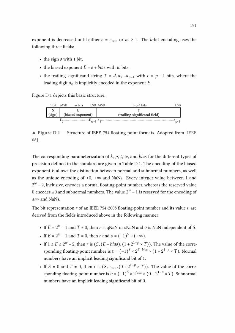
191
exponent is decreased until either e = emin or m ≥ 1. The k-bit encoding uses thefollowing three fields:
• the sign s with 1 bit,
• the biased exponent E = e + bias with w bits,
• the trailing significand string T = d1d2...dp−1 with t = p − 1 bits, where theleading digit d0 is implicitly encoded in the exponent E.
Figure D.1 depicts this basic structure.
S(sign)
E(biased exponent)
T(trailing significand field)
E0………………………..Ew-1
1 bit MSB w bits LSB MSB t=p-1 bits LSB
d1……………………………………………………………..………..dp-1
▲ Figure D.1 — Structure of IEEE-754 floating-point formats. Adopted from [IEEE08].
The corresponding parameterization of k, p, t, w, and bias for the different types ofprecision defined in the standard are given in Table D.1. The encoding of the biasedexponent E allows the distinction between normal and subnormal numbers, as wellas the unique encoding of ±0, ±∞ and NaNs. Every integer value between 1 and2w − 2, inclusive, encodes a normal floating-point number, whereas the reserved value0 encodes ±0 and subnormal numbers. The value 2w − 1 is reserved for the encoding of±∞ and NaNs.
The bit representation r of an IEEE 754-2008 floating-point number and its value v arederived from the fields introduced above in the following manner:
• If E = 2w − 1 and T ≠ 0, then r is qNaN or sNaN and v is NaN independent of S.
• If E = 2w − 1 and T = 0, then r and v = (−1)S × (+∞).• If 1 ≤ E ≤ 2w − 2, then r is (S, (E − bias), (1+ 21−p × T)). The value of the corre-sponding floating-point number is v = (−1)S × 2E−bias × (1+ 21−p × T). Normalnumbers have an implicit leading significand bit of 1.
• If E = 0 and T ≠ 0, then r is (S, emin, (0 + 21−p × T)). The value of the corre-sponding floating-point number is v = (−1)S × 2emin × (0+ 21−p × T). Subnormalnumbers have an implicit leading significand bit of 0.
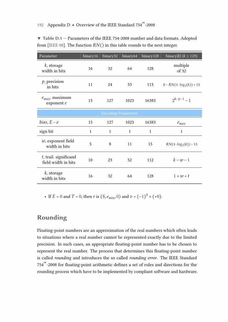
192 Appendix D ● Overview of the IEEE Standard 754™-2008
▼ Table D.1 — Parameters of the IEEE 754-2008 number and data formats. Adoptedfrom [IEEE 08]. The function RN() in this table rounds to the next integer.
Parameter binary16 binary32 binary64 binary128 binary{k} (k ≥ 128)
k, storagewidth in bits 16 32 64 128 multiple
of 32
p, precisionin bits 11 24 53 113 k − RN(4 ⋅ log2(k))+ 13
emax, maximumexponent e 15 127 1023 16383 2k−p−1 − 1
Encoding Parameters
bias, E − e 15 127 1023 16383 emax
sign bit 1 1 1 1 1
w, exponent fieldwidth in bits 5 8 11 15 RN(4 ⋅ log2(k))− 13
t, trail. significandfield width in bits 10 23 52 112 k −w − 1
k, storagewidth in bits 16 32 64 128 1+w + t
• If E = 0 and T = 0, then r is (S, emin, 0) and v = (−1)S × (+0).
Rounding
Floating-point numbers are an approximation of the real numbers which often leadsto situations where a real number cannot be represented exactly due to the limitedprecision. In such cases, an appropriate floating-point number has to be chosen torepresent the real number. The process that determines this floating-point numberis called rounding and introduces the so called rounding error. The IEEE Standard754™-2008 for floating-point arithmetic defines a set of rules and directions for therounding process which have to be implemented by compliant software and hardware.
193
The standard also demands that exceptions such as underflow or overflow have to besignaled appropriately.
The main rounding mode defined by the standard is round to nearest, which offers threedifferent rounding directions. Given an infinitely precise result with a magnitude ofat least bemax(b − 1
2b1−p). This result is rounded to∞ without changing the sign. Themaximum exponent emax and the precision p are determined by the target numberformat (see Table D.1). The rounding directions are:
• RoundTiesToEven: The floating-point number nearest to the infinitely preciseresult is delivered. If there exist two candidates, the floating-point number withan even last significand digit is chosen.
• RoundTiesToAway: The floating-point number nearest to the infinitely preciseresult is delivered. If there exist two candidates, the floating-point number withthe larger magnitude is chosen.
In addition to this main rounding mode, the standard defines three optional roundingdirections:
• RoundTowardPositive: The floating-point number closest to the infinitelyprecise result is delivered, which is no less than this result. +∞ is possible asrounded value.
• RoundTowardNegative: The floating-point number closest to the infinitelyprecise result is delivered, which is no greater than this result. −∞ is possible asrounded value.
• RoundTowardZero: The floating-point number closest to the infinitely preciseresult is delivered, which is no greater in magnitude than this result.
Infinity and Not-a-Number
Floating-point arithmetic, as it is defined in the IEEE standard, uses −∞ and +∞ toexpress operands of arbitrarily large magnitude. Most operations yield exact resultswhen infinity is involved and therefore no exceptions have to be signaled. The standardlists the operations:
• addition(∞, x), addition(x,∞), subtraction(∞, x), subtraction(x.∞) for finite x,
194 Appendix D ● Overview of the IEEE Standard 754™-2008
• multiplication(∞, x) or multiplication(x,∞) for fininte x or infinite x ≠ 0,
• division(∞, x) or division(x,∞) for finite x,
• square root(+∞),
• remainder(x,∞) for finite normal x,
• conversion of infinity to the same infinity in another format.
Cases where exceptions are signaled are:
• ∞ as an invalid operand,
• ∞ created from finite operands by overflow,
• remainder(subnormal,∞) signals underflow.
Values or results that cannot be represented by valid floating-point numbers are setto Not-a-Number. The standard distinguishes two different NaN representations, thesignaling NaN (sNaN) and the quiet NaN (qNaN).
Exceptions
The IEEE Standard 754™-2008 for floating-point arithmetic defines several exceptionsand accompanying methods for the handling of these exceptions. The most importantexceptions are:
• Invalid operation: This exception is signaled if the operands are invalid for thetarget operation or if the result is not defined. The default result for an operationthat throws an invalid operation exception is the quiet NaN.
• Division by zero: This exception is signaled if an exact infinite result is definedfor an operation on finite operands. The default result in this case is∞.
• Overflow: This exception is signaled if the target floating-point number formatdoes not provide a representation which is large enough to map the result.
• Underflow: This exception is signaled if a very small non-zero result is detected.
• Inexact: This exception is signaled when a result is rounded.
Further details on the floating-point number formats, operations, exceptions and imple-mentation requirements defined in the IEEE Standard 754™-2008 can be found in [IEEE08].
Appendix
EImplementation Details
This appendix chapter provides additional details on the different algorithmic stepsthat are performed by the proposed A-Abft method, and which have been omitted inChapter 6 for the sake of conciseness. The procedures for the checksum encoding andthe generation of the candidate sets are described in Algorithm 1. The procedures forthe determination of the rounding error bounds and the check of the computed resultsub-matrices are given in Algorithm 2.
In addition to the central algorithmic steps of A-Abft, pseudocode descriptions forthe QR decomposition based on Householder transformations and the Revised Simplexalgorithm, as they have been used for the case studies in Chapter 7, are given inAlgorithm 3 and Algorithm 4.
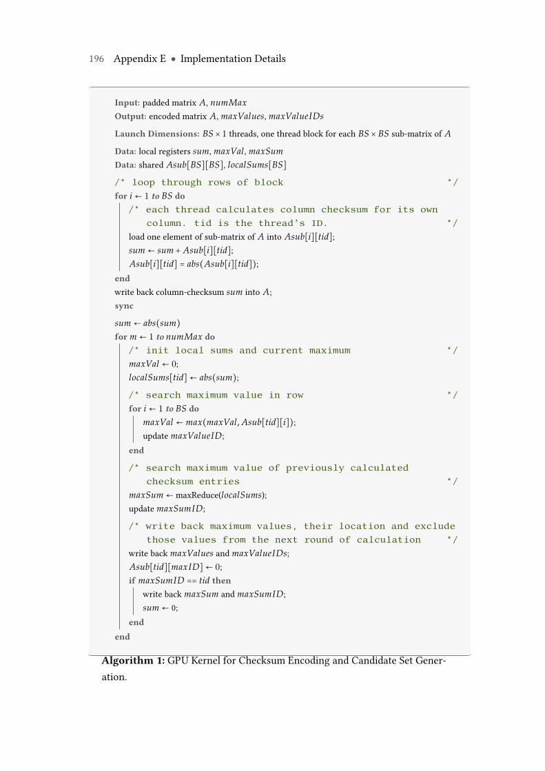
196 Appendix E ● Implementation Details
Input: padded matrix A, numMaxOutput: encoded matrix A, maxValues, maxValueIDs
Launch Dimensions: BS × 1 threads, one thread block for each BS × BS sub-matrix of A
Data: local registers sum, maxVal, maxSumData: shared Asub[BS][BS], localSums[BS]
/* loop through rows of block */for i ← 1 to BS do
/* each thread calculates column checksum for its owncolumn. tid is the thread’s ID. */
load one element of sub-matrix of A into Asub[i][tid];sum ← sum + Asub[i][tid];Asub[i][tid] = abs(Asub[i][tid]);
endwrite back column-checksum sum into A;sync
sum ← abs(sum)for m ← 1 to numMax do
/* init local sums and current maximum */maxVal ← 0;localSums[tid]← abs(sum);
/* search maximum value in row */for i ← 1 to BS do
maxVal ← max(maxVal, Asub[tid][i]);update maxValueID;
end
/* search maximum value of previously calculatedchecksum entries */
maxSum ← maxReduce(localSums);update maxSumID;
/* write back maximum values, their location and excludethose values from the next round of calculation */
write back maxValues and maxValueIDs;Asub[tid][maxID]← 0;if maxSumID == tid then
write back maxSum and maxSumID;sum ← 0;
endend
Algorithm 1: GPU Kernel for Checksum Encoding and Candidate Set Gener-ation.
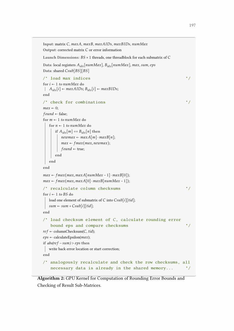
197
Input: matrix C, maxA, maxB, maxAIDs, maxBIDs, numMaxOutput: corrected matrix C or error information
Launch Dimensions: BS × 1 threads, one threadblock for each submatrix of C
Data: local registers Aidx[numMax], Bidx[numMax], max, sum, epsData: shared Csub[BS][BS]
/* load max indices */for i ← 1 to numMax do
Aidx[i]← maxAIDs; Bidx[i]← maxBIDs;end
/* check for combinations */max ← 0;f ound ← false;for m ← 1 to numMax do
for n ← 1 to numMax doif Aidx[m] == Bidx[n] then
newmax ← maxA[m] ⋅maxB[n];max ← f max(max, newmax);f ound ← true;
endend
end
max ← f max(max, maxA[numMax − 1] ⋅maxB[0]);max ← f max(max, maxA[0] ⋅maxB[numMax − 1]);
/* recalculate column checksums */for i ← 1 to BS do
load one element of submatrix of C into Csub[i][tid];sum ← sum +Csub[i][tid];
end
/* load checksum element of C, calculate rounding errorbound eps and compare checksums */
re f ← columnChecksum(C, tid);eps ← calculateEpsilon(max);if abs(re f − sum) > eps then
write back error location or start correction;end
/* analogously recalculate and check the row checksums, allnecessary data is already in the shared memory... */
Algorithm 2: GPU Kernel for Computation of Rounding Error Bounds andChecking of Result Sub-Matrices.
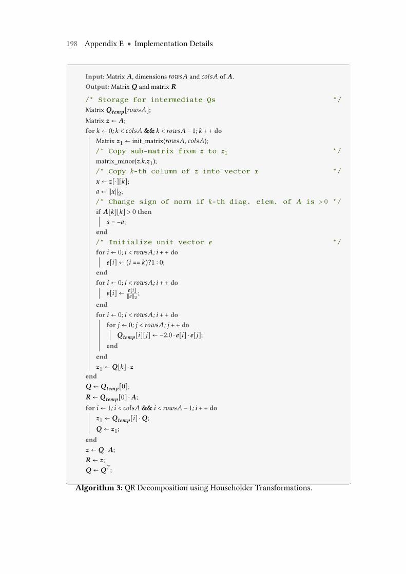
198 Appendix E ● Implementation Details
Input: Matrix A, dimensions rowsA and colsA of A.Output: Matrix Q and matrix R
/* Storage for intermediate Qs */Matrix Qtemp[rowsA];Matrix z ← A;for k ← 0; k < colsA && k < rowsA − 1; k ++ do
Matrix z1 ← init_matrix(rowsA, colsA);/* Copy sub-matrix from z to z1 */matrix_minor(z,k,z1);/* Copy k-th column of z into vector x */x ← z[⋅][k];a ← ∣∣x∣∣2;/* Change sign of norm if k-th diag. elem. of A is > 0 */if A[k][k] > 0 then
a = −a;end/* Initialize unit vector e */for i ← 0; i < rowsA; i ++ do
e[i]← (i == k)?1 ∶ 0;endfor i ← 0; i < rowsA; i ++ do
e[i]← e[i]∣∣e∣∣2 ;
endfor i ← 0; i < rowsA; i ++ do
for j ← 0; j < rowsA; j ++ doQtemp[i][j]← −2.0 ⋅ e[i] ⋅ e[j];
endendz1 ← Q[k] ⋅ z
endQ ← Qtemp[0];R ← Qtemp[0] ⋅ A;for i ← 1; i < colsA && i < rowsA − 1; i ++ do
z1 ← Qtemp[i] ⋅Q;Q ← z1;
endz ← Q ⋅ A;R ← z;Q ← QT ;
Algorithm 3: QR Decomposition using Householder Transformations.
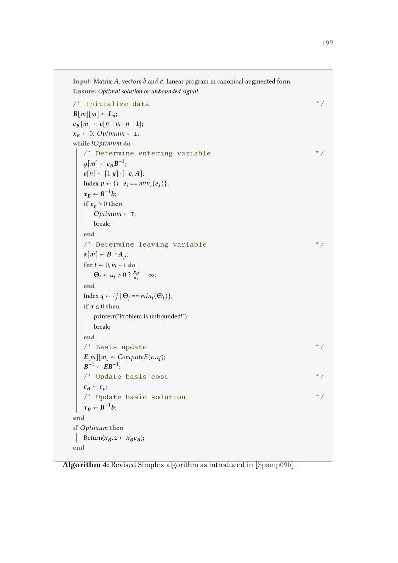
199
Input: Matrix A, vectors b and c. Linear program in canonical augmented form.Ensure: Optimal solution or unbounded signal.
/* Initialize data */B[m][m]← Im;cB[m]← c[n −m ∶ n − 1];xB ← 0; Optimum ← �;while !Optimum do
/* Determine entering variable */y[m]← cBB−1;e[n]← [1 y] ⋅ [−c; A];Index p ← {j ∣ ej == mint(et)};xB ← B−1b;if ep ≥ 0 then
Optimum ← ⊺;break;
end/* Determine leaving variable */α[m]← B−1Ap;for t ← 0, m − 1 do
Θt ← αt > 0 ? xBαt∶ ∞;
endIndex q ← {j ∣ Θj == mint(Θt)};if α ≤ 0 then
printerr("Problem is unbounded!");break;
end/* Basis update */E[m][m]← ComputeE(α, q);B−1 ← EB−1;/* Update basis cost */cB ← cp;/* Update basic solution */xB ← B−1b;
endif Optimum then
Return(xB, z ← xBcB);end
Algorithm 4: Revised Simplex algorithm as introduced in [Spamp09b].

Appendix
FExperimental Data
This appendix provides the reader with additional experimental results for the threemain evaluation areas: performance, quality of error bounds and error detection.
F.1 Hardware and Software Configuration
The experiments for the evaluation part of this work have been performed on two IntelXeon-based compute servers, hereinafter referred to as CPU I and CPU II, which wereequipped with Nvidia Tesla GPU accelerators. The detailed technical hardware andsoftware specifications of the two systems are given in the following:
• Compute server 1 (CPU I )
– 2x Intel Xeon E5-2650 CPU, 2.2GHz clock frequency
– 280 (2x140) GFLOPS theo. double precision peak performance at base clock
– 256 GB memory
– Cent OS 6 Linux operating system
– 2x Nvidia Tesla K20c GPU accelerator
– Nvidia CUDA version 5.5
• Compute server 2 (CPU II )

202 Appendix F ● Experimental Data
– 2x Intel Xeon E5-2687W3 CPU, 3.4GHz clock frequency
– 396 (2x198) GFLOPS theo. double precision peak performance at base clock
– 256 GB memory
– Cent OS 6 Linux operating system
– 1x Nvidia Tesla K40c GPU accelerator
– Nvidia CUDA version 6.5
• Nvidia Tesla K20c GPU accelerator
– CUDA compute capability 3.5
– Nvidia GK110 "Kepler" architecture
– 2496 CUDA processing cores
– 706 MHz GPU clock frequency
– 1.17 TFLOPS theo. double precision peak performance
– 3.52 TFLOPS theo. single precision peak performance
– 5 GB GDDR5 device memory
– External and internal memories with ECC
– With ECC on, 6.25% of the GPU memory is used for ECC bits.
– 2600 MHz memory clock frequency
– 208 GB/sec memory bandwidth
– 320 bit memory bus width
– PCI Express Gen2 ×16 system interface
• Nvidia Tesla K40c GPU accelerator
– CUDA compute capability 3.5
– Nvidia GK110B "Kepler" architecture
– 2880 CUDA processing cores
– 745 MHz GPU clock frequency
– 1.43 TFLOPS theo. double precision peak performance
– 4.29 TFLOPS theo. single precision peak performance
– 12 GB GDDR5 device memory
– External and internal memories with ECC
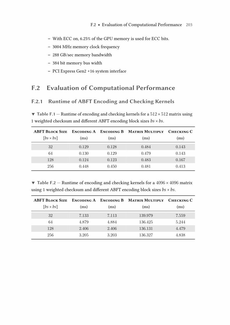
F.2 ● Evaluation of Computational Performance 203
– With ECC on, 6.25% of the GPU memory is used for ECC bits.
– 3004 MHz memory clock frequency
– 288 GB/sec memory bandwidth
– 384 bit memory bus width
– PCI Express Gen2 ×16 system interface
F.2 Evaluation of Computational Performance
F.2.1 Runtime of ABFT Encoding and Checking Kernels
▼ Table F.1 — Runtime of encoding and checking kernels for a 512× 512 matrix using1 weighted checksum and different ABFT encoding block sizes bs × bs.
ABFT Block Size Encoding A Encoding B Matrix Multiply Checking C[bs × bs] (ms) (ms) (ms) (ms)
32 0.129 0.128 0.484 0.14364 0.130 0.129 0.479 0.143128 0.124 0.123 0.483 0.167256 0.448 0.450 0.481 0.413
▼ Table F.2 — Runtime of encoding and checking kernels for a 4096 × 4096 matrixusing 1 weighted checksum and different ABFT encoding block sizes bs × bs.
ABFT Block Size Encoding A Encoding B Matrix Multiply Checking C[bs × bs] (ms) (ms) (ms) (ms)
32 7.133 7.113 139.979 7.55964 4.879 4.884 136.425 5.244128 2.406 2.406 136.131 4.479256 3.205 3.203 136.327 4.838
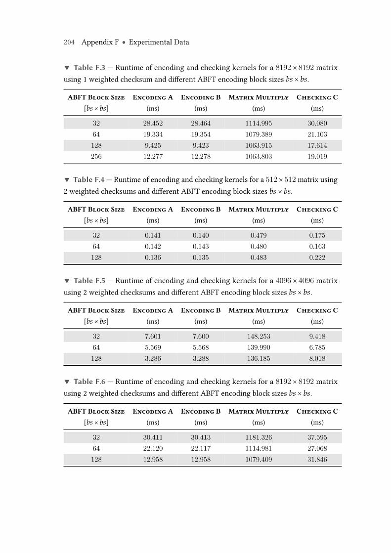
204 Appendix F ● Experimental Data
▼ Table F.3 — Runtime of encoding and checking kernels for a 8192 × 8192 matrixusing 1 weighted checksum and different ABFT encoding block sizes bs × bs.
ABFT Block Size Encoding A Encoding B Matrix Multiply Checking C[bs × bs] (ms) (ms) (ms) (ms)
32 28.452 28.464 1114.995 30.08064 19.334 19.354 1079.389 21.103128 9.425 9.423 1063.915 17.614256 12.277 12.278 1063.803 19.019
▼ Table F.4 — Runtime of encoding and checking kernels for a 512× 512 matrix using2 weighted checksums and different ABFT encoding block sizes bs × bs.
ABFT Block Size Encoding A Encoding B Matrix Multiply Checking C[bs × bs] (ms) (ms) (ms) (ms)
32 0.141 0.140 0.479 0.17564 0.142 0.143 0.480 0.163128 0.136 0.135 0.483 0.222
▼ Table F.5 — Runtime of encoding and checking kernels for a 4096 × 4096 matrixusing 2 weighted checksums and different ABFT encoding block sizes bs × bs.
ABFT Block Size Encoding A Encoding B Matrix Multiply Checking C[bs × bs] (ms) (ms) (ms) (ms)
32 7.601 7.600 148.253 9.41864 5.569 5.568 139.990 6.785128 3.286 3.288 136.185 8.018
▼ Table F.6 — Runtime of encoding and checking kernels for a 8192 × 8192 matrixusing 2 weighted checksums and different ABFT encoding block sizes bs × bs.
ABFT Block Size Encoding A Encoding B Matrix Multiply Checking C[bs × bs] (ms) (ms) (ms) (ms)
32 30.411 30.413 1181.326 37.59564 22.120 22.117 1114.981 27.068128 12.958 12.958 1079.409 31.846
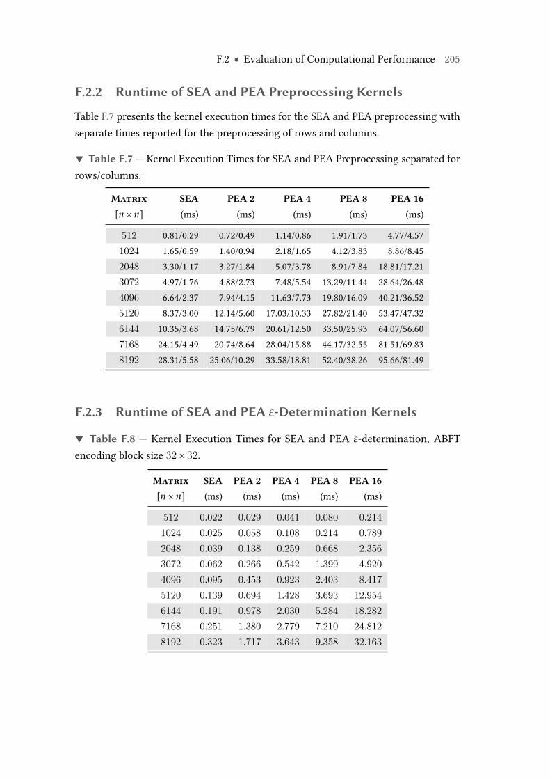
F.2 ● Evaluation of Computational Performance 205
F.2.2 Runtime of SEA and PEA Preprocessing Kernels
Table F.7 presents the kernel execution times for the SEA and PEA preprocessing withseparate times reported for the preprocessing of rows and columns.
▼ Table F.7 — Kernel Execution Times for SEA and PEA Preprocessing separated forrows/columns.
Matrix SEA PEA 2 PEA 4 PEA 8 PEA 16[n × n] (ms) (ms) (ms) (ms) (ms)
512 0.81/0.29 0.72/0.49 1.14/0.86 1.91/1.73 4.77/4.571024 1.65/0.59 1.40/0.94 2.18/1.65 4.12/3.83 8.86/8.452048 3.30/1.17 3.27/1.84 5.07/3.78 8.91/7.84 18.81/17.213072 4.97/1.76 4.88/2.73 7.48/5.54 13.29/11.44 28.64/26.484096 6.64/2.37 7.94/4.15 11.63/7.73 19.80/16.09 40.21/36.525120 8.37/3.00 12.14/5.60 17.03/10.33 27.82/21.40 53.47/47.326144 10.35/3.68 14.75/6.79 20.61/12.50 33.50/25.93 64.07/56.607168 24.15/4.49 20.74/8.64 28.04/15.88 44.17/32.55 81.51/69.838192 28.31/5.58 25.06/10.29 33.58/18.81 52.40/38.26 95.66/81.49
F.2.3 Runtime of SEA and PEA ε-Determination Kernels
▼ Table F.8 — Kernel Execution Times for SEA and PEA ε-determination, ABFTencoding block size 32× 32.
Matrix SEA PEA 2 PEA 4 PEA 8 PEA 16[n × n] (ms) (ms) (ms) (ms) (ms)
512 0.022 0.029 0.041 0.080 0.2141024 0.025 0.058 0.108 0.214 0.7892048 0.039 0.138 0.259 0.668 2.3563072 0.062 0.266 0.542 1.399 4.9204096 0.095 0.453 0.923 2.403 8.4175120 0.139 0.694 1.428 3.693 12.9546144 0.191 0.978 2.030 5.284 18.2827168 0.251 1.380 2.779 7.210 24.8128192 0.323 1.717 3.643 9.358 32.163
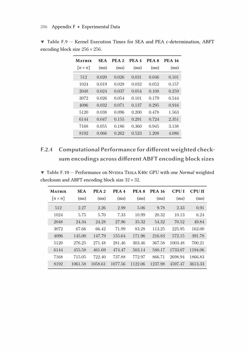
206 Appendix F ● Experimental Data
▼ Table F.9 — Kernel Execution Times for SEA and PEA ε-determination, ABFTencoding block size 256× 256.
Matrix SEA PEA 2 PEA 4 PEA 8 PEA 16[n × n] (ms) (ms) (ms) (ms) (ms)
512 0.020 0.026 0.031 0.046 0.1011024 0.019 0.028 0.032 0.052 0.1572048 0.024 0.037 0.054 0.108 0.2593072 0.026 0.054 0.101 0.179 0.5444096 0.032 0.071 0.137 0.295 0.9165120 0.038 0.096 0.200 0.478 1.5636144 0.047 0.155 0.291 0.724 2.3517168 0.055 0.186 0.360 0.945 3.1388192 0.066 0.262 0.523 1.208 4.086
F.2.4 Computational Performance for differentweighted check-sumencodings across different ABFT encoding block sizes
▼ Table F.10 — Performance on Nvidia Tesla K40c GPU with one Normal weightedchecksum and ABFT encoding block size 32× 32.
Matrix SEA PEA 2 PEA 4 PEA 8 PEA 16 CPU I CPU II[n × n] (ms) (ms) (ms) (ms) (ms) (ms) (ms)
512 2.27 2.26 2.99 5.06 9.78 2.33 0.911024 5.75 5.70 7.33 10.99 20.32 10.13 6.242048 24.34 24.28 27.96 35.32 54.32 70.52 49.843072 67.66 66.42 71.99 83.28 113.25 225.95 162.004096 145.00 147.79 155.64 171.96 216.83 572.15 391.785120 276.25 271.48 281.46 303.46 367.58 1003.48 700.216144 455.58 461.69 474.47 503.14 580.17 1733.07 1194.067168 715.05 722.40 737.88 772.97 866.71 2698.94 1866.838192 1061.58 1058.61 1077.56 1122.06 1237.98 4597.47 3613.33
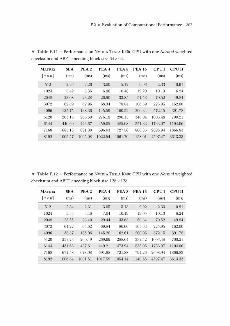
F.2 ● Evaluation of Computational Performance 207
▼ Table F.11 — Performance on Nvidia Tesla K40c GPU with one Normal weightedchecksum and ABFT encoding block size 64× 64.
Matrix SEA PEA 2 PEA 4 PEA 8 PEA 16 CPU I CPU II[n × n] (ms) (ms) (ms) (ms) (ms) (ms) (ms)
512 2.26 2.26 3.00 5.12 9.96 2.33 0.911024 5.42 5.35 6.96 10.48 19.20 10.13 6.242048 23.08 23.28 26.90 33.85 51.53 70.52 49.843072 62.49 62.96 68.34 78.84 106.39 225.95 162.004096 135.75 138.36 145.59 160.52 200.34 572.15 391.785120 263.15 266.60 276.18 296.13 348.04 1003.48 700.216144 440.60 446.67 459.05 485.08 551.33 1733.07 1194.067168 685.18 691.30 696.03 727.56 806.85 2698.94 1866.838192 1005.57 1005.08 1022.54 1061.70 1158.01 4597.47 3613.33
▼ Table F.12 — Performance on Nvidia Tesla K40c GPU with one Normal weightedchecksum and ABFT encoding block size 128× 128.
Matrix SEA PEA 2 PEA 4 PEA 8 PEA 16 CPU I CPU II[n × n] (ms) (ms) (ms) (ms) (ms) (ms) (ms)
512 2.34 2.31 3.05 5.13 9.92 2.33 0.911024 5.55 5.46 7.04 10.49 19.05 10.13 6.242048 23.55 23.40 29.44 33.63 50.34 70.52 49.843072 64.22 64.62 69.84 80.00 105.63 225.95 162.004096 135.57 138.06 145.20 162.61 200.05 572.15 391.785120 257.23 260.49 269.69 288.64 337.42 1003.48 700.216144 431.63 437.61 449.21 473.94 535.05 1733.07 1194.067168 671.58 678.08 691.98 721.88 794.26 2698.94 1866.838192 1006.84 1001.51 1017.59 1054.14 1140.65 4597.47 3613.33

208 Appendix F ● Experimental Data
▼ Table F.13 — Performance on Nvidia Tesla K40c GPU with one Normal weightedchecksum and ABFT encoding block size 256× 256.
Matrix SEA PEA 2 PEA 4 PEA 8 PEA 16 CPU I CPU II[n × n] (ms) (ms) (ms) (ms) (ms) (ms) (ms)
512 2.59 2.55 3.28 5.14 9.84 2.33 0.911024 5.69 5.57 7.16 10.55 19.12 10.13 6.242048 23.93 23.76 27.18 33.83 50.01 70.52 49.843072 64.31 64.66 69.86 79.80 104.79 225.95 162.004096 138.91 141.29 148.22 162.23 197.45 572.15 391.785120 257.97 261.05 270.00 288.36 333.77 1003.48 700.216144 432.63 438.39 449.74 473.52 530.45 1733.07 1194.067168 672.52 679.01 692.72 721.03 791.46 2698.94 1866.838192 1008.83 1002.88 1018.60 1054.09 1136.32 4597.47 3613.33
▼ Table F.14 — Performance on Nvidia Tesla K40c GPU with one Exponentialweighted checksum and ABFT encoding block size 32× 32.
Matrix SEA PEA 2 PEA 4 PEA 8 PEA 16 CPU I CPU II[n × n] (ms) (ms) (ms) (ms) (ms) (ms) (ms)
512 2.27 2.27 3.01 5.09 9.90 2.33 0.911024 5.77 5.71 7.34 10.99 20.24 10.13 6.242048 24.34 24.26 27.95 35.32 54.32 70.52 49.843072 65.88 66.46 72.05 83.43 115.44 225.95 162.004096 145.04 147.76 155.61 171.81 216.49 572.15 391.785120 272.90 276.43 286.36 308.26 367.20 1003.48 700.216144 455.49 461.63 474.57 503.34 580.89 1733.07 1194.067168 715.29 722.50 738.03 773.46 867.37 2698.94 1866.838192 1061.60 1058.69 1077.18 1121.48 1237.24 4597.47 3613.33
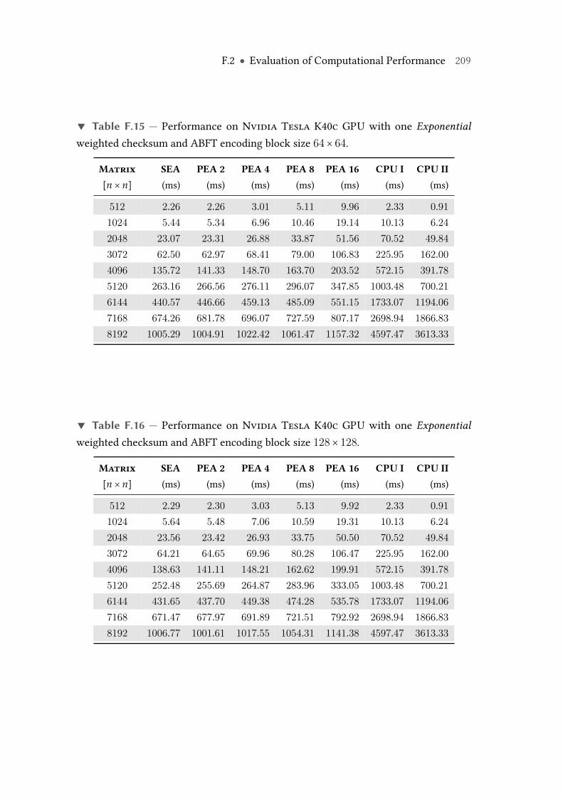
F.2 ● Evaluation of Computational Performance 209
▼ Table F.15 — Performance on Nvidia Tesla K40c GPU with one Exponentialweighted checksum and ABFT encoding block size 64× 64.
Matrix SEA PEA 2 PEA 4 PEA 8 PEA 16 CPU I CPU II[n × n] (ms) (ms) (ms) (ms) (ms) (ms) (ms)
512 2.26 2.26 3.01 5.11 9.96 2.33 0.911024 5.44 5.34 6.96 10.46 19.14 10.13 6.242048 23.07 23.31 26.88 33.87 51.56 70.52 49.843072 62.50 62.97 68.41 79.00 106.83 225.95 162.004096 135.72 141.33 148.70 163.70 203.52 572.15 391.785120 263.16 266.56 276.11 296.07 347.85 1003.48 700.216144 440.57 446.66 459.13 485.09 551.15 1733.07 1194.067168 674.26 681.78 696.07 727.59 807.17 2698.94 1866.838192 1005.29 1004.91 1022.42 1061.47 1157.32 4597.47 3613.33
▼ Table F.16 — Performance on Nvidia Tesla K40c GPU with one Exponentialweighted checksum and ABFT encoding block size 128× 128.
Matrix SEA PEA 2 PEA 4 PEA 8 PEA 16 CPU I CPU II[n × n] (ms) (ms) (ms) (ms) (ms) (ms) (ms)
512 2.29 2.30 3.03 5.13 9.92 2.33 0.911024 5.64 5.48 7.06 10.59 19.31 10.13 6.242048 23.56 23.42 26.93 33.75 50.50 70.52 49.843072 64.21 64.65 69.96 80.28 106.47 225.95 162.004096 138.63 141.11 148.21 162.62 199.91 572.15 391.785120 252.48 255.69 264.87 283.96 333.05 1003.48 700.216144 431.65 437.70 449.38 474.28 535.78 1733.07 1194.067168 671.47 677.97 691.89 721.51 792.92 2698.94 1866.838192 1006.77 1001.61 1017.55 1054.31 1141.38 4597.47 3613.33
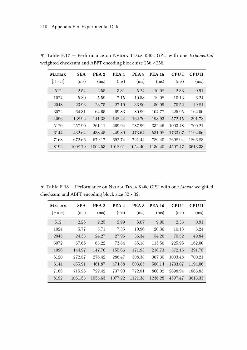
210 Appendix F ● Experimental Data
▼ Table F.17 — Performance on Nvidia Tesla K40c GPU with one Exponentialweighted checksum and ABFT encoding block size 256× 256.
Matrix SEA PEA 2 PEA 4 PEA 8 PEA 16 CPU I CPU II[n × n] (ms) (ms) (ms) (ms) (ms) (ms) (ms)
512 2.54 2.55 3.31 5.24 10.08 2.33 0.911024 5.80 5.59 7.15 10.58 19.08 10.13 6.242048 23.93 23.75 27.19 33.90 50.09 70.52 49.843072 64.31 64.65 69.83 80.99 104.77 225.95 162.004096 138.92 141.38 148.44 162.70 198.93 572.15 391.785120 257.90 261.11 269.94 287.99 332.46 1003.48 700.216144 432.64 438.45 449.89 473.64 531.08 1733.07 1194.067168 672.66 679.17 692.74 721.44 789.40 2698.94 1866.838192 1008.79 1002.53 1018.61 1054.40 1136.40 4597.47 3613.33
▼ Table F.18 — Performance on Nvidia Tesla K40c GPU with one Linear weightedchecksum and ABFT encoding block size 32× 32.
Matrix SEA PEA 2 PEA 4 PEA 8 PEA 16 CPU I CPU II[n × n] (ms) (ms) (ms) (ms) (ms) (ms) (ms)
512 2.26 2.25 2.99 5.07 9.90 2.33 0.911024 5.77 5.71 7.35 10.96 20.36 10.13 6.242048 24.33 24.27 27.95 35.34 54.26 70.52 49.843072 67.66 68.22 73.84 85.18 115.56 225.95 162.004096 144.97 147.76 155.66 171.93 216.73 572.15 391.785120 272.87 276.42 286.47 308.38 367.30 1003.48 700.216144 455.91 461.87 474.88 503.65 580.14 1733.07 1194.067168 715.28 722.42 737.90 772.81 866.02 2698.94 1866.838192 1061.53 1058.63 1077.22 1121.38 1236.28 4597.47 3613.33

F.2 ● Evaluation of Computational Performance 211
▼ Table F.19 — Performance on Nvidia Tesla K40c GPU with one Linear weightedchecksum and ABFT encoding block size 64× 64.
Matrix SEA PEA 2 PEA 4 PEA 8 PEA 16 CPU I CPU II[n × n] (ms) (ms) (ms) (ms) (ms) (ms) (ms)
512 2.25 2.26 2.99 5.05 9.80 2.33 0.911024 5.44 5.34 6.95 10.49 19.24 10.13 6.242048 23.07 23.28 26.79 33.73 51.34 70.52 49.843072 62.50 62.97 68.43 79.07 107.09 225.95 162.004096 138.79 141.35 148.67 163.43 202.79 572.15 391.785120 263.15 266.53 276.08 295.98 347.49 1003.48 700.216144 440.50 446.71 458.87 484.84 550.99 1733.07 1194.067168 674.40 681.81 696.08 727.64 806.89 2698.94 1866.838192 1005.38 1004.87 1022.72 1061.72 1158.01 4597.47 3613.33
▼ Table F.20 — Performance on Nvidia Tesla K40c GPU with one Linear weightedchecksum and ABFT encoding block size 128× 128.
Matrix SEA PEA 2 PEA 4 PEA 8 PEA 16 CPU I CPU II[n × n] (ms) (ms) (ms) (ms) (ms) (ms) (ms)
512 2.29 2.31 3.06 5.19 10.13 2.33 0.911024 5.64 5.48 7.07 10.60 19.31 10.13 6.242048 23.57 23.42 26.89 33.67 50.40 70.52 49.843072 62.52 62.96 68.27 78.59 104.95 225.95 162.004096 138.61 141.08 148.25 162.78 200.48 572.15 391.785120 252.47 255.63 264.92 288.73 337.42 1003.48 700.216144 431.65 437.52 449.32 473.96 535.00 1733.07 1194.067168 671.49 677.97 691.92 721.41 793.22 2698.94 1866.838192 1007.07 1001.35 1017.49 1054.58 1142.25 4597.47 3613.33

212 Appendix F ● Experimental Data
▼ Table F.21 — Performance on Nvidia Tesla K40c GPU with one Linear weightedchecksum and ABFT encoding block size 256× 256.
Matrix SEA PEA 2 PEA 4 PEA 8 PEA 16 CPU I CPU II[n × n] (ms) (ms) (ms) (ms) (ms) (ms) (ms)
512 2.54 2.53 3.25 5.04 9.55 2.33 0.911024 5.78 5.61 7.20 10.71 19.41 10.13 6.242048 23.90 23.75 27.22 33.92 50.25 70.52 49.843072 64.31 64.66 69.85 79.77 104.80 225.95 162.004096 138.92 141.31 148.33 162.36 200.60 572.15 391.785120 257.88 261.01 269.85 287.93 332.37 1003.48 700.216144 432.55 438.38 449.69 473.49 530.62 1733.07 1194.067168 672.62 678.91 692.63 721.21 788.72 2698.94 1866.838192 1008.27 1004.00 1018.22 1053.33 1135.35 4597.47 3613.33
▼ Table F.22 — Performance on Nvidia Tesla K40c GPU with one MDR weightedchecksum and ABFT encoding block size 32× 32.
Matrix SEA PEA 2 PEA 4 PEA 8 PEA 16 CPU I CPU II[n × n] (ms) (ms) (ms) (ms) (ms) (ms) (ms)
512 2.28 2.33 3.07 5.15 10.00 2.33 0.911024 5.94 5.82 7.44 11.09 20.32 10.13 6.242048 24.31 24.24 27.87 35.15 53.91 70.52 49.843072 67.65 68.23 73.82 85.22 115.59 225.95 162.004096 144.99 147.76 155.67 171.80 216.43 572.15 391.785120 272.99 276.46 286.34 308.05 366.65 1003.48 700.216144 455.75 461.83 474.65 503.34 580.25 1733.07 1194.067168 715.27 722.47 737.96 773.01 866.48 2698.94 1866.838192 1061.72 1058.76 1077.37 1121.75 1237.04 4597.47 3613.33
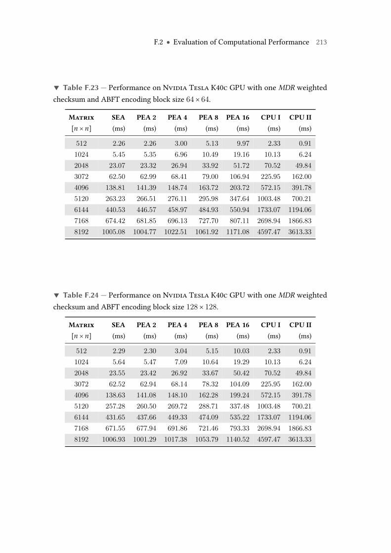
F.2 ● Evaluation of Computational Performance 213
▼ Table F.23 — Performance on Nvidia Tesla K40c GPU with one MDR weightedchecksum and ABFT encoding block size 64× 64.
Matrix SEA PEA 2 PEA 4 PEA 8 PEA 16 CPU I CPU II[n × n] (ms) (ms) (ms) (ms) (ms) (ms) (ms)
512 2.26 2.26 3.00 5.13 9.97 2.33 0.911024 5.45 5.35 6.96 10.49 19.16 10.13 6.242048 23.07 23.32 26.94 33.92 51.72 70.52 49.843072 62.50 62.99 68.41 79.00 106.94 225.95 162.004096 138.81 141.39 148.74 163.72 203.72 572.15 391.785120 263.23 266.51 276.11 295.98 347.64 1003.48 700.216144 440.53 446.57 458.97 484.93 550.94 1733.07 1194.067168 674.42 681.85 696.13 727.70 807.11 2698.94 1866.838192 1005.08 1004.77 1022.51 1061.92 1171.08 4597.47 3613.33
▼ Table F.24 — Performance on Nvidia Tesla K40c GPU with one MDR weightedchecksum and ABFT encoding block size 128× 128.
Matrix SEA PEA 2 PEA 4 PEA 8 PEA 16 CPU I CPU II[n × n] (ms) (ms) (ms) (ms) (ms) (ms) (ms)
512 2.29 2.30 3.04 5.15 10.03 2.33 0.911024 5.64 5.47 7.09 10.64 19.29 10.13 6.242048 23.55 23.42 26.92 33.67 50.42 70.52 49.843072 62.52 62.94 68.14 78.32 104.09 225.95 162.004096 138.63 141.08 148.10 162.28 199.24 572.15 391.785120 257.28 260.50 269.72 288.71 337.48 1003.48 700.216144 431.65 437.66 449.33 474.09 535.22 1733.07 1194.067168 671.55 677.94 691.86 721.46 793.33 2698.94 1866.838192 1006.93 1001.29 1017.38 1053.79 1140.52 4597.47 3613.33
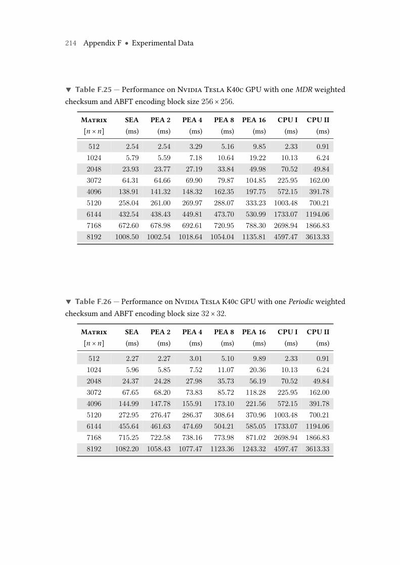
214 Appendix F ● Experimental Data
▼ Table F.25 — Performance on Nvidia Tesla K40c GPU with one MDR weightedchecksum and ABFT encoding block size 256× 256.
Matrix SEA PEA 2 PEA 4 PEA 8 PEA 16 CPU I CPU II[n × n] (ms) (ms) (ms) (ms) (ms) (ms) (ms)
512 2.54 2.54 3.29 5.16 9.85 2.33 0.911024 5.79 5.59 7.18 10.64 19.22 10.13 6.242048 23.93 23.77 27.19 33.84 49.98 70.52 49.843072 64.31 64.66 69.90 79.87 104.85 225.95 162.004096 138.91 141.32 148.32 162.35 197.75 572.15 391.785120 258.04 261.00 269.97 288.07 333.23 1003.48 700.216144 432.54 438.43 449.81 473.70 530.99 1733.07 1194.067168 672.60 678.98 692.61 720.95 788.30 2698.94 1866.838192 1008.50 1002.54 1018.64 1054.04 1135.81 4597.47 3613.33
▼ Table F.26 — Performance on Nvidia Tesla K40c GPU with one Periodic weightedchecksum and ABFT encoding block size 32× 32.
Matrix SEA PEA 2 PEA 4 PEA 8 PEA 16 CPU I CPU II[n × n] (ms) (ms) (ms) (ms) (ms) (ms) (ms)
512 2.27 2.27 3.01 5.10 9.89 2.33 0.911024 5.96 5.85 7.52 11.07 20.36 10.13 6.242048 24.37 24.28 27.98 35.73 56.19 70.52 49.843072 67.65 68.20 73.83 85.72 118.28 225.95 162.004096 144.99 147.78 155.91 173.10 221.56 572.15 391.785120 272.95 276.47 286.37 308.64 370.96 1003.48 700.216144 455.64 461.63 474.69 504.21 585.05 1733.07 1194.067168 715.25 722.58 738.16 773.98 871.02 2698.94 1866.838192 1082.20 1058.43 1077.47 1123.36 1243.32 4597.47 3613.33
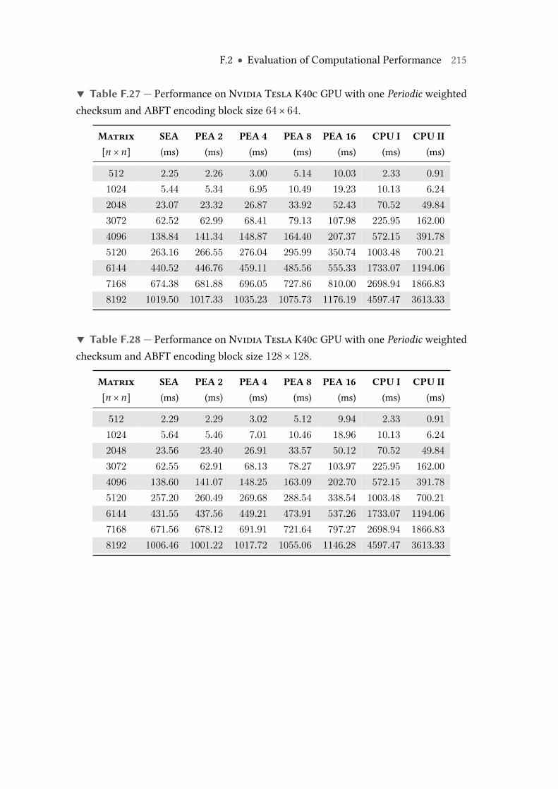
F.2 ● Evaluation of Computational Performance 215
▼ Table F.27 — Performance on Nvidia Tesla K40c GPU with one Periodic weightedchecksum and ABFT encoding block size 64× 64.
Matrix SEA PEA 2 PEA 4 PEA 8 PEA 16 CPU I CPU II[n × n] (ms) (ms) (ms) (ms) (ms) (ms) (ms)
512 2.25 2.26 3.00 5.14 10.03 2.33 0.911024 5.44 5.34 6.95 10.49 19.23 10.13 6.242048 23.07 23.32 26.87 33.92 52.43 70.52 49.843072 62.52 62.99 68.41 79.13 107.98 225.95 162.004096 138.84 141.34 148.87 164.40 207.37 572.15 391.785120 263.16 266.55 276.04 295.99 350.74 1003.48 700.216144 440.52 446.76 459.11 485.56 555.33 1733.07 1194.067168 674.38 681.88 696.05 727.86 810.00 2698.94 1866.838192 1019.50 1017.33 1035.23 1075.73 1176.19 4597.47 3613.33
▼ Table F.28 — Performance on Nvidia Tesla K40c GPU with one Periodic weightedchecksum and ABFT encoding block size 128× 128.
Matrix SEA PEA 2 PEA 4 PEA 8 PEA 16 CPU I CPU II[n × n] (ms) (ms) (ms) (ms) (ms) (ms) (ms)
512 2.29 2.29 3.02 5.12 9.94 2.33 0.911024 5.64 5.46 7.01 10.46 18.96 10.13 6.242048 23.56 23.40 26.91 33.57 50.12 70.52 49.843072 62.55 62.91 68.13 78.27 103.97 225.95 162.004096 138.60 141.07 148.25 163.09 202.70 572.15 391.785120 257.20 260.49 269.68 288.54 338.54 1003.48 700.216144 431.55 437.56 449.21 473.91 537.26 1733.07 1194.067168 671.56 678.12 691.91 721.64 797.27 2698.94 1866.838192 1006.46 1001.22 1017.72 1055.06 1146.28 4597.47 3613.33

216 Appendix F ● Experimental Data
▼ Table F.29 — Performance on Nvidia Tesla K40c GPU with one Periodic weightedchecksum and ABFT encoding block size 256× 256.
Matrix SEA PEA 2 PEA 4 PEA 8 PEA 16 CPU I CPU II[n × n] (ms) (ms) (ms) (ms) (ms) (ms) (ms)
512 2.54 2.54 3.28 5.14 9.84 2.33 0.911024 5.78 5.58 7.16 10.54 19.01 10.13 6.242048 23.93 23.76 27.18 33.91 50.30 70.52 49.843072 64.31 64.62 69.75 79.62 104.45 225.95 162.004096 138.93 141.36 148.35 162.32 197.87 572.15 391.785120 257.90 261.12 270.08 288.36 333.82 1003.48 700.216144 432.60 438.32 449.91 473.70 533.75 1733.07 1194.067168 672.64 679.00 692.53 721.08 788.75 2698.94 1866.838192 1008.30 1002.48 1018.51 1054.58 1139.82 4597.47 3613.33
▼ Table F.30 — Performance on Nvidia Tesla K40c GPU with one Normal and oneLinear weighted checksum and ABFT encoding block size 32× 32.
Matrix SEA PEA 2 PEA 4 PEA 8 PEA 16 CPU I CPU II[n × n] (ms) (ms) (ms) (ms) (ms) (ms) (ms)
512 2.31 2.31 3.09 5.25 10.29 2.33 0.911024 5.91 5.85 7.53 11.26 21.27 10.13 6.242048 24.84 25.25 29.10 36.99 58.51 70.52 49.843072 68.90 69.77 75.80 88.67 125.01 225.95 162.004096 153.78 157.14 165.76 184.45 239.11 572.15 391.785120 287.29 291.59 302.73 328.54 426.58 1003.48 700.216144 483.86 491.07 505.71 539.73 638.28 1733.07 1194.067168 752.90 761.72 779.87 822.80 946.42 2698.94 1866.838192 1123.35 1123.87 1146.46 1200.70 1355.53 4597.47 3613.33
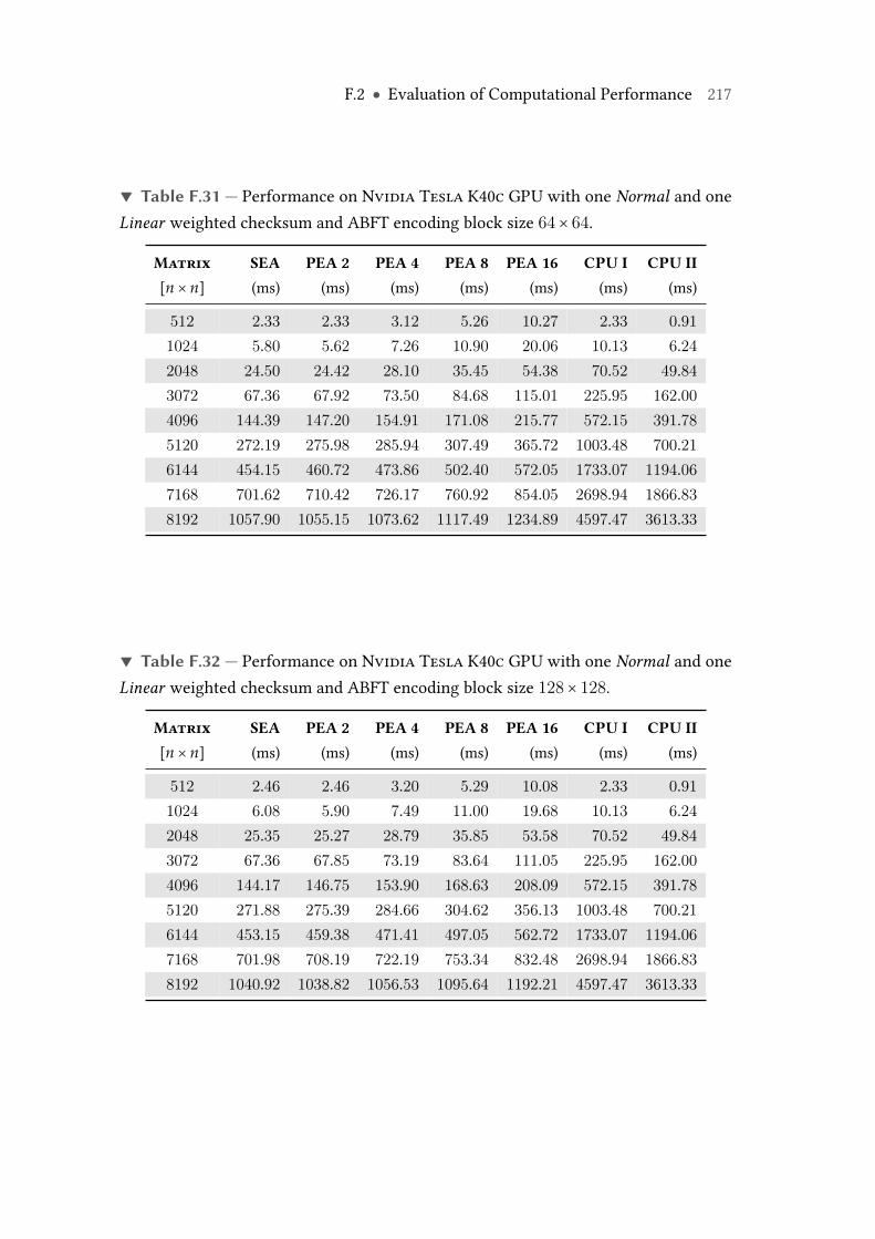
F.2 ● Evaluation of Computational Performance 217
▼ Table F.31 — Performance on Nvidia Tesla K40c GPU with one Normal and oneLinear weighted checksum and ABFT encoding block size 64× 64.
Matrix SEA PEA 2 PEA 4 PEA 8 PEA 16 CPU I CPU II[n × n] (ms) (ms) (ms) (ms) (ms) (ms) (ms)
512 2.33 2.33 3.12 5.26 10.27 2.33 0.911024 5.80 5.62 7.26 10.90 20.06 10.13 6.242048 24.50 24.42 28.10 35.45 54.38 70.52 49.843072 67.36 67.92 73.50 84.68 115.01 225.95 162.004096 144.39 147.20 154.91 171.08 215.77 572.15 391.785120 272.19 275.98 285.94 307.49 365.72 1003.48 700.216144 454.15 460.72 473.86 502.40 572.05 1733.07 1194.067168 701.62 710.42 726.17 760.92 854.05 2698.94 1866.838192 1057.90 1055.15 1073.62 1117.49 1234.89 4597.47 3613.33
▼ Table F.32 — Performance on Nvidia Tesla K40c GPU with one Normal and oneLinear weighted checksum and ABFT encoding block size 128× 128.
Matrix SEA PEA 2 PEA 4 PEA 8 PEA 16 CPU I CPU II[n × n] (ms) (ms) (ms) (ms) (ms) (ms) (ms)
512 2.46 2.46 3.20 5.29 10.08 2.33 0.911024 6.08 5.90 7.49 11.00 19.68 10.13 6.242048 25.35 25.27 28.79 35.85 53.58 70.52 49.843072 67.36 67.85 73.19 83.64 111.05 225.95 162.004096 144.17 146.75 153.90 168.63 208.09 572.15 391.785120 271.88 275.39 284.66 304.62 356.13 1003.48 700.216144 453.15 459.38 471.41 497.05 562.72 1733.07 1194.067168 701.98 708.19 722.19 753.34 832.48 2698.94 1866.838192 1040.92 1038.82 1056.53 1095.64 1192.21 4597.47 3613.33
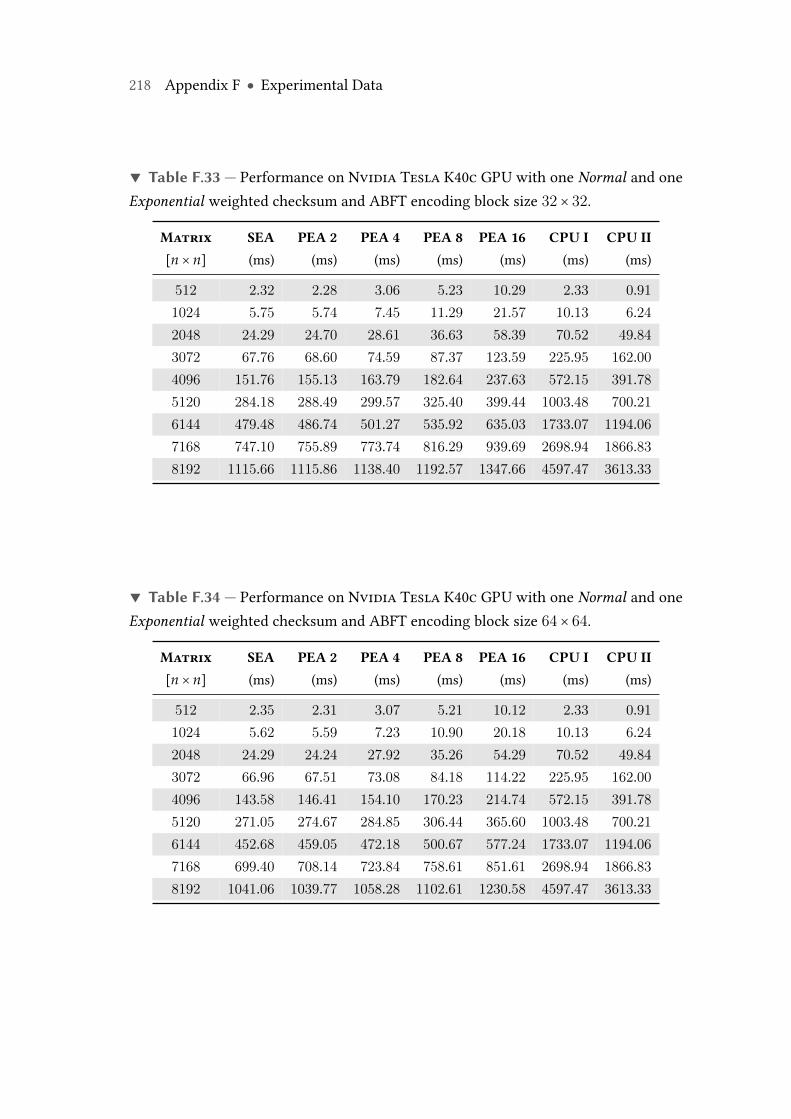
218 Appendix F ● Experimental Data
▼ Table F.33 — Performance on Nvidia Tesla K40c GPU with one Normal and oneExponential weighted checksum and ABFT encoding block size 32× 32.
Matrix SEA PEA 2 PEA 4 PEA 8 PEA 16 CPU I CPU II[n × n] (ms) (ms) (ms) (ms) (ms) (ms) (ms)
512 2.32 2.28 3.06 5.23 10.29 2.33 0.911024 5.75 5.74 7.45 11.29 21.57 10.13 6.242048 24.29 24.70 28.61 36.63 58.39 70.52 49.843072 67.76 68.60 74.59 87.37 123.59 225.95 162.004096 151.76 155.13 163.79 182.64 237.63 572.15 391.785120 284.18 288.49 299.57 325.40 399.44 1003.48 700.216144 479.48 486.74 501.27 535.92 635.03 1733.07 1194.067168 747.10 755.89 773.74 816.29 939.69 2698.94 1866.838192 1115.66 1115.86 1138.40 1192.57 1347.66 4597.47 3613.33
▼ Table F.34 — Performance on Nvidia Tesla K40c GPU with one Normal and oneExponential weighted checksum and ABFT encoding block size 64× 64.
Matrix SEA PEA 2 PEA 4 PEA 8 PEA 16 CPU I CPU II[n × n] (ms) (ms) (ms) (ms) (ms) (ms) (ms)
512 2.35 2.31 3.07 5.21 10.12 2.33 0.911024 5.62 5.59 7.23 10.90 20.18 10.13 6.242048 24.29 24.24 27.92 35.26 54.29 70.52 49.843072 66.96 67.51 73.08 84.18 114.22 225.95 162.004096 143.58 146.41 154.10 170.23 214.74 572.15 391.785120 271.05 274.67 284.85 306.44 365.60 1003.48 700.216144 452.68 459.05 472.18 500.67 577.24 1733.07 1194.067168 699.40 708.14 723.84 758.61 851.61 2698.94 1866.838192 1041.06 1039.77 1058.28 1102.61 1230.58 4597.47 3613.33
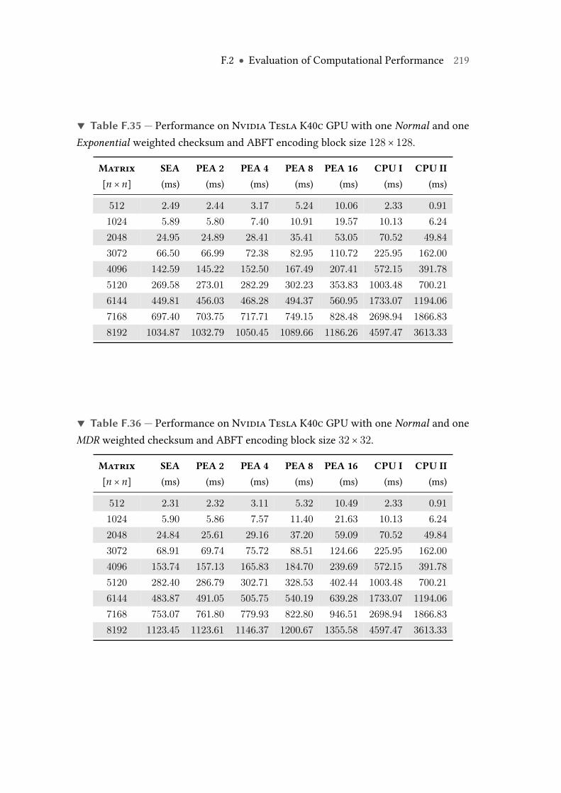
F.2 ● Evaluation of Computational Performance 219
▼ Table F.35 — Performance on Nvidia Tesla K40c GPU with one Normal and oneExponential weighted checksum and ABFT encoding block size 128× 128.
Matrix SEA PEA 2 PEA 4 PEA 8 PEA 16 CPU I CPU II[n × n] (ms) (ms) (ms) (ms) (ms) (ms) (ms)
512 2.49 2.44 3.17 5.24 10.06 2.33 0.911024 5.89 5.80 7.40 10.91 19.57 10.13 6.242048 24.95 24.89 28.41 35.41 53.05 70.52 49.843072 66.50 66.99 72.38 82.95 110.72 225.95 162.004096 142.59 145.22 152.50 167.49 207.41 572.15 391.785120 269.58 273.01 282.29 302.23 353.83 1003.48 700.216144 449.81 456.03 468.28 494.37 560.95 1733.07 1194.067168 697.40 703.75 717.71 749.15 828.48 2698.94 1866.838192 1034.87 1032.79 1050.45 1089.66 1186.26 4597.47 3613.33
▼ Table F.36 — Performance on Nvidia Tesla K40c GPU with one Normal and oneMDR weighted checksum and ABFT encoding block size 32× 32.
Matrix SEA PEA 2 PEA 4 PEA 8 PEA 16 CPU I CPU II[n × n] (ms) (ms) (ms) (ms) (ms) (ms) (ms)
512 2.31 2.32 3.11 5.32 10.49 2.33 0.911024 5.90 5.86 7.57 11.40 21.63 10.13 6.242048 24.84 25.61 29.16 37.20 59.09 70.52 49.843072 68.91 69.74 75.72 88.51 124.66 225.95 162.004096 153.74 157.13 165.83 184.70 239.69 572.15 391.785120 282.40 286.79 302.71 328.53 402.44 1003.48 700.216144 483.87 491.05 505.75 540.19 639.28 1733.07 1194.067168 753.07 761.80 779.93 822.80 946.51 2698.94 1866.838192 1123.45 1123.61 1146.37 1200.67 1355.58 4597.47 3613.33
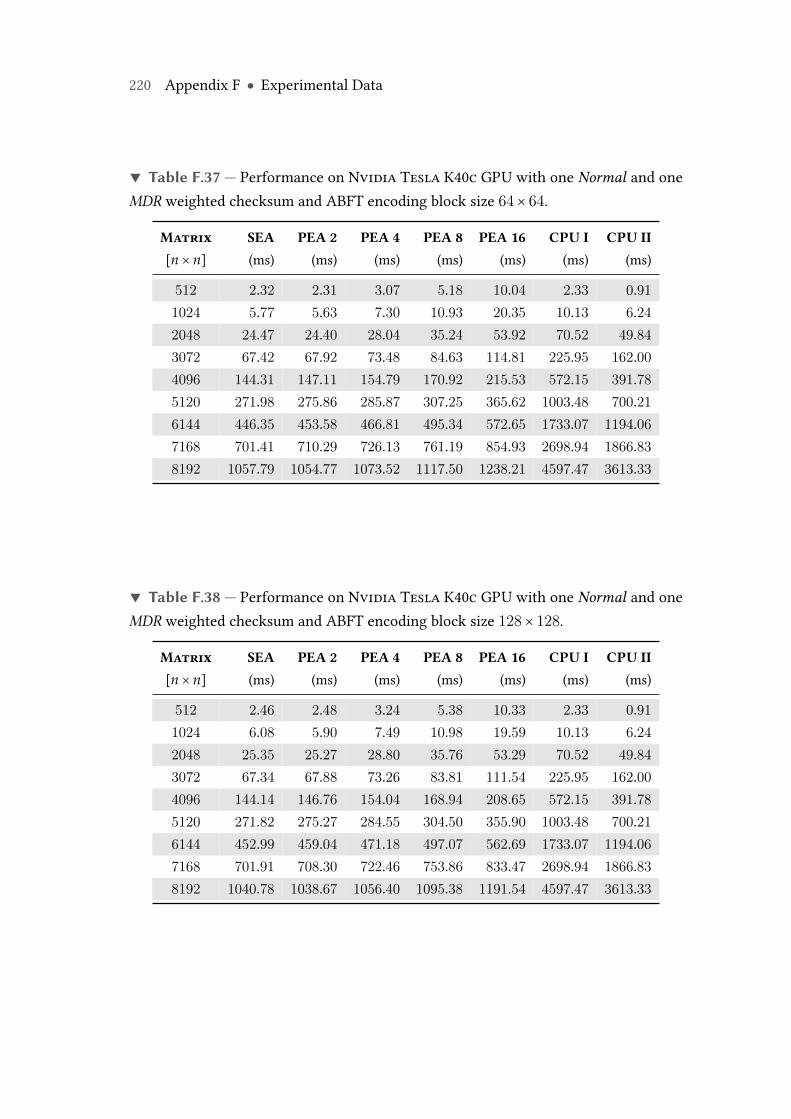
220 Appendix F ● Experimental Data
▼ Table F.37 — Performance on Nvidia Tesla K40c GPU with one Normal and oneMDR weighted checksum and ABFT encoding block size 64× 64.
Matrix SEA PEA 2 PEA 4 PEA 8 PEA 16 CPU I CPU II[n × n] (ms) (ms) (ms) (ms) (ms) (ms) (ms)
512 2.32 2.31 3.07 5.18 10.04 2.33 0.911024 5.77 5.63 7.30 10.93 20.35 10.13 6.242048 24.47 24.40 28.04 35.24 53.92 70.52 49.843072 67.42 67.92 73.48 84.63 114.81 225.95 162.004096 144.31 147.11 154.79 170.92 215.53 572.15 391.785120 271.98 275.86 285.87 307.25 365.62 1003.48 700.216144 446.35 453.58 466.81 495.34 572.65 1733.07 1194.067168 701.41 710.29 726.13 761.19 854.93 2698.94 1866.838192 1057.79 1054.77 1073.52 1117.50 1238.21 4597.47 3613.33
▼ Table F.38 — Performance on Nvidia Tesla K40c GPU with one Normal and oneMDR weighted checksum and ABFT encoding block size 128× 128.
Matrix SEA PEA 2 PEA 4 PEA 8 PEA 16 CPU I CPU II[n × n] (ms) (ms) (ms) (ms) (ms) (ms) (ms)
512 2.46 2.48 3.24 5.38 10.33 2.33 0.911024 6.08 5.90 7.49 10.98 19.59 10.13 6.242048 25.35 25.27 28.80 35.76 53.29 70.52 49.843072 67.34 67.88 73.26 83.81 111.54 225.95 162.004096 144.14 146.76 154.04 168.94 208.65 572.15 391.785120 271.82 275.27 284.55 304.50 355.90 1003.48 700.216144 452.99 459.04 471.18 497.07 562.69 1733.07 1194.067168 701.91 708.30 722.46 753.86 833.47 2698.94 1866.838192 1040.78 1038.67 1056.40 1095.38 1191.54 4597.47 3613.33
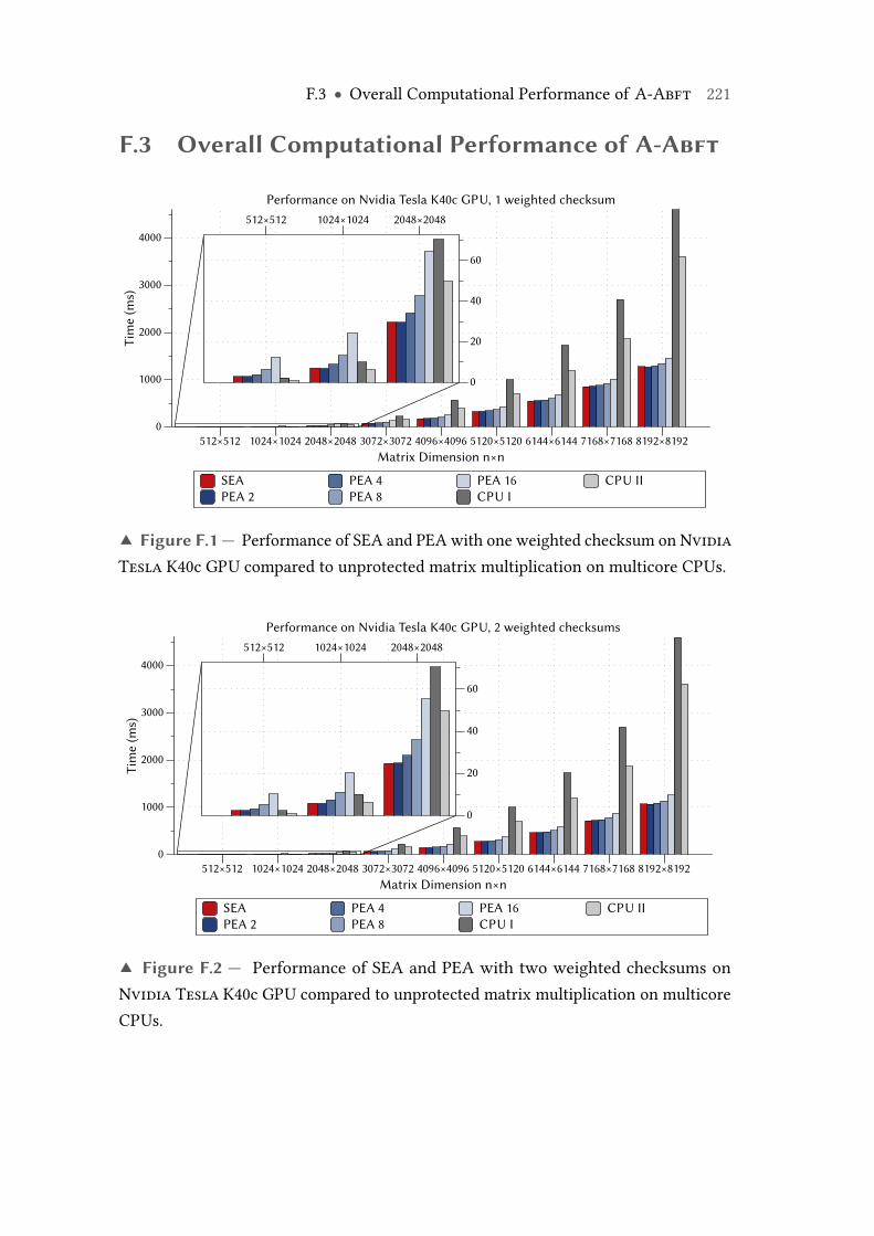
F.3 ● Overall Computational Performance of A-Abft 221
F.3 Overall Computational Performance of A-Abft
SEAPEA 2
PEA 4PEA 8
PEA 16CPU I
CPU II
Tim
e (m
s)
0
1000
2000
3000
4000
Matrix Dimension n×n512×512 1024×1024 2048×2048 3072×3072 4096×4096 5120×5120 6144×6144 7168×7168 8192×8192
Performance on Nvidia Tesla K40c GPU, 1 weighted checksum
0
20
40
60
512×512 1024×1024 2048×2048
▲ Figure F.1 — Performance of SEA and PEA with one weighted checksum on NvidiaTesla K40c GPU compared to unprotected matrix multiplication on multicore CPUs.
SEAPEA 2
PEA 4PEA 8
PEA 16CPU I
CPU II
Tim
e (m
s)
0
1000
2000
3000
4000
Matrix Dimension n×n512×512 1024×1024 2048×2048 3072×3072 4096×4096 5120×5120 6144×6144 7168×7168 8192×8192
Performance on Nvidia Tesla K40c GPU, 2 weighted checksums
0
20
40
60
512×512 1024×1024 2048×2048
▲ Figure F.2 — Performance of SEA and PEA with two weighted checksums onNvidia Tesla K40c GPU compared to unprotected matrix multiplication on multicoreCPUs.
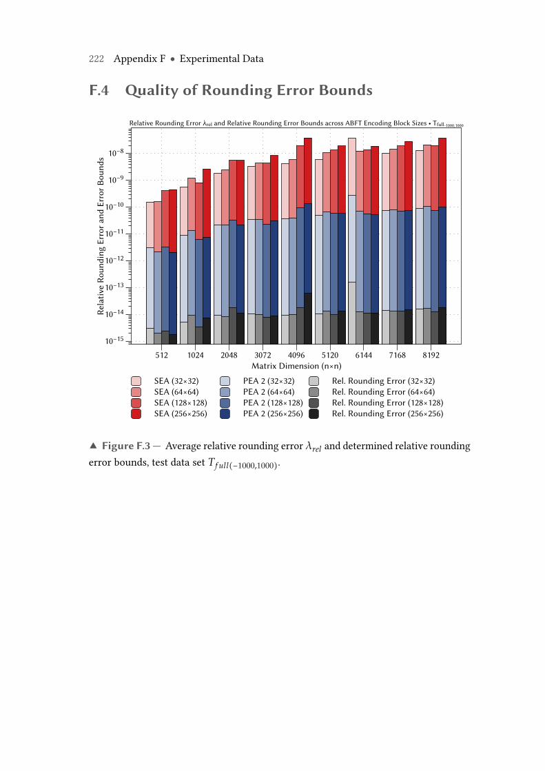
222 Appendix F ● Experimental Data
F.4 Quality of Rounding Error Bounds
SEA (32×32)SEA (64×64)SEA (128×128)SEA (256×256)
PEA 2 (32×32)PEA 2 (64×64)PEA 2 (128×128)PEA 2 (256×256)
Rel. Rounding Error (32×32)Rel. Rounding Error (64×64)Rel. Rounding Error (128×128)Rel. Rounding Error (256×256)
Rela
tive
Roun
ding
Err
or a
nd E
rror
Bou
nds
10−15
10−14
10−13
10−12
10−11
10−10
10−9
10−8
Matrix Dimension (n×n)512 1024 2048 3072 4096 5120 6144 7168 8192
Relative Rounding Error λrel and Relative Rounding Error Bounds across ABFT Encoding Block Sizes • Tfull-1000,1000
▲ Figure F.3 — Average relative rounding error λrel and determined relative roundingerror bounds, test data set Tf ull(−1000,1000).
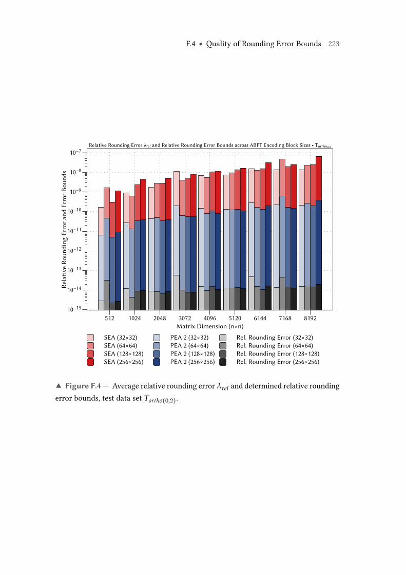
F.4 ● Quality of Rounding Error Bounds 223
SEA (32×32)SEA (64×64)SEA (128×128)SEA (256×256)
PEA 2 (32×32)PEA 2 (64×64)PEA 2 (128×128)PEA 2 (256×256)
Rel. Rounding Error (32×32)Rel. Rounding Error (64×64)Rel. Rounding Error (128×128)Rel. Rounding Error (256×256)
Rela
tive
Roun
ding
Err
or a
nd E
rror
Bou
nds
10−15
10−14
10−13
10−12
10−11
10−10
10−9
10−8
10−7
Matrix Dimension (n×n)512 1024 2048 3072 4096 5120 6144 7168 8192
Relative Rounding Error λrel and Relative Rounding Error Bounds across ABFT Encoding Block Sizes • Tortho0,2
▲ Figure F.4 — Average relative rounding error λrel and determined relative roundingerror bounds, test data set Tortho(0,2).
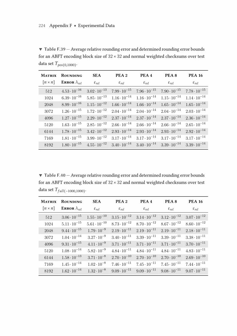
224 Appendix F ● Experimental Data
▼ Table F.39 —Average relative rounding error and determined rounding error boundsfor an ABFT encoding block size of 32× 32 and normal weighted checksums over testdata set Tpos(0,1000).
Matrix Rounding SEA PEA 2 PEA 4 PEA 8 PEA 16[n × n] Error λrel εrel εrel εrel εrel εrel
512 4.53 ⋅ 10−16 3.02 ⋅ 10−13 7.99 ⋅ 10−15 7.96 ⋅ 10−15 7.90 ⋅ 10−15 7.78 ⋅ 10−15
1024 6.39 ⋅ 10−16 5.85 ⋅ 10−13 1.16 ⋅ 10−14 1.16 ⋅ 10−14 1.15 ⋅ 10−14 1.14 ⋅ 10−14
2048 8.99 ⋅ 10−16 1.15 ⋅ 10−12 1.66 ⋅ 10−14 1.66 ⋅ 10−14 1.65 ⋅ 10−14 1.65 ⋅ 10−14
3072 1.26 ⋅ 10−15 1.72 ⋅ 10−12 2.04 ⋅ 10−14 2.04 ⋅ 10−14 2.04 ⋅ 10−14 2.03 ⋅ 10−14
4096 1.27 ⋅ 10−15 2.29 ⋅ 10−12 2.37 ⋅ 10−14 2.37 ⋅ 10−14 2.37 ⋅ 10−14 2.36 ⋅ 10−14
5120 1.63 ⋅ 10−15 2.85 ⋅ 10−12 2.66 ⋅ 10−14 2.66 ⋅ 10−14 2.66 ⋅ 10−14 2.65 ⋅ 10−14
6144 1.78 ⋅ 10−15 3.42 ⋅ 10−12 2.93 ⋅ 10−14 2.93 ⋅ 10−14 2.93 ⋅ 10−14 2.92 ⋅ 10−14
7169 1.81 ⋅ 10−15 3.99 ⋅ 10−12 3.17 ⋅ 10−14 3.17 ⋅ 10−14 3.17 ⋅ 10−14 3.17 ⋅ 10−14
8192 1.80 ⋅ 10−15 4.55 ⋅ 10−12 3.40 ⋅ 10−14 3.40 ⋅ 10−14 3.39 ⋅ 10−14 3.39 ⋅ 10−14
▼ Table F.40 —Average relative rounding error and determined rounding error boundsfor an ABFT encoding block size of 32× 32 and normal weighted checksums over testdata set Tf ull(−1000,1000).
Matrix Rounding SEA PEA 2 PEA 4 PEA 8 PEA 16[n × n] Error λrel εrel εrel εrel εrel εrel
512 3.06 ⋅ 10−15 1.55 ⋅ 10−10 3.15 ⋅ 10−12 3.14 ⋅ 10−12 3.12 ⋅ 10−12 3.07 ⋅ 10−12
1024 5.11 ⋅ 10−15 5.61 ⋅ 10−10 8.73 ⋅ 10−12 8.70 ⋅ 10−12 8.67 ⋅ 10−12 8.60 ⋅ 10−12
2048 9.44 ⋅ 10−15 1.79 ⋅ 10−9 2.19 ⋅ 10−11 2.19 ⋅ 10−11 2.19 ⋅ 10−11 2.18 ⋅ 10−11
3072 1.04 ⋅ 10−14 3.27 ⋅ 10−9 3.40 ⋅ 10−11 3.39 ⋅ 10−11 3.39 ⋅ 10−11 3.38 ⋅ 10−11
4096 9.31 ⋅ 10−15 4.11 ⋅ 10−9 3.71 ⋅ 10−11 3.71 ⋅ 10−11 3.71 ⋅ 10−11 3.70 ⋅ 10−11
5120 1.08 ⋅ 10−14 5.82 ⋅ 10−9 4.84 ⋅ 10−11 4.84 ⋅ 10−11 4.84 ⋅ 10−11 4.83 ⋅ 10−11
6144 1.58 ⋅ 10−13 3.71 ⋅ 10−8 2.70 ⋅ 10−10 2.70 ⋅ 10−10 2.70 ⋅ 10−10 2.69 ⋅ 10−10
7169 1.45 ⋅ 10−14 1.02 ⋅ 10−8 7.46 ⋅ 10−11 7.45 ⋅ 10−11 7.45 ⋅ 10−11 7.44 ⋅ 10−11
8192 1.62 ⋅ 10−14 1.32 ⋅ 10−8 9.09 ⋅ 10−11 9.09 ⋅ 10−11 9.08 ⋅ 10−11 9.07 ⋅ 10−11
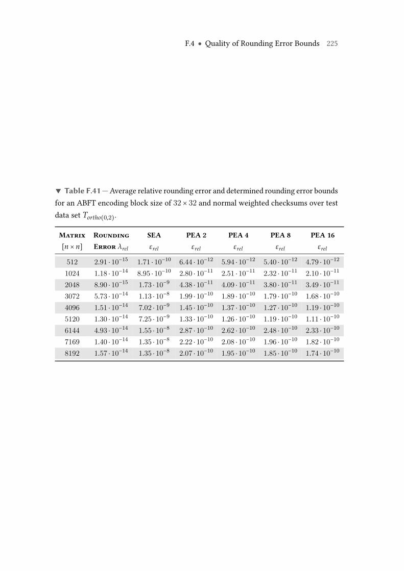
F.4 ● Quality of Rounding Error Bounds 225
▼ Table F.41 —Average relative rounding error and determined rounding error boundsfor an ABFT encoding block size of 32× 32 and normal weighted checksums over testdata set Tortho(0,2).
Matrix Rounding SEA PEA 2 PEA 4 PEA 8 PEA 16[n × n] Error λrel εrel εrel εrel εrel εrel
512 2.91 ⋅ 10−15 1.71 ⋅ 10−10 6.44 ⋅ 10−12 5.94 ⋅ 10−12 5.40 ⋅ 10−12 4.79 ⋅ 10−12
1024 1.18 ⋅ 10−14 8.95 ⋅ 10−10 2.80 ⋅ 10−11 2.51 ⋅ 10−11 2.32 ⋅ 10−11 2.10 ⋅ 10−11
2048 8.90 ⋅ 10−15 1.73 ⋅ 10−9 4.38 ⋅ 10−11 4.09 ⋅ 10−11 3.80 ⋅ 10−11 3.49 ⋅ 10−11
3072 5.73 ⋅ 10−14 1.13 ⋅ 10−8 1.99 ⋅ 10−10 1.89 ⋅ 10−10 1.79 ⋅ 10−10 1.68 ⋅ 10−10
4096 1.51 ⋅ 10−14 7.02 ⋅ 10−9 1.45 ⋅ 10−10 1.37 ⋅ 10−10 1.27 ⋅ 10−10 1.19 ⋅ 10−10
5120 1.30 ⋅ 10−14 7.25 ⋅ 10−9 1.33 ⋅ 10−10 1.26 ⋅ 10−10 1.19 ⋅ 10−10 1.11 ⋅ 10−10
6144 4.93 ⋅ 10−14 1.55 ⋅ 10−8 2.87 ⋅ 10−10 2.62 ⋅ 10−10 2.48 ⋅ 10−10 2.33 ⋅ 10−10
7169 1.40 ⋅ 10−14 1.35 ⋅ 10−8 2.22 ⋅ 10−10 2.08 ⋅ 10−10 1.96 ⋅ 10−10 1.82 ⋅ 10−10
8192 1.57 ⋅ 10−14 1.35 ⋅ 10−8 2.07 ⋅ 10−10 1.95 ⋅ 10−10 1.85 ⋅ 10−10 1.74 ⋅ 10−10
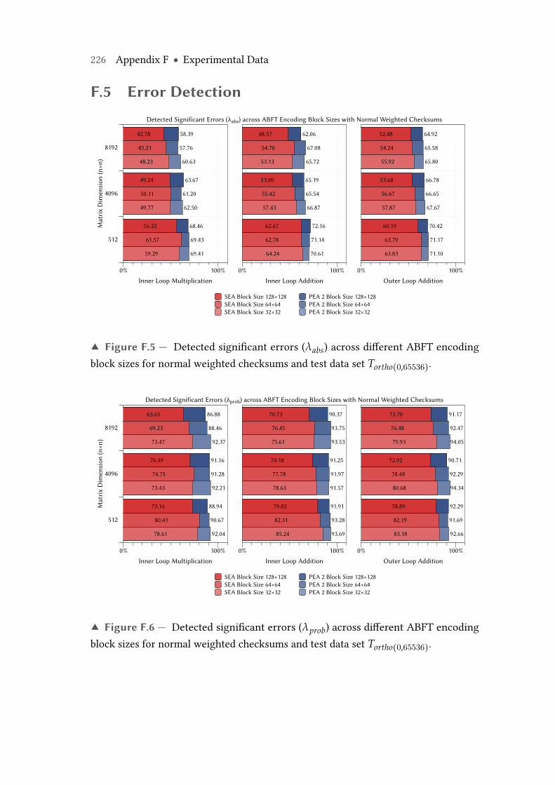
226 Appendix F ● Experimental Data
F.5 Error Detection
69.41
62.50
60.63
69.43
61.20
57.76
68.46
63.67
58.39
59.29
49.77
48.23
61.57
50.11
45.21
56.32
49.24
42.78
70.61
66.87
65.72
71.14
65.54
67.08
72.16
65.19
62.06
64.24
57.43
53.13
62.78
55.42
54.70
62.67
53.00
48.57
71.10
67.67
65.80
71.17
66.65
65.58
70.42
66.78
64.92
63.83
57.87
55.92
63.79
56.67
54.24
60.19
53.68
52.48
SEA Block Size 128×128SEA Block Size 64×64SEA Block Size 32×32
PEA 2 Block Size 128×128PEA 2 Block Size 64×64PEA 2 Block Size 32×32
Mat
rix
Dim
ensi
on (n
×n)
512
4096
8192
Inner Loop Multiplication0% 100%
Inner Loop Addition0% 100%
Outer Loop Addition0% 100%
Detected Significant Errors (λabs) across ABFT Encoding Block Sizes with Normal Weighted Checksums
▲ Figure F.5 — Detected significant errors (λabs) across different ABFT encodingblock sizes for normal weighted checksums and test data set Tortho(0,65536).
92.04
92.21
92.37
90.67
91.28
88.46
88.94
91.16
86.88
78.61
73.43
73.47
80.41
74.75
69.23
73.16
70.49
63.65
93.69
91.57
93.53
93.28
91.97
93.75
91.91
91.25
90.37
85.24
78.63
75.61
82.31
77.78
76.45
79.82
74.18
70.73
92.66
94.34
94.05
91.69
92.29
92.47
92.29
90.71
91.17
83.18
80.68
79.93
82.19
78.48
76.48
78.89
72.92
73.70
SEA Block Size 128×128SEA Block Size 64×64SEA Block Size 32×32
PEA 2 Block Size 128×128PEA 2 Block Size 64×64PEA 2 Block Size 32×32
Mat
rix
Dim
ensi
on (n
×n)
512
4096
8192
Inner Loop Multiplication0% 100%
Inner Loop Addition0% 100%
Outer Loop Addition0% 100%
Detected Significant Errors (λprob) across ABFT Encoding Block Sizes with Normal Weighted Checksums
▲ Figure F.6 — Detected significant errors (λprob) across different ABFT encodingblock sizes for normal weighted checksums and test data set Tortho(0,65536).
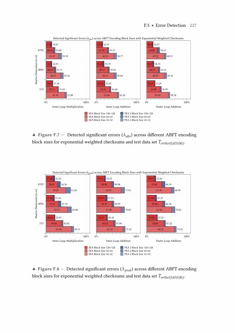
F.5 ● Error Detection 227
51.88
43.56
39.59
31.43
25.17
23.00
17.38
14.97
14.81
47.39
36.57
31.47
29.11
20.69
18.06
15.67
12.13
11.66
56.50
50.44
50.77
36.68
32.96
31.57
21.69
19.79
16.31
52.44
44.12
44.33
33.33
29.17
27.56
19.53
16.43
13.87
58.18
50.10
48.91
36.99
33.21
32.67
21.29
18.19
16.37
53.95
44.17
43.52
33.68
28.54
26.82
19.69
15.17
14.01
SEA Block Size 128×128SEA Block Size 64×64SEA Block Size 32×32
PEA 2 Block Size 128×128PEA 2 Block Size 64×64PEA 2 Block Size 32×32
Mat
rix
Dim
ensi
on (n
×n)
512
4096
8192
Inner Loop Multiplication0% 100%
Inner Loop Addition0% 100%
Outer Loop Addition0% 100%
Detected Significant Errors (λabs) across ABFT Encoding Block Sizes with Exponential Weighted Checksums
▲ Figure F.7 — Detected significant errors (λabs) across different ABFT encodingblock sizes for exponential weighted checksums and test data set Tortho(0,65536).
69.51
64.00
61.69
42.82
37.74
36.36
22.95
21.56
22.33
63.50
53.73
49.05
39.66
31.02
28.55
20.68
17.46
17.58
72.32
70.85
71.01
47.90
44.29
44.08
28.18
27.53
23.22
67.13
61.98
62.01
43.53
39.19
38.48
25.37
22.85
19.76
74.32
70.83
68.90
47.22
46.18
46.10
27.07
25.21
23.26
68.92
62.44
61.30
43.00
39.68
37.84
25.04
21.02
19.91
SEA Block Size 128×128SEA Block Size 64×64SEA Block Size 32×32
PEA 2 Block Size 128×128PEA 2 Block Size 64×64PEA 2 Block Size 32×32
Mat
rix
Dim
ensi
on (n
×n)
512
4096
8192
Inner Loop Multiplication0% 100%
Inner Loop Addition0% 100%
Outer Loop Addition0% 100%
Detected Significant Errors (λprob) across ABFT Encoding Block Sizes with Exponential Weighted Checksums
▲ Figure F.8 — Detected significant errors (λprob) across different ABFT encodingblock sizes for exponential weighted checksums and test data set Tortho(0,65536).
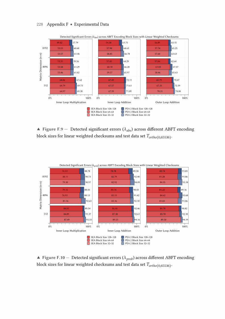
228 Appendix F ● Experimental Data
69.30
61.02
61.46
69.73
61.29
60.60
67.62
59.56
57.79
64.97
53.46
53.57
64.79
53.50
53.51
64.06
53.31
49.82
71.09
65.97
66.78
71.61
66.20
64.63
72.11
64.29
61.75
67.59
59.57
58.85
67.57
60.18
57.90
67.43
57.41
54.30
74.00
65.63
63.63
72.39
67.57
65.25
70.47
62.64
63.15
70.31
58.46
57.60
67.31
61.03
57.74
65.79
57.06
56.89
SEA Block Size 128×128SEA Block Size 64×64SEA Block Size 32×32
PEA 2 Block Size 128×128PEA 2 Block Size 64×64PEA 2 Block Size 32×32
Mat
rix
Dim
ensi
on (n
×n)
512
4096
8192
Inner Loop Multiplication0% 100%
Inner Loop Addition0% 100%
Outer Loop Addition0% 100%
Detected Significant Errors (λabs) across ABFT Encoding Block Sizes with Linear Weighted Checksums
▲ Figure F.9 — Detected significant errors (λabs) across different ABFT encodingblock sizes for linear weighted checksums and test data set Tortho(0,65536).
93.33
92.63
90.97
91.37
88.13
90.73
89.54
88.43
88.78
87.49
81.16
79.30
84.89
76.93
80.11
84.81
79.15
76.53
94.16
92.10
94.09
92.61
91.42
92.40
92.46
90.43
89.58
89.53
83.16
82.92
87.38
83.11
82.79
86.46
80.76
78.78
94.19
91.86
93.18
92.18
93.68
91.86
90.82
89.16
91.85
89.50
81.83
84.35
85.70
84.62
81.28
84.78
81.22
82.74
SEA Block Size 128×128SEA Block Size 64×64SEA Block Size 32×32
PEA 2 Block Size 128×128PEA 2 Block Size 64×64PEA 2 Block Size 32×32
Mat
rix
Dim
ensi
on (n
×n)
512
4096
8192
Inner Loop Multiplication0% 100%
Inner Loop Addition0% 100%
Outer Loop Addition0% 100%
Detected Significant Errors (λprob) across ABFT Encoding Block Sizes with Linear Weighted Checksums
▲ Figure F.10 — Detected significant errors (λprob) across different ABFT encodingblock sizes for linear weighted checksums and test data set Tortho(0,65536).
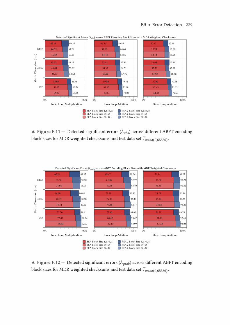
F.5 ● Error Detection 229
69.36
60.63
59.05
69.24
59.82
58.26
66.76
58.15
60.35
59.82
48.53
46.59
58.05
46.48
44.53
55.98
43.93
42.14
73.00
67.76
64.85
71.60
66.51
64.64
70.32
65.86
59.89
64.04
56.52
54.14
61.60
55.53
51.88
59.50
53.41
46.56
72.68
68.58
65.76
71.13
65.09
65.38
70.48
65.80
63.18
64.41
57.92
54.13
62.45
55.70
53.93
60.00
53.94
50.00
SEA Block Size 128×128SEA Block Size 64×64SEA Block Size 32×32
PEA 2 Block Size 128×128PEA 2 Block Size 64×64PEA 2 Block Size 32×32
Mat
rix
Dim
ensi
on (n
×n)
512
4096
8192
Inner Loop Multiplication0% 100%
Inner Loop Addition0% 100%
Outer Loop Addition0% 100%
Detected Significant Errors (λabs) across ABFT Encoding Block Sizes with MDR Weighted Checksums
▲ Figure F.11 — Detected significant errors (λabs) across different ABFT encodingblock sizes for MDR weighted checksums and test data set Tortho(0,65536).
92.57
89.60
90.05
92.84
90.58
90.70
90.11
86.01
89.17
79.83
71.72
71.04
77.83
70.37
69.32
75.56
64.98
62.26
93.99
92.77
93.40
93.47
91.49
92.79
91.00
89.13
89.36
82.45
77.38
77.98
80.42
76.38
74.48
77.00
72.28
69.47
94.04
93.40
92.82
92.45
90.71
93.71
89.74
91.16
90.27
83.33
78.88
76.40
81.16
77.62
77.30
76.39
74.73
71.44
SEA Block Size 128×128SEA Block Size 64×64SEA Block Size 32×32
PEA 2 Block Size 128×128PEA 2 Block Size 64×64PEA 2 Block Size 32×32
Mat
rix
Dim
ensi
on (n
×n)
512
4096
8192
Inner Loop Multiplication0% 100%
Inner Loop Addition0% 100%
Outer Loop Addition0% 100%
Detected Significant Errors (λprob) across ABFT Encoding Block Sizes with MDR Weighted Checksums
▲ Figure F.12 — Detected significant errors (λprob) across different ABFT encodingblock sizes for MDR weighted checksums and test data set Tortho(0,65536).
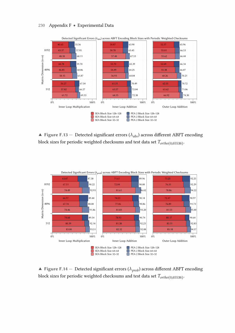
230 Appendix F ● Experimental Data
69.53
61.87
60.11
66.27
60.86
57.95
67.54
59.70
55.56
61.72
50.15
48.18
57.82
46.85
43.37
56.27
44.70
40.65
72.38
64.84
67.53
72.04
64.25
63.45
70.49
65.39
63.90
64.15
56.93
57.40
63.57
54.49
50.78
61.31
53.70
50.87
74.30
70.21
66.44
71.06
66.07
66.53
70.72
66.14
65.96
66.92
60.26
55.62
63.62
55.38
55.01
62.55
52.69
52.37
SEA Block Size 128×128SEA Block Size 64×64SEA Block Size 32×32
PEA 2 Block Size 128×128PEA 2 Block Size 64×64PEA 2 Block Size 32×32
Mat
rix
Dim
ensi
on (n
×n)
512
4096
8192
Inner Loop Multiplication0% 100%
Inner Loop Addition0% 100%
Outer Loop Addition0% 100%
Detected Significant Errors (λabs) across ABFT Encoding Block Sizes with Periodic Weighted Checksums
▲ Figure F.13 — Detected significant errors (λabs) across different ABFT encodingblock sizes for periodic weighted checksums and test data set Tortho(0,65536).
93.51
91.86
92.93
92.14
88.00
90.22
89.54
89.44
87.30
83.00
74.46
74.49
80.39
67.74
67.51
74.60
66.97
63.87
92.88
93.20
96.02
92.23
90.86
90.00
90.74
90.14
89.96
82.32
81.83
81.61
81.38
77.06
72.04
78.93
74.03
71.61
94.57
95.00
94.22
92.83
91.73
92.29
90.64
90.97
92.25
85.18
81.53
78.86
83.11
76.89
76.31
80.17
72.47
73.25
SEA Block Size 128×128SEA Block Size 64×64SEA Block Size 32×32
PEA 2 Block Size 128×128PEA 2 Block Size 64×64PEA 2 Block Size 32×32
Mat
rix
Dim
ensi
on (n
×n)
512
4096
8192
Inner Loop Multiplication0% 100%
Inner Loop Addition0% 100%
Outer Loop Addition0% 100%
Detected Significant Errors (λprob) across ABFT Encoding Block Sizes with Periodic Weighted Checksums
▲ Figure F.14 — Detected significant errors (λprob) across different ABFT encodingblock sizes for periodic weighted checksums and test data set Tortho(0,65536).
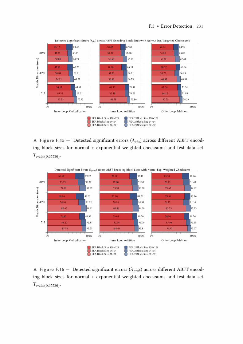
F.5 ● Error Detection 231
70.93
63.22
60.29
69.21
61.81
58.91
65.68
60.75
60.42
63.33
54.01
50.00
60.55
50.84
47.79
56.15
47.51
45.12
73.80
66.75
66.27
70.23
66.71
61.48
70.49
65.11
62.59
66.58
56.89
56.59
62.18
57.23
52.27
61.43
52.96
50.42
74.29
69.99
67.41
71.83
66.63
65.00
71.34
68.34
64.95
67.55
60.82
56.72
64.12
55.75
54.21
62.06
58.37
52.54
SEA Block Size 128×128SEA Block Size 64×64SEA Block Size 32×32
PEA 2 Block Size 128×128PEA 2 Block Size 64×64PEA 2 Block Size 32×32
Mat
rix
Dim
ensi
on (n
×n)
512
4096
8192
Inner Loop Multiplication0% 100%
Inner Loop Addition0% 100%
Outer Loop Addition0% 100%
Detected Significant Errors (λabs) across ABFT Encoding Block Sizes with Norm.+Exp. Weighted Checksums
▲ Figure F.15 — Detected significant errors (λabs) across different ABFT encod-ing block sizes for normal + exponential weighted checksums and test data setTortho(0,65536).
93.55
94.41
92.99
92.81
91.02
90.22
89.92
88.03
89.27
83.53
80.65
77.12
81.20
74.86
73.19
76.87
68.86
66.67
93.81
94.30
93.58
93.00
91.99
91.51
90.70
89.76
90.12
84.64
80.36
79.91
82.34
78.91
77.80
79.04
73.00
72.60
95.07
95.23
94.62
93.55
91.14
91.40
90.76
93.16
90.66
86.43
82.75
79.62
83.50
76.25
76.23
78.96
79.56
73.34
SEA Block Size 128×128SEA Block Size 64×64SEA Block Size 32×32
PEA 2 Block Size 128×128PEA 2 Block Size 64×64PEA 2 Block Size 32×32
Mat
rix
Dim
ensi
on (n
×n)
512
4096
8192
Inner Loop Multiplication0% 100%
Inner Loop Addition0% 100%
Outer Loop Addition0% 100%
Detected Significant Errors (λprob) across ABFT Encoding Block Sizes with Norm.+Exp. Weighted Checksums
▲ Figure F.16 — Detected significant errors (λprob) across different ABFT encod-ing block sizes for normal + exponential weighted checksums and test data setTortho(0,65536).
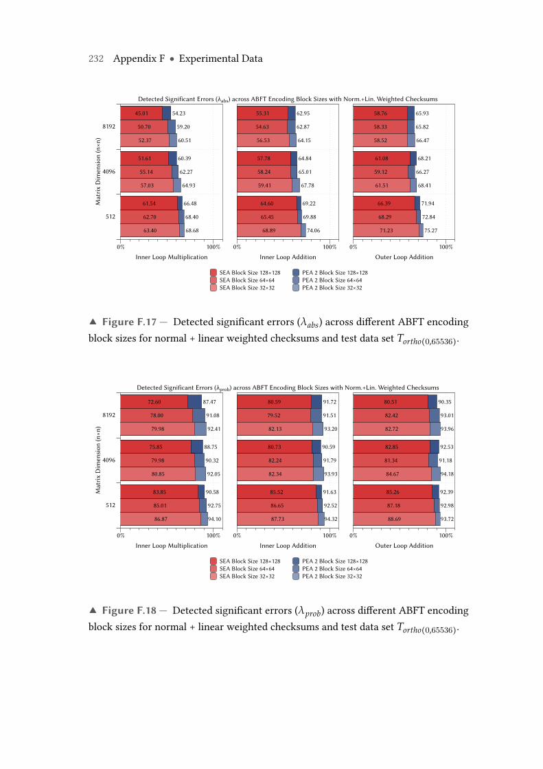
232 Appendix F ● Experimental Data
68.68
64.93
60.51
68.40
62.27
59.20
66.48
60.39
54.23
63.40
57.03
52.37
62.70
55.14
50.70
61.54
51.61
45.01
74.06
67.78
64.15
69.88
65.01
62.87
69.22
64.84
62.95
68.89
59.41
56.53
65.45
58.24
54.63
64.60
57.78
55.31
75.27
68.41
66.47
72.84
66.27
65.82
71.94
68.21
65.93
71.23
61.51
58.52
68.29
59.12
58.33
66.39
61.08
58.76
SEA Block Size 128×128SEA Block Size 64×64SEA Block Size 32×32
PEA 2 Block Size 128×128PEA 2 Block Size 64×64PEA 2 Block Size 32×32
Mat
rix
Dim
ensi
on (n
×n)
512
4096
8192
Inner Loop Multiplication0% 100%
Inner Loop Addition0% 100%
Outer Loop Addition0% 100%
Detected Significant Errors (λabs) across ABFT Encoding Block Sizes with Norm.+Lin. Weighted Checksums
▲ Figure F.17 — Detected significant errors (λabs) across different ABFT encodingblock sizes for normal + linear weighted checksums and test data set Tortho(0,65536).
94.10
92.05
92.41
92.75
90.32
91.08
90.58
88.75
87.47
86.87
80.85
79.98
85.01
79.98
78.00
83.85
75.85
72.60
94.32
93.93
93.20
92.52
91.79
91.51
91.63
90.59
91.72
87.73
82.34
82.13
86.65
82.24
79.52
85.52
80.73
80.59
93.72
94.18
93.96
92.98
91.18
93.01
92.39
92.53
90.35
88.69
84.67
82.72
87.18
81.34
82.42
85.26
82.85
80.51
SEA Block Size 128×128SEA Block Size 64×64SEA Block Size 32×32
PEA 2 Block Size 128×128PEA 2 Block Size 64×64PEA 2 Block Size 32×32
Mat
rix
Dim
ensi
on (n
×n)
512
4096
8192
Inner Loop Multiplication0% 100%
Inner Loop Addition0% 100%
Outer Loop Addition0% 100%
Detected Significant Errors (λprob) across ABFT Encoding Block Sizes with Norm.+Lin. Weighted Checksums
▲ Figure F.18 — Detected significant errors (λprob) across different ABFT encodingblock sizes for normal + linear weighted checksums and test data set Tortho(0,65536).
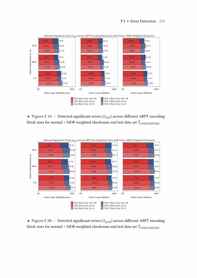
F.5 ● Error Detection 233
71.07
63.18
61.03
67.16
61.38
60.44
67.20
58.77
58.97
61.53
51.74
49.09
58.07
47.47
46.17
55.59
46.01
42.52
72.74
67.49
65.90
71.43
68.65
64.66
70.45
63.78
65.37
63.97
58.39
54.75
63.12
56.90
52.50
60.59
51.57
52.86
73.83
68.50
64.68
71.97
66.14
66.75
72.37
67.22
63.69
64.54
59.54
53.49
63.22
54.68
55.08
61.09
55.32
50.07
SEA Block Size 128×128SEA Block Size 64×64SEA Block Size 32×32
PEA 2 Block Size 128×128PEA 2 Block Size 64×64PEA 2 Block Size 32×32
Mat
rix
Dim
ensi
on (n
×n)
512
4096
8192
Inner Loop Multiplication0% 100%
Inner Loop Addition0% 100%
Outer Loop Addition0% 100%
Detected Significant Errors (λabs) across ABFT Encoding Block Sizes with Norm.+MDR Weighted Checksums
▲ Figure F.19 — Detected significant errors (λabs) across different ABFT encodingblock sizes for normal + MDR weighted checksums and test data set Tortho(0,65536).
95.01
92.46
93.01
91.04
89.40
93.28
91.40
87.76
89.49
82.26
75.72
74.82
78.71
69.13
71.27
75.61
68.71
64.52
93.82
93.22
93.71
93.96
92.80
91.14
91.66
90.27
91.78
82.51
80.66
77.86
83.03
76.92
74.00
78.84
73.00
74.22
94.20
94.33
93.20
93.66
92.07
92.71
92.10
91.53
90.97
82.34
82.00
77.07
82.28
76.12
76.50
77.74
75.32
71.51
SEA Block Size 128×128SEA Block Size 64×64SEA Block Size 32×32
PEA 2 Block Size 128×128PEA 2 Block Size 64×64PEA 2 Block Size 32×32
Mat
rix
Dim
ensi
on (n
×n)
512
4096
8192
Inner Loop Multiplication0% 100%
Inner Loop Addition0% 100%
Outer Loop Addition0% 100%
Detected Significant Errors (λprob) across ABFT Encoding Block Sizes with Norm.+MDR Weighted Checksums
▲ Figure F.20 — Detected significant errors (λprob) across different ABFT encodingblock sizes for normal + MDR weighted checksums and test data set Tortho(0,65536).

Index
A-Abft, 45, 83, 84, 94, 100, 103, 106, 109,114, 121, 130
ABFT, see algorithm-based fault toler-ance
absorption, see floating-point arithmeticalgorithm-based fault tolerance, 12, 21,
44, 55, 81analytical rounding error bound, see er-
ror boundArchitectural Vulnerability Factor, 40,
41availability, 19AVF, see Architectural Vulnerability Fac-
tor
base invariance, 88Benford’s law, 86
first digit law, 86general significant-digit law, 86
big data, 8bioinformatics, 7BLAS, 5block code, 22
linear block code, 22
calibration-based rounding error bound,see error bound
candidate set, 98central processing unit, 5CFD, see computational fluid dynamicscheckpointing, 45checksum, 56
column, 56full, 56reference, 59row, 56
checksum code, 66exponential-weighted, 66linear-weighted, 67minimum dynamic range, 67normalized, 67periodic, 67weighted average, 67
checksum element, see checksumchecksum matrix, 56
column, 56full, 57row, 57weighted, 63
checksum vector, 56column, 56row, 57weighted, 63
236 Index
CLF, see conditional line flipclimate research, 8CMOS, see complementary metal-oxide-
semiconductorcode, 183
reflectivity, 67code rate, 184code space, see codecode vector, 64column summation vector, see check-
sum vectorcolumn-checksummatrix, see checksum
matrixcomplementarymetal-oxide-semiconductor,
10computational biology, 7computational chemistry, 8computational finance, 9computational fluid dynamics, 8computational structural mechanics, 8compute unified device architecture, 27,
34confidence interval, 83correction vector, 65CPU, see central processing unitcross-layer reliability, 13crosstalk, 11CSM, see computational structural me-
chanicsCUDA, see compute unified device ar-
chitecture
defect, 18, 19denormal, see floating-point numberdependability, 17, 19
early-life failure, 11ECC, see error correcting codeelectromigration, 11electronic design automation, 8error, 18, 19
correction, 45, 58, 66detection, 19, 58, 137localization, 58recovery, 19
error bound, 71, 82analytical, 71, 73, 75calibration, 71probabilistic, 84, 95, 100, 106, 114,
121, 125quality, 82, 130
error correcting code, 32, 33, 42–44error correction, see errorerror detection, see errorerror localization, see errorexpectation value, 84, 86, 88, 90exponential weighted checksum code,
see checksum code
failure, 18, 19false-negative, 72, 82false-positive, 72, 82fault, 18, 19
intermittent, 18permanent, 18transient, 18
fault forecasting, 19fault injection, 40, 41, 107, 114, 137fault model, 20
conditional line flip, 20module-level, 21
Index 237
stuck-at, 20transition-delay, 21
fault prevention, 19fault tolerance, 2, 19, 39
software-based fault tolerance, 2hardware-based fault tolerance, 2
first digit law, see Benford’s lawfloating-point arithmetic, 14, 23, 81
absorption, 26round-ties-away, 25round-to-nearest, 25round-to-nearest-even, 25round-towards-+∞, 25round-towards-−∞, 25round-towards-zero, 25rounding, 24rounding error, 14, 24, 71, 82, 84rounding mode, 25subtractive cancellation, 26tie-breaking rule, 25underflow, 26
floating-point numberbase, 23denormal, 24exponent, 23mantissa, 23normalized, 24precision, 23radix, 23sign, 23significand, 23subnormal, 24
forensic financial accounting, 87fraud detection, 87
full-checksum matrix, see checksum ma-trix
fused multiply-add, 30
GDDR5, 33general linear code, see checksum codegeneral significant-digit law, see Ben-
ford’s lawgenerator matrix, 22, 185global device memory, 31GPGPU-Sim, 41, 52GPU, see graphics processing unitgraceful underflow, 24gradual underflow, see graceful under-
flowgraphics processing unit, 5, 27, 29, 30,
35, 40, 41, 44, 83, 94graphics display controller, 5
grids of thread blocks, 36
Hamming distance, 184Hamming weight, 184HCI, see hot carrier injectionhigh-consequence applications, 9hot carrier injection, 11Householder transformation, 104
IEEE Standard 754™ for floating-pointarithmetic, 23, 25, 30
IEEE Standard 754™-2008 for floating-point arithmetic, 84
in-silico, 7integrity, 19IR drop, 11
kernel, 34, 101, 102, 124
238 Index
LAPACK, 5LER, see line edge roughnessline edge roughness, 11linear algebra, 5, 14, 56linear block code, 21, see block code, 185linear programming, 109linearweighted checksum code, see check-
sum codeLINPACK, 5lithography, 11logic simulation, 40
gate-level, 40RT-level, 40
machine epsilon ϵM, 25, 75maintainability, 19mantissa check, 72matrix, 178
conjugate transpose, 178dimension, 178element, 178identity, 178index, 178inverse, 178transpose, 178
matrix multiplication, 5MBU, see multi-bit upsetMCU, see multi-cell upsetMDR, seeminimumdynamic range check-
sum codemeteorology, 8MIMD, see multiple instruction stream,
multiple data streamminimumdynamic range checksum code,
see checksum code
multi-bit upset, 12multi-cell upset, 12multiple instruction stream, multiple data
stream, 6
n-modular redundancy, 13NBTI, see negative-biased temperature
instabilitynegative-biased temperature instability,
11normalized checksum code, see check-
sum codenullspace, 64numbers
complex, C, 178integer, Z, 178natural, N, 178rational, Q, 178real, R, 178
Open Computing Language, 34OpenCL, seeOpenComputing Language
parity-check condition, 187parity-check matrix, 22, 64, 186partitioned encoding, 68, 83PEA, see probabilistic rounding error boundperiodic checksum code, see checksum
codepower droop, 11probabilistic rounding error bound, see
error boundprobability distribution, 84
QR decomposition, 103quality of rounding error bound, see er-
ror bound
Index 239
radiation, 42random dopant fluctuation, 11RDF, see random dopant fluctuationsreciprocal probability distribution, 84,
86, 88redundancy, 39reliability, 9, 19, 39Revised Simplex algorithm, see Simplex
algorithmround-ties-away, see floating-point arith-
meticround-to-nearest, see floating-point arith-
meticround-to-nearest-even, see floating-point
arithmeticround-towards-+∞, see floating-point
arithm.round-towards-−∞, see floating-point
arithm.round-towards-zero, see floating-point
arithm.rounding, see floating-point arithmeticrounding error, see floating-point arith-
meticrounding error bound, see error boundrounding mode, see floating-point arith-
meticrow summation vector, see checksum
vectorrow-checksummatrix, see checksumma-
trix
safety, 9, 19SBST, see software-based self testSBU, see single-bit upset
scalar, 178scale invariance, 88scheduling, 50
thread, 50scientific computing, 3, 9, 81SDC, see silent data corruptionSEA, see simplified error analysisSECDED, see single-error correction, double-
error detection codesecurity, 19SEE, see single event effectSEL, see single-event latchupself-checking circuit, 39SET, see single-event transientSFU, see special-function unitsignificand, 84significand’s error, 84, 85, 88, 90silent data corruption, 10, 42, 43SIMD, see single instruction stream, mul-
tiple data streamSimplex algorithm, 109
revised, 112simplified error analysis, 75, 107, 109,
114, 121, 125simulation technology, 3, 9, 81single error correction, double error de-
tection code, 44single event effect, 12single instruction stream, multiple data
stream, 6, 27single-bit upset, 12single-error correction, double-error de-
tection code, 32single-event latchup, 12single-event transient, 12
240 Index
SMX, see streaming multiprocessor unitsoftware-based fault tolerance, 21software-based self test, 48special-function unit, 29standard deviation, 84stream processor, 28, 29, 137streaming multiprocessor unit, 28, 29,
35, 137subnormal, see floating-point numbersubtractive cancellation, see floating-point
arithmeticsyndrome, 65, 187
column, 60, 81row, 60, 81vector, 65
syndrome vector, see syndromesystem, 18systematic encoding, 186
TDDB, see time-dependent dielectric break-down
thermodynamics, 8thread, 31, 35thread block, 35thread scheduler, 28tie-breaking rule, see floating-point arith-
metictime-dependent dielectriv breakdown,
11
uncertainty, 9unified graphics architecture, 5unit roundoff, see machine epsilon ϵM
variance, 84, 86, 88, 91vector, 177
element, 177index, 177transpose, 178
vector spacedimension, 178
vulnerability, 39–41assessment, 39
warp, 31, 51weight, 62, 65
matrix, 62vector, 62
weight matrix, see weightweight vector, see weightweighted average checksum code, see
checksum codeweighted checksum code, 62, 65, 139weighted checksum matrix, see check-
sum matrixweighted checksum vector, see check-
sum vectorweighted column-checksum matrix, see
checksum matrixweighted full-checksummatrix, see check-
sum matrixweighted row-checksummatrix, see check-
sum matrix
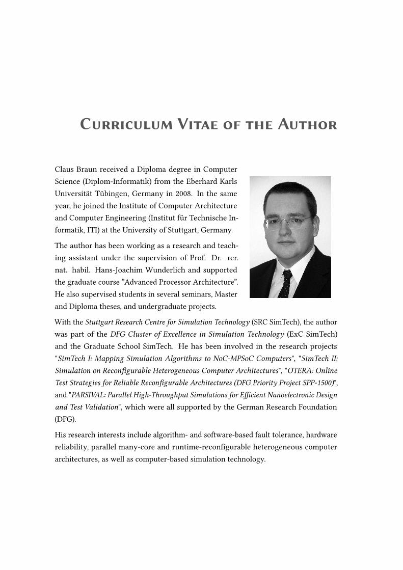
Curriculum Vitae of the Author
Claus Braun received a Diploma degree in ComputerScience (Diplom-Informatik) from the Eberhard KarlsUniversität Tübingen, Germany in 2008. In the sameyear, he joined the Institute of Computer Architectureand Computer Engineering (Institut für Technische In-formatik, ITI) at the University of Stuttgart, Germany.
The author has been working as a research and teach-ing assistant under the supervision of Prof. Dr. rer.nat. habil. Hans-Joachim Wunderlich and supportedthe graduate course ”Advanced Processor Architecture”.He also supervised students in several seminars, Masterand Diploma theses, and undergraduate projects.
With the Stuttgart Research Centre for Simulation Technology (SRC SimTech), the authorwas part of the DFG Cluster of Excellence in Simulation Technology (ExC SimTech)and the Graduate School SimTech. He has been involved in the research projects"SimTech I: Mapping Simulation Algorithms to NoC-MPSoC Computers", "SimTech II:Simulation on Reconfigurable Heterogeneous Computer Architectures", "OTERA: OnlineTest Strategies for Reliable Reconfigurable Architectures (DFG Priority Project SPP-1500)",and "PARSIVAL: Parallel High-Throughput Simulations for Efficient Nanoelectronic Designand Test Validation", which were all supported by the German Research Foundation(DFG).
His research interests include algorithm- and software-based fault tolerance, hardwarereliability, parallel many-core and runtime-reconfigurable heterogeneous computerarchitectures, as well as computer-based simulation technology.

Publications of the Author
• A. Schöll, C. Braun, M.A. Kochte and H.-J. Wunderlich. Efficient On-Line Fault-Tolerance for the Preconditioned Conjugate Gradient Method. to appear in Pro-ceedings of the IEEE International On-Line Testing Symposium (IOLTS’15), Halkidiki,Greece, 6-8 July 2015.
• A. Schöll, C. Braun, M. Daub, G. Schneider and H.-J. Wunderlich. AdaptiveParallel Simulation of a Two-Timescale-Model for Apoptotic Receptor-Clusteringon GPUs. Proceedings of the IEEE International Conference on Bioinformatics andBiomedicine (BIBM’14), Belfast, United Kingdom, 2-5 November 2014, pp. 424-431.
• C. Braun, S. Halder and H.-J. Wunderlich. A-ABFT: Autonomous Algorithm-Based Fault Tolerance for Matrix Multiplications on Graphics Processing Units.Proceedings of The 44th Annual IEEE/IFIP International Conference on DependableSystems and Networks (DSN’14), Atlanta, Georgia, USA, 23-26 June 2014, pp.443-454.
• C. Braun, S. Halder and H.-J. Wunderlich. A-ABFT: Autonomous Algorithm-BasedFault Tolerance on GPUs. Proceedings of the International Workshop on DependableGPU Computing, in conjunction with the ACM/IEEE DATE’14 Conference, Dresden,Germany, 28 March 2014.
• H.-J. Wunderlich, C. Braun and S. Halder. Efficacy and Efficiency of Algorithm-Based Fault Tolerance on GPUs. Proceedings of the IEEE International On-LineTesting Symposium (IOLTS’13), Crete, Greece, 8-10 July 2013, pp. 240-243.
• H. Zhang, L. Bauer, M.A. Kochte, E. Schneider, C. Braun, M.E. Imhof, H.-J. Wunder-lich and J. Henkel. Module Diversification: Fault Tolerance and Aging Mitigation
244
for Runtime Reconfigurable Architectures. Proceedings of the IEEE InternationalTest Conference (ITC’13), Anaheim, California, USA, 10-12 September 2013, pp.1-10.
• L. Bauer, C. Braun, M.E. Imhof, M.A. Kochte, E. Schneider, H. Zhang, J. Henkeland H.-J. Wunderlich. Test Strategies for Reliable Runtime Reconfigurable Ar-chitectures. IEEE Transactions on Computers, Vol. 62(8), Los Alamitos, California,USA August 2013, pp. 1494-1507.
• C. Braun, M. Daub, A. Schöll, G. Schneider and H.-J. Wunderlich. Parallel Simu-lation of Apoptotic Receptor-Clustering on GPGPU Many-Core Architectures.Proceedings of the IEEE International Conference on Bioinformatics and Biomedicine(BIBM’12), Philadelphia, Pennsylvania, USA, 4-7 October 2012, pp. 1-6.
• C. Braun, S. Holst, J. M. Castillo, J. Gross and H.-J. Wunderlich. Acceleration ofMonte-Carlo Molecular Simulations on Hybrid Computing Architectures. Pro-ceedings of the 30th IEEE International Conference on Computer Design (ICCD’12),Montreal, Canada, 30 September-3 October 2012, pp. 207-212.
• M.S. Abdelfattah, L. Bauer, C. Braun, M.E. Imhof, M.A. Kochte, H. Zhang, J. Henkeland H.-J. Wunderlich. Transparent Structural Online Test for ReconfigurableSystems. Proceedings of the 18th IEEE International On-Line Testing Symposium(IOLTS’12), Sitges, Spain, 27-29 June 2012, pp. 37-42.
• L. Bauer, C. Braun, M.E. Imhof, M.A. Kochte, H. Zhang, H.-J. Wunderlich and J.Henkel. OTERA: Online Test Strategies for Reliable Reconfigurable Architectures.Proceedings of the NASA/ESA Conference on Adaptive Hardware and Systems(AHS’12), Erlangen, Germany, 25-28 June 2012, pp. 38-45.
• C. Braun and H.-J. Wunderlich. Algorithmen-basierte Fehlertoleranz für Many-Core-Architekturen (Algorithm-based Fault-Tolerance on Many-Core Architec-tures). it - Information Technology, Vol. 52(4), August 2010, pp. 209-215.
• C. Braun and H.-J. Wunderlich. Algorithm-based fault tolerance for many-corearchitectures. Proceedings of the 15th IEEE European Test Symposium (ETS’10),Praha, Czech Republic, 24-28 May 2010, pp. 253.

Declaration
All the work contained within this thesis,except where otherwise acknowledged, wassolely the effort of the author. At nostage was any collaboration entered intowith any other party.
Claus Braun

246