Embed Size (px)
Citation preview
Inhalt
Kap. 1
Kap. 2
Kap. 3
Kap. 4
Kap. 5
Kap. 6
Kap. 7
Kap. 8
Kap. 9
Kap. 10
Kap. 11
Kap. 12
Kap. 13
Kap. 14
Kap. 15
Kap. 16
Kap. 17
Literatur
Anhang
A
Analyse und VerifikationLVA 185.276, VU 2.0, ECTS 3.0
SS 2013
(Stand: 26.05.2013)
Jens Knoop
Technische Universitat WienInstitut fur Computersprachen uages
complang
uter
1/863

Inhalt
Kap. 1
Kap. 2
Kap. 3
Kap. 4
Kap. 5
Kap. 6
Kap. 7
Kap. 8
Kap. 9
Kap. 10
Kap. 11
Kap. 12
Kap. 13
Kap. 14
Kap. 15
Kap. 16
Kap. 17
Literatur
Anhang
A
Inhaltsverzeichnis
2/863
Inhalt
Kap. 1
Kap. 2
Kap. 3
Kap. 4
Kap. 5
Kap. 6
Kap. 7
Kap. 8
Kap. 9
Kap. 10
Kap. 11
Kap. 12
Kap. 13
Kap. 14
Kap. 15
Kap. 16
Kap. 17
Literatur
Anhang
A
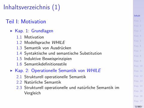
Inhaltsverzeichnis (1)
Teil I: Motivation
I Kap. 1: Grundlagen
1.1 Motivation1.2 Modellsprache WHILE1.3 Semantik von Ausdrucken1.4 Syntaktische und semantische Substitution1.5 Induktive Beweisprinzipien1.6 Semantikdefinitionsstile
I Kap. 2: Operationelle Semantik von WHILE
2.1 Strukturell operationelle Semantik2.2 Naturliche Semantik2.3 Strukturell operationelle und naturliche Semantik im
Vergleich
3/863
Inhalt
Kap. 1
Kap. 2
Kap. 3
Kap. 4
Kap. 5
Kap. 6
Kap. 7
Kap. 8
Kap. 9
Kap. 10
Kap. 11
Kap. 12
Kap. 13
Kap. 14
Kap. 15
Kap. 16
Kap. 17
Literatur
Anhang
A
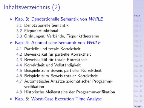
Inhaltsverzeichnis (2)
I Kap. 3: Denotationelle Semantik von WHILE
3.1 Denotationelle Semantik3.2 Fixpunktfunktional3.3 Ordnungen, Verbande, Fixpunkttheoreme
I Kap. 4: Axiomatische Semantik von WHILE
4.1 Partielle und totale Korrektheit4.2 Beweiskalkul fur partielle Korrektheit4.3 Beweiskalkul fur totale Korrektheit4.4 Korrektheit und Vollstandigkeit4.5 Beispiele zum Beweis partieller Korrektheit4.6 Beispiele zum Beweis totaler Korrektheit4.7 Automatische Ansatze axiomatischer Programm-
verifikation4.8 Historische Meilensteine der Programmverifikation
I Kap. 5: Worst-Case Execution Time Analyse
4/863
Inhalt
Kap. 1
Kap. 2
Kap. 3
Kap. 4
Kap. 5
Kap. 6
Kap. 7
Kap. 8
Kap. 9
Kap. 10
Kap. 11
Kap. 12
Kap. 13
Kap. 14
Kap. 15
Kap. 16
Kap. 17
Literatur
Anhang
A
Inhaltsverzeichnis (3)
Teil II: Analyse
I Kap. 6: Programmanalyse
6.1 Motivation6.2 Datenflussanalyse6.3 MOP-Ansatz6.4 MaxFP-Ansatz6.5 Koinzidenz- und Sicherheitstheorem6.6 Generischer Fixpunktalgorithmus und
Terminierungstheorem6.7 Zusammenfassung und Uberblick6.8 Beispiele: Verfugbare Ausdrucke, einfache Konstanten
6.8.1 Verfugbare Ausdrucke6.8.2 Einfache Konstanten
I Kap. 7: Programmverifikation vs. Programmanalyse
5/863
Inhalt
Kap. 1
Kap. 2
Kap. 3
Kap. 4
Kap. 5
Kap. 6
Kap. 7
Kap. 8
Kap. 9
Kap. 10
Kap. 11
Kap. 12
Kap. 13
Kap. 14
Kap. 15
Kap. 16
Kap. 17
Literatur
Anhang
A
Inhaltsverzeichnis (4)I Kap. 8: Reverse Datenflussanalyse
8.1 Grundlagen8.2 rJOP-Ansatz8.3 rMinFP-Ansatz8.4 Reverses Koinzidenz- und Sicherheitstheorem8.5 Generischer Fixpunktalgorithmus und Reverses
Terminierungstheorem8.6 Analyse und Verifikation: Analogien und
Gemeinsamkeiten8.7 Anwendungen reverser Datenflussanalyse8.8 Zusammenfassung
I Kap. 9: Chaotische Fixpunktiteration9.1 Motivation9.2 Chaotisches Fixpunktiterationstheorem9.3 Anwendungen
9.3.1 Vektor-Iteration9.3.2 Datenflussanalyse
6/863
Inhalt
Kap. 1
Kap. 2
Kap. 3
Kap. 4
Kap. 5
Kap. 6
Kap. 7
Kap. 8
Kap. 9
Kap. 10
Kap. 11
Kap. 12
Kap. 13
Kap. 14
Kap. 15
Kap. 16
Kap. 17
Literatur
Anhang
A
Inhaltsverzeichnis (5)
I Kap. 10: Basisblock- vs. Einzelanweisungsgraphen10.1 Motivation
10.1.1 Kantenbenannter Einzelanweisungsansatz10.1.2 Knotenbenannter Basisblockansatz
10.2 Verfugbarkeit von Ausdrucken
10.1.1 Knotenbenannter Basisblockansatz10.2.2 Knotenbenannter Einzelanweisungsansatz10.2.3 Kantenbenannter Einzelanweisungsansatz
10.3 Konstantenausbreitung und -faltung
10.3.1 Kantenbenannter Einzelanweisungsansatz10.3.2 Knotenbenannter Basisblockansatz
10.4 Schattenhafte Variablen10.5 Fazit
7/863
Inhalt
Kap. 1
Kap. 2
Kap. 3
Kap. 4
Kap. 5
Kap. 6
Kap. 7
Kap. 8
Kap. 9
Kap. 10
Kap. 11
Kap. 12
Kap. 13
Kap. 14
Kap. 15
Kap. 16
Kap. 17
Literatur
Anhang
A
Inhaltsverzeichnis (6)
Teil III: Transformation und Optimalitat
I Kap. 11: Elimination partiell toter Anweisungen
11.1 Motivation11.2 PDCE/PFCE: Transformation und Optimalitat11.3 Implementierung von PDCE/PFCE
I Kap. 12: Elimination partiell redundanter Anweisungen
12.1 Motivation12.2 EAM: Einheitliche PREE/PRAE-Behandlung12.3 EAM: Transformation und Optimalitat
I Kap. 13: Kombination von PRAE und PDCE
I Kap. 14: Konstantenfaltung auf dem Wertegraphen
14.1 Motivation14.2 Der VG-Konstantenfaltungsalgorithmus14.3 Der PVG-Konstantenfaltungsalgorithmus
8/863
Inhalt
Kap. 1
Kap. 2
Kap. 3
Kap. 4
Kap. 5
Kap. 6
Kap. 7
Kap. 8
Kap. 9
Kap. 10
Kap. 11
Kap. 12
Kap. 13
Kap. 14
Kap. 15
Kap. 16
Kap. 17
Literatur
Anhang
A
Inhaltsverzeichnis (7)
Teil IV: Abstrakte Interpretation und Modellprufung
I Kap. 15: Abstrakte Interpretation und DFA
15.1 Theorie abstrakter Interpretation15.2 Systematische Konstruktion abstrakter Interpretationen15.3 Korrektheit abstrakter Interpretationen15.4 Vollstandigkeit und Optimalitat
I Kap. 16: Modellprufung und DFA
9/863
Inhalt
Kap. 1
Kap. 2
Kap. 3
Kap. 4
Kap. 5
Kap. 6
Kap. 7
Kap. 8
Kap. 9
Kap. 10
Kap. 11
Kap. 12
Kap. 13
Kap. 14
Kap. 15
Kap. 16
Kap. 17
Literatur
Anhang
A
Inhaltsverzeichnis (8)
Teil V: Abschluss und Ausblick
I Kap. 17: Resumee und Perspektiven
I Literatur
I AnhangI A Mathematische Grundlagen
A.1 Mengen und RelationenA.2 OrdnungenA.3 VerbandeA.4 Vollstandige partielle OrdnungenA.5 Fixpunkte und Fixpunkttheoreme
10/863

Inhalt
Kap. 1
Kap. 2
Kap. 3
Kap. 4
Kap. 5
Kap. 6
Kap. 7
Kap. 8
Kap. 9
Kap. 10
Kap. 11
Kap. 12
Kap. 13
Kap. 14
Kap. 15
Kap. 16
Kap. 17
Literatur
Anhang
A
Teil I
Motivation
11/863

Inhalt
Kap. 1
1.1
1.2
1.3
1.4
1.5
1.6
Kap. 2
Kap. 3
Kap. 4
Kap. 5
Kap. 6
Kap. 7
Kap. 8
Kap. 9
Kap. 10
Kap. 11
Kap. 12
Kap. 13
Kap. 14
Kap. 15
Kap. 16
Kap. 17
Literatur
Anhang
A
Kapitel 1
Grundlagen
12/863
Inhalt
Kap. 1
1.1
1.2
1.3
1.4
1.5
1.6
Kap. 2
Kap. 3
Kap. 4
Kap. 5
Kap. 6
Kap. 7
Kap. 8
Kap. 9
Kap. 10
Kap. 11
Kap. 12
Kap. 13
Kap. 14
Kap. 15
Kap. 16
Kap. 17
Literatur
Anhang
A
Grundlagen
Syntax und Semantik von Programmiersprachen:
I Syntax: Regelwerk zur prazisen Beschreibung wohlge-formter Programme
I Semantik: Regelwerk zur prazisen Beschreibung der Be-deutung oder des Verhaltens wohlgeformter Programmeoder Programmteile (aber auch von Hardware beispiels-weise)
13/863
Inhalt
Kap. 1
1.1
1.2
1.3
1.4
1.5
1.6
Kap. 2
Kap. 3
Kap. 4
Kap. 5
Kap. 6
Kap. 7
Kap. 8
Kap. 9
Kap. 10
Kap. 11
Kap. 12
Kap. 13
Kap. 14
Kap. 15
Kap. 16
Kap. 17
Literatur
Anhang
A
Literaturhinweise (1)
Als Textbucher:
I Hanne R. Nielson, Flemming Nielson. Semantics withApplications: An Appetizer. Springer-V., 2007.
I Hanne R. Nielson, Flemming Nielson. Semantics withApplications: A Formal Introduction. Wiley ProfessionalComputing, Wiley, 1992.
Bem.: Eine (uberarbeitete) Version ist frei erhaltlich auf
www.daimi.au.dk/∼bra8130/Wiley book/wiley.html
14/863
Inhalt
Kap. 1
1.1
1.2
1.3
1.4
1.5
1.6
Kap. 2
Kap. 3
Kap. 4
Kap. 5
Kap. 6
Kap. 7
Kap. 8
Kap. 9
Kap. 10
Kap. 11
Kap. 12
Kap. 13
Kap. 14
Kap. 15
Kap. 16
Kap. 17
Literatur
Anhang
A
Literaturhinweise (2)
Erganzend, weiterfuhrend und vertiefend:
I Krzysztof R. Apt, Frank S. de Boer, Ernst-Rudiger Olde-rog. Verification of Sequential and Concurrent Programs.3. Auflage, Springer-V., 2009.
I Ernst-Rudiger Olderog, Bernhard Steffen. FormaleSemantik und Programmverifikation. In Informatik-Hand-buch, Peter Rechenberg, Gustav Pomberger (Hrsg.), CarlHanser Verlag, 4. Auflage, 145-166, 2006.
I Krzysztof R. Apt, Ernst-Rudiger Olderog. Programmveri-fikation – Sequentielle, parallele und verteilte Programme.Springer-V., 1994.
15/863
Inhalt
Kap. 1
1.1
1.2
1.3
1.4
1.5
1.6
Kap. 2
Kap. 3
Kap. 4
Kap. 5
Kap. 6
Kap. 7
Kap. 8
Kap. 9
Kap. 10
Kap. 11
Kap. 12
Kap. 13
Kap. 14
Kap. 15
Kap. 16
Kap. 17
Literatur
Anhang
A
Literaturhinweise (3)
I Jacques Loeckx, Kurt Sieber. The Foundations of Pro-gram Verification. Wiley, 1984.
I Krzysztof R. Apt. Ten Years of Hoare’s Logic: A Survey –Part 1. ACM Transactions on Programming Languagesand Systems 3(4):431-483, 1981.
I Krzysztof R. Apt. Ten Years of Hoare’s Logic: A Survey –Part II: Nondeterminism. Theoretical Computer Science28(1-2):83-109, 1984.
16/863
Inhalt
Kap. 1
1.1
1.2
1.3
1.4
1.5
1.6
Kap. 2
Kap. 3
Kap. 4
Kap. 5
Kap. 6
Kap. 7
Kap. 8
Kap. 9
Kap. 10
Kap. 11
Kap. 12
Kap. 13
Kap. 14
Kap. 15
Kap. 16
Kap. 17
Literatur
Anhang
A
Unser Beispielszenario
I Modell(programmier)sprache WHILEI Syntax und Semantik
I Semantikdefinitionsstile1. Operationelle Semantik
1.1 Großschritt-Semantik: Naturliche Semantik1.2 Kleinschritt-Semantik: Strukturell operationelle
Semantik
2. Denotationelle Semantik3. Axiomatische Semantik
17/863
Inhalt
Kap. 1
1.1
1.2
1.3
1.4
1.5
1.6
Kap. 2
Kap. 3
Kap. 4
Kap. 5
Kap. 6
Kap. 7
Kap. 8
Kap. 9
Kap. 10
Kap. 11
Kap. 12
Kap. 13
Kap. 14
Kap. 15
Kap. 16
Kap. 17
Literatur
Anhang
A
Intuitiv
I Operationelle Semantik
Die Bedeutung eines (programmiersprachlichen) Konstrukts
ist durch die Berechnung beschrieben, die es bei seiner Aus-
fuhrung auf der Maschine induziert. Wichtig ist insbesondere,
wie der Effekt der Berechnung erzeugt wird.
I Denotationelle SemantikDie Bedeutung eines Konstrukts wird durch mathematische
Objekte modelliert, die den Effekt der Ausfuhrung der Kon-
strukte reprasentieren. Wichtig ist einzig der Effekt, nicht wie
er bewirkt wird.
I Axiomatische SemantikBestimmte Eigenschaften des Effekts der Ausfuhrung eines
Konstrukts werden als Zusicherungen ausgedruckt.
Bestimmte andere Aspekte der Ausfuhrung werden dabei
i.a. ignoriert.
18/863

Inhalt
Kap. 1
1.1
1.2
1.3
1.4
1.5
1.6
Kap. 2
Kap. 3
Kap. 4
Kap. 5
Kap. 6
Kap. 7
Kap. 8
Kap. 9
Kap. 10
Kap. 11
Kap. 12
Kap. 13
Kap. 14
Kap. 15
Kap. 16
Kap. 17
Literatur
Anhang
A
Kapitel 1.1
Motivation
19/863
Inhalt
Kap. 1
1.1
1.2
1.3
1.4
1.5
1.6
Kap. 2
Kap. 3
Kap. 4
Kap. 5
Kap. 6
Kap. 7
Kap. 8
Kap. 9
Kap. 10
Kap. 11
Kap. 12
Kap. 13
Kap. 14
Kap. 15
Kap. 16
Kap. 17
Literatur
Anhang
A
Motivation
...formale Semantik von Programmiersprachen einzufuhren:
Die (mathematische) Rigorositat formaler Semantik
I erlaubt Mehrdeutigkeiten, Uber- und Unterspezifikationennaturlichsprachlicher Beschreibungen aufzudecken undaufzulosen
I bietet die Grundlage fur vertrauenswurdige Implementie-rungen der Programmiersprache, fur die Analyse, Verifi-kation und Transformation von Programmen
20/863
Inhalt
Kap. 1
1.1
1.2
1.3
1.4
1.5
1.6
Kap. 2
Kap. 3
Kap. 4
Kap. 5
Kap. 6
Kap. 7
Kap. 8
Kap. 9
Kap. 10
Kap. 11
Kap. 12
Kap. 13
Kap. 14
Kap. 15
Kap. 16
Kap. 17
Literatur
Anhang
A
Unsere Modellsprache
I Die (Programmier-) Sprache WHILEI SyntaxI Semantik
I Semantikdefinitionsstile
...wofur sie besonders geeignet sind und wie sie inBeziehung zueinander stehen:
I Operationelle Semantik ( Sprachimplementierung)I Naturliche SemantikI Strukturell operationelle Semantik
I Denotationelle Semantik ( Sprachdesign)I Axiomatische Semantik ( Anwend’gsprogrammierung)
I Beweiskalkule fur partielle und totale KorrektheitI Korrektheit, Vollstandigkeit
21/863
Inhalt
Kap. 1
1.1
1.2
1.3
1.4
1.5
1.6
Kap. 2
Kap. 3
Kap. 4
Kap. 5
Kap. 6
Kap. 7
Kap. 8
Kap. 9
Kap. 10
Kap. 11
Kap. 12
Kap. 13
Kap. 14
Kap. 15
Kap. 16
Kap. 17
Literatur
Anhang
A
Kapitel 1.2
Modellsprache WHILE
22/863
Inhalt
Kap. 1
1.1
1.2
1.3
1.4
1.5
1.6
Kap. 2
Kap. 3
Kap. 4
Kap. 5
Kap. 6
Kap. 7
Kap. 8
Kap. 9
Kap. 10
Kap. 11
Kap. 12
Kap. 13
Kap. 14
Kap. 15
Kap. 16
Kap. 17
Literatur
Anhang
A
Modellsprache WHILE
WHILE , der sog. “while”-Kern imperativer Programmier-sprachen, besitzt:
I Zuweisungen (einschließlich der leeren Anweisung)
I Fallunterscheidungen
I while-Schleifen
I Sequentielle Komposition
Bemerkung: WHILE ist “schlank”, doch Turing-machtig!
23/863
Inhalt
Kap. 1
1.1
1.2
1.3
1.4
1.5
1.6
Kap. 2
Kap. 3
Kap. 4
Kap. 5
Kap. 6
Kap. 7
Kap. 8
Kap. 9
Kap. 10
Kap. 11
Kap. 12
Kap. 13
Kap. 14
Kap. 15
Kap. 16
Kap. 17
Literatur
Anhang
A
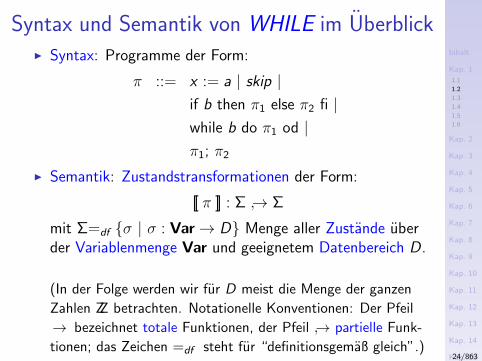
Syntax und Semantik von WHILE im UberblickI Syntax: Programme der Form:
π ::= x := a | skip |if b then π1 else π2 fi |while b do π1 od |π1; π2
I Semantik: Zustandstransformationen der Form:
[[ π ]] : Σ → Σ
mit Σ=df σ | σ : Var→ D Menge aller Zustande uberder Variablenmenge Var und geeignetem Datenbereich D.
(In der Folge werden wir fur D meist die Menge der ganzen
Zahlen ZZ betrachten. Notationelle Konventionen: Der Pfeil
→ bezeichnet totale Funktionen, der Pfeil → partielle Funk-
tionen; das Zeichen =df steht fur “definitionsgemaß gleich”.)24/863
Inhalt
Kap. 1
1.1
1.2
1.3
1.4
1.5
1.6
Kap. 2
Kap. 3
Kap. 4
Kap. 5
Kap. 6
Kap. 7
Kap. 8
Kap. 9
Kap. 10
Kap. 11
Kap. 12
Kap. 13
Kap. 14
Kap. 15
Kap. 16
Kap. 17
Literatur
Anhang
A
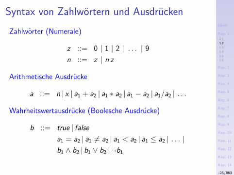
Syntax von Zahlwortern und Ausdrucken
Zahlworter (Numerale)
z ::= 0 | 1 | 2 | . . . | 9
n ::= z | n z
Arithmetische Ausdrucke
a ::= n | x | a1 + a2 | a1 ∗ a2 | a1 − a2 | a1/a2 | . . .
Wahrheitswertausdrucke (Boolesche Ausdrucke)
b ::= true | false |a1 = a2 | a1 6= a2 | a1 < a2 | a1 ≤ a2 | . . . |b1 ∧ b2 | b1 ∨ b2 | ¬b1
25/863
Inhalt
Kap. 1
1.1
1.2
1.3
1.4
1.5
1.6
Kap. 2
Kap. 3
Kap. 4
Kap. 5
Kap. 6
Kap. 7
Kap. 8
Kap. 9
Kap. 10
Kap. 11
Kap. 12
Kap. 13
Kap. 14
Kap. 15
Kap. 16
Kap. 17
Literatur
Anhang
A
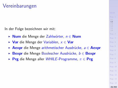
Vereinbarungen
In der Folge bezeichnen wir mit:
I Num die Menge der Zahlworter, n ∈ Num
I Var die Menge der Variablen, x ∈ Var
I Aexpr die Menge arithmetischer Ausdrucke, a ∈ Aexpr
I Bexpr die Menge Boolescher Ausdrucke, b ∈ Bexpr
I Prg die Menge aller WHILE -Programme, π ∈ Prg
26/863
Inhalt
Kap. 1
1.1
1.2
1.3
1.4
1.5
1.6
Kap. 2
Kap. 3
Kap. 4
Kap. 5
Kap. 6
Kap. 7
Kap. 8
Kap. 9
Kap. 10
Kap. 11
Kap. 12
Kap. 13
Kap. 14
Kap. 15
Kap. 16
Kap. 17
Literatur
Anhang
A
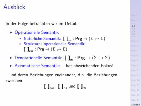
Ausblick
In der Folge betrachten wir im Detail:
I Operationelle SemantikI Naturliche Semantik: [[ ]]ns : Prg→ (Σ → Σ)I Strukturell operationelle Semantik:
[[ ]]sos : Prg→ (Σ → Σ)
I Denotationelle Semantik: [[ ]]ds : Prg→ (Σ → Σ)
I Axiomatische Semantik: ...hat abweichenden Fokus!
...und deren Beziehungen zueinander, d.h. die Beziehungenzwischen
[[ ]]sos , [[ ]]ns und [[ ]]ds
27/863

Inhalt
Kap. 1
1.1
1.2
1.3
1.4
1.5
1.6
Kap. 2
Kap. 3
Kap. 4
Kap. 5
Kap. 6
Kap. 7
Kap. 8
Kap. 9
Kap. 10
Kap. 11
Kap. 12
Kap. 13
Kap. 14
Kap. 15
Kap. 16
Kap. 17
Literatur
Anhang
A
Kapitel 1.3
Semantik von Ausdrucken
28/863
Inhalt
Kap. 1
1.1
1.2
1.3
1.4
1.5
1.6
Kap. 2
Kap. 3
Kap. 4
Kap. 5
Kap. 6
Kap. 7
Kap. 8
Kap. 9
Kap. 10
Kap. 11
Kap. 12
Kap. 13
Kap. 14
Kap. 15
Kap. 16
Kap. 17
Literatur
Anhang
A
Motivation
Die Semantik von WHILE stutzt sich ab auf die Semantikenvon
I Zahlwortern
I arithmetischen Ausdrucken
I Wahrheitswertausdrucken
und den Begriff der
I Speicherzustande
Diese sind daher zunachst festzulegen.
29/863
Inhalt
Kap. 1
1.1
1.2
1.3
1.4
1.5
1.6
Kap. 2
Kap. 3
Kap. 4
Kap. 5
Kap. 6
Kap. 7
Kap. 8
Kap. 9
Kap. 10
Kap. 11
Kap. 12
Kap. 13
Kap. 14
Kap. 15
Kap. 16
Kap. 17
Literatur
Anhang
A
Speicherzustande
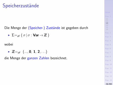
Die Menge der (Speicher-) Zustande ist gegeben durch
I Σ=df σ |σ : Var→ZZ
wobei
I ZZ=df ..., 0, 1, 2, . . .
die Menge der ganzen Zahlen bezeichnet.
30/863
Inhalt
Kap. 1
1.1
1.2
1.3
1.4
1.5
1.6
Kap. 2
Kap. 3
Kap. 4
Kap. 5
Kap. 6
Kap. 7
Kap. 8
Kap. 9
Kap. 10
Kap. 11
Kap. 12
Kap. 13
Kap. 14
Kap. 15
Kap. 16
Kap. 17
Literatur
Anhang
A
Semantik von Zahlwortern
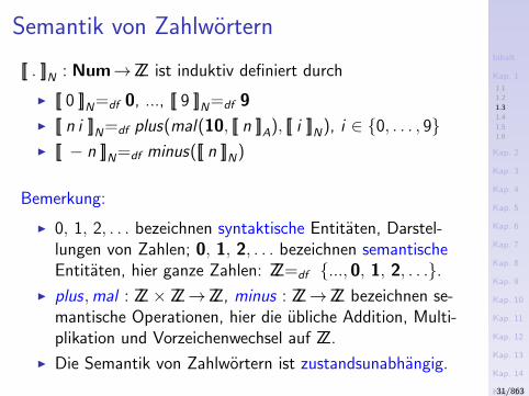
[[ . ]]N : Num→ZZ ist induktiv definiert durch
I [[ 0 ]]N=df 0, ..., [[ 9 ]]N=df 9
I [[ n i ]]N=df plus(mal(10, [[ n ]]A), [[ i ]]N), i ∈ 0, . . . , 9I [[ − n ]]N=df minus([[ n ]]N)
Bemerkung:
I 0, 1, 2, . . . bezeichnen syntaktische Entitaten, Darstel-lungen von Zahlen; 0, 1, 2, . . . bezeichnen semantischeEntitaten, hier ganze Zahlen: ZZ=df ..., 0, 1, 2, . . ..
I plus,mal : ZZ× ZZ→ZZ, minus : ZZ→ZZ bezeichnen se-mantische Operationen, hier die ubliche Addition, Multi-plikation und Vorzeichenwechsel auf ZZ.
I Die Semantik von Zahlwortern ist zustandsunabhangig.
31/863
Inhalt
Kap. 1
1.1
1.2
1.3
1.4
1.5
1.6
Kap. 2
Kap. 3
Kap. 4
Kap. 5
Kap. 6
Kap. 7
Kap. 8
Kap. 9
Kap. 10
Kap. 11
Kap. 12
Kap. 13
Kap. 14
Kap. 15
Kap. 16
Kap. 17
Literatur
Anhang
A
Semantik arithmetischer und Wahrheitswert-
ausdrucke
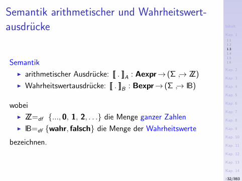
Semantik
I arithmetischer Ausdrucke: [[ . ]]A : Aexpr→ (Σ → ZZ)
I Wahrheitswertausdrucke: [[ . ]]B : Bexpr→ (Σ → IB)
wobei
I ZZ=df ..., 0, 1, 2, . . . die Menge ganzer Zahlen
I IB=df wahr, falsch die Menge der Wahrheitswerte
bezeichnen.
32/863
Inhalt
Kap. 1
1.1
1.2
1.3
1.4
1.5
1.6
Kap. 2
Kap. 3
Kap. 4
Kap. 5
Kap. 6
Kap. 7
Kap. 8
Kap. 9
Kap. 10
Kap. 11
Kap. 12
Kap. 13
Kap. 14
Kap. 15
Kap. 16
Kap. 17
Literatur
Anhang
A
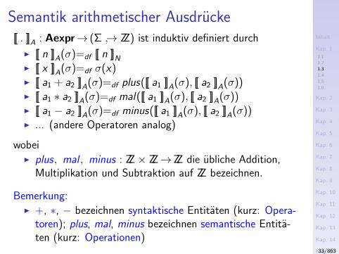
Semantik arithmetischer Ausdrucke[[ . ]]A : Aexpr→ (Σ → ZZ) ist induktiv definiert durch
I [[ n ]]A(σ)=df [[ n ]]NI [[ x ]]A(σ)=df σ(x)I [[ a1 + a2 ]]A(σ)=df plus([[ a1 ]]A(σ), [[ a2 ]]A(σ))I [[ a1 ∗ a2 ]]A(σ)=df mal([[ a1 ]]A(σ), [[ a2 ]]A(σ))I [[ a1 − a2 ]]A(σ)=df minus([[ a1 ]]A(σ), [[ a2 ]]A(σ))I ... (andere Operatoren analog)
wobeiI plus, mal , minus : ZZ× ZZ→ZZ die ubliche Addition,
Multiplikation und Subtraktion auf ZZ bezeichnen.
Bemerkung:I +, ∗, − bezeichnen syntaktische Entitaten (kurz: Opera-
toren); plus, mal, minus bezeichnen semantische Entita-ten (kurz: Operationen)
33/863
Inhalt
Kap. 1
1.1
1.2
1.3
1.4
1.5
1.6
Kap. 2
Kap. 3
Kap. 4
Kap. 5
Kap. 6
Kap. 7
Kap. 8
Kap. 9
Kap. 10
Kap. 11
Kap. 12
Kap. 13
Kap. 14
Kap. 15
Kap. 16
Kap. 17
Literatur
Anhang
A
Semantik Boolescher Ausdrucke (1)
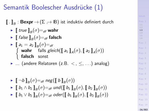
[[ . ]]B : Bexpr→ (Σ → IB) ist induktiv definiert durch
I [[ true ]]B(σ)=df wahr
I [[ false ]]B(σ)=df falsch
I [[ a1 = a2 ]]B(σ)=dfwahr falls gleich([[ a1 ]]A(σ), [[ a2 ]]A(σ))falsch sonst
I ... (andere Relatoren (z.B. < , ≤, . . .) analog)
I [[ ¬b ]]B(σ)=df neg([[ b ]]B(σ))
I [[ b1 ∧ b2 ]]B(σ)=df und([[ b1 ]]B(σ), [[ b2 ]]B(σ))
I [[ b1 ∨ b2 ]]B(σ)=df oder([[ b1 ]]B(σ), [[ b2 ]]B(σ))
34/863
Inhalt
Kap. 1
1.1
1.2
1.3
1.4
1.5
1.6
Kap. 2
Kap. 3
Kap. 4
Kap. 5
Kap. 6
Kap. 7
Kap. 8
Kap. 9
Kap. 10
Kap. 11
Kap. 12
Kap. 13
Kap. 14
Kap. 15
Kap. 16
Kap. 17
Literatur
Anhang
A
Semantik Boolescher Ausdrucke (2)
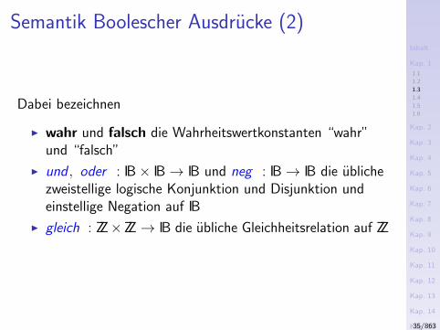
Dabei bezeichnen
I wahr und falsch die Wahrheitswertkonstanten “wahr”und “falsch”
I und , oder : IB× IB→ IB und neg : IB→ IB die ublichezweistellige logische Konjunktion und Disjunktion undeinstellige Negation auf IB
I gleich : ZZ×ZZ→ IB die ubliche Gleichheitsrelation auf ZZ
35/863
Inhalt
Kap. 1
1.1
1.2
1.3
1.4
1.5
1.6
Kap. 2
Kap. 3
Kap. 4
Kap. 5
Kap. 6
Kap. 7
Kap. 8
Kap. 9
Kap. 10
Kap. 11
Kap. 12
Kap. 13
Kap. 14
Kap. 15
Kap. 16
Kap. 17
Literatur
Anhang
A
Semantik Boolescher Ausdrucke (3)
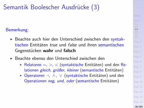
Bemerkung:
I Beachte auch hier den Unterschied zwischen den syntak-tischen Entitaten true und false und ihren semantischenGegenstucken wahr und falsch
I Beachte ebenso den Unterschied zwischen denI Relatoren =, >, < (syntaktische Entitaten) und den Re-
lationen gleich, großer, kleiner (semantische Entitaten)I Operatoren ¬, ∧ , ∨ (syntaktische Entitaten) und den
Operationen neg, und, oder (semantische Entitaten)
36/863
Inhalt
Kap. 1
1.1
1.2
1.3
1.4
1.5
1.6
Kap. 2
Kap. 3
Kap. 4
Kap. 5
Kap. 6
Kap. 7
Kap. 8
Kap. 9
Kap. 10
Kap. 11
Kap. 12
Kap. 13
Kap. 14
Kap. 15
Kap. 16
Kap. 17
Literatur
Anhang
A
Kapitel 1.4
Syntaktische und semantische Substitution
37/863
Inhalt
Kap. 1
1.1
1.2
1.3
1.4
1.5
1.6
Kap. 2
Kap. 3
Kap. 4
Kap. 5
Kap. 6
Kap. 7
Kap. 8
Kap. 9
Kap. 10
Kap. 11
Kap. 12
Kap. 13
Kap. 14
Kap. 15
Kap. 16
Kap. 17
Literatur
Anhang
A
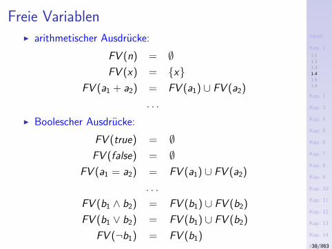
Freie VariablenI arithmetischer Ausdrucke:
FV (n) = ∅FV (x) = x
FV (a1 + a2) = FV (a1) ∪ FV (a2)
. . .
I Boolescher Ausdrucke:
FV (true) = ∅FV (false) = ∅
FV (a1 = a2) = FV (a1) ∪ FV (a2)
. . .
FV (b1 ∧ b2) = FV (b1) ∪ FV (b2)
FV (b1 ∨ b2) = FV (b1) ∪ FV (b2)
FV (¬b1) = FV (b1)38/863
Inhalt
Kap. 1
1.1
1.2
1.3
1.4
1.5
1.6
Kap. 2
Kap. 3
Kap. 4
Kap. 5
Kap. 6
Kap. 7
Kap. 8
Kap. 9
Kap. 10
Kap. 11
Kap. 12
Kap. 13
Kap. 14
Kap. 15
Kap. 16
Kap. 17
Literatur
Anhang
A
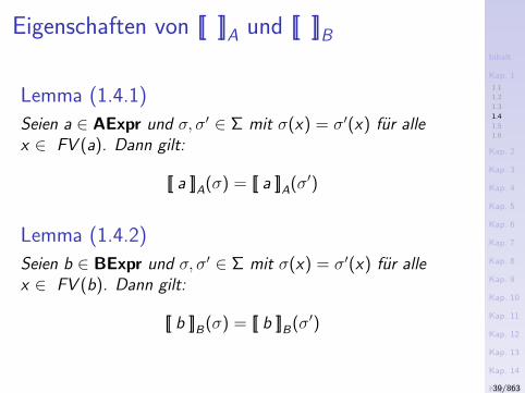
Eigenschaften von [[ ]]A und [[ ]]B
Lemma (1.4.1)
Seien a ∈ AExpr und σ, σ′ ∈ Σ mit σ(x) = σ′(x) fur allex ∈ FV (a). Dann gilt:
[[ a ]]A(σ) = [[ a ]]A(σ′)
Lemma (1.4.2)
Seien b ∈ BExpr und σ, σ′ ∈ Σ mit σ(x) = σ′(x) fur allex ∈ FV (b). Dann gilt:
[[ b ]]B(σ) = [[ b ]]B(σ′)
39/863
Inhalt
Kap. 1
1.1
1.2
1.3
1.4
1.5
1.6
Kap. 2
Kap. 3
Kap. 4
Kap. 5
Kap. 6
Kap. 7
Kap. 8
Kap. 9
Kap. 10
Kap. 11
Kap. 12
Kap. 13
Kap. 14
Kap. 15
Kap. 16
Kap. 17
Literatur
Anhang
A
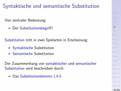
Syntaktische und semantische Substitution
Von zentraler Bedeutung:
I Der Substitutionsbegriff!
Substitution tritt in zwei Spielarten in Erscheinung:
I Syntaktische Substitution
I Semantische Substitution
Der Zusammenhang von syntaktischer und semantischerSubstitution wird beschrieben durch:
I Das Substitutionslemma 1.4.5
40/863
Inhalt
Kap. 1
1.1
1.2
1.3
1.4
1.5
1.6
Kap. 2
Kap. 3
Kap. 4
Kap. 5
Kap. 6
Kap. 7
Kap. 8
Kap. 9
Kap. 10
Kap. 11
Kap. 12
Kap. 13
Kap. 14
Kap. 15
Kap. 16
Kap. 17
Literatur
Anhang
A
Syntaktische Substitution
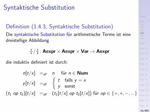
Definition (1.4.3, Syntaktische Substitution)
Die syntaktische Substitution fur arithmetische Terme ist einedreistellige Abbildung
·[·/·] : Aexpr× Aexpr× Var→ Aexpr
die induktiv definiert ist durch:
n[t/x ] =df n fur n ∈ Num
y [t/x ] =df
t falls y = xy sonst
(t1 op t2)[t/x ] =df (t1[t/x ] op t2[t/x ]) fur op ∈ +, ∗,−, ...
41/863
Inhalt
Kap. 1
1.1
1.2
1.3
1.4
1.5
1.6
Kap. 2
Kap. 3
Kap. 4
Kap. 5
Kap. 6
Kap. 7
Kap. 8
Kap. 9
Kap. 10
Kap. 11
Kap. 12
Kap. 13
Kap. 14
Kap. 15
Kap. 16
Kap. 17
Literatur
Anhang
A
Semantische Substitution
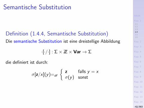
Definition (1.4.4, Semantische Substitution)
Die semantische Substitution ist eine dreistellige Abbildung
·[·/·] : Σ× ZZ× Var→ Σ
die definiert ist durch:
σ[z/x ](y)=df
z falls y = xσ(y) sonst
42/863
Inhalt
Kap. 1
1.1
1.2
1.3
1.4
1.5
1.6
Kap. 2
Kap. 3
Kap. 4
Kap. 5
Kap. 6
Kap. 7
Kap. 8
Kap. 9
Kap. 10
Kap. 11
Kap. 12
Kap. 13
Kap. 14
Kap. 15
Kap. 16
Kap. 17
Literatur
Anhang
A
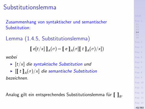
Substitutionslemma
Zusammenhang von syntaktischer und semantischerSubstitution:
Lemma (1.4.5, Substitutionslemma)
[[ e[t/x ] ]]A(σ) = [[ e ]]A(σ[[[ t ]]A(σ)/x ])
wobei
I [t/x ] die syntaktische Substitution und
I [[[ t ]]A(σ)/x ] die semantische Substitution
bezeichnen.
Analog gilt ein entsprechendes Substitutionslemma fur [[ ]]B .
43/863

Inhalt
Kap. 1
1.1
1.2
1.3
1.4
1.5
1.6
Kap. 2
Kap. 3
Kap. 4
Kap. 5
Kap. 6
Kap. 7
Kap. 8
Kap. 9
Kap. 10
Kap. 11
Kap. 12
Kap. 13
Kap. 14
Kap. 15
Kap. 16
Kap. 17
Literatur
Anhang
A
Kapitel 1.5
Induktive Beweisprinzipien
44/863
Inhalt
Kap. 1
1.1
1.2
1.3
1.4
1.5
1.6
Kap. 2
Kap. 3
Kap. 4
Kap. 5
Kap. 6
Kap. 7
Kap. 8
Kap. 9
Kap. 10
Kap. 11
Kap. 12
Kap. 13
Kap. 14
Kap. 15
Kap. 16
Kap. 17
Literatur
Anhang
A
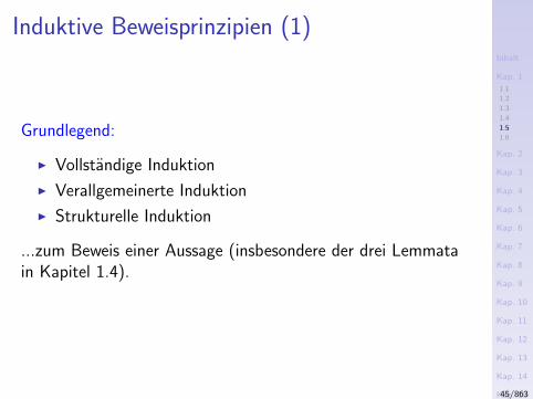
Induktive Beweisprinzipien (1)
Grundlegend:
I Vollstandige Induktion
I Verallgemeinerte Induktion
I Strukturelle Induktion
...zum Beweis einer Aussage (insbesondere der drei Lemmatain Kapitel 1.4).
45/863
Inhalt
Kap. 1
1.1
1.2
1.3
1.4
1.5
1.6
Kap. 2
Kap. 3
Kap. 4
Kap. 5
Kap. 6
Kap. 7
Kap. 8
Kap. 9
Kap. 10
Kap. 11
Kap. 12
Kap. 13
Kap. 14
Kap. 15
Kap. 16
Kap. 17
Literatur
Anhang
A
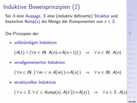
Induktive Beweisprinzipien (2)
Sei A eine Aussage, S eine (induktiv definierte) Struktur undbezeichne Komp(s) die Menge der Komponenten von s ∈ S .
Die Prinzipien der
I vollstandigen Induktion
(A(1) ∧ (∀n ∈ IN .A(n)⇒A(n+1)) ) ⇒ ∀ n ∈ IN . A(n)
I verallgemeinerten Induktion
(∀n ∈ IN . (∀m < n.A(m) )⇒A(n) ) ⇒ ∀ n ∈ IN . A(n)
I strukturellen Induktion
(∀ s ∈ S . ∀ s ′ ∈ Komp(s).A(s ′))⇒A(s) ) ⇒ ∀ s ∈ S . A(s)
46/863

Inhalt
Kap. 1
1.1
1.2
1.3
1.4
1.5
1.6
Kap. 2
Kap. 3
Kap. 4
Kap. 5
Kap. 6
Kap. 7
Kap. 8
Kap. 9
Kap. 10
Kap. 11
Kap. 12
Kap. 13
Kap. 14
Kap. 15
Kap. 16
Kap. 17
Literatur
Anhang
A
Induktive Beweisprinzipien (3)
Bemerkung:
I Vollstandige, verallgemeinerte und strukturelle Induktionsind gleich machtig.
I Abhangig vom Anwendungsfall ist oft eines der Indukti-onsprinzipien zweckmaßiger, d.h. einfacher anzuwenden.
Zum Beweis von Aussagen uber induktiv definierte Daten-strukturen ist i.a. das Prinzip der strukturellen Induktionam zweckmaßigsten.
47/863
Inhalt
Kap. 1
1.1
1.2
1.3
1.4
1.5
1.6
Kap. 2
Kap. 3
Kap. 4
Kap. 5
Kap. 6
Kap. 7
Kap. 8
Kap. 9
Kap. 10
Kap. 11
Kap. 12
Kap. 13
Kap. 14
Kap. 15
Kap. 16
Kap. 17
Literatur
Anhang
A
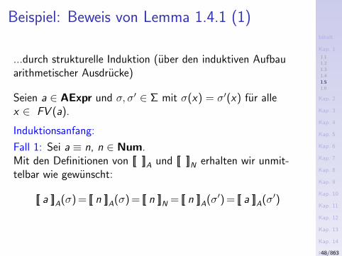
Beispiel: Beweis von Lemma 1.4.1 (1)
...durch strukturelle Induktion (uber den induktiven Aufbauarithmetischer Ausdrucke)
Seien a ∈ AExpr und σ, σ′ ∈ Σ mit σ(x) = σ′(x) fur allex ∈ FV (a).
Induktionsanfang:
Fall 1: Sei a ≡ n, n ∈ Num.Mit den Definitionen von [[ ]]A und [[ ]]N erhalten wir unmit-telbar wie gewunscht:
[[ a ]]A(σ) = [[ n ]]A(σ) = [[ n ]]N = [[ n ]]A(σ′) = [[ a ]]A(σ′)
48/863
Inhalt
Kap. 1
1.1
1.2
1.3
1.4
1.5
1.6
Kap. 2
Kap. 3
Kap. 4
Kap. 5
Kap. 6
Kap. 7
Kap. 8
Kap. 9
Kap. 10
Kap. 11
Kap. 12
Kap. 13
Kap. 14
Kap. 15
Kap. 16
Kap. 17
Literatur
Anhang
A
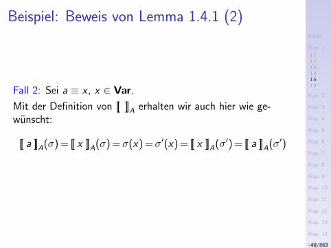
Beispiel: Beweis von Lemma 1.4.1 (2)
Fall 2: Sei a ≡ x , x ∈ Var.
Mit der Definition von [[ ]]A erhalten wir auch hier wie ge-wunscht:
[[ a ]]A(σ) = [[ x ]]A(σ) =σ(x) =σ′(x) = [[ x ]]A(σ′) = [[ a ]]A(σ′)
49/863
Inhalt
Kap. 1
1.1
1.2
1.3
1.4
1.5
1.6
Kap. 2
Kap. 3
Kap. 4
Kap. 5
Kap. 6
Kap. 7
Kap. 8
Kap. 9
Kap. 10
Kap. 11
Kap. 12
Kap. 13
Kap. 14
Kap. 15
Kap. 16
Kap. 17
Literatur
Anhang
A
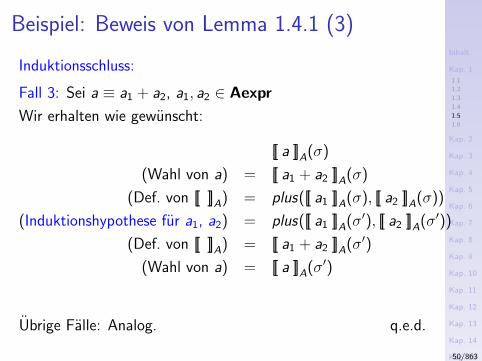
Beispiel: Beweis von Lemma 1.4.1 (3)
Induktionsschluss:
Fall 3: Sei a ≡ a1 + a2, a1, a2 ∈ Aexpr
Wir erhalten wie gewunscht:
[[ a ]]A(σ)
(Wahl von a) = [[ a1 + a2 ]]A(σ)
(Def. von [[ ]]A) = plus([[ a1 ]]A(σ), [[ a2 ]]A(σ))
(Induktionshypothese fur a1, a2) = plus([[ a1 ]]A(σ′), [[ a2 ]]A(σ′))
(Def. von [[ ]]A) = [[ a1 + a2 ]]A(σ′)
(Wahl von a) = [[ a ]]A(σ′)
Ubrige Falle: Analog. q.e.d.
50/863
Inhalt
Kap. 1
1.1
1.2
1.3
1.4
1.5
1.6
Kap. 2
Kap. 3
Kap. 4
Kap. 5
Kap. 6
Kap. 7
Kap. 8
Kap. 9
Kap. 10
Kap. 11
Kap. 12
Kap. 13
Kap. 14
Kap. 15
Kap. 16
Kap. 17
Literatur
Anhang
A
Kapitel 1.6
Semantikdefinitionsstile
51/863
Inhalt
Kap. 1
1.1
1.2
1.3
1.4
1.5
1.6
Kap. 2
Kap. 3
Kap. 4
Kap. 5
Kap. 6
Kap. 7
Kap. 8
Kap. 9
Kap. 10
Kap. 11
Kap. 12
Kap. 13
Kap. 14
Kap. 15
Kap. 16
Kap. 17
Literatur
Anhang
A
Motivation
Die Semantik einer Programmiersprache kann auf verschiedeneWeise festgelegt werden. Wir sprechen hier von unterschied-lichen Definitionsstilen. Sie gewahren eine unterschiedlicheSicht auf die Bedeutung der Sprache und richten sich daherimplizit an andere Adressaten.
Besonders grundlegend und wichtig sind der
I operationelle
I denotationelle
I axiomatische
Definitionsstil.
52/863
Inhalt
Kap. 1
1.1
1.2
1.3
1.4
1.5
1.6
Kap. 2
Kap. 3
Kap. 4
Kap. 5
Kap. 6
Kap. 7
Kap. 8
Kap. 9
Kap. 10
Kap. 11
Kap. 12
Kap. 13
Kap. 14
Kap. 15
Kap. 16
Kap. 17
Literatur
Anhang
A
Intuition und Ausblick
I Sprach- und AnwendungsimplementierersichtI Operationelle Semantik
I Strukturell operationelle Semantik (small-stepsemantics)
I Naturliche Semantik (big-step semantics)
I SprachentwicklersichtI Denotationelle Semantik
I (Anwendungs-) Programmierer- und VerifizierersichtI Axiomatische Semantik
53/863
Inhalt
Kap. 1
1.1
1.2
1.3
1.4
1.5
1.6
Kap. 2
Kap. 3
Kap. 4
Kap. 5
Kap. 6
Kap. 7
Kap. 8
Kap. 9
Kap. 10
Kap. 11
Kap. 12
Kap. 13
Kap. 14
Kap. 15
Kap. 16
Kap. 17
Literatur
Anhang
A
Vertiefende und weiterfuhrende Leseempfeh-
lungen fur Kapitel 1 (1)
Mordechai Ben-Ari. Mathematical Logic for ComputerScience. 2. Auflage, Springer-V., 2001. (Chapter 9.2,Semantics of Programming Languages)
Julien Bertrane, Patrick Cousot, Radhia Cousot, JeromeFeret, Laurent Mauborgne, Antoine Mine, Xavier Rival.Static Analysis and Verification of Aerospace Software byAbstract Interpretation. In Proceedings AIAAInfotech@Aerospace (AIAA I@A 2010), AIAA-2010-3385,American Institute of Aeronautics and Astronautics, 1-38,April 2010.
54/863
Inhalt
Kap. 1
1.1
1.2
1.3
1.4
1.5
1.6
Kap. 2
Kap. 3
Kap. 4
Kap. 5
Kap. 6
Kap. 7
Kap. 8
Kap. 9
Kap. 10
Kap. 11
Kap. 12
Kap. 13
Kap. 14
Kap. 15
Kap. 16
Kap. 17
Literatur
Anhang
A
Vertiefende und weiterfuhrende Leseempfeh-
lungen fur Kapitel 1 (2)
Julien Bertrane, Patrick Cousot, Radhia Cousot, JeromeFeret, Laurent Mauborgne, Antoine Mine, Xavier Rival.Static Analysis by Abstract Interpretation of EmbeddedCritical Software. ACM Software Engineering Notes36(1):1-8, 2011.
Al Bessey, Ken Block, Ben Chelf, Andy Chou, BryanFulton, Seth Hallem, Charles Henri-Gros, Asya Kamsky,Scott McPeak, Dawson Engler. A Few Billion Lines ofCode Later: Using Static Analysis to Find Bugs in the RealWorld. Communications of the ACM 53(2):66-75, 2010.
55/863
Inhalt
Kap. 1
1.1
1.2
1.3
1.4
1.5
1.6
Kap. 2
Kap. 3
Kap. 4
Kap. 5
Kap. 6
Kap. 7
Kap. 8
Kap. 9
Kap. 10
Kap. 11
Kap. 12
Kap. 13
Kap. 14
Kap. 15
Kap. 16
Kap. 17
Literatur
Anhang
A
Vertiefende und weiterfuhrende Leseempfeh-
lungen fur Kapitel 1 (3)
Gilles Dowek. Principles of Programming Languages.Springer-V, 2009. (Chapter 1, Imperative Core; Chapter1.1, Five Constructs)
Gerhard Goos, Wolf Zimmermann. Programmiersprachen.In Informatik-Handbuch, Peter Rechenberg, GustavPomberger (Hrsg.), Carl Hanser Verlag, 4. Auflage,515-562, 2006. (Kapitel 2.2, Elemente von Programmier-sprachen: Syntax, Semantik und Pragmatik, SyntaktischeEigenschaften, Semantische Eigenschaften)
Steve P. Miller, Michael W. Whalen, Darren D. Cofer.Software Model Checking Takes Off. Communications ofthe ACM 53(2):58-64, 2010.
56/863
Inhalt
Kap. 1
1.1
1.2
1.3
1.4
1.5
1.6
Kap. 2
Kap. 3
Kap. 4
Kap. 5
Kap. 6
Kap. 7
Kap. 8
Kap. 9
Kap. 10
Kap. 11
Kap. 12
Kap. 13
Kap. 14
Kap. 15
Kap. 16
Kap. 17
Literatur
Anhang
A
Vertiefende und weiterfuhrende Leseempfeh-
lungen fur Kapitel 1 (4)
Hanne Riis Nielson, Flemming Nielson. Semantics withApplications: A Formal Introduction. Wiley, 1992.(Chapter 1, Introduction)
Hanne Riis Nielson, Flemming Nielson. Semantics withApplications: An Appetizer. Springer-V., 2007. (Chapter1, Introduction)
Glynn Winskel. The Formal Semantics of ProgrammingLanguages: An Introduction. MIT Press, 1993.
57/863
Inhalt
Kap. 1
Kap. 2
2.1
2.2
2.3
Kap. 3
Kap. 4
Kap. 5
Kap. 6
Kap. 7
Kap. 8
Kap. 9
Kap. 10
Kap. 11
Kap. 12
Kap. 13
Kap. 14
Kap. 15
Kap. 16
Kap. 17
Literatur
Anhang
A
Kapitel 2
Operationelle Semantik von WHILE
58/863
Inhalt
Kap. 1
Kap. 2
2.1
2.2
2.3
Kap. 3
Kap. 4
Kap. 5
Kap. 6
Kap. 7
Kap. 8
Kap. 9
Kap. 10
Kap. 11
Kap. 12
Kap. 13
Kap. 14
Kap. 15
Kap. 16
Kap. 17
Literatur
Anhang
A
Operationelle Semantik von WHILE
...die Bedeutung eines (programmiersprachlichen) Konstrukts ist
durch die Berechnung beschrieben, die es bei seiner Ausfuhrung
auf der Maschine induziert. Wichtig ist, wie der Effekt der Berech-
nung erzeugt wird.
59/863

Inhalt
Kap. 1
Kap. 2
2.1
2.2
2.3
Kap. 3
Kap. 4
Kap. 5
Kap. 6
Kap. 7
Kap. 8
Kap. 9
Kap. 10
Kap. 11
Kap. 12
Kap. 13
Kap. 14
Kap. 15
Kap. 16
Kap. 17
Literatur
Anhang
A
Kapitel 2.1
Strukturell operationelle Semantik
60/863
Inhalt
Kap. 1
Kap. 2
2.1
2.2
2.3
Kap. 3
Kap. 4
Kap. 5
Kap. 6
Kap. 7
Kap. 8
Kap. 9
Kap. 10
Kap. 11
Kap. 12
Kap. 13
Kap. 14
Kap. 15
Kap. 16
Kap. 17
Literatur
Anhang
A
Strukturell operationelle Semantik (small-step
semantics)
...beschreibt den Ablauf der einzelnen Berechnungsschritte, die
stattfinden; daher auch die Bezeichnung Kleinschritt-Semantik.
61/863
Inhalt
Kap. 1
Kap. 2
2.1
2.2
2.3
Kap. 3
Kap. 4
Kap. 5
Kap. 6
Kap. 7
Kap. 8
Kap. 9
Kap. 10
Kap. 11
Kap. 12
Kap. 13
Kap. 14
Kap. 15
Kap. 16
Kap. 17
Literatur
Anhang
A
Literaturhinweise
I Gordon D. Plotkin. A Structural Approach to OperationalSemantics. Journal of Logic and Algebraic Programming60-61:17-139, 2004.
I Gordon D. Plotkin. An Operational Semantics for CSP. InProceedings of the TC-2 Working Conference on FormalDescription of Programming Concepts II, Dines Bjørner(Hrsg.), North-Holland, Amsterdam, 1982.
I Gordon D. Plotkin. A Structural Approach to OperationalSemantics. Lecture notes, DAIMI FN-19, Aarhus Univer-sity, Denmark, 1981, reprinted 1991.
62/863
Inhalt
Kap. 1
Kap. 2
2.1
2.2
2.3
Kap. 3
Kap. 4
Kap. 5
Kap. 6
Kap. 7
Kap. 8
Kap. 9
Kap. 10
Kap. 11
Kap. 12
Kap. 13
Kap. 14
Kap. 15
Kap. 16
Kap. 17
Literatur
Anhang
A
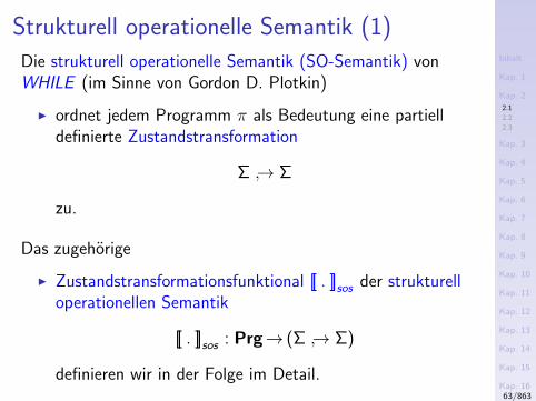
Strukturell operationelle Semantik (1)
Die strukturell operationelle Semantik (SO-Semantik) vonWHILE (im Sinne von Gordon D. Plotkin)
I ordnet jedem Programm π als Bedeutung eine partielldefinierte Zustandstransformation
Σ → Σ
zu.
Das zugehorige
I Zustandstransformationsfunktional [[ . ]]sos der strukturelloperationellen Semantik
[[ . ]]sos : Prg→ (Σ → Σ)
definieren wir in der Folge im Detail.63/863
Inhalt
Kap. 1
Kap. 2
2.1
2.2
2.3
Kap. 3
Kap. 4
Kap. 5
Kap. 6
Kap. 7
Kap. 8
Kap. 9
Kap. 10
Kap. 11
Kap. 12
Kap. 13
Kap. 14
Kap. 15
Kap. 16
Kap. 17
Literatur
Anhang
A
Strukturell operationelle Semantik (2)
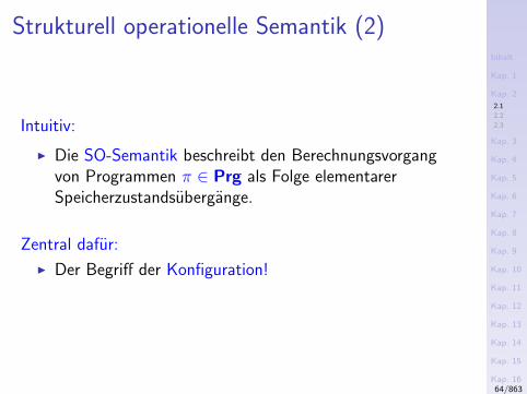
Intuitiv:
I Die SO-Semantik beschreibt den Berechnungsvorgangvon Programmen π ∈ Prg als Folge elementarerSpeicherzustandsubergange.
Zentral dafur:
I Der Begriff der Konfiguration!
64/863
Inhalt
Kap. 1
Kap. 2
2.1
2.2
2.3
Kap. 3
Kap. 4
Kap. 5
Kap. 6
Kap. 7
Kap. 8
Kap. 9
Kap. 10
Kap. 11
Kap. 12
Kap. 13
Kap. 14
Kap. 15
Kap. 16
Kap. 17
Literatur
Anhang
A
Konfigurationen
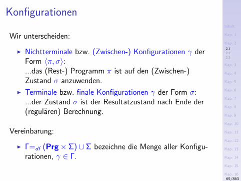
Wir unterscheiden:
I Nichtterminale bzw. (Zwischen-) Konfigurationen γ derForm 〈π, σ〉:...das (Rest-) Programm π ist auf den (Zwischen-)Zustand σ anzuwenden.
I Terminale bzw. finale Konfigurationen γ der Form σ:...der Zustand σ ist der Resultatzustand nach Ende der(regularen) Berechnung.
Vereinbarung:
I Γ=df (Prg× Σ) ∪ Σ bezeichne die Menge aller Konfigu-rationen, γ ∈ Γ.
65/863
Inhalt
Kap. 1
Kap. 2
2.1
2.2
2.3
Kap. 3
Kap. 4
Kap. 5
Kap. 6
Kap. 7
Kap. 8
Kap. 9
Kap. 10
Kap. 11
Kap. 12
Kap. 13
Kap. 14
Kap. 15
Kap. 16
Kap. 17
Literatur
Anhang
A
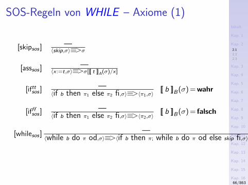
SOS-Regeln von WHILE – Axiome (1)
[skipsos ] —〈skip,σ〉≡>σ
[asssos ] —〈x :=t,σ〉≡>σ[[[ t ]]A(σ)/x]
[ifttsos ] —〈if b then π1 else π2 fi,σ〉≡>〈π1,σ〉
[[ b ]]B(σ) = wahr
[ifffsos ] —〈if b then π1 else π2 fi,σ〉≡>〈π2,σ〉
[[ b ]]B(σ) = falsch
[whilesos ] —〈while b do π od,σ〉≡>〈if b then π; while b do π od else skip fi,σ〉
66/863
Inhalt
Kap. 1
Kap. 2
2.1
2.2
2.3
Kap. 3
Kap. 4
Kap. 5
Kap. 6
Kap. 7
Kap. 8
Kap. 9
Kap. 10
Kap. 11
Kap. 12
Kap. 13
Kap. 14
Kap. 15
Kap. 16
Kap. 17
Literatur
Anhang
A
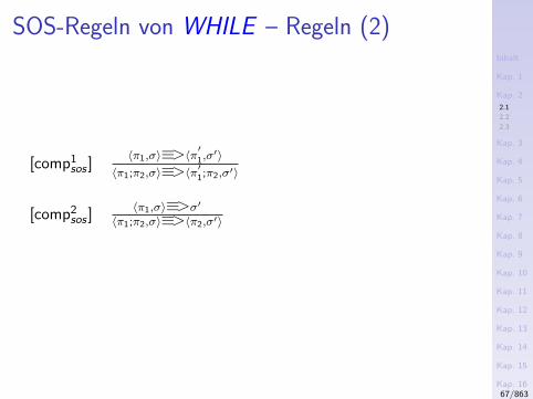
SOS-Regeln von WHILE – Regeln (2)
[comp1sos ]
〈π1,σ〉≡>〈π′1,σ′〉〈π1;π2,σ〉≡>〈π′1;π2,σ′〉
[comp2sos ]
〈π1,σ〉≡>σ′
〈π1;π2,σ〉≡>〈π2,σ′〉
67/863
Inhalt
Kap. 1
Kap. 2
2.1
2.2
2.3
Kap. 3
Kap. 4
Kap. 5
Kap. 6
Kap. 7
Kap. 8
Kap. 9
Kap. 10
Kap. 11
Kap. 12
Kap. 13
Kap. 14
Kap. 15
Kap. 16
Kap. 17
Literatur
Anhang
A
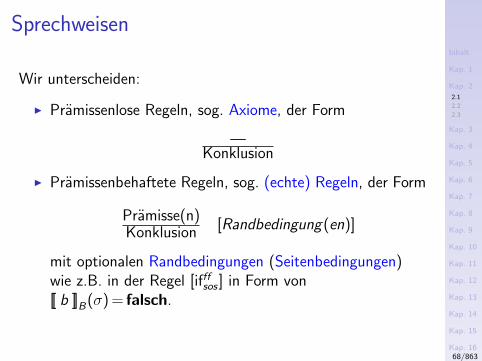
Sprechweisen
Wir unterscheiden:
I Pramissenlose Regeln, sog. Axiome, der Form
—Konklusion
I Pramissenbehaftete Regeln, sog. (echte) Regeln, der Form
Pramisse(n)Konklusion [Randbedingung(en)]
mit optionalen Randbedingungen (Seitenbedingungen)wie z.B. in der Regel [ifffsos ] in Form von[[ b ]]B(σ) = falsch.
68/863
Inhalt
Kap. 1
Kap. 2
2.1
2.2
2.3
Kap. 3
Kap. 4
Kap. 5
Kap. 6
Kap. 7
Kap. 8
Kap. 9
Kap. 10
Kap. 11
Kap. 12
Kap. 13
Kap. 14
Kap. 15
Kap. 16
Kap. 17
Literatur
Anhang
A
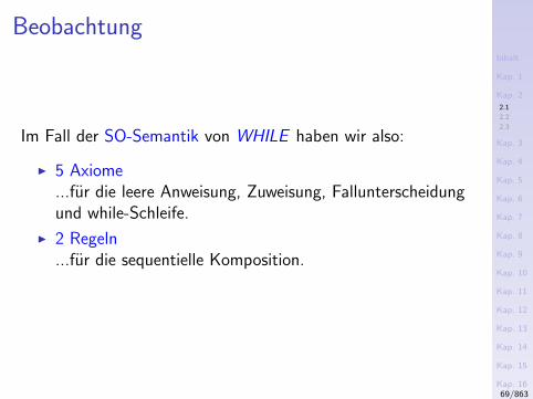
Beobachtung
Im Fall der SO-Semantik von WHILE haben wir also:
I 5 Axiome...fur die leere Anweisung, Zuweisung, Fallunterscheidungund while-Schleife.
I 2 Regeln...fur die sequentielle Komposition.
69/863
Inhalt
Kap. 1
Kap. 2
2.1
2.2
2.3
Kap. 3
Kap. 4
Kap. 5
Kap. 6
Kap. 7
Kap. 8
Kap. 9
Kap. 10
Kap. 11
Kap. 12
Kap. 13
Kap. 14
Kap. 15
Kap. 16
Kap. 17
Literatur
Anhang
A
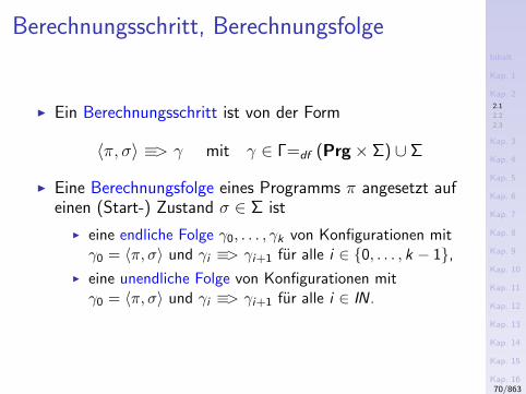
Berechnungsschritt, Berechnungsfolge
I Ein Berechnungsschritt ist von der Form
〈π, σ〉 ≡> γ mit γ ∈ Γ=df (Prg× Σ) ∪ Σ
I Eine Berechnungsfolge eines Programms π angesetzt aufeinen (Start-) Zustand σ ∈ Σ ist
I eine endliche Folge γ0, . . . , γk von Konfigurationen mitγ0 = 〈π, σ〉 und γi ≡> γi+1 fur alle i ∈ 0, . . . , k − 1,
I eine unendliche Folge von Konfigurationen mitγ0 = 〈π, σ〉 und γi ≡> γi+1 fur alle i ∈ IN.
70/863
Inhalt
Kap. 1
Kap. 2
2.1
2.2
2.3
Kap. 3
Kap. 4
Kap. 5
Kap. 6
Kap. 7
Kap. 8
Kap. 9
Kap. 10
Kap. 11
Kap. 12
Kap. 13
Kap. 14
Kap. 15
Kap. 16
Kap. 17
Literatur
Anhang
A
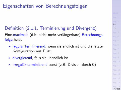
Eigenschaften von Berechnungsfolgen
Definition (2.1.1, Terminierung und Divergenz)
Eine maximale (d.h. nicht mehr verlangerbare) Berechnungs-folge heißt
I regular terminierend, wenn sie endlich ist und die letzteKonfiguration aus Σ ist
I divergierend, falls sie unendlich ist
I irregular terminierend sonst (z.B. Division durch 0)
71/863
Inhalt
Kap. 1
Kap. 2
2.1
2.2
2.3
Kap. 3
Kap. 4
Kap. 5
Kap. 6
Kap. 7
Kap. 8
Kap. 9
Kap. 10
Kap. 11
Kap. 12
Kap. 13
Kap. 14
Kap. 15
Kap. 16
Kap. 17
Literatur
Anhang
A
Beispiel 1(4)
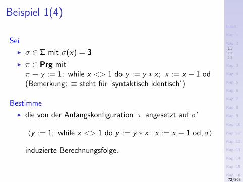
Sei
I σ ∈ Σ mit σ(x) = 3
I π ∈ Prg mitπ ≡ y := 1; while x <> 1 do y := y ∗ x ; x := x − 1 od(Bemerkung: ≡ steht fur ‘syntaktisch identisch’)
Bestimme
I die von der Anfangskonfiguration ‘π angesetzt auf σ’
〈y := 1; while x <> 1 do y := y ∗ x ; x := x − 1 od, σ〉
induzierte Berechnungsfolge.
72/863
Inhalt
Kap. 1
Kap. 2
2.1
2.2
2.3
Kap. 3
Kap. 4
Kap. 5
Kap. 6
Kap. 7
Kap. 8
Kap. 9
Kap. 10
Kap. 11
Kap. 12
Kap. 13
Kap. 14
Kap. 15
Kap. 16
Kap. 17
Literatur
Anhang
A
Beispiel 2(4)
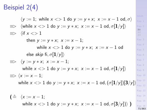
〈y := 1; while x <> 1 do y := y ∗ x ; x := x − 1 od, σ〉≡> 〈while x <> 1 do y := y ∗ x ; x := x − 1 od, σ[1/y ]〉≡> 〈if x <> 1
then y := y ∗ x ; x := x − 1;
while x <> 1 do y := y ∗ x ; x := x − 1 od
else skip fi, σ[1/y ]〉≡> 〈y := y ∗ x ; x := x − 1;
while x <> 1 do y := y ∗ x ; x := x − 1 od, σ[1/y ]〉≡> 〈x := x − 1;
while x <> 1 do y := y ∗ x ; x := x − 1 od, (σ[1/y ])[3/y ]〉
( = 〈x := x − 1;
while x <> 1 do y := y ∗ x ; x := x − 1 od, σ[3/y ])〉 )
≡> 〈while x <> 1 do y := y ∗ x ; x := x − 1 od, (σ[3/y ])[2/x ]〉
73/863
Inhalt
Kap. 1
Kap. 2
2.1
2.2
2.3
Kap. 3
Kap. 4
Kap. 5
Kap. 6
Kap. 7
Kap. 8
Kap. 9
Kap. 10
Kap. 11
Kap. 12
Kap. 13
Kap. 14
Kap. 15
Kap. 16
Kap. 17
Literatur
Anhang
A
Beispiel 3(4)
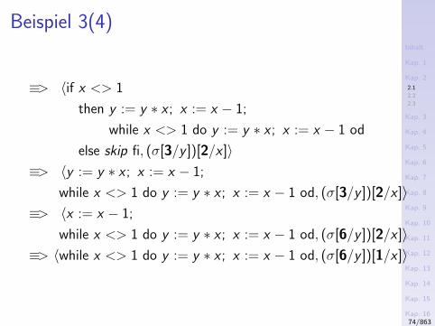
≡> 〈if x <> 1
then y := y ∗ x ; x := x − 1;
while x <> 1 do y := y ∗ x ; x := x − 1 od
else skip fi, (σ[3/y ])[2/x ]〉≡> 〈y := y ∗ x ; x := x − 1;
while x <> 1 do y := y ∗ x ; x := x − 1 od, (σ[3/y ])[2/x ]〉≡> 〈x := x − 1;
while x <> 1 do y := y ∗ x ; x := x − 1 od, (σ[6/y ])[2/x ]〉≡> 〈while x <> 1 do y := y ∗ x ; x := x − 1 od, (σ[6/y ])[1/x ]〉
74/863
Inhalt
Kap. 1
Kap. 2
2.1
2.2
2.3
Kap. 3
Kap. 4
Kap. 5
Kap. 6
Kap. 7
Kap. 8
Kap. 9
Kap. 10
Kap. 11
Kap. 12
Kap. 13
Kap. 14
Kap. 15
Kap. 16
Kap. 17
Literatur
Anhang
A
Beispiel 4(4)
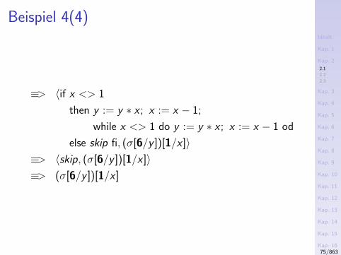
≡> 〈if x <> 1
then y := y ∗ x ; x := x − 1;
while x <> 1 do y := y ∗ x ; x := x − 1 od
else skip fi, (σ[6/y ])[1/x ]〉≡> 〈skip, (σ[6/y ])[1/x ]〉≡> (σ[6/y ])[1/x ]
75/863
Inhalt
Kap. 1
Kap. 2
2.1
2.2
2.3
Kap. 3
Kap. 4
Kap. 5
Kap. 6
Kap. 7
Kap. 8
Kap. 9
Kap. 10
Kap. 11
Kap. 12
Kap. 13
Kap. 14
Kap. 15
Kap. 16
Kap. 17
Literatur
Anhang
A
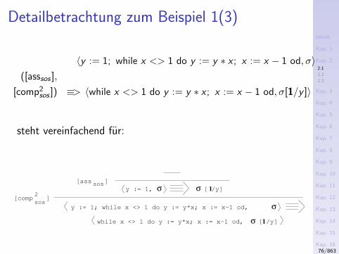
Detailbetrachtung zum Beispiel 1(3)
〈y := 1; while x <> 1 do y := y ∗ x ; x := x − 1 od, σ〉([asssos ],
[comp2sos ]) ≡> 〈while x <> 1 do y := y ∗ x ; x := x − 1 od, σ[1/y ]〉
steht vereinfachend fur:
sos[ass ]
[compsos
2]
while x <> 1 do y := y*x; x := x−1 od,
y := 1; while x <> 1 do y := y*x; x := x−1 od,
y := 1, σ σ [ /y]1
σ [ /y]1
σ
76/863
Inhalt
Kap. 1
Kap. 2
2.1
2.2
2.3
Kap. 3
Kap. 4
Kap. 5
Kap. 6
Kap. 7
Kap. 8
Kap. 9
Kap. 10
Kap. 11
Kap. 12
Kap. 13
Kap. 14
Kap. 15
Kap. 16
Kap. 17
Literatur
Anhang
A
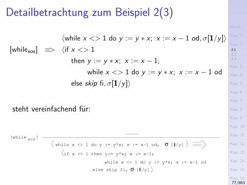
Detailbetrachtung zum Beispiel 2(3)
〈while x <> 1 do y := y ∗ x ; x := x − 1 od, σ[1/y ]〉[whilesos ] ≡> 〈if x <> 1
then y := y ∗ x ; x := x − 1;
while x <> 1 do y := y ∗ x ; x := x − 1 od
else skip fi, σ[1/y ]〉
steht vereinfachend fur:
sos[while ]
if x <> 1 then y:= y*x; x := x−1;
while x <> 1 do y := y*x; x := x−1 od
else skip fi, σ [ /y]
while x <> 1 do y := y*x; x := x−1 od, σ [ /y]
1
1
77/863
Inhalt
Kap. 1
Kap. 2
2.1
2.2
2.3
Kap. 3
Kap. 4
Kap. 5
Kap. 6
Kap. 7
Kap. 8
Kap. 9
Kap. 10
Kap. 11
Kap. 12
Kap. 13
Kap. 14
Kap. 15
Kap. 16
Kap. 17
Literatur
Anhang
A
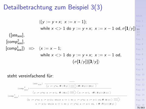
Detailbetrachtung zum Beispiel 3(3)
〈(y := y ∗ x ; x := x − 1);
while x <> 1 do y := y ∗ x ; x := x − 1 od, σ[1/y ]〉([asssos ],
[comp2sos ],
[comp1sos ]) ≡> 〈x := x − 1;
while x <> 1 do y := y ∗ x ; x := x − 1 od,
(σ[1/y ])[3/y ]〉
steht vereinfachend fur:
σ [ /y]
sos[ass ]
σ [ /y]
x := x−1; while x <> 1 do y := y*x; x := x−1 od, (
x := x−1, (
[compsos
1]
[compsos
]2
σ
σ
y := y*x, σ(
[ /y]
1
11
y := y*x; x := x−1, 1
(y := y*x; x := x−1); while x <> 1 do y := y*x; x := x−1 od, σ 1
1
[ /y])[ /y]3
[ /y])[ /y]
[ /y])[ /y]3
3
78/863
Inhalt
Kap. 1
Kap. 2
2.1
2.2
2.3
Kap. 3
Kap. 4
Kap. 5
Kap. 6
Kap. 7
Kap. 8
Kap. 9
Kap. 10
Kap. 11
Kap. 12
Kap. 13
Kap. 14
Kap. 15
Kap. 16
Kap. 17
Literatur
Anhang
A
Determinismus der SOS-Regeln
Lemma (2.1.2)
∀π ∈ Prg, σ ∈ Σ, γ, γ′ ∈Γ. 〈π, σ〉≡>γ ∧ 〈π, σ〉≡>γ′ ⇒ γ = γ′
Korollar (2.1.3)
Die von den SOS-Regeln fur eine Konfiguration induzierteBerechnungsfolge ist eindeutig bestimmt, d.h. deterministisch.
Salopper, wenn auch weniger prazise:
Die SO-Semantik von WHILE ist deterministisch!
79/863
Inhalt
Kap. 1
Kap. 2
2.1
2.2
2.3
Kap. 3
Kap. 4
Kap. 5
Kap. 6
Kap. 7
Kap. 8
Kap. 9
Kap. 10
Kap. 11
Kap. 12
Kap. 13
Kap. 14
Kap. 15
Kap. 16
Kap. 17
Literatur
Anhang
A
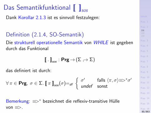
Das Semantikfunktional [[ ]]sos
Dank Korollar 2.1.3 ist es sinnvoll festzulegen:
Definition (2.1.4, SO-Semantik)
Die strukturell operationelle Semantik von WHILE ist gegebendurch das Funktional
[[ . ]]sos : Prg→ (Σ → Σ)
das definiert ist durch:
∀π ∈ Prg, σ ∈ Σ. [[ π ]]sos(σ)=df
σ′ falls 〈π, σ〉≡>∗σ′undef sonst
Bemerkung: ≡>∗ bezeichnet die reflexiv-transitive Hullevon ≡>.
80/863
Inhalt
Kap. 1
Kap. 2
2.1
2.2
2.3
Kap. 3
Kap. 4
Kap. 5
Kap. 6
Kap. 7
Kap. 8
Kap. 9
Kap. 10
Kap. 11
Kap. 12
Kap. 13
Kap. 14
Kap. 15
Kap. 16
Kap. 17
Literatur
Anhang
A
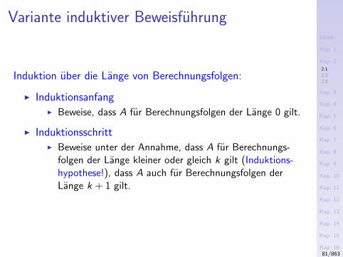
Variante induktiver Beweisfuhrung
Induktion uber die Lange von Berechnungsfolgen:
I InduktionsanfangI Beweise, dass A fur Berechnungsfolgen der Lange 0 gilt.
I InduktionsschrittI Beweise unter der Annahme, dass A fur Berechnungs-
folgen der Lange kleiner oder gleich k gilt (Induktions-hypothese!), dass A auch fur Berechnungsfolgen derLange k + 1 gilt.
81/863
Inhalt
Kap. 1
Kap. 2
2.1
2.2
2.3
Kap. 3
Kap. 4
Kap. 5
Kap. 6
Kap. 7
Kap. 8
Kap. 9
Kap. 10
Kap. 11
Kap. 12
Kap. 13
Kap. 14
Kap. 15
Kap. 16
Kap. 17
Literatur
Anhang
A
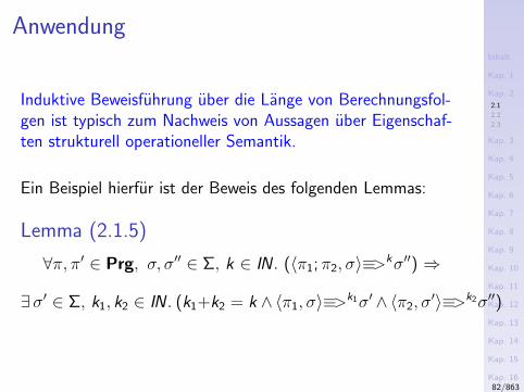
Anwendung
Induktive Beweisfuhrung uber die Lange von Berechnungsfol-gen ist typisch zum Nachweis von Aussagen uber Eigenschaf-ten strukturell operationeller Semantik.
Ein Beispiel hierfur ist der Beweis des folgenden Lemmas:
Lemma (2.1.5)
∀π, π′ ∈ Prg, σ, σ′′ ∈ Σ, k ∈ IN . (〈π1; π2, σ〉≡>kσ′′) ⇒
∃σ′ ∈ Σ, k1, k2 ∈ IN . (k1+k2 = k ∧ 〈π1, σ〉≡>k1σ′ ∧ 〈π2, σ′〉≡>k2σ′′)
82/863
Inhalt
Kap. 1
Kap. 2
2.1
2.2
2.3
Kap. 3
Kap. 4
Kap. 5
Kap. 6
Kap. 7
Kap. 8
Kap. 9
Kap. 10
Kap. 11
Kap. 12
Kap. 13
Kap. 14
Kap. 15
Kap. 16
Kap. 17
Literatur
Anhang
A
Kapitel 2.2
Naturliche Semantik
83/863
Inhalt
Kap. 1
Kap. 2
2.1
2.2
2.3
Kap. 3
Kap. 4
Kap. 5
Kap. 6
Kap. 7
Kap. 8
Kap. 9
Kap. 10
Kap. 11
Kap. 12
Kap. 13
Kap. 14
Kap. 15
Kap. 16
Kap. 17
Literatur
Anhang
A
Naturliche Semantik (big-step semantics)
...beschreibt wie sich das Gesamtergebnis der Programmausfuhrung
ergibt; daher auch die Bezeichnung Großschritt-Semantik.
84/863
Inhalt
Kap. 1
Kap. 2
2.1
2.2
2.3
Kap. 3
Kap. 4
Kap. 5
Kap. 6
Kap. 7
Kap. 8
Kap. 9
Kap. 10
Kap. 11
Kap. 12
Kap. 13
Kap. 14
Kap. 15
Kap. 16
Kap. 17
Literatur
Anhang
A
Naturliche Semantik (1)
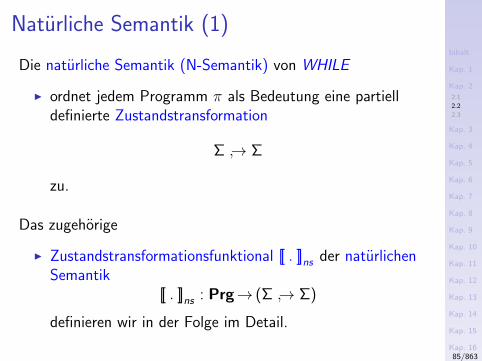
Die naturliche Semantik (N-Semantik) von WHILE
I ordnet jedem Programm π als Bedeutung eine partielldefinierte Zustandstransformation
Σ → Σ
zu.
Das zugehorige
I Zustandstransformationsfunktional [[ . ]]ns der naturlichenSemantik
[[ . ]]ns : Prg→ (Σ → Σ)
definieren wir in der Folge im Detail.
85/863
Inhalt
Kap. 1
Kap. 2
2.1
2.2
2.3
Kap. 3
Kap. 4
Kap. 5
Kap. 6
Kap. 7
Kap. 8
Kap. 9
Kap. 10
Kap. 11
Kap. 12
Kap. 13
Kap. 14
Kap. 15
Kap. 16
Kap. 17
Literatur
Anhang
A
Naturliche Semantik (2)
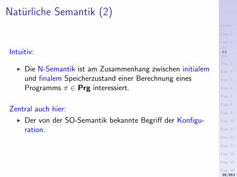
Intuitiv:
I Die N-Semantik ist am Zusammenhang zwischen initialemund finalem Speicherzustand einer Berechnung einesProgramms π ∈ Prg interessiert.
Zentral auch hier:
I Der von der SO-Semantik bekannte Begriff der Konfigu-ration.
86/863
Inhalt
Kap. 1
Kap. 2
2.1
2.2
2.3
Kap. 3
Kap. 4
Kap. 5
Kap. 6
Kap. 7
Kap. 8
Kap. 9
Kap. 10
Kap. 11
Kap. 12
Kap. 13
Kap. 14
Kap. 15
Kap. 16
Kap. 17
Literatur
Anhang
A
NS-Regeln von WHILE (1)
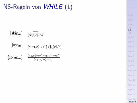
[skipns ] —〈skip,σ〉→σ
[assns ] —〈x :=t,σ〉→σ[[[ t ]]A(σ)/x]
[compns ]〈π1,σ〉→σ′,〈π2,σ
′〉→σ′′〈π1;π2,σ〉→σ′′
87/863
Inhalt
Kap. 1
Kap. 2
2.1
2.2
2.3
Kap. 3
Kap. 4
Kap. 5
Kap. 6
Kap. 7
Kap. 8
Kap. 9
Kap. 10
Kap. 11
Kap. 12
Kap. 13
Kap. 14
Kap. 15
Kap. 16
Kap. 17
Literatur
Anhang
A
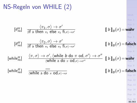
NS-Regeln von WHILE (2)
[ifttns ]〈π1, σ〉 → σ′
〈if b then π1 else π2 fi,σ〉→σ′ [[ b ]]B(σ) = wahr
[ifffns ]〈π2, σ〉 → σ′
〈if b then π1 else π2 fi,σ〉→σ′ [[ b ]]B(σ) = falsch
[whilettns ]〈π, σ〉 → σ′, 〈while b do π od, σ′〉 → σ′′
〈while b do π od,σ〉→σ′′ [[ b ]]B(σ) = wahr
[whileffns ] —〈while b do π od,σ〉→σ [[ b ]]B(σ) = falsch
88/863
Inhalt
Kap. 1
Kap. 2
2.1
2.2
2.3
Kap. 3
Kap. 4
Kap. 5
Kap. 6
Kap. 7
Kap. 8
Kap. 9
Kap. 10
Kap. 11
Kap. 12
Kap. 13
Kap. 14
Kap. 15
Kap. 16
Kap. 17
Literatur
Anhang
A
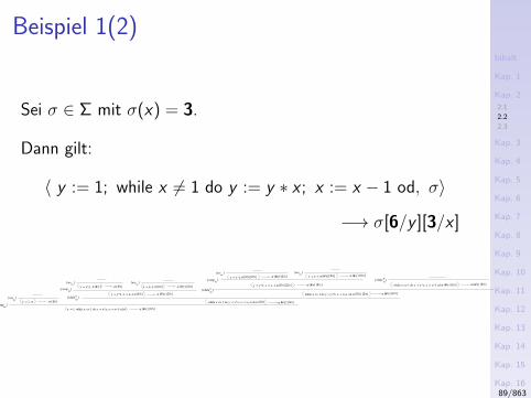
Beispiel 1(2)
Sei σ ∈ Σ mit σ(x) = 3.
Dann gilt:
〈 y := 1; while x 6= 1 do y := y ∗ x ; x := x − 1 od, σ〉
−→ σ[6/y ][3/x ]
ns][comp
[assns
]
ns][while tt
[assns
][assns
]
ns][comp
ns][comp
ns][while tt
[assns
]
ns][while ff
[assns
]
x := x−1,
y := 1; while x <> 1 do y := y*x; x := x−1 od,σ
y := y*x, σ [ /y] σ [ /y]1 3 σ [ /y]3 σ [ /y] [ /x]3 2
y := y*x; x := x−1,σ [ /y]1 σ [ /y] [ /x]3 2
σ [ /y] [ /x]6 1
y := y*x,σ [ /y] [ /x] σ [ /y] [ /x] σ [ /y] [ /x] σ [ /y] [ /x]x := x−1,
y := y*x; x := x−1,
while x <> 1 do y := y*x; x := x−1 od,
σ [ /y] [ /x] σ [ /y] [ /x]
3 2 6 2
3 2 6 1
while x <> 1 do y := y*x; x := x−1 od,σ σ [ /y] [ /x][ /y]1 6 1
6 2 6 1
σ [ /y] [ /x]3 2 σ [ /y] [ /x]
while x <> 1 do y := y*x; x := x−1 od,σ [ /y] [ /x] σ [ /y] [ /x]
6 1
6 1 6 1
y := 1, σ σ [ /y]1
89/863
Inhalt
Kap. 1
Kap. 2
2.1
2.2
2.3
Kap. 3
Kap. 4
Kap. 5
Kap. 6
Kap. 7
Kap. 8
Kap. 9
Kap. 10
Kap. 11
Kap. 12
Kap. 13
Kap. 14
Kap. 15
Kap. 16
Kap. 17
Literatur
Anhang
A
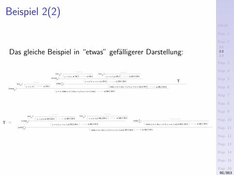
Beispiel 2(2)
Das gleiche Beispiel in “etwas” gefalligerer Darstellung:
ns][while tt
[assns
][assns
]
ns][comp
ns][comp
T ns][comp
[assns
]
ns][while tt
[assns
]
ns][while ff
[assns
]
x := x−1,
y := 1; while x <> 1 do y := y*x; x := x−1 od,σ
T
y := 1, σ σ [ /y]
σ [ /y] [ /x]
y := y*x; x := x−1,σ [ /y]
y := y*x, σ [ /y] σ [ /y]σ [ /y]
1
1 3
6 1
1 σ [ /y] [ /x]3 2
3 σ [ /y] [ /x]3 2
while x <> 1 do y := y*x; x := x−1 od,σ [ /y]σ [ /y] [ /x]1 6 1
y := y*x,σ [ /y] [ /x] σ [ /y] [ /x] σ [ /y] [ /x] σ [ /y] [ /x]x := x−1,
y := y*x; x := x−1,σ [ /y] [ /x] σ [ /y] [ /x]
while x <> 1 do y := y*x; x := x−1 od,σ [ /y] [ /x]
6 2
3 2 6 1
6 2 6 1
3 2 σ [ /x]
while x <> 1 do y := y*x; x := x−1 od,σ [ /y] [ /x]
6 1[ /y]
6 1 σ [ /y] [ /x]6 1
3 2
90/863
Inhalt
Kap. 1
Kap. 2
2.1
2.2
2.3
Kap. 3
Kap. 4
Kap. 5
Kap. 6
Kap. 7
Kap. 8
Kap. 9
Kap. 10
Kap. 11
Kap. 12
Kap. 13
Kap. 14
Kap. 15
Kap. 16
Kap. 17
Literatur
Anhang
A
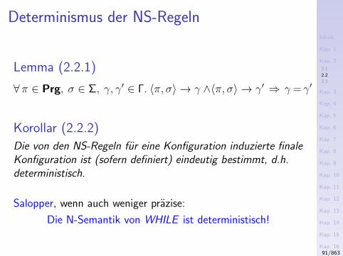
Determinismus der NS-Regeln
Lemma (2.2.1)
∀π ∈ Prg, σ ∈ Σ, γ, γ′ ∈ Γ. 〈π, σ〉 → γ ∧〈π, σ〉 → γ′ ⇒ γ = γ′
Korollar (2.2.2)
Die von den NS-Regeln fur eine Konfiguration induzierte finaleKonfiguration ist (sofern definiert) eindeutig bestimmt, d.h.deterministisch.
Salopper, wenn auch weniger prazise:
Die N-Semantik von WHILE ist deterministisch!
91/863
Inhalt
Kap. 1
Kap. 2
2.1
2.2
2.3
Kap. 3
Kap. 4
Kap. 5
Kap. 6
Kap. 7
Kap. 8
Kap. 9
Kap. 10
Kap. 11
Kap. 12
Kap. 13
Kap. 14
Kap. 15
Kap. 16
Kap. 17
Literatur
Anhang
A
Das Semantikfunktional [[ ]]ns
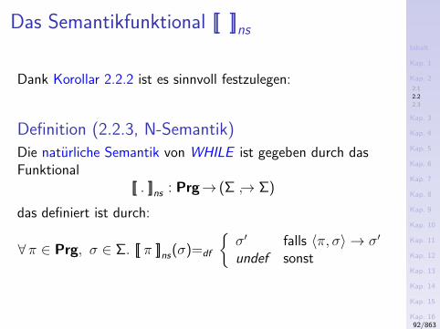
Dank Korollar 2.2.2 ist es sinnvoll festzulegen:
Definition (2.2.3, N-Semantik)
Die naturliche Semantik von WHILE ist gegeben durch dasFunktional
[[ . ]]ns : Prg→ (Σ → Σ)
das definiert ist durch:
∀π ∈ Prg, σ ∈ Σ. [[ π ]]ns(σ)=df
σ′ falls 〈π, σ〉 → σ′
undef sonst
92/863
Inhalt
Kap. 1
Kap. 2
2.1
2.2
2.3
Kap. 3
Kap. 4
Kap. 5
Kap. 6
Kap. 7
Kap. 8
Kap. 9
Kap. 10
Kap. 11
Kap. 12
Kap. 13
Kap. 14
Kap. 15
Kap. 16
Kap. 17
Literatur
Anhang
A
Variante induktiver Beweisfuhrung
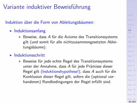
Induktion uber die Form von Ableitungsbaumen:
I InduktionsanfangI Beweise, dass A fur die Axiome des Transitionssystems
gilt (und somit fur alle nichtzusammengesetzten Ablei-tungsbaume).
I InduktionsschrittI Beweise fur jede echte Regel des Transitionssystems
unter der Annahme, dass A fur jede Pramisse dieserRegel gilt (Induktionshypothese!), dass A auch fur dieKonklusion dieser Regel gilt, sofern die (optional vor-handenen) Randbedingungen der Regel erfullt sind.
93/863

Inhalt
Kap. 1
Kap. 2
2.1
2.2
2.3
Kap. 3
Kap. 4
Kap. 5
Kap. 6
Kap. 7
Kap. 8
Kap. 9
Kap. 10
Kap. 11
Kap. 12
Kap. 13
Kap. 14
Kap. 15
Kap. 16
Kap. 17
Literatur
Anhang
A
Anwendung
Induktive Beweisfuhrung uber die Form von Ableitungsbaumenist typisch zum Nachweis von Aussagen uber Eigenschaftennaturlicher Semantik.
Ein Beispiel hierfur ist der Beweis von Lemma 2.2.1!
94/863

Inhalt
Kap. 1
Kap. 2
2.1
2.2
2.3
Kap. 3
Kap. 4
Kap. 5
Kap. 6
Kap. 7
Kap. 8
Kap. 9
Kap. 10
Kap. 11
Kap. 12
Kap. 13
Kap. 14
Kap. 15
Kap. 16
Kap. 17
Literatur
Anhang
A
Kapitel 2.3
Strukturell operationelle und naturlicheSemantik im Vergleich
95/863
Inhalt
Kap. 1
Kap. 2
2.1
2.2
2.3
Kap. 3
Kap. 4
Kap. 5
Kap. 6
Kap. 7
Kap. 8
Kap. 9
Kap. 10
Kap. 11
Kap. 12
Kap. 13
Kap. 14
Kap. 15
Kap. 16
Kap. 17
Literatur
Anhang
A
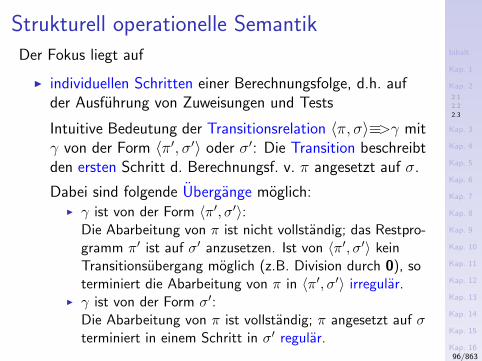
Strukturell operationelle SemantikDer Fokus liegt auf
I individuellen Schritten einer Berechnungsfolge, d.h. aufder Ausfuhrung von Zuweisungen und Tests
Intuitive Bedeutung der Transitionsrelation 〈π, σ〉≡>γ mitγ von der Form 〈π′, σ′〉 oder σ′: Die Transition beschreibtden ersten Schritt d. Berechnungsf. v. π angesetzt auf σ.
Dabei sind folgende Ubergange moglich:I γ ist von der Form 〈π′, σ′〉:
Die Abarbeitung von π ist nicht vollstandig; das Restpro-gramm π′ ist auf σ′ anzusetzen. Ist von 〈π′, σ′〉 keinTransitionsubergang moglich (z.B. Division durch 0), soterminiert die Abarbeitung von π in 〈π′, σ′〉 irregular.
I γ ist von der Form σ′:Die Abarbeitung von π ist vollstandig; π angesetzt auf σterminiert in einem Schritt in σ′ regular.
96/863
Inhalt
Kap. 1
Kap. 2
2.1
2.2
2.3
Kap. 3
Kap. 4
Kap. 5
Kap. 6
Kap. 7
Kap. 8
Kap. 9
Kap. 10
Kap. 11
Kap. 12
Kap. 13
Kap. 14
Kap. 15
Kap. 16
Kap. 17
Literatur
Anhang
A
Naturliche Semantik
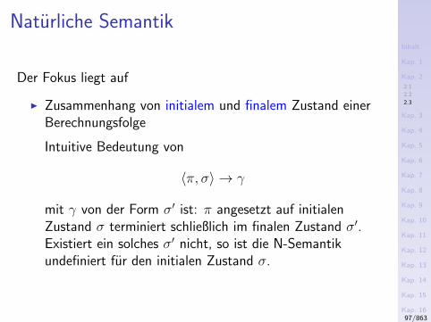
Der Fokus liegt auf
I Zusammenhang von initialem und finalem Zustand einerBerechnungsfolge
Intuitive Bedeutung von
〈π, σ〉 → γ
mit γ von der Form σ′ ist: π angesetzt auf initialenZustand σ terminiert schließlich im finalen Zustand σ′.Existiert ein solches σ′ nicht, so ist die N-Semantikundefiniert fur den initialen Zustand σ.
97/863
Inhalt
Kap. 1
Kap. 2
2.1
2.2
2.3
Kap. 3
Kap. 4
Kap. 5
Kap. 6
Kap. 7
Kap. 8
Kap. 9
Kap. 10
Kap. 11
Kap. 12
Kap. 13
Kap. 14
Kap. 15
Kap. 16
Kap. 17
Literatur
Anhang
A
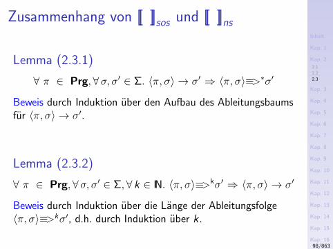
Zusammenhang von [[ ]]sos und [[ ]]ns
Lemma (2.3.1)
∀ π ∈ Prg,∀σ, σ′ ∈ Σ. 〈π, σ〉 → σ′ ⇒ 〈π, σ〉≡>∗σ′
Beweis durch Induktion uber den Aufbau des Ableitungsbaumsfur 〈π, σ〉 → σ′.
Lemma (2.3.2)
∀ π ∈ Prg,∀σ, σ′ ∈ Σ,∀ k ∈ IN. 〈π, σ〉≡>kσ′ ⇒ 〈π, σ〉 → σ′
Beweis durch Induktion uber die Lange der Ableitungsfolge〈π, σ〉≡>kσ′, d.h. durch Induktion uber k .
98/863
Inhalt
Kap. 1
Kap. 2
2.1
2.2
2.3
Kap. 3
Kap. 4
Kap. 5
Kap. 6
Kap. 7
Kap. 8
Kap. 9
Kap. 10
Kap. 11
Kap. 12
Kap. 13
Kap. 14
Kap. 15
Kap. 16
Kap. 17
Literatur
Anhang
A
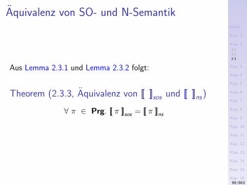
Aquivalenz von SO- und N-Semantik
Aus Lemma 2.3.1 und Lemma 2.3.2 folgt:
Theorem (2.3.3, Aquivalenz von [[ ]]sos und [[ ]]ns)
∀ π ∈ Prg. [[ π ]]sos = [[ π ]]ns
99/863
Inhalt
Kap. 1
Kap. 2
2.1
2.2
2.3
Kap. 3
Kap. 4
Kap. 5
Kap. 6
Kap. 7
Kap. 8
Kap. 9
Kap. 10
Kap. 11
Kap. 12
Kap. 13
Kap. 14
Kap. 15
Kap. 16
Kap. 17
Literatur
Anhang
A
Vertiefende und weiterfuhrende Leseempfeh-
lungen fur Kapitel 2 (1)
Hanne Riis Nielson, Flemming Nielson. Semantics withApplications: A Formal Introduction. Wiley, 1992.(Chapter 2, Operational Semantics)
Hanne Riis Nielson, Flemming Nielson. Semantics withApplications: An Appetizer. Springer-V., 2007. (Chapter2, Operational Semantics)
100/863
Inhalt
Kap. 1
Kap. 2
2.1
2.2
2.3
Kap. 3
Kap. 4
Kap. 5
Kap. 6
Kap. 7
Kap. 8
Kap. 9
Kap. 10
Kap. 11
Kap. 12
Kap. 13
Kap. 14
Kap. 15
Kap. 16
Kap. 17
Literatur
Anhang
A
Vertiefende und weiterfuhrende Leseempfeh-
lungen fur Kapitel 2 (2)
Gordon D. Plotkin. A Structural Approach to OperationalSemantics. Lecture notes, DAIMI FN-19, Aarhus Univer-sity, Denmark, 1981, reprinted 1991.
Gordon D. Plotkin. An Operational Semantics for CSP. InProceedings of TC-2 Working Conference on FormalDescription of Programming Concepts II, Dines Bjørner(Ed.), North-Holland, Amsterdam, 1982.
Gordon D. Plotkin. A Structural Approach to OperationalSemantics. Journal of Logic and Algebraic Programming60-61:17-139, 2004.
101/863
Inhalt
Kap. 1
Kap. 2
Kap. 3
3.1
3.2
3.3
Kap. 4
Kap. 5
Kap. 6
Kap. 7
Kap. 8
Kap. 9
Kap. 10
Kap. 11
Kap. 12
Kap. 13
Kap. 14
Kap. 15
Kap. 16
Kap. 17
Literatur
Anhang
A
Kapitel 3
Denotationelle Semantik von WHILE
102/863
Inhalt
Kap. 1
Kap. 2
Kap. 3
3.1
3.2
3.3
Kap. 4
Kap. 5
Kap. 6
Kap. 7
Kap. 8
Kap. 9
Kap. 10
Kap. 11
Kap. 12
Kap. 13
Kap. 14
Kap. 15
Kap. 16
Kap. 17
Literatur
Anhang
A
Denotationelle Semantik von WHILE
...die Bedeutung eines Konstrukts wird durch mathematische
Objekte modelliert, die den Effekt der Ausfuhrung der Konstrukte
reprasentieren. Wichtig ist einzig der Effekt, nicht wie er bewirkt
wird.
103/863
Inhalt
Kap. 1
Kap. 2
Kap. 3
3.1
3.2
3.3
Kap. 4
Kap. 5
Kap. 6
Kap. 7
Kap. 8
Kap. 9
Kap. 10
Kap. 11
Kap. 12
Kap. 13
Kap. 14
Kap. 15
Kap. 16
Kap. 17
Literatur
Anhang
A
Denotationelle Semantik
Die denotationelle Semantik (D-Semantik) von WHILE
I ordnet jedem Programm π als Bedeutung eine partielldefinierte Zustandstransformation
Σ → Σ
zu.
Das zugehorige
I Zustandstransformationsfunktional [[ . ]]ds derdenotationellen Semantik
[[ . ]]ds : Prg→ (Σ → Σ)
definieren wir in der Folge im Detail.104/863
Inhalt
Kap. 1
Kap. 2
Kap. 3
3.1
3.2
3.3
Kap. 4
Kap. 5
Kap. 6
Kap. 7
Kap. 8
Kap. 9
Kap. 10
Kap. 11
Kap. 12
Kap. 13
Kap. 14
Kap. 15
Kap. 16
Kap. 17
Literatur
Anhang
A
Vergleich operationeller und denotationeller
Semantik
I Operationelle Semantik...der Fokus liegt darauf, wie ein Programm ausgefuhrtwird.
I Denotationelle Semantik...der Fokus liegt auf dem Effekt, den die Ausfuhrungeines Programms hat: Fur jedes syntaktische Konstruktgibt es eine semantische Funktion, die ersterem einmathematisches Objekt zuweist, d.h. eine Funktion, dieden Effekt der Ausfuhrung des Konstrukts beschreibt(jedoch nicht, wie dieser Effekt erreicht wird).
105/863
Inhalt
Kap. 1
Kap. 2
Kap. 3
3.1
3.2
3.3
Kap. 4
Kap. 5
Kap. 6
Kap. 7
Kap. 8
Kap. 9
Kap. 10
Kap. 11
Kap. 12
Kap. 13
Kap. 14
Kap. 15
Kap. 16
Kap. 17
Literatur
Anhang
A
Kompositionalitat
Zentral fur denotationelle Semantiken: Kompositionalitat!
Intuitiv:
I Fur jedes Element der elementaren syntaktischen Kon-strukte/Kategorien gibt es eine zugehorige semantischeFunktion.
I Fur jedes Element eines zusammengesetzten syntaktischenKonstrukts/Kategorie gibt es eine semantische Funktion,die uber die semantischen Funktionen der Komponentendes zusammengesetzten Konstrukts definiert ist.
106/863
Inhalt
Kap. 1
Kap. 2
Kap. 3
3.1
3.2
3.3
Kap. 4
Kap. 5
Kap. 6
Kap. 7
Kap. 8
Kap. 9
Kap. 10
Kap. 11
Kap. 12
Kap. 13
Kap. 14
Kap. 15
Kap. 16
Kap. 17
Literatur
Anhang
A
Kapitel 3.1
Denotationelle Semantik
107/863
Inhalt
Kap. 1
Kap. 2
Kap. 3
3.1
3.2
3.3
Kap. 4
Kap. 5
Kap. 6
Kap. 7
Kap. 8
Kap. 9
Kap. 10
Kap. 11
Kap. 12
Kap. 13
Kap. 14
Kap. 15
Kap. 16
Kap. 17
Literatur
Anhang
A
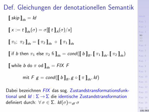
Def. Gleichungen der denotationellen Semantik
[[ skip ]]ds = Id
[[ x := t ]]ds(σ) = σ[[[ t ]]A(σ)/x ]
[[ π1; π2 ]]ds = [[ π2 ]]ds [[ π1 ]]ds
[[ if b then π1 else π2 fi ]]ds = cond([[ b ]]B , [[ π1 ]]ds , [[ π2 ]]ds)
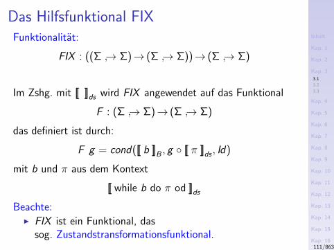
[[ while b do π od ]]ds = FIX F
mit F g = cond([[ b ]]B , g [[ π ]]ds , Id)
Dabei bezeichnen FIX das sog. Zustandstransformationsfunk-tional und Id : Σ→Σ die identische Zustandstransformationdefiniert durch: ∀σ ∈ Σ. Id(σ)=df σ
108/863
Inhalt
Kap. 1
Kap. 2
Kap. 3
3.1
3.2
3.3
Kap. 4
Kap. 5
Kap. 6
Kap. 7
Kap. 8
Kap. 9
Kap. 10
Kap. 11
Kap. 12
Kap. 13
Kap. 14
Kap. 15
Kap. 16
Kap. 17
Literatur
Anhang
A
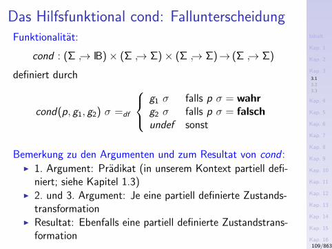
Das Hilfsfunktional cond: FallunterscheidungFunktionalitat:
cond : (Σ → IB)× (Σ → Σ)× (Σ → Σ)→ (Σ → Σ)
definiert durch
cond(p, g1, g2) σ =df
g1 σ falls p σ = wahrg2 σ falls p σ = falschundef sonst
Bemerkung zu den Argumenten und zum Resultat von cond :I 1. Argument: Pradikat (in unserem Kontext partiell defi-
niert; siehe Kapitel 1.3)I 2. und 3. Argument: Je eine partiell definierte Zustands-
transformationI Resultat: Ebenfalls eine partiell definierte Zustandstrans-
formation109/863
Inhalt
Kap. 1
Kap. 2
Kap. 3
3.1
3.2
3.3
Kap. 4
Kap. 5
Kap. 6
Kap. 7
Kap. 8
Kap. 9
Kap. 10
Kap. 11
Kap. 12
Kap. 13
Kap. 14
Kap. 15
Kap. 16
Kap. 17
Literatur
Anhang
A
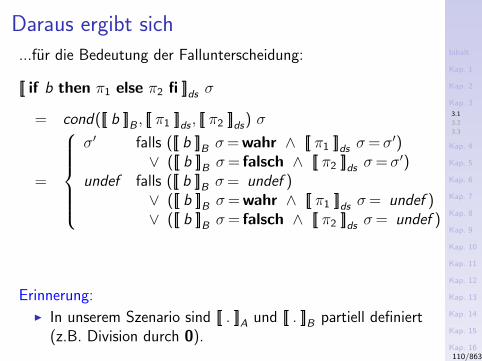
Daraus ergibt sich...fur die Bedeutung der Fallunterscheidung:
[[ if b then π1 else π2 fi ]]ds σ
= cond([[ b ]]B , [[ π1 ]]ds , [[ π2 ]]ds) σ
=
σ′ falls ([[ b ]]B σ= wahr ∧ [[ π1 ]]ds σ=σ′)
∨ ([[ b ]]B σ= falsch ∧ [[ π2 ]]ds σ=σ′)undef falls ([[ b ]]B σ= undef )
∨ ([[ b ]]B σ= wahr ∧ [[ π1 ]]ds σ= undef )∨ ([[ b ]]B σ= falsch ∧ [[ π2 ]]ds σ= undef )
Erinnerung:
I In unserem Szenario sind [[ . ]]A und [[ . ]]B partiell definiert(z.B. Division durch 0).
110/863
Inhalt
Kap. 1
Kap. 2
Kap. 3
3.1
3.2
3.3
Kap. 4
Kap. 5
Kap. 6
Kap. 7
Kap. 8
Kap. 9
Kap. 10
Kap. 11
Kap. 12
Kap. 13
Kap. 14
Kap. 15
Kap. 16
Kap. 17
Literatur
Anhang
A
Das Hilfsfunktional FIXFunktionalitat:
FIX : ((Σ → Σ)→ (Σ → Σ))→ (Σ → Σ)
Im Zshg. mit [[ ]]ds wird FIX angewendet auf das Funktional
F : (Σ → Σ)→ (Σ → Σ)
das definiert ist durch:
F g = cond([[ b ]]B , g [[ π ]]ds , Id)
mit b und π aus dem Kontext
[[ while b do π od ]]ds
Beachte:I FIX ist ein Funktional, das
sog. Zustandstransformationsfunktional.111/863
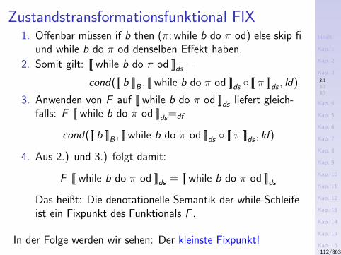
Inhalt
Kap. 1
Kap. 2
Kap. 3
3.1
3.2
3.3
Kap. 4
Kap. 5
Kap. 6
Kap. 7
Kap. 8
Kap. 9
Kap. 10
Kap. 11
Kap. 12
Kap. 13
Kap. 14
Kap. 15
Kap. 16
Kap. 17
Literatur
Anhang
A
Zustandstransformationsfunktional FIX1. Offenbar mussen if b then (π; while b do π od) else skip fi
und while b do π od denselben Effekt haben.
2. Somit gilt: [[ while b do π od ]]ds =
cond([[ b ]]B , [[ while b do π od ]]ds [[ π ]]ds , Id)
3. Anwenden von F auf [[ while b do π od ]]ds liefert gleich-falls: F [[ while b do π od ]]ds=df
cond([[ b ]]B , [[ while b do π od ]]ds [[ π ]]ds , Id)
4. Aus 2.) und 3.) folgt damit:
F [[ while b do π od ]]ds = [[ while b do π od ]]ds
Das heißt: Die denotationelle Semantik der while-Schleifeist ein Fixpunkt des Funktionals F .
In der Folge werden wir sehen: Der kleinste Fixpunkt!112/863
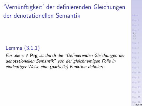
Inhalt
Kap. 1
Kap. 2
Kap. 3
3.1
3.2
3.3
Kap. 4
Kap. 5
Kap. 6
Kap. 7
Kap. 8
Kap. 9
Kap. 10
Kap. 11
Kap. 12
Kap. 13
Kap. 14
Kap. 15
Kap. 16
Kap. 17
Literatur
Anhang
A
‘Vernunftigkeit’ der definierenden Gleichungen
der denotationellen Semantik
Lemma (3.1.1)
Fur alle π ∈ Prg ist durch die “Definierenden Gleichungen derdenotationellen Semantik” von der gleichnamigen Folie ineindeutiger Weise eine (partielle) Funktion definiert.
113/863
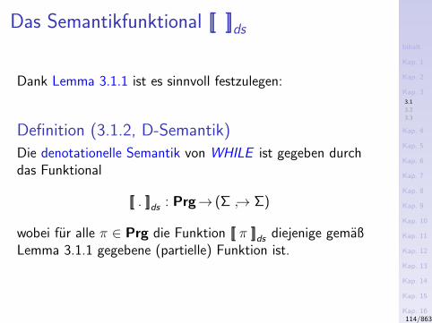
Inhalt
Kap. 1
Kap. 2
Kap. 3
3.1
3.2
3.3
Kap. 4
Kap. 5
Kap. 6
Kap. 7
Kap. 8
Kap. 9
Kap. 10
Kap. 11
Kap. 12
Kap. 13
Kap. 14
Kap. 15
Kap. 16
Kap. 17
Literatur
Anhang
A
Das Semantikfunktional [[ ]]ds
Dank Lemma 3.1.1 ist es sinnvoll festzulegen:
Definition (3.1.2, D-Semantik)
Die denotationelle Semantik von WHILE ist gegeben durchdas Funktional
[[ . ]]ds : Prg→ (Σ → Σ)
wobei fur alle π ∈ Prg die Funktion [[ π ]]ds diejenige gemaßLemma 3.1.1 gegebene (partielle) Funktion ist.
114/863
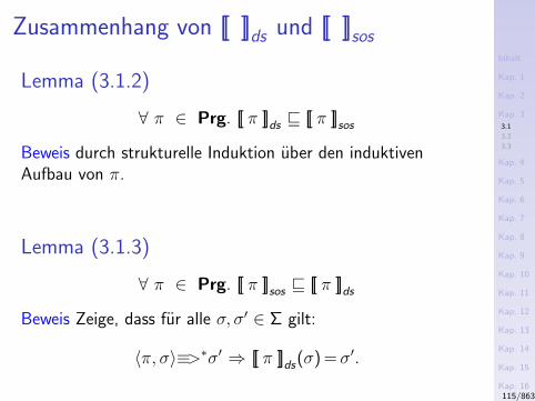
Inhalt
Kap. 1
Kap. 2
Kap. 3
3.1
3.2
3.3
Kap. 4
Kap. 5
Kap. 6
Kap. 7
Kap. 8
Kap. 9
Kap. 10
Kap. 11
Kap. 12
Kap. 13
Kap. 14
Kap. 15
Kap. 16
Kap. 17
Literatur
Anhang
A
Zusammenhang von [[ ]]ds und [[ ]]sos
Lemma (3.1.2)
∀ π ∈ Prg. [[ π ]]ds v [[ π ]]sos
Beweis durch strukturelle Induktion uber den induktivenAufbau von π.
Lemma (3.1.3)
∀ π ∈ Prg. [[ π ]]sos v [[ π ]]ds
Beweis Zeige, dass fur alle σ, σ′ ∈ Σ gilt:
〈π, σ〉≡>∗σ′ ⇒ [[ π ]]ds(σ) =σ′.
115/863
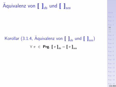
Inhalt
Kap. 1
Kap. 2
Kap. 3
3.1
3.2
3.3
Kap. 4
Kap. 5
Kap. 6
Kap. 7
Kap. 8
Kap. 9
Kap. 10
Kap. 11
Kap. 12
Kap. 13
Kap. 14
Kap. 15
Kap. 16
Kap. 17
Literatur
Anhang
A
Aquivalenz von [[ ]]ds und [[ ]]sos
Korollar (3.1.4, Aquivalenz von [[ ]]ds und [[ ]]sos)
∀ π ∈ Prg. [[ π ]]ds = [[ π ]]sos
116/863
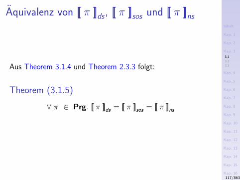
Inhalt
Kap. 1
Kap. 2
Kap. 3
3.1
3.2
3.3
Kap. 4
Kap. 5
Kap. 6
Kap. 7
Kap. 8
Kap. 9
Kap. 10
Kap. 11
Kap. 12
Kap. 13
Kap. 14
Kap. 15
Kap. 16
Kap. 17
Literatur
Anhang
A
Aquivalenz von [[ π ]]ds , [[ π ]]sos und [[ π ]]ns
Aus Theorem 3.1.4 und Theorem 2.3.3 folgt:
Theorem (3.1.5)
∀ π ∈ Prg. [[ π ]]ds = [[ π ]]sos = [[ π ]]ns
117/863
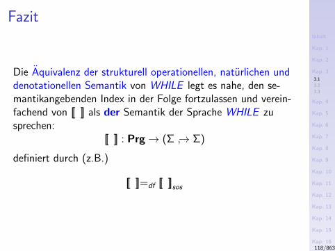
Inhalt
Kap. 1
Kap. 2
Kap. 3
3.1
3.2
3.3
Kap. 4
Kap. 5
Kap. 6
Kap. 7
Kap. 8
Kap. 9
Kap. 10
Kap. 11
Kap. 12
Kap. 13
Kap. 14
Kap. 15
Kap. 16
Kap. 17
Literatur
Anhang
A
Fazit
Die Aquivalenz der strukturell operationellen, naturlichen unddenotationellen Semantik von WHILE legt es nahe, den se-mantikangebenden Index in der Folge fortzulassen und verein-fachend von [[ ]] als der Semantik der Sprache WHILE zusprechen:
[[ ]] : Prg→ (Σ → Σ)
definiert durch (z.B.)
[[ ]]=df [[ ]]sos
118/863

Inhalt
Kap. 1
Kap. 2
Kap. 3
3.1
3.2
3.3
Kap. 4
Kap. 5
Kap. 6
Kap. 7
Kap. 8
Kap. 9
Kap. 10
Kap. 11
Kap. 12
Kap. 13
Kap. 14
Kap. 15
Kap. 16
Kap. 17
Literatur
Anhang
A
Kapitel 3.2
Fixpunktfunktional
119/863
Inhalt
Kap. 1
Kap. 2
Kap. 3
3.1
3.2
3.3
Kap. 4
Kap. 5
Kap. 6
Kap. 7
Kap. 8
Kap. 9
Kap. 10
Kap. 11
Kap. 12
Kap. 13
Kap. 14
Kap. 15
Kap. 16
Kap. 17
Literatur
Anhang
A
Zur Bedeutung von FIX F
In der Folge wollen wir die Bedeutung von
I FIX F
genauer untersuchen und aufklaren.
120/863
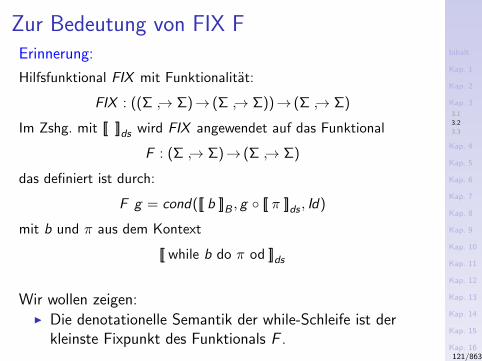
Inhalt
Kap. 1
Kap. 2
Kap. 3
3.1
3.2
3.3
Kap. 4
Kap. 5
Kap. 6
Kap. 7
Kap. 8
Kap. 9
Kap. 10
Kap. 11
Kap. 12
Kap. 13
Kap. 14
Kap. 15
Kap. 16
Kap. 17
Literatur
Anhang
A
Zur Bedeutung von FIX FErinnerung:
Hilfsfunktional FIX mit Funktionalitat:
FIX : ((Σ → Σ)→ (Σ → Σ))→ (Σ → Σ)
Im Zshg. mit [[ ]]ds wird FIX angewendet auf das Funktional
F : (Σ → Σ)→ (Σ → Σ)
das definiert ist durch:
F g = cond([[ b ]]B , g [[ π ]]ds , Id)
mit b und π aus dem Kontext
[[ while b do π od ]]ds
Wir wollen zeigen:I Die denotationelle Semantik der while-Schleife ist der
kleinste Fixpunkt des Funktionals F .121/863
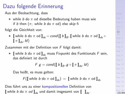
Inhalt
Kap. 1
Kap. 2
Kap. 3
3.1
3.2
3.3
Kap. 4
Kap. 5
Kap. 6
Kap. 7
Kap. 8
Kap. 9
Kap. 10
Kap. 11
Kap. 12
Kap. 13
Kap. 14
Kap. 15
Kap. 16
Kap. 17
Literatur
Anhang
A
Dazu folgende ErinnerungAus der Beobachtung, dass
I while b do π od dieselbe Bedeutung haben muss wieif b then (π; while b do π od) else skip fi
folgt die Gleichheit von:
I [[ while b do π od ]]ds = cond([[ b ]]B , [[ while b do π od ]]ds [[ π ]]ds , Id)
Zusammen mit der Definition von F folgt damit:
I [[ while b do π od ]]ds muss Fixpunkt des Funktionals F sein,das definiert ist durch
F g = cond([[ b ]]B , g [[ π ]]ds , Id)
Das heißt, es muss gelten:
F ([[ while b do π od ]]ds) = [[ while b do π od ]]ds
Dies fuhrt uns zu einer kompositionellen Definition von
[[ while b do π od ]]ds und damit insgesamt von [[ ]]ds . 122/863

Inhalt
Kap. 1
Kap. 2
Kap. 3
3.1
3.2
3.3
Kap. 4
Kap. 5
Kap. 6
Kap. 7
Kap. 8
Kap. 9
Kap. 10
Kap. 11
Kap. 12
Kap. 13
Kap. 14
Kap. 15
Kap. 16
Kap. 17
Literatur
Anhang
A
Unser Arbeitsplan
Wir benotigen:
I Einige Resultate aus der Fixpunkttheorie.
Diese erlauben uns:
I Nachzuweisen, dass diese Resultate auf unsere Situationanwendbar sind.
Dabei wird vorausgesetzt:
I Mathematische Grundlagen uber Ordnungen, CPOs,Stetigkeit von Funktionen und benotigte Resultatedaruber, insbesondere das Fixpunkttheorem.
Diese Grundlagen sind in Kapitel 3.3 (und umfangreicher imAnhang) zusammengefasst.
123/863
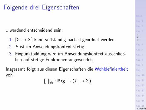
Inhalt
Kap. 1
Kap. 2
Kap. 3
3.1
3.2
3.3
Kap. 4
Kap. 5
Kap. 6
Kap. 7
Kap. 8
Kap. 9
Kap. 10
Kap. 11
Kap. 12
Kap. 13
Kap. 14
Kap. 15
Kap. 16
Kap. 17
Literatur
Anhang
A
Folgende drei Eigenschaften
...werdend entscheidend sein:
1. [Σ → Σ] kann vollstandig partiell geordnet werden.
2. F ist im Anwendungskontext stetig.
3. Fixpunktbildung wird im Anwendungskontext ausschließ-lich auf stetige Funktionen angewendet.
Insgesamt folgt aus diesen Eigenschaften die Wohldefiniertheitvon
[[ ]]ds : Prg→ (Σ → Σ)
124/863
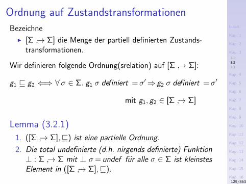
Inhalt
Kap. 1
Kap. 2
Kap. 3
3.1
3.2
3.3
Kap. 4
Kap. 5
Kap. 6
Kap. 7
Kap. 8
Kap. 9
Kap. 10
Kap. 11
Kap. 12
Kap. 13
Kap. 14
Kap. 15
Kap. 16
Kap. 17
Literatur
Anhang
A
Ordnung auf Zustandstransformationen
Bezeichne
I [Σ → Σ] die Menge der partiell definierten Zustands-transformationen.
Wir definieren folgende Ordnung(srelation) auf [Σ → Σ]:
g1 v g2 ⇐⇒ ∀σ ∈ Σ. g1 σ definiert =σ′⇒ g2 σ definiert =σ′
mit g1, g2 ∈ [Σ → Σ]
Lemma (3.2.1)
1. ([Σ → Σ],v) ist eine partielle Ordnung.
2. Die total undefinierte (d.h. nirgends definierte) Funktion⊥ : Σ → Σ mit ⊥ σ= undef fur alle σ ∈ Σ ist kleinstesElement in ([Σ → Σ],v).
125/863
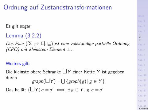
Inhalt
Kap. 1
Kap. 2
Kap. 3
3.1
3.2
3.3
Kap. 4
Kap. 5
Kap. 6
Kap. 7
Kap. 8
Kap. 9
Kap. 10
Kap. 11
Kap. 12
Kap. 13
Kap. 14
Kap. 15
Kap. 16
Kap. 17
Literatur
Anhang
A
Ordnung auf Zustandstransformationen
Es gilt sogar:
Lemma (3.2.2)
Das Paar ([Σ → Σ],v) ist eine vollstandige partielle Ordnung(CPO) mit kleinstem Element ⊥.
Weiters gilt:
Die kleinste obere Schranke tY einer Kette Y ist gegebendurch
graph(tY ) =⋃graph(g) | g ∈ Y
Das heißt: (tY )σ=σ′ ⇐⇒ ∃ g ∈ Y . g σ=σ′
126/863
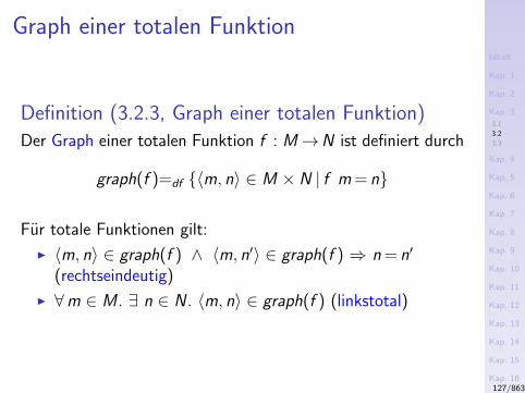
Inhalt
Kap. 1
Kap. 2
Kap. 3
3.1
3.2
3.3
Kap. 4
Kap. 5
Kap. 6
Kap. 7
Kap. 8
Kap. 9
Kap. 10
Kap. 11
Kap. 12
Kap. 13
Kap. 14
Kap. 15
Kap. 16
Kap. 17
Literatur
Anhang
A
Graph einer totalen Funktion
Definition (3.2.3, Graph einer totalen Funktion)
Der Graph einer totalen Funktion f : M→N ist definiert durch
graph(f )=df 〈m, n〉 ∈ M × N | f m = n
Fur totale Funktionen gilt:
I 〈m, n〉 ∈ graph(f ) ∧ 〈m, n′〉 ∈ graph(f ) ⇒ n = n′
(rechtseindeutig)
I ∀m ∈ M . ∃ n ∈ N . 〈m, n〉 ∈ graph(f ) (linkstotal)
127/863
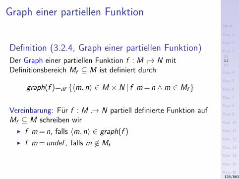
Inhalt
Kap. 1
Kap. 2
Kap. 3
3.1
3.2
3.3
Kap. 4
Kap. 5
Kap. 6
Kap. 7
Kap. 8
Kap. 9
Kap. 10
Kap. 11
Kap. 12
Kap. 13
Kap. 14
Kap. 15
Kap. 16
Kap. 17
Literatur
Anhang
A
Graph einer partiellen Funktion
Definition (3.2.4, Graph einer partiellen Funktion)
Der Graph einer partiellen Funktion f : M → N mitDefinitionsbereich Mf ⊆ M ist definiert durch
graph(f )=df 〈m, n〉 ∈ M × N | f m = n ∧m ∈ Mf
Vereinbarung: Fur f : M → N partiell definierte Funktion aufMf ⊆ M schreiben wir
I f m = n, falls 〈m, n〉 ∈ graph(f )
I f m = undef , falls m 6∈ Mf
128/863
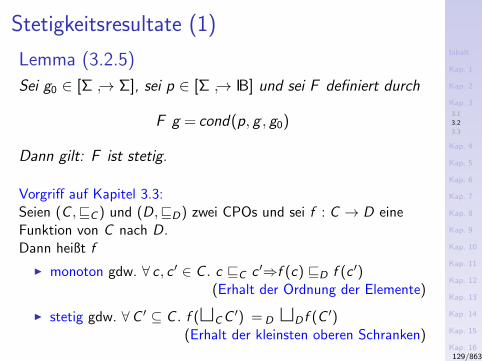
Inhalt
Kap. 1
Kap. 2
Kap. 3
3.1
3.2
3.3
Kap. 4
Kap. 5
Kap. 6
Kap. 7
Kap. 8
Kap. 9
Kap. 10
Kap. 11
Kap. 12
Kap. 13
Kap. 14
Kap. 15
Kap. 16
Kap. 17
Literatur
Anhang
A
Stetigkeitsresultate (1)
Lemma (3.2.5)
Sei g0 ∈ [Σ → Σ], sei p ∈ [Σ → IB] und sei F definiert durch
F g = cond(p, g , g0)
Dann gilt: F ist stetig.
Vorgriff auf Kapitel 3.3:Seien (C ,vC ) und (D,vD) zwei CPOs und sei f : C → D eineFunktion von C nach D.Dann heißt f
I monoton gdw. ∀ c , c ′ ∈ C . c vC c ′⇒f (c) vD f (c ′)(Erhalt der Ordnung der Elemente)
I stetig gdw. ∀C ′ ⊆ C . f (tCC ′) = D tD f (C ′)(Erhalt der kleinsten oberen Schranken)
129/863
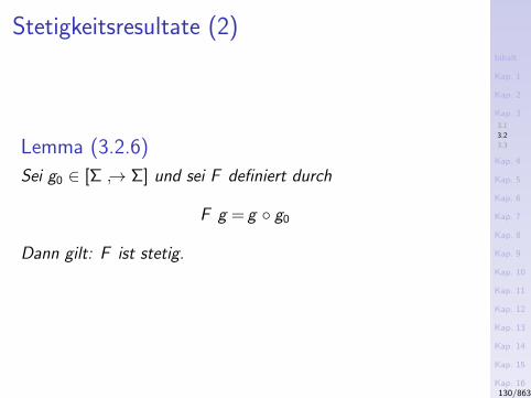
Inhalt
Kap. 1
Kap. 2
Kap. 3
3.1
3.2
3.3
Kap. 4
Kap. 5
Kap. 6
Kap. 7
Kap. 8
Kap. 9
Kap. 10
Kap. 11
Kap. 12
Kap. 13
Kap. 14
Kap. 15
Kap. 16
Kap. 17
Literatur
Anhang
A
Stetigkeitsresultate (2)
Lemma (3.2.6)
Sei g0 ∈ [Σ → Σ] und sei F definiert durch
F g = g g0
Dann gilt: F ist stetig.
130/863
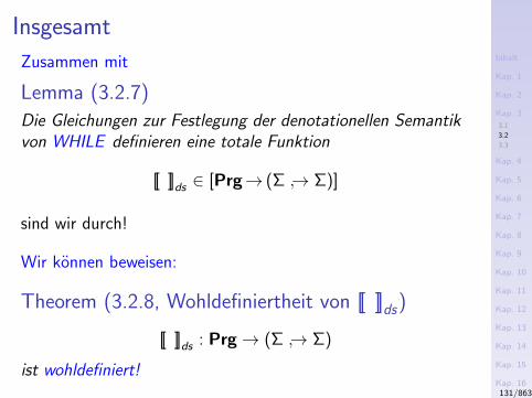
Inhalt
Kap. 1
Kap. 2
Kap. 3
3.1
3.2
3.3
Kap. 4
Kap. 5
Kap. 6
Kap. 7
Kap. 8
Kap. 9
Kap. 10
Kap. 11
Kap. 12
Kap. 13
Kap. 14
Kap. 15
Kap. 16
Kap. 17
Literatur
Anhang
A
Insgesamt
Zusammen mit
Lemma (3.2.7)
Die Gleichungen zur Festlegung der denotationellen Semantikvon WHILE definieren eine totale Funktion
[[ ]]ds ∈ [Prg→ (Σ → Σ)]
sind wir durch!
Wir konnen beweisen:
Theorem (3.2.8, Wohldefiniertheit von [[ ]]ds)
[[ ]]ds : Prg→ (Σ → Σ)
ist wohldefiniert!131/863
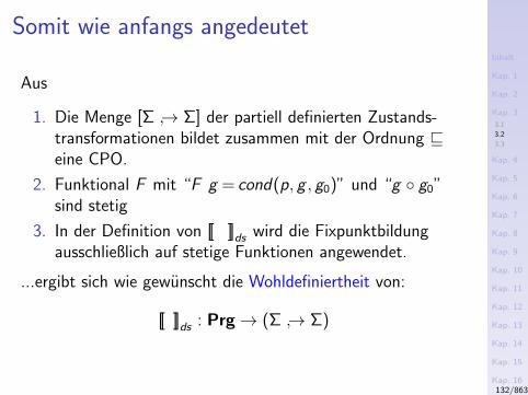
Inhalt
Kap. 1
Kap. 2
Kap. 3
3.1
3.2
3.3
Kap. 4
Kap. 5
Kap. 6
Kap. 7
Kap. 8
Kap. 9
Kap. 10
Kap. 11
Kap. 12
Kap. 13
Kap. 14
Kap. 15
Kap. 16
Kap. 17
Literatur
Anhang
A
Somit wie anfangs angedeutet
Aus
1. Die Menge [Σ → Σ] der partiell definierten Zustands-transformationen bildet zusammen mit der Ordnung veine CPO.
2. Funktional F mit “F g = cond(p, g , g0)” und “g g0”sind stetig
3. In der Definition von [[ ]]ds wird die Fixpunktbildungausschließlich auf stetige Funktionen angewendet.
...ergibt sich wie gewunscht die Wohldefiniertheit von:
[[ ]]ds : Prg→ (Σ → Σ)
132/863

Inhalt
Kap. 1
Kap. 2
Kap. 3
3.1
3.2
3.3
Kap. 4
Kap. 5
Kap. 6
Kap. 7
Kap. 8
Kap. 9
Kap. 10
Kap. 11
Kap. 12
Kap. 13
Kap. 14
Kap. 15
Kap. 16
Kap. 17
Literatur
Anhang
A
Kapitel 3.3
Ordnungen, Verbande, Fixpunkttheoreme
133/863
Inhalt
Kap. 1
Kap. 2
Kap. 3
3.1
3.2
3.3
Kap. 4
Kap. 5
Kap. 6
Kap. 7
Kap. 8
Kap. 9
Kap. 10
Kap. 11
Kap. 12
Kap. 13
Kap. 14
Kap. 15
Kap. 16
Kap. 17
Literatur
Anhang
A
Mathematische Grundlagen
...im Zusammenhang mit der
I Definition der denotationellen Semantik von WHILE imDetail
sowie in spateren Kapiteln mit der
I Definition abstrakter Semantiken fur Programmanalysen
134/863
Inhalt
Kap. 1
Kap. 2
Kap. 3
3.1
3.2
3.3
Kap. 4
Kap. 5
Kap. 6
Kap. 7
Kap. 8
Kap. 9
Kap. 10
Kap. 11
Kap. 12
Kap. 13
Kap. 14
Kap. 15
Kap. 16
Kap. 17
Literatur
Anhang
A
Von besonderer Wichtigkeit
...sind:
I Mengen, Relationen, Verbande
I Partielle und vollstandige partielle Ordnungen
I Schranken, Fixpunkte, Fixpunkttheoreme
Bemerkung: Fur eine umfangreichere Zusammenstellung sieheAnhang.
135/863
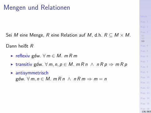
Inhalt
Kap. 1
Kap. 2
Kap. 3
3.1
3.2
3.3
Kap. 4
Kap. 5
Kap. 6
Kap. 7
Kap. 8
Kap. 9
Kap. 10
Kap. 11
Kap. 12
Kap. 13
Kap. 14
Kap. 15
Kap. 16
Kap. 17
Literatur
Anhang
A
Mengen und Relationen
Sei M eine Menge, R eine Relation auf M , d.h. R ⊆ M ×M .
Dann heißt R
I reflexiv gdw. ∀m ∈ M . m R m
I transitiv gdw. ∀m, n, p ∈ M . m R n ∧ n R p ⇒ m R p
I antisymmetrischgdw. ∀m, n ∈ M . m R n ∧ n R m ⇒ m = n
136/863
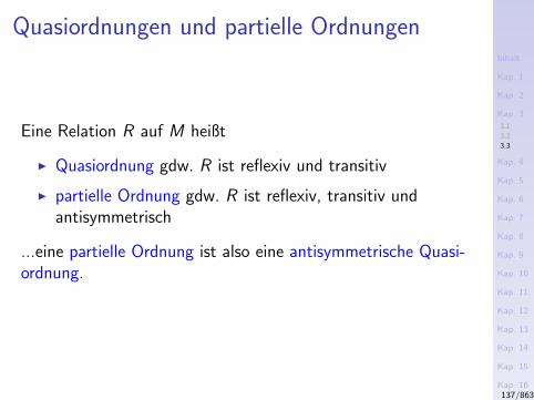
Inhalt
Kap. 1
Kap. 2
Kap. 3
3.1
3.2
3.3
Kap. 4
Kap. 5
Kap. 6
Kap. 7
Kap. 8
Kap. 9
Kap. 10
Kap. 11
Kap. 12
Kap. 13
Kap. 14
Kap. 15
Kap. 16
Kap. 17
Literatur
Anhang
A
Quasiordnungen und partielle Ordnungen
Eine Relation R auf M heißt
I Quasiordnung gdw. R ist reflexiv und transitiv
I partielle Ordnung gdw. R ist reflexiv, transitiv undantisymmetrisch
...eine partielle Ordnung ist also eine antisymmetrische Quasi-ordnung.
137/863
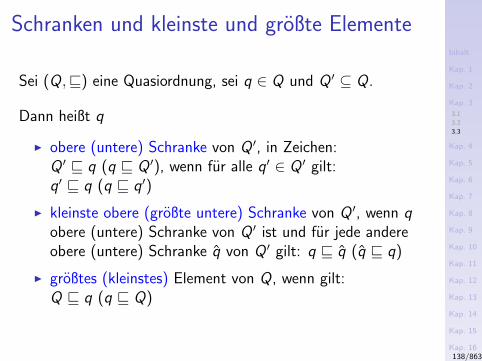
Inhalt
Kap. 1
Kap. 2
Kap. 3
3.1
3.2
3.3
Kap. 4
Kap. 5
Kap. 6
Kap. 7
Kap. 8
Kap. 9
Kap. 10
Kap. 11
Kap. 12
Kap. 13
Kap. 14
Kap. 15
Kap. 16
Kap. 17
Literatur
Anhang
A
Schranken und kleinste und großte Elemente
Sei (Q,v) eine Quasiordnung, sei q ∈ Q und Q ′ ⊆ Q.
Dann heißt q
I obere (untere) Schranke von Q ′, in Zeichen:Q ′ v q (q v Q ′), wenn fur alle q′ ∈ Q ′ gilt:q′ v q (q v q′)
I kleinste obere (großte untere) Schranke von Q ′, wenn qobere (untere) Schranke von Q ′ ist und fur jede andereobere (untere) Schranke q von Q ′ gilt: q v q (q v q)
I großtes (kleinstes) Element von Q, wenn gilt:Q v q (q v Q)
138/863

Inhalt
Kap. 1
Kap. 2
Kap. 3
3.1
3.2
3.3
Kap. 4
Kap. 5
Kap. 6
Kap. 7
Kap. 8
Kap. 9
Kap. 10
Kap. 11
Kap. 12
Kap. 13
Kap. 14
Kap. 15
Kap. 16
Kap. 17
Literatur
Anhang
A
Eindeutigkeit von Schranken und von kleinsten
und großten Elementen
I In partiellen Ordnungen sind kleinste obere und großteuntere Schranken eindeutig bestimmt, wenn sie existieren.
I Existenz (und damit Eindeutigkeit) vorausgesetzt, wirddie kleinste obere (großte untere) Schranke einer MengeP ′ ⊆ P der Grundmenge einer partiellen Ordnung (P ,v)mit tP ′ (uP ′) bezeichnet. Man spricht dann auch vomSupremum und Infimum von P ′.
I Analog fur kleinste und großte Elemente. Existenz voraus-gesetzt, werden sie ublicherweise mit ⊥ und > bezeichnet.
I Beachte: Fur Quasiordnungen gelten die vorstehendenAussagen nicht.
139/863
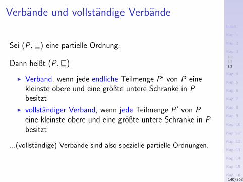
Inhalt
Kap. 1
Kap. 2
Kap. 3
3.1
3.2
3.3
Kap. 4
Kap. 5
Kap. 6
Kap. 7
Kap. 8
Kap. 9
Kap. 10
Kap. 11
Kap. 12
Kap. 13
Kap. 14
Kap. 15
Kap. 16
Kap. 17
Literatur
Anhang
A
Verbande und vollstandige Verbande
Sei (P ,v) eine partielle Ordnung.
Dann heißt (P ,v)
I Verband, wenn jede endliche Teilmenge P ′ von P einekleinste obere und eine großte untere Schranke in Pbesitzt
I vollstandiger Verband, wenn jede Teilmenge P ′ von Peine kleinste obere und eine großte untere Schranke in Pbesitzt
...(vollstandige) Verbande sind also spezielle partielle Ordnungen.
140/863
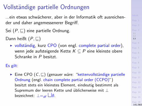
Inhalt
Kap. 1
Kap. 2
Kap. 3
3.1
3.2
3.3
Kap. 4
Kap. 5
Kap. 6
Kap. 7
Kap. 8
Kap. 9
Kap. 10
Kap. 11
Kap. 12
Kap. 13
Kap. 14
Kap. 15
Kap. 16
Kap. 17
Literatur
Anhang
A
Vollstandige partielle Ordnungen
...ein etwas schwacherer, aber in der Informatik oft ausreichen-der und daher angemessenerer Begriff.
Sei (P ,v) eine partielle Ordnung.
Dann heißt (P ,v)
I vollstandig, kurz CPO (von engl. complete partial order),wenn jede aufsteigende Kette K ⊆ P eine kleinste obereSchranke in P besitzt.
Es gilt:
I Eine CPO (C ,v) (genauer ware: “kettenvollstandige partielleOrdnung (engl. chain complete partial order (CCPO)”)besitzt stets ein kleinstes Element, eindeutig bestimmt alsSupremum der leeren Kette und ublicherweise mit ⊥bezeichnet: ⊥=df t∅.
141/863
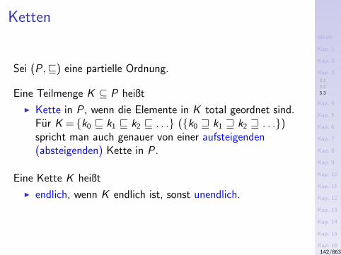
Inhalt
Kap. 1
Kap. 2
Kap. 3
3.1
3.2
3.3
Kap. 4
Kap. 5
Kap. 6
Kap. 7
Kap. 8
Kap. 9
Kap. 10
Kap. 11
Kap. 12
Kap. 13
Kap. 14
Kap. 15
Kap. 16
Kap. 17
Literatur
Anhang
A
Ketten
Sei (P ,v) eine partielle Ordnung.
Eine Teilmenge K ⊆ P heißt
I Kette in P , wenn die Elemente in K total geordnet sind.Fur K = k0 v k1 v k2 v . . . (k0 w k1 w k2 w . . .)spricht man auch genauer von einer aufsteigenden(absteigenden) Kette in P .
Eine Kette K heißt
I endlich, wenn K endlich ist, sonst unendlich.
142/863
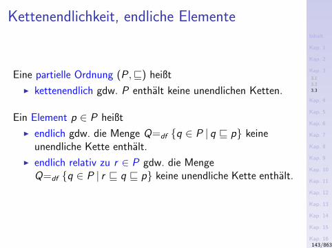
Inhalt
Kap. 1
Kap. 2
Kap. 3
3.1
3.2
3.3
Kap. 4
Kap. 5
Kap. 6
Kap. 7
Kap. 8
Kap. 9
Kap. 10
Kap. 11
Kap. 12
Kap. 13
Kap. 14
Kap. 15
Kap. 16
Kap. 17
Literatur
Anhang
A
Kettenendlichkeit, endliche Elemente
Eine partielle Ordnung (P ,v) heißt
I kettenendlich gdw. P enthalt keine unendlichen Ketten.
Ein Element p ∈ P heißt
I endlich gdw. die Menge Q=df q ∈ P | q v p keineunendliche Kette enthalt.
I endlich relativ zu r ∈ P gdw. die MengeQ=df q ∈ P | r v q v p keine unendliche Kette enthalt.
143/863
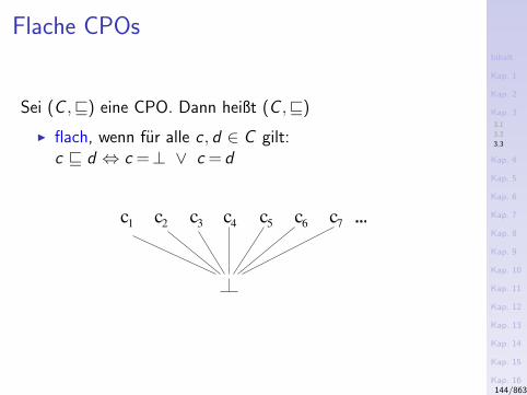
Inhalt
Kap. 1
Kap. 2
Kap. 3
3.1
3.2
3.3
Kap. 4
Kap. 5
Kap. 6
Kap. 7
Kap. 8
Kap. 9
Kap. 10
Kap. 11
Kap. 12
Kap. 13
Kap. 14
Kap. 15
Kap. 16
Kap. 17
Literatur
Anhang
A
Flache CPOs
Sei (C ,v) eine CPO. Dann heißt (C ,v)
I flach, wenn fur alle c , d ∈ C gilt:c v d ⇔ c =⊥ ∨ c = d
c1
c2
c3
c5
c7
c6
c4
144/863
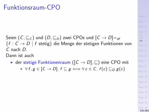
Inhalt
Kap. 1
Kap. 2
Kap. 3
3.1
3.2
3.3
Kap. 4
Kap. 5
Kap. 6
Kap. 7
Kap. 8
Kap. 9
Kap. 10
Kap. 11
Kap. 12
Kap. 13
Kap. 14
Kap. 15
Kap. 16
Kap. 17
Literatur
Anhang
A
Funktionsraum-CPO
Seien (C ,vC ) und (D,vD) zwei CPOs und [C → D]=df
f : C → D | f stetig die Menge der stetigen Funktionen vonC nach D.Dann ist auch
I der stetige Funktionenraum ([C → D],v) eine CPO mitI ∀ f , g ∈ [C → D]. f v g ⇐⇒ ∀ c ∈ C . f (c) vD g(c)
145/863
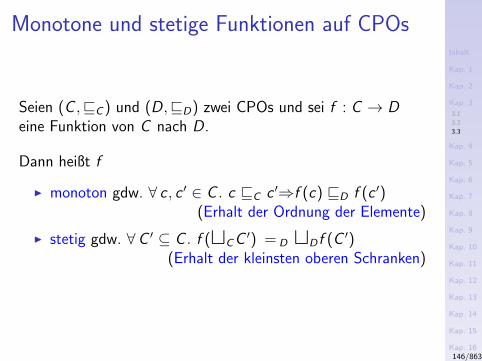
Inhalt
Kap. 1
Kap. 2
Kap. 3
3.1
3.2
3.3
Kap. 4
Kap. 5
Kap. 6
Kap. 7
Kap. 8
Kap. 9
Kap. 10
Kap. 11
Kap. 12
Kap. 13
Kap. 14
Kap. 15
Kap. 16
Kap. 17
Literatur
Anhang
A
Monotone und stetige Funktionen auf CPOs
Seien (C ,vC ) und (D,vD) zwei CPOs und sei f : C → Deine Funktion von C nach D.
Dann heißt f
I monoton gdw. ∀ c , c ′ ∈ C . c vC c ′⇒f (c) vD f (c ′)(Erhalt der Ordnung der Elemente)
I stetig gdw. ∀C ′ ⊆ C . f (tCC ′) = D tD f (C ′)(Erhalt der kleinsten oberen Schranken)
146/863
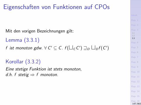
Inhalt
Kap. 1
Kap. 2
Kap. 3
3.1
3.2
3.3
Kap. 4
Kap. 5
Kap. 6
Kap. 7
Kap. 8
Kap. 9
Kap. 10
Kap. 11
Kap. 12
Kap. 13
Kap. 14
Kap. 15
Kap. 16
Kap. 17
Literatur
Anhang
A
Eigenschaften von Funktionen auf CPOs
Mit den vorigen Bezeichnungen gilt:
Lemma (3.3.1)
f ist monoton gdw. ∀C ′ ⊆ C . f (tCC ′) wD tD f (C ′)
Korollar (3.3.2)
Eine stetige Funktion ist stets monoton,d.h. f stetig ⇒ f monoton.
147/863
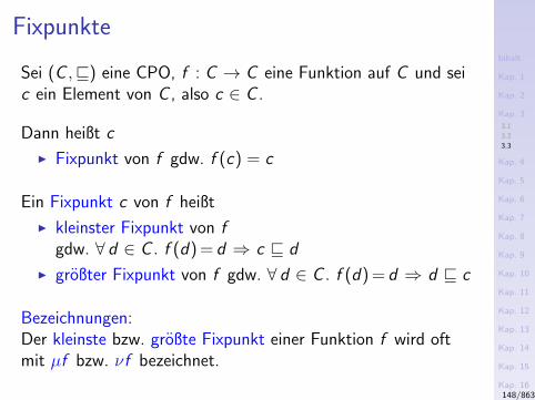
Inhalt
Kap. 1
Kap. 2
Kap. 3
3.1
3.2
3.3
Kap. 4
Kap. 5
Kap. 6
Kap. 7
Kap. 8
Kap. 9
Kap. 10
Kap. 11
Kap. 12
Kap. 13
Kap. 14
Kap. 15
Kap. 16
Kap. 17
Literatur
Anhang
A
Fixpunkte
Sei (C ,v) eine CPO, f : C → C eine Funktion auf C und seic ein Element von C , also c ∈ C .
Dann heißt c
I Fixpunkt von f gdw. f (c) = c
Ein Fixpunkt c von f heißt
I kleinster Fixpunkt von fgdw. ∀ d ∈ C . f (d) = d ⇒ c v d
I großter Fixpunkt von f gdw. ∀ d ∈ C . f (d) = d ⇒ d v c
Bezeichnungen:Der kleinste bzw. großte Fixpunkt einer Funktion f wird oftmit µf bzw. νf bezeichnet.
148/863
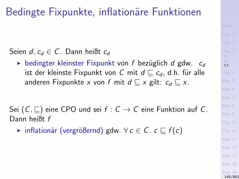
Inhalt
Kap. 1
Kap. 2
Kap. 3
3.1
3.2
3.3
Kap. 4
Kap. 5
Kap. 6
Kap. 7
Kap. 8
Kap. 9
Kap. 10
Kap. 11
Kap. 12
Kap. 13
Kap. 14
Kap. 15
Kap. 16
Kap. 17
Literatur
Anhang
A
Bedingte Fixpunkte, inflationare Funktionen
Seien d , cd ∈ C . Dann heißt cdI bedingter kleinster Fixpunkt von f bezuglich d gdw. cd
ist der kleinste Fixpunkt von C mit d v cd , d.h. fur alleanderen Fixpunkte x von f mit d v x gilt: cd v x .
Sei (C ,v) eine CPO und sei f : C → C eine Funktion auf C .Dann heißt f
I inflationar (vergroßernd) gdw. ∀ c ∈ C . c v f (c)
149/863
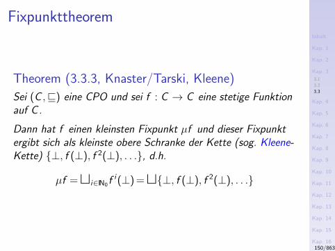
Inhalt
Kap. 1
Kap. 2
Kap. 3
3.1
3.2
3.3
Kap. 4
Kap. 5
Kap. 6
Kap. 7
Kap. 8
Kap. 9
Kap. 10
Kap. 11
Kap. 12
Kap. 13
Kap. 14
Kap. 15
Kap. 16
Kap. 17
Literatur
Anhang
A
Fixpunkttheorem
Theorem (3.3.3, Knaster/Tarski, Kleene)
Sei (C ,v) eine CPO und sei f : C → C eine stetige Funktionauf C .
Dann hat f einen kleinsten Fixpunkt µf und dieser Fixpunktergibt sich als kleinste obere Schranke der Kette (sog. Kleene-Kette) ⊥, f (⊥), f 2(⊥), . . ., d.h.
µf =ti∈IN0f i(⊥) =t⊥, f (⊥), f 2(⊥), . . .
150/863
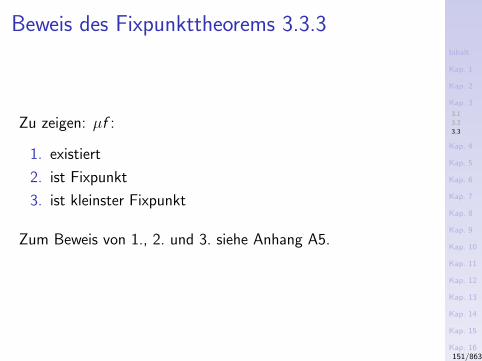
Inhalt
Kap. 1
Kap. 2
Kap. 3
3.1
3.2
3.3
Kap. 4
Kap. 5
Kap. 6
Kap. 7
Kap. 8
Kap. 9
Kap. 10
Kap. 11
Kap. 12
Kap. 13
Kap. 14
Kap. 15
Kap. 16
Kap. 17
Literatur
Anhang
A
Beweis des Fixpunkttheorems 3.3.3
Zu zeigen: µf :
1. existiert
2. ist Fixpunkt
3. ist kleinster Fixpunkt
Zum Beweis von 1., 2. und 3. siehe Anhang A5.
151/863
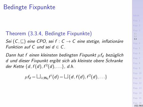
Inhalt
Kap. 1
Kap. 2
Kap. 3
3.1
3.2
3.3
Kap. 4
Kap. 5
Kap. 6
Kap. 7
Kap. 8
Kap. 9
Kap. 10
Kap. 11
Kap. 12
Kap. 13
Kap. 14
Kap. 15
Kap. 16
Kap. 17
Literatur
Anhang
A
Bedingte Fixpunkte
Theorem (3.3.4, Bedingte Fixpunkte)
Sei (C ,v) eine CPO, sei f : C → C eine stetige, inflationareFunktion auf C und sei d ∈ C .
Dann hat f einen kleinsten bedingten Fixpunkt µfd bezuglichd und dieser Fixpunkt ergibt sich als kleinste obere Schrankeder Kette d , f (d), f 2(d), . . ., d.h.
µfd =ti∈IN0f i(d) =td , f (d), f 2(d), . . .
152/863
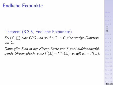
Inhalt
Kap. 1
Kap. 2
Kap. 3
3.1
3.2
3.3
Kap. 4
Kap. 5
Kap. 6
Kap. 7
Kap. 8
Kap. 9
Kap. 10
Kap. 11
Kap. 12
Kap. 13
Kap. 14
Kap. 15
Kap. 16
Kap. 17
Literatur
Anhang
A
Endliche Fixpunkte
Theorem (3.3.5, Endliche Fixpunkte)
Sei (C ,v) eine CPO und sei f : C → C eine stetige Funktionauf C .
Dann gilt: Sind in der Kleene-Kette von f zwei aufeinanderfol-gende Glieder gleich, etwa f i(⊥) = f i+1(⊥), so gilt µf = f i(⊥).
153/863
Inhalt
Kap. 1
Kap. 2
Kap. 3
3.1
3.2
3.3
Kap. 4
Kap. 5
Kap. 6
Kap. 7
Kap. 8
Kap. 9
Kap. 10
Kap. 11
Kap. 12
Kap. 13
Kap. 14
Kap. 15
Kap. 16
Kap. 17
Literatur
Anhang
A
Existenz endlicher Fixpunkte
Hinreichende Bedingungen fur die Existenz endlicher Fixpunktesind:
I Endlichkeit von Definitions- und Wertebereich von f
I f ist von der Form f (c) = c t g(c) fur monotones g uberkettenendlichem Wertebereich
154/863
Inhalt
Kap. 1
Kap. 2
Kap. 3
3.1
3.2
3.3
Kap. 4
Kap. 5
Kap. 6
Kap. 7
Kap. 8
Kap. 9
Kap. 10
Kap. 11
Kap. 12
Kap. 13
Kap. 14
Kap. 15
Kap. 16
Kap. 17
Literatur
Anhang
A
Vertiefende und weiterfuhrende Leseempfeh-
lungen fur Kapitel 3
Michael J.C. Gordon. The Denotational Description ofProgramming Languages. Springer-V., 1979.
Hanne Riis Nielson, Flemming Nielson. Semantics withApplications: A Formal Introduction. Wiley, 1992.(Chapter 4, Denotational Semantics)
Hanne Riis Nielson, Flemming Nielson. Semantics withApplications: An Appetizer. Springer-V., 2007. (Chapter5, Denotational Semantics; Chapter 6, More on Denota-tional Semantics)
Joseph E. Stoy. Denotational Semantics: The Scott-Strachey Approach to Programming Language Theory.MIT Press, 1981.
155/863

Inhalt
Kap. 1
Kap. 2
Kap. 3
Kap. 4
4.1
4.2
4.3
4.4
4.5
4.6
4.7
4.8
Kap. 5
Kap. 6
Kap. 7
Kap. 8
Kap. 9
Kap. 10
Kap. 11
Kap. 12
Kap. 13
Kap. 14
Kap. 15
Kap. 16
Kap. 17
Literatur
Anhang
A
Kapitel 4
Axiomatische Semantik von WHILE
156/863
Inhalt
Kap. 1
Kap. 2
Kap. 3
Kap. 4
4.1
4.2
4.3
4.4
4.5
4.6
4.7
4.8
Kap. 5
Kap. 6
Kap. 7
Kap. 8
Kap. 9
Kap. 10
Kap. 11
Kap. 12
Kap. 13
Kap. 14
Kap. 15
Kap. 16
Kap. 17
Literatur
Anhang
A
Axiomatische Semantik von WHILE
...bestimmte Eigenschaften des Effekts der Ausfuhrung eines
Konstrukts werden als Zusicherungen ausgedruckt. Bestimmte
andere Aspekte der Ausfuhrung werden dabei i.a. ignoriert.
157/863
Inhalt
Kap. 1
Kap. 2
Kap. 3
Kap. 4
4.1
4.2
4.3
4.4
4.5
4.6
4.7
4.8
Kap. 5
Kap. 6
Kap. 7
Kap. 8
Kap. 9
Kap. 10
Kap. 11
Kap. 12
Kap. 13
Kap. 14
Kap. 15
Kap. 16
Kap. 17
Literatur
Anhang
A
Axiomatische Semantik
Wir betrachten insbesondere: Korrektheit und Vollstandigkeitder axiomatischen Semantik
Erinnerung:
I Hoare-Tripel (syntaktische Sicht) bzw.Korrektheitsformeln (semantische Sicht) der Form
p π q bzw. [p] π [q]
I Gultigkeit einer Korrektheitsformel im SinneI partieller KorrektheitI totaler Korrektheit
158/863
Inhalt
Kap. 1
Kap. 2
Kap. 3
Kap. 4
4.1
4.2
4.3
4.4
4.5
4.6
4.7
4.8
Kap. 5
Kap. 6
Kap. 7
Kap. 8
Kap. 9
Kap. 10
Kap. 11
Kap. 12
Kap. 13
Kap. 14
Kap. 15
Kap. 16
Kap. 17
Literatur
Anhang
A
Zwei wegbereitende klassische Arbeiten
I Robert W. Floyd. Assigning Meaning to Programs.Proceedings of Symposium on Applied Mathematics,Mathematical Aspects of Computer Science, AmericanMathematical Society, New York, Vol. 19, 19-32, 1967.
I Charles A.R. Hoare. An Axiomatic Basis for ComputerProgramming. Communications of the ACM 12:576-580,583, 1969.
159/863

Inhalt
Kap. 1
Kap. 2
Kap. 3
Kap. 4
4.1
4.2
4.3
4.4
4.5
4.6
4.7
4.8
Kap. 5
Kap. 6
Kap. 7
Kap. 8
Kap. 9
Kap. 10
Kap. 11
Kap. 12
Kap. 13
Kap. 14
Kap. 15
Kap. 16
Kap. 17
Literatur
Anhang
A
Kapitel 4.1
Partielle und totale Korrektheit
160/863
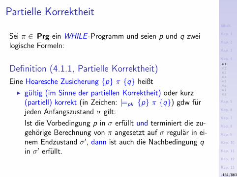
Inhalt
Kap. 1
Kap. 2
Kap. 3
Kap. 4
4.1
4.2
4.3
4.4
4.5
4.6
4.7
4.8
Kap. 5
Kap. 6
Kap. 7
Kap. 8
Kap. 9
Kap. 10
Kap. 11
Kap. 12
Kap. 13
Kap. 14
Kap. 15
Kap. 16
Kap. 17
Literatur
Anhang
A
Partielle Korrektheit
Sei π ∈ Prg ein WHILE -Programm und seien p und q zweilogische Formeln:
Definition (4.1.1, Partielle Korrektheit)
Eine Hoaresche Zusicherung p π q heißt
I gultig (im Sinne der partiellen Korrektheit) oder kurz(partiell) korrekt (in Zeichen: |=pk p π q) gdw furjeden Anfangszustand σ gilt:
Ist die Vorbedingung p in σ erfullt und terminiert die zu-gehorige Berechnung von π angesetzt auf σ regular in ei-nem Endzustand σ′, dann ist auch die Nachbedingung qin σ′ erfullt.
161/863
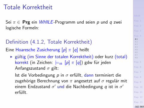
Inhalt
Kap. 1
Kap. 2
Kap. 3
Kap. 4
4.1
4.2
4.3
4.4
4.5
4.6
4.7
4.8
Kap. 5
Kap. 6
Kap. 7
Kap. 8
Kap. 9
Kap. 10
Kap. 11
Kap. 12
Kap. 13
Kap. 14
Kap. 15
Kap. 16
Kap. 17
Literatur
Anhang
A
Totale Korrektheit
Sei π ∈ Prg ein WHILE -Programm und seien p und q zweilogische Formeln:
Definition (4.1.2, Totale Korrektheit)
Eine Hoaresche Zusicherung [p] π [q] heißt
I gultig (im Sinne der totalen Korrektheit) oder kurz (total)korrekt (in Zeichen: |=tk [p] π [q]) gdw fur jedenAnfangszustand σ gilt:
Ist die Vorbedingung p in σ erfullt, dann terminiert diezugehorige Berechnung von π angesetzt auf σ regular miteinem Endzustand σ′ und die Nachbedingung q ist in σ′
erfullt.
162/863
Inhalt
Kap. 1
Kap. 2
Kap. 3
Kap. 4
4.1
4.2
4.3
4.4
4.5
4.6
4.7
4.8
Kap. 5
Kap. 6
Kap. 7
Kap. 8
Kap. 9
Kap. 10
Kap. 11
Kap. 12
Kap. 13
Kap. 14
Kap. 15
Kap. 16
Kap. 17
Literatur
Anhang
A
Informell
“Totale Korrektheit = Partielle Korrektheit + Terminierung”
163/863
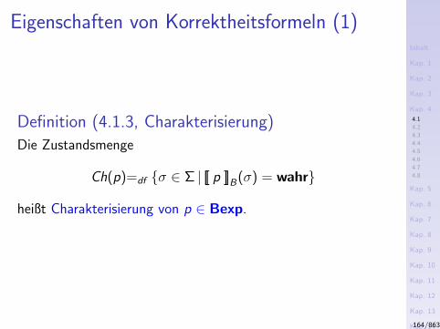
Inhalt
Kap. 1
Kap. 2
Kap. 3
Kap. 4
4.1
4.2
4.3
4.4
4.5
4.6
4.7
4.8
Kap. 5
Kap. 6
Kap. 7
Kap. 8
Kap. 9
Kap. 10
Kap. 11
Kap. 12
Kap. 13
Kap. 14
Kap. 15
Kap. 16
Kap. 17
Literatur
Anhang
A
Eigenschaften von Korrektheitsformeln (1)
Definition (4.1.3, Charakterisierung)
Die Zustandsmenge
Ch(p)=df σ ∈ Σ | [[ p ]]B(σ) = wahr
heißt Charakterisierung von p ∈ Bexp.
164/863
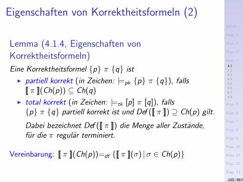
Inhalt
Kap. 1
Kap. 2
Kap. 3
Kap. 4
4.1
4.2
4.3
4.4
4.5
4.6
4.7
4.8
Kap. 5
Kap. 6
Kap. 7
Kap. 8
Kap. 9
Kap. 10
Kap. 11
Kap. 12
Kap. 13
Kap. 14
Kap. 15
Kap. 16
Kap. 17
Literatur
Anhang
A
Eigenschaften von Korrektheitsformeln (2)
Lemma (4.1.4, Eigenschaften vonKorrektheitsformeln)
Eine Korrektheitsformel p π q ist
I partiell korrekt (in Zeichen: |=pk p π q), falls[[ π ]](Ch(p)) ⊆ Ch(q)
I total korrekt (in Zeichen: |=tk [p] π [q]), fallsp π q partiell korrekt ist und Def ([[ π ]]) ⊇ Ch(p) gilt.
Dabei bezeichnet Def ([[ π ]]) die Menge aller Zustande,fur die π regular terminiert.
Vereinbarung: [[ π ]](Ch(p))=df [[ π ]](σ) |σ ∈ Ch(p)
165/863
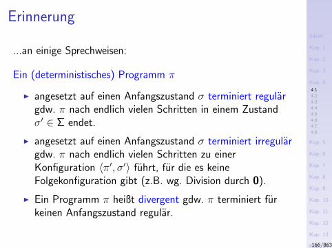
Inhalt
Kap. 1
Kap. 2
Kap. 3
Kap. 4
4.1
4.2
4.3
4.4
4.5
4.6
4.7
4.8
Kap. 5
Kap. 6
Kap. 7
Kap. 8
Kap. 9
Kap. 10
Kap. 11
Kap. 12
Kap. 13
Kap. 14
Kap. 15
Kap. 16
Kap. 17
Literatur
Anhang
A
Erinnerung
...an einige Sprechweisen:
Ein (deterministisches) Programm π
I angesetzt auf einen Anfangszustand σ terminiert regulargdw. π nach endlich vielen Schritten in einem Zustandσ′ ∈ Σ endet.
I angesetzt auf einen Anfangszustand σ terminiert irregulargdw. π nach endlich vielen Schritten zu einerKonfiguration 〈π′, σ′〉 fuhrt, fur die es keineFolgekonfiguration gibt (z.B. wg. Division durch 0).
I Ein Programm π heißt divergent gdw. π terminiert furkeinen Anfangszustand regular.
166/863
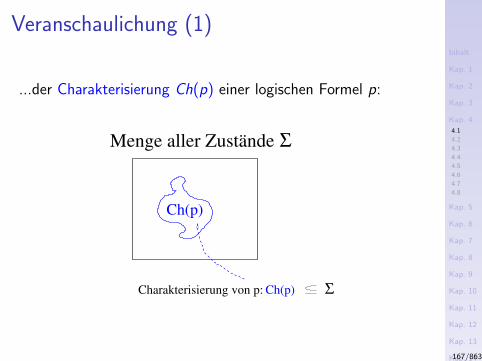
Inhalt
Kap. 1
Kap. 2
Kap. 3
Kap. 4
4.1
4.2
4.3
4.4
4.5
4.6
4.7
4.8
Kap. 5
Kap. 6
Kap. 7
Kap. 8
Kap. 9
Kap. 10
Kap. 11
Kap. 12
Kap. 13
Kap. 14
Kap. 15
Kap. 16
Kap. 17
Literatur
Anhang
A
Veranschaulichung (1)
...der Charakterisierung Ch(p) einer logischen Formel p:
Charakterisierung von p: Ch(p) Σ
ΣMenge aller Zustände
Ch(p)
167/863

Inhalt
Kap. 1
Kap. 2
Kap. 3
Kap. 4
4.1
4.2
4.3
4.4
4.5
4.6
4.7
4.8
Kap. 5
Kap. 6
Kap. 7
Kap. 8
Kap. 9
Kap. 10
Kap. 11
Kap. 12
Kap. 13
Kap. 14
Kap. 15
Kap. 16
Kap. 17
Literatur
Anhang
A
Veranschaulichung (2)
...der Gultigkeit eine Hoareschen Zusicherung p π q imSinne partieller Korrektheit:
πDef( )
Σπ
π π
π π
ΣMenge aller Zustände
Ch(p)Ch(q)
Definitionsbereich von π :
Charakterisierung von p: Ch(p) Σ
)Def(
Bild von für Def( )
Bild von für )Def( Ch(p)
168/863
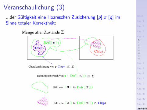
Inhalt
Kap. 1
Kap. 2
Kap. 3
Kap. 4
4.1
4.2
4.3
4.4
4.5
4.6
4.7
4.8
Kap. 5
Kap. 6
Kap. 7
Kap. 8
Kap. 9
Kap. 10
Kap. 11
Kap. 12
Kap. 13
Kap. 14
Kap. 15
Kap. 16
Kap. 17
Literatur
Anhang
A
Veranschaulichung (3)
...der Gultigkeit eine Hoareschen Zusicherung [p] π [q] imSinne totaler Korrektheit:
πDef( )
Σπ
π π
π π
ΣMenge aller Zustände
Ch(p)Ch(q)
Definitionsbereich von π :
Charakterisierung von p: Ch(p) Σ
)Def(
Bild von für Def( )
Bild von für )Def( Ch(p)
169/863

Inhalt
Kap. 1
Kap. 2
Kap. 3
Kap. 4
4.1
4.2
4.3
4.4
4.5
4.6
4.7
4.8
Kap. 5
Kap. 6
Kap. 7
Kap. 8
Kap. 9
Kap. 10
Kap. 11
Kap. 12
Kap. 13
Kap. 14
Kap. 15
Kap. 16
Kap. 17
Literatur
Anhang
A
Starkste Nachbedingungen, schwachste
Vorbedingungen
In der Folge:
Prazisierung der Begriffe
I Starkste Nachbedingung
I Schwachste (liberale) Vorbedingung
170/863
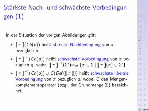
Inhalt
Kap. 1
Kap. 2
Kap. 3
Kap. 4
4.1
4.2
4.3
4.4
4.5
4.6
4.7
4.8
Kap. 5
Kap. 6
Kap. 7
Kap. 8
Kap. 9
Kap. 10
Kap. 11
Kap. 12
Kap. 13
Kap. 14
Kap. 15
Kap. 16
Kap. 17
Literatur
Anhang
A
Starkste Nach- und schwachste Vorbedingun-
gen (1)
In der Situation der vorigen Abbildungen gilt:
I [[ π ]](Ch(p)) heißt starkste Nachbedingung von πbezuglich p.
I [[ π ]]−1(Ch(q)) heißt schwachste Vorbedingung von π be-zuglich q, wobei [[ π ]]−1(Σ′)=df σ ∈ Σ | [[ π ]](σ) ∈ Σ′
I [[ π ]]−1(Ch(q)) ∪ C (Def ([[ π ]])) heißt schwachste liberaleVorbedingung von π bezuglich q, wobei C den Mengen-komplementoperator (bzgl. der Grundmenge Σ) bezeich-net.
171/863
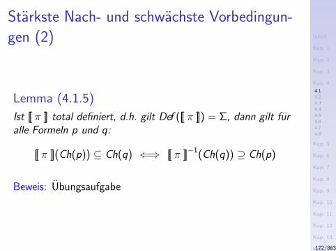
Inhalt
Kap. 1
Kap. 2
Kap. 3
Kap. 4
4.1
4.2
4.3
4.4
4.5
4.6
4.7
4.8
Kap. 5
Kap. 6
Kap. 7
Kap. 8
Kap. 9
Kap. 10
Kap. 11
Kap. 12
Kap. 13
Kap. 14
Kap. 15
Kap. 16
Kap. 17
Literatur
Anhang
A
Starkste Nach- und schwachste Vorbedingun-
gen (2)
Lemma (4.1.5)
Ist [[ π ]] total definiert, d.h. gilt Def ([[ π ]]) = Σ, dann gilt furalle Formeln p und q:
[[ π ]](Ch(p)) ⊆ Ch(q) ⇐⇒ [[ π ]]−1(Ch(q)) ⊇ Ch(p)
Beweis: Ubungsaufgabe
172/863
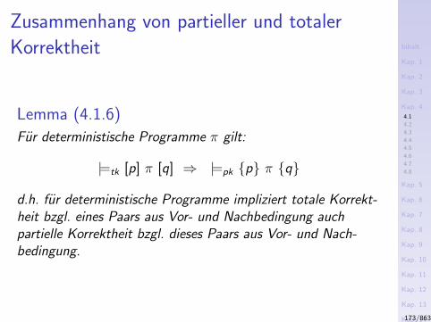
Inhalt
Kap. 1
Kap. 2
Kap. 3
Kap. 4
4.1
4.2
4.3
4.4
4.5
4.6
4.7
4.8
Kap. 5
Kap. 6
Kap. 7
Kap. 8
Kap. 9
Kap. 10
Kap. 11
Kap. 12
Kap. 13
Kap. 14
Kap. 15
Kap. 16
Kap. 17
Literatur
Anhang
A
Zusammenhang von partieller und totaler
Korrektheit
Lemma (4.1.6)
Fur deterministische Programme π gilt:
|=tk [p] π [q] ⇒ |=pk p π q
d.h. fur deterministische Programme impliziert totale Korrekt-heit bzgl. eines Paars aus Vor- und Nachbedingung auchpartielle Korrektheit bzgl. dieses Paars aus Vor- und Nach-bedingung.
173/863
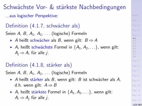
Inhalt
Kap. 1
Kap. 2
Kap. 3
Kap. 4
4.1
4.2
4.3
4.4
4.5
4.6
4.7
4.8
Kap. 5
Kap. 6
Kap. 7
Kap. 8
Kap. 9
Kap. 10
Kap. 11
Kap. 12
Kap. 13
Kap. 14
Kap. 15
Kap. 16
Kap. 17
Literatur
Anhang
A
Schwachste Vor- & starkste Nachbedingungen...aus logischer Perspektive:
Definition (4.1.7, schwacher als)
Seien A, B , A1, A2, . . . (logische) Formeln
I A heißt schwacher als B , wenn gilt: B⇒A
I Ai heißt schwachste Formel in A1,A2, . . ., wenn gilt:Aj⇒Ai fur alle j .
Definition (4.1.8, starker als)
Seien A, B , A1, A2, . . . (logische) Formeln
I A heißt starker als B , wenn gilt: B ist schwacher als A,d.h. wenn gilt: A⇒B
I Ai heißt starkste Formel in A1,A2, . . ., wenn gilt:Ai⇒Aj fur alle j .
174/863
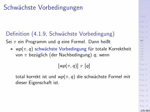
Inhalt
Kap. 1
Kap. 2
Kap. 3
Kap. 4
4.1
4.2
4.3
4.4
4.5
4.6
4.7
4.8
Kap. 5
Kap. 6
Kap. 7
Kap. 8
Kap. 9
Kap. 10
Kap. 11
Kap. 12
Kap. 13
Kap. 14
Kap. 15
Kap. 16
Kap. 17
Literatur
Anhang
A
Schwachste Vorbedingungen
Definition (4.1.9, Schwachste Vorbedingung)
Sei π ein Programm und q eine Formel. Dann heißt
I wp(π, q) schwachste Vorbedingung fur totale Korrektheitvon π bezuglich (der Nachbedingung) q, wenn
[wp(π, q)] π [q]
total korrekt ist und wp(π, q) die schwachste Formel mitdieser Eigenschaft ist.
175/863
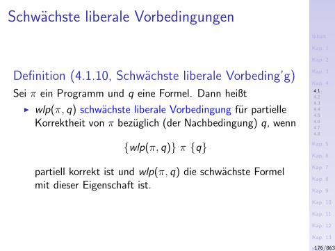
Inhalt
Kap. 1
Kap. 2
Kap. 3
Kap. 4
4.1
4.2
4.3
4.4
4.5
4.6
4.7
4.8
Kap. 5
Kap. 6
Kap. 7
Kap. 8
Kap. 9
Kap. 10
Kap. 11
Kap. 12
Kap. 13
Kap. 14
Kap. 15
Kap. 16
Kap. 17
Literatur
Anhang
A
Schwachste liberale Vorbedingungen
Definition (4.1.10, Schwachste liberale Vorbeding’g)
Sei π ein Programm und q eine Formel. Dann heißt
I wlp(π, q) schwachste liberale Vorbedingung fur partielleKorrektheit von π bezuglich (der Nachbedingung) q, wenn
wlp(π, q) π q
partiell korrekt ist und wlp(π, q) die schwachste Formelmit dieser Eigenschaft ist.
176/863
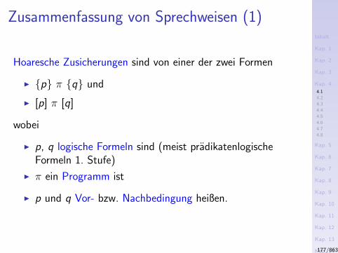
Inhalt
Kap. 1
Kap. 2
Kap. 3
Kap. 4
4.1
4.2
4.3
4.4
4.5
4.6
4.7
4.8
Kap. 5
Kap. 6
Kap. 7
Kap. 8
Kap. 9
Kap. 10
Kap. 11
Kap. 12
Kap. 13
Kap. 14
Kap. 15
Kap. 16
Kap. 17
Literatur
Anhang
A
Zusammenfassung von Sprechweisen (1)
Hoaresche Zusicherungen sind von einer der zwei Formen
I p π q und
I [p] π [q]
wobei
I p, q logische Formeln sind (meist pradikatenlogischeFormeln 1. Stufe)
I π ein Programm ist
I p und q Vor- bzw. Nachbedingung heißen.
177/863
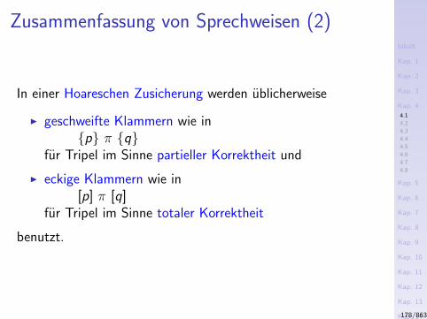
Inhalt
Kap. 1
Kap. 2
Kap. 3
Kap. 4
4.1
4.2
4.3
4.4
4.5
4.6
4.7
4.8
Kap. 5
Kap. 6
Kap. 7
Kap. 8
Kap. 9
Kap. 10
Kap. 11
Kap. 12
Kap. 13
Kap. 14
Kap. 15
Kap. 16
Kap. 17
Literatur
Anhang
A
Zusammenfassung von Sprechweisen (2)
In einer Hoareschen Zusicherung werden ublicherweise
I geschweifte Klammern wie inp π q
fur Tripel im Sinne partieller Korrektheit und
I eckige Klammern wie in[p] π [q]
fur Tripel im Sinne totaler Korrektheit
benutzt.
178/863
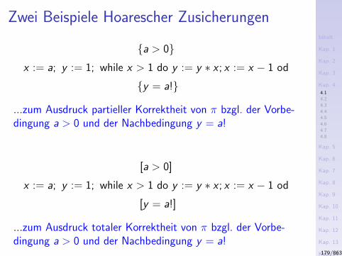
Inhalt
Kap. 1
Kap. 2
Kap. 3
Kap. 4
4.1
4.2
4.3
4.4
4.5
4.6
4.7
4.8
Kap. 5
Kap. 6
Kap. 7
Kap. 8
Kap. 9
Kap. 10
Kap. 11
Kap. 12
Kap. 13
Kap. 14
Kap. 15
Kap. 16
Kap. 17
Literatur
Anhang
A
Zwei Beispiele Hoarescher Zusicherungen
a > 0x := a; y := 1; while x > 1 do y := y ∗ x ; x := x − 1 od
y = a!
...zum Ausdruck partieller Korrektheit von π bzgl. der Vorbe-dingung a > 0 und der Nachbedingung y = a!
[a > 0]
x := a; y := 1; while x > 1 do y := y ∗ x ; x := x − 1 od
[y = a!]
...zum Ausdruck totaler Korrektheit von π bzgl. der Vorbe-dingung a > 0 und der Nachbedingung y = a!
179/863
Inhalt
Kap. 1
Kap. 2
Kap. 3
Kap. 4
4.1
4.2
4.3
4.4
4.5
4.6
4.7
4.8
Kap. 5
Kap. 6
Kap. 7
Kap. 8
Kap. 9
Kap. 10
Kap. 11
Kap. 12
Kap. 13
Kap. 14
Kap. 15
Kap. 16
Kap. 17
Literatur
Anhang
A
Kapitel 4.2
Beweiskalkul fur partielle Korrektheit
180/863
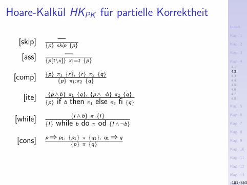
Inhalt
Kap. 1
Kap. 2
Kap. 3
Kap. 4
4.1
4.2
4.3
4.4
4.5
4.6
4.7
4.8
Kap. 5
Kap. 6
Kap. 7
Kap. 8
Kap. 9
Kap. 10
Kap. 11
Kap. 12
Kap. 13
Kap. 14
Kap. 15
Kap. 16
Kap. 17
Literatur
Anhang
A
Hoare-Kalkul HKPK fur partielle Korrektheit
[skip] —p skip p
[ass] —p[t\x] x :=t p
[comp] p π1 r, r π2 qp π1;π2 q
[ite] p ∧ b π1 q, p ∧¬b π2 qp if b then π1 else π2 fi q
[while] I ∧ b π II while b do π od I ∧¬b
[cons] p⇒ p1, p1 π q1, q1⇒ qp π q
181/863
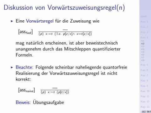
Inhalt
Kap. 1
Kap. 2
Kap. 3
Kap. 4
4.1
4.2
4.3
4.4
4.5
4.6
4.7
4.8
Kap. 5
Kap. 6
Kap. 7
Kap. 8
Kap. 9
Kap. 10
Kap. 11
Kap. 12
Kap. 13
Kap. 14
Kap. 15
Kap. 16
Kap. 17
Literatur
Anhang
A
Diskussion von Vorwartszuweisungsregel(n)
I Eine Vorwartsregel fur die Zuweisung wie
[assfwd ] —p x :=t ∃ z. p[z/x]∧ x=t[z/x]
mag naturlich erscheinen, ist aber beweistechnischunangenehm durch das Mitschleppen quantifizierterFormeln.
I Beachte: Folgende scheinbar naheliegende quantorfreieRealisierung der Vorwartszuweisungsregel ist nichtkorrekt:
[assnaive ] —p x :=t p[t/x]
Beweis: Ubungsaufgabe
182/863
Inhalt
Kap. 1
Kap. 2
Kap. 3
Kap. 4
4.1
4.2
4.3
4.4
4.5
4.6
4.7
4.8
Kap. 5
Kap. 6
Kap. 7
Kap. 8
Kap. 9
Kap. 10
Kap. 11
Kap. 12
Kap. 13
Kap. 14
Kap. 15
Kap. 16
Kap. 17
Literatur
Anhang
A
Kapitel 4.3
Beweiskalkul fur totale Korrektheit
183/863
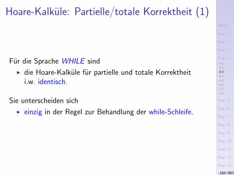
Inhalt
Kap. 1
Kap. 2
Kap. 3
Kap. 4
4.1
4.2
4.3
4.4
4.5
4.6
4.7
4.8
Kap. 5
Kap. 6
Kap. 7
Kap. 8
Kap. 9
Kap. 10
Kap. 11
Kap. 12
Kap. 13
Kap. 14
Kap. 15
Kap. 16
Kap. 17
Literatur
Anhang
A
Hoare-Kalkule: Partielle/totale Korrektheit (1)
Fur die Sprache WHILE sind
I die Hoare-Kalkule fur partielle und totale Korrektheiti.w. identisch.
Sie unterscheiden sich
I einzig in der Regel zur Behandlung der while-Schleife.
184/863
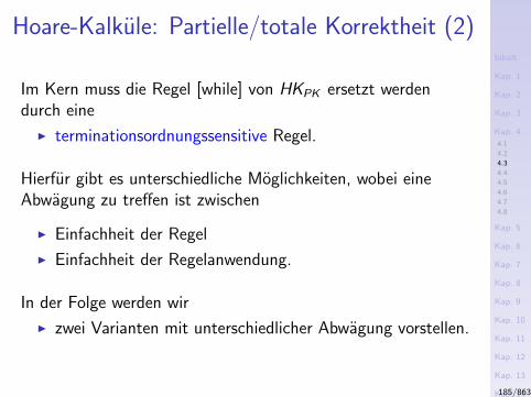
Inhalt
Kap. 1
Kap. 2
Kap. 3
Kap. 4
4.1
4.2
4.3
4.4
4.5
4.6
4.7
4.8
Kap. 5
Kap. 6
Kap. 7
Kap. 8
Kap. 9
Kap. 10
Kap. 11
Kap. 12
Kap. 13
Kap. 14
Kap. 15
Kap. 16
Kap. 17
Literatur
Anhang
A
Hoare-Kalkule: Partielle/totale Korrektheit (2)
Im Kern muss die Regel [while] von HKPK ersetzt werdendurch eine
I terminationsordnungssensitive Regel.
Hierfur gibt es unterschiedliche Moglichkeiten, wobei eineAbwagung zu treffen ist zwischen
I Einfachheit der Regel
I Einfachheit der Regelanwendung.
In der Folge werden wir
I zwei Varianten mit unterschiedlicher Abwagung vorstellen.
185/863
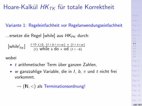
Inhalt
Kap. 1
Kap. 2
Kap. 3
Kap. 4
4.1
4.2
4.3
4.4
4.5
4.6
4.7
4.8
Kap. 5
Kap. 6
Kap. 7
Kap. 8
Kap. 9
Kap. 10
Kap. 11
Kap. 12
Kap. 13
Kap. 14
Kap. 15
Kap. 16
Kap. 17
Literatur
Anhang
A
Hoare-Kalkul HKTK fur totale Korrektheit
Variante 1: Regeleinfachheit vor Regelanwendungseinfachheit
...ersetze die Regel [while] aus HKPK durch:
[while′TK ] I⇒ t≥0, I ∧ b∧ t=w π I ∧ t<wI while b do π od I ∧¬b
wobei
I t arithmetischer Term uber ganzen Zahlen,
I w ganzzahlige Variable, die in I , b, π und t nicht freivorkommt.
(IN, <) als Terminationsordnung!
186/863
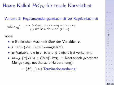
Inhalt
Kap. 1
Kap. 2
Kap. 3
Kap. 4
4.1
4.2
4.3
4.4
4.5
4.6
4.7
4.8
Kap. 5
Kap. 6
Kap. 7
Kap. 8
Kap. 9
Kap. 10
Kap. 11
Kap. 12
Kap. 13
Kap. 14
Kap. 15
Kap. 16
Kap. 17
Literatur
Anhang
A
Hoare-Kalkul HKTK fur totale Korrektheit
Variante 2: Regelanwendungseinfachheit vor Regeleinfachheit
[whileTK ] I ∧ b⇒ u[t/v ], I ∧ b∧ t=w π I ∧ t<wI while b do π od I ∧¬b
wobei
I u Boolescher Ausdruck uber der Variablen v ,
I t Term (sog. Terminierungsterm),
I w Variable, die in I , b, π und t nicht frei vorkommt,
I M=df σ(v) |σ ∈ Ch(u) bzgl. @ Noethersch geordneteMenge (sog. noethersche Halbordnung).
(M ,@) als Terminationsordnung!
187/863
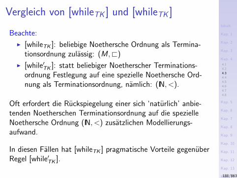
Inhalt
Kap. 1
Kap. 2
Kap. 3
Kap. 4
4.1
4.2
4.3
4.4
4.5
4.6
4.7
4.8
Kap. 5
Kap. 6
Kap. 7
Kap. 8
Kap. 9
Kap. 10
Kap. 11
Kap. 12
Kap. 13
Kap. 14
Kap. 15
Kap. 16
Kap. 17
Literatur
Anhang
A
Vergleich von [whileTK ] und [whileTK ]
Beachte:
I [whileTK ]: beliebige Noethersche Ordnung als Termina-tionsordnung zulassig: (M ,@)
I [while′TK ]: statt beliebiger Noetherscher Terminations-ordnung Festlegung auf eine spezielle Noethersche Ord-nung als Terminationsordnung, namlich: (IN, <).
Oft erfordert die Ruckspiegelung einer sich ‘naturlich’ anbie-tenden Noetherschen Terminationsordnung auf die spezielleNoethersche Ordnung (IN, <) zusatzlichen Modellierungs-aufwand.
In diesen Fallen hat [whileTK ] pragmatische Vorteile gegenuberRegel [while′TK ].
188/863
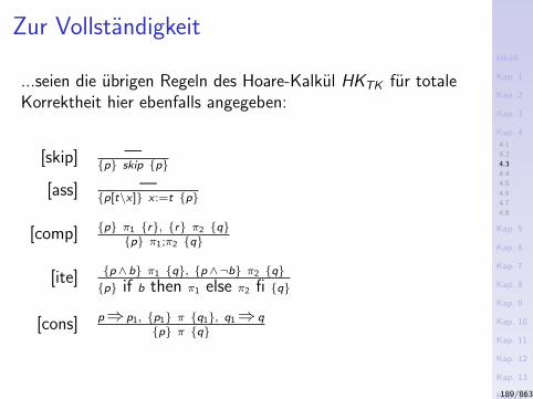
Inhalt
Kap. 1
Kap. 2
Kap. 3
Kap. 4
4.1
4.2
4.3
4.4
4.5
4.6
4.7
4.8
Kap. 5
Kap. 6
Kap. 7
Kap. 8
Kap. 9
Kap. 10
Kap. 11
Kap. 12
Kap. 13
Kap. 14
Kap. 15
Kap. 16
Kap. 17
Literatur
Anhang
A
Zur Vollstandigkeit
...seien die ubrigen Regeln des Hoare-Kalkul HKTK fur totaleKorrektheit hier ebenfalls angegeben:
[skip] —p skip p
[ass] —p[t\x] x :=t p
[comp] p π1 r, r π2 qp π1;π2 q
[ite] p ∧ b π1 q, p ∧¬b π2 qp if b then π1 else π2 fi q
[cons] p⇒ p1, p1 π q1, q1⇒ qp π q
189/863

Inhalt
Kap. 1
Kap. 2
Kap. 3
Kap. 4
4.1
4.2
4.3
4.4
4.5
4.6
4.7
4.8
Kap. 5
Kap. 6
Kap. 7
Kap. 8
Kap. 9
Kap. 10
Kap. 11
Kap. 12
Kap. 13
Kap. 14
Kap. 15
Kap. 16
Kap. 17
Literatur
Anhang
A
Bemerkung
In den vorigen Regeln verwenden wir (auch) fur totaleKorrektheit geschweifte statt eckiger Klammern furzugesicherte Eigenschaften, um einen Bezeichnungskonfliktmit der ebenfalls durch eckige Klammern bezeichnetensyntaktischen Substitution zu vermeiden.
190/863
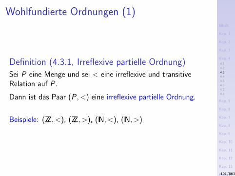
Inhalt
Kap. 1
Kap. 2
Kap. 3
Kap. 4
4.1
4.2
4.3
4.4
4.5
4.6
4.7
4.8
Kap. 5
Kap. 6
Kap. 7
Kap. 8
Kap. 9
Kap. 10
Kap. 11
Kap. 12
Kap. 13
Kap. 14
Kap. 15
Kap. 16
Kap. 17
Literatur
Anhang
A
Wohlfundierte Ordnungen (1)
Definition (4.3.1, Irreflexive partielle Ordnung)
Sei P eine Menge und sei < eine irreflexive und transitiveRelation auf P .
Dann ist das Paar (P , <) eine irreflexive partielle Ordnung.
Beispiele: (ZZ, <), (ZZ, >), (IN, <), (IN, >)
191/863
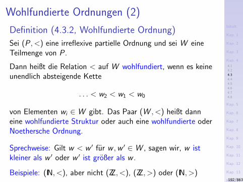
Inhalt
Kap. 1
Kap. 2
Kap. 3
Kap. 4
4.1
4.2
4.3
4.4
4.5
4.6
4.7
4.8
Kap. 5
Kap. 6
Kap. 7
Kap. 8
Kap. 9
Kap. 10
Kap. 11
Kap. 12
Kap. 13
Kap. 14
Kap. 15
Kap. 16
Kap. 17
Literatur
Anhang
A
Wohlfundierte Ordnungen (2)
Definition (4.3.2, Wohlfundierte Ordnung)
Sei (P , <) eine irreflexive partielle Ordnung und sei W eineTeilmenge von P .
Dann heißt die Relation < auf W wohlfundiert, wenn es keineunendlich absteigende Kette
. . . < w2 < w1 < w0
von Elementen wi ∈ W gibt. Das Paar (W , <) heißt danneine wohlfundierte Struktur oder auch eine wohlfundierte oderNoethersche Ordnung.
Sprechweise: Gilt w < w ′ fur w ,w ′ ∈ W , sagen wir, w istkleiner als w ′ oder w ′ ist großer als w .
Beispiele: (IN, <), aber nicht (ZZ, <), (ZZ, >) oder (IN, >)192/863
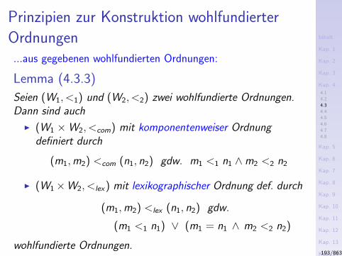
Inhalt
Kap. 1
Kap. 2
Kap. 3
Kap. 4
4.1
4.2
4.3
4.4
4.5
4.6
4.7
4.8
Kap. 5
Kap. 6
Kap. 7
Kap. 8
Kap. 9
Kap. 10
Kap. 11
Kap. 12
Kap. 13
Kap. 14
Kap. 15
Kap. 16
Kap. 17
Literatur
Anhang
A
Prinzipien zur Konstruktion wohlfundierter
Ordnungen...aus gegebenen wohlfundierten Ordnungen:
Lemma (4.3.3)
Seien (W1, <1) und (W2, <2) zwei wohlfundierte Ordnungen.Dann sind auch
I (W1 ×W2, <com) mit komponentenweiser Ordnungdefiniert durch
(m1,m2) <com (n1, n2) gdw. m1 <1 n1 ∧m2 <2 n2
I (W1×W2, <lex) mit lexikographischer Ordnung def. durch
(m1,m2) <lex (n1, n2) gdw.
(m1 <1 n1) ∨ (m1 = n1 ∧ m2 <2 n2)
wohlfundierte Ordnungen.193/863
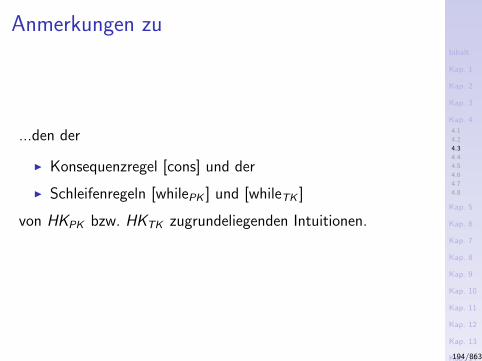
Inhalt
Kap. 1
Kap. 2
Kap. 3
Kap. 4
4.1
4.2
4.3
4.4
4.5
4.6
4.7
4.8
Kap. 5
Kap. 6
Kap. 7
Kap. 8
Kap. 9
Kap. 10
Kap. 11
Kap. 12
Kap. 13
Kap. 14
Kap. 15
Kap. 16
Kap. 17
Literatur
Anhang
A
Anmerkungen zu
...den der
I Konsequenzregel [cons] und der
I Schleifenregeln [whilePK ] und [whileTK ]
von HKPK bzw. HKTK zugrundeliegenden Intuitionen.
194/863
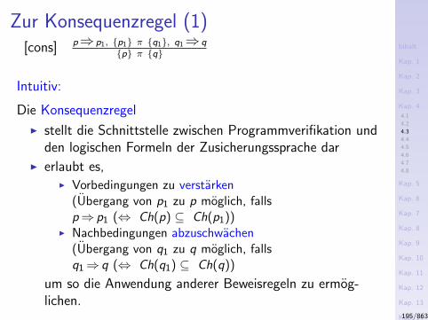
Inhalt
Kap. 1
Kap. 2
Kap. 3
Kap. 4
4.1
4.2
4.3
4.4
4.5
4.6
4.7
4.8
Kap. 5
Kap. 6
Kap. 7
Kap. 8
Kap. 9
Kap. 10
Kap. 11
Kap. 12
Kap. 13
Kap. 14
Kap. 15
Kap. 16
Kap. 17
Literatur
Anhang
A
Zur Konsequenzregel (1)[cons] p⇒ p1, p1 π q1, q1⇒ q
p π q
Intuitiv:
Die Konsequenzregel
I stellt die Schnittstelle zwischen Programmverifikation undden logischen Formeln der Zusicherungssprache dar
I erlaubt es,I Vorbedingungen zu verstarken
(Ubergang von p1 zu p moglich, fallsp⇒ p1 (⇔ Ch(p) ⊆ Ch(p1))
I Nachbedingungen abzuschwachen(Ubergang von q1 zu q moglich, fallsq1⇒ q (⇔ Ch(q1) ⊆ Ch(q))
um so die Anwendung anderer Beweisregeln zu ermog-lichen.
195/863
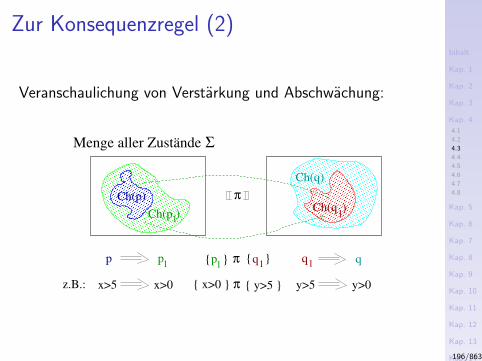
Inhalt
Kap. 1
Kap. 2
Kap. 3
Kap. 4
4.1
4.2
4.3
4.4
4.5
4.6
4.7
4.8
Kap. 5
Kap. 6
Kap. 7
Kap. 8
Kap. 9
Kap. 10
Kap. 11
Kap. 12
Kap. 13
Kap. 14
Kap. 15
Kap. 16
Kap. 17
Literatur
Anhang
A
Zur Konsequenzregel (2)
Veranschaulichung von Verstarkung und Abschwachung:
π
x>5 x>0
ΣMenge aller Zustände
Ch(q1)
Ch(q)
π
z.B.: π y>5 y>0 y>5 x>0
p1 p
1 1 1
Ch(p )1
q
q q
Ch(p)
p
196/863
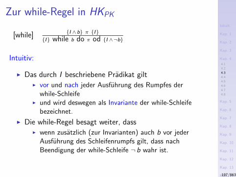
Inhalt
Kap. 1
Kap. 2
Kap. 3
Kap. 4
4.1
4.2
4.3
4.4
4.5
4.6
4.7
4.8
Kap. 5
Kap. 6
Kap. 7
Kap. 8
Kap. 9
Kap. 10
Kap. 11
Kap. 12
Kap. 13
Kap. 14
Kap. 15
Kap. 16
Kap. 17
Literatur
Anhang
A
Zur while-Regel in HKPK
[while] I ∧ b π II while b do π od I ∧¬b
Intuitiv:
I Das durch I beschriebene Pradikat giltI vor und nach jeder Ausfuhrung des Rumpfes der
while-SchleifeI und wird deswegen als Invariante der while-Schleife
bezeichnet.
I Die while-Regel besagt weiter, dassI wenn zusatzlich (zur Invarianten) auch b vor jeder
Ausfuhrung des Schleifenrumpfs gilt, dass nachBeendigung der while-Schleife ¬ b wahr ist.
197/863
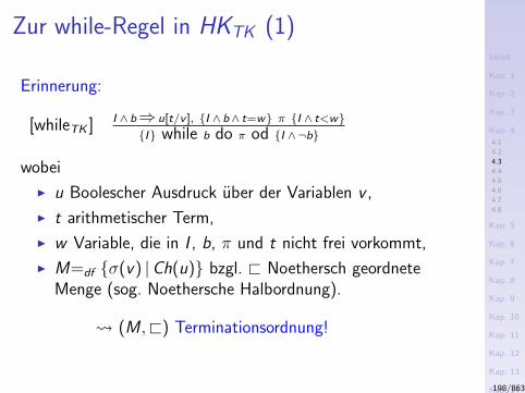
Inhalt
Kap. 1
Kap. 2
Kap. 3
Kap. 4
4.1
4.2
4.3
4.4
4.5
4.6
4.7
4.8
Kap. 5
Kap. 6
Kap. 7
Kap. 8
Kap. 9
Kap. 10
Kap. 11
Kap. 12
Kap. 13
Kap. 14
Kap. 15
Kap. 16
Kap. 17
Literatur
Anhang
A
Zur while-Regel in HKTK (1)
Erinnerung:
[whileTK ] I ∧ b⇒ u[t/v ], I ∧ b∧ t=w π I ∧ t<wI while b do π od I ∧¬b
wobei
I u Boolescher Ausdruck uber der Variablen v ,
I t arithmetischer Term,
I w Variable, die in I , b, π und t nicht frei vorkommt,
I M=df σ(v) |Ch(u) bzgl. @ Noethersch geordneteMenge (sog. Noethersche Halbordnung).
(M ,@) Terminationsordnung!
198/863
Inhalt
Kap. 1
Kap. 2
Kap. 3
Kap. 4
4.1
4.2
4.3
4.4
4.5
4.6
4.7
4.8
Kap. 5
Kap. 6
Kap. 7
Kap. 8
Kap. 9
Kap. 10
Kap. 11
Kap. 12
Kap. 13
Kap. 14
Kap. 15
Kap. 16
Kap. 17
Literatur
Anhang
A
Zur while-Regel in HKTK (2)
I Pramisse 1: I ∧ b⇒ u[t/v ]Wann immer der Schleifenrumpf noch einmal ausgefuhrtwird (d.h. I ∧ b ist wahr), gilt, dass u[t/v ] wahr ist,woraus aufgrund der Definition von M folgt, dass derWert von t Element einer Noethersch geordneten Mengeist.
199/863
Inhalt
Kap. 1
Kap. 2
Kap. 3
Kap. 4
4.1
4.2
4.3
4.4
4.5
4.6
4.7
4.8
Kap. 5
Kap. 6
Kap. 7
Kap. 8
Kap. 9
Kap. 10
Kap. 11
Kap. 12
Kap. 13
Kap. 14
Kap. 15
Kap. 16
Kap. 17
Literatur
Anhang
A
Zur while-Regel in HKTK (3)
I Pramisse 2: I ∧ b∧ t = w π I ∧ t < wI w speichert den initialen Wert von t (w ist sog. logische
Variable), d.h. den Wert, den t vor Eintritt in dieSchleife hat (gilt, da w als logische Variableinsbesondere nicht in π vorkommt)
I Zusammen damit, dass der Wert von w (als logischeVariable) invariant unter der Ausfuhrung desSchleifenrumpfs ist, garantiert t < w in derNachbedingung von Pramisse 2, dass der Wert von tnach jeder Ausfuhrung des Schleifenrumpfs bzgl. dernoetherschen Ordnung abgenommen hat.
200/863
Inhalt
Kap. 1
Kap. 2
Kap. 3
Kap. 4
4.1
4.2
4.3
4.4
4.5
4.6
4.7
4.8
Kap. 5
Kap. 6
Kap. 7
Kap. 8
Kap. 9
Kap. 10
Kap. 11
Kap. 12
Kap. 13
Kap. 14
Kap. 15
Kap. 16
Kap. 17
Literatur
Anhang
A
Zur while-Regel in HKTK (4)
I Zusammen implizieren die obigen beiden Punkte dieTerminierung der while-Schleife, da es in einer Noetherschgeordneten Menge keine unendlich absteigenden Kettengibt. Folglich kann die Bedingung I ∧ b in Pramisse 1nicht unendlich oft wahr sein, da dies zusammen mitPramisse 2 ein unendliches Absteigen erforderte.)
201/863
Inhalt
Kap. 1
Kap. 2
Kap. 3
Kap. 4
4.1
4.2
4.3
4.4
4.5
4.6
4.7
4.8
Kap. 5
Kap. 6
Kap. 7
Kap. 8
Kap. 9
Kap. 10
Kap. 11
Kap. 12
Kap. 13
Kap. 14
Kap. 15
Kap. 16
Kap. 17
Literatur
Anhang
A
Programm- vs. logische Variablen (1)
Wir unterscheiden in Zusicherungen p π q zwischen:
I Programmvariablen
...Variablen, die in π vorkommen
I logischen Variablen
...Variablen, die in π nicht vorkommen
Logische Variablen erlauben
I sich initiale Werte von Programmvariablen zu “merken”,um in Nachbedingungen geeignet darauf Bezug zunehmen.
202/863
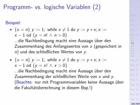
Inhalt
Kap. 1
Kap. 2
Kap. 3
Kap. 4
4.1
4.2
4.3
4.4
4.5
4.6
4.7
4.8
Kap. 5
Kap. 6
Kap. 7
Kap. 8
Kap. 9
Kap. 10
Kap. 11
Kap. 12
Kap. 13
Kap. 14
Kap. 15
Kap. 16
Kap. 17
Literatur
Anhang
A
Programm- vs. logische Variablen (2)
Beispiel:
I x = n y := 1; while x 6= 1 do y := y ∗ x ; x :=x − 1 od y = n! ∧ n > 0...die Nachbedingung macht eine Aussage uber denZusammenhang des Anfangswertes von x (gespeichert inn) und des schließlichen Wertes von y .
I x = n y := 1; while x 6= 1 do y := y ∗ x ; x :=x − 1 od y = x! ∧ x > 0...die Nachbedingung macht eine Aussage uber denZusammenhang der schließlichen Werte von x und y .(Beachte: nur mit Programmvariablen keine Aussage uberdie Fakultatsberechnung in diesem Bsp.!)
203/863
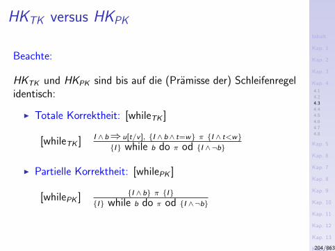
Inhalt
Kap. 1
Kap. 2
Kap. 3
Kap. 4
4.1
4.2
4.3
4.4
4.5
4.6
4.7
4.8
Kap. 5
Kap. 6
Kap. 7
Kap. 8
Kap. 9
Kap. 10
Kap. 11
Kap. 12
Kap. 13
Kap. 14
Kap. 15
Kap. 16
Kap. 17
Literatur
Anhang
A
HKTK versus HKPK
Beachte:
HKTK und HKPK sind bis auf die (Pramisse der) Schleifenregelidentisch:
I Totale Korrektheit: [whileTK ]
[whileTK ] I ∧ b⇒ u[t/v ], I ∧ b∧ t=w π I ∧ t<wI while b do π od I ∧¬b
I Partielle Korrektheit: [whilePK ]
[whilePK ] I ∧ b π II while b do π od I ∧¬b
204/863
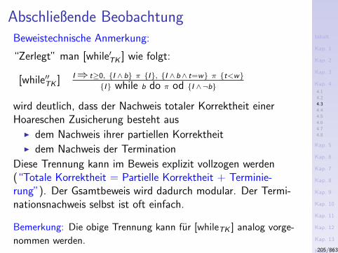
Inhalt
Kap. 1
Kap. 2
Kap. 3
Kap. 4
4.1
4.2
4.3
4.4
4.5
4.6
4.7
4.8
Kap. 5
Kap. 6
Kap. 7
Kap. 8
Kap. 9
Kap. 10
Kap. 11
Kap. 12
Kap. 13
Kap. 14
Kap. 15
Kap. 16
Kap. 17
Literatur
Anhang
A
Abschließende BeobachtungBeweistechnische Anmerkung:
“Zerlegt” man [while′TK ] wie folgt:
[while′′TK ] I⇒ t≥0, I ∧ b π I, I ∧ b∧ t=w π t<wI while b do π od I ∧¬b
wird deutlich, dass der Nachweis totaler Korrektheit einerHoareschen Zusicherung besteht ausI dem Nachweis ihrer partiellen KorrektheitI dem Nachweis der Termination
Diese Trennung kann im Beweis explizit vollzogen werden(“Totale Korrektheit = Partielle Korrektheit + Terminie-rung”). Der Gsamtbeweis wird dadurch modular. Der Termi-nationsnachweis selbst ist oft einfach.
Bemerkung: Die obige Trennung kann fur [whileTK ] analog vorge-
nommen werden.205/863

Inhalt
Kap. 1
Kap. 2
Kap. 3
Kap. 4
4.1
4.2
4.3
4.4
4.5
4.6
4.7
4.8
Kap. 5
Kap. 6
Kap. 7
Kap. 8
Kap. 9
Kap. 10
Kap. 11
Kap. 12
Kap. 13
Kap. 14
Kap. 15
Kap. 16
Kap. 17
Literatur
Anhang
A
Kapitel 4.4
Korrektheit und Vollstandigkeit
206/863
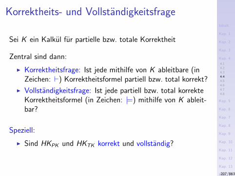
Inhalt
Kap. 1
Kap. 2
Kap. 3
Kap. 4
4.1
4.2
4.3
4.4
4.5
4.6
4.7
4.8
Kap. 5
Kap. 6
Kap. 7
Kap. 8
Kap. 9
Kap. 10
Kap. 11
Kap. 12
Kap. 13
Kap. 14
Kap. 15
Kap. 16
Kap. 17
Literatur
Anhang
A
Korrektheits- und Vollstandigkeitsfrage
Sei K ein Kalkul fur partielle bzw. totale Korrektheit
Zentral sind dann:
I Korrektheitsfrage: Ist jede mithilfe von K ableitbare (inZeichen: `) Korrektheitsformel partiell bzw. total korrekt?
I Vollstandigkeitsfrage: Ist jede partiell bzw. total korrekteKorrektheitsformel (in Zeichen: |=) mithilfe von K ableit-bar?
Speziell:
I Sind HKPK und HKTK korrekt und vollstandig?
207/863
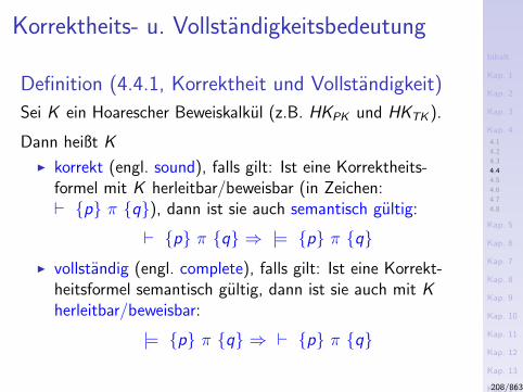
Inhalt
Kap. 1
Kap. 2
Kap. 3
Kap. 4
4.1
4.2
4.3
4.4
4.5
4.6
4.7
4.8
Kap. 5
Kap. 6
Kap. 7
Kap. 8
Kap. 9
Kap. 10
Kap. 11
Kap. 12
Kap. 13
Kap. 14
Kap. 15
Kap. 16
Kap. 17
Literatur
Anhang
A
Korrektheits- u. Vollstandigkeitsbedeutung
Definition (4.4.1, Korrektheit und Vollstandigkeit)
Sei K ein Hoarescher Beweiskalkul (z.B. HKPK und HKTK ).
Dann heißt K
I korrekt (engl. sound), falls gilt: Ist eine Korrektheits-formel mit K herleitbar/beweisbar (in Zeichen:` p π q), dann ist sie auch semantisch gultig:
` p π q ⇒ |= p π qI vollstandig (engl. complete), falls gilt: Ist eine Korrekt-
heitsformel semantisch gultig, dann ist sie auch mit Kherleitbar/beweisbar:
|= p π q ⇒ ` p π q
208/863
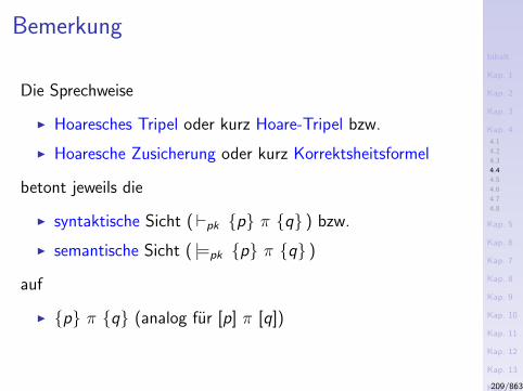
Inhalt
Kap. 1
Kap. 2
Kap. 3
Kap. 4
4.1
4.2
4.3
4.4
4.5
4.6
4.7
4.8
Kap. 5
Kap. 6
Kap. 7
Kap. 8
Kap. 9
Kap. 10
Kap. 11
Kap. 12
Kap. 13
Kap. 14
Kap. 15
Kap. 16
Kap. 17
Literatur
Anhang
A
Bemerkung
Die Sprechweise
I Hoaresches Tripel oder kurz Hoare-Tripel bzw.
I Hoaresche Zusicherung oder kurz Korrektsheitsformel
betont jeweils die
I syntaktische Sicht (`pk p π q ) bzw.
I semantische Sicht ( |=pk p π q )
auf
I p π q (analog fur [p] π [q])
209/863
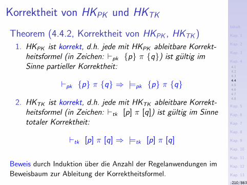
Inhalt
Kap. 1
Kap. 2
Kap. 3
Kap. 4
4.1
4.2
4.3
4.4
4.5
4.6
4.7
4.8
Kap. 5
Kap. 6
Kap. 7
Kap. 8
Kap. 9
Kap. 10
Kap. 11
Kap. 12
Kap. 13
Kap. 14
Kap. 15
Kap. 16
Kap. 17
Literatur
Anhang
A
Korrektheit von HKPK und HKTK
Theorem (4.4.2, Korrektheit von HKPK , HKTK )
1. HKPK ist korrekt, d.h. jede mit HKPK ableitbare Korrekt-heitsformel (in Zeichen: `pk p π q) ist gultig imSinne partieller Korrektheit:
`pk p π q ⇒ |=pk p π q
2. HKTK ist korrekt, d.h. jede mit HKTK ableitbare Korrekt-heitsformel (in Zeichen: `tk [p] π [q]) ist gultig im Sinnetotaler Korrektheit:
`tk [p] π [q] ⇒ |=tk [p] π [q]
Beweis durch Induktion uber die Anzahl der Regelanwendungen im
Beweisbaum zur Ableitung der Korrektheitsformel.210/863

Inhalt
Kap. 1
Kap. 2
Kap. 3
Kap. 4
4.1
4.2
4.3
4.4
4.5
4.6
4.7
4.8
Kap. 5
Kap. 6
Kap. 7
Kap. 8
Kap. 9
Kap. 10
Kap. 11
Kap. 12
Kap. 13
Kap. 14
Kap. 15
Kap. 16
Kap. 17
Literatur
Anhang
A
Zur Vollstandigkeit Hoarescher Beweiskalkule
Generell mussen wir unterscheiden zwischen Vollstandigkeit
I extensionaler und
I intensionaler
Ansatze.
211/863
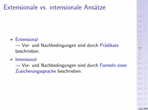
Inhalt
Kap. 1
Kap. 2
Kap. 3
Kap. 4
4.1
4.2
4.3
4.4
4.5
4.6
4.7
4.8
Kap. 5
Kap. 6
Kap. 7
Kap. 8
Kap. 9
Kap. 10
Kap. 11
Kap. 12
Kap. 13
Kap. 14
Kap. 15
Kap. 16
Kap. 17
Literatur
Anhang
A
Extensionale vs. intensionale Ansatze
I Extensional Vor- und Nachbedingungen sind durch Pradikatebeschrieben.
I Intensional Vor- und Nachbedingungen sind durch Formeln einerZusicherungssprache beschrieben.
212/863
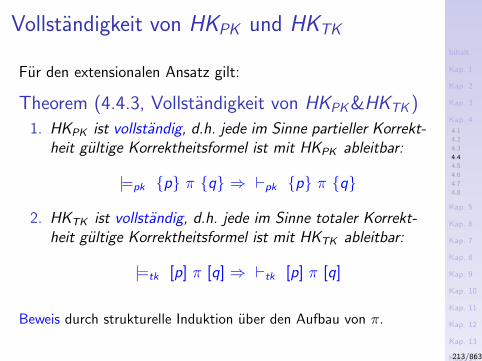
Inhalt
Kap. 1
Kap. 2
Kap. 3
Kap. 4
4.1
4.2
4.3
4.4
4.5
4.6
4.7
4.8
Kap. 5
Kap. 6
Kap. 7
Kap. 8
Kap. 9
Kap. 10
Kap. 11
Kap. 12
Kap. 13
Kap. 14
Kap. 15
Kap. 16
Kap. 17
Literatur
Anhang
A
Vollstandigkeit von HKPK und HKTK
Fur den extensionalen Ansatz gilt:
Theorem (4.4.3, Vollstandigkeit von HKPK &HKTK )
1. HKPK ist vollstandig, d.h. jede im Sinne partieller Korrekt-heit gultige Korrektheitsformel ist mit HKPK ableitbar:
|=pk p π q ⇒ `pk p π q
2. HKTK ist vollstandig, d.h. jede im Sinne totaler Korrekt-heit gultige Korrektheitsformel ist mit HKTK ableitbar:
|=tk [p] π [q] ⇒ `tk [p] π [q]
Beweis durch strukturelle Induktion uber den Aufbau von π.
213/863
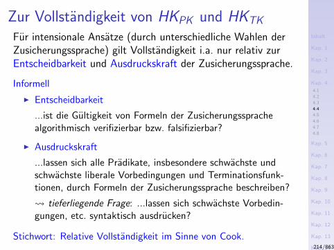
Inhalt
Kap. 1
Kap. 2
Kap. 3
Kap. 4
4.1
4.2
4.3
4.4
4.5
4.6
4.7
4.8
Kap. 5
Kap. 6
Kap. 7
Kap. 8
Kap. 9
Kap. 10
Kap. 11
Kap. 12
Kap. 13
Kap. 14
Kap. 15
Kap. 16
Kap. 17
Literatur
Anhang
A
Zur Vollstandigkeit von HKPK und HKTK
Fur intensionale Ansatze (durch unterschiedliche Wahlen derZusicherungssprache) gilt Vollstandigkeit i.a. nur relativ zurEntscheidbarkeit und Ausdruckskraft der Zusicherungssprache.
Informell
I Entscheidbarkeit
...ist die Gultigkeit von Formeln der Zusicherungssprachealgorithmisch verifizierbar bzw. falsifizierbar?
I Ausdruckskraft
...lassen sich alle Pradikate, insbesondere schwachste undschwachste liberale Vorbedingungen und Terminationsfunk-tionen, durch Formeln der Zusicherungssprache beschreiben?
tieferliegende Frage: ...lassen sich schwachste Vorbedin-gungen, etc. syntaktisch ausdrucken?
Stichwort: Relative Vollstandigkeit im Sinne von Cook.214/863

Inhalt
Kap. 1
Kap. 2
Kap. 3
Kap. 4
4.1
4.2
4.3
4.4
4.5
4.6
4.7
4.8
Kap. 5
Kap. 6
Kap. 7
Kap. 8
Kap. 9
Kap. 10
Kap. 11
Kap. 12
Kap. 13
Kap. 14
Kap. 15
Kap. 16
Kap. 17
Literatur
Anhang
A
Kapitel 4.5
Beispiele zum Beweis partieller Korrektheit
215/863
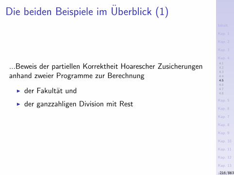
Inhalt
Kap. 1
Kap. 2
Kap. 3
Kap. 4
4.1
4.2
4.3
4.4
4.5
4.6
4.7
4.8
Kap. 5
Kap. 6
Kap. 7
Kap. 8
Kap. 9
Kap. 10
Kap. 11
Kap. 12
Kap. 13
Kap. 14
Kap. 15
Kap. 16
Kap. 17
Literatur
Anhang
A
Die beiden Beispiele im Uberblick (1)
...Beweis der partiellen Korrektheit Hoarescher Zusicherungenanhand zweier Programme zur Berechnung
I der Fakultat und
I der ganzzahligen Division mit Rest
216/863
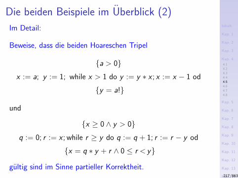
Inhalt
Kap. 1
Kap. 2
Kap. 3
Kap. 4
4.1
4.2
4.3
4.4
4.5
4.6
4.7
4.8
Kap. 5
Kap. 6
Kap. 7
Kap. 8
Kap. 9
Kap. 10
Kap. 11
Kap. 12
Kap. 13
Kap. 14
Kap. 15
Kap. 16
Kap. 17
Literatur
Anhang
A
Die beiden Beispiele im Uberblick (2)
Im Detail:
Beweise, dass die beiden Hoareschen Tripel
a > 0
x := a; y := 1; while x > 1 do y := y ∗ x ; x := x − 1 od
y = a!
und
x ≥ 0 ∧ y > 0
q := 0; r := x ; while r ≥ y do q := q + 1; r := r − y od
x = q ∗ y + r ∧ 0 ≤ r < y
gultig sind im Sinne partieller Korrektheit.217/863
Inhalt
Kap. 1
Kap. 2
Kap. 3
Kap. 4
4.1
4.2
4.3
4.4
4.5
4.6
4.7
4.8
Kap. 5
Kap. 6
Kap. 7
Kap. 8
Kap. 9
Kap. 10
Kap. 11
Kap. 12
Kap. 13
Kap. 14
Kap. 15
Kap. 16
Kap. 17
Literatur
Anhang
A
Die beiden Beispiele im Uberblick (3)
In der Folge geben wir die Beweise dafur in zwei Notations-varianten an:
I baumartig (kanonische Variante)
I lineare Beweisskizze (pragmatische Variante)
218/863
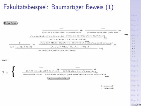
Inhalt
Kap. 1
Kap. 2
Kap. 3
Kap. 4
4.1
4.2
4.3
4.4
4.5
4.6
4.7
4.8
Kap. 5
Kap. 6
Kap. 7
Kap. 8
Kap. 9
Kap. 10
Kap. 11
Kap. 12
Kap. 13
Kap. 14
Kap. 15
Kap. 16
Kap. 17
Literatur
Anhang
A
Fakultatsbeispiel: Baumartiger Beweis (1)
1*a!=a! & a>0 & a=a x:=a; y:=1 y*x!=a! & a>0 & x=aa>0 ==> 1*a!=a! & a>0 & a=a y*x!=a! & a>0 & x=a ==> y*x!=a! & x>0
1*x!=a! & a>0 & x=a y:=1 y*x!=a! & a>0 & x=aAss
1*a!=a! & a>0 & a=a x:=a 1*x!=a! & a>0 & x=aAss
Comp
Cons
a>0 x:=a; y:=1 y*x!=a! & x>0
wobei
T
& : Logisches und
~ : Logisches nicht
Compa>0 x:=a; y:=1; WHILE x>1 DO y:=y*x; x:=x−1 OD y=a!
y*x!=a! & x>0 WHILE x>1 DO y:=y*x; x:= x−1 OD y=a!
y*x!=a! & x>0 & ~(x>1) ==> y=a!y*x!=a! & x>0 WHILE x>1 DO y:=y*x; x:= x−1 OD y*x!=a! & x>0 & ~(x>1)
Cons
y*x!=a! & x>0 & x>1 y:=y*x; x:=x−1 y*x!=a! & x>0Cons
y*x!=a! & x>0 & x>1 ==> (y*x)*(x−1)!=a! & (x−1)>0 (y*x)*(x−1)!=a! & (x−1)>0 y:=y*x; x:=x−1 y*x!=a! & x>0
Ass
y*(x−1)!=a! & (x−1)>0 x:=x−1 y*x!=a! & x>0
a>0 x:=a; y:=1 y*x!=a! & x>0
TCons
Ass
Comp
While
Erster Beweis
(y*x)*(x−1)!=a! & (x−1)>0 y:=y*x y*(x−1)!=a! & (x−1)>0
219/863
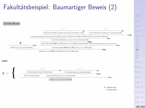
Inhalt
Kap. 1
Kap. 2
Kap. 3
Kap. 4
4.1
4.2
4.3
4.4
4.5
4.6
4.7
4.8
Kap. 5
Kap. 6
Kap. 7
Kap. 8
Kap. 9
Kap. 10
Kap. 11
Kap. 12
Kap. 13
Kap. 14
Kap. 15
Kap. 16
Kap. 17
Literatur
Anhang
A
Fakultatsbeispiel: Baumartiger Beweis (2)
Zweiter Beweis
wobei
T
& : Logisches und
~ : Logisches nicht
1*x!=a! & x>0 y:=1 y*x!=a! & x>0Ass
1*a!=a! & a>0 x:=a 1*x!=a! & x>0Ass
Comp
a>0 x:=a; y:=1 y*x!=a! & x>0
1*a!=a! & a>0 x:=a; y:=1 y*x!=a! & x>0a>0 ==> 1*a!=a! & a>0Cons
Compa>0 x:=a; y:=1; WHILE x>1 DO y:=y*x; x:=x−1 OD y=a!
y*x!=a! & x>0 WHILE x>1 DO y:=y*x; x:= x−1 OD y=a!
y*x!=a! & x>0 & ~(x>1) ==> y=a!y*x!=a! & x>0 WHILE x>1 DO y:=y*x; x:= x−1 OD y*x!=a! & x>0 & ~(x>1)
Cons
y*x!=a! & x>0 & x>1 y:=y*x; x:=x−1 y*x!=a! & x>0Cons
y*x!=a! & x>0 & x>1 ==> (y*x)*(x−1)!=a! & (x−1)>0 (y*x)*(x−1)!=a! & (x−1)>0 y:=y*x; x:=x−1 y*x!=a! & x>0
(y*x)*(x−1)!=a! & (x−1)>0 y:=y*x y*(x−1)!=a! & (x−1)>0
Ass
y*(x−1)!=a! & (x−1)>0 x:=x−1 y*x!=a! & x>0
a>0 x:=a; y:=1 y*x!=a! & x>0
Cons
While
Comp
Ass
T
220/863
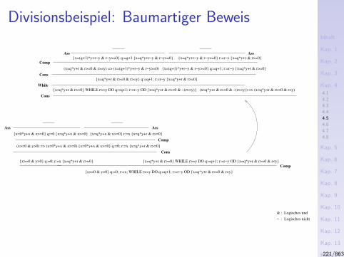
Inhalt
Kap. 1
Kap. 2
Kap. 3
Kap. 4
4.1
4.2
4.3
4.4
4.5
4.6
4.7
4.8
Kap. 5
Kap. 6
Kap. 7
Kap. 8
Kap. 9
Kap. 10
Kap. 11
Kap. 12
Kap. 13
Kap. 14
Kap. 15
Kap. 16
Kap. 17
Literatur
Anhang
A
Divisionsbeispiel: Baumartiger Beweis
& : Logisches und
~ : Logisches nicht
x=q*y+r & r>=0 WHILE r>=y DO q:=q+1; r:=r−y OD x=q*y+r & r>=0 & ~(r>=y) (x=q*y+r & r>=0 & ~(r>=y)) => (x=q*y+r & r>=0 & r<y)
Cons
While
x=q*y+r & r>=0 & r>=y q:=q+1; r:=r−y x=q*y+r & r>=0
(x=q*y+r & r>=0 & r>=y) => (x=(q+1)*y+r−y & r−y>=0) x=(q+1)*y+r−y & r−y>=0 q:=q+1; r:=r−y x=q*y+r & r>=0
Cons
Comp
Ass Ass
Ass Ass
(x>=0 & y>0) => (x=0*y+x & x>=0) x=0*y+x & x>=0 q:=0; r:=x x=q*y+r & r>=0
Comp
x>=0 & y>0 q:=0; r:=x; WHILE r>=y DO q:=q+1; r:=r−y OD x=q*y+r & r>=0 & r<y
x>=0 & y>0 q:=0; r:=x x=q*y+r & r>=0
Comp
Cons
x=q*y+r & r>=0 WHILE r>=y DO q:=q+1; r:=r−y OD x=q*y+r & r>=0 & r<y
x=(q+1)*y+r−y & r−y>=0 q:=q+1 x=q*y+r−y & r−y>=0 x=q*y+r−y & r−y>=0 r:=r−y x=q*y+r & r>=0
x=0*y+x & x>=0 q:=0 x=q*y+x & x>=0 x=q*y+x & x>=0 r:=x x=q*y+r & r>=0
221/863
Inhalt
Kap. 1
Kap. 2
Kap. 3
Kap. 4
4.1
4.2
4.3
4.4
4.5
4.6
4.7
4.8
Kap. 5
Kap. 6
Kap. 7
Kap. 8
Kap. 9
Kap. 10
Kap. 11
Kap. 12
Kap. 13
Kap. 14
Kap. 15
Kap. 16
Kap. 17
Literatur
Anhang
A
Lineare Beweisskizzen
I Die unmittelbare baumartige Notation von HoareschenKorrektheitsbeweisen ist i.a. unhandlich.
I Alternativ hat sich deshalb eine Notationsvariante einge-burgert, bei der in den Programmtext Zusicherungen alsAnnotationen eingestreut werden.
I In der Folge demonstrieren wir diesen Notationsstil amBeispiel des Nachweises der partiellen Korrektheit unseresFakultatsprogramms bezuglich der angegebenen Vor- undNachbedingung. Man spricht auch von einemsog. linearen Beweis bzw. einer linearen Beweisskizze.
222/863
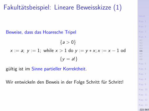
Inhalt
Kap. 1
Kap. 2
Kap. 3
Kap. 4
4.1
4.2
4.3
4.4
4.5
4.6
4.7
4.8
Kap. 5
Kap. 6
Kap. 7
Kap. 8
Kap. 9
Kap. 10
Kap. 11
Kap. 12
Kap. 13
Kap. 14
Kap. 15
Kap. 16
Kap. 17
Literatur
Anhang
A
Fakultatsbeispiel: Lineare Beweisskizze (1)
Beweise, dass das Hoaresche Tripel
a > 0
x := a; y := 1; while x > 1 do y := y ∗ x ; x := x − 1 od
y = a!
gultig ist im Sinne partieller Korrektheit.
Wir entwickeln den Beweis in der Folge Schritt fur Schritt!
223/863
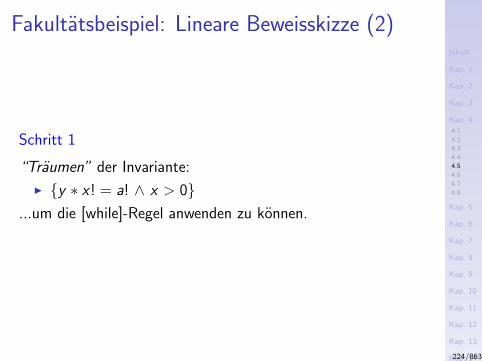
Inhalt
Kap. 1
Kap. 2
Kap. 3
Kap. 4
4.1
4.2
4.3
4.4
4.5
4.6
4.7
4.8
Kap. 5
Kap. 6
Kap. 7
Kap. 8
Kap. 9
Kap. 10
Kap. 11
Kap. 12
Kap. 13
Kap. 14
Kap. 15
Kap. 16
Kap. 17
Literatur
Anhang
A
Fakultatsbeispiel: Lineare Beweisskizze (2)
Schritt 1
“Traumen” der Invariante:
I y ∗ x! = a! ∧ x > 0...um die [while]-Regel anwenden zu konnen.
224/863
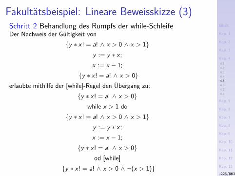
Inhalt
Kap. 1
Kap. 2
Kap. 3
Kap. 4
4.1
4.2
4.3
4.4
4.5
4.6
4.7
4.8
Kap. 5
Kap. 6
Kap. 7
Kap. 8
Kap. 9
Kap. 10
Kap. 11
Kap. 12
Kap. 13
Kap. 14
Kap. 15
Kap. 16
Kap. 17
Literatur
Anhang
A
Fakultatsbeispiel: Lineare Beweisskizze (3)Schritt 2 Behandlung des Rumpfs der while-SchleifeDer Nachweis der Gultigkeit von
y ∗ x! = a! ∧ x > 0 ∧ x > 1y := y ∗ x ;
x := x − 1;
y ∗ x! = a! ∧ x > 0erlaubte mithilfe der [while]-Regel den Ubergang zu:
y ∗ x! = a! ∧ x > 0while x > 1 do
y ∗ x! = a! ∧ x > 0 ∧ x > 1y := y ∗ x ;
x := x − 1;
y ∗ x! = a! ∧ x > 0od [while]
y ∗ x! = a! ∧ x > 0 ∧ ¬(x > 1)225/863
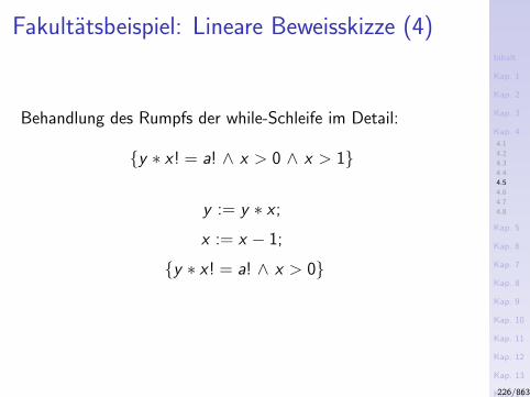
Inhalt
Kap. 1
Kap. 2
Kap. 3
Kap. 4
4.1
4.2
4.3
4.4
4.5
4.6
4.7
4.8
Kap. 5
Kap. 6
Kap. 7
Kap. 8
Kap. 9
Kap. 10
Kap. 11
Kap. 12
Kap. 13
Kap. 14
Kap. 15
Kap. 16
Kap. 17
Literatur
Anhang
A
Fakultatsbeispiel: Lineare Beweisskizze (4)
Behandlung des Rumpfs der while-Schleife im Detail:
y ∗ x! = a! ∧ x > 0 ∧ x > 1
y := y ∗ x ;
x := x − 1;
y ∗ x! = a! ∧ x > 0
226/863
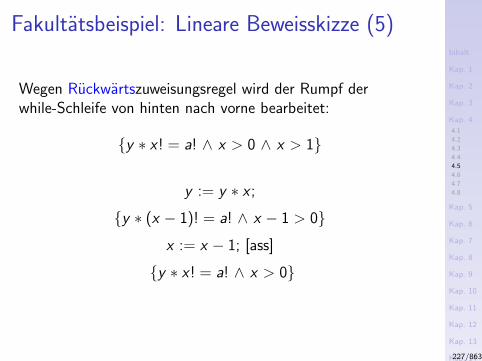
Inhalt
Kap. 1
Kap. 2
Kap. 3
Kap. 4
4.1
4.2
4.3
4.4
4.5
4.6
4.7
4.8
Kap. 5
Kap. 6
Kap. 7
Kap. 8
Kap. 9
Kap. 10
Kap. 11
Kap. 12
Kap. 13
Kap. 14
Kap. 15
Kap. 16
Kap. 17
Literatur
Anhang
A
Fakultatsbeispiel: Lineare Beweisskizze (5)
Wegen Ruckwartszuweisungsregel wird der Rumpf derwhile-Schleife von hinten nach vorne bearbeitet:
y ∗ x! = a! ∧ x > 0 ∧ x > 1
y := y ∗ x ;
y ∗ (x − 1)! = a! ∧ x − 1 > 0
x := x − 1; [ass]
y ∗ x! = a! ∧ x > 0
227/863
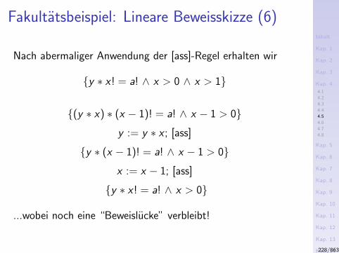
Inhalt
Kap. 1
Kap. 2
Kap. 3
Kap. 4
4.1
4.2
4.3
4.4
4.5
4.6
4.7
4.8
Kap. 5
Kap. 6
Kap. 7
Kap. 8
Kap. 9
Kap. 10
Kap. 11
Kap. 12
Kap. 13
Kap. 14
Kap. 15
Kap. 16
Kap. 17
Literatur
Anhang
A
Fakultatsbeispiel: Lineare Beweisskizze (6)
Nach abermaliger Anwendung der [ass]-Regel erhalten wir
y ∗ x! = a! ∧ x > 0 ∧ x > 1
(y ∗ x) ∗ (x − 1)! = a! ∧ x − 1 > 0
y := y ∗ x ; [ass]
y ∗ (x − 1)! = a! ∧ x − 1 > 0
x := x − 1; [ass]
y ∗ x! = a! ∧ x > 0
...wobei noch eine “Beweislucke” verbleibt!
228/863
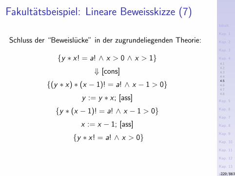
Inhalt
Kap. 1
Kap. 2
Kap. 3
Kap. 4
4.1
4.2
4.3
4.4
4.5
4.6
4.7
4.8
Kap. 5
Kap. 6
Kap. 7
Kap. 8
Kap. 9
Kap. 10
Kap. 11
Kap. 12
Kap. 13
Kap. 14
Kap. 15
Kap. 16
Kap. 17
Literatur
Anhang
A
Fakultatsbeispiel: Lineare Beweisskizze (7)
Schluss der “Beweislucke” in der zugrundeliegenden Theorie:
y ∗ x! = a! ∧ x > 0 ∧ x > 1
⇓ [cons]
(y ∗ x) ∗ (x − 1)! = a! ∧ x − 1 > 0
y := y ∗ x ; [ass]
y ∗ (x − 1)! = a! ∧ x − 1 > 0
x := x − 1; [ass]
y ∗ x! = a! ∧ x > 0
229/863
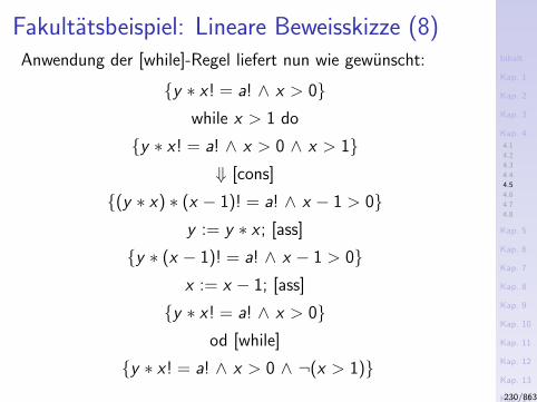
Inhalt
Kap. 1
Kap. 2
Kap. 3
Kap. 4
4.1
4.2
4.3
4.4
4.5
4.6
4.7
4.8
Kap. 5
Kap. 6
Kap. 7
Kap. 8
Kap. 9
Kap. 10
Kap. 11
Kap. 12
Kap. 13
Kap. 14
Kap. 15
Kap. 16
Kap. 17
Literatur
Anhang
A
Fakultatsbeispiel: Lineare Beweisskizze (8)Anwendung der [while]-Regel liefert nun wie gewunscht:
y ∗ x! = a! ∧ x > 0while x > 1 do
y ∗ x! = a! ∧ x > 0 ∧ x > 1⇓ [cons]
(y ∗ x) ∗ (x − 1)! = a! ∧ x − 1 > 0y := y ∗ x ; [ass]
y ∗ (x − 1)! = a! ∧ x − 1 > 0x := x − 1; [ass]
y ∗ x! = a! ∧ x > 0od [while]
y ∗ x! = a! ∧ x > 0 ∧ ¬(x > 1)230/863

Inhalt
Kap. 1
Kap. 2
Kap. 3
Kap. 4
4.1
4.2
4.3
4.4
4.5
4.6
4.7
4.8
Kap. 5
Kap. 6
Kap. 7
Kap. 8
Kap. 9
Kap. 10
Kap. 11
Kap. 12
Kap. 13
Kap. 14
Kap. 15
Kap. 16
Kap. 17
Literatur
Anhang
A
Fakultatsbeispiel: Lineare Beweisskizze (9)Schritt 3 Zur gewunschten Nachbedingung verbleibt offenbarebenfalls eine Beweislucke:
y ∗ x! = a! ∧ x > 0while x > 1 do
y ∗ x! = a! ∧ x > 0 ∧ x > 1⇓ [cons]
(y ∗ x) ∗ (x − 1)! = a! ∧ x − 1 > 0y := y ∗ x ; [ass]
y ∗ (x − 1)! = a! ∧ x − 1 > 0x := x − 1; [ass]
y ∗ x! = a! ∧ x > 0od [while]
y ∗ x! = a! ∧ x > 0 ∧ ¬(x > 1)
y = a!231/863
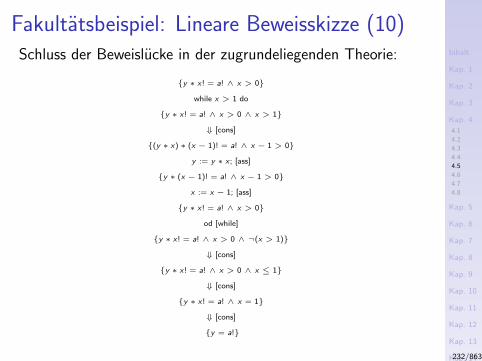
Inhalt
Kap. 1
Kap. 2
Kap. 3
Kap. 4
4.1
4.2
4.3
4.4
4.5
4.6
4.7
4.8
Kap. 5
Kap. 6
Kap. 7
Kap. 8
Kap. 9
Kap. 10
Kap. 11
Kap. 12
Kap. 13
Kap. 14
Kap. 15
Kap. 16
Kap. 17
Literatur
Anhang
A
Fakultatsbeispiel: Lineare Beweisskizze (10)Schluss der Beweislucke in der zugrundeliegenden Theorie:
y ∗ x! = a! ∧ x > 0
while x > 1 do
y ∗ x! = a! ∧ x > 0 ∧ x > 1
⇓ [cons]
(y ∗ x) ∗ (x − 1)! = a! ∧ x − 1 > 0
y := y ∗ x ; [ass]
y ∗ (x − 1)! = a! ∧ x − 1 > 0
x := x − 1; [ass]
y ∗ x! = a! ∧ x > 0
od [while]
y ∗ x! = a! ∧ x > 0 ∧ ¬(x > 1)
⇓ [cons]
y ∗ x! = a! ∧ x > 0 ∧ x ≤ 1
⇓ [cons]
y ∗ x! = a! ∧ x = 1
⇓ [cons]
y = a!
232/863
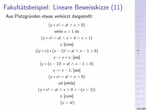
Inhalt
Kap. 1
Kap. 2
Kap. 3
Kap. 4
4.1
4.2
4.3
4.4
4.5
4.6
4.7
4.8
Kap. 5
Kap. 6
Kap. 7
Kap. 8
Kap. 9
Kap. 10
Kap. 11
Kap. 12
Kap. 13
Kap. 14
Kap. 15
Kap. 16
Kap. 17
Literatur
Anhang
A
Fakultatsbeispiel: Lineare Beweisskizze (11)Aus Platzgrunden etwas verkurzt dargestellt:
y ∗ x! = a! ∧ x > 0while x > 1 do
y ∗ x! = a! ∧ x > 0 ∧ x > 1⇓ [cons]
(y ∗ x) ∗ (x − 1)! = a! ∧ x − 1 > 0y := y ∗ x ; [ass]
y ∗ (x − 1)! = a! ∧ x − 1 > 0x := x − 1; [ass]
y ∗ x! = a! ∧ x > 0od [while]
y ∗ x! = a! ∧ x > 0 ∧ ¬(x > 1)⇓ [cons]
y = a!233/863
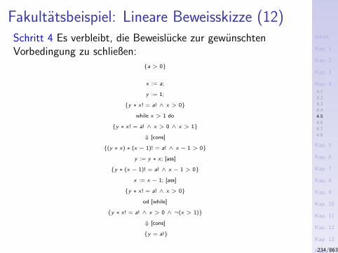
Inhalt
Kap. 1
Kap. 2
Kap. 3
Kap. 4
4.1
4.2
4.3
4.4
4.5
4.6
4.7
4.8
Kap. 5
Kap. 6
Kap. 7
Kap. 8
Kap. 9
Kap. 10
Kap. 11
Kap. 12
Kap. 13
Kap. 14
Kap. 15
Kap. 16
Kap. 17
Literatur
Anhang
A
Fakultatsbeispiel: Lineare Beweisskizze (12)Schritt 4 Es verbleibt, die Beweislucke zur gewunschtenVorbedingung zu schließen:
a > 0
x := a;
y := 1;
y ∗ x! = a! ∧ x > 0
while x > 1 do
y ∗ x! = a! ∧ x > 0 ∧ x > 1
⇓ [cons]
(y ∗ x) ∗ (x − 1)! = a! ∧ x − 1 > 0
y := y ∗ x ; [ass]
y ∗ (x − 1)! = a! ∧ x − 1 > 0
x := x − 1; [ass]
y ∗ x! = a! ∧ x > 0
od [while]
y ∗ x! = a! ∧ x > 0 ∧ ¬(x > 1)
⇓ [cons]
y = a!
234/863
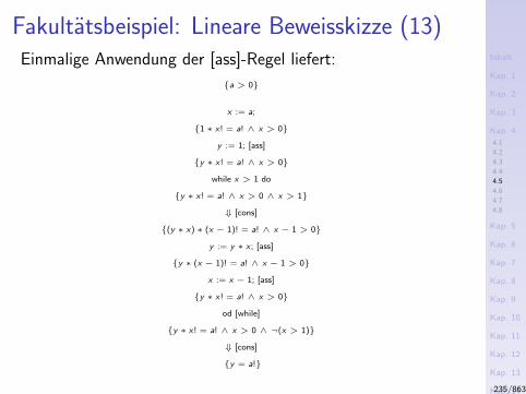
Inhalt
Kap. 1
Kap. 2
Kap. 3
Kap. 4
4.1
4.2
4.3
4.4
4.5
4.6
4.7
4.8
Kap. 5
Kap. 6
Kap. 7
Kap. 8
Kap. 9
Kap. 10
Kap. 11
Kap. 12
Kap. 13
Kap. 14
Kap. 15
Kap. 16
Kap. 17
Literatur
Anhang
A
Fakultatsbeispiel: Lineare Beweisskizze (13)Einmalige Anwendung der [ass]-Regel liefert:
a > 0
x := a;
1 ∗ x! = a! ∧ x > 0
y := 1; [ass]
y ∗ x! = a! ∧ x > 0
while x > 1 do
y ∗ x! = a! ∧ x > 0 ∧ x > 1
⇓ [cons]
(y ∗ x) ∗ (x − 1)! = a! ∧ x − 1 > 0
y := y ∗ x ; [ass]
y ∗ (x − 1)! = a! ∧ x − 1 > 0
x := x − 1; [ass]
y ∗ x! = a! ∧ x > 0
od [while]
y ∗ x! = a! ∧ x > 0 ∧ ¬(x > 1)
⇓ [cons]
y = a!
235/863
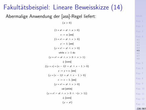
Inhalt
Kap. 1
Kap. 2
Kap. 3
Kap. 4
4.1
4.2
4.3
4.4
4.5
4.6
4.7
4.8
Kap. 5
Kap. 6
Kap. 7
Kap. 8
Kap. 9
Kap. 10
Kap. 11
Kap. 12
Kap. 13
Kap. 14
Kap. 15
Kap. 16
Kap. 17
Literatur
Anhang
A
Fakultatsbeispiel: Lineare Beweisskizze (14)Abermalige Anwendung der [ass]-Regel liefert:
a > 0
1 ∗ a! = a! ∧ a > 0
x := a; [ass]
1 ∗ x! = a! ∧ x > 0
y := 1; [ass]
y ∗ x! = a! ∧ x > 0
while x > 1 do
y ∗ x! = a! ∧ x > 0 ∧ x > 1
⇓ [cons]
(y ∗ x) ∗ (x − 1)! = a! ∧ x − 1 > 0
y := y ∗ x ; [ass]
y ∗ (x − 1)! = a! ∧ x − 1 > 0
x := x − 1; [ass]
y ∗ x! = a! ∧ x > 0
od [while]
y ∗ x! = a! ∧ x > 0 ∧ ¬(x > 1)
⇓ [cons]
y = a!
236/863
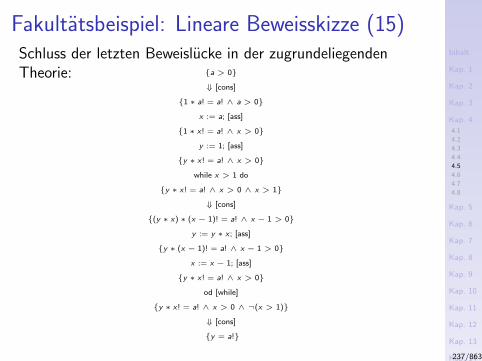
Inhalt
Kap. 1
Kap. 2
Kap. 3
Kap. 4
4.1
4.2
4.3
4.4
4.5
4.6
4.7
4.8
Kap. 5
Kap. 6
Kap. 7
Kap. 8
Kap. 9
Kap. 10
Kap. 11
Kap. 12
Kap. 13
Kap. 14
Kap. 15
Kap. 16
Kap. 17
Literatur
Anhang
A
Fakultatsbeispiel: Lineare Beweisskizze (15)Schluss der letzten Beweislucke in der zugrundeliegendenTheorie: a > 0
⇓ [cons]
1 ∗ a! = a! ∧ a > 0
x := a; [ass]
1 ∗ x! = a! ∧ x > 0
y := 1; [ass]
y ∗ x! = a! ∧ x > 0
while x > 1 do
y ∗ x! = a! ∧ x > 0 ∧ x > 1
⇓ [cons]
(y ∗ x) ∗ (x − 1)! = a! ∧ x − 1 > 0
y := y ∗ x ; [ass]
y ∗ (x − 1)! = a! ∧ x − 1 > 0
x := x − 1; [ass]
y ∗ x! = a! ∧ x > 0
od [while]
y ∗ x! = a! ∧ x > 0 ∧ ¬(x > 1)
⇓ [cons]
y = a!
237/863
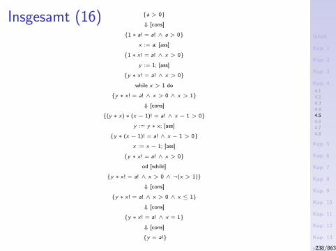
Inhalt
Kap. 1
Kap. 2
Kap. 3
Kap. 4
4.1
4.2
4.3
4.4
4.5
4.6
4.7
4.8
Kap. 5
Kap. 6
Kap. 7
Kap. 8
Kap. 9
Kap. 10
Kap. 11
Kap. 12
Kap. 13
Kap. 14
Kap. 15
Kap. 16
Kap. 17
Literatur
Anhang
A
Insgesamt (16) a > 0
⇓ [cons]
1 ∗ a! = a! ∧ a > 0
x := a; [ass]
1 ∗ x! = a! ∧ x > 0
y := 1; [ass]
y ∗ x! = a! ∧ x > 0
while x > 1 do
y ∗ x! = a! ∧ x > 0 ∧ x > 1
⇓ [cons]
(y ∗ x) ∗ (x − 1)! = a! ∧ x − 1 > 0
y := y ∗ x ; [ass]
y ∗ (x − 1)! = a! ∧ x − 1 > 0
x := x − 1; [ass]
y ∗ x! = a! ∧ x > 0
od [while]
y ∗ x! = a! ∧ x > 0 ∧ ¬(x > 1)
⇓ [cons]
y ∗ x! = a! ∧ x > 0 ∧ x ≤ 1
⇓ [cons]
y ∗ x! = a! ∧ x = 1
⇓ [cons]
y = a!
238/863
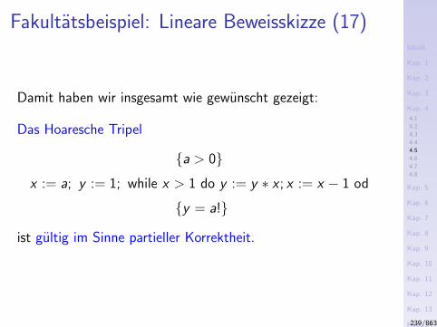
Inhalt
Kap. 1
Kap. 2
Kap. 3
Kap. 4
4.1
4.2
4.3
4.4
4.5
4.6
4.7
4.8
Kap. 5
Kap. 6
Kap. 7
Kap. 8
Kap. 9
Kap. 10
Kap. 11
Kap. 12
Kap. 13
Kap. 14
Kap. 15
Kap. 16
Kap. 17
Literatur
Anhang
A
Fakultatsbeispiel: Lineare Beweisskizze (17)
Damit haben wir insgesamt wie gewunscht gezeigt:
Das Hoaresche Tripel
a > 0
x := a; y := 1; while x > 1 do y := y ∗ x ; x := x − 1 od
y = a!
ist gultig im Sinne partieller Korrektheit.
239/863
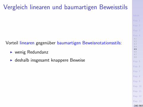
Inhalt
Kap. 1
Kap. 2
Kap. 3
Kap. 4
4.1
4.2
4.3
4.4
4.5
4.6
4.7
4.8
Kap. 5
Kap. 6
Kap. 7
Kap. 8
Kap. 9
Kap. 10
Kap. 11
Kap. 12
Kap. 13
Kap. 14
Kap. 15
Kap. 16
Kap. 17
Literatur
Anhang
A
Vergleich linearen und baumartigen Beweisstils
Vorteil linearen gegenuber baumartigen Beweisnotationsstils:
I wenig Redundanz
I deshalb insgesamt knappere Beweise
240/863

Inhalt
Kap. 1
Kap. 2
Kap. 3
Kap. 4
4.1
4.2
4.3
4.4
4.5
4.6
4.7
4.8
Kap. 5
Kap. 6
Kap. 7
Kap. 8
Kap. 9
Kap. 10
Kap. 11
Kap. 12
Kap. 13
Kap. 14
Kap. 15
Kap. 16
Kap. 17
Literatur
Anhang
A
Kapitel 4.6
Beispiele zum Beweis totaler Korrektheit
241/863
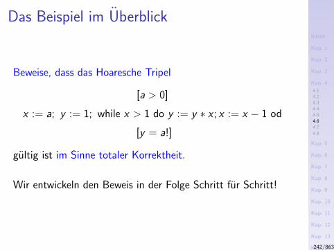
Inhalt
Kap. 1
Kap. 2
Kap. 3
Kap. 4
4.1
4.2
4.3
4.4
4.5
4.6
4.7
4.8
Kap. 5
Kap. 6
Kap. 7
Kap. 8
Kap. 9
Kap. 10
Kap. 11
Kap. 12
Kap. 13
Kap. 14
Kap. 15
Kap. 16
Kap. 17
Literatur
Anhang
A
Das Beispiel im Uberblick
Beweise, dass das Hoaresche Tripel
[a > 0]
x := a; y := 1; while x > 1 do y := y ∗ x ; x := x − 1 od
[y = a!]
gultig ist im Sinne totaler Korrektheit.
Wir entwickeln den Beweis in der Folge Schritt fur Schritt!
242/863
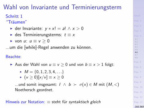
Inhalt
Kap. 1
Kap. 2
Kap. 3
Kap. 4
4.1
4.2
4.3
4.4
4.5
4.6
4.7
4.8
Kap. 5
Kap. 6
Kap. 7
Kap. 8
Kap. 9
Kap. 10
Kap. 11
Kap. 12
Kap. 13
Kap. 14
Kap. 15
Kap. 16
Kap. 17
Literatur
Anhang
A
Wahl von Invariante und TerminierungstermSchritt 1“Traumen”I der Invariante: y ∗ x! = a! ∧ x > 0I des Terminierungsterms: t ≡ xI von u: u ≡ v ≥ 0
...um die [while]-Regel anwenden zu konnen.
Beachte:
I Aus der Wahl von u ≡ v ≥ 0 und von b ≡ x > 1 folgt:
I M = 0, 1, 2, 3, 4, . . .I (v ≥ 0)[x/v ] ≡ x ≥ 0
...und somit insgesamt: I ∧ b σ(x) ∈ M mit (M, <)Noethersch geordnet.
Hinweis zur Notation: ≡ steht fur syntaktisch gleich243/863
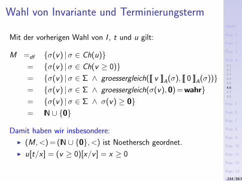
Inhalt
Kap. 1
Kap. 2
Kap. 3
Kap. 4
4.1
4.2
4.3
4.4
4.5
4.6
4.7
4.8
Kap. 5
Kap. 6
Kap. 7
Kap. 8
Kap. 9
Kap. 10
Kap. 11
Kap. 12
Kap. 13
Kap. 14
Kap. 15
Kap. 16
Kap. 17
Literatur
Anhang
A
Wahl von Invariante und Terminierungsterm
Mit der vorherigen Wahl von I , t und u gilt:
M =df σ(v) |σ ∈ Ch(u)= σ(v) |σ ∈ Ch(v ≥ 0)= σ(v) |σ ∈ Σ ∧ groessergleich([[ v ]]A(σ), [[ 0 ]]A(σ))= σ(v) |σ ∈ Σ ∧ groessergleich(σ(v), 0) = wahr= σ(v) |σ ∈ Σ ∧ σ(v) ≥ 0= IN ∪ 0
Damit haben wir insbesondere:
I (M , <) = (IN ∪ 0, <) ist Noethersch geordnet.
I u[t/x ] = (v ≥ 0)[x/v ] = x ≥ 0
244/863

Inhalt
Kap. 1
Kap. 2
Kap. 3
Kap. 4
4.1
4.2
4.3
4.4
4.5
4.6
4.7
4.8
Kap. 5
Kap. 6
Kap. 7
Kap. 8
Kap. 9
Kap. 10
Kap. 11
Kap. 12
Kap. 13
Kap. 14
Kap. 15
Kap. 16
Kap. 17
Literatur
Anhang
A
Bemerkung
Der Beweis wird schrittweise in Form einer linearenBeweisskizze prasentiert.
245/863
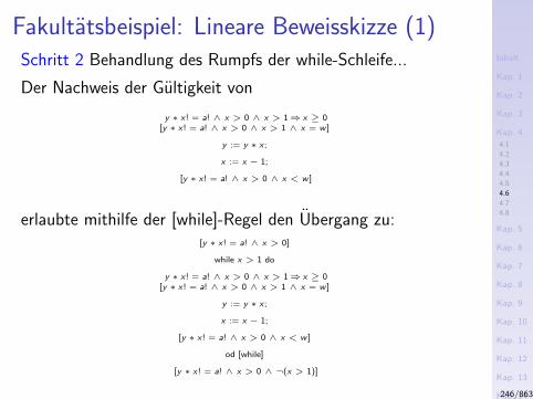
Inhalt
Kap. 1
Kap. 2
Kap. 3
Kap. 4
4.1
4.2
4.3
4.4
4.5
4.6
4.7
4.8
Kap. 5
Kap. 6
Kap. 7
Kap. 8
Kap. 9
Kap. 10
Kap. 11
Kap. 12
Kap. 13
Kap. 14
Kap. 15
Kap. 16
Kap. 17
Literatur
Anhang
A
Fakultatsbeispiel: Lineare Beweisskizze (1)Schritt 2 Behandlung des Rumpfs der while-Schleife...
Der Nachweis der Gultigkeit von
y ∗ x! = a! ∧ x > 0 ∧ x > 1⇒ x ≥ 0[y ∗ x! = a! ∧ x > 0 ∧ x > 1 ∧ x = w ]
y := y ∗ x ;
x := x − 1;
[y ∗ x! = a! ∧ x > 0 ∧ x < w ]
erlaubte mithilfe der [while]-Regel den Ubergang zu:[y ∗ x! = a! ∧ x > 0]
while x > 1 do
y ∗ x! = a! ∧ x > 0 ∧ x > 1⇒ x ≥ 0[y ∗ x! = a! ∧ x > 0 ∧ x > 1 ∧ x = w ]
y := y ∗ x ;
x := x − 1;
[y ∗ x! = a! ∧ x > 0 ∧ x < w ]
od [while]
[y ∗ x! = a! ∧ x > 0 ∧ ¬(x > 1)]
246/863
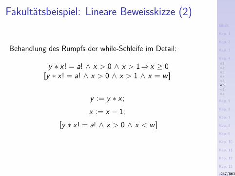
Inhalt
Kap. 1
Kap. 2
Kap. 3
Kap. 4
4.1
4.2
4.3
4.4
4.5
4.6
4.7
4.8
Kap. 5
Kap. 6
Kap. 7
Kap. 8
Kap. 9
Kap. 10
Kap. 11
Kap. 12
Kap. 13
Kap. 14
Kap. 15
Kap. 16
Kap. 17
Literatur
Anhang
A
Fakultatsbeispiel: Lineare Beweisskizze (2)
Behandlung des Rumpfs der while-Schleife im Detail:
y ∗ x! = a! ∧ x > 0 ∧ x > 1⇒ x ≥ 0[y ∗ x! = a! ∧ x > 0 ∧ x > 1 ∧ x = w ]
y := y ∗ x ;
x := x − 1;
[y ∗ x! = a! ∧ x > 0 ∧ x < w ]
247/863
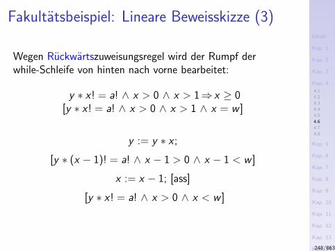
Inhalt
Kap. 1
Kap. 2
Kap. 3
Kap. 4
4.1
4.2
4.3
4.4
4.5
4.6
4.7
4.8
Kap. 5
Kap. 6
Kap. 7
Kap. 8
Kap. 9
Kap. 10
Kap. 11
Kap. 12
Kap. 13
Kap. 14
Kap. 15
Kap. 16
Kap. 17
Literatur
Anhang
A
Fakultatsbeispiel: Lineare Beweisskizze (3)
Wegen Ruckwartszuweisungsregel wird der Rumpf derwhile-Schleife von hinten nach vorne bearbeitet:
y ∗ x! = a! ∧ x > 0 ∧ x > 1⇒ x ≥ 0[y ∗ x! = a! ∧ x > 0 ∧ x > 1 ∧ x = w ]
y := y ∗ x ;
[y ∗ (x − 1)! = a! ∧ x − 1 > 0 ∧ x − 1 < w ]
x := x − 1; [ass]
[y ∗ x! = a! ∧ x > 0 ∧ x < w ]
248/863
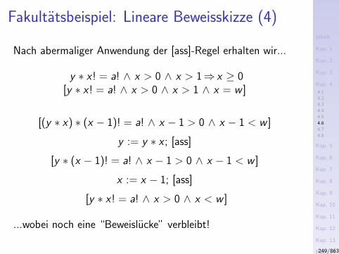
Inhalt
Kap. 1
Kap. 2
Kap. 3
Kap. 4
4.1
4.2
4.3
4.4
4.5
4.6
4.7
4.8
Kap. 5
Kap. 6
Kap. 7
Kap. 8
Kap. 9
Kap. 10
Kap. 11
Kap. 12
Kap. 13
Kap. 14
Kap. 15
Kap. 16
Kap. 17
Literatur
Anhang
A
Fakultatsbeispiel: Lineare Beweisskizze (4)
Nach abermaliger Anwendung der [ass]-Regel erhalten wir...
y ∗ x! = a! ∧ x > 0 ∧ x > 1⇒ x ≥ 0[y ∗ x! = a! ∧ x > 0 ∧ x > 1 ∧ x = w ]
[(y ∗ x) ∗ (x − 1)! = a! ∧ x − 1 > 0 ∧ x − 1 < w ]
y := y ∗ x ; [ass]
[y ∗ (x − 1)! = a! ∧ x − 1 > 0 ∧ x − 1 < w ]
x := x − 1; [ass]
[y ∗ x! = a! ∧ x > 0 ∧ x < w ]
...wobei noch eine “Beweislucke” verbleibt!
249/863
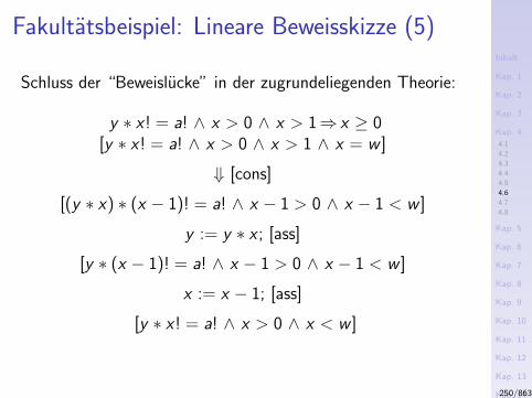
Inhalt
Kap. 1
Kap. 2
Kap. 3
Kap. 4
4.1
4.2
4.3
4.4
4.5
4.6
4.7
4.8
Kap. 5
Kap. 6
Kap. 7
Kap. 8
Kap. 9
Kap. 10
Kap. 11
Kap. 12
Kap. 13
Kap. 14
Kap. 15
Kap. 16
Kap. 17
Literatur
Anhang
A
Fakultatsbeispiel: Lineare Beweisskizze (5)
Schluss der “Beweislucke” in der zugrundeliegenden Theorie:
y ∗ x! = a! ∧ x > 0 ∧ x > 1⇒ x ≥ 0[y ∗ x! = a! ∧ x > 0 ∧ x > 1 ∧ x = w ]
⇓ [cons]
[(y ∗ x) ∗ (x − 1)! = a! ∧ x − 1 > 0 ∧ x − 1 < w ]
y := y ∗ x ; [ass]
[y ∗ (x − 1)! = a! ∧ x − 1 > 0 ∧ x − 1 < w ]
x := x − 1; [ass]
[y ∗ x! = a! ∧ x > 0 ∧ x < w ]
250/863
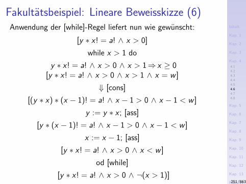
Inhalt
Kap. 1
Kap. 2
Kap. 3
Kap. 4
4.1
4.2
4.3
4.4
4.5
4.6
4.7
4.8
Kap. 5
Kap. 6
Kap. 7
Kap. 8
Kap. 9
Kap. 10
Kap. 11
Kap. 12
Kap. 13
Kap. 14
Kap. 15
Kap. 16
Kap. 17
Literatur
Anhang
A
Fakultatsbeispiel: Lineare Beweisskizze (6)Anwendung der [while]-Regel liefert nun wie gewunscht:
[y ∗ x! = a! ∧ x > 0]
while x > 1 do
y ∗ x! = a! ∧ x > 0 ∧ x > 1⇒ x ≥ 0[y ∗ x! = a! ∧ x > 0 ∧ x > 1 ∧ x = w ]
⇓ [cons]
[(y ∗ x) ∗ (x − 1)! = a! ∧ x − 1 > 0 ∧ x − 1 < w ]
y := y ∗ x ; [ass]
[y ∗ (x − 1)! = a! ∧ x − 1 > 0 ∧ x − 1 < w ]
x := x − 1; [ass]
[y ∗ x! = a! ∧ x > 0 ∧ x < w ]
od [while]
[y ∗ x! = a! ∧ x > 0 ∧ ¬(x > 1)]251/863
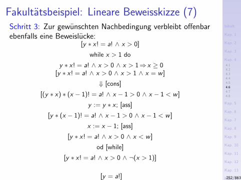
Inhalt
Kap. 1
Kap. 2
Kap. 3
Kap. 4
4.1
4.2
4.3
4.4
4.5
4.6
4.7
4.8
Kap. 5
Kap. 6
Kap. 7
Kap. 8
Kap. 9
Kap. 10
Kap. 11
Kap. 12
Kap. 13
Kap. 14
Kap. 15
Kap. 16
Kap. 17
Literatur
Anhang
A
Fakultatsbeispiel: Lineare Beweisskizze (7)Schritt 3: Zur gewunschten Nachbedingung verbleibt offenbarebenfalls eine Beweislucke:
[y ∗ x! = a! ∧ x > 0]
while x > 1 do
y ∗ x! = a! ∧ x > 0 ∧ x > 1⇒ x ≥ 0[y ∗ x! = a! ∧ x > 0 ∧ x > 1 ∧ x = w ]
⇓ [cons]
[(y ∗ x) ∗ (x − 1)! = a! ∧ x − 1 > 0 ∧ x − 1 < w ]
y := y ∗ x ; [ass]
[y ∗ (x − 1)! = a! ∧ x − 1 > 0 ∧ x − 1 < w ]
x := x − 1; [ass]
[y ∗ x! = a! ∧ x > 0 ∧ x < w ]
od [while]
[y ∗ x! = a! ∧ x > 0 ∧ ¬(x > 1)]
[y = a!] 252/863
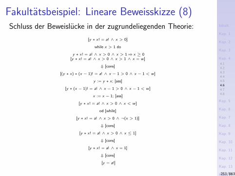
Inhalt
Kap. 1
Kap. 2
Kap. 3
Kap. 4
4.1
4.2
4.3
4.4
4.5
4.6
4.7
4.8
Kap. 5
Kap. 6
Kap. 7
Kap. 8
Kap. 9
Kap. 10
Kap. 11
Kap. 12
Kap. 13
Kap. 14
Kap. 15
Kap. 16
Kap. 17
Literatur
Anhang
A
Fakultatsbeispiel: Lineare Beweisskizze (8)Schluss der Beweislucke in der zugrundeliegenden Theorie:
[y ∗ x! = a! ∧ x > 0]
while x > 1 do
y ∗ x! = a! ∧ x > 0 ∧ x > 1⇒ x ≥ 0[y ∗ x! = a! ∧ x > 0 ∧ x > 1 ∧ x = w ]
⇓ [cons]
[(y ∗ x) ∗ (x − 1)! = a! ∧ x − 1 > 0 ∧ x − 1 < w ]
y := y ∗ x ; [ass]
[y ∗ (x − 1)! = a! ∧ x − 1 > 0 ∧ x − 1 < w ]
x := x − 1; [ass]
[y ∗ x! = a! ∧ x > 0 ∧ x < w ]
od [while]
[y ∗ x! = a! ∧ x > 0 ∧ ¬(x > 1)]
⇓ [cons]
[y ∗ x! = a! ∧ x > 0 ∧ x ≤ 1]
⇓ [cons]
[y ∗ x! = a! ∧ x = 1]
⇓ [cons]
[y = a!]
253/863
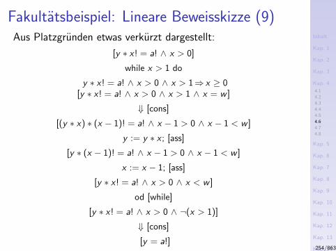
Inhalt
Kap. 1
Kap. 2
Kap. 3
Kap. 4
4.1
4.2
4.3
4.4
4.5
4.6
4.7
4.8
Kap. 5
Kap. 6
Kap. 7
Kap. 8
Kap. 9
Kap. 10
Kap. 11
Kap. 12
Kap. 13
Kap. 14
Kap. 15
Kap. 16
Kap. 17
Literatur
Anhang
A
Fakultatsbeispiel: Lineare Beweisskizze (9)Aus Platzgrunden etwas verkurzt dargestellt:
[y ∗ x! = a! ∧ x > 0]
while x > 1 do
y ∗ x! = a! ∧ x > 0 ∧ x > 1⇒ x ≥ 0[y ∗ x! = a! ∧ x > 0 ∧ x > 1 ∧ x = w ]
⇓ [cons]
[(y ∗ x) ∗ (x − 1)! = a! ∧ x − 1 > 0 ∧ x − 1 < w ]
y := y ∗ x ; [ass]
[y ∗ (x − 1)! = a! ∧ x − 1 > 0 ∧ x − 1 < w ]
x := x − 1; [ass]
[y ∗ x! = a! ∧ x > 0 ∧ x < w ]
od [while]
[y ∗ x! = a! ∧ x > 0 ∧ ¬(x > 1)]
⇓ [cons]
[y = a!]254/863
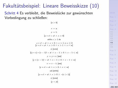
Inhalt
Kap. 1
Kap. 2
Kap. 3
Kap. 4
4.1
4.2
4.3
4.4
4.5
4.6
4.7
4.8
Kap. 5
Kap. 6
Kap. 7
Kap. 8
Kap. 9
Kap. 10
Kap. 11
Kap. 12
Kap. 13
Kap. 14
Kap. 15
Kap. 16
Kap. 17
Literatur
Anhang
A
Fakultatsbeispiel: Lineare Beweisskizze (10)Schritt 4 Es verbleibt, die Beweislucke zur gewunschtenVorbedingung zu schließen:
[a > 0]
x := a;
y := 1;
[y ∗ x! = a! ∧ x > 0]
while x > 1 do
y ∗ x! = a! ∧ x > 0 ∧ x > 1⇒ x ≥ 0[y ∗ x! = a! ∧ x > 0 ∧ x > 1 ∧ x = w ]
⇓ [cons]
[(y ∗ x) ∗ (x − 1)! = a! ∧ x − 1 > 0 ∧ x − 1 < w ]
y := y ∗ x ; [ass]
[y ∗ (x − 1)! = a! ∧ x − 1 > 0 ∧ x − 1 < w ]
x := x − 1; [ass]
[y ∗ x! = a! ∧ x > 0 ∧ x < w ]
od [while]
[y ∗ x! = a! ∧ x > 0 ∧ ¬(x > 1)]
⇓ [cons]
[y = a!]
255/863
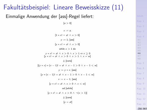
Inhalt
Kap. 1
Kap. 2
Kap. 3
Kap. 4
4.1
4.2
4.3
4.4
4.5
4.6
4.7
4.8
Kap. 5
Kap. 6
Kap. 7
Kap. 8
Kap. 9
Kap. 10
Kap. 11
Kap. 12
Kap. 13
Kap. 14
Kap. 15
Kap. 16
Kap. 17
Literatur
Anhang
A
Fakultatsbeispiel: Lineare Beweisskizze (11)Einmalige Anwendung der [ass]-Regel liefert:
[a > 0]
x := a;
[1 ∗ x! = a! ∧ x > 0]
y := 1; [ass]
[y ∗ x! = a! ∧ x > 0]
while x > 1 do
y ∗ x! = a! ∧ x > 0 ∧ x > 1⇒ x ≥ 0[y ∗ x! = a! ∧ x > 0 ∧ x > 1 ∧ x = w ]
⇓ [cons]
[(y ∗ x) ∗ (x − 1)! = a! ∧ x − 1 > 0 ∧ x − 1 < w ]
y := y ∗ x ; [ass]
[y ∗ (x − 1)! = a! ∧ x − 1 > 0 ∧ x − 1 < w ]
x := x − 1; [ass]
[y ∗ x! = a! ∧ x > 0 ∧ x < w ]
od [while]
[y ∗ x! = a! ∧ x > 0 ∧ ¬(x > 1)]
⇓ [cons]
[y = a!]
256/863
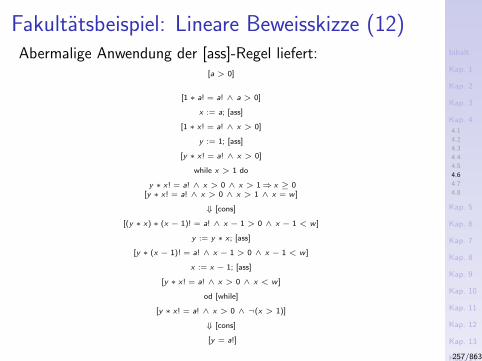
Inhalt
Kap. 1
Kap. 2
Kap. 3
Kap. 4
4.1
4.2
4.3
4.4
4.5
4.6
4.7
4.8
Kap. 5
Kap. 6
Kap. 7
Kap. 8
Kap. 9
Kap. 10
Kap. 11
Kap. 12
Kap. 13
Kap. 14
Kap. 15
Kap. 16
Kap. 17
Literatur
Anhang
A
Fakultatsbeispiel: Lineare Beweisskizze (12)Abermalige Anwendung der [ass]-Regel liefert:
[a > 0]
[1 ∗ a! = a! ∧ a > 0]
x := a; [ass]
[1 ∗ x! = a! ∧ x > 0]
y := 1; [ass]
[y ∗ x! = a! ∧ x > 0]
while x > 1 do
y ∗ x! = a! ∧ x > 0 ∧ x > 1⇒ x ≥ 0[y ∗ x! = a! ∧ x > 0 ∧ x > 1 ∧ x = w ]
⇓ [cons]
[(y ∗ x) ∗ (x − 1)! = a! ∧ x − 1 > 0 ∧ x − 1 < w ]
y := y ∗ x ; [ass]
[y ∗ (x − 1)! = a! ∧ x − 1 > 0 ∧ x − 1 < w ]
x := x − 1; [ass]
[y ∗ x! = a! ∧ x > 0 ∧ x < w ]
od [while]
[y ∗ x! = a! ∧ x > 0 ∧ ¬(x > 1)]
⇓ [cons]
[y = a!]
257/863
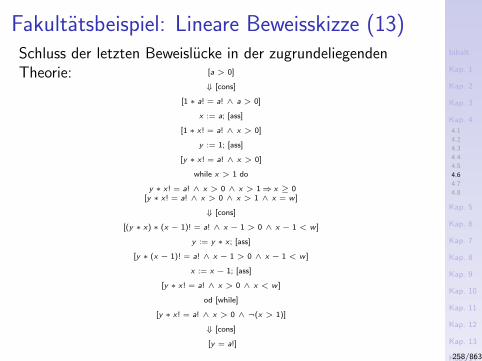
Inhalt
Kap. 1
Kap. 2
Kap. 3
Kap. 4
4.1
4.2
4.3
4.4
4.5
4.6
4.7
4.8
Kap. 5
Kap. 6
Kap. 7
Kap. 8
Kap. 9
Kap. 10
Kap. 11
Kap. 12
Kap. 13
Kap. 14
Kap. 15
Kap. 16
Kap. 17
Literatur
Anhang
A
Fakultatsbeispiel: Lineare Beweisskizze (13)Schluss der letzten Beweislucke in der zugrundeliegendenTheorie: [a > 0]
⇓ [cons]
[1 ∗ a! = a! ∧ a > 0]
x := a; [ass]
[1 ∗ x! = a! ∧ x > 0]
y := 1; [ass]
[y ∗ x! = a! ∧ x > 0]
while x > 1 do
y ∗ x! = a! ∧ x > 0 ∧ x > 1⇒ x ≥ 0[y ∗ x! = a! ∧ x > 0 ∧ x > 1 ∧ x = w ]
⇓ [cons]
[(y ∗ x) ∗ (x − 1)! = a! ∧ x − 1 > 0 ∧ x − 1 < w ]
y := y ∗ x ; [ass]
[y ∗ (x − 1)! = a! ∧ x − 1 > 0 ∧ x − 1 < w ]
x := x − 1; [ass]
[y ∗ x! = a! ∧ x > 0 ∧ x < w ]
od [while]
[y ∗ x! = a! ∧ x > 0 ∧ ¬(x > 1)]
⇓ [cons]
[y = a!]
258/863
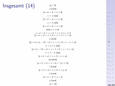
Inhalt
Kap. 1
Kap. 2
Kap. 3
Kap. 4
4.1
4.2
4.3
4.4
4.5
4.6
4.7
4.8
Kap. 5
Kap. 6
Kap. 7
Kap. 8
Kap. 9
Kap. 10
Kap. 11
Kap. 12
Kap. 13
Kap. 14
Kap. 15
Kap. 16
Kap. 17
Literatur
Anhang
A
Insgesamt (14) [a > 0]
⇓ [cons]
[1 ∗ a! = a! ∧ a > 0]
x := a; [ass]
[1 ∗ x! = a! ∧ x > 0]
y := 1; [ass]
[y ∗ x! = a! ∧ x > 0]
while x > 1 do
y ∗ x! = a! ∧ x > 0 ∧ x > 1⇒ x ≥ 0[y ∗ x! = a! ∧ x > 0 ∧ x > 1 ∧ x = w ]
⇓ [cons]
[(y ∗ x) ∗ (x − 1)! = a! ∧ x − 1 > 0 ∧ x − 1 < w ]
y := y ∗ x ; [ass]
[y ∗ (x − 1)! = a! ∧ x − 1 > 0 ∧ x − 1 < w ]
x := x − 1; [ass]
[y ∗ x! = a! ∧ x > 0 ∧ x < w ]
od [while]
[y ∗ x! = a! ∧ x > 0 ∧ ¬(x > 1)]
⇓ [cons]
[y ∗ x! = a! ∧ x > 0 ∧ x ≤ 1]
⇓ [cons]
[y ∗ x! = a! ∧ x = 1]
⇓ [cons]
[y = a!]259/863
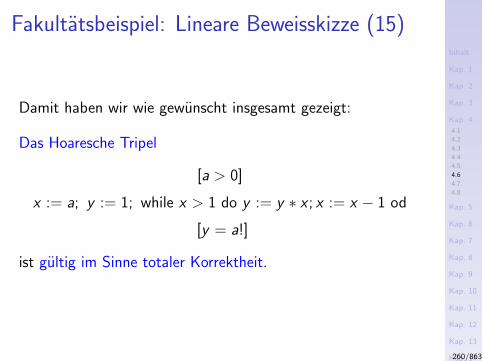
Inhalt
Kap. 1
Kap. 2
Kap. 3
Kap. 4
4.1
4.2
4.3
4.4
4.5
4.6
4.7
4.8
Kap. 5
Kap. 6
Kap. 7
Kap. 8
Kap. 9
Kap. 10
Kap. 11
Kap. 12
Kap. 13
Kap. 14
Kap. 15
Kap. 16
Kap. 17
Literatur
Anhang
A
Fakultatsbeispiel: Lineare Beweisskizze (15)
Damit haben wir wie gewunscht insgesamt gezeigt:
Das Hoaresche Tripel
[a > 0]
x := a; y := 1; while x > 1 do y := y ∗ x ; x := x − 1 od
[y = a!]
ist gultig im Sinne totaler Korrektheit.
260/863
Inhalt
Kap. 1
Kap. 2
Kap. 3
Kap. 4
4.1
4.2
4.3
4.4
4.5
4.6
4.7
4.8
Kap. 5
Kap. 6
Kap. 7
Kap. 8
Kap. 9
Kap. 10
Kap. 11
Kap. 12
Kap. 13
Kap. 14
Kap. 15
Kap. 16
Kap. 17
Literatur
Anhang
A
Kapitel 4.7
Automatische Ansatze axiomatischerProgrammverifikation
261/863
Inhalt
Kap. 1
Kap. 2
Kap. 3
Kap. 4
4.1
4.2
4.3
4.4
4.5
4.6
4.7
4.8
Kap. 5
Kap. 6
Kap. 7
Kap. 8
Kap. 9
Kap. 10
Kap. 11
Kap. 12
Kap. 13
Kap. 14
Kap. 15
Kap. 16
Kap. 17
Literatur
Anhang
A
Ansatze zu (semi-) automatischer axioma-
tischer Programmverifikation
Unter anderem:
I Theorema, RISC, JKU Linz
I KeY-Hoare, KIT Karlsruhe, Chalmers University ofTechnology, TU Darmstadt
I ...
262/863
Inhalt
Kap. 1
Kap. 2
Kap. 3
Kap. 4
4.1
4.2
4.3
4.4
4.5
4.6
4.7
4.8
Kap. 5
Kap. 6
Kap. 7
Kap. 8
Kap. 9
Kap. 10
Kap. 11
Kap. 12
Kap. 13
Kap. 14
Kap. 15
Kap. 16
Kap. 17
Literatur
Anhang
A
Theorema-Projekt, www.theorema.org (1)
“The Theorema project aims at extending current computer
algebra systems by facilities for supporting mathematical proving.
The present early-prototype version of the Theorema software
system is implemented in Mathematica. The system consists of a
general higher-order predicate logic prover and a collection of
special provers that call each other depending on the particular
proof situations. The individual provers imitate the proof style of
human mathematicians and produce human-readable proofs in
natural language presented in nested cells. The special provers are
intimately connected with the functors that build up the various
mathematical domains.
263/863
Inhalt
Kap. 1
Kap. 2
Kap. 3
Kap. 4
4.1
4.2
4.3
4.4
4.5
4.6
4.7
4.8
Kap. 5
Kap. 6
Kap. 7
Kap. 8
Kap. 9
Kap. 10
Kap. 11
Kap. 12
Kap. 13
Kap. 14
Kap. 15
Kap. 16
Kap. 17
Literatur
Anhang
A
Theorema-Projekt, www.theorema.org (2)
The long-term goal of the project is to produce a complete systemwhich supports the mathematician in creating interactive text-books, i.e. books containing, besides the ordinary passive text,active text representing algorithms in executable format, as well asproofs which can be studied at various levels of detail, and whoseroutine parts can be automatically generated. This system willprovide a uniform (logic and software) framework in which aworking mathematician, without leaving the system, can getcomputer-support while looping through all phases of themathematical problem solving cycle. [...]”
(Exzerpt von http://www.theorema.org)
264/863

Inhalt
Kap. 1
Kap. 2
Kap. 3
Kap. 4
4.1
4.2
4.3
4.4
4.5
4.6
4.7
4.8
Kap. 5
Kap. 6
Kap. 7
Kap. 8
Kap. 9
Kap. 10
Kap. 11
Kap. 12
Kap. 13
Kap. 14
Kap. 15
Kap. 16
Kap. 17
Literatur
Anhang
A
KeY-Projekt, www.key-project.org (1)
Integrated Deductive Software Design
“The KeY System is a formal software development tool that aimsto integrate design, implementation, formal specification, andformal verification of object-oriented software as seamlessly aspossible. At the core of the system is a novel theorem prover forthe first-order Dynamic Logic for Java with a user-friendlygraphical interface.
The project was started in November 1998 at the University ofKarlsruhe. It is now a joint project of Karlsruhe Institute ofTechnology and Chalmers University of Technology, Gothenburg,and TU Darmstadt.
The KeY tool is available for down-load. [...]”
(Exzerpt von http://www.key-project.org)
265/863
Inhalt
Kap. 1
Kap. 2
Kap. 3
Kap. 4
4.1
4.2
4.3
4.4
4.5
4.6
4.7
4.8
Kap. 5
Kap. 6
Kap. 7
Kap. 8
Kap. 9
Kap. 10
Kap. 11
Kap. 12
Kap. 13
Kap. 14
Kap. 15
Kap. 16
Kap. 17
Literatur
Anhang
A
KeY-Projekt, www.key-project.org (2)KeY-Hoare, www.key-project.org/download/hoare,unterstutzt
I partielle KorrektheitsbeweiseI totale Korrektheitsbeweise und
Ausfuhrungszeitkorrektheitsbeweise (Versionen ab 0.1.6)I ganzzahlige und Boolesche Felder (Versionen ab 0.1.7)
Nutzliche Handreichung:
I Reiner Hahnle, Richard Bubel. A Hoare-Style Calculuswith Explicit State Updates. Handout in a course onProgram Verification at the Department of ComputerScience at the Chalmers University of Technology on theHoare Calculus and the usage of the tool KeY-Hoare,19 pages.htpp://i12www.iti.uni-karlsruhe.de/∼key/download/hoare/students.pdf
266/863

Inhalt
Kap. 1
Kap. 2
Kap. 3
Kap. 4
4.1
4.2
4.3
4.4
4.5
4.6
4.7
4.8
Kap. 5
Kap. 6
Kap. 7
Kap. 8
Kap. 9
Kap. 10
Kap. 11
Kap. 12
Kap. 13
Kap. 14
Kap. 15
Kap. 16
Kap. 17
Literatur
Anhang
A
Kapitel 4.8
Historische Meilensteine derProgrammverifikation
267/863
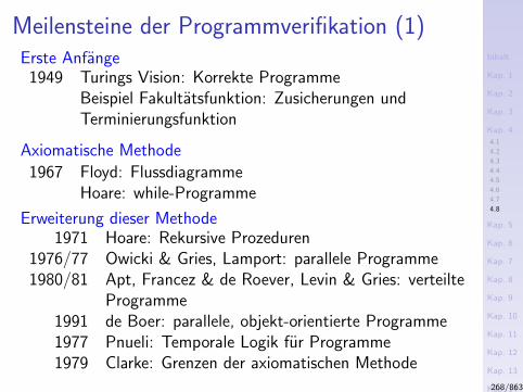
Inhalt
Kap. 1
Kap. 2
Kap. 3
Kap. 4
4.1
4.2
4.3
4.4
4.5
4.6
4.7
4.8
Kap. 5
Kap. 6
Kap. 7
Kap. 8
Kap. 9
Kap. 10
Kap. 11
Kap. 12
Kap. 13
Kap. 14
Kap. 15
Kap. 16
Kap. 17
Literatur
Anhang
A
Meilensteine der Programmverifikation (1)Erste Anfange
1949 Turings Vision: Korrekte ProgrammeBeispiel Fakultatsfunktion: Zusicherungen undTerminierungsfunktion
Axiomatische Methode
1967 Floyd: FlussdiagrammeHoare: while-Programme
Erweiterung dieser Methode1971 Hoare: Rekursive Prozeduren
1976/77 Owicki & Gries, Lamport: parallele Programme1980/81 Apt, Francez & de Roever, Levin & Gries: verteilte
Programme1991 de Boer: parallele, objekt-orientierte Programme1977 Pnueli: Temporale Logik fur Programme1979 Clarke: Grenzen der axiomatischen Methode
268/863
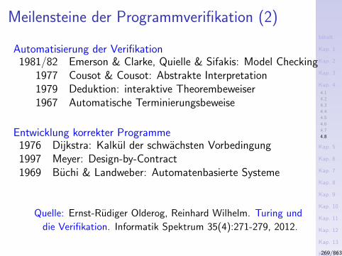
Inhalt
Kap. 1
Kap. 2
Kap. 3
Kap. 4
4.1
4.2
4.3
4.4
4.5
4.6
4.7
4.8
Kap. 5
Kap. 6
Kap. 7
Kap. 8
Kap. 9
Kap. 10
Kap. 11
Kap. 12
Kap. 13
Kap. 14
Kap. 15
Kap. 16
Kap. 17
Literatur
Anhang
A
Meilensteine der Programmverifikation (2)
Automatisierung der Verifikation1981/82 Emerson & Clarke, Quielle & Sifakis: Model Checking
1977 Cousot & Cousot: Abstrakte Interpretation1979 Deduktion: interaktive Theorembeweiser1967 Automatische Terminierungsbeweise
Entwicklung korrekter Programme1976 Dijkstra: Kalkul der schwachsten Vorbedingung1997 Meyer: Design-by-Contract1969 Buchi & Landweber: Automatenbasierte Systeme
Quelle: Ernst-Rudiger Olderog, Reinhard Wilhelm. Turing und
die Verifikation. Informatik Spektrum 35(4):271-279, 2012.
269/863
Inhalt
Kap. 1
Kap. 2
Kap. 3
Kap. 4
4.1
4.2
4.3
4.4
4.5
4.6
4.7
4.8
Kap. 5
Kap. 6
Kap. 7
Kap. 8
Kap. 9
Kap. 10
Kap. 11
Kap. 12
Kap. 13
Kap. 14
Kap. 15
Kap. 16
Kap. 17
Literatur
Anhang
A
Vertiefende und weiterfuhrende Leseempfeh-
lungen fur Kapitel 4 (1)
Krzysztof R. Apt. Ten Years of Hoare’s Logic: A Survey –Part 1. ACM Transactions on Programming Languagesand Systems 3:431-483, 1981.
Krzysztof R. Apt. Ten Years of Hoare’s Logic: A Survey –Part II: Nondeterminism. Theoretical Computer Science28(1-2):83-109, 1984.
Krzysztof R. Apt, Ernst-Rudiger Olderog. Programm-verifikation – Sequentielle, parallele und verteilteProgramme. Springer-V., 1994.
270/863
Inhalt
Kap. 1
Kap. 2
Kap. 3
Kap. 4
4.1
4.2
4.3
4.4
4.5
4.6
4.7
4.8
Kap. 5
Kap. 6
Kap. 7
Kap. 8
Kap. 9
Kap. 10
Kap. 11
Kap. 12
Kap. 13
Kap. 14
Kap. 15
Kap. 16
Kap. 17
Literatur
Anhang
A
Vertiefende und weiterfuhrende Leseempfeh-
lungen fur Kapitel 4 (2)
Krzysztof R. Apt, Frank S. de Boer, Ernst-RudigerOlderog. Verification of Sequential and ConcurrentPrograms. Springer-V., 3rd edition, 2009. (Chapter 3,While Programs; Chap. 3.3, Verification; Chapter 3.4,Proof Outlines – Partial Correctness, Total Correctness;Chapter 3.5, Completeness)
Bernhard Beckert, Reiner Hahnle, Peter H. Schmitt(Hrsg.). Verification of Object-Oriented Software: TheKeYApproach. LNCS 4334, Springer-V., 2007.
Mordechai Ben-Ari. Mathematical Logic for ComputerScience. 2nd edition, Springer-V., 2001. (Chapter 9,Programs: Semantics and Verification)
271/863
Inhalt
Kap. 1
Kap. 2
Kap. 3
Kap. 4
4.1
4.2
4.3
4.4
4.5
4.6
4.7
4.8
Kap. 5
Kap. 6
Kap. 7
Kap. 8
Kap. 9
Kap. 10
Kap. 11
Kap. 12
Kap. 13
Kap. 14
Kap. 15
Kap. 16
Kap. 17
Literatur
Anhang
A
Vertiefende und weiterfuhrende Leseempfeh-
lungen fur Kapitel 4 (3)
Stephen A. Cook. Soundness and Completeness of anAxiom System for Program Verification. SIAM Journal onComputing 7(1):70-90, 1978.
Jaco W. De Backer. Mathematical Theory of ProgramCorrectness. Prentice-Hall, 1980.
Edmund M. Clarke. Programming Language Constructsfor which it is Impossible to Obtain Good Hoare AxiomSystems. Journal of the ACM 26(1):129-147, 1979.
Edmund M. Clarke, Stephen M. German, JosephY. Halpern. Effective Axiomatizations of Hoare Logics.Journal of the ACM 30(1):612-636, 1983.
272/863
Inhalt
Kap. 1
Kap. 2
Kap. 3
Kap. 4
4.1
4.2
4.3
4.4
4.5
4.6
4.7
4.8
Kap. 5
Kap. 6
Kap. 7
Kap. 8
Kap. 9
Kap. 10
Kap. 11
Kap. 12
Kap. 13
Kap. 14
Kap. 15
Kap. 16
Kap. 17
Literatur
Anhang
A
Vertiefende und weiterfuhrende Leseempfeh-
lungen fur Kapitel 4 (4)
Robert W. Floyd. Assigning Meaning to Programs. InProceedings of Symposium on Applied Mathematics,Mathematical Aspects of Computer Science, AmericanMathematical Society, New York, 19:19-32, 1967.
Reiner Hahnle, Richard Bubel. A Hoare-Style Calculuswith Explicit State Updates. Handout in the courseProgram Verification at the Department of ComputerScience at the Chalmers University of Technology, 19pages. i12www.iti.uni-karlsruhe.de/∼key/download/hoare/students.pdf
Charles A.R. Hoare. An Axiomatic Basis for ComputerProgramming. Communications of the ACM12(19):576-580, 583, 1969.
273/863
Inhalt
Kap. 1
Kap. 2
Kap. 3
Kap. 4
4.1
4.2
4.3
4.4
4.5
4.6
4.7
4.8
Kap. 5
Kap. 6
Kap. 7
Kap. 8
Kap. 9
Kap. 10
Kap. 11
Kap. 12
Kap. 13
Kap. 14
Kap. 15
Kap. 16
Kap. 17
Literatur
Anhang
A
Vertiefende und weiterfuhrende Leseempfeh-
lungen fur Kapitel 4 (5)
Tudor Jebelean, Laura Kovacs, Nikolaj Popov. Experi-mental Program Verification in the Theorema System. InProceedings of the 1st International Symposium onLeveraging Applications of Formal Methods (ISoLA 2004),92-99, 2004. www.risc.jku.at/publications/download/risc 2243/KoPoJeb.pdf
Laura Kovacs, Tudor Jebelean. Practical Aspects ofImperative Program Verification using Theorema. InProceedings of the 5th International Workshop onSymbolic and Numeric Algorithms for Scientific Computing(SYNASC 2003), 317-320, 2003. www.risc.jku.at/publications/download/risc 464/synasc03.pdf
274/863
Inhalt
Kap. 1
Kap. 2
Kap. 3
Kap. 4
4.1
4.2
4.3
4.4
4.5
4.6
4.7
4.8
Kap. 5
Kap. 6
Kap. 7
Kap. 8
Kap. 9
Kap. 10
Kap. 11
Kap. 12
Kap. 13
Kap. 14
Kap. 15
Kap. 16
Kap. 17
Literatur
Anhang
A
Vertiefende und weiterfuhrende Leseempfeh-
lungen fur Kapitel 4 (6)
Laura Kovacs, Tudor Jebelean. Generation of Invariants inTheorema. In Proceedings of the 10th InternationalSymposium of Mathematics and its Applications, 407-415,2003. www.risc.jku.at/publications/download/risc 2053/2003-11-06-A.pdf
Janusz Laski, William Stanley. Software Verification andAnalysis. Springer-V., 2009. (Chapter 1, Introduction:What do we want to know about the Program?, Chapter2, How to prove a Program Correct: Programs withoutLoops; Chapter 3, How to prove a Program Correct:Iterative Programs)
275/863
Inhalt
Kap. 1
Kap. 2
Kap. 3
Kap. 4
4.1
4.2
4.3
4.4
4.5
4.6
4.7
4.8
Kap. 5
Kap. 6
Kap. 7
Kap. 8
Kap. 9
Kap. 10
Kap. 11
Kap. 12
Kap. 13
Kap. 14
Kap. 15
Kap. 16
Kap. 17
Literatur
Anhang
A
Vertiefende und weiterfuhrende Leseempfeh-
lungen fur Kapitel 4 (7)
Jacques Loeckx, Kurt Sieber. The Foundations of ProgramVerification. Wiley, 1984.
Robert Lover. Elementary Logic for Software Development.Springer-V., 2008. (Chapter 19, Program CorrectnessProofs; Chapter 19.3, Proofs using Floyd’s Method ofInvariant Assertions; Chapter 20.2.1, Floyd-Hoare Logic)
Hanne Riis Nielson, Flemming Nielson. Semantics withApplications: A Formal Introduction. Wiley, 1992.(Chapter 6, Axiomatic Program Verification)
276/863
Inhalt
Kap. 1
Kap. 2
Kap. 3
Kap. 4
4.1
4.2
4.3
4.4
4.5
4.6
4.7
4.8
Kap. 5
Kap. 6
Kap. 7
Kap. 8
Kap. 9
Kap. 10
Kap. 11
Kap. 12
Kap. 13
Kap. 14
Kap. 15
Kap. 16
Kap. 17
Literatur
Anhang
A
Vertiefende und weiterfuhrende Leseempfeh-
lungen fur Kapitel 4 (8)
Hanne Riis Nielson, Flemming Nielson. Semantics withApplications: An Appetizer. Springer-V., 2007. (Chapter9, Axiomatic Program Verification; Chapter 10, More onAxiomatic Program Verification)
David von Oheimb. Hoare Logic for Java in Isabelle/HOL.Concurrency and Computation: Practice and Experience13(13):1173-1214, 2001.
Ernst-Rudiger Olderog. Correctness of Programs withPascal-like Procedures without Global Variables.Theoretical Computer Science 30(1):49-90, 1984.
277/863
Inhalt
Kap. 1
Kap. 2
Kap. 3
Kap. 4
4.1
4.2
4.3
4.4
4.5
4.6
4.7
4.8
Kap. 5
Kap. 6
Kap. 7
Kap. 8
Kap. 9
Kap. 10
Kap. 11
Kap. 12
Kap. 13
Kap. 14
Kap. 15
Kap. 16
Kap. 17
Literatur
Anhang
A
Vertiefende und weiterfuhrende Leseempfeh-
lungen fur Kapitel 4 (9)
Ernst-Rudiger Olderog, Bernhard Steffen. Formale Seman-tik und Programmverifikation. In Informatik-Handbuch,Peter Rechenberg, Gustav Pomberger (Hrsg.), Carl HanserVerlag, 4. Auflage, 145-166, 2006.
Ernst-Rudiger Olderog, Reinhard Wilhelm. Turing und dieVerifikation. Informatik Spektrum 35(4):271-279, 2012.
278/863
Inhalt
Kap. 1
Kap. 2
Kap. 3
Kap. 4
Kap. 5
Kap. 6
Kap. 7
Kap. 8
Kap. 9
Kap. 10
Kap. 11
Kap. 12
Kap. 13
Kap. 14
Kap. 15
Kap. 16
Kap. 17
Literatur
Anhang
A
Kapitel 5
Worst-Case Execution Time Analyse
279/863
Inhalt
Kap. 1
Kap. 2
Kap. 3
Kap. 4
Kap. 5
Kap. 6
Kap. 7
Kap. 8
Kap. 9
Kap. 10
Kap. 11
Kap. 12
Kap. 13
Kap. 14
Kap. 15
Kap. 16
Kap. 17
Literatur
Anhang
A
Motivation
Von Verifikation zu Analyse:
I Worst-Case Execution Time-Analyse als erstes Beispiel
...nach
I Hanne Riis Nielson, Flemming Nielson. Semantics withApplications – A Formal Introduction. Wiley, 1992.
280/863
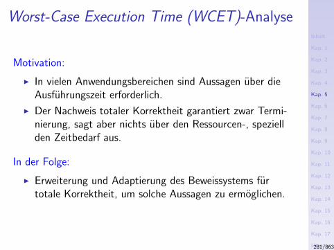
Inhalt
Kap. 1
Kap. 2
Kap. 3
Kap. 4
Kap. 5
Kap. 6
Kap. 7
Kap. 8
Kap. 9
Kap. 10
Kap. 11
Kap. 12
Kap. 13
Kap. 14
Kap. 15
Kap. 16
Kap. 17
Literatur
Anhang
A
Worst-Case Execution Time (WCET)-Analyse
Motivation:
I In vielen Anwendungsbereichen sind Aussagen uber dieAusfuhrungszeit erforderlich.
I Der Nachweis totaler Korrektheit garantiert zwar Termi-nierung, sagt aber nichts uber den Ressourcen-, speziellden Zeitbedarf aus.
In der Folge:
I Erweiterung und Adaptierung des Beweissystems furtotale Korrektheit, um solche Aussagen zu ermoglichen.
281/863
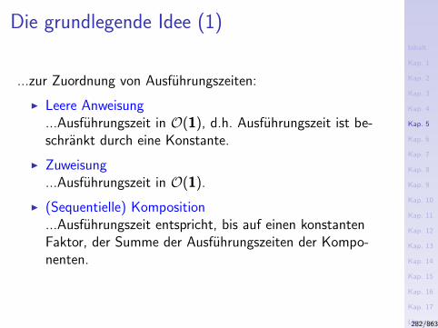
Inhalt
Kap. 1
Kap. 2
Kap. 3
Kap. 4
Kap. 5
Kap. 6
Kap. 7
Kap. 8
Kap. 9
Kap. 10
Kap. 11
Kap. 12
Kap. 13
Kap. 14
Kap. 15
Kap. 16
Kap. 17
Literatur
Anhang
A
Die grundlegende Idee (1)
...zur Zuordnung von Ausfuhrungszeiten:
I Leere Anweisung...Ausfuhrungszeit in O(1), d.h. Ausfuhrungszeit ist be-schrankt durch eine Konstante.
I Zuweisung...Ausfuhrungszeit in O(1).
I (Sequentielle) Komposition...Ausfuhrungszeit entspricht, bis auf einen konstantenFaktor, der Summe der Ausfuhrungszeiten der Kompo-nenten.
282/863
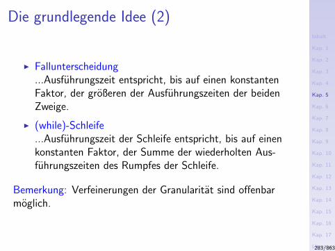
Inhalt
Kap. 1
Kap. 2
Kap. 3
Kap. 4
Kap. 5
Kap. 6
Kap. 7
Kap. 8
Kap. 9
Kap. 10
Kap. 11
Kap. 12
Kap. 13
Kap. 14
Kap. 15
Kap. 16
Kap. 17
Literatur
Anhang
A
Die grundlegende Idee (2)
I Fallunterscheidung...Ausfuhrungszeit entspricht, bis auf einen konstantenFaktor, der großeren der Ausfuhrungszeiten der beidenZweige.
I (while)-Schleife...Ausfuhrungszeit der Schleife entspricht, bis auf einenkonstanten Faktor, der Summe der wiederholten Aus-fuhrungszeiten des Rumpfes der Schleife.
Bemerkung: Verfeinerungen der Granularitat sind offenbarmoglich.
283/863
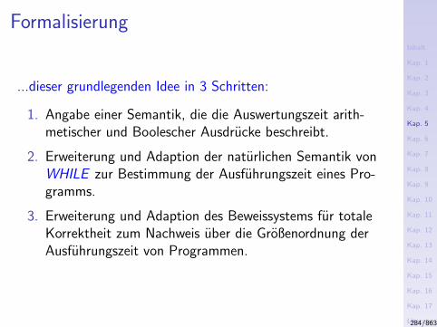
Inhalt
Kap. 1
Kap. 2
Kap. 3
Kap. 4
Kap. 5
Kap. 6
Kap. 7
Kap. 8
Kap. 9
Kap. 10
Kap. 11
Kap. 12
Kap. 13
Kap. 14
Kap. 15
Kap. 16
Kap. 17
Literatur
Anhang
A
Formalisierung
...dieser grundlegenden Idee in 3 Schritten:
1. Angabe einer Semantik, die die Auswertungszeit arith-metischer und Boolescher Ausdrucke beschreibt.
2. Erweiterung und Adaption der naturlichen Semantik vonWHILE zur Bestimmung der Ausfuhrungszeit eines Pro-gramms.
3. Erweiterung und Adaption des Beweissystems fur totaleKorrektheit zum Nachweis uber die Großenordnung derAusfuhrungszeit von Programmen.
284/863
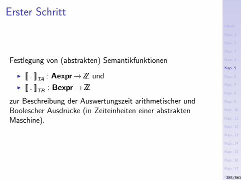
Inhalt
Kap. 1
Kap. 2
Kap. 3
Kap. 4
Kap. 5
Kap. 6
Kap. 7
Kap. 8
Kap. 9
Kap. 10
Kap. 11
Kap. 12
Kap. 13
Kap. 14
Kap. 15
Kap. 16
Kap. 17
Literatur
Anhang
A
Erster Schritt
Festlegung von (abstrakten) Semantikfunktionen
I [[ . ]]TA : Aexpr→ZZ und
I [[ . ]]TB : Bexpr→ZZ
zur Beschreibung der Auswertungszeit arithmetischer undBoolescher Ausdrucke (in Zeiteinheiten einer abstraktenMaschine).
285/863
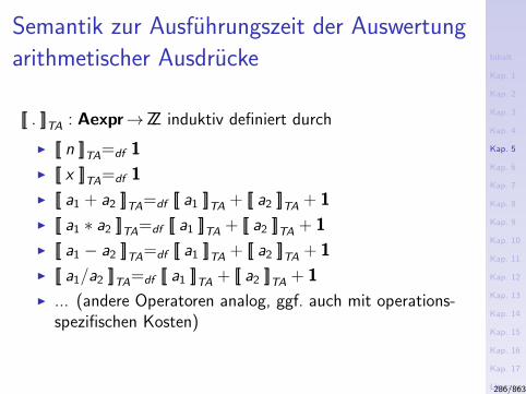
Inhalt
Kap. 1
Kap. 2
Kap. 3
Kap. 4
Kap. 5
Kap. 6
Kap. 7
Kap. 8
Kap. 9
Kap. 10
Kap. 11
Kap. 12
Kap. 13
Kap. 14
Kap. 15
Kap. 16
Kap. 17
Literatur
Anhang
A
Semantik zur Ausfuhrungszeit der Auswertung
arithmetischer Ausdrucke
[[ . ]]TA : Aexpr→ZZ induktiv definiert durch
I [[ n ]]TA=df 1
I [[ x ]]TA=df 1
I [[ a1 + a2 ]]TA=df [[ a1 ]]TA + [[ a2 ]]TA + 1
I [[ a1 ∗ a2 ]]TA=df [[ a1 ]]TA + [[ a2 ]]TA + 1
I [[ a1 − a2 ]]TA=df [[ a1 ]]TA + [[ a2 ]]TA + 1
I [[ a1/a2 ]]TA=df [[ a1 ]]TA + [[ a2 ]]TA + 1
I ... (andere Operatoren analog, ggf. auch mit operations-spezifischen Kosten)
286/863
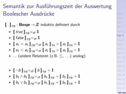
Inhalt
Kap. 1
Kap. 2
Kap. 3
Kap. 4
Kap. 5
Kap. 6
Kap. 7
Kap. 8
Kap. 9
Kap. 10
Kap. 11
Kap. 12
Kap. 13
Kap. 14
Kap. 15
Kap. 16
Kap. 17
Literatur
Anhang
A
Semantik zur Ausfuhrungszeit der Auswertung
Boolescher Ausdrucke
[[ . ]]TB : Bexpr→ZZ induktiv definiert durch
I [[ true ]]TB=df 1
I [[ false ]]TB=df 1
I [[ a1 = a2 ]]TB=df [[ a1 ]]TA + [[ a2 ]]TA + 1
I [[ a1 < a2 ]]TB=df [[ a1 ]]TA + [[ a2 ]]TA + 1
I ... (andere Relatoren (z.B. ≤, . . .) analog)
I [[ ¬b ]]TB=df [[ b ]]TB + 1
I [[ b1 ∧ b2 ]]TB=df [[ b1 ]]TB + [[ b2 ]]TB + 1
I [[ b1 ∨ b2 ]]TB=df [[ b1 ]]TB + [[ b2 ]]TB + 1
287/863
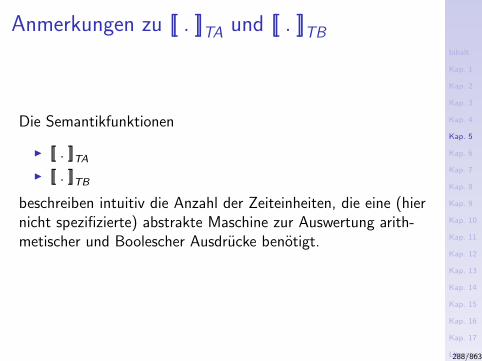
Inhalt
Kap. 1
Kap. 2
Kap. 3
Kap. 4
Kap. 5
Kap. 6
Kap. 7
Kap. 8
Kap. 9
Kap. 10
Kap. 11
Kap. 12
Kap. 13
Kap. 14
Kap. 15
Kap. 16
Kap. 17
Literatur
Anhang
A
Anmerkungen zu [[ . ]]TA und [[ . ]]TB
Die Semantikfunktionen
I [[ . ]]TAI [[ . ]]TB
beschreiben intuitiv die Anzahl der Zeiteinheiten, die eine (hiernicht spezifizierte) abstrakte Maschine zur Auswertung arith-metischer und Boolescher Ausdrucke benotigt.
288/863
Inhalt
Kap. 1
Kap. 2
Kap. 3
Kap. 4
Kap. 5
Kap. 6
Kap. 7
Kap. 8
Kap. 9
Kap. 10
Kap. 11
Kap. 12
Kap. 13
Kap. 14
Kap. 15
Kap. 16
Kap. 17
Literatur
Anhang
A
Zweiter Schritt
Erweiterung und Anpassung der
I naturlichen Semantik von WHILE
zur Bestimmung der Ausfuhrungszeit von Programmen.
289/863
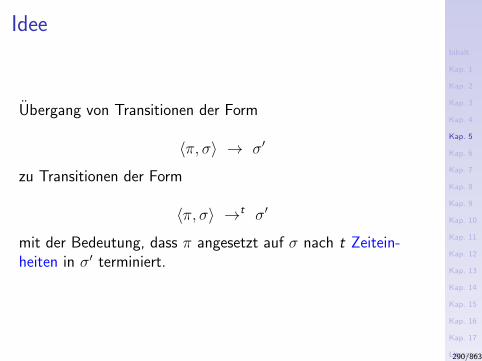
Inhalt
Kap. 1
Kap. 2
Kap. 3
Kap. 4
Kap. 5
Kap. 6
Kap. 7
Kap. 8
Kap. 9
Kap. 10
Kap. 11
Kap. 12
Kap. 13
Kap. 14
Kap. 15
Kap. 16
Kap. 17
Literatur
Anhang
A
Idee
Ubergang von Transitionen der Form
〈π, σ〉 → σ′
zu Transitionen der Form
〈π, σ〉 →t σ′
mit der Bedeutung, dass π angesetzt auf σ nach t Zeitein-heiten in σ′ terminiert.
290/863
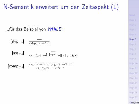
Inhalt
Kap. 1
Kap. 2
Kap. 3
Kap. 4
Kap. 5
Kap. 6
Kap. 7
Kap. 8
Kap. 9
Kap. 10
Kap. 11
Kap. 12
Kap. 13
Kap. 14
Kap. 15
Kap. 16
Kap. 17
Literatur
Anhang
A
N-Semantik erweitert um den Zeitaspekt (1)
...fur das Beispiel von WHILE :
[skiptns ] —〈skip,σ〉 →1 σ
[asstns ] —〈x :=t,σ〉 →[[ t ]]TA+1 σ[[[ t ]]A(σ)/x]
[comptns ]〈π1,σ〉 →t1 σ′,〈π2,σ
′〉 →t2 σ′′
〈π1;π2,σ〉 →t1+t2 σ′′
291/863
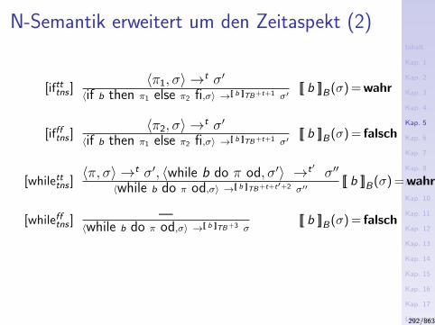
Inhalt
Kap. 1
Kap. 2
Kap. 3
Kap. 4
Kap. 5
Kap. 6
Kap. 7
Kap. 8
Kap. 9
Kap. 10
Kap. 11
Kap. 12
Kap. 13
Kap. 14
Kap. 15
Kap. 16
Kap. 17
Literatur
Anhang
A
N-Semantik erweitert um den Zeitaspekt (2)
[iftttns ]〈π1, σ〉 →t σ′
〈if b then π1 else π2 fi,σ〉 →[[ b ]]TB+t+1 σ′[[ b ]]B(σ) = wahr
[iffftns ]〈π2, σ〉 →t σ′
〈if b then π1 else π2 fi,σ〉 →[[ b ]]TB+t+1 σ′[[ b ]]B(σ) = falsch
[whiletttns ]〈π, σ〉 →t σ′, 〈while b do π od, σ′〉 →t′ σ′′
〈while b do π od,σ〉 →[[ b ]]TB+t+t′+2 σ′′[[ b ]]B(σ) = wahr
[whilefftns ] —〈while b do π od,σ〉 →[[ b ]]TB+3 σ
[[ b ]]B(σ) = falsch
292/863
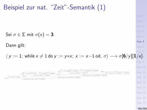
Inhalt
Kap. 1
Kap. 2
Kap. 3
Kap. 4
Kap. 5
Kap. 6
Kap. 7
Kap. 8
Kap. 9
Kap. 10
Kap. 11
Kap. 12
Kap. 13
Kap. 14
Kap. 15
Kap. 16
Kap. 17
Literatur
Anhang
A
Beispiel zur nat. “Zeit”-Semantik (1)
Sei σ ∈ Σ mit σ(x) = 3.
Dann gilt:
〈 y := 1; while x 6= 1 do y := y∗x ; x := x−1 od, σ〉 −→ σ[6/y ][1/x ]
σ [3/y] σ [3/y] [2/x]
ns][comp
σ [6/y] [2/x] σ [6/y] [1/x]x := x−1,
[assns
]
ns][while tt
[assns
][assns
]
σ [1/y] σ [3/y]y := y*x,
ns][comp
ns][comp
ns][while tt
σ [3/y] [2/x] σ [6/y] [1/x]y := y*x; x := x−1,
y := y*x,σ [3/y] [2/x] σ [6/y] [2/x]
[assns
]
σ [6/y] [1/x]while x <> 1 do y := y*x; x := x−1 od,σ [6/y] [1/x]ns
][while ff
[assns
]
σ [1/y]y := 1, σ
σ [1/y] σ [3/y] [2/x]y := y*x; x := x−1, σ [3/y] [2/x] σ [6/y] [1/x]while x <> 1 do y := y*x; x := x−1 od,
σ [1/y]σ [6/y] [1/x]while x <> 1 do y := y*x; x := x−1 od,
x := x−1,
y := 1; while x <> 1 do y := y*x; x := x−1 od,σ σ [6/y] [1/x]
2
4 4
8
4 4
8 6
19
32
34
293/863
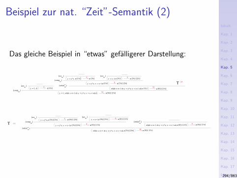
Inhalt
Kap. 1
Kap. 2
Kap. 3
Kap. 4
Kap. 5
Kap. 6
Kap. 7
Kap. 8
Kap. 9
Kap. 10
Kap. 11
Kap. 12
Kap. 13
Kap. 14
Kap. 15
Kap. 16
Kap. 17
Literatur
Anhang
A
Beispiel zur nat. “Zeit”-Semantik (2)
Das gleiche Beispiel in “etwas” gefalligerer Darstellung:
σ [3/y] σ [3/y] [2/x]
σ [6/y] [1/x]
ns][while tt
[assns
][assns
]
σ [1/y] σ [3/y]y := y*x,
ns][comp
ns][comp
[assns
]
σ [1/y]y := 1, σ σ [1/y]σ [6/y] [1/x]while x <> 1 do y := y*x; x := x−1 od,
σ [1/y] σ [3/y] [2/x]y := y*x; x := x−1,
T ns][comp
σ [6/y] [2/x] σ [6/y] [1/x]x := x−1,
[assns
]
ns][while tt
σ [3/y] [2/x] σ [6/y] [1/x]y := y*x; x := x−1,
y := y*x,σ [3/y] [2/x] σ [6/y] [2/x]
[assns
]
σ [6/y] [1/x]while x <> 1 do y := y*x; x := x−1 od,σ [6/y] [1/x]ns
][while ff
σ [3/y] [2/x] σ [6/y] [1/x]while x <> 1 do y := y*x; x := x−1 od,
x := x−1,
y := 1; while x <> 1 do y := y*x; x := x−1 od,σ
T2
4 4
8 19
32
34
4 4
8 6
19
294/863

Inhalt
Kap. 1
Kap. 2
Kap. 3
Kap. 4
Kap. 5
Kap. 6
Kap. 7
Kap. 8
Kap. 9
Kap. 10
Kap. 11
Kap. 12
Kap. 13
Kap. 14
Kap. 15
Kap. 16
Kap. 17
Literatur
Anhang
A
Dritter Schritt
Erweiterung und Anpassung der
I des Beweiskalkuls fur totale Korrektheit
um den Ausfuhrungszeitaspekt von Programmen.
295/863
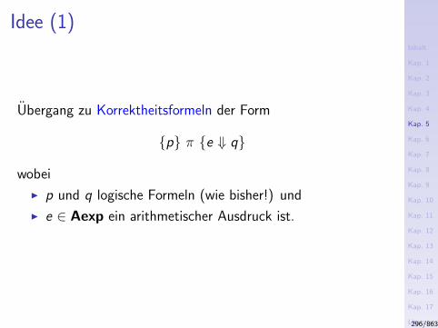
Inhalt
Kap. 1
Kap. 2
Kap. 3
Kap. 4
Kap. 5
Kap. 6
Kap. 7
Kap. 8
Kap. 9
Kap. 10
Kap. 11
Kap. 12
Kap. 13
Kap. 14
Kap. 15
Kap. 16
Kap. 17
Literatur
Anhang
A
Idee (1)
Ubergang zu Korrektheitsformeln der Form
p π e ⇓ q
wobei
I p und q logische Formeln (wie bisher!) und
I e ∈ Aexp ein arithmetischer Ausdruck ist.
296/863
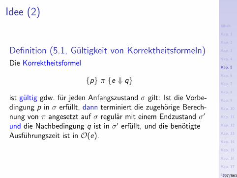
Inhalt
Kap. 1
Kap. 2
Kap. 3
Kap. 4
Kap. 5
Kap. 6
Kap. 7
Kap. 8
Kap. 9
Kap. 10
Kap. 11
Kap. 12
Kap. 13
Kap. 14
Kap. 15
Kap. 16
Kap. 17
Literatur
Anhang
A
Idee (2)
Definition (5.1, Gultigkeit von Korrektheitsformeln)
Die Korrektheitsformel
p π e ⇓ q
ist gultig gdw. fur jeden Anfangszustand σ gilt: Ist die Vorbe-dingung p in σ erfullt, dann terminiert die zugehorige Berech-nung von π angesetzt auf σ regular mit einem Endzustand σ′
und die Nachbedingung q ist in σ′ erfullt, und die benotigteAusfuhrungszeit ist in O(e).
297/863
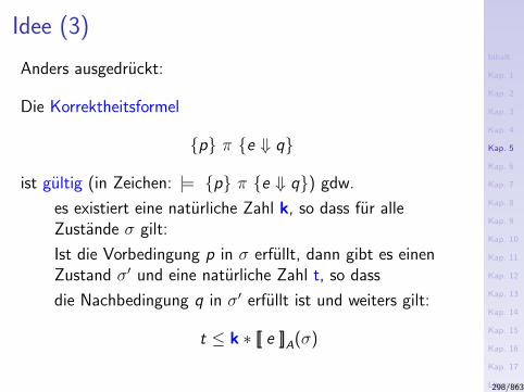
Inhalt
Kap. 1
Kap. 2
Kap. 3
Kap. 4
Kap. 5
Kap. 6
Kap. 7
Kap. 8
Kap. 9
Kap. 10
Kap. 11
Kap. 12
Kap. 13
Kap. 14
Kap. 15
Kap. 16
Kap. 17
Literatur
Anhang
A
Idee (3)
Anders ausgedruckt:
Die Korrektheitsformel
p π e ⇓ q
ist gultig (in Zeichen: |= p π e ⇓ q) gdw.
es existiert eine naturliche Zahl k, so dass fur alleZustande σ gilt:
Ist die Vorbedingung p in σ erfullt, dann gibt es einenZustand σ′ und eine naturliche Zahl t, so dass
die Nachbedingung q in σ′ erfullt ist und weiters gilt:
t ≤ k ∗ [[ e ]]A(σ)
298/863

Inhalt
Kap. 1
Kap. 2
Kap. 3
Kap. 4
Kap. 5
Kap. 6
Kap. 7
Kap. 8
Kap. 9
Kap. 10
Kap. 11
Kap. 12
Kap. 13
Kap. 14
Kap. 15
Kap. 16
Kap. 17
Literatur
Anhang
A
Idee (4)
Beachte:
I Im Ausdruckt ≤ k ∗ [[ e ]]A(σ)
wird der Ausdruck e im Anfangszustand σ ausgewertet,nicht im terminalen Zustand σ′.
I Diesem Umstand ist geschuldet, dass die (jetzt folgende)Festlegung der Regeln [compe ] und [whilee ] komplizierterausfallt als moglicherweise zunachst vermutet.
299/863
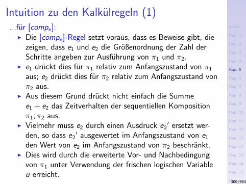
Inhalt
Kap. 1
Kap. 2
Kap. 3
Kap. 4
Kap. 5
Kap. 6
Kap. 7
Kap. 8
Kap. 9
Kap. 10
Kap. 11
Kap. 12
Kap. 13
Kap. 14
Kap. 15
Kap. 16
Kap. 17
Literatur
Anhang
A
Intuition zu den Kalkulregeln (1)...fur [compe ]:I Die [compe ]-Regel setzt voraus, dass es Beweise gibt, die
zeigen, dass e1 und e2 die Großenordnung der Zahl derSchritte angeben zur Ausfuhrung von π1 und π2.
I e1 druckt dies fur π1 relativ zum Anfangszustand von π1
aus; e2 druckt dies fur π2 relativ zum Anfangszustand vonπ2 aus.
I Aus diesem Grund druckt nicht einfach die Summee1 + e2 das Zeitverhalten der sequentiellen Kompositionπ1; π2 aus.
I Vielmehr muss e2 durch einen Ausdruck e2′ ersetzt wer-
den, so dass e2′ ausgewertet im Anfangszustand von e1
den Wert von e2 im Anfangszustand von π2 beschrankt.I Dies wird durch die erweiterte Vor- und Nachbedingung
von π1 unter Verwendung der frischen logischen Variableu erreicht.
300/863
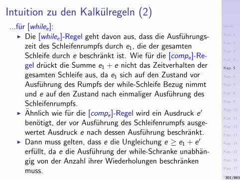
Inhalt
Kap. 1
Kap. 2
Kap. 3
Kap. 4
Kap. 5
Kap. 6
Kap. 7
Kap. 8
Kap. 9
Kap. 10
Kap. 11
Kap. 12
Kap. 13
Kap. 14
Kap. 15
Kap. 16
Kap. 17
Literatur
Anhang
A
Intuition zu den Kalkulregeln (2)...fur [whilee ]:I Die [whilee ]-Regel geht davon aus, dass die Ausfuhrungs-
zeit des Schleifenrumpfs durch e1, die der gesamtenSchleife durch e beschrankt ist. Wie fur die [compe ]-Re-gel druckt die Summe e1 + e nicht das Zeitverhalten dergesamten Schleife aus, da e1 sich auf den Zustand vorAusfuhrung des Rumpfs der while-Schleife Bezug nimmtund e auf den Zustand nach einmaliger Ausfuhrung desSchleifenrumpfs.
I Ahnlich wie fur die [compe ]-Regel wird ein Ausdruck e ′
benotigt, der vor Ausfuhrung des Schleifenrumpfs ausge-wertet Ausdruck e nach dessen Ausfuhrung beschrankt.
I Dann muss gelten, dass e die Ungleichung e ≥ e1 + e ′
erfullt, da e die Ausfuhrung der while-Schranke unabhan-gig von der Anzahl ihrer Wiederholungen beschrankenmuss.
301/863
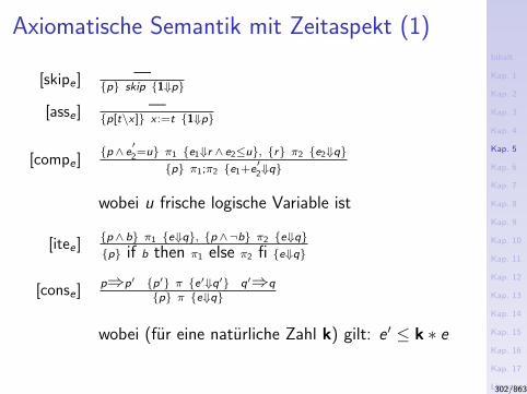
Inhalt
Kap. 1
Kap. 2
Kap. 3
Kap. 4
Kap. 5
Kap. 6
Kap. 7
Kap. 8
Kap. 9
Kap. 10
Kap. 11
Kap. 12
Kap. 13
Kap. 14
Kap. 15
Kap. 16
Kap. 17
Literatur
Anhang
A
Axiomatische Semantik mit Zeitaspekt (1)
[skipe ] —p skip 1⇓p
[asse ] —p[t\x] x :=t 1⇓p
[compe ]p ∧ e′2=u π1 e1⇓r ∧ e2≤u, r π2 e2⇓q
p π1;π2 e1+e′2⇓q
wobei u frische logische Variable ist
[itee ]p ∧ b π1 e⇓q, p ∧¬b π2 e⇓qp if b then π1 else π2 fi e⇓q
[conse ]p⇒p′ p′ π e′⇓q′ q′⇒q
p π e⇓q
wobei (fur eine naturliche Zahl k) gilt: e ′ ≤ k ∗ e
302/863
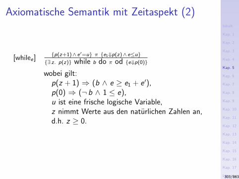
Inhalt
Kap. 1
Kap. 2
Kap. 3
Kap. 4
Kap. 5
Kap. 6
Kap. 7
Kap. 8
Kap. 9
Kap. 10
Kap. 11
Kap. 12
Kap. 13
Kap. 14
Kap. 15
Kap. 16
Kap. 17
Literatur
Anhang
A
Axiomatische Semantik mit Zeitaspekt (2)
[whilee ]p(z+1)∧ e′=u π e1⇓p(z)∧ e≤u
∃ z. p(z) while b do π od e⇓p(0)
wobei gilt:p(z + 1) ⇒ (b ∧ e ≥ e1 + e ′),p(0) ⇒ (¬ b ∧ 1 ≤ e),u ist eine frische logische Variable,z nimmt Werte aus den naturlichen Zahlen an,d.h. z ≥ 0.
303/863
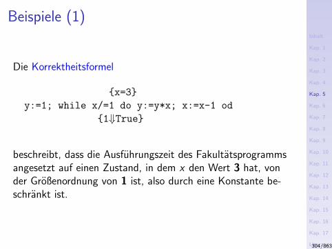
Inhalt
Kap. 1
Kap. 2
Kap. 3
Kap. 4
Kap. 5
Kap. 6
Kap. 7
Kap. 8
Kap. 9
Kap. 10
Kap. 11
Kap. 12
Kap. 13
Kap. 14
Kap. 15
Kap. 16
Kap. 17
Literatur
Anhang
A
Beispiele (1)
Die Korrektheitsformel
x=3
y:=1; while x/=1 do y:=y*x; x:=x-1 od
1⇓True
beschreibt, dass die Ausfuhrungszeit des Fakultatsprogrammsangesetzt auf einen Zustand, in dem x den Wert 3 hat, vonder Großenordnung von 1 ist, also durch eine Konstante be-schrankt ist.
304/863
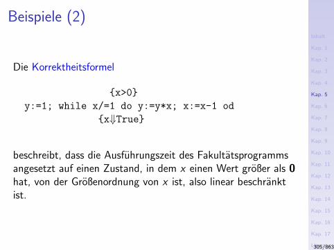
Inhalt
Kap. 1
Kap. 2
Kap. 3
Kap. 4
Kap. 5
Kap. 6
Kap. 7
Kap. 8
Kap. 9
Kap. 10
Kap. 11
Kap. 12
Kap. 13
Kap. 14
Kap. 15
Kap. 16
Kap. 17
Literatur
Anhang
A
Beispiele (2)
Die Korrektheitsformel
x>0
y:=1; while x/=1 do y:=y*x; x:=x-1 od
x⇓True
beschreibt, dass die Ausfuhrungszeit des Fakultatsprogrammsangesetzt auf einen Zustand, in dem x einen Wert großer als 0hat, von der Großenordnung von x ist, also linear beschranktist.
305/863
Inhalt
Kap. 1
Kap. 2
Kap. 3
Kap. 4
Kap. 5
Kap. 6
Kap. 7
Kap. 8
Kap. 9
Kap. 10
Kap. 11
Kap. 12
Kap. 13
Kap. 14
Kap. 15
Kap. 16
Kap. 17
Literatur
Anhang
A
Vertiefende und weiterfuhrende Leseempfeh-
lungen fur Kapitel 5 (1)
Raimund Kirner, Jens Knoop, Adrian Prantl, MarkusSchordan, Albrecht Kadlec. Beyond Loop Bounds:Comparing Annotation Languages for Worst-CaseExecution Time Analysis. Journal of Software and SystemsModeling 10(3):411-437, Springer-V., 2011.
Bjorn Lisper, Andreas Ermedahl, Dietmar Schreiner, JensKnoop, Peter Gliwa. Practical Experiences of ApplyingSource-level WCET Flow Analysis to Industrial Code.Journal of Software Tools for Technology Transfer(STTT) 15(1):53-63, Springer-V., 2013.
306/863
Inhalt
Kap. 1
Kap. 2
Kap. 3
Kap. 4
Kap. 5
Kap. 6
Kap. 7
Kap. 8
Kap. 9
Kap. 10
Kap. 11
Kap. 12
Kap. 13
Kap. 14
Kap. 15
Kap. 16
Kap. 17
Literatur
Anhang
A
Vertiefende und weiterfuhrende Leseempfeh-
lungen fur Kapitel 5 (2)
Hanne Riis Nielson, Flemming Nielson. Semantics withApplications: A Formal Introduction. Wiley, 1992.(Chapter 6.5, Assertions for Execution Time)
Hanne Riis Nielson, Flemming Nielson. Semantics withApplications: An Appetizer. Springer-V., 2007. (Chapter10.2, Assertions for Execution Time)
Peter Puschner, Daniel Prokesch, Benedikt Huber, JensKnoop, Stefan Hepp, Gernot Gebhard. The T-CRESTApproach of Compiler and WCET-Analysis Integration. InProceedings of the 9th International Workshop on Soft-ware Technologies for Future Embedded and UbiquitiousSystems (SEUS 2013), June 2013, to appear.
307/863
Inhalt
Kap. 1
Kap. 2
Kap. 3
Kap. 4
Kap. 5
Kap. 6
Kap. 7
Kap. 8
Kap. 9
Kap. 10
Kap. 11
Kap. 12
Kap. 13
Kap. 14
Kap. 15
Kap. 16
Kap. 17
Literatur
Anhang
A
Vertiefende und weiterfuhrende Leseempfeh-
lungen fur Kapitel 5 (3)
Reinhard Wilhelm, Jakob Engblom, Andreas Ermedahl,Niklas Holsti, Stephan Thesing, David Whalley, GuillemBernat, Christian Ferdinand, Reinhold Heckmann, TulikaMitra, Frank Mueller, Isabelle Puaut, Peter Puschner, JanStaschulat, Per Stenstrom. The Worst-case ExecutionTime Problem – Overview of Methods and Survey ofTools. ACM Transactions on Embedded ComputingSystems 7(3):36.1-36.53, 2008.
308/863

Inhalt
Kap. 1
Kap. 2
Kap. 3
Kap. 4
Kap. 5
Kap. 6
Kap. 7
Kap. 8
Kap. 9
Kap. 10
Kap. 11
Kap. 12
Kap. 13
Kap. 14
Kap. 15
Kap. 16
Kap. 17
Literatur
Anhang
A
Teil II
Analyse
309/863
Inhalt
Kap. 1
Kap. 2
Kap. 3
Kap. 4
Kap. 5
Kap. 6
6.1
6.2
6.3
6.4
6.5
6.6
6.7
6.8
6.8.1
6.8.2
Kap. 7
Kap. 8
Kap. 9
Kap. 10
Kap. 11
Kap. 12
Kap. 13
Kap. 14
Kap. 15
Kap. 16
Kap. 17
Literatur
Anhang
A
Kapitel 6
Programmanalyse
310/863
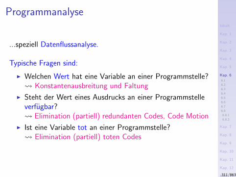
Inhalt
Kap. 1
Kap. 2
Kap. 3
Kap. 4
Kap. 5
Kap. 6
6.1
6.2
6.3
6.4
6.5
6.6
6.7
6.8
6.8.1
6.8.2
Kap. 7
Kap. 8
Kap. 9
Kap. 10
Kap. 11
Kap. 12
Kap. 13
Kap. 14
Kap. 15
Kap. 16
Kap. 17
Literatur
Anhang
A
Programmanalyse
...speziell Datenflussanalyse.
Typische Fragen sind:
I Welchen Wert hat eine Variable an einer Programmstelle? Konstantenausbreitung und Faltung
I Steht der Wert eines Ausdrucks an einer Programmstelleverfugbar? Elimination (partiell) redundanten Codes, Code Motion
I Ist eine Variable tot an einer Programmstelle? Elimination (partiell) toten Codes
311/863

Inhalt
Kap. 1
Kap. 2
Kap. 3
Kap. 4
Kap. 5
Kap. 6
6.1
6.2
6.3
6.4
6.5
6.6
6.7
6.8
6.8.1
6.8.2
Kap. 7
Kap. 8
Kap. 9
Kap. 10
Kap. 11
Kap. 12
Kap. 13
Kap. 14
Kap. 15
Kap. 16
Kap. 17
Literatur
Anhang
A
Kapitel 6.1
Motivation
312/863
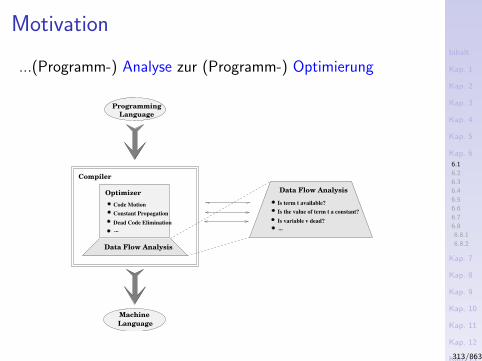
Inhalt
Kap. 1
Kap. 2
Kap. 3
Kap. 4
Kap. 5
Kap. 6
6.1
6.2
6.3
6.4
6.5
6.6
6.7
6.8
6.8.1
6.8.2
Kap. 7
Kap. 8
Kap. 9
Kap. 10
Kap. 11
Kap. 12
Kap. 13
Kap. 14
Kap. 15
Kap. 16
Kap. 17
Literatur
Anhang
A
Motivation
...(Programm-) Analyse zur (Programm-) Optimierung
Language
Machine
Language
Programming
...
Is term t available?
Is the value of term t a constant?
Is variable v dead?
Data Flow AnalysisOptimizer
...
Dead Code Elimination
Constant Propagation
Code Motion
Compiler
Data Flow Analysis
313/863
Inhalt
Kap. 1
Kap. 2
Kap. 3
Kap. 4
Kap. 5
Kap. 6
6.1
6.2
6.3
6.4
6.5
6.6
6.7
6.8
6.8.1
6.8.2
Kap. 7
Kap. 8
Kap. 9
Kap. 10
Kap. 11
Kap. 12
Kap. 13
Kap. 14
Kap. 15
Kap. 16
Kap. 17
Literatur
Anhang
A
Zentrale Fragen
Grundlegendes:
I Was bedeutet Optimalitat...in Analyse und in Optimierung?
Und auch (scheinbar) Nebensachliches:
I Was ist eine angemessene Programmreprasentation?
314/863
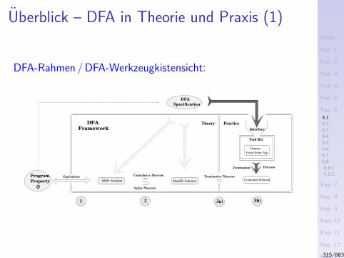
Inhalt
Kap. 1
Kap. 2
Kap. 3
Kap. 4
Kap. 5
Kap. 6
6.1
6.2
6.3
6.4
6.5
6.6
6.7
6.8
6.8.1
6.8.2
Kap. 7
Kap. 8
Kap. 9
Kap. 10
Kap. 11
Kap. 12
Kap. 13
Kap. 14
Kap. 15
Kap. 16
Kap. 17
Literatur
Anhang
A
Uberblick – DFA in Theorie und Praxis (1)
DFA-Rahmen / DFA-Werkzeugkistensicht:
MOP−Solution Computed Solution
DFA
Specification
1 3a) 3b)2
Program
Property
φ
Coincidence Theorem
Theorem
Generic
Fixed Point Alg.
Tool Kit
Theory Practice
Interface
DFAFramework
Equivalence Termination Theorem
Termination
Safety Theorem
MaxFP−Solution
315/863
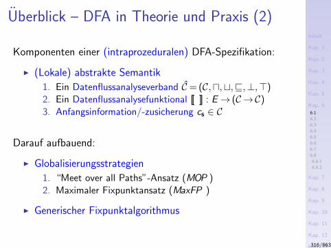
Inhalt
Kap. 1
Kap. 2
Kap. 3
Kap. 4
Kap. 5
Kap. 6
6.1
6.2
6.3
6.4
6.5
6.6
6.7
6.8
6.8.1
6.8.2
Kap. 7
Kap. 8
Kap. 9
Kap. 10
Kap. 11
Kap. 12
Kap. 13
Kap. 14
Kap. 15
Kap. 16
Kap. 17
Literatur
Anhang
A
Uberblick – DFA in Theorie und Praxis (2)
Komponenten einer (intraprozeduralen) DFA-Spezifikation:
I (Lokale) abstrakte Semantik
1. Ein Datenflussanalyseverband C= (C,u,t,v,⊥,>)2. Ein Datenflussanalysefunktional [[ ]] : E→ (C→C)3. Anfangsinformation/-zusicherung cs ∈ C
Darauf aufbauend:
I Globalisierungsstrategien
1. “Meet over all Paths”-Ansatz (MOP )2. Maximaler Fixpunktansatz (MaxFP )
I Generischer Fixpunktalgorithmus
316/863
Inhalt
Kap. 1
Kap. 2
Kap. 3
Kap. 4
Kap. 5
Kap. 6
6.1
6.2
6.3
6.4
6.5
6.6
6.7
6.8
6.8.1
6.8.2
Kap. 7
Kap. 8
Kap. 9
Kap. 10
Kap. 11
Kap. 12
Kap. 13
Kap. 14
Kap. 15
Kap. 16
Kap. 17
Literatur
Anhang
A
Uberblick – DFA in Theorie und Praxis (3)
Hauptresultate:
I Korrektheit: Sicherheits-Theorem
I Vollstandigkeit: Koinzidenz-Theorem
Sowie:
I Effektivitat: Terminierungs-Theorem
317/863
Inhalt
Kap. 1
Kap. 2
Kap. 3
Kap. 4
Kap. 5
Kap. 6
6.1
6.2
6.3
6.4
6.5
6.6
6.7
6.8
6.8.1
6.8.2
Kap. 7
Kap. 8
Kap. 9
Kap. 10
Kap. 11
Kap. 12
Kap. 13
Kap. 14
Kap. 15
Kap. 16
Kap. 17
Literatur
Anhang
A
Uberblick – DFA in Theorie und Praxis (4)
Genauer lassen sich unterscheiden:
I intraprozedurale,
I interprozedurale,
I objektorientierte,
I parallele,
I konditionale,
I ...
Datenflussanalyse (DFA).
Das grundlegende Prinzip...
318/863
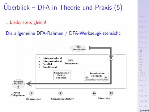
Inhalt
Kap. 1
Kap. 2
Kap. 3
Kap. 4
Kap. 5
Kap. 6
6.1
6.2
6.3
6.4
6.5
6.6
6.7
6.8
6.8.1
6.8.2
Kap. 7
Kap. 8
Kap. 9
Kap. 10
Kap. 11
Kap. 12
Kap. 13
Kap. 14
Kap. 15
Kap. 16
Kap. 17
Literatur
Anhang
A
Uberblick – DFA in Theorie und Praxis (5)
...bleibt stets gleich!
Die allgemeine DFA-Rahmen / DFA-Werkzeugkistensicht:
φ
Program
Coincidence/Safety
TheoremCorrectness Termination
Property
DFA
Specification
1 3b)2
3b)
Intraprocedural
Interprocedural
Conditional
Equivalence Effectivity
DFA
Framework
Theorem3a)
3a)ProofObligations:
Parallel
Coincidence/Safety
Termination
319/863
Inhalt
Kap. 1
Kap. 2
Kap. 3
Kap. 4
Kap. 5
Kap. 6
6.1
6.2
6.3
6.4
6.5
6.6
6.7
6.8
6.8.1
6.8.2
Kap. 7
Kap. 8
Kap. 9
Kap. 10
Kap. 11
Kap. 12
Kap. 13
Kap. 14
Kap. 15
Kap. 16
Kap. 17
Literatur
Anhang
A
Ziel
Optimale Programmoptimierung!
...ein weißer Schimmel in der Informatik?
320/863
Inhalt
Kap. 1
Kap. 2
Kap. 3
Kap. 4
Kap. 5
Kap. 6
6.1
6.2
6.3
6.4
6.5
6.6
6.7
6.8
6.8.1
6.8.2
Kap. 7
Kap. 8
Kap. 9
Kap. 10
Kap. 11
Kap. 12
Kap. 13
Kap. 14
Kap. 15
Kap. 16
Kap. 17
Literatur
Anhang
A
Ohne Fleiß kein Preis!
In der Sprechweise optimierender Ubersetzung:
...ohne Analyse keine Optimierung!
321/863

Inhalt
Kap. 1
Kap. 2
Kap. 3
Kap. 4
Kap. 5
Kap. 6
6.1
6.2
6.3
6.4
6.5
6.6
6.7
6.8
6.8.1
6.8.2
Kap. 7
Kap. 8
Kap. 9
Kap. 10
Kap. 11
Kap. 12
Kap. 13
Kap. 14
Kap. 15
Kap. 16
Kap. 17
Literatur
Anhang
A
Kapitel 6.2
Datenflussanalyse
322/863
Inhalt
Kap. 1
Kap. 2
Kap. 3
Kap. 4
Kap. 5
Kap. 6
6.1
6.2
6.3
6.4
6.5
6.6
6.7
6.8
6.8.1
6.8.2
Kap. 7
Kap. 8
Kap. 9
Kap. 10
Kap. 11
Kap. 12
Kap. 13
Kap. 14
Kap. 15
Kap. 16
Kap. 17
Literatur
Anhang
A
Programmreprasentation
Im Bereich der Programmanalyse, speziell Datenflussanalyse,ist ublich:
I die Reprasentation von Programmen in Form(nichtdeterministischer) Flussgraphen
323/863
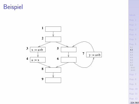
Inhalt
Kap. 1
Kap. 2
Kap. 3
Kap. 4
Kap. 5
Kap. 6
6.1
6.2
6.3
6.4
6.5
6.6
6.7
6.8
6.8.1
6.8.2
Kap. 7
Kap. 8
Kap. 9
Kap. 10
Kap. 11
Kap. 12
Kap. 13
Kap. 14
Kap. 15
Kap. 16
Kap. 17
Literatur
Anhang
A
Beispiel
y := a+b
x := a+b
a := x
1
2
3
4
8
9
5
6
7
324/863
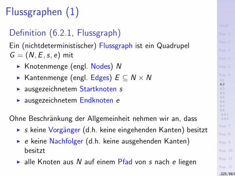
Inhalt
Kap. 1
Kap. 2
Kap. 3
Kap. 4
Kap. 5
Kap. 6
6.1
6.2
6.3
6.4
6.5
6.6
6.7
6.8
6.8.1
6.8.2
Kap. 7
Kap. 8
Kap. 9
Kap. 10
Kap. 11
Kap. 12
Kap. 13
Kap. 14
Kap. 15
Kap. 16
Kap. 17
Literatur
Anhang
A
Flussgraphen (1)
Definition (6.2.1, Flussgraph)
Ein (nichtdeterministischer) Flussgraph ist ein QuadrupelG = (N ,E , s, e) mit
I Knotenmenge (engl. Nodes) N
I Kantenmenge (engl. Edges) E ⊆ N × N
I ausgezeichnetem Startknoten s
I ausgezeichnetem Endknoten e
Ohne Beschrankung der Allgemeinheit nehmen wir an, dass
I s keine Vorganger (d.h. keine eingehenden Kanten) besitzt
I e keine Nachfolger (d.h. keine ausgehenden Kanten)besitzt
I alle Knoten aus N auf einem Pfad von s nach e liegen
325/863
Inhalt
Kap. 1
Kap. 2
Kap. 3
Kap. 4
Kap. 5
Kap. 6
6.1
6.2
6.3
6.4
6.5
6.6
6.7
6.8
6.8.1
6.8.2
Kap. 7
Kap. 8
Kap. 9
Kap. 10
Kap. 11
Kap. 12
Kap. 13
Kap. 14
Kap. 15
Kap. 16
Kap. 17
Literatur
Anhang
A
Flussgraphen (2)
Bemerkung:
I Knoten reprasentieren Programmpunkte
I Kanten die Verzweigungsstruktur.
I Elementare Programmanweisungen (Zuweisungen, Tests)konnen wahlweise durch
I Knoten ( knotenbenannter Flussgraph)I Kanten ( kantenbenannter Flussgraph)
reprasentiert werden.
326/863
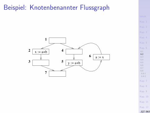
Inhalt
Kap. 1
Kap. 2
Kap. 3
Kap. 4
Kap. 5
Kap. 6
6.1
6.2
6.3
6.4
6.5
6.6
6.7
6.8
6.8.1
6.8.2
Kap. 7
Kap. 8
Kap. 9
Kap. 10
Kap. 11
Kap. 12
Kap. 13
Kap. 14
Kap. 15
Kap. 16
Kap. 17
Literatur
Anhang
A
Beispiel: Knotenbenannter Flussgraph
1
2
3
7
4
5
6
x := a+b
y := a+b
a := x
327/863
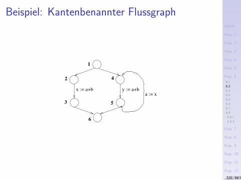
Inhalt
Kap. 1
Kap. 2
Kap. 3
Kap. 4
Kap. 5
Kap. 6
6.1
6.2
6.3
6.4
6.5
6.6
6.7
6.8
6.8.1
6.8.2
Kap. 7
Kap. 8
Kap. 9
Kap. 10
Kap. 11
Kap. 12
Kap. 13
Kap. 14
Kap. 15
Kap. 16
Kap. 17
Literatur
Anhang
A
Beispiel: Kantenbenannter Flussgraph
2 4
1
x := a+b
3
y := a+b
5
6
a := x
328/863
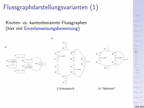
Inhalt
Kap. 1
Kap. 2
Kap. 3
Kap. 4
Kap. 5
Kap. 6
6.1
6.2
6.3
6.4
6.5
6.6
6.7
6.8
6.8.1
6.8.2
Kap. 7
Kap. 8
Kap. 9
Kap. 10
Kap. 11
Kap. 12
Kap. 13
Kap. 14
Kap. 15
Kap. 16
Kap. 17
Literatur
Anhang
A
Flussgraphdarstellungsvarianten (1)
Knoten- vs. kantenbenannte Flussgraphen(hier mit Einzelanweisungsbenennung)
i) Schematisch ii) "Optimiert"
a)
1
2
3
7
4
5
6
x := a+b
y := a+b
a := x
x := a+b
1
2 4
3
6
7
5
1
2
3 5
7
64
y := a+b
a := x
b)
2 4
1
x := a+b
3
y := a+b
5
6
a := x
329/863
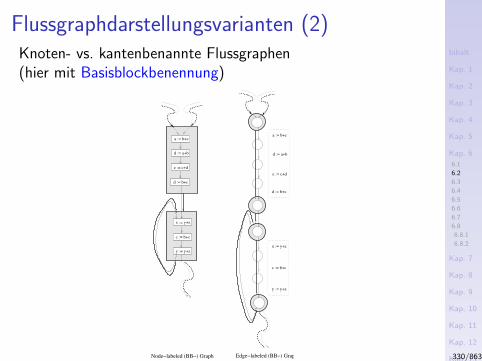
Inhalt
Kap. 1
Kap. 2
Kap. 3
Kap. 4
Kap. 5
Kap. 6
6.1
6.2
6.3
6.4
6.5
6.6
6.7
6.8
6.8.1
6.8.2
Kap. 7
Kap. 8
Kap. 9
Kap. 10
Kap. 11
Kap. 12
Kap. 13
Kap. 14
Kap. 15
Kap. 16
Kap. 17
Literatur
Anhang
A
Flussgraphdarstellungsvarianten (2)Knoten- vs. kantenbenannte Flussgraphen(hier mit Basisblockbenennung)
d := b+c
e := c+d
d := a+b
a := b+c
x := y+z
c := b+c
y := y+z
Node−labeled (BB−) Graph
e := c+d
d := a+b
a := b+c
d := b+c
x := y+z
c := b+c
y := y+z
Edge−labeled (BB−) Graph 330/863
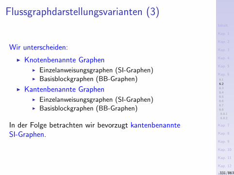
Inhalt
Kap. 1
Kap. 2
Kap. 3
Kap. 4
Kap. 5
Kap. 6
6.1
6.2
6.3
6.4
6.5
6.6
6.7
6.8
6.8.1
6.8.2
Kap. 7
Kap. 8
Kap. 9
Kap. 10
Kap. 11
Kap. 12
Kap. 13
Kap. 14
Kap. 15
Kap. 16
Kap. 17
Literatur
Anhang
A
Flussgraphdarstellungsvarianten (3)
Wir unterscheiden:
I Knotenbenannte GraphenI Einzelanweisungsgraphen (SI-Graphen)I Basisblockgraphen (BB-Graphen)
I Kantenbenannte GraphenI Einzelanweisungsgraphen (SI-Graphen)I Basisblockgraphen (BB-Graphen)
In der Folge betrachten wir bevorzugt kantenbenannteSI-Graphen.
331/863
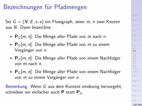
Inhalt
Kap. 1
Kap. 2
Kap. 3
Kap. 4
Kap. 5
Kap. 6
6.1
6.2
6.3
6.4
6.5
6.6
6.7
6.8
6.8.1
6.8.2
Kap. 7
Kap. 8
Kap. 9
Kap. 10
Kap. 11
Kap. 12
Kap. 13
Kap. 14
Kap. 15
Kap. 16
Kap. 17
Literatur
Anhang
A
Bezeichnungen fur Pfadmengen
Sei G = (N ,E , s, e) ein Flussgraph, seien m, n zwei Knotenaus N . Dann bezeichne:
I PG [m, n]: Die Menge aller Pfade von m nach n.
I PG [m, n[: Die Menge aller Pfade von m zu einemVorganger von n.
I PG ]m, n]: Die Menge aller Pfade von einem Nachfolgervon m nach n.
I PG ]m, n[: Die Menge aller Pfade von einem Nachfolgervon m zu einem Vorganger von n.
Bemerkung: Wenn G aus dem Kontext eindeutig hervorgeht,schreiben wir einfacher auch P statt PG .
332/863
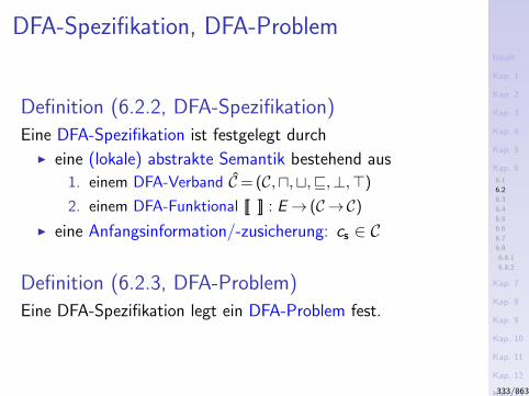
Inhalt
Kap. 1
Kap. 2
Kap. 3
Kap. 4
Kap. 5
Kap. 6
6.1
6.2
6.3
6.4
6.5
6.6
6.7
6.8
6.8.1
6.8.2
Kap. 7
Kap. 8
Kap. 9
Kap. 10
Kap. 11
Kap. 12
Kap. 13
Kap. 14
Kap. 15
Kap. 16
Kap. 17
Literatur
Anhang
A
DFA-Spezifikation, DFA-Problem
Definition (6.2.2, DFA-Spezifikation)
Eine DFA-Spezifikation ist festgelegt durch
I eine (lokale) abstrakte Semantik bestehend aus
1. einem DFA-Verband C= (C,u,t,v,⊥,>)
2. einem DFA-Funktional [[ ]] : E→ (C→C)
I eine Anfangsinformation/-zusicherung: cs ∈ C
Definition (6.2.3, DFA-Problem)
Eine DFA-Spezifikation legt ein DFA-Problem fest.
333/863
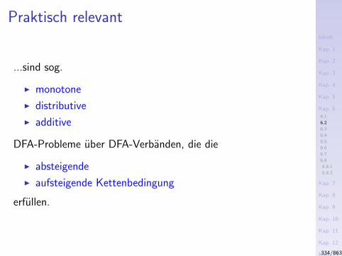
Inhalt
Kap. 1
Kap. 2
Kap. 3
Kap. 4
Kap. 5
Kap. 6
6.1
6.2
6.3
6.4
6.5
6.6
6.7
6.8
6.8.1
6.8.2
Kap. 7
Kap. 8
Kap. 9
Kap. 10
Kap. 11
Kap. 12
Kap. 13
Kap. 14
Kap. 15
Kap. 16
Kap. 17
Literatur
Anhang
A
Praktisch relevant
...sind sog.
I monotone
I distributive
I additive
DFA-Probleme uber DFA-Verbanden, die die
I absteigende
I aufsteigende Kettenbedingung
erfullen.
334/863
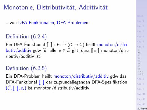
Inhalt
Kap. 1
Kap. 2
Kap. 3
Kap. 4
Kap. 5
Kap. 6
6.1
6.2
6.3
6.4
6.5
6.6
6.7
6.8
6.8.1
6.8.2
Kap. 7
Kap. 8
Kap. 9
Kap. 10
Kap. 11
Kap. 12
Kap. 13
Kap. 14
Kap. 15
Kap. 16
Kap. 17
Literatur
Anhang
A
Monotonie, Distributivitat, Additivitat
...von DFA-Funktionalen, DFA-Problemen:
Definition (6.2.4)
Ein DFA-Funktional [[ ]] : E → (C → C) heißt monoton/distri-butiv/additiv gdw fur alle e ∈ E gilt, dass [[ e ]] monoton/dist-ributiv/additiv ist.
Definition (6.2.5)
Ein DFA-Problem heißt monoton/distributiv/additiv gdw dasDFA-Funktional [[ ]] der zugrundeliegenden DFA-Spezifikation(C, [[ ]], cs) ist monoton/distributiv/additiv.
335/863
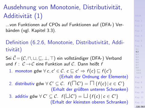
Inhalt
Kap. 1
Kap. 2
Kap. 3
Kap. 4
Kap. 5
Kap. 6
6.1
6.2
6.3
6.4
6.5
6.6
6.7
6.8
6.8.1
6.8.2
Kap. 7
Kap. 8
Kap. 9
Kap. 10
Kap. 11
Kap. 12
Kap. 13
Kap. 14
Kap. 15
Kap. 16
Kap. 17
Literatur
Anhang
A
Ausdehnung von Monotonie, Distributivitat,
Additivitat (1)...von Funktionen auf CPOs auf Funktionen auf (DFA-) Ver-banden (vgl. Kapitel 3.3).
Definition (6.2.6, Monotonie, Distributivitat, Addi-tivitat)
Sei C= (C,u,t,v,⊥,>) ein vollstandiger (DFA-) Verbandund f : C→C eine Funktion auf C. Dann heißt f
1. monoton gdw ∀ c , c ′ ∈ C. c v c ′ ⇒ f (c) v f (c ′)(Erhalt der Ordnung der Elemente)
2. distributiv gdw ∀C ′ ⊆ C. f (uC ′) = u f (c) | c ∈ C ′(Erhalt der großten unteren Schranken)
3. additiv gdw ∀C ′ ⊆ C. f (tC ′) = t f (c) | c ∈ C ′(Erhalt der kleinsten oberen Schranken)
336/863
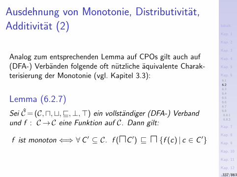
Inhalt
Kap. 1
Kap. 2
Kap. 3
Kap. 4
Kap. 5
Kap. 6
6.1
6.2
6.3
6.4
6.5
6.6
6.7
6.8
6.8.1
6.8.2
Kap. 7
Kap. 8
Kap. 9
Kap. 10
Kap. 11
Kap. 12
Kap. 13
Kap. 14
Kap. 15
Kap. 16
Kap. 17
Literatur
Anhang
A
Ausdehnung von Monotonie, Distributivitat,
Additivitat (2)
Analog zum entsprechenden Lemma auf CPOs gilt auch auf(DFA-) Verbanden folgende oft nutzliche aquivalente Charak-terisierung der Monotonie (vgl. Kapitel 3.3):
Lemma (6.2.7)
Sei C= (C,u,t,v,⊥,>) ein vollstandiger (DFA-) Verbandund f : C→C eine Funktion auf C. Dann gilt:
f ist monoton ⇐⇒ ∀C ′ ⊆ C. f (uC ′) v u f (c) | c ∈ C ′
337/863
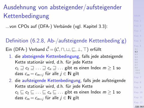
Inhalt
Kap. 1
Kap. 2
Kap. 3
Kap. 4
Kap. 5
Kap. 6
6.1
6.2
6.3
6.4
6.5
6.6
6.7
6.8
6.8.1
6.8.2
Kap. 7
Kap. 8
Kap. 9
Kap. 10
Kap. 11
Kap. 12
Kap. 13
Kap. 14
Kap. 15
Kap. 16
Kap. 17
Literatur
Anhang
A
Ausdehnung von absteigender/aufsteigender
Kettenbedingung
...von CPOs auf (DFA-) Verbande (vgl. Kapitel 3.3):
Definition (6.2.8, Ab-/aufsteigende Kettenbeding’g)
Ein (DFA-) Verband C= (C,u,t,v,⊥,>) erfullt
1. die absteigende Kettenbedingung, falls jede absteigendeKette stationar wird, d.h. fur jede Kettec1 w c2 w . . . w cn w . . . gibt es einen Index m ≥ 1 sodass cm = cm+j fur alle j ∈ IN gilt
2. die aufsteigende Kettenbedingung, falls jede aufsteigendeKette stationar wird, d.h. fur jede Kettec1 v c2 v . . . v cn v . . . gibt es einen Index m ≥ 1 sodass cm = cm+j fur alle j ∈ IN gilt
338/863
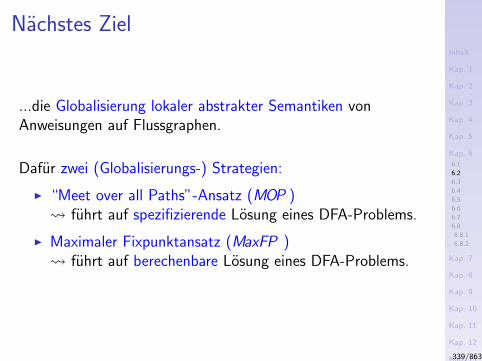
Inhalt
Kap. 1
Kap. 2
Kap. 3
Kap. 4
Kap. 5
Kap. 6
6.1
6.2
6.3
6.4
6.5
6.6
6.7
6.8
6.8.1
6.8.2
Kap. 7
Kap. 8
Kap. 9
Kap. 10
Kap. 11
Kap. 12
Kap. 13
Kap. 14
Kap. 15
Kap. 16
Kap. 17
Literatur
Anhang
A
Nachstes Ziel
...die Globalisierung lokaler abstrakter Semantiken vonAnweisungen auf Flussgraphen.
Dafur zwei (Globalisierungs-) Strategien:
I “Meet over all Paths”-Ansatz (MOP ) fuhrt auf spezifizierende Losung eines DFA-Problems.
I Maximaler Fixpunktansatz (MaxFP ) fuhrt auf berechenbare Losung eines DFA-Problems.
339/863

Inhalt
Kap. 1
Kap. 2
Kap. 3
Kap. 4
Kap. 5
Kap. 6
6.1
6.2
6.3
6.4
6.5
6.6
6.7
6.8
6.8.1
6.8.2
Kap. 7
Kap. 8
Kap. 9
Kap. 10
Kap. 11
Kap. 12
Kap. 13
Kap. 14
Kap. 15
Kap. 16
Kap. 17
Literatur
Anhang
A
Kapitel 6.3
MOP-Ansatz
340/863
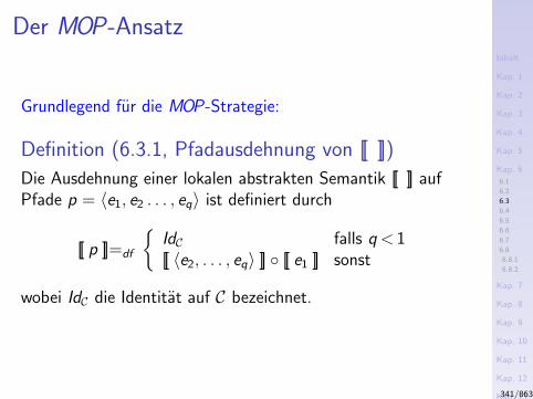
Inhalt
Kap. 1
Kap. 2
Kap. 3
Kap. 4
Kap. 5
Kap. 6
6.1
6.2
6.3
6.4
6.5
6.6
6.7
6.8
6.8.1
6.8.2
Kap. 7
Kap. 8
Kap. 9
Kap. 10
Kap. 11
Kap. 12
Kap. 13
Kap. 14
Kap. 15
Kap. 16
Kap. 17
Literatur
Anhang
A
Der MOP-Ansatz
Grundlegend fur die MOP-Strategie:
Definition (6.3.1, Pfadausdehnung von [[ ]])
Die Ausdehnung einer lokalen abstrakten Semantik [[ ]] aufPfade p = 〈e1, e2 . . . , eq〉 ist definiert durch
[[ p ]]=df
IdC falls q< 1[[ 〈e2, . . . , eq〉 ]] [[ e1 ]] sonst
wobei IdC die Identitat auf C bezeichnet.
341/863
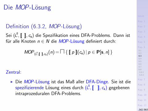
Inhalt
Kap. 1
Kap. 2
Kap. 3
Kap. 4
Kap. 5
Kap. 6
6.1
6.2
6.3
6.4
6.5
6.6
6.7
6.8
6.8.1
6.8.2
Kap. 7
Kap. 8
Kap. 9
Kap. 10
Kap. 11
Kap. 12
Kap. 13
Kap. 14
Kap. 15
Kap. 16
Kap. 17
Literatur
Anhang
A
Die MOP-Losung
Definition (6.3.2, MOP-Losung)
Sei (C, [[ ]], cs) die Spezifikation eines DFA-Problems. Dann istfur alle Knoten n ∈ N die MOP-Losung definiert durch:
MOP (C,[[ ]],cs)(n) =u [[ p ]](cs) | p ∈ P[s, n]
Zentral:
I Die MOP-Losung ist das Maß aller DFA-Dinge. Sie ist diespezifizierende Losung eines durch (C, [[ ]], cs) gegebenenintraprozeduralen DFA-Problems.
342/863
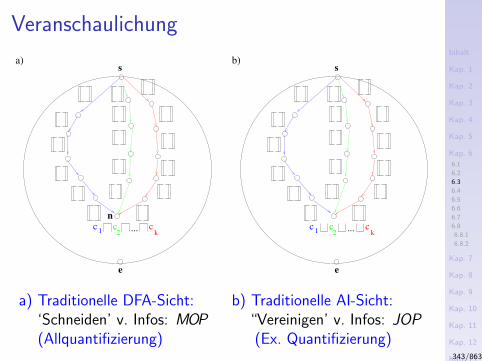
Inhalt
Kap. 1
Kap. 2
Kap. 3
Kap. 4
Kap. 5
Kap. 6
6.1
6.2
6.3
6.4
6.5
6.6
6.7
6.8
6.8.1
6.8.2
Kap. 7
Kap. 8
Kap. 9
Kap. 10
Kap. 11
Kap. 12
Kap. 13
Kap. 14
Kap. 15
Kap. 16
Kap. 17
Literatur
Anhang
A
Veranschaulichung
c1
c2 k
c...
e
s
c1
c2 k
c...
e
s
n
a) b)
a) Traditionelle DFA-Sicht: b) Traditionelle AI-Sicht:‘Schneiden’ v. Infos: MOP “Vereinigen’ v. Infos: JOP(Allquantifizierung) (Ex. Quantifizierung)
343/863
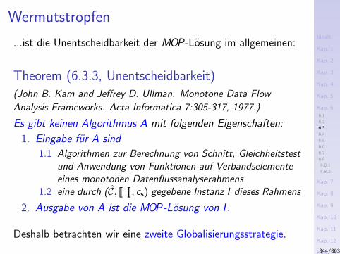
Inhalt
Kap. 1
Kap. 2
Kap. 3
Kap. 4
Kap. 5
Kap. 6
6.1
6.2
6.3
6.4
6.5
6.6
6.7
6.8
6.8.1
6.8.2
Kap. 7
Kap. 8
Kap. 9
Kap. 10
Kap. 11
Kap. 12
Kap. 13
Kap. 14
Kap. 15
Kap. 16
Kap. 17
Literatur
Anhang
A
Wermutstropfen
...ist die Unentscheidbarkeit der MOP-Losung im allgemeinen:
Theorem (6.3.3, Unentscheidbarkeit)
(John B. Kam and Jeffrey D. Ullman. Monotone Data Flow
Analysis Frameworks. Acta Informatica 7:305-317, 1977.)
Es gibt keinen Algorithmus A mit folgenden Eigenschaften:
1. Eingabe fur A sind
1.1 Algorithmen zur Berechnung von Schnitt, Gleichheitstestund Anwendung von Funktionen auf Verbandselementeeines monotonen Datenflussanalyserahmens
1.2 eine durch (C, [[ ]], cs) gegebene Instanz I dieses Rahmens
2. Ausgabe von A ist die MOP-Losung von I .
Deshalb betrachten wir eine zweite Globalisierungsstrategie.
344/863

Inhalt
Kap. 1
Kap. 2
Kap. 3
Kap. 4
Kap. 5
Kap. 6
6.1
6.2
6.3
6.4
6.5
6.6
6.7
6.8
6.8.1
6.8.2
Kap. 7
Kap. 8
Kap. 9
Kap. 10
Kap. 11
Kap. 12
Kap. 13
Kap. 14
Kap. 15
Kap. 16
Kap. 17
Literatur
Anhang
A
Kapitel 6.4
MaxFP-Ansatz
345/863
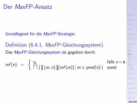
Inhalt
Kap. 1
Kap. 2
Kap. 3
Kap. 4
Kap. 5
Kap. 6
6.1
6.2
6.3
6.4
6.5
6.6
6.7
6.8
6.8.1
6.8.2
Kap. 7
Kap. 8
Kap. 9
Kap. 10
Kap. 11
Kap. 12
Kap. 13
Kap. 14
Kap. 15
Kap. 16
Kap. 17
Literatur
Anhang
A
Der MaxFP-Ansatz
Grundlegend fur die MaxFP-Strategie:
Definition (6.4.1, MaxFP-Gleichungssystem)
Das MaxFP-Gleichungssystem ist gegeben durch:
inf (n) =
cs falls n = su [[ (m, n) ]](inf (m)) |m ∈ pred(n) sonst
346/863
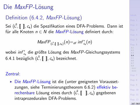
Inhalt
Kap. 1
Kap. 2
Kap. 3
Kap. 4
Kap. 5
Kap. 6
6.1
6.2
6.3
6.4
6.5
6.6
6.7
6.8
6.8.1
6.8.2
Kap. 7
Kap. 8
Kap. 9
Kap. 10
Kap. 11
Kap. 12
Kap. 13
Kap. 14
Kap. 15
Kap. 16
Kap. 17
Literatur
Anhang
A
Die MaxFP-Losung
Definition (6.4.2, MaxFP-Losung)
Sei (C, [[ ]], cs) die Spezifikation eines DFA-Problems. Dann istfur alle Knoten n ∈ N die MaxFP-Losung definiert durch:
MaxFP (C,[[ ]],cs)(n)=df inf ∗cs(n)
wobei inf ∗csdie großte Losung des MaxFP-Gleichungssystems
6.4.1 bezuglich (C, [[ ]], cs) bezeichnet.
Zentral:
I Die MaxFP-Losung ist die (unter geeigneten Vorausset-zungen, siehe Terminierungstheorem 6.6.2) effektiv be-rechenbare Losung eines durch (C, [[ ]], cs) gegebenenintraprozeduralen DFA-Problems.
347/863

Inhalt
Kap. 1
Kap. 2
Kap. 3
Kap. 4
Kap. 5
Kap. 6
6.1
6.2
6.3
6.4
6.5
6.6
6.7
6.8
6.8.1
6.8.2
Kap. 7
Kap. 8
Kap. 9
Kap. 10
Kap. 11
Kap. 12
Kap. 13
Kap. 14
Kap. 15
Kap. 16
Kap. 17
Literatur
Anhang
A
Kapitel 6.5
Koinzidenz- und Sicherheitstheorem
348/863
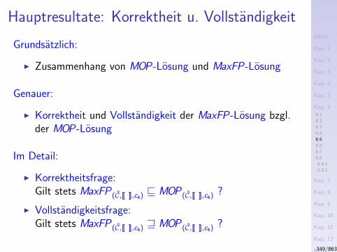
Inhalt
Kap. 1
Kap. 2
Kap. 3
Kap. 4
Kap. 5
Kap. 6
6.1
6.2
6.3
6.4
6.5
6.6
6.7
6.8
6.8.1
6.8.2
Kap. 7
Kap. 8
Kap. 9
Kap. 10
Kap. 11
Kap. 12
Kap. 13
Kap. 14
Kap. 15
Kap. 16
Kap. 17
Literatur
Anhang
A
Hauptresultate: Korrektheit u. Vollstandigkeit
Grundsatzlich:
I Zusammenhang von MOP-Losung und MaxFP-Losung
Genauer:
I Korrektheit und Vollstandigkeit der MaxFP-Losung bzgl.der MOP-Losung
Im Detail:
I Korrektheitsfrage:Gilt stets MaxFP (C,[[ ]],cs) v MOP (C,[[ ]],cs) ?
I Vollstandigkeitsfrage:Gilt stets MaxFP (C,[[ ]],cs) w MOP (C,[[ ]],cs) ?
349/863
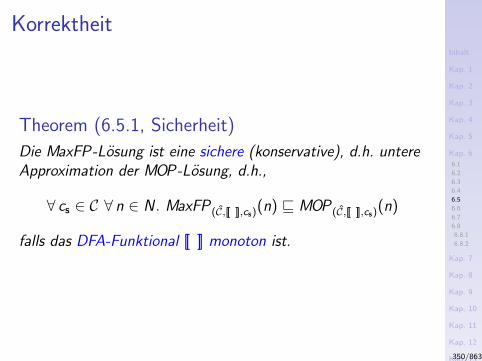
Inhalt
Kap. 1
Kap. 2
Kap. 3
Kap. 4
Kap. 5
Kap. 6
6.1
6.2
6.3
6.4
6.5
6.6
6.7
6.8
6.8.1
6.8.2
Kap. 7
Kap. 8
Kap. 9
Kap. 10
Kap. 11
Kap. 12
Kap. 13
Kap. 14
Kap. 15
Kap. 16
Kap. 17
Literatur
Anhang
A
Korrektheit
Theorem (6.5.1, Sicherheit)
Die MaxFP-Losung ist eine sichere (konservative), d.h. untereApproximation der MOP-Losung, d.h.,
∀ cs ∈ C ∀ n ∈ N . MaxFP (C,[[ ]],cs)(n) v MOP (C,[[ ]],cs)(n)
falls das DFA-Funktional [[ ]] monoton ist.
350/863
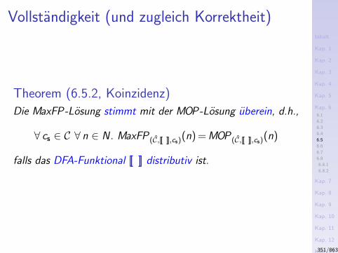
Inhalt
Kap. 1
Kap. 2
Kap. 3
Kap. 4
Kap. 5
Kap. 6
6.1
6.2
6.3
6.4
6.5
6.6
6.7
6.8
6.8.1
6.8.2
Kap. 7
Kap. 8
Kap. 9
Kap. 10
Kap. 11
Kap. 12
Kap. 13
Kap. 14
Kap. 15
Kap. 16
Kap. 17
Literatur
Anhang
A
Vollstandigkeit (und zugleich Korrektheit)
Theorem (6.5.2, Koinzidenz)
Die MaxFP-Losung stimmt mit der MOP-Losung uberein, d.h.,
∀ cs ∈ C ∀ n ∈ N . MaxFP (C,[[ ]],cs)(n) = MOP (C,[[ ]],cs)(n)
falls das DFA-Funktional [[ ]] distributiv ist.
351/863
Inhalt
Kap. 1
Kap. 2
Kap. 3
Kap. 4
Kap. 5
Kap. 6
6.1
6.2
6.3
6.4
6.5
6.6
6.7
6.8
6.8.1
6.8.2
Kap. 7
Kap. 8
Kap. 9
Kap. 10
Kap. 11
Kap. 12
Kap. 13
Kap. 14
Kap. 15
Kap. 16
Kap. 17
Literatur
Anhang
A
Bemerkung
Statt von
I Korrektheit
I Vollstandigkeit
spricht man im Zusammenhang mit DFA traditionell von
I Sicherheit
I Koinzidenz
352/863

Inhalt
Kap. 1
Kap. 2
Kap. 3
Kap. 4
Kap. 5
Kap. 6
6.1
6.2
6.3
6.4
6.5
6.6
6.7
6.8
6.8.1
6.8.2
Kap. 7
Kap. 8
Kap. 9
Kap. 10
Kap. 11
Kap. 12
Kap. 13
Kap. 14
Kap. 15
Kap. 16
Kap. 17
Literatur
Anhang
A
Kapitel 6.6
Generischer Fixpunktalgorithmus undTerminierungstheorem
353/863
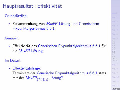
Inhalt
Kap. 1
Kap. 2
Kap. 3
Kap. 4
Kap. 5
Kap. 6
6.1
6.2
6.3
6.4
6.5
6.6
6.7
6.8
6.8.1
6.8.2
Kap. 7
Kap. 8
Kap. 9
Kap. 10
Kap. 11
Kap. 12
Kap. 13
Kap. 14
Kap. 15
Kap. 16
Kap. 17
Literatur
Anhang
A
Hauptresultat: Effektivitat
Grundsatzlich:
I Zusammenhang von MaxFP-Losung und GenerischemFixpunktalgorithmus 6.6.1
Genauer:
I Effektivitat des Generischen Fixpunktalgorithmus 6.6.1 furdie MaxFP-Losung
Im Detail:
I Effektivitatsfrage:Terminiert der Generische Fixpunktalgorithmus 6.6.1 stetsmit der MaxFP (C,[[ ]],cs)-Losung?
354/863
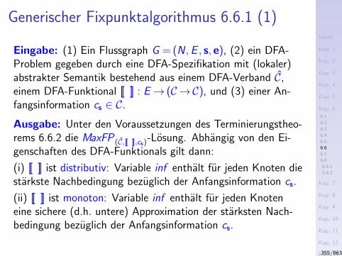
Inhalt
Kap. 1
Kap. 2
Kap. 3
Kap. 4
Kap. 5
Kap. 6
6.1
6.2
6.3
6.4
6.5
6.6
6.7
6.8
6.8.1
6.8.2
Kap. 7
Kap. 8
Kap. 9
Kap. 10
Kap. 11
Kap. 12
Kap. 13
Kap. 14
Kap. 15
Kap. 16
Kap. 17
Literatur
Anhang
A
Generischer Fixpunktalgorithmus 6.6.1 (1)
Eingabe: (1) Ein Flussgraph G = (N ,E , s, e), (2) ein DFA-Problem gegeben durch eine DFA-Spezifikation mit (lokaler)abstrakter Semantik bestehend aus einem DFA-Verband C,einem DFA-Funktional [[ ]] : E→ (C→C), und (3) einer An-fangsinformation cs ∈ C.
Ausgabe: Unter den Voraussetzungen des Terminierungstheo-rems 6.6.2 die MaxFP (C,[[ ]],cs)-Losung. Abhangig von den Ei-genschaften des DFA-Funktionals gilt dann:
(i) [[ ]] ist distributiv: Variable inf enthalt fur jeden Knoten diestarkste Nachbedingung bezuglich der Anfangsinformation cs.
(ii) [[ ]] ist monoton: Variable inf enthalt fur jeden Knoteneine sichere (d.h. untere) Approximation der starksten Nach-bedingung bezuglich der Anfangsinformation cs.
355/863
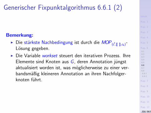
Inhalt
Kap. 1
Kap. 2
Kap. 3
Kap. 4
Kap. 5
Kap. 6
6.1
6.2
6.3
6.4
6.5
6.6
6.7
6.8
6.8.1
6.8.2
Kap. 7
Kap. 8
Kap. 9
Kap. 10
Kap. 11
Kap. 12
Kap. 13
Kap. 14
Kap. 15
Kap. 16
Kap. 17
Literatur
Anhang
A
Generischer Fixpunktalgorithmus 6.6.1 (2)
Bemerkung:
I Die starkste Nachbedingung ist durch die MOP (C,[[ ]],cs)-Losung gegeben.
I Die Variable workset steuert den iterativen Prozess. IhreElemente sind Knoten aus G , deren Annotation jungstaktualisiert worden ist, was moglicherweise zu einer ver-bandsmaßig kleineren Annotation an ihren Nachfolger-knoten fuhrt.
356/863
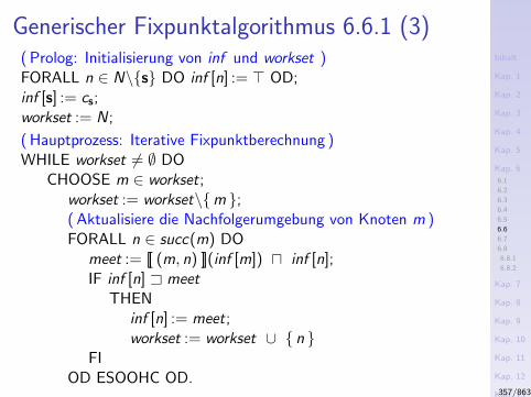
Inhalt
Kap. 1
Kap. 2
Kap. 3
Kap. 4
Kap. 5
Kap. 6
6.1
6.2
6.3
6.4
6.5
6.6
6.7
6.8
6.8.1
6.8.2
Kap. 7
Kap. 8
Kap. 9
Kap. 10
Kap. 11
Kap. 12
Kap. 13
Kap. 14
Kap. 15
Kap. 16
Kap. 17
Literatur
Anhang
A
Generischer Fixpunktalgorithmus 6.6.1 (3)( Prolog: Initialisierung von inf und workset )FORALL n ∈ N\s DO inf [n] := > OD;inf [s] := cs;workset := N;
( Hauptprozess: Iterative Fixpunktberechnung )WHILE workset 6= ∅ DO
CHOOSE m ∈ workset;workset := workset\m ;( Aktualisiere die Nachfolgerumgebung von Knoten m )FORALL n ∈ succ(m) DO
meet := [[ (m, n) ]](inf [m]) u inf [n];IF inf [n] A meet
THENinf [n] := meet;workset := workset ∪ n
FIOD ESOOHC OD.
357/863
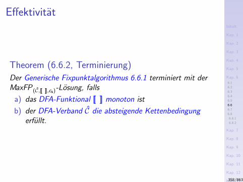
Inhalt
Kap. 1
Kap. 2
Kap. 3
Kap. 4
Kap. 5
Kap. 6
6.1
6.2
6.3
6.4
6.5
6.6
6.7
6.8
6.8.1
6.8.2
Kap. 7
Kap. 8
Kap. 9
Kap. 10
Kap. 11
Kap. 12
Kap. 13
Kap. 14
Kap. 15
Kap. 16
Kap. 17
Literatur
Anhang
A
Effektivitat
Theorem (6.6.2, Terminierung)
Der Generische Fixpunktalgorithmus 6.6.1 terminiert mit derMaxFP (C,[[ ]],cs)-Losung, falls
a) das DFA-Funktional [[ ]] monoton ist
b) der DFA-Verband C die absteigende Kettenbedingungerfullt.
358/863
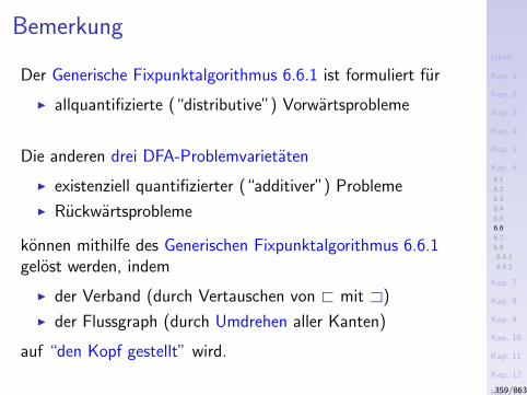
Inhalt
Kap. 1
Kap. 2
Kap. 3
Kap. 4
Kap. 5
Kap. 6
6.1
6.2
6.3
6.4
6.5
6.6
6.7
6.8
6.8.1
6.8.2
Kap. 7
Kap. 8
Kap. 9
Kap. 10
Kap. 11
Kap. 12
Kap. 13
Kap. 14
Kap. 15
Kap. 16
Kap. 17
Literatur
Anhang
A
Bemerkung
Der Generische Fixpunktalgorithmus 6.6.1 ist formuliert fur
I allquantifizierte (“distributive”) Vorwartsprobleme
Die anderen drei DFA-Problemvarietaten
I existenziell quantifizierter (“additiver”) Probleme
I Ruckwartsprobleme
konnen mithilfe des Generischen Fixpunktalgorithmus 6.6.1gelost werden, indem
I der Verband (durch Vertauschen von @ mit A)
I der Flussgraph (durch Umdrehen aller Kanten)
auf “den Kopf gestellt” wird.
359/863

Inhalt
Kap. 1
Kap. 2
Kap. 3
Kap. 4
Kap. 5
Kap. 6
6.1
6.2
6.3
6.4
6.5
6.6
6.7
6.8
6.8.1
6.8.2
Kap. 7
Kap. 8
Kap. 9
Kap. 10
Kap. 11
Kap. 12
Kap. 13
Kap. 14
Kap. 15
Kap. 16
Kap. 17
Literatur
Anhang
A
Kapitel 6.7
Zusammenfassung und Uberblick
360/863
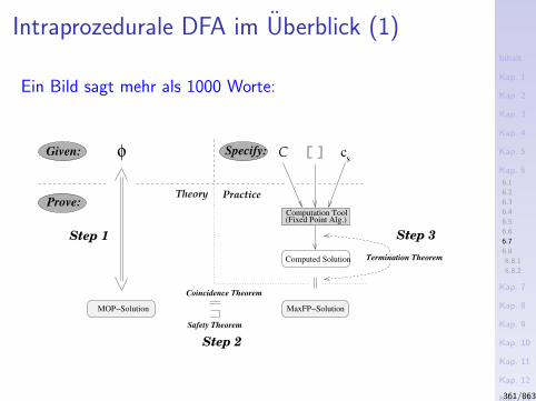
Inhalt
Kap. 1
Kap. 2
Kap. 3
Kap. 4
Kap. 5
Kap. 6
6.1
6.2
6.3
6.4
6.5
6.6
6.7
6.8
6.8.1
6.8.2
Kap. 7
Kap. 8
Kap. 9
Kap. 10
Kap. 11
Kap. 12
Kap. 13
Kap. 14
Kap. 15
Kap. 16
Kap. 17
Literatur
Anhang
A
Intraprozedurale DFA im Uberblick (1)
Ein Bild sagt mehr als 1000 Worte:
Computed Solution
Specify:
MOP−Solution
φ C cs
Practice
Step 3
TheoryProve:
Given:
Computation Tool
Termination Theorem
(Fixed Point Alg.)
MaxFP−Solution
Coincidence Theorem
Safety Theorem
Step 2
Step 1
361/863
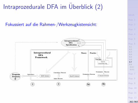
Inhalt
Kap. 1
Kap. 2
Kap. 3
Kap. 4
Kap. 5
Kap. 6
6.1
6.2
6.3
6.4
6.5
6.6
6.7
6.8
6.8.1
6.8.2
Kap. 7
Kap. 8
Kap. 9
Kap. 10
Kap. 11
Kap. 12
Kap. 13
Kap. 14
Kap. 15
Kap. 16
Kap. 17
Literatur
Anhang
A
Intraprozedurale DFA im Uberblick (2)
Fokussiert auf die Rahmen-/Werkzeugkistensicht:
MOP−Solution Computed Solution
1 3a) 3b)2
Program
Property
φ
DFAFramework
Intraprocedural Theory Practice
Tool Kit
Equivalence
Coincidence Theorem
Safety Theorem
MaxFP−Solution
Termination Theorem
Theorem
Generic
Fixed Point Alg.
C
Specification
DFA
Intraprocedural
cs
Termination
362/863

Inhalt
Kap. 1
Kap. 2
Kap. 3
Kap. 4
Kap. 5
Kap. 6
6.1
6.2
6.3
6.4
6.5
6.6
6.7
6.8
6.8.1
6.8.2
Kap. 7
Kap. 8
Kap. 9
Kap. 10
Kap. 11
Kap. 12
Kap. 13
Kap. 14
Kap. 15
Kap. 16
Kap. 17
Literatur
Anhang
A
Kapitel 6.8
Beispiele: Verfugbare Ausdrucke, einfacheKonstanten
363/863
Inhalt
Kap. 1
Kap. 2
Kap. 3
Kap. 4
Kap. 5
Kap. 6
6.1
6.2
6.3
6.4
6.5
6.6
6.7
6.8
6.8.1
6.8.2
Kap. 7
Kap. 8
Kap. 9
Kap. 10
Kap. 11
Kap. 12
Kap. 13
Kap. 14
Kap. 15
Kap. 16
Kap. 17
Literatur
Anhang
A
Zwei prototypische DFA-Probleme
I Verfugbare Ausdrucke kanonisches Bsp. eines distributiven DFA-Problems
I Einfache Konstanten kanonisches Bsp. eines monotonen DFA-Problems
364/863

Inhalt
Kap. 1
Kap. 2
Kap. 3
Kap. 4
Kap. 5
Kap. 6
6.1
6.2
6.3
6.4
6.5
6.6
6.7
6.8
6.8.1
6.8.2
Kap. 7
Kap. 8
Kap. 9
Kap. 10
Kap. 11
Kap. 12
Kap. 13
Kap. 14
Kap. 15
Kap. 16
Kap. 17
Literatur
Anhang
A
Kapitel 6.6.1
Verfugbare Ausdrucke
365/863
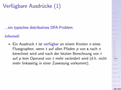
Inhalt
Kap. 1
Kap. 2
Kap. 3
Kap. 4
Kap. 5
Kap. 6
6.1
6.2
6.3
6.4
6.5
6.6
6.7
6.8
6.8.1
6.8.2
Kap. 7
Kap. 8
Kap. 9
Kap. 10
Kap. 11
Kap. 12
Kap. 13
Kap. 14
Kap. 15
Kap. 16
Kap. 17
Literatur
Anhang
A
Verfugbare Ausdrucke (1)
...ein typisches distributives DFA-Problem.
Informell:
I Ein Ausdruck t ist verfugbar an einem Knoten n einesFlussgraphen, wenn t auf allen Pfaden p von s nach nberechnet wird und nach der letzten Berechnung von tauf p kein Operand von t mehr verandert wird (d.h. nichtmehr linksseitig in einer Zuweisung vorkommt).
366/863
Inhalt
Kap. 1
Kap. 2
Kap. 3
Kap. 4
Kap. 5
Kap. 6
6.1
6.2
6.3
6.4
6.5
6.6
6.7
6.8
6.8.1
6.8.2
Kap. 7
Kap. 8
Kap. 9
Kap. 10
Kap. 11
Kap. 12
Kap. 13
Kap. 14
Kap. 15
Kap. 16
Kap. 17
Literatur
Anhang
A
Verfugbare Ausdrucke (2)
Bemerkung:
I t wird oft als Kandidatenausdruck bezeichnet.
I Ist t verfugbar an einem Knoten n, so kann eine Wieder-berechnung an n durch Ruckgriff auf seinen zuvor berech-neten (und zu diesem Zweck gespeicherten) Wert vermie-den werden; dadurch entsteht bestimmter Berechnungs-aufwand zur Laufzeit uberhaupt nicht, er wird vermieden:Performanzverbesserung Optimierung
367/863
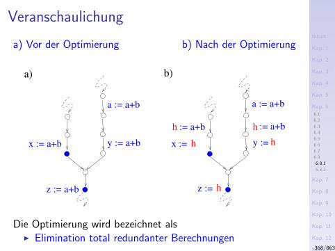
Inhalt
Kap. 1
Kap. 2
Kap. 3
Kap. 4
Kap. 5
Kap. 6
6.1
6.2
6.3
6.4
6.5
6.6
6.7
6.8
6.8.1
6.8.2
Kap. 7
Kap. 8
Kap. 9
Kap. 10
Kap. 11
Kap. 12
Kap. 13
Kap. 14
Kap. 15
Kap. 16
Kap. 17
Literatur
Anhang
A
Veranschaulichung
a) Vor der Optimierung b) Nach der Optimierung
y := a+b x := y :=
h := a+b h := a+b
h h
hz :=z := a+b
x := a+b
a := a+b a := a+b
b)a)
Die Optimierung wird bezeichnet alsI Elimination total redundanter Berechnungen
368/863
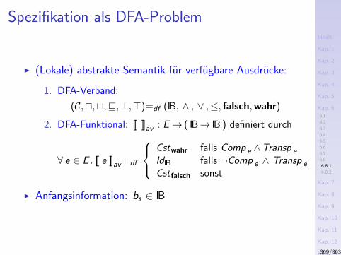
Inhalt
Kap. 1
Kap. 2
Kap. 3
Kap. 4
Kap. 5
Kap. 6
6.1
6.2
6.3
6.4
6.5
6.6
6.7
6.8
6.8.1
6.8.2
Kap. 7
Kap. 8
Kap. 9
Kap. 10
Kap. 11
Kap. 12
Kap. 13
Kap. 14
Kap. 15
Kap. 16
Kap. 17
Literatur
Anhang
A
Spezifikation als DFA-Problem
I (Lokale) abstrakte Semantik fur verfugbare Ausdrucke:
1. DFA-Verband:
(C,u,t,v,⊥,>)=df (IB, ∧ , ∨ ,≤, falsch,wahr)
2. DFA-Funktional: [[ ]]av : E→ ( IB→ IB ) definiert durch
∀ e ∈ E . [[ e ]]av=df
Cstwahr falls Comp e ∧Transp e
IdIB falls ¬Comp e ∧ Transp e
Cstfalsch sonst
I Anfangsinformation: bs ∈ IB
369/863
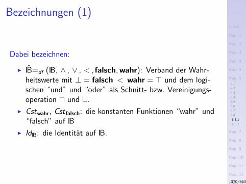
Inhalt
Kap. 1
Kap. 2
Kap. 3
Kap. 4
Kap. 5
Kap. 6
6.1
6.2
6.3
6.4
6.5
6.6
6.7
6.8
6.8.1
6.8.2
Kap. 7
Kap. 8
Kap. 9
Kap. 10
Kap. 11
Kap. 12
Kap. 13
Kap. 14
Kap. 15
Kap. 16
Kap. 17
Literatur
Anhang
A
Bezeichnungen (1)
Dabei bezeichnen:
I IB=df (IB, ∧ , ∨ , < , falsch,wahr): Verband der Wahr-heitswerte mit ⊥ = falsch < wahr = > und dem logi-schen “und” und “oder” als Schnitt- bzw. Vereinigungs-operation u und t.
I Cstwahr, Cst falsch: die konstanten Funktionen “wahr” und“falsch” auf IB
I IdIB: die Identitat auf IB.
370/863
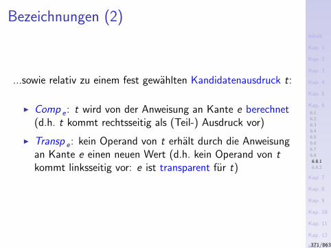
Inhalt
Kap. 1
Kap. 2
Kap. 3
Kap. 4
Kap. 5
Kap. 6
6.1
6.2
6.3
6.4
6.5
6.6
6.7
6.8
6.8.1
6.8.2
Kap. 7
Kap. 8
Kap. 9
Kap. 10
Kap. 11
Kap. 12
Kap. 13
Kap. 14
Kap. 15
Kap. 16
Kap. 17
Literatur
Anhang
A
Bezeichnungen (2)
...sowie relativ zu einem fest gewahlten Kandidatenausdruck t:
I Comp e : t wird von der Anweisung an Kante e berechnet(d.h. t kommt rechtsseitig als (Teil-) Ausdruck vor)
I Transp e : kein Operand von t erhalt durch die Anweisungan Kante e einen neuen Wert (d.h. kein Operand von tkommt linksseitig vor: e ist transparent fur t)
371/863
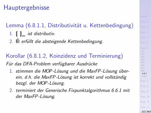
Inhalt
Kap. 1
Kap. 2
Kap. 3
Kap. 4
Kap. 5
Kap. 6
6.1
6.2
6.3
6.4
6.5
6.6
6.7
6.8
6.8.1
6.8.2
Kap. 7
Kap. 8
Kap. 9
Kap. 10
Kap. 11
Kap. 12
Kap. 13
Kap. 14
Kap. 15
Kap. 16
Kap. 17
Literatur
Anhang
A
Hauptergebnisse
Lemma (6.8.1.1, Distributivitat u. Kettenbedingung)
1. [[ ]]av ist distributiv.
2. IB erfullt die absteigende Kettenbedingung.
Korollar (6.8.1.2, Koinzidenz und Terminierung)
Fur das DFA-Problem verfugbarer Ausdrucke
1. stimmen die MOP-Losung und die MaxFP-Losung uber-ein, d.h. die MaxFP-Losung ist korrekt und vollstandigbezgl. der MOP-Losung.
2. terminiert der Generische Fixpunktalgorithmus 6.6.1 mitder MaxFP-Losung.
372/863

Inhalt
Kap. 1
Kap. 2
Kap. 3
Kap. 4
Kap. 5
Kap. 6
6.1
6.2
6.3
6.4
6.5
6.6
6.7
6.8
6.8.1
6.8.2
Kap. 7
Kap. 8
Kap. 9
Kap. 10
Kap. 11
Kap. 12
Kap. 13
Kap. 14
Kap. 15
Kap. 16
Kap. 17
Literatur
Anhang
A
Kapitel 6.6.2
Einfache Konstanten
373/863
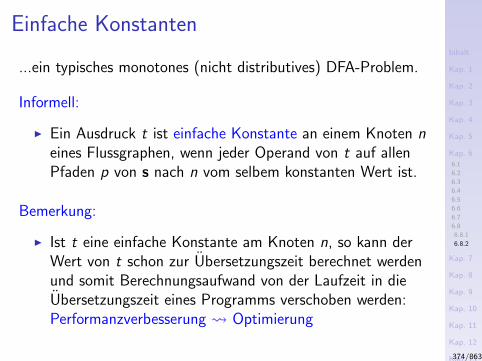
Inhalt
Kap. 1
Kap. 2
Kap. 3
Kap. 4
Kap. 5
Kap. 6
6.1
6.2
6.3
6.4
6.5
6.6
6.7
6.8
6.8.1
6.8.2
Kap. 7
Kap. 8
Kap. 9
Kap. 10
Kap. 11
Kap. 12
Kap. 13
Kap. 14
Kap. 15
Kap. 16
Kap. 17
Literatur
Anhang
A
Einfache Konstanten
...ein typisches monotones (nicht distributives) DFA-Problem.
Informell:
I Ein Ausdruck t ist einfache Konstante an einem Knoten neines Flussgraphen, wenn jeder Operand von t auf allenPfaden p von s nach n vom selbem konstanten Wert ist.
Bemerkung:
I Ist t eine einfache Konstante am Knoten n, so kann derWert von t schon zur Ubersetzungszeit berechnet werdenund somit Berechnungsaufwand von der Laufzeit in dieUbersetzungszeit eines Programms verschoben werden:Performanzverbesserung Optimierung
374/863
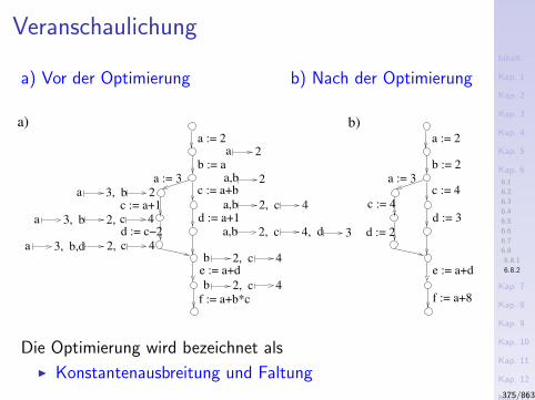
Inhalt
Kap. 1
Kap. 2
Kap. 3
Kap. 4
Kap. 5
Kap. 6
6.1
6.2
6.3
6.4
6.5
6.6
6.7
6.8
6.8.1
6.8.2
Kap. 7
Kap. 8
Kap. 9
Kap. 10
Kap. 11
Kap. 12
Kap. 13
Kap. 14
Kap. 15
Kap. 16
Kap. 17
Literatur
Anhang
A
Veranschaulichung
a) Vor der Optimierung b) Nach der Optimierung
2, c 4b
2, c 4b
a 3, b 2c 4
c 4a 3, b 2,
c 4a 3, b,d 2,
a,b
b)
d := c−2
c := a+1
a)
b := 2
a := 2
c := 4
d := 3
a := 3
b := a
a := 2
c := a+b
d := a+1
c := 4
d := 2
e := a+d
f := a+b*c
e := a+d
f := a+8
a
a := 3
2
2
a,b 2, c 4, d 3
a,b 2,
Die Optimierung wird bezeichnet als
I Konstantenausbreitung und Faltung375/863
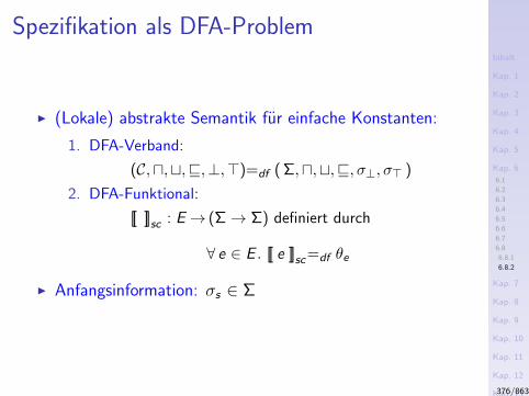
Inhalt
Kap. 1
Kap. 2
Kap. 3
Kap. 4
Kap. 5
Kap. 6
6.1
6.2
6.3
6.4
6.5
6.6
6.7
6.8
6.8.1
6.8.2
Kap. 7
Kap. 8
Kap. 9
Kap. 10
Kap. 11
Kap. 12
Kap. 13
Kap. 14
Kap. 15
Kap. 16
Kap. 17
Literatur
Anhang
A
Spezifikation als DFA-Problem
I (Lokale) abstrakte Semantik fur einfache Konstanten:
1. DFA-Verband:
(C,u,t,v,⊥,>)=df ( Σ,u,t,v, σ⊥, σ> )
2. DFA-Funktional:
[[ ]]sc : E→ (Σ→ Σ) definiert durch
∀ e ∈ E . [[ e ]]sc=df θe
I Anfangsinformation: σs ∈ Σ
376/863
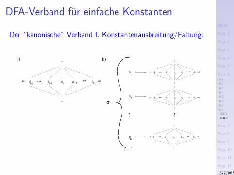
Inhalt
Kap. 1
Kap. 2
Kap. 3
Kap. 4
Kap. 5
Kap. 6
6.1
6.2
6.3
6.4
6.5
6.6
6.7
6.8
6.8.1
6.8.2
Kap. 7
Kap. 8
Kap. 9
Kap. 10
Kap. 11
Kap. 12
Kap. 13
Kap. 14
Kap. 15
Kap. 16
Kap. 17
Literatur
Anhang
A
DFA-Verband fur einfache Konstanten
Der “kanonische” Verband f. Konstantenausbreitung/Faltung:
σ :
v
v1
2
vk
di−j
di−1
di
di+1 di+j
di−j
di−1 d
idi+1 di+j
di−j
di−1 d
idi+1 di+j
di−j
di−1 d
idi+1 di+j
a) b)
377/863
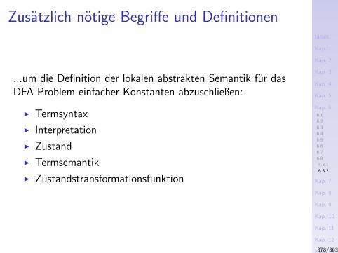
Inhalt
Kap. 1
Kap. 2
Kap. 3
Kap. 4
Kap. 5
Kap. 6
6.1
6.2
6.3
6.4
6.5
6.6
6.7
6.8
6.8.1
6.8.2
Kap. 7
Kap. 8
Kap. 9
Kap. 10
Kap. 11
Kap. 12
Kap. 13
Kap. 14
Kap. 15
Kap. 16
Kap. 17
Literatur
Anhang
A
Zusatzlich notige Begriffe und Definitionen
...um die Definition der lokalen abstrakten Semantik fur dasDFA-Problem einfacher Konstanten abzuschließen:
I Termsyntax
I Interpretation
I Zustand
I Termsemantik
I Zustandstransformationsfunktion
378/863
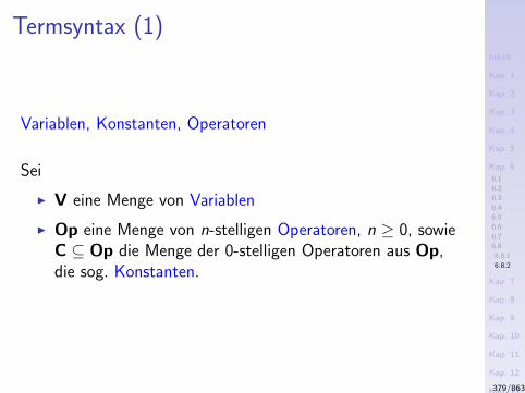
Inhalt
Kap. 1
Kap. 2
Kap. 3
Kap. 4
Kap. 5
Kap. 6
6.1
6.2
6.3
6.4
6.5
6.6
6.7
6.8
6.8.1
6.8.2
Kap. 7
Kap. 8
Kap. 9
Kap. 10
Kap. 11
Kap. 12
Kap. 13
Kap. 14
Kap. 15
Kap. 16
Kap. 17
Literatur
Anhang
A
Termsyntax (1)
Variablen, Konstanten, Operatoren
Sei
I V eine Menge von Variablen
I Op eine Menge von n-stelligen Operatoren, n ≥ 0, sowieC ⊆ Op die Menge der 0-stelligen Operatoren aus Op,die sog. Konstanten.
379/863
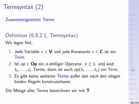
Inhalt
Kap. 1
Kap. 2
Kap. 3
Kap. 4
Kap. 5
Kap. 6
6.1
6.2
6.3
6.4
6.5
6.6
6.7
6.8
6.8.1
6.8.2
Kap. 7
Kap. 8
Kap. 9
Kap. 10
Kap. 11
Kap. 12
Kap. 13
Kap. 14
Kap. 15
Kap. 16
Kap. 17
Literatur
Anhang
A
Termsyntax (2)
Zusammengesetzte Terme
Definition (6.8.2.1, Termsyntax)
Wir legen fest:
1. Jede Variable v ∈ V und jede Konstante c ∈ C ist einTerm.
2. Ist op ∈ Op ein n-stelliger Operator, n ≥ 1, und sindt1, . . . , tn Terme, dann ist auch op(t1, . . . , tn) ein Term.
3. Es gibt keine weiteren Terme außer den nach den obigenbeiden Regeln konstruierbaren.
Die Menge aller Terme bezeichnen wir mit T.
380/863
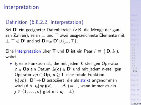
Inhalt
Kap. 1
Kap. 2
Kap. 3
Kap. 4
Kap. 5
Kap. 6
6.1
6.2
6.3
6.4
6.5
6.6
6.7
6.8
6.8.1
6.8.2
Kap. 7
Kap. 8
Kap. 9
Kap. 10
Kap. 11
Kap. 12
Kap. 13
Kap. 14
Kap. 15
Kap. 16
Kap. 17
Literatur
Anhang
A
Interpretation
Definition (6.8.2.2, Interpretation)
Sei D′ ein geeigneter Datenbereich (z.B. die Menge der gan-zen Zahlen), seien ⊥ und > zwei ausgezeichnete Elemente mit⊥,> 6∈ D′ und sei D=df D′ ∪⊥,>.
Eine Interpretation uber T und D ist ein Paar I ≡ ( D, I0 ),wobei
I I0 eine Funktion ist, die mit jedem 0-stelligen Operatorc ∈ Op ein Datum I0(c) ∈ D′ und mit jedem n-stelligenOperator op ∈ Op, n ≥ 1, eine totale FunktionI0(op) : Dn→D assoziiert, die als strikt angenommenwird (d.h. I0(op)(d1, . . . , dn ) =⊥, wann immer es einj ∈ 1, . . . , n gibt mit dj =⊥)
381/863
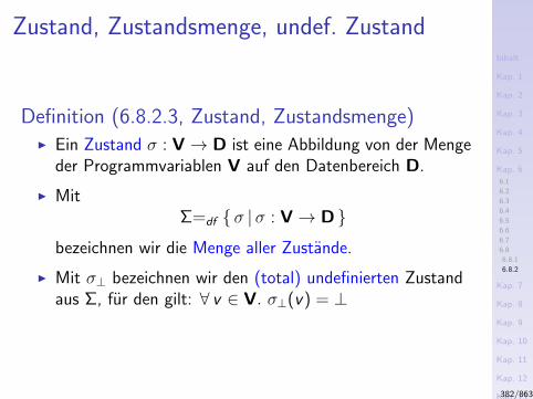
Inhalt
Kap. 1
Kap. 2
Kap. 3
Kap. 4
Kap. 5
Kap. 6
6.1
6.2
6.3
6.4
6.5
6.6
6.7
6.8
6.8.1
6.8.2
Kap. 7
Kap. 8
Kap. 9
Kap. 10
Kap. 11
Kap. 12
Kap. 13
Kap. 14
Kap. 15
Kap. 16
Kap. 17
Literatur
Anhang
A
Zustand, Zustandsmenge, undef. Zustand
Definition (6.8.2.3, Zustand, Zustandsmenge)I Ein Zustand σ : V→ D ist eine Abbildung von der Menge
der Programmvariablen V auf den Datenbereich D.
I MitΣ=df σ |σ : V→ D
bezeichnen wir die Menge aller Zustande.
I Mit σ⊥ bezeichnen wir den (total) undefinierten Zustandaus Σ, fur den gilt: ∀ v ∈ V. σ⊥(v) = ⊥
382/863
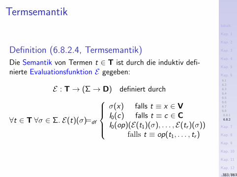
Inhalt
Kap. 1
Kap. 2
Kap. 3
Kap. 4
Kap. 5
Kap. 6
6.1
6.2
6.3
6.4
6.5
6.6
6.7
6.8
6.8.1
6.8.2
Kap. 7
Kap. 8
Kap. 9
Kap. 10
Kap. 11
Kap. 12
Kap. 13
Kap. 14
Kap. 15
Kap. 16
Kap. 17
Literatur
Anhang
A
Termsemantik
Definition (6.8.2.4, Termsemantik)
Die Semantik von Termen t ∈ T ist durch die induktiv defi-nierte Evaluationsfunktion E gegeben:
E : T→ (Σ→ D) definiert durch
∀t ∈ T ∀σ ∈ Σ. E(t)(σ)=df
σ(x) falls t ≡ x ∈ VI0(c) falls t ≡ c ∈ CI0(op)(E(t1)(σ), . . . , E(tr )(σ))
falls t ≡ op(t1, . . . , tr )
383/863
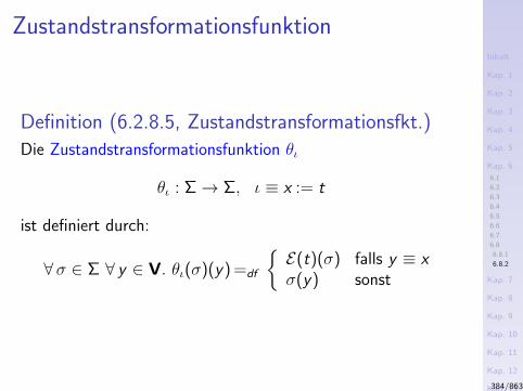
Inhalt
Kap. 1
Kap. 2
Kap. 3
Kap. 4
Kap. 5
Kap. 6
6.1
6.2
6.3
6.4
6.5
6.6
6.7
6.8
6.8.1
6.8.2
Kap. 7
Kap. 8
Kap. 9
Kap. 10
Kap. 11
Kap. 12
Kap. 13
Kap. 14
Kap. 15
Kap. 16
Kap. 17
Literatur
Anhang
A
Zustandstransformationsfunktion
Definition (6.2.8.5, Zustandstransformationsfkt.)
Die Zustandstransformationsfunktion θι
θι : Σ→ Σ, ι ≡ x := t
ist definiert durch:
∀σ ∈ Σ ∀ y ∈ V. θι(σ)(y) =df
E(t)(σ) falls y ≡ xσ(y) sonst
384/863
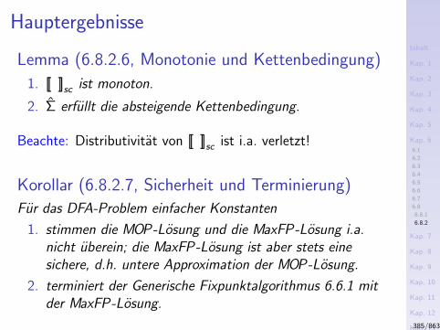
Inhalt
Kap. 1
Kap. 2
Kap. 3
Kap. 4
Kap. 5
Kap. 6
6.1
6.2
6.3
6.4
6.5
6.6
6.7
6.8
6.8.1
6.8.2
Kap. 7
Kap. 8
Kap. 9
Kap. 10
Kap. 11
Kap. 12
Kap. 13
Kap. 14
Kap. 15
Kap. 16
Kap. 17
Literatur
Anhang
A
Hauptergebnisse
Lemma (6.8.2.6, Monotonie und Kettenbedingung)
1. [[ ]]sc ist monoton.
2. Σ erfullt die absteigende Kettenbedingung.
Beachte: Distributivitat von [[ ]]sc ist i.a. verletzt!
Korollar (6.8.2.7, Sicherheit und Terminierung)
Fur das DFA-Problem einfacher Konstanten
1. stimmen die MOP-Losung und die MaxFP-Losung i.a.nicht uberein; die MaxFP-Losung ist aber stets einesichere, d.h. untere Approximation der MOP-Losung.
2. terminiert der Generische Fixpunktalgorithmus 6.6.1 mitder MaxFP-Losung.
385/863
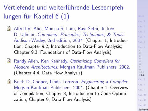
Inhalt
Kap. 1
Kap. 2
Kap. 3
Kap. 4
Kap. 5
Kap. 6
6.1
6.2
6.3
6.4
6.5
6.6
6.7
6.8
6.8.1
6.8.2
Kap. 7
Kap. 8
Kap. 9
Kap. 10
Kap. 11
Kap. 12
Kap. 13
Kap. 14
Kap. 15
Kap. 16
Kap. 17
Literatur
Anhang
A
Vertiefende und weiterfuhrende Leseempfeh-
lungen fur Kapitel 6 (1)
Alfred V. Aho, Monica S. Lam, Ravi Sethi, JeffreyD. Ullman. Compilers: Principles, Techniques, & Tools.Addison-Wesley, 2nd edition, 2007. (Chapter 1, Introduc-tion; Chapter 9.2, Introduction to Data-Flow Analysis;Chapter 9.3, Foundations of Data-Flow Analysis)
Randy Allen, Ken Kennedy. Optimizing Compilers forModern Architectures. Morgan Kaufman Publishers, 2002.(Chapter 4.4, Data Flow Analysis)
Keith D. Cooper, Linda Torczon. Engineering a Compiler.Morgan Kaufman Publishers, 2004. (Chapter 1, Overviewof Compilation; Chapter 8, Introduction to Code Optimi-zation; Chapter 9, Data Flow Analysis)
386/863
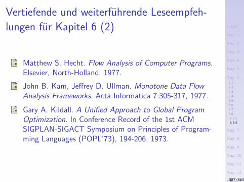
Inhalt
Kap. 1
Kap. 2
Kap. 3
Kap. 4
Kap. 5
Kap. 6
6.1
6.2
6.3
6.4
6.5
6.6
6.7
6.8
6.8.1
6.8.2
Kap. 7
Kap. 8
Kap. 9
Kap. 10
Kap. 11
Kap. 12
Kap. 13
Kap. 14
Kap. 15
Kap. 16
Kap. 17
Literatur
Anhang
A
Vertiefende und weiterfuhrende Leseempfeh-
lungen fur Kapitel 6 (2)
Matthew S. Hecht. Flow Analysis of Computer Programs.Elsevier, North-Holland, 1977.
John B. Kam, Jeffrey D. Ullman. Monotone Data FlowAnalysis Frameworks. Acta Informatica 7:305-317, 1977.
Gary A. Kildall. A Unified Approach to Global ProgramOptimization. In Conference Record of the 1st ACMSIGPLAN-SIGACT Symposium on Principles of Program-ming Languages (POPL’73), 194-206, 1973.
387/863
Inhalt
Kap. 1
Kap. 2
Kap. 3
Kap. 4
Kap. 5
Kap. 6
6.1
6.2
6.3
6.4
6.5
6.6
6.7
6.8
6.8.1
6.8.2
Kap. 7
Kap. 8
Kap. 9
Kap. 10
Kap. 11
Kap. 12
Kap. 13
Kap. 14
Kap. 15
Kap. 16
Kap. 17
Literatur
Anhang
A
Vertiefende und weiterfuhrende Leseempfeh-
lungen fur Kapitel 6 (3)
Jens Knoop. From DFA-frameworks to DFA-generators: Aunifying multiparadigm approach. In Proceedings of the5th International Conference on Tools and Algorithms forthe Construction and Analysis of Systems (TACAS’99),Springer-V., LNCS 1579, 360-374, 1999.
Jens Knoop, Bernhard Steffen. The InterproceduralCoincidence Theorem. In Proceedings of the 4thInternational Conference on Compiler Construction(CC’92), Springer-V., LNCS 641, 125-140, 1992.
Jens Knoop, Bernhard Steffen, Jurgen Vollmer. Parallelismfor Free: Efficient and Optimal Bitvector Analyses forParallel Programs. ACM Transactions on ProgrammingLanguages and Systems 18(3):268-299, 1996.
388/863
Inhalt
Kap. 1
Kap. 2
Kap. 3
Kap. 4
Kap. 5
Kap. 6
6.1
6.2
6.3
6.4
6.5
6.6
6.7
6.8
6.8.1
6.8.2
Kap. 7
Kap. 8
Kap. 9
Kap. 10
Kap. 11
Kap. 12
Kap. 13
Kap. 14
Kap. 15
Kap. 16
Kap. 17
Literatur
Anhang
A
Vertiefende und weiterfuhrende Leseempfeh-
lungen fur Kapitel 6 (4)Janusz Laski, William Stanley. Software Verification andAnalysis. Springer-V., 2009. (Chapter 7, What can one tellabout a Program without its Execution: Static Analysis)
Thomas J. Marlowe, Barbara G. Ryder. Properties of DataFlow Frameworks. Acta Informatica 20:121-163, 1990.
Robert Morgan. Building an Optimizing Compiler. DigitalPress, 1998.
Stephen S. Muchnick. Advanced Compiler Design Imple-mentation. Morgan Kaufman Publishers, 1997. (Chapter 1,Introduction to Advanced Topics; Chapter 4, IntermediateRepresentations; Chapter 7, Control-Flow Analysis; Chap-ter 8, Data Flow Analysis; Chapter 11, Introduction toOptimization; Chapter 12, Early Optimizations)
389/863
Inhalt
Kap. 1
Kap. 2
Kap. 3
Kap. 4
Kap. 5
Kap. 6
6.1
6.2
6.3
6.4
6.5
6.6
6.7
6.8
6.8.1
6.8.2
Kap. 7
Kap. 8
Kap. 9
Kap. 10
Kap. 11
Kap. 12
Kap. 13
Kap. 14
Kap. 15
Kap. 16
Kap. 17
Literatur
Anhang
A
Vertiefende und weiterfuhrende Leseempfeh-
lungen fur Kapitel 6 (5)
Hanne Riis Nielson, Flemming Nielson. Semantics withApplications: A Formal Introduction. Wiley, 1992.(Chapter 5, Static Program Analysis)
Hanne Riis Nielson, Flemming Nielson. Semantics withApplications: An Appetizer. Springer-V., 2007. (Chapter 7,Program Analysis; Chapter 8, More on Program Analysis;Appendix B, Implementation of Program Analysis)
Flemming Nielson, Hanne Riis Nielson, Chris Hankin.Principles of Program Analysis. 2nd edition, Springer-V.,2005. (Chapter 1, Introduction; Chapter 2, Data FlowAnalysis; Chapter 6, Algorithms)
390/863
Inhalt
Kap. 1
Kap. 2
Kap. 3
Kap. 4
Kap. 5
Kap. 6
Kap. 7
Kap. 8
Kap. 9
Kap. 10
Kap. 11
Kap. 12
Kap. 13
Kap. 14
Kap. 15
Kap. 16
Kap. 17
Literatur
Anhang
A
Kapitel 7
Programmverifikation vs. Programmanalyse
391/863
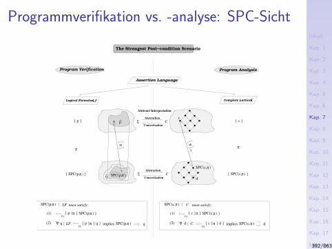
Inhalt
Kap. 1
Kap. 2
Kap. 3
Kap. 4
Kap. 5
Kap. 6
Kap. 7
Kap. 8
Kap. 9
Kap. 10
Kap. 11
Kap. 12
Kap. 13
Kap. 14
Kap. 15
Kap. 16
Kap. 17
Literatur
Anhang
A
Programmverifikation vs. -analyse: SPC-Sicht
π
SPC(p,π ) SPC(c,π )
Σ C
Abstraction
Concretization
Σ C
Abstraction
Concretization
Program Verification Program Analysis
p~
π )SPC(p,
A
SPC(p,π ) PV
p π(1)
A
π )SPC(p,
π )SPC(p, q
The Strongest Post−condition Scenario
π
π )SPC(c,
d
p
π
c
π
Abstract Interpretation
Logical Formulas Complete Lattices
τ
LF
(2) dPA
c π d
must satisfy:
implies
π )SPC(c, C
(1)PA
c π SPC(c,π )
C π )SPC(c, d.(2)PV
p π q
LF must satisfy:
impliesq LF.
Assertion Language
C
σ
q~
c
PA
392/863
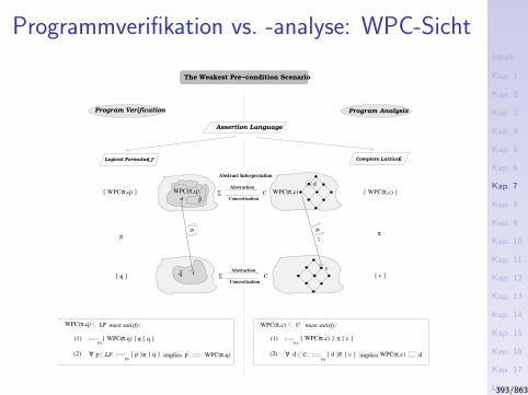
Inhalt
Kap. 1
Kap. 2
Kap. 3
Kap. 4
Kap. 5
Kap. 6
Kap. 7
Kap. 8
Kap. 9
Kap. 10
Kap. 11
Kap. 12
Kap. 13
Kap. 14
Kap. 15
Kap. 16
Kap. 17
Literatur
Anhang
A
Programmverifikation vs. -analyse: WPC-Sicht
π
Σ C
Abstraction
Concretization
Σ C
Abstraction
Concretization
Program Verification Program Analysis
AA
WPC(π,q)
WPC(π,q)
WPC(π,c)
WPC(π,c)
WPC(π,c)
WPC(π,c)
WPC(π,q)
π
q~
WPC(π,c)
πPA
p~WPC(π,q)
σ
ππ
Abstract Interpretation
Logical Formulas Complete LatticesLF
(2) dPA
d c
must satisfy:
implies
C
(1)PA
C .(2)PV
p π q
LF must satisfy:
impliesp LF.
Assertion Language
C
The Weakest Pre−condition Scenario
(1)PV
p
π q π c
π d
c q
WPC( ,q)
τ
d
c
393/863
Inhalt
Kap. 1
Kap. 2
Kap. 3
Kap. 4
Kap. 5
Kap. 6
Kap. 7
Kap. 8
8.1
8.2
8.3
8.4
8.5
8.6
8.7
8.8
Kap. 9
Kap. 10
Kap. 11
Kap. 12
Kap. 13
Kap. 14
Kap. 15
Kap. 16
Kap. 17
Literatur
Anhang
A
Kapitel 8
Reverse Datenflussanalyse
394/863

Inhalt
Kap. 1
Kap. 2
Kap. 3
Kap. 4
Kap. 5
Kap. 6
Kap. 7
Kap. 8
8.1
8.2
8.3
8.4
8.5
8.6
8.7
8.8
Kap. 9
Kap. 10
Kap. 11
Kap. 12
Kap. 13
Kap. 14
Kap. 15
Kap. 16
Kap. 17
Literatur
Anhang
A
Kapitel 8.1
Grundlagen
395/863
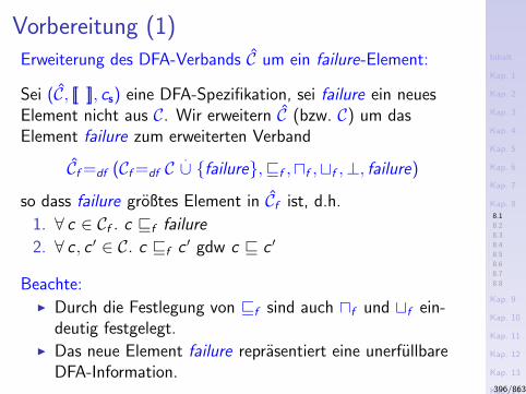
Inhalt
Kap. 1
Kap. 2
Kap. 3
Kap. 4
Kap. 5
Kap. 6
Kap. 7
Kap. 8
8.1
8.2
8.3
8.4
8.5
8.6
8.7
8.8
Kap. 9
Kap. 10
Kap. 11
Kap. 12
Kap. 13
Kap. 14
Kap. 15
Kap. 16
Kap. 17
Literatur
Anhang
A
Vorbereitung (1)Erweiterung des DFA-Verbands C um ein failure-Element:
Sei (C, [[ ]], cs) eine DFA-Spezifikation, sei failure ein neuesElement nicht aus C. Wir erweitern C (bzw. C) um dasElement failure zum erweiterten Verband
Cf =df (Cf =df C.∪ failure,vf ,uf ,tf ,⊥, failure)
so dass failure großtes Element in Cf ist, d.h.
1. ∀ c ∈ Cf . c vf failure
2. ∀ c , c ′ ∈ C. c vf c ′ gdw c v c ′
Beachte:I Durch die Festlegung von vf sind auch uf und tf ein-
deutig festgelegt.I Das neue Element failure reprasentiert eine unerfullbare
DFA-Information.396/863
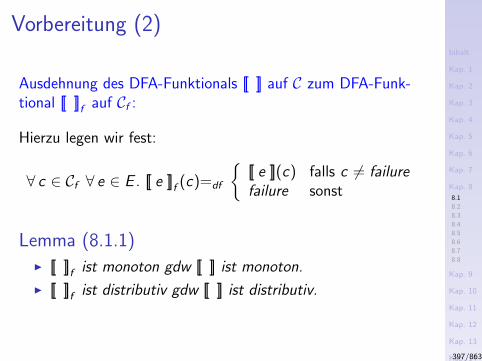
Inhalt
Kap. 1
Kap. 2
Kap. 3
Kap. 4
Kap. 5
Kap. 6
Kap. 7
Kap. 8
8.1
8.2
8.3
8.4
8.5
8.6
8.7
8.8
Kap. 9
Kap. 10
Kap. 11
Kap. 12
Kap. 13
Kap. 14
Kap. 15
Kap. 16
Kap. 17
Literatur
Anhang
A
Vorbereitung (2)
Ausdehnung des DFA-Funktionals [[ ]] auf C zum DFA-Funk-tional [[ ]]f auf Cf :
Hierzu legen wir fest:
∀ c ∈ Cf ∀ e ∈ E . [[ e ]]f (c)=df
[[ e ]](c) falls c 6= failurefailure sonst
Lemma (8.1.1)I [[ ]]f ist monoton gdw [[ ]] ist monoton.
I [[ ]]f ist distributiv gdw [[ ]] ist distributiv.
397/863
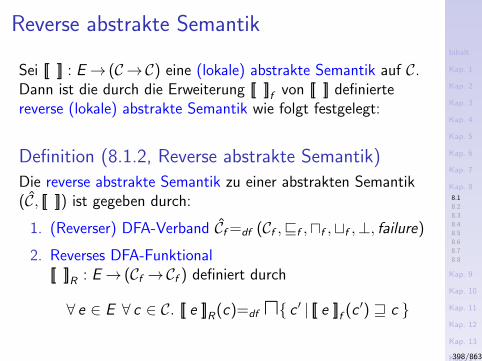
Inhalt
Kap. 1
Kap. 2
Kap. 3
Kap. 4
Kap. 5
Kap. 6
Kap. 7
Kap. 8
8.1
8.2
8.3
8.4
8.5
8.6
8.7
8.8
Kap. 9
Kap. 10
Kap. 11
Kap. 12
Kap. 13
Kap. 14
Kap. 15
Kap. 16
Kap. 17
Literatur
Anhang
A
Reverse abstrakte Semantik
Sei [[ ]] : E→ (C→C) eine (lokale) abstrakte Semantik auf C.Dann ist die durch die Erweiterung [[ ]]f von [[ ]] definiertereverse (lokale) abstrakte Semantik wie folgt festgelegt:
Definition (8.1.2, Reverse abstrakte Semantik)
Die reverse abstrakte Semantik zu einer abstrakten Semantik(C, [[ ]]) ist gegeben durch:
1. (Reverser) DFA-Verband Cf =df (Cf ,vf ,uf ,tf ,⊥, failure)
2. Reverses DFA-Funktional[[ ]]R : E→ (Cf →Cf ) definiert durch
∀ e ∈ E ∀ c ∈ C. [[ e ]]R(c)=df u c ′ | [[ e ]]f (c ′) w c
398/863
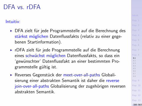
Inhalt
Kap. 1
Kap. 2
Kap. 3
Kap. 4
Kap. 5
Kap. 6
Kap. 7
Kap. 8
8.1
8.2
8.3
8.4
8.5
8.6
8.7
8.8
Kap. 9
Kap. 10
Kap. 11
Kap. 12
Kap. 13
Kap. 14
Kap. 15
Kap. 16
Kap. 17
Literatur
Anhang
A
DFA vs. rDFA
Intuitiv:
I DFA zielt fur jede Programmstelle auf die Berechnung desstarkst moglichen Datenflussfakts (relativ zu einer gege-benen Startinformation).
I rDFA zielt fur jede Programmstelle auf die Berechnungeines schwachst moglichen Datenflussfakts, so dass ein‘gewunschter’ Datenflussfakt an einer bestimmten Pro-grammstelle gultig ist.
I Reverses Gegenstuck der meet-over-all-paths Globali-sierung einer abstrakten Semantik ist daher die reversejoin-over-all-paths Globalisierung der zugehorigen reversenabstrakten Semantik.
399/863
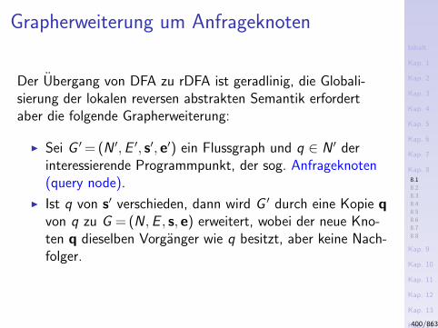
Inhalt
Kap. 1
Kap. 2
Kap. 3
Kap. 4
Kap. 5
Kap. 6
Kap. 7
Kap. 8
8.1
8.2
8.3
8.4
8.5
8.6
8.7
8.8
Kap. 9
Kap. 10
Kap. 11
Kap. 12
Kap. 13
Kap. 14
Kap. 15
Kap. 16
Kap. 17
Literatur
Anhang
A
Grapherweiterung um Anfrageknoten
Der Ubergang von DFA zu rDFA ist geradlinig, die Globali-sierung der lokalen reversen abstrakten Semantik erfordertaber die folgende Grapherweiterung:
I Sei G ′= (N ′,E ′, s′, e′) ein Flussgraph und q ∈ N ′ derinteressierende Programmpunkt, der sog. Anfrageknoten(query node).
I Ist q von s′ verschieden, dann wird G ′ durch eine Kopie qvon q zu G = (N ,E , s, e) erweitert, wobei der neue Kno-ten q dieselben Vorganger wie q besitzt, aber keine Nach-folger.
400/863
Inhalt
Kap. 1
Kap. 2
Kap. 3
Kap. 4
Kap. 5
Kap. 6
Kap. 7
Kap. 8
8.1
8.2
8.3
8.4
8.5
8.6
8.7
8.8
Kap. 9
Kap. 10
Kap. 11
Kap. 12
Kap. 13
Kap. 14
Kap. 15
Kap. 16
Kap. 17
Literatur
Anhang
A
Beobachtung
Es gilt:
I Die Hinzunahme von q hat keinen Einfluss auf die MOP-Losung irgendeines der ursprunglichen Knoten von G .
I Die MOP-Losungen von q und q stimmen uberein.
Die folgenden drei Lemmata fassen diese Beobachtungenzusammen und formalisieren sie.
401/863
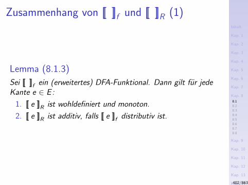
Inhalt
Kap. 1
Kap. 2
Kap. 3
Kap. 4
Kap. 5
Kap. 6
Kap. 7
Kap. 8
8.1
8.2
8.3
8.4
8.5
8.6
8.7
8.8
Kap. 9
Kap. 10
Kap. 11
Kap. 12
Kap. 13
Kap. 14
Kap. 15
Kap. 16
Kap. 17
Literatur
Anhang
A
Zusammenhang von [[ ]]f und [[ ]]R (1)
Lemma (8.1.3)
Sei [[ ]]f ein (erweitertes) DFA-Funktional. Dann gilt fur jedeKante e ∈ E :
1. [[ e ]]R ist wohldefiniert und monoton.
2. [[ e ]]R ist additiv, falls [[ e ]]f distributiv ist.
402/863
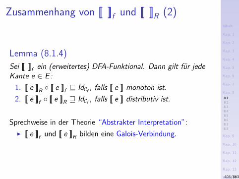
Inhalt
Kap. 1
Kap. 2
Kap. 3
Kap. 4
Kap. 5
Kap. 6
Kap. 7
Kap. 8
8.1
8.2
8.3
8.4
8.5
8.6
8.7
8.8
Kap. 9
Kap. 10
Kap. 11
Kap. 12
Kap. 13
Kap. 14
Kap. 15
Kap. 16
Kap. 17
Literatur
Anhang
A
Zusammenhang von [[ ]]f und [[ ]]R (2)
Lemma (8.1.4)
Sei [[ ]]f ein (erweitertes) DFA-Funktional. Dann gilt fur jedeKante e ∈ E :
1. [[ e ]]R [[ e ]]f v IdCf , falls [[ e ]] monoton ist.
2. [[ e ]]f [[ e ]]R w IdCf , falls [[ e ]] distributiv ist.
Sprechweise in der Theorie “Abstrakter Interpretation”:
I [[ e ]]f und [[ e ]]R bilden eine Galois-Verbindung.
403/863
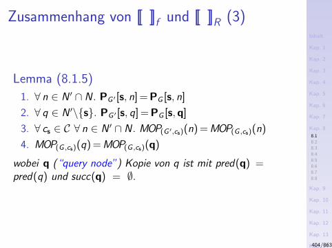
Inhalt
Kap. 1
Kap. 2
Kap. 3
Kap. 4
Kap. 5
Kap. 6
Kap. 7
Kap. 8
8.1
8.2
8.3
8.4
8.5
8.6
8.7
8.8
Kap. 9
Kap. 10
Kap. 11
Kap. 12
Kap. 13
Kap. 14
Kap. 15
Kap. 16
Kap. 17
Literatur
Anhang
A
Zusammenhang von [[ ]]f und [[ ]]R (3)
Lemma (8.1.5)
1. ∀ n ∈ N ′ ∩ N . PG ′[s, n] = PG [s, n]
2. ∀ q ∈ N ′\s. PG ′[s, q] = PG [s,q]
3. ∀ cs ∈ C ∀ n ∈ N ′ ∩ N . MOP(G ′,cs)(n) = MOP(G ,cs)(n)
4. MOP(G ,cs)(q) = MOP(G ,cs)(q)
wobei q (“query node”) Kopie von q ist mit pred(q) =pred(q) und succ(q) = ∅.
404/863
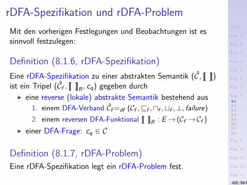
Inhalt
Kap. 1
Kap. 2
Kap. 3
Kap. 4
Kap. 5
Kap. 6
Kap. 7
Kap. 8
8.1
8.2
8.3
8.4
8.5
8.6
8.7
8.8
Kap. 9
Kap. 10
Kap. 11
Kap. 12
Kap. 13
Kap. 14
Kap. 15
Kap. 16
Kap. 17
Literatur
Anhang
A
rDFA-Spezifikation und rDFA-Problem
Mit den vorherigen Festlegungen und Beobachtungen ist essinnvoll festzulegen:
Definition (8.1.6, rDFA-Spezifikation)
Eine rDFA-Spezifikation zu einer abstrakten Semantik (C, [[ ]])ist ein Tripel (Cf , [[ ]]R , cq) gegeben durch
I eine reverse (lokale) abstrakte Semantik bestehend aus
1. einem DFA-Verband Cf =df (Cf ,vf ,uf ,tf ,⊥, failure)
2. einem reversen DFA-Funktional [[ ]]R : E→ (Cf →Cf )
I einer DFA-Frage: cq ∈ C
Definition (8.1.7, rDFA-Problem)
Eine rDFA-Spezifikation legt ein rDFA-Problem fest.
405/863
Inhalt
Kap. 1
Kap. 2
Kap. 3
Kap. 4
Kap. 5
Kap. 6
Kap. 7
Kap. 8
8.1
8.2
8.3
8.4
8.5
8.6
8.7
8.8
Kap. 9
Kap. 10
Kap. 11
Kap. 12
Kap. 13
Kap. 14
Kap. 15
Kap. 16
Kap. 17
Literatur
Anhang
A
Kapitel 8.2
rJOP-Ansatz
406/863
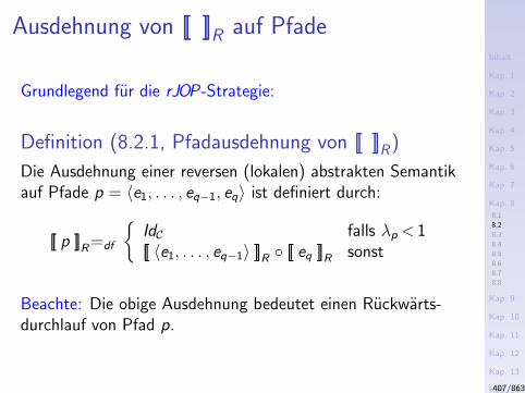
Inhalt
Kap. 1
Kap. 2
Kap. 3
Kap. 4
Kap. 5
Kap. 6
Kap. 7
Kap. 8
8.1
8.2
8.3
8.4
8.5
8.6
8.7
8.8
Kap. 9
Kap. 10
Kap. 11
Kap. 12
Kap. 13
Kap. 14
Kap. 15
Kap. 16
Kap. 17
Literatur
Anhang
A
Ausdehnung von [[ ]]R auf Pfade
Grundlegend fur die rJOP-Strategie:
Definition (8.2.1, Pfadausdehnung von [[ ]]R)
Die Ausdehnung einer reversen (lokalen) abstrakten Semantikauf Pfade p = 〈e1, . . . , eq−1, eq〉 ist definiert durch:
[[ p ]]R=df
IdC falls λp < 1[[ 〈e1, . . . , eq−1〉 ]]R [[ eq ]]R sonst
Beachte: Die obige Ausdehnung bedeutet einen Ruckwarts-durchlauf von Pfad p.
407/863

Inhalt
Kap. 1
Kap. 2
Kap. 3
Kap. 4
Kap. 5
Kap. 6
Kap. 7
Kap. 8
8.1
8.2
8.3
8.4
8.5
8.6
8.7
8.8
Kap. 9
Kap. 10
Kap. 11
Kap. 12
Kap. 13
Kap. 14
Kap. 15
Kap. 16
Kap. 17
Literatur
Anhang
A
Der rJOP-Ansatz
Definition (8.3.2, rJOP-Losung)
Sei (Cf , [[ ]]R , cq) die Spezifikation eines rDFA-Problems. Dannist fur alle Knoten n ∈ N die rJOP-Losung definiert durch:
rJOP(Cf ,[[ ]]R ,cq)(n)=df t [[ p ]]R(cq) | p ∈ P[n,q]
408/863
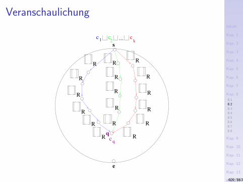
Inhalt
Kap. 1
Kap. 2
Kap. 3
Kap. 4
Kap. 5
Kap. 6
Kap. 7
Kap. 8
8.1
8.2
8.3
8.4
8.5
8.6
8.7
8.8
Kap. 9
Kap. 10
Kap. 11
Kap. 12
Kap. 13
Kap. 14
Kap. 15
Kap. 16
Kap. 17
Literatur
Anhang
A
Veranschaulichung
c1
c2 k
c...
q
e
s
qc R
R
R
R
R
RR
R
R
R
R
R
R
R
R
R
R
409/863

Inhalt
Kap. 1
Kap. 2
Kap. 3
Kap. 4
Kap. 5
Kap. 6
Kap. 7
Kap. 8
8.1
8.2
8.3
8.4
8.5
8.6
8.7
8.8
Kap. 9
Kap. 10
Kap. 11
Kap. 12
Kap. 13
Kap. 14
Kap. 15
Kap. 16
Kap. 17
Literatur
Anhang
A
Kapitel 8.3
rMinFP-Ansatz
410/863
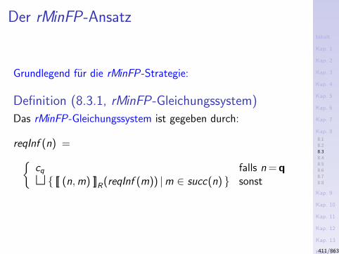
Inhalt
Kap. 1
Kap. 2
Kap. 3
Kap. 4
Kap. 5
Kap. 6
Kap. 7
Kap. 8
8.1
8.2
8.3
8.4
8.5
8.6
8.7
8.8
Kap. 9
Kap. 10
Kap. 11
Kap. 12
Kap. 13
Kap. 14
Kap. 15
Kap. 16
Kap. 17
Literatur
Anhang
A
Der rMinFP-Ansatz
Grundlegend fur die rMinFP-Strategie:
Definition (8.3.1, rMinFP-Gleichungssystem)
Das rMinFP-Gleichungssystem ist gegeben durch:
reqInf (n) =cq falls n = qt [[ (n,m) ]]R(reqInf (m)) |m ∈ succ(n) sonst
411/863
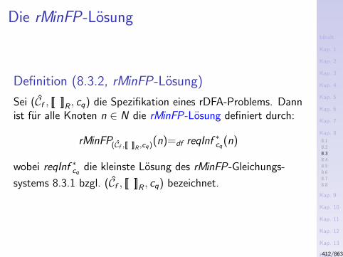
Inhalt
Kap. 1
Kap. 2
Kap. 3
Kap. 4
Kap. 5
Kap. 6
Kap. 7
Kap. 8
8.1
8.2
8.3
8.4
8.5
8.6
8.7
8.8
Kap. 9
Kap. 10
Kap. 11
Kap. 12
Kap. 13
Kap. 14
Kap. 15
Kap. 16
Kap. 17
Literatur
Anhang
A
Die rMinFP-Losung
Definition (8.3.2, rMinFP-Losung)
Sei (Cf , [[ ]]R , cq) die Spezifikation eines rDFA-Problems. Dannist fur alle Knoten n ∈ N die rMinFP-Losung definiert durch:
rMinFP(Cf ,[[ ]]R ,cq)(n)=df reqInf ∗cq(n)
wobei reqInf ∗cq die kleinste Losung des rMinFP-Gleichungs-
systems 8.3.1 bzgl. (Cf , [[ ]]R , cq) bezeichnet.
412/863

Inhalt
Kap. 1
Kap. 2
Kap. 3
Kap. 4
Kap. 5
Kap. 6
Kap. 7
Kap. 8
8.1
8.2
8.3
8.4
8.5
8.6
8.7
8.8
Kap. 9
Kap. 10
Kap. 11
Kap. 12
Kap. 13
Kap. 14
Kap. 15
Kap. 16
Kap. 17
Literatur
Anhang
A
Kapitel 8.4
Reverses Koinzidenz- und Sicherheitstheorem
413/863
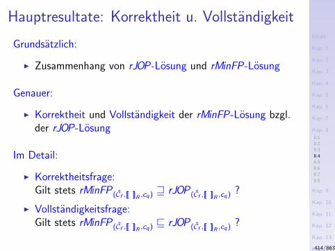
Inhalt
Kap. 1
Kap. 2
Kap. 3
Kap. 4
Kap. 5
Kap. 6
Kap. 7
Kap. 8
8.1
8.2
8.3
8.4
8.5
8.6
8.7
8.8
Kap. 9
Kap. 10
Kap. 11
Kap. 12
Kap. 13
Kap. 14
Kap. 15
Kap. 16
Kap. 17
Literatur
Anhang
A
Hauptresultate: Korrektheit u. Vollstandigkeit
Grundsatzlich:
I Zusammenhang von rJOP-Losung und rMinFP-Losung
Genauer:
I Korrektheit und Vollstandigkeit der rMinFP-Losung bzgl.der rJOP-Losung
Im Detail:
I Korrektheitsfrage:Gilt stets rMinFP (Cf ,[[ ]]R ,cq) w rJOP (Cf ,[[ ]]R ,cq) ?
I Vollstandigkeitsfrage:Gilt stets rMinFP (Cf ,[[ ]]R ,cq) v rJOP (Cf ,[[ ]]R ,cq) ?
414/863
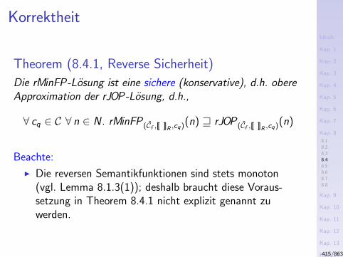
Inhalt
Kap. 1
Kap. 2
Kap. 3
Kap. 4
Kap. 5
Kap. 6
Kap. 7
Kap. 8
8.1
8.2
8.3
8.4
8.5
8.6
8.7
8.8
Kap. 9
Kap. 10
Kap. 11
Kap. 12
Kap. 13
Kap. 14
Kap. 15
Kap. 16
Kap. 17
Literatur
Anhang
A
Korrektheit
Theorem (8.4.1, Reverse Sicherheit)
Die rMinFP-Losung ist eine sichere (konservative), d.h. obereApproximation der rJOP-Losung, d.h.,
∀ cq ∈ C ∀ n ∈ N . rMinFP (Cf ,[[ ]]R ,cq)(n) w rJOP (Cf ,[[ ]]R ,cq)(n)
Beachte:
I Die reversen Semantikfunktionen sind stets monoton(vgl. Lemma 8.1.3(1)); deshalb braucht diese Voraus-setzung in Theorem 8.4.1 nicht explizit genannt zuwerden.
415/863
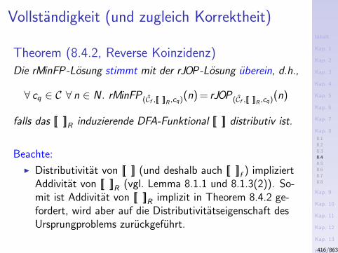
Inhalt
Kap. 1
Kap. 2
Kap. 3
Kap. 4
Kap. 5
Kap. 6
Kap. 7
Kap. 8
8.1
8.2
8.3
8.4
8.5
8.6
8.7
8.8
Kap. 9
Kap. 10
Kap. 11
Kap. 12
Kap. 13
Kap. 14
Kap. 15
Kap. 16
Kap. 17
Literatur
Anhang
A
Vollstandigkeit (und zugleich Korrektheit)
Theorem (8.4.2, Reverse Koinzidenz)
Die rMinFP-Losung stimmt mit der rJOP-Losung uberein, d.h.,
∀ cq ∈ C ∀ n ∈ N . rMinFP (Cf ,[[ ]]R ,cq)(n) = rJOP (Cf ,[[ ]]R ,cq)(n)
falls das [[ ]]R induzierende DFA-Funktional [[ ]] distributiv ist.
Beachte:
I Distributivitat von [[ ]] (und deshalb auch [[ ]]f ) impliziertAddivitat von [[ ]]R (vgl. Lemma 8.1.1 und 8.1.3(2)). So-mit ist Addivitat von [[ ]]R implizit in Theorem 8.4.2 ge-fordert, wird aber auf die Distributivitatseigenschaft desUrsprungproblems zuruckgefuhrt.
416/863

Inhalt
Kap. 1
Kap. 2
Kap. 3
Kap. 4
Kap. 5
Kap. 6
Kap. 7
Kap. 8
8.1
8.2
8.3
8.4
8.5
8.6
8.7
8.8
Kap. 9
Kap. 10
Kap. 11
Kap. 12
Kap. 13
Kap. 14
Kap. 15
Kap. 16
Kap. 17
Literatur
Anhang
A
Kapitel 8.5
Generischer Fixpunktalgorithmus undReverses Terminierungstheorem
417/863
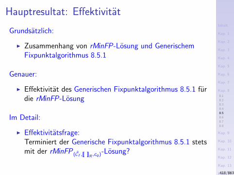
Inhalt
Kap. 1
Kap. 2
Kap. 3
Kap. 4
Kap. 5
Kap. 6
Kap. 7
Kap. 8
8.1
8.2
8.3
8.4
8.5
8.6
8.7
8.8
Kap. 9
Kap. 10
Kap. 11
Kap. 12
Kap. 13
Kap. 14
Kap. 15
Kap. 16
Kap. 17
Literatur
Anhang
A
Hauptresultat: Effektivitat
Grundsatzlich:
I Zusammenhang von rMinFP-Losung und GenerischemFixpunktalgorithmus 8.5.1
Genauer:
I Effektivitat des Generischen Fixpunktalgorithmus 8.5.1 furdie rMinFP-Losung
Im Detail:
I Effektivitatsfrage:Terminiert der Generische Fixpunktalgorithmus 8.5.1 stetsmit der rMinFP (Cf ,[[ ]]R ,cq)-Losung?
418/863
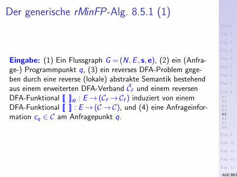
Inhalt
Kap. 1
Kap. 2
Kap. 3
Kap. 4
Kap. 5
Kap. 6
Kap. 7
Kap. 8
8.1
8.2
8.3
8.4
8.5
8.6
8.7
8.8
Kap. 9
Kap. 10
Kap. 11
Kap. 12
Kap. 13
Kap. 14
Kap. 15
Kap. 16
Kap. 17
Literatur
Anhang
A
Der generische rMinFP-Alg. 8.5.1 (1)
Eingabe: (1) Ein Flussgraph G = (N ,E , s, e), (2) ein (Anfra-ge-) Programmpunkt q, (3) ein reverses DFA-Problem gege-ben durch eine reverse (lokale) abstrakte Semantik bestehendaus einem erweiterten DFA-Verband Cf und einem reversenDFA-Funktional [[ ]]R : E→ (Cf →Cf ) induziert von einemDFA-Funktional [[ ]] : E→ (C→C), und (4) eine Anfrageinfor-mation cq ∈ C am Anfragepunkt q.
419/863
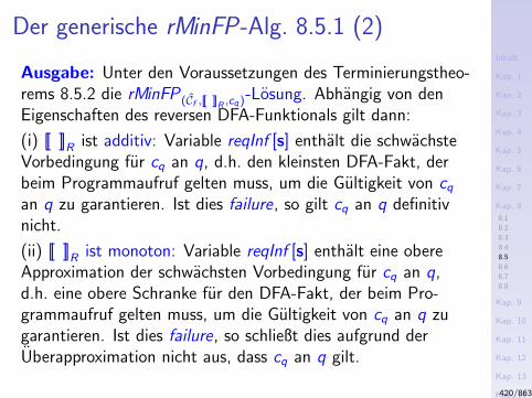
Inhalt
Kap. 1
Kap. 2
Kap. 3
Kap. 4
Kap. 5
Kap. 6
Kap. 7
Kap. 8
8.1
8.2
8.3
8.4
8.5
8.6
8.7
8.8
Kap. 9
Kap. 10
Kap. 11
Kap. 12
Kap. 13
Kap. 14
Kap. 15
Kap. 16
Kap. 17
Literatur
Anhang
A
Der generische rMinFP-Alg. 8.5.1 (2)
Ausgabe: Unter den Voraussetzungen des Terminierungstheo-rems 8.5.2 die rMinFP (Cf ,[[ ]]R ,cq)-Losung. Abhangig von denEigenschaften des reversen DFA-Funktionals gilt dann:
(i) [[ ]]R ist additiv: Variable reqInf [s] enthalt die schwachsteVorbedingung fur cq an q, d.h. den kleinsten DFA-Fakt, derbeim Programmaufruf gelten muss, um die Gultigkeit von cqan q zu garantieren. Ist dies failure, so gilt cq an q definitivnicht.
(ii) [[ ]]R ist monoton: Variable reqInf [s] enthalt eine obereApproximation der schwachsten Vorbedingung fur cq an q,d.h. eine obere Schranke fur den DFA-Fakt, der beim Pro-grammaufruf gelten muss, um die Gultigkeit von cq an q zugarantieren. Ist dies failure, so schließt dies aufgrund derUberapproximation nicht aus, dass cq an q gilt.
420/863
Inhalt
Kap. 1
Kap. 2
Kap. 3
Kap. 4
Kap. 5
Kap. 6
Kap. 7
Kap. 8
8.1
8.2
8.3
8.4
8.5
8.6
8.7
8.8
Kap. 9
Kap. 10
Kap. 11
Kap. 12
Kap. 13
Kap. 14
Kap. 15
Kap. 16
Kap. 17
Literatur
Anhang
A
Der generische rMinFP-Alg. 8.5.1 (3)
Bemerkung:
I Die schwachste Vorbedingung ist durch dierJOP (Cf ,[[ ]]R ,cq)-Losung gegeben.
I Die Variable workset steuert den iterativen Prozess. IhreElemente sind Knoten aus dem erweiterten FlussgraphenG ′, deren Annotation jungst aktualisiert worden ist, wasmoglicherweise zu einer verbandsmaßig großeren Annota-tion an ihren Vorgangerknoten fuhrt.
421/863
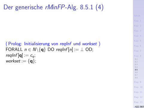
Inhalt
Kap. 1
Kap. 2
Kap. 3
Kap. 4
Kap. 5
Kap. 6
Kap. 7
Kap. 8
8.1
8.2
8.3
8.4
8.5
8.6
8.7
8.8
Kap. 9
Kap. 10
Kap. 11
Kap. 12
Kap. 13
Kap. 14
Kap. 15
Kap. 16
Kap. 17
Literatur
Anhang
A
Der generische rMinFP-Alg. 8.5.1 (4)
( Prolog: Initialisierung von reqInf und workset )FORALL n ∈ N\q DO reqInf [n] := ⊥ OD;reqInf [q] := cq;workset := q;
422/863
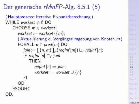
Inhalt
Kap. 1
Kap. 2
Kap. 3
Kap. 4
Kap. 5
Kap. 6
Kap. 7
Kap. 8
8.1
8.2
8.3
8.4
8.5
8.6
8.7
8.8
Kap. 9
Kap. 10
Kap. 11
Kap. 12
Kap. 13
Kap. 14
Kap. 15
Kap. 16
Kap. 17
Literatur
Anhang
A
Der generische rMinFP-Alg. 8.5.1 (5)
( Hauptprozess: Iterative Fixpunktberechnung )WHILE workset 6= ∅ DO
CHOOSE m ∈ workset;workset := workset\m;( Aktualisierung d. Vorgangerumgebung von Knoten m )FORALL n ∈ pred(m) DO
join := [[ (n,m) ]]R(reqInf [m]) tf reqInf [n];IF reqInf [n] @f join
THENreqInf [n] := join;workset := workset ∪ n
FIOD
ESOOHCOD.
423/863
Inhalt
Kap. 1
Kap. 2
Kap. 3
Kap. 4
Kap. 5
Kap. 6
Kap. 7
Kap. 8
8.1
8.2
8.3
8.4
8.5
8.6
8.7
8.8
Kap. 9
Kap. 10
Kap. 11
Kap. 12
Kap. 13
Kap. 14
Kap. 15
Kap. 16
Kap. 17
Literatur
Anhang
A
Effektivitat
Aufgrund der stets gegebenen Monotonie der reversen Seman-tikfunktionen (vgl. Lemma 8.1.2(1)) erhalten wir:
Theorem (8.5.2, Reverse Terminierung)
Der Generische Fixpunktalgorithmus 8.5.1 terminiert mit derrMinFP (Cf ,[[ ]]R ,cq)-Losung, falls der DFA-Verband C die aufstei-gende Kettenbedingung erfullt.
Beachte:
I Cf erfullt die aufsteigende Kettenbedingung gdw C dieaufsteigende Kettenbedingung erfullt. Wie bei Theorem8.4.2 wird hier die entscheidende Voraussetzung auf dieentsprechende Eigenschaft des Ursprungsproblems zuruck-gefuhrt.
424/863
Inhalt
Kap. 1
Kap. 2
Kap. 3
Kap. 4
Kap. 5
Kap. 6
Kap. 7
Kap. 8
8.1
8.2
8.3
8.4
8.5
8.6
8.7
8.8
Kap. 9
Kap. 10
Kap. 11
Kap. 12
Kap. 13
Kap. 14
Kap. 15
Kap. 16
Kap. 17
Literatur
Anhang
A
Kapitel 8.6
Analyse und Verifikation: Analogien undGemeinsamkeiten
425/863
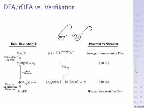
Inhalt
Kap. 1
Kap. 2
Kap. 3
Kap. 4
Kap. 5
Kap. 6
Kap. 7
Kap. 8
8.1
8.2
8.3
8.4
8.5
8.6
8.7
8.8
Kap. 9
Kap. 10
Kap. 11
Kap. 12
Kap. 13
Kap. 14
Kap. 15
Kap. 16
Kap. 17
Literatur
Anhang
A
DFA/rDFA vs. Verifikation
cscq
TheoremLink
?
?
π qp
s( ) cs
MaxFP
MOP
rMinFP
Coincidence
Theorem
Data−flow Analysis
(q)
C Cdistributive
Program Verification
π q
Weakest Precondition View
πp
Strongest Postcondition View
eR(c) =df (c ) c
DFA PV
e
ec |
induces
Coincidence
Theorem
ReverserJOP cq
426/863
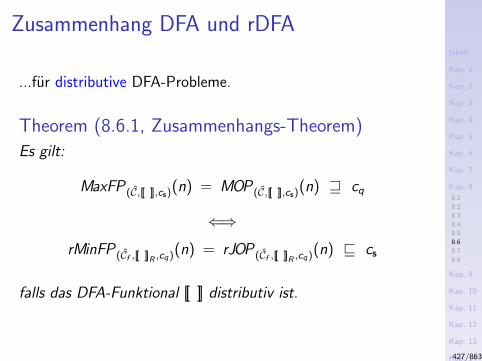
Inhalt
Kap. 1
Kap. 2
Kap. 3
Kap. 4
Kap. 5
Kap. 6
Kap. 7
Kap. 8
8.1
8.2
8.3
8.4
8.5
8.6
8.7
8.8
Kap. 9
Kap. 10
Kap. 11
Kap. 12
Kap. 13
Kap. 14
Kap. 15
Kap. 16
Kap. 17
Literatur
Anhang
A
Zusammenhang DFA und rDFA
...fur distributive DFA-Probleme.
Theorem (8.6.1, Zusammenhangs-Theorem)
Es gilt:
MaxFP (C,[[ ]],cs)(n) = MOP (C,[[ ]],cs)(n) w cq
⇐⇒
rMinFP (Cf ,[[ ]]R ,cq)(n) = rJOP (Cf ,[[ ]]R ,cq)(n) v cs
falls das DFA-Funktional [[ ]] distributiv ist.
427/863
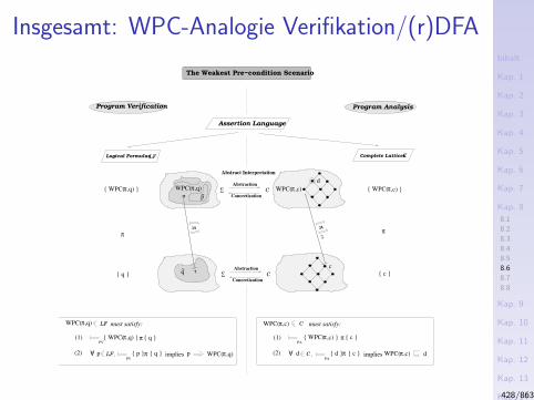
Inhalt
Kap. 1
Kap. 2
Kap. 3
Kap. 4
Kap. 5
Kap. 6
Kap. 7
Kap. 8
8.1
8.2
8.3
8.4
8.5
8.6
8.7
8.8
Kap. 9
Kap. 10
Kap. 11
Kap. 12
Kap. 13
Kap. 14
Kap. 15
Kap. 16
Kap. 17
Literatur
Anhang
A
Insgesamt: WPC-Analogie Verifikation/(r)DFA
π
Σ C
Abstraction
Concretization
Σ C
Abstraction
Concretization
Program Verification Program Analysis
AA
WPC(π,q)
WPC(π,q)
WPC(π,c)
WPC(π,c)
WPC(π,c)
WPC(π,c)
WPC(π,q)
π
q~
WPC(π,c)
πPA
p~WPC(π,q)
σ
ππ
Abstract Interpretation
Logical Formulas Complete LatticesLF
(2) dPA
d c
must satisfy:
implies
C
(1)PA
C .(2)PV
p π q
LF must satisfy:
impliesp LF.
Assertion Language
C
The Weakest Pre−condition Scenario
(1)PV
p
π q π c
π d
c q
WPC( ,q)
τ
d
c
428/863
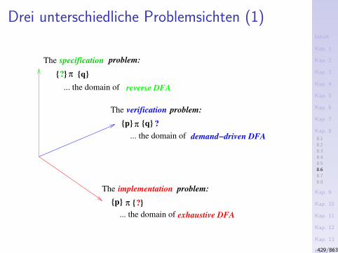
Inhalt
Kap. 1
Kap. 2
Kap. 3
Kap. 4
Kap. 5
Kap. 6
Kap. 7
Kap. 8
8.1
8.2
8.3
8.4
8.5
8.6
8.7
8.8
Kap. 9
Kap. 10
Kap. 11
Kap. 12
Kap. 13
Kap. 14
Kap. 15
Kap. 16
Kap. 17
Literatur
Anhang
A
Drei unterschiedliche Problemsichten (1)
?
... the domain of
... the domain of
The verification
The specification
implementationThe
pπ q ?
p π ?
demand−driven DFA
exhaustive DFA
problem:
problem:
problem:
qπ
... the domain of reverse DFA
429/863
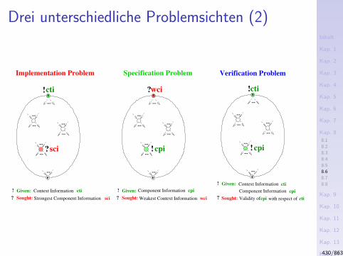
Inhalt
Kap. 1
Kap. 2
Kap. 3
Kap. 4
Kap. 5
Kap. 6
Kap. 7
Kap. 8
8.1
8.2
8.3
8.4
8.5
8.6
8.7
8.8
Kap. 9
Kap. 10
Kap. 11
Kap. 12
Kap. 13
Kap. 14
Kap. 15
Kap. 16
Kap. 17
Literatur
Anhang
A
Drei unterschiedliche Problemsichten (2)
...
sci?
...
! cpi
wci?
...
! cpi
cti!
Implementation Problem Specification Problem Verification Problem
Given:! Context Information
Sought:? Validity of with respect of
Given:
Sought:
...
...
...
...
...
...
...
s
e
!
?
cti!
Given:
Sought:
...
...
...
...
...
...
...
s
e
!
?
...
...
...
...
...
...
...
s
e
Context Information
Strongest Component Information Weakest Context Information
Component Information Component Information
cpi
cti
sci
cpi
wci
cti
cpi
cti
430/863
Inhalt
Kap. 1
Kap. 2
Kap. 3
Kap. 4
Kap. 5
Kap. 6
Kap. 7
Kap. 8
8.1
8.2
8.3
8.4
8.5
8.6
8.7
8.8
Kap. 9
Kap. 10
Kap. 11
Kap. 12
Kap. 13
Kap. 14
Kap. 15
Kap. 16
Kap. 17
Literatur
Anhang
A
Kapitel 8.7
Anwendungen reverser Datenflussanalyse
431/863
Inhalt
Kap. 1
Kap. 2
Kap. 3
Kap. 4
Kap. 5
Kap. 6
Kap. 7
Kap. 8
8.1
8.2
8.3
8.4
8.5
8.6
8.7
8.8
Kap. 9
Kap. 10
Kap. 11
Kap. 12
Kap. 13
Kap. 14
Kap. 15
Kap. 16
Kap. 17
Literatur
Anhang
A
Beispiele
Anwendungen reverser DFA
I Einfache Analysatoren und Optimierer
I “Hot Spot” Programmanalyse und -optimierung
I Debugger
I ...
Insbesondere
I Anforderungsgetriebene Datenflussanalyse(demand-driven data-flow analysis)
432/863
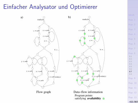
Inhalt
Kap. 1
Kap. 2
Kap. 3
Kap. 4
Kap. 5
Kap. 6
Kap. 7
Kap. 8
8.1
8.2
8.3
8.4
8.5
8.6
8.7
8.8
Kap. 9
Kap. 10
Kap. 11
Kap. 12
Kap. 13
Kap. 14
Kap. 15
Kap. 16
Kap. 17
Literatur
Anhang
A
Einfacher Analysator und Optimierer
Flow graph Data−flow information
x := a+b
x := a+b
y := a+b
c := a+b
a := ...
x := a+b
b := ...
z := a+b
z := a+b
Program pointssatisfying
read(a,b)
write(c)z := a+b
x := a+b x := a+b x := a+b
y := a+b
c := a+b
a := ...
x := a+b
x := a+b
z := a+b
b := ...
z := a+b
read(a,b)
write(c)
ex
z := a+bx
f
availability
a) b)
433/863
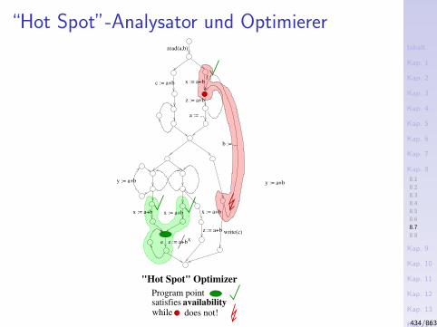
Inhalt
Kap. 1
Kap. 2
Kap. 3
Kap. 4
Kap. 5
Kap. 6
Kap. 7
Kap. 8
8.1
8.2
8.3
8.4
8.5
8.6
8.7
8.8
Kap. 9
Kap. 10
Kap. 11
Kap. 12
Kap. 13
Kap. 14
Kap. 15
Kap. 16
Kap. 17
Literatur
Anhang
A
“Hot Spot”-Analysator und Optimiererread(a,b)
y := a+b
x := a+b
x := a+b
y := a+b
c := a+b
a := ...
x := a+b
b := ...
z := a+b
Program pointsatisfies ,
does not!while
"Hot Spot" Optimizer
z := a+bx
write(c)z := a+b
x := a+b
e
availability
f
434/863
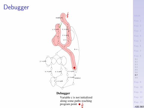
Inhalt
Kap. 1
Kap. 2
Kap. 3
Kap. 4
Kap. 5
Kap. 6
Kap. 7
Kap. 8
8.1
8.2
8.3
8.4
8.5
8.6
8.7
8.8
Kap. 9
Kap. 10
Kap. 11
Kap. 12
Kap. 13
Kap. 14
Kap. 15
Kap. 16
Kap. 17
Literatur
Anhang
A
Debugger
read(a,b)
x := a+b
y := a+b
c := a+b
a := ...
x := a+b
z := a+b
b := ...
z := a+b
x := a+b
Debugger
write(c)
Variable c is not initialized
program point
z := a+b
x := a+b
along some paths reaching
e
g
f
435/863
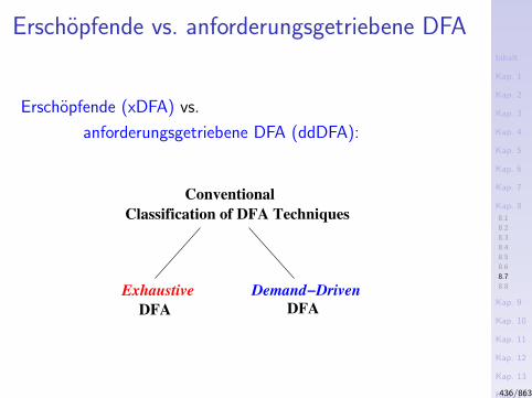
Inhalt
Kap. 1
Kap. 2
Kap. 3
Kap. 4
Kap. 5
Kap. 6
Kap. 7
Kap. 8
8.1
8.2
8.3
8.4
8.5
8.6
8.7
8.8
Kap. 9
Kap. 10
Kap. 11
Kap. 12
Kap. 13
Kap. 14
Kap. 15
Kap. 16
Kap. 17
Literatur
Anhang
A
Erschopfende vs. anforderungsgetriebene DFA
Erschopfende (xDFA) vs.
anforderungsgetriebene DFA (ddDFA):
Exhaustive Demand−Driven
DFA DFA
Classification of DFA Techniques
Conventional
436/863
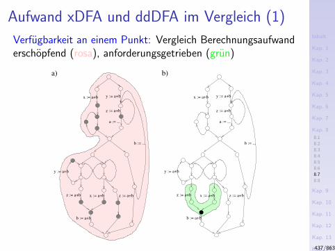
Inhalt
Kap. 1
Kap. 2
Kap. 3
Kap. 4
Kap. 5
Kap. 6
Kap. 7
Kap. 8
8.1
8.2
8.3
8.4
8.5
8.6
8.7
8.8
Kap. 9
Kap. 10
Kap. 11
Kap. 12
Kap. 13
Kap. 14
Kap. 15
Kap. 16
Kap. 17
Literatur
Anhang
A
Aufwand xDFA und ddDFA im Vergleich (1)
Verfugbarkeit an einem Punkt: Vergleich Berechnungsaufwanderschopfend (rosa), anforderungsgetrieben (grun)
y := a+b
b := a+b
x := a+b z := a+b
a)
y := a+b
x := a+b
a := ...
z := a+b
b := ...
z := a+b
y := a+b
b := a+b
x := a+b z := a+b
b)
y := a+b
x := a+b
a := ...
z := a+b
b := ...
z := a+b
437/863
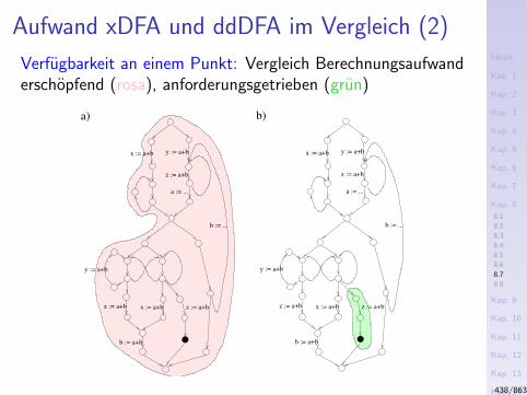
Inhalt
Kap. 1
Kap. 2
Kap. 3
Kap. 4
Kap. 5
Kap. 6
Kap. 7
Kap. 8
8.1
8.2
8.3
8.4
8.5
8.6
8.7
8.8
Kap. 9
Kap. 10
Kap. 11
Kap. 12
Kap. 13
Kap. 14
Kap. 15
Kap. 16
Kap. 17
Literatur
Anhang
A
Aufwand xDFA und ddDFA im Vergleich (2)
Verfugbarkeit an einem Punkt: Vergleich Berechnungsaufwanderschopfend (rosa), anforderungsgetrieben (grun)
y := a+b
b := a+b
x := a+b z := a+b
a)
y := a+b
x := a+b
a := ...
z := a+b
b := ...
z := a+b
y := a+b
b := a+b
x := a+b z := a+b
b)
y := a+b
x := a+b
a := ...
z := a+b
b := ...
z := a+b
438/863
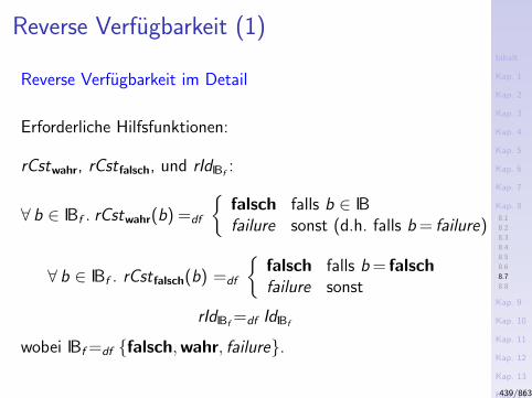
Inhalt
Kap. 1
Kap. 2
Kap. 3
Kap. 4
Kap. 5
Kap. 6
Kap. 7
Kap. 8
8.1
8.2
8.3
8.4
8.5
8.6
8.7
8.8
Kap. 9
Kap. 10
Kap. 11
Kap. 12
Kap. 13
Kap. 14
Kap. 15
Kap. 16
Kap. 17
Literatur
Anhang
A
Reverse Verfugbarkeit (1)
Reverse Verfugbarkeit im Detail
Erforderliche Hilfsfunktionen:
rCstwahr, rCst falsch, und rIdIBf:
∀ b ∈ IBf . rCstwahr(b) =df
falsch falls b ∈ IBfailure sonst (d.h. falls b = failure)
∀ b ∈ IBf . rCst falsch(b) =df
falsch falls b = falschfailure sonst
rIdIBf=df IdIBf
wobei IBf =df falsch,wahr, failure.
439/863
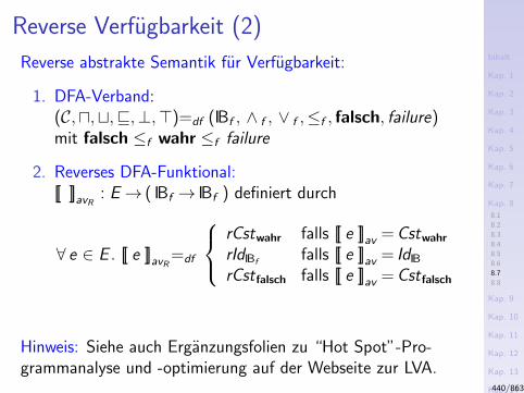
Inhalt
Kap. 1
Kap. 2
Kap. 3
Kap. 4
Kap. 5
Kap. 6
Kap. 7
Kap. 8
8.1
8.2
8.3
8.4
8.5
8.6
8.7
8.8
Kap. 9
Kap. 10
Kap. 11
Kap. 12
Kap. 13
Kap. 14
Kap. 15
Kap. 16
Kap. 17
Literatur
Anhang
A
Reverse Verfugbarkeit (2)
Reverse abstrakte Semantik fur Verfugbarkeit:
1. DFA-Verband:(C,u,t,v,⊥,>)=df (IBf , ∧ f , ∨ f ,≤f , falsch, failure)mit falsch ≤f wahr ≤f failure
2. Reverses DFA-Funktional:[[ ]]avR : E→ ( IBf → IBf ) definiert durch
∀ e ∈ E . [[ e ]]avR =df
rCstwahr falls [[ e ]]av = Cstwahr
rIdIBffalls [[ e ]]av = IdIB
rCst falsch falls [[ e ]]av = Cst falsch
Hinweis: Siehe auch Erganzungsfolien zu “Hot Spot”-Pro-grammanalyse und -optimierung auf der Webseite zur LVA.
440/863

Inhalt
Kap. 1
Kap. 2
Kap. 3
Kap. 4
Kap. 5
Kap. 6
Kap. 7
Kap. 8
8.1
8.2
8.3
8.4
8.5
8.6
8.7
8.8
Kap. 9
Kap. 10
Kap. 11
Kap. 12
Kap. 13
Kap. 14
Kap. 15
Kap. 16
Kap. 17
Literatur
Anhang
A
Kapitel 8.8
Zusammenfassung
441/863
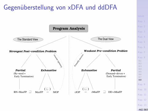
Inhalt
Kap. 1
Kap. 2
Kap. 3
Kap. 4
Kap. 5
Kap. 6
Kap. 7
Kap. 8
8.1
8.2
8.3
8.4
8.5
8.6
8.7
8.8
Kap. 9
Kap. 10
Kap. 11
Kap. 12
Kap. 13
Kap. 14
Kap. 15
Kap. 16
Kap. 17
Literatur
Anhang
A
Gegenuberstellung von xDFA und ddDFA
( ) ( )
For
mal
ly a
nsw
ers
For
mal
ly a
nsw
ers
Weakest Pre−condition Problem
(Demand−driven +
Early Termination) Early Termination)(By−need +
BN−MaxFP rMinFP DD−rMinFPMOPMaxFP
Exhaustive ExhaustivePartial Partial
The Standard View The Dual View
Strongest Post−condition Problem
rJOP
Program Analysis
442/863
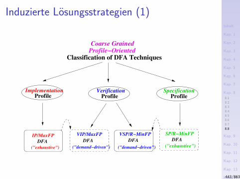
Inhalt
Kap. 1
Kap. 2
Kap. 3
Kap. 4
Kap. 5
Kap. 6
Kap. 7
Kap. 8
8.1
8.2
8.3
8.4
8.5
8.6
8.7
8.8
Kap. 9
Kap. 10
Kap. 11
Kap. 12
Kap. 13
Kap. 14
Kap. 15
Kap. 16
Kap. 17
Literatur
Anhang
A
Induzierte Losungsstrategien (1)
IP/MaxFP
("exhaustive")
DFA DFA
VIP/MaxFP
("demand−driven")
Implementation Verification SpecificationProfileProfile Profile
Classification of DFA TechniquesProfile−OrientedCoarse Grained
DFA
("demand−driven")
DFA
("exhaustive")
VSP/R−MinFP SP/R−MinFP
443/863
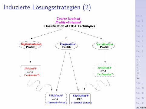
Inhalt
Kap. 1
Kap. 2
Kap. 3
Kap. 4
Kap. 5
Kap. 6
Kap. 7
Kap. 8
8.1
8.2
8.3
8.4
8.5
8.6
8.7
8.8
Kap. 9
Kap. 10
Kap. 11
Kap. 12
Kap. 13
Kap. 14
Kap. 15
Kap. 16
Kap. 17
Literatur
Anhang
A
Induzierte Losungsstrategien (2)
IP/MaxFP
("exhaustive")
DFA DFA
SP/RMinFP
("exhaustive")
DFA
VSP/RMinFP
("demand−driven")
DFA
VIP/MaxFP
("demand−driven")
Implementation Verification SpecificationProfileProfile Profile
Classification of DFA TechniquesProfile−OrientedCoarse Grained
444/863
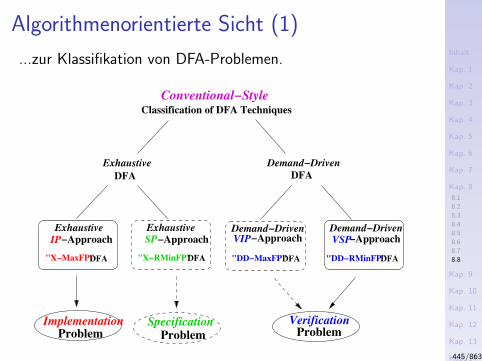
Inhalt
Kap. 1
Kap. 2
Kap. 3
Kap. 4
Kap. 5
Kap. 6
Kap. 7
Kap. 8
8.1
8.2
8.3
8.4
8.5
8.6
8.7
8.8
Kap. 9
Kap. 10
Kap. 11
Kap. 12
Kap. 13
Kap. 14
Kap. 15
Kap. 16
Kap. 17
Literatur
Anhang
A
Algorithmenorientierte Sicht (1)
...zur Klassifikation von DFA-Problemen.
ImplementationProblem
DFA
Demand−Driven
DFA
Demand−DrivenExhaustive
"DD−MaxFP""X−RMinFP""X−MaxFP"
Demand−DrivenExhaustive
Exhaustive
SpecificationProblem
VerificationProblem
"DD−RMinFP"DFA DFA DFA DFA
Classification of DFA Techniques
−ApproachIP −ApproachSP −ApproachVIP VSP−Approach
Conventional−Style
445/863
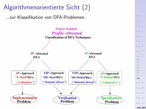
Inhalt
Kap. 1
Kap. 2
Kap. 3
Kap. 4
Kap. 5
Kap. 6
Kap. 7
Kap. 8
8.1
8.2
8.3
8.4
8.5
8.6
8.7
8.8
Kap. 9
Kap. 10
Kap. 11
Kap. 12
Kap. 13
Kap. 14
Kap. 15
Kap. 16
Kap. 17
Literatur
Anhang
A
Algorithmenorientierte Sicht (2)
...zur Klassifikation von DFA-Problemen.
"X−MaxFP" "DD−MaxFP" "X−RMinFP"
("demand−driven") ("exhaustive")("exhaustive") ("demand−driven")
VIP VSP SP
DFA DFA DFA"DD−RMinFP"DFA
ImplementationProblem
VerificationProblem
SpecificationProblem
Classification of DFA Techniques
DFA DFA
Profile−OrientedCoarse Grained
IP−Approach −Approach −Approach −Approach
IP SP−Oriented −Oriented
446/863
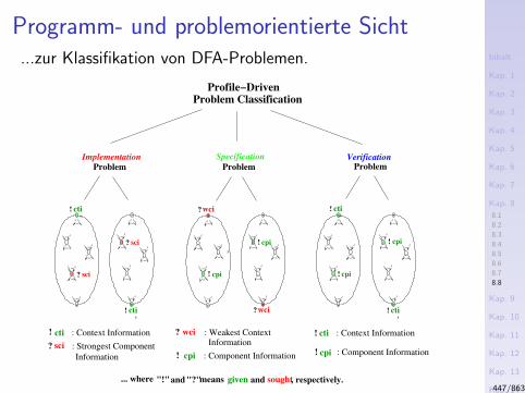
Inhalt
Kap. 1
Kap. 2
Kap. 3
Kap. 4
Kap. 5
Kap. 6
Kap. 7
Kap. 8
8.1
8.2
8.3
8.4
8.5
8.6
8.7
8.8
Kap. 9
Kap. 10
Kap. 11
Kap. 12
Kap. 13
Kap. 14
Kap. 15
Kap. 16
Kap. 17
Literatur
Anhang
A
Programm- und problemorientierte Sicht...zur Klassifikation von DFA-Problemen.
... ...
...
...
...
...
...
... ...
...
...
... ...
...
...
...
...
...
ImplementationProblem
Specification
Problem ProblemVerification
sci : Strongest Component
Information
: Weakest Contextwci
Information
cpi : Component Information
e
s
e
...
...
...
...
...
...
...
...
...
s
e
s
e
...
...
...
...
...
...
...
...
...
...
...
s
?
e
s
e
...
...
...
...
...
...
...
...
...
!
?
?
!
!
!
!
!
!
! cpi
cpi
cpi
cpi
: Context Informationcti
s
cti!
s
cti!
wci?
wci?
cpi : Component Information
cti
s
cti!
s
cti!
means given and sought, respectively.
sci?
sci?
...
... where "!"and "?"
: Context Information
Profile−DrivenProblem Classification
447/863
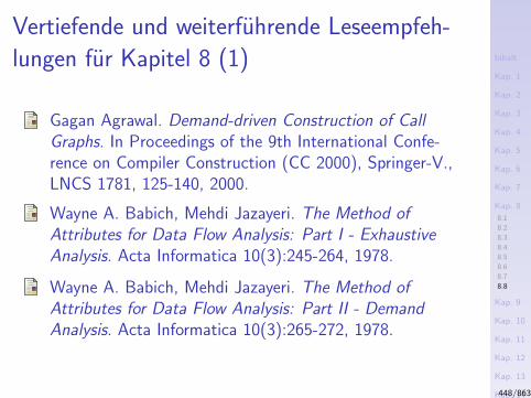
Inhalt
Kap. 1
Kap. 2
Kap. 3
Kap. 4
Kap. 5
Kap. 6
Kap. 7
Kap. 8
8.1
8.2
8.3
8.4
8.5
8.6
8.7
8.8
Kap. 9
Kap. 10
Kap. 11
Kap. 12
Kap. 13
Kap. 14
Kap. 15
Kap. 16
Kap. 17
Literatur
Anhang
A
Vertiefende und weiterfuhrende Leseempfeh-
lungen fur Kapitel 8 (1)
Gagan Agrawal. Demand-driven Construction of CallGraphs. In Proceedings of the 9th International Confe-rence on Compiler Construction (CC 2000), Springer-V.,LNCS 1781, 125-140, 2000.
Wayne A. Babich, Mehdi Jazayeri. The Method ofAttributes for Data Flow Analysis: Part I - ExhaustiveAnalysis. Acta Informatica 10(3):245-264, 1978.
Wayne A. Babich, Mehdi Jazayeri. The Method ofAttributes for Data Flow Analysis: Part II - DemandAnalysis. Acta Informatica 10(3):265-272, 1978.
448/863
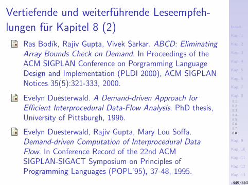
Inhalt
Kap. 1
Kap. 2
Kap. 3
Kap. 4
Kap. 5
Kap. 6
Kap. 7
Kap. 8
8.1
8.2
8.3
8.4
8.5
8.6
8.7
8.8
Kap. 9
Kap. 10
Kap. 11
Kap. 12
Kap. 13
Kap. 14
Kap. 15
Kap. 16
Kap. 17
Literatur
Anhang
A
Vertiefende und weiterfuhrende Leseempfeh-
lungen fur Kapitel 8 (2)
Ras Bodık, Rajiv Gupta, Vivek Sarkar. ABCD: EliminatingArray Bounds Check on Demand. In Proceedings of theACM SIGPLAN Conference on Porgramming LanguageDesign and Implementation (PLDI 2000), ACM SIGPLANNotices 35(5):321-333, 2000.
Evelyn Duesterwald. A Demand-driven Approach forEfficient Interprocedural Data-Flow Analysis. PhD thesis,University of Pittsburgh, 1996.
Evelyn Duesterwald, Rajiv Gupta, Mary Lou Soffa.Demand-driven Computation of Interprocedural DataFlow. In Conference Record of the 22nd ACMSIGPLAN-SIGACT Symposium on Principles ofProgramming Languages (POPL’95), 37-48, 1995.
449/863
Inhalt
Kap. 1
Kap. 2
Kap. 3
Kap. 4
Kap. 5
Kap. 6
Kap. 7
Kap. 8
8.1
8.2
8.3
8.4
8.5
8.6
8.7
8.8
Kap. 9
Kap. 10
Kap. 11
Kap. 12
Kap. 13
Kap. 14
Kap. 15
Kap. 16
Kap. 17
Literatur
Anhang
A
Vertiefende und weiterfuhrende Leseempfeh-
lungen fur Kapitel 8 (3)
Evelyn Duesterwald, Rajiv Gupta, Mary Lou Soffa. ADemand-driven Analyzer for Data Flow Testing at theIntegration Level. In Proceedings of the IEEE Conferenceon Software Engineering (CoSE’96), 575-586, 1996.
Evelyn Duesterwald, Rajiv Gupta, Mary Lou Soffa. APractical Framework for Demand-driven InterproceduralData Flow Analysis. ACM Transactions on ProgrammingLanguages and Systems (TOPLAS) 19(6):992-1030, 1997.
Susan Horwitz, Thomas Reps, Mooly Sagiv. DemandInterprocedural Data Flow Analysis. In Proceedings of the3rd ACM SIGSOFT Symposium on the Foundations ofSoftware Engineering (FSE-3), 104-115, 1995.
450/863
Inhalt
Kap. 1
Kap. 2
Kap. 3
Kap. 4
Kap. 5
Kap. 6
Kap. 7
Kap. 8
8.1
8.2
8.3
8.4
8.5
8.6
8.7
8.8
Kap. 9
Kap. 10
Kap. 11
Kap. 12
Kap. 13
Kap. 14
Kap. 15
Kap. 16
Kap. 17
Literatur
Anhang
A
Vertiefende und weiterfuhrende Leseempfeh-
lungen fur Kapitel 8 (4)
John Hughes, John Launchbury. Reversing AbstractInterpretations. In Proceedings of the 4th EuropeanSymposium on Programming (ESOP’92), Springer-V.,LNCS 582, 269-286, 1992.
John Hughes, John Launchbury. Reversing AbstractInterpretations. Science of Computer Programming22:307-326, 1994.
Jens Knoop. Demand-driven Analysis of Explicitly ParallelPrograms: An Approach based on Reverse Data-FlowAnalysis. In Proceedings of the 9th International Workshopon Compilers for Parallel Computers (CPC 2001),151-162, 2001.
451/863
Inhalt
Kap. 1
Kap. 2
Kap. 3
Kap. 4
Kap. 5
Kap. 6
Kap. 7
Kap. 8
8.1
8.2
8.3
8.4
8.5
8.6
8.7
8.8
Kap. 9
Kap. 10
Kap. 11
Kap. 12
Kap. 13
Kap. 14
Kap. 15
Kap. 16
Kap. 17
Literatur
Anhang
A
Vertiefende und weiterfuhrende Leseempfeh-
lungen fur Kapitel 8 (5)
Jens Knoop. Data-Flow Analysis for Hot-Spot ProgramOptimization. In Proceedings of the 14th Biennial Work-shop on “Programmiersprachen und Grundlagen der Pro-grammierung” (KPS 2007). Bericht A-07-07 der Institutefur Mathematik und Informatik, Universitat Lubeck,Germany, 124-131, 2007.
Yuan Lin, David A. Padua. Demand-driven InterproceduralArray Property Analysis. In Proceedings of the 12thInternational Conference on Languages and Compilers forParallel Computing (LCPC’99), Springer-V., LNCS, 1999.
452/863
Inhalt
Kap. 1
Kap. 2
Kap. 3
Kap. 4
Kap. 5
Kap. 6
Kap. 7
Kap. 8
8.1
8.2
8.3
8.4
8.5
8.6
8.7
8.8
Kap. 9
Kap. 10
Kap. 11
Kap. 12
Kap. 13
Kap. 14
Kap. 15
Kap. 16
Kap. 17
Literatur
Anhang
A
Vertiefende und weiterfuhrende Leseempfeh-
lungen fur Kapitel 8 (6)
Thomas Reps. Solving Demand Versions of InterproceduralAnalysis Problems. In Proceedings of the 5th InternationalConference on Compiler Construction (CC’95), Sprin-ger-V., LNCS 786, 389-403, 1994.
Thomas Reps. Demand Interprocedural Program Analysisusing Logic Databases. In Applications of Logic Databa-ses, R. Ramakrishnan (Ed.), Kluwer Academic Publishers,1994.
Mary Lou Soffa. Tutorial: Techniques to improve theScalability and Precision of Data Flow Analysis. InProceedings of the 6th Static Analysis Symposium(SAS’99), Springer-V., LNCS 1694, 355-356, 1999.
453/863
Inhalt
Kap. 1
Kap. 2
Kap. 3
Kap. 4
Kap. 5
Kap. 6
Kap. 7
Kap. 8
8.1
8.2
8.3
8.4
8.5
8.6
8.7
8.8
Kap. 9
Kap. 10
Kap. 11
Kap. 12
Kap. 13
Kap. 14
Kap. 15
Kap. 16
Kap. 17
Literatur
Anhang
A
Vertiefende und weiterfuhrende Leseempfeh-
lungen fur Kapitel 8 (7)
Peng Tu, David A. Padua. Gated SSA-basedDemand-driven Symbolic Analysis for ParallelizingComputers. In Proceedings of the International Conferenceon Supercomputing (SC’95), 414-423, 1995.
X. Yuan, Rajiv Gupta, R. Melham. Demand-driven DataFlow Analysis for Communication Optimization. ParallelProcessing Letters 7(4):359-370, 1997.
454/863

Inhalt
Kap. 1
Kap. 2
Kap. 3
Kap. 4
Kap. 5
Kap. 6
Kap. 7
Kap. 8
Kap. 9
9.1
9.2
9.3
9.3.1
9.3.2
Kap. 10
Kap. 11
Kap. 12
Kap. 13
Kap. 14
Kap. 15
Kap. 16
Kap. 17
Literatur
Anhang
A
Kapitel 9
Chaotische Fixpunktiteration
455/863

Inhalt
Kap. 1
Kap. 2
Kap. 3
Kap. 4
Kap. 5
Kap. 6
Kap. 7
Kap. 8
Kap. 9
9.1
9.2
9.3
9.3.1
9.3.2
Kap. 10
Kap. 11
Kap. 12
Kap. 13
Kap. 14
Kap. 15
Kap. 16
Kap. 17
Literatur
Anhang
A
Kapitel 9.1
Motivation
456/863
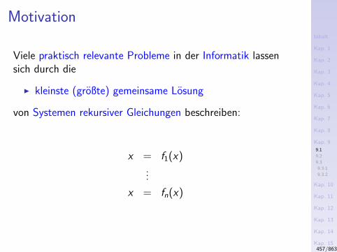
Inhalt
Kap. 1
Kap. 2
Kap. 3
Kap. 4
Kap. 5
Kap. 6
Kap. 7
Kap. 8
Kap. 9
9.1
9.2
9.3
9.3.1
9.3.2
Kap. 10
Kap. 11
Kap. 12
Kap. 13
Kap. 14
Kap. 15
Kap. 16
Kap. 17
Literatur
Anhang
A
Motivation
Viele praktisch relevante Probleme in der Informatik lassensich durch die
I kleinste (großte) gemeinsame Losung
von Systemen rekursiver Gleichungen beschreiben:
x = f1(x)...
x = fn(x)
457/863
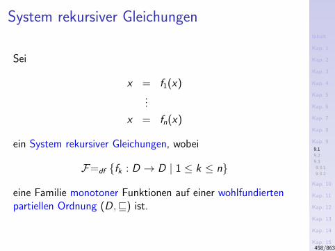
Inhalt
Kap. 1
Kap. 2
Kap. 3
Kap. 4
Kap. 5
Kap. 6
Kap. 7
Kap. 8
Kap. 9
9.1
9.2
9.3
9.3.1
9.3.2
Kap. 10
Kap. 11
Kap. 12
Kap. 13
Kap. 14
Kap. 15
Kap. 16
Kap. 17
Literatur
Anhang
A
System rekursiver Gleichungen
Sei
x = f1(x)...
x = fn(x)
ein System rekursiver Gleichungen, wobei
F=df fk : D → D | 1 ≤ k ≤ n
eine Familie monotoner Funktionen auf einer wohlfundiertenpartiellen Ordnung (D,v) ist.
458/863
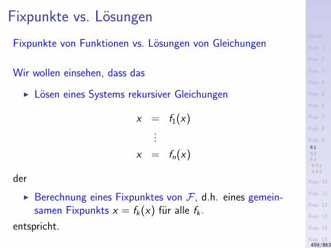
Inhalt
Kap. 1
Kap. 2
Kap. 3
Kap. 4
Kap. 5
Kap. 6
Kap. 7
Kap. 8
Kap. 9
9.1
9.2
9.3
9.3.1
9.3.2
Kap. 10
Kap. 11
Kap. 12
Kap. 13
Kap. 14
Kap. 15
Kap. 16
Kap. 17
Literatur
Anhang
A
Fixpunkte vs. Losungen
Fixpunkte von Funktionen vs. Losungen von Gleichungen
Wir wollen einsehen, dass das
I Losen eines Systems rekursiver Gleichungen
x = f1(x)...
x = fn(x)
der
I Berechnung eines Fixpunktes von F , d.h. eines gemein-samen Fixpunkts x = fk(x) fur alle fk .
entspricht.
459/863
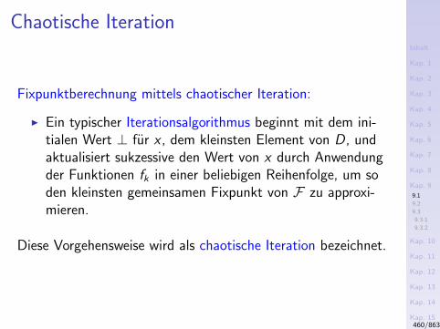
Inhalt
Kap. 1
Kap. 2
Kap. 3
Kap. 4
Kap. 5
Kap. 6
Kap. 7
Kap. 8
Kap. 9
9.1
9.2
9.3
9.3.1
9.3.2
Kap. 10
Kap. 11
Kap. 12
Kap. 13
Kap. 14
Kap. 15
Kap. 16
Kap. 17
Literatur
Anhang
A
Chaotische Iteration
Fixpunktberechnung mittels chaotischer Iteration:
I Ein typischer Iterationsalgorithmus beginnt mit dem ini-tialen Wert ⊥ fur x , dem kleinsten Element von D, undaktualisiert sukzessive den Wert von x durch Anwendungder Funktionen fk in einer beliebigen Reihenfolge, um soden kleinsten gemeinsamen Fixpunkt von F zu approxi-mieren.
Diese Vorgehensweise wird als chaotische Iteration bezeichnet.
460/863
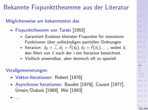
Inhalt
Kap. 1
Kap. 2
Kap. 3
Kap. 4
Kap. 5
Kap. 6
Kap. 7
Kap. 8
Kap. 9
9.1
9.2
9.3
9.3.1
9.3.2
Kap. 10
Kap. 11
Kap. 12
Kap. 13
Kap. 14
Kap. 15
Kap. 16
Kap. 17
Literatur
Anhang
A
Bekannte Fixpunkttheoreme aus der Literatur
Moglicherweise am bekanntesten das
I Fixpunkttheorem von Tarski [1955]I Garantiert Existenz kleinster Fixpunkte fur monotone
Funktionen uber vollstandigen partiellen OrdnungenI Iteration: ~x0 = ~⊥,~x1 = ~f (~x0),~x2 = ~f (~x1), . . ., wobei ~xi
den Wert von ~x nach der i-ten Iteration bezeichnet.I Vielfach anwendbar, aber dennoch oft zu speziell.
Verallgemeinerungen:
I Vektor-Iterationen: Robert [1976]
I Asynchrone Iterationen: Baudet [1978], Cousot [1977],Uresin/Dubois [1989], Wei [1993]
I ...
461/863
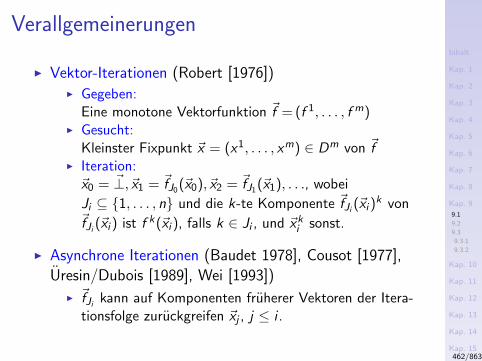
Inhalt
Kap. 1
Kap. 2
Kap. 3
Kap. 4
Kap. 5
Kap. 6
Kap. 7
Kap. 8
Kap. 9
9.1
9.2
9.3
9.3.1
9.3.2
Kap. 10
Kap. 11
Kap. 12
Kap. 13
Kap. 14
Kap. 15
Kap. 16
Kap. 17
Literatur
Anhang
A
Verallgemeinerungen
I Vektor-Iterationen (Robert [1976])I Gegeben:
Eine monotone Vektorfunktion ~f = (f 1, . . . , f m)I Gesucht:
Kleinster Fixpunkt ~x = (x1, . . . , xm) ∈ Dm von ~fI Iteration:~x0 = ~⊥,~x1 = ~fJ0(~x0),~x2 = ~fJ1(~x1), . . ., wobei
Ji ⊆ 1, . . . , n und die k-te Komponente ~fJi (~xi )k von
~fJi (~xi ) ist f k(~xi ), falls k ∈ Ji , und ~xki sonst.
I Asynchrone Iterationen (Baudet 1978], Cousot [1977],Uresin/Dubois [1989], Wei [1993])
I ~fJi kann auf Komponenten fruherer Vektoren der Itera-tionsfolge zuruckgreifen ~xj , j ≤ i .
462/863
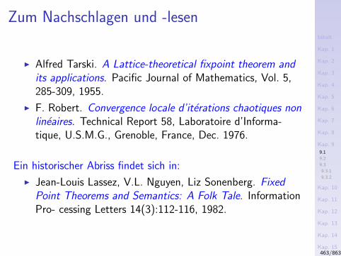
Inhalt
Kap. 1
Kap. 2
Kap. 3
Kap. 4
Kap. 5
Kap. 6
Kap. 7
Kap. 8
Kap. 9
9.1
9.2
9.3
9.3.1
9.3.2
Kap. 10
Kap. 11
Kap. 12
Kap. 13
Kap. 14
Kap. 15
Kap. 16
Kap. 17
Literatur
Anhang
A
Zum Nachschlagen und -lesen
I Alfred Tarski. A Lattice-theoretical fixpoint theorem andits applications. Pacific Journal of Mathematics, Vol. 5,285-309, 1955.
I F. Robert. Convergence locale d’iterations chaotiques nonlineaires. Technical Report 58, Laboratoire d’Informa-tique, U.S.M.G., Grenoble, France, Dec. 1976.
Ein historischer Abriss findet sich in:
I Jean-Louis Lassez, V.L. Nguyen, Liz Sonenberg. FixedPoint Theorems and Semantics: A Folk Tale. InformationPro- cessing Letters 14(3):112-116, 1982.
463/863
Inhalt
Kap. 1
Kap. 2
Kap. 3
Kap. 4
Kap. 5
Kap. 6
Kap. 7
Kap. 8
Kap. 9
9.1
9.2
9.3
9.3.1
9.3.2
Kap. 10
Kap. 11
Kap. 12
Kap. 13
Kap. 14
Kap. 15
Kap. 16
Kap. 17
Literatur
Anhang
A
In diesem Kapitel
Vorstellung eines weiteren Fixpunkttheorems, das ohneMonotonie auskommt!
I Alfons Geser, Jens Knoop, Gerald Luttgen, OliverRuthing, Bernhard Steffen. Non-monotone FixpointIterations to Resolve Second Order Effects. InProceedings of the 6th International Conference onCompiler Construction (CC’96), Springer-V., LNCS 1060,106-120, 1996.
464/863

Inhalt
Kap. 1
Kap. 2
Kap. 3
Kap. 4
Kap. 5
Kap. 6
Kap. 7
Kap. 8
Kap. 9
9.1
9.2
9.3
9.3.1
9.3.2
Kap. 10
Kap. 11
Kap. 12
Kap. 13
Kap. 14
Kap. 15
Kap. 16
Kap. 17
Literatur
Anhang
A
Kapitel 9.2
Chaotisches Fixpunktiterationstheorem
465/863
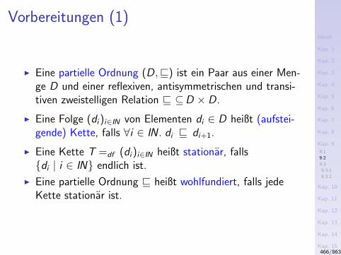
Inhalt
Kap. 1
Kap. 2
Kap. 3
Kap. 4
Kap. 5
Kap. 6
Kap. 7
Kap. 8
Kap. 9
9.1
9.2
9.3
9.3.1
9.3.2
Kap. 10
Kap. 11
Kap. 12
Kap. 13
Kap. 14
Kap. 15
Kap. 16
Kap. 17
Literatur
Anhang
A
Vorbereitungen (1)
I Eine partielle Ordnung (D,v) ist ein Paar aus einer Men-ge D und einer reflexiven, antisymmetrischen und transi-tiven zweistelligen Relation v ⊆D × D.
I Eine Folge (di)i∈IN von Elementen di ∈ D heißt (aufstei-gende) Kette, falls ∀i ∈ IN . di v di+1.
I Eine Kette T =df (di)i∈IN heißt stationar, fallsdi | i ∈ IN endlich ist.
I Eine partielle Ordnung v heißt wohlfundiert, falls jedeKette stationar ist.
466/863
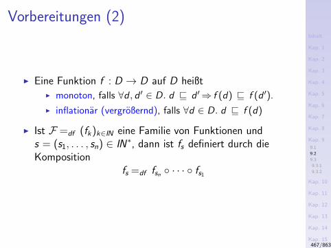
Inhalt
Kap. 1
Kap. 2
Kap. 3
Kap. 4
Kap. 5
Kap. 6
Kap. 7
Kap. 8
Kap. 9
9.1
9.2
9.3
9.3.1
9.3.2
Kap. 10
Kap. 11
Kap. 12
Kap. 13
Kap. 14
Kap. 15
Kap. 16
Kap. 17
Literatur
Anhang
A
Vorbereitungen (2)
I Eine Funktion f : D → D auf D heißtI monoton, falls ∀d , d ′ ∈ D. d v d ′⇒ f (d) v f (d ′).
I inflationar (vergroßernd), falls ∀d ∈ D. d v f (d)
I Ist F =df (fk)k∈IN eine Familie von Funktionen unds = (s1, . . . , sn) ∈ IN∗, dann ist fs definiert durch dieKomposition
fs =df fsn · · · fs1
467/863
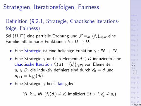
Inhalt
Kap. 1
Kap. 2
Kap. 3
Kap. 4
Kap. 5
Kap. 6
Kap. 7
Kap. 8
Kap. 9
9.1
9.2
9.3
9.3.1
9.3.2
Kap. 10
Kap. 11
Kap. 12
Kap. 13
Kap. 14
Kap. 15
Kap. 16
Kap. 17
Literatur
Anhang
A
Strategien, Iterationsfolgen, Fairness
Definition (9.2.1, Strategie, Chaotische Iterations-folge, Fairness)
Sei (D,v) eine partielle Ordnung und F =df (fk)k∈IN eineFamilie inflationarer Funktionen fk : D → D.
I Eine Strategie ist eine beliebige Funktion γ : IN → IN .
I Eine Strategie γ und ein Element d ∈ D induzieren einechaotische Iteration fγ(d) = (di)i∈IN von Elementendi ∈ D, die induktiv definiert sind durch d0 = d unddi+1 = fγ(i)(di).
I Eine Strategie γ heißt fair gdw
∀i , k ∈ IN . (fk(di) 6= di impliziert ∃j > i . dj 6= di)
468/863
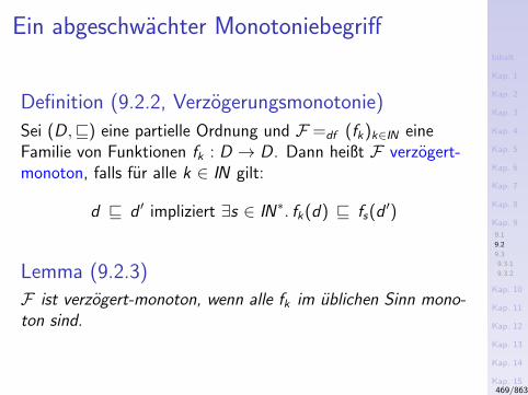
Inhalt
Kap. 1
Kap. 2
Kap. 3
Kap. 4
Kap. 5
Kap. 6
Kap. 7
Kap. 8
Kap. 9
9.1
9.2
9.3
9.3.1
9.3.2
Kap. 10
Kap. 11
Kap. 12
Kap. 13
Kap. 14
Kap. 15
Kap. 16
Kap. 17
Literatur
Anhang
A
Ein abgeschwachter Monotoniebegriff
Definition (9.2.2, Verzogerungsmonotonie)
Sei (D,v) eine partielle Ordnung und F =df (fk)k∈IN eineFamilie von Funktionen fk : D → D. Dann heißt F verzogert-monoton, falls fur alle k ∈ IN gilt:
d v d ′ impliziert ∃s ∈ IN∗. fk(d) v fs(d ′)
Lemma (9.2.3)
F ist verzogert-monoton, wenn alle fk im ublichen Sinn mono-ton sind.
469/863
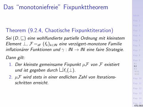
Inhalt
Kap. 1
Kap. 2
Kap. 3
Kap. 4
Kap. 5
Kap. 6
Kap. 7
Kap. 8
Kap. 9
9.1
9.2
9.3
9.3.1
9.3.2
Kap. 10
Kap. 11
Kap. 12
Kap. 13
Kap. 14
Kap. 15
Kap. 16
Kap. 17
Literatur
Anhang
A
Das “monotoniefreie” Fixpunkttheorem
Theorem (9.2.4, Chaotische Fixpunktiteration)
Sei (D,v) eine wohlfundierte partielle Ordnung mit kleinstemElement ⊥, F =df (fk)k∈IN eine verzogert-monotone Familieinflationarer Funktionen und γ : IN → IN eine faire Strategie.
Dann gilt:
1. Der kleinste gemeinsame Fixpunkt µF von F existiertund ist gegeben durch tfγ(⊥).
2. µF wird stets in einer endlichen Zahl von Iterations-schritten erreicht.
470/863
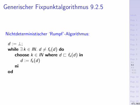
Inhalt
Kap. 1
Kap. 2
Kap. 3
Kap. 4
Kap. 5
Kap. 6
Kap. 7
Kap. 8
Kap. 9
9.1
9.2
9.3
9.3.1
9.3.2
Kap. 10
Kap. 11
Kap. 12
Kap. 13
Kap. 14
Kap. 15
Kap. 16
Kap. 17
Literatur
Anhang
A
Generischer Fixpunktalgorithmus 9.2.5
Nichtdeterministischer ‘Rumpf’-Algorithmus:
d := ⊥;while ∃ k ∈ IN . d 6= fk(d) do
choose k ∈ IN where d @ fk(d) ind := fk(d)
niod
471/863

Inhalt
Kap. 1
Kap. 2
Kap. 3
Kap. 4
Kap. 5
Kap. 6
Kap. 7
Kap. 8
Kap. 9
9.1
9.2
9.3
9.3.1
9.3.2
Kap. 10
Kap. 11
Kap. 12
Kap. 13
Kap. 14
Kap. 15
Kap. 16
Kap. 17
Literatur
Anhang
A
Kapitel 9.3
Anwendungen
472/863

Inhalt
Kap. 1
Kap. 2
Kap. 3
Kap. 4
Kap. 5
Kap. 6
Kap. 7
Kap. 8
Kap. 9
9.1
9.2
9.3
9.3.1
9.3.2
Kap. 10
Kap. 11
Kap. 12
Kap. 13
Kap. 14
Kap. 15
Kap. 16
Kap. 17
Literatur
Anhang
A
Kapitel 9.3.1
Vektor-Iteration
473/863
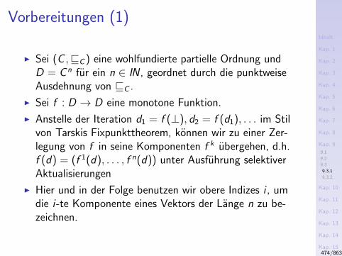
Inhalt
Kap. 1
Kap. 2
Kap. 3
Kap. 4
Kap. 5
Kap. 6
Kap. 7
Kap. 8
Kap. 9
9.1
9.2
9.3
9.3.1
9.3.2
Kap. 10
Kap. 11
Kap. 12
Kap. 13
Kap. 14
Kap. 15
Kap. 16
Kap. 17
Literatur
Anhang
A
Vorbereitungen (1)
I Sei (C ,vC ) eine wohlfundierte partielle Ordnung undD = C n fur ein n ∈ IN , geordnet durch die punktweiseAusdehnung von vC .
I Sei f : D → D eine monotone Funktion.
I Anstelle der Iteration d1 = f (⊥), d2 = f (d1), . . . im Stilvon Tarskis Fixpunkttheorem, konnen wir zu einer Zer-legung von f in seine Komponenten f k ubergehen, d.h.f (d) = (f 1(d), . . . , f n(d)) unter Ausfuhrung selektiverAktualisierungen
I Hier und in der Folge benutzen wir obere Indizes i , umdie i -te Komponente eines Vektors der Lange n zu be-zeichnen.
474/863
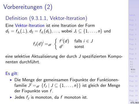
Inhalt
Kap. 1
Kap. 2
Kap. 3
Kap. 4
Kap. 5
Kap. 6
Kap. 7
Kap. 8
Kap. 9
9.1
9.2
9.3
9.3.1
9.3.2
Kap. 10
Kap. 11
Kap. 12
Kap. 13
Kap. 14
Kap. 15
Kap. 16
Kap. 17
Literatur
Anhang
A
Vorbereitungen (2)
Definition (9.3.1.1, Vektor-Iteration)
Eine Vektor-Iteration ist eine Iteration der Formd1 = fJ0(⊥), d2 = fJ1(d1), . . ., wobei Ji ⊆ 1, . . . , n und
fJ(d)i =df
f i(d) falls i ∈ Jd i sonst
eine selektive Aktualisierung der durch J spezifizierten Kompo-nenten durchfuhrt.
Es gilt:
I Die Menge der gemeinsamen Fixpunkte der Funktionen-familie F =df fJ | J ⊆ 1, . . . , n ist gleich der Mengeder Fixpunkte von f .
I Jedes fJ is monoton, da f monoton ist.475/863
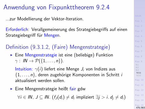
Inhalt
Kap. 1
Kap. 2
Kap. 3
Kap. 4
Kap. 5
Kap. 6
Kap. 7
Kap. 8
Kap. 9
9.1
9.2
9.3
9.3.1
9.3.2
Kap. 10
Kap. 11
Kap. 12
Kap. 13
Kap. 14
Kap. 15
Kap. 16
Kap. 17
Literatur
Anhang
A
Anwendung von Fixpunkttheorem 9.2.4
...zur Modellierung der Vektor-Iteration.
Erforderlich: Verallgemeinerung des Strategiebegriffs auf einenStrategiebegriff fur Mengen.
Definition (9.3.1.2, (Faire) Mengenstrategie)I Eine Mengenstrategie ist eine (beliebige) Funktionγ : IN → P(1, . . . , n).
Intuition: γ(i) liefert eine Menge Ji von Indizes aus1, . . . , n, deren zugehorige Komponenten in Schritt iaktualisiert werden sollen.
I Eine Mengenstrategie heißt fair gdw
∀i ∈ IN , J ⊆ IN . (fJ(di) 6= di impliziert ∃j > i . dj 6= di)
476/863
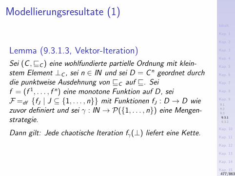
Inhalt
Kap. 1
Kap. 2
Kap. 3
Kap. 4
Kap. 5
Kap. 6
Kap. 7
Kap. 8
Kap. 9
9.1
9.2
9.3
9.3.1
9.3.2
Kap. 10
Kap. 11
Kap. 12
Kap. 13
Kap. 14
Kap. 15
Kap. 16
Kap. 17
Literatur
Anhang
A
Modellierungsresultate (1)
Lemma (9.3.1.3, Vektor-Iteration)
Sei (C ,vC ) eine wohlfundierte partielle Ordnung mit klein-stem Element ⊥C , sei n ∈ IN und sei D = C n geordnet durchdie punktweise Ausdehnung von vC auf v. Seif = (f 1, . . . , f n) eine monotone Funktion auf D, seiF =df fJ | J ⊆ 1, . . . , n mit Funktionen fJ : D → D wiezuvor definiert und sei γ : IN → P(1, . . . , n) eine Mengen-strategie.
Dann gilt: Jede chaotische Iteration fγ(⊥) liefert eine Kette.
477/863
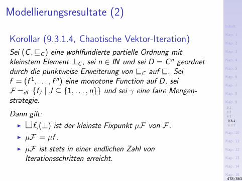
Inhalt
Kap. 1
Kap. 2
Kap. 3
Kap. 4
Kap. 5
Kap. 6
Kap. 7
Kap. 8
Kap. 9
9.1
9.2
9.3
9.3.1
9.3.2
Kap. 10
Kap. 11
Kap. 12
Kap. 13
Kap. 14
Kap. 15
Kap. 16
Kap. 17
Literatur
Anhang
A
Modellierungsresultate (2)
Korollar (9.3.1.4, Chaotische Vektor-Iteration)
Sei (C ,vC ) eine wohlfundierte partielle Ordnung mitkleinstem Element ⊥C , sei n ∈ IN und sei D = C n geordnetdurch die punktweise Erweiterung von vC auf v. Seif = (f 1, . . . , f n) eine monotone Function auf D, seiF =df fJ | J ⊆ 1, . . . , n und sei γ eine faire Mengen-strategie.
Dann gilt:
I tfγ(⊥) ist der kleinste Fixpunkt µF von F .
I µF = µf .
I µF ist stets in einer endlichen Zahl vonIterationsschritten erreicht.
478/863
Inhalt
Kap. 1
Kap. 2
Kap. 3
Kap. 4
Kap. 5
Kap. 6
Kap. 7
Kap. 8
Kap. 9
9.1
9.2
9.3
9.3.1
9.3.2
Kap. 10
Kap. 11
Kap. 12
Kap. 13
Kap. 14
Kap. 15
Kap. 16
Kap. 17
Literatur
Anhang
A
Modellierungsresultate (3)
Bemerkungen:
I Korollar 9.3.1.4 ist ein Spezialfall von Fixpunkttheorem9.2.4 fur Vektor-Iterationen und folgt zusammen mitLemma 9.3.1.3.
I Fur |F| = 1 reduziert sich Korollar 9.3.1.4 auf Tarskis Fix-punkttheorem im Fall wohlfundierter partieller Ordnungen.
479/863
Inhalt
Kap. 1
Kap. 2
Kap. 3
Kap. 4
Kap. 5
Kap. 6
Kap. 7
Kap. 8
Kap. 9
9.1
9.2
9.3
9.3.1
9.3.2
Kap. 10
Kap. 11
Kap. 12
Kap. 13
Kap. 14
Kap. 15
Kap. 16
Kap. 17
Literatur
Anhang
A
Kapitel 9.3.2
Datenflussanalyse
480/863
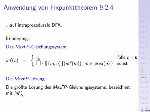
Inhalt
Kap. 1
Kap. 2
Kap. 3
Kap. 4
Kap. 5
Kap. 6
Kap. 7
Kap. 8
Kap. 9
9.1
9.2
9.3
9.3.1
9.3.2
Kap. 10
Kap. 11
Kap. 12
Kap. 13
Kap. 14
Kap. 15
Kap. 16
Kap. 17
Literatur
Anhang
A
Anwendung von Fixpunkttheorem 9.2.4
...auf intraprozedurale DFA.
Erinnerung:
Das MaxFP-Gleichungssystem:
inf (n) =
cs falls n = su [[ (m, n) ]](inf (m)) |m ∈ pred(n) sonst
Die MaxFP-Losung:
Die großte Losung des MaxFP-Gleichungssystems, bezeichnetmit inf ∗cs
.
481/863
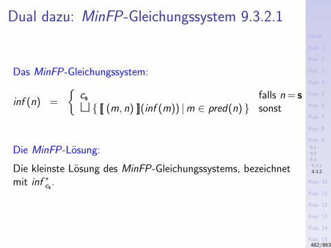
Inhalt
Kap. 1
Kap. 2
Kap. 3
Kap. 4
Kap. 5
Kap. 6
Kap. 7
Kap. 8
Kap. 9
9.1
9.2
9.3
9.3.1
9.3.2
Kap. 10
Kap. 11
Kap. 12
Kap. 13
Kap. 14
Kap. 15
Kap. 16
Kap. 17
Literatur
Anhang
A
Dual dazu: MinFP-Gleichungssystem 9.3.2.1
Das MinFP-Gleichungssystem:
inf (n) =
cs falls n = st [[ (m, n) ]](inf (m)) |m ∈ pred(n) sonst
Die MinFP-Losung:
Die kleinste Losung des MinFP-Gleichungssystems, bezeichnetmit inf ∗cs
.
482/863
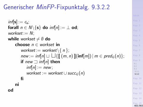
Inhalt
Kap. 1
Kap. 2
Kap. 3
Kap. 4
Kap. 5
Kap. 6
Kap. 7
Kap. 8
Kap. 9
9.1
9.2
9.3
9.3.1
9.3.2
Kap. 10
Kap. 11
Kap. 12
Kap. 13
Kap. 14
Kap. 15
Kap. 16
Kap. 17
Literatur
Anhang
A
Generischer MinFP-Fixpunktalg. 9.3.2.2
inf[s] := cs;forall n ∈ N\s do inf[n] := ⊥ od;workset := N ;while workset 6= ∅ do
choose n ∈ workset inworkset := workset\ n ;new := inf[n] t t[[ (m, n) ]](inf[m]) |m ∈ predG (n);if new A inf[n] then
inf[n] := new ;workset := workset ∪ succG (n)
fini
od
483/863
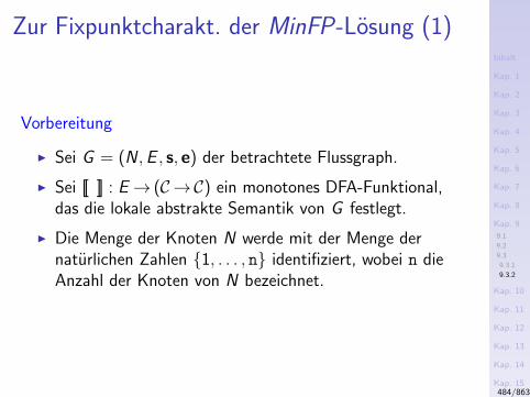
Inhalt
Kap. 1
Kap. 2
Kap. 3
Kap. 4
Kap. 5
Kap. 6
Kap. 7
Kap. 8
Kap. 9
9.1
9.2
9.3
9.3.1
9.3.2
Kap. 10
Kap. 11
Kap. 12
Kap. 13
Kap. 14
Kap. 15
Kap. 16
Kap. 17
Literatur
Anhang
A
Zur Fixpunktcharakt. der MinFP-Losung (1)
Vorbereitung
I Sei G = (N ,E , s, e) der betrachtete Flussgraph.
I Sei [[ ]] : E→ (C→C) ein monotones DFA-Funktional,das die lokale abstrakte Semantik von G festlegt.
I Die Menge der Knoten N werde mit der Menge dernaturlichen Zahlen 1, . . . , n identifiziert, wobei n dieAnzahl der Knoten von N bezeichnet.
484/863
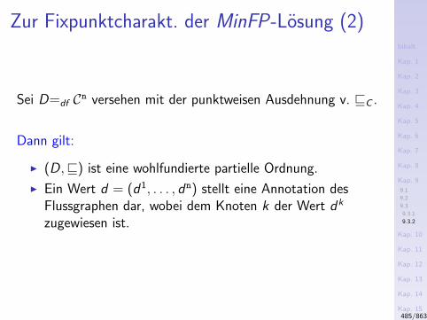
Inhalt
Kap. 1
Kap. 2
Kap. 3
Kap. 4
Kap. 5
Kap. 6
Kap. 7
Kap. 8
Kap. 9
9.1
9.2
9.3
9.3.1
9.3.2
Kap. 10
Kap. 11
Kap. 12
Kap. 13
Kap. 14
Kap. 15
Kap. 16
Kap. 17
Literatur
Anhang
A
Zur Fixpunktcharakt. der MinFP-Losung (2)
Sei D=df Cn versehen mit der punktweisen Ausdehnung v. vC .
Dann gilt:
I (D,v) ist eine wohlfundierte partielle Ordnung.
I Ein Wert d = (d1, . . . , dn) stellt eine Annotation desFlussgraphen dar, wobei dem Knoten k der Wert dk
zugewiesen ist.
485/863
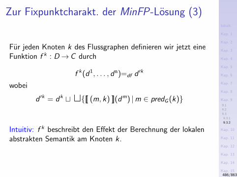
Inhalt
Kap. 1
Kap. 2
Kap. 3
Kap. 4
Kap. 5
Kap. 6
Kap. 7
Kap. 8
Kap. 9
9.1
9.2
9.3
9.3.1
9.3.2
Kap. 10
Kap. 11
Kap. 12
Kap. 13
Kap. 14
Kap. 15
Kap. 16
Kap. 17
Literatur
Anhang
A
Zur Fixpunktcharakt. der MinFP-Losung (3)
Fur jeden Knoten k des Flussgraphen definieren wir jetzt eineFunktion f k : D→C durch
f k(d1, . . . , dn)=df d ′k
wobei
d ′k = dk t t[[ (m, k) ]](dm) |m ∈ predG (k)
Intuitiv: f k beschreibt den Effekt der Berechnung der lokalenabstrakten Semantik am Knoten k .
486/863
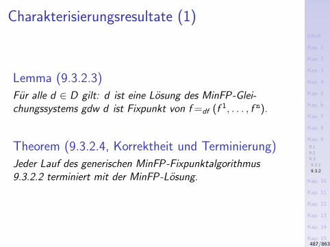
Inhalt
Kap. 1
Kap. 2
Kap. 3
Kap. 4
Kap. 5
Kap. 6
Kap. 7
Kap. 8
Kap. 9
9.1
9.2
9.3
9.3.1
9.3.2
Kap. 10
Kap. 11
Kap. 12
Kap. 13
Kap. 14
Kap. 15
Kap. 16
Kap. 17
Literatur
Anhang
A
Charakterisierungsresultate (1)
Lemma (9.3.2.3)
Fur alle d ∈ D gilt: d ist eine Losung des MinFP-Glei-chungssystems gdw d ist Fixpunkt von f =df (f 1, . . . , f n).
Theorem (9.3.2.4, Korrektheit und Terminierung)
Jeder Lauf des generischen MinFP-Fixpunktalgorithmus9.3.2.2 terminiert mit der MinFP-Losung.
487/863
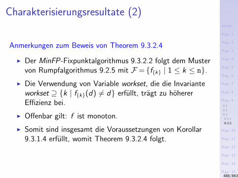
Inhalt
Kap. 1
Kap. 2
Kap. 3
Kap. 4
Kap. 5
Kap. 6
Kap. 7
Kap. 8
Kap. 9
9.1
9.2
9.3
9.3.1
9.3.2
Kap. 10
Kap. 11
Kap. 12
Kap. 13
Kap. 14
Kap. 15
Kap. 16
Kap. 17
Literatur
Anhang
A
Charakterisierungsresultate (2)
Anmerkungen zum Beweis von Theorem 9.3.2.4
I Der MinFP-Fixpunktalgorithmus 9.3.2.2 folgt dem Mustervon Rumpfalgorithmus 9.2.5 mit F = fk | 1 ≤ k ≤ n.
I Die Verwendung von Variable workset, die die Invarianteworkset ⊇ k | fk(d) 6= d erfullt, tragt zu hohererEffizienz bei.
I Offenbar gilt: f ist monoton.
I Somit sind insgesamt die Voraussetzungen von Korollar9.3.1.4 erfullt, womit Theorem 9.3.2.4 folgt.
488/863
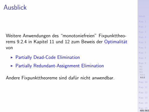
Inhalt
Kap. 1
Kap. 2
Kap. 3
Kap. 4
Kap. 5
Kap. 6
Kap. 7
Kap. 8
Kap. 9
9.1
9.2
9.3
9.3.1
9.3.2
Kap. 10
Kap. 11
Kap. 12
Kap. 13
Kap. 14
Kap. 15
Kap. 16
Kap. 17
Literatur
Anhang
A
Ausblick
Weitere Anwendungen des “monotoniefreien” Fixpunkttheo-rems 9.2.4 in Kapitel 11 und 12 zum Beweis der Optimalitatvon
I Partially Dead-Code Elimination
I Partially Redundant-Assignment Elimination
Andere Fixpunkttheoreme sind dafur nicht anwendbar.
489/863
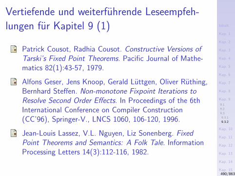
Inhalt
Kap. 1
Kap. 2
Kap. 3
Kap. 4
Kap. 5
Kap. 6
Kap. 7
Kap. 8
Kap. 9
9.1
9.2
9.3
9.3.1
9.3.2
Kap. 10
Kap. 11
Kap. 12
Kap. 13
Kap. 14
Kap. 15
Kap. 16
Kap. 17
Literatur
Anhang
A
Vertiefende und weiterfuhrende Leseempfeh-
lungen fur Kapitel 9 (1)
Patrick Cousot, Radhia Cousot. Constructive Versions ofTarski’s Fixed Point Theorems. Pacific Journal of Mathe-matics 82(1):43-57, 1979.
Alfons Geser, Jens Knoop, Gerald Luttgen, Oliver Ruthing,Bernhard Steffen. Non-monotone Fixpoint Iterations toResolve Second Order Effects. In Proceedings of the 6thInternational Conference on Compiler Construction(CC’96), Springer-V., LNCS 1060, 106-120, 1996.
Jean-Louis Lassez, V.L. Nguyen, Liz Sonenberg. FixedPoint Theorems and Semantics: A Folk Tale. InformationProcessing Letters 14(3):112-116, 1982.
490/863
Inhalt
Kap. 1
Kap. 2
Kap. 3
Kap. 4
Kap. 5
Kap. 6
Kap. 7
Kap. 8
Kap. 9
9.1
9.2
9.3
9.3.1
9.3.2
Kap. 10
Kap. 11
Kap. 12
Kap. 13
Kap. 14
Kap. 15
Kap. 16
Kap. 17
Literatur
Anhang
A
Vertiefende und weiterfuhrende Leseempfeh-
lungen fur Kapitel 9 (2)
F. Robert. Convergence locale d’iterations chaotiques nonlineaires. Technical Report 58, Laboratoire d’Informatique,U.S.M.G., Grenoble, France, Dec. 1976.
Alfred Tarski. A Lattice-theoretical Fixpoint Theorem andits Applications. Pacific Journal of Mathematics5:285-309, 1955.
491/863

Inhalt
Kap. 1
Kap. 2
Kap. 3
Kap. 4
Kap. 5
Kap. 6
Kap. 7
Kap. 8
Kap. 9
Kap. 10
10.1
10.1.1
10.1.2
10.2
10.2.1
10.2.2
10.2.3
10.3
10.3.1
10.3.2
10.4
10.5
Kap. 11
Kap. 12
Kap. 13
Kap. 14
Kap. 15
Kap. 16
Kap. 17
Literatur
Anhang
A
Kapitel 10
Basisblock- vs. Einzelanweisungsgraphen
492/863

Inhalt
Kap. 1
Kap. 2
Kap. 3
Kap. 4
Kap. 5
Kap. 6
Kap. 7
Kap. 8
Kap. 9
Kap. 10
10.1
10.1.1
10.1.2
10.2
10.2.1
10.2.2
10.2.3
10.3
10.3.1
10.3.2
10.4
10.5
Kap. 11
Kap. 12
Kap. 13
Kap. 14
Kap. 15
Kap. 16
Kap. 17
Literatur
Anhang
A
Kapitel 10.1
Motivation
493/863
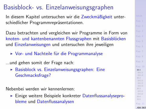
Inhalt
Kap. 1
Kap. 2
Kap. 3
Kap. 4
Kap. 5
Kap. 6
Kap. 7
Kap. 8
Kap. 9
Kap. 10
10.1
10.1.1
10.1.2
10.2
10.2.1
10.2.2
10.2.3
10.3
10.3.1
10.3.2
10.4
10.5
Kap. 11
Kap. 12
Kap. 13
Kap. 14
Kap. 15
Kap. 16
Kap. 17
Literatur
Anhang
A
Basisblock- vs. Einzelanweisungsgraphen
In diesem Kapitel untersuchen wir die Zweckmaßigkeit unter-schiedlicher Programmreprasentationen.
Dazu betrachten und vergleichen wir Programme in Form vonknoten- und kantenbenannten Flussgraphen mit Basisblockenund Einzelanweisungen und untersuchen ihre jeweiligen
I Vor- und Nachteile fur die Programmanalyse
...und gehen somit der Frage nach:
I Basisblock vs. Einzelanweisungsgraphen: EineGeschmacksfrage?
Nebenbei werden wir kennenlernen:
I Einige weitere Beispiele konkreter Datenflussanalysepro-bleme und Datenflussanalysen
494/863
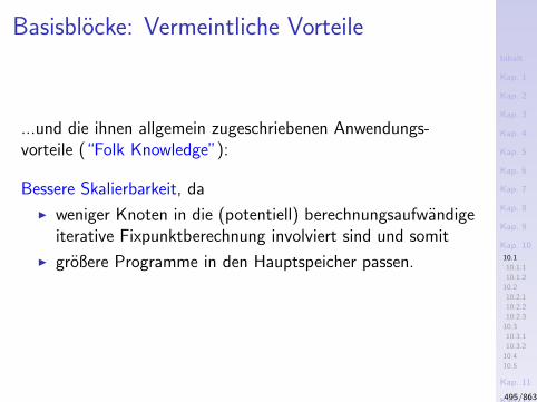
Inhalt
Kap. 1
Kap. 2
Kap. 3
Kap. 4
Kap. 5
Kap. 6
Kap. 7
Kap. 8
Kap. 9
Kap. 10
10.1
10.1.1
10.1.2
10.2
10.2.1
10.2.2
10.2.3
10.3
10.3.1
10.3.2
10.4
10.5
Kap. 11
Kap. 12
Kap. 13
Kap. 14
Kap. 15
Kap. 16
Kap. 17
Literatur
Anhang
A
Basisblocke: Vermeintliche Vorteile
...und die ihnen allgemein zugeschriebenen Anwendungs-vorteile (“Folk Knowledge”):
Bessere Skalierbarkeit, da
I weniger Knoten in die (potentiell) berechnungsaufwandigeiterative Fixpunktberechnung involviert sind und somit
I großere Programme in den Hauptspeicher passen.
495/863
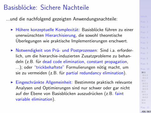
Inhalt
Kap. 1
Kap. 2
Kap. 3
Kap. 4
Kap. 5
Kap. 6
Kap. 7
Kap. 8
Kap. 9
Kap. 10
10.1
10.1.1
10.1.2
10.2
10.2.1
10.2.2
10.2.3
10.3
10.3.1
10.3.2
10.4
10.5
Kap. 11
Kap. 12
Kap. 13
Kap. 14
Kap. 15
Kap. 16
Kap. 17
Literatur
Anhang
A
Basisblocke: Sichere Nachteile
...und die nachfolgend gezeigten Anwendungsnachteile:
I Hohere konzeptuelle Komplexitat: Basisblocke fuhren zu einerunerwunschten Hierarchisierung, die sowohl theoretischeUberlegungen wie praktische Implementierungen erschwert.
I Notwendigkeit von Pra- und Postprozessen: Sind i.a. erforder-lich, um die hierarchie-induzierten Zusatzprobleme zu behan-deln (z.B. fur dead code elimination, constant propagation,...); oder “trickbehaftete” Formulierungen notig macht, umsie zu vermeiden (z.B. fur partial redundancy elimination).
I Eingeschrankte Allgemeinheit: Bestimmte praktisch relevanteAnalysen und Optimierungen sind nur schwer oder gar nichtauf der Ebene von Basisblocken auszudrucken (z.B. faintvariable elimination).
496/863
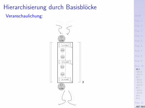
Inhalt
Kap. 1
Kap. 2
Kap. 3
Kap. 4
Kap. 5
Kap. 6
Kap. 7
Kap. 8
Kap. 9
Kap. 10
10.1
10.1.1
10.1.2
10.2
10.2.1
10.2.2
10.2.3
10.3
10.3.1
10.3.2
10.4
10.5
Kap. 11
Kap. 12
Kap. 13
Kap. 14
Kap. 15
Kap. 16
Kap. 17
Literatur
Anhang
A
Hierarchisierung durch BasisblockeVeranschaulichung:
a := b+c
d := a+b
e := c+d
ι
ι
ι
X−I
X−BB
=
N−I
X−I
N−I
X−I
N−I
N−BB
=
β
497/863
Inhalt
Kap. 1
Kap. 2
Kap. 3
Kap. 4
Kap. 5
Kap. 6
Kap. 7
Kap. 8
Kap. 9
Kap. 10
10.1
10.1.1
10.1.2
10.2
10.2.1
10.2.2
10.2.3
10.3
10.3.1
10.3.2
10.4
10.5
Kap. 11
Kap. 12
Kap. 13
Kap. 14
Kap. 15
Kap. 16
Kap. 17
Literatur
Anhang
A
In der Folge
Untersuchung von
I Vor- und Nachteilen von Basisblock- (BB) gegenuberEinzelanweisungsgraphen (EA)
anhand von Beispielen
I einiger bereits von uns betrachteterI Verfugbarkeit von AusdruckenI Einfache Konstanten
und neuer DatenflussanalyseproblemeI Schattenhafte (faint) Variablen
498/863

Inhalt
Kap. 1
Kap. 2
Kap. 3
Kap. 4
Kap. 5
Kap. 6
Kap. 7
Kap. 8
Kap. 9
Kap. 10
10.1
10.1.1
10.1.2
10.2
10.2.1
10.2.2
10.2.3
10.3
10.3.1
10.3.2
10.4
10.5
Kap. 11
Kap. 12
Kap. 13
Kap. 14
Kap. 15
Kap. 16
Kap. 17
Literatur
Anhang
A
Kapitel 10.1.1
Kantenbenannter Einzelanweisungsansatz
499/863
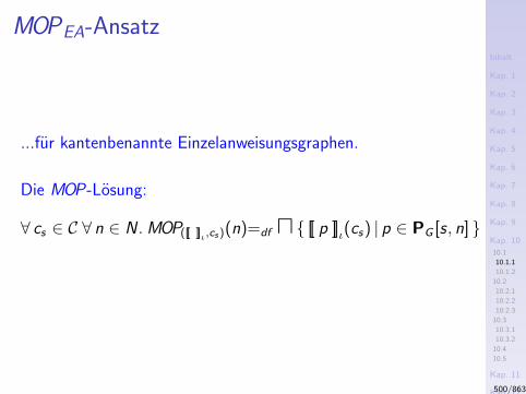
Inhalt
Kap. 1
Kap. 2
Kap. 3
Kap. 4
Kap. 5
Kap. 6
Kap. 7
Kap. 8
Kap. 9
Kap. 10
10.1
10.1.1
10.1.2
10.2
10.2.1
10.2.2
10.2.3
10.3
10.3.1
10.3.2
10.4
10.5
Kap. 11
Kap. 12
Kap. 13
Kap. 14
Kap. 15
Kap. 16
Kap. 17
Literatur
Anhang
A
MOPEA-Ansatz
...fur kantenbenannte Einzelanweisungsgraphen.
Die MOP-Losung:
∀ cs ∈ C ∀ n ∈ N . MOP([[ ]]ι,cs)(n)=df u [[ p ]]ι(cs) | p ∈ PG [s, n]
500/863
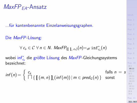
Inhalt
Kap. 1
Kap. 2
Kap. 3
Kap. 4
Kap. 5
Kap. 6
Kap. 7
Kap. 8
Kap. 9
Kap. 10
10.1
10.1.1
10.1.2
10.2
10.2.1
10.2.2
10.2.3
10.3
10.3.1
10.3.2
10.4
10.5
Kap. 11
Kap. 12
Kap. 13
Kap. 14
Kap. 15
Kap. 16
Kap. 17
Literatur
Anhang
A
MaxFPEA-Ansatz
...fur kantenbenannte Einzelanweisungsgraphen.
Die MaxFP-Losung:
∀ cs ∈ C ∀ n ∈ N . MaxFP([[ ]]ι,cs)(n)=df inf∗cs (n)
wobei inf∗cs die großte Losung des MaxFP-Gleichungssystemsbezeichnet:
inf (n) =
cs falls n = su [[ (m, n) ]]ι(inf (m)) |m ∈ predG (n) sonst
501/863

Inhalt
Kap. 1
Kap. 2
Kap. 3
Kap. 4
Kap. 5
Kap. 6
Kap. 7
Kap. 8
Kap. 9
Kap. 10
10.1
10.1.1
10.1.2
10.2
10.2.1
10.2.2
10.2.3
10.3
10.3.1
10.3.2
10.4
10.5
Kap. 11
Kap. 12
Kap. 13
Kap. 14
Kap. 15
Kap. 16
Kap. 17
Literatur
Anhang
A
Kapitel 10.1.2
Knotenbenannter Basisblockansatz
502/863
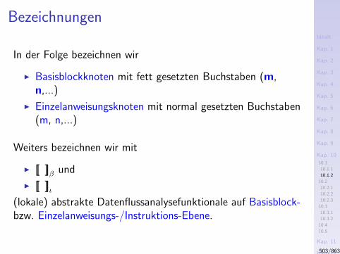
Inhalt
Kap. 1
Kap. 2
Kap. 3
Kap. 4
Kap. 5
Kap. 6
Kap. 7
Kap. 8
Kap. 9
Kap. 10
10.1
10.1.1
10.1.2
10.2
10.2.1
10.2.2
10.2.3
10.3
10.3.1
10.3.2
10.4
10.5
Kap. 11
Kap. 12
Kap. 13
Kap. 14
Kap. 15
Kap. 16
Kap. 17
Literatur
Anhang
A
Bezeichnungen
In der Folge bezeichnen wir
I Basisblockknoten mit fett gesetzten Buchstaben (m,n,...)
I Einzelanweisungsknoten mit normal gesetzten Buchstaben(m, n,...)
Weiters bezeichnen wir mit
I [[ ]]β und
I [[ ]]ι(lokale) abstrakte Datenflussanalysefunktionale auf Basisblock-bzw. Einzelanweisungs-/Instruktions-Ebene.
503/863
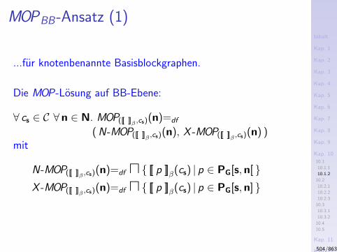
Inhalt
Kap. 1
Kap. 2
Kap. 3
Kap. 4
Kap. 5
Kap. 6
Kap. 7
Kap. 8
Kap. 9
Kap. 10
10.1
10.1.1
10.1.2
10.2
10.2.1
10.2.2
10.2.3
10.3
10.3.1
10.3.2
10.4
10.5
Kap. 11
Kap. 12
Kap. 13
Kap. 14
Kap. 15
Kap. 16
Kap. 17
Literatur
Anhang
A
MOPBB-Ansatz (1)
...fur knotenbenannte Basisblockgraphen.
Die MOP-Losung auf BB-Ebene:
∀ cs ∈ C ∀n ∈ N. MOP([[ ]]β ,cs)(n)=df
( N-MOP([[ ]]β ,cs)(n), X -MOP([[ ]]β ,cs)(n) )mit
N-MOP([[ ]]β ,cs)(n)=df u [[ p ]]β(cs) | p ∈ PG[s,n[ X -MOP([[ ]]β ,cs)(n)=df u [[ p ]]β(cs) | p ∈ PG[s,n]
504/863
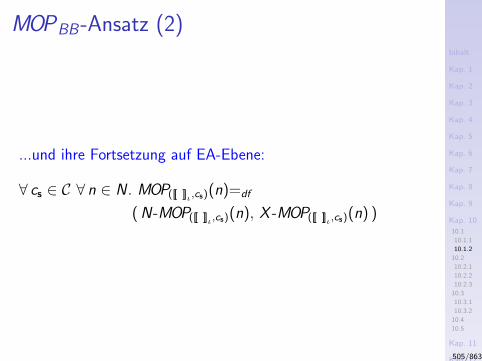
Inhalt
Kap. 1
Kap. 2
Kap. 3
Kap. 4
Kap. 5
Kap. 6
Kap. 7
Kap. 8
Kap. 9
Kap. 10
10.1
10.1.1
10.1.2
10.2
10.2.1
10.2.2
10.2.3
10.3
10.3.1
10.3.2
10.4
10.5
Kap. 11
Kap. 12
Kap. 13
Kap. 14
Kap. 15
Kap. 16
Kap. 17
Literatur
Anhang
A
MOPBB-Ansatz (2)
...und ihre Fortsetzung auf EA-Ebene:
∀ cs ∈ C ∀ n ∈ N . MOP([[ ]]ι,cs)(n)=df
( N-MOP([[ ]]ι,cs)(n), X -MOP([[ ]]ι,cs)(n) )
505/863
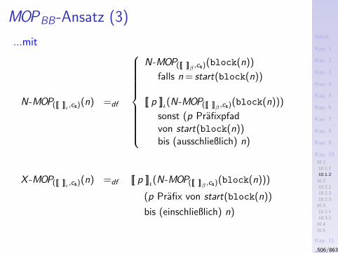
Inhalt
Kap. 1
Kap. 2
Kap. 3
Kap. 4
Kap. 5
Kap. 6
Kap. 7
Kap. 8
Kap. 9
Kap. 10
10.1
10.1.1
10.1.2
10.2
10.2.1
10.2.2
10.2.3
10.3
10.3.1
10.3.2
10.4
10.5
Kap. 11
Kap. 12
Kap. 13
Kap. 14
Kap. 15
Kap. 16
Kap. 17
Literatur
Anhang
A
MOPBB-Ansatz (3)
...mit
N-MOP([[ ]]ι,cs)(n) =df
N-MOP([[ ]]β ,cs)(block(n))
falls n = start(block(n))
[[ p ]]ι(N-MOP([[ ]]β ,cs)(block(n)))
sonst (p Prafixpfadvon start(block(n))bis (ausschließlich) n)
X -MOP([[ ]]ι,cs)(n) =df [[ p ]]ι(N-MOP([[ ]]β ,cs)(block(n)))
(p Prafix von start(block(n))
bis (einschließlich) n)
506/863
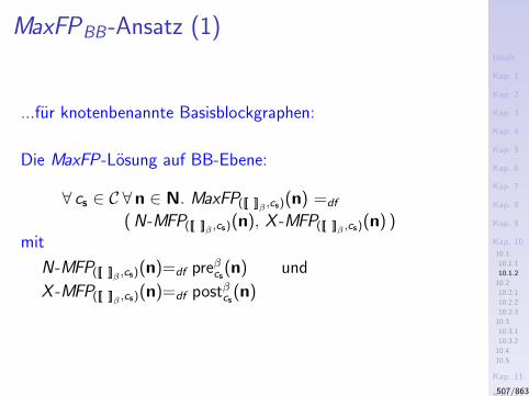
Inhalt
Kap. 1
Kap. 2
Kap. 3
Kap. 4
Kap. 5
Kap. 6
Kap. 7
Kap. 8
Kap. 9
Kap. 10
10.1
10.1.1
10.1.2
10.2
10.2.1
10.2.2
10.2.3
10.3
10.3.1
10.3.2
10.4
10.5
Kap. 11
Kap. 12
Kap. 13
Kap. 14
Kap. 15
Kap. 16
Kap. 17
Literatur
Anhang
A
MaxFPBB-Ansatz (1)
...fur knotenbenannte Basisblockgraphen:
Die MaxFP-Losung auf BB-Ebene:
∀ cs ∈ C ∀n ∈ N. MaxFP([[ ]]β ,cs)(n) =df
( N-MFP([[ ]]β ,cs)(n), X -MFP([[ ]]β ,cs)(n) )mit
N-MFP([[ ]]β ,cs)(n)=df preβcs(n) und
X -MFP([[ ]]β ,cs)(n)=df postβcs(n)
507/863
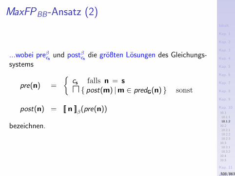
Inhalt
Kap. 1
Kap. 2
Kap. 3
Kap. 4
Kap. 5
Kap. 6
Kap. 7
Kap. 8
Kap. 9
Kap. 10
10.1
10.1.1
10.1.2
10.2
10.2.1
10.2.2
10.2.3
10.3
10.3.1
10.3.2
10.4
10.5
Kap. 11
Kap. 12
Kap. 13
Kap. 14
Kap. 15
Kap. 16
Kap. 17
Literatur
Anhang
A
MaxFPBB-Ansatz (2)
...wobei preβcsund postβcs
die großten Losungen des Gleichungs-systems
pre(n) =
cs falls n = su post(m) |m ∈ predG(n) sonst
post(n) = [[ n ]]β(pre(n))
bezeichnen.
508/863
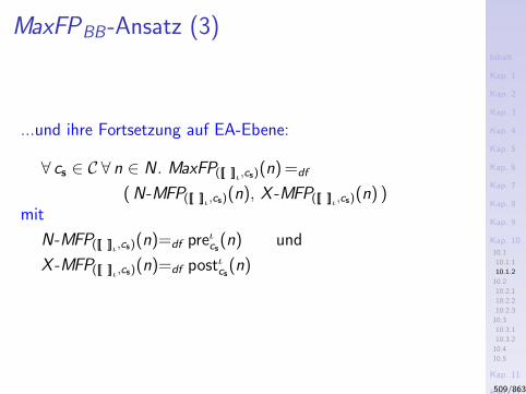
Inhalt
Kap. 1
Kap. 2
Kap. 3
Kap. 4
Kap. 5
Kap. 6
Kap. 7
Kap. 8
Kap. 9
Kap. 10
10.1
10.1.1
10.1.2
10.2
10.2.1
10.2.2
10.2.3
10.3
10.3.1
10.3.2
10.4
10.5
Kap. 11
Kap. 12
Kap. 13
Kap. 14
Kap. 15
Kap. 16
Kap. 17
Literatur
Anhang
A
MaxFPBB-Ansatz (3)
...und ihre Fortsetzung auf EA-Ebene:
∀ cs ∈ C ∀ n ∈ N . MaxFP([[ ]]ι,cs)(n) =df
( N-MFP([[ ]]ι,cs)(n), X -MFP([[ ]]ι,cs)(n) )mit
N-MFP([[ ]]ι,cs)(n)=df preιcs(n) und
X -MFP([[ ]]ι,cs)(n)=df postιcs(n)
509/863
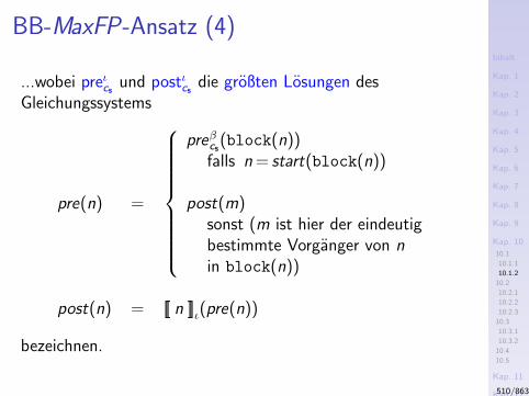
Inhalt
Kap. 1
Kap. 2
Kap. 3
Kap. 4
Kap. 5
Kap. 6
Kap. 7
Kap. 8
Kap. 9
Kap. 10
10.1
10.1.1
10.1.2
10.2
10.2.1
10.2.2
10.2.3
10.3
10.3.1
10.3.2
10.4
10.5
Kap. 11
Kap. 12
Kap. 13
Kap. 14
Kap. 15
Kap. 16
Kap. 17
Literatur
Anhang
A
BB-MaxFP-Ansatz (4)
...wobei preιcsund postιcs
die großten Losungen desGleichungssystems
pre(n) =
preβcs(block(n))
falls n = start(block(n))
post(m)sonst (m ist hier der eindeutigbestimmte Vorganger von nin block(n))
post(n) = [[ n ]]ι(pre(n))
bezeichnen.
510/863

Inhalt
Kap. 1
Kap. 2
Kap. 3
Kap. 4
Kap. 5
Kap. 6
Kap. 7
Kap. 8
Kap. 9
Kap. 10
10.1
10.1.1
10.1.2
10.2
10.2.1
10.2.2
10.2.3
10.3
10.3.1
10.3.2
10.4
10.5
Kap. 11
Kap. 12
Kap. 13
Kap. 14
Kap. 15
Kap. 16
Kap. 17
Literatur
Anhang
A
Kapitel 10.2
Verfugbarkeit von Ausdrucken
511/863

Inhalt
Kap. 1
Kap. 2
Kap. 3
Kap. 4
Kap. 5
Kap. 6
Kap. 7
Kap. 8
Kap. 9
Kap. 10
10.1
10.1.1
10.1.2
10.2
10.2.1
10.2.2
10.2.3
10.3
10.3.1
10.3.2
10.4
10.5
Kap. 11
Kap. 12
Kap. 13
Kap. 14
Kap. 15
Kap. 16
Kap. 17
Literatur
Anhang
A
Kapitel 10.2.1
Knotenbenannter Basisblockansatz
512/863
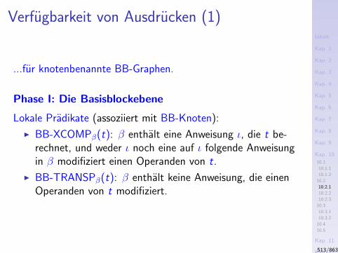
Inhalt
Kap. 1
Kap. 2
Kap. 3
Kap. 4
Kap. 5
Kap. 6
Kap. 7
Kap. 8
Kap. 9
Kap. 10
10.1
10.1.1
10.1.2
10.2
10.2.1
10.2.2
10.2.3
10.3
10.3.1
10.3.2
10.4
10.5
Kap. 11
Kap. 12
Kap. 13
Kap. 14
Kap. 15
Kap. 16
Kap. 17
Literatur
Anhang
A
Verfugbarkeit von Ausdrucken (1)
...fur knotenbenannte BB-Graphen.
Phase I: Die Basisblockebene
Lokale Pradikate (assoziiert mit BB-Knoten):
I BB-XCOMPβ(t): β enthalt eine Anweisung ι, die t be-rechnet, und weder ι noch eine auf ι folgende Anweisungin β modifiziert einen Operanden von t.
I BB-TRANSPβ(t): β enthalt keine Anweisung, die einenOperanden von t modifiziert.
513/863
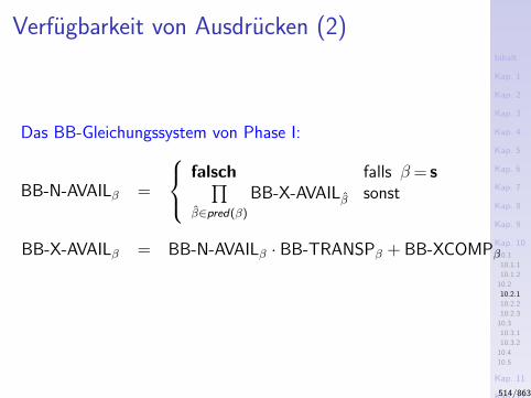
Inhalt
Kap. 1
Kap. 2
Kap. 3
Kap. 4
Kap. 5
Kap. 6
Kap. 7
Kap. 8
Kap. 9
Kap. 10
10.1
10.1.1
10.1.2
10.2
10.2.1
10.2.2
10.2.3
10.3
10.3.1
10.3.2
10.4
10.5
Kap. 11
Kap. 12
Kap. 13
Kap. 14
Kap. 15
Kap. 16
Kap. 17
Literatur
Anhang
A
Verfugbarkeit von Ausdrucken (2)
Das BB-Gleichungssystem von Phase I:
BB-N-AVAILβ =
falsch falls β = s∏β∈pred(β)
BB-X-AVAILβ sonst
BB-X-AVAILβ = BB-N-AVAILβ · BB-TRANSPβ + BB-XCOMPβ
514/863
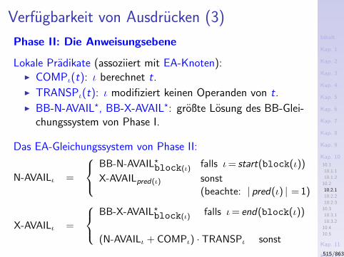
Inhalt
Kap. 1
Kap. 2
Kap. 3
Kap. 4
Kap. 5
Kap. 6
Kap. 7
Kap. 8
Kap. 9
Kap. 10
10.1
10.1.1
10.1.2
10.2
10.2.1
10.2.2
10.2.3
10.3
10.3.1
10.3.2
10.4
10.5
Kap. 11
Kap. 12
Kap. 13
Kap. 14
Kap. 15
Kap. 16
Kap. 17
Literatur
Anhang
A
Verfugbarkeit von Ausdrucken (3)
Phase II: Die Anweisungsebene
Lokale Pradikate (assoziiert mit EA-Knoten):I COMPι(t): ι berechnet t.
I TRANSPι(t): ι modifiziert keinen Operanden von t.
I BB-N-AVAIL?, BB-X-AVAIL?: großte Losung des BB-Glei-chungssystem von Phase I.
Das EA-Gleichungssystem von Phase II:
N-AVAILι =
BB-N-AVAIL?block(ι) falls ι= start(block(ι))
X-AVAILpred(ι) sonst(beachte: | pred(ι) | = 1)
X-AVAILι =
BB-X-AVAIL?block(ι) falls ι= end(block(ι))
(N-AVAILι + COMPι) · TRANSPι sonst
515/863

Inhalt
Kap. 1
Kap. 2
Kap. 3
Kap. 4
Kap. 5
Kap. 6
Kap. 7
Kap. 8
Kap. 9
Kap. 10
10.1
10.1.1
10.1.2
10.2
10.2.1
10.2.2
10.2.3
10.3
10.3.1
10.3.2
10.4
10.5
Kap. 11
Kap. 12
Kap. 13
Kap. 14
Kap. 15
Kap. 16
Kap. 17
Literatur
Anhang
A
Kapitel 10.2.2
Knotenbenannter Einzelanweisungsansatz
516/863
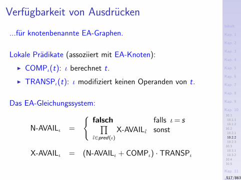
Inhalt
Kap. 1
Kap. 2
Kap. 3
Kap. 4
Kap. 5
Kap. 6
Kap. 7
Kap. 8
Kap. 9
Kap. 10
10.1
10.1.1
10.1.2
10.2
10.2.1
10.2.2
10.2.3
10.3
10.3.1
10.3.2
10.4
10.5
Kap. 11
Kap. 12
Kap. 13
Kap. 14
Kap. 15
Kap. 16
Kap. 17
Literatur
Anhang
A
Verfugbarkeit von Ausdrucken
...fur knotenbenannte EA-Graphen.
Lokale Pradikate (assoziiert mit EA-Knoten):
I COMPι(t): ι berechnet t.
I TRANSPι(t): ι modifiziert keinen Operanden von t.
Das EA-Gleichungssystem:
N-AVAILι =
falsch falls ι= s∏ι∈pred(ι)
X-AVAILι sonst
X-AVAILι = (N-AVAILι + COMPι) · TRANSPι
517/863

Inhalt
Kap. 1
Kap. 2
Kap. 3
Kap. 4
Kap. 5
Kap. 6
Kap. 7
Kap. 8
Kap. 9
Kap. 10
10.1
10.1.1
10.1.2
10.2
10.2.1
10.2.2
10.2.3
10.3
10.3.1
10.3.2
10.4
10.5
Kap. 11
Kap. 12
Kap. 13
Kap. 14
Kap. 15
Kap. 16
Kap. 17
Literatur
Anhang
A
Kapitel 10.2.3
Kantenbenannter Einzelanweisungsansatz
518/863
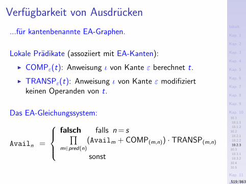
Inhalt
Kap. 1
Kap. 2
Kap. 3
Kap. 4
Kap. 5
Kap. 6
Kap. 7
Kap. 8
Kap. 9
Kap. 10
10.1
10.1.1
10.1.2
10.2
10.2.1
10.2.2
10.2.3
10.3
10.3.1
10.3.2
10.4
10.5
Kap. 11
Kap. 12
Kap. 13
Kap. 14
Kap. 15
Kap. 16
Kap. 17
Literatur
Anhang
A
Verfugbarkeit von Ausdrucken
...fur kantenbenannte EA-Graphen.
Lokale Pradikate (assoziiert mit EA-Kanten):
I COMPε(t): Anweisung ι von Kante ε berechnet t.
I TRANSPε(t): Anweisung ι von Kante ε modifiziertkeinen Operanden von t.
Das EA-Gleichungssystem:
Availn =
falsch falls n = s∏m∈pred(n)
(Availm + COMP(m,n)) · TRANSP(m,n)
sonst
519/863
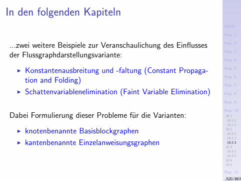
Inhalt
Kap. 1
Kap. 2
Kap. 3
Kap. 4
Kap. 5
Kap. 6
Kap. 7
Kap. 8
Kap. 9
Kap. 10
10.1
10.1.1
10.1.2
10.2
10.2.1
10.2.2
10.2.3
10.3
10.3.1
10.3.2
10.4
10.5
Kap. 11
Kap. 12
Kap. 13
Kap. 14
Kap. 15
Kap. 16
Kap. 17
Literatur
Anhang
A
In den folgenden Kapiteln
...zwei weitere Beispiele zur Veranschaulichung des Einflussesder Flussgraphdarstellungsvariante:
I Konstantenausbreitung und -faltung (Constant Propaga-tion and Folding)
I Schattenvariablenelimination (Faint Variable Elimination)
Dabei Formulierung dieser Probleme fur die Varianten:
I knotenbenannte Basisblockgraphen
I kantenbenannte Einzelanweisungsgraphen
520/863

Inhalt
Kap. 1
Kap. 2
Kap. 3
Kap. 4
Kap. 5
Kap. 6
Kap. 7
Kap. 8
Kap. 9
Kap. 10
10.1
10.1.1
10.1.2
10.2
10.2.1
10.2.2
10.2.3
10.3
10.3.1
10.3.2
10.4
10.5
Kap. 11
Kap. 12
Kap. 13
Kap. 14
Kap. 15
Kap. 16
Kap. 17
Literatur
Anhang
A
Kapitel 10.3
Konstantenausbreitung und -faltung
521/863

Inhalt
Kap. 1
Kap. 2
Kap. 3
Kap. 4
Kap. 5
Kap. 6
Kap. 7
Kap. 8
Kap. 9
Kap. 10
10.1
10.1.1
10.1.2
10.2
10.2.1
10.2.2
10.2.3
10.3
10.3.1
10.3.2
10.4
10.5
Kap. 11
Kap. 12
Kap. 13
Kap. 14
Kap. 15
Kap. 16
Kap. 17
Literatur
Anhang
A
Konstantenausbreitung und -faltung
... am Beispiel “Einfacher Konstanten”.
Wir benotigen dazu zwei Hilfsfunktionen:
I Ruckwartssubstitution
I Zustandstransformation(sfunktion)
522/863
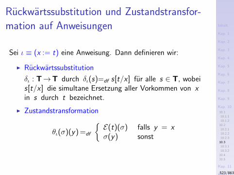
Inhalt
Kap. 1
Kap. 2
Kap. 3
Kap. 4
Kap. 5
Kap. 6
Kap. 7
Kap. 8
Kap. 9
Kap. 10
10.1
10.1.1
10.1.2
10.2
10.2.1
10.2.2
10.2.3
10.3
10.3.1
10.3.2
10.4
10.5
Kap. 11
Kap. 12
Kap. 13
Kap. 14
Kap. 15
Kap. 16
Kap. 17
Literatur
Anhang
A
Ruckwartssubstitution und Zustandstransfor-
mation auf Anweisungen
Sei ι ≡ (x := t) eine Anweisung. Dann definieren wir:
I Ruckwartssubstitution
δι : T→T durch δι(s)=df s[t/x ] fur alle s ∈ T, wobeis[t/x ] die simultane Ersetzung aller Vorkommen von xin s durch t bezeichnet.
I Zustandstransformation
θι(σ)(y) =df
E(t)(σ) falls y = xσ(y) sonst
523/863
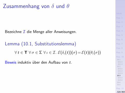
Inhalt
Kap. 1
Kap. 2
Kap. 3
Kap. 4
Kap. 5
Kap. 6
Kap. 7
Kap. 8
Kap. 9
Kap. 10
10.1
10.1.1
10.1.2
10.2
10.2.1
10.2.2
10.2.3
10.3
10.3.1
10.3.2
10.4
10.5
Kap. 11
Kap. 12
Kap. 13
Kap. 14
Kap. 15
Kap. 16
Kap. 17
Literatur
Anhang
A
Zusammenhang von δ und θ
Bezeichne I die Menge aller Anweisungen.
Lemma (10.1, Substitutionslemma)
∀ t ∈ T ∀σ ∈ Σ ∀ ι ∈ I. E(δι(t))(σ) = E(t)(θι(σ))
Beweis induktiv uber den Aufbau von t.
524/863

Inhalt
Kap. 1
Kap. 2
Kap. 3
Kap. 4
Kap. 5
Kap. 6
Kap. 7
Kap. 8
Kap. 9
Kap. 10
10.1
10.1.1
10.1.2
10.2
10.2.1
10.2.2
10.2.3
10.3
10.3.1
10.3.2
10.4
10.5
Kap. 11
Kap. 12
Kap. 13
Kap. 14
Kap. 15
Kap. 16
Kap. 17
Literatur
Anhang
A
Kapitel 10.3.1
Kantenbenannter Einzelanweisungsansatz
525/863
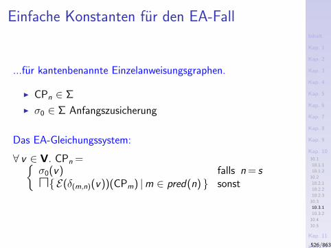
Inhalt
Kap. 1
Kap. 2
Kap. 3
Kap. 4
Kap. 5
Kap. 6
Kap. 7
Kap. 8
Kap. 9
Kap. 10
10.1
10.1.1
10.1.2
10.2
10.2.1
10.2.2
10.2.3
10.3
10.3.1
10.3.2
10.4
10.5
Kap. 11
Kap. 12
Kap. 13
Kap. 14
Kap. 15
Kap. 16
Kap. 17
Literatur
Anhang
A
Einfache Konstanten fur den EA-Fall
...fur kantenbenannte Einzelanweisungsgraphen.
I CPn ∈ Σ
I σ0 ∈ Σ Anfangszusicherung
Das EA-Gleichungssystem:
∀ v ∈ V. CPn =σ0(v) falls n = su E(δ(m,n)(v))(CPm) |m ∈ pred(n) sonst
526/863

Inhalt
Kap. 1
Kap. 2
Kap. 3
Kap. 4
Kap. 5
Kap. 6
Kap. 7
Kap. 8
Kap. 9
Kap. 10
10.1
10.1.1
10.1.2
10.2
10.2.1
10.2.2
10.2.3
10.3
10.3.1
10.3.2
10.4
10.5
Kap. 11
Kap. 12
Kap. 13
Kap. 14
Kap. 15
Kap. 16
Kap. 17
Literatur
Anhang
A
Kapitel 10.3.2
Knotenbenannter Basisblockansatz
527/863
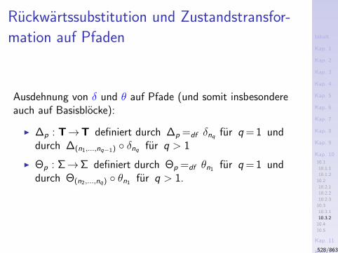
Inhalt
Kap. 1
Kap. 2
Kap. 3
Kap. 4
Kap. 5
Kap. 6
Kap. 7
Kap. 8
Kap. 9
Kap. 10
10.1
10.1.1
10.1.2
10.2
10.2.1
10.2.2
10.2.3
10.3
10.3.1
10.3.2
10.4
10.5
Kap. 11
Kap. 12
Kap. 13
Kap. 14
Kap. 15
Kap. 16
Kap. 17
Literatur
Anhang
A
Ruckwartssubstitution und Zustandstransfor-
mation auf Pfaden
Ausdehnung von δ und θ auf Pfade (und somit insbesondereauch auf Basisblocke):
I ∆p : T→T definiert durch ∆p =df δnq fur q = 1 unddurch ∆(n1,...,nq−1) δnq fur q > 1
I Θp : Σ→Σ definiert durch Θp =df θn1 fur q = 1 unddurch Θ(n2,...,nq) θn1 fur q > 1.
528/863
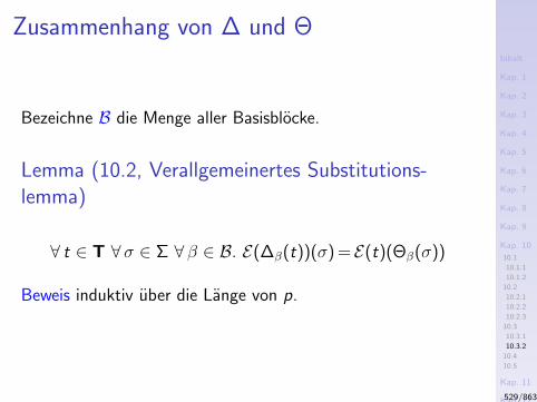
Inhalt
Kap. 1
Kap. 2
Kap. 3
Kap. 4
Kap. 5
Kap. 6
Kap. 7
Kap. 8
Kap. 9
Kap. 10
10.1
10.1.1
10.1.2
10.2
10.2.1
10.2.2
10.2.3
10.3
10.3.1
10.3.2
10.4
10.5
Kap. 11
Kap. 12
Kap. 13
Kap. 14
Kap. 15
Kap. 16
Kap. 17
Literatur
Anhang
A
Zusammenhang von ∆ und Θ
Bezeichne B die Menge aller Basisblocke.
Lemma (10.2, Verallgemeinertes Substitutions-lemma)
∀ t ∈ T ∀σ ∈ Σ ∀ β ∈ B. E(∆β(t))(σ) = E(t)(Θβ(σ))
Beweis induktiv uber die Lange von p.
529/863
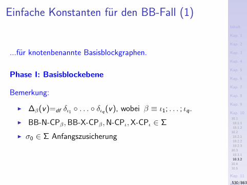
Inhalt
Kap. 1
Kap. 2
Kap. 3
Kap. 4
Kap. 5
Kap. 6
Kap. 7
Kap. 8
Kap. 9
Kap. 10
10.1
10.1.1
10.1.2
10.2
10.2.1
10.2.2
10.2.3
10.3
10.3.1
10.3.2
10.4
10.5
Kap. 11
Kap. 12
Kap. 13
Kap. 14
Kap. 15
Kap. 16
Kap. 17
Literatur
Anhang
A
Einfache Konstanten fur den BB-Fall (1)
...fur knotenbenannte Basisblockgraphen.
Phase I: Basisblockebene
Bemerkung:
I ∆β(v)=df δι1 . . . διq(v), wobei β ≡ ι1; . . . ; ιq.
I BB-N-CPβ,BB-X-CPβ,N-CPι,X-CPι ∈ Σ
I σ0 ∈ Σ Anfangszusicherung
530/863
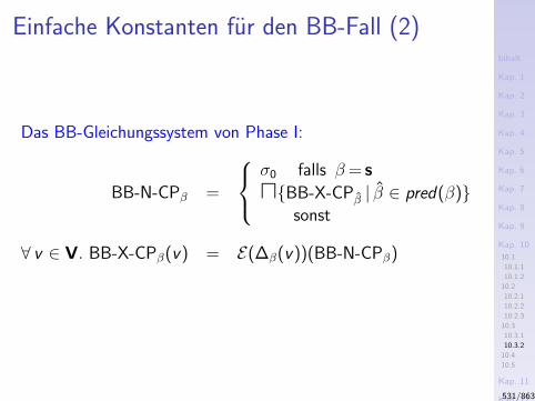
Inhalt
Kap. 1
Kap. 2
Kap. 3
Kap. 4
Kap. 5
Kap. 6
Kap. 7
Kap. 8
Kap. 9
Kap. 10
10.1
10.1.1
10.1.2
10.2
10.2.1
10.2.2
10.2.3
10.3
10.3.1
10.3.2
10.4
10.5
Kap. 11
Kap. 12
Kap. 13
Kap. 14
Kap. 15
Kap. 16
Kap. 17
Literatur
Anhang
A
Einfache Konstanten fur den BB-Fall (2)
Das BB-Gleichungssystem von Phase I:
BB-N-CPβ =
σ0 falls β = s
uBB-X-CPβ | β ∈ pred(β)sonst
∀ v ∈ V. BB-X-CPβ(v) = E(∆β(v))(BB-N-CPβ)
531/863
Inhalt
Kap. 1
Kap. 2
Kap. 3
Kap. 4
Kap. 5
Kap. 6
Kap. 7
Kap. 8
Kap. 9
Kap. 10
10.1
10.1.1
10.1.2
10.2
10.2.1
10.2.2
10.2.3
10.3
10.3.1
10.3.2
10.4
10.5
Kap. 11
Kap. 12
Kap. 13
Kap. 14
Kap. 15
Kap. 16
Kap. 17
Literatur
Anhang
A
Einfache Konstanten fur den BB-Fall (3)
Phase II: Anweisungsebene
Vorberechnete Resultate (aus Phase I):
I BB-N-CP?, BB-X-CP?: die großte Losung des Glei-chungssystems von Phase I.
532/863
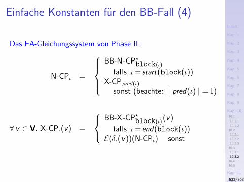
Inhalt
Kap. 1
Kap. 2
Kap. 3
Kap. 4
Kap. 5
Kap. 6
Kap. 7
Kap. 8
Kap. 9
Kap. 10
10.1
10.1.1
10.1.2
10.2
10.2.1
10.2.2
10.2.3
10.3
10.3.1
10.3.2
10.4
10.5
Kap. 11
Kap. 12
Kap. 13
Kap. 14
Kap. 15
Kap. 16
Kap. 17
Literatur
Anhang
A
Einfache Konstanten fur den BB-Fall (4)
Das EA-Gleichungssystem von Phase II:
N-CPι =
BB-N-CP?block(ι)
falls ι= start(block(ι))X-CPpred(ι)
sonst (beachte: | pred(ι) | = 1)
∀ v ∈ V. X-CPι(v) =
BB-X-CP?block(ι)
(v)
falls ι= end(block(ι))E(δι(v))(N-CPι) sonst
533/863

Inhalt
Kap. 1
Kap. 2
Kap. 3
Kap. 4
Kap. 5
Kap. 6
Kap. 7
Kap. 8
Kap. 9
Kap. 10
10.1
10.1.1
10.1.2
10.2
10.2.1
10.2.2
10.2.3
10.3
10.3.1
10.3.2
10.4
10.5
Kap. 11
Kap. 12
Kap. 13
Kap. 14
Kap. 15
Kap. 16
Kap. 17
Literatur
Anhang
A
Kapitel 10.4
Schattenvariablen
534/863
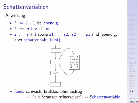
Inhalt
Kap. 1
Kap. 2
Kap. 3
Kap. 4
Kap. 5
Kap. 6
Kap. 7
Kap. 8
Kap. 9
Kap. 10
10.1
10.1.1
10.1.2
10.2
10.2.1
10.2.2
10.2.3
10.3
10.3.1
10.3.2
10.4
10.5
Kap. 11
Kap. 12
Kap. 13
Kap. 14
Kap. 15
Kap. 16
Kap. 17
Literatur
Anhang
A
SchattenvariablenAnweisung
I l := l + 1 ist lebendig.I t := u + v ist tot.I s := s + 1 sowie s1 := s2; s2 := s1 sind lebendig,
aber schattenhaft (faint).
e
out(l)
l := l+1t := u+v
s1 := s2
s2 := s1s := s+1
I faint: schwach, kraftlos, ohnmachtig “ein Schatten seinerselbst” Schattenvariable
535/863
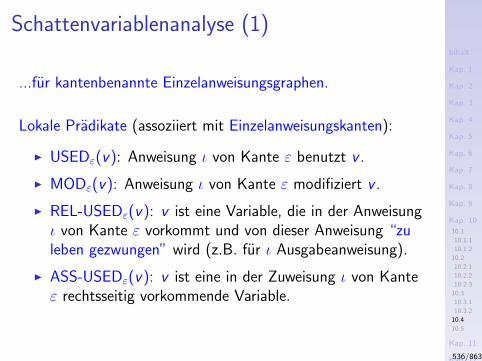
Inhalt
Kap. 1
Kap. 2
Kap. 3
Kap. 4
Kap. 5
Kap. 6
Kap. 7
Kap. 8
Kap. 9
Kap. 10
10.1
10.1.1
10.1.2
10.2
10.2.1
10.2.2
10.2.3
10.3
10.3.1
10.3.2
10.4
10.5
Kap. 11
Kap. 12
Kap. 13
Kap. 14
Kap. 15
Kap. 16
Kap. 17
Literatur
Anhang
A
Schattenvariablenanalyse (1)
...fur kantenbenannte Einzelanweisungsgraphen.
Lokale Pradikate (assoziiert mit Einzelanweisungskanten):
I USEDε(v): Anweisung ι von Kante ε benutzt v .
I MODε(v): Anweisung ι von Kante ε modifiziert v .
I REL-USEDε(v): v ist eine Variable, die in der Anweisungι von Kante ε vorkommt und von dieser Anweisung “zuleben gezwungen” wird (z.B. fur ι Ausgabeanweisung).
I ASS-USEDε(v): v ist eine in der Zuweisung ι von Kanteε rechtsseitig vorkommende Variable.
536/863
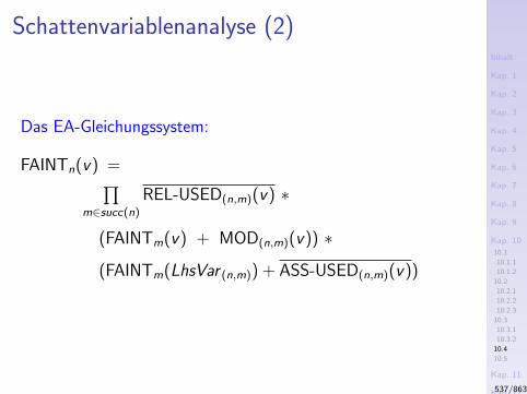
Inhalt
Kap. 1
Kap. 2
Kap. 3
Kap. 4
Kap. 5
Kap. 6
Kap. 7
Kap. 8
Kap. 9
Kap. 10
10.1
10.1.1
10.1.2
10.2
10.2.1
10.2.2
10.2.3
10.3
10.3.1
10.3.2
10.4
10.5
Kap. 11
Kap. 12
Kap. 13
Kap. 14
Kap. 15
Kap. 16
Kap. 17
Literatur
Anhang
A
Schattenvariablenanalyse (2)
Das EA-Gleichungssystem:
FAINTn(v) =∏m∈succ(n)
REL-USED(n,m)(v) ∗
(FAINTm(v) + MOD(n,m)(v)) ∗
(FAINTm(LhsVar (n,m)) + ASS-USED(n,m)(v))
537/863
Inhalt
Kap. 1
Kap. 2
Kap. 3
Kap. 4
Kap. 5
Kap. 6
Kap. 7
Kap. 8
Kap. 9
Kap. 10
10.1
10.1.1
10.1.2
10.2
10.2.1
10.2.2
10.2.3
10.3
10.3.1
10.3.2
10.4
10.5
Kap. 11
Kap. 12
Kap. 13
Kap. 14
Kap. 15
Kap. 16
Kap. 17
Literatur
Anhang
A
Schattenvariablenanalyse (3)
...ein Beispiel fur ein DFA-Problem, fur das eine Formulierung
I auf (knoten- und kantenbenannten) Einzelanweisungs-graphen offensichtlich ist,
I auf (knoten- und kantenbenannten) Basisblockgraphenalles andere als ersichtlich, nicht moglich ist.
538/863

Inhalt
Kap. 1
Kap. 2
Kap. 3
Kap. 4
Kap. 5
Kap. 6
Kap. 7
Kap. 8
Kap. 9
Kap. 10
10.1
10.1.1
10.1.2
10.2
10.2.1
10.2.2
10.2.3
10.3
10.3.1
10.3.2
10.4
10.5
Kap. 11
Kap. 12
Kap. 13
Kap. 14
Kap. 15
Kap. 16
Kap. 17
Literatur
Anhang
A
Kapitel 10.5
Fazit
539/863
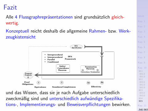
Inhalt
Kap. 1
Kap. 2
Kap. 3
Kap. 4
Kap. 5
Kap. 6
Kap. 7
Kap. 8
Kap. 9
Kap. 10
10.1
10.1.1
10.1.2
10.2
10.2.1
10.2.2
10.2.3
10.3
10.3.1
10.3.2
10.4
10.5
Kap. 11
Kap. 12
Kap. 13
Kap. 14
Kap. 15
Kap. 16
Kap. 17
Literatur
Anhang
A
Fazit
Alle 4 Flussgraphreprasentationen sind grundsatzlich gleich-wertig.
Konzeptuell reicht deshalb die allgemeine Rahmen- bzw. Werk-zeugkistensicht
φ
Program
TheoremCorrectness Termination
Property
Safety/Coincidence
1 3b)2
3b)
Intraprocedural
Interprocedural
Conditional
Equivalence Effectivity
DFA
Framework
Theorem3a)
3a)ProofObligations:
Parallel
Termination
Soundness/Completeness
DFA
Specification
und das Wissen, dass sie je nach Aufgabe unterschiedlichzweckmaßig sind und unterschiedlich aufwandige Spezifika-tions-, Implementierungs- und Beweisverpflichtungen bewirken.
540/863
Inhalt
Kap. 1
Kap. 2
Kap. 3
Kap. 4
Kap. 5
Kap. 6
Kap. 7
Kap. 8
Kap. 9
Kap. 10
10.1
10.1.1
10.1.2
10.2
10.2.1
10.2.2
10.2.3
10.3
10.3.1
10.3.2
10.4
10.5
Kap. 11
Kap. 12
Kap. 13
Kap. 14
Kap. 15
Kap. 16
Kap. 17
Literatur
Anhang
A
Vertiefende und weiterfuhrende Leseempfeh-
lungen fur Kapitel 10
Jens Knoop, Dirk Koschutzki, Bernhard Steffen. Basic-block graphs: Living dinosaurs? In Proceedings of the 7thInternational Conference on Compiler Construction(CC’98), Springer-V., LNCS 1383, 65 - 79, 1998.
541/863

Inhalt
Kap. 1
Kap. 2
Kap. 3
Kap. 4
Kap. 5
Kap. 6
Kap. 7
Kap. 8
Kap. 9
Kap. 10
10.1
10.1.1
10.1.2
10.2
10.2.1
10.2.2
10.2.3
10.3
10.3.1
10.3.2
10.4
10.5
Kap. 11
Kap. 12
Kap. 13
Kap. 14
Kap. 15
Kap. 16
Kap. 17
Literatur
Anhang
A
Teil III
Transformation und Optimalitat
542/863
Inhalt
Kap. 1
Kap. 2
Kap. 3
Kap. 4
Kap. 5
Kap. 6
Kap. 7
Kap. 8
Kap. 9
Kap. 10
10.1
10.1.1
10.1.2
10.2
10.2.1
10.2.2
10.2.3
10.3
10.3.1
10.3.2
10.4
10.5
Kap. 11
Kap. 12
Kap. 13
Kap. 14
Kap. 15
Kap. 16
Kap. 17
Literatur
Anhang
A
Intuition
Optimalitat = Korrektheit + Vollstandigkeit
543/863

Inhalt
Kap. 1
Kap. 2
Kap. 3
Kap. 4
Kap. 5
Kap. 6
Kap. 7
Kap. 8
Kap. 9
Kap. 10
Kap. 11
11.1
11.2
11.3
Kap. 12
Kap. 13
Kap. 14
Kap. 15
Kap. 16
Kap. 17
Literatur
Anhang
A
Kapitel 11
Elimination partiell toter Anweisungen
544/863

Inhalt
Kap. 1
Kap. 2
Kap. 3
Kap. 4
Kap. 5
Kap. 6
Kap. 7
Kap. 8
Kap. 9
Kap. 10
Kap. 11
11.1
11.2
11.3
Kap. 12
Kap. 13
Kap. 14
Kap. 15
Kap. 16
Kap. 17
Literatur
Anhang
A
Kapitel 11.1
Motivation
545/863
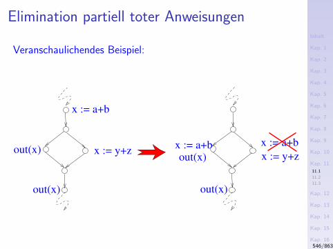
Inhalt
Kap. 1
Kap. 2
Kap. 3
Kap. 4
Kap. 5
Kap. 6
Kap. 7
Kap. 8
Kap. 9
Kap. 10
Kap. 11
11.1
11.2
11.3
Kap. 12
Kap. 13
Kap. 14
Kap. 15
Kap. 16
Kap. 17
Literatur
Anhang
A
Elimination partiell toter Anweisungen
Veranschaulichendes Beispiel:
out(x)
x := a+b
out(x) x := y+z
out(x)
out(x)x := a+b
x := y+z
x := a+b
546/863
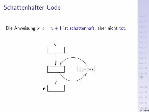
Inhalt
Kap. 1
Kap. 2
Kap. 3
Kap. 4
Kap. 5
Kap. 6
Kap. 7
Kap. 8
Kap. 9
Kap. 10
Kap. 11
11.1
11.2
11.3
Kap. 12
Kap. 13
Kap. 14
Kap. 15
Kap. 16
Kap. 17
Literatur
Anhang
A
Schattenhafter Code
Die Anweisung x := x + 1 ist schattenhaft, aber nicht tot.
e
x := x+1
547/863
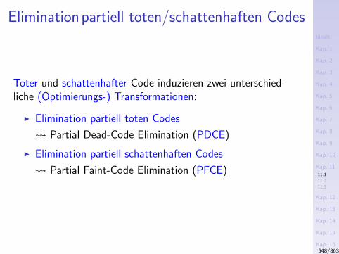
Inhalt
Kap. 1
Kap. 2
Kap. 3
Kap. 4
Kap. 5
Kap. 6
Kap. 7
Kap. 8
Kap. 9
Kap. 10
Kap. 11
11.1
11.2
11.3
Kap. 12
Kap. 13
Kap. 14
Kap. 15
Kap. 16
Kap. 17
Literatur
Anhang
A
Elimination partiell toten/schattenhaften Codes
Toter und schattenhafter Code induzieren zwei unterschied-liche (Optimierungs-) Transformationen:
I Elimination partiell toten Codes
Partial Dead-Code Elimination (PDCE)
I Elimination partiell schattenhaften Codes
Partial Faint-Code Elimination (PFCE)
548/863
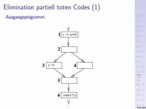
Inhalt
Kap. 1
Kap. 2
Kap. 3
Kap. 4
Kap. 5
Kap. 6
Kap. 7
Kap. 8
Kap. 9
Kap. 10
Kap. 11
11.1
11.2
11.3
Kap. 12
Kap. 13
Kap. 14
Kap. 15
Kap. 16
Kap. 17
Literatur
Anhang
A
Elimination partiell toten Codes (1)
Ausgangsprogramm:
1
2
3 4
5
6 out(x*y)
y :=
y := a+b
549/863
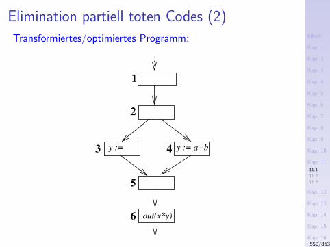
Inhalt
Kap. 1
Kap. 2
Kap. 3
Kap. 4
Kap. 5
Kap. 6
Kap. 7
Kap. 8
Kap. 9
Kap. 10
Kap. 11
11.1
11.2
11.3
Kap. 12
Kap. 13
Kap. 14
Kap. 15
Kap. 16
Kap. 17
Literatur
Anhang
A
Elimination partiell toten Codes (2)
Transformiertes/optimiertes Programm:
1
2
3 4
5
6 out(x*y)
y := y := a+b
550/863
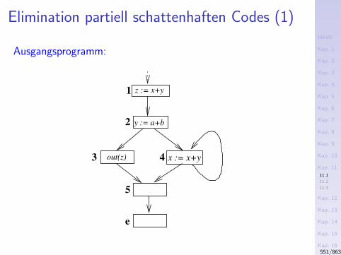
Inhalt
Kap. 1
Kap. 2
Kap. 3
Kap. 4
Kap. 5
Kap. 6
Kap. 7
Kap. 8
Kap. 9
Kap. 10
Kap. 11
11.1
11.2
11.3
Kap. 12
Kap. 13
Kap. 14
Kap. 15
Kap. 16
Kap. 17
Literatur
Anhang
A
Elimination partiell schattenhaften Codes (1)
Ausgangsprogramm:
1
2
3 4
5
e
z := x+y
x := x+y
y := a+b
out(z)
551/863
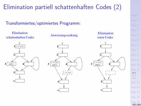
Inhalt
Kap. 1
Kap. 2
Kap. 3
Kap. 4
Kap. 5
Kap. 6
Kap. 7
Kap. 8
Kap. 9
Kap. 10
Kap. 11
11.1
11.2
11.3
Kap. 12
Kap. 13
Kap. 14
Kap. 15
Kap. 16
Kap. 17
Literatur
Anhang
A
Elimination partiell schattenhaften Codes (2)
Transformiertes/optimiertes Programm:
Elimination
schattenhaften CodesAnweisungssenkung
Elimination
toten Codes
1
2
3 4out(z)z := x+y
1
2
3 4
5
e
z := x+y
out(z)
1
2
3 4out(z)z := x+y
z := x+y
5
e
5
e
552/863
Inhalt
Kap. 1
Kap. 2
Kap. 3
Kap. 4
Kap. 5
Kap. 6
Kap. 7
Kap. 8
Kap. 9
Kap. 10
Kap. 11
11.1
11.2
11.3
Kap. 12
Kap. 13
Kap. 14
Kap. 15
Kap. 16
Kap. 17
Literatur
Anhang
A
Elimination partiell schattenhaften Codes (3)
Beachte:
I “Echt” partiell schattenhaften Code gibt es nicht.
Die Elimination schattenhaften Codes
I kann aber durch die Beseitigung von Codesenkungs-blockaden die Elimination weiteren partiell toten Codesermoglichen.
In diesem Sinne ist
I Elimination partiell schattenhaften Codes
zu verstehen.
553/863

Inhalt
Kap. 1
Kap. 2
Kap. 3
Kap. 4
Kap. 5
Kap. 6
Kap. 7
Kap. 8
Kap. 9
Kap. 10
Kap. 11
11.1
11.2
11.3
Kap. 12
Kap. 13
Kap. 14
Kap. 15
Kap. 16
Kap. 17
Literatur
Anhang
A
Kapitel 11.2
PDCE/PFCE: Transformation undOptimalitat
554/863
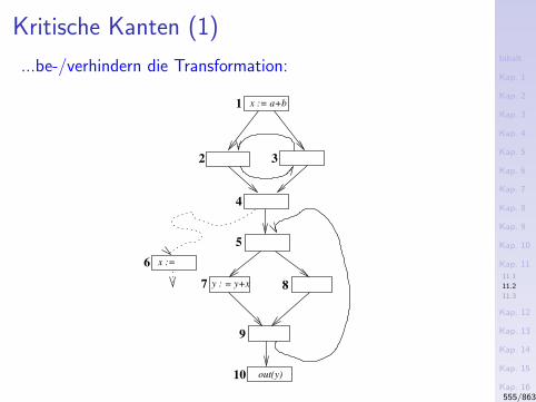
Inhalt
Kap. 1
Kap. 2
Kap. 3
Kap. 4
Kap. 5
Kap. 6
Kap. 7
Kap. 8
Kap. 9
Kap. 10
Kap. 11
11.1
11.2
11.3
Kap. 12
Kap. 13
Kap. 14
Kap. 15
Kap. 16
Kap. 17
Literatur
Anhang
A
Kritische Kanten (1)
...be-/verhindern die Transformation:
7 8
out(y)
y : = y+x
2 3
10
9
1 x := a+b
x := 6
4
5
555/863
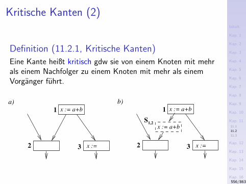
Inhalt
Kap. 1
Kap. 2
Kap. 3
Kap. 4
Kap. 5
Kap. 6
Kap. 7
Kap. 8
Kap. 9
Kap. 10
Kap. 11
11.1
11.2
11.3
Kap. 12
Kap. 13
Kap. 14
Kap. 15
Kap. 16
Kap. 17
Literatur
Anhang
A
Kritische Kanten (2)
Definition (11.2.1, Kritische Kanten)
Eine Kante heißt kritisch gdw sie von einem Knoten mit mehrals einem Nachfolger zu einem Knoten mit mehr als einemVorganger fuhrt.
x := a+b
x :=
1
2 3
a)x := a+b
x :=
1
2 3
b)
x := a+bS1,2
556/863
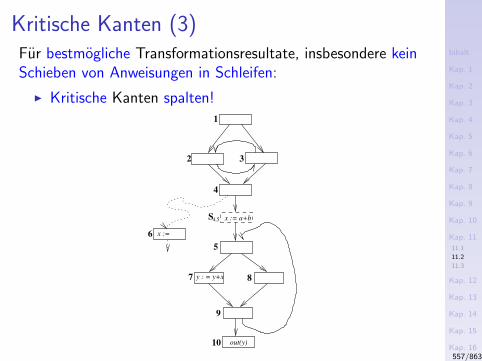
Inhalt
Kap. 1
Kap. 2
Kap. 3
Kap. 4
Kap. 5
Kap. 6
Kap. 7
Kap. 8
Kap. 9
Kap. 10
Kap. 11
11.1
11.2
11.3
Kap. 12
Kap. 13
Kap. 14
Kap. 15
Kap. 16
Kap. 17
Literatur
Anhang
A
Kritische Kanten (3)Fur bestmogliche Transformationsresultate, insbesondere keinSchieben von Anweisungen in Schleifen:
I Kritische Kanten spalten!
6
2 3
1
x :=
4
S4,5
8
out(y)
y : = y+x
10
9
5
x := a+b
7
557/863
Inhalt
Kap. 1
Kap. 2
Kap. 3
Kap. 4
Kap. 5
Kap. 6
Kap. 7
Kap. 8
Kap. 9
Kap. 10
Kap. 11
11.1
11.2
11.3
Kap. 12
Kap. 13
Kap. 14
Kap. 15
Kap. 16
Kap. 17
Literatur
Anhang
A
Anweisungsmuster
In der Folge bezeichne:
I α ein sog. Anweisungsmuster: α ≡ x := t
I AP die Menge aller Anweisungsmuster
558/863
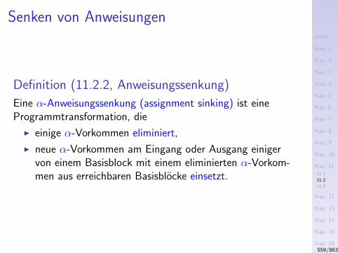
Inhalt
Kap. 1
Kap. 2
Kap. 3
Kap. 4
Kap. 5
Kap. 6
Kap. 7
Kap. 8
Kap. 9
Kap. 10
Kap. 11
11.1
11.2
11.3
Kap. 12
Kap. 13
Kap. 14
Kap. 15
Kap. 16
Kap. 17
Literatur
Anhang
A
Senken von Anweisungen
Definition (11.2.2, Anweisungssenkung)
Eine α-Anweisungssenkung (assignment sinking) ist eineProgrammtransformation, die
I einige α-Vorkommen eliminiert,
I neue α-Vorkommen am Eingang oder Ausgang einigervon einem Basisblock mit einem eliminierten α-Vorkom-men aus erreichbaren Basisblocke einsetzt.
559/863
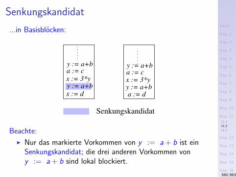
Inhalt
Kap. 1
Kap. 2
Kap. 3
Kap. 4
Kap. 5
Kap. 6
Kap. 7
Kap. 8
Kap. 9
Kap. 10
Kap. 11
11.1
11.2
11.3
Kap. 12
Kap. 13
Kap. 14
Kap. 15
Kap. 16
Kap. 17
Literatur
Anhang
A
Senkungskandidat
...in Basisblocken:
Senkungskandidat
x := d
x := 3*y
y := a+ba := c
y := a+b
a := dy := a+bx := 3*ya := cy := a+b
Beachte:
I Nur das markierte Vorkommen von y := a + b ist einSenkungskandidat; die drei anderen Vorkommen vony := a + b sind lokal blockiert.
560/863
Inhalt
Kap. 1
Kap. 2
Kap. 3
Kap. 4
Kap. 5
Kap. 6
Kap. 7
Kap. 8
Kap. 9
Kap. 10
Kap. 11
11.1
11.2
11.3
Kap. 12
Kap. 13
Kap. 14
Kap. 15
Kap. 16
Kap. 17
Literatur
Anhang
A
Lokale Barrieren
Definition (11.2.3, Lokale Barrieren)
Eine α-Anweisungssenkung wird blockiert von einerAnweisung, die
I einen Operanden von t modifiziert oder
I die Variable x liest oder modifiziert.
561/863
Inhalt
Kap. 1
Kap. 2
Kap. 3
Kap. 4
Kap. 5
Kap. 6
Kap. 7
Kap. 8
Kap. 9
Kap. 10
Kap. 11
11.1
11.2
11.3
Kap. 12
Kap. 13
Kap. 14
Kap. 15
Kap. 16
Kap. 17
Literatur
Anhang
A
Zulassiges Senken von Anweisungen
Definition (11.2.4, Zulassige Anweisungssenkung)
Ein α-Anweisungssenkung ist zulassig gdw
1. Die eliminierten α-Vorkommen werden ersetzt, d.h. aufjedem von einem Knoten n mit eliminiertem α-Vorkom-men ausgehenden Pfad zum Endknoten e gibt es einenKnoten m, an dem ein neues α-Vorkommen eingesetztwird und α von keiner Anweisung zwischen n and mblockiert ist.
2. Jedes neue Vorkommen von α ist gerechtfertigt, d.h., aufjedem vom Startknoten s aus einen Knoten n mit neueingesetztem α-Vorkommen erreichenden Pfad gibt eseinen Knoten m, an dem ein (ursprungliches) α-Vorkom-men eliminiert worden ist und α von keiner Anweisungzwischen m and n blockiert ist.
562/863
Inhalt
Kap. 1
Kap. 2
Kap. 3
Kap. 4
Kap. 5
Kap. 6
Kap. 7
Kap. 8
Kap. 9
Kap. 10
Kap. 11
11.1
11.2
11.3
Kap. 12
Kap. 13
Kap. 14
Kap. 15
Kap. 16
Kap. 17
Literatur
Anhang
A
Elimination von Anweisungen
Definition (11.2.5, Anweisungselimination)
Eine α-Anweisungselimination (assignment elimination) isteine Programmtransformation, die einige α-Vorkommen ausdem Argumentprogramm streicht.
563/863
Inhalt
Kap. 1
Kap. 2
Kap. 3
Kap. 4
Kap. 5
Kap. 6
Kap. 7
Kap. 8
Kap. 9
Kap. 10
Kap. 11
11.1
11.2
11.3
Kap. 12
Kap. 13
Kap. 14
Kap. 15
Kap. 16
Kap. 17
Literatur
Anhang
A
Zulassige Elimination von Anweisungen
Definition (11.2.6, Zulassige Anweisungselimination)
Eine α-Anweisungselimination ist zulassig gdw sie streichteinige
I tote
I schattenhafte
α-Vorkommen aus dem Argumentprogramm.
Wir bezeichnen diese beiden Transformationen als
I Elimination toten Codes
Dead-Code Elimination (DCE)
I Elimination schattenhaften Codes
Faint-Code Elimination (FCE)
564/863
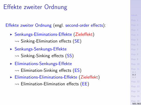
Inhalt
Kap. 1
Kap. 2
Kap. 3
Kap. 4
Kap. 5
Kap. 6
Kap. 7
Kap. 8
Kap. 9
Kap. 10
Kap. 11
11.1
11.2
11.3
Kap. 12
Kap. 13
Kap. 14
Kap. 15
Kap. 16
Kap. 17
Literatur
Anhang
A
Effekte zweiter Ordnung
Effekte zweiter Ordnung (engl. second-order effects):
I Senkungs-Eliminations-Effekte (Zieleffekt)
Sinking-Elimination effects (SE)
I Senkungs-Senkungs-Effekte
Sinking-Sinking effects (SS)
I Eliminations-Senkungs-Effekte
Elimination-Sinking effects (ES)
I Eliminations-Eliminations-Effekte (Zieleffekt)
Elimination-Elimination effects (EE)
565/863
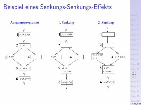
Inhalt
Kap. 1
Kap. 2
Kap. 3
Kap. 4
Kap. 5
Kap. 6
Kap. 7
Kap. 8
Kap. 9
Kap. 10
Kap. 11
11.1
11.2
11.3
Kap. 12
Kap. 13
Kap. 14
Kap. 15
Kap. 16
Kap. 17
Literatur
Anhang
A
Beispiel eines Senkungs-Senkungs-Effekts
Ausgangsprogramm 2. Senkung1. Senkung
1
2
4
5
6 out(x*y)
y :=
a :=
y := a+b
x := a+c
6 out(x*y)
3
1
2
4
5
y :=
x := a+c
a :=
6 out(x*y)
y := a+b 1
2
4
5
y := a+b
x := a+c
a :=
y :=
y := a+b
566/863
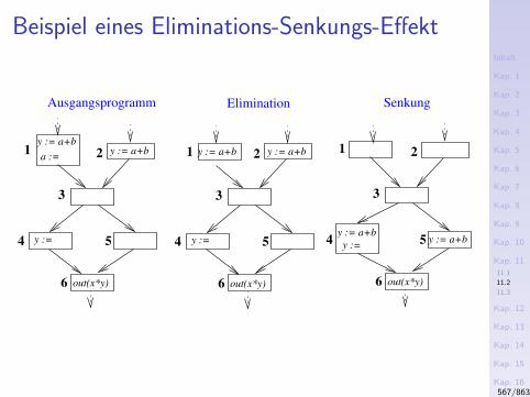
Inhalt
Kap. 1
Kap. 2
Kap. 3
Kap. 4
Kap. 5
Kap. 6
Kap. 7
Kap. 8
Kap. 9
Kap. 10
Kap. 11
11.1
11.2
11.3
Kap. 12
Kap. 13
Kap. 14
Kap. 15
Kap. 16
Kap. 17
Literatur
Anhang
A
Beispiel eines Eliminations-Senkungs-Effekt
SenkungEliminationAusgangsprogramm
y := a+by := a+b
4 5
6
y :=
2
3
out(x*y)
5
6
21
3
out(x*y)
y := a+b1
y :=
y := a+by := a+b5
6
y :=
21y := a+b
a :=
3
out(x*y)
4 4
567/863
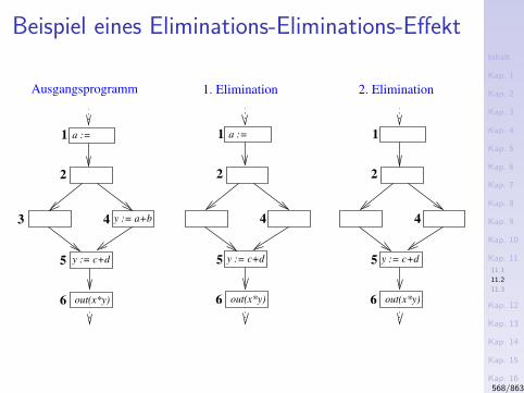
Inhalt
Kap. 1
Kap. 2
Kap. 3
Kap. 4
Kap. 5
Kap. 6
Kap. 7
Kap. 8
Kap. 9
Kap. 10
Kap. 11
11.1
11.2
11.3
Kap. 12
Kap. 13
Kap. 14
Kap. 15
Kap. 16
Kap. 17
Literatur
Anhang
A
Beispiel eines Eliminations-Eliminations-Effekt
Ausgangsprogramm 1. Elimination 2. Elimination
6 out(x*y)
1
2
4
5 y := c+d
6 out(x*y)
3
1
2
4
5
6 out(x*y)
y := a+b
a :=
y := c+d
1
2
4
5 y := c+d
a :=
568/863
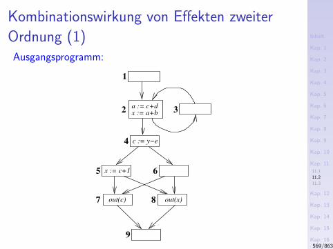
Inhalt
Kap. 1
Kap. 2
Kap. 3
Kap. 4
Kap. 5
Kap. 6
Kap. 7
Kap. 8
Kap. 9
Kap. 10
Kap. 11
11.1
11.2
11.3
Kap. 12
Kap. 13
Kap. 14
Kap. 15
Kap. 16
Kap. 17
Literatur
Anhang
A
Kombinationswirkung von Effekten zweiter
Ordnung (1)Ausgangsprogramm:
1
2a := c+dx := a+b 3
4
5 6
7
9
8 out(x)
c := y−e
out(c)
x := c+1
569/863
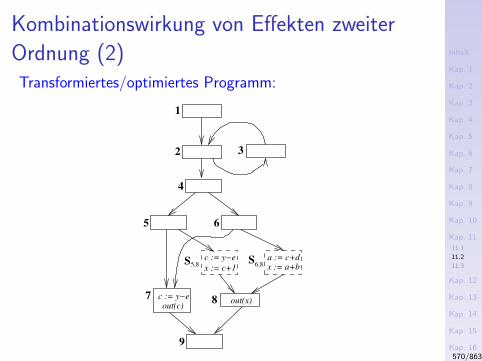
Inhalt
Kap. 1
Kap. 2
Kap. 3
Kap. 4
Kap. 5
Kap. 6
Kap. 7
Kap. 8
Kap. 9
Kap. 10
Kap. 11
11.1
11.2
11.3
Kap. 12
Kap. 13
Kap. 14
Kap. 15
Kap. 16
Kap. 17
Literatur
Anhang
A
Kombinationswirkung von Effekten zweiter
Ordnung (2)Transformiertes/optimiertes Programm:
4
5 6
7out(c)
c := y−e
x := c+1
c := y−e8
5,8S 6,8S
x := a+ba := c+d
out(x)
9
2 3
1
570/863
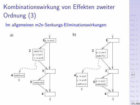
Inhalt
Kap. 1
Kap. 2
Kap. 3
Kap. 4
Kap. 5
Kap. 6
Kap. 7
Kap. 8
Kap. 9
Kap. 10
Kap. 11
11.1
11.2
11.3
Kap. 12
Kap. 13
Kap. 14
Kap. 15
Kap. 16
Kap. 17
Literatur
Anhang
A
Kombinationswirkung von Effekten zweiter
Ordnung (3)
Im allgemeinen m2n-Senkungs-Eliminationswirkungen:
a) b)
1a := a+1
out(x*y)
y := a+b
a := a+1
out(a+b)
out(x+y)
2
5
3
4
6
1
2
5
3
4
6
out(x+y)
y := a+b
a := a+1
out(x*y)
a := a+1
out(a+b)
a := a+1
571/863
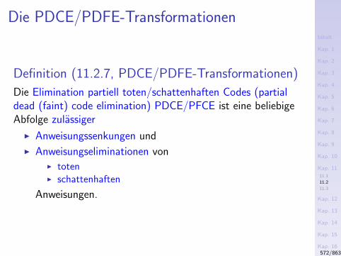
Inhalt
Kap. 1
Kap. 2
Kap. 3
Kap. 4
Kap. 5
Kap. 6
Kap. 7
Kap. 8
Kap. 9
Kap. 10
Kap. 11
11.1
11.2
11.3
Kap. 12
Kap. 13
Kap. 14
Kap. 15
Kap. 16
Kap. 17
Literatur
Anhang
A
Die PDCE/PDFE-Transformationen
Definition (11.2.7, PDCE/PDFE-Transformationen)
Die Elimination partiell toten/schattenhaften Codes (partialdead (faint) code elimination) PDCE/PFCE ist eine beliebigeAbfolge zulassiger
I Anweisungssenkungen und
I Anweisungseliminationen vonI totenI schattenhaften
Anweisungen.
572/863
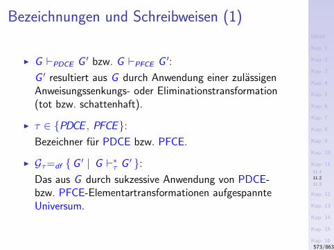
Inhalt
Kap. 1
Kap. 2
Kap. 3
Kap. 4
Kap. 5
Kap. 6
Kap. 7
Kap. 8
Kap. 9
Kap. 10
Kap. 11
11.1
11.2
11.3
Kap. 12
Kap. 13
Kap. 14
Kap. 15
Kap. 16
Kap. 17
Literatur
Anhang
A
Bezeichnungen und Schreibweisen (1)
I G `PDCE G ′ bzw. G `PFCE G ′:
G ′ resultiert aus G durch Anwendung einer zulassigenAnweisungssenkungs- oder Eliminationstransformation(tot bzw. schattenhaft).
I τ ∈ PDCE , PFCE:Bezeichner fur PDCE bzw. PFCE.
I Gτ=df G ′ | G `∗τ G ′ :Das aus G durch sukzessive Anwendung von PDCE-bzw. PFCE-Elementartransformationen aufgespannteUniversum.
573/863
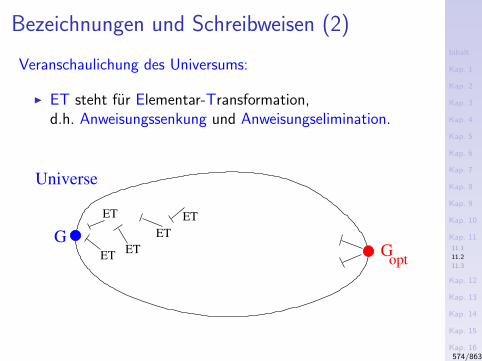
Inhalt
Kap. 1
Kap. 2
Kap. 3
Kap. 4
Kap. 5
Kap. 6
Kap. 7
Kap. 8
Kap. 9
Kap. 10
Kap. 11
11.1
11.2
11.3
Kap. 12
Kap. 13
Kap. 14
Kap. 15
Kap. 16
Kap. 17
Literatur
Anhang
A
Bezeichnungen und Schreibweisen (2)
Veranschaulichung des Universums:
I ET steht fur Elementar-Transformation,d.h. Anweisungssenkung und Anweisungselimination.
ET
ET
ETET
ET
GGopt
Universe
574/863
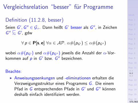
Inhalt
Kap. 1
Kap. 2
Kap. 3
Kap. 4
Kap. 5
Kap. 6
Kap. 7
Kap. 8
Kap. 9
Kap. 10
Kap. 11
11.1
11.2
11.3
Kap. 12
Kap. 13
Kap. 14
Kap. 15
Kap. 16
Kap. 17
Literatur
Anhang
A
Vergleichsrelation “besser” fur Programme
Definition (11.2.8, besser)
Seien G ′,G ′′ ∈ Gτ . Dann heißt G ’ besser als G ′′, in ZeichenG ′′ @∼ G ′, gdw
∀ p ∈ P[s, e] ∀α ∈ AP . α#(pG ′) ≤ α#(pG ′′)
wobei α#(pG ′) und α#(pG ′′) jeweils die Anzahl der α-Vor-kommen auf p in G ′ bzw. G ′′ bezeichnen.
Beachte:
I Anweisungssenkungen und -eliminationen erhalten dieVerzweigungsstruktur eines Programms G . Die einemPfad in G entsprechenden Pfade in G ′ und G ′′ konnendeshalb einfach identifiziert werden.
575/863
Inhalt
Kap. 1
Kap. 2
Kap. 3
Kap. 4
Kap. 5
Kap. 6
Kap. 7
Kap. 8
Kap. 9
Kap. 10
Kap. 11
11.1
11.2
11.3
Kap. 12
Kap. 13
Kap. 14
Kap. 15
Kap. 16
Kap. 17
Literatur
Anhang
A
Eigenschaften der Relation “besser”
Lemma (11.2.9)
Die Vergleichsrelation @∼ ist eine
I Quasiordnung (d.h. reflexiv und transitiv, aber nichtantisymmetrisch).
576/863
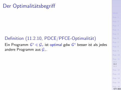
Inhalt
Kap. 1
Kap. 2
Kap. 3
Kap. 4
Kap. 5
Kap. 6
Kap. 7
Kap. 8
Kap. 9
Kap. 10
Kap. 11
11.1
11.2
11.3
Kap. 12
Kap. 13
Kap. 14
Kap. 15
Kap. 16
Kap. 17
Literatur
Anhang
A
Der Optimalitatsbegriff
Definition (11.2.10, PDCE/PFCE-Optimalitat)
Ein Programm G ∗ ∈ Gτ ist optimal gdw G ∗ besser ist als jedesandere Programm aus Gτ .
577/863
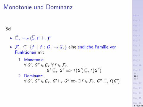
Inhalt
Kap. 1
Kap. 2
Kap. 3
Kap. 4
Kap. 5
Kap. 6
Kap. 7
Kap. 8
Kap. 9
Kap. 10
Kap. 11
11.1
11.2
11.3
Kap. 12
Kap. 13
Kap. 14
Kap. 15
Kap. 16
Kap. 17
Literatur
Anhang
A
Monotonie und Dominanz
Sei
I ~vτ =df (@∼ ∩ `τ )∗
I Fτ ⊆ f | f : Gτ → Gτ eine endliche Familie vonFunktionen mit
1. Monotonie:∀G ′, G ′′ ∈ Gτ ∀ f ∈ Fτ .
G ′ ~vτ G ′′ ≡> f (G ′) ~vτ f (G ′′)2. Dominanz:∀G ′, G ′′ ∈ Gτ . G ′ `τ G ′′ ≡> ∃ f ∈ Fτ . G ′′ ~vτ f (G ′)
578/863
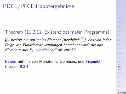
Inhalt
Kap. 1
Kap. 2
Kap. 3
Kap. 4
Kap. 5
Kap. 6
Kap. 7
Kap. 8
Kap. 9
Kap. 10
Kap. 11
11.1
11.2
11.3
Kap. 12
Kap. 13
Kap. 14
Kap. 15
Kap. 16
Kap. 17
Literatur
Anhang
A
PDCE/PFCE-Hauptergebnisse
Theorem (11.2.11, Existenz optimalen Programms)
Gτ besitzt ein optimales Element (bezuglich @∼), das von jederFolge von Funktionsanwendungen berechnet wird, die alleElemente aus Fτ ‘hinreichend’ oft enthalt.
Beweis mithilfe von Monotonie, Dominanz und Fixpunkt-theorem 9.2.4.
579/863
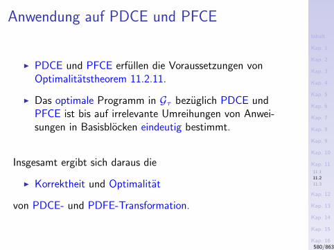
Inhalt
Kap. 1
Kap. 2
Kap. 3
Kap. 4
Kap. 5
Kap. 6
Kap. 7
Kap. 8
Kap. 9
Kap. 10
Kap. 11
11.1
11.2
11.3
Kap. 12
Kap. 13
Kap. 14
Kap. 15
Kap. 16
Kap. 17
Literatur
Anhang
A
Anwendung auf PDCE und PFCE
I PDCE und PFCE erfullen die Voraussetzungen vonOptimalitatstheorem 11.2.11.
I Das optimale Programm in Gτ bezuglich PDCE undPFCE ist bis auf irrelevante Umreihungen von Anwei-sungen in Basisblocken eindeutig bestimmt.
Insgesamt ergibt sich daraus die
I Korrektheit und Optimalitat
von PDCE- und PDFE-Transformation.
580/863
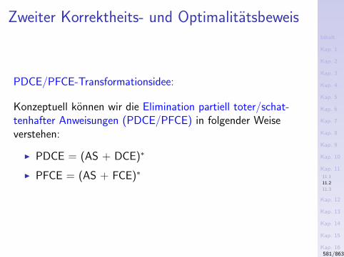
Inhalt
Kap. 1
Kap. 2
Kap. 3
Kap. 4
Kap. 5
Kap. 6
Kap. 7
Kap. 8
Kap. 9
Kap. 10
Kap. 11
11.1
11.2
11.3
Kap. 12
Kap. 13
Kap. 14
Kap. 15
Kap. 16
Kap. 17
Literatur
Anhang
A
Zweiter Korrektheits- und Optimalitatsbeweis
PDCE/PFCE-Transformationsidee:
Konzeptuell konnen wir die Elimination partiell toter/schat-tenhafter Anweisungen (PDCE/PFCE) in folgender Weiseverstehen:
I PDCE = (AS + DCE)∗
I PFCE = (AS + FCE)∗
581/863
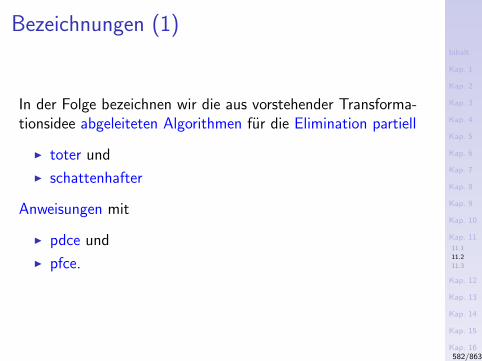
Inhalt
Kap. 1
Kap. 2
Kap. 3
Kap. 4
Kap. 5
Kap. 6
Kap. 7
Kap. 8
Kap. 9
Kap. 10
Kap. 11
11.1
11.2
11.3
Kap. 12
Kap. 13
Kap. 14
Kap. 15
Kap. 16
Kap. 17
Literatur
Anhang
A
Bezeichnungen (1)
In der Folge bezeichnen wir die aus vorstehender Transforma-tionsidee abgeleiteten Algorithmen fur die Elimination partiell
I toter und
I schattenhafter
Anweisungen mit
I pdce und
I pfce.
582/863
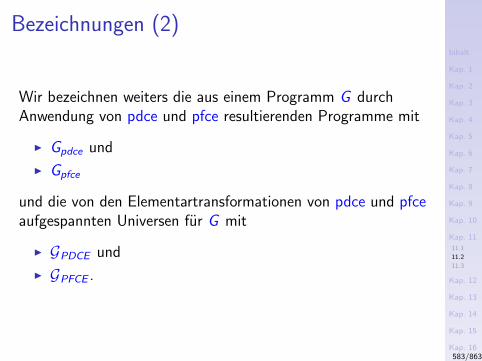
Inhalt
Kap. 1
Kap. 2
Kap. 3
Kap. 4
Kap. 5
Kap. 6
Kap. 7
Kap. 8
Kap. 9
Kap. 10
Kap. 11
11.1
11.2
11.3
Kap. 12
Kap. 13
Kap. 14
Kap. 15
Kap. 16
Kap. 17
Literatur
Anhang
A
Bezeichnungen (2)
Wir bezeichnen weiters die aus einem Programm G durchAnwendung von pdce und pfce resultierenden Programme mit
I Gpdce und
I Gpfce
und die von den Elementartransformationen von pdce und pfceaufgespannten Universen fur G mit
I GPDCE und
I GPFCE .
583/863
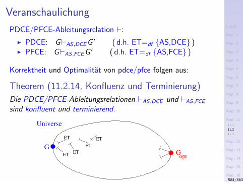
Inhalt
Kap. 1
Kap. 2
Kap. 3
Kap. 4
Kap. 5
Kap. 6
Kap. 7
Kap. 8
Kap. 9
Kap. 10
Kap. 11
11.1
11.2
11.3
Kap. 12
Kap. 13
Kap. 14
Kap. 15
Kap. 16
Kap. 17
Literatur
Anhang
A
Veranschaulichung
PDCE/PFCE-Ableitungsrelation `:
I PDCE: G`AS ,DCEG ′ ( d.h. ET=df AS,DCE )I PFCE: G`AS ,FCEG ′ ( d.h. ET=df AS,FCE )
Korrektheit und Optimalitat von pdce/pfce folgen aus:
Theorem (11.2.14, Konfluenz und Terminierung)
Die PDCE/PFCE-Ableitungsrelationen `AS ,DCE und `AS ,FCEsind konfluent und terminierend.
ET
ET
ETET
ET
GGopt
Universe
584/863
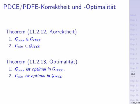
Inhalt
Kap. 1
Kap. 2
Kap. 3
Kap. 4
Kap. 5
Kap. 6
Kap. 7
Kap. 8
Kap. 9
Kap. 10
Kap. 11
11.1
11.2
11.3
Kap. 12
Kap. 13
Kap. 14
Kap. 15
Kap. 16
Kap. 17
Literatur
Anhang
A
PDCE/PDFE-Korrektheit und -Optimalitat
Theorem (11.2.12, Korrektheit)
1. Gpdce ∈ GPDCE2. Gpfce ∈ GPFCE
Theorem (11.2.13, Optimalitat)
1. Gpdce ist optimal in GPDCE .
2. Gpfce ist optimal in GPFCE
585/863

Inhalt
Kap. 1
Kap. 2
Kap. 3
Kap. 4
Kap. 5
Kap. 6
Kap. 7
Kap. 8
Kap. 9
Kap. 10
Kap. 11
11.1
11.2
11.3
Kap. 12
Kap. 13
Kap. 14
Kap. 15
Kap. 16
Kap. 17
Literatur
Anhang
A
Kapitel 11.3
Implementierung von PDCE/PFCE
586/863
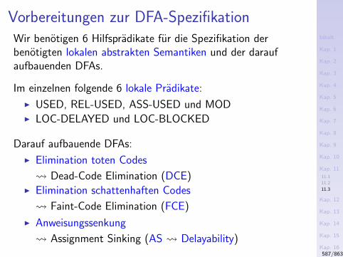
Inhalt
Kap. 1
Kap. 2
Kap. 3
Kap. 4
Kap. 5
Kap. 6
Kap. 7
Kap. 8
Kap. 9
Kap. 10
Kap. 11
11.1
11.2
11.3
Kap. 12
Kap. 13
Kap. 14
Kap. 15
Kap. 16
Kap. 17
Literatur
Anhang
A
Vorbereitungen zur DFA-SpezifikationWir benotigen 6 Hilfspradikate fur die Spezifikation derbenotigten lokalen abstrakten Semantiken und der daraufaufbauenden DFAs.
Im einzelnen folgende 6 lokale Pradikate:
I USED, REL-USED, ASS-USED und MODI LOC-DELAYED und LOC-BLOCKED
Darauf aufbauende DFAs:
I Elimination toten Codes
Dead-Code Elimination (DCE)I Elimination schattenhaften Codes
Faint-Code Elimination (FCE)
I Anweisungssenkung
Assignment Sinking (AS Delayability)587/863
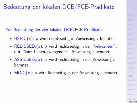
Inhalt
Kap. 1
Kap. 2
Kap. 3
Kap. 4
Kap. 5
Kap. 6
Kap. 7
Kap. 8
Kap. 9
Kap. 10
Kap. 11
11.1
11.2
11.3
Kap. 12
Kap. 13
Kap. 14
Kap. 15
Kap. 16
Kap. 17
Literatur
Anhang
A
Bedeutung der lokalen DCE/FCE-Pradikate
Zur Bedeutung der vier lokalen DCE/FCE-Pradikate:
I USEDι(x): x wird rechtsseitig in Anweisung ι benutzt.
I REL-USEDι(x): x wird rechtsseitig in der “relevanten”,d.h. “zum Leben zwingenden” Anweisung ι benutzt.
I ASS-USEDι(x): x wird rechtsseitig in der Zuweisung ιbenutzt.
I MODι(x): x wird linksseitig in der Anweisung ι benutzt.
588/863
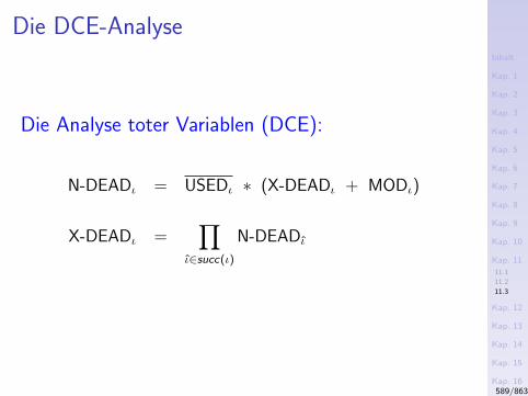
Inhalt
Kap. 1
Kap. 2
Kap. 3
Kap. 4
Kap. 5
Kap. 6
Kap. 7
Kap. 8
Kap. 9
Kap. 10
Kap. 11
11.1
11.2
11.3
Kap. 12
Kap. 13
Kap. 14
Kap. 15
Kap. 16
Kap. 17
Literatur
Anhang
A
Die DCE-Analyse
Die Analyse toter Variablen (DCE):
N-DEADι = USEDι ∗ (X-DEADι + MODι)
X-DEADι =∏
ι∈succ(ι)
N-DEADι
589/863
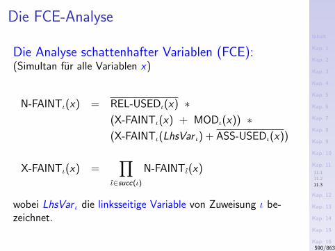
Inhalt
Kap. 1
Kap. 2
Kap. 3
Kap. 4
Kap. 5
Kap. 6
Kap. 7
Kap. 8
Kap. 9
Kap. 10
Kap. 11
11.1
11.2
11.3
Kap. 12
Kap. 13
Kap. 14
Kap. 15
Kap. 16
Kap. 17
Literatur
Anhang
A
Die FCE-Analyse
Die Analyse schattenhafter Variablen (FCE):(Simultan fur alle Variablen x)
N-FAINTι(x) = REL-USEDι(x) ∗(X-FAINTι(x) + MODι(x)) ∗(X-FAINTι(LhsVar ι) + ASS-USEDι(x))
X-FAINTι(x) =∏
ι∈succ(ι)
N-FAINTι(x)
wobei LhsVar ι die linksseitige Variable von Zuweisung ι be-zeichnet.
590/863
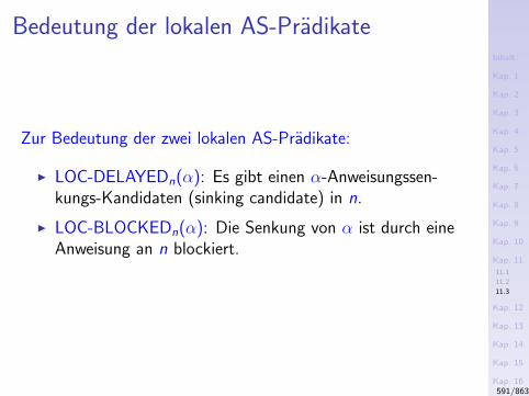
Inhalt
Kap. 1
Kap. 2
Kap. 3
Kap. 4
Kap. 5
Kap. 6
Kap. 7
Kap. 8
Kap. 9
Kap. 10
Kap. 11
11.1
11.2
11.3
Kap. 12
Kap. 13
Kap. 14
Kap. 15
Kap. 16
Kap. 17
Literatur
Anhang
A
Bedeutung der lokalen AS-Pradikate
Zur Bedeutung der zwei lokalen AS-Pradikate:
I LOC-DELAYEDn(α): Es gibt einen α-Anweisungssen-kungs-Kandidaten (sinking candidate) in n.
I LOC-BLOCKEDn(α): Die Senkung von α ist durch eineAnweisung an n blockiert.
591/863
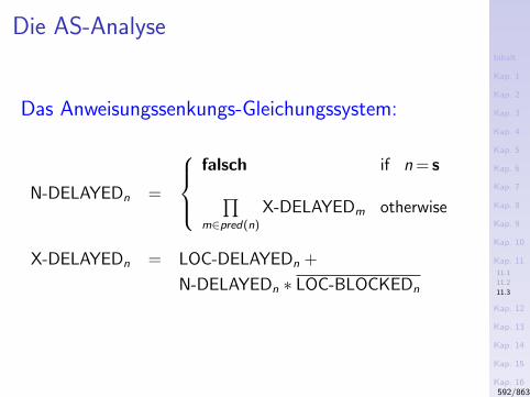
Inhalt
Kap. 1
Kap. 2
Kap. 3
Kap. 4
Kap. 5
Kap. 6
Kap. 7
Kap. 8
Kap. 9
Kap. 10
Kap. 11
11.1
11.2
11.3
Kap. 12
Kap. 13
Kap. 14
Kap. 15
Kap. 16
Kap. 17
Literatur
Anhang
A
Die AS-Analyse
Das Anweisungssenkungs-Gleichungssystem:
N-DELAYEDn =
falsch if n = s∏m∈pred(n)
X-DELAYEDm otherwise
X-DELAYEDn = LOC-DELAYEDn +
N-DELAYEDn ∗ LOC-BLOCKEDn
592/863
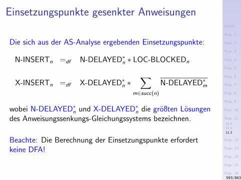
Inhalt
Kap. 1
Kap. 2
Kap. 3
Kap. 4
Kap. 5
Kap. 6
Kap. 7
Kap. 8
Kap. 9
Kap. 10
Kap. 11
11.1
11.2
11.3
Kap. 12
Kap. 13
Kap. 14
Kap. 15
Kap. 16
Kap. 17
Literatur
Anhang
A
Einsetzungspunkte gesenkter Anweisungen
Die sich aus der AS-Analyse ergebenden Einsetzungspunkte:
N-INSERTn =df N-DELAYED∗n ∗ LOC-BLOCKEDn
X-INSERTn =df X-DELAYED∗n ∗∑
m∈succ(n)
N-DELAYED∗m
wobei N-DELAYED∗n und X-DELAYED∗n die großten Losungendes Anweisungssenkungs-Gleichungssystems bezeichnen.
Beachte: Die Berechnung der Einsetzungspunkte erfordertkeine DFA!
593/863
Inhalt
Kap. 1
Kap. 2
Kap. 3
Kap. 4
Kap. 5
Kap. 6
Kap. 7
Kap. 8
Kap. 9
Kap. 10
Kap. 11
11.1
11.2
11.3
Kap. 12
Kap. 13
Kap. 14
Kap. 15
Kap. 16
Kap. 17
Literatur
Anhang
A
Vertiefende und weiterfuhrende Leseempfeh-
lungen fur Kapitel 11 (1)
Ras Bodik, Rajiv Gupta. Partial Dead Code Eliminationusing Slicing Transformations. In Proceedings of the ACMSIGPLAN’97 Conference on Programming LanguageDesign and Implementation (PLDI’97), ACM SIGPLANNotices 32(6):159-170, 1997.
L. Feigen, D. Klappholz, R. Casazza, X. Xue. The RevivalTransformation. In Conference Record of the 21st ACMSIGPLAN-SIGACT Symposium on Principles of Program-ming Languages (POPL’94), 1994.
594/863
Inhalt
Kap. 1
Kap. 2
Kap. 3
Kap. 4
Kap. 5
Kap. 6
Kap. 7
Kap. 8
Kap. 9
Kap. 10
Kap. 11
11.1
11.2
11.3
Kap. 12
Kap. 13
Kap. 14
Kap. 15
Kap. 16
Kap. 17
Literatur
Anhang
A
Vertiefende und weiterfuhrende Leseempfeh-
lungen fur Kapitel 11 (2)
Jens Knoop, Oliver Ruthing, Bernhard Steffen. PartialDead Code Elimination. In Proceedings of the ACMSIGPLAN’94 Conference on Programming LanguageDesign and Implementation (PLDI’94), ACM SIGPLANNotices 29(6):147-158, 1994.
Ronald J. Mintz, Gerald A. Fisher, Micha Sharir. TheDesign of a Global Optimizer. In Proceedings of the ACMSIGPLAN’79 Symposium on Compiler Construction(SoCC’79), ACM SIGPLAN Notices 14(8):226-234, 1979.
Munehiro Takimoto, Kenichi Harada. Partial Dead CodeElimination Using Extended Value Graph. In Proceedingsof the 6th Static Analysis Symposium (SAS’99), Sprin-ger-V., LNCS 1694, 179-193, 1999.
595/863
Inhalt
Kap. 1
Kap. 2
Kap. 3
Kap. 4
Kap. 5
Kap. 6
Kap. 7
Kap. 8
Kap. 9
Kap. 10
Kap. 11
Kap. 12
12.1
12.2
12.3
Kap. 13
Kap. 14
Kap. 15
Kap. 16
Kap. 17
Literatur
Anhang
A
Kapitel 12
Elimination partiell redundanter Anweisungen
596/863

Inhalt
Kap. 1
Kap. 2
Kap. 3
Kap. 4
Kap. 5
Kap. 6
Kap. 7
Kap. 8
Kap. 9
Kap. 10
Kap. 11
Kap. 12
12.1
12.2
12.3
Kap. 13
Kap. 14
Kap. 15
Kap. 16
Kap. 17
Literatur
Anhang
A
Kapitel 12.1
Motivation
597/863
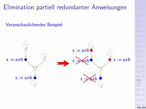
Inhalt
Kap. 1
Kap. 2
Kap. 3
Kap. 4
Kap. 5
Kap. 6
Kap. 7
Kap. 8
Kap. 9
Kap. 10
Kap. 11
Kap. 12
12.1
12.2
12.3
Kap. 13
Kap. 14
Kap. 15
Kap. 16
Kap. 17
Literatur
Anhang
A
Elimination partiell redundanter Anweisungen
Veranschaulichendes Beispiel:
x := a+bx := a+b
x := a+b
x := a+b
x := a+b
x := a+b
598/863
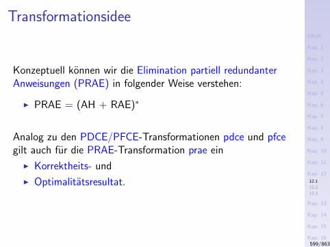
Inhalt
Kap. 1
Kap. 2
Kap. 3
Kap. 4
Kap. 5
Kap. 6
Kap. 7
Kap. 8
Kap. 9
Kap. 10
Kap. 11
Kap. 12
12.1
12.2
12.3
Kap. 13
Kap. 14
Kap. 15
Kap. 16
Kap. 17
Literatur
Anhang
A
Transformationsidee
Konzeptuell konnen wir die Elimination partiell redundanterAnweisungen (PRAE) in folgender Weise verstehen:
I PRAE = (AH + RAE)∗
Analog zu den PDCE/PFCE-Transformationen pdce und pfcegilt auch fur die PRAE-Transformation prae ein
I Korrektheits- und
I Optimalitatsresultat.
599/863
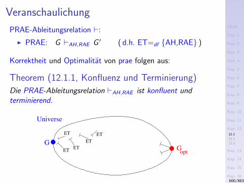
Inhalt
Kap. 1
Kap. 2
Kap. 3
Kap. 4
Kap. 5
Kap. 6
Kap. 7
Kap. 8
Kap. 9
Kap. 10
Kap. 11
Kap. 12
12.1
12.2
12.3
Kap. 13
Kap. 14
Kap. 15
Kap. 16
Kap. 17
Literatur
Anhang
A
Veranschaulichung
PRAE-Ableitungsrelation `:
I PRAE: G `AH,RAE G ′ ( d.h. ET=df AH,RAE )
Korrektheit und Optimalitat von prae folgen aus:
Theorem (12.1.1, Konfluenz und Terminierung)
Die PRAE-Ableitungsrelation `AH,RAE ist konfluent undterminierend.
ET
ET
ETET
ET
GGopt
Universe
600/863
Inhalt
Kap. 1
Kap. 2
Kap. 3
Kap. 4
Kap. 5
Kap. 6
Kap. 7
Kap. 8
Kap. 9
Kap. 10
Kap. 11
Kap. 12
12.1
12.2
12.3
Kap. 13
Kap. 14
Kap. 15
Kap. 16
Kap. 17
Literatur
Anhang
A
PRAE-Korrektheit und -Optimalitat
Theorem (12.1.2, Korrektheit)
Gprae ∈ GPRAE
Theorem (12.1.3, Optimalitat)
Gprae ist optimal in GPRAE .
601/863

Inhalt
Kap. 1
Kap. 2
Kap. 3
Kap. 4
Kap. 5
Kap. 6
Kap. 7
Kap. 8
Kap. 9
Kap. 10
Kap. 11
Kap. 12
12.1
12.2
12.3
Kap. 13
Kap. 14
Kap. 15
Kap. 16
Kap. 17
Literatur
Anhang
A
Kapitel 12.2
EAM: Einheitliche PREE/PRAE-Behandlung
602/863
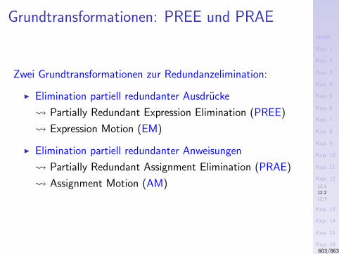
Inhalt
Kap. 1
Kap. 2
Kap. 3
Kap. 4
Kap. 5
Kap. 6
Kap. 7
Kap. 8
Kap. 9
Kap. 10
Kap. 11
Kap. 12
12.1
12.2
12.3
Kap. 13
Kap. 14
Kap. 15
Kap. 16
Kap. 17
Literatur
Anhang
A
Grundtransformationen: PREE und PRAE
Zwei Grundtransformationen zur Redundanzelimination:
I Elimination partiell redundanter Ausdrucke
Partially Redundant Expression Elimination (PREE)
Expression Motion (EM)
I Elimination partiell redundanter Anweisungen
Partially Redundant Assignment Elimination (PRAE)
Assignment Motion (AM)
603/863
Inhalt
Kap. 1
Kap. 2
Kap. 3
Kap. 4
Kap. 5
Kap. 6
Kap. 7
Kap. 8
Kap. 9
Kap. 10
Kap. 11
Kap. 12
12.1
12.2
12.3
Kap. 13
Kap. 14
Kap. 15
Kap. 16
Kap. 17
Literatur
Anhang
A
Kombinierte PRE/AE-Transformation: EAM
Kombinierte Transformation zur Redundanzelimination:
I Elimination partiell redundanter Ausdrucke undAnweisungen
Partially Redundant Expression and AssignmentElimination (PREAE)
Expression and Assignment Motion (EAM)
604/863
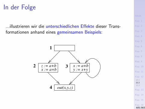
Inhalt
Kap. 1
Kap. 2
Kap. 3
Kap. 4
Kap. 5
Kap. 6
Kap. 7
Kap. 8
Kap. 9
Kap. 10
Kap. 11
Kap. 12
12.1
12.2
12.3
Kap. 13
Kap. 14
Kap. 15
Kap. 16
Kap. 17
Literatur
Anhang
A
In der Folge
...illustrieren wir die unterschiedlichen Effekte dieser Trans-formationen anhand eines gemeinsamen Beispiels:
3 x := a+b
1
4 out(x,y,z)
z := a+bx := a+b
2y := x+y
605/863
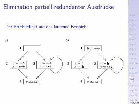
Inhalt
Kap. 1
Kap. 2
Kap. 3
Kap. 4
Kap. 5
Kap. 6
Kap. 7
Kap. 8
Kap. 9
Kap. 10
Kap. 11
Kap. 12
12.1
12.2
12.3
Kap. 13
Kap. 14
Kap. 15
Kap. 16
Kap. 17
Literatur
Anhang
A
Elimination partiell redundanter Ausdrucke
Der PREE-Effekt auf das laufende Beispiel:
3 x := a+b
1
4 out(x,y,z)
a)
3
1
4
y := x+y
out(x,y,z)
x := h
h
b)
z := a+bx := a+b
2 2 h
h
z :=x :=y := x+y
:= a+b
606/863
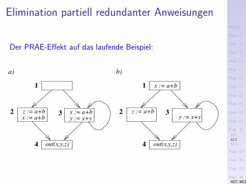
Inhalt
Kap. 1
Kap. 2
Kap. 3
Kap. 4
Kap. 5
Kap. 6
Kap. 7
Kap. 8
Kap. 9
Kap. 10
Kap. 11
Kap. 12
12.1
12.2
12.3
Kap. 13
Kap. 14
Kap. 15
Kap. 16
Kap. 17
Literatur
Anhang
A
Elimination partiell redundanter Anweisungen
Der PRAE-Effekt auf das laufende Beispiel:
3 x := a+b
1
4
y := x+y
a)
1
4
b)
x := a+b
y := x+y2 z := a+b2
x := a+bz := a+b 3
out(x,y,z)out(x,y,z)
607/863
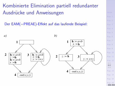
Inhalt
Kap. 1
Kap. 2
Kap. 3
Kap. 4
Kap. 5
Kap. 6
Kap. 7
Kap. 8
Kap. 9
Kap. 10
Kap. 11
Kap. 12
12.1
12.2
12.3
Kap. 13
Kap. 14
Kap. 15
Kap. 16
Kap. 17
Literatur
Anhang
A
Kombinierte Elimination partiell redundanter
Ausdrucke und Anweisungen
Der EAM(=PREAE)-Effekt auf das laufende Beispiel:
h := a+bx :=h
3
1
a) b)
2
y := x+y
h:= a+bz :=hh:= a+bx := h
x := hh := a+b
4 out(x,y,z)
3
4 out(x,y,z)
2 hz :=
1
y := x+y
608/863
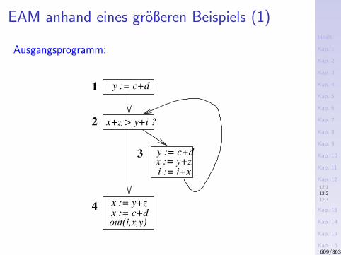
Inhalt
Kap. 1
Kap. 2
Kap. 3
Kap. 4
Kap. 5
Kap. 6
Kap. 7
Kap. 8
Kap. 9
Kap. 10
Kap. 11
Kap. 12
12.1
12.2
12.3
Kap. 13
Kap. 14
Kap. 15
Kap. 16
Kap. 17
Literatur
Anhang
A
EAM anhand eines großeren Beispiels (1)
Ausgangsprogramm:
1
2
y := c+d
3 y := c+d
i := i+x
4
out(i,x,y)
x := y+z
x := y+zx := c+d
x+z > y+i ?
609/863
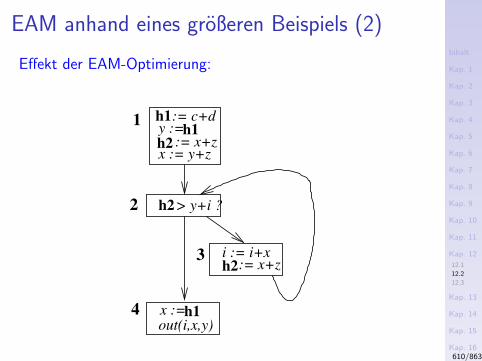
Inhalt
Kap. 1
Kap. 2
Kap. 3
Kap. 4
Kap. 5
Kap. 6
Kap. 7
Kap. 8
Kap. 9
Kap. 10
Kap. 11
Kap. 12
12.1
12.2
12.3
Kap. 13
Kap. 14
Kap. 15
Kap. 16
Kap. 17
Literatur
Anhang
A
EAM anhand eines großeren Beispiels (2)
Effekt der EAM-Optimierung:
2
4
out(i,x,y)
i := i+x3
> y+i ?h2
h2
x :=
:= c+d1h1
h1y :=h2
h1
:= x+z
:= x+z
x := y+z
610/863
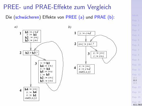
Inhalt
Kap. 1
Kap. 2
Kap. 3
Kap. 4
Kap. 5
Kap. 6
Kap. 7
Kap. 8
Kap. 9
Kap. 10
Kap. 11
Kap. 12
12.1
12.2
12.3
Kap. 13
Kap. 14
Kap. 15
Kap. 16
Kap. 17
Literatur
Anhang
A
PREE- und PRAE-Effekte zum Vergleich
Die (schwacheren) Effekte von PREE (a) und PRAE (b):
2
4
b)a)
h1 := c+d
h2
y := 1
3i := i+xx := y+z
h3
2 >
y :=
i :=h2
3
h3
h2
h5
:= y+i
4
1
x+z > y+i ?
x := y+zx := c+dout(i,x,y)
:= y+z
x := out(i,x,y)
:= y+z
h3
:= i+xh4
h1
h5
:= x+z
h1
h4x :=h4
x := h4
:= x+z:= y+i
?
y := c+dh1
611/863

Inhalt
Kap. 1
Kap. 2
Kap. 3
Kap. 4
Kap. 5
Kap. 6
Kap. 7
Kap. 8
Kap. 9
Kap. 10
Kap. 11
Kap. 12
12.1
12.2
12.3
Kap. 13
Kap. 14
Kap. 15
Kap. 16
Kap. 17
Literatur
Anhang
A
Kapitel 12.3
EAM: Transformation und Optimalitat
612/863
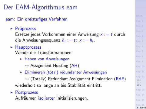
Inhalt
Kap. 1
Kap. 2
Kap. 3
Kap. 4
Kap. 5
Kap. 6
Kap. 7
Kap. 8
Kap. 9
Kap. 10
Kap. 11
Kap. 12
12.1
12.2
12.3
Kap. 13
Kap. 14
Kap. 15
Kap. 16
Kap. 17
Literatur
Anhang
A
Der EAM-Algorithmus eam
eam: Ein dreistufiges Verfahren
I PraprozessErsetze jedes Vorkommen einer Anweisung x := t durchdie Anweisungssequenz ht := t; x := ht .
I HauptprozessWende die Transformationen
I Heben von Anweisungen
Assignment Hoisting (AH)
I Eliminieren (total) redundanter Anweisungen
(Totally) Redundant Assignment Elimination (RAE)
wiederholt so lange an bis Stabilitat eintritt.
I PostprozessAufraumen isolierter Initialisierungen.
613/863
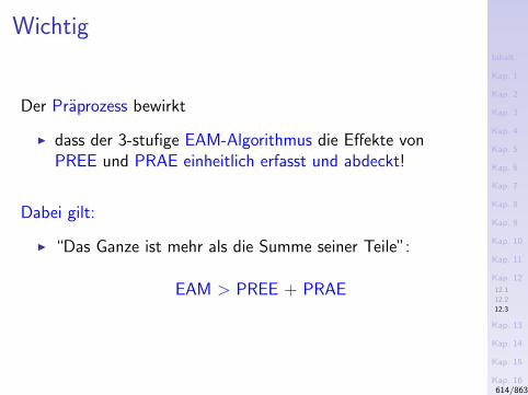
Inhalt
Kap. 1
Kap. 2
Kap. 3
Kap. 4
Kap. 5
Kap. 6
Kap. 7
Kap. 8
Kap. 9
Kap. 10
Kap. 11
Kap. 12
12.1
12.2
12.3
Kap. 13
Kap. 14
Kap. 15
Kap. 16
Kap. 17
Literatur
Anhang
A
Wichtig
Der Praprozess bewirkt
I dass der 3-stufige EAM-Algorithmus die Effekte vonPREE und PRAE einheitlich erfasst und abdeckt!
Dabei gilt:
I “Das Ganze ist mehr als die Summe seiner Teile”:
EAM > PREE + PRAE
614/863
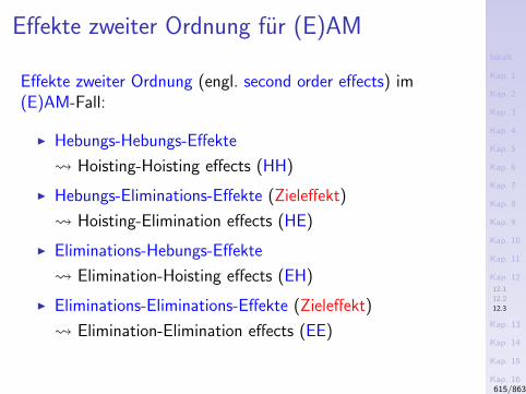
Inhalt
Kap. 1
Kap. 2
Kap. 3
Kap. 4
Kap. 5
Kap. 6
Kap. 7
Kap. 8
Kap. 9
Kap. 10
Kap. 11
Kap. 12
12.1
12.2
12.3
Kap. 13
Kap. 14
Kap. 15
Kap. 16
Kap. 17
Literatur
Anhang
A
Effekte zweiter Ordnung fur (E)AM
Effekte zweiter Ordnung (engl. second order effects) im(E)AM-Fall:
I Hebungs-Hebungs-Effekte
Hoisting-Hoisting effects (HH)
I Hebungs-Eliminations-Effekte (Zieleffekt)
Hoisting-Elimination effects (HE)
I Eliminations-Hebungs-Effekte
Elimination-Hoisting effects (EH)
I Eliminations-Eliminations-Effekte (Zieleffekt)
Elimination-Elimination effects (EE)
615/863
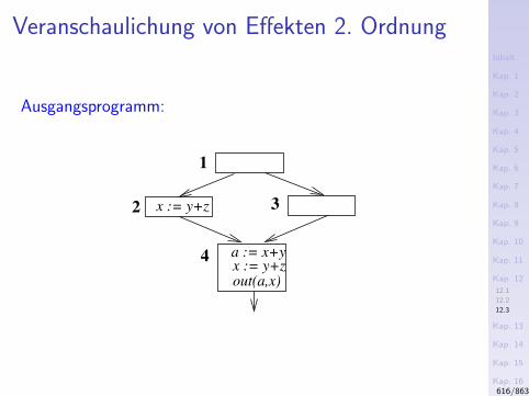
Inhalt
Kap. 1
Kap. 2
Kap. 3
Kap. 4
Kap. 5
Kap. 6
Kap. 7
Kap. 8
Kap. 9
Kap. 10
Kap. 11
Kap. 12
12.1
12.2
12.3
Kap. 13
Kap. 14
Kap. 15
Kap. 16
Kap. 17
Literatur
Anhang
A
Veranschaulichung von Effekten 2. Ordnung
Ausgangsprogramm:
2 3
x := y+za := x+y
1
x := y+z
out(a,x)
4
616/863
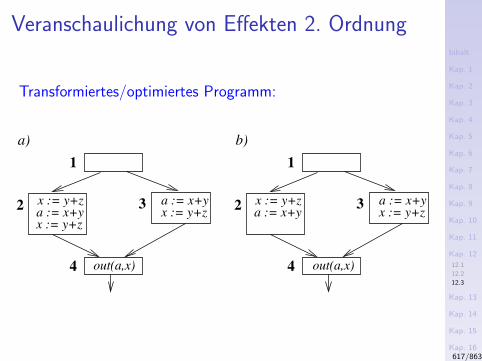
Inhalt
Kap. 1
Kap. 2
Kap. 3
Kap. 4
Kap. 5
Kap. 6
Kap. 7
Kap. 8
Kap. 9
Kap. 10
Kap. 11
Kap. 12
12.1
12.2
12.3
Kap. 13
Kap. 14
Kap. 15
Kap. 16
Kap. 17
Literatur
Anhang
A
Veranschaulichung von Effekten 2. Ordnung
Transformiertes/optimiertes Programm:
a)
x := y+za := x+yx := y+z
2
1
a := x+yx := y+z
3
4
x := y+za := x+y
2
1
a := x+yx := y+z
3
4
b)
out(a,x) out(a,x)
617/863
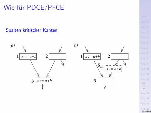
Inhalt
Kap. 1
Kap. 2
Kap. 3
Kap. 4
Kap. 5
Kap. 6
Kap. 7
Kap. 8
Kap. 9
Kap. 10
Kap. 11
Kap. 12
12.1
12.2
12.3
Kap. 13
Kap. 14
Kap. 15
Kap. 16
Kap. 17
Literatur
Anhang
A
Wie fur PDCE/PFCE
Spalten kritischer Kanten:
S2,3
b)a)
x := a+b
x := a+b
x := a+b
3
1 2 1 2x := a+b
3
618/863
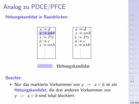
Inhalt
Kap. 1
Kap. 2
Kap. 3
Kap. 4
Kap. 5
Kap. 6
Kap. 7
Kap. 8
Kap. 9
Kap. 10
Kap. 11
Kap. 12
12.1
12.2
12.3
Kap. 13
Kap. 14
Kap. 15
Kap. 16
Kap. 17
Literatur
Anhang
A
Analog zu PDCE/PFCE
Hebungskandidat in Basisblocken:
y := a+bx := 3*ya := cy := a+b
x := d
x := 3*ya := cy := a+b
a := d
Hebungskandidat
y := a+b
Beachte:
I Nur das markierte Vorkommen von y := a + b ist einHebungskandidat; die drei anderen Vorkommen vony := a + b sind lokal blockiert.
619/863
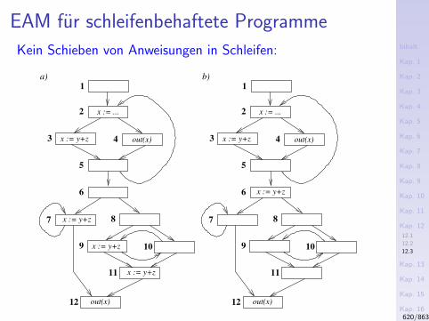
Inhalt
Kap. 1
Kap. 2
Kap. 3
Kap. 4
Kap. 5
Kap. 6
Kap. 7
Kap. 8
Kap. 9
Kap. 10
Kap. 11
Kap. 12
12.1
12.2
12.3
Kap. 13
Kap. 14
Kap. 15
Kap. 16
Kap. 17
Literatur
Anhang
A
EAM fur schleifenbehaftete Programme
Kein Schieben von Anweisungen in Schleifen:
x := y+z
out(x)x := y+z
out(x)
x := y+z
x := y+z
x := ...
1
2
3 4
5
6
7 8
9 10
11
12
a)
out(x)x := y+z
out(x)
x := ...
1
2
3 4
5
6
7 8
9 10
11
12
b)
x := y+z
620/863
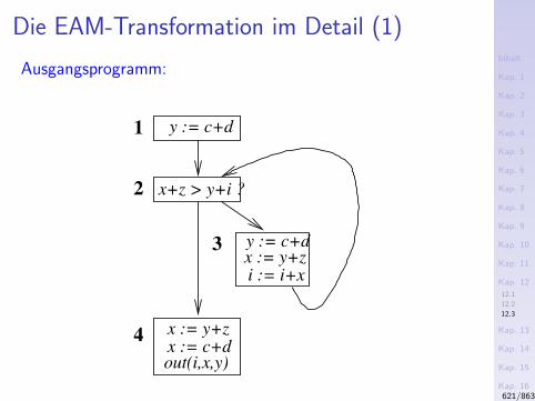
Inhalt
Kap. 1
Kap. 2
Kap. 3
Kap. 4
Kap. 5
Kap. 6
Kap. 7
Kap. 8
Kap. 9
Kap. 10
Kap. 11
Kap. 12
12.1
12.2
12.3
Kap. 13
Kap. 14
Kap. 15
Kap. 16
Kap. 17
Literatur
Anhang
A
Die EAM-Transformation im Detail (1)
Ausgangsprogramm:
1
2
y := c+d
3 y := c+d
i := i+x
4
out(i,x,y)
x := y+z
x := y+zx := c+d
x+z > y+i ?
621/863
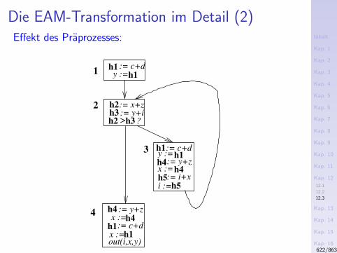
Inhalt
Kap. 1
Kap. 2
Kap. 3
Kap. 4
Kap. 5
Kap. 6
Kap. 7
Kap. 8
Kap. 9
Kap. 10
Kap. 11
Kap. 12
12.1
12.2
12.3
Kap. 13
Kap. 14
Kap. 15
Kap. 16
Kap. 17
Literatur
Anhang
A
Die EAM-Transformation im Detail (2)Effekt des Praprozesses:
h11
2
4:= y+z
x :=
i :=
h1:= c+dh1y :=
:= y+z
3
:= c+dy := h1
h4h4
h5
h5
:= i+x
x :=h4
h4
x :=out(i,x,y)
h1:= c+dh1
h2 > ?:= y+i
h2
h3
h3
:= x+z
622/863
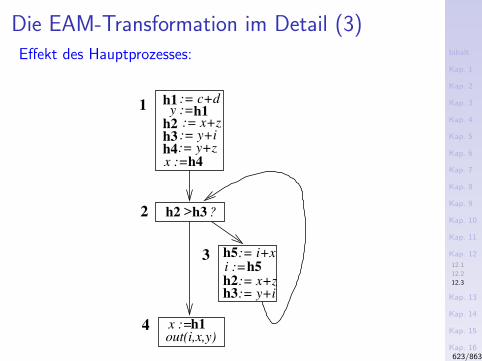
Inhalt
Kap. 1
Kap. 2
Kap. 3
Kap. 4
Kap. 5
Kap. 6
Kap. 7
Kap. 8
Kap. 9
Kap. 10
Kap. 11
Kap. 12
12.1
12.2
12.3
Kap. 13
Kap. 14
Kap. 15
Kap. 16
Kap. 17
Literatur
Anhang
A
Die EAM-Transformation im Detail (3)Effekt des Hauptprozesses:
4 h1x :=out(i,x,y)
2
3
h2 > ?
h5:= i+xi :=h5
h1 := c+d
h3
h1
h2
y :=
h4
1
x :=
:= y+i
h4
h3
:= y+z
:= x+z
:= x+zh2
:= y+ih3
623/863
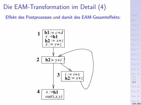
Inhalt
Kap. 1
Kap. 2
Kap. 3
Kap. 4
Kap. 5
Kap. 6
Kap. 7
Kap. 8
Kap. 9
Kap. 10
Kap. 11
Kap. 12
12.1
12.2
12.3
Kap. 13
Kap. 14
Kap. 15
Kap. 16
Kap. 17
Literatur
Anhang
A
Die EAM-Transformation im Detail (4)
Effekt des Postprozesses und damit des EAM-Gesamteffekts:
2
4
out(i,x,y)
i := i+x3
> y+i ?h2
h2
x :=
:= c+d1h1
h1y :=h2
h1
:= x+z
:= x+z
x := y+z
624/863
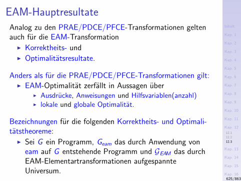
Inhalt
Kap. 1
Kap. 2
Kap. 3
Kap. 4
Kap. 5
Kap. 6
Kap. 7
Kap. 8
Kap. 9
Kap. 10
Kap. 11
Kap. 12
12.1
12.2
12.3
Kap. 13
Kap. 14
Kap. 15
Kap. 16
Kap. 17
Literatur
Anhang
A
EAM-HauptresultateAnalog zu den PRAE/PDCE/PFCE-Transformationen geltenauch fur die EAM-TransformationI Korrektheits- undI Optimalitatsresultate.
Anders als fur die PRAE/PDCE/PFCE-Transformationen gilt:I EAM-Optimalitat zerfallt in Aussagen uber
I Ausdrucke, Anweisungen und Hilfsvariablen(anzahl)I lokale und globale Optimalitat.
Bezeichnungen fur die folgenden Korrektheits- und Optimali-tatstheoreme:I Sei G ein Programm, Geam das durch Anwendung von
eam auf G entstehende Programm und GEAM das durchEAM-Elementartransformationen aufgespannteUniversum.
625/863
Inhalt
Kap. 1
Kap. 2
Kap. 3
Kap. 4
Kap. 5
Kap. 6
Kap. 7
Kap. 8
Kap. 9
Kap. 10
Kap. 11
Kap. 12
12.1
12.2
12.3
Kap. 13
Kap. 14
Kap. 15
Kap. 16
Kap. 17
Literatur
Anhang
A
EAM-Korrektheit
Theorem (12.2.1, Korrektheit)
Geam ∈ GEAM
626/863
Inhalt
Kap. 1
Kap. 2
Kap. 3
Kap. 4
Kap. 5
Kap. 6
Kap. 7
Kap. 8
Kap. 9
Kap. 10
Kap. 11
Kap. 12
12.1
12.2
12.3
Kap. 13
Kap. 14
Kap. 15
Kap. 16
Kap. 17
Literatur
Anhang
A
EAM-Optimalitat: Ausdrucksoptimalitat
Theorem (12.2.2, Ausdrucksoptimalitat)
Geam is ausdrucksoptimal in GEAM , d.h., wahrend seiner Aus-fuhrung werden hochstens so viele Ausdrucke ausgewertet wiein jedem anderen Programm, das durch Anwendung vonPREE- und PRAE-Transformationen entstehen kann.
627/863
Inhalt
Kap. 1
Kap. 2
Kap. 3
Kap. 4
Kap. 5
Kap. 6
Kap. 7
Kap. 8
Kap. 9
Kap. 10
Kap. 11
Kap. 12
12.1
12.2
12.3
Kap. 13
Kap. 14
Kap. 15
Kap. 16
Kap. 17
Literatur
Anhang
A
EAM-Optimalitat: Anweisungsoptimalitat
Theorem (12.2.3, Relative Anweisungsoptimalitat)
Geam ist relativ anweisungsoptimal in GEAM , d.h. es ist nichtmoglich, die Zahl der von Geam zur Laufzeit ausgefuhrtenAnweisungen durch PREE- und PRAE-Transformationen zuverringern.
628/863
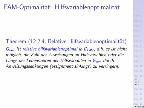
Inhalt
Kap. 1
Kap. 2
Kap. 3
Kap. 4
Kap. 5
Kap. 6
Kap. 7
Kap. 8
Kap. 9
Kap. 10
Kap. 11
Kap. 12
12.1
12.2
12.3
Kap. 13
Kap. 14
Kap. 15
Kap. 16
Kap. 17
Literatur
Anhang
A
EAM-Optimalitat: Hilfsvariablenoptimalitat
Theorem (12.2.4, Relative Hilfsvariablenoptimalitat)
Geam ist relative hilfsvariablenoptimal in GEAM , d.h. es ist nichtmoglich, die Zahl der Zuweisungen an Hilfsvariablen oder dieLange der Lebenszeiten der Hilfsvariablen in Geam durchAnweisungssenkungen (assignment sinkings) zu verringern.
629/863
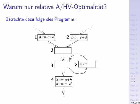
Inhalt
Kap. 1
Kap. 2
Kap. 3
Kap. 4
Kap. 5
Kap. 6
Kap. 7
Kap. 8
Kap. 9
Kap. 10
Kap. 11
Kap. 12
12.1
12.2
12.3
Kap. 13
Kap. 14
Kap. 15
Kap. 16
Kap. 17
Literatur
Anhang
A
Warum nur relative A/HV-Optimalitat?
Betrachte dazu folgendes Programm:
x := a+b
x :=
a := c+d b := c+d1 2
4 5
6
a := c+d
3
630/863
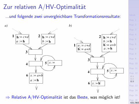
Inhalt
Kap. 1
Kap. 2
Kap. 3
Kap. 4
Kap. 5
Kap. 6
Kap. 7
Kap. 8
Kap. 9
Kap. 10
Kap. 11
Kap. 12
12.1
12.2
12.3
Kap. 13
Kap. 14
Kap. 15
Kap. 16
Kap. 17
Literatur
Anhang
A
Zur relativen A/HV-Optimalitat
...und folgende zwei unvergleichbare Transformationsresultate:
:= a+bh
:= c+d
b :=
h
h
a) b)
x := a+b
x := 4 5
6
a :=h
h:= c+d h := c+d
b := h
a :=h
2
x := 4 5
6 x :=
a :=h
a := c+d
2
:= a+b3
3
1
1
h
h
⇒ Relative A/HV-Optimalitat ist das Beste, was moglich ist!631/863
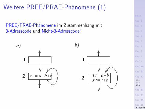
Inhalt
Kap. 1
Kap. 2
Kap. 3
Kap. 4
Kap. 5
Kap. 6
Kap. 7
Kap. 8
Kap. 9
Kap. 10
Kap. 11
Kap. 12
12.1
12.2
12.3
Kap. 13
Kap. 14
Kap. 15
Kap. 16
Kap. 17
Literatur
Anhang
A
Weitere PREE/PRAE-Phanomene (1)
PREE/PRAE-Phanomene im Zusammenhang mit3-Adresscode und Nicht-3-Adresscode:
a)
1
x := a+b+c22
t := a+bx := t+c
1
b)
632/863
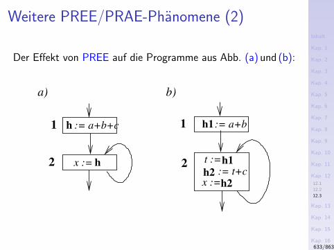
Inhalt
Kap. 1
Kap. 2
Kap. 3
Kap. 4
Kap. 5
Kap. 6
Kap. 7
Kap. 8
Kap. 9
Kap. 10
Kap. 11
Kap. 12
12.1
12.2
12.3
Kap. 13
Kap. 14
Kap. 15
Kap. 16
Kap. 17
Literatur
Anhang
A
Weitere PREE/PRAE-Phanomene (2)
Der Effekt von PREE auf die Programme aus Abb. (a) und (b):
:= t+cx :=h2
t := h1
h2
b)
h1 := a+b11 h := a+b+c
hx := 2
a)
2
633/863
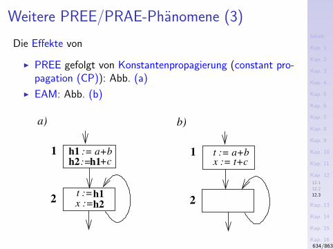
Inhalt
Kap. 1
Kap. 2
Kap. 3
Kap. 4
Kap. 5
Kap. 6
Kap. 7
Kap. 8
Kap. 9
Kap. 10
Kap. 11
Kap. 12
12.1
12.2
12.3
Kap. 13
Kap. 14
Kap. 15
Kap. 16
Kap. 17
Literatur
Anhang
A
Weitere PREE/PRAE-Phanomene (3)
Die Effekte von
I PREE gefolgt von Konstantenpropagierung (constant pro-pagation (CP)): Abb. (a)
I EAM: Abb. (b)
h1
h1+ch2 :=
t := h1x :=h2
2 2
a)
1 := a+b
b)
1 t := a+bx := t+c
634/863
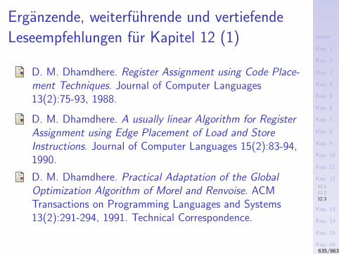
Inhalt
Kap. 1
Kap. 2
Kap. 3
Kap. 4
Kap. 5
Kap. 6
Kap. 7
Kap. 8
Kap. 9
Kap. 10
Kap. 11
Kap. 12
12.1
12.2
12.3
Kap. 13
Kap. 14
Kap. 15
Kap. 16
Kap. 17
Literatur
Anhang
A
Erganzende, weiterfuhrende und vertiefende
Leseempfehlungen fur Kapitel 12 (1)
D. M. Dhamdhere. Register Assignment using Code Place-ment Techniques. Journal of Computer Languages13(2):75-93, 1988.
D. M. Dhamdhere. A usually linear Algorithm for RegisterAssignment using Edge Placement of Load and StoreInstructions. Journal of Computer Languages 15(2):83-94,1990.
D. M. Dhamdhere. Practical Adaptation of the GlobalOptimization Algorithm of Morel and Renvoise. ACMTransactions on Programming Languages and Systems13(2):291-294, 1991. Technical Correspondence.
635/863
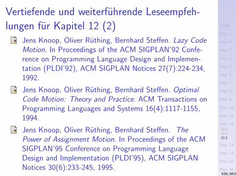
Inhalt
Kap. 1
Kap. 2
Kap. 3
Kap. 4
Kap. 5
Kap. 6
Kap. 7
Kap. 8
Kap. 9
Kap. 10
Kap. 11
Kap. 12
12.1
12.2
12.3
Kap. 13
Kap. 14
Kap. 15
Kap. 16
Kap. 17
Literatur
Anhang
A
Vertiefende und weiterfuhrende Leseempfeh-
lungen fur Kapitel 12 (2)Jens Knoop, Oliver Ruthing, Bernhard Steffen. Lazy CodeMotion. In Proceedings of the ACM SIGPLAN’92 Confe-rence on Programming Language Design and Implemen-tation (PLDI’92), ACM SIGPLAN Notices 27(7):224-234,1992.
Jens Knoop, Oliver Ruthing, Bernhard Steffen. OptimalCode Motion: Theory and Practice. ACM Transactions onProgramming Languages and Systems 16(4):1117-1155,1994.
Jens Knoop, Oliver Ruthing, Bernhard Steffen. ThePower of Assignment Motion. In Proceedings of the ACMSIGPLAN’95 Conference on Programming LanguageDesign and Implementation (PLDI’95), ACM SIGPLANNotices 30(6):233-245, 1995.
636/863
Inhalt
Kap. 1
Kap. 2
Kap. 3
Kap. 4
Kap. 5
Kap. 6
Kap. 7
Kap. 8
Kap. 9
Kap. 10
Kap. 11
Kap. 12
12.1
12.2
12.3
Kap. 13
Kap. 14
Kap. 15
Kap. 16
Kap. 17
Literatur
Anhang
A
Vertiefende und weiterfuhrende Leseempfeh-
lungen fur Kapitel 12 (3)
Jens Knoop, Oliver Ruthing, Bernhard Steffen.Retrospective: Lazy Code Motion. In ”20 Years of theACM SIGPLAN Conference on Programming LanguageDesign and Implementation (1979 - 1999): A Selection”,ACM SIGPLAN Notices 39(4):460-461&462-472, 2004.
Munehiro Takimoto, Kenichi Harada. Effective PartialRedundancy Elimination based on Extended Value Graph.Information Processing Society of Japan38(11):2237-2250, 1990.
637/863

Inhalt
Kap. 1
Kap. 2
Kap. 3
Kap. 4
Kap. 5
Kap. 6
Kap. 7
Kap. 8
Kap. 9
Kap. 10
Kap. 11
Kap. 12
Kap. 13
Kap. 14
Kap. 15
Kap. 16
Kap. 17
Literatur
Anhang
A
Kapitel 13
Kombination von PRAE und PDCE
638/863
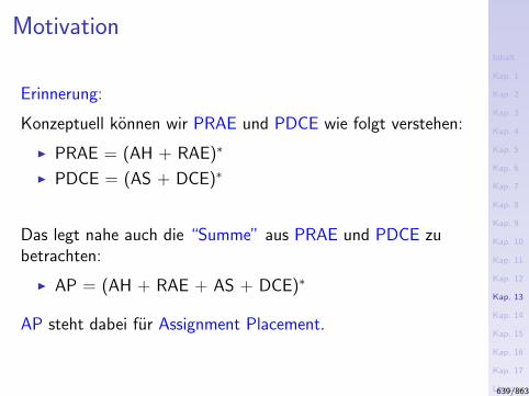
Inhalt
Kap. 1
Kap. 2
Kap. 3
Kap. 4
Kap. 5
Kap. 6
Kap. 7
Kap. 8
Kap. 9
Kap. 10
Kap. 11
Kap. 12
Kap. 13
Kap. 14
Kap. 15
Kap. 16
Kap. 17
Literatur
Anhang
A
Motivation
Erinnerung:
Konzeptuell konnen wir PRAE und PDCE wie folgt verstehen:
I PRAE = (AH + RAE)∗
I PDCE = (AS + DCE)∗
Das legt nahe auch die “Summe” aus PRAE und PDCE zubetrachten:
I AP = (AH + RAE + AS + DCE)∗
AP steht dabei fur Assignment Placement.
639/863
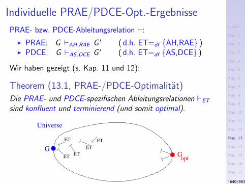
Inhalt
Kap. 1
Kap. 2
Kap. 3
Kap. 4
Kap. 5
Kap. 6
Kap. 7
Kap. 8
Kap. 9
Kap. 10
Kap. 11
Kap. 12
Kap. 13
Kap. 14
Kap. 15
Kap. 16
Kap. 17
Literatur
Anhang
A
Individuelle PRAE/PDCE-Opt.-Ergebnisse
PRAE- bzw. PDCE-Ableitungsrelation `:
I PRAE: G `AH,RAE G ′ ( d.h. ET=df AH,RAE )I PDCE: G `AS ,DCE G ′ ( d.h. ET=df AS,DCE )
Wir haben gezeigt (s. Kap. 11 und 12):
Theorem (13.1, PRAE-/PDCE-Optimalitat)
Die PRAE- und PDCE-spezifischen Ableitungsrelationen `ETsind konfluent und terminierend (und somit optimal).
ET
ET
ETET
ET
GGopt
Universe
640/863
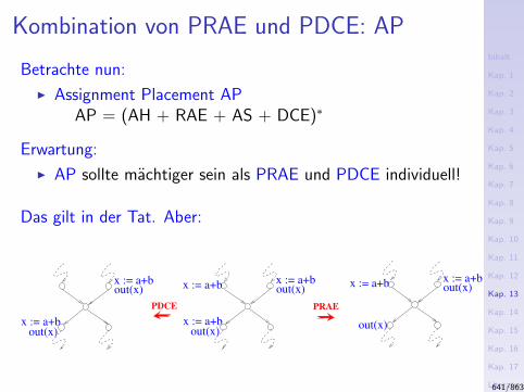
Inhalt
Kap. 1
Kap. 2
Kap. 3
Kap. 4
Kap. 5
Kap. 6
Kap. 7
Kap. 8
Kap. 9
Kap. 10
Kap. 11
Kap. 12
Kap. 13
Kap. 14
Kap. 15
Kap. 16
Kap. 17
Literatur
Anhang
A
Kombination von PRAE und PDCE: AP
Betrachte nun:
I Assignment Placement APAP = (AH + RAE + AS + DCE)∗
Erwartung:
I AP sollte machtiger sein als PRAE und PDCE individuell!
Das gilt in der Tat. Aber:
x := a+bout(x)x := a+b
x := a+bout(x)
x := a+bout(x)x := a+b
out(x)
x := a+bout(x)
x := a+bout(x)
PRAEPDCE
641/863
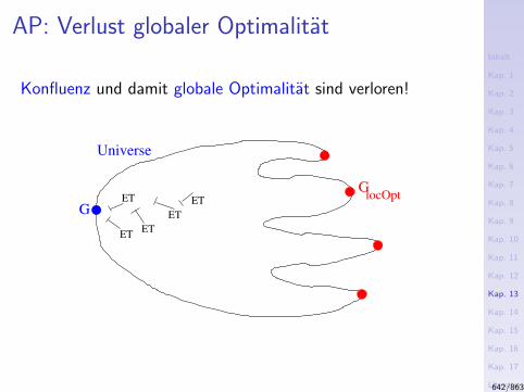
Inhalt
Kap. 1
Kap. 2
Kap. 3
Kap. 4
Kap. 5
Kap. 6
Kap. 7
Kap. 8
Kap. 9
Kap. 10
Kap. 11
Kap. 12
Kap. 13
Kap. 14
Kap. 15
Kap. 16
Kap. 17
Literatur
Anhang
A
AP: Verlust globaler Optimalitat
Konfluenz und damit globale Optimalitat sind verloren!
ET
ET
ETET
ETGlocOpt
G
Universe
642/863
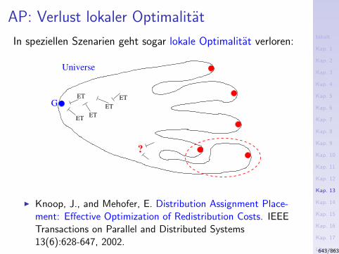
Inhalt
Kap. 1
Kap. 2
Kap. 3
Kap. 4
Kap. 5
Kap. 6
Kap. 7
Kap. 8
Kap. 9
Kap. 10
Kap. 11
Kap. 12
Kap. 13
Kap. 14
Kap. 15
Kap. 16
Kap. 17
Literatur
Anhang
A
AP: Verlust lokaler Optimalitat
In speziellen Szenarien geht sogar lokale Optimalitat verloren:
G
Universe
ET
ET
ETET
ET
?
I Knoop, J., and Mehofer, E. Distribution Assignment Place-ment: Effective Optimization of Redistribution Costs. IEEETransactions on Parallel and Distributed Systems13(6):628-647, 2002.
643/863
Inhalt
Kap. 1
Kap. 2
Kap. 3
Kap. 4
Kap. 5
Kap. 6
Kap. 7
Kap. 8
Kap. 9
Kap. 10
Kap. 11
Kap. 12
Kap. 13
Kap. 14
Kap. 15
Kap. 16
Kap. 17
Literatur
Anhang
A
Vertiefende und weiterfuhrende Leseempfeh-
lungen fur Kapitel 13
Jens Knoop, Oliver Ruthing, Bernhard Steffen. CodeMotion and Code Placement: Just Synonyms? In Procee-dings of the 7th European Symposium on Programming(ESOP’98), Springer-V., LNCS 1381, 154-169, 1998.
Jens Knoop, Eduard Mehofer. Distribution AssignmentPlacement: Effective Optimization of Redistribution Costs.IEEE Transactions on Parallel and Distributed Systems13(6):628-647, 2002.
644/863

Inhalt
Kap. 1
Kap. 2
Kap. 3
Kap. 4
Kap. 5
Kap. 6
Kap. 7
Kap. 8
Kap. 9
Kap. 10
Kap. 11
Kap. 12
Kap. 13
Kap. 14
14.1
14.2
14.3
Kap. 15
Kap. 16
Kap. 17
Literatur
Anhang
A
Kapitel 14
Konstantenfaltung auf dem Wertegraphen
645/863
Inhalt
Kap. 1
Kap. 2
Kap. 3
Kap. 4
Kap. 5
Kap. 6
Kap. 7
Kap. 8
Kap. 9
Kap. 10
Kap. 11
Kap. 12
Kap. 13
Kap. 14
14.1
14.2
14.3
Kap. 15
Kap. 16
Kap. 17
Literatur
Anhang
A
Arbeitsplan
Konstantenfaltung und -ausbreitung
I Hintergrund und Motivation
I Der VG-Konstantenfaltungsalgorithmus
I Der PVG-Konstantenfaltungsalgorithmus
646/863

Inhalt
Kap. 1
Kap. 2
Kap. 3
Kap. 4
Kap. 5
Kap. 6
Kap. 7
Kap. 8
Kap. 9
Kap. 10
Kap. 11
Kap. 12
Kap. 13
Kap. 14
14.1
14.2
14.3
Kap. 15
Kap. 16
Kap. 17
Literatur
Anhang
A
Kapitel 14.1
Motivation
647/863
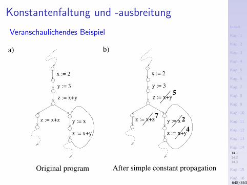
Inhalt
Kap. 1
Kap. 2
Kap. 3
Kap. 4
Kap. 5
Kap. 6
Kap. 7
Kap. 8
Kap. 9
Kap. 10
Kap. 11
Kap. 12
Kap. 13
Kap. 14
14.1
14.2
14.3
Kap. 15
Kap. 16
Kap. 17
Literatur
Anhang
A
Konstantenfaltung und -ausbreitung
Veranschaulichendes Beispiel
a) b)
2
4
7
5
After simple constant propagationOriginal program
x := 2
y := 3
z := x+y
z := x+z y := x
z := x+y
x := 2
y := 3
z := x+y
z := x+z y := x
z := x+y
648/863
Inhalt
Kap. 1
Kap. 2
Kap. 3
Kap. 4
Kap. 5
Kap. 6
Kap. 7
Kap. 8
Kap. 9
Kap. 10
Kap. 11
Kap. 12
Kap. 13
Kap. 14
14.1
14.2
14.3
Kap. 15
Kap. 16
Kap. 17
Literatur
Anhang
A
Ursprung und Entwicklung
...von Algorithmen zu Konstantenfaltung und -ausbreitung.
Pragend:
I Gary A. Kildalls Algorithmus zur Berechnung einfacherKonstanten (engl. simple constants (SC) (POPL’73).
Beachte:
I Der Algorithmus zur Berechnung einfacher Konstantenaus Kapitel 6.6 stimmt im Ergebnis, nicht jedoch in denverwendeten Datenstrukturen mit Kildalls Algorithmusuberein.
649/863
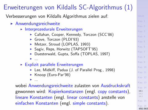
Inhalt
Kap. 1
Kap. 2
Kap. 3
Kap. 4
Kap. 5
Kap. 6
Kap. 7
Kap. 8
Kap. 9
Kap. 10
Kap. 11
Kap. 12
Kap. 13
Kap. 14
14.1
14.2
14.3
Kap. 15
Kap. 16
Kap. 17
Literatur
Anhang
A
Erweiterungen von Kildalls SC-Algorithmus (1)Verbesserungen von Kildalls Algorithmus zielen auf:
I AnwendungsreichweiteI Interprozedurale Erweiterungen
I Callahan, Cooper, Kennedy, Torczon (SCC’86)I Grove, Torczon (PLDI’93)I Metzer, Stroud (LOPLAS, 1993)I Sagiv, Reps, Horwitz (TAPSOFT’95)I Duesterwald, Gupta, Soffa (TOPLAS, 1997)I ...
I Explizit parallele ErweiterungenI Lee, Midkiff, Padua (J. of Parallel Prog., 1998)I Knoop (Euro-Par’98)I ...
wobei Anwendungsreichweite zulasten von Ausdruckskraftgewonnen wird: Kopierkonstanzen (engl. copy constants),lineare Konstanten (engl. linear constants) anstelle voneinfachen Konstanten (engl. simple constants).
650/863
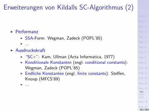
Inhalt
Kap. 1
Kap. 2
Kap. 3
Kap. 4
Kap. 5
Kap. 6
Kap. 7
Kap. 8
Kap. 9
Kap. 10
Kap. 11
Kap. 12
Kap. 13
Kap. 14
14.1
14.2
14.3
Kap. 15
Kap. 16
Kap. 17
Literatur
Anhang
A
Erweiterungen von Kildalls SC-Algorithmus (2)
I PerformanzI SSA-Form: Wegman, Zadeck (POPL’85)I ...
I AusdruckskraftI “SC+”: Kam, Ullman (Acta Informatica, 1977)I Konditionale Konstanten (engl. conditional constants):
Wegman, Zadeck (POPL’85)I Endliche Konstanten (engl. finite constants): Steffen,
Knoop (MFCS’89)I ...
651/863
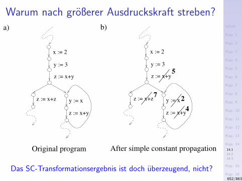
Inhalt
Kap. 1
Kap. 2
Kap. 3
Kap. 4
Kap. 5
Kap. 6
Kap. 7
Kap. 8
Kap. 9
Kap. 10
Kap. 11
Kap. 12
Kap. 13
Kap. 14
14.1
14.2
14.3
Kap. 15
Kap. 16
Kap. 17
Literatur
Anhang
A
Warum nach großerer Ausdruckskraft streben?a) b)
2
4
7
5
After simple constant propagationOriginal program
x := 2
y := 3
z := x+y
z := x+z y := x
z := x+y
x := 2
y := 3
z := x+y
z := x+z y := x
z := x+y
Das SC-Transformationsergebnis ist doch uberzeugend, nicht?652/863
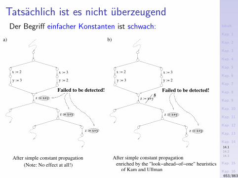
Inhalt
Kap. 1
Kap. 2
Kap. 3
Kap. 4
Kap. 5
Kap. 6
Kap. 7
Kap. 8
Kap. 9
Kap. 10
Kap. 11
Kap. 12
Kap. 13
Kap. 14
14.1
14.2
14.3
Kap. 15
Kap. 16
Kap. 17
Literatur
Anhang
A
Tatsachlich ist es nicht uberzeugendDer Begriff einfacher Konstanten ist schwach:
b)a)
Failed to be detected!
5
Failed to be detected!
After simple constant propagation
(Note: No effect at all!)
After simple constant propagation
enriched by the "look−ahead−of−one" heuristicsof Kam and Ullman
z := x+y
z := x+y
z := x+y z := x+y
z := x+y
x := 2
y := 3
x := 3
y := 2
x := 2
y := 3
x := 3
y := 2
z := x+y
653/863
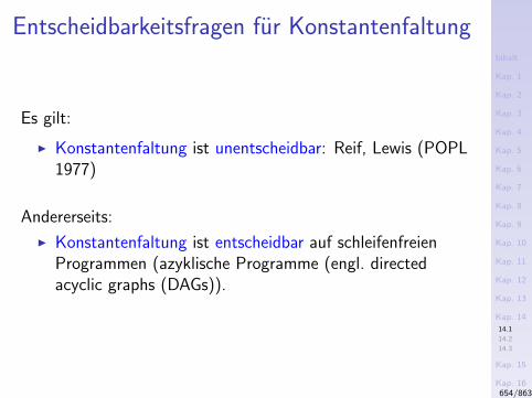
Inhalt
Kap. 1
Kap. 2
Kap. 3
Kap. 4
Kap. 5
Kap. 6
Kap. 7
Kap. 8
Kap. 9
Kap. 10
Kap. 11
Kap. 12
Kap. 13
Kap. 14
14.1
14.2
14.3
Kap. 15
Kap. 16
Kap. 17
Literatur
Anhang
A
Entscheidbarkeitsfragen fur Konstantenfaltung
Es gilt:
I Konstantenfaltung ist unentscheidbar: Reif, Lewis (POPL1977)
Andererseits:
I Konstantenfaltung ist entscheidbar auf schleifenfreienProgrammen (azyklische Programme (engl. directedacyclic graphs (DAGs)).
654/863
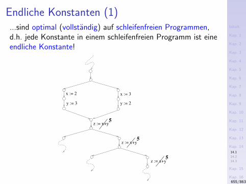
Inhalt
Kap. 1
Kap. 2
Kap. 3
Kap. 4
Kap. 5
Kap. 6
Kap. 7
Kap. 8
Kap. 9
Kap. 10
Kap. 11
Kap. 12
Kap. 13
Kap. 14
14.1
14.2
14.3
Kap. 15
Kap. 16
Kap. 17
Literatur
Anhang
A
Endliche Konstanten (1)...sind optimal (vollstandig) auf schleifenfreien Programmen,d.h. jede Konstante in einem schleifenfreien Programm ist eineendliche Konstante!
5
5
5
The effect of the new algorithm
z := x+y
z := x+y
z := x+y
x := 2
y := 3
x := 3
y := 2
655/863
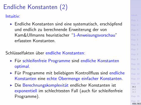
Inhalt
Kap. 1
Kap. 2
Kap. 3
Kap. 4
Kap. 5
Kap. 6
Kap. 7
Kap. 8
Kap. 9
Kap. 10
Kap. 11
Kap. 12
Kap. 13
Kap. 14
14.1
14.2
14.3
Kap. 15
Kap. 16
Kap. 17
Literatur
Anhang
A
Endliche Konstanten (2)
Intuitiv:
I Endliche Konstanten sind eine systematisch, erschopfendund endlich zu berechnende Erweiterung der vonKam&Ullmanns heuristischer “1-Anweisungsvorschau”erfassten Konstanten.
Schlusselfakten uber endliche Konstanten:
I Fur schleifenfreie Programme sind endliche Konstantenoptimal.
I Fur Programme mit beliebigem Kontrollfluss sind endlicheKonstanten eine echte Obermenge einfacher Konstanten.
I Die Berechnungskomplexitat endlicher Konstanten istexponentiell im schlechtesten Fall (auch fur schleifenfreieProgramme).
656/863
Inhalt
Kap. 1
Kap. 2
Kap. 3
Kap. 4
Kap. 5
Kap. 6
Kap. 7
Kap. 8
Kap. 9
Kap. 10
Kap. 11
Kap. 12
Kap. 13
Kap. 14
14.1
14.2
14.3
Kap. 15
Kap. 16
Kap. 17
Literatur
Anhang
A
Hinsichtlich der Berechnungskomplexitat
...endlicher Konstanten sollte man bedenken:
Theorem (14.1.1)
Konstantenfaltung und -ausbreitung ist fur schleifenfreieProgramme co-NP-vollstandig.
Knoop, Ruthing (CC’00)
Muller-Olm, Ruthing (ESOP’01)
657/863
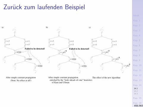
Inhalt
Kap. 1
Kap. 2
Kap. 3
Kap. 4
Kap. 5
Kap. 6
Kap. 7
Kap. 8
Kap. 9
Kap. 10
Kap. 11
Kap. 12
Kap. 13
Kap. 14
14.1
14.2
14.3
Kap. 15
Kap. 16
Kap. 17
Literatur
Anhang
A
Zuruck zum laufenden Beispiel
5
5
5
c)b)a)
Failed to be detected!
5
Failed to be detected!
After simple constant propagation
(Note: No effect at all!)
The effect of the new algorithmAfter simple constant propagation
enriched by the "look−ahead−of−one" heuristicsof Kam and Ullman
z := x+y
z := x+y
z := x+y z := x+y
z := x+y z := x+y
z := x+y
z := x+y
x := 2
y := 3
x := 3
y := 2
x := 2
y := 3
x := 3
y := 2
x := 2
y := 3
x := 3
y := 2
z := x+y
658/863
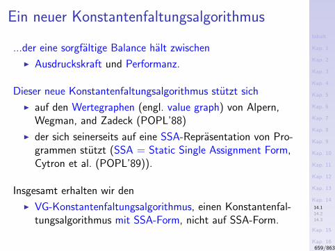
Inhalt
Kap. 1
Kap. 2
Kap. 3
Kap. 4
Kap. 5
Kap. 6
Kap. 7
Kap. 8
Kap. 9
Kap. 10
Kap. 11
Kap. 12
Kap. 13
Kap. 14
14.1
14.2
14.3
Kap. 15
Kap. 16
Kap. 17
Literatur
Anhang
A
Ein neuer Konstantenfaltungsalgorithmus
...der eine sorgfaltige Balance halt zwischen
I Ausdruckskraft und Performanz.
Dieser neue Konstantenfaltungsalgorithmus stutzt sich
I auf den Wertegraphen (engl. value graph) von Alpern,Wegman, and Zadeck (POPL’88)
I der sich seinerseits auf eine SSA-Reprasentation von Pro-grammen stutzt (SSA = Static Single Assignment Form,Cytron et al. (POPL’89)).
Insgesamt erhalten wir den
I VG-Konstantenfaltungsalgorithmus, einen Konstantenfal-tungsalgorithmus mit SSA-Form, nicht auf SSA-Form.
659/863

Inhalt
Kap. 1
Kap. 2
Kap. 3
Kap. 4
Kap. 5
Kap. 6
Kap. 7
Kap. 8
Kap. 9
Kap. 10
Kap. 11
Kap. 12
Kap. 13
Kap. 14
14.1
14.2
14.3
Kap. 15
Kap. 16
Kap. 17
Literatur
Anhang
A
Kapitel 14.2
Der VG-Konstantenfaltungsalgorithmus
660/863
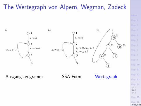
Inhalt
Kap. 1
Kap. 2
Kap. 3
Kap. 4
Kap. 5
Kap. 6
Kap. 7
Kap. 8
Kap. 9
Kap. 10
Kap. 11
Kap. 12
Kap. 13
Kap. 14
14.1
14.2
14.3
Kap. 15
Kap. 16
Kap. 17
Literatur
Anhang
A
The Wertegraph von Alpern, Wegman, Zadeck
x0
x1
Φ
+
1
2x
−
1
x3
0
x := x −1
x := 00
3 2x := x +112
1 Φ 32
x := 0
x := x+1x := x−1
a) b) c)
2
x := 0(x , x )
1
2
3
1
3
2
Ausgangsprogramm SSA-Form Wertegraph
661/863
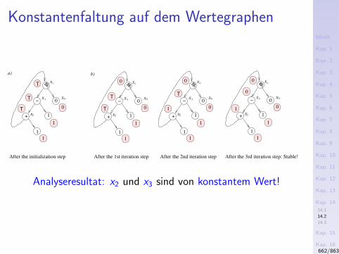
Inhalt
Kap. 1
Kap. 2
Kap. 3
Kap. 4
Kap. 5
Kap. 6
Kap. 7
Kap. 8
Kap. 9
Kap. 10
Kap. 11
Kap. 12
Kap. 13
Kap. 14
14.1
14.2
14.3
Kap. 15
Kap. 16
Kap. 17
Literatur
Anhang
A
Konstantenfaltung auf dem Wertegraphen
T
T
T
1
1
x1Φ
+
1
2x
−
1
x3 0x0
01
0
0
1
1
1
1
T
TT
x1Φ
+
1
2x
−
1
x3 0x0
0
1
1
x1Φ
+
1
2x
−
1
x3 0x0
0
0 x1Φ
+
1
2x
−
1
x3 0x0
0
0
1
After the 1st iteration step After the 2nd iteration step After the 3rd iteration step: Stable!After the initialization step
22
a) b)
2 2
Analyseresultat: x2 und x3 sind von konstantem Wert!
662/863
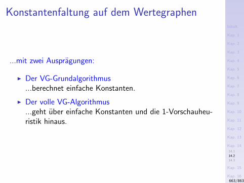
Inhalt
Kap. 1
Kap. 2
Kap. 3
Kap. 4
Kap. 5
Kap. 6
Kap. 7
Kap. 8
Kap. 9
Kap. 10
Kap. 11
Kap. 12
Kap. 13
Kap. 14
14.1
14.2
14.3
Kap. 15
Kap. 16
Kap. 17
Literatur
Anhang
A
Konstantenfaltung auf dem Wertegraphen
...mit zwei Auspragungen:
I Der VG-Grundalgorithmus...berechnet einfache Konstanten.
I Der volle VG-Algorithmus...geht uber einfache Konstanten und die 1-Vorschauheu-ristik hinaus.
663/863
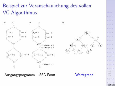
Inhalt
Kap. 1
Kap. 2
Kap. 3
Kap. 4
Kap. 5
Kap. 6
Kap. 7
Kap. 8
Kap. 9
Kap. 10
Kap. 11
Kap. 12
Kap. 13
Kap. 14
14.1
14.2
14.3
Kap. 15
Kap. 16
Kap. 17
Literatur
Anhang
A
Beispiel zur Veranschaulichung des vollen
VG-Algorithmus
+
Φ Φ
2 23 3x0 1x1 0y y
y2x2
z0
2
Φ
−
6 1
z 1
z
x := Φn(x , x )0 12 n n
m
y := 3
x := 3
y := 2
z := x + y z := 6−1
x := 2
y := 3
x := 3
y := 2
z := x+y z := 6−1
x := 20
0 1
1
y := Φn(y , y )0 12
n
2 20 0
z := Φm(z , z )0 12
b)a)
m
c)
Ausgangsprogramm SSA-Form Wertegraph
664/863
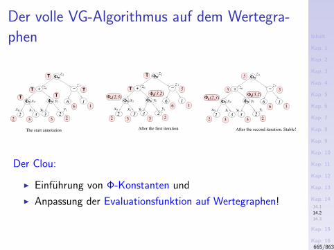
Inhalt
Kap. 1
Kap. 2
Kap. 3
Kap. 4
Kap. 5
Kap. 6
Kap. 7
Kap. 8
Kap. 9
Kap. 10
Kap. 11
Kap. 12
Kap. 13
Kap. 14
14.1
14.2
14.3
Kap. 15
Kap. 16
Kap. 17
Literatur
Anhang
A
Der volle VG-Algorithmus auf dem Wertegra-
phen
2 22
+
Φ Φ
2 23 3x0 1x1 0y y
y2x2
z0
2
Φ
−
6 1
z 1
z
3
6 1
3
T
T
2
T
T
T
+
Φ Φ
2 23 3x0 1x1 0y y
y2x2
z0
2
Φ
−
6 1
z 1
z
3
6 1
5
5
2
5
Φ (2,3)Φ (3,2)
3
After the second iteration. Stable!
+
Φ Φ
2 23 3x0 1x1 0y y
y2x2
z0
2
Φ
−
6 1
z 1
z
3
6 1
T
T
2
5
Φ (2,3)Φ (3,2)
3
After the first iterationThe start annotation
n n
m
n n
m
n
n
n n
m
n
n
Der Clou:
I Einfuhrung von Φ-Konstanten und
I Anpassung der Evaluationsfunktion auf Wertegraphen!
665/863
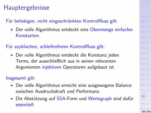
Inhalt
Kap. 1
Kap. 2
Kap. 3
Kap. 4
Kap. 5
Kap. 6
Kap. 7
Kap. 8
Kap. 9
Kap. 10
Kap. 11
Kap. 12
Kap. 13
Kap. 14
14.1
14.2
14.3
Kap. 15
Kap. 16
Kap. 17
Literatur
Anhang
A
Hauptergebnisse
Fur beliebigen, nicht eingeschrankten Kontrollfluss gilt:
I Der volle Algorithmus entdeckt eine Obermenge einfacherKonstanten.
Fur azyklischen, schleifenfreien Kontrollfluss gilt:
I Der volle Algorithmus entdeckt die Konstanz jedenTerms, der ausschließlich aus in seinen relevantenArgumenten injektiven Operatoren aufgebaut ist.
Insgesamt gilt:
I Der volle Algorithmus erreicht eine ausgewogene Balancezwischen Ausdruckskraft und Performanz.
I Die Abstutzung auf SSA-Form und Wertegraph sind dafuressentiell.
666/863
Inhalt
Kap. 1
Kap. 2
Kap. 3
Kap. 4
Kap. 5
Kap. 6
Kap. 7
Kap. 8
Kap. 9
Kap. 10
Kap. 11
Kap. 12
Kap. 13
Kap. 14
14.1
14.2
14.3
Kap. 15
Kap. 16
Kap. 17
Literatur
Anhang
A
Literaturhinweis
...zum VG-Konstantenfaltungsalgorithmus:
I Jens Knoop, Oliver Ruthing. Constant Propagation onthe Value Graph: Simple Constants and Beyond. InProceedings of the 9th International Conference onCompiler Construction (CC 2000), Springer-V., LNCS1781, 94-109, 2000.
667/863

Inhalt
Kap. 1
Kap. 2
Kap. 3
Kap. 4
Kap. 5
Kap. 6
Kap. 7
Kap. 8
Kap. 9
Kap. 10
Kap. 11
Kap. 12
Kap. 13
Kap. 14
14.1
14.2
14.3
Kap. 15
Kap. 16
Kap. 17
Literatur
Anhang
A
Kapitel 14.3
Der PVG-Konstantenfaltungsalgorithmus
668/863
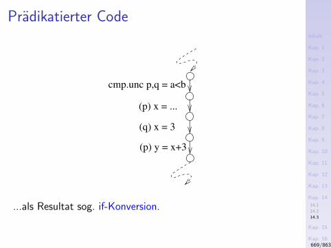
Inhalt
Kap. 1
Kap. 2
Kap. 3
Kap. 4
Kap. 5
Kap. 6
Kap. 7
Kap. 8
Kap. 9
Kap. 10
Kap. 11
Kap. 12
Kap. 13
Kap. 14
14.1
14.2
14.3
Kap. 15
Kap. 16
Kap. 17
Literatur
Anhang
A
Pradikatierter Code
(q) x = 3
(p) y = x+3
cmp.unc p,q = a<b
(p) x = ...
...als Resultat sog. if-Konversion.
669/863
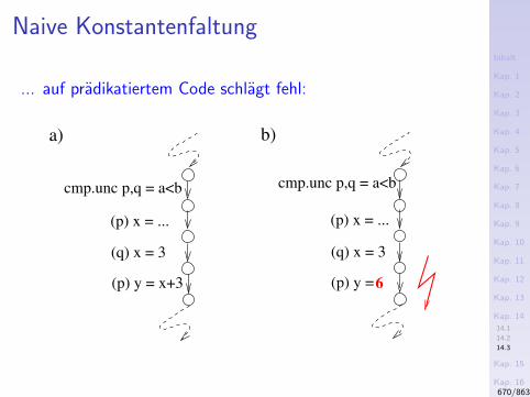
Inhalt
Kap. 1
Kap. 2
Kap. 3
Kap. 4
Kap. 5
Kap. 6
Kap. 7
Kap. 8
Kap. 9
Kap. 10
Kap. 11
Kap. 12
Kap. 13
Kap. 14
14.1
14.2
14.3
Kap. 15
Kap. 16
Kap. 17
Literatur
Anhang
A
Naive Konstantenfaltung
... auf pradikatiertem Code schlagt fehl:
b)
(q) x = 3
(p) y = x+3
a)
cmp.unc p,q = a<bcmp.unc p,q = a<b
(p) x = ...
(q) x = 3
6(p) y =
(p) x = ...
670/863
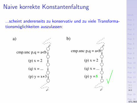
Inhalt
Kap. 1
Kap. 2
Kap. 3
Kap. 4
Kap. 5
Kap. 6
Kap. 7
Kap. 8
Kap. 9
Kap. 10
Kap. 11
Kap. 12
Kap. 13
Kap. 14
14.1
14.2
14.3
Kap. 15
Kap. 16
Kap. 17
Literatur
Anhang
A
Naive korrekte Konstantenfaltung
...scheint andererseits zu konservativ und zu viele Transforma-tionsmoglichkeiten auszulassen:
b)
(p) x = 2
(q) x = ...
(p) y = x+3
a)
cmp.unc p,q = a<bcmp.unc p,q = a<b
(q) x = ...
5(p) y =
(p) x = 2
671/863
Inhalt
Kap. 1
Kap. 2
Kap. 3
Kap. 4
Kap. 5
Kap. 6
Kap. 7
Kap. 8
Kap. 9
Kap. 10
Kap. 11
Kap. 12
Kap. 13
Kap. 14
14.1
14.2
14.3
Kap. 15
Kap. 16
Kap. 17
Literatur
Anhang
A
Ziel
Ein intelligenterer Umgang mit pradikatiertem Code.
Hyperblocke sind
I wichtige Komponenten pradikatierten Codes.
672/863
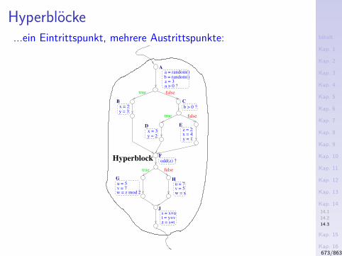
Inhalt
Kap. 1
Kap. 2
Kap. 3
Kap. 4
Kap. 5
Kap. 6
Kap. 7
Kap. 8
Kap. 9
Kap. 10
Kap. 11
Kap. 12
Kap. 13
Kap. 14
14.1
14.2
14.3
Kap. 15
Kap. 16
Kap. 17
Literatur
Anhang
A
Hyperblocke...ein Eintrittspunkt, mehrere Austrittspunkte:
b > 0 ?
C
H
w = xv = 5u = 7
x = 3y = 2
D
x = 2y = 3
B
b = random()z = 3a > 0 ?
a = random()A
odd(z) ?F
y = 1x = 4z = 2
E
w = z mod 2
G
v = 7u = 5
J
z = s+tt = y+vs = x+u
true false
true false
true false
Hyperblock
673/863
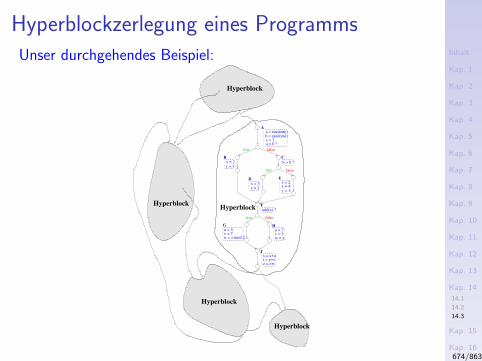
Inhalt
Kap. 1
Kap. 2
Kap. 3
Kap. 4
Kap. 5
Kap. 6
Kap. 7
Kap. 8
Kap. 9
Kap. 10
Kap. 11
Kap. 12
Kap. 13
Kap. 14
14.1
14.2
14.3
Kap. 15
Kap. 16
Kap. 17
Literatur
Anhang
A
Hyperblockzerlegung eines Programms
Unser durchgehendes Beispiel:
b > 0 ?
C
H
w = xv = 5u = 7
x = 3y = 2
D
x = 2y = 3
B
b = random()z = 3a > 0 ?
a = random()A
odd(z) ?F
y = 1x = 4z = 2
E
w = z mod 2
G
v = 7u = 5
J
z = s+tt = y+vs = x+u
true false
true false
true false
Hyperblock
Hyperblock
Hyperblock
Hyperblock
Hyperblock
674/863
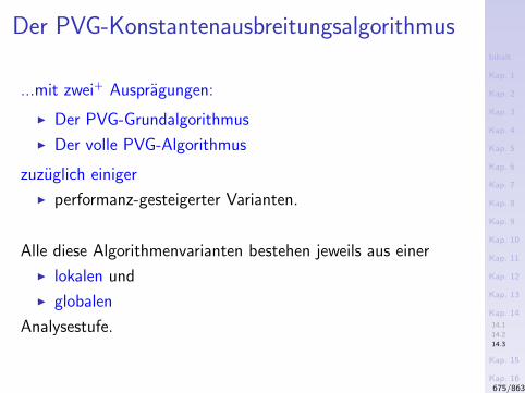
Inhalt
Kap. 1
Kap. 2
Kap. 3
Kap. 4
Kap. 5
Kap. 6
Kap. 7
Kap. 8
Kap. 9
Kap. 10
Kap. 11
Kap. 12
Kap. 13
Kap. 14
14.1
14.2
14.3
Kap. 15
Kap. 16
Kap. 17
Literatur
Anhang
A
Der PVG-Konstantenausbreitungsalgorithmus
...mit zwei+ Auspragungen:
I Der PVG-Grundalgorithmus
I Der volle PVG-Algorithmus
zuzuglich einiger
I performanz-gesteigerter Varianten.
Alle diese Algorithmenvarianten bestehen jeweils aus einer
I lokalen und
I globalen
Analysestufe.
675/863
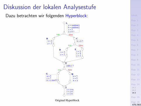
Inhalt
Kap. 1
Kap. 2
Kap. 3
Kap. 4
Kap. 5
Kap. 6
Kap. 7
Kap. 8
Kap. 9
Kap. 10
Kap. 11
Kap. 12
Kap. 13
Kap. 14
14.1
14.2
14.3
Kap. 15
Kap. 16
Kap. 17
Literatur
Anhang
A
Diskussion der lokalen AnalysestufeDazu betrachten wir folgenden Hyperblock:
b > 0 ?
C
H
w = xv = 5u = 7
x = 3y = 2
D
x = 2y = 3
B
b = random()z = 3a > 0 ?
a = random()A
odd(z) ?F
y = 1x = 4z = 2
E
w = z mod 2
G
v = 7u = 5
J
z = s+tt = y+vs = x+u
true false
true false
true false
Original Hyperblock
676/863
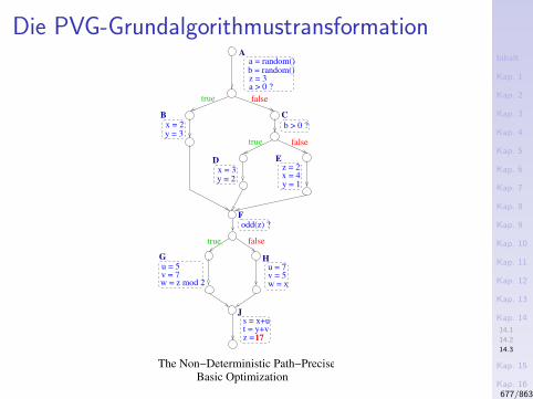
Inhalt
Kap. 1
Kap. 2
Kap. 3
Kap. 4
Kap. 5
Kap. 6
Kap. 7
Kap. 8
Kap. 9
Kap. 10
Kap. 11
Kap. 12
Kap. 13
Kap. 14
14.1
14.2
14.3
Kap. 15
Kap. 16
Kap. 17
Literatur
Anhang
A
Die PVG-Grundalgorithmustransformation
b > 0 ?
C
H
w = xv = 5u = 7
x = 3y = 2
D
x = 2y = 3
B
b = random()z = 3a > 0 ?
a = random()A
odd(z) ?F
y = 1x = 4z = 2
E
w = z mod 2
G
v = 7u = 5
J
z =t = y+vs = x+u
true false
true false
true false
17
The Non−Deterministic Path−PreciseBasic Optimization
677/863
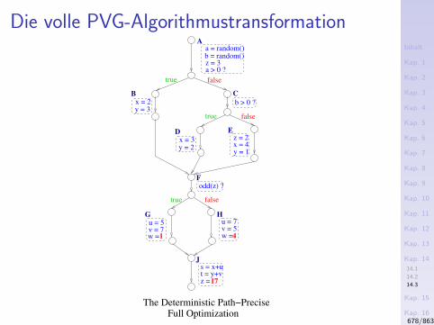
Inhalt
Kap. 1
Kap. 2
Kap. 3
Kap. 4
Kap. 5
Kap. 6
Kap. 7
Kap. 8
Kap. 9
Kap. 10
Kap. 11
Kap. 12
Kap. 13
Kap. 14
14.1
14.2
14.3
Kap. 15
Kap. 16
Kap. 17
Literatur
Anhang
A
Die volle PVG-Algorithmustransformation
b > 0 ?
C
w = v = 7u = 5
1
G
x = 3y = 2
D
x = 2y = 3
B
b = random()z = 3a > 0 ?
a = random()A
odd(z) ?F
y = 1x = 4z = 2
E
J
z =t = y+vs = x+u
true false
true false
true false
17
H
w =v = 5u = 7
4
The Deterministic Path−PreciseFull Optimization
678/863
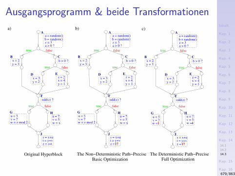
Inhalt
Kap. 1
Kap. 2
Kap. 3
Kap. 4
Kap. 5
Kap. 6
Kap. 7
Kap. 8
Kap. 9
Kap. 10
Kap. 11
Kap. 12
Kap. 13
Kap. 14
14.1
14.2
14.3
Kap. 15
Kap. 16
Kap. 17
Literatur
Anhang
A
Ausgangsprogramm & beide Transformationen
b > 0 ?
C
w = v = 7u = 5
1
G
b > 0 ?
C
H
w = xv = 5u = 7
b > 0 ?
C
H
w = xv = 5u = 7
x = 3y = 2
D
x = 2y = 3
B
b = random()z = 3a > 0 ?
a = random()A
odd(z) ?F
y = 1x = 4z = 2
E
w = z mod 2
G
v = 7u = 5
J
z = s+tt = y+vs = x+u
true false
true false
true false
c)
x = 3y = 2
D
x = 2y = 3
B
b = random()z = 3a > 0 ?
a = random()A
odd(z) ?F
y = 1x = 4z = 2
E
J
z =t = y+vs = x+u
true false
true false
true false
17
H
w =v = 5u = 7
4
The Deterministic Path−Precise
b)
x = 3y = 2
D
x = 2y = 3
B
b = random()z = 3a > 0 ?
a = random()A
odd(z) ?F
y = 1x = 4z = 2
E
w = z mod 2
G
v = 7u = 5
J
z =t = y+vs = x+u
true false
true false
true false
17
The Non−Deterministic Path−PreciseFull OptimizationBasic Optimization
a)
Original Hyperblock
679/863
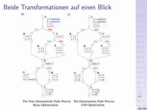
Inhalt
Kap. 1
Kap. 2
Kap. 3
Kap. 4
Kap. 5
Kap. 6
Kap. 7
Kap. 8
Kap. 9
Kap. 10
Kap. 11
Kap. 12
Kap. 13
Kap. 14
14.1
14.2
14.3
Kap. 15
Kap. 16
Kap. 17
Literatur
Anhang
A
Beide Transformationen auf einen Blick
b > 0 ?
C
w = v = 7u = 5
1
G
b > 0 ?
C
H
w = xv = 5u = 7
c)
x = 3y = 2
D
x = 2y = 3
B
b = random()z = 3a > 0 ?
a = random()A
odd(z) ?F
y = 1x = 4z = 2
E
J
z =t = y+vs = x+u
true false
true false
true false
17
H
w =v = 5u = 7
4
The Deterministic Path−Precise
b)
x = 3y = 2
D
x = 2y = 3
B
b = random()z = 3a > 0 ?
a = random()A
odd(z) ?F
y = 1x = 4z = 2
E
w = z mod 2
G
v = 7u = 5
J
z =t = y+vs = x+u
true false
true false
true false
17
The Non−Deterministic Path−PreciseFull OptimizationBasic Optimization
680/863
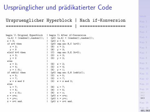
Inhalt
Kap. 1
Kap. 2
Kap. 3
Kap. 4
Kap. 5
Kap. 6
Kap. 7
Kap. 8
Kap. 9
Kap. 10
Kap. 11
Kap. 12
Kap. 13
Kap. 14
14.1
14.2
14.3
Kap. 15
Kap. 16
Kap. 17
Literatur
Anhang
A
Ursprunglicher und pradikatierter Code
Urspruenglicher Hyperblock | Nach if-Konversion
========================== | ==================
begin \\ Original Hyperblock | begin \\ After if-Conversion
(a,b) = (random(),random()); | (p0) (a,b) = (random(),random());
z = 3; | (p0) z = 3;
if a>0 then | (p0) cmp.unc B,C (a>0);
x = 2; | (B) x = 2;
y = 3 | (B) y = 3;
elsif b>0 then | (C) cmp.unc D,E (b>0);
x = 3; | (D) x = 3;
y = 2 | (D) y = 2;
else |
z = 2; | (E) z = 2;
x = 4; | (E) x = 4;
y = 1 fi; | (E) y = 1;
if odd(z) then | (p0) cmp.unc G,H (odd(z));
u = 5; | (G) u = 5;
v = 7; | (G) v = 7;
w = z mod 2 | (G) w = z mod 2;
else |
u = 7; | (H) u = 7;
v = 5; | (H) v = 5;
w = x fi; | (H) w = x;
s = x+u; | (p0) s = x+u;
t = y+v; | (p0) t = y+v;
z = s+t end. | (p0) z = s+t end.
681/863
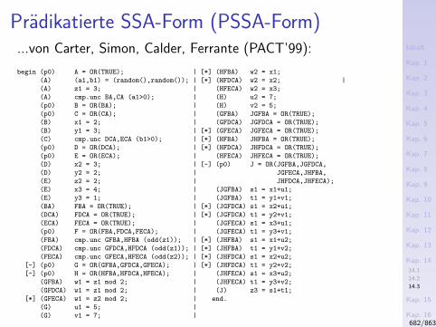
Inhalt
Kap. 1
Kap. 2
Kap. 3
Kap. 4
Kap. 5
Kap. 6
Kap. 7
Kap. 8
Kap. 9
Kap. 10
Kap. 11
Kap. 12
Kap. 13
Kap. 14
14.1
14.2
14.3
Kap. 15
Kap. 16
Kap. 17
Literatur
Anhang
A
Pradikatierte SSA-Form (PSSA-Form)...von Carter, Simon, Calder, Ferrante (PACT’99):
begin (p0) A = OR(TRUE); | [*] (HFBA) w2 = x1;
(A) (a1,b1) = (random(),random()); | [*] (HFDCA) w2 = x2; |
(A) z1 = 3; | (HFECA) w2 = x3;
(A) cmp.unc BA,CA (a1>0); | (H) u2 = 7;
(p0) B = OR(BA); | (H) v2 = 5;
(p0) C = OR(CA); | (GFBA) JGFBA = OR(TRUE);
(B) x1 = 2; | (GFDCA) JGFDCA = OR(TRUE);
(B) y1 = 3; | [*] (GFECA) JGFECA = OR(TRUE);
(C) cmp.unc DCA,ECA (b1>0); | [*] (HFBA) JHFBA = OR(TRUE);
(p0) D = OR(DCA); | [*] (HFDCA) JHFDCA = OR(TRUE);
(p0) E = OR(ECA); | (HFECA) JHFECA = OR(TRUE);
(D) x2 = 3; | [-] (p0) J = OR(JGFBA,JGFDCA,
(D) y2 = 2; | JGFECA,JHFBA,
(E) z2 = 2; | JHFDCA,JHFECA);
(E) x3 = 4; | (JGFBA) s1 = x1+u1;
(E) y3 = 1; | (JGFBA) t1 = y1+v1;
(BA) FBA = OR(TRUE); | [*] (JGFDCA) s1 = x2+u1;
(DCA) FDCA = OR(TRUE); | [*] (JGFDCA) t1 = y2+v1;
(ECA) FECA = OR(TRUE); | (JGFECA) s1 = x3+u1;
(p0) F = OR(FBA,FDCA,FECA); | (JGFECA) t1 = y3+v1;
(FBA) cmp.unc GFBA,HFBA (odd(z1)); | [*] (JHFBA) s1 = x1+u2;
(FDCA) cmp.unc GFDCA,HFDCA (odd(z1)); | [*] (JHFBA) t1 = y1+v2;
(FECA) cmp.unc GFECA,HFECA (odd(z2)); | [*] (JHFDCA) s1 = x2+u2;
[-] (p0) G = OR(GFBA,GFDCA,GFECA); | [*] (JHFDCA) t1 = y2+v2;
[-] (p0) H = OR(HFBA,HFDCA,HFECA); | (JHFECA) s1 = x3+u2;
(GFBA) w1 = z1 mod 2; | (JHFECA) t1 = y3+v2;
(GFDCA) w1 = z1 mod 2; | (J) z3 = s1+t1;
[*] (GFECA) w1 = z2 mod 2; | end.
(G) u1 = 5; |
(G) v1 = 7; |682/863
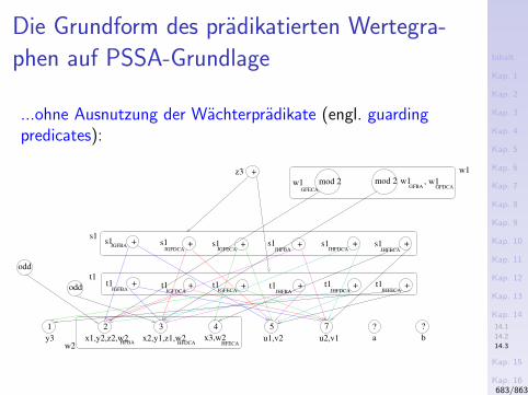
Inhalt
Kap. 1
Kap. 2
Kap. 3
Kap. 4
Kap. 5
Kap. 6
Kap. 7
Kap. 8
Kap. 9
Kap. 10
Kap. 11
Kap. 12
Kap. 13
Kap. 14
14.1
14.2
14.3
Kap. 15
Kap. 16
Kap. 17
Literatur
Anhang
A
Die Grundform des pradikatierten Wertegra-
phen auf PSSA-Grundlage
...ohne Ausnutzung der Wachterpradikate (engl. guardingpredicates):
+
odd
odd
z3
1 2 3 4 5 7
x1,y2,z2,w2 x2,y1,z1,w2
? ?
u2,v1u1,v2 a b
+
+ +
+ +
+
+
+
+
++
+
mod 2 mod 2 w1
w2y3 x3,w2
s1s1
t1
s1
t1t1
t1
s1
t1
s1 s1
t1
s1
t1
w1 , w1
w1
JGFBA
JGFBA
JGFDCA
JGFDCA
JGFECA
JGFECA
JHFBA
JHFBA JHFDCA
JHFDCA JHFECA
JHFECA
HFBA HFDCA HFECA
GFECAGFBA GFDCA
683/863
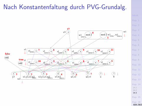
Inhalt
Kap. 1
Kap. 2
Kap. 3
Kap. 4
Kap. 5
Kap. 6
Kap. 7
Kap. 8
Kap. 9
Kap. 10
Kap. 11
Kap. 12
Kap. 13
Kap. 14
14.1
14.2
14.3
Kap. 15
Kap. 16
Kap. 17
Literatur
Anhang
A
Nach Konstantenfaltung durch PVG-Grundalg.
+
odd
odd
false
true
1 2 3 4 5 7
10 9 8 8 7
z3
1 2 3 4 5 7
x1,y2,z2,w2 x2,y1,z1,w2
? ?
u2,v1u1,v2 a b
+
+ +
+ +
+
+
+
+
++
+
mod 2 mod 2 w1
w2y3 x3,w2
s1s1
t1
s1
t1t1
t1
s1
t1
s1 s1
t1
s1
t1
w1 , w1
w1
7 8 9 9 10 11
6
17
0
1
JGFBA
JGFBA
JGFDCA
JGFDCA
JGFECA
JGFECA
JHFBA
JHFBA JHFDCA
JHFDCA JHFECA
JHFECA
HFBA HFDCA HFECA
GFECAGFBA GFDCA
684/863
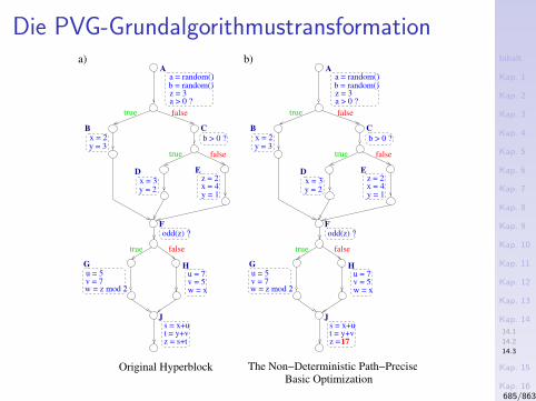
Inhalt
Kap. 1
Kap. 2
Kap. 3
Kap. 4
Kap. 5
Kap. 6
Kap. 7
Kap. 8
Kap. 9
Kap. 10
Kap. 11
Kap. 12
Kap. 13
Kap. 14
14.1
14.2
14.3
Kap. 15
Kap. 16
Kap. 17
Literatur
Anhang
A
Die PVG-Grundalgorithmustransformation
b > 0 ?
C
H
w = xv = 5u = 7
b > 0 ?
C
H
w = xv = 5u = 7
x = 3y = 2
D
x = 2y = 3
B
b = random()z = 3a > 0 ?
a = random()A
odd(z) ?F
y = 1x = 4z = 2
E
w = z mod 2
G
v = 7u = 5
J
z = s+tt = y+vs = x+u
true false
true false
true false
b)
x = 3y = 2
D
x = 2y = 3
B
b = random()z = 3a > 0 ?
a = random()A
odd(z) ?F
y = 1x = 4z = 2
E
w = z mod 2
G
v = 7u = 5
J
z =t = y+vs = x+u
true false
true false
true false
17
The Non−Deterministic Path−PreciseBasic Optimization
a)
Original Hyperblock
685/863
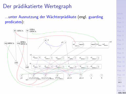
Inhalt
Kap. 1
Kap. 2
Kap. 3
Kap. 4
Kap. 5
Kap. 6
Kap. 7
Kap. 8
Kap. 9
Kap. 10
Kap. 11
Kap. 12
Kap. 13
Kap. 14
14.1
14.2
14.3
Kap. 15
Kap. 16
Kap. 17
Literatur
Anhang
A
Der pradikatierte Wertegraph
...unter Ausnutzung der Wachterpradikate (engl. guardingpredicates):
+
odd
odd
s1 s1 s1 s1 s1 s1
t1 t1 t1 t1 t1 t1
w1 , w1z3
1 2 3 4 5 7
x1,y2,z2,w2 x2,y1,z1,w2
? ?
u2,v1u1,v2 a b
+
+ +
+ +
+
+
+
+
++
+
mod 2 mod 2
w2x3,w2y3
HFBAHFDCAHFECAneg neg
GFBAGFDCAId GFECA Id
Jor
s1
t1
w1
w1
JGFBAJGFDCA JGFECA JHFBA JHFDCA JHFECA
JGFBA JGFDCA JGFECA JHFBA JHFDCA JHFECA
GFBA GFDCA
HFBA HFDCA HFECA
GFECA
686/863
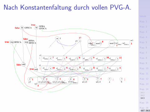
Inhalt
Kap. 1
Kap. 2
Kap. 3
Kap. 4
Kap. 5
Kap. 6
Kap. 7
Kap. 8
Kap. 9
Kap. 10
Kap. 11
Kap. 12
Kap. 13
Kap. 14
14.1
14.2
14.3
Kap. 15
Kap. 16
Kap. 17
Literatur
Anhang
A
Nach Konstantenfaltung durch vollen PVG-A.
+
odd
odd
s1 s1 s1 s1 s1 s1
t1 t1 t1 t1 t1 t1
w1 , w1w1’’’
z3
1 2 3 4 5 7
x1,y2,z2,w2 x2,y1,z1,w2
? ?
u2,v1u1,v2 a b
+
+ +
+ +
+
+
+
+
++
+
mod 2 mod 2
w2x3,w2y3
HFBAHFDCAHFECAneg neg
GFBAGFDCAId GFECA Id
Jor
s1
t1
w1
w1
false
true
false
true
false
true
1
4
2 3 4 5 7
10 9 8 8 7 6
7 8 9 9 10 11
17
01
1
JGFBAJGFDCA JGFECA JHFBA JHFDCA JHFECA
JGFBA JGFDCA JGFECA JHFBA JHFDCA JHFECA
GFBA GFDCA
HFBA HFDCA HFECA
GFECA
687/863
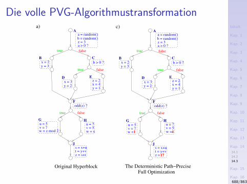
Inhalt
Kap. 1
Kap. 2
Kap. 3
Kap. 4
Kap. 5
Kap. 6
Kap. 7
Kap. 8
Kap. 9
Kap. 10
Kap. 11
Kap. 12
Kap. 13
Kap. 14
14.1
14.2
14.3
Kap. 15
Kap. 16
Kap. 17
Literatur
Anhang
A
Die volle PVG-Algorithmustransformation
b > 0 ?
C
H
w = xv = 5u = 7
x = 3y = 2
D
x = 2y = 3
B
b = random()z = 3a > 0 ?
a = random()A
odd(z) ?F
y = 1x = 4z = 2
E
w = z mod 2
G
v = 7u = 5
J
z = s+tt = y+vs = x+u
true false
true false
true false
b > 0 ?
C
w = v = 7u = 5
1
G
c)
x = 3y = 2
D
x = 2y = 3
B
b = random()z = 3a > 0 ?
a = random()A
odd(z) ?F
y = 1x = 4z = 2
E
J
z =t = y+vs = x+u
true false
true false
true false
17
H
w =v = 5u = 7
4
The Deterministic Path−PreciseFull Optimization
a)
Original Hyperblock
688/863
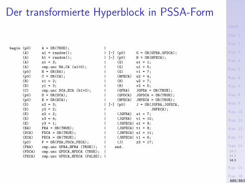
Inhalt
Kap. 1
Kap. 2
Kap. 3
Kap. 4
Kap. 5
Kap. 6
Kap. 7
Kap. 8
Kap. 9
Kap. 10
Kap. 11
Kap. 12
Kap. 13
Kap. 14
14.1
14.2
14.3
Kap. 15
Kap. 16
Kap. 17
Literatur
Anhang
A
Der transformierte Hyperblock in PSSA-Form
begin (p0) A = OR(TRUE); |
(A) a1 = random(); | [-] (p0) G = OR(GFBA,GFDCA);
(A) b1 = random(); | [-] (p0) H = OR(HFECA);
(A) z1 = 3; | (G) w1 = 1;
(A) cmp.unc BA,CA (a1>0); | (G) u1 = 5;
(p0) B = OR(BA); | (G) v1 = 7;
(p0) C = OR(CA); | (HFECA) w2 = 4;
(B) x1 = 2; | (H) u2 = 7;
(B) y1 = 3; | (H) v2 = 5;
(C) cmp.unc DCA,ECA (b1>0); | (GFBA) JGFBA = OR(TRUE);
(p0) D = OR(DCA); | (GFDCA) JGFDCA = OR(TRUE);
(p0) E = OR(ECA); | (HFECA) JHFECA = OR(TRUE);
(D) x2 = 3; | [-] (p0) J = OR(JGFBA,JGFECA,
(D) y2 = 2; | JHFECA);
(E) z2 = 2; | (JGFBA) s1 = 7;
(E) x3 = 4; | (JGFBA) t1 = 10;
(E) y3 = 1; | (JGFECA) s1 = 9;
(BA) FBA = OR(TRUE); | (JGFECA) t1 = 8;
(DCA) FDCA = OR(TRUE); | (JHFECA) s1 = 11;
(ECA) FECA = OR(TRUE); | (JHFECA) t1 = 6;
(p0) F = OR(FBA,FDCA,FECA); | (J) z3 = 17;
(FBA) cmp.unc GFBA,HFBA (TRUE)); | end.
(FDCA) cmp.unc GFDCA,HFDCA (TRUE); |
(FECA) cmp.unc GFECA,HFECA (FALSE); |
689/863
Inhalt
Kap. 1
Kap. 2
Kap. 3
Kap. 4
Kap. 5
Kap. 6
Kap. 7
Kap. 8
Kap. 9
Kap. 10
Kap. 11
Kap. 12
Kap. 13
Kap. 14
14.1
14.2
14.3
Kap. 15
Kap. 16
Kap. 17
Literatur
Anhang
A
Hauptergebnisse
Korrektheit
I Der globale Konstantenfaltungsalgorithmus ist korrekt(sowohl fur die Grundform wie fur die volle Variante derlokalen Analysestufe).
Vollstandigkeit/Optimalitat
I Der Grundalgorithmus der lokalen Analysestufe istpfad-prazise bezuglich nicht-deterministischer Inter-pretation von Verzweigungsbedingungen.
I Der volle Algorithmus der lokalen Analysestufe istpradikatssensitiv pfad-prazise.
690/863
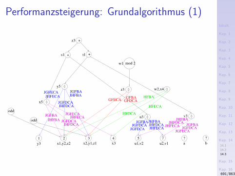
Inhalt
Kap. 1
Kap. 2
Kap. 3
Kap. 4
Kap. 5
Kap. 6
Kap. 7
Kap. 8
Kap. 9
Kap. 10
Kap. 11
Kap. 12
Kap. 13
Kap. 14
14.1
14.2
14.3
Kap. 15
Kap. 16
Kap. 17
Literatur
Anhang
A
Performanzsteigerung: Grundalgorithmus (1)
z3
odd
odd
y5
v3
+s1 +t1
mod 2w1
JGFECAJHFECA
JGFBAJHFBA
1 2 3 4 5 7 ? ?
u2,v1u1,v2 a by3 x1,y2,z2 x2,y1,z1 x3
w2,x4
HFECA
HFDCA
HFBAGFECA
GFBA
x5
JHFECAJGFBA
JHFBA
GFDCA
JGFDCAJHFDCA
JGFDCAJHFDCA
JGFECAu3
JGFBAJGFDCA
JGFECAJGFBA
JGFDCAJGFECA
JHFBAJHFDCAJHFBA
JHFDCAJHFECA
JHFECA
+z3
691/863
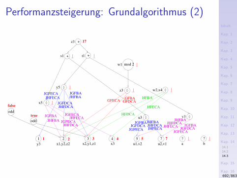
Inhalt
Kap. 1
Kap. 2
Kap. 3
Kap. 4
Kap. 5
Kap. 6
Kap. 7
Kap. 8
Kap. 9
Kap. 10
Kap. 11
Kap. 12
Kap. 13
Kap. 14
14.1
14.2
14.3
Kap. 15
Kap. 16
Kap. 17
Literatur
Anhang
A
Performanzsteigerung: Grundalgorithmus (2)
z3
odd
odd
y5
v3
+s1 +t1
mod 2w1
JGFECAJHFECA
JGFBAJHFBA
1 2 3 4 5 7 ? ?
u2,v1u1,v2 a by3 x1,y2,z2 x2,y1,z1 x3
w2,x4
HFECA
HFDCA
HFBAGFECA
GFBA
x5
JHFECAJGFBA
JHFBA
GFDCA
JGFDCAJHFDCA
JGFDCAJHFDCA
JGFECAu3
JGFBAJGFDCA
JGFECAJGFBA
JGFDCAJGFECA
JHFBAJHFDCAJHFBA
JHFDCAJHFECA
JHFECA
+z3
2 3 4 5 71
false
true
17
692/863
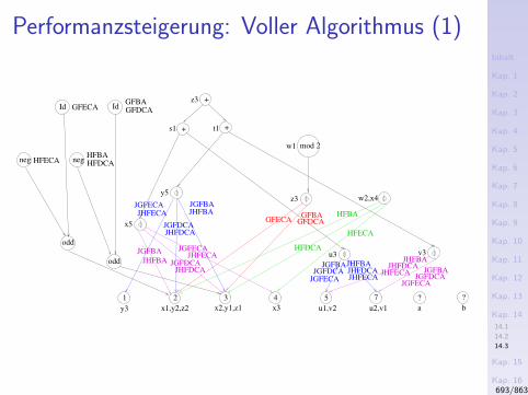
Inhalt
Kap. 1
Kap. 2
Kap. 3
Kap. 4
Kap. 5
Kap. 6
Kap. 7
Kap. 8
Kap. 9
Kap. 10
Kap. 11
Kap. 12
Kap. 13
Kap. 14
14.1
14.2
14.3
Kap. 15
Kap. 16
Kap. 17
Literatur
Anhang
A
Performanzsteigerung: Voller Algorithmus (1)
z3
odd
odd
y5
v3
+s1 +t1
mod 2w1
JGFECAJHFECA JHFBA
JGFBA
1 2 3 4 5 7 ? ?
u2,v1u1,v2 a by3 x1,y2,z2 x2,y1,z1 x3
w2,x4
HFECA
HFDCA
HFBAGFECA
GFBA
HFBAHFDCAHFECAneg neg
GFBAGFDCAId GFECA Id
x5
JHFECAJGFBA
JHFBA
GFDCA
JGFDCAJHFDCA
JGFDCAJHFDCA
JGFECAu3
JGFBAJGFDCA
JGFECAJGFBA
JGFDCAJGFECA
JHFBAJHFDCAJHFBA
JHFDCAJHFECA
JHFECA
+z3
693/863
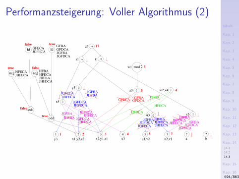
Inhalt
Kap. 1
Kap. 2
Kap. 3
Kap. 4
Kap. 5
Kap. 6
Kap. 7
Kap. 8
Kap. 9
Kap. 10
Kap. 11
Kap. 12
Kap. 13
Kap. 14
14.1
14.2
14.3
Kap. 15
Kap. 16
Kap. 17
Literatur
Anhang
A
Performanzsteigerung: Voller Algorithmus (2)
z3
odd
odd
y5
v3
+s1 +t1
mod 2w1
JGFECAJHFECA
JGFBAJHFBA
1 2 3 4 5 7 ? ?
u2,v1u1,v2 a by3 x1,y2,z2 x2,y1,z1 x3
w2,x4
HFECA
HFDCA
HFBAGFECA
GFBA
HFBAHFDCA
neg neg
Id Id
x5
JHFECAJGFBA
JHFBA
GFDCA
JGFDCAJHFDCA
JGFDCAJHFDCA
JGFECAu3
JGFBAJGFDCA
JGFECAJGFBA
JGFDCAJGFECA
JHFBAJHFDCAJHFBA
JHFDCAJHFECA
JHFECA
+z3
2 3 4 5 71
false
true
true
true
false
false
3 4
GFBAGFDCAJGFBAJGFDCA
GFECAJGFECA
JHFBAJHFDCA
HFECAJHFECA
1
17
694/863
Inhalt
Kap. 1
Kap. 2
Kap. 3
Kap. 4
Kap. 5
Kap. 6
Kap. 7
Kap. 8
Kap. 9
Kap. 10
Kap. 11
Kap. 12
Kap. 13
Kap. 14
14.1
14.2
14.3
Kap. 15
Kap. 16
Kap. 17
Literatur
Anhang
A
Zusammenfassung und Schlussfolgerungen
Konstantenfaltung und SSA/PSSA-Form:
I sind perfekt aufeinander abgestimmt – SSA/PSSA sindwirklich von Hilfe fur Analyse und Transformation!
I Der Schlussel: Wertegraph und pradikatierter Wertegraph.
Offen fur Erweiterungen, z.B.:
I Wertegraph: Bedingte Konstanten (engl. conditionalconstants).
Zusammenfassend:
I Konstantenfaltung ist besonders geeignet, Vorteile aus derNutzung von (P)SSA zur Programmreprasentation aufzu-zeigen.
695/863
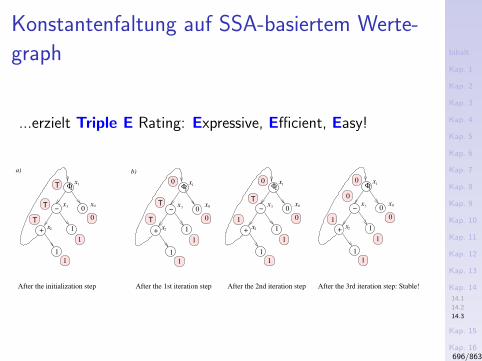
Inhalt
Kap. 1
Kap. 2
Kap. 3
Kap. 4
Kap. 5
Kap. 6
Kap. 7
Kap. 8
Kap. 9
Kap. 10
Kap. 11
Kap. 12
Kap. 13
Kap. 14
14.1
14.2
14.3
Kap. 15
Kap. 16
Kap. 17
Literatur
Anhang
A
Konstantenfaltung auf SSA-basiertem Werte-
graph
...erzielt Triple E Rating: Expressive, Efficient, Easy!
T
T
T
1
1
x1Φ
+
1
2x
−
1
x3 0x0
01
0
0
1
1
1
1
T
TT
x1Φ
+
1
2x
−
1
x3 0x0
0
1
1
x1Φ
+
1
2x
−
1
x3 0x0
0
0 x1Φ
+
1
2x
−
1
x3 0x0
0
0
1
After the 1st iteration step After the 2nd iteration step After the 3rd iteration step: Stable!After the initialization step
22
a) b)
2 2
696/863
Inhalt
Kap. 1
Kap. 2
Kap. 3
Kap. 4
Kap. 5
Kap. 6
Kap. 7
Kap. 8
Kap. 9
Kap. 10
Kap. 11
Kap. 12
Kap. 13
Kap. 14
14.1
14.2
14.3
Kap. 15
Kap. 16
Kap. 17
Literatur
Anhang
A
Literaturhinweis
...zum PVG-Konstantenfaltungsalgorithmus:
I Jens Knoop, Oliver Ruthing. Constant Propagation onPredicated Code. Journal of Universal Computer Science9(8):829-850, 2003. (Sonderausgabe zur SBLP’03).
697/863
Inhalt
Kap. 1
Kap. 2
Kap. 3
Kap. 4
Kap. 5
Kap. 6
Kap. 7
Kap. 8
Kap. 9
Kap. 10
Kap. 11
Kap. 12
Kap. 13
Kap. 14
14.1
14.2
14.3
Kap. 15
Kap. 16
Kap. 17
Literatur
Anhang
A
Vertiefende und weiterfuhrende Leseempfeh-
lungen fur Kapitel 14 (1)
Bowen Alpern, Mark N. Wegman, F. Ken Zadeck. Detec-ting Equality of Variables in Programs. In ConferenceRecord of the 15th ACM SIGPLAN-SIGACT Symposiumon Principles of Programming Languages (POPL’88),1-11, 1988.
Ron Cytron, Jeanne Ferrante, Barry K. Rosen, MarkN. Wegman, F. Ken Zadeck. An Efficient Method ofComputing Static Single Assignment Form. In ConferenceRecord of the 16th ACM SIGPLAN-SIGACT Symposiumon Principles of Programming Languages (POPL’89),25-35, 1989.
698/863
Inhalt
Kap. 1
Kap. 2
Kap. 3
Kap. 4
Kap. 5
Kap. 6
Kap. 7
Kap. 8
Kap. 9
Kap. 10
Kap. 11
Kap. 12
Kap. 13
Kap. 14
14.1
14.2
14.3
Kap. 15
Kap. 16
Kap. 17
Literatur
Anhang
A
Vertiefende und weiterfuhrende Leseempfeh-
lungen fur Kapitel 14 (2)
Ron Cytron, Jeanne Ferrante, Barry K. Rosen, MarkN. Wegman, F. Ken Zadeck. Efficiently Computing StaticSingle Assignment Form and the Control DependenceGraph. ACM Transactions on Programming Languagesand Systems (TOPLAS) 13(4):451-490, 1991.
John B. Kam, Jeffrey D. Ullman. Monotone Data FlowAnalysis Frameworks. Acta Informatica 7:305-317, 1977.
Gary A. Kildall. A Unified Approach to Global ProgramOptimization. In Conference Record of the 1st ACMSIGPLAN-SIGACT Symposium on Principles of Program-ming Languages (POPL’73), 194-206, 1973.
699/863
Inhalt
Kap. 1
Kap. 2
Kap. 3
Kap. 4
Kap. 5
Kap. 6
Kap. 7
Kap. 8
Kap. 9
Kap. 10
Kap. 11
Kap. 12
Kap. 13
Kap. 14
14.1
14.2
14.3
Kap. 15
Kap. 16
Kap. 17
Literatur
Anhang
A
Vertiefende und weiterfuhrende Leseempfeh-
lungen fur Kapitel 14 (3)
Jens Knoop, Oliver Ruthing. Constant Propagation on theValue Graph: Simple Constants and Beyond. In Procee-dings of the 9th International Conference on CompilerConstruction (CC 2000), Springer-V., LNCS 1781, 94-109,2000.
Jens Knoop, Oliver Ruthing. Constant Propagation onPredicated Code. Journal of Universal Computer Science9(8):829-850, 2003. (Sonderausgabe zur SBLP’03).
John H. Reif, Harry R. Lewis. Symbolic Evaluation and theGlobal Value Graph. In Conference Record of the 4thAnnual ACM SIGACT-SIGPLAN Symposium on Principlesof Programming Languages (POPL’77), 104-118, 1977.
700/863
Inhalt
Kap. 1
Kap. 2
Kap. 3
Kap. 4
Kap. 5
Kap. 6
Kap. 7
Kap. 8
Kap. 9
Kap. 10
Kap. 11
Kap. 12
Kap. 13
Kap. 14
14.1
14.2
14.3
Kap. 15
Kap. 16
Kap. 17
Literatur
Anhang
A
Vertiefende und weiterfuhrende Leseempfeh-
lungen fur Kapitel 14 (4)
Oliver Ruthing, Jens Knoop, Bernhard Steffen. DetectingEqualities of Variables: Combining Efficiency withPrecision. In Proceedings of the 6th Static Analysis Sym-posium (SAS’99), Springer-V., LNCS 1694, 232-247, 1999.
Oliver Ruthing, Markus Muller-Olm. On the Complexity ofConstant Propagation. In Proceedings of the 10thEuropean Symposium on Programming (ESOP 2001),Springer-V., LNCS 2028, 190-205, 2001.
Bernhard Steffen, Jens Knoop. Finite Constants:Characterizations of a New Decidable Set of Constants.Theoretical Computer Science 80(2):303-318, 1991.
701/863
Inhalt
Kap. 1
Kap. 2
Kap. 3
Kap. 4
Kap. 5
Kap. 6
Kap. 7
Kap. 8
Kap. 9
Kap. 10
Kap. 11
Kap. 12
Kap. 13
Kap. 14
14.1
14.2
14.3
Kap. 15
Kap. 16
Kap. 17
Literatur
Anhang
A
Vertiefende und weiterfuhrende Leseempfeh-
lungen fur Kapitel 14 (5)
Munehiro Takimoto, Kenichi Harada. Effective PartialRedundancy Elimination based on Extended Value Graph.Information Processing Society of Japan38(11):2237-2250, 1990.
Munehiro Takimoto, Kenichi Harada. Partial Dead CodeElimination Using Extended Value Graph. In Proceedingsof the 6th Static Analysis Symposium (SAS’99), Sprin-ger-V., LNCS 1694, 179-193, 1999.
Mark N. Wegman, F. Ken Zadeck. Constant Propagationwith Conditional Branches. ACM Transactions on Pro-gramming Languages and Systems 13(2):181-201, 1991.
702/863
Inhalt
Kap. 1
Kap. 2
Kap. 3
Kap. 4
Kap. 5
Kap. 6
Kap. 7
Kap. 8
Kap. 9
Kap. 10
Kap. 11
Kap. 12
Kap. 13
Kap. 14
14.1
14.2
14.3
Kap. 15
Kap. 16
Kap. 17
Literatur
Anhang
A
Teil IV
Abstrakte Interpretation und Modellprufung
703/863

Inhalt
Kap. 1
Kap. 2
Kap. 3
Kap. 4
Kap. 5
Kap. 6
Kap. 7
Kap. 8
Kap. 9
Kap. 10
Kap. 11
Kap. 12
Kap. 13
Kap. 14
Kap. 15
15.1
15.2
15.3
15.4
Kap. 16
Kap. 17
Literatur
Anhang
A
Kapitel 15
Abstrakte Interpretation und DFA
704/863
Inhalt
Kap. 1
Kap. 2
Kap. 3
Kap. 4
Kap. 5
Kap. 6
Kap. 7
Kap. 8
Kap. 9
Kap. 10
Kap. 11
Kap. 12
Kap. 13
Kap. 14
Kap. 15
15.1
15.2
15.3
15.4
Kap. 16
Kap. 17
Literatur
Anhang
A
Motivation
Die Theorie abstrakter Interpretation — ein “mondaner” Pro-grammanalyseansatz.
Intuitiv:
I Der DFA-Ansatz beinhaltet die Spezifikation einer Pro-grammanalyse, deren Korrektheit separat und unabhangiga posteriori validiert wird.
I Der abstrakte Interpretationsansatz beinhaltet denKorrektheitsnachweis von Anfang an als integralenBestandteil der Programmanalyse.
705/863
Inhalt
Kap. 1
Kap. 2
Kap. 3
Kap. 4
Kap. 5
Kap. 6
Kap. 7
Kap. 8
Kap. 9
Kap. 10
Kap. 11
Kap. 12
Kap. 13
Kap. 14
Kap. 15
15.1
15.2
15.3
15.4
Kap. 16
Kap. 17
Literatur
Anhang
A
Kapitel 15.1
Theorie abstrakter Interpretation
706/863
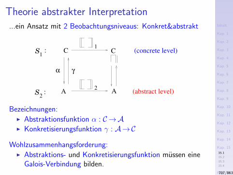
Inhalt
Kap. 1
Kap. 2
Kap. 3
Kap. 4
Kap. 5
Kap. 6
Kap. 7
Kap. 8
Kap. 9
Kap. 10
Kap. 11
Kap. 12
Kap. 13
Kap. 14
Kap. 15
15.1
15.2
15.3
15.4
Kap. 16
Kap. 17
Literatur
Anhang
A
Theorie abstrakter Interpretation...ein Ansatz mit 2 Beobachtungsniveaus: Konkret&abstrakt
A
C1
2
S
S
1
2:
: (concrete level)
(abstract level)
α γ
C
A
Bezeichnungen:I Abstraktionsfunktion α : C→AI Konkretisierungsfunktion γ : A→C
Wohlzusammenhangsforderung:I Abstraktions- und Konkretisierungsfunktion mussen eine
Galois-Verbindung bilden.707/863
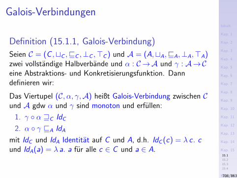
Inhalt
Kap. 1
Kap. 2
Kap. 3
Kap. 4
Kap. 5
Kap. 6
Kap. 7
Kap. 8
Kap. 9
Kap. 10
Kap. 11
Kap. 12
Kap. 13
Kap. 14
Kap. 15
15.1
15.2
15.3
15.4
Kap. 16
Kap. 17
Literatur
Anhang
A
Galois-Verbindungen
Definition (15.1.1, Galois-Verbindung)
Seien C = (C ,tC ,vC ,⊥C ,>C ) und A = (A,tA,vA,⊥A,>A)zwei vollstandige Halbverbande und α : C→A und γ : A→Ceine Abstraktions- und Konkretisierungsfunktion. Danndefinieren wir:
Das Viertupel (C, α, γ,A) heißt Galois-Verbindung zwischen Cund A gdw α und γ sind monoton und erfullen:
1. γ α wC IdC
2. α γ vA IdA
mit IdC und IdA Identitat auf C und A, d.h. IdC (c) = λ c . cund IdA(a) = λ a. a fur alle c ∈ C und a ∈ A.
708/863
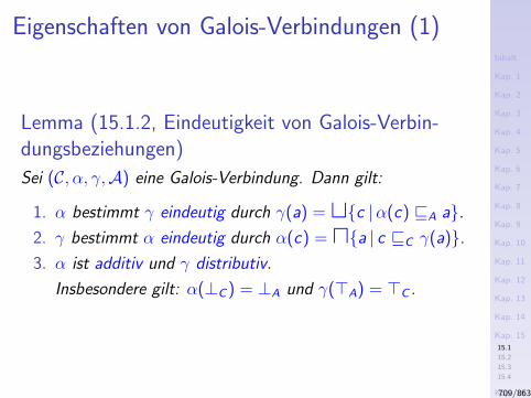
Inhalt
Kap. 1
Kap. 2
Kap. 3
Kap. 4
Kap. 5
Kap. 6
Kap. 7
Kap. 8
Kap. 9
Kap. 10
Kap. 11
Kap. 12
Kap. 13
Kap. 14
Kap. 15
15.1
15.2
15.3
15.4
Kap. 16
Kap. 17
Literatur
Anhang
A
Eigenschaften von Galois-Verbindungen (1)
Lemma (15.1.2, Eindeutigkeit von Galois-Verbin-dungsbeziehungen)
Sei (C, α, γ,A) eine Galois-Verbindung. Dann gilt:
1. α bestimmt γ eindeutig durch γ(a) =tc |α(c) vA a.2. γ bestimmt α eindeutig durch α(c) =ua | c vC γ(a).3. α ist additiv und γ distributiv.
Insbesondere gilt: α(⊥C ) = ⊥A und γ(>A) = >C .
709/863
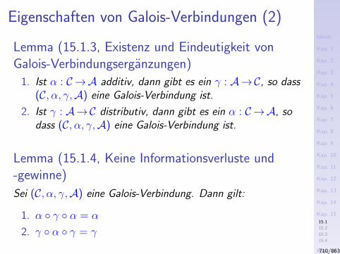
Inhalt
Kap. 1
Kap. 2
Kap. 3
Kap. 4
Kap. 5
Kap. 6
Kap. 7
Kap. 8
Kap. 9
Kap. 10
Kap. 11
Kap. 12
Kap. 13
Kap. 14
Kap. 15
15.1
15.2
15.3
15.4
Kap. 16
Kap. 17
Literatur
Anhang
A
Eigenschaften von Galois-Verbindungen (2)
Lemma (15.1.3, Existenz und Eindeutigkeit vonGalois-Verbindungserganzungen)
1. Ist α : C→A additiv, dann gibt es ein γ : A→C, so dass(C, α, γ,A) eine Galois-Verbindung ist.
2. Ist γ : A→C distributiv, dann gibt es ein α : C→A, sodass (C, α, γ,A) eine Galois-Verbindung ist.
Lemma (15.1.4, Keine Informationsverluste und-gewinne)
Sei (C, α, γ,A) eine Galois-Verbindung. Dann gilt:
1. α γ α = α
2. γ α γ = γ
710/863

Inhalt
Kap. 1
Kap. 2
Kap. 3
Kap. 4
Kap. 5
Kap. 6
Kap. 7
Kap. 8
Kap. 9
Kap. 10
Kap. 11
Kap. 12
Kap. 13
Kap. 14
Kap. 15
15.1
15.2
15.3
15.4
Kap. 16
Kap. 17
Literatur
Anhang
A
Galois-Einpassungen
Definition (15.1.5, Galois-Einpassung)
Seien C = (C ,tC ,vC ,⊥C ,>C ) und A = (A,tA,vA,⊥A,>A)zwei vollstandige Halbverbande und α : C→A und γ : A→Ceine Abstraktions- und Konkretisierungsfunktion. Danndefinieren wir:
Das Viertupel (C, α, γ,A) heißt Galois-Einpassung zwischen Cund A gdw α und γ sind monoton und erfullen:
1. γ α wC IdC
2. α γ = IdA
mit IdC und IdA Identitat auf C und A, d.h. IdC (c) = λ c . cund IdA(a) = λ a. a fur alle c ∈ C und a ∈ A.
711/863
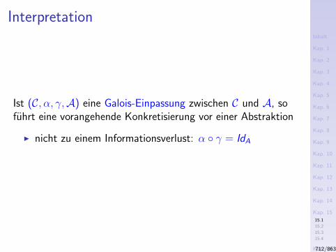
Inhalt
Kap. 1
Kap. 2
Kap. 3
Kap. 4
Kap. 5
Kap. 6
Kap. 7
Kap. 8
Kap. 9
Kap. 10
Kap. 11
Kap. 12
Kap. 13
Kap. 14
Kap. 15
15.1
15.2
15.3
15.4
Kap. 16
Kap. 17
Literatur
Anhang
A
Interpretation
Ist (C, α, γ,A) eine Galois-Einpassung zwischen C und A, sofuhrt eine vorangehende Konkretisierung vor einer Abstraktion
I nicht zu einem Informationsverlust: α γ = IdA
712/863
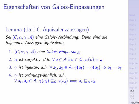
Inhalt
Kap. 1
Kap. 2
Kap. 3
Kap. 4
Kap. 5
Kap. 6
Kap. 7
Kap. 8
Kap. 9
Kap. 10
Kap. 11
Kap. 12
Kap. 13
Kap. 14
Kap. 15
15.1
15.2
15.3
15.4
Kap. 16
Kap. 17
Literatur
Anhang
A
Eigenschaften von Galois-Einpassungen
Lemma (15.1.6, Aquivalenzaussagen)
Sei (C, α, γ,A) eine Galois-Verbindung. Dann sind diefolgenden Aussagen aquivalent:
1. (C, α, γ,A) eine Galois-Einpassung.
2. α ist surjektiv, d.h. ∀ a ∈ A ∃ c ∈ C . α(c) = a.
3. γ ist injektiv, d.h. ∀ a1, a2 ∈ A. γ(a1) = γ(a2)⇒ a1 = a2.
4. γ ist ordnungs-ahnlich, d.h.∀ a1, a2 ∈ A. γ(a1) vC γ(a2)⇐⇒ a1 vA a2.
713/863
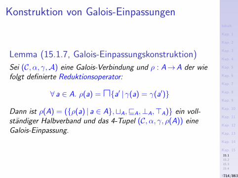
Inhalt
Kap. 1
Kap. 2
Kap. 3
Kap. 4
Kap. 5
Kap. 6
Kap. 7
Kap. 8
Kap. 9
Kap. 10
Kap. 11
Kap. 12
Kap. 13
Kap. 14
Kap. 15
15.1
15.2
15.3
15.4
Kap. 16
Kap. 17
Literatur
Anhang
A
Konstruktion von Galois-Einpassungen
Lemma (15.1.7, Galois-Einpassungskonstruktion)
Sei (C, α, γ,A) eine Galois-Verbindung und ρ : A→A der wiefolgt definierte Reduktionsoperator:
∀ a ∈ A. ρ(a) =ua′ | γ(a) = γ(a′)
Dann ist ρ(A) = (ρ(a) | a ∈ A,tA,vA,⊥A,>A) ein voll-standiger Halbverband und das 4-Tupel (C, α, γ, ρ(A)) eineGalois-Einpassung.
714/863
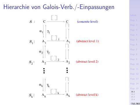
Inhalt
Kap. 1
Kap. 2
Kap. 3
Kap. 4
Kap. 5
Kap. 6
Kap. 7
Kap. 8
Kap. 9
Kap. 10
Kap. 11
Kap. 12
Kap. 13
Kap. 14
Kap. 15
15.1
15.2
15.3
15.4
Kap. 16
Kap. 17
Literatur
Anhang
A
Hierarchie von Galois-Verb./-Einpassungen
CS : (concrete level)C
Ak
Sk
: (abstract level k)
α γ
Ak k
k k
A2
S2
: (abstract level 2)
α γ
A2 2
2 2
A1
S1
: (abstract level 1)
α γ
A1 1
1 1
715/863

Inhalt
Kap. 1
Kap. 2
Kap. 3
Kap. 4
Kap. 5
Kap. 6
Kap. 7
Kap. 8
Kap. 9
Kap. 10
Kap. 11
Kap. 12
Kap. 13
Kap. 14
Kap. 15
15.1
15.2
15.3
15.4
Kap. 16
Kap. 17
Literatur
Anhang
A
Kapitel 15.2
Systematische Konstruktion abstrakterInterpretationen
716/863
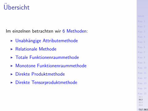
Inhalt
Kap. 1
Kap. 2
Kap. 3
Kap. 4
Kap. 5
Kap. 6
Kap. 7
Kap. 8
Kap. 9
Kap. 10
Kap. 11
Kap. 12
Kap. 13
Kap. 14
Kap. 15
15.1
15.2
15.3
15.4
Kap. 16
Kap. 17
Literatur
Anhang
A
Ubersicht
Im einzelnen betrachten wir 6 Methoden:
I Unabhangige Attributemethode
I Relationale Methode
I Totale Funktionenraummethode
I Monotone Funktionenraummethode
I Direkte Produktmethode
I Direkte Tensorproduktmethode
717/863
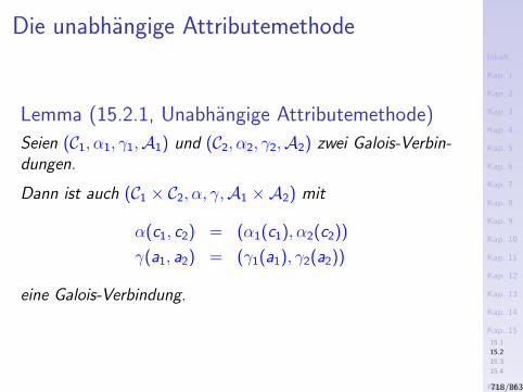
Inhalt
Kap. 1
Kap. 2
Kap. 3
Kap. 4
Kap. 5
Kap. 6
Kap. 7
Kap. 8
Kap. 9
Kap. 10
Kap. 11
Kap. 12
Kap. 13
Kap. 14
Kap. 15
15.1
15.2
15.3
15.4
Kap. 16
Kap. 17
Literatur
Anhang
A
Die unabhangige Attributemethode
Lemma (15.2.1, Unabhangige Attributemethode)
Seien (C1, α1, γ1,A1) und (C2, α2, γ2,A2) zwei Galois-Verbin-dungen.
Dann ist auch (C1 × C2, α, γ,A1 ×A2) mit
α(c1, c2) = (α1(c1), α2(c2))
γ(a1, a2) = (γ1(a1), γ2(a2))
eine Galois-Verbindung.
718/863
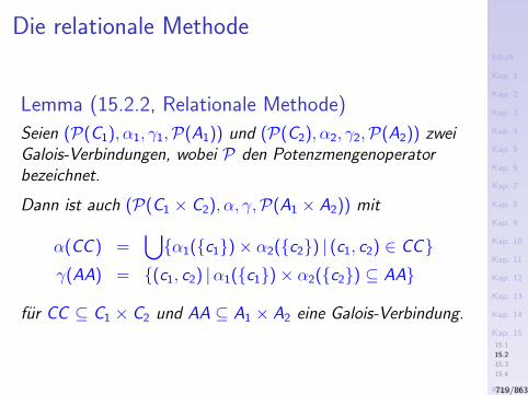
Inhalt
Kap. 1
Kap. 2
Kap. 3
Kap. 4
Kap. 5
Kap. 6
Kap. 7
Kap. 8
Kap. 9
Kap. 10
Kap. 11
Kap. 12
Kap. 13
Kap. 14
Kap. 15
15.1
15.2
15.3
15.4
Kap. 16
Kap. 17
Literatur
Anhang
A
Die relationale Methode
Lemma (15.2.2, Relationale Methode)
Seien (P(C1), α1, γ1,P(A1)) und (P(C2), α2, γ2,P(A2)) zweiGalois-Verbindungen, wobei P den Potenzmengenoperatorbezeichnet.
Dann ist auch (P(C1 × C2), α, γ,P(A1 × A2)) mit
α(CC ) =⋃α1(c1)× α2(c2) | (c1, c2) ∈ CC
γ(AA) = (c1, c2) |α1(c1)× α2(c2) ⊆ AA
fur CC ⊆ C1 × C2 und AA ⊆ A1 × A2 eine Galois-Verbindung.
719/863
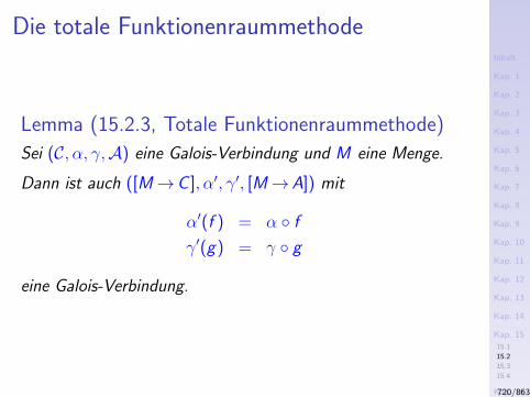
Inhalt
Kap. 1
Kap. 2
Kap. 3
Kap. 4
Kap. 5
Kap. 6
Kap. 7
Kap. 8
Kap. 9
Kap. 10
Kap. 11
Kap. 12
Kap. 13
Kap. 14
Kap. 15
15.1
15.2
15.3
15.4
Kap. 16
Kap. 17
Literatur
Anhang
A
Die totale Funktionenraummethode
Lemma (15.2.3, Totale Funktionenraummethode)
Sei (C, α, γ,A) eine Galois-Verbindung und M eine Menge.
Dann ist auch ([M→C ], α′, γ′, [M→A]) mit
α′(f ) = α f
γ′(g) = γ g
eine Galois-Verbindung.
720/863
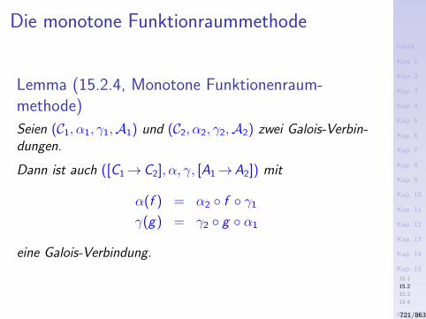
Inhalt
Kap. 1
Kap. 2
Kap. 3
Kap. 4
Kap. 5
Kap. 6
Kap. 7
Kap. 8
Kap. 9
Kap. 10
Kap. 11
Kap. 12
Kap. 13
Kap. 14
Kap. 15
15.1
15.2
15.3
15.4
Kap. 16
Kap. 17
Literatur
Anhang
A
Die monotone Funktionraummethode
Lemma (15.2.4, Monotone Funktionenraum-methode)
Seien (C1, α1, γ1,A1) und (C2, α2, γ2,A2) zwei Galois-Verbin-dungen.
Dann ist auch ([C1→C2], α, γ, [A1→A2]) mit
α(f ) = α2 f γ1
γ(g) = γ2 g α1
eine Galois-Verbindung.
721/863
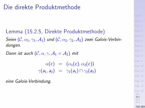
Inhalt
Kap. 1
Kap. 2
Kap. 3
Kap. 4
Kap. 5
Kap. 6
Kap. 7
Kap. 8
Kap. 9
Kap. 10
Kap. 11
Kap. 12
Kap. 13
Kap. 14
Kap. 15
15.1
15.2
15.3
15.4
Kap. 16
Kap. 17
Literatur
Anhang
A
Die direkte Produktmethode
Lemma (15.2.5, Direkte Produktmethode)
Seien (C, α1, γ1,A1) und (C, α2, γ2,A2) zwei Galois-Verbin-dungen.
Dann ist auch (C, α, γ,A1 ×A2) mit
α(c) = (α1(c), α2(c))
γ(a1, a2) = γ1(a1) u γ2(a2)
eine Galois-Verbindung.
722/863
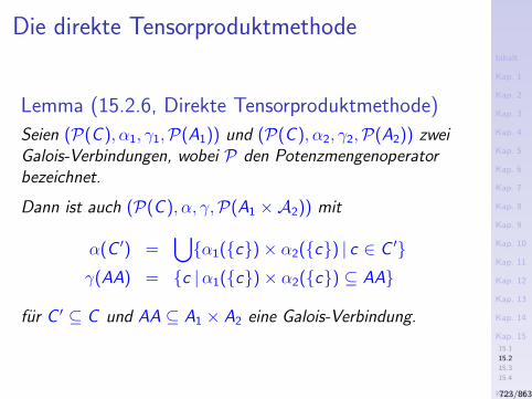
Inhalt
Kap. 1
Kap. 2
Kap. 3
Kap. 4
Kap. 5
Kap. 6
Kap. 7
Kap. 8
Kap. 9
Kap. 10
Kap. 11
Kap. 12
Kap. 13
Kap. 14
Kap. 15
15.1
15.2
15.3
15.4
Kap. 16
Kap. 17
Literatur
Anhang
A
Die direkte Tensorproduktmethode
Lemma (15.2.6, Direkte Tensorproduktmethode)
Seien (P(C ), α1, γ1,P(A1)) und (P(C ), α2, γ2,P(A2)) zweiGalois-Verbindungen, wobei P den Potenzmengenoperatorbezeichnet.
Dann ist auch (P(C ), α, γ,P(A1 ×A2)) mit
α(C ′) =⋃α1(c)× α2(c) | c ∈ C ′
γ(AA) = c |α1(c)× α2(c) ⊆ AA
fur C ′ ⊆ C und AA ⊆ A1 × A2 eine Galois-Verbindung.
723/863

Inhalt
Kap. 1
Kap. 2
Kap. 3
Kap. 4
Kap. 5
Kap. 6
Kap. 7
Kap. 8
Kap. 9
Kap. 10
Kap. 11
Kap. 12
Kap. 13
Kap. 14
Kap. 15
15.1
15.2
15.3
15.4
Kap. 16
Kap. 17
Literatur
Anhang
A
Kapitel 15.3
Korrektheit abstrakter Interpretationen
724/863
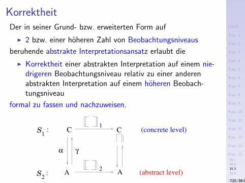
Inhalt
Kap. 1
Kap. 2
Kap. 3
Kap. 4
Kap. 5
Kap. 6
Kap. 7
Kap. 8
Kap. 9
Kap. 10
Kap. 11
Kap. 12
Kap. 13
Kap. 14
Kap. 15
15.1
15.2
15.3
15.4
Kap. 16
Kap. 17
Literatur
Anhang
A
KorrektheitDer in seiner Grund- bzw. erweiterten Form auf
I 2 bzw. einer hoheren Zahl von Beobachtungsniveaus
beruhende abstrakte Interpretationsansatz erlaubt die
I Korrektheit einer abstrakten Interpretation auf einem nie-drigeren Beobachtungsniveau relativ zu einer anderenabstrakten Interpretation auf einem hoheren Beobach-tungsniveau
formal zu fassen und nachzuweisen.
A
C1
2
S
S
1
2:
: (concrete level)
(abstract level)
α γ
C
A725/863
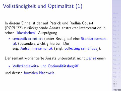
Inhalt
Kap. 1
Kap. 2
Kap. 3
Kap. 4
Kap. 5
Kap. 6
Kap. 7
Kap. 8
Kap. 9
Kap. 10
Kap. 11
Kap. 12
Kap. 13
Kap. 14
Kap. 15
15.1
15.2
15.3
15.4
Kap. 16
Kap. 17
Literatur
Anhang
A
Vollstandigkeit und Optimalitat (1)
In diesem Sinne ist der auf Patrick und Radhia Cousot(POPL’77) zuruckgehende Ansatz abstrakter Interpretation inseiner “klassischen” Auspragung
I semantik-orientiert (unter Bezug auf eine Standardseman-tik (besonders wichtig hierbei: Diesog. Aufsammelsemantik (engl. collecting semantics)).
Der semantik-orientierte Ansatz unterstutzt nicht per se einen
I Vollstandigkeits- und Optimalitatsbegriff
und dessen formalen Nachweis.
726/863
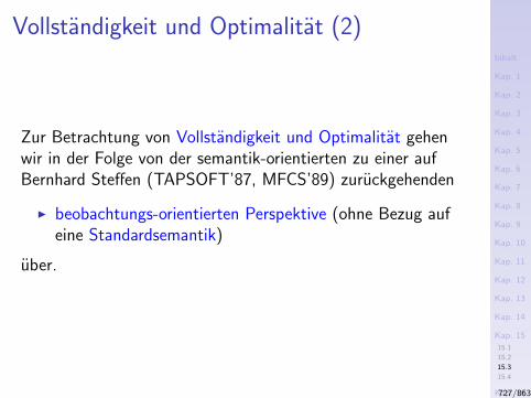
Inhalt
Kap. 1
Kap. 2
Kap. 3
Kap. 4
Kap. 5
Kap. 6
Kap. 7
Kap. 8
Kap. 9
Kap. 10
Kap. 11
Kap. 12
Kap. 13
Kap. 14
Kap. 15
15.1
15.2
15.3
15.4
Kap. 16
Kap. 17
Literatur
Anhang
A
Vollstandigkeit und Optimalitat (2)
Zur Betrachtung von Vollstandigkeit und Optimalitat gehenwir in der Folge von der semantik-orientierten zu einer aufBernhard Steffen (TAPSOFT’87, MFCS’89) zuruckgehenden
I beobachtungs-orientierten Perspektive (ohne Bezug aufeine Standardsemantik)
uber.
727/863

Inhalt
Kap. 1
Kap. 2
Kap. 3
Kap. 4
Kap. 5
Kap. 6
Kap. 7
Kap. 8
Kap. 9
Kap. 10
Kap. 11
Kap. 12
Kap. 13
Kap. 14
Kap. 15
15.1
15.2
15.3
15.4
Kap. 16
Kap. 17
Literatur
Anhang
A
Kapitel 15.4
Vollstandigkeit und Optimalitat
728/863
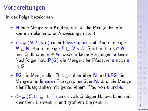
Inhalt
Kap. 1
Kap. 2
Kap. 3
Kap. 4
Kap. 5
Kap. 6
Kap. 7
Kap. 8
Kap. 9
Kap. 10
Kap. 11
Kap. 12
Kap. 13
Kap. 14
Kap. 15
15.1
15.2
15.3
15.4
Kap. 16
Kap. 17
Literatur
Anhang
A
Vorbereitungen
In der Folge bezeichnen
I N eine Menge von Knoten, die fur die Menge der Vor-kommen elementarer Anweisungen steht,
I G =df (N ,E , s, e) einen Flussgraphen mit KnotenmengeN ⊆ N, Kantenmenge E v N × N , Startknoten s ∈ Nund Endknoten e ∈ N , wobei s keine Vorganger, e keineNachfolger hat; P(G ) die Menge aller Pfadevon s nach ein G ,
I FG die Menge aller Flussgraphen uber N und LFG dieMenge aller linearen Flussgraphen uber N, d.h. die Mengealler Flussgraphen mit genau einem Pfad von s und e,
I C=df (C ,t,v,⊥,>) einen vollstandigen Halbverband mitkleinstem Element ⊥ und großtem Element >.
729/863
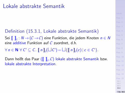
Inhalt
Kap. 1
Kap. 2
Kap. 3
Kap. 4
Kap. 5
Kap. 6
Kap. 7
Kap. 8
Kap. 9
Kap. 10
Kap. 11
Kap. 12
Kap. 13
Kap. 14
Kap. 15
15.1
15.2
15.3
15.4
Kap. 16
Kap. 17
Literatur
Anhang
A
Lokale abstrakte Semantik
Definition (15.3.1, Lokale abstrakte Semantik)
Sei [[ ]]l : N→ (C→C) eine Funktion, die jedem Knoten n ∈ Neine additive Funktion auf C zuordnet, d.h.
∀ n ∈ N ∀C ′ ⊆ C . [[ n ]]l(tC ′) =t[[ n ]]l(c) | c ∈ C ′.
Dann heißt das Paar ([[ ]]l , C) lokale abstrakte Semantik bzw.lokale abstrakte Interpretation.
730/863
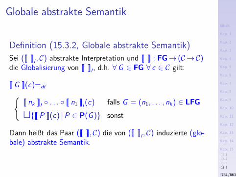
Inhalt
Kap. 1
Kap. 2
Kap. 3
Kap. 4
Kap. 5
Kap. 6
Kap. 7
Kap. 8
Kap. 9
Kap. 10
Kap. 11
Kap. 12
Kap. 13
Kap. 14
Kap. 15
15.1
15.2
15.3
15.4
Kap. 16
Kap. 17
Literatur
Anhang
A
Globale abstrakte Semantik
Definition (15.3.2, Globale abstrakte Semantik)
Sei ([[ ]]l , C) abstrakte Interpretation und [[ ]] : FG→ (C→C)die Globalisierung von [[ ]]l , d.h. ∀G ∈ FG ∀ c ∈ C gilt:
[[ G ]](c)=df[[ nk ]]l . . . [[ n1 ]]l(c) falls G = (n1, . . . , nk) ∈ LFG
t[[ P ]](c) |P ∈ P(G ) sonst
Dann heißt das Paar ([[ ]], C) die von ([[ ]]l , C) induzierte (glo-bale) abstrakte Semantik.
731/863
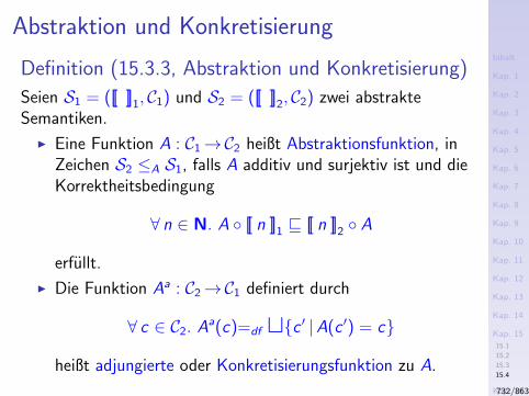
Inhalt
Kap. 1
Kap. 2
Kap. 3
Kap. 4
Kap. 5
Kap. 6
Kap. 7
Kap. 8
Kap. 9
Kap. 10
Kap. 11
Kap. 12
Kap. 13
Kap. 14
Kap. 15
15.1
15.2
15.3
15.4
Kap. 16
Kap. 17
Literatur
Anhang
A
Abstraktion und Konkretisierung
Definition (15.3.3, Abstraktion und Konkretisierung)
Seien S1 = ([[ ]]1, C1) und S2 = ([[ ]]2, C2) zwei abstrakteSemantiken.
I Eine Funktion A : C1→C2 heißt Abstraktionsfunktion, inZeichen S2 ≤A S1, falls A additiv und surjektiv ist und dieKorrektheitsbedingung
∀ n ∈ N. A [[ n ]]1 v [[ n ]]2 A
erfullt.
I Die Funktion Aa : C2→C1 definiert durch
∀ c ∈ C2. Aa(c)=df tc ′ |A(c ′) = c
heißt adjungierte oder Konkretisierungsfunktion zu A.
732/863
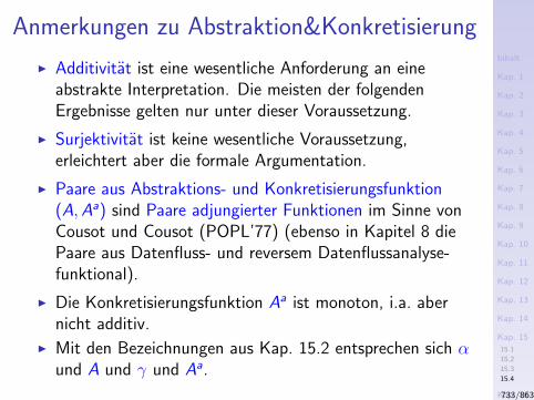
Inhalt
Kap. 1
Kap. 2
Kap. 3
Kap. 4
Kap. 5
Kap. 6
Kap. 7
Kap. 8
Kap. 9
Kap. 10
Kap. 11
Kap. 12
Kap. 13
Kap. 14
Kap. 15
15.1
15.2
15.3
15.4
Kap. 16
Kap. 17
Literatur
Anhang
A
Anmerkungen zu Abstraktion&Konkretisierung
I Additivitat ist eine wesentliche Anforderung an eineabstrakte Interpretation. Die meisten der folgendenErgebnisse gelten nur unter dieser Voraussetzung.
I Surjektivitat ist keine wesentliche Voraussetzung,erleichtert aber die formale Argumentation.
I Paare aus Abstraktions- und Konkretisierungsfunktion(A,Aa) sind Paare adjungierter Funktionen im Sinne vonCousot und Cousot (POPL’77) (ebenso in Kapitel 8 diePaare aus Datenfluss- und reversem Datenflussanalyse-funktional).
I Die Konkretisierungsfunktion Aa ist monoton, i.a. abernicht additiv.
I Mit den Bezeichnungen aus Kap. 15.2 entsprechen sich αund A und γ und Aa.
733/863
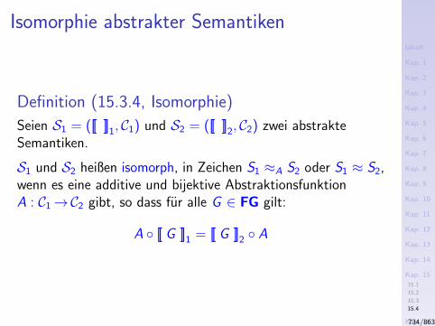
Inhalt
Kap. 1
Kap. 2
Kap. 3
Kap. 4
Kap. 5
Kap. 6
Kap. 7
Kap. 8
Kap. 9
Kap. 10
Kap. 11
Kap. 12
Kap. 13
Kap. 14
Kap. 15
15.1
15.2
15.3
15.4
Kap. 16
Kap. 17
Literatur
Anhang
A
Isomorphie abstrakter Semantiken
Definition (15.3.4, Isomorphie)
Seien S1 = ([[ ]]1, C1) und S2 = ([[ ]]2, C2) zwei abstrakteSemantiken.
S1 und S2 heißen isomorph, in Zeichen S1 ≈A S2 oder S1 ≈ S2,wenn es eine additive und bijektive AbstraktionsfunktionA : C1→C2 gibt, so dass fur alle G ∈ FG gilt:
A [[ G ]]1 = [[ G ]]2 A
734/863
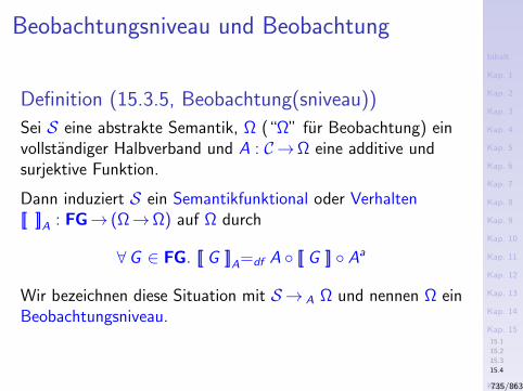
Inhalt
Kap. 1
Kap. 2
Kap. 3
Kap. 4
Kap. 5
Kap. 6
Kap. 7
Kap. 8
Kap. 9
Kap. 10
Kap. 11
Kap. 12
Kap. 13
Kap. 14
Kap. 15
15.1
15.2
15.3
15.4
Kap. 16
Kap. 17
Literatur
Anhang
A
Beobachtungsniveau und Beobachtung
Definition (15.3.5, Beobachtung(sniveau))
Sei S eine abstrakte Semantik, Ω (“Ω” fur Beobachtung) einvollstandiger Halbverband und A : C→Ω eine additive undsurjektive Funktion.
Dann induziert S ein Semantikfunktional oder Verhalten[[ ]]A : FG→ (Ω→Ω) auf Ω durch
∀G ∈ FG. [[ G ]]A=df A [[ G ]] Aa
Wir bezeichnen diese Situation mit S → A Ω und nennen Ω einBeobachtungsniveau.
735/863
Inhalt
Kap. 1
Kap. 2
Kap. 3
Kap. 4
Kap. 5
Kap. 6
Kap. 7
Kap. 8
Kap. 9
Kap. 10
Kap. 11
Kap. 12
Kap. 13
Kap. 14
Kap. 15
15.1
15.2
15.3
15.4
Kap. 16
Kap. 17
Literatur
Anhang
A
Modell
Definition (15.3.6, Modell)
Sei Ω ein Beobachtungsniveau und S eine abstrakte Semantikmit S → A Ω.
Dann heißt das Paar (S,A) ein Modell von Ω.
736/863
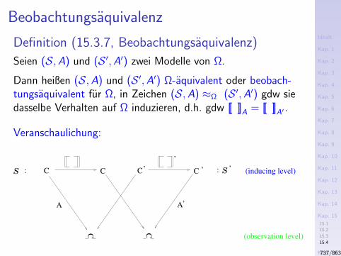
Inhalt
Kap. 1
Kap. 2
Kap. 3
Kap. 4
Kap. 5
Kap. 6
Kap. 7
Kap. 8
Kap. 9
Kap. 10
Kap. 11
Kap. 12
Kap. 13
Kap. 14
Kap. 15
15.1
15.2
15.3
15.4
Kap. 16
Kap. 17
Literatur
Anhang
A
Beobachtungsaquivalenz
Definition (15.3.7, Beobachtungsaquivalenz)
Seien (S,A) und (S ′,A′) zwei Modelle von Ω.
Dann heißen (S,A) und (S ′,A′) Ω-aquivalent oder beobach-tungsaquivalent fur Ω, in Zeichen (S,A) ≈Ω (S ′,A′) gdw siedasselbe Verhalten auf Ω induzieren, d.h. gdw [[ ]]A = [[ ]]A′ .
Veranschaulichung:
CC
S : CC CC’ ’
’
A A’
: ’S (inducing level)
(observation level)
737/863
Inhalt
Kap. 1
Kap. 2
Kap. 3
Kap. 4
Kap. 5
Kap. 6
Kap. 7
Kap. 8
Kap. 9
Kap. 10
Kap. 11
Kap. 12
Kap. 13
Kap. 14
Kap. 15
15.1
15.2
15.3
15.4
Kap. 16
Kap. 17
Literatur
Anhang
A
Eigenschaften der Relation ≈Ω
Lemma (15.3.8, Aquivalenzrelation)
Die Relation ≈Ω ist eine Aquivalenzrelation auf der Mengealler Modelle von Ω.
738/863
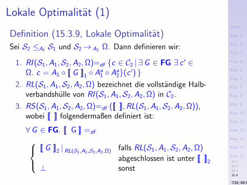
Inhalt
Kap. 1
Kap. 2
Kap. 3
Kap. 4
Kap. 5
Kap. 6
Kap. 7
Kap. 8
Kap. 9
Kap. 10
Kap. 11
Kap. 12
Kap. 13
Kap. 14
Kap. 15
15.1
15.2
15.3
15.4
Kap. 16
Kap. 17
Literatur
Anhang
A
Lokale Optimalitat (1)
Definition (15.3.9, Lokale Optimalitat)
Sei S2 ≤A1 S1 und S2→ A2 Ω. Dann definieren wir:
1. RI (S1,A1,S2,A2,Ω)=df c ∈ C2 | ∃G ∈ FG ∃ c ′ ∈Ω. c = A1 [[ G ]]1 Aa
1 Aa2(c ′)
2. RL(S1,A1,S2,A2,Ω) bezeichnet die vollstandige Halb-verbandshulle von RI (S1,A1,S2,A2,Ω) in C2.
3. RS(S1,A1,S2,A2,Ω)=df ([[ ]],RL(S1,A1,S2,A2,Ω)),wobei [[ ]] folgendermaßen definiert ist:
∀G ∈ FG. [[ G ]] =df[[ G ]]2 | RL(S1,A1,S2,A2,Ω) falls RL(S1,A1,S2,A2,Ω)
abgeschlossen ist unter [[ ]]2
⊥ sonst
739/863
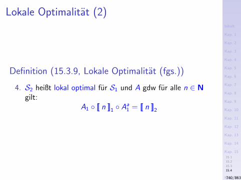
Inhalt
Kap. 1
Kap. 2
Kap. 3
Kap. 4
Kap. 5
Kap. 6
Kap. 7
Kap. 8
Kap. 9
Kap. 10
Kap. 11
Kap. 12
Kap. 13
Kap. 14
Kap. 15
15.1
15.2
15.3
15.4
Kap. 16
Kap. 17
Literatur
Anhang
A
Lokale Optimalitat (2)
Definition (15.3.9, Lokale Optimalitat (fgs.))
4. S2 heißt lokal optimal fur S1 und A gdw fur alle n ∈ Ngilt:
A1 [[ n ]]1 Aa1 = [[ n ]]2
740/863
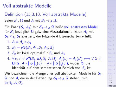
Inhalt
Kap. 1
Kap. 2
Kap. 3
Kap. 4
Kap. 5
Kap. 6
Kap. 7
Kap. 8
Kap. 9
Kap. 10
Kap. 11
Kap. 12
Kap. 13
Kap. 14
Kap. 15
15.1
15.2
15.3
15.4
Kap. 16
Kap. 17
Literatur
Anhang
A
Voll abstrakte Modelle
Definition (15.3.10, Voll abstrakte Modelle)
Seien S1, Ω und A mit S1→ A Ω.
Ein Paar (S2,A2) mit S2→ A Ω heißt voll abstraktes Modellfur S1 bezuglich Ω gdw eine Abstraktionsfunktion A1 mitS2 ≤A1 S1 existiert, die folgende 4 Eigenschaften erfullt:
1. A = A2 A1
2. S2 = RS(S1,A1,S2,A2,Ω)
3. S2 ist lokal optimal fur S1 und A1
4. ∀ c , c ′ ∈ RI (S1, ID,S1,A,Ω). A1(c) = A1(c ′)⇐⇒ ∀G ∈LFG. A [[ G ]]1(c) = A [[ G ]]1(c ′), wobei ID dieIdentitat auf dem semantischen Bereich von S1 ist.
Wir bezeichnen die Menge aller voll abstrakten Modelle fur S1,Ω und A, die in der Beziehung S1→ A Ω stehen, mitΦ(S1,A,Ω).
741/863
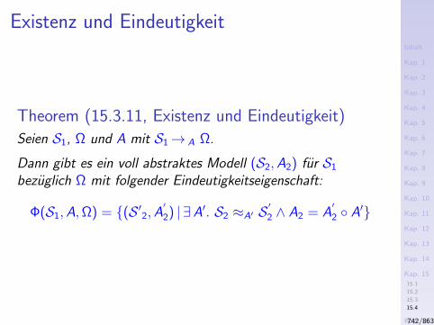
Inhalt
Kap. 1
Kap. 2
Kap. 3
Kap. 4
Kap. 5
Kap. 6
Kap. 7
Kap. 8
Kap. 9
Kap. 10
Kap. 11
Kap. 12
Kap. 13
Kap. 14
Kap. 15
15.1
15.2
15.3
15.4
Kap. 16
Kap. 17
Literatur
Anhang
A
Existenz und Eindeutigkeit
Theorem (15.3.11, Existenz und Eindeutigkeit)
Seien S1, Ω und A mit S1→ A Ω.
Dann gibt es ein voll abstraktes Modell (S2,A2) fur S1
bezuglich Ω mit folgender Eindeutigkeitseigenschaft:
Φ(S1,A,Ω) = (S ′2,A′
2) | ∃A′. S2 ≈A′ S′
2 ∧ A2 = A′
2 A′
742/863
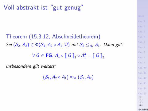
Inhalt
Kap. 1
Kap. 2
Kap. 3
Kap. 4
Kap. 5
Kap. 6
Kap. 7
Kap. 8
Kap. 9
Kap. 10
Kap. 11
Kap. 12
Kap. 13
Kap. 14
Kap. 15
15.1
15.2
15.3
15.4
Kap. 16
Kap. 17
Literatur
Anhang
A
Voll abstrakt ist “gut genug”
Theorem (15.3.12, Abschneidetheorem)
Sei (S2,A2) ∈ Φ(S1,A2 A1,Ω) mit S2 ≤A1 S1. Dann gilt:
∀G ∈ FG. A1 [[ G ]]1 Aa1 = [[ G ]]2
Insbesondere gilt weiters:
(S1,A2 A1) ≈Ω (S2,A2)
743/863
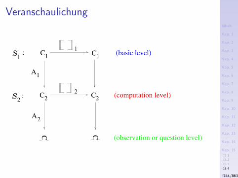
Inhalt
Kap. 1
Kap. 2
Kap. 3
Kap. 4
Kap. 5
Kap. 6
Kap. 7
Kap. 8
Kap. 9
Kap. 10
Kap. 11
Kap. 12
Kap. 13
Kap. 14
Kap. 15
15.1
15.2
15.3
15.4
Kap. 16
Kap. 17
Literatur
Anhang
A
Veranschaulichung
C1
C C
C2
C
C1
1
2
2
S
S
1
2:
:
A
A
1
2
(basic level)
(computation level)
(observation or question level)
744/863
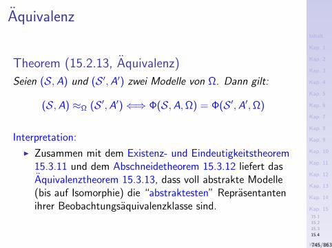
Inhalt
Kap. 1
Kap. 2
Kap. 3
Kap. 4
Kap. 5
Kap. 6
Kap. 7
Kap. 8
Kap. 9
Kap. 10
Kap. 11
Kap. 12
Kap. 13
Kap. 14
Kap. 15
15.1
15.2
15.3
15.4
Kap. 16
Kap. 17
Literatur
Anhang
A
Aquivalenz
Theorem (15.2.13, Aquivalenz)
Seien (S,A) und (S ′,A′) zwei Modelle von Ω. Dann gilt:
(S,A) ≈Ω (S ′,A′)⇐⇒ Φ(S,A,Ω) = Φ(S ′,A′,Ω)
Interpretation:
I Zusammen mit dem Existenz- und Eindeutigkeitstheorem15.3.11 und dem Abschneidetheorem 15.3.12 liefert dasAquivalenztheorem 15.3.13, dass voll abstrakte Modelle(bis auf Isomorphie) die “abstraktesten” Reprasentantenihrer Beobachtungsaquivalenzklasse sind.
745/863
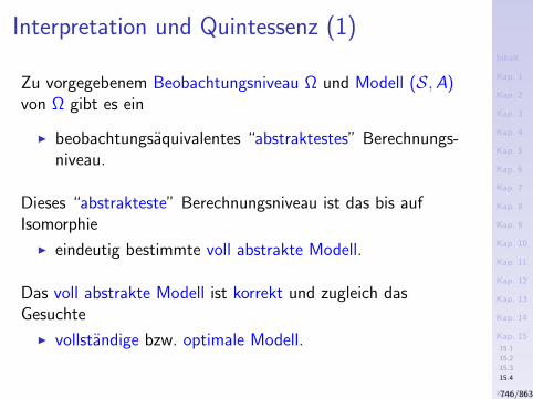
Inhalt
Kap. 1
Kap. 2
Kap. 3
Kap. 4
Kap. 5
Kap. 6
Kap. 7
Kap. 8
Kap. 9
Kap. 10
Kap. 11
Kap. 12
Kap. 13
Kap. 14
Kap. 15
15.1
15.2
15.3
15.4
Kap. 16
Kap. 17
Literatur
Anhang
A
Interpretation und Quintessenz (1)
Zu vorgegebenem Beobachtungsniveau Ω und Modell (S,A)von Ω gibt es ein
I beobachtungsaquivalentes “abstraktestes” Berechnungs-niveau.
Dieses “abstrakteste” Berechnungsniveau ist das bis aufIsomorphie
I eindeutig bestimmte voll abstrakte Modell.
Das voll abstrakte Modell ist korrekt und zugleich dasGesuchte
I vollstandige bzw. optimale Modell.
746/863
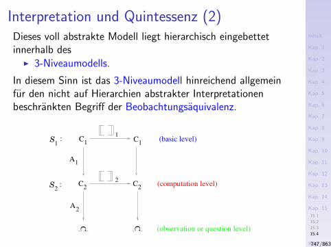
Inhalt
Kap. 1
Kap. 2
Kap. 3
Kap. 4
Kap. 5
Kap. 6
Kap. 7
Kap. 8
Kap. 9
Kap. 10
Kap. 11
Kap. 12
Kap. 13
Kap. 14
Kap. 15
15.1
15.2
15.3
15.4
Kap. 16
Kap. 17
Literatur
Anhang
A
Interpretation und Quintessenz (2)Dieses voll abstrakte Modell liegt hierarchisch eingebettetinnerhalb desI 3-Niveaumodells.
In diesem Sinn ist das 3-Niveaumodell hinreichend allgemeinfur den nicht auf Hierarchien abstrakter Interpretationenbeschrankten Begriff der Beobachtungsaquivalenz.
C1
C C
C2
C
C1
1
2
2
S
S
1
2:
:
A
A
1
2
(basic level)
(computation level)
(observation or question level)
747/863
Inhalt
Kap. 1
Kap. 2
Kap. 3
Kap. 4
Kap. 5
Kap. 6
Kap. 7
Kap. 8
Kap. 9
Kap. 10
Kap. 11
Kap. 12
Kap. 13
Kap. 14
Kap. 15
15.1
15.2
15.3
15.4
Kap. 16
Kap. 17
Literatur
Anhang
A
Vertiefende und weiterfuhrende Leseempfeh-
lungen fur Kapitel 15 (1)
Samson Abramsky, Chris Hankin. An Introduction toAbstract Interpretation. In Abstract Interpretation ofDeclarative Languages, Samson Abramsky, Chris Hankin(Eds). Prentice Hall, 63-102, 1987.
Patrick Cousot. Methods and Logics for ProvingPrograms. In Handbook of Theoretical Computer Science,Jan van Leeuwen (Ed.), Elsevier Science Publishers B. V.,chapter 15, 841-993, 1990.
Patrick Cousot. Abstract Interpretation. ACM ComputingSurveys 28(2):324-328, 1996.
Patrick Cousot. Refining Model-Checking by AbstractInterpretation. Autom. Softw. Eng. 6(1):69-95, 1999.
748/863
Inhalt
Kap. 1
Kap. 2
Kap. 3
Kap. 4
Kap. 5
Kap. 6
Kap. 7
Kap. 8
Kap. 9
Kap. 10
Kap. 11
Kap. 12
Kap. 13
Kap. 14
Kap. 15
15.1
15.2
15.3
15.4
Kap. 16
Kap. 17
Literatur
Anhang
A
Vertiefende und weiterfuhrende Leseempfeh-
lungen fur Kapitel 15 (2)
Patrick Cousot. Design of Syntactic Program Transforma-tions by Abstract Interpretation of Semantic Transforma-tions. In Proceedings of the 17th International Conferenceon Logic Programming (ICLP 2001), Springer-V., LNCS2237, 4-5, 2001.
Patrick Cousot. The Verification Grand Challenge andAbstract Interpretation. In Proceedings of VerifiedSoftware: Theories, Tools, Experiments (VSTTE 2005),Springer-V, LNCS 4171, 189-201, 2005.
Patrick Cousot. Verification by Abstract Interpretation. InProceedings of the 4th International Conference onVerification, Model-Checking, Abstract Interpretation(VMCAI 2003), Springer-V., LNCS 2575, 20-24, 2003.
749/863
Inhalt
Kap. 1
Kap. 2
Kap. 3
Kap. 4
Kap. 5
Kap. 6
Kap. 7
Kap. 8
Kap. 9
Kap. 10
Kap. 11
Kap. 12
Kap. 13
Kap. 14
Kap. 15
15.1
15.2
15.3
15.4
Kap. 16
Kap. 17
Literatur
Anhang
A
Vertiefende und weiterfuhrende Leseempfeh-
lungen fur Kapitel 15 (3)
Patrick Cousot. Verification by Abstract Interpretation. InVerification: Theory and Practice, Essays dedicated toZohar Manna on the Occasion of His 64th Birthday.Springer-V., LNCS 2772, 243-268, 2003.
Patrick Cousot, Radhia Cousot. Abstract Interpretation: AUnified Lattice Model for Static Analysis of Programs byConstruction or Approximation of Fixpoints. In ConferenceRecord of the 4th Annual ACM SIGACT-SIGPLANSymposium on Principles of Programming Languages(POPL’77), 238-252, 1977.
750/863
Inhalt
Kap. 1
Kap. 2
Kap. 3
Kap. 4
Kap. 5
Kap. 6
Kap. 7
Kap. 8
Kap. 9
Kap. 10
Kap. 11
Kap. 12
Kap. 13
Kap. 14
Kap. 15
15.1
15.2
15.3
15.4
Kap. 16
Kap. 17
Literatur
Anhang
A
Vertiefende und weiterfuhrende Leseempfeh-
lungen fur Kapitel 15 (4)
Patrick Cousot, Radhia Cousot. Systematic Design ofProgram Analysis Frameworks. In Conference Record ofthe 6th Annual ACM SIGACT-SIGPLAN Symposium onPrinciples of Programming Languages (POPL’79),269-282, 1979.
Patrick Cousot, Radhia Cousot. Abstract InterpretationFrameworks. Journal of Logic and Computation2(4):511-547, 1992.
Patrick Cousot, Radhia Cousot. Systematic Design ofProgram Transformation Frameworks by AbstractInterpretation. In Conference Record of the 29th AnnualACM SIGACT-SIGPLAN Symposium on Principles ofProgramming Languages (POPL 2002), 178-190, 2002.
751/863
Inhalt
Kap. 1
Kap. 2
Kap. 3
Kap. 4
Kap. 5
Kap. 6
Kap. 7
Kap. 8
Kap. 9
Kap. 10
Kap. 11
Kap. 12
Kap. 13
Kap. 14
Kap. 15
15.1
15.2
15.3
15.4
Kap. 16
Kap. 17
Literatur
Anhang
A
Vertiefende und weiterfuhrende Leseempfeh-
lungen fur Kapitel 15 (5)Patrick Cousot, Radhia Cousot. A Gentle Introduction toFormal Verification of Computer Systems by AbstractInterpretation. In Logics and Languages for Reliability andSecurity. NATO Sience for Peace and Security - D; Infor-mation and Communication Security, Vol. 25, IOS Press,2010. ISBN 978-1-60750–099-5.
Patrick Cousot, Radhia Cousot, Laurent Mauborgne.Theories, Solvers and Static Analysis by Abstract Interpre-tation. Journal of the ACM 59(6), Article 31, 56 Seiten,2012.
Patrick Cousot, Michael Monerau. Probabilistic AbstractInterpretation. In Proceedings 21st Symposium on Pro-gramming (ESOP 2012), Springer-V., LNCS 7211,169-193, 2012.
752/863
Inhalt
Kap. 1
Kap. 2
Kap. 3
Kap. 4
Kap. 5
Kap. 6
Kap. 7
Kap. 8
Kap. 9
Kap. 10
Kap. 11
Kap. 12
Kap. 13
Kap. 14
Kap. 15
15.1
15.2
15.3
15.4
Kap. 16
Kap. 17
Literatur
Anhang
A
Vertiefende und weiterfuhrende Leseempfeh-
lungen fur Kapitel 15 (6)Nevin Heintze, Joxan Jaffar, Razvan Voicu. A Frameworkfor Combining Analysis and Verification. In ConferenceRecord of the 27th Annual ACM SIGACT-SIGPLANSymposium on Principles of Programming Languages(POPL 2000), 26-39, 2000.
Kim Marriot. Frameworks for Abstract Interpretation. ActaInformatica 30:103-129, 1993.
Flemming Nielson. A Bibliography on Abstract Interpre-tations. ACM SIGPLAN Notices 21:31-38, 1986.
Flemming Nielson, Hanne Riis Nielson, Chris Hankin.Principles of Program Analysis. 2nd edition, Springer-V.,2005. (Chapter 1.5, Abstract Interpretation; Chapter 4,Abstract Interpretation)
753/863
Inhalt
Kap. 1
Kap. 2
Kap. 3
Kap. 4
Kap. 5
Kap. 6
Kap. 7
Kap. 8
Kap. 9
Kap. 10
Kap. 11
Kap. 12
Kap. 13
Kap. 14
Kap. 15
15.1
15.2
15.3
15.4
Kap. 16
Kap. 17
Literatur
Anhang
A
Vertiefende und weiterfuhrende Leseempfeh-
lungen fur Kapitel 15 (7)
Bernhard Steffen. Optimal Run Time Optimization –Proved by a New Look at Abstract Interpretation. InProceedings of the 2nd Joint International Conference onthe Theory and Practice of Software Development(TAPSOFT’87), Springer-V., LNCS 249, 52-68, 1987.
Bernhard Steffen. Optimal Data Flow Analysis viaObservational Equivalence. In Proceedings of the 14thInternational Symposium on Mathematical Foundations ofComputer Science (MFCS’89), Springer-V., LNCS 379,492-502, 1989.
754/863

Inhalt
Kap. 1
Kap. 2
Kap. 3
Kap. 4
Kap. 5
Kap. 6
Kap. 7
Kap. 8
Kap. 9
Kap. 10
Kap. 11
Kap. 12
Kap. 13
Kap. 14
Kap. 15
Kap. 16
Kap. 17
Literatur
Anhang
A
Kapitel 16
Modellprufung und DFA
755/863
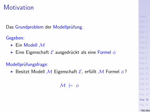
Inhalt
Kap. 1
Kap. 2
Kap. 3
Kap. 4
Kap. 5
Kap. 6
Kap. 7
Kap. 8
Kap. 9
Kap. 10
Kap. 11
Kap. 12
Kap. 13
Kap. 14
Kap. 15
Kap. 16
Kap. 17
Literatur
Anhang
A
Motivation
Das Grundproblem der Modellprufung.
Gegeben:
I Ein Modell MI Eine Eigenschaft E ausgedruckt als eine Formel φ
Modellprufungsfrage:
I Besitzt Modell M Eigenschaft E , erfullt M Formel φ ?
M |= φ
756/863
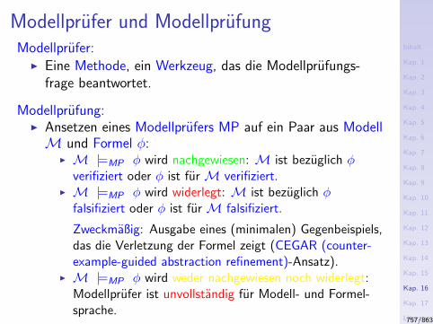
Inhalt
Kap. 1
Kap. 2
Kap. 3
Kap. 4
Kap. 5
Kap. 6
Kap. 7
Kap. 8
Kap. 9
Kap. 10
Kap. 11
Kap. 12
Kap. 13
Kap. 14
Kap. 15
Kap. 16
Kap. 17
Literatur
Anhang
A
Modellprufer und ModellprufungModellprufer:I Eine Methode, ein Werkzeug, das die Modellprufungs-
frage beantwortet.
Modellprufung:I Ansetzen eines Modellprufers MP auf ein Paar aus ModellM und Formel φ:
I M |=MP φ wird nachgewiesen: M ist bezuglich φverifiziert oder φ ist fur M verifiziert.
I M |=MP φ wird widerlegt: M ist bezuglich φfalsifiziert oder φ ist fur M falsifiziert.
Zweckmaßig: Ausgabe eines (minimalen) Gegenbeispiels,das die Verletzung der Formel zeigt (CEGAR (counter-example-guided abstraction refinement)-Ansatz).
I M |=MP φ wird weder nachgewiesen noch widerlegt:Modellprufer ist unvollstandig fur Modell- und Formel-sprache.
757/863
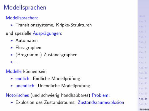
Inhalt
Kap. 1
Kap. 2
Kap. 3
Kap. 4
Kap. 5
Kap. 6
Kap. 7
Kap. 8
Kap. 9
Kap. 10
Kap. 11
Kap. 12
Kap. 13
Kap. 14
Kap. 15
Kap. 16
Kap. 17
Literatur
Anhang
A
Modellsprachen
Modellsprachen:
I Transitionssysteme, Kripke-Strukturen
und spezielle Auspragungen:
I Automaten
I Flussgraphen
I (Programm-) Zustandsgraphen
I ...
Modelle konnen sein
I endlich: Endliche Modellprufung
I unendlich: Unendliche Modellprufung
Notorisches (und schwierig handhabbares) Problem:
I Explosion des Zustandsraums: Zustandsraumexplosion
758/863
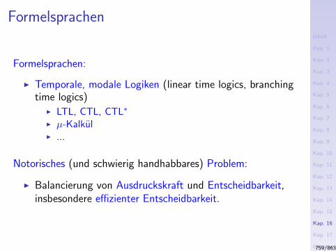
Inhalt
Kap. 1
Kap. 2
Kap. 3
Kap. 4
Kap. 5
Kap. 6
Kap. 7
Kap. 8
Kap. 9
Kap. 10
Kap. 11
Kap. 12
Kap. 13
Kap. 14
Kap. 15
Kap. 16
Kap. 17
Literatur
Anhang
A
Formelsprachen
Formelsprachen:
I Temporale, modale Logiken (linear time logics, branchingtime logics)
I LTL, CTL, CTL∗
I µ-KalkulI ...
Notorisches (und schwierig handhabbares) Problem:
I Balancierung von Ausdruckskraft und Entscheidbarkeit,insbesondere effizienter Entscheidbarkeit.
759/863
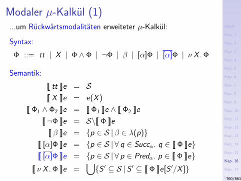
Inhalt
Kap. 1
Kap. 2
Kap. 3
Kap. 4
Kap. 5
Kap. 6
Kap. 7
Kap. 8
Kap. 9
Kap. 10
Kap. 11
Kap. 12
Kap. 13
Kap. 14
Kap. 15
Kap. 16
Kap. 17
Literatur
Anhang
A
Modaler µ-Kalkul (1)...um Ruckwartsmodalitaten erweiteter µ-Kalkul:
Syntax:
Φ ::= tt | X | Φ ∧ Φ | ¬Φ | β | [α]Φ | [α]Φ | ν X .Φ
Semantik:
[[ tt ]]e = S[[ X ]]e = e(X )
[[ Φ1 ∧ Φ2 ]]e = [[ Φ1 ]]e ∧ [[ Φ2 ]]e
[[ ¬Φ ]]e = S\[[ Φ ]]e
[[ β ]]e = p ∈ S | β ∈ λ(p)[[ [α]Φ ]]e = p ∈ S | ∀ q ∈ Succα. q ∈ [[ Φ ]]e[[ [α]Φ ]]e = p ∈ S | ∀ p ∈ Predα. p ∈ [[ Φ ]]e
[[ ν X .Φ ]]e =⋃S ′ ⊆ S | S ′ ⊆ [[ Φ ]]e[S ′/X ]
760/863
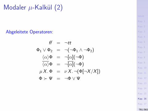
Inhalt
Kap. 1
Kap. 2
Kap. 3
Kap. 4
Kap. 5
Kap. 6
Kap. 7
Kap. 8
Kap. 9
Kap. 10
Kap. 11
Kap. 12
Kap. 13
Kap. 14
Kap. 15
Kap. 16
Kap. 17
Literatur
Anhang
A
Modaler µ-Kalkul (2)
Abgeleitete Operatoren:
ff = ¬tt
Φ1 ∨ Φ2 = ¬(¬Φ1 ∧ ¬Φ2)
〈α〉Φ = ¬[α](¬Φ)
〈α〉Φ = ¬[α](¬Φ)
µX .Φ = ν X .¬(Φ[¬X/X ])
Φ Ψ = ¬Φ ∨Ψ
761/863
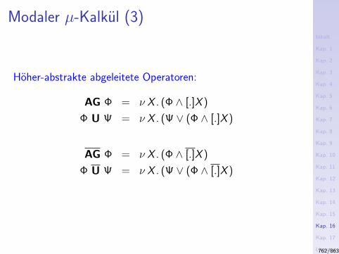
Inhalt
Kap. 1
Kap. 2
Kap. 3
Kap. 4
Kap. 5
Kap. 6
Kap. 7
Kap. 8
Kap. 9
Kap. 10
Kap. 11
Kap. 12
Kap. 13
Kap. 14
Kap. 15
Kap. 16
Kap. 17
Literatur
Anhang
A
Modaler µ-Kalkul (3)
Hoher-abstrakte abgeleitete Operatoren:
AG Φ = ν X . (Φ ∧ [.]X )
Φ U Ψ = ν X . (Ψ ∨ (Φ ∧ [.]X )
AG Φ = ν X . (Φ ∧ [.]X )
Φ U Ψ = ν X . (Ψ ∨ (Φ ∧ [.]X )
762/863
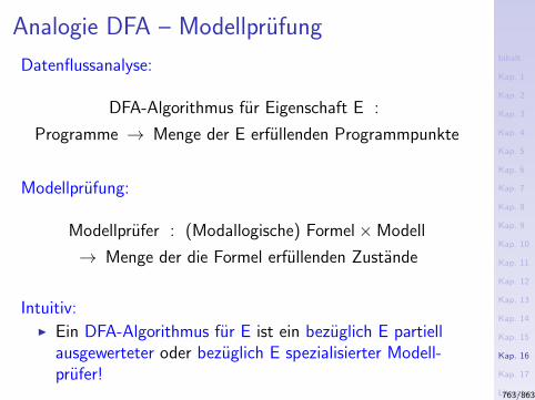
Inhalt
Kap. 1
Kap. 2
Kap. 3
Kap. 4
Kap. 5
Kap. 6
Kap. 7
Kap. 8
Kap. 9
Kap. 10
Kap. 11
Kap. 12
Kap. 13
Kap. 14
Kap. 15
Kap. 16
Kap. 17
Literatur
Anhang
A
Analogie DFA – Modellprufung
Datenflussanalyse:
DFA-Algorithmus fur Eigenschaft E :
Programme → Menge der E erfullenden Programmpunkte
Modellprufung:
Modellprufer : (Modallogische) Formel×Modell
→ Menge der die Formel erfullenden Zustande
Intuitiv:I Ein DFA-Algorithmus fur E ist ein bezuglich E partiell
ausgewerteter oder bezuglich E spezialisierter Modell-prufer!
763/863
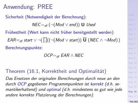
Inhalt
Kap. 1
Kap. 2
Kap. 3
Kap. 4
Kap. 5
Kap. 6
Kap. 7
Kap. 8
Kap. 9
Kap. 10
Kap. 11
Kap. 12
Kap. 13
Kap. 14
Kap. 15
Kap. 16
Kap. 17
Literatur
Anhang
A
Anwendung: PREE
Sicherheit (Notwendigkeit der Berechnung):
NEC =df (¬(Mod ∨ end)) U Used
Fruhestheit (Wert kann nicht fruher bereitgestellt werden):
EAR=df start ∨ ¬( [.]((¬(Mod ∨ start)) U (NEC ∧ ¬Mod) )
Berechnungspunkte:
OCP=df EAR ∧ NEC
Theorem (16.1, Korrektheit und Optimalitat)
Das Ersetzen der originalen Berechnungen durch neue an dendurch OCP gegebenen Programmpunkten ist korrekt (d.h. se-mantikerhaltend) und optimal (d.h. mindestens so gut wie jedeandere korrekte Platzierung der Berechnungen).
764/863
Inhalt
Kap. 1
Kap. 2
Kap. 3
Kap. 4
Kap. 5
Kap. 6
Kap. 7
Kap. 8
Kap. 9
Kap. 10
Kap. 11
Kap. 12
Kap. 13
Kap. 14
Kap. 15
Kap. 16
Kap. 17
Literatur
Anhang
A
Zusammenfassung (1)
Diese Charakterisierung des Zusammenhangs von DFA undModellprufung und die PREE-Anwendung geht zuruck auf:
I Bernhard Steffen. Data Flow Analysis as Model Checking.In Proceedings of the International Conference onTheoretical Aspects of Computer Software (TACS’91),Springer-V., LNCS 526, 346-365, 1991.
I Bernhard Steffen. Generating Data Flow AnalysisAlgorithms from Modal Specifications. InternationalJournal on Science of Computer Programming21:115-139, 1993.
765/863
Inhalt
Kap. 1
Kap. 2
Kap. 3
Kap. 4
Kap. 5
Kap. 6
Kap. 7
Kap. 8
Kap. 9
Kap. 10
Kap. 11
Kap. 12
Kap. 13
Kap. 14
Kap. 15
Kap. 16
Kap. 17
Literatur
Anhang
A
Zusammenfassung (2)
...ist aufgegriffen worden von:
I David A. Schmidt. Data Flow is Model Checking ofAbstract Interpretations. In Conference Record of the25th Annual ACM SIGACT-SIGPLAN Symposium onPrinciples of Programming Languages (POPL’98), 38-48,1998.
...und hat in der Folge gefuhrt zu:
I David A. Schmidt, Bernhard Steffen. Program Analysis asModel Checking of Abstract Interpretations. In Procee-dings of the 5th Static Analysis Symposium (SAS’98),Springer-V., LNCS 1503, 351-380, 1998.
766/863
Inhalt
Kap. 1
Kap. 2
Kap. 3
Kap. 4
Kap. 5
Kap. 6
Kap. 7
Kap. 8
Kap. 9
Kap. 10
Kap. 11
Kap. 12
Kap. 13
Kap. 14
Kap. 15
Kap. 16
Kap. 17
Literatur
Anhang
A
Vertiefende und weiterfuhrende Leseempfeh-
lungen fur Kapitel 16 (1)
Beatrice Berard, Michel Bidoit, Alain Finkel, Francois La-roussinie, Antoine Peit, Laure Petrucci, Philippe Schnoe-belen with Pierre McKenzie. Systems and Software Verifi-cation: Model-Checking Techniques and Tools. Sprin-ger-V., 2001.
Edmund M. Clarke, Orna Grumberg, Doron Peled. ModelChecking. MIT Press, 2001.
Edmund M. Clarke, H. Schlingloff. Model Checking. InHandbook of Automated Deduction, A. Robinson,A. Voronkov (Hrsg.), Vol. II, Elsevier, 1635-1790, 2000.
767/863
Inhalt
Kap. 1
Kap. 2
Kap. 3
Kap. 4
Kap. 5
Kap. 6
Kap. 7
Kap. 8
Kap. 9
Kap. 10
Kap. 11
Kap. 12
Kap. 13
Kap. 14
Kap. 15
Kap. 16
Kap. 17
Literatur
Anhang
A
Vertiefende und weiterfuhrende Leseempfeh-
lungen fur Kapitel 16 (2)
Patrick Cousot, Radhia Cousot. Temporal Abstract Inter-pretation. In Conference Record of the 27th Annual ACMSIGACT-SIGPLAN Symposium on Principles of Program-ming Languages (POPL 2000), 12-25, 2000.
E. Allen Emerson. Temporal and Modal Logic. In Hand-book of Theoretical Computer Science, Jan van Leeuwen(Hrsg.), Elsevier, 995-1072, 1990.
Orna Grumberg, Helmut Veith. 25 Years of ModelChecking: History, Achievements, Perspectives.Springer-V., LNCS 5000, 2008.
George E. Hughes, Max J. Cresswell. An Introduction toModal Logic. Methuan, 1968.
768/863
Inhalt
Kap. 1
Kap. 2
Kap. 3
Kap. 4
Kap. 5
Kap. 6
Kap. 7
Kap. 8
Kap. 9
Kap. 10
Kap. 11
Kap. 12
Kap. 13
Kap. 14
Kap. 15
Kap. 16
Kap. 17
Literatur
Anhang
A
Vertiefende und weiterfuhrende Leseempfeh-
lungen fur Kapitel 16 (3)
George E. Hughes, Max J. Cresswell. A Companion toModal Logic. Methuan, 1986.
George E. Hughes, Max J. Cresswell. A New Introductionto Modal Logic. Routledge, 1996.
Fred Kroger, Stephan Merz. Temporal Logic and StateSystems. Springer-V., 2008. (Chapter 3, Extensions ofLinear Time Logic; Chapter 5, First-Order Linear TimeLogic; Chapter 10, Other Temporal Logics; Chapter 11,System Verification by Model Checking)
Janusz Laski, William Stanley. Software Verification andAnalysis: An Integrated, Hands-On Approach. Springer-V.,2009.
769/863
Inhalt
Kap. 1
Kap. 2
Kap. 3
Kap. 4
Kap. 5
Kap. 6
Kap. 7
Kap. 8
Kap. 9
Kap. 10
Kap. 11
Kap. 12
Kap. 13
Kap. 14
Kap. 15
Kap. 16
Kap. 17
Literatur
Anhang
A
Vertiefende und weiterfuhrende Leseempfeh-
lungen fur Kapitel 16 (4)
Robert Lover. Elementary Logic for Software Develop-ment. Springer-V., 2008. (Chapter 20.2.2, Temporal,Modal, and Dynamic Logics)
Markus Muller-Olm, David A. Schmidt, Bernhard Steffen.Model-Checking: A Tutorial Introduction. In Proceedingsof the 6th Static Analysis Symposium (SAS’99), Sprin-ger-V., LNCS 1694, 330-354, 1999.
Doron A. Peled. Software Reliability Methods. Springer-V.,2001.
Dirk Richter. Programmanalysen zur Verbesserung derSoftwaremodellprufung. Dissertation, Universitat Halle-Wittenberg, 2012.
770/863
Inhalt
Kap. 1
Kap. 2
Kap. 3
Kap. 4
Kap. 5
Kap. 6
Kap. 7
Kap. 8
Kap. 9
Kap. 10
Kap. 11
Kap. 12
Kap. 13
Kap. 14
Kap. 15
Kap. 16
Kap. 17
Literatur
Anhang
A
Vertiefende und weiterfuhrende Leseempfeh-
lungen fur Kapitel 16 (5)
David A. Schmidt. Data Flow Analysis is Model Checkingof Abstract Interpretations. In Conference Record of the25th Annual ACM SIGACT-SIGPLAN Symposium onPrinciples of Programming Languages (POPL’98), 38-48,1998.
David A. Schmidt, Bernhard Steffen. Program Analysis asModel Checking of Abstract Interpretations. In Procee-dings of the 5th Static Analysis Symposium (SAS’98),Springer-V., LNCS 1503, 351-380, 1998.
Bernhard Steffen. Data Flow Analysis as Model Checking.In Proceedings of the International Conference on Theo-retical Aspects of Computer Software (TACS’91), Sprin-ger-V., LNCS 526, 346-365, 1991.
771/863
Inhalt
Kap. 1
Kap. 2
Kap. 3
Kap. 4
Kap. 5
Kap. 6
Kap. 7
Kap. 8
Kap. 9
Kap. 10
Kap. 11
Kap. 12
Kap. 13
Kap. 14
Kap. 15
Kap. 16
Kap. 17
Literatur
Anhang
A
Vertiefende und weiterfuhrende Leseempfeh-
lungen fur Kapitel 16 (6)
Bernhard Steffen. Generating Data Flow Analysis Algor-ithms from Modal Specifications. International Journal onScience of Computer Programming 21:115-139, 1993.
Bernhard Steffen. Property-Oriented Expansion. In Pro-ceedings of the 3rd Static Analysis Symposium (SAS’96),Springer-V., LNCS 1145, 22-41, 1996.
772/863

Inhalt
Kap. 1
Kap. 2
Kap. 3
Kap. 4
Kap. 5
Kap. 6
Kap. 7
Kap. 8
Kap. 9
Kap. 10
Kap. 11
Kap. 12
Kap. 13
Kap. 14
Kap. 15
Kap. 16
Kap. 17
Literatur
Anhang
A
Teil V
Abschluss und Ausblick
773/863

Inhalt
Kap. 1
Kap. 2
Kap. 3
Kap. 4
Kap. 5
Kap. 6
Kap. 7
Kap. 8
Kap. 9
Kap. 10
Kap. 11
Kap. 12
Kap. 13
Kap. 14
Kap. 15
Kap. 16
Kap. 17
Literatur
Anhang
A
Kapitel 17
Resumee und Perspektiven
774/863
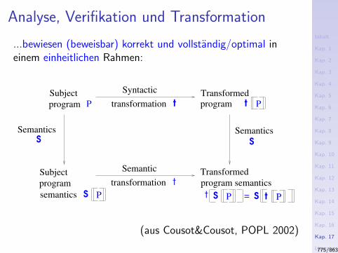
Inhalt
Kap. 1
Kap. 2
Kap. 3
Kap. 4
Kap. 5
Kap. 6
Kap. 7
Kap. 8
Kap. 9
Kap. 10
Kap. 11
Kap. 12
Kap. 13
Kap. 14
Kap. 15
Kap. 16
Kap. 17
Literatur
Anhang
A
Analyse, Verifikation und Transformation
...bewiesen (beweisbar) korrekt und vollstandig/optimal ineinem einheitlichen Rahmen:
PSP
Pt
Pt
TransformedSemantic
transformation t
semantics
program
Subject
program
TransformedSubject
program P
Syntactic
transformation t
program semantics
t =S S
Semantics
S
SemanticsS
(aus Cousot&Cousot, POPL 2002)
775/863

Inhalt
Kap. 1
Kap. 2
Kap. 3
Kap. 4
Kap. 5
Kap. 6
Kap. 7
Kap. 8
Kap. 9
Kap. 10
Kap. 11
Kap. 12
Kap. 13
Kap. 14
Kap. 15
Kap. 16
Kap. 17
Literatur
Anhang
A
Wichtig fur verschiedenste Gebiete, darunter:I Optimierende Ubersetzer (Performanz, Energie,...)I Software-VerifikationI Ubersetzer-Verifikation, Betriebssystem-Verifikation,...I Software
I -Spezifikation, -Analyse, -Validierung, -Generierung(insbesondere auch modellgetriebene Spezifikation,Analyse, Verifikation, Generierung, Testung,...)
I -VerstehenI RefaktorisierungI (Re-)engineering, Reverse EngineeringI Dokumentation
I -(Kunden)anpassung, -spezialisierung (customization)I Safety and Security (security policy enforcement,...)I Datenschurfung und -ausbeutung (data mining)I Hardware-VerifikationI ...I Grune Informationstechnologie
776/863
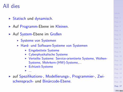
Inhalt
Kap. 1
Kap. 2
Kap. 3
Kap. 4
Kap. 5
Kap. 6
Kap. 7
Kap. 8
Kap. 9
Kap. 10
Kap. 11
Kap. 12
Kap. 13
Kap. 14
Kap. 15
Kap. 16
Kap. 17
Literatur
Anhang
A
All dies
I Statisch und dynamisch.
I Auf Programm-Ebene im Kleinen.
I Auf System-Ebene im Großen
I Systeme von SystemenI Hard- und Software-Systeme von Systemen
I Eingebettete SystemeI Cyberphysikalische SystemeI Verteilte Systeme: Service-orientierte Systeme, Wolken-
Systeme, Mehrkern-(HW)-Systeme,...I Echtzeit-SystemeI ...
I auf Spezifikations-, Modellierungs-, Programmier-, Zwi-schensprach- und Binarcode-Ebene.
777/863
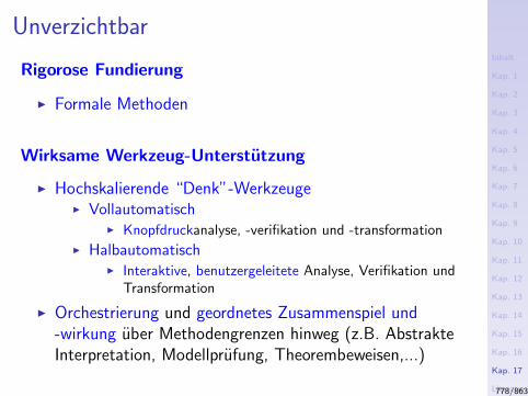
Inhalt
Kap. 1
Kap. 2
Kap. 3
Kap. 4
Kap. 5
Kap. 6
Kap. 7
Kap. 8
Kap. 9
Kap. 10
Kap. 11
Kap. 12
Kap. 13
Kap. 14
Kap. 15
Kap. 16
Kap. 17
Literatur
Anhang
A
Unverzichtbar
Rigorose Fundierung
I Formale Methoden
Wirksame Werkzeug-Unterstutzung
I Hochskalierende “Denk”-WerkzeugeI Vollautomatisch
I Knopfdruckanalyse, -verifikation und -transformationI Halbautomatisch
I Interaktive, benutzergeleitete Analyse, Verifikation undTransformation
I Orchestrierung und geordnetes Zusammenspiel und-wirkung uber Methodengrenzen hinweg (z.B. AbstrakteInterpretation, Modellprufung, Theorembeweisen,...)
778/863
Inhalt
Kap. 1
Kap. 2
Kap. 3
Kap. 4
Kap. 5
Kap. 6
Kap. 7
Kap. 8
Kap. 9
Kap. 10
Kap. 11
Kap. 12
Kap. 13
Kap. 14
Kap. 15
Kap. 16
Kap. 17
Literatur
Anhang
A
Wichtige Konferenzen und Zeitschriften (1)
I Annual International Conference on Verification, Model-Checking, Abstract Interpretation (VMCAI) Series,Springer-V., LNCS series, since 2000.
I Annual International Conference on Tools and Algorithmsfor the Construction and Analysis of Systems (TACAS),Springer-V., LNCS series, since 1995.
I Annual International Conference on Computer-Aided Veri-fication (CAV) Series, Springer-V., LNCS series, since1989.
I Annual International Conference on Software Testing,Verification and Validation (ICST) Series, IEEE, since2008.
779/863
Inhalt
Kap. 1
Kap. 2
Kap. 3
Kap. 4
Kap. 5
Kap. 6
Kap. 7
Kap. 8
Kap. 9
Kap. 10
Kap. 11
Kap. 12
Kap. 13
Kap. 14
Kap. 15
Kap. 16
Kap. 17
Literatur
Anhang
A
Wichtige Konferenzen und Zeitschriften (2)
I Annual International Symposium on Formal Methods(FM) Series, Springer-V., LNCS series, since 1995.
I Biennial International Symposium on LeveragingApplications of Formal Methods, Verification, andValidation (ISoLA) Series, Springer-V., LNCS series, since2004.
I International Journal on Software Tools for TechnologyTransfer (STTT), Springer-V, since 1999.
780/863
Inhalt
Kap. 1
Kap. 2
Kap. 3
Kap. 4
Kap. 5
Kap. 6
Kap. 7
Kap. 8
Kap. 9
Kap. 10
Kap. 11
Kap. 12
Kap. 13
Kap. 14
Kap. 15
Kap. 16
Kap. 17
Literatur
Anhang
A
Vertiefende und weiterfuhrende Leseempfeh-
lungen fur Kapitel 17 (1)
Julien Bertrane, Patrick Cousot, Radhia Cousot, JeromeFeret, Laurent Mauborgne, Antoine Mine, Xavier Rival.Static Analysis and Verification of Aerospace Software byAbstract Interpretation. In Proceedings AIAAInfotech@Aerospace (AIAA I@A 2010), AIAA-2010-3385,American Institute of Aeronautics and Astronautics, 1-38,April 2010.
Julien Bertrane, Patrick Cousot, Radhia Cousot, JeromeFeret, Laurent Mauborgne, Antoine Mine, Xavier Rival.Static Analysis by Abstract Interpretation of EmbeddedCritical Software. ACM Software Engineering Notes36(1):1-8, 2011.
781/863
Inhalt
Kap. 1
Kap. 2
Kap. 3
Kap. 4
Kap. 5
Kap. 6
Kap. 7
Kap. 8
Kap. 9
Kap. 10
Kap. 11
Kap. 12
Kap. 13
Kap. 14
Kap. 15
Kap. 16
Kap. 17
Literatur
Anhang
A
Vertiefende und weiterfuhrende Leseempfeh-
lungen fur Kapitel 17 (2)
Cristian Cadar, Koushik Sen. Symbolic Execution for Soft-ware Testing: Three Decades Later. Communications ofthe ACM 56(2):82-90, 2013.
Patrick Cousot, Radhia Cousot. Systematic Design ofProgram Transformation Frameworks by AbstractInterpretation. In Conference Record of the 29th AnnualACM SIGACT-SIGPLAN Symposium on Principles ofProgramming Languages (POPL 2002), 178-190, 2002.
Nevin Heintze, Joxan Jaffar, Razvan Voicu. A Frameworkfor Combining Analysis and Verification. In ConferenceRecord of the 27th Annual ACM SIGACT-SIGPLANSymposium on Principles of Programming Languages(POPL 2000), 26-39, 2000.
782/863
Inhalt
Kap. 1
Kap. 2
Kap. 3
Kap. 4
Kap. 5
Kap. 6
Kap. 7
Kap. 8
Kap. 9
Kap. 10
Kap. 11
Kap. 12
Kap. 13
Kap. 14
Kap. 15
Kap. 16
Kap. 17
Literatur
Anhang
A
Vertiefende und weiterfuhrende Leseempfeh-
lungen fur Kapitel 17 (3)
Ashish Tiwari, Sumit Gulwani. Static Program AnalysisUsing Theorem Proving. In Proceedings of the 21stConference on Automated Deduction (CADE-21), LNCS4603, Springer-V., 147-166, 2007.
Daniel Weise. Static Analysis of Mega-Programs (InvitedPaper). In Proceedings of the 6th Static Analysis Sympo-sium (SAS’99), Springer-V., LNCS 1694, 300-302, 1999.
783/863

Inhalt
Kap. 1
Kap. 2
Kap. 3
Kap. 4
Kap. 5
Kap. 6
Kap. 7
Kap. 8
Kap. 9
Kap. 10
Kap. 11
Kap. 12
Kap. 13
Kap. 14
Kap. 15
Kap. 16
Kap. 17
Literatur
Anhang
A
Literatur
784/863

Inhalt
Kap. 1
Kap. 2
Kap. 3
Kap. 4
Kap. 5
Kap. 6
Kap. 7
Kap. 8
Kap. 9
Kap. 10
Kap. 11
Kap. 12
Kap. 13
Kap. 14
Kap. 15
Kap. 16
Kap. 17
Literatur
Anhang
A
Literaturhinweise und Leseempfehlungen
...zum vertiefenden und weiterfuhrenden Selbststudium.
I I Lehrbucher
I II Artikel, Dissertationen, Sammelbande
785/863
Inhalt
Kap. 1
Kap. 2
Kap. 3
Kap. 4
Kap. 5
Kap. 6
Kap. 7
Kap. 8
Kap. 9
Kap. 10
Kap. 11
Kap. 12
Kap. 13
Kap. 14
Kap. 15
Kap. 16
Kap. 17
Literatur
Anhang
A
I Lehrbucher (1)
Alfred V. Aho, Monica S. Lam, Ravi Sethi, Jeffrey D.Ullman. Compilers: Principles, Techniques, & Tools.2. Auflage, Addison-Wesley, 2007.
Randy Allen, Ken Kennedy. Optimizing Compilers forModern Architectures. Morgan Kaufman Publishers, 2002.
Krzysztof R. Apt, Ernst-Rudiger Olderog. Programmveri-fikation – Sequentielle, parallele und verteilte Programme.Springer-V., 1994.
Krzysztof R. Apt, Frank S. de Boer, Ernst-Rudiger Olde-rog. Verification of Sequential and Concurrent Programs.3. Auflage, Springer-V., 2009.
Mordechai Ben-Ari. Mathematical Logic for ComputerScience. 2. Auflage, Springer-V., 2001.
786/863
Inhalt
Kap. 1
Kap. 2
Kap. 3
Kap. 4
Kap. 5
Kap. 6
Kap. 7
Kap. 8
Kap. 9
Kap. 10
Kap. 11
Kap. 12
Kap. 13
Kap. 14
Kap. 15
Kap. 16
Kap. 17
Literatur
Anhang
A
I Lehrbucher (2)
Beatrice Berard, Michel Bidoit, Alain Finkel, FrancoisLaroussinie, Antoine Peit, Laure Petrucci, PhilippeSchnoebelen with Pierre McKenzie. Systems and SoftwareVerification: Model-Checking Techniques and Tools.Springer-V., 2001.
Edmund M. Clarke, Orna Grumberg, Doron Peled. ModelChecking. MIT Press, 2001.
Keith D. Cooper, Linda Torczon. Engineering a Compiler.Morgan Kaufman Publishers, 2004.
Jaco W. De Backer. Mathematical Theory of ProgramCorrectness. Prentice-Hall, 1980.
Gilles Dowek. Principles of Programming Languages.Springer-V, 2009.
787/863
Inhalt
Kap. 1
Kap. 2
Kap. 3
Kap. 4
Kap. 5
Kap. 6
Kap. 7
Kap. 8
Kap. 9
Kap. 10
Kap. 11
Kap. 12
Kap. 13
Kap. 14
Kap. 15
Kap. 16
Kap. 17
Literatur
Anhang
A
I Lehrbucher (3)
Michael J.C. Gordon. The Denotational Description ofProgramming Languages. Springer-V., 1979.
Matthew S. Hecht. Flow Analysis of Computer Programs.Elsevier, North-Holland, 1977.
George E. Hughes, Max J. Cresswell. An Introduction toModal Logic. Methuan, 1968.
George E. Hughes, Max J. Cresswell. A Companion toModal Logic. Methuan, 1986.
George E. Hughes, Max J. Cresswell. A New Introductionto Modal Logic. Routledge, 1996.
Fred Kroger, Stephan Merz. Temporal Logic and StateSystems. Springer-V., 2008.
788/863
Inhalt
Kap. 1
Kap. 2
Kap. 3
Kap. 4
Kap. 5
Kap. 6
Kap. 7
Kap. 8
Kap. 9
Kap. 10
Kap. 11
Kap. 12
Kap. 13
Kap. 14
Kap. 15
Kap. 16
Kap. 17
Literatur
Anhang
A
I Lehrbucher (4)
Janusz Laski, William Stanley. Software Verification andAnalysis. Springer-V., 2009.
Jacques Loeckx, Kurt Sieber. The Foundations of ProgramVerification. Wiley, 1984.
Robert Lover. Elementary Logic for Software Develop-ment. Springer-V., 2008.
Robert Morgan. Building an Optimizing Compiler. DigitalPress, 1998.
Stephen S. Muchnick. Advanced Compiler Design Imple-mentation. Morgan Kaufman Publishers, 1997.
Hanne Riis Nielson, Flemming Nielson. Semantics withApplications: A Formal Introduction. Wiley, 1992.
789/863
Inhalt
Kap. 1
Kap. 2
Kap. 3
Kap. 4
Kap. 5
Kap. 6
Kap. 7
Kap. 8
Kap. 9
Kap. 10
Kap. 11
Kap. 12
Kap. 13
Kap. 14
Kap. 15
Kap. 16
Kap. 17
Literatur
Anhang
A
I Lehrbucher (5)
Hanne Riis Nielson, Flemming Nielson. Semantics withApplications: An Appetizer. Springer-V., 2007.
Flemming Nielson, Hanne Riis Nielson, Chris Hankin. Prin-ciples of Program Analysis. 2. Auflage, Springer-V., 2005.
Doron A. Peled. Software Reliability Methods. Springer-V.,2001.
Joseph E. Stoy. Denotational Semantics: The Scott-Strachey Approach to Programming Language Theory.MIT Press, 1981.
Glynn Winskel. The Formal Semantics of ProgrammingLanguages: An Introduction. MIT Press, 1993.
790/863
Inhalt
Kap. 1
Kap. 2
Kap. 3
Kap. 4
Kap. 5
Kap. 6
Kap. 7
Kap. 8
Kap. 9
Kap. 10
Kap. 11
Kap. 12
Kap. 13
Kap. 14
Kap. 15
Kap. 16
Kap. 17
Literatur
Anhang
A
II Artikel, Dissertationen, Sammelbande (1)
Samson Abramsky, Chris Hankin. An Introduction toAbstract Interpretation. In Abstract Interpretation ofDeclarative Languages, Samson Abramsky, Chris Hankin(Eds). Prentice Hall, 63-102, 1987.
Gagan Agrawal. Demand-driven Construction of CallGraphs. In Proceedings of the 9th International Confe-rence on Compiler Construction (CC 2000), Springer-V.,LNCS 1781, 125-140, 2000.
Bowen Alpern, Mark N. Wegman, F. Ken Zadeck. Detec-ting Equality of Variables in Programs. In ConferenceRecord of the 15th ACM SIGPLAN-SIGACT Symposiumon Principles of Programming Languages (POPL’88),1-11, 1988.
791/863
Inhalt
Kap. 1
Kap. 2
Kap. 3
Kap. 4
Kap. 5
Kap. 6
Kap. 7
Kap. 8
Kap. 9
Kap. 10
Kap. 11
Kap. 12
Kap. 13
Kap. 14
Kap. 15
Kap. 16
Kap. 17
Literatur
Anhang
A
II Artikel, Dissertationen, Sammelbande (2)
Krzysztof R. Apt. Ten Years of Hoare’s Logic: A Survey –Part 1. ACM Transactions on Programming Languagesand Systems 3(4):431-483, 1981.
Krzysztof R. Apt. Ten Years of Hoare’s Logic: A Survey –Part II: Nondeterminism. Theoretical Computer Science28(1-2):83-109, 1984.
Wayne A. Babich, Mehdi Jazayeri. The Method ofAttributes for Data Flow Analysis: Part I - ExhaustiveAnalysis. Acta Informatica 10(3):245-264, 1978.
Wayne A. Babich, Mehdi Jazayeri. The Method ofAttributes for Data Flow Analysis: Part II - DemandAnalysis. Acta Informatica 10(3):265-272, 1978.
792/863
Inhalt
Kap. 1
Kap. 2
Kap. 3
Kap. 4
Kap. 5
Kap. 6
Kap. 7
Kap. 8
Kap. 9
Kap. 10
Kap. 11
Kap. 12
Kap. 13
Kap. 14
Kap. 15
Kap. 16
Kap. 17
Literatur
Anhang
A
II Artikel, Dissertationen, Sammelbande (3)Bernhard Beckert, Reiner Hahnle, Peter H. Schmitt(Hrsg.). Verification of Object-Oriented Software: TheKeY Approach. LNCS 4334, Springer-V., 2007.
Julien Bertrane, Patrick Cousot, Radhia Cousot, JeromeFeret, Laurent Mauborgne, Antoine Mine, Xavier Rival.Static Analysis and Verification of Aerospace Software byAbstract Interpretation. In Proceedings AIAAInfotech@Aerospace (AIAA I@A 2010), AIAA-2010-3385,American Institute of Aeronautics and Astronautics, 1-38,April 2010.
Julien Bertrane, Patrick Cousot, Radhia Cousot, JeromeFeret, Laurent Mauborgne, Antoine Mine, Xavier Rival.Static Analysis by Abstract Interpretation of EmbeddedCritical Software. ACM Software Engineering Notes36(1):1-8, 2011.
793/863
Inhalt
Kap. 1
Kap. 2
Kap. 3
Kap. 4
Kap. 5
Kap. 6
Kap. 7
Kap. 8
Kap. 9
Kap. 10
Kap. 11
Kap. 12
Kap. 13
Kap. 14
Kap. 15
Kap. 16
Kap. 17
Literatur
Anhang
A
II Artikel, Dissertationen, Sammelbande (4)
Al Bessey, Ken Block, Ben Chelf, Andy Chou, BryanFulton, Seth Hallem, Charles Henri-Gros, Asya Kamsky,Scott McPeak, Dawson Engler. A Few Billion Lines ofCode Later: Using Static Analysis to Find Bugs in the RealWorld. Communications of the ACM 53(2):66-75, 2010.
Ras Bodik, Rajiv Gupta. Partial Dead Code Eliminationusing Slicing Transformations. In Proceedings of the ACMSIGPLAN’97 Conference on Programming LanguageDesign and Implementation (PLDI’97), ACM SIGPLANNotices 32(6):159-170, 1997.
794/863
Inhalt
Kap. 1
Kap. 2
Kap. 3
Kap. 4
Kap. 5
Kap. 6
Kap. 7
Kap. 8
Kap. 9
Kap. 10
Kap. 11
Kap. 12
Kap. 13
Kap. 14
Kap. 15
Kap. 16
Kap. 17
Literatur
Anhang
A
II Artikel, Dissertationen, Sammelbande (5)
Ras Bodık, Rajiv Gupta, Vivek Sarkar. ABCD: EliminatingArray Bounds Check on Demand. In Proceedings of theACM SIGPLAN Conference on Porgramming LanguageDesign and Implementation (PLDI’00), ACM SIGPLANNotices 35(5):321-333, 2000.
Cristian Cadar, Koushik Sen. Symbolic Execution for Soft-ware Testing: Three Decades Later. Communications ofthe ACM 56(2):82-90, 2013.
Edmund M. Clarke. Programming Language Constructsfor which it is Impossible to Obtain Good Hoare AxiomSystems. Journal of the ACM 26(1):129-147, 1979.
Edmund M. Clarke, Stephen M. German, JosephY. Halpern. Effective Axiomatizations of Hoare Logics.Journal of the ACM 30(1):612-636, 1983.
795/863
Inhalt
Kap. 1
Kap. 2
Kap. 3
Kap. 4
Kap. 5
Kap. 6
Kap. 7
Kap. 8
Kap. 9
Kap. 10
Kap. 11
Kap. 12
Kap. 13
Kap. 14
Kap. 15
Kap. 16
Kap. 17
Literatur
Anhang
A
II Artikel, Dissertationen, Sammelbande (6)
Edmund M. Clarke, Orna Grumberg, David E. Long.Model Checking and Abstraction. ACM Transactions onProgramming Languages and Systems 16(5):1512-1542,1994.
Edmund M. Clarke, H. Schlingloff. Model Checking. InHandbook of Automated Deduction, A. Robinson,A. Voronkov (Hrsg.), Vol. II, Elsevier, 1635-1790, 2000.
Stephen A. Cook. Soundness and Completeness of anAxiom System for Program Verification. SIAM Journal onComputing 7(1):70-90, 1978.
Patrick Cousot. Methods and Logics for Proving Pro-grams. In Handbook of Theoretical Computer Science, Janvan Leeuwen (Ed.), Elsevier Science Publishers B. V.,Chapter 15, 841-993, 1990.
796/863
Inhalt
Kap. 1
Kap. 2
Kap. 3
Kap. 4
Kap. 5
Kap. 6
Kap. 7
Kap. 8
Kap. 9
Kap. 10
Kap. 11
Kap. 12
Kap. 13
Kap. 14
Kap. 15
Kap. 16
Kap. 17
Literatur
Anhang
A
II Artikel, Dissertationen, Sammelbande (7)
Patrick Cousot. Abstract Interpretation. ACM ComputingSurveys 28(2):324-328, 1996.
Patrick Cousot. Refining Model-Checking by AbstractInterpretation. Autom. Softw. Eng. 6(1):69-95, 1999.
Patrick Cousot. Design of Syntactic Program Transforma-tions by Abstract Interpretation of Semantic Transforma-tions. In Proceedings of the 17th International Conferenceon Logic Programming (ICLP 2001), Springer-V., LNCS2237, 4-5, 2001.
Patrick Cousot. The Verification Grand Challenge andAbstract Interpretation. In Proceedings of Verified Soft-ware: Theories, Tools, Experiments (VSTTE 2005),Springer-V, LNCS 4171, 189-201, 2005.
797/863
Inhalt
Kap. 1
Kap. 2
Kap. 3
Kap. 4
Kap. 5
Kap. 6
Kap. 7
Kap. 8
Kap. 9
Kap. 10
Kap. 11
Kap. 12
Kap. 13
Kap. 14
Kap. 15
Kap. 16
Kap. 17
Literatur
Anhang
A
II Artikel, Dissertationen, Sammelbande (8)
Patrick Cousot. Verification by Abstract Interpretation. InProceedings of the 4th International Conference onVerification, Model-Checking, Abstract Interpretation(VMCAI 2003), Springer-V., LNCS 2575, 20-24, 2003.
Patrick Cousot. Verification by Abstract Interpretation. InVerification: Theory and Practice, Essays dedicated toZohar Manna on the Occasion of His 64th Birthday.Springer-V., LNCS 2772, 243-268, 2003.
Patrick Cousot, Radhia Cousot. Abstract Interpretation: AUnified Lattice Model for Static Analysis of Programs byConstruction or Approximation of Fixpoints. In ConferenceRecord of the 4th Annual ACM SIGACT-SIGPLANSymposium on Principles of Programming Languages(POPL’77), 238-252, 1977.
798/863
Inhalt
Kap. 1
Kap. 2
Kap. 3
Kap. 4
Kap. 5
Kap. 6
Kap. 7
Kap. 8
Kap. 9
Kap. 10
Kap. 11
Kap. 12
Kap. 13
Kap. 14
Kap. 15
Kap. 16
Kap. 17
Literatur
Anhang
A
II Artikel, Dissertationen, Sammelbande (9)
Patrick Cousot, Radhia Cousot. Constructive Versions ofTarski’s Fixed Point Theorems. Pacific Journal ofMathematics 82(1):43-57, 1979.
Patrick Cousot, Radhia Cousot. Systematic Design ofProgram Analysis Frameworks. In Conference Record ofthe 6th Annual ACM SIGACT-SIGPLAN Symposium onPrinciples of Programming Languages (POPL’79),269-282, 1979.
Patrick Cousot, Radhia Cousot. Abstract InterpretationFrameworks. Journal of Logic and Computation2(4):511-547, 1992.
799/863
Inhalt
Kap. 1
Kap. 2
Kap. 3
Kap. 4
Kap. 5
Kap. 6
Kap. 7
Kap. 8
Kap. 9
Kap. 10
Kap. 11
Kap. 12
Kap. 13
Kap. 14
Kap. 15
Kap. 16
Kap. 17
Literatur
Anhang
A
II Artikel, Dissertationen, Sammelbande (10)Patrick Cousot, Radhia Cousot. Temporal Abstract Inter-pretation. In Conference Record of the 27th Annual ACMSIGACT-SIGPLAN Symposium on Principles ofProgramming Languages (POPL 2000), 12-25, 2000.
Patrick Cousot, Radhia Cousot. Systematic Design ofProgram Transformation Frameworks by Abstract Inter-pretation. In Conference Record of the 29th Annual ACMSIGACT-SIGPLAN Symposium on Principles ofProgramming Languages (POPL 2002), 178-190, 2002.
Patrick Cousot, Radhia Cousot. A Gentle Introduction toFormal Verification of Computer Systems by AbstractInterpretation. In Logics and Languages for Reliability andSecurity. NATO Sience for Peace and Security - D; Infor-mation and Communication Security, Vol. 25, IOS Press,2010. ISBN 978-1-60750–099-5.
800/863
Inhalt
Kap. 1
Kap. 2
Kap. 3
Kap. 4
Kap. 5
Kap. 6
Kap. 7
Kap. 8
Kap. 9
Kap. 10
Kap. 11
Kap. 12
Kap. 13
Kap. 14
Kap. 15
Kap. 16
Kap. 17
Literatur
Anhang
A
II Artikel, Dissertationen, Sammelbande (11)
Patrick Cousot, Radhia Cousot, Laurent Mauborgne.Theories, Solvers and Static Analysis by Abstract Interpre-tation. Journal of the ACM 59(6), Article 31, 56 Seiten,2012.
Patrick Cousot, Michael Monerau. Probabilistic AbstractInterpretation. In Proceedings 21st Symposium on Pro-gramming (ESOP 2012), Springer-V., LNCS 7211,169-193, 2012.
Ron Cytron, Jeanne Ferrante, Barry K. Rosen, MarkN. Wegman, F. Ken Zadeck. An Efficient Method ofComputing Static Single Assignment Form. In ConferenceRecord of the 16th ACM SIGPLAN-SIGACT Symposiumon Principles of Programming Languages (POPL’89),25-35, 1989.
801/863
Inhalt
Kap. 1
Kap. 2
Kap. 3
Kap. 4
Kap. 5
Kap. 6
Kap. 7
Kap. 8
Kap. 9
Kap. 10
Kap. 11
Kap. 12
Kap. 13
Kap. 14
Kap. 15
Kap. 16
Kap. 17
Literatur
Anhang
A
II Artikel, Dissertationen, Sammelbande (12)
Ron Cytron, Jeanne Ferrante, Barry K. Rosen, MarkN. Wegman, F. Ken Zadeck. Efficiently Computing StaticSingle Assignment Form and the Control DependenceGraph. ACM Transactions on Programming Languagesand Systems 13(4):451-490, 1991.
D. M. Dhamdhere. Register Assignment using Code Place-ment Techniques. Journal of Computer Languages13(2):75-93, 1988.
D. M. Dhamdhere. A usually linear Algorithm for RegisterAssignment using Edge Placement of Load and StoreInstructions. Journal of Computer Languages 15(2):83-94,1990.
802/863
Inhalt
Kap. 1
Kap. 2
Kap. 3
Kap. 4
Kap. 5
Kap. 6
Kap. 7
Kap. 8
Kap. 9
Kap. 10
Kap. 11
Kap. 12
Kap. 13
Kap. 14
Kap. 15
Kap. 16
Kap. 17
Literatur
Anhang
A
II Artikel, Dissertationen, Sammelbande (13)
D. M. Dhamdhere. Practical Adaptation of the GlobalOptimization Algorithm of Morel and Renvoise. ACMTransactions on Programming Languages and Systems13(2):291-294, 1991. Technical Correspondence.
Evelyn Duesterwald. A Demand-driven Approach forEfficient Interprocedural Data-Flow Analysis. PhD thesis,University of Pittsburgh, 1996.
Evelyn Duesterwald, Rajiv Gupta, Mary Lou Soffa.Demand-driven Computation of Interprocedural DataFlow. In Conference Record of the 22nd ACMSIGPLAN-SIGACT Symposium on Principles ofProgramming Languages (POPL’95), 37-48, 1995.
803/863
Inhalt
Kap. 1
Kap. 2
Kap. 3
Kap. 4
Kap. 5
Kap. 6
Kap. 7
Kap. 8
Kap. 9
Kap. 10
Kap. 11
Kap. 12
Kap. 13
Kap. 14
Kap. 15
Kap. 16
Kap. 17
Literatur
Anhang
A
II Artikel, Dissertationen, Sammelbande (14)
Evelyn Duesterwald, Rajiv Gupta, Mary Lou Soffa. ADemand-driven Analyzer for Data Flow Testing at theIntegration Level. In Proceedings of the IEEE Conferenceon Software Engineering (CoSE’96), 575-586, 1996.
Evelyn Duesterwald, Rajiv Gupta, Mary Lou Soffa. APractical Framework for Demand-driven InterproceduralData Flow Analysis. ACM Transactions on ProgrammingLanguages and Systems 19(6):992-1030, 1997.
E. Allen Emerson. Temporal and Modal Logic. InHandbook of Theoretical Computer Science, Jan vanLeeuwen (Hrsg.), Elsevier, 995-1072, 1990.
804/863
Inhalt
Kap. 1
Kap. 2
Kap. 3
Kap. 4
Kap. 5
Kap. 6
Kap. 7
Kap. 8
Kap. 9
Kap. 10
Kap. 11
Kap. 12
Kap. 13
Kap. 14
Kap. 15
Kap. 16
Kap. 17
Literatur
Anhang
A
II Artikel, Dissertationen, Sammelbande (15)
L. Feigen, D. Klappholz, R. Casazza, X. Xue. The RevivalTransformation. In Conference Record of the 21st ACMSIGPLAN-SIGACT Symposium on Principles of Program-ming Languages (POPL’94), 1994.
Robert W. Floyd. Assigning Meaning to Programs. InProceedings of Symposium on Applied Mathematics,Mathematical Aspects of Computer Science, AmericanMathematical Society, New York, 19:19-32, 1967.
Alfons Geser, Jens Knoop, Gerald Luttgen, Oliver Ruthing,Bernhard Steffen. Non-monotone Fixpoint Iterations toResolve Second Order Effects. In Proceedings of the 6thInternational Conference on Compiler Construction(CC’96), Springer-V., LNCS 1060, 106-120, 1996.
805/863
Inhalt
Kap. 1
Kap. 2
Kap. 3
Kap. 4
Kap. 5
Kap. 6
Kap. 7
Kap. 8
Kap. 9
Kap. 10
Kap. 11
Kap. 12
Kap. 13
Kap. 14
Kap. 15
Kap. 16
Kap. 17
Literatur
Anhang
A
II Artikel, Dissertationen, Sammelbande (16)
Orna Grumberg, Helmut Veith. 25 Years of ModelChecking: History, Achievements, Perspectives.Springer-V., LNCS 5000, 2008.
Reiner Hahnle, Richard Bubel. A Hoare-Style Calculuswith Explicit State Updates. Handout in the courseProgram Verification at the Department of ComputerScience at the Chalmers University of Technology, 19pages. i12www.iti.uni-karlsruhe.de/∼key/download/hoare/students.pdf
Nevin Heintze, Joxan Jaffar, Razvan Voicu. A Frameworkfor Combining Analysis and Verification. In ConferenceRecord of the 27th Annual ACM SIGACT-SIGPLANSymposium on Principles of Programming Languages(POPL 2000), 26-39, 2000.
806/863
Inhalt
Kap. 1
Kap. 2
Kap. 3
Kap. 4
Kap. 5
Kap. 6
Kap. 7
Kap. 8
Kap. 9
Kap. 10
Kap. 11
Kap. 12
Kap. 13
Kap. 14
Kap. 15
Kap. 16
Kap. 17
Literatur
Anhang
A
II Artikel, Dissertationen, Sammelbande (17)
Charles A.R. Hoare. An Axiomatic Basis for ComputerProgramming. Communications of the ACM12(19):576-580, 583, 1969.
Susan Horwitz, Thomas Reps, Mooly Sagiv. DemandInterprocedural Data Flow Analysis. In Proceedings of the3rd ACM SIGSOFT Symposium on the Foundations ofSoftware Engineering (FSE-3), 104-115, 1995.
John Hughes, John Launchbury. Reversing AbstractInterpretations. In Proceedings of the 4th EuropeanSymposium on Programming (ESOP’92), Springer-V.,LNCS 582, 269-286, 1992.
John Hughes, John Launchbury. Reversing AbstractInterpretations. Science of Computer Programming22:307-326, 1994.
807/863
Inhalt
Kap. 1
Kap. 2
Kap. 3
Kap. 4
Kap. 5
Kap. 6
Kap. 7
Kap. 8
Kap. 9
Kap. 10
Kap. 11
Kap. 12
Kap. 13
Kap. 14
Kap. 15
Kap. 16
Kap. 17
Literatur
Anhang
A
II Artikel, Dissertationen, Sammelbande (18)
Tudor Jebelean, Laura Kovacs, Nikolaj Popov. Experi-mental Program Verification in the Theorema System. InProceedings of the International Symposium onLeveraging Applications of Formal Methods (ISoLA 2004),92-99, 2004. www.risc.jku.at/publications/download/risc 2243/KoPoJeb.pdf
John B. Kam, Jeffrey D. Ullman. Monotone Data FlowAnalysis Frameworks. Acta Informatica 7:305-317, 1977.
Gary A. Kildall. A Unified Approach to Global ProgramOptimization. In Conference Record of the 1st ACMSIGPLAN-SIGACT Symposium on Principles of Program-ming Languages (POPL’73), 194-206, 1973.
808/863
Inhalt
Kap. 1
Kap. 2
Kap. 3
Kap. 4
Kap. 5
Kap. 6
Kap. 7
Kap. 8
Kap. 9
Kap. 10
Kap. 11
Kap. 12
Kap. 13
Kap. 14
Kap. 15
Kap. 16
Kap. 17
Literatur
Anhang
A
II Artikel, Dissertationen, Sammelbande (19)Raimund Kirner, Jens Knoop, Adrian Prantl, MarkusSchordan, Albrecht Kadlec. Beyond Loop Bounds: Compa-ring Annotation Languages for Worst-Case ExecutionTime Analysis. Journal of Software and Systems Modeling10(3):411-437, Springer-V., 2011.
Jens Knoop. From DFA-frameworks to DFA-generators: AUnifying Multiparadigm Approach. In Proceedings of the5th International Conference on Tools and Algorithms forthe Construction and Analysis of Systems (TACAS’99),Springer-V., LNCS 1579, 360-374, 1999.
Jens Knoop. Demand-driven Analysis of Explicitly ParallelPrograms: An Approach based on Reverse Data-FlowAnalysis. In Proceedings of the 9th International Workshopon Compilers for Parallel Computers (CPC 2001),151-162, 2001.
809/863
Inhalt
Kap. 1
Kap. 2
Kap. 3
Kap. 4
Kap. 5
Kap. 6
Kap. 7
Kap. 8
Kap. 9
Kap. 10
Kap. 11
Kap. 12
Kap. 13
Kap. 14
Kap. 15
Kap. 16
Kap. 17
Literatur
Anhang
A
II Artikel, Dissertationen, Sammelbande (20)
Jens Knoop. Data-Flow Analysis for Hot-Spot ProgramOptimization. In Proceedings of the 14th Biennial Work-shop on “Programmiersprachen und Grundlagen der Pro-grammierung” (KPS 2007). Bericht A-07-07 der Institutefur Mathematik und Informatik, Universitat Lubeck,Germany, 124-131, 2007.
Jens Knoop, Dirk Koschutzki, Bernhard Steffen. Basic-block Graphs: Living Dinosaurs? In Proceedings of the 7thInternational Conference on Compiler Construction(CC’98), Springer-V., LNCS 1383, 65 - 79, 1998.
Jens Knoop, Eduard Mehofer. Distribution AssignmentPlacement: Effective Optimization of Redistribution Costs.IEEE Transactions on Parallel and Distributed Systems13(6):628-647, 2002.
810/863
Inhalt
Kap. 1
Kap. 2
Kap. 3
Kap. 4
Kap. 5
Kap. 6
Kap. 7
Kap. 8
Kap. 9
Kap. 10
Kap. 11
Kap. 12
Kap. 13
Kap. 14
Kap. 15
Kap. 16
Kap. 17
Literatur
Anhang
A
II Artikel, Dissertationen, Sammelbande (21)
Jens Knoop, Oliver Ruthing, Bernhard Steffen. Lazy CodeMotion. In Proceedings of the ACM SIGPLAN’92 Confe-rence on Programming Language Design and Implemen-tation (PLDI’92), ACM SIGPLAN Notices 27(7):224-234,1992.
Jens Knoop, Oliver Ruthing, Bernhard Steffen. PartialDead Code Elimination. In Proceedings of the ACMSIGPLAN’94 Conference on Programming LanguageDesign and Implementation (PLDI’94), ACM SIGPLANNotices 29(6):147-158, 1994.
Jens Knoop, Oliver Ruthing, Bernhard Steffen. OptimalCode Motion: Theory and Practice. ACM Transactions onProgramming Languages and Systems 16(4):1117-1155,1994.
811/863
Inhalt
Kap. 1
Kap. 2
Kap. 3
Kap. 4
Kap. 5
Kap. 6
Kap. 7
Kap. 8
Kap. 9
Kap. 10
Kap. 11
Kap. 12
Kap. 13
Kap. 14
Kap. 15
Kap. 16
Kap. 17
Literatur
Anhang
A
II Artikel, Dissertationen, Sammelbande (22)
Jens Knoop, Oliver Ruthing, Bernhard Steffen. The Powerof Assignment Motion. In Proceedings of the ACMSIGPLAN’95 Conference on Programming LanguageDesign and Implementation (PLDI’95), ACM SIGPLANNotices 30(6):233-245, 1995.
Jens Knoop, Oliver Ruthing, Bernhard Steffen. CodeMotion and Code Placement: Just Synonyms? In Procee-dings of the 7th European Symposium on Programming(ESOP’98), Springer-V., LNCS 1381, 154-169, 1998.
Jens Knoop, Oliver Ruthing. Constant Propagation on theValue Graph: Simple Constants and Beyond. In Procee-dings of the 9th International Conference on CompilerConstruction (CC 2000), Springer-V., LNCS 1781, 94-109,2000.
812/863
Inhalt
Kap. 1
Kap. 2
Kap. 3
Kap. 4
Kap. 5
Kap. 6
Kap. 7
Kap. 8
Kap. 9
Kap. 10
Kap. 11
Kap. 12
Kap. 13
Kap. 14
Kap. 15
Kap. 16
Kap. 17
Literatur
Anhang
A
II Artikel, Dissertationen, Sammelbande (23)
Jens Knoop, Oliver Ruthing. Constant Propagation onPredicated Code. Journal of Universal Computer Science9(8):829-850, 2003. (special issue devoted to SBLP’03).
Jens Knoop, Oliver Ruthing, Bernhard Steffen.Retrospective: Lazy Code Motion. In ”20 Years of theACM SIGPLAN Conference on Programming LanguageDesign and Implementation (1979 - 1999): A Selection”,ACM SIGPLAN Notices 39(4):460-461&462-472, 2004.
Jens Knoop, Bernhard Steffen. The Interprocedural Coin-cidence Theorem. In Proceedings of the 4th InternationalConference on Compiler Construction (CC’92), Sprin-ger-V., LNCS 641, 125-140, 1992.
813/863
Inhalt
Kap. 1
Kap. 2
Kap. 3
Kap. 4
Kap. 5
Kap. 6
Kap. 7
Kap. 8
Kap. 9
Kap. 10
Kap. 11
Kap. 12
Kap. 13
Kap. 14
Kap. 15
Kap. 16
Kap. 17
Literatur
Anhang
A
II Artikel, Dissertationen, Sammelbande (24)
Jens Knoop, Bernhard Steffen, Jurgen Vollmer. Parallelismfor Free: Efficient and Optimal Bitvector Analyses forParallel Programs. ACM Transactions on ProgrammingLanguages and Systems 18(3):268-299, 1996.
Laura Kovacs, Tudor Jebelean. Practical Aspects of Impe-rative Program Verification using Theorema. In Procee-dings of the 5th International Workshop on Symbolic andNumeric Algorithms for Scientific Computing (SYNASC2003), 317-320, 2003. www.risc.jku.at/publications/download/risc 464/synasc03.pdf
814/863
Inhalt
Kap. 1
Kap. 2
Kap. 3
Kap. 4
Kap. 5
Kap. 6
Kap. 7
Kap. 8
Kap. 9
Kap. 10
Kap. 11
Kap. 12
Kap. 13
Kap. 14
Kap. 15
Kap. 16
Kap. 17
Literatur
Anhang
A
II Artikel, Dissertationen, Sammelbande (25)
Laura Kovacs, Tudor Jebelean. Generation of Invariants inTheorema. In Proceedings of the 10th International Sym-posium of Mathematics and its Applications, 407-415,2003. www.risc.jku.at/publications/download/risc 2053/2003-11-06-A.pdf
Jean-Louis Lassez, V.L. Nguyen, Liz Sonenberg. FixedPoint Theorems and Semantics: A Folk Tale. InformationProcessing Letters 14(3):112-116, 1982.
Yuan Lin, David A. Padua. Demand-driven InterproceduralArray Property Analysis. In Proceedings of the 12thInternational Conference on Languages and Compilers forParallel Computing (LCPC’99), Springer-V., LNCS, 1999.
815/863
Inhalt
Kap. 1
Kap. 2
Kap. 3
Kap. 4
Kap. 5
Kap. 6
Kap. 7
Kap. 8
Kap. 9
Kap. 10
Kap. 11
Kap. 12
Kap. 13
Kap. 14
Kap. 15
Kap. 16
Kap. 17
Literatur
Anhang
A
II Artikel, Dissertationen, Sammelbande (26)
Bjorn Lisper, Andreas Ermedahl, Dietmar Schreiner, JensKnoop, Peter Gliwa. Practical Experiences of ApplyingSource-level WCET Flow Analysis to Industrial Code.Journal of Software Tools for Technology Transfer(STTT) 15(1):53-63, Springer-V., 2013.
Thomas J. Marlowe, Barbara G. Ryder. Properties of DataFlow Frameworks. Acta Informatica 20:121-163, 1990.
Kim Marriot. Frameworks for Abstract Interpretation. ActaInformatica 30:103-129, 1993.
Steve P. Miller, Michael W. Whalen, Darren D. Cofer.Software Model Checking Takes Off. Communications ofthe ACM 53(2):58-64, 2010.
816/863
Inhalt
Kap. 1
Kap. 2
Kap. 3
Kap. 4
Kap. 5
Kap. 6
Kap. 7
Kap. 8
Kap. 9
Kap. 10
Kap. 11
Kap. 12
Kap. 13
Kap. 14
Kap. 15
Kap. 16
Kap. 17
Literatur
Anhang
A
II Artikel, Dissertationen, Sammelbande (27)
Ronald J. Mintz, Gerald A. Fisher, Micha Sharir. TheDesign of a Global Optimizer. In Proceedings of the ACMSIGPLAN’79 Symposium on Compiler Construction(SoCC’79), ACM SIGPLAN Notices 14(8):226-234, 1979.
Markus Muller-Olm, David A. Schmidt, Bernhard Steffen.Model-Checking: A Tutorial Introduction. In Proceedingsof the 6th Static Analysis Symposium (SAS’99), Sprin-ger-V., LNCS 1694, 330-354, 1999.
Flemming Nielson. A Bibliography on Abstract Interpre-tations. ACM SIGPLAN Notices 21:31-38, 1986.
David von Oheimb. Hoare Logic for Java in Isabelle/HOL.Concurrency and Computation: Practice and Experience13(13):1173-1214, 2001.
817/863
Inhalt
Kap. 1
Kap. 2
Kap. 3
Kap. 4
Kap. 5
Kap. 6
Kap. 7
Kap. 8
Kap. 9
Kap. 10
Kap. 11
Kap. 12
Kap. 13
Kap. 14
Kap. 15
Kap. 16
Kap. 17
Literatur
Anhang
A
II Artikel, Dissertationen, Sammelbande (28)
Ernst-Rudiger Olderog. Correctness of Programs withPascal-like Procedures without Global Variables.Theoretical Computer Science 30(1):49-90, 1984.
Ernst-Rudiger Olderog, Bernhard Steffen. Formale Seman-tik und Programmverifikation. In Informatik-Handbuch,Peter Rechenberg, Gustav Pomberger (Hrsg.), Carl HanserVerlag, 4. Auflage, 145-166, 2006.
Ernst-Rudiger Olderog, Reinhard Wilhelm. Turing und dieVerifikation. Informatik Spektrum 35(4):271-279, 2012.
Gordon D. Plotkin. A Structural Approach to OperationalSemantics. Lecture notes, DAIMI FN-19, Aarhus Univer-sity, Denmark, 1981, reprinted 1991.
818/863
Inhalt
Kap. 1
Kap. 2
Kap. 3
Kap. 4
Kap. 5
Kap. 6
Kap. 7
Kap. 8
Kap. 9
Kap. 10
Kap. 11
Kap. 12
Kap. 13
Kap. 14
Kap. 15
Kap. 16
Kap. 17
Literatur
Anhang
A
II Artikel, Dissertationen, Sammelbande (29)
Gordon D. Plotkin. An Operational Semantics for CSP. InProceedings of TC-2 Working Conference on FormalDescription of Programming Concepts II, Dines Bjørner(Ed.), North-Holland, Amsterdam, 1982.
Gordon D. Plotkin. A Structural Approach to OperationalSemantics. Journal of Logic and Algebraic Programming60-61:17-139, 2004.
Peter Puschner, Daniel Prokesch, Benedikt Huber, JensKnoop, Stefan Hepp, Gernot Gebhard. The T-CRESTApproach of Compiler and WCET-Analysis Integration. InProceedings of the 9th International Workshop on Soft-ware Technologies for Future Embedded and UbiquitiousSystems (SEUS 2013), June 2013, to appear.
819/863
Inhalt
Kap. 1
Kap. 2
Kap. 3
Kap. 4
Kap. 5
Kap. 6
Kap. 7
Kap. 8
Kap. 9
Kap. 10
Kap. 11
Kap. 12
Kap. 13
Kap. 14
Kap. 15
Kap. 16
Kap. 17
Literatur
Anhang
A
II Artikel, Dissertationen, Sammelbande (30)
John H. Reif, Harry R. Lewis. Symbolic Evaluation and theGlobal Value Graph. In Conference Record of the 4thAnnual ACM SIGACT-SIGPLAN Symposium on Principlesof Programming Languages (POPL’77), 104-118, 1977.
Thomas Reps. Solving Demand Versions of InterproceduralAnalysis Problems. In Proceedings of the 5th InternationalConference on Compiler Construction (CC’95), Sprin-ger-V., LNCS 786, 389-403, 1994.
Thomas Reps. Demand Interprocedural Program Analysisusing Logic Databases. In Applications of Logic Databa-ses, R. Ramakrishnan (Ed.), Kluwer Academic Publishers,1994.
820/863
Inhalt
Kap. 1
Kap. 2
Kap. 3
Kap. 4
Kap. 5
Kap. 6
Kap. 7
Kap. 8
Kap. 9
Kap. 10
Kap. 11
Kap. 12
Kap. 13
Kap. 14
Kap. 15
Kap. 16
Kap. 17
Literatur
Anhang
A
II Artikel, Dissertationen, Sammelbande (31)
Dirk Richter. Programmanalysen zur Verbesserung derSoftwaremodellprufung. Dissertation, Universitat Halle-Wittenberg, 2012.
F. Robert. Convergence locale d’iterations chaotiques nonlineaires. Technical Report 58, Laboratoire d’Informatique,U.S.M.G., Grenoble, France, Dec. 1976.
Oliver Ruthing, Jens Knoop, Bernhard Steffen. DetectingEqualities of Variables: Combining Efficiency with Pre-cision. In Proceedings of the 6th Static Analysis Sympo-sium (SAS’99), Springer-V., LNCS 1694, 232-247, 1999.
Oliver Ruthing, Markus Muller-Olm. On the Complexity ofConstant Propagation. In Proceedings of the 10th Euro-pean Symposium on Programming (ESOP 2001), Sprin-ger-V., LNCS 2028, 190-205, 2001.
821/863
Inhalt
Kap. 1
Kap. 2
Kap. 3
Kap. 4
Kap. 5
Kap. 6
Kap. 7
Kap. 8
Kap. 9
Kap. 10
Kap. 11
Kap. 12
Kap. 13
Kap. 14
Kap. 15
Kap. 16
Kap. 17
Literatur
Anhang
A
II Artikel, Dissertationen, Sammelbande (32)
David A. Schmidt. Data Flow Analysis is Model Checkingof Abstract Interpretations. In Conference Record of the25th Annual ACM SIGACT-SIGPLAN Symposium onPrinciples of Programming Languages (POPL’98), 38-48,1998.
David A. Schmidt, Bernhard Steffen. Program Analysis asModel Checking of Abstract Interpretations. In Pro-ceedings of the 5th Static Analysis Symposium (SAS’98),Springer-V., LNCS 1503, 351-380, 1998.
Mary Lou Soffa. Tutorial: Techniques to improve theScalability and Precision of Data Flow Analysis. In Pro-ceedings of the 6th Static Analysis Symposium (SAS’99),Springer-V., LNCS 1694, 355-356, 1999.
822/863
Inhalt
Kap. 1
Kap. 2
Kap. 3
Kap. 4
Kap. 5
Kap. 6
Kap. 7
Kap. 8
Kap. 9
Kap. 10
Kap. 11
Kap. 12
Kap. 13
Kap. 14
Kap. 15
Kap. 16
Kap. 17
Literatur
Anhang
A
II Artikel, Dissertationen, Sammelbande (33)
Bernhard Steffen. Optimal Run Time Optimization –Proved by a New Look at Abstract Interpretation. InProceedings of the 2nd Joint International Conference onthe Theory and Practice of Software Development(TAPSOFT’87), Springer-V., LNCS 249, 52-68, 1987.
Bernhard Steffen. Optimal Data Flow Analysis via Obser-vational Equivalence. In Proceedings of the 14th Inter-national Symposium on Mathematical Foundations ofComputer Science (MFCS’89), Springer-V., LNCS 379,492-502, 1989.
Bernhard Steffen. Data Flow Analysis as Model Checking.In Proceedings of the International Conference on Theore-tical Aspects of Computer Software (TACS’91), Sprin-ger-V., LNCS 526, 346-365, 1991.
823/863
Inhalt
Kap. 1
Kap. 2
Kap. 3
Kap. 4
Kap. 5
Kap. 6
Kap. 7
Kap. 8
Kap. 9
Kap. 10
Kap. 11
Kap. 12
Kap. 13
Kap. 14
Kap. 15
Kap. 16
Kap. 17
Literatur
Anhang
A
II Artikel, Dissertationen, Sammelbande (34)
Bernhard Steffen. Generating Data Flow Analysis Algor-ithms from Modal Specifications. International Journal onScience of Computer Programming 21:115-139, 1993.
Bernhard Steffen. Property-Oriented Expansion. In Pro-ceedings of the 3rd Static Analysis Symposium (SAS’96),Springer-V., LNCS 1145, 22-41, 1996.
Bernhard Steffen, Jens Knoop. Finite Constants: Charac-terizations of a New Decidable Set of Constants. Theore-tical Computer Science 80(2):303-318, 1991.
Munehiro Takimoto, Kenichi Harada. Effective PartialRedundancy Elimination based on Extended Value Graph.Information Processing Society of Japan38(11):2237-2250, 1990.
824/863
Inhalt
Kap. 1
Kap. 2
Kap. 3
Kap. 4
Kap. 5
Kap. 6
Kap. 7
Kap. 8
Kap. 9
Kap. 10
Kap. 11
Kap. 12
Kap. 13
Kap. 14
Kap. 15
Kap. 16
Kap. 17
Literatur
Anhang
A
II Artikel, Dissertationen, Sammelbande (35)
Munehiro Takimoto, Kenichi Harada. Partial Dead CodeElimination Using Extended Value Graph. In Proceedingsof the 6th Static Analysis Symposium (SAS’99), Sprin-ger-V., LNCS 1694, 179-193, 1999.
Alfred Tarski. A Lattice-theoretical Fixpoint Theorem andits Applications. Pacific Journal of Mathematics5:285-309, 1955.
Ashish Tiwari, Sumit Gulwani. Static Program AnalysisUsing Theorem Proving. In Proceedings of the 21st Con-ference on Automated Deduction (CADE-21), LNCS 4603,Springer-V., 147-166, 2007.
825/863
Inhalt
Kap. 1
Kap. 2
Kap. 3
Kap. 4
Kap. 5
Kap. 6
Kap. 7
Kap. 8
Kap. 9
Kap. 10
Kap. 11
Kap. 12
Kap. 13
Kap. 14
Kap. 15
Kap. 16
Kap. 17
Literatur
Anhang
A
II Artikel, Dissertationen, Sammelbande (36)
Peng Tu, David A. Padua. Gated SSA-based Demand-driven Symbolic Analysis for Parallelizing Computers. InProceedings of the International Conference on Super-computing (SC’95), 414-423, 1995.
Mark N. Wegman, F. Ken Zadeck. Constant PropagationWith Conditional Branches. ACM Transactions on Pro-gramming Languages and Systems 13(2):181-201, 1991.
Daniel Weise. Static Analysis of Mega-Programs (InvitedPaper). In Proceedings of the 6th Static Analysis Sympo-sium (SAS’99), Springer-V., LNCS 1694, 300-302, 1999.
826/863
Inhalt
Kap. 1
Kap. 2
Kap. 3
Kap. 4
Kap. 5
Kap. 6
Kap. 7
Kap. 8
Kap. 9
Kap. 10
Kap. 11
Kap. 12
Kap. 13
Kap. 14
Kap. 15
Kap. 16
Kap. 17
Literatur
Anhang
A
II Artikel, Dissertationen, Sammelbande (37)
Reinhard Wilhelm, Jakob Engblom, Andreas Ermedahl,Niklas Holsti, Stephan Thesing, David Whalley, GuillemBernat, Christian Ferdinand, Reinhold Heckmann, TulikaMitra, Frank Mueller, Isabelle Puaut, Peter Puschner, JanStaschulat, Per Stenstrom. The Worst-case ExecutionTime Problem – Overview of Methods and Survey ofTools. ACM Transactions on Embedded ComputingSystems 7(3):36.1-36.53, 2008.
X. Yuan, Rajiv Gupta, R. Melham. Demand-driven DataFlow Analysis for Communication Optimization. ParallelProcessing Letters 7(4):359-370, 1997.
827/863

Inhalt
Kap. 1
Kap. 2
Kap. 3
Kap. 4
Kap. 5
Kap. 6
Kap. 7
Kap. 8
Kap. 9
Kap. 10
Kap. 11
Kap. 12
Kap. 13
Kap. 14
Kap. 15
Kap. 16
Kap. 17
Literatur
Anhang
A
Anhang
828/863
Inhalt
Kap. 1
Kap. 2
Kap. 3
Kap. 4
Kap. 5
Kap. 6
Kap. 7
Kap. 8
Kap. 9
Kap. 10
Kap. 11
Kap. 12
Kap. 13
Kap. 14
Kap. 15
Kap. 16
Kap. 17
Literatur
Anhang
A
A.1
A.2
A.3
A.4
A.5
A
Mathematische Grundlagen
829/863
Inhalt
Kap. 1
Kap. 2
Kap. 3
Kap. 4
Kap. 5
Kap. 6
Kap. 7
Kap. 8
Kap. 9
Kap. 10
Kap. 11
Kap. 12
Kap. 13
Kap. 14
Kap. 15
Kap. 16
Kap. 17
Literatur
Anhang
A
A.1
A.2
A.3
A.4
A.5
Mathematische Grundlagen
...im Zusammenhang mit der Festlegung
I der denotationellen Semantik von WHILE ,
I der abstrakten Semantiken fur Programmanalysen,
I formaler Optimalitatskriterien von Programmtransfor-mationen.
Insbesondere
I Mengen, Relationen, Verbande
I Partielle und vollstandige partielle Ordnungen
I Fixpunkte und Fixpunkttheoreme
830/863
Inhalt
Kap. 1
Kap. 2
Kap. 3
Kap. 4
Kap. 5
Kap. 6
Kap. 7
Kap. 8
Kap. 9
Kap. 10
Kap. 11
Kap. 12
Kap. 13
Kap. 14
Kap. 15
Kap. 16
Kap. 17
Literatur
Anhang
A
A.1
A.2
A.3
A.4
A.5
A.1
Mengen und Relationen
831/863
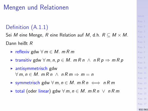
Inhalt
Kap. 1
Kap. 2
Kap. 3
Kap. 4
Kap. 5
Kap. 6
Kap. 7
Kap. 8
Kap. 9
Kap. 10
Kap. 11
Kap. 12
Kap. 13
Kap. 14
Kap. 15
Kap. 16
Kap. 17
Literatur
Anhang
A
A.1
A.2
A.3
A.4
A.5
Mengen und Relationen
Definition (A.1.1)
Sei M eine Menge, R eine Relation auf M , d.h. R ⊆ M ×M .
Dann heißt R
I reflexiv gdw ∀m ∈ M . m R m
I transitiv gdw ∀m, n, p ∈ M . m R n ∧ n R p ⇒ m R p
I antisymmetrisch gdw∀m, n ∈ M . m R n ∧ n R m ⇒ m = n
I symmetrisch gdw ∀m, n ∈ M . m R n ⇐⇒ n R m
I total (oder linear) gdw ∀m, n ∈ M . m R n ∨ n R m
832/863
Inhalt
Kap. 1
Kap. 2
Kap. 3
Kap. 4
Kap. 5
Kap. 6
Kap. 7
Kap. 8
Kap. 9
Kap. 10
Kap. 11
Kap. 12
Kap. 13
Kap. 14
Kap. 15
Kap. 16
Kap. 17
Literatur
Anhang
A
A.1
A.2
A.3
A.4
A.5
A.2
Ordnungen
833/863
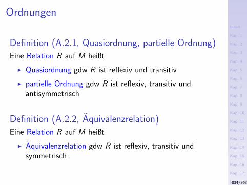
Inhalt
Kap. 1
Kap. 2
Kap. 3
Kap. 4
Kap. 5
Kap. 6
Kap. 7
Kap. 8
Kap. 9
Kap. 10
Kap. 11
Kap. 12
Kap. 13
Kap. 14
Kap. 15
Kap. 16
Kap. 17
Literatur
Anhang
A
A.1
A.2
A.3
A.4
A.5
Ordnungen
Definition (A.2.1, Quasiordnung, partielle Ordnung)
Eine Relation R auf M heißt
I Quasiordnung gdw R ist reflexiv und transitiv
I partielle Ordnung gdw R ist reflexiv, transitiv undantisymmetrisch
Definition (A.2.2, Aquivalenzrelation)
Eine Relation R auf M heißt
I Aquivalenzrelation gdw R ist reflexiv, transitiv undsymmetrisch
834/863
Inhalt
Kap. 1
Kap. 2
Kap. 3
Kap. 4
Kap. 5
Kap. 6
Kap. 7
Kap. 8
Kap. 9
Kap. 10
Kap. 11
Kap. 12
Kap. 13
Kap. 14
Kap. 15
Kap. 16
Kap. 17
Literatur
Anhang
A
A.1
A.2
A.3
A.4
A.5
Beachte
...eine partielle Ordnung ist also eine antisymmetrische Quasi-ordnung, eine Aquivalenzrelation eine symmetrische Quasiord-nung.
835/863
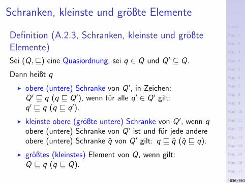
Inhalt
Kap. 1
Kap. 2
Kap. 3
Kap. 4
Kap. 5
Kap. 6
Kap. 7
Kap. 8
Kap. 9
Kap. 10
Kap. 11
Kap. 12
Kap. 13
Kap. 14
Kap. 15
Kap. 16
Kap. 17
Literatur
Anhang
A
A.1
A.2
A.3
A.4
A.5
Schranken, kleinste und großte Elemente
Definition (A.2.3, Schranken, kleinste und großteElemente)
Sei (Q,v) eine Quasiordnung, sei q ∈ Q und Q ′ ⊆ Q.
Dann heißt q
I obere (untere) Schranke von Q ′, in Zeichen:Q ′ v q (q v Q ′), wenn fur alle q′ ∈ Q ′ gilt:q′ v q (q v q′).
I kleinste obere (großte untere) Schranke von Q ′, wenn qobere (untere) Schranke von Q ′ ist und fur jede andereobere (untere) Schranke q von Q ′ gilt: q v q (q v q).
I großtes (kleinstes) Element von Q, wenn gilt:Q v q (q v Q).
836/863
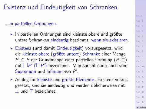
Inhalt
Kap. 1
Kap. 2
Kap. 3
Kap. 4
Kap. 5
Kap. 6
Kap. 7
Kap. 8
Kap. 9
Kap. 10
Kap. 11
Kap. 12
Kap. 13
Kap. 14
Kap. 15
Kap. 16
Kap. 17
Literatur
Anhang
A
A.1
A.2
A.3
A.4
A.5
Existenz und Eindeutigkeit von Schranken
...in partiellen Ordnungen.
I In partiellen Ordnungen sind kleinste obere und großteuntere Schranken eindeutig bestimmt, wenn sie existieren.
I Existenz (und damit Eindeutigkeit) vorausgesetzt, wirddie kleinste obere (großte untere) Schranke einer MengeP ′ ⊆ P der Grundmenge einer partiellen Ordnung (P ,v)mit tP ′ (uP ′) bezeichnet. Man spricht dann auch vomSupremum und Infimum von P ′.
I Analog fur kleinste und großte Elemente. Existenz voraus-gesetzt, sind sie eindeutig und werden ublicherweise mit⊥ und > bezeichnet.
837/863

Inhalt
Kap. 1
Kap. 2
Kap. 3
Kap. 4
Kap. 5
Kap. 6
Kap. 7
Kap. 8
Kap. 9
Kap. 10
Kap. 11
Kap. 12
Kap. 13
Kap. 14
Kap. 15
Kap. 16
Kap. 17
Literatur
Anhang
A
A.1
A.2
A.3
A.4
A.5
A.3
Verbande
838/863
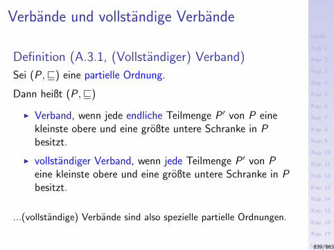
Inhalt
Kap. 1
Kap. 2
Kap. 3
Kap. 4
Kap. 5
Kap. 6
Kap. 7
Kap. 8
Kap. 9
Kap. 10
Kap. 11
Kap. 12
Kap. 13
Kap. 14
Kap. 15
Kap. 16
Kap. 17
Literatur
Anhang
A
A.1
A.2
A.3
A.4
A.5
Verbande und vollstandige Verbande
Definition (A.3.1, (Vollstandiger) Verband)
Sei (P ,v) eine partielle Ordnung.
Dann heißt (P ,v)
I Verband, wenn jede endliche Teilmenge P ′ von P einekleinste obere und eine großte untere Schranke in Pbesitzt.
I vollstandiger Verband, wenn jede Teilmenge P ′ von Peine kleinste obere und eine großte untere Schranke in Pbesitzt.
...(vollstandige) Verbande sind also spezielle partielle Ordnungen.
839/863
Inhalt
Kap. 1
Kap. 2
Kap. 3
Kap. 4
Kap. 5
Kap. 6
Kap. 7
Kap. 8
Kap. 9
Kap. 10
Kap. 11
Kap. 12
Kap. 13
Kap. 14
Kap. 15
Kap. 16
Kap. 17
Literatur
Anhang
A
A.1
A.2
A.3
A.4
A.5
A.4
Vollstandige partielle Ordnungen
840/863
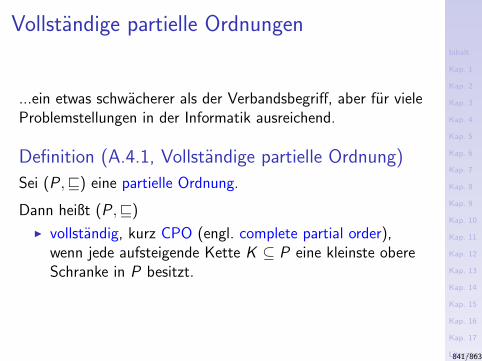
Inhalt
Kap. 1
Kap. 2
Kap. 3
Kap. 4
Kap. 5
Kap. 6
Kap. 7
Kap. 8
Kap. 9
Kap. 10
Kap. 11
Kap. 12
Kap. 13
Kap. 14
Kap. 15
Kap. 16
Kap. 17
Literatur
Anhang
A
A.1
A.2
A.3
A.4
A.5
Vollstandige partielle Ordnungen
...ein etwas schwacherer als der Verbandsbegriff, aber fur vieleProblemstellungen in der Informatik ausreichend.
Definition (A.4.1, Vollstandige partielle Ordnung)
Sei (P ,v) eine partielle Ordnung.
Dann heißt (P ,v)
I vollstandig, kurz CPO (engl. complete partial order),wenn jede aufsteigende Kette K ⊆ P eine kleinste obereSchranke in P besitzt.
841/863
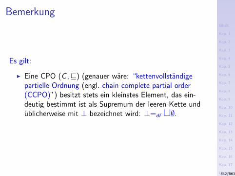
Inhalt
Kap. 1
Kap. 2
Kap. 3
Kap. 4
Kap. 5
Kap. 6
Kap. 7
Kap. 8
Kap. 9
Kap. 10
Kap. 11
Kap. 12
Kap. 13
Kap. 14
Kap. 15
Kap. 16
Kap. 17
Literatur
Anhang
A
A.1
A.2
A.3
A.4
A.5
Bemerkung
Es gilt:
I Eine CPO (C ,v) (genauer ware: “kettenvollstandigepartielle Ordnung (engl. chain complete partial order(CCPO)”) besitzt stets ein kleinstes Element, das ein-deutig bestimmt ist als Supremum der leeren Kette undublicherweise mit ⊥ bezeichnet wird: ⊥=df t∅.
842/863
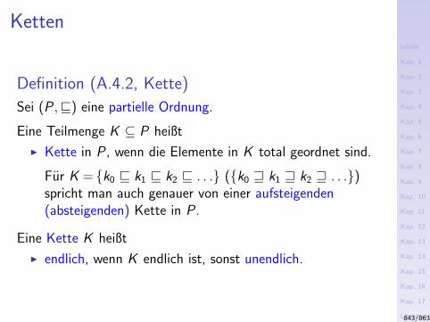
Inhalt
Kap. 1
Kap. 2
Kap. 3
Kap. 4
Kap. 5
Kap. 6
Kap. 7
Kap. 8
Kap. 9
Kap. 10
Kap. 11
Kap. 12
Kap. 13
Kap. 14
Kap. 15
Kap. 16
Kap. 17
Literatur
Anhang
A
A.1
A.2
A.3
A.4
A.5
Ketten
Definition (A.4.2, Kette)
Sei (P ,v) eine partielle Ordnung.
Eine Teilmenge K ⊆ P heißt
I Kette in P , wenn die Elemente in K total geordnet sind.
Fur K = k0 v k1 v k2 v . . . (k0 w k1 w k2 w . . .)spricht man auch genauer von einer aufsteigenden(absteigenden) Kette in P .
Eine Kette K heißt
I endlich, wenn K endlich ist, sonst unendlich.
843/863
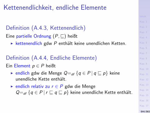
Inhalt
Kap. 1
Kap. 2
Kap. 3
Kap. 4
Kap. 5
Kap. 6
Kap. 7
Kap. 8
Kap. 9
Kap. 10
Kap. 11
Kap. 12
Kap. 13
Kap. 14
Kap. 15
Kap. 16
Kap. 17
Literatur
Anhang
A
A.1
A.2
A.3
A.4
A.5
Kettenendlichkeit, endliche Elemente
Definition (A.4.3, Kettenendlich)
Eine partielle Ordnung (P ,v) heißt
I kettenendlich gdw P enthalt keine unendlichen Ketten.
Definition (A.4.4, Endliche Elemente)
Ein Element p ∈ P heißt
I endlich gdw die Menge Q=df q ∈ P | q v p keineunendliche Kette enthalt.
I endlich relativ zu r ∈ P gdw die MengeQ=df q ∈ P | r v q v p keine unendliche Kette enthalt.
844/863
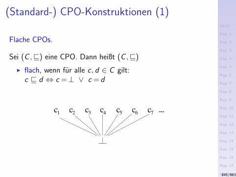
Inhalt
Kap. 1
Kap. 2
Kap. 3
Kap. 4
Kap. 5
Kap. 6
Kap. 7
Kap. 8
Kap. 9
Kap. 10
Kap. 11
Kap. 12
Kap. 13
Kap. 14
Kap. 15
Kap. 16
Kap. 17
Literatur
Anhang
A
A.1
A.2
A.3
A.4
A.5
(Standard-) CPO-Konstruktionen (1)
Flache CPOs.
Sei (C ,v) eine CPO. Dann heißt (C ,v)
I flach, wenn fur alle c , d ∈ C gilt:c v d ⇔ c =⊥ ∨ c = d
c1
c2
c3
c5
c7
c6
c4
845/863
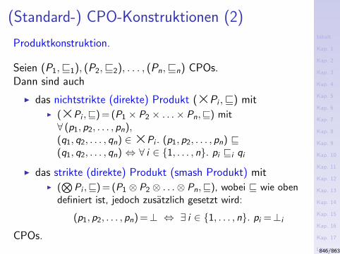
Inhalt
Kap. 1
Kap. 2
Kap. 3
Kap. 4
Kap. 5
Kap. 6
Kap. 7
Kap. 8
Kap. 9
Kap. 10
Kap. 11
Kap. 12
Kap. 13
Kap. 14
Kap. 15
Kap. 16
Kap. 17
Literatur
Anhang
A
A.1
A.2
A.3
A.4
A.5
(Standard-) CPO-Konstruktionen (2)
Produktkonstruktion.
Seien (P1,v1), (P2,v2), . . . , (Pn,vn) CPOs.Dann sind auch
I das nichtstrikte (direkte) Produkt (×Pi ,v) mitI (×Pi ,v) = (P1 × P2 × . . .× Pn,v) mit∀ (p1, p2, . . . , pn),(q1, q2, . . . , qn) ∈×Pi . (p1, p2, . . . , pn) v(q1, q2, . . . , qn) ⇔ ∀ i ∈ 1, . . . , n. pi vi qi
I das strikte (direkte) Produkt (smash Produkt) mitI (⊗
Pi ,v) = (P1 ⊗ P2 ⊗ . . .⊗ Pn,v), wobei v wie obendefiniert ist, jedoch zusatzlich gesetzt wird:
(p1, p2, . . . , pn) =⊥ ⇔ ∃ i ∈ 1, . . . , n. pi =⊥i
CPOs.846/863
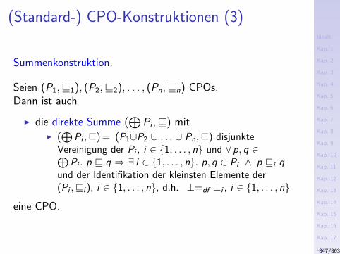
Inhalt
Kap. 1
Kap. 2
Kap. 3
Kap. 4
Kap. 5
Kap. 6
Kap. 7
Kap. 8
Kap. 9
Kap. 10
Kap. 11
Kap. 12
Kap. 13
Kap. 14
Kap. 15
Kap. 16
Kap. 17
Literatur
Anhang
A
A.1
A.2
A.3
A.4
A.5
(Standard-) CPO-Konstruktionen (3)
Summenkonstruktion.
Seien (P1,v1), (P2,v2), . . . , (Pn,vn) CPOs.Dann ist auch
I die direkte Summe (⊕
Pi ,v) mitI (⊕
Pi ,v) = (P1.∪P2
.∪ . . .
.∪ Pn,v) disjunkte
Vereinigung der Pi , i ∈ 1, . . . , n und ∀ p, q ∈⊕Pi . p v q ⇒ ∃ i ∈ 1, . . . , n. p, q ∈ Pi ∧ p vi q
und der Identifikation der kleinsten Elemente der(Pi ,vi ), i ∈ 1, . . . , n, d.h. ⊥=df ⊥i , i ∈ 1, . . . , n
eine CPO.
847/863
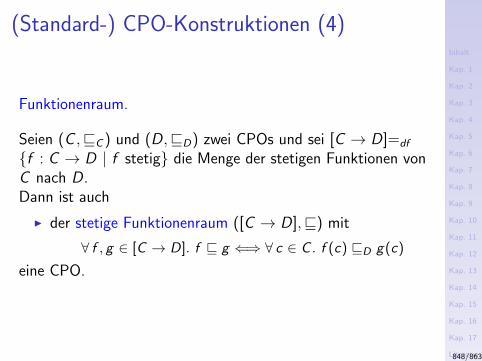
Inhalt
Kap. 1
Kap. 2
Kap. 3
Kap. 4
Kap. 5
Kap. 6
Kap. 7
Kap. 8
Kap. 9
Kap. 10
Kap. 11
Kap. 12
Kap. 13
Kap. 14
Kap. 15
Kap. 16
Kap. 17
Literatur
Anhang
A
A.1
A.2
A.3
A.4
A.5
(Standard-) CPO-Konstruktionen (4)
Funktionenraum.
Seien (C ,vC ) und (D,vD) zwei CPOs und sei [C → D]=df
f : C → D | f stetig die Menge der stetigen Funktionen vonC nach D.Dann ist auch
I der stetige Funktionenraum ([C → D],v) mit
∀ f , g ∈ [C → D]. f v g ⇐⇒ ∀ c ∈ C . f (c) vD g(c)
eine CPO.
848/863
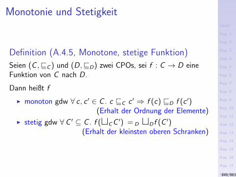
Inhalt
Kap. 1
Kap. 2
Kap. 3
Kap. 4
Kap. 5
Kap. 6
Kap. 7
Kap. 8
Kap. 9
Kap. 10
Kap. 11
Kap. 12
Kap. 13
Kap. 14
Kap. 15
Kap. 16
Kap. 17
Literatur
Anhang
A
A.1
A.2
A.3
A.4
A.5
Monotonie und Stetigkeit
Definition (A.4.5, Monotone, stetige Funktion)
Seien (C ,vC ) und (D,vD) zwei CPOs, sei f : C → D eineFunktion von C nach D.
Dann heißt f
I monoton gdw ∀ c , c ′ ∈ C . c vC c ′ ⇒ f (c) vD f (c ′)(Erhalt der Ordnung der Elemente)
I stetig gdw ∀C ′ ⊆ C . f (tCC ′) = D tD f (C ′)(Erhalt der kleinsten oberen Schranken)
849/863
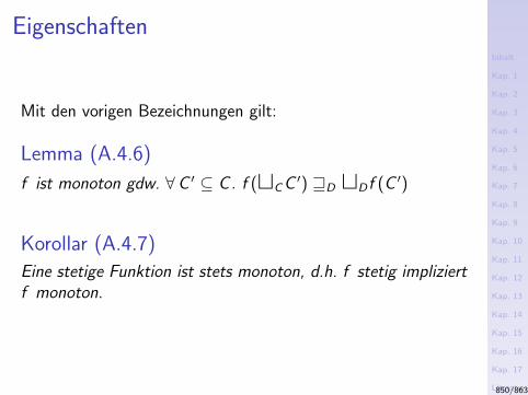
Inhalt
Kap. 1
Kap. 2
Kap. 3
Kap. 4
Kap. 5
Kap. 6
Kap. 7
Kap. 8
Kap. 9
Kap. 10
Kap. 11
Kap. 12
Kap. 13
Kap. 14
Kap. 15
Kap. 16
Kap. 17
Literatur
Anhang
A
A.1
A.2
A.3
A.4
A.5
Eigenschaften
Mit den vorigen Bezeichnungen gilt:
Lemma (A.4.6)
f ist monoton gdw. ∀C ′ ⊆ C . f (tCC ′) wD tD f (C ′)
Korollar (A.4.7)
Eine stetige Funktion ist stets monoton, d.h. f stetig impliziertf monoton.
850/863
Inhalt
Kap. 1
Kap. 2
Kap. 3
Kap. 4
Kap. 5
Kap. 6
Kap. 7
Kap. 8
Kap. 9
Kap. 10
Kap. 11
Kap. 12
Kap. 13
Kap. 14
Kap. 15
Kap. 16
Kap. 17
Literatur
Anhang
A
A.1
A.2
A.3
A.4
A.5
Inflationaritat
Definition (A.4.8, Inflationare Funktion)
Sei (C ,v) eine CPO, sei f : C → C eine Funktion auf C .
Dann heißt f
I inflationar (vergroßernd) gdw ∀ c ∈ C . c v f (c)
851/863
Inhalt
Kap. 1
Kap. 2
Kap. 3
Kap. 4
Kap. 5
Kap. 6
Kap. 7
Kap. 8
Kap. 9
Kap. 10
Kap. 11
Kap. 12
Kap. 13
Kap. 14
Kap. 15
Kap. 16
Kap. 17
Literatur
Anhang
A
A.1
A.2
A.3
A.4
A.5
A.5
Fixpunkte und Fixpunkttheoreme
852/863
Inhalt
Kap. 1
Kap. 2
Kap. 3
Kap. 4
Kap. 5
Kap. 6
Kap. 7
Kap. 8
Kap. 9
Kap. 10
Kap. 11
Kap. 12
Kap. 13
Kap. 14
Kap. 15
Kap. 16
Kap. 17
Literatur
Anhang
A
A.1
A.2
A.3
A.4
A.5
Fixpunkte
Definition (A.5.1, (Kleinster/großter) Fixpunkt)
Sei (C ,v) eine CPO, f : C → C eine Funktion auf C und seic ein Element von C , d.h. c ∈ C .
Dann heißt c
I Fixpunkt von f gdw f (c) = c
Ein Fixpunkt c von f heißt
I kleinster Fixpunkt von f gdw ∀ d ∈ C . f (d) = d ⇒ c v d
I großter Fixpunkt von f gdw ∀ d ∈ C . f (d) = d ⇒ d v c
Bezeichnungen:
I Der kleinste bzw. großte Fixpunkt einer Funktion f wirdmeist mit µf bzw. νf bezeichnet.
853/863
Inhalt
Kap. 1
Kap. 2
Kap. 3
Kap. 4
Kap. 5
Kap. 6
Kap. 7
Kap. 8
Kap. 9
Kap. 10
Kap. 11
Kap. 12
Kap. 13
Kap. 14
Kap. 15
Kap. 16
Kap. 17
Literatur
Anhang
A
A.1
A.2
A.3
A.4
A.5
Bedingte Fixpunkte
Definition (A.5.2, Bedingter Fixpunkt)
Sei (C ,v) eine CPO, f : C → C eine Funktion auf C undseien d , cd ∈ C .
Dann heißt cd
I bedingter kleinster Fixpunkt von f bezuglich d gdw cd istder kleinste Fixpunkt von C mit d v cd , d.h. fur alleanderen Fixpunkte x von f mit d v x gilt: cd v x .
854/863
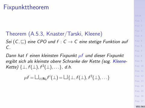
Inhalt
Kap. 1
Kap. 2
Kap. 3
Kap. 4
Kap. 5
Kap. 6
Kap. 7
Kap. 8
Kap. 9
Kap. 10
Kap. 11
Kap. 12
Kap. 13
Kap. 14
Kap. 15
Kap. 16
Kap. 17
Literatur
Anhang
A
A.1
A.2
A.3
A.4
A.5
Fixpunkttheorem
Theorem (A.5.3, Knaster/Tarski, Kleene)
Sei (C ,v) eine CPO und f : C → C eine stetige Funktion aufC .
Dann hat f einen kleinsten Fixpunkt µf und dieser Fixpunktergibt sich als kleinste obere Schranke der Kette (sog. Kleene-Kette) ⊥, f (⊥), f 2(⊥), . . ., d.h.
µf =ti∈IN0f i(⊥) =t⊥, f (⊥), f 2(⊥), . . .
855/863
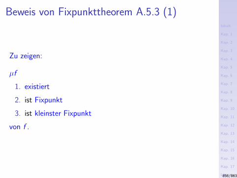
Inhalt
Kap. 1
Kap. 2
Kap. 3
Kap. 4
Kap. 5
Kap. 6
Kap. 7
Kap. 8
Kap. 9
Kap. 10
Kap. 11
Kap. 12
Kap. 13
Kap. 14
Kap. 15
Kap. 16
Kap. 17
Literatur
Anhang
A
A.1
A.2
A.3
A.4
A.5
Beweis von Fixpunkttheorem A.5.3 (1)
Zu zeigen:
µf
1. existiert
2. ist Fixpunkt
3. ist kleinster Fixpunkt
von f .
856/863
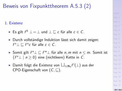
Inhalt
Kap. 1
Kap. 2
Kap. 3
Kap. 4
Kap. 5
Kap. 6
Kap. 7
Kap. 8
Kap. 9
Kap. 10
Kap. 11
Kap. 12
Kap. 13
Kap. 14
Kap. 15
Kap. 16
Kap. 17
Literatur
Anhang
A
A.1
A.2
A.3
A.4
A.5
Beweis von Fixpunkttheorem A.5.3 (2)
1. Existenz
I Es gilt f 0 ⊥=⊥ und ⊥ v c fur alle c ∈ C .
I Durch vollstandige Induktion lasst sich damit zeigen:f n⊥ v f nc fur alle c ∈ C .
I Somit gilt f n⊥ v f m⊥ fur alle n,m mit n ≤ m. Somit istf n⊥ | n ≥ 0 eine (nichtleere) Kette in C .
I Damit folgt die Existenz von ti∈IN0f i(⊥) aus derCPO-Eigenschaft von (C ,v).
857/863
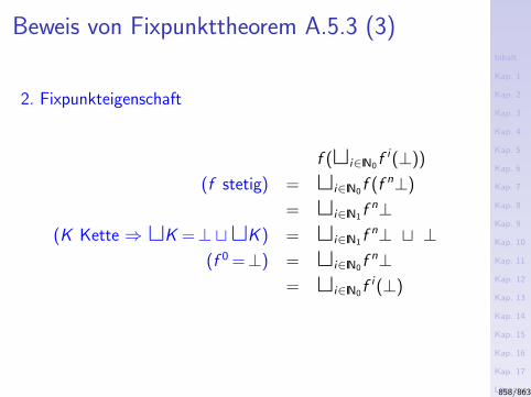
Inhalt
Kap. 1
Kap. 2
Kap. 3
Kap. 4
Kap. 5
Kap. 6
Kap. 7
Kap. 8
Kap. 9
Kap. 10
Kap. 11
Kap. 12
Kap. 13
Kap. 14
Kap. 15
Kap. 16
Kap. 17
Literatur
Anhang
A
A.1
A.2
A.3
A.4
A.5
Beweis von Fixpunkttheorem A.5.3 (3)
2. Fixpunkteigenschaft
f (ti∈IN0f i(⊥))
(f stetig) = ti∈IN0f (f n⊥)
= ti∈IN1f n⊥(K Kette ⇒ tK =⊥ ttK ) = ti∈IN1f n⊥ t ⊥
(f 0 =⊥) = ti∈IN0f n⊥= ti∈IN0f i(⊥)
858/863
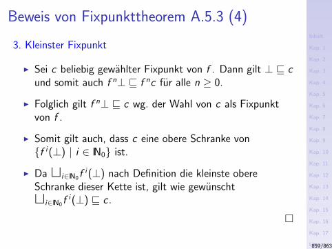
Inhalt
Kap. 1
Kap. 2
Kap. 3
Kap. 4
Kap. 5
Kap. 6
Kap. 7
Kap. 8
Kap. 9
Kap. 10
Kap. 11
Kap. 12
Kap. 13
Kap. 14
Kap. 15
Kap. 16
Kap. 17
Literatur
Anhang
A
A.1
A.2
A.3
A.4
A.5
Beweis von Fixpunkttheorem A.5.3 (4)
3. Kleinster Fixpunkt
I Sei c beliebig gewahlter Fixpunkt von f . Dann gilt ⊥ v cund somit auch f n⊥ v f nc fur alle n ≥ 0.
I Folglich gilt f n⊥ v c wg. der Wahl von c als Fixpunktvon f .
I Somit gilt auch, dass c eine obere Schranke vonf i(⊥) | i ∈ IN0 ist.
I Da ti∈IN0f i(⊥) nach Definition die kleinste obereSchranke dieser Kette ist, gilt wie gewunschtti∈IN0f i(⊥) v c .
859/863

Inhalt
Kap. 1
Kap. 2
Kap. 3
Kap. 4
Kap. 5
Kap. 6
Kap. 7
Kap. 8
Kap. 9
Kap. 10
Kap. 11
Kap. 12
Kap. 13
Kap. 14
Kap. 15
Kap. 16
Kap. 17
Literatur
Anhang
A
A.1
A.2
A.3
A.4
A.5
Bedingte Fixpunkte
Theorem (A.5.4, Bedingte Fixpunkte)
Sei (C ,v) eine CPO und f : C → C eine stetige, inflationareFunktion auf C und sei d ∈ C .
Dann hat f einen kleinsten bedingten Fixpunkt µfd bezuglichd und dieser Fixpunkt ergibt sich als kleinste obere Schrankeder Kette d , f (d), f 2(d), . . ., d.h.
µfd =ti∈IN0f i(d) =td , f (d), f 2(d), . . .
860/863
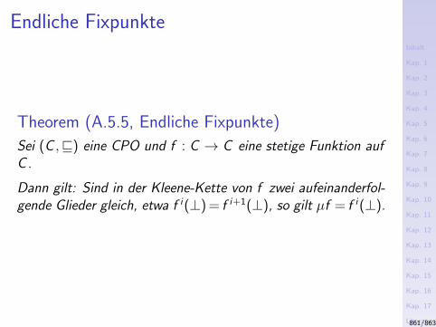
Inhalt
Kap. 1
Kap. 2
Kap. 3
Kap. 4
Kap. 5
Kap. 6
Kap. 7
Kap. 8
Kap. 9
Kap. 10
Kap. 11
Kap. 12
Kap. 13
Kap. 14
Kap. 15
Kap. 16
Kap. 17
Literatur
Anhang
A
A.1
A.2
A.3
A.4
A.5
Endliche Fixpunkte
Theorem (A.5.5, Endliche Fixpunkte)
Sei (C ,v) eine CPO und f : C → C eine stetige Funktion aufC .
Dann gilt: Sind in der Kleene-Kette von f zwei aufeinanderfol-gende Glieder gleich, etwa f i(⊥) = f i+1(⊥), so gilt µf = f i(⊥).
861/863
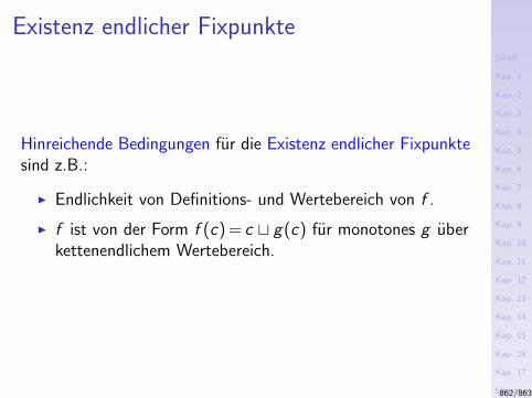
Inhalt
Kap. 1
Kap. 2
Kap. 3
Kap. 4
Kap. 5
Kap. 6
Kap. 7
Kap. 8
Kap. 9
Kap. 10
Kap. 11
Kap. 12
Kap. 13
Kap. 14
Kap. 15
Kap. 16
Kap. 17
Literatur
Anhang
A
A.1
A.2
A.3
A.4
A.5
Existenz endlicher Fixpunkte
Hinreichende Bedingungen fur die Existenz endlicher Fixpunktesind z.B.:
I Endlichkeit von Definitions- und Wertebereich von f .
I f ist von der Form f (c) = c t g(c) fur monotones g uberkettenendlichem Wertebereich.
862/863
Inhalt
Kap. 1
Kap. 2
Kap. 3
Kap. 4
Kap. 5
Kap. 6
Kap. 7
Kap. 8
Kap. 9
Kap. 10
Kap. 11
Kap. 12
Kap. 13
Kap. 14
Kap. 15
Kap. 16
Kap. 17
Literatur
Anhang
A
A.1
A.2
A.3
A.4
A.5
Leseempfehlungen fur Anhang A
Hanne Riis Nielson, Flemming Nielson. Semantics withApplications: A Formal Introduction. Wiley, 1992.(Chapter 4, Denotational Semantics)
Hanne Riis Nielson, Flemming Nielson. Semantics withApplications: An Appetizer. Springer-V., 2007. (Chapter5, Denotational Semantics)
863/863


![Veri erCloud: Implementierung eines Web-Service zur Software … · 2017-03-06 · 2.3 JAX-RS API Java API for RESTful Web Services 4 ist die Spezi kation [6] ... JSR 339 auf ersionV](https://img.pdfslide.org/doc/110x75/5be43de709d3f26f228c73d1/veri-ercloud-implementierung-eines-web-service-zur-software-2017-03-06.jpg)