Embed Size (px)
Citation preview
Bootstrap mit SASBootstrapBootstrap mit SASmit SASP. E. Rudolph*, A. Tuchscherer*, B. Jäger**, M.Tuchscherer*
7. Konferenz für SAS-Anwender in Forschung und Entwicklung 20. - 21. Februar 2003, Universität Potsdam
** Institut für Biometrie und Medizinische InformatikErnst-Moritz-Arndt-Universität Greifswald
* Forschungsinstitut für die Biologie landwirtschaftlicher Nutztiere Dummerstorf
7. KSFE, Uni Potsdam:7. KSFE, Uni Potsdam: BootstrapBootstrap mit SASmit SAS 22
Bootstrap mit SASBootstrapBootstrap mit SASmit SAS
Gliederung:Gliederung:
Einleitung11
Bootstrap-Macros im SAS-Programm JACKBOOT.SAS22
Ein Bootstrap-Macro mit SAS-IML33
Literatur44
7. KSFE, Uni Potsdam:7. KSFE, Uni Potsdam: BootstrapBootstrap mit SASmit SAS 33
11
22
33
44
EinleitungEinleitungEinleitung
7. KSFE, Uni Potsdam:7. KSFE, Uni Potsdam: BootstrapBootstrap mit SASmit SAS 44
EinleitungEinleitung
11
22
33
44
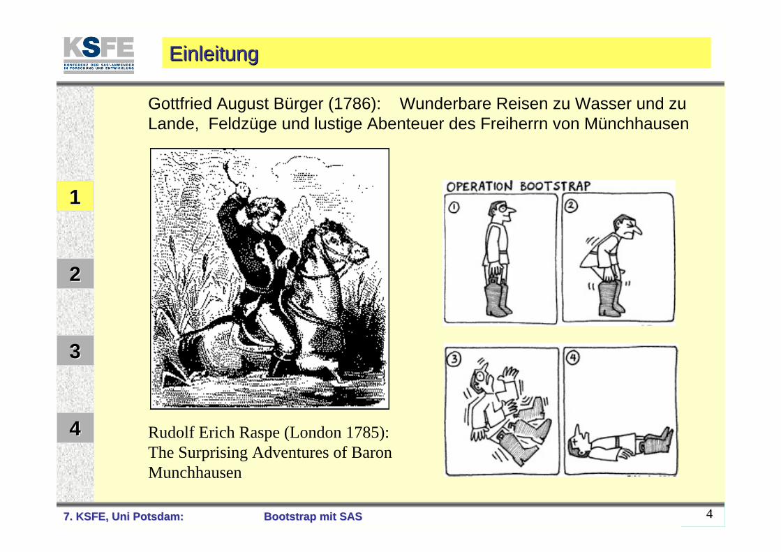
Gottfried August Bürger (1786): Wunderbare Reisen zu Wasser und zu Lande, Feldzüge und lustige Abenteuer des Freiherrn von Münchhausen
Rudolf Erich Raspe (London 1785): The Surprising Adventures of Baron Munchhausen
7. KSFE, Uni Potsdam:7. KSFE, Uni Potsdam: BootstrapBootstrap mit SASmit SAS 55
EinleitungEinleitung
11
22
33
44
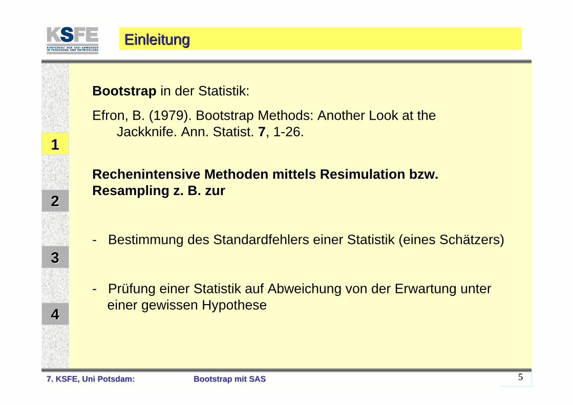
Bootstrap in der Statistik:
Efron, B. (1979). Bootstrap Methods: Another Look at the Jackknife. Ann. Statist. 7, 1-26.
Rechenintensive Methoden mittels Rechenintensive Methoden mittels ResimulationResimulation bzw. bzw. ResamplingResampling z. B. zur z. B. zur
- Bestimmung des Standardfehlers einer Statistik (eines Schätzers)
- Prüfung einer Statistik auf Abweichung von der Erwartung unter einer gewissen Hypothese
7. KSFE, Uni Potsdam:7. KSFE, Uni Potsdam: BootstrapBootstrap mit SASmit SAS 66
EinleitungEinleitung
11
22
33
44
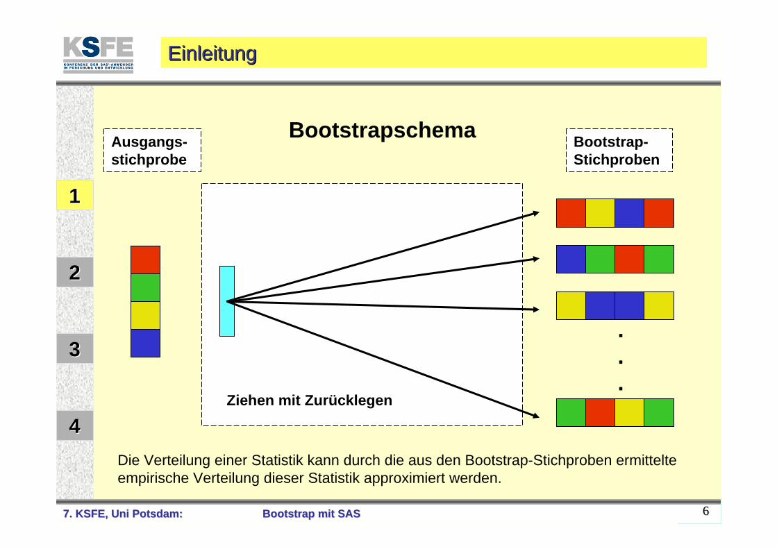
Bootstrapschema
Die Verteilung einer Statistik kann durch die aus den Bootstrap-Stichproben ermittelte empirische Verteilung dieser Statistik approximiert werden.
Bootstrap-Stichproben
Ausgangs-stichprobe
.
.
.Ziehen mit Zurücklegen
7. KSFE, Uni Potsdam:7. KSFE, Uni Potsdam: BootstrapBootstrap mit SASmit SAS 77
EinleitungEinleitung
11
22
33
44
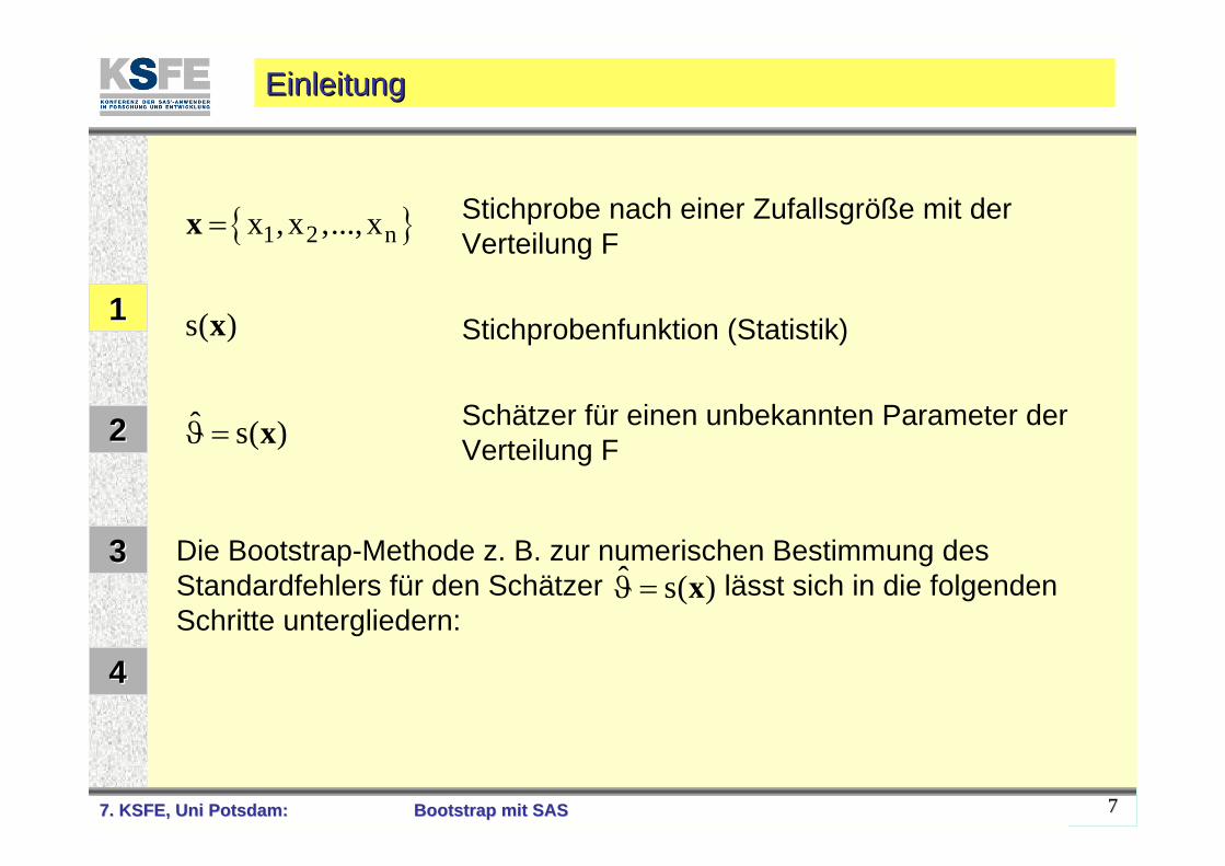
{ }1 2 nx ,x ,..., x=x Stichprobe nach einer Zufallsgröße mit der Verteilung F
s( )x Stichprobenfunktion (Statistik)
ˆ s( )ϑ = x Schätzer für einen unbekannten Parameter der Verteilung F
Die Bootstrap-Methode z. B. zur numerischen Bestimmung des Standardfehlers für den Schätzer lässt sich in die folgenden Schritte untergliedern:
ˆ s( )ϑ = x
7. KSFE, Uni Potsdam:7. KSFE, Uni Potsdam: BootstrapBootstrap mit SASmit SAS 88
EinleitungEinleitung
11
22
33
44
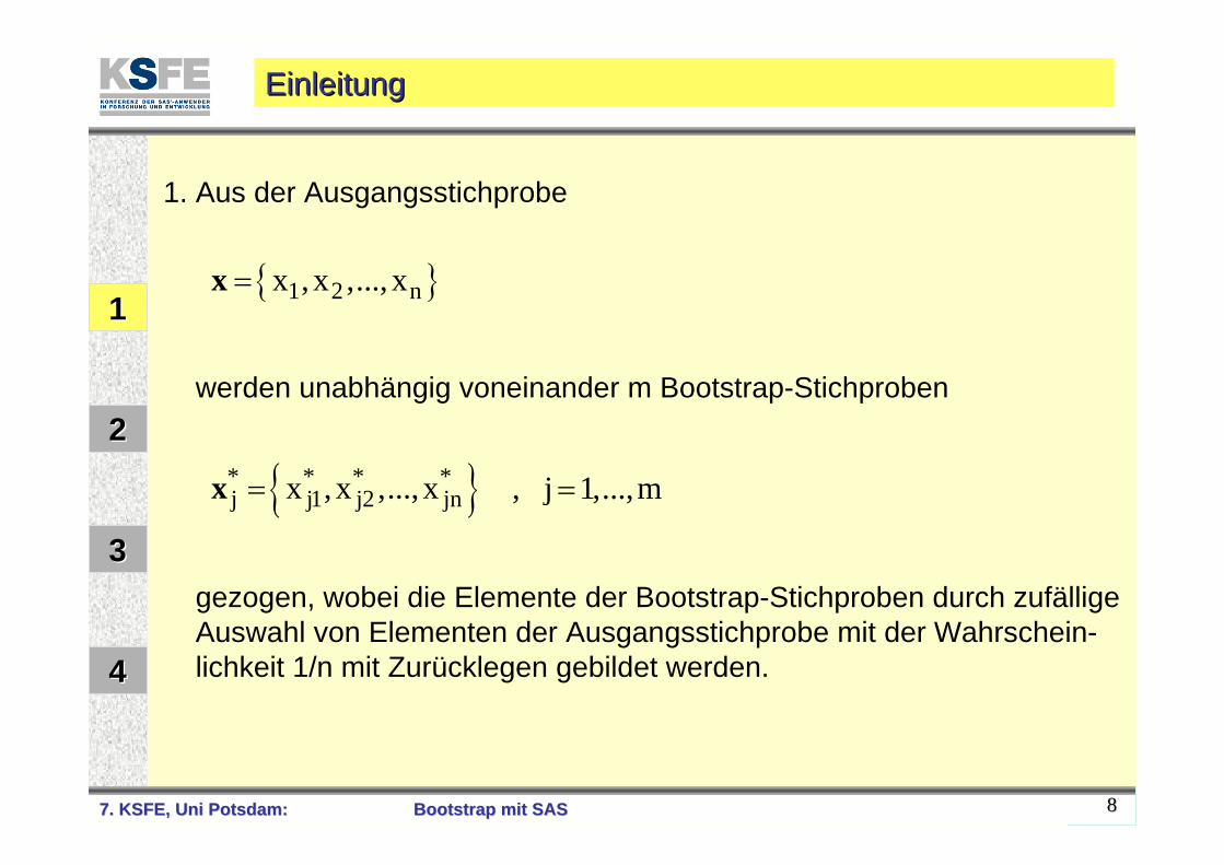
{ }1 2 nx ,x ,..., x=x
1. Aus der Ausgangsstichprobe
werden unabhängig voneinander m Bootstrap-Stichproben
{ }* * * *j j1 j2 jnx ,x ,..., x=x , j 1,...,m=
gezogen, wobei die Elemente der Bootstrap-Stichproben durch zufällige Auswahl von Elementen der Ausgangsstichprobe mit der Wahrschein-lichkeit 1/n mit Zurücklegen gebildet werden.
7. KSFE, Uni Potsdam:7. KSFE, Uni Potsdam: BootstrapBootstrap mit SASmit SAS 99
EinleitungEinleitung
11
22
33
44
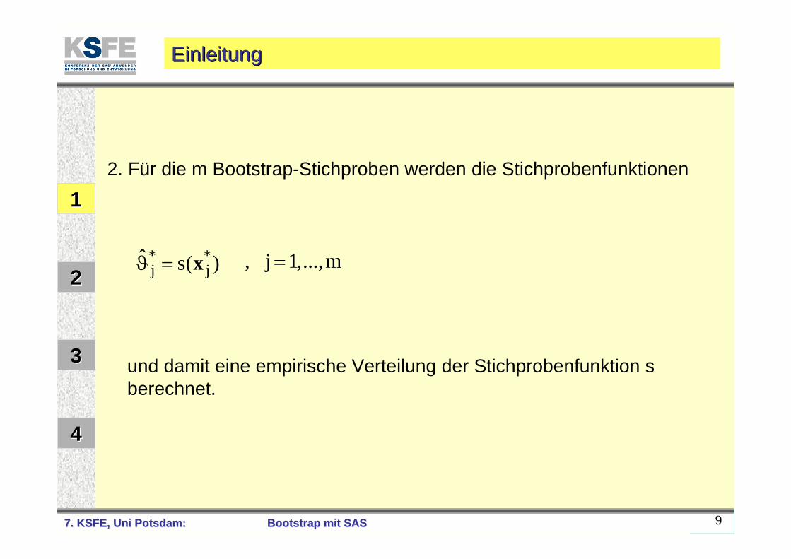
2. Für die m Bootstrap-Stichproben werden die Stichprobenfunktionen
* *j j
ˆ s( )ϑ = x , j 1,...,m=
und damit eine empirische Verteilung der Stichprobenfunktion s berechnet.
7. KSFE, Uni Potsdam:7. KSFE, Uni Potsdam: BootstrapBootstrap mit SASmit SAS 1010
EinleitungEinleitung
11
22
33
44
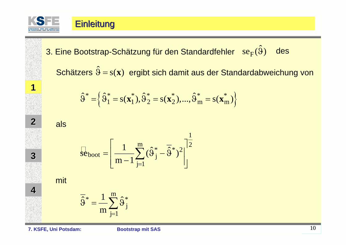
3. Eine Bootstrap-Schätzung für den Standardfehler Fˆse ( )ϑ des
Schätzers ˆ s( )ϑ = x ergibt sich damit aus der Standardabweichung von
{ }* * * * * * *1 1 2 2 m m
ˆ ˆ ˆ ˆs( ), s( ),..., s( )ϑ = ϑ = ϑ = ϑ =x x x
als
mit
1m 2
* * 2boot j
j 1
1 ˆ ˆse ( )m 1 =
⎡ ⎤= ⎢ ϑ − ϑ ⎥
−⎢ ⎥⎣ ⎦∑
m* *
jj 1
1ˆ ˆm =
ϑ = ϑ∑
7. KSFE, Uni Potsdam:7. KSFE, Uni Potsdam: BootstrapBootstrap mit SASmit SAS 1111
11
22
33
44
Bootstrap-Macros im SAS-Programm JACKBOOT.SASBootstrapBootstrap--MacrosMacros im SASim SAS--Programm JACKBOOT.SASProgramm JACKBOOT.SAS
7. KSFE, Uni Potsdam:7. KSFE, Uni Potsdam: BootstrapBootstrap mit SASmit SAS 1212
BootstrapBootstrap--MacrosMacros im SASim SAS--Programm JACKBOOT.SASProgramm JACKBOOT.SAS
11
22
33
44
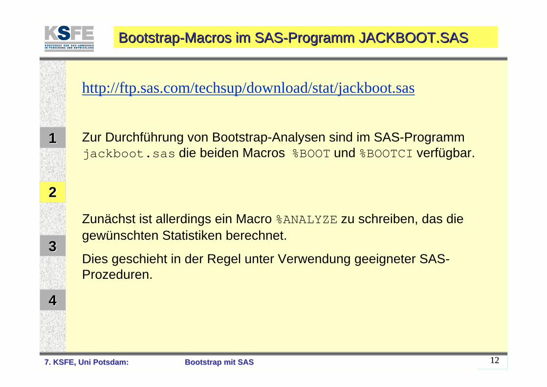
http://ftp.sas.com/techsup/download/stat/jackboot.sas
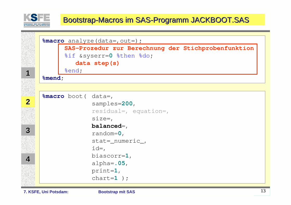
Zur Durchführung von Bootstrap-Analysen sind im SAS-Programmjackboot.sas die beiden Macros %BOOT und %BOOTCI verfügbar.
Zunächst ist allerdings ein Macro %ANALYZE zu schreiben, das die gewünschten Statistiken berechnet.
Dies geschieht in der Regel unter Verwendung geeigneter SAS-Prozeduren.
7. KSFE, Uni Potsdam:7. KSFE, Uni Potsdam: BootstrapBootstrap mit SASmit SAS 1313
BootstrapBootstrap--MacrosMacros im SASim SAS--Programm JACKBOOT.SASProgramm JACKBOOT.SAS
11
22
33
44
%macro boot( data=, samples=200, residual=, equation=,size=, balanced=, random=0, stat=_numeric_,id=, biascorr=1, alpha=.05, print=1, chart=1 );
%macro analyze(data=,out=);SAS-Prozedur zur Berechnung der Stichprobenfunktion%if &syserr=0 %then %do;
data step(s)%end;
%mend;
7. KSFE, Uni Potsdam:7. KSFE, Uni Potsdam: BootstrapBootstrap mit SASmit SAS 1414
Ein Ein BootstrapBootstrap--MacroMacro mit SASmit SAS--IMLIML
11
22
33
44
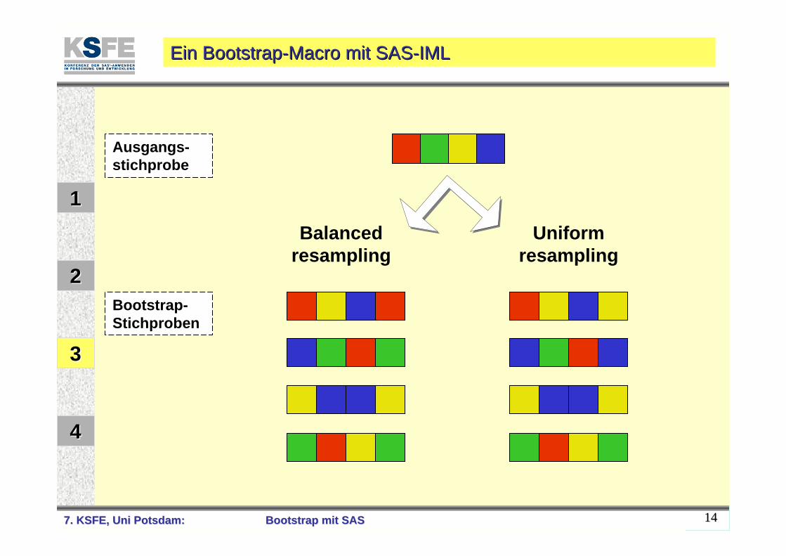
Bootstrap-Stichproben
Ausgangs-stichprobe
Balancedresampling
Uniform resampling
7. KSFE, Uni Potsdam:7. KSFE, Uni Potsdam: BootstrapBootstrap mit SASmit SAS 1515
BootstrapBootstrap--MacrosMacros im SASim SAS--Programm JACKBOOT.SASProgramm JACKBOOT.SAS
11
22
33
44
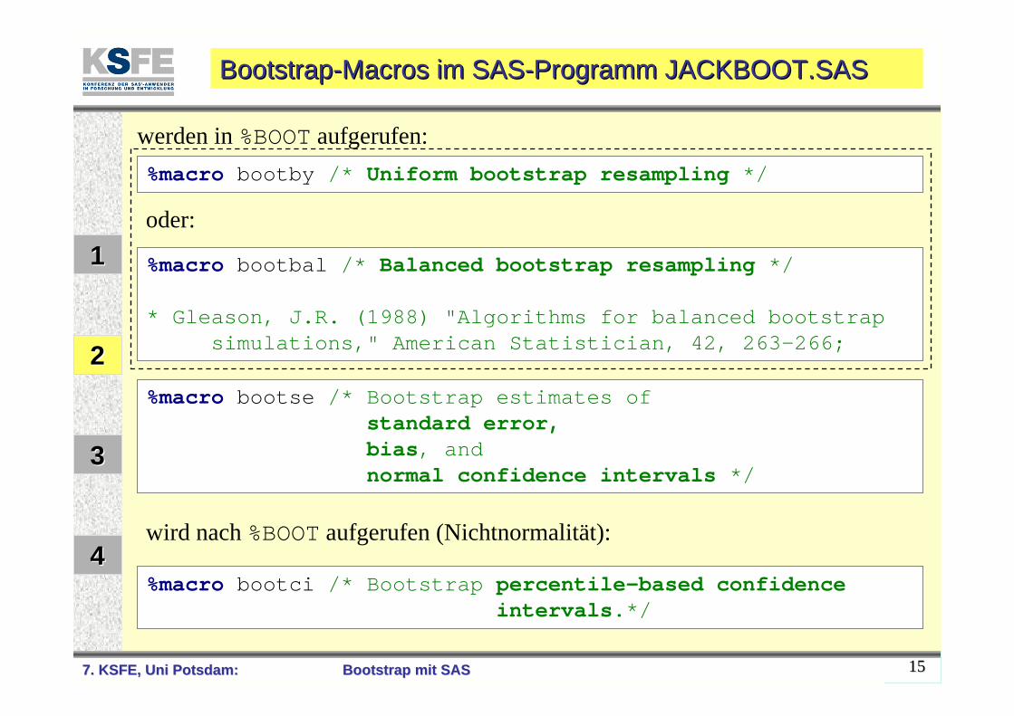
%macro bootbal /* Balanced bootstrap resampling */
* Gleason, J.R. (1988) "Algorithms for balanced bootstrapsimulations," American Statistician, 42, 263-266;
%macro bootby /* Uniform bootstrap resampling */
werden in %BOOT aufgerufen:
oder:
%macro bootse /* Bootstrap estimates of standard error, bias, andnormal confidence intervals */
%macro bootci /* Bootstrap percentile-based confidenceintervals.*/
wird nach %BOOT aufgerufen (Nichtnormalität):
7. KSFE, Uni Potsdam:7. KSFE, Uni Potsdam: BootstrapBootstrap mit SASmit SAS 1616
BootstrapBootstrap--MacrosMacros im SASim SAS--Programm JACKBOOT.SASProgramm JACKBOOT.SAS
11
22
33
44
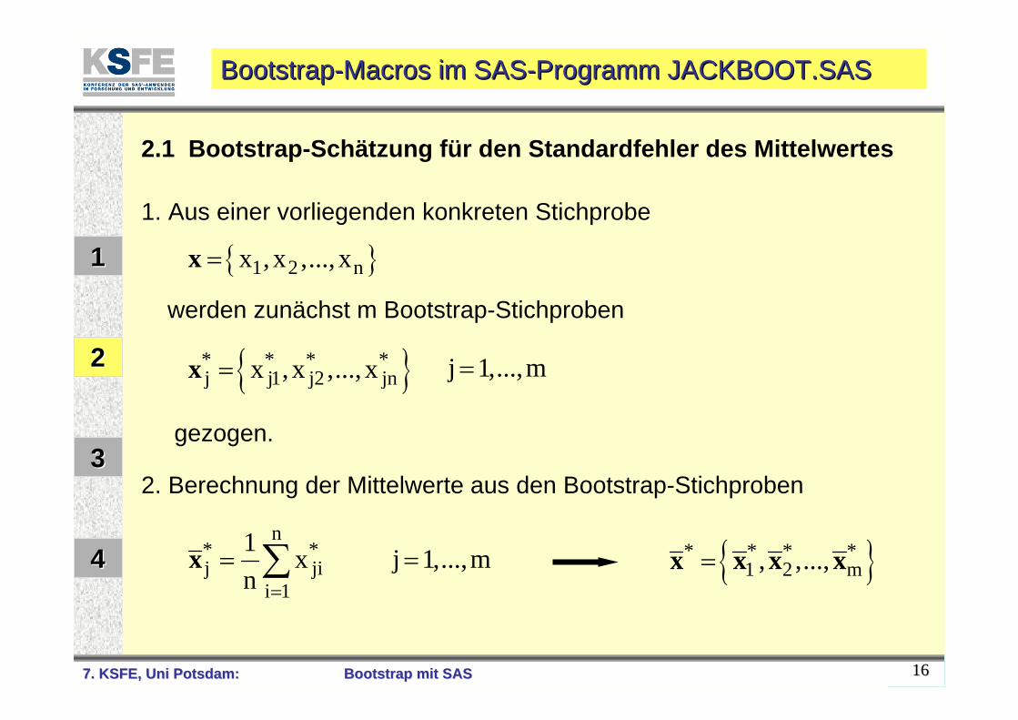
2.1 Bootstrap-Schätzung für den Standardfehler des Mittelwertes
2. Berechnung der Mittelwerte aus den Bootstrap-Stichproben
n* *j ji
i 1
1 xn =
= ∑x j 1,...,m=
{ }1 2 nx ,x ,..., x=x
{ }* * * *j j1 j2 jnx ,x ,..., x=x j 1,...,m=
1. Aus einer vorliegenden konkreten Stichprobe
werden zunächst m Bootstrap-Stichproben
gezogen.
{ }* * * *1 2 m, ,...,=x x x x
7. KSFE, Uni Potsdam:7. KSFE, Uni Potsdam: BootstrapBootstrap mit SASmit SAS 1717
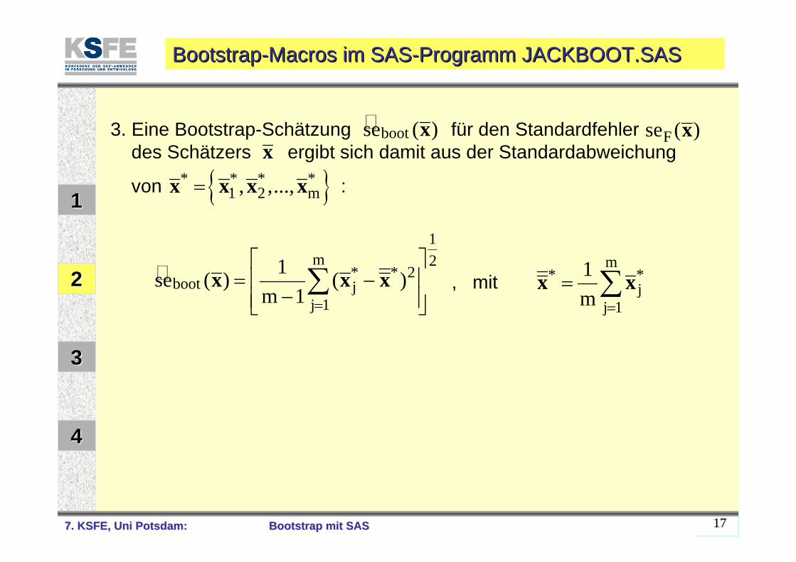
3. Eine Bootstrap-Schätzung für den Standardfehlerdes Schätzers ergibt sich damit aus der Standardabweichung
von :
BootstrapBootstrap--MacrosMacros im SASim SAS--Programm JACKBOOT.SASProgramm JACKBOOT.SAS
11
22
33
44
xbootse ( )x Fse ( )x
{ }* * * *1 2 m, ,...,=x x x x
1m 2
* * 2boot j
j 1
1se ( ) ( )m 1 =
⎡ ⎤= ⎢ − ⎥
−⎢ ⎥⎣ ⎦∑x x x
m* *
jj 1
1m =
= ∑x x, mit
7. KSFE, Uni Potsdam:7. KSFE, Uni Potsdam: BootstrapBootstrap mit SASmit SAS 1818
BootstrapBootstrap--MacrosMacros im SASim SAS--Programm JACKBOOT.SASProgramm JACKBOOT.SAS
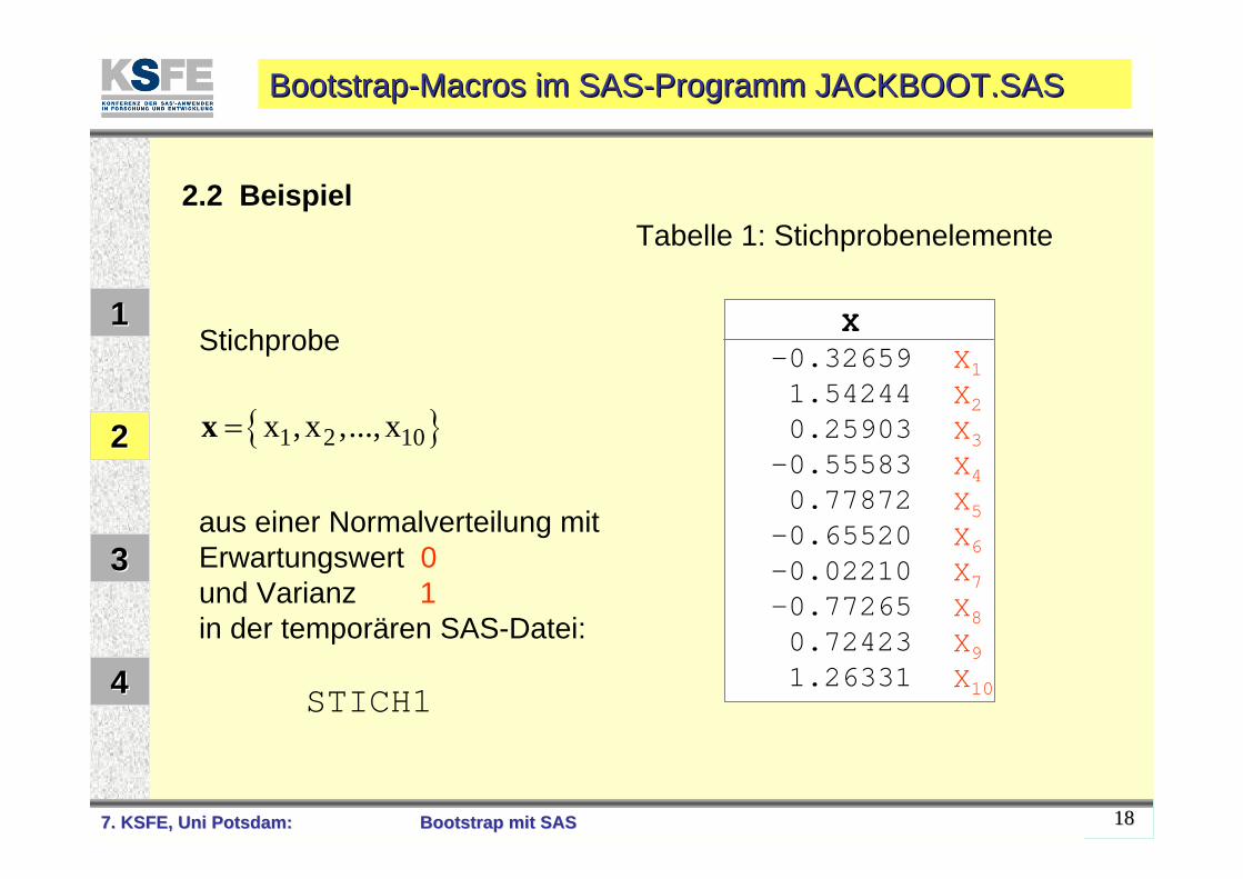
2.2 Beispiel
X-0.326591.542440.25903
-0.555830.77872
-0.65520-0.02210-0.772650.724231.26331
Tabelle 1: Stichprobenelemente
11
22
33
44
{ }1 2 10x ,x ,..., x=x
Stichprobe
aus einer Normalverteilung mitErwartungswert 0und Varianz 1in der temporären SAS-Datei:
STICH1
X1X2X3X4X5X6X7X8X9X10
7. KSFE, Uni Potsdam:7. KSFE, Uni Potsdam: BootstrapBootstrap mit SASmit SAS 1919
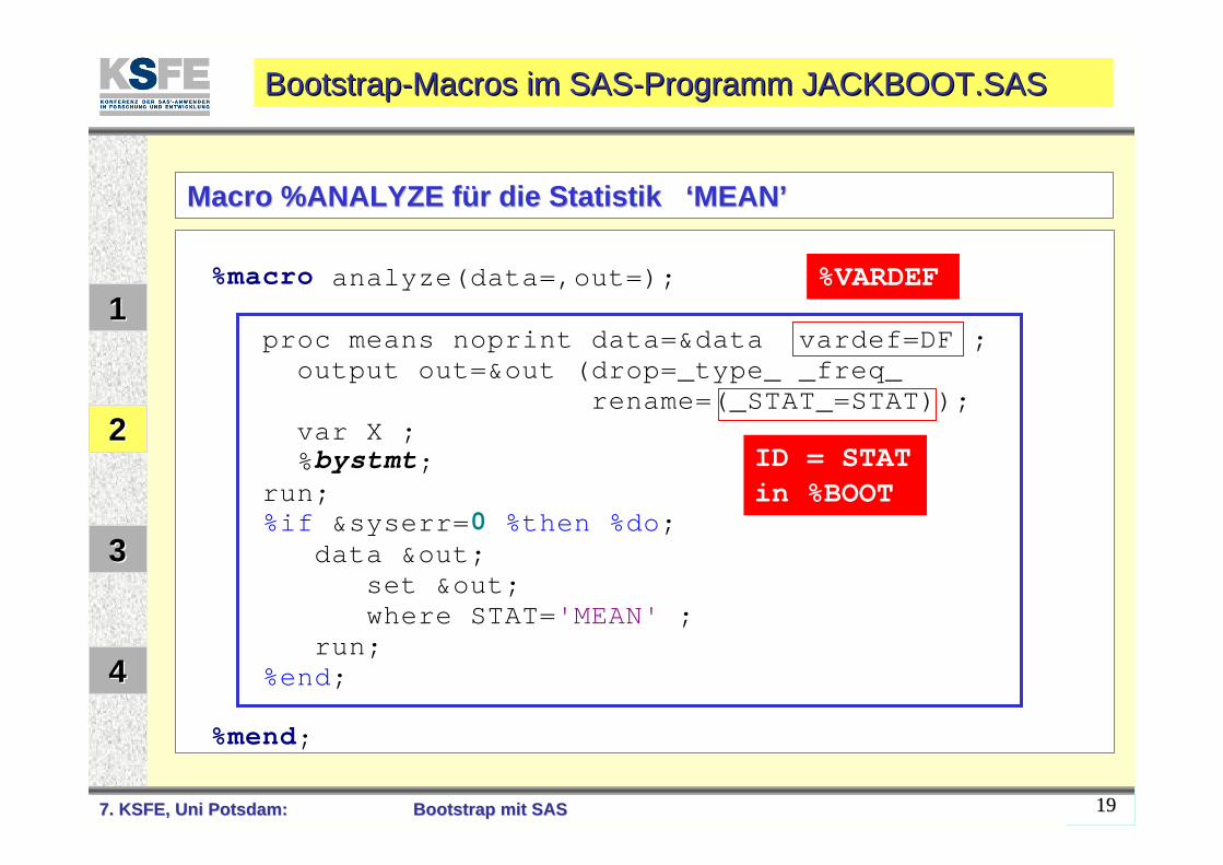
%macro analyze(data=,out=); proc means noprint data=&data vardef=DF ; output out=&out (drop=_type_ _freq_ rename=(_STAT_=STAT)); var X ; %bystmt; run; %if &syserr=0 %then %do; data &out; set &out; where STAT='MEAN' ; run; %end; %mend;
Macro %ANALYZE Macro %ANALYZE ffüürr die die StatistikStatistik ‘‘MEANMEAN’’
%VARDEF11
22
33
44
BootstrapBootstrap--MacrosMacros im SASim SAS--Programm JACKBOOT.SASProgramm JACKBOOT.SAS
ID = STAT in %BOOT
7. KSFE, Uni Potsdam:7. KSFE, Uni Potsdam: BootstrapBootstrap mit SASmit SAS 2020
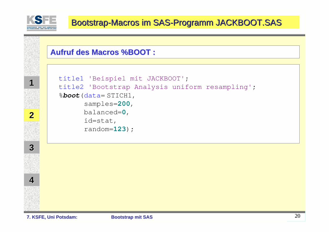
AufrufAufruf des Macros %BOOT :des Macros %BOOT :
11
22
33
44
BootstrapBootstrap--MacrosMacros im SASim SAS--Programm JACKBOOT.SASProgramm JACKBOOT.SAS
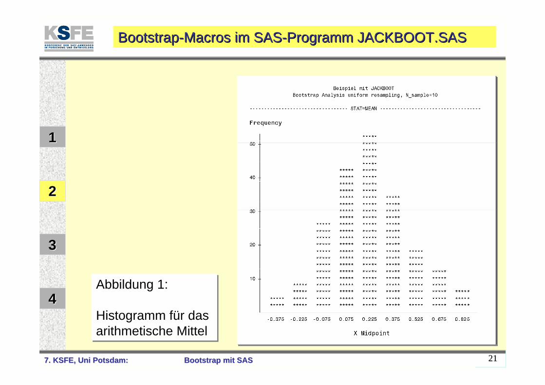
title1 'Beispiel mit JACKBOOT';title2 'Bootstrap Analysis uniform resampling';%boot(data= STICH1,
samples=200, balanced=0, id=stat, random=123);
7. KSFE, Uni Potsdam:7. KSFE, Uni Potsdam: BootstrapBootstrap mit SASmit SAS 2121
11
22
33
44
BootstrapBootstrap--MacrosMacros im SASim SAS--Programm JACKBOOT.SASProgramm JACKBOOT.SAS
Abbildung 1:
Histogramm für das arithmetische Mittel
Abbildung 1:
Histogramm für das arithmetische Mittel
7. KSFE, Uni Potsdam:7. KSFE, Uni Potsdam: BootstrapBootstrap mit SASmit SAS 2222
11
22
33
44
BootstrapBootstrap--MacrosMacros im SASim SAS--Programm JACKBOOT.SASProgramm JACKBOOT.SAS
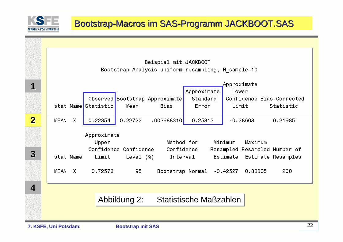
Abbildung 2: Statistische MaßzahlenAbbildung 2: Statistische Maßzahlen
7. KSFE, Uni Potsdam:7. KSFE, Uni Potsdam: BootstrapBootstrap mit SASmit SAS 2323
11
22
33
44
BootstrapBootstrap--MacrosMacros im SASim SAS--Programm JACKBOOT.SASProgramm JACKBOOT.SAS
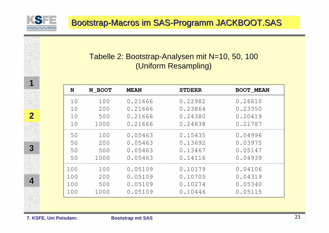
N N_BOOT MEAN STDERR BOOT_MEAN
10 100 0.21666 0.22982 0.2661010 200 0.21666 0.23864 0.2335010 500 0.21666 0.24380 0.2041910 1000 0.21666 0.24838 0.21787
50 100 0.05463 0.15435 0.0499650 200 0.05463 0.13692 0.0397550 500 0.05463 0.13467 0.0514750 1000 0.05463 0.14116 0.04939
100 100 0.05109 0.10179 0.04106100 200 0.05109 0.10705 0.04319100 500 0.05109 0.10274 0.05340100 1000 0.05109 0.10446 0.05115
Tabelle 2: Bootstrap-Analysen mit N=10, 50, 100 (Uniform Resampling)
7. KSFE, Uni Potsdam:7. KSFE, Uni Potsdam: BootstrapBootstrap mit SASmit SAS 2424
BootstrapBootstrap--MacrosMacros im SASim SAS--Programm JACKBOOT.SASProgramm JACKBOOT.SAS
11
22
33
44
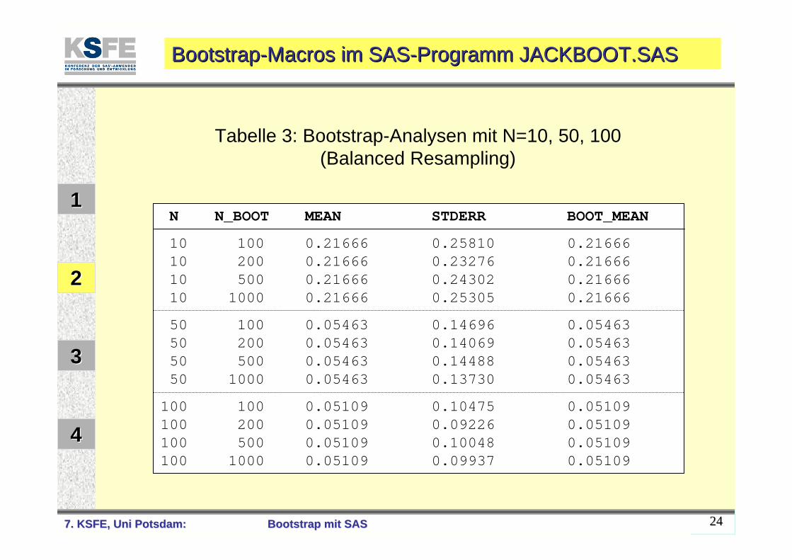
N N_BOOT MEAN STDERR BOOT_MEAN
10 100 0.21666 0.25810 0.2166610 200 0.21666 0.23276 0.2166610 500 0.21666 0.24302 0.2166610 1000 0.21666 0.25305 0.21666
50 100 0.05463 0.14696 0.0546350 200 0.05463 0.14069 0.0546350 500 0.05463 0.14488 0.0546350 1000 0.05463 0.13730 0.05463
100 100 0.05109 0.10475 0.05109100 200 0.05109 0.09226 0.05109100 500 0.05109 0.10048 0.05109100 1000 0.05109 0.09937 0.05109
Tabelle 3: Bootstrap-Analysen mit N=10, 50, 100 (Balanced Resampling)
7. KSFE, Uni Potsdam:7. KSFE, Uni Potsdam: BootstrapBootstrap mit SASmit SAS 2525
BootstrapBootstrap--MacrosMacros im SASim SAS--Programm JACKBOOT.SASProgramm JACKBOOT.SAS
11
22
33
44
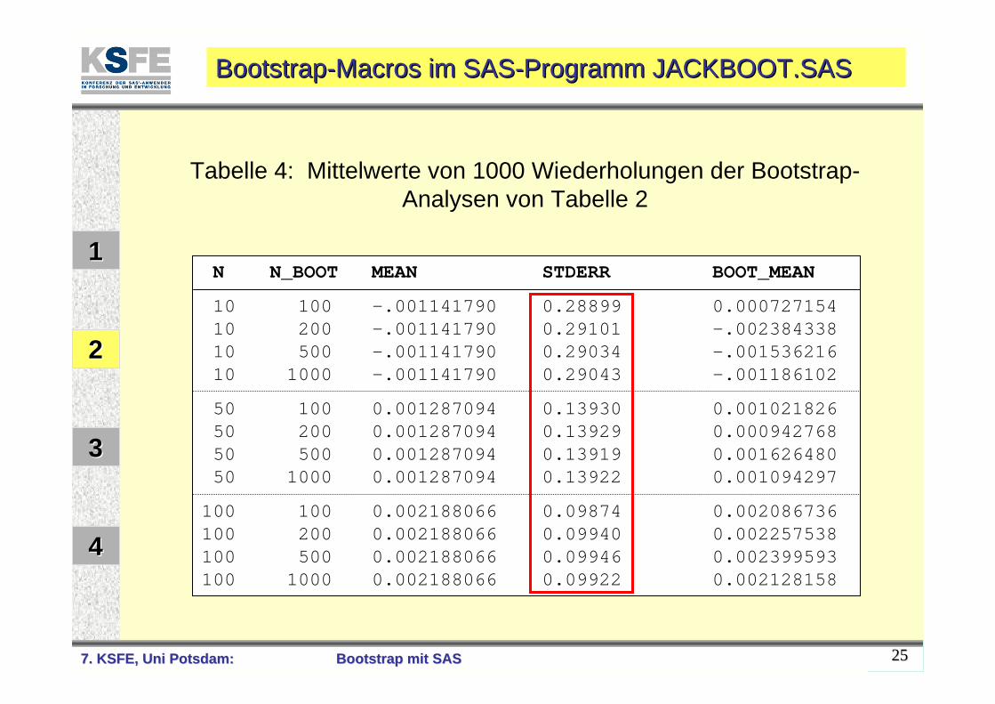
N N_BOOT MEAN STDERR BOOT_MEAN
10 100 -.001141790 0.28899 0.00072715410 200 -.001141790 0.29101 -.00238433810 500 -.001141790 0.29034 -.00153621610 1000 -.001141790 0.29043 -.001186102
50 100 0.001287094 0.13930 0.00102182650 200 0.001287094 0.13929 0.00094276850 500 0.001287094 0.13919 0.00162648050 1000 0.001287094 0.13922 0.001094297
100 100 0.002188066 0.09874 0.002086736100 200 0.002188066 0.09940 0.002257538100 500 0.002188066 0.09946 0.002399593100 1000 0.002188066 0.09922 0.002128158
Tabelle 4: Mittelwerte von 1000 Wiederholungen der Bootstrap-Analysen von Tabelle 2
7. KSFE, Uni Potsdam:7. KSFE, Uni Potsdam: BootstrapBootstrap mit SASmit SAS 2626
11
22
33
44
Ein Bootstrap-Macro mit SAS-IMLEin Ein BootstrapBootstrap--MacroMacro mit SASmit SAS--IMLIML
7. KSFE, Uni Potsdam:7. KSFE, Uni Potsdam: BootstrapBootstrap mit SASmit SAS 2727
Ein Ein BootstrapBootstrap--MacroMacro mit SASmit SAS--IMLIML
11
22
33
44
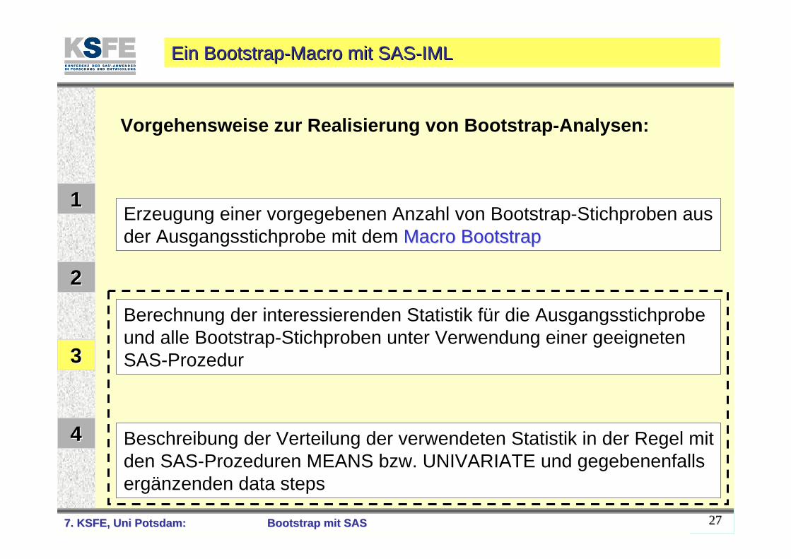
Vorgehensweise zur Realisierung von Bootstrap-Analysen:
Erzeugung einer vorgegebenen Anzahl von Bootstrap-Stichproben aus der Ausgangsstichprobe mit dem MacroMacro BootstrapBootstrap
Berechnung der interessierenden Statistik für die Ausgangsstichprobe und alle Bootstrap-Stichproben unter Verwendung einer geeigneten SAS-Prozedur
Beschreibung der Verteilung der verwendeten Statistik in der Regel mit den SAS-Prozeduren MEANS bzw. UNIVARIATE und gegebenenfalls ergänzenden data steps
7. KSFE, Uni Potsdam:7. KSFE, Uni Potsdam: BootstrapBootstrap mit SASmit SAS 2828
Ein Ein BootstrapBootstrap--MacroMacro mit SASmit SAS--IMLIML
11
22
33
44
3.1 Das SAS-Macro %BOOTSTRAP
Vorausetzung für die Anwendung des Macros ist das Vorliegender SAS-Datei SAMPLE, die die Ausgangsstichprobe enthält.
Die Anwendung dieses Macros erfordert keine Kenntnisse der Macro-Programmierung. Man muß nur die Parameter beimAufruf des Macros setzen.
7. KSFE, Uni Potsdam:7. KSFE, Uni Potsdam: BootstrapBootstrap mit SASmit SAS 2929
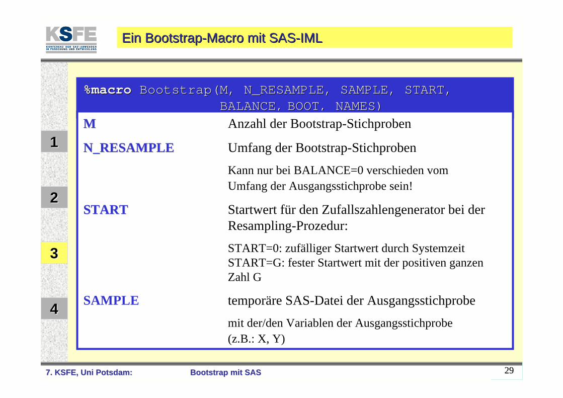
%macro%macro Bootstrap(MBootstrap(M, N_RESAMPLE, SAMPLE, START, , N_RESAMPLE, SAMPLE, START, BALANCE,BALANCE, BOOT, NAMES)BOOT, NAMES)
MM Anzahl der Bootstrap-Stichproben
N_RESAMPLEN_RESAMPLE Umfang der Bootstrap-Stichproben
Kann nur bei BALANCE=0 verschieden vom Umfang der Ausgangsstichprobe sein!
STARTSTART Startwert für den Zufallszahlengenerator bei der Resampling-Prozedur:
START=0: zufälliger Startwert durch SystemzeitSTART=G: fester Startwert mit der positiven ganzen Zahl G
SAMPLE temporäre SAS-Datei der Ausgangsstichprobe
mit der/den Variablen der Ausgangsstichprobe (z.B.: X, Y)
11
22
33
44
Ein Ein BootstrapBootstrap--MacroMacro mit SASmit SAS--IMLIML
7. KSFE, Uni Potsdam:7. KSFE, Uni Potsdam: BootstrapBootstrap mit SASmit SAS 3030
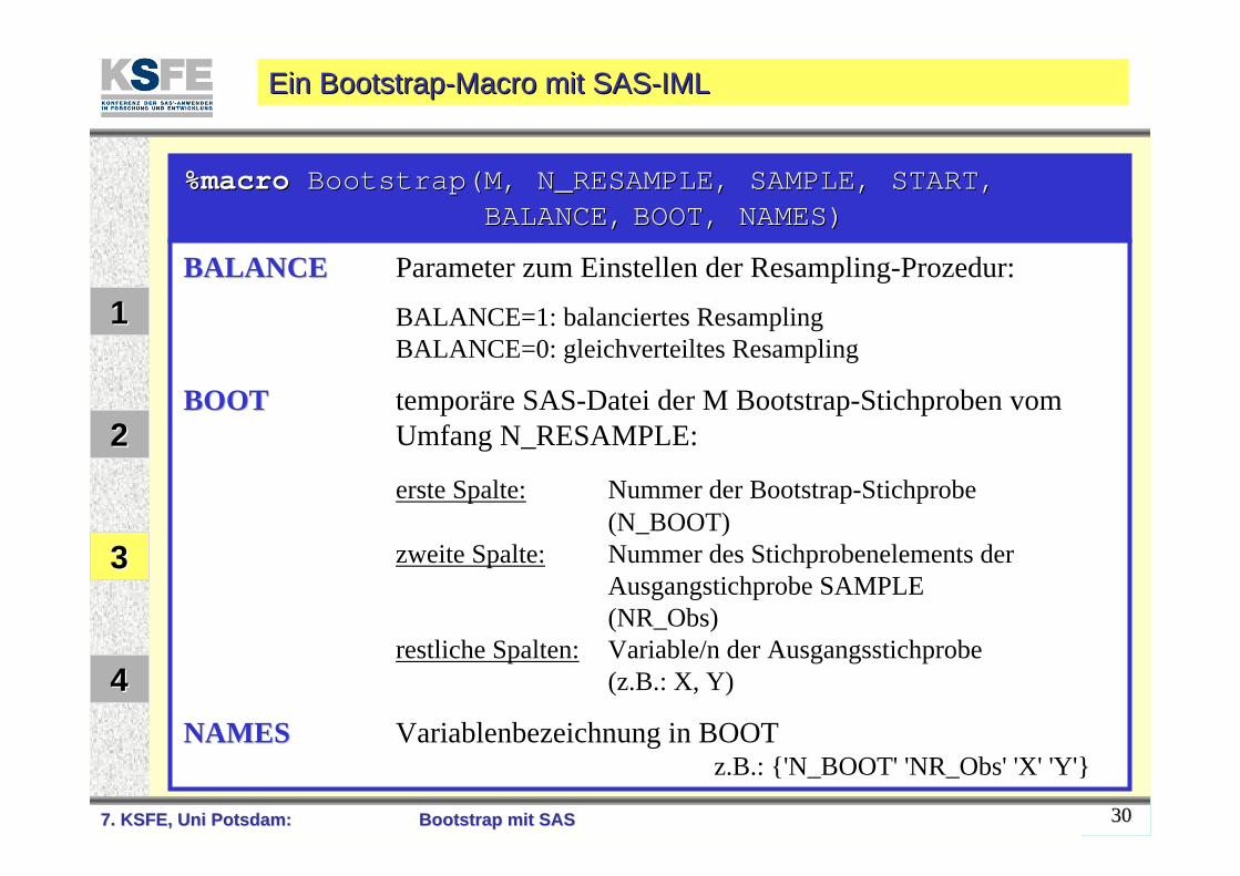
%macro%macro Bootstrap(MBootstrap(M, N_RESAMPLE, SAMPLE, START, , N_RESAMPLE, SAMPLE, START, BALANCE,BALANCE, BOOT, NAMES)BOOT, NAMES)
BALANCEBALANCE Parameter zum Einstellen der Resampling-Prozedur:
BALANCE=1: balanciertes ResamplingBALANCE=0: gleichverteiltes Resampling
BOOTBOOT temporäre SAS-Datei der M Bootstrap-Stichproben vom Umfang N_RESAMPLE:
erste Spalte: Nummer der Bootstrap-Stichprobe(N_BOOT)
zweite Spalte: Nummer des Stichprobenelements derAusgangstichprobe SAMPLE(NR_Obs)
restliche Spalten: Variable/n der Ausgangsstichprobe(z.B.: X, Y)
NAMESNAMES Variablenbezeichnung in BOOTz.B.: {'N_BOOT' 'NR_Obs' 'X' 'Y'}
11
22
33
44
Ein Ein BootstrapBootstrap--MacroMacro mit SASmit SAS--IMLIML
7. KSFE, Uni Potsdam:7. KSFE, Uni Potsdam: BootstrapBootstrap mit SASmit SAS 3131
Ein Ein BootstrapBootstrap--MacroMacro mit SASmit SAS--IMLIML
11
22
33
44
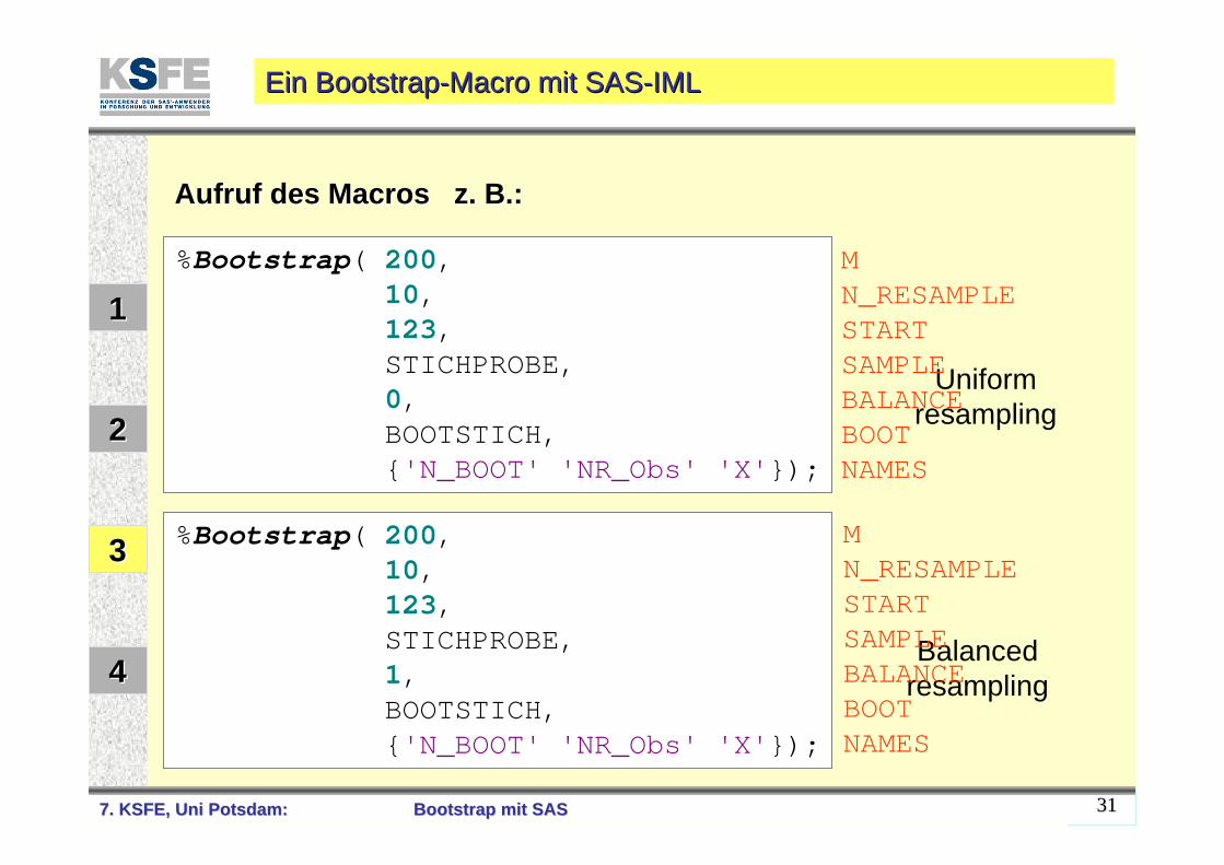
%Bootstrap( 200,10,123,STICHPROBE,0,BOOTSTICH,{'N_BOOT' 'NR_Obs' 'X'});
%Bootstrap( 200,10,123,STICHPROBE,1,BOOTSTICH,{'N_BOOT' 'NR_Obs' 'X'});
Balancedresampling
Uniform resampling
Aufruf des Aufruf des MacrosMacros z. B.:z. B.:
MN_RESAMPLESTARTSAMPLEBALANCEBOOTNAMES
MN_RESAMPLESTARTSAMPLEBALANCEBOOTNAMES
7. KSFE, Uni Potsdam:7. KSFE, Uni Potsdam: BootstrapBootstrap mit SASmit SAS 3232
Ein Ein BootstrapBootstrap--MacroMacro mit SASmit SAS--IMLIML
11
22
33
44
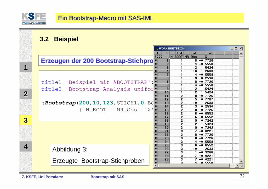
Erzeugen der 200 Erzeugen der 200 BootstrapBootstrap--StichprobenStichproben
title1 'Beispiel mit %BOOTSTRAP';title2 'Bootstrap Analysis uniform resampling,
N_sample=10';%Bootstrap(200,10,123,STICH1,0,BOOTSTICH,
{'N_BOOT' 'NR_Obs' 'X'});
3.2 Beispiel
Abbildung 3:
Erzeugte Bootstrap-Stichproben
Abbildung 3:
Erzeugte Bootstrap-Stichproben
7. KSFE, Uni Potsdam:7. KSFE, Uni Potsdam: BootstrapBootstrap mit SASmit SAS 3333
11
22
33
44
Ein Ein BootstrapBootstrap--MacroMacro mit SASmit SAS--IMLIML
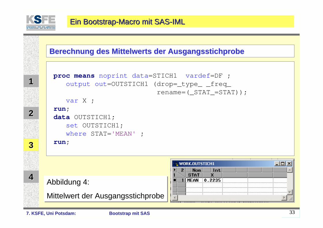
Berechnung des Mittelwerts der AusgangsstichprobeBerechnung des Mittelwerts der Ausgangsstichprobe
proc means noprint data=STICH1 vardef=DF ;output out=OUTSTICH1 (drop=_type_ _freq_
rename=(_STAT_=STAT));var X ;
run;data OUTSTICH1;
set OUTSTICH1;where STAT='MEAN' ;
run;
Abbildung 4:
Mittelwert der Ausgangsstichprobe
Abbildung 4:
Mittelwert der Ausgangsstichprobe
7. KSFE, Uni Potsdam:7. KSFE, Uni Potsdam: BootstrapBootstrap mit SASmit SAS 3434
11
22
33
44
Ein Ein BootstrapBootstrap--MacroMacro mit SASmit SAS--IMLIML
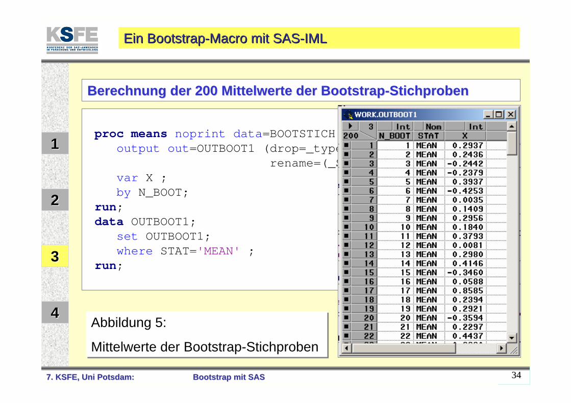
Berechnung der 200 Mittelwerte der Berechnung der 200 Mittelwerte der BootstrapBootstrap--StichprobenStichproben
proc means noprint data=BOOTSTICH vardef=DF ;output out=OUTBOOT1 (drop=_type_ _freq_
rename=(_STAT_=STAT));var X ;by N_BOOT;
run;data OUTBOOT1;
set OUTBOOT1;where STAT='MEAN' ;
run;
Abbildung 5:
Mittelwerte der Bootstrap-Stichproben
Abbildung 5:
Mittelwerte der Bootstrap-Stichproben
7. KSFE, Uni Potsdam:7. KSFE, Uni Potsdam: BootstrapBootstrap mit SASmit SAS 3535
11
22
33
44
Ein Ein BootstrapBootstrap--MacroMacro mit SASmit SAS--IMLIML
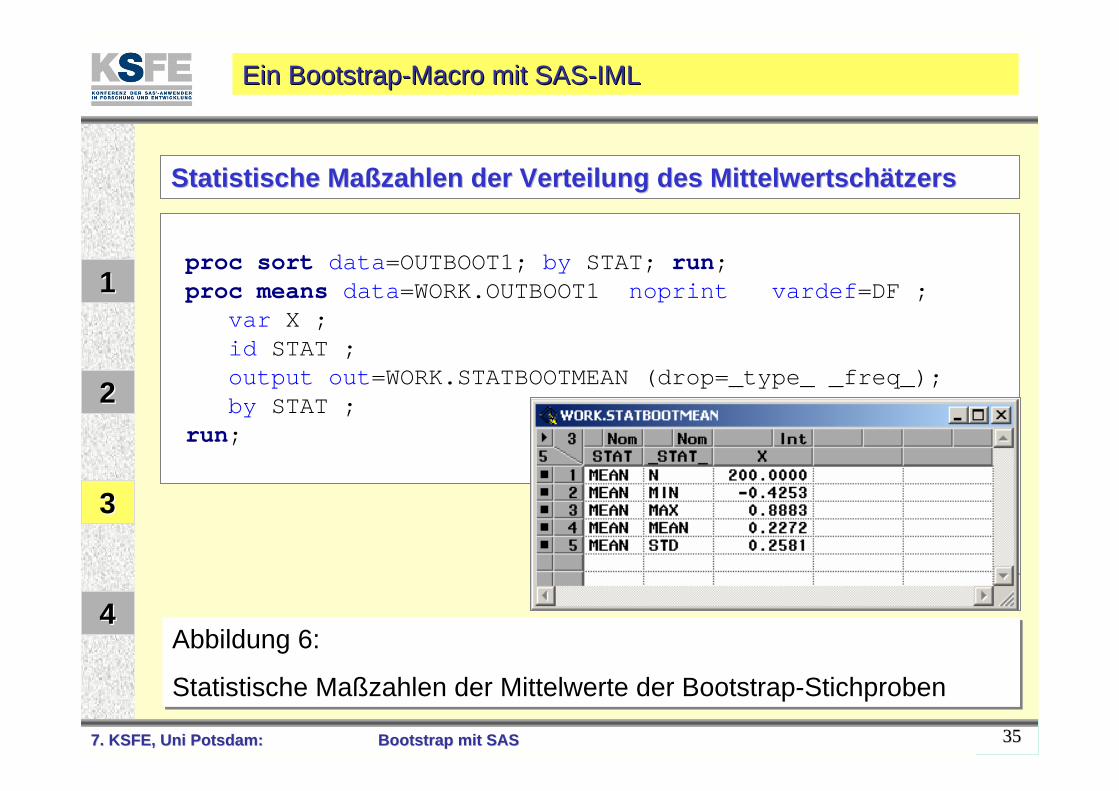
proc sort data=OUTBOOT1; by STAT; run;proc means data=WORK.OUTBOOT1 noprint vardef=DF ;
var X ;id STAT ;output out=WORK.STATBOOTMEAN (drop=_type_ _freq_);by STAT ;
run;
Statistische MaStatistische Maßßzahlen der Verteilung des Mittelwertschzahlen der Verteilung des Mittelwertschäätzerstzers
Abbildung 6:
Statistische Maßzahlen der Mittelwerte der Bootstrap-Stichproben
Abbildung 6:
Statistische Maßzahlen der Mittelwerte der Bootstrap-Stichproben
7. KSFE, Uni Potsdam:7. KSFE, Uni Potsdam: BootstrapBootstrap mit SASmit SAS 3636
Ein Ein BootstrapBootstrap--MacroMacro mit SASmit SAS--IMLIML
11
22
33
44
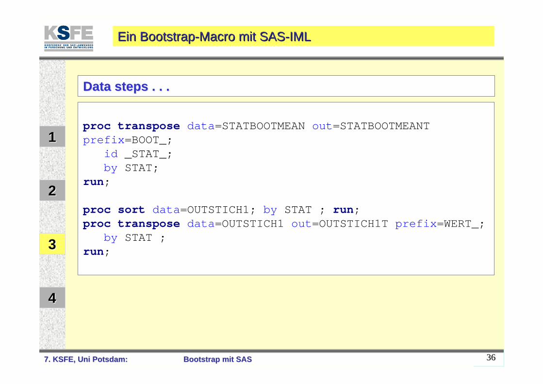
DataData stepssteps . . .. . .
proc transpose data=STATBOOTMEAN out=STATBOOTMEANT prefix=BOOT_;
id _STAT_;by STAT;
run;
proc sort data=OUTSTICH1; by STAT ; run;proc transpose data=OUTSTICH1 out=OUTSTICH1T prefix=WERT_;
by STAT ;run;
7. KSFE, Uni Potsdam:7. KSFE, Uni Potsdam: BootstrapBootstrap mit SASmit SAS 3737
Ein Ein BootstrapBootstrap--MacroMacro mit SASmit SAS--IMLIML
11
22
33
44
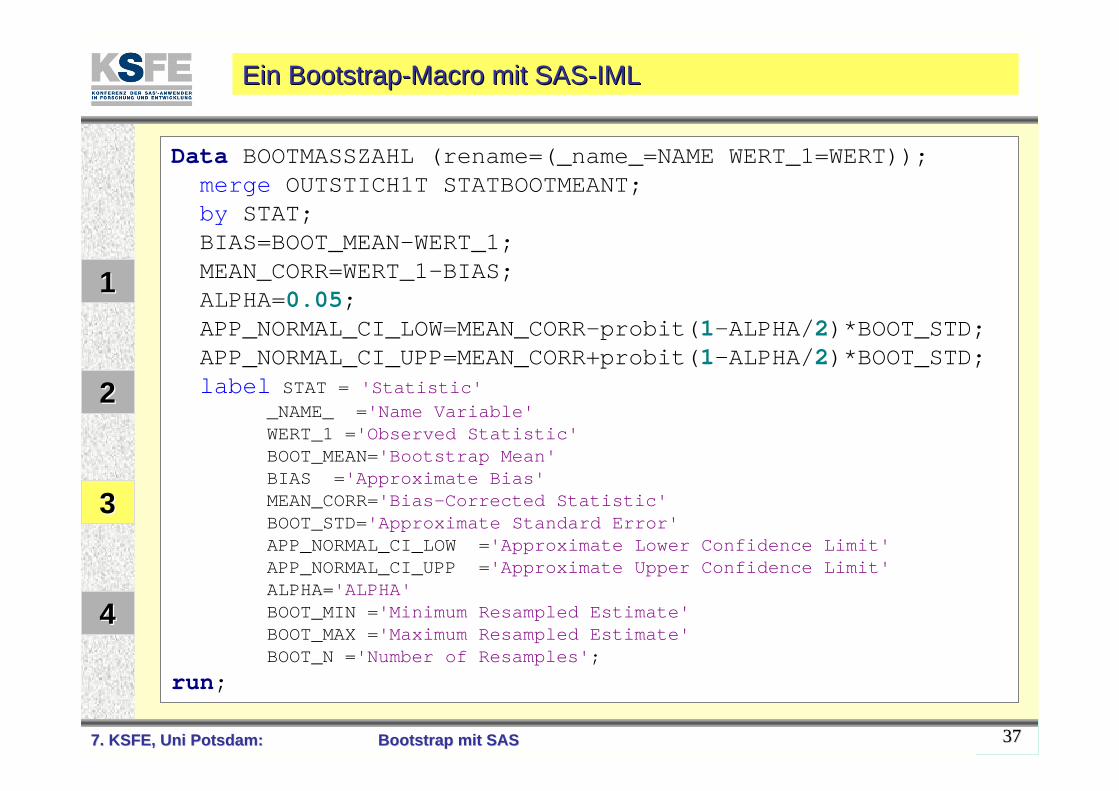
Data BOOTMASSZAHL (rename=(_name_=NAME WERT_1=WERT));merge OUTSTICH1T STATBOOTMEANT;by STAT;BIAS=BOOT_MEAN-WERT_1;MEAN_CORR=WERT_1-BIAS;ALPHA=0.05;APP_NORMAL_CI_LOW=MEAN_CORR-probit(1-ALPHA/2)*BOOT_STD;APP_NORMAL_CI_UPP=MEAN_CORR+probit(1-ALPHA/2)*BOOT_STD;label STAT = 'Statistic'
_NAME_ ='Name Variable'WERT_1 ='Observed Statistic'BOOT_MEAN='Bootstrap Mean'BIAS ='Approximate Bias'MEAN_CORR='Bias-Corrected Statistic'BOOT_STD='Approximate Standard Error'APP_NORMAL_CI_LOW ='Approximate Lower Confidence Limit'APP_NORMAL_CI_UPP ='Approximate Upper Confidence Limit'ALPHA='ALPHA'BOOT_MIN ='Minimum Resampled Estimate'BOOT_MAX ='Maximum Resampled Estimate'BOOT_N ='Number of Resamples';
run;
7. KSFE, Uni Potsdam:7. KSFE, Uni Potsdam: BootstrapBootstrap mit SASmit SAS 3838
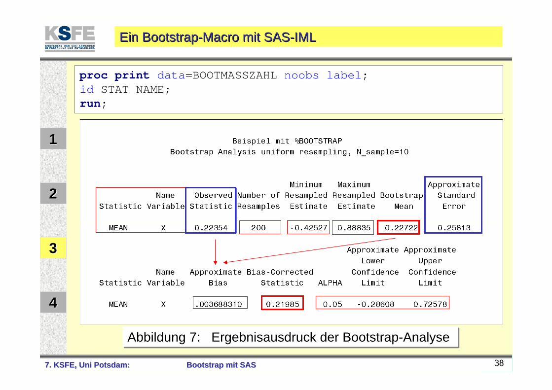
Abbildung 7: Ergebnisausdruck der Bootstrap-AnalyseAbbildung 7: Ergebnisausdruck der Bootstrap-Analyse
11
22
33
44
Ein Ein BootstrapBootstrap--MacroMacro mit SASmit SAS--IMLIML
proc print data=BOOTMASSZAHL noobs label;id STAT NAME;run;
7. KSFE, Uni Potsdam:7. KSFE, Uni Potsdam: BootstrapBootstrap mit SASmit SAS 3939
Ein Ein BootstrapBootstrap--MacroMacro mit SASmit SAS--IMLIML
11
22
33
44
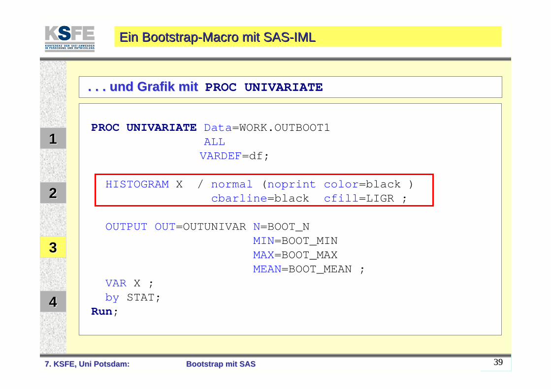
. . . und Grafik mit . . . und Grafik mit PROC UNIVARIATE
PROC UNIVARIATE Data=WORK.OUTBOOT1 ALLVARDEF=df;
HISTOGRAM X / normal (noprint color=black ) cbarline=black cfill=LIGR ;
OUTPUT OUT=OUTUNIVAR N=BOOT_N MIN=BOOT_MIN MAX=BOOT_MAX MEAN=BOOT_MEAN ;
VAR X ;by STAT;
Run;
7. KSFE, Uni Potsdam:7. KSFE, Uni Potsdam: BootstrapBootstrap mit SASmit SAS 4040
11
22
33
44
Ein Ein BootstrapBootstrap--MacroMacro mit SASmit SAS--IMLIML
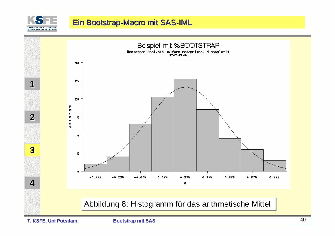
Abbildung 8: Histogramm für das arithmetische MittelAbbildung 8: Histogramm für das arithmetische Mittel
7. KSFE, Uni Potsdam:7. KSFE, Uni Potsdam: BootstrapBootstrap mit SASmit SAS 4141
11
22
33
44 LiteraturLiteraturLiteratur
7. KSFE, Uni Potsdam:7. KSFE, Uni Potsdam: BootstrapBootstrap mit SASmit SAS 4242
LiteraturLiteratur
11
22
33
44
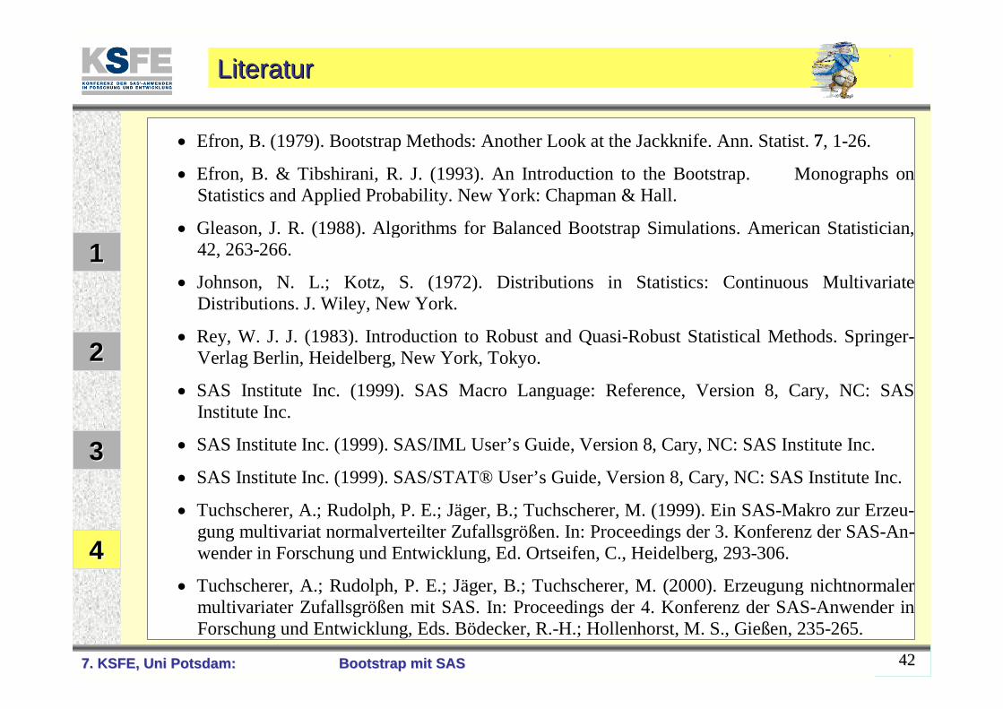
• Efron, B. (1979). Bootstrap Methods: Another Look at the Jackknife. Ann. Statist. 7, 1-26.
• Efron, B. & Tibshirani, R. J. (1993). An Introduction to the Bootstrap. Monographs onStatistics and Applied Probability. New York: Chapman & Hall.
• Gleason, J. R. (1988). Algorithms for Balanced Bootstrap Simulations. American Statistician,42, 263-266.
• Johnson, N. L.; Kotz, S. (1972). Distributions in Statistics: Continuous Multivariate Distributions. J. Wiley, New York.
• Rey, W. J. J. (1983). Introduction to Robust and Quasi-Robust Statistical Methods. Springer-Verlag Berlin, Heidelberg, New York, Tokyo.
• SAS Institute Inc. (1999). SAS Macro Language: Reference, Version 8, Cary, NC: SASInstitute Inc.
• SAS Institute Inc. (1999). SAS/IML User’s Guide, Version 8, Cary, NC: SAS Institute Inc.
• SAS Institute Inc. (1999). SAS/STAT® User’s Guide, Version 8, Cary, NC: SAS Institute Inc.
• Tuchscherer, A.; Rudolph, P. E.; Jäger, B.; Tuchscherer, M. (1999). Ein SAS-Makro zur Erzeu-gung multivariat normalverteilter Zufallsgrößen. In: Proceedings der 3. Konferenz der SAS-An-wender in Forschung und Entwicklung, Ed. Ortseifen, C., Heidelberg, 293-306.
• Tuchscherer, A.; Rudolph, P. E.; Jäger, B.; Tuchscherer, M. (2000). Erzeugung nichtnormaler multivariater Zufallsgrößen mit SAS. In: Proceedings der 4. Konferenz der SAS-Anwender in Forschung und Entwicklung, Eds. Bödecker, R.-H.; Hollenhorst, M. S., Gießen, 235-265.