Embed Size (px)
Citation preview
„Im Rahmen der hochschulweiten Open-Access-Strategie für die Zweitveröffentlichung identifiziert durch die Universitätsbibliothek Ilmenau.“
“Within the academic Open Access Strategy identified for deposition by Ilmenau University Library.”
„Dieser Beitrag ist mit Zustimmung des Rechteinhabers aufgrund einer (DFG-geförderten) Allianz- bzw. Nationallizenz frei zugänglich.“
„This publication is with permission of the rights owner freely accessible due to an Alliance licence and a national licence (funded by the DFG, German Research Foundation) respectively.”
Shi, Nan; Emran, Mohammad S.; Schumacher, Jörg:
Boundary layer structure in turbulent Rayleigh-Bénard convection
URN: urn:nbn:de:gbv:ilm1-2014210036
Published OpenAccess: September 2014
Original published in: Journal of fluid mechanics. - Cambridge [u.a.] : Cambridge Univ. Press (ISSN 1469-7645). - 706 (2012), S. 5-33. DOI: 10.1017/jfm.2012.207 URL: http://dx.doi.org/10.1017/jfm.2012.207 [Visited: 2014-08-27]
J. Fluid Mech. (2012), vol. 706, pp. 5–33. c© Cambridge University Press 2012 5doi:10.1017/jfm.2012.207
Boundary layer structure in turbulentRayleigh–Bénard convection
Nan Shi‡, Mohammad S. Emran†‡ and Jörg Schumacher
Institut fur Thermo- und Fluiddynamik, Technische Universitat Ilmenau,Postfach 100565, D-98684 Ilmenau, Germany
(Received 24 October 2011; revised 17 April 2012; accepted 25 April 2012;first published online 13 June 2012)
The structure of the boundary layers in turbulent Rayleigh–Benard convection isstudied by means of three-dimensional direct numerical simulations. We considerconvection in a cylindrical cell at aspect ratio one for Rayleigh numbers ofRa= 3×10⁹ and 3×10¹⁰ at fixed Prandtl number Pr = 0.7. Similar to the experimentalresults in the same setup and for the same Prandtl number, the structure of thelaminar boundary layers of the velocity and temperature fields is found to deviatefrom the prediction of Prandtl–Blasius–Pohlhausen theory. Deviations decrease whena dynamical rescaling of the data with an instantaneously defined boundary layerthickness is performed and the analysis plane is aligned with the instantaneousdirection of the large-scale circulation in the closed cell. Our numerical resultsdemonstrate that important assumptions of existing classical laminar boundary layertheories for forced and natural convection are violated, such as the strict two-dimensionality of the dynamics or the steadiness of the fluid motion. The boundarylayer dynamics consists of two essential local dynamical building blocks, a plumedetachment and a post-plume phase. The former is associated with larger variationsof the instantaneous thickness of velocity and temperature boundary layer and afully three-dimensional local flow. The post-plume dynamics is connected with thelarge-scale circulation in the cell that penetrates the boundary region from above. Themean turbulence profiles taken in localized sections of the boundary layer for eachdynamical phase are also compared with solutions of perturbation expansions of theboundary layer equations of forced or natural convection towards mixed convection.Our analysis of both boundary layers shows that the near-wall dynamics combineselements of forced Blasius-type and natural convection.
Key words: boundary layer structure, Benard convection, turbulent convection
1. IntroductionTurbulent Rayleigh–Benard convection can be initiated in a fluid which is confined
between a cold isothermal plate at the top and a hot isothermal plate at the bottom,provided that a sufficiently strong temperature difference is sustained. In the turbulentregime, the majority of the heat is carried by convective transport through the layeror cell. It is only in the vicinity of the top and bottom plates, where the fluid
† Email address for correspondence: [email protected]‡ The first two authors contributed equally to this work.
6 N. Shi, M. S. Emran and J. Schumacher
velocities are small, that conductive transport takes over and becomes important. Asin all other wall-bounded flows, boundary layers form. In the present system these areboundary layers of the velocity and temperature fields. The structure of these boundarylayers turns out to be crucial for a deeper understanding of the local and globaltransport processes, as discussed for example in a recent review (Ahlers, Grossmann& Lohse 2009b). Furthermore, the boundary layers interact with a so-called large-scalecirculation (LSC) that is always established in a closed turbulent convection cell. ThisLSC can take the form of a single roll for aspect ratios of order unity or multipleroll patterns for larger ones (du Puits, Resagk & Thess 2007b; van Reeuwijk, Jonker& Hanjalic 2008a; Bailon-Cuba, Emran & Schumacher 2010; Mishra et al. 2011). Onthe one hand, the LSC is triggered by packets of thermal plumes: fragments of thethermal boundary layers which detach randomly from the top and bottom plates intothe bulk of the cell. On the other hand, the fully established LSC with its complexthree-dimensional dynamics can be expected to affect and partly even drive the laminarflow dynamics close to the walls. This interplay has not yet been studied in detail forcylindrical convection cells and provides one central motivation for the present work.
From a global perspective the heat transport in a turbulent convection cell, whichis measured by the dimensionless Nusselt number Nu, is a function of the threedimensionless control parameters in Rayleigh–Benard convection, namely the Rayleighnumber Ra, the Prandtl number Pr and the aspect ratio Γ of the convectioncell, i.e. Nu = f (Ra,Pr, Γ ). Two scaling theories yield different predictions forthe turbulent heat transport in convection based on different assumptions on theboundary layer structure. While the scaling theory of Shraiman and Siggia (Siggia1994) is based on a turbulent boundary layer with a logarithmic profile for the meanstreamwise velocity, Grossmann & Lohse (2000) assume laminar boundary layers ofPrandtl–Blasius–Pohlhausen type (Prandtl 1905; Blasius 1908; Pohlhausen 1921) inorder to estimate the boundary layer contributions to the thermal and kinetic energydissipation rates. Such a laminar boundary layer evolves in purely forced convection,i.e. for a laminar flow over a flat plate. The temperature is treated as a passive scalar(Pohlhausen 1921).
Measuring the boundary layer structure is, however, difficult in laboratoryexperiments for high-Rayleigh-number convection. The reason is that the thicknessof the thermal boundary layer, δT , decreases as the Rayleigh and thus the Nusseltnumber grow. This thickness is given by
δT = H
2Nu, (1.1)
where H is the height of the convection cell. For a convection flow at Pr ∼ O(1),the corresponding velocity boundary layer will have a similar thickness of δv ∼ δT
and will thus decrease similarly with increasing Rayleigh number (see e.g. Shishkinaet al. 2010). Detailed measurements of boundary layer profiles at higher Rayleighnumbers (Ra > 109) thus require large devices such as the ‘Barrel of Ilmenau’ for theconvection in air (du Puits, Resagk & Thess 2007a, 2010) or high-resolution particleimage velocimetry, as is possible for convection in water (Sun, Cheung & Xia 2008;Zhou & Xia 2010a). Statistical time series analyses of the mean temperature andvelocity profiles in the boundary layer yielded deviations from the predicted laminarBlasius profiles (du Puits et al. 2007a; Zhou & Xia 2010a). A dynamic rescalingof the data with respect to an instantaneous boundary layer thickness (which will beexplained further below in the text) tends to bring it closer to the Blasius prediction inthe water experiment by Zhou & Xia (2010a). The latter result was also confirmed by
Boundary layer structure in turbulent Rayleigh–Bénard convection 7
a series of two-dimensional direct numerical simulations by Zhou et al. (2010, 2011).However, in both cases, the large-scale circulation is a (quasi-) two-dimensional flowwhich cannot fluctuate in the third direction.
Du Puits et al. (2007a) concluded from their work that the deviations from theBlasius shape arise due to the characteristic near-wall coherent structures – so-calledthermal plumes – which permanently detach from the thermal boundary layer. Directnumerical simulation (DNS) by van Reeuwijk, Jonker & Hanjalic (2008b) for Rayleighnumbers up to 108 supports systematic deviations from a laminar boundary layeron the basis of an analysis of the friction factor and the Reynolds stress budgets.Their DNS showed that the integral of the streamwise pressure gradients have alarge magnitude compared to Reynolds stresses and are not zero as in the Blasiuscase. Recall also that the active nature of the temperature field is not incorporated inPrandtl–Blasius–Pohlhausen theory.
Similarity solutions for natural convection, complementary to Prandtl–Blasius–Pohlhausen theory for forced convection, are well known (see e.g. Stewartson 1958;Rotem & Claassen 1969). Here the buoyancy term remains in the momentum equation(see below) and is balanced by a wall-normal pressure gradient. The temperaturedifferences now initiate fluid motion. Both purely forced and natural convection weresubject to perturbation expansions towards mixed convection, which combines forcedand natural convection (Sparrow & Minkowycz 1962). This means that either theactive role of temperature is included as a small-size effect in forced convectionor a weak outer flow is imposed in natural convection. Hieber (1973) solvednumerically the equations which arise from perturbative expansions of forced andnatural convection. These classical studies are combined with more recent efforts todevelop two-dimensional boundary layer models for the plume detachment (Fuji 1963;Theerthan & Arakeri 1998; Puthenveettil & Arakeri 2005; Puthenveettil et al. 2011).The models assume two-dimensional line-like thermal plumes with no significantvariation perpendicular to the flow plane.
In this work, we want to resolve the boundary layer structure and its relation tothe large-scale circulation for Ra > 109 by means of three-dimensional DNS. We aimat better understanding of the physical reasons for the deviations of the boundarylayer profiles from the classical Prandtl–Blasius–Pohlhausen and Stewartson theoriesfor forced and natural convection, respectively. We therefore conduct two long-timedirect numerical simulations of turbulent Rayleigh–Benard convection in a cylindricalcell at an aspect ratio Γ = 1. Step by step we test which assumptions of the originalderivations of the similarity solutions are satisfied. Our studies will include analysesof the LSC, the pressure gradient fluctuations, the importance of violations of thetwo-dimensionality of the flow and the active role of the temperature at the isothermalwalls. The coupling between the two boundary layers is also analysed. We will showthat in fact most of the original assumptions of all boundary layer theories are notestablished in the present cellular flow. Furthermore, we relate locally measuredturbulence profiles with the results from idealized mixed convection boundary layers.
The outline of the paper is as follows. In the next section, we summarize thenumerical model and the equations of motion. We then present the boundary layerprofiles from the classical time series analysis and the dynamical rescaling procedure.The studies are followed by investigations of the large-scale circulation, the pressurefluctuations, and time variations of the local boundary layer structure. In § 4 weresolve the dynamics in the boundary layer in a small observation window and relate
8 N. Shi, M. S. Emran and J. Schumacher
the findings to results of the boundary layer theory of mixed convection. We concludeour work with a summary and an outlook.
2. Numerical modelThe three-dimensional Navier–Stokes equations in the Boussinesq approximation are
solved in combination with an advection–diffusion equation for the temperature field.The system of equations is given by
∂ui
∂t+ uj
∂ui
∂xj=− ∂p
∂xi+ ν ∂
2ui
∂x2j
+ αgTδiz, (2.1)
∂ui
∂xi= 0, (2.2)
∂T
∂t+ uj
∂T
∂xj= κ ∂
2T
∂x2j
, (2.3)
where i, j = x, y, z. Here p(x, y, z, t) is the kinematic pressure, ui(x, y, z, t) the velocityfield, T(x, y, z, t) the total temperature field, ν the kinematic viscosity, and κ thediffusivity of the temperature. The dimensionless control parameters, the Rayleighnumber Ra, the Prandtl number Pr , and the aspect ratio Γ are defined by
Ra= gα1TH3
νκ, Pr = ν
κ, Γ = 2R
H. (2.4)
Our studies are conducted for Γ = 1, Pr = 0.7 and Ra = 3 × 10⁹ and 3 × 10¹⁰.Constant α is the thermal expansion coefficient, g the gravitational acceleration, 1Tthe outer temperature difference, R the radius and H the height of the cylindricalcell. The characteristic length is H, the characteristic velocity is the free-fall velocityUf =√gα1TH. Times are consequently given in units of the free-fall time Tf = H/Uf .The cylindrical geometry requires a switch from Cartesian to cylindrical coordinates,(x, y, z)→ (r, φ, z). No-slip boundary conditions for the velocity field components,i.e. ui ≡ 0, hold at all walls. The top and bottom plates are held isothermal at fixedtemperatures Tbottom and Ttop, respectively. The sidewalls are adiabatic with ∂T/∂r = 0.The grid resolutions are Nr × Nφ × Nz = 301 × 513 × 360 for Ra = 3 × 10⁹ and513 × 1153 × 861 for Ra = 3 × 10¹⁰, where Nr, Nφ and Nz are the number of gridpoints in the radial, azimuthal and axial directions respectively.
The equations are discretized on a staggered grid with a second-order finitedifference scheme (Verzicco & Orlandi 1996; Verzicco & Camussi 2003). Thepressure field p is determined by a two-dimensional Poisson solver after applyinga one-dimensional fast Fourier transform (FFT) in the azimuthal direction. The timeadvancement is done by a third-order Runge–Kutta scheme. The grid spacings arenon-equidistant in the radial and vertical directions. In the vertical direction, the gridspacing is close to Chebyshev collocation points. The grid resolutions are chosen suchthat the criterion by Grotzbach (1983) is satisfied plane by plane. We therefore definea height-dependent Kolmogorov scale as
ηK(z)= ν3/4
〈ε (z)〉1/4A,t
, (2.5)
where the symbol 〈·〉A,t denotes an average over a plane at a fixed height z andan ensemble of statistically independent snapshots. Following Emran & Schumacher
Boundary layer structure in turbulent Rayleigh–Bénard convection 9
(2008) and Bailon-Cuba et al. (2010), we define the maximum of the geometricmean of the grid spacing at height z by 1(z) = max[ 3
√r1φ1r(r)1z(z)]. The thermal
boundary layer is resolved with 18 grid planes for Ra = 3 × 10⁹ and with 23 gridplanes for Ra = 3 × 10¹⁰. Thus the recently discussed resolution criterion (Shishkinaet al. 2010), which would result in 9 and 13 grid planes for the thermal boundarylayer, is satisfied and over-resolved by almost a factor of 2 in both cases.
The Nusselt number is found to be Nu = 90.32 ± 0.63 for Ra = 3 × 10⁹ witha standard deviation of 0.7 %. The second run at Ra = 3 × 10¹⁰ resulted inNu = 189.65 ± 1.5, which gives a standard deviation of 0.8 %. The standard deviationis determined in the same way as in Bailon-Cuba et al. (2010). We take the Nusseltnumber plane by plane and determine the fluctuation about the global mean.
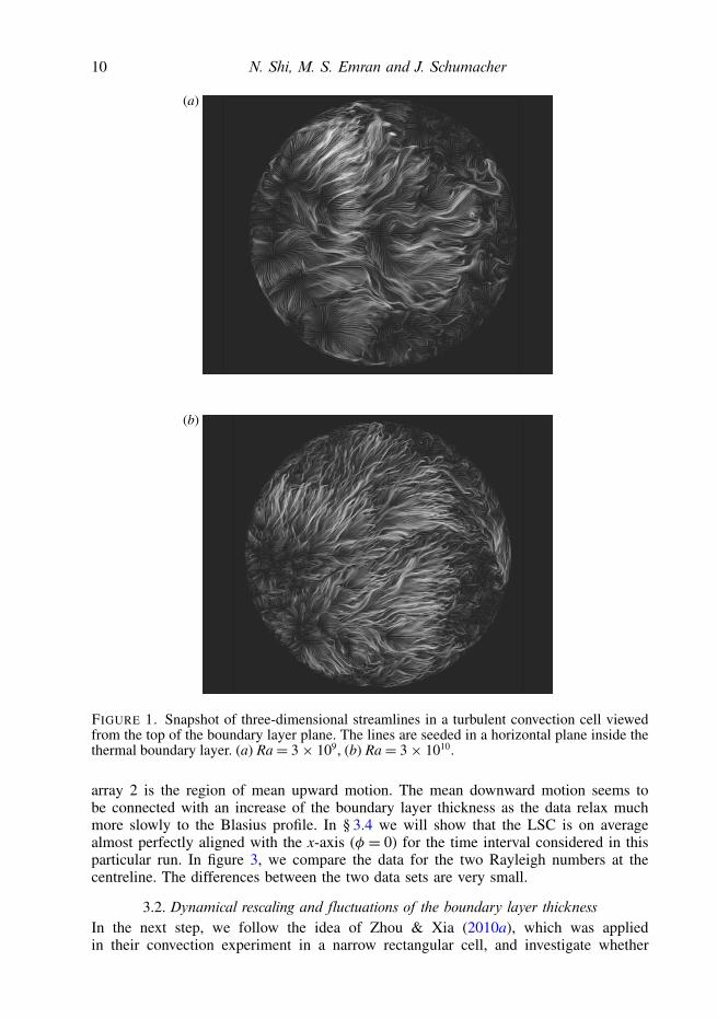
Figure 1 displays instantaneous three-dimensional velocity fields viewed from thetop to the edge of the boundary layer close to the bottom plate for two Rayleighnumbers. Although a preferential mean flow direction is observable, we see significantdeviations from two-dimensionality as visible by the wavy streamlines. With increasingRayleigh number the streamline plot shows more and more textures on an ever finerscale.
3. Boundary layer analysis3.1. Vertical mean profiles from time series analysis
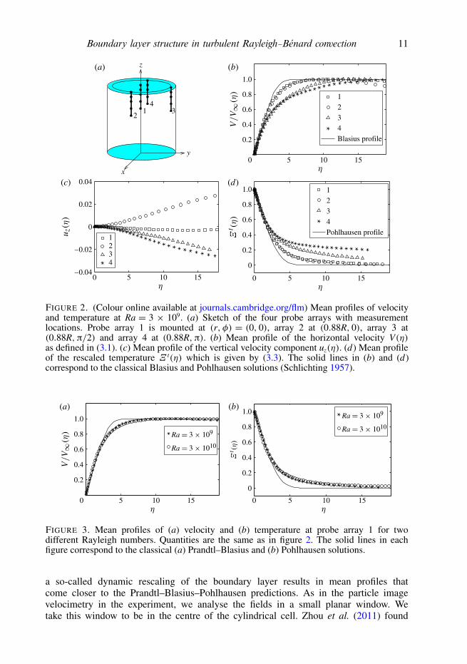
Our numerical approach follows the experimental procedure. The latter consists ofmeasuring time series of the three velocity components or temperature at a givenpoint (r, φ, z) in the cell, computing time-averages and repeating the measurementfor different values of z. The results of such procedures are mean profiles oftemperature or velocity. In our direct numerical simulation we compute such timeseries simultaneously for an array of 40 (and 100) points starting from z = H. Probearray 1 is at the centreline. Probe arrays 2, 3 and 4 are at r = 0.88R and φ = 0,π/2and π, respectively (see figure 2a). We compare the one-dimensional mean profiles forthe horizontal velocity V (as defined in du Puits et al. 2007a), which is given by
V(r, φ, z, t)=√
u2r (r, φ, z, t)+ u2
φ(r, φ, z, t), (3.1)
the vertical velocity component uz and the normalized temperatures Ξ from the top (t)and bottom (b) plates, which are defined by
Ξ t(r, φ, z, t)= T(z= H/2)− T(r, φ, z, t)
T(z= H/2)− Ttop, (3.2)
Ξ b(r, φ, z, t)= T(r, φ, z, t)− T(z= H/2)Tbottom − T(z= H/2)
, (3.3)
with the corresponding profiles arising from Prandtl–Blasius–Pohlhausen theory (seefigure 2b–d). Here η is the similarity variable defined in the Appendix in (A 1). Thetime series contains 57 000 data points for Ra= 3× 10⁹ (and 23 000 for Ra= 3× 10¹⁰)at each position of the probe array. This corresponds to 122 (and 58 for Ra= 3× 10¹⁰)free-fall time units Tf . Similar to the laboratory experiments by du Puits et al. (2007a)and Zhou & Xia (2010a), we detect clear deviations from the Blasius and Pohlhausensolutions, which are also shown in the figures. Furthermore, significant differences canbe seen between the four profiles, which are caused by the existing large-scale flowin the cell. Our profiles at Ra = 3 × 10⁹ suggest that probe array 4 (and probablyarray 3 as well) are significantly altered by a mean downward motion, while probe
10 N. Shi, M. S. Emran and J. Schumacher
(a)
(b)
FIGURE 1. Snapshot of three-dimensional streamlines in a turbulent convection cell viewedfrom the top of the boundary layer plane. The lines are seeded in a horizontal plane inside thethermal boundary layer. (a) Ra= 3× 10⁹, (b) Ra= 3× 10¹⁰.
array 2 is the region of mean upward motion. The mean downward motion seems tobe connected with an increase of the boundary layer thickness as the data relax muchmore slowly to the Blasius profile. In § 3.4 we will show that the LSC is on averagealmost perfectly aligned with the x-axis (φ = 0) for the time interval considered in thisparticular run. In figure 3, we compare the data for the two Rayleigh numbers at thecentreline. The differences between the two data sets are very small.
3.2. Dynamical rescaling and fluctuations of the boundary layer thicknessIn the next step, we follow the idea of Zhou & Xia (2010a), which was appliedin their convection experiment in a narrow rectangular cell, and investigate whether
Boundary layer structure in turbulent Rayleigh–Bénard convection 11
12
34
x
y
z
5 10 15
1234Blasius profile
1234
1234Pohlhausen profile
0 5 10 150 5 10 15
0
0.2
0.4
0.6
0.8
1.0
–0.04
–0.02
0
0.02
0.04
0
0.2
0.4
0.6
0.8
1.0
(a)
(c) (d)
(b)
FIGURE 2. (Colour online available at journals.cambridge.org/flm) Mean profiles of velocityand temperature at Ra = 3 × 10⁹. (a) Sketch of the four probe arrays with measurementlocations. Probe array 1 is mounted at (r, φ) = (0, 0), array 2 at (0.88R, 0), array 3 at(0.88R,π/2) and array 4 at (0.88R,π). (b) Mean profile of the horizontal velocity V(η)as defined in (3.1). (c) Mean profile of the vertical velocity component uz(η). (d) Mean profileof the rescaled temperature Ξ t(η) which is given by (3.3). The solid lines in (b) and (d)correspond to the classical Blasius and Pohlhausen solutions (Schlichting 1957).
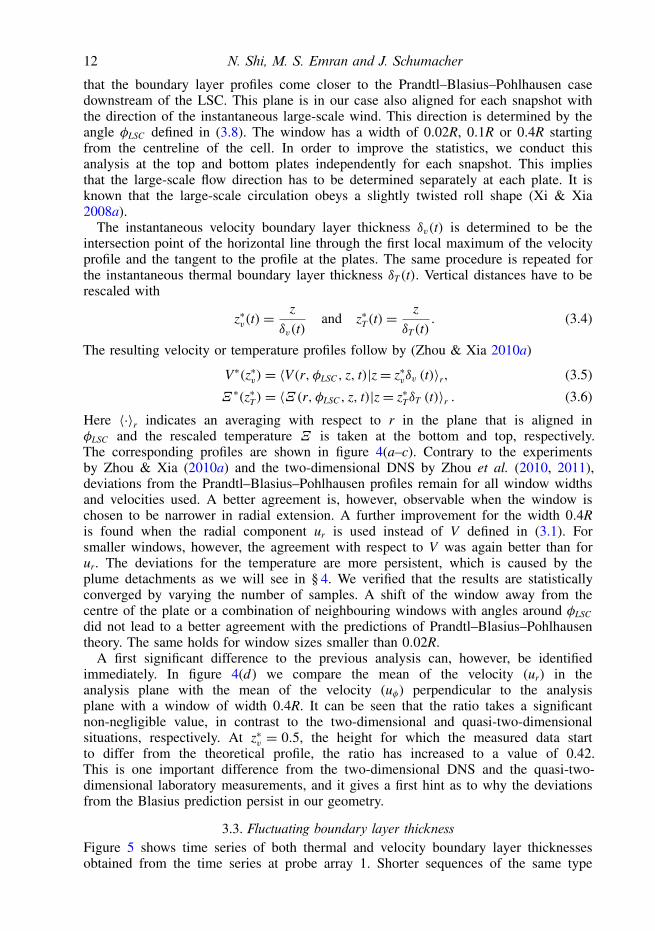
5 10 15 50 10 150
0.2
0.4
0.6
0.8
1.0
(a) (b)
0
0.2
0.4
0.6
0.8
1.0
FIGURE 3. Mean profiles of (a) velocity and (b) temperature at probe array 1 for twodifferent Rayleigh numbers. Quantities are the same as in figure 2. The solid lines in eachfigure correspond to the classical (a) Prandtl–Blasius and (b) Pohlhausen solutions.
a so-called dynamic rescaling of the boundary layer results in mean profiles thatcome closer to the Prandtl–Blasius–Pohlhausen predictions. As in the particle imagevelocimetry in the experiment, we analyse the fields in a small planar window. Wetake this window to be in the centre of the cylindrical cell. Zhou et al. (2011) found
12 N. Shi, M. S. Emran and J. Schumacher
that the boundary layer profiles come closer to the Prandtl–Blasius–Pohlhausen casedownstream of the LSC. This plane is in our case also aligned for each snapshot withthe direction of the instantaneous large-scale wind. This direction is determined by theangle φLSC defined in (3.8). The window has a width of 0.02R, 0.1R or 0.4R startingfrom the centreline of the cell. In order to improve the statistics, we conduct thisanalysis at the top and bottom plates independently for each snapshot. This impliesthat the large-scale flow direction has to be determined separately at each plate. It isknown that the large-scale circulation obeys a slightly twisted roll shape (Xi & Xia2008a).
The instantaneous velocity boundary layer thickness δv(t) is determined to be theintersection point of the horizontal line through the first local maximum of the velocityprofile and the tangent to the profile at the plates. The same procedure is repeated forthe instantaneous thermal boundary layer thickness δT(t). Vertical distances have to berescaled with
z∗v(t)=z
δv(t)and z∗T(t)=
z
δT(t). (3.4)
The resulting velocity or temperature profiles follow by (Zhou & Xia 2010a)
V∗(z∗v)= 〈V(r, φLSC , z, t)|z= z∗vδv (t)〉r, (3.5)
Ξ ∗(z∗T)= 〈Ξ(r, φLSC , z, t)|z= z∗TδT (t)〉r . (3.6)
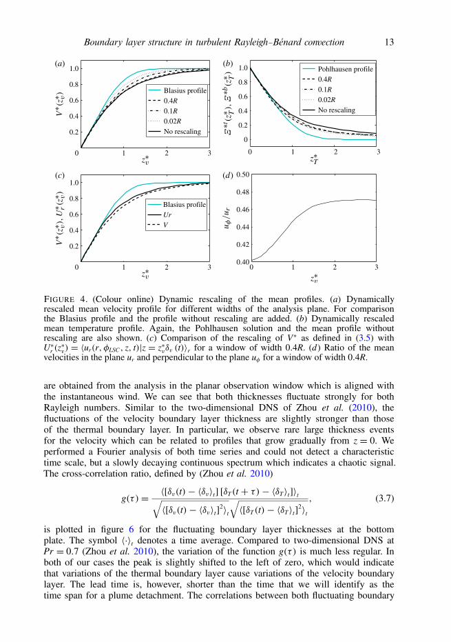
Here 〈·〉r indicates an averaging with respect to r in the plane that is aligned inφLSC and the rescaled temperature Ξ is taken at the bottom and top, respectively.The corresponding profiles are shown in figure 4(a–c). Contrary to the experimentsby Zhou & Xia (2010a) and the two-dimensional DNS by Zhou et al. (2010, 2011),deviations from the Prandtl–Blasius–Pohlhausen profiles remain for all window widthsand velocities used. A better agreement is, however, observable when the window ischosen to be narrower in radial extension. A further improvement for the width 0.4Ris found when the radial component ur is used instead of V defined in (3.1). Forsmaller windows, however, the agreement with respect to V was again better than forur. The deviations for the temperature are more persistent, which is caused by theplume detachments as we will see in § 4. We verified that the results are statisticallyconverged by varying the number of samples. A shift of the window away from thecentre of the plate or a combination of neighbouring windows with angles around φLSCdid not lead to a better agreement with the predictions of Prandtl–Blasius–Pohlhausentheory. The same holds for window sizes smaller than 0.02R.
A first significant difference to the previous analysis can, however, be identifiedimmediately. In figure 4(d) we compare the mean of the velocity (ur) in theanalysis plane with the mean of the velocity (uφ) perpendicular to the analysisplane with a window of width 0.4R. It can be seen that the ratio takes a significantnon-negligible value, in contrast to the two-dimensional and quasi-two-dimensionalsituations, respectively. At z∗v = 0.5, the height for which the measured data startto differ from the theoretical profile, the ratio has increased to a value of 0.42.This is one important difference from the two-dimensional DNS and the quasi-two-dimensional laboratory measurements, and it gives a first hint as to why the deviationsfrom the Blasius prediction persist in our geometry.
3.3. Fluctuating boundary layer thicknessFigure 5 shows time series of both thermal and velocity boundary layer thicknessesobtained from the time series at probe array 1. Shorter sequences of the same type
Boundary layer structure in turbulent Rayleigh–Bénard convection 13
1 2 3
Blasius profile0.4R
0.1R
0.02R
No rescaling
Pohlhausen profile0.4R
0.1R
0.02R
No rescaling
Blasius profileUr
V
0 1 2 3
0
0.2
0.4
0.6
0.8
1.0
0 1 2 3
1 2 30
0.2
0.4
0.6
0.8
1.0
0
0.2
0.4
0.6
0.8
1.0(a) (b)
(c) (d)
0.40
0.42
0.44
0.46
0.48
0.50
FIGURE 4. (Colour online) Dynamic rescaling of the mean profiles. (a) Dynamicallyrescaled mean velocity profile for different widths of the analysis plane. For comparisonthe Blasius profile and the profile without rescaling are added. (b) Dynamically rescaledmean temperature profile. Again, the Pohlhausen solution and the mean profile withoutrescaling are also shown. (c) Comparison of the rescaling of V∗ as defined in (3.5) withU∗r (z
∗v) = 〈ur(r, φLSC , z, t)|z = z∗vδv (t)〉r for a window of width 0.4R. (d) Ratio of the mean
velocities in the plane ur and perpendicular to the plane uφ for a window of width 0.4R.
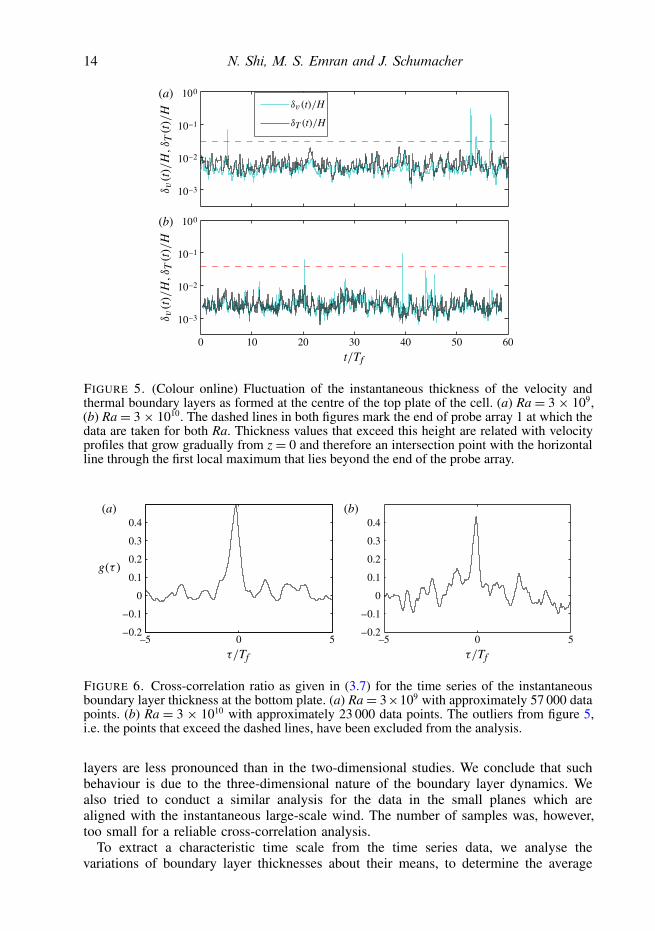
are obtained from the analysis in the planar observation window which is aligned withthe instantaneous wind. We can see that both thicknesses fluctuate strongly for bothRayleigh numbers. Similar to the two-dimensional DNS of Zhou et al. (2010), thefluctuations of the velocity boundary layer thickness are slightly stronger than thoseof the thermal boundary layer. In particular, we observe rare large thickness eventsfor the velocity which can be related to profiles that grow gradually from z = 0. Weperformed a Fourier analysis of both time series and could not detect a characteristictime scale, but a slowly decaying continuous spectrum which indicates a chaotic signal.The cross-correlation ratio, defined by (Zhou et al. 2010)
g(τ )= 〈[δv(t)− 〈δv〉t] [δT(t + τ)− 〈δT〉t]〉t√〈[δv(t)− 〈δv〉t]2〉t
√〈[δT(t)− 〈δT〉t]2〉t
, (3.7)
is plotted in figure 6 for the fluctuating boundary layer thicknesses at the bottomplate. The symbol 〈·〉t denotes a time average. Compared to two-dimensional DNS atPr = 0.7 (Zhou et al. 2010), the variation of the function g(τ ) is much less regular. Inboth of our cases the peak is slightly shifted to the left of zero, which would indicatethat variations of the thermal boundary layer cause variations of the velocity boundarylayer. The lead time is, however, shorter than the time that we will identify as thetime span for a plume detachment. The correlations between both fluctuating boundary
14 N. Shi, M. S. Emran and J. Schumacher
0 10 20 30 40 50 60
10–3
10–2
10–1
100
10–3
10–2
10–1
100(a)
(b)
FIGURE 5. (Colour online) Fluctuation of the instantaneous thickness of the velocity andthermal boundary layers as formed at the centre of the top plate of the cell. (a) Ra = 3 × 10⁹,(b) Ra= 3× 10¹⁰. The dashed lines in both figures mark the end of probe array 1 at which thedata are taken for both Ra. Thickness values that exceed this height are related with velocityprofiles that grow gradually from z= 0 and therefore an intersection point with the horizontalline through the first local maximum that lies beyond the end of the probe array.
–5 0 5 –5 0 5–0.2
–0.1
0
0.1
0.2
0.3
0.4
–0.2
–0.1
0
0.1
0.2
0.3
0.4(a) (b)
FIGURE 6. Cross-correlation ratio as given in (3.7) for the time series of the instantaneousboundary layer thickness at the bottom plate. (a) Ra= 3×10⁹ with approximately 57 000 datapoints. (b) Ra = 3 × 10¹⁰ with approximately 23 000 data points. The outliers from figure 5,i.e. the points that exceed the dashed lines, have been excluded from the analysis.
layers are less pronounced than in the two-dimensional studies. We conclude that suchbehaviour is due to the three-dimensional nature of the boundary layer dynamics. Wealso tried to conduct a similar analysis for the data in the small planes which arealigned with the instantaneous large-scale wind. The number of samples was, however,too small for a reliable cross-correlation analysis.
To extract a characteristic time scale from the time series data, we analyse thevariations of boundary layer thicknesses about their means, to determine the average
Boundary layer structure in turbulent Rayleigh–Bénard convection 15
100 2000
0.05
0.10
–50
0
50
0.05
0.10
0.15
0.20
100 2000
0.05
0.10
–50
0
50
0.05
0.10
0.15
0.20
(a) (b)
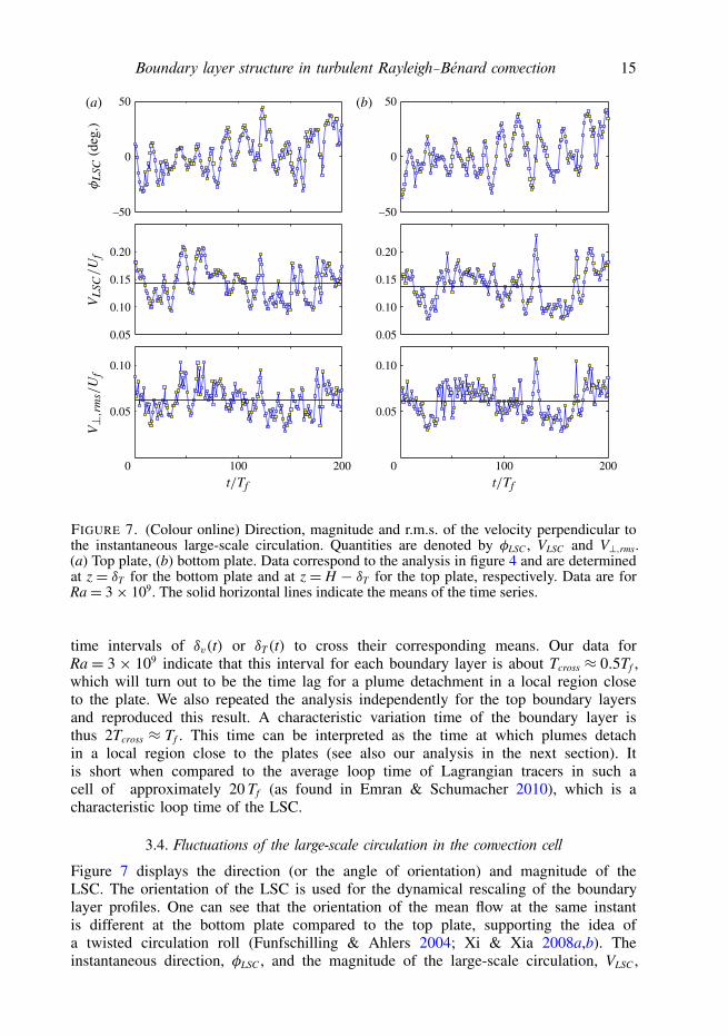
FIGURE 7. (Colour online) Direction, magnitude and r.m.s. of the velocity perpendicular tothe instantaneous large-scale circulation. Quantities are denoted by φLSC , VLSC and V⊥,rms.(a) Top plate, (b) bottom plate. Data correspond to the analysis in figure 4 and are determinedat z = δT for the bottom plate and at z = H − δT for the top plate, respectively. Data are forRa= 3× 10⁹. The solid horizontal lines indicate the means of the time series.
time intervals of δv(t) or δT(t) to cross their corresponding means. Our data forRa = 3 × 10⁹ indicate that this interval for each boundary layer is about Tcross ≈ 0.5Tf ,which will turn out to be the time lag for a plume detachment in a local region closeto the plate. We also repeated the analysis independently for the top boundary layersand reproduced this result. A characteristic variation time of the boundary layer isthus 2Tcross ≈ Tf . This time can be interpreted as the time at which plumes detachin a local region close to the plates (see also our analysis in the next section). Itis short when compared to the average loop time of Lagrangian tracers in such acell of approximately 20 Tf (as found in Emran & Schumacher 2010), which is acharacteristic loop time of the LSC.
3.4. Fluctuations of the large-scale circulation in the convection cell
Figure 7 displays the direction (or the angle of orientation) and magnitude of theLSC. The orientation of the LSC is used for the dynamical rescaling of the boundarylayer profiles. One can see that the orientation of the mean flow at the same instantis different at the bottom plate compared to the top plate, supporting the idea ofa twisted circulation roll (Funfschilling & Ahlers 2004; Xi & Xia 2008a,b). Theinstantaneous direction, φLSC , and the magnitude of the large-scale circulation, VLSC ,
16 N. Shi, M. S. Emran and J. Schumacher
are determined by
φLSC(t0)=⟨
arctanuy(x, y, z0, t0)
ux(x, y, z0, t0)
⟩Ar
, (3.8)
VLSC(t0)=⟨√
ux (x, y, z0, t0)2+uy (x, y, z0, t0)
2
⟩Ar
, (3.9)
where the subscript Ar denotes the average over a circular cross-section with r 6 0.88Rat z0 = δT for the bottom or z0 = H − δT for the top plate. Furthermore we showthe root-mean-square of the velocity vector, which is perpendicular to v = uxex + uyey.This cross-flow velocity vector is determined by the relation v⊥ · v = 0 at each point(x, y, z0) ∈ Ar. The quantity is given by
V⊥,rms(t0)=√〈v2⊥(x, y, z0, t0)〉Ar
. (3.10)
It is seen that the circulation varies strongly in both amplitude and angle. In thecase of the angle we do observe a fast variation of the orientation over a range ofapproximately 50◦. On average the LSC is almost perfectly aligned with the x-axis(φ = 0) along which we have positioned the probe arrays 1, 2 and 4. The amountof fluctuation perpendicular to the large-scale wind velocity is also significant, andreaches up to 50 % of VLSC . The mean magnitude of VLSC can be used to estimatean LSC turnover time by τLSC = V
−1LSC × 2π(H/2) ≈ 21Tf , which is close to the
estimate from previous Lagrangian studies, as mentioned at the end of § 3.3 (Emran& Schumacher 2010). It is also consistent with an LSC turnover time of 18 Tf (whichcorresponds to 35 s) in the Barrel of Ilmenau. Furthermore, Ahlers et al. (2009a)report a time scale of 25 s from their helium experiment at Γ = 1/2, which can beconverted into 33 s by multiplication with 4/3 for a unit aspect ratio cell.
Superimposed on the fast oscillation is a very slow drift of the angle (see panelsin the upper row of figure 7). This indicates that a small fraction of a very slowprecession of the large-scale circulation is being observed. This slow mode can bepresent since the mean orientation of the roll is not locked in one particular direction,as is frequently observed in experiments. We are, however, not able to study this slowmode of motion in our DNS since it would exceed our present numerical capabilitiesin terms of the length of the simulation. Better access to this very slow large-scaledynamics would require investigation with low-dimensional models (Brown & Ahlers2009) or models obtained by proper orthogonal decomposition of the turbulence fields(Bailon-Cuba & Schumacher 2011).
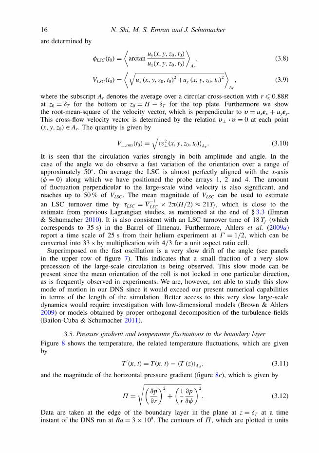
3.5. Pressure gradient and temperature fluctuations in the boundary layerFigure 8 shows the temperature, the related temperature fluctuations, which are givenby
T ′(x, t)= T(x, t)− 〈T (z)〉A,t, (3.11)
and the magnitude of the horizontal pressure gradient (figure 8c), which is given by
Π =√(
∂p
∂r
)2
+(
1r
∂p
∂φ
)2
. (3.12)
Data are taken at the edge of the boundary layer in the plane at z = δT at a timeinstant of the DNS run at Ra= 3× 10⁹. The contours of Π , which are plotted in units
Boundary layer structure in turbulent Rayleigh–Bénard convection 17
0.900.850.800.750.700.650.600.550.500.450.40
(a)
(b) (c) (d)
FIGURE 8. Spatial correlation between the horizontal pressure gradient and temperature. (a)A horizontal cross-section of temperature T . The three contour plots below show (b) thethresholded temperature fluctuations T ′c, (c) the pressure gradient magnitude Πc, and (d) theproduct of both. Data are for Ra = 3 × 10⁹ and taken at z = δT . Pressure gradient magnitudeand product are shown in logarithmic units.
of the logarithm to the base of 10, imply that the pressure field varies strongly in thehorizontal plane at this height. In more detail, we display in figure 8 the quantity
Πc(x, t)=Π(x, t)Θ(Π − C), (3.13)
with the Heaviside function Θ and a threshold C. The pressure field in theincompressible flow limit is directly connected with the flow, and thus reflects thehigh spatial (and temporal) variability of the flow, including the large-scale circulationas analysed in figure 7.
Theerthan & Arakeri (1998) and Puthenveettil & Arakeri (2005) have discussedin detail that the horizontal pressure differences are an essential driver of thevelocity inside the boundary layer. In figure 9 we compare vertical profiles takenwith respect to time and different horizontal cross-sections A = πr2. Averages of theradial component of the pressure gradient 〈∂p/∂r〉A,t and the Reynolds stress 〈u′ru′z〉A,tare shown as examples. The pressure gradient component is non-negligible in theboundary layer. As in van Reeuwijk et al. (2008b), we compare here the ratio
γ =
∣∣∣∣∫ δv
0〈∂p/∂r (z)〉A,t dz
∣∣∣∣| 〈u′ru′z〉A,t |δv
. (3.14)
Note that both terms contribute to the friction factor. Values of γ = 1.16, 1.77 and5.21 were obtained for cross-sections A with radius R, R/2 and R/5. We thus confirm
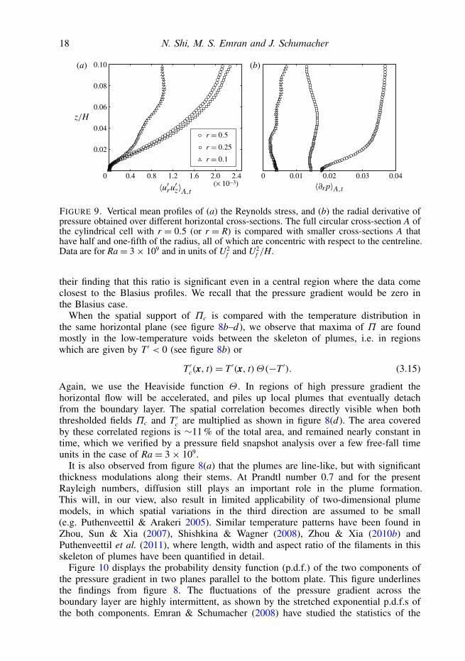
18 N. Shi, M. S. Emran and J. Schumacher
0 0.4 0.8 2.42.01.61.2
0.02
0.04
0 0.01 0.02 0.03 0.04
0.06
0.08
0.10(a) (b)
(× 10–3)
FIGURE 9. Vertical mean profiles of (a) the Reynolds stress, and (b) the radial derivative ofpressure obtained over different horizontal cross-sections. The full circular cross-section A ofthe cylindrical cell with r = 0.5 (or r = R) is compared with smaller cross-sections A thathave half and one-fifth of the radius, all of which are concentric with respect to the centreline.Data are for Ra= 3× 10⁹ and in units of U2
f and U2f /H.
their finding that this ratio is significant even in a central region where the data comeclosest to the Blasius profiles. We recall that the pressure gradient would be zero inthe Blasius case.
When the spatial support of Πc is compared with the temperature distribution inthe same horizontal plane (see figure 8b–d), we observe that maxima of Π are foundmostly in the low-temperature voids between the skeleton of plumes, i.e. in regionswhich are given by T ′ < 0 (see figure 8b) or
T ′c(x, t)= T ′(x, t)Θ(−T ′). (3.15)
Again, we use the Heaviside function Θ . In regions of high pressure gradient thehorizontal flow will be accelerated, and piles up local plumes that eventually detachfrom the boundary layer. The spatial correlation becomes directly visible when boththresholded fields Πc and T ′c are multiplied as shown in figure 8(d). The area coveredby these correlated regions is ∼11 % of the total area, and remained nearly constant intime, which we verified by a pressure field snapshot analysis over a few free-fall timeunits in the case of Ra= 3× 10⁹.
It is also observed from figure 8(a) that the plumes are line-like, but with significantthickness modulations along their stems. At Prandtl number 0.7 and for the presentRayleigh numbers, diffusion still plays an important role in the plume formation.This will, in our view, also result in limited applicability of two-dimensional plumemodels, in which spatial variations in the third direction are assumed to be small(e.g. Puthenveettil & Arakeri 2005). Similar temperature patterns have been found inZhou, Sun & Xia (2007), Shishkina & Wagner (2008), Zhou & Xia (2010b) andPuthenveettil et al. (2011), where length, width and aspect ratio of the filaments in thisskeleton of plumes have been quantified in detail.
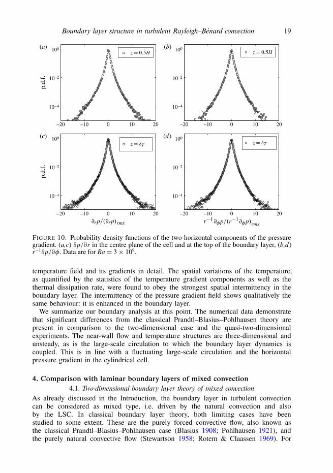
Figure 10 displays the probability density function (p.d.f.) of the two components ofthe pressure gradient in two planes parallel to the bottom plate. This figure underlinesthe findings from figure 8. The fluctuations of the pressure gradient across theboundary layer are highly intermittent, as shown by the stretched exponential p.d.f.s ofthe both components. Emran & Schumacher (2008) have studied the statistics of the
Boundary layer structure in turbulent Rayleigh–Bénard convection 19
–20 –10 0 10 20 –20 –10 0 10 20
10–4
10–2
100
–20 –10 0 10 20 –20 –10 0 10 20
10–4
10–2
100
10–4
10–2
100
10–4
10–2
100(a) (b)
(c) (d)
FIGURE 10. Probability density functions of the two horizontal components of the pressuregradient. (a,c) ∂p/∂r in the centre plane of the cell and at the top of the boundary layer, (b,d)r−1∂p/∂φ. Data are for Ra= 3× 10⁹.
temperature field and its gradients in detail. The spatial variations of the temperature,as quantified by the statistics of the temperature gradient components as well as thethermal dissipation rate, were found to obey the strongest spatial intermittency in theboundary layer. The intermittency of the pressure gradient field shows qualitatively thesame behaviour: it is enhanced in the boundary layer.
We summarize our boundary analysis at this point. The numerical data demonstratethat significant differences from the classical Prandtl–Blasius–Pohlhausen theory arepresent in comparison to the two-dimensional case and the quasi-two-dimensionalexperiments. The near-wall flow and temperature structures are three-dimensional andunsteady, as is the large-scale circulation to which the boundary layer dynamics iscoupled. This is in line with a fluctuating large-scale circulation and the horizontalpressure gradient in the cylindrical cell.
4. Comparison with laminar boundary layers of mixed convection4.1. Two-dimensional boundary layer theory of mixed convection
As already discussed in the Introduction, the boundary layer in turbulent convectioncan be considered as mixed type, i.e. driven by the natural convection and alsoby the LSC. In classical boundary layer theory, both limiting cases have beenstudied to some extent. These are the purely forced convective flow, also known asthe classical Prandtl–Blasius–Pohlhausen case (Blasius 1908; Pohlhausen 1921), andthe purely natural convective flow (Stewartson 1958; Rotem & Claassen 1969). For
20 N. Shi, M. S. Emran and J. Schumacher
mixed convection, the Boussinesq equations of motion (2.1)–(2.3) are reduced to thefollowing set of two-dimensional and steady boundary layer equations (Schlichting1957):
ux∂ux
∂x+ uz
∂ux
∂z=−∂p
∂x+ ν ∂
2ux
∂z2, (4.1)
0=−∂p
∂z+ αgT, (4.2)
∂ux
∂x+ ∂uz
∂z= 0, (4.3)
ux∂T
∂x+ uz
∂T
∂z= κ ∂
2T
∂z2. (4.4)
The corresponding dimensionless parameters are the Reynolds and Grashof numbers ofthe problem, which are given by
Rex = V∞x
ν, Grx = gα(Tw − T∞)x3
ν2. (4.5)
At the plate (z = 0), the boundary conditions are T = Tw and ux = uz = 0. Far awayfrom the plate (z→∞), it follows that T = T∞ and
ux(z→∞)={
V∞ for forced convection,0 for natural convection.
(4.6)
In both cases one can define similarity variables η and parameters ε for theperturbation expansion of mixed convection. In agreement with the definitions(3.1)–(3.3) we can proceed as follows. Starting from purely forced convection, theexpansion reads (Sparrow & Minkowycz 1962)
ur(x, z)
V∞= f ′0(η)+ εf ′1(η)+ · · · , (4.7)
Ξ(x, z)= T(x, z)− T∞Tw − T∞
= θ0(η)+ εθ1(η)+ · · · , (4.8)
while starting from purely natural convection, it reads (Stewartson 1958)
ur(x, z)
Vn(x)= g′0(η)+ εg′1(η)+ · · · , (4.9)
Ξ(x, z)= T(x, z)− T∞Tw − T∞
= χ0(η)+ εχ1(η)+ · · · , (4.10)
where functions with index 0 represent the unperturbed velocity components ortemperature. Furthermore Vn(x) = (νg2α2 (Tw − T∞)
2 x)1/5
. More details are providedin the Appendix for completeness. The resulting systems of perturbation equations forthe boundary value problems can be solved by a shooting method using a fourth-orderRunge–Kutta scheme (Hieber 1973).
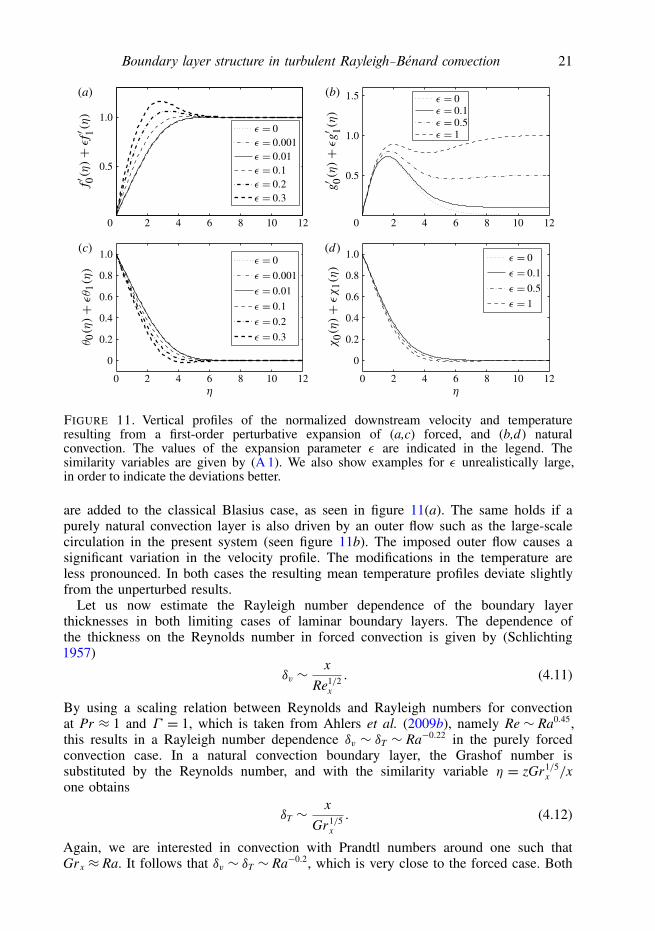
Figure 11 shows the resulting mean streamwise flow and temperature profiles forthe case of Pr = 0.7. The perturbation expansion has been carried out to first orderonly, and curves are plotted for different magnitudes of ε as given in (A 2). Severalaspects can be observed. The boundary layer flow is accelerated if buoyancy effects
Boundary layer structure in turbulent Rayleigh–Bénard convection 21
2 4 6 8 10 120
0.5
1.0
2 4 6 8 10 12
0 2 4 6 8 10 12 0 2 4 6 8 10 12
0
0.2
0.4
0.6
0.8
1.0
0
0.2
0.4
0.6
0.8
1.0
0
0.5
1.0
1.5(a) (b)
(c) (d)
FIGURE 11. Vertical profiles of the normalized downstream velocity and temperatureresulting from a first-order perturbative expansion of (a,c) forced, and (b,d) naturalconvection. The values of the expansion parameter ε are indicated in the legend. Thesimilarity variables are given by (A 1). We also show examples for ε unrealistically large,in order to indicate the deviations better.
are added to the classical Blasius case, as seen in figure 11(a). The same holds if apurely natural convection layer is also driven by an outer flow such as the large-scalecirculation in the present system (seen figure 11b). The imposed outer flow causes asignificant variation in the velocity profile. The modifications in the temperature areless pronounced. In both cases the resulting mean temperature profiles deviate slightlyfrom the unperturbed results.
Let us now estimate the Rayleigh number dependence of the boundary layerthicknesses in both limiting cases of laminar boundary layers. The dependence ofthe thickness on the Reynolds number in forced convection is given by (Schlichting1957)
δv ∼ x
Re1/2x
. (4.11)
By using a scaling relation between Reynolds and Rayleigh numbers for convectionat Pr ≈ 1 and Γ = 1, which is taken from Ahlers et al. (2009b), namely Re ∼ Ra0.45,this results in a Rayleigh number dependence δv ∼ δT ∼ Ra−0.22 in the purely forcedconvection case. In a natural convection boundary layer, the Grashof number issubstituted by the Reynolds number, and with the similarity variable η = zGr1/5
x /xone obtains
δT ∼ x
Gr1/5x
. (4.12)
Again, we are interested in convection with Prandtl numbers around one such thatGrx ≈ Ra. It follows that δv ∼ δT ∼ Ra−0.2, which is very close to the forced case. Both
22 N. Shi, M. S. Emran and J. Schumacher
scaling estimates suggest that the differences in the Rayleigh number dependence ofthe boundary layer thicknesses are rather small when both limits – natural and forcedconvection – are compared. With only two runs at different Rayleigh numbers, we arenot able to conduct scaling laws of the thicknesses with respect to Ra.
4.2. Boundary layer dynamics in a small observation windowThe present direct numerical simulations give us the opportunity to zoom into theboundary layer dynamics at higher Rayleigh numbers, and to test how closely the localprofiles match the results of the classical boundary layer theories that we have justdiscussed. Out of the comprehensive data record, we have picked two characteristicdynamic sequences of the boundary layer structures: a plume detachment event andthe post-plume-detachment phase for which the boundary layer relaminarizes. Eachof these typical sequences covers a time lag of ∼0.45Tf for our data at eachRayleigh number. We consider them to be the two essential building blocks of theboundary layer dynamics. In order to connect with classical boundary layer theory, weanalyse the fields again in a small vertical observation plane that is aligned with theinstantaneous large-scale circulation. Our observation window has a size of length ×height equal to 9δT×9δT for Ra= 3×10⁹ and 19δT×19δT for Ra= 3×10¹⁰. The densetemporal output of the data spans 35Tf for Ra = 3 × 10⁹ and 5Tf for Ra = 3 × 10¹⁰
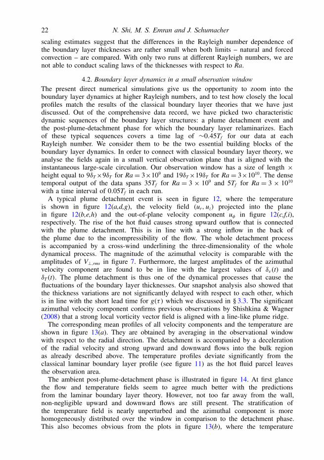
with a time interval of 0.05Tf in each run.A typical plume detachment event is seen in figure 12, where the temperature
is shown in figure 12(a,d,g), the velocity field (ur, uz) projected into the planein figure 12(b,e,h) and the out-of-plane velocity component uφ in figure 12(c,f,i),respectively. The rise of the hot fluid causes strong upward outflow that is connectedwith the plume detachment. This is in line with a strong inflow in the back ofthe plume due to the incompressibility of the flow. The whole detachment processis accompanied by a cross-wind underlining the three-dimensionality of the wholedynamical process. The magnitude of the azimuthal velocity is comparable with theamplitudes of V⊥,rms in figure 7. Furthermore, the largest amplitudes of the azimuthalvelocity component are found to be in line with the largest values of δv(t) andδT(t). The plume detachment is thus one of the dynamical processes that cause thefluctuations of the boundary layer thicknesses. Our snapshot analysis also showed thatthe thickness variations are not significantly delayed with respect to each other, whichis in line with the short lead time for g(τ ) which we discussed in § 3.3. The significantazimuthal velocity component confirms previous observations by Shishkina & Wagner(2008) that a strong local vorticity vector field is aligned with a line-like plume ridge.
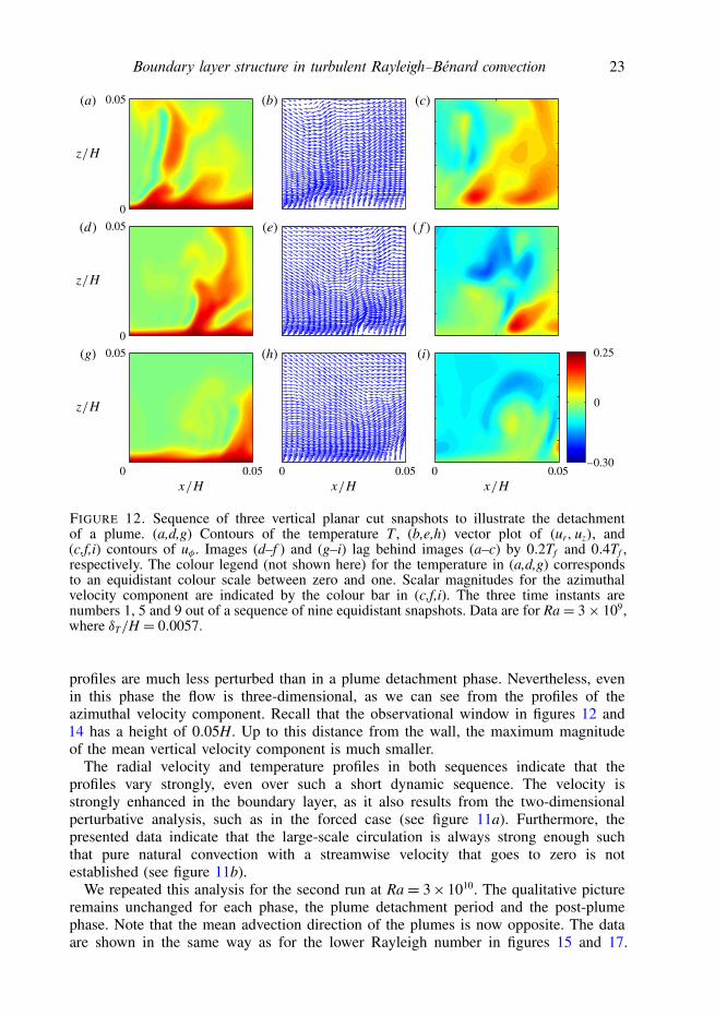
The corresponding mean profiles of all velocity components and the temperature areshown in figure 13(a). They are obtained by averaging in the observational windowwith respect to the radial direction. The detachment is accompanied by a decelerationof the radial velocity and strong upward and downward flows into the bulk regionas already described above. The temperature profiles deviate significantly from theclassical laminar boundary layer profile (see figure 11) as the hot fluid parcel leavesthe observation area.
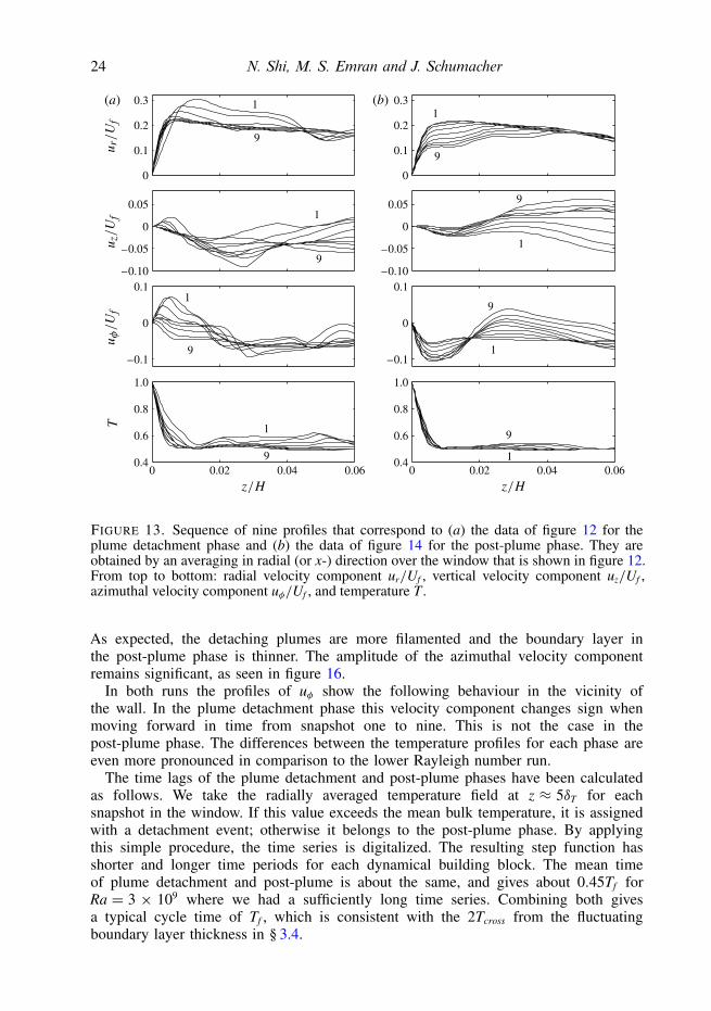
The ambient post-plume-detachment phase is illustrated in figure 14. At first glancethe flow and temperature fields seem to agree much better with the predictionsfrom the laminar boundary layer theory. However, not too far away from the wall,non-negligible upward and downward flows are still present. The stratification ofthe temperature field is nearly unperturbed and the azimuthal component is morehomogeneously distributed over the window in comparison to the detachment phase.This also becomes obvious from the plots in figure 13(b), where the temperature
Boundary layer structure in turbulent Rayleigh–Bénard convection 23
0.05–0.30
0
0.25
0
0.05
0
0.05
0
0.05
0 0.05 0 0.05
(a)
(d)
(g)
(b)
(e)
(h)
(c)
( f )
(i)
FIGURE 12. Sequence of three vertical planar cut snapshots to illustrate the detachmentof a plume. (a,d,g) Contours of the temperature T , (b,e,h) vector plot of (ur, uz), and(c,f,i) contours of uφ . Images (d–f ) and (g–i) lag behind images (a–c) by 0.2Tf and 0.4Tf ,respectively. The colour legend (not shown here) for the temperature in (a,d,g) correspondsto an equidistant colour scale between zero and one. Scalar magnitudes for the azimuthalvelocity component are indicated by the colour bar in (c,f,i). The three time instants arenumbers 1, 5 and 9 out of a sequence of nine equidistant snapshots. Data are for Ra= 3× 10⁹,where δT/H = 0.0057.
profiles are much less perturbed than in a plume detachment phase. Nevertheless, evenin this phase the flow is three-dimensional, as we can see from the profiles of theazimuthal velocity component. Recall that the observational window in figures 12 and14 has a height of 0.05H. Up to this distance from the wall, the maximum magnitudeof the mean vertical velocity component is much smaller.
The radial velocity and temperature profiles in both sequences indicate that theprofiles vary strongly, even over such a short dynamic sequence. The velocity isstrongly enhanced in the boundary layer, as it also results from the two-dimensionalperturbative analysis, such as in the forced case (see figure 11a). Furthermore, thepresented data indicate that the large-scale circulation is always strong enough suchthat pure natural convection with a streamwise velocity that goes to zero is notestablished (see figure 11b).
We repeated this analysis for the second run at Ra= 3×10¹⁰. The qualitative pictureremains unchanged for each phase, the plume detachment period and the post-plumephase. Note that the mean advection direction of the plumes is now opposite. The dataare shown in the same way as for the lower Rayleigh number in figures 15 and 17.
24 N. Shi, M. S. Emran and J. Schumacher
0 0.02 0.04 0.06
1
9
9
1
1
9
1
9
1
9
9
1
9
1
1
9
0
0.1
0.2
0.3
–0.10
–0.05
0
0.05
–0.1
0
0.1
0.4
0.6
0.8
1.0
0 0.02 0.04 0.06
0
0.1
0.2
0.3
–0.10
–0.05
0
0.05
–0.1
0
0.1
0.4
0.6
0.8
1.0
(a) (b)
FIGURE 13. Sequence of nine profiles that correspond to (a) the data of figure 12 for theplume detachment phase and (b) the data of figure 14 for the post-plume phase. They areobtained by an averaging in radial (or x-) direction over the window that is shown in figure 12.From top to bottom: radial velocity component ur/Uf , vertical velocity component uz/Uf ,azimuthal velocity component uφ/Uf , and temperature T .
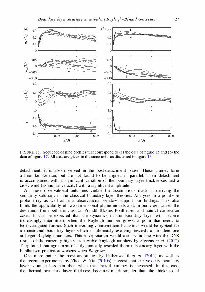
As expected, the detaching plumes are more filamented and the boundary layer inthe post-plume phase is thinner. The amplitude of the azimuthal velocity componentremains significant, as seen in figure 16.
In both runs the profiles of uφ show the following behaviour in the vicinity ofthe wall. In the plume detachment phase this velocity component changes sign whenmoving forward in time from snapshot one to nine. This is not the case in thepost-plume phase. The differences between the temperature profiles for each phase areeven more pronounced in comparison to the lower Rayleigh number run.
The time lags of the plume detachment and post-plume phases have been calculatedas follows. We take the radially averaged temperature field at z ≈ 5δT for eachsnapshot in the window. If this value exceeds the mean bulk temperature, it is assignedwith a detachment event; otherwise it belongs to the post-plume phase. By applyingthis simple procedure, the time series is digitalized. The resulting step function hasshorter and longer time periods for each dynamical building block. The mean timeof plume detachment and post-plume is about the same, and gives about 0.45Tf forRa = 3 × 10⁹ where we had a sufficiently long time series. Combining both givesa typical cycle time of Tf , which is consistent with the 2Tcross from the fluctuatingboundary layer thickness in § 3.4.
Boundary layer structure in turbulent Rayleigh–Bénard convection 25
0.05
0
0.05
0
0.05
0
0.05
0 0.05 0 0.05
(b)
(e)
(h)
(c)
( f )
(i)
–0.30
0
0.25
(a)
(d)
(g)
FIGURE 14. Sequence of three vertical planar cut snapshots to illustrate the phase after thedetachment of a plume. (a,d,g) Contours of the temperature T , (b,e,h) vector plot of (ur, uz),and (c,f,i) contours of uφ . Images (d–f ) and (g–i) lag behind images (a–c) by 0.2Tf and 0.4Tf ,respectively. The colour legend (not shown here) for the temperature in (a,d,g) correspondsto an equidistant colour scale between zero and one. Scalar magnitudes for the azimuthalvelocity component are indicated by the colour bar in (c,f,i). The three time instants arenumbers 1, 5 and 9 out of a sequence of nine equidistant snapshots. Data are again forRa= 3× 10⁹.
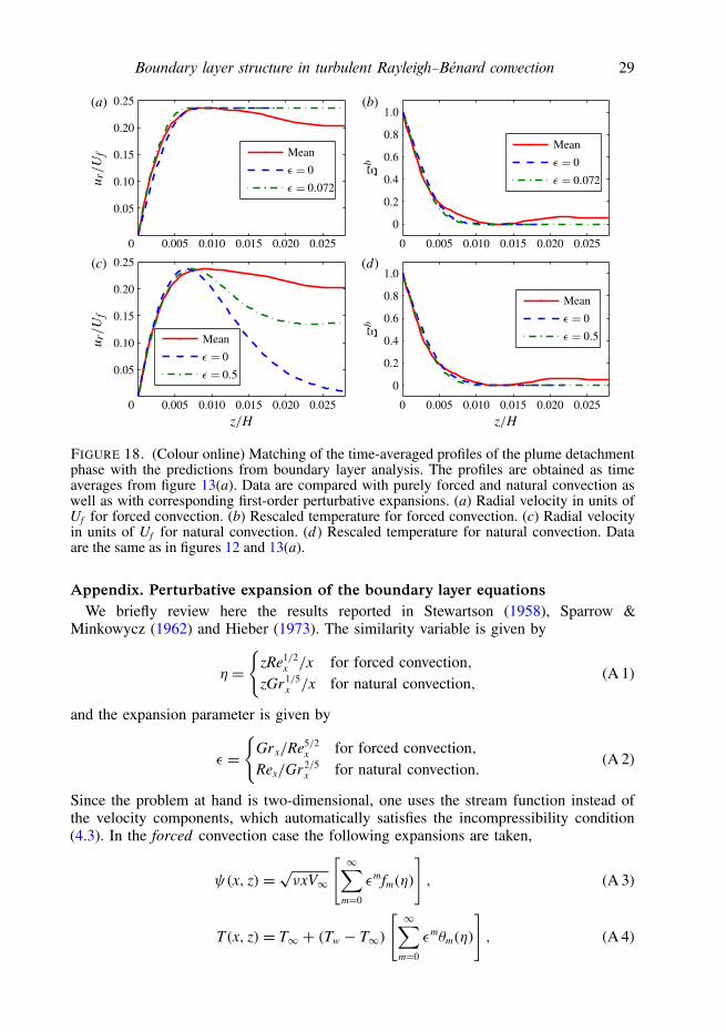
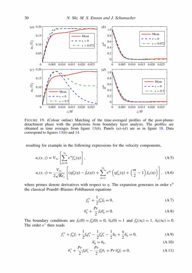
In figures 18 and 19 we try to match the time-averaged profiles obtained from theshort dynamic sequences with the predictions from the mixed convection boundarylayer theory including the first-order perturbation. Our profiles again display thefeatures we detected in the original time series analysis over much longer timeintervals (see figure 3). However, we can now trace the slower increase of thetemperature profile clearly back to the plume detachment events. Similar connectionholds for the velocity profile in the post-plume-detachment phase. The local dynamicalbehaviour suggests that the three-dimensional large-scale circulation is now connectedto the boundary layer section. Inflows from the top of our observation window areobserved, which cause large variations in the velocity profiles. These variations reachthe same magnitude as in the plume detachment phase and manifest in the deviationsfor velocity profile 〈ur〉r in the observation plane (see figure 19). We have thus shownthat the simulation data combine elements of forced and natural convection. Neither inthe plume detachment nor in the post-plume phase can the theoretical profiles of boththe temperature and velocity fields be perfectly matched to the data. The dynamicsclose to the walls is always three-dimensional.
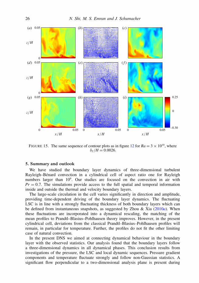
26 N. Shi, M. S. Emran and J. Schumacher
0.05
0
0.05
0
0.05
0
0.05
0 0.05 0 0.05
(b)
(e)
(h)
(c)
( f )
(i)
–0.30
0
0.25
(a)
(d)
(g)
FIGURE 15. The same sequence of contour plots as in figure 12 for Ra= 3× 10¹⁰, whereδT/H = 0.0026.
5. Summary and outlookWe have studied the boundary layer dynamics of three-dimensional turbulent
Rayleigh–Benard convection in a cylindrical cell of aspect ratio one for Rayleighnumbers larger than 109. Our studies are focused on the convection in air withPr = 0.7. The simulations provide access to the full spatial and temporal informationinside and outside the thermal and velocity boundary layers.
The large-scale circulation in the cell varies significantly in direction and amplitude,providing time-dependent driving of the boundary layer dynamics. The fluctuatingLSC is in line with a strongly fluctuating thickness of both boundary layers which canbe defined from instantaneous snapshots, as suggested by Zhou & Xia (2010a). Whenthese fluctuations are incorporated into a dynamical rescaling, the matching of themean profiles to Prandtl–Blasius–Pohlhausen theory improves. However, in the presentcylindrical cell, deviations from the classical Prandtl–Blasius–Pohlhausen profiles willremain, in particular for temperature. Further, the profiles do not fit the other limitingcase of natural convection.
In the present DNS we aimed at connecting dynamical behaviour in the boundarylayer with the observed statistics. Our analysis found that the boundary layers followa three-dimensional dynamics in all dynamical phases. This conclusion results frominvestigations of the pressure, the LSC and local dynamic sequences. Pressure gradientcomponents and temperature fluctuate strongly and follow non-Gaussian statistics. Asignificant flow perpendicular to a two-dimensional analysis plane is present during
Boundary layer structure in turbulent Rayleigh–Bénard convection 27
9
1
1
9
9
1
9
1
1
9
1
9
1
9
9
10 0.02 0.04 0.06
0
0.1
0.2
0.3
–0.10
–0.05
0
0.05
0.1
0.2
0
0.4
0.6
0.8
1.0
0
0.1
0.2
0.3
–0.10
–0.05
0
0.05
0.1
0.2
0
0.4
0.6
0.8
1.0
0 0.02 0.04 0.06
(a) (b)
FIGURE 16. Sequence of nine profiles that correspond to (a) the data of figure 15 and (b) thedata of figure 17. All data are given in the same units as discussed in figure 13.
detachment; it is also observed in the post-detachment phase. These plumes forma line-like skeleton, but are not found to be aligned in parallel. Their detachmentis accompanied with a significant variation of the boundary layer thicknesses and across-wind (azimuthal velocity) with a significant amplitude.
All these observational outcomes violate the assumptions made in deriving thesimilarity solutions in the classical boundary layer theories. Analyses in a pointwiseprobe array as well as in a observational window support our findings. This alsolimits the applicability of two-dimensional plume models and, in our view, causes thedeviations from both the classical Prandtl–Blasius–Pohlhausen and natural convectioncases. It can be expected that the dynamics in the boundary layer will becomeincreasingly intermittent when the Rayleigh number grows, a point that needs tobe investigated further. Such increasingly intermittent behaviour would be typical fora transitional boundary layer which is ultimately evolving towards a turbulent oneat larger Rayleigh numbers. This interpretation would also be in line with the DNSresults of the currently highest achievable Rayleigh numbers by Stevens et al. (2012).They found that agreement of a dynamically rescaled thermal boundary layer with thePohlhausen prediction worsens when Ra grows.
One more point: the previous studies by Puthenveettil et al. (2011) as well asthe recent experiments by Zhou & Xia (2010a) suggest that the velocity boundarylayer is much less perturbed when the Prandtl number is increased. In this case,the thermal boundary layer thickness becomes much smaller than the thickness of
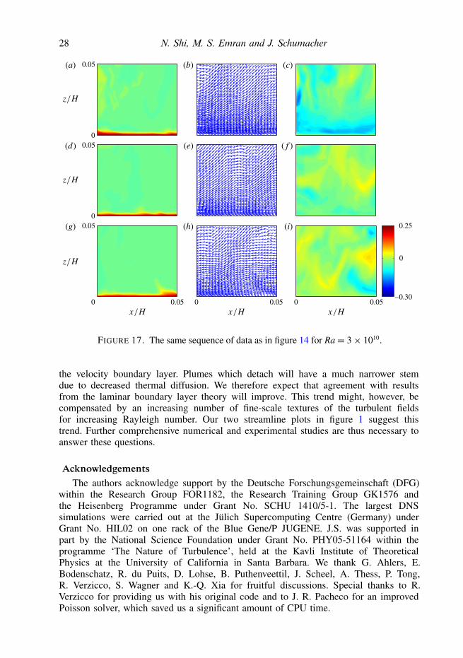
28 N. Shi, M. S. Emran and J. Schumacher
0.05
0
0.05
0
0.05
0
0.05
0 0.05 0 0.05
(b)
(e)
(h)
(c)
( f )
(i)
–0.30
0
0.25
(a)
(d)
(g)
FIGURE 17. The same sequence of data as in figure 14 for Ra= 3× 10¹⁰.
the velocity boundary layer. Plumes which detach will have a much narrower stemdue to decreased thermal diffusion. We therefore expect that agreement with resultsfrom the laminar boundary layer theory will improve. This trend might, however, becompensated by an increasing number of fine-scale textures of the turbulent fieldsfor increasing Rayleigh number. Our two streamline plots in figure 1 suggest thistrend. Further comprehensive numerical and experimental studies are thus necessary toanswer these questions.
AcknowledgementsThe authors acknowledge support by the Deutsche Forschungsgemeinschaft (DFG)
within the Research Group FOR1182, the Research Training Group GK1576 andthe Heisenberg Programme under Grant No. SCHU 1410/5-1. The largest DNSsimulations were carried out at the Julich Supercomputing Centre (Germany) underGrant No. HIL02 on one rack of the Blue Gene/P JUGENE. J.S. was supported inpart by the National Science Foundation under Grant No. PHY05-51164 within theprogramme ‘The Nature of Turbulence’, held at the Kavli Institute of TheoreticalPhysics at the University of California in Santa Barbara. We thank G. Ahlers, E.Bodenschatz, R. du Puits, D. Lohse, B. Puthenveettil, J. Scheel, A. Thess, P. Tong,R. Verzicco, S. Wagner and K.-Q. Xia for fruitful discussions. Special thanks to R.Verzicco for providing us with his original code and to J. R. Pacheco for an improvedPoisson solver, which saved us a significant amount of CPU time.
Boundary layer structure in turbulent Rayleigh–Bénard convection 29
0.005 0.010 0.015 0.020 0.025
Mean
0 0.005 0.010 0.015 0.020 0.025
MeanMean
Mean
0
0.05
0.10
0.15
0.20
0.25
0
0.2
0.4
0.6
0.8
1.0(c) (d)
0.005 0.010 0.015 0.020 0.025 0 0.005 0.010 0.015 0.020 0.0250
0.05
0.10
0.15
0.20
0.25
0
0.2
0.4
0.6
0.8
1.0(a) (b)
FIGURE 18. (Colour online) Matching of the time-averaged profiles of the plume detachmentphase with the predictions from boundary layer analysis. The profiles are obtained as timeaverages from figure 13(a). Data are compared with purely forced and natural convection aswell as with corresponding first-order perturbative expansions. (a) Radial velocity in units ofUf for forced convection. (b) Rescaled temperature for forced convection. (c) Radial velocityin units of Uf for natural convection. (d) Rescaled temperature for natural convection. Dataare the same as in figures 12 and 13(a).
Appendix. Perturbative expansion of the boundary layer equationsWe briefly review here the results reported in Stewartson (1958), Sparrow &
Minkowycz (1962) and Hieber (1973). The similarity variable is given by
η ={
zRe1/2x /x for forced convection,
zGr1/5x /x for natural convection,
(A 1)
and the expansion parameter is given by
ε ={Grx/Re
5/2x for forced convection,
Rex/Gr2/5x for natural convection.
(A 2)
Since the problem at hand is two-dimensional, one uses the stream function instead ofthe velocity components, which automatically satisfies the incompressibility condition(4.3). In the forced convection case the following expansions are taken,
ψ(x, z)=√νxV∞
[ ∞∑m=0
εmfm(η)
], (A 3)
T(x, z)= T∞ + (Tw − T∞)
[ ∞∑m=0
εmθm(η)
], (A 4)
30 N. Shi, M. S. Emran and J. Schumacher
MeanMean
Mean
Mean
0
0.05
0.10
0.15
0.20(c)
0.005 0.010 0.015 0.020 0.025 0 0.005 0.010 0.015 0.020 0.025
0
0.2
0.4
0.6
0.8
1.0(d)
0
0.05
0.10
0.15
0.20(a)
0.005 0.010 0.015 0.020 0.025 0 0.005 0.010 0.015 0.020 0.025
0
0.2
0.4
0.6
0.8
1.0(b)
FIGURE 19. (Colour online) Matching of the time-averaged profiles of the post-plume-detachment phase with the predictions from boundary layer analysis. The profiles areobtained as time averages from figure 13(b). Panels (a)–(d) are as in figure 18. Datacorrespond to figures 13(b) and 14.
resulting for example in the following expressions for the velocity components,
ux(x, z)= V∞
[ ∞∑m=0
εmf ′m(η)
], (A 5)
uz(x, z)= V∞2√Rex
[(ηf ′0(η)− f0(η))+
∞∑m=1
εm(ηf ′m(η)+
(m
2− 1)
fm(η))], (A 6)
where primes denote derivatives with respect to η. The expansion generates in order ε0
the classical Prandtl–Blasius–Pohlhausen equations
f ′′′0 +12
f ′′0 f0 = 0, (A 7)
θ ′′0 +Pr
2f0θ′0 = 0. (A 8)
The boundary conditions are f0(0) = f ′0(0) = 0, θ0(0) = 1 and f ′0(∞) = 1, θ0(∞) = 0.The order ε1 then reads
f ′′′1 + f ′′0 f1 + 12
f0f ′′1 −12
f ′0f ′1 −12
h0 + η2 h′0 = 0, (A 9)
h′0 = θ0, (A 10)
θ ′′1 +Pr
2f0θ′1 −
Pr
2f ′0θ1 + Pr θ ′0f1 = 0. (A 11)
Boundary layer structure in turbulent Rayleigh–Bénard convection 31
The additional boundary conditions are f1(0) = f ′1(0) = θ1(0) = 0 and f ′1(∞) =θ1(∞) = h0(∞) = 0. The last two terms of (A 9) containing h0 and h′0 as wellas (A 10) arise from the pressure term. In natural convection, the expansions areadapted to
ψ(x, z)= 5√ν3gα(Tw − T∞)x3
[ ∞∑m=0
εmgm(η)
], (A 12)
T(x, z)= T∞ + (Tw − T∞)
[ ∞∑m=0
εmχm(η)
]. (A 13)
The order ε0 was first discussed by Stewartson (1958) and given by
g′′′0 +35
g′′0g0 − 15
g′0g′0 −25
k0 + 25ηk′0 = 0, (A 14)
k′0 = χ0, (A 15)
χ ′′0 +3Pr
5g0χ
′0 = 0. (A 16)
The boundary conditions are g0(0) = g′0(0) = 0, χ0(0) = 1 and g′0(∞) = χ0(∞) =k0(∞)= 0. The perturbative expansion to mixed convection with order ε1 reads
g′′′1 +35
g′′1g0 − 15
g′1g′0 +25
g′′0g1 − 15
k1 + 25ηk′1 = 0, (A 17)
k′1 = χ1, (A 18)
χ ′′1 +3Pr
5g0χ
′1 +
Pr
5g′0χ1 + 2Pr
5χ ′0g1 = 0, (A 19)
with g1(0) = g′1(0) = χ1(0) = χ1(∞) = k1(∞) = 0 and g′1(∞) = 1. Again, k0 and k1
arise from the pressure term. Equations (A 7)–(A 11) and (A 14)–(A 19) were solved inorder to obtain the results displayed in figure 11.
R E F E R E N C E S
AHLERS, G., BODENSCHATZ, E., FUNFSCHILLING, D. & HOGG, J. 2009a TurbulentRayleigh–Benard convection for a Prandtl number of 0.67. J. Fluid Mech. 641, 157–167.
AHLERS, G., GROSSMANN, S. & LOHSE, D. 2009b Heat transfer & large-scale dynamics inturbulent Rayleigh–Benard convection. Rev. Mod. Phys. 81, 503–537.
BAILON-CUBA, J., EMRAN, M. S. & SCHUMACHER, J. 2010 Aspect ratio dependence of heattransfer and large-scale flow in turbulent convection. J. Fluid Mech. 655, 152–173.
BAILON-CUBA, J. & SCHUMACHER, J. 2011 Low-dimensional model of turbulent Rayleigh–Benardconvection in a Cartesian cell with square domain. Phys. Fluids 23, 077101.
BLASIUS, H. 1908 Grenzschichten in Flussigkeiten mit kleiner Reibung. Z. Math. Phys. 56, 1–37.BROWN, E. & AHLERS, G. 2009 The origin of oscillations of the large-scale circulation of turbulent
Rayleigh–Benard convection. J. Fluid Mech. 638, 383–400.EMRAN, M. S. & SCHUMACHER, J. 2008 Fine-scale statistics of temperature and its derivatives in
convective turbulence. J. Fluid Mech. 611, 13–34.EMRAN, M. S. & SCHUMACHER, J. 2010 Lagrangian tracer dynamics in a closed cylindrical
turbulent convection cell. Phys. Rev. E 82, 016303.FUJI, T. 1963 Theory of the steady laminar natural convection above a horizontal line source and a
point heat source. Intl J. Heat Mass Transfer 6, 597–606.
32 N. Shi, M. S. Emran and J. Schumacher
FUNFSCHILLING, D. & AHLERS, G. 2004 Plume motion and large-scale circulation in a cylindricalRayleigh–Benard cell. Phys. Rev. Lett. 92, 194502.
GROSSMANN, S. & LOHSE, D. 2000 Scaling in thermal convection: a unifying theory. J. FluidMech. 407, 27–56.
GROTZBACH, G. 1983 Spatial resolution requirements for direct numerical simulation of theRayleigh–Benard convection. J. Comput. Phys. 49, 241–264.
HIEBER, C. A. 1973 Mixed convection above a heated horizontal surface. Intl J. Heat Mass Transfer16, 769–785.
MISHRA, P. K., DE, A. K., VERMA, M. K. & ESWARAN, V. 2011 Dynamics of reorientations andreversals of large-scale flow in Rayleigh–Benard convection. J. Fluid Mech. 668, 480–499.
POHLHAUSEN, E. 1921 Der Warmetausch zwischen festen Korpern und Flussigkeiten mit kleinerReibung und kleiner Warmeleitung. Z. Angew. Math. Mech. 1, 115–121.
PRANDTL, L. 1905 Uber Flussigkeitsbewegung bei sehr kleiner Reibung. In Proceedings of the ThirdInternational Mathematicians’ Congress, Heidelberg, 1904, pp. 484–491. B. G. Teubner.
DU PUITS, R., RESAGK, C. & THESS, A. 2007a Mean velocity profile in confined turbulentconvection. Phys. Rev. Lett. 99, 234504.
DU PUITS, R., RESAGK, C. & THESS, A. 2007b Breakdown of wind in turbulent thermalconvection. Phys. Rev. E 75, 016302.
DU PUITS, R., RESAGK, C. & THESS, A. 2010 Measurements of the instantaneous local heat flux inturbulent Rayeigh–Benard convection. New J. Phys. 12, 075023.
PUTHENVEETTIL, B. A. & ARAKERI, J. H. 2005 Plume structure in high-Rayleigh-numberconvection. J. Fluid Mech. 542, 217–249.
PUTHENVEETTIL, B. A., GUNASEGARANE, G. S., AGRAWAL, Y. K., SCHMELING, D., BOSBACH,J. & ARAKERI, J. H. 2011 Length of near-wall plumes in turbulent convection. J. FluidMech. 685, 335–364.
ROTEM, Z. & CLAASSEN, L. 1969 Natural convection above unconfined horizontal surfaces. J. FluidMech. 39, 173–192.
SCHLICHTING, H. 1957 Boundary Layer Theory. McGraw-Hill.SHISHKINA, O., STEVENS, R. J. A. M., GROSSMANN, S. & LOHSE, D. 2010 Boundary layer
structure in turbulent thermal convection and its consequences for the required numericalresolution. New J. Phys. 12, 075022.
SHISHKINA, O. & WAGNER, C. 2008 Analysis of sheet-like thermal plumes in turbulentRayleigh–Benard convection. J. Fluid Mech. 599, 383–404.
SIGGIA, E. D. 1994 High Rayleigh number convection. Annu. Rev. Fluid Mech. 26, 137–168.SPARROW, E. M. & MINKOWYCZ, W. J. 1962 Buoyancy effects on horizontal boundary-layer flow
and heat transfer. Intl J. Heat Mass Transfer 5, 505–511.STEVENS, R. J. A. M., ZHOU, Q., GROSSMANN, S., VERZICCO, R., XIA, K.-Q. & LOHSE, D.
2012 Thermal boundary layer profiles in turbulent Rayleigh–Benard convection in a cylindricalsample. Phys. Rev. E 85, 027301.
STEWARTSON, K. 1958 On the free convection from a horizontal plate. Z. Angew. Math. Phys. 9,276–282.
SUN, C., CHEUNG, Y.-H. & XIA, K.-Q. 2008 Experimental studies of the viscous boundary layerproperties in turbulent Rayleigh–Benard convection. J. Fluid Mech. 605, 79–113.
THEERTHAN, S. A. & ARAKERI, J. H. 1998 A model for near-wall dynamics in turbulentRayleigh–Benard convection. J. Fluid Mech. 373, 221–254.
VAN REEUWIJK, M., JONKER, H. J. J. & HANJALIC, K. 2008a Wind and boundary layers inRayleigh–Benard convection. Part 1. Analysis and modelling. Phys. Rev. E 77, 036311.
VAN REEUWIJK, M., JONKER, H. J. J. & HANJALIC, K. 2008b Wind and boundary layers inRayleigh–Benard convection. Part 2. Boundary layer character and scaling. Phys. Rev. E 77,036312.
VERZICCO, R. & CAMUSSI, R. 2003 Numerical experiments on strongly turbulent thermalconvection in a slender cylindrical cell. J. Fluid Mech. 477, 19–49.
Boundary layer structure in turbulent Rayleigh–Bénard convection 33
VERZICCO, R. & ORLANDI, P. 1996 A finite-difference scheme for three-dimensional incompressibleflows in cylindrical coordinates. J. Comput. Phys. 123, 402–414.
XI, H.-D. & XIA, K.-Q. 2008a Azimuthal motion, reorientation, cessation, and reversal of thelarge-scale circulation in turbulent thermal convection: a comparative study in aspect ratio oneand one-half geometries. Phys. Rev. E 78, 036326.
XI, H.-D. & XIA, K.-Q. 2008b Flow mode transitions in turbulent thermal convection. Phys. Fluids20, 055104.
ZHOU, Q., STEVENS, R. J. A. M., SUGIYAMA, K., GROSSMANN, S., LOHSE, D. & XIA,K.-Q. 2010 Prandtl–Blasius temperature and velocity boundary-layer profiles in turbulentRayleigh–Benard convection. J. Fluid Mech. 664, 297–312.
ZHOU, Q., SUGIYAMA, K., STEVENS, R. J. A. M., GROSSMANN, S., LOHSE, D. & XIA, K.-Q.2011 Horizontal structures of velocity and temperature boundary layers in two-dimensionalnumerical turbulent Rayleigh–Benard convection. Phys. Fluids 23, 125104.
ZHOU, Q., SUN, C. & XIA, K.-Q. 2007 Morphological evolution of thermal plumes in turbulentRayleigh–Benard convection. Phys. Rev. Lett. 98, 074501.
ZHOU, Q. & XIA, K.-Q. 2010a Measured instantaneous viscous boundary layer in turbulentRayleigh–Benard convection. Phys. Rev. Lett. 104, 104301.
ZHOU, Q. & XIA, K.-Q. 2010b Physical and geometrical properties of thermal plumes in turbulentRayleigh–Benard convection. New J. Phys. 12, 075006.