Embed Size (px)
Citation preview
Combustion Modeling for
Diesel Engine Control Design
Von der Fakultat fur Maschinenwesen derRheinisch-Westfalischen Technischen Hochschule Aachen
zur Erlangung des akademischen Grades eines Doktors derIngenieurwissenschaften genehmigte Dissertation
vorgelegt von
Diplom-Ingenieur
Christian Felsch
aus Neuss
Berichter: Univ.-Prof. Dr.-Ing. Dr. h.c. Dr.-Ing. E.h. N. Peters
Univ.-Prof. Dr.-Ing. D. Abel
Tag der mundlichen Prufung: 27. August 2009
Diese Dissertation ist auf den Internetseiten
der Hochschulbibliothek online verfugbar.
Shaker VerlagAachen 2009
Berichte aus der Energietechnik
Christian Felsch
Combustion Modeling forDiesel Engine Control Design
WICHTIG: D 82 überprüfen !!!

Bibliographic information published by the Deutsche NationalbibliothekThe Deutsche Nationalbibliothek lists this publication in the DeutscheNationalbibliografie; detailed bibliographic data are available in the Internet athttp://dnb.d-nb.de.
Zugl.: D 82 (Diss. RWTH Aachen University, 2009)
Copyright Shaker Verlag 2009All rights reserved. No part of this publication may be reproduced, stored in aretrieval system, or transmitted, in any form or by any means, electronic,mechanical, photocopying, recording or otherwise, without the prior permissionof the publishers.
Printed in Germany.
ISBN 978-3-8322-8545-6ISSN 0945-0726
Shaker Verlag GmbH • P.O. BOX 101818 • D-52018 AachenPhone: 0049/2407/9596-0 • Telefax: 0049/2407/9596-9Internet: www.shaker.de • e-mail: [email protected]
Vorwort/Preface
Diese Arbeit entstand wahrend meiner Tatigkeit als wissenschaftlicher Mitarbeiteram Institut fur Technische Verbrennung (ehemals Institut fur Technische Mechanik)der RWTH Aachen University. Sie wurde im Rahmen des Teilprojekts B1 Mo-dellreduktion bei Niedertemperatur-Brennverfahren durch CFD-Simulationen undMehrzonen-Modelle im Sonderforschungsbereich 686 Modellbasierte Regelung derhomogenisierten Niedertemperatur-Verbrennung durchgefuhrt, der an der RWTHAachen University und der Universitat Bielefeld bearbeitet wird. Der DeutschenForschungsgemeinschaft danke ich in diesem Zusammenhang fur die finanzielleForderung.
Mein besonderer Dank gilt Herrn Professor Dr.-Ing. Dr. h.c. Dr.-Ing. E.h. NorbertPeters fur seine Unterstutzung, seine kritischen Anmerkungen und die mir gewahrteFreiheit. Herrn Professor Dr.-Ing. Dirk Abel danke ich fur sein stetiges Interessean meiner Arbeit und fur die Tatigkeit als weiterer Berichter. Herrn ProfessorDr.-Ing. (USA) Stefan Pischinger danke ich fur die Ubernahme des Vorsitzes derPrufungskommission.
Ausdrucklich mochte ich mich bei Jeremy Weckering, Vivak Luckhchoura, MichaelGauding, Bernhard Jochim, Bruno Kerschgens, Christoph Glawe, Johannes Kepp-ner, Hanno Friederichs, Benedikt Sonntag und Abhinav Sharma bedanken, diemich durch ihre Studien- oder Diplomarbeiten bzw. durch ihre Arbeit als wissen-schaftliche Hilfskrafte tatkraftig unterstutzt haben. Außerdem gilt mein Dankallen jetzigen und ehemaligen Mitarbeitern des Instituts fur Technische Verbren-nung, die ebenfalls zum Gelingen dieser Arbeit beigetragen haben. Ich bedankemich bei Christian Hasse, Stefan Vogel, Jost Weber, Frank Freikamp, Jens Ewald,Peter Spiekermann, Sylvie Honnet, Elmar Riesmeier, Christoph Kortschik, SvenJerzembeck, Rainer Dahms, Anyelo Vanegas, Olaf Rohl, Peng Zeng, JoachimBeeckmann, Hyun Woo Won, Klaus-Dieter Stoehr, Jens Henrik Gobbert, TomoyaWada, Lipo Wang, Stefanie Bordihn, Sonja Engels, Yvonne Lichtenfeld, DieterOsthoff, Bernd Binninger und Gunter Paczko.
Daruber hinaus bedanke ich mich sehr bei Peter Drews und vor allem bei KaiHoffmann vom Institut fur Regelungstechnik der RWTH Aachen University furdie hervorragende Zusammenarbeit im Sonderforschungsbereich 686.
iii
I would like to thank Andreas Lippert for making my research stays at GeneralMotors R&D in Warren, MI, USA, possible. Furthermore, I would like thankTom Sloane, Jaehoon Han, Mark Huebler, Brian Peterson, Vinod Natarajan, andCarl-Anders Hergart for our good collaboration there. Thanks are also due toNicole Wermuth of General Motors R&D for providing the experimental data onthe HCCI engine. My most sincere thanks go to Hardo Barths of General MotorsPowertrain, who provided me with valuable advice and ideas in numerous helpfuldiscussions.
Bei meinen Freunden Tobias Krockel, Torsten Moll, Simon Frischemeier, AdamGacka und Martin Ross bedanke ich mich fur unseren gemeinsamen Spaß amMaschinenbau.
Ein großer Dank gilt meinen Eltern, die mich in jeder Phase meiner Ausbildungunterstutzt und motiviert haben.
Meiner Freundin Kathrin Borggrebe danke ich ebenfalls sehr fur ihre außeror-dentliche Unterstutzung, auf die ich mich immer verlassen konnte.
Aachen, im August 2009
Christian Felsch
iv
Combustion Modeling for
Diesel Engine Control Design
Zusammenfassung
Gegenstand dieser Arbeit ist zunachst die Entwicklung eines konsistenten Mi-schungsmodells fur die interaktive Kopplung eines CFD-Codes und eines aufmehreren nulldimensionalen Reaktoren basierenden Mehrzonenmodells. Das in-teraktiv gekoppelte Modell ermoglicht eine rechenzeit-effiziente Modellierung vonHCCI- und PCCI-Verbrennung. Der physikalische Bereich im CFD-Code wird mit-tels dreier Phasenvariablen (Mischungsbruch, Verdunnung und totale Enthalpie)in mehrere Zonen unterteilt. Die Phasenvariablen reichen aus, um den ther-modynamischen Zustand jeder Zone zu definieren, da diese denselben Druckaufweisen. Jede Zone im CFD-Code wird durch eine korrespondierende Zone imnulldimensionalen Code abgebildet. Das Mehrzonenmodell lost die Chemie furjede Zone, und die Warmefreisetzung wird zum CFD-Code zuruckgefuhrt. DieSchwierigkeit bei dieser Methodik liegt darin, den thermodynamischen Zustandjeder Zone zwischen CFD-Code und nulldimensionalem Code konsistent zu hal-ten, nachdem die Initialisierung der Zonen im Mehrzonenmodell stattgefundenhat. Der thermodynamische Zustand jeder Zone (und daher auch die Phasen-variablen) verandert sich mit der Zeit aufgrund von Mischung und Quelltermen(z.B. Verdampfung des Brennstoffs, Wandwarmetransfer). Der Fokus dieser Ar-beit liegt auf einer einheitlichen Beschreibung der Mischung zwischen den Zonenim Phasenraum des nulldimensionalen Codes, basierend auf der Losung des CFD-Codes. Zwei Mischungsmodelle mit unterschiedlichen Stufen von Genauigkeit,Komplexitat und numerischem Aufwand werden beschrieben. Das am bestenausgearbeitete Mischungsmodell (sowie eine angemessene Behandlung der Quell-terme) halt den thermodynamischen Zustand der Zonen im CFD-Code und imnulldimensionalen Code identisch. Die Modelle werden auf einen Testfall derHCCI-Verbrennung in einem Benzinmotor angewandt. Von dort ausgehend wirdein Simulationsmodell fur PCCI-Verbrennung erstellt, welches fur die Entwicklunggeschlossener Regelkreise verwendet werden kann. Fur den Hochdruckteil des Mo-torzyklus’ wird das interaktiv gekoppelte CFD-Mehrzonenmodell systematisch zueinem eigenstandigen Mehrzonenmodell reduziert. Das eigenstandige Mehrzonen-modell wird um ein Mittelwertmodell erganzt, welches die Ladungswechselverlusteberucksichtigt. Das resultierende Modell ist in der Lage, PCCI-Verbrennung mitstationarer Genauigkeit zu beschreiben und ist gleichzeitig sehr effizient bezuglichder benotigten Rechenzeit. Das Modell wird weiterhin um eine identifizierte Sys-temdynamik erweitert, welche die stationaren Stellgroßen beeinflusst. Zu diesem
v

Zweck wird ein Wiener-Modell erstellt, welches das stationare Modell als einenichtlineare Systemabbildung verwendet. Auf diese Weise wird ein dynamischesnichtlineares Modell zur Abbildung der Regelstrecke Dieselmotor entworfen.
vi
Combustion Modeling for
Diesel Engine Control Design
Abstract
This thesis deals at first with the development of a consistent mixing model forthe interactive coupling (two-way-coupling) of a CFD code and a multi-zone codebased on multiple zero-dimensional reactors. The interactive coupling allows fora computationally efficient modeling of HCCI or PCCI combustion, respectively.The physical domain in the CFD code is subdivided into multiple zones based onthree phase variables (fuel mixture fraction, dilution, and total enthalpy). Thesephase variables are sufficient for the description of the thermodynamic state ofeach zone, assuming that each zone is at the same pressure. Each zone in the CFDcode is represented by a corresponding one in the zero-dimensional code. Thezero-dimensional code solves the chemistry for each zone, and the heat release isfed back into the CFD code. The difficulty in facing this kind of methodology isto keep the thermodynamic state of each zone consistent between the CFD codeand the zero-dimensional code after the initialization of the zones in the multi-zone code has taken place. The thermodynamic state of each zone (and therebythe phase variables) changes in time due to mixing and source terms (e.g., va-porization of fuel, wall heat transfer). The focus of this work lies on a consistentdescription of the mixing between the zones in phase space in the zero-dimensionalcode, based on the solution of the CFD code. Two mixing models with differentdegrees of accuracy, complexity, and numerical effort are described. The mostelaborate mixing model (and an appropriate treatment of the source terms) keepsthe thermodynamic state of the zones in the CFD code and the zero-dimensionalcode identical. The models are applied to a test case of HCCI combustion in agasoline single-cylinder research engine. Following from there, a simulation modelfor PCCI combustion is derived that can be used in closed-loop control develop-ment. For the high-pressure part of the engine cycle, the interactively coupledCFD-multi-zone approach is systematically reduced to a stand-alone multi-zonechemistry model. This multi-zone chemistry model is extended by a mean valuemodel accounting for the gas exchange losses. The resulting model is capable ofdescribing PCCI combustion with stationary exactness, and is at the same timevery economic with respect to computational costs. The model is further extendedby identified system dynamics influencing the stationary inputs. For this purpose,a Wiener model is set up that uses the stationary model as a nonlinear systemrepresentation. In this way, a dynamic nonlinear model for the representation ofthe controlled plant Diesel engine is created.
vii
Publications
This thesis is mainly based on the following publications; some material is updated,together with some new introduced results:
• H. Barths, C. Felsch, and N. Peters. Mixing models for the two-way-couplingof CFD codes and zero-dimensional multi-zone codes to model HCCI com-bustion. Combust. Flame, 156:130-139, 2009.
• C. Felsch, R. Dahms, B. Glodde, S. Vogel, S. Jerzembeck, N. Peters, H.Barths, T. Sloane, N. Wermuth, and A. M. Lippert. An Interactively Cou-pled CFD-Multi-Zone Approach to Model HCCI Combustion. Flow, Turbu-lence and Combustion, 82:621-641, 2009.
• C. Felsch, K. Hoffmann, A. Vanegas, P. Drews, H. Barths, D. Abel, andN. Peters. Combustion model reduction for Diesel engine control design.International Journal of Engine Research, 2009, accepted for publication.
viii
Contents
Title i
Vorwort/Preface iii
Zusammenfassung v
Abstract vii
Publications viii
Contents ix
1 Introduction 1
2 Multi-Zone Chemistry Model 52.1 Multi-Zone Modeling Overview . . . . . . . . . . . . . . . . . . . . 52.2 Multi-Zone Model . . . . . . . . . . . . . . . . . . . . . . . . . . . . 62.3 Chemistry Model . . . . . . . . . . . . . . . . . . . . . . . . . . . . 7
3 Modeling of Chemically Reacting Turbulent Two-Phase Flows 93.1 Governing Equations . . . . . . . . . . . . . . . . . . . . . . . . . . 93.2 Scales of Turbulent Motion . . . . . . . . . . . . . . . . . . . . . . . 123.3 Averaging . . . . . . . . . . . . . . . . . . . . . . . . . . . . . . . . 133.4 Turbulent Flow and Mixing Field . . . . . . . . . . . . . . . . . . . 143.5 CFD Code . . . . . . . . . . . . . . . . . . . . . . . . . . . . . . . . 173.6 Liquid Phase . . . . . . . . . . . . . . . . . . . . . . . . . . . . . . 19
4 Interactive Coupling of the CFD Code and the Multi-Zone Model 214.1 Initialization of the Interactive Coupling . . . . . . . . . . . . . . . 214.2 Mixing Models . . . . . . . . . . . . . . . . . . . . . . . . . . . . . 22
4.2.1 Neighboring Zone Mixing . . . . . . . . . . . . . . . . . . . 224.2.2 The Global Mass Exchange Rate . . . . . . . . . . . . . . . 244.2.3 The Individual Mass Exchange Rate . . . . . . . . . . . . . 24
4.3 Consistency of Heat Release . . . . . . . . . . . . . . . . . . . . . . 254.4 Treatment of Source Terms . . . . . . . . . . . . . . . . . . . . . . . 26
ix
Contents
4.5 Consistent Modeling of Source Terms . . . . . . . . . . . . . . . . . 264.6 Concept Analysis . . . . . . . . . . . . . . . . . . . . . . . . . . . . 27
5 Validation of the Interactive Coupling 295.1 Experimental and Numerical Setup . . . . . . . . . . . . . . . . . . 29
5.1.1 Experimental Setup . . . . . . . . . . . . . . . . . . . . . . . 295.1.2 Numerical Setup . . . . . . . . . . . . . . . . . . . . . . . . 30
5.2 Results and Discussion . . . . . . . . . . . . . . . . . . . . . . . . . 325.2.1 Sensitivity Study . . . . . . . . . . . . . . . . . . . . . . . . 325.2.2 Importance of Incorporating Mixing . . . . . . . . . . . . . . 34
5.3 Concluding Remarks . . . . . . . . . . . . . . . . . . . . . . . . . . 42
6 Systematic Reduction towards a Stand-alone Multi-Zone Model 436.1 Extended Interactive Coupling for PCCI Combustion . . . . . . . . 446.2 Reduction Methodology . . . . . . . . . . . . . . . . . . . . . . . . 46
6.2.1 Heat Transfer to the Walls . . . . . . . . . . . . . . . . . . . 466.2.2 Fuel Injection and Evaporation . . . . . . . . . . . . . . . . 466.2.3 Simplified Mixing Model . . . . . . . . . . . . . . . . . . . . 466.2.4 Further Reduction Potential . . . . . . . . . . . . . . . . . . 47
6.3 Computational Accuracy and Efficiency . . . . . . . . . . . . . . . . 476.3.1 Interactively Coupled CFD-Multi-Zone Approach . . . . . . 476.3.2 Stand-alone Multi-Zone Model . . . . . . . . . . . . . . . . . 486.3.3 Run Time Comparison . . . . . . . . . . . . . . . . . . . . . 48
7 Validation of the Systematic Reduction 517.1 Experimental and Numerical Setup . . . . . . . . . . . . . . . . . . 51
7.1.1 Experimental Setup . . . . . . . . . . . . . . . . . . . . . . . 517.1.2 Numerical Setup . . . . . . . . . . . . . . . . . . . . . . . . 53
7.2 Results and Discussion . . . . . . . . . . . . . . . . . . . . . . . . . 557.2.1 Interactively Coupled CFD-Multi-Zone Approach . . . . . . 567.2.2 Stand-alone Multi-Zone Model . . . . . . . . . . . . . . . . . 60
7.3 Concluding Remarks . . . . . . . . . . . . . . . . . . . . . . . . . . 66
8 Gas Exchange 67
9 System Identification 719.1 Wiener Model . . . . . . . . . . . . . . . . . . . . . . . . . . . . . . 719.2 Step Response Experiments . . . . . . . . . . . . . . . . . . . . . . 729.3 Dynamic Transfer Functions . . . . . . . . . . . . . . . . . . . . . . 73
10 Integrated Model 7910.1 Suitable Test Environment for Control Applications . . . . . . . . . 79
x
Contents
10.2 Transient Simulations . . . . . . . . . . . . . . . . . . . . . . . . . . 8010.3 Potential within Closed-Loop Control Development . . . . . . . . . 81
11 Summary and Conclusion 85
12 Future Work 87
Bibliography 89
Definitions, Acronyms, Abbreviations 99
Lebenslauf 101
xi
1 Introduction
There is a strong demand to explore new combustion concepts capable of meet-ing the stringent future emission standards, such as Tier 2 Bin5 on the NorthAmerican market or EURO VI on the European market. Due to its potentialto simultaneously achieve both high efficiency and low pollutant engine-out emis-sions, many engine researchers have therefore investigated Homogeneous ChargeCompression Ignition (HCCI) in the recent past. From a modeling perspective, itideally represents a zero-dimensional auto-ignition problem that could be solved inonly one zone, because of its homogeneity. In reality, the temperature is stratifiedin the engine due to wall heat transfer. Depending on the operating strategy ofHCCI engines, the dilution level (Exhaust Gas Recirculation, EGR, internal orexternal), as well as the fuel/air equivalence ratio, is stratified (e.g., due to directinjection), too. In addition, since the flow in engines is turbulent, the turbulentfluctuations of the quantities mentioned above (temperature, dilution, and fuel/airequivalence ratio) have to be accounted for in order to achieve a precise descrip-tion of the HCCI combustion process. Thus, a closure problem for the chemicalsource terms in the coupled partial differential equations describing this processis encountered, similar to the closure problem for conventional spark-ignited andDiesel combustion systems [66].
Several models for the description of HCCI combustion with varying degrees ofaccuracy and complexity have been proposed. References [1, 14, 15, 21, 31, 34, 36,39, 45, 57, 60, 72, 76, 97, 103, 105] give a good overview of the modeling work inthis field up-to-date. The overall progress and recent trends in HCCI engines arediscussed in the work by Yao et al. [104].
In the first part of this thesis, an interactively coupled CFD-multi-zone approachfor HCCI combustion is developed that is precise enough for the description of thechemistry, but is at the same time economical enough to allow application inan industrial environment. The basic idea is similar to that of a RepresentativeInteractive Flamelet model or a PDF method, where the chemistry is solved inphase space instead of the physical space in the CFD code. In the PDF method,for example, each particle in phase space can be considered as a single zone. Theconcept analogies and differences with respect to the Representative InteractiveFlamelet model are discussed at length.
It is assumed that the transport of all scalars (e.g., species mass fractions, to-tal enthalpy) can be represented by a smaller set of phase variables (fuel mixture
1
1 Introduction
fraction, EGR mass fraction, and total enthalpy). The distribution function of thephase variables is subdivided into discrete zones in phase space, and the chem-istry is solved in these zones. Because the focus lies on the interactive coupling(two-way-coupling) between a CFD code and a zero-dimensional code, the massweighted distribution function is obtained, for reasons of simplicity, by assumingthat the variance in each computational cell is negligible and the local PDF is adelta function. The error introduced by this simplifying assumption depends onthe homogeneity of the charge and is small for near homogeneous cases.
The coupling of a CFD code to a zero-dimensional multi-zone code poses twomajor challenges to keep the thermodynamic states in both codes consistent:
1. the description of the mass and energy exchange between the zones, and
2. the treatment of the source terms (e.g., vaporization of fuel, wall heat trans-fer).
The emphasis is on the modeling of the interactive coupling of the codes and, inparticular, the proper modeling of the exchange between zones. The exchange be-tween the zones is based on the three-dimensional fuel mixture fraction distributionin the CFD domain. Two exchange models are discussed:
1. an exchange model using a least square fit to approximate the exchangebetween zones, and
2. an exchange model that requires the solution of a system of algebraic equa-tions equal to the number of zones, but is exact (i.e., it keeps the value ofthe phase variables and the thermodynamic state identical for each corre-sponding zone in both codes).
The first part of this thesis closes with the validation of the interactive cou-pling against a test case of HCCI combustion in a gasoline single-cylinder researchengine.
Premixed Charge Compression Ignition (PCCI), or Premixed CompressionIgnition (PCI), as it is sometimes referred to, has emerged as another inter-esting alternative to conventional Diesel combustion in the part-load operatingrange [37, 47, 90]. PCCI combustion is conceptually similar to HCCI combus-tion. It involves relatively early injection timings, high external EGR rates, andcooled intake air, leading to a low-temperature combustion (LTC) process withlow NOx and particulate emissions. A general review of LTC processes, includingboth HCCI and PCCI combustion, can be found in [17]. However, in contrast toconventional Diesel combustion, with early direct-injection LTC it can be difficultto prevent combustion from occuring before top dead center (TDC), which often
2
increases noise and reduces engine efficiency. Sophisticated closed-loop controlof the combustion process is one means to overcome this difficulty. Against thisbackground, the thesis further deals with a first step towards the development ofa controller for the PCCI combustion process.
The most important characteristics for the operation of an internal combustionengine are the engine’s load and its combustion efficiency. The former is directlydependent on the indicated mean effective pressure (IMEP), the latter can becharacterized by the centre of combustion, where 50 % of the total injected fuelmass is burned (CA50). The engine’s load is set by the driver in an automobileapplication. For CA50, a set point can be determined which is dependent on theoperating point and gives the best combustion efficiency. These two variables arethe main focus of the controller to be developed. For influencing the process, thestart of injection (SOI), the external EGR rate, and the total fuel mass injectedare suitable actors.
In the recent past, several efforts have been reported in the literature that aim atcontrolling engine combustion. Among these, [9, 42, 43, 56, 58, 87, 94] can be men-tioned. The standard procedure for creating a controller includes the modeling partas the first step [4, 10, 57, 86, 88]. Often these models differ in several aspects frommodels widely used for gathering a deeper understanding of combustion details,like three-dimensional computational fluid dynamics (CFD) models [8, 13, 71, 77].From the viewpoint of automatic control, the dynamics describing the dependencyof the system’s outputs (IMEP, CA50) on the actors (SOI, external EGR rate, andtotal fuel mass injected) is of highest priority. Nevertheless, stationary exactnessof the model is important, too. Another requirement is an acceptable calculationspeed, as it is usually applied in dynamic closed-loop simulations.
The second part of this thesis presents a new approach to the development of asimulation model for the use in closed-loop control development. The interactivelycoupled CFD-multi-zone approach formulated in the first part is reduced to acomputationally efficient stand-alone multi-zone model. The stand-alone multi-zone model covers the nonlinear dependencies within the high-pressure part of theengine cycle with stationary exactness. This model is extended by a physicallyinspired description of the gas exchange part of the engine cycle. For the usein closed-loop simulations, the system’s dynamics have to be covered. For thisreason, the stationary model is further extended by identified system dynamicsinfluencing the stationary inputs. In this manner, a stationary exact model isextended to a Wiener-type model with a static part describing the nonlinearitiesand an upstream part describing the system’s dynamics. This novel procedureintegrates the detailed knowledge from combustion simulation tools into closed-loop control and establishes a broad field of possibilities for testing completely newcontrolled process variables.
3
1 Introduction
This thesis is arranged as follows: Chapters 2, 3, and 4 deal with the combus-tion modeling approach employed in the present investigation. The theory andassumptions underlying the interactive coupling of a CFD code and a multi-zonemodel are reviewed. Chapter 5 contains its application to a test case of HCCIcombustion in a gasoline single-cylinder research engine. In the following Chap-ter 6, the reduction of the three-dimensional CFD model to a computationallyefficient stand-alone multi-zone chemistry model is described. After this, Chap-ter 7 presents the validation of the reduction against PCCI combustion in a Dieselengine. Subsequently, the physically inspired description of the gas exchange partof the engine cycle is put forward in Chapter 8. Afterwards, Chapter 9 identifiesthe system’s dynamics. Following this, the integrated model composed of all threemodel parts (stand-alone multi-zone model, gas exchange model, and dynamictime response) is validated against transient experimental data in Chapter 10.Finally, the conclusions and major findings from the thesis are summarized andan outlook to future work is given. Frequently used definitions, acronyms, andabbreviations are included at the end of this thesis, following the references.
4
2 Multi-Zone Chemistry Model
2.1 Multi-Zone Modeling Overview
In HCCI or PCCI engines, where substantial premixing occurs, the cylinder chargemay be divided into several distinct regions, each characterized by a certain ther-modynamic state. A major requirement is for the variance within each individualzone to be small, since the multi-zone chemistry code solves only for the averagevalues provided.
Several multi-zone approaches have been proposed in the literature. Aceves etal. [2, 3] used zones based on the temperature to account for thermal gradientsinside the cylinder of heavy-duty truck engines running in HCCI mode on naturalgas and propane.
Babajimopoulos et al. [6] used equivalence ratio, temperature, and EGR todefine the zones in investigating various variable valve actuation (VVA) strategiesin a heavy-duty truck engine fueled by natural gas. In all these studies, the zoneswere initialized based on three-dimensional CFD calculations of the flow up to acertain crank angle at which chemical reactions start to occur. The mass of eachzone was primarily governed by the given temperature distribution in the cylinder,and no mixing occurred between the zones in the multi-zone chemistry code. Inthe study by Babajimopoulos et al. [6], each temperature zone was divided intothree equivalence ratio zones of equal mass.
In a more recent publication, Babajimopoulos et al. [5] extended the sequentialapproach presented in [6] to a fully coupled computational fluid dynamics andmulti-zone model with detailed chemical kinetics. The multi-zone model commu-nicated with the CFD code at each computational time step, and the compositionof the CFD cells was mapped back and forth between the CFD code and themulti-zone model. This approach was validated against experimental data in [30]and [40].
5
2 Multi-Zone Chemistry Model
2.2 Multi-Zone Model
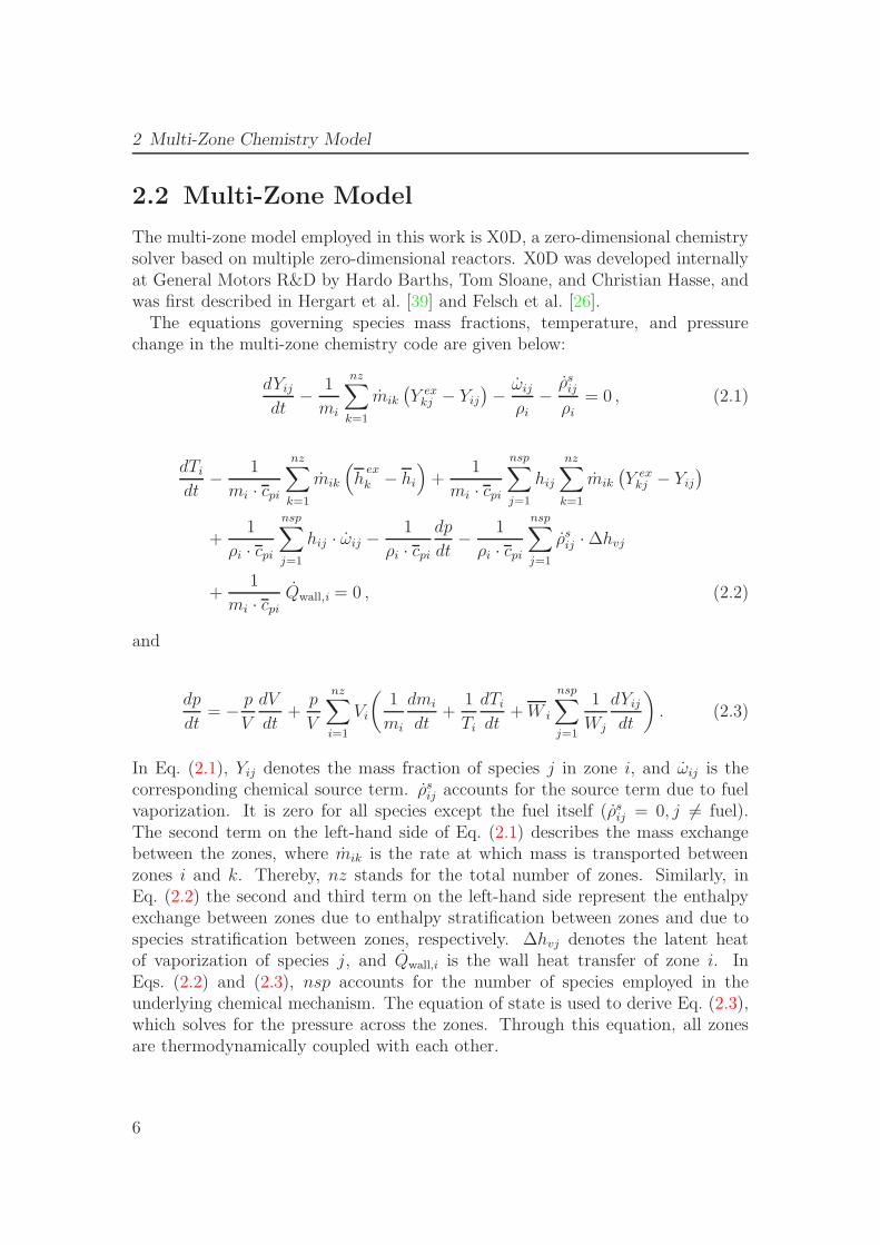
The multi-zone model employed in this work is X0D, a zero-dimensional chemistrysolver based on multiple zero-dimensional reactors. X0D was developed internallyat General Motors R&D by Hardo Barths, Tom Sloane, and Christian Hasse, andwas first described in Hergart et al. [39] and Felsch et al. [26].
The equations governing species mass fractions, temperature, and pressurechange in the multi-zone chemistry code are given below:
dYij
dt− 1
mi
nz∑
k=1
mik
(Y ex
kj − Yij
)− ωij
ρi−
ρsij
ρi= 0 , (2.1)
dTi
dt− 1
mi · cpi
nz∑
k=1
mik
(h
ex
k − hi
)+
1
mi · cpi
nsp∑
j=1
hij
nz∑
k=1
mik
(Y ex
kj − Yij
)
+1
ρi · cpi
nsp∑
j=1
hij · ωij −1
ρi · cpi
dp
dt− 1
ρi · cpi
nsp∑
j=1
ρsij · ∆hvj
+1
mi · cpiQwall,i = 0 , (2.2)
and
dp
dt= − p
V
dV
dt+
p
V
nz∑
i=1
Vi
(1
mi
dmi
dt+
1
Ti
dTi
dt+ W i
nsp∑
j=1
1
Wj
dYij
dt
). (2.3)
In Eq. (2.1), Yij denotes the mass fraction of species j in zone i, and ωij is thecorresponding chemical source term. ρs
ij accounts for the source term due to fuelvaporization. It is zero for all species except the fuel itself (ρs
ij = 0, j 6= fuel).The second term on the left-hand side of Eq. (2.1) describes the mass exchangebetween the zones, where mik is the rate at which mass is transported betweenzones i and k. Thereby, nz stands for the total number of zones. Similarly, inEq. (2.2) the second and third term on the left-hand side represent the enthalpyexchange between zones due to enthalpy stratification between zones and due tospecies stratification between zones, respectively. ∆hvj denotes the latent heatof vaporization of species j, and Qwall,i is the wall heat transfer of zone i. InEqs. (2.2) and (2.3), nsp accounts for the number of species employed in theunderlying chemical mechanism. The equation of state is used to derive Eq. (2.3),which solves for the pressure across the zones. Through this equation, all zonesare thermodynamically coupled with each other.
6
2.3 Chemistry Model
Wall heat transfer is described as
Qwall,i =
nwall∑
l=1
Awall,l,i · hwall,l,i(Ti − Twall,l) , (2.4)
where nwall denotes the total number of walls in the engine, Awall,l,i the area of walll belonging to zone i, hwall,l,i the heat transfer coefficient of zone i to wall l, Ti thetemperature of zone i, and Twall,l the temperature of wall l.
The mixing in the multi-zone model is accounted for by allowing the differentzones to exchange mass and energy with each other, in addition to the interactionthrough the pressure. They exchange their scalar quantities (species compositionand enthalpy) based on the rate at which they exchange their mass. The mass ofeach zone is kept constant and the model can accommodate any number of zones.
The multi-zone model is written in FORTRAN 77. Equations (2.1), (2.2),and (2.3) are numerically solved using the differential/algebraic system solverDASSL [68].
2.3 Chemistry Model
A major aspect in modeling engine combustion is the treatment of the chemistry.The advantage of using a zero-dimensional multi-zone model is that complex chem-ical mechanisms can be used. In addition to its own very fast chemical solver, X0Dhas an interface to CHEMKIN [49] and can therefore use any mechanism availablein this format. This is important in state-of-the-art applications (to investigatepollutant formation, for example).
In the gasoline HCCI combustion simulations (see Chapter 5), combustion chem-istry in X0D is described by a detailed chemical kinetic mechanism that incorpo-rates low, intermediate, and high temperature oxidation chemistry of n-heptane- iso-octane mixtures. This mechanism, which consists of 115 species and 482reactions, was constructed by Advanced Combustion GmbH [70]. All these calcu-lations were performed using a PRF82 mixture, which consists of 82 % iso-octaneand 18 % n-heptane by liquid volume.
In the PCCI combustion simulations (see Chapter 7), combustion chemistryin X0D is described by a detailed chemical kinetic mechanism that comprises59 elementary reactions among 38 chemical species. This mechanism describeslow-temperature auto-ignition and combustion of n-heptane, which serves as asurrogate fuel for Diesel in these simulations. Furthermore, it accounts for thermalNO formation. The chemical mechanism for n-heptane was constructed by Peterset al. [67]. The NO-submechanism, which is part of the full mechanism, is theextended Zeldovich mechanism [41].
7

3 Description and Modeling ofChemically Reacting TurbulentTwo-Phase Flows
This chapter first provides a short description of the governing equations for achemically reacting two-phase system with a gas phase and an evaporating liquidphase. Following the introduction of the scales of turbulent motion and the averag-ing procedure for the governing equations, the favre-averaged governing equationsfor the turbulent flow and mixing field are presented. After this, the implemen-tation of these equations into the CFD code AC-FluX is depicted. Finally, thischapter closes with a brief description of the modeling of the liquid phase.
3.1 Governing Equations
Fluid flows are described by a system of coupled, nonlinear, partial differentialequations. In cases where chemical reactions occur, additional equations for thespecies mass fractions, as well as an underlying chemical mechanism, are required.The governing equations for the gas phase are presented in the following for atwo-phase system with a gas phase and an evaporating liquid phase.
The equation for the gas phase density ρ reads
∂ρ
∂t+
∂
∂xα(ρvα) = ρs , (3.1)
where ρs denotes the source term due to the presence of the evaporating liquidphase.
The rate of change of the gas phase momentum in each direction α is given by
∂
∂t(ρvα) +
∂
∂xβ
(ρvαvβ) = − ∂p
∂xα
+∂ταβ
∂xβ
+ f sα, α = 1, 2, 3 , (3.2)
where f sα is the rate of momentum gain per unit volume due to interaction with the
liquid phase. Gravitational influences are neglected. ταβ is the symmetric stresstensor. Assuming a Newtonian fluid, it is usually expressed as
ταβ = ρν
(∂vα
∂xβ+
∂vβ
∂xα
)− 2
3ρν
∂vγ
∂xγδαβ , (3.3)
9
3 Modeling of Chemically Reacting Turbulent Two-Phase Flows
with δαβ denoting the Kronecker delta. ν is the laminar viscosity.
The equation for the mixture enthalpy h, which includes the species heat offormation ∆h0
f according to
h =
nsp∑
j=1
Yj
(∆h0
fj +
∫ T
T 0
cpj dT
), (3.4)
is given by
∂
∂t(ρh) +
∂
∂xα
(ρvαh) =Dp
Dt+ ταβ
∂vβ
∂xα
− ∂jqα
∂xα
+ qs − qr − qwall . (3.5)
In Eq. (3.5), ταβ ∂vβ/∂xα denotes the viscous heating term. This term is smallfor low-speed flows and is therefore not considered further on. qs and qr describechanges due to interaction with the liquid phase and due to radiative heat losses,respectively. The latter are neglected in this work. qwall denotes the heat transferto the walls. Equation (3.5) does not contain a chemical source term as the heatof formation of all species is included in the enthalpy. The heat flux jq
α accountsfor thermal diffusion and enthalpy transport by species diffusion, yielding
jqα = −λ
∂T
∂xα+
nsp∑
j=1
jαj hj . (3.6)
The second term on the right-hand side is identical zero, because all Lewis numbersare assumed equal to unity in this work.
The composition of the charge is represented by four so-called active speciesstreams, which are the mass fraction of fuel Yfuel, the mass fraction of air Yair, themass fraction of combustion products (carbon dioxide and water) Yproducts, and themass fraction of residuals YEGR. The corresponding transport equation reads
∂
∂t(ρYj) +
∂
∂xi
(ρviYj) =∂
∂xi
(ρDj
∂Yj
∂xi
)+ ρωj + ρs
j . (3.7)
In Eq. (3.7), Yj denotes active species stream j, Dj the diffusion coefficient ofactive stream j, and ωj the chemical source term of active stream j. The sourceterm for the residuals is identical zero (ωEGR = 0), because they are assumed tobe chemically inert. The residuals are therefore an indicator for dilution. Thedetermination of the remaining source terms (ωfuel, ωair, and ωproducts) is describedin Sec. 4.3. Here again, the term ρs
j represents the source term due to evaporationof liquid fuel. It is zero for all species except the fuel itself (ρs
j = 0, j 6= fuel).
The link between pressure, temperature, active species streams, and density isestablished by means of the ideal gas law, given by
10
3.1 Governing Equations
p
ρ=
nsp∑
j
Yj
Wj
RT , (3.8)
where R is the ideal gas constant and Wj the molecular weight of species j. Usingthe mean molecular weight W defined as
W =
(nsp∑
j
Yj
Wj
)−1
, (3.9)
Eq. (3.8) is reduced to
p =ρ
WRT . (3.10)
The mixing field is described by two additional scalars. These are the fuelmixture fraction Zfuel and an artificial scalar S.
The fuel mixture fraction Zfuel is the dominant quantity for the description ofnon-premixed combustion and can be related to the commonly used equivalenceratio φ or the combustion-air ratio λ, respectively, according to
φ =1
λ=
Zfuel
1 − Zfuel
(1 − Zfuel,st)
Zfuel,st, (3.11)
where Zfuel,st is the fuel mixture fraction at stoichiometric mixture [66]. The cor-responding transport equation reads
∂
∂t(ρZfuel) +
∂
∂xα
(ρvαZfuel) =∂
∂xα
(ρDZ
∂Zfuel
∂xα
)+ ρs
fuel . (3.12)
Similar to Eq. (3.1), the term ρsfuel represents the source term due to fuel evapora-
tion.
In addition to the transport equation for the fuel mixture fraction Zfuel, a genericconvection diffusion equation without source terms is considered for the artificialscalar S. This transport equation reads
∂
∂t(ρS) +
∂
∂xα
(ρvαS) =∂
∂xα
(ρDS
∂S
∂xα
). (3.13)
It is assumed that the diffusion coefficients Dj , DZ , and DS are identical.
Accounting for the fuel mixture fraction and an artificial scalar is mandatoryin order to establish the interactive coupling of the CFD code AC-FluX and themulti-zone model X0D. For HCCI combustion, the interactive coupling is describedin Chapter 4. For PCCI combustion, it is described in Sec. 6.1.
11
3 Modeling of Chemically Reacting Turbulent Two-Phase Flows
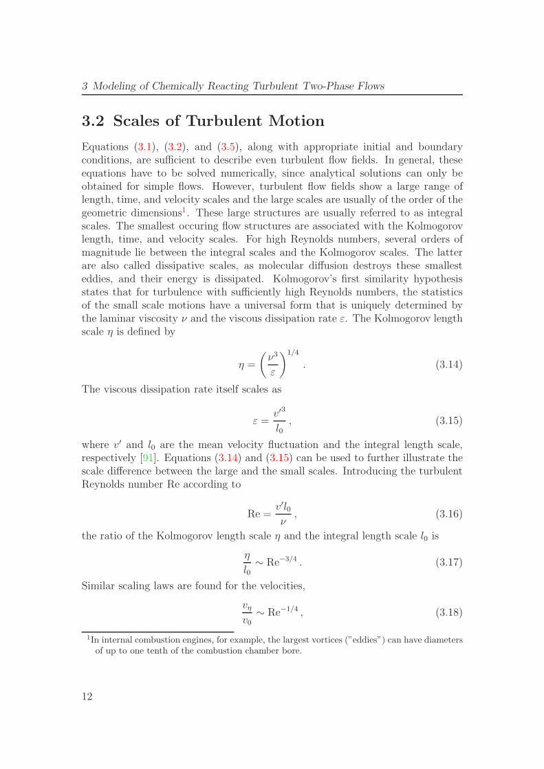
3.2 Scales of Turbulent Motion
Equations (3.1), (3.2), and (3.5), along with appropriate initial and boundaryconditions, are sufficient to describe even turbulent flow fields. In general, theseequations have to be solved numerically, since analytical solutions can only beobtained for simple flows. However, turbulent flow fields show a large range oflength, time, and velocity scales and the large scales are usually of the order of thegeometric dimensions1. These large structures are usually referred to as integralscales. The smallest occuring flow structures are associated with the Kolmogorovlength, time, and velocity scales. For high Reynolds numbers, several orders ofmagnitude lie between the integral scales and the Kolmogorov scales. The latterare also called dissipative scales, as molecular diffusion destroys these smallesteddies, and their energy is dissipated. Kolmogorov’s first similarity hypothesisstates that for turbulence with sufficiently high Reynolds numbers, the statisticsof the small scale motions have a universal form that is uniquely determined bythe laminar viscosity ν and the viscous dissipation rate ε. The Kolmogorov lengthscale η is defined by
η =
(ν3
ε
)1/4
. (3.14)
The viscous dissipation rate itself scales as
ε =v′3
l0, (3.15)
where v′ and l0 are the mean velocity fluctuation and the integral length scale,respectively [91]. Equations (3.14) and (3.15) can be used to further illustrate thescale difference between the large and the small scales. Introducing the turbulentReynolds number Re according to
Re =v′l0ν
, (3.16)
the ratio of the Kolmogorov length scale η and the integral length scale l0 is
η
l0∼ Re−3/4 . (3.17)
Similar scaling laws are found for the velocities,
vη
v0∼ Re−1/4 , (3.18)
1In internal combustion engines, for example, the largest vortices (”eddies”) can have diametersof up to one tenth of the combustion chamber bore.
12
3.3 Averaging
and the time scales,
τη
τ0∼ Re−1/2 , (3.19)
where τ0 can be interpreted as the turnover time of an eddy with the size l0, whichhas a characteristic velocity v0 [73]. The characteristic velocity v0 is of the sameorder of magnitude as v′. It can be seen from Eqs. (3.17), (3.18), and (3.19) thatfor a sufficiently high Reynolds numbers a wide range of length, time, and velocityscales exists in a turbulent flow. Solving Eqs. (3.1), (3.2), and (3.5) numericallytherefore requires sufficiently fine meshes and small time steps, as even the smallscales have to be resolved completely. However, with current computer capabilities,this direct numerical simulation (DNS) is only possible for simple geometries andmoderate Reynolds numbers. Since engineering applications generally have highReynolds numbers, significant parts of the small scale motions have to be modeled.
3.3 Averaging
Modeling parts of the small scale motion is usually achieved by averaging theoriginal equations.
According to Reynolds, each variable f is split into a mean component f and afluctuating component f ′, leading to
f = f + f ′ . (3.20)
Ensemble averaging is most commonly used for obtaining the mean component f .This yields
fN =1
N
N∑
i=1
fi , (3.21)
where N is the number of realizations, over which the instantaneous values fi areaveraged.
For flows with large density changes as occur in combustion, it is often convenientto introduce a density-weighted average f , called the Favre average, by splitting finto f and f ′′ as
f = f + f ′′ . (3.22)
This averaging procedure is defined by requiring that the average of the productof f ′′ with the density ρ (rather than f ′′ itself) vanishes:
ρf ′′ = 0 . (3.23)
13
3 Modeling of Chemically Reacting Turbulent Two-Phase Flows
Reynolds averaging and Favre averaging are related to each other according to
f =ρf
ρand f ′′ = −ρ′f ′
ρ. (3.24)
3.4 Turbulent Flow and Mixing Field
The splitting operations described above can also be applied to the governingequations presented in Sec. 3.1 instead of a single quantity only. The ensembleaveraging procedure then yields the Reynolds Averaged Navier-Stokes (RANS)equations. These equations only describe the motion on the integral length, time,and velocity scales, while every motion on smaller scales needs to be modeled, evenif the grid size is much smaller than the integral length scale. Filtering with filterwidths smaller than the integral scales allows to resolve more of the small scalemotion. This is typically done in Large Eddy Simulations (LES) or Very LargeEddy Simulations (VLES), for more details see [28] or [73]. In this work, a RANSapproach is used.
The continuity equation reads, after averaging,
∂ρ
∂t+
∂
∂xα
(ρvα) = ρs . (3.25)
Equation (3.25) is very similar to Eq. (3.1). All instantaneous quantities are re-placed by the average values and no additional terms occur.
The averaged momentum equations are
∂
∂t(ρvα) +
∂
∂xβ
(ρvαvβ) = − ∂p
∂xα
+∂ταβ
∂xβ
− ∂
∂xβ
(ρv′′
αv′′
β
)+ f s
α . (3.26)
with the averaged symmetric stress tensor ταβ being
ταβ = ρν
(∂vα
∂xβ+
∂vβ
∂xα
)− 2
3ρν
∂vγ
∂xγδαβ . (3.27)
In Eq. (3.26), in addition to the original contributions the so-called Reynoldsstresses −ρv′′
αv′′
β appear. They represent the classical closure problem of turbu-lent flows. Reynolds stresses are second-order correlations, and they describe theconvective momentum transport by turbulent fluctuations. Transport equationscan be derived for the Reynolds stress tensor; however, these equations containtriple correlations of the sort ρv′′
αv′′
βv′′
γ . These triple correlations are also unclosed.They therefore require a modeling approach. Furthermore, unclosed correlationsof pressure fluctuations and velocity gradients, the so-called pressure-rate-of-straintensor, appear. First modeling suggestions were made by Rotta [81]. Instead of
14
3.4 Turbulent Flow and Mixing Field
modeling the triple correlations, it is also possible to derive equations for them,which then contain correlations of fourth order. This indicates an infinite modelinghierarchy and thus no closed equations can be obtained directly.
The averaged enthalpy equation is obtained as
∂
∂t
(ρh)
+∂
∂xα
(ρvαh
)=
Dp
Dt− ∂jq
α
∂xα
− ∂
∂xα
(ρv′′
αh′′
)+ qs − qwall . (3.28)
In Eq. (3.28), the term −ρv′′
αh′′ is similar to the Reynolds stresses in Eq. (3.26).It represents the convective enthalpy transport by turbulent fluctuations and itneeds to be modeled, as it is unclosed, too.
If no equations for the turbulent transport terms are solved, a model is requiredwhich relates these terms to known quantities. Boussinesq [11] proposed the con-cept of a turbulent viscosity νt, which is often referred to as an eddy viscosity. Itis used to relate the turbulent stresses to the mean field, yielding
− ρv′′
αv′′
β = τt,αβ = ρνt
[∂vα
∂xβ+
∂vβ
∂vα− 2
3
∂vγ
∂xγδαβ
]− 2
3ρkδαβ
= ρνt
[Sij −
2
3
∂vγ
∂xγδαβ
]− 2
3ρkδαβ , (3.29)
where Sij denotes the rate-of-strain tensor and k the mean turbulent kinetic energydefined by
k =1
2v′′
αv′′
α . (3.30)
The turbulent viscosity νt is not a fluid property such as the laminar viscosity ν. Itdepends on the turbulence in the vicinity. It can be considered to be the productof a velocity scale and a length scale. Several models for the turbulent viscosityare available, and they are usually classified according to the number of additionalequations that need to be solved. Prandtl [74] related the turbulent viscosity toa mixing length lm and the absolute gradient of the mean velocity field. As noadditional equations are solved, this model belongs to the class of zero-equationmodels. One of the first one-equation models was proposed by Prandtl [75]. Theturbulent viscosity is determined using the turbulent kinetic energy, for which anequation is solved, and a length scale, which is determined empirically. Rotta [82]derived an equation for the length scale by integrating the two-point correlationover the correlation coordinate. This leads to a k− l model, which then belongs tothe class of two-equation models. Rodi and Spalding [80] first used an l-equation
15
3 Modeling of Chemically Reacting Turbulent Two-Phase Flows
to compute a turbulent jet flow. The most popular two-equation model is the k−εmodel, where ε is the turbulent dissipation. The ’standard’ k − ε model was firstdeveloped by Jones and Launder [48] and improved model constants were providedby Launder and Sharma [51]. Turbulent length, time, and velocity scales can beeasily formed using these two quantities. The length scale, for example, can beexpressed as
l ∼ k3/2/ε . (3.31)
The turbulent viscosity is modeled according to
νt = Cµk2
ε, Cµ = 0.09 . (3.32)
The modeling constant Cµ was already proposed by Launder and Sharma [51]. Itis usually not changed. The equation for the turbulent kinetic energy that is usedin this work reads
∂
∂t(ρk) +
∂
∂xα(ρvαk) =
∂
∂xα
[(ρν +
ρνt
Prt,k
)∂k
∂xα
]+ τt,αβ
∂vα
∂xβ− ρε + W s
k , (3.33)
where W sk describes the effect of turbulent dispersion of droplets on the turbulent
kinetic energy. For constant-density flows, the equation for the turbulent kineticenergy can be derived systematically. From this derivation follows the definitionof the viscous dissipation rate, reading
ε = ν
[∂v′′
β
∂xα+
∂v′′
α
∂xβ
]∂v′′
β
∂xα. (3.34)
An ε-equation is difficult to derive and to close in a systematic manner. Instead,a model equation, which is partly empirically, is solved according to
∂
∂t(ρε) +
∂
∂xα(ρvαε) =
∂
∂xα
[(ρν +
ρνt
Prt,ε
)∂ε
∂xα
]+ Cε1
ε
kτt,αβ
∂vα
∂xβ
− Cε2 ρε2
k+ Cε3 ρ ε
∂vα
∂xα
+ε
kCs W s
k . (3.35)
The model constants are given as Prt,k = 1.0, Prt,ε = 1.22, Cε1 = 1.44, Cε2 = 1.92,Cε3 = −0.33, and Cs = 1.5.
16
3.5 CFD Code
After closing the turbulent transport term in Eq. (3.28) with a gradient fluxapproximation,
ρv′′
αh′′ = − ρνt
Pr
∂h
∂xα, (3.36)
the final equation for turbulent mean enthalpy reads
∂
∂t
(ρh)
+∂
∂xα
(ρvαh
)=
Dp
Dt+
∂
∂xα
[(λ
cp+
ρνt
Prt
)∂h
∂xα
]+ qs − qwall . (3.37)
Averaging Eq. (3.7) representing the composition of the charge leads to
∂
∂t
(ρYj
)+
∂
∂xi
(ρviYj
)=
∂
∂xi
[(ρν
SceYj
+ρνt
Sct,eYj
)∂Yj
∂xi
]+ ρωj + ρs
j . (3.38)
The density-weighted averaged mixture field is accounted for by
∂
∂t
(ρZfuel
)+
∂
∂xi
(ρviZfuel
)=
∂
∂xi
[(ρν
Sc eZfuel
+ρνt
Sct, eZfuel
)∂Zfuel
∂xi
]+ ρs
fuel (3.39)
and
∂
∂t
(ρS)
+∂
∂xi
(ρviS
)=
∂
∂xi
[(ρν
SceS
+ρνt
Sct, eS
)∂S
∂xi
]. (3.40)
3.5 CFD Code
The averaged equations for the gas phase described in the previous section aresolved by the CFD code AC-FluX (formerly known as GMTEC). AC-FluX isa flow solver based on Finite Volume methods [29] that employs unstructured,mostly hexahedral meshes. AC-FluX is mainly used for internal combustion en-gine simulations, for gasoline as well as for Diesel enginges. The code is able totreat moving meshes and non-conforming internal mesh motion boundaries thatfacilitate generating a realistic geometric model of intake ports, exhaust ports, andthe in-cylinder in combination with valve motion. In order to provide high spatialaccuracy, adaptive run time controlled mesh refinement can be used optionally.
17
3 Modeling of Chemically Reacting Turbulent Two-Phase Flows
This section briefly covers the numerical algorithms and the general code struc-ture of AC-FluX. More details (e.g., regarding spatial and temporal discretizationschemes) are given in Khalighi et al. [50], Ewald et al. [24], and Freikamp [32].
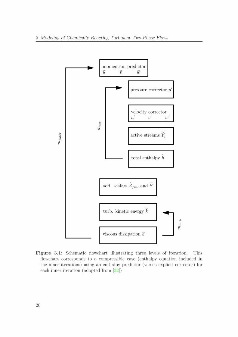
AC-FluX uses an iterative implicit pressure-based sequential solution procedureto solve the coupled system of governing partial differential equations. The equa-tions are solved sequentially rather than simultaneously; coupling is achieved via aniterative updating procedure. The procedure accommodates incompressible and/orcompressible flows, as well as steady and/or transient flows. It is applicable for es-sentially arbitrary Mach numbers, although for Mach numbers much greater thanunity the efficiency of the approach decreases significantly. AC-FluX’s pressurealgorithm is patterned after SIMPLE (Semi–Implicit Method for Pressure–LinkedEquations, [62]) and PISO (Pressure–Implicit Split Operator, [46]). PISO origi-nally was conceived as a predictor-corrector method to be used with a fixed numberof passes through the equations on each time step; however, a pure PISO methodgenerally is neither sufficiently efficient nor sufficiently robust for the highly dis-torted computational meshes and complex three-dimensional time-dependent flowsthat characterize practical engineering applications. The algorithm used in AC-FluX can be thought of as a modified PISO scheme, where both the numbers ofouter and inner iterations are variable. In the case of a single outer loop (momen-tum predictor) and a single inner loop (pressure/velocity corrector) per time step,this algorithm reduces to a SIMPLE-like method.
The essential steps in the pressure/momentum/continuity coupling to advancethe solution over one computational time step are:
1. momentum predictor – compute a new velocity field using the current pres-sure field; this velocity field does not satisfy continuity.
2. pressure/velocity correctors – compute corrections to the pressure and ve-locity fields to enforce continuity.
The momentum predictor and pressure corrector each require the solution ofa sparse implicit linear system that corresponds to a linearised discretised formof the governing partial differential equations. The velocity corrector is explicit.Equations for additional quantities (e.g., total enthalpy, species mass fractions)are included in each pressure/velocity corrector step to maintain tight couplingamong the equations. At the end of the pressure/velocity corrections, equationsrequiring a lesser degree of coupling are solved (e.g., turbulence model equations).The process then is repeated as necessary, starting from the momentum predictor,to obtain a converged solution for the current time step or global iteration. Threelevels of iteration are thus employed on each time step (each global iteration fora steady solution algorithm): an outer loop or outer iteration, an inner loop or
18
3.6 Liquid Phase
inner iteration, and iterations within the linear equation solvers. The outer it-eration corresponds to the momentum predictor step, the inner iteration to thepressure/velocity corrector step. The basic sequence is displayed in Fig. 3.1.
The calculation of the source terms in the gas-phase equations is a preparatorystep to the sequential solution procedure described above. The mathematicalformulation of the liquid phase is subject of the following section. The formulationof the chemical source terms is elaborated on in Sec. 4.3.
3.6 Liquid Phase
The previous sections discuss the governing equations of the gas phase and theirimplementation into the CFD code AC-FluX. During the injection period in aninternal combustion engine an additional liquid phase is present, which must beadequately described to obtain the spray-related source terms in the gas phaseequations (see Eqs. (3.25), (3.26), (3.33), (3.35), (3.37), (3.38), and (3.39)). Solv-ing for the dynamics of a spray with a wide distribution of drop sizes, velocities,and temperatures is a complicated problem. A mathematical formulation capableof describing this distribution is the spray equation proposed by Williams [101]. Itis an evolution equation for the probability density function f with the independentvariables droplet position, droplet velocity, temperature, radius, distortion fromsphericity y, and its time derivative dy/dt. Depending on the specific problem,additional variables can be introduced. A direct solution of this equation is ex-tremely difficult due to its high dimensionality; the aforementioned variables aloneconstitute a 10-dimensional space and associated storage and computing time re-quirements. Instead, a sufficiently large number of particles are introduced, which,according to Crowe et al. [16], are called parcels. This model is usually referredto as the discrete droplet model (DDM). Each parcel represents an ensemble ofdroplets. Within one parcel, all droplets have the same properties, which corre-spond to the independent variables described above. The ensemble of all parcelsprovides the statistical information on the spray. All the subprocesses that are notresolved on the parcel level are modeled using a Monte-Carlo method [19]. Impor-tant subprocesses, which need to be described, are breakup, collision, coalescence,evaporation, and dispersion. A detailed description of the models for these sub-processes, the formulation of the source terms for the gas phase equations, and itsimplementation into the CFD code AC-FluX can be found in [89].
19
3 Modeling of Chemically Reacting Turbulent Two-Phase Flows
total enthalpy h
velocity correctorw′v′u′
viscous dissipation ε
turb. kinetic energy k
add. scalars Zfuel and S
momentum predictorwvu
active streams Yj
pressure corrector p′
mcc
p
mtu
rb
moute
r
Figure 3.1: Schematic flowchart illustrating three levels of iteration. Thisflowchart corresponds to a compressible case (enthalpy equation included inthe inner iterations) using an enthalpy predictor (versus explicit corrector) foreach inner iteration (adopted from [32])
20
4 Interactive Coupling of the CFD Codeand the Multi-Zone Model
The interactive coupling (two-way-coupling) of the three-dimensional CFD codeAC-FluX and the multi-zone model X0D is outlined in this chapter. After ini-tialization, the interactive coupling comprises one information stream which is fedfrom the CFD code to the multi-zone model. Mixing effects are introduced into themulti-zone model based on the CFD solution. Vice versa, one information streamis fed from the multi-zone model to the CFD code in order to keep the heat releaseconsistent between both codes. The initialization of the interactive coupling andthe two information streams are addressed in Secs. 4.1, 4.2, and 4.3. Section 4.4deals with the treatment of source terms within the interactive coupling. A methodhow to account for source terms in a completely consistent manner is described inSec. 4.5. At the end of this chapter, Sec. 4.6 discusses this modeling concept inthe context of the Representative Interactive Flamelet model.
4.1 Initialization of the Interactive Coupling
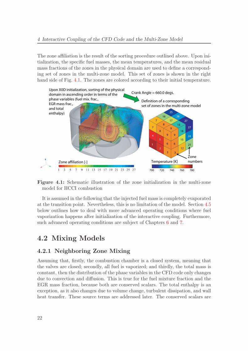
In order to construct the mass distribution function and subdivide it into discretezones in phase space, the computational cells in the physical domain in the CFDcode are sorted in ascending order in terms of the phase variables (fuel mixturefraction, EGR mass fraction, and total enthalpy). The computational cells are thenassigned to the zones so that these have equal mass. It is not required that thezones have equal mass, but it simplifies the derivation and implementation. Thisprocedure is repeated at each time step of the CFD code. Only once, however, at acertain crank angle prior to any chemical reactions starting to occur, a correspond-ing set of zones defined by specific fuel masses, temperatures, and residual massfractions is initialized in the multi-zone model X0D. From this transition point on,both codes interact back and forth throughout the engine cycle. The two codesrun independently but simultaneously, without any reinitialization of the zones(and the numerical solver for the differential equations) in the multi-zone model.
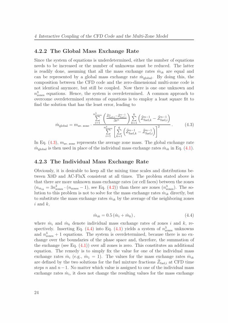
Figure 4.1 schematically illustrates how the AC-FluX CFD code is used to ini-tialize the zones in X0D, for which the chemistry is solved. For the gasoline HCCIengine test case investigated (see Chapter 5), the left hand side of Fig. 4.1 showstwo injector cut planes colored by zone affiliation at time of X0D initialization.
21
4 Interactive Coupling of the CFD Code and the Multi-Zone Model
The zone affiliation is the result of the sorting procedure outlined above. Upon ini-tialization, the specific fuel masses, the mean temperatures, and the mean residualmass fractions of the zones in the physical domain are used to define a correspond-ing set of zones in the multi-zone model. This set of zones is shown in the righthand side of Fig. 4.1. The zones are colored according to their initial temperature.
700 720 740 760 780
33
21
12
7
24
8
4
6
9
2
1
27
27
26
25
9
9
6
5
7
8
18
18
16
17
15
Temperature [K]
Zone
numbersZone affiliation [-]
Definition of a corresponding
set of zones in the multi-zone model
Upon X0D initialization, sorting of the physical
domain in ascending order in terms of the
phase variables (fuel mix. frac.,
EGR mass frac.,
and total
enthalpy)
Crank Angle = 660.0 degs.
Figure 4.1: Schematic illustration of the zone initialization in the multi-zonemodel for HCCI combustion
It is assumed in the following that the injected fuel mass is completely evaporatedat the transition point. Nevertheless, this is no limitation of the model. Section 4.5below outlines how to deal with more advanced operating conditions where fuelvaporization happens after initialization of the interactive coupling. Furthermore,such advanced operating conditions are subject of Chapters 6 and 7.
4.2 Mixing Models
4.2.1 Neighboring Zone Mixing
Assuming that, firstly, the combustion chamber is a closed system, meaning thatthe valves are closed; secondly, all fuel is vaporized; and thirdly, the total mass isconstant, then the distribution of the phase variables in the CFD code only changesdue to convection and diffusion. This is true for the fuel mixture fraction and theEGR mass fraction, because both are conserved scalars. The total enthalpy is anexception, as it also changes due to volume change, turbulent dissipation, and wallheat transfer. These source terms are addressed later. The conserved scalars are
22
4.2 Mixing Models
considered first. The change for the mean fuel mixture fraction from CFD timestep n − 1 to CFD time step n in the individual zones can be formulated as
mi ·Zn
fuel,i − Zn−1fuel,i
∆tn=
6∑
k=1
mik
(Zn−1
fuel,k − Zn−1fuel,i
), (4.1)
where ∆tn is the time increment, mi the mass of zone i, and mik the mass exchangerate of zone i with neighboring zone k (see Eqs. (2.1) and (2.2)). Since the phasespace is three-dimensional, each zone in phase space can have up to six neighborsto exchange their scalar quantities with.
Allowing mixing only between neighboring zones in phase space is a logicalchoice, because transitions in phase space have to be continuous. If a state B isintermediate between two states A and C, then a zone of state A cannot transitto state C without passing through state B during a diffusive process. The zonesin phase space are therefore arranged in ascending (or descending) order, as il-lustrated in Fig. 4.1. Consequently, neighboring zone mixing is used throughoutthe remainder of the thesis. This is analogous to a Representative InteractiveFlamelet. In the flamelet equations, the scalar dissipation rate χ is an exter-nal parameter that is imposed on the flamelet structure. It can be thought ofas a diffusivity in mixture fraction space that accounts for an exchange betweenadjacent reactive scalars (temperature and species mass fractions) in mixture frac-tion space. The laminar flamelet equations were derived by Peters [64, 65, 66]and integrated into the concept of Representative Interactive Flamelets by hisco-workers [8, 25, 38, 69].
The challenge in developing a mixing model is to extract the rate of exchangebetween each of the zones from the CFD code based on the mass distributionfunction of the current and the previous time step. Why this is a challenge becomesapparent when the number of unknowns and equations is considered. If nzones is thenumber of zones in each of the three directions of the independent phase variables,then
nmik= 3n2
zones · (nzones − 1) (4.2)
unknown mass exchange rates exist between the n3zones zones. It is easy to show
that for nzones ≥ 2, the number of unknown mass exchange rates nmikexceeds
the total number of zones n3zones, and it follows that the system of equations is
underdetermined and not directly solvable. In the following, two approaches toovercome this difficulty are presented. These two approaches allow for a calculationof the mass exchange rates mik so that they can be updated in the multi-zone codeat every CFD time step.
23
4 Interactive Coupling of the CFD Code and the Multi-Zone Model
4.2.2 The Global Mass Exchange Rate
Since the system of equations is underdetermined, either the number of equationsneeds to be increased or the number of unknowns must be reduced. The latteris readily done, assuming that all the mass exchange rates mik are equal andcan be represented by a global mass exchange rate mglobal. By doing this, thecomposition between the CFD code and the zero-dimensional multi-zone code isnot identical anymore, but still be coupled. Now there is one one unknown andn3
zones equations. Hence, the system is overdetermined. A common approach toovercome overdetermined systems of equations is to employ a least square fit tofind the solution that has the least error, leading to
mglobal = mav. zone ·
n3zones∑i=1
(Zn
fuel,i−Zn−1
fuel,i
∆tn
)6∑
k=1
(Zn−1
fuel,k − Zn−1fuel,i
)
n3zones∑i=1
[6∑
k=1
(Zn−1
fuel,k − Zn−1fuel,i
)]2 . (4.3)
In Eq. (4.3), mav. zone represents the average zone mass. The global exchange ratemglobal is then used in place of the individual mass exchange rates mik in Eq. (4.1).
4.2.3 The Individual Mass Exchange Rate
Obviously, it is desirable to keep all the mixing time scales and distributions be-tween X0D and AC-FluX consistent at all times. The problem stated above isthat there are more unknown mass exchange rates (or cell faces) between the zones(nmik
= 3n2zones · (nzones − 1), see Eq. (4.2)) than there are zones (n3
zones). The so-lution to this problem is not to solve for the mass exchange rates mik directly, butto substitute the mass exchange rates mik by the average of the neighboring zonesi and k,
mik = 0.5 (mi + mk) , (4.4)
where mi and mk denote individual mass exchange rates of zones i and k, re-spectively. Inserting Eq. (4.4) into Eq. (4.1) yields a system of n3
zones unknownsand n3
zones + 1 equations. The system is overdetermined, because there is no ex-change over the boundaries of the phase space and, therefore, the summation ofthe exchange (see Eq. (4.1)) over all zones is zero. This constitutes an additionalequation. The remedy is to simply fix the value for one of the individual massexchange rates mi (e.g., m1 = 1). The values for the mass exchange rates mik
are defined by the two solutions for the fuel mixture fractions Zfuel,i at CFD timesteps n and n−1. No matter which value is assigned to one of the individual massexchange rates mi, it does not change the resulting values for the mass exchange
24
4.3 Consistency of Heat Release
rates mik.
4.3 Consistency of Heat Release
The chemical source terms ωj (see Eq. (3.38)) couple the CFD code AC-FluXto the multi-zone model X0D and keep the heat release consistent between bothcodes. The fuel mass fraction Yfuel acts as a progress variable for the heat release.In the CFD code, the average rate of change for the fuel mass mfuel,i in zone i iscoupled to the gross heat release in the multi-zone model through
mfuel,i =Qch,X0D,i
QLHVp
. (4.5)
In Eq. (4.5), Qch,X0D,i denotes the gross heat-release rate of zone i that is takenfrom the multi-zone model. QLHVp
is the lower heating value of the fuel.The actual value of the mean fuel mixture fraction in each CFD cell varies from
the average value of the zone it belongs to. For this reason, in order to properlydistribute the conversion of fuel over the CFD cells, the average rate of change forthe fuel mass mfuel,i in zone i is weighted with the ratio of the actual mean fuelmixture fraction in CFD cell ijk and the average mean fuel mixture fraction ofthe corresponding zone i. This yields
mCFDfuel,ijk =
ZCFDfuel,ijk
Zfuel,i
· mfuel,i , (4.6)
where mCFDfuel,ijk denotes the rate of change for the fuel mass in CFD cell ijk and
ZCFDfuel,ijk the actual mean fuel mixture fraction in CFD cell ijk.The other species (air and products of combustion) which are accounted for
in AC-FluX are computed via a one-step global reaction corresponding to thestoichiometry.
25
4 Interactive Coupling of the CFD Code and the Multi-Zone Model
4.4 Treatment of Source Terms
The conservation equation for the mean total enthalpy h, reading
∂
∂t
(ρh)
+∂
∂xα
(ρvαh
)=
Dp
Dt+
∂
∂xα
[(λ
cp+
ρνt
Prt
)∂h
∂xα
]
+qs − qwall (cf. Eq. (3.37) , (4.7)
has two source terms (qs and qwall) that need to be accounted for in the multi-zonemodel X0D.
As mentioned above, it is assumed that the fuel is fully vaporized and the sourceterm for the spray is identical zero (qs = 0).
In X0D, wall heat transfer (cf. Eqs. (2.2) and (2.4)) is described as
qwall,i · Vi = Qwall,i =
nwall∑
l=1
Awall,l,i · hwall,l,i(Ti − Twall,l) , (4.8)
The area Awall,l,i of wall l belonging to zone i is taken from the CFD solutionand updated in the multi-zone model at every CFD time step. The heat transfercoefficient hwall,l,i of zone i to wall l is continuously recalculated based on the CFDsolution and updated in the multi-zone model at every CFD time step such thatthe wall heat transfer in the multi-zone model exactly matches the one in the CFDcode. The recalculation of hwall,l,i uses the source term qwall in Eq. (4.7), averagedfor each zone in the CFD code.
The pressure change in X0D is described by Eq. (2.3), where the spatial pressurefluctuations are neglected and only the average cylinder pressure change, whichis due to the volume change and heat release, is taken into account. The volumechange in both codes is computed by using the same slider-crank-equation [41].
Thereby, the full interactive coupling of AC-FluX and X0D is accomplished.
4.5 Consistent Modeling of Source Terms
A further improvement over the current modeling may be achieved by a more so-phisticated treatment of phase variables whose partial differential equations con-tain source terms. This is the case for the total enthalpy and the fuel mixturefraction (if we allow for the vaporization of fuel after initializing the interactivecoupling). As discussed previously, the mixing coefficients for those phase variablescannot be computed in the current approach, because of the presence of sourceterms, which would cause disturbances.
26
4.6 Concept Analysis
Consider a generic convection diffusion equation with source terms representingthe phase variables according to
∂
∂t
(ρS)
+∂
∂xi
(ρviS
)=
∂
∂xi
[(ρν
SceS
+ρνt
Sct, eS
)∂S
∂xi
]+ ρS . (4.9)
Then, with each CFD time step, the solution for the variable S is numericallyadvanced from its state Sn at time tn to its new state Sn+1 at time tn+1. Byintroducing an additional conservation equation for the variable S omitting thesource term S,
∂
∂t
(ρSc
)+
∂
∂xi
(ρviSc
)=
∂
∂xi
[(ρν
SceSc
+ρνt
Sct, eSc
)∂Sc
∂xi
], (4.10)
and initializing Snc = Sn at time tn, then advancing it numerically to Sn+1
c at timetn+1, a solution for variable S is obtained that is again purely based on mixing.The two solutions Sn
c = Sn and Sn+1c can now be used to compute the mixing
coefficients for variable S with the help of Eqs. (4.1) and (4.4). Furthermore, thedifference Sn+1
c − Sn+1 divided by the time increment ∆tn = tn+1 − tn,
S∼
=Sn+1
c − Sn+1
∆tn, (4.11)
is the numerical representation of the source term for variable S. This source termcan then be averaged for each zone and passed on to X0D. Therefore, using themixing coefficients and source terms generated in this manner makes the couplingbetween AC-FluX and X0D completely consistent in the limit of the numericalerror.
4.6 Concept Analysis
The similarities between the multi-zone equations for species mass fractions andtemperature (see Eqs. (2.1) and (2.2)) and the corresponding laminar flameletequations are noteworthy. Both sets of equations feature a transient term, termsdescribing the mixing, and a chemical source term. This may seem somewhatsurprising, considering the fact that no assumptions of fast chemistry went intoderiving the multi-zone equations.
The laminar flamelet equations could alternatively be interpreted as describing aseries of coupled flow reactors (or zones), where the scalar dissipation rate, throughits functional dependence on the mixture fraction, governs the mixing betweenthem. As discussed in Subsec. 4.2.1, only flow reactors adjacent to each other
27
4 Interactive Coupling of the CFD Code and the Multi-Zone Model
in phase space, i.e. mixture fraction space, exchange mass and energy with eachother. Conceptually, this interpretation does not rely on the flamelet assumptions.
In situations where both methods could be applied, the interactively coupledCFD-multi-zone approach clearly offers an advantage in terms of computationalefficiency. Several flamelets are required to properly account for various regions ofmixing and heat transfer. Each flamelet calculation typically involves solving ap-proximately 100 coupled flow reactors. As shown in Chapters 5 and 7, significantlyless zones are needed in the CFD-multi-zone approach. It should be emphasizedthat the Representative Interactive Flamelet model, when interpreted as solving aseries of flow reactors, should no longer be referred to as a flamelet concept, butrather a multi-zone approach.
Hergart et al. [39] investigated a single-cylinder heavy-duty Diesel engine thatwas operated in PCCI mode. In the simulations, the authors first applied a se-quential treatment of the in-cylinder processes, where the injection processes andthe fluid dynamics were modeled using the CFD code AC-FluX and the chemi-cal reactions were treated in the multi-zone model X0D. Secondly, they appliedthe Representative Interactive Flamelet model. Both modeling approaches provedsuccessful in predicting auto-ignition, subsequent heat release, and pollutant for-mation. This work also contains a detailed discussion about the relative merits ofboth modeling approaches.
28
5 Validation of the Interactive Coupling
In this chapter, the interactive coupling of the three-dimensional CFD code AC-FluX and the multi-zone model X0D is validated against a test case of HCCIcombustion in a gasoline single-cylinder research engine.
5.1 Experimental and Numerical Setup
5.1.1 Experimental Setup
The experimental data were generated at General Motors Corporation in a directinjection gasoline single-cylinder research engine with four valves and negativevalve overlap (NVO). The main characteristics of the engine are summarized inTable 5.1.
Engine type: Single-cylinder research engineBore: 86.0 mmStroke: 94.6 mmConnecting rod length: 152.2 mmPiston pin offset: -0.8 mmCompression ratio: 12.0:1Injection system: 8-hole injectorIncluded spray angle: 60.0 degs.Hole diameter: 0.4 mmFuel: Standard gasoline
Table 5.1: Engine specifications
The engine was operated in HCCI mode. The valve timings given in Table 5.2were chosen such that the exhaust valves closed before top dead center of theexhaust stroke, and the intake valves opened after top dead center of the samestroke. This provided an NVO interval of 182.0 degs. CA, in which both theexhaust and intake valves were closed. NVO is a variable valve actuation (VVA)strategy that helps in assisting with combustion phasing and to extend operationto low speed and loads. Closing the exhaust valve before top dead center of theexhaust stroke, thus trapping and recompressing some of the hot residual, raises
29
5 Validation of the Interactive Coupling
the enthalpy level enough to enable the charge to auto-ignite at the subsequentcombustion cycle. The use of VVA was suggested by Willand et al. [100], andseveral examples of its exploitation appeared [20, 52, 61, 84, 96].
EVO: 148.0 degs. CA aTDCEVC: 268.0 degs. CA aTDCIVO: 450.0 degs. CA aTDCIVC: 570.0 degs. CA aTDCNVO: 182.0 degs. CA
Table 5.2: Valve timings
The engine was operated at a speed of 3000 rpm. A quantity of 6.0 mg fuel wasinjected at 270.0 degs. CA before top dead center (bTDC) firing. With injectionearly in the intake stroke, the charge is fairly homogeneous at the end of the maincompression when auto-ignition occurs. The operating conditions are summarizedin Table 5.3.
Engine speed: 3000 rpmGlobal air/fuel ratio: 25.0External EGR: 0 %Injected fuel mass: 6.0 mgStart of Injection (SOI): 285.2 degs. CA bTDCEnd of Injection (EOI): 270.0 degs. CA bTDCSpark Adv.: No sparkPIVC: 1.26 barTIVC: 529.0 K
Table 5.3: Engine operating point
5.1.2 Numerical Setup
The simulation was run from 197.0 degs. CA after top dead center (aTDC) untilexhaust valve opening (EVO). This captured almost the whole gas exchange andthe complete heat release, including pollutant formation. In the first part of theCFD simulation, AC-FluX was run alone. At 660.0 degs. CA aTDC, the couplingto X0D was initiated.
The computational domain included the intake runner and the exhaust systemup to the first closely coupled muffler in addition to the cylinder. The transient
30
5.1 Experimental and Numerical Setup
boundary condition for the orifices at intake and exhaust, as well as the initialconditions, were taken from a one-dimensional simulation of the complete systemin the test cell with the WAVE code by Ricardo [78].
The in-cylinder region of the computational mesh consisted of 91454 cells at topdead center (TDC) firing. An outline of the in-cylinder region of the computationalmesh is given in Figs. 5.1 and 5.2. In Fig. 5.1, the piston bowl and the cylinderwall are removed for illustration purposes. Vice versa, in Fig. 5.2, the cylinderhead and the cylinder wall are removed for the sake of a clear insight into thebowl.
Figure 5.1: Computational grid at TDC firing showing the cylinder head surface.Piston bowl and cylinder wall are removed for illustration purposes
Figure 5.2: Computational grid at TDC firing showing the piston bowl surface.Cylinder head and cylinder wall are removed for illustration purposes
31
5 Validation of the Interactive Coupling
5.2 Results and Discussion
5.2.1 Sensitivity Study
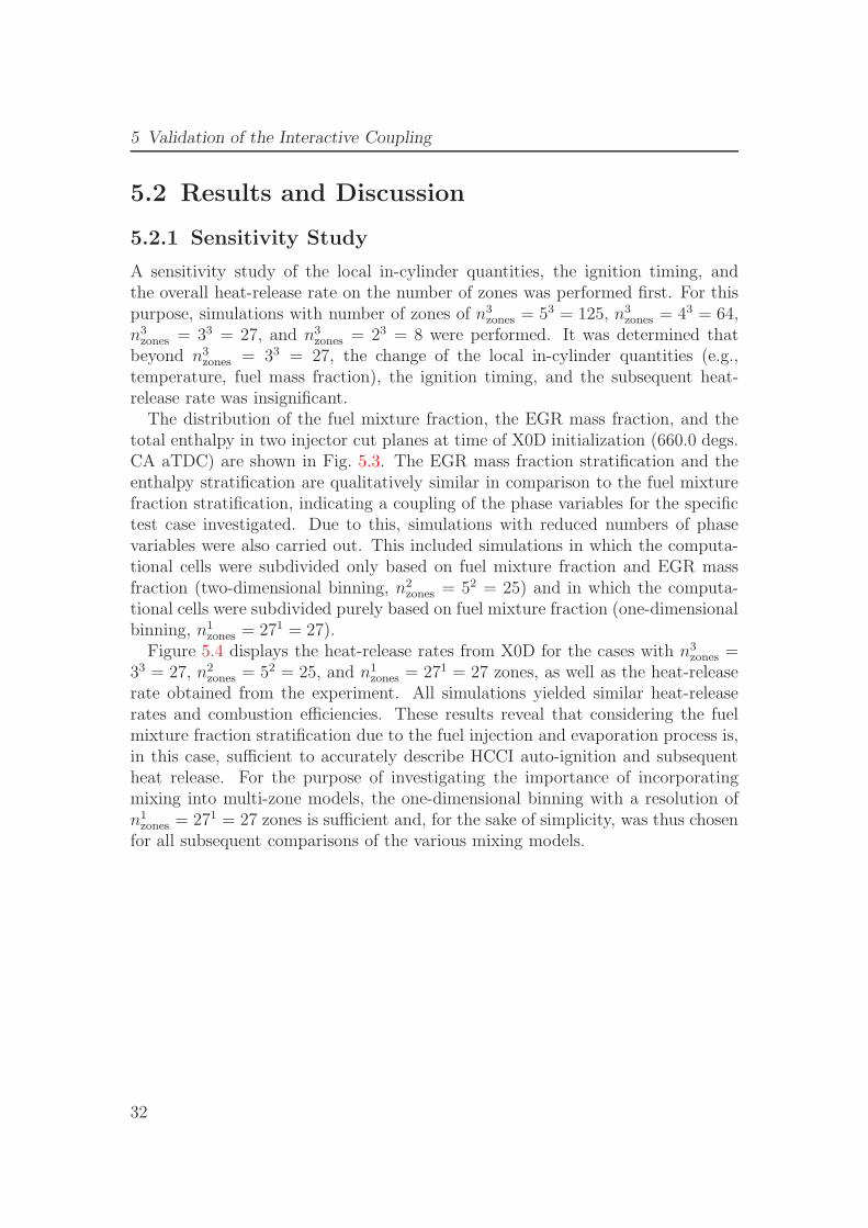
A sensitivity study of the local in-cylinder quantities, the ignition timing, andthe overall heat-release rate on the number of zones was performed first. For thispurpose, simulations with number of zones of n3
zones = 53 = 125, n3zones = 43 = 64,
n3zones = 33 = 27, and n3
zones = 23 = 8 were performed. It was determined thatbeyond n3
zones = 33 = 27, the change of the local in-cylinder quantities (e.g.,temperature, fuel mass fraction), the ignition timing, and the subsequent heat-release rate was insignificant.
The distribution of the fuel mixture fraction, the EGR mass fraction, and thetotal enthalpy in two injector cut planes at time of X0D initialization (660.0 degs.CA aTDC) are shown in Fig. 5.3. The EGR mass fraction stratification and theenthalpy stratification are qualitatively similar in comparison to the fuel mixturefraction stratification, indicating a coupling of the phase variables for the specifictest case investigated. Due to this, simulations with reduced numbers of phasevariables were also carried out. This included simulations in which the computa-tional cells were subdivided only based on fuel mixture fraction and EGR massfraction (two-dimensional binning, n2
zones = 52 = 25) and in which the computa-tional cells were subdivided purely based on fuel mixture fraction (one-dimensionalbinning, n1
zones = 271 = 27).Figure 5.4 displays the heat-release rates from X0D for the cases with n3
zones =33 = 27, n2
zones = 52 = 25, and n1zones = 271 = 27 zones, as well as the heat-release
rate obtained from the experiment. All simulations yielded similar heat-releaserates and combustion efficiencies. These results reveal that considering the fuelmixture fraction stratification due to the fuel injection and evaporation process is,in this case, sufficient to accurately describe HCCI auto-ignition and subsequentheat release. For the purpose of investigating the importance of incorporatingmixing into multi-zone models, the one-dimensional binning with a resolution ofn1
zones = 271 = 27 zones is sufficient and, for the sake of simplicity, was thus chosenfor all subsequent comparisons of the various mixing models.
32
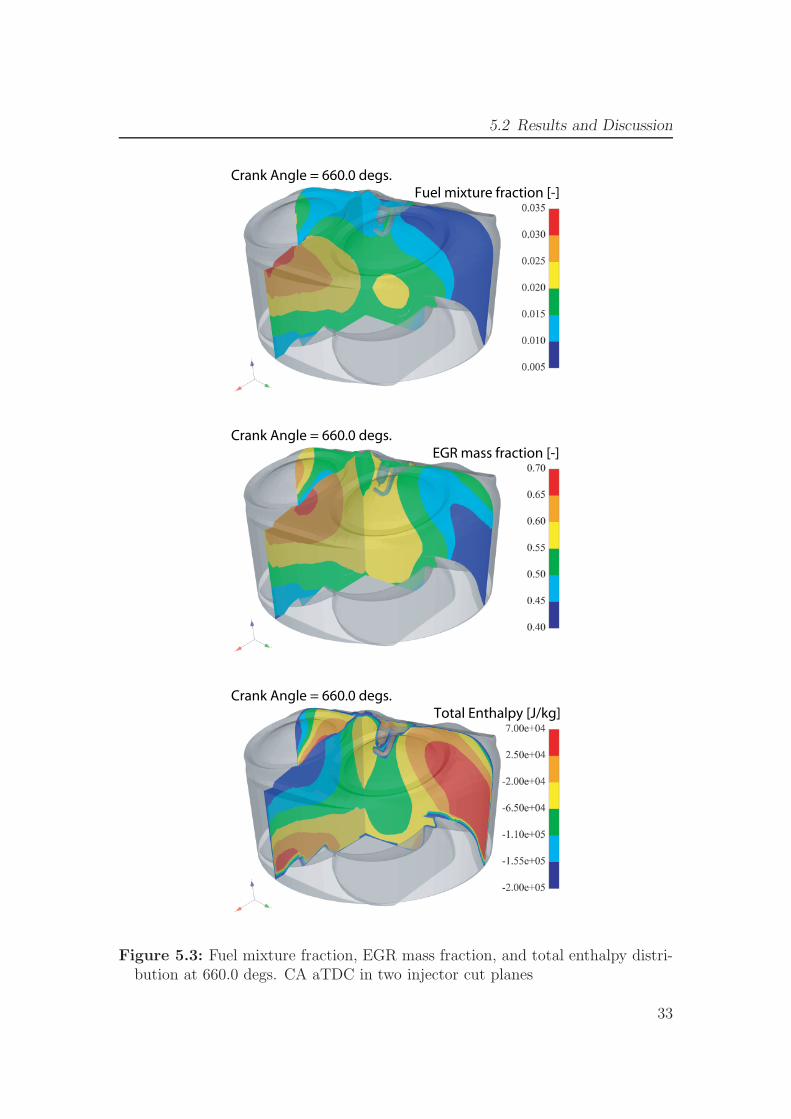
5.2 Results and Discussion
Fuel mixture fraction [-]Crank Angle = 660.0 degs.
Crank Angle = 660.0 degs.
EGR mass fraction [-]
Total Enthalpy [J/kg]Crank Angle = 660.0 degs.
Figure 5.3: Fuel mixture fraction, EGR mass fraction, and total enthalpy distri-bution at 660.0 degs. CA aTDC in two injector cut planes
33
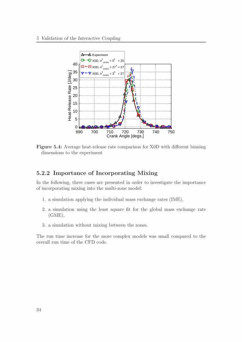
5 Validation of the Interactive Coupling
690 700 710 720 730 740 750Crank Angle [degs.]
0
5
10
15
20
25
30
35
40H
eat-
Rel
ease
Rat
e [J
/deg
.]
Experiment
X0D, n2
zones = 52 = 25
X0D, n1
zones = 271 = 27
X0D, n3
zones = 33 = 27
Figure 5.4: Average heat-release rate comparison for X0D with different binningdimensions to the experiment
5.2.2 Importance of Incorporating Mixing
In the following, three cases are presented in order to investigate the importanceof incorporating mixing into the multi-zone model:
1. a simulation applying the individual mass exchange rates (IME),
2. a simulation using the least square fit for the global mass exchange rate(GME),
3. a simulation without mixing between the zones.
The run time increase for the more complex models was small compared to theoverall run time of the CFD code.
34
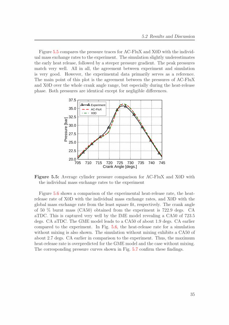
5.2 Results and Discussion
Figure 5.5 compares the pressure traces for AC-FluX and X0D with the individ-ual mass exchange rates to the experiment. The simulation slightly underestimatesthe early heat release, followed by a steeper pressure gradient. The peak pressuresmatch very well. All in all, the agreement between experiment and simulationis very good. However, the experimental data primarily serves as a reference.The main point of this plot is the agreement between the pressures of AC-FluXand X0D over the whole crank angle range, but especially during the heat-releasephase. Both pressures are identical except for negligible differences.
705 710 715 720 725 730 735 740 745Crank Angle [degs.]
20.0
22.5
25.0
27.5
30.0
32.5
35.0
37.5
Pre
ssur
e [b
ar]
Experiment
AC-FluXX0D
Figure 5.5: Average cylinder pressure comparison for AC-FluX and X0D withthe individual mass exchange rates to the experiment
Figure 5.6 shows a comparison of the experimental heat-release rate, the heat-release rate of X0D with the individual mass exchange rates, and X0D with theglobal mass exchange rate from the least square fit, respectively. The crank angleof 50 % burnt mass (CA50) obtained from the experiment is 722.9 degs. CAaTDC. This is captured very well by the IME model revealing a CA50 of 723.5degs. CA aTDC. The GME model leads to a CA50 of about 1.9 degs. CA earliercompared to the experiment. In Fig. 5.6, the heat-release rate for a simulationwithout mixing is also shown. The simulation without mixing exhibits a CA50 ofabout 2.7 degs. CA earlier in comparison to the experiment. Thus, the maximumheat-release rate is overpredicted for the GME model and the case without mixing.The corresponding pressure curves shown in Fig. 5.7 confirm these findings.
35
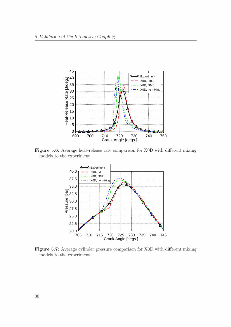
5 Validation of the Interactive Coupling
690 700 710 720 730 740 750Crank Angle [degs.]
0
5
10
15
20
25
30
35
40
45H
eat-
Rel
ease
Rat
e [J
/deg
.] Experiment
X0D, IME
X0D, GME
X0D, no mixing
Figure 5.6: Average heat-release rate comparison for X0D with different mixingmodels to the experiment
705 710 715 720 725 730 735 740 745Crank Angle [degs.]
20.0
22.5
25.0
27.5
30.0
32.5
35.0
37.5
40.0
Pre
ssur
e [b
ar]
Experiment
X0D, IME
X0D, GME
X0D, no mixing
Figure 5.7: Average cylinder pressure comparison for X0D with different mixingmodels to the experiment
36
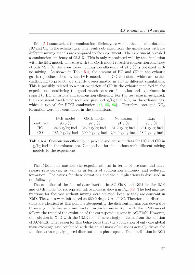
5.2 Results and Discussion
Table 5.4 summarizes the combustion efficiency, as well as the emission data forHC and CO in the exhaust gas. The results obtained from the simulations with thedifferent mixing models are compared to the experiment. The experiment revealeda combustion efficiency of 95.3 %. This is only reproduced well by the simulationwith the IME model. The case with the GME model reveals a combustion efficiencyof only 92.1 %. An even lower combustion efficiency of 91.6 % is obtained withno mixing. As shown in Table 5.4, the amount of HC and CO in the exhaustgas is reproduced best by the IME model. The CO emissions, which are ratherchallenging to predict, are slightly overestimated in all the different simulations.This is possibly related to a post-oxidation of CO in the exhaust manifold in theexperiment, considering the good match between simulation and experiment inregard to HC emissions and combustion efficiency. For the test case investigated,the experiment yielded no soot and just 0.21 g/kg fuel NOx in the exhaust gas,which is typical for HCCI combustion [12, 55, 93]. Therefore, soot and NOx
formation were not considered in the simulations.
IME model GME model No mixing Exp.Comb. eff. 95.6 % 92.5 % 91.6 % 95.3 %
HC 24.6 g/kg fuel 26.9 g/kg fuel 61.2 g/kg fuel 30.1 g/kg fuelCO 185.0 g/kg fuel 300.0 g/kg fuel 204.0 g/kg fuel 68.6 g/kg fuel
Table 5.4: Combustion efficiency in percent and emission data for HC and CO ing/kg fuel in the exhaust gas. Comparison for simulations with different mixingmodels to the experiment
The IME model matches the experiment best in terms of pressure and heat-release rate curves, as well as in terms of combustion efficiency and pollutantformation. The causes for these deviations and their implications is discussed inthe following.
The evolution of the fuel mixture fraction in AC-FluX and X0D for the IMEand GME model for six representative zones is shown in Fig. 5.8. The fuel mixturefractions for the case without mixing were omitted, because they are constant inX0D. The zones were initialized at 660.0 degs. CA aTDC. Therefore, all distribu-tions are identical at this point. Subsequently, the distribution narrows down dueto mixing. The fuel mixture fraction in each zone in X0D with the GME modelfollows the trend of the evolution of the corresponding zone in AC-FluX. However,the solution in X0D with the GME model increasingly deviates from the solutionof AC-FluX. The reason for this behavior is that the application of only one globalmass exchange rate combined with the equal mass of all zones actually drives thesolution to an equally spaced distribution in phase space. The distribution in X0D
37
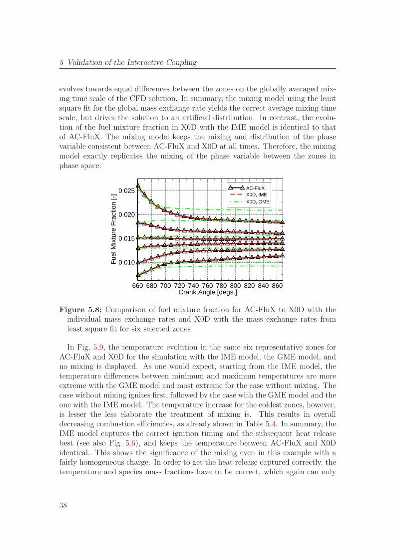
5 Validation of the Interactive Coupling
evolves towards equal differences between the zones on the globally averaged mix-ing time scale of the CFD solution. In summary, the mixing model using the leastsquare fit for the global mass exchange rate yields the correct average mixing timescale, but drives the solution to an artificial distribution. In contrast, the evolu-tion of the fuel mixture fraction in X0D with the IME model is identical to thatof AC-FluX. The mixing model keeps the mixing and distribution of the phasevariable consistent between AC-FluX and X0D at all times. Therefore, the mixingmodel exactly replicates the mixing of the phase variable between the zones inphase space.
660 680 700 720 740 760 780 800 820 840 860Crank Angle [degs.]
0.010
0.015
0.020
0.025
Fue
l Mix
ture
Fra
ctio
n [-
]
AC-FluXX0D, IME
X0D, GME
Figure 5.8: Comparison of fuel mixture fraction for AC-FluX to X0D with theindividual mass exchange rates and X0D with the mass exchange rates fromleast square fit for six selected zones
In Fig. 5.9, the temperature evolution in the same six representative zones forAC-FluX and X0D for the simulation with the IME model, the GME model, andno mixing is displayed. As one would expect, starting from the IME model, thetemperature differences between minimum and maximum temperatures are moreextreme with the GME model and most extreme for the case without mixing. Thecase without mixing ignites first, followed by the case with the GME model and theone with the IME model. The temperature increase for the coldest zones, however,is lesser the less elaborate the treatment of mixing is. This results in overalldecreasing combustion efficiencies, as already shown in Table 5.4. In summary, theIME model captures the correct ignition timing and the subsequent heat releasebest (see also Fig. 5.6), and keeps the temperature between AC-FluX and X0Didentical. This shows the significance of the mixing even in this example with afairly homogeneous charge. In order to get the heat release captured correctly, thetemperature and species mass fractions have to be correct, which again can only
38
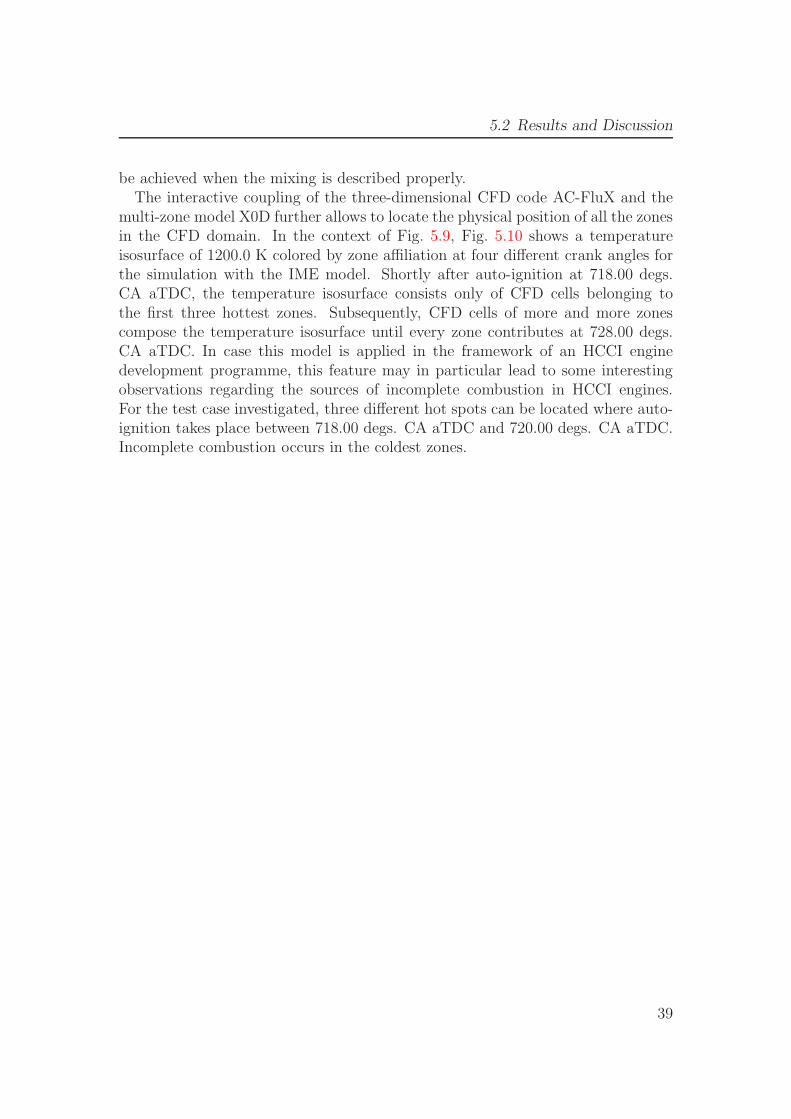
5.2 Results and Discussion
be achieved when the mixing is described properly.The interactive coupling of the three-dimensional CFD code AC-FluX and the
multi-zone model X0D further allows to locate the physical position of all the zonesin the CFD domain. In the context of Fig. 5.9, Fig. 5.10 shows a temperatureisosurface of 1200.0 K colored by zone affiliation at four different crank angles forthe simulation with the IME model. Shortly after auto-ignition at 718.00 degs.CA aTDC, the temperature isosurface consists only of CFD cells belonging tothe first three hottest zones. Subsequently, CFD cells of more and more zonescompose the temperature isosurface until every zone contributes at 728.00 degs.CA aTDC. In case this model is applied in the framework of an HCCI enginedevelopment programme, this feature may in particular lead to some interestingobservations regarding the sources of incomplete combustion in HCCI engines.For the test case investigated, three different hot spots can be located where auto-ignition takes place between 718.00 degs. CA aTDC and 720.00 degs. CA aTDC.Incomplete combustion occurs in the coldest zones.
39
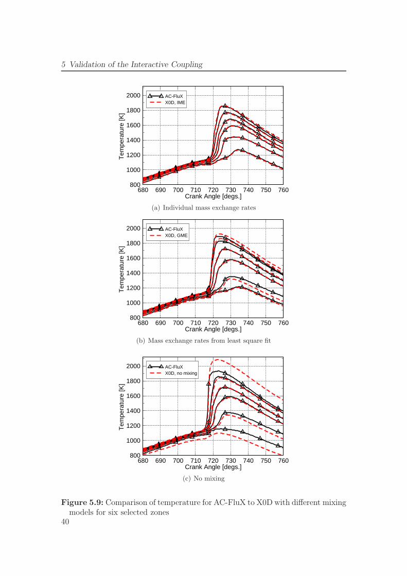
5 Validation of the Interactive Coupling
680 690 700 710 720 730 740 750 760Crank Angle [degs.]
800
1000
1200
1400
1600
1800
2000
Tem
pera
ture
[K]
AC-FluXX0D, IME
(a) Individual mass exchange rates
680 690 700 710 720 730 740 750 760Crank Angle [degs.]
800
1000
1200
1400
1600
1800
2000
Tem
pera
ture
[K]
AC-FluXX0D, GME
(b) Mass exchange rates from least square fit
680 690 700 710 720 730 740 750 760Crank Angle [degs.]
800
1000
1200
1400
1600
1800
2000
Tem
pera
ture
[K]
AC-FluXX0D, no mixing
(c) No mixing
Figure 5.9: Comparison of temperature for AC-FluX to X0D with different mixingmodels for six selected zones
40
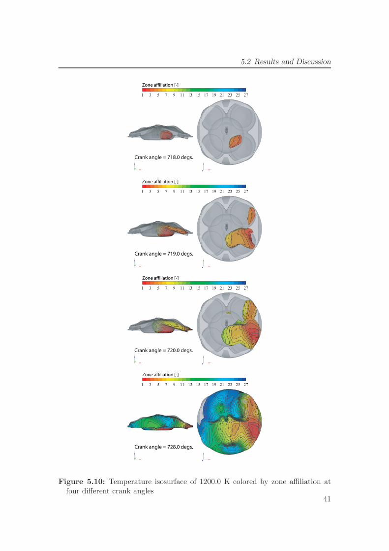
5.2 Results and Discussion
Crank angle = 718.0 degs.
Zone affiliation [-]
Crank angle = 719.0 degs.
Zone affiliation [-]
Crank angle = 720.0 degs.
Zone affiliation [-]
Crank angle = 728.0 degs.
Zone affiliation [-]
Figure 5.10: Temperature isosurface of 1200.0 K colored by zone affiliation atfour different crank angles
41
5 Validation of the Interactive Coupling
5.3 Concluding Remarks
A zero-dimensional multi-zone code (X0D) was interactively coupled to a CFDcode (AC-FluX) to solve the chemistry for HCCI combustion. Two models forthe mass exchange between zones in phase space based on the CFD solution werepresented and applied to an HCCI engine test case. The IME model, where in-dividual mass exchange rates for each zone are computed, replicates the CFDsolution identically in terms of mixing. The GME model is less accurate with de-viations from the ideal solution. The strong deviations of the results without anymixing emphasize the importance of incorporating mixing. The differences in theresults for the different models are expected to be more pronounced for cases withgreater stratification. An approach for the consistent modeling of the exchangeof source terms between the CFD code and the zero-dimensional multi-zone codewas proposed.
42
6 Systematic Reduction of theInteractively CoupledCFD-Multi-Zone Approach towards aStand-alone Multi-Zone Model
Chapter 4 depicts the exchange of information between the CFD code and themulti-zone model. Two information streams and an appropriate treatment of thesource terms establish the interactive coupling of both codes. Chapter 5 containsits validation against HCCI combustion in a gasoline single-cylinder research en-gine. In this chapter, the interactive coupling is first extended to account for PCCIcombustion in Sec. 6.1. Following this, a methodology is presented in Sec. 6.2 ofhow the information that is fed from the CFD code to the multi-zone model can beaccounted for within the multi-zone model. This allows for decoupling the multi-zone model from the CFD code and leads to a systematic reduction of the interac-tively coupled CFD-multi-zone approach towards a stand-alone multi-zone modelfor PCCI combustion. In detail, Subsecs. 6.2.1 and 6.2.2 describe an appropriatemodeling of the sink and source terms (heat transfer to the walls, fuel injectionand vaporization) within the multi-zone model. In addition, Subsec. 6.2.3 presentsa simplified mixing model within the multi-zone model. Finally, Subsec. 6.2.4 out-lines further reduction potential. Section 6.3 then discusses the computational ac-curacy and efficiency of both the interactively coupled CFD-multi-zone approachand the stand-alone multi-zone model.
43
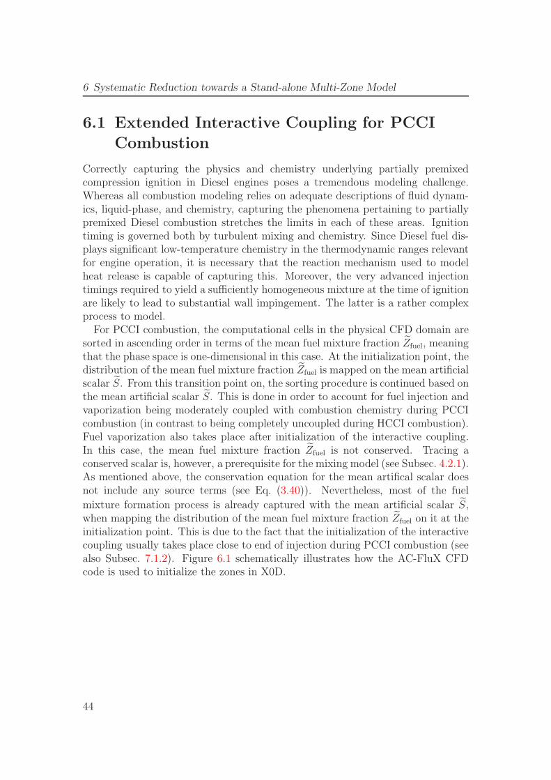
6 Systematic Reduction towards a Stand-alone Multi-Zone Model
6.1 Extended Interactive Coupling for PCCI
Combustion
Correctly capturing the physics and chemistry underlying partially premixedcompression ignition in Diesel engines poses a tremendous modeling challenge.Whereas all combustion modeling relies on adequate descriptions of fluid dynam-ics, liquid-phase, and chemistry, capturing the phenomena pertaining to partiallypremixed Diesel combustion stretches the limits in each of these areas. Ignitiontiming is governed both by turbulent mixing and chemistry. Since Diesel fuel dis-plays significant low-temperature chemistry in the thermodynamic ranges relevantfor engine operation, it is necessary that the reaction mechanism used to modelheat release is capable of capturing this. Moreover, the very advanced injectiontimings required to yield a sufficiently homogeneous mixture at the time of ignitionare likely to lead to substantial wall impingement. The latter is a rather complexprocess to model.
For PCCI combustion, the computational cells in the physical CFD domain aresorted in ascending order in terms of the mean fuel mixture fraction Zfuel, meaningthat the phase space is one-dimensional in this case. At the initialization point, thedistribution of the mean fuel mixture fraction Zfuel is mapped on the mean artificialscalar S. From this transition point on, the sorting procedure is continued based onthe mean artificial scalar S. This is done in order to account for fuel injection andvaporization being moderately coupled with combustion chemistry during PCCIcombustion (in contrast to being completely uncoupled during HCCI combustion).Fuel vaporization also takes place after initialization of the interactive coupling.In this case, the mean fuel mixture fraction Zfuel is not conserved. Tracing aconserved scalar is, however, a prerequisite for the mixing model (see Subsec. 4.2.1).As mentioned above, the conservation equation for the mean artifical scalar doesnot include any source terms (see Eq. (3.40)). Nevertheless, most of the fuel
mixture formation process is already captured with the mean artificial scalar S,when mapping the distribution of the mean fuel mixture fraction Zfuel on it at theinitialization point. This is due to the fact that the initialization of the interactivecoupling usually takes place close to end of injection during PCCI combustion (seealso Subsec. 7.1.2). Figure 6.1 schematically illustrates how the AC-FluX CFDcode is used to initialize the zones in X0D.
44
6.1 Extended Interactive Coupling for PCCI Combustion
1
2
3
4
5
6
7
8
9
10
11
12
13
14
15
740
760
780
800
820
840
860
880
900
Upon X0D initialization, sorting of
the physical domain in ascending
order in terms of the phase
variable (fuel mix. fraction).
Definition of a corresponding
set of zones in the multi-zone model
Crank Angle = -19.0 degs. aTDC
Zone affiliation [-]
Zone
numbers
Te
mp
era
ture
[K
]
Figure 6.1: Schematic illustration of the zone initialization in the multi-zonemodel for PCCI combustion
Mixing is incorporated into the multi-zone model based on the mean artificialscalar S. The change for the mean artificial scalar Si from CFD time step n − 1to CFD time step n in the individual zones can be described as
mi ·Sn
i − Sn−1i
∆tn=
2∑
k=1
mik
(Sn−1
k − Sn−1i
). (6.1)
Equation (6.1) is then used instead of Eq. (4.1).
Within the extended interactive coupling, vaporization of fuel in the multi-zonemodel is accounted for by averaging the source term ρs
fuel in Eq. (3.39) for eachzone in the CFD code. This averaging procedure yields the source term ρs
ij,j=fuel
in Eqs. (2.1) and (2.2) and is linked to the source term for the spray in Eq. (4.7)according to
qsi =
nsp∑
j=1
ρsij · ∆hvj with ρs
ij = 0, j 6= fuel . (6.2)
45
6 Systematic Reduction towards a Stand-alone Multi-Zone Model
6.2 Reduction Methodology
6.2.1 Heat Transfer to the Walls
In the multi-zone model, heat transfer to the walls is accounted for by Eq. (2.4).Instead of using CFD information to calculate the heat transfer coefficient hwall,l,i,it can also be modeled with the Woschni correlation [102], reading
hwall,l,i = hwall = 3.26 · b−0.2 · p0.8 · T−0.53av. (C1 · vpiston)
0.8 , (6.3)
where b is the bore of the engine, p the mean cylinder pressure, Tav. the averagein-cylinder temperature, and vpiston the mean piston speed. The constant C1 isadjustable and is set to 0.5. Since the average in-cylinder temperature Tav. is usedwithin the Woschni correlation and hwall,l,i does not depend on any specific wall, theheat transfer coefficient is equal for all zones and walls, leading to hwall,l,i = hwall.
For the specific engine investigated, the area Awall,l,i of wall l belonging to zonei has to be taken from a preceding simulation with the interactively coupled CFD-multi-zone approach so that this information can be incorporated into a successivesimulation with the stand-alone multi-zone model.
6.2.2 Fuel Injection and Evaporation
A preceding simulation with the interactively coupled CFD-multi-zone approachalso allows to determine the amount of fuel that is injected and vaporizes in eachCFD zone. This information can then be incorporated into a successive simulationwith the stand-alone multi-zone model (see source term ρs
ij,j=fuel in Eqs. (2.1)and (2.2)).
6.2.3 Simplified Mixing Model
The simplified mixing model within the stand-alone multi-zone model assumesthat the previously introduced mass exchange rate mik of zone i with neighboringzone k (see Eqs. (2.1) and (2.2)) is proportional to the wall heat transfer coefficienthwall and the area A both zones share [39]. This is an analogy to the well knownempirical Lewis law which assumes a similarity between heat and mass transfer [7].The heat transfer to the walls and the mass exchange between the zones are bothinduced by the turbulence intensity so that they can be related to each other. Thecorresponding equation reads
mik = rMB · A · mi + mk
(micpi + mkcpk)· hwall . (6.4)
46
6.3 Computational Accuracy and Efficiency
In Eq. (6.4), cpi is the average heat capacity at constant pressure of zone i. rMB
is a parameter that is adjusted to yield the desired level of mixing. The exactchoice of rMB is discussed in Subsec. 7.2.2 below. The area A is computed fromthe volumes Vi and Vk of the two zones i and k according to
A = 4π
[3
4π(Vi + Vk)
] 23
. (6.5)
6.2.4 Further Reduction Potential
A possible further reduction beyond the decoupling of the multi-zone model fromthe CFD code could be achieved by reducing the chemical mechanism applied inthe PCCI simulations (see Sec. 2.3). The work by Muller et al. [54] describes areduced chemical mechanism for n-heptane with only four global reactions and fiveglobal chemical species. Two of these four global reactions account for the high-temperature branch and the other two for the low-temperature branch of the igni-tion kinetics. Using this mechanism instead of the one by Peters et al. [67] wouldhighly reduce the number of partial differential equations that need to be solved inthe multi-zone model (see Subsec. 6.3.3 below). However, no NO-submechanismcan be integrated into this reduced mechanism, because it does not contain thenecessary chemical species.
6.3 Computational Accuracy and Efficiency
6.3.1 Interactively Coupled CFD-Multi-Zone Approach
The interactively coupled CFD-multi-zone approach efficiently separates the solu-tion of the flow field from the solution of the chemistry. During one time step ofthe CFD code, the multi-zone code solves Eqs. (2.1), (2.2), and (2.3) with timesteps that can be much smaller, depending on the chemistry. In this way, the timescales of the chemistry and the fluid dynamics are decoupled. Thus, the approachdoes not need to simplify the highly nonlinear chemistry, allowing for any detailedreaction mechanisms to be used. These mechanisms may also include pollutantformation and destruction. This procedure yields an approach that includes an ac-curate description of PCCI chemistry with only a small penalty in computationalcost, since even during auto-ignition, the CFD time step has hardly to be reducedcompared to an inert computation of the chemistry.
Decoupling the time scales of the chemistry and the fluid dynamics has provensuccessful in predicting conventional Diesel engine combustion in the frameworkof Representative Interactive Flamelets (RIF).
47
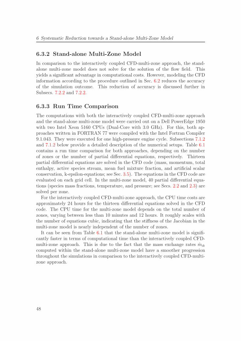
6 Systematic Reduction towards a Stand-alone Multi-Zone Model
6.3.2 Stand-alone Multi-Zone Model
In comparison to the interactively coupled CFD-multi-zone approach, the stand-alone multi-zone model does not solve for the solution of the flow field. Thisyields a significant advantage in computational costs. However, modeling the CFDinformation according to the procedure outlined in Sec. 6.2 reduces the accuracyof the simulation outcome. This reduction of accuracy is discussed further inSubsecs. 7.2.2 and 7.2.2.
6.3.3 Run Time Comparison
The computations with both the interactively coupled CFD-multi-zone approachand the stand-alone multi-zone model were carried out on a Dell PowerEdge 1950with two Intel Xeon 5160 CPUs (Dual-Core with 3.0 GHz). For this, both ap-proaches written in FORTRAN 77 were compiled with the Intel Fortran Compiler9.1.043. They were executed for one high-pressure engine cycle. Subsections 7.1.2and 7.1.2 below provide a detailed description of the numerical setups. Table 6.1contains a run time comparison for both approaches, depending on the numberof zones or the number of partial differential equations, respectively. Thirteenpartial differential equations are solved in the CFD code (mass, momentum, totalenthalpy, active species stream, mean fuel mixture fraction, and artificial scalarconservation, k-epsilon-equations; see Sec. 3.5). The equations in the CFD code areevaluated on each grid cell. In the multi-zone model, 40 partial differential equa-tions (species mass fractions, temperature, and pressure; see Secs. 2.2 and 2.3) aresolved per zone.
For the interactively coupled CFD-multi-zone approach, the CPU time costs areapproximately 24 hours for the thirteen differential equations solved in the CFDcode. The CPU time for the multi-zone model depends on the total number ofzones, varying between less than 10 minutes and 12 hours. It roughly scales withthe number of equations cubic, indicating that the stiffness of the Jacobian in themulti-zone model is nearly independent of the number of zones.
It can be seen from Table 6.1 that the stand-alone multi-zone model is signifi-cantly faster in terms of computational time than the interactively coupled CFD-multi-zone approach. This is due to the fact that the mass exchange rates mik
computed within the stand-alone multi-zone model have a smoother progressionthroughout the simulations in comparison to the interactively coupled CFD-multi-zone approach.
48
6.3 Computational Accuracy and Efficiency
Number of zones/number of eqs.
forCFD-multi-zone
approach orstand-alone
multi-zone model
CPU time forinteractively
coupledCFD-multi-zone
approach
CPU time for stand-alone multi-zone model
5 zones/13+200 eqs. or 200eqs., respectively
∼ 24.1 hours ∼ 0.2 minutes
10 zones/13+400 eqs. or 400eqs., respectively
∼ 24.8 hours ∼ 1.1 minutes
15 zones/13+600 eqs. or 600eqs., respectively
∼ 25.5 hours ∼ 3.3 minutes
20 zones/13+800 eqs. or 800eqs., respectively
∼ 28.0 hours ∼ 8.5 minutes
25 zones/13+1000 eqs. or
1000 eqs.,respectively
∼ 36.0 hours ∼ 22.5 minutes
Table 6.1: Run time comparison for the interactively coupled CFD-multi-zoneapproach and the stand-alone multi-zone model. Depending on the numberof zones, the left column contains the number of partial differential equationsthat are solved in the CFD-multi-zone approach or the stand-alone multi-zonemodel, respectively. The second and third column contain the correspondingCPU times for one high-pressure engine cycle simulation
49

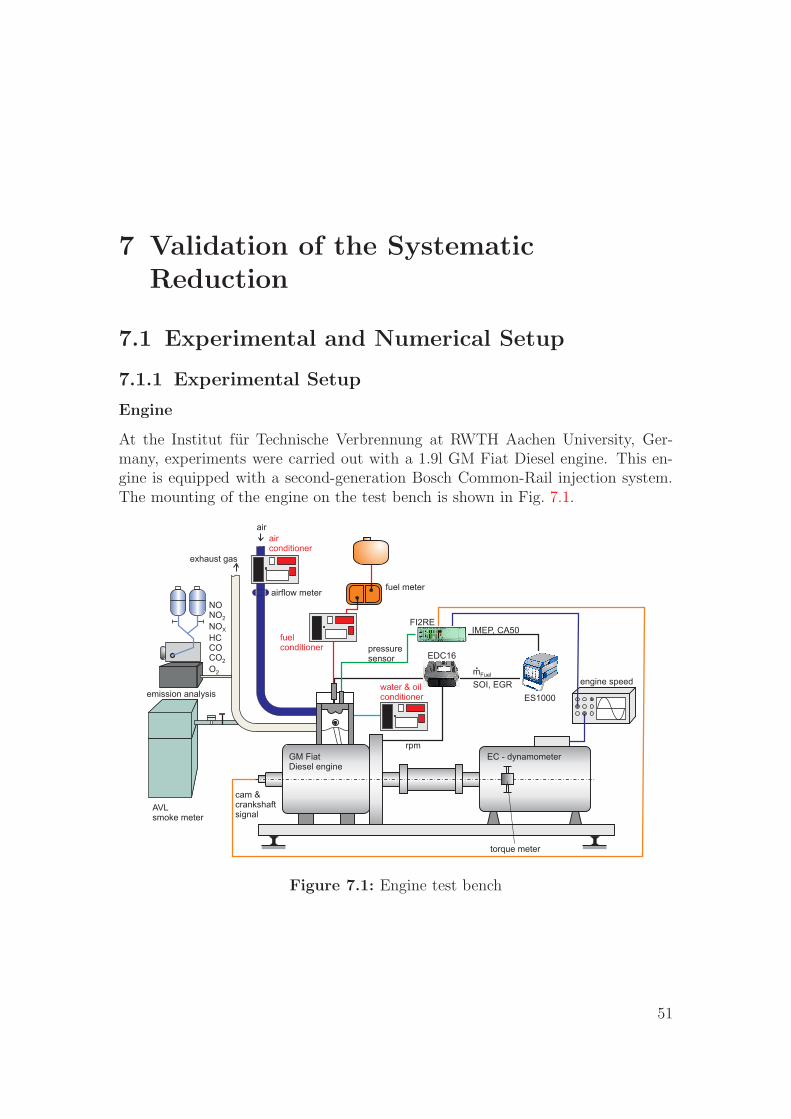
7 Validation of the SystematicReduction
7.1 Experimental and Numerical Setup
7.1.1 Experimental Setup
Engine
At the Institut fur Technische Verbrennung at RWTH Aachen University, Ger-many, experiments were carried out with a 1.9l GM Fiat Diesel engine. This en-gine is equipped with a second-generation Bosch Common-Rail injection system.The mounting of the engine on the test bench is shown in Fig. 7.1.
torque meter
EC - dynamometer
engine speed
AVLsmoke meter
emission analysis
exhaust gas
fuel meter
pressuresensor
fuelconditioner
water & oilconditioner
airconditioner
airflow meter
cam &crankshaftsignal
NONO
NO
HCCOCO
O
2
X
2
2
air
FI2RE
rpm
GM FiatDiesel engine
ES1000
IMEP, CA50
SOI, EGR
mFuel
EDC16
Figure 7.1: Engine test bench
51
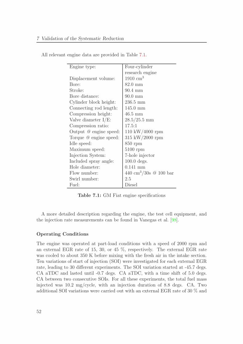
7 Validation of the Systematic Reduction
All relevant engine data are provided in Table 7.1.
Engine type: Four-cylinderresearch engine
Displacement volume: 1910 cm3
Bore: 82.0 mmStroke: 90.4 mmBore distance: 90.0 mmCylinder block height: 236.5 mmConnecting rod length: 145.0 mmCompression height: 46.5 mmValve diameter I/E: 28.5/25.5 mmCompression ratio: 17.5:1Output @ engine speed: 110 kW/4000 rpmTorque @ engine speed: 315 kW/2000 rpmIdle speed: 850 rpmMaximum speed: 5100 rpmInjection System: 7-hole injectorIncluded spray angle: 100.0 degs.Hole diameter: 0.141 mmFlow number: 440 cm3/30s @ 100 barSwirl number: 2.5Fuel: Diesel
Table 7.1: GM Fiat engine specifications
A more detailed description regarding the engine, the test cell equipment, andthe injection rate measurements can be found in Vanegas et al. [98].
Operating Conditions
The engine was operated at part-load conditions with a speed of 2000 rpm andan external EGR rate of 15, 30, or 45 %, respectively. The external EGR ratewas cooled to about 350 K before mixing with the fresh air in the intake section.Ten variations of start of injection (SOI) were investigated for each external EGRrate, leading to 30 different experiments. The SOI variation started at -45.7 degs.CA aTDC and lasted until -0.7 degs. CA aTDC, with a time shift of 5.0 degs.CA between two consecutive SOIs. For all these experiments, the total fuel massinjected was 10.2 mg/cycle, with an injection duration of 8.8 degs. CA. Twoadditional SOI variations were carried out with an external EGR rate of 30 % and
52
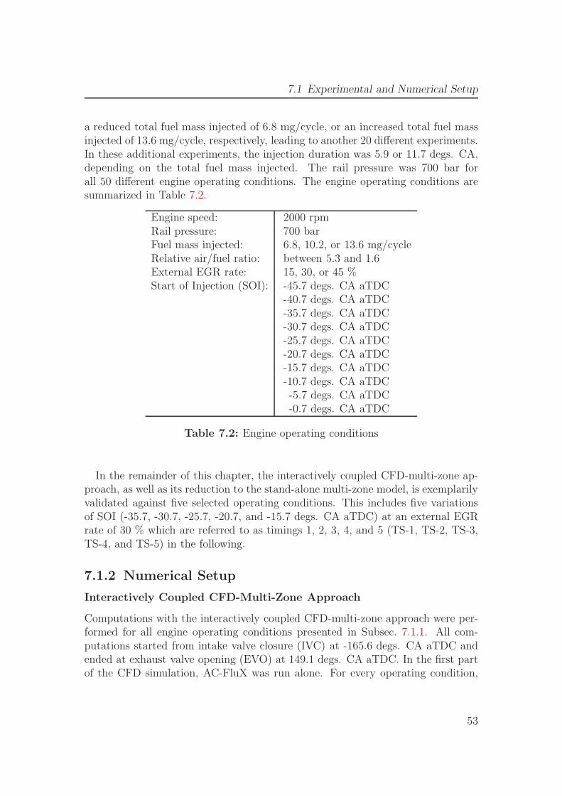
7.1 Experimental and Numerical Setup
a reduced total fuel mass injected of 6.8 mg/cycle, or an increased total fuel massinjected of 13.6 mg/cycle, respectively, leading to another 20 different experiments.In these additional experiments, the injection duration was 5.9 or 11.7 degs. CA,depending on the total fuel mass injected. The rail pressure was 700 bar forall 50 different engine operating conditions. The engine operating conditions aresummarized in Table 7.2.
Engine speed: 2000 rpmRail pressure: 700 barFuel mass injected: 6.8, 10.2, or 13.6 mg/cycleRelative air/fuel ratio: between 5.3 and 1.6External EGR rate: 15, 30, or 45 %Start of Injection (SOI): -45.7 degs. CA aTDC
-40.7 degs. CA aTDC-35.7 degs. CA aTDC-30.7 degs. CA aTDC-25.7 degs. CA aTDC-20.7 degs. CA aTDC-15.7 degs. CA aTDC-10.7 degs. CA aTDC-5.7 degs. CA aTDC-0.7 degs. CA aTDC
Table 7.2: Engine operating conditions
In the remainder of this chapter, the interactively coupled CFD-multi-zone ap-proach, as well as its reduction to the stand-alone multi-zone model, is exemplarilyvalidated against five selected operating conditions. This includes five variationsof SOI (-35.7, -30.7, -25.7, -20.7, and -15.7 degs. CA aTDC) at an external EGRrate of 30 % which are referred to as timings 1, 2, 3, 4, and 5 (TS-1, TS-2, TS-3,TS-4, and TS-5) in the following.
7.1.2 Numerical Setup
Interactively Coupled CFD-Multi-Zone Approach
Computations with the interactively coupled CFD-multi-zone approach were per-formed for all engine operating conditions presented in Subsec. 7.1.1. All com-putations started from intake valve closure (IVC) at -165.6 degs. CA aTDC andended at exhaust valve opening (EVO) at 149.1 degs. CA aTDC. In the first partof the CFD simulation, AC-FluX was run alone. For every operating condition,
53
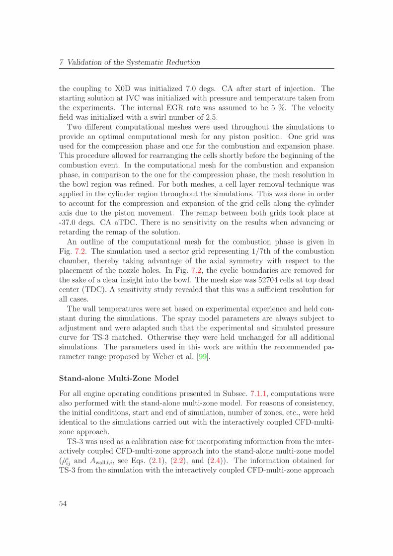
7 Validation of the Systematic Reduction
the coupling to X0D was initialized 7.0 degs. CA after start of injection. Thestarting solution at IVC was initialized with pressure and temperature taken fromthe experiments. The internal EGR rate was assumed to be 5 %. The velocityfield was initialized with a swirl number of 2.5.
Two different computational meshes were used throughout the simulations toprovide an optimal computational mesh for any piston position. One grid wasused for the compression phase and one for the combustion and expansion phase.This procedure allowed for rearranging the cells shortly before the beginning of thecombustion event. In the computational mesh for the combustion and expansionphase, in comparison to the one for the compression phase, the mesh resolution inthe bowl region was refined. For both meshes, a cell layer removal technique wasapplied in the cylinder region throughout the simulations. This was done in orderto account for the compression and expansion of the grid cells along the cylinderaxis due to the piston movement. The remap between both grids took place at-37.0 degs. CA aTDC. There is no sensitivity on the results when advancing orretarding the remap of the solution.
An outline of the computational mesh for the combustion phase is given inFig. 7.2. The simulation used a sector grid representing 1/7th of the combustionchamber, thereby taking advantage of the axial symmetry with respect to theplacement of the nozzle holes. In Fig. 7.2, the cyclic boundaries are removed forthe sake of a clear insight into the bowl. The mesh size was 52704 cells at top deadcenter (TDC). A sensitivity study revealed that this was a sufficient resolution forall cases.
The wall temperatures were set based on experimental experience and held con-stant during the simulations. The spray model parameters are always subject toadjustment and were adapted such that the experimental and simulated pressurecurve for TS-3 matched. Otherwise they were held unchanged for all additionalsimulations. The parameters used in this work are within the recommended pa-rameter range proposed by Weber et al. [99].
Stand-alone Multi-Zone Model
For all engine operating conditions presented in Subsec. 7.1.1, computations werealso performed with the stand-alone multi-zone model. For reasons of consistency,the initial conditions, start and end of simulation, number of zones, etc., were heldidentical to the simulations carried out with the interactively coupled CFD-multi-zone approach.
TS-3 was used as a calibration case for incorporating information from the inter-actively coupled CFD-multi-zone approach into the stand-alone multi-zone model(ρs
ij and Awall,l,i, see Eqs. (2.1), (2.2), and (2.4)). The information obtained forTS-3 from the simulation with the interactively coupled CFD-multi-zone approach
54
7.2 Results and Discussion
was used for all experiments investigated with the stand-alone multi-zone model.This introduces a small error into the other stand-alone multi-zone model simula-tions (e.g., TS-1, TS-2, TS-4, and TS-5). However, this error is small, since thecalibration conditions of TS-3 do not deviate significantly from all other engineoperating conditions.
Figure 7.2: Computational grid at -25.0 degs. CA aTDC. Cyclic boundaries areremoved for illustration purposes
7.2 Results and Discussion
In this section, the interactively coupled CFD-multi-zone approach is first val-idated against experimental data in terms of pressure curves, IMEPHP, CA10,CA50, CO emissions, combustion efficiency, and NO/NOx emissions for all fiveaforementioned SOI timings (TS-1, TS-2, TS-3, TS-4, and TS-5). After this, TS-3is considered in detail. The exchange of information between the CFD code andthe multi-zone model within the interactively coupled CFD-multi-zone approach isinvestigated. Following this, the systematic reduction of the interactively coupledCFD-multi-zone approach towards the stand-alone multi-zone model is exemplar-ily shown for TS-3. Finally, simulation results obtained with the stand-alonemulti-zone model for all five SOI timings are compared to experimental data.
55
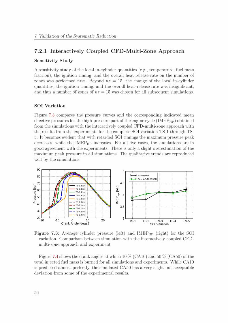
7 Validation of the Systematic Reduction
7.2.1 Interactively Coupled CFD-Multi-Zone Approach
Sensitivity Study
A sensitivity study of the local in-cylinder quantities (e.g., temperature, fuel massfraction), the ignition timing, and the overall heat-release rate on the number ofzones was performed first. Beyond nz = 15, the change of the local in-cylinderquantities, the ignition timing, and the overall heat-release rate was insignificant,and thus a number of zones of nz = 15 was chosen for all subsequent simulations.
SOI Variation
Figure 7.3 compares the pressure curves and the corresponding indicated meaneffective pressures for the high-pressure part of the engine cycle (IMEPHP) obtainedfrom the simulations with the interactively coupled CFD-multi-zone approach withthe results from the experiments for the complete SOI variation TS-1 through TS-5. It becomes evident that with retarded SOI timings the maximum pressure peakdecreases, while the IMEPHP increases. For all five cases, the simulations are ingood agreement with the experiments. There is only a slight overestimation of themaximum peak pressure in all simulations. The qualitative trends are reproducedwell by the simulations.
-20 -10 0 10 20Crank Angle [degs.]
20
30
40
50
60
70
80
90
Pre
ssur
e [b
ar]
TS-1, Exp.
TS-2, Exp.
TS-3, Exp.
TS-4, Exp.
TS-5, Exp.
TS-1, Sim.
TS-2, Sim.
TS-3, Sim.
TS-4, Sim.
TS-5, Sim.
TS-1 TS-2 TS-3 TS-4 TS-5SOI Variation
3
3.5
4
4.5
5
IME
PH
P [b
ar]
Experiment
Sim. AC-FluX-X0D
Figure 7.3: Average cylinder pressure (left) and IMEPHP (right) for the SOIvariation. Comparison between simulation with the interactively coupled CFD-multi-zone approach and experiment
Figure 7.4 shows the crank angles at which 10 % (CA10) and 50 % (CA50) of thetotal injected fuel mass is burned for all simulations and experiments. While CA10is predicted almost perfectly, the simulated CA50 has a very slight but acceptabledeviation from some of the experimental results.
56
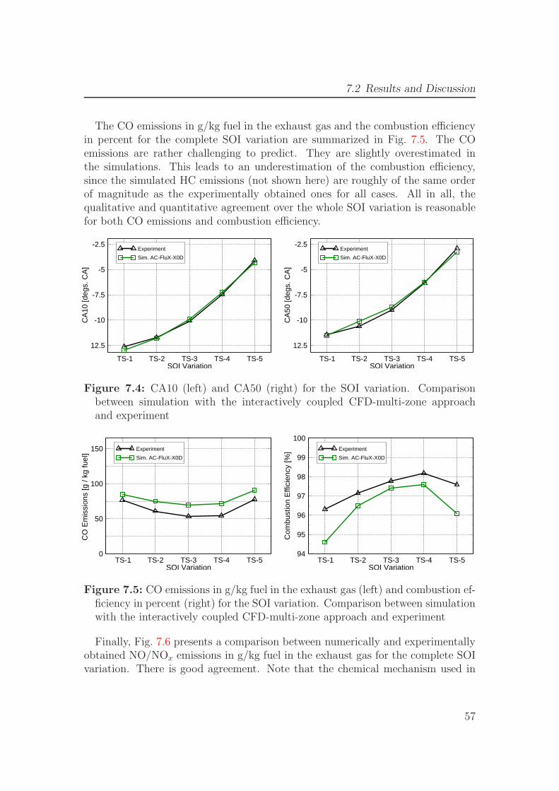
7.2 Results and Discussion
The CO emissions in g/kg fuel in the exhaust gas and the combustion efficiencyin percent for the complete SOI variation are summarized in Fig. 7.5. The COemissions are rather challenging to predict. They are slightly overestimated inthe simulations. This leads to an underestimation of the combustion efficiency,since the simulated HC emissions (not shown here) are roughly of the same orderof magnitude as the experimentally obtained ones for all cases. All in all, thequalitative and quantitative agreement over the whole SOI variation is reasonablefor both CO emissions and combustion efficiency.
TS-1 TS-2 TS-3 TS-4 TS-5SOI Variation
12.5
-10
-7.5
-5
-2.5
CA
10 [d
egs.
CA
]
Experiment
Sim. AC-FluX-X0D
TS-1 TS-2 TS-3 TS-4 TS-5SOI Variation
12.5
-10
-7.5
-5
-2.5
CA
50 [d
egs.
CA
]
Experiment
Sim. AC-FluX-X0D
Figure 7.4: CA10 (left) and CA50 (right) for the SOI variation. Comparisonbetween simulation with the interactively coupled CFD-multi-zone approachand experiment
TS-1 TS-2 TS-3 TS-4 TS-5SOI Variation
0
50
100
150
CO
Em
issi
ons
[g /
kg fu
el]
Experiment
Sim. AC-FluX-X0D
TS-1 TS-2 TS-3 TS-4 TS-5SOI Variation
94
95
96
97
98
99
100
Com
bust
ion
Effi
cien
cy [%
] Experiment
Sim. AC-FluX-X0D
Figure 7.5: CO emissions in g/kg fuel in the exhaust gas (left) and combustion ef-ficiency in percent (right) for the SOI variation. Comparison between simulationwith the interactively coupled CFD-multi-zone approach and experiment
Finally, Fig. 7.6 presents a comparison between numerically and experimentallyobtained NO/NOx emissions in g/kg fuel in the exhaust gas for the complete SOIvariation. There is good agreement. Note that the chemical mechanism used in
57
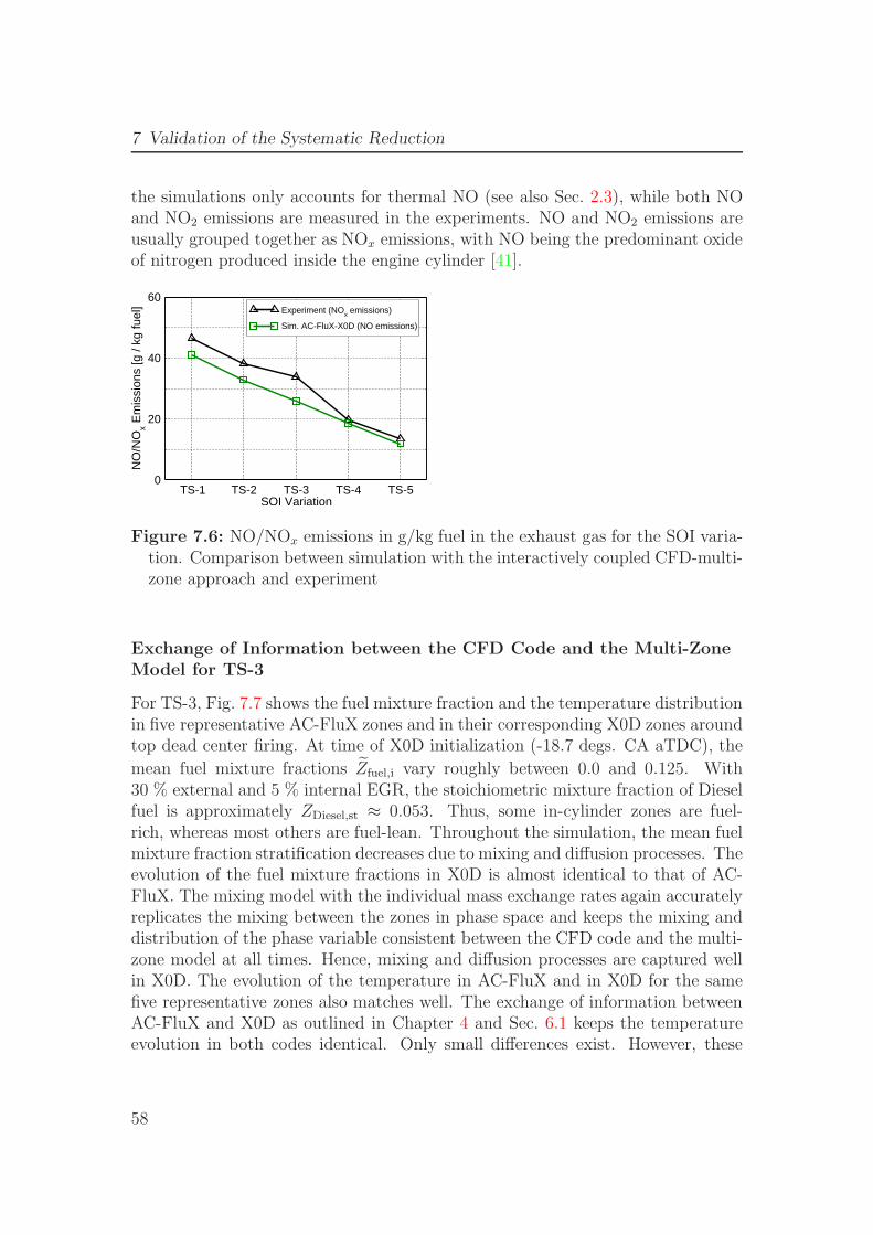
7 Validation of the Systematic Reduction
the simulations only accounts for thermal NO (see also Sec. 2.3), while both NOand NO2 emissions are measured in the experiments. NO and NO2 emissions areusually grouped together as NOx emissions, with NO being the predominant oxideof nitrogen produced inside the engine cylinder [41].
TS-1 TS-2 TS-3 TS-4 TS-5SOI Variation
0
20
40
60
NO
/NO
x Em
issi
ons
[g /
kg fu
el] Experiment (NOx emissions)
Sim. AC-FluX-X0D (NO emissions)
Figure 7.6: NO/NOx emissions in g/kg fuel in the exhaust gas for the SOI varia-tion. Comparison between simulation with the interactively coupled CFD-multi-zone approach and experiment
Exchange of Information between the CFD Code and the Multi-ZoneModel for TS-3
For TS-3, Fig. 7.7 shows the fuel mixture fraction and the temperature distributionin five representative AC-FluX zones and in their corresponding X0D zones aroundtop dead center firing. At time of X0D initialization (-18.7 degs. CA aTDC), the
mean fuel mixture fractions Zfuel,i vary roughly between 0.0 and 0.125. With30 % external and 5 % internal EGR, the stoichiometric mixture fraction of Dieselfuel is approximately ZDiesel,st ≈ 0.053. Thus, some in-cylinder zones are fuel-rich, whereas most others are fuel-lean. Throughout the simulation, the mean fuelmixture fraction stratification decreases due to mixing and diffusion processes. Theevolution of the fuel mixture fractions in X0D is almost identical to that of AC-FluX. The mixing model with the individual mass exchange rates again accuratelyreplicates the mixing between the zones in phase space and keeps the mixing anddistribution of the phase variable consistent between the CFD code and the multi-zone model at all times. Hence, mixing and diffusion processes are captured wellin X0D. The evolution of the temperature in AC-FluX and in X0D for the samefive representative zones also matches well. The exchange of information betweenAC-FluX and X0D as outlined in Chapter 4 and Sec. 6.1 keeps the temperatureevolution in both codes identical. Only small differences exist. However, these
58
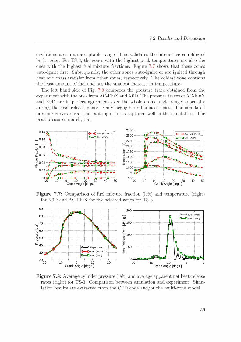
7.2 Results and Discussion
deviations are in an acceptable range. This validates the interactive coupling ofboth codes. For TS-3, the zones with the highest peak temperatures are also theones with the highest fuel mixture fractions. Figure 7.7 shows that these zonesauto-ignite first. Subsequently, the other zones auto-ignite or are ignited throughheat and mass transfer from other zones, respectively. The coldest zone containsthe least amount of fuel and has the smallest increase in temperature.
The left hand side of Fig. 7.8 compares the pressure trace obtained from theexperiment with the ones from AC-FluX and X0D. The pressure traces of AC-FluXand X0D are in perfect agreement over the whole crank angle range, especiallyduring the heat-release phase. Only negligible differences exist. The simulatedpressure curves reveal that auto-ignition is captured well in the simulation. Thepeak pressures match, too.
-20 -10 0 10 20 30 40 50Crank Angle [degs.]
0
0.02
0.04
0.06
0.08
0.10
0.12
Mix
ture
Fra
ctio
n [ -
]
Sim. (AC-FluX)
Sim. (X0D)
-20 -10 0 10 20 30 40 50Crank Angle [degs.]
500
750
1000
1250
1500
1750
2000
2250
2500
2750
Tem
pera
ture
[K]
Sim. (AC-FluX)
Sim. (X0D)
Figure 7.7: Comparison of fuel mixture fraction (left) and temperature (right)for X0D and AC-FluX for five selected zones for TS-3
-20 -10 0 10 20Crank Angle [degs.]
20
30
40
50
60
70
80
90
Pre
ssur
e [b
ar]
Experiment
Sim. (AC-FluX)
Sim. (X0D)
-20 -15 -10 -5 0Crank Angle [degs.]
0
50
100
150
200
Hea
t-R
elea
se R
ate
[J/d
eg.] Experiment
Sim. (X0D)
Figure 7.8: Average cylinder pressure (left) and average apparent net heat-releaserates (right) for TS-3. Comparison between simulation and experiment. Simu-lation results are extracted from the CFD code and/or the multi-zone model
59
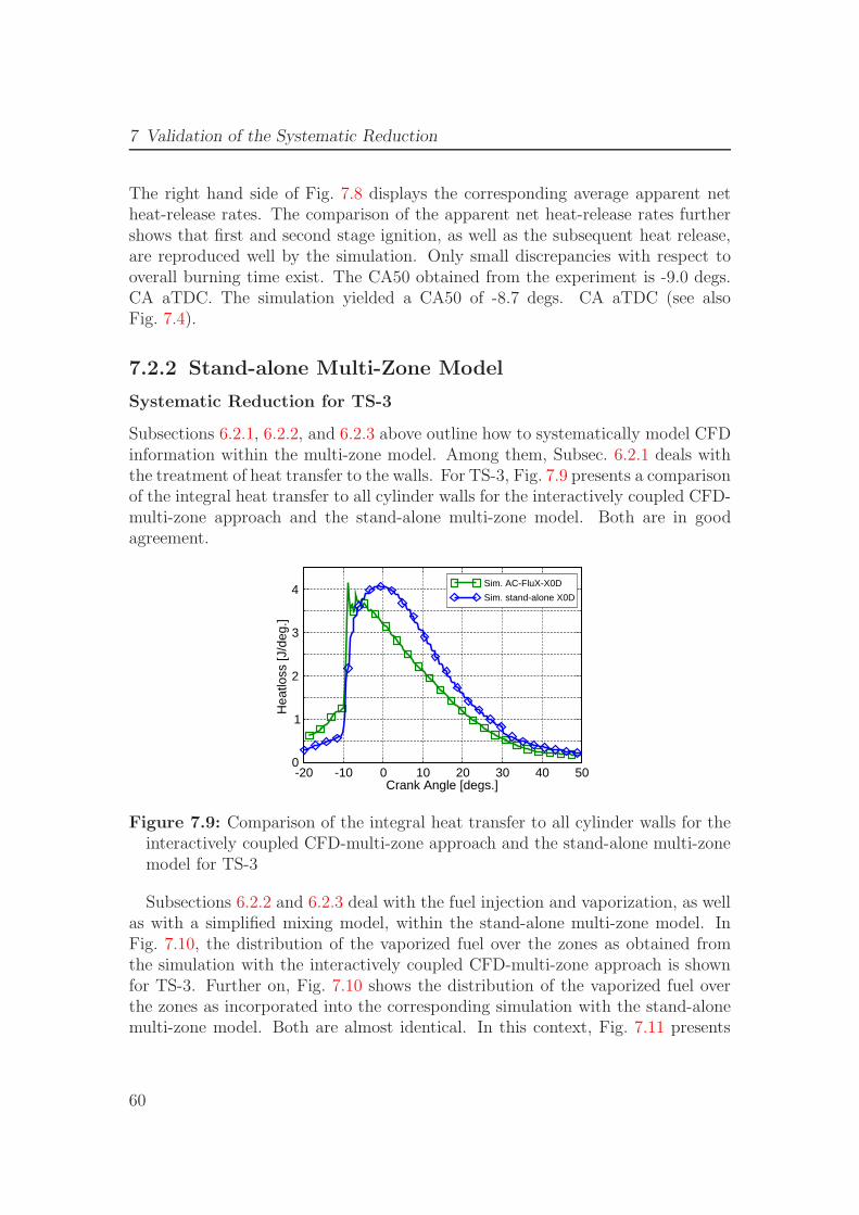
7 Validation of the Systematic Reduction
The right hand side of Fig. 7.8 displays the corresponding average apparent netheat-release rates. The comparison of the apparent net heat-release rates furthershows that first and second stage ignition, as well as the subsequent heat release,are reproduced well by the simulation. Only small discrepancies with respect tooverall burning time exist. The CA50 obtained from the experiment is -9.0 degs.CA aTDC. The simulation yielded a CA50 of -8.7 degs. CA aTDC (see alsoFig. 7.4).
7.2.2 Stand-alone Multi-Zone Model
Systematic Reduction for TS-3
Subsections 6.2.1, 6.2.2, and 6.2.3 above outline how to systematically model CFDinformation within the multi-zone model. Among them, Subsec. 6.2.1 deals withthe treatment of heat transfer to the walls. For TS-3, Fig. 7.9 presents a comparisonof the integral heat transfer to all cylinder walls for the interactively coupled CFD-multi-zone approach and the stand-alone multi-zone model. Both are in goodagreement.
-20 -10 0 10 20 30 40 50Crank Angle [degs.]
0
1
2
3
4
Hea
tloss
[J/d
eg.]
Sim. AC-FluX-X0D
Sim. stand-alone X0D
Figure 7.9: Comparison of the integral heat transfer to all cylinder walls for theinteractively coupled CFD-multi-zone approach and the stand-alone multi-zonemodel for TS-3
Subsections 6.2.2 and 6.2.3 deal with the fuel injection and vaporization, as wellas with a simplified mixing model, within the stand-alone multi-zone model. InFig. 7.10, the distribution of the vaporized fuel over the zones as obtained fromthe simulation with the interactively coupled CFD-multi-zone approach is shownfor TS-3. Further on, Fig. 7.10 shows the distribution of the vaporized fuel overthe zones as incorporated into the corresponding simulation with the stand-alonemulti-zone model. Both are almost identical. In this context, Fig. 7.11 presents
60
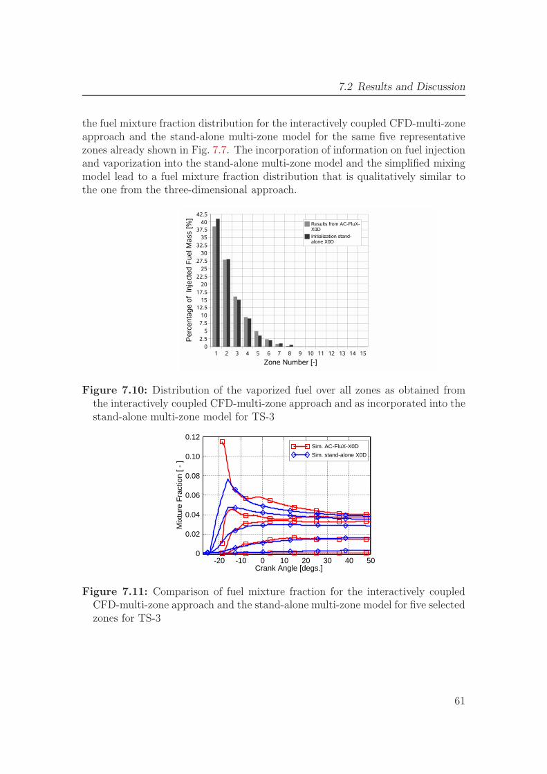
7.2 Results and Discussion
the fuel mixture fraction distribution for the interactively coupled CFD-multi-zoneapproach and the stand-alone multi-zone model for the same five representativezones already shown in Fig. 7.7. The incorporation of information on fuel injectionand vaporization into the stand-alone multi-zone model and the simplified mixingmodel lead to a fuel mixture fraction distribution that is qualitatively similar tothe one from the three-dimensional approach.
Figure 7.10: Distribution of the vaporized fuel over all zones as obtained fromthe interactively coupled CFD-multi-zone approach and as incorporated into thestand-alone multi-zone model for TS-3
-20 -10 0 10 20 30 40 50Crank Angle [degs.]
0
0.02
0.04
0.06
0.08
0.10
0.12
Mix
ture
Fra
ctio
n [ -
]
Sim. AC-FluX-X0D
Sim. stand-alone X0D
Figure 7.11: Comparison of fuel mixture fraction for the interactively coupledCFD-multi-zone approach and the stand-alone multi-zone model for five selectedzones for TS-3
61
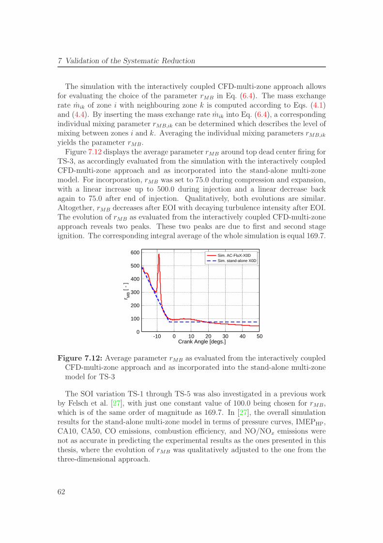
7 Validation of the Systematic Reduction
The simulation with the interactively coupled CFD-multi-zone approach allowsfor evaluating the choice of the parameter rMB in Eq. (6.4). The mass exchangerate mik of zone i with neighbouring zone k is computed according to Eqs. (4.1)and (4.4). By inserting the mass exchange rate mik into Eq. (6.4), a correspondingindividual mixing parameter rMB,ik can be determined which describes the level ofmixing between zones i and k. Averaging the individual mixing parameters rMB,ik
yields the parameter rMB.Figure 7.12 displays the average parameter rMB around top dead center firing for
TS-3, as accordingly evaluated from the simulation with the interactively coupledCFD-multi-zone approach and as incorporated into the stand-alone multi-zonemodel. For incorporation, rMB was set to 75.0 during compression and expansion,with a linear increase up to 500.0 during injection and a linear decrease backagain to 75.0 after end of injection. Qualitatively, both evolutions are similar.Altogether, rMB decreases after EOI with decaying turbulence intensity after EOI.The evolution of rMB as evaluated from the interactively coupled CFD-multi-zoneapproach reveals two peaks. These two peaks are due to first and second stageignition. The corresponding integral average of the whole simulation is equal 169.7.
-10 0 10 20 30 40 50Crank Angle [degs.]
0
100
200
300
400
500
600
r MB [
- ]
Sim. AC-FluX-X0DSim. stand-alone X0D
Figure 7.12: Average parameter rMB as evaluated from the interactively coupledCFD-multi-zone approach and as incorporated into the stand-alone multi-zonemodel for TS-3
The SOI variation TS-1 through TS-5 was also investigated in a previous workby Felsch et al. [27], with just one constant value of 100.0 being chosen for rMB,which is of the same order of magnitude as 169.7. In [27], the overall simulationresults for the stand-alone multi-zone model in terms of pressure curves, IMEPHP,CA10, CA50, CO emissions, combustion efficiency, and NO/NOx emissions werenot as accurate in predicting the experimental results as the ones presented in thisthesis, where the evolution of rMB was qualitatively adjusted to the one from thethree-dimensional approach.
62
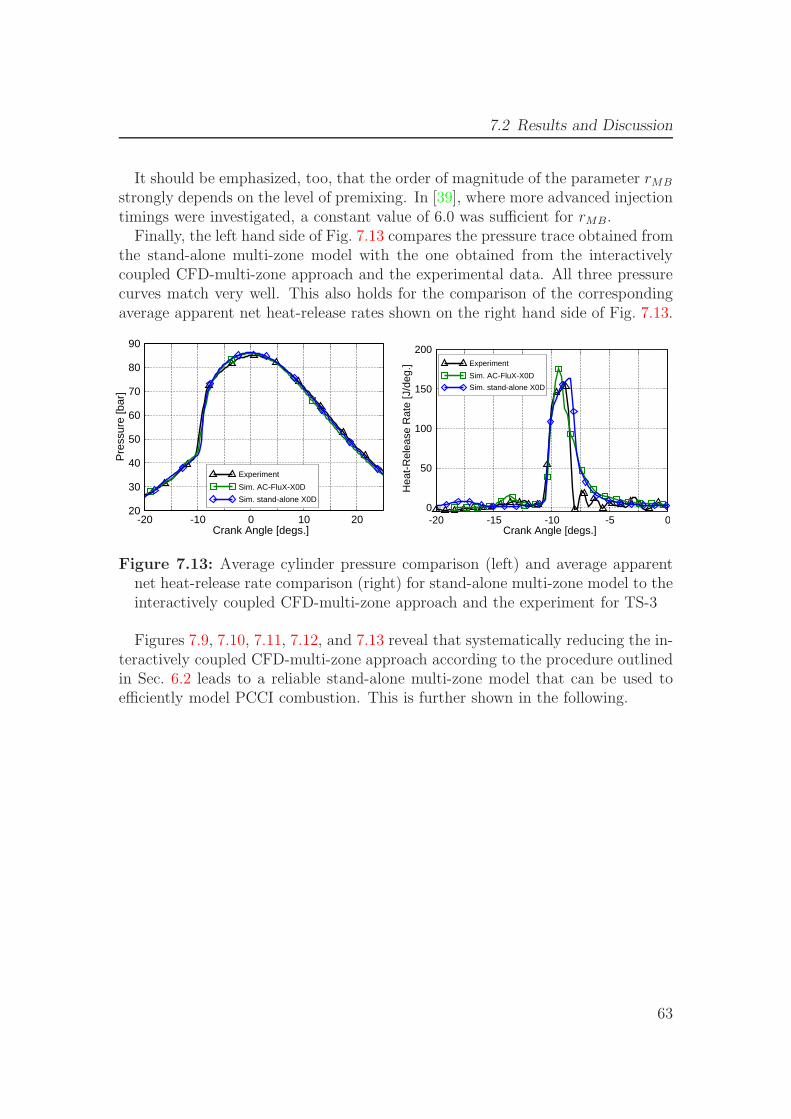
7.2 Results and Discussion
It should be emphasized, too, that the order of magnitude of the parameter rMB
strongly depends on the level of premixing. In [39], where more advanced injectiontimings were investigated, a constant value of 6.0 was sufficient for rMB.
Finally, the left hand side of Fig. 7.13 compares the pressure trace obtained fromthe stand-alone multi-zone model with the one obtained from the interactivelycoupled CFD-multi-zone approach and the experimental data. All three pressurecurves match very well. This also holds for the comparison of the correspondingaverage apparent net heat-release rates shown on the right hand side of Fig. 7.13.
-20 -10 0 10 20Crank Angle [degs.]
20
30
40
50
60
70
80
90
Pre
ssur
e [b
ar]
Experiment
Sim. AC-FluX-X0D
Sim. stand-alone X0D
-20 -15 -10 -5 0Crank Angle [degs.]
0
50
100
150
200
Hea
t-R
elea
se R
ate
[J/d
eg.] Experiment
Sim. AC-FluX-X0D
Sim. stand-alone X0D
Figure 7.13: Average cylinder pressure comparison (left) and average apparentnet heat-release rate comparison (right) for stand-alone multi-zone model to theinteractively coupled CFD-multi-zone approach and the experiment for TS-3
Figures 7.9, 7.10, 7.11, 7.12, and 7.13 reveal that systematically reducing the in-teractively coupled CFD-multi-zone approach according to the procedure outlinedin Sec. 6.2 leads to a reliable stand-alone multi-zone model that can be used toefficiently model PCCI combustion. This is further shown in the following.
63
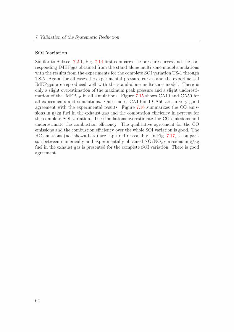
7 Validation of the Systematic Reduction
SOI Variation
Similar to Subsec. 7.2.1, Fig. 7.14 first compares the pressure curves and the cor-responding IMEPHPs obtained from the stand-alone multi-zone model simulationswith the results from the experiments for the complete SOI variation TS-1 throughTS-5. Again, for all cases the experimental pressure curves and the experimentalIMEPHPs are reproduced well with the stand-alone multi-zone model. There isonly a slight overestimation of the maximum peak pressure and a slight underesti-mation of the IMEPHP in all simulations. Figure 7.15 shows CA10 and CA50 forall experiments and simulations. Once more, CA10 and CA50 are in very goodagreement with the experimental results. Figure 7.16 summarizes the CO emis-sions in g/kg fuel in the exhaust gas and the combustion efficiency in percent forthe complete SOI variation. The simulations overestimate the CO emissions andunderestimate the combustion efficiency. The qualitative agreement for the COemissions and the combustion efficiency over the whole SOI variation is good. TheHC emissions (not shown here) are captured reasonably. In Fig. 7.17, a compari-son between numerically and experimentally obtained NO/NOx emissions in g/kgfuel in the exhaust gas is presented for the complete SOI variation. There is goodagreement.
64
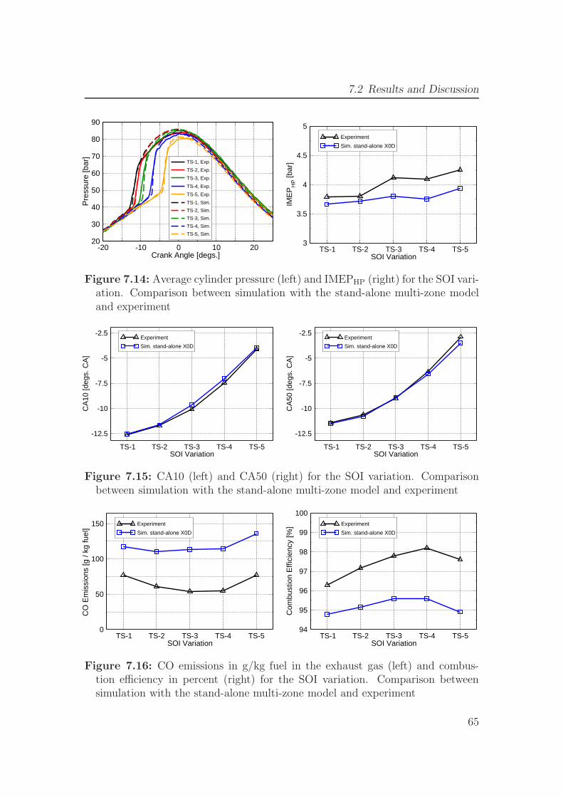
7.2 Results and Discussion
-20 -10 0 10 20Crank Angle [degs.]
20
30
40
50
60
70
80
90
Pre
ssur
e [b
ar]
TS-1, Exp.
TS-2, Exp.
TS-3, Exp.
TS-4, Exp.
TS-5, Exp.
TS-1, Sim.
TS-2, Sim.
TS-3, Sim.
TS-4, Sim.
TS-5, Sim.
TS-1 TS-2 TS-3 TS-4 TS-5SOI Variation
3
3.5
4
4.5
5
IME
PH
P [b
ar]
Experiment
Sim. stand-alone X0D
Figure 7.14: Average cylinder pressure (left) and IMEPHP (right) for the SOI vari-ation. Comparison between simulation with the stand-alone multi-zone modeland experiment
TS-1 TS-2 TS-3 TS-4 TS-5SOI Variation
-12.5
-10
-7.5
-5
-2.5
CA
10 [d
egs.
CA
]
Experiment
Sim. stand-alone X0D
TS-1 TS-2 TS-3 TS-4 TS-5SOI Variation
-12.5
-10
-7.5
-5
-2.5
CA
50 [d
egs.
CA
]
Experiment
Sim. stand-alone X0D
Figure 7.15: CA10 (left) and CA50 (right) for the SOI variation. Comparisonbetween simulation with the stand-alone multi-zone model and experiment
TS-1 TS-2 TS-3 TS-4 TS-5SOI Variation
0
50
100
150
CO
Em
issi
ons
[g /
kg fu
el]
Experiment
Sim. stand-alone X0D
TS-1 TS-2 TS-3 TS-4 TS-5SOI Variation
94
95
96
97
98
99
100
Com
bust
ion
Effi
cien
cy [%
] Experiment
Sim. stand-alone X0D
Figure 7.16: CO emissions in g/kg fuel in the exhaust gas (left) and combus-tion efficiency in percent (right) for the SOI variation. Comparison betweensimulation with the stand-alone multi-zone model and experiment
65
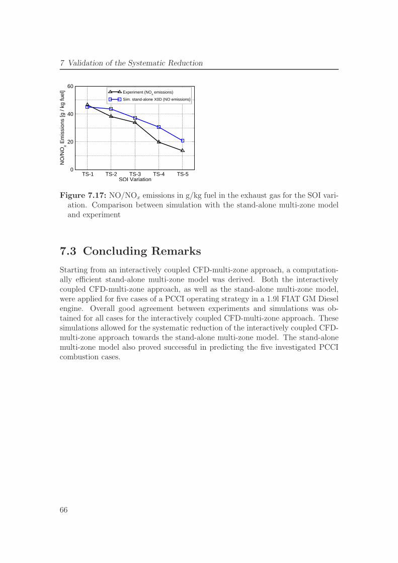
7 Validation of the Systematic Reduction
TS-1 TS-2 TS-3 TS-4 TS-5SOI Variation
0
20
40
60
NO
/NO
x Em
issi
ons
[g /
kg fu
el] Experiment (NOx emissions)
Sim. stand-alone X0D (NO emissions)
Figure 7.17: NO/NOx emissions in g/kg fuel in the exhaust gas for the SOI vari-ation. Comparison between simulation with the stand-alone multi-zone modeland experiment
7.3 Concluding Remarks
Starting from an interactively coupled CFD-multi-zone approach, a computation-ally efficient stand-alone multi-zone model was derived. Both the interactivelycoupled CFD-multi-zone approach, as well as the stand-alone multi-zone model,were applied for five cases of a PCCI operating strategy in a 1.9l FIAT GM Dieselengine. Overall good agreement between experiments and simulations was ob-tained for all cases for the interactively coupled CFD-multi-zone approach. Thesesimulations allowed for the systematic reduction of the interactively coupled CFD-multi-zone approach towards the stand-alone multi-zone model. The stand-alonemulti-zone model also proved successful in predicting the five investigated PCCIcombustion cases.
66
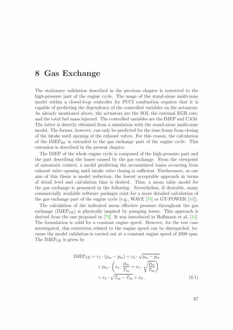
8 Gas Exchange
The stationary validation described in the previous chapter is restricted to thehigh-pressure part of the engine cycle. The usage of the stand-alone multi-zonemodel within a closed-loop controller for PCCI combustion requires that it iscapable of predicting the dependency of the controlled variables on the actuators.As already mentioned above, the actuators are the SOI, the external EGR rate,and the total fuel mass injected. The controlled variables are the IMEP and CA50.The latter is directly obtained from a simulation with the stand-alone multi-zonemodel. The former, however, can only be predicted for the time frame from closingof the intake until opening of the exhaust valves. For this reason, the calculationof the IMEPHP is extended to the gas exchange part of the engine cycle. Thisextension is described in the present chapter.
The IMEP of the whole engine cycle is composed of the high-pressure part andthe part describing the losses caused by the gas exchange. From the viewpointof automatic control, a model predicting the accumulated losses occurring fromexhaust valve opening until intake valve closing is sufficient. Furthermore, as oneaim of this thesis is model reduction, the lowest acceptable approach in termsof detail level and calculation time is desired. Thus, a mean value model forthe gas exchange is presented in the following. Nevertheless, if desirable, manycommercially available software packages exist for a more detailed calculation ofthe gas exchange part of the engine cycle (e.g., WAVE [78] or GT-POWER [33]).
The calculation of the indicated mean effective pressure throughout the gasexchange (IMEPGE) is physically inspired by pumping losses. This approach isderived from the one proposed in [79]. It was introduced in Hoffmann et al. [44].The formulation is valid for a constant engine speed. However, for the test caseinvestigated, this restriction related to the engine speed can be disregarded, be-cause the model validation is carried out at a constant engine speed of 2000 rpm.The IMEPGE is given by
IMEPGE = x1 · (pae − pbe) + x2 ·√
pae − pbe
+ pbe ·(
x3 ·pbe
Tbe+ x4 ·
√pbe
Tbe
)
+ x5 ·√
Tae − Tbe + x6 . (8.1)
67
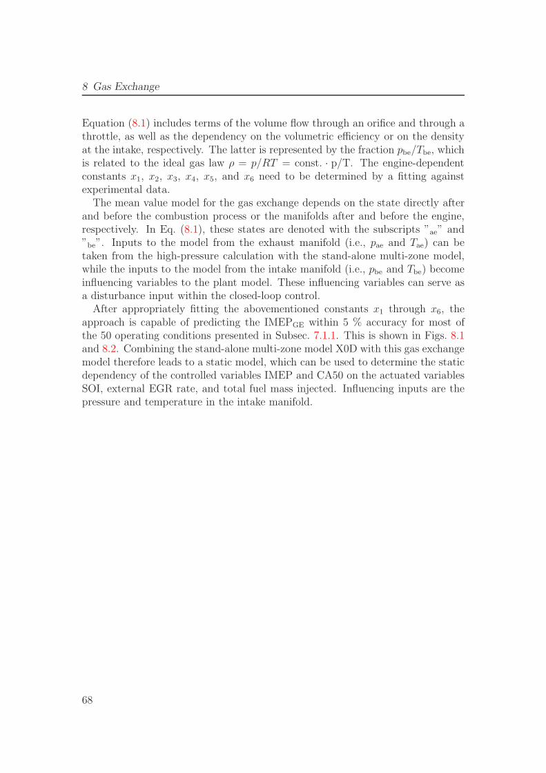
8 Gas Exchange
Equation (8.1) includes terms of the volume flow through an orifice and through athrottle, as well as the dependency on the volumetric efficiency or on the densityat the intake, respectively. The latter is represented by the fraction pbe/Tbe, whichis related to the ideal gas law ρ = p/RT = const. · p/T. The engine-dependentconstants x1, x2, x3, x4, x5, and x6 need to be determined by a fitting againstexperimental data.
The mean value model for the gas exchange depends on the state directly afterand before the combustion process or the manifolds after and before the engine,respectively. In Eq. (8.1), these states are denoted with the subscripts ”ae” and”be”. Inputs to the model from the exhaust manifold (i.e., pae and Tae) can betaken from the high-pressure calculation with the stand-alone multi-zone model,while the inputs to the model from the intake manifold (i.e., pbe and Tbe) becomeinfluencing variables to the plant model. These influencing variables can serve asa disturbance input within the closed-loop control.
After appropriately fitting the abovementioned constants x1 through x6, theapproach is capable of predicting the IMEPGE within 5 % accuracy for most ofthe 50 operating conditions presented in Subsec. 7.1.1. This is shown in Figs. 8.1and 8.2. Combining the stand-alone multi-zone model X0D with this gas exchangemodel therefore leads to a static model, which can be used to determine the staticdependency of the controlled variables IMEP and CA50 on the actuated variablesSOI, external EGR rate, and total fuel mass injected. Influencing inputs are thepressure and temperature in the intake manifold.
68
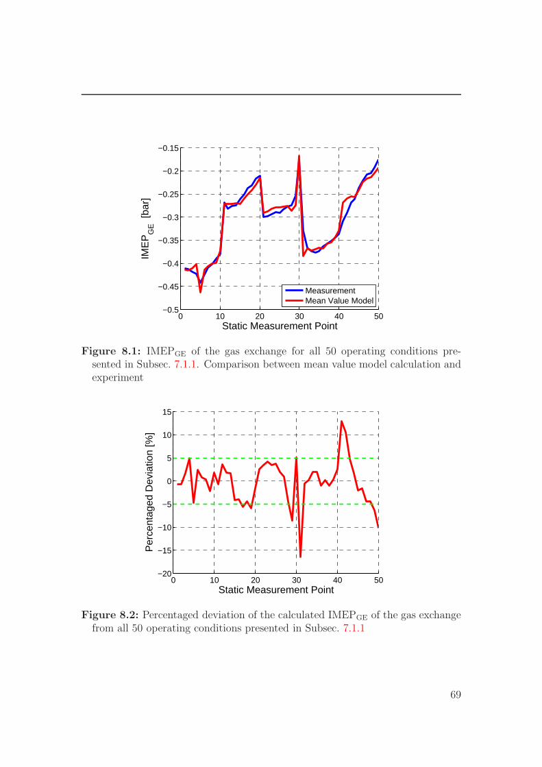
0 10 20 30 40 50−0.5
−0.45
−0.4
−0.35
−0.3
−0.25
−0.2
−0.15
Static Measurement Point
IME
PG
E [
bar]
MeasurementMean Value Model
Figure 8.1: IMEPGE of the gas exchange for all 50 operating conditions pre-sented in Subsec. 7.1.1. Comparison between mean value model calculation andexperiment
0 10 20 30 40 50−20
−15
−10
−5
0
5
10
15
Static Measurement Point
Per
cent
aged
Dev
iatio
n [%
]
Figure 8.2: Percentaged deviation of the calculated IMEPGE of the gas exchangefrom all 50 operating conditions presented in Subsec. 7.1.1
69

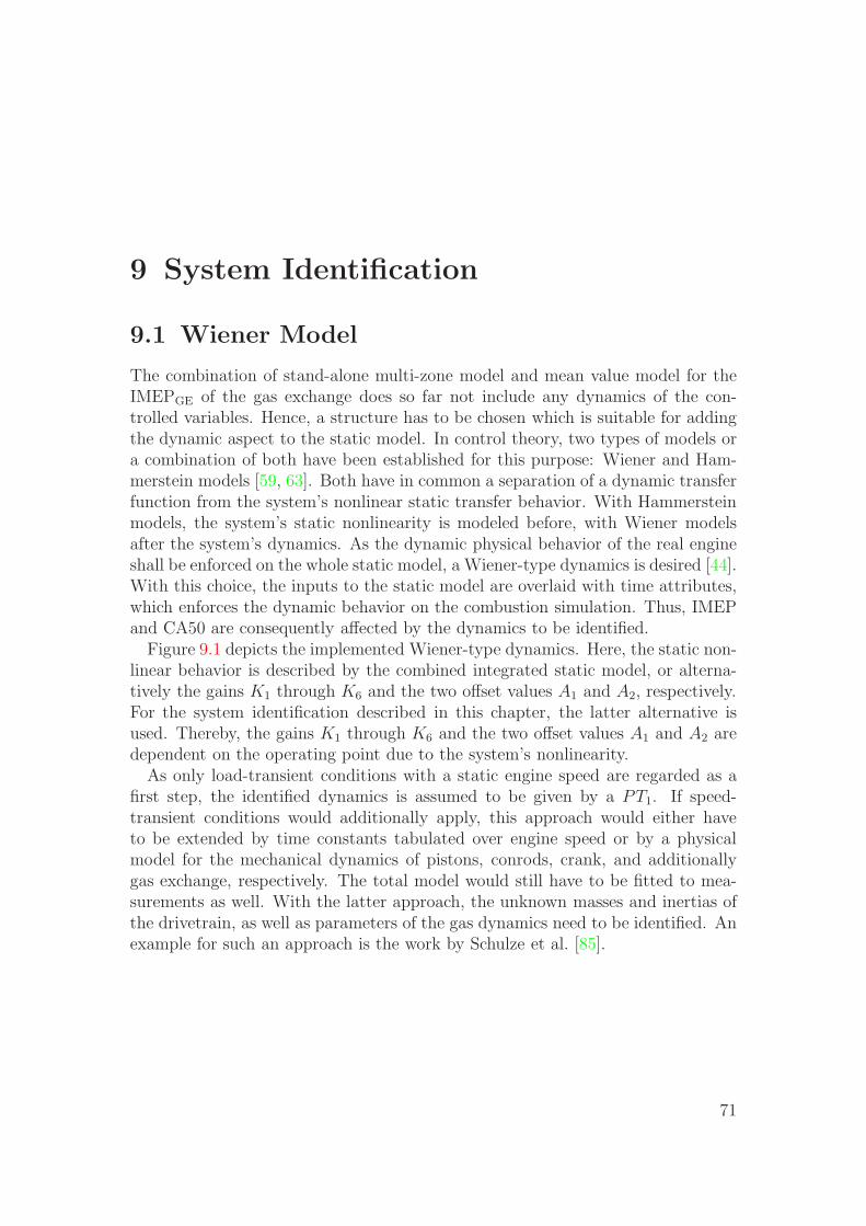
9 System Identification
9.1 Wiener Model
The combination of stand-alone multi-zone model and mean value model for theIMEPGE of the gas exchange does so far not include any dynamics of the con-trolled variables. Hence, a structure has to be chosen which is suitable for addingthe dynamic aspect to the static model. In control theory, two types of models ora combination of both have been established for this purpose: Wiener and Ham-merstein models [59, 63]. Both have in common a separation of a dynamic transferfunction from the system’s nonlinear static transfer behavior. With Hammersteinmodels, the system’s static nonlinearity is modeled before, with Wiener modelsafter the system’s dynamics. As the dynamic physical behavior of the real engineshall be enforced on the whole static model, a Wiener-type dynamics is desired [44].With this choice, the inputs to the static model are overlaid with time attributes,which enforces the dynamic behavior on the combustion simulation. Thus, IMEPand CA50 are consequently affected by the dynamics to be identified.
Figure 9.1 depicts the implemented Wiener-type dynamics. Here, the static non-linear behavior is described by the combined integrated static model, or alterna-tively the gains K1 through K6 and the two offset values A1 and A2, respectively.For the system identification described in this chapter, the latter alternative isused. Thereby, the gains K1 through K6 and the two offset values A1 and A2 aredependent on the operating point due to the system’s nonlinearity.
As only load-transient conditions with a static engine speed are regarded as afirst step, the identified dynamics is assumed to be given by a PT1. If speed-transient conditions would additionally apply, this approach would either haveto be extended by time constants tabulated over engine speed or by a physicalmodel for the mechanical dynamics of pistons, conrods, crank, and additionallygas exchange, respectively. The total model would still have to be fitted to mea-surements as well. With the latter approach, the unknown masses and inertias ofthe drivetrain, as well as parameters of the gas dynamics need to be identified. Anexample for such an approach is the work by Schulze et al. [85].
71
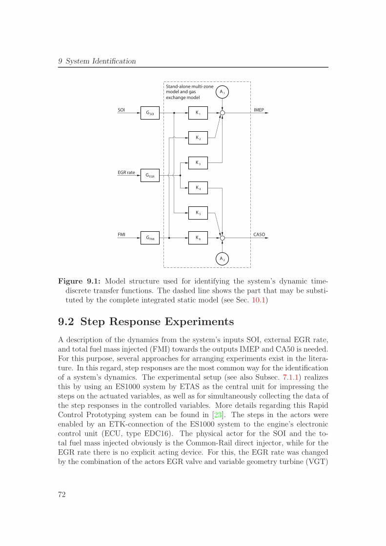
9 System Identification
IMEPK 1
K 2
K 3
K 4
A 1
CA5O
A 2
GSOI
GEGR
Stand-alone multi-zonemodel and gas
exchange model
SOI
EGR rate
K 5
K 6GFMI
FMI
Figure 9.1: Model structure used for identifying the system’s dynamic time-discrete transfer functions. The dashed line shows the part that may be substi-tuted by the complete integrated static model (see Sec. 10.1)
9.2 Step Response Experiments
A description of the dynamics from the system’s inputs SOI, external EGR rate,and total fuel mass injected (FMI) towards the outputs IMEP and CA50 is needed.For this purpose, several approaches for arranging experiments exist in the litera-ture. In this regard, step responses are the most common way for the identificationof a system’s dynamics. The experimental setup (see also Subsec. 7.1.1) realizesthis by using an ES1000 system by ETAS as the central unit for impressing thesteps on the actuated variables, as well as for simultaneously collecting the data ofthe step responses in the controlled variables. More details regarding this RapidControl Prototyping system can be found in [23]. The steps in the actors wereenabled by an ETK-connection of the ES1000 system to the engine’s electroniccontrol unit (ECU, type EDC16). The physical actor for the SOI and the to-tal fuel mass injected obviously is the Common-Rail direct injector, while for theEGR rate there is no explicit acting device. For this, the EGR rate was changedby the combination of the actors EGR valve and variable geometry turbine (VGT)
72
9.3 Dynamic Transfer Functions
position. It is impossible to make the engine step in EGR rate. Nevertheless,the system shows a dynamic response to a change in the EGR rate caused bya simultaneous step in EGR valve and VGT position. For the operating pointsto step between, the corresponding values for EGR throttle and VGT positionwere determined for a steady state operation. Furthermore, the test bed offers nodirect possibility to measure the dynamics of the EGR rate, which is the inputand actuating variable for the static model. Commonly, in modern ECUs in se-ries applications, the mass flow of fresh air aspirated by the engine is measuredinstead [35]. The EGR rate can be calculated by
EGR rate =mEGR
mtrapp. mass=
mtrapp. mass − mair
mtrapp. mass, (9.1)
where mair denotes the mass flow of fresh air. The total trapped gas massmtrapp. mass mainly depends on the engine speed, as well as on the pressure andtemperature in the intake manifold. The engine was run at a constant speed. Inaddition, the intake manifold conditions did not vary significantly during the stepresponse experiments. The total trapped gas mass mtrapp. mass is therefore con-sidered approximately constant and, for this reason, the main dynamics affectingthe EGR rate in this case is the same but negative dynamics as with the fresh airmass mair. This was measured by the engine’s ECU, but also handed over to themeasuring device ES1000 via ETK. Because the steady state value for the EGRrate is known before and after applying the step in VGT position and EGR valve,the dynamic EGR rate during the tests can be recalculated and used as an inputto the model.
Another prerequisite for the system identification is the measurement of thetarget values or outputs of the model, respectively. Both IMEP and CA50 arecalculated from the pressure progression measurement. This has to be realized byan additional device, as in series applications no pressure analysis is implementedin the ECU. In this work, a FI2RE system by IAV was used [95]. It analyzes thepressure signal in real time and hands it over to the measurement system ES1000via CAN.
9.3 Dynamic Transfer Functions
The step response experiments provide a dataset containing the temporally re-solved signals for SOI, external EGR rate, and FMI, as well as the correspondingresponse in IMEP and CA50. The aim of the extraction of the system’s dynamics isthe abovementioned Wiener-type dynamics. The advantage of this approach is alsoits disadvantage. By assigning the system’s dynamics to the inputs, a relativelysimple model structure concerning the dynamic transfer functions is achieved, astheir number is reduced to the number of inputs (see Fig. 9.1). But this also is
73
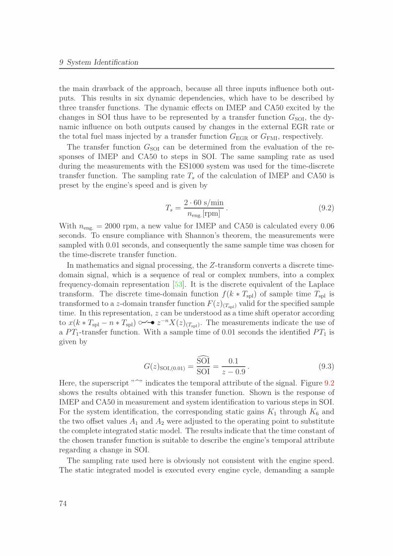
9 System Identification
the main drawback of the approach, because all three inputs influence both out-puts. This results in six dynamic dependencies, which have to be described bythree transfer functions. The dynamic effects on IMEP and CA50 excited by thechanges in SOI thus have to be represented by a transfer function GSOI, the dy-namic influence on both outputs caused by changes in the external EGR rate orthe total fuel mass injected by a transfer function GEGR or GFMI, respectively.
The transfer function GSOI can be determined from the evaluation of the re-sponses of IMEP and CA50 to steps in SOI. The same sampling rate as usedduring the measurements with the ES1000 system was used for the time-discretetransfer function. The sampling rate Ts of the calculation of IMEP and CA50 ispreset by the engine’s speed and is given by
Ts =2 · 60 s/min
neng.[rpm]. (9.2)
With neng. = 2000 rpm, a new value for IMEP and CA50 is calculated every 0.06seconds. To ensure compliance with Shannon’s theorem, the measurements weresampled with 0.01 seconds, and consequently the same sample time was chosen forthe time-discrete transfer function.
In mathematics and signal processing, the Z-transform converts a discrete time-domain signal, which is a sequence of real or complex numbers, into a complexfrequency-domain representation [53]. It is the discrete equivalent of the Laplacetransform. The discrete time-domain function f(k ∗ Tspl) of sample time Tspl istransformed to a z-domain transfer function F (z)(Tspl) valid for the specified sampletime. In this representation, z can be understood as a time shift operator accordingto x(k ∗ Tspl − n ∗ Tspl) d ..........
. tz−nX(z)(Tspl). The measurements indicate the use ofa PT1-transfer function. With a sample time of 0.01 seconds the identified PT1 isgiven by
G(z)SOI,(0.01) =SOI
SOI=
0.1
z − 0.9. (9.3)
Here, the superscript ”” indicates the temporal attribute of the signal. Figure 9.2shows the results obtained with this transfer function. Shown is the response ofIMEP and CA50 in measurement and system identification to various steps in SOI.For the system identification, the corresponding static gains K1 through K6 andthe two offset values A1 and A2 were adjusted to the operating point to substitutethe complete integrated static model. The results indicate that the time constant ofthe chosen transfer function is suitable to describe the engine’s temporal attributeregarding a change in SOI.
The sampling rate used here is obviously not consistent with the engine speed.The static integrated model is executed every engine cycle, demanding a sample
74
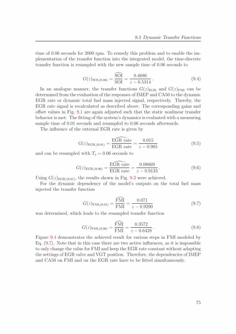
9.3 Dynamic Transfer Functions
time of 0.06 seconds for 2000 rpm. To remedy this problem and to enable the im-plementation of the transfer function into the integrated model, the time-discretetransfer function is resampled with the new sample time of 0.06 seconds to
G(z)SOI,(0.06) =SOI
SOI=
0.4686
z − 0.5314. (9.4)
In an analogue manner, the transfer functions G(z)EGR and G(z)FMI can bedetermined from the evaluation of the responses of IMEP and CA50 to the dynamicEGR rate or dynamic total fuel mass injected signal, respectively. Thereby, theEGR rate signal is recalculated as described above. The corresponding gains andoffset values in Fig. 9.1 are again adjusted such that the static nonlinear transferbehavior is met. The fitting of the system’s dynamics is evaluated with a measuringsample time of 0.01 seconds and resampled to 0.06 seconds afterwards.
The influence of the external EGR rate is given by
G(z)EGR,(0.01) =EGR rate
EGR rate=
0.015
z − 0.985(9.5)
and can be resampled with Ts = 0.06 seconds to
G(z)EGR,(0.06) =EGR rate
EGR rate=
0.08669
z − 0.9133. (9.6)
Using G(z)EGR,(0.01), the results shown in Fig. 9.3 were achieved.For the dynamic dependency of the model’s outputs on the total fuel mass
injected the transfer function
G(z)FMI,(0.01) =FMI
FMI=
0.071
z − 0.9290(9.7)
was determined, which leads to the resampled transfer function
G(z)FMI,(0.06) =FMI
FMI=
0.3572
z − 0.6428. (9.8)
Figure 9.4 demonstrates the achieved result for various steps in FMI modeled byEq. (9.7). Note that in this case there are two active influences, as it is impossibleto only change the value for FMI and keep the EGR rate constant without adaptingthe settings of EGR valve and VGT position. Therefore, the dependencies of IMEPand CA50 on FMI and on the EGR rate have to be fitted simultaneously.
75
9 System Identification
42 44 46 48 50 52
2.6
2.8
3
3.2
3.4
IME
P [b
ar]
Time [s]
MeasurementSystem Ident.
42 44 46 48 50 52
−13.5
−13
−12.5
−12
−11.5
−11
−10.5
−10
CA
50 [d
egs.
CA
]
Time [s]
MeasurementSystem Ident.
(a) IMEP (left) and CA50 (right) for an SOI step from -40.7 to -30.7 degs. CA aTDC and backwith an external EGR rate of 30 % and an injected fuel mass of 10.2 mg/cycle
34 36 38 40 42 44
2.8
2.9
3
3.1
3.2
3.3
3.4
IME
P [b
ar]
Time [s]
MeasurementSystem Ident.
34 36 38 40 42 44
−13
−12
−11
−10
−9
−8
−7
−6
−5
−4
CA
50 [d
egs.
CA
]
Time [s]
MeasurementSystem Ident.
(b) IMEP (left) and CA50 (right) for an SOI step from -20.7 to -30.7 degs. CA aTDC and backwith an external EGR rate of 30 % and an injected fuel mass of 10.2 mg/cycle
22 24 26 28 30 322.8
2.9
3
3.1
3.2
3.3
IME
P [b
ar]
Time [s]
MeasurementSystem Ident.
22 24 26 28 30 32
−8
−7
−6
−5
−4
−3
−2
−1
CA
50 [d
egs.
CA
]
Time [s]
MeasurementSystem Ident.
(c) IMEP (left) and CA50 (right) for an SOI step from -30.7 to -20.7 degs. CA aTDC and backwith an external EGR rate of 45 % and an injected fuel mass of 10.2 mg/cycle
Figure 9.2: Comparison between experiment and system identification with iden-tified discrete transfer function G(z)SOI,(0.01)
76
9.3 Dynamic Transfer Functions
10 20 30 40 50 60 70 80
2.4
2.6
2.8
3
3.2
IME
P [b
ar]
Time [s]
MeasurementSystem Ident.
10 20 30 40 50 60 70 80
−14
−12
−10
−8
−6
−4
−2
CA
50 [d
egs.
CA
]
Time [s]
MeasurementSystem Ident.
(a) IMEP (left) and CA50 (right) for an EGR step from 30 to 45 % and back with an SOI of-40.7 degs. CA aTDC and an injected fuel mass of 10.2 mg/cycle
30 40 50 60 70 80
2.7
2.8
2.9
3
3.1
3.2
3.3
3.4
3.5
IME
P [b
ar]
Time [s]
MeasurementSystem Ident.
30 40 50 60 70 80
−12
−10
−8
−6
−4
−2
0
2
CA
50 [d
egs.
CA
]
Time [s]
MeasurementSystem Ident.
(b) IMEP (left) and CA50 (right) for an EGR step from 30 to 45 % and back with an SOI of-30.7 degs. CA aTDC and an injected fuel mass of 10.2 mg/cycle
10 20 30 40 502.9
3
3.1
3.2
3.3
3.4
IME
P [b
ar]
Time [s]
MeasurementSystem Ident.
10 20 30 40 50−8
−7
−6
−5
−4
−3
−2
−1
0
1
CA
50 [d
egs.
CA
]
Time [s]
MeasurementSystem Ident.
(c) IMEP (left) and CA50 (right) for an EGR step from 30 to 45 % and back with an SOI of-20.7 degs. CA aTDC and an injected fuel mass of 10.2 mg/cycle
Figure 9.3: Comparison between experiment and system identification with iden-tified discrete transfer function G(z)EGR,(0.01)
77
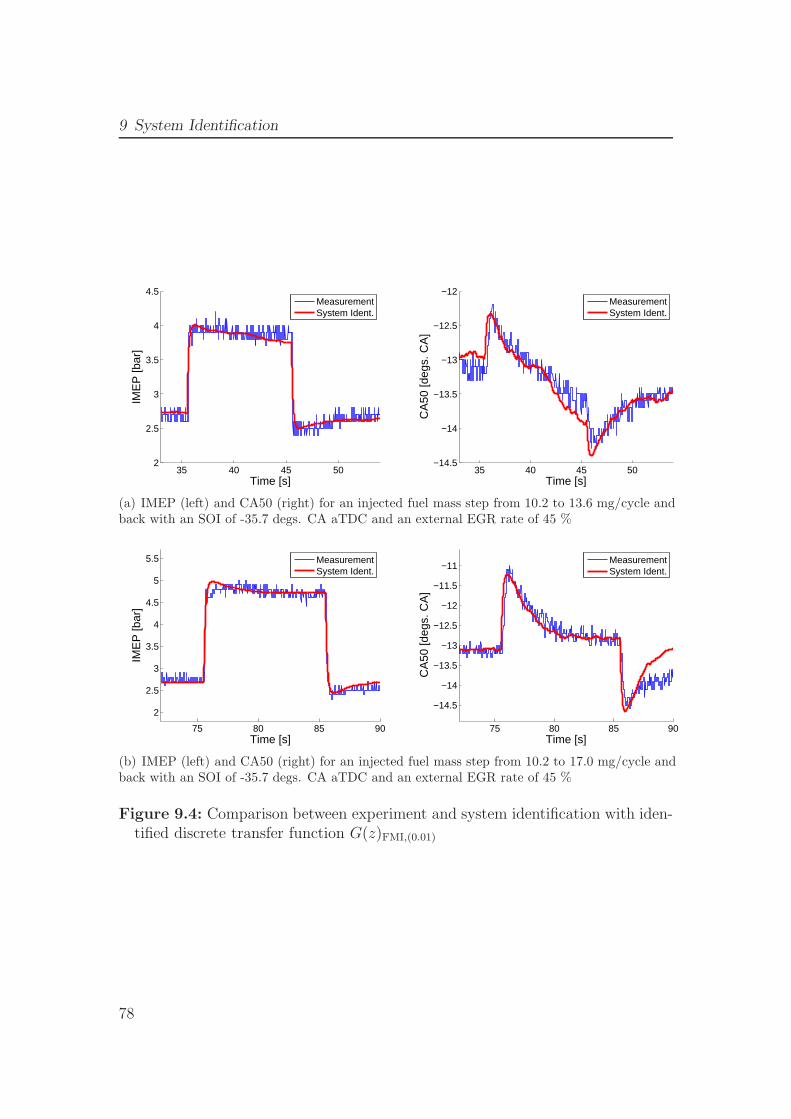
9 System Identification
35 40 45 502
2.5
3
3.5
4
4.5
IME
P [b
ar]
Time [s]
MeasurementSystem Ident.
35 40 45 50−14.5
−14
−13.5
−13
−12.5
−12
CA
50 [d
egs.
CA
]
Time [s]
MeasurementSystem Ident.
(a) IMEP (left) and CA50 (right) for an injected fuel mass step from 10.2 to 13.6 mg/cycle andback with an SOI of -35.7 degs. CA aTDC and an external EGR rate of 45 %
75 80 85 90
2
2.5
3
3.5
4
4.5
5
5.5
IME
P [b
ar]
Time [s]
MeasurementSystem Ident.
75 80 85 90
−14.5
−14
−13.5
−13
−12.5
−12
−11.5
−11
CA
50 [d
egs.
CA
]
Time [s]
MeasurementSystem Ident.
(b) IMEP (left) and CA50 (right) for an injected fuel mass step from 10.2 to 17.0 mg/cycle andback with an SOI of -35.7 degs. CA aTDC and an external EGR rate of 45 %
Figure 9.4: Comparison between experiment and system identification with iden-tified discrete transfer function G(z)FMI,(0.01)
78
10 Integrated Model
In the previous three chapters, all discussed model parts (stand-alone multi-zonemodel, gas exchange model, and dynamic time response) were each validated sep-arately. In this chapter, the realization of an integrated model composed of thesethree parts within a suitable test environment for control applications is described.Afterwards, the integrated model is validated against transient experimental data.This chapter closes with a discussion of this model’s potential in the framework ofclosed-loop control development.
10.1 Suitable Test Environment for Control
Applications
For application within a closed-loop control simulation, the stand-alone multi-zonemodel was transferred to an environment suitable for the conception and testing ofcontrollers. For this study, the Matlab/Simulink environment of The MathWorks,Inc. was chosen as an appropriate platform [92]. The stand-alone multi-zonemodel X0D written in FORTRAN 77 was embedded into a Matlab/Simulink FOR-TRAN s-function enabling the simulation of the stand-alone multi-zone model fromwithin Matlab/Simulink. Moreover, the gas exchange model was implemented intothis FORTRAN s-function. The three dynamic transfer functions were added bymeans of time-discrete PT1-dynamics within appropriate function blocks. TheMatlab/Simulink setup is visualized in Fig. 10.1.
The simulation environment is realized such that the initial in-cylinder con-ditions reflect the engine-out conditions of the prior cycle. This establishes thecycle-to-cycle connectivity. However, as the external EGR was cooled (see alsoSubsec. 7.1.1), the measurements did not show a strong dependency of the intakeconditions on the engine-out conditions, except for the external EGR composi-tion when varying the total fuel mass injected. Aside from the initial in-cylinderconditions, the numerical setup for the multi-zone model (e.g., start and end ofsimulation, number of zones, incorporated information, etc.) within the Mat-lab/Simulink environment was kept unchanged in comparison to the stand-alonemulti-zone model simulation setup described in Subsec. 7.1.2.
79
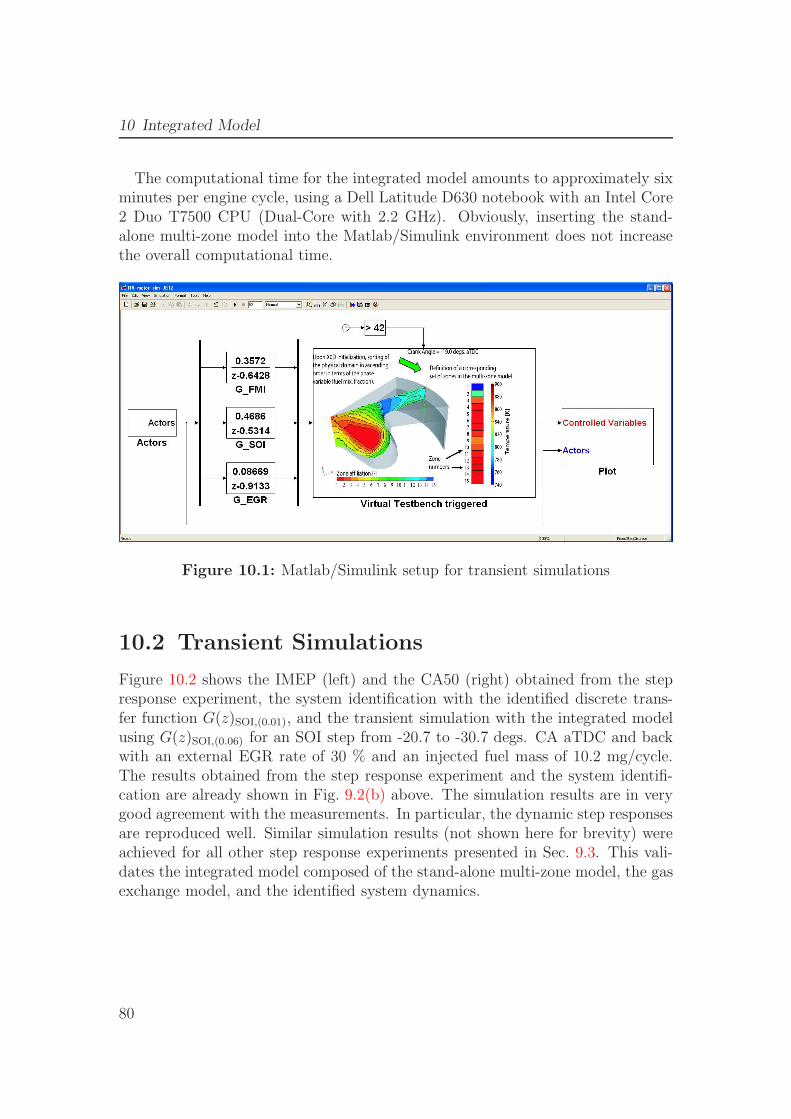
10 Integrated Model
The computational time for the integrated model amounts to approximately sixminutes per engine cycle, using a Dell Latitude D630 notebook with an Intel Core2 Duo T7500 CPU (Dual-Core with 2.2 GHz). Obviously, inserting the stand-alone multi-zone model into the Matlab/Simulink environment does not increasethe overall computational time.
Figure 10.1: Matlab/Simulink setup for transient simulations
10.2 Transient Simulations
Figure 10.2 shows the IMEP (left) and the CA50 (right) obtained from the stepresponse experiment, the system identification with the identified discrete trans-fer function G(z)SOI,(0.01), and the transient simulation with the integrated modelusing G(z)SOI,(0.06) for an SOI step from -20.7 to -30.7 degs. CA aTDC and backwith an external EGR rate of 30 % and an injected fuel mass of 10.2 mg/cycle.The results obtained from the step response experiment and the system identifi-cation are already shown in Fig. 9.2(b) above. The simulation results are in verygood agreement with the measurements. In particular, the dynamic step responsesare reproduced well. Similar simulation results (not shown here for brevity) wereachieved for all other step response experiments presented in Sec. 9.3. This vali-dates the integrated model composed of the stand-alone multi-zone model, the gasexchange model, and the identified system dynamics.
80
10.3 Potential within Closed-Loop Control Development
34 36 38 40 42 442.8
2.9
3
3.1
3.2
3.3
3.4
3.5
IME
P [b
ar]
Time [s]
MeasurementSystem Ident.Integrated Model
34 36 38 40 42 44
−12
−11
−10
−9
−8
−7
−6
−5
−4
CA
50 [d
egs.
CA
]
Time [s]
MeasurementSystem Ident.Integrated Model
Figure 10.2: IMEP (left) and CA50 (right) for an SOI step from -20.7 to -30.7degs. CA aTDC and back with an external EGR rate of 30 % and an injected fuelmass of 10.2 mg/cycle. Comparison between experiment, system identificationwith identified discrete transfer function G(z)SOI,(0.01), and integrated model
10.3 Potential within Closed-Loop Control
Development
The strict derivation of the stand-alone multi-zone model from a detailed three-dimensional CFD approach integrates the detailed knowledge from combustionsimulation tools into closed-loop control. This novel procedure establishes a broadfield of possibilities for testing completely new controlled process variables. In thiscontext, Fig. 10.3 displays further outcomes of the transient simulation for an SOIstep from -20.7 to -30.7 degs. CA aTDC and back with an external EGR rate of30 % and an injected fuel mass of 10.2 mg/cycle. Exemplary, the NO emissions,the maximum pressure, the burning time from CA10 to CA90, and the ringingintensity are shown.
The combustion noise level is quantified applying the ringing intensity correla-tion developed by Eng [22]. This correlation relates the ringing intensity to themaximum pressure rise rate, the maximum pressure, and the speed of sound. Theringing intensity is expressed as
Ringing Intensity ≈ 1
2 γ
(β dp
dt max
)2
pmax
√γ R Tmax . (10.1)
In Eq. (10.1), dp/dtmax denotes the maximum pressure rise rate, pmax the maximumpressure, and Tmax the maximum temperature. β is a scaling factor determined
81
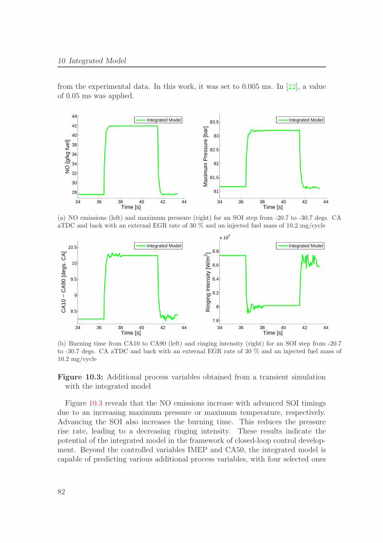
10 Integrated Model
from the experimental data. In this work, it was set to 0.005 ms. In [22], a valueof 0.05 ms was applied.
34 36 38 40 42 44
28
30
32
34
36
38
40
42
44
NO
[g/k
g fu
el]
Time [s]
Integrated Model
34 36 38 40 42 44
81
81.5
82
82.5
83
83.5
Max
imum
Pre
ssur
e [b
ar]
Time [s]
Integrated Model
(a) NO emissions (left) and maximum pressure (right) for an SOI step from -20.7 to -30.7 degs. CAaTDC and back with an external EGR rate of 30 % and an injected fuel mass of 10.2 mg/cycle
34 36 38 40 42 44
8.5
9
9.5
10
10.5
CA
10 −
CA
90 [d
egs.
CA
]
Time [s]
Integrated Model
34 36 38 40 42 44
7.8
8
8.2
8.4
8.6
8.8
x 106
Rin
ging
Inte
nsity
[W/m
2 ]
Time [s]
Integrated Model
(b) Burning time from CA10 to CA90 (left) and ringing intensity (right) for an SOI step from -20.7to -30.7 degs. CA aTDC and back with an external EGR rate of 30 % and an injected fuel mass of10.2 mg/cycle
Figure 10.3: Additional process variables obtained from a transient simulationwith the integrated model
Figure 10.3 reveals that the NO emissions increase with advanced SOI timingsdue to an increasing maximum pressure or maximum temperature, respectively.Advancing the SOI also increases the burning time. This reduces the pressurerise rate, leading to a decreasing ringing intensity. These results indicate thepotential of the integrated model in the framework of closed-loop control develop-ment. Beyond the controlled variables IMEP and CA50, the integrated model iscapable of predicting various additional process variables, with four selected ones
82

10.3 Potential within Closed-Loop Control Development
being briefly discussed in this section. These additional process variables allowfor defining further process constraints or may even replace the original controlledvariables, depending on the specific control task.
83

11 Summary and Conclusion
This thesis proposes a new approach for the integration of detailed physical com-bustion knowledge into closed-loop simulations. Closed-loop simulations are anecessary and common tool in the development process of controllers. A detailedinteractively coupled CFD-multi-zone approach was derived for modeling com-pression ignition combustion. This detailed interactively coupled CFD-multi-zoneapproach was validated against a test case of HCCI combustion in a gasolinesingle-cylinder research engine. Addressing PCCI combustion, the approach wasthen reduced to a stand-alone multi-zone model such that the resulting calcula-tion time could be significantly lowered with only a small penalty in accuracy.The stand-alone multi-zone model is capable of describing the PCCI combustioncharacteristics for the high-pressure part of the engine cycle. The controller tobe developed shall actuate SOI, external EGR rate, and total fuel mass injectedto control the IMEP of the whole engine cycle and the CA50. The IMEPHP ofthe high-pressure engine cycle and the CA50 can be extracted from simulationswith the stand-alone multi-zone model. The former was combined with a newlyproposed mean value model for the losses of the gas exchange to calculate theIMEP of the whole engine cycle. The combination of these models leads to anaccurate static model, which was further extended to a Wiener model for captur-ing temporal cycle-to-cycle dependencies. For every input of the model, a transferfunction was determined, forcing the whole model to follow the engine’s dynamics.All model parts (stand-alone multi-zone model, gas exchange model, and dynamictime response) were each validated separately. Afterwards, the integrated modelcomposed of all three model parts was validated against transient experimentalengine data.
85

12 Future Work
The dynamic model will build the framework in which a controller for the PCCIcombustion process will be developed. With the developed plant model, this con-troller will be laid out and tested.
The actuated variable external EGR rate is theoretical as long as there is nocorresponding actor to it. Because of this, the overall goal of this research project(carried out within the Collaborative Research Centre ”SFB 686 - ModellbasierteRegelung der homogenisierten Niedertemperatur-Verbrennung” at RWTH AachenUniversity, Germany, and Bielefeld University, Germany [83]) is to develop notonly a controller for the PCCI combustion process, but also an additional con-troller enabling the fastest possible changes in external EGR rate by simultane-ously adjusting EGR valve and VGT position [18]. This controller, in combinationwith its actuated variables EGR valve and VGT position, will serve as the virtualactor for the external EGR rate.
87

Bibliography
[1] S. M. Aceves, D. L. Flowers, F. Espinoza-Loza, A. Babajimopoulos, andD. N. Assanis. Analysis of Premixed Charge Compression Ignition Combus-tion with a Sequential Fluid Mechanics-Multizone Chemical Kinetics Model.Paper No. SAE 2005-01-0115, 2005. 1
[2] S. M. Aceves, D. L. Flowers, J. Martinez-Frias, J. R. Smith, C. K. Westbrook,W. Pitz, R. Dibble, M. Christensen, and B. Johansson. A Multi-Zone Modelfor Prediction of HCCI Combustion and Emissions. Paper No. SAE 2000-01-0327, 2000. 2.1
[3] S. M. Aceves, D. L. Flowers, J. Martinez-Frias, J. R. Smith, C. K. West-brook, W. Pitz, R. Dibble, J. F. Wright, W. C. Akinyemi, and R. P. Hes-sel. A Sequential Fluid-Mechanic Chemical Kinetic Model of Propane HCCICombustion. Paper No. SAE 2001-01-1027, 2001. 2.1
[4] A. Albrecht, O. Grondin, F. Le Berr, and G. Le Solliec. Towards a StrongerSimulation Support for Engine Control Design: a Methodological Point ofView. Oil & Gas Science and Technology - Rev. IFP, 62:437–456, 2007. 1
[5] A. Babajimopoulos, D. N. Assanis, D. L. Flowers, S. M. Aceves, and R. P.Hessel. A fully coupled computational fluid dynamics and multi-zone modelwith detailed chemical kinetics for the simulation of premixed charge com-pression ignition engines. International Journal of Engine Research, 6:497–512, 2005. 2.1
[6] A. Babajimopoulos, G. A. Lavoie, and D. N. Assanis. Modelling HCCICombustion with High Levels of Residual Gas Fraction - A Comparison ofTwo VVA Strategies. Paper No. SAE 2003-01-3220, 2003. 2.1
[7] H. D. Baehr and K. Stephan. Warme- und Stoffubertragung. Springer, Berlin,2006. 6.2.3
[8] H. Barths, C. Hasse, and N. Peters. Computational fluid dynamics modellingof non-premixed combustion in direct injection diesel engines. InternationalJournal of Engine Research, 1:249–267, 2000. 1, 4.2.1
89
Bibliography
[9] J. Bengtsson, P. Strandh, R. Johansson, P. Tunestal, and B. Johansson.Hybrid control of homogeneous charge compression ignition (HCCI) enginedynamics. International Journal of Control, 79:422–448, 2006. 1
[10] J. Bengtsson, P. Strandh, R. Johansson, P. Tunestal, and B. Johansson. Hy-brid modelling of homogeneous charge compression ignition (HCCI) enginedynamics - a survey. International Journal of Control, 80:1814–1847, 2007.1
[11] J. Boussinesq. Theorie de l’Ecoulement Tourbillant. Mem. Presentes parDivers Savants Acad. Sci. Inst. Fr., 23:46–50, 1877. 3.4
[12] M. Christensen, B. Johansson, and P. Einewall. Homogeneous Charge Com-pression Ignition (HCCI) using Isooctane, Ethanol and Natural Gas - a Com-parison with Spark Ignition Operation. Paper No. SAE 972874, 1997. 5.2.2
[13] O. Colin and A. Benkenida. The 3-Zones Extended Coherent Flame Model(ECFM3Z) for Computing Premixed/Diffusion Combustion. Oil & Gas Sci-ence and Technology - Rev. IFP, 59:593–609, 2004. 1
[14] O. Colin, A. Pires da Cruz, and S. Jay. Detailed chemistry-based auto-ignition model including low temperature phenomena applied to 3-D enginecalculations. Proc. Combust. Inst., 30:2649–2656, 2005. 1
[15] D. J. Cook, H. Pitsch, J. H. Chen, and R. E. Hawkes. Flamelet-basedmodeling of auto-ignition with thermal inhomogeneities for application toHCCI engines. Proc. Combust. Inst., 31:2903–2911, 2007. 1
[16] C. T. Crowe, M. P. Sharma, and D. E. Stock. The particle-source-in cell (PSI-Cell) model for gas-droplet flows. Journal of Fluids Engineering, 99:325–332,1977. 3.6
[17] J. E. Dec. Advanced compression-ignition engines – Understanding the in-cylinder processes. Proc. Combust. Inst., 32:2727–2742, 2009. 1
[18] P. Drews, K. Hoffmann, R. Beck, R. Gasper, A. Vanegas, C. Felsch,N. Peters, and D. Abel. Fast Model Predictive Control for the Air Pathof a Turbocharged Diesel Engine. In European Control Conference 2009,Budapest, Hungary, 2009. 12
[19] J. K. Dukowicz. A particle-fluid model numerical model for liquid sprays. J.Comput. Phys., 35:229–253, 1980. 3.6
90
Bibliography
[20] P. Duret and J. Lavy. Gasoline Controlled Auto-Ignition (CAI) - Potentialand Prospects for the Future Automotive Application. In IMechE Interna-tional Conference: 21st Century Emissions Technologies, London, UK, 2000.5.1.1
[21] E. Easley, A. Agarwal, and G. A. Lavoie. Modeling of HCCI Combustion andEmissions Using Detailed Chemistry. Paper No. SAE 2001-01-1029, 2001. 1
[22] J. A. Eng. Characterization of Pressure Waves in HCCI Combustion. PaperNo. SAE 2002-01-2859, 2002. 10.3, 10.3
[23] ETAS GmbH. ES 1000.3 Benutzerhandbuch. Technical report, ETAS GmbH,2008. 9.2
[24] J. Ewald, F. Freikamp, G. Paczko, J. Weber, D. C. Haworth, and N. Peters.GMTEC: GMTEC Developer’s Manual. Technical report, Advanced Com-bustion GmbH, 2003. 3.5
[25] C. Felsch, M. Gauding, C. Hasse, S. Vogel, and N. Peters. An extendedflamelet model for multiple injections in DI Diesel engines. Proc. Combust.Inst., 32:2775–2783, 2009. 4.2.1
[26] C. Felsch, T. Sloane, J. Han, H. Barths, and A. M. Lippert. NumericalInvestigation of Recompression and Fuel Reforming in a SIDI-HCCI Engine.Paper No. SAE 2007-01-1878, 2007. 2.2
[27] C. Felsch, A. Vanegas, B. Kerschgens, N. Peters, K. Hoffmann, P. Drews,D. Abel, and H. Barths. Systematic Reduction of an Interactively CoupledCFD-Multi-Zone Approach Towards a Stand-alone Multi-Zone Model forPCCI Combustion. In Thiesel 2008: Thermo-and fluid dynamic processes inDiesel Engines, Universidad Politecnica de Valencia, Valencia, Spain, 2008.7.2.2
[28] J. H. Ferziger. Higher level simulations of turbulent flows. In J.-A. Essers(Ed.), Computational Methods for Turbulent, Transonic, and Viscous Flows.Springer, Berlin, 1983. 3.4
[29] J. H. Ferziger and M. Peric. Computational Methods for Fluid Dynamics.Springer, Berlin, 2002. 3.5
[30] D. L. Flowers, S. M. Aceves, and A. Babajimopoulos. Effects of Charge Non-Uniformity on Heat Release and Emissions in PCCI Engine Combustion.Paper No. SAE 2006-01-1363, 2006. 2.1
91
Bibliography
[31] D. L. Flowers, S. M. Aceves, J. Martinez-Frias, R. P. Hessel, and R. Dibble.Effects of Mixing on Hydrocarbon and Carbon Monoxide Emissions Predic-tion for Isooctane HCCI Engine Combustion Using a Multi-Zone DetailedKinetics Solver. Paper No. SAE 2003-01-1821, 2003. 1
[32] F. Freikamp. Towards Multi-Cycle Simulation of In-Cylinder Flow and Com-bustion. PhD thesis, RWTH Aachen University, Germany, 2008. 3.5, 3.1
[33] Gamma Technologies. GT-POWER User’s Manual and Tutorial, GT-SUITEVersion 7.0. Technical report, Gamma Technologies, 2008. 8
[34] O. Gicquel, N. Darabiha, and D. Thevenin. Laminar premixed hydrogen/aircounterflow flame simulations using flame prolongation of ILDM with differ-ential diffusion. Proc. Combust. Inst., 28:1901–1908, 2000. 1
[35] L. Guzzella and C. H. Onder. Introduction to Modeling and Control of In-ternal Combustion Engine Systems. Springer, Berlin, 2004. 9.2
[36] V. Hamosfakidis, H. G. Im, and D. N. Assanis. A regenerative multiple zonemodel for HCCI combustion. Combust. Flame, 156:928–941, 2009. 1
[37] A. Harada, N. Shimazaki, S. Sasaki, T. Miyamoto, H. Akagawa, and K. Tsu-jimura. The Effects of Mixture Formation on Premixed Lean Diesel Com-bustion. Paper No. SAE 980533, 1998. 1
[38] C. Hasse and N. Peters. A two mixture fraction flamelet model applied tosplit injections in a DI Diesel engine. Proc. Combust. Inst., 30:2755–2762,2005. 4.2.1
[39] C.-A. Hergart, H. Barths, and R. M. Siewert. Modeling Approaches forPartially Premixed Compression Ignition Combustion. Paper No. SAE 2005-01-0218, 2005. 1, 2.2, 4.6, 6.2.3, 7.2.2
[40] R. P. Hessel, D. E. Foster, S. M. Aceves, M. Davisson, F. J. Espinosa-Loza,D. L. Flowers, W. Pitz, J. E. Dec, M. Sjoberg, and A. Babajimopoulos.Modeling Iso-octane HCCI using CFD with Multi-Zone Detailed Chemistry;Comparison to Detailed Specification Data over a Range of Lean EquivalenceRatios. Paper No. SAE 2008-01-0047, 2008. 2.1
[41] J. B. Heywood. Internal Engine Combustion Fundamentals. McGraw-Hill,New York, 1988. 2.3, 4.4, 7.2.1
[42] M. Hillion, H. Buhlbuck, J. Chauvin, and N. Petit. Combustion Control ofDiesel Engines Using Injection Timing. Paper No. SAE 2009-01-0367, 2009.1
92
Bibliography
[43] M. Hillion, J. Chauvin, O. Grondin, and N. Petit. Active Combustion Con-trol of Diesel HCCI Engine: Combustion Timing. Paper No. SAE 2008-01-0984, 2008. 1
[44] K. Hoffmann, P. Drews, D. Abel, C. Felsch, A. Vanegas, and N. Peters.A Cycle-Based Multi-Zone Simulation Approach Including Cycle-to-CycleDynamics for the Development of a Controller for PCCI Combustion. PaperNo. SAE 2009-01-0671, 2009. 8, 9.1
[45] D. T. Hountalas, D. A. Kouremenos, G. C. Mavropoulos, K. B. Binder,and V. Schwarz. Multi-Zone Combustion Modelling as a Tool for DI DieselEngine Development-Application for the Effects of Injection Pressure. PaperNo. SAE 2004-01-0115, 2004. 1
[46] R. I. Issa. Solution of the implicitly discretised fluid flow equations byoperator-splitting. J. Comput. Phys., 62:40–65, 1986. 3.5
[47] Y. Iwabuchi, K. Kawai, T. Shoji, and Y. Takeda. Trial of New ConceptDiesel Combustion System - Premixed Compression Ignited Combustion.Paper No. SAE 1999-01-0185, 1999. 1
[48] W. P. Jones and B. E. Launder. The prediction of laminarization with atwo-equation model of turbulence. Int. J. Heat Mass Transfer, 15:301–314,1972. 3.4
[49] R. J. Kee, F. M. Rupley, and J. A. Miller. CHEMKIN-II: A Fortran ChemicalKinetics Package for the Analysis of Gas-Phase Chemical Kinetics. Technicalreport, Sandia Report SAND89-8009, Sandia National Laboratories, 1989.2.3
[50] B. Khalighi, S. H. El Thary, D. C. Haworth, and M. S. Huebler. Computationand Measurement of Flow and Combustion in a Four-Valve Engine withIntake Variations. Paper No. SAE 950287, 1995. 3.5
[51] B. E. Launder and B. I. Sharma. Application of the energy-dissipation modelof turbulence to the calculation of flow near a spinning disc. Lett. Heat MassTransfer, 1:131–138, 1974. 3.4, 3.4
[52] D. Law, D. Kemp, J. Allen, G. Kirkpatrick, and T. Copland. ControlledCombustion in an IC-Engine with a Fully Variable Valve Train. Paper No.SAE 2001-01-0251, 2001. 5.1.1
[53] J. Lunze. Regelungstechnik 2: Mehrgroßensysteme, Digitale Regelung.Springer, Berlin, 2008. 9.3
93
Bibliography
[54] U. C. Muller, N. Peters, and A. Linan. Global kinetics for n-heptane ignitionat high pressures. Symposium (International) on Combustion, 24:777–784,1992. 6.2.4
[55] P. M. Najt and D. E. Foster. Compression-Ignited Homogeneous ChargeCombustion. Paper No. SAE 830264, 1983. 5.2.2
[56] S. Nakayama, T. Ibuki, H. Hosaki, and H. Tominaga. An Application of aModel Based Combustion Control to Transient Cycle-by-Cycle Diesel Com-bustion. Paper No. SAE 2008-01-1311, 2008. 1
[57] K. Narayanaswamy, R. P. Hessel, and C. J. Rutland. A New Approach toModel DI-Diesel HCCI Combustion for Use in Cycle Simulation Studies.Paper No. SAE 2005-01-3743, 2005. 1, 1
[58] K. Narayanaswamy and C. J. Rutland. A Modeling Investigation of Com-bustion Control Variables During DI-Diesel HCCI Engine Transients. PaperNo. SAE 2006-01-1084, 2006. 1
[59] O. Nelles. Nonlinear System Identification: From Classical Approaches toNeural Networks and Fuzzy Models. Springer, Berlin, 2000. 9.1
[60] T. Noda and D. E. Foster. A Numerical Study to Control CombustionDuration of Hydrogen-fueled HCCI by Using Multi-Zone Chemical KineticsSimulation. Paper No. SAE 2001-01-0250, 2001. 1
[61] A. Oakley, H. Zhao, N. Ladommatos, and T. Ma. Experimental Studieson Controlled Auto-Ignition (CAI) Combustion of Gasoline in a 4-StrokeEngine. Paper No. SAE 2001-01-1030, 2001. 5.1.1
[62] S. V. Patankar. Numerical Heat Transfer and Fluid Flow. Taylor & Francis,London, 1980. 3.5
[63] E. Perez, X. Blasco, S. Garcıa-Nieto, and J. Sanchis. Diesel Engine Identi-fication and Predictive Control using Wiener and Hammerstein Models. InProceedings of the 2006 IEEE International Conference on Control Applica-tions, Munich, Germany, 2006. 9.1
[64] N. Peters. Laminar diffusion flamelet models in non-premixed turbulentcombustion. Prog. Energy Combust. Sci., 10:319–339, 1984. 4.2.1
[65] N. Peters. Laminar flamelet concepts in turbulent combustion. Symposium(International) on Combustion, 21:1231–1250, 1986. 4.2.1
94
Bibliography
[66] N. Peters. Turbulent Combustion. Cambridge Univ. Press, Cambridge, 2000.1, 3.1, 4.2.1
[67] N. Peters, G. Paczko, R. Seiser, and K. Seshadri. Temperature cross-over andnon-thermal runaway at two-stage ignition of n-heptane. Combust. Flame,28:38–59, 2002. 2.3, 6.2.4
[68] L. R. Petzold. A Description of DASSL: A Differential/Algebraic SystemSolver. Technical report, Sandia Report SAND82-8637, Sandia NationalLaboratories, 1982. 2.2
[69] H. Pitsch, H. Barths, and N. Peters. Three-Dimensional Modeling of NOx
and Soot Formation in DI-Diesel Engines Using Detailed Chemistry Basedon the Interactive Flamelet Approach. Paper No. SAE 962057, 1996. 4.2.1
[70] H. Pitsch and N. Peters. Private Communication, 2001. 2.3
[71] S. B. Pope. PDF methods for turbulent reactive flows. Prog. Energy Com-bust. Sci., 11:119–192, 1985. 1
[72] S. B. Pope. Computationally efficient implementation of combustion chem-istry using in situ adaptive tabulation. Combust. Theory & Modelling, 1:41–63, 1997. 1
[73] S. B. Pope. Turbulent Flows. Cambridge Univ. Press, Cambridge, 2000. 3.2,3.4
[74] L. Prandtl. Uber die ausgebildete Turbulenz. ZAMM, 5:136–139, 1925. 3.4
[75] L. Prandtl. Uber ein neues Formelsystem fur die ausgebildete Turbulenz.Nachr. Akad. Wiss. Gottingen, Math.-Phys. Klasse, pages 6–19, 1945. 3.4
[76] C. D. Rakopoulos and D. T. Hountalas. Development and Validation of a3-D Multi-Zone Combustion Model for the Prediction of DI Diesel EnginesPerformance and Pollutants Emissions. Paper No. SAE 981021, 1998. 1
[77] R. Reitz and C. J. Rutland. Development and testing of diesel engine CFDmodels. Prog. Energy Combust. Sci., 21:173–196, 1995. 1
[78] Ricardo Software. WAVE Basic Manual, Documentation/User’s Manual,Version 5.0. Technical report, Ricardo Software, 2003. 5.1.2, 8
[79] F. Richert. Objektorientierte Modellbildung und Nichtlineare PradiktiveRegelung von Dieselmotoren. PhD thesis, RWTH Aachen University, Ger-many, 2005. 8
95
Bibliography
[80] W. Rodi and D. B. Spalding. A two-parameter model of turbulence and itsapplication to free jets. Warme- und Stoffubertragung, 3:85–95, 1970. 3.4
[81] J. C. Rotta. Statistische Theorie nichthomogener Turbulenz. Zeitschrift fuerPhysik, 129:547–572, 1951. 3.4
[82] J. C. Rotta. Turbulente Stromungen. Teubner Verlag, Stuttgart, 1972. 3.4
[83] RWTH Aachen University and Bielefeld University. SFB 686 - Mod-ellbasierte Regelung der homogenisierten Niedertemperatur-Verbrennung.http://www.sfb686.rwth-aachen.de. 12
[84] H. Santoso, J. Matthews, and W. Cheng. Characteristics of HCCI EngineOperating in the Negative-Valve-Overlap Mode. Paper No. SAE 2005-01-2133, 2005. 5.1.1
[85] T. Schulze, M. Wiedemeier, and H. Schuette. Crank Angle - Based DieselEngine Modeling for Hardware-in-the-Loop Applications with In-CylinderPressure Sensors. Paper No. SAE 2007-01-1303, 2007. 9.1
[86] G. M. Shaver, J. C. Gerdes, M. J. Roelle, P. A. Caton, and C. F. Edwards.Dynamic Modeling of Residual-Affected Homogeneous Charge CompressionIgnition Engines with Variable Valve Actuation. Journal of Dynamic Sys-tems, Measurement, and Control, 127:374–381, 2005. 1
[87] G. M. Shaver, M. J. Roelle, P. A. Caton, N. B. Kaahaaina, N. Ravi, J.-P.Hathout, J. Ahmed, A. Kojic, S. Park, C. F. Edwards, and J. C. Gerdes.A physics-based approach to the control of homogeneous charge compres-sion ignition engines with variable valve actuation. International Journal ofEngine Research, 6:361–375, 2005. 1
[88] G. M. Shaver, M. J. Roelle, and J. C. Gerdes. Modeling cycle-to-cycle dy-namics and mode transition in HCCI engines with variable valve actuation.Control Engineering Practice, 14:213–222, 2006. 1
[89] P. Spiekermann, S. Jerzembeck, C. Felsch, S. Vogel, M. Gauding, andN. Peters. Experimental Data and Numerical Simulation of Common-RailEthanol Sprays at Diesel Engine-Like Conditions. Atomization and Sprays,19:357–386, 2009. 3.6
[90] Y. Takeda and N. Keiichi. Emission Characteristics of Premixed Lean DieselCombustion with Extremely Early Staged Fuel Injection. Paper No. SAE961163, 1996. 1
96
Bibliography
[91] H. Tennekes and J. L. Lumley. A First Course in Turbulence. The MITPress, Cambridge, 1972. 3.2
[92] The MathWorks, Inc.. Matlab 7.6 Manual (R2008a). Technical report, TheMathWorks, Inc., 2008. 10.1
[93] R. H. Thring. Homogeneous Charge Compression Ignition (HCCI) Engines.Paper No. SAE 892068, 1989. 5.2.2
[94] R. Turin, R. Zhang, and M.-F. Chang. Systematic Model-Based EngineControl Design. Paper No. SAE 2008-01-0994, 2008. 1
[95] IAV GmbH Ingenieursgesellschaft Auto und Verkehr. FI2RE- Flexible Injection and Ignition for Rapid Engineering.http://www.iav.com/de/1 engineering/powertrainmechatronik/messtechnik/fi2re.php,2008. 9.2
[96] T. Urushihara, K. Hiraya, A. Kakuhou, and T. Itoh. Expansion of HCCIOperating Region by the Combination of Direct Fuel Injection, NegativeValve Overlap, and Internal Fuel Reformation. Paper No. SAE 2003-01-0749, 2003. 5.1.1
[97] J. A. van Oijen, F. A. Lammers, and L. P. H. de Goey. Modeling of complexpremixed burner systems by using flamelet-generated manifolds. Combust.Flame, 127:2124–2134, 2001. 1
[98] A. Vanegas, H. Won, C. Felsch, M. Gauding, and N. Peters. ExperimentalInvestigation of the Effect of Multiple Injections on Pollutant Formation ina Common-Rail DI Diesel Engine. Paper No. SAE 2008-01-1191, 2008. 7.1.1
[99] J. Weber, P. Spiekermann, and N. Peters. Model Calibration for SprayPenetration and Mixture Formation in a High-Pressure Fuel Spray Using aMicro-Genetic Algorithm and Optical Data. Paper No. SAE 2005-01-2099,2005. 7.1.2
[100] J. Willand, R.-G. Nieberding, G. Vent, and C. Enderle. The KnockingSyndrome: Its Cure and Potential. Paper No. SAE 982483, 1998. 5.1.1
[101] F. A. Williams. Spray Combustion and Atomization. Phys. Fluids, 1:541–545, 1958. 3.6
[102] G. Woschni. A Universally Applicable Equation for Instantaneous HeatTransfer Coefficients in the Internal Combustion Engine. Paper No. SAE670931, 1967. 6.2.1
97
Bibliography
[103] H. Xu. Modelling of HCCI Engines: Comparison of Single-Zone, Multi-Zoneand Test Data. Paper No. SAE 2005-01-2123, 2005. 1
[104] M. Yao, Z. Zheng, and H. Liu. Progress and recent trends in homogeneouscharge compression ignition (HCCI) engines. Prog. Energy Combust. Sci.,35:398–437, 2009. 1
[105] Y. Z. Zhang, E. H. Kung, and D. C. Haworth. A PDF method formultidimensional modeling of HCCI engine combustion: effects of turbu-lence/chemistry interactions on ignition timing and emissions. Proc. Com-bust. Inst., 30:2763–2771, 2005. 1
98
Definitions, Acronyms, Abbreviations
aTDC after Top Dead Center
CA Crank Angle
CA10 Crank Angle of 10 % burnt mass
CA50 Crank Angle of 50 % burnt mass
CFD Computational Fluid Dynamics
CO Carbon Monoxide
DDM Discrete Droplet Model
ECU Electronic Control Unit
EGR Exhaust Gas Recirculated
EOI End of Injection
EVO Exhaust Valve Opening
FMI Total Fuel Mass Injected
HCCI Homogeneous Charge Compression Ignition
IMEP Indicated Mean Effective Pressure
IMEPGE Indicated Mean Effective Pressure of the Gas Exchange
IMEPHP Indicated Mean Effective Pressure of the High-Pressure Cycle
IVC Intake Valve Closure
LTC Low-temperature Combustion
NOx Nitrogen Oxides
pae Pressure in the Exhaust Manifold (after engine)
pbe Pressure in the Intake Manifold (before engine)
PCCI Premixed Charge Compression Ignition
PCI Premixed Charge Ignition
rpm Revolutions per Minute
RWTH Rheinisch Westfalische Technische Hochschule Aachen
SOI Start of Injection
Tae Temperature in the Exhaust Manifold
99

Tbe Temperature in the Intake Manifold
TDC Top Dead Center
TS Timing Sweep
VGT Variable Geometry Turbine
100
Lebenslauf
Personliche Daten
Name Christian Felsch
Geburtsdatum 25. Dezember 1977
Geburtsort Neuss
Familienstand ledig
Nationalitat deutsch
Schulbildung
08/1988–06/1997 Stadtisches Meerbusch-Gymnasium, Meerbusch;Abschluss: Abitur
Grundwehrdienst
07/1997–04/1998 Luftwaffe, Goslar und Geilenkirchen
Studium
10/1998–09/2000 Grundstudium Maschinenbau an der Gerhard-Mercator-Universitat Duisburg;Abschluss: Diplom-Vorprufung
10/2000–07/2003 Hauptstudium Maschinenbau an der RWTH AachenUniversity, Fachrichtung Luftfahrttechnik;Abschluss: Diplom
Externe DiplomarbeitInvestigation of Boundary Conditions and PressureWaves in Numerical Modelling of Compressible Turbu-lent Flow with CombustionDepartment of Energy and Process Engineering, Norwe-gian University of Science and Technology, Trondheim,Norwegen (im Rahmen eines DAAD-Stipendiums)
Beruflicher Werdegang
seit 10/2003 Wissenschaftlicher Angestellter am Institut fur Tech-nische Verbrennung (ehemals Institut fur TechnischeMechanik) der RWTH Aachen University


![Titelfolie Einleitung: Wieso Holzenergie ? Wieso ... · Combustion Modeling Verenum [Bruch & Nussbaumer, 1998] Verenum Titelfolie F&E 2: Stickoxide. Verenum Luft- und Brennstoffstufung](https://img.pdfslide.org/doc/110x75/5e21f6c165b8b032e2649e4f/titelfolie-einleitung-wieso-holzenergie-wieso-combustion-modeling-verenum.jpg)