COMPUTATIONAL MODELLING OF - Technische …tuprints.ulb.tu-darmstadt.de/6217/1/subhash_final_version_of... · ... research on ‘Computational Modelling of Liquid Jet ... of Water

COMPUTATIONAL MODELLING OF

LIQUID JET IMPINGEMENT

ONTO HEATED SURFACE

Vom Fachbereich Maschinenbau

an der Technischen Universität Darmstadt

zur

Erlangung des Grades eines Doktor-Ingenieurs

(Dr.-Ing.)

genehmigte

D i s s e r t a t i o n

vorgelegt von

Maharshi Subhash, M. Tech

from Dehradun, India

Berichterstatter: Prof. Dr.-Ing. habil. Cameron Tropea

Mitberichterstatter: apl. Prof. Dr.-Ing. habil. Suad Jakirlic

apl. Prof. Dr. rer. Nat. Amsini Sadiki

Tag der Einreichung: 30th November, 2015

Tag der mündlichen Prüfung: 17th February, 2016

Darmstadt 2017

D17

2

Erklärung

3

Erklärung

Erklärung

Hiermit erkläre ich, dass ich die vorliegende Dissertation selbstständig verfasst und nur

die angegebenen Hilfsmittel an den entsprechend gekennzeichneten Stellen verwendet

habe. Ich habe bisher noch keinen Promotionsversuch unternommen.

Dehradun, im November 2015

Maharshi Subhash

4

5

Dedicated to my supervisor and co-supervisor

Prof. Dr. Ing.Cameron Tropea ,

apl. Prof. Dr. Ing. Suad Jakirlic

and

my parents, my wife Sudha and daughter

Samriddhi

6

7

Foreword

Foreword One of the joys of completion is to look over the journey past and remember all those,

who had helped and supported along this long but fulfilling road. This Ph.D. thesis is the

result of a challenging journey, upon which many people have contributed and given

their supports.

It would not have been possible without the help, support, and patience of my mentor

Prof. Jakirlic, not to mention his advice and unsurpassed knowledge of numerical simu-

lation and turbulence model. My sincere gratitude to my Prof. and head of the Institute,

Prof. Tropea for giving the opportunity of research on ‘Computational Modelling of

Liquid Jet Impingement onto Heated Surface.' The present work was accomplished

during the period June 2008 to March 2012.

This work has been financially supported by the steel company Dillinger

Hütte, GTS. The fruitful discussion with research and development head of the company

Prof. Karl-Hermann Tacke and other members of research committee Dr. Roland

Schorr, Mr. Eberwein Klaus, and Mr. Kirsh Hans-Juergen during the project meeting

encouraged me a lot. The fruitful discussion with Dr. Karwa and Prof. Stephan from

Institute of Technical Thermodynamics (TTD) brought this research at the good level in

terms of findings.

Throughout this research work, the enumerable help from co-supervisor enhanced the

quality of the results.

During the research work, time-to-time discussion with Prof. Sadiki helped me to under-

stand the computational error.

I also express gratitude to Dr. Basara the head of Advanced Simulation Tech-

nology from AVL List Company, Graz Austria, for providing the CFD code AVL Fire.

Thanks to Mr. David Greif, who helped me to learn the tools of this code.

Also, the time-to-time discussion with Dr.-Ing. Ilia Roisman helped to under-

stand the theoretical aspects of the film-boiling model.

Other colleagues Mrs. Gisa Kadavelil, Dr. Samual Chang, Dr. Robert Maduta and others

helped me to work with some software tools. Sometimes, Mr. Michael Kron (computer

administrator), provided extra computation time which helped me to produce the results

for those cases which consumed large computing time.

Mrs. Lath and Mrs. Neuthe had offered great support during my stay in Darmstadt.

Moreover, co-supervisor’s consistent patience on me has created a humble and eternal

respect towards him for rest of my life.

At last, but not least, I would like to express my deep respect and love to my parents and

my family members for great moral support during the research.

Maharshi Subhash

8

9

Abstract

Abstract

Quenching of heated surfaces through impinging liquid jets is of great im-

portance for numerous applications like steel processing, nuclear power plants, automo-

bile industries, etc. Therefore, computational modelling of the surface quenching

through circular water jets impinging normally onto a heated flat surface has vital im-

portance in order to reveal the physics of the quenching process.

At first, a numerical model was developed for single jet impingement process.

A conjugate heat transfer problem was solved implying consideration of both regions,

one occupied by fluid (multi-phase flow consisting of water, vapor and ambient air) and

one accommodating the solid surface within the same solution domain.

Numerical simulations were performed in a range of relevant operating param-

eters: jet velocities (2.5, 5, 7.5 and 10 m/s), water sub-cooling (75 K) and wall-superheat

(650 K - 800 K) corresponding closely to those encountered in the industrial water jet

cooling banks. Due to the high initial temperature of the surface, the boiling process

exhibits strong spatial and temporal fluctuations. Its effect on the boundary layer profiles

at the stagnation region at different time intervals are analyzed. The analysis reveals a

highly distorted field of both mean flow and turbulence quantities. It represents an im-

portant outcome, also with respect to appropriate model improvements. The different

boiling characteristics are envisaged in detail to increase the level of understanding of

the phenomena. The influence of the turbulent kinetic energy investigated at the boiling

front as well as the jet-acceleration region has been studied. The physically relevant

results are obtained and analyzed along with reference database provided experimentally

by Karwa (2012, ‘Experimental Study of Water Jet Impingement Cooling of Hot Steel

Plates,' Dissertation, FG TTD, TU Darmstadt). The intensive quenching process is

consistent with the high rate of sub-cooling and high jet velocities. The surface tempera-

ture predicted by quenching model within the impingement region and the subsequent

wall-jet region agrees reasonably well with the measurements, the outcome being par-

ticularly valid at higher jet velocities. However, a steep temperature gradient at the

position corresponding to boiling threshold has not been captured under the condition of

the numerical grid adopted. On the other hand, a reasonably good prediction of the

wetting front propagation phenomena advocates the future development of the model.

The high-intensity back motion of the vapor phase in the stagnation region at the earlier

times of the water jet impingement can induce an appropriately high turbulence level,

which could be accounted well by the turbulence model applied.

The second part of the present work deals with multiple liquid jet impinge-

ment. When the multiple jets impact onto the heated surface, the heat flux is extracted

from the surface by the mass flow rate. The heat flux is dependent on the several flow

conditions and configurations of the nozzle array system. Therefore, one needs to study

the nozzle array configuration along with several flow parameters for the better design

10

Abstract

of the cooling header system. Accordingly, the hydrodynamics of the multiple jets has

been studied computationally realizing the need for optimum configuration of the nozzle

array. The effects of the mass flow rate, target plate width and the turbulence produced

due to the impingement were studied. Afterward, an analytical model is proposed for the

quenching of the multiple jets system. It has been realized that, when jet impinges onto

the surface at very high initial temperature, the film boiling may play a role in the heat

transfer mechanism. Therefore, development has been made in the film-boiling model

considering the effect of turbulence at the liquid jet stagnation region at the Leidenfrost

point. The Leidenfrost point is the minimum temperature at which the film boiling can

sustain. However, the vapor-liquid interface has the dynamic character; it oscillates with

high frequency and causes the additional momentum diffusivity. Therefore, the need for

introducing the effect of associated turbulence has been felt. The length and velocity

scale of the turbulent structure has been approximated by assuming homogeneous turbu-

lence. The new model for the heat flux and wall superheat yielded results agreeing well

with published experimental results.

11

Zusammenfassung

Zusammenfassung („Numerische Modellierung des Aufpralls von Flüssigkeitsstrahlen auf beheizte Oberflächen“)

Kühlung der beheizten Oberflächen durch aufprallende Flüssigkeitsstrahlen ist im Fall

zahlreicher industrieller Anwendungen von großer Bedeutung: Stahlherstellung, Kern-

energiekraftwerke, Fahrzeugindustrie, usw. Das Stellt die Hauptmotivation der vorlie-

genden Arbeit dar, die die numerische Modellierung der Kühlung von heißen Oberflä-

chen durch runde, senkrecht auf die Fläche aufprallende Wasserstrahlen umfasst.

Zuerst wurde der Aufprall eines einzelnen Wasserstrahls (‘single jet impinge-

ment’) modelliert. Es wurde ein gekoppeltes Wärmeübertragungsproblem behandelt,

indem beide Teilgebiete, das Flüssigkeit (d.h. mehrphasige, das Wasser, den Dampf und

die umgebende Luft charakterisierende Strömung) und die feste Wand umfassend, in-

nerhalb des gleichen Lösungsgebietes berücksichtigt wurden. Numerische Simulationen

wurden im Bereich der relevanten Arbeitsparameter, bezogen auf Strahlgeschwindigkei-

ten (2.5, 5, 7.5, 10 m/s), Wasserunterkühlungstemperaturen von 75 K (Water sub-

cooling) und Wandüberhitzungstemperaturen von 650 K bis 800 K (wall superheat),

durchgeführt. Diese entsprechen den Betriebsbedingungen der in der industriellen Praxis

anzutreffenden Kühlungsanlagen. Infolge der großen Anfangstemperatur der Oberfläche

wird das Siedeprozess von starken räumlichen und zeitlichen Schwankungen begleitet.

Das beeinflusst entscheidend das temporäre Verhalten der wandnahen Grenzschicht. Die

ausführlich durchgeführte Analyse offenbart stark modifizierte Felder der Hauptströ-

mung und der turbulenten Größen. Das stellt eine wichtige Erkenntnis dar, womit ein

Beitrag zum weiteren Verständnis des vorliegenden Phänomens geleistet werden konnte.

Dabei wurde große Aufmerksamkeit dem Einfluss der kinetischen Turbulenzenergie im

Gebiet der Strömungsbeschleunigung geschenkt. Physikalisch relevante Ergebnisse

wurden gewonnen und mit der Datenbasis des komplementären, von Karwa durchge-

führten Experimenten (2012, ‘Experimental Study of Water Jet Impingement Cooling of

Hot Steel Plate’, Dissertation, FG TTD, TU Darmstadt) direkt verglichen. Grundlegend

betrachtet ist der Kühlungsprozess der glühend heißen Stahlplatte konsistent mit der

Intensität der Wärmeabfuhr infolge höher Aufprallgeschwindigkeiten. Die mit dem

vorliegenden Berechnungsmodell für die Erfassung der Stahlabkühlung wurden die

Ergebnisse gewonnen, die eine gute Übereinstimmung mit den experimentellen Daten

im Aufprallgebiet aufweisen; dies trifft insbesondere im Fall höhere Aufprallgeschwin-

digkeiten zu. Allerdings wurde der steile Temperaturgradient an der der Siedeschwelle

(‘boiling threshold’) entsprechenden Wandposition unter Bedingungen der verwendeten

räumlichen Auflösung nicht erfasst. Trotzdem wurde die Ausbreitung der benetzten

Front korrekt vorhergesagt, was für das hohe Potential des Modells im Fall praktischer

12

Anwendungen spricht. Die intensive Rückströmung innerhalb der Dampfphase im Auf-

prallgebiet und der damit verbundene Anstieg der Turbulenzintensität im Aufprallgebiet

konnten mit dem eingesetzten Turbulenzmodell wiedergegeben werden.

Der Zweite Teil der vorliegenden Arbeit untersucht die Effekte von mehreren, parallel

angeordneten, gleichzeitig aufprallenden Wasserstrahlen (‘multiple jets impingement’).

Der im Fall mehrerer auf die beheizte Oberfläche aufprallender Strahlen abgeführte

Wärmefluss hängt von unterschiedlichen Strömungsparametern aber auch von der Dü-

senkonfiguration ab, deren verschiedene Anordnungen eines der Ziele der Untersuchung

darstellen. Diesbezüglich lag der Schwerpunkt auf der Hydrodynamik des mehrfachen

Aufpralls. Der Wasser-Volumenstrom im Hinblick auf unterschiedliche Anzahl der

Düsen sowie die Abmessungen der Platte wurden variiert. Anschließend wurde ein

analytisches Modell für die Oberflächenabkühlung formuliert, das als Grundlage das

Phänomen der ‘film boiling’ Prozesse betrachtet. Die Effekte der Turbulenz unter Be-

dingungen des sog. Leidenfrost Phänomens wurden am Staugebiet berücksichtigt. Das

Dampf-Flüssig Interface weist einen dynamischen Charakter auf, indem es mit entspre-

chend hoher Frequenz oszilliert, was als Folge einen zusätzlichen Impulstransport hat.

Dabei wurden die turbulenten Längen- und Geschwindigkeitsmaßstäbe durch die An-

nahme homogener Turbulenz approximiert. Das neue, den Wärmefluss und die Wand-

überhitzung berücksichtigende Modell resultiert in einer guten Übereinstimmung mit

den in der veröffentlichten Literatur verfügbaren Ergebnissen.

13

Table of Contents

Table of Contents

Foreword ........................................................................................................... 5

Abstract ............................................................................................................. 9

Zusammenfassung .......................................................................................... 11

Table of Contents ............................................................................................ 13

Nomenclature .................................................................................................. 17

List of Abbreviations ...................................................................................... 23

1. Introduction and Motivation ............................................................... 25

1.1. The objectives of the research ............................................................ 30

1.2. Outline of the Thesis ........................................................................... 31

2. State of the Art ..................................................................................... 33

2.1. Hydrodynamics and convective heat transfer ..................................... 33

2.2. Quenching through jets ...................................................................... 33

2.3. Bubble dynamics in nucleate boiling .................................................. 37

2.4. Maximum heat flux ............................................................................. 39

2.5. Film collapse at minimum heat-flux ................................................... 41

2.6. Jet impingement film boiling .............................................................. 42

2.7. Turbulence in jet impingement flow boiling ....................................... 45

2.8. Another quenching studies ................................................................. 47

2.9. Multiple jet impingement on the flat surface ...................................... 49

3. Mathematical Modeling ....................................................................... 51

3.1. Eulerian averaging ............................................................................. 52

14

3.2. Computational model for multi-fluid flow with phase change ........... 55 3.2.1. Mass Conservation ...................................................................... 55 3.2.2. Quenching Model ....................................................................... 55 3.2.3. Momentum Equation .................................................................. 58 3.2.4. Energy Equation ......................................................................... 59 3.2.5. Heat Conduction Equation for the Solid Region ......................... 61

3.3. Computational model for multi-fluid flow without phase change ...... 61 3.3.1. Volume-of-fluid interfacial momentum exchange model ........... 62

3.4. Turbulence and its modeling .............................................................. 63 3.4.1. Hybrid Wall-treatment ................................................................ 64

3.5. Numerical Solution Methodology ...................................................... 65 3.5.1. Introduction ................................................................................. 65 3.5.2. Integral form of equations ........................................................... 65 3.5.3. Differencing Schemes ................................................................. 66 3.5.4. Time Integration ......................................................................... 67 3.5.5. Algebraic Equations .................................................................... 67 3.5.6. SIMPLE-Based Pressure-Velocity Coupling .............................. 68 3.5.7. Solution Procedure ...................................................................... 68 3.5.8. Segregated Approach .................................................................. 69 3.5.9. Under-relaxation ......................................................................... 69 3.5.10. Implementation of boundary conditions .................................. 70

3.6. Conjugate Heat Transfer ................................................................... 71

3.7. Parallelization with MPI .................................................................... 71

4. Single Jet Impingement ....................................................................... 73

4.1. Hydrodynamics of the single jet ......................................................... 73

4.2. Model of hydrodynamics study........................................................... 73

4.3. Decision of turbulence model for quenching simulation .................... 77

4.4. Description of flow configuration ...................................................... 79

4.5. Solution procedure and computational details .................................. 80

4.6. Boundary Conditions ......................................................................... 82

15

4.7. Results and Discussions ..................................................................... 83 4.7.1. Study of boundary layer at the quenching surface....................... 83 4.7.2. Study of turbulent kinetic energy (TKE) at the quenching surface . ..................................................................................................... 87 4.7.3. Study of quenching at the surface ............................................... 90

5. Multiple Jets Impingement ............................................................... 105

5.1. Introduction ...................................................................................... 105

5.2. Theoretical model for the multiple jet impingement ......................... 105 5.2.1. Static Pressure and Pool Height ................................................ 106 5.2.2. Edge discharge condition .......................................................... 107

5.3. Problem description and solution procedure ................................... 110

5.4. Results and discussion ...................................................................... 112 5.4.1. Jet arrays configuration ............................................................. 112 5.4.2. Jets Interactions ......................................................................... 114 5.4.3. Static pressure distribution at the surface .................................. 115 5.4.4. Water pool height ...................................................................... 116 5.4.5. Average velocity of the water pool ........................................... 118

5.5. Heat transfer model for the multiple jets .......................................... 119

6. Film Boiling Model at Stagnation Region ........................................ 123

6.1. Introduction ...................................................................................... 123

6.2. Theoretical Study .............................................................................. 124 6.2.1. Model for the Planar Jet ............................................................ 124 6.2.2. Model for the Circular jet .......................................................... 129

6.3. Rayleigh-Taylor instability criteria .................................................. 131

6.4. Results and discussion ...................................................................... 135

7. Conclusions and Future Recommendations .................................... 139

7.1. Surface quenching through single jet ............................................... 139

7.2. Theoretical and numerical study of the hydrodynamics of the multiple

jets .......................................................................................................... 140

16

7.3. Model for film boiling at stagnation region considering the effect of

instability .................................................................................................... 141

7.4. Future Recommendations ................................................................ 141

List of Figures ............................................................................................... 143

List of Tables ................................................................................................ 147

References ..................................................................................................... 149

Appendix ....................................................................................................... 163

Lebenslauf ..................................................................................................... 167

17

Nomenclature

Nomenclature A constant of shape function

A area, m²

CA closure coefficient, (Ch. 3)

CD coefficient of drag, (Eq. 3.37)

Cm vapor formation

C1 constant of length scale

C2 constant of wave number

Cp specific heat capacity at constant pressure, J/(kgK)

d diameter, m

D steel plate diameter, m

Db bubble diameter, m (Ch. 3)

Ds substrate diameter, m (Eq. 2.8)

F force vector, N

f volume fraction of liquid or vapour

g gravity, m/s2

H enthalpy, J

⟨��,⟩� intrinsic volume-averaged enthalpy of the ��ℎ phase at the interface, J (Eq.

3.42)

∆hevap latent heat, J/kg (Ch.2)

�� enthalpy of solid material, J (Eq. 3.49)

h heat transfer coefficient, J/(m²K)

hfg latent heat of vaporization, J/kg

hn nozzle to plate spacing, m

I identity tensor

i complex number

Ja Jacob number, = � �� − �� ℎ��⁄ Ji mass flux of ith species relative to mass-averaged velocity, kg/ (m²s)

k thermal conductivity, W/(mK)(ch. 2), wave number, m-1

Kchf transient critical heat flux factor, (Ch. 3)

18

Nomenclature

Kmhf transient minimum heat flux factor (Ch. 3)

l wave length, m

L latent heat of phase transition (Eq. 2.4)

�� mass source per unit volume

� �, momentum exchange coefficient between phases j and k (Eq. 3.36)

�� unit normal vector

p pressure, N/m2

P mean pressure, N/m²

Pe Peclet number, Pe=Re× Pr,

Pr Prandtl number,Pr=µCp/k � heat flux, W/m2 (Ch. 2)

! heat flux vector, W/m² (Eq. 3.41)

!� turbulent heat flux vector, W/m² (Eq. 3.41)

Q heat flux, W/m2 (Ch. 3)

r radial coordinate, radius, m (Ch.2)

R radius of curvature, m

Reb Reynolds number of vapor bubble (Eq. 3.39)

Rg Individual gas constant (Eq. 2.4)

"� �� Bubble growth rate, m/s (Eq. 2.4)

Re Reynolds number, Re=Ujd/ν

rn nozzle radius, rn=dn/2, m

t time, s

T temperature, K

T0 saturation temperature at the static pressure, K (Eq. 2.4)

Tsat saturation temperature of liquid (water), K

Ttls thermodynamic limit of liquid superheat, K (Ch. 2)

(∆Tw)fc wall temperature at film collapse, K

∆Tsat wall superheat, ∆Tsat=Tw-Tsat, K

∆Tsub liquid (water) sub-cooling, ∆Tsub=Tsat-Tl, K

Tw wall temperature, K

19

Nomenclature

T∞ ambient temperature, K

u velocity of fluid in x or r direction, m/s

uj jet velocity, m/s

us surface velocity, m/s

v velocity of fluid normal to the surface, m/s

V velocity, m/s

V volume, m3, (Ch. 3)

#$% velocity vector, m/s

Δ' volume element for volume average, m³

wp wetting parameter (Eq. 3.24)

y normal-to-wall coordinate

∆θsat wall superheat=θw - θsat, K (Ch. 2)

∆θsub liquid sub-cooling=θsat - θl, K (Ch. 2)

Greek Symbols

α thermal diffusivity of fluid, m2/s, volume fraction,(Ch. 3)

β evaporation – condensation coefficient (Eq. 2.4)

γ total acceleration of fluid, m2/s

δ thickness, liquid layer thickness (Ch. 2), m

ε volume fraction, momentum diffusivity by turbulent, m2/s

εd dispersed phase volume, m3 (Ch. 3)

ε+ non-dimensional effective diffusivity [-](Ch. 2)

ζ shape function,

θ azimuthal coordinate, temperature, K

λ thermal conductivity, W/mK

µ dynamic viscosity, kg/m.s

ρ density, kg/m3

() density of ith species σ surface tension, N/m

Π number of different phases, (Ch. 3)

τ shear stress tensor, N/m²

20

Nomenclature

ϕ arbitrary property function, (Ch. 3) Φ arbitrary property function, (Ch. 3) Φ, time average of property function, (Ch. 3) Ψ arbitrary property function, (Ch. 3) Ω arbitrary property function, (Ch. 3) ∇ Laplace operator vector ℑ Laplacian filter 1 kinematic viscosity, m²/s, ω wave frequency, s-1

Subscripts

c continuous phase, critical

cb convective boiling

CHF Critical Heat flux

crit critical

d disperse phase

i ith component

I interface

j jet

k kth phase in multiphase system

l liquid

m momentum

min minimum

p plate

sat saturation state

v vapour phase

v vapour

w wall

w wall

t turbulent, thermal

21

Superscripts

k phase index

n normal component

t tangential component,

´ perturbed function

^ base magnitude of perturbed function

Others

volume averaged

k phase average

22

23

List of Abbreviations


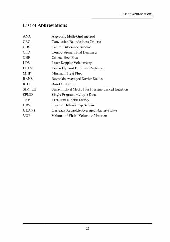
AMG Algebraic Multi-Grid method

CBC Convection Boundedness Criteria

CDS Central Difference Scheme

CFD Computational Fluid Dynamics

CHF Critical Heat Flux

LDV Laser Doppler Velocimetry

LUDS Linear Upwind Difference Scheme

MHF Minimum Heat Flux

RANS Reynolds-Averaged Navier-Stokes

ROT Run-Out-Table

SIMPLE Semi-Implicit Method for Pressure Linked Equation

SPMD Single Program Multiple Data

TKE Turbulent Kinetic Energy

UDS Upwind Differencing Scheme

URANS Unsteady Reynolds-Averaged Navier-Stokes

VOF Volume-of-Fluid, Volume-of-fraction

24


25

Introduction and Motivation

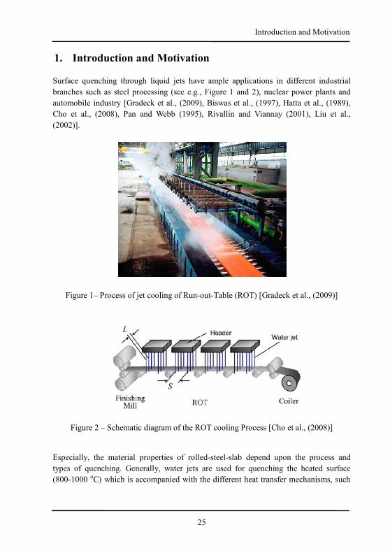
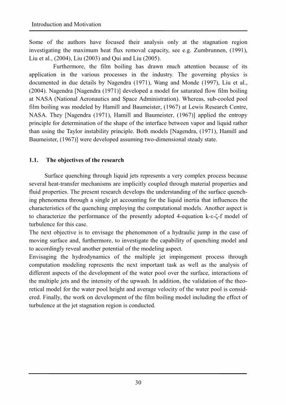
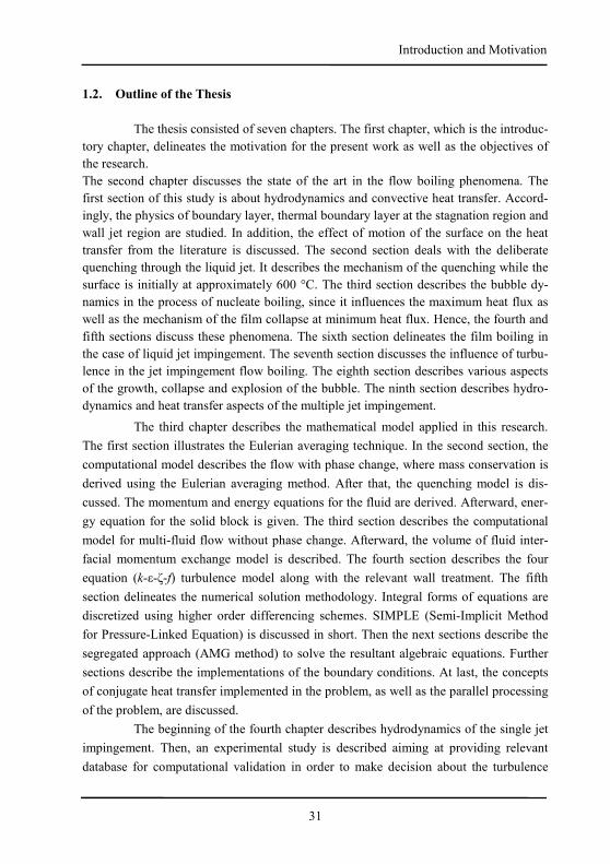
1. Introduction and Motivation Surface quenching through liquid jets have ample applications in different industrial

branches such as steel processing (see e.g., Figure 1 and 2), nuclear power plants and

automobile industry [Gradeck et al., (2009), Biswas et al., (1997), Hatta et al., (1989),

Cho et al., (2008), Pan and Webb (1995), Rivallin and Viannay (2001), Liu et al.,

(2002)].

Figure 1– Process of jet cooling of Run-out-Table (ROT) [Gradeck et al., (2009)]

Figure 2 – Schematic diagram of the ROT cooling Process [Cho et al., (2008)]

Especially, the material properties of rolled-steel-slab depend upon the process and

types of quenching. Generally, water jets are used for quenching the heated surface

(800-1000 oC) which is accompanied with the different heat transfer mechanisms, such

26


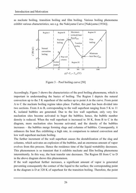
as nucleate boiling, transition boiling and film boiling. Various boiling phenomena

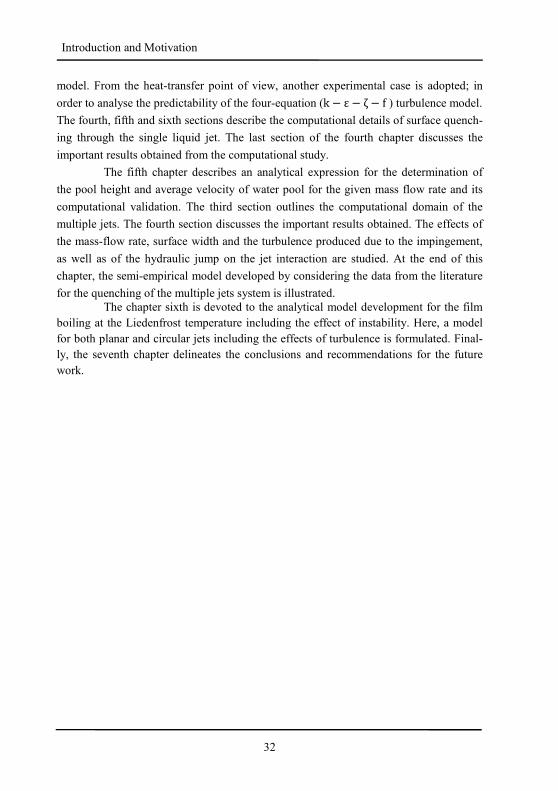
exhibit various characteristics; see e.g. the Nukiyama Curve [Nukiyama (1934)].

Figure 3 – Pool boiling curve [50]

Accordingly, Figure 3 shows the characteristics of the pool boiling phenomena, which is

important in understanding the basics of boiling. The Region I depicts the natural

convection up to the 5 K superheat of the surface up to point A in the curve. From point

A to C the nucleate boiling regime takes place. Further, this part has been divided into

two sections. From A to B, corresponding to the wall superheat ranging from 5 K to 11

K, isolated bubbles are generated. Due to the low wall superheat, only very few

nucleation sites become activated to beget the bubbles; hence, the bubble number

density is reduced. When the wall superheat is increased to 30 K, from B to C in the

diagram, more nucleation sites become activated, and the density of the bubbles

increases – the bubbles merge forming slugs and columns of bubbles. Consequently, it

enhances the heat flux exhibiting a high rate, in comparison to natural convection and

low wall superheat nucleate boiling.

The further increment of the wall superheat causes the destabilization of the slug and

columns, which activates an explosion of the bubbles, and an enormous amount of vapor

evolves from this process. Hence the residence time of the liquid wettability decreases.

This phenomenon is so transient that it exhibits nucleate and film boiling phenomena

intermittently. In this way, the heat transfer rate decreases. The Region III from C to D

in the above diagram shows this phenomenon.

If the wall superheat further increases, a significant amount of vapor is generated

preventing consequently the contact of the liquid to the surface; the corresponding point

in the diagram is D at 320 K of superheat for the transition boiling. Therefore, the point

27


D (Figure 3) represents the minimum heat flux, and the vapor layer becomes stabilized.

A thorough vapor layer is formed below the liquid layer at the vicinity of the surface.

The point D is called the Leidenfrost point, known as incipient of the film boiling. The

further increment of the wall superheat from D to E in the above diagram, in Region IV,

relates to the film boiling. Due to the high degree of wall superheat, the radiation

mechanism plays important role in transferring the heat, increasing consequently the

wall heat flux.

The aforementioned boiling curve was obtained for the case of when the liquid pool is

contained in a vessel and is heated through the gas burner. In the event of the surface

quenching the Nukiyama curve can be reproduced from E-D-C-B-A. However, due to

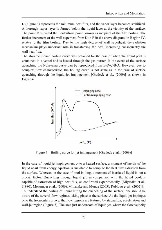
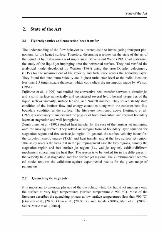
complex flow characteristic, the boiling curve is not same as in the case of surface

quenching through the liquid jet impingement [Gradeck et al., (2009)] as shown in

Figure 4.

Figure 4 – Boiling curve for jet impingement [Gradeck et al., (2009)]

In the case of liquid jet impingement onto a heated surface, a moment of inertia of the

liquid apart from energy equation is inevitable to compute the heat flux extracted from

the surface. Whereas, in the case of pool boiling, a moment of inertia of liquid is not a

crucial factor. Quenching through liquid jet, in comparison with the liquid pool, is

capable of extraction of high heat-flux, as confirmed experimentally, [Miyasaka et al.,

(1980), Mozumder et al., (2006), Mitsutake and Monde (2003), Robidou et al., (2002)].

To understand the boiling of liquid during the quenching of the surface, one should be

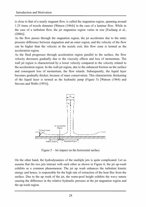
aware of the several flow regimes taking place at the surface. As the liquid jet impinges

onto the horizontal surface, the flow regions are featured by stagnation, acceleration and

wall-jet region (Figure 5). The area just underneath of liquid jet, where the flow velocity

28


is close to that of a nearly stagnant flow, is called the stagnation region, spanning around

1.25 times of nozzle diameter [Watson (1964)] in the case of a laminar flow. While in

the case of a turbulent flow, the jet stagnation region varies in size [Fuchang et al.,

(2006)].

As the flow passes through the stagnation region, the jet accelerates due to the static

pressure difference between stagnation and an outer region, and the velocity of the flow

can be higher than the velocity at the nozzle exit; this flow zone is termed as the

acceleration region.

As the fluid progresses through acceleration region parallel to the surface, the flow

velocity decreases gradually due to the viscosity effects and loss of momentum. The

wall jet region is characterized by a lower velocity compared to the velocity related to

the acceleration region. In the wall-jet region, due to the enhanced friction on the surface

and consequent loss of momentum, the flow retards. Subsequently, the liquid layer

becomes gradually thicker, because of mass conservation. This characteristic thickening

of the liquid layer is termed as the hydraulic jump (Figure 5) [Watson (1964) and

Stevens and Webb (1993)].

Figure 5 – Jet impact on the horizontal surface

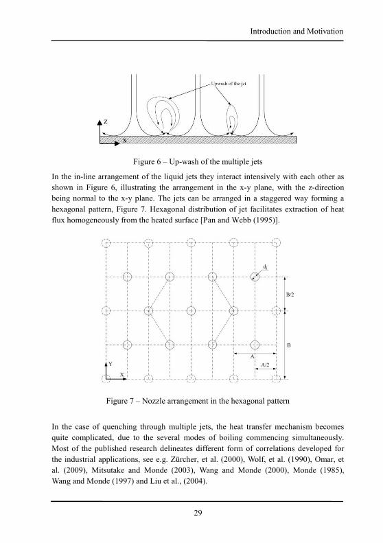
On the other hand, the hydrodynamics of the multiple jets is quite complicated. Let us

assume that the two jets interact with each other as shown in Figure 6; the jet up-wash

exhibits as a common phenomenon. The jet up wash enhances the turbulent kinetic

energy and hence, is responsible for the high rate of extraction of the heat flux from the

surface. Due to the up wash of the jet, the water-pool height exhibits the wavy nature

causing the difference in the relative hydraulic pressure at the jet stagnation region and

the up-wash region.

29


Figure 6 – Up-wash of the multiple jets

In the in-line arrangement of the liquid jets they interact intensively with each other as

shown in Figure 6, illustrating the arrangement in the x-y plane, with the z-direction

being normal to the x-y plane. The jets can be arranged in a staggered way forming a

hexagonal pattern, Figure 7. Hexagonal distribution of jet facilitates extraction of heat

flux homogeneously from the heated surface [Pan and Webb (1995)].

Figure 7 – Nozzle arrangement in the hexagonal pattern

In the case of quenching through multiple jets, the heat transfer mechanism becomes

quite complicated, due to the several modes of boiling commencing simultaneously.

Most of the published research delineates different form of correlations developed for

the industrial applications, see e.g. Zürcher, et al. (2000), Wolf, et al. (1990), Omar, et

al. (2009), Mitsutake and Monde (2003), Wang and Monde (2000), Monde (1985),

Wang and Monde (1997) and Liu et al., (2004).

z

sx

s

30


Some of the authors have focused their analysis only at the stagnation region

investigating the maximum heat flux removal capacity, see e.g. Zumbrunnen, (1991),

Liu et al., (2004), Liu (2003) and Qui and Liu (2005).

Furthermore, the film boiling has drawn much attention because of its

application in the various processes in the industry. The governing physics is

documented in due details by Nagendra (1971), Wang and Monde (1997), Liu et al.,

(2004). Nagendra [Nagendra (1971)] developed a model for saturated flow film boiling

at NASA (National Aeronautics and Space Administration). Whereas, sub-cooled pool

film boiling was modeled by Hamill and Baumeister, (1967) at Lewis Research Centre,

NASA. They [Nagendra (1971), Hamill and Baumeister, (1967)] applied the entropy

principle for determination of the shape of the interface between vapor and liquid rather

than using the Taylor instability principle. Both models [Nagendra, (1971), Hamill and

Baumeister, (1967)] were developed assuming two-dimensional steady state.

1.1. The objectives of the research

Surface quenching through liquid jets represents a very complex process because

several heat-transfer mechanisms are implicitly coupled through material properties and

fluid properties. The present research develops the understanding of the surface quench-

ing phenomena through a single jet accounting for the liquid inertia that influences the

characteristics of the quenching employing the computational models. Another aspect is

to characterize the performance of the presently adopted 4-equation k-ε-ζ-f model of

turbulence for this case.

The next objective is to envisage the phenomenon of a hydraulic jump in the case of

moving surface and, furthermore, to investigate the capability of quenching model and

to accordingly reveal another potential of the modeling aspect.

Envisaging the hydrodynamics of the multiple jet impingement process through

computation modeling represents the next important task as well as the analysis of

different aspects of the development of the water pool over the surface, interactions of

the multiple jets and the intensity of the upwash. In addition, the validation of the theo-

retical model for the water pool height and average velocity of the water pool is consid-

ered. Finally, the work on development of the film boiling model including the effect of

turbulence at the jet stagnation region is conducted.

31


1.2. Outline of the Thesis

The thesis consisted of seven chapters. The first chapter, which is the introduc-

tory chapter, delineates the motivation for the present work as well as the objectives of

the research.

The second chapter discusses the state of the art in the flow boiling phenomena. The

first section of this study is about hydrodynamics and convective heat transfer. Accord-

ingly, the physics of boundary layer, thermal boundary layer at the stagnation region and

wall jet region are studied. In addition, the effect of motion of the surface on the heat

transfer from the literature is discussed. The second section deals with the deliberate

quenching through the liquid jet. It describes the mechanism of the quenching while the

surface is initially at approximately 600 °C. The third section describes the bubble dy-

namics in the process of nucleate boiling, since it influences the maximum heat flux as

well as the mechanism of the film collapse at minimum heat flux. Hence, the fourth and

fifth sections discuss these phenomena. The sixth section delineates the film boiling in

the case of liquid jet impingement. The seventh section discusses the influence of turbu-

lence in the jet impingement flow boiling. The eighth section describes various aspects

of the growth, collapse and explosion of the bubble. The ninth section describes hydro-

dynamics and heat transfer aspects of the multiple jet impingement.

The third chapter describes the mathematical model applied in this research.

The first section illustrates the Eulerian averaging technique. In the second section, the

computational model describes the flow with phase change, where mass conservation is

derived using the Eulerian averaging method. After that, the quenching model is dis-

cussed. The momentum and energy equations for the fluid are derived. Afterward, ener-

gy equation for the solid block is given. The third section describes the computational

model for multi-fluid flow without phase change. Afterward, the volume of fluid inter-

facial momentum exchange model is described. The fourth section describes the four

equation (k-ε-ζ-f) turbulence model along with the relevant wall treatment. The fifth

section delineates the numerical solution methodology. Integral forms of equations are

discretized using higher order differencing schemes. SIMPLE (Semi-Implicit Method

for Pressure-Linked Equation) is discussed in short. Then the next sections describe the

segregated approach (AMG method) to solve the resultant algebraic equations. Further

sections describe the implementations of the boundary conditions. At last, the concepts

of conjugate heat transfer implemented in the problem, as well as the parallel processing

of the problem, are discussed.

The beginning of the fourth chapter describes hydrodynamics of the single jet

impingement. Then, an experimental study is described aiming at providing relevant

database for computational validation in order to make decision about the turbulence

32


model. From the heat-transfer point of view, another experimental case is adopted; in

order to analyse the predictability of the four-equation (k − ε − ζ − f ) turbulence model.

The fourth, fifth and sixth sections describe the computational details of surface quench-

ing through the single liquid jet. The last section of the fourth chapter discusses the

important results obtained from the computational study.

The fifth chapter describes an analytical expression for the determination of

the pool height and average velocity of water pool for the given mass flow rate and its

computational validation. The third section outlines the computational domain of the

multiple jets. The fourth section discusses the important results obtained. The effects of

the mass-flow rate, surface width and the turbulence produced due to the impingement,

as well as of the hydraulic jump on the jet interaction are studied. At the end of this

chapter, the semi-empirical model developed by considering the data from the literature

for the quenching of the multiple jets system is illustrated. The chapter sixth is devoted to the analytical model development for the film

boiling at the Liedenfrost temperature including the effect of instability. Here, a model

for both planar and circular jets including the effects of turbulence is formulated. Final-

ly, the seventh chapter delineates the conclusions and recommendations for the future

work.

33

State of the Art

2. State of the Art

2.1. Hydrodynamics and convection heat transfer

The understanding of the flow behavior is a prerequisite to investigating transport phe-

nomena for the heated surface. Therefore, discussing a review on the state of the art of

the liquid jet hydrodynamics is of importance. Stevens and Webb (1993) had performed

the study of the liquid jet impinging onto the horizontal surface. They had verified the

analytical model developed by Watson (1964) using the laser-Doppler velocimetry

(LDV) for the measurement of the velocity and turbulence across the boundary layer.

They found that maximum velocity and highest turbulence level at the radial locations

less than 2.5 times nozzle diameter; which contradicts the assumption made by Watson

(1964).

Fujimoto et al., (1999) had studied the convective heat transfer between a circular jet

and a solid surface numerically and considered several hydrothermal properties of the

liquid such as viscosity, surface tension, and Nusselt number. They solved steady state

condition of the laminar flow and energy equations along with the constant heat flux

boundary condition at the surface. The literature mentioned above [Fujimoto et al.,

(1999)] is necessary to understand the physics of both momentum and thermal boundary

layers at stagnation and wall jet regions.

Zumbrunnen et al. (1992) studied heat transfer for the case of the laminar jet impinging

onto the moving surface. They solved an integral form of boundary layer equation for

stagnation region and free surface jet region. In general, the surface velocity intensifies

the turbulent kinetic energy (TKE) and heat transfer rate at the free surface jet region.

This study reveals the facts that in the jet impingement case the two regions, namely the

stagnation region and free surface jet region (i.e., wall-jet region), exhibit different

mechanism concerning the heat flux. The reason is to be looked for in the differences in

the velocity field at stagnation and free surface jet regions. The Zumbrunnen’s theoreti-

cal model requires the validation against experimental results for the given range of

parameters.

2.2. Quenching through jets

It is important to envisage physics of the quenching while the liquid jet impinges onto

the surface at very high temperatures (surface temperature > 900 °C). Most of the

literature describes the quenching process at low surface temperatures (less than 900 °C)

[Gradeck et al., (2009), Omar et al., (2009), Xu and Gadala, (2006), Islam et al., (2008),

Seiler-Marie et al., (2004)].

34

State of the Art

At the surface temperature lower than 900 °C, an experimental investigation

[Islam et al., (2008)] shows that the liquid comes into contact with the heated surface

and starts the heterogeneous/homogeneous nucleation. The tiny bubble formation starts

just after the impingement. Islam et al., (2008) conducted such experiments considering

water jet diameter of 2 mm, the sub-cooling range of water between 5-80 K and nozzle

velocity 3-15 m/s; surface was made up of steel/brass, which was heated up to 500-600

°C. For the steel block at an initial temperature of 500 °C, 5 m/s of jet velocity and 80

°C of water temperature, the high-speed video imaging show circular shiny liquid sheet

at the center of the steel block encompassing the time interval between 3 and 30

milliseconds. The quiet and calm flow and no boiling sound were evidence of no contact

of liquid to the surface. At the start of impingement, there may be the liquid-solid con-

tact for short period in which the bubbles form, coalesce and generate a tiny liquid sheet

onto which the jet slides. Slightly later, around 200 milliseconds, there is the contact of

the jet with the surface, influencing the onset of homogeneous/heterogeneous

nucleation, and subsequently of the boiling sound. Hence, the tiny liquid sheet began to

disappear. Some of the bubbles splashed at a certain angle from the surface. After 500

milliseconds, more contact with the surface was occurred and rigorous generation,

coalesce, and splashing of the bubble took place.

While for a brass surface, just after the impingement, flow exhibits the explosive pat-

tern, the mechanisms mentioned are not pertinent to the case of surface temperature

equal to or higher than 900 °C for the steel. In the case of steel surface equal to or more

than 900 °C, quenching through water jet leads to different boiling phenomena. The heat

transfer process governed by several boiling mechanisms depends upon wall-superheat

(∆Tsurface - ∆Tsat). These heat transfer mechanisms are convection, nucleate, transition,

and film boiling. In the convection, heat transfer takes place through the motion of the

fluid. The convection heat transfer is easy to calculate, described in Leinhard IV and

Leinhard V (2011) through the equation as given below.

ℎ = 6�7897∞� = − !�7897∞� :7:;<;=> (2.1)

Nevertheless, other boiling heat transfer mechanism such as nucleate, transition and film

boiling are very complex in nature and already discussed in the first chapter, Figures 3

and 4. However, the prediction of heat-flux was facilitated through numerous

correlations and theoretical models proposed by different authors [Omar et al., (2009),

Xu and Gadala (2006), Islam et al., (2008), Andreani and Yadigaroglu (1992), Mitsutake

and Monde (2003), Timm et al., (2003), Rivallin and Viannay (2001), Robidou et al.,

(2002)]. The wall-superheat and associated heat-flux determine the different heat trans-

fer mechanism depending upon the flow condition. One of the models developed by the

Zürcher et al., (2000) to differentiate between nucleate boiling and convective evapora-

35

State of the Art

tion inside a horizontal tube to predict the heat flux at the onset of nucleate boiling is

given as:

�?@A, C = DE7FGH IJK,JLMHNJLMH O P ∆IRSGT (2.2)

The heat transfer coefficient hcb, crit defined as:

hVW,VXYZ = C Reδ Pra>.c λdδefgh (2.3)

Where, the values of the two constants, C = 0.01361 and m = 0.6965, are based on ex-

perimental results of pure convective heat transfer in annular flow for ammonia refriger-

ant (R-717).

Robidou et al. (2002) performed an experiment under steady state condition for con-

trolled cooling of the heated surface through a water jet. They studied the influence of

the jet velocity, sub-cooling of water and the surface temperature. For a jet velocity of

0.8 m/s, the surface temperature of about 450 °C, and sub-cooling of 16 K the film

boiling takes place at stagnation region. The reason may lie on the mechanism that,

because of the low jet velocity and a high temperature, the water is not capable of pene-

trating the vapor formed near the surface.

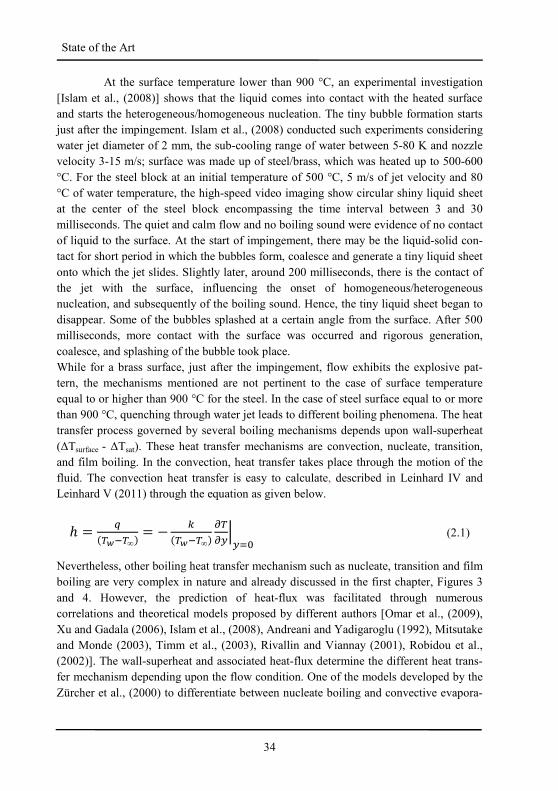
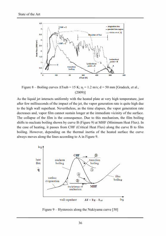
Gradeck et al., (2009) described the boiling curve for several locations at the curved

surface through jet impingement. They explored the mechanism of the quenching

through planar water jet of the heated rolling cylinder experimentally. The initial tem-

perature of the cylinder was 500-600 °C, the sub-cooling range of water was 10-83 K,

the jet velocity range was 0.8-1.2 m/s and the jet velocity to surface velocity ratio (us/uj)

was in range between 0.5 and 1.25. They found aberration from the standard boiling

curve (Nukiyama Curve), i.e., the existence of the “shoulder of flux” in the stagnation

region as shown in Figure 8. The width of the shoulder of heat-flux increased with the

sub-cooling of liquid. At some other locations at the surface, e.g. as within the wall-jet

region; the relevant boiling curve depicts approximately the standard one.

36

State of the Art

Figure 8 – Boiling curves ∆Tsub = 15 K; uj = 1.2 m/s; d = 50 mm [Gradeck, et al.,

(2009)]

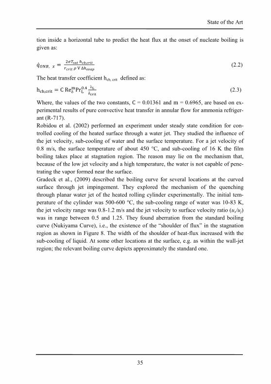
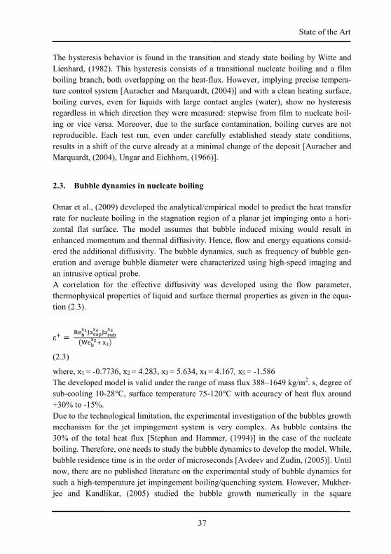
As the liquid jet interacts uniformly with the heated plate at very high temperature, just

after few milliseconds of the impact of the jet, the vapor generation rate is quite high due

to the high wall superheat. Nevertheless, as the time elapses, the vapor generation rate

decreases and, vapor film cannot sustain longer at the immediate vicinity of the surface.

The collapse of the film is the consequence. Due to this mechanism, the film boiling

shifts to nucleate boiling shown by curve B (Figure 9) at MHF (Minimum Heat Flux). In

the case of heating, it passes from CHF (Critical Heat Flux) along the curve B to film

boiling. However, depending on the thermal inertia of the heated surface the curve

always moves along the lines according to A in Figure 9.

Figure 9 – Hysteresis along the Nukiyama curve [50]

37

State of the Art

The hysteresis behavior is found in the transition and steady state boiling by Witte and

Lienhard, (1982). This hysteresis consists of a transitional nucleate boiling and a film

boiling branch, both overlapping on the heat-flux. However, implying precise tempera-

ture control system [Auracher and Marquardt, (2004)] and with a clean heating surface,

boiling curves, even for liquids with large contact angles (water), show no hysteresis

regardless in which direction they were measured: stepwise from film to nucleate boil-

ing or vice versa. Moreover, due to the surface contamination, boiling curves are not

reproducible. Each test run, even under carefully established steady state conditions,

results in a shift of the curve already at a minimal change of the deposit [Auracher and

Marquardt, (2004), Ungar and Eichhorn, (1966)].

2.3. Bubble dynamics in nucleate boiling

Omar et al., (2009) developed the analytical/empirical model to predict the heat transfer

rate for nucleate boiling in the stagnation region of a planar jet impinging onto a hori-

zontal flat surface. The model assumes that bubble induced mixing would result in

enhanced momentum and thermal diffusivity. Hence, flow and energy equations consid-

ered the additional diffusivity. The bubble dynamics, such as frequency of bubble gen-

eration and average bubble diameter were characterized using high-speed imaging and

an intrusive optical probe.

A correlation for the effective diffusivity was developed using the flow parameter,

thermophysical properties of liquid and surface thermal properties as given in the equa-

tion (2.3).

εj = klmnopqrstnu pqrsmnvwxlmnyj z{|

(2.3)

where, x1 = -0.7736, x2 = 4.283, x3 = 5.634, x4 = 4.167, x5 = -1.586

The developed model is valid under the range of mass flux 388–1649 kg/m2. s, degree of

sub-cooling 10-28°C, surface temperature 75-120°C with accuracy of heat flux around

+30% to -15%.

Due to the technological limitation, the experimental investigation of the bubbles growth

mechanism for the jet impingement system is very complex. As bubble contains the

30% of the total heat flux [Stephan and Hammer, (1994)] in the case of the nucleate

boiling. Therefore, one needs to study the bubble dynamics to develop the model. While,

bubble residence time is in the order of microseconds [Avdeev and Zudin, (2005)]. Until

now, there are no published literature on the experimental study of bubble dynamics for

such a high-temperature jet impingement boiling/quenching system. However, Mukher-

jee and Kandlikar, (2005) studied the bubble growth numerically in the square

38

State of the Art

microchannel of size 200 µm. Bubble resides at the center, and the superheated liquid

fills the entire channel. They found that the bubble growth rate increases with the incom-

ing superheated liquid while, it decreases with Reynolds number. They noticed the

forward and backward movement of the bubble, and there was little effect of the gravity

on the bubble growth. The other study on the bubble dynamics are by Mann et al.,

(2000) and Fuchs et al., (2006) and are important in mentioning a detailed study by the

interested researchers.

Very few works based on numerical simulation, exist for the nucleate boiling

considering the jet impingement flow boiling. Nucleate boiling contains mainly four

processes such as the formation of nucleation site, bubble formation, merger, and explo-

sion. Son et al., (2002), investigated the bubble merger process numerically. They found

that the thin liquid film forms underneath a growing bubble attached to the wall and this

part contribute 30% of the total heat flux carried by the bubble. Therefore, it is important

to include for the numerical study.

The bubble growth behavior differs at different atmospheric pressure. The precise exper-

iment on nucleate pool boiling by Kim et al., (2007) is evident. The bubble growth rate

at sub-atmospheric pressure is larger than at atmospheric pressure irrespective of the

fluid properties. Also, because of the relatively higher pressure, momentum is strong,

based on the Rayleigh-Plesset equation owing to the high specific volume.

Avdeev and Zudin (2005) developed the inertial thermal model, which grows in the

superheated liquid. They suggested the general inertial thermal model for the vapor

bubble growth inside the superheated pool of liquid.

However, a simple way of determining the bubble growth rate is given by molecular-

kinetic laws of evaporation of liquid from the superheated interface as given in equation

(2.4):

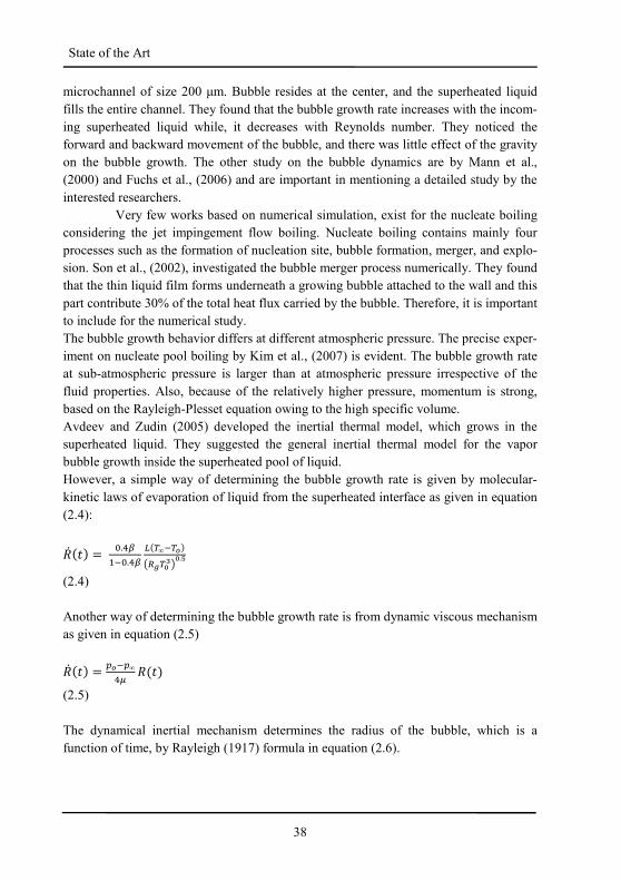
"� �� = >.c��9>.c� ��7∞97��w��7�{|�.v

(2.4)

Another way of determining the bubble growth rate is from dynamic viscous mechanism

as given in equation (2.5)

"� �� = �9 ∞c� "��

(2.5)

The dynamical inertial mechanism determines the radius of the bubble, which is a

function of time, by Rayleigh (1917) formula in equation (2.6).

39

State of the Art

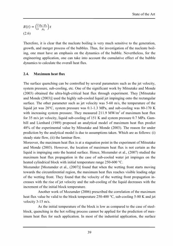
"�� = �D� �9 ∞O� � �

(2.6)

Therefore, it is clear that the nucleate boiling is very much sensitive to the generation,

growth, and merger process of the bubbles. Thus, for investigation of the nucleate boil-

ing, one must have an emphasis on the dynamics of the bubble. Nevertheless, for the

engineering application, one can take into account the cumulative effect of the bubble

dynamics to calculate the overall heat flux.

2.4. Maximum heat flux

The surface quenching can be controlled by several parameters such as the jet velocity,

system pressure, sub-cooling, etc. One of the significant work by Mitsutake and Monde

(2003) obtained the ultra-high-critical heat flux through experiment. They [Mitsutake

and Monde (2003)] used the highly sub-cooled liquid jet impinging onto the rectangular

surface. The other parameter such as jet velocity was 5-60 m/s, the temperature of the

liquid jet was 20°C, system pressure was 0.1-1.3 MPa, and sub-cooling was 80-170 K

with increasing system pressure. They measured 211.9 MW/m2 of maximum heat flux

for 35 m/s jet velocity, liquid sub-cooling of 151 K and system pressure 0.7 MPa. Gam-

bill and Lienhard (1989) proposed an analytical model of maximum heat flux predict

48% of the experimental value by Mitsutake and Monde (2003). The reason for under

prediction by the analytical model is due to assumptions taken. Which are as follows: (i)

steady state flow, (ii) the laminar flow.

Moreover, the maximum heat flux is at a stagnation point in the experiment of Mitsutake

and Monde (2003). However, the location of maximum heat flux is not certain as the

liquid is impinging onto the heated surface. Hence, Mozumder et al., (2007) studied the

maximum heat flux propagation in the case of sub-cooled water jet impinges on the

heated cylindrical block with initial temperature range 250-600 °C.

Mozumder [Mozumder et al., (2007)] found that when the wetting front starts moving

towards the circumferential region, the maximum heat flux reaches visible leading edge

of the wetting front. They found that the velocity of the wetting front propagation in-

creases with the rise of jet velocity and the sub-cooling of the liquid decreases with the

increment of the initial block temperature.

Another work of Mozumder (2006) prescribed the correlation of the maximum

heat flux value be valid to the block temperature 250-400 °C, sub-cooling 5-80 K and jet

velocity 3-15 m/s.

As the initial temperature of the block is low as compared to the case of steel-

block, quenching in the hot rolling process cannot be applied for the prediction of max-

imum heat flux for such application. In most of the industrial application, the surface

40

State of the Art

temperature is around 800-1100°C. When the initial temperature of the block is higher,

the quenching process is transient in nature.

The correlation developed by them predicts ± 30% of the maximum heat flux for the

brass and copper material, but for steel material, the error lies in the much larger region.

The reason for such aberration may lie on different thermal material properties of the

brass and copper as compared to steel.

Qui and Liu (2005) developed a correlation of critical heat- flux (CHF) for the

jet velocity range 0.5-10 m/s, at the jet stagnation region employing a saturated liquid jet

of water, ethanol, R-113, R-11. They took the same heater diameter as of the jet diame-

ter. However, as discussed before the stagnation region is greater than the jet diameter.

They proposed correlation in the following form (Equation 2.7).

6J,�O��I�� = 0.130 �1 + OSO��/� � EO��y��/� �OSO��.c/� (2.7)

This correlation shows that there is no effect of thermal properties of the substrate mate-

rial. The correlation factor found by the wide range of jet velocities from the experi-

ment.

Liu and Qui (2008) developed the correlation of Critical-Heat-Flux (CHF) for

the jet stagnation region for the super hydrophilic surface. They formed the super hy-

drophilic surface by coating the copper cleaned and mirrored surface with titanium

oxide. When the surface irradiated with the UV-light, the water contact angle becomes

zero after some time. The effect of the super hydrophilic surface seen as 30% enhanced

heat transfer from the surface. Considering the substrate diameter is greater than the jet

diameter and proposed the correlation in the following form (Equation 2.8).

6J,�O��I�� = 0.0985 �OSO��>.D�� EO��y��/� � ��j>.>>�� w�F/��|y� (2.8)

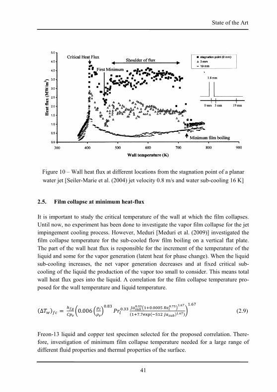
Transition boiling exhibits distinct characteristics as evidence from the experiment of

the Seiler-Marie et al. (2004). When the maximum heat flux is achieved at certain wall-

superheat, then a further increment of the wall-superheat the first minimum heat-flux

comes, and further increment of wall-superheat resulted in an increment of the heat-flux

for a broad range of the wall-superheat. Which is termed as the shoulder of heat-flux as

shown in Figure 10. The beginning of the shoulder of heat flux comes at a first mini-

mum and ends with minimum film boiling point. They developed the model for the

shoulder of heat flux, first minimum boiling point, i.e., start of the shoulder of heat flux

and second minimum boiling point (which is incipient of the film boiling). Their model

assumes that existence of periodic bubble oscillation at the wall caused by the jet hydro-

dynamics.

41

State of the Art

Figure 10 – Wall heat flux at different locations from the stagnation point of a planar

water jet [Seiler-Marie et al. (2004) jet velocity 0.8 m/s and water sub-cooling 16 K]

2.5. Film collapse at minimum heat-flux

It is important to study the critical temperature of the wall at which the film collapses.

Until now, no experiment has been done to investigate the vapor film collapse for the jet

impingement cooling process. However, Meduri [Meduri et al. (2009)] investigated the

film collapse temperature for the sub-cooled flow film boiling on a vertical flat plate.

The part of the wall heat flux is responsible for the increment of the temperature of the

liquid and some for the vapor generation (latent heat for phase change). When the liquid

sub-cooling increases, the net vapor generation decreases and at fixed critical sub-

cooling of the liquid the production of the vapor too small to consider. This means total

wall heat flux goes into the liquid. A correlation for the film collapse temperature pro-

posed for the wall temperature and liquid temperature.

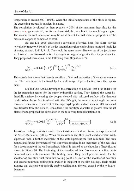
�∆�� = I�� S �0.006 �O�OS�>.¡� ¢£�>.�� ¤�F¥K�.{{w�j>.>>>� �¦��.§v|o.¨§��j�.�lz©�9��D ¤�F¥K�o.¨§��

�.ª� (2.9)

Freon-13 liquid and copper test specimen selected for the proposed correlation. There-

fore, investigation of minimum film collapse temperature needed for a large range of

different fluid properties and thermal properties of the surface.

42

State of the Art

Ohtake and Koizumi (2004) investigated the mechanism of the vapor-film

collapse through the propagation of the film. They found that when the local cold spot

temperature decreased, and propagation velocity of vapor-film collapse would decrease.

As a result, Minimum Heat Flux (MHF) temperature would increase. The significant

increments registered in MHF temperature for the case of local cold spot temperature

lower than the thermodynamic limit of liquid superheat, Ttls.

2.6. Jet impingement film boiling

In the case of film-boiling and nucleate boiling, as the wall superheat increases, the wall

heat flux also increases. However, in the event of transition boiling as the wall superheat

increases the heat flux decreases. The reason for the decrement of the heat flux with

increasing the wall superheat is as the wall superheat increases beyond the maximum

heat flux ( the corresponding wall superheat) the bubbles formation rate increase and

bubble dynamics such as growth, merger, and explosion, can trigger intermittent contact

of the liquid jet to the heated surface. In other words, because of the high rate of for-

mation of vapor, the residence time of the contact of the liquid jet to the heated surface

decreases.

Furthermore, the increment of the wall superheat, the bubbles merge together

and forms the vapor layer on the heated surface. Once, this vapor layer is stable the heat

transfer rate becomes minimum, because of the very low conductivity of the vapor. This

minimum heat flux is called as Leidenfrost heat- flux and the corresponding wall

superheat as Leidenfrost temperature.

The existence of the turbulent film boiling for the liquid jet impingement cooling is

evident from the fact that high oscillation of the vapor-liquid interface. As the flow over

heated surface exhibits the turbulent nature results in an increment of thermal diffusivity

of the vapor and consequently, increases the wall heat flux. Sarma et al., (2001) per-

formed the analysis of the turbulent film boiling over the cylinder. Due to the steep

temperature gradient in the vapor layer, the thermo-physical properties of the vapor

varied and taken into account. They included the effect of the radiation and found satis-

factory agreement with the experiment.

Liu and Wang (2001) have done a theoretical and experimental study of the film boiling

at jet stagnation region for high sub-cooling of the water. They proposed the semi-

empirical correlations for the wall-heat-flux as follows.

� = «1.414 "��/D¢£��/ª�¬�¬Δ®��¯Δ®��/D° ±²³

(2.10)

43

State of the Art

The correlation has -5% to +25% variations from the experimental results. For higher jet

velocity and the high sub-cooling correlation exhibits larger (more than 40%) deviations

from the experimental wall heat flux. The reason may lie in the fact that the high jet

velocity enhances the turbulent intensity near the surface and its effect on heat-flux is

not accounted.

Liu et al., (2002) performed the experiment on the quenching of heated surface through

the nozzle. In this case, the initial temperature of the plate was 700-900 °C and the water

temperature was 13 °C and 30 °C. They plotted the boiling curve have not shown the

film boiling phenomena for such a high sub-cooling of the liquid. Although, they agree

upon the fact, that just after the impact of the jet, the liquid cannot contact the surface as

the film formed underneath the jet. Another reason is the surface temperature for a very

short interval of the time, just after the impact is hard to measure, due to the experi-

mental limitations.

The Leidenfrost temperature depends on several parameters, like jet impinge-

ment velocity, wall-superheat, sub-cooling of liquid, the conductivity of the material, the

thermal heat capacity of the material and some other material aspects (such as surface

roughness, granular structure of the surface). How these parameters affect to the type of

quenching of the surface are not well understood. To understand the complexity of the

problem, mathematically, the Leidenfrost temperature is a function of thermal and mate-

rial properties of the plate. It is possible to model, only when, one could do the charac-

terization of the material properties by the Leidenfrost point considering the thermal and

flow parameters as mentioned above. This would require an enormous amount of data-

base only for film boiling at Leidenfrost temperature. Consequently, Direct-Numerical-

Simulation for this problem would require plenty of computer hardware space and RAM

to execute and store the calculation and output results. Therefore, the computational cost

will be too much. Therefore, it is complex phenomena to model from the first principle.

Here, the first principle implies that the Direct Numerical Simulation.

The current status of the research on the boiling at Leidenfrost temperature is only

experimental works exist till date [Ishigai et al., (1978), Robidou et al., (2002),

Bogdanic et al., (2009), Seiler-Marie et al., (2004), Liu (2003) and Woodfield et al.,

(2005)].

Ishigai et al., (1978) performed the experiment for the film boiling at stagnation region

for the planar jet and then analytical study with two-phase boundary layer theory. Their

result shows qualitatively good agreement, but 1.6-1.7 times higher heat flux than ana-

lytical results.

Bogdanic et al., (2009) analyzed the vapor–liquid structures at stagnation region by

using the miniaturized optical probe for sub-cooled (20 K) planar (1 mm-9 mm) water

jet with a velocity of 0.4 m/s. They measured the liquid surface contact frequency at the

incipience of nucleate boiling is about 40 Hz and at the end of the transition boiling

44

State of the Art

nearly 20,000 Hz. Therefore, it infers that for film boiling the frequency of the liquid-

vapor interface is higher than 20,000 Hz.

Meduri et al., (2009) conducted an experiment on the sub-cooled flow film boiling on a

vertical flat surface. The correlation calculated the heat flux around ± 20% for the given

wall-superheat 200-400°C.

Some of the experimental studies [Meduri et al., (2009), Hsu and Westwater (1960),

Coury and Duckler (1970), Suryanarayana and Merte (1972)] on film boiling over the

vertical plate advocate that the vapor film is turbulent in nature. The reason may lie in

this fact that oscillation frequency (> 20,000) [Bogdanic et al. (2009)] of vapor film

interface due to gravitational force and inertia force of liquid jet on the vapor film. Note

that, oscillation frequency may increase or decrease, depending upon nature of the

application of inertia force on the vapor film. Sarma et al. (2001) investigated the turbu-

lent film boiling on the cylinder. While the effect of inertia force on the vapor film is

very less. On the contrary, both inertia and gravity forces of liquid jet acted on the vapor

film, which causes the higher oscillation frequency. Chou and Witte (1995) developed

the analytical model for the stable sub-cooled flow film boiling on the cylinder surface.

They [Chou and Witte (1995)] developed the model of film boiling for the wake region

of the flow. However, the model did not consider the turbulent flow. Therefore, this

model is not suitable for the inertia dominated turbulent flow film boiling.

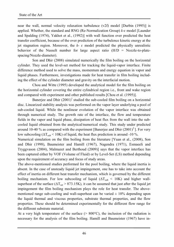
Almost explosive flow pattern visualized at the wall superheat greater than 300 K. Quite

chaotic and turbulence flow observed by Woodfield at al. (2005) during the quenching

of the heated surface. The Woodfield’s [Woodfield at al. (2005)] observation supports

the consideration of the turbulence in the jet impingement quenching process. Because,

inertia, thermal buoyancy, and gravity forces play a vital role in the flow being turbu-

lent. Before, going into the details of the modeling process, the discussion of the physics

of the liquid jet impingement onto the high wall superheated plate at stagnation region at

the Leidenfrost point is necessary. Due to the high wall-superheat, vapor generates at a

high rate, which cannot escape in the normal direction to the plate due to the liquid jet, it

has the only way to escape through parallel to the wall. In this way, vapor layer forms at

the vicinity of the wall and liquid layer exist over vapor layer. Consequently, the film

boiling establishes. Due to the formation of the vapor near the wall, the inertia force of

the fluid increases and the gravity force also come into play. Consequently, Rayleigh-

Taylor instability [Rayleigh (1917)] establishes despite the low jet velocity called the

thermal buoyancy effect on the film. Due to the high frequency of oscillation of liquid-

vapor interface exhibits dynamic behavior, which contributes to enhancing the momen-

tum and thermal diffusivity. The instantaneous flow can be divided into two parts, which

are mean (Reynolds average), and the fluctuating part. The fluctuating part can be

modeled as turbulent diffusivity.

Previously, the assumption was that due to the low velocity at the stagnation region the

flow is laminar. However, in the case of multiphase flow phenomena at the stagnation

45

State of the Art

region there exists the vortex-flow phenomenon studied by Sakakibara et al., (1997).

Therefore, to calculate the heat flux and the temperature at the Leidenfrost point, the

introduction of the turbulent thermal diffusivity is necessary. Karwa et al., (2011) pro-

posed the model without considering the turbulence near Leidenfrost temperature. They

reported 46% less wall heat flux and 70% less wall-superheat. Therefore, there was the

necessity to develop the model considering the effect of turbulence especially, for turbu-

lent jet and a higher degree of sub-cooling (< 45 K).

2.7. Turbulence in jet impingement flow boiling

Shigechi et al., (1989) studied analytically the two-dimensional, steady state and laminar

film boiling with a downward facing at the jet stagnation region considering the saturat-

ed liquid with radiation heat transfer and compared the heat flux and wall superheat with

experiment. Although the qualitative results were good, the quantitative was two times

less.

Fillipovic et al., (1993) studied the laminar film boiling over the moving

isothermal plate. They obtained the similarity solution for the boundary layer on the

surface. Because of the vapor layer at the surface, the viscous force and heat transfer rate

reduced in comparison with the complete liquid layer (in the case of convection) and

vapor-droplet mixture (in the event of nucleate and transition boiling) at the surface.

Furthermore, Filipovic et al., (1994) dedicated to studies of the effects of turbulent film

boiling phenomena for the isothermal moving plate using the modified Cebeci-Smith

(1967) eddy-viscosity model with the Cebeci-Bradshaw (1984) algorithm. A correlation

proposed for the surface heat flux resulted in the maximum error of -30% for liquid sub-

cooling (∆Tsub = 70K), free stream velocity 5.3 m/s and plate temperature 873.15 K

along with the ratio of the plate velocity-to-free-stream velocity. Therefore, there is

room to increase the range of the parameters, accomplishes in chapter five, developed

the film boiling model including the effect of the interface oscillation.

Wolf et al., (1990) showed the importance of the turbulence to enhance the

heat flux removal rate from the surface. The range of the jet Reynolds number was from

15000-54000. Increasing the jet Reynolds number enhancements of the heat-flux at-

tributed due to the enhanced turbulence at high jet velocity for the single-phase convec-

tion and nucleate boiling. The substantial work performed by the Castrogiovanni and

Sfroza (1997) considered turbulence in their analysis by assuming the dynamics of

bubble formation, merger, explosion, and implosion in the boiling phenomena, which in

turn enhanced the momentum and thermal diffusivity. They used the genetic algorithm

(GA) to quantify the bubble dynamics and applied it for the boiling inside a pipe flow.

Behnia et al., (1998) predicted the heat transfer in an axis-symmetric turbulent air jet

impingement on a heated flat plate. Because of the anisotropic nature of the turbulence

46

State of the Art

near the wall, normal velocity relaxation turbulence (v2f) model [Durbin (1995)] is

applied. Whether, the standard and RNG (Re-Normalization Group) k-ɛ model [Launder

and Spalding (1974), Yakhot et al., (1992)] with wall function over predicted the heat

transfer coefficient, because of the over prediction of the turbulence kinetic energy at the

jet stagnation region. Moreover, the k- ɛ model predicted the physically unrealistic

behavior of the Nusselt number for large aspect ratio (H/D = Nozzle-to-plate-

spacing/Nozzle-diameter).

Son and Dhir (2008) simulated numerically the film boiling on the horizontal

cylinder. They used the level-set method for tracking the liquid-vapor interface. Finite

difference method used to solve the mass, momentum and energy equation in vapor and

liquid phases. Furthermore, investigations made for heat transfer in film boiling includ-

ing the effect of the cylinder diameter and gravity on the interfacial motion.

Chou and Witte (1995) developed the analytical model for the film boiling on

the horizontal cylinder covering the entire cylindrical region i.e., front and wake region

and compared with experiment and other published results [Chou et al. (1995)].

Banerjee and Dhir (2001)1 studied the sub-cooled film boiling on a horizontal

disc. Linearized stability analysis was performed on the vapor layer underlying a pool of

sub-cooled liquid. While the nonlinear evolution of the vapor interface was obtained

through numerical study. The growth rate of the interface, the flow and temperature

fields in the vapor and liquid phase, dissipation of heat flux from the wall into the sub-

cooled liquid obtained from the analytical/numerical study. This study under predicted

around 10-40 % as compared with the experiment [Banerjee and Dhir (2001)2 ]. For very

low subcooling (∆Tsub < 10K) of liquid, the heat flux prediction is around -10 %.

Numerical simulation on the film boiling from the literature [Yuan et al., (2008), Son

and Dhir (1998), Baumeister and Hamill (1967), Nagendra (1971), Esmaeeli and

Tryggvason (2004), Malmazet and Berthoud (2009)] says that the vapor interface has

been captured either by VOF (Volume of Fluid) or by Level-Set (LS) method depending

upon the requirement of accuracy and focus of study areas.

The above-mentioned studies performed for the pool boiling, where the liquid inertia is

absent. In the case of unsteady liquid jet impingement, one has to take into account the

effect of inertia on different heat transfer mechanism, which is governed by the different

boiling mechanism. For low subcooling of liquid (∆Tsub < 10K) and higher wall-

superheat of the surface (∆Tsat > 873.15K), it can be assumed that just after the liquid jet

impingement the film boiling mechanism plays the role for heat transfer. The above-

mentioned range sub-cooling and wall-superheat can be varied ± 10% depending upon

the liquid thermal and viscous properties, substrate thermal properties, and the flow

properties. These should be determined experimentally for the different flow range for

the different substrate material.

At a very high temperature of the surface (> 800°C), the inclusion of the radiation is

necessary for the analysis of the film boiling. Hamill and Baumeister (1967) have in-

47

State of the Art

cluded the effect of radiation for the case of sub-cooled pool film boiling. The analysis

based on the concept of maximization of the entropy. In the case of the flow film boil-

ing, inertia effect would be included in the concept of entropy maximization to deter-

mine the heat flux.

Through the above discussion, it has been felt that in the case of liquid jet impingement

onto the heated surface the turbulence plays a vital role in the heat transfer mechanism.

It has been found that the accurate modeling and computation of production and dissipa-

tion rate of the turbulent kinetic energy at the vicinity of the surface is required which

plays a significant effect on computation of heat-flux [Wolf et al. (1995)]. The turbulent

dissipation is the rate at which turbulent kinetic energy converted into thermal internal

energy, equal to the mean rate at which work done by the fluctuating part of the strain

rate against the fluctuating viscous stresses.

2.8. Another quenching studies

Fuchang and Gadala (2006) used the iterative and sequential heat transfer analysis to

determine the heat flux at the stagnation region of water jet impingement at the

stationary heated surface. They noticed that heat transfer behavior is significantly affect-

ed by the water temperature rather than water flow-rate.

Hall et al., (2001) investigated a technique for controlling the boiling heat transfer by

injecting the gas into the circular liquid jet. They did the experiment with the cylindrical

copper specimen. The gas injected with void-fraction range 0-0.4 and the liquid velocity

ranging from 2-4 m/s. They reported the enhanced convective heat transfer by a factor of

2.1 in the stagnation region as compared to single-phase convective heat transfer. Never-

theless, the maximum heat flux is unaffected with a various void fraction of gas. While

the minimum film boiling temperature increases and minimum heat flux decreases.

Wang et al., (1989) did the analytical study on the heat transfer between an axis-

symmetrical impinging jet and a solid flat surface with non-uniform surface temperature

or heat flux. They found that increment of the surface temperature or heat flux with

radial distance reduction in the stagnation point Nusselt number and vice-versa.

When the liquid jet impinges on the surface from the downward face, then ob-

servation of the flow behavior and investigation of the heat flux (Figure 11) is important.

Thus, Woodfield et al., (2005) studied the different flow pattern for different wall-

superheat as shown in Figure 11.

They used the microphone to hear the boiling sound. When the initial temperature was

above 300 °C, the explosive sound heard. This phenomenon was observed because of

the fact that, liquid sheet flow structure destroyed due to the abrupt formation of bubbles

at high wall superheat. When the wall superheat went down to 300 °C, a liquid sheet

structure observed and the change in the boiling sound accompanied. When the liquid

48

State of the Art

sheet appeared this signified the higher heat transfer rate than the explosive structure of

the boiling.

Figure 11 – Phenomenological history during quenching [Woodfield et al., (2005)]

In this quenching process, buoyancy influences the flow structures and heat transfer

mechanism. The remarkable work done by Papell (1971) determined experimentally the

effect of the buoyancy on the flow boiling of liquid hydrogen using the vertical test plate

with up-flow and down-flow. The influence of buoyancy on a vertical flowing film

boiling system found at low heat flux transition from the nucleate to film boiling

prematurely; same heat flux supports nucleate boiling for up-flow.

The study of buoyancy on the flat surface quenching through jet impingement from the

downward would be one of the parameters.

Very few works on numerical simulation of the quenching through the liquid

jet are reported in the literature, because of the complex mechanism, only empirical

correlations developed to quantify the heat transfer rate. However, some of the research-

ers have contributed towards the enhancement of the understanding of the phenomena.

Hatta and Osakabe [Osakabe (1989)] considers the laminar water curtains are impinging

onto the steel plate for the numerical modeling. The laminar jet impinged onto the plate,

and heat transfer led to the film boiling phenomena for quenching. It implies that the

inertia force of the water jet in not enough to penetrate the vapor film formed near the

heated surface. In industrial case, the water jet is always turbulent in nature as the jet

Reynolds number is in the range of 30,000-50,000. Therefore, enough inertia of liquid

can penetrate the vapor film, and film boiling cannot exist, and even at high wall-

superheat nucleate boiling can be established. Furthermore, nucleate boiling exhibited

the more heat-flux than film boiling.

Hatta et al., (1989) did the numerical study on the quenching process of the heated steel

plates by the water curtains. The numerical model gave quite satisfactory results with

the measured value. However, they were unable to quantify the different boiling phe-

nomena during the process in detail. Because of quenching phenomenon is very much

49

State of the Art

transient in nature. Therefore, it is necessary to reveal the phenomena to understand the

cooling process.

Timm et al., (2003) proposed the mechanistic model for the jet impingement boiling

phenomena. They assumed that due to the high wall superheat (> 800°C) large popula-

tion of the vapor bubble generated near the surface and viscous sub layer could not exist.

Furthermore, they took advantage of the Prandtl mixing length model to analyze the

phenomena.

Due to the growth, collapse, and the explosion of the bubbles created additional diffusiv-

ity in the flow. They emphasized on the fact that, one need more information about the

bubble dynamics to improve the prediction of heat-flux. However, on the contrary, in

the case of temperature controlled boiling the transition boiling phenomena, where heat

flux decreases with increasing wall superheat, the mechanistic model by Timm et al.,

(2003) is unable to predict the heat flux. However, the concept of this model successful-

ly implemented for the nucleate boiling by Omar et al., (2009).

2.9. Multiple jet impingement onto the flat surface

Quenching of heated surface through multiple liquid jets have [Liu and Samarasekera

(2004), Sengupta et al., (2005)] many industrial applications to achieve the desirable

product quality. Mainly in the steel industry, new technologies emerge [Hermann

(2001), Sekiguchi et al. (2004), Kromhout et al. (2006)] results in lower production

costs, improves product quality, to fulfill the increased demands of the developing coun-

tries for infrastructure development. For example, production of the high-strength steel

is achieved with less alloying elements. Several technologies [Akio et al. (2002), Sun et

al. (2002), Lucas et al. (2004)] employs to increase the quenching rate in the Run-Out-

Table (ROT) milling process. Very high rate of quenching can produce high strength of

the steel, because, the formation of Martensitic steel [Akio and Kazuo (2005)] depend-

ing on the plate thickness. Therefore, in order to envisage the phenomena in details; it

has been realized that there are several parameters like mass-flow rate, plate width,

nozzle to plate spacing, nozzle configuration. onto which the heat transfer coefficient

depends on [Sun et al. (2002), Smith and Weinzierl (2007)].

It is evident from the experiment [Chong et al., (2008)] that in the case of mul-

tiple liquid jet impingement onto the isothermal surface, liquid pool develops on it.

Chong et al., (2008) experimentally and numerically studied the hydrodynamics of

multiple water jet impingement on Run-Out-Table (ROT) quenching process. They

found that the water pool-height on the surface increases with increasing the water flow

rate and width of the surface, while, static pressure at the jet stagnation region decreases.

The pool-height, flow-rate, and static pressure implicitly affect the mechanism

of the heat-transfer. In the case of the single jet impinging onto the heated surface

50

State of the Art

(<600°C), then just after impingement (within ten milliseconds), transient boiling phe-

nomena visualized with some explosion pattern of the bubble dynamics [Woodfield et

al. (2005)]. The question arises that, what happens when multiple jets impinge onto the

heated surface. What heat-transfer mechanism takes place at the temperature of the

surface more than 600°C? Until now there is no such experiment exist in the literature as

being the complex phenomena to predict the mechanism, because, its dependencies on

so many parameters are non-linear in nature. Initially, the bubble formation is high, as

the time elapses, its formation rate decreases and the liquid pool started to develop on

the surface. Due to the high temperature of the surface, bubble began to form within the

liquid pool. The bubble dynamics is a function of the density of nucleation site on the

surface plays a crucial role in extracting heat flux from the heated surface. The density

of nucleation site is a function of surface roughness and types of the granular surface. In

the case of, high surface roughness and mixed type of surface structure in the processed

metal block the nucleation site density is greater than the smooth and polished surface.

This large number of bubbles convey a large amount of heat-flux. Therefore, the dynam-

ics of the bubbles are necessary to study.

Hatta and Osakabe (1989) proposed a model for the temperature change of quenching of

moving steel through the laminar water curtain. They also investigated the effect of the

surface velocity on the cooling intensity. They said that there was certain surface veloci-

ty at which the cooling intensity was minimum. The critical velocity found for determin-

ing whether the film boiling occurs or not. This model did not take into account the

turbulent diffusivity and did not envisage the boiling phenomena in detail.

Tsay et al., (1996) carried out an experimental investigation of the pool boiling heat

transfer. They took the water at saturation temperature and found enhancement of the

heat transfer for the rough surface and decrement when the stainless steel screen covers

the heated surface, and the screen size was comparable to the bubble departure diameter.

When they decreased the level of water from 60 to 5 mm, decreased the heat transfer

rate. This study will help to the development of the heat transfer model for many jets

impinge on the heated surface.

Rivallin and Viannay (2001) reported the general principle for the controlled cooling in

the metallurgical process. They developed the theoretical model for the forced convec-

tion through sub-cooled water in the film boiling regime and correlated with experiment.

They found the film boiling plays a role to quench the surface.

51

Mathematical Modeling

3. Mathematical Modeling In this research work, the Eulerian technique is used to describe the flow. The basic

concept of this approach is to observe the flow properties from a fixed location about a

reference frame. The reference frame can be stationary or more generally moves at its

own velocity. The Eulerian approach gives the values of the fluid variable at a given

point (x, y, z) at a given time t. For example, the velocity can be expressed as V = V(x, y,

z, t), where x, y, and z are independent of t.

Since the Eulerian approach is consistent with conventional experimental observation

techniques, therefore adopted for mathematical formulations in the present work [Fagari

and Zhang (2010)].

In order to mathematical formulations of the multiphase flow, there are three Euler-Euler approaches of multiphase models listed in the order of increasing accuracy:

• Homogeneous (Equilibrium) Model • Multi-fluid Model • Volume-of-Fluid (VOF) Free-Surface Model

The homogeneous model is the least accurate multiphase model based on the Euler-

Euler approach. A volume fraction equation is computed for each phase. However, only

a single momentum equation is solved for the phases in momentum equilibrium.

In the multi-fluid model, all conservation equations are solved for each phase.

From the numerical perspective, the Volume-of-fluid (VOF) model is very similar to the

homogeneous model. A single momentum equation is computed for all phases that

interact using the VOF model. However, the calculation of volume fraction equations

using VOF model is considerably more accurate allowing the sharp resolution of the

interfaces. One of the common defects of the VOF calculation can occur when the inter-

face is not resolved sharply despite the use of the high-order discretization techniques

for the volume fraction equation – in that case, the VOF model degenerates into the

homogeneous model. This is quite common in many practical calculations. It happens

due to very high-resolution requirements of the VOF model that can often be hard to

fulfill.

In this research work, multi-fluid model and VOF (Volume of Fluid) methods are

used for the formulations of the governing equations based on the requirement.

Now, in the next section, the Eulerian averaging technique is described.

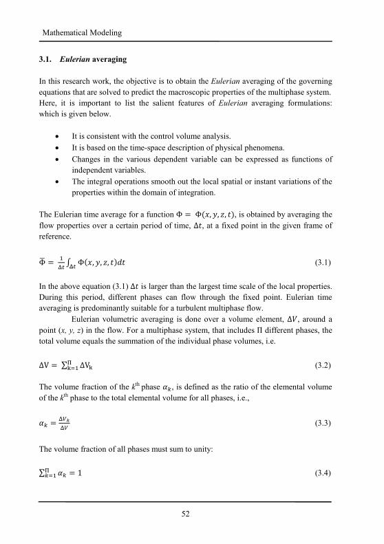
52


3.1. Eulerian averaging

In this research work, the objective is to obtain the Eulerian averaging of the governing

equations that are solved to predict the macroscopic properties of the multiphase system.

Here, it is important to list the salient features of Eulerian averaging formulations:

which is given below.

• It is consistent with the control volume analysis.

• It is based on the time-space description of physical phenomena.

• Changes in the various dependent variable can be expressed as functions of

independent variables.

• The integral operations smooth out the local spatial or instant variations of the

properties within the domain of integration.

The Eulerian time average for a function Φ = Φ�´, µ, ¶, ��, is obtained by averaging the

flow properties over a certain period of time, Δ�, at a fixed point in the given frame of

reference.

Φ, = �·� ¸ Φ�´, µ, ¶, ��±�·� (3.1)

In the above equation (3.1) Δ� is larger than the largest time scale of the local properties.

During this period, different phases can flow through the fixed point. Eulerian time

averaging is predominantly suitable for a turbulent multiphase flow.

Eulerian volumetric averaging is done over a volume element, Δ#, around a

point (x, y, z) in the flow. For a multiphase system, that includes Π different phases, the

total volume equals the summation of the individual phase volumes, i.e.

ΔV = ∑ ΔV»¼»=� (3.2)

The volume fraction of the kth phase ½!, is defined as the ratio of the elemental volume

of the kth phase to the total elemental volume for all phases, i.e.,

½! = ·¾¿·¾ (3.3)

The volume fraction of all phases must sum to unity:

∑ ½!¼!=� = 1 (3.4)

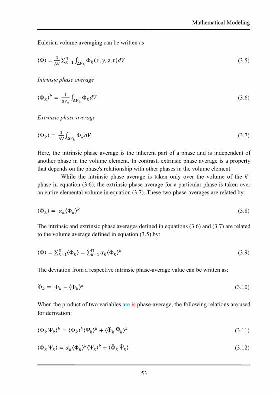
53


Eulerian volume averaging can be written as

⟨Φ⟩ = �·¾ ∑ ¸ Φ!�´, µ, ¶, ��±#·¾¿¼!=� (3.5)

Intrinsic phase average

⟨Φ!⟩! = �·¾¿ ¸ Φ!±#·¾¿ (3.6)

Extrinsic phase average

⟨Φ!⟩ = �∆P ¸ Φ!±#·¾¿ (3.7)

Here, the intrinsic phase average is the inherent part of a phase and is independent of

another phase in the volume element. In contrast, extrinsic phase average is a property

that depends on the phase's relationship with other phases in the volume element.

While the intrinsic phase average is taken only over the volume of the kth

phase in equation (3.6), the extrinsic phase average for a particular phase is taken over

an entire elemental volume in equation (3.7). These two phase-averages are related by:

⟨Φ!⟩ = ½!⟨Φ!⟩! (3.8)

The intrinsic and extrinsic phase averages defined in equations (3.6) and (3.7) are related

to the volume average defined in equation (3.5) by:

⟨Φ⟩ = ∑ ⟨Φ!⟩¼!=� = ∑ ½!⟨Φ!⟩!¼!=� (3.9)

The deviation from a respective intrinsic phase-average value can be written as:

ΦÀ ! = Φ! − ⟨Φ!⟩! (3.10)

When the product of two variables are is phase-average, the following relations are used

for derivation:

⟨Φ! Ψ!⟩! = ⟨Φ!⟩!⟨Ψ!⟩! + ⟨ΦÀ ! ΨÀ!⟩! (3.11)

⟨Φ! Ψ!⟩ = ½!⟨Φ!⟩!⟨Ψ!⟩! + ⟨ΦÀ ! ΨÀ!⟩ (3.12)

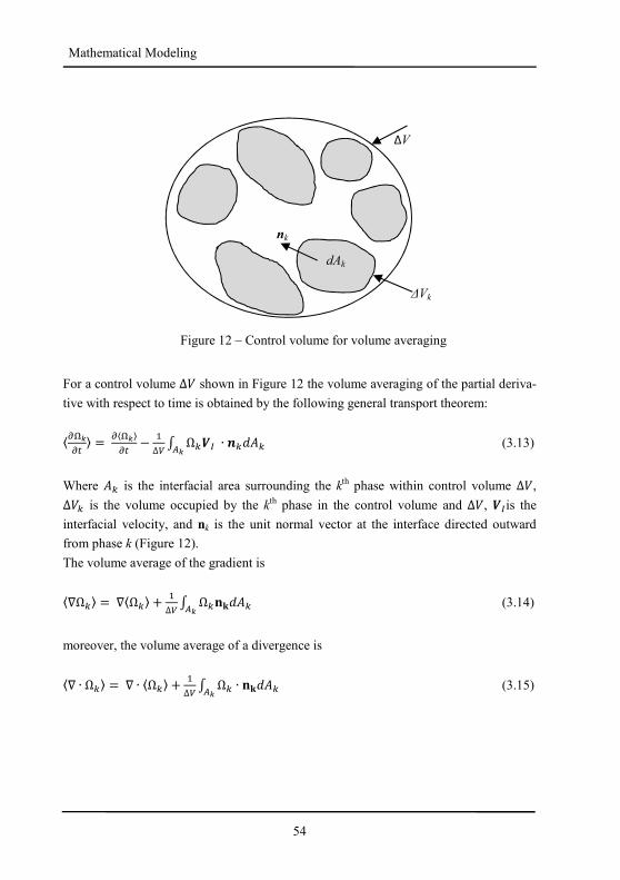
54


For a control volume Δ# shown in Figure 12 the volume averaging of the partial deriva-

tive with respect to time is obtained by the following general transport theorem:

⟨:Á¿:� ⟩ = :⟨Á¿⟩:� − �∆¾ ¸ Ω!ÂÃÄ¿ ∙ Æ!±Ç! (3.13)

Where Ç! is the interfacial area surrounding the kth phase within control volume Δ#, Δ#! is the volume occupied by the kth phase in the control volume and Δ#, ÂÃis the

interfacial velocity, and nk is the unit normal vector at the interface directed outward

from phase k (Figure 12).

The volume average of the gradient is

⟨∇Ω!⟩ = ∇⟨Ω!⟩ + �∆¾ ¸ Ω!ÈÉ±Ç!Ä¿ (3.14)

moreover, the volume average of a divergence is

⟨∇ ∙ Ω!⟩ = ∇ ∙ ⟨Ω!⟩ + �∆¾ ¸ Ω! ∙ ÈÉ±Ç!Ä¿ (3.15)

ΔV

∆Vk

nk

dAk

Figure 12 – Control volume for volume averaging

55


3.2. Computational model for multi-fluid flow with phase change

The computational model describing the two-phase flow in the fluid region relies on

solving the mass, momentum and energy equations simultaneously. At this moment, the

two-fluid model is being applied for multiphase flow calculation. In the framework of

this method, the motion of both phases, considered as two interpenetrating continuum

media, is described by a particular set of transport equations relying upon the

corresponding conservation laws. In the solid region, only the energy equation described

the heat conduction process.

3.2.1. Mass Conservation

The volume-averaged form of the continuity equation for the kth phase reads

:wÊ¿⟨O¿⟩¿|:� + ∇ ∙ w½!⟨(!⟩!⟨#$%!⟩!| = ∑ �� ²!Π²=��²Ë!� (3.16)

The volume fraction satisfying the condition of the compatibility:∑ ½! = 1Π!=� .

The modeling of the source term originating from the phase change taking place due to

heat transfer between the fluid and the heated surface (quenched surface) is the subject

of the following section.

3.2.2. Quenching Model

The afore-mentioned mass transfer rate between the liquid and the vapor generated by

the presence of the quenched solid part, in which the temperature field simultaneously

investigated, defined as follows:

�� ²! = �Ì�ÍIÄM∆7I�� = −�!Î� (3.17)

Where, h is the heat transfer coefficient existing in the relevant boiling mode; ∆T=Tw-

Tsat is the excess wall temperature, Tw being the wall temperature and Tsat the liquid

saturation temperature. The area considered in the boiling model is given as Ai = 6εd/Db,

with Db (=0.1 mm is the typical value) being the bubble diameter and εd dispersed phase

volume fraction. Cm represents the vapor formation coefficient in the film boiling mode

(taking the value of 100) and the vapor collapse coefficient in the transition to nucleate

boiling stage (with the corresponding value of 20). The closure coefficient CA is given

by the following relationship

56


ÏÄ = 1 − Ð ½� + ½Ñ)Ò½ ��! − ½Ñ)Ò

The heat transfer coefficient corresponding to the film boiling mode is computed by

using Bromley’s (1955) equation.

ℎ = 0.62 Ó!S{OS�O�9OS��wI��j>.c�TS∆7|�K�S∆7 Ô>.D� (3.18)

To evaluate the heat transfer coefficient in the transition boiling regime and to identify

the limits of the phase change rates, the Critical Heat Flux (CHF) and Minimum Heat

Flux (MHF) limits are evaluated based on the properties of the interacting phases. An

estimation of the critical heat flux value pertaining to the current system is established

by using Zuber’s (1958) relation.

Õ�Ö× = 0.131(ℎ�� «E��O�9OS�OSy °>.D� (3.19)

With σ representing the surface tension of the liquid. The effect of sub-cooling is taken

into account using the relation of Hua and Xu (2000) as following.

ØÙÚÛ,F¥KJ��ØÙÚÛ,FGH = 1 + 0.345 ¤�Ü¦�.yv (3.20)

A constant ‘transient critical heat flux factor,' Kchf, is provided to identify the effect of

transient burn out approximation [Auracher and Buchholz (2005)] on the CHF during

the quenching process. The modified Critical Heat Flux value is computed as following.

Õ�Ö×,��¯�ÝÝ� = Þ�I�Õ�Ö×,�� 1 + 0.345 ¤�Ü¦�.yv� (3.21)

Where Ja and Pe are the Jacob and Peclet numbers respectively. The value of Kchf is

taken between 0.5 – 4.0. The Minimum Heat Flux (MHF) approximation in the quench-

ing system is estimated as:

ÕßÖ× = 0.09(ℎ�� «��O�9OS�O�jOS °>.� « E��O�9OS�°>.D� (3.22)

57


Similar to the burn out approximation factor, a constant ‘transient minimum heat flux

factor,' Kmhf, is introduced to describe the variations in the computed minimum heat flux

owing to the local fluctuations, boundary layer modulation, and solid surface character-

istics. Accordingly, the modified Minimum Heat Flux reads.

ÕßÖ× = ÞÑI�ÕßÖ× (3.23)

The range of the variation of the Kmhf values is 2-15. The heat flux experienced during

the transition boiling (TB) mode in the near-wall region is.

Õ7A = Õ�Ö× Óà 7Já�w7897Já�|Ô (3.24)

Where Tchf is the temperature value taken at the Critical Heat Flux limit. QCHF is defined

using equation (3.19). The parameter wp, defined as the wetting parameter, provides the

instantaneous flux disposition when the wall temperature drops below the Leidenfrost

temperature limit. In the following equation, the heat transfer coefficient in the nucleate

boiling (NB) regime is obtained by presuming the similar relationship as for the transi-

tion boiling mode (QNB ≈ QTB)

ℎ@A = Øâã7897FGH (3.25)

The limits of phase change process during the film and nucleate boiling modes are given

by the following.

Γ�)Ñ) = ØMÄ8RHI�� (3.26)

With i denoting the critical heat flux (i ≡CHF) in the nucleate boiling mode and mini-

mum heat flux (i ≡MHF) in the film boiling mode. The corresponding CHF and MHF

limits, given by equation (3.21) and (3.22) respectively, are to be inserted here. Awet

represents the wetted area given by

Ç�¦� = w1 − ä ��!|Ç� (3.27)

As in equation (3.27) denotes the physical interface area exposed to the boiling process.

αpack is the phase packing limit defined by

½ ��! = ½�N; + å½�¦� (3.28)

Factor F takes the value of 1 if the interface temperature is less than the Leidenfrost

temperature (nucleate boiling mode) or 0 otherwise (film boiling mode). ½�N; and ½�¦�

are the dry and wet phases packing limits.

58


3.2.3. Momentum Equation

The intrinsic volume-averaged momentum equation for the ��I phase is given by

:wÊ¿⟨O¿⟩¿⟨¾$$%¿⟩¿|:� + ∇ ∙ w½!⟨(!⟩!⟨#$%!#$%!⟩!| =−⟨æ!⟩!ç + ∇ ∙ �½!⟨è! + �!�⟩� − �∆é ¸ (!#$%!w#$%! − #$%Ã| ∙ �!±Ç!Ä¿ + �∆é ¸ è! ∙ �!±Ç!Ä¿

(3.29)

Where, ⟨è!⟩! is the phase-averaged stress tensor of the ��I phase,

⟨è!⟩! = ê! «∇⟨#$%!⟩ + w∇⟨#$%!⟩!|7° − D� ê!w∇ ∙ ⟨#$%!⟩!|ç (3.30)

⟨�!�⟩! = −(!⟨ëì′ëÎ′ííííí⟩! = ê!� «�∇⟨#$%!⟩ + w∇⟨#$%!⟩!|7� − D� �∇ ∙ ⟨#!⟩!�ç° − D� (!⟨Þ!⟩!ç

(3.31)

The turbulent viscosity

ê!� = (!��î ïðyñ¿ (3.32)

The third and fourth terms on the right-hand side of equation (3.29) represent the mo-

mentum exchanges and interactive forces between the phases:

− �∆é ¸ (!Ä¿ #$%!w#$%! − #$%Ã| ∙ �! ±Ç! = ∑ w⟨�� ²!⟩⟨#!,Ã⟩|²=��²Ë!� (3.33)

�∆é ¸ è! ∙ �!±Ç!Ä¿ = ∑ ⟨å%²!⟩Π²=��²Ë!� (3.34)

Here, ⟨#$%!,)⟩! is the intrinsic volume-averaged velocity of the ��I phase at the interface.

The velocity difference between two adjacent phases results solely from their density

difference. å%²! is an interactive force between the jth and kth phases depending upon the

friction, pressure and cohesion between different phases. Newton’s third law requires

that the contact interaction forces (action and reaction force pair) satisfy the conditions ⟨å%²!⟩ = −⟨å%!²⟩ (3.35)

The interactive force can be determined by:

59


⟨å%²!⟩ = � ¦,²!w⟨#$%²⟩² − ⟨#$%!⟩!| (3.36)

� ¦,²! representing the momentum exchange coefficient between phases j and k. If liquid

is the primary phase and vapor is the secondary phase, the vapor disperses in liquid as

vapor bubbles. The momentum exchange coefficient can be than estimated by following

equations:

�¦, ²! = �c �� Ê�⟨O¿⟩�K ò⟨#$%²⟩² − ⟨#$%!⟩!ò (3.37)

Where k denotes the primary phase and j the secondary phase. Db is the diameter of the

vapor bubbles or liquid droplets of the secondary phase j. CD is the drag coefficient

based on the relative Reynolds number, which is obtained from the following empirical

correlation:

�� = ó Dc�¦K w1 + 0.15"�>.ª¡�| ôõ "�¯ ≤ 10000.44 ôõ "�¯ > 1000 (3.38)

"�¯ = ⟨O¿⟩ò⟨¾$$%�⟩�9⟨¾$$%¿⟩¿ò�K�� (3.39)

Introduction to the equations (3.33) - (3.34) into equation (3.29) results in the final form

of the volume-averaged, multi-fluid momentum equation, applied in the present work:

:wÊ¿⟨O¿⟩¿⟨¾$$%¿⟩¿|:� + ∇ ∙ w½!⟨(!⟩!⟨#$%!#$%!⟩!| =−⟨æ!⟩!ç + ∇ ∙ �½!⟨è! + �!�⟩� + ∑ ⟨�Î!� ⟩⟨#$%!,Ã⟩!²=��²Ë!� + ∑ ⟨å%²!⟩Π²=��²Ë��

(3.40)

3.2.4. Energy Equation

The intrinsic volume-averaged energy equation for the ��I phase is given as follows

:wÊ¿⟨O¿⟩¿⟨Ö¿⟩¿|:� + ∇w½!⟨(!⟩!⟨#$%!�!⟩!| = −∇⟨ ! + !� ⟩ + ½! �⟨ ¿⟩¿�� + ∇⟨#$%!⟩: ⟨è!⟩ −

�∆é ¸ (!�!w#$%! − #$%Ã| ∙ �!±Ç!Ä¿ − �∆é ¸ ! ∙ �!±Ç!Ä¿ (3.41)

60


The next to last term on the right-hand side of equation (3.41) represents the enthalpy

exchange between the kth phase and other participating phases featured by the ongoing

mass transfer:

− �∆é ¸ (!�!w#$%! − #$%Ã| ∙ �!±Ç!Ä¿ = ∑ �� ²!⟨�!,Ã⟩!Π²=��²Ë!� (3.42)

Where,⟨�!,Ã⟩! is the intrinsic volume-averaged enthalpy of the ��I phase at the inter-

face. The last term on the right hand side of equation (3.41) describes the heat transfer

between the ��I phase and all other participating phases:

− �∆é ¸ ! ∙ �!±Ç!Ä¿ = ∑ ⟨ ²!⟩!Π²=��²Ë!� (3.43)

The important heat exchange process is based on the Ranz- Marshall (1952) correlation

for the Nusselt number, Nu:

ùú = 2.0 + 0.6"��/D¢£�/� (3.44)

Where Reb is the local bubble Reynolds number and Pr is the Prandtl number. This

model should also be used when the Ranz-Marshall correlation is employed for the

calculation of mass exchange due to boiling process.

The heat transfer rate becomes:

⟨ ²!⟩ = � ûJ�K ùú ∙ Ç) ∙ �� − �� = −⟨ !²⟩ (3.45)

Presently, Cb = 1 and Cc = 0 were adopted (boiling and condensation coefficients respec-

tively). ü� represents the conductivity of the continuous phase. Td and Tc are the temper-

atures of the dispersed and continuous phases respectively. The final form of the energy

equation solved presently is as follows:

:wÊ¿⟨O¿⟩¿⟨Ö¿⟩¿|:� + ∇w½!⟨(!⟩!⟨#$%!�!⟩!| = −∇ ∙ ⟨ ! + !� ⟩ + ½! �⟨ ¿⟩¿�� + ∇⟨#$%!⟩: ⟨è!⟩ +

∑ ý⟨ ²!⟩ + �� ²!⟨�!,Ã⟩!þΠ²=��²Ë!� (3.46)

Heat flux ! is defined as:

! = ûJ, ¿�T,¿ ∇ ⋅ ⟨�!⟩! (3.47)

Where ü�, ! is the thermal conductivity and Cpk is the heat capacity of kth phase.

Turbulent heat flux !� equals:

61


!� = −(!⟨ëì′�Î′íííííí⟩! = �¿HE� ∇ ⋅ ⟨�!⟩! (3.48)

3.2.5. Heat Conduction Equation for the Solid Region

The heat transfer (conduction) computation in the solid region is based on the solution

of an appropriate enthalpy equation.

⟨:�OFÖF�:� ⟩ = −⟨∇ ∙ �⟩ (3.49)

The heat flux formulation is given as � = ûF�TF ∇��

3.3. Computational model for multi-fluid flow without phase change

The hydrodynamics and convection heat transfer of jet impingement onto the flat hori-

zontal surface used the following model for computational study.

Mass balance:

:wÊ¿⟨O¿⟩¿|:� + ∇ ∙ w½!⟨(!⟩!⟨#$%!⟩!| = 0 (3.50)

Momentum Balance:

:wÊ¿⟨O¿⟩¿⟨¾$$%¿⟩¿|:� + ∇ ∙ w½!⟨(!⟩!⟨#$%!#$%!⟩!| = −⟨æ!⟩!ç + ∇ ∙ �½!⟨è! + �!�⟩!� (3.51)

The volume fraction satisfying the condition of the compatibility: ∑ ½! = 1Π!=�

Where, ⟨è!⟩! is the phase-averaged stress tensor of the thk phase.

VOF (Volume-of-Fluid) method is used only in the case of multiple jets or the jet with-

out phase change. The VOF method proposed by Hirt and Nichols (1981) is used to

capture the free surface of the water jet.

The volume fraction of the tracked phase can be written in the conservative form as:

:Ê:� + ∇ ∙ ½#$% = 0 (3.52)

Where ε is the volume fraction of the tracked phase and # $$$%is the velocity field. A com-

putational cell can be associated with the value ½ =1, if fully occupied by the tracked

62


phase, otherwise ½ = 0. In the partially filled cells the volume fraction takes the values

0< ½ <1. A single set of governing equations is solved for the “effective” fluid repre-

senting a mixture of the participating phases. The local density and viscosity of this

mixture occupying the whole computational domain are defined with help of the follow-

ing volumetric-fraction-weighted relationships, with the subscripts j and k denoting the

different phases.

(Ñ = ½(² + �1 − ½�(! (3.53)

êÑ = ½ê² + �1 − ½�ê! (3.54)

3.3.1. Volume-of-fluid interfacial momentum exchange model

In the flows with the interface, surface tension on the interface plays a significant role.

Continuum-surface-force model is employed and treated as body force:

fE = ¸ � ü∇½ ±V = �üÜ�∇½�ÜVÜP (3.55)

Where, � is surface tension, üÜ is the curvature of the interface calculated from the

following expression:

üÜ = −�∇ ∙ �� = − «∇ ∙ � ∇Ê|∇Ê|�°Ü = − �PT ∑ S² ∙ ��∇Ê��|∇Ê|� �Ò�²=> (3.56)

Where, �� is unit normal to the surface. An accurate evaluation of the curvature using

(3.56) demands the smoothing of the volume fraction field (which is discontinuous on a

discretized mesh without smoothing). This task can be achieved by applying the Lapla-

cian filter several times, defined as:

ℑ�α�� = ∑ ½�òò��=� ∑ òò�²=�³

(3.57)

When fluid interfaces are in contact with wall boundaries, the effects of wall adhesion

must be accounted. The simplest approach within the framework of the CSF model is to

adjust the normal vector to the interface according to the contact angle θw (the angle

between the wall and the tangent to the interface at the wall, measured inside the tracked

phase).

At points X$$%� on the wall, the unit normal vector can be expressed as: n� = n��q�� cos θ� + n�Z sin θ� (3.58)

63


n��q�� is the unit wall normal directed into the wall and is computed from the geometry,

whereas, n�Z lies on the wall and is normal to the contact line between the interface and

the wall at X$$%�.

The value of n�Z is computed from the known volume fraction field by applying the

symmetry condition at the wall boundary. Once, n� is evaluated using (C), it is

substituted in the curvature expression (3.56) as a boundary condition for the cells near

the wall. This change in curvature, in turn, modifies the surface tension (3.55) near the

wall (dynamic treatment).

In reality, the physics associated with wall adhesion is very complex - the contact angle

θw is not only a fluid property but also a function of the geometry and smoothness of the

wall surface. Besides, when the contact line is moving, it depends on the local fluid

conditions as well, and additional modeling is necessary.

3.4. Turbulence and its modeling

It is evidence from the experiment [Islam et al. (2008), Mitsutake and Monde (2003),

Nishio et al. (1998)] that heat transfer mechanism at the surface which is being

quenched by liquid jet is governed by turbulent diffusion caused by dynamics (bubble

growth, merger, and collapse) of vapour bubbles. A pioneer work by Paul Durbin [Dur-

bin, 1993)] demonstrated the fact that, the standard k-ε model over predicts the heat-flux

and developed the new ëDííí − õ model which shows some improvements.

In order to improve numerical stability of the original ëDííí − õ model by solving a

transport equation for the velocity scale î = yíííí! instead of velocity scale ëDííí. The variable î represents a scalar whose near-wall behaviour resembles that of the normal-to-wall

Reynolds stress component.

Incorporating the Durbin’s [Durbin, (1995)] elliptic relaxation concept, a new eddy-

viscosity turbulence model comprising four equation denoted as � − ä − î − õ devel-

oped by Hanjalic et al. (2004).

The eddy-viscosity is obtained in the following from:

1� = ��î !yñ (3.59)

moreover, the rest of variables from the following set of model equation, thus

:�Ê¿O¿»¿�:� + ::C� �½!(!v!k!� = ::C� Ó½! �ê! + �¿HE¿� :»¿:C�Ô + ½!(!�P! − ä!� + ∑ K²!¼)=�,²Ë! + k! ∑ �� ²!¼)=�,²Ë!

(3.60)

64


:�Ê¿O¿�¿�:� + ::C� �½!(!v!ε!� = w��o∗ Ü¿Ê¿ñ¿9��yÊ¿ñ¿y|»¿ + ::C� Ó½! �ê! + �¿HE�� :ñ¿:C�Ô +∑ D²!¼)=�,²Ë! + ε! ∑ �� ²!¼)=�,²Ë!

(3.61)

:�Ê¿O¿�¿�:� + ::C� �½!(!v!ζ!� = (õ − ( �! ¢! + ::C� Ó½! �ê! + �¿HE�� :�¿:C�Ô (3.62)

Where the following form of the f equation is adopted as

õ − �D :y�:C�:C� = �� + �D Ü¿� � �y{9��7 (3.63)

The turbulent time scale T and length scale L are given by

� = �´ ��ô� �!ñ , Ê! yííí�!√ª#y� , �7 �$ñ��/D� (3.64)

� = ��´ ��ô� �!{/yñ , !{/y

yííí�!√ª#y� , �% �${ñ ��/D� (3.65)

Additional modifications to the ε-equation is that the constant Cε1 is dampened close to

the wall thus �ñ�∗ = �ñ�w1 + 0.045&1/î| (3.66)

This is computationally more robust than the original model fv −2 .

3.4.1. Hybrid Wall-treatment

This wall treatment should ensure a gradual change between viscous sub-layer formula-

tions and the wall functions. Popovac and Hanjalic (2005) extended Kader’s (1981)

proposal for the description of temperature profile in the wall boundary layer also on all

turbulence properties, thus

'j = µj�9( + �û ln�*µj��9�/( (3.67)

ê� = ê ;+,-+, (3.68)

Γ = >.>��X ;,�u�j�ÜN{;, (3.69)

This wall treatment provides the standard wall function for the large values of y + as well

as the integration of equations up to the wall for the very small values of y+. Similarly,

the relationships for a dissipation rate and turbulence viscosity at the point next to the

65


wall are derived. The production of turbulence kinetic energy near the wall is modified

as well to ensure that results are the same for the small y+ as provided by low-Re models

and the results are the same as with the standard wall function for the high y+. All mod-

els given above are implemented in conjunction with this wall treatment also.

3.5. Numerical Solution Methodology

3.5.1. Introduction

This section discusses numerical aspects of the method employed to solve the governing

equations described in sections 3.2 and 3.3. First of all, the integral form of the modeling

equations, which is the preliminary for the finite volume discretization, is presented. The

fundamental features of the discretization method such as Linear Upwind Differencing

Schemes (LUDS), time integration and basis of algebraic equations are delineated. The

SIMPLE (Semi-Implicit Method for Pressure-Linked Equation) -like segregated method

used to connect the momentum, continuity and energy equations (i.e. coupling between

the velocities, pressure, and density) is essential to the whole procedure and is

deliberated. Next, the overall solution procedure is presented, and the implementation of

various boundary conditions is described.

3.5.2. Integral form of equations

The differential form of the generic conservation equation is given as:

:wñ¿⟨O¿⟩¿⟨/¿⟩¿|:� + ∇ ∙ wä!⟨(!⟩!⟨#$%!0!⟩!| = ∇ ∙ wä!Γ/,!∇⟨0!⟩!| + ∇ ∙ wä!123,4| +⟨0!,Ã⟩! ∑ ⟨�Î!� ⟩Π²=��²Ë!� + ∑ ⟨5/,!�⟩Π²=��²Ë�� (3.70)

The above equation integrated over the cell volume to provide the generic conservation

equation in the integral form:

::� ¸ ä»⟨(»⟩!⟨0»⟩!±#»¾ + ¸ ä»⟨(»⟩!⟨#$%!0!⟩! ∙ ds# = ¸ ä»Γ/,!∇⟨0!⟩! ∙ ds# +¸ ä» 789,» ∙ ds# + ¸ w⟨0»,Ã⟩! ∑ ⟨�� ²!⟩Π²=��²Ë»� + ∑ ⟨5/,!�⟩Π²=��²Ë�� |¾ dV

(3.71)

k= 1,….,N

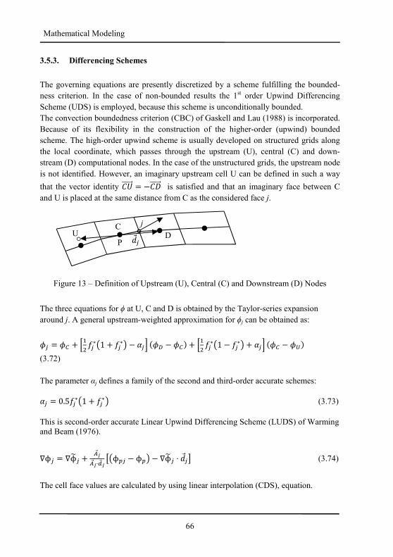
66


3.5.3. Differencing Schemes

The governing equations are presently discretized by a scheme fulfilling the bounded-

ness criterion. In the case of non-bounded results the 1st order Upwind Differencing

Scheme (UDS) is employed, because this scheme is unconditionally bounded.

The convection boundedness criterion (CBC) of Gaskell and Lau (1988) is incorporated.

Because of its flexibility in the construction of the higher-order (upwind) bounded

scheme. The high-order upwind scheme is usually developed on structured grids along

the local coordinate, which passes through the upstream (U), central (C) and down-

stream (D) computational nodes. In the case of the unstructured grids, the upstream node

is not identified. However, an imaginary upstream cell U can be defined in such a way

that the vector identity �'$$$$$% = −�:$$$$$% is satisfied and that an imaginary face between C

and U is placed at the same distance from C as the considered face j.

Figure 13 – Definition of Upstream (U), Central (C) and Downstream (D) Nodes

The three equations for ϕ at U, C and D is obtained by the Taylor-series expansion

around j. A general upstream-weighted approximation for ϕj can be obtained as:

0² = 0� + «�D õ²∗w1 + õ²∗| − ½²° �0� − 0�� + «�D õ²∗w1 − õ²∗| + ½²° �0� − 0-�

(3.72)

The parameter αj defines a family of the second and third-order accurate schemes: ½² = 0.5õ²∗w1 + õ²∗| (3.73) This is second-order accurate Linear Upwind Differencing Scheme (LUDS) of Warming and Beam (1976).

∇ϕ² = ∇ϕ<² + Ä%�Ä%�⋅�%� ýwϕ ² − ϕ | − ∇ϕ<² ⋅ ±%²þ (3.74)

The cell face values are calculated by using linear interpolation (CDS), equation.

j

U C

D P ±%²

67


3.5.4. Time Integration

For unsteady fluid flow problems, the semi-discretized equation resembles a first order ordinary differential equation: �=�� + Φ�0, �� = 0, Ψ = �(#0�Ü (3.75)

In which all fluxes and sources are replaced by the quantity Φ:

Φ = ∑ �²Ò�²=� − ∑ :²Ò�²=� − �5/¾ + ∑ w5/Ä|²Ò�²=� � = � − : − 5 (3.76)

In order to advance the solution method in time step by step (time ‘marching’ proce-

dure) the above equation need to be integrated over each time interval ∆t. Explicit meth-

ods used to evaluate the fluxes and sources contained in Φ(ϕ, t). Explicit schemes in-

volve a stability requirement that Courant number (defined for the 1D case as U ∆t/∆x)

should be less than unity. If this condition is violated, the solution becomes unstable.

3.5.5. Algebraic Equations

The outcome of the discretization procedure is a set of algebraic equations, which can be written in the form: 0 = ∑ ²0 ²ÒM²=� + 5/ (3.77)

where ni is the number of internal faces which make a volume around the computational node P. The central coefficient ap, the coefficients aj associated with the values of the dependent variable φ at neighboring nodes Pj and the source term Sϕ are assembled as:

² = ²� + ²� = maxw−�� ² , 0| + Γí/² Ä�yÄ%�⋅�%� (3.78)

Ü = ∑ ¯ÒK²=� + � + 5/ (3.79)

� = c�O¾�+?@o9�O¾�+?@yD·� (3.80)

68


5/ = ∑ ÓA/ò�� ²ò0² �0Ü − 0Ü�� + Γí/²∇0Îííííí ⋅ �Ç%² − Ä�yÄ%�⋅�%� ±%²�Ô + ∑ «¯0¯ +ÒK¯=�ÒM²=�Γ/¯∇0Ü ⋅ �Ç%¯ − ÄKyÄ%K⋅�%K ±%¯�° + 5/B + ∑ w5/Ä|²

Ò�²=� + 5/�

(3.81)

5/� = c�O¾/�+?@o9�O¾/�+?@yD·� (3.82)

Note that the boundary coefficients ab are defined in the same way as aj, see

equation (3.78). There are nb = nf − ni boundary faces for the given cell P. The second order explicit scheme is used to discretize for the unsteady term.

3.5.6. SIMPLE Based Pressure-Velocity Coupling

The principal difficulty in solving the momentum equations for incompressible flows

lies in the determination of the pressure. In the iterative SIMPLE-like [Semi-Implicit

Method for Pressure-Linked Equations, Patankar and Spalding (1972)] algorithms, the

discrete form of the continuity equation is converted into an equation for the pressure

correction. The pressure corrections are then used to update the pressure and velocity

fields so that the velocity components obtained from the solution of momentum equa-

tions satisfy the continuity equation.

For computation of incompressible and compressible flows, the Unsteady SIMPLE

method can be extended by introducing density corrections and coupling them via an

equation of state with the pressure corrections, see Karki and Patankar (1989) and

Demirdzic at al., (1993).

3.5.7. Solution Procedure

For a computational domain with M control volumes, a system of M × N algebraic equa-

tions like equation (3.77) need to be solved for N dependent variables ϕ. The equations

are non-linear and also coupled with more than one dependent variable features in each

equation. Since the nonlinearity in the equations the iterative solution techniques are

used.

There are two approaches: the coupled (simultaneous) and segregated (sequential). In

the segregated approach, each equation for the considered variable is decoupled by

treating other variables as known. This leads to a subset of M linear algebraic equations

for each dependent variable. Having much smaller storage requirements, the segregated

approach is adopted in the computations.

69


3.5.8. Segregated Approach

In this approach, the coefficients aj and the source term Sϕ are calculated by using varia-

ble values from the previous iteration or time step. The resulting sub-system of linear-

ized algebraic equations can be arranged in a matrix form as: Ç/0 = 5/ (3.83)

Where, Aϕ is the M ×M coefficient matrix and 5/ are vectors of the unknown variable ϕ

and the source term, respectively. It is important to note that the matrix Aϕ is sparse

(there are ni + 1 non-zero elements in each row, ni is the number of the nearest neigh-

bours, i.e. internal faces), asymmetric, except for the pressure correction equation for

incompressible flows, and diagonally dominant (A number of iterative methods which

retain the sparsity of the above matrix can be used.

Algebraic multigrid methods (AMG) are among the most efficient solvers of large

sparse linear systems. The idea behind multigrid methods is that long wavelength errors

on the fine level appear as short wavelength errors on coarser levels and therefore, can

be effectively damped out by a relaxation scheme [Borzi (2000)].

3.5.9. Under-relaxation

After solving the linearized system (3.83), a change of variable values from the previous

(outer) iteration (0!9�) to the next iteration (0! ) is limited in order to ensure the con-

vergence of the solution procedure. The limitation, i.e. under-relaxation is done implicit-

ly, as proposed by Patankar (1980)

0! = 0!9� + ½/�0Ò¦� − 0!9�� (3.84) where 0Ò¦� is the solution of (3.83) and φ α is the under-relaxation factor with values

between 0 and 1. The implicit implementation of the above relaxation formula leads to

the modified algebraic equation (3.78). It retains the same form but, the central coeffi-

cient (a diagonal element of matrix Aϕ) and the source term are redefined as:

Ü∗ = �+ÊC , 5/∗ = 5/ + �9ÊCÊC Ü0Ü!9� (3.85)

so that the modified equation: Ü∗0Ü = ∑ ²0Ü²ÒM²=� + 5/∗ (3.86)

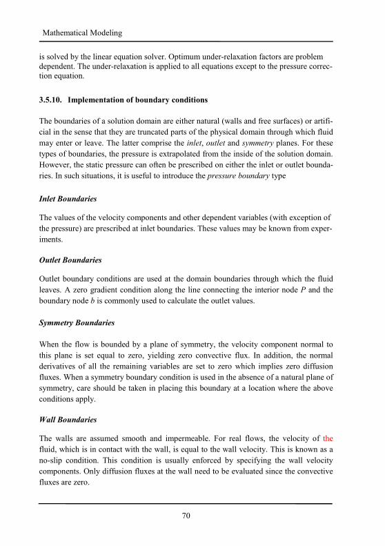
70


is solved by the linear equation solver. Optimum under-relaxation factors are problem dependent. The under-relaxation is applied to all equations except to the pressure correc-tion equation.

3.5.10. Implementation of boundary conditions

The boundaries of a solution domain are either natural (walls and free surfaces) or artifi-

cial in the sense that they are truncated parts of the physical domain through which fluid

may enter or leave. The latter comprise the inlet, outlet and symmetry planes. For these

types of boundaries, the pressure is extrapolated from the inside of the solution domain.

However, the static pressure can often be prescribed on either the inlet or outlet bounda-

ries. In such situations, it is useful to introduce the pressure boundary type

Inlet Boundaries

The values of the velocity components and other dependent variables (with exception of

the pressure) are prescribed at inlet boundaries. These values may be known from exper-

iments.

Outlet Boundaries

Outlet boundary conditions are used at the domain boundaries through which the fluid

leaves. A zero gradient condition along the line connecting the interior node P and the

boundary node b is commonly used to calculate the outlet values.

Symmetry Boundaries

When the flow is bounded by a plane of symmetry, the velocity component normal to

this plane is set equal to zero, yielding zero convective flux. In addition, the normal

derivatives of all the remaining variables are set to zero which implies zero diffusion

fluxes. When a symmetry boundary condition is used in the absence of a natural plane of

symmetry, care should be taken in placing this boundary at a location where the above

conditions apply.

Wall Boundaries

The walls are assumed smooth and impermeable. For real flows, the velocity of the

fluid, which is in contact with the wall, is equal to the wall velocity. This is known as a

no-slip condition. This condition is usually enforced by specifying the wall velocity

components. Only diffusion fluxes at the wall need to be evaluated since the convective

fluxes are zero.

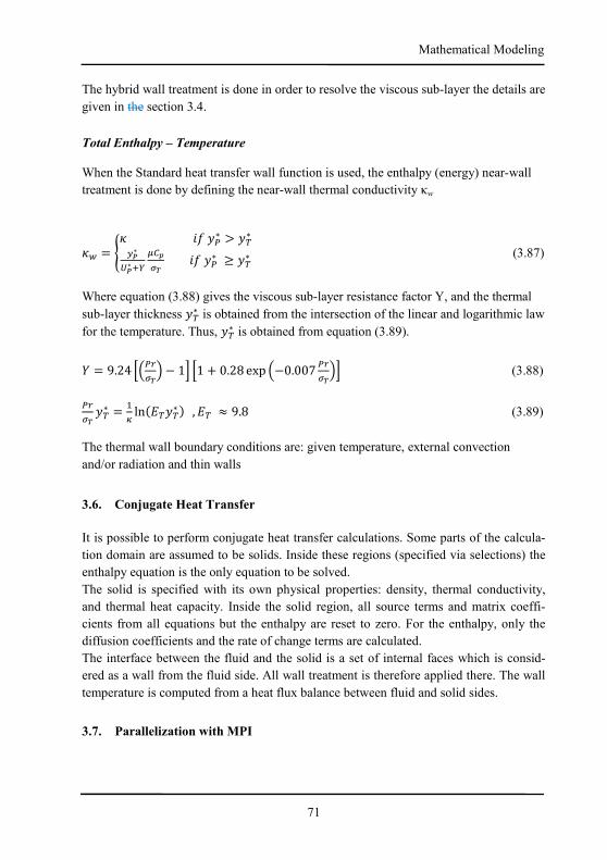
71


The hybrid wall treatment is done in order to resolve the viscous sub-layer the details are

given in the section 3.4.

Total Enthalpy – Temperature

When the Standard heat transfer wall function is used, the enthalpy (energy) near-wall

treatment is done by defining the near-wall thermal conductivity κw

ü� = Dü ôõ µÜ∗ > µ7∗;+∗-+∗jE ��TE� ôõ µÜ∗ ≥ µ7∗ (3.87)

Where equation (3.88) gives the viscous sub-layer resistance factor Y, and the thermal

sub-layer thickness µ7∗ is obtained from the intersection of the linear and logarithmic law

for the temperature. Thus, µ7∗ is obtained from equation (3.89).

G = 9.24 «�ÜNE�� − 1° «1 + 0.28 exp �−0.007 ÜNE��° (3.88)

ÜNE� µ7∗ = �û ln�*7µ7∗� ,*7 ≈ 9.8 (3.89)

The thermal wall boundary conditions are: given temperature, external convection

and/or radiation and thin walls

3.6. Conjugate Heat Transfer

It is possible to perform conjugate heat transfer calculations. Some parts of the calcula-

tion domain are assumed to be solids. Inside these regions (specified via selections) the

enthalpy equation is the only equation to be solved.

The solid is specified with its own physical properties: density, thermal conductivity,

and thermal heat capacity. Inside the solid region, all source terms and matrix coeffi-

cients from all equations but the enthalpy are reset to zero. For the enthalpy, only the

diffusion coefficients and the rate of change terms are calculated.

The interface between the fluid and the solid is a set of internal faces which is consid-

ered as a wall from the fluid side. All wall treatment is therefore applied there. The wall

temperature is computed from a heat flux balance between fluid and solid sides.

3.7. Parallelization with MPI

72


This section describes the basic principles and techniques used for parallel execution of

the computations. It uses the concept of the single program multiple data (SPMD) para-

digm. This means that a single copy of the executable program can operate on multiple

data. In this process, each processor has its own physical memory (or a part of the total

memory space) attached to it and processors cannot access local memory of other pro-

cessors. Data can be exchanged among processors by explicit message passing. In our

case, a program is the CFD solver and multiple data sub-domains. Messages are ex-

changed with the MPI library. An advantage of SPMD paradigm is that programs devel-

oped with it can be executed on both distributed and shared computers.

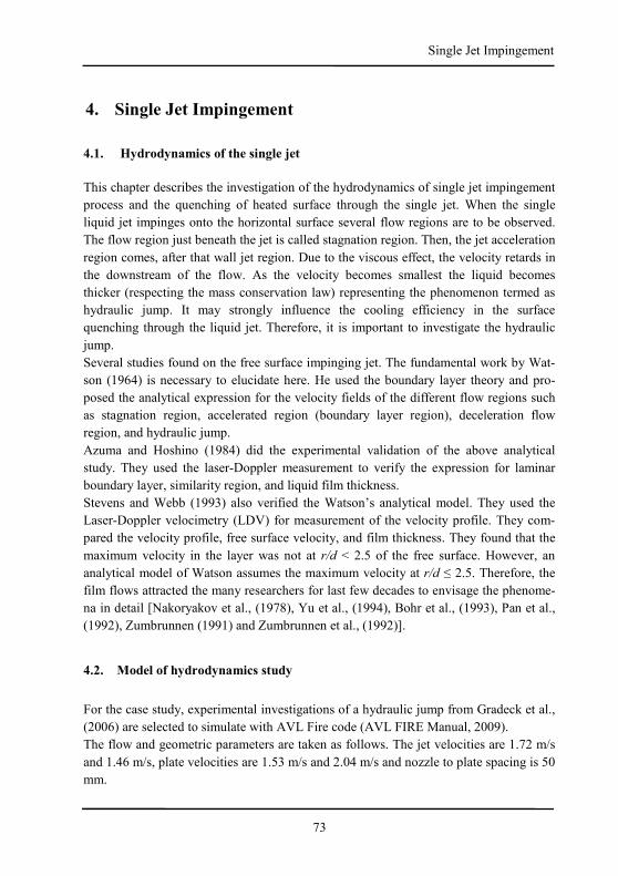
73

Single Jet Impingement

4. Single Jet Impingement

4.1. Hydrodynamics of the single jet

This chapter describes the investigation of the hydrodynamics of single jet impingement

process and the quenching of heated surface through the single jet. When the single

liquid jet impinges onto the horizontal surface several flow regions are to be observed.

The flow region just beneath the jet is called stagnation region. Then, the jet acceleration

region comes, after that wall jet region. Due to the viscous effect, the velocity retards in

the downstream of the flow. As the velocity becomes smallest the liquid becomes

thicker (respecting the mass conservation law) representing the phenomenon termed as

hydraulic jump. It may strongly influence the cooling efficiency in the surface

quenching through the liquid jet. Therefore, it is important to investigate the hydraulic

jump.

Several studies found on the free surface impinging jet. The fundamental work by Wat-

son (1964) is necessary to elucidate here. He used the boundary layer theory and pro-

posed the analytical expression for the velocity fields of the different flow regions such

as stagnation region, accelerated region (boundary layer region), deceleration flow

region, and hydraulic jump.

Azuma and Hoshino (1984) did the experimental validation of the above analytical

study. They used the laser-Doppler measurement to verify the expression for laminar

boundary layer, similarity region, and liquid film thickness.

Stevens and Webb (1993) also verified the Watson’s analytical model. They used the

Laser-Doppler velocimetry (LDV) for measurement of the velocity profile. They com-

pared the velocity profile, free surface velocity, and film thickness. They found that the

maximum velocity in the layer was not at r/d < 2.5 of the free surface. However, an

analytical model of Watson assumes the maximum velocity at r/d ≤ 2.5. Therefore, the

film flows attracted the many researchers for last few decades to envisage the phenome-

na in detail [Nakoryakov et al., (1978), Yu et al., (1994), Bohr et al., (1993), Pan et al.,

(1992), Zumbrunnen (1991) and Zumbrunnen et al., (1992)].

4.2. Model of hydrodynamics study

For the case study, experimental investigations of a hydraulic jump from Gradeck et al.,

(2006) are selected to simulate with AVL Fire code (AVL FIRE Manual, 2009).

The flow and geometric parameters are taken as follows. The jet velocities are 1.72 m/s

and 1.46 m/s, plate velocities are 1.53 m/s and 2.04 m/s and nozzle to plate spacing is 50

mm.

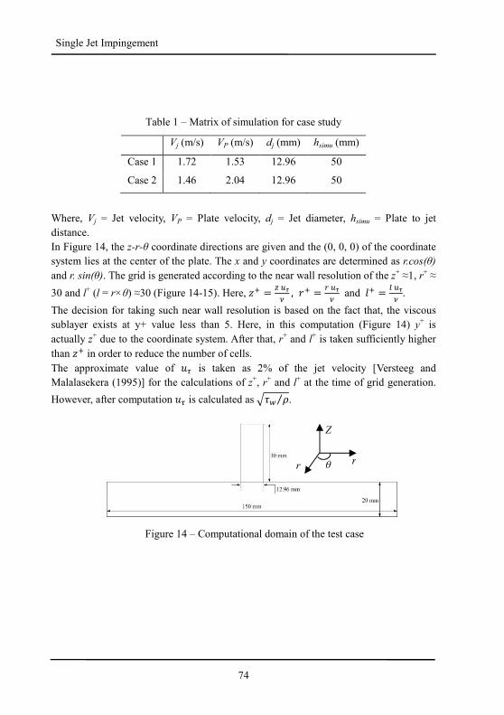
74


Table 1 – Matrix of simulation for case study

Where, Vj = Jet velocity, VP = Plate velocity, dj = Jet diameter, hsimu = Plate to jet

distance. In Figure 14, the z-r-θ coordinate directions are given and the (0, 0, 0) of the coordinate

system lies at the center of the plate. The x and y coordinates are determined as r.cos(θ)

and r. sin(θ). The grid is generated according to the near wall resolution of the z+ ≈1, r+ ≈

30 and l+ (l = r×θ) ≈30 (Figure 14-15). Here, ¶j = K �L$ , £j = N �L$ and Mj = � �L$ .

The decision for taking such near wall resolution is based on the fact that, the viscous

sublayer exists at y+ value less than 5. Here, in this computation (Figure 14) y+ is

actually z+ due to the coordinate system. After that, r+ and l+ is taken sufficiently higher

than ¶j in order to reduce the number of cells.

The approximate value of úN is taken as 2% of the jet velocity [Versteeg and

Malalasekera (1995)] for the calculations of z+, r+ and l+ at the time of grid generation.

However, after computation úN is calculated as &è� (⁄ .

Vj (m/s) VP (m/s) dj (mm) hsimu (mm)

Case 1 1.72 1.53 12.96 50

Case 2 1.46 2.04 12.96 50

r r

Z

θ

Figure 14 – Computational domain of the test case

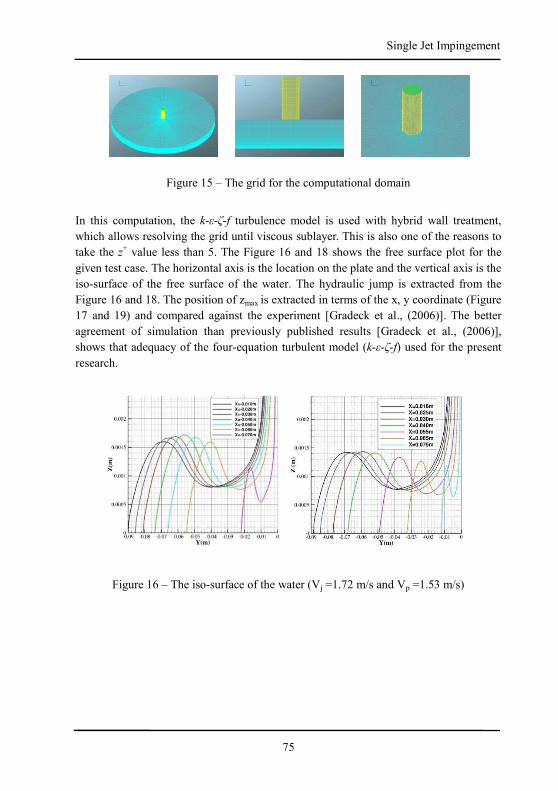
75


Figure 15 – The grid for the computational domain

In this computation, the k-ε-ζ-f turbulence model is used with hybrid wall treatment,

which allows resolving the grid until viscous sublayer. This is also one of the reasons to

take the z+ value less than 5. The Figure 16 and 18 shows the free surface plot for the

given test case. The horizontal axis is the location on the plate and the vertical axis is the

iso-surface of the free surface of the water. The hydraulic jump is extracted from the

Figure 16 and 18. The position of zmax is extracted in terms of the x, y coordinate (Figure

17 and 19) and compared against the experiment [Gradeck et al., (2006)]. The better

agreement of simulation than previously published results [Gradeck et al., (2006)],

shows that adequacy of the four-equation turbulent model (k-ε-ζ-f) used for the present

research.

Figure 16 – The iso-surface of the water (Vj =1.72 m/s and Vp =1.53 m/s)

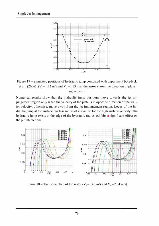
76


Figure 17 – Simulated positions of hydraulic jump compared with experiment [Gradeck

et al., (2006)] (Vj =1.72 m/s and Vp =1.53 m/s, the arrow shows the direction of plate

movement)

Numerical results show that the hydraulic jump positions move towards the jet im-

pingement region only when the velocity of the plate is in opposite direction of the wall-

jet velocity, otherwise, move away from the jet impingement region. Locus of the hy-

draulic jump at the surface has less radius of curvature for the high surface velocity. The

hydraulic jump exists at the edge of the hydraulic radius exhibits a significant effect on

the jet interactions.

Figure 18 – The iso-surface of the water (Vj =1.46 m/s and Vp =2.04 m/s)

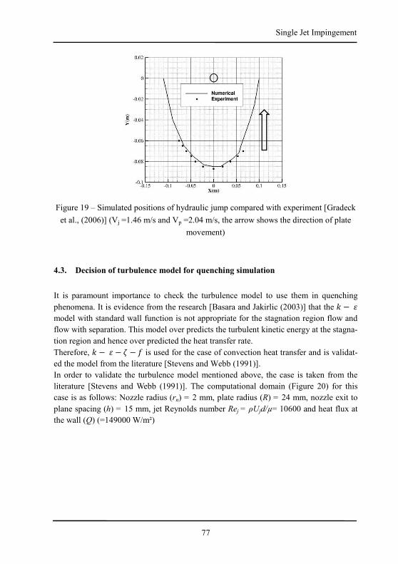
77



et al., (2006)] (Vj =1.46 m/s and Vp =2.04 m/s, the arrow shows the direction of plate

movement)

4.3. Decision of turbulence model for quenching simulation

It is paramount importance to check the turbulence model to use them in quenching

phenomena. It is evidence from the research [Basara and Jakirlic (2003)] that the � − ä

model with standard wall function is not appropriate for the stagnation region flow and

flow with separation. This model over predicts the turbulent kinetic energy at the stagna-

tion region and hence over predicted the heat transfer rate.

Therefore, � − ä − î − õ is used for the case of convection heat transfer and is validat-

ed the model from the literature [Stevens and Webb (1991)].

In order to validate the turbulence model mentioned above, the case is taken from the

literature [Stevens and Webb (1991)]. The computational domain (Figure 20) for this

case is as follows: Nozzle radius (rn) = 2 mm, plate radius (R) = 24 mm, nozzle exit to

plane spacing (h) = 15 mm, jet Reynolds number Rej = ρUjd/µ= 10600 and heat flux at

the wall (Q) (=149000 W/m²)

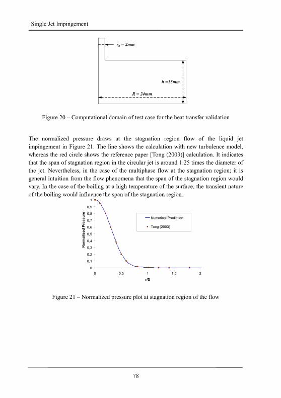
78


Figure 20 – Computational domain of test case for the heat transfer validation

The normalized pressure draws at the stagnation region flow of the liquid jet

impingement in Figure 21. The line shows the calculation with new turbulence model,

whereas the red circle shows the reference paper [Tong (2003)] calculation. It indicates

that the span of stagnation region in the circular jet is around 1.25 times the diameter of

the jet. Nevertheless, in the case of the multiphase flow at the stagnation region; it is

general intuition from the flow phenomena that the span of the stagnation region would

vary. In the case of the boiling at a high temperature of the surface, the transient nature

of the boiling would influence the span of the stagnation region.

Figure 21 – Normalized pressure plot at stagnation region of the flow

0

0,1

0,2

0,3

0,4

0,5

0,6

0,7

0,8

0,9

1

0 0,5 1 1,5 2

r/D

No

rm

ali

se

d P

re

ss

ure

Numerical Prediction

Tong (2003)

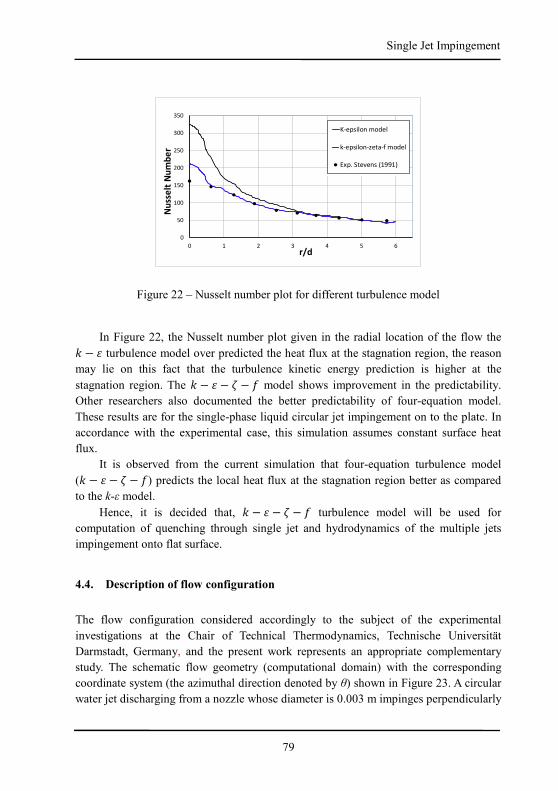
79


0

50

100

150

200

250

300

350

0 1 2 3 4 5 6

Nu

sse

lt N

um

be

r

r/d

K-epsilon model

k-epsilon-zeta-f model

Exp. Stevens (1991)

Figure 22 – Nusselt number plot for different turbulence model

In Figure 22, the Nusselt number plot given in the radial location of the flow the � − ä turbulence model over predicted the heat flux at the stagnation region, the reason

may lie on this fact that the turbulence kinetic energy prediction is higher at the

stagnation region. The � − ä − î − õ model shows improvement in the predictability.

Other researchers also documented the better predictability of four-equation model.

These results are for the single-phase liquid circular jet impingement on to the plate. In

accordance with the experimental case, this simulation assumes constant surface heat

flux.

It is observed from the current simulation that four-equation turbulence model

(� − ä − î − õ) predicts the local heat flux at the stagnation region better as compared

to the k-ε model.

Hence, it is decided that, � − ä − î − õ turbulence model will be used for

computation of quenching through single jet and hydrodynamics of the multiple jets

impingement onto flat surface.

4.4. Description of flow configuration

The flow configuration considered accordingly to the subject of the experimental

investigations at the Chair of Technical Thermodynamics, Technische Universität

Darmstadt, Germany, and the present work represents an appropriate complementary

study. The schematic flow geometry (computational domain) with the corresponding

coordinate system (the azimuthal direction denoted by θ) shown in Figure 23. A circular

water jet discharging from a nozzle whose diameter is 0.003 m impinges perpendicularly

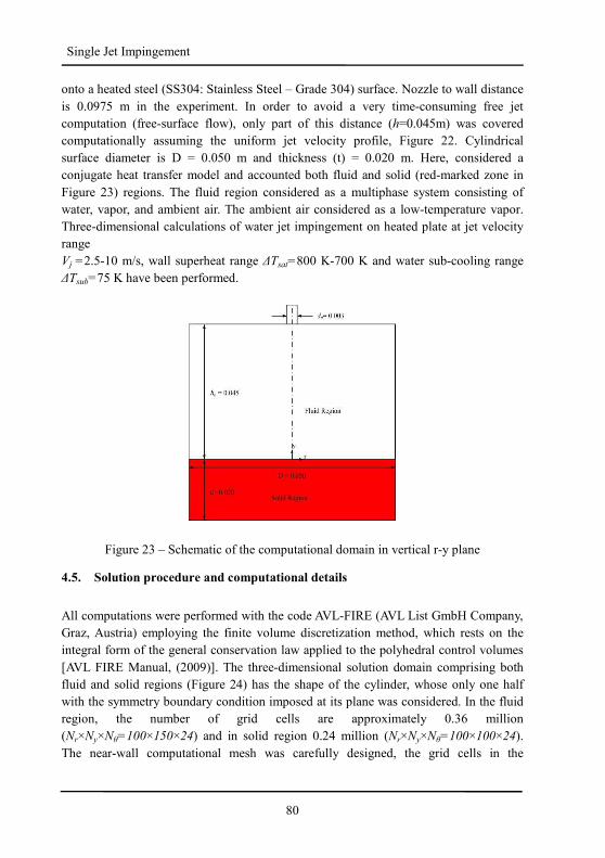
80


onto a heated steel (SS304: Stainless Steel – Grade 304) surface. Nozzle to wall distance

is 0.0975 m in the experiment. In order to avoid a very time-consuming free jet

computation (free-surface flow), only part of this distance (h=0.045m) was covered

computationally assuming the uniform jet velocity profile, Figure 22. Cylindrical

surface diameter is D = 0.050 m and thickness (t) = 0.020 m. Here, considered a

conjugate heat transfer model and accounted both fluid and solid (red-marked zone in

Figure 23) regions. The fluid region considered as a multiphase system consisting of

water, vapor, and ambient air. The ambient air considered as a low-temperature vapor.

Three-dimensional calculations of water jet impingement on heated plate at jet velocity

range

Vj =2.5-10 m/s, wall superheat range ∆Tsat=800 K-700 K and water sub-cooling range

∆Tsub=75 K have been performed.

Figure 23 – Schematic of the computational domain in vertical r-y plane

4.5. Solution procedure and computational details

All computations were performed with the code AVL-FIRE (AVL List GmbH Company,

Graz, Austria) employing the finite volume discretization method, which rests on the

integral form of the general conservation law applied to the polyhedral control volumes

[AVL FIRE Manual, (2009)]. The three-dimensional solution domain comprising both

fluid and solid regions (Figure 24) has the shape of the cylinder, whose only one half

with the symmetry boundary condition imposed at its plane was considered. In the fluid

region, the number of grid cells are approximately 0.36 million

(Nr×Ny×Nθ=100×150×24) and in solid region 0.24 million (Nr×Ny×Nθ=100×100×24).

The near-wall computational mesh was carefully designed, the grid cells in the

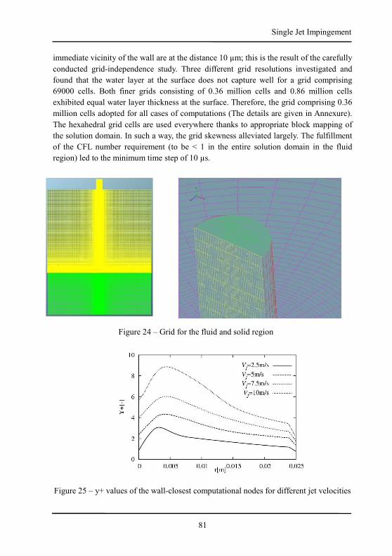
81


immediate vicinity of the wall are at the distance 10 µm; this is the result of the carefully

conducted grid-independence study. Three different grid resolutions investigated and

found that the water layer at the surface does not capture well for a grid comprising

69000 cells. Both finer grids consisting of 0.36 million cells and 0.86 million cells

exhibited equal water layer thickness at the surface. Therefore, the grid comprising 0.36

million cells adopted for all cases of computations (The details are given in Annexure).

The hexahedral grid cells are used everywhere thanks to appropriate block mapping of

the solution domain. In such a way, the grid skewness alleviated largely. The fulfillment

of the CFL number requirement (to be < 1 in the entire solution domain in the fluid

region) led to the minimum time step of 10 µs.

Figure 25 – y+ values of the wall-closest computational nodes for different jet velocities

Figure 24 – Grid for the fluid and solid region

82


The transport equations are discretized using the linear upwind scheme. Pressure and

velocity are coupled through the well-known SIMPLE algorithm.

For the calculation of the y+ value before the computation for generating the grid, ú�� is taken as 2-5% of the free jet velocity as suggested by ERCOFTAC (2000) guidelines.

The y+ value obtained at the first grid from the wall for the different jet velocities

(Figure 25) revealed some flow features. For the jet velocities of 2.5-5 m/s the grid

resolves the viscous sub-layer (hydro-dynamically), and for the higher jet velocities (7.5

m/s and 10 m/s the first grid cell at the vicinity of the surface are positioned somewhere

in the transition-layer. Due to multiphase flow at the stagnation region, the flow velocity

is higher for the jet velocities 7.5 and 10 m/s,

Separate computational domains constructed for the solid part (green part in

Figure 23) and the liquid domain are numerically coupled at the interface of the solid-

liquid boundary using the AVL-Code-Coupling-Interface (ACCI) feature. The advanced

ACCI procedure allows the information about the phase change rates in the liquid

domain to appear as cooling rates on the solid boundaries. Furthermore, one notes also

the same grid resolutions in the radial and azimuthal direction: Nr×Nθ (fluid) = 100×24

vs. Nr×Nθ (solid) = 100×24. The advantage of the AVL-Code-Connectivity feature is

used here to enable a smooth variable exchange.

4.6. Boundary Conditions

The following boundary conditions have been employed (see Figure 24 to follow the

coordinate directions better):

• Wall boundary conditions, r=0-R, y=0 for all θ

No-slip boundary Vk,j=0; T(r, t) prescribed

• Far-field boundaries, r=d/2-R, y=h

Atmospheric pressure prescribed

O(!,)Oµ = O#$%!,)Oµ = Oä!,)Oµ = 0

Far-field boundaries, r=R, 0<y <h

Atmospheric pressure prescribed

O(!,)O£ = O#$%!,)O£ = Oä!,)O£ = 0

Inlet boundary (jet), r=0-d/2, y=h

#$%!,) = −#$%�C)�� (prescribed)

83


Symmetry boundary, r=0, 0<y <h

O¢!,)O£ = O(!,)O£ = O#$%!,)O£ = Oä!,)O£ = O�!,)O£ = OõO£ = 0

The computations have been performed taking initially the uniform temperature of the

steel block being of cylindrical shape. The upper flat surface is the impinging surface.

The side-curved wall and the bottom surface of the solid part kept as adiabatic.

4.7. Results and Discussions

The understanding of the quenching through the liquid jet is enhanced through the

computational study. Since the initial temperature of the solid block is high, the vapour

generation is quite high. Hence, the vapour formation at the immediate vicinity of the

wall is computed and analysed through the corresponding boundary layer development

with respect to time and radial positions on the solid surface. After this, the influence of

the turbulent kinetic energy on the boundary layer and heat transfer rate is analysed. The

boiling curves are analysed at different jet velocities. The heat flux and surface

temperatures are compared with experimental investigations for different velocities with

respect to time. Furthermore, the boiling front propagations are analysed

computationally and compared with experimental investigations.

4.7.1. Study of boundary layer at the quenching surface

Numerical investigations of the quenching of heated flat surface revealed many essential

physics of flow. It is imperative to know the flow behavior at the surface before going

into details of the surface quenching.

The hydrodynamic study of quenching surface is vital from two aspects. First, it

provides valuable information to develop the quenching model and another it provides

supplementary data to perform the experimental investigations.

The boundary layer profiles at radial location R = 1.5 mm (radial location from the

center of the circular surface) of the flow are obtained (Figure 26) at three different

times (2.0s, 2.5s, and 3.0s). These times are computed from as the jet impinged on the

surface and started boiling.

After the jet impinged on the heated surface, the liquid starts boiling, and at 2s of the

boiling (solid line in Figure 25), a linear velocity gradient at the vicinity of the wall is

obtained, which implies the presence of vapor at the immediate vicinity of the heated

surface.

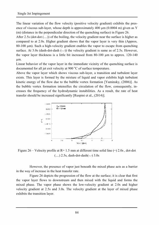
84


The linear variation of the flow velocity (positive velocity gradient) exhibits the pres-

ence of viscous sub-layer, whose depth is approximately 400 µm (0.0004 m) given as Y

(m) (distance in the perpendicular direction of the quenching surface) in Figure 26.

After 2.5s (dot-dot (....)) of the boiling, the velocity gradient near the surface is higher as

compared to at 2.0s. Higher gradient shows that the vapor layer is very thin (Approx.

80-100 µm). Such a high-velocity gradient enables the vapor to escape from quenching

surface. At 3.0s (dash-dot-dash (-.-)) the velocity gradient is same as of 2.5s. However,

the vapor layer thickness is a little bit increased from 80-100 µm to approx. 120-140

µm.

Linear behavior of the vapor layer in the immediate vicinity of the quenching surface is

documented for all jet exit velocity at 900 oC of surface temperature.

Above the vapor layer which shows viscous sub-layer, a transition and turbulent layer

exists. This layer is formed by the mixture of liquid and vapor exhibits high turbulent

kinetic energy of the flow due to the bubble vortex formation [Yaminsky, (2006)]. As

the bubble vortex formation intensifies the circulation of the flow, consequently, in-

creases the frequency of the hydrodynamic instabilities. As a result, the rate of heat

transfer should be increased significantly [Ruspini et al., (2014)].

Figure 26 – Velocity profile at R= 1.5 mm at different time solid line ( ) 2.0s , dot-dot

(....) 2.5s, dash-dot-dash(-.-) 3.0s

However, the presence of vapor just beneath the mixed phase acts as a barrier

in the way of increase in the heat transfer rate.

Figure 26 depicts the progression of the flow at the surface; it is clear that first

the vapor layer flows to downstream and then mixed with the liquid and forms the

mixed phase. The vapor phase shows the low-velocity gradient at 2.0s and higher

velocity gradient at 2.5s and 3.0s. The velocity gradient at the layer of mixed phase

exhibits the transition layer.

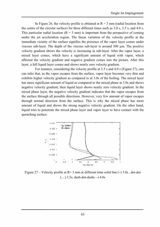
85


In Figure 26, the velocity profile is obtained at R = 3 mm (radial location from

the centre of the circular surface) for three different times such as 3.0 s, 3.5 s, and 4.0 s.

This particular radial location (R = 3 mm) is important from the perspective of coming

under the jet acceleration region. The linear variation of the velocity profile at the

immediate vicinity of the surface signifies the presence of the vapor layer comes under

viscous sub-layer. The depth of the viscous sub-layer is around 500 µm. The positive

velocity gradient shows the velocity is increasing in sub-layer. After the vapor layer, a

mixed layer comes, which have a significant amount of liquid with vapor, which

affected the velocity gradient and negative gradient comes into the picture. After this

layer, a full liquid layer comes and shows nearly zero velocity gradient.

For instance, considering the velocity profile at 3.5 s and 4.0 s (Figure 27), one

can infer that, as the vapor escapes from the surface, vapor layer becomes very thin and

exhibits higher velocity gradient as compared to at 3.0s of the boiling. The mixed layer

has more significant amount of liquid as compared to the mixed phase at 3.0s and shows

negative velocity gradient; then liquid layer shows nearly zero velocity gradient. In the

mixed phase layer, the negative velocity gradient indicates that the vapor escapes from

the surface through all possible directions. However, very few amount of vapor escapes

through normal direction from the surface. This is why the mixed phase has more

amount of liquid and shows the strong negative velocity gradient. On the other hand,

liquid tries to penetrate the mixed phase layer and vapor layer to have contact with the

quenching surface.

Figure 27 – Velocity profile at R= 3 mm at different time solid line ( ) 3.0s , dot-dot

(....) 3.5s, dash-dot-dash(-.-) 4.0s

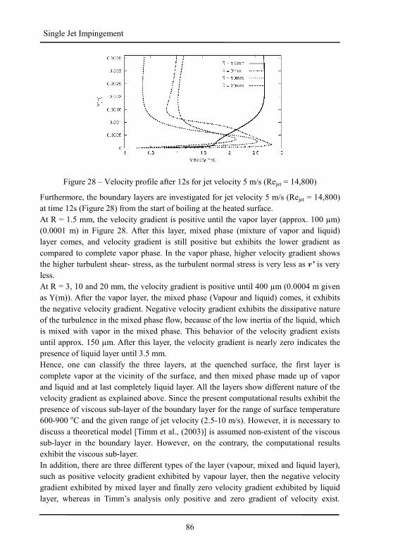
86


Figure 28 – Velocity profile after 12s for jet velocity 5 m/s (Rejet = 14,800)

Furthermore, the boundary layers are investigated for jet velocity 5 m/s (Rejet = 14,800)

at time 12s (Figure 28) from the start of boiling at the heated surface.

At R = 1.5 mm, the velocity gradient is positive until the vapor layer (approx. 100 µm)

(0.0001 m) in Figure 28. After this layer, mixed phase (mixture of vapor and liquid)

layer comes, and velocity gradient is still positive but exhibits the lower gradient as

compared to complete vapor phase. In the vapor phase, higher velocity gradient shows

the higher turbulent shear- stress, as the turbulent normal stress is very less as v’ is very

less.

At R = 3, 10 and 20 mm, the velocity gradient is positive until 400 µm (0.0004 m given

as Y(m)). After the vapor layer, the mixed phase (Vapour and liquid) comes, it exhibits

the negative velocity gradient. Negative velocity gradient exhibits the dissipative nature

of the turbulence in the mixed phase flow, because of the low inertia of the liquid, which

is mixed with vapor in the mixed phase. This behavior of the velocity gradient exists

until approx. 150 µm. After this layer, the velocity gradient is nearly zero indicates the

presence of liquid layer until 3.5 mm.

Hence, one can classify the three layers, at the quenched surface, the first layer is

complete vapor at the vicinity of the surface, and then mixed phase made up of vapor

and liquid and at last completely liquid layer. All the layers show different nature of the

velocity gradient as explained above. Since the present computational results exhibit the

presence of viscous sub-layer of the boundary layer for the range of surface temperature

600-900 oC and the given range of jet velocity (2.5-10 m/s). However, it is necessary to

discuss a theoretical model [Timm et al., (2003)] is assumed non-existent of the viscous

sub-layer in the boundary layer. However, on the contrary, the computational results

exhibit the viscous sub-layer.

In addition, there are three different types of the layer (vapour, mixed and liquid layer),

such as positive velocity gradient exhibited by vapour layer, then the negative velocity

gradient exhibited by mixed layer and finally zero velocity gradient exhibited by liquid

layer, whereas in Timm’s analysis only positive and zero gradient of velocity exist.

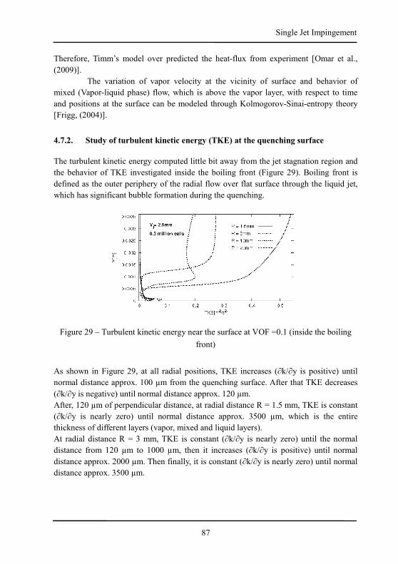
87


Therefore, Timm’s model over predicted the heat-flux from experiment [Omar et al.,

(2009)].

The variation of vapor velocity at the vicinity of surface and behavior of

mixed (Vapor-liquid phase) flow, which is above the vapor layer, with respect to time

and positions at the surface can be modeled through Kolmogorov-Sinai-entropy theory

[Frigg, (2004)].

4.7.2. Study of turbulent kinetic energy (TKE) at the quenching surface

The turbulent kinetic energy computed little bit away from the jet stagnation region and

the behavior of TKE investigated inside the boiling front (Figure 29). Boiling front is

defined as the outer periphery of the radial flow over flat surface through the liquid jet,

which has significant bubble formation during the quenching.

Figure 29 – Turbulent kinetic energy near the surface at VOF =0.1 (inside the boiling

front)

As shown in Figure 29, at all radial positions, TKE increases (∂k/∂y is positive) until

normal distance approx. 100 µm from the quenching surface. After that TKE decreases

(∂k/∂y is negative) until normal distance approx. 120 µm.

After, 120 µm of perpendicular distance, at radial distance R = 1.5 mm, TKE is constant

(∂k/∂y is nearly zero) until normal distance approx. 3500 µm, which is the entire

thickness of different layers (vapor, mixed and liquid layers).

At radial distance R = 3 mm, TKE is constant (∂k/∂y is nearly zero) until the normal

distance from 120 µm to 1000 µm, then it increases (∂k/∂y is positive) until normal

distance approx. 2000 µm. Then finally, it is constant (∂k/∂y is nearly zero) until normal

distance approx. 3500 µm.

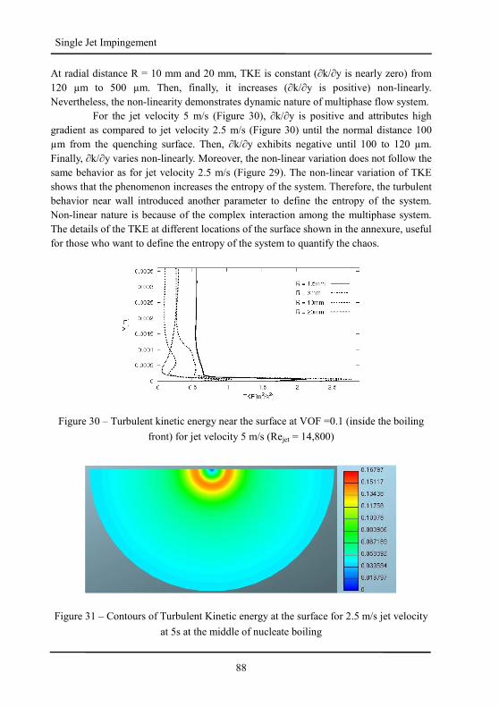
88


At radial distance R = 10 mm and 20 mm, TKE is constant (∂k/∂y is nearly zero) from

120 µm to 500 µm. Then, finally, it increases (∂k/∂y is positive) non-linearly.

Nevertheless, the non-linearity demonstrates dynamic nature of multiphase flow system.

For the jet velocity 5 m/s (Figure 30), ∂k/∂y is positive and attributes high

gradient as compared to jet velocity 2.5 m/s (Figure 30) until the normal distance 100

µm from the quenching surface. Then, ∂k/∂y exhibits negative until 100 to 120 µm.

Finally, ∂k/∂y varies non-linearly. Moreover, the non-linear variation does not follow the

same behavior as for jet velocity 2.5 m/s (Figure 29). The non-linear variation of TKE

shows that the phenomenon increases the entropy of the system. Therefore, the turbulent

behavior near wall introduced another parameter to define the entropy of the system.

Non-linear nature is because of the complex interaction among the multiphase system.

The details of the TKE at different locations of the surface shown in the annexure, useful

for those who want to define the entropy of the system to quantify the chaos.


front) for jet velocity 5 m/s (Rejet = 14,800)

Figure 31 – Contours of Turbulent Kinetic energy at the surface for 2.5 m/s jet velocity

at 5s at the middle of nucleate boiling

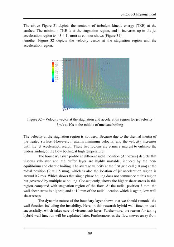
89


The above Figure 31 depicts the contours of turbulent kinetic energy (TKE) at the

surface. The minimum TKE is at the stagnation region, and it increases up to the jet

acceleration region (r ≈ 3-4.11 mm) as contour shows (Figure 31).

Another Figure 32 depicts the velocity vector at the stagnation region and the

acceleration region.

Figure 32 – Velocity vector at the stagnation and acceleration region for jet velocity

5m/s at 10s at the middle of nucleate boiling

The velocity at the stagnation region is not zero. Because due to the thermal inertia of

the heated surface. However, it attains minimum velocity, and the velocity increases

until the jet acceleration region. These two regions are primary interest to enhance the

understanding of the flow boiling at high temperature.

The boundary layer profile at different radial position (Annexure) depicts that

viscous sub-layer and the buffer layer are highly unstable, induced by the non-

equilibrium and chaotic boiling. The average velocity at the first grid cell (10 µm) at the

radial position (R = 1.5 mm), which is also the location of jet acceleration region is

around 0.7 m/s. Which shows that single phase boiling does not commence at this region

but governed by multiphase boiling. Consequently, shows the higher shear stress in this

region compared with stagnation region of the flow. At the radial position 3 mm, the

wall shear stress is highest, and at 10 mm of the radial location which is again, low wall

shear stress.

The dynamic nature of the boundary layer shows that we should remodel the

wall function including the instability. Here, in this research hybrid wall-function used

successfully, which takes care of viscous sub-layer. Furthermore, the reason for taking

hybrid wall function will be explained later. Furthermore, as the flow moves away from

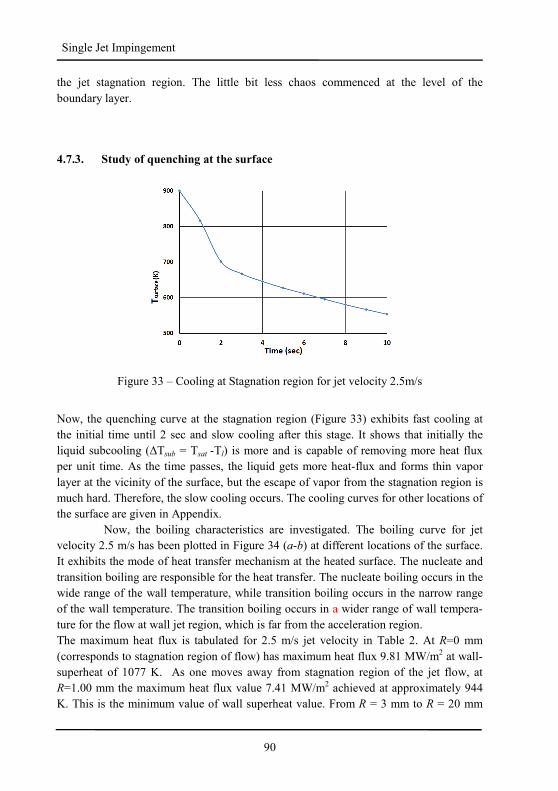
90


the jet stagnation region. The little bit less chaos commenced at the level of the

boundary layer.

4.7.3. Study of quenching at the surface

Figure 33 – Cooling at Stagnation region for jet velocity 2.5m/s

Now, the quenching curve at the stagnation region (Figure 33) exhibits fast cooling at

the initial time until 2 sec and slow cooling after this stage. It shows that initially the

liquid subcooling (∆Tsub = Tsat -Tl) is more and is capable of removing more heat flux

per unit time. As the time passes, the liquid gets more heat-flux and forms thin vapor

layer at the vicinity of the surface, but the escape of vapor from the stagnation region is

much hard. Therefore, the slow cooling occurs. The cooling curves for other locations of

the surface are given in Appendix.

Now, the boiling characteristics are investigated. The boiling curve for jet

velocity 2.5 m/s has been plotted in Figure 34 (a-b) at different locations of the surface.

It exhibits the mode of heat transfer mechanism at the heated surface. The nucleate and

transition boiling are responsible for the heat transfer. The nucleate boiling occurs in the

wide range of the wall temperature, while transition boiling occurs in the narrow range

of the wall temperature. The transition boiling occurs in a wider range of wall tempera-

ture for the flow at wall jet region, which is far from the acceleration region.

The maximum heat flux is tabulated for 2.5 m/s jet velocity in Table 2. At R=0 mm

(corresponds to stagnation region of flow) has maximum heat flux 9.81 MW/m2 at wall-

superheat of 1077 K. As one moves away from stagnation region of the jet flow, at

R=1.00 mm the maximum heat flux value 7.41 MW/m2 achieved at approximately 944

K. This is the minimum value of wall superheat value. From R = 3 mm to R = 20 mm

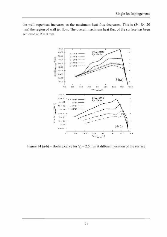
91


the wall superheat increases as the maximum heat flux decreases. This is (3< R< 20

mm) the region of wall jet flow. The overall maximum heat flux of the surface has been

achieved at R = 0 mm.

Figure 34 (a-b) – Boiling curve for Vj = 2.5 m/s at different location of the surface

34(a)

34(b)

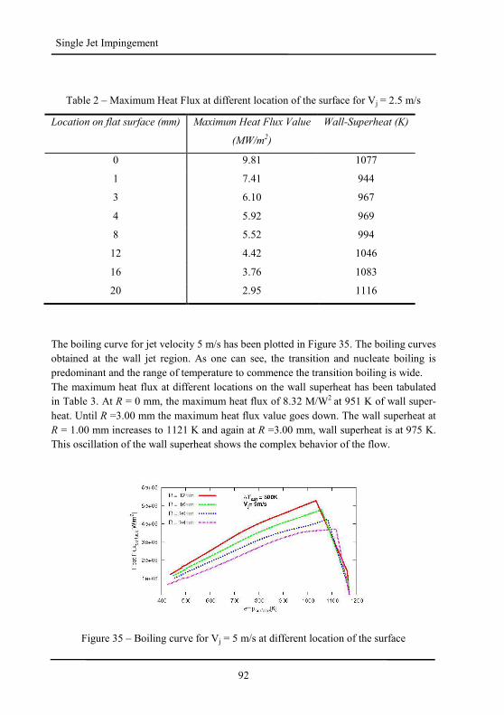
92


Table 2 – Maximum Heat Flux at different location of the surface for Vj = 2.5 m/s

Location on flat surface (mm) Maximum Heat Flux Value

(MW/m2)

Wall-Superheat (K)

0 9.81 1077

1 7.41 944

3 6.10 967

4 5.92 969

8 5.52 994

12 4.42 1046

16 3.76 1083

20 2.95 1116

The boiling curve for jet velocity 5 m/s has been plotted in Figure 35. The boiling curves

obtained at the wall jet region. As one can see, the transition and nucleate boiling is

predominant and the range of temperature to commence the transition boiling is wide.

The maximum heat flux at different locations on the wall superheat has been tabulated

in Table 3. At R = 0 mm, the maximum heat flux of 8.32 M/W2 at 951 K of wall super-

heat. Until R =3.00 mm the maximum heat flux value goes down. The wall superheat at

R = 1.00 mm increases to 1121 K and again at R =3.00 mm, wall superheat is at 975 K.

This oscillation of the wall superheat shows the complex behavior of the flow.

Figure 35 – Boiling curve for Vj = 5 m/s at different location of the surface

93


Table 3 – Maximum Heat Flux at different location of the surface for Vj = 5 m/s

Location on

flat surface

(mm)

Maximum Heat Flux Value (MW/m2) Wall-Superheat (K)

0 8.32 951

1 7.23 1121

3 6.91 975

4 7.13 968

8 6.07 1002

12 5.27 1035

16 4.78 1058

20 4.25 1082

24 3.72 1117

At R = 4 mm, the maximum heat flux get the value 7.13 MW/m2 at 968 K wall super-

heat. Now, from R = 4 mm to 24 mm, the maximum wall heat flux goes down, and wall

superheat increases.

The boiling curve for jet velocity 7.5 m/s has been plotted in Figure 36. On the other

hand, for jet velocity 7.5 m/s, again the range of temperature to occur the transition

boiling at the wall jet region becomes narrow as compared to the jet velocity 2.5 m/s and

5 m/s. It indicates the influence of the jet velocity on the transition boiling.

The maximum heat flux has been tabulated in Table 4. At R = 0.00 mm the maximum

heat flux 8.77 MW/m2 has been attained at 1086 K of wall superheat. At R = 1.00 mm

the decrement of the maximum heat flux 7.49 MW/m2 and wall superheat 1099 K has

been registered. At R = 2.00 mm to 4.10 mm wall heat flux increases. From R = 4.10

mm to 20.00 mm the wall heat flux decreases.

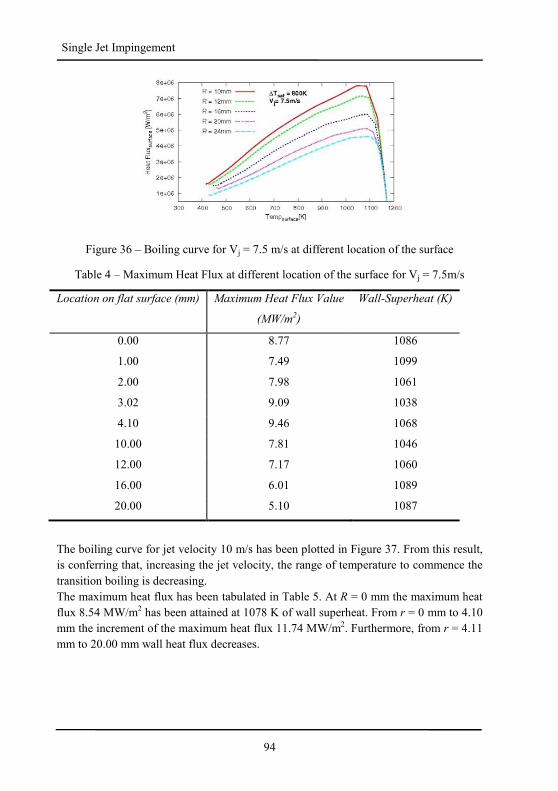
94


Figure 36 – Boiling curve for Vj = 7.5 m/s at different location of the surface

Table 4 – Maximum Heat Flux at different location of the surface for Vj = 7.5m/s


(MW/m2)

Wall-Superheat (K)

0.00 8.77 1086

1.00 7.49 1099

2.00 7.98 1061

3.02 9.09 1038

4.10 9.46 1068

10.00 7.81 1046

12.00 7.17 1060

16.00 6.01 1089

20.00 5.10 1087

The boiling curve for jet velocity 10 m/s has been plotted in Figure 37. From this result,

is conferring that, increasing the jet velocity, the range of temperature to commence the

transition boiling is decreasing.

The maximum heat flux has been tabulated in Table 5. At R = 0 mm the maximum heat

flux 8.54 MW/m2 has been attained at 1078 K of wall superheat. From r = 0 mm to 4.10

mm the increment of the maximum heat flux 11.74 MW/m2. Furthermore, from r = 4.11

mm to 20.00 mm wall heat flux decreases.

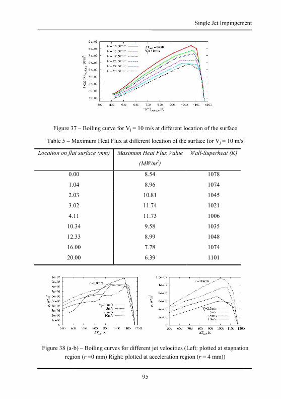
95


Figure 37 – Boiling curve for Vj = 10 m/s at different location of the surface

Table 5 – Maximum Heat Flux at different location of the surface for Vj = 10 m/s


(MW/m2)

Wall-Superheat (K)

0.00 8.54 1078

1.04 8.96 1074

2.03 10.81 1045

3.02 11.74 1021

4.11 11.73 1006

10.34 9.58 1035

12.33 8.99 1048

16.00 7.78 1074

20.00 6.39 1101

Figure 38 (a-b) – Boiling curves for different jet velocities (Left: plotted at stagnation

region (r =0 mm) Right: plotted at acceleration region (r = 4 mm))

96


The effect of the flow velocity can be seen in the boiling curve in Figure 38 (a-b). As the

velocity of the jet increases, the heated surface liberates more amount of heat flux.

The influence of the jet velocity on the boiling curve shows the heat transfer mechanism

at the heated surface. Transition boiling and nucleate boiling play a pivotal role for the

heat-flux extraction mechanism. In this simulation, sub-cooling of the liquid is 75 K and

the jet Reynolds number varies from (7400 to 30000 approx.). The published experi-

mental results [Islam et al (2008)] shows that for liquid sub-cooling more than 55 K and

high velocity of the jet, the formation of the stable vapor layer at the immediate vicinity

of the heated surface are not possible. Rather than the explosive pattern has been seen

just after the impact of the liquid jet until few millisecond of the flow. Due to the transi-

ent boiling characteristic, the heat flux for jet velocity 2.5 m/s at r = 0 mm is 9.81

MW/m2 for the wall superheat 1077 K. While for higher velocity of the jet at 5, 7.5 and

10 m/s the heat flux are 8.32, 8.77 and 8.54 MW/m2 and wall superheat are 951 K, 1086

K and 1078 K respectively. This can be explained by the residence time of the liquid at

stagnation region and corresponding boiling behavior. For the low velocity of the jet, for

the certain control volume of the liquid which passes through the stagnation region of

the flow will stay longer and takes heat flux from the surface and formation of a large

number of vapor bubbles and heat transfer mechanism at boiling may lead to higher heat

flux. On the other hand, for higher velocity, the residence time for the same control

volume of the liquid will decrease and corresponding heat transfer mechanism may lead

to different thermal diffusivity. It is still hard to say which is more dominant the resi-

dence time of the liquid control volume or the formation of a bubble at certain wall

superheat. Furthermore, this hypothesis can be validated through the high precision

experiment.

As the flow move away from the location r = 0 mm, for the jet velocity 2.5 m/s, the

maximum heat flux goes down and the corresponding wall superheat increases as shown

in Table 2. This can be explained by again with a residence time of the certain liquid

control volume. Due to the higher residence time of moving control volume, the liquid

temperature will attain the saturation temperature in less time. Therefore, the liquid is

not capable of extracting higher heat flux than heat flux at r = 0 mm. At this velocity of

the jet, the boiling heat transfer is more pronounced by the sub-cooling of the liquid.

For the jet velocity 5 m/s, the decrement of the heat flux has been registered

from r = 0 mm to 3.00 mm, at r= 4 mm the heat flux again get little bit higher value

approximately 7.13 MW/m2. From r = 4.00 mm to 24.00 mm, the heat flux decreases. At

this velocity of the jet, the effect of the flow velocity on the heat flux has been seen. It

can be said that the stagnation region span around r = 0 to 3.00 mm and the jet accelera-

tion region from 3.00 mm to 4.00 mm. At the jet acceleration region, the thermal diffu-

sivity gets higher value, capable of extracting the higher heat flux value than the heat

flux at r = 1.00 mm and 3.00 mm. However, still the heat flux at R = 0 mm is higher

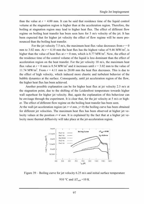
97


than the value at r = 4.00 mm. It can be said that residence time of the liquid control

volume at the stagnation region is higher than at the acceleration region. Therefore, the

boiling at stagnation region may lead to higher heat flux. The effect of different flow

regime on boiling heat transfer has been seen here for 5 m/s velocity of the jet. It has

been expected that for higher jet velocity the effect of flow regime will be more pro-

nounced than the boiling heat transfer.

For the jet velocity 7.5 m/s, the maximum heat flux value decreases from r = 0

mm to 3.02 mm. At r = 4.10 mm the heat flux has the highest value of 9.46 MW/m2, is

higher than the value of heat flux at r = 0 mm, which is 8.77 MW/m2. Now, the effect of

the residence time of the control volume of the liquid is less dominant than the effect of

acceleration region on the heat transfer. For the jet velocity 10 m/s, the maximum heat

flux value at r = 0 mm is 8.54 MW/m2 and it increases until r = 3.02 mm to the value of

11.74 MW/m2. From r = 4.11 mm to 20.00 mm the heat flux decreases. This is due to

the effect of high velocity, which induced more chaotic and turbulent behavior of the

bubble dynamics at the surface. Consequently, until jet acceleration region of the flow,

the higher heat flux has been achieved.

Another possible explanation can be for higher heat flux at jet velocity 2.5 m/s at

the stagnation point, due to the shifting of the Leidenfrost temperature towards higher

wall superheat for higher jet velocity. But, again the explanation of this behaviour can

be envisage through the experiment. It is clear that, for the jet velocity at 5 m/s or high-

er. The effect of different flow regime on the boiling heat transfer has been seen.

At the wall-jet acceleration region (at r=4 mm, y=0) the boiling curve has been obtained

for different jet velocities. The maximum heat flux has been observed at higher jet ve-

locity values at the position r=4 mm. It is explained by the fact that at a higher jet ve-

locity more thermal diffusivity will take place at the jet-acceleration region.

Figure 39 – Boiling curve for jet velocity 6.25 m/s and initial surface temperature

910 °C and ∆Tsub =10 K

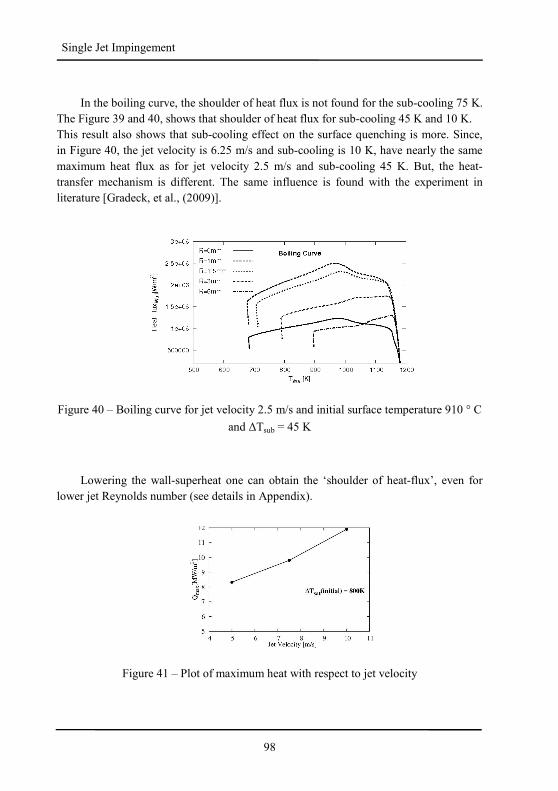
98


In the boiling curve, the shoulder of heat flux is not found for the sub-cooling 75 K.

The Figure 39 and 40, shows that shoulder of heat flux for sub-cooling 45 K and 10 K.

This result also shows that sub-cooling effect on the surface quenching is more. Since,

in Figure 40, the jet velocity is 6.25 m/s and sub-cooling is 10 K, have nearly the same

maximum heat flux as for jet velocity 2.5 m/s and sub-cooling 45 K. But, the heat-

transfer mechanism is different. The same influence is found with the experiment in

literature [Gradeck, et al., (2009)].

Figure 40 – Boiling curve for jet velocity 2.5 m/s and initial surface temperature 910 ° C

and ∆Tsub = 45 K

Lowering the wall-superheat one can obtain the ‘shoulder of heat-flux’, even for

lower jet Reynolds number (see details in Appendix).

Figure 41 – Plot of maximum heat with respect to jet velocity

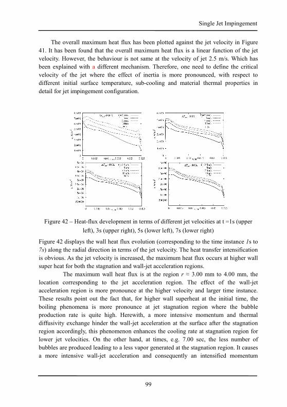
99


The overall maximum heat flux has been plotted against the jet velocity in Figure

41. It has been found that the overall maximum heat flux is a linear function of the jet

velocity. However, the behaviour is not same at the velocity of jet 2.5 m/s. Which has

been explained with a different mechanism. Therefore, one need to define the critical

velocity of the jet where the effect of inertia is more pronounced, with respect to

different initial surface temperature, sub-cooling and material thermal properties in

detail for jet impingement configuration.

Figure 42 – Heat-flux development in terms of different jet velocities at t =1s (upper

left), 3s (upper right), 5s (lower left), 7s (lower right)

Figure 42 displays the wall heat flux evolution (corresponding to the time instance 1s to

7s) along the radial direction in terms of the jet velocity. The heat transfer intensification

is obvious. As the jet velocity is increased, the maximum heat flux occurs at higher wall

super heat for both the stagnation and wall-jet acceleration regions.

The maximum wall heat flux is at the region r ≈ 3.00 mm to 4.00 mm, the

location corresponding to the jet acceleration region. The effect of the wall-jet

acceleration region is more pronounce at the higher velocity and larger time instance.

These results point out the fact that, for higher wall superheat at the initial time, the

boiling phenomena is more pronounce at jet stagnation region where the bubble

production rate is quite high. Herewith, a more intensive momentum and thermal

diffusivity exchange hinder the wall-jet acceleration at the surface after the stagnation

region accordingly, this phenomenon enhances the cooling rate at stagnation region for

lower jet velocities. On the other hand, at times, e.g. 7.00 sec, the less number of

bubbles are produced leading to a less vapor generated at the stagnation region. It causes

a more intensive wall-jet acceleration and consequently an intensified momentum

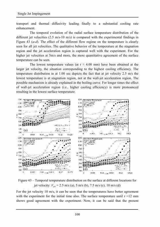
100


transport and thermal diffusivity leading finally to a substantial cooling rate

enhancement.

The temporal evolution of the radial surface temperature distribution of the

different jet velocities (2.5 m/s-10 m/s) is compared with the experimental findings in

Figure 43 (a-d). The effect of the different flow regime on the temperature is clearly

seen for all jet velocities. The qualitative behavior of the temperature at the stagnation

region and the jet acceleration region is captured well with the experiment. For the

higher jet velocities at 5m/s and more, the more quantitative agreement of the surface

temperature can be seen.

The lowest temperature values (at r ≈ 4.00 mm) have been obtained at the

larger jet velocity, the situation corresponding to the highest cooling efficiency. The

temperature distribution in at 1.00 sec depicts the fact that at jet velocity 2.5 m/s the

lowest temperature is at stagnation region, not at the wall-jet acceleration region. The

possible mechanism is already explained in the boiling curve. For longer times the effect

of wall-jet acceleration region (i.e., higher cooling efficiency) is more pronounced

resulting in the lowest surface temperature.

Figure 43 – Temporal temperature distribution on the surface at different locations for

jet velocity: Vjet = 2.5 m/s (a), 5 m/s (b), 7.5 m/s (c), 10 m/s (d)

For the jet velocity 10 m/s, it can be seen that the temperatures have better agreement

with the experiment for the initial time also. The surface temperature until r ≈12 mm

shows good agreement with the experiment. Now, it can be said that the present

(a) (b)

(c) (d)

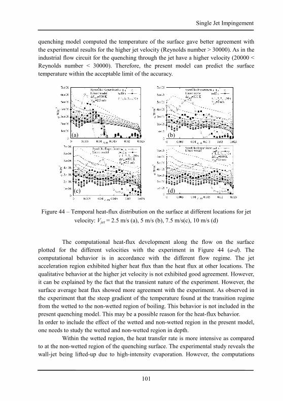
101


quenching model computed the temperature of the surface gave better agreement with

the experimental results for the higher jet velocity (Reynolds number > 30000). As in the

industrial flow circuit for the quenching through the jet have a higher velocity (20000 <

Reynolds number < 30000). Therefore, the present model can predict the surface

temperature within the acceptable limit of the accuracy.

Figure 44 – Temporal heat-flux distribution on the surface at different locations for jet

velocity: Vjet = 2.5 m/s (a), 5 m/s (b), 7.5 m/s(c), 10 m/s (d)

The computational heat-flux development along the flow on the surface

plotted for the different velocities with the experiment in Figure 44 (a-d). The

computational behavior is in accordance with the different flow regime. The jet

acceleration region exhibited higher heat flux than the heat flux at other locations. The

qualitative behavior at the higher jet velocity is not exhibited good agreement. However,

it can be explained by the fact that the transient nature of the experiment. However, the

surface average heat flux showed more agreement with the experiment. As observed in

the experiment that the steep gradient of the temperature found at the transition regime

from the wetted to the non-wetted region of boiling. This behavior is not included in the

present quenching model. This may be a possible reason for the heat-flux behavior.

In order to include the effect of the wetted and non-wetted region in the present model,

one needs to study the wetted and non-wetted region in depth.

Within the wetted region, the heat transfer rate is more intensive as compared

to at the non-wetted region of the quenching surface. The experimental study reveals the

wall-jet being lifted-up due to high-intensity evaporation. However, the computations

(c) (d)

(b) (a)

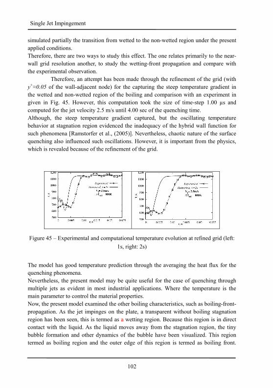
102


simulated partially the transition from wetted to the non-wetted region under the present

applied conditions.

Therefore, there are two ways to study this effect. The one relates primarily to the near-

wall grid resolution another, to study the wetting-front propagation and compare with

the experimental observation.

Therefore, an attempt has been made through the refinement of the grid (with

y+≈0.05 of the wall-adjacent node) for the capturing the steep temperature gradient in

the wetted and non-wetted region of the boiling and comparison with an experiment in

given in Fig. 45. However, this computation took the size of time-step 1.00 µs and

computed for the jet velocity 2.5 m/s until 4.00 sec of the quenching time.

Although, the steep temperature gradient captured, but the oscillating temperature

behavior at stagnation region evidenced the inadequacy of the hybrid wall function for

such phenomena [Ramstorfer et al., (2005)]. Nevertheless, chaotic nature of the surface

quenching also influenced such oscillations. However, it is important from the physics,

which is revealed because of the refinement of the grid.

Figure 45 – Experimental and computational temperature evolution at refined grid (left:

1s, right: 2s)

The model has good temperature prediction through the averaging the heat flux for the

quenching phenomena.

Nevertheless, the present model may be quite useful for the case of quenching through

multiple jets as evident in most industrial applications. Where the temperature is the

main parameter to control the material properties.

Now, the present model examined the other boiling characteristics, such as boiling-front-

propagation. As the jet impinges on the plate, a transparent without boiling stagnation

region has been seen, this is termed as a wetting region. Because this region is in direct

contact with the liquid. As the liquid moves away from the stagnation region, the tiny

bubble formation and other dynamics of the bubble have been visualized. This region

termed as boiling region and the outer edge of this region is termed as boiling front.

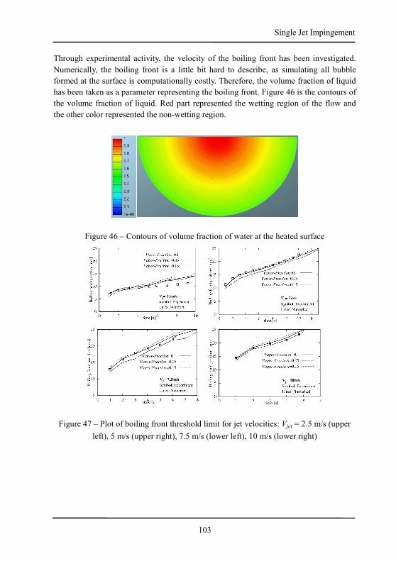
103


Through experimental activity, the velocity of the boiling front has been investigated.

Numerically, the boiling front is a little bit hard to describe, as simulating all bubble

formed at the surface is computationally costly. Therefore, the volume fraction of liquid

has been taken as a parameter representing the boiling front. Figure 46 is the contours of

the volume fraction of liquid. Red part represented the wetting region of the flow and

the other color represented the non-wetting region.

Figure 46 – Contours of volume fraction of water at the heated surface

Figure 47 – Plot of boiling front threshold limit for jet velocities: Vjet = 2.5 m/s (upper

left), 5 m/s (upper right), 7.5 m/s (lower left), 10 m/s (lower right)

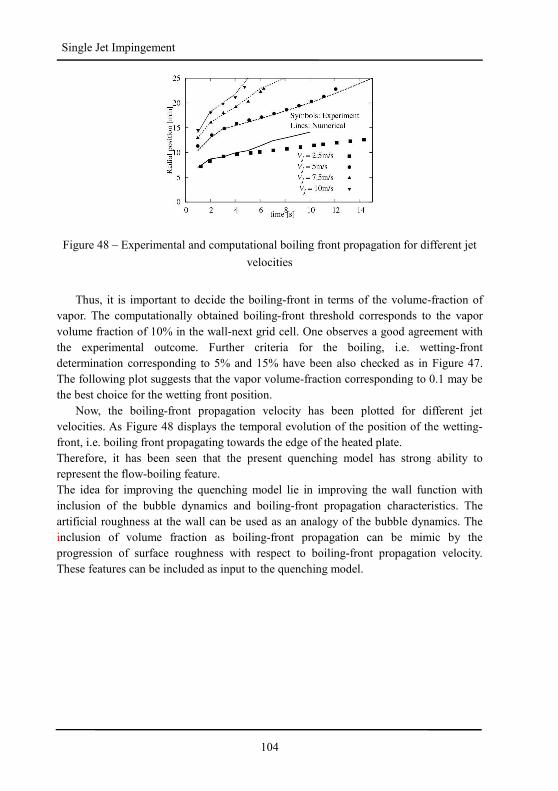
104


Figure 48 – Experimental and computational boiling front propagation for different jet

velocities

Thus, it is important to decide the boiling-front in terms of the volume-fraction of

vapor. The computationally obtained boiling-front threshold corresponds to the vapor

volume fraction of 10% in the wall-next grid cell. One observes a good agreement with

the experimental outcome. Further criteria for the boiling, i.e. wetting-front

determination corresponding to 5% and 15% have been also checked as in Figure 47.

The following plot suggests that the vapor volume-fraction corresponding to 0.1 may be

the best choice for the wetting front position.

Now, the boiling-front propagation velocity has been plotted for different jet

velocities. As Figure 48 displays the temporal evolution of the position of the wetting-

front, i.e. boiling front propagating towards the edge of the heated plate.

Therefore, it has been seen that the present quenching model has strong ability to

represent the flow-boiling feature.

The idea for improving the quenching model lie in improving the wall function with

inclusion of the bubble dynamics and boiling-front propagation characteristics. The

artificial roughness at the wall can be used as an analogy of the bubble dynamics. The

inclusion of volume fraction as boiling-front propagation can be mimic by the

progression of surface roughness with respect to boiling-front propagation velocity.

These features can be included as input to the quenching model.

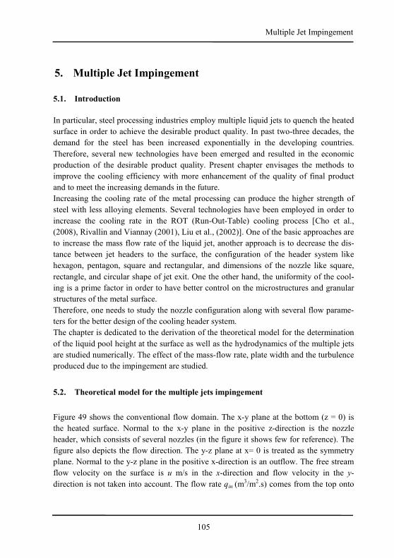
105

Multiple Jet Impingement

5. Multiple Jet Impingement

5.1. Introduction

In particular, steel processing industries employ multiple liquid jets to quench the heated

surface in order to achieve the desirable product quality. In past two-three decades, the

demand for the steel has been increased exponentially in the developing countries.

Therefore, several new technologies have been emerged and resulted in the economic

production of the desirable product quality. Present chapter envisages the methods to

improve the cooling efficiency with more enhancement of the quality of final product

and to meet the increasing demands in the future.

Increasing the cooling rate of the metal processing can produce the higher strength of

steel with less alloying elements. Several technologies have been employed in order to

increase the cooling rate in the ROT (Run-Out-Table) cooling process [Cho et al.,

(2008), Rivallin and Viannay (2001), Liu et al., (2002)]. One of the basic approaches are

to increase the mass flow rate of the liquid jet, another approach is to decrease the dis-

tance between jet headers to the surface, the configuration of the header system like

hexagon, pentagon, square and rectangular, and dimensions of the nozzle like square,

rectangle, and circular shape of jet exit. One the other hand, the uniformity of the cool-

ing is a prime factor in order to have better control on the microstructures and granular

structures of the metal surface.

Therefore, one needs to study the nozzle configuration along with several flow parame-

ters for the better design of the cooling header system.

The chapter is dedicated to the derivation of the theoretical model for the determination

of the liquid pool height at the surface as well as the hydrodynamics of the multiple jets

are studied numerically. The effect of the mass-flow rate, plate width and the turbulence

produced due to the impingement are studied.

5.2. Theoretical model for the multiple jets impingement

Figure 49 shows the conventional flow domain. The x-y plane at the bottom (z = 0) is

the heated surface. Normal to the x-y plane in the positive z-direction is the nozzle

header, which consists of several nozzles (in the figure it shows few for reference). The

figure also depicts the flow direction. The y-z plane at x= 0 is treated as the symmetry

plane. Normal to the y-z plane in the positive x-direction is an outflow. The free stream

flow velocity on the surface is u m/s in the x-direction and flow velocity in the y-

direction is not taken into account. The flow rate qin (m3/m2.s) comes from the top onto

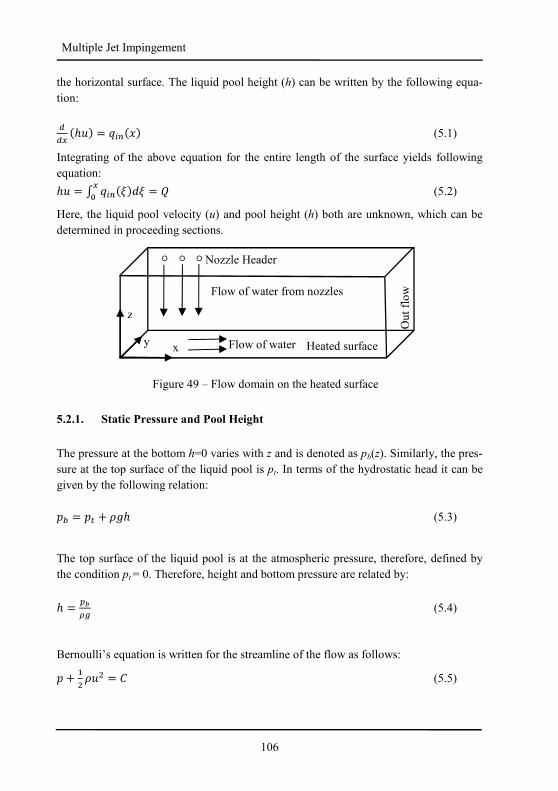
106


the horizontal surface. The liquid pool height (h) can be written by the following equa-

tion:

��C �ℎú� = )Ò�´� (5.1)

Integrating of the above equation for the entire length of the surface yields following

equation: ℎú = ¸ )Ò�P�±P = ÕC> (5.2)

Here, the liquid pool velocity (u) and pool height (h) both are unknown, which can be

determined in proceeding sections.

5.2.1. Static Pressure and Pool Height

The pressure at the bottom h=0 varies with z and is denoted as pb(z). Similarly, the pres-

sure at the top surface of the liquid pool is pt. In terms of the hydrostatic head it can be

given by the following relation:

æ¯ = æ� + (Qℎ (5.3)

The top surface of the liquid pool is at the atmospheric pressure, therefore, defined by

the condition pt = 0. Therefore, height and bottom pressure are related by:

ℎ = KO� (5.4)

Bernoulli’s equation is written for the streamline of the flow as follows:

æ + �D (úD = � (5.5)

Flow of water from nozzles

z

x y Flow of water

Nozzle Header

Heated surface

Out

flo

w

Figure 49 – Flow domain on the heated surface

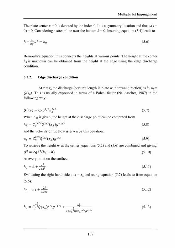
107


The plate center x = 0 is denoted by the index 0. It is a symmetry location and thus u(x =

0) = 0. Considering a streamline near the bottom h = 0. Inserting equation (5.4) leads to

ℎ + �D� úD = ℎ> (5.6)

Bernoulli’s equation thus connects the heights at various points. The height at the center

h0 is unknown can be obtained from the height at the edge using the edge discharge

condition.

5.2.2. Edge discharge condition

At x = xE the discharge (per unit length in plate withdrawal direction) is hE uE =

Q(xE). This is usually expressed in terms of a Poleni factor (Naudascher, 1987) in the

following way:

Õ�´R� = ��Q�/DℎR�/D (5.7)

When CD is given, the height at the discharge point can be computed from

ℎR = ��9D/�ÕD/��´R�Q9�/� (5.8)

and the velocity of the flow is given by this equation:

úR = ��D/�Õ�/��´R�Q�/� (5.9)

To retrieve the height h0 at the center, equations (5.2) and (5.6) are combined and giving

ÕD = 2QℎD�ℎ> − ℎ� (5.10)

At every point on the surface:

ℎ> = ℎ + ØyD�Iy (5.11)

Evaluating the right-hand side at x = xE and using equation (5.7) leads to from equation

(5.6):

ℎ> = ℎR + ØSyD�ISy (5.12)

ℎ> = ��9y{Õ�´R�D/�Q9�/� + ØSy

D��T@u{Ø�CS�u/{�@y/{ (5.13)

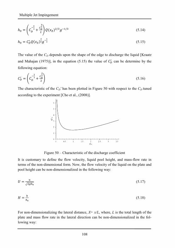
108


ℎ> = U��9y{ + �Tu{D VÕ�´R�D/�Q9�/� (5.14)

ℎ> = ��B Õ�´R�y{Q9o{ (5.15)

The value of the CD depends upon the shape of the edge to discharge the liquid [Kraatz

and Mahajan (1975)], in the equation (5.15) the value of ��B can be determine by the

following equation:

��B = U��9y{ + �Tu{D V (5.16)

The characteristic of the CD' has been plotted in Figure 50 with respect to the CD tuned

according to the experiment [Cho et al., (2008)].

Figure 50 – Characteristic of the discharge coefficient

It is customary to define the flow velocity, liquid pool height, and mass-flow rate in

terms of the non-dimensional form. Now, the flow velocity of the liquid on the plate and

pool height can be non-dimensionalized in the following way:

' = �&D�I� (5.17)

� = II� (5.18)

For non-dimensionalizing the lateral distance, X= x/L, where, L is the total length of the

plate and mass flow rate in the lateral direction can be non-dimensionalized in the fol-

lowing way:

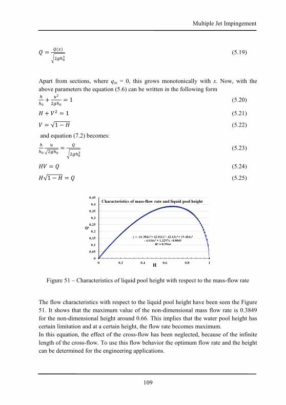
109


Õ = Ø�C�WD�I�{

(5.19)

Apart from sections, where qin = 0, this grows monotonically with x. Now, with the

above parameters the equation (5.6) can be written in the following form II� + �yD�I� = 1 (5.20)

� + #D = 1 (5.21)

# = √1 − � (5.22)

and equation (7.2) becomes:

II��

&D�I� = ØWD�I�{

(5.23)

�# = Õ (5.24)

�√1 − � = Õ (5.25)

Figure 51 – Characteristics of liquid pool height with respect to the mass-flow rate

The flow characteristics with respect to the liquid pool height have been seen the Figure

51. It shows that the maximum value of the non-dimensional mass flow rate is 0.3849

for the non-dimensional height around 0.66. This implies that the water pool height has

certain limitation and at a certain height, the flow rate becomes maximum.

In this equation, the effect of the cross-flow has been neglected, because of the infinite

length of the cross-flow. To use this flow behavior the optimum flow rate and the height

can be determined for the engineering applications.

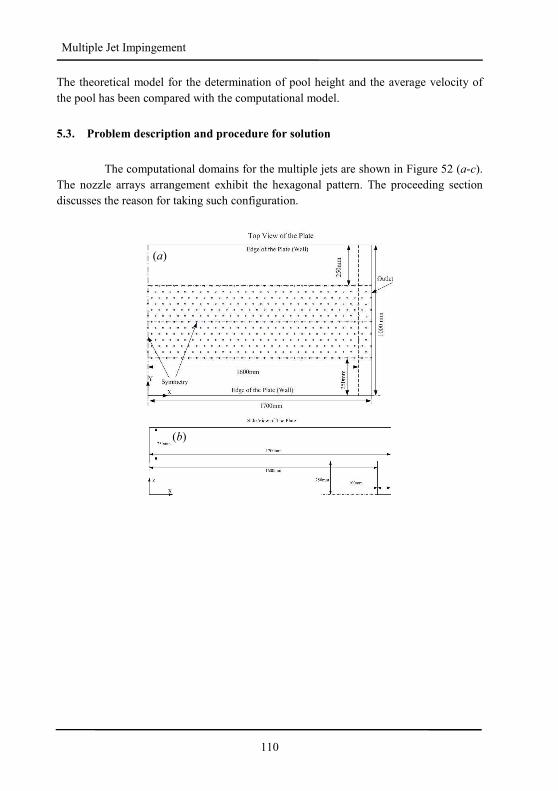
110


The theoretical model for the determination of pool height and the average velocity of

the pool has been compared with the computational model.

5.3. Problem description and procedure for solution

The computational domains for the multiple jets are shown in Figure 52 (a-c).

The nozzle arrays arrangement exhibit the hexagonal pattern. The proceeding section

discusses the reason for taking such configuration.

(a)

(b)

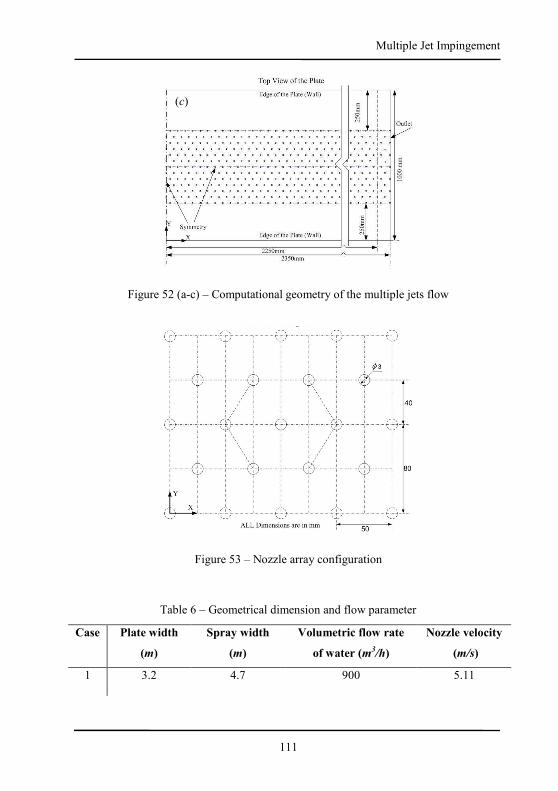
111


Figure 52 (a-c) – Computational geometry of the multiple jets flow

Figure 53 – Nozzle array configuration

Table 6 – Geometrical dimension and flow parameter

Case Plate width

(m)

Spray width

(m)

Volumetric flow rate

of water (m3/h)

Nozzle velocity

(m/s)

1 3.2 4.7 900 5.11

(c)

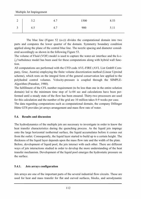
112


2 3.2 4.7 1500 8.53

3 4.5 4.7 900 5.11

The blue line (Figure 52 (a-c)) divides the computational domain into two

parts and computes the lower quarter of the domain. Symmetry boundary condition

applied along the plane of the central blue line. The nozzle spacing and diameter consid-

ered accordingly as shown in the following Figure 53.

The volume of Fluid (VOF) model is used to capture the water-air interface and the k-ε-

ζ-f turbulence model has been used for these computations along with hybrid wall func-

tion.

All computations are performed with the CFD code AVL-FIRE (AVL List GmbH Com-

pany, Graz, Austria) employing the finite volume discretization method (Linear Upwind

scheme), which rests on the integral form of the general conservation law applied to the

polyhedral control volumes. Velocity-pressure is coupled through the SIMPLE-

Algorithm (Patanker, 1980).

The fulfillment of the CFL number requirement (to be less than one in the entire solution

domain) led to the minimum time step of 1e-04 sec and calculations have been per-

formed until a steady state of the flow has been ensured. Thirty-two processors are used

for this calculation and the number of the grid are 10 million takes 8-9 weeks per case.

The data regarding computations such as computational domain, the company Dillinger

Hütte GTS provides jet arrays arrangement and mass flow rate of water.

5.4. Results and discussion

The hydrodynamics of the multiple jets are necessary to investigate in order to know the

heat transfer characteristics during the quenching process. As the liquid jets impinge

onto the large horizontal isothermal surface, the liquid accumulates before it comes out

from the outlet. Consequently, the liquid layer started to build up to a certain height. The

thickness of the liquid layer depends upon the mass flow rate and the width of the plate.

Before, development of liquid pool, the jets interact with each other. There are different

ways of jets interactions studied in order to develop the more understanding of the heat

transfer mechanism. Development of the liquid pool emerges the hydrostatic pressure on

the surface.

5.4.1. Jets arrays configuration

Jets arrays are one of the important parts of the several industrial flow circuits. These are

used for heat and mass transfer for flat and curved surfaces, blocks, and aerodynamic

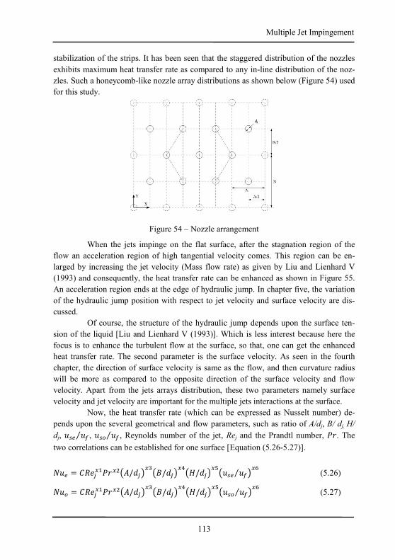
113


stabilization of the strips. It has been seen that the staggered distribution of the nozzles

exhibits maximum heat transfer rate as compared to any in-line distribution of the noz-

zles. Such a honeycomb-like nozzle array distributions as shown below (Figure 54) used

for this study.

Figure 54 – Nozzle arrangement

When the jets impinge on the flat surface, after the stagnation region of the

flow an acceleration region of high tangential velocity comes. This region can be en-

larged by increasing the jet velocity (Mass flow rate) as given by Liu and Lienhard V

(1993) and consequently, the heat transfer rate can be enhanced as shown in Figure 55.

An acceleration region ends at the edge of hydraulic jump. In chapter five, the variation

of the hydraulic jump position with respect to jet velocity and surface velocity are dis-

cussed.

Of course, the structure of the hydraulic jump depends upon the surface ten-

sion of the liquid [Liu and Lienhard V (1993)]. Which is less interest because here the

focus is to enhance the turbulent flow at the surface, so that, one can get the enhanced

heat transfer rate. The second parameter is the surface velocity. As seen in the fourth

chapter, the direction of surface velocity is same as the flow, and then curvature radius

will be more as compared to the opposite direction of the surface velocity and flow

velocity. Apart from the jets arrays distribution, these two parameters namely surface

velocity and jet velocity are important for the multiple jets interactions at the surface.

Now, the heat transfer rate (which can be expressed as Nusselt number) de-

pends upon the several geometrical and flow parameters, such as ratio of A/dj, B/ dj, H/

dj, ú�¦ ú�⁄ , ú�Ý ú�⁄ , Reynolds number of the jet, Rej and the Prandtl number, ¢£. The

two correlations can be established for one surface [Equation (5.26-5.27)].

ùú¦ = �"�²C�¢£CDwÇ/±²|C�wX/±²|Ccw�/±²|C�wú�¦ ú�⁄ |Cª (5.26)

ùúÝ = �"�²C�¢£CDwÇ/±²|C�wX/±²|Ccw�/±²|C�wú�Ý ú�⁄ |Cª (5.27)

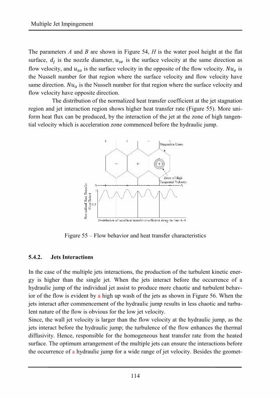
114


The parameters A and B are shown in Figure 54, H is the water pool height at the flat

surface, ±² is the nozzle diameter, ú�¦ is the surface velocity at the same direction as

flow velocity, and ú�Ý is the surface velocity in the opposite of the flow velocity. ùú¦ is

the Nusselt number for that region where the surface velocity and flow velocity have

same direction. ùúÝ is the Nusselt number for that region where the surface velocity and

flow velocity have opposite direction.

The distribution of the normalized heat transfer coefficient at the jet stagnation

region and jet interaction region shows higher heat transfer rate (Figure 55). More uni-

form heat flux can be produced, by the interaction of the jet at the zone of high tangen-

tial velocity which is acceleration zone commenced before the hydraulic jump.

Figure 55 – Flow behavior and heat transfer characteristics

5.4.2. Jets Interactions

In the case of the multiple jets interactions, the production of the turbulent kinetic ener-

gy is higher than the single jet. When the jets interact before the occurrence of a

hydraulic jump of the individual jet assist to produce more chaotic and turbulent behav-

ior of the flow is evident by a high up wash of the jets as shown in Figure 56. When the

jets interact after commencement of the hydraulic jump results in less chaotic and turbu-

lent nature of the flow is obvious for the low jet velocity.

Since, the wall jet velocity is larger than the flow velocity at the hydraulic jump, as the

jets interact before the hydraulic jump; the turbulence of the flow enhances the thermal

diffusivity. Hence, responsible for the homogeneous heat transfer rate from the heated

surface. The optimum arrangement of the multiple jets can ensure the interactions before

the occurrence of a hydraulic jump for a wide range of jet velocity. Besides the geomet-

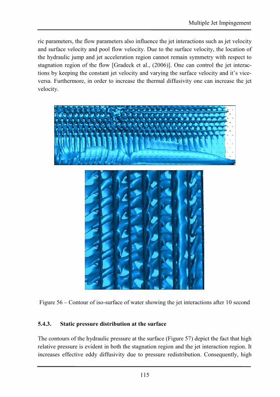
115


ric parameters, the flow parameters also influence the jet interactions such as jet velocity

and surface velocity and pool flow velocity. Due to the surface velocity, the location of

the hydraulic jump and jet acceleration region cannot remain symmetry with respect to

stagnation region of the flow [Gradeck et al., (2006)]. One can control the jet interac-

tions by keeping the constant jet velocity and varying the surface velocity and it’s vice-

versa. Furthermore, in order to increase the thermal diffusivity one can increase the jet

velocity.

Figure 56 – Contour of iso-surface of water showing the jet interactions after 10 second

5.4.3. Static pressure distribution at the surface

The contours of the hydraulic pressure at the surface (Figure 57) depict the fact that high

relative pressure is evident in both the stagnation region and the jet interaction region. It

increases effective eddy diffusivity due to pressure redistribution. Consequently, high

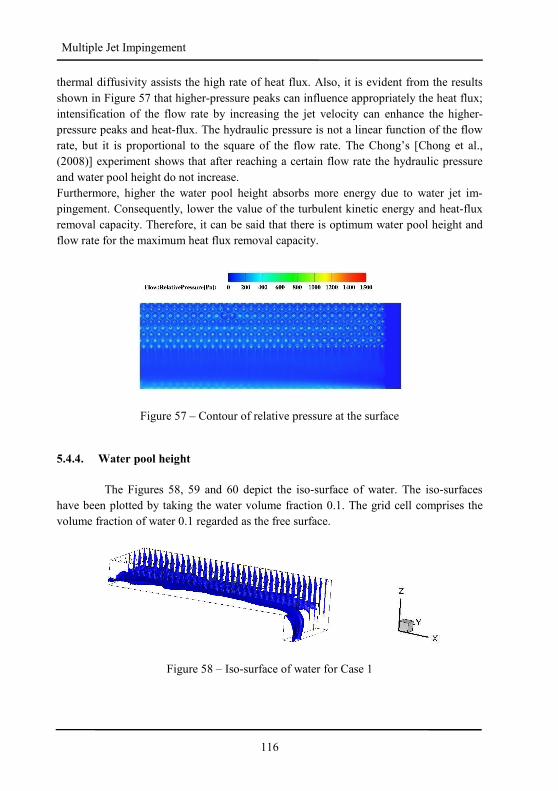
116


thermal diffusivity assists the high rate of heat flux. Also, it is evident from the results

shown in Figure 57 that higher-pressure peaks can influence appropriately the heat flux;

intensification of the flow rate by increasing the jet velocity can enhance the higher-

pressure peaks and heat-flux. The hydraulic pressure is not a linear function of the flow

rate, but it is proportional to the square of the flow rate. The Chong’s [Chong et al.,

(2008)] experiment shows that after reaching a certain flow rate the hydraulic pressure

and water pool height do not increase.

Furthermore, higher the water pool height absorbs more energy due to water jet im-

pingement. Consequently, lower the value of the turbulent kinetic energy and heat-flux

removal capacity. Therefore, it can be said that there is optimum water pool height and

flow rate for the maximum heat flux removal capacity.

Figure 57 – Contour of relative pressure at the surface

5.4.4. Water pool height

The Figures 58, 59 and 60 depict the iso-surface of water. The iso-surfaces

have been plotted by taking the water volume fraction 0.1. The grid cell comprises the

volume fraction of water 0.1 regarded as the free surface.

Figure 58 – Iso-surface of water for Case 1

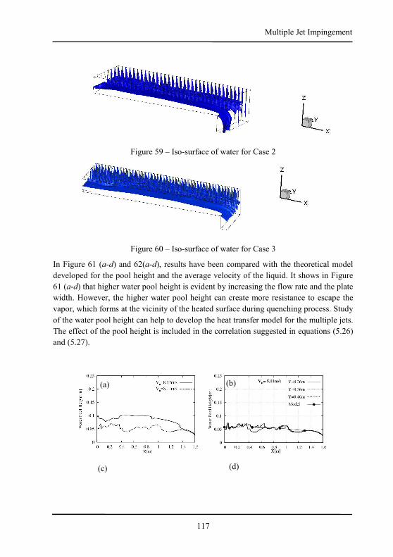
117




In Figure 61 (a-d) and 62(a-d), results have been compared with the theoretical model

developed for the pool height and the average velocity of the liquid. It shows in Figure

61 (a-d) that higher water pool height is evident by increasing the flow rate and the plate

width. However, the higher water pool height can create more resistance to escape the

vapor, which forms at the vicinity of the heated surface during quenching process. Study

of the water pool height can help to develop the heat transfer model for the multiple jets.

The effect of the pool height is included in the correlation suggested in equations (5.26)

and (5.27).

(a) (b)

(c) (d)

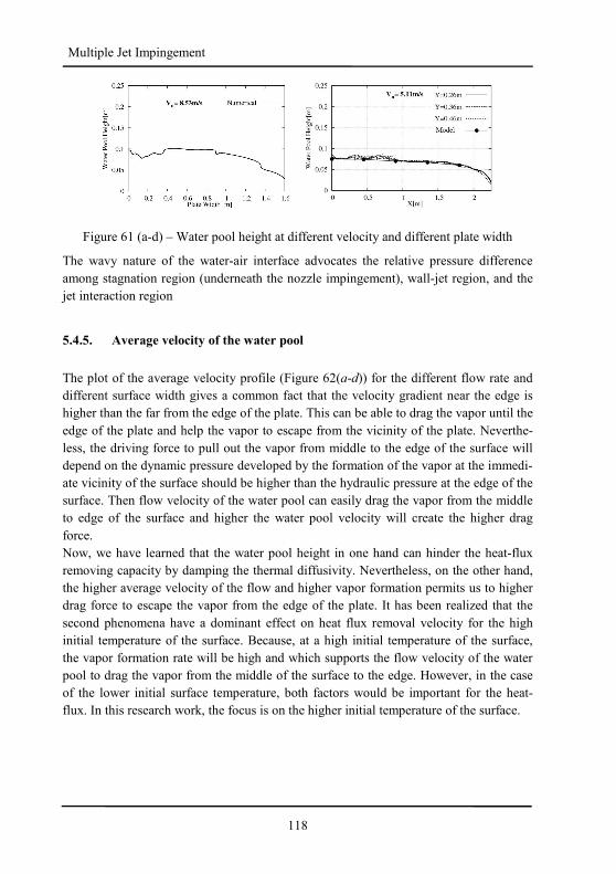
118


Figure 61 (a-d) – Water pool height at different velocity and different plate width

The wavy nature of the water-air interface advocates the relative pressure difference

among stagnation region (underneath the nozzle impingement), wall-jet region, and the

jet interaction region

5.4.5. Average velocity of the water pool

The plot of the average velocity profile (Figure 62(a-d)) for the different flow rate and

different surface width gives a common fact that the velocity gradient near the edge is

higher than the far from the edge of the plate. This can be able to drag the vapor until the

edge of the plate and help the vapor to escape from the vicinity of the plate. Neverthe-

less, the driving force to pull out the vapor from middle to the edge of the surface will

depend on the dynamic pressure developed by the formation of the vapor at the immedi-

ate vicinity of the surface should be higher than the hydraulic pressure at the edge of the

surface. Then flow velocity of the water pool can easily drag the vapor from the middle

to edge of the surface and higher the water pool velocity will create the higher drag

force.

Now, we have learned that the water pool height in one hand can hinder the heat-flux

removing capacity by damping the thermal diffusivity. Nevertheless, on the other hand,

the higher average velocity of the flow and higher vapor formation permits us to higher

drag force to escape the vapor from the edge of the plate. It has been realized that the

second phenomena have a dominant effect on heat flux removal velocity for the high

initial temperature of the surface. Because, at a high initial temperature of the surface,

the vapor formation rate will be high and which supports the flow velocity of the water

pool to drag the vapor from the middle of the surface to the edge. However, in the case

of the lower initial surface temperature, both factors would be important for the heat-

flux. In this research work, the focus is on the higher initial temperature of the surface.

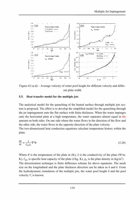
119


Figure 62 (a-d) – Average velocity of water pool height for different velocity and differ-

ent plate width

5.5. Heat transfer model for the multiple jets

The analytical model for the quenching of the heated surface through multiple jets sys-

tem is proposed. The effort is to develop the simplified model for the quenching through

the jet impingement onto the flat surface with finite thickness. When the water impinges

onto the horizontal plate at a high temperature, the water separates almost equal in the

amount on both sides. On one side where the water flows in the direction of the flow and

the other side, the water flows in the opposite direction of the plate velocity.

The two-dimensional heat conduction equations calculate temperature history within the

plate.

:Y:� = Z�TFOF ∇D® (5.28)

Where ® is the temperature of the plate in (K), ¬ is the conductivity of the plate (W/m.

K), � � is specific heat capacity of the plate (J/kg. K), (� is the plate density in (kg/m3).

The discretization technique is finite difference scheme for above equations. The mesh

size on the longitudinal and the plate thickness direction can be taken as h and k. From

the hydrodynamic simulation of the multiple jets, the water pool height δ and the pool

velocity Vi is known.

(a) (b)

(c) (d)

120


Assuming that the thickness of the water film is uniform in the thickness direction, the

amount of the temperature rise ∆θ of water in certain cell per incremental time Δ�� = I¾M (5.29)

can be expressed by

Δ® = Ê8�YF9Y8�·#.·�8�T8O8·¾ (5.30)

®� is the temperature of water in the concerned cell (K)

®� is the temperature of the plate surface contacting with the water in the foregoing cell

(K)

½� is the heat transfer coefficient from the plate surface to the water film (W/m2 K)

� � is the specific heat of water (J/kg. K)

(� is the density of the cooling water (kg/m3)

Where Δ5 is the contact area of a cell between the water film and plate surface in m2 and Δ# is the water volume in a cell in m3. If the cell width of the water film is chosen at

unity, we have

5 = ℎ. 1 and Δ# = ℎ. [. 1

This corresponds to the amount of temperature rise of the water film, as the water film

progresses from one cell to another cell. Let it now be assumed that the water tempera-

ture in the ith cell is ®�. Thus, the water temperature in the (i+1)th cell reaches (®�+Δ®)

after the lapse of Δ��. Here, it should be noted that Δ�� is taken to be equal to the period

required to shift the water from a cell to the next cell.

In fact, the effect of the thickness of thermal boundary layer δt is introduced to the esti-

mation of the temperature change in the cooling water. We now consider the effect of δt.

The thickness of thermal boundary layer of a laminar flow parallel to a flat plate is

commonly given by [Incropera and Dewitt, (1985)].

[�´ = 4.87"�C9�/D¢£9�/� �5.31�

Where, "�C = C¾M$ , ¢£ = �T�Z8

x is the distance measured from the leading edge corresponding to the impinging point

121


(m)

¬� is the thermal conductivity of water (W/ (m.K))

ê is the dynamic viscosity of water (kg/(m.s))

1 is the kinematic viscosity of water (m2/s)

When [>[�, the temperature rises may be restricted to the thickness at in the

water film cell. Let [�,) denote the thickness of the thermal boundary layer in the i-th

cell. Again, it may be regarded that the temperature rise of the water element within [�,) is equivalent to Δ® and the temperature of the element being between [�,)and [ is kept

constant at ®� on the condition that [>[�. Thus, the heat balance between the nearest

neighboring cells may be formulated as-

®�,)j� = Y8w\H,M,o9\H,M|\H,M,o + �Y8.Mj]Y�\H,M\H,M,o (5.32)

Again, we consider the heat transfer coefficient in the wetting and non-wetting zones.

We have given it in the form of-

½� = 0.063 Z8C "�Cc/�¢£�/� (5.33)

Using the analytical model one can understand the quenching at different locations of

the heated plate. However, the quenching model discussed in chapter four can be also

used for prediction of the temperature.

122


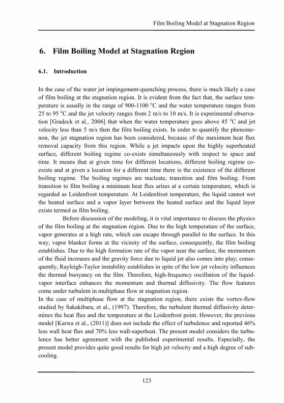
123

Film Boiling Model at Stagnation Region

6. Film Boiling Model at Stagnation Region

6.1. Introduction

In the case of the water jet impingement-quenching process, there is much likely a case

of film boiling at the stagnation region. It is evident from the fact that, the surface tem-

perature is usually in the range of 900-1100 oC and the water temperature ranges from

25 to 95 oC and the jet velocity ranges from 2 m/s to 10 m/s. It is experimental observa-

tion [Gradeck et al., 2006] that when the water temperature goes above 45 oC and jet

velocity less than 5 m/s then the film boiling exists. In order to quantify the phenome-

non, the jet stagnation region has been considered, because of the maximum heat flux

removal capacity from this region. While a jet impacts upon the highly superheated

surface, different boiling regime co-exists simultaneously with respect to space and

time. It means that at given time for different locations, different boiling regime co-

exists and at given a location for a different time there is the existence of the different

boiling regime. The boiling regimes are nucleate, transition and film boiling. From

transition to film boiling a minimum heat flux arises at a certain temperature, which is

regarded as Leidenfrost temperature. At Leidenfrost temperature, the liquid cannot wet

the heated surface and a vapor layer between the heated surface and the liquid layer

exists termed as film boiling.

Before discussion of the modeling, it is vital importance to discuss the physics

of the film boiling at the stagnation region. Due to the high temperature of the surface,

vapor generates at a high rate, which can escape through parallel to the surface. In this

way, vapor blanket forms at the vicinity of the surface, consequently, the film boiling

establishes. Due to the high formation rate of the vapor near the surface, the momentum

of the fluid increases and the gravity force due to liquid jet also comes into play; conse-

quently, Rayleigh-Taylor instability establishes in spite of the low jet velocity influences

the thermal buoyancy on the film. Therefore, high-frequency oscillation of the liquid-

vapor interface enhances the momentum and thermal diffusivity. The flow features

come under turbulent in multiphase flow at stagnation region.

In the case of multiphase flow at the stagnation region, there exists the vortex-flow

studied by Sakakibara, et al., (1997). Therefore, the turbulent thermal diffusivity deter-

mines the heat flux and the temperature at the Leidenfrost point. However, the previous

model [Karwa et al., (2011)] does not include the effect of turbulence and reported 46%

less wall heat flux and 70% less wall-superheat. The present model considers the turbu-

lence has better agreement with the published experimental results. Especially, the

present model provides quite good results for high jet velocity and a high degree of sub-

cooling.

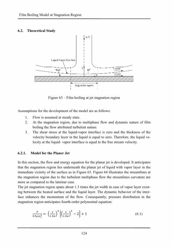
124


6.2. Theoretical Study

Figure 63 – Film boiling at jet stagnation region

Assumptions for the development of the model are as follows:

1. Flow is assumed at steady state.

2. At the stagnation region, due to multiphase flow and dynamic nature of film

boiling the flow attributed turbulent nature.

3. The shear stress at the liquid-vapor interface is zero and the thickness of the

velocity boundary layer in the liquid is equal to zero. Therefore, the liquid ve-

locity at the liquid- vapor interface is equal to the free stream velocity.

6.2.1. Model for the Planer Jet

In this section, the flow and energy equation for the planar jet is developed. It anticipates

that the stagnation region lies underneath the planar jet of liquid with vapor layer in the

immediate vicinity of the surface as in Figure 63. Figure 64 illustrates the streamlines at

the stagnation region due to the turbulent multiphase flow the streamlines curvature are

more as compared to the laminar case.

The jet stagnation region spans about 1.3 times the jet width in case of vapor layer exist-

ing between the heated surface and the liquid layer. The dynamic behavior of the inter-

face enhances the momentum of the flow. Consequently, pressure distribution in the

stagnation region anticipates fourth-order polynomial equation:

Ü>.�O��y = � C�.��D ^� C�.��D − 2_ + 1 (6.1)

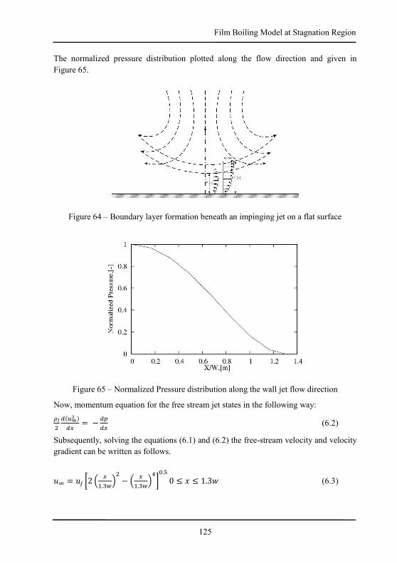
125


The normalized pressure distribution plotted along the flow direction and given in

Figure 65.

Figure 64 – Boundary layer formation beneath an impinging jet on a flat surface

Figure 65 – Normalized Pressure distribution along the wall jet flow direction

Now, momentum equation for the free stream jet states in the following way:

O�D ��y ��C = − � �C (6.2)

Subsequently, solving the equations (6.1) and (6.2) the free-stream velocity and velocity

gradient can be written as follows.

úa = ú² Ó2 � C�.��D − � C�.��cÔ>.� 0 ≤ ´ ≤ 1.3à (6.3)

126


��`�C = D��y�.��` Ó� C�.�� − � C�.��Ô 0 ≤ ´ ≤ 1.3à (6.4)

At this instant, the energy equation can be written in the integral form comprising the

additional thermal diffusivity in the liquid layer. The additional thermal diffusivity

begets due to the turbulent flow at the stagnation region.

��C ¸ úa�® − ®a�±µ′\H�C�> = −�½� + ½�� Y�;B<;c=> (6.5)

Here, [��´� is the thickness of the thermal boundary layer.

Now, the third order polynomial determines the temperature profile in the following

way:

Y9YFGHYFGH9Y` = � ;BD\H� Ó�;B

\H�D − 3Ô (6.6)

The above temperature profile must satisfy the following boundary condition (equations

6.7-6.9) at the liquid-vapor interface (µB = 0) and at the outer edge of the thermal

boundary layer (µB = [�)

®|;c=> = ®�� (6.7) ®|;c=\H = ®a (6.8)

O® Oµ′⁄ |;c=\H = 0 (6.9)

The thermal boundary layer thickness is determined by substituting the temperature

profile obtained in equation (6.6), into the energy equation (6.5).

�\H�C = D�Ê�jÊH�\H�` − �D \H�`

��`�C (6.10)

Due to symmetry condition at the stagnation line at x = 0, the left-hand side of the equa-

tion (6.10) becomes zero and the thickness of the thermal boundary layer is given by:

[�|C=> = � �c�Ê�jÊH� ��`�C <C=>�9>.� (6.11)

Now, putting the value of the velocity gradient at the stagnation point, from equation

(6.3) and (6.4), gives the following equation.

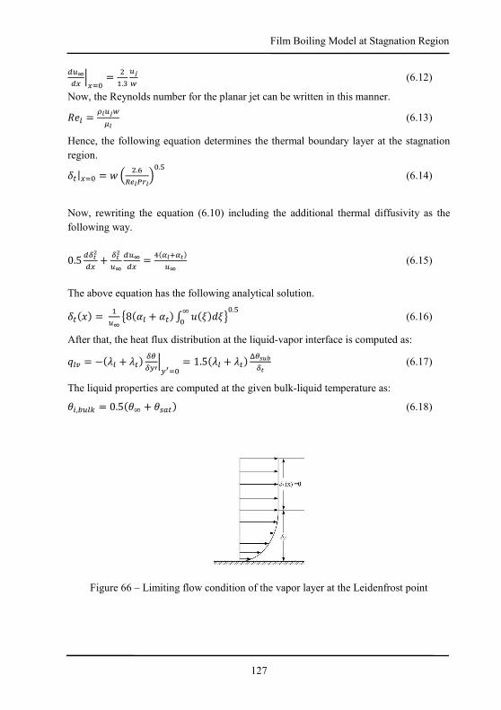
127


��`�C <C=> = D�.� �� (6.12)

Now, the Reynolds number for the planar jet can be written in this manner.

"�� = O�� (6.13)

Hence, the following equation determines the thermal boundary layer at the stagnation

region.

[�|C=> = à � D.ª�¦�ÜN��>.� (6.14)

Now, rewriting the equation (6.10) including the additional thermal diffusivity as the

following way.

0.5 �\Hy�C + \Hy�`��`�C = c�Ê�jÊH��` (6.15)

The above equation has the following analytical solution.

[��´� = ��` d8�½� + ½�� ¸ ú�P�±Pa> e>.� (6.16)

After that, the heat flux distribution at the liquid-vapor interface is computed as:

� = −�¬� + ¬�� \Y\;B<;c=> = 1.5�¬� + ¬�� ·YF¥K\H (6.17)

The liquid properties are computed at the given bulk-liquid temperature as:

®),¯��! = 0.5�®a + ®�� (6.18)

Figure 66 – Limiting flow condition of the vapor layer at the Leidenfrost point

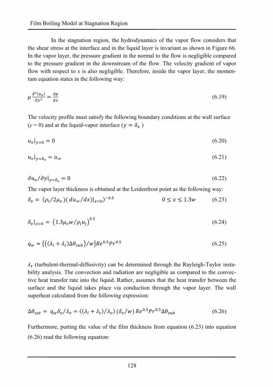
128


In the stagnation region, the hydrodynamics of the vapor flow considers that

the shear stress at the interface and in the liquid layer is invariant as shown in Figure 66.

In the vapor layer, the pressure gradient in the normal to the flow is negligible compared

to the pressure gradient in the downstream of the flow. The velocity gradient of vapor

flow with respect to x is also negligible. Therefore, inside the vapor layer, the momen-

tum equation states in the following way:

ê :y��S�:;y = � �C (6.19)

The velocity profile must satisfy the following boundary conditions at the wall surface

(y = 0) and at the liquid-vapor interface (µ = [ )

ú|;=> = 0 (6.20)

ú|;=\S = úa (6.21)

Oú Oµ⁄ |;=\S = 0 (6.22)

The vapor layer thickness is obtained at the Leidenfrost point as the following way:

[ = �(� 2ê ��⁄ ±úa ±´⁄ �|C=>�9>.� 0 ≤ ´ ≤ 1.3à (6.23)

[|C=> = w1.3êà (�ú²⁄ |>.� (6.24)

� ≈ dw�¬� + ¬��Δ®��¯| à⁄ e"�>.�¢£>.� (6.25)

¬� (turbulent-thermal-diffusivity) can be determined through the Rayleigh-Taylor insta-

bility analysis. The convection and radiation are negligible as compared to the convec-

tive heat transfer rate into the liquid. Rather, assumes that the heat transfer between the

surface and the liquid takes place via conduction through the vapor layer. The wall

superheat calculated from the following expression:

Δ®�� = �[ ¬⁄ = ��¬� + ¬�� ¬⁄ � �[ à�⁄ "�>.�¢£>.�Δ®��¯ (6.26)

Furthermore, putting the value of the film thickness from equation (6.23) into equation

(6.26) read the following equation:

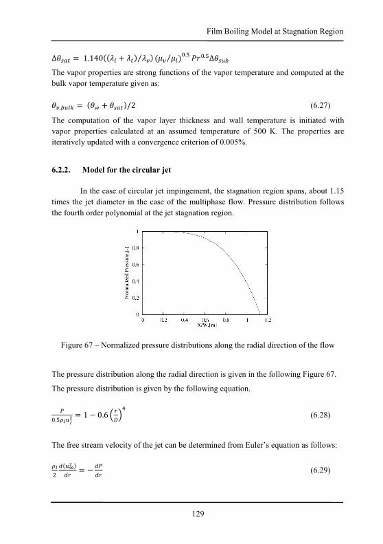
129


Δ®�� = 1.140��¬� + ¬�� ¬⁄ � �ê ê��⁄ >.� ¢£>.�Δ®��¯

The vapor properties are strong functions of the vapor temperature and computed at the

bulk vapor temperature given as:

®,¯��! = �®� + ®��/2 (6.27)

The computation of the vapor layer thickness and wall temperature is initiated with

vapor properties calculated at an assumed temperature of 500 K. The properties are

iteratively updated with a convergence criterion of 0.005%.

6.2.2. Model for the circular jet

In the case of circular jet impingement, the stagnation region spans, about 1.15

times the jet diameter in the case of the multiphase flow. Pressure distribution follows

the fourth order polynomial at the jet stagnation region.

Figure 67 – Normalized pressure distributions along the radial direction of the flow

The pressure distribution along the radial direction is given in the following Figure 67.

The pressure distribution is given by the following equation.

Ü>.�O��y = 1 − 0.6 �N��c

(6.28)

The free stream velocity of the jet can be determined from Euler’s equation as follows:

O�D ��y ��N = − �Ü�N (6.29)

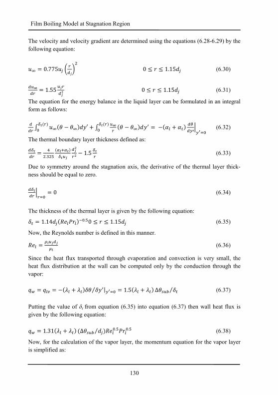
130


The velocity and velocity gradient are determined using the equations (6.28-6.29) by the

following equation:

úa = 0.775ú² � N��D 0 ≤ £ ≤ 1.15±² (6.30)

��`�N = 1.55 ��N��y 0 ≤ £ ≤ 1.15±² (6.31)

The equation for the energy balance in the liquid layer can be formulated in an integral

form as follows:

��N ¸ úa�® − ®a�±µ′\H�N�> + ¸ �`N\H�N�> �® − ®a�±µB = −�½� + ½�� Y�;B<;c=> (6.32)

The thermal boundary layer thickness defined as:

�\H�N = cD.�D� �Ê�jÊH�\H��

��yNy − 1.5 \HN (6.33)

Due to symmetry around the stagnation axis, the derivative of the thermal layer thick-

ness should be equal to zero.

�\H�N <N=> = 0 (6.34)

The thickness of the thermal layer is given by the following equation:

[� = 1.14±²�"��¢£��9>.�0 ≤ £ ≤ 1.15±² (6.35)

Now, the Reynolds number is defined in this manner.

"�� = O�� (6.36)

Since the heat flux transported through evaporation and convection is very small, the

heat flux distribution at the wall can be computed only by the conduction through the

vapor:

� = � = −�¬� + ¬��[® [µB⁄ |;c=> = 1.5�¬� + ¬�� Δ®��¯ [�⁄ (6.37)

Putting the value of δt from equation (6.35) into equation (6.37) then wall heat flux is

given by the following equation:

� = 1.31�¬� + ¬�� Δ®��¯ ±²�"��>.�¢£�>.�⁄ (6.38)

Now, for the calculation of the vapor layer, the momentum equation for the vapor layer

is simplified as:

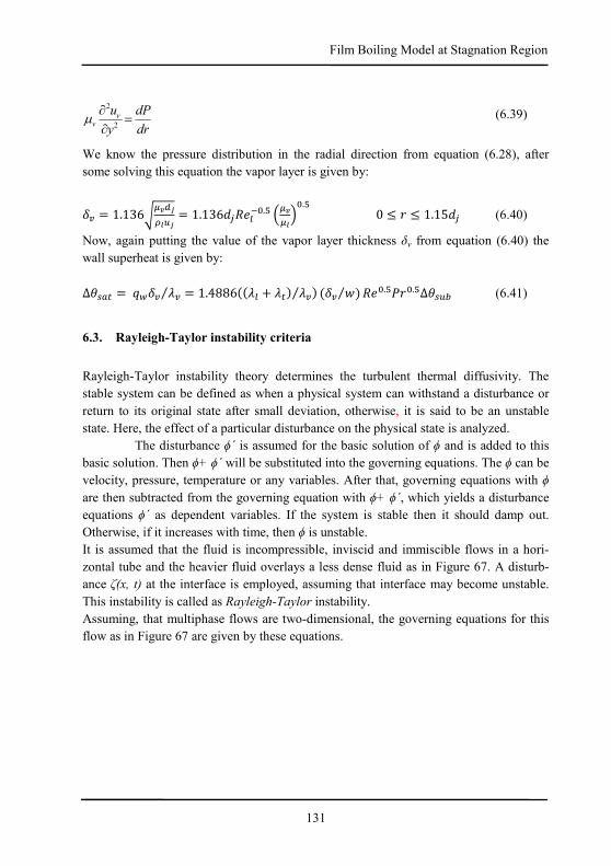
131


dr

dP

y

uvv =∂∂

2

2

µ (6.39)

We know the pressure distribution in the radial direction from equation (6.28), after

some solving this equation the vapor layer is given by:

[ = 1.136W�S��O�� = 1.136±²"��9>.� ��S��>.� 0 ≤ £ ≤ 1.15±² (6.40)

Now, again putting the value of the vapor layer thickness δv from equation (6.40) the

wall superheat is given by:

Δ®�� = �[ ¬⁄ = 1.4886��¬� + ¬�� ¬⁄ � �[ à�⁄ "�>.�¢£>.�Δ®��¯ (6.41)

6.3. Rayleigh-Taylor instability criteria

Rayleigh-Taylor instability theory determines the turbulent thermal diffusivity. The

stable system can be defined as when a physical system can withstand a disturbance or

return to its original state after small deviation, otherwise, it is said to be an unstable

state. Here, the effect of a particular disturbance on the physical state is analyzed.

The disturbance ϕ´ is assumed for the basic solution of ϕ and is added to this

basic solution. Then ϕ+ ϕ´ will be substituted into the governing equations. The ϕ can be

velocity, pressure, temperature or any variables. After that, governing equations with ϕ

are then subtracted from the governing equation with ϕ+ ϕ´, which yields a disturbance

equations ϕ´ as dependent variables. If the system is stable then it should damp out.

Otherwise, if it increases with time, then ϕ is unstable.

It is assumed that the fluid is incompressible, inviscid and immiscible flows in a hori-

zontal tube and the heavier fluid overlays a less dense fluid as in Figure 67. A disturb-

ance ζ(x, t) at the interface is employed, assuming that interface may become unstable.

This instability is called as Rayleigh-Taylor instability.

Assuming, that multiphase flows are two-dimensional, the governing equations for this

flow as in Figure 67 are given by these equations.

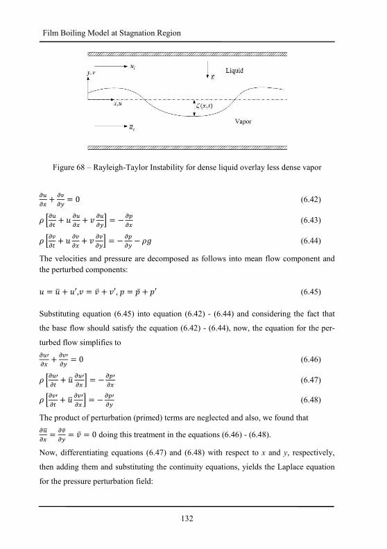
132


Figure 68 – Rayleigh-Taylor Instability for dense liquid overlay less dense vapor

:�:C + ::; = 0 (6.42)

( «:�:� + ú :�:C + ë :�:;° = − : :C (6.43)

( «::� + ú ::C + ë ::;° = − : :; − (Q (6.44)

The velocities and pressure are decomposed as follows into mean flow component and

the perturbed components:

ú = úí + ú′,ë = ë + ë′, æ = æ + æ′ (6.45)

Substituting equation (6.45) into equation (6.42) - (6.44) and considering the fact that

the base flow should satisfy the equation (6.42) - (6.44), now, the equation for the per-

turbed flow simplifies to

:�B:C + :B:; = 0 (6.46)

( «:�B:� + úí :�B:C ° = − : B:C (6.47)

( «:B:� + úí :B:C ° = − : B:; (6.48)

The product of perturbation (primed) terms are neglected and also, we found that

:�,:C = :í:; = ë = 0 doing this treatment in the equations (6.46) - (6.48).

Now, differentiating equations (6.47) and (6.48) with respect to x and y, respectively,

then adding them and substituting the continuity equations, yields the Laplace equation

for the pressure perturbation field:

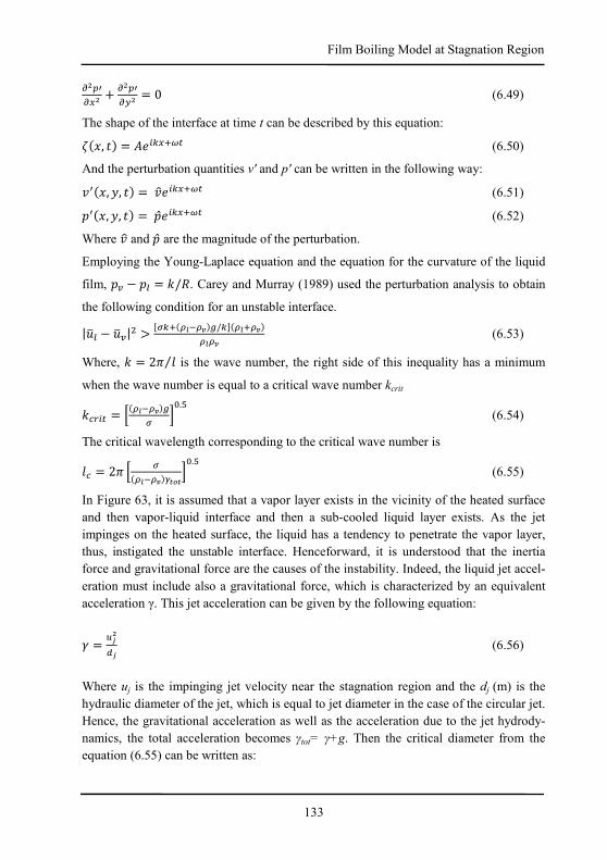
133


:y B:Cy + :y B:;y = 0 (6.49)

The shape of the interface at time t can be described by this equation:

î�´, �� = Ç�)!Cjg� (6.50)

And the perturbation quantities v' and p' can be written in the following way:

ëB�´, µ, �� = ë��)!Cjg� (6.51)

æB�´, µ, �� = æ�)!Cjg� (6.52)

Where ë� and æ are the magnitude of the perturbation.

Employing the Young-Laplace equation and the equation for the curvature of the liquid

film, æ − æ� = �/". Carey and Murray (1989) used the perturbation analysis to obtain

the following condition for an unstable interface.

|úí� − úí|D > iE!j�O�9OS��/!j�O�jOS�O�OS (6.53)

Where, � = 2k M⁄ is the wave number, the right side of this inequality has a minimum

when the wave number is equal to a critical wave number kcrit

��N)� = «�O�9OS��E °>.� (6.54)

The critical wavelength corresponding to the critical wave number is

M� = 2k « E�O�9OS�lH�H°>.� (6.55)

In Figure 63, it is assumed that a vapor layer exists in the vicinity of the heated surface

and then vapor-liquid interface and then a sub-cooled liquid layer exists. As the jet

impinges on the heated surface, the liquid has a tendency to penetrate the vapor layer,

thus, instigated the unstable interface. Henceforward, it is understood that the inertia

force and gravitational force are the causes of the instability. Indeed, the liquid jet accel-

eration must include also a gravitational force, which is characterized by an equivalent

acceleration γ. This jet acceleration can be given by the following equation:

A = ��y�� (6.56)

Where uj is the impinging jet velocity near the stagnation region and the dj (m) is the

hydraulic diameter of the jet, which is equal to jet diameter in the case of the circular jet.

Hence, the gravitational acceleration as well as the acceleration due to the jet hydrody-

namics, the total acceleration becomes γtot= γ+g. Then the critical diameter from the

equation (6.55) can be written as:

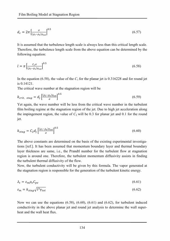
134


±� = 2k « E�O�9OS�lH�H°>.� (6.57)

It is assumed that the turbulence length scale is always less than this critical length scale.

Therefore, the turbulence length scale from the above equation can be determined by the

following equation:

M = k « �oE�O�9OS�lH�H°>.� (6.58)

In the equation (6.58), the value of the C1 for the planar jet is 0.316228 and for round jet

is 0.14121.

The critical wave number at the stagnation region will be

��N)�, �� = ±² «�O�9OS�lH�HE °>.� (6.59)

Yet again, the wave number will be less from the critical wave number in the turbulent

film boiling regime at the stagnation region of the jet. Due to high jet acceleration along

the impingement region, the value of C2 will be 0.3 for planar jet and 0.1 for the round

jet.

�� = �D±² «�O�9OS�lH�HE °>.� (6.60)

The above constants are determined on the basis of the existing experimental investiga-

tions [ref.]. It has been assumed that momentum boundary layer and thermal boundary

layer thickness are same, i.e., the Prandtl number for the turbulent flow at stagnation

region is around one. Therefore, the turbulent momentum diffusivity assists in finding

the turbulent thermal diffusivity of the flow.

Now, the turbulent conductivity will be given by this formula. The vapor generated at

the stagnation region is responsible for the generation of the turbulent kinetic energy.

¬� = äÑ(� (6.61)

äÑ = ��&M�A�Ý� (6.62)

Now we can use the equations (6.58), (6.60), (6.61) and (6.62), for turbulent induced

conductivity in the above planar jet and round jet analysis to determine the wall super-

heat and the wall heat flux.

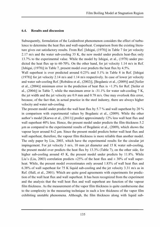
135


6.4. Results and discussion

Subsequently, formulation of the Leidenfrost phenomenon considers the effect of turbu-

lence to determine the heat flux and wall-superheat. Comparison from the existing litera-

ture gives out satisfactory results. From Ref. [Ishigai, (1978)] in Table 7 for jet velocity

2.17 m/s and the water sub-cooling 35 K, the new model under predicts heat-flux only

13.7% to the experimental value. While the model by Ishigai, et al., (1978) under pre-

dicted the heat flux up to 60-70%. On the other hand, for jet velocity 1.14 m/s in Ref.

[Ishigai, (1978)] in Table 7, present model over predicts the heat flux by 4.5%.

Wall superheat is over predicted around 0.23% and 5.1% in Table 8 in Ref. [Ishigai

(1978)] for jet velocity 2.14 m/s and 1.14 m/s respectively. In case of lower jet velocity

and water sub-cooling Ref. [Robidou et al., (2002)], [Bogdanic et al., (2009)] and [Seiler

et al., (2004)] minimum error in the prediction of heat flux is +1.3% for Ref. [Seiler et

al., (2004)] in Table 7, while the maximum error is -31.1% for water sub-cooling 7 K,

the jet width and the jet velocity are 0.9 mm and 0.78 m/s. One may overlook this error,

because, of the fact that, in actual practice in the steel industry, there are always higher

velocity and water sub-cooling.

The present model under predict the wall heat flux by 5.7 % and wall superheat by 20 %

in comparison with experimental values by Bogdanic et al., (2009). While the other

author’s model [Karwa et al., (2011)] predict approximately 12% less wall heat flux and

wall superheat 40% less. Hence, the present model under predicts the film thickness 5.2

µm as compared to the experimental results of Bogdanic et al., (2009), which shows the

vapour layer around 8±2 µm. Since the present model predicts better wall heat flux and

wall superheat, therefore, the vapour film thickness is more reliable than another model.

The only paper by Liu, 2003, which have the experimental results for the circular jet

impingement. For jet velocity 3 m/s, 10 mm jet diameter and 15 K water sub-cooling,

the present model over predicts the heat flux by 13.3% (Table 7), on the other side, for

higher sub-cooling around 45 K, the present model under predicts by 11.8%. While

Liu’s (Liu, 2003) correlation predicts ±25% of the heat flux and ± 30% of wall super-

heat. While, the present model overestimates only around 1.83% of wall heat flux and

6.38% of wall superheat for 75 K liquid sub-cooling and the jet velocity 3.31 m/s as in

Ref. (Hall, et al., 2001). Which are quite good agreements with experiments for predic-

tion of the wall heat flux and wall superheat. It has been recognized from the experiment

and the analysis that the wall heat flux and wall superheat are function of the vapour

film thickness. As the measurement of the vapor film thickness is quite cumbersome due

to the complexity in the measuring technique in such a low thickness of the vapor film

exhibiting unstable phenomena. Although, the film thickness along with liquid sub-

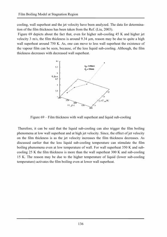
136


cooling, wall superheat and the jet velocity have been analyzed. The data for determina-

tion of the film thickness has been taken from the Ref. (Liu, 2003).

Figure 69 depicts about the fact that, even for higher sub-cooling 45 K and higher jet

velocity 3 m/s, the film thickness is around 9.34 µm, reason may be due to quite a high

wall superheat around 750 K. As, one can move to less wall superheat the existence of

the vapour film can be seen, because, of the less liquid sub-cooling. Although, the film

thickness decreases with decreased wall superheat.

Figure 69 – Film thickness with wall superheat and liquid sub-cooling

Therefore, it can be said that the liquid sub-cooling can also trigger the film boiling

phenomena at low wall superheat and at high jet velocity. Since, the effect of jet velocity

on the film thickness is as the jet velocity increases the film thickness decreases. As

discussed earlier that the less liquid sub-cooling temperature can stimulate the film

boiling phenomena even at low temperature of wall. For wall superheat 350 K and sub-

cooling 25 K the film thickness is more than the wall superheat 300 K and sub-cooling

15 K. The reason may be due to the higher temperature of liquid (lower sub-cooling

temperature) activates the film boiling even at lower wall superheat.

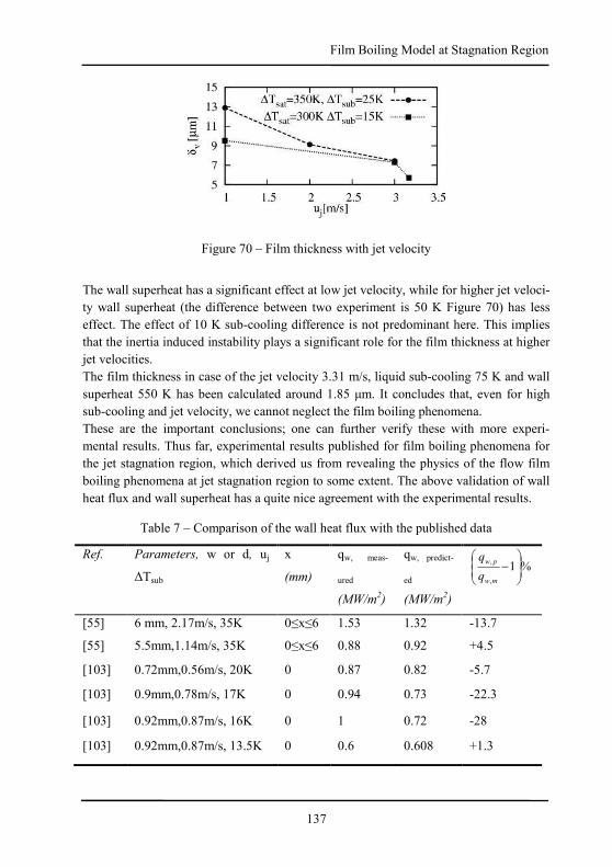
137


Figure 70 – Film thickness with jet velocity

The wall superheat has a significant effect at low jet velocity, while for higher jet veloci-

ty wall superheat (the difference between two experiment is 50 K Figure 70) has less

effect. The effect of 10 K sub-cooling difference is not predominant here. This implies

that the inertia induced instability plays a significant role for the film thickness at higher

jet velocities.

The film thickness in case of the jet velocity 3.31 m/s, liquid sub-cooling 75 K and wall

superheat 550 K has been calculated around 1.85 µm. It concludes that, even for high

sub-cooling and jet velocity, we cannot neglect the film boiling phenomena.

These are the important conclusions; one can further verify these with more experi-

mental results. Thus far, experimental results published for film boiling phenomena for

the jet stagnation region, which derived us from revealing the physics of the flow film

boiling phenomena at jet stagnation region to some extent. The above validation of wall

heat flux and wall superheat has a quite nice agreement with the experimental results.

Table 7 – Comparison of the wall heat flux with the published data

Ref. Parameters, w or d, uj

∆Tsub

x

(mm)

qw, meas-

ured

(MW/m2)

qw, predict-

ed

(MW/m2)

%1,

,

−

mw

pw

q

q

[55] 6 mm, 2.17m/s, 35K 0≤x≤6 1.53 1.32 -13.7

[55] 5.5mm,1.14m/s, 35K 0≤x≤6 0.88 0.92 +4.5

[103] 0.72mm,0.56m/s, 20K 0 0.87 0.82 -5.7

[103] 0.9mm,0.78m/s, 17K 0 0.94 0.73 -22.3

[103] 0.92mm,0.87m/s, 16K 0 1 0.72 -28

[103] 0.92mm,0.87m/s, 13.5K 0 0.6 0.608 +1.3

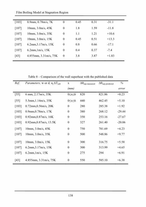
138


[103] 0.9mm, 0.78m/s, 7K 0 0.45 0.31 -31.1

[107] 10mm, 3.0m/s, 45K 0 1.8 1.59 -11.8

[107] 10mm, 3.0m/s, 35K 0 1.1 1.21 +10.6

[107] 10mm, 3.0m/s, 15K 0 0.45 0.51 +13.3

[107] 6.2mm,3.17m/s, 15K 0 0.8 0.66 -17.1

[107] 6.2mm,1m/s, 15K 0 0.4 0.37 -7.4

[43] 4.855mm, 3.31m/s, 75K 0 3.8 3.87 +1.83

Table 8 – Comparison of the wall superheat with the published data

Ref. Parameters, w or d, uj ∆Tsub x

(mm)

∆θsup.measured ∆θsup.predicted %

error

[55] 6 mm, 2.17m/s, 35K 0≤x≤6 820 821.86 +0.23

[55] 5.5mm,1.14m/s, 35K 0≤x≤6 440 462.45 +5.10

[103] 0.72mm,0.56m/s, 20K 0 280 285.38 +1.92

[103] 0.9mm,0.78m/s, 17K 0 380 268.12 -29.44

[103] 0.92mm,0.87m/s, 16K 0 350 253.16 -27.67

[103] 0.92mm,0.87m/s, 13.5K 0 327 261.40 -20.06

[107] 10mm, 3.0m/s, 45K 0 750 781.69 +4.23

[107] 10mm, 3.0m/s, 35K 0 500 548.86 +9.77

[107] 10mm, 3.0m/s, 15K 0 300 316.75 +5.58

[107] 6.2mm,3.17m/s, 15K 0 300 313.99 +4.65

[107] 6.2mm,1m/s, 15K 0 275 294 +6.91

[43] 4.855mm, 3.31m/s, 75K 0 550 585.10 +6.38

139

Conclusions and Future Recommendations

7. Conclusions and Future Recommendations

7.1. Surface quenching through single jet

The computational study has been performed in order to enhance the understanding of

the flow quenching phenomena for the single jet impinging onto a heated plate. Tem-

poral evolution of the boundary layer profile demonstrated the dynamic nature of the

flow boiling evidenced by the formation, growth and explosion of the vapor bubbles

near the surface. The velocity gradient exhibits a linear behavior in the case of a higher

vapor volume fraction at the surface. On the other hand, it is non-linear in the case of the

vapor-liquid mixture. This behavior is also due to the different heat-transfer mechanism

(nucleate boiling, transition boiling and film boiling). The boundary layer profile devel-

opment, evaluated at different radial positions, indicates that the viscous sublayer and

the buffer layer are highly unstable, representing the outcome caused by the boiling of

the liquid. The fast cooling from the time of initialization of quenching to 2 s is achieved

at the stagnation region, while slow cooling rate represents the characteristics of the later

time period. It clearly shows the effect of liquid sub-cooling which is initially very high.

For a longer time, the liquid forms the vapor layer at the surface being incapable of

escaping from the stagnation region. Higher values of heat-flux are found at the jet

acceleration region in comparison with wall jet region. For higher jet velocities (7.5 m/s

and 10 m/s), the acceleration region exhibits more intensive heat flux removal from the

surface. For higher wall superheat at the initial time, the quenching phenomena are more

pronounced at jet stagnation region where the bubble production rate is quite high.

Herewith, a more intensive momentum and thermal diffusivity exchange hinder the

wall-jet acceleration at the surface after the stagnation region accordingly; this phenom-

enon enhances the cooling rate at stagnation region for lower jet velocities.

Temporal evolution of the heat transfer mechanism is discussed in detail. For

longer times, e.g. around 7 s, less number of bubbles are produced leading to a lower

vapor fraction generated at the stagnation region. It causes a more intensive wall-jet

acceleration and consequently an intensified momentum transport and thermal

diffusivity, leading finally to a substantial cooling rate enhancement at the jet

acceleration region. In the boiling curve, the shoulder of heat flux is not found for the

sub-cooling 75 K. Shoulder of heat flux is commonly achieved for sub-cooling 45 K and

10 K, representing the outcome which can be evidenced in the experiment by Gradeck,

et al. (2009). The effect of the sub-cooling on heat flux removal rate from the heated

surface is more pronounced than that of the jet velocity. Effect of flow velocity has been

examined in detail, which is relevant to the many industrial quenching applications.

140


Intensive quenching process is consistent with the high rate of sub-cooling and high jet

velocities. The surface temperature predicted by quenching model within the

impingement region and the consequent wall-jet region agrees reasonably well with the

measurements, the outcome being particularly valid at higher jet velocities. However, a

steep temperature gradient at the position corresponding to the boiling threshold was not

captured under the conditions of the numerical grid resolution adopted. Despite,

reasonably good predictions of the wetting front propagation phenomena have been

achieved, advocating the necessity for future development of the model.

7.2. Theoretical and numerical study of the hydrodynamics of the multiple jets

A theoretical model for the determination of the pool height for the given mass

flow rate is proposed. The model results are compared to those obtained from the CFD

study showing good agreement. The flow characteristics are also analyzed resulting in

the maximum value of the non-dimensional mass flow rate corresponding to 0.3849 for

the non-dimensional height around 0.66. This implies that for certain liquid pool height

the flow rate becomes maximum. This can be useful for determination of the optimum

flow rate and the liquid pool height. It has been realized that the honeycomb-like nozzle

array distribution can enhance the heat-transfer rate, because, this exhibited the most

intensive interactions of the jets. Intensification of the jet interactions is also of im-

portance in relation to the heat transfer rate enhancement. It is especially the case if the

jet interactions take place before the hydraulic jump appearance, which, on the other

hand, could create a high level of up wash. Static pressure distribution on the surface

affected the heat flux removal rate by a corresponding liquid-pool height level. The

liquid pool height in one hand can hinder the heat-flux removing capacity by damping

the thermal diffusivity. However, on the other hand, the higher average velocity of the

flow and higher vapor formation rate permitted higher drag force to enable escape of the

vapor from the edge of the plate. Therefore, the high average velocity of the flow is a

desirable feature for fast removal of heat flux at the high initial temperature of the sur-

face. Because, at a high initial temperature of the surface, the vapor formation rate will

be appropriately high supporting the flow velocity of the water pool to drag the vapor

from the middle of the surface to the edge. Nevertheless, in the case of the lower initial

surface temperature, both factors would be less important for the removal of heat-flux.

Apart from these studies, a model for the prediction of the temperature for multiple jets

impingement on the heated surface is proposed, which can be useful for the engineering

purposes.

141


7.3. Model for film boiling at stagnation region considering the effect of instabil-

ity

The model for the prediction of the heat flux and surface temperature is developed

for the film boiling at stagnation region. The interface between the liquid and vapor is

highly unstable. This instability affects the turbulence increase and, consequently, the

increase in the thermal diffusivity. A significant improvement in the prediction of the

heat flux and the wall superheat was illustrated in direct comparison with available

experimental results. Moreover, the model shows lower error for higher jet velocities

and higher sub-cooling. The results for the film thickness in terms of the jet velocity,

wall superheat and liquid sub-cooling enable important conclusions to be drawn.

7.4. Future Recommendations

Having the computational database obtained by the present research about the in-

fluence of the boundary layer development and associated turbulence structure, one can

work on a reformulation of the quenching model. Another aspect can also be included,

representing the boiling-front propagation characteristics. Further experimental studies

for the model validation would be necessary, keeping in mind the transient nature of the

quenching phenomenon, which is certainly difficult to reproduce correctly. Knowledge

of the flow parameters as well as thermal and material properties of solid surface is of

decisive importance. The model should be developed for a larger range of operating

parameters such as jet velocity, sub-cooling intensity, wall-superheat in terms of differ-

ent surface thermal properties. Testing the quenching model should be performed by

computing the multiple jet process keeping in mind that the relevant phenomena are

much richer in comparison with the single jet. It relates especially to very complex

hydrodynamics. As shown presently, the jet interactions, liquid pool height and the

associated mean velocity and turbulent kinetic energy may contribute significantly to the

heat transfer process. The non-linear dependence of these parameters on the complex

hydrodynamics along with the boiling at the surface is evident.

Fast cooling of the surface starting from very high initial temperatures may lead to

film boiling. An analytical model, proposed in the present work, should be validated

experimentally; furthermore it can be done accounting for a wide range of operating

parameters.

Introduction of the surface roughness effects in the wall–function method can

mimic the multiphase flow near the surface more generally. It can be implemented along

with the boiling front propagation characteristics.

142


143

List of Figures

List of Figures

Figure 1– Process of jet cooling of Run-out-Table (ROT) [Gradeck et al., (2009)] ....... 25

Figure 2 – Schematic diagram of the ROT cooling Process [Cho et al., (2008)] ............ 25

Figure 3 – Pool boiling curve [50] .................................................................................. 26

Figure 4 – Boiling curve for jet impingement [Gradeck et al., (2009)] .......................... 27

Figure 5 – Jet impact on the horizontal surface .............................................................. 28

Figure 6 – Up-wash of the multiple jets.......................................................................... 29

Figure 7 – Nozzle arrangement in the hexagonal pattern ................................................ 29

Figure 8 – Boiling curves ∆Tsub = 15 K; uj = 1.2 m/s; d = 50 mm [Gradeck, et al.,

(2009)] .................................................................................................................... 36

Figure 9 – Hysteresis along the Nukiyama curve ........................................................... 36

Figure 10 – Wall heat flux at different locations from the stagnation point of a planar

water jet [Seiler-Marie et al. (2004) jet velocity 0.8 m/s and water sub-cooling 16

K] ............................................................................................................................ 41

Figure 11 – Phenomenological history during quenching [Woodfield et al., (2005)] ..... 48

Figure 12 – Control volume for volume averaging ......................................................... 54

Figure 13 – Definition of Upstream (U), Central (C) and Downstream (D) Nodes ........ 66

Figure 14 – Computational domain of the test case ........................................................ 74

Figure 15 – The grid for the computational domain ....................................................... 75

Figure 16 – The iso-surface of the water (Vj =1.72 m/s and Vp =1.53 m/s).................... 75


et al., (2006)] (Vj =1.72 m/s and Vp =1.53 m/s, the arrow shows the direction of

plate movement) ..................................................................................................... 76

Figure 18 – The iso-surface of the water (Vj =1.46 m/s and Vp =2.04 m/s).................... 76


et al., (2006)] (Vj =1.46 m/s and Vp =2.04 m/s, the arrow shows the direction of

plate movement) ..................................................................................................... 77

Figure 20 – Computational domain of test case for the heat transfer validation ............. 78

Figure 21 – Normalized pressure plot at stagnation region of the flow .......................... 78

Figure 22 – Nusselt number plot for different turbulence model .................................... 79

Figure 23 – Schematic of the computational domain in vertical r-y plane ...................... 80

Figure 24 – Grid for the fluid and solid region ............................................................... 81

Figure 25 – y+ values of the wall-closest computational nodes for different jet velocities

................................................................................................................................ 81

144

List of Figures

Figure 26 – Velocity profile at R= 1.5 mm at different time solid line ( ) 2.0s , dot-dot

(....) 2.5s, dash-dot-dash(-.-) 3.0s ............................................................................84

Figure 27 – Velocity profile at R= 3 mm at different time solid line ( ) 3.0s , dot-dot

(....) 3.5s, dash-dot-dash(-.-) 4.0s ............................................................................85

Figure 28 – Velocity profile after 12s for jet velocity 5 m/s (Rejet = 14,800) .................86


front) .......................................................................................................................87


front) for jet velocity 5 m/s (Rejet = 14,800) ...........................................................88

Figure 31 – Contours of Turbulent Kinetic energy at the surface for 2.5 m/s jet velocity

at 5s at the middle of nucleate boiling ....................................................................88

Figure 32 – Velocity vector at the stagnation and acceleration region for jet velocity

5m/s at 10s at the middle of nucleate boiling ..........................................................89

Figure 33 – Cooling at Stagnation region for jet velocity 2.5m/s ...................................90

Figure 34 (a-b) – Boiling curve for Vj = 2.5 m/s at different location of the surface .....91

Figure 35 – Boiling curve for Vj = 5 m/s at different location of the surface .................92

Figure 36 – Boiling curve for Vj = 7.5 m/s at different location of the surface ..............94

Figure 37 – Boiling curve for Vj = 10 m/s at different location of the surface ...............95

Figure 38 (a-b) – Boiling curves for different jet velocities (Left: plotted at stagnation

region (r =0 mm) Right: plotted at acceleration region (r = 4 mm)) .......................95

Figure 39 – Boiling curve for jet velocity 6.25 m/s and initial surface temperature .......97

Figure 40 – Boiling curve for jet velocity 2.5 m/s and initial surface temperature 910 ° C

and ∆Tsub = 45 K ...................................................................................................98

Figure 41 – Plot of maximum heat with respect to jet velocity .......................................98

Figure 42 – Heat-flux development in terms of different jet velocities at t =1s (upper

left), 3s (upper right), 5s (lower left), 7s (lower right) ............................................99

Figure 43 – Temporal temperature distribution on the surface at different locations for

jet velocity: Vjet = 2.5 m/s (a), 5 m/s (b), 7.5 m/s (c), 10 m/s (d) ...........................100

Figure 44 – Temporal heat-flux distribution on the surface at different locations for jet

velocity: Vjet = 2.5 m/s (a), 5 m/s (b), 7.5 m/s(c), 10 m/s (d) ................................101

Figure 45 – Experimental and computational temperature evolution at refined grid (left:

1s, right: 2s) ..........................................................................................................102

Figure 46 – Contours of volume fraction of water at the heated surface ......................103

Figure 47 – Plot of boiling front threshold limit for jet velocities: Vjet = 2.5 m/s (upper

left), 5 m/s (upper right), 7.5 m/s (lower left), 10 m/s (lower right) ......................103

Figure 48 – Experimental and computational boiling front propagation for different jet

velocities ...............................................................................................................104

145

List of Figures

Figure 49 – Flow domain on the heated surface ........................................................... 106

Figure 50 – Characteristic of the discharge coefficient................................................. 108

Figure 51 – Characteristics of liquid pool height with respect to the mass-flow rate ... 109

Figure 52 (a-c) – Computational geometry of the multiple jets flow ............................ 111

Figure 53 – Nozzle array configuration ........................................................................ 111

Figure 54 – Nozzle arrangement ................................................................................... 113

Figure 55 – Flow behavior and heat transfer characteristics ......................................... 114

Figure 56 – Contour of iso-surface of water showing the jet interactions after 10 second

.............................................................................................................................. 115

Figure 57 – Contour of relative pressure at the surface ................................................ 116

Figure 58 – Iso-surface of water for Case 1 .................................................................. 116



Figure 61 (a-d) – Water pool height at different velocity and different plate width ..... 118

Figure 62 (a-d) – Average velocity of water pool height for different velocity and

different plate width .............................................................................................. 119

Figure 63 – Film boiling at jet stagnation region .......................................................... 124

Figure 64 – Boundary layer formation beneath an impinging jet on a flat surface ....... 125

Figure 65 – Normalized Pressure distribution along the wall jet flow direction ........... 125

Figure 66 – Limiting flow condition of the vapor layer at the Leidenfrost point .......... 127

Figure 67 – Normalized pressure distributions along the radial direction of the flow .. 129

Figure 68 – Rayleigh-Taylor Instability for dense liquid overlay less dense vapor ...... 132

Figure 69 – Film thickness with wall superheat and liquid sub-cooling ....................... 136

Figure 70 – Film thickness with jet velocity ................................................................. 137

Figure 71 – Boundary layer profile at Solid-Line (–) 10.0 s, dash-dot-dash (-.-) 10.5 s,

dot-dot (.....) 11.0 s ............................................................................................... 163


dot-dot (...) 21.0 s ................................................................................................. 163

Figure 73 – TKE at Solid-Line (–) 1.5s, dash-dot-dash (-.-) 2.0s, dot-dot (.....) 2.5s .... 163

Figure 74 – TKE at Solid-Line (–) 3.0s, dash-dot-dash(-.-) 3.5s, dot-dot (.....) 4.0s ..... 164

Figure 75 – TKE at Solid-Line (–) 10.0s, dash-dot-dash (-.-) 10.5s, dot-dot (.....) 11.0s

.............................................................................................................................. 164

Figure 76 – Cooling curve for the jet velocity 2.5 m/s and initial temperature of the plate

is 900 K ................................................................................................................ 164

Figure 77 (a-b) – Boiling curves at wall-superheat 700 K and jet velocity 2.5 m/s and

water sub-cooling temperature 45 K ..................................................................... 165

Figure 78 (a-d) – Iso-surface of the hydraulic jump for the moving surface ................ 166

146

147

List of Tables

List of Tables

Table 1 – Matrix of simulation for case study ................................................................ 74

Table 2 – Maximum Heat Flux at different location of the surface for Vj = 2.5 m/s ...... 92

Table 3 – Maximum Heat Flux at different location of the surface for Vj = 5 m/s ......... 93

Table 4 – Maximum Heat Flux at different location of the surface for Vj = 7.5m/s ....... 94

Table 5 – Maximum Heat Flux at different location of the surface for Vj = 10 m/s ....... 95

Table 6 – Geometrical dimension and flow parameter ................................................. 111

Table 7 – Comparison of the wall heat flux with the published data ............................ 137

Table 8 – Comparison of the wall superheat with the published data ........................... 138

148

149

References

References

[1] Akio, F., Sadanori, I., Yoshimich, H., Toru, M., Yoichi, M., Shozo, I. (2002), EP Patent Application EP 1 210 993 A1.

[2] Andreani, M. and Yadigaroglu, G., (1992), “Difficulties in modelling

dispersed-flow film boiling”, Wärme- und Stofffübertragung, 27, pp. 37-49.

[3] Auracher, H., Buchholz, M., (2005), “Experiments on The Fundamental

Mechanisms of Boiling Heat Transfer”, J. of the Brazilian Society of

Mechanical Science & Engineering, Jan-March, XXVII (1), 2005.

[4] Auracher, H., Marquardt, W., (2004), “Heat transfer characteristics and mech-anisms along entire boiling curves under steady-state and transient condi-tions”, Int. J. Heat Fluid Flow, 25, pp. 223–242.

[5] Avdeev, A. A., Zudin, Y. B., (2005), “Inertial-thermal governed vapor bubble growth in highly superheated liquid”, Heat Mass Transfer, 41, pp. 855–863.

[6] AVL FIRE Manual, (2009), AVL List GmbH, Graz

[7] Azuma, T., Hoshino, T., (1984), “The radial flow of thin liquid film”, Trans. Jpn. Mech. Engrs., 50, pp. 974–1136.

[8] Banerjee, D., and Dhir, V. K., (2001)1,“Study of subcooled film boiling on a horizontal disc: Part I—Analysis”, J. Heat Transf., 123, pp. 271-284.

[9] Banerjee, D., and Dhir, V. K., (2001)2, “Study of subcooled film boiling on a horizontal disc: Part 2—Experiments”, J. Heat Transf., 123, pp. 285-293.

[10] Basara B. Jakirlic, S., (2003),”A new hybrid turbulence modelling strategy for industrial CFD,” Int. J. Numer. Meth. Fluids, 42, pp. 89–116.

[11] Baumeister, K. J., Hamill, T. D., (1967), “Laminar flow analysis of film boil-ing from a horizontal wire”, NASA TN D-4035.

[12] Behnia, M., and Parneix, S. Durbin, P.A., (1998), “Prediction of heat transfer in an axisymmetric turbulent jet impinging on a flat plate”, International Jour-nal of Heat Mass Transfer, 41(12), pp. 1845-1855.

[13] Biswas, S. K., Chen, S-J., Satyanarayana, A., (1997), “Optimal temperature tracking for accelerated cooling processes in hot rolling of steel”, Dynamics and Control, 7, pp. 327-340

150

References

[14] Bogdanic, L., Auracher, H., Ziegler, F., (2009), “Two-phase structure above

hot surfaces in jet impingement”, Heat Mass Transfer, 45, pp. 1019-1028.

[15] Bohr, T., Dimon, P., Putkaradze, V., (1993), “Shallow water approach to the circular hydraulic jump”, J. Fluid Mech. 254, pp. 635–648.

[16] Borisenko, A.I., and Tarapov, I.E, (1968), "Vector and tensor analysis with applications", Prentice Hall, Inc., Englewood Cliffs, N.J., USA.

[17] Borzi, A., "Swift AMG", Tech. Report AST-2000-009, Graz, 2000.

[18] Bromely, L. A., (1950), “Heat transfer in stable film boiling” Chem. Eng.

Prog. 58, pp. 67-72.

[19] Buyevitch, Y. A., Ustinov, V.A., (1994), “Hydrodynamic conditions of trans-fer processes through a radial jet spreading over a flat surface”, Int. J. Heat Mass Transfer, 37 (1), pp. 165–173.

[20] Carey, G.F., Murray, P., (1989), “Perturbation analysis of a shrinking core”,

Chemical Engineering Science, 44(4), pp. 979-983.

[21] Casey, M., Wintergerste, T., (2000), “ERCOFTAC Special Interest Group on

“Quality and Trust in Industrial CFD-Best practice guidelines”, ERCOFTAC.

[22] Castrogiovanni, A., Sforza, P.M., (1997), “A Genetic Algorithm Model for High Heat Flux Flow Boiling”, Experimental Thermal and Fluid Science, 15, pp. 193-201.

[23] Cho, M. J., Thomas, B.G., Lee, P. J., (2008), “Three-Dimensional numerical study of impinging water jets in runout table cooling processes”, Metallurgical and Materials Transactions B, 39B, pp. 593–602

[24] Chou, X. S., Sankaran, S., Witte, L. C., (1995), “Subcooled flow film boiling

across a horizontal cylinder: Part II--Comparison to Experimental Data”, J. Heat Transf., 117, pp. 175–178.

[25] Chou, X. S., Witte, L. C., (1995), “Sub-cooled flow film boiling across a hori-zontal cylinder: Part I- Analytical Model”, J. Heat Transfer, 117, pp. 167–174.

[26] Coury, G. E., Duckler, A. E., (1970), “Turbulent film boiling on vertical sur-faces. A study including the influence of interfacial waves”, Proceedings of Int. Heat Transfer Conf., Paris, Paper No. B.3.6.

151

References

[27] Demirdzic, I., Lilek, Z., Peric, M. (1993) "A collocated finite volume method for predicting flows at all speeds", Int. Journal for Numerical Methods in Flu-ids, 16, pp. 1029-1050.

[28] Durbin, P.A. (1995) "Separated flow computations with the k-ε-v2 model",

AIAA Journal, 33, pp. 659-664.

[29] Esmaeeli, A., Tryggvason, G., (2004), “Computations of film boiling. Part I: numerical method” International Journal of Heat and Mass Transfer, 47, pp. 5451–5461.

[30] Esmaeeli, A., Tryggvason, G., (2004), “Computations of film boiling. Part II:

numerical method” International Journal of Heat and Mass Transfer, 47, pp.

5463–5476

[31] Faghri, A., Zhang, Y., (2010), ‘Transport Phenomena in Multiphase Systems’,

Elsevier Inc.

[32] Ferziger, J., Peric, M., 1997, "Computational methods for fluid dynamics",

Springer, Berlin.

[33] Filipovic, J., Viskanta, R., and Incropera, F. P., (1993), “Similarity solution

for laminar film boiling over a moving isothermal surface”, Int. J. Heat Mass Transf, 36(12), pp. 2957-2963.

[34] Filipovic, J., Viskanta, R., and Incropera, F. P., (1994), “An analysis of sub-cooled turbulent film boiling on a moving isothermal surface”, Int. J. Heat Mass Transf, 37(17), pp. 2661-2673.

[35] Frigg, R., (2004), “In what sense is the Kolmogorov-Sinai entropy a measure

for chaotic behaviour? - Bridging the gap between dynamical systems theory

and communication theory”, Journal for the Philosophy of Science, 55, pp.

411-434.

[36] Fuchang, Xu., Mohamed S. Gadala, (2006), “Heat transfer behavior in the im-pingement zone under circular water jet”, Int. J. Heat and Mass Transf., 49, pp. 3785–3799.

[37] Fuchs, T., Kern, J., Stephan, P., (2006), “A transient nucleate boiling model including microscale effects and wall heat transfer”, ASME Journal of Heat Transfer, 128, pp. 1257-1265.

152

References

[38] Fujimoto, H., Hatta, N., and Viskanta, R., (1999), “Numerical simulation of convective heat transfer to a radial free surface jet impinging on a hot solid”, Heat and Mass Transf., 35, pp. 266-272.

[39] Gambill, W. R. and Lienhard, J. H., (1989), “An upper bound for the critical boiling heat flux”, ASME J. Heat Transfer, 111 (3), pp. 815-818.

[40] Gaskell, P.H., Lau, A.K.C., (1988), "Curvature-compensated convective transport: SMART, A new boundedness preserving transport algorithm". Int. J. for Numerical Methods in Fluids, 8, pp. 617-641.

[41] Gradeck, M., Kouachi, A, Dani, A., Arnoult, D., Borean, J. L., (2006), “Ex-perimental and numerical study of the hydraulic jump of an impinging jet on a moving surface”, Exp. Thermal Fluid Sci., 30, pp. 193-201.

[42] Gradeck, M., Kouachi, A., Lebouché, M., Volle, F., Maillet, D., Borean, J. L.,

(2009), “Boiling curves in relation to quenching of a high temperature moving surface with liquid jet impingement”, Int. J. Heat Mass Transf, 52, pp. 1094–1104.

[43] Hall, D. E., Incropera, F. P., Viskanta, R., (2001), “Jet impingement boiling from a circular free-surface jet during quenching: Part 1—Two-phase jet”, Journal of Heat Transfer, 123, pp. 911-917.

[44] Hamill, T. D., and Baumeister, K. J. (1967), ‘‘Effect of subcooling and radia-tion on film-boiling heat transfer from a flat plate,’’ NASA TND D-3925.

[45] Hanjalic, K., Popovac, M., Hadziabdic, M., (2004), “A robust near-wall elliptic-relaxation eddy-viscosity turbulence model for CFD”, Int. J. Heat Fluid Flow, 25(6), pp. 1047-1051.

[46] Harten, A., (1983), "High-resolution schemes for hyperbolic conservation laws". J. of Computational Physics, 49, pp. 357-393.

[47] Hatta, N., and Osakabe, H., (1989), “Numerical modelling for cooling a lami-

nar water curtain”, ISIJ International, 29(11), pp. 919-925.

[48] Hatta, N., Tanaka, Y., Takuda, H., Kokado, J-I., (1989), “A numerical study on cooling process of hot steel plates by a water curtain”, ISIJ International, 29(8), pp. 673-679.

[49] Herman, J.C., (2001), Iron making and Steel making, 28, pp. 159–63.

[50] Hirt, C.W., Nichols, B.D., (1981), “Volume of fluid (VOF) method for the dy-namics of free boundaries”, J. Comput. Phys., 39,pp. 201–225.

153

References

[51] Hsu, Y.Y., Westwater, J.W., (1960), “Approximate theory for film boiling on vertical surfaces”, Chem. Eng. Progress Symp. Ser. 56, pp. 15–24.

[52] https://www.thermalfluidscentral.org/encyclopedia/index.php/Pool_Boiling_R

egimes

[53] Hua, T.C., Xu, J.J., (2000), “Quenching boiling in subcooled liquid nitrogen for solidification of aqueous materials”, Materials Science and Eng. A, 292, pp.169-172.

[54] Incropera, F., DeWitt, D. P., (1985): Fundamentals of Heat and Mass Transfer,

John Wiley &Sons, New York, 317.

[55] Ishigai, S., Nakanishi, S., Ochi, T., (1978), “Boiling heat transfer for a plane water jet impinging on a hot surface”, Proc. 6th Int. Heat Transfer Conf., To-ronto, Canada, pp. 445-450.

[56] Islam, A., Monde, M., Woodfield, P. L., and Mitsutake, Y., (2008), “Jet im-

pingement quenching phenomena for hot surfaces well above the limiting temperature for solid–liquid contact”, Int. J. Heat and Mass Transf., 51, pp. 1226–1237.

[57] Karki, K.C., Patankar, S.V., (1989) "Pressure-based calculation procedure for viscous flows at all speeds in arbitrary configurations", AIAA Journal, 27, pp. 1167-1174.

[58] Karwa, N., Gambaryan-Roisman, T., Stephan, P., Tropea, C., (2011), “A hy-drodynamic model for sub-cooled liquid jet impingement at the Leidenfrost condition”, Int. J. Thermal Sci., 50, pp. 993-1000.

[59] Kim, J., Huh, C., Kim, M. H., (2007), “On the growth behavior of bubbles

during saturated nucleate pool boiling at sub-atmospheric pressure”, Int. J. Heat and Mass Transf., 50, pp. 3695–3699.

[60] Koldin, A. V., and Platonov, N. I., (2008), “A study of heat transfer in the surface layer of metal during the Impingement of a Liquid Jet”, Therm. Eng., 55(3), pp. 223–227.

[61] Kromhout, J. A., Kamperman, A. A., Kick, M., Mensonides, F., (2006), Iron

making and Steelmaking, 33, pp. 362–366.

[62] Kraatz, D. B., Mahajan, I. K., "Small hydraulic structures", Food and Agricul-

ture Organisation of the United Nations, Rome 1975.

154

References

[63] Launder, B.E. and Spalding, D.B. (1974). "The numerical computation of tur-bulent flows", Computer Methods in Applied Mechanics and ing, 3 (2), pp. 269–289.

[64] Lienhard IV, J. H., Lienhard V, J. H., 2011, A Heat Transfer Hand Book, 4th Edition, MA: Phlogiston Press, Cambridge, Massachusetts, USA, pp. 269-386.

[65] Liu, Z. D., Fraser, D., Samarasekera, I. V., (2002), “Experimental study and calculation of boiling heat transfer on steel plates during runout table operation”, Canadian Metallurgical Quarterly, 41(1), pp. 63-74.

[66] Liu, X., Lienhard V, J.H., (1993), “The hydraulic jump in circular jet

impingement and in other thin liquid films”, Experiments in Fluids, 15, pp. 108-116.

[67] Liu, M-Y., Qiang, A-H., Sun, B-F., (2006), “Chaotic characteristics in an

evaporator with a vapor-liquid-solid boiling flow”, Chemical Engg. and Processing: Process Intensification, 45(1), pp. 73-78.

[68] Liu, Z. D., Samarasekera, I.V., (2004), J. Iron Steel Res. Int., 11, pp. 15–23.

[69] Liu, Z. -H. , Wang, J., (2001), “Study of film boiling heat transfer for water jet

impinging on high temperature flat plate”, Int. J. Heat and Mass Transf.,44, pp. 2475-2481.

[70] Liu, Z. -H., (2003), “Prediction of minimum heat flux for water jet boiling on

a hot plate”, J. Thermo physics Heat Transfer, 17(2), pp. 159-165.

[71] Liu, Z. -H., Tong, T-F., Qui, Y-H., (2004), “Critical heat flux of steady boiling for subcooled water jet impingement on the flat stagnation zone”, J. Heat Transf., 126, pp. 179-183.

[72] Liu, Z., Qiu, Y., (2008), “Nucleate boiling on the super hydrophilic surface with a small water impingement jet”, International Journal of Heat and Mass Transfer, 51, pp. 1683-1690.

[73] Liu, Z-.H. , Wang, J., (2001), “Study of film boiling heat transfer for water jet impinging on high temperature flat plate”, Int. J. Heat and Mass Transf., 44, pp. 2475-2481.

[74] Lucas, A., Simon, P., Bourdon, G., Herman, J. C., Riche, P., Neutjens, J., Har-let, P., (2004), Steel Res. Int., 75, pp. 139–46.

155

References

[75] Malmazet, E., Berthoud, G., (2009), “Convection film boiling on horizontal cylinders”, Int. J. Heat and Mass Transf., 52, pp. 4731–4747.

[76] Mann, M., Stephan, K. Stephan, P., (2000), “Influence of heat conduction in the wall on nucleate boiling heat transfer”, International Journal of Heat and Mass Transfer, 43, pp. 2193-2203.

[77] Meduri, P. K., Warrier, G. R., Dhir, V. K., (2009), “Wall heat flux partitioning

during subcooled forced flow film boiling of water on a vertical surface”, Int. J. Heat and Mass Transf., 52, pp. 3534–3546.

[78] Mitsutake, Y., Monde, M., (2003), “Ultra high critical heat flux during forced flow boiling heat transfer with an impinging jet”, Transactions of ASME, 125, pp. 1038–1045.

[79] Miyasaka, Y., Inada, S, and Owase, Y., (1980), “Critical heat flux and sub-cooled nucleate boiling in transient region between a two-dimensional”, Jour-nal of Chemical Engineering of Japan, 13(1), pp. 29-35.

[80] Monde, M., (1985), “Critical heat flux in saturated forced convective boiling on a heated disk with an impinging jet a generalized correlation”, Wärme- und Stoffübertragung, 19, pp. 205-209.

[81] Mozumder, A. K., Monde, M., Woodfield, P. L., Islam, M., A., 2006, “Maxi-mum heat flux in relation to quenching of a high temperature surface with Liquid Jet Impingement”, International Journal of Heat and Mass Transfer, 49, pp. 2877–2888.

[82] Mozumder, A. K., Woodfield, P. L., Islam, M., A., Monde, M., (2007), “Max-imum heat flux propagation velocity during quenching by water jet impinge-ment”, International Journal of Heat and Mass Transfer, 50, pp. 1559–1568.

[83] Mukherjee, A., Kandlikar, S. G., (2005), “Numerical simulation of growth of a vapour bubble during flow boiling of water in a micro channel”, Microfluid Nanofluid, 1, pp. 137–145.

[84] Nagendra, H. R., (1971), “Transient-forced convection film boiling on an iso-thermal flat plate”, NASA TN D-6554.

[85] Nakoryakov, V. E., Pokusaev, B. G., Troyan, E. N., (1978), “Impingement of an axisymmetric liquid jet on a barrier”, Int. J. Heat Mass Transf., 21, pp. 1175–1184.

[86] Naudascher, E., (1987), “Hydraulik der Gerinne und Gerinnebauwerke”,

Springer-Verlag Wien.

156

References

[87] Nishio, S., Gotoh, T., Nagai, N., (1998), “Observation of boiling structures in

high heat-flux boiling”, Int. J. Heat and Mass Transf., 41, pp. 3191-3201.

[88] Nukiyama, S., (1934), “Maximum and minimum values of heat q transmitted from metal to boiling water under atmospheric pressure”, J. Japan Soc. Mech. Engrs., 37, pp. 367-374. (Reprinted in Int. J. Heat Mass Transfer, 27(7), pp. 959-970, 1984.)

[89] Ohtake, H., Koizumi, Y., (2004), “Study on propagative collapse of a vapor film in film boiling (mechanism of vapor-film collapse at all temperature above the thermodynamic limit of liquid superheat)”, Int. J. Heat and Mass Transf., 47, pp. 1965–1977.

[90] Omar, A.M.T., Hamed, M. S., and Shoukri, M., (2009), “Modeling of nucleate boiling heat transfer under an impinging free jet”, Int. J. Heat Mass Transfer, 52, 5557–5566.

[91] Pan, Y., Stevens, J., Webb, B. W., (1992), “Effect of nozzle configuration on

transport in the stagnation zone of axisymmetric, impinging free surface liquid jets. Part 2—Local heat transfer”, J. Heat Transf., 114, pp. 880–886.

[92] Papell, S. S., (1971), “Film boiling of cryogenic hydrogen during upward and

downward flow”, NASA TM X- 67855.

[93] Patankar, S.V., (1980), "Numerical Heat Transfer and Fluid Flow", McGraw-

Hill, New York.

[94] Patankar, S.V., Spalding, D.B., (1972), "A calculation procedure for heat, mass and momentum transfer in three-dimensional parabolic flows", Int. J. Heat Mass Transfer, 15, pp. 1787-1806.

[95] Peric, M., (1985), "A Finite Volume Method for the Prediction of Three-Dimensional Fluid Flow in Complex Ducts". PhD Thesis, University of Lon-don.

[96] Popovac, M., Hanjalic, K. (2005), “Compound Wall Treatment for RANS Computations of Complex Turbulent Flows”: 3rd M.I.T. Conference on Com-

putational Fluid and Solid Mechanics, Boston.

[97] Qiu, Y-H., Liu, Z-H.,( 2005), “Critical heat flux of steady boiling for saturated

liquids jet impinging on the stagnation zone”, International Journal of Heat and Mass Transfer, 48, pp. 4590-4597

157

References

[98] Ramstorfer, F., Breistschadel, B., Steiner, H., Bree, G., (2005), “Modelling of the near-wall liquid velocity field in subcooled boiling flow”, Proc. ASME Summer Heat Transfer Conf., San Fransico, CA, July 2005, HT2005-72182.

[99] Ranz, W. E., Marshall, W. R. JR., (1952),"Evaporation from drops", Chemical Engineering Progress, 48, pp. 141-146.

[100] Rayleigh, L., (1917), “On the pressure developed in a liquid during the col-lapse of a spherical cavity”, Philos. Mag, 34, pp. 94–98.

[101] Rhie, C.M., Chow, W.L., (1983), "Numerical study of the turbulent flow past an airfoil with trailing edge separation". AIAA J.,21, pp. 1525-1532.

[102] Rivallin, J., Viannay, S., (2001), “General Principles of Controlled Water Cooling for Metallurgical on-line Hot Rolling Processes: Forced Flow and Sprayed Surfaces with Film Boiling Regime and Rewetting Phenomena”, Int. J. Therm. Sci., 40, pp. 263–272.

[103] Robidou, H., Auracher, H., Gardin, P., and Lebouche, M., (2002), Controlled

cooling of a hot plate with water jet, Exp. Therm. and Fluid Sci., 26, pp. 123-129.

[104] Ruspini, L.C., Marcel, C. P., Clausse, A., (2014),”Two-phase flow instabili-

ties: A Review”, International Journal of heat and Mass Transfer, 71, pp. 521-

548.

[105] Sakakibara, J., Hishida, K., Maeda, M., (1997), “Vortex structure and heat transfer in the stagnation region of an impinging plane jet (simultaneous measurements of velocity and temperature fields by digital particle image ve-locimetry and laser-induced fluorescence)”, Int. J. Heat Mass Transfer, 40, pp. 3163-3176.

[106] Sarma, P.K., Subrahmanyam, T., Rao, V.D., Bergles, A.E., (2001), “Turbulent

film boiling on a horizontal cylinder”, Int. J. Heat and Mass Transf., 44, pp. 207–214.

[107] Seiler-Marie, N., Seiler, J.-M., Simonin, O., (2004), “Transition boiling at jet impingement”, Int. J. Heat and Mass Transf., 47, pp. 5059–5070.

[108] Sekiguchi, K., Anbe, Y., Imanari, H., (2004), “Temperature control of hot strip finishing mill with inter stand cooling”, Trans. Institute of Electrical En-gineers of Japan, 124 (2), pp. 190–95.

158

References

[109] Sengupta, J., Thomas, B.G., Wells, M.A., (2005), “Use of water cooling dur-ing the continuous casting of steel and aluminum alloys”, Metallurgical and Materials Transactions A-Physical Metallurgy and Material Science, 36A (1), pp. 187–204.

[110] Shigechi, T., Kawae, N., Tokita, Y., Yamada, T., “Film boiling heat transfer

from a horizontal circular plate facing downward”, JSME International Jour-nal, series II, 32(4), pp. 646-651

[111] Shu, J-.J, and Wilks, G., (2008), “Heat Transfer in the flow of a cold, axisymmetric vertical liquid jet against a hot horizontal plate”, J. Heat Transf., 130, pp. 012202-1– 012202-11.

[112] Smith, A. M. O. and Cebeci, T., (1967), “Numerical solution of the turbulent

boundary layer equations”, Douglas aircraft division report DAC-33735.

[113] Smith, M.A., Weinzierl, K., (2007), Iron Steel Technol., 4, pp. 108–18

[114] Son, G., Dhir, V. K., (1998), “Numerical simulation of film boiling near criti-cal pressures with a level set method”, J. Heat Transf., 120, pp. 183– 192.

[115] Son, G., Dhir, V. K., (2008), “Three-dimensional simulation of saturated film

boiling on a horizontal cylinder”, Int. J. Heat and Mass Transf., 51, pp. 1156–1167.

[116] Son, G., Ramanujapu, N., Dhir, V. K., (2002), “Numerical simulation of bub-

ble merger process on a single nucleation site during pool nucleate boiling”, J. Heat Transf., 124, pp. 51- 62.

[117] Stephan, P., Hammer, P., (1994), “A new model for nucleate boiling heat transfer,” Wärme und Stoffübertragung, 30, pp.119-125.

[118] Stevens, J., Webb, B. W., (1991), “Local heat transfer coefficients under an

axisymmetric single-phase liquid jet”, J. Heat Transfer, 113, pp. 71–78.

[119] Stevens, J., Webb, B. W., (1993), “Measurements of flow structure in the ra-dial layer of impinging free-surface liquid jets”, Int. J. Heat and Mass Transf., 36(15), pp. 3751-3758.

[120] Sun, C.G., Han, H. N., Lee, J. K., Jin, Y. S., Hwang, S. M., (2002), “A finite element model for the prediction of thermal and metallurgical behavior of strip on run-out-table in hot rolling” ISIJ Int., 42 (4), pp. 392–400.

159

References

[121] Suryanarayana, N. V., Merte, H. Jr., (1972), “Film boiling on vertical surfac-es”, ASME J. Heat Transfer, 94, pp. 371–384.

[122] Sweby, P.K., (1984), "High resolution schemes using flux limiters for hyper-bolic conservation laws". SIAM Journal Numer. Anal., 21, pp. 995-1011.

[123] Timm, W., Weinzierl, K. Leipertz, A., (2003), “Heat transfer in subcooled jet

impingement boiling at high wall temperatures”, International Journal of Heat and Mass Transfer, 46, pp. 1385–1393.

[124] Tong, A., (2003), “A Numerical study on the hydrodynamics and heat transfer

of a circular liquid jet impinging on to a substrate”, Numerical Heat Transfer Part A, 44, pp. 1-19.

[125] Tsay, J.Y., Yan, Y.Y., Lin, T.F., (1996), “Enhancement of pool boiling heat

transfer in a horizontal water layer through surface roughness and screen cov-erage”, Heat and Mass Transf., 32, pp.17-26

[126] Ungar, E. K., Eichhorn, R., (1996), “Transition boiling curves in saturated pool boiling from horizontal cylinders”, J. Heat Transfer, 118, pp. 654-661.

[127] Versteeg, H. K. and Malalasekera, W., (1995), “An Introduction to Computa-

tional Fluid Dynamics-The finite volume method”, Longman Scientific & Technical.

[128] Wang, X. S., Dagan, Z., and Jiji, L. M., (1989), “Heat transfer between a cir-cular free impinging jet and a solid surface with non-uniform wall temperature or wall heat flux-l. Solution for the stagnation region”, Int. J. Heat and Mass Transf., 32(7), pp. 1351-1360

[129] Wang, X., and Monde, M., (1997), “Critical heat flux in forced convective subcooled boiling with a plane wall jet (effect of subcooling on CHF)”, Heat and Mass Transf., 33, pp. 167– 175.

[130] Wang, X., Monde, M., (2000), “Critical heat flux in forced convective sub-cooled boiling with a plane jet (Revised correlation for saturation condition)”, Heat and Mass Transf., 36, pp. 97- 101

[131] Warming, R.F., Beam, R.M., (1976) “Upwind Second Order Difference

Schemes and Applications in Aerodynamic Flow.” AIAA J., 14, pp. 1241-1249

[132] Watson, E. J., (1964), “The radial spread of a liquid jet over a horizontal

plane”, J. Fluid Mech., 20, pp. 481–495

160

References

[133] Witte, L. C., Lienhard, J. H., (1982), “On the existence of two transition boil-

ing curves”, Int. J. Heat Mass Transfer, 25, pp. 771-779.

[134] Wolf, D. H., Viskanta, R., Incropera, F. P., (1990), “Local convective heat transfer from a heated surface to a planar jet of water with a non-uniform ve-locity profile”, J. Heat Transf. 112, pp. 899–905

[135] Wolf, D. H., Viskanta, R., Incropera, F.P., (1995), “Turbulence dissipation in a free-surface jet of water and its effect on local Impingement Heat Transfer from a Heated Surface: Part 2---Local Heat Transfer”, J. Heat Transf, 117, pp. 95-103.

[136] Woodfield, P. L., Monde, M., Mozumder, A. K., (2005), “Observations of high temperature impinging-jet boiling phenomena”, Int. J. Heat Mass Transf, 48, pp.2032–2041.

[137] Yakhot, V., Orszag, S.A., Thangam, S., Gatski, T.B. & Speziale, C.G. (1992),

"Development of turbulence models for shear flows by a double expansion technique", Physics of Fluids A, 4 (7), pp. 1510-1520.

[138] Yaminsky, V.V., (2006), “Bubble vortex at surfaces of evaporating liquids”,

Journal of Colloid and Interface Science, 297 (1), pp. 251-260.

[139] Yuan, M. H., Yang, Y. H., Li, T. S., Hu, Z. H., (2008), “Numerical simula-tion of film boiling on a sphere with a volume of fluid interface tracking method”, Int. J. Heat and Mass Transf., 51, pp. 1646–1657.

[140] Zuber, N., (1958), “On the stability of boiling heat transfer”, Trans ASME, 80, pp. 711-720.

[141] Zürcher, O., Thome, J. R. Favrat, D., (2000), “An onset of nucleate boiling

criterion for horizontal flow Boiling”, Int. J. Therm. Sci. 39, pp. 909–918.

[142] Zumbrunnen, D. A., (1991), “Convective heat and mass transfer in the stagna-tion region of a laminar planar jet impinging on a moving surface”, J. Heat Transf., 113, pp. 563–570.

[143] Zumbrunnen, D. A., Incropera, F. P., Viskanta, R., (1992), “A laminar bound-ary layer model of heat transfer due to a non-uniform planar jet impinging on a moving plate”, Wärme- und Stofffübertragung, 27, pp. 311-319.

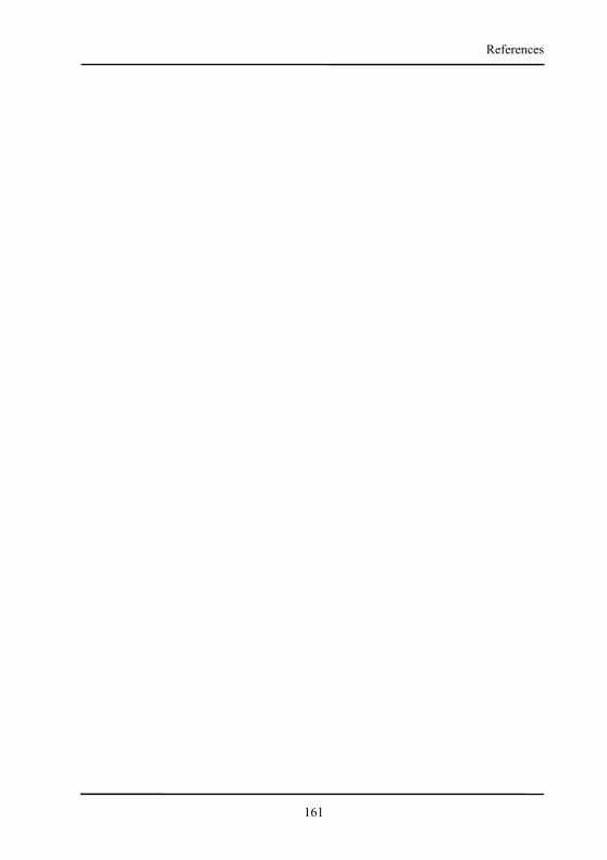
161

References

162

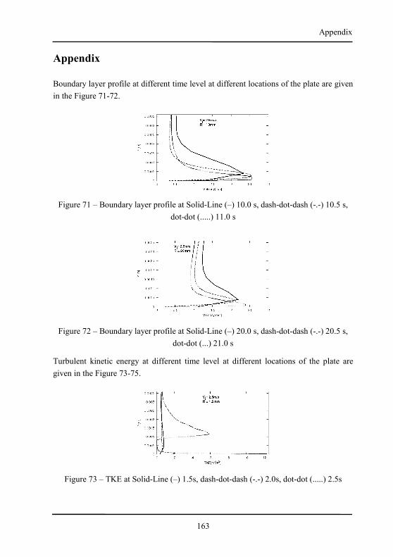
163

Appendix

Appendix

Boundary layer profile at different time level at different locations of the plate are given

in the Figure 71-72.


dot-dot (.....) 11.0 s


dot-dot (...) 21.0 s

Turbulent kinetic energy at different time level at different locations of the plate are

given in the Figure 73-75.


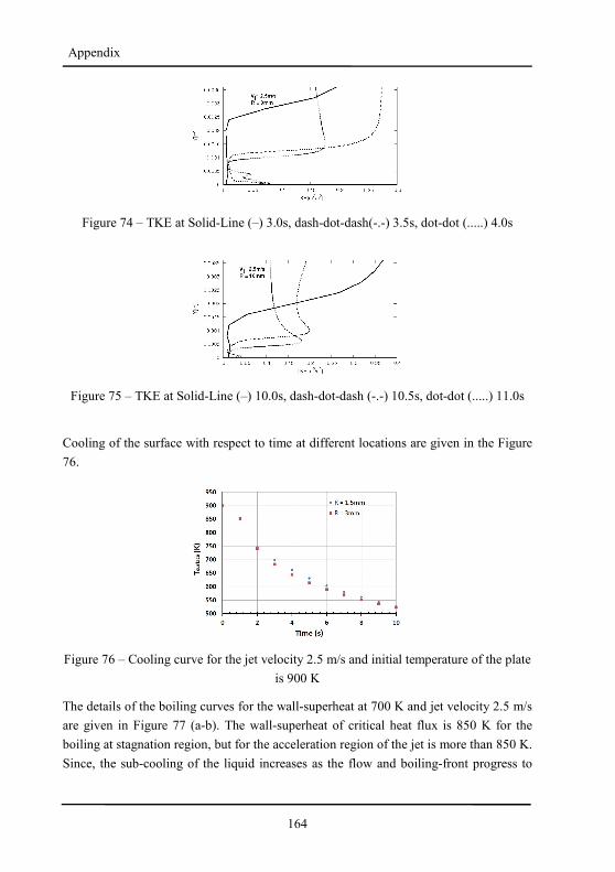
164

Appendix

Figure 74 – TKE at Solid-Line (–) 3.0s, dash-dot-dash(-.-) 3.5s, dot-dot (.....) 4.0s


Cooling of the surface with respect to time at different locations are given in the Figure

76.

Figure 76 – Cooling curve for the jet velocity 2.5 m/s and initial temperature of the plate

is 900 K

The details of the boiling curves for the wall-superheat at 700 K and jet velocity 2.5 m/s

are given in Figure 77 (a-b). The wall-superheat of critical heat flux is 850 K for the

boiling at stagnation region, but for the acceleration region of the jet is more than 850 K.

Since, the sub-cooling of the liquid increases as the flow and boiling-front progress to

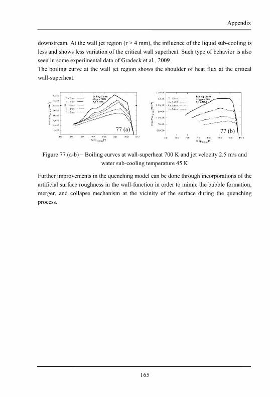
165

Appendix

downstream. At the wall jet region (r > 4 mm), the influence of the liquid sub-cooling is

less and shows less variation of the critical wall superheat. Such type of behavior is also

seen in some experimental data of Gradeck et al., 2009.

The boiling curve at the wall jet region shows the shoulder of heat flux at the critical

wall-superheat.

Figure 77 (a-b) – Boiling curves at wall-superheat 700 K and jet velocity 2.5 m/s and

water sub-cooling temperature 45 K

Further improvements in the quenching model can be done through incorporations of the

artificial surface roughness in the wall-function in order to mimic the bubble formation,

merger, and collapse mechanism at the vicinity of the surface during the quenching

process.

77 (a) 77 (b)

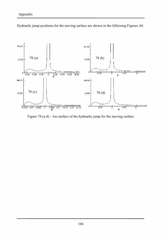
166

Appendix

Hydraulic jump positions for the moving surface are shown in the following Figures A8.

Figure 78 (a-d) – Iso-surface of the hydraulic jump for the moving surface

78 (a) 78 (b)

78 (c) 78 (d)

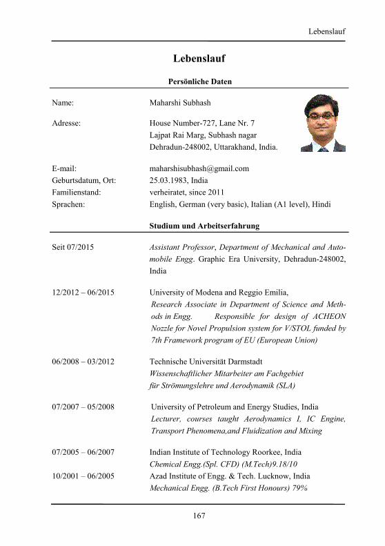
167

Lebenslauf

Lebenslauf

Persönliche Daten

Name: Maharshi Subhash

Adresse: House Number-727, Lane Nr. 7

Lajpat Rai Marg, Subhash nagar

Dehradun-248002, Uttarakhand, India.

E-mail: [email protected]

Geburtsdatum, Ort: 25.03.1983, India

Familienstand: verheiratet, since 2011

Sprachen: English, German (very basic), Italian (A1 level), Hindi

Studium und Arbeitserfahrung

Seit 07/2015 Assistant Professor, Department of Mechanical and Auto-

mobile Engg. Graphic Era University, Dehradun-248002,

India

12/2012 – 06/2015 University of Modena and Reggio Emilia,

Research Associate in Department of Science and Meth-

ods in Engg. Responsible for design of ACHEON

Nozzle for Novel Propulsion system for V/STOL funded by

7th Framework program of EU (European Union)

06/2008 – 03/2012 Technische Universität Darmstadt

Wissenschaftlicher Mitarbeiter am Fachgebiet

für Strömungslehre und Aerodynamik (SLA)

07/2007 – 05/2008 University of Petroleum and Energy Studies, India

Lecturer, courses taught Aerodynamics I, IC Engine,

Transport Phenomena,and Fluidization and Mixing

07/2005 – 06/2007 Indian Institute of Technology Roorkee, India

Chemical Engg.(Spl. CFD) (M.Tech)9.18/10

10/2001 – 06/2005 Azad Institute of Engg. & Tech. Lucknow, India

Mechanical Engg. (B.Tech First Honours) 79%

168

Lebenslauf

Documents

COMPUTATIONAL MODELLING OF - Technische …tuprints.ulb.tu-darmstadt.de/6217/1/subhash_final_version_of... · ... research on ‘Computational Modelling of Liquid Jet ... of Water