Embed Size (px)
Citation preview
TECHNISCHE UNIVERSITÄT MÜNCHEN
Lehrstuhl für Nukleartechnik
Computational Simulations of DirectContact Condensation as the Driving
Force for Water Hammer
Sabin-Cristian Ceuca
Vollständiger Abdruck der von der Fakultät für Maschinenwesen
der Technischen Universität München zur Erlangung des akademischen Grades eines
Doktor-Ingenieurs (Dr.-Ing.)
genehmigten Dissertation.
Vorsitzender: Univ.-Prof. dr. ir. Daniel J. Rixen
Prüfer der Dissertation: 1. Univ.-Prof. Rafael Macián-Juan
2. Univ-Prof. Dr.-Ing. Michael Schlüter,
Technische Universität Hamburg-Harburg
Die Dissertation wurde am 24.06.2014 bei der Technischen Universität München
eingereicht und durch die Fakultät für Maschinenwesen am 27.04.2015 angenommen.

Abstract
An analysis, based on Computer Simulations of the Direct Contact Condensation
as the Driving Force for the Condensation Induced Water Hammer phenomenon
is performed within this thesis. The goal of the work is to develop a mechanistic
HTC model, with predictive capabilities for the simulation of horizontal or nearly
horizontal two-phase �ows with complex patterns including the e�ect of interfacial
heat and mass transfer. The newly developed HTC model was implemented into
the system code ATHLET and into the CFD tools ANSYS CFX and OpenFOAM.
Validation calculations have been performed for horizontal or nearly horizontal
�ows, where simulation results have been compared against the local measurement
data such as void and temperature or area averaged data delivered by a wire mesh
sensor.
Contents
Abstract iii
Table of Contents vi
List of Figures xiv
List of Acronyms xv
1 Introduction 1
2 Horizontal and nearly Horizontal Two-Phase Flow Dynamics 5
2.1 Introduction to Two-Phase Flow Dynamics . . . . . . . . . . . . . . 5
2.2 Horizontal or nearly Horizontal Two-Phase Flow Patterns . . . . . . 7
2.3 The In�uence of Phase Change on Horizontal or nearly Horizontal
Two-Phase Flow Dynamics . . . . . . . . . . . . . . . . . . . . . . . 13
2.4 The Phenomenon of Water Hammer . . . . . . . . . . . . . . . . . . 16
2.4.1 A Particular Type of Water Hammer Caused by Condensa-
tion Induced Flow Transition . . . . . . . . . . . . . . . . . 20
2.5 Introduction to Dimensionless Numbers . . . . . . . . . . . . . . . . 24
3 Numerical Simulation of Two-Phase Flow 27
3.1 Introduction to the Numerical Simulation of Two-Phase Flow . . . . 27
3.2 Introduction to relevant Conservation Equations . . . . . . . . . . . 30
3.3 Introduction to System Codes . . . . . . . . . . . . . . . . . . . . . 33
3.4 Introduction to CFD Codes . . . . . . . . . . . . . . . . . . . . . . 36
CONTENTS
3.4.1 The Volume of Fluid Model . . . . . . . . . . . . . . . . . . 36
3.4.2 Turbulence Modeling in CFD . . . . . . . . . . . . . . . . . 41
3.5 Introduction to the Surface Renewal Theory . . . . . . . . . . . . . 46
3.5.1 Surface Renewal Theory accounting for Microscopic Eddies
for Scalar Exchange . . . . . . . . . . . . . . . . . . . . . . . 49
3.5.2 Surface Renewal Theory accounting for Macroscopic Eddies
for Scalar Exchange . . . . . . . . . . . . . . . . . . . . . . . 50
4 Present Contribution to the Calculation of CIWH 51
4.1 Development of a Hybrid Heat Transfer Coe�cient (HTC) Model
accounting for Microscopic and Macroscopic Eddie Scales . . . . . . 52
4.2 Implementation of the new Hybrid HTC Model into the System
Code ATHLET . . . . . . . . . . . . . . . . . . . . . . . . . . . . . 54
4.3 Implementation of the new Hybrid HTC Model into CFD Codes . . 55
4.4 Calibration of the new Hybrid HTC Model based on Experimental
Measurement Data . . . . . . . . . . . . . . . . . . . . . . . . . . . 57
4.4.1 Description of the LAOKOON Experimental Facility . . . . 57
4.4.2 Simulation of the LAOKOON Experimental Facility . . . . . 60
5 Description of the Experiments used for the Assessment of the
New Hybrid HTC Model 68
5.1 Description of the PMK-2 Experimental Facility . . . . . . . . . . . 69
5.2 Description of the TUHH Experimental Facility . . . . . . . . . . . 73
6 Assessment of the New Hybrid HTC Model for the Simulation of
Transient Two-Phase Flow with Finite Volume Computer Codes 76
6.1 Simulations of the PMK-2 Experimental Facility . . . . . . . . . . . 78
6.1.1 Simulations of the PMK-2 Experimental Facility with AN-
SYS CFX . . . . . . . . . . . . . . . . . . . . . . . . . . . . 78
6.1.2 Simulations of the PMK-2 Experiments with the System
Code ATHLET . . . . . . . . . . . . . . . . . . . . . . . . . 89
6.2 CFD Simulations of the TUHH Experimental Facility . . . . . . . . 102
v

CONTENTS
6.2.1 CFD Simulation of the TUHH Experiment Fr03T40 . . . . . 104
6.2.2 CFD Simulation of the TUHH Experiment Fr06T40 . . . . . 113
6.2.3 CFD Simulation of the TUHH Experiment Fr06T60 . . . . . 125
7 Conclusions and Outlook 136
A Appendix 1 PMK-2 Experiments Series 142
Bibliography 153
vi
List of Figures
2.1 Schematic representation of typical �ow patterns for horizontal two-
phase �ow [1] . . . . . . . . . . . . . . . . . . . . . . . . . . . . . . 8
2.2 The Mandhane et al. horizontal �ow regime map [2] . . . . . . . . . 12
2.3 Schematic representation of the phase distribution during an CIWH
in a horizontal pipe . . . . . . . . . . . . . . . . . . . . . . . . . . 22
3.1 Employed staggered grid used by the System Code ATHLET [3] . . 35
3.2 Schematic representation of the theoretical phase distribution com-
puted with VOF, [4] . . . . . . . . . . . . . . . . . . . . . . . . . . 37
3.3 Measured velocity in a turbulent �ow [5] . . . . . . . . . . . . . . . 42
4.1 Flow-wise cross section of the LAOKOON experimental facility [6] . 58
4.2 Channel cross section of the LAOKOON experimental facility [7] . . 59
4.3 Flow-wise cross section of the LAOKOON experimental facility [4] . 61
4.4 Eddy velocity and Length Scale based on the MaSE model for the
CFX simulation of LAOKOON [4] . . . . . . . . . . . . . . . . . . . 61
4.5 Eddy velocity and Length Scale based on the MiSE model in the
CFX simulation of LAOKOON[4] . . . . . . . . . . . . . . . . . . . 62
4.6 Comparison of the SRP computed by means of the MaSE and the
MiSE model based on the surface renewal theory SRT predicted by
the CFX simulations of LAOKOON . . . . . . . . . . . . . . . . . . 63
4.7 Comparison of the HTC by means of the MaSE and the MiSE model
in the CFX simulation of LAOKOON [4] . . . . . . . . . . . . . . . 64
LIST OF FIGURES
4.8 Comparison of the channel-wise temperature pro�le as calculated
using the MaSE and the MiSE based HTC model in the CFX sim-
ulation of LAOKOON . . . . . . . . . . . . . . . . . . . . . . . . . 64
4.9 Flow-wise HTC distribution by means of the hybrid model in the
CFX simulation of LAOKOON . . . . . . . . . . . . . . . . . . . . 64
4.10 Flow-wise temperature distribution by means of the hybrid model
in the CFX simulation of LAOKOON . . . . . . . . . . . . . . . . . 65
4.11 Temperature pro�le at the measurement plane of the LAOKOON
facility . . . . . . . . . . . . . . . . . . . . . . . . . . . . . . . . . . 65
5.1 Schematic representation of the PMK-2 experimental facility [8] . . 71
5.2 Interpolated isobars of measured pressure peaks (dots) at the PMK-
2 test facility [9] . . . . . . . . . . . . . . . . . . . . . . . . . . . . . 72
5.3 Schematic representation of the TUHH experimental facility [10] . . 73
5.4 Schematic representation of the test-section of the TUHH experi-
mental facility, adapted from [11] . . . . . . . . . . . . . . . . . . . 74
6.1 Flow pattern predicted with Shen's model in the PMK-2 facility at
key points in time (7.5 s, 9.0 s, 11.5 s, 12.5 s, 13.5 s, 15.0 s, 16.5 s),
represented by the void fraction (red: steam, blue: water) [4] . . . . 79
6.2 Computed HTC using Shen's model in the PMK-2 facility at key
points in time (7.5 s, 9.0 s, 11.5 s, 12.5 s, 13.5 s, 15.0 s, 16.5 s).
Black lines represent the contour for a volume fraction of 0.5, cor-
responding to the location of a two-phase interface [4] . . . . . . . . 80
6.3 Computed pressure using Shen's model in the PMK-2 facility at key
points in time (7.5 s, 9.0 s, 11.5 s, 12.5 s, 13.5 s, 15.0 s, 16.5 s).
Black lines represent the contour for a volume fraction of 0.5, cor-
responding to the location of a two-phase interface . . . . . . . . . . 81
6.4 Computed IAD using Shen's model in the PMK-2 facility at key
points in time (7.5 s, 9.0 s, 11.5 s, 12.5 s, 13.5 s, 15.0 s, 16.5 s).
Black lines represent the contour for a volume fraction of 0.5, cor-
responding to the location of a two-phase interface . . . . . . . . . . 82
viii
LIST OF FIGURES
6.5 Computed turbulent Reynolds number using Shen's model in the
PMK-2 facility at key points in time (7.5 s, 9.0 s, 11.5 s, 12.5 s,
13.5 s, 15.0 s, 16.5 s). Black lines represent the contour at volume
fraction at 0.5 corresponding to the location of the two-phase interface 83
6.6 Flow pattern in the simulation of the PMK-2 facility with the SRT
model based on micro eddies, close to the left bend, at key points
in time (5.0 s, 5.5 s, 5.85 s, 5.87 s, 5.88 s, 5.89 s) represented by
the void fraction (red: steam, blue: water) [12] . . . . . . . . . . . . 84
6.7 Relative System Pressure for the CFD simulation of the PMK-2
facility with HTC model employing micro eddies . . . . . . . . . . . 84
6.8 Flow pattern in the simulation of the PMK-2 facility with the hybrid
SRT model, at key points in time (6.8 s, 7.0 s, 7.2 s, 7.25 s, 7.3 s,
7.5 s) (red: steam, blue: water) . . . . . . . . . . . . . . . . . . . . 85
6.9 Pressure �eld in the simulation of the PMK-2 facility with the hy-
brid SRT model, at key points in time (6.8 s, 7.0 s, 7.2 s, 7.25 s,
7.3 s, 7.5 s) . . . . . . . . . . . . . . . . . . . . . . . . . . . . . . . 85
6.10 IAD �eld in the simulation of the PMK-2 facility with the hybrid
SRT model, at key points in time (6.8 s, 7.0 s, 7.2 s, 7.25 s, 7.3 s,
7.5 s) . . . . . . . . . . . . . . . . . . . . . . . . . . . . . . . . . . . 85
6.11 Temperature and void at VT1, VT2, VT3 and VT4 of the PMK-2
facility [12] . . . . . . . . . . . . . . . . . . . . . . . . . . . . . . . . 87
6.12 Void Fraction at WMS of the PMK-2 facility [12] . . . . . . . . . . 88
6.13 Simulated �ow patterns in the PMK-2 facility shortly before the
CIWH, at 7.0 s, 7.51 s, 7,55 s . . . . . . . . . . . . . . . . . . . . . 91
6.14 Temperature and void fraction at VT1, VT2, VT3 and VT4 of the
PMK-2 facility [12] . . . . . . . . . . . . . . . . . . . . . . . . . . . 93
6.15 Void Fraction at WMS of the PMK-2 facility [12] . . . . . . . . . . 95
6.16 System Pressure of the PMK-2 facility . . . . . . . . . . . . . . . . 96
6.17 Pressure Increase Ratio as a function of the Re, Fr, Ja and At numbers 99
6.18 Pressure Increase Ratio as a function of the Re and Ja numbers . . 99
6.19 Pressure Increase Ratio as a function of the Re and Fr numbers . . 100
ix
LIST OF FIGURES
6.20 Pipe network of the PMK-2 model for the simulation of quasi-2D
�ow regimes with ATHLET [12] . . . . . . . . . . . . . . . . . . . . 101
6.21 Volumetric �ow rates of three characteristic experiments conducted
at the TUHH experimental facility . . . . . . . . . . . . . . . . . . 103
6.22 CFD results of the fully developed 'water fountain' at problem time
1.70 s, TUHH experiment Fr03T40 . . . . . . . . . . . . . . . . . . 107
6.23 CFD results of the transition from horizontal to wavy �ow at prob-
lem time 4.10 s, TUHH experiment Fr03T40 . . . . . . . . . . . . . 107
6.24 CFD results of the water wave growing to form a slug at problem
time 4.45 s, TUHH experiment Fr03T40 . . . . . . . . . . . . . . . 108
6.25 CFD results of the decay of the water wave at problem time 4.55 s,
TUHH experiment Fr03T40 . . . . . . . . . . . . . . . . . . . . . . 108
6.26 CFD results of the relative pressure �eld with 0.5 void fraction con-
tour line at problem time 1,70 s, TUHH experiment Fr03T40 . . . . 109
6.27 CFD results of the relative pressure �eld with 0.5 void fraction con-
tour line at problem time 4.10 s, TUHH experiment Fr03T40 . . . . 109
6.28 CFD results of the relative pressure �eld with 0.5 void fraction con-
tour line at problem time 4.45 s, TUHH experiment Fr03T40 . . . . 109
6.29 CFD results of the relative pressure �eld with 0.5 void fraction con-
tour line at problem time 4.55 s, TUHH experiment Fr03T40 . . . . 109
6.30 CFD results of the HTC �eld with 0.5 void fraction contour line at
problem time 1.70 s, TUHH experiment Fr03T40 . . . . . . . . . . 110
6.31 CFD results of the HTC �eld with 0.5 void fraction contour line at
problem time 4.10 s, TUHH experiment Fr03T40 . . . . . . . . . . 110
6.32 CFD results of the HTC �eld with 0.5 void fraction contour line at
problem time 4.45 s, TUHH experiment Fr03T40 . . . . . . . . . . 110
6.33 CFD results of the HTC �eld with 0.5 void fraction contour line at
problem time 4.55 s, TUHH experiment Fr03T40 . . . . . . . . . . 110
6.34 CFD results of the fully developed 'water fountain' at problem time
1.70 s, TUHH experiment Fr03T40 . . . . . . . . . . . . . . . . . . 111
x
LIST OF FIGURES
6.35 CFD results of the transition from horizontal to wavy �ow at prob-
lem time 4.10 s, TUHH experiment Fr03T40 . . . . . . . . . . . . . 111
6.36 CFD results of the water wave growing to form a slug at problem
time 4.45 s, TUHH experiment Fr03T40 . . . . . . . . . . . . . . . 111
6.37 CFD results of the decay of the water wave at problem time 4.55 s,
TUHH experiment Fr03T40 . . . . . . . . . . . . . . . . . . . . . . 111
6.38 CFD results of the temperature at the thermo-couples Tf and Tg,
TUHH experiment Fr03T40 . . . . . . . . . . . . . . . . . . . . . . 112
6.39 CFD results of the fully developed 'water fountain' with built up
water �lm at problem time 1.80 s, TUHH experiment Fr06T40 . . . 116
6.40 CFD results of the transition from horizontal to wavy �ow at prob-
lem time 1.90 s, TUHH experiment Fr06T40 . . . . . . . . . . . . . 116
6.41 CFD results of the water wave growing to form a slug at problem
time 3.55 s, TUHH experiment Fr06T40 . . . . . . . . . . . . . . . 117
6.42 CFD results of the decay of the water wave at problem time 3.70 s,
TUHH experiment Fr06T40 . . . . . . . . . . . . . . . . . . . . . . 117
6.43 CFD results of the second water wave growing to form a slug at
problem time 4.05 s, TUHH experiment Fr06T40 . . . . . . . . . . 118
6.44 CFD results of the third water wave growing to form a slug at
problem time 4.90 s, TUHH experiment Fr06T40 . . . . . . . . . . 118
6.45 CFD results of the fourth water wave growing to form a slug at
problem time 6.05 s, TUHH experiment Fr06T40 . . . . . . . . . . 119
6.46 CFD results of the relative pressure �eld with 0.5 void fraction con-
tour line at problem time 1.80 s, TUHH experiment Fr06T40 . . . . 120
6.47 CFD results of the relative pressure �eld with 0.5 void fraction con-
tour line at problem time 1.90 s, TUHH experiment Fr06T40 . . . . 120
6.48 CFD results of the relative pressure �eld with 0.5 void fraction con-
tour line at problem time 3.55 s, TUHH experiment Fr06T40 . . . . 120
6.49 CFD results of the relative pressure �eld with 0.5 void fraction con-
tour line at problem time 3.70 s, TUHH experiment Fr06T40 . . . . 120
xi
LIST OF FIGURES
6.50 CFD results of the relative pressure �eld with 0.5 void fraction con-
tour line at problem time 4.05 s, TUHH experiment Fr06T40 . . . . 120
6.51 CFD results of the relative pressure �eld with 0.5 void fraction con-
tour line at problem time 4.90 s, TUHH experiment Fr06T40 . . . . 121
6.52 CFD results of the relative pressure �eld with 0.5 void fraction con-
tour line at problem time 6.05 s, TUHH experiment Fr06T40 . . . . 121
6.53 CFD results of the HTC �eld with 0.5 void fraction contour line at
problem time 1.80 s, TUHH experiment Fr06T40 . . . . . . . . . . 121
6.54 CFD results of the HTC �eld with 0.5 void fraction contour line at
problem time 1.90 s, TUHH experiment Fr06T40 . . . . . . . . . . 121
6.55 CFD results of the HTC �eld with 0.5 void fraction contour line at
problem time 3.55 s, TUHH experiment Fr06T40 . . . . . . . . . . 121
6.56 CFD results of the HTC �eld with 0.5 void fraction contour line at
problem time 3.70 s, TUHH experiment Fr06T40 . . . . . . . . . . 122
6.57 CFD results of the HTC �eld with 0.5 void fraction contour line at
problem time 4.05 s, TUHH experiment Fr06T40 . . . . . . . . . . 122
6.58 CFD results of the HTC �eld with 0.5 void fraction contour line at
problem time 4.90 s, TUHH experiment Fr06T40 . . . . . . . . . . 122
6.59 CFD results of the HTC �eld with 0.5 void fraction contour line at
problem time 6.05 s, TUHH experiment Fr06T40 . . . . . . . . . . 122
6.60 CFD results of the fully developed 'water fountain' with a liquid �lm
at the bottom of the pipe at problem time 1.80s, TUHH experiment
Fr06T40 . . . . . . . . . . . . . . . . . . . . . . . . . . . . . . . . . 122
6.61 CFD results of the transition from horizontal to wavy �ow at prob-
lem time 1.90 s, TUHH experiment Fr06T40 . . . . . . . . . . . . . 123
6.62 CFD results of the water wave growth to become a slug problem
time 3.55 s, TUHH experiment Fr06T40 . . . . . . . . . . . . . . . 123
6.63 CFD results of the collapse of entrapped steam pocket at problem
time 3.70 s, TUHH experiment Fr06T40 . . . . . . . . . . . . . . . 123
6.64 CFD results of the second water wave growing to form a slug at
problem time 4.05 s, TUHH experiment Fr06T40 . . . . . . . . . . 123
xii
LIST OF FIGURES
6.65 CFD results of the third water wave growing to form a slug at
problem time 4.90 s, TUHH experiment Fr06T40 . . . . . . . . . . 123
6.66 CFD results of the third water wave growing to form a slug at
problem time 6.05 s, TUHH experiment Fr06T40 . . . . . . . . . . 124
6.67 CFD results of the temperature at the thermo-couples Tf and Tg
TUHH experiment Fr06T40 . . . . . . . . . . . . . . . . . . . . . . 124
6.68 CFD results of the fully developed 'water fountain' with built up
water �lm at problem time 2.60 s, TUHH experiment Fr06T60 . . . 128
6.69 CFD results of the transition from horizontal to wavy �ow at prob-
lem time 2.70 s, TUHH experiment Fr06T60 . . . . . . . . . . . . . 128
6.70 CFD results of the water wave growing to form a slug at problem
time 2.80 s, TUHH experiment Fr06T60 . . . . . . . . . . . . . . . 129
6.71 CFD results of the collapse of the entrapped steam pocket at prob-
lem time 3.00 s, TUHH experiment Fr06T60 . . . . . . . . . . . . . 129
6.72 CFD results of the second water wave growing to form a slug at
problem time 3.75 s, TUHH experiment Fr06T60 . . . . . . . . . . 130
6.73 CFD results of the third water wave growing to form a slug at
problem time 5.90 s, TUHH experiment Fr06T60 . . . . . . . . . . 130
6.74 CFD results of the relative pressure �eld with 0.5 void fraction con-
tour line at problem time 2.60 s, TUHH experiment Fr06T60 . . . . 131
6.75 CFD results of the relative pressure �eld with 0.5 void fraction con-
tour line at problem time 2.70 s, TUHH experiment Fr06T60 . . . . 131
6.76 CFD results of the relative pressure �eld with 0.5 void fraction con-
tour line at problem time 2.80 s, TUHH experiment Fr06T60 . . . . 131
6.77 CFD results of the relative pressure �eld with 0.5 void fraction con-
tour line at problem time 3.00 s, TUHH experiment Fr06T60 . . . . 131
6.78 CFD results of the relative pressure �eld with 0.5 void fraction con-
tour line at problem time 3.75 s, TUHH experiment Fr06T60 . . . . 132
6.79 CFD results of the relative pressure �eld with 0.5 void fraction con-
tour line at problem time 5.90 s, TUHH experiment Fr06T60 . . . . 132
xiii
LIST OF FIGURES
6.80 CFD results of the HTC �eld with 0.5 void fraction contour line at
problem time 2.60 s, TUHH experiment Fr06T60 . . . . . . . . . . 132
6.81 CFD results of the HTC �eld with 0.5 void fraction contour line at
problem time 2.70 s, TUHH experiment Fr06T60 . . . . . . . . . . 132
6.82 CFD results of the HTC �eld with 0.5 void fraction contour line at
problem time 2.80 s, TUHH experiment Fr06T60 . . . . . . . . . . 133
6.83 CFD results of the HTC �eld with 0.5 void fraction contour line at
problem time 3.00 s, TUHH experiment Fr06T60 . . . . . . . . . . 133
6.84 CFD results of the HTC �eld with 0.5 void fraction contour line at
problem time 3.75 s, TUHH experiment Fr06T60 . . . . . . . . . . 133
6.85 CFD results of the HTC �eld with 0.5 void fraction contour line at
problem time 5.90 s, TUHH experiment Fr06T60 . . . . . . . . . . 133
6.86 CFD results of the fully developed 'water fountain' with built up
water �lm at problem time 2.60 s, TUHH experiment Fr06T60 . . . 134
6.87 CFD results of the transition from horizontal to wavy �ow at prob-
lem time 2.70 s, TUHH experiment Fr06T60 . . . . . . . . . . . . . 134
6.88 CFD results of the water wave growing to form a slug at problem
time 2.80 s, TUHH experiment Fr06T60 . . . . . . . . . . . . . . . 134
6.89 CFD results of the collapse of the entrapped steam pocket at prob-
lem time 3.00 s, TUHH experiment Fr06T60 . . . . . . . . . . . . . 134
6.90 CFD results of the second water wave growing to form a slug at
problem time 3.75 s, TUHH experiment Fr06T60 . . . . . . . . . . 135
6.91 CFD results of the third water wave growing to form a slug at
problem time 5.90 s, TUHH experiment Fr06T60 . . . . . . . . . . 135
6.92 CFD results of the temperature at the thermo-couples Tf and Tg,
TUHH experiment Fr06T60 . . . . . . . . . . . . . . . . . . . . . . 135
xiv
List of Acronyms
AEKI Atomic Energy Research Institute
ATHLET Analysis of Thermal-Hydraulics and LEaks
BC Boundary Condition
BWR Boiling Water Reactor
CEL CFX Expression Language
CFD Computational Fluid Dynamics
CFL Courant-Friedrich-Levy Number
CIWA Condensation Induced WAter Hammers
CIWH Condensation Induced Water Hammer
CV Control Volume
DCC Direct Contact Condensation
ECCS Emergency Core Cooling System
FSI Fluid-Structure Interaction
FZD Forschungszentrum Dresden Rosendorf
GRS Gesellschaft für Anlagen- und Reaktorsicherheit
HFKI Hungarian Academy of Sciences
HTC Heat Transfer Coe�cient
IAD Interfacial Area Density
IAPWS International Association for the Properties of Water and Steam
LDA Laser Doppler Anemometer
LES Large Eddy Simulation
LOCA Loss of Coolant Accident
LSM Level Set Method
LWR Light Water Reactors
MaSE Macro Scale Eddies
MiSE Micro Scale Eddies
NPP Nuclear Power Plant
OpenFOAM Open Source Field Operation and Manipulation
PDE Partial Di�erential Equation
PISO Pressure Implicit with Splitting of Operators
PTS Pressurized Thermal Shock
PWR Pressurized Water Reactor
RANS Reynolds Averaged Navier-Stokes
RHS Right Hand Side
RPV Reactor Pressure Vessel
SG Steam Generator
SRP Surface Renewal Period
xvi
SRT Surface Renewal Theory
SST Shear Stress Transport
TKE Turbulent Kinetic Energy
TUHH Technische Universität Hamburg-Harburg
TUM Technische Universität München
UMSICHT Frauenhofer Institut für Umwelt-, Sicherheits- und Energietechnik
UNIBW Universität der Bundeswehr München
USNRC U.S. Nuclear Regulatory Commission
VOF Volume Of Fluid
VVER Water-Water Power Reactor
WMS Wire Mesh Sensor
Dimensionless Numbers
At Atwood Number
Fr Froude Number
Ja Jakob Number
Pr Prandtl Number
Re Reynolds Number
Roman Symbols
a Speed of sound
ai Interfacial area density
xvii

Ainterface Interfacial area
cp Speci�c heat capacity
D Pipes inner diameter
e Pipe wall thickness
E Young's modulus of the pipe wall
g Gravitational acceleration
h Enthalpy
HTC Heat transfer coe�cient
I Turbulence intensity
j Super�cial velocity
k Turbulent kinetic energy
K Bulk modulus, i.e. the inverse value of the compressibility
Lt Turbulent eddy length scale
n Normal vector to the interface
p Pressure
Q Volumetric �ow rate
q Heat �ux
S Source term
t Time
trp Surface renewal period
T Temperature
xviii
U Velocity
V Volume
Vt Turbulent eddy velocity scale
Sub Scripts
1 Liquid
2 Gas
eff E�ective
c Compression
g Gas
i Interfacial
k Phase index
liq Liquid
max Maximum
mix Mixture
rel Relative
sat Saturation
t Turbulent
x Component along the x axes
y Component along the y axes
xix

z Component along the z axes
Super Scripts
→ Vector
− Average value
MaSE Macroscopic eddies
MiSE Microscopic eddies
′ Fluctuating component
t turbulent
tot total
Greek Symbols
α Volumetric gas fraction or thermal di�usivity
ε Eddy dissipation rate
∆ Di�erence
γ Volumetric liquid fraction
Γ Phase exchange rate
κ Surface curvature
λ Thermal conductivity
µ Dynamic viscosity
ν Kinematic viscosity
ω Turbulent frequency
xx

ρ Density
σ Surface tension
τ Interfacial friction
xxi
Acknowledgment
The following work was performed during my stay at the Department of Nuclear
Engineering at the Technische Universität München as part of the CIWA project
funded by the German Federal Ministry of Education and Research BMBF, under
the reference number 02NUK011E, which I would like to thank at this point.
First of all I would like to send special thanks to my two supervisors namely Univ-
Prof. Rafael Macián-Juan PhD, for giving me the opportunity to do this research
work at the TUM and being a constant source of support and Univ-Prof. Dr.-Ing.
Michael Schlüter from TUHH, for his continuous support and the scienti�c input
for my work. I would like to thank Prof. dr. ir. Daniel Rixen for kindly taking
the role of commission chairman. Special thanks go out to the entire sta� of the
department, technical or administrative, to all my students and to all the people
I met who in�uenced this work as well as to all the other fellow researchers at the
department; I know, I have put your patience to a test, when talking to you about
the problems encountered in my research and every day life. My best thoughts go
out to all CIWA project partners, with whom I have enjoyed sharing the time with
during interesting project meetings and helpful discussions. I also want to mention
the very helpful and supportive conversations with many of the GRS sta�, related
to the implementation of the hybrid model in ATHLET: Dr. H. Austregesilo, Mr.
G. Lerchl and Mr P. Schö�el, just to name the main contributors. Working with
all of You in such an environment was a great pleasure and contributed a lot to
this work.
Looking back at the years spent to accomplish this work, one realizes that in life
not everything lies in our own hands. At this point I want to mention and to

commemorate two experts that accompanied this work for only a too short time:
Univ-Prof. Dr.-Ing. Erik Pasche from TUHH, whom I had the honor to meet if
only brie�y at the beginning of my work and Dipl.-Ing. Harald Swidersky from
TÜV SÜD, to whom I am grateful for the time we worked together, for his support
and advice both invaluable and di�cult to express in words.
Last but not least I would like to thank my family, especially my parents, my
brother, my 'Munich based family' and to all my friends for their continuous un-
derstanding and support. Special thanks go to my beloved girlfriend Olivia I would
like to thank her, for the ongoing encouragement, as she was a very important drive
for this work.
To all of You I can only say: V mulµumesc!
xxiii
Chapter 1
Introduction
Simultaneous interfacial heat and mass transfer due to condensation or evapora-
tion is a commonly encountered phenomenon in many systems through various
industrial applications. Accurate simulation models are of particular importance
in industries where higher safety standards are applied, as in the case of the nuclear
and chemical industries. The realistic modeling of the interfacial heat and mass
transfer phenomenon is a key goal for best estimate simulations of Condensation
Induced Water Hammer (CIWH). The prompt and potentially violent CIWHs
events generate locally additional mechanical loads. If these loads are not consid-
ered, during the designing phase of that component, they can potentially result in
mechanical component failure. Experiments have highlighted the destructive force
of such pressure surges, especially in the low pressure levels, where peaks more
than 10 times higher than the system pressure have been measured. In the past a
lot of e�ort has been put on the development of avoidance and mitigation guide-
lines for the CIWH phenomenon. Recently guidelines have even been released for
the avoidance of CIWH events in thermal solar plants.
The danger of CIWH events in nuclear power plants was already highlighted by
the U.S. Nuclear Regulatory Commission (USNRC) in the 1970's, getting in the
spotlight after the incident at the Nuclear Power Plant Indian Point No. 2. The
ability to analyze the complex dynamic two-phase �ow behavior with computer
system codes is an integral part of any safety assessment study in which detailed
scenarios such as the postulated Loss of Coolant Accident (LOCA) or loss of o�-
site power are analyzed. During a LOCA event, subcooled water can be injected
by the Emergency Core Cooling System (ECCS), into the pipe network of the
primary power plant loop, counter-currently to the gas phase exiting the reactor
pressure vessel. A CIWH can under certain circumstances arise during an o�-site
power loss, an event expected to occur at least once during the life time of the
nuclear power plant. During the loss of o�-site power, depending on the steam
generator feed-water inlet design, auxiliary cold water can be injected through a
horizontal pipe into the steam generator. If this steam generator has a low enough
liquid level a water hammer event can be triggered by direct contact condensa-
tion. CIWH potentially occurs in any one-component two-phase �ow whenever
an entrapped gas bubble suddenly collapses due to high turbulence and due to a
su�ciently high liquid phase subcooling. As underlined within this work, Direct
Contact Condensation (DCC) can independently act as the main driving force for
�ow pattern changes in horizontal or nearly horizontal �ow. The di�erence in the
phase densities between the vapor and the liquid results in local depressurization
and in the acceleration of the liquid phase which has to �ll the void of the con-
densed steam thus enhancing the Kelvin-Helmholtz instability. The present work
focuses on the two-phase �ow of liquid water and steam, as water is still one of
the most widely used working �uid in the �eld of commercial energy production.
Examples of famous investigations for CIWH for working �uids di�erent than wa-
ter were done by Martin et al., [13].
Complex dynamic mechanisms in the interactions between the two-phases present
in two-phase �ow have to be considered in realistic computer simulations. Com-
puter simulations are currently intensively used in deterministic safety assessments
or during the designing phase of industrial scale facilities. Depending on the de-
sired results accuracy, two computing approaches are commonly used: system
code or computational �uid dynamics simulations. The system codes are fast run-
ning computer codes, which can perform full-system analysis employing relatively
2
coarse computational grids. The spatial resolution of their results is good enough
to understand the overall system behavior. If more local and physically accurate
results are needed, then high resolution resource intensive Computational Fluid
Dynamics (CFD) simulations have to be employed. The relatively large compu-
tational resources required by CFD simulations limit their applicability to full
system behavior analysis. Interfacial momentum, heat and mass exchange are de-
scribed in computer codes based on so called closure laws. In the particular case
of DCC, which occurs on the interface separating the phases key variables to be
modeled by a computer code in order to correctly capture the phase change are
the HTC and the Interfacial Area Density (IAD). The temperature and enthalpy
di�erence required for the calculation of the condensation rate results after solving
the conservation equations. The present work focuses on the mechanistic modeling
of the HTC and presents the development of a new hybrid model. This hybrid
model takes into consideration the e�ect of turbulent eddies on the structure of
the two-phase �ow. In order to assess its performance, this new model is imple-
mented into two CFD codes, ANSYS CFX and Open Source Field Operation and
Manipulation (OpenFOAM) and one system code, ATHLET. A validation of the
hybrid HTC model together with the Volume Of Fluid (VOF) approach for CFD
simulations and with the two-�uid model for the system code simulation will be
presented for a set of experiments performed at three di�erent facilities.
3
Outline of the Thesis
The thesis contains the following �ve major sections:
• Chapter 2 gives a general description of the two-phase �ow dynamics, focus-
ing on horizontal and nearly horizontal �ow channels. Typical �ow patterns
emerging in such channels will be presented with special emphasis on those
relevant for the description of the particular type of water hammers, driven
by direct contact condensation. Some dimensionless numbers, used for a later
analysis of the in�uence of particular parameters on the occurrence and mag-
nitude of the condensation induced water hammer, will also be introduced
within this chapter.
• Chapter 3 gives an overview on the computational tools later used in chapter
6, for the simulation of two-phase �ow with heat and mass transfer. This
chapter also includes the description of the conservation equations employed
by the models and the description of the mechanistic HTC approach based
on the surface renewal theory.
• The development work of the new hybrid HTC is presented in chapter 4.
After the new model is set up, its implementation into the used CFD tools
and the system code is presented. The threshold for the dynamic switch of
the hybrid HTC model is calibrated based on the measurement data acquired
in a quasi-steady state experiment.
• Chapter 5 includes the description of the experimental facilities which deliv-
ered the measurement data used for the assessment of the developed HTC
model. Special focus is set on the geometric set-up of the core part, the
test-section and the particularities of the installed data acquiring system at
each facility.
• The 6th chapter contains the simulation results of the computer calculations.
In total, 36 di�erent experiments have been simulated for the assessment of
the hybrid HTC model, 33 experiments have been simulated with the system
code and 4 experiments have been simulated with the CFD codes.
4
Chapter 2
Horizontal and nearly Horizontal
Two-Phase Flow Dynamics
A short overview will be given in this chapter on the two-phase �ow dynamics, the
possible complex �ow con�guration of two-phase �ow, the �ow patterns and the
e�ect of DCC on the two-phase �ow dynamics in a horizontal or nearly horizon-
tal channel. This chapter introduces the theoretical background required for the
analysis of a horizontal or nearly horizontal two-phase �ow. A general overview
of the di�erent types of water hammer phenomena will also be presented within
this chapter. Special emphasis will be put on the particular case of water hammer
driven by the contact condensation phenomenon.
Within this work, experiments of horizontal or nearly horizontal two-phase �ow
between saturated steam and subcooled water will be analyzed. Due to this reason
only horizontal or nearly horizontal two-phase �ow patterns will be introduced and
discussed in the next chapters.
2.1 Introduction to Two-Phase Flow Dynamics
The understanding and the study of multiphase �ow is of great importance in
many technological applications, especially in industrial facilities. In particular
Introduction to Two-Phase Flow Dynamics
two-phase �ows consisting of a liquid and a gas phase are found in many indus-
tries, such as power production, chemical and petro-chemical installations, process
engineering, lubrication systems and environmental control including meteorolog-
ical phenomena, etc.[14]. A correct understanding and modeling of the physics
of two-phase �ow plays a very important role during the design phase of new
equipment and in the assessment of the safety and e�ciency of its operation.
One of the most important areas in which two-phase �ow dynamics is of special
relevance is in power systems engineering. Heat and mass transfer processes are
crucial in the performance of power plants. The nuclear industry in particular is
very active in the development of detailed and reliable two-phase �ow models that
can be implemented into computer codes and used for the assessment of thermal-
hydraulic systems. Large increases in computational power in the recent past have
facilitated the development of sophisticated computer programs capable of simu-
lating the behavior of entire plants in two-phase �ow conditions, while considering
the complex heat, momentum and mass transfer mechanisms between the phases
and between these and the systems components.
The need for even more accurate simulations of the behavior of complex �uid
based systems, in which multiphase conditions play a crucial role in de�ning the
operation and safety of �uid based systems, has been a strong drive for research
and development aiming for a better understanding of the two-phase �ow phe-
nomenon. This has led to the development of more mechanistic models, based on
physical principles, rather than empirical correlations based on relatively simple
adjustments of measured data that can then be implemented into computer codes.
This trend has accelerated with the need for an increase in the operational safety
and in the e�ciency, which can result in an optimized use of the natural resources
in industrial systems. Even more, in the safety oriented nuclear industry, state-of-
the-art two-phase models are required in order to enhance the safety of a facility
and thus to decrease the risk of potential accidents.
6
Horizontal or nearly Horizontal Two-Phase Flow Patterns
2.2 Horizontal or nearly Horizontal Two-Phase
Flow Patterns
Horizontal or nearly horizontal pipes are used in many industrial facilities, such as
power plants, chemical and petro-chemical installations, thermo-solar parks, pro-
cess facilities, etc.
The phase distribution within a �ow channel with two-phase �ow is one of the
most important aspects of its description. Flow regime maps have been histori-
cally developed in order to more easily characterize two-phase �ow dynamics [15].
These maps determine the structure and morphology of the �ow as a function of
variables such as characteristic phase velocities, mass �uxes, void fractions, etc.
that delimit speci�c regions in the map with similar phase distribution character-
istics: the so-called �ow regimes. Flow regime maps are empirically developed and
therefore, depend to a certain extent on the geometrical set-up of the facility on
which the experiments have been conducted, on the thermo-physical properties of
the working �uid or �uids used and on the volumetric phase concentration within
the experimental section of the channel.
In particular, horizontal or nearly horizontal two-phase �ow patterns usually show
a clear phase separation caused by the in�uence of the gravitational force on the
phases with di�erent densities. If the inclination angle formed with the horizontal
axis is only a few degrees (< 5◦), the in�uence of the gravity on the phase distri-
bution is only limited. Thus a common practice is to use adapted horizontal �ow
patterns for slightly inclined �ow channels, mainly because very few �ow-regime
maps are available in the literature that account for every possible pipe inclination.
The lack of available �ow regime maps for nearly inclined pipes is partially due to
the practical impossibility of creating these maps for every desirable inclination.
Still some important experimental investigations have been performed for inclined
pipes with upward �ow by Weisman and Kang [16] and by Barnea et. al[17].
In the present thesis two-phase �ow of subcooled liquid water and saturated steam
together with the phenomenon of CIWH in horizontal or slightly inclined pipes
is analyzed. Therefore, only �ow regimes for such inclinations will be discussed
7
Horizontal or nearly Horizontal Two-Phase Flow Patterns
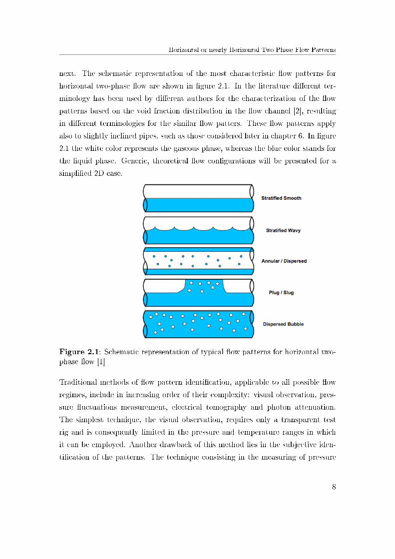
next. The schematic representation of the most characteristic �ow patterns for
horizontal two-phase �ow are shown in �gure 2.1. In the literature di�erent ter-
minology has been used by di�erent authors for the characterization of the �ow
patterns based on the void fraction distribution in the �ow channel [2], resulting
in di�erent terminologies for the similar �ow patters. These �ow patterns apply
also to slightly inclined pipes, such as those considered later in chapter 6. In �gure
2.1 the white color represents the gaseous phase, whereas the blue color stands for
the liquid phase. Generic, theoretical �ow con�gurations will be presented for a
simpli�ed 2D case.
Figure 2.1: Schematic representation of typical �ow patterns for horizontal two-phase �ow [1]
Traditional methods of �ow pattern identi�cation, applicable to all possible �ow
regimes, include in increasing order of their complexity: visual observation, pres-
sure �uctuations measurement, electrical tomography and photon attenuation.
The simplest technique, the visual observation, requires only a transparent test
rig and is consequently limited in the pressure and temperature ranges in which
it can be employed. Another drawback of this method lies in the subjective iden-
ti�cation of the patterns. The technique consisting in the measuring of pressure
8
Horizontal or nearly Horizontal Two-Phase Flow Patterns
�uctuations can be applied to a broader range of pressures and temperatures,
with the price of losing the optical investigation possibility because of the use of
metallic, opaque pipes. The more sophisticated and expensive photon attenuation
technique can still give an insight into opaque pipes. Electrical tomography is a
method of area averaged phase tracking with the major drawback typical to all
�ow invasive measurement techniques of perturbing the �ow. Still it is a widely
used method, which can deliver useful results with the high temporal and spacial
resolution required for the validation of CFD-codes for two-phase �ow conditions.
Variables often used as parameters in the axes of �ow regime maps include: the
volumetric phase concentration also referred to as the void fraction de�ned in the
equation (2.1), where V represents the volume; and the phasic gas and liquid
super�cial velocities, as de�ned in the equation (2.2), where Qk represents the
volumetric �ow rate of phase k, A represents the cross-section area and Uk is the
velocity of phase k. The void fraction, can be computed as a volumetric or an area
averaged value, and represents the amount of gaseous phase in the region where it
is computed. Equation (2.1) presents the volumetric averaged void fraction, as it
is used also in the �nite volume computer codes, later employed for the simulation
of two-phase �ow with DCC in chapter 6. The super�cial velocity jk describes the
hypothetical velocity of a speci�c phase k, as if it �owed alone in the entire channel
shared by the two phases. The super�cial velocity can be calculated as the ratio
between volumetric �ow rate of the phase k and the entire channel cross-sectional
area or by forming the product between the phase k fraction multiplied by its
phase velocity.
α =1
V
∫∫∫V
αdV =VgV
(2.1)
jk =Qk
Achannel= α · Uk (2.2)
The most known and still most used �ow regime maps in order of their publication
date are: the one developed by Baker [18], Mandhane's et al. [19] and Taitel and
Dukler's [20].
9
Horizontal or nearly Horizontal Two-Phase Flow Patterns
Baker's experimental investigations for adiabatic horizontal �ows, resulted in the
design of one of the �rst �ow regime maps, [18]. He stressed the in�uence of the
�ow pattern on pressure losses and heat and mass transfer in tubes. The two axes
of his map consider the super�cial phase-velocity and some additional parameters
accounting for the in�uence of the thermo-physical properties of the �uids, in or-
der to o�er extrapolation capabilities to other combinations of working �uids. The
map was developed using experimental data from large diameter pipes of adiabatic
air-water or water-oil �ow.
The Mandhane et al. �ow regime map was developed for low system pressure
conditions with small gas density changes [19]. Mandhane et al. consider that the
in�uence of the thermo-physical properties on the �ow pattern is not that strong
as stated by Baker, [19]. This map builds up on the Baker map, but neglects the
pipe diameter, resulting in a map with limited applicability even if a large database
of measurements of adiabatic air-water �ow was used for its development.
Perhaps the most used and implemented horizontal two-phase �ow regime map
in computer codes is the Taitel and Dukler map [20]. They developed a �ow
regime map after realizing, based on the comparison of di�erent available maps,
that sometimes big discrepancies exist between these maps, especially in the tran-
sition regions. Using a more theoretical approach, Taitel and Dukler combined the
in�uences of the thermo-physical properties, the gravitational acceleration, the
pressure gradient, phase velocities, channel inclination and channel geometry in a
more mechanistic model.
A short characterization of the main �ow patterns for horizontal or nearly hor-
izontal two-phase �ow will be de�ned based on the �ow regime map developed
by Mandhane et al. [19] and represented in �gure 2.2. Mandhane et al. initially
developed this map for adiabatic �ow conditions within a channel with a circular
cross section. Starting from low volumetric �uxes and going in a counter-clockwise
direction in the map, the following major patterns are identi�ed: strati�ed, (strat-
10
Horizontal or nearly Horizontal Two-Phase Flow Patterns
i�ed) wavy, annular, slug, plug and bubbly �ow.
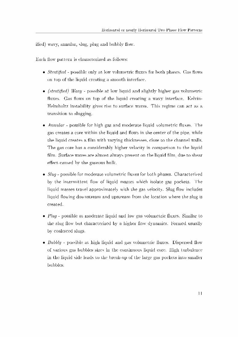
Each �ow pattern is characterized as follows:
• Strati�ed - possible only at low volumetric �uxes for both phases. Gas �ows
on top of the liquid creating a smooth interface.
• (strati�ed) Wavy - possible at low liquid and slightly higher gas volumetric
�uxes. Gas �ows on top of the liquid creating a wavy interface. Kelvin-
Helmholtz instability gives rise to surface waves. This regime can act as a
transition to slugging.
• Annular - possible for high gas and moderate liquid volumetric �uxes. The
gas creates a core within the liquid and �ows in the center of the pipe, while
the liquid creates a �lm with varying thicknesses, close to the channel walls.
The gas core has a considerably higher velocity in comparison to the liquid
�lm. Surface waves are almost always present on the liquid �lm, due to shear
e�ect caused by the gaseous bulk.
• Slug - possible for moderate volumetric �uxes for both phases. Characterized
by the intermittent �ow of liquid masses which isolate gas pockets. The
liquid masses travel approximately with the gas velocity. Slug �ow includes
liquid �owing downstream and upstream from the location where the slug is
created.
• Plug - possible at moderate liquid and low gas volumetric �uxes. Similar to
the slug �ow but characterized by a higher �ow dynamics. Formed usually
by coalesced slugs.
• Bubbly - possible at high liquid and gas volumetric �uxes. Dispersed �ow
of various gas bubbles sizes in the continuous liquid core. High turbulence
in the liquid side leads to the break-up of the large gas pockets into smaller
bubbles.
11
Horizontal or nearly Horizontal Two-Phase Flow Patterns
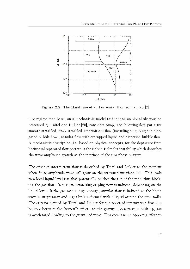
Figure 2.2: The Mandhane et al. horizontal �ow regime map [2]
The regime map based on a mechanistic model rather than on visual observation
presented by Taitel and Dukler [20], considers (only) the following �ow patterns:
smooth strati�ed, wavy strati�ed, intermittent �ow (including slug, plug and elon-
gated bubble �ow), annular �ow with entrapped liquid and dispersed bubble �ow.
A mechanistic description, i.e. based on physical concepts, for the departure from
horizontal separated �ow pattern is the Kelvin-Helmoltz instability which describes
the wave amplitude growth at the interface of the two phase mixture.
The onset of intermittent �ow is described by Taitel and Dukler as the moment
when �nite amplitude wave will grow on the strati�ed interface [20]. This leads
to a local liquid level rise that potentially reaches the top of the pipe, thus block-
ing the gas �ow. In this situation slug or plug �ow is induced, depending on the
liquid level. If the gas rate is high enough, annular �ow is induced as the liquid
wave is swept away and a gas bulk is formed with a liquid around the pipe walls.
The criteria de�ned by Taitel and Dukler for the onset of intermittent �ow is a
balance between the Bernoulli e�ect and the gravity. As a wave is built up, gas
is accelerated, leading to the growth of wave. This comes as an opposing e�ect to
12
The In�uence of Phase Change on Horizontal or nearly Horizontal Two-Phase Flow Dynamics
the wave decreasing e�ect of the gravitational acceleration. The presentation of
the characteristic patterns in a horizontal two-phase �ow was presented based on
the Mandhane �ow regime map, because the axis of the Taitel and Dukler map
depend on the �ow conditions, the geometric set up of the �ow channel and on the
thermo-physical properties of the �uids.
The Taitel and Dukler �ow regime map was developed for adiabatic �ow conditions
but is widely applied to diabatic �ow regimes.
Since these maps have been developed under adiabatic conditions, it is di�cult
to account for the e�ect of phase change onto the two-phase �ow dynamics. The
literature presents some examples of �ow regime maps where the e�ect of phase
change has been included within heat exchangers. Extensive research was also
done for refrigeration agents in small diameter tubes. One of the �rst studies
was carried out by Haraguchi et al. [21] later, work was done and published by
the group of Cavallini, Thome and El Hajal [22], [23], [24], [25]. Within these
publications phase change occurs preponderantly at the �ow channel walls and
not, as in the case of the analyzed DCC in this thesis, at the two-phase interface.
Section 2.3 will present the in�uence of phase change in two-phase �ow dynamics,
while chapter 6 will highlight this in�uence based on computer simulations.
2.3 The In�uence of Phase Change on Horizontal
or nearly Horizontal Two-Phase Flow
Dynamics
The DCC describes a phase change that takes place at the interface of direct
contact between the liquid and vapor phases. The interface is assumed to be at
saturation conditions, whereas the liquid and/or the steam can be away from satu-
ration. Thermal equilibrium is locally assumed and the interface is not considered
to add any resistance to the heat and mass transfer between the phases.
Interfacial heat and mass transfer, such as the DCC, is encountered in many in-
13
The In�uence of Phase Change on Horizontal or nearly Horizontal Two-Phase Flow Dynamics
dustrial systems. It is of particular importance in the nuclear power and chemical
installations. DCC is a phenomenon which can appear in any system-component
with a single component two-phase �ow. This phenomenon can appear with any
combination of a liquid and its vapor under thermal non-equilibrium conditions.
In the power generation industry water is the most often used work �uid, but DCC
can also occur in refrigeration systems or petro-chemical installations with other
�uids.
The modeling of DCC must consider several key parameters that describe the
macroscopic phase change phenomena, such as the local heat transfer coe�cient
HTC, the area of contact between both phases (interfacial area), and the sub-
cooling of the liquid phase. The �rst two parameters have to be correctly pre-
dicted by using special models in computer simulations, while the last one is a
direct consequence of solving the conservation equations with a strong feedback
from the �rst two parameters.
The e�ect of the condensation process on the IAD is opposed to the case of va-
porization because the interfacial area density tends to decrease, as condensation
damps the interfacial ripples [15].
In the case of vaporization (boiling), the formation of bubbles and the bubble in-
duced turbulence and bubble break-up mechanisms tend to increase the interfacial
area available for heat and mass transfer between the phases. The decrease of
phase contact surface in DCC reduces the phasic interchange of energy and mass
and has an in�uence on the overall condensation rate, which in turn, determines
the magnitude of the pressure spikes in CIWH situations.
An example of scenarios in which DCC plays an important role is during a postu-
lated LOCA in a Nuclear Power Plant (NPP) especially during the re-�ooding
stage as subcooled water is injected by the Emergency Core Cooling System
(ECCS) into the primary side pipes and it �ows counter-currently to the steam ex-
iting the reactor core. Accurate safety related simulations of the re-�ooding stage
of a LOCA, require models that can predict high condensation rates as correctly
as possible, particularly at locations close to the injection point of the ECCS or
14
The In�uence of Phase Change on Horizontal or nearly Horizontal Two-Phase Flow Dynamics
in areas of high �ow turbulence which, together with a high sub-cooling of the
water in contact with the saturated or superheated steam can lead to sudden �ow
regime changes and very fast condensation of the steam. The analysis of the local
e�ects during the re-�ooding stage of the LOCA is very complex due to the highly
dynamic character of the two-phase �ow. A reliable prediction of the transient
�ow patterns is required, in addition to the correct modeling of the heat and mass
transfer processes over the wide range of �ow patterns.
A visual investigation on a transparent test-section with a geometry similar to
that of the ECCS injection was performed at the Technische Universität Hamburg-
Harburg (TUHH) and showed the changes in �ow pattern caused by the conden-
sation process. Measurement data from the Universität der Bundeswehr München
(UNIBW), the TUHH and the PMK-2 facility in Hungary clearly proved the in-
�uence of DCC in two-phase �ow dynamics.
Flow patterns that can occur in horizontal or nearly horizontal �ow channels can
be grouped based on the values of local parameters such as the super�cial velocities
of the phases and local void fraction. These �ow patterns span from strati�ed to
slug �ow with entrainment of the disperse phase, which can be both steam bubbles
and water droplets depending on the two-phase �ow con�guration and void frac-
tion. Under certain conditions DCC can also act as the driving force for changes
in the �ow pattern. The �ow regime maps that can be used in such conditions
should take into account the in�uence of local depressurization due to DCC when
de�ning the transition regions on the maps.
A local decrease in pressure within a pipe containing a two-phase mixture caused
by phase change can lead to the dangerous, prompt and violent condensation phe-
nomenon also called CIWH. The decreasing pressure can locally change the �ow
pattern from strati�ed to slug �ow and thus to prompt steam bubble collapse.
The phenomenon of CIWH is most destructive at low and intermediate system
pressures, because of the high di�erences in phase density, resulting in a higher
�ow acceleration potential during the collapsing phase and the release of a larger
latent heat. The resulting violent pressure surge adds a supplementary mechanical
15
The Phenomenon of Water Hammer
load to the system component in which it appears. If this phenomenon was not
considered within the designing phase of that component, a mechanical failure is
plausible. Such integrity failures can have serious consequences. There is there-
fore, a large practical interest in the accurate modeling of DCC both during the
design phase of safety equipment, as well as part of the periodic system safety
assessments of vital components. A more comprehensive overlook over the phe-
nomenon of CIWH will be provided in chapter 2.4.
Recommended models for the computation of the HTC directly linked with tur-
bulence quantities will be presented in chapter 3.5 and chapter 4.
The in�uence of the condensation rate on the change in the �ow pattern, will be
presented within the chapter 6.1, when the results of the Surface Renewal Theory
(SRT) based HTC models are presented and when the experimental measurement
data of the PMK-2 and the TUHH facility will be discussed. It will be shown
that DCC can act as the driving force for the change in the �ow pattern using the
results of computer simulations, both system code and of CFD tools.
2.4 The Phenomenon of Water Hammer
In general a typical water hammer event is a rapid change in pressure resulting in
a propagating pressure wave. It appears in pipes or pipe networks and is caused
by a rapid change in �uid velocity. This particular change can be the result, for
example, of events such as a pump starting or rapid coast-down, the operation of
a valve or as a result of DCC. In the literature water hammers have been grouped
in categories based on the di�erent water hammer triggering mechanisms. One
of the most analyzed water hammer types is the one with column separation, as
it can occur in many industrial applications, with a single-phase working �uid.
This sub-group of water hammers is characterized by the direct feedback between
a rapidly changing �uid velocity and the pressure changes experienced by the �uid
as a result. In the case of the CIWH it is the formation of a large bubble of steam
16
The Phenomenon of Water Hammer
(slug) in a horizontal or nearly horizontal pipe, leading to an entrapment of a vapor
pocket by subcooled liquid. The fast condensation of the steam bubble creates a
vacuum which is rapidly �lled by an accelerating liquid traveling towards it. As
the bubble collapses, high velocity liquid surfaces collide and create a compressive
local pressure spike that propagates along the system.
The typical sequence of a pressure surge scenario is: a triggering event causes a
rapid change in �ow velocity (deceleration) which induces a rising pressure peak as
the �uid's momentum is transformed in pressure energy. The propagation of the
pressure peak creates a traveling pressure wave followed by an equal and opposite
re�ected wave. This re�ection can take place either at a forming two-phase inter-
face or at the piping system's structure. If two re�ected waves meet, then higher
pressures than the initial surge can arise. Eventually, because of energy losses
caused by friction and elastic interaction of the �uid with the solid surfaces, the
energy of the pressure wave dissipates and the pressure returns to its initial value.
If the maximum pressure reached is high enough, the integrity of the system can
be compromised by the appearance of cracks or by the bursting of pipe lines and
other system components or increase the material fatigue. This may lead to serious
consequences of release of pipe contents to the surroundings due to rupture causing
eventually environmental and health hazards. The high pressure wave can damage
pipe bridges, the pipe mounting system or components such as foundations pumps
or valves. The depressurization wave can lead to pipe collapses or to the suction
of air or slope water into the main pipe. In the work presented in this thesis, the
re�ection of the pressure wave has only been considered at the two-phase interface,
since no �uid-structure interaction was modeled. The high compressibility rate of
the gaseous phase leads to only a minimal pressure oscillation within this phase
and results in a fast damping pressure within a short pipe length away from the
point of steam bubble collapse.
A method often used to calculate potential water hammers in piping systems,
even if it was one of the �rst developed models, is based on Joukowsky's model
presented in equation (2.3). This model directly correlates the maximum pressure
variation with the product of the liquid slug velocity variation, the local speed of
17
The Phenomenon of Water Hammer
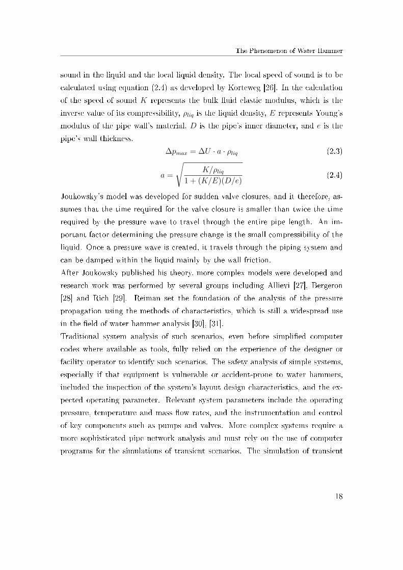
sound in the liquid and the local liquid density. The local speed of sound is to be
calculated using equation (2.4) as developed by Korteweg [26]. In the calculation
of the speed of sound K represents the bulk �uid elastic modulus, which is the
inverse value of its compressibility, ρliq is the liquid density, E represents Young's
modulus of the pipe wall's material, D is the pipe's inner diameter, and e is the
pipe's wall thickness.
∆pmax = ∆U · a · ρliq (2.3)
a =
√K/ρliq
1 + (K/E)(D/e)(2.4)
Joukowsky's model was developed for sudden valve closures, and it therefore, as-
sumes that the time required for the valve closure is smaller than twice the time
required by the pressure wave to travel through the entire pipe length. An im-
portant factor determining the pressure change is the small compressibility of the
liquid. Once a pressure wave is created, it travels through the piping system and
can be damped within the liquid mainly by the wall friction.
After Joukowsky published his theory, more complex models were developed and
research work was performed by several groups including Allievi [27], Bergeron
[28] and Rich [29]. Reiman set the foundation of the analysis of the pressure
propagation using the methods of characteristics, which is still a widespread use
in the �eld of water hammer analysis [30], [31].
Traditional system analysis of such scenarios, even before simpli�ed computer
codes where available as tools, fully relied on the experience of the designer or
facility operator to identify such scenarios. The safety analysis of simple systems,
especially if that equipment is vulnerable or accident-prone to water hammers,
included the inspection of the system's layout design characteristics, and the ex-
pected operating parameter. Relevant system parameters include the operating
pressure, temperature and mass �ow rates, and the instrumentation and control
of key components such as pumps and valves. More complex systems require a
more sophisticated pipe network analysis and must rely on the use of computer
programs for the simulations of transient scenarios. The simulation of transient
18
The Phenomenon of Water Hammer
scenarios gives better insights on the onset and evolution of possible water hammer
events.
If two-phase �ow is to be present at the onset or during the evolution of the water
hammer event, the main requirement for such computer programs is the capability
to realistically and reliably predict the two-phase �ow in complex geometries for
various transient scenarios within reasonable computational time. Key variables
such as the phase velocity, phase volume fractions and pressures throughout the
analyzed system must be accurately predicted by the employed transient analysis
computer code. Otherwise, the formation of the pressure wave, its propagation
along the system and the maximum pressure values may not be correctly predicted.
Still, the evaluation of the computational results by an experienced user remains
vital in order to determine the possibility of water hammer in the analyzed system
and its severity so that e�ective pressure surge protection measures can be taken.
The consequences of water hammer events in facilities having operated for a certain
time are more severe than in newly built facilities, because if water hammers
are large enough, the e�ect of aging, fatigue and corrosion-erosion of the solid
structures can lead to cracks or bursting. In aged installations such events have
the potential to aggravate many safety problems [32]. Even if the initial pressure
spikes may not be large enough, the interaction of the traveling pressure waves with
the system-structure-equipment can result in vibrations and even in resonances,
which eventually can also lead to system breaks. A worst case scenario would be
when water hammer events appear during abnormal or accident situations, thus
aggravating the seriousness of the emergency situation.
The main di�erence between the two groups of the discussed water hammer phe-
nomena, consists in the initiating mechanism: in the case of the water hammer
with column separation it is for instance a fast closure of a valve while in the case
of the CIWH it is the slug formation in a horizontal or nearly horizontal pipe,
leading to an entrapment of a vapor pocket by subcooled liquid.
19
The Phenomenon of Water Hammer
2.4.1 A Particular Type of Water Hammer Caused by
Condensation Induced Flow Transition
Experimental research designed to address the phenomenon of CIWH in detail
was initiated by the USNRC in the 1970s after some incidents having this phe-
nomenon as a precursor occurred in nuclear power plants with potentially serious
consequences. The �rst incident in a NPP took place at Indian Point Unit No. 2
in 1973. A feed-water pipe was damaged due to CIWH when subcooled feed-water
was introduced into the steam-generator following a low-water-level reactor trip.
Steam exited counter-currently from the steam generator and �owed into the feed-
water line mixing with the subcooled water �owing inside. After this event, other
similar cases have been reported world wide and the topic has become an area
of active experimental, theoretical and developmental research, with applications
beyond the nuclear industry. This phenomenon is not only a threat to steam-
water systems, but also to any system in which a liquid and its vapor �ow in a
two-phase regime: if vapor of a �uid comes into contact with its subcooled, liquid
phase of that component, a CIWH may result. Examples of relevant investigations
for CIWH for working �uids di�erent to water have been done, for example, by
Martin et al.[13].
As brie�y discussed in the previous section, the phenomenon of CIWH potentially
occurs in two-phase �ow systems whenever an entrapped steam bubble suddenly
collapses due to a very large condensation rate caused by high turbulence and
su�ciently high subcooling of the liquid phase. The di�erence in phase speci�c
volumes results in a large local depressurization as the bubble collapses and in
the acceleration of the liquid phase that has to �ll in the void left empty by the
condensing steam. A su�ciently large liquid velocity leads to a pressure surge when
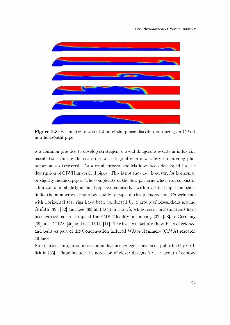
the two water fronts meet. A schematic representation of such an event is shown
in �gure 2.3. This schematic representation shows a horizontal pipe in which water
(blue) is injected from the left hand side into a steam (red) �lled pipe. In this case
the �ow regime changes locally from horizontal strati�ed to horizontal wavy (see
20
The Phenomenon of Water Hammer
second �gure from top). The instability occurs as steam �ows counter-currently due
to the large condensation rate in contact with the subcooled liquid. The local liquid
waves continue to grow and form a slug which completely isolates the steam pocket
at the top of the pipe (third �gure in the same sequence). A sudden condensation
of the entrapped steam pocket causes a signi�cant local depressurization because
of the high speci�c volume of the steam. The local pressure in the steam bubble
decreases almost to the saturation pressure corresponding to the temperature of
the liquid phase [33]. If the pressure decreases enough, additional vaporization can
occur. As the steam condenses, water is sucked in to replace its volume (fourth
and �fth �gure). In some cases, the depressurization can even cause the collapse of
pipe segments. The acceleration of the water fronts toward each other can lead to
a CIWH event as the fronts collide if the steam bubble condensation is fast enough.
A high pressure wave is then created, which can harm or burst pipe sections and
add mechanical load onto the pipe bends and their supports. The pressure wave
hits the free surface in the �ow and is either re�ected or dissipated if, for example,
it encounters a steam bubble swarm. The duration of the resulting forces applied
on pipes is very short, yet it may be su�cient to produce structural damage on
the pipe or its supports [33].
The depressurization is more pronounced in systems operating at lower pressures
because of the larger di�erence between steam and liquid water speci�c volumes,
thus making CIWH more dangerous when they appear in low pressure systems.
This often corresponds to ab-normal operational regimes in NPPs during or after
loss of coolant or other kinds of scenarios, but can also be normal non-full power
modes of operation. It is important to notice that locally high condensation rates
can alone act as the driving force for local two-phase �ow pattern changes that
may initiate water hammer events. The DCC e�ect thus enhances the Kelvin-
Helmholtz instability.
Early experimental work on the phenomenon of CIWH in test rigs in�uenced by the
needs of the nuclear industry was conducted by Block et al. [34]. His initial experi-
ments, also known as the "water canon experiments" were carried out on a vertical
pipe and resulted in the development of mitigation strategies for such events. It
21
The Phenomenon of Water Hammer
Figure 2.3: Schematic representation of the phase distribution during an CIWHin a horizontal pipe
is a common practice to develop strategies to avoid dangerous events in industrial
installations during the early research stage after a new safety-threatening phe-
nomenon is discovered. As a result several models have been developed for the
description of CIWH in vertical pipes. This is not the case, however, for horizontal
or slightly inclined pipes. The complexity of the �ow patterns which can coexist in
a horizontal or slightly inclined pipe overcomes that within vertical pipes and thus,
limits the number existing models able to capture this phenomenon. Experiments
with horizontal test rigs have been conducted by a group of researchers around
Gri�th [35], [32] and Lee [36] all based in the US, while recent investigations have
been carried out in Europe at the PMK-2 facility in Hungary [37], [38], in Germany
[39], at UNIBW [40] and at TUHH [11]. The last two facilities have been developed
and built as part of the Condensation Induced WAter Hammers (CIWA) research
alliance.
Elimination, mitigation or accommodation strategies have been published by Grif-
�th in [33]. These include the adoption of clever designs for the layout of compo-
22
The Phenomenon of Water Hammer
nents, precise operation procedures or the use of non-condensable gases to decrease
the condensation rates, just to enumerate some of them.
The literature o�ers a set of CIWH mitigation measures, for instance by Chou and
Gri�th [32]; but no reliable calculation model is yet available. The comprehensive
work of Chou and Gri�th included CIWH mitigation strategies based on:
• Development of �ow stability maps for piping systems, with di�erent orien-
tations, as a function of �lling velocities and water subcooling.
• Development of check lists for the designing phase of pipe systems.
• Development of simpli�ed, analytical models.
The initial pressure wave in the case of CIWH, contrary to the water hammer
with single-phase column separation, is always negative because it is caused by
the condensation of the vapor. This wave later results in an equal and opposite
re�ected wave. In case of the water hammer initiated by pump or valve operation,
the initial pressure wave can be both positive or negative. Another particularity
of this kind of water hammer triggered by condensation, compared to the other
types, is its stochastic behavior regarding its appearance rate, its location and the
maximum amplitude of the pressure spike.
One conservative way to account for the e�ect of CIWH on the design of com-
ponents is presented by Joukowski's equation introduced in the previous section,
which usually over-predicts the water wave impact intensity [41]. The main draw-
back of Joukowsky's model is the fact that it highly overestimates the intensity
of the water hammer because of the many uncertainties related to the individual
variables used. While o�ering a conservative value for the potential CIWH equa-
tion (2.3), it does not consider any in�uence from the two-phase �ow morphology
and it is highly sensitive to the liquid slug velocity and its thermo-physical prop-
erties all of which have to be estimated based on experience. All these drawbacks
make such correlations to be only limitedly applicable in the designing phase of
facility equipment. A tool which is capable to correctly model the two-phase �ow
dynamics including the heat and mass transfer will be more helpful as it can be
23
Introduction to Dimensionless Numbers
used to assess the potential for CIWH of a series of �ow scenarios under realistic
conditions.
Previous simulations of the DCC or experimental work have both also been per-
formed within the framework of the EU-sponsored NURESIM and NURISP projects
[42], Lucas et al. [43], Ruile [44], the Ecora Project [45] and [46]. Di�erent ap-
proaches had been used both in single or multi-dimension computational domains.
As the DCC acts as the driving force for CIWH, one of the key variables identi-
�ed, which is the subject of this thesis, is the mechanistic description of the HTC.
The description of the new Hybrid SRT based HTC model is introduced in the
sub-chapter 4.1. Comprehensive results using this model in either 1D or 3D CFD
simulation will be introduced in chapter 6. Additionally, a critical review will be
performed in order to ascertain whether such models are suited for the prediction
of CIWH in combination with a system code or within a CFD environment.
2.5 Introduction to Dimensionless Numbers
For the sensitivity analysis of the magnitude of CIWH presented in sub-section
6.1.2 the following dimensionless numbers will be used and therefore, need to be
introduced in this section. They are the Reynolds number (Re), the Froude num-
ber (Fr), the Jakob number (Ja), and the Atwood number (At).
Traditionally dimensionless analysis is an engineering technique developed to an-
alyze complex processes when a direct relationship between signi�cant variables
is not well understood or simply unknown. It is a well used approach in �uid
dynamics and in the analysis and modeling of heat and mass transfer processes.
Dimensionless numbers are used to characterize the most important physical phe-
nomena governing a complex process based on similarities, which include relevant
system variables with a clear in�uence on these phenomena. The relations devel-
oped based on such variables, the so-called dimensionless numbers, are expected to
de�ne similar behaviors for systems at di�erent scales if the values of such numbers
are the same.
First introduced is the dimensionless Reynolds number. It compares by means
24
Introduction to Dimensionless Numbers
of a specially de�ned ratio of important �ow variables the magnitude of the iner-
tial forces to that of the the viscous forces driving a �uid �ow. The value of the
Reynolds number provides information on whether the viscous forces predominate
over the inertial ones. Thanks to its de�nition, Re can characterize the uniformity
of the �ow �led, i.e. its turbulence. In the sensitivity study carried out in section
6.1.2 Re is used as an indicator of the degree of turbulence in the horizontally
strati�ed �ow in which the CIWH occurs. The mathematical de�nition of Re for
pipe �ow is a function of a characteristic velocity, usually the mean value U , a
characteristic length scale, usually the hydraulic pipe diameter Dh, and the �uid
kinematic viscosity ν in the following form:
Re =U ·Dh
ν(2.5)
The Froude number, Fr, is also commonly used in hydrodynamics and relates the
inertial to the gravitational forces acting on the �uid. This number was identi�ed
by Gri�th [33] as one key variable to be considered in the CIWH mitigation
strategies. The Fr number has been used in subsection 6.1.2 as an indicator of
the transition form horizontally strati�ed to slug �ow. The expression de�ning
Fr is shown in equation 2.6 where U represents the mean �ow velocity, g is the
gravitational acceleration and DTS the inner diameter of the test-section.
Fr =U√
g ·DTS
(2.6)
The Jakob number, Ja, is de�ned by equation 2.7 as the ratio for a given volume
of the sensible to the latent heat interchanged during the phase-change between
liquid and vapor (condensation or evaporation). In CIWH the Jakobs number is
used to quantify the e�ect of the liquid sub-cooling on the DCC phenomenon.
Ja =ρliqρg
cliqp ∆T
∆hliq−g(2.7)
The dimensionless number proposed by Atwood, At, de�ned in 2.8 represents,
in the case of steam-water �ow the ratio between the densities of the phases.
25
Introduction to Dimensionless Numbers
Physically, it tries to characterize the hydrodynamic instabilities in strati�ed �ows.
In the sensitivity analysis performed in 6.1.2 this number was used to account for
the amount of liquid needed to �ll up the collapsed void pocket left empty when
the steam has condensed, which acts as the driving force for the liquid water front
acceleration towards the location of the collapsing vapor bubble.
At =ρliq − ρgρliq + ρg
(2.8)
26
Chapter 3
Numerical Simulation of Two-Phase
Flow
The generic conservation laws and their implementation into system codes and
CFD-software will be presented in this chapter. The emphasis will be on the
particularities of the implementation of the conservation equations.
3.1 Introduction to the Numerical Simulation of
Two-Phase Flow
The basic equations of two-phase �ow dynamics written in di�erent forms are
all based on the principles of conservation laws for mass, momentum and energy.
Depending on the nature of the analyzed �ow, several versions of the conservation
equations can be found ranging from simpli�ed models such as the homogeneous
equilibrium model, in which both phases are assumed to be in thermodynamic and
mechanical equilibrium, to more complex models such as the separated two-�uid
model, in which both phases can have di�erent temperatures and velocities.
The description of a given two-phase �ow by means of these models can be carried
out through the analytical or numerical solution of the conservation equations.
Engineering applications limit the applicability of analytical solutions because the
Introduction to the Numerical Simulation of Two-Phase Flow
simplifying assumptions that need to be made in such cases would signi�cantly
alter the actual physical description of the �ow and render solutions that could
not re�ect the real �ow with the needed accuracy. In order to obtain high resolution
and acceptable characterization of the results numerical solutions of the two-phase
�ow conservation equations are required.
The numerical solutions that describe two-phase �ows are in general more com-
putationally intensive than those used to simulate single-phase �ows due to the
complexity added by the presence of two phases that need to be tracked along the
�ow. It is also fundamental to model their interactions in terms of interchange of
mass, momentum and energy across the surface that separates them. Depending
on the degree of detail desired, such models can require substantial computer power
in order to obtain results that are su�ciently accurate for the application of in-
terest. The introduction of simpli�cations in the numerical and physical modeling
can reduce the computer resources needed but usually at the cost of a signi�-
cant reduction of accuracy. A description of the most commonly used models for
two-phase interface tracking and phase interaction will be presented in chapter 3.4.
The phenomenon of DCC under system conditions that may generate CIWH, the
topic of this thesis, is an example of a complex two-phase �ow situation in which
the physical and numerical quality of the models used have an important impact
on the prediction of the onset of CIWH and on the evolution of the generated pres-
sure waves in the system. For this case, two well established numerical simulation
methods, both based on the characteristic physical length scales that de�ne the
most important physical phenomena, will be used for the simulation and analysis
of the DCC and CIWH phenomena in the following chapters. For a system scale
analysis in which local e�ects at scales smaller than the dimensions of the �ow
channel diameters are averaged, only their in�uence on the main variables at the
system scale is consequently important and coarse numerical spatial discretizations
and spatially averaged physical models are therefore used. If the dimensionality
of the �ow is such that only one main direction is relevant if compared with the
other two, the �nal model treats the system as a one dimensional �ow and provides
a global system behavior. If the spatially averaged physical models are accurate
28
Introduction to the Numerical Simulation of Two-Phase Flow
enough and the numerical methods solve the volume-averaged conservation equa-
tions also in an accurate manner, the solutions of these kinds of analysis may
provide results which are acceptably close to the expected physical behavior for
the objectives of the analysis of interest.
If highly detailed high resolution results are required, a Reynolds Averaged Navier-
Stokes (RANS) based CFD simulation should be employed. This approach focuses
on smaller spatial scales with physical models that attempt to simulate local as-
pects of two-phase �ow interactions and are averaged at a much smaller scale than
the geometrical dimensions of the system being analyzed. Numerical discretiza-
tions are also focusing on these small scales and the �nal result is a much more
accurate local description of the two-phase �ow dynamics whose e�ects can then
be seen on variables de�ned at the larger scales of the system. i.e. average tem-
peratures, vapor fractions, heat transfer with the solids, etc. These high resolution
approaches are usually three dimensional in their nature, since they try to simulate
the evolution of the two-phase �ow structure as closely as possible to reality, and
also signi�cantly more computationally intensive.
In principle, if both descriptions are well de�ned and consistent with each other,
the results of the more local one, should be of a comparable quality for variables
de�ned at the scales of the less spatially re�ned approach. Each of these two
approaches, based on a technique that solves the conservation equations through
a �nite volume discretization of the computational domain within an Eulerian
framework, will be explained in more detail in the next chapters.
29
Introduction to relevant Conservation Equations
3.2 Introduction to relevant Conservation
Equations
In this chapter, the generic conservation equations used for the description of a
two-phase �ow in typical Eulerian �nite-volume based computer codes are pre-
sented. This class of codes employs either �xed, time independent computational
grids for the �ow development, or continuously adapts the mesh. In the following
computer simulation, a �xed grid was used, for both the system code and CFD
simulations.
One important assumption made in order to describe a �ow according to the fol-
lowing conservation laws is the continuum approach of the considered �uid. Under
this assumption the molecular structure of the �uid is ignored, due to its very small
length scales. Keeping track of these length scales would require both large com-
putational power and computational time.
The analytical solution of the governing equations is impossible in case of unsteady,
turbulent �ows in complex industrial facilities. Due to this reason, a numerical
solution of the conservation equations is required.
The mathematical description of the governing conservation equations of the tran-
sient two-�uid model, in a �nite-volume approach takes the following form for the
phase k (liquid or gas):
1. Phase mass conservation
∂αkρk∂t
+∇ ·(αkρk−→Uk
)= Γk (3.1)
with the source / sink term Γk accounting for phase change.
2. Phase momentum conservation
∂αkρk−→Uk
∂t+∇ ·
(αkρk−→Uk−→Uk
)=
−αk∇p+∇ ·[αk(τk + τ tk
)]+ αkρk
−→g + SM
(3.2)
30
Introduction to relevant Conservation Equations
with the interfacial momentum transfer term SM = Γk−→Uki +Mk.
3. Phase energy conservation
∂αkρkhtotk
∂t+∇ ·
(αkρkh
totk
−→Uk
)=
αk∂p
∂t+ αkρk
−→g ·−→Uk −∇ ·
[αk
(−→qk +−→qtk
)]+ SE
(3.3)
with the energy transfer term SE = Γkhtotk + q′′kiai + q′′′wk where h
totk represents
the sum of the phase-averaged enthalpy for phase k and its kinetic energyU2k
2.
The above compact conservation equations represent a system of nonlinear partial
di�erential equations. It is a convention that source terms have a positive sign
while sink terms have a negative sign. One has to keep in mind that there is a big
di�erence between the general form of a conservation equation at its implementa-
tion in a computer code, which requires additional processing operations.
The variables used for the description of the conservation equations, excepting
the source and sink terms due to phase change, are: αk represents the volumetric
phase fraction, ρk the density,−→Uk is the velocity vector, p is the averaged pressure
�eld, τk and τ tk the molecular stress tensor respectively the Reynolds (turbulent)
stress tensor, −→g represents the gravitational acceleration vector, Mk represents
the interfacial momentum exchange, −→qk and−→qTk the molecular respectively the tur-
bulent heat �uxes vectors, q′′kiai and q′′′wk are the interfacial heat transfer and the
heat transfer from the wall to the �uid, where ai is the IAD.
It is an often used convention in �uid dynamics that by the void fraction the
instantaneous volume-averaged void fraction is meant. The expressions for the
void fraction α was introduced in equation (2.1) while the interfacial area density
ai is computed according to:
ai =Ainterface
V. (3.4)
The additional variables introduced in these two equations are: V which represents
the total volume of the considered geometric entity and A for the interfacial area.
31
Introduction to relevant Conservation Equations
Additional expressions also called closure laws are required for certain variables in
the conservation equations. The volumetric interface mass transfer source or sink
term Γk is computed by performing a heat balance at the two-phase interface:
Γk =HTCk (Tg − Tliq)
hg − hliqai (3.5)
where T is the temperature and h is the enthalpy. In the case of the momen-
tum conservation equation, the relative phase velocity to the interface velocity is
calculated as follows:−→Uki =
−→Uk −
−→Ui (3.6)
Special models have to be implemented to calculate IAD or HTC in system codes
as well as in CFD tools. Recently special e�ort has been put into setting up a
conservation equation for tracing the IAD in computer codes, both system codes
and CFD codes. The initial model was proposed by Kocamustafaogullari and Ishii
[47]. Special models have to be considered for the calculation of the interfacial
area source and sink terms, Sa. Still no universal model applicable for all types
of �ow patterns is available. The source term Sa on the Right Hand Side (RHS)
of equation 3.7 accounts for di�erent in�uences that can increase the IAD such as
�ow pattern changes or interface shearing, resulting in interface break-up or IAD
decreasing due to interface coalescence.
∂ai∂t
+∇ ·(ai−→Uk
)= Sa (3.7)
The conservation laws are solved based on a computational grid consisting of �nite-
volumes. A staggered grid approach can be used in �nite-volume system codes in
order to avoid the so called `odd-even decoupling' between the pressure and the ve-
locity with the price of storing variables in di�erent locations of the computational
grid. Variables such as the phase fraction, temperature and pressure are stored
in the cell center, whereas the velocity is stored at the cell interfaces. If a collo-
cated grid is used, with the advantage in requiring a lower storage memory, special
care is required to overcome the occurrence of oscillations in the pressure-velocity
32
Introduction to System Codes
coupling. One solution to this problem is the Rhie and Chow interpolation [48].
Since the development of this method, collocated grids have been widely adopted,
especially in CFD codes. The 3D character of CFD computational domains and
the relatively high number of computational cells, make a collocated grid approach
very attractive, as simulations are already computationally expensive.
The employed system code Analysis of Thermal-Hydraulics and LEaks (ATHLET)
uses the staggered grid approach while the used CFD codes, both CFX and
OpenFOAM employ collocated grids.
3.3 Introduction to System Codes
Even with the fast increase of computational power in recent years, one dimen-
sional system codes are still extensively used for the simulation of two-phase �ow
in large thermal-hydraulic systems such as NPPs, chemical engineering facilities,
thermal power plants, etc. Particularly the simulation of long lasting and phys-
ically complex transients is especially suited for these types of codes when the
relevant results are those re�ecting the overall system behavior. System codes
can provide average values for important system variables with relatively short
computational times. Although traditionally one-dimensional in nature, system
codes have recently acquired multi-dimensional capabilities in order to be able to
successfully deal with a series of applications in the nuclear safety �elds related to
the LOCA. Complex asymmetric two-phase �ow patterns commonly arise in large
volume components during the progression of a LOCA. The desire for higher ac-
curacy in the results strongly drives the development of multidimensional system
codes with better physical models.
Modern one-dimensional system codes solve the �ow conservation laws separately
for the steam and liquid phase by making use of the two-�uid six-equation approach
(although additional �elds are also possible). The two-�uid �ow model used by
these codes still requires some empirically determined closure laws, due to the de-
scription of the �ow based on coarse computational cells in which locally occurring
physical phenomena must be averaged to the scales of the computational volumes.
33
Introduction to System Codes
The conservation laws of the two-�uid model haven been previously introduced in
equations (3.1) to (3.3) of chapter 3.2.
The system code used in this thesis is the German thermal-hydraulic system code
ATHLET. It is released by the Gesellschaft für Anlagen- und Reaktorsicherheit
(GRS) and is under continuous development and improvement. The code was
created for the analysis of anticipated and abnormal nuclear power plant transients,
small, intermediate and large loss of coolant accidents [49].
The system code describes the two-phase �ow on a �nite volume decomposition
of the simulation domain. It o�ers several two-phase �ow models available for the
user and considering the low computational time in the case of one-dimensional
simulations, the two-�uid model was applied for the analysis carried out in this
thesis instead of the �ve conservation equations plus a drift �ux model to calculate
the relative velocity between the phases also available. ATHLET already includes
an IAD transport equation, which follows the form presented in equation (3.7),
[50].
A schematic representation of a typical staggered grid as employed in ATHLET is
presented in �gure 3.1. The variables p, TL, TV and XM stored at the cell center
represent the pressure, the temperature of the liquid phase, the temperature of
the gaseous phase, and the mass quality. On the cell interfaces, the variables wVA
and wLA are stored, which represent the product between the individual phase
velocity and the total area of the junction.
The numerical methods implemented into the system code ATHLET produce a
�rst order accurate, fully implicit solution of the non-linear system of Partial Dif-
ferential Equation (PDE). The linearization of the implicit system is done using
the Jacobian matrix of the PDE system. By using a fully implicit time discretiza-
tion scheme, ATHLET overcomes the limitations of the small time steps required
by explicit schemes in order to avoid the Courant-Friedrich-Levy Number (CFL)
number becoming larger than one. Spatial discretization follows a �rst-order donor
cell approach, which introduces the drawback of numerical di�usion in the solu-
tion of the equations and tends to smear sharp interfaces of �ow variables as they
are transported along the computational volumes. ATHLET can also make use
34
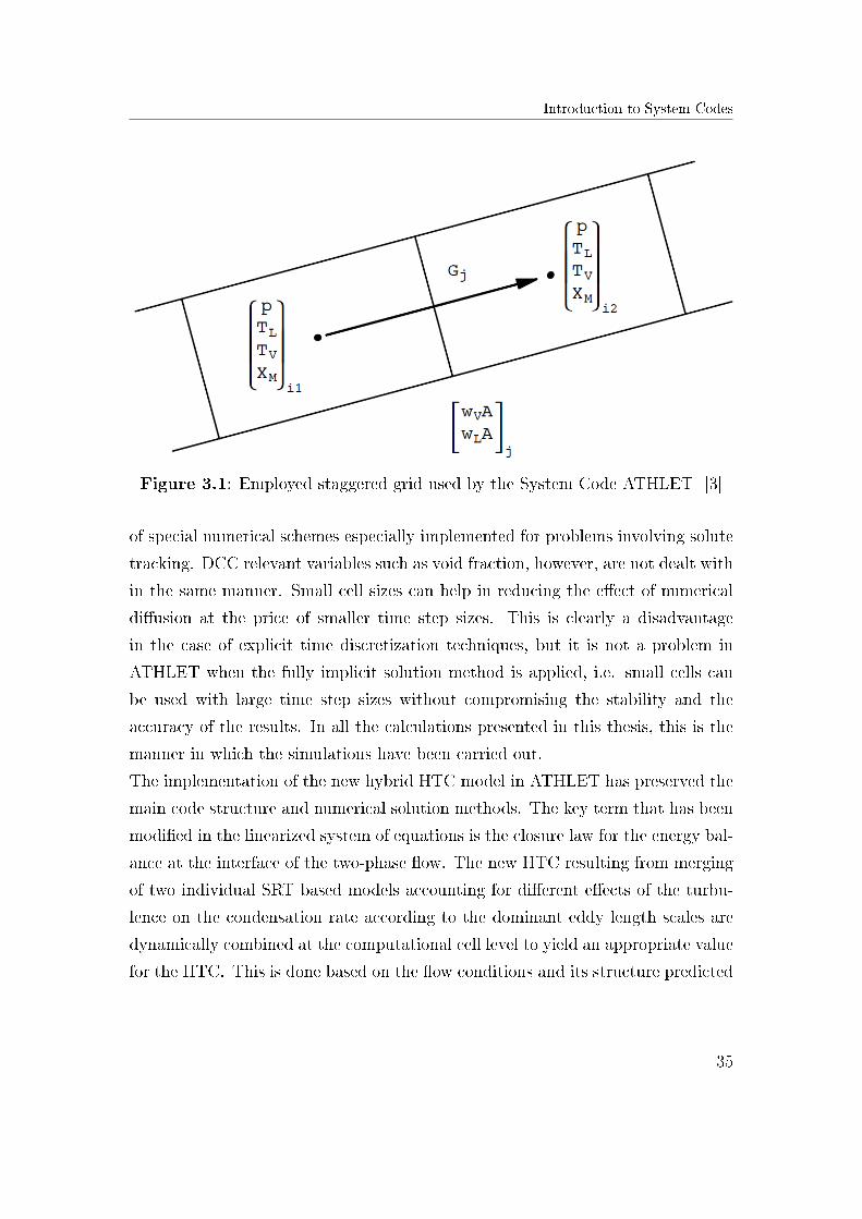
Introduction to System Codes
Figure 3.1: Employed staggered grid used by the System Code ATHLET [3]
of special numerical schemes especially implemented for problems involving solute
tracking. DCC relevant variables such as void fraction, however, are not dealt with
in the same manner. Small cell sizes can help in reducing the e�ect of numerical
di�usion at the price of smaller time step sizes. This is clearly a disadvantage
in the case of explicit time discretization techniques, but it is not a problem in
ATHLET when the fully implicit solution method is applied, i.e. small cells can
be used with large time step sizes without compromising the stability and the
accuracy of the results. In all the calculations presented in this thesis, this is the
manner in which the simulations have been carried out.
The implementation of the new hybrid HTC model in ATHLET has preserved the
main code structure and numerical solution methods. The key term that has been
modi�ed in the linearized system of equations is the closure law for the energy bal-
ance at the interface of the two-phase �ow. The new HTC resulting from merging
of two individual SRT based models accounting for di�erent e�ects of the turbu-
lence on the condensation rate according to the dominant eddy length scales are
dynamically combined at the computational cell level to yield an appropriate value
for the HTC. This is done based on the �ow conditions and its structure predicted
35
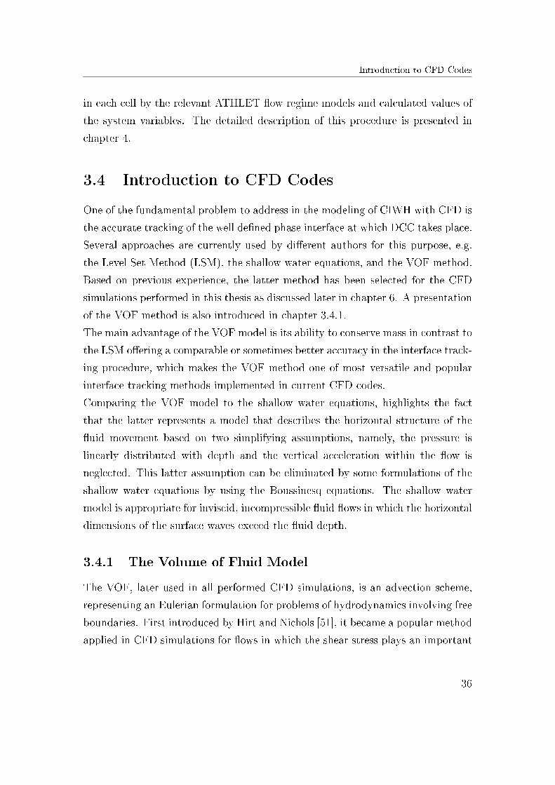
Introduction to CFD Codes
in each cell by the relevant ATHLET �ow regime models and calculated values of
the system variables. The detailed description of this procedure is presented in
chapter 4.
3.4 Introduction to CFD Codes
One of the fundamental problem to address in the modeling of CIWH with CFD is
the accurate tracking of the well de�ned phase interface at which DCC takes place.
Several approaches are currently used by di�erent authors for this purpose, e.g.
the Level Set Method (LSM), the shallow water equations, and the VOF method.
Based on previous experience, the latter method has been selected for the CFD
simulations performed in this thesis as discussed later in chapter 6. A presentation
of the VOF method is also introduced in chapter 3.4.1.
The main advantage of the VOF model is its ability to conserve mass in contrast to
the LSM o�ering a comparable or sometimes better accuracy in the interface track-
ing procedure, which makes the VOF method one of most versatile and popular
interface tracking methods implemented in current CFD codes.
Comparing the VOF model to the shallow water equations, highlights the fact
that the latter represents a model that describes the horizontal structure of the
�uid movement based on two simplifying assumptions, namely, the pressure is
linearly distributed with depth and the vertical acceleration within the �ow is
neglected. This latter assumption can be eliminated by some formulations of the
shallow water equations by using the Boussinesq equations. The shallow water
model is appropriate for inviscid, incompressible �uid �ows in which the horizontal
dimensions of the surface waves exceed the �uid depth.
3.4.1 The Volume of Fluid Model
The VOF, later used in all performed CFD simulations, is an advection scheme,
representing an Eulerian formulation for problems of hydrodynamics involving free
boundaries. First introduced by Hirt and Nichols [51], it became a popular method
applied in CFD simulations for �ows in which the shear stress plays an important
36
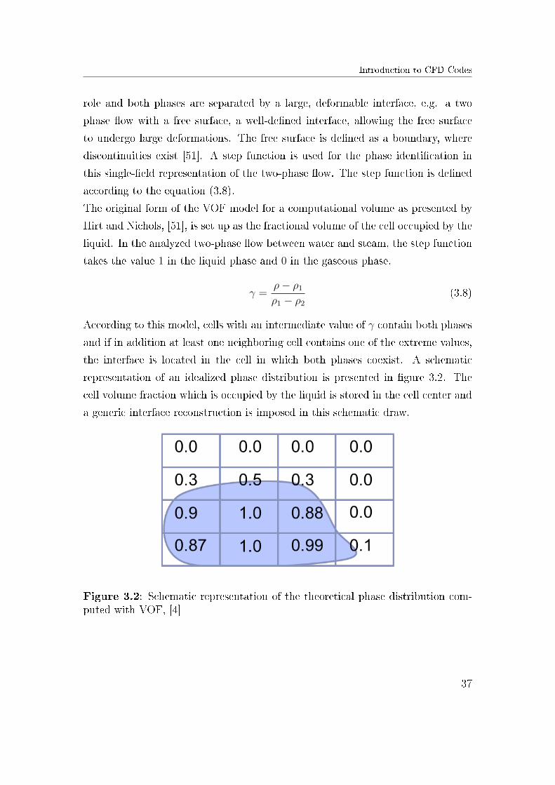
Introduction to CFD Codes
role and both phases are separated by a large, deformable interface, e.g. a two
phase �ow with a free surface, a well-de�ned interface, allowing the free surface
to undergo large deformations. The free surface is de�ned as a boundary, where
discontinuities exist [51]. A step function is used for the phase identi�cation in
this single-�eld representation of the two-phase �ow. The step function is de�ned
according to the equation (3.8).
The original form of the VOF model for a computational volume as presented by
Hirt and Nichols, [51], is set up as the fractional volume of the cell occupied by the
liquid. In the analyzed two-phase �ow between water and steam, the step function
takes the value 1 in the liquid phase and 0 in the gaseous phase.
γ =ρ− ρ1
ρ1 − ρ2
(3.8)
According to this model, cells with an intermediate value of γ contain both phases
and if in addition at least one neighboring cell contains one of the extreme values,
the interface is located in the cell in which both phases coexist. A schematic
representation of an idealized phase distribution is presented in �gure 3.2. The
cell volume fraction which is occupied by the liquid is stored in the cell center and
a generic interface reconstruction is imposed in this schematic draw.
Figure 3.2: Schematic representation of the theoretical phase distribution com-puted with VOF, [4]
37
Introduction to CFD Codes
Within the VOF model, a mixture �uid is created, where the thermo-physical
properties of the new �uid are obtained by linear interpolation using the volume
fraction γ as shown in the equation (3.9). Any particular thermo-physical property,
ζmix can be averaged, using the phase indicator in the following way:
ζmix = γ · ζ1 + (1− γ) · ζ2 (3.9)
The transport equation for the phase identi�er in the case of the standard VOF
model is presented in equation (3.10).
∂ρ1γ
∂t+∇ · (ρ1γ
−→U ) = Sγ (3.10)
The source and sink term, Sγ, on the RHS of equation (3.10) is accounting for
phase change and it is computed as Sγ = Γk. For phase change due to DCC it
takes the form expressed in equation (3.5). For the computation of the IAD, which
per computational cell represents the ratio between the interfacial area within the
cell and the cell's volume, the following equation is employed:
ai = |∇γ| (3.11)
The momentum transport equation corresponds to the typical RANS approach,
with the additional consideration of a continuous surface tension. A particularity
of the VOF model is that it only accounts for a single velocity �eld which is shared
by both phases: equation (3.12). The fact that within this model both phases share
a single velocity �eld makes it inappropriate for the description of polydispersed
�ows with a large density ratio between the two phases. In the particular case of
polydispersed �ows, the phase relative velocity becomes important and thus a�ects
the terms representing interfacial friction, drag forces etc.
∂ρ−→U
∂t+∇ ·
(ρ−→U−→U)
= −∇p+∇ · µ∇−→U + ρ−→g + fi (3.12)
38
Introduction to CFD Codes
The last term on the RHS, fi, represents the momentum source term due to surface
tension. It is only active at the interface, i.e. in those cells with γ ∈ (0, 1). It
depends on the curvature of the surface κ, on the surface tension σ and on the
normal vector to the interface −→n . The normal vector to the interface is presentedin equation (3.13) and the surface curvature is expressed in equation (3.14).
−→n =∇γ|∇γ|
(3.13)
κ = −∇ ·(∇γ|∇γ|
)(3.14)
The conservation of energy of an incompressible two-phase �ow is presented in
equation (3.15).
∂ρhtot
∂t+∇ · (ρhtot
−→U ) = ∇ · (keff∇T ) + SE (3.15)
The last term in the equation (3.15), SE accounts for the heat transfer at the phase
interface.
Special attention has been given to the interface in order to avoid the 'smearing'
of the step function, in terms of the employed numerics. To conclude: a sharp
interface delivers more accurate results, while a more smeared interface enhances
the robustness of the simulation as the gradients become less sharp. In order to
avoid numerical di�culty where calculating the interface unit normal vector of a
very sharp surface, a smoothing method must be implied.
As this model requires the storage of only one additional variable per computa-
tional cell and not necessarily requiring a logical interface reconstruction algorithm,
makes this method attractive for CFD simulations of large computational domains
within a reasonable amount of computational time. In other words it o�ers an eco-
nomic way to track free boundaries in multi-dimensional meshes [51].
39
Introduction to CFD Codes
Particularities of the implementation of the VOF model in
OpenFOAM 1.7.1
The general VOF model for an incompressible �uid is already implemented into
OpenFOAM version 1.7.1 with some particularities. The relevant particularities
and the additional development work carried out for the custom tailored solver
will be presented in this chapter. A more detailed description of the standard
implemented VOF model as available in OpenFOAM can be found in [52].
In the case of the phase indicator transport equation, special attention has to
be given to avoid the smearing of the interface through several computational
cells. In OpenFOAM this is handled not by employing a compressive di�erencing
scheme but rather by imposing an additional compression velocity (−→U c) at the
phase interface. The solution procedure as implemented in OpenFOAM developed
by Weller is presented in [52]. Considering these particularities, the original VOF
conservation equation (3.10) is modi�ed into the form of equation (3.16).
∂α
∂t+∇ · (α
−→U ) +∇ · (α(1− α)
−→U c) =
Γ
ρ1
(3.16)
The additional arti�cial term is used only in the cells containing intermediate
values of α due to the multiplication term α (1− α). In the case of the VOF solver
implemented in OpenFOAM, the compression velocity−→U c is calculated based on
an user adjustable ampli�cation factor, the unit normal vector at the interface
and the maximum velocity magnitude [52]. The user de�ned factor is used to
arti�cially enhance the interface sharpness. At the same time the user has to �nd
a compromise between sharpness of the interface and numerically smooth gradients
for robustness of the simulation, when the interface curvature is calculated.
In the OpenFOAM built-in VOF solver, the index 1 refers to the liquid or denser
phase whereas the index 2 refers to the gaseous, less denser phase. The divergence
free condition available in the standard VOF based solver in OpenFOAM does no
longer apply for phase change and has to be adapted to:
∇ ·−→U = Γ
(1
ρ2
− 1
ρ1
)(3.17)
40
Introduction to CFD Codes
The momentum equation is solved by means of a pressure-velocity coupling, Pres-
sure Implicit with Splitting of Operators (PISO). The PISO algorithm is an ef-
�cient procedure to solve the Navier-Stokes equations for unsteady problems. A
detailed description of the PISO method can be found in [53].
In a nutshell the PISO algorithm for one time step consists of following stages:
• Setting up of the Boundary Condition (BC)
• Solving the momentum equation to compute the intermediate velocity �eld
and the mass �uxes at the cell faces
• Solving the pressure equation
• Updating and correcting the mass �uxes
• Solving and correcting the velocities based on the pressure �eld to ful�ll the
mass conservation
• Updating the BC
Due to some numerical problems, resulting in the unboundedness of the solving
variables the energy conservation equations have been collapsed into just the liquid
side energy conservation equation. This was possible as the DCC of steam into
subcooled liquid is assumed to occur at the saturated two-phase interface.
The accompanied turbulence models, used with the VOF model, will be introduced
in chapter 3.4.2.
3.4.2 Turbulence Modeling in CFD
Turbulence is a �ow regime in which the motion is intrinsically unsteady even
with constant boundary conditions, where the velocity, similar to other �ow prop-
erties, varies in a chaotic and arbitrary way. Turbulence is a phenomenon of
great complexity and has puzzled theoreticians for over a hundred years [5]. For
a more convenient description of the �ow, a decomposition of the �ow velocity in
41
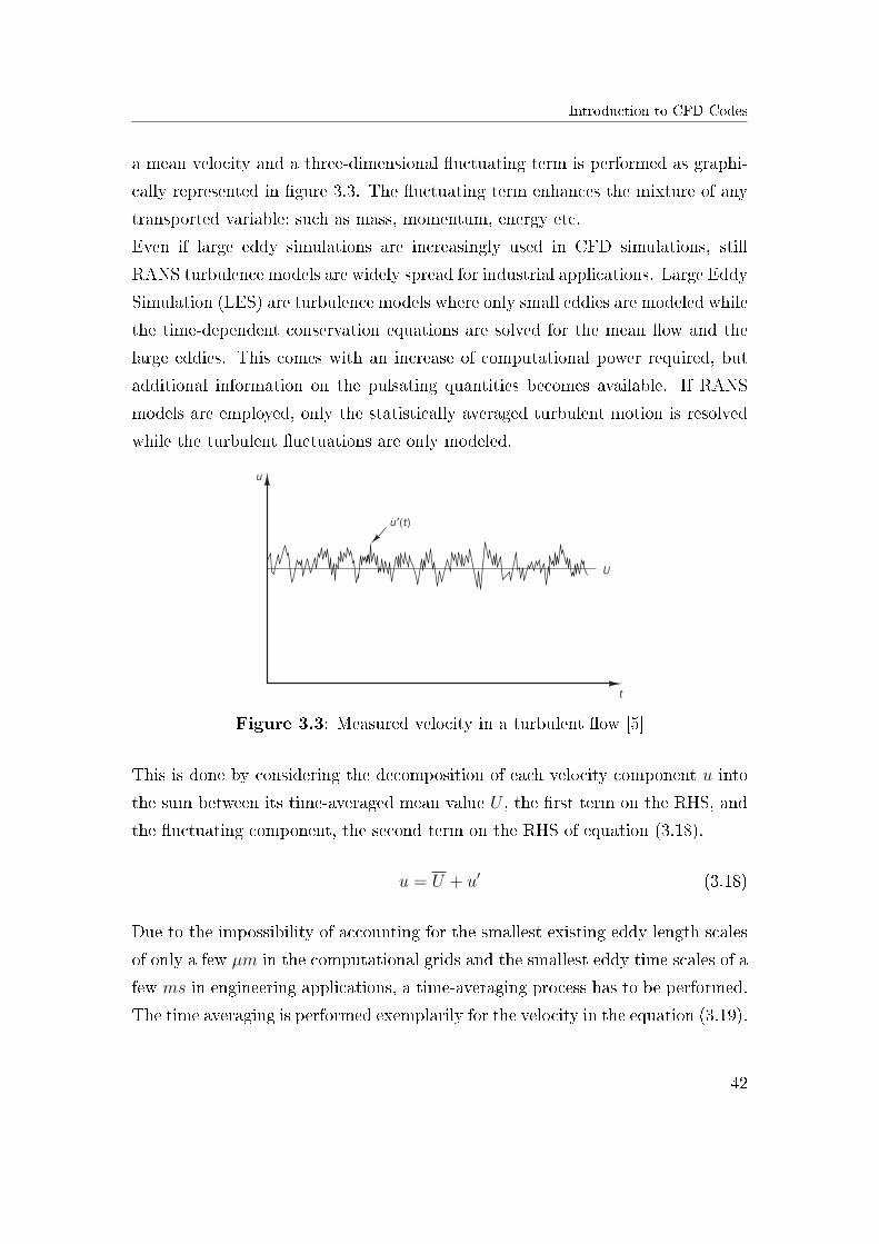
Introduction to CFD Codes
a mean velocity and a three-dimensional �uctuating term is performed as graphi-
cally represented in �gure 3.3. The �uctuating term enhances the mixture of any
transported variable; such as mass, momentum, energy etc.
Even if large eddy simulations are increasingly used in CFD simulations, still
RANS turbulence models are widely spread for industrial applications. Large Eddy
Simulation (LES) are turbulence models where only small eddies are modeled while
the time-dependent conservation equations are solved for the mean �ow and the
large eddies. This comes with an increase of computational power required, but
additional information on the pulsating quantities becomes available. If RANS
models are employed, only the statistically averaged turbulent motion is resolved
while the turbulent �uctuations are only modeled.
Figure 3.3: Measured velocity in a turbulent �ow [5]
This is done by considering the decomposition of each velocity component u into
the sum between its time-averaged mean value U , the �rst term on the RHS, and
the �uctuating component, the second term on the RHS of equation (3.18).
u = U + u′ (3.18)
Due to the impossibility of accounting for the smallest existing eddy length scales
of only a few µm in the computational grids and the smallest eddy time scales of a
few ms in engineering applications, a time-averaging process has to be performed.
The time averaging is performed exemplarily for the velocity in the equation (3.19).
42
Introduction to CFD Codes
If the averaging is performed over a time interval, ∆t, at least larger than the time
scale of the largest eddy, the averaging of the pulsating velocity will result in zero.
U =1
∆t
∫ ∆t
0
u(t)dt (3.19)
The decomposition of the �ow into a part governed by the average property and
a pulsating one will introduce additional terms in the conservation equations that
account for the in�uence of the �uctuating terms.
The high resolution of computational grids employed in CFD simulations o�ers
the possibility to use transport equations for the turbulent quantities.
One of the imposed requirements on turbulent models is that these should be able
to cover a wide applicability range. Typical turbulence models in order of their
complexity are:
• Algebraic models also called zero equation models as they consist of algebraic
equations rather than of PDEs. These models consist of algebraic equations
for the turbulent viscosity and the turbulent Prandtl number.
• One-equation models consist of a di�erential equation for the Turbulent Ki-
netic Energy (TKE).
• Two-equation models consist of a set of two PDE, one for the TKE and one
for the dissipation rate, in the case of the k − ε model or the frequency in
case of the k − ω model.
• Reynolds stress models include either algebraic equations or PDE for each
of the Reynolds stress tensor components.
A commonly used variable for most RANS based turbulence models is the TKE,
generally denoted as k. The TKE is de�ned as:
k =1
2(u′x
2 + u′y2 + u′z
2) (3.20)
The individual contributions on the RHS of equation (3.20) are the individual com-
ponents of the �uctuating velocity vector u′ in the Cartesian coordinate system.
43
Introduction to CFD Codes
Another variable used for the characterization of turbulence is the turbulence in-
tensity I. It relates the root mean square of the turbulent velocity �uctuations
(u′) to the mean velocity of the �ow:
I =u′U
=
√13(u′x
2 + u′y2 + u′z
2)√Ux
2+ Uy
2+ Uz
2(3.21)
Only the two equations k− ωSST turbulence model was used in the CFD simula-
tions within this work and will thus be covered in detail. This model is employed as
it is recommended for two-phase �ow without any special tuning. The description
of the k − ωSST turbulence model also includes the k − ε model implicitly.
The k − ε Turbulence model
The standard k − ε model is probably the most widespread and popular two-
equation turbulence model in today's CFD simulations for engineering applications
and was initially developed by Launder and Spalding, [54]. It is best performing
at high Reynolds numbers but yields poor results in near-wall regions.
The k − ε model introduces two additional PDE in the system of equations, one
for the turbulent kinetic energy k and one for the turbulence dissipation rate ε.
The e�ective viscosity that operates with the velocity gradients is de�ned as
µeff = µ+ µt (3.22)
In equation (3.22), µt is the turbulence viscosity. The k− ε assumes the followingrelation between the turbulence viscosity, k and ε:
µt = Cµρk2
ε(3.23)
where Cµ = 0.09 is a constant. The two transport equations for k and ε are
∂ρk
∂t+∇(ρUk) = ∇[(µ+
µtσk
)∇k] + Pk + Pkb − ρε (3.24)
44
Introduction to CFD Codes
∂ρε
∂t+∇(ρUε) = ∇[(µ+
µtσε
)∇ε] +ε
k(Cε1(Pk + Pεb)− Cερε) (3.25)
Where Cε1, Cε1, σk and σε are constants. Pk is the turbulent generation and is
determined by
Pk = µt∇U · (∇U +∇UT )− 2
3∇ · U(3µt∇ · U + ρk) (3.26)
Pkb and Pεb account for the in�uence of buoyancy forces. If the full buoyancy
model is used, Pkb takes the following form
Pkb = − µtρσρ
g · ∇ρ (3.27)
Pεb is taken proportionally to Pkb and must be positive and C3 is a constant
Pεb = C3 ·max(0, Pkb) (3.28)
The k − ω Turbulence Model
In the k − ω turbulence model developed by Wilcox [55] it is assumed that the
eddy viscosity is linked to the TKE and the turbulence frequency ω as expressed
in equation (3.29).
µt = ρk
ω(3.29)
The two transport equations for k and ω are presented in the equations (3.30) and
(3.31).∂ρk
∂t+∇(ρUk) = ∇[(µ+
µtσk
)∇k] + Pk + Pkb − β′ρkω (3.30)
∂ρω
∂t+∇(ρUω) = ∇[(µ+
µtσω
)∇ω] + αω
kPk + Pωb − βρkω (3.31)
The newly introduced variables β′, β, α, σk and σω are model built-in constants.
The source term Pωb, on the RHS of equations (3.32) is calculated as shown in
equation (3.32).
Pωb =ω
k((α + 1)C3 ·max(0, Pkb)− Pkb) (3.32)
45
Introduction to the Surface Renewal Theory
The k − ω model, [55], was developed for low-Reynolds-number applications and
delivers good performances especially in the proximity of wall regions thus com-
plementing the �aw in the k − ε model. Similar to the k − ε turbulence model,
this model requires two additional conservation equations to be solved; one for the
TKE and one for the turbulence frequency ω.
The Shear Stress Transport (SST) Model
The SST model combines the advantages of both the k − ε and the k − ω model
by using the recommended model in the region where it is best performing. The
switching between the two models is done based on a transition function. Ac-
cordingly the SST model combines the best features of the two models and o�ers
higher reliability and accuracy while maintaining stability and reasonable comput-
ing time.
3.5 Introduction to the Surface Renewal Theory
This section contains state-of-the-art information about the SRT as a mechanistic
description of heat transfer. The theoretical background will be introduced here,
while the implementation in computer codes will be presented in chapter 4.
The original concept of SRT was introduced by Higbie, [56] initially describing
the transport of gases into liquids. Phenomenologically it is based on small liquid
volumes which are considered to reach the two-phase interface where they interact
with the gaseous phase before being removed and transported back into the liquid
bulk by turbulent eddies. A continuous scalar exchange is directly controlled by
the exposure time of the small liquid volumes at the interface. The exposure time
of these `micro-volumes' also linked with the Surface Renewal Period (SRP) is the
ratio between a length and a velocity scale and has to be determined within the
model.
Mass transfer occurring at the interface is governed by molecular di�usion during
the contact time between the small liquid volumes and the interface. Initially, the
contact time was assumed to be uniform for all scales of turbulent eddies.
46
Introduction to the Surface Renewal Theory
Once this model became widely accepted and used, new concepts were added to the
original theory of SRT in order to improve its accuracy and predictive capability.
For example, the modi�cation proposed by Danckwerts [57] considered two new
parameters, the variable and random age residence times at the interface. The
model developed by Torr and Marchello [58] which added a �nite dimension to the
region of the surface renewal.
In an analogy with convective mass and heat transfer one can say that the SRT
accounts for convective transport of small liquid volumes carrying mass and energy
by turbulent eddies which can break through the laminar sub-layer of the liquid in
contact with the interface and replace the already saturated small liquid volumes
at the interface with fresh, subcooled liquid volumes from the �uid bulk. Through
this mechanism heat and mass transfer are controlled by the contact time at the
surface represented by the interface. Physically the contact time re�ects the time
spent by the eddies interacting on the two-phase interface. It therefore, controls
the amount of energy and mass that can be transferred across the surface. The
contact time SRT is computed as the ratio between the characteristic eddy length
scale Lt and the eddy velocity scale Vt as presented in equation 3.33.
SRT =LtVt
(3.33)
In order to include heat transfer in the SRT, an energy balance has to be performed
at the interface as indicated by Banerjee [59]. The HTC controlling the heat �ux
at the gas-liquid interface is given in its general form as:
HTCliq =C√πλPr
1/2liq (Lt)
n−1
(Vtνliq
)n(3.34)
The variable C is a model-speci�c constant, λ is thermal conductivity of the liquid,
Pr the Prandtl number of the liquid, Lt and Vt are the characteristic eddy length
and velocity scales, ν the liquid kinetic viscosity and n a model dependent constant.
The assumption that the liquid o�ers the only resistance to the heat transfer
in�uenced by its thermo-physical properties holds as long as the gaseous phase
remains at saturation, which is applicable in the analyzed case of DCC.
47
Introduction to the Surface Renewal Theory
Interfacial heat transfer models based on this approach directly correlate the cal-
culation of the HTC to the turbulence character of the �ow i.e. to the TKE, the
turbulent eddy dissipation rate ε and the thermo-physical properties of the liquid.
The strong link between turbulence and the HTC transforms SRT based models
into mechanistic approaches of the DCC phenomenon. Their theoretical ability
of o�ering a continuous smooth transition of the HTC for di�erent �ow regimes
makes the SRT based models attractive to be applied for the calculation of the
HTC for all transient horizontal �ow patterns.
The di�culty in choosing the adequate SRT based model lies in the selection of the
proper length and velocity scales of these turbulent eddies driving the interfacial
heat and mass transfers, which in�uences the SRP. Some authors have for example
proposed objectively calculated fractions of channel depths, wavelengths of surface
oscillations or mean �ow dimensions as characteristic eddy sizes.
The applicability of the theory to pipe �ow has been demonstrated by Du�ey and
Hughes in [60]. All individual, stand-alone SRT based models have the following
limitation in their present form: these models mainly o�er the possibility of inter-
preting measurement data with some parameter tuning e�ort, but have di�culties
when used as predicting tools [61]. Under these circumstances the quality of even-
tual simulation results relies on the knowledge and experience of the user and may
lead to high uncertainties in the �nal results. Available individual, stand-alone
SRT based models are thus di�cult to be used for safety assessment of the oper-
ation of industrial systems such as nuclear power plants or chemical installations.
In such applications reliable predictive capabilities of the employed modeling ap-
proach are fundamental in producing so-called conservative predictions (worst case
scenario) of the safety of a system's behavior.
One of the two individual models used in chapter 4 for the development of the
new hybrid HTC model was developed by Hughes and Du�ey, i.e. the Micro Scale
Eddies (MiSE) model [62], while the other was developed by Shen et al. [63], i.e.
the Macro Scale Eddies (MaSE) model. The model accounting for mirco eddies in
the calculation of the HTC will be presented in subsection 3.5.1, the SRT based
HTC model considering macroscopic eddies will be introduced in subsection 3.5.2.
48
Introduction to the Surface Renewal Theory
3.5.1 Surface Renewal Theory accounting for Microscopic
Eddies for Scalar Exchange
The model developed by Hughes and Du�ey [62] considers that the smallest scales
in a turbulent �ow also known as Kolmogorov micro-scales are mainly responsible
for the transfer of energy. Considering the small length scale and correspondingly
high velocity scale, this model delivers a short SRP, which results in more energy
being transferred between the interface and the liquid bulk per unit time, i.e. a
higher energy transfer rate. Hughes and Du�ey's model is based on the hypothesis
set by Kolmogorov for isotropic turbulence, which holds for very small eddies [64].
Such eddies are formed at the interface mainly by shear stresses or by the in�uence
of a nearby wall [62].
The calculation of the heat �ux at the gaseous-liquid interface is done as proposed
by Banerjee, [59] based on equation (3.34). The general form of the interfacial
heat �ux has then the form:
qig−liq = 2ρliquidcp,liq
(αliqπ
)1/2(
1
tMiSErp
)1/2
(Tsat − Tliq) (3.35)
The variable αliq in (3.35) represents the thermal di�usivity of the liquid phase
while 1/trp stands for the SRP which has to be calculated based on the Kolmogorov
length and velocity eddy scales according to (3.36) and respectively (3.37).
LMiSEt =
(ν3liq
ε
)1/4
(3.36)
V MiSEt = (νliqε)
1/4 (3.37)
Rearranging the terms in equation (3.35) and replacing trp with the ratio between
the eddy length and its velocity scale, leads to the �nal form of the HTC shown
in equation (3.38).
HTCMiSEliq = Cρliqcp,liq
(αliqπ
)1/2(
ε
νliq
)1/4
(3.38)
49
Introduction to the Surface Renewal Theory
3.5.2 Surface Renewal Theory accounting for Macroscopic
Eddies for Scalar Exchange
The Shen et al. model [63] considers that larger eddies are mainly responsible for
the transport energy across the liquid-gas interface.
Even if the validity of computing the large scale eddies based on the k−εmodel andusing the dissipation rate might by questioned, this is applicable at low Reynolds
numbers as the rate at which large eddies remove energy from the mean �ow
is approximated to the rate of transfer of energy across the energy spectrum to
smaller, dissipating eddies [5].
The mathematical form of the MaSE model is based on the general formulation
proposed by Hughes and Du�ey described in the previous section, di�ering basi-
cally in the de�nition of the turbulent length and velocity scales Lt and Vt. Shen et
al's model uses the length scale of the standard k-ε model and a slightly modi�ed
Kolmogorov velocity scale as shown in equations (3.39) and (3.40).
LMaSEt = Cµ
k3/2
ε(3.39)
V MaSEt = C1/2
µ (νlε)1/4 (3.40)
HTCMaSEliq =
C√πλliqPr
1/2liq (Lt)
−1/3
(Vtνliq
)2/3
(3.41)
The larger length scale yields larger SRP values which result in lower values for
the HTC than if micro-scale eddies are considered for the calculation of the SRP.
The �nal version of the HTC based on macro-scale eddies is taken from [46], and
presented in equation (3.41).
50
Chapter 4
Present Contribution to the
Calculation of CIWH
The newly developed hybrid SRT based HTC model, together with its implemen-
tation into the system code ATHLET and into the CFD codes, both ANSYS CFX
and OpenFOAM, will be presented in this chapter.
The problem of realistically describing the DCC and the implementation of such
a model into a computer code requires the mechanistic modeling of the interfacial
heat and mass transfer. The main di�erence between the simulation of such a
phenomenon with either system codes or CFD codes lies within the length scales
that the two di�erent computer tools can consider. A phenomenon such as the
DCC, which is in�uenced by highly local e�ects, has to be modeled within a sys-
tem code, traditionally, by considering only bulk-averaged values of main �uid
variables, whereas, in the case of CFD codes, a higher spatial resolution of the
�ow and the consideration of smaller scales can be achieved. The higher spacial
resolution comes at the cost of larger computational times.
Regardless of the length scales used, the phase change occurring at the two-phase
interface is computed based on a local energy balance in those cells containing
both phases and, implicitly, the interface. The interface and the vapor phase are
Development of a Hybrid HTC Model accounting for Microscopic and Macroscopic Eddie Scales
considered to be at saturation. Consequently, the liquid �lm in contact with the
interface provides the only heat transfer resistance in the process of DCC. The
calculation of the mass transfer rate Γ used as both source and sink term (depend-
ing on its sign) in the conservation equations was previously discussed in chapter
3.2. For the calculation of the HTC, one of the fundamental quantities for the cal-
culation of the interfacial mass and energy transfer rates, a hybrid model has been
developed which will be presented in the following chapter. The other relevant
variables such as the temperature di�erence between the two phases, the IAD and
the latent heat are obtained from the solutions of conservation equations, from the
�uid properties, or are explicitly modeled in the code.
4.1 Development of a Hybrid HTC Model
accounting for Microscopic and Macroscopic
Eddie Scales
In order to overcome the drawbacks of stand-alone SRT based HTC models, an
approach of a hybrid model is developed in this section. The stand-alone SRT
based models can mainly be used after a parameter tuning based on experimental
measurement data has been performed. The main di�erences between the two
individual models consists in the manner in which they consider the length scales
of the eddies responsible for the heat transfer from the interface towards the liquid
bulk. A summary of the two individual SRT models is presented in the following
table.
The hybrid HTC model whose development is shown in this section is based on the
assumption proposed in [65] that the energy in a turbulent �ow is carried predom-
inantly by micro eddies when the turbulent Reynolds exceeds a threshold value
of 500; below this value larger eddies are then mainly responsible for this trans-
port. This assumption was applied to the mechanism of energy transport inherent
to the surface renewal process and while assuming that the micro eddies are the
52
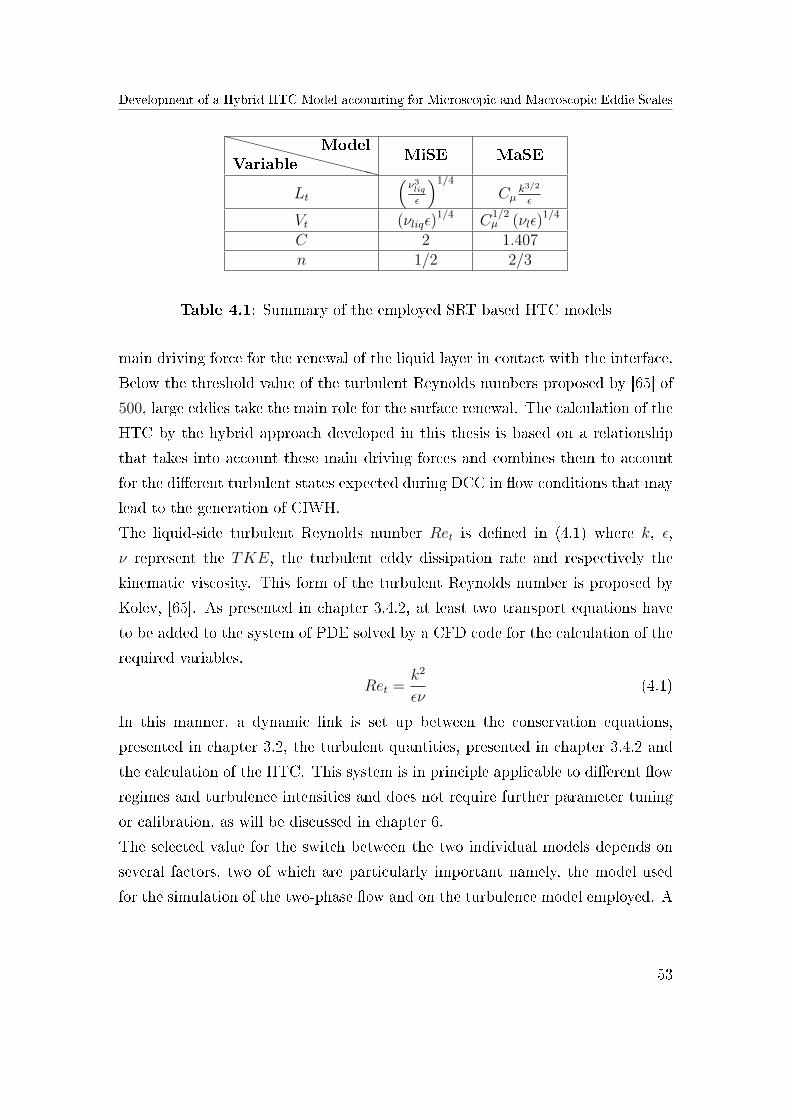
Development of a Hybrid HTC Model accounting for Microscopic and Macroscopic Eddie Scales
XXXXXXXXXXXXVariableModel
MiSE MaSE
Lt
(ν3liqε
)1/4
Cµk3/2
ε
Vt (νliqε)1/4 C
1/2µ (νlε)
1/4
C 2 1.407n 1/2 2/3
Table 4.1: Summary of the employed SRT based HTC models
main driving force for the renewal of the liquid layer in contact with the interface.
Below the threshold value of the turbulent Reynolds numbers proposed by [65] of
500, large eddies take the main role for the surface renewal. The calculation of the
HTC by the hybrid approach developed in this thesis is based on a relationship
that takes into account these main driving forces and combines them to account
for the di�erent turbulent states expected during DCC in �ow conditions that may
lead to the generation of CIWH.
The liquid-side turbulent Reynolds number Ret is de�ned in (4.1) where k, ε,
ν represent the TKE, the turbulent eddy dissipation rate and respectively the
kinematic viscosity. This form of the turbulent Reynolds number is proposed by
Kolev, [65]. As presented in chapter 3.4.2, at least two transport equations have
to be added to the system of PDE solved by a CFD code for the calculation of the
required variables.
Ret =k2
εν(4.1)
In this manner, a dynamic link is set up between the conservation equations,
presented in chapter 3.2, the turbulent quantities, presented in chapter 3.4.2 and
the calculation of the HTC. This system is in principle applicable to di�erent �ow
regimes and turbulence intensities and does not require further parameter tuning
or calibration, as will be discussed in chapter 6.
The selected value for the switch between the two individual models depends on
several factors, two of which are particularly important namely, the model used
for the simulation of the two-phase �ow and on the turbulence model employed. A
53
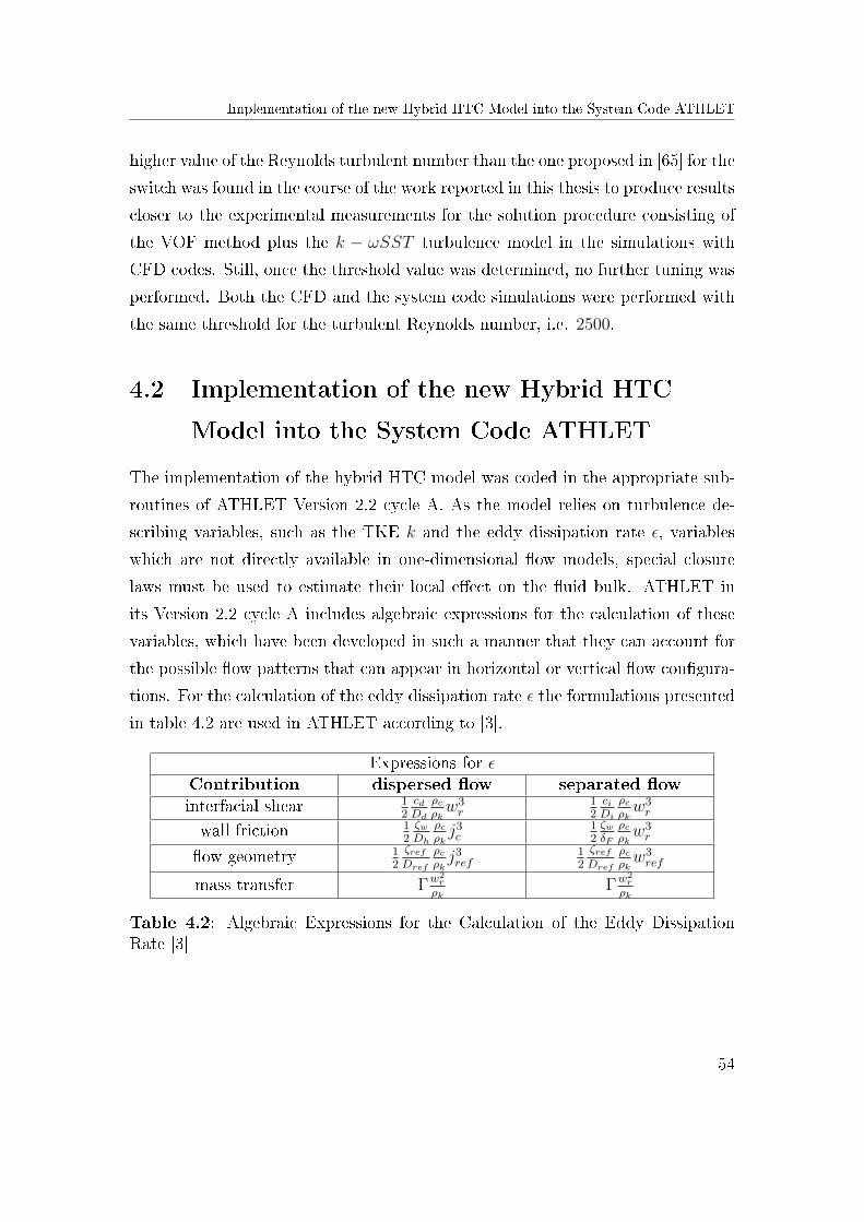
Implementation of the new Hybrid HTC Model into the System Code ATHLET
higher value of the Reynolds turbulent number than the one proposed in [65] for the
switch was found in the course of the work reported in this thesis to produce results
closer to the experimental measurements for the solution procedure consisting of
the VOF method plus the k − ωSST turbulence model in the simulations with
CFD codes. Still, once the threshold value was determined, no further tuning was
performed. Both the CFD and the system code simulations were performed with
the same threshold for the turbulent Reynolds number, i.e. 2500.
4.2 Implementation of the new Hybrid HTC
Model into the System Code ATHLET
The implementation of the hybrid HTC model was coded in the appropriate sub-
routines of ATHLET Version 2.2 cycle A. As the model relies on turbulence de-
scribing variables, such as the TKE k and the eddy dissipation rate ε, variables
which are not directly available in one-dimensional �ow models, special closure
laws must be used to estimate their local e�ect on the �uid bulk. ATHLET in
its Version 2.2 cycle A includes algebraic expressions for the calculation of these
variables, which have been developed in such a manner that they can account for
the possible �ow patterns that can appear in horizontal or vertical �ow con�gura-
tions. For the calculation of the eddy dissipation rate ε the formulations presented
in table 4.2 are used in ATHLET according to [3].
Expressions for εContribution dispersed �ow separated �owinterfacial shear 1
2cdDd
ρcρkw3r
12ciDi
ρcρkw3r
wall friction 12ζwDh
ρcρkj3c
12ζwδF
ρcρkw3r
�ow geometry 12
ζrefDref
ρcρkj3ref
12
ζrefDref
ρcρkw3ref
mass transfer Γw2r
ρkΓw2
r
ρk
Table 4.2: Algebraic Expressions for the Calculation of the Eddy DissipationRate [3]
54
Implementation of the new Hybrid HTC Model into CFD Codes
In table 4.2 the symbols c, ζ, j, wr, ρ and D represent the shear coe�cient, the
friction coe�cient, the super�cial velocity, the relative velocity, the density and
respectively the channel diameter. The indexes c, ref and k are used for the
continuous phase respectively the reference value and the phase (steam or water).
It is assumed that the relative velocity is responsible for the shear stress at the
interface and is also used for the determination of the TKE in equation (4.2).
k =3
2w′2 ≈ 3
2w2rel (4.2)
For the calculation of the IAD an additional transport equation is solved in
ATHLET. The model can deal with both bubble and droplet �ow with the appro-
priate IAD sink and source terms: bubble and droplet break-up and coalescence
models, as well as bubble and droplet formation and disappearance models (evap-
oration, entrainment and condensation), while for the intermediate �ow patterns
an interpolation function is used [50].
4.3 Implementation of the new Hybrid HTC
Model into CFD Codes
Two CFD codes were used in the work reported in this thesis, namely the com-
mercial software ANSYS CFX and the open source software OpenFOAM.
In the case of the commercial computer code ANSYS CFX, the implementa-
tion of the hybrid HTC model was done by means of the CFX Expression Lan-
guage (CEL), which is a powerful de�nition language enabling the user to add new
relationships between the ANSYS CFX internal variables. CEL is an interpreted,
declarative language developed to enable CFX users to enhance their simulations
without the need of writing and linking separate external FORTRAN routines. It
can be used to add new physical models, create additional solution variables, de-
�ne property relationships and set boundary conditions and pro�les. CEL includes
many prede�ned functions and operators to allow easy customization of simula-
tions in a number of ways. The user however, cannot control the time point at
55
Implementation of the new Hybrid HTC Model into CFD Codes
which the solver algorithm evaluates the CEL-based addition, as this is managed
internally by CFX. Using the CEL both individual SRT based HTC models have
been implemented into ANSYS CFX. The code evaluates at each computational
point the expressions of each HTC model and chooses based on the threshold value
of the turbulent Reynolds number according to a step function which value of the
heat transfer coe�cient will be used for the evaluation of the source and sink terms
in�uencing the employed conservation equations.
All developments to OpenFOAM have been directly built into the source code
because of its open source character. In this way the user has full control on the
time point at which speci�c variables and expressions are evaluated and equations
are solved.
Before the hybrid HTC model could be implemented in OpenFOAM Version 1.7.1
an energy conservation equation had to be added to the PDE system that de-
scribes the �ow. The newly developed OpenFOAM solver employing the VOF
method is capable of simulating the DCC phenomenon. The implemented energy
equation corresponds to equation to (3.15). Due to numerical problems, only a
single mixture based �uid energy conservation equation could be implemented.
Since for the phenomenon of DCC modeled in this thesis the steam is assumed at
saturation, the lack of an independent vapor energy equation is not vital for the
correct prediction of the phenomenon. If the vapor were subcooled or superheated,
such an equation would clearly be necessary. Numerical problems arose because
of the OpenFOAM's built in PDE solver, which has to process the equations in
a segregated way. The matrix solver has to individually process each group of
PDEs and cannot, up to OpenFOAM Version 1.x.y, simultaneously solve the as-
sembled matrix containing all the linearized terms of the conservation equations.
Because of this limitation and considering the strong coupling between the source
and sink terms stemming from the explicitly treated interfacial phase-change, only
the liquid energy equation was implemented. Even in this case under-relaxation
techniques and an additional predictor-corrector iterative step had to be used in
order to assure variable boundedness and �nal convergence. The additional cor-
rector step checks whether the current time step is fully converged, i.e. whether
56
Calibration of the new Hybrid HTC Model based on Experimental Measurement Data
the iterative solving procedure of the conservation equations has converged. Addi-
tionally, a minimum number of three internal iteration steps has to be performed
to assure that the residuals do not incidentally fall outside the relative convergence
limits and will again over-shoot in the next iterative step.
4.4 Calibration of the new Hybrid HTC Model
based on Experimental Measurement Data
For the calibration of the newly developed hybrid HTC model, which accounts for
both macro scale and micro scale turbulent eddies, for the heat removal from the
saturated two-phase interface, high resolution measurement data available from
the LAOKOON experimental facility will be used. Only the results obtained with
ANSYS CFX, will be presented in section 4.4.2, because the quasi-steady state
simulation of this facility, with an imposed liquid level BC, was not successful
with OpenFOAM. Even with an imposed hydrostatic outlet pressure, the liquid
height continuously decreased within the OpenFOAM simulations. This resulted
�rst of all in a wrong liquid height which again led to higher water temperature.
Simulation results of all three SRT models, the two individual and the hybrid
model are presented for the selected experiments carried out in this facility, in or-
der to highlight the drawbacks of the stand-alone models for a quasi-steady state
DCC situation. The measured data from a quasi-steady state �ow are very well
suited for the assessment of such a model, as the feedback from the �ow dynamics
is small in comparison to the main condensation phenomenon.
4.4.1 Description of the LAOKOON Experimental Facility
A series of experiments were performed in the LAOKOON facility at the Technis-
che Universität München (TUM) for the investigation of the DCC phenomenon
in horizontal two-phase �ow conditions[44],[7], [46],[6]. The experimental set-up
of the facility consists of a rectangular channel, L = 1200mm x H = 106mm
57
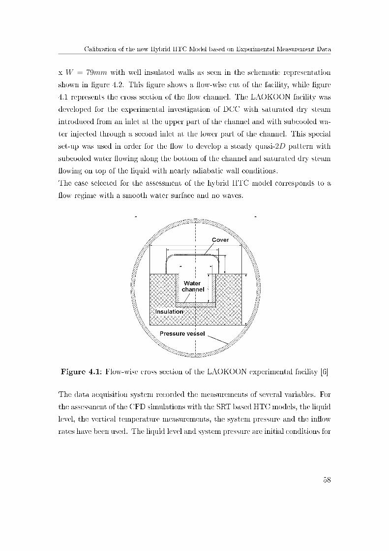
Calibration of the new Hybrid HTC Model based on Experimental Measurement Data
x W = 79mm with well insulated walls as seen in the schematic representation
shown in �gure 4.2. This �gure shows a �ow-wise cut of the facility, while �gure
4.1 represents the cross section of the �ow channel. The LAOKOON facility was
developed for the experimental investigation of DCC with saturated dry steam
introduced from an inlet at the upper part of the channel and with subcooled wa-
ter injected through a second inlet at the lower part of the channel. This special
set-up was used in order for the �ow to develop a steady quasi-2D pattern with
subcooled water �owing along the bottom of the channel and saturated dry steam
�owing on top of the liquid with nearly adiabatic wall conditions.
The case selected for the assessment of the hybrid HTC model corresponds to a
�ow regime with a smooth water surface and no waves.
Figure 4.1: Flow-wise cross section of the LAOKOON experimental facility [6]
The data acquisition system recorded the measurements of several variables. For
the assessment of the CFD simulations with the SRT based HTC models, the liquid
level, the vertical temperature measurements, the system pressure and the in�ow
rates have been used. The liquid level and system pressure are initial conditions for
58
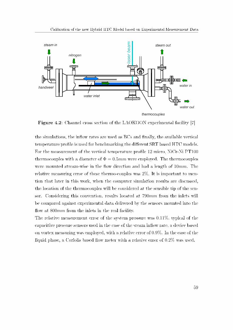
Calibration of the new Hybrid HTC Model based on Experimental Measurement Data
Figure 4.2: Channel cross section of the LAOKOON experimental facility [7]
the simulations, the in�ow rates are used as BCs and �nally, the available vertical
temperature pro�le is used for benchmarking the di�erent SRT based HTC models.
For the measurement of the vertical temperature pro�le 12 micro, NiCr-Ni PT100
thermocouples with a diameter of Φ = 0.5mm were employed. The thermocouples
were mounted stream-wise in the �ow direction and had a length of 10mm. The
relative measuring error of these thermo-couples was 2%. It is important to men-
tion that later in this work, when the computer simulation results are discussed,
the location of the thermocouples will be considered at the sensible tip of the sen-
sor. Considering this convention, results located at 790mm from the inlets will
be compared against experimental data delivered by the sensors mounted into the
�ow at 800mm from the inlets in the real facility.
The relative measurement error of the system pressure was 0.11%, typical of the
capacitive pressure sensors used in the case of the steam in�ow rate, a device based
on vortex measuring was employed, with a relative error of 0.9%. In the case of the
liquid phase, a Coriolis based �ow meter with a relative error of 0.2% was used.
59
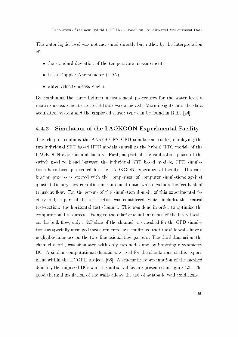
Calibration of the new Hybrid HTC Model based on Experimental Measurement Data
The water liquid level was not measured directly but rather by the interpretation
of:
• the standard deviation of the temperature measurement,
• Laser Doppler Anemometer (LDA),
• water velocity measurement.
By combining the three indirect measurement procedures for the water level a
relative measurement error of ±1mm was achieved. More insights into the data
acquisition system and the employed sensor type can be found in Ruile [44].
4.4.2 Simulation of the LAOKOON Experimental Facility
This chapter contains the ANSYS CFX CFD simulation results, employing the
two individual SRT based HTC models as well as the hybrid HTC model, of the
LAOKOON experimental facility. First, as part of the calibration phase of the
switch used to blend between the individual SRT based models, CFD simula-
tions have been performed for the LAOKOON experimental facility. The cali-
bration process is started with the comparison of computer simulations against
quasi-stationary �ow condition measurement data, which exclude the feedback of
transient �ow. For the set-up of the simulation domain of this experimental fa-
cility, only a part of the test-section was considered, which includes the central
test-section: the horizontal test channel. This was done in order to optimize the
computational resources. Owing to the relative small in�uence of the lateral walls
on the bulk �ow, only a 2D slice of the channel was meshed for the CFD simula-
tions as specially arranged measurements have con�rmed that the side walls have a
negligible in�uence on the two-dimensional �ow pattern. The third dimension, the
channel depth, was simulated with only two nodes and by imposing a symmetry
BC. A similar computational domain was used for the simulations of this experi-
ment within the ECORE project, [66]. A schematic representation of the meshed
domain, the imposed BCs and the initial values are presented in �gure 4.3. The
good thermal insulation of the walls allows the use of adiabatic wall conditions.
60
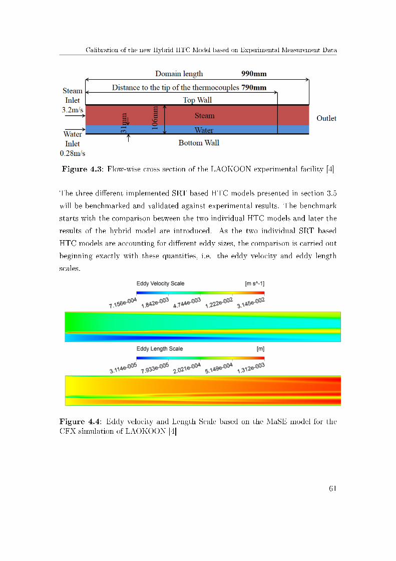
Calibration of the new Hybrid HTC Model based on Experimental Measurement Data
Figure 4.3: Flow-wise cross section of the LAOKOON experimental facility [4]
The three di�erent implemented SRT based HTC models presented in section 3.5
will be benchmarked and validated against experimental results. The benchmark
starts with the comparison between the two individual HTC models and later the
results of the hybrid model are introduced. As the two individual SRT based
HTC models are accounting for di�erent eddy sizes, the comparison is carried out
beginning exactly with these quantities, i.e. the eddy velocity and eddy length
scales.
Figure 4.4: Eddy velocity and Length Scale based on the MaSE model for theCFX simulation of LAOKOON [4]
61
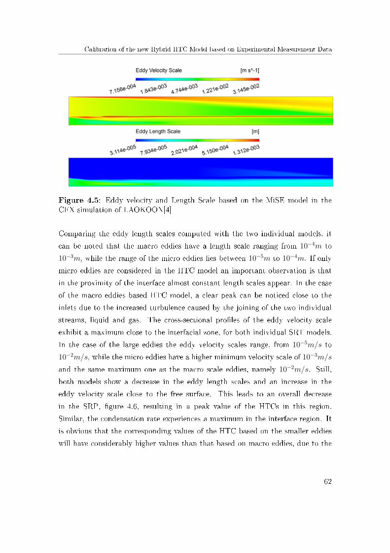
Calibration of the new Hybrid HTC Model based on Experimental Measurement Data
Figure 4.5: Eddy velocity and Length Scale based on the MiSE model in theCFX simulation of LAOKOON[4]
Comparing the eddy length scales computed with the two individual models, it
can be noted that the macro eddies have a length scale ranging from 10−4m to
10−3m, while the range of the micro eddies lies between 10−5m to 10−4m. If only
micro eddies are considered in the HTC model an important observation is that
in the proximity of the interface almost constant length scales appear. In the case
of the macro eddies based HTC model, a clear peak can be noticed close to the
inlets due to the increased turbulence caused by the joining of the two individual
streams, liquid and gas. The cross-sectional pro�les of the eddy velocity scale
exhibit a maximum close to the interfacial zone, for both individual SRT models.
In the case of the large eddies the eddy velocity scales range, from 10−5m/s to
10−2m/s, while the micro eddies have a higher minimum velocity scale of 10−3m/s
and the same maximum one as the macro scale eddies, namely 10−2m/s. Still,
both models show a decrease in the eddy length scales and an increase in the
eddy velocity scale close to the free surface. This leads to an overall decrease
in the SRP, �gure 4.6, resulting in a peak value of the HTCs in this region.
Similar, the condensation rate experiences a maximum in the interface region. It
is obvious that the corresponding values of the HTC based on the smaller eddies
will have considerably higher values than that based on macro eddies, due to the
62
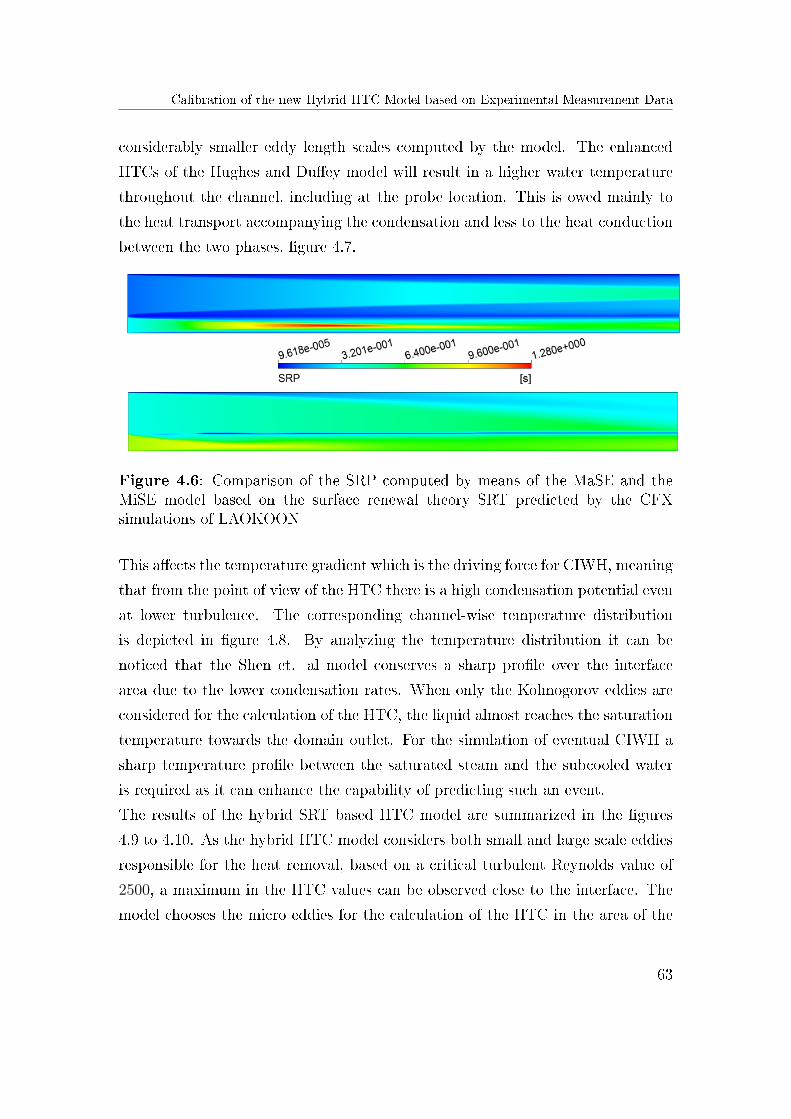
Calibration of the new Hybrid HTC Model based on Experimental Measurement Data
considerably smaller eddy length scales computed by the model. The enhanced
HTCs of the Hughes and Du�ey model will result in a higher water temperature
throughout the channel, including at the probe location. This is owed mainly to
the heat transport accompanying the condensation and less to the heat conduction
between the two phases, �gure 4.7.
Figure 4.6: Comparison of the SRP computed by means of the MaSE and theMiSE model based on the surface renewal theory SRT predicted by the CFXsimulations of LAOKOON
This a�ects the temperature gradient which is the driving force for CIWH, meaning
that from the point of view of the HTC there is a high condensation potential even
at lower turbulence. The corresponding channel-wise temperature distribution
is depicted in �gure 4.8. By analyzing the temperature distribution it can be
noticed that the Shen et. al model conserves a sharp pro�le over the interface
area due to the lower condensation rates. When only the Kolmogorov eddies are
considered for the calculation of the HTC, the liquid almost reaches the saturation
temperature towards the domain outlet. For the simulation of eventual CIWH a
sharp temperature pro�le between the saturated steam and the subcooled water
is required as it can enhance the capability of predicting such an event.
The results of the hybrid SRT based HTC model are summarized in the �gures
4.9 to 4.10. As the hybrid HTC model considers both small and large scale eddies
responsible for the heat removal, based on a critical turbulent Reynolds value of
2500, a maximum in the HTC values can be observed close to the interface. The
model chooses the micro eddies for the calculation of the HTC in the area of the
63
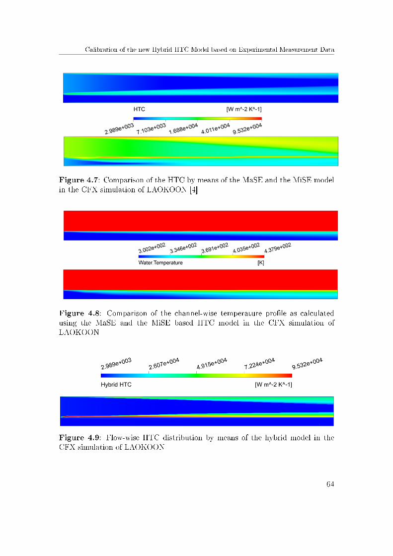
Calibration of the new Hybrid HTC Model based on Experimental Measurement Data
Figure 4.7: Comparison of the HTC by means of the MaSE and the MiSE modelin the CFX simulation of LAOKOON [4]
Figure 4.8: Comparison of the channel-wise temperature pro�le as calculatedusing the MaSE and the MiSE based HTC model in the CFX simulation ofLAOKOON
Figure 4.9: Flow-wise HTC distribution by means of the hybrid model in theCFX simulation of LAOKOON
64
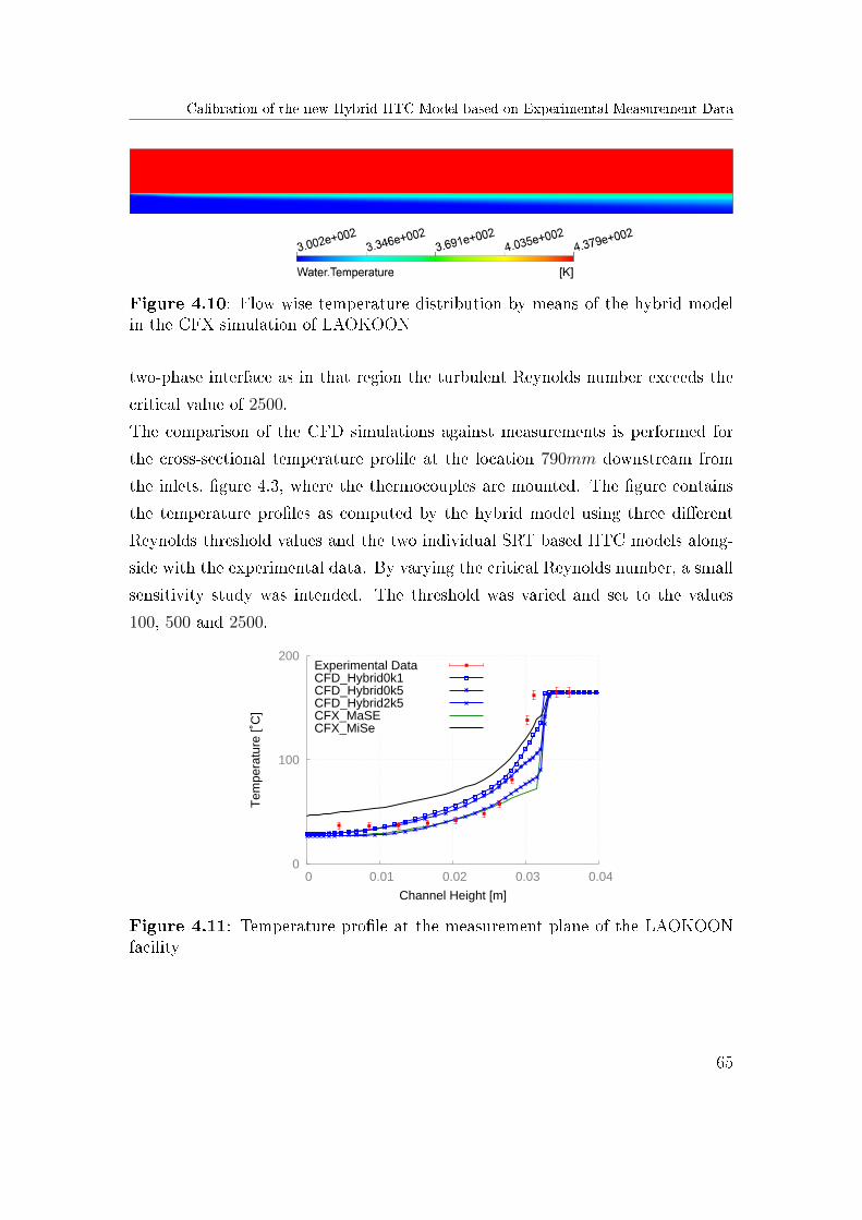
Calibration of the new Hybrid HTC Model based on Experimental Measurement Data
Figure 4.10: Flow-wise temperature distribution by means of the hybrid modelin the CFX simulation of LAOKOON
two-phase interface as in that region the turbulent Reynolds number exceeds the
critical value of 2500.
The comparison of the CFD simulations against measurements is performed for
the cross-sectional temperature pro�le at the location 790mm downstream from
the inlets, �gure 4.3, where the thermocouples are mounted. The �gure contains
the temperature pro�les as computed by the hybrid model using three di�erent
Reynolds threshold values and the two individual SRT based HTC models along-
side with the experimental data. By varying the critical Reynolds number, a small
sensitivity study was intended. The threshold was varied and set to the values
100, 500 and 2500.
0
100
200
0 0.01 0.02 0.03 0.04
Tem
pera
ture
[˚C
]
Channel Height [m]
CFX_MiSeCFX_MaSECFD_Hybrid2k5CFD_Hybrid0k5CFD_Hybrid0k1Experimental Data
Figure 4.11: Temperature pro�le at the measurement plane of the LAOKOONfacility
65
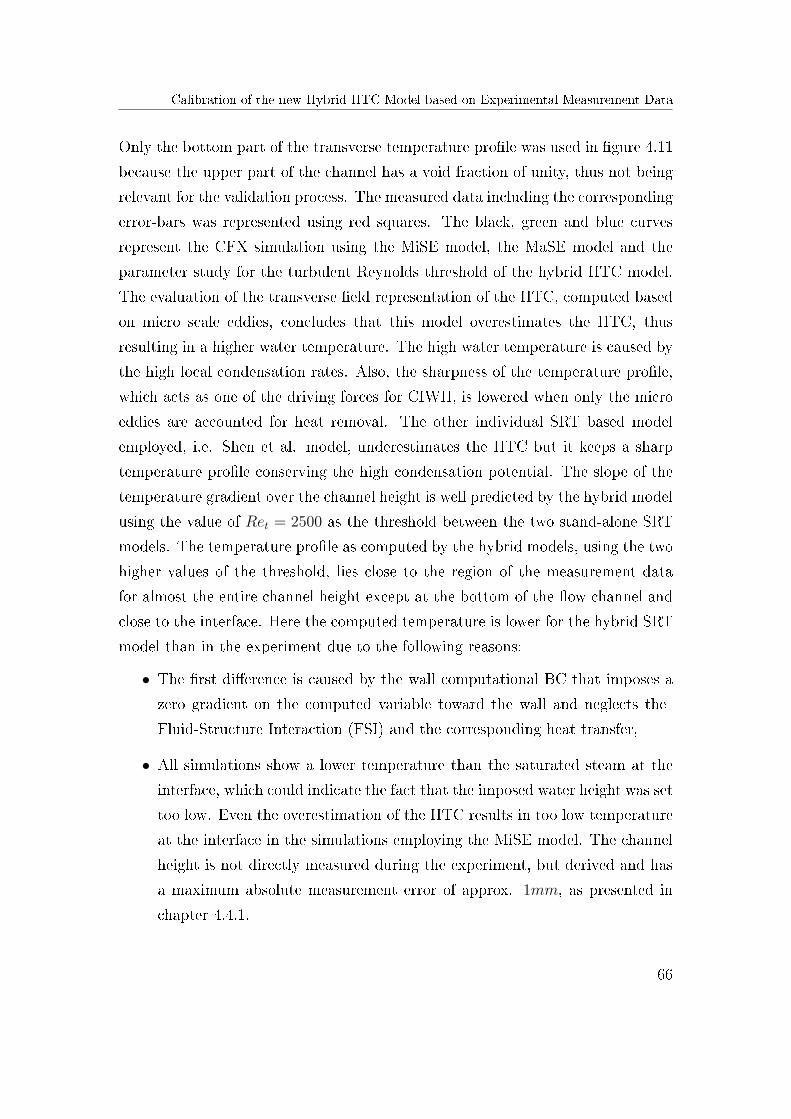
Calibration of the new Hybrid HTC Model based on Experimental Measurement Data
Only the bottom part of the transverse temperature pro�le was used in �gure 4.11
because the upper part of the channel has a void fraction of unity, thus not being
relevant for the validation process. The measured data including the corresponding
error-bars was represented using red squares. The black, green and blue curves
represent the CFX simulation using the MiSE model, the MaSE model and the
parameter study for the turbulent Reynolds threshold of the hybrid HTC model.
The evaluation of the transverse �eld representation of the HTC, computed based
on micro scale eddies, concludes that this model overestimates the HTC, thus
resulting in a higher water temperature. The high water temperature is caused by
the high local condensation rates. Also, the sharpness of the temperature pro�le,
which acts as one of the driving forces for CIWH, is lowered when only the micro
eddies are accounted for heat removal. The other individual SRT based model
employed, i.e. Shen et al. model, underestimates the HTC but it keeps a sharp
temperature pro�le conserving the high condensation potential. The slope of the
temperature gradient over the channel height is well predicted by the hybrid model
using the value of Ret = 2500 as the threshold between the two stand-alone SRT
models. The temperature pro�le as computed by the hybrid models, using the two
higher values of the threshold, lies close to the region of the measurement data
for almost the entire channel height except at the bottom of the �ow channel and
close to the interface. Here the computed temperature is lower for the hybrid SRT
model than in the experiment due to the following reasons:
• The �rst di�erence is caused by the wall computational BC that imposes a
zero gradient on the computed variable toward the wall and neglects the
Fluid-Structure Interaction (FSI) and the corresponding heat transfer,
• All simulations show a lower temperature than the saturated steam at the
interface, which could indicate the fact that the imposed water height was set
too low. Even the overestimation of the HTC results in too low temperature
at the interface in the simulations employing the MiSE model. The channel
height is not directly measured during the experiment, but derived and has
a maximum absolute measurement error of approx. 1mm, as presented in
chapter 4.4.1.
66
Calibration of the new Hybrid HTC Model based on Experimental Measurement Data
These three simulations with di�erent turbulent Reynolds threshold values indicate
that the temperature pro�le is clearly sensitive to this parameter. Figure 4.11
shows that if the Reynolds turbulent threshold value is selected too low, then
the hybrid HTC model delivers values close to the micro eddies based stand-
alone model and thus overestimates the condensation rates and consequently the
temperature. If the values for the critical Reynolds number are chosen higher the
hybrid model converges towards the results of the stand alone model considering
only large eddies for the heat removal from the interface. Even if it appears that
other threshold values would eventually deliver better results for this particular
case of quasi-steady state horizontal two-phase �ow, one has to bear in mind that
this model will be applied for the more complex cases of transient horizontal �ows.
The higher value for the switch is recommended for the system consisting of VOF
and the k − ω SST turbulence model and will also be used in the system code
ATHLET.
The conclusion that can be drawn from the �rst validation step of the newly de-
veloped hybrid HTC model is that the simulations employing only the individual
SRT based HTCs justify the need of a hybrid model for the realistic simulation
of DCC. When only micro eddies are accountable for the heat removal from the
interface, the liquid can quickly become saturated, hence damping the condensa-
tion as the HTC is overestimated. If only macro eddies are considered in the HTC
model, an underestimation of this variable is performed; still a steep temperature
gradient is preserved, similar to the experimental measurement data. The hybrid
model together with a suitable threshold value for the turbulent Reynolds num-
ber preserves the advantages of both models and clearly improves the predictive
qualities of the computational simulations.
67
Chapter 5
Description of the Experiments used
for the Assessment of the New
Hybrid HTC Model
The design of the di�erent experimental facilities and the description of the exper-
iments will be presented within this chapter. The hybrid model was calibrated and
together with the individual SRT models it was bench-marked against measure-
ment data of a horizontal two-phase �ow. This chapter contains the simulation
results of the hybrid HTC model as it was implemented in the computer codes to
accurately simulate heavy DCC as the precursor of water hammers. The analyzed
facilities have the geometrical characteristics required for the appearance of CIWH
as presented by Gri�th [33]. The PMK-2 has a horizontal test-section while the
slope of the TUHH facility is less than 2.4◦. The ratio between the length of the
test-section and its inner diameter is in the case of the PMK-2 facility approxi-
mately 39, while in the case of the TUHH experimental facility it is approximately
50. The water subcooling was always larger than 20◦C and the injection rate
was always smaller than the one corresponding to a Fr of unity. All experiments
were initiated with the test-section full of vapor. These initial conditions and BCs
correspond to a set-up which is prone to CIWH as presented by Gri�th in [33].
Description of the PMK-2 Experimental Facility
5.1 Description of the PMK-2 Experimental
Facility
The horizontal PMK-2 experimental facility built at the KFKI Institute, Budapest
Hungary, has a complex set up and �ow characteristics. A schematic representa-
tion of the PMK-2 facility is represented in the �gure 5.1. Several experiments
were performed at this facility, in which di�erent phenomena have been analyzed.
One of the experimental series in the WAHALoads project included the analy-
sis of the CIWH phenomenon. The WAHALoads project took place within the
5th EU framework and studied transients involving two-phase �ow water ham-
mers and the induced loads on materials and structures of NPP components. A
total of 35 experiments have been performed within the frame of the four year
WAHALoads project, whereby a CIWH event occurred in 26 cases, [37] and [38].
The initial conditions of these experiments together with the observation whether
a CIWH e�ect occurred, are summarized in the Appendix A. The need for the
experimental analysis of accident scenarios in the Russian type Pressurized Water
Reactor (PWR) Water-Water Power Reactor (VVER) Series 440 NPP led to the
creation of this experimental facility consisting of an integral thermal-hydraulic
model of a down-scaled steam line. The goal of this experimental series was to
deliver system code and CFD validation grade measurement data. The insights
at the phenomenological level gained at this facility can be extrapolated to other
reactor types while the measurement data is a highly valuable database for hori-
zontal two-phase �ow, including DCC and for the two-phase �ow dynamics during
CIWH events.
All 33 experiments were initiated by opening the valve labelled number (6) in �g-
ure 5.1 isolating the pressurized feed-water tank containing pressurized subcooled
water from the experimental facility. A nitrogen gas cushion pressurized the sub-
cooled water, which after the opening of the valve, entered the test-section through
the elbow (3). Subcooled water would then interact with the stagnant steam which
initially �lled up the test-section. The test rig had an internal pipe diameter of
73mm. From an instrumentation point of view, the test-section was equipped with
69
Description of the PMK-2 Experimental Facility
four void-temperature sensors marked as number (8), three pressure transducers
marked as number (3) and a wire mesh sensor labelled with number (9) in the
�gure 5.1. The elbow on the left hand side marked with number (2) connects the
steam generator with the test-section. The sensors number (8) and (3) deliver
highly local values, while the wire mesh sensors yields area averaged void fractions
for the entire pipe cross-section. The measurement data recorded by the Wire
Mesh Sensor (WMS) are valuable for the reconstruction of the �ow pattern and
thus, for the assessments of CFD codes. This local information is only of limited
value for the validation of 1D system codes.
The particularity of the instrumentation available on this experimental facility
compared to that mounted in the other analyzed facilities described later is the
WMS. This measuring device consists of two parallel planes each including a num-
ber of 12 electrodes with a 2mm vertical pitch between the planes. By measuring
the distribution of the instantaneous conductivity and with prior calibration based
on the conductivity of the liquid phase, the void distribution can be reconstructed
with a resolution equal to the wire horizontal pitch of 5.9mm and a time reso-
lution of 1kHz. The WMS is designed to be used under system pressures up to
7MPa and temperatures up to 285◦C [67]. More detailed information about the
instrumentation installed in the test facility and especially about the WMS can be
found in [8]. System codes yield only coarse volume averaged values, for instance
for the void fraction and thus can be compared only to some extent against highly
local measurement data as those of the void-temperature probes. On the other
hand, the area averaged results of the void fraction distribution give a hint on
the two-phase �ow dynamics and can be compared with interpreted system code
results.
A very e�cient thermal insulation of the test-section's walls was required in order
to reach a void fraction close to unity at the beginning of the experiments, while
also simplifying the BCs for the latter validation process. Still, at the beginning of
the experiments a thin liquid �lm is recorded by the WMS, which is very di�cult
to initialize in the computer simulations, as no detailed information is available
from experiment logs performed at the PMK-2 facility. This liquid �lm has an in-
70
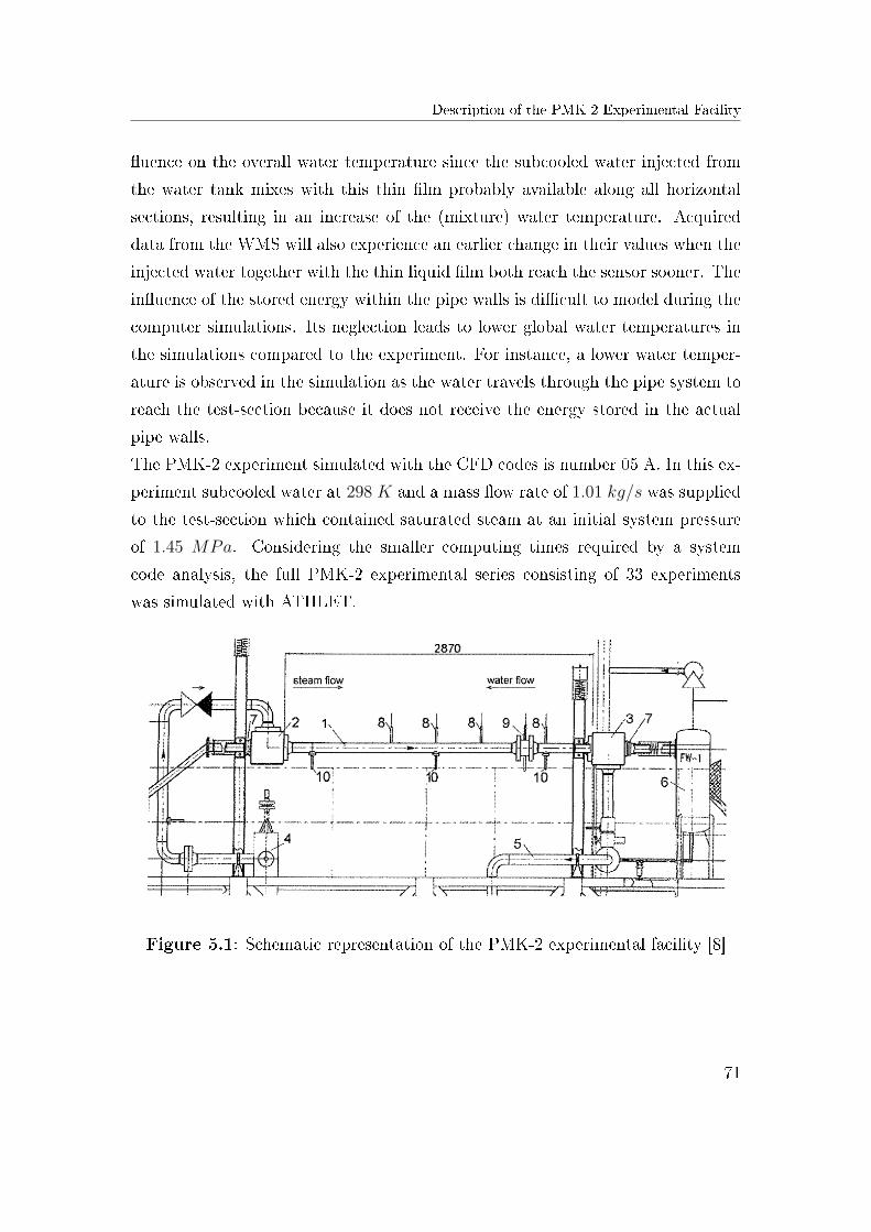
Description of the PMK-2 Experimental Facility
�uence on the overall water temperature since the subcooled water injected from
the water tank mixes with this thin �lm probably available along all horizontal
sections, resulting in an increase of the (mixture) water temperature. Acquired
data from the WMS will also experience an earlier change in their values when the
injected water together with the thin liquid �lm both reach the sensor sooner. The
in�uence of the stored energy within the pipe walls is di�cult to model during the
computer simulations. Its neglection leads to lower global water temperatures in
the simulations compared to the experiment. For instance, a lower water temper-
ature is observed in the simulation as the water travels through the pipe system to
reach the test-section because it does not receive the energy stored in the actual
pipe walls.
The PMK-2 experiment simulated with the CFD codes is number 05 A. In this ex-
periment subcooled water at 298 K and a mass �ow rate of 1.01 kg/s was supplied
to the test-section which contained saturated steam at an initial system pressure
of 1.45 MPa. Considering the smaller computing times required by a system
code analysis, the full PMK-2 experimental series consisting of 33 experiments
was simulated with ATHLET.
Figure 5.1: Schematic representation of the PMK-2 experimental facility [8]
71
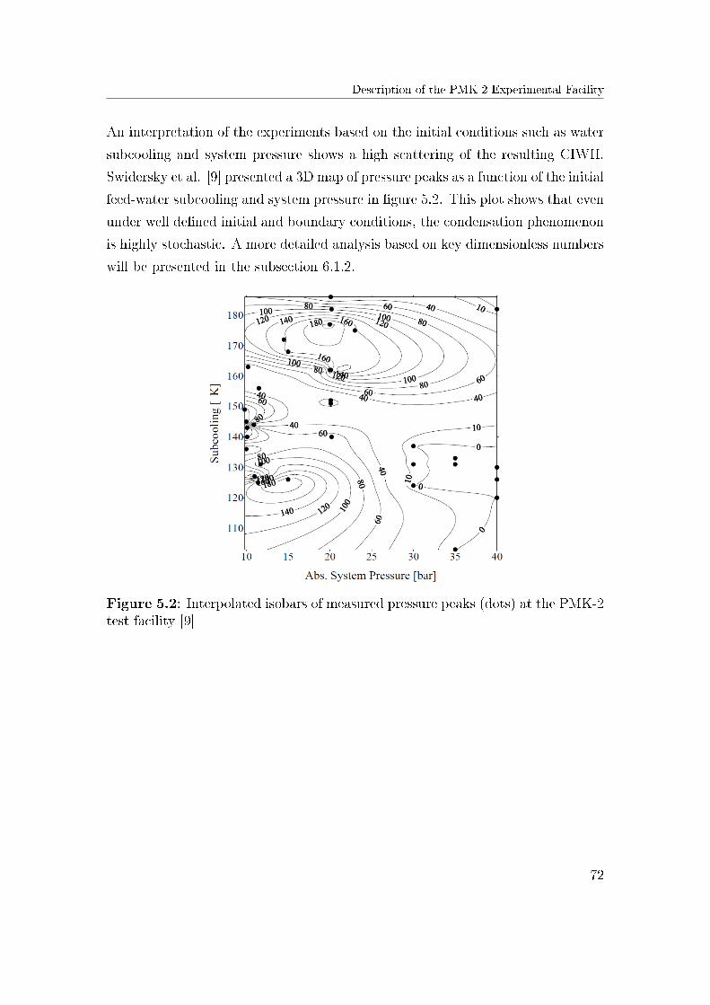
Description of the PMK-2 Experimental Facility
An interpretation of the experiments based on the initial conditions such as water
subcooling and system pressure shows a high scattering of the resulting CIWH.
Swidersky et al. [9] presented a 3D map of pressure peaks as a function of the initial
feed-water subcooling and system pressure in �gure 5.2. This plot shows that even
under well de�ned initial and boundary conditions, the condensation phenomenon
is highly stochastic. A more detailed analysis based on key dimensionless numbers
will be presented in the subsection 6.1.2.
Figure 5.2: Interpolated isobars of measured pressure peaks (dots) at the PMK-2test facility [9]
72
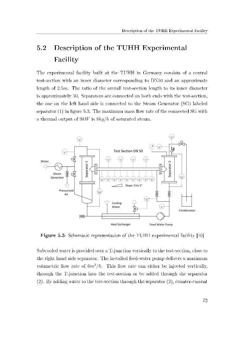
Description of the TUHH Experimental Facility
5.2 Description of the TUHH Experimental
Facility
The experimental facility built at the TUHH in Germany consists of a central
test-section with an inner diameter corresponding to DN50 and an approximate
length of 2.5m. The ratio of the overall test-section length to its inner diameter
is approximately 50. Separators are connected on both ends with the test-section,
the one on the left hand side is connected to the Steam Generator (SG) labeled
separator (1) in �gure 5.3. The maximum mass �ow rate of the connected SG with
a thermal output of 9kW is 8kg/h of saturated steam.
Dampf-
erzeuger
LIA±
LIA+
FI
FI
FI
PI
TIC
VE-Wasser
Pumpe
Kühlwasser
Wärmetauscher
Druckluft
Kondensations-becken
Gefälle: 0 bis 5°
Teststrecke DN 50
Sep
arat
or
1
Sep
arat
or
2
PI
PI PI PI PI PITI TI TI TI
TI TI TITI
Test Section DN 50
Slope: 0 to 5°
Cooling Water
Heat Exchanger Feed Water Pump
Condensator
Pressurized Air
Steam Generator
Water
Figure 5.3: Schematic representation of the TUHH experimental facility [10]
Subcooled water is provided over a T-junction vertically to the test-section, close to
the right hand side separator. The installed feed-water pump delivers a maximum
volumetric �ow rate of 6m3/h. This �ow rate can either be injected vertically,
through the T-junction into the test-section or be added through the separator
(2). By adding water to the test-section through the separator (2), counter-current
73
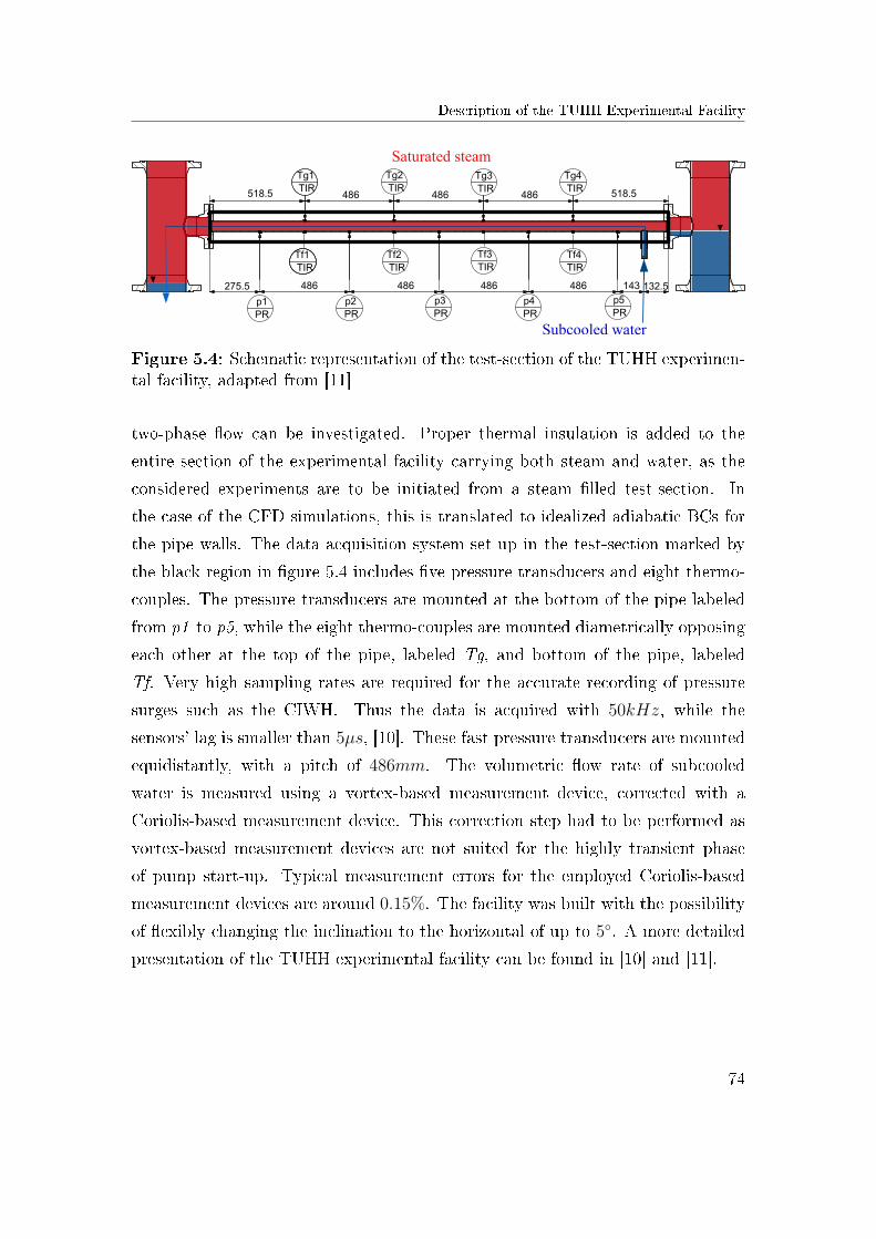
Description of the TUHH Experimental Facility
132.5
518.5486486486518.5
486486486486275.5
p1
PR
143
p2
PR
p3
PR
p4
PR
p5
PR
Tg4
TIR
Tg3
TIR
Tg2
TIR
Tg1
TIR
Saturated steam
Subcooled water
Tf1
TIR
Tf2
TIR
Tf3
TIR
Tf4
TIR
Figure 5.4: Schematic representation of the test-section of the TUHH experimen-tal facility, adapted from [11]
two-phase �ow can be investigated. Proper thermal insulation is added to the
entire section of the experimental facility carrying both steam and water, as the
considered experiments are to be initiated from a steam �lled test-section. In
the case of the CFD simulations, this is translated to idealized adiabatic BCs for
the pipe walls. The data acquisition system set up in the test-section marked by
the black region in �gure 5.4 includes �ve pressure transducers and eight thermo-
couples. The pressure transducers are mounted at the bottom of the pipe labeled
from p1 to p5, while the eight thermo-couples are mounted diametrically opposing
each other at the top of the pipe, labeled Tg, and bottom of the pipe, labeled
Tf. Very high sampling rates are required for the accurate recording of pressure
surges such as the CIWH. Thus the data is acquired with 50kHz, while the
sensors' lag is smaller than 5µs, [10]. These fast pressure transducers are mounted
equidistantly, with a pitch of 486mm. The volumetric �ow rate of subcooled
water is measured using a vortex-based measurement device, corrected with a
Coriolis-based measurement device. This correction step had to be performed as
vortex-based measurement devices are not suited for the highly transient phase
of pump start-up. Typical measurement errors for the employed Coriolis-based
measurement devices are around 0.15%. The facility was built with the possibility
of �exibly changing the inclination to the horizontal of up to 5◦. A more detailed
presentation of the TUHH experimental facility can be found in [10] and [11].
74
Description of the TUHH Experimental Facility
The facility was designed bearing in mind the following objectives: the measure-
ment of pressure, temperature in the test-section and liquid level in the two sepa-
rators. The test-section was designed with a length to its inner diameter fraction
which is typical for power plants. Additionally the special feature of adding a
transparent pipe section for the visual investigation of the CIWH phenomena was
pursued [10]. Creating a database for the validation of computer codes as well as
for the development of the hybrid HTC model were typical goals considered in the
design phase of this experimental facility.
75
Chapter 6
Assessment of the New Hybrid HTC
Model for the Simulation of
Transient Two-Phase Flow with
Finite Volume Computer Codes
This chapter includes the computational results of the di�erent computer codes
used for the simulation of DCC as the driving force for CIWH together with the
benchmark of the SRT based HTC models employed.
As computer codes that consider a di�erent number of dimensions were used to
analyze the �ow, additional post processing is needed to fully validate the em-
ployed models; for the calculation of the HTC. This is required when the results
of the system code simulations are discussed. For the validation of the hybrid HTC
model, measurement data from di�erent experimental facilities are used. The re-
sults of the simulations will be progressively presented. The results of the computer
simulation of a horizontal quasi-steady state two-phase �ow, at the LAOKOON
facility, have been used for the calibration of the newly developed SRT based HTC
model in chapter 4.4.2. The hybrid HTC model will now be assessed based on the
results of the simulations of fully transient horizontal two-phase �ow experiments.
The data is provided from the facilities PMK-2, chapter 6.1 and TUHH, chapter
6.2.
In the case of the two fully transient �ow facilities, the overall behavior of the
system consisting of VOF and SRT based HTC models will be validated against
measurement data. The system code will be used only to simulate experiments of
the transient two-phase �ow because a comparison of 1D simulation results with
high resolution measurement data from the LAOKOON facility would be incon-
clusive.
The simulation results of the PMK-2 experimental facility include both the results
obtained with the system code ATHLET and ANSYS CFX. The system code
simulations include the typical 1D approach and an approach with a quasi-2D
computational grid. In the case of the CFD analysis, the results of all three HTC
models will be presented and discussed in order to underline the necessity of a
hybrid model for the calculation of the HTC for the �ow patterns spanning from
horizontal strati�ed to slug and plug �ow. These �ow patterns have characteristic
turbulence intensities re�ected by turbulent quantities such as the TKE and the
turbulent eddy dissipation rate.
The TUHH experimental facility, which was developed and build within the frame-
work of the CIWA project, will be simulated only with the open-source CFD tool-
box OpenFOAM. The results of this analysis will be presented in chapter 6.2.
The CFD simulations have been performed on structured grids, i.e. o-grids. In
order to minimize the computational time, only one half of the axis-symmetrical
computational domain has been meshed and a symmetry BC was used for this
patch to account for the other pipe half. A grid independent study however has
not been performed due to the relatively long problem times and consequently
long computational times of each experiment.
77
Simulations of the PMK-2 Experimental Facility
6.1 Simulations of the PMK-2 Experimental
Facility
The PMK-2 facility in this set-up was used for a total of 33 experiments of hor-
izontal two-phase �ow, where subcooled water was injected into a steam �lled
test-section. The complete matrix of the experiment series is presented in ap-
pendix A. The experiments are described in various papers or journal articles in
the literature; the most comprehensive sources have been published within the
framework of the WAHALOADS project: [37] and [38] etc. Out of the 33 docu-
mented experiments conducted at this facility, 26 recorded a CIWH event.
Chapter 6.1.1 presents the ANSYS CFX simulation results, including runs with
the individual SRT based models, the MiSE and MaSE models.
The assessment of the newly developed HTC within the system code ATHLET
will be presented in chapter 6.1.2.
6.1.1 Simulations of the PMK-2 Experimental Facility
with ANSYS CFX
In order to justify the need of an hybrid HTC model for the reliable simulation of
CIWH in horizontal two-phase �ow with free surface, the ANSYS CFX results of
each of the individual SRT models will be discussed.
During the design of the computational grid employed in the simulations, the
in�uence of the measurement sensors on the �ow was not taken into account.
Even if intrusive measurement techniques such as the WMS are implemented into
the test section, the e�ort of considering such sensors in the computational grid is
considerably high and has thus been neglected. It also results in a correspondingly
higher computational time because of a very detailed mesh re�nement needed near
the sensors. It is however believed that the e�ect of the grid on the development
of the CIWH away from the sensor is not important enough to require explicit
modeling.
78
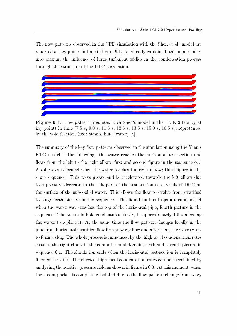
Simulations of the PMK-2 Experimental Facility
The �ow patterns observed in the CFD simulation with the Shen et al. model are
reported at key points in time in �gure 6.1. As already explained, this model takes
into account the in�uence of large turbulent eddies in the condensation process
through the structure of the HTC correlation.
Figure 6.1: Flow pattern predicted with Shen's model in the PMK-2 facility atkey points in time (7.5 s, 9.0 s, 11.5 s, 12.5 s, 13.5 s, 15.0 s, 16.5 s), representedby the void fraction (red: steam, blue: water) [4]
The summary of the key �ow patterns observed in the simulation using the Shen's
HTC model is the following: the water reaches the horizontal test-section and
�ows from the left to the right elbow; �rst and second �gure in the sequence 6.1.
A roll-wave is formed when the water reaches the right elbow; third �gure in the
same sequence. This wave grows and is accelerated towards the left elbow due
to a pressure decrease in the left part of the test-section as a result of DCC on
the surface of the subcooled water. This allows the �ow to evolve from strati�ed
to slug; forth picture in the sequence. The liquid bulk entraps a steam pocket
when the water wave reaches the top of the horizontal pipe, fourth picture in the
sequence. The steam bubble condensates slowly, in approximately 1.5 s allowing
the water to replace it. At the same time the �ow pattern changes locally in the
pipe from horizontal strati�ed �ow �rst to wavy �ow and after that, the waves grow
to form a slug. The whole process is in�uenced by the high local condensation rates
close to the right elbow in the computational domain, sixth and seventh picture in
sequence 6.1. The simulation ends when the horizontal test-section is completely
�lled with water. The e�ect of high local condensation rates can be ascertained by
analyzing the relative pressure �eld as shown in �gure in 6.3. At this moment, when
the steam pocket is completely isolated due to the �ow pattern change from wavy
79
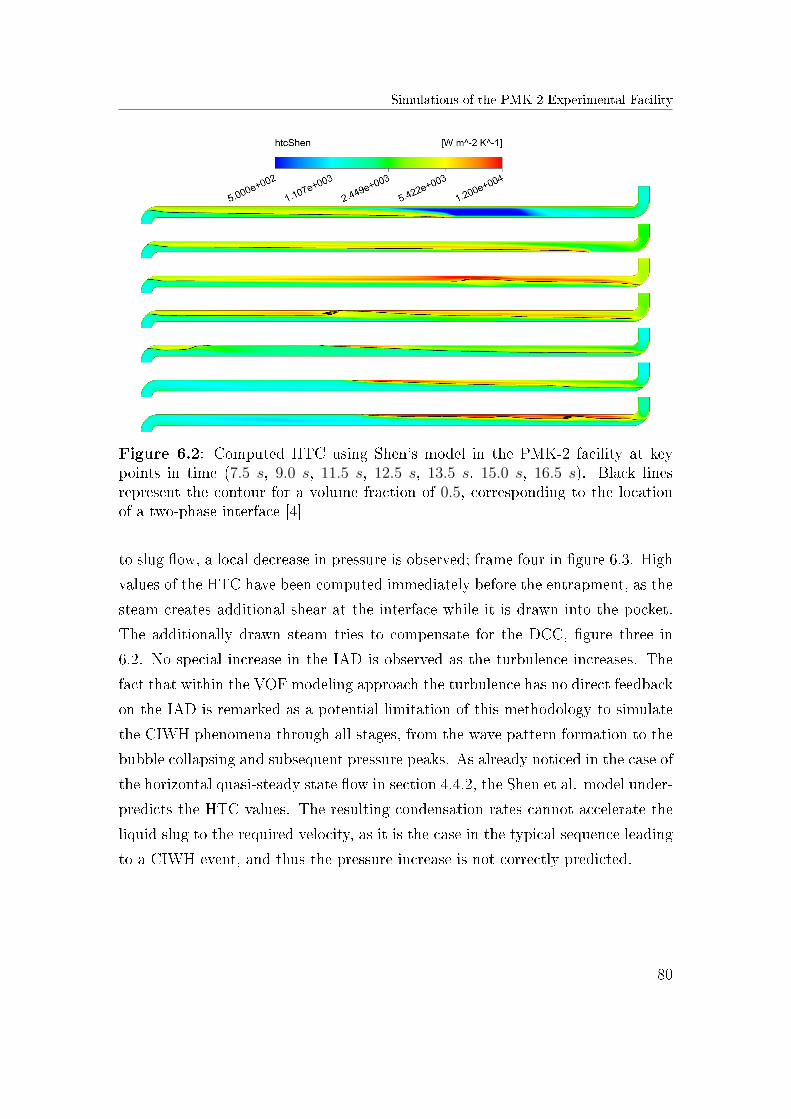
Simulations of the PMK-2 Experimental Facility
Figure 6.2: Computed HTC using Shen's model in the PMK-2 facility at keypoints in time (7.5 s, 9.0 s, 11.5 s, 12.5 s, 13.5 s, 15.0 s, 16.5 s). Black linesrepresent the contour for a volume fraction of 0.5, corresponding to the locationof a two-phase interface [4]
to slug �ow, a local decrease in pressure is observed; frame four in �gure 6.3. High
values of the HTC have been computed immediately before the entrapment, as the
steam creates additional shear at the interface while it is drawn into the pocket.
The additionally drawn steam tries to compensate for the DCC, �gure three in
6.2. No special increase in the IAD is observed as the turbulence increases. The
fact that within the VOF modeling approach the turbulence has no direct feedback
on the IAD is remarked as a potential limitation of this methodology to simulate
the CIWH phenomena through all stages, from the wave pattern formation to the
bubble collapsing and subsequent pressure peaks. As already noticed in the case of
the horizontal quasi-steady state �ow in section 4.4.2, the Shen et al. model under-
predicts the HTC values. The resulting condensation rates cannot accelerate the
liquid slug to the required velocity, as it is the case in the typical sequence leading
to a CIWH event, and thus the pressure increase is not correctly predicted.
80
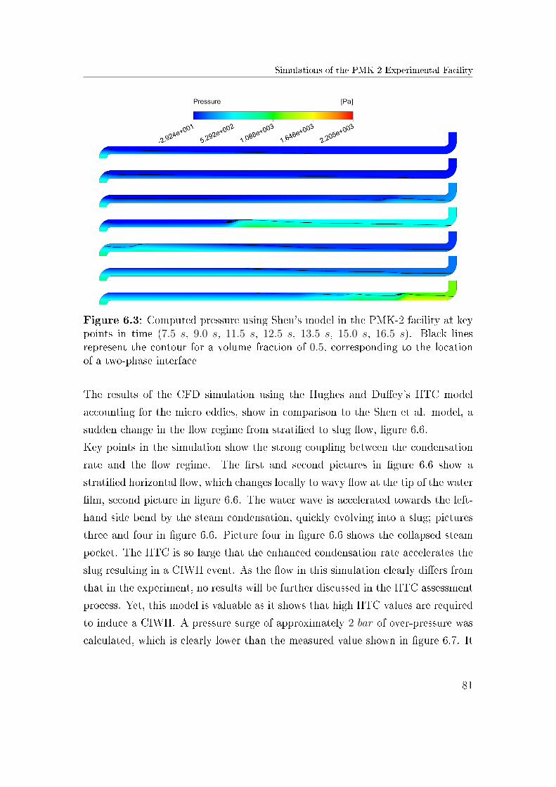
Simulations of the PMK-2 Experimental Facility
Figure 6.3: Computed pressure using Shen's model in the PMK-2 facility at keypoints in time (7.5 s, 9.0 s, 11.5 s, 12.5 s, 13.5 s, 15.0 s, 16.5 s). Black linesrepresent the contour for a volume fraction of 0.5, corresponding to the locationof a two-phase interface
The results of the CFD simulation using the Hughes and Du�ey's HTC model
accounting for the micro eddies, show in comparison to the Shen et al. model, a
sudden change in the �ow regime from strati�ed to slug �ow, �gure 6.6.
Key points in the simulation show the strong coupling between the condensation
rate and the �ow regime. The �rst and second pictures in �gure 6.6 show a
strati�ed horizontal �ow, which changes locally to wavy �ow at the tip of the water
�lm, second picture in �gure 6.6. The water wave is accelerated towards the left-
hand side bend by the steam condensation, quickly evolving into a slug; pictures
three and four in �gure 6.6. Picture four in �gure 6.6 shows the collapsed steam
pocket. The HTC is so large that the enhanced condensation rate accelerates the
slug resulting in a CIWH event. As the �ow in this simulation clearly di�ers from
that in the experiment, no results will be further discussed in the HTC assessment
process. Yet, this model is valuable as it shows that high HTC values are required
to induce a CIWH. A pressure surge of approximately 2 bar of over-pressure was
calculated, which is clearly lower than the measured value shown in �gure 6.7. It
81
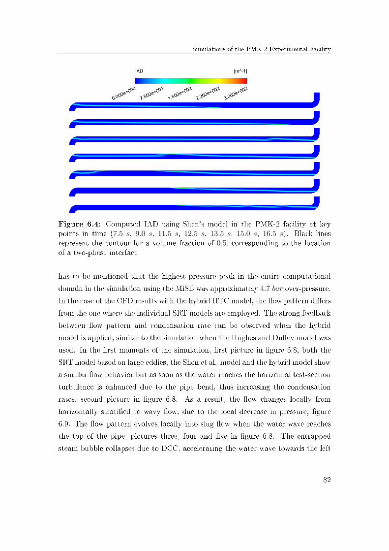
Simulations of the PMK-2 Experimental Facility
Figure 6.4: Computed IAD using Shen's model in the PMK-2 facility at keypoints in time (7.5 s, 9.0 s, 11.5 s, 12.5 s, 13.5 s, 15.0 s, 16.5 s). Black linesrepresent the contour for a volume fraction of 0.5, corresponding to the locationof a two-phase interface
has to be mentioned that the highest pressure peak in the entire computational
domain in the simulation using the MiSE was approximately 4.7 bar over-pressure.
In the case of the CFD results with the hybrid HTC model, the �ow pattern di�ers
from the one where the individual SRT models are employed. The strong feedback
between �ow pattern and condensation rate can be observed when the hybrid
model is applied, similar to the simulation when the Hughes and Du�ey model was
used. In the �rst moments of the simulation, �rst picture in �gure 6.8, both the
SRT model based on large eddies, the Shen et al. model and the hybrid model show
a similar �ow behavior but as soon as the water reaches the horizontal test-section
turbulence is enhanced due to the pipe bend, thus increasing the condensation
rates, second picture in �gure 6.8. As a result, the �ow changes locally from
horizontally strati�ed to wavy �ow, due to the local decrease in pressure; �gure
6.9. The �ow pattern evolves locally into slug �ow when the water wave reaches
the top of the pipe, pictures three, four and �ve in �gure 6.8. The entrapped
steam bubble collapses due to DCC, accelerating the water wave towards the left
82
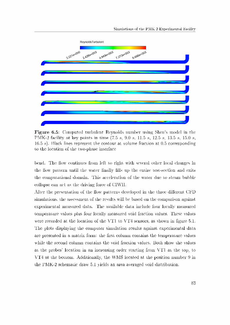
Simulations of the PMK-2 Experimental Facility
Figure 6.5: Computed turbulent Reynolds number using Shen's model in thePMK-2 facility at key points in time (7.5 s, 9.0 s, 11.5 s, 12.5 s, 13.5 s, 15.0 s,16.5 s). Black lines represent the contour at volume fraction at 0.5 correspondingto the location of the two-phase interface
bend. The �ow continues from left to right with several other local changes in
the �ow pattern until the water �nally �lls up the entire test-section and exits
the computational domain. This acceleration of the water due to steam bubble
collapse can act as the driving force of CIWH.
After the presentation of the �ow patterns developed in the three di�erent CFD
simulations, the assessment of the results will be based on the comparison against
experimental measured data. The available data include four locally measured
temperature values plus four locally measured void fraction values. These values
were recorded at the location of the VT1 to VT4 sensors, as shown in �gure 5.1.
The plots displaying the computer simulation results against experimental data
are presented in a matrix form: the �rst column contains the temperature values
while the second column contains the void fraction values. Both show the values
at the probes' location in an increasing order starting from VT1 at the top, to
VT4 at the bottom. Additionally, the WMS located at the position number 9 in
the PMK-2 schematic draw 5.1 yields an area averaged void distribution.
83
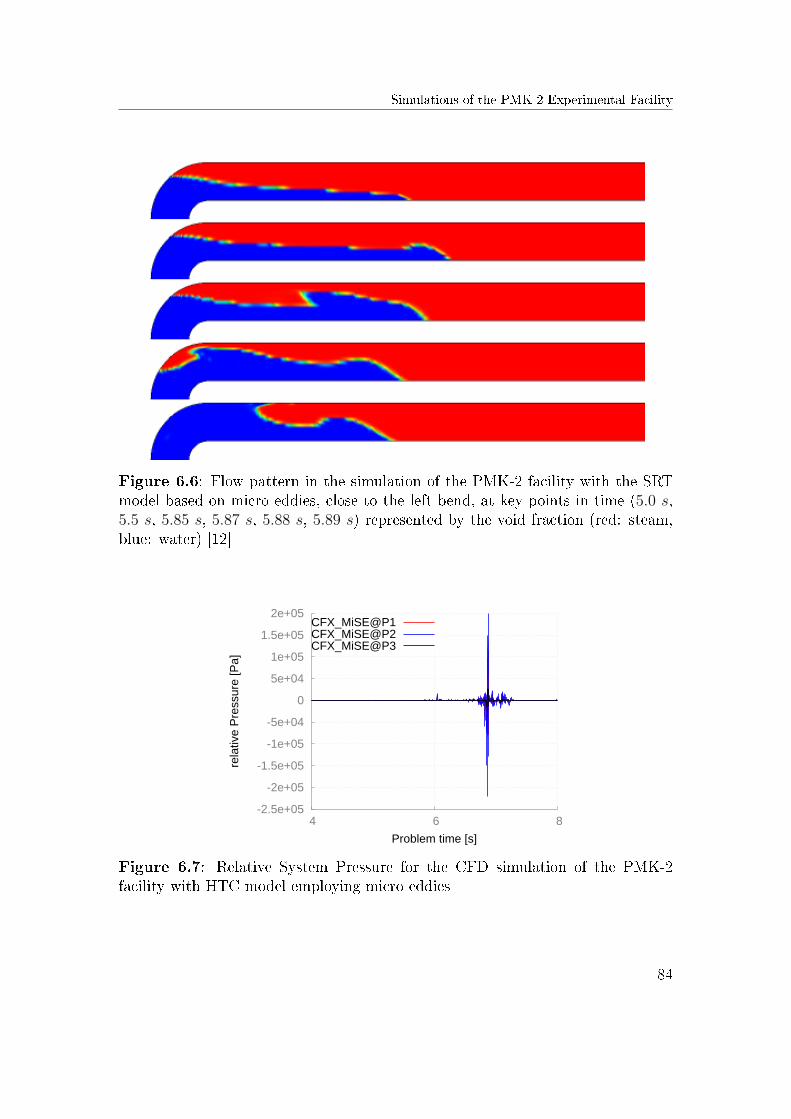
Simulations of the PMK-2 Experimental Facility
Figure 6.6: Flow pattern in the simulation of the PMK-2 facility with the SRTmodel based on micro eddies, close to the left bend, at key points in time (5.0 s,5.5 s, 5.85 s, 5.87 s, 5.88 s, 5.89 s) represented by the void fraction (red: steam,blue: water) [12]
-2.5e+05
-2e+05
-1.5e+05
-1e+05
-5e+04
0
5e+04
1e+05
1.5e+05
2e+05
4 6 8
rela
tive
Pre
ssur
e [P
a]
Problem time [s]
CFX_MiSE@P1CFX_MiSE@P2CFX_MiSE@P3
Figure 6.7: Relative System Pressure for the CFD simulation of the PMK-2facility with HTC model employing micro eddies
84
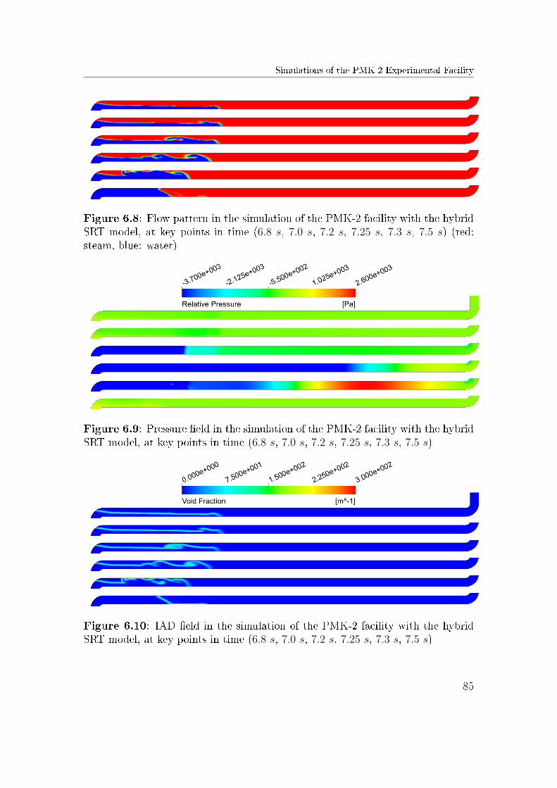
Simulations of the PMK-2 Experimental Facility
Figure 6.8: Flow pattern in the simulation of the PMK-2 facility with the hybridSRT model, at key points in time (6.8 s, 7.0 s, 7.2 s, 7.25 s, 7.3 s, 7.5 s) (red:steam, blue: water)
Figure 6.9: Pressure �eld in the simulation of the PMK-2 facility with the hybridSRT model, at key points in time (6.8 s, 7.0 s, 7.2 s, 7.25 s, 7.3 s, 7.5 s)
Figure 6.10: IAD �eld in the simulation of the PMK-2 facility with the hybridSRT model, at key points in time (6.8 s, 7.0 s, 7.2 s, 7.25 s, 7.3 s, 7.5 s)
85
Simulations of the PMK-2 Experimental Facility
When considering the �ow patterns of the CFD simulation using the SRT based
model which accounts only for the e�ect of large eddies (the Shen et al. model),
it can be observed that both the temperature and void fraction values di�er from
those measured in the experiment. Nevertheless the �ow behavior seems physi-
cally reasonable. It can be noticed that there is a certain lag in the decrease of
the temperature and void fraction near the point where the measurement probes
are located. This is due to the fact that the calculated values for HTC do not
lead to the change in the �ow pattern from strati�ed to wavy/slug �ow which is
required for a fast temperature drop near the measurement probes VT1 to VT4
in �gure 6.11. The liquid needs �rst to reach the bend on the right-hand side of
the computational domain before a wavy �ow and eventually, a slug is created
thus decreasing the temperature and void fraction at the top of the pipe. When
only the Shen model is used in the CFD simulation, a smooth decrease of the void
fraction can be observed, which leads to the conclusion that the water wave/slug
velocity is too small to either condense the steam or to push it away resulting
in a sudden void drop as indicated in �gure 6.11. The lack of slug acceleration
yields a �ow without a CIWH event. Analyzing the measured area averaged void
fraction as measured by the wire mesh sensor at approximately 9 s, a spike of void
is observed. Considering the �lling process of the pipe, this increase in the void
fraction has to be the cause of a �ow reversal triggered by DCC. This e�ect is not
captured in the CFD simulation where the HTC accounts only for macroscopic
eddies that can only account for the e�ect of the larger turbulent eddies on the
condensation process.
On the other hand the hybrid model represents the experimental data better than
the two individual SRT based HTC models. The timing of the �rst major slug
is predicted reasonably well, as can be observed in the comparison with the mea-
surement data from the WMS shown in �gure 6.12 and from the measurement
data from all four void fraction probes presented in �gure 6.11. The shape of the
decrease of the computed void fraction with the hybrid model in the area of the
WMS is very similar to the actual measured trend. Even the sudden void fraction
increase measured by the WMS around the time point 9 s is predicted by the
86
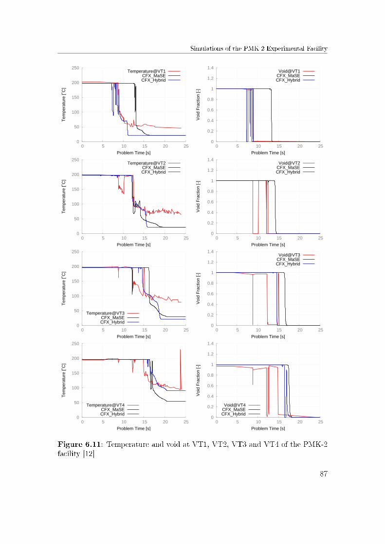
Simulations of the PMK-2 Experimental Facility
0
50
100
150
200
250
0 5 10 15 20 25
Tem
pera
ture
[˚C
]
Problem Time [s]
Temperature@VT1CFX_MaSECFX_Hybrid
0
0.2
0.4
0.6
0.8
1
1.2
1.4
0 5 10 15 20 25
Voi
d F
ract
ion
[-]
Problem Time [s]
Void@VT1CFX_MaSECFX_Hybrid
0
50
100
150
200
250
0 5 10 15 20 25
Tem
pera
ture
[˚C
]
Problem Time [s]
Temperature@VT2CFX_MaSECFX_Hybrid
0
0.2
0.4
0.6
0.8
1
1.2
1.4
0 5 10 15 20 25
Voi
d F
ract
ion
[-]
Problem Time [s]
Void@VT2CFX_MaSECFX_Hybrid
0
50
100
150
200
250
0 5 10 15 20 25
Tem
pera
ture
[˚C
]
Problem Time [s]
Temperature@VT3CFX_MaSECFX_Hybrid
0
0.2
0.4
0.6
0.8
1
1.2
1.4
0 5 10 15 20 25
Voi
d F
ract
ion
[-]
Problem Time [s]
Void@VT3CFX_MaSECFX_Hybrid
0
50
100
150
200
250
0 5 10 15 20 25
Tem
pera
ture
[˚C
]
Problem Time [s]
Temperature@VT4CFX_MaSECFX_Hybrid
0
0.2
0.4
0.6
0.8
1
1.2
1.4
0 5 10 15 20 25
Voi
d F
ract
ion
[-]
Problem Time [s]
Void@VT4CFX_MaSECFX_Hybrid
Figure 6.11: Temperature and void at VT1, VT2, VT3 and VT4 of the PMK-2facility [12]
87
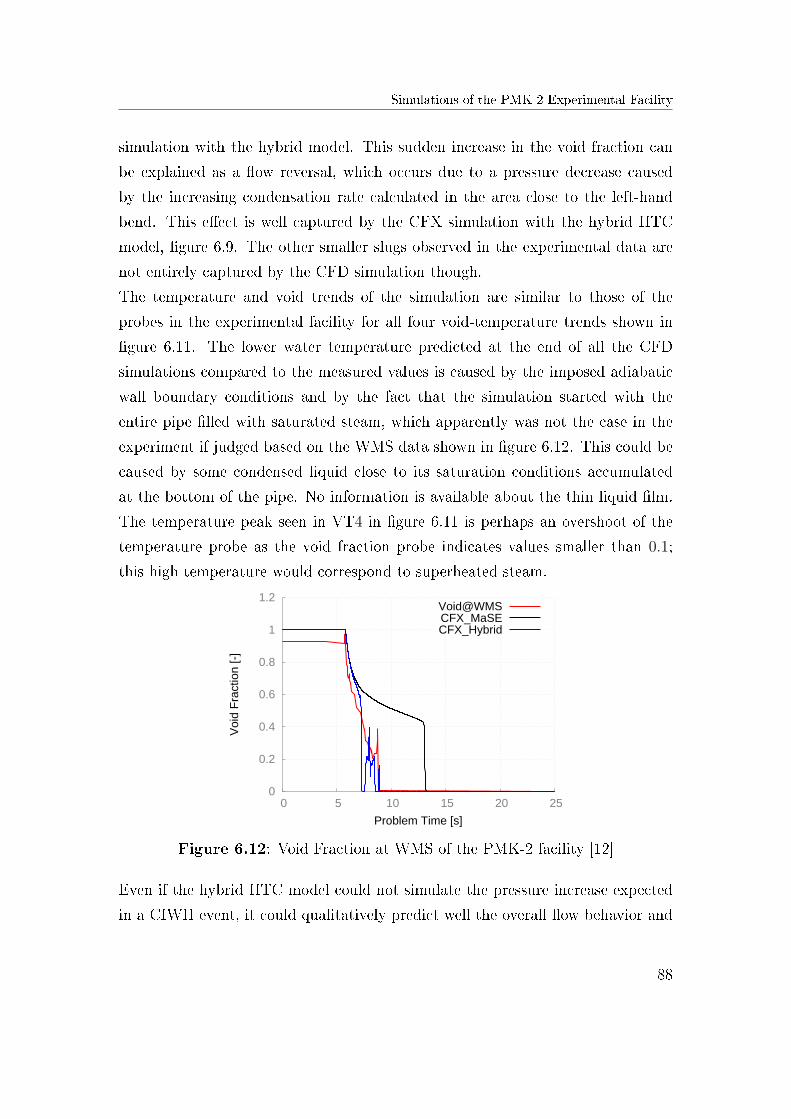
Simulations of the PMK-2 Experimental Facility
simulation with the hybrid model. This sudden increase in the void fraction can
be explained as a �ow reversal, which occurs due to a pressure decrease caused
by the increasing condensation rate calculated in the area close to the left-hand
bend. This e�ect is well captured by the CFX simulation with the hybrid HTC
model, �gure 6.9. The other smaller slugs observed in the experimental data are
not entirely captured by the CFD simulation though.
The temperature and void trends of the simulation are similar to those of the
probes in the experimental facility for all four void-temperature trends shown in
�gure 6.11. The lower water temperature predicted at the end of all the CFD
simulations compared to the measured values is caused by the imposed adiabatic
wall boundary conditions and by the fact that the simulation started with the
entire pipe �lled with saturated steam, which apparently was not the case in the
experiment if judged based on the WMS data shown in �gure 6.12. This could be
caused by some condensed liquid close to its saturation conditions accumulated
at the bottom of the pipe. No information is available about the thin liquid �lm.
The temperature peak seen in VT4 in �gure 6.11 is perhaps an overshoot of the
temperature probe as the void fraction probe indicates values smaller than 0.1;
this high temperature would correspond to superheated steam.
0
0.2
0.4
0.6
0.8
1
1.2
0 5 10 15 20 25
Voi
d F
ract
ion
[-]
Problem Time [s]
Void@WMSCFX_MaSECFX_Hybrid
Figure 6.12: Void Fraction at WMS of the PMK-2 facility [12]
Even if the hybrid HTC model could not simulate the pressure increase expected
in a CIWH event, it could qualitatively predict well the overall �ow behavior and
88
Simulations of the PMK-2 Experimental Facility
even local measured quantities such as void fractions and temperatures, proving
that the �ow behavior was correctly captured by within the simulation. The
simulation with the HTC based only on the in�uence of micro eddies (Hughes
and Du�ey's model) could predict the formation of a CIWH, still the magnitude
of the pressure increase was well below the experimental results. Considering
the relatively high local values of the calculated HTC we can conclude that this
model can realistically simulate phenomena such as the pressure surges triggered
by DCC only if additional e�ort is spent on the modeling of the IAD, as this
quantity appears to be under-predicted by the VOF approach for complex two-
phase �ows. The value of the condensation rate proportional to the product of
the HTC and the IAD strongly depends on the values calculated for these two
variables. Even with a large HTC, if the IAD is not accurately computed, the
resulting condensation rate will be less than the actual value. Correlations for
the HTC such as the one developed in this thesis, can compensate to a certain
extent for low IAD values but as the �ow becomes more complex and the interface
is highly turbulent, they cannot compensate for the large discrepancy between
the calculated and the real IAD. For this reason, and based on the analysis of the
physical processes that create the CIWH, it has been found that a better prediction
of the IAD is necessary to accelerate the vapor bubble collapse and to create the
subsequent pressure increase. Another problem observed is the stability of the
numerical solution in the CFD codes when large pressure variations take place
within very short time intervals, which the current numerical solution methods
used by both ANSY-CFX and OpenFOAM appear not to be able to handle in a
robust manner.
6.1.2 Simulations of the PMK-2 Experiments with the
System Code ATHLET
As system code simulations are still indispensable for the safety assessment of large,
complex systems especially over large problem times, continuous development and
improvement of such codes is fundamental to achieve better simulation results.
Following this work, the hybrid HTC model has been included in the system
89
Simulations of the PMK-2 Experimental Facility
code ATHLET, as reported in section 4.2. The objective of this section is to
assess the overall performance of the modi�ed system code together with the new
DCC module. The results of several ATHLET simulations will be compared in
detail with measurements of experiment 05 of the PMK-2 series. Because of the
relatively small computation time of the simulation of such an experiment, the
entire CIWH experiment-series performed at the PMK-2 facility has been run.
A global overview on the experimental matrix is also included in the summary
presented in the appendix A. As the system code in its original state was not
validated for CIWH events, the following plots will include its results but without
any special comments.
The sequence of events in experiment 05 has been introduced in the presentation
of the CFD simulations results. A comparison between the standard ATHLET
and the modi�ed version will be discussed. The key �ow regimes, which appear
just before the CIWH, are presented in �gure 6.13. Subcooled water enters the
test-section forming a strati�ed �ow pattern up to simulation time 7.51s. After
this point, the �ow changes in the modi�ed system code computer simulations to
wavy and locally a wave evolves to form a slug entrapping a steam bubble. This
causes a �ow reversal as the steam pocket condenses and accelerates the liquid
from right to left towards the location of the injection. After the entrapped steam
bubble has completely collapsed, water continues to �ow from left to right while
other slugs are formed until the test-section is full of water. This �ow development
was also recognized in the corresponding CFD simulations. In general the time
points at which key changes in the �ow appear in the simulation with the modi�ed
ATHLET do not coincide with those of the CFD simulations.
In order to assess the performance of the newly developed HTC model, the plots
showing the temperature, void fraction and pressure will be presented. As only 1-D
ATHLET components were available for simulation, only coarse volume-averaged
values are computed by the modi�ed system code. When these averaged results are
directly compared with local variables as those provided by the void-temperature
sensors, some problems arise. The results of the CFX simulations have been post-
processed and mapped onto a computational grid similar with that used for the
90
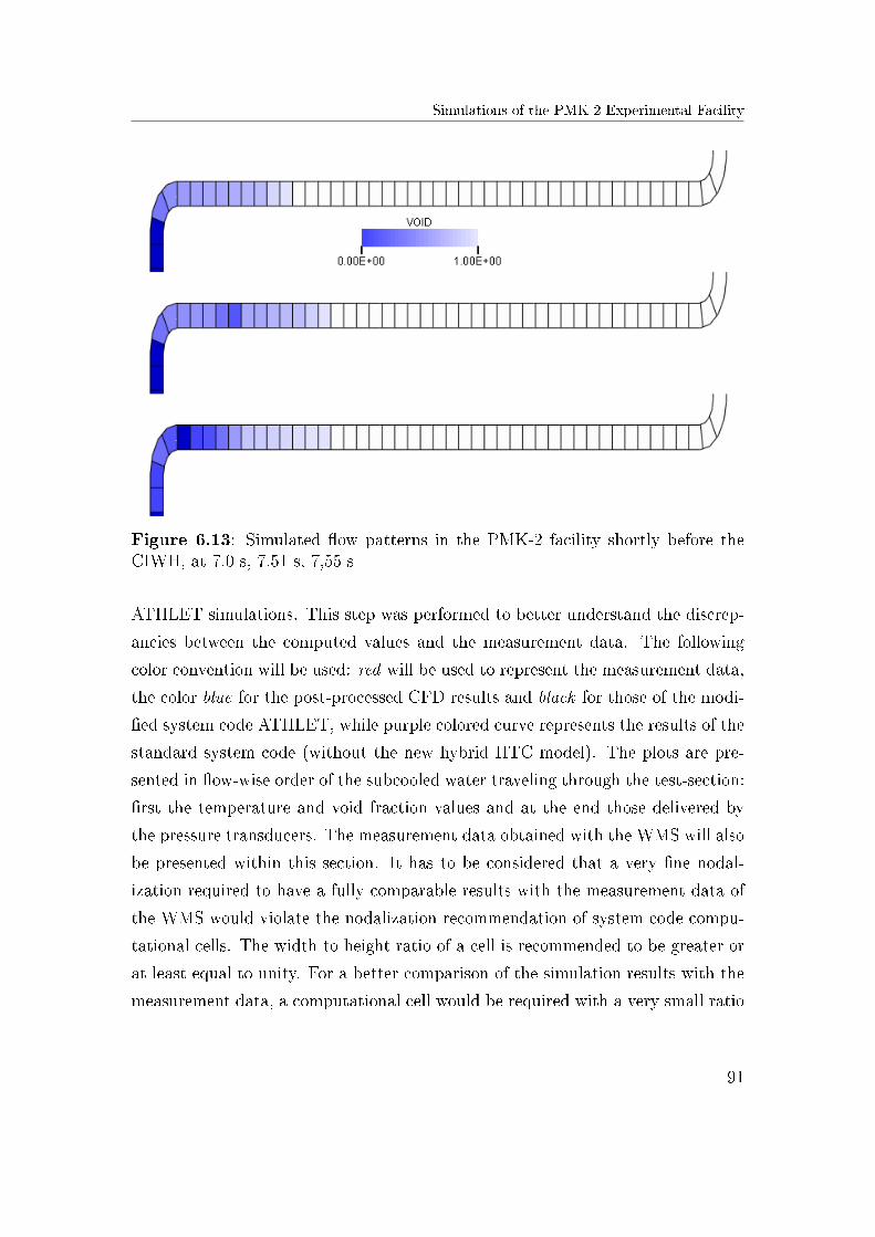
Simulations of the PMK-2 Experimental Facility
Figure 6.13: Simulated �ow patterns in the PMK-2 facility shortly before theCIWH, at 7.0 s, 7.51 s, 7,55 s
ATHLET simulations. This step was performed to better understand the discrep-
ancies between the computed values and the measurement data. The following
color convention will be used: red will be used to represent the measurement data,
the color blue for the post-processed CFD results and black for those of the modi-
�ed system code ATHLET, while purple colored curve represents the results of the
standard system code (without the new hybrid HTC model). The plots are pre-
sented in �ow-wise order of the subcooled water traveling through the test-section:
�rst the temperature and void fraction values and at the end those delivered by
the pressure transducers. The measurement data obtained with the WMS will also
be presented within this section. It has to be considered that a very �ne nodal-
ization required to have a fully comparable results with the measurement data of
the WMS would violate the nodalization recommendation of system code compu-
tational cells. The width to height ratio of a cell is recommended to be greater or
at least equal to unity. For a better comparison of the simulation results with the
measurement data, a computational cell would be required with a very small ratio
91
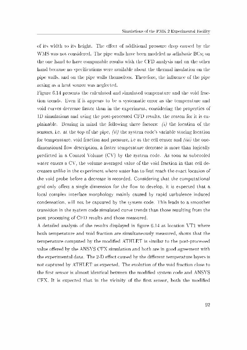
Simulations of the PMK-2 Experimental Facility
of its width to its height. The e�ect of additional pressure drop caused by the
WMS was not considered. The pipe walls have been modeled as adiabatic BCs; on
the one hand to have comparable results with the CFD analysis and on the other
hand because no speci�cations were available about the thermal insulation on the
pipe walls, and on the pipe walls themselves. Therefore, the in�uence of the pipe
acting as a heat source was neglected.
Figure 6.14 presents the calculated and simulated temperature and the void frac-
tion trends. Even if it appears to be a systematic error as the temperature and
void curves decrease faster than in the experiment, considering the properties of
1D simulations and using the post-processed CFD results, the reason for it is ex-
plainable. Bearing in mind the following three factors: (i) the location of the
sensors, i.e. at the top of the pipe, (ii) the system code's variable storing location
for temperature, void fraction and pressure, i.e at the cell center and (iii) the one-
dimensional �ow description, a faster temperature decrease is more than logically
predicted in a Control Volume (CV) by the system code. As soon as subcooled
water enters a CV, the volume averaged value of the void fraction in that cell de-
creases unlike in the experiment where water has to �rst reach the exact location of
the void probe before a decrease is recorded. Considering that the computational
grid only o�ers a single dimension for the �ow to develop, it is expected that a
local complex interface morphology mainly caused by rapid turbulence induced
condensation, will not be captured by the system code. This leads to a smoother
transition in the system code simulated curve trends than those resulting from the
post-processing of CFD results and those measured.
A detailed analysis of the results displayed in �gure 6.14 at location VT1 where
both temperature and void fraction are simultaneously measured, shows that the
temperature computed by the modi�ed ATHLET is similar to the post-processed
value o�ered by the ANSYS CFX simulation and both are in good agreement with
the experimental data. The 2-D e�ect caused by the di�erent temperature layers is
not captured by ATHLET as expected. The evolution of the void fraction close to
the �rst sensor is almost identical between the modi�ed system code and ANSYS
CFX. It is expected that in the vicinity of the �rst sensor, both the modi�ed
92
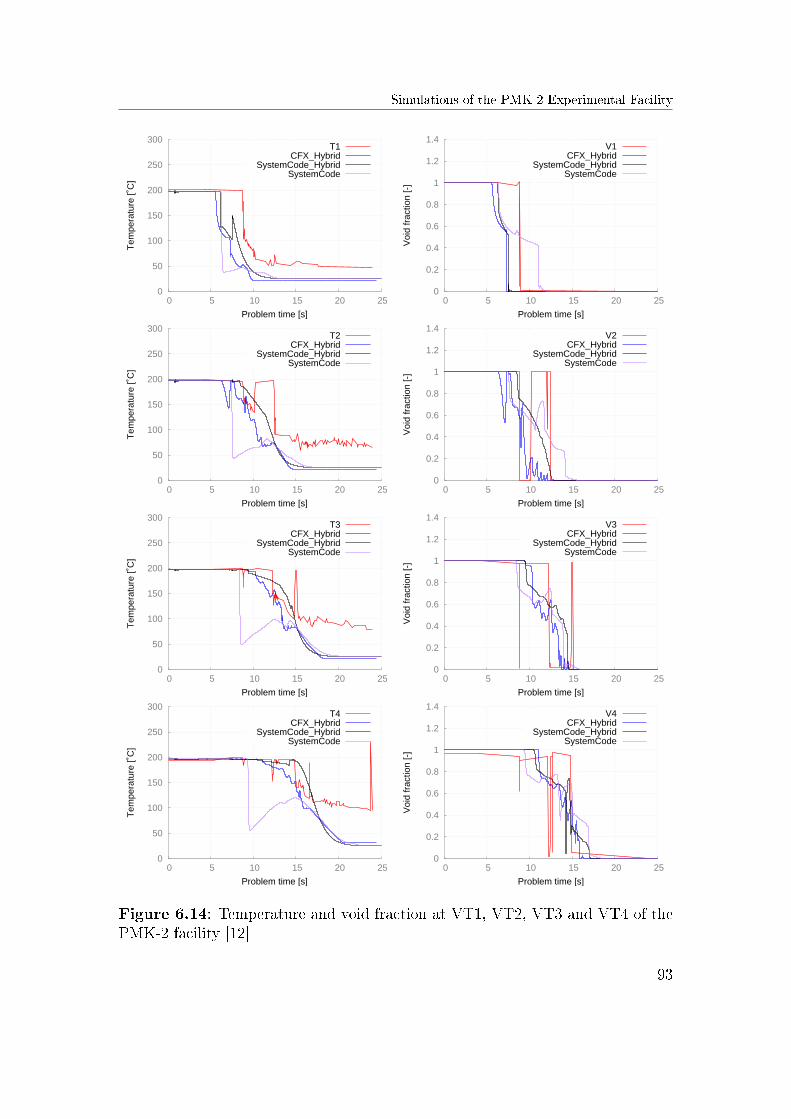
Simulations of the PMK-2 Experimental Facility
0
50
100
150
200
250
300
0 5 10 15 20 25
Tem
pera
ture
[˚C
]
Problem time [s]
T1CFX_Hybrid
SystemCode_HybridSystemCode
0
0.2
0.4
0.6
0.8
1
1.2
1.4
0 5 10 15 20 25
Voi
d fr
actio
n [-
]
Problem time [s]
V1CFX_Hybrid
SystemCode_HybridSystemCode
0
50
100
150
200
250
300
0 5 10 15 20 25
Tem
pera
ture
[˚C
]
Problem time [s]
T2CFX_Hybrid
SystemCode_HybridSystemCode
0
0.2
0.4
0.6
0.8
1
1.2
1.4
0 5 10 15 20 25
Voi
d fr
actio
n [-
]
Problem time [s]
V2CFX_Hybrid
SystemCode_HybridSystemCode
0
50
100
150
200
250
300
0 5 10 15 20 25
Tem
pera
ture
[˚C
]
Problem time [s]
T3CFX_Hybrid
SystemCode_HybridSystemCode
0
0.2
0.4
0.6
0.8
1
1.2
1.4
0 5 10 15 20 25
Voi
d fr
actio
n [-
]
Problem time [s]
V3CFX_Hybrid
SystemCode_HybridSystemCode
0
50
100
150
200
250
300
0 5 10 15 20 25
Tem
pera
ture
[˚C
]
Problem time [s]
T4CFX_Hybrid
SystemCode_HybridSystemCode
0
0.2
0.4
0.6
0.8
1
1.2
1.4
0 5 10 15 20 25
Voi
d fr
actio
n [-
]
Problem time [s]
V4CFX_Hybrid
SystemCode_HybridSystemCode
Figure 6.14: Temperature and void fraction at VT1, VT2, VT3 and VT4 of thePMK-2 facility [12]
93
Simulations of the PMK-2 Experimental Facility
system code and CFX predictions display a similar behavior. Thus, in the pipe
segments before the left elbow a strati�ed vertical �ow appears, whereas in the
horizontal test-section, as the IAD increases with the in�ow of subcooled water, a
multidimensional �ow pattern develops.
With the data provided by the sensor VT2, some di�erences are noticed between
the results of the computer codes used. The modi�ed system code predicts very
well the onset of the slug �ow, which is recorded by the sensor at around 9 s and by
ANSYS CFX at around 6 s. A rather smooth transition from steam to subcooled
water is predicted close to VT2 and VT3. The two-phase �ow dynamics close
to VT4 is again well predicted if compared with the post-processed CFD results.
Slugs traveling through the pipe can be observed following the interpretation of the
void fraction computed at this location. In general both codes capture a similar
dynamic behavior of the two-phase �ow in the test-section. In both cases a slug
travels through the pipe, which is accelerated toward the left bend as a result of
the high steam condensation rate. According to the experimental data, the slug
travels past VT4 at approximately 13 s problem time whereas in both simulations
this slug is predicted to reach that sensor between the time-points 14 s and 15 s.
The relatively lower temperatures observed towards the end of the computer sim-
ulations are caused by the simpli�cations of assuming adiabatic pipe walls and by
the location of the temperature sensors mounted at the top of the pipe, while the
results are presented as volume averaged values over the entire pipe cross section.
During the analyzed experiment 05, a CIWH phenomenon was recorded by the
pressure transducers. The highest recorded pressure peak was at around 150 bar,
corresponding to a tenfold increase in nominal pressure considering the initial
14.5 bar. Comparing the predicted void fraction at the location of the WMS, it
can be noticed that even if the overall �ow patterns are simulated correctly, the
time predictions do not overlap between the modi�ed system code results and the
measurement data. In the experiment a slug is recorded to travel past the WMS
at approximately 9 s, while the modi�ed system code predicts this slug earlier.
This over-anticipation of the time-point of the slugging onset, a�ects the evolution
of the pressure in the test-section. The pressure predicted at the locations of the
94
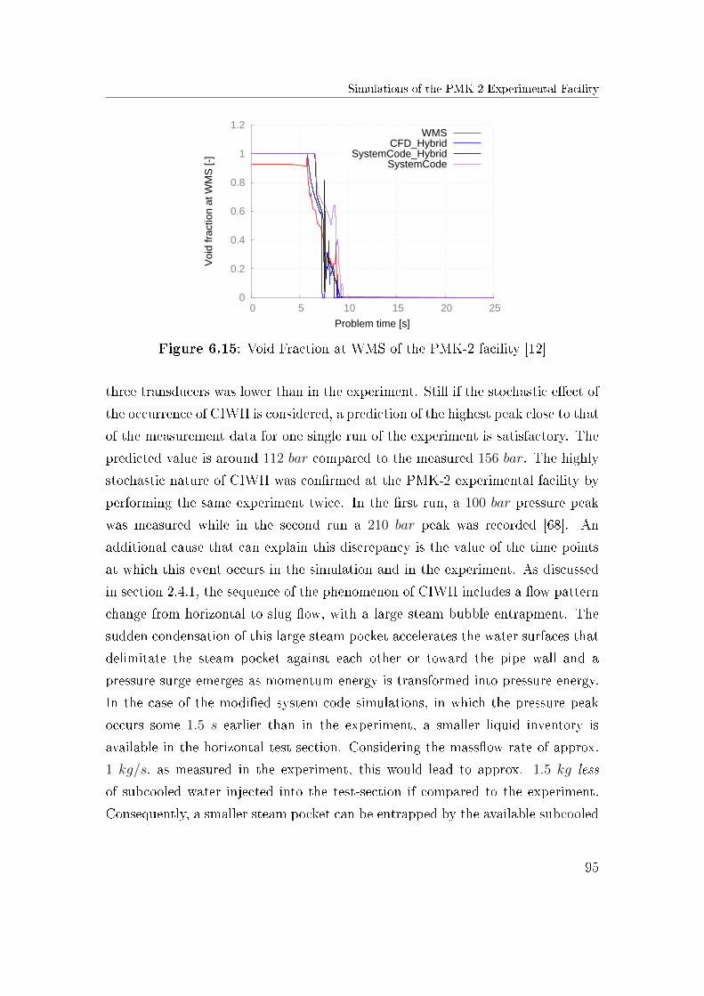
Simulations of the PMK-2 Experimental Facility
0
0.2
0.4
0.6
0.8
1
1.2
0 5 10 15 20 25
Voi
d fr
actio
n at
WM
S [-
]
Problem time [s]
WMSCFD_Hybrid
SystemCode_HybridSystemCode
Figure 6.15: Void Fraction at WMS of the PMK-2 facility [12]
three transducers was lower than in the experiment. Still if the stochastic e�ect of
the occurrence of CIWH is considered, a prediction of the highest peak close to that
of the measurement data for one single run of the experiment is satisfactory. The
predicted value is around 112 bar compared to the measured 156 bar. The highly
stochastic nature of CIWH was con�rmed at the PMK-2 experimental facility by
performing the same experiment twice. In the �rst run, a 100 bar pressure peak
was measured while in the second run a 210 bar peak was recorded [68]. An
additional cause that can explain this discrepancy is the value of the time points
at which this event occurs in the simulation and in the experiment. As discussed
in section 2.4.1, the sequence of the phenomenon of CIWH includes a �ow pattern
change from horizontal to slug �ow, with a large steam bubble entrapment. The
sudden condensation of this large steam pocket accelerates the water surfaces that
delimitate the steam pocket against each other or toward the pipe wall and a
pressure surge emerges as momentum energy is transformed into pressure energy.
In the case of the modi�ed system code simulations, in which the pressure peak
occurs some 1.5 s earlier than in the experiment, a smaller liquid inventory is
available in the horizontal test-section. Considering the mass�ow rate of approx.
1 kg/s, as measured in the experiment, this would lead to approx. 1.5 kg less
of subcooled water injected into the test-section if compared to the experiment.
Consequently, a smaller steam pocket can be entrapped by the available subcooled
95
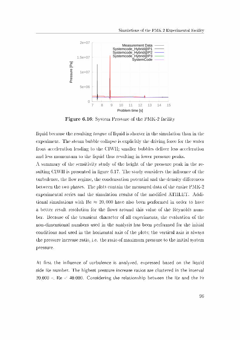
Simulations of the PMK-2 Experimental Facility
0
5e+06
1e+07
1.5e+07
2e+07
7 8 9 10 11 12 13 14 15
Pre
ssur
e [P
a]
Problem time [s]
Measurement DataSystemcode_Hybrid@P1Systemcode_Hybrid@P2Systemcode_Hybrid@P3
SystemCode
Figure 6.16: System Pressure of the PMK-2 facility
liquid because the resulting tongue of liquid is shorter in the simulation than in the
experiment. The steam bubble collapse is explicitly the driving force for the water
front acceleration leading to the CIWH; smaller bubbles deliver less acceleration
and less momentum to the liquid thus resulting in lower pressure peaks.
A summary of the sensitivity study of the height of the pressure peak in the re-
sulting CIWH is presented in �gure 6.17. The study considers the in�uence of the
turbulence, the �ow regime, the condensation potential and the density di�erences
between the two phases. The plots contain the measured data of the entire PMK-2
experimental series and the simulation results of the modi�ed ATHLET. Addi-
tional simulations with Re ≈ 20, 000 have also been performed in order to have
a better result resolution for the �ows around this value of the Reynolds num-
ber. Because of the transient character of all experiments, the evaluation of the
non-dimensional numbers used in the analysis has been performed for the initial
conditions and used in the horizontal axis of the plots; the vertical axis is always
the pressure increase ratio, i.e. the ratio of maximum pressure to the initial system
pressure.
At �rst the in�uence of turbulence is analyzed, expressed based on the liquid
side Re number. The highest pressure increase ratios are clustered in the interval
20,000 < Re < 40,000. Considering the relationship between the Re and the Fr
96
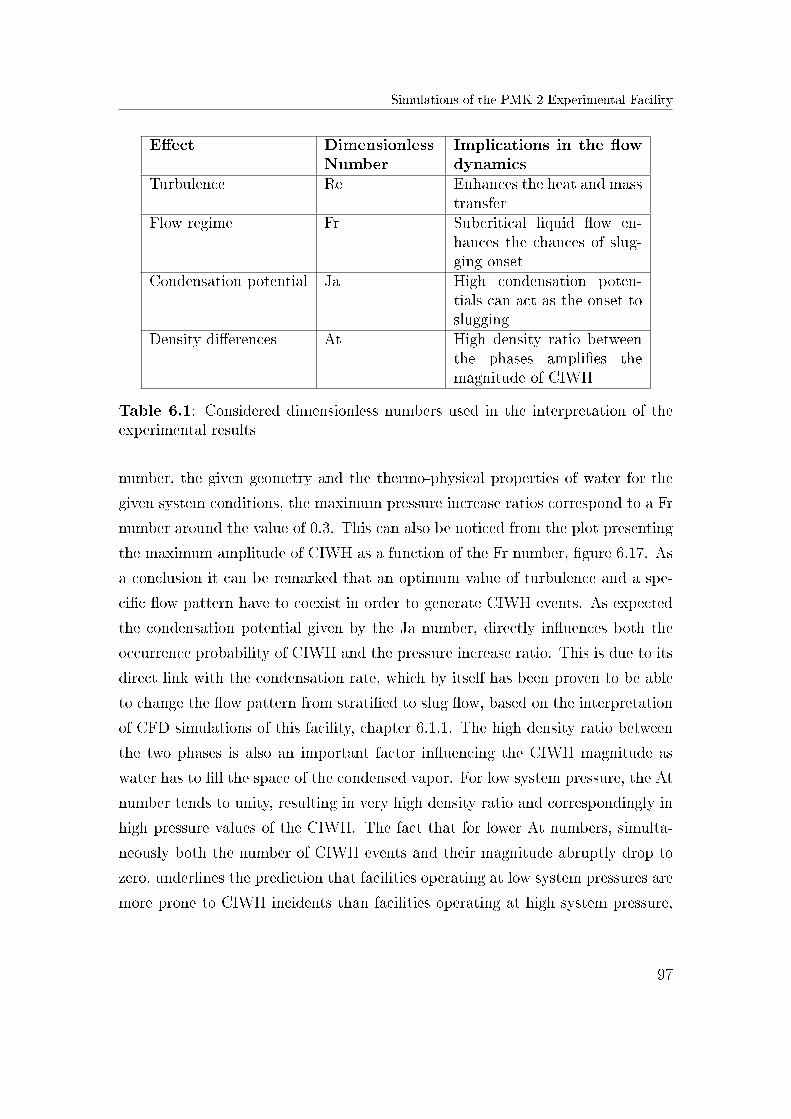
Simulations of the PMK-2 Experimental Facility
E�ect DimensionlessNumber
Implications in the �owdynamics
Turbulence Re Enhances the heat and masstransfer
Flow regime Fr Subcritical liquid �ow en-hances the chances of slug-ging onset
Condensation potential Ja High condensation poten-tials can act as the onset toslugging
Density di�erences At High density ratio betweenthe phases ampli�es themagnitude of CIWH
Table 6.1: Considered dimensionless numbers used in the interpretation of theexperimental results
number, the given geometry and the thermo-physical properties of water for the
given system conditions, the maximum pressure increase ratios correspond to a Fr
number around the value of 0.3. This can also be noticed from the plot presenting
the maximum amplitude of CIWH as a function of the Fr number, �gure 6.17. As
a conclusion it can be remarked that an optimum value of turbulence and a spe-
ci�c �ow pattern have to coexist in order to generate CIWH events. As expected
the condensation potential given by the Ja number, directly in�uences both the
occurrence probability of CIWH and the pressure increase ratio. This is due to its
direct link with the condensation rate, which by itself has been proven to be able
to change the �ow pattern from strati�ed to slug �ow, based on the interpretation
of CFD simulations of this facility, chapter 6.1.1. The high density ratio between
the two phases is also an important factor in�uencing the CIWH magnitude as
water has to �ll the space of the condensed vapor. For low system pressure, the At
number tends to unity, resulting in very high density ratio and correspondingly in
high pressure values of the CIWH. The fact that for lower At numbers, simulta-
neously both the number of CIWH events and their magnitude abruptly drop to
zero, underlines the prediction that facilities operating at low system pressures are
more prone to CIWH incidents than facilities operating at high system pressure,
97
Simulations of the PMK-2 Experimental Facility
where the densities of the phases tend to the similar order of magnitude. This is a
logical consequence of the fact that at low system pressure, the higher di�erences
between the densities leads to higher acceleration of the liquid side in the case
of DCC. It has to be considered that even a high increase rate of a low initial
pressure might not be as dangerous for a plant equipment as a smaller increase
rate of a high initial pressure. Nevertheless, a low initial system pressure increases
the probability of CIWH events.
The intensity plots depicted in �gure 6.18 represents the combined e�ects of the
turbulence and the condensation potential as the driving forces for CIWH events.
It can be highlighted that the plots, showing both experimental data and the sim-
ulations' results with the modi�ed ATHLET exhibit a maximum pressure increase
ratio around Re ≈ 20, 000, with a clear in�uence from the Ja number. For smaller
values of Re, almost no CIWH events are measured or simulated. Around Re
≈ 90, 000, both in the simulations and the measurement data, no CIWH were
recorded. The region in the interval 90,000 < Re < 120,000, is again prone to
CIWH. A consistent behavior is observed between the simulation results and the
experimental data based on the concomitant in�uence of the turbulence and the
�ow character on both the occurrence of CIWH and the pressure surge magnitude,
�gure 6.19.
This sensitivity study shows that the simulations are in�uenced in the same manner
by the key parameters responsible for the magnitude of CIWH and their occurrence
as the experiments. As a result it can be concluded that the newly implemented
hybrid, mechanistic, HTC model clearly improves the overall prediction capabil-
ities of CIWH events, with the system code ATHLET without the need of any
parameter tuning.
To remove the limitations of a typical 1D simulation in ATHLET, a more detailed
modeling network has been set up in such a way that the development of 2D �ow
patterns can be simulated using only 1D components. The standard ATHLET in
its Version 2.2 Cycle A o�ers the possibility to use cross connection objects, which
98
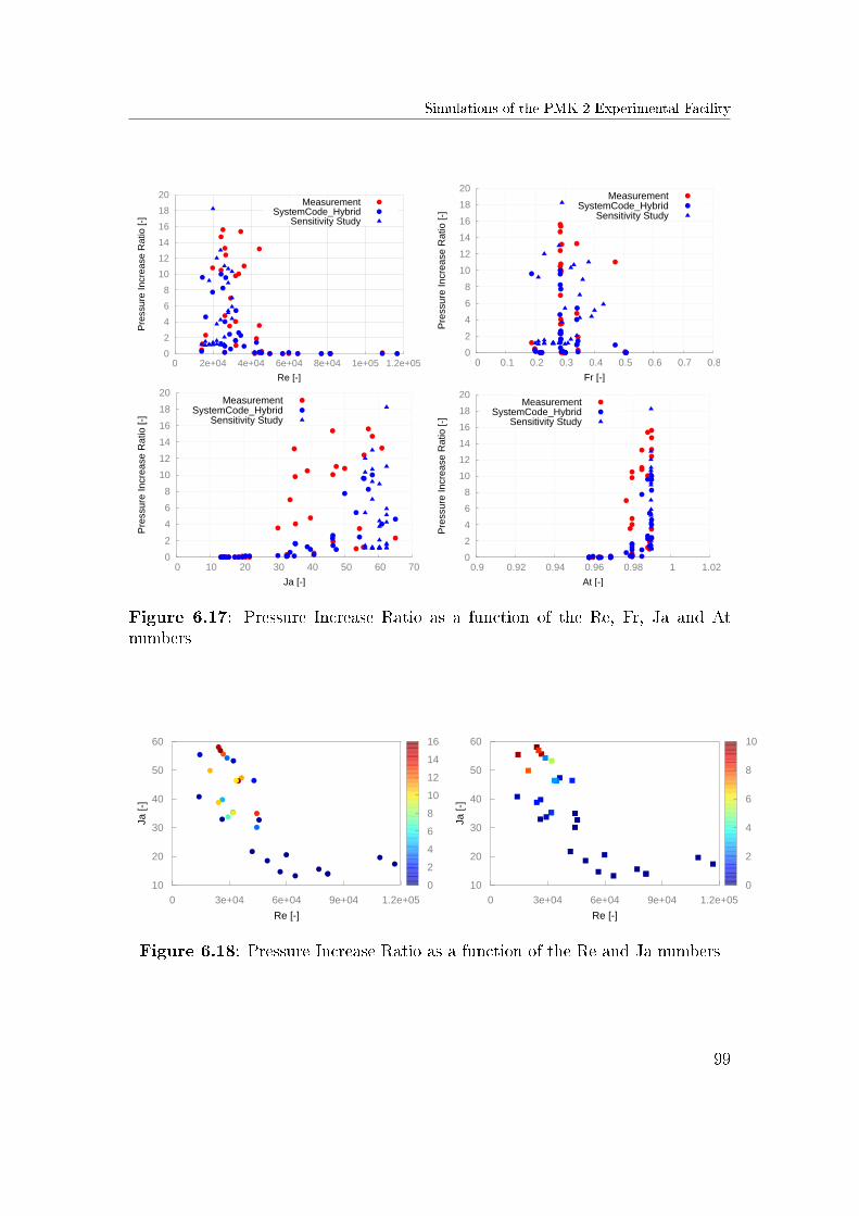
Simulations of the PMK-2 Experimental Facility
0
2
4
6
8
10
12
14
16
18
20
0 2e+04 4e+04 6e+04 8e+04 1e+05 1.2e+05
Pre
ssur
e In
crea
se R
atio
[-]
Re [-]
MeasurementSystemCode_Hybrid
Sensitivity Study
0
2
4
6
8
10
12
14
16
18
20
0 0.1 0.2 0.3 0.4 0.5 0.6 0.7 0.8
Pre
ssur
e In
crea
se R
atio
[-]
Fr [-]
MeasurementSystemCode_Hybrid
Sensitivity Study
0
2
4
6
8
10
12
14
16
18
20
0 10 20 30 40 50 60 70
Pre
ssur
e In
crea
se R
atio
[-]
Ja [-]
MeasurementSystemCode_Hybrid
Sensitivity Study
0
2
4
6
8
10
12
14
16
18
20
0.9 0.92 0.94 0.96 0.98 1 1.02
Pre
ssur
e In
crea
se R
atio
[-]
At [-]
MeasurementSystemCode_Hybrid
Sensitivity Study
Figure 6.17: Pressure Increase Ratio as a function of the Re, Fr, Ja and Atnumbers
0 3e+04 6e+04 9e+04 1.2e+05
Re [-]
10
20
30
40
50
60
Ja [
-]
0
2
4
6
8
10
12
14
16
0 3e+04 6e+04 9e+04 1.2e+05
Re [-]
10
20
30
40
50
60
Ja [
-]
0
2
4
6
8
10
Figure 6.18: Pressure Increase Ratio as a function of the Re and Ja numbers
99
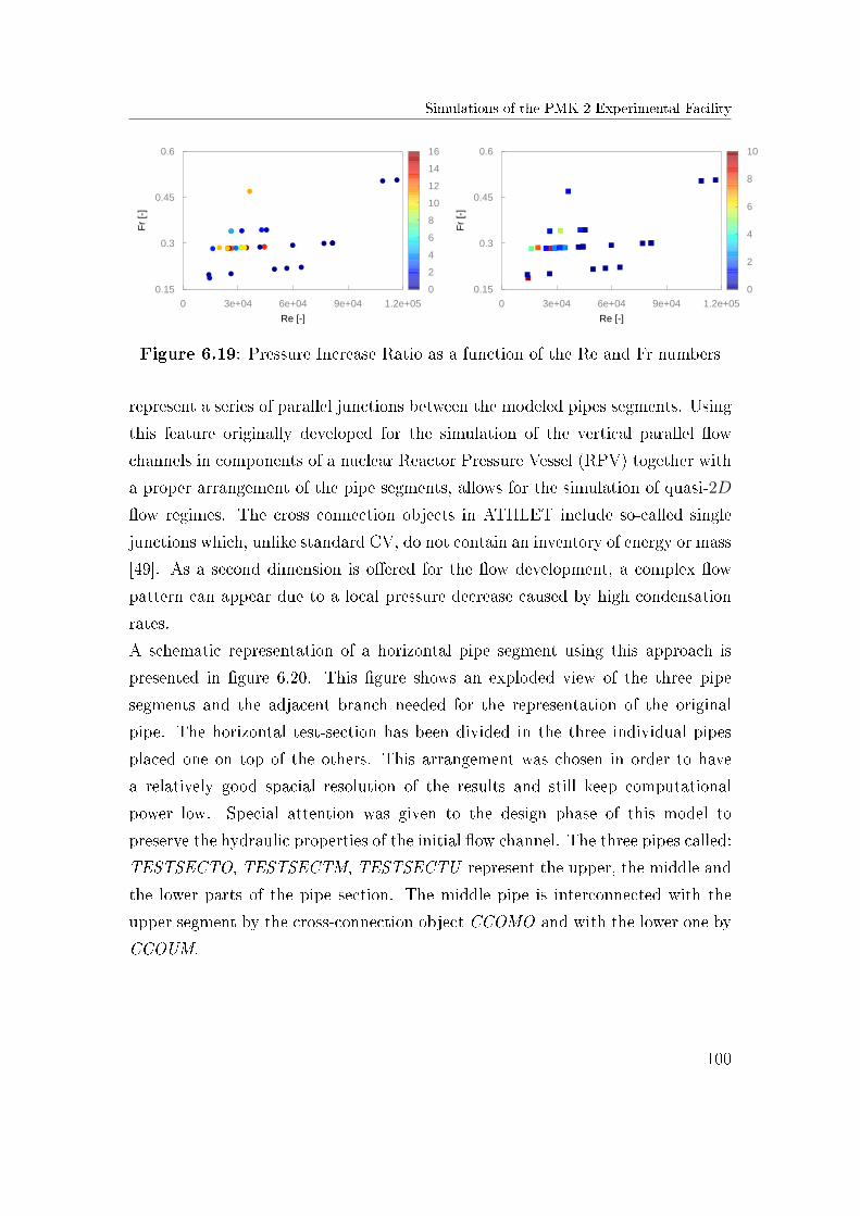
Simulations of the PMK-2 Experimental Facility
0 3e+04 6e+04 9e+04 1.2e+05
Re [-]
0.15
0.3
0.45
0.6
Fr
[-]
0
2
4
6
8
10
12
14
16
0 3e+04 6e+04 9e+04 1.2e+05
Re [-]
0.15
0.3
0.45
0.6
Fr
[-]
0
2
4
6
8
10
Figure 6.19: Pressure Increase Ratio as a function of the Re and Fr numbers
represent a series of parallel junctions between the modeled pipes segments. Using
this feature originally developed for the simulation of the vertical parallel �ow
channels in components of a nuclear Reactor Pressure Vessel (RPV) together with
a proper arrangement of the pipe segments, allows for the simulation of quasi-2D
�ow regimes. The cross connection objects in ATHLET include so-called single
junctions which, unlike standard CV, do not contain an inventory of energy or mass
[49]. As a second dimension is o�ered for the �ow development, a complex �ow
pattern can appear due to a local pressure decrease caused by high condensation
rates.
A schematic representation of a horizontal pipe segment using this approach is
presented in �gure 6.20. This �gure shows an exploded view of the three pipe
segments and the adjacent branch needed for the representation of the original
pipe. The horizontal test-section has been divided in the three individual pipes
placed one on top of the others. This arrangement was chosen in order to have
a relatively good spacial resolution of the results and still keep computational
power low. Special attention was given to the design phase of this model to
preserve the hydraulic properties of the initial �ow channel. The three pipes called:
TESTSECTO, TESTSECTM, TESTSECTU represent the upper, the middle and
the lower parts of the pipe section. The middle pipe is interconnected with the
upper segment by the cross-connection object CCOMO and with the lower one by
CCOUM.
100
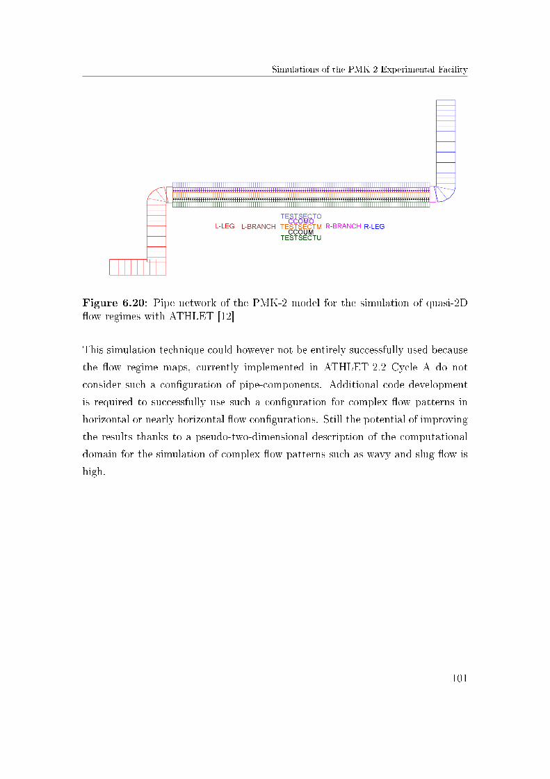
Simulations of the PMK-2 Experimental Facility
Figure 6.20: Pipe network of the PMK-2 model for the simulation of quasi-2D�ow regimes with ATHLET [12]
This simulation technique could however not be entirely successfully used because
the �ow regime maps, currently implemented in ATHLET-2.2 Cycle A do not
consider such a con�guration of pipe-components. Additional code development
is required to successfully use such a con�guration for complex �ow patterns in
horizontal or nearly horizontal �ow con�gurations. Still the potential of improving
the results thanks to a pseudo-two-dimensional description of the computational
domain for the simulation of complex �ow patterns such as wavy and slug �ow is
high.
101
CFD Simulations of the TUHH Experimental Facility
6.2 CFD Simulations of the TUHH Experimental
Facility
For the validation of the newly developed HTC model, three characteristic experi-
ments performed at the facility constructed and operated at TUHH have been cho-
sen. The volumetric �ow rate of the injected subcooled water was implemented as
a BC into the CFD simulations carried out with the OpenFOAM code. No ANSYS
CFX simulations have been performed because of license limitations, limitations
which do not apply to OpenFOAM.
Three of the TUHH experimental series were selected for the assessment of the hy-
brid HTC model implemented into a VOF based CFD code. Experiment Fr03T40
corresponds to a maximum Froude number of approximately 0.3 and a water sub-
cooling of 40 K; experiment Fr06T40 corresponds to a maximum Fr number of
approximately 0.6 and a subcooling of 40 K; and experiment Fr06T60 corresponds
to a maximum Froude number of approximately 0.6 and a water subcooling of
60 K. These particular experiments were selected for the assessment of the new
HTC model because di�erent �ow characteristics emerge based on the imposed
BCs. In the �rst experiment the �ow is controlled by a small volumetric �ow rate
of the subcooled water. In the second experiment the corresponding Fr number
is doubled compared to the �rst experiment, while the water subcooling is kept
constant. This second experiment should underline the e�ect of the �ow rate on
the two-phase �ow dynamics. The last experiment should highlight the in�uence
of high water subcooling and high turbulence induced by the high water �ow rate.
The three di�erent curves corresponding to the pump starting process for each of
the experiments considered are presented in �gure 6.21 and used as BC for the
simulations.
The selected experiments were conducted with the facility having a slope of 1.4◦
with respect to the horizontal axis. This means that the right separator was
situated slightly higher than the left one, thus favoring the �ow of subcooled water
from the injection location towards the left separator.
102
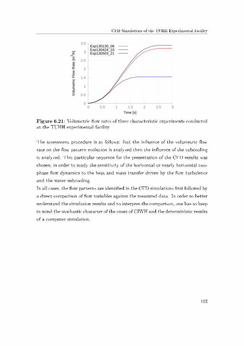
CFD Simulations of the TUHH Experimental Facility
0
0.5
1
1.5
2
2.5
3
3.5
0 0.5 1 1.5 2 2.5 3
Vol
umet
ric F
low
Rat
e [m
3 /h]
Time [s]
Exp130130_06Exp130424_10Exp130503_21
Figure 6.21: Volumetric �ow rates of three characteristic experiments conductedat the TUHH experimental facility
The assessment procedure is as follows: �rst the in�uence of the volumetric �ow
rate on the �ow pattern evolution is analyzed then the in�uence of the subcooling
is analyzed. This particular sequence for the presentation of the CFD results was
chosen, in order to study the sensitivity of the horizontal or nearly horizontal two-
phase �ow dynamics to the heat and mass transfer driven by the �ow turbulence
and the water subcooling.
In all cases, the �ow patterns are identi�ed in the CFD simulations �rst followed by
a direct comparison of �ow variables against the measured data. In order to better
understand the simulation results and to interpret the comparison, one has to keep
in mind the stochastic character of the onset of CIWH and the deterministic results
of a computer simulation.
103
CFD Simulations of the TUHH Experimental Facility
6.2.1 CFD Simulation of the TUHH Experiment Fr03T40
The presentation of the TUHH simulation results begins with the experiment
Fr03T40, in which the lowest volumetric rate of subcooled water was injected
into the test-section. During this experiment a maximum volumetric �ow rate
corresponding to a maximum Fr number of approximately 0.3 was reached. The
liquid has the lowest subcooling of all experiments, namely 40 K.
Because of the low �ow rate injected, a low turbulence intensity in the �ow is ex-
pected which, together with the low subcooling of the liquid, leads to relatively low
condensation rates. From the evaluation of the developed �ow patterns shown in
�gures 6.22 to 6.25, the scenario of this simulation can be summarized as follows:
the injected subcooled liquid rises vertically in the T-junction and hits the upper
part of the test-section pipe by the time the maximum �ow rate corresponding to
Fr=0.3 is reached. The water then �ows around the pipe wall towards its bottom
predominantly to the left end of the injection point. The test-section has a 1.4◦
slope and the mass �ow rate is not enough for the liquid to �ow towards the sep-
arator located to the right of the injection.
A liquid layer forms at the bottom of the pipe as water in continuously injected
into the test-section. This can be seen in the void fraction values at the pipe's
cross-sections where the thermo-couples are mounted as displayed in �gure 6.23.
At approximately 4.10 s, a wave builds up almost halfway between the thermo-
couples T4 and T3 due to locally increasing condensation rates caused by an
increasing local HTC. Figure 6.31 and the associated local decrease in the local
pressure shown in �gure 6.27 re�ect this behavior. The water wave continues to
grow driven by direct contact condensation and a steam pocket starts being iso-
lated as can be seen in �gure 6.24 showing the void fraction close to the location
of T4. The complex interface morphology of a breaking water wave can also be
observed in �gure 6.24. It is obvious how the crest of the wave rolls back into the
liquid bulk, by regarding the evolution of void fraction �eld. This can be observed
by focusing on the region close to the pipe's central axis, where a light blue col-
ored region is noticed above the dark blue region of the bulk of subcooled water.
104
CFD Simulations of the TUHH Experimental Facility
The region above the bulk, the transition from blue to red colors, is the 'smeared'
interfacial area between the entrapped steam bubbles and the subcooled water. In
the steam region the void fraction does not correspond to pure steam but to steam
with small entrapped droplets of water. A signi�cant water drop is even expelled
from the wave and projected against the top of the pipe, the light blue region close
to the pipe wall in the same picture.
A later decrease in the local HTC coe�cients reduces the counter-�ow water wave
acceleration as shown in �gure 6.33 and also noticed from the observation of the
relative pressure �eld in �gure 6.29. After the water wave gradually disappears,
strati�ed �ow formation is observed from the T-junction towards the left-side sep-
arator with a continuous generation and decay of small water waves due to an
increased local direct contact condensation phenomenon. Still the �ow never fully
transforms into slug �ow in the more than 10 s of experiment simulated.
The analysis of the results above reinforces the conclusion reached in the simu-
lations of the PMK-2 experiment in section 6.1.1, where it was noticed that the
high condensation rates can act independently as the driving force for �ow pattern
changes.
The IAD shows higher values especially in the regions where water splashes against
the pipe wall close to the T-junction injection, or where a very thin liquid layer
exists. This is the case of the water front �owing towards the left side of the
test-section. The combined in�uence of the increased IAD and HTC trigger the
�ow pattern change. The comparison of the eight measured temperature trends
against the simulated ones reveals a good overall prediction of the temperature
distribution by the CFD simulation as shown in �gure 6.38. The subcooled water
�ows past the four instrumented locations from T4 to T1. The constant pressure
boundary condition and the idealized concept of open boundaries at the left and
right extremes of the computational domain o�er an 'unlimited' steam inventory to
be sucked by the reduction in pressure caused by the condensation. In the experi-
ment the steam inventory is certainly limited. As continuous steam condensation
105
CFD Simulations of the TUHH Experimental Facility
causes a pressure decrease, a continuous decrease of the saturation temperature is
observed. Therefore, this e�ect could not be considered in the CFD simulations
and the saturation temperature is kept constant and linked to the constant bound-
ary pressure.
Comparing the trends of the curves Tf4 and Tg4, it can be concluded that the
�ow pattern produced by the computer simulations represents the experimentally
observed two-phase �ow dynamics satisfactorily. The time points at which the
temperatures decrease marking the passing of subcooled water coincide well in the
simulation and the experiment. The �ow pattern close to T3 however, di�ers be-
tween the simulation and the experiment. The time at which the �rst temperature
decrease occurs is predicted well by the simulation at this location but afterward
because of the high condensation rates, the direction of the advancing liquid �lm
is reversed towards the injection point. An increase of the temperature is then
predicted, as saturated steam replaces subcooled water. The discrepancy between
simulation results and measured data close to the left boundary of the computa-
tional domain is partially in�uenced by the open boundary condition employed.
Nevertheless the simulations show a similar behavior to that inferred from the an-
alyzed experimental data. The converging curves for Tf and Tg near the end of the
simulation suggest that the test section is �lled with water at this time. However
the analysis of the measured temperature evolution leads to the conclusion that
the test section was never completely �lled with subcooled water.
106
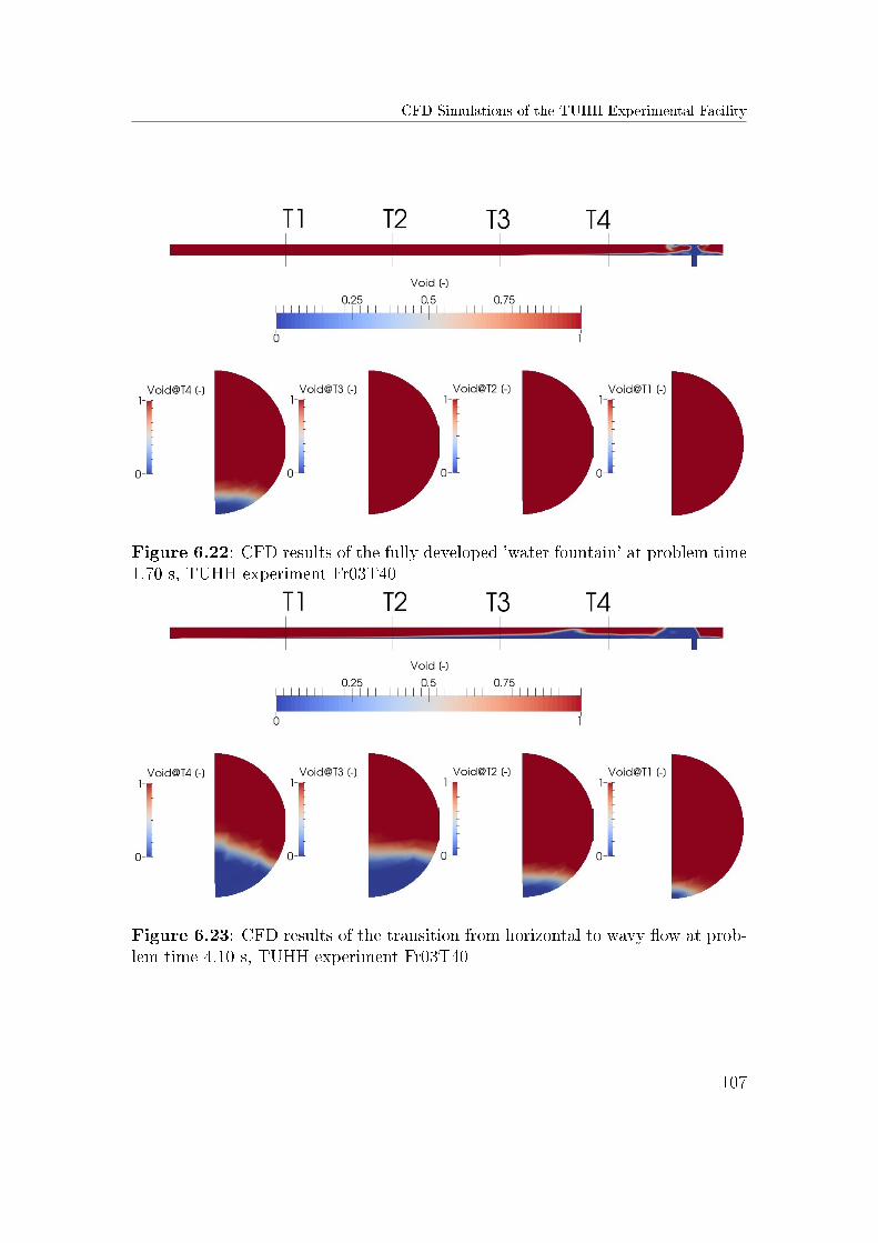
CFD Simulations of the TUHH Experimental Facility
Figure 6.22: CFD results of the fully developed 'water fountain' at problem time1.70 s, TUHH experiment Fr03T40
Figure 6.23: CFD results of the transition from horizontal to wavy �ow at prob-lem time 4.10 s, TUHH experiment Fr03T40
107
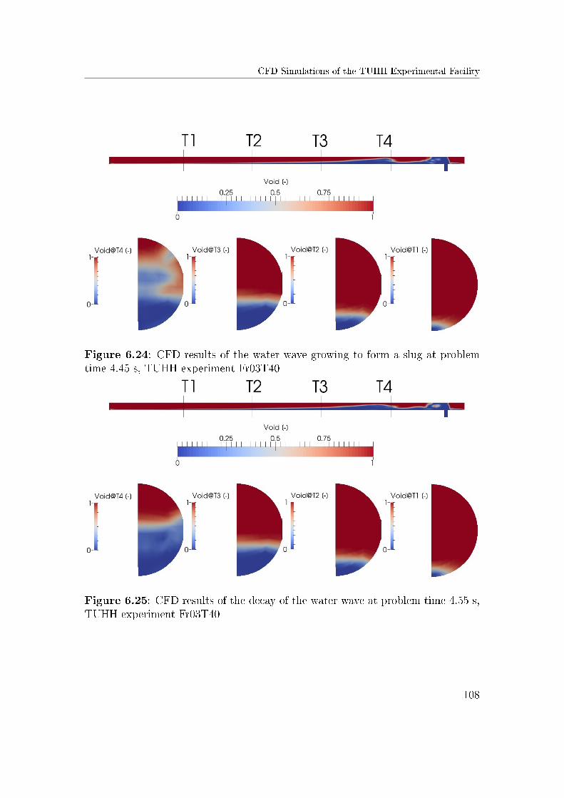
CFD Simulations of the TUHH Experimental Facility
Figure 6.24: CFD results of the water wave growing to form a slug at problemtime 4.45 s, TUHH experiment Fr03T40
Figure 6.25: CFD results of the decay of the water wave at problem time 4.55 s,TUHH experiment Fr03T40
108
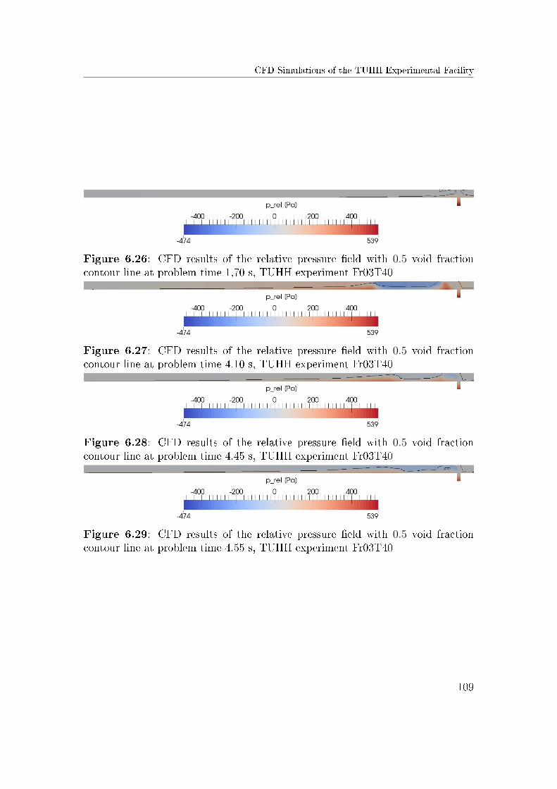
CFD Simulations of the TUHH Experimental Facility
Figure 6.26: CFD results of the relative pressure �eld with 0.5 void fractioncontour line at problem time 1,70 s, TUHH experiment Fr03T40
Figure 6.27: CFD results of the relative pressure �eld with 0.5 void fractioncontour line at problem time 4.10 s, TUHH experiment Fr03T40
Figure 6.28: CFD results of the relative pressure �eld with 0.5 void fractioncontour line at problem time 4.45 s, TUHH experiment Fr03T40
Figure 6.29: CFD results of the relative pressure �eld with 0.5 void fractioncontour line at problem time 4.55 s, TUHH experiment Fr03T40
109
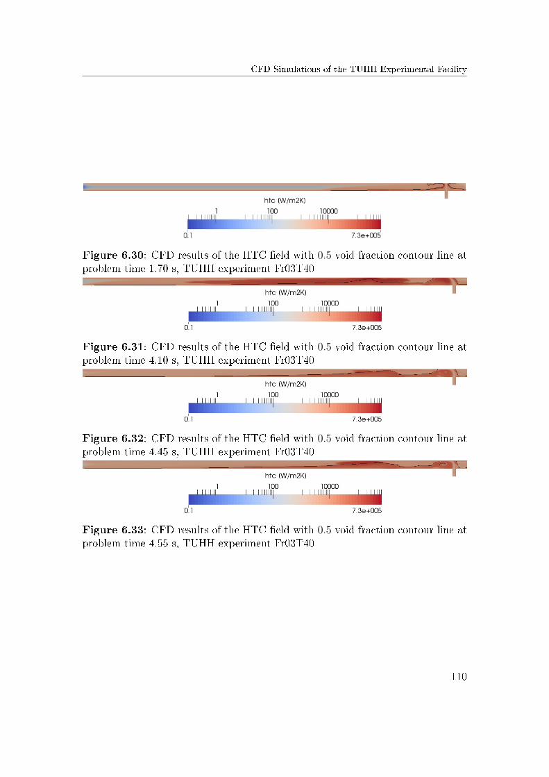
CFD Simulations of the TUHH Experimental Facility
Figure 6.30: CFD results of the HTC �eld with 0.5 void fraction contour line atproblem time 1.70 s, TUHH experiment Fr03T40
Figure 6.31: CFD results of the HTC �eld with 0.5 void fraction contour line atproblem time 4.10 s, TUHH experiment Fr03T40
Figure 6.32: CFD results of the HTC �eld with 0.5 void fraction contour line atproblem time 4.45 s, TUHH experiment Fr03T40
Figure 6.33: CFD results of the HTC �eld with 0.5 void fraction contour line atproblem time 4.55 s, TUHH experiment Fr03T40
110
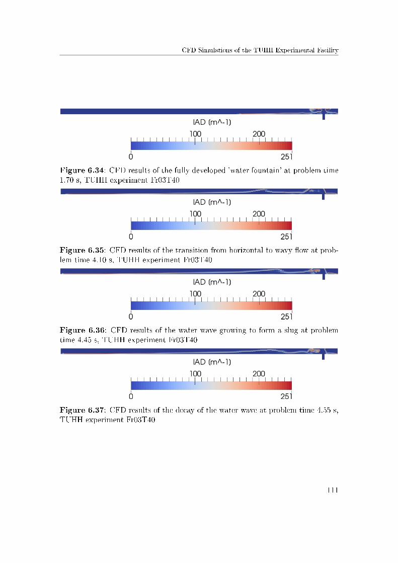
CFD Simulations of the TUHH Experimental Facility
Figure 6.34: CFD results of the fully developed 'water fountain' at problem time1.70 s, TUHH experiment Fr03T40
Figure 6.35: CFD results of the transition from horizontal to wavy �ow at prob-lem time 4.10 s, TUHH experiment Fr03T40
Figure 6.36: CFD results of the water wave growing to form a slug at problemtime 4.45 s, TUHH experiment Fr03T40
Figure 6.37: CFD results of the decay of the water wave at problem time 4.55 s,TUHH experiment Fr03T40
111
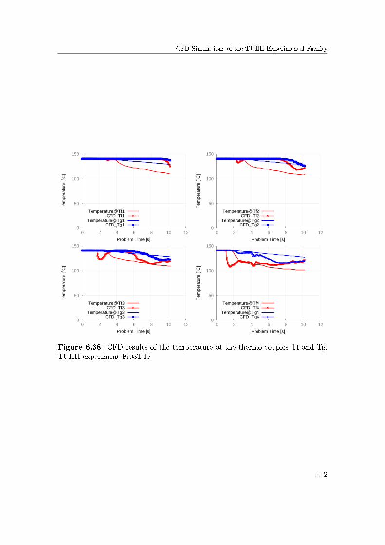
CFD Simulations of the TUHH Experimental Facility
0
50
100
150
0 2 4 6 8 10 12
Tem
pera
ture
[˚C
]
Problem Time [s]
Temperature@Tf1CFD_Tf1
Temperature@Tg1CFD_Tg1
0
50
100
150
0 2 4 6 8 10 12
Tem
pera
ture
[˚C
]
Problem Time [s]
Temperature@Tf2CFD_Tf2
Temperature@Tg2CFD_Tg2
0
50
100
150
0 2 4 6 8 10 12
Tem
pera
ture
[˚C
]
Problem Time [s]
Temperature@Tf3CFD_Tf3
Temperature@Tg3CFD_Tg3
0
50
100
150
0 2 4 6 8 10 12
Tem
pera
ture
[˚C
]
Problem Time [s]
Temperature@Tf4CFD_Tf4
Temperature@Tg4CFD_Tg4
Figure 6.38: CFD results of the temperature at the thermo-couples Tf and Tg,TUHH experiment Fr03T40
112
CFD Simulations of the TUHH Experimental Facility
6.2.2 CFD Simulation of the TUHH Experiment Fr06T40
During this experiment a maximum Fr number of 0.6 was reached while keeping
the water subcooling at the low value of 40 K. The increase in the maximum �ow
rate delivered by the pump with the same subcooling as in the previously analyzed
experiment Fr03T40, should only highlight the in�uence of a larger turbulence on
the direct contact condensation phenomenon and on the two-phase �ow dynamics.
The simulation results allow for an explanation of the sequence of events during
this experiment as follows: As the pump delivers twice the volumetric �ow rate as
in the experiment Fr03T40, a longer time period is needed for the pump to reach
its maximum �ow rate. At the beginning of the injection, subcooled water reaches
the top of the pipe and �ows along the pipe walls downwards to form a liquid �lm
at the bottom of the pipe similar to the Fr03T40 experiment; see �gure 6.39. As
the subcooled water �ows downwards, it entraps a steam pocket which condensates
in contact with the cold liquid surface; see �gure 6.40. During this experiment,
the volumetric �ow rate of the subcooled water is continuously increasing until the
time reaches 3.0 s. Figure 6.41 shows the �ow at 3.05 s, when the maximum �ow
rate has already been reached and a water wave is growing to become a slug; see
�gure 6.42.
The transition from strati�ed to slug �ow is mainly driven by the high turbulence
of the �ow and only minimally in�uenced by the relatively low subcooling. This
e�ect can be noticed if the distribution of the HTC is analyzed at 3.55 s. The
maximum HTC values for the entire simulation domain are located in the cells very
close to the free surface, as �gure 6.55 shows. The condensation of the entrapped
steam pocket causes a local depressurization as seen in �gure 6.49 and accelerates
the water to �ll the void. In �gure 6.57 at 4.05 s, a detailed representation of the
wave breaking process can be identi�ed in the cross section at location T4. The
region in the center of the test pipe shows how the wave rolls back into the liq-
uid bulk, while the transition region between steam and liquid shows a two-phase
mixture of entrapped steam bubbles in liquid and water droplets in steam. As
no interface reconstruction or special modeling of the disperse phase is made, no
sudden increase in the value of the interfacial area density is to observe for the cells
113
CFD Simulations of the TUHH Experimental Facility
corresponding to the high HTC values shown in �gure 6.64 due to the increased
turbulence.
The comparison of the simulation results against the measured values for the data
recorded by the thermo-couples is presented in �gure 6.67. The overall �ow be-
havior in the simulation corresponds well with that observed in the experiment.
However, the in�uence of the boundary conditions to the left- and the right-hand
side of the computational domain (modeled as openings), in�uence the temperature
development before the liquid water reaches the location of the thermo-couples.
In the experiment a decrease in temperature is recorded due to the decrease in
pressure caused by the DCC of steam on the surface of the injected subcooled
water. This e�ect was neglected in the simulation because a constant pressure BC
was used for the left and right-hand side separator. The time points at which the
temperature signi�cantly decreases when the subcooled water comes into contact
with the temperature probes are predicted very well for the locations T3, T2 and
T1. In the case of T4, the predicted time point does not match the experiment
compared with the other locations but still the �ow behavior in the simulation is
similar to the one in the experiment. At the location of T4, in both the simulation
and the experiment, some temperature oscillations are observed between problem
time 2.0 s and 8.0 s. Considering the �ow pattern presented in �gures 6.41 to
6.45 and the temperature oscillations, it can be concluded that the temperature
distribution is not yet fully homogenized in the liquid resulting in strati�ed �uid
layers at di�erent temperatures. Such temperature oscillations can be observed in
both simulation results and measured data at the location of the other thermo-
couples. The time accuracy of the numerical predictions is even better at locations
T1 to T3. The fact that this e�ect is caught by the CFD simulation is of poten-
tial interest if the implications of the formation of a Pressurized Thermal Shock
are analyzed. It proves that with a similar set-up as the one used in this thesis
consisting of the VOF approach with a SRT based HTC model, the phenomenon
of Pressurized Thermal Shock could also be accurately analyzed.
114
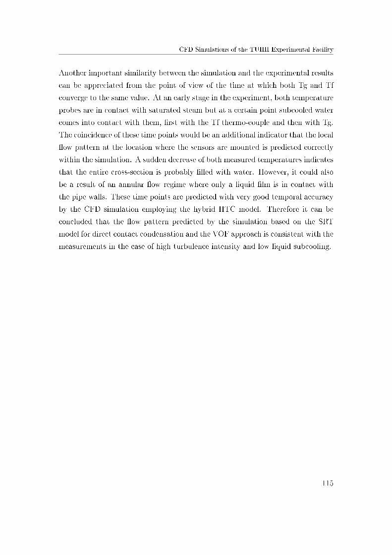
CFD Simulations of the TUHH Experimental Facility
Another important similarity between the simulation and the experimental results
can be appreciated from the point of view of the time at which both Tg and Tf
converge to the same value. At an early stage in the experiment, both temperature
probes are in contact with saturated steam but at a certain point subcooled water
comes into contact with them, �rst with the Tf thermo-couple and then with Tg.
The coincidence of these time points would be an additional indicator that the local
�ow pattern at the location where the sensors are mounted is predicted correctly
within the simulation. A sudden decrease of both measured temperatures indicates
that the entire cross-section is probably �lled with water. However, it could also
be a result of an annular �ow regime where only a liquid �lm is in contact with
the pipe walls. These time points are predicted with very good temporal accuracy
by the CFD simulation employing the hybrid HTC model. Therefore it can be
concluded that the �ow pattern predicted by the simulation based on the SRT
model for direct contact condensation and the VOF approach is consistent with the
measurements in the case of high turbulence intensity and low liquid subcooling.
115
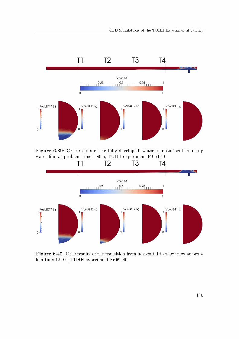
CFD Simulations of the TUHH Experimental Facility
Figure 6.39: CFD results of the fully developed 'water fountain' with built upwater �lm at problem time 1.80 s, TUHH experiment Fr06T40
Figure 6.40: CFD results of the transition from horizontal to wavy �ow at prob-lem time 1.90 s, TUHH experiment Fr06T40
116
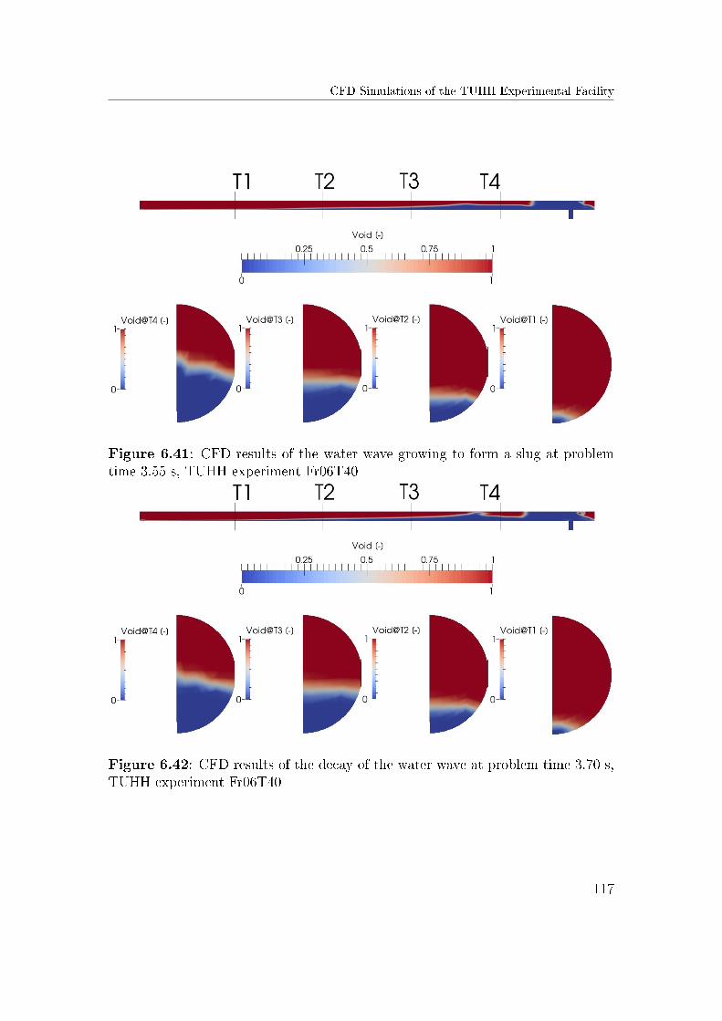
CFD Simulations of the TUHH Experimental Facility
Figure 6.41: CFD results of the water wave growing to form a slug at problemtime 3.55 s, TUHH experiment Fr06T40
Figure 6.42: CFD results of the decay of the water wave at problem time 3.70 s,TUHH experiment Fr06T40
117
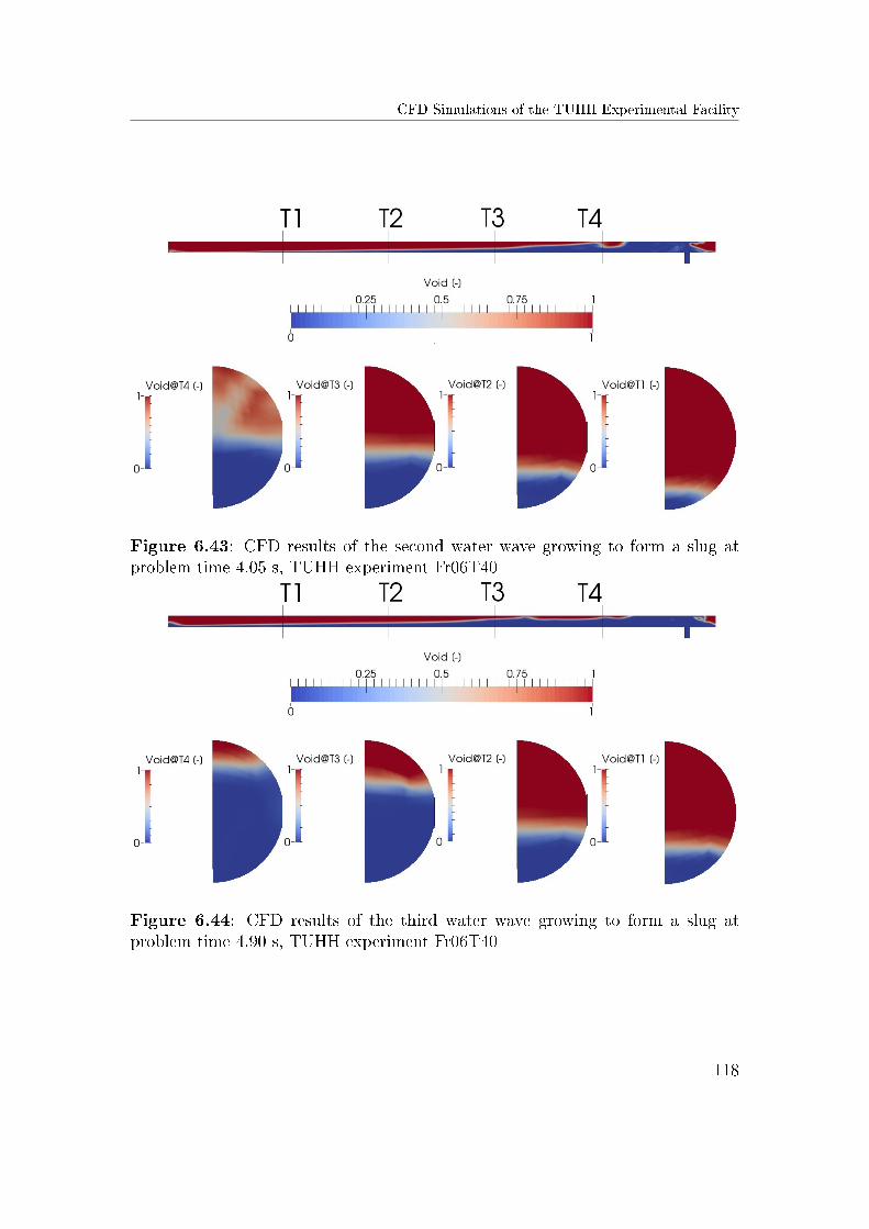
CFD Simulations of the TUHH Experimental Facility
Figure 6.43: CFD results of the second water wave growing to form a slug atproblem time 4.05 s, TUHH experiment Fr06T40
Figure 6.44: CFD results of the third water wave growing to form a slug atproblem time 4.90 s, TUHH experiment Fr06T40
118
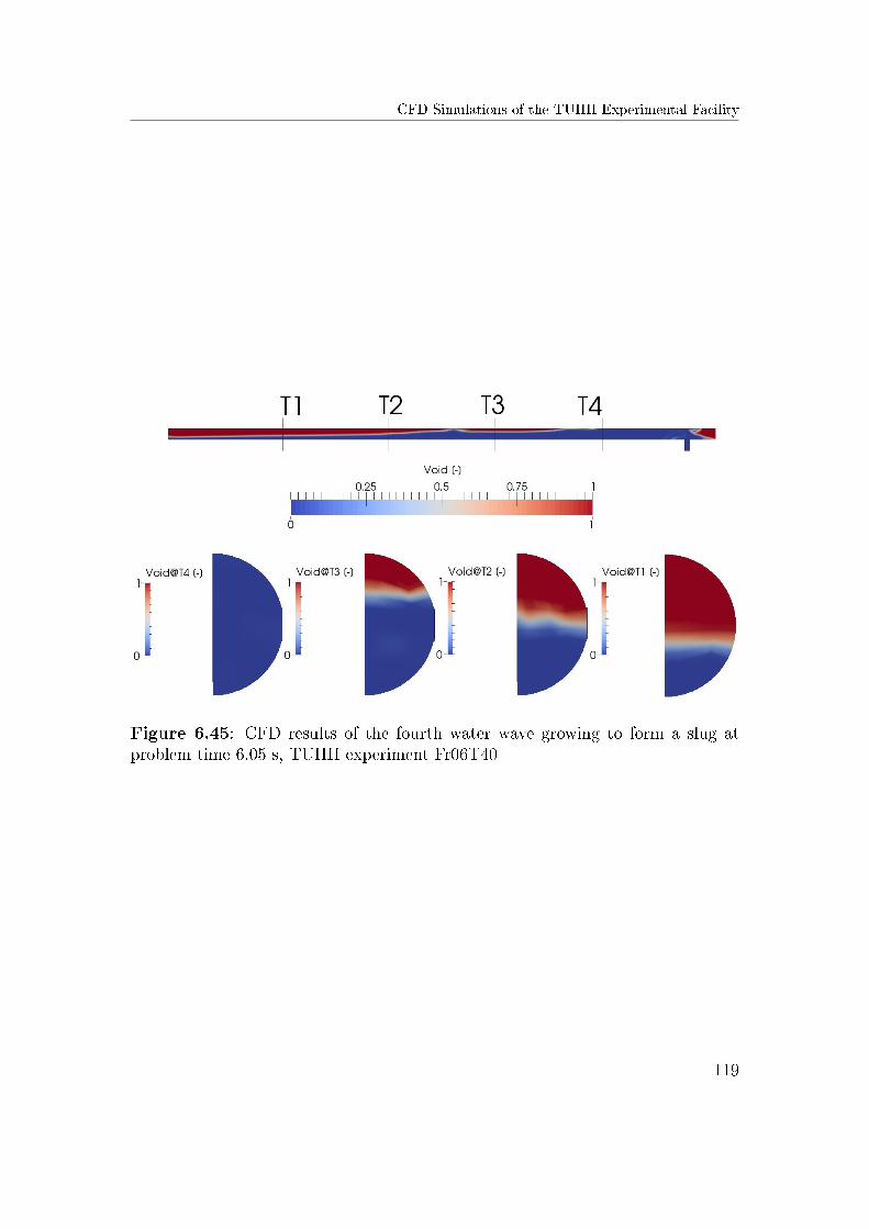
CFD Simulations of the TUHH Experimental Facility
Figure 6.45: CFD results of the fourth water wave growing to form a slug atproblem time 6.05 s, TUHH experiment Fr06T40
119
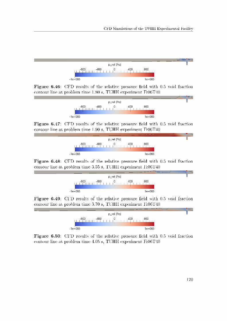
CFD Simulations of the TUHH Experimental Facility
Figure 6.46: CFD results of the relative pressure �eld with 0.5 void fractioncontour line at problem time 1.80 s, TUHH experiment Fr06T40
Figure 6.47: CFD results of the relative pressure �eld with 0.5 void fractioncontour line at problem time 1.90 s, TUHH experiment Fr06T40
Figure 6.48: CFD results of the relative pressure �eld with 0.5 void fractioncontour line at problem time 3.55 s, TUHH experiment Fr06T40
Figure 6.49: CFD results of the relative pressure �eld with 0.5 void fractioncontour line at problem time 3.70 s, TUHH experiment Fr06T40
Figure 6.50: CFD results of the relative pressure �eld with 0.5 void fractioncontour line at problem time 4.05 s, TUHH experiment Fr06T40
120
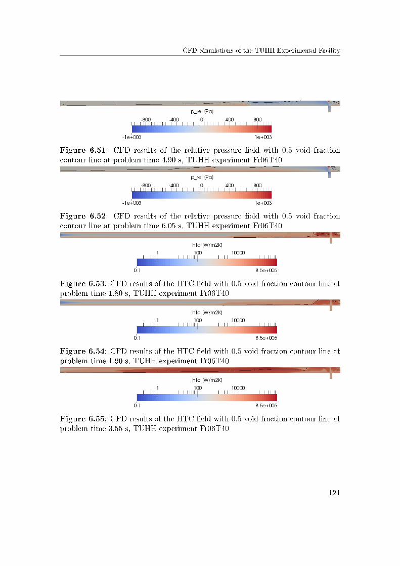
CFD Simulations of the TUHH Experimental Facility
Figure 6.51: CFD results of the relative pressure �eld with 0.5 void fractioncontour line at problem time 4.90 s, TUHH experiment Fr06T40
Figure 6.52: CFD results of the relative pressure �eld with 0.5 void fractioncontour line at problem time 6.05 s, TUHH experiment Fr06T40
Figure 6.53: CFD results of the HTC �eld with 0.5 void fraction contour line atproblem time 1.80 s, TUHH experiment Fr06T40
Figure 6.54: CFD results of the HTC �eld with 0.5 void fraction contour line atproblem time 1.90 s, TUHH experiment Fr06T40
Figure 6.55: CFD results of the HTC �eld with 0.5 void fraction contour line atproblem time 3.55 s, TUHH experiment Fr06T40
121
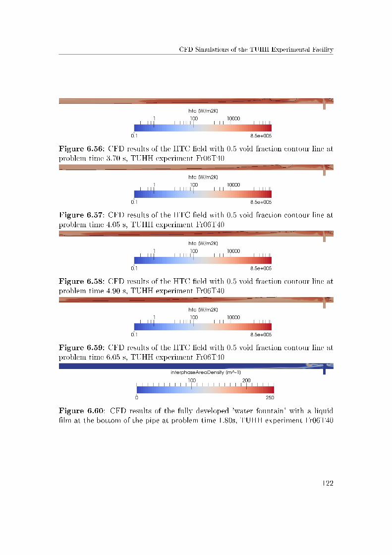
CFD Simulations of the TUHH Experimental Facility
Figure 6.56: CFD results of the HTC �eld with 0.5 void fraction contour line atproblem time 3.70 s, TUHH experiment Fr06T40
Figure 6.57: CFD results of the HTC �eld with 0.5 void fraction contour line atproblem time 4.05 s, TUHH experiment Fr06T40
Figure 6.58: CFD results of the HTC �eld with 0.5 void fraction contour line atproblem time 4.90 s, TUHH experiment Fr06T40
Figure 6.59: CFD results of the HTC �eld with 0.5 void fraction contour line atproblem time 6.05 s, TUHH experiment Fr06T40
Figure 6.60: CFD results of the fully developed 'water fountain' with a liquid�lm at the bottom of the pipe at problem time 1.80s, TUHH experiment Fr06T40
122
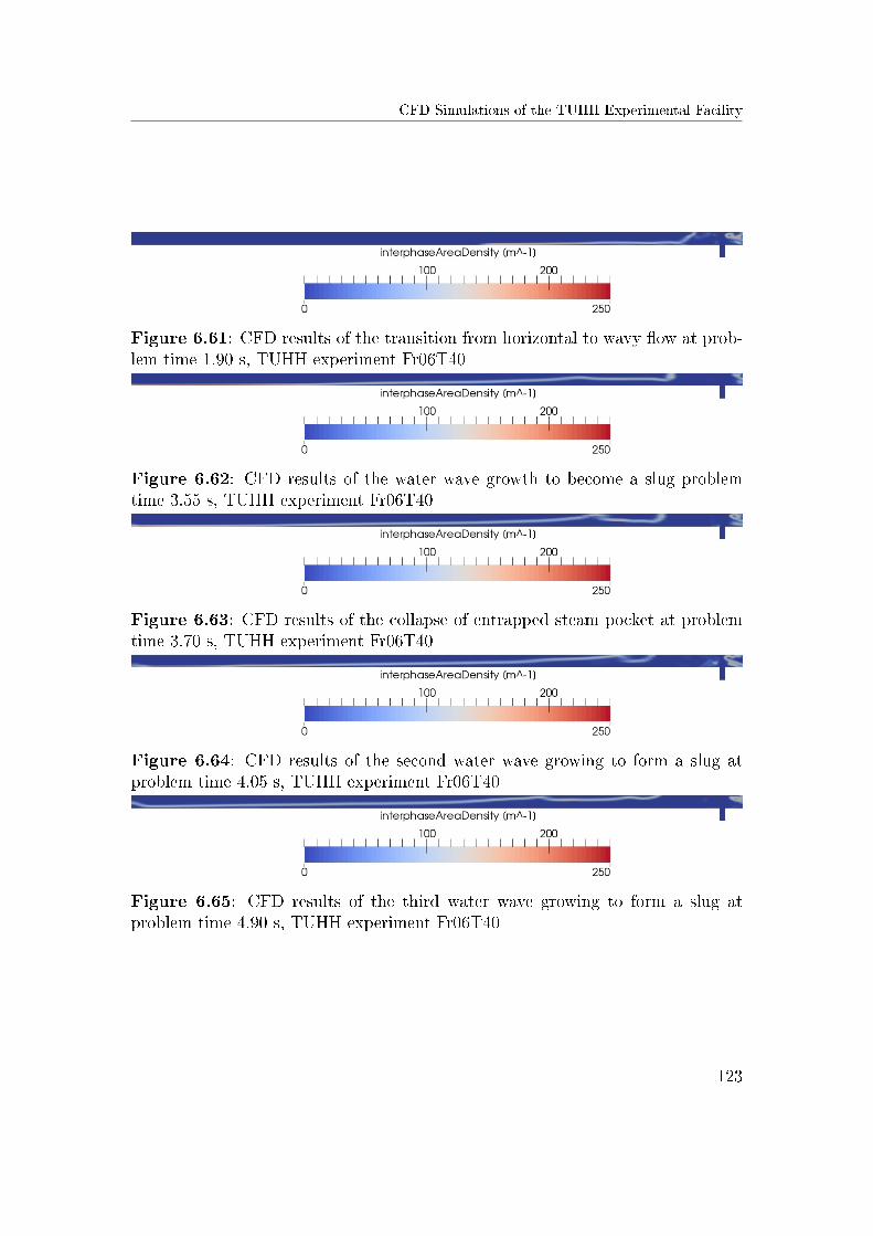
CFD Simulations of the TUHH Experimental Facility
Figure 6.61: CFD results of the transition from horizontal to wavy �ow at prob-lem time 1.90 s, TUHH experiment Fr06T40
Figure 6.62: CFD results of the water wave growth to become a slug problemtime 3.55 s, TUHH experiment Fr06T40
Figure 6.63: CFD results of the collapse of entrapped steam pocket at problemtime 3.70 s, TUHH experiment Fr06T40
Figure 6.64: CFD results of the second water wave growing to form a slug atproblem time 4.05 s, TUHH experiment Fr06T40
Figure 6.65: CFD results of the third water wave growing to form a slug atproblem time 4.90 s, TUHH experiment Fr06T40
123
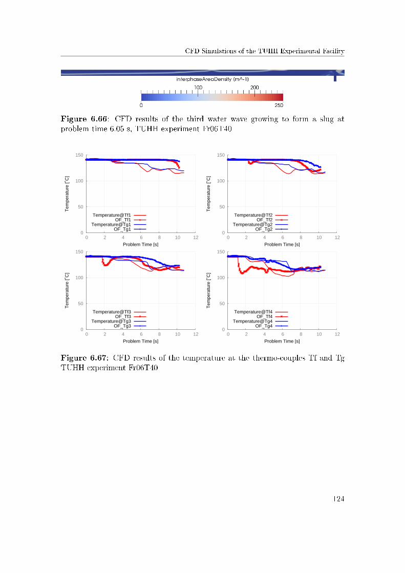
CFD Simulations of the TUHH Experimental Facility
Figure 6.66: CFD results of the third water wave growing to form a slug atproblem time 6.05 s, TUHH experiment Fr06T40
0
50
100
150
0 2 4 6 8 10 12
Tem
pera
ture
[˚C
]
Problem Time [s]
Temperature@Tf1OF_Tf1
Temperature@Tg1OF_Tg1
0
50
100
150
0 2 4 6 8 10 12
Tem
pera
ture
[˚C
]
Problem Time [s]
Temperature@Tf2OF_Tf2
Temperature@Tg2OF_Tg2
0
50
100
150
0 2 4 6 8 10 12
Tem
pera
ture
[˚C
]
Problem Time [s]
Temperature@Tf3OF_Tf3
Temperature@Tg3OF_Tg3
0
50
100
150
0 2 4 6 8 10 12
Tem
pera
ture
[˚C
]
Problem Time [s]
Temperature@Tf4OF_Tf4
Temperature@Tg4OF_Tg4
Figure 6.67: CFD results of the temperature at the thermo-couples Tf and TgTUHH experiment Fr06T40
124
CFD Simulations of the TUHH Experimental Facility
6.2.3 CFD Simulation of the TUHH Experiment Fr06T60
The experiment Fr06T060 provides data for the �ow with the highest Froude
Number (Fr) number reached in the TUHH experimental series together with the
highest subcooling of the injected feed-water. According to the CFD analysis of
the previously described experiments of transient two-phase �ow, two performed
at the TUHH and one at PMK-2, it can be expected, that both driving forces of
�ow pattern changes, i.e. the subcooling and the turbulence intensity will impact
the two-phase �ow dynamics in this experiment. The analysis of the �ow evolution
based on the time dependent patterns in the test-section, represented with the help
of the void fraction as shown in �gures 6.68 to 6.73, proves that the two-phase �ow
simulated in this experiment possesses the most complex dynamics of all TUHH
simulated experiments. This con�rms the fact that the in�uence of the �ow turbu-
lence considered in the mathematical formulation of the SRT based hybrid HTC is
consistent with experimental observations. According to the simulation results, in
the early phase of this experiment the subcooled water reaches the top of the test
pipe and forms the water fountain already described in the previously simulated
TUHH experiments. A liquid �lm is created as the water rejoins at the bottom of
the pipe after �owing down its wall. This liquid �lm then �ows towards the left
side of the test-section and passes by the measurement location T4 according to
�gure 6.68. Due to the high condensation rates in�uenced by the high turbulence
intensity and the high liquid subcooling, a liquid mass with the shape of a plug
forms very close to the injection location. The strati�ed �ow then changes to a
wavy pattern after only 2.70 s and shortly thereafter this wave grows to a slug
entrapping a steam pocket. The entrapment occurs at approximately 2.80 s, as
shown in �gure 6.70. This wave eventually grows to form a slug. This behavior
can be explained by analyzing the increase in the value of the condensation HTC
as shown in �gure 6.81 leading together with a su�ciently high IAD resulting from
high turbulence, see �gure 6.87, to a signi�cant increase in the local condensation
rate. The entrapped steam bubble then rapidly collapses and the water continues
to �ow towards the left side of the test-section; see �gure 6.71. It is important to
notice that following the high condensation rates, such an important depressur-
125
CFD Simulations of the TUHH Experimental Facility
ization appears, that the entire water inventory introduced into the test-section is
drawn back to the region of the T-junction, as can be noticed in �gures 6.70 and
6.71. The water �lm which has almost reached T3 travels upstream, even with
the 1.4 slope of the pipe, due to the large local depressurization. Some more slugs
are created as the �ow continues to the left. These slugs travel upstream toward
the injection location at the T-junction according to �gures 6.72 and 6.73. Optical
observations of the �ow con�rmed a similar �ow behavior no CIWH event could
be noticed in the simulations [10]. Still the �ow behavior predicted by the CFD
simulation describes in detail the �ow pattern evolution which has to be present
in a two-phase �ow in order for a CIWH to occur.
The standard VOF employed method for the calculation of the IAD fails to real-
istically compute the interfacial area in the regions with high turbulence, i.e. the
same regions showing increased HTC values. This is also one cause why no CIWH
could be computed in this simulation, whereas in the experiment some events have
been observed [11]. The OpenFOAM simulation temperature distribution results
of this experiment and the measured data are presented in �gure 6.92. As in the
previous simulations of the TUHH experimental facility, the boundary conditions
employed on the left and right-hand side of the test-section do not consider the
�nite steam inventory available in the real facility. Consequently, a constant pres-
sure is kept during the early phase of the simulation due to in�ow of saturated
steam.
The comparison of the temperature trends measured at T4 shows that the sub-
cooled water reaches the location of the thermo-couples Tf4 and Tg4 sooner in
the simulation than in the experiment. Still, the overall trend recorded by Tf4:
initially decreasing then increasing back to the saturation temperature and then
both temperatures Tf4 and Tg4 decreasing, is also observed in the experiment.
The fact that the temperature �rst decreases close to Tf4 and then it increases
back to the saturation temperature both in the simulation and in the experiment
proves that the subcooled liquid reaches the location of Tf4 and then is drawn back
to the location of the T-junction. Considering that the liquid has to overcome the
slope of the test-section, only heavy condensation rates close to the injection point
126
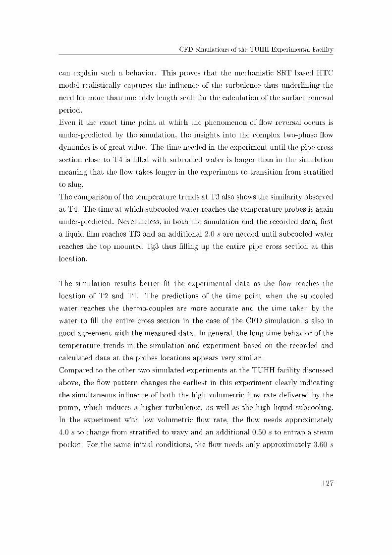
CFD Simulations of the TUHH Experimental Facility
can explain such a behavior. This proves that the mechanistic SRT based HTC
model realistically captures the in�uence of the turbulence thus underlining the
need for more than one eddy length scale for the calculation of the surface renewal
period.
Even if the exact time point at which the phenomenon of �ow reversal occurs is
under-predicted by the simulation, the insights into the complex two-phase �ow
dynamics is of great value. The time needed in the experiment until the pipe cross
section close to T4 is �lled with subcooled water is longer than in the simulation
meaning that the �ow takes longer in the experiment to transition from strati�ed
to slug.
The comparison of the temperature trends at T3 also shows the similarity observed
at T4. The time at which subcooled water reaches the temperature probes is again
under-predicted. Nevertheless, in both the simulation and the recorded data, �rst
a liquid �lm reaches Tf3 and an additional 2.0 s are needed until subcooled water
reaches the top mounted Tg3 thus �lling up the entire pipe cross section at this
location.
The simulation results better �t the experimental data as the �ow reaches the
location of T2 and T1. The predictions of the time point when the subcooled
water reaches the thermo-couples are more accurate and the time taken by the
water to �ll the entire cross section in the case of the CFD simulation is also in
good agreement with the measured data. In general, the long time behavior of the
temperature trends in the simulation and experiment based on the recorded and
calculated data at the probes locations appears very similar.
Compared to the other two simulated experiments at the TUHH facility discussed
above, the �ow pattern changes the earliest in this experiment clearly indicating
the simultaneous in�uence of both the high volumetric �ow rate delivered by the
pump, which induces a higher turbulence, as well as the high liquid subcooling.
In the experiment with low volumetric �ow rate, the �ow needs approximately
4.0 s to change from strati�ed to wavy and an additional 0.50 s to entrap a steam
pocket. For the same initial conditions, the �ow needs only approximately 3.60 s
127
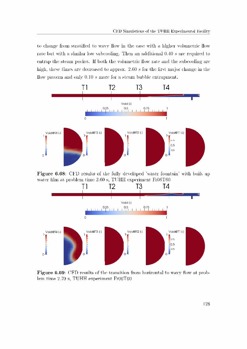
CFD Simulations of the TUHH Experimental Facility
to change from strati�ed to wavy �ow in the case with a higher volumetric �ow
rate but with a similar low subcooling. Then an additional 0.40 s are required to
entrap the steam pocket. If both the volumetric �ow rate and the subcooling are
high, these times are decreased to approx. 2.60 s for the �rst major change in the
�ow pattern and only 0.10 s more for a steam bubble entrapment.
Figure 6.68: CFD results of the fully developed 'water fountain' with built upwater �lm at problem time 2.60 s, TUHH experiment Fr06T60
Figure 6.69: CFD results of the transition from horizontal to wavy �ow at prob-lem time 2.70 s, TUHH experiment Fr06T60
128
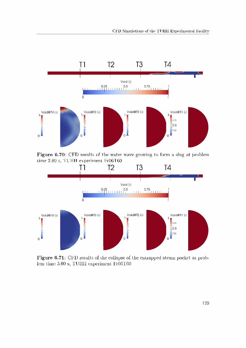
CFD Simulations of the TUHH Experimental Facility
Figure 6.70: CFD results of the water wave growing to form a slug at problemtime 2.80 s, TUHH experiment Fr06T60
Figure 6.71: CFD results of the collapse of the entrapped steam pocket at prob-lem time 3.00 s, TUHH experiment Fr06T60
129
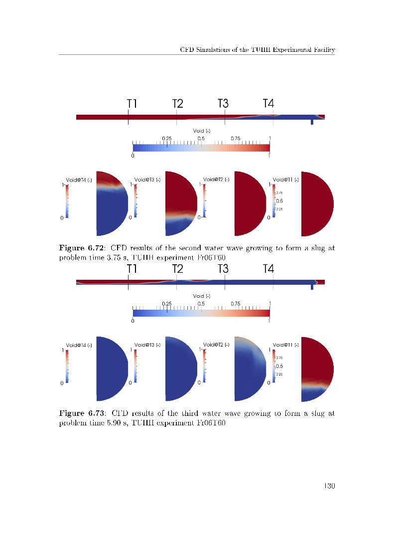
CFD Simulations of the TUHH Experimental Facility
Figure 6.72: CFD results of the second water wave growing to form a slug atproblem time 3.75 s, TUHH experiment Fr06T60
Figure 6.73: CFD results of the third water wave growing to form a slug atproblem time 5.90 s, TUHH experiment Fr06T60
130
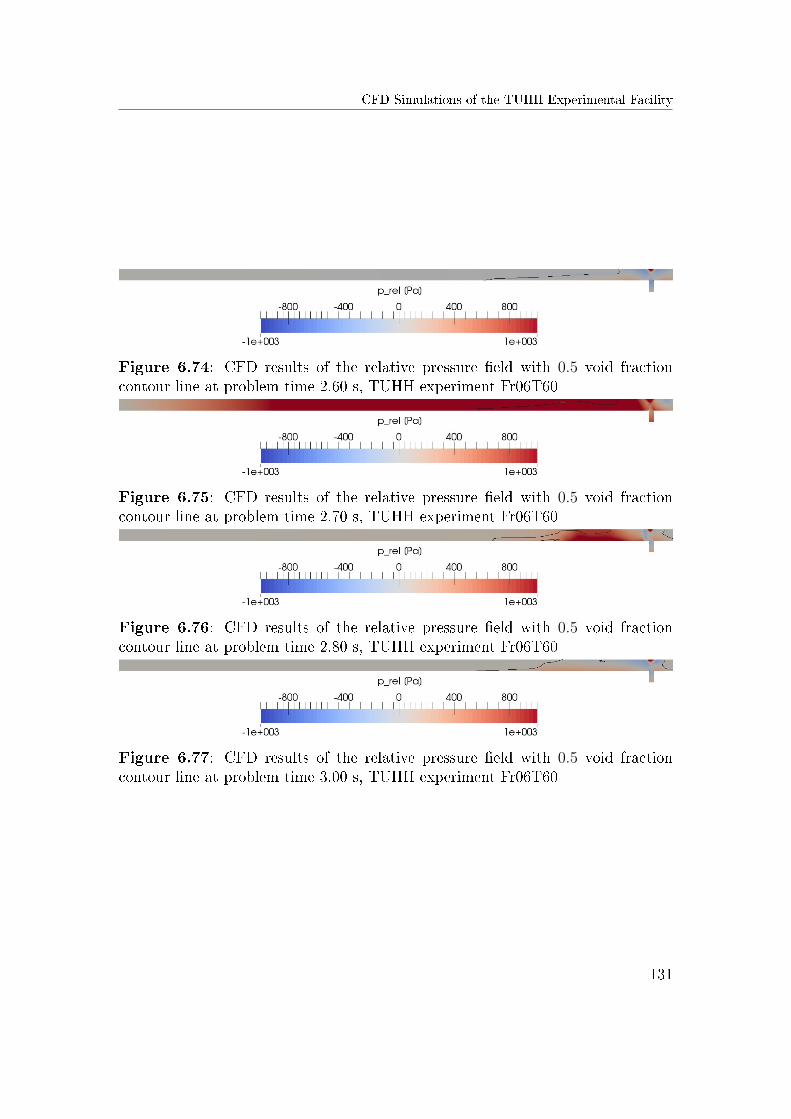
CFD Simulations of the TUHH Experimental Facility
Figure 6.74: CFD results of the relative pressure �eld with 0.5 void fractioncontour line at problem time 2.60 s, TUHH experiment Fr06T60
Figure 6.75: CFD results of the relative pressure �eld with 0.5 void fractioncontour line at problem time 2.70 s, TUHH experiment Fr06T60
Figure 6.76: CFD results of the relative pressure �eld with 0.5 void fractioncontour line at problem time 2.80 s, TUHH experiment Fr06T60
Figure 6.77: CFD results of the relative pressure �eld with 0.5 void fractioncontour line at problem time 3.00 s, TUHH experiment Fr06T60
131
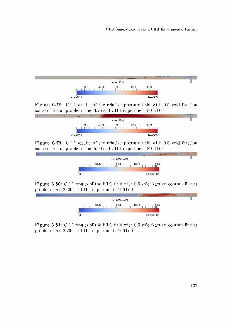
CFD Simulations of the TUHH Experimental Facility
Figure 6.78: CFD results of the relative pressure �eld with 0.5 void fractioncontour line at problem time 3.75 s, TUHH experiment Fr06T60
Figure 6.79: CFD results of the relative pressure �eld with 0.5 void fractioncontour line at problem time 5.90 s, TUHH experiment Fr06T60
Figure 6.80: CFD results of the HTC �eld with 0.5 void fraction contour line atproblem time 2.60 s, TUHH experiment Fr06T60
Figure 6.81: CFD results of the HTC �eld with 0.5 void fraction contour line atproblem time 2.70 s, TUHH experiment Fr06T60
132
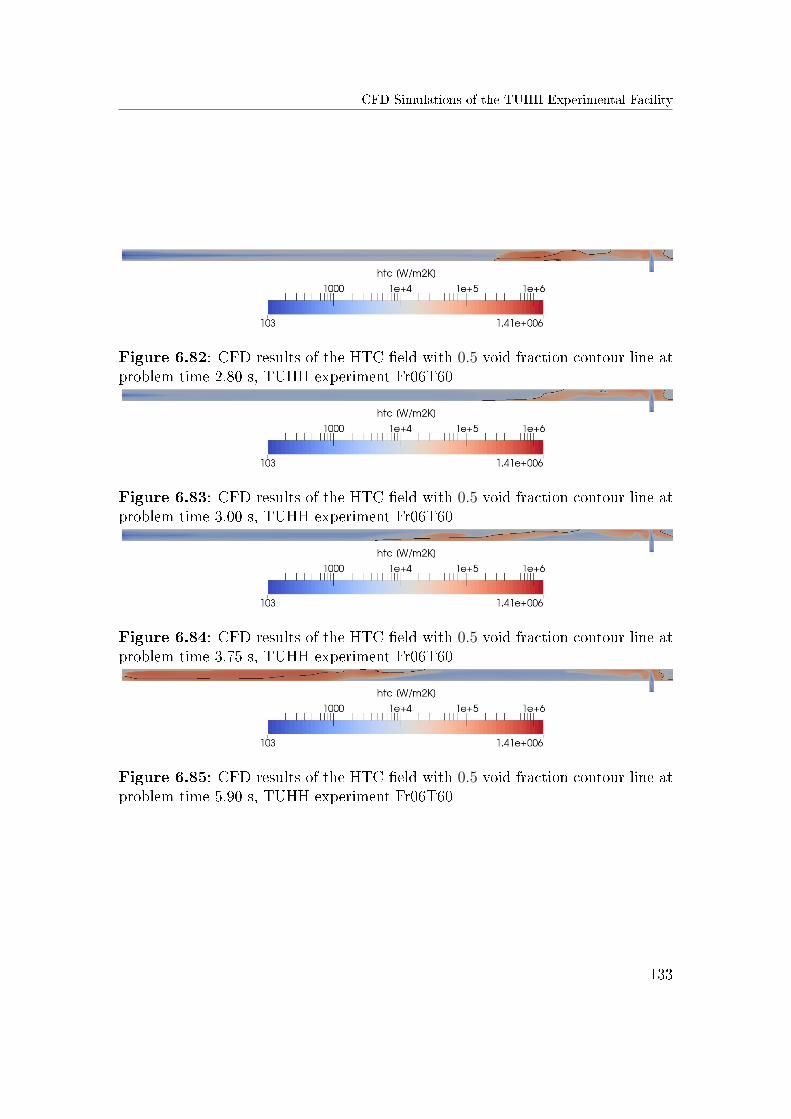
CFD Simulations of the TUHH Experimental Facility
Figure 6.82: CFD results of the HTC �eld with 0.5 void fraction contour line atproblem time 2.80 s, TUHH experiment Fr06T60
Figure 6.83: CFD results of the HTC �eld with 0.5 void fraction contour line atproblem time 3.00 s, TUHH experiment Fr06T60
Figure 6.84: CFD results of the HTC �eld with 0.5 void fraction contour line atproblem time 3.75 s, TUHH experiment Fr06T60
Figure 6.85: CFD results of the HTC �eld with 0.5 void fraction contour line atproblem time 5.90 s, TUHH experiment Fr06T60
133
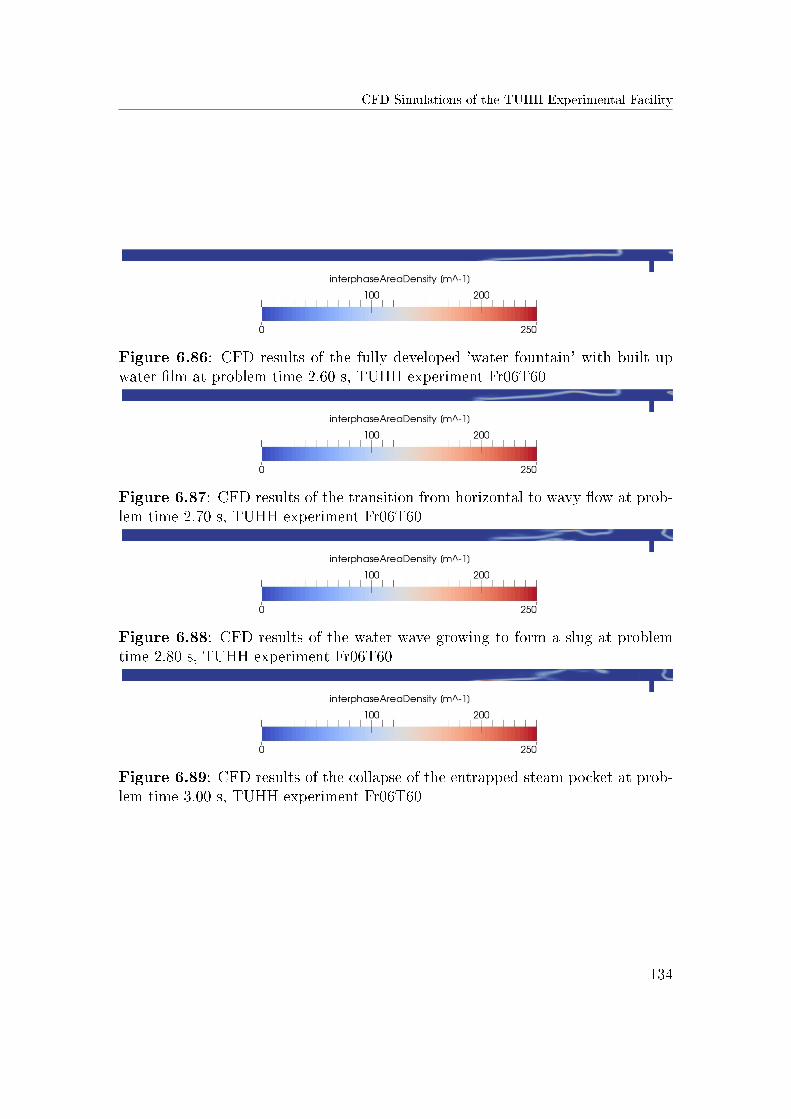
CFD Simulations of the TUHH Experimental Facility
Figure 6.86: CFD results of the fully developed 'water fountain' with built upwater �lm at problem time 2.60 s, TUHH experiment Fr06T60
Figure 6.87: CFD results of the transition from horizontal to wavy �ow at prob-lem time 2.70 s, TUHH experiment Fr06T60
Figure 6.88: CFD results of the water wave growing to form a slug at problemtime 2.80 s, TUHH experiment Fr06T60
Figure 6.89: CFD results of the collapse of the entrapped steam pocket at prob-lem time 3.00 s, TUHH experiment Fr06T60
134
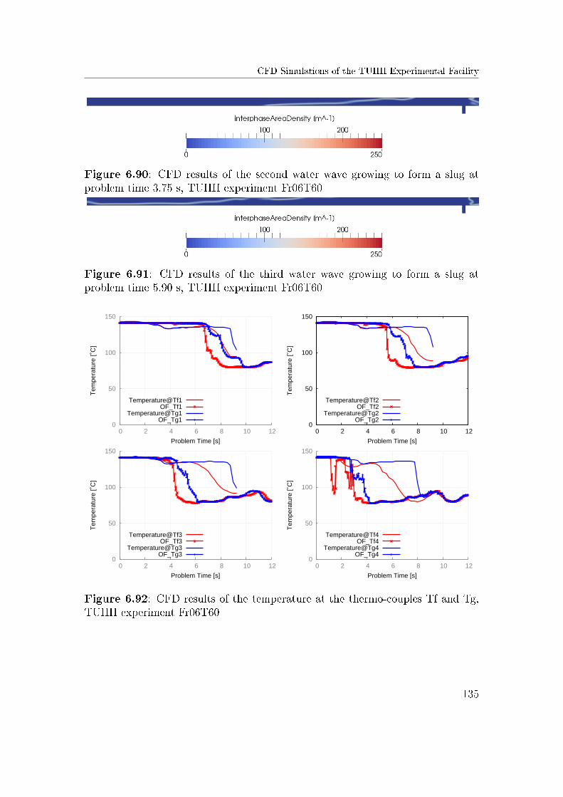
CFD Simulations of the TUHH Experimental Facility
Figure 6.90: CFD results of the second water wave growing to form a slug atproblem time 3.75 s, TUHH experiment Fr06T60
Figure 6.91: CFD results of the third water wave growing to form a slug atproblem time 5.90 s, TUHH experiment Fr06T60
0
50
100
150
0 2 4 6 8 10 12
Tem
pera
ture
[˚C
]
Problem Time [s]
Temperature@Tf1OF_Tf1
Temperature@Tg1OF_Tg1
0
50
100
150
0 2 4 6 8 10 12
Tem
pera
ture
[˚C
]
Problem Time [s]
Temperature@Tf2OF_Tf2
Temperature@Tg2OF_Tg2
0
50
100
150
0 2 4 6 8 10 12
Tem
pera
ture
[˚C
]
Problem Time [s]
Temperature@Tf3OF_Tf3
Temperature@Tg3OF_Tg3
0
50
100
150
0 2 4 6 8 10 12
Tem
pera
ture
[˚C
]
Problem Time [s]
Temperature@Tf4OF_Tf4
Temperature@Tg4OF_Tg4
Figure 6.92: CFD results of the temperature at the thermo-couples Tf and Tg,TUHH experiment Fr06T60
135
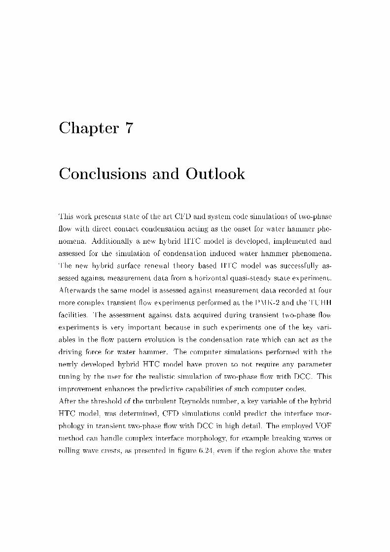
Chapter 7
Conclusions and Outlook
This work presents state of the art CFD and system code simulations of two-phase
�ow with direct contact condensation acting as the onset for water hammer phe-
nomena. Additionally a new hybrid HTC model is developed, implemented and
assessed for the simulation of condensation induced water hammer phenomena.
The new hybrid surface renewal theory based HTC model was successfully as-
sessed against measurement data from a horizontal quasi-steady state experiment.
Afterwards the same model is assessed against measurement data recorded at four
more complex transient �ow experiments performed at the PMK-2 and the TUHH
facilities. The assessment against data acquired during transient two-phase �ow
experiments is very important because in such experiments one of the key vari-
ables in the �ow pattern evolution is the condensation rate which can act as the
driving force for water hammer. The computer simulations performed with the
newly developed hybrid HTC model have proven to not require any parameter
tuning by the user for the realistic simulation of two-phase �ow with DCC. This
improvement enhances the predictive capabilities of such computer codes.
After the threshold of the turbulent Reynolds number, a key variable of the hybrid
HTC model, was determined, CFD simulations could predict the interface mor-
phology in transient two-phase �ow with DCC in high detail. The employed VOF
method can handle complex interface morphology, for example breaking waves or
rolling wave crests, as presented in �gure 6.24, even if the region above the water
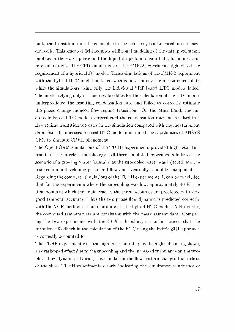
bulk, the transition from the color blue to the color red, is a 'smeared' area of sev-
eral cells. This smeared �eld requires additional modeling of the entrapped steam
bubbles in the water phase and the liquid droplets in steam bulk, for more accu-
rate simulations. The CFD simulations of the PMK-2 experiment highlighted the
requirement of a hybrid HTC model. These simulations of the PMK-2 experiment
with the hybrid HTC model matched with good accuracy the measurement data
while the simulations using only the individual SRT based HTC models failed.
The model relying only on macroscale eddies for the calculation of the HTC model
underpredicted the resulting condensation rate and failed to correctly estimate
the phase change induced �ow regime transition. On the other hand, the mi-
croscale based HTC model overpredicted the condensation rate and resulted in a
�ow regime transition too early in the simulation compared with the measurement
data. Still the microscale based HTC model underlined the capabilities of ANSYS
CFX to simulate CIWH phenomena.
The OpenFOAM simulations of the TUHH experiments provided high resolution
results of the interface morphology. All three simulated experiments followed the
scenario of a growing `water fountain' as the subcooled water was injected into the
test-section, a developing peripheral �ow and eventually a bubble entrapment.
Regarding the computer simulations of the TUHH experiments, it can be concluded
that for the experiments where the subcooling was low, approximately 40 K, the
time points at which the liquid reaches the thermo-couples are predicted with very
good temporal accuracy. Thus the two-phase �ow dynamic is predicted correctly
with the VOF method in combination with the hybrid HTC model. Additionally,
the computed temperatures are consistent with the measurement data. Compar-
ing the two experiments with the 40 K subcooling, it can be noticed that the
turbulence feedback in the calculation of the HTC using the hybrid SRT approach
is correctly accounted for.
The TUHH experiment with the high injection rate plus the high subcooling shows,
an overlapped e�ect due to the subcooling and the increased turbulence on the two-
phase �ow dynamics. During this simulation the �ow pattern changes the earliest
of the three TUHH experiments clearly indicating the simultaneous in�uence of
137
both the high volumetric �ow rate delivered by the pump and the high subcooling.
In the experiment with the low volumetric �ow rate and low subcooling, the �ow
needs approximately 4.00 s to change from strati�ed to wavy and an additional
0.50 s to trap a steam pocket. In the experiment with the high injection rate but
with the low subcooling, the �ow needs only approx. 3.60 s to change from strat-
i�ed to wavy �ow; to entrap a steam pocket an additional 0.40 s problem time is
required. If both the volumetric �ow rate and the subcooling are high, these time
periods are decreased to approximately 2.60 s for the �rst major change in the �ow
pattern and only 0.10 s more seconds for a steam bubble entrapment. Considering
that the pump needs approximately 2.60 s to reach its maximum volumetric �ow,
the shorter time needed in the experiment with the 60 K subcooling, is a direct
and clear cause of the increased subcooling.
Even if the results of all CFD simulations matched with very good accuracy the
measurement data, no pressure surges could be realistically simulated with any of
the CFD tools. The reasons why no CIWH could be reliably simulated with any of
the CFD tools is on one hand the lack of robust high order numerical schemes for
solving the individual terms of the two-phase �ow conservation equations and on
the other hand, the fact that the model used for the calculation of the IAD within
VOF has no feedback due to an increase of the turbulence. At this point, this
seems to be a limitation of the standard VOF methodology for the simulations of
CIWH phenomena. The available method for calculating the IAD in VOF models
requires a very �ne nodalization of the computational domain whereas, if improved
models are used, the IAD could be more easily modeled accounting also for the
local turbulence intensity. Such models should consider, in the calculation of the
interfacial area characteristic turbulence indicators such as the TKE and the eddy
dissipation rate.
The capability of tracking the two-phase �ow with such spatial resolution proves
the potential of VOF and the hybrid HTC model to also realistically simulate the
complex Pressurized Thermal Shock (PTS) phenomenon, a two-phase �ow scenario
138
where cold water touches hot walls. PTS increases the material thermal fatigue,
potentially resulting in small cracks in the pipe structure. The phenomenon of PTS
is caused by the variation over a short period of time of high thermal stresses due to
dilatation or contraction within a system component. Stresses above the material
yield strength can arise if the thermal dilatation or contraction is constrained.
It could be noticed during both the simulations of the PMK-2 and the TUHH
facilities that the temperature of the water touching the pipe walls was oscillating.
Using the VOF method the phenomenon of temperature layering can be analyzed
as the results of the simulations show. The fact that this e�ect is caught by the
CFD simulation is of potential interest for the application of the hybrid HTC for
other transient scenarios.
These local e�ects observed in the CFD simulations could not be caught with
the traditional 1D approach of system codes but on the other hand system code
simulations are less computational power-consuming and less prone to simulation
crashes or numerically induced variable oscillations as in the case of the CFD sim-
ulations.
The hybrid HTC model was also successfully implemented into the German sys-
tem code ATHLET. System codes are still widely used for the safety assessment of
large systems such as industrial scale facilities especially for long lasting transients.
The system code simulations represented the measurement data qualitatively well.
The idea of employing a quasi-2D computational domain for the ATHLET simula-
tions, with interconnected 1D components using cross-connection objects, requires
additional model development and additional validation work. Still this set-up
could simulate e�ects, such as wave growing more realistically in horizontal or
nearly horizontal two-phase �ow. Nevertheless, ATHLET could predict the overall
behavior of the �ow quite well and as in the case of the CFD simulation, a direct
link between subcooling turbulence on one hand and the �ow pattern, on the other
hand, could be observed. The advantage of system code analysis of large facilities
is the possibility of having an entire complex representations of components. In
this way, closed piping systems can be simulated without the need of using sim-
139
pli�ed BCs, which a�ect the simulation results, as in the case of CFD analysis.
A short sensitivity study based on the in�uence of the dimensionless numbers Re,
Ja, Fr and At has been performed for both the system code simulation results and
the experimental data. A similar dependency on the key dimensionless numbers
has been observed between computer simulations and recorded data. These simu-
lations even predicted the pressure surges recorded in the di�erent experiments.
The concomitant and complementary use of multi-dimensional CFD tools and fast
running system codes is the key in analyzing the CIWH phenomenon in piping
systems. The sequence of events observed in all computer simulations performed
with ANSYS CFX, OpenFOAM and ATHLET presented the typical behavior for
a CIWH event:
• As the water injection velocity was low enough, a tongue of liquid formed at
the bottom of the pipe,
• Due to steam condensation a counter-current �ow is initiated which leads to
the instability of the interface and generates a plug,
• The pressure decrease in the entrapped steam pocket, accelerates the water
fronts.
This behavior was also described by [33] to be the onset of CIWH events. The key
feedbacks of the variables in�uencing the two-phase �ow dynamics typical during
a CIWH event are correctly captured by the hybrid HTC model. This is the case
both in combination with the VOF in the case of the CFD simulations and the
two-�uid model employed in ATHLET. Computer tools, which correctly capture
the complex two-phase �ow dynamics emerging during a CIWH event, can help to
create pressure surge mitigation and avoidance strategies, due to the complemen-
tary information delivered by the di�erent approaches. CFD simulations deliver
high-resolution results of the complex two-phase �ow demanding high computa-
tional power. The performed system code simulations proved that in combination
with the hybrid HTC model these computer tools are capable to deliver qualita-
tively good results of the overall �ow behavior together with a good prediction
of eventual pressure peaks. Still the exact magnitude of the CIWH is di�cult to
140
predict because of the stochastic nature of surface waves which eventually evolve
to slugs and the resulting steam pocket entrapment.
An additional variable which has to be investigated for its role in triggering CIWH,
is the pump start-up behavior. It was underlined, also during the performed sim-
ulations that the slugging can be triggered before the pump reaches its maximum
�ow rate. As a consequence CIWH event could arise in the start-up phase before
the pump delivers enough �ow rate to �ll the pipe with water.
The newly developed HTC model adds to the predictive capabilities of any two-
phase �ow computer simulation due to its mechanistic character. Its capabilities to
reliably simulate complex two-phase �ow dynamics were proven by the validation
of CFD and system code simulations against experimental measurement data.
Overall system safety enhancements can only be established by replacing as many
empirically developed models as possible with mechanistic ones, such as the newly
developed hybrid SRT based HTC model. Still the hybrid HTC model needs state
of the art models for the best estimate simulation of the complex two-phase �ow
phenomenon during a CIWH, especially for the calculation of the interfacial area
density combined with reliable high order numerical schemes.
141
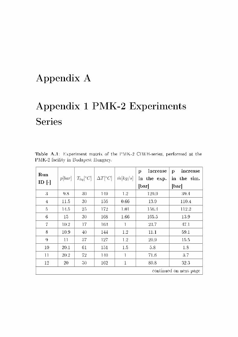
Appendix A
Appendix 1 PMK-2 Experiments
Series
Table A.1: Experiment matrix of the PMK-2 CIWH-series, performed at thePMK-2 facility in Budapest Hungary.
Run
ID [-]p[bar] Tliq[
◦C] ∆T [◦C] m[kg/s]
p increase
in the exp.
[bar]
p increase
in the sim.
[bar]
3 9.8 30 149 1.2 129.9 39.4
4 11.5 30 156 0.66 13.9 110.4
5 14.5 25 172 1.01 156.4 112.2
6 15 30 168 1.66 165.5 13.9
7 10.2 17 163 1 23.7 47.1
8 10.9 40 144 1.2 11.1 59.1
9 11 57 127 1.2 20.9 15.5
10 20.1 61 151 1.5 5.8 1.8
11 20.2 72 140 1 71.6 3.7
12 20 50 162 1 80.8 32.3
continued on next page
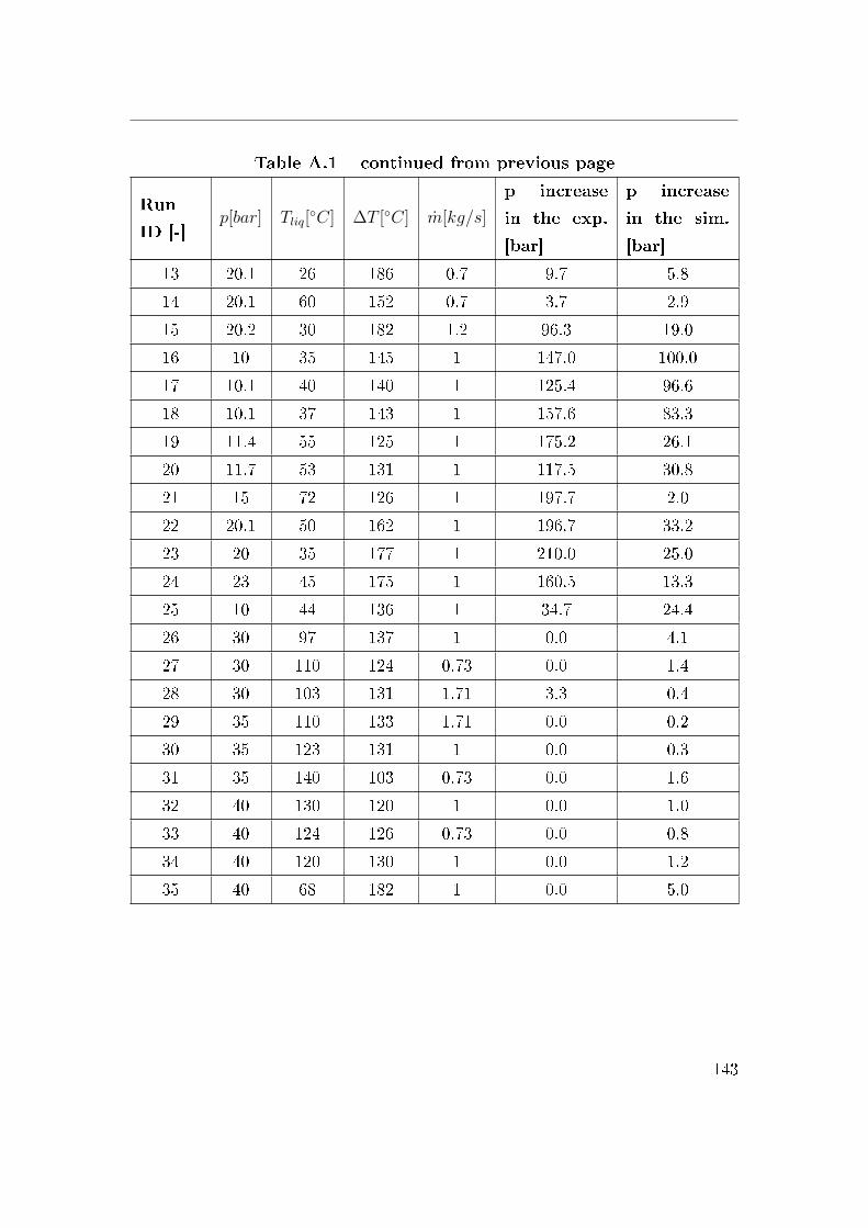
Table A.1 � continued from previous page
Run
ID [-]p[bar] Tliq[
◦C] ∆T [◦C] m[kg/s]
p increase
in the exp.
[bar]
p increase
in the sim.
[bar]
13 20.1 26 186 0.7 9.7 5.8
14 20.1 60 152 0.7 3.7 2.9
15 20.2 30 182 1.2 96.3 19.0
16 10 35 145 1 147.0 100.0
17 10.1 40 140 1 125.4 96.6
18 10.1 37 143 1 157.6 83.3
19 11.4 55 125 1 175.2 26.1
20 11.7 53 131 1 117.5 30.8
21 15 72 126 1 197.7 2.0
22 20.1 50 162 1 196.7 33.2
23 20 35 177 1 210.0 25.0
24 23 45 175 1 160.5 13.3
25 10 44 136 1 34.7 24.4
26 30 97 137 1 0.0 4.1
27 30 110 124 0.73 0.0 1.4
28 30 103 131 1.71 3.3 0.4
29 35 110 133 1.71 0.0 0.2
30 35 123 131 1 0.0 0.3
31 35 140 103 0.73 0.0 1.6
32 40 130 120 1 0.0 1.0
33 40 124 126 0.73 0.0 0.8
34 40 120 130 1 0.0 1.2
35 40 68 182 1 0.0 5.0
143
Bibliography
[1] USNRC. TRACE V5.0 Theory Manual: Field Equations, Solution Methods,
and Physical Models.
[2] N.E. Todreas and M.S. Kazimi. NUCLEAR SYSTEMS I, Thermal Hydraulics
Fundamentals. Taylor & Francis, 1990.
[3] H. Austregesilo, C. Bals, A. Hora, G. Lerchl, and P. Romstedt. ATHLET
Mod 2.2 Cycle A Models and Methods GRS - P - 1 / Vol 4 Rev. 2. GRS, July
2009.
[4] S.C. Ceuca and R. Macián-Juan. CFD Simulation Of Direct Contact Con-
densation with ANSYS CFX using locally de�ned Heat Transfer Coe�cients.
Proceedings of the 20th International Conference on Nuclear Engineering col-
located with the ASME 2012 Power Conference, 2012.
[5] H.K. Versteeg and W. Malalasekera. An Introduction to Computational Fluid
Dynamics. Longman Scienti�c & Technical, 1995.
[6] D. Lucas. Deliverable D 2.1.2: Review of the existing Data Basis For the
Validation of Models for PTS. Technical report, Technical report, 2005.
[7] J. Karl and D. Hein. Measuring Water Temperature Pro�les at Strati�ed
Flow by means of Linear Raman Spectroscopy. Proceedings of the Japanese-
German Symposium on Multiphase Flow, 1997.
BIBLIOGRAPHY
[8] H.-M Prasser, Gy. Ézsöl, G. Baranyai, and T. Sühnel. Spontaneous Water
Hammers in a Steam Line in Case of Cold Water Ingress. Multiphase Science
and Technology, 20:265�289, 2008.
[9] H. Swidersky, A. Scha�rath, and A. Dudlik. Computational Models to deter-
mine Fluiddynamical Transients due to Condensation Induced Water Hammer
(CIWH). Proceedings of the 14th International Topical Meeting on Nuclear
Reactor Thermal-Hydraulics (NURETH-14), 14, 2011.
[10] C. Urban and M. Schlüter. Optical Investigations on key Phenomena of
Condensation Induced Water Hammers. Proceedings of the 15th Interna-
tional Topical Meeting on Nuclear Reactor Thermal-Hydraulics (NURETH-
15), 2013.
[11] C. Urban and M. Schlüter. Untersuchungen zu Kondensationsschlägen in
Rohrleitungssystemen: Experimentelle Ergebnisse an der Technischen Uni-
versität Hamburg-Harburg (in German). 1. Projektstatusgespräch zur BMBF
geförderten Nuklearen Sicherheitsforschung, 2013.
[12] S.C. Ceuca and R. Macián-Juan. Benchmark of Surface Renewal Theory based
Heat Transfer Coe�cients for the Simulations of Direct Contact Condensa-
tion in Pipes using the 1D and 3D Approach. Proceedings of the 15th Interna-
tional Topical Meeting on Nuclear Reactor Thermal-Hydraulics (NURETH-
15), 2013.
[13] C. Martin, R. Brown, and J. Brown. Condensation-Induced Hydraulic Shock
Laboratory Study. American Society of Heating, Refrigeration, and Air Con-
ditioning Engineers - ASHRAE 970-RP, 2007.
[14] M. Ishii and T. Hibiki. Thermo-�uid Dynamics of Two-phase Flow. Springer
Science+Business Media, Inc., 2006.
[15] John R. Thome. Engineering Data Book III. Wolverine Tube, Inc Online,
2010.
145
BIBLIOGRAPHY
[16] J. Weisman and S.Y. Kang. Flow Pattern Transitions in Vertical and Up-
wardly Inclined Lines. International Journal Multiphase Flow, 7:271�291,
1981.
[17] Y. Taitel D. Barenea, O. Shoham and A. E. Dukler. Gas-Liquid Flow in
Inclined Tubes: Flow Pattern Transitions for Upward Flow. Chemical Engi-
neering Science, 40:131�136, 1985.
[18] O. Baker. Designing for Simultaneous Flow of Oil and Gas. Oil and Gas
Journal, 53:185�195, 1954.
[19] G.A. Gregory J.M. Mandhane and K. Aziz. A Flow Pattern Map for Gas-
Liquid Flow in Horizontal Pipes. International Journal Multiphase Flow,
1:537�553, 1974.
[20] Y. Taitel and A.E. Dukler. A Model for Predicting Flow Regime Transitions
in Horizontal and near Horizontal Gas-Liquid Flow. Journal of the American
Institute of Chemical Engineers, 22:47�55, 1976.
[21] S. Koyama H. Haraguchi and T. Fujii. Condensation of Refrigerants HCFC 22,
HFC 134a, and HCFC 123 in a Horizontal Smooth Tube (2nd report, Proposal
of Empirical Expressions for Local Heat Transfer Coe�cient). Trans. JSME,
60(574):245�252, 1994.
[22] A. Cavallini, G. Censi, D. Del Col, L. Doretti, G.A. Longo, and L. Rossetto.
In-Tube Condensation of Halogenated Refrigerants. ASHRAE Transactions,
108:1:146�161, 2002.
[23] A. Cavallini, G. Censi, D. Del Col, L. Doretti, G.A. Longo, L. Rossetto, and
C. Zilio. Condensation Inside and Outside Smooth and Enhanced Tubes - A
Review of Recent Research. International Journal of Refrigeration, 26:1:373�
392, 2003.
[24] J. El Hajal J.R. Thome and A. Cavalini. Condensation in Horizontal Tubes,
Part 2: New Heat Transfer Model Based on Flow Regimes. International
Journal of Heat and Mass Transfer, 46:3365�3387, 2003.
146
BIBLIOGRAPHY
[25] J.R. Thome J. El Hajal and A. Cavalini. Condensation in Horizontal Tubes,
Part 1: Two-Phase Flow Pattern Map. International Journal of Heat and
Mass Transfer, 46:3349�3363, 2003.
[26] D.J. Korteweg. Über die Fortp�anzungsgeschwindigkeit des Schalles in elastis-
chen Röhren. (On the velocity of propagation of sound in elastic tubes.). An-
nalen der Physik und Chemie, New Series 5, 5:525�542, 1878.
[27] L. Allievi. Theory of Water Hammer (translated from Italian by E. E. Halmos
for the American Society of Civil Engineers, 1925). Technical report, printed
by R. Garoni, 1913.
[28] L. Bergeron. Water Hammer in Hydraulic and Wave Surges in Electricity.
John Wiley and Sons Inc. New York, 1960.
[29] G.R. Rich. Water Hammer Analysis by Laplace Mellin Transformation. Trans-
action American Society of Mechanical Engineers, pages 361�376, 1945.
[30] H.W. Reddick and F.H. Miller. Advanced Mathematics for Engineer. John
Wiley and Sons Inc. New York, 1957.
[31] A. Sommer�eld. Partial Di�erential Equations in Physics. Academic Press
New York, 1949.
[32] Y. Chou and P. Gri�th. Admitting Cold Water into Steam Filled Pipes
without Waterhammer due to Steam Bubble Collapse. Nuclear Engineering
and Design, 121:367�378, 1990.
[33] P. Gri�th. Screening Reactor Steam/Water Piping Systems for Water Ham-
mer, NUREG/CR-6519. Technical report, USNRC, 1997.
[34] J.A. Block et al. An Evaluation of PWR Steam Generator Water Hammer,
NUREG-0291. Technical report, USNRC, 1977.
[35] A.B. Jackobek and P. Gri�th. Investigation of Cold Leg Water Hammer in a
PWR due to the Admission of Emergency Core Cooling during a Small Break
LOCA, NUREG/CR-3895. Technical report, USNRC, 1984.
147
BIBLIOGRAPHY
[36] S.C. Lee. Stability of Steam-Water Countercurrent Strati�ed Flow,
NUREG/CR-4416. Technical report, USNRC, 1985.
[37] H.-M Prasser, Gy. Ézsöl, and G. Baranyai. Water Hammer Tests, Condensa-
tion caused by Cold Water Injection into Main Steam-Line of VVER-440-type
PWR - Quick-Look Report (QLR). Technical report, WAHALoads project
deliverable D48, 2004.
[38] H.-M Prasser, Gy. Ézsöl, and G. Baranyai. Water Hammer Tests, Conden-
sation caused by Cold Water Injection into Main Steam-Line of VVER-440-
type PWR � Data Evaluation Report (DER). Technical report, WAHALoads
project deliverable D51, 2004.
[39] W. Schnellhammer. Rohrleitungskräfte bei Überspeisung der
Frischdamp�eitung infolge Fehlö�nens eines Hauptspeisewasserregelven-
tils - Arbeitsbericht (in german). Technical report, AREVA Nuclear Power,
2008.
[40] S. Dirndorfer, M. Dör�er, H. Kulisch, and A. Malcherek. Condensation-
Induced Water Hammer - Overview and Own Experiments. Proceedings of the
14th International Topical Meeting on Nuclear Reactor Thermal-Hydraulics
(NURETH-14), 14, 2011.
[41] N. Joukowsky. Über den hydraulischen Stoss in Wasserleitungsröhren (On
the Hydraulic Hammer in Water Supply Pipes). Mémoires de l'Académie
Impériale des Sciences de St.-Pétersbourg, Series 8, 9(5), 1900.
[42] D. Lucas, D. Bestion, E. Bodèle, P. Coste, M. Scheuerer, F. D'Auria, D. Mazz-
ini, B. Smith, I. Tiselj, A. Martin, D. Lakehal, J.-M. Seynhaeve, R. Kyrki-
Rajamäki, M. Ilvonen, and J. Macek. An Overview of the Pressurized Ther-
mal Shock Issue in the Context of the NURESIM Project. Technical report,
European Union, 2009.
[43] D. Lucas, D. Bestion, P. Coste, P. Pouvreau, Ch. Morel, A. Martin,
M. Boucker, E. Bodele, M. Schmidtke, M. Scheuerer, B. Smith, M. T. Dhotre,
148
BIBLIOGRAPHY
B. Niceno, D. Lakehal, M. C. Galassi, D. Mazzini, F. D'Auria, Z. Bartosiewicz,
J.-M. Seynhaeve, I. Tiselj, L. �trubelj, M. Ilvonen, R. Kyrki-Rajamäki,
V. Tanskanen, M. Laine, and J. Puustinen. Main Results of the European
Project NURESIM on the CFD-Modelling of Two-Phase Pressurized Thermal
Shock (PTS). Kerntechnik, 74:238�242, 2009.
[44] H. Ruile, J. Karl, and D. Hein. Kühlmittelerwärmung bei Direktkontak-
tkondensation an horizontalen Schichten und vertikalen Streifen zur Quan-
ti�zierung des druckbelasteten Thermoschocks. Technical report, BMFT-
Forschungsvorhaben 1500906, Abschluÿbericht, Lehrstuhl für Thermische
Kraftanlagen, TU München, Germany., 1995.
[45] ECORA. Two-Phase Flow Water Hammer Transients and Induced Loads on
Materials and Structures of Nuclear Power Plants (Ecora Project Report).
Technical report, Technical report, 2004.
[46] Y. Egorov, M. Boucker, Martin A, S. Pigny, M. Scheuerer, and S. Willemsen.
Validation of CFD Codes with PTS-Relevant Test Cases. Technical report,
Technical report, 2004.
[47] G. Kocamustafaogullari and M. Ishii. Foundations of the Interfacial Area
Transport Equation and its Closure Relations. International Journal Heat
and Mass Transfer, 38:481�493, 1995.
[48] C. M. Rhie and W. L. Chow. A Numerical Study of the Turbulent Flow past
an Isolated Airfoil with Trailing Edge Separation. AIAA Journal, 21:1525�
1532, 1983.
[49] G. Lerchl and H. Austregesilo. ATHLET Mod 2.2 Cycle A User's Manual
GRS - P - 1 / Vol 1 Rev. 5. GRS, July 2009.
[50] H. Austregesilo and K. Trambauer. Modelling of the Interfacial Area Con-
centration in the System Code ATHLET. Proceedings of the 11th Interna-
tional Topical Meeting on Nuclear Reactor Thermal-Hydraulics (NURETH-
11), 2005.
149
BIBLIOGRAPHY
[51] C.W. Hirt and B.D. Nichols. Volume of Fluid (VOF) Method for the Dynamics
of Free Boundaries. Journal of Computational Physics, 39:207�225, 1981.
[52] H. Rusche. Computation Fluid Dynamics of Dispersed Two-Phase Flow at
High Phase Factions. Technical report, PhD Thesis, University of London
UK, 2002.
[53] R. I. Issa. Solution of the Implicit Discretized Fluid Flow Equations by Op-
erator Splitting. Mechanical Engineering Rep., FS:82�15, 1982.
[54] B. E. Launder and D. B. Spalding. The Numerical Computation of Turbulent
Flows. Comput. Methods Appl. Mech. Eng., 3:269�289, 1974.
[55] D.C. Wilcox. Turbulence Modeling for CFD. DCW Industries Inc., 1998.
[56] R. Higbie. The Rate of Absorption of a Pure Gas into a Still Liquid during a
Short Time of Exposure. Transactions of the American Institute of Chemical
Engineers, 31:365�389, 1935.
[57] P.V Danckwerts. Signi�cance of Liquid- Film Coe�cients in Gas Absorption.
Industrial and Engineering Chemistry, 43:1460�1467, 1951.
[58] H.L. Torr and J.M. Marchello. Film-Penetration Model for Mass and Heat
Transfer. Journal of the American Institute of Chemical Engineers, 4:97�101,
1958.
[59] S. Banerjee. A Surface Renewal Model for Interfacial Heat and Mass Transfer
in Transient Two-Phase Flow. International Journal Multiphase Flow, 4:571�
573, 1978.
[60] R.B. Du�ey and E.D. Hughes. Gas Mass Transfer for Strati�ed Flows, BNL�
61801(Rev.6/95). Technical report, DOE, 1995.
[61] W.J. Brtko and R.L.Kabel. Transfer of Gases at Natural Air-Water Interfaces.
Journal of Physical Oceanography, 8:543�556, 1978.
150
BIBLIOGRAPHY
[62] E.D. Hughes and R.B. Du�ey. Direct Contact Condensation and Momentum
Transfer in Turbulent Separated Flows. International Journal Multiphase
Flow, 17:599�619, 1991.
[63] L. Shen, G.S. Triantafyllou, and D.K.P. Yue. Turbulent Di�usion near a Free
Surface. Journal of Fluid Mechanics, 407:145�166, 2000.
[64] N. I. Kolev. Multiphase Flow Dynamics II. Springer, 2007.
[65] N. I. Kolev. Multiphase Flow Dynamics I. Springer, 2007.
[66] M. Scheuerer. Selection of PTS-Relevant Test Cases. Technical report. Tech-
nical report, European Commission 5th EURATOM Framework Programme
1998-2002, 2002.
[67] H.-M Prasser, A. Böttger, and J. Zschau. A new Electrode-Mesh Tomograph
for Gas-Liquid Flows. Flow Measurement and Instrumentation, 9:111�119,
1998.
[68] I.F. Barna, A.R. Imre, G. Baranyai, and Gy. Ézsöl. Experimental and The-
oretical Study of Steam Condensation Induced Water Hammer Phenomena.
Nuclear Engineering and Design, 240:146�150, 2010.
[69] E. Carpintero-Rogero. Experimental Investigation of Developing Plug and
Slug Flows. PhD thesis, Technische Universität München, Germany, 2009.
[70] S.G. Banko� and H.J. Kim. Local Condensation Rates in Nearly Horizontal
Strati�ed Countercurrent Flow of Steam and Cold Water. Heat Transfer
AIChE Symposium Series, 79:225:209�223, 1983.
[71] H.J. Kim and S.G. Banko�. Local Heat Transfer Coe�cients for Condensation
in Strati�ed Countercurrent Steam-Water Flows. Journal of Heat Transfer,
105:706�711, 1983.
[72] S.C. Lee and S.G. Banko�. Stability of Steam-Water countercurrent Flow
in an Inclined Channel: Part II - Condensation-Induced Waterhammer,
NUREG/CR-2289. Technical report, USNRC, 1981.
151
BIBLIOGRAPHY
[73] I.S. Lin, S.G. Banko�, R.S. Tankin, and M.C. Yuen. Cocurrent Steam/Water
Flow in a Horizontal Channel. Journal of Heat Transfer, 106:900�902, 1984.
[74] S.C. Lee and S.G. Banko�. Parametric e�ects on the onset of �ooding in �at-
plate geometries. International Journal of Mass Transfer, 27:10:1691�1700,
1984.
[75] S.G. Banko� and S.C. Lee. Condensation in Strati�ed Flow. Multiphase
Science and Technology, 3:1-4:398�422, 1984.
[76] P. Gri�th and J.R Silva. Steam Bubble Collapse Induced Water Hammer in
Draining Pipes. Proceedings of the Pressure Vessels and Piping Conference
(PVP), 231:115�119, 1992.
[77] R.W. Bjorge and P. Gri�th. Initiation of Water Hammer in horizontal and
nearly horizontal Pipes containing Steam and sub-cooled Water. ASME Jour-
nal of Heat Transfer, 106:835�840, 1984.
[78] Y. Chou and P. Gri�th. Avoiding Steam-Bubble-Collapse-Induced Water
Hammers in piping Systems, EPRI Research Project NP-6647. Technical
report, EPRI, 1997.
[79] S. Komori, R. Nagaosa, and Y. Murakami. Turbulence Structure and Mass
Transfer across a sheared Air-Water Interface in Wind-Driven Turbulence.
Journal of Fluid Mechanics, 249:161�193, 1993.
[80] S.V. Patankar. Numerical Heat Transfer and Fluid Flow. Taylor & Francis,
1980.
[81] S. Banerjee, D. S. Scott, and E. Rhodes. Mass Transfer to Falling Wavy
Liquid Films in Turbulent Flow. Ind. Engng Chem. Fundam., 7:22�26, 1968.
[82] N.E. Todreas and M.S. Kazimi. NUCLEAR SYSTEMS II, Elements of Ther-
mal Hydraulic Design. Taylor & Francis, 1990.
[83] P. Saha. An Evaluation of Condensation-Induced Wter Hammer in Preheat
Steam Generator, NUREG/CR-1606. Technical report, USNRC, 1980.
152
BIBLIOGRAPHY
[84] R.W. Bjorge. Initiation of Water Hammer in Horizontal or Nearly-Horizontal
Pipes Containing Steam and Subcooled Water, PhD-Thesis. Technical report,
MIT, Department of Mechanical Engineering, 1983.
[85] T. Fujii and K. Akagawa. Analysis of Water Hammer in Bubbly Flows (1st
Report, Two-component, Two-phase Flow. Bulletin of JSME, 29:1746�1751,
1986.
[86] A. Dudlik and A. Scha�rath. Forschungsantrag Untersuchungen zu Kondensa-
tionsschlägen in Rohrleitungssystemen - Condensation Induced Water Ham-
mer, CIWA, Rev.1. Technical report, Fraunhofer UMSICHT, 2010.
[87] S.C. Ceuca and R. Macián-Juan. Validation of a Hybrid Surface Renewal
Theory Based HTC Model for the Simulation of Condensation Induced Wa-
ter Hammer. Proceedings of the 21th International Conference on Nuclear
Engineering, 2013.
[88] ANSYS CFX User Manual, Release 14.5. ANSYS, 2014.
[89] OpenFOAM User Manual, Version 1.7.1. OpenFOAM, 2010.
153