Embed Size (px)
Citation preview
Technische Universität MünchenDepartment Chemie
Lehrstuhl II für Organische Chemie
Cooperative Pulses—
Towards Global Pulse Sequence Optimization
Michael Braun
Vollständiger Abdruck der von der Fakultät Chemie der TechnischenUniversität München zur Erlangung des akademischen Grades eines
Doktors der Naturwissenschaften
genehmigten Dissertation
Vorsitzender: Univ.-Prof. Dr. B. Reif
Prüfer der Dissertation: 1. Univ.-Prof. Dr. St. J. Glaser
2. Univ.-Prof. Dr. K.-O. Hinrichsen
Die Dissertation wurde am 10.10.2011 bei der Technischen UniversitätMünchen eingereicht und durch die Fakultät für Chemie am 21.11.2011angenommen.

Abstract
The present thesis deals with the concept of cooperative (COOP) pulsesthat are designed to cancel each other’s imperfections and act in a coop-erative manner. Multi-scan COOP pulses are applied in several scansand at the same position in a pulse sequence so that undesired sig-nal contributions can be canceled. They complement and generalizephase cycles and difference spectroscopy. We experimentally demon-strate their advantages for broadband and band-selective pulses. Single-scan cooperative (S2-COOP) pulses are applied at different positions ofa pulse sequence in a single scan. They can be used to find general-ized solutions for common building blocks in NMR spectroscopy. Theadvantage of the S2-COOP approach is demonstrated in theory and ex-periment for NOESY-type frequency-labeling blocks. Optimal trackingis a generalization of the gradient ascent pulse engineering (GRAPE)algorithm which allows for the design of pulse sequences that steer theevolution of an ensemble of spin systems such that at defined points intime, a specific trajectory of the density operator is tracked as closely aspossible. Optimal tracking has been used for the design of low-powerheteronuclear decoupling sequences for in vivo applications. Here, wepresent the theory of cooperative tracking representing a generalizationof optimal tracking and multi-scan COOP pulses. Cooperative trackingpulses, multi-scan and single-scan COOP pulses can be efficiently opti-mized with extended versions of the GRAPE algorithm.
III

IV
Zusammenfassung
Die vorliegende Arbeit behandelt das Konzept kooperativer (COOP)Pulse, die dazu ausgelegt sind, ihre Imperfektionen gegenseitig auszu-gleichen und auf kooperative Weise zu wirken. Multi-Scan COOP Pul-se werden in mehreren Scans an der gleichen Stelle einer Pulssequenzeingesetzt, sodass sich unerwünschte Signalbeiträge gegenseitig aufhe-ben können. Sie ergänzen und verallgemeinern Phasenzyklen und Dif-ferenzspektroskopie. In Experimenten zeigen wir ihre Vorteile als breit-bandige und bandselektive Pulse. Single-Scan-kooperative (S2-COOP)Pulse werden an verschiedenen Positionen einer Pulssequenz in einemScan eingesetzt. Sie können dazu verwendet werden, um verallgemei-nerte Lösungen für gängige Bausteine in der NMR-Spektroskopie zufinden. Vorteile des S2-COOP-Verfahrens werden theoretisch und expe-rimentell anhand NOESY-artiger Evolutionssequenzen aufgezeigt. Op-timal Tracking ist eine Verallgemeinerung des gradient ascent pulse en-gineering (GRAPE) Algorithmus’, die es ermöglicht, Pulssequenzen zuentwickeln, die die Evolution eines Ensembles von Spinsystemen derartsteuern, dass zu bestimmten Zeitpunkten einer spezifischen Trajektoriedes Dichteoperators so genau wie möglich gefolgt wird. Mit OptimalTracking wurden bereits heteronukleare Entkopplungssequenzen mitniedriger Leistung für in vivo Anwendungen entwickelt. Hier erläuternwir die Theorie des Cooperative Tracking, einer Verallgemeinerung vonOptimal Tracking und multi-scan COOP Pulsen. Cooperative TrackingPulse, multi-scan und single-scan COOP Pulse können mit erweitertenVersionen des GRAPE-Algorithmus’ effizient optimiert werden.
V

VI
Eidesstattliche Versicherung
Ich versichere, dass ich die von mir vorgelegte Dissertation selbständigangefertigt, die benutzten Quellen und Hilfsmittel vollständig angege-ben und die Stellen der Arbeit, die anderen Werken im Wortlaut oderdem Sinn nach entnommen sind, in jedem Einzelfall als Entlehnungkenntlich gemacht habe; dass diese Dissertation noch keiner anderenFakultät oder Universität zur Prüfung vorgelegen hat; dass sie – ab-gesehen von unten angegebenen Teilpublikationen – noch nicht veröf-fentlicht worden ist sowie, dass ich eine solche Veröffentlichung vorAbschluss des Promotionsverfahrens nicht vornehmen werde. Die Be-stimmungen dieser Promotionsordnung sind mir bekannt. Die von mirvorgelegte Dissertation ist von Herrn Prof. Dr. Steffen J. Glaser betreutworden.
Publikationsliste:
1. M. Lapert, Y. Zhang, M. Braun, S. J. Glaser, D. Sugny, Singular ex-tremals for the time-optimal control of dissipative spin ½ particles,Phys. Rev. Lett. 104 (2010) 083001.
2. E. Assémat, M. Lapert, Y. Zhang, M. Braun, S. J. Glaser, D. Sugny,Simultaneous time-optimal control of the inversion of two spin ½particles, Phys. Rev. A 82 (2010) 013415.
3. M. Braun, S. J. Glaser, Cooperative pulses, J. Magn. Reson. 207(2010) 114-123.
4. M. Lapert, Y. Zhang, M. Braun, S. J. Glaser, D. Sugny, Geometricversus numerical optimal control of a dissipative spin ½ particle,Phys. Rev. A 82 (2010) 063418.
5. Y. Zhang, M. Lapert, D. Sugny, M. Braun, S. J. Glaser, Time-optimalcontrol of spin ½ particles in the presence of radiation dampingand relaxation, J. Chem. Phys. 134 (2011) 054103.
6. T. E. Skinner, M. Braun, K. Woelk, N. I. Gershenzon, S. J. Glaser,Design and application of robust rf pulses for toroid cavity NMRspectroscopy, J. Magn. Reson. 209 (2011) 282-290.
VII

VIII
Danksagung
Ich danke Herrn Professor Dr. Steffen J. Glaser dafür, dass er mir dieGelegenheit gab, dieses spannende und ergiebige Thema zu bearbeiten.Als hervorragender Betreuer ist er stets zur Diskussion bereit, vermagzu motivieren wie kein anderer und gewährt die notwendige Freiheit.Ich danke meinen Eltern, deren unermüdlicher Einsatz mir das Chemie-studium wesentlich erleichtert hat.Mein besonderer Dank gilt meiner Freundin Anna, die mir immer wie-der Kraft, Zuversicht und Liebe schenkt.Ebenso gilt mein Dank allen Mitgliedern des AK Glaser, die zu vielenbereichernden Erfahrungen beigetragen haben.Schließlich möchte ich noch all jenen danken, die durch ihren Einsatzdie Aufrechterhaltung von Forschung und Lehre ermöglichen.
IX

X
Contents
1 Introduction 1
2 Multi-scan cooperative pulses 72.1 Introduction . . . . . . . . . . . . . . . . . . . . . . . . . . . 72.2 Theory . . . . . . . . . . . . . . . . . . . . . . . . . . . . . . 8
2.2.1 Single pulse optimization . . . . . . . . . . . . . . . 82.2.2 Optimization of COOP pulses . . . . . . . . . . . . 10
2.3 Examples . . . . . . . . . . . . . . . . . . . . . . . . . . . . . 122.3.1 Total elimination of magnetization . . . . . . . . . . 122.3.2 Band-selective excitation pulses . . . . . . . . . . . 132.3.3 Broadband excitation of x magnetization with min-
imum phase error . . . . . . . . . . . . . . . . . . . 172.3.4 Broadband excitation with linear offset dependence
of phase . . . . . . . . . . . . . . . . . . . . . . . . . 242.3.5 COOP WET pulses . . . . . . . . . . . . . . . . . . . 27
2.4 Discussion and conclusion . . . . . . . . . . . . . . . . . . . 30
3 Single-scan cooperative pulses 333.1 Introduction . . . . . . . . . . . . . . . . . . . . . . . . . . . 333.2 Theory . . . . . . . . . . . . . . . . . . . . . . . . . . . . . . 34
3.2.1 Frequency-labeling of z magnetization . . . . . . . 343.2.2 Frequency-labeling with S2-COOP pulses . . . . . . 393.2.3 S2-COOP pulses with linear phase slope . . . . . . 46
3.3 Examples . . . . . . . . . . . . . . . . . . . . . . . . . . . . . 483.4 Discussion and conclusion . . . . . . . . . . . . . . . . . . . 583.5 Appendix . . . . . . . . . . . . . . . . . . . . . . . . . . . . 64
3.5.1 Conversion of a PPz→x to a PPx→z pulse . . . . . . 643.5.2 Relations between the effective rotation matrices
of symmetric S2-COOP and pseudo-S2-COOP pulsepairs . . . . . . . . . . . . . . . . . . . . . . . . . . . 65
3.5.3 Theoretical description of selected frequency-labelingsequences . . . . . . . . . . . . . . . . . . . . . . . . 66
XI

Contents
3.5.4 Universal rotations . . . . . . . . . . . . . . . . . . . 663.5.5 Point-to-point transformations . . . . . . . . . . . . 673.5.6 Point-to-point transformations with linear phase
slope . . . . . . . . . . . . . . . . . . . . . . . . . . . 673.5.7 Single-scan cooperative pulses . . . . . . . . . . . . 683.5.8 Quality factor for S2-COOP pulses with linear phase
slope . . . . . . . . . . . . . . . . . . . . . . . . . . . 693.5.9 Dynamic target optimization of pseudo-S2-COOP
pulses . . . . . . . . . . . . . . . . . . . . . . . . . . 70
4 Theory of cooperative tracking 73
XII
1 Introduction
WünschelruteSchläft ein Lied in allen DingenDie da träumen fort und fortUnd die Welt hebt an zu singenTriffst du nur das Zauberwort
Joseph von Eichendorff
In most interpretations of the above poem, its themes are poetry, chantand the magic of speech. An interpretation from a different perspective– thoughts are free – might show how the poetry of nature becomesconceivable by scientific methods. Seen from a very special point ofview, it is the nuclear magnetic resonance (NMR) spectroscopist whohits the world (or the nuclear spins in it) with his magic words (orradio-frequency (rf) pulses) upon which a secret tune (free inductiondecay, FID) can be heard, a tune which hitherto has been fast asleepand now unravels the secrets of the world beyond our senses. Is itnot tempting to make the world sing? But as beautiful as it may be,the art of spin manipulation using rf pulses is not free from pitfalls.Undesired side-effects might be bothersome at first. But only whenthey get bothersome enough to incite us to get rid of them and we aresuccessful in developing a method which lifts the problem will we find– again – beauty and elegance.As soon as Fourier-transform (FT) NMR was introduced [1], rectangularrf pulses became the central tool in NMR spectroscopy. An rf pulse iscalled “rectangular” or “square” when its amplitude and phase are con-stant during the entire pulse duration. Rectangular pulses are simple,their experimental implementation is straightforward and they performwell within a certain parameter range. However, their applicability islimited due to their imperfections. E.g. off-resonance effects are wellknown [1] and limit the offset range that is covered by a rectangularpulse of finite duration.
1
1 Introduction
In order to compensate for undesired pulse imperfections composite(i.e. with constant amplitudes but variable phases) [2–5] and shaped(i.e. with both phases and amplitudes being varied) [6, 7] pulses weredeveloped. Among the class of shaped pulses, adiabatic pulses [7–9]are among the best performing inversion pulses even if they tend tohave rather long durations. The ways in which these pulses have beendeveloped often rely on symmetry principles, analytical insights intospin dynamics and intuition. Although many composite and shapedpulses produce very good results, the traditional art of pulse designvery likely reached its limits as the complexity of the problems thatneed to be solved have increased.Fortunately, pulse design was lifted to a new level with help from opti-mal control theory [10]. The latter was mainly developed in the courseof the United States and Soviet spaceflight programs and found appli-cations in various fields ranging from engineering to economics. In thefield of NMR pulse design, optimal control theory forms the foundationof gradient ascent pulse engineering (GRAPE) [11] which is a fast andefficient algorithm for the numerical optimization of shaped rf pulses.With the help of GRAPE, the art of pulse design has been transformedinto a science [12]: GRAPE has made it possible to explore the physicallimits of pulse performance [13–15]. Excitation pulses that are robustwith respect to offset frequency [16] and rf-field inhomogeneity [17] (or,to some extent, even both [18]) have been developed with an unprece-dented quality. In addition, broadband excitation and inversion pulseswith restricted rf amplitude [19] or restricted rf power [14], minimized[20] or linear [21] phase dispersion have been presented. Relaxation-optimized excitation pulses have been developed as well [22]. Notonly can excitation and inversion pulses representing point-to-point(PP) transformations be designed, but it is possible to find high-quality90◦ and 180◦ universal rotation (UR) [11,17,23] pulses as well. Also, se-lective pulses with highly complicated excitation patterns that are at thesame time dependent on the rf field strength and the offset frequency,so-called pattern pulses, can be designed [24]. GRAPE-designed pulseshave become part of the standard software package for Bruker spec-trometers TOPSPIN [25]. GRAPE is stretching its arms like an octo-pus [26] into all related fields: liquid-state NMR [11, 13–24] and solid-state NMR [27–29], in vivo spectroscopy [30], EPR, quantum information
2
processing [31] and MRI [32], just to name the most important. Recently,the convergence properties of GRAPE have been improved by exploit-ing second-order information [33, 34] which can be efficiently approxi-mated using the limited-memory Broyden-Fletcher-Goldfarb-Shanno (l-BFGS) quasi-Newton algorithm [35]. (GRAPE is not the only numericalpulse optimization algorithm: so-called Krotov methods [36] can be ofcomparable performance with respect to GRAPE [34]. Analytical so-lutions for problems of pulse design have been provided as well butcurrently they are restricted to special cases [37–42].)All the above examples represent cases where GRAPE is used to createsingle and isolated transfers. However, most NMR experiments rely onpulse sequences with many different transfer steps. Stand-alone pulsesfor the necessary transfers can be designed using GRAPE and replacethe former pulses [43]. However, remaining pulse imperfections mightaccumulate during the sequence and reduce the overall experimentalquality despite a good performance of the individual pulses. The prob-lem of error accumulation can be alleviated by several methods. One ofthem is to keep track of the magnetization during a pulse sequence ora pulse train that is to be optimized: with the so-called optimal track-ing algorithm [44], not only a single, isolated transfer or rotation butan arbitrary number of successive transfers can be designed. The ad-vantage of this approach lies in the fact that, for a later transfer, thereis no assumption about the initial state it is acting upon. Instead, theinitial state of all (but the first) pulses are defined by the outcome ofthe precedent pulse. Thus, the possible deviations from ideal behaviorof a precedent pulse are handed over to the subsequent pulse so thaterror compensation is possible. If the signal is recorded at the end of apulse sequence imperfections of individual pulses are irrelevant if theseimperfections cancel in the course of the pulse sequence. In addition,the rf amplitudes at a given time slice have an influence on the fol-lowing trajectory of the density operator and therefore on all followingtracking points. This is taken into account by the tracking algorithm: allfollowing tracking points have an influence on the rf parameters of eachearlier time slice. Optimal tracking has been successfully applied to theproblem of low-power decoupling for in vivo applications [44]. How-ever, optimal tracking is not limited to decoupling but can in principlebe applied to many different pulse sequences.
3
1 Introduction
Most NMR experiments rely on pulse sequences with many differentpulses. In addition, in multi-scan experiments the overall signal is ob-tained by averaging the signals obtained from each scan. Imperfectionsin individual scans are irrelevant if these imperfections cancel in the to-tal accumulated signal. Phase cycling [45–48] is routinely used for thesuppression of artifacts or unwanted signals: In each scan, a sequenceof identical pulses is repeated, except for a systematic phase variationof the pulses (and the receiver). However, it is not only possible to justchange the overall phase of a given pulse in subsequent scans, but alsoto cycle through a set of pulses which can be of any shape. We referto this class of cooperatively acting pulses as COOP pulses [49] whichcan be efficiently optimized using an adapted version of the GRAPE al-gorithm. In contrast to the version of the COOP pulse approach wherea single transfer is optimized by taking advantage of error cancelationbetween several scans, it is – as with optimal tracking – possible to op-timize several transfers in a single scan. We dub this modified COOPapproach single-scan COOP (S2-COOP) which makes it possible to fur-ther improve the performance of pulse sequences.So far, the main restriction of GRAPE consisted in the fact that onlyisolated stand-alone pulses could be optimized. With GRAPE we havebeen able to find pulses that compensate their own imperfections to avery high degree. With optimal tracking and the concept of cooperativepulses we command two powerful methods that open up a new dimen-sion in pulse sequence design. Now we are able to develop pulses thatdo not only compensate their own but at equal measure each other’s im-perfections, hence act in a cooperative manner.The present thesis discusses how the properties of COOP pulses can beapplied to common problems in NMR spectroscopy:
• Chapter 2: COOP pulses in several scans, so-called COOP cycles,are applied at the same position in several scans and carry out asingle transfer. Possible applications consist of excitation with min-imized phase errors, band-selective excitation and inversion andthe suppression of solvent signals.
• Chapter 3: COOP pulses in a single scan, so-called S2-COOPpulses, are applied at different positions in a single scan and carryout different transfers. Here, we discuss the optimization of a
4
frequency-labeling block consisting of two pulses separated bya variable delay. Sequences of this kind are needed for variousNMR experiments, e.g NOESY [50, 51], INEPT-blocks [52], Ram-sey experiments [53] and others.
• Chapter 4: We show in theory how the two methods of optimaltracking and COOP pulses for several scans can be combined. Thepresented method is particularly interesting for the design of het-eronuclear decoupling sequences.
The shaped pulses presented in this thesis have been optimized usingan extended version of the OCTOPUS optimization software [26] incombination with IPOPT, an implementation of the l-BFGS algorithm[54].
5

1 Introduction
6
2 Multi-scan cooperative pulses
In this chapter, we introduce the concept of cooperative (COOP) pulseswhich are designed to compensate each other’s imperfections. In multi-scan experiments, COOP pulses can cancel undesired signal contribu-tions, complementing and generalizing phase cycles. COOP pulses canbe efficiently optimized using an extended version of the optimal con-trol based gradient ascent pulse engineering (GRAPE) algorithm. Theadvantage of the COOP approach is experimentally demonstrated forbroadband and band-selective pulses.
2.1 Introduction
In addition to simple rectangular rf pulses with constant amplitudesand phases, composite and shaped pulses [3–6] are powerful tools forthe manipulation of spins in modern NMR spectroscopy and imaging.In practice, both composite and shaped pulses are implemented as asequence of rectangular pulses (with different amplitudes and phases)and in the following, we will use the generic term “pulse” for bothcomposite or shaped pulses. Only recently has it become possible toexplore the physical limits of pulse performance [13–15] using methodsfrom optimal control theory [10]. For example, for a given maximumrf amplitude and a desired bandwidth and robustness with respect torf inhomogeneity, there exists a minimum pulse duration T∗ that is re-quired to achieve a desired average fidelity or performance index. Itis not possible for a pulse to compensate its own imperfections to thedesired degree if the pulse duration is shorter than T∗. Here, we showthat pulse durations can be further reduced by allowing pulses to com-pensate each other’s imperfections. We refer to this class of cooperativelyacting pulses as COOP pulses. In multi-scan experiments, for exam-ple, imperfections in individual scans are irrelevant if these imperfec-tions cancel in the total accumulated signal. In many multi-scan ex-periments, phase cycles [45–48] are routinely used for the suppression
7
2 Multi-scan cooperative pulses
of artifacts or unwanted signals: In each scan, a sequence of identicalpulses is repeated, except for a systematic phase variation of the pulses(and the receiver). Here, we demonstrate that it is possible to improvethe performance of pulse sequences by not only changing the overallphase of a given pulse in subsequent scans, but by cycling through aset of carefully designed COOP pulses which are in general not iden-tical. Highly compensating COOP cycles can be efficiently optimizedusing an adapted version of the optimal-control-based gradient ascentpulse engineering (GRAPE) algorithm [11, 55].
2.2 Theory
Before describing the algorithm for the simultaneous optimization ofa set of COOP pulses, we briefly review the standard optimal-controlbased gradient ascent algorithm for the optimization of a single (shapedor composite) pulse.
2.2.1 Single pulse optimization
Suppose for a given initial magnetization vector M(0) we want to finda pulse of duration T that optimizes a defined performance index orquality factor Φ, which depends only on the final magnetization vectorM(T). In the case of an excitation pulse, for example, we start with zmagnetization, i.e. M(0) = (0, 0, 1)>, and a simple quality factor couldbe defined as the x component of the final magnetization [16]. A givenpulse is fully characterized by the time-dependent x and y componentsνx(t) = −γBr f ,x(t)/2π and νy(t) = −γBr f ,y(t)/2π (or alternatively by
the total rf amplitude νr f (t) =√
ν2x(t) + ν2
y(t) and rf phase ϕ(t) =
tan−1{νy(t))/νx(t)}).We can improve the pulse if we know how the quality factor Φ respondswhen the controls νx(t) and νy(t) are varied, i.e. if we know the gradi-ents δΦ/δνx(t) and δΦ/δνy(t). These gradients can be approximatedusing finite differences.The same high-dimensional gradients δΦ/δνx(t) and δΦ/δνy(t) can effi-ciently be calculated to first order based on principles of optimal controltheory [10, 11, 16, 55, 56]. This approach requires calculation of the tra-
8
2.2 Theory
jectories of the magnetization vector M(t), and of the so-called costatevector λ(t), for 0 ≤ t ≤ T [10, 11, 16, 18–20, 22, 24, 55, 56]. The desiredgradients are approximated to first order by the x and y components ofthe cross product M(t)× λ(t) [16, 19, 20]:
δΦδνx(t)
= My(t)λz(t)− Mz(t)λy(t), (2.1)
δΦδνy(t)
= Mz(t)λx(t)− Mx(t)λz(t). (2.2)
For a spin with offset νo f f , the effective field vector νe(t) is defined as
νe(t) = (νx(t), νy(t), νo f f )> (2.3)
and starting from the initial magnetization vector M(0) = M i, the tra-jectory of the magnetization vector M(t) can be calculated by solvingthe Bloch equations
M(t) = 2πνe(t)× M(t). (2.4)
Here, for simplicity we assume that relaxation effects can be neglected,however if necessary they can be taken into account in a straightforwardway [11, 22].If the pulse performance Φ depends only on the magnetization vec-tor M(T) at the end of the pulse, the costate vector λ(T) is givenby ∂Φ/∂M(T) [16], i.e. the three components of the costate vectorλ(T) = (λx(T), λy(T), λz(T))> are
λx(T) =∂Φ
∂Mx(T), λy(T) =
∂Φ∂My(T)
, λz(T) =∂Φ
∂Mz(T). (2.5)
For example, if the quality factor is simply the projection of the finalmagnetization vector onto a desired target state F, i.e.
Φa = Mx(T)Fx + My(T)Fy + Mz(T)Fz, (2.6)
the final costate vector is simply λ(T) = F [16]. On the other hand, ifthe quality to reach a target state F is defined as [20]
Φb = 1− a1(Mx(T)− Fx)2 − a2(My(T)− Fy)2 − a3(Mz(T)− Fz)2, (2.7)
9
2 Multi-scan cooperative pulses
the resulting final costate vector is given by λ(T) = −(2a1(Mx − Fx),2a2(My − Fy), 2a3(Mz − Fz))>. Here a1, a2 and a3 represent the relativeweights given to the desired match of the x, y, and z components of themagnetization vector and the target state.The equation of motion for the costate vector has the same form as theBloch equations (cf. Eq. 2.4) [16, 19, 20, 22], i.e.
λ(t) = 2πνe(t)× λ(t), (2.8)
and by propagating λ(T) backward in time, we obtain λ(t) for 0 ≤ t ≤T.Robustness with respect to offset and rf inhomogeneity can be achievedby averaging the gradients over all offsets νo f f and rf scaling factors s ofinterest [11, 16]. Starting from an initial pulse with rf amplitudes νx(t)and νy(t), the pulse performance can be optimized by following thisaveraged gradient. In the simplest approach, the gradient informationcan be used in steepest ascent algorithms, but faster convergence can of-ten be found using conjugate gradient or efficient quasi-Newton meth-ods [54] that are also based on the gradients δΦ/δνx(t) and δΦ/δνy(t).
2.2.2 Optimization of COOP pulses
Now we consider a set of N individual pulses P(j) of duration T withrf amplitudes ν
(j)x (t) and ν
(j)y (t) for j ∈ {1, 2, . . . , N}. For a given initial
state M(1)(0) = M(2)(0) = · · · = M(N)(0) = M i, the corresponding Ntrajectories M(j)(t) of the magnetization vectors under the pulses P(j)
can be calculated for 0 ≤ t ≤ T using the Bloch equations. If the qualityfactor Φ depends only on the final magnetization vectors M(j)(T), thecomponents of the costate vectors λ(j)(T) are given by
λ(j)x (T) =
∂Φ
∂M(j)x (T)
, λ(j)y (T) =
∂Φ
∂M(j)y (T)
, λ(j)z (T) =
∂Φ
∂M(j)z (T)
(2.9)
and the N trajectories λ(j)(t) can be calculated for 0 ≤ t ≤ T using theequation of motion of the costate vectors in analogy to Eq. 2.8. Thegradient of the quality factor Φ with respect to the controls ν
(j)x (t) and
ν(j)y (t) is given by the x and y components of the vectors M(j)(t)×λ(j)(t)
10
2.2 Theory
[16]:δΦ
δν(j)x (t)
= M(j)y (t)λ
(j)z (t)− M(j)
z (t)λ(j)y (t), (2.10)
δΦ
δν(j)y (t)
= M(j)z (t)λ
(j)x (t)− M(j)
x (t)λ(j)z (t). (2.11)
For example, consider the optimization of COOP excitation pulses withminimal overall phase error. If applied in successive scans, the real andimaginary parts of the accumulated signal Sx+iSy are proportional tothe x and y components of the average magnetization vector
M(T) =1N
N
∑j=1
M(j)(T). (2.12)
The goal is to maximize Mx(T) and to minimize My(T) in order tominimize the phase error of the accumulated signal, while Mz(T) isirrelevant. This goal can be quantified by
Φc = 1− (1− Mx(T))2 − a My(T)2, (2.13)
which is a generalization of the quality factor Φb (cf. Eq. 2.7), whereM(T) is replaced by M(T), with F = (1, 0, 0)>, a1 = 1, a2 = a, anda3 = 0. Here, the relative weight given to the deviation of Mx andMy from the target values Fx = 1 and Fy = 0 can be adjusted by theparameter a. According to Eq. 2.9, the costate vectors λ(j)(T) are givenby
λ(j)(T) =2N
(1− Mx(T),−a My(T), 0)>, (2.14)
which is independent of j, i.e. all costate vectors are identical at theend of the pulse (λ(1)(T) = λ(2)(T) = · · · = λ(N)(T)) and depend onthe average magnetization vector M(T). However, the back propaga-tion of the costates under the different pulses P(j) results in differenttrajectories λ(j)(t) for 0 ≤ t < T.
With the trajectories M(j)(t) and λ(j)(t), the gradients (Eqs. 2.10, 2.11)can be efficiently calculated, providing a powerful means for the simul-taneous optimization of a set of mutually compensating COOP pulses.In the following, illustrative examples will be given to demonstrate theCOOP approach. Experiments were performed on Bruker AV 250 andAV III 600 spectrometers using a sample of ≈ 1% H2O in D2O dopedwith copper sulfate.
11
2 Multi-scan cooperative pulses
2.3 Examples
2.3.1 Total elimination of magnetization
As a first illustrative example, we consider the problem of completelyeliminating all components of the average magnetization vector, i.e.Mx = My = Mz = 0 in the absence of B0 gradients, B1 inhomogene-ity and relaxation effects, starting from z magnetization. Clearly, thiscannot be accomplished by a single pulse and at least two scans arerequired to achieve this goal. We optimized COOP cycles consisting oftwo or three individual pulses, using the quality factor
Φelim = 1− Mx(T)2 − My(T)2 − Mz(T)2. (2.15)
For the simplest case of a single spin on resonance, the extended GRAPEalgorithm finds the intuitive solution of two rectangular 90◦ pulses witha relative phase-shift of 180◦. Similarly, the optimization of a three-stepCOOP cycle yields three 90◦ pulses with phase differences of 120◦ and240◦ as expected (data not shown), demonstrating that the algorithmis able to “rediscover” simple phase cycles. If the elimination of mag-netization is desired not only for the on-resonance case but for a finiterange of offsets and limited rf amplitudes, the optimal solution is notclear a priori. For an offset range of ±10 kHz and a maximum rf am-plitude of 10 kHz we optimized a two-step COOP cycle, consisting oftwo individual pulses with a duration of 50 µs each. For each individ-ual pulse a different random pulse shape was created at the start ofthe optimization and no symmetry constraints were imposed. Fig. 2.1shows the optimized pulse shapes, the final magnetization componentsafter each individual pulse and the components of the average finalmagnetization vector as a function of offset. The two-step COOP cy-cle efficiently eliminates the average magnetization vector as expected.Here, the optimal solution consists of two saturation pulses that areidentical up to an overall phase shift of 180◦. Each individual satura-tion pulse brings the magnetization vector to the transverse plane andhence eliminates the z component in each scan with high fidelity for thedesired range of offsets. The remaining transverse magnetization com-ponents are then averaged to zero by repeating the saturation pulsewith a phase shift of 180◦. This solution is not unexpected and a singlesaturation pulse could have been optimized and phase cycled with the
12
2.3 Examples
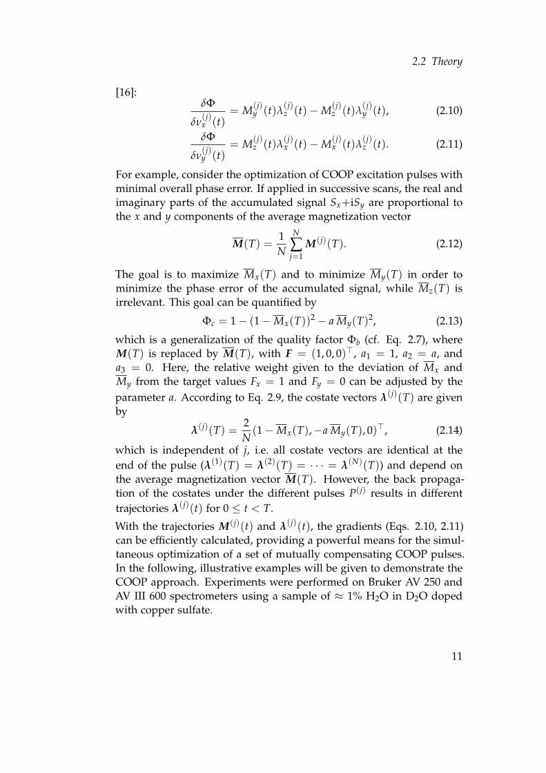
same result. However, initially it was by no means clear if this is in factthe best possible strategy. As the COOP approach is not limited to arestricted set of solutions (e.g. pairs of saturation pulses), it is also ableto find unexpected solutions if they exist, as will be shown in the nextexamples.
0 50
0
360
t [µs]
ϕ(1
)[d
eg]
A
0 50
0
360
t [µs]
ϕ(2
)[d
eg]
B
−10 10−1
1
first pulse
νoff [kHz]
M(1
)
−10 10−1
1
second pulse
νoff [kHz]
M(2
)
−10 10−1
1
average magnetization
νoff [kHz]
M
C D E
Figure 2.1: Two-step COOP cycle for the complete elimination of the av-erage magnetization vector M for offsets in the range of ±10kHz for a constant rf amplitude νr f = 10 kHz and a pulse du-ration of 50 µs. A and B show the phase modulations ϕ(1)(t)and ϕ(2)(t), simulated offset-profiles of M(1)(T), M(2)(T)and M(T) are drawn in C, D and E. The x, y and z com-ponents are plotted as solid black, dashed gray and solidgray curves, respectively.
2.3.2 Band-selective excitation pulses
As a second example, we consider band-selective COOP pulses thatexcite magnetization in a defined offset range and simultaneously elim-inate the average magnetization vector in other offset ranges. We use
13
2 Multi-scan cooperative pulses
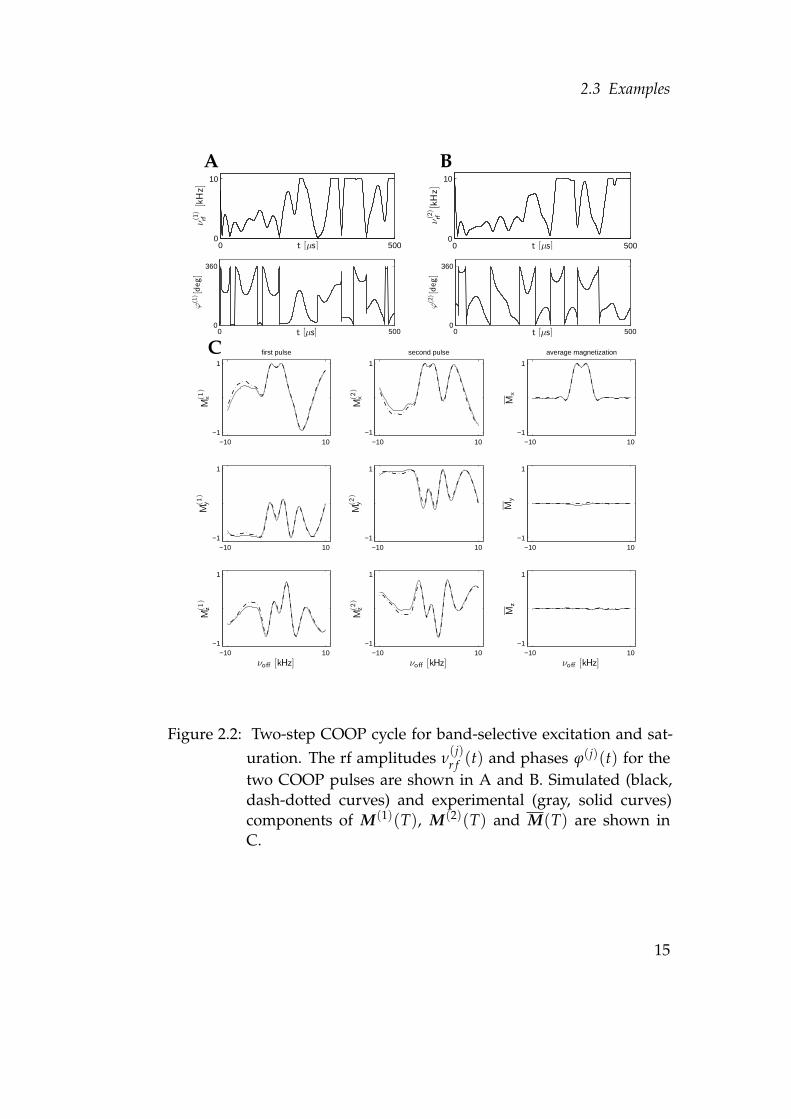
the quality factor Φb (Eq. 2.7) for various offset-dependent target statesF(νo f f ). Here we consider the example where F(νo f f ) = (1, 0, 0)> for|νo f f | ≤ 2 kHz (the “pass band”) and F(νo f f ) = (0, 0, 0)> for 2 kHz< |νo f f | ≤ 10 kHz (the “stop band”) . The pulse duration T andthe maximum rf amplitude νmax
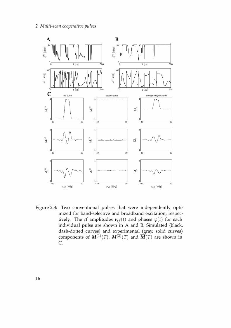
r f were set to 500 µs and 10 kHz, re-spectively. In contrast to the first example, in this case the COOP opti-mization yields two different pulses that are not simply related by anoverall phase shift (Fig. 2.2). Figure 2.2 also shows the simulated andexperimental final magnetization components created by the individualpulses and the average magnetization vector. While the response of theindividual COOP pulses appears to be erratic, the cancelation of the un-desired terms is almost perfect. An excellent match is found betweenexperimental (gray) and simulated (black) data.For comparison, Fig. 2.3 shows the results of a conventional approachbased on two individually optimized pulses: a broadband pulse witha target state F1(νo f f ) = (1, 0, 0)> for |νo f f | ≤ 10 kHz and a band-selective pulse with F2(νo f f ) = (1, 0, 0)> for |νo f f | ≤ 2 kHz and F2(νo f f ) =(−1, 0, 0)> for 2 kHz < |νo f f | ≤ 10 kHz. These pulses also yield thedesired average magnetization profile. Very good suppression of thex component is achieved by this approach in the stop band. However,large residual y and z components of the average magnetization vectorof more than 40% remain in the vicinity of the transition regions at ±2kHz (see Fig. 2.3). In contrast, using the the COOP approach, the unde-sired y and z components can be almost completely suppressed in thepass band, the stop band as well as in the transition region (cf. Fig. 2.2).Similar results were found for band-selective inversion pulses and dif-ferent ranges of pass and stop bands (data not shown). It is interestingto note that in the case of band-selective inversion (and complete elimi-nation of the average magnetization vector in the stop band), the COOPapproach resulted in two very similar pulses with a relative phase shiftof 180◦. In this case, the target profile of the average magnetization vec-tor can be approached by a pulse that inverts the magnetization in thepass band and brings it into the transverse plane in the stop band. Byrepeating the pulse with a phase shift of 180◦, all transverse magnetiza-tion components are perfectly canceled. Hence in this case, the COOPapproach yields a solution that could also be constructed using a con-ventional optimization of a single pulse combined with a phase cycle.
14
2.3 Examples
0 5000
10
t [µs]
ν(1
)rf
[kH
z]
A
0 5000
10
t [µs]
ν(2
)rf
[kH
z]
B
0 5000
360
t [µs]
ϕ(1
)[d
eg]
0 5000
360
t [µs]
ϕ(2
)[d
eg]
−10 10−1
1
first pulse
M(1)
x
−10 10−1
1
second pulseM
(2)
x
−10 10−1
1
average magnetization
Mx
−10 10−1
1
M(1)
y
−10 10−1
1
M(2)
y
−10 10−1
1
My
−10 10−1
1
νoff [kHz]
M(1)
z
−10 10−1
1
νoff [kHz]
M(2)
z
−10 10−1
1
νoff [kHz]
Mz
C
Figure 2.2: Two-step COOP cycle for band-selective excitation and sat-uration. The rf amplitudes ν
(j)r f (t) and phases ϕ(j)(t) for the
two COOP pulses are shown in A and B. Simulated (black,dash-dotted curves) and experimental (gray, solid curves)components of M(1)(T), M(2)(T) and M(T) are shown inC.
15
2 Multi-scan cooperative pulses
0 5000
10
t [µs]
ν(1
)rf
[kH
z]
A
0 5000
10
t [µs]
ν(2
)rf
[kH
z]
B
0 5000
360
t [µs]
ϕ(1
)[d
eg]
0 5000
360
t [µs]
ϕ(2
)[d
eg]
−10 10−1
1
first pulse
M(1)
x
−10 10−1
1
second pulse
M(2)
x
−10 10−1
1
average magnetization
Mx
−10 10−1
1
M(1)
y
−10 10−1
1
M(2)
y
−10 10−1
1
My
−10 10−1
1
νoff [kHz]
M(1)
z
−10 10−1
1
νoff [kHz]
M(2)
z
−10 10−1
1
νoff [kHz]
Mz
C
Figure 2.3: Two conventional pulses that were independently opti-mized for band-selective and broadband excitation, respec-tively. The rf amplitudes νr f (t) and phases ϕ(t) for eachindividual pulse are shown in A and B. Simulated (black,dash-dotted curves) and experimental (gray, solid curves)components of M(1)(T), M(2)(T) and M(T) are shown inC.
16
2.3 Examples
However, it was by no means obvious before that this approach yieldsthe optimal solution, which is in fact very different from the naive ap-proach of combining individually optimized pulses for band-selectiveand broadband inversion.
2.3.3 Broadband excitation of x magnetization with minimum phaseerror
Here we ask the question of whether the duration of broadband exci-tation pulses can be reduced using the COOP approach. In order toavoid phase errors in the resulting spectrum, a single pulse for broad-band excitation of x magnetization is not allowed to create significanty components in the desired offset range. In contrast, the creation ofrelatively large y components |M(j)
y (T)| by the individual members ofa cycle of COOP excitation pulses is acceptable, provided |My(T)| issmall (and Mx(T) is large). This provides additional degrees of free-dom in the optimization.As a concrete example, we consider the optimal excitation of x mag-netization with minimal phase errors in an offset range of ±20 kHzwith a maximum rf amplitude of νmax
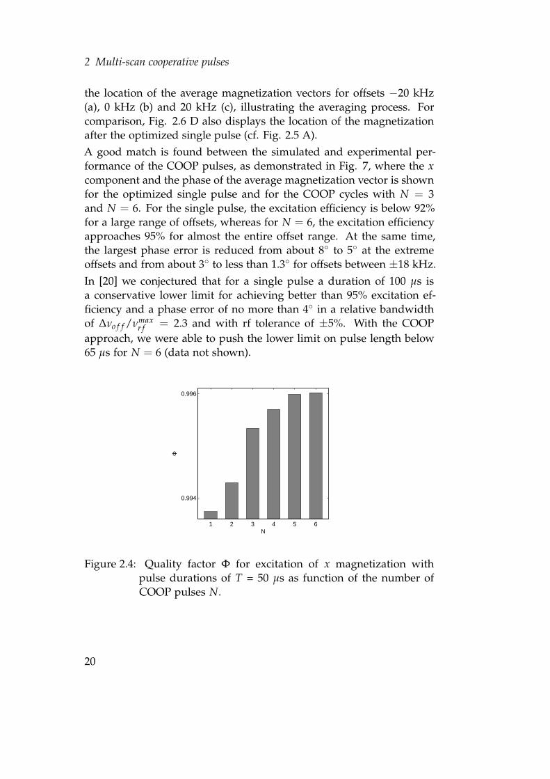
r f = 17.5 kHz [16, 19, 20] and a ro-bustness with respect to variations of the rf amplitude of ±5%. For thisproblem, the duration of efficient optimal control based pulses could bereduced from 2 ms [16] to 500 µs [19] by generalizing the algorithm totake rf limit limits into account during the optimization. Subsequently,the pulse duration could be reduced even further to only 125 µs [20] byusing a quality factor similar to Φc (Eq. 2.13) for N = 1 that is betteradapted to the problem of excitation with minimal phase errors thanquality factors based on Φa (Eq. 2.6).For the same specifications, we optimized a single pulse (N = 1) andCOOP cycles (N > 1) using the quality factor Φc (Eq. 2.13). The numer-ically determined quality factor Φc (Eq. 2.13 with a = 1) of the single125 µs long pulse from [20] is Φc =0.999852. The gradient of the qualityfactor for the COOP pulse optimization can be efficiently approximatedto first order using Eqs. 2.10 – 2.11, where λ(j)(T) is given by Eq. 2.14.For example, for a three-step COOP cycle, a comparable quality factor(Φc = 0.999856) can be achieved with a reduced duration of only 100µs of each individual pulse. Hence, in this case it is possible to reduce
17
2 Multi-scan cooperative pulses
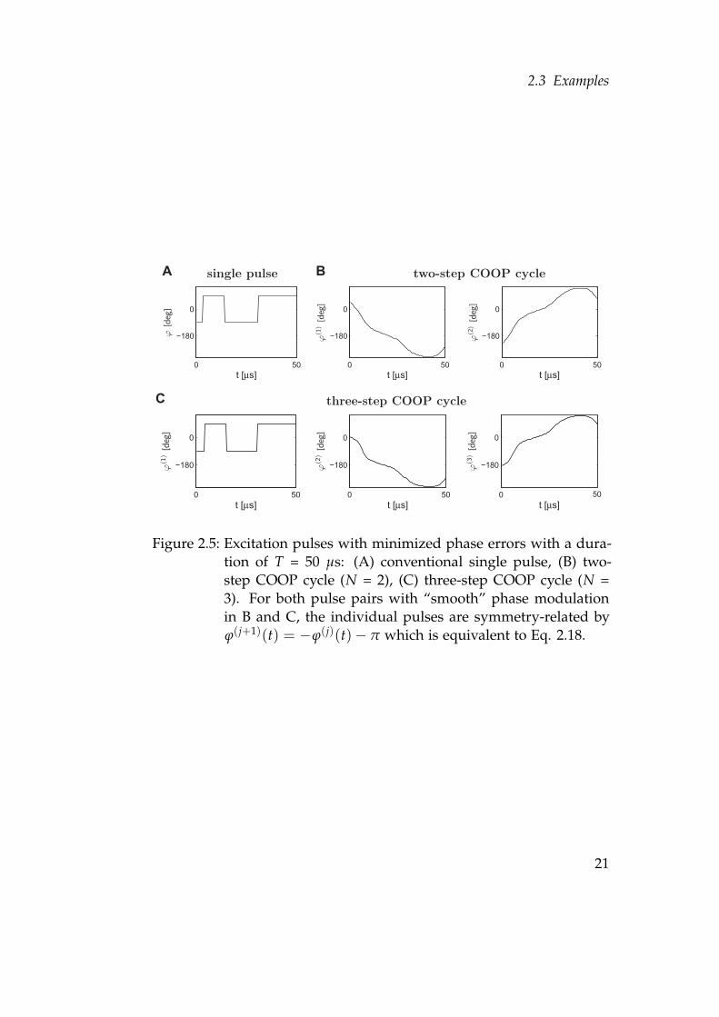
the duration of excitation pulses by an additional 20% without loss inpulse performance using the COOP approach. The x component of theexcited average magnetization vector is about 0.99, and the phase erroris less than 0.4◦ for the entire offset range of 40 kHz.In order to explore the performance limit of even shorter pulses, wealso optimized single and COOP pulses with a duration of T = 50 µs,which is only 3.5 times longer than the duration of a hard 90◦ pulsefor an rf amplitude of 17.5 kHz. Fig. 2.4 shows the achieved qualityfactors for a single pulse (N = 1) and for COOP cycles with N between2 and 6. The optimized pulses for N = 1, 2, and 3 are shown in Fig.2.5. All pulses have constant amplitude, taking full advantage of themaximum allowed rf amplitude of νmax
r f =17.5 kHz. The optimal singlepulse (N = 1) shown in Fig. 2.5 A is purely phase-alternating withphases ±π/2. This class of phase-alternating pulses implies the fol-lowing symmetry relations for the x and y components of the excitedmagnetization vectors at offsets ±ν [4]:
Mx(ν) = Mx(−ν), (2.16)
My(ν) = −My(−ν). (2.17)
(In additon, Mz(ν) = Mz(−ν), however, this is not relevant here, as Φchas no explicit Mz dependence, cf. Eq. 2.13.) The symmetry relationsfor the x and the y components of the final magnetization vectors matchthe symmetry of the problem: Maximum Mx(ν) is desired both for pos-itive offsets (between 0 and 20 kHz) and for negative offsets (between0 and −20 kHz), and, according to Eq. 2.16, a large Mx(ν) implies anequally large Mx(−ν). In addition, |My|(ν) ≈ 0 is desired both for pos-itive and negative offsets, and, according to Eq. 2.17, a small |My|(ν) atfrequency ν implies an equally small |My|(−ν).In contrast to the case N = 1, the individual COOP pulses for N = 2shown in Fig. 2.5 B are not phase-alternating but have smooth phasemodulations. However, the phase modulations are not independent butare related by phase inversion and an additional phase shift by π:
ϕ(2)(t) = −ϕ(1)(t) + π, (2.18)
corresponding to a reflection of the phase around π/2. (In terms of thex and y components of the rf amplitudes, this relation corresponds to
18
2.3 Examples
ν(2)x = −ν
(1)x and ν
(2)y = ν
(1)y .) Applying well-known principles of pulse
sequence analysis [4], it is straightforward to show that Eq. 2.18 impliesthe following symmetry relations between the transverse componentsof the excited magnetization vectors after the first and second pulse:
M(2)x (ν) = M(1)
x (−ν), (2.19)
M(2)y (ν) = −M(1)
y (−ν) (2.20)
(and in addition M(2)z (ν) = M(1)
z (−ν)). As a direct consequence of Eqs.2.19 and 2.20, the transverse components of the average magnetizationvector after the two-step COOP cycle are related by
Mx(ν) = Mx(−ν), (2.21)
My(ν) = −My(−ν). (2.22)
which is analogous to the relations in Eqs. 2.16 and 2.17 for a singlephase-alternating pulse and which matches the symmetry of the prob-lem as discussed above. The symmetry relations for the average trans-verse magnetization components (Eqs. 2.21 and 2.22) can always berealized if the N-step COOP cycle consists of symmetry-related pulsepairs (with phase relations corresponding to Eq. 2.18) and/or phase-alternating pulses with phases ±π/2. For example, the three-step COOPcycle consists of one symmetry-related pulse pair and one phase-alter-nating pulse (see Fig. 2.5 C). For N = 4, 5, and 6, we always find twosymmetry-related pulse pairs and an according number of phase-alter-nating pulses.Fig. 2.6 shows the location of the individual and of the average magne-tization vectors in the y-z plane after the three-step COOP cycle (N = 3)(cf. Fig. 2.5 C). The points denoted a, b, and c correspond to offsetsof −20 kHz, 0 kHz and 20 kHz, respectively. Figs. 2.6 B and C illus-trate the symmetry relations of Eqs. 2.16, 2.17 and of Eqs. 2.21, 2.22.Relatively large y components of up to 40% are found for each individ-ual pulse, illustrating the additional degrees of freedom gained by theCOOP approach. However, the average magnetization vectors are lo-cated very close to the x-z plane as shown in Fig. 2.6 E. In Fig. 2.6 F, thecorners of the triangles represent the locations of the magnetization vec-tors after the individual pulses and the centers of the triangles indicate
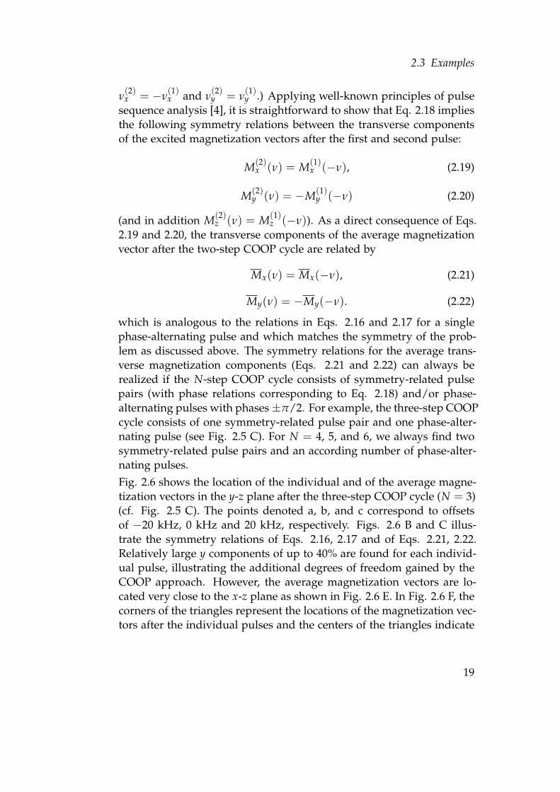
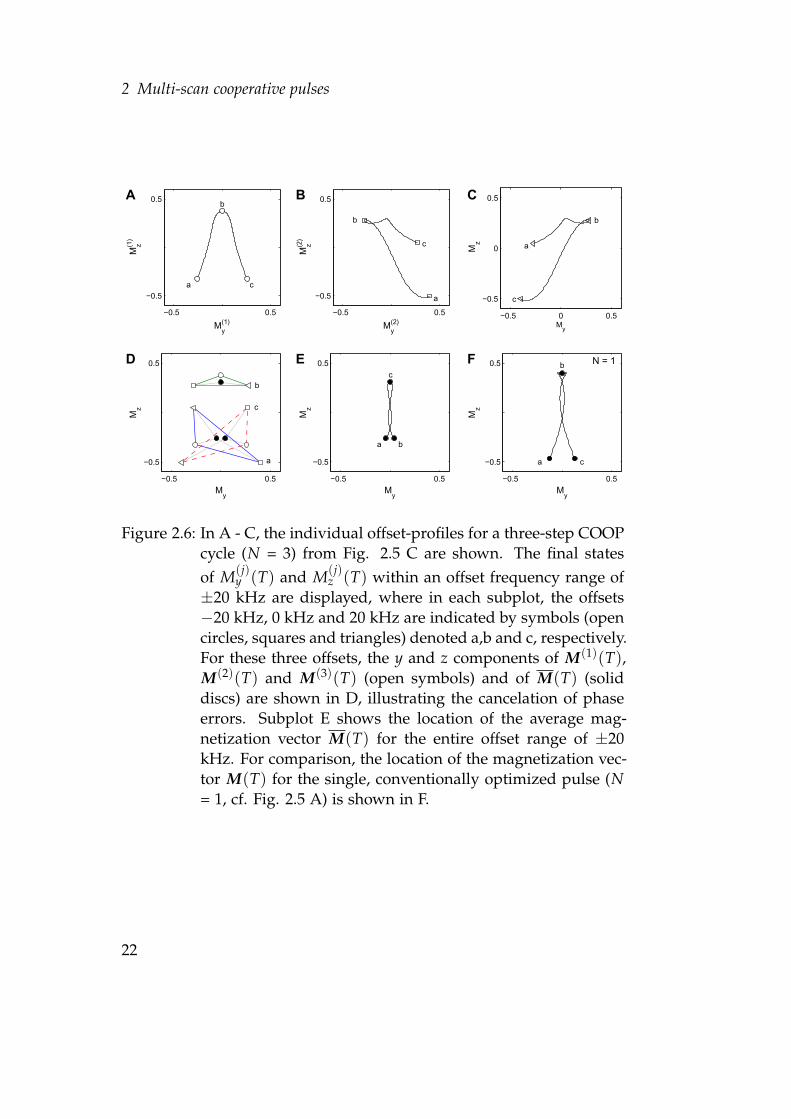
19
2 Multi-scan cooperative pulses
the location of the average magnetization vectors for offsets −20 kHz(a), 0 kHz (b) and 20 kHz (c), illustrating the averaging process. Forcomparison, Fig. 2.6 D also displays the location of the magnetizationafter the optimized single pulse (cf. Fig. 2.5 A).A good match is found between the simulated and experimental per-formance of the COOP pulses, as demonstrated in Fig. 7, where the xcomponent and the phase of the average magnetization vector is shownfor the optimized single pulse and for the COOP cycles with N = 3and N = 6. For the single pulse, the excitation efficiency is below 92%for a large range of offsets, whereas for N = 6, the excitation efficiencyapproaches 95% for almost the entire offset range. At the same time,the largest phase error is reduced from about 8◦ to 5◦ at the extremeoffsets and from about 3◦ to less than 1.3◦ for offsets between ±18 kHz.In [20] we conjectured that for a single pulse a duration of 100 µs isa conservative lower limit for achieving better than 95% excitation ef-ficiency and a phase error of no more than 4◦ in a relative bandwidthof ∆νo f f /νmax
r f = 2.3 and with rf tolerance of ±5%. With the COOPapproach, we were able to push the lower limit on pulse length below65 µs for N = 6 (data not shown).
1 2 3 4 5 6
0.994
0.996
N
Φ
Figure 2.4: Quality factor Φ for excitation of x magnetization withpulse durations of T = 50 µs as function of the number ofCOOP pulses N.
20
2.3 Examples
Author's personal copy
for the x and y components of the excited magnetization vectors atoffsets ±m [2]:
MxðmÞ ¼ Mxð�mÞ; ð16ÞMyðmÞ ¼ �Myð�mÞ: ð17Þ
(In additon, Mz(m) = Mz(�m), however this is not relevant here, as Uc
has no explicit Mz dependence, c.f. Eq. (13).) The symmetry relationsfor the x and the y components of the final magnetization vectorsmatch the symmetry of the problem: Maximum Mx(m) is desiredboth for positive offsets (between 0 and 20 kHz) and for negativeoffsets (between 0 and �20 kHz), and, according to Eq. (16), a largeMx(m) implies an equally large Mx(�m). In addition, jMyj(m) � 0 is de-sired both for positive and negative offsets, and, according to Eq.(17), a small jMyj(m) at frequency m implies an equally smalljMyj(�m).
In contrast to the case N = 1, the individual COOP pulses forN = 2 shown in Fig. 5B are not phase-alternating but have smoothphase modulations. However, the phase modulations are not
independent but are related by phase inversion and an additionalphase shift by p:
uð2ÞðtÞ ¼ �uð1ÞðtÞ þ p; ð18Þ
corresponding to a reflection of the phase around p/2. (In terms ofthe x and y components of the rf amplitudes, this relation corre-sponds to mð2Þx ¼ �mð1Þx and mð2Þy ¼ mð1Þy .) Applying well known princi-ples of pulse sequence analysis [2], it is straightforward to showthat Eq. (18) implies the following symmetry relations betweenthe transverse components of the excited magnetization vectorsafter the first and second pulse:
Mð2Þx ðmÞ ¼ Mð1Þ
x ð�mÞ; ð19ÞMð2Þ
y ðmÞ ¼ �Mð1Þy ð�mÞ ð20Þ
(and in additon Mð2Þz ðmÞ ¼ Mð1Þ
z ð�mÞ). As a direct consequence of Eqs.(19) and (20), the transverse components of the average magnetiza-tion vector after the two-step COOP cycle are related by
MxðmÞ ¼ Mxð�mÞ; ð21ÞMyðmÞ ¼ �Myð�mÞ: ð22Þ
which is analogous to the relations in Eqs. (16) and (17) for asingle phase-alternating pulse and which matches the symmetryof the problem as discussed above. The symmetry relations forthe average transverse magnetization components (Eqs. (21) and(22)) can always be realized if the N-step COOP cycle consists ofsymmetry-related pulse pairs (with phase relations correspondingto Eq. (18)) and/or phase-alternating pulses with phases ±p/2. Forexample, the three-step COOP cycle consists of one symmetry-re-lated pulse pair and one phase-alternating pulse (see Fig. 5C). ForN = 4, 5, and 6, we always find two symmetry-related pulse pairsand an according number of phase-alternating pulses.
Fig. 6 shows the location of the individual and of the averagemagnetization vectors in the y-z plane after the three-step COOPcycle (N = 3) (c.f. Fig. 5C). The points denoted a, b, and c correspondto offsets of �20 kHz, 0 kHz and 20 kHz, respectively. Figs. 6B and Cillustrate the symmetry relations of Eqs. (16), (17) and of Eqs. (21),(22). Relatively large y components of up to 40% are found for eachindividual pulse, illustrating the additional degrees of freedomgained by the COOP approach. However, the average magnetization
1 2 3 4 5 6
0.994
0.996
N
Φ
Fig. 4. Quality factor U for excitation of x magnetization with pulse durations ofT = 50 ls as function of the number of COOP pulses N.
A
C
B
Fig. 5. Excitation pulses with minimized phase errors with a duration of T = 50 ls: (A) conventional single pulse, (B) two-step COOP cycle (N = 2), (C) three-step COOP cycle(N = 3). For both pulse pairs with ‘‘smooth” phase modulation in B and C, the individual pulses are symmetry-related by u(j+1)(t) = �u(j)(t) � p which is equvalent to Eq. (18).
M. Braun, S.J. Glaser / Journal of Magnetic Resonance 207 (2010) 114–123 119
Figure 2.5: Excitation pulses with minimized phase errors with a dura-tion of T = 50 µs: (A) conventional single pulse, (B) two-step COOP cycle (N = 2), (C) three-step COOP cycle (N =3). For both pulse pairs with “smooth” phase modulationin B and C, the individual pulses are symmetry-related byϕ(j+1)(t) = −ϕ(j)(t)− π which is equivalent to Eq. 2.18.
21
2 Multi-scan cooperative pulsesAuthor's personal copy
vectors are located very close to the x-z plane as shown in Fig. 6E.In Fig. 6D, the corners of the triangles represent the locations of themagnetization vectors after the individual pulses and the centersof the triangles indicate the location of the average magnetizationvectors for offsets �20 kHz (a), 0 kHz (b) and 20 kHz (c), illustrat-ing the averaging process. For comparison, Fig. 6F also displaysthe location of the magnetization after the optimized single pulsepulse (c.f. Fig. 5A).
A good match is found between the simulated and experimentalperformance of the COOP pulses, as demonstrated in Fig. 7, wherethe x component and the phase of the average magnetization vec-tor is shown for the optimized single pulse and for the COOP cycles
with N = 3 and N = 6. For the single pulse, the excitation efficiencyis below 92% for a large range of offsets, whereas for N = 6, the exci-tation efficiency approaches 95% for almost the entire offset range.At the same time, the largest phase error is reduced from about 8�to 5� at the extreme offsets and from about 3� to less than 1.3� foroffsets between ±18 kHz.
In [18] we conjectured that for a single pulse a duration of100 ls is a conservative lower limit for achieving better than 95%excitation efficiency and a phase error of no more than 4� in a rel-ative bandwidth of Dmoff =mmax
rf ¼ 2:3 and with rf tolerance of ±5%.With the COOP approach, we were able to push the lower limiton pulse length below 65 ls for N = 6 (data not shown).
−0.5 0.5
−0.5
0.5
My(1)
Mz(1
)
ca
b
−0.5 0.5
−0.5
0.5
My(2)
Mz(2
) c
b
a
−0.5 0 0.5
−0.5
0
0.5
My
b
a
c
−0.5 0.5
−0.5
0.5
My
Mz
b
c
a
−0.5 0.5
−0.5
0.5
My
Mz
a b
c
−0.5 0.5
−0.5
0.5
Mz
Mz
My
N = 1
a
b
c
A B C
D E F
Fig. 6. In A–C, the individual offset-profiles for a three-step COOP cycle (N = 3) from Fig. 5C are shown. The final states of MðjÞy ðTÞ and MðjÞ
z ðTÞ within an offset frequency rangeof ±20 kHz are displayed, where in each subplot, the offsets �20 kHz, 0 kHz and 20 kHz are indicated by symbols (open circles, squares and triangles) denoted a, b and c,respectively. For these three offsets, the y and z components of M(1)(T), M(2)(T) and M(3)(T) (open symbols) and of MðTÞ (solid discs) are shown in D, illustrating thecancellation of phase errors. Subplot E shows the location of the average magnetization vector MðTÞ for the entire offset range of ±20 kHz. For comparison, the location of themagnetization vector M(T) for the single, conventionally optimized pulse N = 1, c.f. Fig. 5A is shown in F.
Fig. 7. Simulated and experimental offset-profiles for the average magnetization MxðTÞ and the phase error p(T) for a single pulse (N = 1, c.f. Fig. 5A) and COOP cycles withN = 3 (c.f. Fig. 5C) and N = 6.
120 M. Braun, S.J. Glaser / Journal of Magnetic Resonance 207 (2010) 114–123
Figure 2.6: In A - C, the individual offset-profiles for a three-step COOPcycle (N = 3) from Fig. 2.5 C are shown. The final statesof M(j)
y (T) and M(j)z (T) within an offset frequency range of
±20 kHz are displayed, where in each subplot, the offsets−20 kHz, 0 kHz and 20 kHz are indicated by symbols (opencircles, squares and triangles) denoted a,b and c, respectively.For these three offsets, the y and z components of M(1)(T),M(2)(T) and M(3)(T) (open symbols) and of M(T) (soliddiscs) are shown in D, illustrating the cancelation of phaseerrors. Subplot E shows the location of the average mag-netization vector M(T) for the entire offset range of ±20kHz. For comparison, the location of the magnetization vec-tor M(T) for the single, conventionally optimized pulse (N= 1, cf. Fig. 2.5 A) is shown in F.
22
2.3 Examples
0.9
1
Mx
−20 20
−5
5
νoff
[kHz]
φ[d
eg]
1 3
6
simulation
0.9
1
−20 20
−5
0
5
νoff
[kHz]
experiment
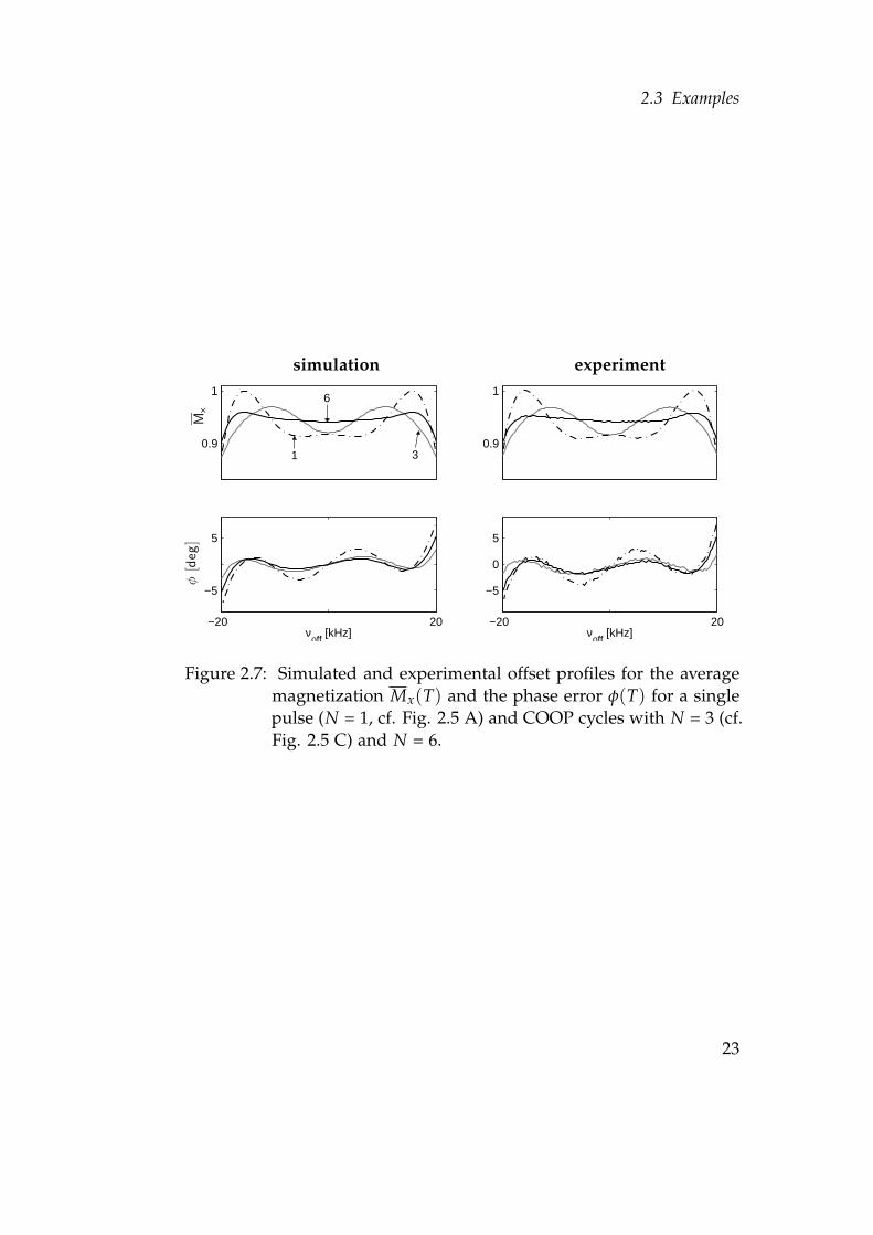
Figure 2.7: Simulated and experimental offset profiles for the averagemagnetization Mx(T) and the phase error φ(T) for a singlepulse (N = 1, cf. Fig. 2.5 A) and COOP cycles with N = 3 (cf.Fig. 2.5 C) and N = 6.
23
2 Multi-scan cooperative pulses
2.3.4 Broadband excitation with linear offset dependence of phase
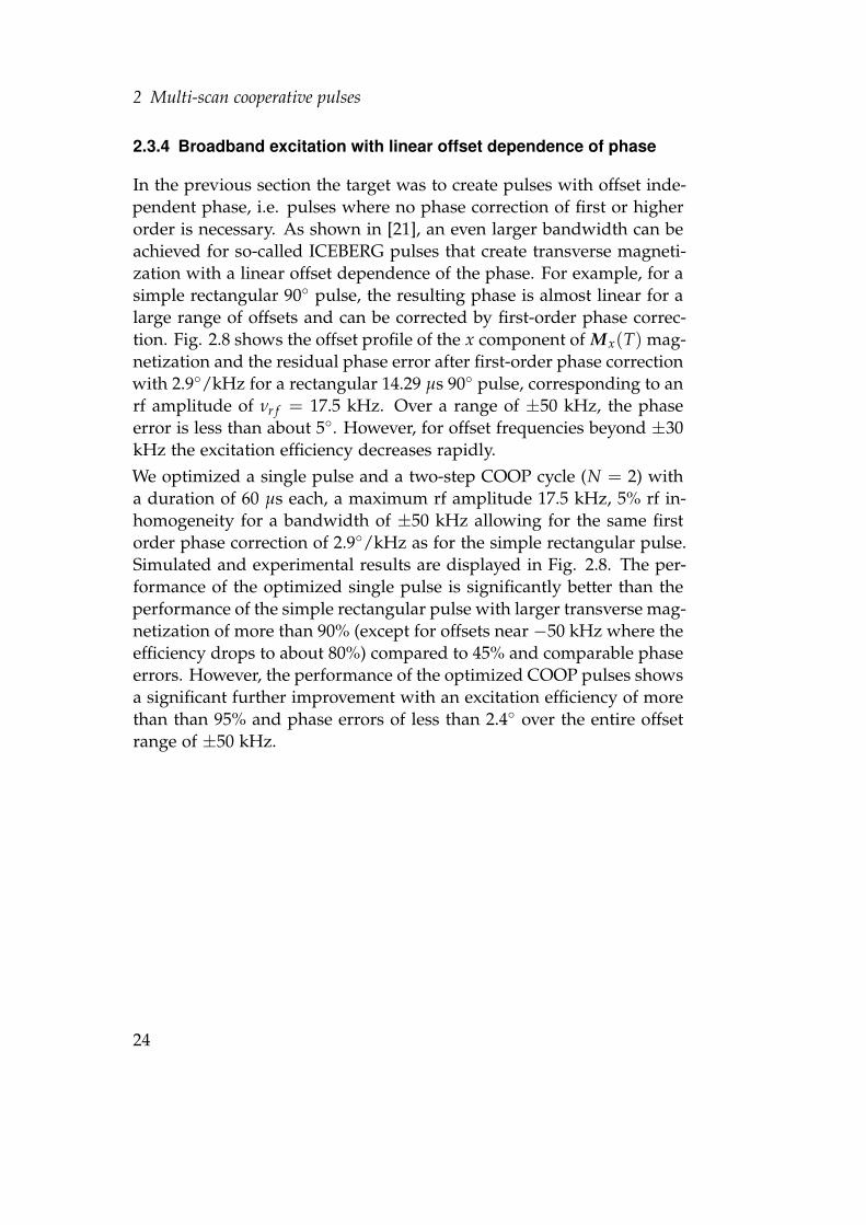
In the previous section the target was to create pulses with offset inde-pendent phase, i.e. pulses where no phase correction of first or higherorder is necessary. As shown in [21], an even larger bandwidth can beachieved for so-called ICEBERG pulses that create transverse magneti-zation with a linear offset dependence of the phase. For example, for asimple rectangular 90◦ pulse, the resulting phase is almost linear for alarge range of offsets and can be corrected by first-order phase correc-tion. Fig. 2.8 shows the offset profile of the x component of Mx(T) mag-netization and the residual phase error after first-order phase correctionwith 2.9◦/kHz for a rectangular 14.29 µs 90◦ pulse, corresponding to anrf amplitude of νr f = 17.5 kHz. Over a range of ±50 kHz, the phaseerror is less than about 5◦. However, for offset frequencies beyond ±30kHz the excitation efficiency decreases rapidly.We optimized a single pulse and a two-step COOP cycle (N = 2) witha duration of 60 µs each, a maximum rf amplitude 17.5 kHz, 5% rf in-homogeneity for a bandwidth of ±50 kHz allowing for the same firstorder phase correction of 2.9◦/kHz as for the simple rectangular pulse.Simulated and experimental results are displayed in Fig. 2.8. The per-formance of the optimized single pulse is significantly better than theperformance of the simple rectangular pulse with larger transverse mag-netization of more than 90% (except for offsets near −50 kHz where theefficiency drops to about 80%) compared to 45% and comparable phaseerrors. However, the performance of the optimized COOP pulses showsa significant further improvement with an excitation efficiency of morethan than 95% and phase errors of less than 2.4◦ over the entire offsetrange of ±50 kHz.
24
2.3 Examples
0.5
1
M′ x
−50 50
5
−5
νoff
[kHz]
∆φ
[deg
]
A
0.5
1
M′ x
−50 50
−5
0
5
νoff
[kHz]
B
0.5
1
M′ x
−50 50
−5
0
5
νoff
[kHz]
C
Figure 2.8: Offset profiles for M′x and phase deviation ∆φ for a single
rectangular pulse (A), an optimized individual ICEBERGpulse [21] with N = 1 (B, cf. dash-dotted curve in Fig. 2.9)and a two-step COOP cycle (N = 2) (C, cf. solid curves inFig. 2.9). M′
x is the x component of M(T) and ∆φ is theresidual phase error after a first-order phase correction of2.9◦/kHz. Solid gray and dash-dotted black curves repre-sent experimental and simulated data.
25
2 Multi-scan cooperative pulses
0 60
−360
90360
t [µs]
ϕ[d
eg]
N = 1
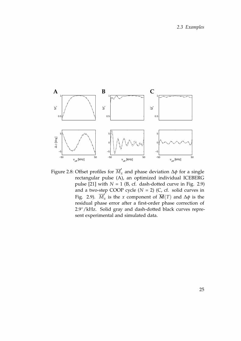
Figure 2.9: A single (dash-dotted gray curve) ICEBERG and a two-step(N = 2) COOP ICEBERG cycle (solid black curves). For theCOOP pulse pair the symmetry relation from Eq. 2.18 isapproximately fulfilled.
26
2.3 Examples
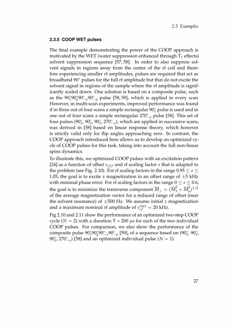
2.3.5 COOP WET pulses
The final example demonstrating the power of the COOP approach ismotivated by the WET (water suppression enhanced through T1 effects)solvent suppression sequence [57, 58]. In order to also suppress sol-vent signals in regions away from the center of the rf coil and there-fore experiencing smaller rf amplitudes, pulses are required that act asbroadband 90◦ pulses for the full rf amplitude but that do not excite thesolvent signal in regions of the sample where the rf amplitude is signif-icantly scaled down. One solution is based on a composite pulse, suchas the 90◦x90◦y90◦−x90◦−y pulse [58, 59], which is applied in every scan.However, in multi-scan experiments, improved performance was foundif in three out of four scans a simple rectangular 90◦x pulse is used and inone out of four scans a simple rectangular 270◦−x pulse [58]. This set offour pulses (90◦x, 90◦x, 90◦x, 270◦−x), which are applied in successive scans,was derived in [58] based on linear response theory, which howeveris strictly valid only for flip angles approaching zero. In contrast, theCOOP approach introduced here allows us to develop an optimized cy-cle of COOP pulses for this task, taking into account the full non-linearspins dynamics.To illustrate this, we optimized COOP pulses with an excitation pattern[24] as a function of offset νo f f and rf scaling factor s that is adapted tothe problem (see Fig. 2.10). For rf scaling factors in the range 0.95 ≤ s ≤1.05, the goal is to excite x magnetization in an offset range of ±5 kHzwith minimal phase error. For rf scaling factors in the range 0 ≤ s ≤ 0.6,the goal is to minimize the transverse component M⊥ = (M2
x + M2y)1/2
of the average magnetization vector for a reduced range of offset (nearthe solvent resonance) of ±500 Hz. We assume initial z magnetizationand a maximum nominal rf amplitude of νmax
r f = 20 kHz.
Fig 2.10 and 2.11 show the performance of an optimized two-step COOPcycle (N = 2) with a duration T = 200 µs for each of the two individualCOOP pulses. For comparison, we also show the performance of thecomposite pulse 90◦x90◦y90◦−x90◦−y [59], of a sequence based on (90◦x, 90◦x,90◦x, 270◦−x) [58] and an optimized individual pulse (N = 1).
27
2 Multi-scan cooperative pulses
0.98
0.98
0.5
0.1
0.1
0.001
νoff
[kHz]
s
−5 0 50
0.5
1
A 90◦x90◦y90◦−x90◦−y
0.98
0.5
0.1
0.001
νoff
[kHz]s
−5 0 50
0.5
1
B 90◦x; 90◦x; 90◦x; 270◦−x
0.98
0.5
0.50.98
0.98
0.1
0.001
νoff
[kHz]
s
−5 0 50
0.5
1
C single optimized pulse
0.98
0.50.1
0.001
νoff
[kHz]
s
−5 0 50
0.5
1
D COOP (N = 2)
Figure 2.10: Comparison of the average transverse magnetization as afunction of offset νo f f and rf scaling s for a two-step cycleof COOP WET pulses (D, N = 2) with the 90◦x90◦y90◦−x90◦−ycomposite pulse (A, [59]), the four-scan sequence based on90◦x; 90◦x; 90◦x; 270◦−x (B, [58]) and an optimized individualpulse (C, N = 1). The areas for which optimal excitationand optimal suppression of transverse magnetization aredesired are indicated by black and white dashed rectan-gles.
28
2.3 Examples
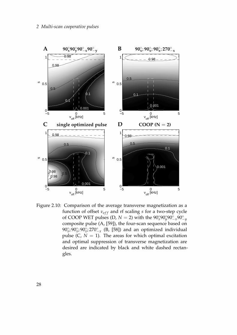
0 0.6 10
1
s
M⊥
Figure 2.11: Slices from Fig. 2.10 A (dotted), B (dash-dotted), C (dashed)and D (solid curve) for the on resonance case. The graysquares and black discs represent experimental data for theconventionally optimized pulse and the two-step COOPWET cycle from Fig. 2.10 C and D, respectively.
29
2 Multi-scan cooperative pulses
2.4 Discussion and conclusion
In this chapter, we introduced the concept of simultaneously optimizedpulses that act in a cooperative way, compensating each other’s imper-fections. Although for simplicity only examples involving uncoupledspins were considered, it is important to note that the COOP approachcan also be applied to coupled spin systems. With the help of gener-alized optimal control based algorithms, such as the presented variantof the GRAPE (gradient ascent pulse engineering) algorithm, COOPpulses can be efficiently optimized.Although the COOP approach is not limited to multi-scan experiments,here we focussed on applications where different members of a COOPcycle are used in different scans. In such multi-scan experiments, theCOOP approach can be viewed as complementing and/or generaliz-ing phase cycling [45–48] and difference spectroscopy. In conventionalphase cycling, identical pulses are applied in each scan, up to an overallphase shift. In section 2.3.1, the optimal COOP cycle also consisted ofpulses that were identical up to an overall phase shift. Hence, it is pos-sible to automatically generate phase cycles using the COOP approach.However, it is important to point out that here it was not possible toachieve the target of the optimization by considering coherence orderpathways alone. Hence, the COOP solution relied on the simultaneousoptimization of specific pulse shapes (saturation pulses) in combinationwith the resulting simple phase cycle. As demonstrated in sections 2.3.2– 2.3.5, COOP pulses are in general not simply related by overall phaseshifts. In the presented COOP examples, a constant receiver phase wasassumed. However, it is straightforward to lift this restriction by addingone additional control for the receiver phase for increased flexibilityas in conventional phase cycles or in difference spectroscopy. In con-ventional difference spectroscopy, often different pulses are applied insuccessive scans. However, these pulses are typically either simple rect-angular pulses or are optimized for each individual scan, not takingadvantage of the full flexibility of the COOP approach introduced here.For example, this was illustrated in section 2.3.5 for the problem ofsolvent suppression.Optimal control based techniques for the efficient optimization of com-plex COOP pulses open new avenues for pulse sequence optimization.
30
2.4 Discussion and conclusion
The goal of the presented examples was to illustrate the basic conceptand to point out potential applications of COOP pulses. For example,in section 2.3.5 it was demonstrated that the approach may be usefulfor water suppression techniques such as WET. However, for practicalsolvent suppression, it is necessary to adjust the design criteria for theoptimized COOP pulses, which is beyond the scope of the present the-sis. It is also important to point out that the presented algorithm for theoptimization of COOP pulses can be generalized in a straightforwardway to include relaxation effects [11, 22]. We hope that the presentedCOOP approach will find practical applications in NMR spectroscopyand imaging.
31

2 Multi-scan cooperative pulses
32
3 Single-scan cooperative pulses
In this chapter, we present the concept of single-scan cooperative (S2-COOP) pulses. In contrast to multi-scan COOP pulses that are appliedat the same position in different scans, S2-COOP pulses act in a singlescan and at different positions of a pulse sequence. S2-COOP pulsescan be efficiently optimized using an extended version of the gradientascent pulse engineering (GRAPE) algorithm. The advantage of the S2-COOP approach is demonstrated in theory and experiment for NOESY-type frequency-labeling blocks.
3.1 Introduction
In the previous chapter, we have shown that the physical limits of pulseperformance can be extended using the concept of cooperative (COOP)pulses that complements and generalizes phase-cycles [49]. In multi-scan experiments, COOP pulses can cancel undesired signal contribu-tions: At the same position of a pulse sequence, a different pulse isapplied in each scan so that the constituents of a so-called COOP cyclecan cancel each other’s imperfections. By taking advantage of the pos-sibility of error cancelation between several scans the optimization en-hances the overall fidelity of a selected transfer step in a pulse sequence.However, most NMR experiments rely on pulse sequences with severaldifferent transfer steps. Although it is possible to independently opti-mize different pulses before combining them to a pulse sequence [43]these pulses will only cancel each other’s errors by chance or will evenaccumulate each other’s errors in the course of a pulse sequence. There-fore, the demand on the fidelity of individually optimized pulses thatare grouped together to a pulse sequence is extraordinarily high. It hasbeen shown before how undesired effects of a precedent pulse can inpart be canceled out by a subsequent pulse [5, 56, 60]. There, in con-trast to the more flexible COOP approach, the precedent pulse remainsunchanged so that the subsequent pulse alone has to compensate the
33
3 Single-scan cooperative pulses
errors of the precedent pulse. Another approach to avoid error accu-mulation is optimal tracking [44] which has so far only been applied togenerate heteronuclear decoupling pulses. Here, we show that in con-trast to our earlier COOP approach where a single transfer is optimizedby taking advantage of error cancelation between several scans, it is pos-sible to optimize several transfers in a single scan. We dub this modifiedCOOP approach single-scan COOP (S2-COOP) which makes it possibleto further improve the performance of pulse sequences.
3.2 Theory
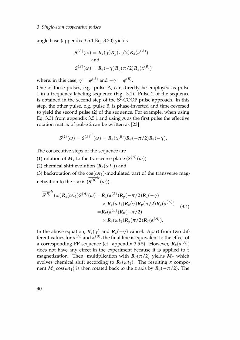
As a simple and illustrative example, we consider the frequency-labelingblock in a standard 2D NOESY experiment. Building-blocks of this kindare routinely used in multidimensional NMR experiments in order tocreate offset-frequency labelled z magnetization [50, 51]. In addition,they can be used as initial and final pulses in a modified INEPT blockwhere instead of the central 180◦ universal rotation (UR) pulses twopairs of PP inversion pulses are applied on both nuclei [61, 62]. Here,we will focus on the frequency-labeling block of a 2D NOESY experi-ment. In Fig. 3.1 (top) the pulse sequence of a 2D NOESY experimentis drawn schematically.
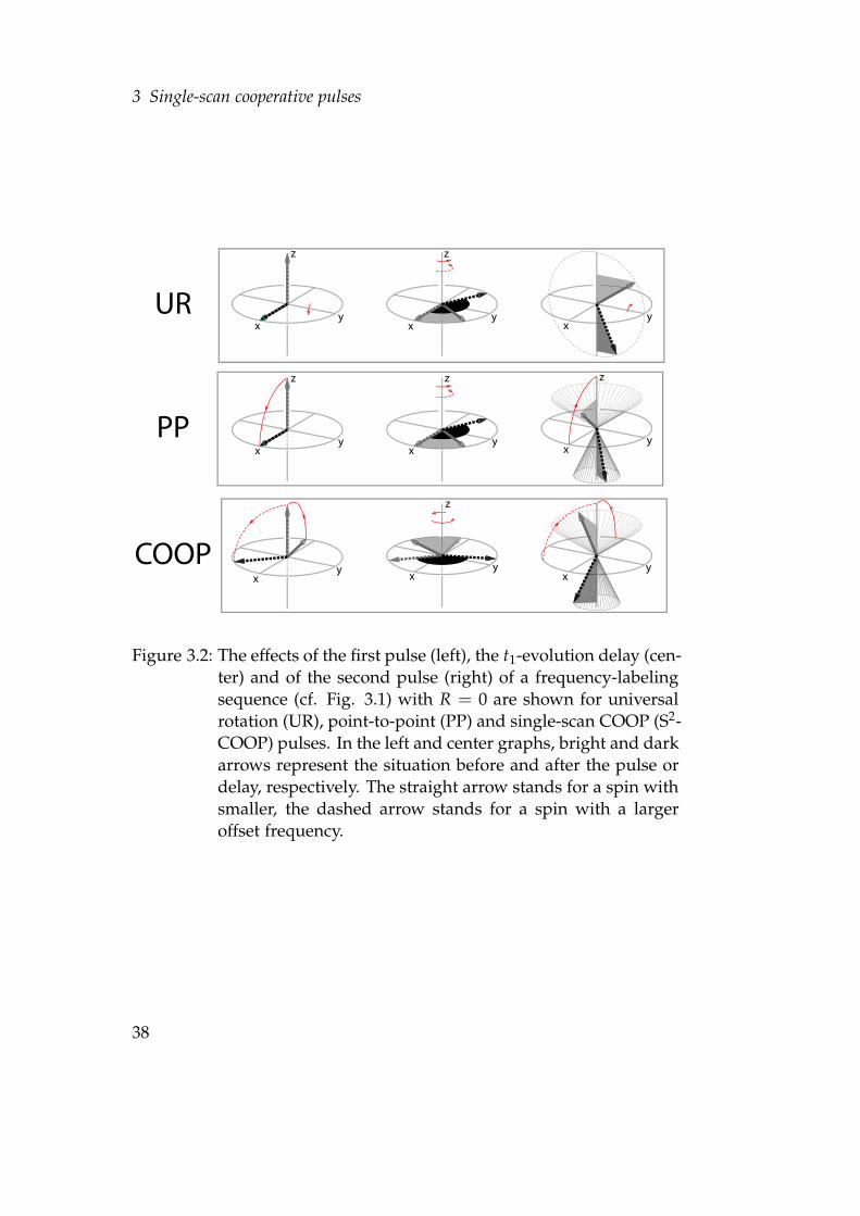
3.2.1 Frequency-labeling of z magnetization
The consecutive steps of an ideal conventional (i.e. using perfect 90◦
UR pulses [11, 23]) 2D NOESY frequency-labeling block are shown inthe upper panel of Fig. 3.2. Two exemplary magnetization vectorswith two different offset frequencies are drawn as solid and dashed ar-rows. The successive UR rotations are indicated by red arrows aroundthe corresponding rotation axis. (PP and S2-COOP transformationsare indicated by segments of meridians on the Bloch sphere.) Thetheoretical effects of the first pulse (left), the t1 evolution delay (cen-ter) and last pulse (right) are shown. Brighter arrows correspond tothe magnetizations before a pulse or delay, darker arrows show thesituation afterwards. In an ideal version of the 2D NOESY experi-ment based on UR pulses (top panel of Fig. 3.2), an initial 90◦y pulse(left) uniformly and independently of ω creates x magnetization, i.e.
34
3.2 Theory
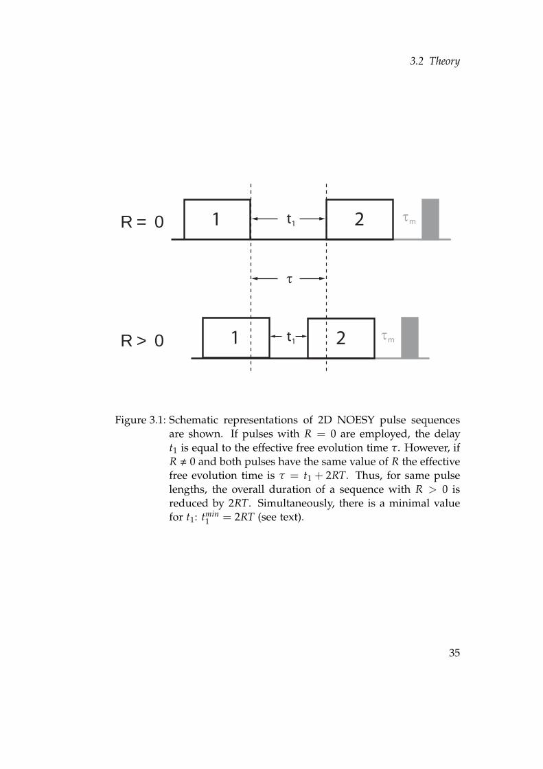
1 2
τ
τmR = 0
R > 0 1 2 τm
t1
t1
Figure 3.1: Schematic representations of 2D NOESY pulse sequencesare shown. If pulses with R = 0 are employed, the delayt1 is equal to the effective free evolution time τ. However, ifR , 0 and both pulses have the same value of R the effectivefree evolution time is τ = t1 + 2RT. Thus, for same pulselengths, the overall duration of a sequence with R > 0 isreduced by 2RT. Simultaneously, there is a minimal valuefor t1: tmin
1 = 2RT (see text).
35
3 Single-scan cooperative pulses
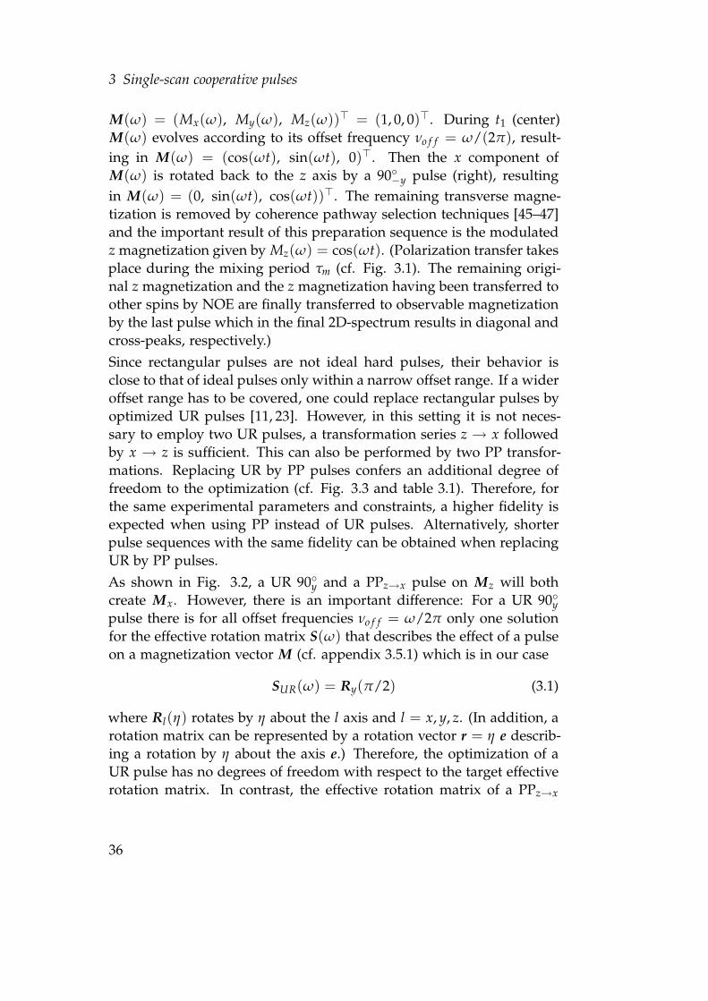
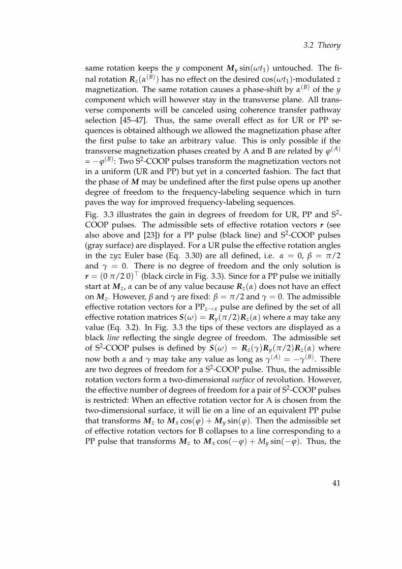
M(ω) = (Mx(ω), My(ω), Mz(ω))> = (1, 0, 0)>. During t1 (center)M(ω) evolves according to its offset frequency νo f f = ω/(2π), result-ing in M(ω) = (cos(ωt), sin(ωt), 0)>. Then the x component ofM(ω) is rotated back to the z axis by a 90◦−y pulse (right), resultingin M(ω) = (0, sin(ωt), cos(ωt))>. The remaining transverse magne-tization is removed by coherence pathway selection techniques [45–47]and the important result of this preparation sequence is the modulatedz magnetization given by Mz(ω) = cos(ωt). (Polarization transfer takesplace during the mixing period τm (cf. Fig. 3.1). The remaining origi-nal z magnetization and the z magnetization having been transferred toother spins by NOE are finally transferred to observable magnetizationby the last pulse which in the final 2D-spectrum results in diagonal andcross-peaks, respectively.)Since rectangular pulses are not ideal hard pulses, their behavior isclose to that of ideal pulses only within a narrow offset range. If a wideroffset range has to be covered, one could replace rectangular pulses byoptimized UR pulses [11, 23]. However, in this setting it is not neces-sary to employ two UR pulses, a transformation series z → x followedby x → z is sufficient. This can also be performed by two PP transfor-mations. Replacing UR by PP pulses confers an additional degree offreedom to the optimization (cf. Fig. 3.3 and table 3.1). Therefore, forthe same experimental parameters and constraints, a higher fidelity isexpected when using PP instead of UR pulses. Alternatively, shorterpulse sequences with the same fidelity can be obtained when replacingUR by PP pulses.As shown in Fig. 3.2, a UR 90◦y and a PPz→x pulse on Mz will bothcreate Mx. However, there is an important difference: For a UR 90◦ypulse there is for all offset frequencies νo f f = ω/2π only one solutionfor the effective rotation matrix S(ω) that describes the effect of a pulseon a magnetization vector M (cf. appendix 3.5.1) which is in our case
SUR(ω) = Ry(π/2) (3.1)
where Rl(η) rotates by η about the l axis and l = x, y, z. (In addition, arotation matrix can be represented by a rotation vector r = η e describ-ing a rotation by η about the axis e.) Therefore, the optimization of aUR pulse has no degrees of freedom with respect to the target effectiverotation matrix. In contrast, the effective rotation matrix of a PPz→x
36
3.2 Theory
pulse can be written as
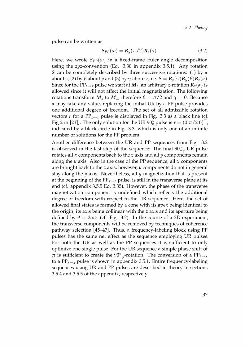
SPP(ω) = Ry(π/2)Rz(α). (3.2)
Here, we wrote SPP(ω) in a fixed-frame Euler angle decompositionusing the zyz-convention (Eq. 3.30 in appendix 3.5.1): Any rotationS can be completely described by three successive rotations: (1) by α
about z, (2) by β about y and (3) by γ about z, i.e. S = Rz(γ)Ry(β)Rz(α).Since for the PPz→x pulse we start at Mz, an arbitrary z-rotation Rz(α) isallowed since it will not affect the initial magnetization. The followingrotations transform Mz to Mx, therefore β = π/2 and γ = 0. Becauseα may take any value, replacing the initial UR by a PP pulse providesone additional degree of freedom. The set of all admissible rotationvectors r for a PPz→x pulse is displayed in Fig. 3.3 as a black line (cf.Fig 2 in [23]). The only solution for the UR 90◦y pulse is r = (0 π/2 0)>,indicated by a black circle in Fig. 3.3, which is only one of an infinitenumber of solutions for the PP problem.Another difference between the UR and PP sequences from Fig. 3.2is observed in the last step of the sequence: The final 90◦−y UR pulserotates all x components back to the z axis and all y components remainalong the y axis. Also in the case of the PP sequence, all x componentsare brought back to the z axis, however, y components do not in generalstay along the y axis. Nevertheless, all y magnetization that is presentat the beginning of the PPx→z pulse, is still in the transverse plane at itsend (cf. appendix 3.5.5 Eq. 3.35). However, the phase of the transversemagnetization component is undefined which reflects the additionaldegree of freedom with respect to the UR sequence. Here, the set ofallowed final states is formed by a cone with its apex being identical tothe origin, its axis being collinear with the z axis and its aperture beingdefined by θ = 2ωt1 (cf. Fig. 3.2). In the course of a 2D experiment,the transverse components will be removed by techniques of coherencepathway selection [45–47]. Thus, a frequency-labeling block using PPpulses has the same net effect as the sequence employing UR pulses.For both the UR as well as the PP sequences it is sufficient to onlyoptimize one single pulse. For the UR sequence a simple phase shift ofπ is sufficient to create the 90◦−y-rotation. The conversion of a PPz→xto a PPx→z pulse is shown in appendix 3.5.1. Entire frequency-labelingsequences using UR and PP pulses are described in theory in sections3.5.4 and 3.5.5 of the appendix, respectively.
37
3 Single-scan cooperative pulses
UR
PP
COOP
z
xy
z
xy
z
xy
xy
z
xy
z
xy
z
xy
xy
xy
Figure 3.2: The effects of the first pulse (left), the t1-evolution delay (cen-ter) and of the second pulse (right) of a frequency-labelingsequence (cf. Fig. 3.1) with R = 0 are shown for universalrotation (UR), point-to-point (PP) and single-scan COOP (S2-COOP) pulses. In the left and center graphs, bright and darkarrows represent the situation before and after the pulse ordelay, respectively. The straight arrow stands for a spin withsmaller, the dashed arrow stands for a spin with a largeroffset frequency.
38
3.2 Theory
3.2.2 Frequency-labeling with S2-COOP pulses
In the conventional implementations of the NOESY experiment whichwe discussed so far, a first pulse transforms Mz to Mx, i.e. magnetiza-tion with uniform phase for all offsets ω, and the second pulse rotatesMx back to Mz. For t1 > 0 only the remaining x component is rotatedback to z and retained whereas all other components are discarded (Fig.3.2 PP and UR). However, it is not necessary that all magnetization vec-tors are oriented along the same axis after the first pulse. In principle,the first pulse can rotate the initial z magnetization to any position in thetransverse plane. However, the second pulse of the sequence then hasto pick up the magnetization at the same place where it was placed bythe first pulse. Due to the chemical shift evolution during t1 the magne-tization will be rotated by ωt1 and only the cos(ωt1)-modulated compo-nent of M will be rotated back to z wheras the sin(ωt1)-component willremain in the transverse plane. The overall result of such a sequence isequivalent to the results of the UR and PP sequences (Fig. 3.2).This results in the problem to find a pair of pulses of which the first,starting from Mz, creates transverse magnetization with arbitrary phaseand the second brings back this magnetization to the initial z magne-tization. This problem can be solved by a new approach which wecall single-scan cooperative (S2-COOP) pulses. The S2-COOP approachrepresents a modification of our previously presented multi-scan COOPpulses (cf. chapter 2 and [49]).
General description of the S2-COOP approach
The S2-COOP pulse approach comprises two steps: The first step isthe optimization of a pulse pair A and B that starting from Mz createstransverse magnetization with opposite phase ϕ, i.e.
ϕ(A) = −ϕ(B). (3.3)
In other words, starting from z magnetization for each pulse, the twofinal magnetization vectors created by the pulses must be symmetricwith respect to the x axis (Fig. 3.4). Representing the effective rotationmatrices of the pulses A and B, S(A)(ω) and S(B)(ω), in the zyz Euler
39
3 Single-scan cooperative pulses
angle base (appendix 3.5.1 Eq. 3.30) yields
S(A)(ω) = Rz(γ)Ry(π/2)Rz(α(A))and
S(B)(ω) = Rz(−γ)Ry(π/2)Rz(α(B))
where, in this case, γ = ϕ(A) and −γ = ϕ(B).One of these pulses, e.g. pulse A, can directly be employed as pulse1 in a frequency-labeling sequence (Fig. 3.1). Pulse 2 of the sequenceis obtained in the second step of the S2-COOP pulse approach. In thisstep, the other pulse, e.g. pulse B, is phase-inverted and time-reversedto yield the second pulse (2) of the sequence. For example, when usingEq. 3.31 from appendix 3.5.1 and using A as the first pulse the effectiverotation matrix of pulse 2 can be written as [23]
S(2)(ω) = S(B)tr(ω) = Rz(α(B))Ry(−π/2)Rz(−γ).
The consecutive steps of the sequence are
(1) rotation of Mz to the transverse plane (S(A)(ω))(2) chemical shift evolution (Rz(ωt1)) and(3) backrotation of the cos(ωt1)-modulated part of the transverse mag-
netization to the z axis (S(B)tr(ω)):
S(B)tr(ω)Rz(ωt1)S(A)(ω) =Rz(α(B))Ry(−π/2)Rz(−γ)
× Rz(ωt1)Rz(γ)Ry(π/2)Rz(α(A))
=Rz(α(B))Ry(−π/2)
× Rz(ωt1)Ry(π/2)Rz(α(A)).
(3.4)
In the above equation, Rz(γ) and Rz(−γ) cancel. Apart from two dif-ferent values for α(A) and α(B), the final line is equivalent to the effect ofa corresponding PP sequence (cf. appendix 3.5.5). However, Rz(α(A))does not have any effect in the experiment because it is applied to zmagnetization. Then, multiplication with Ry(π/2) yields Mx whichevolves chemical shift according to Rz(ωt1). The resulting x compo-nent Mx cos(ωt1) is then rotated back to the z axis by Ry(−π/2). The
40
3.2 Theory
same rotation keeps the y component My sin(ωt1) untouched. The fi-nal rotation Rz(α(B)) has no effect on the desired cos(ωt1)-modulated zmagnetization. The same rotation causes a phase-shift by α(B) of the ycomponent which will however stay in the transverse plane. All trans-verse components will be canceled using coherence transfer pathwayselection [45–47]. Thus, the same overall effect as for UR or PP se-quences is obtained although we allowed the magnetization phase afterthe first pulse to take an arbitrary value. This is only possible if thetransverse magnetization phases created by A and B are related by ϕ(A)
= −ϕ(B): Two S2-COOP pulses transform the magnetization vectors notin a uniform (UR and PP) but yet in a concerted fashion. The fact thatthe phase of M may be undefined after the first pulse opens up anotherdegree of freedom to the frequency-labeling sequence which in turnpaves the way for improved frequency-labeling sequences.Fig. 3.3 illustrates the gain in degrees of freedom for UR, PP and S2-COOP pulses. The admissible sets of effective rotation vectors r (seealso above and [23]) for a PP pulse (black line) and S2-COOP pulses(gray surface) are displayed. For a UR pulse the effective rotation anglesin the zyz Euler base (Eq. 3.30) are all defined, i.e. α = 0, β = π/2and γ = 0. There is no degree of freedom and the only solution isr = (0 π/2 0)> (black circle in Fig. 3.3). Since for a PP pulse we initiallystart at Mz, α can be of any value because Rz(α) does not have an effecton Mz. However, β and γ are fixed: β = π/2 and γ = 0. The admissibleeffective rotation vectors for a PPz→x pulse are defined by the set of alleffective rotation matrices S(ω) = Ry(π/2)Rz(α) where α may take anyvalue (Eq. 3.2). In Fig. 3.3 the tips of these vectors are displayed as ablack line reflecting the single degree of freedom. The admissible setof S2-COOP pulses is defined by S(ω) = Rz(γ)Ry(π/2)Rz(α) wherenow both α and γ may take any value as long as γ(A) = −γ(B). Thereare two degrees of freedom for a S2-COOP pulse. Thus, the admissiblerotation vectors form a two-dimensional surface of revolution. However,the effective number of degrees of freedom for a pair of S2-COOP pulsesis restricted: When an effective rotation vector for A is chosen from thetwo-dimensional surface, it will lie on a line of an equivalent PP pulsethat transforms Mz to Mx cos(ϕ) + My sin(ϕ). Then the admissible setof effective rotation vectors for B collapses to a line corresponding to aPP pulse that transforms Mz to Mx cos(−ϕ) + My sin(−ϕ). Thus, the
41
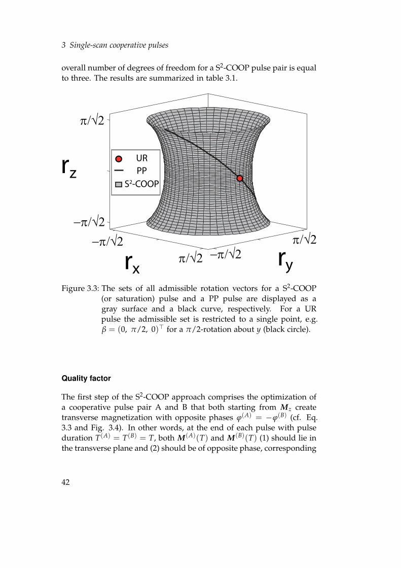
3 Single-scan cooperative pulses
overall number of degrees of freedom for a S2-COOP pulse pair is equalto three. The results are summarized in table 3.1.
π/√2
−π/√2
rz
x yr r−π/√2
−π/√2π/√2
π/√2
PPUR
S2-COOP
Figure 3.3: The sets of all admissible rotation vectors for a S2-COOP(or saturation) pulse and a PP pulse are displayed as agray surface and a black curve, respectively. For a URpulse the admissible set is restricted to a single point, e.g.β = (0, π/2, 0)> for a π/2-rotation about y (black circle).
Quality factor
The first step of the S2-COOP approach comprises the optimization ofa cooperative pulse pair A and B that both starting from Mz createtransverse magnetization with opposite phases ϕ(A) = −ϕ(B) (cf. Eq.3.3 and Fig. 3.4). In other words, at the end of each pulse with pulseduration T(A) = T(B) = T, both M(A)(T) and M(B)(T) (1) should lie inthe transverse plane and (2) should be of opposite phase, corresponding
42
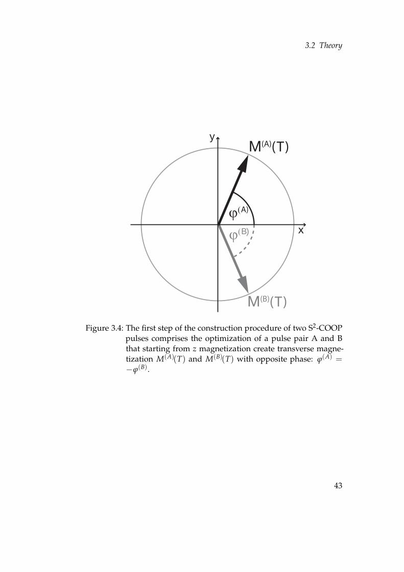
3.2 Theory
ϕ(A)
ϕ(B) x
yM(A)(T)
M(B)(T)
Figure 3.4: The first step of the construction procedure of two S2-COOPpulses comprises the optimization of a pulse pair A and Bthat starting from z magnetization create transverse magne-tization M(A)(T) and M(B)(T) with opposite phase: ϕ(A) =−ϕ(B).
43
3 Single-scan cooperative pulses
Table 3.1: Euler rotation angles for different frequency-labeling se-quences.
UR PP pseudo-S2-COOP S2-COOPα(1) 0 undefinedI α(1)(ω) = −γ(2)(−ω) undefinedβ(1) π/2 π/2 π/2 π/2γ(1) 0 0 γ(1) = −α(2) γ(1) = −α(2)
α(2) 0 0 α(2) = −γ(1) α(2) = −γ(1)
β(2) π/2 −π/2 −π/2 −π/2γ(2) 0 undefinedI γ(2)(ω) = −α(1)(−ω) undefined
degrees of freedom 0 1 2 3
The effective rotation matrices of pulses 1 and 2 of the frequency-labeling sequences can be written as S(1)(ω) = Rz(γ(1))Ry(β(1))Rz(α(1))and S(2)(ω) = Rz(γ(2))Ry(β(2))Rz(α(2)). For (pseudo-)S2-COOP pulsepairs (p. 54) α(2) = −γ(1) (Eq. 3.3). For pseudo-S2-COOP pulses (andsymmetric S2-COOP pulse pairs, cf. Eq. 3.16): S(2)(ω) = (S(1)(−ω))−1
(Eq. 3.22), e.g. α(1)(ω) = −γ(2)(−ω). In addition, for ideal S2-COOPpulses that act symmetrically with respect to ω (Eqs. 3.19 and 3.20)pulse 2 is the inverse of pulse 1: S(2) = (S(1))−1 (Eq. 3.23), e.g.α(1) = −γ(2).
(I) If the conversion principle from appendix 3.5.1 is used, then α(1) =γ(2) (Eq. 3.30).
44
3.2 Theory
to a π-rotation about the x axis (cf. Fig. 3.4):
M(A)(T) =
M(A)x (T)
M(A)y (T)
0
=
M(B)x (T)
−M(B)y (T)0
= Rx(π)M(B)(T). (3.5)
(S2-COOP pulses can in principle have different pulse durations. Forsimplicity reasons, here, we only consider the case where both pulsesA and B have the same duration T.) One way to achieve this is to max-imize the scalar product of M(A)(T) and the image of M(B)(T) rotatedby π about the x axis:
Φa = M(A)x (T) · M(B)
x (T)− M(A)y (T) · M(B)
y (T) (3.6)
Here, the pulse performance Φa only depends on the final magneti-zation vectors M(k)(T) (k =A,B) after each pulse of duration T(A) =T(B) = T so that the costate vectors λ(k)(T) of the GRAPE procedureare given by ∂Φ/∂M(k)(T) [16, 49]. For Φa the costate vectors are
λ(A)(T) =
M(B)x (T)
−M(B)y (T)0
(3.7)
and
λ(B)(T) =
M(A)x (T)
−M(A)y (T)0
. (3.8)
The costate λ(k)(T) of one pulse exclusively depends on the final trans-verse magnetization vectors generated by the other pulse. This reflectsthat, although two different pulses are optimized, they are tightly inter-twined. The gradient of the quality factor with respect to the controlsν
(k)x (t) = ω
(k)x (t)/2π and ν
(k)y (t) = ω
(k)y (t)/2π is given by the x and y
components of the vectors M(k)(t)× λ(k)(t) [16, 49]:
δΦ
δν(k)x
= M(k)y (t)λ
(k)z (t)− M(k)
z (t)λ(k)y (t) (3.9)
45
3 Single-scan cooperative pulses
andδΦ
δν(k)y
= M(k)z (t)λ
(k)x (t)− M(k)
x (t)λ(k)z (t) (3.10)
A schematic overview of the gradient calculation is shown in Fig. 3.5.
3.2.3 S2-COOP pulses with linear phase slope
There are many practical applications where an excitation pulse is fol-lowed by a free-evolution delay. This is also the case for the presentNOESY frequency-labeling block. We have shown before that in suchcases excitation pulses with uniform phase can be replaced by so-calledICEBERG pulses that create transverse magnetization with linear phaseslope [21].The phase slope of ICEBERG pulses can be characterized by the ratioR of a virtual time T′ – during which chemical shift (and coupling)evolution is active – and the pulse duration T: R = T′/T. A valueof R = 0 denotes an excitation pulse with uniform phase, whereasR = 1 indicates that the corresponding pulse creates a magnetizationprofile as if magnetization with uniform phase had been present att = 0 and free evolution took place during the entire duration of thepulse T. Pulses with good performance can be optimized even if R < 0.It has been shown that in many cases ICEBERG pulses perform betterthan comparable uniform phase excitation pulses.When a pulse that is applied before a free-evolution delay is to be re-placed by an ICEBERG pulse one has to consider that for R > 0 chem-ical shift and coupling already start to be effective during the pulse at1− RT. Therefore, the pulse has to be shifted by RT [21] which shortensthe total duration of the entire excitation-delay sequence (cf. Fig. 3.1).In analogy to the ICEBERG formalism, we derived a quality factor (ap-pendix 3.5.8) that allows to shift both pulses of a S2-COOP frequency-labeling sequence towards t1 (Fig. 3.1). Therefore, the duration of thewhole frequency-labeling block is shortened by 2RT. When the actualdelay between the two pulses is set to zero, the minimal effective free-evolution time tmin
1 is 2RT. The consequence on a 2D NOESY spectrumthat has been recorded with S2-COOP pulses with R , 0 is a linearphase error in t1 which can be removed by first-order phase correction.For larger values of RT first-order phase correction will lead to a rolling
46
3.2 Theory
M(A)(0)=0
0
1( (pulse A
M(A)(T)=
λ(A)(T)= Mx
(B)(T)-My
(B)(T) 0
( (
Mx(A)(T)
My(A)(T)
Mz(A)(T)
( (λ(A)(0)
M(B)(0)=0
0
1( (pulse B
M(B)(T)=
λ(B)(T)= Mx
(A)(T)-My
(A)(T) 0
( (
Mx(B)(T)
My(B)(T)
Mz(A)(T)
( (λ(B)(0)
Figure 3.5: The gradient calculation during the optimization of a pairof S2-COOP pulses A and B is drawn schematically. First,the trajectories of both magnetization vectors M(A)(t) andM(B)(t) are calculated. Then, the final costate vectors λ(k)(T)are calculated: The final costate vector of one pulse entirelydepends on the final state of the other pulse (red and bluearrows). Then, the trajectories of the costates λ(k)(t) are cal-culated backward in time upon which the gradients of allcontrols δΦ/δν
(k)x (t) and δΦ/δν
(k)y (t) are calculated accord-
ing to Eqs. 3.9 and 3.10. Either pulse A or B can be usedas the first pulse of a frequency-labeling sequence. Its coun-terpart (B or A) is then time-reversed and phase-inverted toyield the second pulse of the sequence (see text).
47
3 Single-scan cooperative pulses
base-line. This problem can be alleviated by applying backward linearprediction instead of large first-order phase correction.In terms of the Euler angle decomposition from appendix 3.5.1 (Eq.3.30), the effective rotation matrices of the pulses A and B become
S(A)(ω) = Rz(γ(A))Ry(π/2)Rz(α(A))
= Rz(γ′(A))Rz(RTω)Ry(π/2)Rz(α(A))(3.11)
and
S(B)(ω) = Rz(γ(B))Ry(π/2)Rz(α(B))
= Rz(γ′(B))Rz(RTω)Ry(π/2)Rz(α(B))(3.12)
For conventional ICEBERG pulses γ′(A) = γ′(B) = 0. For S2-COOPpulses with linear phase slope Eq. 3.3 still holds in a modified version:
γ′(A) = −γ′(B). (3.13)
For R = 0, A and B ideally create transverse magnetization vectors thatare symmetric with respect to a π-rotation about the x axis (Eq. 3.5).Due to the additional z-rotation Rz(RTω) this rotation symmetry axisbecomes offset-dependent:
M(A)(T) = R(RTω)(π)M(B)(T) (3.14)
In the above equation, R(RTω)(π) corresponds to a π-rotation about anaxis in the transverse plane that forms an angle of RTω with respectto the x axis. Since for conventional ICEBERG pulses γ′(k) = 0, themagnetization then lies on this symmetry axis.
3.3 Examples
As an illustrative example, we developed S2-COOP pulses for 2D 13C–13C NOESY experiments [63, 64] for a potential 30.5 T (1.3 GHz protonresonance frequency) spectrometer. The pulses have to cover an off-set frequency range of 70 kHz corresponding to a chemical shift rangeof 215 ppm. The maximum allowed rf field amplitude was set to 10kHz and an rf field inhomogeneity of ±5% was considered. The pulse
48
3.3 Examples
lengths for all optimized pulses was set to T = 75 µs which is only threetimes the duration of a rectangular π/2 pulse at the same rf amplitude.Pulse pairs for R ranging from 0 to 0.9 were optimized. ConventionalICEBERG pulses and a PPz→x pulse were optimized using the fidelityfunction
Φ0 = 1− (Tx − Mx(T))2 − (Ty − My(T))2 − Mz(T)2 (3.15)
where Tx = cos(RTω) and Ty = sin(RTω) and the second pulse ofthe sequence was created by phase-inversion and time-reversal of theoriginal pulse. The pulses were evaluated using Φa (Eq. 3.6) and Φb(Eq. 3.43), respectively . The results are displayed in Fig. 3.6.For all considered values of R, S2-COOP pulse pairs perform betterthan PP or ICEBERG pulses. The performance of S2-COOP pulses isoptimal for R being close to 0.5. The best ICEBERG pulse was foundfor R = 0.6. For R > 0.7 the difference in performance of S2-COOP andICEBERG pulses becomes smaller with increasing R. For R = 0.9 theperformances only differ by 0.0163 and the pulse shapes of ICEBERGand S2-COOP pulses show large resemblance (Fig. 3.7). If R is close to1 the effective chemical shift evolution time T′ = RT (Eq. [21]) is closeto the physical maximum T of a free evolution delay without any pulse.Then, the freedom of the S2-COOP approach is reduced, since it has toassure that chemical shift evolution takes place during almost the entirepulse duration. As a consequence, the difference between the optimalsolutions for S2-COOP and ICEBERG pulses becomes small for valuesof R that are only slightly smaller than one.The phases of the S2-COOP pulses for R = 0.9 shown in Fig. 3.7 alternatebetween the values ±π/2 + δ for pulse A and ±π/2− δ for pulse B. Thevalue for δ is constant and has no effect on the performance of this pulsepair. In fact, the latter is true for any S2-COOP pulse pair. If a constantvalue δ is added to the phase of pulse A and subtracted of the phaseof pulse B the same is true for the phases of the final magnetizationvectors ϕ(A) and ϕ(B). In Eq. 3.3, addition of ϕ(B) to both sides yields
ϕ(A) + ϕ(B) = 0.
If a constant value δ is added to ϕ(A) and subtracted of ϕ(B) we get
(ϕ(A) + δ) + (ϕ(B) − δ) = 0,
49
3 Single-scan cooperative pulses
0 0.25 0.50 0.75 1.00
0.4
0.6
0.8
1.0
Φ
RFigure 3.6: The quality functions Φa and Φb, respectively, are plotted
versus R for S2-COOP pulses (solid gray line and gray discs)and for ICEBERG pulses (dashed black line and black discs).The quality of a rectangular pulse is displayed as a square.The performance of the pulse pair that was constructed us-ing a saturation pulse and Eq. 3.16 is displayed as a blackcross. However, this construction principle does not workfor saturation pulses in general (see text).
50
3.3 Examples
ICEBERG S2-COOP
t [ s] t [ s]t [ s]
10
0
0 00 757575
90
-90
rf [
kHz]
(A)
rf [
kHz]
(B)
rf [
kHz]
pulse A pulse B
[deg
]
(A) [d
eg]
(B) [d
eg]
Figure 3.7: Pulse shapes of an ICEBERG pulse and a S2-COOP pulsepair for R = 0.9. The time-dependent pulse amplitudes νr f =√
(ν2x + ν2
y) (top) and phases φ = atan(νy/νx) (bottom) areshown. Note the large resemblance of the ICEBERG andS2-COOP pulse shapes. The S2-COOP pulses obey Eq. 3.16.In addition, the phases of both S2-COOP pulses alternatebetween the values ±π/2 + δ for pulse A and ±π/2− δ forpulse B. The value for δ is constant and has no effect on theperformance of this pulse pair (see text).
51
3 Single-scan cooperative pulses
where δ cancels and Eq. 3.3 still holds.The performance of a rectangular excitation pulse is indicated in Fig.3.6 as a black square. The same rf amplitude as for the optimizedpulses (νmax
r f = 10 kHz) was chosen. Here, the optimal value for R wasfound to be Ropt = 0.567 (Φb = 0.62445). Close to resonance, the pulseperforms well, but for increasing offset the performance decreases andalmost reaches zero at the edges of the offset range (cf. Fig. 3.11 andFig. 3.9).All S2-COOP pulses with R ≤ 0.6 are almost perfect constant amplitudepulses completely exploiting the allowed maximum rf amplitude of 10kHz. The amplitude profiles of all other S2-COOP pulse pairs that wereoptimized are, for each pulse pair, almost identical. For all S2-COOPpulse shapes with R > 0.1 as well as for the S2-COOP pulse pair withR = 0.05 we find that the phases of the individual COOP pulses arerelated by phase inversion and an additional phase shift by π:
ϕ(B) = −ϕ(A) + π, (3.16)
which is equivalent to a reflection of the phase around π/2. In chap-ter 2, where the COOP approach for several scans was presented, weobserved exactly the same symmetry for the case of multi-scan COOPpulses for broadband excitation of x magnetization with minimum pha-se error [49]. Although it seems counterintuitive that the S2-COOPpulses A and B, generating magnetization with arbitrary phase, sharesymmetry properties with excitation pulses that generate magnetiza-tion with exact phase, what these different types of COOP pulses havein common, however, is that y magnetization that is present for an off-set ω at the end of one pulse has preferably the same magnitude but anopposite sign than its counterpart, i.e. M(B)
y (ω) = −M(A)y (ω). (The dif-
ference between the two COOP pulse types is that a small |M(k)y (ω)| is
favorable for excitation with minimum phase error whereas |M(k)y (ω)|
can be of any value for the present S2-COOP pulses.)The relations we deduced for excitation pulses with minimum phaseerror in [49] are also valid here. Thus for any pulse pair fulfilling Eq.3.16 we can write
52
3.3 Examples
M(A)x (ω) = M(B)
x (−ω)
M(A)y (ω) = −M(B)
y (−ω),(3.17)
and Φa simultaneously maximizes the amount of transverse magnetiza-tion at the end of A and B with the condition that M(A)(T) be symmet-ric to M(B)(T) with respect to a π-rotation about the x axis. Thus, foran ideal S2-COOP pulse pair A and B we find
M(A)x (ω) = M(B)
x (ω)
M(A)y (ω) = −M(B)
y (ω).(3.18)
Upon combination of the two above equations we obtain
M(A)x (ω) = M(A)
x (−ω)
M(A)y (ω) = M(A)
y (−ω),(3.19)
and
M(B)x (ω) = M(B)
x (−ω)
M(B)y (ω) = M(B)
y (−ω),(3.20)
i.e. each pulse acts symmetrically with respect to ω. For the case whereR , 0, a linear, offset-dependent component RTω is added. Then theoffset profile of the magnetization phase can be described as the sumof a linear (RTω) and a symmetric component.The pulse shapes are symmetric with respect to a π-rotation about they axis, so that the corresponding effective rotation matrices S(A)(ω) andS(B)(−ω) are related by (appendix 3.5.2):
S(A)(ω) = Ry(π) S(B)(−ω) R−1y (π) (3.21)
Because Eq. 3.21 also holds for the inverse elements of S(A)(ω) andS(B)(−ω), using Eq. 3.31 we can write
S(B)tr(−ω) = Ry(π) (S(B)(−ω))−1 R−1
y (π) = (S(A)(ω))−1. (3.22)
53
3 Single-scan cooperative pulses
For an ideal S2-COOP pulse which acts symmetric with respect to ω
(Eqs. 3.19 and 3.20) the above relation becomes
S(B)tr(ω) = (S(A)(ω))−1, (3.23)
A direct consequence of Eq. 3.23 is that in Eq. 3.4 α(A) = −α(B). There-fore, for the cases where the pulse shapes of A and B obey the symme-try rule of Eq. 3.16 and Eqs. 3.19 and 3.20, the optimization algorithmconverges to pulses where pulse 2 is the inverse of pulse 1, which is,however, not a necessary condition for S2-COOP pulses.
Pseudo-S2-COOP pulses
The pulse symmetry we observed for some of our optimized pulses(cf. Eq. 3.16) can be used to construct symmetric pseudo-S2-COOPpulses from a single optimized pulse (appendix 3.5.9). The symmetryconstruction of pseudo-S2-COOP pulses A and B can be summarizedas follows:
• Optimize a pulse A that starting from Mz maximizes transversemagnetization. The magnetization phase ϕ(ω) must be the sumof a symmetric term s(ω) and a linear term RTω
ϕ(ω) = s(ω) + RTω, (3.24)
where s(ω) = s(−ω).
• Create pulse B by inverting the x control of pulse A.
Like for the original S2-COOP approach any pulse A or B can be usedas the first pulse of the sequence whereas the counterpart of this firstpulse (B or A) has to be time-reversed and phase-inverted to yield thesecond pulse of the frequency-labeling sequence.In order to find a pulse with optimal R, we implemented a dynamictarget optimization scheme where R is variable (cf. appendix 3.5.9).We were able to obtain a pulse with R = 0.531 and Φb = 0.99633. Acorresponding optimization of an S2-COOP pulse with equal R gave apulse pair with Φb = 0.99643 which is slightly better than the singlepulse. The S2-COOP pulse pair approximately obeys the symmetry
54
3.3 Examples
relation of Eq. 3.16. The transverse magnetization profile at the end ofeach pulse is almost identical and has values above 0.9975 for the entireoffset range of 70 kHz. The difference in quality mainly translates toa difference in phase errors: The S2-COOP pulse pair keeps the phaseerror smaller then 1◦ whereas the single pulse produces phase errorsup to slightly less than 2◦. Here, we demonstrated that it is possibleto construct pseudo-S2-COOP pulses where the optimization of only asingle pulse is necessary. However, the imposed symmetry representsan unnecessary restriction which might in turn lead to reduced fidelitywith respect to the more general S2-COOP pulses.Earlier, we had optimized a saturation pulse using the performancefunction
Φsat = 1− M2z(T) (3.25)
with the same specification as for the S2-COOP pulses. The optimiza-tion produced a high-quality pulse with Φsat = 0.99670. We noticedthe striking similarity of the pulse shape of the conventional saturationpulse and the S2-COOP pulses with R = 0.5. Upon application of thesymmetry rule defined in Eq. 3.16, a second pulse could be constructedso that two pulses A and B were obtained similar to the S2-COOP pro-cedure. This pulse pair was also evaluated for various values of Rusing Φb as a quality measure. For R = 0.529 this constructed pulsepair performed almost as well as the equivalent S2-COOP analogues.(The values of Φb were 0.99373 (saturation, black cross in Fig. 3.6) vs.0.99645 (S2-COOP).) We found that this pulse approximately fulfills Eq.3.24: By optimizing a saturation pulse we found a pseudo-S2-COOPpulse by chance. We optimized a further saturation pulse using Φsat fordifferent parameters. Although this pulse is a high-quality saturationpulse (Φsat = 0.99682) it does not obey Eq. 3.24 and we were not able togenerate a S2-COOP pulse pair with acceptable performance. This con-firms our finding that conventional saturation pulses cannot in generalbe used as an alternative to S2-COOP pulses.In Fig. 3.3 we show the set of admissible effective rotation vectors rof an ideal S2-COOP pulse pair which forms a two-dimensional planeof revolution. In Fig. 3.8 we compare this set of admissible effectiverotation vectors with the calculated effective rotation vectors of an op-timized S2-COOP pulse (R = 0.529). For better clarity, in Fig. 3.8 wedo not show the three-dimensional information (like in Fig. 3.3) but
55
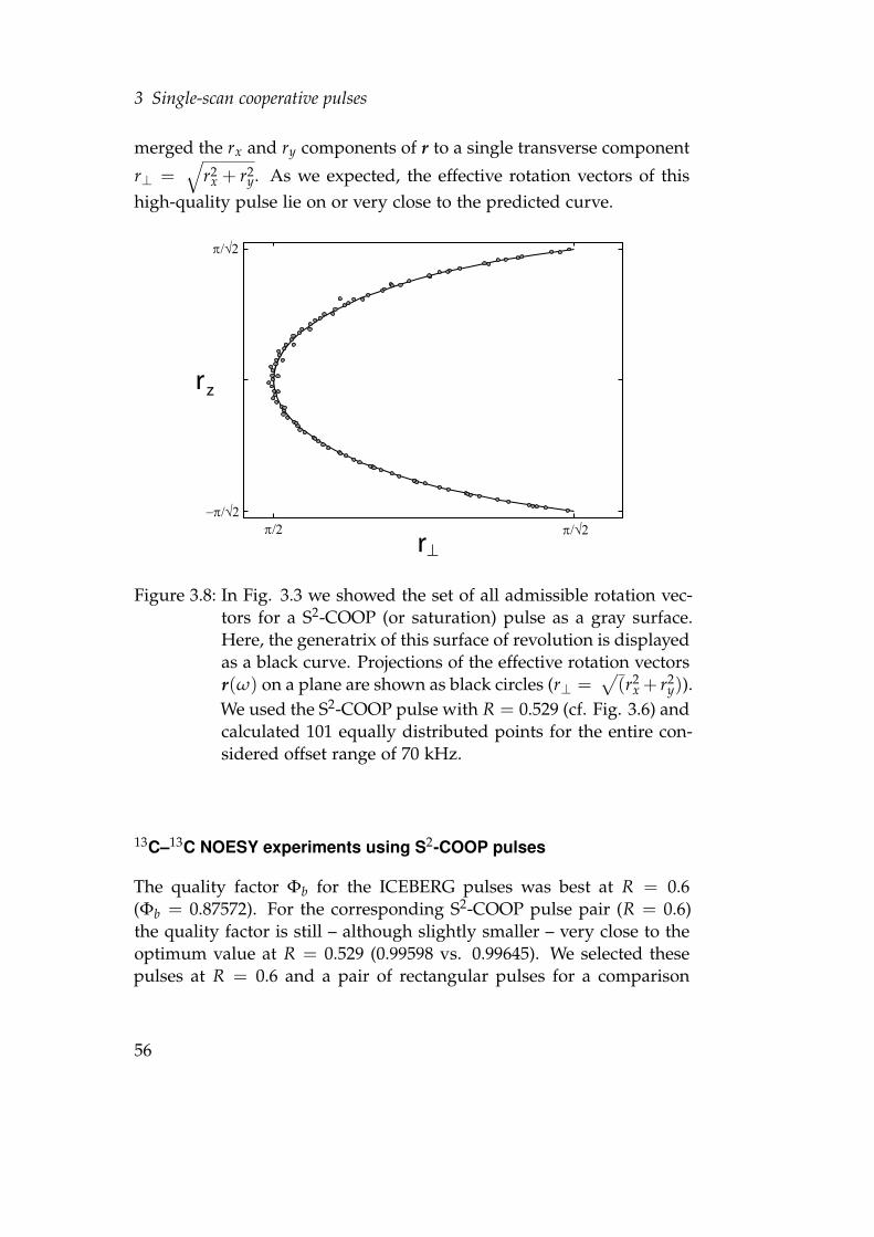
3 Single-scan cooperative pulses
merged the rx and ry components of r to a single transverse component
r⊥ =√
r2x + r2
y. As we expected, the effective rotation vectors of thishigh-quality pulse lie on or very close to the predicted curve.
rz
r⊥π/2 π/√2
π/√2
−π/√2
Figure 3.8: In Fig. 3.3 we showed the set of all admissible rotation vec-tors for a S2-COOP (or saturation) pulse as a gray surface.Here, the generatrix of this surface of revolution is displayedas a black curve. Projections of the effective rotation vectorsr(ω) on a plane are shown as black circles (r⊥ =
√(r2
x + r2y)).
We used the S2-COOP pulse with R = 0.529 (cf. Fig. 3.6) andcalculated 101 equally distributed points for the entire con-sidered offset range of 70 kHz.
13C–13C NOESY experiments using S2-COOP pulses
The quality factor Φb for the ICEBERG pulses was best at R = 0.6(Φb = 0.87572). For the corresponding S2-COOP pulse pair (R = 0.6)the quality factor is still – although slightly smaller – very close to theoptimum value at R = 0.529 (0.99598 vs. 0.99645). We selected thesepulses at R = 0.6 and a pair of rectangular pulses for a comparison
56
3.3 Examples
of the conventional approach and the new S2-COOP pulses in order toillustrate that even where the performance of conventional ICEBERGpulses is best, the S2-COOP approach is far superior to the classicalmethod.Two-dimensional 13C–13C NOESY experiments were performed on aBruker AV III 600 spectrometer using a sample of 13C-labelled α-D-glucose in DMSO which was chosen as a solvent in order to avoid mu-tarotation [65]. We used the 13C–13C NOESY pulse sequence from [64]where the unnecessary 15N-decoupling pulses were omitted. Due tolarge undesired contributions originating from zero-quantum coher-ences we added a swept pulse/gradient pair for zero-quantum suppres-sion [66]. A schematic drawing of the pulse sequence is displayed in Fig.3.12 . The original pulse durations and maximum rf amplitudes werechanged from their original values 25 µs (rectangular pulses), 75 µs(ICEBERG and S2-COOP pulses) and 10 kHz to 289.8 µs, 869.4 µs and862.7 Hz in order to reduce the original bandwidth of the optimizedpulse (70 kHz) to match the spectral width (6.04 kHz corresponding to40 ppm). The last pulse of the sequence was a conventional rectangular90◦ pulse (T = 20.5 µs) which was sufficient for the present experimen-tal conditions. For larger bandwidths, this pulse could be replaced byan optimized broadband excitation pulse [14, 16, 19, 20, 22]. The mixingtime and recycle delay were set to 50 ms and 280 ms, respectively. Thespectra were recorded on a TXI probe at 293 K with 8192 × 512 datapoints and 16 scans for each increment. Due to the considerable phaseslope in F1 the spectra were processed using backward linear predic-tion (12 data points in t1) in order to reduce base-line roll caused bylarge first-order phase correction. Processing parameters for both spec-tra were identical. Selected slices of the 13C–13C NOESY spectra forrectangular, ICEBERG and S2-COOP pulses are shown in Fig. 3.9.Close to the edges of the considered offset range, the ICEBERG pulsepair produces phase errors larger than 50◦ in F1. However, for a largeportion of the considered offset range, the phase error does not excessan absolute value of 13◦. The absolute phase error of the S2-COOPpulses remains below 1.33◦ for the entire offset range of 70 kHz. Thisphase error is due to imperfections of the pulse performance: Thefirst pulse of a frequency-labeling sequence excites magnetization withphase ϕ(A) = γ′(A) + RTω. Pulse B, in turn, creates transverse magne-
57
3 Single-scan cooperative pulses
tization with phase ϕ(B) = γ′(B) + RTω. Ideally, for S2-COOP pulseswith linear phase slope, Eq. 3.3 is fulfilled: −γ′(B) = γ′(A). However,for non-ideal pulses, the second pulse might pick up the magnetizationat the wrong phase so that −γ′(B) = γ′(A) + ∆ϕ. Thus,
∆ϕ = −(γ′(A) + γ′(B)) (3.26)
is the phase error we observe in F1. For both ICEBERG and S2-COOPpulses ∆ϕ is plotted as black curves in Fig. 3.10. One-dimensional slicesat constant F1 were extracted from the spectra and phase-corrected man-ually using zero-order phase correction. The corresponding values forthe phase errors are represented as squares in Fig. 3.10. There is a rea-sonable match of calculated and experimental values. A synopsis of theperformances of UR, PP, ICEBERG and S2-COOP pulses for R = 0 andR , 0 is shown in Fig. 3.11. The results shown in the figures 3.9, 3.10and 3.11 clearly demonstrate the superiority of the S2-COOP approachcompared to the conventional method of pulse optimization.
3.4 Discussion and conclusion
Here, we introduced the concept of S2-COOP pulses that are optimizedsimultaneously and act in a cooperative way at different positions in asingle scan. The S2-COOP approach is a modification of the cooperativepulse concept for several scans presented in chapter 2 and in [49]. Withthe help of generalized optimal control based algorithms, such as thepresented variant of the GRAPE (gradient ascent pulse engineering)algorithm, S2-COOP pulses can be efficiently optimized.For simplicity, here, we focused on the example of a frequency-labelingsequence for NOESY-type experiments which is an important build-ing block of many multi-dimensional NMR experiments. Frequency-labeling sequences can be designed using standard stand-alone PPz→xand ICEBERG pulses. The goal of such pulses is to steer initial z mag-netization to one defined final state where this final state can be con-stant (PP) or offset-dependent (ICEBERG). However, between the firstand second pulses of a frequency-labeling sequence the magnetizationmay be located anywhere in the transverse plane. Here, we showedhow this additional degree of freedom can be exploited in order todesign improved frequency-labeling sequences. In addition, we were
58
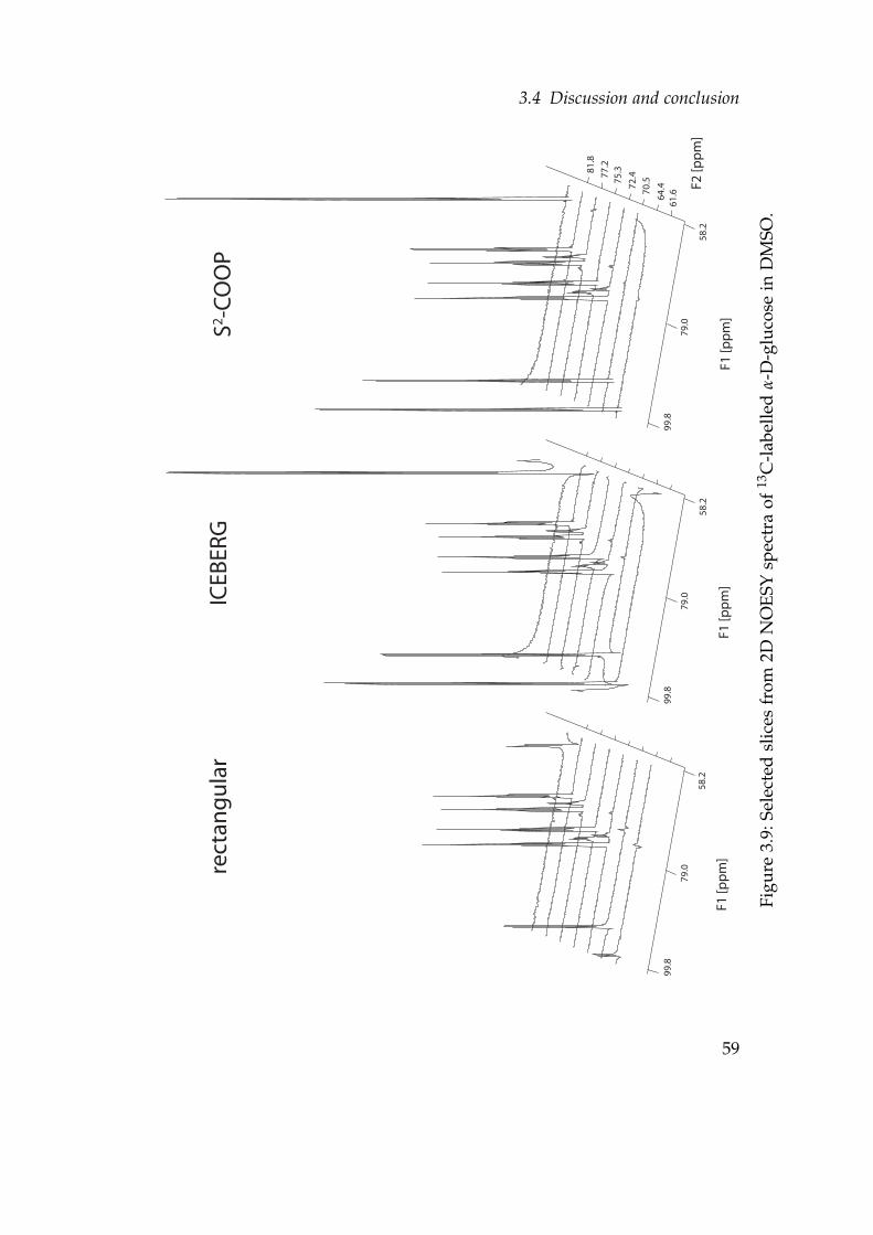
3.4 Discussion and conclusion
61.664
.470.572
.475.377
.281.8
F2 [p
pm
]
F1
[pp
m]
F1
[pp
m]
F1
[pp
m]
99.8
79.0
58.2
99.8
79.0
58.2
rect
ang
ula
rIC
EBER
GS2 -C
OO
P
99.8
79.0
58.2
Figu
re3.
9:Se
lect
edsl
ices
from
2DN
OES
Ysp
ectr
aof
13C
-lab
elle
dα
-D-g
luco
sein
DM
SO.
59
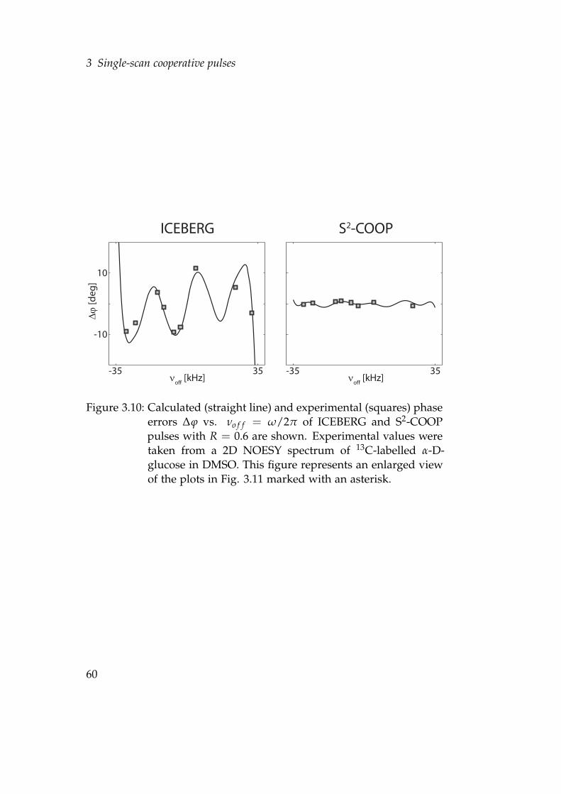
3 Single-scan cooperative pulses
ICEBERG S2-COOP
νoff
[kHz]-35 35
Δϕ [d
eg]
10
-10
-35 35ν
off [kHz]
Figure 3.10: Calculated (straight line) and experimental (squares) phaseerrors ∆ϕ vs. νo f f = ω/2π of ICEBERG and S2-COOPpulses with R = 0.6 are shown. Experimental values weretaken from a 2D NOESY spectrum of 13C-labelled α-D-glucose in DMSO. This figure represents an enlarged viewof the plots in Fig. 3.11 marked with an asterisk.
60
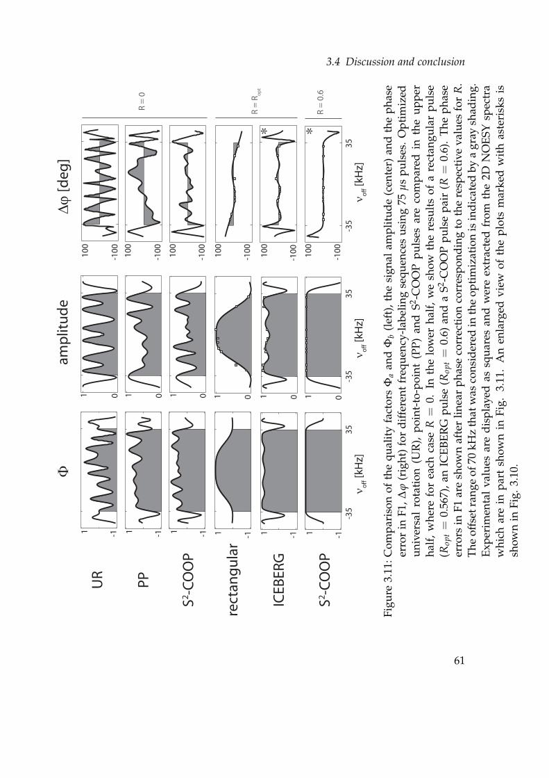
3.4 Discussion and conclusion
UR
PP
S2 -CO
OP
rect
ang
ula
r
ICEB
ERG
S2 -CO
OP
ΦΔϕ
[deg
]
ν off [k
Hz]
ν off [k
Hz]
ν off [k
Hz]
100
100
100
100
100
100
-100
-100
-100
-100
-100
-100
0000001 1 1 1 1 1
1 1 1 1 1 1-1 -1 -1 -1 -1 -1-3
5-3
5-3
535
3535
R =
0
R =
Ro
pt
amp
litu
de
R =
0.6
* *
Figu
re3.
11:C
ompa
riso
nof
the
qual
ity
fact
ors
Φa
and
Φb
(lef
t),t
hesi
gnal
ampl
itud
e(c
ente
r)an
dth
eph
ase
erro
rin
F1,∆
ϕ(r
ight
)fo
rdi
ffer
ent
freq
uenc
y-la
belin
gse
quen
ces
usin
g75
µs
puls
es.
Opt
imiz
edun
iver
sal
rota
tion
(UR
),po
int-
to-p
oint
(PP)
and
S2 -CO
OP
puls
esar
eco
mpa
red
inth
eup
per
half
,w
here
for
each
case
R=
0.In
the
low
erha
lf,
we
show
the
resu
lts
ofa
rect
angu
lar
puls
e(R
opt=
0.56
7),a
nIC
EBER
Gpu
lse
(Rop
t=
0.6)
and
aS2 -C
OO
Ppu
lse
pair
(R=
0.6)
.T
heph
ase
erro
rsin
F1ar
esh
own
afte
rlin
ear
phas
eco
rrec
tion
corr
espo
ndin
gto
the
resp
ecti
veva
lues
for
R.
The
offs
etra
nge
of70
kHz
that
was
cons
ider
edin
the
opti
miz
atio
nis
indi
cate
dby
agr
aysh
adin
g.Ex
peri
men
tal
valu
esar
edi
spla
yed
assq
uare
san
dw
ere
extr
acte
dfr
omth
e2D
NO
ESY
spec
tra
whi
char
ein
part
show
nin
Fig.
3.11
.A
nen
larg
edvi
ewof
the
plot
sm
arke
dw
ith
aste
risk
sis
show
nin
Fig.
3.10
.
61
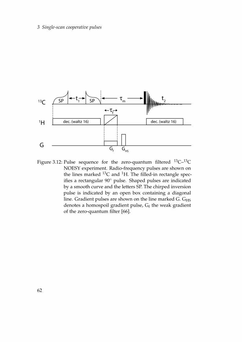
3 Single-scan cooperative pulses
dec. (waltz 16)
t1 m
dec. (waltz 16)
13C
1H
G
SP SP
Gf G
HS
t2
f
Figure 3.12: Pulse sequence for the zero-quantum filtered 13C–13CNOESY experiment. Radio-frequency pulses are shown onthe lines marked 13C and 1H. The filled-in rectangle spec-ifies a rectangular 90◦ pulse. Shaped pulses are indicatedby a smooth curve and the letters SP. The chirped inversionpulse is indicated by an open box containing a diagonalline. Gradient pulses are shown on the line marked G. GHSdenotes a homospoil gradient pulse, Gf the weak gradientof the zero-quantum filter [66].
62
3.4 Discussion and conclusion
able to derive an alternative method for the optimization of pulses forfrequency-labeling sequences that involves the optimization of only asingle pulse. However, this method imposes unnecessary restrictions tothe optimization which might impair the pulse performance. In bothsimulations and experiments S2-COOP pulse pairs achieve improvedresults with respect to conventional pulses (section 3.3). However, it isimportant to note that, apart from frequency-labeling, the S2-COOP ap-proach can also be applied to other problems, like INEPT-steps [52, 62]and Ramsey experiments [53]. In principle, the very S2-COOP pulsespresented in this chapter could be employed for such experiments.So far, optimal control based techniques for the efficient optimizationof rf pulses were restricted to single steps. The S2-COOP approachlifts this restriction to single transfers and thus opens up new avenueson the way to global pulse sequence optimizations. We hope that thepresented S2-COOP approach will find practical applications in NMRspectroscopy and imaging.
63
3 Single-scan cooperative pulses
3.5 Appendix
3.5.1 Conversion of a PPz→x to a PPx→z pulse
We consider an ensemble of uncoupled spin ½ particles without relax-ation which can be described by the Bloch equations:
M(t) = A M(t) =
0 −ω ωyω 0 −ωx−ωy ωx 0
M(t). (3.27)
If ω = (ωx, ωy, ω)> is constant during ∆t the solution is
M(t + ∆t) = e∆tA M(t) = R M(t). (3.28)
R is a rotation matrix acting on M(t). Shaped pulses are in practicerealized as a sequence of N piecewise-constant rectangular pulses withduration ∆t. Therefore, the effect of a shaped pulse on a magnetizationvector can be described by sequentially rotating the initial magnetiza-tion vector M(0) for all ωj with j ranging from 1 to N. The sequence ofrotation matrices can be grouped together to yield an effective rotationmatrix S(ω):
M(T) = (RNRN−1 ... Rj ... R2R1) M(0) = S(ω)M(0). (3.29)
S(ω) can be described by a Euler angle decomposition in the zyz fixed-frame convention:
S(ω) = Rz(γ)Ry(β)Rz(α), (3.30)
It has been shown before that the transformation performed by a phaseinverted (S) and time reversed (Str) pulse is the inverse of the originaltransformation rotated by π about the y axis (Eq. 6 from [23]):
Str(ω) = Ry(π) S−1(ω) R−1y (π)
= Ry(π)[Rz(γ) Ry(β) Rz(α)
]−1 R−1y (π)
= Ry(π) R−1z (α) R−1
y (β) R−1z (γ) R−1
y (π)
=[
Ry(π)R−1z (α)R−1
y (π)]
R−1y (β)
[Ry(π)R−1
z (γ)R−1y (π)
]= Rz(α) Ry(−β) Rz(γ)
(3.31)
64
3.5 Appendix
In the second line S−1(ω) was replaced using Eq. 3.30. In the thirdline, simple matrix algebra was used: (ABC)−1 = C−1B−1A−1. Thenwe multiplied with a unity matrix 1 = R−1
y (π) Ry(π) in the fourth lineand exchanged the commuting operators R−1
y (β) and R−1y (π). In the
last line we applied the resulting πy-rotation on R−1z (α) and R−1
z (γ)yielding Rz(α) and Rz(γ), respectively. Thus, we obtained the sameresult as in Eq. 3.30 with the difference that β has changed sign and α
and γ have changed places.For an ideal PPz→x pulse β = π/2 and γ = 0 so that upon time-reversaland phase-inversion we obtain
Strz→x(ω) = Rz(α) Ry(−π/2)
= Sx→z(ω).
The (−π/2)y-rotation transforms Mx to Mz upon which the αz-rotationhas no effect. Thus we have obtained the desired transformation fromx to z.
3.5.2 Relations between the effective rotation matrices of symmetricS2-COOP and pseudo-S2-COOP pulse pairs
The controls of some S2-COOP and all pseudo-S2-COOP pulse pairs Aand B fulfill Eq. 3.16:
ϕ(B) = −ϕ(A) + π,
which is equivalent to a rotation of the controls by π about the y axis.In terms of the x and y components of ω, this relation corresponds toω
(A)x = −ω
(B)x and ω
(A)y = ω
(B)y . Then, the rotation matrix at the j-th
increment of pulse A can be written as
R(A)j (ω) = exp
∆t
0 −ω ω(A)y
ω 0 −ω(A)x
−ω(A)y ω
(A)x 0
= exp
∆t
0 −ω ω(B)y
ω 0 ω(B)x
−ω(B)y −ω
(B)x 0
65
3 Single-scan cooperative pulses
= exp
∆t Ry(π)
0 ω ω(B)y
−ω 0 −ω(B)x
−ω(B)y ω
(B)x 0
R−1y (π)
= Ry(π) R(B)
j (−ω) R−1y (π), (3.32)
where in the last line we used the fact that Ry(π) is orthogonal: Forany orthogonal (or unitary) matrix V we can write exp{V AV−1} =V exp{A} V−1,which is a general result from matrix algebra.The effective rotation matrix of pulse A is
S(A)(ω) =R(A)N (ω) . . . R(A)
j (ω) . . . R(A)1 (ω)
=Ry(π)R(B)N (−ω)R−1
y (π) . . . Ry(π)R(B)j (−ω)R−1
y (π) . . .
× Ry(π)R(B)1 (−ω)R−1
y (π)
=Ry(π)[
R(B)N (−ω) . . . R(B)
j (−ω) . . . R(B)1 (−ω)
]R−1
y (π)
=Ry(π)[S(B)(−ω)
]R−1
y (π),
(3.33)
which is the relation we used in Eq. 3.21.
3.5.3 Theoretical description of selected frequency-labelingsequences
Here, we describe the effect of various frequency-labeling sequences us-ing the zyz-Euler angle decomposition of the effective rotation matricesof the pulses (Eq. 3.30). Corresponding drawings are given in Fig. 3.2.
3.5.4 Universal rotations
The UR pulses of this sequence perform rotations about the y axis:
90◦y : S(ω) = Ry(π/2) −90◦y : S(ω) = Ry(−π/2).
Chemical shift evolution during t1 corresponds to a z-rotation by an
66
3.5 Appendix
angle ωt1:
Ry(−π/2) Rz(ωt1) Ry(π/2) Mz == Ry(−π/2) Rz(ωt1) Mx
= Ry(−π/2)(
Mx cos(ωt1) + My sin(ωt1))
= Mz cos(ωt1) + My sin(ωt1). (3.34)
3.5.5 Point-to-point transformations
Now we consider the case where the two UR pulses are replaced by PPpulses.
Strz→x(ω) Rz(ωt1) Sz→x(ω)Mz == Rz(α)Ry(−π/2)Rz(ωt1)Ry(π/2)Rz(α) Mz
= Rz(α)Ry(−π/2)Rz(ωt1) Mx
= Rz(α)Ry(−π/2)(
Mx cos(ωt1) + My sin(ωt1))
= Mz cos(ωt1) + Rz(α)(
My sin(ωt1))
(3.35)
After the PPx→z pulse we obtain the desired cos(ωt1)-modulated z mag-netization plus a term Rz(α)
(My sin(ωt1)
)=(
My sin(ωt1))
cos(α) −(Mx sin(ωt1)) sin(α) which represents transverse magnetization beingremoved by coherence transfer pathway selection [45–47]. Because α
may take any value, the last line of Eq. 3.35 defines the set of admis-sible magnetization vectors which is drawn as a cone on the rightmostdrawing of the PP-sequence in Fig. 3.2
3.5.6 Point-to-point transformations with linear phase slope
Now we consider the case of an excitation pulse with linear phaseslope [21]. Using the Euler angle decomposition from Eq. 3.30 wecan write γ = RTω where R is the fraction of the pulse duration T dur-ing which chemical shift is active. In the frequency-labeling sequence,the first pulse creates transverse magnetization with linear phase slope,i.e. Mx cos(RTω) + My sin(RTω) = Rz(RTω) Mx. At t1 = 0 thetime-reversed and phase-inverted pulse performs the rotation sequence
67
3 Single-scan cooperative pulses
Rz(α)Ry(−π/2) Rz(RTω) (Eq. 3.31) and we obtain:
Rz(α)Ry(−π/2)Rz(RTω) Rz(RTω)Mx =Rz(α)Ry(−π/2) Rz(2RT︸︷︷︸
tmin1
ω)Mx (3.36)
which corresponds to the above result for PPz→x pulses with the differ-ence that t1 has been replaced by 2RT. Therefore, when a frequency-labeling sequence consisting of an excitation pulse with linear phaseslope followed by its time-reversed and phase-inverted counterpart isapplied, the effective evolution time τ does not correspond to the inter-pulse delay t1 (cf. Fig. 3.1):
τ = t1 + 2RT (3.37)
In a two-dimensional Fourier-transformed NOESY spectrum this re-sults in a linear phase error with respect to F1 which can be phase-corrected by first-order phase correction. For larger values of RT first-order phase correction will lead to a rolling base-line. This problem canbe alleviated by applying backward linear prediction.
3.5.7 Single-scan cooperative pulses
Single-scan cooperative pulses create transverse magnetization with op-posite phase, i.e. ϕ(A) = −ϕ(B). In other words, the final Euler rotationangles (γ in Eq. 3.30) about z are of opposite sign:
S(A)(ω) = Rz(γ)Ry(π/2)Rz(α(A))and
S(B)(ω) = Rz(−γ)Ry(π/2)Rz(α(B)).
(3.38)
In the above equation, S(A)(ω) and S(B)(ω) are the effective rotationmatrices of two S2-COOP pulse A and B, respectively. In a frequency-labeling sequence we can directly use one of these pulses as first pulseand its time-reversed and phase-inverted counterpart as second pulse.Here, we use A as the first pulse. The effective rotation matrix of the
68
3.5 Appendix
entire sequence is
S(B)tr(ω)Rz(ωt1)S(A)(ω) =
= Rz(α(B))Ry(−π/2)Rz(−γ)Rz(ωt1)Rz(γ)Ry(π/2)Rz(α(A))
= Rz(α(B))Ry(−π/2)Rz(ωt1)Ry(π/2)Rz(α(A)). (3.39)
The rotations Rz(γ) and Rz(−γ) cancel: The pair of S2-COOP pulsesacts in a cooperative way such that the two pulses cancel each other’simperfections. The above result is equivalent to the result for PP pulses(appendix 3.5.5). However, allowing an additional arbitrary rotationR(γ) adds an additional degree of freedom to S2-COOP pulses withrespect to PP pulses.When using S2-COOP pulses with linear phase slope the effective rota-tion matrices are
S(A)(ω) = Rz(γ(A))Ry(π/2)Rz(α(A))
= Rz(γ′ + RTω)Ry(π/2)Rz(α(A))
= Rz(γ′)Rz(RTω)Ry(π/2)Rz(α(A))
(3.40)
and
S(B)(ω) = Rz(γ(B))Ry(π/2)Rz(α(A))
= Rz(−γ′ + RTω)Ry(π/2)Rz(α(A))
= Rz(−γ′)Rz(RTω)Ry(π/2)Rz(α(A)).
(3.41)
Again, in a frequency-labeling sequence γ′ and −γ′ cancel yielding aresult equivalent to excitation pulses with linear phase slope (appendix3.5.6).
3.5.8 Quality factor for S2-COOP pulses with linear phase slope
The first step of the S2-COOP approach comprises the optimization oftwo pulses that rotate initial z magnetization to the transverse plane.For the case of zero phase slope (R = 0), the two resulting transversemagnetization vectors have to be related by a π-rotation about the xaxis (Eq. 3.5):
M(A)(T) = Rx(π)M(B)(T)
69
3 Single-scan cooperative pulses
If R , 0 Rx is rotated by RTω about z corresponding to a linear phaseslope of RT. Thus we can write Eq. 3.5 in a generalized form that allowsnonzero values for the phase slope:
M(A)(T) = RRTω(π)M(B)(T)
=[
Rz(RTω)Rx(π)R−1z (RTω)
]M(B)(T)
(3.42)
The quality factor then becomes
Φb =(
M(A)x (T)M(B)
x (T)− M(A)y (T)M(B)
y (T))· (C2 − S2)
+ 2(
M(A)x (T)M(B)
y (T) + M(A)y (T)M(B)
x (T))· (CS).
(3.43)
where we used C = cos(RTω) and S = sin(RTω). Using the relationλ(k)(T) = ∂Φ/∂M(k)(T) [16] we obtain the following costate vectors:
λ(A)(T) =
(C2 − S2) · M(B)x (T) + 2CS · M(B)
y (T)−(C2 − S2) · M(B)
y (T) + 2CS · M(B)x (T)
0
(3.44)
and
λ(B)(T) =
(C2 − S2) · M(A)x (T) + 2CS · M(A)
y (T)−(C2 − S2) · M(A)
y (T) + 2CS · M(A)x (T)
0
(3.45)
3.5.9 Dynamic target optimization of pseudo-S2-COOP pulses
The offset-profile of the magnetization phase ϕ(ω) of any pulse canbe decomposed into a symmetric part s(ω) and an antisymmetric parta(ω):
ϕ(ω) = s(ω) + a(ω) = s(ω) + RTω + a′(ω) (3.46)
with s(ω) = 12(ϕ(ω) + ϕ(−ω)) and a(ω) = 1
2(ϕ(ω) − ϕ(−ω)). Theantisymmetric part a(ω), in turn, can be decomposed to a linear com-ponent RTω and an antisymmetric, non-linear component a′(ω). Inorder to fulfill Eq. 3.24, a′(ω) has to vanish. Therefore, the goal of theoptimization is to minimize a′(ω).In a practical optimization, we choose a random pulse shape for which,starting from z magnetization, the offset-profile of the phase of the final
70
3.5 Appendix
magnetization at the end of the pulse ϕ(ω) is computed. Using theabove equations, we derive s(ω) (which is stored for a step later in theoptimization) and a(ω). Then the radian phase of a(ω) is unwrappedby subtracting (adding) 2π from (to) a(ωj + 1) if
(a(ωj + 1)− a(ωj)
)is
larger (smaller) than (−)π. Then the slope of the linear, antisymmetriccomponent RTω can be extracted by linear regression:
RT =∑n
j=1 a(ωj) ωj
∑nj=1 ω2
j(3.47)
Now the target phase ϕt(ω) is constructed according to Eq. 3.24:
ϕt(ω) = s(ω) + RTω. (3.48)
The quality function we use is Φ0 = 1− (Tx − Mx(T))2 −(Ty − My(T))2
−Mz(T)2 (Eq. 3.15) where the target magnetization vector is T =(cos(ϕt) sin(ϕt) 0)>. The gradients are calculated accordingly andadded to the pulse shape. This updated pulse is then used in the nextiteration to re-calculate ϕt(ω) in the manner we described above uponwhich new gradients are added to the pulse shapes. This process isrepeated iteratively until a convergence criterion is fulfilled.The symmetric component of the phase profile s(ω) may be of anyshape (cf. Fig. 3.13). In addition, the value for R is not fixed at the be-ginning of the optimization and its optimal value is updated in each iter-ation. Therefore, the dynamic target optimization of pseudo-S2-COOPpulses also optimizes the phase slope R.
71
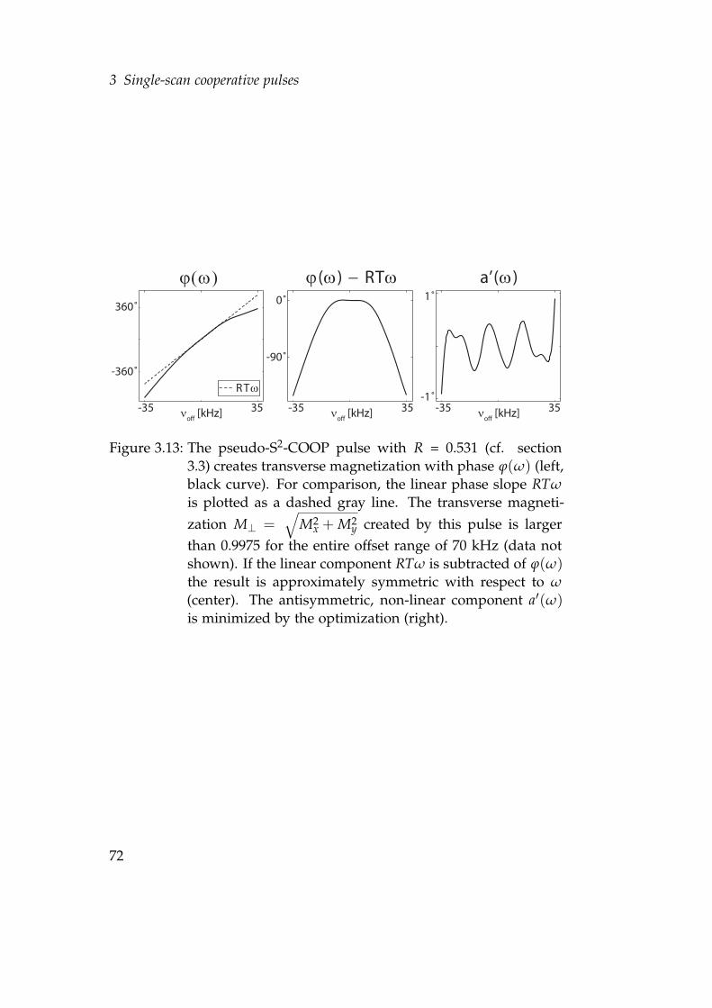
3 Single-scan cooperative pulses
360˚
-360˚
0˚
-90˚
RTω
1˚
-1˚
νoff
[kHz]-35 35
ϕ(ω) − RTωϕ(ω) a’(ω)
νoff
[kHz]-35 35 νoff
[kHz]-35 35
Figure 3.13: The pseudo-S2-COOP pulse with R = 0.531 (cf. section3.3) creates transverse magnetization with phase ϕ(ω) (left,black curve). For comparison, the linear phase slope RTω
is plotted as a dashed gray line. The transverse magneti-zation M⊥ =
√M2
x + M2y created by this pulse is larger
than 0.9975 for the entire offset range of 70 kHz (data notshown). If the linear component RTω is subtracted of ϕ(ω)the result is approximately symmetric with respect to ω
(center). The antisymmetric, non-linear component a′(ω)is minimized by the optimization (right).
72
4 Theory of cooperative tracking
In the previous chapters 2 and 3, we showed how COOP pulses can bedesigned either as COOP cycles which are used for a single transfer inseveral scans or as S2-COOP pulses which perform different transfersin a single scan. For each case, COOP pulses cancel each other’s im-perfections and act in a cooperative manner which enables enhancedpulse sequence performances with respect to classical methods of pulsesequence design.Another method for the design of successive transvers in a single scanis optimal tracking: A desired trajectory of the density matrix (or mag-netization vector) at specified points in time is tracked as closely aspossible. Optimal tracking has been used for the development of novellow-power heteronuclear decoupling sequences in the liquid state for invivo applications [44]. However, optimal tracking is not limited to thedesign of decoupling sequences but could in principle be used for thedevelopment of various pulse sequences.In the present chapter, we discuss the theoretical framework of an algo-rithm which combines the COOP pulse approach with optimal trackingfor the design of novel heteronuclear decoupling sequences: During theoptimization, we keep track of the density operator at all acquisitionpoints [44] and at the same time we allow for the signal to be the aver-age of several scans [49], i.e. we optimize a set of cooperative heteronu-clear decoupling pulses which are in general not identical. We hopethat this novel algorithm which we call cooperative tracking will resultin improved decoupling sequences, creating spectra with large and uni-form signal amplitudes as well as reduced intensities of the decouplingsidebands. In our description of the cooperative tracking algorithm wewill redraw the theory of optimal tracking as it is presented in [44].
Heteronuclear decoupling of two spins ½
Consider the case of a heteronuclear two-spin system with two spins½ labeled I and S. We assume that spin I is observed while spin S is
73
4 Theory of cooperative tracking
irradiated with a decoupling sequence. The overall Hamiltonian in adoubly rotating frame [67] takes the form
H(t) = HIo f f +HS
o f f +HISJ +HS
r f (t) (4.1)
whereHI
o f f = 2πνI Iz (4.2)
andHS
o f f = 2πνSSz (4.3)
are the offset terms of spin I and spin S, respectively. The heteronuclearJ coupling term is
HISJ = 2π JSz Iz. (4.4)
The remaining term represents the irradiated decoupling sequence:
HSr f (t) = 2πε{ux(t)Sx + uy(t)Sy}, (4.5)
where the controls ux(t) and uy(t) represent the x and y componentsof the rf field and ε is an rf scaling factor taking rf inhomogeneity andmiscalibration into account. Since HI
o f f commutes with the terms HSo f f ,
HISJ and HS
r f (t) it is sufficient to consider the simplified Hamiltonian
H′(t) = HSo f f +HIS
J +HSr f (t). (4.6)
If no decoupling sequence is applied, i.e. HSr f (t) = 0, then the evolution
of an initial density operator ρ(t0) = Ix is only governed by HISJ because
HSo f f and Ix commute:
ρ(t) = Ix cos(π Jt) + 2IySz sin(π Jt). (4.7)
Due to the cos(π Jt)-modulation of the detectable operator Ix, the Fouriertransformation of the time-domain signal that represents the expecta-tion value 〈Ix〉 yields a spectrum consisting of a doublet with splittingJ. The J coupling can be used for different types of experiments, e.g.J-resolved spectroscopy [68, 69] and for heteronuclear coherence trans-fer [52]. However, in many cases it is advantageous to suppress theJ-coupling evolution. In general, decoupled spectra show fewer peaksthan spectra that have been recorded without decoupling which facil-itates the analysis of the spectrum [67]. The task of a heteronuclear
74
decoupling sequence is to suppress the effects of HISJ so that the dou-
blet collapses to a single line and, in the absence of relaxation effects,ρ(t) = Ix throughout the decoupling sequence. Typically, the time-domain signal is not recorded continuously but only at discrete pointsin time Tk. Therefore, for decoupling it is sufficient that ρ(t) is equal toIx at the Naq + 1 acquisition points Tk (0 ≤ k ≤ Naq) which are typicallyevenly spaced over the acquisition time Taq. For the case of non-uniformsampling the position in time of the acquisition points can be adjustedaccordingly. So we can write
ρ(Tk) = Ix. (4.8)
Typically, the dwell-time ∆T = Tk−Tk−1 between two acquisition pointsis longer than the duration ∆t = tm − tm−1 of an increment of the de-coupling sequence, i.e. the discretization of the decoupling sequenceis typically finer than the digitization of the detected signal. (Here,M = ∆T/∆t is the number of pulse increments per interval ∆T. Thevalues of ∆T and ∆t are chosen such that M is an integer.)In analogy to COOP pulses in several scans (Chapter 2), we try to op-timize a set of N decoupling pulses that are in general not identical.Hence, the entire COOP decoupling cycle consists of N pulse sequences.Each of the latter consists of NaqM pulse increments and is character-
ized by control amplitudes u(n)x (j) and u(n)
y (j) with 1 ≤ j ≤ NaqM and1 ≤ n ≤ N. The overall signal sk is obtained by averaging the N signalss(n)
k that are obtained in N scans where we cycle through the entire setof N COOP decoupling sequences:
sk =1N
N
∑n=1
s(n)k
=1N
N
∑n=1
〈Ix|ρ(n)(Tk)〉
= 〈Ix|1N
N
∑n=1
ρ(n)(Tk)〉
= 〈Ix|ρ (Tk)〉
(4.9)
with〈Ix | ρ (Tk)〉 = tr{I†
x ρ (Tk)}. (4.10)
75
4 Theory of cooperative tracking
Although signal averaging cannot increase the amplitude of a decou-pled resonance line, it allows for cancelation of undesired signal con-tributions such as decoupling sidebands and deviations from a desiredoffset profile. Thus, even if the individual members of a COOP de-coupling cycle show imperfections in terms of undesired signal contri-butions, the COOP tracking algorithm is given the possibility to findsolutions where these undesired signals cancel upon signal averaging.A desired offset profile in the context of heteronuclear decoupling canbe a maximum and uniform amplitude of the decoupled signal overthe entire considered offset range which is of special interest for decou-pling sequences in quantitative NMR experiments [70]. Other desiredoffset profiles can be band-selective decoupling profiles where the de-coupling sequence only affects a certain offset range and has no effectfor the remaining considered offset frequencies [71, 72]. Yet another de-sired offset profile is a defined, offset-dependent scaling of the couplingconstant J as it has been shown in [73].One method for the reduction of decoupling sidebands in several scans,DESIRE [74], is a two-dimensional NMR technique where the decou-pled spectrum corresponds to the slice of the 2D spectrum at F1 = 0.The decoupling sidebands appear at F1 , 0 where the value of F1 cor-responds to the splitting of the decoupling sidebands. With DESIREan up to 100-fold reduction of the decoupling sideband intensities canbe achieved. However, in order to obtain a decoupled spectrum withDESIRE, a considerable number of scans in order to sufficiently resolvethe spectrum in the indirect dimension is necessary. (In [74] the showndecoupled spectra were recorded with 64 and 128 t1-increments, respec-tively.) Another method for the reduction of decoupling sidebands inseveral scans is bi-level decoupling [75]. In bi-level decoupling, severaldifferent decoupling sequences are applied in different scans so that de-coupling sidebands are cancelled in part upon signal averaging. In thefirst scan of a bi-level decoupling cycle decoupling is performed witha low rf amplitude (“low-level decoupling”). In all successive scans, adecoupling sequence with high rf amplitude (“high-level decoupling”)is applied at the beginning of the sequence which is followed by a low-level decoupling sequence. The duration of the high-level sequence isincreased with each scan. The total signal is obtained by averaging theindividual signals from each scan. Thus, it is possible to reduce the
76
intensities of the decoupling sidebands. Bi-level decoupling has beenapplied to the chemical analysis of polymer compounds [76]. However,the necessary rf amplitudes for high-level decoupling are considerablylarge. Another disadvantage of bi-level decoupling, especially with re-spect to quantitative NMR, are the large deviations from a uniformoffset profile of the amplitudes of the decoupled signal. A uniform de-coupling profile can be obtained when decoupling sequences based onadapted adiabatic pulses are applied [70]. However, in [70] the prob-lem of decoupling sidebands is not addressed and the possibilities thatthe latter can be reduced by signal averaging is not taken into account.Here, we present the theory of cooperative tracking which is in prin-ciple able to find decoupling sequence cycles that create both uniformand maximum decoupled signal amplitudes for the considered offsetrange and minimize decoupling sidebands.The amplitude of a decoupled on-resonance signal in the spin I spec-trum for a given rf scaling factor ε and offset νS is given by
φ(ε, νS) =1
Naq + 1
Naq
∑k=0
sk(ε, νS)
=1
Naq + 1
Naq
∑k=0
〈Ix|ρ (ε, νS, Tk)〉
(4.11)
where in the first line we replaced sk(ε, νS) in Eq. 13 from [44] withsk(ε, νS). In the second line we used the identity from Eq. 4.9.Here, instead of using the signal amplitude φ(ε, νS) as the quality factorof a decoupling sequence at a specific rf scaling factor ε and a specificoffset frequency νS, we choose φ′(ε, νS) which is
φ′(ε, νS) =1
Naq + 1
Naq
∑k=0
(1− (1− sk(ε, νS))2
)=
1Naq + 1
Naq
∑k=0
(1− (1− 〈Ix | ρ (ε, νS, Tk)〉)2
).
(4.12)
This choice assures that full advantage is taken of the COOP pulse prin-ciple (cf. Eq. 4.36). We define the overall performance function Φ ofa decoupling sequence as the average of all quality factors φ′(ε, νS) for
77
4 Theory of cooperative tracking
all Nε rf scaling factors and all Nν offsets of interest [44]:
Φ =1
NεNν
Nε
∑p=1
Nν
∑q=1
φ′(
ε(p), ν(q)S
). (4.13)
Simplified relaxation model
The general analytical expressions for the gradients δΦ/δu(n)α (j) (for
u(n)α (j) = εu(n)
x (j) and εu(n)y (j)) can be derived for the case of an arbi-
trary relaxation matrix. However, a simplified relaxation model wherethe relevant terms of the density operator relax with the similar rate κ
reflecting T2 (or T∗2 ) allows a tremendous simplification of the trackingalgorithm. For many cases, this is a reasonable approximation. In thesimplified relaxation model, the density operator at time tm of the nthscan is given by
ρ(n)(tm) = exp{−κtm} ρ (n)(tm) (4.14)
andρ (n)(tm) = U(n)
m ... U(n)1 ρ(n)(t0) U(n)†
1 ... U(n)†m . (4.15)
The propagator Uµ for the µth time slice of the nth scan is given by
U(n)µ = exp{−i∆tH′(n)
µ } (4.16)
where
H′(n)µ = HS
o f f +HISJ + 2πε
(u(n)
x (µ) Sx + u(n)y (µ) Sy
)(4.17)
with u(n)x (µ) and u(n)
y (µ) being the constant control amplitudes duringthis time slice. Hence, using this simplified relaxation model we canwrite for the signal amplitude sk:
sk = exp{−κTk}〈Ix|ρ (Tk)〉. (4.18)
where in the context of the simplified relaxation model (Eq. 4.14)
ρ (Tk) =1N
N
∑n=1
ρ (n)(Tk). (4.19)
78
Derivation of the gradient δΦ/δu(n)α (j)
The gradient δΦ/δu(n)α (j) is given by
δΦ
δu(n)α (j)
=δ
δu(n)α (j)
(1
NεNν
Nε
∑p=1
Nν
∑q=1
φ′(
ε(p), ν(q)S
))
=1
NεNν
Nε
∑p=1
Nν
∑q=1
δφ′(
ε(p), ν(q)S
)δu(n)
α (j).
(4.20)
Thus we need to average all gradients for all rf scaling factors ε(p) andall offset frequencies ν
(q)S of interests. The gradient δφ′(ε, νS)/δu(n)
α (j)for a specific scaling factor ε and a specific offset frequency νS is
δφ′(ε, νS)
δu(n)α (j)
=δ
δu(n)α (j)
(1
Naq + 1
Naq
∑k=0
(1− (1− sk(ε, νS))2
)). (4.21)
Now we are interested in the effect on the quality factor φ′(ε, νS) ifthe control amplitude u(n)
x (j) or u(n)y (j) is varied in the jth time slice,
i.e. between the time points tj−1 and tj. This time slice lies betweenthe acquisition points Tl and Tl+1, where b j/M c is the truncated value(also called floor function) of the ratio j/M, i.e. the number of completeintervals ∆T between the time points t0 and tj. The controls u(n)
x (j) and
u(n)y (j) only have an effect on the detected signal sk for k > l = b j/M c.
Hence we find
δφ′(ε, νS)
δu(n)α (j)
=δ
δu(n)α (j)
(1
Naq + 1 ∑k>l
(1− (1− sk(ε, νS))2
))
=−2
Naq + 1 ∑k>l
(1− sk(ε, νS))
(δ sk(ε, νS)
δu(n)α (j)
).
(4.22)
Using our simplified relaxation model (Eq. 4.14) for δ sk(ε, νS)/δu(n)α (j)
we find
δ sk(ε, νS)
δu(n)α (j)
= exp{−κTk}δ〈Ix|ρ (Tk)〉
δu(n)α (j)
=1N
exp{−κTk}δ〈Ix|ρ (n)(Tk)〉
δu(n)α (j)
.(4.23)
79
4 Theory of cooperative tracking
The density operator at the acquisition time Tk of the nth scan canbe calculated by propagation of the initial density operator which isρ(n)(t0) = Ix for all N COOP decoupling sequences. Thus we can write
δ〈Ix|ρ (n)(Tk)〉δu(n)
α (j)=
δ
δu(n)α (j)
〈Ix|U(n)k ... U(n)
j ... U(n)1 ρ(t0)U(n)†
1 ... U(n)†j ... U(n)†
k 〉
=δ
δu(n)α (j)
tr{
IxU(n)k ... U(n)
j ... U(n)1 ρ(t0)U(n)†
1 ... U(n)†j ... U(n)†
k
}
= tr{IxU(n)k ...
δU(n)j
δu(n)α (j)
... U(n)1 ρ(t0)U(n)†
1 ... U(n)†j ... U(n)†
k
+ IxU(n)k ... U(n)
j ... U(n)1 ρ(t0)U(n)†
1 ...δU(n)†
j
δu(n)α (j)
... U(n)†k }.
(4.24)
where we used Eq. 4.10 and took advantage of Ix being Hermitian (i.e.Ix = I†
x ) in the second line and in the third line we applied the productrule. Using Eq. 4.16 the propagator U(n)
j can be written as
U(n)j = exp{−i∆tH′(n)(tj)} (4.25)
with
H′(n)(tj) = H′(t) = HSo f f +HIS
J + 2πε {u(n)x (j) Sx + u(n)
y (j) Sy} (4.26)
where u(n)x (j) and u(n)
y (j) are the controls of the nth COOP decouplingsequence at the jth time slice. In the limit where ∆t � ||H′(n)(tj)||−1
[11, 77] we obtain to first order in t
δU(n)j
δu(n)α (j)
= −i 2π∆t Sα U(n)j (4.27)
and
δU(n)†j
δu(n)α (j)
= i 2π∆t U(n)†j Sα. (4.28)
80

Plugging this result into equation 4.24 we can write
δ〈Ix|ρ (n)(Tk)〉δu(n)
α (j)=
= −i 2π∆t tr{IxU(n)k ... Sα U(n)
j ... U(n)1 ρ(t0) U(n)†
1 ... U(n)†k
−IxU(n)k ... U(n)
1 ρ(t0) U(n)†1 ... U(n)†
j Sα ... U(n)†k }
= −i 2π∆t×tr{U(n)†
j+1 ... U(n)†k IxU(n)
k ... U(n)j+1︸ ︷︷ ︸
λ(n)k (tj)
Sα U(n)j ... U(n)
1 ρ(t0)U(n)†1 ... U(n)†
j︸ ︷︷ ︸ρ (n)(tj)
−U(n)†j+1 ... U(n)†
k IxU(n)k ... U(n)
j+1︸ ︷︷ ︸λ
(n)k (tj)
U(n)j ... U(n)
1 ρ(t0)U(n)†1 ... U(n)†
j︸ ︷︷ ︸ρ (n)(tj)
Sα}
= −i 2π∆t tr{λ(n)k (tj) Sα ρ (n)(tj)− ρ (n)(tj) Sα λ
(n)k (tj)}
= −i 2π∆t 〈Sα | [ρ (n)(tj), λ(n)k (tj)]〉. (4.29)
Hence we can write the gradient of the quality function δφ′(ε, νS)/δu(n)α (j)
to first order in ∆t as
δφ′(ε, νS)
δu(n)α (j)
= i 2π∆t1
Naq + 12N ∑
k>lexp{−κTk}
× (1− sk(ε, νS)) 〈Sα | [ ρ (n)(tj), λ(n)k (tj) ]〉
(4.30)
We can refine this result by replacing λ(n)k (tj) with λ′
(n)k (tj) which is
λ′(n)k (tj) =
2N
(1− sk(ε, νS)) λ(n)k (tj) (4.31)
and we obtain
δφ′(ε, νS)
δu(n)α (j)
= i 2π∆t1
Naq + 1
× ∑k>l
exp{−κTk} 〈 Sα | [ ρ (n)(tj), λ′(n)k (tj) ] 〉
= i 2π∆t1
Naq + 1〈 Sα | [ ρ (n)(tj), Λ(n)
k (tj) ] 〉
(4.32)
81
4 Theory of cooperative tracking
so that we are now able to calculate the gradients δΦ/δu(n)α (j) (Eq. 4.13).
The operator Λ(n)(tj) is defined as
Λ(n)(tj) = ∑k>l
exp{−κTk} λ′(n)k (tj) (4.33)
and can efficiently be calculated in complete analogy to the method pre-sented in Appendix 3 of [44]. For each of the N members of the COOPcycle, the density operator at time point tj is obtained by unitarily evolv-ing the initial density operator ρ(1)(t0) = ρ(2)(t0) = . . . = ρ(N)(t0) = Ixforward in time (Eq. 4.15). We call
λ′(n)k (tj) = U(n)†
j+1 . . . U(n)†kM λ′(Tk) U(n)
km . . . U(n)k+1 (4.34)
the kth costate of the nth COOP decoupling sequence at time point tj
that is obtained by unitarily evolving λ′(n)(Tk) backward in time whereλ′(n)(Tk) is defined as
λ′(n)k (Tk) =
2N
(1− 〈Ix|ρ(ε, νS, Tk)〉) Ix, (4.35)
which is independent of n, i.e. at the same acquisition time Tk all Ncostates are identical (λ′(1)(Tk) = λ′(2)(Tk) = . . . = λ(N)(Tk)) and de-pend on the average expectation value 〈Ix〉 = 〈Ix|ρ (ε, νS, Tk)〉. However,the back propagation of the costates under the different decoupling se-quences results in different trajectories λ
′(n)k (tj) for 1 ≤ j ≤ NaqM. If,
instead of φ′(ε, νS), we choose φ(ε, νS) (Eq. 4.11) as a quality factor thecorresponding costate is
λ(n)k (Tk) =
1N
Ix. (4.36)
The costate λ(n)k (Tk) is independent of the average expectation value
〈Ix〉 = 〈Ix|ρ (ε, νS, Tk)〉 and does not contain any information from theother members of the COOP decoupling sequence cycle. Hence, anoptimization where φ(ε, νS) is employed as the quality factor, can nottake advantage from the COOP pulse principle and equals to a paralleloptimization of N stand-alone decoupling sequences.
By following the gradients δΦ/δu(n)α (j), i.e.
u(n)α (j) → u(n)
α (j) + εδΦ
δu(n)α
(4.37)
82
where ε is a variable step size, we are able to create a set of controls withimproved performance Φ. This is taken as the basis of a generalizedversion of the GRAPE algorithm [11] which combines the advantagesof both optimal tracking [44] and the cooperative pulse approach (cf.Chapter 2 and [49]) which can be applied to the problem of efficientheteronuclear decoupling with minimized side-bands and uniform am-plitude of the decoupled signal.
Summary of the cooperative tracking algorithm
For the case of uniform relaxation rates κ considered here, the basiccooperative GRAPE tracking algorithm can be summarized as follows:
1. Guess initial controls u(n)x (j) and u(n)
y (j) for 1 ≤ j ≤ NaqM and1 ≤ n ≤ N.
2. Starting from ρ(1)(t0) = ρ(2)(t0) = . . . = ρ(N)(t0) = Ix calculate allρ (n)(tj) for 1 ≤ j ≤ NaqM and 1 ≤ n ≤ N using Eq. 4.15.
3. Starting from Λ(1)(TNaq) = Λ(2)(TNaq) = . . . = Λ(N)(TNaq) = (2/N)× (1− 〈Ix|ρ (ε, νS, Tk)〉) Ix calculate all Λ(n)(tj) for 1 ≤ j ≤ NaqMand 1 ≤ n ≤ N using Eqs. 4.33–4.35.
4. Calculate δφ(ε(p), ν(q)S )/δu(n)
α (j) for 1 ≤ j ≤ NaqM and 1 ≤ n ≤ Nusing Eq. 4.32.
5. Repeat steps 2–4 for all rf scaling factors ε(p) and offsets ν(q)S and
calculate δΦ/δu(n)x (j) and δΦ/δu(n)
y (j) for 0 ≤ j ≤ NaqM and 0 ≤n ≤ N using Eq. 4.20.
6. Update the 2NaqMN control amplitudes u(n)x (j) and u(n)
y (j) accord-ing to Eq. 4.37.
7. With these as the new controls, go to step 2.
The algorithm is terminated if a certain convergence criterion is ful-filled. For faster convergence, the gradient information (Eq. 4.20) canbe used in more general optimizing algorithms such as conjugate gradi-ents or quasi-Newton methods like limited-memory BFGS [35, 54]. The
83
4 Theory of cooperative tracking
rf power of the decoupling sequence can be minimized or fixed as de-scribed in [11, 14]. The maximum rf amplitude umax can be limited byresetting the amplitude to the maximum amplitude if it is exceededafter step 6 [11, 19].In addition, it is possible to describe the system with a reduced four-dimensional state vector [44,78–80] which minimizes the computationaleffort. Cooperative tracking is not limited to the simplified relaxationmodel which we used here. For example, the system of interest canalso be described using a full relaxation matrix approach. In addition,cooperative tracking is not restricted to the optimization of decouplingsequences but the present algorithm could in principle be used for theoptimization of various pulse sequences.In order to be able to take rf field inhomogeneity and miscalibration intoaccount, we derived gradients for the scaled controls u(n)
α (j) = εu(n)x (j)
and εu(n)y (j). Thus, we do not optimize a single set of controls u(n)
x (j)
and u(n)y (j) but a distribution of control sets discretized by ε. In [44] the
gradients were derived for u′(n)α (j) = u(n)
x (j) and u(n)y (j) no matter which
value is taken by ε. In the context of cooperative tracking an accordingderivation would lead to the modified gradient
δφ′′(ε, νS)
δu(n)α (j)
= i 2πε∆t1
Naq + 1〈 Sα | [ ρ (n)(tj), Λ(n)
k (tj) ] 〉, (4.38)
which differs from Eq. 4.32 by a factor ε. By the principle of reci-procity [81] the detection sensitivity is proportional to ε which repre-sents a physical justification for a scaling of the gradients according toEq. 4.38. However, the transmitter and receiver coils are not identicalin general and especially not for the case of heteronuclear decoupling.If the deviations of ε from 1 are small the difference between the gra-dients from Eqs. 4.32 and 4.38 are probably negligible. However, forlarger inhomogeneities [17] different convergence properties might beobservable for the two different gradients. All pulses presented in thisthesis where rf inhomogeneity was taken into account, were optimizedusing gradients in analogy to Eq. 4.32 where the gradient is not scaledby ε. It remains an open question if one of the two methods is to bepreferred in general.
84
We expect our new algorithm to be especially interesting for 13C-detectedquantitative NMR where uniform signal amplitudes and minimizedsidebands are desired for the considered offset frequency range [70].Existing decoupling techniques either reduce decoupling sidebands inseveral scans or create a uniform decoupling profile in a single scan.Optimal tracking [44] has lead to excellent low-power decoupling se-quences. With cooperative tracking, where we applied the cooperativepulse approach to optimal tracking, we provide a method that is inprinciple capable of creating decoupling sequence cycles that both havea highly uniform offset profile and, at a time, minimize decouplingsidebands.
85

4 Theory of cooperative tracking
86
References
[1] R. R. Ernst, Application of Fourier transform spectroscopy to mag-netic resonance, Rev. Sci. Instrum. 37 (1966) 93–102.
[2] M. H. Levitt, R. Freeman, NMR population inversion using a com-posite pulse, J. Magn. Reson. 33 (1979) 473–476.
[3] R. Freeman, S. Kempsell, M. Levitt, Radiofrequency pulse se-quences which compensate their own imperfections, J. Magn. Re-son 38 (1980) 453–479.
[4] M. H. Levitt, Composite pulses, Prog. Nucl. Magn. Reson. Spec-trosc. 18 (1986) 61–122.
[5] M. H. Levitt, Encyclopedia of Nuclear Magnetic Resonance, Wiley,1996, Ch. Composite pulses, pp. 1396–1411.
[6] W. S. Warren, M. S. Silver, The art of pulse crafting: applications tomagnetic resonance and laser spectroscopy, Adv. Magn. Reson. 12(1988) 247–384.
[7] R. Freeman, Shaped radiofrequency pulses in high resolutionNMR, Prog. Nucl. Magn. Reson. Spectrosc. 32 (1998) 59–106.
[8] J.-M. Bohlen, M. Rey, G. Bodenhausen, Refocusing with chirpedpulses for broadband excitation without phase dispersion, J. Magn.Reson. 84 (1989) 191 – 197.
[9] E. Kupce, Applications of adiabatic pulses in biomolecular nuclearmagnetic resonance, in: Nuclear magnetic resonance of biologicalmacromolecules, Vol. 338 of Methods in enzymology, AcademicPress Inc., 2001, pp. 82–111.
[10] A. Bryson Jr., Y.-C. Ho, Applied optimal control, Hemisphere,Washington, D.C., 1975.
87
References
[11] N. Khaneja, T. Reiss, C. T. Kehlet, T. Schulte-Herbrüggen, S. J.Glaser, Optimal control of coupled spin dynamics: Design of NMRpulse sequences by gradient ascent algorithms, J. Magn. Reson. 172(2005) 296–305.
[12] T. E. Skinner, personal communication.
[13] K. Kobzar, T. E. Skinner, N. Khaneja, S. J. Glaser, B. Luy, Exploringthe limits of broadband excitation and inversion pulses, J. Magn.Reson. 170 (2004) 236–243.
[14] K. Kobzar, T. E. Skinner, N. Khaneja, S. J. Glaser, B. Luy, Explor-ing the limits of excitation and inversion pulses II. RF-power opti-mized pulses, J. Magn. Reson. 194 (2008) 58–66.
[15] J. L. Neves, B. Heitmann, T. O. Reiss, H. Schor, N. Khaneja, S. J.Glaser, Exploring the limits of polarization transfer efficiency inhomonuclear three spin systems, J. Magn. Reson. 181 (2006) 126–134.
[16] T. E. Skinner, T. O. Reiss, B. Luy, N. Khaneja, S. J. Glaser, Appli-cation of optimal control theory to the design of broadband exci-tation pulses for high resolution NMR, J. Magn. Reson. 163 (2003)8–15.
[17] T. E. Skinner, M. Braun, K. Woelk, N. I. Gershenzon, S. J. Glaser,Design and application of robust rf pulses for toroid cavity NMRspectroscopy, J. Magn. Reson. 209 (2011) 282–290.
[18] T. E. Skinner, K. Kobzar, B. Luy, R. Bendall, W. Bermel, N. Khaneja,S. J. Glaser, Optimal control design of constant amplitude phase-modulated pulses: Application to calibration-free broadband exci-tation, J. Magn. Reson. 179 (2006) 241–249.
[19] T. E. Skinner, T. O. Reiss, B. Luy, N. Khaneja, S. J. Glaser, Reducingthe duration of broadband excitation pulses using optimal controlwith limited rf amplitude, J. Magn. Reson. 167 (2004) 68–74.
[20] T. E. Skinner, T. O. Reiss, B. Luy, N. Khaneja, S. J. Glaser, Tailoringthe optimal control cost function to a desired output: Applicationto minimizing phase errors in short broadband excitation pulses, J.Magn. Reson. 172 (2005) 17–23.
88
References
[21] N. I. Gershenzon, T. E. Skinner, B. Brutscher, N. Khaneja, M. Nim-balkar, B. Luy, S. J. Glaser, Linear phase slope in pulse design: ap-plication to coherence transfer, J. Magn. Reson. 192 (2008) 335–343.
[22] N. I. Gershenzon, K. Kobzar, B. Luy, S. J. Glaser, T. E. Skinner, Opti-mal control design of excitation pulses that accomodate relaxation,J. Magn. Reson. 188 (2007) 330–336.
[23] B. Luy, K. Kobzar, T. E. Skinner, N. Khaneja, S. J. Glaser, Construc-tion of universal rotations from point-to-point transformations, J.Magn. Reson. 176 (2005) 179–186.
[24] K. Kobzar, B. Luy, N. Khaneja, S. J. Glaser, Pattern pulses: Designof arbitrary excitation profiles as a function of pulse amplitude andoffset, J. Magn. Reson. 173 (2005) 229–235.
[25] Topspin release January 2010.
[26] K. Kobzar, Optimal control, partial alignment and more: the de-sign of novel tools for NMR spectroscopy of small molecules, Ph.D.thesis, Technische Universität München, Department Chemie(2007).
[27] C. T. Kehlet, A. C. Sivertsen, M. Bjerring, T. O. Reiss, N. Khaneja,S. J. Glaser, N. C. Nielsen, Improving solid-state NMR dipolar re-coupling by optimal control, J. Am. Chem. Soc. 126 (2004) 10202–10203.
[28] C. T. Kehlet, T. V. Vosegaard, N. Khaneja, S. J. Glaser, N. C. Nielsen,Low-power homonuclear dipolar recoupling in solid-state NMRdeveloped using optimal control theory, Chem. Phys. Lett. 414(2005) 204–209.
[29] Z. Tošner, S. J. Glaser, N. Khaneja, N. C. Nielsen, Effective hamil-tonians by optimal control: solid-state NMR double-quantumplanar and isotropic dipolar recoupling, Chem. Phys. 125 (2006)184502/1–10.
[30] G. B. Matson, K. Young, L. G. Kaiser, RF pulses for in vivo spec-troscopy at high field designed under conditions of limited powerusing optimal control, J. Magn. Reson. 199 (2009) 30–40.
89
References
[31] T. Schulte-Herbrüggen, A. K. Spörl, R. Marx, N. Khaneja, J. M.Myers, A. F. Fahmy, S. J. Glaser, Quantum computing implementedvia optimal control: theory and application to spin- and pseudo-spin systems, Lectures on quantum information, Wiley-VCH, 2006,pp. 481–501.
[32] M. A. Janich, R. F. Schulte, M. Schwaiger, S. J. Glaser, Robust slice-selective broadband refocusing pulses, submitted to J. Magn. Re-son.
[33] P. de Fouquieres, S. Schirmer, S. Glaser, I. Kuprov, Second or-der gradient ascent pulse engineering, e-print: arXiv:1102.4096v2[quant-ph].
[34] S. Machnes, U. Sander, S. Glaser, P. de Fouquieres, A. Gruslys,S. Schirmer, T. Schulte-Herbrüggen, Comparing, optimising andbenchmarking quantum control algorithms in a unifying program-ming framework, e-print: arXiv:1011.4874v3 [quant-ph].
[35] R. Fletcher, Practical methods of optimization, Wiley, 1987.
[36] I. I. Maximov, Z. Tošner, N. C. Nielsen, Optimal control design ofNMR and dynamic nuclear polarization experiments using mono-tonically convergent algorithms, J. Chem. Phys. 128 (2008) 184505.
[37] M. Lapert, Y. Zhang, M. Braun, S. J. Glaser, D. Sugny, Singular ex-tremals for the time-optimal control of dissipative spin ½ particles,Phys. Rev. Lett. 104 (2010) 083001.
[38] E. Assémat, M. Lapert, Y. Zhang, M. Braun, S. J. Glaser, D. Sugny,Simultaneous time-optimal control of the inversion of two spin ½particles, Phys. Rev. A 82 (2010) 013415.
[39] M. Lapert, Y. Zhang, M. Braun, S. J. Glaser, D. Sugny, Geometricversus numerical optimal control of a dissipative spin ½ particle,Phys. Rev. A 82 (2010) 063418.
[40] Y. Zhang, M. Lapert, D. Sugny, M. Braun, S. J. Glaser, Time-optimalcontrol of spin ½ particles in the presence of radiation dampingand relaxation, J. Chem. Phys. 134 (2011) 054103.
90
References
[41] F. Mintert, M. Lapert, Y. Zhang, S. J. Glaser, D. Sugny, Saturationof a spin ½ particle by generalized local control, J. Chem. Phys. 148(2011) 073001.
[42] M. Lapert, Y. Zhang, S. J. Glaser, D. Sugny, Towards the time-optimal control of dissipative spin ½ particles in nuclear magneticresonance, J. Phys. B 44 (2011) 154014.
[43] T. E. Skinner, M. Nimbalkar, S. J. Glaser, Fantastic four: plug andplay pulses, under preparation.
[44] J. L. Neves, B. Heitmann, N. Khaneja, S. J. Glaser, Heteronucleardecoupling by optimal tracking, J. Magn. Reson. 201 (2009) 7–17.
[45] J. Keeler, Understanding NMR Spectroscopy, Wiley, Chichester,200.
[46] G. Bodenhausen, H. Kogler, R. R. Ernst, Selection of coherence-transfer pathways in NMR pulse experiments, J. Magn. Reson. 58(1984) 370–388.
[47] A. D. Bain, Coherence levels and coherence pathways in NMR, Asimple way to design phase cycling procedures, J. Magn. Reson. 56(1984) 418–427.
[48] M. H. Levitt, P. K. Madhu, C. E. Hughes, Cogwheel phase cycling,J. Magn. Reson. 155 (2002) 300–306.
[49] M. Braun, S. Glaser, Cooperative pulses, J. Magn. Reson. 207 (2010)114–123.
[50] W. P. Aue, E. Bartholdi, R. R. Ernst, Two-dimensional spectroscopy.Application to nuclear magnetic resonance, J. Chem. Phys 64 (1976)2229–2246.
[51] J. Jeener, B. H. Meier, P. Bachmann, R. R. Ernst, Investigation of ex-change processes by two-dimensional NMR spectroscopy, J. Chem.Phys 71 (1979) 4546–4553.
[52] G. A. Morris, R. Freeman, Enhancement of nuclear magnetic reso-nance signals by polarization transfer, J. Am. Chem. Soc. 101 (1979)760–762.
91
References
[53] N. F. Ramsey, Molecular beams, Clarendon Press, Oxford, 1956.
[54] A. Wächter, L. T. Biegler, On the implementation of a primal-dualinterior point filter line search algorithm for large-scale nonlinearprogramming, Math. Program. Ser. A 106 (2006) 25–57.
[55] Z. Tošner, T. Vosegaard, C. T. Kehlet, N. Khaneja, S. J. Glaser, N. C.Nielsen, Optimal control in NMR spectroscopy: Numerical imple-mentation in SIMPSON, J. Magn. Reson. 197 (2009) 120–134.
[56] S. Conolly, D. Nishimura, A. Macovski, Optimal control solutionsto the magnetic resonance selective excitation problem, IEEE Trans.Med. Imag. MI-5 (1986) 106115.
[57] R. J. Ogg, P. B. Kingsley, J. S. Taylor, WET, a T1- and B1-insensitivewater-suppression method for in vivo localized 1H NMR spec-troscopy, J. Magn. Reson. B 104 (1994) 1–10.
[58] S. Zhang, X. Yang, D. G. Gorenstein, Enhanced suppression ofresidual water in a “270” WET sequence, J. Magn. Reson. 143 (2000)382–386.
[59] A. Bax, A spatially selective composite 90◦ radiofrequencey pulse,J. Magn. Reson. 64 (1985) 142–145.
[60] J.-Y. Park, M. Garwood, Spin-echo MRI using π/2 and π hyper-bolic secant pulses, Magn. Reson. Med. 61 (2009) 175–187.
[61] T.-L. Hwang, A. J. Shaka, Water suppression that works. Excitationsculpting using arbirtrary waveforms and pulsed field gradients, J.Magn. Reson. A 112 (1995) 275–279.
[62] B. Adams, HSQC pulse sequences for 19F, Magn. Reson. Chem. 46(2008) 377–380.
[63] I. Bertini, I. C. Felli, R. Kümmerle, D. Moskau, R. Pietrattelli, 13C–13C NOESY: An attractive alternative for studying large macro-molecules, J. Am. Chem. Soc. 126 (2004) 464–465.
[64] W. Bermel, I. Bertini, I. C. Felli, R. Kümmerle, R. Pietrattelli,13C direct detection experiments on the paramagnetic oxidizedmonomeric copper, zinc superoxide dismutase, J. Am. Chem. Soc.125 (2003) 16423–16429.
92
References
[65] P. Qrtiz, E. Reguera, J. Fernández-Bertrán, Study of the interactionof KF with carbohydrates in DMSO-d6 by 1H and 13C NMR spec-troscopy, J. Fluorine Chem. 113 (2002) 7–12.
[66] M. J. Thrippleton, J. Keeler, Elimination of zero-quantum interfer-ence in two-dimensional NMR spectra, Angew. Chem. Int. Ed. 42(2003) 3938–3941.
[67] R. R. Ernst, G. Bodenhausen, A. Wokaun, Principles of nuclearmagnetic resonance in one and two dimensions, Clarendon Press,Oxford, 1987.
[68] R. Freeman, H. D. W. Hill, High-resolution study of NMR spinechoes: J-spectra, J. Chem. Phys. 54 (1971) 301–313.
[69] G. Bodenhausen, R. Freeman, D. Turner, Two-dimensional J-spectroscopy: proton-coupled carbon-13 NMR, J. Chem. Phys. 65(1976) 839–840.
[70] E. Tenailleau, S. Akoka, Adiabatic 1H decoupling scheme for veryaccurate intensity measurements in 13C NMR, J. Magn. Reson. 185(2007) 50–58.
[71] U. Eggenberger, P. Schmidt, M. Sattler, S. J. Glaser, C. Griesinger,Frequency-selective decoupling with recursively expanded softpulses in multinuclear NMR, J. Magn. Reson. 100 (1992) 604–610.
[72] E. R. P. Zuiderweg, S. W. Fesik, Band-selective heteronuclear de-coupling using shaped pulses as an aid in measuring long-rangeheteronuclear coupling constants, J. Magn. Reson. 93 (1991) 653–658.
[73] C. R. R. Grace, R. Riek, Pseudomultidimensional NMR by spin-state selective off-resonance decoupling, J. Am. Chem. Soc. 125(2003) 16104–16113.
[74] E. Kupce, R. Freeman, A two-dimensional experiment that sepa-rates decoupling sidebands from the main peaks, J. Magn. Reson.151 (2001) 142–145.
93
References
[75] E. Kupce, R. Freeman, G. Wider, K. Wüthrich, Suppression of cy-cling sidebands using bi-level adiabatic decoupling, J. Magn. Re-son. A 122 (1996) 81–84.
[76] Z. Zhou, R. Kümmerle, X. Qiu, D. Redwine, R. Cong, A. Taha,D. Baugh, B. Winniford, A new decoupling method for accuratequantification of polyethylene copolymer composition and triadsequence distribution with 13C NMR, J. Magn. Reson. 187 (2007)225–233.
[77] R. Fisher, Optimal control of multi-level quantum systems, Ph.D.thesis, Technische Universität München, Department Chemie(2010).
[78] T. E. Skinner, M. R. Bendall, Exact product operator evolution ofweakly coupled spin ½ ImSn systems during arbitrary rf irradiationof the I spins, J. Magn. Reson. 141 (1999) 271–285.
[79] M. R. Bendall, T. E. Skinner, Comparison and use of vector andquantum descriptions of J coupled spin evolution during rf irradi-ation of one spin in an IS spin system, J. Magn. Reson. 143 (2000)329–351.
[80] T. E. Skinner, M. R. Bendall, J-coupling and chemical shift evolu-tion during I-spin irradiation of ImSn spin systems: product op-erator solutions and applications, Conc. Magn. Reson. 14 (2002)287–307.
[81] D. I. Hoult, R. E. Richards, The signal-to-noise ratio of the nuclearmagnetic resonance experiment, J. Magn. Reson. 24 (1976) 71–85.
94