core.ac.uk · ferent resources. Households in the lower permanent income quintiles are much more likely to receive Medicaid transfers, but the transfers that they receive are on average

econstor www.econstor.eu

Der Open-Access-Publikationsserver der ZBW – Leibniz-Informationszentrum WirtschaftThe Open Access Publication Server of the ZBW – Leibniz Information Centre for Economics

Standard-Nutzungsbedingungen:

Die Dokumente auf EconStor dürfen zu eigenen wissenschaftlichenZwecken und zum Privatgebrauch gespeichert und kopiert werden.

Sie dürfen die Dokumente nicht für öffentliche oder kommerzielleZwecke vervielfältigen, öffentlich ausstellen, öffentlich zugänglichmachen, vertreiben oder anderweitig nutzen.

Sofern die Verfasser die Dokumente unter Open-Content-Lizenzen(insbesondere CC-Lizenzen) zur Verfügung gestellt haben sollten,gelten abweichend von diesen Nutzungsbedingungen die in der dortgenannten Lizenz gewährten Nutzungsrechte.

Terms of use:

Documents in EconStor may be saved and copied for yourpersonal and scholarly purposes.

You are not to copy documents for public or commercialpurposes, to exhibit the documents publicly, to make thempublicly available on the internet, or to distribute or otherwiseuse the documents in public.

If the documents have been made available under an OpenContent Licence (especially Creative Commons Licences), youmay exercise further usage rights as specified in the indicatedlicence.

zbw Leibniz-Informationszentrum WirtschaftLeibniz Information Centre for Economics

De Nardi, Mariacristina; French, Eric; Jones, John Bailey

Working Paper

Medicaid insurance in old age

Working Paper, Federal Reserve Bank of Chicago, No. 2012-13

Provided in Cooperation with:Federal Reserve Bank of Chicago

Suggested Citation: De Nardi, Mariacristina; French, Eric; Jones, John Bailey (2012) : Medicaidinsurance in old age, Working Paper, Federal Reserve Bank of Chicago, No. 2012-13

This Version is available at:http://hdl.handle.net/10419/70548

Fe

dera

l Res

erve

Ban

k of

Chi

cago

Medicaid Insurance in Old Age

Mariacristina De Nardi, Eric French, and John Bailey Jones

WP 2012-13

Medicaid Insurance in Old Age

Mariacristina De Nardi, Eric French, and John Bailey Jones∗

November 30, 2012

Abstract

Medicaid was primarily designed to protect and insure the poor againstmedical shocks. Yet, poorer people tend to live shorter lifespans and incurlower medical expenses before death than richer people. Taking these and otherimportant dimensions of heterogeneity into account, and carefully modeling keyinstitutional aspects, we estimate a structural model of savings and endogenousmedical expenses to assess the costs and benefits of Medicaid for single retirees.

We show that even higher-income retirees benefit from Medicaid, if theylive long enough for their resources to be depleted by medical expenses. Wealso find that all retirees value Medicaid insurance coverage highly, comparedto the value of the Medicaid transfers that they actually receive on average.

∗Mariacristina De Nardi: Federal Reserve Bank of Chicago and NBER. Eric French: Federal Re-serve Bank of Chicago. John Bailey Jones: University at Albany, SUNY. For useful comments andsuggestions we thank Norma Coe, Amy Finkelstein, Karl Scholz, and Gianluca Violante. Jones grate-fully acknowledges financial support from the Social Security Administration through the MichiganRetirement Research Center (MRRC grants UM10-16 and UM12-12). The views expressed in thispaper are those of the authors and not necessarily those of the Federal Reserve Bank of Chicago,the Social Security Administration or the MRRC. Jones gratefully acknowledges the hospitality ofthe Federal Reserve Bank of Chicago.

1

1 Introduction

The pervasive discussions on the “fiscal cliff” have made it clear that most en-titlement programs in the United States will be scrutinized for cost-saving reforms.One of the most debated programs is Medicaid, a means-tested, public health insur-ance program for the poor that covers any medical expenses not picked up by otherinsurance programs. In this paper we analyze the properties of Medicaid during oldage.

It has been argued that Medicaid has outgrown its initial mandate, (e.g. Brownand Finkelstein [5]) and is now also insuring also middle- and higher-income retirees,besides the lower income ones. One force generating Medicaid transfers to higherincome people is that richer people are more likely to live long and face expensivemedical conditions, such as nursing home stays, when very old. In contrast, poorerpeople tend to live shorter lives and to die before incurring large medical expenses.Another force reducing Medicaid redistribution is that while Medicaid was initiallydesigned to protect and insure the lifetime poor, it was later expanded to insure richerpeople impoverished by high medical expenses, including nursing homes, which arelarge and not generally covered by other public or private insurance.

Despite the increasing importance (and cost) of Medicaid in the presence of anaging population and ever increasing medical costs, very little is known about theinsurance properties of Medicaid, its degree of redistribution through transfers, thedegree to which various segments in the population benefit by it, and how muchretirees value Medicaid insurance. These are important aspects to know before settingout to implement reforms to the system currently in place. This paper seeks to fillthis gap.

In this paper, first, we document who in the Assets and Health Dynamics ofthe Oldest Old (AHEAD) receives Medicaid. We find that even high income peoplebecome Medicaid recipients if they live long enough and are hit by expensive medicalconditions. The Medicaid recipiency rate for those at the bottom income quintilestays flat around 60%-70% throughout their retirement. In contrast, the recipiencyrate by higher-income retirees is initially much lower, but it increases by age, reaching5-20% after age 90.

Then, taking life expectancy and other important dimensions of heterogeneityinto account, we estimate a structural model of savings and endogenous medicalexpenses to assess the costs and benefits of Medicaid for single retirees. Our modelmatches key aspects of the data well and produces parameter estimates within thebounds previously used in many works. It also generates an elasticity of total medicalexpenditures to co-payment changes that is close to the one estimated by Manninget al. [35] using the RAND Health Insurance Experiment.

Finally, we set out to use our estimated model. We compute how Medicaid pay-ments by vary by age, gender, permanent income, and health status. We find that thecurrent Medicaid system provides different kinds of insurance to households with dif-

2

ferent resources. Households in the lower permanent income quintiles are much morelikely to receive Medicaid transfers, but the transfers that they receive are on averagerelatively small. Households in the higher permanent income quintiles are much lesslikely to receive any Medicaid pay-outs, but when they do, these pay-outs are verybig and correspond to severe and expensive medical conditions. Therefore, Medicaidis an effective insurance device for the poorest, but also offers valuable insurance tothe rich by insuring them against catastrophic medical conditions.

We find that, per-period of life, the retirees at the bottom income quintile receivetransfers that are almost three times larger than that of the higher-income people.Once we compute discounted present values over all of one’s remaining expectedlifetime, however, this ratio decreases to two. Hence, differential life expectancy andmedical needs that increase with age do have a significant impact on the amount ofredistribution performed by Medicaid.

Our model also allows us to compute the valuation that a retiree attributes toMedicaid insurance, thus enabling us to perform a cost and benefit analysis of theprogram. We find that, with an estimated aversion against medical expense risk ofjust over 3, and a long tail risk of outliving ones’ life expectancy, retirees in all incomequintiles and asset levels value Medicaid insurance much more than its expected costand that cutting the program would impose very large welfare costs compared to theresulting savings.

Our findings come from a life-cycle model of consumption and endogenous medicalexpenditure that accounts for Medicare, Supplemental Social Insurance (SSI) andMedicaid. Agents in the model face uncertainty about their health, lifespan, andmedical needs (including nursing home stays). This uncertainty is partially offset bythe insurance provided by the government and private institutions. Agents choosewhether they want to apply for Medicaid if they are eligible, how much to save, andhow to split their consumption between medical and non-medical goods. Consistentwith program rules, we model two pathways to Medicaid.

To appropriately evaluate redistribution, we allow for heterogeneity in wealth,permanent income (PI), health, gender, life expectancy, and medical needs. We alsorequire our model to fit well across the entire income distribution, rather than simplyexplain mean or median behavior. Our model closely matches the life-cycle profilesof assets, out-of-pocket medical spending, and Medicaid recipiency rates for elderlysingles in different cohorts and permanent income groups.

2 Literature review

This paper is related to several previous papers on savings, health risks, and socialinsurance. Hurd [26] and Hurd, McFadden, Merrill [27] highlight the importance ofaccounting for the link between wealth and mortality risk when estimating life-cyclemodels. Kotlikoff [33] stresses the importance of modeling health expenditures tounderstand precautionary savings.

3

Hubbard et al. [24] and Palumbo [45] solve dynamic programming models of sav-ings with medical expense risk and find that medical expenses have relatively smalleffects. The key reason why these papers underestimate medical spending risk isthat the data sets available at that time had poor measures of medical spending and,in particular, were missing late-in-life medical spending and had poor measures ofnursing home costs. As a result, they underestimate the extent to which medicalexpenses rise with age and income. DeNardi et al. [12] and Marshall, McGarry, andSkinner [37] find that late life medical expenses are large and generate powerful sav-ings incentives. Furthermore, Poterba, Venti, and Wise [48] show that those in poorhealth have considerably lower assets than similar individuals in good health. Lock-wood [34] and Nakajima and Telyukova [39] add to the literature by estimating lifecycle models that allow for longevity and medical expense risk jointly with bequestmotives.

Hubbard et al. [25] and Scholz et al. [52] argue that means-tested social insuranceprograms (in the form of a minimum consumption floor) provide strong incentives forlow-income individuals not to save. Kopecky and Koreshkova [32] find that old-agemedical expenses, and the coverage of these expenses provided by Medicaid, havelarge effects on aggregate capital accumulation. Brown and Finkelstein [5] developa dynamic model of optimal savings and long-term care purchase decisions. Theyconclude that Medicaid could explain the lack of private long-term care insurance forabout two-thirds of the wealth distribution. Consistent with this evidence, Brown etal. [6] exploit cross-state variation in Medicaid rules and also find significant crowdingout.

Several new papers (Hansen et al. [23], Paschenko and Porapakkarm [46], Imrohorogluand Kitao [28]) study the importance of medical expense risk in the aggregate. Ourcontribution relative to these papers is that medical spending is endogenous in ourmodel, and we estimate the parameters of the model.

Koijen, Van Nieuwerburgh, and Yogo [30] develop risk measures for health andlongevity insurance and compare the risk exposure of each household in the Healthand Retirement Study with the model predicted optimal risk exposure.

Three recent papers contain life-cycle models where the choice of medical expen-ditures are endogenous. In addition to having different emphases, these papers modelMedicaid in ways different from ours. Feng [16] models Medicaid as an insurance pol-icy with no premiums and extremely low—possibly zero—co-payment rates. Fonsecaet al. [20] and Scholz and Seshadri [51] assume that the consumption floor is invariantto medical needs. Ozkan [43] assumes that indigent individuals receive curative, butnot preventative, care.

This paper also contributes to the literature on the redistribution generated byvarious government programs. Although there is a lot of research about the amountof redistribution provided by Social Security and a smaller amount of research aboutMedicare, to the best of our knowledge this is the first paper to examine the amount oftransfers provided to different income groups by Medicaid in old age. Furthermore, we

4

are the first to assess individuals’ valuation of the insurance provided by Medicaid.Unlike Social Security, unemployment benefits, and disability insurance, Medicaidis not financed using a specific tax, but by general government revenue, making itdifficult to determine how redistributive “Medicaid taxes” are. For this reason, wefocus on the redistribution generated by Medicaid benefits.

3 Some important aspects of the Medicaid pro-

gram

In the United States, there are two major public insurance programs helping theelderly with their medical expenses. The first is Medicare, a federal program thatprovides health insurance to almost every person over the age of 65. The secondis Medicaid, a means-tested program that is run jointly by the federal and stategovernments1.

An important characteristic of Medicaid is that it is the payer of “last resort”:Medicaid contributes only after Medicare and private insurance pay their share, andthe individual spends down his assets to a “disregard” amount. Because Medicaid re-stricts benefits to those with assets below the disregard, it discourages saving throughan additional channel not present in non-means-tested insurance, which reduces sav-ings only by reducing risks. One area where Medicaid is particularly important islong-term care. Medicare reimburses only a limited amount of long-term care costs,and most elderly people do not have private long-term care insurance. As a result,Medicaid covers almost all nursing home costs of poor old recipients; in fact, Medicaidnow assists 70 percent of nursing home residents. In fact, Medicaid ends up financing70% of nursing home residents (Kaiser Foundation [42]), and these costs are of theorder of $60,000 to $75,000 a year (in 2005).

Medicaid-eligible individuals can be divided into two main groups. The first groupcomprises the categorically needy, whose income and assets fall below certain thresh-olds. People who receive SSI typically qualify under the categorically needy provision.The second group comprises the medically needy, who are individuals whose income isnot particularly low, but who face such high medical expenditures that their resourcesbecome small in comparison.

The categorically needy provision thus affects the saving of people who have beenpoor throughout most of their lives, but has no impact on the saving of middle- andupper-income people. The medically needy provision, instead, provides insurance topeople with higher income and assets who are still at risk of being impoverished byexpensive medical conditions.

1We document many important aspects of Medicaid insurance in old age in [13].

5

4 Some Data

4.1 The AHEAD dataset

We use data from the Assets and Health Dynamics of the Oldest Old (AHEAD)data set. The AHEAD is a survey of individuals who were non-institutionalizedand aged 70 or older in 1994. It is part of the Health and Retirement Survey (HRS)conducted by the University of Michigan. We consider only single (i.e., never married,divorced, or widowed) retired individuals. A total of 3,872 singles were interviewedfor the AHEAD survey in late 1993-early 1994, which we refer to as 1994. Theseindividuals were interviewed again in 1996, 1998, 2000, 2002, 2004, 2006, 2008, and2010. This leaves us with 3,243 individuals, of whom 588 are men and 2,655 arewomen. Of these 3,243 individuals, 370 are still alive in 2010. We do not use 1994assets or medical expenses. Assets in 1994 were underreported (Rohwedder et al. [50])and medical expenses appear to be underreported as well.

A key advantage of the AHEAD relative to other datasets is that it providespanel data on health status, including nursing home stays. We assign individuals ahealth status of “good” if self-reported health is excellent, very good or good and areassigned a health status of “bad” if self-reported health is fair or poor. We assignindividuals to the nursing home state if they were in a nursing home at least 120 dayssince the last interview or if they spent at least 60 days in a nursing home before thenext scheduled interview and died before that scheduled interview.

We break the data into 5 cohorts. The first cohort consists of individuals thatwere ages 72-76 in 1996; the second cohort contains ages 77-81; the third ages 82-86;the fourth ages 87-91; and the final cohort, for sample size reasons, contains ages92-102.2 We use data for 8 different years; 1996, 1998, 2000, 2002, 2004, 2006, 2008,and 2010. We calculate summary statistics (e.g., medians), cohort-by-cohort, forsurviving individuals in each calendar year—we use an unbalanced panel. We thenconstruct life-cycle profiles by ordering the summary statistics by cohort and age ateach year of observation. Moving from the left-hand-side to the right-hand-side ofour graphs, we thus show data for four cohorts, with each cohort’s data starting outat the cohort’s average age in 1996. Our graphs omit profiles for the oldest cohortbecause sample size for this cohort is tiny.

Since we want to understand the role of income, we further stratify the data bypost-retirement permanent income (PI). Hence, for each cohort our graphs usuallydisplay several horizontal lines showing, for example, average Medicaid status in eachPI group in each calendar year. These lines also identify the moment conditions weuse when estimating the model.

We measure post-retirement PI as the individual’s average non-asset income over

2Even with the longer interval, the final cohort contains relatively few observations, yieldingshort and erratic profiles. In the interest of clarity, we therefore exclude this cohort from our graphs,although we use many of the observations when estimating the model.

6

all periods during which he or she is observed. Non-asset income includes the valueof Social Security benefits, defined benefit pension benefits, veterans benefits andannuities. Since we model social insurance explicitly, we do not include SSI transfers.Because there is a roughly monotonic relationship between lifetime earnings and theincome variables that we use, our measure of post-retirement PI is also a good measureof lifetime permanent income.

4.2 Medicaid Recipiency

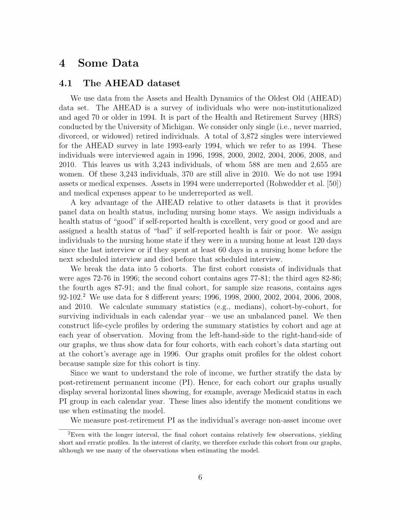
Figure 1: Medicaid recipiency rates by age, cohort, and permanent income. Thicker linesrefer to higher PI groups.

AHEAD respondents are asked whether they are currently covered by Medicaid.Figure 1 plots the fraction of the sample receiving Medicaid by age, birth cohortand income quintile for all the individuals alive at each moment in time. There arefour lines representing PI groupings within each cohort. We split the data into PIquintiles, but then merge the richest two quintiles together because at younger agesno one in the top PI quintile is on Medicaid.

The members of the first cohort appear in our sample at an average age of 74 in1996. We then observe them in 1998, when they are on average 76 years old, andthen again every two years until 2010. The other cohorts start from older initial agesand are also followed for ten years. The graph reports the Medicaid recipiency ratefor each cohort and PI grouping for six data points over time.

Unsurprisingly, Medicaid usage is inversely related to permanent income: the topline shows the fraction of Medicaid recipients in the bottom 20% of the permanentincome distribution, while the bottom line shows median assets in the top 40%. Forexample, the top left line shows that for the bottom PI quintile of the cohort aged 74in 1996, about 70% of the sample receives Medicaid in 1996; this fraction stays rather

7

stable over time. This suggests that the poorest people are qualifying for Medicaidunder the categorically needy provision, where eligibility depends on income andassets, but not the amount of the medical expenses.

The Medicaid recipiency rate tends to rise with age most quickly for people inthe middle and highest PI groups. For example, Medicaid recipiency in the oldestcohort and top two permanent income quintiles rises from about 4% at age 89 to over20% at age 96. Even people with relatively large resources can be hit by medicalshocks severe enough to exhaust their assets and qualify them for Medicaid under themedically needy provision.

4.3 Medical expense profiles

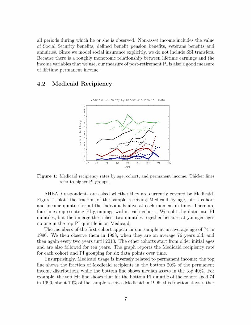
In all waves, AHEAD respondents are asked about what medical expenses theypaid out of pocket. Out-of-pocket medical expenses are the sum of what the indi-vidual spends out of pocket on insurance premia, drug costs, and costs for hospital,nursing home care, doctor visits, dental visits, and outpatient care. It includes med-ical expenses during the last year of life. It does not include expenses covered byinsurance, either public or private.

a b

Figure 2: Median out-of-pocket medical expenditures by age, cohort, and permanent in-come.

French and Jones [21] show that the medical expense data in the AHEAD lineup with the aggregate statistics. For our sample, mean medical expenses are $4,605with a standard deviation of $14,450 in 2005 dollars. Although this figure is large,it is not surprising, because Medicare did not cover prescription drugs for most ofthe sample period, requires co-pays for services, and caps the number of reimbursednursing home and hospital nights.

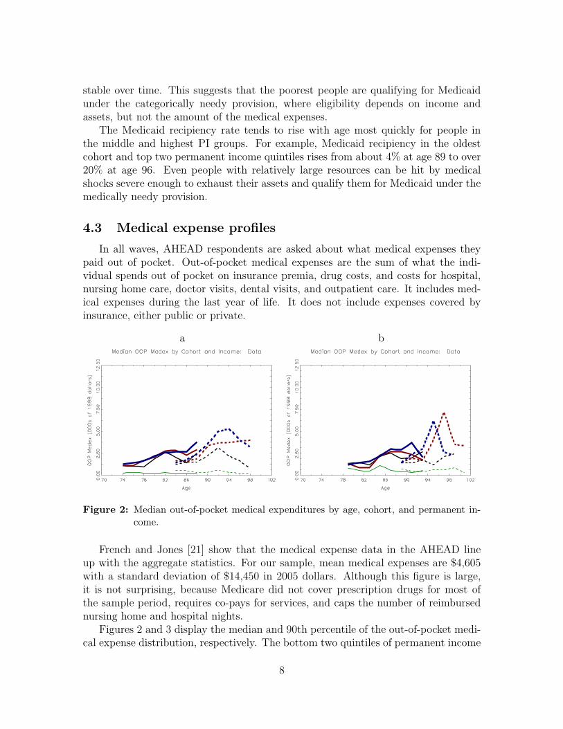
Figures 2 and 3 display the median and 90th percentile of the out-of-pocket medi-cal expense distribution, respectively. The bottom two quintiles of permanent income

8

a b

Figure 3: 90th percentile out-of-pocket medical expenditures by age, cohort, and perma-nent income.

are merged as there is very little variation in out-of-pocket medical expenses in thelowest quintile until very late in life: at younger ages, most of the expenses in thebottom quintile are bottom-coded at $250. The graphs highlight the large increasein out-of-pocket medical expenses as people reach very advanced ages and show thatthis increase is especially pronounced for people in the highest PI quintiles.

4.4 Net worth profiles

Our measure of net worth (or assets) is the sum of all assets less mortgages andother debts. The AHEAD has information on the value of housing and real estate,autos, liquid assets (which include money market accounts, savings accounts, T-bills,etc.), IRAs, Keoghs, stocks, the value of a farm or business, mutual funds, bonds,and “other” assets.

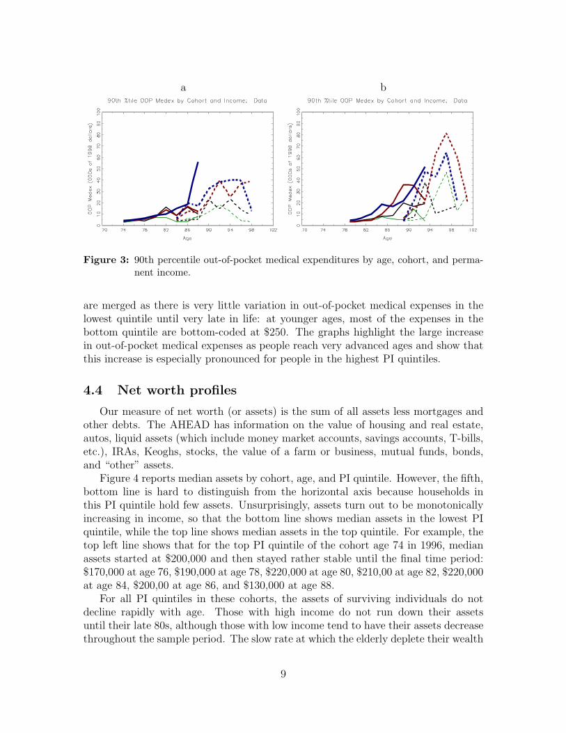
Figure 4 reports median assets by cohort, age, and PI quintile. However, the fifth,bottom line is hard to distinguish from the horizontal axis because households inthis PI quintile hold few assets. Unsurprisingly, assets turn out to be monotonicallyincreasing in income, so that the bottom line shows median assets in the lowest PIquintile, while the top line shows median assets in the top quintile. For example, thetop left line shows that for the top PI quintile of the cohort age 74 in 1996, medianassets started at $200,000 and then stayed rather stable until the final time period:$170,000 at age 76, $190,000 at age 78, $220,000 at age 80, $210,00 at age 82, $220,000at age 84, $200,00 at age 86, and $130,000 at age 88.

For all PI quintiles in these cohorts, the assets of surviving individuals do notdecline rapidly with age. Those with high income do not run down their assetsuntil their late 80s, although those with low income tend to have their assets decreasethroughout the sample period. The slow rate at which the elderly deplete their wealth

9

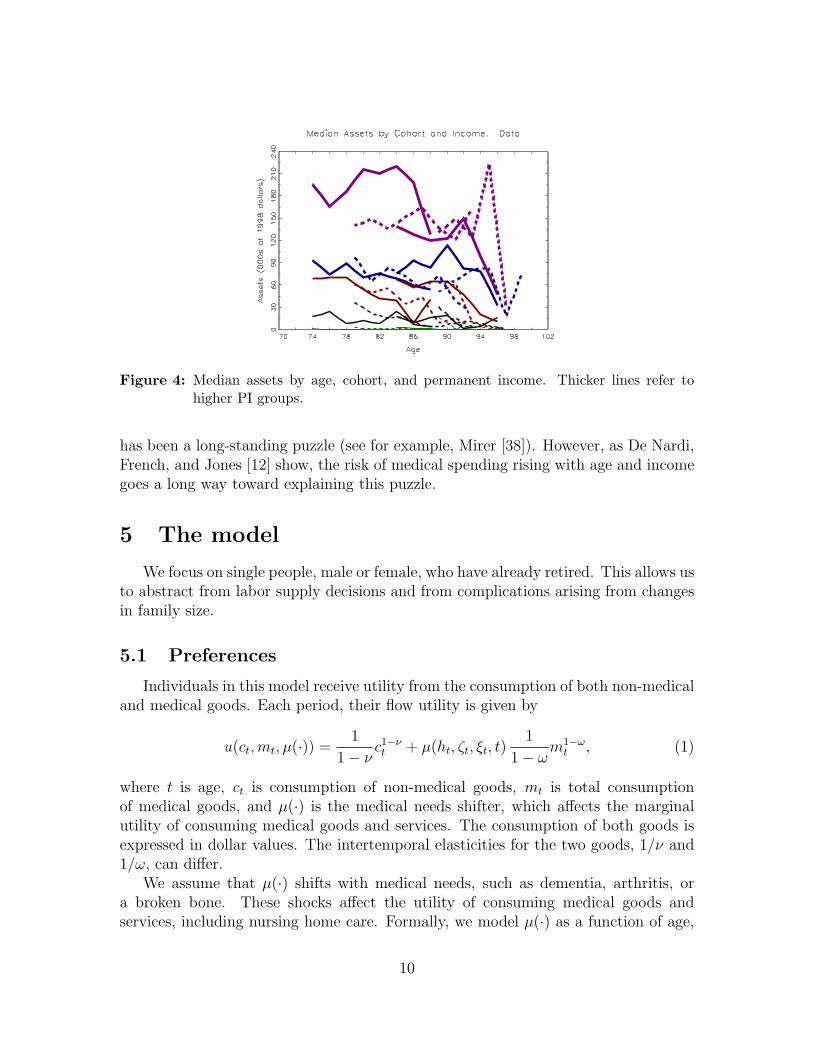
Figure 4: Median assets by age, cohort, and permanent income. Thicker lines refer tohigher PI groups.

has been a long-standing puzzle (see for example, Mirer [38]). However, as De Nardi,French, and Jones [12] show, the risk of medical spending rising with age and incomegoes a long way toward explaining this puzzle.

5 The model

We focus on single people, male or female, who have already retired. This allows usto abstract from labor supply decisions and from complications arising from changesin family size.

5.1 Preferences

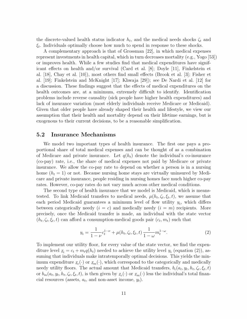
Individuals in this model receive utility from the consumption of both non-medicaland medical goods. Each period, their flow utility is given by

u(ct,mt, µ(·)) =1

1− νc1−νt + µ(ht, ζt, ξt, t)

1

1− ωm1−ω

t , (1)

where t is age, ct is consumption of non-medical goods, mt is total consumptionof medical goods, and µ(·) is the medical needs shifter, which affects the marginalutility of consuming medical goods and services. The consumption of both goods isexpressed in dollar values. The intertemporal elasticities for the two goods, 1/ν and1/ω, can differ.

We assume that µ(·) shifts with medical needs, such as dementia, arthritis, ora broken bone. These shocks affect the utility of consuming medical goods andservices, including nursing home care. Formally, we model µ(·) as a function of age,

10

the discrete-valued health status indicator ht, and the medical needs shocks ζt andξt. Individuals optimally choose how much to spend in response to these shocks.

A complementary approach is that of Grossman [22], in which medical expensesrepresent investments in health capital, which in turn decreases mortality (e.g., Yogo [53])or improves health. While a few studies find that medical expenditures have signif-icant effects on health and/or survival (Card et al. [8]; Doyle [11], Finkelstein etal. [18], Chay et al. [10]), most others find small effects (Brook et al. [3]; Fisher etal. [19]; Finkelstein and McKnight [17]; Khwaja [29]); see De Nardi et al. [12] fora discussion. These findings suggest that the effects of medical expenditures on thehealth outcomes are, at a minimum, extremely difficult to identify. Identificationproblems include reverse causality (sick people have higher health expenditures) andlack of insurance variation (most elderly individuals receive Medicare or Medicaid).Given that older people have already shaped their health and lifestyle, we view ourassumption that their health and mortality depend on their lifetime earnings, but isexogenous to their current decisions, to be a reasonable simplification.

5.2 Insurance Mechanisms

We model two important types of health insurance. The first one pays a pro-portional share of total medical expenses and can be thought of as a combinationof Medicare and private insurance. Let q(ht) denote the individual’s co-insurance(co-pay) rate, i.e., the share of medical expenses not paid by Medicare or privateinsurance. We allow the co-pay rate to depend on whether a person is in a nursinghome (ht = 1) or not. Because nursing home stays are virtually uninsured by Medi-care and private insurance, people residing in nursing homes face much higher co-payrates. However, co-pay rates do not vary much across other medical conditions.

The second type of health insurance that we model is Medicaid, which is means-tested. To link Medicaid transfers to medical needs, µ(ht, ζt, ξt, t), we assume thateach period Medicaid guarantees a minimum level of flow utility u

¯i, which differs

between categorically needy (i = c) and medically needy (i = m) recipients. Moreprecisely, once the Medicaid transfer is made, an individual with the state vector(ht, ζt, ξt, t) can afford a consumption-medical goods pair (ct,mt) such that

u¯i

=1

1− νc1−νt + µ(ht, ζt, ξt, t)

1

1− ωm1−ω

t . (2)

To implement our utility floor, for every value of the state vector, we find the expen-diture level x

¯i= ct +mtq(ht) needed to achieve the utility level u

¯i(equation (2)), as-

suming that individuals make intratemporally optimal decisions. This yields the min-imum expenditure x

¯c(·) or x

¯m(·), which correspond to the categorically and medically

needy utility floors. The actual amount that Medicaid transfers, bc(at, yt, ht, ζt, ξt, t)or bm(at, yt, ht, ζt, ξt, t), is then given by x

¯c(·) or x

¯m(·) less the individual’s total finan-

cial resources (assets, at, and non-asset income, yt).

11

5.3 Uncertainty and Non-Asset Income

The individual faces several sources of risk, which we treat as exogenous: healthstatus risk, survival risk, and medical needs risk. At the beginning of each period,the individual’s health status, and medical needs shocks are realized and need-basedtransfers are given. The individual then chooses consumption, medical expenditure,and saves. Finally, the survival shock hits.

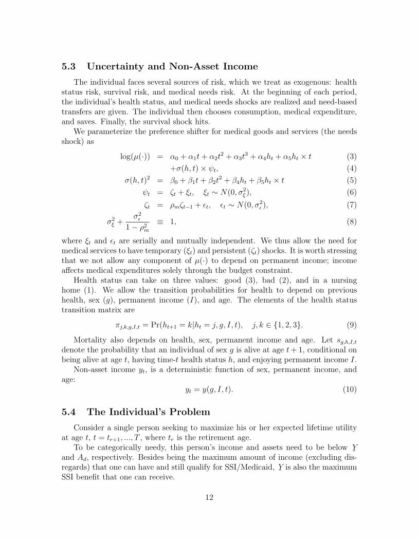
We parameterize the preference shifter for medical goods and services (the needsshock) as

log(µ(·)) = α0 + α1t+ α2t2 + α3t

3 + α4ht + α5ht × t (3)

+σ(h, t)× ψt, (4)

σ(h, t)2 = β0 + β1t+ β2t2 + β4ht + β5ht × t (5)

ψt = ζt + ξt, ξt ∼ N(0, σ2ξ ), (6)

ζt = ρmζt−1 + ϵt, ϵt ∼ N(0, σ2ϵ ), (7)

σ2ξ +

σ2ϵ

1− ρ2m≡ 1, (8)

where ξt and ϵt are serially and mutually independent. We thus allow the need formedical services to have temporary (ξt) and persistent (ζt) shocks. It is worth stressingthat we not allow any component of µ(·) to depend on permanent income; incomeaffects medical expenditures solely through the budget constraint.

Health status can take on three values: good (3), bad (2), and in a nursinghome (1). We allow the transition probabilities for health to depend on previoushealth, sex (g), permanent income (I), and age. The elements of the health statustransition matrix are

πj,k,g,I,t = Pr(ht+1 = k|ht = j, g, I, t), j, k ∈ {1, 2, 3}. (9)

Mortality also depends on health, sex, permanent income and age. Let sg,h,I,tdenote the probability that an individual of sex g is alive at age t+1, conditional onbeing alive at age t, having time-t health status h, and enjoying permanent income I.

Non-asset income yt, is a deterministic function of sex, permanent income, andage:

yt = y(g, I, t). (10)

5.4 The Individual’s Problem

Consider a single person seeking to maximize his or her expected lifetime utilityat age t, t = tr+1, ..., T , where tr is the retirement age.

To be categorically needy, this person’s income and assets need to be below Y¯

and Ad, respectively. Besides being the maximum amount of income (excluding dis-regards) that one can have and still qualify for SSI/Medicaid, Y

¯is also the maximum

SSI benefit that one can receive.

12

Note that Medicaid and SSI apply to income gross of taxes. Let at denote assetsand r the real interest rate. The SSI benefit equals Y

¯−max{yt + rat − yd, 0}, where

yd is the income disregard.If a person is categorically needy and applies for SSI and Medicaid, he receives the

SSI transfer and Medicaid goods and services as dictated by his medical needs shockand utility floor. The combined SSI/Medicaid transfer for the categorically needy isthus given by:

bc(at, yt, µ(·)

)= Y

¯−max{yt+rat−yd, 0}+max

{0, x

¯c−max{at+Y

¯−Ad, 0}

}, (11)

Under this formulation, agents with assets in excess of the disregard Ad can spenddown their wealth and qualify for Medicaid.

If the person’s total income is above Y¯and or assets are above and Ad, she is not

eligible for SSI. If the person applies for Medicaid, transfers are given by

bm(at, yt, µ(·)

)= max

{0, x

¯m(·)−max{at + rat + yt − Ad, 0}

}, (12)

where we assume that the asset disregard Ad is the same as under the categoricallyneedy pathway.

Each period eligible individuals choose whether to receive Medicaid or not. Wewill use the indicator function IM to denote this choice, with IM = 1 if the personapplies for Medicaid and IM = 0 if the person does not apply.

When the person dies, any remaining assets are left to his or her heirs. We denotewith e the estate net of taxes. Estates are linked to assets by

et = e(at) = at −max{0, τ · (at − x)}.

The parameter τ denotes the tax rate on estates in excess of x, the estate exemptionlevel. The utility the household derives from leaving the estate e is

ϕ(e) = θ(e+ k)

1− ν

(1−ν)

,

where θ is the intensity of the bequest motive, while k determines the curvature ofthe bequest function and hence the extent to which bequests are luxury goods.

Using β to denote the discount factor, we can then write the individual’s valuefunction as:

Vt(at, g, ht, I, ζt, ξt) = maxct,mt,at+1,IM

{u(ct,mt, µ(·))

+ βsg,h,I,tEt

(Vt+1(at+1, g, ht+1, I, ζt+1, ξt+1)

)+ β(1− sg,h,I,t)θ

(e(at+1) + k)

1− ν

(1−ν)}, (13)

13

subject to the law of motion for the shocks and the following constraints. If IM = 0,i.e., the person does not apply for SSI and Medicaid.

at+1 = at + yn(rat + yt)− ct − q(ht)mt ≥ 0, (14)

where the function yn(·) converts pre-tax to post-tax income. If IM = 1, i.e., theperson applies for SSI and Medicaid, we have

at+1 = bi(·) + at + yn(rat + yt)− ct − q(ht)mt ≥ 0, (15)

at+1 ≤ min{Ad, at}, (16)

where bi(·) = bc(·) if yt + rat − yd ≤ Y¯and bi(·) = bm(·) otherwise. Equations (14)

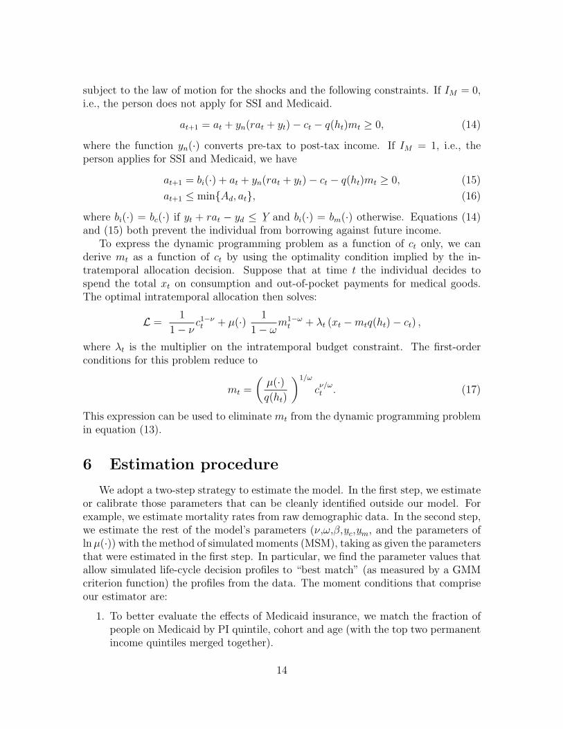
and (15) both prevent the individual from borrowing against future income.To express the dynamic programming problem as a function of ct only, we can

derive mt as a function of ct by using the optimality condition implied by the in-tratemporal allocation decision. Suppose that at time t the individual decides tospend the total xt on consumption and out-of-pocket payments for medical goods.The optimal intratemporal allocation then solves:

L =1

1− νc1−νt + µ(·) 1

1− ωm1−ω

t + λt (xt −mtq(ht)− ct) ,

where λt is the multiplier on the intratemporal budget constraint. The first-orderconditions for this problem reduce to

mt =

(µ(·)q(ht)

)1/ω

cν/ωt . (17)

This expression can be used to eliminate mt from the dynamic programming problemin equation (13).

6 Estimation procedure

We adopt a two-step strategy to estimate the model. In the first step, we estimateor calibrate those parameters that can be cleanly identified outside our model. Forexample, we estimate mortality rates from raw demographic data. In the second step,we estimate the rest of the model’s parameters (ν,ω,β,u

¯c,u¯m

, and the parameters oflnµ(·)) with the method of simulated moments (MSM), taking as given the parametersthat were estimated in the first step. In particular, we find the parameter values thatallow simulated life-cycle decision profiles to “best match” (as measured by a GMMcriterion function) the profiles from the data. The moment conditions that compriseour estimator are:

1. To better evaluate the effects of Medicaid insurance, we match the fraction ofpeople on Medicaid by PI quintile, cohort and age (with the top two permanentincome quintiles merged together).

14

2. Because the effects of Medicaid depend directly on an individual’s asset hold-ings, we match median asset holdings by birth-year cohort, permanent income,and calendar year. We sort individuals into PI quintiles, and the 5 birth-yearcohorts described in section 4. We then compare data and model-generated cellmedians in 5 different years (1998, 2000, 2002, 2004, and 2006).3

3. We match the median and 90th percentile of the out-of-pocket medical expensedistribution in each year-cohort-PI cell (the bottom two quintiles are merged).Because the AHEAD’s medical expense data are reported net of any Medicaidpayments, we deduct government transfers from the model-generated expensesbefore making any comparisons.

4. To capture the dynamics of medical expenses, we match the first and secondautocorrelations for medical expenses in each year-cohort-PI cell.

The mechanics of our MSM approach are as follows. We compute life-cycle histo-ries for a large number of artificial individuals. Each of these individuals is endowedwith a value of the state vector (t, at, g, ht, I) drawn from the data distribution for1996, and each is assigned the entire health and mortality history realized by theperson in the AHEAD data with the same initial conditions. The simulated medicalneeds shocks ζ and ξ are Monte Carlo draws from discretized versions of our estimatedshock processes.

We discretize the asset grid and, using value function iteration, we solve themodel numerically. This yields a set of decision rules, which, in combination with thesimulated endowments and shocks, allows us to simulate each individual’s net worth,medical expenditures, health, and mortality. We then compute asset, medical expenseand Medicaid profiles from the artificial histories in the same way as we computethem from the real data. We use these profiles to construct moment conditions, andevaluate the match using our GMM criterion. We search over the parameter space forthe values that minimize the criterion. Appendix A contains a detailed descriptionof our moment conditions, the weighting matrix in our GMM criterion function, andthe asymptotic distribution of our parameter estimates.

7 First-step estimation results

In this section, we briefly discuss the life-cycle profiles of the stochastic variablesused in our dynamic programming model. The process for income is estimated usingthe procedure in in De Nardi et al. [12], and is described in more detail there. Theprocedure for estimating demographic transition probabilities and and co-pay ratesare new.

3Simulated agents are endowed with asset levels drawn from the 1996 data distribution. Cellswith less than 10 observations are excluded from the moment conditions.

15

7.1 Income profiles

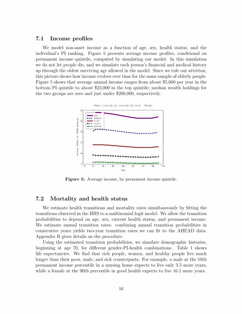
We model non-asset income as a function of age, sex, health status, and theindividual’s PI ranking. Figure 5 presents average income profiles, conditional onpermanent income quintile, computed by simulating our model. In this simulationwe do not let people die, and we simulate each person’s financial and medical historyup through the oldest surviving age allowed in the model. Since we rule out attrition,this picture shows how income evolves over time for the same sample of elderly people.Figure 5 shows that average annual income ranges from about $5,000 per year in thebottom PI quintile to about $23,000 in the top quintile; median wealth holdings forthe two groups are zero and just under $200,000, respectively.

Figure 5: Average income, by permanent income quintile.

7.2 Mortality and health status

We estimate health transitions and mortality rates simultaneously by fitting thetransitions observed in the HRS to a multinomial logit model. We allow the transitionprobabilities to depend on age, sex, current health status, and permanent income.We estimate annual transition rates: combining annual transition probabilities inconsecutive years yields two-year transition rates we can fit to the AHEAD data.Appendix B gives details on the procedure.

Using the estimated transition probabilities, we simulate demographic histories,beginning at age 70, for different gender-PI-health combinations. Table 1 showslife expectancies. We find that rich people, women, and healthy people live muchlonger than their poor, male, and sick counterparts. For example, a male at the 10thpermanent income percentile in a nursing home expects to live only 3.5 more years,while a female at the 90th percentile in good health expects to live 16.1 more years.

16

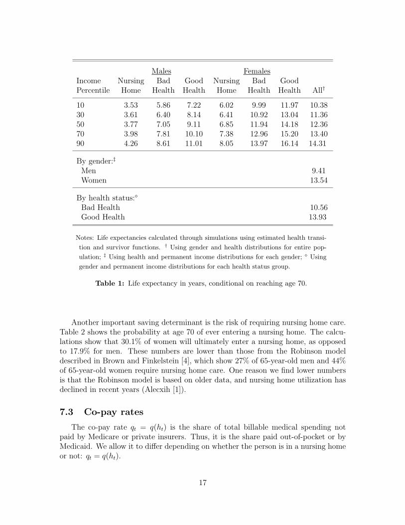
Males FemalesIncome Nursing Bad Good Nursing Bad GoodPercentile Home Health Health Home Health Health All†

10 3.53 5.86 7.22 6.02 9.99 11.97 10.3830 3.61 6.40 8.14 6.41 10.92 13.04 11.3650 3.77 7.05 9.11 6.85 11.94 14.18 12.3670 3.98 7.81 10.10 7.38 12.96 15.20 13.4090 4.26 8.61 11.01 8.05 13.97 16.14 14.31

By gender:‡

Men 9.41Women 13.54

By health status:⋄

Bad Health 10.56Good Health 13.93

Notes: Life expectancies calculated through simulations using estimated health transi-

tion and survivor functions. † Using gender and health distributions for entire pop-

ulation; ‡ Using health and permanent income distributions for each gender; ⋄ Using

gender and permanent income distributions for each health status group.

Table 1: Life expectancy in years, conditional on reaching age 70.

Another important saving determinant is the risk of requiring nursing home care.Table 2 shows the probability at age 70 of ever entering a nursing home. The calcu-lations show that 30.1% of women will ultimately enter a nursing home, as opposedto 17.9% for men. These numbers are lower than those from the Robinson modeldescribed in Brown and Finkelstein [4], which show 27% of 65-year-old men and 44%of 65-year-old women require nursing home care. One reason we find lower numbersis that the Robinson model is based on older data, and nursing home utilization hasdeclined in recent years (Alecxih [1]).

7.3 Co-pay rates

The co-pay rate qt = q(ht) is the share of total billable medical spending notpaid by Medicare or private insurers. Thus, it is the share paid out-of-pocket or byMedicaid. We allow it to differ depending on whether the person is in a nursing homeor not: qt = q(ht).

17

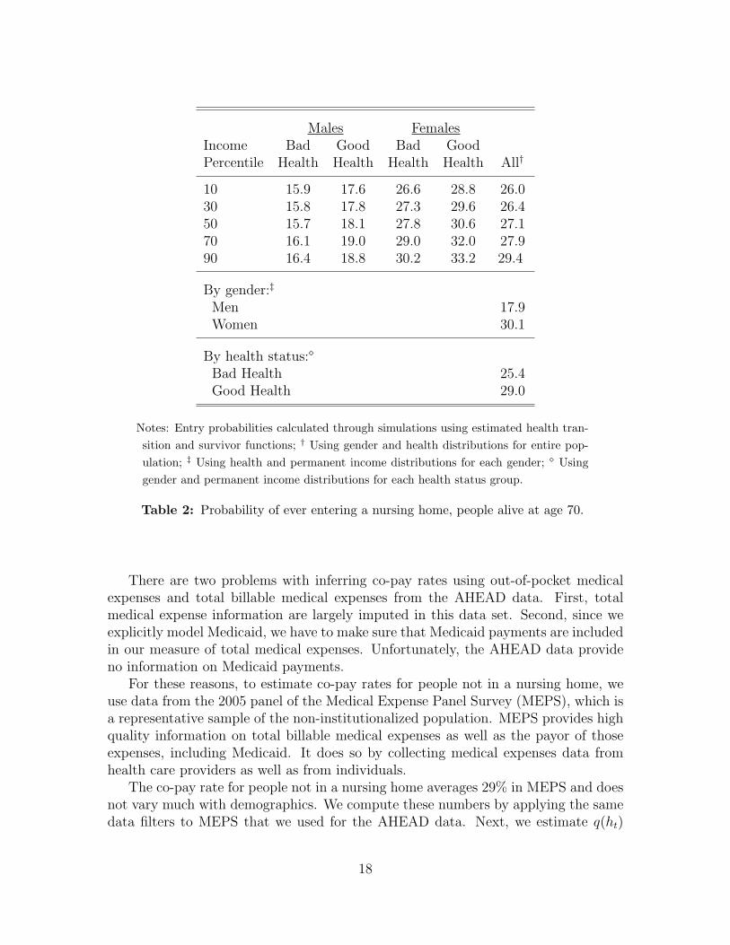
Males FemalesIncome Bad Good Bad GoodPercentile Health Health Health Health All†

10 15.9 17.6 26.6 28.8 26.030 15.8 17.8 27.3 29.6 26.450 15.7 18.1 27.8 30.6 27.170 16.1 19.0 29.0 32.0 27.990 16.4 18.8 30.2 33.2 29.4

By gender:‡

Men 17.9Women 30.1

By health status:⋄

Bad Health 25.4Good Health 29.0

Notes: Entry probabilities calculated through simulations using estimated health tran-

sition and survivor functions; † Using gender and health distributions for entire pop-

ulation; ‡ Using health and permanent income distributions for each gender; ⋄ Using

gender and permanent income distributions for each health status group.

Table 2: Probability of ever entering a nursing home, people alive at age 70.

There are two problems with inferring co-pay rates using out-of-pocket medicalexpenses and total billable medical expenses from the AHEAD data. First, totalmedical expense information are largely imputed in this data set. Second, since weexplicitly model Medicaid, we have to make sure that Medicaid payments are includedin our measure of total medical expenses. Unfortunately, the AHEAD data provideno information on Medicaid payments.

For these reasons, to estimate co-pay rates for people not in a nursing home, weuse data from the 2005 panel of the Medical Expense Panel Survey (MEPS), which isa representative sample of the non-institutionalized population. MEPS provides highquality information on total billable medical expenses as well as the payor of thoseexpenses, including Medicaid. It does so by collecting medical expenses data fromhealth care providers as well as from individuals.

The co-pay rate for people not in a nursing home averages 29% in MEPS and doesnot vary much with demographics. We compute these numbers by applying the samedata filters to MEPS that we used for the AHEAD data. Next, we estimate q(ht)

18

by taking the ratio of mean out-of-pocket spending plus Medicaid payments to meantotal medical expenses.

To estimate the co-pay rate for those in nursing homes we use data from the 2006Medicare Current Beneficiary Survey (MCBS), which is a representative sample ofMedicare enrolees aged 65+. These data reveal that the co-pay rate for those innursing homes is 92%. For every dollar spent on nursing homes, 47 cents come fromMedicaid and 45 cents are from out of pocket, with only 8 cents coming from Medicareor other sources. In our model, we round this number to 90%.

8 Second step results and model fit

8.1 Parameter values

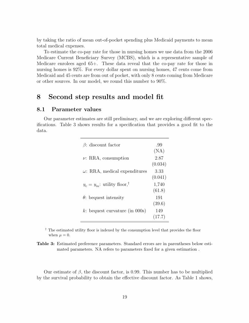
Our parameter estimates are still preliminary, and we are exploring different spec-ifications. Table 3 shows results for a specification that provides a good fit to thedata.

β: discount factor .99(NA)

ν: RRA, consumption 2.87(0.034)

ω: RRA, medical expenditures 3.33(0.041)

u¯c

= u¯m

: utility floor,† 1,740(61.8)

θ: bequest intensity 191(39.6)

k: bequest curvature (in 000s) 149(17.7)

† The estimated utility floor is indexed by the consumption level that provides the floorwhen µ = 0.

Table 3: Estimated preference parameters. Standard errors are in parentheses below esti-mated parameters. NA refers to parameters fixed for a given estimation .

Our estimate of β, the discount factor, is 0.99. This number has to be multipliedby the survival probability to obtain the effective discount factor. As Table 1 shows,

19

the survival probability for our sample of older individuals is low, implying an effectivediscount factor much lower than β.

The estimate of ν, the coefficient of relative risk aversion for “regular” consump-tion, is 2.9, while the estimate of ω, the coefficient of relative risk aversion for medicalgoods, is 3.3; the demand for medical goods is less elastic than the demand for con-sumption.

To start, we constrain the two utility floors to be the same, as Medicaid generositydoes not appear to be drastically different across the two categories of recipients. Theutility floor corresponds to the utility level of consuming $1,740 a year when healthy.It should be noted that the medically needy are guaranteed a minimum income levelof $7,000 by SSI, so that their total consumption when healthy is actually $7,000 ayear. However, when there are large medical needs, transfers are determined by theMedicaid-induced utility floor.

The point estimates of θ = 191 and k = 149, 000 imply that, before the period be-fore certain death, the bequest motive becomes operative once consumption exceeds$24,000 per year. (See De Nardi, French, and Jones [12] for a derivation.) For indi-viduals in this group, the marginal propensity to bequeath above that consumptionlevel is high, with 86 cents of every extra dollar above the threshold being left asbequests.

These preference parameters are identified jointly. There are multiple ways togenerate high saving by the elderly: large values of the discount rate β, low valuesof the utility floors u

¯cand u

¯m, large values of the curvature parameters ν and ω, or

strong and pervasive bequest motives (high values of θ and small values of k) . Dynan,Skinner and Zeldes [15] point out that the same assets can simultaneously addressboth precautionary and bequest needs. There are also multiple ways to ensure that theincome-poorest elderly do not save, including high utility floors and bequest motivesthat become operative only at high levels of consumption. We acquire additionalidentification in several ways. The most obvious of these is that we fix β to 0.99,a standard value. Another step is that we require our model to match Medicaidrecipiency rates, which helps pin down the utility floors. Matching disaggregatedout-of-pocket medical expenditures also helps identify the utility floors, as Medicaidaffects the way in which out-of-pocket medical expenditures (which exclude Medicaidpayments) vary by income.

We also estimate the coefficients for the mean of the logged medical needs shifterµ(ht, ψt, t), the volatility scaler σ(ht, t) and the process for the shocks ζt and ξt. As weshow in the graphs that follow, the estimates for these parameters (available from theauthors on request) imply that the demand for medical services rises rapidly with age.Matching the median and 90th percentile of out-of-pocket medical expenditures, alongwith their first and second autocorrelations, is of course the principal way in whichwe identify these parameters. The fact that the medical needs shocks do not dependdirectly on income—the only link is through the health transition probabilities—also helps us identify other parameters, as the expenditure profiles we match are

20

disaggregated by income. Most notably, the income gradient of medical expenditureshelps us pin down the curvature parameters ν and ω.

We now turn to discussing how well the model fits the some key aspects of thedata and also look at some additional model implications.

8.2 Medicaid recipiency

a b

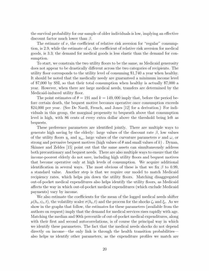
Figure 6: Medicaid recipiency by cohort and PI quintile: data (solid lines) and model(dashed lines).

Figure 6 compares the Medicaid recipiency profiles generated by the model (dashedline) to those in the data (solid line) for the members of two birth-year cohorts. Inpanel a, the lines at the far left of the graph are for the youngest cohort, whosemembers in 1996 were aged 72-76, with an average age of 74. The second set of linesare for the cohort aged 82-86 in 1996. Panel b displays the two other cohorts, startingrespectively at age 79 and 89. The graphs show that the model matches well boththe usage levels and their rise by age and permanent income.

8.3 Net worth profiles

Figure 7 plots median net worth by age, cohort, and permanent income. Heretoo the model does well, matching the observation that the savings patterns differ bypermanent income and that higher PI people don’t run down their assets until wellpast age 90.

8.4 Medical expenses

Figure 8 displays median out-of-pocket medical expenses (that is, net of Medicaidpayments and private and public insurance co-pays) paid by people in the model and

21

a b

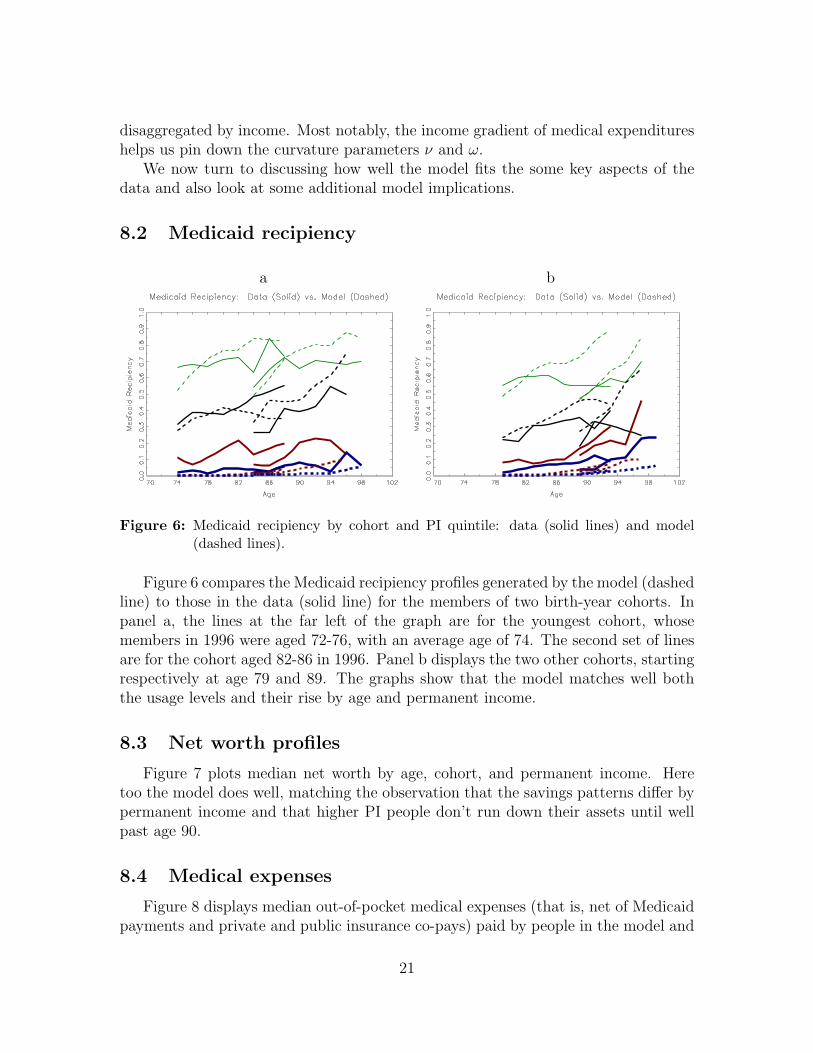
Figure 7: Median net worth by cohort and PI quintile: data (solid lines) and model(dashed lines).

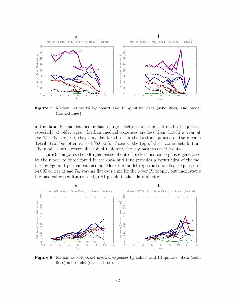
in the data. Permanent income has a large effect on out-of-pocket medical expenses,especially at older ages. Median medical expenses are less than $1,500 a year atage 75. By age 100, they stay flat for those in the bottom quintile of the incomedistribution but often exceed $5,000 for those at the top of the income distribution.The model does a reasonable job of matching the key patterns in the data.

Figure 9 compares the 90th percentile of out-of-pocket medical expenses generatedby the model to those found in the data and thus provides a better idea of the tailrisk by age and permanent income. Here the model reproduces medical expenses of$4,000 or less at age 74, staying flat over time for the lower PI people, but understatesthe medical expenditures of high-PI people in their late nineties.

a b

Figure 8: Median out-of-pocket medical expenses by cohort and PI quintile: data (solidlines) and model (dashed lines).

22

a b

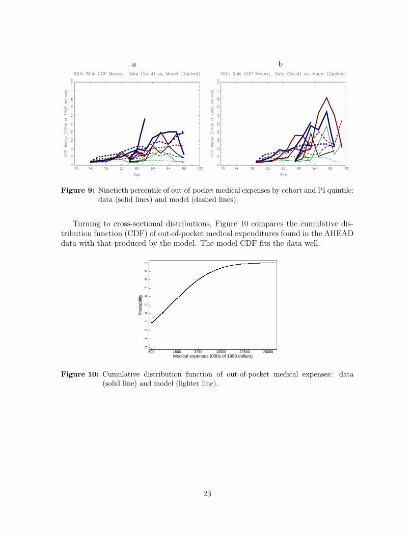
Figure 9: Ninetieth percentile of out-of-pocket medical expenses by cohort and PI quintile:data (solid lines) and model (dashed lines).

Turning to cross-sectional distributions, Figure 10 compares the cumulative dis-tribution function (CDF) of out-of-pocket medical expenditures found in the AHEADdata with that produced by the model. The model CDF fits the data well.

0.1

.2.3

.4.5

.6.7

.8.9

1

500 1500 3750 10000 27500 75000Medical expenses (000s of 1998 dollars)

Pro

babi

lity

Figure 10: Cumulative distribution function of out-of-pocket medical expenses: data(solid line) and model (lighter line).

23

a b

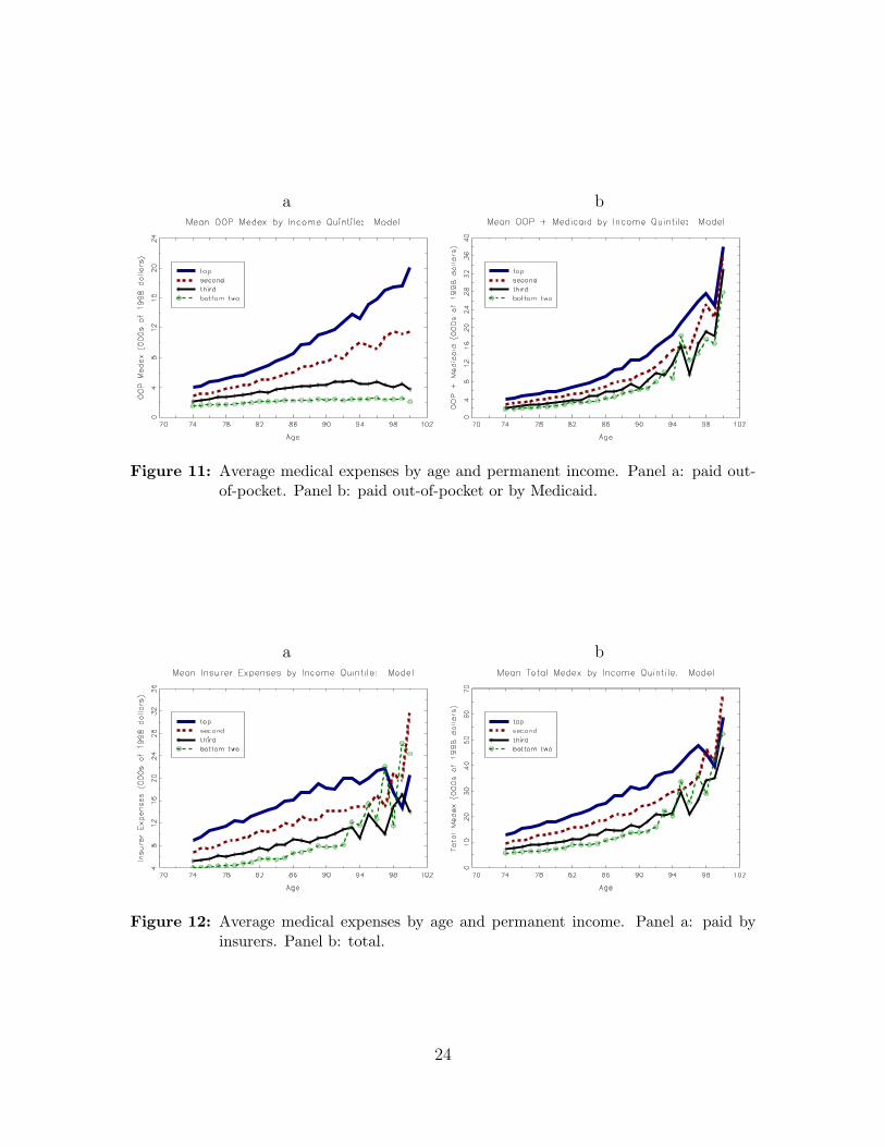
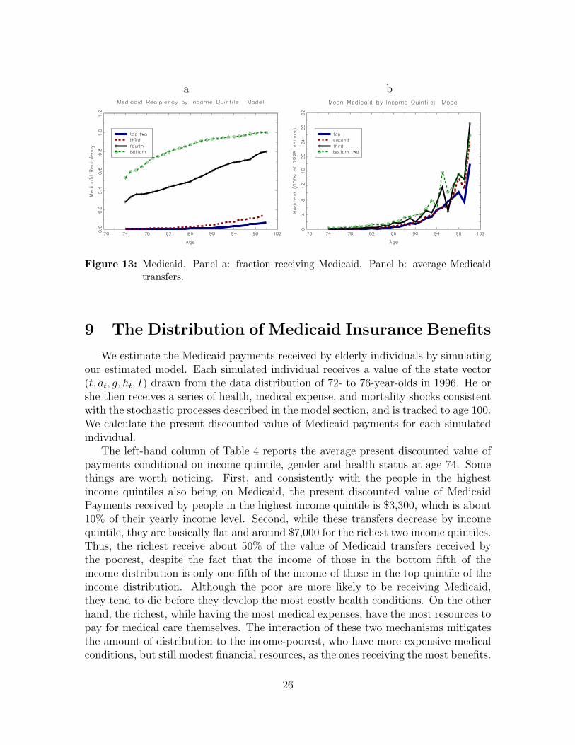
Figure 11: Average medical expenses by age and permanent income. Panel a: paid out-of-pocket. Panel b: paid out-of-pocket or by Medicaid.

a b

Figure 12: Average medical expenses by age and permanent income. Panel a: paid byinsurers. Panel b: total.

24

Figure 11 presents profiles that arise when the youngest cohort is simulated fromages 74 to (potentially) 100. Panel a shows average out-of-pocket medical expenses,which follow a pattern similar to that in Figures 8 and 9. Panel b of Figure 11 showsthe sum of medical expenses paid out-of-pocket and the expenses paid by Medicaid,the latter measured as the increase in q(ht)mt generated by government transfers.These sums also increase rapidly with age, going from around $3,000 at age 74 to$35,000 at age 100. Medicaid allows poorer people to consume proportionally muchmore medical goods and services than they pay for. As a result, the expense sumshown in panel b rises more slowly with income than the out-of-pocket expendituresshown in panel a.

Panel a of Figure 12 displays average medical expenses covered by private andpublic insurers. These payments are very large and also increase by age and per-manent income, reaching over $20,000 for the oldest members of the top permanentincome quintile. The oldest in the poorest permanent income quintile, however, alsobenefit from these payments, which reach around $12,000 at age 98. Panel b of Fig-ure 12 displays total medical expenses, which in this case also coincide with totalconsumption of medical goods and services. Comparing the two panels makes it clearthat most elderly individuals consume far more medical care than they for pay out-of-pocket. The increase in total medical expenses after retirement is very large, goingfrom around $10,000 at age 74 to $60,000 at age 100.

8.5 Utility floor, preference shocks, and implied insurancesystem

Through the interaction of the utility floor and medical needs shocks, the modelhas interesting implications on the insurance provided by means-tested programs.

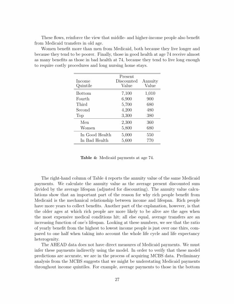
Figure 13 describes the transfers generated by the model. Panel a of this figureshows the fraction of individuals receiving transfers, while panel b shows averagetransfers, taken across both recipients and non-recipients. Panel a shows that peo-ple in the bottom two permanent income quintiles receive Medicaid at fairly highrates throughout their retirement. Most of these people qualify through the categor-ically needy pathway. People in the top income quintiles, in contrast, use Medicaidmuch more heavily at older ages, when large medical expenditures make them eligiblethrough the medically needy pathway.

Panel b of Figure 13 shows average Medicaid transfers. While low-income peopleare much more likely to qualify for Medicaid, the categorically needy provision allowsthem to qualify with small medical needs. The medically needy provision allows high-income people to qualify only when their medical expenses are high relative to theirresources. Although the poor on average receive more Medicaid benefits than the richat younger ages, at very old ages the two groups receive similar benefits.

25

a b

Figure 13: Medicaid. Panel a: fraction receiving Medicaid. Panel b: average Medicaidtransfers.

9 The Distribution of Medicaid Insurance Benefits

We estimate the Medicaid payments received by elderly individuals by simulatingour estimated model. Each simulated individual receives a value of the state vector(t, at, g, ht, I) drawn from the data distribution of 72- to 76-year-olds in 1996. He orshe then receives a series of health, medical expense, and mortality shocks consistentwith the stochastic processes described in the model section, and is tracked to age 100.We calculate the present discounted value of Medicaid payments for each simulatedindividual.

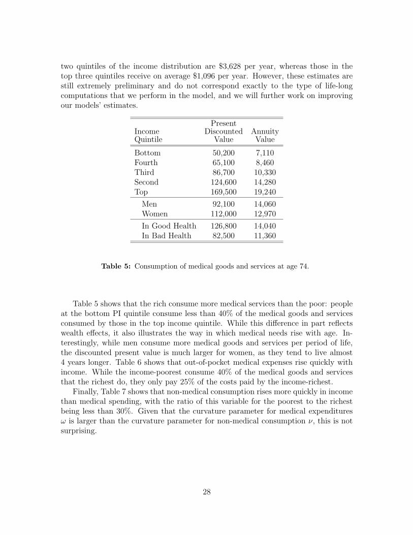
The left-hand column of Table 4 reports the average present discounted value ofpayments conditional on income quintile, gender and health status at age 74. Somethings are worth noticing. First, and consistently with the people in the highestincome quintiles also being on Medicaid, the present discounted value of MedicaidPayments received by people in the highest income quintile is $3,300, which is about10% of their yearly income level. Second, while these transfers decrease by incomequintile, they are basically flat and around $7,000 for the richest two income quintiles.Thus, the richest receive about 50% of the value of Medicaid transfers received bythe poorest, despite the fact that the income of those in the bottom fifth of theincome distribution is only one fifth of the income of those in the top quintile of theincome distribution. Although the poor are more likely to be receiving Medicaid,they tend to die before they develop the most costly health conditions. On the otherhand, the richest, while having the most medical expenses, have the most resources topay for medical care themselves. The interaction of these two mechanisms mitigatesthe amount of distribution to the income-poorest, who have more expensive medicalconditions, but still modest financial resources, as the ones receiving the most benefits.

26

These flows, reinforce the view that middle- and higher-income people also benefitfrom Medicaid transfers in old age.

Women benefit more than men from Medicaid, both because they live longer andbecause they tend to be poorer. Finally, those in good health at age 74 receive almostas many benefits as those in bad health at 74, because they tend to live long enoughto require costly procedures and long nursing home stays.

PresentIncome Discounted AnnuityQuintile Value Value

Bottom 7,100 1,010Fourth 6,900 900Third 5,700 680Second 4,200 480Top 3,300 380

Men 2,300 360Women 5,800 680

In Good Health 5,000 550In Bad Health 5,600 770

Table 4: Medicaid payments at age 74.

The right-hand column of Table 4 reports the annuity value of the same Medicaidpayments. We calculate the annuity value as the average present discounted sumdivided by the average lifespan (adjusted for discounting). The annuity value calcu-lations show that an important part of the reason for why rich people benefit fromMedicaid is the mechanical relationship between income and lifespan. Rich peoplehave more years to collect benefits. Another part of the explanation, however, is thatthe older ages at which rich people are more likely to be alive are the ages whenthe most expensive medical conditions hit; all else equal, average transfers are anincreasing function of one’s lifespan. Looking at these numbers, we see that the ratioof yearly benefit from the highest to lowest income people is just over one thirs, com-pared to one half when taking into account the whole life cycle and life expectancyheterogenity.

The AHEAD data does not have direct measures of Medicaid payments. We mustinfer these payments indirectly using the model. In order to verify that these modelpredictions are accurate, we are in the process of acquiring MCBS data. Preliminaryanalysis from the MCBS suggests that we might be understating Medicaid paymentsthroughout income quintiles. For example, average payments to those in the bottom

27

two quintiles of the income distribution are $3,628 per year, whereas those in thetop three quintiles receive on average $1,096 per year. However, these estimates arestill extremely preliminary and do not correspond exactly to the type of life-longcomputations that we perform in the model, and we will further work on improvingour models’ estimates.


Bottom 50,200 7,110Fourth 65,100 8,460Third 86,700 10,330Second 124,600 14,280Top 169,500 19,240

Men 92,100 14,060Women 112,000 12,970

In Good Health 126,800 14,040In Bad Health 82,500 11,360

Table 5: Consumption of medical goods and services at age 74.

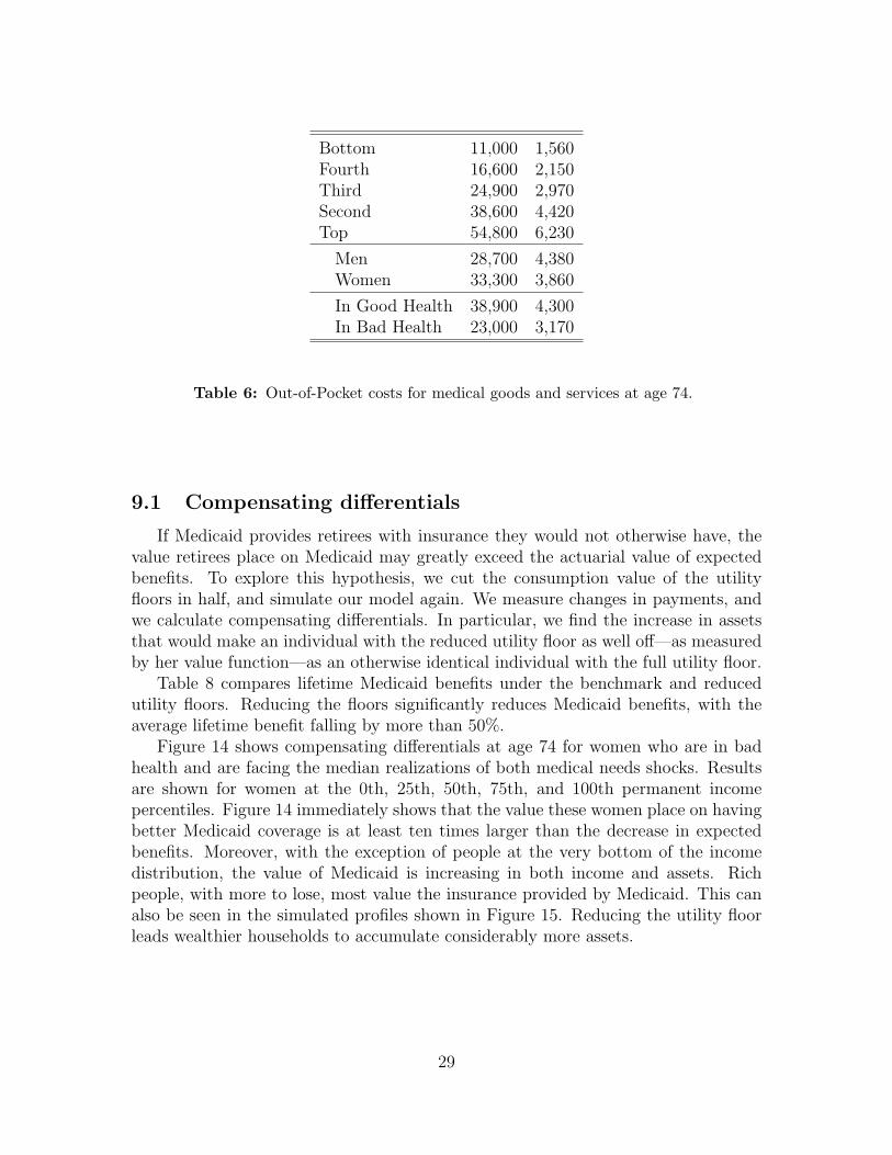
Table 5 shows that the rich consume more medical services than the poor: peopleat the bottom PI quintile consume less than 40% of the medical goods and servicesconsumed by those in the top income quintile. While this difference in part reflectswealth effects, it also illustrates the way in which medical needs rise with age. In-terestingly, while men consume more medical goods and services per period of life,the discounted present value is much larger for women, as they tend to live almost4 years longer. Table 6 shows that out-of-pocket medical expenses rise quickly withincome. While the income-poorest consume 40% of the medical goods and servicesthat the richest do, they only pay 25% of the costs paid by the income-richest.

Finally, Table 7 shows that non-medical consumption rises more quickly in incomethan medical spending, with the ratio of this variable for the poorest to the richestbeing less than 30%. Given that the curvature parameter for medical expendituresω is larger than the curvature parameter for non-medical consumption ν, this is notsurprising.

28


Men 28,700 4,380Women 33,300 3,860


Table 6: Out-of-Pocket costs for medical goods and services at age 74.

9.1 Compensating differentials

If Medicaid provides retirees with insurance they would not otherwise have, thevalue retirees place on Medicaid may greatly exceed the actuarial value of expectedbenefits. To explore this hypothesis, we cut the consumption value of the utilityfloors in half, and simulate our model again. We measure changes in payments, andwe calculate compensating differentials. In particular, we find the increase in assetsthat would make an individual with the reduced utility floor as well off—as measuredby her value function—as an otherwise identical individual with the full utility floor.

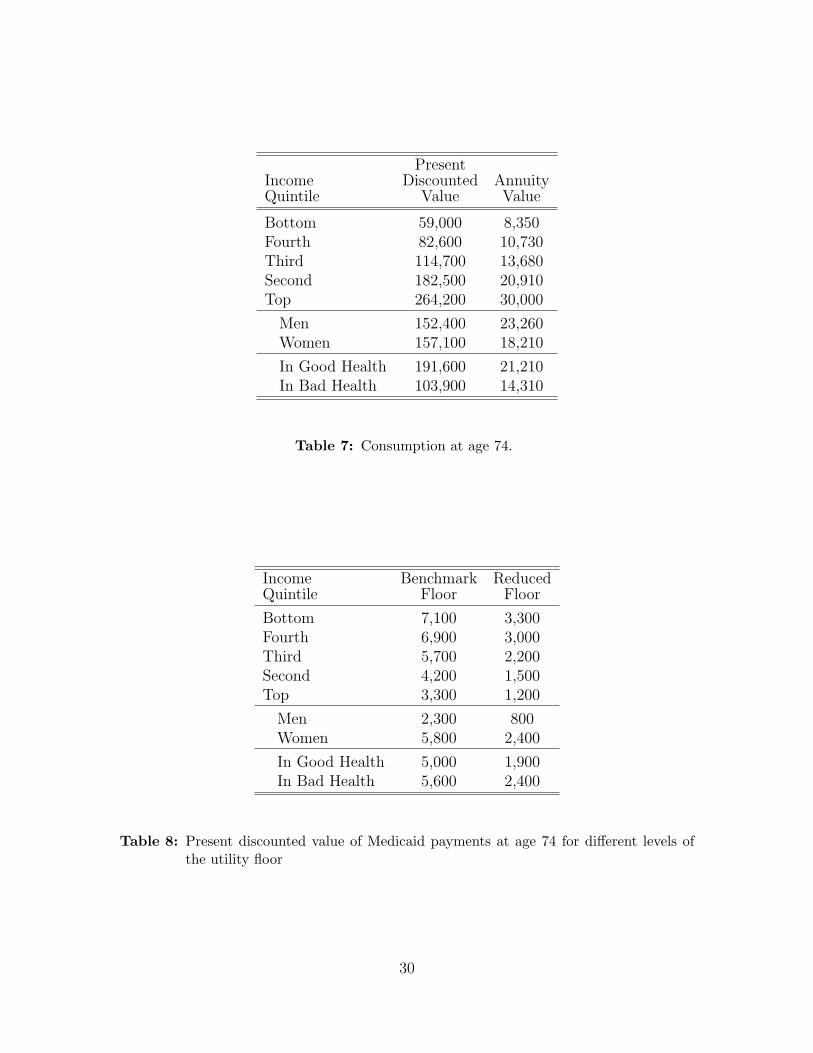
Table 8 compares lifetime Medicaid benefits under the benchmark and reducedutility floors. Reducing the floors significantly reduces Medicaid benefits, with theaverage lifetime benefit falling by more than 50%.

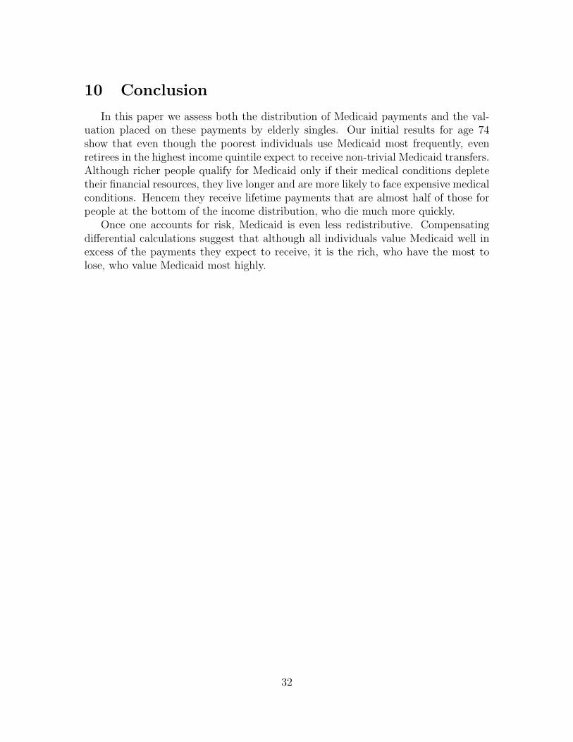
Figure 14 shows compensating differentials at age 74 for women who are in badhealth and are facing the median realizations of both medical needs shocks. Resultsare shown for women at the 0th, 25th, 50th, 75th, and 100th permanent incomepercentiles. Figure 14 immediately shows that the value these women place on havingbetter Medicaid coverage is at least ten times larger than the decrease in expectedbenefits. Moreover, with the exception of people at the very bottom of the incomedistribution, the value of Medicaid is increasing in both income and assets. Richpeople, with more to lose, most value the insurance provided by Medicaid. This canalso be seen in the simulated profiles shown in Figure 15. Reducing the utility floorleads wealthier households to accumulate considerably more assets.

29



Men 152,400 23,260Women 157,100 18,210


Table 7: Consumption at age 74.

Income Benchmark ReducedQuintile Floor Floor


Men 2,300 800Women 5,800 2,400


Table 8: Present discounted value of Medicaid payments at age 74 for different levels ofthe utility floor

30

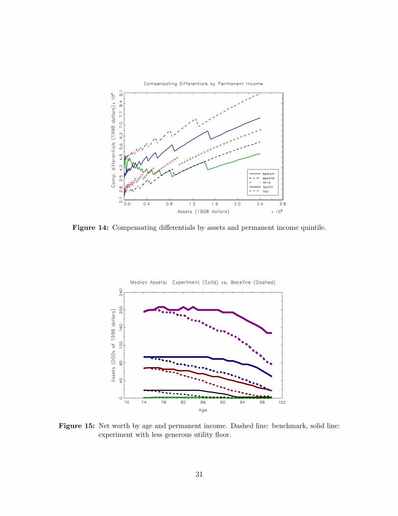
Figure 14: Compensating differentials by assets and permanent income quintile.

Figure 15: Net worth by age and permanent income. Dashed line: benchmark, solid line:experiment with less generous utility floor.

31

10 Conclusion

In this paper we assess both the distribution of Medicaid payments and the val-uation placed on these payments by elderly singles. Our initial results for age 74show that even though the poorest individuals use Medicaid most frequently, evenretirees in the highest income quintile expect to receive non-trivial Medicaid transfers.Although richer people qualify for Medicaid only if their medical conditions depletetheir financial resources, they live longer and are more likely to face expensive medicalconditions. Hencem they receive lifetime payments that are almost half of those forpeople at the bottom of the income distribution, who die much more quickly.

Once one accounts for risk, Medicaid is even less redistributive. Compensatingdifferential calculations suggest that although all individuals value Medicaid well inexcess of the payments they expect to receive, it is the rich, who have the most tolose, who value Medicaid most highly.

32

References

[1] Lisa Alecxih. Nursing home use by “oldest old” sharply declines. Mimeo, 2006.

[2] Joseph G. Altonji and Lewis M. Segal. Small sample bias in gmm estimation ofcovariance structures. Journal of Business and Economic Statistics, 14(3):353–366, 1996.

[3] Robert Brook, John E. Ware, William H. Rogers, Emmett B. Keeler, Allyson R.Davies, Cathy A. Donald, George A. Goldberg, Kathleen N. Lohr, Patricia C.Masthay, and Joseph P. Newhouse. Does free care improve adults’ health? resultsfrom a randomized trial. New England Journal of Medicine, 309(23):1426–1434,1983.

[4] Jeff Brown and Amy Finkelstein. The interaction of public and private insurance:Medicaid and the long term care insurance market. NBERWorking Paper 10989,2004.

[5] Jeff Brown and Amy Finkelstein. The interaction of public and private insurance:Medicaid and the long term care insurance market. American Economic Review,98(5):837–880, 2008.

[6] Jeffrey R. Brown, Norma B. Coe, and Amy Finkelstein. Medicaid crowd-out ofprivate long-term care insurance demand: Evidence from the health and retire-ment survey. In James M. Poterba, editor, Tax Policy and the Economy. MITPress, 2007.

[7] Moshe Buchinsky. Recent advances in quantile regression models: A practicalguideline for empirical research. Journal of Human Resources, 33:88–126, 1998.

[8] David Card, Carlos Dobkin, and Nicole Maestas. Does medicare save lives? TheQuarterly Journal of Economics, 124(2):597–636, 2009.

[9] Gary Chamberlain. Comment: Sequential moment restrictions in panel data.Journal of Business & Economic Statistics,, 10(1):20–26, 1992.

[10] Kenneth Y. Chay, Daeho Kim, and Shailender Swaminathan. Medicare, hospitalutilization and mortality: Evidence from the programs origins. Mimeo, 2010.

[11] Joseph Doyle. Returns to local-area healthcare spending: Using health shocksto patients far from home. American Economic Journal: Applied Economics,3(3):221–243, 2011.

[12] Mariacristina De Nardi, Eric French, and John B. Jones. Why do the elderlysave? the role of medical expenses. Journal of Political Economy, 118(1):39–75,2010.

33

[13] Mariacristina De Nardi, Eric French, and John B. Jones. Medicaid and theelderly. NBER Working Paper 17689, 2011.

[14] Darrell Duffie and Kenneth J. Singleton. Simulated moments estimation ofmarkov models of asset prices. Econometrica, 61(4):929–952, 1993.

[15] Karen E. Dynan, Jonathan Skinner, and Stephen P. Zeldes. The importance ofbequests and life-cycle saving in capital accumulation: A new answer. AmericanEconomic Review, 92(2):274–278, 2002.

[16] Zhigang Feng. Macroeconomic consequences of alternative reforms to the healthinsurance system in the u.s. Mimeo, 2009.

[17] Amy Finkelstein and Robin McKnight. What did medicare do? the initial impactof medicare on mortality and out of pocket medical spending. Journal of PublicEconomics, 92(7):1644–1669, 2008.

[18] Amy Finkelstein, Sarah Taubman, Bill Wright, Mira Bernstein, JonathanGruber, Heidi Allen Joseph P. Newhouse, Katherine Baicker, and OregonHealth Study Group. The oregon health insurance experiment: Evidence fromthe first year. Quarterly Journal of Economics, 127(3):1057–1106, 2012.

[19] Elliott S. Fisher, David E. Wennberg, Therese A. Stukel, Daniel J. Gottlieb, F.L.Lucas, and Etoile L. Pinder. The implications of regional variations in medicarespending. part 2: Health outcomes and satisfaction with care. Annals of InternalMedicine, 138(4):288–322, 2003.

[20] Raquel Fonseca, Pierre-Carl Michaud, Titus Galama, and Arie Kapteyn. On therise of health spending and longevity. Rand Working Paper WR-722, 2009.

[21] Eric French and John Bailey Jones. On the distribution and dynamics of healthcare costs. Journal of Applied Econometrics, 19(4):705–721, 2004.

[22] Michael Grossman. On the concept of health capital and the demand for health.Journal of Political Economy, 80(2):223–255, 1972.

[23] Gary D. Hansen, Minchung Hsu, and Junsang Lee. Health insurance reform:The impact of a medicare buy-in. Working Paper 18529, National Bureau ofEconomic Research, November 2012.

[24] R. Glenn Hubbard, Jonathan Skinner, and Stephen P. Zeldes. Expanding thelife-cycle model: Precautionary saving and public policy. American EconomicReview, 84:174–179, 1994.

[25] R. Glenn Hubbard, Jonathan Skinner, and Stephen P. Zeldes. Precautionarysaving and social insurance. Journal of Political Economy, 103(2):360–399, 1995.

34

[26] Michael D. Hurd. Mortality risk and bequests. Econometrica, 57(4):779–813,1989.

[27] Michael D. Hurd, Daniel McFadden, and Angela Merrill. Predictors of mortalityamong the elderly. Working Paper 7440, National Bureau of Economic Research,1999.

[28] Selahattin Imrohoroglu and Sagiri Kitao. Social security, benefit claiming andlabor force participation: A quantitative general equilibrium approach. Mimeo,2009.

[29] Ahmed Khwaja. Estimating willingness to pay for medicare using a dynamiclife-cycle model of demand for health insurance. Journal of Econometrics,156(1):130–147, 2010.

[30] Ralph S. J. Koijen, Stijn Van Nieuwerburgh, and Motohiro Yogooijen. Healthand mortality delta: Assessing the welfare cost of household insurance choice.Mimeo, 2012.

[31] Ruud H. Koning. Kernel: A gauss library for kernel estimation.http://www.xs4all.nl/

[32] Karen Kopecky and Tatyana Koreshkova. The impact of medical and nursinghome expenses and social insurance policies on savings and inequality. Mimeo,2009.

[33] Laurence J. Kotlikoff. Health expenditures and precautionary savings. In Lau-rence J. Kotlikoff, editor, What Determines Saving? Cambridge, MIT Press,1988, 1988.

[34] Lee Lockwood. Incidental bequests: Bequest motives and the choice to self-insurelate-life risks. Mimeo, 2012.

[35] Willard G. Manning, Joseph P. Newhouse, Naihua Duan, Emmett B. Keeler, andArleen Leibowitz. Health insurance and the demand for medical care: Evidencefrom a randomized experiment. American Economic Review, 77:251–277, 1987.

[36] Charles F. Manski. Analog Estimation Methods in Econometrics. Chapman andHall, 1988.

[37] Samuel Marshall, Kathleen M. McGarry, and Jonathan S. Skinner. The risk ofout-of-pocket health care expenditure at the end of life. Working Paper 16170,National Bureau of Economic Research, 2010.

[38] Thad Mirer. The wealth-age relation among the aged. American EconomicReview, 69:435–443, 1979.

35

[39] Makoto Nakajima and Irina Telyukova. Home equity in retirement. Mimeo,2012.

[40] Whitney K. Newey. Generalized method of moments specification testing. Jour-nal of Econometrics, 29(3):229–256, 1985.

[41] Whitney K. Newey and Daniel L. McFadden. Large sample estimation andhypothesis testing. In Robert Engle and Daniel L. McFadden, editors, Handbookof Econometrics, Volume 4. Elsevier, Amsterdam, 1994.

[42] The Kaiser Commission on Medicaid and the Uninsured. Medicaid: A Primer.Menlo Park, CA, The Henry J. Kaiser Family Foundation, 2010.

[43] Serdar Ozkan. Income inequality and health care expenditures over the life cycle.Mimeo, Federal Reserve Board, 2011.

[44] Ariel Pakes and David Pollard. Simulation and the aysmptotics of optimizationestimators. Econometrica, 57(5):1027–1057, 1989.

[45] Michael G. Palumbo. Uncertain medical expenses and precautionary saving nearthe end of the life cycle. Review of Economic Studies, 66:395–421, 1999.

[46] Svetlana Paschenko and Ponpoje Porapakkarm. Quantitative analysis of healthinsurance reform: Separating regulation from redistribution. Mimeo, 2012.

[47] Jorn-Steffen Pischke. Measurement error and earnings dynamics: Some estimatesfrom the PSID validation study. Journal of Business & Economics Statistics,13(3):305–314, 1995.

[48] James M. Poterba, Steven F. Venti, and David A. Wise. The asset cost of poorhealth. Working Paper 16389, National Bureau of Economic Research, 2010.

[49] James Powell. Estimation of semiparametric models. In Robert Engle andDaniel L McFadden, editors, Handbook of Econometrics, Volume 4. Elsevier,Amsterdam, 1994.

[50] Susann Rohwedder, Steven J. Haider, and Michael Hurd. Increases in wealthamong the elderly in the early 1990s: How much is due to survey design? Reviewof Income and Wealth, 52(4):509–524, 2006.

[51] John Karl Scholz and Ananth Seshadri. Health and wealth in a lifecycle model.Mimeo, 2012.

[52] John Karl Scholz, Ananth Seshadri, and Surachai Khitatrakun. Are americanssaving optimally for retirement? Journal of Political Economy, 114:607–643,2006.

36

[53] Motohiro Yogo. Portfolio choice in retirement: Health risk and the demand forannuities, housing, and risky assets. Mimeo, University of Pennsylvania, 2009.

37

Appendix A: Moment conditions and asymptotic distributionof parameter estimates

Recall that we estimate the parameters of our model in the two steps. In thefirst step, we estimate the vector χ, the set of parameters than can be estimatedwith explicitly using our model. In the second step, we use the method of simulatedmoments (MSM) to estimate the remaining parameters, which are contained in theM × 1 vector ∆. The elements of ∆ are ν, ω, β, c, θ, k, and the parameters oflnµ(·). Our estimate, ∆, of the “true” parameter vector ∆0 is the value of ∆ thatminimizes the (weighted) distance between the life-cycle profiles found in the dataand the simulated profiles generated by the model.

For each calendar year t ∈ {t0, ..., tT} = {1996, 1998, 2000, 2002, 2004, 2006}, wematch median assets for QA = 5 permanent income quintiles in P = 5 birth yearcohorts.4 The 1996 (period-t0) distribution of simulated assets, however, is boot-strapped from the 1996 data distribution, and thus we match assets to the data for1998, ..., 2006. In addition, we require each cohort-income-age cell have at least 10observations to be included in the GMM criterion.

Suppose that individual i belongs to birth cohort p and his permanent incomelevel falls in the qth permanent income quintile. Let apqt(∆, χ) denote the model-predicted median asset level for individuals in individual i’s group at time t, where χincludes all parameters estimated in the first stage (including the permanent incomeboundaries). Assuming that observed assets have a continuous conditional density,apqt will satisfy

Pr(ait ≤ apqt(∆0, χ0) |p, q, t, individual i observed at t

)= 1/2.

The preceding equation can be rewritten as a moment condition (Manski [36], Pow-ell [49] and Buchinsky [7]). In particular, applying the indicator function produces

E(1{ait ≤ apqt(∆0, χ0)} − 1/2 |p, q, t, individual i observed at t

)= 0. (18)

Letting Iq denote the values contained in the qth permanent income quintile, we canconvert this conditional moment equation into an unconditional one (e.g., Chamber-lain [9]):

E([1{ait ≤ apqt(∆0, χ0)} − 1/2]× 1{pi = p} × 1{Ii ∈ Iq}

× 1{individual i observed at t}∣∣ t) = 0 (19)

for p ∈ {1, 2, ..., P}, q ∈ {1, 2, ..., QA}, t ∈ {t1, t2..., tT}.4Because we do not allow for macro shocks, in any given cohort t is used only to identify the

individual’s age.

38

We also include several moment conditions relating to medical expenses. To usethese moment conditions, we first simulate medical expenses at an annual frequency,and then take two-year averages to produce a measure of medical expenses comparableto the ones contained in the AHEAD.

As with assets, we divide individuals into 5 cohorts and match data from 5 wavescovering the period 1998-2006. The moment conditions for medical expenses aresplit by permanent income as well. However, we combine the bottom two incomequintiles, as there is very little variation in out-of-pocket medical expenses in thebottom quintile until very late in life; QM = 4.

We require the model to match the median out-of-pocket medical expendituresin each cohort-income-age cell. Let m50

pqt(∆, χ) denote the model-predicted 50th per-centile for individuals in cohort p and permanent income group q at time (age) t.Proceeding as before, we have the following moment condition:

E([1{mit ≤ m50

pqt(∆0, χ0)} − 0.5]× 1{pi = p} × 1{Ii ∈ Iq}


for p ∈ {1, 2, ..., P}, q ∈ {1, 2, ..., QM}, t ∈ {t1, t2..., tT}.To fit the upper tail of the medical expense distribution, we require the model

to match the 90th percentile of out-of-pocket medical expenditures in each cohort-income-age cell. Letting m90

pqt(∆, χ) denote the model-predicted 90th percentile, wehave the following moment condition:

E([1{mit ≤ m90

pqt(∆0, χ0)} − 0.9]× 1{pi = p} × 1{Ii ∈ Iq}


for p ∈ {1, 2, ..., P}, q ∈ {1, 2, ..., QM}, t ∈ {t1, t2..., tT}.To pin down the autocorrelation coefficient for ζ (ρm), and its contribution to the

total variance ζ + ξ, we require the model to match the first and second autocorrela-tions of logged medical expenses. Define the residual Rit as

Rit = ln(mit)− lnmpqt,

lnmpqt = E(ln(mit)|pi = p, qi = q, t)

and define the standard deviation σpqt as

σpqt =√E(R2

it|pi = p, qi = q, t).

Both lnmpqt and σpqt can be estimated non-parametrically as elements of χ. Usingthese quantities, the autocorrelation coefficient ACpqtj is:

ACpqtj = E

(RitRi,t−j

σpqt σpq,t−j

∣∣∣∣∣ pi = p, qi = q

).

39

Let ACpqtj(∆, χ) be the jth autocorrelation coefficient implied by the model, calcu-lated using model values of lnmpqt and σpqt. The resulting moment condition for thefirst autocorrelation is

E

([RitRi,t−1

σpqt σpq,t−1

− ACpqt1(∆0, χ0)

]× 1{pi = p} × 1{Ii ∈ Iq}

× 1{individual i observed at t & t− 1}∣∣∣∣ t)

= 0. (22)

The corresponding moment condition for the second autocorrelation is

E

([RitRi,t−2

σpqt σpq,t−2

− ACpqt2(∆0, χ0)

]× 1{pi = p} × 1{Ii ∈ Iq}

× 1{individual i observed at t & t− 2}∣∣∣∣ t)

= 0. (23)

Finally, we match Medicaid utilization (take-up) rates. Once again, we divideindividuals into 5 cohorts, match data from 5 waves, and stratify the data by perma-nent income. We combine the top two quintiles because in many cases no one in thetop permanent income quintile is on Medicaid: QU = 4.

Let upqt(∆, χ) denote the model-predicted utilization rate for individuals in cohortp and permanent income group q at age t. Let uit be the {0, 1} indicator that equals1 when individual i receives Medicaid. The associated moment condition is

E([uit − upqt(∆0, χ0)

]× 1{pi = p} × 1{Ii ∈ Iq}


for p ∈ {1, 2, ..., P}, q ∈ {1, 2, ..., QU}, t ∈ {t1, t2..., tT}.To summarize, the moment conditions used to estimate model with endogenous

medical expenses consist of: the moments for asset medians described by equation(19); the moments for median medical expenses described by equation (20); the mo-ments for the 90th percentile of medical expenses described by equation (21); themoments for the autocorrelations of logged medical expenses described by equations(22) and (23); and the moments for the Medicaid utilization rates described by equa-tion (24). In the end, we have a total of J = 478 moment conditions.

Suppose we have a dataset of I independent individuals that are each observedat up to T separate calendar years. Let φ(∆;χ0) denote the J-element vector ofmoment conditions described immediately above, and let φI(.) denote its sample

analog. Letting WI denote a J × J weighting matrix, the MSM estimator ∆ is givenby

argmin∆

I

1 + τφI(∆;χ0)

′WIφI(∆;χ0),

40

where τ is the ratio of the number of observations to the number of simulated obser-vations.

In practice, we estimate χ0 as well, using the approach described in the main text.Computational concerns, however, compel us to treat χ0 as known in the analysis thatfollows. Under regularity conditions stated in Pakes and Pollard [44] and Duffie andSingleton [14], the MSM estimator ∆ is both consistent and asymptotically normallydistributed: √

I(∆−∆0

) N(0,V),

with the variance-covariance matrix V given by

V = (1 + τ)(D′WD)−1D′WSWD(D′WD)−1,

where: S is the variance-covariance matrix of the data;

D =∂φ(∆;χ0)

∂∆′

∣∣∣∆=∆0

(25)

is the J×M gradient matrix of the population moment vector; andW = plimI→∞{WI}.Moreover, Newey [40] shows that if the model is properly specified,

I

1 + τφI(∆;χ0)

′R−1φI(∆;χ0) χ2J−M ,

where R−1 is the generalized inverse of

R = PSP,

P = I−D(D′WD)−1D′W.

The asymptotically efficient weighting matrix arises when WI converges to S−1,the inverse of the variance-covariance matrix of the data. When W = S−1, V sim-plifies to (1 + τ)(D′S−1D)−1, and R is replaced with S.

But even though the optimal weighting matrix is asymptotically efficient, it canbe biased in small samples. (See, for example, Altonji and Segal [2].) To check forrobustness, we also use a “diagonal” weighting matrix, as suggested by Pischke [47].This diagonal weighting scheme uses the inverse of the matrix that is the same as Salong the diagonal and has zeros off the diagonal of the matrix. This matrix deliversparameter estimates very similar to our benchmark estimates.

We estimate D, S, and W with their sample analogs. For example, our estimateof S is the J × J estimated variance-covariance matrix of the sample data. Whenestimating this matrix, we use sample statistics, so that apqt(∆, χ) is replaced withthe sample median for group pqt.

One complication in estimating the gradient matrix D is that the functions in-side the moment condition φ(∆;χ) are non-differentiable at certain data points; see

41

equation (19). This means that we cannot consistently estimate D as the numericalderivative of φI(.). Our asymptotic results therefore do not follow from the standardGMM approach, but rather the approach for non-smooth functions described in Pakesand Pollard [44], Newey and McFadden [41] (section 7), and Powell [49].

To find D, it is helpful to rewrite equation (19) as

Pr(pi = p & Ii ∈ Iq & individual i observed at t

)×[∫ apqt(∆0,χ0)

−∞f(ait∣∣ p, Ii ∈ Iq, t

)dait − 1

2

]= 0. (26)

It follows that the rows of D are given by

Pr(pi = p & Ii ∈ Iq & individual i observed at t

)×

f(apqt

∣∣ p, Ii ∈ Iq, t)× ∂apqt(∆0;χ0)

∂∆′ . (27)

In practice, we find f(apfqt|p, q, t

), the conditional p.d.f. of assets evaluated at the

median apqt, with a kernel density estimator written by Koning [31]. The gradientsfor equations (20) and (21) are found in a similar fashion.

Appendix B: Demographic Transition Probabilities in the HRS/AHEAD

Let ht ∈ {0, 1, 2, 3} denote death (ht = 0) and the 3 mutually exclusive healthstates of the living (nursing home = 1, bad = 2, good = 3, respectively). Let x bea vector that includes a constant, age, permanent income, gender, and powers andinteractions of these variables, and indicators for previous health and previous healthinteracted with age. Our goal is to construct the likelihood function for the transitionprobabilities.

Using a multivariate logit specification, we have, for i ∈ {1, 2, 3}, j ∈ {0, 1, 2, 3},

πij,t = Pr(ht+1 = j|ht = i)

= γij

/ ∑k∈{0,1,2,3}

γik,

γi0 ≡ 1, ∀i,γ1k = exp (xβk) , k ∈ {1, 2, 3},γ2k = exp (xβk) , k ∈ {1, 2, 3},γ3k = exp (xβk) , k ∈ {1, 2, 3},

where {βk}3k=0 are sets of coefficient vectors and of course Pr(ht+1 = 0|ht = 0) = 1.

42

The formulae above give 1-period-ahead transition probabilities,Pr(ht+1 = j|ht = i). What we observe in the AHEAD dataset, however, are 2-periodahead probabilities, Pr(ht+2 = j|ht = i). The two sets of probabilities are linked,however, by

Pr(ht+2 = j|ht = i) =∑k

Pr(ht+2 = j|ht+1 = k) Pr(ht+1 = k|ht = i)

=∑k

πkj,t+1πik,t.

This allows us to estimate {βk} directly from the data using maximum likelihood.

43

1

Working Paper Series

A series of research studies on regional economic issues relating to the Seventh Federal Reserve District, and on financial and economic topics.

Why Has Home Ownership Fallen Among the Young? WP-09-01 Jonas D.M. Fisher and Martin Gervais Why do the Elderly Save? The Role of Medical Expenses WP-09-02 Mariacristina De Nardi, Eric French, and John Bailey Jones Using Stock Returns to Identify Government Spending Shocks WP-09-03 Jonas D.M. Fisher and Ryan Peters Stochastic Volatility WP-09-04 Torben G. Andersen and Luca Benzoni The Effect of Disability Insurance Receipt on Labor Supply WP-09-05 Eric French and Jae Song CEO Overconfidence and Dividend Policy WP-09-06 Sanjay Deshmukh, Anand M. Goel, and Keith M. Howe Do Financial Counseling Mandates Improve Mortgage Choice and Performance? WP-09-07 Evidence from a Legislative Experiment Sumit Agarwal,Gene Amromin, Itzhak Ben-David, Souphala Chomsisengphet, and Douglas D. Evanoff Perverse Incentives at the Banks? Evidence from a Natural Experiment WP-09-08 Sumit Agarwal and Faye H. Wang Pay for Percentile WP-09-09 Gadi Barlevy and Derek Neal The Life and Times of Nicolas Dutot WP-09-10 François R. Velde Regulating Two-Sided Markets: An Empirical Investigation WP-09-11 Santiago Carbó Valverde, Sujit Chakravorti, and Francisco Rodriguez Fernandez The Case of the Undying Debt WP-09-12 François R. Velde Paying for Performance: The Education Impacts of a Community College Scholarship Program for Low-income Adults WP-09-13 Lisa Barrow, Lashawn Richburg-Hayes, Cecilia Elena Rouse, and Thomas Brock Establishments Dynamics, Vacancies and Unemployment: A Neoclassical Synthesis WP-09-14 Marcelo Veracierto

2

Working Paper Series (continued) The Price of Gasoline and the Demand for Fuel Economy: Evidence from Monthly New Vehicles Sales Data WP-09-15 Thomas Klier and Joshua Linn Estimation of a Transformation Model with Truncation, Interval Observation and Time-Varying Covariates WP-09-16 Bo E. Honoré and Luojia Hu Self-Enforcing Trade Agreements: Evidence from Time-Varying Trade Policy WP-09-17 Chad P. Bown and Meredith A. Crowley Too much right can make a wrong: Setting the stage for the financial crisis WP-09-18 Richard J. Rosen Can Structural Small Open Economy Models Account for the Influence of Foreign Disturbances? WP-09-19 Alejandro Justiniano and Bruce Preston Liquidity Constraints of the Middle Class WP-09-20 Jeffrey R. Campbell and Zvi Hercowitz Monetary Policy and Uncertainty in an Empirical Small Open Economy Model WP-09-21 Alejandro Justiniano and Bruce Preston Firm boundaries and buyer-supplier match in market transaction: IT system procurement of U.S. credit unions WP-09-22 Yukako Ono and Junichi Suzuki Health and the Savings of Insured Versus Uninsured, Working-Age Households in the U.S. WP-09-23 Maude Toussaint-Comeau and Jonathan Hartley The Economics of “Radiator Springs:” Industry Dynamics, Sunk Costs, and Spatial Demand Shifts WP-09-24 Jeffrey R. Campbell and Thomas N. Hubbard On the Relationship between Mobility, Population Growth, and Capital Spending in the United States WP-09-25 Marco Bassetto and Leslie McGranahan The Impact of Rosenwald Schools on Black Achievement WP-09-26 Daniel Aaronson and Bhashkar Mazumder Comment on “Letting Different Views about Business Cycles Compete” WP-10-01 Jonas D.M. Fisher Macroeconomic Implications of Agglomeration WP-10-02 Morris A. Davis, Jonas D.M. Fisher and Toni M. Whited Accounting for non-annuitization WP-10-03 Svetlana Pashchenko

3

Working Paper Series (continued) Robustness and Macroeconomic Policy WP-10-04 Gadi Barlevy Benefits of Relationship Banking: Evidence from Consumer Credit Markets WP-10-05 Sumit Agarwal, Souphala Chomsisengphet, Chunlin Liu, and Nicholas S. Souleles The Effect of Sales Tax Holidays on Household Consumption Patterns WP-10-06 Nathan Marwell and Leslie McGranahan Gathering Insights on the Forest from the Trees: A New Metric for Financial Conditions WP-10-07 Scott Brave and R. Andrew Butters Identification of Models of the Labor Market WP-10-08 Eric French and Christopher Taber Public Pensions and Labor Supply Over the Life Cycle WP-10-09 Eric French and John Jones Explaining Asset Pricing Puzzles Associated with the 1987 Market Crash WP-10-10 Luca Benzoni, Pierre Collin-Dufresne, and Robert S. Goldstein Prenatal Sex Selection and Girls’ Well‐Being: Evidence from India WP-10-11 Luojia Hu and Analía Schlosser Mortgage Choices and Housing Speculation WP-10-12 Gadi Barlevy and Jonas D.M. Fisher Did Adhering to the Gold Standard Reduce the Cost of Capital? WP-10-13 Ron Alquist and Benjamin Chabot Introduction to the Macroeconomic Dynamics: Special issues on money, credit, and liquidity WP-10-14 Ed Nosal, Christopher Waller, and Randall Wright Summer Workshop on Money, Banking, Payments and Finance: An Overview WP-10-15 Ed Nosal and Randall Wright Cognitive Abilities and Household Financial Decision Making WP-10-16 Sumit Agarwal and Bhashkar Mazumder Complex Mortgages WP-10-17 Gene Amromin, Jennifer Huang, Clemens Sialm, and Edward Zhong The Role of Housing in Labor Reallocation WP-10-18 Morris Davis, Jonas Fisher, and Marcelo Veracierto Why Do Banks Reward their Customers to Use their Credit Cards? WP-10-19 Sumit Agarwal, Sujit Chakravorti, and Anna Lunn

4

Working Paper Series (continued) The impact of the originate-to-distribute model on banks before and during the financial crisis WP-10-20 Richard J. Rosen Simple Markov-Perfect Industry Dynamics WP-10-21 Jaap H. Abbring, Jeffrey R. Campbell, and Nan Yang Commodity Money with Frequent Search WP-10-22 Ezra Oberfield and Nicholas Trachter Corporate Average Fuel Economy Standards and the Market for New Vehicles WP-11-01 Thomas Klier and Joshua Linn The Role of Securitization in Mortgage Renegotiation WP-11-02 Sumit Agarwal, Gene Amromin, Itzhak Ben-David, Souphala Chomsisengphet, and Douglas D. Evanoff Market-Based Loss Mitigation Practices for Troubled Mortgages Following the Financial Crisis WP-11-03 Sumit Agarwal, Gene Amromin, Itzhak Ben-David, Souphala Chomsisengphet, and Douglas D. Evanoff Federal Reserve Policies and Financial Market Conditions During the Crisis WP-11-04 Scott A. Brave and Hesna Genay The Financial Labor Supply Accelerator WP-11-05 Jeffrey R. Campbell and Zvi Hercowitz Survival and long-run dynamics with heterogeneous beliefs under recursive preferences WP-11-06 Jaroslav Borovička A Leverage-based Model of Speculative Bubbles (Revised) WP-11-07 Gadi Barlevy Estimation of Panel Data Regression Models with Two-Sided Censoring or Truncation WP-11-08 Sule Alan, Bo E. Honoré, Luojia Hu, and Søren Leth–Petersen Fertility Transitions Along the Extensive and Intensive Margins WP-11-09 Daniel Aaronson, Fabian Lange, and Bhashkar Mazumder Black-White Differences in Intergenerational Economic Mobility in the US WP-11-10 Bhashkar Mazumder Can Standard Preferences Explain the Prices of Out-of-the-Money S&P 500 Put Options? WP-11-11 Luca Benzoni, Pierre Collin-Dufresne, and Robert S. Goldstein Business Networks, Production Chains, and Productivity: A Theory of Input-Output Architecture WP-11-12 Ezra Oberfield Equilibrium Bank Runs Revisited WP-11-13 Ed Nosal

5

Working Paper Series (continued) Are Covered Bonds a Substitute for Mortgage-Backed Securities? WP-11-14 Santiago Carbó-Valverde, Richard J. Rosen, and Francisco Rodríguez-Fernández The Cost of Banking Panics in an Age before “Too Big to Fail” WP-11-15 Benjamin Chabot Import Protection, Business Cycles, and Exchange Rates: Evidence from the Great Recession WP-11-16 Chad P. Bown and Meredith A. Crowley Examining Macroeconomic Models through the Lens of Asset Pricing WP-12-01 Jaroslav Borovička and Lars Peter Hansen The Chicago Fed DSGE Model WP-12-02 Scott A. Brave, Jeffrey R. Campbell, Jonas D.M. Fisher, and Alejandro Justiniano Macroeconomic Effects of Federal Reserve Forward Guidance WP-12-03 Jeffrey R. Campbell, Charles L. Evans, Jonas D.M. Fisher, and Alejandro Justiniano Modeling Credit Contagion via the Updating of Fragile Beliefs WP-12-04 Luca Benzoni, Pierre Collin-Dufresne, Robert S. Goldstein, and Jean Helwege Signaling Effects of Monetary Policy WP-12-05 Leonardo Melosi Empirical Research on Sovereign Debt and Default WP-12-06 Michael Tomz and Mark L. J. Wright Credit Risk and Disaster Risk WP-12-07 François Gourio From the Horse’s Mouth: How do Investor Expectations of Risk and Return Vary with Economic Conditions? WP-12-08 Gene Amromin and Steven A. Sharpe Using Vehicle Taxes To Reduce Carbon Dioxide Emissions Rates of New Passenger Vehicles: Evidence from France, Germany, and Sweden WP-12-09 Thomas Klier and Joshua Linn Spending Responses to State Sales Tax Holidays WP-12-10 Sumit Agarwal and Leslie McGranahan Micro Data and Macro Technology WP-12-11 Ezra Oberfield and Devesh Raval The Effect of Disability Insurance Receipt on Labor Supply: A Dynamic Analysis WP-12-12 Eric French and Jae Song

6

Working Paper Series (continued) Medicaid Insurance in Old Age WP-12-13 Mariacristina De Nardi, Eric French, and John Bailey Jones