econstor www.econstor.eu

Der Open-Access-Publikationsserver der ZBW – Leibniz-Informationszentrum WirtschaftThe Open Access Publication Server of the ZBW – Leibniz Information Centre for Economics

Standard-Nutzungsbedingungen:

Die Dokumente auf EconStor dürfen zu eigenen wissenschaftlichenZwecken und zum Privatgebrauch gespeichert und kopiert werden.

Sie dürfen die Dokumente nicht für öffentliche oder kommerzielleZwecke vervielfältigen, öffentlich ausstellen, öffentlich zugänglichmachen, vertreiben oder anderweitig nutzen.

Sofern die Verfasser die Dokumente unter Open-Content-Lizenzen(insbesondere CC-Lizenzen) zur Verfügung gestellt haben sollten,gelten abweichend von diesen Nutzungsbedingungen die in der dortgenannten Lizenz gewährten Nutzungsrechte.

Terms of use:

Documents in EconStor may be saved and copied for yourpersonal and scholarly purposes.

You are not to copy documents for public or commercialpurposes, to exhibit the documents publicly, to make thempublicly available on the internet, or to distribute or otherwiseuse the documents in public.

If the documents have been made available under an OpenContent Licence (especially Creative Commons Licences), youmay exercise further usage rights as specified in the indicatedlicence.

zbw Leibniz-Informationszentrum WirtschaftLeibniz Information Centre for Economics

Bredvad Nilsson, Christian

Working Paper

The Policy Mix in a Two-tier Monetary Union withConstraints on Stabilization Policy

Serie, No. 71

Provided in Cooperation with:Central Bank of Sweden, Stockholm

Suggested Citation: Bredvad Nilsson, Christian (1998) : The Policy Mix in a Two-tier MonetaryUnion with Constraints on Stabilization Policy, Serie, No. 71

This Version is available at:http://hdl.handle.net/10419/82421

8LI�4SPMG]�1M\�MR�E�8[S�XMIV�1SRIXEV]�9RMSR[MXL�'SRWXVEMRXW�SR�7XEFMPM^EXMSR�4SPMG]

'LVMWXMER�&VIHZEH�2MPWWSR∗

3GXSFIV�����

$EVWUDFW

The paper studies the interaction between the monetary and fiscal authoritiesin the Euro area and the block of outside countries during the Third Stage ofEMU. Restraints on fiscal policies and outside monetary policy areintroduced as utility costs related to the use of the tax instruments and, forthe outside central bank, the volatility of the outside/Euro nominal exchangerate. Due to the asymmetries of the macromodel, I use simulations toanalyze the constrained policy games that arise in response to supply anddemand shocks. The exercises in the paper illustrate the importance oftaking into account the interaction between the different policymakers whenimposing restrictions on a subset of these policymakers.

-(/�&ODVVLILFDWLRQ� E63, F42

.H\ZRUGV� Monetary union, policy mix, Stability Pact

∗ Economics Department, Sveriges Riksbank and Department of Economics, Stockholm University. $GGUHVV:Economics Department, Sveriges Riksbank, 103 37 Stockholm, Sweden. (�PDLO: Christian.Nilsson@riksbank.se.This is a revised version of my licentiat thesis defended at Stockholm University October 1st 1998. The majorpart of this work was carried out during a temporary assignment to the Research Department of the Riksbank. Iwould like to thank my thesis advisor Torsten Persson, Henrik Jensen, Stefan Palmqvist, Anders Vredin andseminar participants at the Riksbank and Stockholm University for valuable comments and suggestions. Theviews in this paper are those of the author and do not necessarily reflect those of Sveriges Riksbank.

2

� ,QWURGXFWLRQ

In May 1998, the European Council decided that eleven EU countries would launch the Third

Stage of the Economic and Monetary Union in January 1st 1999. The EU countries will then be

separated into a large group of core countries that form the European currency union, and a small

group of periphery countries that for various reasons remain, at least initially, outside the

currency union.

The European Central Bank (ECB) will pursue a goal of price stability in the monetary union.

The fiscal policy stance in the monetary union will predominantly be determined by the national

governments, subject to the co-ordination of policies that may take place in EcoFin, or in the still

unofficial “Euro-11”. The fiscal policy of the insider countries will be restrained by the Stability

and Growth Pact as well as by the Maastricht convergence criteria. The fiscal policy of the

outsider countries will also be restrained by the Maastricht convergence criteria, however without

being subject to possible sanctions. The outsider countries will have a choice concerning

exchange rate regime, but this choice might matter for their possibilities to enter into EMU. The

currencies of the outsider countries participating in ERM2 will have a (negotiated) central parity

with the Euro and a rather large fluctuation band, +15%, around this central parity.1 Another

possibility is that the outsider countries initially choose a flexible exchange rate regime, using a

domestic monetary target aiming at price stability (most likely a targeted inflation rate or money

stock growth). Currently it is not clear whether such a strategy, if resulting in a stable exchange

rate, will be considered to be in accordance with the Maastricht convergence criteria, or if

participation in ERM2 at some stage will be necessary before an outsider can become an insider.

This multi-country policy game involving governments and monetary authorities raises a number

of questions; what are the costs and benefits of different monetary regimes within EU? What

tensions may arise between the ECB, EcoFin, national governments and national central banks?

What are the rationales for various types of fiscal constraints as well as constraints on exchange

rate fluctuations?2

In this paper I use a 2-country Mundell-Fleming macromodel to study the interaction between the

monetary and fiscal authorities in the Euro area and the block of outside countries during the

Third Stage of EMU. The focus of the paper is on the policy mix that emerges from the

1 The size of this fluctuation margin might vary between countries. The Danish krone will participate in ERM2with a fluctuation band of +2.25%, while the Greek drachma will participate with a +15% margin.2 See for instance Artis and Winkler (1997), Beetsma and Bovenberg (1995a,b), Beetsma and Uhlig (1997),Ghironi and Giavazzi (1997b), and Persson and Tabellini (1996).

3

monetary-fiscal stabilization game between the four policymakers. Monetary and fiscal policies

are based on explicitly stated preferences over price and employment stability. The central banks

are more concerned with price stability, while the fiscal authorities emphasize stable

employment. The credibility of economic policy is not an issue in the paper, since the

policymakers do not have over-ambitious targets for employment and consumer prices. 3

Restraints on fiscal policies and outside monetary policy are introduced as utility costs related to

the use of the tax instruments and, for the outside central bank, the volatility of the outside/Euro

nominal exchange rate.4

An important property of the model is that fiscal policy has a non-Keynesian flavor in that

budget-balanced expenditure -and tax - rate reductions are expansionary. This characteristic is

due to the mechanism that supply side distortions are alleviated when the tax rate is reduced,

which more than compensates for the accompanying decrease in government demand.

Contrary to the classical Mundell-Fleming model, fiscal policy measures that expand domestic

output will contract foreign output while the spillover effect from expansive monetary policy

on foreign output is positive. Due to the asymmetries of the macromodel, analytical solutions

are intractable. Instead, I parameterize the model and simulate the outcome of the constrained

policy games that arise in response to supply and demand shocks.

As the model is set up, the outcome of the policy game is first best when there are no costs

related to the tax rates and the volatility in the nominal outside/Euro exchange rate. The

policymakers then succeed in completely eliminating the effects of the various shocks on the

target variables employment and inflation. In the presence of such costs, the interaction

between the four policymakers will stabilize consumer prices but magnify the employment

losses when the EU countries are hit by a common (negative) supply shock. When fiscal

policy is restricted, negative externalities in monetary policy will bring about a very poor

equilibrium, with both high unemployment and high inflation.

In the event of an asymmetric demand shock shifting aggregate demand from the outside good

to the Euro good, the interaction between the four policymakers will stabilize consumer prices

in both areas, but the overemployment problem in the Euro area will be amplified. In contrast

to the symmetric supply shock case, the Euro authorities will benefit from increased fiscal

3 The paper is thus more related to the literature on economic policy coordination than to the more recentresearch field dealing with credibility issues.4 The paper does not deal with the benefits of restraining (national) fiscal policy in a monetary union. Forinstance, the Stability Pact may be instrumental in reducing the likelihood of public debt crises and inflationarybailouts in EMU. This would enhance the credibility of the ECB. See Eichengreen and Wyplosz (1998) for anextensive discussion of the costs and benefits of the Stability Pact.

4

rigidity in the outside area, since this will lead to better stabilization of both Euro employment

and consumer prices.

When consumer preferences are such that the import share equals the relative size of the

partner region, the optimal stabilization of a common (negative) aggregate demand shock will

be a symmetric expansion of the money supplies and fiscal policy will be completely inactive.

This result does not hold in the presence of differing home bias. In this case, and differently

from the two earlier cases, the monetary-fiscal policy game will stabilize consumer prices and

employment in both regions.

The exercises in the paper illustrate the importance of taking into account the interaction between

the different policymakers when imposing restrictions on a subset of these policymakers. The

general message is that modifications of the fiscal policy framework should not be undertaken

isolated from the monetary policy framework.

In Section 2 I describe the policymakers’ decision problems and the underlying 2-country

macromodel. In Section 3 I parameterize the model and discuss the reduced forms. I also discuss

the employment-inflation tradeoffs faced by the policymakers, which play a major role in the

analysis. Section 4 contains the results from simulations with the model. In Section 5 I extend the

framework by introducing a home bias in consumption. Section 6 concludes.

� 7KH�PRGHO

The economic regions in the model consist of the Euro area, and the block of EU countries that

initially are outside EMU. The monetary policy of the Euro area is determined by the European

Central Bank (ECB). I also assume that some European Fiscal Authority (EFA) determines the

fiscal policy of the Euro area. The monetary and fiscal policies of the block of outside countries

are represented by the actions of an outside central bank (OCB) and an outside fiscal authority

(OFA).5

5 The model used in this paper is close to the setup in Ghironi and Giavazzi (1997b) and Eichengreen andGhironi (1997). However, these authors include a third “country” in their models. Ghironi and Giavazzi study theissue of the optimal size of the Euro area and of the optimal intra-EU exchange rate regime. For differentmonetary and fiscal regimes, Ghironi and Giavazzi simulate their model and evaluate the losses of thepolicymakers that arise in the stabilization game following a symmetric supply disturbance (optimality is definedin terms of the policymakers’ loss functions). Eichengreen and Ghironi analyze the U.S. – European policyinteractions in case of a symmetric supply shock under different assumptions about the intra-EU exchange ratearrangements and the effects on output of budget-balanced fiscal policy measures.

5

The economic behavior of firms and households in the two EU regions is represented by a two-

country Mundell-Fleming macromodel. The macromodel differs from the standard textbook

treatment in two respects. First, a distortionary tax on the firms’ total revenues is used to finance

government expenditures. The presence of the distortionary tax, and the balanced-budget

requirement, gives the model a non-Keynesian property in that increases in government

expenditure (taxes) are contractionary.6, 7 Second, the specification of the demand functions for

the respective good allows for two kinds of asymmetries, differences in country size and

differences in propensity to import. The size of the Euro area, measured as the share of total EU

production (in common currency) is represented by the parameter D . That a relatively large

number of EU countries participate in the monetary union is represented by the choice of

D =0.75. In the main analysis I follow Ghironi and Giavazzi (1997a, b) and assume that the

import share in each EU region is equal to the size of the partner region.8

All variables are expressed as deviations from no-disturbance equilibrium values, and are in

logs except for interest rates, tax rates and public expenditure rates. Superindex ( is attached

to Euro area variables and superindex 2 is attached to outside variables. The notation( ;

W W +1 is used for the rationally expected value of the variable X in period t+1, based on

information in period t.

��� 7KH�SROLF\PDNHUV��SUHIHUHQFHV��UHVWULFWLRQV�DQG�SROLF\�YDULDEOHV

The four policymakers are assumed to care about employment, (Q QW

(

W

2, ), and consumer prices,

(T TW

(

W

2, ).

Both central banks experience disutility when consumer prices and employment levels deviate

from their no-disturbance equilibrium values. In addition to this, the outside central bank may

suffer from the volatility in the outside/Euro nominal exchange rate. This can be seen as a crude

way to capture that stability of the nominal exchange rate is one of the Maastricht convergence

criteria. In particular, participation in the ERM2 requires that the outside nominal exchange rate

is stable relative to the Euro.9

6 This non-Keynesian character of the macromodel also depends on the parameterization of the model. SeeSection 3.2.7 Another reason why a contractionary fiscal policy can be expansionary is that expectations of futuredistortionary taxes may be reduced, which would stimulate the demand side of the economy. See Eichengreenand Ghironi (1997) and references therein.8 Ghironi and Giavazzi (1997b) examine the effects of varying the size of the Euro area. The assumed tradepattern requires (is compatible with) that consumer preferences in the EU are identical and such that theexpenditure shares on the various goods are constant, i.e. European consumers are assumed to have identicalCobb-Douglas preferences. In Section 5 I check for the importance of this assumption and allow for “home bias”;in this case the import shares are assumed to be smaller than the relative size of the partner region.9 With this interpretation, participation in ERM2 would correspond to a large weight on the outside/Euro nominalexchange rate. In the literature, see for instance Ghironi and Giavazzi (1997a,b), the ERM2 regime has been

6

Specifically, the loss function of the central bank in the Euro area is

(2.1) / T Q(&% (&%

W

( (&%

W

(= + −1

212 2ψ ψ( ) ( )( )< A

and the loss function of the central bank in the outside block is

(2.2) / T Q V2&% 2&%

W

2 2&%

W

2 2&%

W

2= + − +1

212 2 2ψ ψ χ( ) ( )( ) ( )< A .

The relative weight given to price stability is 0 1< < =ψ ,&% , ( 2, ,for . The importance

accorded to keeping down the volatility of the outside nominal/Euro exchange rate is captured bythe weight χ 2&% > 0 in the OCB loss function.

The central banks choose money supplies in order to minimize their losses in the face of a

shock.10 The first-order condition for the ECB is

(2.3) ψ ψ(&% (

(

(

(&% (

(

(T

TP

QQP

∂∂

+ − ∂∂

=( )1 0 .

The OCB also has to take into consideration constraints on (costs related to) the volatility of the

nominal exchange rate, which gives rise to a third term in the first-order condition,

(2.4) ψ ψ χ&% &% &%TTP

QQP

VVP

∂∂

+ − ∂∂

+ ∂∂

=( )1 0 .

Fiscal policy is constrained by the need to comply with the Maastricht convergence criteria and

the Stability Pact.11 A crude way to capture this is to assume that the national budgets must

balance. A drawback with this assumption is that there is no way to analyze how fiscal policy

modeled as a fixed exchange rate regime in which ECB sets the Euro money supply and OCB sets theoutside/Euro nominal exchange rate. As Ghironi and Giavazzi note, however, such a fixed exchange raterepresentation of EMR2 is more a model of how the central parity is set than of how the nominal exchange ratefluctuates around this central parity. The simulations in the present paper correspond to situations when theshocks are not so important that a change in central parity is called for.10 The policy games studied in later sections are non-cooperative, so the policymakers only care about the effecton their own loss functions.11 The Stability Pact clarifies the meaning of the excessive deficit provision in the Maastricht Treaty. The Pactalso specifies how sanctions shall be applied to countries that are deemed to have an excessive deficit. Thespecifics of the excessive deficit procedures are not taken into account in the present study. For a closerpresentation of the Stability Pact, see Artis and Winkler (1997) and Eichengreen and Wyplosz (1998).

7

choices affect the rate at which the outside country converges.12 In order to keep an already

complex problem manageable I nevertheless make this assumption. Active fiscal policy in the

shape of budget-balanced variations in tax and government spending rates is still possible. In

addition to the requirement of balanced budgets, the governments are assumed to bear costs

related to the size of budget-balanced tax rate.

Neglecting seigniorage13, the government budget constraints are

(2.5) J , ( 2= =τ for , .

The government’s policy variables are thus effectively reduced to one, either the expenditureshare (of total income =output)J or the tax rate (on total output) τ

W

, .

The loss function of the government (fiscal authority) in the Euro area is

(2.6) / T Q()$ ()$

W

( ()$

W

( ()$

W

(= + − +1

212 2 2ψ ψ ϑ τ( ) ( )( ) ( )> C ,

where 0 1< <ψ ()$ measures the weight the fiscal authority in the Euro area attaches to inflation

relative to employment and ϑ ()$ ≥ 0 is a measure of constraints on fiscal activism. When ϑ ()$

is high, a high weight is put on changes in the tax rate relative to inflation and employment. This

is meant to capture the situation when the fiscal authority in the Euro area cannot vary its fiscal

instruments freely in response to shocks.

The loss function of the government (fiscal authority) in the outside area is

(2.7) / T Q)$ )$

W

)$

W

)$

W= + − +1

212 2 2ψ ψ ϑ τ( ) ( )( ) ( )> C

with analogous interpretations of ψ )$ and ϑ 2)$ .14

The fiscal authorities will choose tax rates in order to minimize their losses, according to the first

order condition

12 Even if the budget is balanced, the country may fail other Maastricht convergence criteria, as e.g. the debtcriterion.13 Seigniorage is a minor source of government revenue in most EU countries.14 Arguably, the outside government would also suffer from excessive movements in the nominal exchange rate.In this paper, however, the purpose of introducing costs related to the volatility in the nominal exchange rate is torestrain outside monetary policy.

8

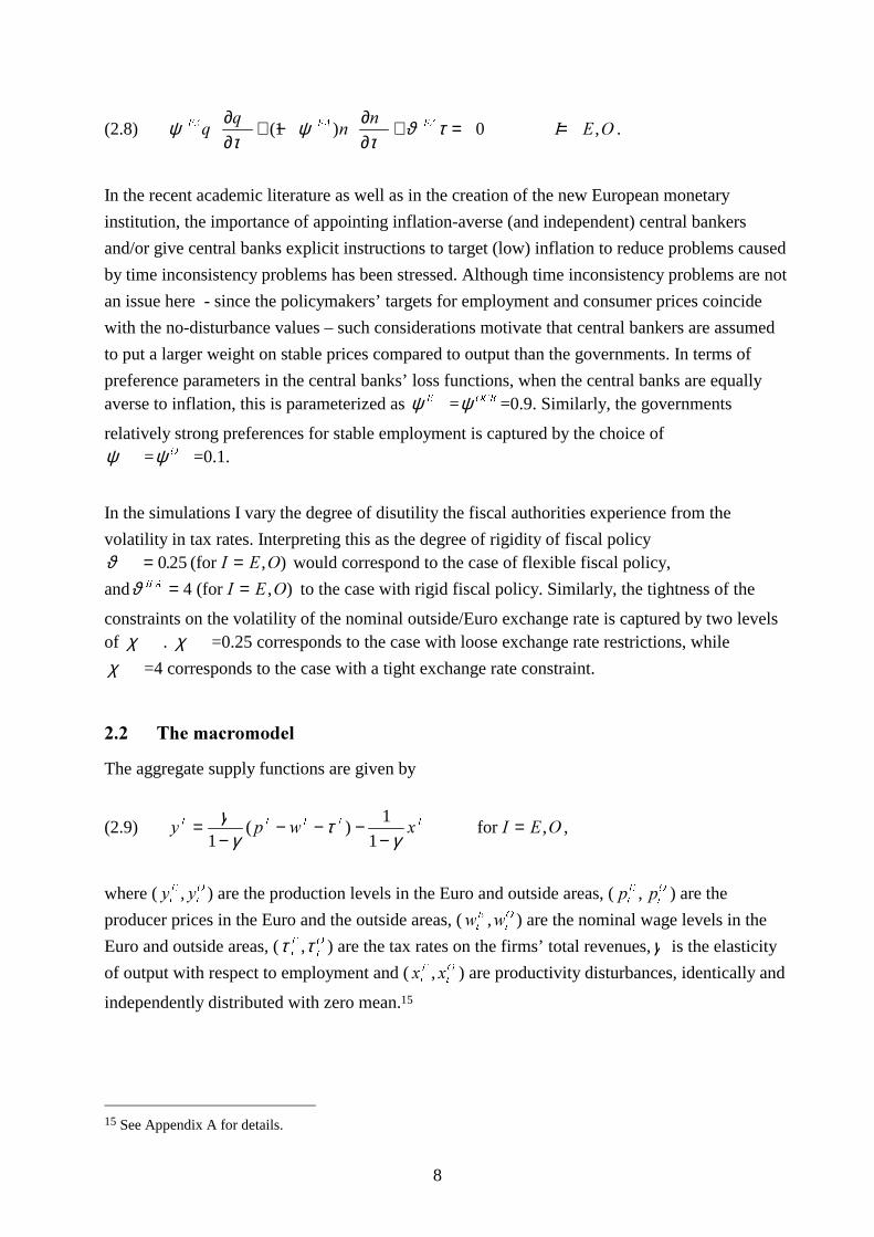
(2.8) ψτ

ψτ

ϑ τ)$ )$ )$TT

QQ

, ( 2∂∂

+ − ∂∂

+ = =( ) ,1 0 .

In the recent academic literature as well as in the creation of the new European monetary

institution, the importance of appointing inflation-averse (and independent) central bankers

and/or give central banks explicit instructions to target (low) inflation to reduce problems caused

by time inconsistency problems has been stressed. Although time inconsistency problems are not

an issue here - since the policymakers’ targets for employment and consumer prices coincide

with the no-disturbance values – such considerations motivate that central bankers are assumed

to put a larger weight on stable prices compared to output than the governments. In terms of

preference parameters in the central banks’ loss functions, when the central banks are equallyaverse to inflation, this is parameterized as ψ ( =ψ 2&% =0.9. Similarly, the governments

relatively strong preferences for stable employment is captured by the choice ofψ =ψ 2 =0.1.

In the simulations I vary the degree of disutility the fiscal authorities experience from the

volatility in tax rates. Interpreting this as the degree of rigidity of fiscal policyϑ , ( 2= =0 25. ,(for ) would correspond to the case of flexible fiscal policy,

andϑ ,)$ , ( 2= =4 (for ), to the case with rigid fiscal policy. Similarly, the tightness of the

constraints on the volatility of the nominal outside/Euro exchange rate is captured by two levelsof χ . χ =0.25 corresponds to the case with loose exchange rate restrictions, while

χ =4 corresponds to the case with a tight exchange rate constraint.

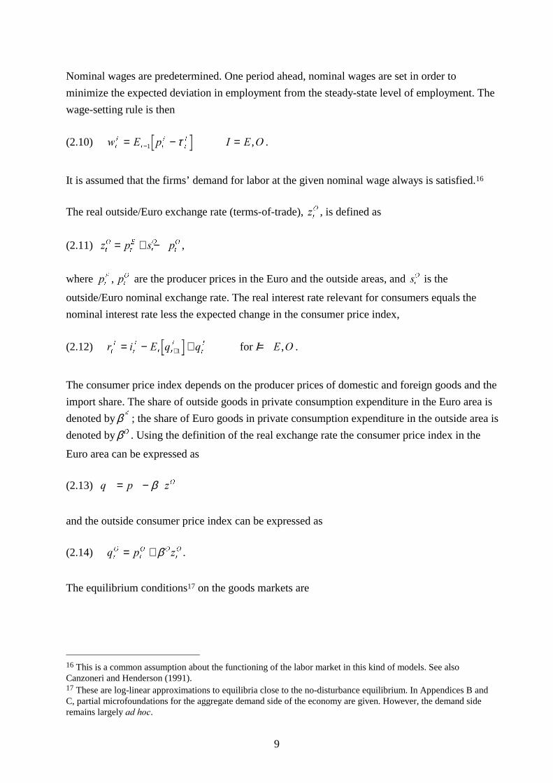
��� 7KH�PDFURPRGHO

The aggregate supply functions are given by

(2.9) \ S Z [ , ( 2, , , , ,=−

− − −−

=γγ

τγ1

1

1( ) ,for ,

where (\ \W

(

W

2, ) are the production levels in the Euro and outside areas, (S SW

(

W

2, ) are the

producer prices in the Euro and the outside areas, (Z ZW

(

W

2, ) are the nominal wage levels in the

Euro and outside areas, (τ τW

(

W

2, ) are the tax rates on the firms’ total revenues,γ is the elasticity

of output with respect to employment and ([ [W

(

W

2, ) are productivity disturbances, identically and

independently distributed with zero mean.15

15 See Appendix A for details.

9

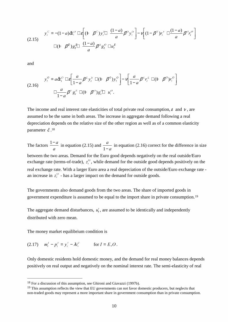
Nominal wages are predetermined. One period ahead, nominal wages are set in order to

minimize the expected deviation in employment from the steady-state level of employment. The

wage-setting rule is then

(2.10) Z ( S , ( 2W

,

W W

,

W

,= − =−1 τ , .

It is assumed that the firms’ demand for labor at the given nominal wage always is satisfied.16

The real outside/Euro exchange rate (terms-of-trade), ]W

2 , is defined as

(2.11) ] S V SW

2

W

(

W

2

W

2= + − ,

where S SW

(

W

2, are the producer prices in the Euro and the outside areas, and VW

2 is the

outside/Euro nominal exchange rate. The real interest rate relevant for consumers equals the

nominal interest rate less the expected change in the consumer price index,

(2.12) U L ( T T , ( 2W

,

W

,

W W

,

W

,= − + =+1 for , .

The consumer price index depends on the producer prices of domestic and foreign goods and the

import share. The share of outside goods in private consumption expenditure in the Euro area is

denoted byβ(

; the share of Euro goods in private consumption expenditure in the outside area is

denoted byβ2 . Using the definition of the real exchange rate the consumer price index in the

Euro area can be expressed as

(2.13) T S ]2= − β

and the outside consumer price index can be expressed as

(2.14) T S ]W

2

W

2 2

W

2= + β .

The equilibrium conditions17 on the goods markets are

16 This is a common assumption about the functioning of the labor market in this kind of models. See alsoCanzoneri and Henderson (1991).17 These are log-linear approximations to equilibria close to the no-disturbance equilibrium. In Appendices B andC, partial microfoundations for the aggregate demand side of the economy are given. However, the demand sideremains largely DG�KRF.

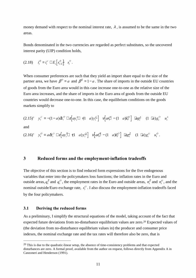
10

(2.15)\ D ] \

DD

\ UD

DU

JD

DJ X

W

(

W

2 (

W

( 2

W

2 (

W

( 2

W

2

(

W

( 2

W

2

W

(

= − − + − + −�!

"$# − − + −�

! "$#

+ − + − +

( ) ( )( )

( )( )

( )( )

1 11

11

11

δ ε β β ν β β

β β

and

(2.16)\ D ]

DD

\ \DD

U U

DD

J J X

W

2

W

2 (

W

( 2

W

2 (

W

( 2

W

2

(

W

( 2

W

2

W

2

= +−

+ −�!

"$# −

−+ −�

! "$#

+−

+ − +

δ ε β β ν β β

β β

11

11

11

( ) ( )

( ) .

The income and real interest rate elasticities of total private real consumption, ε and ν , are

assumed to be the same in both areas. The increase in aggregate demand following a real

depreciation depends on the relative size of the other region as well as of a common elasticity

parameter δ .18

The factors 1− DD

in equation (2.15) and DD1−

in equation (2.16) correct for the difference in size

between the two areas. Demand for the Euro good depends negatively on the real outside/Euroexchange rate (terms-of-trade), ]

W

2 , while demand for the outside good depends positively on the

real exchange rate. With a larger Euro area a real depreciation of the outside/Euro exchange rate -an increase in ]

W

2 - has a larger impact on the demand for outside goods.

The governments also demand goods from the two areas. The share of imported goods in

government expenditure is assumed to be equal to the import share in private consumption.19

The aggregate demand disturbances, XW

L , are assumed to be identically and independently

distributed with zero mean.

The money market equilibrium condition is

(2.17) P S \ L , ( 2W

,

W

,

W

,

W

,− = − =λ for , .

Only domestic residents hold domestic money, and the demand for real money balances depends

positively on real output and negatively on the nominal interest rate. The semi-elasticity of real

18 For a discussion of this assumption, see Ghironi and Giavazzi (1997b).19 This assumption reflects the view that EU governments can not favor domestic producers, but neglects thatnon-traded goods may represent a more important share in government consumption than in private consumption.

11

money demand with respect to the nominal interest rate, λ , is assumed to be the same in the two

areas.

Bonds denominated in the two currencies are regarded as perfect substitutes, so the uncovered

interest parity (UIP) condition holds,

(2.18) L L ( V VW

2

W

(

W W

2

W

2= + −+1 .

When consumer preferences are such that they yield an import share equal to the size of thepartner area, we have β2 D= and β ( D= −1 . The share of imports in the outside EU countries

of goods from the Euro area would in this case increase one-to-one as the relative size of the

Euro area increases, and the share of imports in the Euro area of goods from the outside EU

countries would decrease one-to-one. In this case, the equilibrium conditions on the goods

markets simplify to

(2.15)’ \ D ] D\ D \ DU D U DJ D J XW

(

W

2

W

(

W

2

W

(

W

2

W

(

W

2

W

(= − − + + − − + − + + − +( ) ( ) ( ) ( )1 1 1 1δ ε ν

and

(2.16)’ \ D ] D\ D \ DU D U DJ D J XW

2

W

2

W

(

W

2

W

(

W

2

W

(

W

2

W

2= + + − − + − + + − +δ ε ν( ) ( ) ( )1 1 1 .

� 5HGXFHG�IRUPV�DQG�WKH�HPSOR\PHQW�LQIODWLRQ�WUDGHRIIV

The objective of this section is to find reduced form expressions for the five endogenous

variables that enter into the policymakers loss functions; the inflation rates in the Euro andoutside areas,T

W

( and TW

2 , the employment rates in the Euro and outside areas, QW

( and QW

2 , and the

nominal outside/Euro exchange rate, VW

2 . I also discuss the employment-inflation tradeoffs faced

by the four policymakers.

��� �'HULYLQJ�WKH�UHGXFHG�IRUPV

As a preliminary, I simplify the structural equations of the model, taking account of the fact that

expected future deviations from no-disturbance equilibrium values are zero.20 Expected values of

(the deviation from no-disturbance equilibrium values in) the producer and consumer price

indexes, the nominal exchange rate and the tax rates will therefore also be zero, that is

20 This is due to the quadratic-linear setup, the absence of time-consistency problems and that expecteddisturbances are zero. A formal proof, available from the author on request, follows directly from Appendix A inCanzoneri and Henderson (1991).

12

(3.1) ( S ( T ( V ( , ( 2W W

,

W W

,

W W

2

W W

,

+ + + += = = = =1 1 1 1 0τ for , .

Since equation (3.1) holds at all times, an immediate result is that the nominal wages are set –

one period ahead - at their no-disturbance equilibrium values. According to equation (2.10)Z

W

, = 0 . This leaves us with a system of 12 equations ((2.9), (2.11)-(2.18)) to be solved for 12

endogenous variables as functions of the policy variables and the disturbances. Since the

policymakers are assumed to have preferences over employment, rather than output, the

production functions

(3.2) \ Q [ , ( 2W

,

W

,

W

,= − =γ for ,

are inverted to derive reduced forms for employment.

��� 3DUDPHWHUL]LQJ�WKH�UHGXFHG�IRUPV

The coefficients in the reduced form equations are complicated functions of the basic parameters

of the model. The asymmetries in the model make analytical solutions intractable, so I resort to

simulations. I choose values for these parameters so that the parameterized model is comparable

to the European Union (2-country model) block in Ghironi and Giavazzi (1997b). This meansthat I set δ =0.8, γ =0.66, λ =0.6, ε =0.8, and ν=0.4.

Reflecting the fact that the Euro area is large I set D =0.75. Assuming that consumer preferences

in the two areas are such that they yield an import share equal to the size of the partner area, that

is(

β = 0.25 and 2β =0.75, the reduced forms for employment in the Euro area and in the block

of outside countries are given by

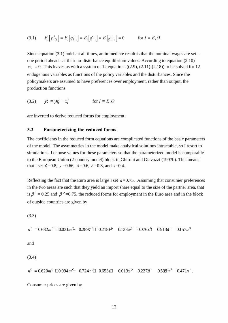
(3.3)

Q P P [ [ X X( ( 2 ( 2 ( 2 ( 2= + − + − − + +0 682 0 031 0 289 0 218 0138 0 076 0 913 0157. . . . . . . .τ τ

and

(3.4)

Q P P [ [ X X2 2 ( 2 ( 2 ( 2 (= + − + + − + +0 620 0 094 0 724 0 653 0 013 0 227 0599 0 471. . . . . . . .τ τ .

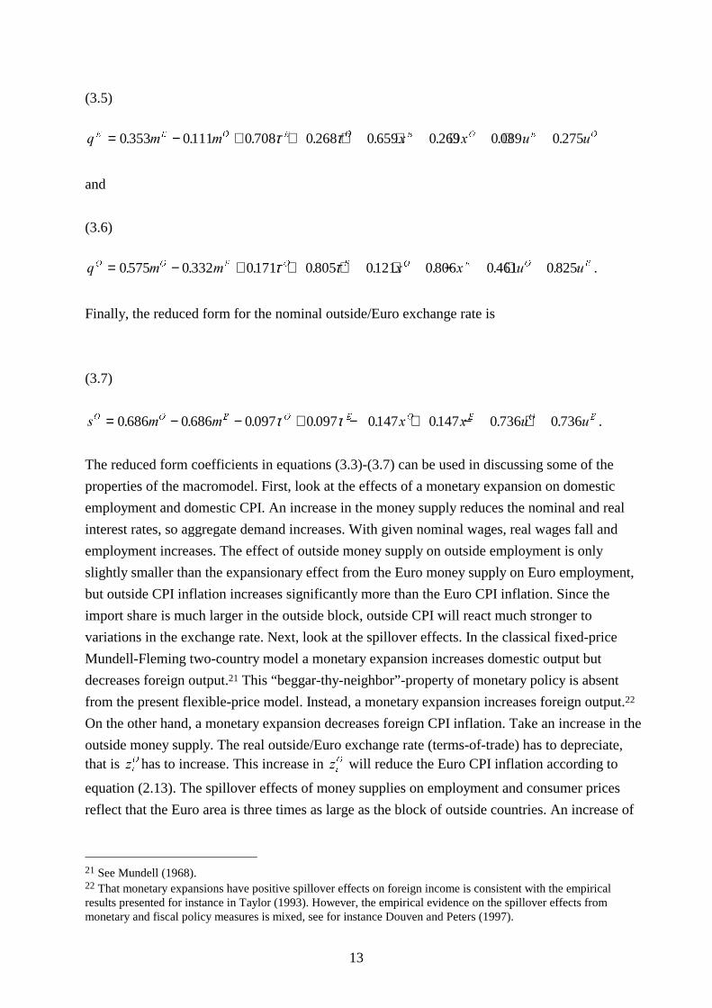
Consumer prices are given by

13

(3.5)

T P P [ [ X X( ( 2 ( 2 ( 2 ( 2= − + + + + + +0 353 0111 0 708 0 268 0 659 0 269 0 089 0 275. . . . . . . .τ τ

and

(3.6)

T P P [ [ X X2 2 ( 2 ( 2 ( 2 (= − + + + + − +0575 0 332 0171 0 805 0121 0 806 0 461 0 825. . . . . . . .τ τ .

Finally, the reduced form for the nominal outside/Euro exchange rate is

(3.7)

V P P [ [ X X2 2 ( 2 ( 2 ( 2 (= − − + − + − +0 686 0 686 0 097 0 097 0147 0147 0 736 0 736. . . . . . . .τ τ .

The reduced form coefficients in equations (3.3)-(3.7) can be used in discussing some of the

properties of the macromodel. First, look at the effects of a monetary expansion on domestic

employment and domestic CPI. An increase in the money supply reduces the nominal and real

interest rates, so aggregate demand increases. With given nominal wages, real wages fall and

employment increases. The effect of outside money supply on outside employment is only

slightly smaller than the expansionary effect from the Euro money supply on Euro employment,

but outside CPI inflation increases significantly more than the Euro CPI inflation. Since the

import share is much larger in the outside block, outside CPI will react much stronger to

variations in the exchange rate. Next, look at the spillover effects. In the classical fixed-price

Mundell-Fleming two-country model a monetary expansion increases domestic output but

decreases foreign output.21 This “beggar-thy-neighbor”-property of monetary policy is absent

from the present flexible-price model. Instead, a monetary expansion increases foreign output.22

On the other hand, a monetary expansion decreases foreign CPI inflation. Take an increase in the

outside money supply. The real outside/Euro exchange rate (terms-of-trade) has to depreciate,that is ]

W

2 has to increase. This increase in ]W

2 will reduce the Euro CPI inflation according to

equation (2.13). The spillover effects of money supplies on employment and consumer prices

reflect that the Euro area is three times as large as the block of outside countries. An increase of

21 See Mundell (1968).22 That monetary expansions have positive spillover effects on foreign income is consistent with the empiricalresults presented for instance in Taylor (1993). However, the empirical evidence on the spillover effects frommonetary and fiscal policy measures is mixed, see for instance Douven and Peters (1997).

14

outside money supply will depreciate the nominal outside/Euro exchange rate, while equal

changes in the outside and Euro money supplies leave the nominal exchange rate unchanged.

The treatment of fiscal policy in the present model constitutes an even more drastic departure

from the classical Mundell-Fleming model, in that budget-balanced increases are contractionary.

This non-Keynesian flavor of the model is due to the mechanism that the negative effect on

employment of the increased tax distortion outweighs the positive demand effect from increased

government consumption.23 The strength of this effect depends on the size of the economy. An

increase of the Euro tax rate by one percentage point (accompanied by an increase in the Euro

expenditure ratio of equal size) leads to a fall of 0.3 per cent of Euro employment on impact. A

budget-balanced one percentage point increase of the outside tax rate will reduce the outside

employment level by 0.7 per cent. The difference is due to the fact that an increase in the tax rate

directly hits only domestic supply, while the increase in government expenditure spills over in

demand for the foreign good. Since the block of outside countries is more open than the Euro

area, the net effect on own employment is more negative. Furthermore, in the Mundell-Fleming

model, fiscal policy has a “locomotive” property; a fiscal expansion increases foreign income as

well as domestic income. In the present model, expansionary fiscal policy corresponds to a

budget-balanced reduction in tax and expenditure rates. Such a reduction will have a negative

spillover effect on foreign employment (income). A budget-balanced tax increase will increase

domestic as well as foreign CPI. The effect on domestic CPI is much larger in the Euro area than

in the outside area. The spillover effects on employment and consumer prices reflect the relative

size of the Euro area.

��� 7KH�HPSOR\PHQW�LQIODWLRQ�WUDGHRIIV

When the monetary policymakers set their policy variables so as to minimize their loss functions

in equations (2.1), (2.2), (2.6) and (2.7), the constraints they face are given by the reduced forms

in equations (3.3)-(3.7). In trying to reduce their losses, the policymakers face a tradeoff between

employment and inflation that is captured by the reduced form coefficients.

In a symmetric (flexible exchange rate) monetary regime, in which both central banks set money

supplies, the central banks’ tradeoffs are given by

23 This property depends on the parameterization of the model. For instance, reducing the elasticity of aggregatedemand w.r.t the real interest rates, ν , from 0.4 to 0.3 and increasing the interest rate semi-elasticity of money

demand, λ , from 0.6 to 0.8 will change the impact of Euro tax rate changes on Euro employment. With thischange a cut in the Euro tax rate will reduce Euro employment as well as Euro CPI. Assuming that domesticgoods represent a more important share in government expenditure would also give the model more Keynesianproperties.

15

(3.8)∂∂

=∂ ∂∂ ∂

=TQ

T P

Q P, ( 2

,

,

,&%

, ,

, ,for , .

For a central bank that places a large weight on price stability, compared to stable employment

levels, it is better with a steeper tradeoff, i.e. a higher value for the tradeoff. A steeper tradeoff

allows the central bank to stabilize prices at a lesser cost in terms of employment variability. As

an example, consider a negative supply shock that increases inflation and creates unemployment.

With a loss function as in equation (2.1), and with a high weight on price stability, the central

bank will want to contract the money supply in order to counter the inflationary impulse from the

supply shock. However, a monetary contraction will further increase the unemployment problem.

The steeper the employment-inflation tradeoff, the less will employment fall for a given

reduction in prices.

The fiscal authorities’ tradeoffs are given by

(3.9)∂∂

=∂ ∂∂ ∂

=TQ

T

Q, ( 2

,

,

,)$

, ,

, ,

ττ

for ,

Since the underlying macroeconomic model has non-Keynesian features the slope of the

government’s employment-inflation tradeoff will be negative, since a tax cut will increase

employment and reduce inflation.

For a government/fiscal authority that places a relatively large weight on employment compared

to inflation, one can argue that it is better with a flatter tradeoff, i.e. a less negative value for the

tradeoff.24 A flat tradeoff allows the fiscal authority to vary the employment level at a lesser cost

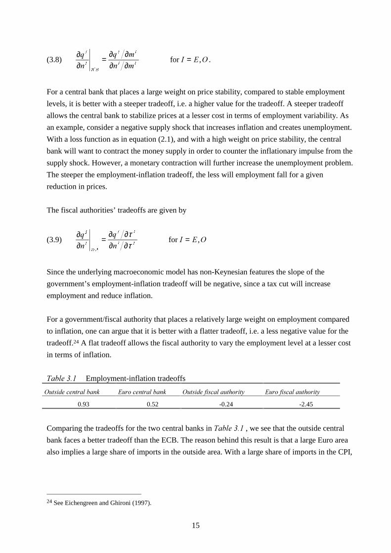
in terms of inflation.

7DEOH���� Employment-inflation tradeoffs

2XWVLGH�FHQWUDO�EDQN (XUR�FHQWUDO�EDQN 2XWVLGH�ILVFDO�DXWKRULW\ (XUR�ILVFDO�DXWKRULW\

0.93 0.52 -0.24 -2.45

Comparing the tradeoffs for the two central banks in 7DEOH���� , we see that the outside central

bank faces a better tradeoff than the ECB. The reason behind this result is that a large Euro area

also implies a large share of imports in the outside area. With a large share of imports in the CPI,

24 See Eichengreen and Ghironi (1997).

16

the effect on CPI of a change in the exchange rate is large, so the outside central bank does not

have to contract the economy so much to get the desired reduction of CPI inflation.25

Since the outside fiscal authority also faces a better (since flatter) tradeoff than the Euro fiscal

authority, the underlying macromodel is such that the two outside authorities have the “upper

hand” compared to their Euro colleagues.

�� 0RQHWDU\�DQG�ILVFDO�SROLF\�LQWHUDFWLRQ�LQ�D�WZR�UHJLRQ�(XURSH

The type of policy game studied in this paper is non-cooperative: when the EU countries are

hit by shocks each of the four policymakers will try to minimize its own losses, as described

in Section 2.1. This seems to be a natural point of departure. An important feature of the

Maastricht treaty (as well as of recent national central banking legislation in Europe) is the

independence accorded to the ECB and the outside central banks.

��� 7KH�PRQHWDU\�DQG�ILVFDO�SROLF\�JDPH

In the Nash equilibrium of the monetary and fiscal policy game the four policymakers are

fully aware of the shock that has hit the European economies, and each policymaker chooses

his best policy, given the policy choices of the three other policymakers. The Nash

equilibrium is therefore described by the four equation system consisting of the first-order

conditions for the policymakers, equations (2.3), (2.4) and (2.8).

The employment-inflation tradeoffs discussed in Section 3.3 are useful when analyzing the

mechanisms behind the outcome of the policy game. Another important determinant of the

outcome is the presence of externalities between the four policymakers.26 These externalities

occur both between regions (Euro area versus the outside area) and within regions (central

bank versus the fiscal authority). Whether the externalities are positive or negative depends on

the shocks that hit the two regions, the mechanisms built into the macromodel and the

assumed preferences of the policymakers. 27

25 See Ghironi and Giavazzi (1997a) for a discussion of how central banks employment-inflation tradeoffs areaffected by monetary regime and monetary union size.26 See also the discussion in Canzoneri and Henderson (1991) for the case with two monetary policymakers.27 The central banks are mainly concerned about price stability and the fiscal authorities care more about stableemployment.

17

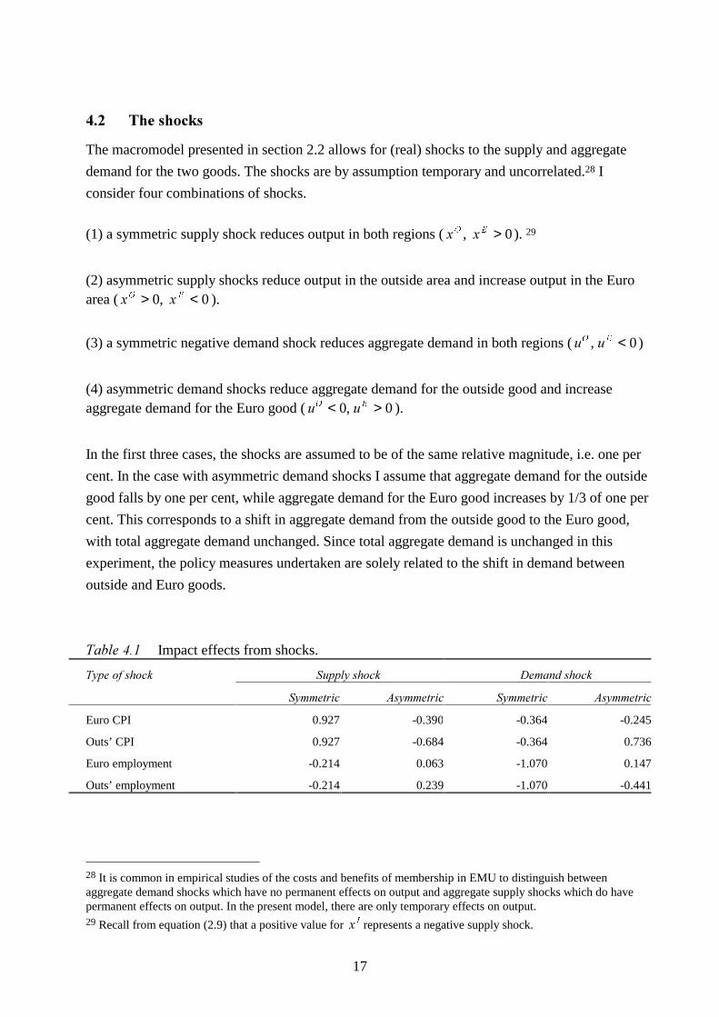
��� 7KH�VKRFNV

The macromodel presented in section 2.2 allows for (real) shocks to the supply and aggregate

demand for the two goods. The shocks are by assumption temporary and uncorrelated.28 I

consider four combinations of shocks.

(1) a symmetric supply shock reduces output in both regions ( [ [2 (, > 0). 29

(2) asymmetric supply shocks reduce output in the outside area and increase output in the Euroarea ( [ [2 (> <0 0, ).

(3) a symmetric negative demand shock reduces aggregate demand in both regions (X X2 (, < 0)

(4) asymmetric demand shocks reduce aggregate demand for the outside good and increaseaggregate demand for the Euro good ( X X2 (< >0 0, ).

In the first three cases, the shocks are assumed to be of the same relative magnitude, i.e. one per

cent. In the case with asymmetric demand shocks I assume that aggregate demand for the outside

good falls by one per cent, while aggregate demand for the Euro good increases by 1/3 of one per

cent. This corresponds to a shift in aggregate demand from the outside good to the Euro good,

with total aggregate demand unchanged. Since total aggregate demand is unchanged in this

experiment, the policy measures undertaken are solely related to the shift in demand between

outside and Euro goods.

7DEOH���� Impact effects from shocks.

6XSSO\�VKRFN 'HPDQG�VKRFN7\SH�RI�VKRFN

6\PPHWULF $V\PPHWULF 6\PPHWULF $V\PPHWULF

Euro CPI 0.927 -0.390 -0.364 -0.245

Outs’ CPI 0.927 -0.684 -0.364 0.736

Euro employment -0.214 0.063 -1.070 0.147

Outs’ employment -0.214 0.239 -1.070 -0.441

28 It is common in empirical studies of the costs and benefits of membership in EMU to distinguish betweenaggregate demand shocks which have no permanent effects on output and aggregate supply shocks which do havepermanent effects on output. In the present model, there are only temporary effects on output.29 Recall from equation (2.9) that a positive value for [ , represents a negative supply shock.

18

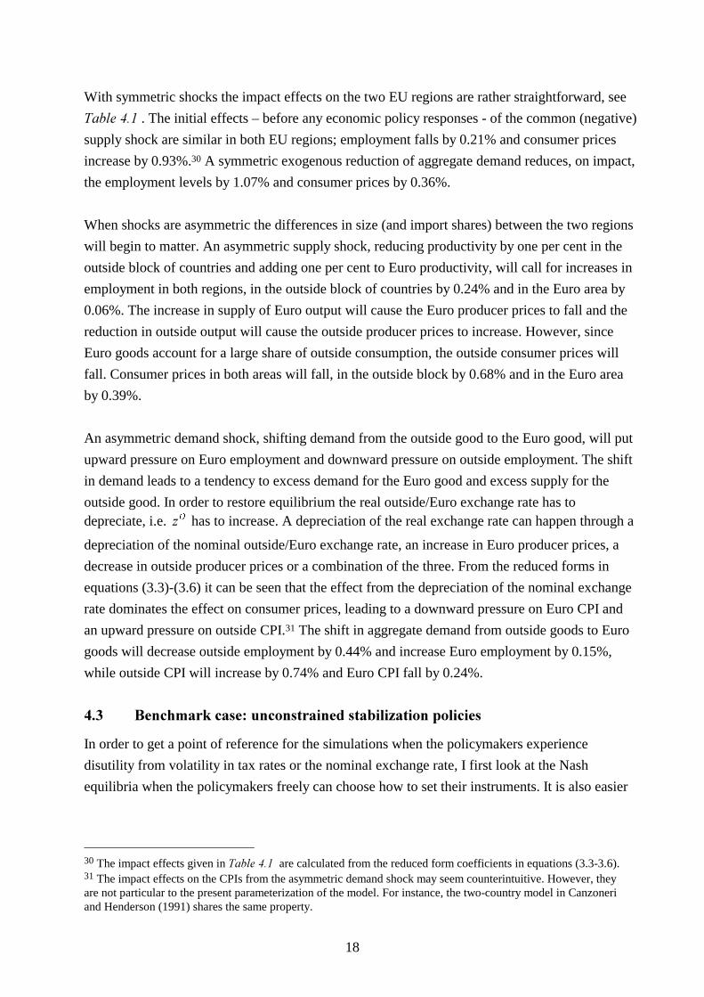
With symmetric shocks the impact effects on the two EU regions are rather straightforward, see

7DEOH���� . The initial effects – before any economic policy responses - of the common (negative)

supply shock are similar in both EU regions; employment falls by 0.21% and consumer prices

increase by 0.93%.30 A symmetric exogenous reduction of aggregate demand reduces, on impact,

the employment levels by 1.07% and consumer prices by 0.36%.

When shocks are asymmetric the differences in size (and import shares) between the two regions

will begin to matter. An asymmetric supply shock, reducing productivity by one per cent in the

outside block of countries and adding one per cent to Euro productivity, will call for increases in

employment in both regions, in the outside block of countries by 0.24% and in the Euro area by

0.06%. The increase in supply of Euro output will cause the Euro producer prices to fall and the

reduction in outside output will cause the outside producer prices to increase. However, since

Euro goods account for a large share of outside consumption, the outside consumer prices will

fall. Consumer prices in both areas will fall, in the outside block by 0.68% and in the Euro area

by 0.39%.

An asymmetric demand shock, shifting demand from the outside good to the Euro good, will put

upward pressure on Euro employment and downward pressure on outside employment. The shift

in demand leads to a tendency to excess demand for the Euro good and excess supply for the

outside good. In order to restore equilibrium the real outside/Euro exchange rate has todepreciate, i.e. ]2 has to increase. A depreciation of the real exchange rate can happen through a

depreciation of the nominal outside/Euro exchange rate, an increase in Euro producer prices, a

decrease in outside producer prices or a combination of the three. From the reduced forms in

equations (3.3)-(3.6) it can be seen that the effect from the depreciation of the nominal exchange

rate dominates the effect on consumer prices, leading to a downward pressure on Euro CPI and

an upward pressure on outside CPI.31 The shift in aggregate demand from outside goods to Euro

goods will decrease outside employment by 0.44% and increase Euro employment by 0.15%,

while outside CPI will increase by 0.74% and Euro CPI fall by 0.24%.

��� %HQFKPDUN�FDVH��XQFRQVWUDLQHG�VWDELOL]DWLRQ�SROLFLHV

In order to get a point of reference for the simulations when the policymakers experience

disutility from volatility in tax rates or the nominal exchange rate, I first look at the Nash

equilibria when the policymakers freely can choose how to set their instruments. It is also easier

30 The impact effects given in 7DEOH���� are calculated from the reduced form coefficients in equations (3.3-3.6).31 The impact effects on the CPIs from the asymmetric demand shock may seem counterintuitive. However, theyare not particular to the present parameterization of the model. For instance, the two-country model in Canzoneriand Henderson (1991) shares the same property.

19

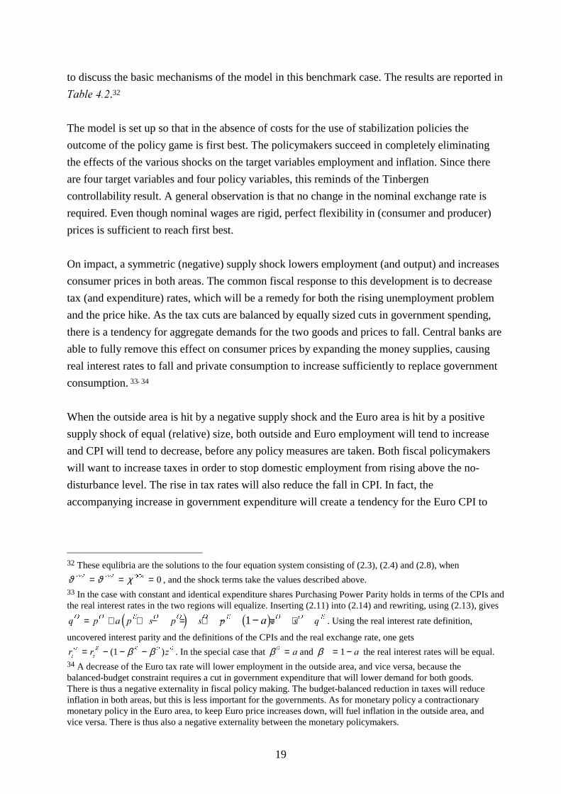
to discuss the basic mechanisms of the model in this benchmark case. The results are reported in

7DEOH����.32

The model is set up so that in the absence of costs for the use of stabilization policies the

outcome of the policy game is first best. The policymakers succeed in completely eliminating

the effects of the various shocks on the target variables employment and inflation. Since there

are four target variables and four policy variables, this reminds of the Tinbergen

controllability result. A general observation is that no change in the nominal exchange rate is

required. Even though nominal wages are rigid, perfect flexibility in (consumer and producer)

prices is sufficient to reach first best.

On impact, a symmetric (negative) supply shock lowers employment (and output) and increases

consumer prices in both areas. The common fiscal response to this development is to decrease

tax (and expenditure) rates, which will be a remedy for both the rising unemployment problem

and the price hike. As the tax cuts are balanced by equally sized cuts in government spending,

there is a tendency for aggregate demands for the two goods and prices to fall. Central banks are

able to fully remove this effect on consumer prices by expanding the money supplies, causing

real interest rates to fall and private consumption to increase sufficiently to replace government

consumption. 33, 34

When the outside area is hit by a negative supply shock and the Euro area is hit by a positive

supply shock of equal (relative) size, both outside and Euro employment will tend to increase

and CPI will tend to decrease, before any policy measures are taken. Both fiscal policymakers

will want to increase taxes in order to stop domestic employment from rising above the no-

disturbance level. The rise in tax rates will also reduce the fall in CPI. In fact, the

accompanying increase in government expenditure will create a tendency for the Euro CPI to

32 These equlibria are the solutions to the four equation system consisting of (2.3), (2.4) and (2.8), when

ϑ ϑ χ()$ ()$ 2&%= = = 0 , and the shock terms take the values described above.33 In the case with constant and identical expenditure shares Purchasing Power Parity holds in terms of the CPIs andthe real interest rates in the two regions will equalize. Inserting (2.11) into (2.14) and rewriting, using (2.13), gives

T S D S V S V S ] V T2 2 ( 2 2 2 ( 2 2 (D= + + − = + − = +−2 7 1 61 . Using the real interest rate definition,

uncovered interest parity and the definitions of the CPIs and the real exchange rate, one gets

U U ]W

2

W

( ( 2 2= − − −( )1 β β . In the special case that β 2 D= and β D= −1 the real interest rates will be equal.34 A decrease of the Euro tax rate will lower employment in the outside area, and vice versa, because thebalanced-budget constraint requires a cut in government expenditure that will lower demand for both goods.There is thus a negative externality in fiscal policy making. The budget-balanced reduction in taxes will reduceinflation in both areas, but this is less important for the governments. As for monetary policy a contractionarymonetary policy in the Euro area, to keep Euro price increases down, will fuel inflation in the outside area, andvice versa. There is thus also a negative externality between the monetary policymakers.

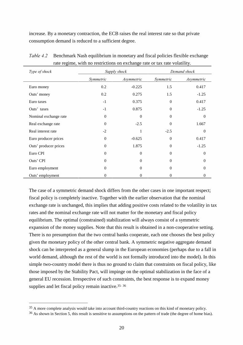
20

increase. By a monetary contraction, the ECB raises the real interest rate so that private

consumption demand is reduced to a sufficient degree.

7DEOH���� Benchmark Nash equilibrium in monetary and fiscal policies flexible exchange

rate regime, with no restrictions on exchange rate or tax rate volatility.

7\SH�RI�VKRFN 6XSSO\�VKRFN 'HPDQG�VKRFN

6\PPHWULF $V\PPHWULF 6\PPHWULF $V\PPHWULF

Euro money 0.2 -0.225 1.5 0.417

Outs’ money 0.2 0.275 1.5 -1.25

Euro taxes -1 0.375 0 0.417

Outs’ taxes -1 0.875 0 -1.25

Nominal exchange rate 0 0 0 0

Real exchange rate 0 -2.5 0 1.667

Real interest rate -2 1 -2.5 0

Euro producer prices 0 -0.625 0 0.417

Outs’ producer prices 0 1.875 0 -1.25

Euro CPI 0 0 0 0

Outs’ CPI 0 0 0 0

Euro employment 0 0 0 0

Outs’ employment 0 0 0 0

The case of a symmetric demand shock differs from the other cases in one important respect;

fiscal policy is completely inactive. Together with the earlier observation that the nominal

exchange rate is unchanged, this implies that adding positive costs related to the volatility in tax

rates and the nominal exchange rate will not matter for the monetary and fiscal policy

equilibrium. The optimal (constrained) stabilization will always consist of a symmetric

expansion of the money supplies. Note that this result is obtained in a non-cooperative setting.

There is no presumption that the two central banks cooperate, each one chooses the best policy

given the monetary policy of the other central bank. A symmetric negative aggregate demand

shock can be interpreted as a general slump in the European economies (perhaps due to a fall in

world demand, although the rest of the world is not formally introduced into the model). In this

simple two-country model there is thus no ground to claim that constraints on fiscal policy, like

those imposed by the Stability Pact, will impinge on the optimal stabilization in the face of a

general EU recession. Irrespective of such constraints, the best response is to expand money

supplies and let fiscal policy remain inactive.35, 36

35 A more complete analysis would take into account third-country reactions on this kind of monetary policy.36 As shown in Section 5, this result is sensitive to assumptions on the pattern of trade (the degree of home bias).

21

An asymmetric demand shock, shifting demand from the outside good to the Euro good, will put

upward pressure on Euro employment and downward pressure on outside employment. The shift

in demand will also put a downward pressure on Euro CPI and an upward pressure on outside

CPI, for the reasons discussed in Section 3.2.37 The Euro fiscal policy response is to tighten fiscal

policy by an increase in taxes/expenditure, which reduces the impact on both employment and

prices. The outside government will want to reduce taxes in order to reduce unemployment (and

at the same time reduce inflation). ECB has an incentive to expand Euro money supply to fight

deflation, while the outside central bank will contract in order to reduce the inflationary effects of

the demand shock.38

In the following two sections I study the effects of introducing costs for volatility in the tax rates

and in the nominal exchange rate in two cases; a symmetric (negative) supply shock and an

asymmetric demand shock that shifts aggregate demand from the outside good to the Euro good.

��� 0RQHWDU\�DQG�ILVFDO�SROLF\�UHVSRQVHV�WR�FRPPRQ�VXSSO\�VKRFNV

Two cases of constrained fiscal policy making are considered; flexible fiscal policy making,which corresponds to setting ϑ ,)$ , ( 2= =0 25. (for , ) ; and rigid fiscal policy making, which

corresponds to setting ϑ ,)$ , ( 2= =4 (for , ) . The restrictions on the volatility of the nominal

outside/Euro exchange rate are also examined for two cases; loose restrictions (low costs)corresponds to χ &% =0.25 and tight restrictions (high costs) correspond to χ &% =4.39

In 7DEOH���� I present the results from the stabilization game when efforts to stabilize the

economies are costly. In this exercise it is assumed that the outside central bank has positive but

low costs related to the volatility of the nominal exchange rate (loose restrictions). The table

shows how the outcome of the stabilization game varies with the degree of rigidity in fiscal

policies. A general pattern in the simulations reported in 7DEOH���� is that in relation to the impact

effects of the symmetric supply shock, see 7DEOH���� , the monetary-fiscal policy game will

amplify employment losses while the inflation rates are stabilized.

When the negative supply shock hits the EU area, the fiscal authorities will try to cushion the

negative effect on employment by lowering the tax rates. Although the constraint of a balanced

37 An excess supply of the outside good will necessitate a real depreciation.38 Since an increase in Euro taxes/expenditure will increase outside employment, Euro fiscal policy will in thiscase have a positive externality on OFA. Likewise, outside fiscal policy will have a positive externality on EFA.Since an expansion of the Euro money stock reduces outside CPI inflation, and a contraction of the outsidemoney stock increases Euro CPI, there is also a positive externality between the two monetary policymakers.39 Of course, these weights can only be suggestive. The weighting of the volatility of the tax rates corresponds tothe one used by Ghironi and Giavazzi (1997b) and Eichengreen and Ghironi (1997), taking into account that thefiscal authorities’ loss functions are differently, but equivalently, formulated. These authors do not take intoaccount costs/restrictions on nominal exchange rate volatility.

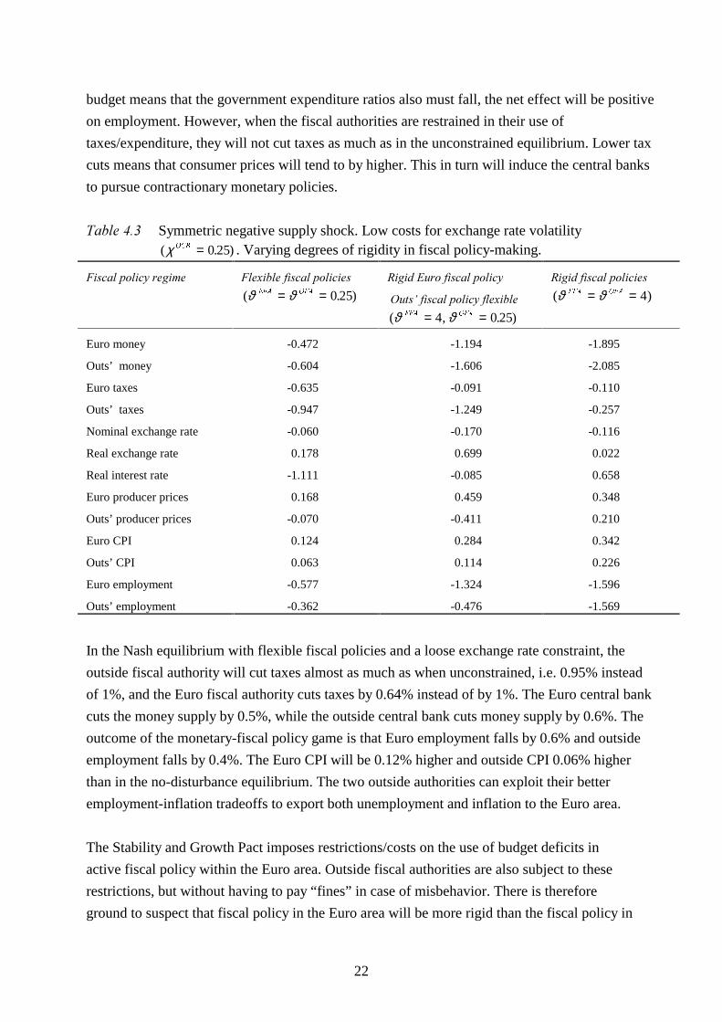
22

budget means that the government expenditure ratios also must fall, the net effect will be positive

on employment. However, when the fiscal authorities are restrained in their use of

taxes/expenditure, they will not cut taxes as much as in the unconstrained equilibrium. Lower tax

cuts means that consumer prices will tend to by higher. This in turn will induce the central banks

to pursue contractionary monetary policies.

7DEOH���� Symmetric negative supply shock. Low costs for exchange rate volatility( . )χ 2&% = 0 25 . Varying degrees of rigidity in fiscal policy-making.

)LVFDO�SROLF\�UHJLPH )OH[LEOH�ILVFDO�SROLFLHV

( . )ϑ ϑ()$ 2)$= = 0 25

5LJLG�(XUR�ILVFDO�SROLF\

�2XWV¶�ILVFDO�SROLF\�IOH[LEOH

( , . )ϑ ϑ()$ 2)$= =4 0 25

5LJLG�ILVFDO�SROLFLHV

( )ϑ ϑ()$ 2)$= = 4

Euro money -0.472 -1.194 -1.895

Outs’ money -0.604 -1.606 -2.085

Euro taxes -0.635 -0.091 -0.110

Outs’ taxes -0.947 -1.249 -0.257

Nominal exchange rate -0.060 -0.170 -0.116

Real exchange rate 0.178 0.699 0.022

Real interest rate -1.111 -0.085 0.658

Euro producer prices 0.168 0.459 0.348

Outs’ producer prices -0.070 -0.411 0.210

Euro CPI 0.124 0.284 0.342

Outs’ CPI 0.063 0.114 0.226

Euro employment -0.577 -1.324 -1.596

Outs’ employment -0.362 -0.476 -1.569

In the Nash equilibrium with flexible fiscal policies and a loose exchange rate constraint, the

outside fiscal authority will cut taxes almost as much as when unconstrained, i.e. 0.95% instead

of 1%, and the Euro fiscal authority cuts taxes by 0.64% instead of by 1%. The Euro central bank

cuts the money supply by 0.5%, while the outside central bank cuts money supply by 0.6%. The

outcome of the monetary-fiscal policy game is that Euro employment falls by 0.6% and outside

employment falls by 0.4%. The Euro CPI will be 0.12% higher and outside CPI 0.06% higher

than in the no-disturbance equilibrium. The two outside authorities can exploit their better

employment-inflation tradeoffs to export both unemployment and inflation to the Euro area.

The Stability and Growth Pact imposes restrictions/costs on the use of budget deficits in

active fiscal policy within the Euro area. Outside fiscal authorities are also subject to these

restrictions, but without having to pay “fines” in case of misbehavior. There is therefore

ground to suspect that fiscal policy in the Euro area will be more rigid than the fiscal policy in

23

the outside area. The third column in 7DEOH���� corresponds to the case where the fiscal policy

conducted by EFA is more rigid than that conducted by OFA. In fact, the Euro tax rate now

barely moves, EFA reduces the tax rate by 0.09% instead of by 0.64% in the flexible fiscal

policy equilibrium in the second column of 7DEOH����. In the case of a symmetric supply shock

there are negative externalities between the fiscal policymakers. This follows from the impact

effects of the common supply shock and the reduced form coefficients on fiscal policies (tax

rates). From equation (3.4), with a less negative value for the Euro tax rate, FHWHULV�SDULEXV�

OFA can obtain the same stabilization of outside employment with a smaller reduction in the

outside tax rate. 40 A more rigid Euro fiscal policy would therefore, by itself, imply that

outside fiscal policy could be less expansive. However, the outside fiscal authority will reduce

taxes more when Euro fiscal policy is rigid, in fact even more than in the unconstrained

equilibrium in 7DEOH���� (by 1.25% instead of 1%). The reason for this can be understood by

looking at the central banks’ behavior. When Euro fiscal policy can not be used to stop

unemployment and consumer prices from rising, the ECB – mostly concerned about the rise in

consumer prices – reduces the Euro money supply. This monetary contraction in the Euro area

spills over in increases in outside CPI. Outside tax reductions will be insufficient to keep

outside CPI at a level acceptable to the outside central bank, so OCB will try to keep CPI in

check by decreasing the outside money stock. The negative externalities in monetary policy

will lead to drastic cuts in money supplies; in equilibrium the Euro money supply is reduced

by 1.2% and the outside money supply by 1.6%. In spite of this general tightness of monetary

policy conditions, the Euro CPI is up 0.3% and outside CPI is up 0.1% from the unconstrained

equilibrium. The most drastic effect, however, is found on the Euro labor market. The

combined effect of contractionary EU monetary policies, heavy tax reductions in the outside

area and practically inactive Euro fiscal policy is that employment in the Euro area falls by

1.3% from its no-disturbance equilibrium value. Outside employment is also negatively

affected by the tight monetary conditions, but to a much lesser degree.

In the last column of 7DEOH���� I examine the case where outside fiscal policy is subject to the

same constraints/costs as Euro fiscal policy. This could correspond to a development in which

the Euro government manages to impose its own degree of fiscal discipline on the outside

government, or that the outside government for other reasons would feel compelled to be as

rigid as its Euro colleague. Would that improve matters? The answer – in the present setting -

is no. The “chicken race” between the two central banks will be even fiercer, since the outside

central bank now has to compensate for the lack of outside fiscal policy when trying to keep

CPI down. The reduction in employment will now be nearly the same in the outside area as in

40 Outside CPI would less well stabilized, but price stability carries a much lower weight than employmentstability in the outside fiscal authority’s loss function.

24

the Euro area (1.6%). The increases in consumer prices are also up compared to the case with

flexible outside fiscal policy.

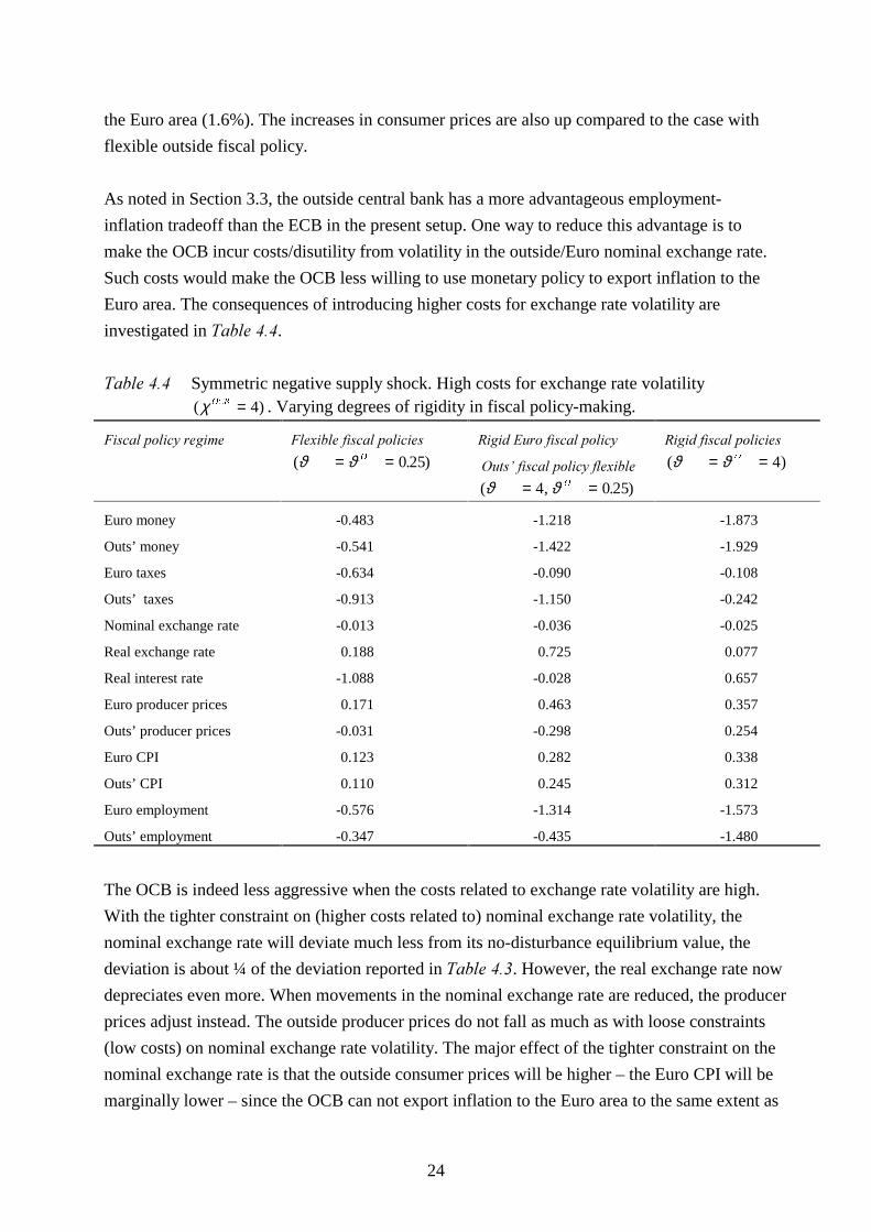
As noted in Section 3.3, the outside central bank has a more advantageous employment-

inflation tradeoff than the ECB in the present setup. One way to reduce this advantage is to

make the OCB incur costs/disutility from volatility in the outside/Euro nominal exchange rate.

Such costs would make the OCB less willing to use monetary policy to export inflation to the

Euro area. The consequences of introducing higher costs for exchange rate volatility are

investigated in 7DEOH����.

7DEOH���� Symmetric negative supply shock. High costs for exchange rate volatility( )χ 2&% = 4 . Varying degrees of rigidity in fiscal policy-making.

)LVFDO�SROLF\�UHJLPH )OH[LEOH�ILVFDO�SROLFLHV

( . )ϑ ϑ 2= = 0 25

5LJLG�(XUR�ILVFDO�SROLF\

�2XWV¶�ILVFDO�SROLF\�IOH[LEOH

( , . )ϑ ϑ 2= =4 0 25

5LJLG�ILVFDO�SROLFLHV

( )ϑ ϑ 2= = 4

Euro money -0.483 -1.218 -1.873

Outs’ money -0.541 -1.422 -1.929

Euro taxes -0.634 -0.090 -0.108

Outs’ taxes -0.913 -1.150 -0.242

Nominal exchange rate -0.013 -0.036 -0.025

Real exchange rate 0.188 0.725 0.077

Real interest rate -1.088 -0.028 0.657

Euro producer prices 0.171 0.463 0.357

Outs’ producer prices -0.031 -0.298 0.254

Euro CPI 0.123 0.282 0.338

Outs’ CPI 0.110 0.245 0.312

Euro employment -0.576 -1.314 -1.573

Outs’ employment -0.347 -0.435 -1.480

The OCB is indeed less aggressive when the costs related to exchange rate volatility are high.

With the tighter constraint on (higher costs related to) nominal exchange rate volatility, the

nominal exchange rate will deviate much less from its no-disturbance equilibrium value, the

deviation is about ¼ of the deviation reported in 7DEOH����. However, the real exchange rate now

depreciates even more. When movements in the nominal exchange rate are reduced, the producer

prices adjust instead. The outside producer prices do not fall as much as with loose constraints

(low costs) on nominal exchange rate volatility. The major effect of the tighter constraint on the

nominal exchange rate is that the outside consumer prices will be higher – the Euro CPI will be

marginally lower – since the OCB can not export inflation to the Euro area to the same extent as

25

in the case with loose restrictions on nominal exchange rate volatility. Outside CPI inflation will

be between one and a half times and twice as large as with low costs. Another effect of the less

contractionary outside monetary policy is that unemployment in both the outside and the Euro

area will be lower.

To sum up, in the case of an EU-wide supply shock all four authorities loose from imposing

restrictions on fiscal policy. In the case when Euro fiscal policy is rigid while outside fiscal

policy is relatively flexible, unemployment and inflation in the Euro area will be considerably

higher. The ECB will be more contractive, and the externalities in monetary policy will make

outside inflation and unemployment higher as well compared to the case with flexible EU fiscal

policy. However, the Euro area is relatively worse off. Making outside fiscal policy as rigid as

Euro fiscal policy worsens the unemployment situation in the outside area, and the increase in

outside CPI will be larger. Consumer prices and unemployment in the Euro area would also be

higher in the case with rigid outside fiscal policy. The Euro authorities would benefit – although

not by much with the present calibration - from restrictions on the nominal outside/Euro

exchange rate; both Euro consumer prices and employment are marginally better stabilized. The

outside fiscal authority also benefits from restrictions on the nominal outside/Euro exchange rate,

since outside unemployment will be lower.41 The most important effect of imposing higher

volatility costs on the nominal outside/Euro exchange rate is that outside CPI inflation will be

higher in the event of a symmetric (negative) supply shock.

��� 0RQHWDU\�DQG�ILVFDO�SROLF\�UHVSRQVHV�WR�DV\PPHWULF�GHPDQG�VKRFNV

In this section I study the stabilization game when an aggregate demand shock shifts demand

from the outside good to the Euro good.

Compared to the impact effects of the asymmetric demand shock the interaction between the four

policymakers will stabilize CPI in both the Euro area and in the outside block of countries, but

the over-employment problem in the Euro area will be amplified. In the flexible fiscal policy

equilibrium Euro CPI falls by 0.04% (impact effect -0.24%), outside CPI increases by 0.02%

(impact effect 0.74%), Euro employment increases by 0.19% (impact effect 0.15%) and outside

employment falls by 0.31% (impact effect -0.44%). When outside fiscal policy is flexible, tax

cuts can be used to reduce the negative impact effect on outside employment. However, with

rigid fiscal policy in both the Euro area and the outside area the outside unemployment problem

will be aggravated by the monetary-fiscal stabilization game. Contractionary outside monetary

policy will reduce employment as well as stabilize consumer prices.

41 Even though CPI in the outside area is higher when outside monetary policy is restricted, OFA is still better offgiven its relatively high preference for stable employment.

26

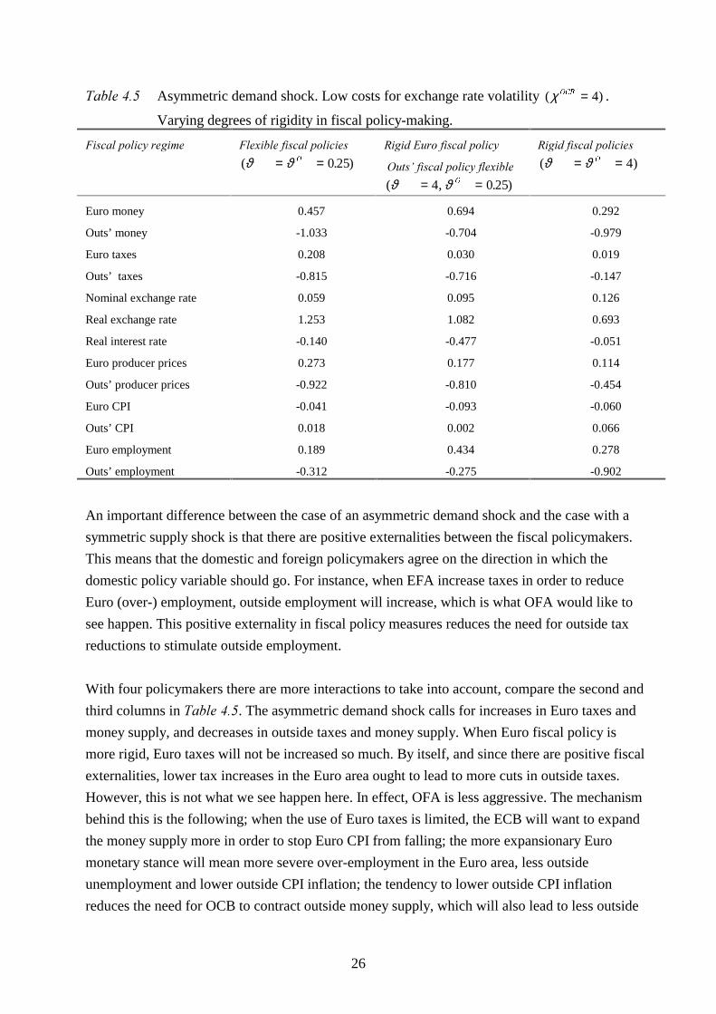
7DEOH���� Asymmetric demand shock. Low costs for exchange rate volatility ( )χ 2&% = 4 .

Varying degrees of rigidity in fiscal policy-making.

)LVFDO�SROLF\�UHJLPH )OH[LEOH�ILVFDO�SROLFLHV

( . )ϑ ϑ 2= = 0 25

5LJLG�(XUR�ILVFDO�SROLF\

�2XWV¶�ILVFDO�SROLF\�IOH[LEOH

( , . )ϑ ϑ 2= =4 0 25

5LJLG�ILVFDO�SROLFLHV

( )ϑ ϑ 2= = 4

Euro money 0.457 0.694 0.292

Outs’ money -1.033 -0.704 -0.979

Euro taxes 0.208 0.030 0.019

Outs’ taxes -0.815 -0.716 -0.147

Nominal exchange rate 0.059 0.095 0.126

Real exchange rate 1.253 1.082 0.693

Real interest rate -0.140 -0.477 -0.051

Euro producer prices 0.273 0.177 0.114

Outs’ producer prices -0.922 -0.810 -0.454

Euro CPI -0.041 -0.093 -0.060

Outs’ CPI 0.018 0.002 0.066

Euro employment 0.189 0.434 0.278

Outs’ employment -0.312 -0.275 -0.902

An important difference between the case of an asymmetric demand shock and the case with a

symmetric supply shock is that there are positive externalities between the fiscal policymakers.

This means that the domestic and foreign policymakers agree on the direction in which the

domestic policy variable should go. For instance, when EFA increase taxes in order to reduce

Euro (over-) employment, outside employment will increase, which is what OFA would like to

see happen. This positive externality in fiscal policy measures reduces the need for outside tax

reductions to stimulate outside employment.

With four policymakers there are more interactions to take into account, compare the second and

third columns in 7DEOH����. The asymmetric demand shock calls for increases in Euro taxes and

money supply, and decreases in outside taxes and money supply. When Euro fiscal policy is

more rigid, Euro taxes will not be increased so much. By itself, and since there are positive fiscal

externalities, lower tax increases in the Euro area ought to lead to more cuts in outside taxes.

However, this is not what we see happen here. In effect, OFA is less aggressive. The mechanism

behind this is the following; when the use of Euro taxes is limited, the ECB will want to expand

the money supply more in order to stop Euro CPI from falling; the more expansionary Euro

monetary stance will mean more severe over-employment in the Euro area, less outside

unemployment and lower outside CPI inflation; the tendency to lower outside CPI inflation

reduces the need for OCB to contract outside money supply, which will also lead to less outside

27

unemployment; all this is good news for the outside government, which will not have to decrease

taxes as much to avoid a large unemployment problem as a result of the asymmetric demand

shock.

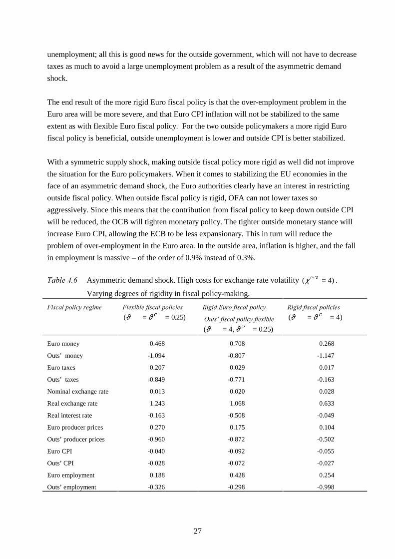
The end result of the more rigid Euro fiscal policy is that the over-employment problem in the

Euro area will be more severe, and that Euro CPI inflation will not be stabilized to the same

extent as with flexible Euro fiscal policy. For the two outside policymakers a more rigid Euro

fiscal policy is beneficial, outside unemployment is lower and outside CPI is better stabilized.

With a symmetric supply shock, making outside fiscal policy more rigid as well did not improve

the situation for the Euro policymakers. When it comes to stabilizing the EU economies in the

face of an asymmetric demand shock, the Euro authorities clearly have an interest in restricting

outside fiscal policy. When outside fiscal policy is rigid, OFA can not lower taxes so

aggressively. Since this means that the contribution from fiscal policy to keep down outside CPI

will be reduced, the OCB will tighten monetary policy. The tighter outside monetary stance will

increase Euro CPI, allowing the ECB to be less expansionary. This in turn will reduce the

problem of over-employment in the Euro area. In the outside area, inflation is higher, and the fall

in employment is massive – of the order of 0.9% instead of 0.3%.

7DEOH���� Asymmetric demand shock. High costs for exchange rate volatility ( )χ 2&% = 4 .

Varying degrees of rigidity in fiscal policy-making.

)LVFDO�SROLF\�UHJLPH )OH[LEOH�ILVFDO�SROLFLHV

( . )ϑ ϑ 2= = 0 25

5LJLG�(XUR�ILVFDO�SROLF\

�2XWV¶�ILVFDO�SROLF\�IOH[LEOH

( , . )ϑ ϑ 2= =4 0 25

5LJLG�ILVFDO�SROLFLHV

( )ϑ ϑ 2= = 4

Euro money 0.468 0.708 0.268

Outs’ money -1.094 -0.807 -1.147

Euro taxes 0.207 0.029 0.017

Outs’ taxes -0.849 -0.771 -0.163

Nominal exchange rate 0.013 0.020 0.028

Real exchange rate 1.243 1.068 0.633

Real interest rate -0.163 -0.508 -0.049

Euro producer prices 0.270 0.175 0.104

Outs’ producer prices -0.960 -0.872 -0.502

Euro CPI -0.040 -0.092 -0.055

Outs’ CPI -0.028 -0.072 -0.027

Euro employment 0.188 0.428 0.254

Outs’ employment -0.326 -0.298 -0.998

28

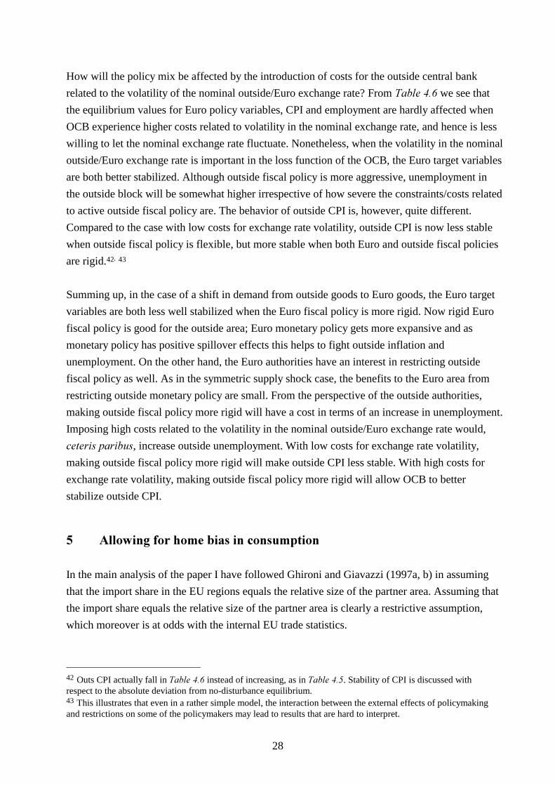
How will the policy mix be affected by the introduction of costs for the outside central bank

related to the volatility of the nominal outside/Euro exchange rate? From 7DEOH���� we see that

the equilibrium values for Euro policy variables, CPI and employment are hardly affected when

OCB experience higher costs related to volatility in the nominal exchange rate, and hence is less

willing to let the nominal exchange rate fluctuate. Nonetheless, when the volatility in the nominal

outside/Euro exchange rate is important in the loss function of the OCB, the Euro target variables

are both better stabilized. Although outside fiscal policy is more aggressive, unemployment in

the outside block will be somewhat higher irrespective of how severe the constraints/costs related

to active outside fiscal policy are. The behavior of outside CPI is, however, quite different.

Compared to the case with low costs for exchange rate volatility, outside CPI is now less stable

when outside fiscal policy is flexible, but more stable when both Euro and outside fiscal policies

are rigid.42, 43

Summing up, in the case of a shift in demand from outside goods to Euro goods, the Euro target

variables are both less well stabilized when the Euro fiscal policy is more rigid. Now rigid Euro

fiscal policy is good for the outside area; Euro monetary policy gets more expansive and as

monetary policy has positive spillover effects this helps to fight outside inflation and

unemployment. On the other hand, the Euro authorities have an interest in restricting outside

fiscal policy as well. As in the symmetric supply shock case, the benefits to the Euro area from

restricting outside monetary policy are small. From the perspective of the outside authorities,

making outside fiscal policy more rigid will have a cost in terms of an increase in unemployment.

Imposing high costs related to the volatility in the nominal outside/Euro exchange rate would,

FHWHULV�SDULEXV, increase outside unemployment. With low costs for exchange rate volatility,

making outside fiscal policy more rigid will make outside CPI less stable. With high costs for

exchange rate volatility, making outside fiscal policy more rigid will allow OCB to better

stabilize outside CPI.

� $OORZLQJ�IRU�KRPH�ELDV�LQ�FRQVXPSWLRQ

In the main analysis of the paper I have followed Ghironi and Giavazzi (1997a, b) in assuming

that the import share in the EU regions equals the relative size of the partner area. Assuming that

the import share equals the relative size of the partner area is clearly a restrictive assumption,

which moreover is at odds with the internal EU trade statistics.

42 Outs CPI actually fall in 7DEOH���� instead of increasing, as in 7DEOH����. Stability of CPI is discussed withrespect to the absolute deviation from no-disturbance equilibrium.43 This illustrates that even in a rather simple model, the interaction between the external effects of policymakingand restrictions on some of the policymakers may lead to results that are hard to interpret.

29

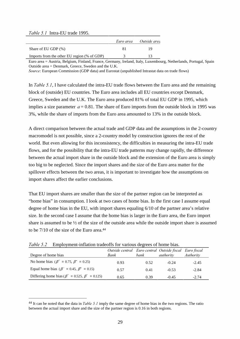
7DEOH���� Intra-EU trade 1995.

(XUR�DUHD 2XWVLGH�DUHD

Share of EU GDP (%) 81 19

Imports from the other EU region (% of GDP) 3 13Euro area = Austria, Belgium, Finland, France, Germany, Ireland, Italy, Luxembourg, Netherlands, Portugal, SpainOutside area = Denmark, Greece, Sweden and the U.K.6RXUFH: European Commission (GDP data) and Eurostat (unpublished Intrastat data on trade flows)

In 7DEOH����, I have calculated the intra-EU trade flows between the Euro area and the remaining

block of (outside) EU countries. The Euro area includes all EU countries except Denmark,

Greece, Sweden and the U.K. The Euro area produced 81% of total EU GDP in 1995, which

implies a size parameter D = 0.81. The share of Euro imports from the outside block in 1995 was

3%, while the share of imports from the Euro area amounted to 13% in the outside block.

A direct comparison between the actual trade and GDP data and the assumptions in the 2-country

macromodel is not possible, since a 2-country model by construction ignores the rest of the

world. But even allowing for this inconsistency, the difficulties in measuring the intra-EU trade

flows, and for the possibility that the intra-EU trade patterns may change rapidly, the difference

between the actual import share in the outside block and the extension of the Euro area is simply

too big to be neglected. Since the import shares and the size of the Euro area matter for the

spillover effects between the two areas, it is important to investigate how the assumptions on

import shares affect the earlier conclusions.

That EU import shares are smaller than the size of the partner region can be interpreted as

“home bias” in consumption. I look at two cases of home bias. In the first case I assume equal

degree of home bias in the EU, with import shares equaling 6/10 of the partner area’s relative

size. In the second case I assume that the home bias is larger in the Euro area, the Euro import

share is assumed to be ½ of the size of the outside area while the outside import share is assumed

to be 7/10 of the size of the Euro area.44

7DEOH���� Employment-inflation tradeoffs for various degrees of home bias.

Degree of home bias2XWVLGH�FHQWUDO%DQN

(XUR�FHQWUDOEDQN

2XWVLGH�ILVFDODXWKRULW\

(XUR�ILVFDO$XWKRULW\

No home bias ( . , . )β β2 (= =0 75 0 25 0.93 0.52 -0.24 -2.45

Equal home bias ( . , . )β β2 (= =0 45 0 15 0.57 0.41 -0.53 -2.84

Differing home bias ( . , . )β β2 (= =0 525 0 125 0.65 0.39 -0.45 -2.74

44 It can be noted that the data in 7DEOH���� imply the same degree of home bias in the two regions. The ratiobetween the actual import share and the size of the partner region is 0.16 in both regions.

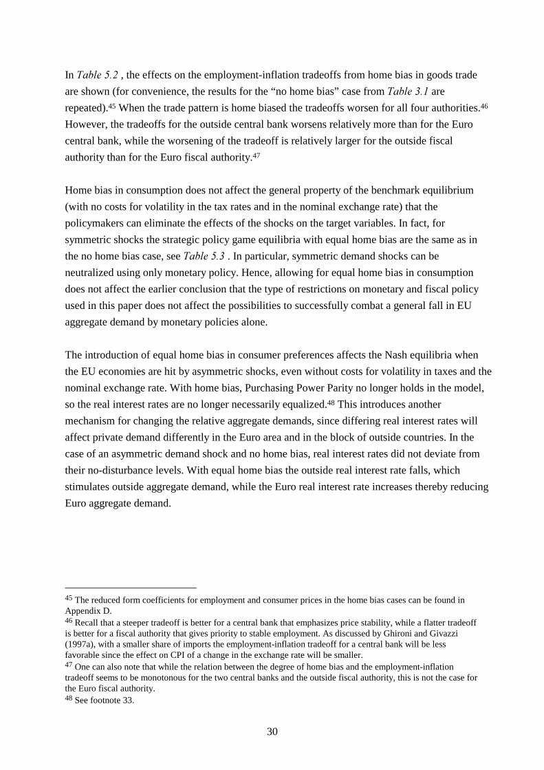
30

In 7DEOH���� , the effects on the employment-inflation tradeoffs from home bias in goods trade

are shown (for convenience, the results for the “no home bias” case from 7DEOH���� are

repeated).45 When the trade pattern is home biased the tradeoffs worsen for all four authorities.46

However, the tradeoffs for the outside central bank worsens relatively more than for the Euro

central bank, while the worsening of the tradeoff is relatively larger for the outside fiscal

authority than for the Euro fiscal authority.47

Home bias in consumption does not affect the general property of the benchmark equilibrium

(with no costs for volatility in the tax rates and in the nominal exchange rate) that the

policymakers can eliminate the effects of the shocks on the target variables. In fact, for

symmetric shocks the strategic policy game equilibria with equal home bias are the same as in

the no home bias case, see 7DEOH���� . In particular, symmetric demand shocks can be

neutralized using only monetary policy. Hence, allowing for equal home bias in consumption

does not affect the earlier conclusion that the type of restrictions on monetary and fiscal policy

used in this paper does not affect the possibilities to successfully combat a general fall in EU

aggregate demand by monetary policies alone.

The introduction of equal home bias in consumer preferences affects the Nash equilibria when

the EU economies are hit by asymmetric shocks, even without costs for volatility in taxes and the

nominal exchange rate. With home bias, Purchasing Power Parity no longer holds in the model,

so the real interest rates are no longer necessarily equalized.48 This introduces another

mechanism for changing the relative aggregate demands, since differing real interest rates will

affect private demand differently in the Euro area and in the block of outside countries. In the

case of an asymmetric demand shock and no home bias, real interest rates did not deviate from

their no-disturbance levels. With equal home bias the outside real interest rate falls, which

stimulates outside aggregate demand, while the Euro real interest rate increases thereby reducing

Euro aggregate demand.

45 The reduced form coefficients for employment and consumer prices in the home bias cases can be found inAppendix D.46 Recall that a steeper tradeoff is better for a central bank that emphasizes price stability, while a flatter tradeoffis better for a fiscal authority that gives priority to stable employment. As discussed by Ghironi and Givazzi(1997a), with a smaller share of imports the employment-inflation tradeoff for a central bank will be lessfavorable since the effect on CPI of a change in the exchange rate will be smaller.47 One can also note that while the relation between the degree of home bias and the employment-inflationtradeoff seems to be monotonous for the two central banks and the outside fiscal authority, this is not the case forthe Euro fiscal authority.48 See footnote 33.

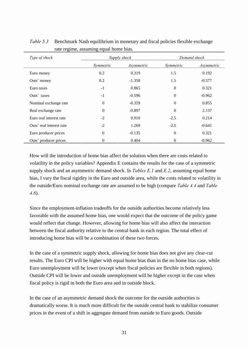
31

7DEOH���� Benchmark Nash equilibrium in monetary and fiscal policies flexible exchange

rate regime, assuming equal home bias.

6XSSO\�VKRFN 'HPDQG�VKRFN7\SH�RI�VKRFN

6\PPHWULF $V\PPHWULF 6\PPHWULF $V\PPHWULF

Euro money 0.2 0.319 1.5 0.192

Outs’ money 0.2 -1.358 1.5 -0.577

Euro taxes -1 0.865 0 0.321

Outs’ taxes -1 -0.596 0 -0.962

Nominal exchange rate 0 -0.359 0 0.855

Real exchange rate 0 -0.897 0 2.137

Euro real interest rate -2 0.910 -2.5 0.214

Outs’ real interest rate -2 1.269 -2.5 -0.641

Euro producer prices 0 -0.135 0 0.321

Outs’ producer prices 0 0.404 0 -0.962

How will the introduction of home bias affect the solution when there are costs related to

volatility in the policy variables? Appendix E contains the results for the case of a symmetric

supply shock and an asymmetric demand shock. In 7DEOHV�(�� and (��, assuming equal home

bias, I vary the fiscal rigidity in the Euro and outside area, while the costs related to volatility in

the outside/Euro nominal exchange rate are assumed to be high (compare 7DEOH���� and 7DEOH

���).

Since the employment-inflation tradeoffs for the outside authorities become relatively less

favorable with the assumed home bias, one would expect that the outcome of the policy game

would reflect that change. However, allowing for home bias will also affect the interaction

between the fiscal authority relative to the central bank in each region. The total effect of

introducing home bias will be a combination of these two forces.

In the case of a symmetric supply shock, allowing for home bias does not give any clear-cut

results. The Euro CPI will be higher with equal home bias than in the no home bias case, while

Euro unemployment will be lower (except when fiscal policies are flexible in both regions).

Outside CPI will be lower and outside unemployment will be higher except in the case when

fiscal policy is rigid in both the Euro area and in outside block.

In the case of an asymmetric demand shock the outcome for the outside authorities is

dramatically worse. It is much more difficult for the outside central bank to stabilize consumer

prices in the event of a shift in aggregate demand from outside to Euro goods. Outside

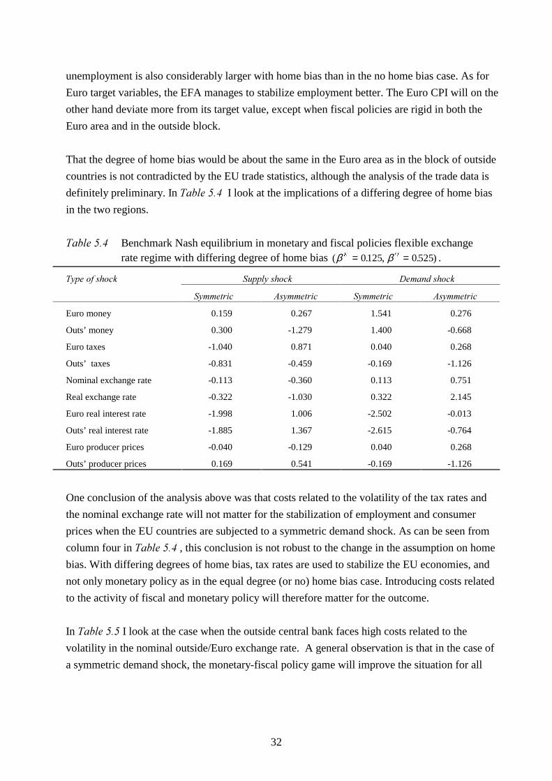
32

unemployment is also considerably larger with home bias than in the no home bias case. As for

Euro target variables, the EFA manages to stabilize employment better. The Euro CPI will on the

other hand deviate more from its target value, except when fiscal policies are rigid in both the

Euro area and in the outside block.

That the degree of home bias would be about the same in the Euro area as in the block of outside

countries is not contradicted by the EU trade statistics, although the analysis of the trade data is

definitely preliminary. In 7DEOH���� I look at the implications of a differing degree of home bias

in the two regions.

7DEOH���� Benchmark Nash equilibrium in monetary and fiscal policies flexible exchangerate regime with differing degree of home bias ( . , . )β β( 2= =0125 0 525 .

6XSSO\�VKRFN 'HPDQG�VKRFN7\SH�RI�VKRFN

6\PPHWULF $V\PPHWULF 6\PPHWULF $V\PPHWULF

Euro money 0.159 0.267 1.541 0.276

Outs’ money 0.300 -1.279 1.400 -0.668

Euro taxes -1.040 0.871 0.040 0.268

Outs’ taxes -0.831 -0.459 -0.169 -1.126

Nominal exchange rate -0.113 -0.360 0.113 0.751

Real exchange rate -0.322 -1.030 0.322 2.145

Euro real interest rate -1.998 1.006 -2.502 -0.013

Outs’ real interest rate -1.885 1.367 -2.615 -0.764

Euro producer prices -0.040 -0.129 0.040 0.268

Outs’ producer prices 0.169 0.541 -0.169 -1.126

One conclusion of the analysis above was that costs related to the volatility of the tax rates and

the nominal exchange rate will not matter for the stabilization of employment and consumer

prices when the EU countries are subjected to a symmetric demand shock. As can be seen from

column four in 7DEOH���� , this conclusion is not robust to the change in the assumption on home

bias. With differing degrees of home bias, tax rates are used to stabilize the EU economies, and

not only monetary policy as in the equal degree (or no) home bias case. Introducing costs related

to the activity of fiscal and monetary policy will therefore matter for the outcome.

In 7DEOH���� I look at the case when the outside central bank faces high costs related to the

volatility in the nominal outside/Euro exchange rate. A general observation is that in the case of

a symmetric demand shock, the monetary-fiscal policy game will improve the situation for all

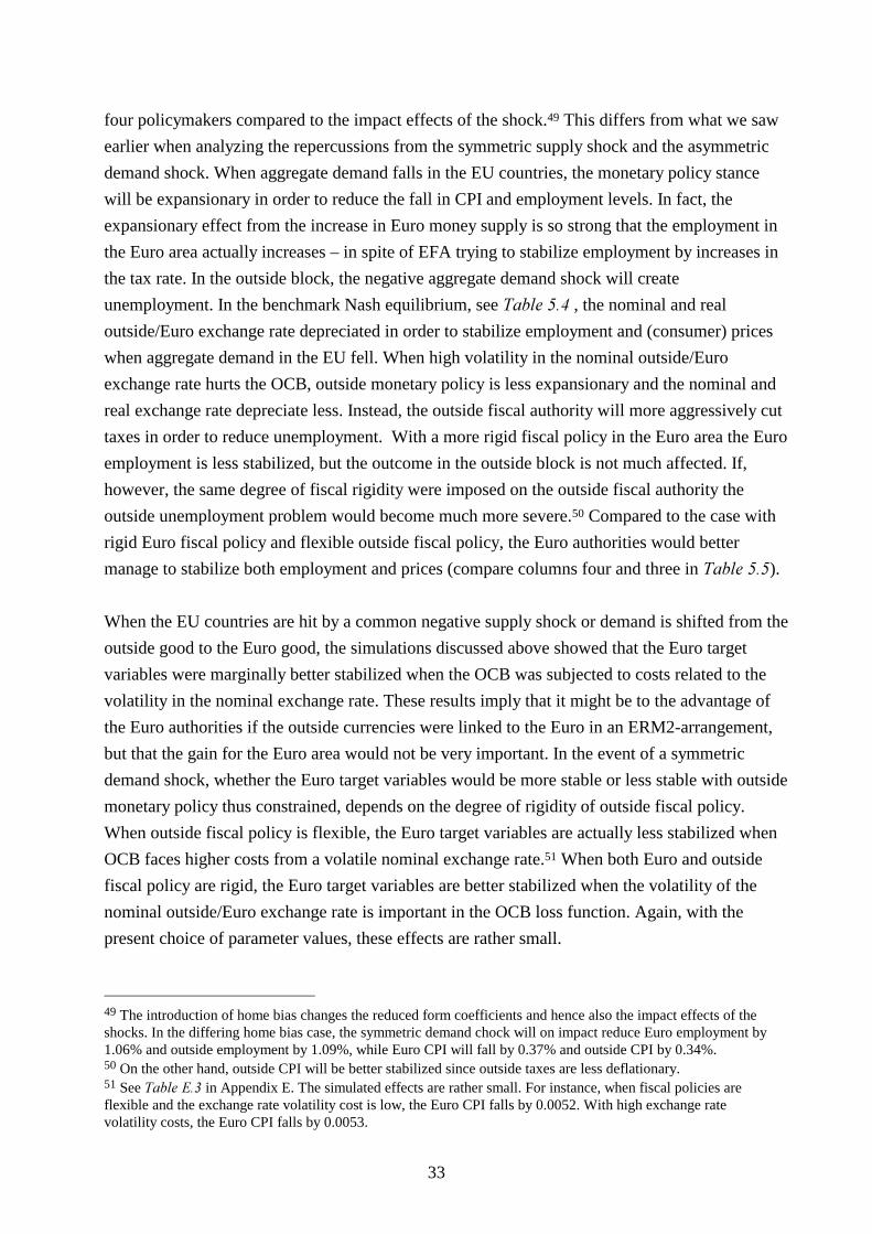
33

four policymakers compared to the impact effects of the shock.49 This differs from what we saw

earlier when analyzing the repercussions from the symmetric supply shock and the asymmetric

demand shock. When aggregate demand falls in the EU countries, the monetary policy stance

will be expansionary in order to reduce the fall in CPI and employment levels. In fact, the

expansionary effect from the increase in Euro money supply is so strong that the employment in

the Euro area actually increases – in spite of EFA trying to stabilize employment by increases in

the tax rate. In the outside block, the negative aggregate demand shock will create

unemployment. In the benchmark Nash equilibrium, see 7DEOH���� , the nominal and real

outside/Euro exchange rate depreciated in order to stabilize employment and (consumer) prices

when aggregate demand in the EU fell. When high volatility in the nominal outside/Euro

exchange rate hurts the OCB, outside monetary policy is less expansionary and the nominal and

real exchange rate depreciate less. Instead, the outside fiscal authority will more aggressively cut

taxes in order to reduce unemployment. With a more rigid fiscal policy in the Euro area the Euro

employment is less stabilized, but the outcome in the outside block is not much affected. If,

however, the same degree of fiscal rigidity were imposed on the outside fiscal authority the

outside unemployment problem would become much more severe.50 Compared to the case with

rigid Euro fiscal policy and flexible outside fiscal policy, the Euro authorities would better

manage to stabilize both employment and prices (compare columns four and three in 7DEOH����).

When the EU countries are hit by a common negative supply shock or demand is shifted from the

outside good to the Euro good, the simulations discussed above showed that the Euro target

variables were marginally better stabilized when the OCB was subjected to costs related to the

volatility in the nominal exchange rate. These results imply that it might be to the advantage of

the Euro authorities if the outside currencies were linked to the Euro in an ERM2-arrangement,

but that the gain for the Euro area would not be very important. In the event of a symmetric

demand shock, whether the Euro target variables would be more stable or less stable with outside

monetary policy thus constrained, depends on the degree of rigidity of outside fiscal policy.

When outside fiscal policy is flexible, the Euro target variables are actually less stabilized when

OCB faces higher costs from a volatile nominal exchange rate.51 When both Euro and outside

fiscal policy are rigid, the Euro target variables are better stabilized when the volatility of the

nominal outside/Euro exchange rate is important in the OCB loss function. Again, with the

present choice of parameter values, these effects are rather small.

49 The introduction of home bias changes the reduced form coefficients and hence also the impact effects of theshocks. In the differing home bias case, the symmetric demand chock will on impact reduce Euro employment by1.06% and outside employment by 1.09%, while Euro CPI will fall by 0.37% and outside CPI by 0.34%.50 On the other hand, outside CPI will be better stabilized since outside taxes are less deflationary.51 See 7DEOH�(�� in Appendix E. The simulated effects are rather small. For instance, when fiscal policies areflexible and the exchange rate volatility cost is low, the Euro CPI falls by 0.0052. With high exchange ratevolatility costs, the Euro CPI falls by 0.0053.

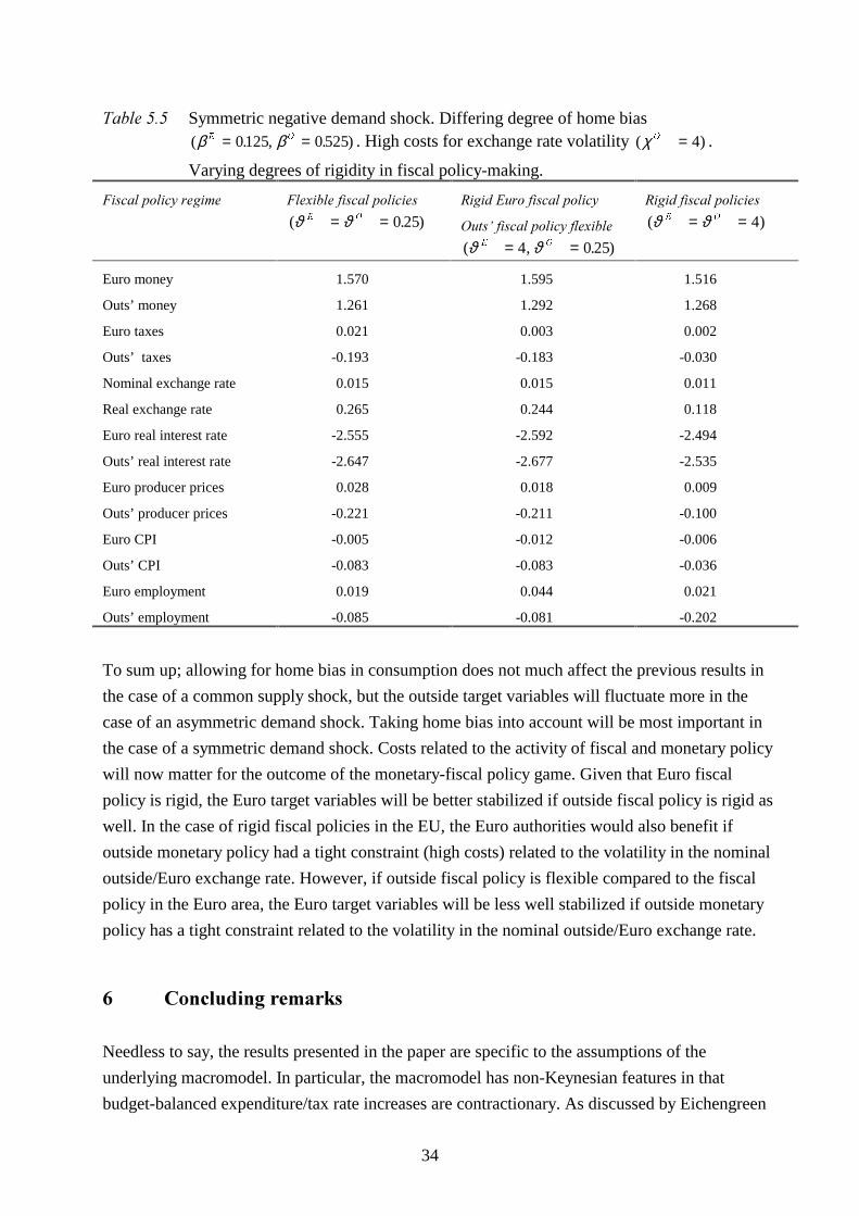
34

7DEOH���� Symmetric negative demand shock. Differing degree of home bias( . , . )β β( 2= =0125 0 525 . High costs for exchange rate volatility ( )χ 2 = 4 .

Varying degrees of rigidity in fiscal policy-making.

)LVFDO�SROLF\�UHJLPH )OH[LEOH�ILVFDO�SROLFLHV

( . )ϑ ϑ( 2= = 0 25

5LJLG�(XUR�ILVFDO�SROLF\

2XWV¶�ILVFDO�SROLF\�IOH[LEOH

( , . )ϑ ϑ( 2= =4 0 25

5LJLG�ILVFDO�SROLFLHV

( )ϑ ϑ( 2= = 4

Euro money 1.570 1.595 1.516

Outs’ money 1.261 1.292 1.268

Euro taxes 0.021 0.003 0.002

Outs’ taxes -0.193 -0.183 -0.030

Nominal exchange rate 0.015 0.015 0.011

Real exchange rate 0.265 0.244 0.118

Euro real interest rate -2.555 -2.592 -2.494

Outs’ real interest rate -2.647 -2.677 -2.535

Euro producer prices 0.028 0.018 0.009

Outs’ producer prices -0.221 -0.211 -0.100

Euro CPI -0.005 -0.012 -0.006

Outs’ CPI -0.083 -0.083 -0.036

Euro employment 0.019 0.044 0.021

Outs’ employment -0.085 -0.081 -0.202

To sum up; allowing for home bias in consumption does not much affect the previous results in

the case of a common supply shock, but the outside target variables will fluctuate more in the

case of an asymmetric demand shock. Taking home bias into account will be most important in

the case of a symmetric demand shock. Costs related to the activity of fiscal and monetary policy

will now matter for the outcome of the monetary-fiscal policy game. Given that Euro fiscal

policy is rigid, the Euro target variables will be better stabilized if outside fiscal policy is rigid as

well. In the case of rigid fiscal policies in the EU, the Euro authorities would also benefit if

outside monetary policy had a tight constraint (high costs) related to the volatility in the nominal

outside/Euro exchange rate. However, if outside fiscal policy is flexible compared to the fiscal

policy in the Euro area, the Euro target variables will be less well stabilized if outside monetary

policy has a tight constraint related to the volatility in the nominal outside/Euro exchange rate.

� &RQFOXGLQJ�UHPDUNV

Needless to say, the results presented in the paper are specific to the assumptions of the

underlying macromodel. In particular, the macromodel has non-Keynesian features in that

budget-balanced expenditure/tax rate increases are contractionary. As discussed by Eichengreen

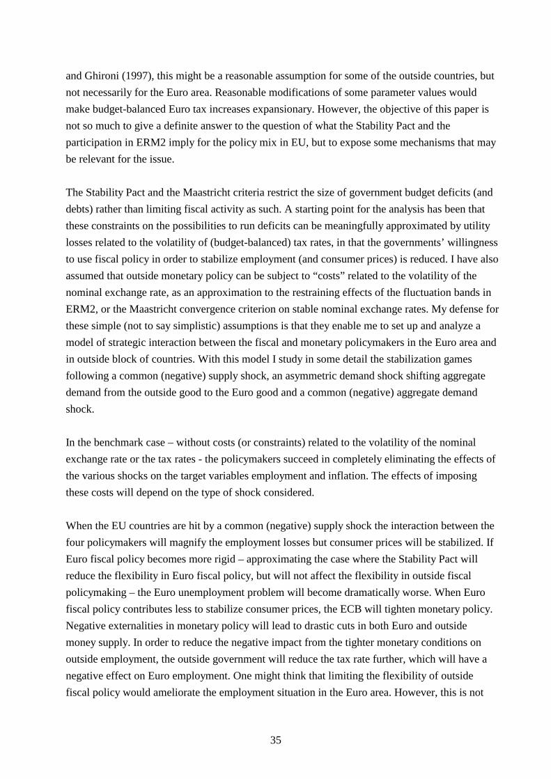
35

and Ghironi (1997), this might be a reasonable assumption for some of the outside countries, but

not necessarily for the Euro area. Reasonable modifications of some parameter values would

make budget-balanced Euro tax increases expansionary. However, the objective of this paper is

not so much to give a definite answer to the question of what the Stability Pact and the

participation in ERM2 imply for the policy mix in EU, but to expose some mechanisms that may

be relevant for the issue.

The Stability Pact and the Maastricht criteria restrict the size of government budget deficits (and

debts) rather than limiting fiscal activity as such. A starting point for the analysis has been that

these constraints on the possibilities to run deficits can be meaningfully approximated by utility

losses related to the volatility of (budget-balanced) tax rates, in that the governments’ willingness

to use fiscal policy in order to stabilize employment (and consumer prices) is reduced. I have also

assumed that outside monetary policy can be subject to “costs” related to the volatility of the

nominal exchange rate, as an approximation to the restraining effects of the fluctuation bands in

ERM2, or the Maastricht convergence criterion on stable nominal exchange rates. My defense for

these simple (not to say simplistic) assumptions is that they enable me to set up and analyze a

model of strategic interaction between the fiscal and monetary policymakers in the Euro area and

in outside block of countries. With this model I study in some detail the stabilization games

following a common (negative) supply shock, an asymmetric demand shock shifting aggregate

demand from the outside good to the Euro good and a common (negative) aggregate demand

shock.

In the benchmark case – without costs (or constraints) related to the volatility of the nominal

exchange rate or the tax rates - the policymakers succeed in completely eliminating the effects of

the various shocks on the target variables employment and inflation. The effects of imposing

these costs will depend on the type of shock considered.

When the EU countries are hit by a common (negative) supply shock the interaction between the

four policymakers will magnify the employment losses but consumer prices will be stabilized. If

Euro fiscal policy becomes more rigid – approximating the case where the Stability Pact will

reduce the flexibility in Euro fiscal policy, but will not affect the flexibility in outside fiscal

policymaking – the Euro unemployment problem will become dramatically worse. When Euro

fiscal policy contributes less to stabilize consumer prices, the ECB will tighten monetary policy.

Negative externalities in monetary policy will lead to drastic cuts in both Euro and outside

money supply. In order to reduce the negative impact from the tighter monetary conditions on

outside employment, the outside government will reduce the tax rate further, which will have a

negative effect on Euro employment. One might think that limiting the flexibility of outside

fiscal policy would ameliorate the employment situation in the Euro area. However, this is not

36

the case in the present model. With rigid outside fiscal policy the OCB will compensate with

even tighter monetary policy to keep outside inflation down, which in turn will induce the ECB

to further reduce the Euro money supply. This will result in heavy employment losses in both

areas, and consumer prices will be higher.

In the event of an asymmetric demand shock shifting aggregate demand from the outside good to

the Euro good, the interaction between the four policymakers will stabilize CPI in both areas, but

the overemployment problem in the Euro area will be amplified. When outside fiscal policy is

flexible, tax cuts can be used to reduce the negative impact effect on outside employment. With

rigid fiscal policy in both the Euro area and the outside area the outside unemployment problem

will be aggravated by the monetary-fiscal stabilization game. In contrast to the symmetric supply

shock case, the Euro authorities will benefit from increased fiscal rigidity in the outside area,

since this will lead to better stabilization of both Euro employment and CPI.

When consumer preferences are such that the import share equals the relative size of the

partner region, the optimal stabilization of a common (negative) aggregate demand shock will

be a symmetric expansion of the money supplies and fiscal policy will be completely inactive.

This holds in the present model whether or not any costs related to the volatility in tax rates or

the nominal outside/Euro exchange rate are imposed. This conclusion continues to hold when

equal home bias is introduced, but it does not hold in the presence of differing home bias. In

the paper I assume that the degree of home bias is larger in the Euro area. In this case, and

differently from the two earlier cases, the monetary-fiscal policy game will stabilize CPI and

employment in both regions. Furthermore, the Euro authorities gain from increasing outside

fiscal rigidity.

The exercises presented in the paper point to the importance of taking into account the

interaction between the different policymakers when imposing restrictions on a subset of these

policymakers. One example of this is the case with a common negative supply shock. When the

fiscal policy of the Euro government (or both governments) is restricted, the negative

externalities in monetary policy will bring about a very poor equilibrium, with both high

unemployment and high inflation. The general message is that modifications of the fiscal policy

framework should not be undertaken isolated from the monetary policy framework. For instance,

from the point of view of stabilization policy one can argue that the constraints on fiscal policy

contained in the Stability and Growth Pact ought to influence how much weight the ECB is to

put on price stability versus employment stabilization.

A natural subject for future research is to modify the assumptions of the macromodel to allow an

analysis of the Keynesian regime of fiscal policymaking. A more challenging task would be to

37

better represent the specifics of the Stability Pact, in particular, recognizing that the Stability Pact

limits budget deficits rather than budget-balanced changes in the tax rates.

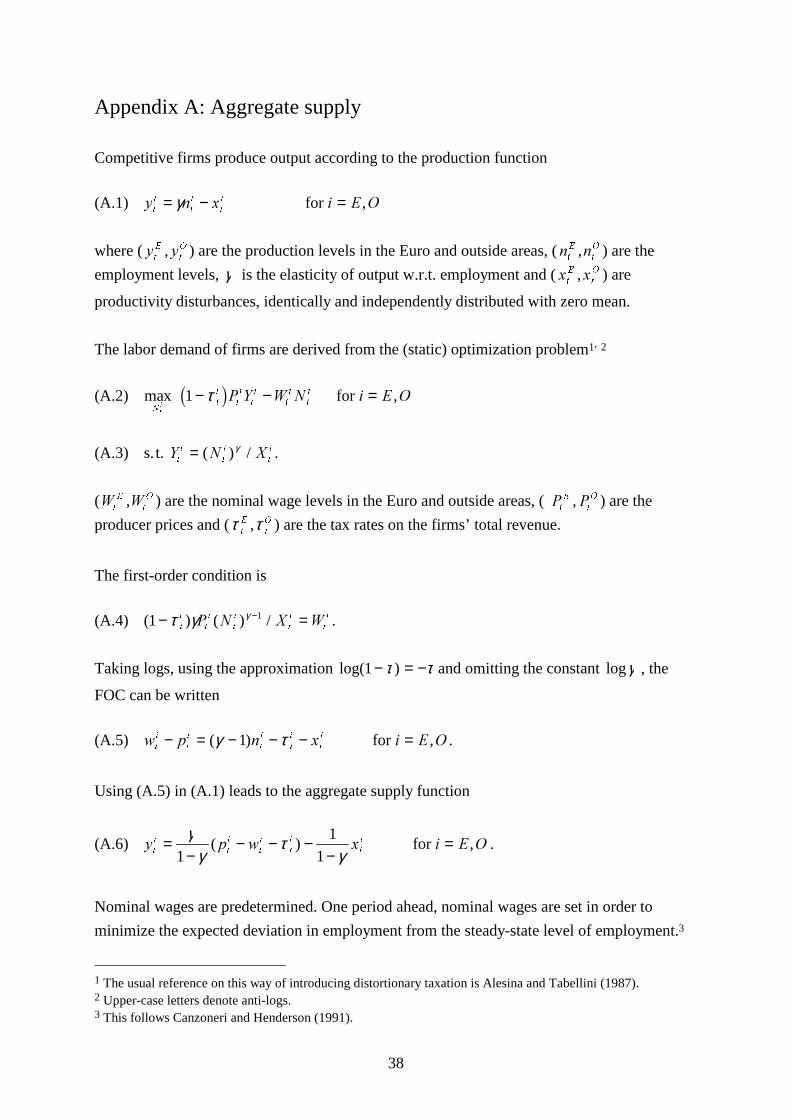
38

Appendix A: Aggregate supply

Competitive firms produce output according to the production function

(A.1) \ Q [ L ( 2W

L

W

L

W

L= − =γ for ,

where ( \ \W

(

W

2, ) are the production levels in the Euro and outside areas, (Q QW

(

W

2, ) are the

employment levels, γ is the elasticity of output w.r.t. employment and ( [ [W

(

W

2, ) are

productivity disturbances, identically and independently distributed with zero mean.

The labor demand of firms are derived from the (static) optimization problem1, 2

(A.2) max for 1

W

L

W

L

W

L

W

L

W

L

W

L

3 < : 1 L ( 21− − =τ2 7 ,

(A.3) s. t. < 1 ;W

L

W

L

W

L= ( ) /γ .

(: :W

(

W

2, ) are the nominal wage levels in the Euro and outside areas, ( 3 3W

(

W

2, ) are the

producer prices and (τ τW

(

W

2, ) are the tax rates on the firms’ total revenue.

The first-order condition is

(A.4) ( ) ( ) /1 1− =−τ γ γW

L

W

L

W

L

W

L

W

L3 1 ; : .

Taking logs, using the approximation log( )1− = −τ τ and omitting the constant logγ , the

FOC can be written

(A.5) Z S Q [ L ( 2W

L

W

L

W

L

W

L

W

L− = − − − =( ) ,γ τ1 for .

Using (A.5) in (A.1) leads to the aggregate supply function

(A.6) \ S Z [ L ( 2W

L

W

L

W

L

W

L

W

L=−

− − −−

=γγ

τγ1

1

1( ) ,for .

Nominal wages are predetermined. One period ahead, nominal wages are set in order to

minimize the expected deviation in employment from the steady-state level of employment.3

1 The usual reference on this way of introducing distortionary taxation is Alesina and Tabellini (1987).2 Upper-case letters denote anti-logs.3 This follows Canzoneri and Henderson (1991).

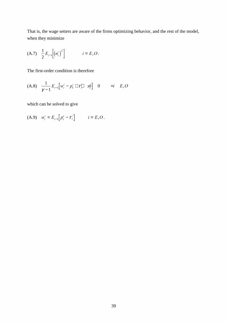
39

That is, the wage setters are aware of the firms optimizing behavior, and the rest of the model,

when they minimize

(A.7)1

2 1

2( Q L ( 2

W W

L

− =2 7 , .

The first-order condition is therefore

(A.8)1

101γ

τ−

− + + = =−( Z S [ L ( 2W W

L

W

L

W

L

W

L ,

which can be solved to give

(A.9) Z ( S L ( 2W

L

W W

L

W

L= − =−1 τ , .

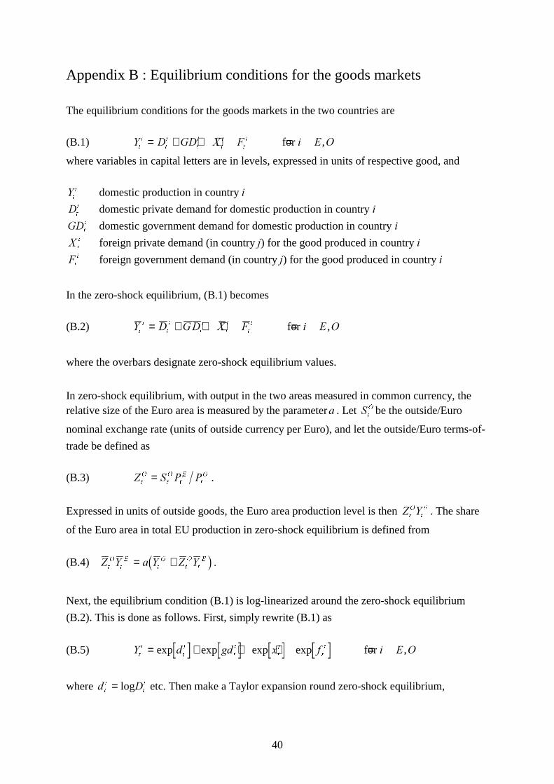
40

Appendix B : Equilibrium conditions for the goods markets

The equilibrium conditions for the goods markets in the two countries are

(B.1) < ' *' ; ) L ( 2W

L

W

L

W

L

W

L

W

L= + + + =for ,

where variables in capital letters are in levels, expressed in units of respective good, and

<W

L domestic production in country L

'W

L domestic private demand for domestic production in country L

*'W

L domestic government demand for domestic production in country L

;W

L foreign private demand (in country M) for the good produced in country L

)W

L foreign government demand (in country M) for the good produced in country L

In the zero-shock equilibrium, (B.1) becomes

(B.2) < ' *' ; ) L ( 2W

L

W

L

W

L

W

L

W

L= + + + =for ,

where the overbars designate zero-shock equilibrium values.

In zero-shock equilibrium, with output in the two areas measured in common currency, therelative size of the Euro area is measured by the parameterD . Let 6

W

2 be the outside/Euro

nominal exchange rate (units of outside currency per Euro), and let the outside/Euro terms-of-

trade be defined as

(B.3) = 6 3 3W

2

W

2

W

(

W

2= .

Expressed in units of outside goods, the Euro area production level is then = <W

2

W

( . The share

of the Euro area in total EU production in zero-shock equilibrium is defined from

(B.4) = < D < = <W

2

W

(

W

2

W

2

W

(= +2 7 .

Next, the equilibrium condition (B.1) is log-linearized around the zero-shock equilibrium

(B.2). This is done as follows. First, simply rewrite (B.1) as

(B.5) < G JG [ I L ( 2W

L

W

L

W

L

W

L

W

L= + + + =exp exp exp exp for ,

where G 'W

L

W

L= log etc. Then make a Taylor expansion round zero-shock equilibrium,

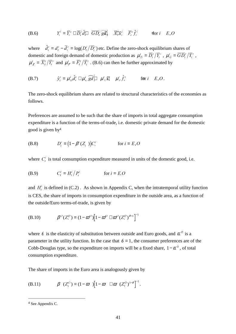
41

(B.6) < < ' G *' JG ; [ ) I L ( 2W

L

W

L

W

L

W

L

W

L

W

L

W

L

W

L

W

L

W

L= + + + + =$ $ $ ,for

where $ log( )G G G ' 'W

L

W

L

W

L

W

L

W

L= − = etc. Define the zero-shock equilibrium shares of

domestic and foreign demand of domestic production as µ'

L

W

L

W

L' <= , µ*

L

W

L

W

L*' <= ,

µ;

L

W

L

W

L; <= and µ)

L

W

L

W

L) <= . (B.6) can then be further approximated by

(B.7) $ $ $ $ ,\ G JG [ I L ( 2W

L

'

L

W

L

*

L

W

L

;

L

W

L

)

L

W

L= + + + =µ µ µ µ for .

The zero-shock equilibrium shares are related to structural characteristics of the economies as

follows.

Preferences are assumed to be such that the share of imports in total aggregate consumption

expenditure is a function of the terms-of-trade, i.e. domestic private demand for the domestic

good is given by4

(B.8) ' = & L ( 2W

L L

W W

L= − =1 β ( ) ,2 7 for

where &W

L is total consumption expenditure measured in units of the domestic good, i.e.

(B.9) & + 3 L (�2W

L

W

L

W

L= = for

and +W

L is defined in (C.2) . As shown in Appendix C, when the intratemporal utility function

is CES, the share of imports in consumption expenditure in the outside area, as a function of

the outside/Euro terms-of-trade, is given by

(B.10) β ω ω ω θ2

W

2 2 2 2

W

2= =( ) ( ) ( )= − − + − −1 1 1 1

where θ is the elasticity of substitution between outside and Euro goods, and ω 2 is a

parameter in the utility function. In the case that θ = 1, the consumer preferences are of the

Cobb-Douglas type, so the expenditure on imports will be a fixed share, 1− ω 2 , of total

consumption expenditure.

The share of imports in the Euro area is analogously given by

(B.11) β ω ω ω θW

2

W

2= =( ) ( ) ( )= − − + − −1 1 1 1

.

4 See Appendix C.

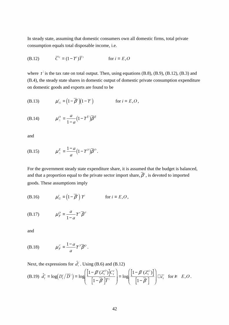
42

In steady state, assuming that domestic consumers own all domestic firms, total private

consumption equals total disposable income, i.e.

(B.12) & < L ( 2L L L= − =( ) ,1 τ for

where τ L is the tax rate on total output. Then, using equations (B.8), (B.9), (B.12), (B.3) and

(B.4), the steady state shares in domestic output of domestic private consumption expenditure

on domestic goods and exports are found to be

(B.13) µ β τ'

L L L L ( 2= − − =1 13 82 7 for , ,

(B.14) µ τ β;

2 ( (DD

=−

−1

12 7

and

(B.15) µ τ β;

( 2 2DD

= − −112 7 .

For the government steady state expenditure share, it is assumed that the budget is balanced,

and that a proportion equal to the private sector import share, β L , is devoted to imported

goods. These assumptions imply

(B.16) µ β τ*

L L L L ( 2= − =13 8 for , ,

(B.17) µ τ β)

2 ( (DD

=−1

and

(B.18) µ τ β)

( 2 2DD

= −1.

Next, the expressions for $GW

L . Using (B.6) and (B.12)

(B.19) $ log log( )

log( )

$ ,G ' '= &

<

=F L ( 2

W

L

W

L L

L

W

2

W

L

L L

L

W

2

LW

L= =−

−

����

���� =

−

−

����

���� + =2 7 1

1

1

1

β

β

β

β for .

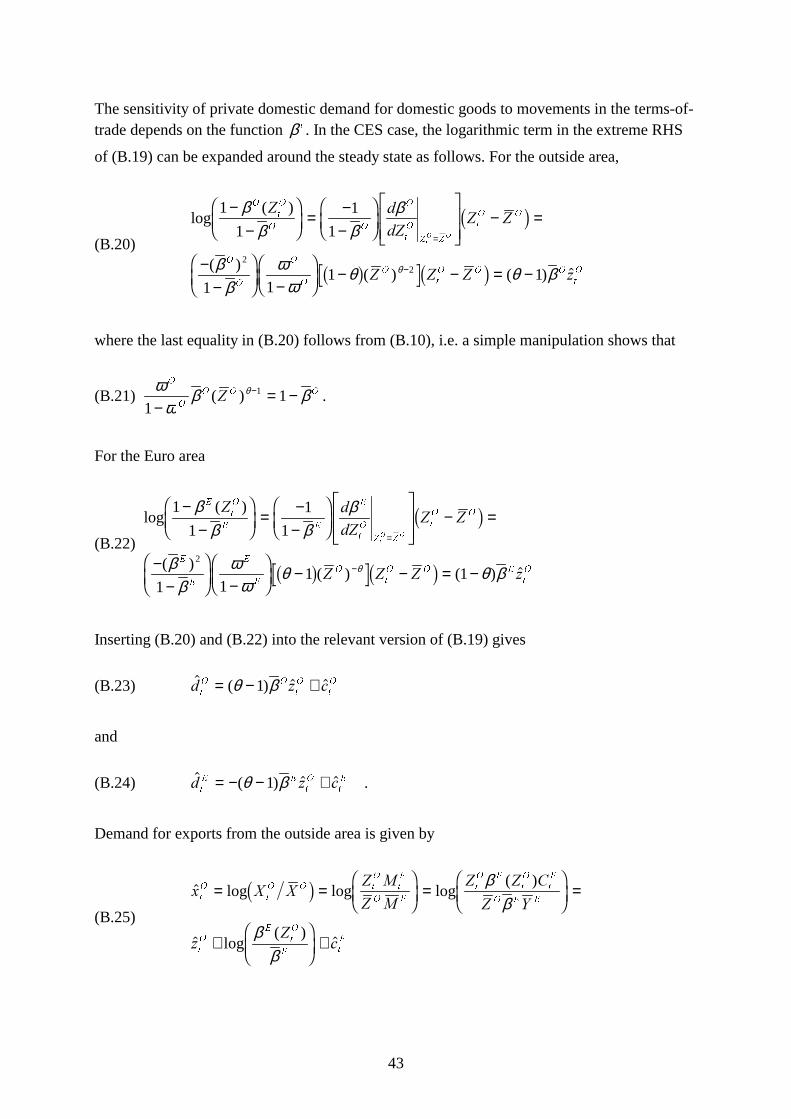
43

The sensitivity of private domestic demand for domestic goods to movements in the terms-of-trade depends on the function β L . In the CES case, the logarithmic term in the extreme RHS

of (B.19) can be expanded around the steady state as follows. For the outside area,

(B.20)

log( )

( )( ) ( ) $

1

1

1

1

1 11 1

22

−−

���

��� = −

−���

����!

"$## − =

−−

���

��� −���

��� − − = −

=

−

ββ β

β

ββ

ωω

θ θ βθ

2

W

2

2 2

2

W

2

= =

W

2 2

2

2

2

2

2

W

2 2 2

W

2

= GG=

= =

= = = ]

W

2 2

2 7

1 6 2 7

where the last equality in (B.20) follows from (B.10), i.e. a simple manipulation shows that

(B.21)ω

ωβ βθ

2

2

2 2 2=1

11

−= −−( ) .

For the Euro area

(B.22)

log( )

( )( ) ( ) $

1

1

1

1

1 11 1

2

−−

���

��� = −

−���

����!

"$## − =

−−

���

��� −���

��� − − = −

=

−

ββ β

β

ββ

ωω

θ θ βθ

(

W

2

( (

(

W

2

= =

W

2 2

(

(

(

(

2

W

2 2 (

W

2

= GG=

= =

= = = ]

W

2 2

2 7

1 6 2 7

Inserting (B.20) and (B.22) into the relevant version of (B.19) gives

(B.23) $ ( ) $ $G ] FW

2 2

W

2

W

2= − +θ β1

and

(B.24) $ ( ) $ $G ] FW

( (

W

2

W

(= − − +θ β1 .

Demand for exports from the outside area is given by

(B.25)

$ log log log( )

$ log( )

$

[ ; ;= 0

= 0

= = &

= <

]=

F

W

2

W

2 2 W

2

W

(

2 (

W

2 (

W

2

W

(

2 ( (

W

2

(

W

2

( W

(

= =���

��� =

���

��� =

+���

��� +

2 7 ββ

ββ

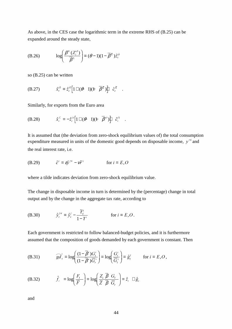
44

As above, in the CES case the logarithmic term in the extreme RHS of (B.25) can be

expanded around the steady state,

(B.26) log( )

( )( ) $β

βθ β

(

W

2

(

(

W

2=

]���

��� = − −1 1

so (B.25) can be written

(B.27) $ $ ( )( ) $[ ] FW

2

W

2 (

W

(= + − − +1 1 1θ β .

Similarly, for exports from the Euro area

(B.28) $ $ ( )( ) $[ ] FW

(

W

2 2

W

2= − + − − +1 1 1θ β .

It is assumed that (the deviation from zero-shock equilibrium values of) the total consumptionexpenditure measured in units of the domestic good depends on disposable income, \ 'L and

the real interest rate, i.e.

(B.29) $ $ ~ ,F \ U L ( 2L 'L L= − =ε ν for

where a tilde indicates deviation from zero-shock equilibrium value.

The change in disposable income in turn is determined by the (percentage) change in total

output and by the change in the aggregate tax rate, according to

(B.30) $ $~

,\ \ L ( 2W

'L

W

L W

L

L= −

−=

ττ1

for .

Each government is restricted to follow balanced-budget policies, and it is furthermore

assumed that the composition of goods demanded by each government is constant. Then

(B.31) JG*

*

*

*J L ( 2

W

LL

W

L

L

W

L

W

L

W

L W

L=−−

���

��� =

���

��� = =log

( )

( )log $ ,

1

1

ββ

for ,

(B.32) $ log log $ $I)

)

= *

= *] J

W

W W W

W

W W=

���

��� =

���

��� = +

ββ

and

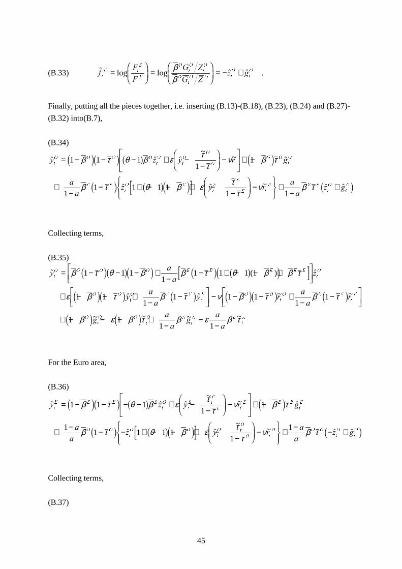
45

(B.33) $ log log $ $I)

)

* =

* =] J

W

( W

(

(

2

W

2

W

2

2

W

2 2 W

2

W

2=���

��� =

���

��� = − +

ββ

.

Finally, putting all the pieces together, i.e. inserting (B.13)-(B.18), (B.23), (B.24) and (B.27)-

(B.32) into(B.7),

(B.34)

$ $ $~

~ $

$ $~

~ $ $

\ ] \ U J

DD

] \ UDD

] J

W

2 2 2 2

W

2

W

2

2

2

2 2

W

2

( (

W

2 (

W

(

(

( W

( ( (

W

2

W

(

= − − − + −−

���

��� −

�!

"$#

+ −

+−

− + − − + −−

���

��� −

%&'()*

+−

+

1 1 11

1

11 1 1 1

1 1

β τ θ β ε ττ

ν β τ

β τ θ β ε ττ

ν β τ

3 82 7 1 6 3 8

2 7 1 63 8 2 7

Collecting terms,

(B.35)

$ ( ) $

$ $ ~ ~

~ ~ ~

\DD

]

\DD

\ UDD

U

JDD

J

W

2 2 2 2 ( ( ( ( (

W

2

2 2

W

2 ( (

W

( 2 2

W

2 ( (

W

(

2

W

2 2

W

2 (

= − − − +−

− + − − +�!

"$#

+ − − +−

−�!

"$# − − − +

−−�

! "$#

+ − − − +−

β τ θ β β τ θ β β τ

ε β τ β τ ν β τ β τ

β ε β τ β

1 1 11

1 1 1 1

1 11

1 1 11

1

1 11

2 71 63 8 2 7 1 63 8

3 82 7 2 7 3 82 7 2 7

3 8 3 8 W

( (

W

(DD

−−

ε β τ1

~

For the Euro area,

(B.36)

$ $ $~

~ $

$ $~

~ $ $

\ ] \ U J

DD

] \ UDD

] J

W

( ( ( (

W

2

W

( W

(

( W

( ( (

W

(

2 2

W

2 2

W

2 W

2

2 W

2 2 2

W

2

W

2

= − − − − + −−

���

��� −

�!

"$#

+ −

+ − − − + − − + −−

���

��� −

%&'K()*K

+ − − +

1 1 11

1

11 1 1 1

1

1

β τ θ β ε ττ

ν β τ

β τ θ β ε ττ

ν β τ

3 82 7 1 6 3 8

2 7 1 63 8 2 7

Collecting terms,

(B.37)

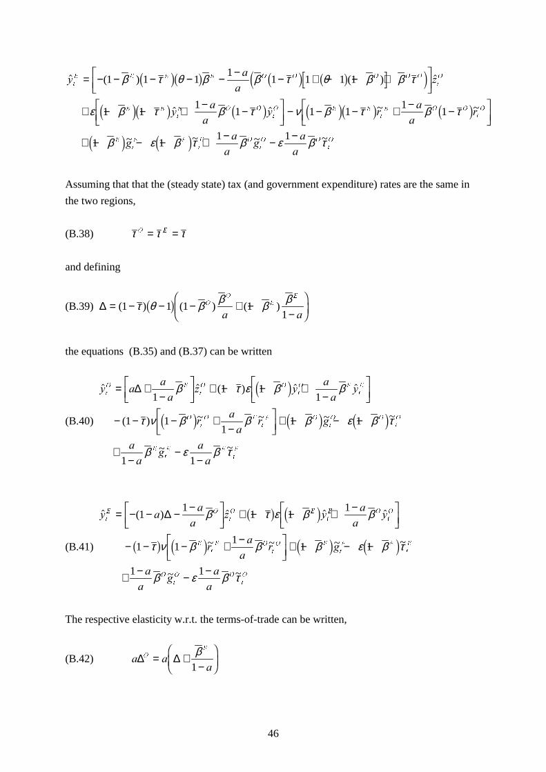
46

$ ( ) ( ) $

$ $ ~ ~

~ ~ ~

\DD

]

\DD

\ UDD

U

JDD

W

( ( ( ( 2 2 2 2 2

W

2

( (

W

( 2 2

W

2 ( (

W

( 2 2

W

2

(

W

( (

W

( 2

= − − − − − − − + − − +�!

"$#

+ − − + − −�!

"$# − − − + − −�

! "$#

+ − − − + −

1 1 11

1 1 1 1

1 11

1 1 11

1

1 11

β τ θ β β τ θ β β τ

ε β τ β τ ν β τ β τ

β ε β τ β

2 71 6 2 7 1 64 9

3 82 7 2 7 3 82 7 2 7

3 8 3 8 JDDW

2 2

W

2− −ε β τ1 ~

Assuming that that the (steady state) tax (and government expenditure) rates are the same in

the two regions,

(B.38) τ τ τ2 (= =

and defining

(B.39) ∆ = − − − + −−

���

���( ) ( ) ( )1 1 1 1

1τ θ β β β β1 6 2

2

(

(

D D

the equations (B.35) and (B.37) can be written

(B.40)

$ $ ( ) $ $

( ) ~ ~ ~ ~

~ ~

\ DDD

] \DD

\

UDD

U J

DD

JDD

W

2 (

W

2 2

W

2 (

W

(

2

W

2 (

W

( 2

W

2 2

W

2

(

W

( (

W

(

= +−

�!

"$# + − − +

−�!

"$#

− − − +−

�!

"$# + − − −

+−

−−

∆1

1 11

1 11

1 1

1 1

β τ ε β β

τ ν β β β ε β τ

β ε β τ

3 8

3 8 3 8 3 8

(B.41)

$ ( ) $ $ $

~ ~ ~ ~

~ ~

\ DDD

] \DD

\

UDD

U J

DD

JDD

W

( 2

W

2 (

W

( 2

W

2

(

W

( 2

W

2 (

W

( (

W

(

2

W

2 2

W

2

= − − − −�!

"$# + − − + −�

! "$#

− − − + −�!

"$# + − − −

+ − − −

11

1 11

1 11

1 1

1 1

∆ β τ ε β β

τ ν β β β ε β τ

β ε β τ

1 6 3 8

1 6 3 8 3 8 3 8

The respective elasticity w.r.t. the terms-of-trade can be written,

(B.42) D DD

2

(

∆ ∆= +−

���

���

β1

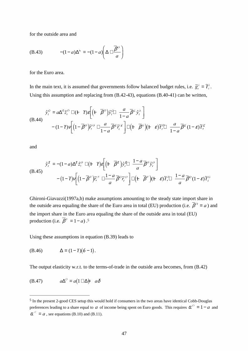
47

for the outside area and

(B.43) − − = − − +���

���( ) ( )1 1D D

D(

2

∆ ∆ β

for the Euro area.

In the main text, it is assumed that governments follow balanced budget rules, i.e. ~ ~JW

L

W

L= τ .

Using this assumption and replacing from (B.42-43), equations (B.40-41) can be written,

(B.44)

$ $ ( ) $ $

( ) ~ ~ ~ ( )~

\ D ] \DD

\

UDD

UDD

W

2 2

W

2 2

W

2 (

W

(

2

W

2 (

W

( 2

W

2 (

W

(

= + − − +−

�!

"$#

− − − +−

�!

"$# + − − +

−−

∆ 1 11

1 11

1 11

1

τ ε β β

τ ν β β β ε τ β ε τ

3 8

3 8 3 81 6

and

(B.45)

$ ( ) $ $ $

~ ~ ( )~ ( )~

\ D ] \DD

\

UDD

UDD

W

( (

W

2 (

W

( 2

W

2

(

W

( 2

W

2 (

W

( 2

W

2

= − − + − − + −�!

"$#

− − − + −�!

"$# + − − + − −

1 1 11

1 11

1 11

1

∆ τ ε β β

τ ν β β β ε τ β ε τ

1 6 3 8

1 6 3 8 3 8

Ghironi-Giavazzi(1997a,b) make assumptions amounting to the steady state import share in

the outside area equaling the share of the Euro area in total (EU) production (i.e. β 2 D= ) and

the import share in the Euro area equaling the share of the outside area in total (EU)

production (i.e. β ( D= −1 ) .5

Using these assumptions in equation (B.39) leads to

(B.46) ∆ = − −( )1 1τ θ1 6 .

The output elasticity w.r.t. to the terms-of-trade in the outside area becomes, from (B.42)

(B.47) D D D2∆ ∆= + =11 6 δ

5 In the present 2-good CES setup this would hold if consumers in the two areas have identical Cobb-Douglas

preferences leading to a share equal to D of income being spent on Euro goods. This requires ω 2 D= −1 and

ω ( D= , see equations (B.10) and (B.11).

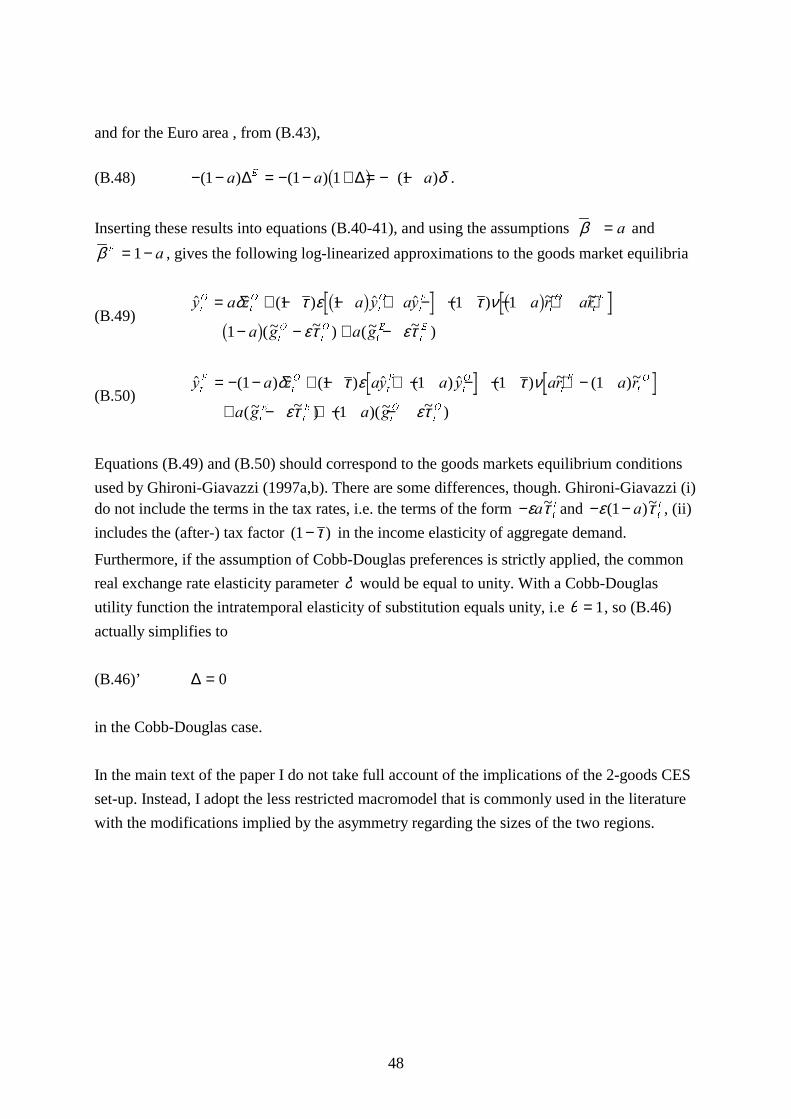
48

and for the Euro area , from (B.43),

(B.48) − − = − − + = − −( ) ( ) ( )1 1 1 1D D D(∆ ∆1 6 δ .

Inserting these results into equations (B.40-41), and using the assumptions β D= and

β ( D= −1 , gives the following log-linearized approximations to the goods market equilibria

(B.49)$ $ ( ) $ $ ( ) ~ ~

(~ ~ ) (~ ~ )

\ D ] D \ D\ D U DU

D J D J

W

2

W

2

W

2

W

(

W

2

W

(

W

2

W

2

W

(

W

(

= + − − + − − − + +

− − + −

δ τ ε τ ν

ετ ετ

1 1 1 1

1

1 6 1 61 6

(B.50)$ ( ) $ ( ) $ ( ) $ ( ) ~ ( )~

(~ ~ ) ( )(~ ~ )

\ D ] D\ D \ DU D U

D J D J

W

(

W

2

W

(

W

2

W

(

W

2

W

(

W

(

W

2

W

2

= − − + − + − − − + −

+ − + − −

1 1 1 1 1

1

δ τ ε τ ν

ετ ετ

Equations (B.49) and (B.50) should correspond to the goods markets equilibrium conditions

used by Ghironi-Giavazzi (1997a,b). There are some differences, though. Ghironi-Giavazzi (i)do not include the terms in the tax rates, i.e. the terms of the form −ε τD

W

L~ and − −ε τ( )~1 DW

L , (ii)

includes the (after-) tax factor ( )1− τ in the income elasticity of aggregate demand.

Furthermore, if the assumption of Cobb-Douglas preferences is strictly applied, the common

real exchange rate elasticity parameter δ would be equal to unity. With a Cobb-Douglas

utility function the intratemporal elasticity of substitution equals unity, i.e θ = 1, so (B.46)

actually simplifies to

(B.46)’ ∆ = 0

in the Cobb-Douglas case.

In the main text of the paper I do not take full account of the implications of the 2-goods CES

set-up. Instead, I adopt the less restricted macromodel that is commonly used in the literature

with the modifications implied by the asymmetry regarding the sizes of the two regions.

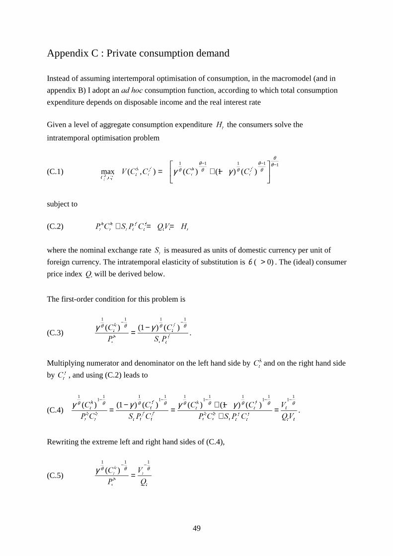
49

Appendix C : Private consumption demand

Instead of assuming intertemporal optimisation of consumption, in the macromodel (and in

appendix B) I adopt an DG�KRF�consumption function, according to which total consumption

expenditure depends on disposable income and the real interest rate

Given a level of aggregate consumption expenditure +W the consumers solve the

intratemporal optimisation problem

(C.1) max ( , ) ( ) ( ) ( ),& &

W

K

W

I

W

K

W

I

WK

WI9 & & & &= + −

�!

"$#

− − −

γ γθθθ θ

θθ

θθ1 1 1 1 1

1

subject to

(C.2) 3 & 6 3 & 49 +W

K

W

K

W W

I

W

I

W W W+ = =

where the nominal exchange rate 6W is measured as units of domestic currency per unit of

foreign currency. The intratemporal elasticity of substitution is θ ( )> 0 . The (ideal) consumer

price index 4Wwill be derived below.

The first-order condition for this problem is

(C.3)γ γθ θ θ θ

1 1 1 1

1( ) ( ) ( )&

3

&

6 3W

K

W

K

W

I

W W

I

− −

=−

.

Multiplying numerator and denominator on the left hand side by &W

K and on the right hand side

by &W

I , and using (C.2) leads to

(C.4)γ γ γ γθ θ θ θ θ θ θ θ θ

11

1 11

1 11

1 11

11

1

1 1( ) ( ) ( ) ( ) ( ) ( )&

3 &

&

6 3 &

& &

3 & 6 3 &

949

W

K

W

K

W

K

W

I

W W

I

W

I

W

K

W

I

W

K

W

K

W W

I

W

I

W

W W

− − − − −

=−

=+ −

+= .

Rewriting the extreme left and right hand sides of (C.4),

(C.5)γ θ θ θ

1 1 1

( )&

3

94

W

K

W

K

W

W

− −

=

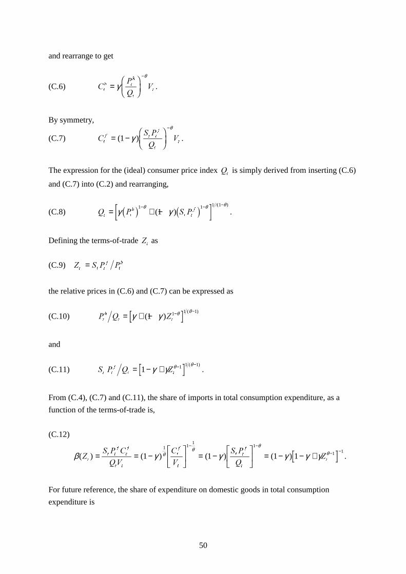
50

and rearrange to get

(C.6) &3

49

W

K W

K

W

W=

���

���

−

γθ

.

By symmetry,

(C.7) &6 3

49W

I W W

I

W

W= −���

���

−

( )1 γθ

.

The expression for the (ideal) consumer price index 4W is simply derived from inserting (C.6)

and (C.7) into (C.2) and rearranging,

(C.8) 4 3 6 3W W

K

W W

I= + −− − −

γ γθ θ θ

2 7 2 71 1 1 1

1( )/( )

.

Defining the terms-of-trade =W

as

(C.9) = 6 3 3W W W

I

W

K=

the relative prices in (C.6) and (C.7) can be expressed as

(C.10) 3 4 =W

K

W W= + − − −

γ γ θ θ( )

( )1 1 1 1

and

(C.11) 6 3 4 =W W

I

W W= − + − −1 1 1 1

γ γ θ θ( ).

From (C.4), (C.7) and (C.11), the share of imports in total consumption expenditure, as a

function of the terms-of-trade is,

(C.12)

β γ γ γ γ γθθ

θθ( ) ( ) ( ) ( )=

6 3 &

49

&

9

6 3

4=W

W W

I

W

I

W W

W

I

W

W W

I

W

W= = −�!

"$#

= −�!

"$#

= − − +− −

− −1 1 1 1

1 11

1

1 1.

For future reference, the share of expenditure on domestic goods in total consumption

expenditure is

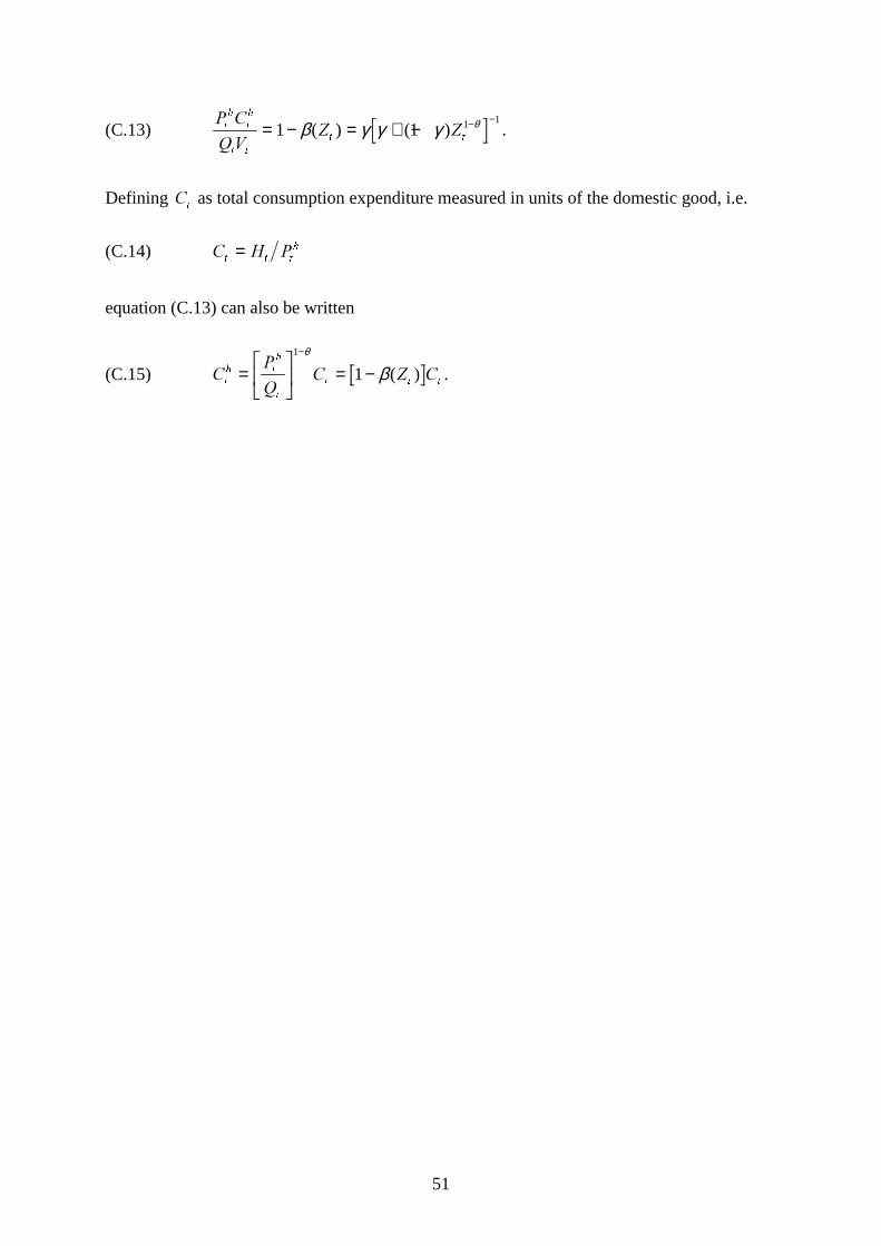
51

(C.13)3 &49

= =W

K

W

K

W W

W W= − = + − − −

1 1 1 1β γ γ γ θ( ) ( ) .

Defining &W as total consumption expenditure measured in units of the domestic good, i.e.

(C.14) & + 3W W W

K=

equation (C.13) can also be written

(C.15) &3

4& = &

W

K W

K

W

W W W=

�!

"$#

= −−1

1θ

β( ) .

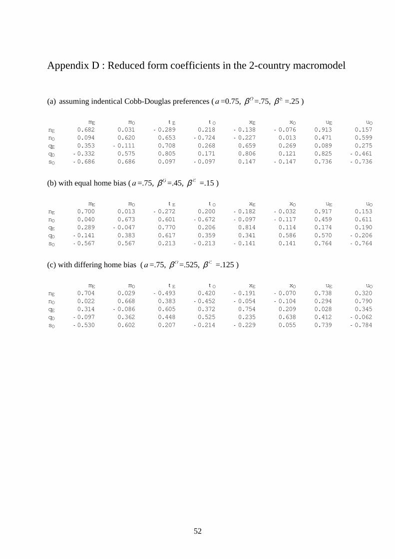
52

Appendix D : Reduced form coefficients in the 2-country macromodel

(a) assuming indentical Cobb-Douglas preferences (D =0.75, β 2=.75, β ( =.25 )

mE mO t E t O xE xO uE uOnE 0.682 0.031 - 0.289 0.218 - 0.138 - 0.076 0.913 0.157nO 0.094 0.620 0.653 - 0.724 - 0.227 0.013 0.471 0.599qE 0.353 - 0.111 0.708 0.268 0.659 0.269 0.089 0.275qO - 0.332 0.575 0.805 0.171 0.806 0.121 0.825 - 0.461sO - 0.686 0.686 0.097 - 0.097 0.147 - 0.147 0.736 - 0.736

(b) with equal home bias (D =.75, β 2=.45, β ( =.15 )

mE mO t E t O xE xO uE uOnE 0.700 0.013 - 0.272 0.200 - 0.182 - 0.032 0.917 0.153nO 0.040 0.673 0.601 - 0.672 - 0.097 - 0.117 0.459 0.611qE 0.289 - 0.047 0.770 0.206 0.814 0.114 0.174 0.190qO - 0.141 0.383 0.617 0.359 0.341 0.586 0.570 - 0.206sO - 0.567 0.567 0.213 - 0.213 - 0.141 0.141 0.764 - 0.764

(c) with differing home bias (D =.75, β 2=.525, β ( =.125 )

mE mO t E t O xE xO uE uOnE 0.704 0.029 - 0.493 0.420 - 0.191 - 0.070 0.738 0.320nO 0.022 0.668 0.383 - 0.452 - 0.054 - 0.104 0.294 0.790qE 0.314 - 0.086 0.605 0.372 0.754 0.209 0.028 0.345qO - 0.097 0.362 0.448 0.525 0.235 0.638 0.412 - 0.062sO - 0.530 0.602 0.207 - 0.214 - 0.229 0.055 0.739 - 0.784

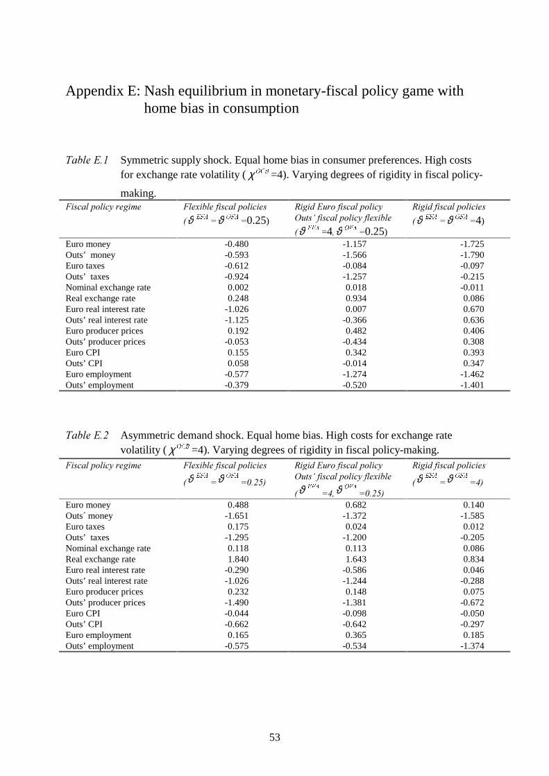
53

Appendix E: Nash equilibrium in monetary-fiscal policy game withhome bias in consumption

7DEOH�(�� Symmetric supply shock. Equal home bias in consumer preferences. High costsfor exchange rate volatility ( χ 2&% =4). Varying degrees of rigidity in fiscal policy-

making.)LVFDO�SROLF\�UHJLPH )OH[LEOH�ILVFDO�SROLFLHV

�ϑ ()$ ϑ 2)$ 0.25)

5LJLG�(XUR�ILVFDO�SROLF\2XWV¶�ILVFDO�SROLF\�IOH[LEOH

�ϑ ()$ =4�ϑ 2)$ 0.25)

5LJLG�ILVFDO�SROLFLHV

�ϑ ()$ ϑ 2)$ 4)

Euro money -0.480 -1.157 -1.725Outs’ money -0.593 -1.566 -1.790Euro taxes -0.612 -0.084 -0.097Outs’ taxes -0.924 -1.257 -0.215Nominal exchange rate 0.002 0.018 -0.011Real exchange rate 0.248 0.934 0.086Euro real interest rate -1.026 0.007 0.670Outs’ real interest rate -1.125 -0.366 0.636Euro producer prices 0.192 0.482 0.406Outs’ producer prices -0.053 -0.434 0.308Euro CPI 0.155 0.342 0.393Outs’ CPI 0.058 -0.014 0.347Euro employment -0.577 -1.274 -1.462Outs’ employment -0.379 -0.520 -1.401

7DEOH�(�� Asymmetric demand shock. Equal home bias. High costs for exchange ratevolatility ( χ 2&% =4). Varying degrees of rigidity in fiscal policy-making.

)LVFDO�SROLF\�UHJLPH )OH[LEOH�ILVFDO�SROLFLHV

�ϑ()$

ϑ 2)$

�����

5LJLG�(XUR�ILVFDO�SROLF\2XWV¶�ILVFDO�SROLF\�IOH[LEOH

�ϑ()$

��ϑ2)$

�����

5LJLG�ILVFDO�SROLFLHV

�ϑ()$

ϑ 2)$

��

Euro money 0.488 0.682 0.140Outs´ money -1.651 -1.372 -1.585Euro taxes 0.175 0.024 0.012Outs’ taxes -1.295 -1.200 -0.205Nominal exchange rate 0.118 0.113 0.086Real exchange rate 1.840 1.643 0.834Euro real interest rate -0.290 -0.586 0.046Outs’ real interest rate -1.026 -1.244 -0.288Euro producer prices 0.232 0.148 0.075Outs’ producer prices -1.490 -1.381 -0.672Euro CPI -0.044 -0.098 -0.050Outs’ CPI -0.662 -0.642 -0.297Euro employment 0.165 0.365 0.185Outs’ employment -0.575 -0.534 -1.374

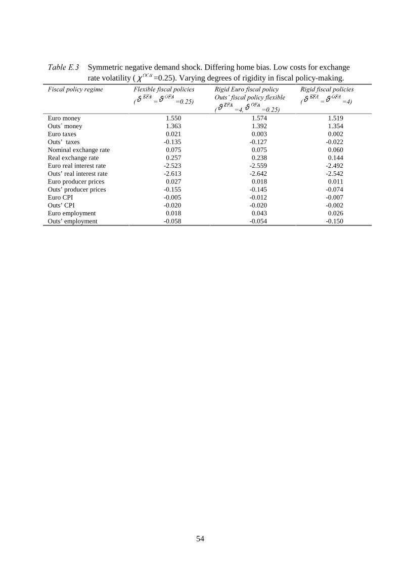
54

7DEOH�(�� Symmetric negative demand shock. Differing home bias. Low costs for exchangerate volatility ( χ 2&% =0.25). Varying degrees of rigidity in fiscal policy-making.

)LVFDO�SROLF\�UHJLPH )OH[LEOH�ILVFDO�SROLFLHV

�ϑ()$

ϑ 2)$

�����

5LJLG�(XUR�ILVFDO�SROLF\2XWV¶�ILVFDO�SROLF\�IOH[LEOH

�ϑ()$

��ϑ2)$

�����

5LJLG�ILVFDO�SROLFLHV

�ϑ()$

ϑ 2)$

��

Euro money 1.550 1.574 1.519Outs´ money 1.363 1.392 1.354Euro taxes 0.021 0.003 0.002Outs’ taxes -0.135 -0.127 -0.022Nominal exchange rate 0.075 0.075 0.060Real exchange rate 0.257 0.238 0.144Euro real interest rate -2.523 -2.559 -2.492Outs’ real interest rate -2.613 -2.642 -2.542Euro producer prices 0.027 0.018 0.011Outs’ producer prices -0.155 -0.145 -0.074Euro CPI -0.005 -0.012 -0.007Outs’ CPI -0.020 -0.020 -0.002Euro employment 0.018 0.043 0.026Outs’ employment -0.058 -0.054 -0.150

55

5HIHUHQFHV

Alesina, Alberto and Guido Tabellini (1987): ”Rules and Discretion with Non-coordinatedMonetary and Fiscal Policies”, (FRQRPLF�,QTXLU\ 25, pp. 619-630.

Artis, Michael J. and Bernhard Winkler (1997): 7KH� 6WDELOLW\� 3DFW�� 6DIHJXDUGLQJ� WKH&UHGLELOLW\�RI�WKH�(XURSHDQ�&HQWUDO�%DQN, CEPR Discussion Paper no. 1688.

Beetsma, Roel M.W.J. and A. Lans Bovenberg (1995a): 'HVLJQLQJ� )LVFDO� DQG�0RQHWDU\,QVWLWXWLRQV�IRU�D�(XURSHDQ�0RQHWDU\�8QLRQ, CEPR Discussion Paper no. 1303.

Beetsma, Roel M.W.J. and A. Lans Bovenberg (1995b): 'HVLJQLQJ� )LVFDO� DQG�0RQHWDU\,QVWLWXWLRQV�LQ�D�6HFRQG�%HVW�:RUOG, mimeo, April, DELTA and CentER.

Beetsma, Roel M.W.J. and Harald Uhlig (1997): $Q�DQDO\VLV�RI�WKH��VWDELOLW\�SDFW�� CEPRDiscussion Paper no. 1669.

Canzoneri, Matthew B., and Dale W. Henderson (1991): 0RQHWDU\�3ROLF\�LQ�,QWHUGHSHQGHQW(FRQRPLHV��$�*DPH�7KHRUHWLF�$SSURDFK, Cambridge. MIT Press.

Douven, Rudy and Marga Peeters (1997): *'3�VSLOORYHUV� LQ�PXOWL�FRXQWU\�PRGHOV, ESRCMacroeconomic Modelling Burea, Discussion Paper no. 46.

Eichengreen, Barry and Fabio Ghironi (1997): +RZ�:LOO�7UDQVDWODQWLF�3ROLF\� ,QWHUDFWLRQV&KDQJH�ZLWK�WKH�$GYHQW�RI�(08", CEPR Discussion Paper no. 1643.

Eichengreen, Barry and Charles Wyplosz (1998): 7KH� 6WDELOLW\� 3DFW�� PRUH� WKDQ� D� PLQRUQXLVDQFH", Economic Policy, April 1998.

Ghironi, Fabio and Francesco Giavazzi (1997a): CXUUHQF\� XQLRQV�� LQWHUQDWLRQDO�PRQHWDU\UHJLPHV�DQG�WKH�HPSOR\PHQW�LQIODWLRQ,�mimeo February 1977.

Ghironi, Fabio and Francesco Giavazzi (1997b): 2XW� LQ� WKH�6XQVKLQH"�2XWVLGHUV�� ,QVLGHUVDQG�WKH�8QLWHG�6WDWHV�LQ�����, CEPR Discussion Paper no. 1547.

Mundell, Robert (1968): ,QWHUQDWLRQDO�(FRQRPLFV, New York: Macmillan.

Persson, Torsten and Guido Tabellini (1996): 0RQHWDU\� &RKDELWDWLRQ� LQ� (XURSH, NBERWorking Paper no. 5532.

Taylor, John (1993): 0DFURHFRQRPLF�3ROLF\�LQ�D�:RUOG�(FRQRP\, New York: Norton.