Embed Size (px)
Citation preview

Fakultat fur Mathematik und Informatik
INSTITUT FUR INFORMATIK
Theoretische Informatik I
Deterministic Random Walkson Infinite Grids
Diplomarbeit
zur Erlangung des akademischen Grades
Diplom-Mathematiker
Tobias Friedrich, M.Sc.
geb. am 28.07.1980 in Neustrelitz
Betreuer an der Friedrich-Schiller-Universitat Jena:
PD Dr. rer. nat. habil. Harald Hempel
Betreuer am Max-Planck-Institut fur Informatik, Saarbrucken:
Dr. rer. nat. habil. Benjamin Doerr
Jena, den 19.12.2005

Zusammenfassung
Zusammenfassung
Jim Propp’s Rotor-Router-Modell ist ein einfaches, deterministisches Analogon
zum Random Walk (zufallige Irrfahrt). Anstatt Chips an zufallige Nachbarn zu
verteilen, werden die Nachbarn in einer fester Reihenfolge bedient. Diese Diplom-
arbeit untersucht, wie gut dieser Prozess einen Random Walk auf dem unendlichen
zweidimensionalen Gitter simuliert. Unabhangig von der Ausgangskonfiguration
weicht zu jedem Zeitpunkt und auf jedem Knoten die Anzahl der Chips auf ei-
nem Knoten von der erwarteten Anzahl der Chips im Random-Walk-Modell um
maximal eine Konstante c ab. Es wird bewiesen, dass 7,2 < c < 11,8 gilt. Diese
Schranken hangen erstaunlicherweise von der Reihenfolge ab, in der die Nachbarn
bedient werden. Fur eine Verallgemeinerung, bei welcher nur gefordert wird, dass
kein Nachbar mehr als ∆ Chips mehr bekommt als ein anderer, wird gezeigt, dass
es ebenso eine Konstante c′ gibt. Fur diese gilt 7,7∆ < c′ < 26,9∆.
i

Abstract
Abstract
The rotor-router model is a simple deterministic analogue of random walk invented
by Jim Propp. Instead of distributing chips to randomly chosen neighbors, it
serves the neighbors in a fixed order. This thesis investigates how well this process
simulates a random walk on an infinite two-dimensional grid. Independent of the
starting configuration, at each time and on each vertex, the number of chips on
this vertex deviates from the expected number of chips in the random walk model
by at most a constant c. It is proved that 7.2 < c < 11.8 in general. Surprisingly,
these bounds depend on the order in which the neighbors are served. It is also
shown that in a generalized setting, where one just requires that no neighbor
gets more than ∆ chips more than another, there is also such a constant c′ with
7.7∆ < c′ < 26.9∆.
Acknowledgements
I would like to thank Dr. Benjamin Doerr for drawing my interest on deterministic
random walks and for many long nights working together. I am also grateful to
Dr. Harald Hempel for supervising this thesis.
I am thankful to the German National Merit Foundation (“Studienstiftung des
deutschen Volkes”) and the Max Planck Society for financial support, good work-
ing conditions and travel allowance.
ii
Contents
Contents
1 Introduction 1
1.1 Deterministic Random Walks . . . . . . . . . . . . . . . . . . . . 1
1.2 Preliminaries and Notation . . . . . . . . . . . . . . . . . . . . . . 3
1.3 Rotor Sequence . . . . . . . . . . . . . . . . . . . . . . . . . . . . 6
1.4 Related Work . . . . . . . . . . . . . . . . . . . . . . . . . . . . . 7
2 The Basic Method 12
2.1 Characterizing the Discrepancy . . . . . . . . . . . . . . . . . . . 12
2.2 Unimodality . . . . . . . . . . . . . . . . . . . . . . . . . . . . . . 15
3 Upper Bound 21
3.1 Dependence on the Chosen Rotor Sequence . . . . . . . . . . . . . 21
3.2 Convergence of the Series . . . . . . . . . . . . . . . . . . . . . . . 24
3.3 Computation . . . . . . . . . . . . . . . . . . . . . . . . . . . . . 25
4 Lower Bound 31
4.1 Arrow-forcing Theorem . . . . . . . . . . . . . . . . . . . . . . . . 31
4.2 Computation . . . . . . . . . . . . . . . . . . . . . . . . . . . . . 35
5 Free Propp Machine 38
5.1 Upper Bound . . . . . . . . . . . . . . . . . . . . . . . . . . . . . 38
5.2 Lower Bound . . . . . . . . . . . . . . . . . . . . . . . . . . . . . 41
6 Conclusions and Further Work 42
Bibliography 44
A Mathematical Basics 48
iii

Chapter 1Introduction
1.1 Deterministic Random Walks
Quasirandomness
Since antiquity, randomness and unpredictability were discussed in conncetion
both with questions of free will and games of chance. In the 18th century ran-
domness became very important in philosophy and science. However, nowadays
true randomness is not available in computer simulations and also often undesired.
Hence, a growing interest in “quasirandomness” is recently noticeable [6]. This is
a deterministic progress specifically designed to give the same limiting behavior
(of some quantities of interest) as a random process, but with faster convergence.
Quasirandomness is not to be confused with “pseudorandomness”, a process that
is supposed to be statistically indistinguishable from the truly random process it
imitates. In contrast to this, quasirandomness will typically have many regulari-
ties that mark it as non-random.
Often, with a quasirandom simulation that focuses on reducing discrepancy, one
can obtain much more precise estimates of the average case behavior of the system
than via (purely random) Monte Carlo simulation. In other words, a quasirandom
process gives deterministic error-bounds rather than (usually larger) confidence-
intervals.
1

1. Introduction Deterministic Random Walks
Random Walk
Given an arbitrary graph, a random walk of a chip is a path, which begins at
a given starting point and chooses the next node with equal probability out of
the set of its current neighbors. Random walks have been used to model a wide
variety of processes in economics (share prices), physics (Brownian motion of
molecules in gases and liquids), medicine (cascades of neurons firing in the brain),
and mathematics (estimations and modeling of gambling).
Propp Machine
The Propp machine is the quasirandom analogue of random walk invented by Jim
Propp. He called this the “Rotor router model”, while Joel Spencer [10] coined
the term “Propp machine”. We will use the latter.
Instead of distributing chips to randomly chosen neighbors, it deterministically
serves the neighbors in a fixed order by associating to each vertex a “rotor” point-
ing to one oft its neighbors. The first chip reaching a vertex moves on in the
direction the rotor is pointing, then the rotor direction is updated to the next
direction in some cyclic ordering. The second chip is then send in this new di-
rection, the rotor is updated, and so on. This ensures the chips are distributed
highly evenly among the neighbors.
The question is, how well the Propp machine resembles an expected random walk.
A comparison can be drawn by contrasting different aspects. We focus on the
single vertrex discrepancy. That is, we distribute some finite number of chips
arbitrarily on the vertices and let evolve this distribution with the chips following
the rotors. One step consists of every chip incrementing and then following the
rotor at the point it is on. Running in parallel Propp machine and expected
random walk on the same initial configuration, we calculate the maximal deviation
of the number of chips on each vertex. Jim Propp on the other hand, concentrates
on the aggregation model, where each chip is content to stay put when they reach
an uninhabitated site (cf. Section 1.4).
On strong connected finite graphs the discrepancy on a single vertex is bounded
by a constant. For arbitrary graphs there is not much known about the Propp
machine. This is different for infinite grids Zd. There one can fix a certain order
(cf. Section 1.3) in which the 2d neighbors are served (e.g. North, East, South,
and West for d = 2). Astonishingly, Cooper and Spencer [10, 11] showed that this
discrepancy is bounded by a constant cd, which only depends on the dimension d,
2

1. Introduction Preliminaries and Notation
i.e., this constant is independent of the number of steps, the initial distribution of
the chips, and the states of the rotors. Note, that this is only valid for “checkered”
initial distributions, but this technicality we defer to Section 1.2. The constant
discrepancy is particularly surprising when keeping in mind that in a single step
the random walk splits n chips to its 2d neighbors with a standard deviation of√n. This shows that the Propp machine simulates a random walk extremely well.
Together with Doerr and Tardos, they further analyzed the one-dimensional case
in [8, 9]. They showed that for Z1 the actual constant is c1 ≈ 2.29. Further on, for
intervals of length L, the deviation between both models is only O(log L) (instead
of, e.g., 2.29L).
Our Results
We continue the work of Cooper et al. [8, 9] by regarding the single vertex dis-
crepancy on the two-dimensional grid Z2. This is the most frequently considered
infinite grid for random walks. In Chapter 3, we prove that independent of the
initial (even) configuration, the discrepancy is bounded by 11.8 on all vertices at
all times. Surprisingly, this constant improves to 10.9 for all rotor sequences (cf.
Section 1.3), which do not update the rotor clockwise or counterclockwise. In
Chapter 4, we show that there are configurations, which enforce a discrepancy of
at least 7.2 on a single vertex. This time, there are configurations with higher dis-
crepancy, namely 7.7, if the rotors do change clockwise or counterclockwise. This
suggests that the single vertex discrepancy depends on the chosen rotor sequence.
In Chapter 5 we introduce a generalized “free” Propp machine. Instead of fixing a
certain cyclic order and updating the rotors according to this, here we just require
the rotors to change in such a way that the number of chips sent in each direction
differs by at most a constant ∆. In this model, we can prove an upper bound of
26.9∆ and a lower bound of 7.7∆ for the discrepancy on a single vertex.
1.2 Preliminaries and Notation
First, we explain the technicality mentioned in Section 1.1. Without Assumption 1
below, also the results of [8–11] are not valid. Since Zd is bipartite, chips that start
on even vertices (x with x1 +x2 ≡ 0(mod 2)) never mix with those starting on odd
positions (x with x1 + x2 ≡ 1(mod 2))1. It looks like we are playing two games
1Note, that the definition of odd/even vertices will be changed after Assumption 2.
3
1. Introduction Preliminaries and Notation
at once. However, this is not true, because chips of different parity may affect
each other through the rotors. The odd chips may even reset the arrows and thus
mess up the even chips and vice versa. Similar to the Arrow-forcing Theorem 9
from Section 4.1, one can cleverly arrange piles of off-parity chips to reorient the
rotors and steer them away from random walk simulation. We therefore require
the following.
Assumption 1. The starting configuration has chips only on one parity.
Without loss of generality, we consider only “even starting configurations”, where
chips are only on even positions. Odd starting configurations can be handled in
an analogous manner.
A random walk can be described nicely by its probability density [26]. We will
draw on the following notation.
Definition 1. Let H(x, t) denote the probability that a chip from the origin arrives
at location x at time t in a simple random walk.
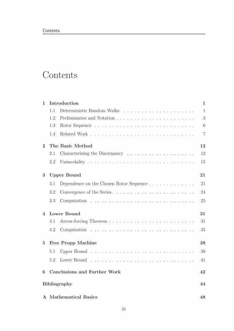
Unfortunately, the equations for H(x, t) on the standard two-dimensional grid Z2
(with arrows pointing up/down/left/right) shown in Figure 1(a) are not handy at
all, because the two dimensions of Z2 are not varying independedly in a random
walk. Since the quantities x1 + x2 and x1 − x2 are indeed varying independently,
(a) Original grid. (b) Our new definition of the gridand the rotors.
Figure 1: Visualization of the applied coordinate transformation. Grid (b) can beseen as grid (a) rotated counterclockwise by 45◦ and scaled by
√2. The black
and gray dots mark even and odd positions according, respectively. The redarrows indicate the neighborhood of the origin.
4

1. Introduction Preliminaries and Notation
the coordinate transformation
x′1 := x1+x2
x′2 := x1−x2
(1)
for all (x1, x2) = x ∈ Z2 results in a representation, where both dimensions vary
independently at each step2. This is the reason for the following assumption.
Assumption 2. The neighbors of a vertex are in the directions
dir :={ր,ց,ւ,տ
}:={(
+1+1
),(+1−1
),(−1−1
),(−1+1
)}.
Thus, chips move only on positions x ∈ Z2 with x1 + x2 ≡ 0 (mod 2). Via
Equation (1) our results can immediately be translated into the standard two-
dimensional grid model with neighbors {↑,→, ↓,←}.
We need some notation to describe chips on the grid.
Definition 2. Let x ∈ Z2 and t ∈ N0, then x ∼ t denotes x1 ≡ x2 ≡ t (mod 2)
and x ∼ y denotes x1 ≡ x2 ≡ y1 ≡ y2 (mod 2). A position x is called “even” or
“odd” if x ∼ 0 or x ∼ 1, respectively. A configuration is called “even” or “odd”
if all chips are at an even or all at an odd positions, respectively.
Therefore,
H(x, t) =
{
4−t(
t(t+x1)/2
)(t
(t+x2)/2
)if x ∼ t and ‖x‖∞ ≤ t
0 otherwise.
We now fix a certain configuration and describe the state of both Propp machine
and expected random walk.
Definition 3. For a fixed starting configuration, f(x, t) denotes the number of
chips and arr(x, t) denotes the direction of the arrow at position x after t steps
of the Propp machine. E(x, t) denotes the expected number of chips at location x
after running a random walk for t steps.
In the proofs, we also need the following mixed notation.
Definition 4. For a fixed starting configuration, E(x, t1, t2) denotes the expected
number of chips at location x after t1 Propp and t2 − t1 random steps.
2Subscript k will always denote the k-th component of a vector.
5

1. Introduction Rotor Sequence
1.3 Rotor Sequence
To minimize the discrepancy between the number of chips sent left and right in
the one-dimensional case, the arrow must switch back and forth after each chip
sent. Two consecutive chips in the same direction would instantly increase the
deviation of the Propp machine compared to the random walk. Hence, there is
just one reasonable way to decide which arrow direction comes next, that is, to
strictly alternate the arrows. This optimally equals out chips sent to the left and
the right. In higher dimension this cannot be achieved for all dimensions at the
same time.
On the two-dimensional grid Z2, Levine and Peres [29, 30] rotated the arrow
clockwise by 90 degrees during each step. In our notation, they only considered
the rotor sequence (ր,ց,ւ,տ). Cooper and Spencer [10] were more general
and allowed arbitrary cyclic orderings of the neighbors. Hence, we will also fix a
certain permutation of the four directions and use this to define a cyclic function
next : dir→ dir with dir as defined in Assumption 2, which gives the respective
next arrow direction. With this, we can describe the resulting arrow after one
Propp step as
arr(x, t + 1) := nextf(x,t)
(arr(x, t)
).
Note that nextk can be calculated easily. So for example for the above mentioned
rotor sequence (ր,ց,ւ,տ), we have
nextk(A) =
(
(−1)⌊k2− 3
4+
A22 (A1
2+1)⌋, (−1)⌊k
2+
A22 (A1
2+1)⌋
)
.
We now want to classify the 4! = 24 permutations of the four arrows. Without loss
of generality we fix the first arrow to(+1+1
) (=ր
)and thus only need to examine
3! = 6 permutations. These differ on how equally they distribute the chips. How
well a certain permutation equals out the chips sent in the four directions can be
Figure 2: Colorings
measured by colorings χ : dir → {±1} of the arrows.
Without loss of generality we assume χ((
+1+1
))= +1 for
all colorings. Then there are three balanced colorings,
i.e., colorings with |χ−1(+1)| = |χ−1(−1)| = 2. These
are χx
((xy
)):= x, χy
((xy
)):= y, and χxy
((xy
)):= xy,
as shown in Figure 2. χx, χy, and χxy measure how
equal the arrows swap horizontally, vertically, and diagonally, respectively. A
good permutation should minimize∑
A∈arr|χ(A) + χ(next(A))| for all three
colorings χ.
6

1. Introduction Related Work
Arrow sequence Permutation π χx(π) χy(π) χxy(π)
(ր,ց,ւ,տ)((
+1+1
),(+1−1
),(−1−1
),(−1+1
))(+, +,−,−) (+,−,−, +) (+,−, +,−)
(ր,տ,ւ,ց)((
+1+1
),(−1+1
),(−1−1
),(+1−1
))(+,−,−, +) (+, +,−,−) (+,−, +,−)
(ր,տ,ց,ւ)((
+1+1
),(−1+1
),(+1−1
),(−1−1
))(+,−, +,−) (+, +,−,−) (+,−,−, +)
(ր,ւ,ց,տ)((
+1+1
),(−1−1
),(+1−1
),(−1+1
))(+,−, +,−) (+,−,−, +) (+, +,−,−)
(ր,ց,տ,ւ)((
+1+1
),(+1−1
),(−1+1
),(−1−1
))(+, +,−,−) (+,−, +,−) (+,−,−, +)
(ր,ւ,տ,ց)((
+1+1
),(−1−1
),(−1+1
),(+1−1
))(+,−,−, +) (+,−, +,−) (+, +,−,−)
Table 1: All six permutations and their respective ±1 sequences for each coloring.For the sake of readability we use “+” and “−” as short form of +1 and −1.
Table 1 shows that each permutation only strictly alternates on exactly one col-
oring and alternates in groups of two on the other two colorings. Note that
the two probably most natural permutations, where the arrow goes in turns, i.e.
(ր,ց,ւ,տ) and (ր,տ,ւ,ց), are the two most unbalanced in terms of ver-
tical and horizontal balance.
Beside fixing a certain permutation, there are other models how to define next.
These are discussed in Chapter 5.
1.4 Related Work
Diffusion-Limited Aggregation (DLA)
DLA is a growth model on the infinite grid Zd, which was introduced in 1981 by
Witten and Sander [41, 42] to model aggregates of condensing metal vapor. It has
since then attracted much interest3 both among mathematicians and physicists. It
simulates, for example, the coral growth, the path taken by a lightning, coalescing
of dust or smoke particles, and the growth of some crystals [5].
In contrast to our Propp model, in DLA there is never more than one particle
(chip) on a single point. The process starts with only the origin 0 being occupied.
With each step, one particle diffuses in “from infinity” according to a random walk
and attaches itself to the first boundary site visited. By the boundary of a cluster
we mean all points adjacent, but not belonging to it. See Figure 3 for a typical
example on Z2. Computer simulations suggest that after sufficiently many steps
these clusters are highly ramified, of low density and their radius is of greater
3[41] on this subject is the 9th most cited Physical Review Letter in the history of the journal.
7

1. Introduction Related Work
order of magnitude than the d-th root of the number of particles [15]. Martin T.
Barlow [1] conjectured that the resulting cluster has a fractal dimension exceeding
1, but rigorous results are hard to establish in this model.
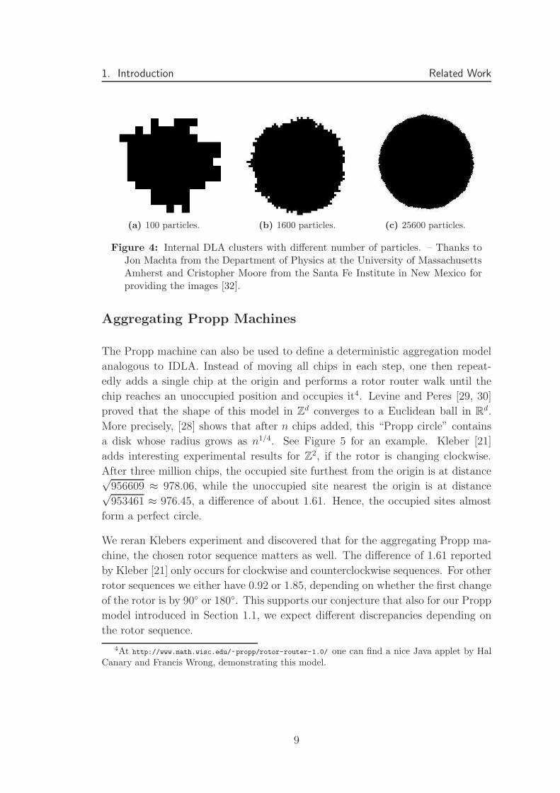
Internal Diffusion-Limited Aggregation (IDLA)
Diaconis and Fulton [13] introduced Internal DLA in 1991 as a variant of classical
DLA. There, the random walk begins at the origin and the particle occupies
the first empty site it reaches. This yields a central growing blob. Since the
next particle is more likely to fill an unoccupied site close to the origin than one
further away, one intuitively expects this blob to be a sphere. Figure 4 shows three
IDLA clusters with different numbers of particles accumulated. Lawler, Bramson,
and Griffeath [27] showed in 1992 that the limiting shape after n steps is indeed
a Euclidean ball as n → ∞. In a subsequent paper, Lawler [25] proved that
with high probability the fluctuations around this limiting shape are bounded by
O(n1/3). Moore and Machta [32] observed experimentally that these error terms
were even smaller, namely of logarithmic size. Soon after, Blachere [4] claimed to
have shown that the fluctuations are at most logarithmic, but there is an error
in his main theorem. Consequently, it is still unknown how to bridge this gap
between theory and observation.
Figure 3: A typical example of two-dimensional diffusion limited aggregation. –Thanks to Paul Bourke from the Centre for Astrophysics and Supercomputing,Swinburne University for providing the image [5].
8
1. Introduction Related Work
(a) 100 particles. (b) 1600 particles. (c) 25600 particles.
Figure 4: Internal DLA clusters with different number of particles. – Thanks toJon Machta from the Department of Physics at the University of MassachusettsAmherst and Cristopher Moore from the Santa Fe Institute in New Mexico forproviding the images [32].
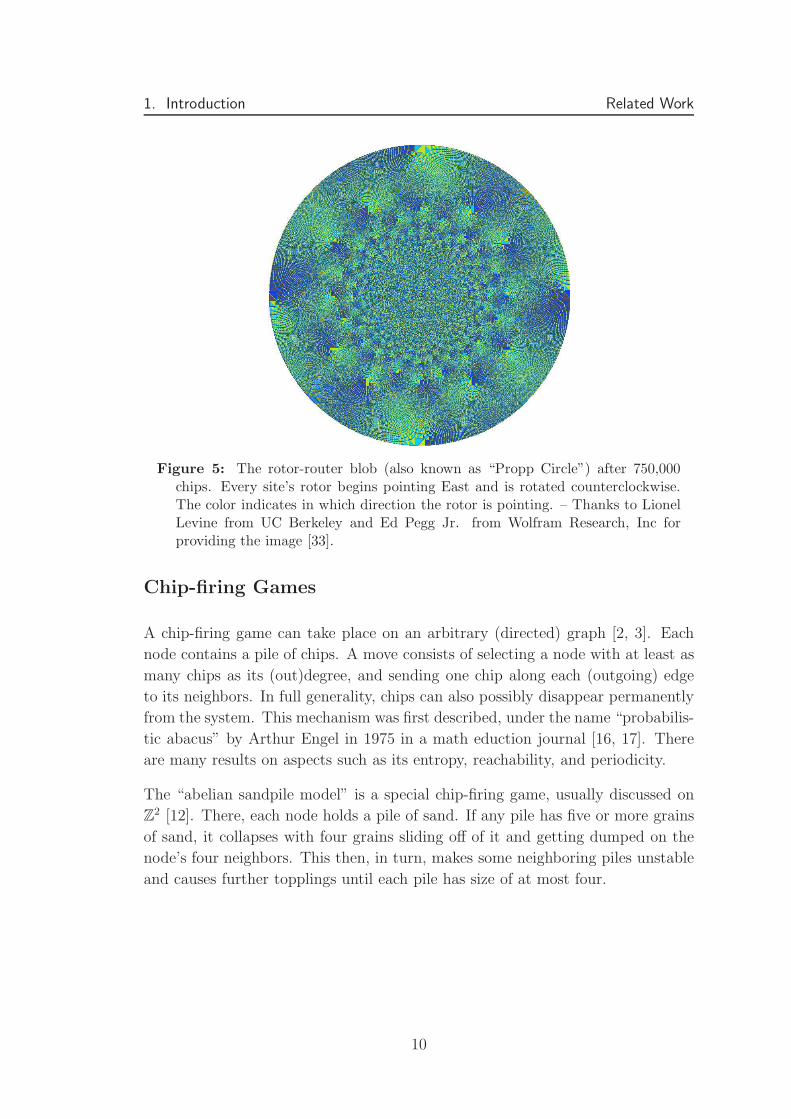
Aggregating Propp Machines
The Propp machine can also be used to define a deterministic aggregation model
analogous to IDLA. Instead of moving all chips in each step, one then repeat-
edly adds a single chip at the origin and performs a rotor router walk until the
chip reaches an unoccupied position and occupies it4. Levine and Peres [29, 30]
proved that the shape of this model in Zd converges to a Euclidean ball in R
d.
More precisely, [28] shows that after n chips added, this “Propp circle” contains
a disk whose radius grows as n1/4. See Figure 5 for an example. Kleber [21]
adds interesting experimental results for Z2, if the rotor is changing clockwise.
After three million chips, the occupied site furthest from the origin is at distance√956609 ≈ 978.06, while the unoccupied site nearest the origin is at distance√953461 ≈ 976.45, a difference of about 1.61. Hence, the occupied sites almost
form a perfect circle.
We reran Klebers experiment and discovered that for the aggregating Propp ma-
chine, the chosen rotor sequence matters as well. The difference of 1.61 reported
by Kleber [21] only occurs for clockwise and counterclockwise sequences. For other
rotor sequences we either have 0.92 or 1.85, depending on whether the first change
of the rotor is by 90◦ or 180◦. This supports our conjecture that also for our Propp
model introduced in Section 1.1, we expect different discrepancies depending on
the rotor sequence.
4At http://www.math.wisc.edu/~propp/rotor-router-1.0/ one can find a nice Java applet by HalCanary and Francis Wrong, demonstrating this model.
9
1. Introduction Related Work
Figure 5: The rotor-router blob (also known as “Propp Circle”) after 750,000chips. Every site’s rotor begins pointing East and is rotated counterclockwise.The color indicates in which direction the rotor is pointing. – Thanks to LionelLevine from UC Berkeley and Ed Pegg Jr. from Wolfram Research, Inc forproviding the image [33].
Chip-firing Games
A chip-firing game can take place on an arbitrary (directed) graph [2, 3]. Each
node contains a pile of chips. A move consists of selecting a node with at least as
many chips as its (out)degree, and sending one chip along each (outgoing) edge
to its neighbors. In full generality, chips can also possibly disappear permanently
from the system. This mechanism was first described, under the name “probabilis-
tic abacus” by Arthur Engel in 1975 in a math eduction journal [16, 17]. There
are many results on aspects such as its entropy, reachability, and periodicity.
The “abelian sandpile model” is a special chip-firing game, usually discussed on
Z2 [12]. There, each node holds a pile of sand. If any pile has five or more grains
of sand, it collapses with four grains sliding off of it and getting dumped on the
node’s four neighbors. This then, in turn, makes some neighboring piles unstable
and causes further topplings until each pile has size of at most four.
10

1. Introduction Related Work
Load-Balancing
In parallel computing, load-balancing a distributed network is an important task.
The processors are modeled as the vertices of an undirected connected graph and
links between them as edges. Initially, each processor has a collection of unit-
size tasks. The object is to balance the number of tasks at each processor by
transmitting tasks along edges according to some local scheme. Dynamic load
balancing is crucial for the efficiency of highly parallel systems when solving non-
uniform problems with unpredictable load estimates [40].
Diffusion is one well-established algorithm for load balancing. If a processor has
more tasks than one of its neighbors, it sends some of its task to the neighbor.
The number sent is proportional to the differential between the two processors
and some constant depending on the connecting edge. A standard choice for
these constants is uniform diffusion, in which each processor simply averages the
loads of its neighbors at each step [36].
There are some thousand research papers on dynamic load balancing. Many model
load-balancing algorithms as a Markov chain, which converges to the uniform load
vector. Thereby, they allow sending fractional tasks and ignore the rounding to
whole tasks at each local balancing step. This deviation can be large depending
on the specific network topology [18, 36, 39].
11

Chapter 2The Basic Method
This chapter gives the basic formulas to compare Propp machine and expected
random walk based on the number of chips on a single vertex.
2.1 Characterizing the Discrepancy
In order to avoid discussing all equations in the expected sense and thereby to
simplify the presentation, one can treat the expected random walk as a “linear
machine” [10]. Here, in each time step a pile of k chips is split evenly, with k/4
chips going to each neighbor. The (possibly non-integral) number of chips at
position x at time t is exactly the expected number of chips E(x, t) in the random
walk model.
Using the notation of Definition 3, we are interested in bounding the discrepancies
f(x, t)− E(x, t) for all vertices x and all times t. Via translation on the infinite
grid, it suffices to prove the result for the vertex x = 0. Clearly,
E(0, 0, t) = E(0, t),
E(0, t, t) = f(0, t),
so that
f(0, t)− E(0, t) =t−1∑
s=0
(E(0, s + 1, t)−E(0, s, t)) . (2)
12
2. The Basic Method Characterizing the Discrepancy
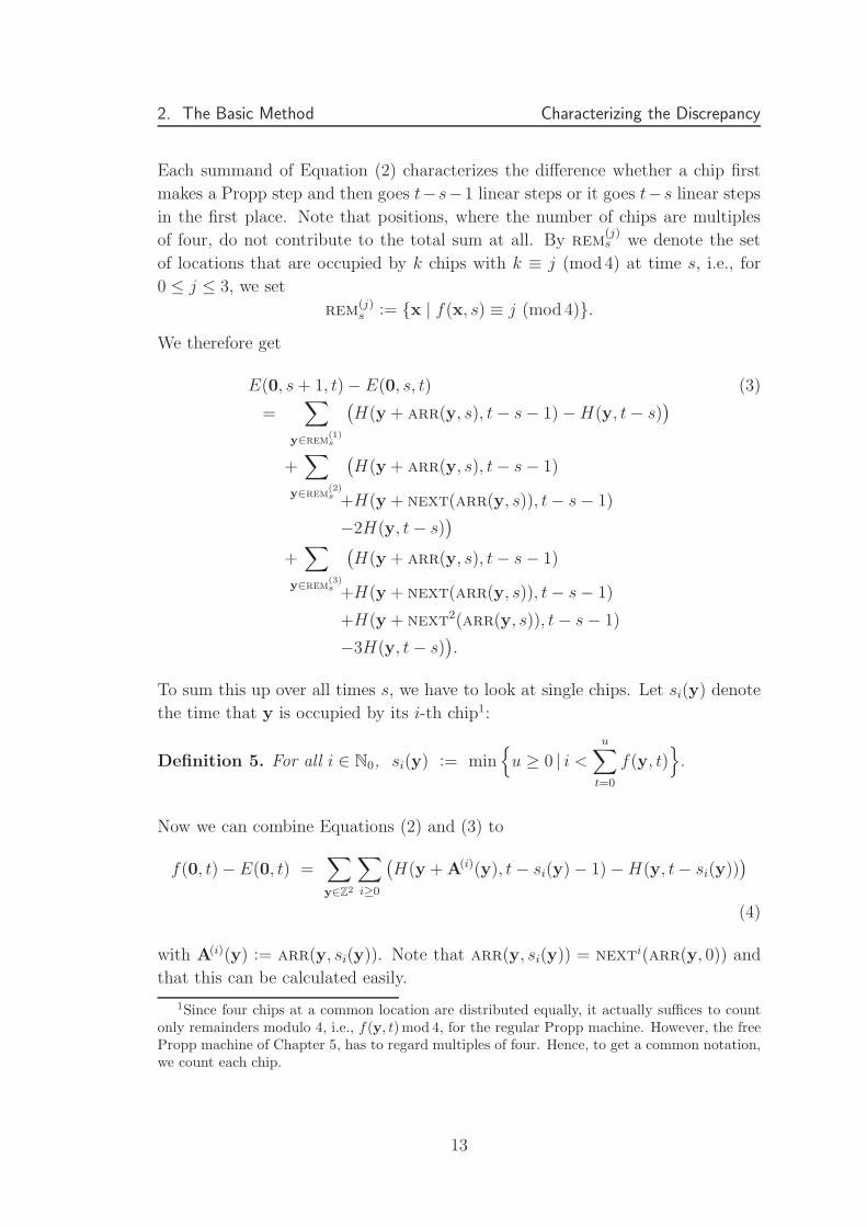
Each summand of Equation (2) characterizes the difference whether a chip first
makes a Propp step and then goes t−s−1 linear steps or it goes t−s linear steps
in the first place. Note that positions, where the number of chips are multiples
of four, do not contribute to the total sum at all. By rem(j)s we denote the set
of locations that are occupied by k chips with k ≡ j (mod 4) at time s, i.e., for
0 ≤ j ≤ 3, we set
rem(j)s := {x | f(x, s) ≡ j (mod 4)}.
We therefore get
E(0, s + 1, t)− E(0, s, t) (3)
=∑
y∈rem(1)s
(H(y + arr(y, s), t− s− 1)−H(y, t− s)
)
+∑
y∈rem(2)s
(H(y + arr(y, s), t− s− 1)
+H(y + next(arr(y, s)), t− s− 1)
−2H(y, t− s))
+∑
y∈rem(3)s
(H(y + arr(y, s), t− s− 1)
+H(y + next(arr(y, s)), t− s− 1)
+H(y + next2(arr(y, s)), t− s− 1)
−3H(y, t− s)).
To sum this up over all times s, we have to look at single chips. Let si(y) denote
the time that y is occupied by its i-th chip1:
Definition 5. For all i ∈ N0, si(y) := min{
u ≥ 0 | i <u∑
t=0
f(y, t)}
.
Now we can combine Equations (2) and (3) to
f(0, t)−E(0, t) =∑
y∈Z2
∑
i≥0
(H(y + A(i)(y), t− si(y)− 1)−H(y, t− si(y))
)
(4)
with A(i)(y) := arr(y, si(y)). Note that arr(y, si(y)) = nexti(arr(y, 0)) and
that this can be calculated easily.
1Since four chips at a common location are distributed equally, it actually suffices to countonly remainders modulo 4, i.e., f(y, t)mod 4, for the regular Propp machine. However, the freePropp machine of Chapter 5, has to regard multiples of four. Hence, to get a common notation,we count each chip.
13
2. The Basic Method Characterizing the Discrepancy
The inner summand of Equation (4) can be simplified. For all y ∈ Z2, A ∈ dir,
and y ∼ t, we have
H(y + A, t− 1)−H(y, t)
= 41−t
(t
(t− 1 + y1 + A1)/2
)(t
(t− 1 + y2 + A2)/2
)
−
4−t
(t
(t + y1)/2
)(t
(t + y2)/2
)
=(
(t− 1)!2 41−t ( t+y1
2)!( t−y1
2)!( t+y2
2)!( t−y2
2)! −
t!2 4−t ( t−1+y1+A1
2)!( t−1−y1−A1
2)!( t−1+y2+A2
2)!( t−1−y2−A2
2)!) /
(
( t−1+y1+A1
2)!( t+y1
2)!( t−1−y1−A1
2)!( t−y1
2)!
( t−1+y2+A2
2)!( t+y2
2)!( t−1−y2−A2
2)!( t−y2
2)!)
=
(4(
t−1(t−1+y1+A1)/2
)(t−1
(t−1+y2+A2)/2
)
(t
(t+y1)/2
)(t
(t+y2)/2
) − 1
)
H(y, t)
=((A1y1 · A2y2)t
−2 − (A1y1 + A2y2)t−1)H(y, t). (5)
The last equality holds due to(
t−1(t−1+y+A)/2
)/(t
(t+y1)/2
)= 1
2
(1−Ay
t
)for A = ±1
and y1, y2 ≤ t.
Combining Equations (4) and (5), we now obtain our Lemma 1, which will be
crucial in the remainder:
Lemma 1. For all times t ∈ N0,
f(0, t)− E(0, t) =∑
y∈Z2
(∑
i≥0
−A(i)1 (y)y1
t− si(y)H(y, t− si(y)) +
∑
i≥0
−A(i)2 (y)y2
t− si(y)H(y, t− si(y)) +
∑
i≥0
A(i)1 (y)A
(i)2 (y)y1y2
(t− si(y))2H(y, t− si(y))
)
.
with A(i)(y) := arr(y, si(y)) and si(y) as in Definition 5.
Note that, independent of the rotor sequence (cf. Table 1), the sequences
(A(i)1 (y))i≥0, (A
(i)2 (y))i≥0, and (A
(i)1 (y)A
(i)2 (y))i≥0 are all (either strictly or in groups
of two) alternating. We will exploit this in Section 3.1.
14

2. The Basic Method Unimodality
2.2 Unimodality
To calculate the discrepancy between the Propp and the linear machine, we have
to bound the alternating sums of Lemma 1. To achieve this, we will use the
following property of the involved functions:
Definition 6. Let X ⊆ R. We call a mapping f : X → R unimodal, if there is
an m ∈ X such that f is monotonically increasing in {x ∈ X | x ≤ m} and f is
monotonically decreasing in {x ∈ X | x ≥ m}.
Unimodal functions are popular in optimization and probability theory. The prob-
ability H(x, t) that a chip from the origin arrives at location x at time t in a simple
random walk is unimodal in t. This is depicted in Figure 6. The specific shape
can be explained easily. For t < ‖x‖∞ the probability that a chip from the ori-
gin arrives at x is zero. With more time elapsed, the probability raises due to
the increasing number of paths of length t to x, but since the number of reach-
able positions rises quadratically, the probability decreases again after a certain
threshold. That H(x, t) is indeed unimodal in t can be proven with Sturm’s the-
orem [38]. For Lemma 7, we will require unimodality of H(x, t)/t and H(x, t)/t2
in t. This is less intuitive than the unimodality of H(x, t) and will be proven in
Lemmas 4 and 5.
Our interest in unimodality of the functions H(x, t)/t and H(x, t)/t2 from Lemma 1
is due to the following lemma.
Figure 6: Plot of H((
64
), t)
as an example of a unimodal function.
15
2. The Basic Method Unimodality
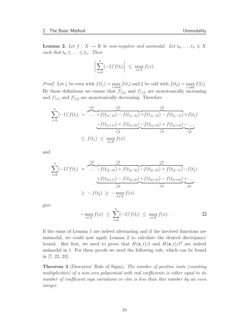
Lemma 2. Let f : X → R be non-negative and unimodal. Let t0, . . . , tn ∈ X
such that t0 ≤ . . . ≤ tn. Then
∣∣∣∣
n∑
i=0
(−1)if(ti)
∣∣∣∣≤ max
x∈Xf(x).
Proof. Let ζ be even with f(tζ) = maxi even
f(ti) and ξ be odd with f(tξ) = maxi odd
f(ti).
By these definitions we ensure that f |≤ζ and f |≤ξ are monotonically increasing
and f |≥ζ and f |≥ξ are monotonically decreasing. Therefore
n∑
i=0
(−1)if(ti) =
≤0︷︸︸︷
. . .
≤0︷ ︸︸ ︷
+f(t(ζ−4))− f(t(ζ−3))
≤0︷ ︸︸ ︷
+f(t(ζ−2))− f(t(ζ−1)) +f(tζ)
−f(t(ζ+1)) + f(t(ζ+2))︸ ︷︷ ︸
≤0
−f(t(ζ+3)) + f(t(ζ+4))︸ ︷︷ ︸
≤0
− . . .︸ ︷︷ ︸
≤0
≤ f(tζ) ≤ maxx∈X
f(x)
and
n∑
i=0
(−1)if(ti) =
≥0︷︸︸︷
. . .
≥0︷ ︸︸ ︷
−f(t(ξ−4)) + f(t(ξ−3))
≥0︷ ︸︸ ︷
−f(t(ξ−2)) + f(t(ξ−1))−f(tξ)
+f(t(ξ+1))− f(t(ξ+2))︸ ︷︷ ︸
≥0
+f(t(ξ+3))− f(t(ξ+4))︸ ︷︷ ︸
≥0
+ . . .︸ ︷︷ ︸
≥0
≥ − f(tξ) ≥ −maxx∈X
f(x)
give
−maxx∈X
f(x) ≤n∑
i=0
(−1)if(ti) ≤ maxx∈X
f(x).
If the sums of Lemma 1 are indeed alternating and if the involved functions are
unimodal, we could now apply Lemma 2 to calculate the desired discrepancy
bound. But first, we need to prove that H(x, t)/t and H(x, t)/t2 are indeed
unimodal in t. For these proofs we need the following rule, which can be found
in [7, 22, 23]:
Theorem 3 (Descartes’ Rule of Signs). The number of positive roots (counting
multiplicities) of a non-zero polynomial with real coefficients is either equal to its
number of coefficient sign variations or else is less than this number by an even
integer.
16

2. The Basic Method Unimodality
With this, we are now well equipped to prove unimodality of H(x, t)/t and
H(x, t)/t2. For the calculations in Sections 3.2 and 3.3, we also already derive the
exact times, when these discrete functions are maximal.
Lemma 4. H(x, t)/t is a unimodal function in t with its global maximum at
tmax(x) ∈[
x21+x2
2
4− 2,
x21+x2
2
4+ 1
2
]
.
Proof. Without loss of generality x1 + x2 > 4 and 0 ≤ x1 ≤ x2. By definition
H(x, t)/t = 0 for t < x2. We want to show H(x, t)/t has only one maximum in
t ∈ [x2,∞). Consequently, we compute the discrete derivative of H(x, t)/t via
(u ≥ 3)
H(x, u− 2)
u− 2− H(x, u)
u
=4−u
(4u3 − (x2
1 + x22 + 5)u2 + 2u + x2
1x22
)(u− 3)! (u− 2)!
(u+x1
2)! (u−x1
2)! (u+x2
2)! (u−x2
2)!
.
Since all but one factors are always positive, it suffices to show that
p(u) := 4u3 − (x21 + x2
2 + 5)u2 + 2u + x21x
22
has not more than one real root greater than x2. This can be done with Descartes’
Sign Rule described in Theorem 3. Since we assumed x1 and x2 to be nonnegative,
p(u) has two sign changes. Descartes’ Rule now says that p(u) has exactly zero
or two positive real roots. With
p(u− x2) = 4u3 − (x21 + x2
2 + 12x2 + 5)u2
+ (2x32 + 12x2
2 + 2x21x2 + 10x2 + 2)u− (x4
2 + 4x32 + 5x2
2 + 2x2)
Descartes furthermore testifies that p has exactly one or three real roots in [x2,∞).
Both implications together yield the desired result that there is only one real root
in [x2,∞).
To find the global maximum tmax(x) of H(x, t)/t, the cubic formula gives us the
exact position of the only relevant root u0 of p(u):
u0 =1
12
(
x21 + x2
2 + 5 + P +x4
1 + x42 + 2x2
1x22 + 10x2
1 + 10x22 + 1
P
)
17
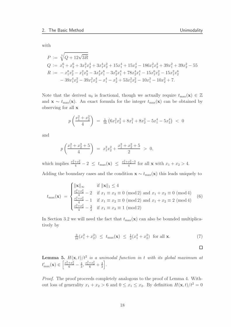
2. The Basic Method Unimodality
with
P :=3
√
Q + 12√
3R
Q := x61 + x6
2 + 3x21x
42 + 3x4
1x22 + 15x4
1 + 15x42 − 186x2
1x22 + 39x2
1 + 39x22 − 55
R := − x81x
22 − x2
1x82 − 3x4
2x61 − 3x6
2x41 + 78x4
2x41 − 15x6
1x22 − 15x2
1x62
− 39x41x
22 − 39x2
1x42 − x4
1 − x42 + 53x2
1x22 − 10x2
1 − 10x22 + 7.
Note that the derived u0 is fractional, though we actually require tmax(x) ∈ Z
and x ∼ tmax(x). An exact formula for the integer tmax(x) can be obtained by
observing for all x
p
(x2
1 + x22
4
)
= 116
(6x2
1x22 + 8x2
1 + 8x22 − 5x4
1 − 5x42
)< 0
and
p
(x2
1 + x22 + 5
4
)
= x21x
22 +
x21 + x2
2 + 5
2> 0,
which impliesx21+x2
2
4− 2 ≤ tmax(x) ≤ x2
1+x22−3
4for all x with x1 + x2 > 4.
Adding the boundary cases and the condition x ∼ tmax(x) this leads uniquely to
tmax(x) =
‖x‖∞ if ‖x‖1 ≤ 4x21+x2
2
4− 2 if x1 ≡ x2 ≡ 0 (mod 2) and x1 + x2 ≡ 0 (mod 4)
x21+x2
2
4− 1 if x1 ≡ x2 ≡ 0 (mod 2) and x1 + x2 ≡ 2 (mod 4)
x21+x2
2
4− 3
2if x1 ≡ x2 ≡ 1 (mod 2)
(6)
In Section 3.2 we will need the fact that tmax(x) can also be bounded multiplica-
tively by
316
(x21 + x2
2) ≤ tmax(x) ≤ 12(x2
1 + x22) for all x. (7)
Lemma 5. H(x, t)/t2 is a unimodal function in t with its global maximum at
t′max(x) ∈[
x21+x2
2
6− 4
3,
x21+x2
2
6+ 4
3
]
.
Proof. The proof proceeds completely analogous to the proof of Lemma 4. With-
out loss of generality x1 + x2 > 6 and 0 ≤ x1 ≤ x2. By definition H(x, t)/t2 = 0
18

2. The Basic Method Unimodality
for t < x2. We want to show that H(x, t)/t2 has only one maxima in t ∈ [x2,∞).
The discrete derivative of H(x, t)/t2 is
H(x, u− 2)
(u− 2)2− H(x, u)
u2
=4−u(6u3 − (x2
1 + x22 + 13)u2 + 12u + x2
1x22 − 4
)((u− 3)!
)2
(u+x1
2)!(u−x1
2)!(u+x2
2)!(u−x2
2)!
.
Since again all but one factors are always positive, it suffices to show that
p(u) := 6u3 − (x21 + x2
2 + 13)u2 + 12u + (x21x
22 − 4)
has not more than one real root greater than x2. Due to x1 + x2 > 6, p(u) has
two sign changes and therewith zero or two positive real roots.
p(u− x2) = 6u3 − (x21 + x2
2 + 18x2 + 13)u2
+ (2x21x2 + 2x3
2 + 18x22 + 26x2 + 12)u
− (x42 + 6x3
2 + 13x22 + 12x2 + 4)
has three sign chances, i.e., p has exactly one real root in [x2,∞).
To find the global maximum t′max(x) of H(x, t)/t2, the cubic formula gives us the
exact position of the only relevant root u0 of p(u):
u0 =1
18
(
x21 + x2
2 + 13 + P +x4
1 + x42 + 2x2
1x22 + 26x2
1 + 26x22 − 47
P
)
with
P :=3
√
Q + 18√
3R
Q := x61 + x6
2 + 3x41x
22 + 3x2
1x42 + 39x4
1 + 39x42 + 183x2
1 + 183x22 − 408x2
1x22 − 71
R := − x81x
22 − x2
1x82 − 3x6
1x42 − 3x4
1x62 − 39x6
1x22 − 39x2
1x62 + 165x4
2x41
+ 4x62 + 4x6
1 − 171x41x
22 − 171x2
1x42 + 120x4
1 + 120x42 + 311x2
1x22
− 204x21 − 204x2
2 + 112.
To get an exact formula for t′max(x), it is again easy to see that for all x
p
(x2
1 + x22 + 3
6
)
= 118
(6x2
1 + 6x22 + 8x2
1x22 − 5x4
1 − 5x42 − 9
)< 0
19
2. The Basic Method Unimodality
and
p
(x2
1 + x22 + 13
6
)
= 2x21 + 2x2
2 + x21x
22 + 22 > 0,
which impliesx21+x2
2+3
6− 2 ≤ t′max(x) ≤ x2
1+x22+1
6for all x with x1 + x2 > 6.
Adding the boundary cases and the condition t′max(x) ≡ x1 ≡ x2 (mod 2) this
leads uniquely to
t′max(x) =
‖x‖∞ if ‖x‖1 ≤ 6x21+x2
2
6− 4
3if x1 6≡ 0 6≡ x2 (mod 3)
x21+x2
2
6− 2
3if x1 6≡ 0 ≡ x2 (mod 3) or x1 ≡ 0 6≡ x2 (mod 3)
x21+x2
2
6if x1 ≡ 0 ≡ x2 (mod 3)
(8)
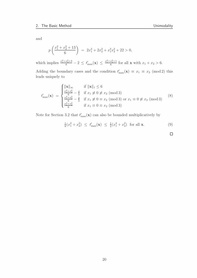
Note for Section 3.2 that t′max(x) can also be bounded multiplicatively by
18(x2
1 + x22) ≤ t′max(x) ≤ 1
2(x2
1 + x22) for all x. (9)
20
Chapter 3Upper Bound
Building on Lemma 1, we utilize Lemma 2, 4, and 5 of the previous chapter to
prove the following upper bound on the single vertex discrepancy.
Theorem 6. Independent of the initial even configuration, the time t, and the lo-
cation x, we have for clockwise (ր,ց,ւ,տ) and counterclockwise (ր,տ,ւ,ց)
rotor sequences
|f(x, t)−E(x, t)| < 11.8,
and for all other rotor sequences, i.e., for (ր,տ,ց,ւ), (ր,ւ,ց,տ),
(ր,ց,տ,ւ), and (ր,ւ,տ,ց),
|f(x, t)−E(x, t)| < 10.9.
3.1 Dependence on the Chosen Rotor Sequence
It remains to decompose the sums of Lemma 1 in strictly alternating sums of
unimodal functions. Here a crucial difference to the one-dimensional case emerges:
this decomposition, and therewith the upper bound, depends on the chosen rotor
sequence (cf. Section 1.3).
We fix a y ∈ Z2 and set A(i) := A(i)(y) = arr(y, si(y)) and t(i) := t − si(y).
For all three inner sums of Lemma 1 we now have to distinguish how the arrow
alternates. Let us first look at the sum∑
i≥0−A
(i)1 y1
t(i)H(y, t(i)). For both rotor
sequences π ∈ {(ր,տ,ց,ւ) , (ր,ւ,ց,տ)} we have χx(π) = (+,−, +,−)
and A(i)1 strictly alternating. Hence, there is an α ∈ {0, 1} that only depends on
21

3. Upper Bound Dependence on the Chosen Rotor Sequence
arr(y, 0) such that
∑
i≥0
−A(i)1 y1
t(i)H(y, t(i)) = (−1)α
∑
i≥0
(−1)i y1H(y, t(i))
t(i)
=
∣∣∣∣∣
∑
i≥0
(−1)i
∣∣∣∣
y1H(y, t(i))
t(i)
∣∣∣∣
∣∣∣∣∣.
Since we have proven unimodality of H(x, t)/t in Lemma 4, we can now apply
Lemma 2 and obtain∣∣∣∣∣
∑
i≥0
−A(i)1 y1
t(i)H(y, t(i))
∣∣∣∣∣≤ max
t
∣∣∣∣
y1H(y, t)
t.
∣∣∣∣
If the rotor sequence does not strictly alternate in the first dimension, we have
to be more careful. For the remaining permutations we have either χx(π) =
(+, +,−,−) or χx(π) = (+,−,−, +). This means that we can divide the sum in
two alternating sums, which yields
∣∣∣∣∣
∑
i≥0
−A(i)1 y1
t(i)H(y, t(i))
∣∣∣∣∣
≤∣∣∣∣∣
∑
i≥0,i odd
−A(i)1 y1
t(i)H(y, t(i))
∣∣∣∣∣
+
∣∣∣∣∣
∑
i≥0,i even
−A(i)1 y1
t(i)H(y, t(i))
∣∣∣∣∣
=
∣∣∣∣∣
∑
i≥0,i odd
(−1)i y1H(y, t(i))
t(i)
∣∣∣∣∣
+
∣∣∣∣∣
∑
i≥0,i even
(−1)i y1H(y, t(i))
t(i)
∣∣∣∣∣
≤ 2 maxt
∣∣∣∣
y1H(y, t)
t
∣∣∣∣.
For the second sum of Lemma 1 one can analogously prove
∣∣∣∣∣
∑
i≥0
−A(i)2 y2
t(i)H(y, t(i))
∣∣∣∣∣≤ max
t
∣∣∣∣
y2H(y, t)
t
∣∣∣∣
for the permutations (ր,ց,տ,ւ) and (ր,ւ,տ,ց), which satisfy χy(π) =
(+,−, +,−). Also
∣∣∣∣∣
∑
i≥0
−A(i)2 y2
t(i)H(y, t(i))
∣∣∣∣∣≤ 2 max
t
∣∣∣∣
y2H(y, t)
t
∣∣∣∣
22

3. Upper Bound Dependence on the Chosen Rotor Sequence
for the other four permutations with χy(π) = (+, +,−,−) or χy(π) = (+,−,−, +).
The third sum of Lemma 1 can also be bounded by
∣∣∣∣∣
∑
i≥0
A(i)1 A
(i)2 y1y2
t(i)H(y, t(i))
∣∣∣∣∣≤ max
t
∣∣∣∣
y1y2H(y, t)
t2
∣∣∣∣
for the permutations (ր,ց,ւ,տ) and (ր,տ,ւ,ց) with χxy(π) = (+,−, +,−)
and by
∣∣∣∣∣
∑
i≥0
A(i)1 A
(i)2 y1y2
t(i)H(y, t(i))
∣∣∣∣∣≤ 2 max
t
∣∣∣∣
y1y2H(y, t)
t2
∣∣∣∣
for the four permutations with χxy(π) = (+, +,−,−) or χxy(π) = (+,−,−, +).
Due to symmetry in the two dimensions, we also have
maxt
∣∣∣∣
y1H(y, t)
t
∣∣∣∣
= maxt
∣∣∣∣
y2H(y, t)
t
∣∣∣∣.
Putting all this together, we obtain
Lemma 7. Independent of the initial even configuration and the time t, we have
for clockwise (ր,ց,ւ,տ) and counterclockwise (ր,տ,ւ,ց) rotor sequences
|f(0, t)− E(0, t)| ≤∑
y∈Z2
(
4 maxt
∣∣∣∣
y1H(y, t)
t
∣∣∣∣+ max
t
∣∣∣∣
y1y2H(y, t)
t2
∣∣∣∣
)
and for all other rotor sequences, i.e., for (ր,տ,ց,ւ), (ր,ւ,ց,տ),
(ր,ց,տ,ւ), and (ր,ւ,տ,ց),
|f(0, t)−E(0, t)| ≤∑
y∈Z2
(
3 maxt
∣∣∣∣
y1H(y, t)
t
∣∣∣∣+ 2 max
t
∣∣∣∣
y1y2H(y, t)
t2
∣∣∣∣
)
.
23

3. Upper Bound Convergence of the Series
3.2 Convergence of the Series
To obtain the desired numerical bounds via Lemma 7, we want to calculate∑
y maxt
∣∣y1H(y,t)
t
∣∣ and
∑
y maxt
∣∣y1y2H(y,t)
t2
∣∣. This depends on the convergence of
both series.
The summands can be bounded as follows. By Lemma 14 and Equation (7),
maxt
∣∣∣∣
y1H(y, t)
t
∣∣∣∣
=|y1|
tmax(y)H(y, tmax(y))
=|y1|
tmax(y)4−tmax(y)
(tmax(y)
(tmax(y) + y1)/2
)(tmax(y)
(tmax(y) + y2)/2
)
≤ |y1|tmax(y)
(
2−tmax(y)
(tmax(y)
tmax(y)/2
))2
≤ |y1|tmax(y)2
≤ 256 |y1|9 (y2
1 + y22)
2, (10)
and analogously by Lemma 14 and Equation (9),
maxt
∣∣∣∣
y1y2H(y, t)
t2
∣∣∣∣
=|y1y2|
t′max(y)2H(y, t′max(y))
=|y1y2|
t′max(y)24−t′max
(t′max(y)
(t′max(y) + y1)/2
)(t′max(y)
(t′max(y) + y2)/2
)
≤ |y1y2|t′max(y)2
(
2−t′max
(t′max(y)
t′max(y)/2
))2
≤ |y1y2|t′max(y)3
≤ 83 |y1y2|(y2
1 + y22)
3≤ 256
(y21 + y2
2)2. (11)
The last inequality is due to |y1y2|y21+y2
2≤ 1
2(Binomial Theorem).
For all y1 ≥ 1 by Lemma 13,
∞∑
y2=0
1
(y21 + y2
2)2
=
y1∑
y2=0
1
(y21 + y2
2)2
+∑
y2>y1
1
(y21 + y2
2)2
≤y1∑
y2=0
1
y41
+∑
y2>y1
1
y42
≤ y1 + 1
y41
+1
3 y31
=4y1 + 3
3 y41
≤ 4y1 + 3y1
3 y41
=7
3 y31
. (12)
24
3. Upper Bound Computation
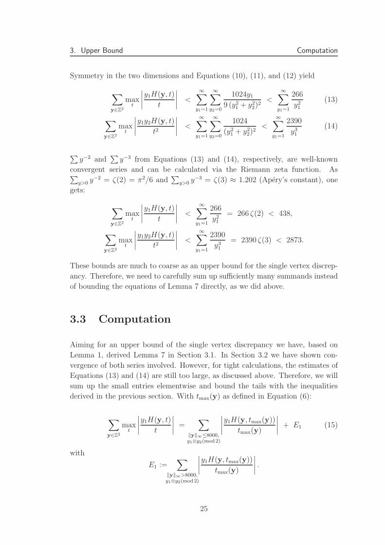
Symmetry in the two dimensions and Equations (10), (11), and (12) yield
∑
y∈Z2
maxt
∣∣∣∣
y1H(y, t)
t
∣∣∣∣
<
∞∑
y1=1
∞∑
y2=0
1024y1
9 (y21 + y2
2)2
<
∞∑
y1=1
266
y21
(13)
∑
y∈Z2
maxt
∣∣∣∣
y1y2H(y, t)
t2
∣∣∣∣
<∞∑
y1=1
∞∑
y2=0
1024
(y21 + y2
2)2
<∞∑
y1=1
2390
y31
(14)
∑y−2 and
∑y−3 from Equations (13) and (14), respectively, are well-known
convergent series and can be calculated via the Riemann zeta function. As∑
y>0 y−2 = ζ(2) = π2/6 and∑
y>0 y−3 = ζ(3) ≈ 1.202 (Apery’s constant), one
gets:
∑
y∈Z2
maxt
∣∣∣∣
y1H(y, t)
t
∣∣∣∣
<∞∑
y1=1
266
y21
= 266 ζ(2) < 438,
∑
y∈Z2
maxt
∣∣∣∣
y1y2H(y, t)
t2
∣∣∣∣
<∞∑
y1=1
2390
y31
= 2390 ζ(3) < 2873.
These bounds are much to coarse as an upper bound for the single vertex discrep-
ancy. Therefore, we need to carefully sum up sufficiently many summands instead
of bounding the equations of Lemma 7 directly, as we did above.
3.3 Computation
Aiming for an upper bound of the single vertex discrepancy we have, based on
Lemma 1, derived Lemma 7 in Section 3.1. In Section 3.2 we have shown con-
vergence of both series involved. However, for tight calculations, the estimates of
Equations (13) and (14) are still too large, as discussed above. Therefore, we will
sum up the small entries elementwise and bound the tails with the inequalities
derived in the previous section. With tmax(y) as defined in Equation (6):
∑
y∈Z2
maxt
∣∣∣∣
y1H(y, t)
t
∣∣∣∣
=∑
‖y‖∞≤8000,y1≡y2(mod 2)
∣∣∣∣
y1H(y, tmax(y))
tmax(y)
∣∣∣∣
+ E1 (15)
with
E1 :=∑
‖y‖∞>8000,y1≡y2(mod 2)
∣∣∣∣
y1H(y, tmax(y))
tmax(y)
∣∣∣∣.
25

3. Upper Bound Computation
This “error” E1 must be small according to Equation (13) and will be evaluated
in Equation (19) below. With a computer algebra system like Maple, one now
easily calculates the main contribution to∑
y∈Z2 maxt
∣∣ y1H(y,t)
t
∣∣, using symmetry:
∑
‖y‖∞≤8000,y1≡y2(mod 2)
∣∣∣∣
y1H(y, tmax(y))
tmax(y)
∣∣∣∣
= 4
8000∑
y1=1
8000∑
y2=1,y2≡y1(mod 2)
y1H(y, tmax(y))
tmax(y)+ 2
8000∑
y1=1,y1≡0(mod 2)
y1H((
y1
0
), tmax(y)
)
tmax(y)
= 4
8000∑
y1=1
8000∑
y2=1,y2≡y1(mod 2)
y14−tmax(y)
tmax(y)
(tmax(y)
(tmax(y) + y1)/2
)(tmax
(tmax(y) + y2)/2
)
+ 2
8000∑
y1=1,y1≡0(mod 2)
y14−tmax(y)
tmax(y)
(tmax(y)
(tmax(y) + y1)/2
)(tmax(y)
tmax(y)/2
)
< 2.5248. (16)
For the second sum, we obtain analogously (with t′max(y) as defined in Equa-
tion (8)):
∑
y∈Z2
maxt
∣∣∣∣
y1y2H(y, t)
t2
∣∣∣∣
<∑
‖y‖∞≤3000,y1≡y2(mod 2)
∣∣∣∣
y1y2H(y, t′max(y))
(t′max(y))2
∣∣∣∣
+ E2. (17)
By only summing up over y with ‖y‖∞ ≤ 3000, we missed
E2 :=∑
‖y‖∞>3000,y1≡y2(mod 2)
y1y2H(y, t′max(y))
(t′max(y))2,
which will be bounded in Equation (25) below.
For Equation (17), one calculates
∑
‖y‖∞≤3000,y1≡y2(mod 2)
∣∣∣∣
y1y2H(y, t′max(y))
(t′max(y))2
∣∣∣∣
= 43000∑
y1=1
3000∑
y2=1,y2≡y1(mod 2)
y1y2H(y, t′max(y))
(t′max(y))2
= 43000∑
y1=1
3000∑
y2=1,y2≡y1(mod 2)
y1y24−t′max(y)
(t′max(y))2
(t′max(y)
(t′max(y) + y1)/2
)(t′max(y)
(t′max(y) + y2)/2
)
< 1.6439. (18)
26

3. Upper Bound Computation
To get exact upper bounds for∑
maxt
∣∣y1H(y,t)
t
∣∣ and
∑maxt
∣∣y1y2H(y,t)
t2
∣∣, we need to
Figure 7: Schematic explanation of
Equation (19).
upper bound the tail errors E1 and E2.
For E1, we need to be very careful. In
Equation (16) we only summed up over
|y1|, |y2| ≤ 8000. Hence, there are three
kinds of summands in E1: Such with
|y1| ≤ 8000 and |y2| > 8000 (Eq. 21),
|y1| > 8000 and |y2| ≤ 8000 (Eq. 23), and
|y1|, |y2| > 8000 (Eq. 24). These three
sums correspond to the yellow-shaded
area shown in Figure 7 and to the three
sums of Equation (19) below. Note that
Equation (19) is an inequality, because
on the right side we sum up over y with
|y1| > 8000 and y2 = 0 twice. This sim-
plifies the calculation and overestimates
E1 by just < 10−6.
E1 <
see Equation (21)︷ ︸︸ ︷
48000∑
y1=1
∞∑
y2=8001,y2≡y1(mod 2)
y1H(y, tmax(y))
tmax(y)+
see Equation (23)︷ ︸︸ ︷
4∞∑
y1=8001
8000∑
y2=1,y2≡y1(mod 2)
y1H(y, tmax(y))
tmax(y)
+ 4
∞∑
y1=8001
∞∑
y2=8001,y2≡y1(mod 2)
y1H(y, tmax(y))
tmax(y)
︸ ︷︷ ︸
see Equation (24)
< 0.0064. (19)
We want to utilize Equation (10) from the previous section to estimate the three
sums of Equation (19) above. This results in infinite sums over y1
(y21+y2
2)2, which
can expressed as finite sums of the digamma function Ψ0 and the first polygamma
function Ψ1. Fortunately, these infinite sums can be bounded tightly much easier
via integral calculus. Hence, for c ∈ {0, 1} and α, γ ∈ Z:
∑
y>α,y≡c(mod 2)
1
(y2 + γ2)2=
∑
y>(α−c)/2
1
((2y + c)2 + γ2)2
≤∫ ∞
y=(α−c)/2
1
((2y + c)2 + γ2)2
=
(π − 2 arctan(α
γ))(α2 + γ2)− 2αγ
8(α2 + γ2)γ3. (20)
27

3. Upper Bound Computation
Equipped with this, Equation (10) yields for the first sum of E1:
48000∑
y1=1
∞∑
y2=8001,y2≡y1(mod 2)
y1H(y, tmax(y))
tmax(y)
< 10249
8000∑
y1=1
y1
∑
y2>8000,y2≡y1(mod 2)
1
(y21 + y2
2)2
≤ 1289
8000∑
y1=1
(80002 + y21)(π − 2 arctan(8000/y1)
)− 16000 y1
(y21 + 80002) y2
1
.
< 0.0008. (21)
For the second sum of E1, we need
∑
y>α,y≡c(mod 2)
y
(y2 + γ2)2=
∑
y>(α−c)/2
2y + c
((2y + c)2 + γ2)2
≤∫ ∞
y=(α−c)/2
2y + c
((2y + c)2 + γ2)2
=1
4(α2 + γ2). (22)
With this, the second sum of E1 can be bounded as follows:
4∞∑
y1=8001
8000∑
y2=0,y2≡y1(mod 2)
y1H(y, tmax(y))
tmax(y)
= 48000∑
y2=0
∞∑
y1=8001,y1≡y2(mod 2)
y1H(y, tmax(y))
tmax(y)
< 10249
8000∑
y2=0
∑
y1>8000,y1≡y2(mod 2)
y1
(y21 + y2
2)2
≤ 2569
8000∑
y2=0
1
y22 + 80002
< 0.0028. (23)
28

3. Upper Bound Computation
For the third sum of Equation (19), we need Equation (20) and
∑
y>β
π − 2 arctan(αy)
y2≤
∫ ∞
y=β
π − 2 arctan(αy)
y2
=ln(α2 + β2)− 2 ln(β)
α+
π − 2 arctan(αβ)
β∑
y≥β
1
(α2 + y2)y≥
∫ ∞
y=β
1
(α2 + y2)y
=ln(α2 + β2)− 2 ln(β)
2α2.
With this and Equations (10) and (20), we get for the third sum of E1:
4
∞∑
y1=8001
∞∑
y2=8001,y2≡y1(mod 2)
y1H(y, tmax(y))
tmax(y)
≤ 10249
∑
y1>8000
y1
∑
y2>8000,y2≡y1(mod 2)
1
(y21 + y2
2)2
≤ 1289
∑
y1>8000
(π − 2 arctan(8000
y1))(80002 + y2
1)− 16000y1
(80002 + y21)y
21
≤ 128
9
(ln(2 · 80002)− 2 ln(8000)
8000+
π/2
8000− ln(2 · 80012)− 2 ln(8001)
8001
)
< 0.0028. (24)
The second error E2 (cf. Equation (17)) is much easier to bound. With Equa-
tions (11) and (12), we get
E2 < 4
3000∑
y1=1
∑
y2>3000
y1y2H(y, t′max(y))
(t′max(y))2+ 4
∑
y1>3000
∑
y2>0
y1y2H(y, t′max(y))
(t′max(y))2
< 4
3000∑
y1=1
∑
y2>3000
1024
(y21 + y2
2)2
+ 4∑
y1>3000
∑
y2≥0
1024
(y21 + y2
2)2
<
3000∑
y1=1
∑
y2>3000
4096
y42
+∑
y1>3000
28672
3 y31
by Lemma 13
≤ 4096
3 · 30002+
14336
3 · 30002
< 0.0007. (25)
29
3. Upper Bound Computation
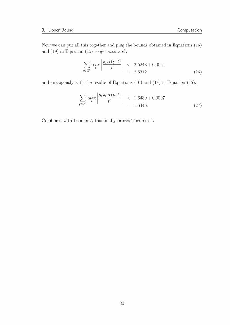
Now we can put all this together and plug the bounds obtained in Equations (16)
and (19) in Equation (15) to get accurately
∑
y∈Z2
maxt
∣∣∣∣
y1H(y, t)
t
∣∣∣∣
< 2.5248 + 0.0064
= 2.5312 (26)
and analogously with the results of Equations (16) and (19) in Equation (15):
∑
y∈Z2
maxt
∣∣∣∣
y1y2H(y, t)
t2
∣∣∣∣
< 1.6439 + 0.0007
= 1.6446. (27)
Combined with Lemma 7, this finally proves Theorem 6.
30
Chapter 4Lower Bound
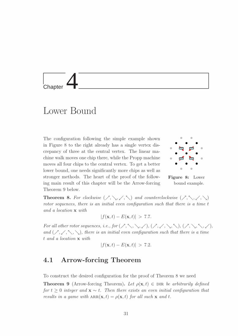
Figure 8: Lower
bound example.
The configuration following the simple example shown
in Figure 8 to the right already has a single vertex dis-
crepancy of three at the central vertex. The linear ma-
chine walk moves one chip there, while the Propp machine
moves all four chips to the central vertex. To get a better
lower bound, one needs significantly more chips as well as
stronger methods. The heart of the proof of the follow-
ing main result of this chapter will be the Arrow-forcing
Theorem 9 below.
Theorem 8. For clockwise (ր,ց,ւ,տ) and counterclockwise (ր,տ,ւ,ց)
rotor sequences, there is an initial even configuration such that there is a time t
and a location x with
|f(x, t)− E(x, t)| > 7.7.
For all other rotor sequences, i.e., for (ր,տ,ց,ւ), (ր,ւ,ց,տ), (ր,ց,տ,ւ),
and (ր,ւ,տ,ց), there is an initial even configuration such that there is a time
t and a location x with
|f(x, t)− E(x, t)| > 7.2.
4.1 Arrow-forcing Theorem
To construct the desired configuration for the proof of Theorem 8 we need
Theorem 9 (Arrow-forcing Theorem). Let ρ(x, t) ∈ dir be arbitrarily defined
for t ≥ 0 integer and x ∼ t. Then there exists an even initial configuration that
results in a game with arr(x, t) = ρ(x, t) for all such x and t.
31
4. Lower Bound Arrow-forcing Theorem
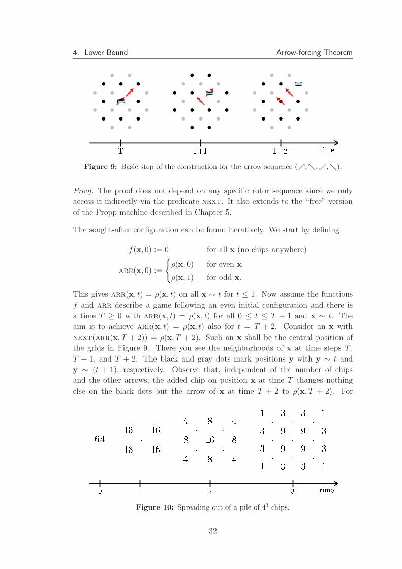
Figure 9: Basic step of the construction for the arrow sequence (ր,տ,ւ,ց).
Proof. The proof does not depend on any specific rotor sequence since we only
access it indirectly via the predicate next. It also extends to the “free” version
of the Propp machine described in Chapter 5.
The sought-after configuration can be found iteratively. We start by defining
f(x, 0) := 0 for all x (no chips anywhere)
arr(x, 0) :=
{
ρ(x, 0) for even x
ρ(x, 1) for odd x.
This gives arr(x, t) = ρ(x, t) on all x ∼ t for t ≤ 1. Now assume the functions
f and arr describe a game following an even initial configuration and there is
a time T ≥ 0 with arr(x, t) = ρ(x, t) for all 0 ≤ t ≤ T + 1 and x ∼ t. The
aim is to achieve arr(x, t) = ρ(x, t) also for t = T + 2. Consider an x with
next(arr(x, T + 2)) = ρ(x, T + 2). Such an x shall be the central position of
the grids in Figure 9. There you see the neighborhoods of x at time steps T ,
T + 1, and T + 2. The black and gray dots mark positions y with y ∼ t and
y ∼ (t + 1), respectively. Observe that, independent of the number of chips
and the other arrows, the added chip on position x at time T changes nothing
else on the black dots but the arrow of x at time T + 2 to ρ(x, T + 2). For
Figure 10: Spreading out of a pile of 43 chips.
32
4. Lower Bound Arrow-forcing Theorem
nextk(arr(x, T + 2)) = ρ(x, T + 2) this can be achieved analoguously by adding
k chips on position x.
The question remains, how we get the additional chips on a position x at time
T without changing the arrows in the previous time steps. This can be done by
adding multiples of 4T chips (see Figure 10) on the right positions at time 0 since
a pile of 4T chips will split evenly T times so that the arrows at time t ≤ T remain
the same.
Hence, we modify our initial configuration by setting
f ′(x, 0) :=
{
f(x, 0) + εx4T for even x
0 for odd x.
arr′(x, 0) := arr(x, 0) for all x.
Here, the εx ∈ {0, 1, 2, 3} are to be determined. Our goal is to choose the values of
εx so that arr′(x, t) = ρ(x, t) for all t ≤ T +2 and x ∼ t. Due to the T even splits
of the piles of 4T chips this holds automatically for t ≤ T . Since we started with
an even initial configuration there are no chips on x ∼ T + 1 at time T . Hence,
for x ∼ T + 1 at time T + 1 we have arr′(x, T + 1) = arr
′(x, T ) = arr(x, T ) =
arr(x, T + 1) = ρ(x, T + 1). To make sure the equality also holds for time T + 2
we need to ensure that the parities of the piles f ′(x, T ) are right. Observe that
arr′(x, T + 2) = next
k(arr′(x, T )) for f ′(x, T ) ≡ k (mod 4). Hence, for x ∼ T
we want f ′(x, T ) ≡ k (mod 4) exactly for ρ(x, T +2) = nextk(ρ(x, T )). For that,
we watch closely how the “extra” groups of 4T chips are spreading:
f ′(x, 1) = f(x, 1) + 4T−1∑
d∈dir
εx+d (for odd x and T ≥ 1)
= f(x, 1) + 4T−1(
εx+(1
1)+ ε
x+( 1−1)
+ εx+(−1
1 ) + εx+(−1
−1)
)
f ′(x, 2) = f(x, 2) + 4T−2∑
d1∈dir
∑
d2∈dir
εx+d1+d2 (for even x and T ≥ 2)
= f(x, 2) + 4T−2(
εx+(2
2)+ ε
x+( 2−2)
+ εx+(−2
2 ) + εx+(−2
−2)
)
+ 4T−1.5(
εx+(0
2)+ ε
x+(20)
+ εx+( 0
−2)+ ε
x+(−20 )
)
+ 4T−1 εx
· · ·f ′(x, T ) = f(x, T ) +
∑
d1∈dir
∑
d2∈dir
· · ·∑
dT ∈dir
ε(x+PT
i=1 di) (for x ∼ T )
= f(x, T ) +∑
y∼0‖y−x‖∞≤T
εy
(T
T+x1−y1
2
)(T
T+x2−y2
2
)
33

4. Lower Bound Arrow-forcing Theorem
The last sum describes the three-dimensional analogon of Pascal’s Triangle. For
T = 0 the sum is εx, hence, for all even x with ρ(x, 2) = nextk(ρ(x, 0)) we add k
chips on x, i.e., εx := k, and get the aspired arr′(x, t) = ρ(x, t) on all x ∼ t for
t ≤ 2.
For T > 0 notice, that
∑
y∼0‖y−x‖∞≤T
εy
(T
T+x1−y1
2
)(T
T+x2−y2
2
)
= εx+(T
T) + εx+( T
−T)+ ε
x+(−TT ) + ε
x+(−T−T)
+ h,
where h depends only on εy with x1 − T ≤ y1 ≤ x1 + T ∧ x2 − T < y2 < x2 + T
or x1−T < y1 < x1 + T ∧ x2−T ≤ y2 ≤ x2 + T . We now have to determine the
εy sequentially for growing rectangles of side length ℓ, namely we define
Rℓ :={(
x1
x2
)| |x1| ≤ ℓ ∧ |x2| ≤ ℓ
}and
∂Rℓ :={(
x1
x2
)| |x1| = ℓ ∨ |x2| = ℓ
}.
We start the inductive process with εy := 0 for all y ∈ RT \ {(
TT
)}. For odd T
we also set ε(TT)
:= 0 and for even T we define ε(TT) := k with ρ(
(00
), T + 2) =
nextk(ρ(
(00
), T )). In both cases this yields arr
′(x, T + 2) = ρ(x, T + 2) on all
x ∼ T with x ∈ R0.
Assume we have achieved arr′(x, T + 2) = ρ(x, T + 2) on all x ∼ T with x ∈ Rℓ.
and εy has been defined for all y ∈ Rℓ+T . The next step is to define the εy for
all even y ∈ ∂Rℓ+T+1 to obtain arr′(x, T + 2) = ρ(x, T + 2) also on all x ∼ T
with x ∈ ∂Rℓ+1. Since we have 2(ℓ + 1) equations, but 2(ℓ + T + 1) many εy, the
εy’s are under-determined and can be assigned sequentially by walking around the
rectangle ∂Rℓ+T+1.
The described procedure changes an even initial configuration that matches the
prescription in ρ for times t ≤ T + 1 into another one that matches for times
t ≤ T + 2. Please note, that thereby we do not change the initial configuration
of arrows arr(x, 0) at all, and we change the initial number of chips f(x, 0) at
position x only if ‖x‖∞ ≥ T . Hence, at all positions x the initial number of
chips will be constant after the first ‖x‖∞ iterations. This shows that the process
converges to an even initial configuration, which leads to the given game.
34

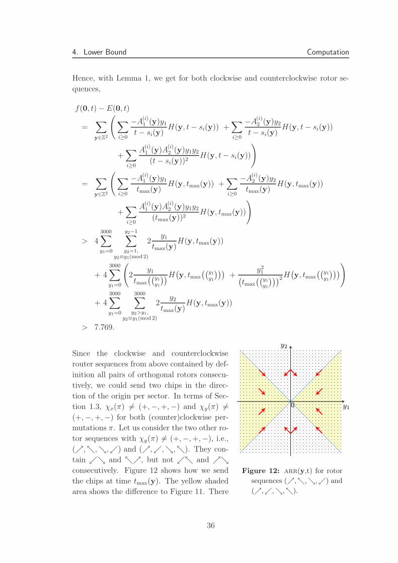
4. Lower Bound Computation
4.2 Computation
Figure 11: arr(y,t) for clock-
wise rotor sequences.
To get a large discrepancy at the origin, we
choose via Theorem 9 above an initial config-
uration that sends as many chips as possible at
the worst time tmax(y) in the direction of the
origin. This maximizes the sums of Lemma 1.
For clockwise rotor sequences, we send the
chips as shown in Figure 11, i.e., one on
both diagonals and two in the sectors between
them. This is possible for (ր,ց,ւ,տ) and
(ր,տ,ւ,ց), because ւց (|y1| < y2 > 0),
տր (|y1| < −y2 > 0), ւտ (0 < y1 > |y2|),and րց (0 < −y1 > |y2|) are consecutive ro-
tor positions, which allows sending one chip
in both directions at time tmax(y). Let x 6= 0
be an arbitrary even position and t0 := tmax(x) as defined in Equation (6). For
(ր,ց,ւ,տ) we apply the Arrow-forcing Theorem 9 to find an even starting
position such that for all positions y we have
arr(y, t) :=
ր for all 0 > y1 ≤ y2 < −y1 and t ≤ t0 − tmax(y)
or 0 > −y1 ≤ y2 < y1 and t > t0 − tmax(y)
ց for all 0 > −y2 ≤ y1 < y2 and t ≤ t0 − tmax(y)
or 0 > y2 ≤ y1 < −y2 and t > t0 − tmax(y)
ւ for all 0 > −y1 < y2 ≤ y1 and t ≤ t0 − tmax(y)
or 0 > y1 < y2 ≤ −y1 and t > t0 − tmax(y)
տ for all 0 > y2 < y1 ≤ −y2 and t ≤ t0 − tmax(y)
or 0 > −y2 < y1 ≤ y2 and t > t0 − tmax(y)
or 0 = y1 = y2.
Note that in this case at a position y with ‖y‖2 ≤ ‖x‖2 we have a number of chips
that is not a multiple of four exactly once at time t0 − tmax(y). For y1 = y2 there
is exactly one chip at time s0(y) = t0 − tmax(y), otherwise there are two chips at
time s0(y) = s1(y) = t0 − tmax(y). The same holds true for the counterclockwise
rotor sequence (ր,տ,ւ,ց) with a similar arr′(y, t).
35
4. Lower Bound Computation
Hence, with Lemma 1, we get for both clockwise and counterclockwise rotor se-
quences,
f(0, t)− E(0, t)
=∑
y∈Z2
(∑
i≥0
−A(i)1 (y)y1
t− si(y)H(y, t− si(y)) +
∑
i≥0
−A(i)2 (y)y2
t− si(y)H(y, t− si(y))
+∑
i≥0
A(i)1 (y)A
(i)2 (y)y1y2
(t− si(y))2H(y, t− si(y))
)
=∑
y∈Z2
(∑
i≥0
−A(i)1 (y)y1
tmax(y)H(y, tmax(y)) +
∑
i≥0
−A(i)2 (y)y2
tmax(y)H(y, tmax(y))
+∑
i≥0
A(i)1 (y)A
(i)2 (y)y1y2
(tmax(y))2H(y, tmax(y))
)
> 43000∑
y1=0
y2−1∑
y2=1,y2≡y1(mod 2)
2y1
tmax(y)H(y, tmax(y))
+ 43000∑
y1=0
(
2y1
tmax
((y1
y1
))H(y, tmax
((y1
y1
)))+
y21
(tmax
((y1
y1
)))2H(y, tmax
((y1
y1
)))
)
+ 43000∑
y1=0
3000∑
y2>y1,y2≡y1(mod 2)
2y2
tmax(y)H(y, tmax(y))
> 7.769.
Figure 12: arr(y,t) for rotor
sequences (ր,տ,ց,ւ) and
(ր,ւ,ց,տ).
Since the clockwise and counterclockwise
router sequences from above contained by def-
inition all pairs of orthogonal rotors consecu-
tively, we could send two chips in the direc-
tion of the origin per sector. In terms of Sec-
tion 1.3, χx(π) 6= (+,−, +,−) and χy(π) 6=(+,−, +,−) for both (counter)clockwise per-
mutations π. Let us consider the two other ro-
tor sequences with χy(π) 6= (+,−, +,−), i.e.,
(ր,տ,ց,ւ) and (ր,ւ,ց,տ). They con-
tain ւց and տր, but not ւտ and րցconsecutively. Figure 12 shows how we send
the chips at time tmax(y). The yellow shaded
area shows the difference to Figure 11. There
36

4. Lower Bound Computation
we can just send a single chip to the origin. Both remaining rotor sequences
with χx(π) 6= (+,−, +,−), i.e., (ր,ց,տ,ւ) and (ր,ւ,տ,ց), can be han-
dled analogously. They contain ւտ and րց, but not ւց and տր consecu-
tively. Hence, with Lemma 1, we get for all four rotor sequences (ր,տ,ց,ւ),
(ր,ւ,ց,տ), (ր,ց,տ,ւ), and (ր,ւ,տ,ց),
f(0, t)− E(0, t)
> 43000∑
y1=1
y1∑
y2=1,y2≡y1(mod 2)
(
y1
tmax(y)H(y, tmax(y)) +
y2
tmax(y)H(y, tmax(y))
+y1y2
(tmax(y))2H(y, tmax(y))
)
+ 83000∑
y1=1
3000∑
y2=y1+2,y2≡y1(mod 2)
y2
tmax(y)H(y, tmax(y))
+ 6
3000∑
y1=2,y1≡0(mod 2)
y1
tmax
((y1
0
))H((
y1
0
), tmax
((y1
0
)))
> 7.223.
This proves Theorem 8.
37

Chapter 5Free Propp Machine
Apart from changing the arrows according to a fixed permutation as described in
Section 1.3, one can also just require the arrows to change in such a way that the
number of chips sent in each direction differs by at most a constant ∆.
Definition 7. A rotor sequence A = (A(0),A(1),A(2), . . .) is called “∆-free” if
maxt≥0
(
maxd∈dir
∣∣{i ≤ t | A(i) = d}
∣∣− min
d∈dir
∣∣{i ≤ t | A(i) = d}
∣∣
)
≤ ∆.
Definition 8. A free Propp machine is a Propp machine as described in Sec-
tion 1.2, but the rotor sequences of all vertices are ∆-free for fixed ∆.
The permutations of Section 1.3 are a special case of the free Propp machine with
∆ = 1. Note, that in contrast to the original Propp machine, here we are not
distributing multiples of four chips equally to all four neighbors.
5.1 Upper Bound
For the discrepancy on a single vertex, we prove the following theorem.
Theorem 10. Independent of the initial even configuration, the time t, and the
location x, we have
|f(x, t)−E(x, t)| < 26.9 ·∆.
For the proof of Theorem 10, we will need the following lemma.
38

5. Free Propp Machine Upper Bound
Lemma 11. For every ∆-free rotor sequence A, there is a 4∆-coloring1 χ : N0 →[1, 4∆] such that all monochromatic subsequences are alternating on the first di-
mension. This is optimal.
Proof. First, we show that for arbitrary ∆-free rotor sequences there is no coloring
with less colors. Consider the following ∆-free rotor sequence:
A′ :=(ր . . .ր︸ ︷︷ ︸
∆ times
ց . . .ց︸ ︷︷ ︸
∆ times
տ . . .տ︸ ︷︷ ︸
∆ times
ւ . . .ւ︸ ︷︷ ︸
∆ times
տ . . .տ︸ ︷︷ ︸
∆ times
ւ . . .ւ︸ ︷︷ ︸
∆ times
. . .).
One requires at least 4∆ colors to separate alternating sequences on the first
dimension:
A′1 =
(+ . . .+︸ ︷︷ ︸
2∆ times
− . . .−︸ ︷︷ ︸
4∆ times
. . .).
Now consider the first dimension A(i)1 of the given rotor sequence. For all t ≥ 0:
∣∣∣
t∑
i=0
A(i)1
∣∣∣ =
∣∣
+1 on 1-st dim.︷ ︸︸ ︷
{i ≤ t | A(i) =ր}+ {i ≤ t | A(i) =ց}−{i ≤ t | A(i) =տ}− {i ≤ t | A(i) =ւ}︸ ︷︷ ︸
−1 on 1-st dim.
∣∣
≤∣∣∣2 max
d∈dir
∣∣{i ≤ t | A(i) = d}
∣∣− 2 min
d∈dir
∣∣{i ≤ t | A(i) = d}
∣∣
∣∣∣
= 2∆. (28)
Given any sequence A(i)1 of {−1, +1} satisfying Equation (28), we now seek a
4∆-coloring of A(i)1 such that all monochromatic subsequences are alternating se-
quences on their own. Our 4∆ colors are called {−4∆ + 1,−4∆ + 3, . . . , 4∆ −3, 4∆− 1} for the time being. We color each A
(t)1 with
χ(t) := 2t−1∑
i=0
A(i)1 + A
(t)1 .
This is a valid color for all t since Equation (28) gives |∑t−1
i=0 A(i)1 |+ |
∑ti=0 A
(i)1 | ≤
4∆, which yields |2∑t−1
i=0 A(i)1 + A
(t)1 | ≤ 4∆ given that
∑t−1i=0 A
(i)1 and
∑ti=0 A
(i)1
cannot be of opposite sign. It remains to prove that all 4∆ monochromatic sub-
sequences are alternating. Between two consecutive items A(k) and A(ℓ) of equal
color, there are as many +1 as −1 on the first dimension, i.e.,∑l−1
i=k+1 A(i)1 = 0.
χ(k) = χ(ℓ) implies 2∑l−1
i=k A(i)1 +A
(ℓ)1 = A
(k)1 , thus A
(k)1 +A
(ℓ)1 = 0 by
∑l−1i=k+1 A
(i)1 =
1Note that these colorings are different from the colorings in Section 1.3.
39

5. Free Propp Machine Upper Bound
0. Hence, A(k)1 and A
(ℓ)1 are indeed of opposite sign and therefore χ(i) a valid color-
ing. Renumbering the colors gives the final coloring χ′(i) := (χ(i)+4∆+1)/2.
Proof of Theorem 10. The only difference between the original Propp machine
introduced in Chapter 1 and the free Propp machine considered here, is the more
general concept of the ∆-free rotor sequences according to Definition 7. In the
proof of the upper bound of the original Propp machine (cf. Theorem 6), this
becomes important when the three sums of Lemma 1 are decomposed in strictly
alternating sums in Section 3.1.
We first study decompositions of∑
i≥0−A
(i)1 (y)y1
t−si(y)H(y, t−si(y)). In Section 3.1, this
was easy: For two out of six rotor sequences, A(i)1 (y) was already alternating. For
all other rotor sequences, we decomposed the sum into an alternating sum of the
even and an alternating sum of the odd elements. For the free Propp machine,
Lemma 11 gives us a 4∆-coloring χ of the ∆-free rotor sequence such that all
monochromatic subsequences are alternating on the first dimension. Now each
subsum gets one color assigned:
∑
i≥0
−A(i)1 (y)y1
t− si(y)H(y, t− si(y)) =
∑
c≤4∆
∑
i≥0,χ(i)=c
−A(i)1 (y)y1
t− si(y)H(y, t− si(y)).
Analogously to Lemma 11, one can prove that there are 4∆-colorings such that
A(i)1 (y) or A
(i)1 (y)A
(i)2 (y) are alternating. Hence, similar to Lemma 7, we have
independent of the initial even configuration, the time t, and the location x,
f(x, t)− E(x, t) ≤∑
y∈Z2
(
8∆ maxt
∣∣∣∣
y1H(y, t)
t
∣∣∣∣
+ 4∆ maxt
∣∣∣∣
y1y2H(y, t)
t2
∣∣∣∣
)
.
Plugged in the constants from Equations (26) and (27), we finally get Theorem 10.
40

5. Free Propp Machine Lower Bound
5.2 Lower Bound
Figure 13: Lower
bound example.
Analogous to the introductory example of Chapter 4, the
configuration following the right Figure 13 has discrep-
ancy 3 ∆ at the central vertex if the rotor sequence is suit-
ably chosen. Fortunately, this concept of gluing ∆ chips
together scales well. Therefore, consider a classic Propp
machine with rotor sequence (ր,ց,ւ,տ) and an initial
configuration which has discrepancy > 7.7 on a vertex x
at time t. Such a machine exists according to Theorem 8.
Out of this, we construct an initial configuration for a free
Propp machine with rotor sequence
(ր . . .ր︸ ︷︷ ︸
∆ times
ց . . .ց︸ ︷︷ ︸
∆ times
ւ . . .ւ︸ ︷︷ ︸
∆ times
տ . . .տ︸ ︷︷ ︸
∆ times
).
On each vertex with k chips in the original initial configuration, we now place a
pile of ∆ k chips. We also adopt the arrows by choosing the first arrow of the same
direction within the rotor sequence for each location of the initial configuration.
This results in a free Propp machine, which runs exactly as the original Propp
machine, but with piles of ∆ chips moving instead of single chips. This leads to
a discrepancy of 7.7 ∆ on x at time ∆ t and thus to the following theorem.
Theorem 12. For each ∆, there is an initial even configuration and a rotor
sequence such that there is a time t and a location x with
|f(x, t)− E(x, t)| ≥ 7.7 · ∆.
This proof does not use that the free Propp machine might even send 2∆ chips
in one direction. For example the ∆-free rotor sequence
(ր . . .ր︸ ︷︷ ︸
∆ times
ց . . .ց︸ ︷︷ ︸
∆ times
ւ . . .ւ︸ ︷︷ ︸
∆ times
ւ . . .ւ︸ ︷︷ ︸
∆ times
. . .).
sends 2∆ chips in the direction ւ. We expect this fact to help gaining a lower
bound of 15∆ for the single vertex discrepancy of the free Propp machine.
41

Chapter 6Conclusions and Further Work
We examined the Propp machine on the two-dimensional infinite grid Z2. In-
dependent of the starting configuration, at each time and on each vertex, the
number of chips on a vertex deviates from the expected number of chips in the
random walk model by at most a constant c. If the rotor is changing clockwise
or counterclockwise, this can be bounded by 7.7 < c < 11.8. For all other rotor
sequences (cf. Section 1.3), this can be lowered to 7.2 < c < 10.9. It remains
to prove that both intervals are actually disjoint. However, to the best of our
knowledge, this is the first work to indicate an influence of the rotor sequence on
the discrepancy. This is also supported experimentally, as discussed in Section 1.4
for the aggregating Propp machine.
In addition, we analyzed a “free” variant of the Propp machine, where we only
required the rotors to change in such a way that the number of chips sent in
different directions differs by at most a constant ∆. For this model, we bounded
the single vertex discrepancy c′ by 7.7∆ < c′ < 27∆. Also here, it remains to
bridge the gap between the lower and upper bound. We expect the lower bound
to be significantly higher.
We regarded as well the discrepancy on a single vertex over a time interval.
For x ∈ Z2 and finite S ⊆ N0, we set analogously to Definition 3, f(x, S) :=
∑
t∈S f(x, t) and E(x, S) :=∑
t∈S E(x, t). With Lemma 1 one can prove that
the discrepancy of a single vertex x in a time interval S of length T is at most
|f(x, S) − E(x, S)| = O(√
T log T ). It would also be interesting to examine the
discrepancy on a rectangle or circle.
42

6. Conclusions and Further Work
In higher dimensions, there is no equivalent to Lemma 1. Also note that in
higher dimensions, there is no coordinate transformation, which results in all
dimensions varying independently (cf. Assumption 2). However, we can ana-
lyze Zd with another neighborhood definition. That is, we allow 2d rotor di-
rections {x | xi ∈ {−1, +1}} instead of the 2d rotor directions {x | ‖x‖1 = 1}we had before. Since we still require Assumption 1, the probability that a
chip from the origin arrives at x at time t in a simple random walk on Zd is
H(x, t) = 2−dt∏d
i=1
(t
(t+xi)/2
)for x ∼ t (cf. Definition 1). Analogously to Lem-
mas 4 and 5, one can show arg maxt
(H(x, t)/tk
)≈∑d
i=1 x2i /(d + 2k) for all
1 ≤ k ≤ d. The higher dimensional equivalent to Lemma 1 is f(0, t)− E(0, t) =∑
y∈Zd
(∑d
i=1(−1)i(
di
)Qij=1 A
(i)j yj
(t−si(y))i H(y, t − si(y)))
. This can be used to calculate
discrepancy bounds for these graphs.
Furthermore, one could look at rotors with biased directions. Propp [35] suggested
to study the rotor sequences →↑←→↑←→↑← . . . or ↑→↑→ . . . on Z2. One could
also try to use fewer rotors, e.g., to allow just the directions ↑ and ↓ if i + j is
even and ← and → if i + j is odd. We expect these Propp machines to behave
very similar to the corresponding expected random walks.
Besides the just discussed graphs, it would be interesting to examine where the
difference lies between a graph with and without constant single vertex discrep-
ancy. It is know that finite graphs and infinite grids obey this “Propp property”.
On the other hand, 3-regular trees seem to have unbounded discrepancy [14].
Further studies for other graph classes would be valuable.
43

Bibliography
[1] Martin T. Barlow. Fractals and diffusion-limited aggregation. Bulletin des
Sciences Mathematiques, 117(1):161–169, 1993.
[2] Anders Bjorner and Laszlo Lovasz. Chip-firing games on directed graphs.
Journal of Algebraic Combinatorics, 1(4):305–328, 1992. (see http://dx.doi.
org/10.1023/A:1022467132614).
[3] Anders Bjorner, Laszlo Lovasz, and Peter W. Shor. Chip-firing games on
graphs. European Journal of Combinatorics, 12(4):283–291, 1991.
[4] Sebastien Blachere. Logarithmic fluctuations for the internal diffusion limited
aggregation, 2001. (see http://arxiv.org/math/0111253).
[5] Paul Bourke. Diffusion limited aggregation, 2004. (see http://astronomy.swin.
edu.au/~pbourke/fractals/dla/).
[6] F. R. K. Chung, R. L. Graham, and R. M. Wilson. Quasi-random graphs.
Combinatorica, 9(4):345–362, 1989. (see http://www.pnas.org/cgi/content/
abstract/85/4/969).
[7] George E. Collins and Alkiviadis G. Akritas. Polynomial real root isolation
using descarte’s rule of signs. In SYMSAC ’76: Proceedings of the third ACM
symposium on Symbolic and algebraic computation, pages 272–275, New York,
NY, USA, 1976. ACM Press. (see http://doi.acm.org/10.1145/800205.806346).
[8] Joshua Cooper, Benjamin Doerr, Joel Spencer, and Gabor Tardos. Deter-
ministic random walks on the integers. European Journal of Combinatorics.
To appear.
[9] Joshua Cooper, Benjamin Doerr, Joel Spencer, and Gabor Tardos. Determin-
istic random walks on the integers. In Stefan Felsner, editor, 2005 European
44

Bibliography
Conference on Combinatorics, Graph Theory and Applications (EuroComb
’05), volume AE, pages 73–76. Discrete Mathematics and Theoretical Com-
puter Science, 2005. (see http://www.dmtcs.org/proceedings/html/dmAE0115.
abs.html).
[10] Joshua N. Cooper and Joel Spencer. Simulating a random walk with constant
error, 2004. (see http://arxiv.org/math/0402323).
[11] Joshua N. Cooper and Joel Spencer. Simulating a random walk with constant
error. Combinatorics, Probability and Computing. To appear.
[12] Deepak Dhar. Self-organized critical state of sandpile automaton models.
Physical Review Letters, 64(14):1613–1616, 1990. (see http://dx.doi.org/10.
1103/PhysRevLett.64.1613).
[13] Persi Diaconis and William Fulton. A growth model, a game, an algebra,
Lagrange inversion, and characteristic classes. Rend. Sem. Mat. Univ. Pol.
Torino, 49(1):95–119, 1990.
[14] Benjamin Doerr. Max-Planck-Institut fur Informatik, Saarbrucken, Germany,
December 2005. Personal communication.
[15] Dorothea M. Eberz-Wagner. Discrete growth models. Ph.D. thesis, University
of Washington, 1999. (see http://arxiv.org/math/9908030).
[16] Arthur Engel. The probabilistic abacus. Educational Studies in Mathematics,
6:1–22, 1975.
[17] Arthur Engel. Why does the probabilistic abacus work? Educational Studies
in Mathematics, 7:59–69, 1976.
[18] Bhaskar Ghosh, F. T. Leighton, Bruce M. Maggs, S. Muthukrishnan, C. Greg
Plaxton, R. Rajaraman, Andrea W. Richa, Robert E. Tarjan, and David
Zuckerman. Tight analyses of two local load balancing algorithms. SIAM
Journal of Computing, 29(1):29–64, 2000. (see http://dx.doi.org/10.1137/
S0097539795292208).
[19] Harry Kesten. How long are the arms in DLA? Journal of Physics A, 20:
29–33, 1987. (see http://dx.doi.org/10.1088/0305-4470/20/1/007).
[20] Harry Kesten. Upper bounds for the growth rate of DLA. Physica A, 168
(1):529–535, 1990.
[21] Michael Kleber. Goldbug Variations. The Mathematical Intelligencer, 27(1),
2005. (see http://arxiv.org/math/0501497).
45

Bibliography
[22] Werner Krandick and Kurt Mehlhorn. New bounds for the Descartes method.
Journal of Symbolic Computation. (to appear, see http://dx.doi.org/10.1016/
j.jsc.2005.02.004).
[23] Werner Krandick and Kurt Mehlhorn. New bounds for the Descartes method.
Technical Report DU-CS-04-04, Drexel University, Philadelphia, USA, 2004.
(see http://www.cs.drexel.edu/static/reports/DU-CS-04-04.pdf).
[24] Hernan Larralde, Francois Leyvraz, and Carlos Mejıa-Monasterio. Transport
properties of a modified lorentz gas. Journal of Statistical Physics, 113(1–2):
197–231, 2003. (see http://dx.doi.org/10.1023/A:1025726905782).
[25] Gregory F Lawler. Subdiffusive fluctuations for internal diffusion limited
aggregation. Annals of Probability, 23(1):71–86, 1995. (see http://www.jstor.
org/browse/00911798/di983847/98p0166e).
[26] Gregory F. Lawler. Intersections of Random Walks. Probability and its
Applications. Birkhauser, Boston, MA, 1996. ISBN 0-817-63892-X.
[27] Gregory F. Lawler, Maury Bramson, and David Griffeath. Internal diffu-
sion limited aggregation. Annals of Probability, 20(4):2117–2140, 1992. (see
http://www.jstor.org/browse/00911798/di983838/98p0189n).
[28] Lionel Levine. The rotor-router model. Senior thesis, Harvard University,
2004. (see http://arxiv.org/math/0409407).
[29] Lionel Levine and Yuval Peres. Spherical asymptotics for the rotor-router
model in Zd, 2005. (see http://arxiv.org/math/0503251).
[30] Lionel Levine and Yuval Peres. The Rotor-Router Shape is Spherical. The
Mathematical Intelligencer. (to appear, see http://math.berkeley.edu/~levine/
rlet.pdf).
[31] Carlos Mejıa-Monasterio, Hernan Larralde, and Francois Leyvraz. Coupled
normal heat and matter transport in a simple model system. Physical Review
Letters, 86(24):5417–5420, 2001. (see http://dx.doi.org/10.1103/PhysRevLett.
86.5417).
[32] Cristopher Moore and Jonathan Machta. Internal diffusion-limited aggrega-
tion: Parallel algorithms and complexity. Journal of Statistical Physics, 99
(3–4):661–690, 2000. (see http://dx.doi.org/10.1023/A:1018627008925).
[33] Ed Pegg. Propp circles, 2003. (see http://www.mathpuzzle.com/29Jun2003.html).
46

Bibliography
[34] Vyatcheslav B. Priezzhev, Deepak Dhar, Abhishek Dhar, and Supriya Krish-
namurthy. Eulerian walkers as a model of self-organized criticality. Physi-
cal Review Letters, 77(25):5079–5082, 1996. (see http://dx.doi.org/10.1103/
PhysRevLett.77.5079).
[35] James Propp. Quasirandom walk with rotor-routers. Talk at U.C. Berkeley
in September 2004 (see http://www.math.wisc.edu/~propp/berkeley.html).
[36] Yuval Rabani, Alistair Sinclair, and Rolf Wanka. Local divergence of markov
chains and the analysis of iterative load-balancing schemes. In Proceedings
of the 39th Annual Symposium on Foundations of Computer Science (FOCS-
98), pages 694–705. IEEE Computer Society, 1998. ISBN 0-8186-9172-7. (see
http://doi.ieeecomputersociety.org/10.1109/SFCS.1998.743520).
[37] Herbert Robbins. A remark on Stirling’s formula. American Mathematical
Monthly, 62:26–29, 1955.
[38] Jacques Charles Francois Sturm. Memoire sur la resolution des equations
numeriques. In Memoires presentes par divers Savants etrangers a l’Academie
royale des sciences, section Sc. math. phys., volume 6, pages 273–318, 1835.
[39] Raghu Subramanian and Isaac D. Scherson. An analysis of diffusive load-
balancing. In SPAA ’94: Proceedings of the sixth annual ACM symposium
on Parallel algorithms and architectures, pages 220–225, New York, NY,
USA, 1994. ACM Press. ISBN 0-89791-671-9. (see http://dx.doi.org/10.
1145/181014.181361).
[40] Marc H. Willebeek-LeMair and Anthony P. Reeves. Strategies for dynamic
load balancing on highly parallel computers. IEEE Trans. Parallel Distrib.
Syst., 4(9):979–993, 1993. (see http://dx.doi.org/10.1109/71.243526).
[41] Thomas A. Witten and Leonard M. Sander. Diffusion-limited aggregation,
a kinetic critical phenomenon. Physical Review Letters, 47(19):1400–1403,
1981. (see http://dx.doi.org/10.1103/PhysRevLett.47.1400).
[42] Thomas A. Witten and Leonard M. Sander. Diffusion-limited aggregation.
Physical Review B, 27(9):5686–5697, 1983. (see http://dx.doi.org/10.1103/
PhysRevB.27.5686).
47
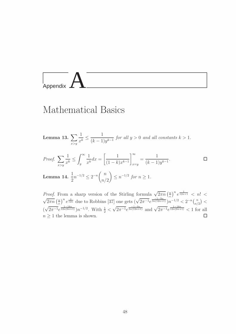
Appendix AMathematical Basics
Lemma 13.∑
x>y
1
xk≤ 1
(k − 1)yk−1for all y > 0 and all constants k > 1.
Proof.∑
x>y
1
xk≤∫ ∞
y
1
xkdx =
[1
(1− k)xk−1
]∞
x=y
=1
(k − 1)yk−1.
Lemma 14.1
2n−1/2 ≤ 2−n
(n
n/2
)
≤ n−1/2 for n ≥ 1.
Proof. From a sharp version of the Stirling formula√
2πn(
ne
)ne
112n+1 < n! <√
2πn(
ne
)ne
112n due to Robbins [37] one gets (
√2π−1e
−1−9n3n(12n+1) )n−1/2 < 2−n
(n
n/2
)<
(√
2π−1e1−18n
12n(6n+1) )n−1/2. With 12
<√
2π−1e−1−9n
3n(12n+1) and√
2π−1e1−18n
12n(6n+1) < 1 for all
n ≥ 1 the lemma is shown.
48
Selbststandigkeitserklarung
Ich versichere, dass ich die Arbeit ohne fremde Hilfe und ohne Benutzung anderer
als der angegebenen Quellen angefertigt habe und dass die Arbeit in gleicher oder
ahnlicher Form noch keiner anderen Prufungsbehorde vorgelegen hat und von
dieser als Teil einer Prufungsleistung angenommen wurde. Alle Ausfuhrungen,
die wortlich oder sinngemaß ubernommen wurden, sind als solche gekennzeichnet.
Jena, den 19. Dezember 2005 . . . . . . . . . . . . . . . . . . . . . . . .(Tobias Friedrich)
49