Embed Size (px)
Citation preview
Development and Analysis of Advanced Explicit Algebraic Turbulence
and Scalar Flux Models for
Complex Engineering Configurations
Vom Fachbereich Maschinenbau an der Technischen Universität Darmstadt
zur Erlangung des Titels eines Doktor-Ingenieurs (Dr.-Ing.)
genehmigte
Dissertation vorgelegt von
Dipl. –Ing. Alexander Yun aus Moskau (Russische Föderation)
Berichterstatter Prof. Dr.-Ing. J. Janicka Mitberichterstatter Prof. Dr.-Ing. B. Stoffel Mitberichterstatter Prof. Dr. rer. nat. A. Sadiki Tag der Einreichung 28.02.2005 Tag der mündlichen Prüfung 20.04.2005
Darmstadt 2005
Acknowledgements
The present work has been done for the last three years during my scientific fellowship in the Institute of Energy and Power Plant Technology, Darmstadt University of Technology and financially supported by the Deutsche Forschungsgemeinschaft through the program “Modellierung und numerische Beschreibung technischer Strömungen”. I would like to express my deep gratitude to my supervisor Prof. Dr.-Ing. Johannes Janicka for introducing me to the big world of turbulence modeling and for his continual encouragement.
Furthermore, I would like to thank Prof. Dr.-Ing. Bernd Stoffel for his willingness to be a co-referent of this work.
An arduous reviewing of this manuscript and many useful suggestions and corrections of Prof. Dr. rer. nat. Amsini Sadiki are gratefully acknowledged.
Many thanks are also extended to Rajani Kumar Akula, Dmitry Goryntsev, Ying Huai and Elena Schneider for reviewing of this manuscript and many helpful discussions.
Many thanks are due to all my colleagues for useful discussions and suggestions as well as their technical and moral support during my time in Darmstadt. They are Andreas Dreizler, Mouldi Chrigui, Jesus Conteras Espada, Markus Klein, Petra Knopp, Andreas Ludwig, Alexander Maltsev, my vice-office mate Sunil Kumar Omar, Bernhard Wegner, Elisabeth Zweyrohn and many other.
Many thanks to my new friends, Anette, Natasha, Olya, Saltanat and Vera for continuously moral support and help to me.
I am grateful to my father for giving me the opportunity to choose my way and for support.
Finally, I would like to thank my wife for her constant support, patience and faith in me.
Alexander Yun Darmstadt, February, 2005
III
Contents Nomenclature V
1. Introduction 1 1.1 Motivation . . . . . . . . . . . . . . . . . . . . 1 1.2 EARSM, EARSFM: State of the art . . . . . . . . . 3 1.3 Objectives and strategy . . . . . . . . . . . . . . 4 2. Physical basics 6 2.1 Balance equations . . . . . . . . . . . . . . . . 6 2.1.1 Mass conservation . . . . . . . . . . . . 6 2.1.2 Momentum conservation . . . . . . . . . 7 2.1.3 Energy and scalar equation . . . . . . . . 9 2.2 Turbulence . . . . . . . . . . . . . . . . . . . . 11 2.2.1 Direct numerical simulation . . . . . . . . 12 2.2.2 Large Eddy simulation . . . . . . . . . . . 13 2.2.3 Simulation based on the statistical averaging 14 3. Modeling approach 16 3.1 Boussinesq approximation . . . . . . . . . . . . . 16 3.2 Nonlinear models . . . . . . . . . . . . . . . . 23 3.3 Explicit algebraic Reynolds stress models . . . . . . 26 3.4 Explicit algebraic scalar flux model . . . . . . . . 34 3.5 Near wall treatment . . . . . . . . . . . . . . . . 38 3.5.1 Wall function . . . . . . . . . . . . . . . 39 3.5.2 Low Reynolds number effects . . . . . . . 41 3.6 Some improvement of EARSM . . . . . . . . . . . 47 3.6.1 Streamline curvature . . . . . . . . . . . 47 3.6.2 Anisotropy dissipation and nonlinear
pressure strain rate . . . . . . . . . . . .
50 3.6.3 Unsteady Reynolds averaged Navier-Stokes
equation . . . . . . . . . . . . . . . . .
52 3.7 Thermodynamically consistence for turbulent models
and realizability . . . . . . . . . . . . . . . . . .
55 4. Numerical procedure 56 4.1 Finite volume method . . . . . . . . . . . . . . . 56 4.2 Coordinate transformation . . . . . . . . . . . . 57 4.3 Discretisation form for diffusion term . . . . . . . . 60 4.4 Discretisation form for convective term . . . . . . . 61 4.5 Discretisation form for unsteady term . . . . . . . 61 4.6 Discretisation form for source term . . . . . . . . 62 4.7 Interpolation methods . . . . . . . . . . . . . . . 64 4.8 General system equations . . . . . . . . . . . . . 66 4.9 Pressure-velocity coupling . . . . . . . . . . . . . 66 4.10 Solution method . . . . . . . . . . . . . . . . . 69 5. Application 72 5.1 Flow in U-duct channel . . . . . . . . . . . . . . 73 5.1.1 Configurations and numerical setup . . . . 73 5.1.2 Results and discussion . . . . . . . . . . 74 5.2 Confined swirled flow . . . . . . . . . . . . . . . 77
IV
5.2.1 Configurations and numerical setup . . . . 78 5.2.2 Results and discussion . . . . . . . . . . 79 5.3 Non-confined swirled flow . . . . . . . . . . . . . 85 5.3.1 Configurations and numerical setup . . . . . 85 5.3.2 Results and discussion . . . . . . . . . . 87 6. Conclusions 92 Bibliography 95 Appendix A: Model governing equations: summary 100 Appendix B: Structure of used models 103
V
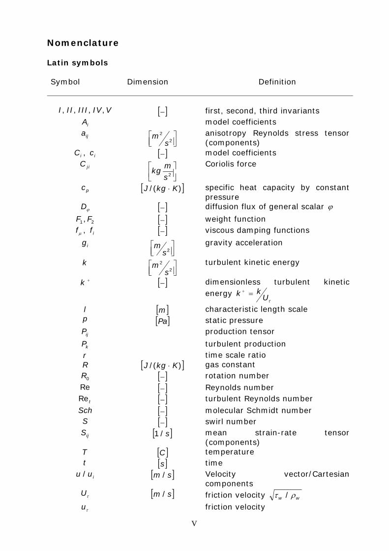
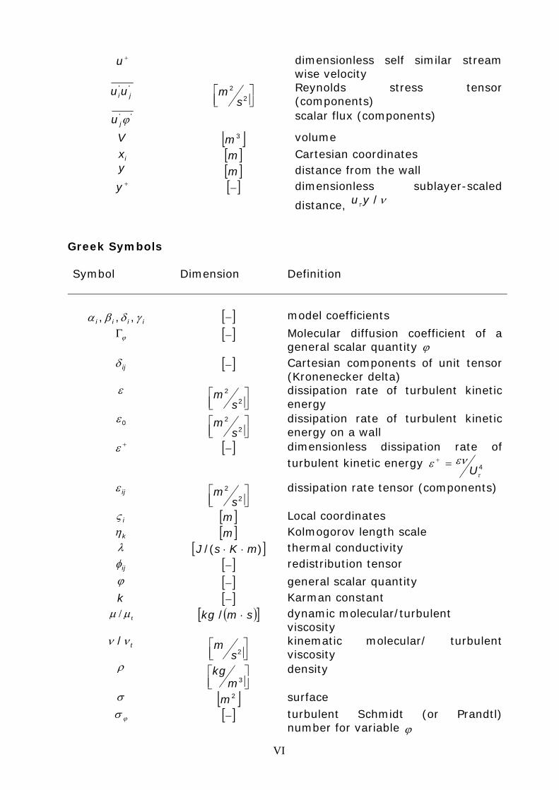
Nomenclature Latin symbols Symbol
Dimension Definition
VIVIIIIII ,,,, [ ]− first, second, third invariants
iA model coefficients
ija ⎥⎦⎤
⎢⎣⎡
2
2
sm
anisotropy Reynolds stress tensor (components)
iC , ic [ ]− model coefficients
jiC ⎥⎦⎤
⎢⎣⎡
2sm
kg Coriolis force
pc [ ])/( KkgJ ⋅ specific heat capacity by constant pressure
ϕD [ ]− diffusion flux of general scalar ϕ
21,FF [ ]− weight function
μf , if [ ]− viscous damping functions
ig ⎥⎦⎤
⎢⎣⎡
2sm
gravity acceleration
k ⎥⎦⎤
⎢⎣⎡
2
2
sm
turbulent kinetic energy
+k [ ]− dimensionless turbulent kinetic energy
τUkk =+
l [ ]m characteristic length scale p [ ]Pa static pressure
ijP production tensor
kP turbulent production r time scale ratio R [ ])/( KkgJ ⋅ gas constant
0R [ ]− rotation number Re [ ]− Reynolds number
tRe [ ]− turbulent Reynolds number Sch [ ]− molecular Schmidt number S [ ]− swirl number
ijS [ ]s/1 mean strain-rate tensor (components)
T [ ]C temperature t [ ]s time
iuu / [ ]sm / Velocity vector/Cartesian components
τU [ ]sm / friction velocity ww ρτ /
τu friction velocity
VI
+u dimensionless self similar stream wise velocity
''jiuu
⎥⎦⎤
⎢⎣⎡
2
2
sm
Reynolds stress tensor (components)
''ϕju scalar flux (components)
V [ ]3m volume
ix [ ]m Cartesian coordinates y [ ]m distance from the wall +y [ ]−
dimensionless sublayer-scaled
distance, ντ /yu Greek Symbols Symbol Dimension Definition
iiii γδβα ,,, [ ]− model coefficients
ϕΓ [ ]− Molecular diffusion coefficient of a general scalar quantity ϕ
ijδ [ ]− Cartesian components of unit tensor (Kronenecker delta)
ε ⎥⎦⎤
⎢⎣⎡
2
2
sm
dissipation rate of turbulent kinetic energy
0ε ⎥⎦⎤
⎢⎣⎡
2
2
sm
dissipation rate of turbulent kinetic energy on a wall
+ε [ ]− dimensionless dissipation rate of turbulent kinetic energy 4
τ
ενεU
=+
ijε
⎥⎦⎤
⎢⎣⎡
2
2
sm
dissipation rate tensor (components)
iς [ ]m Local coordinates
kη [ ]m Kolmogorov length scale λ [ ])/( mKsJ ⋅⋅ thermal conductivity
ijφ [ ]− redistribution tensor ϕ [ ]− general scalar quantity k [ ]− Karman constant
tμμ / ( )[ ]smkg ⋅/ dynamic molecular/turbulent viscosity
tνν / ⎥⎦⎤
⎢⎣⎡
2sm
kinematic molecular/ turbulent viscosity
ρ ⎥⎦⎤
⎢⎣⎡
3mkg
density
σ [ ]2m surface
ϕσ [ ]− turbulent Schmidt (or Prandtl) number for variable ϕ
VII
τ [ ]s turbulent time scale
kτ [ ]s Kolmogorov time scale
ijτ
⎥⎦⎤
⎢⎣⎡
2
2
sm
Reynolds stress tensor (components)
wτ surface shear stress
ijΩ [ ]s/1 mean vorticity tensor (components)
kΩ , iω [ ]s/1 rotation rate ω specific dissipation rate Φ [ ]− general scalar quantity
Operators
Operator Definition
( )⋅ Reynolds averaging
( )⋅div divergence ( )⋅grad gradient
Abbreviations
Abbreviation Definition
AS Abe, Suga CDS Central Difference Scheme CFD Computational Fluid Dynamics CLS Craft, Lauder, Suga CV Control Volume DES Detached Eddy Simulation DH Daly, Harlow DNS Direct Numeric Simulation EARSM Explicit algebraic Reynolds stress model EASFM Explicit algebraic scalar flux model EDC Eddy-dissipation concept EVM Eddy-viscosity model GGDH General gradient-diffusion hypothesis GL Gibson, Launder GS Gatski, Speziale IARSM Implicit algebraic Reynolds stress model KM Kim, Moin LDV Laser Doppler Velocimetry LES Large Eddy Simulation LRR Launder, Reece, Rodi LU Lower-Upper decomposition PVC Precessing Vortex Core RANS Reynolds Averaging based Numerical
Simulations
VIII
RSM Reynolds stress model RSFM Reynolds scalar flux model RST Reynolds stress tensor SJ Sjorgen, Johansson SGS Suga, Gatski and Speziale SIMPLE Semi Implicit Method for Pressure Linked
Equations SIP Strongly Implicit Procedure SMC Second Moment Closure SSG Speziale, Sarkar, Gatski SST Shear Stress Transport UDS Upwind Difference Scheme URANS Unsteady RANS WJ Wallin, Johansson WWJ Wirkstrom, Wallin, Johansson
1
Chapter 1 Introduction 1.1 Motivation
The performance of high-speed computers in last 30 years has sharply
changed the application of fluid mechanics and heat transfer field to find solution of engineering problems. Alongside with development of conventional methods, such as analytical and experimental, numerical methods by means of Computational Fluid Dynamics (CFD) allow to lower essentially the cost and time of design and optimization of flow systems. Notwithstanding the important role of experiments, especially in understanding of complicated flows, the use of computational methods is continuously increasing in designing processes.
The majority of flows of Newtonian fluids in engineering context are turbulent, i.e. unsteady, three dimensional, fluctuating with diffusion and dissipation processes.
To describe such flows, governing equations of mass, momentum, energy and species concentration are used. To solve the resulting system of equations many methods can be used. Direct Numerical Simulation (DNS), that allows to resolve all turbulent structures, requires significant computational resources. As the computational cost for DNS is proportional to
3Re (for example for 100000Re = in a channel flow, DNS needs 122 years for a computer power of 1 Tflops/s [46]), the state-of-the-art computer technologies allows to calculate only turbulent flows of low Reynolds number using economical time. As pointed out in Pope (2000), at high Reynolds numbers over 99 percent of the computational expense of DNS is used to resolve the dissipation range of the turbulent energy spectrum of the flow field. This may be more to resolve the dissipation range of the turbulent scalar energy spectrum for 1≥Sch or 1Pr ≥ as it is dependent on the Schmidt/Prandtl number. However, the energy-containing scales determine most of the flow-dependent transport properties, such as second-order quantities like Reynolds stresses or scalar flux vector. An attempt to overcome the limitation of DNS may be to resolve only the largest (flow-dependent) scales and to model the remaining small scales [79]. This approach is known as Large Eddy Simulation (LES). Therefore they are fully three-dimensional and time-dependent. LES is still relatively expensive. Although the increased accuracy of the characterization of the energy-containing scales with increases of computer power makes LES an attractive method for the future, today LES experiences some modeling and numerical problems (high computer resources, near wall flows, etc.) that do not allow it to be applied widely in the industry. Therefore the third strategy of simulation of turbulent flows, and also the most used in the industry is the Reynolds Averaging based Numerical Simulation (RANS), sometimes called statistical modeling strategy. Applying Reynolds or Favre averaging procedure to the governing equations, it results the so called Reynolds or Favre averaged equations, in which models are needed to express unknown turbulent quantities, appearing in these equations. The computer resources needed and
2
the rising trends in reducing the cost of ownership and shortening the time to design, development and product commercialization will compel this practical way at least for several decades, especially in relation with flows that are strongly affected by viscous near-wall processes. The present work focuses on this practical strategy.
In the literature, there exist different approaches to formulate statistical models needed in the averaged governing equations. They go from the standard model of first order level (Boussinesq approximation) or linear eddy-viscosity/diffusivity models (EVM/EDM) to models of second order, through non-linear or algebraic assumptions [79].
Despite of their inherent capability to account better for the flow physics, the second moment closure (SMC) schemes, recognized as an optimum compromise between the standard but deficient engineering tool (such as k -ε model), and the resolved (in the space and time) computational schemes (DNS or LES), experience a less attractivity in last years. In flow systems exhibiting mass and heat transfer phenomena the coupling between the transport equations for the turbulent quantities of the flow field (Reynolds stress tensor) and the scalar field (scalar flux vector), the number of additional transport equations to be solved increase dramatically. This complexity, together with equations stiffness reduces the practical usage of the SMC models. Recent trends in improving this model are concentrated on various nonlinear models [14], [20] or algebraic models [74], [78] where an attempt is made to account for various effects that can not be represented by means of the linear formulation. The derivation of nonlinear terms in nonlinear or algebraic models can be based on different mathematical or physical principles [19]. For example, renormalization group theory (Rubinstein and Barton 1990), realizability principle (Shih et. al. 1993), rational mechanics (Pope 1975, Taulbee 1993, Gatski and Speziale 1993, Wallin and Johansson 2000) or extended thermodynamics (Sadiki, 2002, 2004).
Non-linear assumptions have the disadvantage to contain a large number of model coefficients and hence a strong sensitivity of the model performance to the coefficient calibration [14]. The algebraic type models offer a compromising route, accounting for most of the physical sounds included in their parent SMC models without adding any additional transport equations [74].
Focused on algebraic modeling methods there have been many proposals for deriving implicit algebraic Reynolds stress/scalar flux models (ARSM/ASFM) and explicit formulation (EARSM/EASFM), either by direct truncation of original differential equations using near equilibrium assumption or by tensor expansions in terms of integrity bases, originated by Pope (1975).
So, various and complex algebraic formulations emerged from the inversion of implicit algebraic form of the Reynolds-stress/Scalar flux transport equations to yield explicit forms (EARSM [74] and EASFM [78]). This model class does not suffer from coefficient calibration weakness, and represents a compromise between the first class mentioned and the parents transport equations. This work will deal with this model class. It must however be mentioned, that turbulent flows are real and irreversible
3
processes. This requires in the modeling that they must fulfill the second law of thermodynamics in their evolution. In relation to ARSM/ASFM this means, that the modeling of the tensor of anisotropy and the scalar flux vector should account for the second law of thermodynamics [56], [57], [58].
Tab. 1.1 summarizes the basic existing strategies of turbulence simulations, in which no account is made for PDF approach [70].
I. DNS account for all structures existing in turbulent flow;
super-high demands to computational resources II. LES compute large structures existing in turbulent flow;
high demands to computational resources III. RANS first order algebraic empirical information, easy to calibrate; attachment to
one kind of flows one equation semi empirical information; easy to calibrate; absence
of many effects, intrinsic turbulent flows two equations simple; intrinsic to Boussinesq approximation,
isotropic eddy-viscosity/diffusivity nonlinear non-isotropic eddy viscosity/diffusivity; account for
many effects, which are taken into account in models of 2-nd order; strong attachment to calibrate modeling coefficients in nonlinear terms
EARSM/EASFM non-isotropic eddy viscosity/diffusivity; contains many effects, which are taken into account in models of 2-nd order, calibration of the modeling coefficients in nonlinear terms taken from the parent 2-nd order models
second order RSM/RSFM required the solution of 6/3 nonlinear equations for
Reynolds stress/scalar flux components, complex
Table 1.1: Basic existing turbulence models classes and simulation strategies.
1.2 EARSM, EASFM: State of the art The most commonly used turbulence model in industry is the standard
k -ε model [29] that has proven its limited performance in many engineering computations. Giving quite accurate predictions in simple two-dimensional shear turbulent flows this model often fails in predicting complex swirled flows. As mentioned above, the nonlinear models have strong attachment to calibrate modeling coefficients [14]. In contrast to nonlinear models, EARSM has not this disadvantage. Originally EARSM was proposed by Pope [50] and later developed by Gatski and Speziale [20]. It was based on the simplification of RSM for steady turbulence by assuming the local equilibrium of Reynolds stresses in the flow. Such approach allows to remove limitations related to simple models, such as isotropy of the eddy viscosity and considers some effects like: rotation, effects of streamline curvature and three-
4
dimensionality of the flow. By the way of this simplification, the transport equation for Reynolds stress tensor is reduced to a system of algebraic equations [52] leading to so-called implicit algebraic Reynolds stress models (IARSM). These can be reformulated by means of the invariant theory [64], [83] in explicit nonlinear form yielding the so-called explicit algebraic Reynolds stress model (EARSM). Their connection to the parents RSM allows to keep advantages related to RSM removing the transport of the Reynolds stress tensor and keeping the production contribution closed. In this way, essential advantage of RSM are presented, so that, a cheap and accurate near wall treatment in flow processes strongly affected by the presence of wall can be performed.
With regard to passive scalar transport the widely used model for passive scalar flux modeling is based on an eddy-dissipation concept (EDC) [53] in analogy to eddy-viscosity assumption. The inclusion of the word “passive” expresses that the scalar is affected by the flow, but in turn does not affect the flow. The linear assumption between the scalar flux vector and the mean scalar gradient has the same disadvantages as EVM. Similar to the explicit Reynolds stress models described above, the scalar flux vector can be obtained by models of the same complexity level and derived in the same way. Dally and Harlow [15] proposed first a general gradient-diffusion hypothesis (GGDH), in which the linear assumption is replaced by the relation of Reynolds stress tensor and mean scalar gradient. In spite of the fact that GGDH has taken further development in works [1], [2], [3], these models do not take into account relevant effects dominating scalar transport. Advanced formulations can be described by constructing special transport equation for scalar flux vector similar to transport equation for Reynolds stress tensor. Accordingly, explicit nonlinear algebraic form for the scalar flux vector can be constructed [78]. This has been studied by several researches, e.g. Adumitroaie et al. 1997, Girimaji and Balachandar 1998 among others.
1.3 Objectives and strategy
The central objective of the present work is the development, analysis and application of efficient and reliable explicit, anisotropy-resolving algebraic turbulence models for simulation of complex turbulent flows dominated with mass and heat transfer processes typical for engineering flow configurations.
In order to illustrate the applicability and performance of the proposed models, various configurations of different complexities have been numerically investigated. Three main application configurations have been chosen:
1. Configurations with confinement to point out near wall effects on the one side, and the prediction of the heat transfer phenomena on the other side. So, in curved ducts (U-duct) of relevance in heat exchangers, cooling passages of gas turbines and automobile engines, turbulent flow and heat transfer give rise to the existence of “camel back” shapes in the streamwise mean velocity and temperature distribution of the curvature [31]. This is not captured by k -ε or nonlinear models [16]. It is hardly predicted by RSM provided some particular corrections are made.
5
2. Configurations with joint effects of confinement and swirl. With regard to design effort, by adjusting the swirl intensity it is possible to improve the mixing quality of the flow and to influence or to control physico-chemical processes. Swirled, confined configurations are used to evaluate the capability of the models in predicting flow properties in internal combustion engines, such as gas turbine combustion chamber, motors or other confined configurations exploiting swirl characteristics. Effects of low ( 45.0=S [51]) and high ( 24.2=S [61]) swirl numbers will be highlighted.
3. Open configurations with swirl to analyze entrainment effects on turbulent structures and turbulent unsteady processes [59]. While enhanced mixing by the swirl is a desirable feature, swirled flows often exhibit hydrodynamic instabilities. For design purposes, it is important to predict such instabilities in terms of peak frequencies, amplitude and ongoing processes.
Different submodels or specific terms of complex models have first been tested in different, academic configurations. For the flow field, there are: (1) square channel flows to retrieve the secondary flows, (2) channel with back-ward-facing step to capture the reattachment point, (3) channel with fence on the wall to capture near wall effects, (4) rotating pipe flow and rotating channel to capture rotations effects, (5) U-channel to capture curvature and unsteady effects. For the scalar field, there are: (1) the free jet to retrieve mixing effects, (2) the ribbed channel to capture heat transfer near the wall, (3) channel with obstacle to capture heat transfer with separated flow.
This work is subdivided as following. The physical basics, necessary for the derivation of the mathematical models, are discussed in chapter 2. Chapter 3 establishes the modeling approach providing the system of governing equations and modeling unclosed terms. In chapter 4 the numerical procedure with details of the model implementation, boundary conditions and error estimation are given. In chapter 5 the applications of models are discussed while concluding remarks are summarized in chapter 6.
6
Chapter 2 Physical basics
For the flow description in many technical devices the abstraction of
continuum mechanics is well applicable. Contrary to the Boltzmann statistical consideration, in continuum mechanics a medium is considered such as the material itself and its physical properties are continuously distributed in space. The part of continuum mechanics that deals with motion of gas or liquid (in contrast to a solid body) is called fluid mechanics. The fundamental equations of fluid mechanics are based on universal laws of conservation: conservation of mass, conservation of momentum and conservation of energy or scalar. Here non-polar fluids are considered. Except some cases, the analytical solution of the above equations is impossible especially in the case of turbulent flows, which are unsteady in nature. Alternative to the analytical solution is solving the equations by using numerical techniques. In engineering applications dominated by turbulent flow processes, Reynolds averaging method is often used, where any instant values of flow parameters are decomposed in an averaged value part and its fluctuation part. After such averaging new unknown correlations (Reynolds stresses/scalar flux) appear, which require modeling.
2.1 Balance equations
2.1.1 Mass conservation The integral form of mass conservation equation is written as:
0=+∂∂
∫∫4342143421
III
V
dnudVt
σρρσ
, (2.1)
where V denotes a fixed (not moving) control volume for which the mass conservation is formulated, σ the surface enclosing this control volume, u the fluid velocity vector and n the unit vector normal to σ and directed outwards. Eq. (2.1) expresses the fact that the mass changes in the fixed volume V (term I) are entirely caused by the mass flow through the volume boundary σ (term II). Using the Gauss divergence theorem the surface integral in term II can be transformed into a volume integral, so that (2.1) becomes
( ) 0=+∂∂
∫∫VV
dVudivdVt
ρρ . (2.2)
7
The differential form of the conservation law of mass in Cartesian coordinates results then as
{
0=∂∂
+∂∂
321II
i
i
I
xu
tρρ
, (2.3)
where the first term represents the unsteady mass density change of the flow and the second term is convective mass density transfer.
For incompressible flows ( 0=∂∂tρ
), the equation of mass conservation is
reduced to
0=∂∂
i
i
xu
. (2.4)
2.1.2. Momentum conservation
Analogously to the continuity equation the momentum conservation equation in integral form can be written as
fdnuudVut V
Σ=+∂∂
∫∫ σρρσ
, (2.5)
where the right side of the equation represents the sum of all forces (surface forces – pressure, normal and shear stress, etc.; body (or volume) forces – gravity, electromagnetic forces, etc.) acting on the fluid control volume. For a single phase flow, it is sufficient to consider only the stresses as surface force and the gravity as body force:
∫∫∫∫∫ ++−=+∂∂
VV
dVgdndnpdnuudVut
ρστσσρρσσσ
, (2.6)
where g is the gravity acceleration vector and τ is the stress tensor that represents the microscopic or molecular momentum flux across the surface. Applying the Gauss divergence theorem on the equation (2.6) for surface integrals and allowing the control volumes to become infinitely small one can write the differential form of the momentum conservation equation
{
{ngravitatio
i
diffusion
j
ij
gradientpressure
i
convective
j
ji
ssunsteadine
i gxx
px
uu
tu
ρτρρ
+∂
∂+
∂∂
−=∂
∂+
∂∂
32143421321 . (2.7)
8
For Newtonian fluids, the stresses based on Stokes hypothesis [70] are represented as
ijк
к
j
i
i
iij x
uxu
xu
δμμτ∂∂
−⎟⎟⎠
⎞⎜⎜⎝
⎛
∂∂
+∂∂
=32
, (2.8)
with ijδ - Kronecker delta ( 0;1 =→≠=→= ijij jiji δδ ).
In case of flow in rotating system, the Coriolis ( )u×Ω−r
2 and the
centrifugal acceleration ( )xr
×Ω×Ω− must be added. Eq. (2.7) is transformed in following form
**
fxx
px
uu
tu
j
ij
ij
jii +∂
∂+
∂∂
−=∂
∂+
∂∂ τρρ
, (2.9)
where the quantity pressure *p
( )( ) ( )( )ккiiккii xxxxpp ΩΩ+ΩΩ−=∗ ρρ 5050 .. (2.10)
while body force with Coriolis acceleration is кjijкii ueff Ω−=∗ ρ2 . (2.11)
ijкe is the permutation tensor defined as
⎪⎩
⎪⎨
⎧=−=
=elsewhere
,,ijkfor,,ijkfor
eijк
03211322131
3122311231. (2.12)
In view of eq. (2.8), the equation for the conservation law of
momentum emerges in the following form:
iijк
к
j
i
i
i
jij
jii gxu
xu
xu
xxp
x
uu
tu
ρδμμρρ
+⎥⎥⎦
⎤
⎢⎢⎣
⎡
∂∂
−⎟⎟⎠
⎞⎜⎜⎝
⎛
∂∂
+∂∂
∂∂
+∂∂
−=∂
∂+
∂∂
32
, (2.13)
mostly known as Navier-Stockes equation.
For incompressible flows with constant viscosity, Navier-Stockes equation reduced to
ijj
i
ij
ij
i gxx
uxp
xu
utu
+∂∂
∂+
∂∂
−=∂∂
+∂∂ 21
ρμ
ρ. (2.14)
9
2.1.3 Energy and scalar equations
Many turbulent flow processes of engineering importance exhibit highly complex interacting phenomena, such as mixing, heat and mass transfer, chemical reaction, etc. All of the involving quantities: energy, enthalpy, temperature or mass fraction of species, are scalar quantities. Similar to conservation equations, balance equation for scalar in the integral form is
ϕσ
σρϕρϕ fdnudVt V
Σ=⋅+∂∂
∫∫ , (2.15)
here ϕ represents any scalar, ϕf denotes contributions representing transport
of ϕ by mechanisms other than convection, such as sources and sinks of ϕ . For a single phase flow, it is sufficient to consider only diffusive transport and source term. Diffusive transport is always present additionally to the convective one. One gets then from (2.15)
∫∫∫∫ +⋅=⋅+∂∂
VV
dVSdnDdnudVt ϕ
σϕ
σ
σσρϕρϕr
. (2.16)
Similarly to the molecular rate of momentum (2.8) the diffusive flux ϕD
of heat or mass is described by means of Fourier’s or Fick’s law, respectively. These laws represent a gradient approximation and are generally written as
ϕϕϕ gradD Γ= , (2.17)
here ϕΓ is either the heat or mass diffusivity coefficient for the scalar ϕ .
Substituting the diffusive flux (2.17) into expression (2.16) using the Gauss divergence theorem and after taking the control volume to be infinitely small, the differential form for scalar equation can be written as
ϕϕϕρ
ϕρϕρ S
xxxu
t jii
i +⎟⎟⎠
⎞⎜⎜⎝
⎛
∂∂
Γ∂∂
=∂∂
+∂∂
. (2.18)
The diffusion coefficient ϕΓ generally is expressed, as a ratio of viscosity
ν and Schmidt (Prandtl) number:
ϕ
φ σν
=Γ . (2.19)
Setting TC p=ϕ , the same form has the differential equation of the
conservation of energy and is given by:
Sx
u
xq
x
Tcu
t
Tc
j
iij
i
i
i
pip +∂
∂+
∂∂
−=∂
∂+
∂
∂ τρρ , (2.20)
10
here pc is specific heat capacity at constant pressure, T temperature, iq
heat transfer determined by the Fourier’s law i
i xT
q∂∂
−= λ , λ is heat
conductivity. The last two quantities in (2.20) are the dissipation of energy and source term, respectively.
To characterize the heat transfer processes, the so-called Nusselt number is usually introduced
λα 0l
Nul
k == , (2.21)
where kq is the heat transfer by convection, lq the heat transfer by conductivity, α the heat transfer coefficient and 0l the characteristic length. The quantity kq is defined by
( )Gk TTx
q −= 11
λ (2.22)
and lq by
( )Gml TTl
q −=0
λ, (2.23)
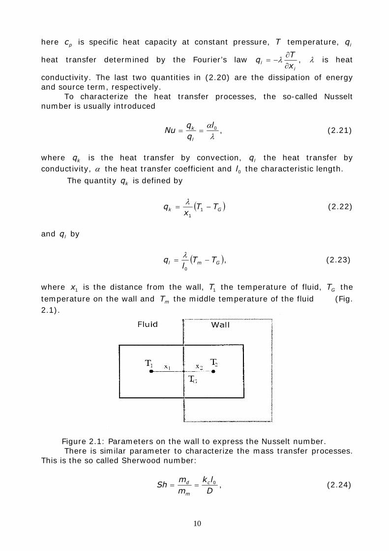
where 1x is the distance from the wall, 1T the temperature of fluid, GT the temperature on the wall and mT the middle temperature of the fluid (Fig. 2.1).
Figure 2.1: Parameters on the wall to express the Nusselt number. There is similar parameter to characterize the mass transfer processes.
This is the so called Sherwood number:
Dlk
mm
Sh c
m
d 0== , (2.24)
11
where dm is the mass transfer by mass diffusivity, mm the mass transfer by molecular diffusivity, ck the overall mass transfer coefficient, D the diffusion coefficient and 0l the characteristic length.
2.2 Turbulence
The majority of flow of Newtonian fluids in technical applications are rather turbulent than laminar. Peter Bradshaw in his introduction to the book «Turbulence» wrote that: «the one uncontroversial fact about turbulence is that it is the most complicated kind of fluid motion».
Since 1883, following Osborne Reynolds it is possible to characterize the state of flow by the Reynolds number Re:
ν
00Reul ⋅
= . (2.25)
Here 0l is a typical length, 0u a typical bulk velocity and ν the kinematic
viscosity. The Reynolds number expresses the ratio between the inertial and viscous (or molecular) forces. If this ratio is small the viscous (or molecular) forces are comparable to the inertial forces and the flow keeps its regular structure (laminar flow). If the ratio becomes large the viscous forces do not suffice to compensate inertial forces. The flow becomes unstable and small initial perturbations destroy the regular flow structure leading to the turbulence (turbulent flow). Turbulent flows can be imagined as collections of eddies. Turbulence increases the rate at which conserved quantities are stirred. I. e. parcels of fluid with different contents of conserved quantity (momentum, energy, concentration, etc) are brought into contact. This is often called turbulent mixing or turbulent diffusion. The molecular viscosity reduces velocity gradients causing destruction of the turbulent eddies and dissipation of the flow kinetic energy into internal energy of the fluid. The bigger eddies dissipate into smaller ones transferring the kinetic energy of turbulent fluctuations. This process, first revealed by Kolmogorov [38], is called energy cascade. A reverse process when small eddies build a bigger one is also possible and is called back scattering.
Recent investigations have shown the existence in turbulent flows of coherent structures repeatable and essentially of deterministic character. The random part dominating in turbulent flows causes these events to differ in size, strength and time interval between occurrences. There are, however, some flows that feature coherent structures with clear periodicity, and certain frequency can be referred to such a periodical motion. To summarize, it appears clearly that turbulent flows are
- randomly in time and space, - unsteady, - three dimensional, - dissipative, - vortical.
12
It is possible to describe the turbulent motion by laws of probability following a probability density function (PDF) approach [53]. In this work, averaged values of various quantities (velocity, pressure, density, etc.) of the flow are solely needed. For this purpose, different approaches are also feasible, going from DNS, LES to URANS and RANS.
2.2.1 Direct numerical simulation (DNS) Direct numerical simulation (DNS) assumes the solution of full Navier-Stokes equations and other balance equations. This means that there is no additional modeling. In fact, all physically and chemically important length and time scales as shown in Fig. 2.2 must be resolved on the computational grid and in time. This, of course, restricts enormously the size of computational cell and time steps. These requirements essentially surpass the modern computer powers for flows with high Reynolds numbers.
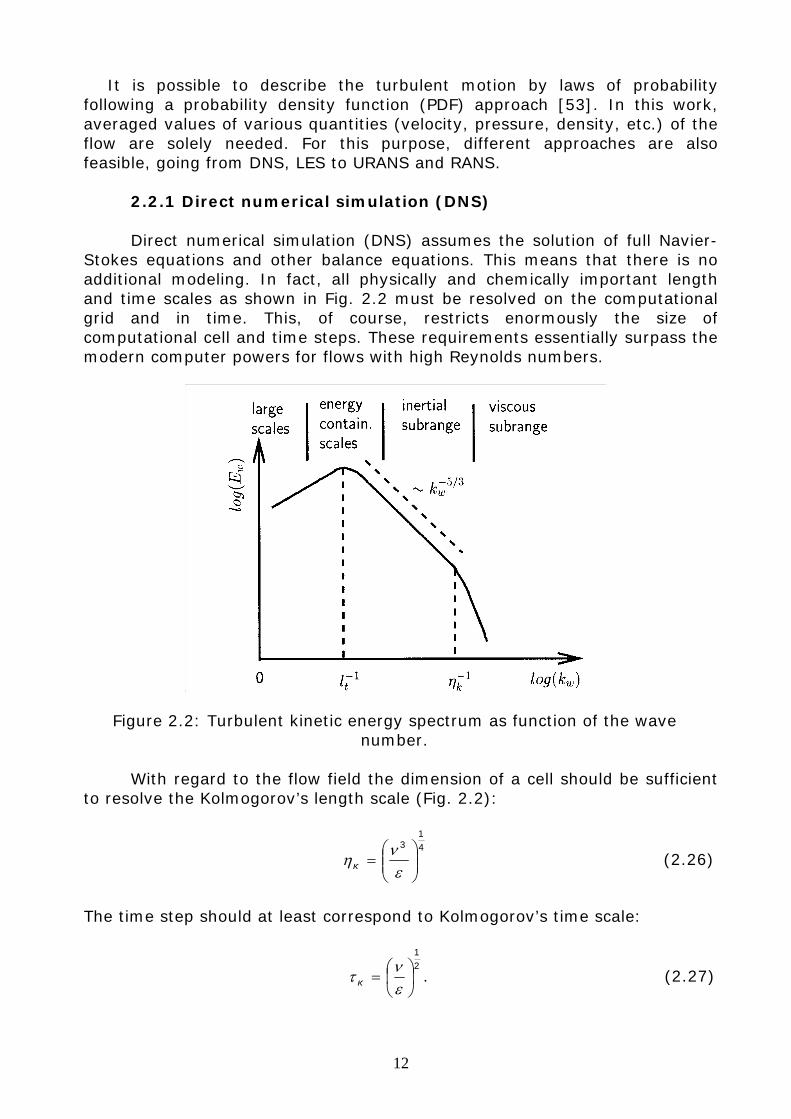
Figure 2.2: Turbulent kinetic energy spectrum as function of the wave number.
With regard to the flow field the dimension of a cell should be sufficient
to resolve the Kolmogorov’s length scale (Fig. 2.2):
41
3
⎟⎟⎠
⎞⎜⎜⎝
⎛=
ενηк (2.26)
The time step should at least correspond to Kolmogorov’s time scale:
21
⎟⎠⎞
⎜⎝⎛=εντ к . (2.27)
13
Based on Taylor hypothesis one can show that the ratio between the large and the small length scales is
43
Re≈k
tlη
. (2.28)
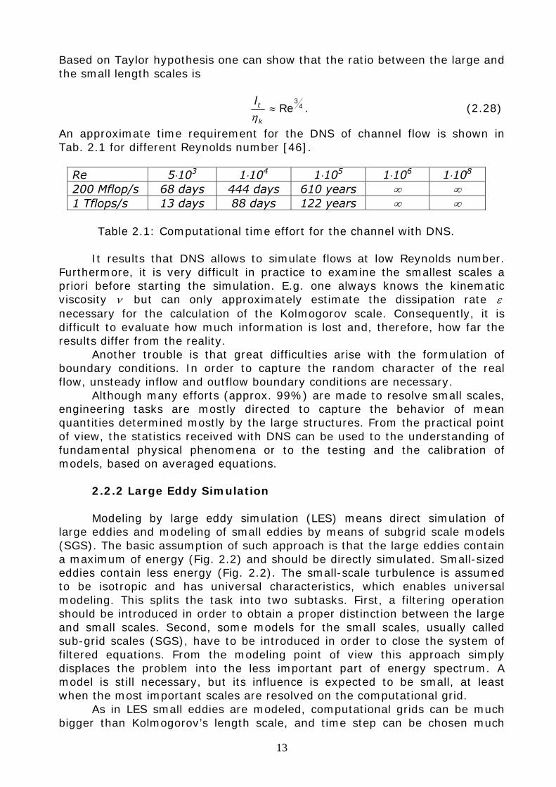
An approximate time requirement for the DNS of channel flow is shown in Tab. 2.1 for different Reynolds number [46].
Re 5⋅103 1⋅104 1⋅105 1⋅106 1⋅108 200 Mflop/s 68 days 444 days 610 years ∞ ∞ 1 Tflops/s 13 days 88 days 122 years ∞ ∞
Table 2.1: Computational time effort for the channel with DNS.
It results that DNS allows to simulate flows at low Reynolds number. Furthermore, it is very difficult in practice to examine the smallest scales a priori before starting the simulation. E.g. one always knows the kinematic viscosity ν but can only approximately estimate the dissipation rate ε necessary for the calculation of the Kolmogorov scale. Consequently, it is difficult to evaluate how much information is lost and, therefore, how far the results differ from the reality. Another trouble is that great difficulties arise with the formulation of boundary conditions. In order to capture the random character of the real flow, unsteady inflow and outflow boundary conditions are necessary.
Although many efforts (approx. 99%) are made to resolve small scales, engineering tasks are mostly directed to capture the behavior of mean quantities determined mostly by the large structures. From the practical point of view, the statistics received with DNS can be used to the understanding of fundamental physical phenomena or to the testing and the calibration of models, based on averaged equations.
2.2.2 Large Eddy Simulation Modeling by large eddy simulation (LES) means direct simulation of large eddies and modeling of small eddies by means of subgrid scale models (SGS). The basic assumption of such approach is that the large eddies contain a maximum of energy (Fig. 2.2) and should be directly simulated. Small-sized eddies contain less energy (Fig. 2.2). The small-scale turbulence is assumed to be isotropic and has universal characteristics, which enables universal modeling. This splits the task into two subtasks. First, a filtering operation should be introduced in order to obtain a proper distinction between the large and small scales. Second, some models for the small scales, usually called sub-grid scales (SGS), have to be introduced in order to close the system of filtered equations. From the modeling point of view this approach simply displaces the problem into the less important part of energy spectrum. A model is still necessary, but its influence is expected to be small, at least when the most important scales are resolved on the computational grid. As in LES small eddies are modeled, computational grids can be much bigger than Kolmogorov’s length scale, and time step can be chosen much
14
bigger than in DNS. So the requirements of computing resources for LES are much lower than for DNS. With the rapid development of computer facilities the area of application of LES is considerably increasing. There are some assumptions that LES in next decade will surpass RANS. Such point of view is rather disputable. Till now, in LES the problem of wall flows is not solved. It is obvious, that near the wall all vortexes are small so that both the space and time steps required for LES drop up to values of characteristic DNS. Existing solutions, such as anisotropic filters and dynamic procedures, yet do not give satisfactory results. One of solutions for this wall problem for LES is the combination of LES and RANS, so-called isolated LES – DES (Detached eddy simulation) [71]. In DES, RANS is used near the wall zone, and LES is used away from the wall. But also here there are problems of connecting these zones. Therefore, research is still needed for both LES part and RANS part. This work may contribute to RANS approach.
2.2.3 Simulation based on the statistical averaging
For technical applications, more useful solution of the fluid equations are based on the solution of Reynolds averaged equations. For this purpose any instant values of hydrodynamic parameters are represented by the mean value f and its fluctuating value 'f (Fig. 2.3 (b)): ( ) ( ) ( )txftxftxf iii
',, += , (2.29)
. where, the mean value f can be obtained from a statistical averaging. It may be, for instance, an ensemble averaging that is taken over a sufficiently large number N of experiments having the same initial and boundary conditions:
( ) ( )∑=
=N
nini xtf
Nxtf
1
,1
, (2.30)
In case of quasi-steady or stationary random turbulent flow field (i.e. no
regular coherent structure is present in the flow) (Fig. 2.3 (a)) the simple time averaging is suitable
( ) ( )∫=1
01
,1 t
ii dtxtft
xf (2.31)
with 1t being a sufficiently large period of time. Equation (2.31) will provide the same results as the ensemble averaging (2.30). However the mean value depends only on the spatial coordinate ix but is not a function of time t .
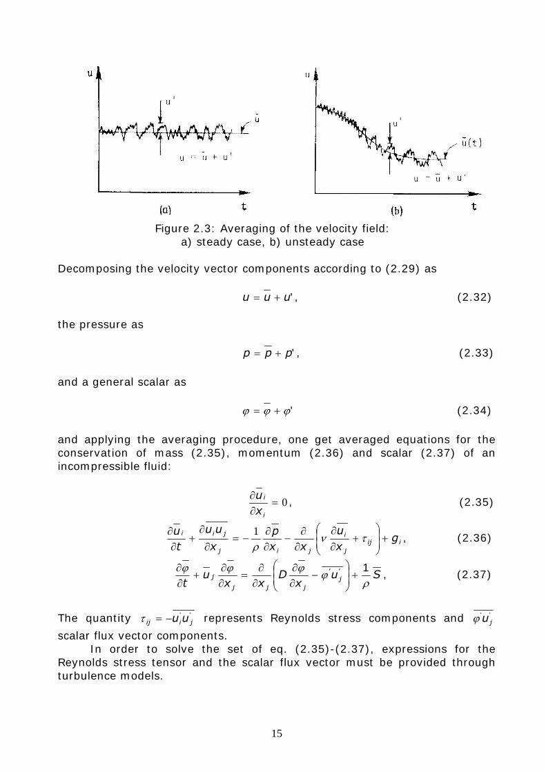
15
Figure 2.3: Averaging of the velocity field:
a) steady case, b) unsteady case Decomposing the velocity vector components according to (2.29) as
'uuu += , (2.32)
the pressure as
'ppp += , (2.33)
and a general scalar as
'ϕϕϕ += (2.34)
and applying the averaging procedure, one get averaged equations for the conservation of mass (2.35), momentum (2.36) and scalar (2.37) of an incompressible fluid:
0=∂∂
i
i
xu
, (2.35)
iijj
i
jij
jii gxu
xxp
x
uu
tu
+⎟⎟⎠
⎞⎜⎜⎝
⎛+
∂∂
∂∂
−∂∂
−=∂
∂+
∂∂ τν
ρ1
, (2.36)
Sux
Dxx
ut
'j
'
jjj
jρ
ϕϕϕϕ 1+⎟
⎟⎠
⎞⎜⎜⎝
⎛−
∂∂
∂∂
=∂∂
+∂∂
, (2.37)
The quantity ''jiij uu−=τ represents Reynolds stress components and ''
juϕ
scalar flux vector components. In order to solve the set of eq. (2.35)-(2.37), expressions for the
Reynolds stress tensor and the scalar flux vector must be provided through turbulence models.
16
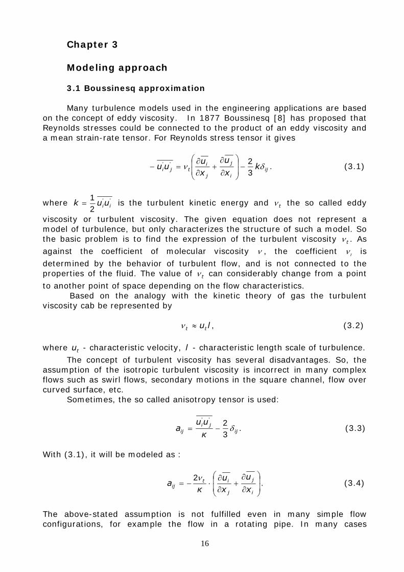
Chapter 3 Modeling approach 3.1 Boussinesq approximation
Many turbulence models used in the engineering applications are based on the concept of eddy viscosity. In 1877 Boussinesq [8] has proposed that Reynolds stresses could be connected to the product of an eddy viscosity and a mean strain-rate tensor. For Reynolds stress tensor it gives
iji
j
j
itji k
x
u
xu
uu δν32'' −
⎟⎟
⎠
⎞
⎜⎜
⎝
⎛
∂
∂+
∂∂
=− . (3.1)
where ''
21
iiuuk = is the turbulent kinetic energy and tν the so called eddy
viscosity or turbulent viscosity. The given equation does not represent a model of turbulence, but only characterizes the structure of such a model. So the basic problem is to find the expression of the turbulent viscosity tν . As against the coefficient of molecular viscosity ν , the coefficient tν is
determined by the behavior of turbulent flow, and is not connected to the properties of the fluid. The value of tν can considerably change from a point
to another point of space depending on the flow characteristics. Based on the analogy with the kinetic theory of gas the turbulent viscosity cab be represented by lutt ≈ν , (3.2)
where tu - characteristic velocity, l - characteristic length scale of turbulence.
The concept of turbulent viscosity has several disadvantages. So, the assumption of the isotropic turbulent viscosity is incorrect in many complex flows such as swirl flows, secondary motions in the square channel, flow over curved surface, etc.
Sometimes, the so called anisotropy tensor is used:
ijji
ij к
uua δ
32''
−= . (3.3)
With (3.1), it will be modeled as :
⎟⎟
⎠
⎞
⎜⎜
⎝
⎛
∂
∂+
∂∂
⋅−=i
j
j
itij x
u
xu
кa
ν2. (3.4)
The above-stated assumption is not fulfilled even in many simple flow configurations, for example the flow in a rotating pipe. In many cases
17
especially the analysis of flow in which the basic influence on the mean flow is provided only by one of the components of Reynolds stress tensor - shear stress components xyτ , the disadvantage of the hypothesis of Boussinesq does
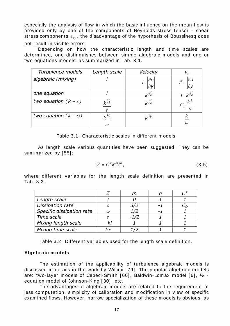
not result in visible errors. Depending on how the characteristic length and time scales are
determined, one distinguishes between simple algebraic models and one or two equations models, as summarized in Tab. 3.1.
Turbulence models Length scale Velocity tν
algebraic (mixing) l yu
l∂∂
⋅ yu
l∂∂
⋅2
one equation l 21
k 21
kl ⋅ two equation ( ε−k )
ε
23
k
21
k εμ
2kC
two equation ( ω−k )
ω
21
k
21
k ωk
Table 3.1: Characteristic scales in different models.
As length scale various quantities have been suggested. They can be
summarized by [55]: nmz lkCZ = , (3.5)
where different variables for the length scale definition are presented in Tab. 3.2.
Z m n zC Length scale l 0 1 1 Dissipation rate ε 3/2 -1 CD
Specific dissipation rate ω 1/2 -1 1 Time scale τ -1/2 1 1 Mixing length scale kl 1 1 1 Mixing time scale τk 1/2 1 1
Table 3.2: Different variables used for the length scale definition.
Algebraic models The estimation of the applicability of turbulence algebraic models is discussed in details in the work by Wilcox [79]. The popular algebraic models are: two-layer models of Cebeci-Smith [60], Baldwin-Lomax model [6], ½ - equation model of Johnson-King [30], etc. The advantages of algebraic models are related to the requirement of less computation, simplicity of calibration and modification in view of specific examined flows. However, narrow specialization of these models is obvious, as
18
they are based on the empirical information about the structures of defined flows. The algebraic models assume the local balance of the simulated turbulence. It means that in each point of space the balance of generation and dissipation of turbulent energy is observed, on which the transfer from the next points and previous development of process do not influence. Thus algebraic models are inapplicable in cases with dominant influence of convective and diffusion transfer of turbulence or when a dominant role is played by the prehistory of the process. Besides, the large difficulty for complex flows represents the task of distributions of the mixing length. One equation models
To overcome the limitation of a mixing-length hypothesis and algebraic models new turbulence models were developed, which allow to take into account of the transfer of turbulence by introducing a differential equation for this transfer.
There are similar models with one equation, which use the transport equations for the turbulent kinetic energy (Bradshaw, Ferriss, Atwell) [9], for the turbulent viscosity (Nee, Kovasznay [49], Spalart–Allmaras [63]) and several other models [79].
The models with one differential equation have the greater acceptability of the description of compressible turbulent, transition phenomena, curvature and flow separations. However, the objects of their applications are simple flow configurations. As well as in case of algebraic models, the binding to calibrating types of flows is strong. To remove these specified restrictions, it is possible, for example, to define the scale of turbulence as dependent variable, i.e. construction of the additional transport equation. Two equations models
Most used turbulence models in engineering application for the
simulations of turbulent flows are the models with two differential equations. A first model was proposed by Kolmogorov (1942) [38]. This model contains the transport equation for the turbulent kinetic energy k , and the specific dissipation rate ω .
Another popular model in industry with two differential equations is the k -ε model which was suggested by Chou (1945) [13] and came to further developments in the contribution of Jones-Launder (1972) [29].
The models of turbulence such as ε−k model better describe properties of shear flows and the models of a ( ω−k ) type have advantages at modeling near wall flows. Basing on it, Menter (1993) has proposed model combining the specified strong sides of ε−k and ω−k models. For this purpose the
ε−k model was reformulated in the terms k and ω , and then a weight function 1F is entered in the final equation, providing smooth transition from
ω−k model in the wall area to ε−k model far from a wall. Thus, the model of Menter is written by a superposition of ω−k and ε−k models, multiplied accordingly by a weight function 1F and ( )11 F− . The function constructs 1F to be equal one on the upper boundary of a boundary layer and aspires to zero as it approaches the wall. Besides, Menter has changed the standard relation
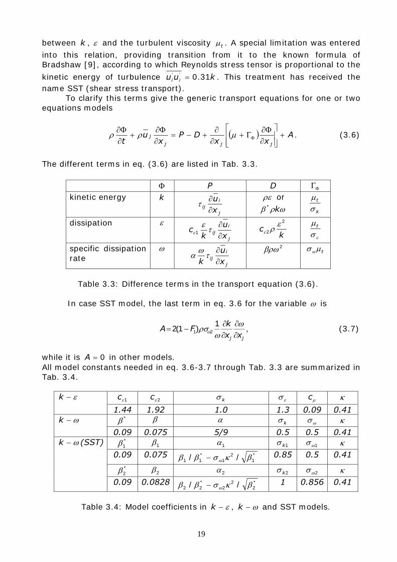
19
between k , ε and the turbulent viscosity tμ . A special limitation was entered into this relation, providing transition from it to the known formula of Bradshaw [9], according to which Reynolds stress tensor is proportional to the
kinetic energy of turbulence kuu ii 31.0'' = . This treatment has received the name SST (shear stress transport).
To clarify this terms give the generic transport equations for one or two equations models
( ) Axx
DPx
ut jjj
j +⎥⎥⎦
⎤
⎢⎢⎣
⎡
∂Φ∂
Γ+∂∂
+−=∂Φ∂
+∂Φ∂
Φμρρ . (3.6)
The different terms in eq. (3.6) are listed in Tab. 3.3.
Φ P D ΦΓ kinetic energy k
j
iij x
u∂∂τ
ρε or ωρβ k* k
t
σμ
dissipation ε
j
iij x
uk
c∂∂τεε1
kc
2
2
ερε εσ
μt
specific dissipation rate
ω
j
iij x
uk ∂
∂τωα 2βρω tμσω
Table 3.3: Difference terms in the transport equation (3.6).
In case SST model, the last term in eq. 3.6 for the variable ω is
jj xx
kFA
∂∂
∂∂
−=ω
ωρσω
1)1(2 21 , (3.7)
while it is 0=A in other models. All model constants needed in eq. 3.6-3.7 through Tab. 3.3 are summarized in Tab. 3.4.
1εc 2εc kσ εσ μc κ ε−k
1.44 1.92 1.0 1.3 0.09 0.41 *β β α kσ ωσ κ ω−k
0.09 0.075 5/9 0.5 0.5 0.41 *1β 1β 1α 1kσ 1ωσ κ
0.09 0.075 *1
21
*11 // βκσββ ω− 0.85 0.5 0.41
*2β 2β 2α 2kσ 2ωσ κ
ω−k (SST)
0.09 0.0828 *2
22
*22 // βκσββ ω− 1 0.856 0.41
Table 3.4: Model coefficients in ε−k , ω−k and SST models.
20
Other model constants for the SST model are found as superposition of the constants in Tab. 3.4 and a weight function. Denoting the generalized parameter 1φ with a set of constants of the original model ω−k with index 1 and accordingly 2φ with similar set of constants of a transformed ε−k model, it is possible to get
( ) 2111 1 φφφ FF −+= , (3.8)
where the weight function is determined as follows )tanh(arg4
11 =F . (3.9)
⎥⎥⎦
⎤
⎢⎢⎣
⎡⎟⎟⎠
⎞⎜⎜⎝
⎛=
22
2*1
4;
500;maxminarg
yCDk
yyk
kω
ωρσων
ωβ, (3.10)
⎪⎩
⎪⎨⎧
⎪⎭
⎪⎬⎫
∂∂
∂∂
= −202 10,
12max
jjk xx
kCD
ωω
ρσωω , (3.11)
According to the theory of Bradshaw the shear stress in a boundary layer is proportional to the kinetic energy
ka1ρτ = , (3.12) where 1a is constant. Furthermore, in models with two equations the shear stresses are calculated following
Ω= tμτ , (3.13)
where yu∂∂
=Ω .
To satisfy the Bradshaw equation in the boundary the coefficient of the turbulent viscosity should be redefined as follows:
Ω
=ka
t1ν . (3.14)
To extend the formulation of the eddy viscosity for free shear layers to situations where the Bradshaw proposal is not necessarily applied, the SST-model was updated for flows limited to wall configurations. For this purpose mixing function 2F is introduced in (3.14), so that
( )21
1
,max Faka
t Ω=
ων , (3.15)
where 2F is determined according to (3.11) as
( )222 argtanh=F , (3.16)
21
⎥⎦
⎤⎢⎣
⎡=
ωνω
22
500;09,0/2maxarg
yyk , (3.17)
New constants considered in an internal layer are
31.0;//;41.0
;5.0;85.0;075.0;09.0
1*2
1*
11
111*
=−==
====
a
k
βκσββγκ
σσββ
ω
ω
They did not vary in an external layer. As it can be recognized, near wall correction can be introduced at any level of modeling to better capture near wall effects in most quantities close to solid wall. These formulations are commonly called Low-Reynolds number correction. They are usually based on local Reynolds number introduced to decrease in the proximity of walls. Different formulations of Low-Reynolds models will be presented in section 3.5.2.
To illustrate the performance limitations alluded above, results of simulation of a flow over a backward-facing step [42], [82] with ε−k , ω−k and two-layer models are presented and discussed. For these flow simulations near the wall the wall functions are used (section 3.5.1).
This and other simulations in this work were performed using CFD-package FASTEST-3D. More details about the program FASTEST-3D are given in chapter 4.
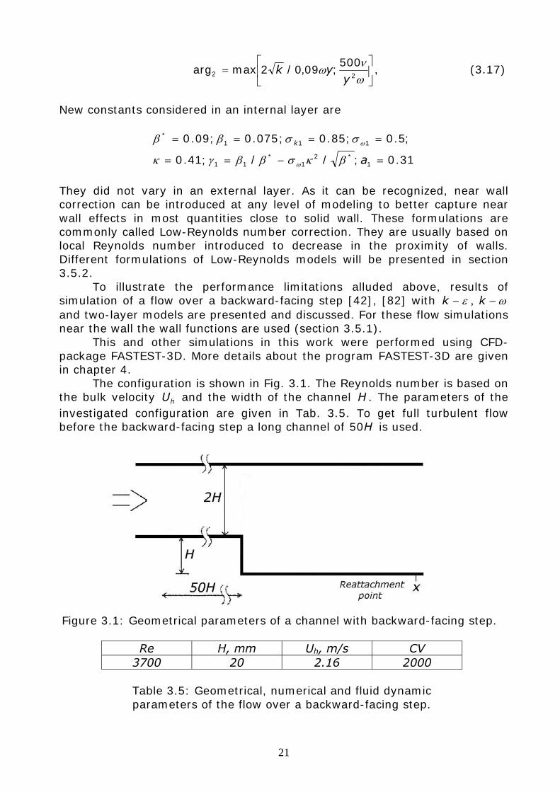
The configuration is shown in Fig. 3.1. The Reynolds number is based on the bulk velocity hU and the width of the channel H . The parameters of the investigated configuration are given in Tab. 3.5. To get full turbulent flow before the backward-facing step a long channel of H50 is used.
Figure 3.1: Geometrical parameters of a channel with backward-facing step.
Re H, mm Uh, m/s CV 3700 20 2.16 2000
Table 3.5: Geometrical, numerical and fluid dynamic parameters of the flow over a backward-facing step.
22
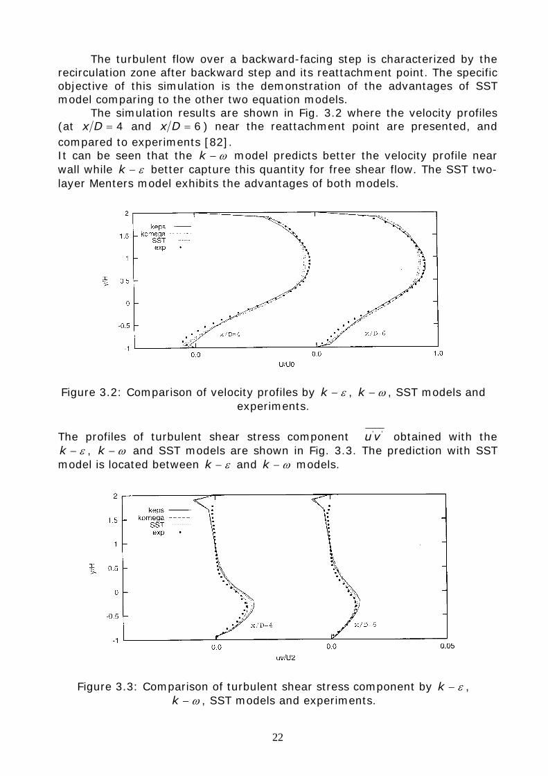
The turbulent flow over a backward-facing step is characterized by the recirculation zone after backward step and its reattachment point. The specific objective of this simulation is the demonstration of the advantages of SST model comparing to the other two equation models.
The simulation results are shown in Fig. 3.2 where the velocity profiles (at 4=Dx and 6=Dx ) near the reattachment point are presented, and compared to experiments [82]. It can be seen that the ω−k model predicts better the velocity profile near wall while ε−k better capture this quantity for free shear flow. The SST two-layer Menters model exhibits the advantages of both models.
Figure 3.2: Comparison of velocity profiles by ε−k , ω−k , SST models and experiments.
The profiles of turbulent shear stress component ''vu obtained with the ε−k , ω−k and SST models are shown in Fig. 3.3. The prediction with SST
model is located between ε−k and ω−k models.
Figure 3.3: Comparison of turbulent shear stress component by ε−k , ω−k , SST models and experiments.
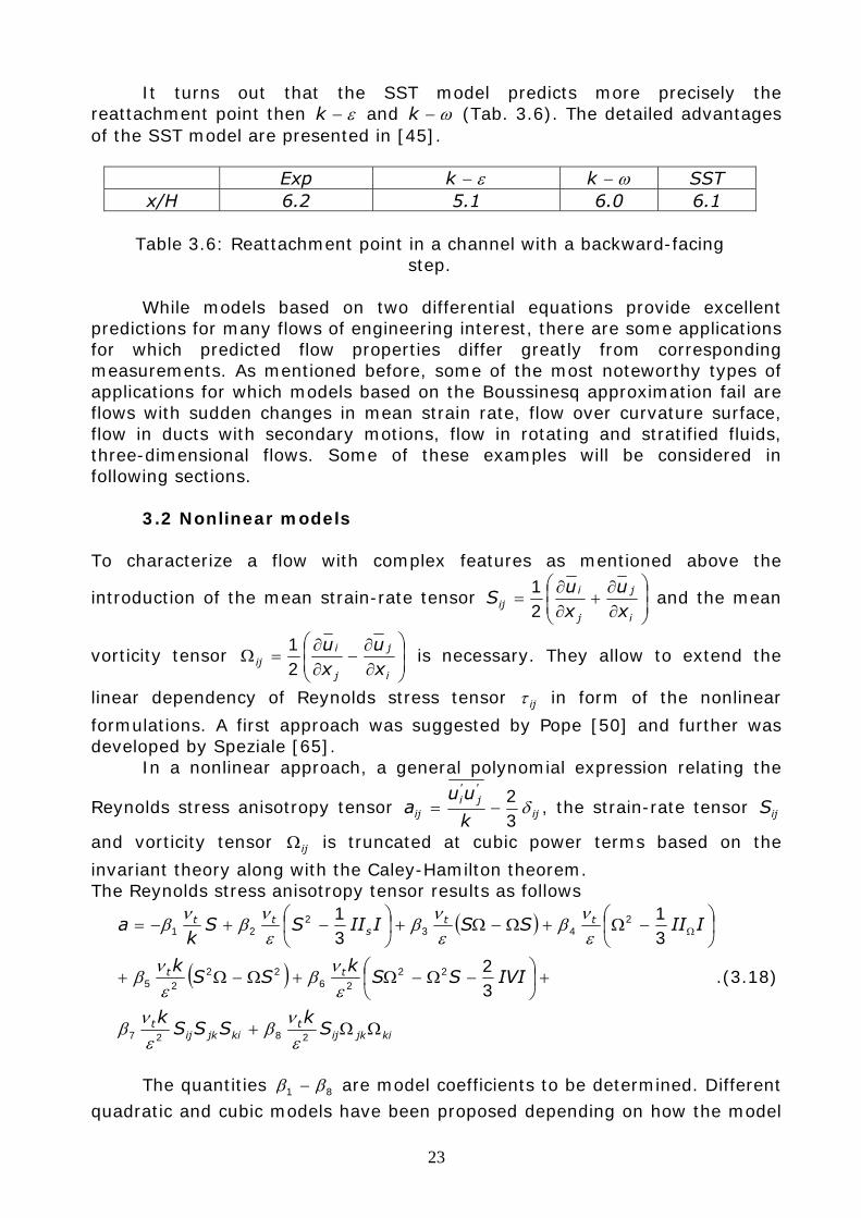
23
It turns out that the SST model predicts more precisely the reattachment point then ε−k and ω−k (Tab. 3.6). The detailed advantages of the SST model are presented in [45].
Exp ε−k ω−k SST
x/H 6.2 5.1 6.0 6.1
Table 3.6: Reattachment point in a channel with a backward-facing step.
While models based on two differential equations provide excellent
predictions for many flows of engineering interest, there are some applications for which predicted flow properties differ greatly from corresponding measurements. As mentioned before, some of the most noteworthy types of applications for which models based on the Boussinesq approximation fail are flows with sudden changes in mean strain rate, flow over curvature surface, flow in ducts with secondary motions, flow in rotating and stratified fluids, three-dimensional flows. Some of these examples will be considered in following sections.
3.2 Nonlinear models
To characterize a flow with complex features as mentioned above the
introduction of the mean strain-rate tensor ⎟⎟⎠
⎞⎜⎜⎝
⎛
∂∂
+∂∂
=i
j
j
iij x
uxu
S21
and the mean
vorticity tensor ⎟⎟⎠
⎞⎜⎜⎝
⎛
∂∂
−∂∂
=Ωi
j
j
iij x
uxu
21
is necessary. They allow to extend the
linear dependency of Reynolds stress tensor ijτ in form of the nonlinear
formulations. A first approach was suggested by Pope [50] and further was developed by Speziale [65]. In a nonlinear approach, a general polynomial expression relating the
Reynolds stress anisotropy tensor ij
'j
'i
ij k
uua δ
32
−= , the strain-rate tensor ijS
and vorticity tensor ijΩ is truncated at cubic power terms based on the
invariant theory along with the Caley-Hamilton theorem. The Reynolds stress anisotropy tensor results as follows
( )
( )
kijkijt
kijkijt
tt
tts
tt
Sk
SSSk
IVISSk
SSk
IIISSIIISSk
a
ΩΩ+
+⎟⎠⎞
⎜⎝⎛ −Ω−Ω+Ω−Ω+
⎟⎠⎞
⎜⎝⎛ −Ω+Ω−Ω+⎟
⎠⎞
⎜⎝⎛ −+−= Ω
2827
2226
2225
243
221
32
31
31
εν
βεν
β
εν
βεν
β
εν
βεν
βεν
βν
β
.(3.18)
The quantities 81 ββ − are model coefficients to be determined. Different
quadratic and cubic models have been proposed depending on how the model
24
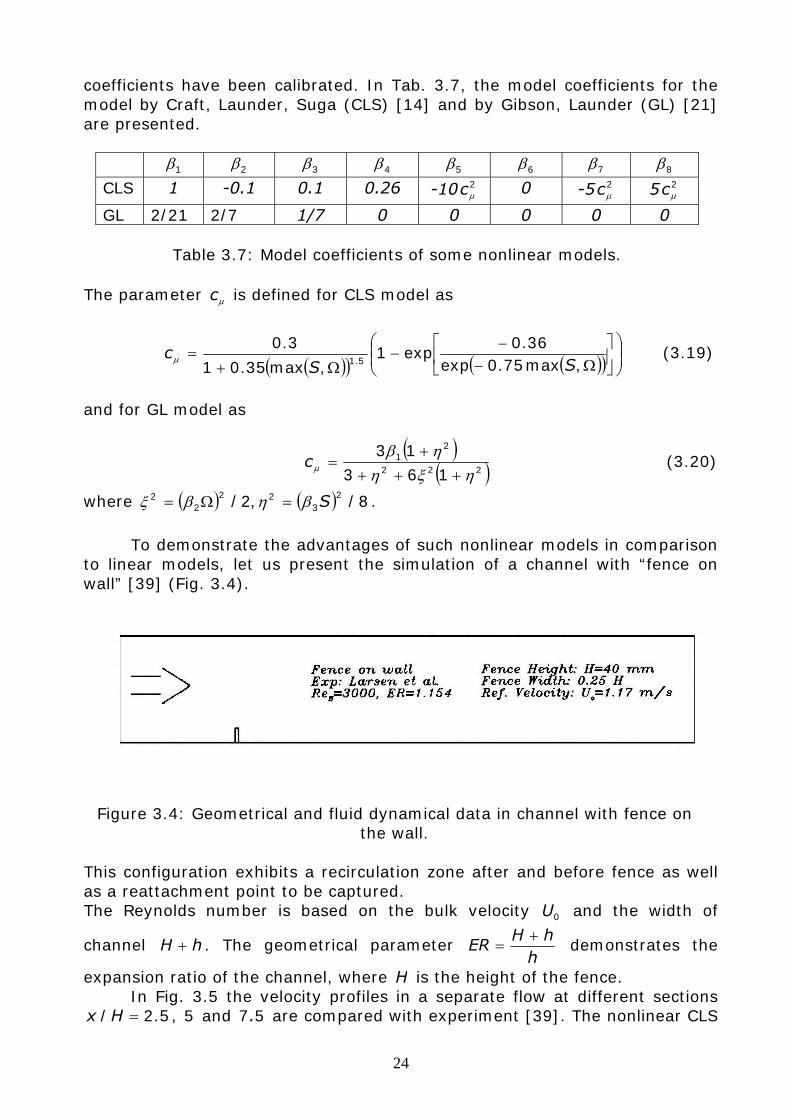
coefficients have been calibrated. In Tab. 3.7, the model coefficients for the model by Craft, Launder, Suga (CLS) [14] and by Gibson, Launder (GL) [21] are presented.
1β 2β 3β 4β 5β 6β 7β 8β
CLS 1 -0.1 0.1 0.26 -10 2μc 0 -5 2
μc 5 2μc
GL 2/21 2/7 1/7 0 0 0 0 0
Table 3.7: Model coefficients of some nonlinear models. The parameter μc is defined for CLS model as
( )( ) ( )( ) ⎟⎟
⎠
⎞⎜⎜⎝
⎛⎥⎦
⎤⎢⎣
⎡Ω−
−−
Ω+=
,max75.0exp36.0
exp1,max35.01
3.05.1 SS
cμ (3.19)
and for GL model as
( )
( )222
21
163
13
ηξηηβ
μ ++++
=c (3.20)
where ( ) ( ) 8/,2/ 23
222
2 Sβηβξ =Ω= . To demonstrate the advantages of such nonlinear models in comparison to linear models, let us present the simulation of a channel with “fence on wall” [39] (Fig. 3.4).
Figure 3.4: Geometrical and fluid dynamical data in channel with fence on
the wall.
This configuration exhibits a recirculation zone after and before fence as well as a reattachment point to be captured. The Reynolds number is based on the bulk velocity 0U and the width of
channel hH + . The geometrical parameter h
hHER
+= demonstrates the
expansion ratio of the channel, where H is the height of the fence. In Fig. 3.5 the velocity profiles in a separate flow at different sections
5.2/ =Hx , 5 and 57. are compared with experiment [39]. The nonlinear CLS
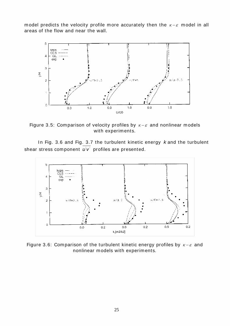
25
model predicts the velocity profile more accurately then the ε−к model in all areas of the flow and near the wall.
Figure 3.5: Comparison of velocity profiles by ε−к and nonlinear models with experiments.
In Fig. 3.6 and Fig. 3.7 the turbulent kinetic energy k and the turbulent
shear stress component ''vu profiles are presented.
Figure 3.6: Comparison of the turbulent kinetic energy profiles by ε−к and nonlinear models with experiments.
26
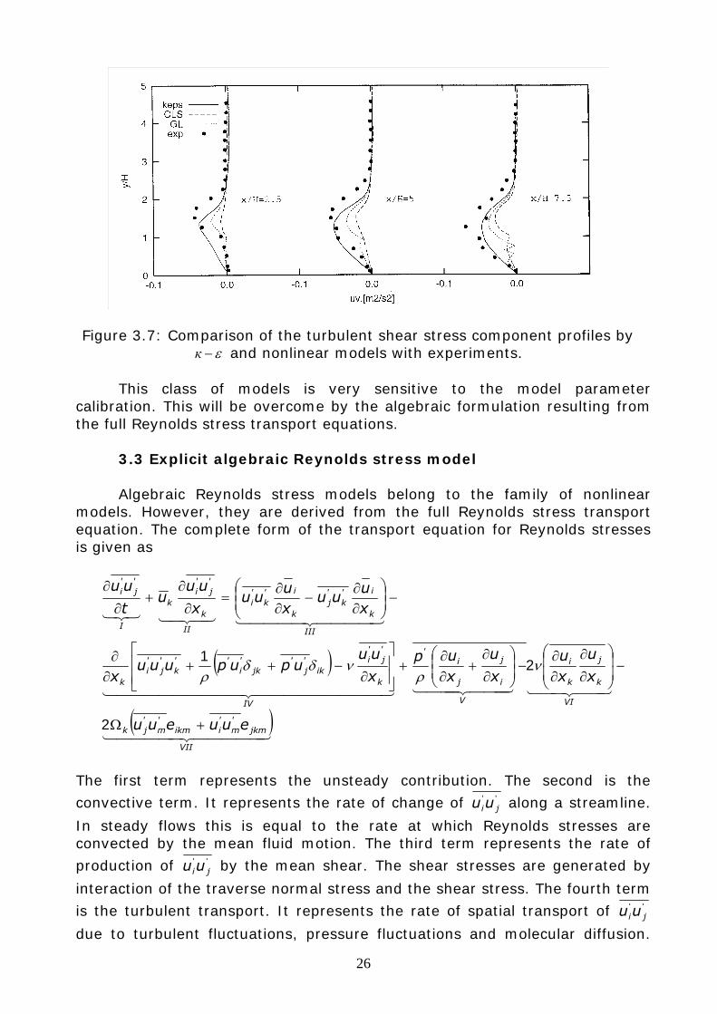
Figure 3.7: Comparison of the turbulent shear stress component profiles by ε−к and nonlinear models with experiments.
This class of models is very sensitive to the model parameter calibration. This will be overcome by the algebraic formulation resulting from the full Reynolds stress transport equations.
3.3 Explicit algebraic Reynolds stress model Algebraic Reynolds stress models belong to the family of nonlinear models. However, they are derived from the full Reynolds stress transport equation. The complete form of the transport equation for Reynolds stresses is given as
( )
( )44444 344444 21
44 344 21444 3444 21444444444 3444444444 21
4444 34444 2143421321
VII
jkm'm
'iikm
'm
'jk
VI
k
j
k
i
V
i
j
j
i'
IV
k
'j
'i
ik'j
'jk
'i
''k
'j
'i
k
III
k
i'k
'j
k
i'k
'i
II
k
'j
'i
k
I
'j
'i
euueuu
x
u
xu
x
u
xup
x
uuupupuuu
x
xu
uuxu
uux
uuu
t
uu
+Ω
−⎟⎟
⎠
⎞
⎜⎜
⎝
⎛
∂
∂
∂∂
−⎟⎟⎠
⎞⎜⎜⎝
⎛
∂
∂+
∂∂
+⎥⎥⎦
⎤
⎢⎢⎣
⎡
∂−++
∂∂
−⎟⎟⎠
⎞⎜⎜⎝
⎛
∂∂
−∂∂
=∂
∂+
∂
∂
2
21 ν
ρνδδ
ρ
The first term represents the unsteady contribution. The second is the
convective term. It represents the rate of change of ''jiuu along a streamline.
In steady flows this is equal to the rate at which Reynolds stresses are convected by the mean fluid motion. The third term represents the rate of
production of ''jiuu by the mean shear. The shear stresses are generated by
interaction of the traverse normal stress and the shear stress. The fourth term
is the turbulent transport. It represents the rate of spatial transport of ''jiuu
due to turbulent fluctuations, pressure fluctuations and molecular diffusion.
27
The fifth is the redistribution term, which is also called the pressure-strain term. It represents the redistribution of the available turbulent kinetic energy among the fluctuating velocity components. The sixth term represents the
dissipation rate of ''jiuu due to molecular viscous action, while the seventh is
the Coriolis term in case of rotational system coordinates. It is similarly possible to write down the transfer equation for the anisotropy tensor, according to [74]. It can be presented as
ijijijijjilji
l
ljiij CPP
k
uu
xku
k
uu
x
uuu
Dt
Dak++−+⎟
⎠⎞
⎜⎝⎛ −=⎟
⎟
⎠
⎞
⎜⎜
⎝
⎛
∂∂
−∂
∂∂−
εφ
εε
εεεε1
'''''''
. (3.22)
Here P represents the production (k
ikj
k
ikiij x
uuu
xu
uuP∂∂
−∂∂
−= '''' , 2/ijPP = ), ijε is
the dissipation, ijφ the pressure-strain rate and ijC the Coriolis contribution.
The dissipation rate tensor ijε and the redistribution tensor ijφ need to be
modeled. The production ijP and 2/ijPP = and the Coriolis term ijC do not
need any modeling since they can be calculated directly from the Reynolds stress tensor.
Many inhomogeneous flows of engineering interest are steady flows and satisfy the weak equilibrium assumption. In this case it is possible to neglect the advection and diffusion terms. It is the basic idea of Algebraic Reynolds Stress Model (ARSM). This is written as
0'''''
=⎟⎟
⎠
⎞
⎜⎜
⎝
⎛
∂∂
−∂
∂∂−
xku
k
uu
x
uuu
Dt
Dak lji
l
ljiij
εε. (3.23)
Thus in ARSM, the isotropic turbulent viscosity assumption in models
using the Boussinesq assumption is replaced by some assumptions of the local
balance of ''jiuu , whose reliability is quite obvious for many flows. The
advection term Dt
Daij equals exactly zero for all stationary parallel mean flows,
such as fully developed channel and pipe flows. For inhomogeneous flows the assumption of negligible diffusion effects can cause problems, particularly in regions where the production term is small or where the inhomogenity is strong. However, ARSM assumption includes effects of rotation, streamlines curvature and three-dimensionality of the flows.
In view of the above-stated implicit algebraic form of the equation, one can write
ijijijijji C
PPk
uu++−=⎟
⎠⎞
⎜⎝⎛ −
εφ
εε
εε1
''
. (3.24)
28
In (3.24) the dissipation rate tensor ijε and the redistribution tensor ijφ should
be modeled. For the present modeling purpose the dissipation rate tensor is assumed to be isotropic. Because the dissipation occurs at the smallest scales, most modelers use the Kolmogorov hypothesis of local isotropy. Here the quantity normalized by the dissipation rate ε is written as
ijij δεε
32
= , (3.25)
where k
i
k
i
xu
xu
∂∂
∂∂
=''
νε . Since the dissipation is in reality anisotropic, particularly
close to solid boundaries, some efforts have been made to model this effect. The anisotropy of the dissipation will be considered in section 3.6.2.
The pressure strain redistribution term is usually modeled in two subparts, slow s
ijφ and rapid rijφ redistribution terms:
r
ijsijij φφφ += . (3.26)
According to reference [41] the slow redistribution rate can be
considered linear in terms of the anisotropy tensor:
ij
sij aC1−=εφ
, (3.27)
where 1C - model constant. For the rapid redistribution rate the linear model by Launder, Reece and Rodi (LRR) [27], [41] is generally chosen. It is written as
( )kjikkjikijkmkmkjikkjikij
rij aa
CSaaSSa
CS **22
11107
32
1169
54
Ω−Ω−
+⎟⎠⎞
⎜⎝⎛ −+
++= δ
εφ
,
where *
kjΩ is the absolute mean vorticity tensor:
s
ijij*kj Ω+Ω=Ω , (3.28)
including beside ijΩ the system rotation s
ijΩ . Nonlinear relations for the pressure strain redistribution term will be considered in section 3.6.2.
Substituting already modeled terms the following implicit form can be then obtained from
29
( )
⎟⎠⎞
⎜⎝⎛ −+
−−
Ω−Ω+
+−=⎟⎠⎞
⎜⎝⎛ +−
kiikijkjikkjik
kjikkjikijij
SaaSSaC
aaC
SaP
С
δ
ε
32
1195
1117
158
1
2
21
or
( ) ⎟⎠⎞
⎜⎝⎛ −+−Ω−Ω+−=⎟
⎠⎞
⎜⎝⎛ + kiikijkjikkjikkjikkjikijij SaaSSaAaaSAa
PAA δ
ε 32
2143 ,
where ( )( )
1711
,17111
,17
95,
171188
24
2
13
2
22
21 +
=+−
=+
−=
+=
CA
CC
AC
CA
CA are model
coefficients. In more compact (matrix) form it can be written as
( ) ( ) ⎟⎠
⎞⎜⎝
⎛ −+−Ω−Ω+−= IaStraceSaaSAaaSANa32
21 , (3.31)
where εP
AAN 43 += . The values of modeling coefficients in eq. (3.30), (3.31)
are given in Tab. 3.8.
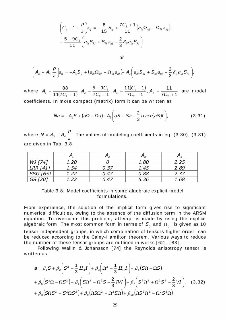
1A 2A 3A 4A
WJ [74] 1.20 0 1.80 2.25 LRR [41] 1.54 0.37 1.45 2.89 SSG [65] 1.22 0.47 0.88 2.37 GS [20] 1.22 0.47 5.36 1.68
Table 3.8: Model coefficients in some algebraic explicit model
formulations.
From experience, the solution of the implicit form gives rise to significant numerical difficulties, owing to the absence of the diffusion term in the ARSM equation. To overcome this problem, attempt is made by using the explicit algebraic form. The most common form in terms of ijS and ijΩ is given as 10
tensor independent groups, in which combination of tensors higher order can be reduced according to the Caley-Hamilton theorem. Various ways to reduce the number of these tensor groups are outlined in works [62], [83].
Following Wallin & Johansson [74] the Reynolds anisotropy tensor is written as
( )
( )( ) ( ) ( )ΩΩ−ΩΩ+ΩΩ−ΩΩ+Ω−Ω+
⎟⎠⎞
⎜⎝⎛ −Ω+Ω+⎟
⎠⎞
⎜⎝⎛ −Ω−Ω+Ω−Ω+
Ω−Ω+⎟⎠⎞
⎜⎝⎛ −Ω+⎟
⎠⎞
⎜⎝⎛ −+= Ω
222210
229
2228
22227
226
225
42
32
21
32
32
31
31
SSSSSSSS
VISSIVISSSS
SSIIIIIISSa s
βββ
βββ
ββββ
, (3.32)
30
where ⎟⎟⎠
⎞⎜⎜⎝
⎛
∂∂
+∂∂
=i
j
j
iij x
uxu
S2τ
, ⎟⎟⎟
⎠
⎞
⎜⎜⎜
⎝
⎛
∂
∂−
∂∂
=Ωixju
jxiu
ij 2τ
are here normalized by means
of the turbulent time scale, ε
τ k= . For simplification, in the following the
notations ijaa = , ijSS = , ijΩ=Ω will be used. The coefficients iβ are
functions of five independent invariants of S and Ω :
jkkjjkij
kijkij
kijkij
jiij
ijijs
SSSV
SSIV
SSSSIII
II
SSSII
ΩΩ=Ω=
ΩΩ=Ω=
==
ΩΩ=Ω=
==
Ω
22
2
3
2
2
(3.33)
Solving together equations (3.31) and (3.32) it is possible to find out the unknown coefficients iβ and the Reynolds stresses anisotropy tensor. Let us mention that for two-dimensional mean flows the cubic terms in eq. (3.32) vanish. According to [74], coefficients β are then given for 2D-flows by
Ω−
−=IIN
NA22
11β ,
Ω−−=
IINA221
4β . (3.34)
Eq. (3.31) can be simplified to the following form
( )aaSANa Ω−Ω+−= 1 , (3.35) and (3.32) to ( )SSSa Ω−Ω+= 41 ββ . (3.36) By substituting (3.34) to (3.36) and (3.36) to (3.35) it can be got a third order algebraic equation in terms of N :
( ) 022 341
23
3 =Ω++−− Ω IIANIIAANAN . (3.37) Solution obtained is:
⎩⎨⎧
<≥
=00
22
21
PforNPforN
N , (3.38)
with
( ) ( ) 31
21216
1
213
1 3PPPPsignPP
AN +++++= (3.39)
31
and
( )⎟⎟⎟
⎠
⎞
⎜⎜⎜
⎝
⎛
⎟⎟
⎠
⎞
⎜⎜
⎝
⎛
−−+=
22
1
161
22
13
2 arccos31
cos23 PP
PPP
AN , (3.40)
where
341
23
1 32
627AIIII
AAAP s ⎟⎟
⎠
⎞⎜⎜⎝
⎛−+= Ω , (3.41)
3
41232
12 32
39 ⎟⎟⎠
⎞⎜⎜⎝
⎛++−= ΩIIII
AAAPP s . (3.42)
After solving (3.37) the unknown coefficients iβ in (3.34) can be found along with the Reynolds stresses anisotropy tensor ija from (3.36). For three-
dimensional cases, solutions are described in detail in [74], [75]. Examining the thermodynamical consistency of this kind of modeling,
Sadiki et al. (2004) [56] pointed out that the behavior of the model coefficients plays a great role. For quadratic type models sufficient to retrieve secondary streamlines, they found namely that the coefficients: 12 ββ ≥ .
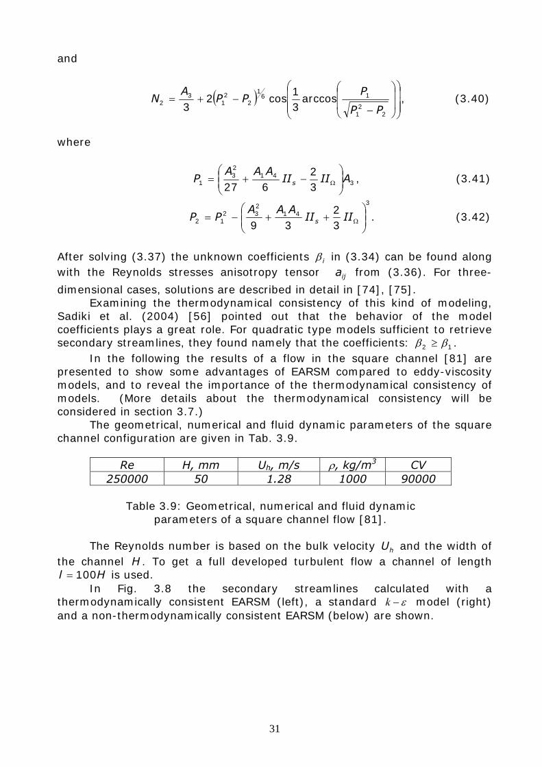
In the following the results of a flow in the square channel [81] are presented to show some advantages of EARSM compared to eddy-viscosity models, and to reveal the importance of the thermodynamical consistency of models. (More details about the thermodynamical consistency will be considered in section 3.7.)
The geometrical, numerical and fluid dynamic parameters of the square channel configuration are given in Tab. 3.9.
Re H, mm Uh, m/s ρ, kg/m3 CV
250000 50 1.28 1000 90000
Table 3.9: Geometrical, numerical and fluid dynamic parameters of a square channel flow [81].
The Reynolds number is based on the bulk velocity hU and the width of
the channel H . To get a full developed turbulent flow a channel of length Hl 100= is used.
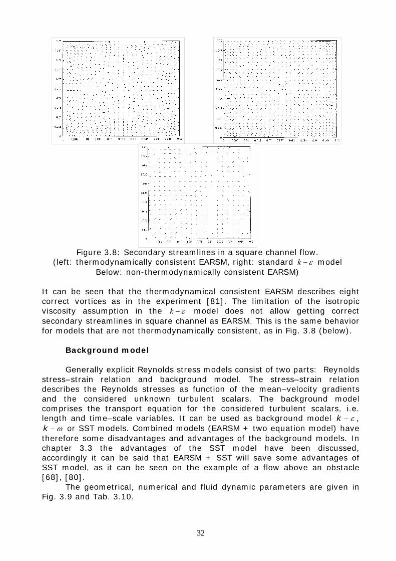
In Fig. 3.8 the secondary streamlines calculated with a thermodynamically consistent EARSM (left), a standard ε−k model (right) and a non-thermodynamically consistent EARSM (below) are shown.
32
Figure 3.8: Secondary streamlines in a square channel flow.
(left: thermodynamically consistent EARSM, right: standard ε−k model Below: non-thermodynamically consistent EARSM)
It can be seen that the thermodynamical consistent EARSM describes eight correct vortices as in the experiment [81]. The limitation of the isotropic viscosity assumption in the ε−k model does not allow getting correct secondary streamlines in square channel as EARSM. This is the same behavior for models that are not thermodynamically consistent, as in Fig. 3.8 (below).
Background model
Generally explicit Reynolds stress models consist of two parts: Reynolds stress–strain relation and background model. The stress–strain relation describes the Reynolds stresses as function of the mean–velocity gradients and the considered unknown turbulent scalars. The background model comprises the transport equation for the considered turbulent scalars, i.e. length and time–scale variables. It can be used as background model ε−k ,
ω−k or SST models. Combined models (EARSM + two equation model) have therefore some disadvantages and advantages of the background models. In chapter 3.3 the advantages of the SST model have been discussed, accordingly it can be said that EARSM + SST will save some advantages of SST model, as it can be seen on the example of a flow above an obstacle [68], [80].
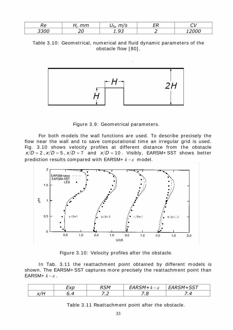
The geometrical, numerical and fluid dynamic parameters are given in Fig. 3.9 and Tab. 3.10.
33
Re H, mm Uh, m/s ER CV 3300 20 1.93 2 12000
Table 3.10: Geometrical, numerical and fluid dynamic parameters of the
obstacle flow [80].
Figure 3.9: Geometrical parameters. For both models the wall functions are used. To describe precisely the
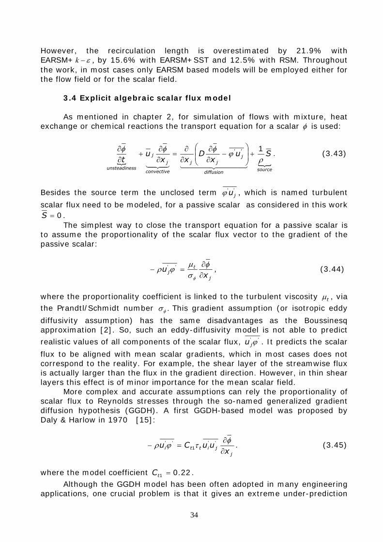
flow near the wall and to save computational time an irregular grid is used. Fig. 3.10 shows velocity profiles at different distance from the obstacle
2=Dx , 5=Dx , 7=Dx and 10=Dx . Visibly, EARSM+SST shows better prediction results compared with EARSM+ ε−k model.
Figure 3.10: Velocity profiles after the obstacle. In Tab. 3.11 the reattachment point obtained by different models is
shown. The EARSM+SST captures more precisely the reattachment point than EARSM+ ε−k .
Exp RSM EARSM+ ε−k EARSM+SST
x/H 6.4 7.2 7.8 7.4
Table 3.11 Reattachment point after the obstacle.
34
However, the recirculation length is overestimated by 21.9% with EARSM+ ε−k , by 15.6% with EARSM+SST and 12.5% with RSM. Throughout the work, in most cases only EARSM based models will be employed either for the flow field or for the scalar field.
3.4 Explicit algebraic scalar flux model
As mentioned in chapter 2, for simulation of flows with mixture, heat exchange or chemical reactions the transport equation for a scalar φ is used:
{ {
sourcediffusion
'j
'
jj
convective
j
j
ssunsteadine
Sux
Dxx
ut ρ
ϕφφφ 1+⎟
⎟⎠
⎞⎜⎜⎝
⎛−
∂∂
∂∂
=∂∂
+∂∂
444 3444 2143421
. (3.43)
Besides the source term the unclosed term ''juϕ , which is named turbulent
scalar flux need to be modeled, for a passive scalar as considered in this work 0=S .
The simplest way to close the transport equation for a passive scalar is to assume the proportionality of the scalar flux vector to the gradient of the passive scalar:
j
tj x
u∂∂
=−φ
σμ
ϕρφ
'' , (3.44)
where the proportionality coefficient is linked to the turbulent viscosity tμ , via the Prandtl/Schmidt number φσ . This gradient assumption (or isotropic eddy
diffusivity assumption) has the same disadvantages as the Boussinesq approximation [2]. So, such an eddy-diffusivity model is not able to predict
realistic values of all components of the scalar flux, ''ϕju . It predicts the scalar
flux to be aligned with mean scalar gradients, which in most cases does not correspond to the reality. For example, the shear layer of the streamwise flux is actually larger than the flux in the gradient direction. However, in thin shear layers this effect is of minor importance for the mean scalar field. More complex and accurate assumptions can rely the proportionality of scalar flux to Reynolds stresses through the so-named generalized gradient diffusion hypothesis (GGDH). A first GGDH-based model was proposed by Daly & Harlow in 1970 [15]:
j
jitti xuuCu
∂∂
=−φτϕρ ''
1'' . (3.45)
where the model coefficient 22.01 =tC .
Although the GGDH model has been often adopted in many engineering applications, one crucial problem is that it gives an extreme under-prediction
35
of the streamwise scalar flux jx∂
∂φ even in simple wall-shear flows. Considering
that the scalar fluctuation in the wall-shear region correlates more strongly with the streamwise velocity fluctuation than with the wall-normal one, Kim & Moin (KM) (1989) [36] proposed some improvements of the DH model:
j
'j
'k
'k
'i
tt''
i xk
uuuuCu
∂∂
⎟⎟
⎠
⎞
⎜⎜
⎝
⎛=−
φτϕρ 2 . (3.46)
Abe & Suga (AS) (2000) [3], [69] combined both models to get the expression:
j
jkkit
jitti xk
uuuuC
k
uuCku
∂∂
⎟⎟
⎠
⎞
⎜⎜
⎝
⎛+=−
φτϕρ2
''''
2
''
1'' , (3.47)
where the model coefficients are 2201 .Ct = and 4502 .Ct = .
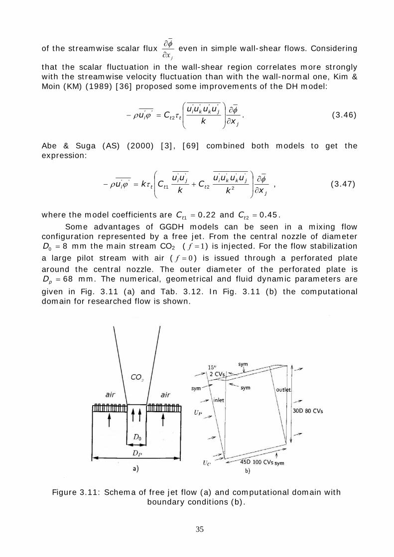
Some advantages of GGDH models can be seen in a mixing flow configuration represented by a free jet. From the central nozzle of diameter
80 =D mm the main stream CO2 ( 1=f ) is injected. For the flow stabilization a large pilot stream with air ( 0=f ) is issued through a perforated plate around the central nozzle. The outer diameter of the perforated plate is
68=pD mm. The numerical, geometrical and fluid dynamic parameters are
given in Fig. 3.11 (a) and Tab. 3.12. In Fig. 3.11 (b) the computational domain for researched flow is shown.
Figure 3.11: Schema of free jet flow (a) and computational domain with boundary conditions (b).
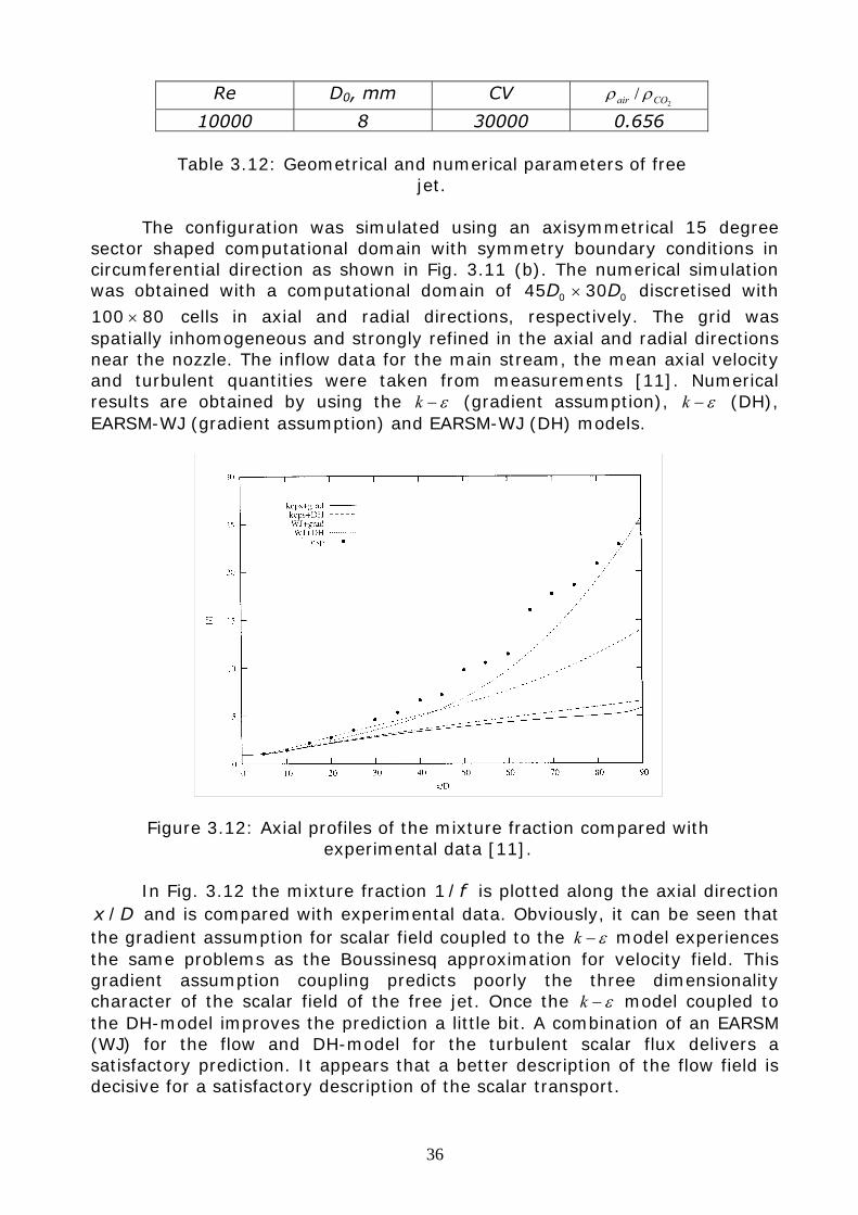
36
Re D0, mm CV 2
/ COair ρρ
10000 8 30000 0.656
Table 3.12: Geometrical and numerical parameters of free jet.
The configuration was simulated using an axisymmetrical 15 degree
sector shaped computational domain with symmetry boundary conditions in circumferential direction as shown in Fig. 3.11 (b). The numerical simulation was obtained with a computational domain of 00 3045 DD × discretised with
80100 × cells in axial and radial directions, respectively. The grid was spatially inhomogeneous and strongly refined in the axial and radial directions near the nozzle. The inflow data for the main stream, the mean axial velocity and turbulent quantities were taken from measurements [11]. Numerical results are obtained by using the ε−k (gradient assumption), ε−k (DH), EARSM-WJ (gradient assumption) and EARSM-WJ (DH) models.
Figure 3.12: Axial profiles of the mixture fraction compared with experimental data [11].
In Fig. 3.12 the mixture fraction f/1 is plotted along the axial direction
Dx / and is compared with experimental data. Obviously, it can be seen that the gradient assumption for scalar field coupled to the ε−k model experiences the same problems as the Boussinesq approximation for velocity field. This gradient assumption coupling predicts poorly the three dimensionality character of the scalar field of the free jet. Once the ε−k model coupled to the DH-model improves the prediction a little bit. A combination of an EARSM (WJ) for the flow and DH-model for the turbulent scalar flux delivers a satisfactory prediction. It appears that a better description of the flow field is decisive for a satisfactory description of the scalar transport.
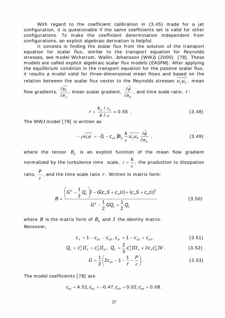
37
With regard to the coefficient calibration in (3.45) made for a jet configuration, it is questionable if the same coefficients set is valid for other configurations. To make the coefficient determination independent from configurations, an explicit algebraic derivation is helpful.
It consists in finding the scalar flux from the solution of the transport equation for scalar flux, similar to the transport equation for Reynolds stresses, see model Wirkstrom, Wallin, Johansson (WWJ) (2000) [78]. These models are called explicit algebraic scalar flux models (EASFM). After applying the equilibrium condition in the transport equation for the passive scalar flux, it results a model valid for three-dimensional mean flows and based on the
relation between the scalar flux vector to the Reynolds stresses ''kjuu , mean
flow gradients, j
i
xu
∂∂
, mean scalar gradient, kx∂
∂φ, and time scale ratio, r :
55.0/
/≈=
εεφφ
k
kr . (3.48)
The WWJ model [78] is written as
( )k
kjiji xuu
kBcu
∂∂
−−=−φ
εφρ ϕ
''4
'' 1 , (3.49)
where the tensor ijB is an explicit function of the mean flow gradient
normalized by the turbulence time scale, ε
τ k= , the production to dissipation
ratio, εP
, and the time scale ratio r . Written in matrix form:
( ) ( )
213
21
2
21
21
21
QGQG
cSccScGIQGB
ss
+−
Ω++Ω+−⎟⎠⎞
⎜⎝⎛ −
=ΩΩ
(3.50)
where B is the matrix form of ijB and I the identity matrix.
Moreover,
3232 1,1 φφφφ ccccccs +−=−−= Ω , (3.51)
ΩΩ+= IIcIIcQ ss22
1 , IVccIIIcQ sss23
2 232
Ω+= . (3.52)
⎟⎠
⎞⎜⎝
⎛ −−−=εφP
rcG
112
21
1 . (3.53)
The model coefficients [78] are
08.0,02.0,47.0,51.4 4321 ==−== φφφφ cccc .
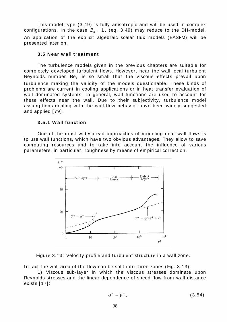
38
This model type (3.49) is fully anisotropic and will be used in complex configurations. In the case 1=ijB , (eq. 3.49) may reduce to the DH-model.
An application of the explicit algebraic scalar flux models (EASFM) will be presented later on.
3.5 Near wall treatment The turbulence models given in the previous chapters are suitable for
completely developed turbulent flows. However, near the wall local turbulent Reynolds number tRe is so small that the viscous effects prevail upon turbulence making the validity of the models questionable. These kinds of problems are current in cooling applications or in heat transfer evaluation of wall dominated systems. In general, wall functions are used to account for these effects near the wall. Due to their subjectivity, turbulence model assumptions dealing with the wall-flow behavior have been widely suggested and applied [79]. 3.5.1 Wall function
One of the most widespread approaches of modeling near wall flows is to use wall functions, which have two obvious advantages. They allow to save computing resources and to take into account the influence of various parameters, in particular, roughness by means of empirical correction.
Figure 3.13: Velocity profile and turbulent structure in a wall zone.
In fact the wall area of the flow can be split into three zones (Fig. 3.13): 1) Viscous sub-layer in which the viscous stresses dominate upon
Reynolds stresses and the linear dependence of speed flow from wall distance exists [17]:
++ = yu , (3.54)
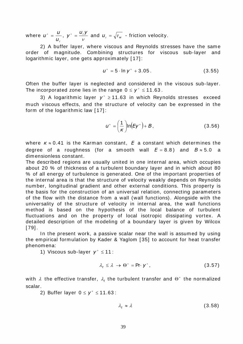
39
where τu
uu =+ ,
ντ yu
y =+ and wu ττ = - friction velocity.
2) A buffer layer, where viscous and Reynolds stresses have the same order of magnitude. Combining structures for viscous sub-layer and logarithmic layer, one gets approximately [17]:
05.3ln5 +⋅= ++ yu . (3.55)
Often the buffer layer is neglected and considered in the viscous sub-layer. The incorporated zone lies in the range 63.110 ≤≤ +y .
3) A logarithmic layer 63.11≥+y in which Reynolds stresses exceed much viscous effects, and the structure of velocity can be expressed in the form of the logarithmic law [17]:
( ) BEyк
u +⎟⎠⎞
⎜⎝⎛= ++ ln1
, (3.56)
where 41.0≈к is the Karman constant, Е a constant which determines the degree of a roughness (for a smooth wall 8.8=E ) and 0.5≈B a dimensionless constant. The described regions are usually united in one internal area, which occupies about 20 % of thickness of a turbulent boundary layer and in which about 80 % of all energy of turbulence is generated. One of the important properties of the internal area is that the structure of velocity weakly depends on Reynolds number, longitudinal gradient and other external conditions. This property is the basis for the construction of an universal relation, connecting parameters of the flow with the distance from a wall (wall functions). Alongside with the universality of the structure of velocity in internal area, the wall functions method is based on the hypothesis of the local balance of turbulent fluctuations and on the property of local isotropic dissipating vortex. A detailed description of the modeling of a boundary layer is given by Wilcox [79]. In the present work, a passive scalar near the wall is assumed by using the empirical formulation by Kader & Yaglom [35] to account for heat transfer phenomena:
1) Viscous sub-layer 11≤+y : λλ ≤t → ++ ⋅=Θ yPr , (3.57)
with λ the effective transfer, tλ the turbulent transfer and +Θ the normalized
scalar. 2) Buffer layer 63.110 ≤≤ +y : λλ ≈t (3.58)
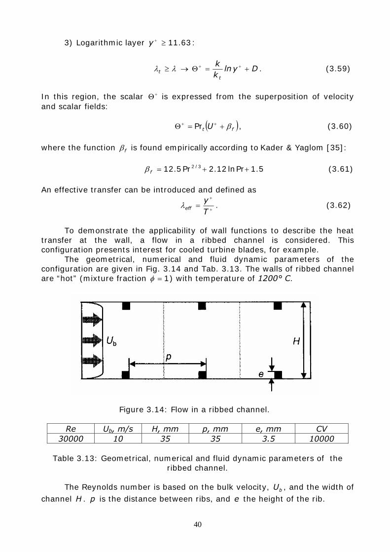
40
3) Logarithmic layer 63.11≥+y :
λλ ≥t → Dylnkk
t
+=Θ ++ . (3.59)
In this region, the scalar +Θ is expressed from the superposition of velocity and scalar fields:
( )ft U β+=Θ ++ Pr , (3.60)
where the function fβ is found empirically according to Kader & Yaglom [35]:
5.1Prln12.2Pr5.12 3/2 ++=fβ (3.61)
An effective transfer can be introduced and defined as
+
+
=Ty
effλ . (3.62)
To demonstrate the applicability of wall functions to describe the heat transfer at the wall, a flow in a ribbed channel is considered. This configuration presents interest for cooled turbine blades, for example.
The geometrical, numerical and fluid dynamic parameters of the configuration are given in Fig. 3.14 and Tab. 3.13. The walls of ribbed channel are “hot” (mixture fraction 1=φ ) with temperature of 1200° C.
Figure 3.14: Flow in a ribbed channel. Re Ub, m/s H, mm p, mm e, mm CV
30000 10 35 35 3.5 10000
Table 3.13: Geometrical, numerical and fluid dynamic parameters of the ribbed channel.
The Reynolds number is based on the bulk velocity, bU , and the width of
channel H . p is the distance between ribs, and e the height of the rib.
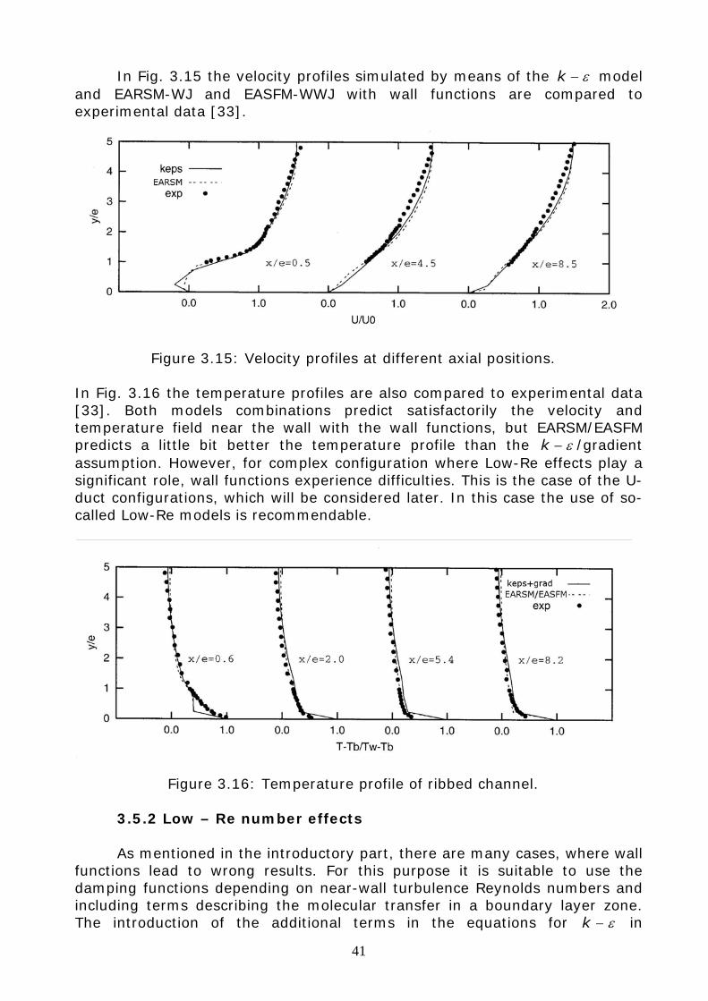
41
In Fig. 3.15 the velocity profiles simulated by means of the ε−k model and EARSM-WJ and EASFM-WWJ with wall functions are compared to experimental data [33].
Figure 3.15: Velocity profiles at different axial positions. In Fig. 3.16 the temperature profiles are also compared to experimental data [33]. Both models combinations predict satisfactorily the velocity and temperature field near the wall with the wall functions, but EARSM/EASFM predicts a little bit better the temperature profile than the ε−k /gradient assumption. However, for complex configuration where Low-Re effects play a significant role, wall functions experience difficulties. This is the case of the U-duct configurations, which will be considered later. In this case the use of so-called Low-Re models is recommendable.
Figure 3.16: Temperature profile of ribbed channel. 3.5.2 Low – Re number effects As mentioned in the introductory part, there are many cases, where wall functions lead to wrong results. For this purpose it is suitable to use the damping functions depending on near-wall turbulence Reynolds numbers and including terms describing the molecular transfer in a boundary layer zone. The introduction of the additional terms in the equations for ε−k in
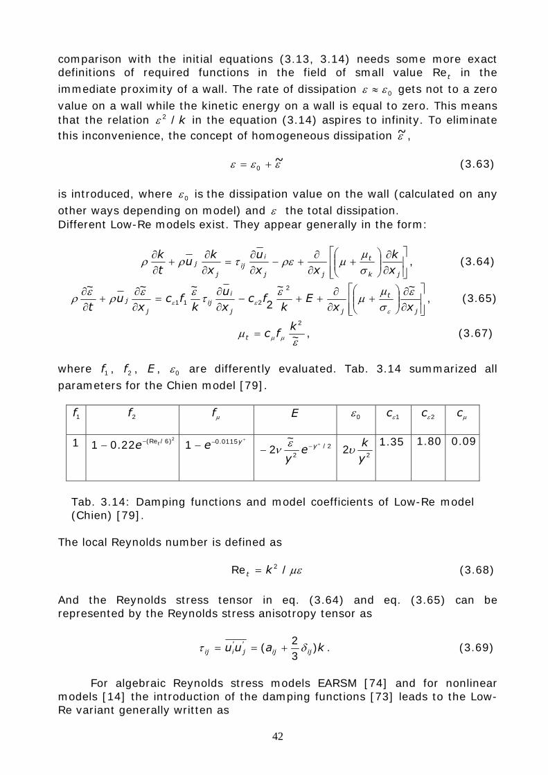
42
comparison with the initial equations (3.13, 3.14) needs some more exact definitions of required functions in the field of small value tRe in the immediate proximity of a wall. The rate of dissipation 0εε ≈ gets not to a zero value on a wall while the kinetic energy on a wall is equal to zero. This means that the relation k/2ε in the equation (3.14) aspires to infinity. To eliminate this inconvenience, the concept of homogeneous dissipation ε~ , εεε ~+= 0 (3.63)
is introduced, where 0ε is the dissipation value on the wall (calculated on any other ways depending on model) and ε the total dissipation. Different Low-Re models exist. They appear generally in the form:
⎥⎥⎦
⎤
⎢⎢⎣
⎡
∂∂
⎟⎟⎠
⎞⎜⎜⎝
⎛+
∂∂
+−∂∂
=∂∂
+∂∂
jk
t
jj
iij
j
jxk
xxu
xk
utk
σμ
μρετρρ , (3.64)
⎥⎥⎦
⎤
⎢⎢⎣
⎡
∂∂
⎟⎟⎠
⎞⎜⎜⎝
⎛+
∂∂
++−∂∂
=∂∂
+∂∂
j
t
jj
iij
j
jxx
Ek
fcxu
kfc
xu
tε
σμ
μετεερερε
εε
~~
2
~~~ 2
211 , (3.65)
ε
μ μμ ~2k
fct = , (3.67)
where 1f , 2f , E , 0ε are differently evaluated. Tab. 3.14 summarized all parameters for the Chien model [79].
1f
2f μf E 0ε 1εc 2εc μc
1 2)6/(Re22.01 te−−
+−− ye 0115.01 2/2
~2
+−− yeyεν
22
ykυ
35.1 80.1
09.0
Tab. 3.14: Damping functions and model coefficients of Low-Re model (Chien) [79].
The local Reynolds number is defined as
με/Re 2kt = (3.68)
And the Reynolds stress tensor in eq. (3.64) and eq. (3.65) can be represented by the Reynolds stress anisotropy tensor as
kauu ijij'j
'iij )
32
( δτ +== . (3.69)
For algebraic Reynolds stress models EARSM [74] and for nonlinear
models [14] the introduction of the damping functions [73] leads to the Low-Re variant generally written as
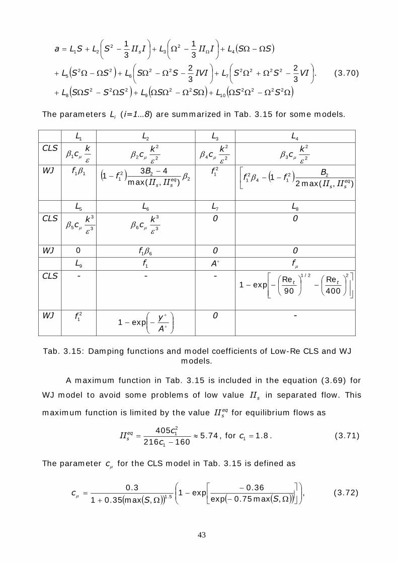
43
( )
( )( ) ( ) ( )ΩΩ−ΩΩ+ΩΩ−ΩΩ+Ω−Ω+
⎟⎠⎞
⎜⎝⎛ −Ω+Ω+⎟
⎠⎞
⎜⎝⎛ −Ω−Ω+Ω−Ω+
Ω−Ω+⎟⎠⎞
⎜⎝⎛ −Ω+⎟
⎠⎞
⎜⎝⎛ −+= Ω
222210
229
2228
22227
226
225
42
32
21
32
32
31
31
SSLSSLSSSSL
VISSLIVISSLSSL
SSLIIILIIISLSLa s
. (3.70)
The parameters iL (i=1…8) are summarized in Tab. 3.15 for some models.
1L 2L 3L 4L
CLS ε
β μk
c1 2
2
2 εβ μ
kc
2
2
4 εβ μ
kc
2
2
3 εβ μ
kc
WJ 11βf ( ) 222
1 ),max(43
1 βeqss IIII
Bf
−−
21f ( ) ⎥⎢
⎣
⎡−−
),max(21 22
142
1 eqss IIII
Bff β
5L 6L 7L 8L
CLS 3
3
5 εβ μ
kc
3
3
6 εβ μ
kc
0 0
WJ 0 61βf 0 0
9L 1f +A μf
CLS - - -
⎥⎥⎦
⎤
⎢⎢⎣
⎡⎟⎠
⎞⎜⎝
⎛−⎟
⎠
⎞⎜⎝
⎛−−
22/1
400Re
90Re
exp1 tt
WJ 2
1f ⎟⎟⎠
⎞⎜⎜⎝
⎛−−
+
+
Ay
exp1 0 -
Tab. 3.15: Damping functions and model coefficients of Low-Re CLS and WJ
models. A maximum function in Tab. 3.15 is included in the equation (3.69) for
WJ model to avoid some problems of low value sII in separated flow. This
maximum function is limited by the value eqsII for equilibrium flows as
74.5160216
405
1
21 ≈
−=
cc
IIeqs , for 8.11 =c . (3.71)
The parameter μc for the CLS model in Tab. 3.15 is defined as
( )( ) ( )( ) ⎟⎟
⎠
⎞⎜⎜⎝
⎛⎥⎦
⎤⎢⎣
⎡Ω−
−−
Ω+=
,max75.0exp36.0
exp1,max35.01
3.05.1 SS
cμ , (3.72)
44
while the coefficients iβ are defined as in section 3.2.
For validation cases, two classical turbulent flows in channel with different Reynolds number are considered.
In Fig. 3.17 axial velocity, normalized axial velocity +u , normalized kinetic energy, +k , and dissipation rate +ε obtained by means of the Low-Re CLS and DNS data [37], [44] for channel flow ( 5600Re = (left) and
13750Re = (right)) are presented. The Reynolds number is based on the bulk velocity 0U and the width of the channel H . For the simulation, fine grids near
the wall are used; the first grid point being at the 1=+y . For the 5600Re = case, the Low-Re CLS shows better results than for
configuration with 13750Re = . In both cases the Low–Re CLS delivers good results for a full developed turbulent flow in a channel.
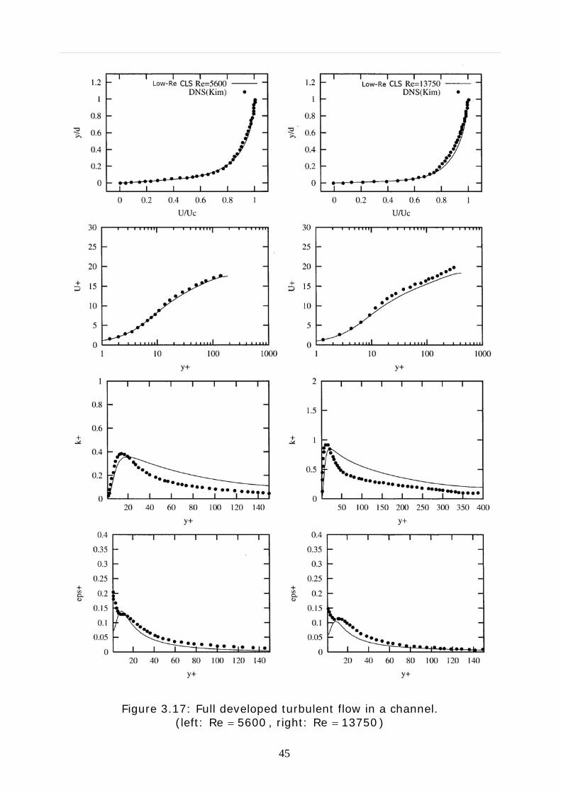
45
Figure 3.17: Full developed turbulent flow in a channel. (left: 5600Re = , right: 13750Re = )
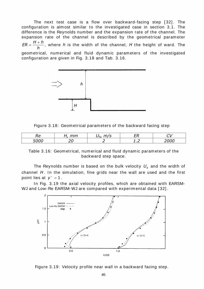
46
The next test case is a flow over backward-facing step [32]. The configuration is almost similar to the investigated case in section 3.1. The difference is the Reynolds number and the expansion rate of the channel. The expansion rate of the channel is described by the geometrical parameter
hhH
ER+
= , where h is the width of the channel, H the height of ward. The
geometrical, numerical and fluid dynamic parameters of the investigated configuration are given in Fig. 3.18 and Tab. 3.16.
Figure 3.18: Geometrical parameters of the backward facing step Re H, mm Uh, m/s ER CV
5000 20 2 1.2 2000
Table 3.16: Geometrical, numerical and fluid dynamic parameters of the backward step space.
The Reynolds number is based on the bulk velocity bU and the width of
channel H . In the simulation, fine grids near the wall are used and the first point lies at 1=+y .
In Fig. 3.19 the axial velocity profiles, which are obtained with EARSM-WJ and Low-Re EARSM-WJ are compared with experimental data [32].
Figure 3.19: Velocity profile near wall in a backward facing step.
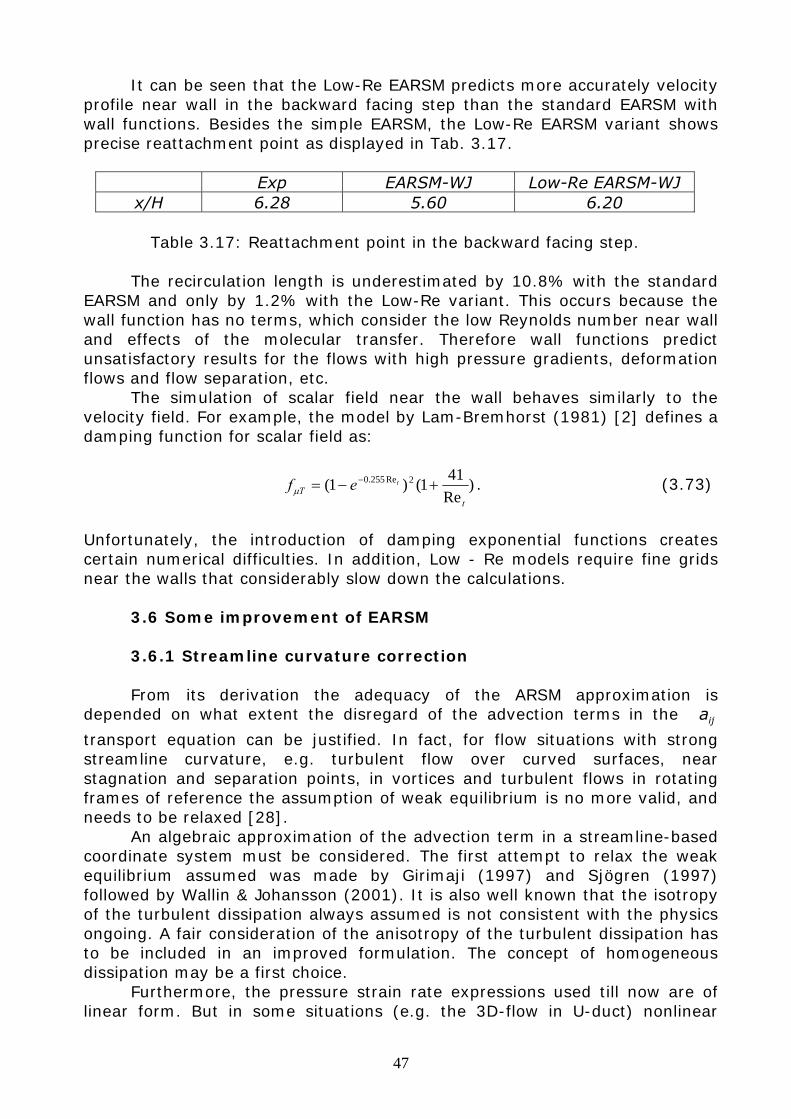
47
It can be seen that the Low-Re EARSM predicts more accurately velocity profile near wall in the backward facing step than the standard EARSM with wall functions. Besides the simple EARSM, the Low-Re EARSM variant shows precise reattachment point as displayed in Tab. 3.17.
Exp EARSM-WJ Low-Re EARSM-WJ
x/H 6.28 5.60 6.20
Table 3.17: Reattachment point in the backward facing step. The recirculation length is underestimated by 10.8% with the standard
EARSM and only by 1.2% with the Low-Re variant. This occurs because the wall function has no terms, which consider the low Reynolds number near wall and effects of the molecular transfer. Therefore wall functions predict unsatisfactory results for the flows with high pressure gradients, deformation flows and flow separation, etc.
The simulation of scalar field near the wall behaves similarly to the velocity field. For example, the model by Lam-Bremhorst (1981) [2] defines a damping function for scalar field as:
)Re411()1( 2Re255.0
tT
tef +−= −μ . (3.73)
Unfortunately, the introduction of damping exponential functions creates certain numerical difficulties. In addition, Low - Re models require fine grids near the walls that considerably slow down the calculations.
3.6 Some improvement of EARSM
3.6.1 Streamline curvature correction
From its derivation the adequacy of the ARSM approximation is
depended on what extent the disregard of the advection terms in the ija
transport equation can be justified. In fact, for flow situations with strong streamline curvature, e.g. turbulent flow over curved surfaces, near stagnation and separation points, in vortices and turbulent flows in rotating frames of reference the assumption of weak equilibrium is no more valid, and needs to be relaxed [28].
An algebraic approximation of the advection term in a streamline-based coordinate system must be considered. The first attempt to relax the weak equilibrium assumed was made by Girimaji (1997) and Sjögren (1997) followed by Wallin & Johansson (2001). It is also well known that the isotropy of the turbulent dissipation always assumed is not consistent with the physics ongoing. A fair consideration of the anisotropy of the turbulent dissipation has to be included in an improved formulation. The concept of homogeneous dissipation may be a first choice.
Furthermore, the pressure strain rate expressions used till now are of linear form. But in some situations (e.g. the 3D-flow in U-duct) nonlinear
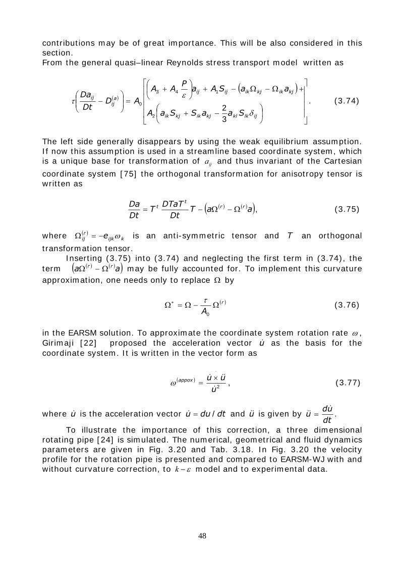
48
contributions may be of great importance. This will be also considered in this section. From the general quasi–linear Reynolds stress transport model written as
( )( )
⎥⎥⎥⎥
⎦
⎤
⎢⎢⎢⎢
⎣
⎡
⎟⎠⎞
⎜⎝⎛ −+
+Ω−Ω−+⎟⎠⎞
⎜⎝⎛ +
=⎟⎟⎠
⎞⎜⎜⎝
⎛−
ijlkklkjikkjik
kjikkjikijija
ijij
SaaSSaA
aaSAaP
AA
ADDt
Da
δ
ετ
32
2
143
0 . (3.74)
The left side generally disappears by using the weak equilibrium assumption. If now this assumption is used in a streamline based coordinate system, which is a unique base for transformation of ija and thus invariant of the Cartesian
coordinate system [75] the orthogonal transformation for anisotropy tensor is written as
( ) ( )( )aaTDt
DTaTT
DtDa rr
tt Ω−Ω−= , (3.75)
where ( )
kijkrij e ω−=Ω is an anti-symmetric tensor and T an orthogonal
transformation tensor. Inserting (3.75) into (3.74) and neglecting the first term in (3.74), the term ( ) ( )( )aa rr Ω−Ω may be fully accounted for. To implement this curvature approximation, one needs only to replace Ω by
( )r
AΩ−Ω=Ω∗
0
τ (3.76)
in the EARSM solution. To approximate the coordinate system rotation rate ω , Girimaji [22] proposed the acceleration vector u& as the basis for the coordinate system. It is written in the vector form as
( )2uuuappox
&
&&&⋅
×=ω , (3.77)
where u& is the acceleration vector dtduu /=& and u&& is given by dtud
u&
&& = .
To illustrate the importance of this correction, a three dimensional rotating pipe [24] is simulated. The numerical, geometrical and fluid dynamics parameters are given in Fig. 3.20 and Tab. 3.18. In Fig. 3.20 the velocity profile for the rotation pipe is presented and compared to EARSM-WJ with and without curvature correction, to ε−k model and to experimental data.
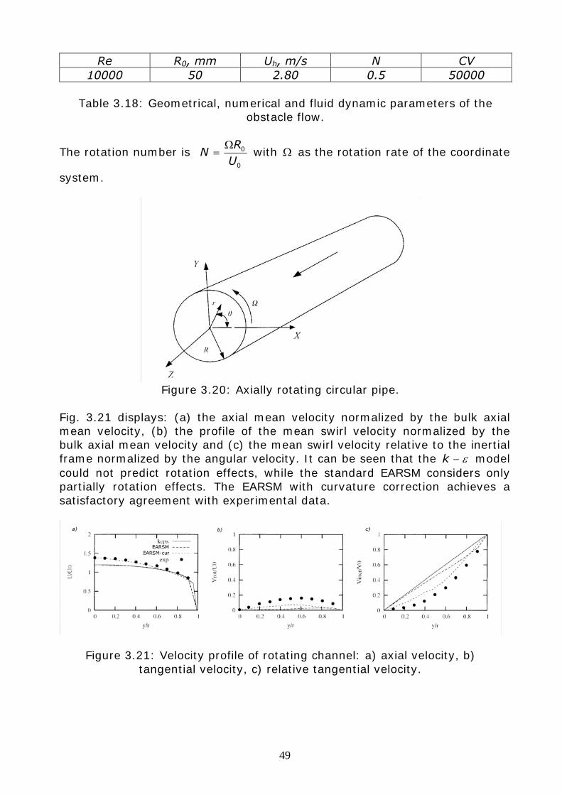
49
Re R0, mm Uh, m/s N CV 10000 50 2.80 0.5 50000
Table 3.18: Geometrical, numerical and fluid dynamic parameters of the
obstacle flow.
The rotation number is 0
0
UR
NΩ
= with Ω as the rotation rate of the coordinate
system.
Figure 3.20: Axially rotating circular pipe.
Fig. 3.21 displays: (a) the axial mean velocity normalized by the bulk axial mean velocity, (b) the profile of the mean swirl velocity normalized by the bulk axial mean velocity and (c) the mean swirl velocity relative to the inertial frame normalized by the angular velocity. It can be seen that the ε−k model could not predict rotation effects, while the standard EARSM considers only partially rotation effects. The EARSM with curvature correction achieves a satisfactory agreement with experimental data.
Figure 3.21: Velocity profile of rotating channel: a) axial velocity, b) tangential velocity, c) relative tangential velocity.
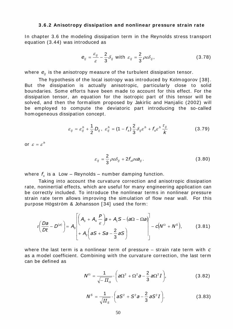
50
3.6.2 Anisotropy dissipation and nonlinear pressure strain rate In chapter 3.6 the modeling dissipation term in the Reynolds stress transport equation (3.44) was introduced as
ijij
ije δεε
32
−= with ijij ρεδε32
= , (3.78)
where ije is the anisotropy measure of the turbulent dissipation tensor.
The hypothesis of the local isotropy was introduced by Kolmogorov [38]. But the dissipation is actually anisotropic, particularly close to solid boundaries. Some efforts have been made to account for this effect. For the dissipation tensor, an equation for the isotropic part of this tensor will be solved, and then the formalism proposed by Jakirlic and Hanjalic (2002) will be employed to compute the deviatoric part introducing the so-called homogeneous dissipation concept.
ijhijij D
21
+= εε , k
ff ijhs
hijs
hij
τεεδε +−=
32
)1( (3.79)
or hεε =
ijsijij af ρερεδε 232
+= . (3.80)
where sf is a Low – Reynolds – number damping function.
Taking into account the curvature correction and anisotropic dissipation rate, noninertial effects, which are useful for many engineering application can be correctly included. To introduce the nonlinear terms in nonlinear pressure strain rate term allows improving the simulation of flow near wall. For this purpose Högström & Johansson [34] used the form:
( )( )
( )Sa NNc
aSSaaSA
aaSAaP
AA
ADDtDa
+−
⎥⎥⎥⎥
⎦
⎤
⎢⎢⎢⎢
⎣
⎡
⎟⎠⎞
⎜⎝⎛ −++
Ω−Ω−+⎟⎠⎞
⎜⎝⎛ +
=⎟⎠⎞
⎜⎝⎛ − Ω
32
2
143
0
ετ , (3.81)
where the last term is a nonlinear term of pressure – strain rate term with c as a model coefficient. Combining with the curvature correction, the last term can be defined as
⎟⎠⎞
⎜⎝⎛ Ω−Ω+Ω⋅
−=
Ω
Ω IaaaII
N 222
321 , (3.82)
⎟⎠⎞
⎜⎝⎛ −+⋅= IaSaSaS
IIN
S
S 222
321 . (3.83)
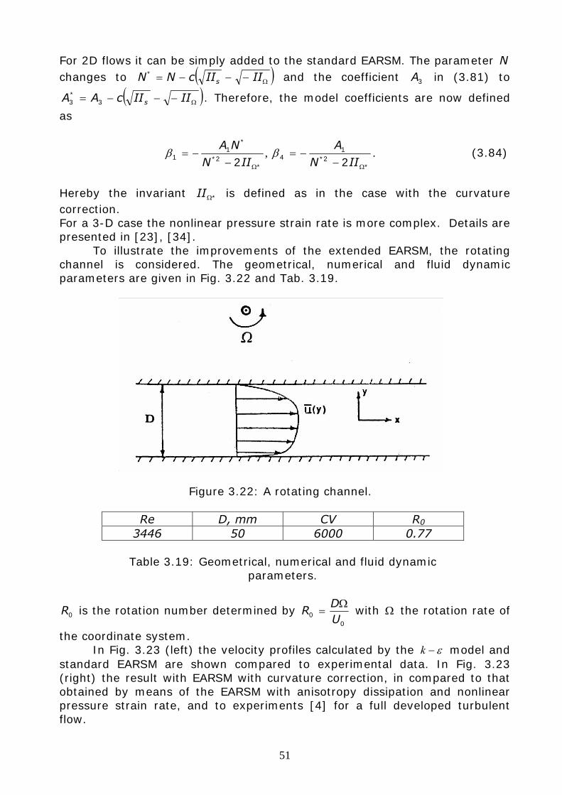
51
For 2D flows it can be simply added to the standard EARSM. The parameter N changes to ( )Ω−−−= IIIIcNN s
* and the coefficient 3A in (3.81) to
( )Ω−−−= IIIIcAA s3*3 . Therefore, the model coefficients are now defined
as
*
2*
*1
1 2 Ω−−=
IIN
NAβ ,
*2*
14 2 Ω−
−=IIN
Aβ . (3.84)
Hereby the invariant *ΩII is defined as in the case with the curvature correction. For a 3-D case the nonlinear pressure strain rate is more complex. Details are presented in [23], [34].
To illustrate the improvements of the extended EARSM, the rotating channel is considered. The geometrical, numerical and fluid dynamic parameters are given in Fig. 3.22 and Tab. 3.19.
Figure 3.22: A rotating channel.
Re D, mm CV R0
3446 50 6000 0.77
Table 3.19: Geometrical, numerical and fluid dynamic parameters.
0R is the rotation number determined by 0
0 UD
RΩ
= with Ω the rotation rate of
the coordinate system. In Fig. 3.23 (left) the velocity profiles calculated by the ε−k model and
standard EARSM are shown compared to experimental data. In Fig. 3.23 (right) the result with EARSM with curvature correction, in compared to that obtained by means of the EARSM with anisotropy dissipation and nonlinear pressure strain rate, and to experiments [4] for a full developed turbulent flow.
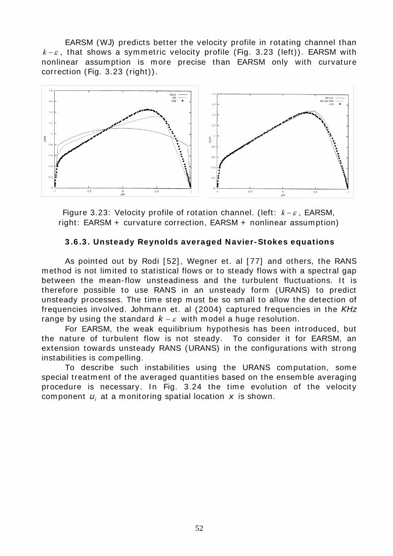
52
EARSM (WJ) predicts better the velocity profile in rotating channel than ε−k , that shows a symmetric velocity profile (Fig. 3.23 (left)). EARSM with
nonlinear assumption is more precise than EARSM only with curvature correction (Fig. 3.23 (right)).
Figure 3.23: Velocity profile of rotation channel. (left: ε−k , EARSM, right: EARSM + curvature correction, EARSM + nonlinear assumption)
3.6.3. Unsteady Reynolds averaged Navier-Stokes equations As pointed out by Rodi [52], Wegner et. al [77] and others, the RANS
method is not limited to statistical flows or to steady flows with a spectral gap between the mean-flow unsteadiness and the turbulent fluctuations. It is therefore possible to use RANS in an unsteady form (URANS) to predict unsteady processes. The time step must be so small to allow the detection of frequencies involved. Johmann et. al (2004) captured frequencies in the KHz range by using the standard ε−k with model a huge resolution.
For EARSM, the weak equilibrium hypothesis has been introduced, but the nature of turbulent flow is not steady. To consider it for EARSM, an extension towards unsteady RANS (URANS) in the configurations with strong instabilities is compelling.
To describe such instabilities using the URANS computation, some special treatment of the averaged quantities based on the ensemble averaging procedure is necessary. In Fig. 3.24 the time evolution of the velocity component iu at a monitoring spatial location x is shown.
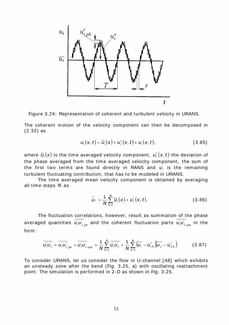
53
Figure 3.24: Representation of coherent and turbulent velocity in URANS.
The coherent motion of the velocity component can then be decomposed in (2.32) as
( ) ( ) ( ) ( )txutxuxutxu iiii ,,, '* ++= , (3.85)
where ( )xui is the time averaged velocity component, ( )txui ,* the deviation of the phase averaged from the time averaged velocity component, the sum of the first two terms are found directly in RANS and '
iu is the remaining turbulent fluctuating contribution, that has to be modeled in URANS.
The time averaged mean velocity component is obtained by averaging all time steps N as
( ) ( )∑=
+=N
kiii txuxu
Nu
1
* ,1 . (3.86)
The fluctuation correlations, however, result as summation of the phase
averaged quantities phjiuu '' and the coherent fluctuation parts
cohjiuu '' in the
form:
( )( )∑∑==
−−+=+=N
kkjjkii
N
kjicohjiphjiji uuuu
Nuu
Nuuuuuu
1
*,
*,
1
'''''''' 11 (3.87)
To consider URANS, let us consider the flow in U-channel [48] which exhibits an unsteady zone after the bend (Fig. 3.25, a) with oscillating reattachment point. The simulation is performed in 2-D as shown in Fig. 3.25.
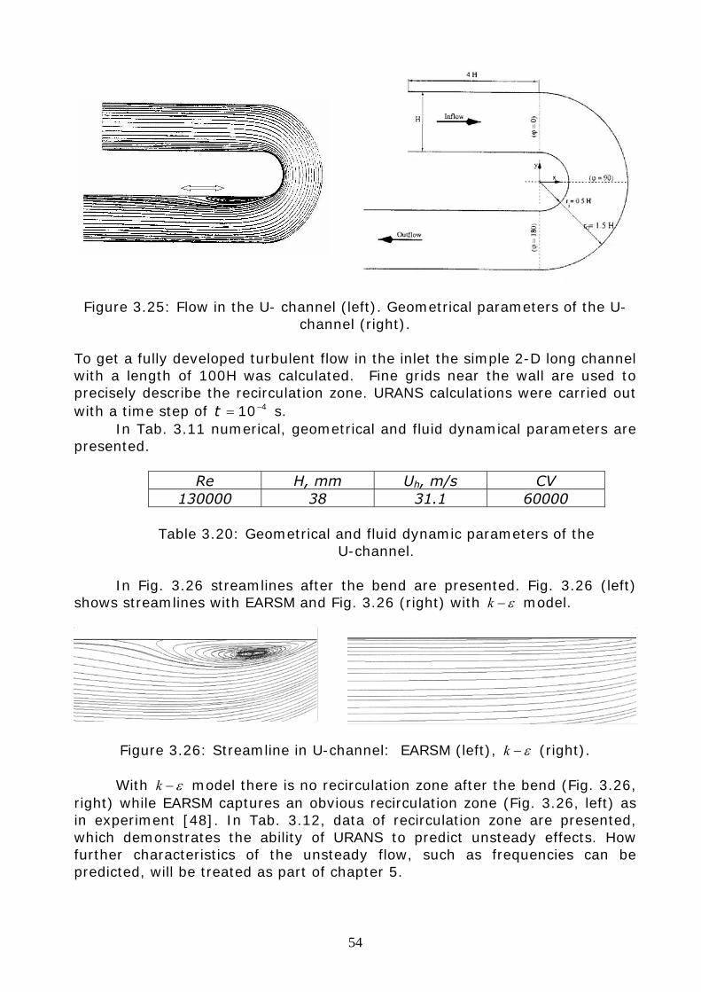
54
Figure 3.25: Flow in the U- channel (left). Geometrical parameters of the U-channel (right).
To get a fully developed turbulent flow in the inlet the simple 2-D long channel with a length of 100H was calculated. Fine grids near the wall are used to precisely describe the recirculation zone. URANS calculations were carried out with a time step of 410−=t s.
In Tab. 3.11 numerical, geometrical and fluid dynamical parameters are presented.
Re H, mm Uh, m/s CV
130000 38 31.1 60000
Table 3.20: Geometrical and fluid dynamic parameters of the U-channel.
In Fig. 3.26 streamlines after the bend are presented. Fig. 3.26 (left)
shows streamlines with EARSM and Fig. 3.26 (right) with ε−k model.
Figure 3.26: Streamline in U-channel: EARSM (left), ε−k (right). With ε−k model there is no recirculation zone after the bend (Fig. 3.26,
right) while EARSM captures an obvious recirculation zone (Fig. 3.26, left) as in experiment [48]. In Tab. 3.12, data of recirculation zone are presented, which demonstrates the ability of URANS to predict unsteady effects. How further characteristics of the unsteady flow, such as frequencies can be predicted, will be treated as part of chapter 5.
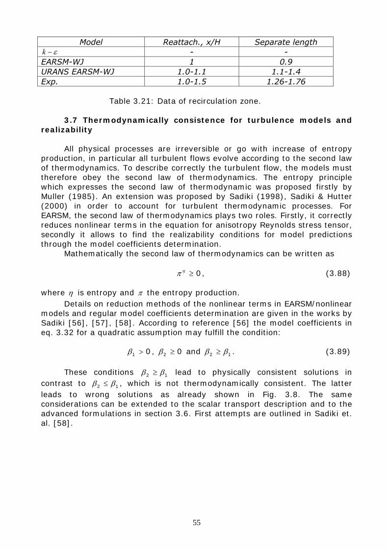
55
Model Reattach., x/H Separate length ε−k - -
EARSM-WJ 1 0.9 URANS EARSM-WJ 1.0-1.1 1.1-1.4 Exp. 1.0-1.5 1.26-1.76
Table 3.21: Data of recirculation zone.
3.7 Thermodynamically consistence for turbulence models and
realizability All physical processes are irreversible or go with increase of entropy production, in particular all turbulent flows evolve according to the second law of thermodynamics. To describe correctly the turbulent flow, the models must therefore obey the second law of thermodynamics. The entropy principle which expresses the second law of thermodynamic was proposed firstly by Muller (1985). An extension was proposed by Sadiki (1998), Sadiki & Hutter (2000) in order to account for turbulent thermodynamic processes. For EARSM, the second law of thermodynamics plays two roles. Firstly, it correctly reduces nonlinear terms in the equation for anisotropy Reynolds stress tensor, secondly it allows to find the realizability conditions for model predictions through the model coefficients determination.
Mathematically the second law of thermodynamics can be written as 0≥ηπ , (3.88) where η is entropy and π the entropy production. Details on reduction methods of the nonlinear terms in EARSM/nonlinear models and regular model coefficients determination are given in the works by Sadiki [56], [57], [58]. According to reference [56] the model coefficients in eq. 3.32 for a quadratic assumption may fulfill the condition: 01 >β , 02 ≥β and 12 ββ ≥ . (3.89) These conditions 12 ββ ≥ lead to physically consistent solutions in contrast to 12 ββ ≤ , which is not thermodynamically consistent. The latter leads to wrong solutions as already shown in Fig. 3.8. The same considerations can be extended to the scalar transport description and to the advanced formulations in section 3.6. First attempts are outlined in Sadiki et. al. [58].
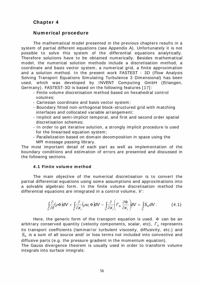
56
Chapter 4
Numerical procedure
The mathematical model presented in the previous chapters results in a system of partial different equations (see Appendix A). Unfortunately it is not possible to solve this system of the differential equations analytically. Therefore solutions have to be obtained numerically. Besides mathematical model, the numerical solution methods include a discretisation method, a coordinate and basis vector system, a numerical grid, a finite approximation and a solution method. In the present work FASTEST - 3D (Flow Analysis Solving Transport Equations Simulating Turbulence 3 Dimensional) has been used, which was developed by INVENT Computing GmbH (Erlangen, Germany). FASTEST-3D is based on the following features [17]:
- Finite volume discretisation method based on hexahedral control volumes; - Cartesian coordinate and basis vector system; - Boundary fitted non-orthogonal block-structured grid with matching interfaces and collocated variable arrangement; - Implicit and semi-implicit temporal, and first and second order spatial discretisation schemes; - In order to get iterative solution, a strongly implicit procedure is used for the linearised equation system; - Parallelization based on domain decomposition in space using the MPI message passing library.
The most important detail of each part as well as implementation of the boundary conditions and estimation of errors are presented and discussed in the following sections. 4.1 Finite volume method The main objective of the numerical discretisation is to convert the partial differential equations using some assumptions and approximations into a solvable algebraic form. In the finite volume discretisation method the differential equations are integrated in a control volume, V :
( ) ( ) ∫∫∫∫ ΦΦ =⎟⎟⎠
⎞⎜⎜⎝
⎛∂Φ∂
∂∂
−Φ∂∂
+Φ∂∂
ViV ii
V iV
dVSdVx
Гx
dVux
dVt
ρρ . (4.1)
Here, the generic form of the transport equation is used. Φ can be an
arbitrary conserved quantity (velocity components, scalar, etc), ΦГ represents its transport coefficients (laminar/or turbulent viscosity, diffusivity, etc.) and
ΦS is a sum of all source and/ or loss terms not included into convective and diffusive parts (e.g. the pressure gradient in the momentum equation). The Gauss divergence theorem is usually used in order to transform volume integrals into surface integrals:
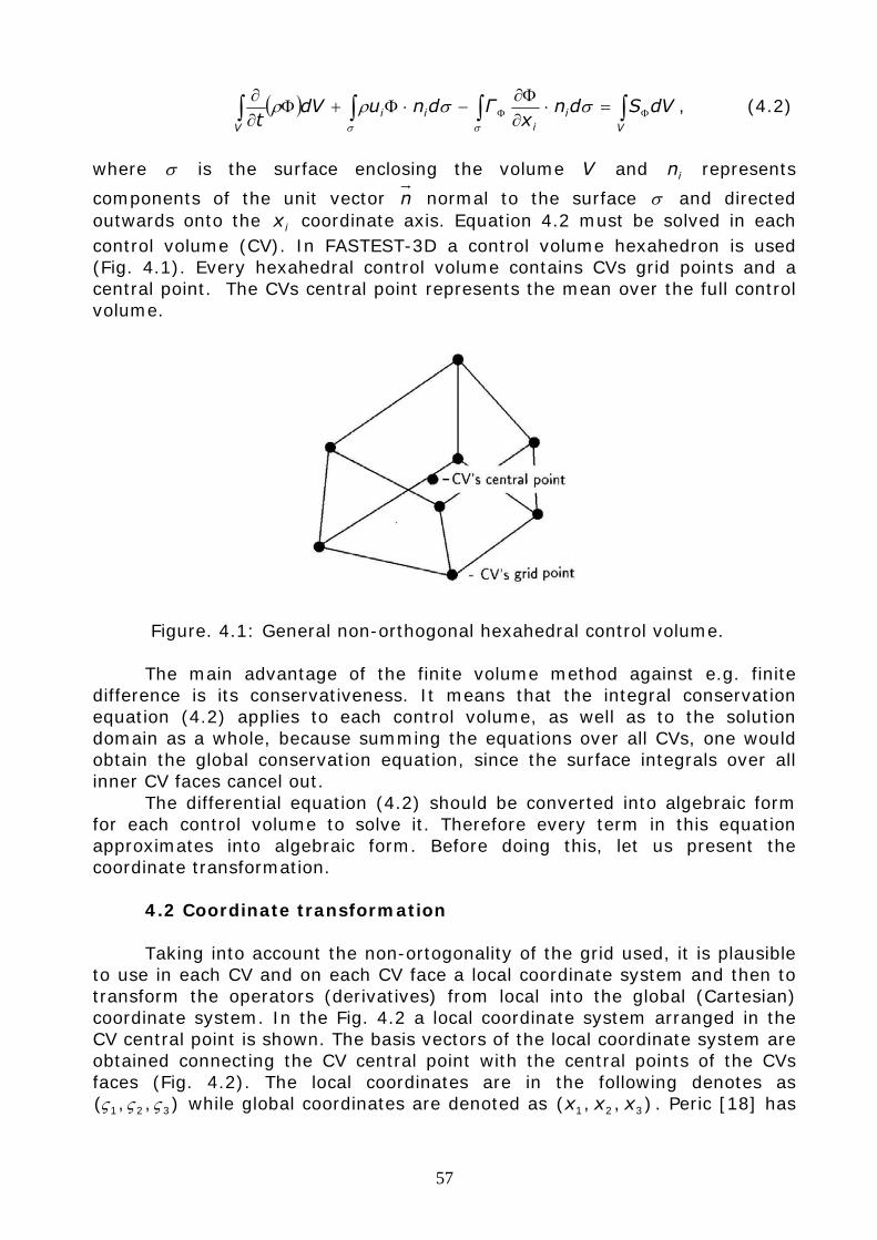
57
( ) dVSdnx
ГdnudVt V
ii
iiV
∫∫∫∫ ΦΦ =⋅∂Φ∂
−⋅Φ+Φ∂∂
σσ
σσρρ , (4.2)
where σ is the surface enclosing the volume V and in represents
components of the unit vector n normal to the surface σ and directed outwards onto the ix coordinate axis. Equation 4.2 must be solved in each control volume (CV). In FASTEST-3D a control volume hexahedron is used (Fig. 4.1). Every hexahedral control volume contains CVs grid points and a central point. The CVs central point represents the mean over the full control volume.
Figure. 4.1: General non-orthogonal hexahedral control volume.
The main advantage of the finite volume method against e.g. finite difference is its conservativeness. It means that the integral conservation equation (4.2) applies to each control volume, as well as to the solution domain as a whole, because summing the equations over all CVs, one would obtain the global conservation equation, since the surface integrals over all inner CV faces cancel out. The differential equation (4.2) should be converted into algebraic form for each control volume to solve it. Therefore every term in this equation approximates into algebraic form. Before doing this, let us present the coordinate transformation.
4.2 Coordinate transformation Taking into account the non-ortogonality of the grid used, it is plausible to use in each CV and on each CV face a local coordinate system and then to transform the operators (derivatives) from local into the global (Cartesian) coordinate system. In the Fig. 4.2 a local coordinate system arranged in the CV central point is shown. The basis vectors of the local coordinate system are obtained connecting the CV central point with the central points of the CVs faces (Fig. 4.2). The local coordinates are in the following denotes as
),,( 321 ςςς while global coordinates are denoted as ),,( 321 xxx . Peric [18] has
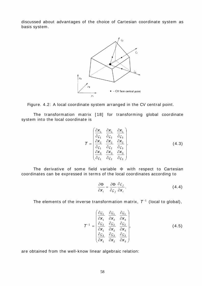
58
discussed about advantages of the choice of Cartesian coordinate system as basis system.
Figure. 4.2: A local coordinate system arranged in the CV central point. The transformation matrix [18] for transforming global coordinate system into the local coordinate is
⎟⎟⎟⎟⎟⎟⎟
⎠
⎞
⎜⎜⎜⎜⎜⎜⎜
⎝
⎛
∂∂
∂∂
∂∂
∂∂
∂∂
∂∂
∂∂
∂∂
∂∂
=
3
3
2
3
1
3
3
2
2
2
1
2
3
1
2
1
1
1
ςςς
ςςς
ςςς
xxx
xxx
xxx
T . (4.3)
The derivative of some field variable Φ with respect to Cartesian coordinates can be expressed in terms of the local coordinates according to
i
j
ji xx ∂
∂
∂Φ∂
=∂Φ∂ ς
ς. (4.4)
The elements of the inverse transformation matrix, 1−T (local to global),
⎟⎟⎟⎟⎟⎟⎟
⎠
⎞
⎜⎜⎜⎜⎜⎜⎜
⎝
⎛
∂∂
∂∂
∂∂
∂∂
∂∂
∂∂
∂∂
∂∂
∂∂
=−
3
3
2
3
1
3
3
2
2
2
1
2
3
1
2
1
1
1
1
xxx
xxx
xxx
T
ςςς
ςςς
ςςς
, (4.5)
are obtained from the well-know linear algebraic relation:
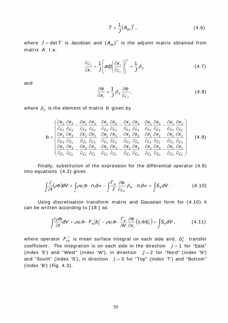
59
( )TadAJ
T1
= , (4.6)
where TJ det= is Jacobian and T
adA )( is the adjoint matrix obtained from matrix A . I.e.
iji
i
i
j
Jx
adjJx
βς
ς 11=⎥
⎦
⎤⎢⎣
⎡⎟⎟⎠
⎞⎜⎜⎝
⎛∂∂
=∂
∂Τ
(4.7)
and
j
iji Jx ς
β∂Φ∂
=∂Φ∂ 1
, (4.8)
where ijβ is the element of matrix Β given by
⎟⎟⎟⎟⎟⎟⎟
⎠
⎞
⎜⎜⎜⎜⎜⎜⎜
⎝
⎛
∂∂
∂∂
−∂∂
∂∂
∂∂
∂∂
−∂∂
∂∂
∂∂
∂∂
−∂∂
∂∂
∂∂
∂∂
−∂∂
∂∂
∂∂
∂∂
−∂∂
∂∂
∂∂
∂∂
−∂∂
∂∂
∂∂
∂∂
−∂∂
∂∂
∂∂
∂∂
−∂∂
∂∂
∂∂
∂∂
−∂∂
∂∂
=Β
2
1
2
1
2
2
1
1
2
3
1
1
1
3
2
1
1
3
2
2
2
3
1
2
3
2
1
1
1
2
3
1
1
3
3
1
3
3
1
1
3
3
1
2
1
3
3
2
2
2
3
1
3
2
2
1
3
3
2
1
2
3
3
1
2
3
3
2
3
3
2
2
ςςςςςςςςςςςς
ςςςςςςςςςςςς
ςςςςςςςςςςςς
xxxxxxxxxxxx
xxxxxxxxxxxx
xxxxxxxxxxxx
. (4.9)
Finally, substitution of the expression for the differential operator (4.8) into equations (4.2) gives
( ) dVSdnJГ
dnudVt V
iikk
iiV
∫∫∫∫ ΦΦ =⋅∂Φ∂
−⋅Φ+Φ∂∂
σσ
σβς
σρρ . (4.10)
Using discretisation transform matrix and Gaussian form for (4.10) it
can be written according to [18 ] as
( ) ∫∫ ΦΦ =ΦΔ∂Φ∂
⋅Φ−⋅Φ+∂Φ∂
V
lkl
ii
jк
jbni
V
dVSbxV
ГubFudV
t δρρρ
, (4.11)
where operator j
bnF is mean surface integral on each side and, jкb transfer
coefficient. The integration is on each side in the direction 1=j for “East” (index ’E’) and “West” (index ’W’), in direction 2=j for “Nord” (index ’N’) and “South” (index ’S’), in direction 3=j for “Top” (index ’T’) and “Bottom” (index ’B’) (Fig. 4.3).
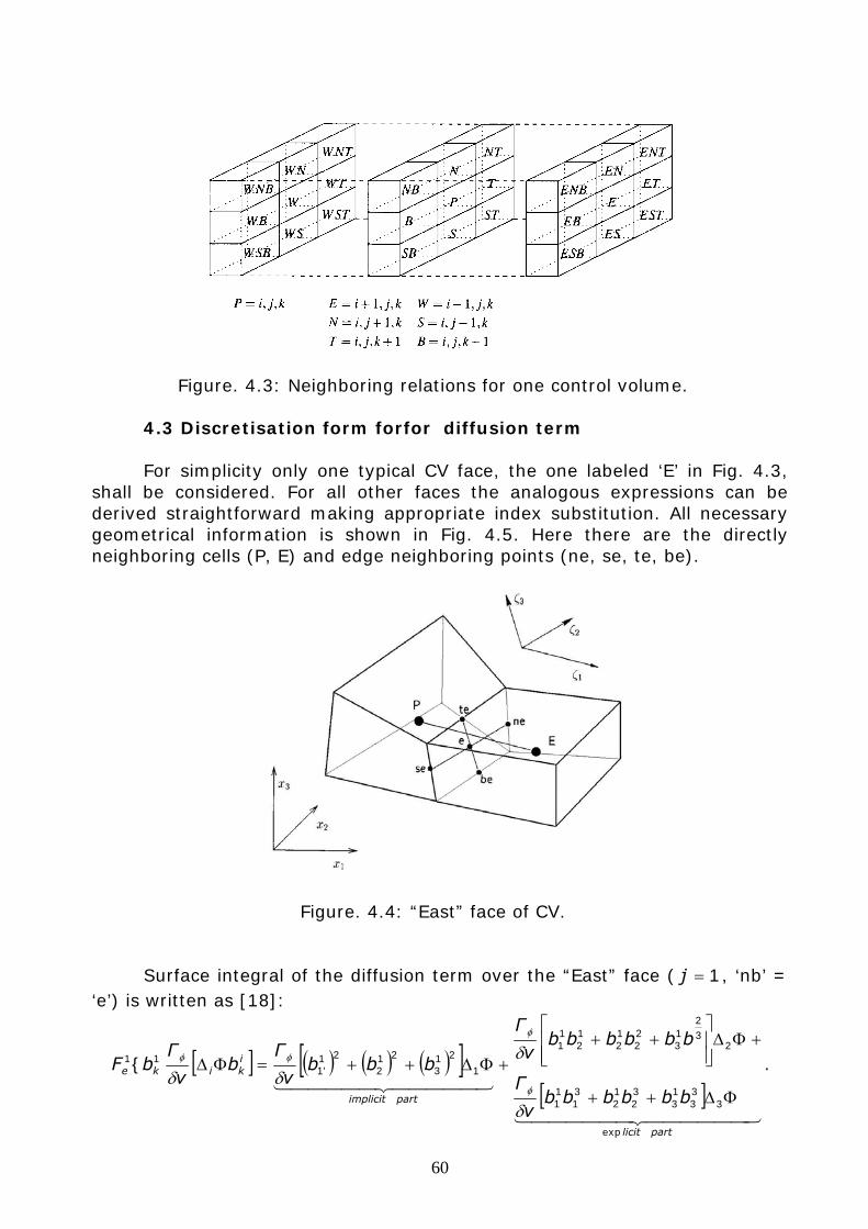
60
Figure. 4.3: Neighboring relations for one control volume. 4.3 Discretisation form forfor diffusion term
For simplicity only one typical CV face, the one labeled ‘E’ in Fig. 4.3,
shall be considered. For all other faces the analogous expressions can be derived straightforward making appropriate index substitution. All necessary geometrical information is shown in Fig. 4.5. Here there are the directly neighboring cells (P, E) and edge neighboring points (ne, se, te, be).
Figure. 4.4: “East” face of CV.
Surface integral of the diffusion term over the “East” face ( 1=j , ‘nb’ =
‘e’) is written as [18]:
[ ] ( ) ( ) ( )[ ][ ]
444444 3444444 21
44444 344444 21
partlicit
partimplicit
ikike
bbbbbbv
Г
bbbbbbv
Г
bbbv
Гb
v
ГbF
exp
333
13
32
12
31
11
232
13
22
12
12
11
1
213
212
21'1
11{
ΦΔ++
+ΦΔ⎥⎥⎦
⎤
⎢⎢⎣
⎡++
+ΦΔ++=ΦΔ
δ
δδδ
φ
φ
φφ .
61
The difference ΦΔ i is defined through center point of control volume and the boundary surface (Fig. 4.4) as: pE Φ−Φ=ΦΔ1 ,
sene Φ−Φ=ΦΔ2 ,. (4.13) bete Φ−Φ=ΦΔ3 . An orthogonal grid can be considered as a special case of a non-orthogonal one, in which the two last terms on right side of (4.12) become zero. However, in the non-orthogonal case they can not be neglected. It means that not only the values of the dependent variable Φ in the point P and E but also its values in the other neighbors points, ne, se, te, be, are necessary for the approximation. The implicit discretisation of all terms would lead to a huge coefficient matrix. Therefore, all terms excluding those containing EΦ and pΦ are treated explicitly and added to the source term (eq.
4.12). The values neΦ , seΦ , teΦ , beΦ are calculated from a trilinear interpolation between the points P, E, N, S, T, B, ne, se, te, be.
4.4 Discretisation form for convective term Analogically to diffusion term, the convective part over the “East” ( 1=j , ‘nb’ = ‘e’) can be discretised as
( ) ( ) eeeeeke mububububF Φ=Φ++=Φ•
3132
121
11
11 }{ ρρ , (4.14)
where em•
denotes a convective flux through the “East” face:
( )3132
121
11 ubububme ++=
•
ρ . (4.15) From the continuity equation it is wis written as
0=−−−++••••••
bswtne mmmmmm . (4.16) FASTEST-3D uses collocated grid and stores velocity and pressure in the center point of CV, i.e. to obtain convective term only interpolation between the CV central values is needed. 4.5 Discretisation form for unsteady term In unsteady computations (or pseudo-unsteady) the unsteady term has to be included accounted for each transport equation (4.2).
62
The unsteady term is approximated as
( )∫ Φ∂∂
≈∂Φ∂
PVPP V
tdV
tδρρ
. (4.17)
where PVδ is the volume of CV. For the finite approximation of the time derivative among implicit methods the simplest approach is the fully implicit Euler method that is of first order of accuracy in time:
( ) ( ) n
PnP
Nb
nP
nNb
nNb
nP
nP ASA
tVV
Φ−+Φ=Δ
Φ−Φ ∑−1δρδρ
. (4.18)
Here, tΔ denotes a time step and the superscripts n and 1−n are related to the actual and previous time steps, respectively. The first term on the left side of (4.18) is treated implicitly and added to the coefficient PA while the second term is added to the source term pS . This method is sufficient at least for
pseudo-unsteady computations, if only a steady state solution is sought without interest in the time history. It provides a reasonable approximation for the real unsteady computation. Therefore the discretisation form for time is written as
( ) ( )
( ) ⎟⎠
⎞⎜⎝
⎛+Φ+Φ⋅−+
⎟⎠
⎞⎜⎝
⎛+Φ+Φ⋅=
ΔΦ−Φ
−Φ
−−−−
Φ
−
∑
∑
11111
1
1 n
Nb
nNb
nNb
nP
nP
n
Nb
nNb
nNb
nP
nP
nP
nP
SAAf
SAAft
VV δρδρ
. (4.19)
If 0=f then it is a fully implicit Euler method that is thea first order approximation. If 5.0=f then it is a Crank-Nicolson method that is a second order approximation. The Crank-Nicolson method is less stable, but more accurate.
4.6 Discretisation form for source term In section 4.3-4.5 the discretisation of terms oin the left side of
transport equation (4.11) was described. On the right side there is a source term. Extra variables and explicit part of convective and diffusion flux are included in this term. Some volume integrals contain spatial gradients of different quantities (e.g. the pressure gradient in the Navier-Stokes or velocity gradients in the Reynolds stress transport equations, etc.). For their approximation the transformation coefficients regarding to local coordinate system connected to the CV central point (fig. 4.5) are necessary.
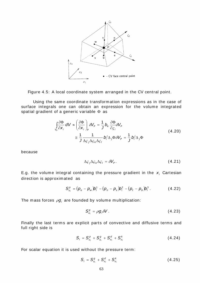
63
Figure 4.5: A local coordinate system arranged in the CV central point. Using the same coordinate transformation expressions as in the case of
surface integrals one can obtain an expression for the volume integrated spatial gradient of a generic variable Φ as
ΦΔ=ΦΔΔΔΔ
≅
∂Φ∂
=⎟⎟⎠
⎞⎜⎜⎝
⎛∂Φ∂
≈∂Φ∂
∫
jjiPj
ji
lkj
PV i
kP
Pii
bJ
VbJ
VbJ
Vx
dVx
P
111
1
δςςς
δς
δ (4.20)
because
Plkj Vδςςς =ΔΔΔ . (4.21)
E.g. the volume integral containing the pressure gradient in the ix Cartesian direction is approximated as ( ) ( ) ( ) 321
ibtisniwepu bppbppbppS
i−−−−−= . (4.22)
The mass forces igρ are founded by volume multiplication: VgS i
gui
δρ= . (4.23)
Finally the last terms are explicit parts of convective and diffusive terms and full right side is
k
udu
gu
pui iiii
SSSSS +++= (4.24)
For scalar equation it is used without the pressure term:
ku
du
gui iii
SSSS ++= (4.25)
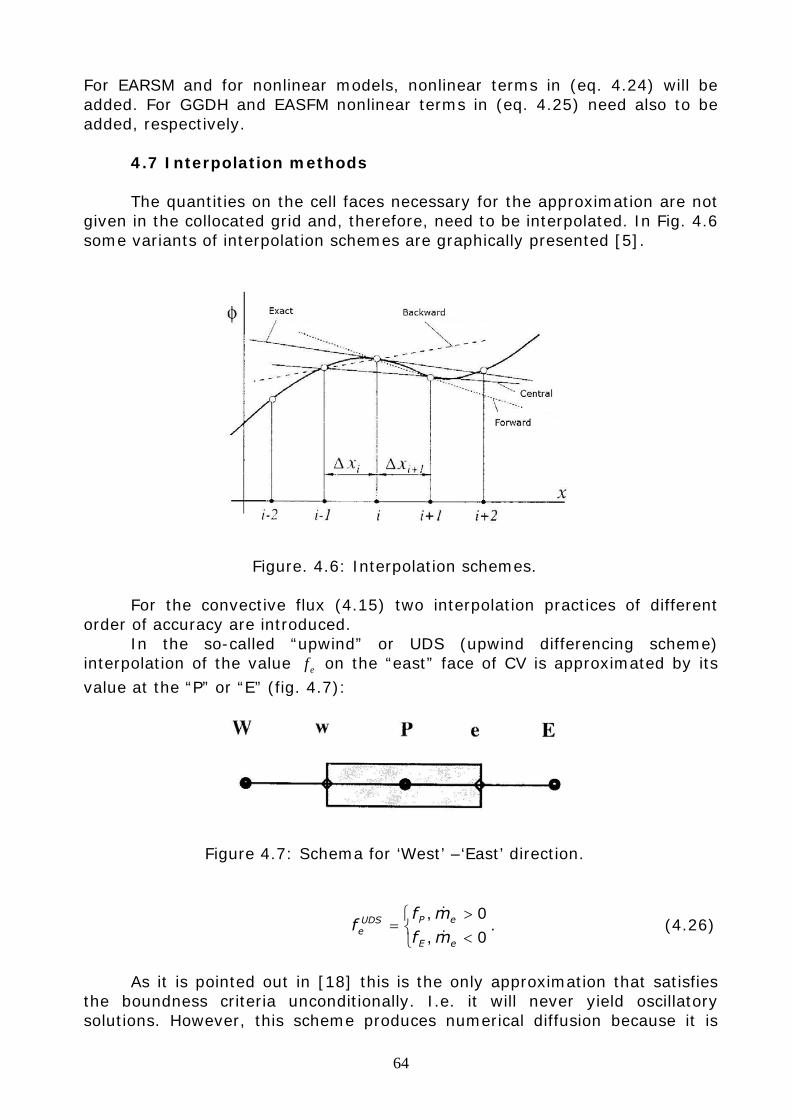
64
For EARSM and for nonlinear models, nonlinear terms in (eq. 4.24) will be added. For GGDH and EASFM nonlinear terms in (eq. 4.25) need also to be added, respectively.
4.7 Interpolation methods The quantities on the cell faces necessary for the approximation are not
given in the collocated grid and, therefore, need to be interpolated. In Fig. 4.6 some variants of interpolation schemes are graphically presented [5].
Figure. 4.6: Interpolation schemes. For the convective flux (4.15) two interpolation practices of different
order of accuracy are introduced. In the so-called “upwind” or UDS (upwind differencing scheme)
interpolation of the value ef on the “east” face of CV is approximated by its
value at the “P” or “E” (fig. 4.7):
Figure 4.7: Schema for ‘West’ –‘East’ direction.
⎩⎨⎧
<>
=0,0,
eE
ePUDSe mf
mff
&
&. (4.26)
As it is pointed out in [18] this is the only approximation that satisfies
the boundness criteria unconditionally. I.e. it will never yield oscillatory solutions. However, this scheme produces numerical diffusion because it is
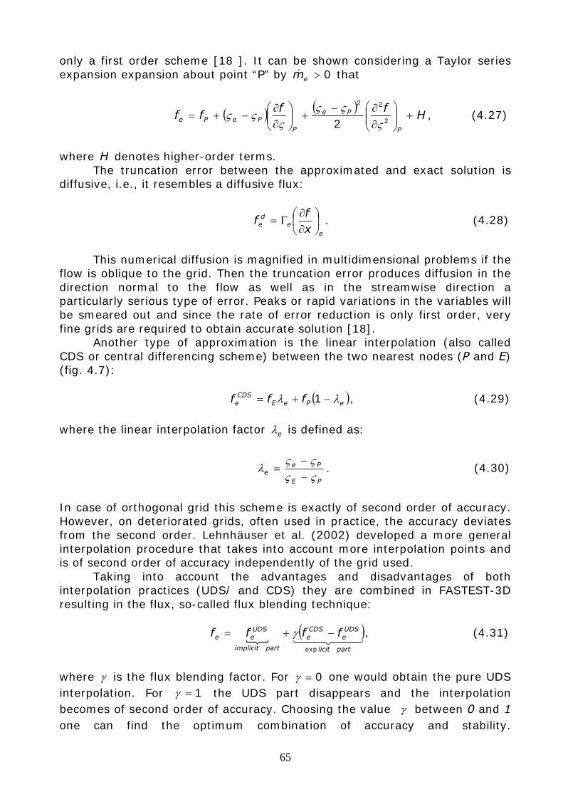
65
only a first order scheme [18 ]. It can be shown considering a Taylor series expansion expansion about point “P” by 0>em& that
( ) ( )H
ffff
P
Pe
PPePe +⎟⎟
⎠
⎞⎜⎜⎝
⎛∂∂−
+⎟⎟⎠
⎞⎜⎜⎝
⎛∂∂
−+=2
22
2 ςςς
ςςς , (4.27)
where H denotes higher-order terms.
The truncation error between the approximated and exact solution is diffusive, i.e., it resembles a diffusive flux:
e
ed
e xf
f ⎟⎠⎞
⎜⎝⎛∂∂
Γ= . (4.28)
This numerical diffusion is magnified in multidimensional problems if the
flow is oblique to the grid. Then the truncation error produces diffusion in the direction normal to the flow as well as in the streamwise direction a particularly serious type of error. Peaks or rapid variations in the variables will be smeared out and since the rate of error reduction is only first order, very fine grids are required to obtain accurate solution [18].
Another type of approximation is the linear interpolation (also called CDS or central differencing scheme) between the two nearest nodes (P and E) (fig. 4.7):
( )ePeE
CDSe fff λλ −+= 1 , (4.29)
where the linear interpolation factor eλ is defined as:
PE
Pee ςς
ςςλ
−−
= . (4.30)
In case of orthogonal grid this scheme is exactly of second order of accuracy. However, on deteriorated grids, often used in practice, the accuracy deviates from the second order. Lehnhäuser et al. (2002) developed a more general interpolation procedure that takes into account more interpolation points and is of second order of accuracy independently of the grid used.
Taking into account the advantages and disadvantages of both interpolation practices (UDS/ and CDS) they are combined in FASTEST-3D resulting in the flux, so-called flux blending technique:
{
( )44 344 21
partlicit
UDSe
CDSe
partimplicit
UDSee ffff
exp
−+= γ , (4.31)
where γ is the flux blending factor. For 0=γ one would obtain the pure UDS interpolation. For 1=γ the UDS part disappears and the interpolation becomes of second order of accuracy. Choosing the value γ between 0 and 1 one can find the optimum combination of accuracy and stability.
66
Independently of γ , the UDS part of (4.31) is treated implicitly and the difference between the CDS and UDS parts is treated explicitly and added to the source term.
4.8 General system equations In previous sections, the discretisation terms were considered. To solve the discretised equation it is necessary to write the special form as {
partlicit
P
partimplicit
NbNb
Nbpp SAAexp
=Φ−Φ ∑444 3444 21
. (4.32)
Here pA is the coefficient of the mean quantity pΦ at the point P (control
volume) and NbA are coefficients of all neighbors points.
Equation (4.32) can be divided into two parts: PNb
NbNbNb
NbNbpp SAAA =Φ−Φ−Φ ∑∑ )2(
)2()2()1(
)1()1( , (4.33)
where Nb(1)=E, W, N, S, T, B and Nb(2)=EN, WN, ES, WS, NT, NB, ST, SB, ET, EB, WT, WB, ENT, ENB, WNT, WNB, EST, ESB, WST, WSB, based on Fig. 4.3. By transferring the second summation to the right side, it is possible to get the form: ( )( )2)1(
)1()1( NbSAA PNb
NbNbpp =Φ−Φ ∑ . (4.34)
For iteration algebraic system equation for the mean quantity 1+Φn for
new time step 1+n is ( )( )21
)1()1(
)1(1 NbSAA n
PnNb
NbNb
npp =Φ−Φ ++ ∑ . (4.35)
The pressure is added to the momentum equation through the pressure
gradient. This can be seen in the following section.
4.9 Pressure – velocity coupling The special feature of the momentum equations, distinguishing them from other generic transport equations, is the non-linearity of the convective terms. In the iterative solution a linearization of the convective terms is performed by assuming the mass flux (4.15) through the CV face to be known and calculated from the velocity values from the previous iteration. For the successful solution of the low Mach number Navier-Stokes equations the exact value of the absolute pressure is of no significance. Only the pressure gradients contribute to the transport of momentum. In the SIMPLE based algorithms, a modification of which is also used in FASTEST-3D, for the
67
numerical solution of such low Mach number Navier-Stokes equation the continuity equation is not solved explicitly but is used as a kinematic constraint in order to construct the pressure field so that the satisfaction of the continuity equation is guaranteed. The pressure-velocity coupling procedure used in FASTEST-3D is that proposed by Rhie and Chou [17] and further refined by Peric [18]. This procedure was intentionally designed for collocated grids. For each new outer iteration m the mass fluxes and pressure values from the previous outer iteration 1−m are used. The linear equation system (4.35) for each velocity component iu can be written as p
mi
mP
Nb
mNbi
uNb
mPi
up pQuAuA
mm
)( 11,,
11 −− −=− ∑−−
δ . (4.36)
Here, the source term pS on the right side is decomposed into the pressure
gradient denoted here as pm
ip )( 1−δ and the remaining part 1−mPQ . The
superscripts 1−mu emphasize that the matrix coefficients are computed using the velocity field from the previous outer iteration. For given pressure field
1* −= mpp a velocity field *u is obtained resolving (4.36) with regard to *,Piu
as
( ) ⎥⎦
⎤⎢⎣
⎡−+= −∑
−
− PimP
NbNbi
uNbu
P
Pi pQuAA
um
m
*1*,
*,
1
1
1 δ . (4.37)
This field *
iu satisfies the discretised momentum equation but does not satisfy the discretised continuity equation. An unphysical mass source appearing in each CV is *******
btsnwep FFFFFFm −+−+−=Δ , (4.38)
where the fluxes through the CV faces are obtained from the interpolated *
iu velocity field as
1,
*,
*eieiee buF ρ= . (4.39)
If the velocities on the CV faces are simply interpolated between the CV central points the well-known problem of decoupling the pressure and velocity on a collocated grid leads to pressure oscillations. In order to overcome this problem the interpolated CV face velocities ( *
,eiu , *,niu , etc) are modified so that
the interpolated velocities and the pressure values in the CV central points and, consequently, pressure oscillations are avoided. In order to satisfy the momentum and continuity equations simultaneously the corresponding velocity field **
iu and pressure field **p are introduced. They are related to the already calculated “wrong” pressure and velocity fields via corresponding corrections:
coriii uuu += *** , cor
iii ppp += *** . (4.40)
68
Since both **iu and **p must satisfy the momentum equation, the
following expression should be satisfied:
( ) ⎥⎦
⎤⎢⎣
⎡−+= −∑
−
− PimP
NbNbi
uNbu
P
Pi pQuAA
um
m
**1*,
**,
1
1
1 δ . (4.41)
Here, the neighbor velocity components *
,Nbiu and not **,Nbiu are used assuming
the difference between *,Nbiu and not **
,Nbiu to asymptotically approach zero
once the method converges ( 0→coriu ). Now subtracting (4.37) from (4.41)
one obtains the relation between the velocity and the pressure corrections: ( )Pcor
icorPi pu δ=, . (4.42)
For the CV face ‘e’ it follows that ( )ecor
icor
ei pu δ=, . (4.43)
The corrections for the mass fluxes: 1
,, eicoreie
core buF ρ= (4.44)
must satisfy the equation cor
bcor
tcors
corn
corw
corep FFFFFFm −+−+−=Δ * . (4.45)
in order to remove the mass source *
PmΔ appearing from the “wrong” velocity field *
iu . The consequent substitution of expressions (4.43) into (4.44) and finally into (4.45) gives a linear equation for the pressure corrections
*p
cor
NbNbNb
corpp mpApA Δ=− ∑ , (4.46)
which can be solved using the SIP method. The procedure used in FASTEST-3D consist of two steps:
predictor – Equation (4.37) is solved for a given pressure and velocity field from previous outer iteration 1−m resulting in the estimated velocity field *
iu . The estimated velocity field *u and the pressure field 1* −= mpp is used in order to interpolate the estimated velocity values in the CV boundaries and to compute the mass source *
PmΔ according to (4.38). corrector – the mass source *
PmΔ is substituted into the pressure correction equation (4.46) which is solved obtaining the pressure correction field corp . This pressure correction field is added to the pressure field from the previous iteration:
69
corpppp α+= *** , 10 ≤< pα (4.47)
Here Pα is an underrelaxation factor in order to avoid instabilities due to the big pressure changes during the first iterations. The corrected pressure field
mpp =** is used in the next m-1-st iteration. Furthermore, for given pressure correction corp the velocity field *
iu in order to obtain the velocity and mass flux values **
iu , **,eiF , etc. that are used in the next outer iteration.
4.10 Solution method The discretisation of the governing equation, summarized in Appendix A by means of the finite volume procedure explained in sections 4.2-4.6, results in a system of linear algebraic equations each having a form (4.32). This system of equation can beis written in a matrix form as SA =Φ , (4.48) where A is square coefficient matrix built from the coefficients of the linear equations (4.32) for each CV matrix, Φ is a vector containing the values of the variable Φ in each CV and S is the vector containing the terms on the right side of (4.32). The system (4.48) has to be solved by means of an efficient solution method. The coefficient matrix A resulting from (4.32) is sparse, i.e. most of its elements are zero and the non-zero elements lie on a small number of well-defined diagonals (in FASTEST-3D seven diagonals). Advantage should be taken from this structure. Since direct methods like Gauss elimination or LU decomposition do not take this advantage. Being quite costly, and since discretisation errors are normally much larger than the computer accuracy, there is a clear reason to apply an iterative method. Furthermore, the fully implicitly discretised momentum equations are actually non-linear and can not be solved by means of a direct method. The details of their linearization are discussed below. In an iterative method some initial solution is guessed and then systematically improved. One would have after n iterations an approximate solution of (4.48), nΦ , that is not an exact one. The non-zero residual vector
nr (a difference between the left and the right side of (4.48) satisfies the expression nn rSA −=Φ . (4.49) An iterative scheme for the linear system, that should drive the residual to zero, can be written as BNM nn +Φ=Φ +1 . (4.50) Subtracting nMΦ from each side of (4.50) one obtains ( ) ( ) nnn NMBM Φ−−=Φ−Φ +1 (4.51)
70
or nn rM =δ . (4.52) Here, nnn Φ−Φ= +1δ is the correction vector which is simultaneously an approximation to the convergence error. Once the computation of nNΦ is inexpensive and the solution of (4.50) converges rapidly the optimal iterative method is found. For rapid convergence in the solution of (4.50) the matrix M must be as good an approximation to A as possible. For that purpose the strongly implicit procedure (SIP), originally proposed by Stone [66] and further developed for the seven diagonal coefficient matrix by Leister and Peric [18], is applied in FASTEST-3D. In this method the matrix M is chosen to be equal to the incomplete LU decomposition (ILU): NALUM +== . (4.53) In the ILU decomposition the procedure is the same as in standard LU factorization, but for each zero element of the original matrix A a corresponding element of the lower triangular matrix L or the upper triangle matrix U is set zero too. Even though L and U have the non-zero elements only on the same diagonals as A (W, E, S, N, B, T, P), their product LU has additional non-zero diagonals (SE, NW, etc.). Stone [66] found that convergence can be improved by allowing N to have non-zero elements on the diagonals corresponding to all non-zero diagonals of LU. The elements of the matrix N must be defined so that the elements of vector 0≈ΦN in order for the matrix M to be the best approximation to A. This means that the contribution of the terms on the ‘additional’ diagonals (SE, NW, etc.) in N must be nearly cancelled by the contribution of other diagonals (W, E, S, N, B, T, P). Expecting the solution of the elliptic partial differential equations to be smooth, Stone [66] approximated the unknown function values in ‘additional’ nodes in terms of the known function values at nodes corresponding to the diagonals f A. Finally, one proceeds as following. Having a matrix A the elements of N can be found. The elements of M, which are the sum of A and N, do not need to be computed. Instead the elements of L and U are found in sequential order for given A and N. Once the elements of L and U are known, the inner iterations begin. The system (4.52) can be rewritten as nn rLU =δ (4.54) or nnn RrLU == −1δ . (4.55) Using the advantage of LU decomposition the elements of the vector nR are computed first using (4.55) by marching in the order of increasing CVs index (forward substitution). Then elements of the correction vector nδ are calculated by marching in the order of decreasing CVs index (backward substitution) and the variable values in the CVs are updated following
71
nnn δ+Φ=Φ +1 . The iterations proceed until the sum over all elements of the residual vector nr becomes lower than some given tolerance.
In steady computations a steady state solution of the governing equation system is sought. In this case the time history is of no interest. One can either neglect the unsteady terms in the governing equations and iterate until the steady equations are satisfied or march in time without requiring full satisfaction of the equations at each time step.
The iteration within one time step or during steady computations, in which the coefficient matrices and source vectors in (4.32) are updated, are called outer iterations in order to distinguish them from the inner iterations performed on the linear systems (4.32) with fixed coefficients (in the SIP solver).
The changes in variables after each outer iteration may be significant and particularly at the beginning, may cause instabilities. In order to reduce this effect the under-relaxation of the variables is applied:
( )11 −− −+= mnewmm φφαφφ φ , (4.56)
where mφ and 1−mφ are the values of the variable mφ after m-th and (m-1)st outer iteration, newφ is the result of solution of equation (4.32) and the under-relaxation factor φα satisfies 10 ≤< φα .
In unsteady computations (in this work URANS) the time accuracy is required in order to resolve in time e.g. some periodical process. In this case the iterations must be continued within each time step until the entire system of governing equations is satisfied to within a narrow tolerance.
72
Chapter 5
Applications
Many turbulent flow processes of engineering importance exhibit highly complex interacting phenomena, such as mixing, heat and mass transfer, chemical reactions, etc.
In this chapter the applications of the complete derived CFD model to the simulation of 3-D turbulent complex flows are presented and discussed. The complete model consists in a combination of advanced EARSM/EASFM based models. A systematical model assessment will actually consists in comparing numerical results with available experimental data in different configurations of various complexities. Distinct aspects have to be investigated, first separately and thereafter collectively increasing the complexity of the flow configurations. The choice is justified by the relevance of the investigated systems in relation to mixing and heat transfer applications. Two classes of configurations are considered: U-bend duct flow and swirled combustor flow.
In curved duct of relevance in heat exchangers, cooling passages of gas turbines and automobile engines, turbulent flow and heat transfer give rise to the existence of the so-called “camel back” shapes in the streamwise mean velocity and temperature distribution of the curvature [10]. To capture this phenomenon is challenging for statistical turbulence models. All nonlinear and algebraic models fail in predicting this behavior while models of second order enable to account for this only with particular improvements [10]. LES results are not available, as wall effects play an important role. In order to reduce the computational time, it is important to look at how the RSM improvements included in advanced EARSM/EASFM based models can serve to obtain comparable results for the flow field and the heat transfer on the wall.
In swirled flows, by adjusting the swirl intensity it is possible to improve the mixing quality of the flow and to influence or to control thermo-fluid or physicochemical processes in internal combustion engines, for example. The effect of swirling number variation on turbulent transport and mixing processes in confined swirling recirculating flows has been investigated by means of second order models [25]. Results are mitigated with regard to very known numerical problems experienced by these models. Attempts to apply LES for such complex configurations are still rare [47] due to required computational resources. This application is chosen here to outline the performance of advanced EARSM/EASFM models in predicting the flow and scalar characteristics using economical computation time desirable for design and optimization purpose. The swirled combustor flows are presented with swirl number 24.2=S [61] and 45.0=S [51], so that some parameters studies are carried out by varying the swirl number S and the expansion ratio. Unsteady phenomena in non-confined swirled flows [59] expressing precessing vortex core (PVC) are also investigated in the frame of unsteady RANS.
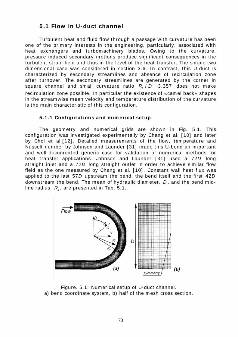
73
5.1 Flow in U-duct channel Turbulent heat and fluid flow through a passage with curvature has been
one of the primary interests in the engineering, particularly, associated with heat exchangers and turbomachinery blades. Owing to the curvature, pressure induced secondary motions produce significant consequences in the turbulent strain field and thus in the level of the heat transfer. The simple two dimensional case was considered in section 3.6. In contrast, this U-duct is characterized by secondary streamlines and absence of recirculation zone after turnover. The secondary streamlines are generated by the corner in square channel and small curvature ratio 357.3/ =DRc does not make
recirculation zone possible. In particular the existence of «camel back» shapes in the streamwise mean velocity and temperature distribution of the curvature is the main characteristic of this configuration.
5.1.1 Configurations and numerical setup The geometry and numerical grids are shown in Fig. 5.1. This
configuration was investigated experimentally by Chang et al. [10] and later by Choi et al.[12]. Detailed measurements of the flow, temperature and Nusselt number by Johnson and Launder [31] made this U-bend an important and well-documented generic case for validation of numerical methods for heat transfer applications. Johnson and Launder [31] used a D72 long straight inlet and a D72 long straight outlet in order to achieve similar flow field as the one measured by Chang et al. [10]. Constant wall heat flux was applied to the last D57 upstream the bend, the bend itself and the first D42 downstream the bend. The mean of hydraulic diameter, D , and the bend mid-line radius, cR , are presented in Tab. 5.1.
Figure. 5.1: Numerical setup of U-duct channel. a) bend coordinate system, b) half of the mesh cross section.
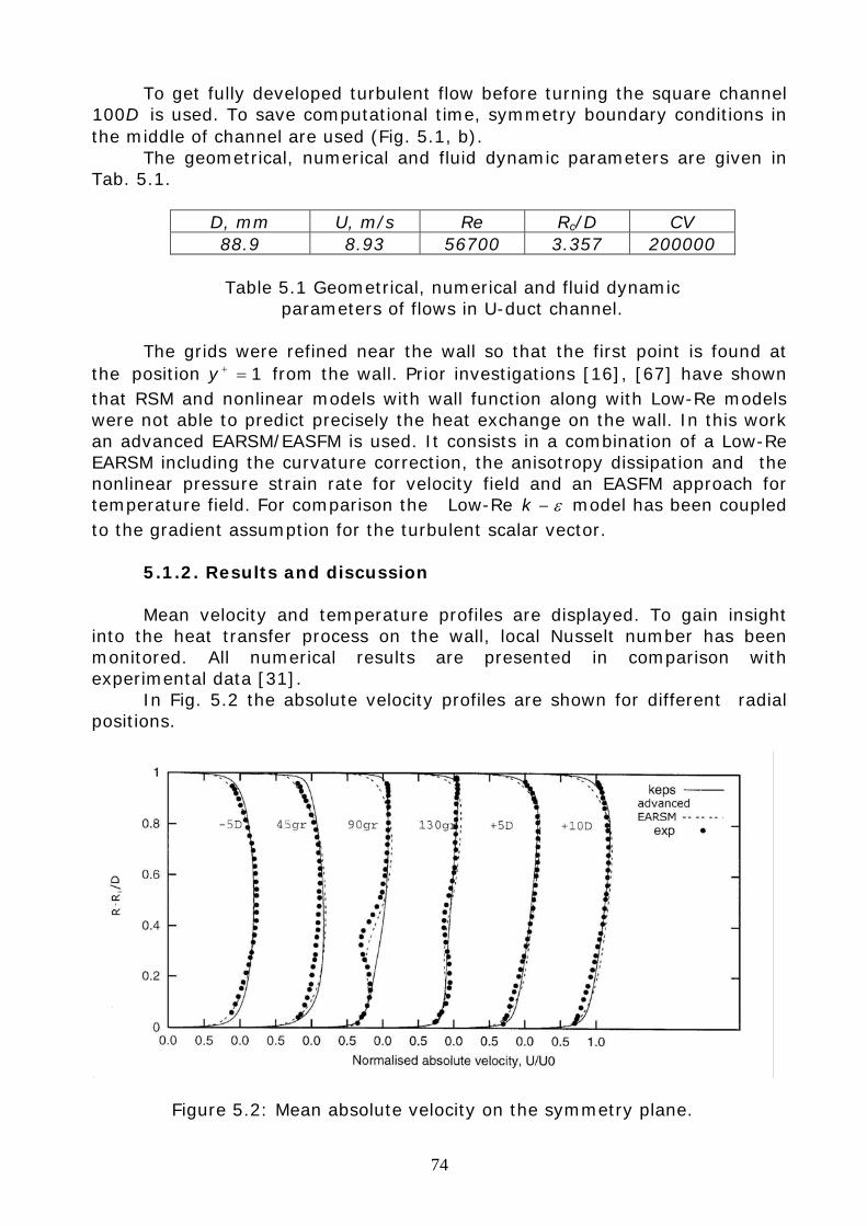
74
To get fully developed turbulent flow before turning the square channel D100 is used. To save computational time, symmetry boundary conditions in
the middle of channel are used (Fig. 5.1, b). The geometrical, numerical and fluid dynamic parameters are given in
Tab. 5.1.
D, mm U, m/s Re Rc/D CV 88.9 8.93 56700 3.357 200000
Table 5.1 Geometrical, numerical and fluid dynamic
parameters of flows in U-duct channel. The grids were refined near the wall so that the first point is found at
the position 1=+y from the wall. Prior investigations [16], [67] have shown that RSM and nonlinear models with wall function along with Low-Re models were not able to predict precisely the heat exchange on the wall. In this work an advanced EARSM/EASFM is used. It consists in a combination of a Low-Re EARSM including the curvature correction, the anisotropy dissipation and the nonlinear pressure strain rate for velocity field and an EASFM approach for temperature field. For comparison the Low-Re ε−k model has been coupled to the gradient assumption for the turbulent scalar vector.
5.1.2. Results and discussion Mean velocity and temperature profiles are displayed. To gain insight
into the heat transfer process on the wall, local Nusselt number has been monitored. All numerical results are presented in comparison with experimental data [31].
In Fig. 5.2 the absolute velocity profiles are shown for different radial positions.
Figure 5.2: Mean absolute velocity on the symmetry plane.
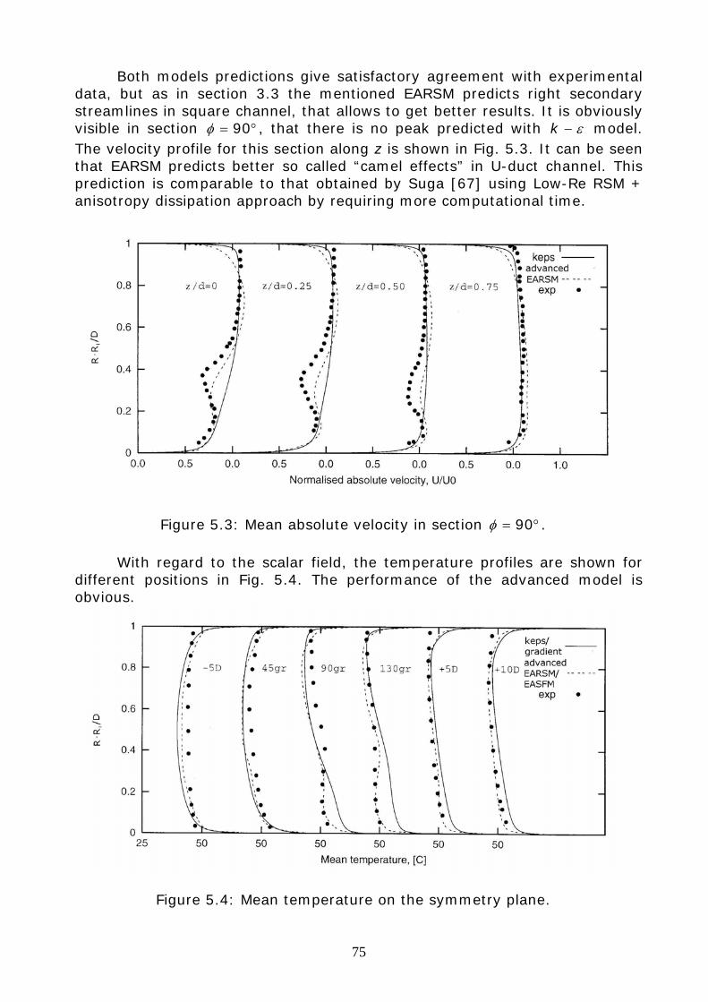
75
Both models predictions give satisfactory agreement with experimental data, but as in section 3.3 the mentioned EARSM predicts right secondary streamlines in square channel, that allows to get better results. It is obviously visible in section °= 90φ , that there is no peak predicted with ε−k model. The velocity profile for this section along z is shown in Fig. 5.3. It can be seen that EARSM predicts better so called “camel effects” in U-duct channel. This prediction is comparable to that obtained by Suga [67] using Low-Re RSM + anisotropy dissipation approach by requiring more computational time.
Figure 5.3: Mean absolute velocity in section °= 90φ . With regard to the scalar field, the temperature profiles are shown for
different positions in Fig. 5.4. The performance of the advanced model is obvious.
Figure 5.4: Mean temperature on the symmetry plane.
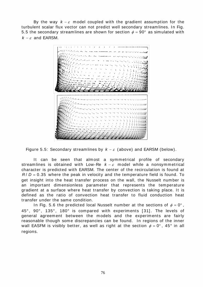
76
By the way ε−k model coupled with the gradient assumption for the turbulent scalar flux vector can not predict well secondary streamlines. In Fig. 5.5 the secondary streamlines are shown for section °= 90φ as simulated with
ε−k and EARSM.
Figure 5.5: Secondary streamlines by ε−k (above) and EARSM (below). It can be seen that almost a symmetrical profile of secondary
streamlines is obtained with Low-Re ε−k model while a nonsymmetrical character is predicted with EARSM. The center of the recirculation is found at
35.0/ =DR where the peak in velocity and the temperature field is found. To get insight into the heat transfer process on the wall, the Nusselt number is an important dimensionless parameter that represents the temperature gradient at a surface where heat transfer by convection is taking place. It is defined as the ratio of convection heat transfer to fluid conduction heat transfer under the same condition.
In Fig. 5.6 the predicted local Nusselt number at the sections of °= 0φ , 45°, 90°, 135°, 180° is compared with experiments [31]. The levels of general agreement between the models and the experiments are fairly reasonable though some discrepancies can be found. In regions of the inner wall EASFM is visibly better, as well as right at the section °= 0φ , 45° in all regions.
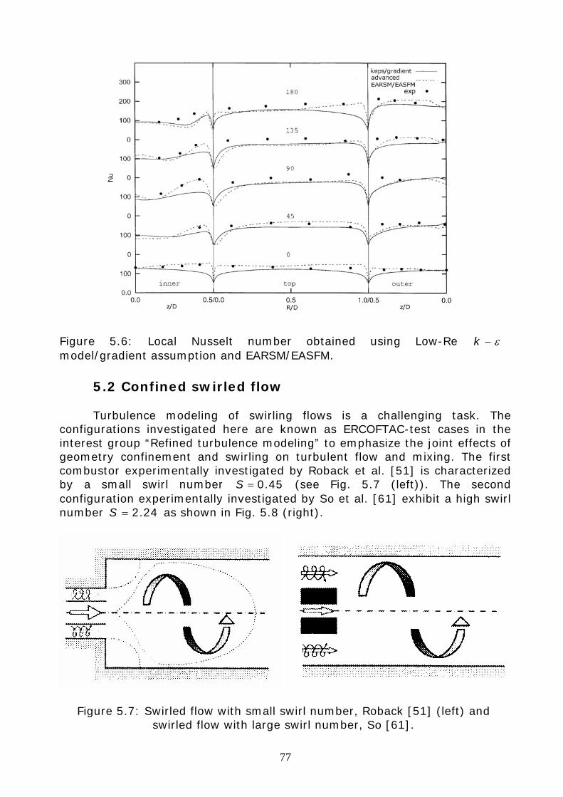
77
Figure 5.6: Local Nusselt number obtained using Low-Re ε−k model/gradient assumption and EARSM/EASFM.
5.2 Confined swirled flow Turbulence modeling of swirling flows is a challenging task. The
configurations investigated here are known as ERCOFTAC-test cases in the interest group “Refined turbulence modeling” to emphasize the joint effects of geometry confinement and swirling on turbulent flow and mixing. The first combustor experimentally investigated by Roback et al. [51] is characterized by a small swirl number 45.0=S (see Fig. 5.7 (left)). The second configuration experimentally investigated by So et al. [61] exhibit a high swirl number 24.2=S as shown in Fig. 5.8 (right).
Figure 5.7: Swirled flow with small swirl number, Roback [51] (left) and
swirled flow with large swirl number, So [61].
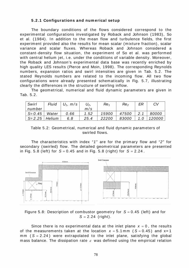
78
5.2.1 Configurations and numerical setup The boundary conditions of the flows considered correspond to the
experimental configurations investigated by Roback and Johnson (1983), So et al. (1984). In addition to the mean flow and turbulence fields, the first experiment provided also the results for mean scalar (mixture fraction), scalar variance and scalar fluxes. Whereas Roback and Johnson considered a constant-density flow situation, the experiment of So et al. was performed with central helium jet, i.e. under the conditions of variable density. Moreover, the Roback and Johnson’s experimental data base was recently enriched by high quality LES results (Pierce and Moin, 1998). The corresponding Reynolds numbers, expansion ratios and swirl intensities are given in Tab. 5.2. The stated Reynolds numbers are related to the incoming flow. All two flow configurations were already presented schematically in Fig. 5.7, illustrating clearly the differences in the structure of swirling inflow.
The geometrical, numerical and fluid dynamic parameters are given in Tab. 5.2.
Swirl number
Fluid U1, m/s U2, m/s
Re1 Re2 ER CV
S=0.45 Water 0.66 1.52 15900 47500 2.1 80000 S=2.25 Helium 6.8 25.4 22200 83000 1.0 120000
Table 5.2: Geometrical, numerical and fluid dynamic parameters of
swirled flows. The characteristics with index “1” are for the primary flow and “2” for
secondary (swirled) flow. The detailed geometrical parameters are presented in Fig. 5.8 (left) for 45.0=S and in Fig. 5.8 (right) for 24.2=S .
Figure 5.8: Description of combustor geometry for 45.0=S (left) and for 24.2=S (right).
Since there is no experimental data at the inlet plane 0=x , the results
of the measurements taken at the location 1.5=x mm ( 45.0=S ) and x=1 mm ( 24.2=S ) were extrapolated to the inlet plane, satisfying the global mass balance. The dissipation rate ε was defined using the empirical relation
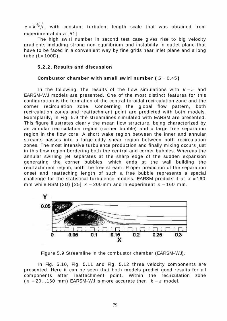
79
tlk 23
=ε with constant turbulent length scale that was obtained from experimental data [51].
The high swirl number in second test case gives rise to big velocity gradients including strong non-equilibrium and instability in outlet plane that have to be faced in a convenient way by fine grids near inlet plane and a long tube (L=100D).
5.2.2. Results and discussion Combustor chamber with small swirl number ( 45.0=S ) In the following, the results of the flow simulations with ε−k and
EARSM-WJ models are presented. One of the most distinct features for this configuration is the formation of the central toroidal recirculation zone and the corner recirculation zone. Concerning the global flow pattern, both recirculation zones and reattachment point are predicted with both models. Exemplarily, in Fig. 5.9 the streamlines simulated with EARSM are presented. This figure illustrates clearly the mean flow structure, being characterized by an annular recirculation region (corner bubble) and a large free separation region in the flow core. A short wake region between the inner and annular streams passes into a large-eddy shear region between both recirculation zones. The most intensive turbulence production and finally mixing occurs just in this flow region bordering both the central and corner bubbles. Whereas the annular swirling jet separates at the sharp edge of the sudden expansion generating the corner bubbles, which ends at the wall building the reattachment region, both the free stream. Proper prediction of the separation onset and reattaching length of such a free bubble represents a special challenge for the statistical turbulence models. EARSM predicts it at 160=x mm while RSM (2D) [25] 200=x mm and in experiment 160=x mm.
Figure 5.9 Streamline in the combustor chamber (EARSM-WJ). In Fig. 5.10, Fig. 5.11 and Fig. 5.12 three velocity components are
presented. Here it can be seen that both models predict good results for all components after reattachment point. Within the recirculation zone ( 160...20=x mm) EARSM-WJ is more accurate then ε−k model.
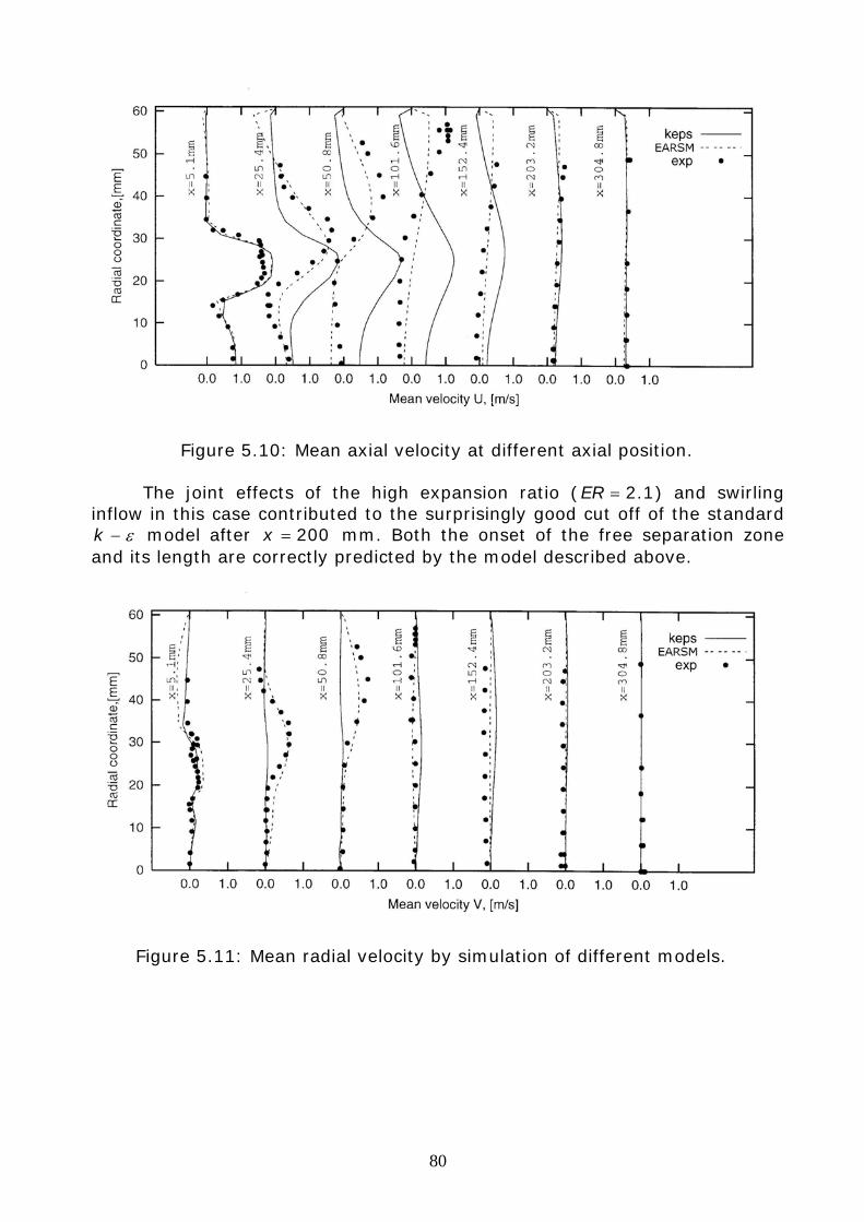
80
Figure 5.10: Mean axial velocity at different axial position. The joint effects of the high expansion ratio ( 1.2=ER ) and swirling
inflow in this case contributed to the surprisingly good cut off of the standard ε−k model after 200=x mm. Both the onset of the free separation zone
and its length are correctly predicted by the model described above.
Figure 5.11: Mean radial velocity by simulation of different models.
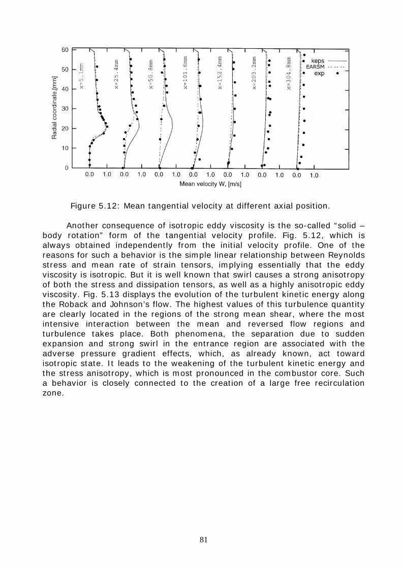
81
Figure 5.12: Mean tangential velocity at different axial position. Another consequence of isotropic eddy viscosity is the so-called “solid –
body rotation” form of the tangential velocity profile. Fig. 5.12, which is always obtained independently from the initial velocity profile. One of the reasons for such a behavior is the simple linear relationship between Reynolds stress and mean rate of strain tensors, implying essentially that the eddy viscosity is isotropic. But it is well known that swirl causes a strong anisotropy of both the stress and dissipation tensors, as well as a highly anisotropic eddy viscosity. Fig. 5.13 displays the evolution of the turbulent kinetic energy along the Roback and Johnson’s flow. The highest values of this turbulence quantity are clearly located in the regions of the strong mean shear, where the most intensive interaction between the mean and reversed flow regions and turbulence takes place. Both phenomena, the separation due to sudden expansion and strong swirl in the entrance region are associated with the adverse pressure gradient effects, which, as already known, act toward isotropic state. It leads to the weakening of the turbulent kinetic energy and the stress anisotropy, which is most pronounced in the combustor core. Such a behavior is closely connected to the creation of a large free recirculation zone.
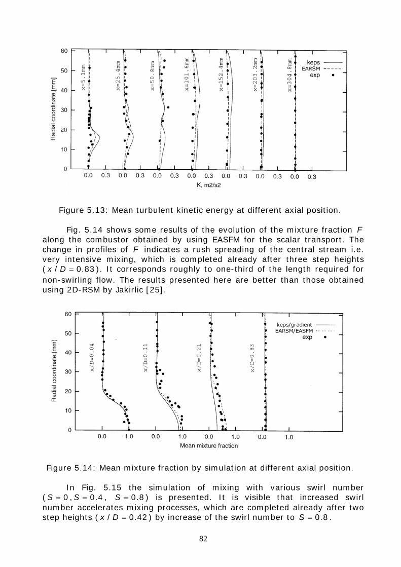
82
Figure 5.13: Mean turbulent kinetic energy at different axial position. Fig. 5.14 shows some results of the evolution of the mixture fraction F
along the combustor obtained by using EASFM for the scalar transport. The change in profiles of F indicates a rush spreading of the central stream i.e. very intensive mixing, which is completed already after three step heights ( 83.0/ =Dx ). It corresponds roughly to one-third of the length required for non-swirling flow. The results presented here are better than those obtained using 2D-RSM by Jakirlic [25].
Figure 5.14: Mean mixture fraction by simulation at different axial position. In Fig. 5.15 the simulation of mixing with various swirl number
( 0=S , 4.0=S , 8.0=S ) is presented. It is visible that increased swirl number accelerates mixing processes, which are completed already after two step heights ( 42.0/ =Dx ) by increase of the swirl number to 8.0=S .
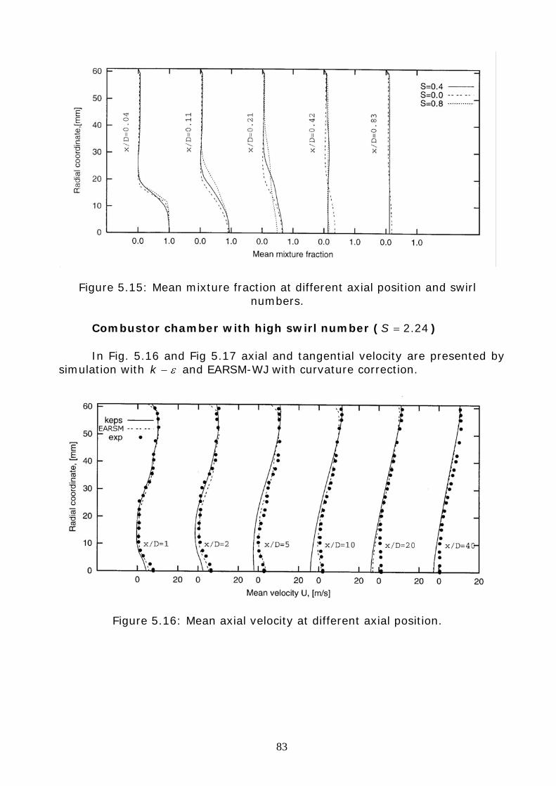
83
Figure 5.15: Mean mixture fraction at different axial position and swirl numbers.
Combustor chamber with high swirl number ( 24.2=S ) In Fig. 5.16 and Fig 5.17 axial and tangential velocity are presented by
simulation with ε−k and EARSM-WJ with curvature correction.
Figure 5.16: Mean axial velocity at different axial position.
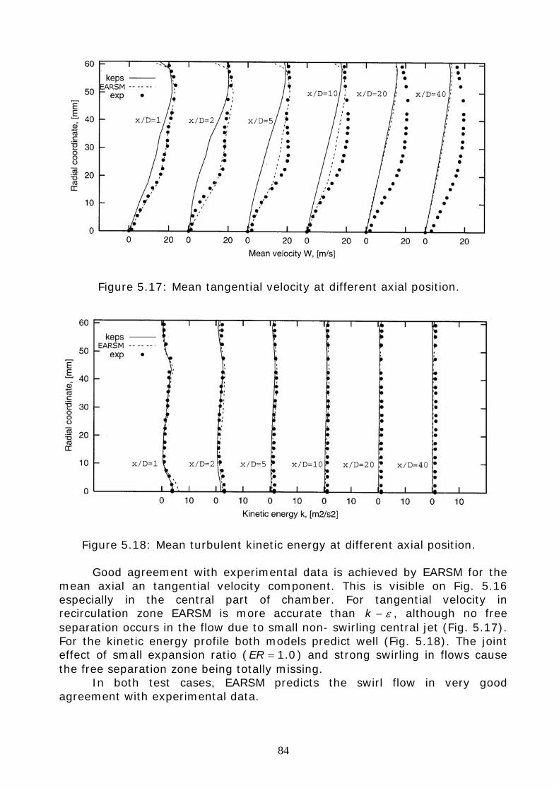
84
Figure 5.17: Mean tangential velocity at different axial position.
Figure 5.18: Mean turbulent kinetic energy at different axial position. Good agreement with experimental data is achieved by EARSM for the
mean axial an tangential velocity component. This is visible on Fig. 5.16 especially in the central part of chamber. For tangential velocity in recirculation zone EARSM is more accurate than ε−k , although no free separation occurs in the flow due to small non- swirling central jet (Fig. 5.17). For the kinetic energy profile both models predict well (Fig. 5.18). The joint effect of small expansion ratio ( 0.1=ER ) and strong swirling in flows cause the free separation zone being totally missing.
In both test cases, EARSM predicts the swirl flow in very good agreement with experimental data.
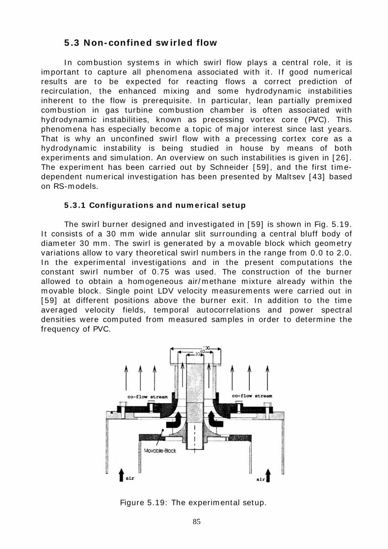
85
5.3 Non-confined swirled flow In combustion systems in which swirl flow plays a central role, it is
important to capture all phenomena associated with it. If good numerical results are to be expected for reacting flows a correct prediction of recirculation, the enhanced mixing and some hydrodynamic instabilities inherent to the flow is prerequisite. In particular, lean partially premixed combustion in gas turbine combustion chamber is often associated with hydrodynamic instabilities, known as precessing vortex core (PVC). This phenomena has especially become a topic of major interest since last years. That is why an unconfined swirl flow with a precessing cortex core as a hydrodynamic instability is being studied in house by means of both experiments and simulation. An overview on such instabilities is given in [26]. The experiment has been carried out by Schneider [59], and the first time-dependent numerical investigation has been presented by Maltsev [43] based on RS-models.
5.3.1 Configurations and numerical setup The swirl burner designed and investigated in [59] is shown in Fig. 5.19.
It consists of a 30 mm wide annular slit surrounding a central bluff body of diameter 30 mm. The swirl is generated by a movable block which geometry variations allow to vary theoretical swirl numbers in the range from 0.0 to 2.0. In the experimental investigations and in the present computations the constant swirl number of 0.75 was used. The construction of the burner allowed to obtain a homogeneous air/methane mixture already within the movable block. Single point LDV velocity measurements were carried out in [59] at different positions above the burner exit. In addition to the time averaged velocity fields, temporal autocorrelations and power spectral densities were computed from measured samples in order to determine the frequency of PVC.
Figure 5.19: The experimental setup.
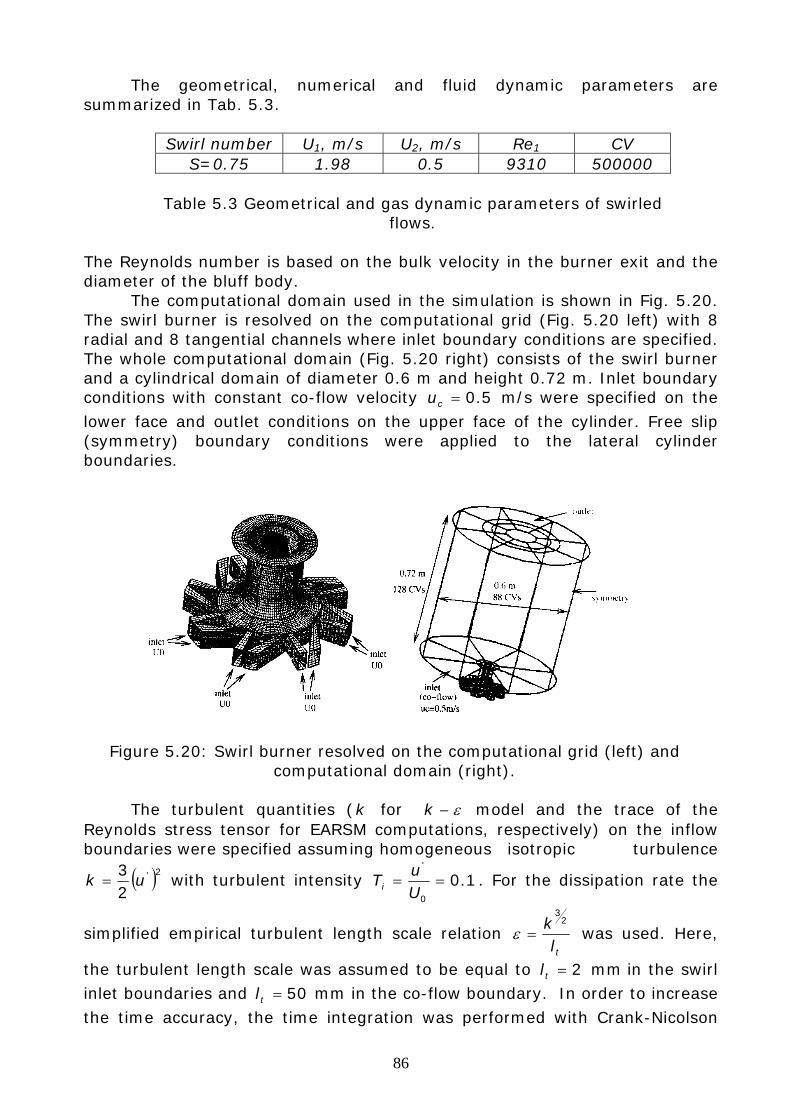
86
The geometrical, numerical and fluid dynamic parameters are summarized in Tab. 5.3.
Swirl number U1, m/s U2, m/s Re1 CV
S=0.75 1.98 0.5 9310 500000
Table 5.3 Geometrical and gas dynamic parameters of swirled flows.
The Reynolds number is based on the bulk velocity in the burner exit and the diameter of the bluff body.
The computational domain used in the simulation is shown in Fig. 5.20. The swirl burner is resolved on the computational grid (Fig. 5.20 left) with 8 radial and 8 tangential channels where inlet boundary conditions are specified. The whole computational domain (Fig. 5.20 right) consists of the swirl burner and a cylindrical domain of diameter 0.6 m and height 0.72 m. Inlet boundary conditions with constant co-flow velocity 5.0=cu m/s were specified on the lower face and outlet conditions on the upper face of the cylinder. Free slip (symmetry) boundary conditions were applied to the lateral cylinder boundaries.
Figure 5.20: Swirl burner resolved on the computational grid (left) and computational domain (right).
The turbulent quantities (k for ε−k model and the trace of the
Reynolds stress tensor for EARSM computations, respectively) on the inflow boundaries were specified assuming homogeneous isotropic turbulence
( )2'
23
uk = with turbulent intensity 1.00
'
==Uu
Ti . For the dissipation rate the
simplified empirical turbulent length scale relation tl
k 23
=ε was used. Here,
the turbulent length scale was assumed to be equal to 2=tl mm in the swirl inlet boundaries and 50=tl mm in the co-flow boundary. In order to increase the time accuracy, the time integration was performed with Crank-Nicolson
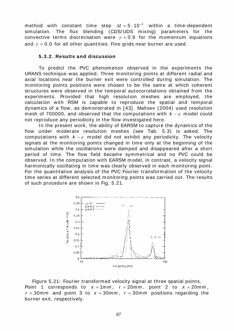
87
method with constant time step 4105 −⋅=Δt within a time-dependent simulation. The flux blending (CDS/UDS mixing) parameters for the convective terms discretisation were 9.0=γ for the momentum equations and 0.0=γ for all other quantities. Fine grids near burner are used.
5.3.2. Results and discussion To predict the PVC phenomenon observed in the experiments the
URANS technique was applied. Three monitoring points at different radial and axial locations near the burner exit were controlled during simulation. The monitoring points positions were chosen to be the same at which coherent structures were observed in the temporal autocorrelations obtained from the experiments. Provided that high resolution meshes are employed, the calculation with RSM is capable to reproduce the spatial and temporal dynamics of a flow, as demonstrated in [43]. Maltsev (2004) used resolution mesh of 700000, and observed that the computations with ε−k model could not reproduce any periodicity in the flow investigated here.
In the present work, the ability of EARSM to capture the dynamics of the flow under moderate resolution meshes (see Tab. 5.3) is asked. The computations with ε−k model did not exhibit any periodicity. The velocity signals at the monitoring points changed in time only at the beginning of the simulation while the oscillations were damped and disappeared after a short period of time. The flow field became symmetrical and no PVC could be observed. In the computation with EARSM model, in contrast, a velocity signal harmonically oscillating in time was clearly observed in each monitoring point. For the quantitative analysis of the PVC Fourier transformation of the velocity time series at different selected monitoring points was carried out. The results of such procedure are shown in Fig. 5.21.
Figure 5.21: Fourier transformed velocity signal at three spatial points. Point 1 corresponds to mmx 1= , mmr 20= , point 2 to mmx 20= ,
mmr 30= and point 3 to mmx 30= , mmr 30= positions regarding the burner exit, respectively.
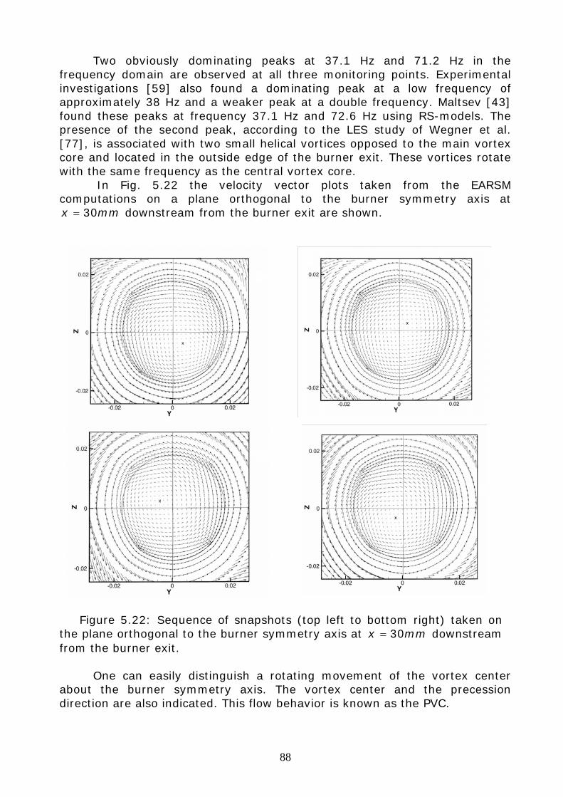
88
Two obviously dominating peaks at 37.1 Hz and 71.2 Hz in the frequency domain are observed at all three monitoring points. Experimental investigations [59] also found a dominating peak at a low frequency of approximately 38 Hz and a weaker peak at a double frequency. Maltsev [43] found these peaks at frequency 37.1 Hz and 72.6 Hz using RS-models. The presence of the second peak, according to the LES study of Wegner et al. [77], is associated with two small helical vortices opposed to the main vortex core and located in the outside edge of the burner exit. These vortices rotate with the same frequency as the central vortex core.
In Fig. 5.22 the velocity vector plots taken from the EARSM computations on a plane orthogonal to the burner symmetry axis at
mmx 30= downstream from the burner exit are shown.
Figure 5.22: Sequence of snapshots (top left to bottom right) taken on the plane orthogonal to the burner symmetry axis at mmx 30= downstream from the burner exit.
One can easily distinguish a rotating movement of the vortex center
about the burner symmetry axis. The vortex center and the precession direction are also indicated. This flow behavior is known as the PVC.
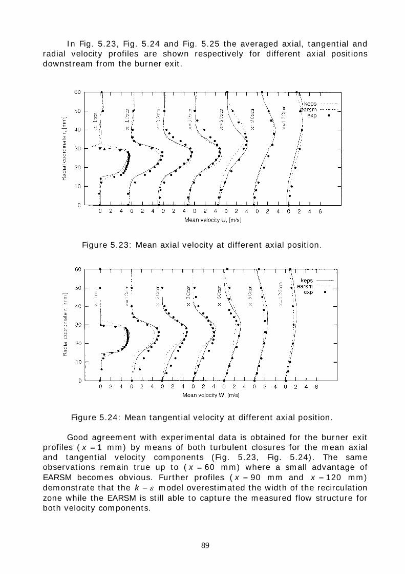
89
In Fig. 5.23, Fig. 5.24 and Fig. 5.25 the averaged axial, tangential and radial velocity profiles are shown respectively for different axial positions downstream from the burner exit.
Figure 5.23: Mean axial velocity at different axial position.
Figure 5.24: Mean tangential velocity at different axial position. Good agreement with experimental data is obtained for the burner exit
profiles ( 1=x mm) by means of both turbulent closures for the mean axial and tangential velocity components (Fig. 5.23, Fig. 5.24). The same observations remain true up to ( 60=x mm) where a small advantage of EARSM becomes obvious. Further profiles ( 90=x mm and 120=x mm) demonstrate that the ε−k model overestimated the width of the recirculation zone while the EARSM is still able to capture the measured flow structure for both velocity components.
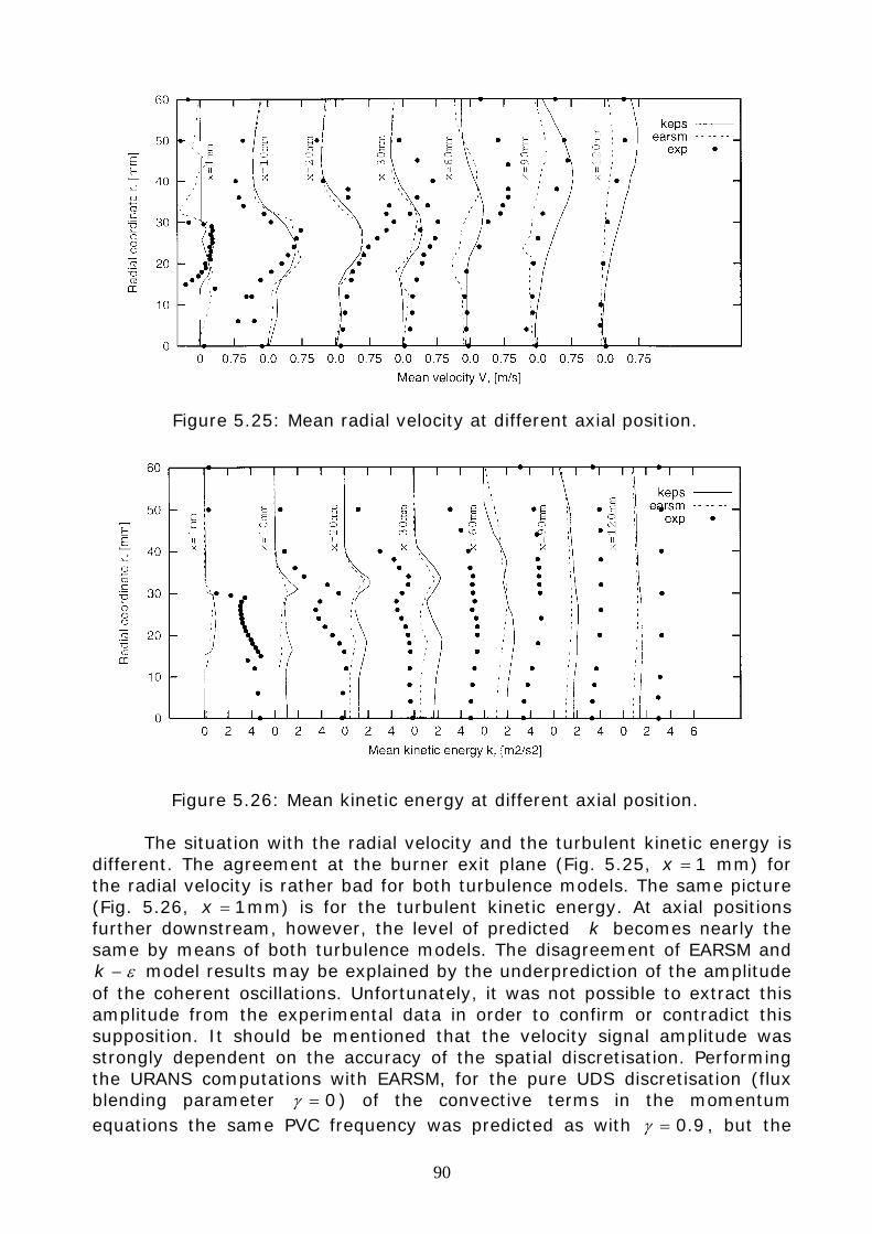
90
Figure 5.25: Mean radial velocity at different axial position.
Figure 5.26: Mean kinetic energy at different axial position. The situation with the radial velocity and the turbulent kinetic energy is
different. The agreement at the burner exit plane (Fig. 5.25, 1=x mm) for the radial velocity is rather bad for both turbulence models. The same picture (Fig. 5.26, 1=x mm) is for the turbulent kinetic energy. At axial positions further downstream, however, the level of predicted k becomes nearly the same by means of both turbulence models. The disagreement of EARSM and
ε−k model results may be explained by the underprediction of the amplitude of the coherent oscillations. Unfortunately, it was not possible to extract this amplitude from the experimental data in order to confirm or contradict this supposition. It should be mentioned that the velocity signal amplitude was strongly dependent on the accuracy of the spatial discretisation. Performing the URANS computations with EARSM, for the pure UDS discretisation (flux blending parameter 0=γ ) of the convective terms in the momentum equations the same PVC frequency was predicted as with 9.0=γ , but the
91
amplitude of the coherent oscillations was significantly smaller than that predicted with 9.0=γ . This fact reveals the importance of the numerical accuracy in the prediction of the coherent motion. The values of the radial velocity are captured with reasonable agreement with both EARSM and ε−k model. Though the measured data for such small mean velocity values (nearly zero) at such a high level of turbulence should be considered very carefully.
92
Chapter 6 Conclusions
In the present work, a complete CFD model for the simulation of turbulent flows in complex geometries was developed and systematically assessed in technically relevant configurations. The model is formulated in the explicit algebraic RANS-context, and includes following elements: • The closure for velocity and scalar turbulence is properly extended for taking into account non-equilibrium turbulence effects through nonlinear pressure-strain correlation term, curvature correction and dissipation anisotropy. This defines advanced EARSM/EASFM with Low-Re features. Besides the eddy viscosity/diffusivity formulations, based on the standard linear ε−k model, nonlinear models and classical EARSM/EASFM are also considered in this work for velocity and scalar turbulence. A constant density formulation has been adopted, so that no chemical reaction has been included. • A link to the thermodynamical consistency of the models has been outlined to formulate thermodynamically consistent models along with physically realizable models. • The established coupled model was integrated into a complex three-dimensional geometry flexible CFD code. The details of the implementation, numerical solution method as well as setting up of the boundary conditions and estimation of errors were described and discussed in detail. • For the model assessment and validation a systematical computational study on configurations of various complexitycomplexities was carried out. In the simulations the iterative errors were reduced driving the residual to acceptably low values. The suppression of numerical diffusion was applied by continuous switching from lower (UDS) to higher (CDS) order discretisation schemes as long as stable convergence was possible. A systematical grid refinement was carried out in order to minimize the discretisation errors and to obtain a grid independent solution. In the model assessment several aspects were investigated and the following concluding remarks can be made: 1. The combination of advanced EARSM/EASFM allows to predict satisfactorily the flow processes with mixing and heat transfer phenomena in complex configurations without numerical problems inherent to RS-models. 2. In curved ducts of relevance in heat-exchangers, cooling passages of gas turbines and automobile engines, the existence of the so-called “camel back” shapes in the streamwise mean velocity and temperature distribution in the curvature has been predicted well, in contrast to linear, nonlinear ε−k models and some RS-models. 3. In swirled confined flows, turbulent flow and mixing processes dominated by joint effects of geometry confinement (expansion ratio ER), circumferential velocity type (two configurations with annular and central swirling jet) and swirl intensity (S) are satisfactorily described. Some results (velocity components) are better than those from computations using RSM. 4. The numerical study of a non-confined isothermal swirled flow induced by a swirl burner revealed the complete inability of the linear eddy
93
viscosity ( ε−k ) formulation to even qualitatively capture a swirl flow instability (PVC) by means of transient computations. The EARSM based turbulence closure was, in contrast, able to obtain the harmonic oscillations with nearly constant (in time) amplitude. The quantitative comparison with experimental results has demonstrated the remarkably accurate prediction of the precession frequency by means of the EARSM approach. The predicted amplitude of the harmonic oscillations was strongly influenced by the spatial discretisation of the convective terms in the momentum equations. This amplitude was, however, underpredicted even with numerical scheme of the highest possible accuracy. This underprediction caused, in turn, the underprediction of the whole fluctuating energy with deviation of even 100% at some flow locations. Further investigations on grid refinement and modeling parameters are necessary for this reason, as demonstrated in [26]. 5. The modeling of turbulence remained the most critical aspect throughout the simulated configurations. Good agreement with experimental data for more simple flows with or without separation and rotation has been achieved. The thermodynamical consistency has to be included in the advanced formulation. 6. Dealing with configurations exhibiting strong wall effects, Low-Re approach is recommendable, as shown in this work. In such cases, LES can not be high performance. As U-RANS performs well in predicting unsteady behavior, one approach to get around the LES bottleneck is the hybrid LES-RANS, in which RANS is used near wall while LES is utilized in the remaining part of the domain.
Furthermore, the need of simulating complex systems with several parts that have to be computed with different flow solvers requires an exchange of information at the interfaces of the computational domains of each part. Gas turbine systems including multi-component phenomena, such as compressor/combustor instability or combustor/turbine hot-streak migration are typical examples. In the compressor and the turbine part, the flow solver must better account for the moving blades, the wall turbulence, and predict the pressure and density distribution. Such a flow solver has to be based on the RANS-approach. In the combustion chamber part, the flow solver has to be able to handle with flows governed by large scale turbulence, chemical reaction, and radiation. This flow solver may be based on LES. 7. In the RANS-context, EARSM/EASFM does not experience numerical problems as their parents “transport equations” models, and in general, EARSM/EASFM does not demand considerable computer resources as LES or RSM (see Tab. 6.1). In Tab. 6.1 the estimated time is presented for different models based on RANS depending on configurations.
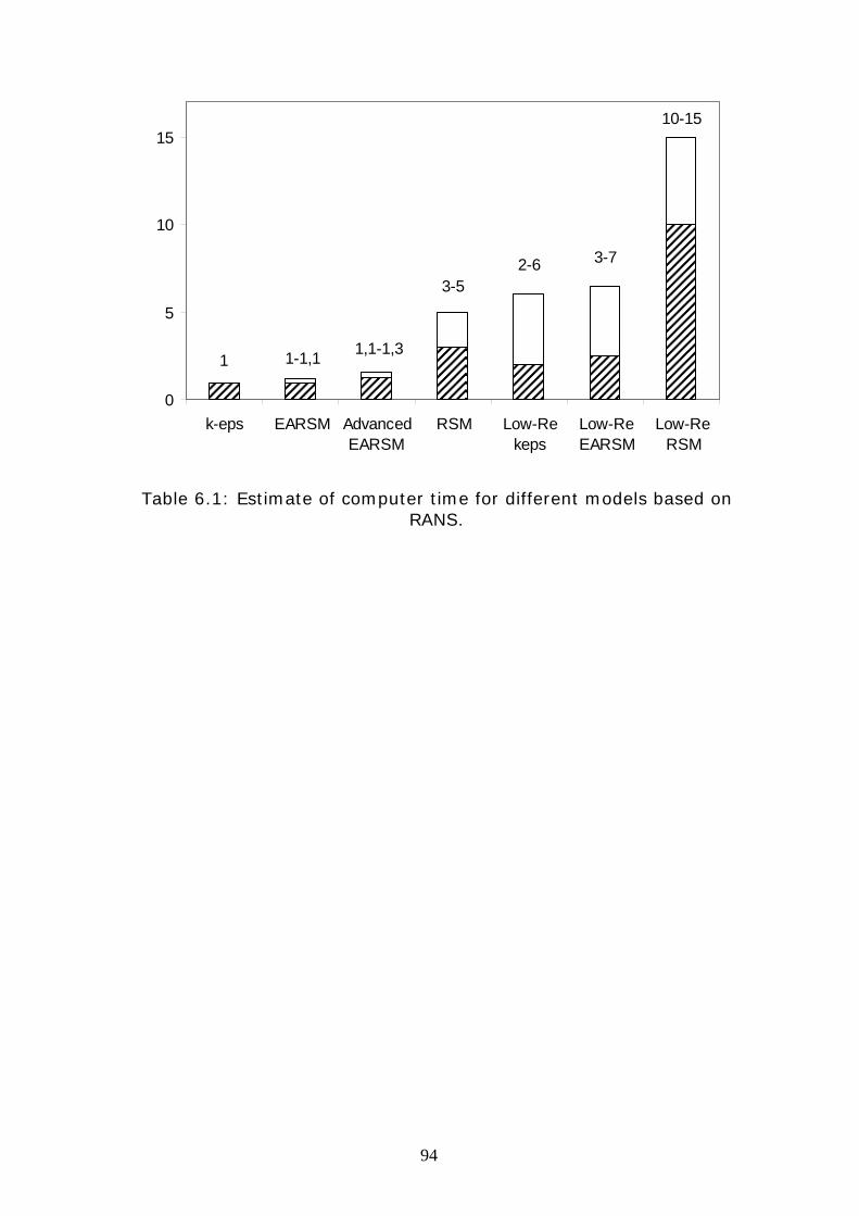
94
10-15
3-72-6
1 1-1,1 1,1-1,3
3-5
0
5
10
15
k-eps EARSM AdvancedEARSM
RSM Low-Rekeps
Low-ReEARSM
Low-ReRSM
Table 6.1: Estimate of computer time for different models based on RANS.
95
Bibliography 1. Abe K. An investigation of algebraic turbulence and turbulent scalar-flux
models for complex flow fields with impingement and separation. Turbulence and Shear Flow Phenomena II, Stockholm, II: 223-228, June 27-29.2001.
2. Abe K., Kondoh T., Nagano Y. A new turbulence model for predicting fluid flow and heat transfer in separating and reattaching flows. Int. J. Heat Mass Transfer, Vol. 37, pp. 139-151., 1994.
3. Abe K., Suga K. Towards the Development of a Reynolds – Averaged algebraic Turbulent Scalar – Flux Model. Int. J. Heat Fluid Flow, Vol. 22, pp. 19-29, 2001.
4. Alvelius K., Johansson A.V. Direct numerical simulation of rotating channel flow at various Reynolds numbers and rotation number. In PhD thesis of K. Alvelius. Dept. of Mechanics, KTH, Stockholm, Sweden, 1999.
5. Anderson D.A., Tannehill J.C., Pletcher R.H. Computational fluid mechanics and heat transfer. Moscow, “Mir”, 1990.
6. Baldwin B.S., Lomax H. Thin – Layer Approximation and algebraic Model for Separated Turbulent Flows”. AIAA Paper 78-257, Huntsville, AL , 1978.
7. Bauer W., Berechnung turbulenter Strömungen mit starken Stromlinienkrümmungen beziehungweise mit Rotation. Darmstadt, 1998.
8. Boussinesq. J. Theorie de l’ Ecoulemen Tourbillant. Mem. Presentes par Divers Savants Acad. Sci. Inst. Fr. , Vol. 23, pp. 46-50, 1877.
9. Bradshaw P., Ferris D.H., Atwell N.P. Calculation of Boundary Layer Development Using the Turbulent Energy Equation. Journal of Fluid Mechanics, Vol. 28, Pt.3 , pp. 593-616.
10. Chang S.M., Humphrey J.A.C., Modavi A. Turbulent flow in a strongly curved U-Bend and downstream tangent of square cross-sections. Phys. Chem. Hydrodyn. 4 (3) 243-269. 1983.
11. Chen C.J., Rodi W. Vertical Turbulent Buoyant Jets. A review of experimental data. Pergamon Press, 1980.
12. Choi Y.D., Moon C., Yang. Measurement of turbulent flow characteristics of square duct with a 180° bend by hot wire anemometer. Intl. Symp. On Engng. Turbulence Modelling and Measurements. Elsevier, pp. 429-438, 1990.
13. Chou P.Y. On the Velocity Correlations and the Solution of the Equations of Turbulent Fluctuation. Quart. Appl. Math. , Vol. 3, p. 38.
14. Craft T.J., Launder B.E. and Suga K. Development and application of a cubic eddy – viscosity model of turbulence. Int. J. Heat and Fluid Flow 17: 108-115, 1996.
15. Daly B.J., Harlow F.H. Transport equations in turbulence. Phys. Fluids 13:2634-2649.
16. Etemad S., Rokni M., Sunden B. and Daunis O. Analysis of Turbulent Flow and Heat Transfer in A Square-Sectioned U-Bend. Turbulence. Heat and mass Transfer 4. Begell House, 2003.
17. FASTEST-3D-CFD-Code. Handbuch, Invent Computing GmbH, Erlangen, 1997.
18. Ferziger J.H., Peric M. Computational Methods for Fluid Dynamics. Berlin. 1996.
96
19. Fu S., Rung T., Thiele F. Realizability of non – linear stress strain relationships for Reynolds – Stress closures. Symposium on Turbulent Shear Flows. Vol 7, Grenolle, 1997.
20. Gatski T.B., Speziale C.G. On explicit algebraic stress models for complex turbulent flows. Journal of fluid Mechanics. Vol. 254, pp. 59-78, 1993.
21. Gibson M.M., Launder B.E. Ground effects on pressure fluctuations in the atmospheric boundary layer. J. Fluid Mech. 86:491-511, 1978.
22. Girimaji S. Fully-Explicit and Self-Consistent Algebraic Reynolds Stress Model. NASA Research Center, Hampton, Va 23681-0001.
23. Grundestam O., Wallin S., Johansson A. A generalized EARSM based on a nonlinear pressure strain rate model. Turbulence and Shear Flow Phenomena II, Stockholm, II: 223-228, June 27-29.2001.
24. Imao S., Itoh M., Harada T. Turbulent characteristics of the flow in an axiall rotating pipe. Int. J. Heat Fluid Flow 17, 444-451.
25. Jakirlic S., Tropea C. Numerische Modellierung konvektiver Wärmeübertragung unter Berücksichtigung wandnaher Turbulenz. Sonderforschungsbereich 568, 2003.
26. Johmann P., Sinigersky A., Hehle M., Schäfer O, Koch R. Numerical Simulation of a Precessing Vortex Breakdown. Elsevier, 2004.
27. Johansson A.V., Hallbäck M. Modeling of rapid pressure-strain in Reynolds stress closures. J. Fluid Mech., vol. 269, pp. 143-168, 1994.
28. Jongen T., Machiels L., Gatski T.B. Predicting Noninertial Effects With Algebraic Stress Models Which Account for Dissipation Rate Anisotropies. NASA Technical Memorandum 112853, 1997.
29. Jones W.P., Launder B.E. The prediction of laminarization with a two-equation model of turbulence. Int. J. Heat Mass Transfer, 15:301-314, 1972.
30. Johnson D.A., King L.S. A Mathematically Simple Turbulence Closure Model for Attached and Separated Turbulent Boundary Layers. AIAA Journal, Vol. 23, No. 11, pp. 1684-1692.
31. Johnson D.A., Launder B. E. Local Nusselt number and temperature field in turbulent flow through a heated square-sectioned U-bend. Intl. J. Heat and Fluid flow, Vol. 6, No. 3, pp. 171-180, 1985.
32. Jovic S. An experimental study on the Recovery of a Turbulent Boundary layer downstream of the Reattachment Engineering Turbulence Modeling and Experiments 2. pp. 509-517. 1993.
33. Han J.C. Heat Transfer and Friction in Channels with two Opposite Rib Roughened Walls. J. Heat Transfer, 106:774-781, 1984.
34. Högström C., Wallin S., Johansson A.V. Passive scalar flux modeling for CFD. Turbulence and Shear Flow Phenomena II, Stockholm, II: 223-228, June 27-29.2001.
35. Kader B.A., Yaglom A.M. Heat and mass transfer lows for fully turbulent wall flows. Int. J. Heat Mass Transfer. Vol. 15. pp. 2329-2351,1972.
36. Kim J., Moin P. Transport of Passive Scalars in a Turbulent Channel Flows. Turbulent Shear Flows 6, pp. 85-96, 1989.
37. Kim J., Moin P., Moser R. Turbulence statistics in fully developed channel flow at the low – Reynolds number. J. Fluid Mech., Vol. 177, pp. 133-166.
38. Kolmogorov A.N. Equations of turbulent motion of an incompressible fluid. Izvestia Academy of Sciences, USSR; Physics 6:56-58, 1942.
97
39. Larsen P.S., Westergaard C.H., Koch C.W., Schmidt J.J. Experimental and numerical Study of fence – on – wall case. 12 – Month intermediate report of AFM Technical University of Denmark.
40. Laufer J. Flow in a two dimensional channel. Report 1053, 1950. 41. Launder B.E., Reece G.J. and Rodi W. Progress in the development of a
Reynolds – stress turbulence closure. J. Fluid Mech. 68:537-566. 1975 42. Le H., Moin P., Kim J. Direct Numerical Simulation of Turbulent flow over a
Backward – Facing Step. Proc. Of 9-th Sump. On Turbulent Shear flows. Paper №13-2, Kyoto, August 16-18, 1993.
43. Maltsev A. Towards the Development and Assessment of Complete CFD Models for the Simulation of Stationary Gas Turbine Combustion Processes. Doctor thesis. Darmstadt. 2004.
44. Mansour N.N., Kim J., Moin P., Reynolds – stress and dissipation – rate budgets in a turbulent channel flow. J. Fluid Mech., Vol. 194,pp. 15-44. 1988.
45. Menter F.R. Zonal two Equation ω−k Turbulence Models for Aerodynamic Flows. A/AA 93-2906.
46. Menter F.R. Methoden, Moeglichkeiten und Grenzen numerischer Stroemungsberechnungen. Numet. Erlangen, 2002.
47. Moin P. LES of a confined coaxial jet with swirl and heat release. AIAA Paper 98-2892, 1998.
48. Monson D.J., Seegmiller H.L. An experimental investigation of subsonic flow in a two dimensional u – duct. NASA TM – 103931, 1992.
49. Nee V.W., Kovasznay L.S.G. The calculation of the incompressible Turbulent Boundary Layer by a Simple Theory. Physics of Fluid, Vol. 12, p. 473.
50. Pope S. A more general effective viscosity hypothesis. J. Fluid Mech. 72: 331-340. 1975
51. Roback R., Johnson B.V. Mass and Momentum Turbulent Transport Experiments with Confined Swirling Coaxial jets. NASA Contractor Report 168252, 1983.
52. Rodi W. A New algebraic Relation for Calculating the Reynolds Stresses. Mechanical of Fluid, ZAMM 56, T219-T221, 1976.
53. Rotta J. C. Statistische Theorie Nichthomogener Turbulenz. Z. Phys., Vol. 129, pp. 547-575, 1951.
54. Rumsey C., Gatski T., Morrison J. Turbulence Model Predictions of Extra-Strain Rate Effects in Strongly-Curved flows. AIAA 99-0157, 1999.
55. Sadiki A. Thermodynamik und Turulenzmodellirung. Habilitationschrift., Darmstadt, 1998.
56. Sadiki A., Hutter K., Janicka J. Thermodynamically consistent second order turbulent turbulence modeling based on extended thermodynamics. Engineering Turbulence Modeling and Experiments 4, Elsevier, pp. 93-102, 1999.
57. Sadiki A., Hutter K. On thermodynamics of Turbulence: Development of First Order Closure Models and Critical Evaluation of existing Models. J. Non-Equilb. Thermodyn. 25(2), 2000.
58. Sadiki A., Jakirlic S., Hanjalic K. Towards a Thermodynamically Consistent, Anisotropy-Resolving Turbulence Model for Conjugate Flow, Heat and Mass Transfer. Turbulence, Heat and Mass Transfer 4. Begell House, Inc., 2003.
98
59. Schneider C. Über die Characterisierung von Turbulenzstrukturen in verdrallten Strömungen. PhD thesis, Darmstadt, 2003.
60. Smith A.M.O., Cebeci T. Numerical Solution of the Turbulent Boundary – Layer Equatio., Douglas Aircraft Division Report DAC 33735, 1967.
61. So R.M.S, Ahmed S.A., Mongia H.C. An Experimental Investigation of Gas Jets in Confined Swirling Air Flow. NASA Contractor Report 3832. 1984.
62. Song Fu, Weiqi Qian, Guanghua Zhang. Development of Nonlinear Eddy-Viscosity Model for Numerical Simulation of Three-Dimensional Turbulent Boundary Layer. Elsevier Science. 2002.
63. Spalart P.R., Allmaras S.R A One-Equation Turbulence model for Aerodynamics. Conference Reno, Nevada, USA, 92-439. 1999.
64. Spenser A. J.M., Rivlin R.S. The theory of matrix polynomials and its application to the mechanics of isotropic continua. Arch. Rat. Mech. Anal. 2:309-336, 1959.
65. Speziale C.G., Sarkar S., Gatski T.B. Modeling the pressure strain correlation of turbulence: an invariant dynamical systems approach. J. Fluid Mech. 227:245-272, 1991.
66. Stone H. L. Iterative solution of implicit approximations of multidimensional partial differential equation. SIAM J. Numer. Anal. Vol. 5, No. 3, pp. 530-558, 1968.
67. Suga K. Predicting turbulence and heat transfer in 3-D curved ducts by near-wall second moment closures. International Journal of Heat and Mass Transfer 46. 2002.
68. Suga K. Improvement of Second Moment Closure for Turbulent Obstacle Flow and Heat Transfer. Begell House, Inc., 2003.
69. Suga K., Abe K. Nonlinear Eddy Viscosity Modeling for turbulence and Heat Transfer Near Wall and Shear Free Boundaries. Int. J. Heat Fluid flow. Vol. 21, pp. 37-48, 2000.
70. Spurk J.H. Stroemungslerhe. 2 Auflage. Springer-Verlag, Berlin, 1989. 71. Strelets M. Detached eddy simulation of massively separated flows. AIAA-
00-2306, 2000. 72. TURBOMECA. Technical report N13294: final report on the design with
numerical simulation of the MAKILA DLN combustor (concept 2). May 1998.
73. Van Driest E. R. On turbulent Flow Near a Wall. Journal of the Aeronautical Sciences, Vol. 18, pp. 145-160, 1956.
74. Wallin S. Engineering turbulence modeling for CFD with a focus on explicit algebraic Reynolds stress models. Doctoral thesis. Norsteds Truckeri, Stockholm, Sweden, 2000.
75. Wallin S., Hellsten A., Schatz M., Rung T., Peshkin D., Johansson A.V. Streamline curvature corrected algebraic Reynolds stress turbulence modeling. Turbulence and Shear Flow Phenomena II, Stockholm, II: 223-228, June 27-29.2001.
76. Wallin S., Johansson A.V. Modeling of streamline curvature effects on turbulence in explicit algebraic Reynolds stress turbulence models. Turbulence and Shear Flow Phenomena II, Stockholm, II: 223-228, June 27-29.2001.
99
77. Wegner B., Maltsev A., Schneider C., Dreizler A., Sadiki A., Janicka J. Evaluation of URANS performance in Predicting an Unconfined Swirling Flow with Precessing Vortex core based on LES and Experiments. Third International Symposium on Turbulence and Shear Flow Phenomena, TSFP3, Sendai, Japan, vol. 1, pp. 51-56, June 25-27, 2003.
78. Wikstrom P.M., Wallin S., Johansson A.V. Derivation and investigation of a new explicit algebraic model for the passive scalar flux. Phy. Fluids. 12:688-702. 2000.
79. Wilcox D.C. Turbulence Modeling for CFD. California, 1994. 80. Yang K.S. & Ferzigen J.H. Large-Eddy Simulation of Turbulent Obstacle
Flow Using a Dynamic Subgrid-Scale Model. AIAA J. Vol. 31, pp. 1406-1413, 1993.
81. Yokosawa H., Fujita H., Hirota M. & Iwata S., Measurement of turbulent flow in square duct with roughened walls on two opposite sides. Int. J. Meat and Fluid Flow, Vol. 10, No.2, pp. 125-130,1989.
82. Yoshioka, Obi, Masudu. Turbulence statistics of Periodically perturbed separated flow over backward – facing step. Int. Journal of Heat and Fluid, Vol. 22, pp. 393-401, 2001.
83. Zheng Q. Theory of representation for tensor function – A unified invariant approach to constitutive equation. Appl. Mech. Rev. 47 (11): 545-587. 1994.
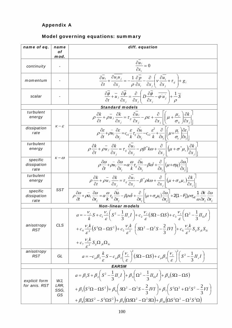
100
Appendix A Model governing equations: summary
name of eq. name
of mod.
diff. equation
continuity
- 0=
∂∂
i
i
xu
momentum
- iij
j
i
jij
jii gxu
xxp
xuu
tu
+⎟⎟⎠
⎞⎜⎜⎝
⎛+
∂∂
∂∂
−∂∂
−=∂
∂+
∂∂ τν
ρ1
scalar
- Su
xD
xxu
t jjjj
jρ
ϕφφφ 1'' +⎟⎟⎠
⎞⎜⎜⎝
⎛−
∂∂
∂∂
=∂∂
+∂∂
Standard models turbulent energy
⎥⎥⎦
⎤
⎢⎢⎣
⎡
∂∂
⎟⎟⎠
⎞⎜⎜⎝
⎛+
∂∂
+−∂∂
=∂∂
+∂∂
jk
t
jj
iij
j
jxk
xxu
xku
tk
σμ
μρετρρ
dissipation rate
ε−к
⎥⎥⎦
⎤
⎢⎢⎣
⎡
∂∂
⎟⎟⎠
⎞⎜⎜⎝
⎛+
∂∂
+−∂∂
=∂∂
+∂∂
j
t
jj
iij
j
jxxk
cxu
kc
xu
tε
σμμετεερερε
εε
2
21
turbulent energy ( )
⎥⎥⎦
⎤
⎢⎢⎣
⎡
∂∂
+∂∂
+−∂∂
=∂∂
+∂∂
jt
jj
iij
j
jxk
xk
xu
xku
tk μσμωρβτρρ **
specific dissipation
rate
ω−к
( )⎥⎥⎦
⎤
⎢⎢⎣
⎡
∂∂
+∂∂
+−∂∂
=∂∂
+∂∂
jt
jj
iij
j
jxxx
ukx
ut
ωσμμβωτωαωρωρ 2
turbulent energy ( )
⎥⎥⎦
⎤
⎢⎢⎣
⎡
∂∂
+∂∂
+−∂∂
=∂∂
+∂∂
jtk
jj
iij
j
jxk
xk
xu
xku
tk μσμωρβτρρ *
specific dissipation
rate
SST ( )
jjjt
jj
iij
j
jxx
kF
xxxu
kxu
t ∂∂
∂∂
−+⎥⎥⎦
⎤
⎢⎢⎣
⎡
∂∂
+∂∂
+−∂∂
=∂∂
+∂∂ ω
ωρσωμσμβρωτωαωρωρ ωω
1)1(2 21
2
Non-linear models
anisotropy RST
CLS
( )
( )
kijkijt
kijkijttt
tts
tt
Sk
c
SSSk
cIVISSk
cSSk
c
IIIcSScIIIScSk
a
ΩΩ+
+⎟⎠⎞
⎜⎝⎛ −Ω−Ω+Ω−Ω+
⎟⎠⎞
⎜⎝⎛ −Ω+Ω−Ω+⎟
⎠⎞
⎜⎝⎛ −+−= Ω
27
2622
2522
24
232
21
32
31
31
εν
εν
εν
εν
εν
εν
ενν
anisotropy RST
GL ( ) ⎟
⎠⎞
⎜⎝⎛ −⎟
⎠⎞
⎜⎝⎛+Ω−Ω⎟
⎠⎞
⎜⎝⎛−−= IIIScSScSkca s
tt
312
2
3
2
21 εν
βεν
βε
β μμμ
EARSM
explicit form for anis. RST
WJ, LRR, SSG, GS
( )
( )( ) ( ) ( )ΩΩ−ΩΩ+ΩΩ−ΩΩ+Ω−Ω+
⎟⎠⎞
⎜⎝⎛ −Ω+Ω+⎟
⎠⎞
⎜⎝⎛ −Ω−Ω+Ω−Ω+
Ω−Ω+⎟⎠⎞
⎜⎝⎛ −Ω+⎟
⎠⎞
⎜⎝⎛ −+= Ω
222210
229
2228
22227
226
225
42
32
21
32
3231
31
SSSSSSSS
VISSIVISSSS
SSIIIIIISSa s
βββ
βββ
ββββ
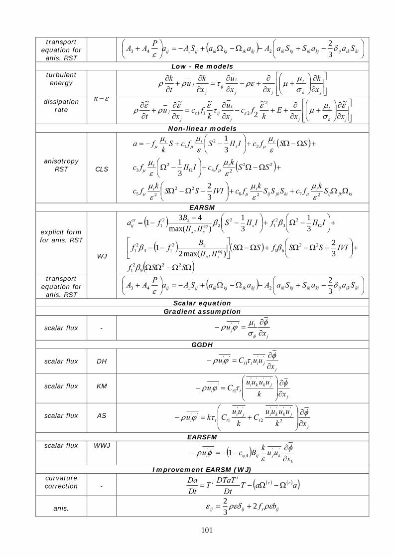
101
transport equation for anis. RST
( ) ⎟⎠⎞
⎜⎝⎛ −+−Ω−Ω+−=⎟
⎠⎞
⎜⎝⎛ + kiikijkjikkjikkjikkjikijij SaaSSaAaaSAaPAA δ
ε 32
2143
Low - Re models turbulent energy
⎥⎥⎦
⎤
⎢⎢⎣
⎡
∂∂
⎟⎟⎠
⎞⎜⎜⎝
⎛+
∂∂
+−∂∂
=∂∂
+∂∂
jk
t
jj
iij
j
jxk
xxu
xku
tk
σμ
μρετρρ
dissipation rate
ε−к
⎥⎥⎦
⎤
⎢⎢⎣
⎡
∂∂
⎟⎟⎠
⎞⎜⎜⎝
⎛+
∂∂
++−∂∂
=∂∂
+∂∂
j
t
jj
iij
j
jxx
Ek
fcxu
kfc
xu
tε
σμμετεερερε
εε
~~2
~~~ 2
211
Non-linear models
anisotropy RST
CLS
( )
( )
kijkijt
kijkijtt
tt
ts
tt
SkfcSSSkfcIVISSkfc
SSkfcIIIfc
SSfcIIISfcSk
fa
ΩΩ++⎟⎠⎞
⎜⎝⎛ −Ω−Ω
+Ω−Ω+⎟⎠⎞
⎜⎝⎛ −Ω
+Ω−Ω+⎟⎠⎞
⎜⎝⎛ −+−=
Ω
272622
25
2224
23
22
1
32
31
31
εμ
εμ
εμ
εμ
εμ
εμ
εμμ
μμμ
μμ
μμμ
EARSM
explicit form for anis. RST
( )
( ) ( )
( )ΩΩ−ΩΩ
+⎟⎠⎞
⎜⎝⎛ −Ω−Ω+Ω−Ω⎥
⎦
⎤⎢⎣
⎡−−
+⎟⎠⎞
⎜⎝⎛ −Ω+⎟
⎠⎞
⎜⎝⎛ −
−−= Ω
SSf
IVISSfSSIIII
Bff
IIIfIIISIIII
Bfa
eqss
seqss
exij
229
21
2261
2214
21
23
21
22
221
32
),max(21
31
31
),max(431
β
ββ
ββ
transport equation for anis. RST
WJ
( ) ⎟⎠⎞
⎜⎝⎛ −+−Ω−Ω+−=⎟
⎠⎞
⎜⎝⎛ + kiikijkjikkjikkjikkjikijij SaaSSaAaaSAaPAA δ
ε 32
2143
Scalar equation Gradient assumption
scalar flux
-
j
tj x
u∂∂
=−φ
σμϕρφ
''
GGDH
scalar flux
DH j
jitti xuuCu∂∂
=−φτϕρ ''
1''
scalar flux
KM
j
jkkitti xk
uuuuCu
∂∂
⎟⎟
⎠
⎞
⎜⎜
⎝
⎛=−
φτϕρ''''
1''
scalar flux
AS
j
jkkit
jitti xk
uuuuC
kuu
Cku∂∂
⎟⎟
⎠
⎞
⎜⎜
⎝
⎛+=−
φτϕρ 2
''''
2
''
1''
EARSFM scalar flux WWJ ( )
kkjiji x
uukBcu∂∂
−−=−φ
εφρ ϕ
''4
'' 1
Improvement EARSM (WJ) curvature correction
-
( ) ( )( )aaTDt
DTaTTDtDa rr
tt Ω−Ω−=
anis.
ijsijij bf ρερεδε 2
32
+=
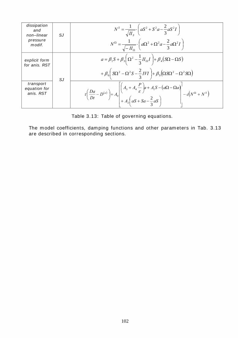
102
dissipation and
non–linear pressure modif.
SJ
⎟⎠⎞
⎜⎝⎛ −+⋅= IaSaSaS
IIN
S
S 222
321
⎟⎠⎞
⎜⎝⎛ Ω−Ω+Ω⋅
−=
Ω
Ω IaaaII
N 222
321
explicit form for anis. RST
( )
( )ΩΩ−ΩΩ+⎟⎠⎞
⎜⎝⎛ −Ω−Ω+
Ω−Ω+⎟⎠⎞
⎜⎝⎛ −Ω+= Ω
SSIVISS
SSIIISa
229
226
42
31
3231
ββ
βββ
transport equation for anis. RST
SJ
( )( )
( )Sa NNcaSSaaSA
aaSAaPAAAD
DtDa
+−
⎥⎥⎥⎥
⎦
⎤
⎢⎢⎢⎢
⎣
⎡
⎟⎠⎞
⎜⎝⎛ −++
Ω−Ω−+⎟⎠⎞
⎜⎝⎛ +
=⎟⎠⎞
⎜⎝⎛ − Ω
32
2
143
0ε
τ
Table 3.13: Table of governing equations.
The model coefficients, damping functions and other parameters in Tab. 3.13 are described in corresponding sections.
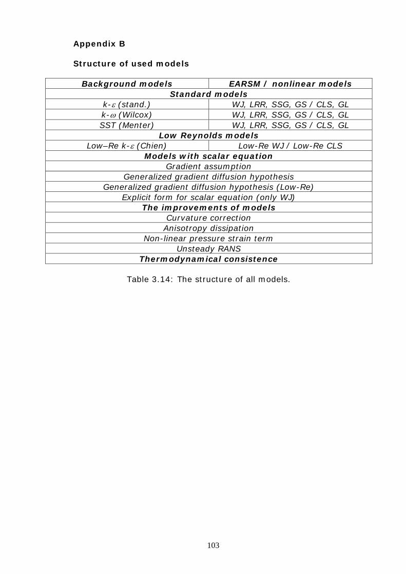
103
Appendix B Structure of used models
Background models EARSM / nonlinear models
Standard models k-ε (stand.) WJ, LRR, SSG, GS / CLS, GL k-ω (Wilcox) WJ, LRR, SSG, GS / CLS, GL SST (Menter) WJ, LRR, SSG, GS / CLS, GL
Low Reynolds models Low–Re k-ε (Chien) Low-Re WJ / Low-Re CLS
Models with scalar equation Gradient assumption
Generalized gradient diffusion hypothesis Generalized gradient diffusion hypothesis (Low-Re)
Explicit form for scalar equation (only WJ) The improvements of models
Curvature correction Anisotropy dissipation
Non-linear pressure strain term Unsteady RANS
Thermodynamical consistence
Table 3.14: The structure of all models.
Lebenslauf Name:
Yun
Vorname:
Alexander
Geburstag:
14. Februar 1974
Geburstort:
Bekabad, Uzbekistan
Familienstand:
verheiratet
Schul- und Berufausbildung: 1981-1985
Grundschule Nr. 4 Kizilorda, Kasachstan
1985-1992
Gymnasium Nr. 5, Kizilorda, Kasachstan
1993
Prüfung zur Aufnahme an der Technischen Universität Moskau
1993
Studienbeginn an der Technischen Universität Moskau, Russland,
Fachrichtung „Flugzeugmotoren und energetische Anlagen“
9/02/1999
Studiumabschluss. Dipl.-Ing.
1999-2002
Wissenschaftlicher Mitarbeiter an der Technischen Universität Moskau. Schwerpunkt: Design and Untersuchnungen der stationären Gasturbinen- Anlagen und Flugmotoren.
2002-2005
Doktorand im Fachbereich Maschinenbau an der TU Darmstadt. Schwerpunkt: Die Untersuchungen der Strömungen im RANS Kontext.


![ecdl news 1aa-05 - ECDL European Computer Driving Licence · ECDL Advanced Word 2010 Advanced Excel 2010 Advanced Access 2010 Advanced PowerPoint 2010 Advanced D ] } L Æ o î ì](https://img.pdfslide.org/doc/110x75/5e053e2e5e4d4c416b466a98/ecdl-news-1aa-05-ecdl-european-computer-driving-licence-ecdl-advanced-word-2010.jpg)

![Tensor Triangulated Categories in Algebraic Geometry · The focus of this study are tensor triangulated categories in algebraic geometry. The starting point was Balmer’s paper [3]](https://img.pdfslide.org/doc/110x75/5f0287107e708231d404b53a/tensor-triangulated-categories-in-algebraic-geometry-the-focus-of-this-study-are.jpg)