Embed Size (px)
Citation preview
DISSERTATION
Digital Pre-distortion
ofMicrowave Power Amplifiers
ausgefuhrt zum Zwecke der Erlangung des akademischen Gradeseines Doktors der technischen Wissenschaften
eingereicht an der Technischen Universitat WienFakultat fur Elektrotechnik und Informationstechnik
von
DI Ernst AschbacherHerndlgasse 22/34
A-1100 Wien
geboren am 4. September 1970 in Bruneck (IT)Matrikelnummer: 9326558
Wien, im September 2005


Begutachter:
Univ. Prof. Dr. Markus RuppInstitut fur Nachrichtentechnik und Hochfrequenztechnik
Technische Universitat WienOsterreich
Univ. Prof. Dr. Timo I. LaaksoSignal Processing Laboratory
Helsinki University of TechnologyFinland

Abstract
With the advent of spectrally efficient wireless communication systems employing modulationschemes with varying amplitude of the communication signal, linearisation techniques fornonlinear microwave power amplifiers have gained significant interest. The availability of fastand cheap digital processing technology makes digital pre-distortion an attractive candidate asa means for power amplifier linearisation since it promises high power efficiency and flexibility.Digital pre-distortion is further in line with the current efforts towards software defined radiosystems, where a principal aim is to substitute costly and inflexible analogue circuitry withcheap and reprogrammable digital circuitry.
Microwave power amplifiers are most efficient in terms of delivered microwave output powervs. supplied power if driven near the saturation point. In this operational mode, the amplifierbehaves as a nonlinear device, which introduces undesired distortions in the information bear-ing microwave signal. These nonlinear distortions degrade the system performance in termsof increased bit error rate and produce disturbance in adjacent channels. A compensation ofthe nonlinear distortions is therefore of significant importance, not only to keep the systemperformance high, but also to comply with regulatory specifications regarding the maximumallowed disturbance of adjacent channels. Nonlinear equalisation at the receiver is possiblebut complicated due to the unknown effects of the channel. Further, this method does notreduce the disturbance in adjacent channels, thus additional analogue filters would have to beplaced at the output of the power amplifier. It is therefore natural to reduce the nonlineardistortions at the point where they occur, namely at the transmitter.
Different linearisation methods exist which aim to reduce the nonlinear distortions whilekeeping the power amplifier in the nonlinear and efficient mode. Traditionally, these techniquesemploy additional analogue circuitry. Linearisation by digital pre-distortion is a new methodwhich applies digital signal processing techniques for compensating the nonlinear distortions.
Digital pre-distortion splits into three tasks: modelling of the microwave power amplifier,adaptive identification of the model parameters, and development of the pre-distortion filter.These tasks are addressed in this thesis. Further, a prototype system is developed which allowsto test the pre-distortion algorithm in real-time using a fixed-point environment.
For the first task, measurements on microwave power amplifier were performed in order toevaluate different models. The difficulty is to find low-complex but at the same time accuratemodels, which describe not only the nonlinear effects, but account also for the memory effectsof the power amplifier.
The adaptive identification of the parameters of two nonlinear models, namely a Volterramodel and a Wiener model, is presented thereafter. Gradient-type algorithms are developedand investigated with respect to stability in a deterministic context.
A powerful method for the determination of the pre-distortion filter is presented next. Fornonlinear systems it is in general not possible to devise analytic solutions for the pre-inversewhich linearises the system for a certain class of input signals. Here, an iterative technique ispresented which finds an approximate solution for the pre-inverse.
Based on the developed pre-distortion algorithm, a real-time prototype system is devel-oped. This system proves that the algorithm can be implemented with a limited amount ofhardware resources. Further, measurement results show that the algorithm keeps its excellentperformance also in an environment with a limited data- and arithmetic accuracy.
i

ii

Kurzfassung
Mit der Einfuhrung von spektral effizenten drahtlosen Kommunikationsystemen, die Modula-tionsformate einsetzen, die auch die Amplitude des Nachrichtensignals verandern, gewannenLinearisierungsverfahren fur nichtlineare Mikrowellen-Leistungsverstarker immer mehr an In-teresse. Die Verfugbarkeit von schneller und billiger digitaler Signalverarbeitungstechnologiemacht die digitale Vorverzerrung als Methode zur Linearisierung von Leistungsverstarkernsehr attraktiv, da sie hohe Leistungseffizienz und hohe Flexibilitat verspricht. Digitale Vor-verzerrung steht weiters im Einklang mit den gegenwartigen Bestrebungen eine moglichstSoftware-definierte Funkubertragung zu schaffen. Ein wichtiges Ziel hierbei ist, kostspieligeund unflexible analoge Schaltkreise auf das unbedingt notige Maß zu reduzieren und durchbillige und re-programmierbare digitale Technologie zu ersetzen.
Mikrowellen-Leistungsverstarker sind am effizientesten wenn sie in der Sattigung betriebenwerden. Effizienz heißt hier, daß moglichst viel zugefuhrte Leistung in abgegebene Mikrowel-lenleistung umgesetzt wird. In dieser Betriebsweise ist der Verstarker nichlinear, was zu Verz-errungen im informationstragenden Mikrowellensignal fuhrt. Diese ungewollten Verzerrungenfuhren zu erhohten Bitfehlerraten und verschlechtern somit die Gute des Funksystems. Weit-ers werden Storungen in benachbarte Frequenzbander emittiert. Eine Kompensation dieserSignalverzerrungen erhoht demnach nicht nur die Gute des Funksystems, sondern macht dasSystem konform mit Regulationsspezifikationen. Eine nichtlineare Entzerrung des Signals amEmpfanger ist moglich aber kompliziert wegen der unbekannten Effekte des Funkkanals. DieseMethode reduziert weiters nicht die Storungen in benachbarten Frequenzbandern. Zusatzlicheanaloge Filter mussen am Sender eingesetzt werden. Es ist daher naturlich, die Verzerrungenan der Stelle ihres Auftretens, namlich am Sender, zu kompensieren.
Verschiedene analoge Linearisierungsverfahren existieren. Sie versuchen die Verzerrungenbei gleichzeitigem nichtlinearen Betrieb des Verstarkers zu kompensieren. Digitale Vorverzer-rung ist eine neue Methode, die digitale Technologie zur Entzerrung des Verstarkes einsetzt.
Digitale Vorverzerrung kann in drei Teile aufgeteilt werden: Modellierung des Leistungsver-starkers, adaptive Identifikation der Modellparameter und Entwicklung des Vorverzerrungsfil-ters. Alle drei Aufgaben werden in dieser Dissertation behandelt. Weiters wird ein Prototyp-System entwickelt, das es gestattet, den Vorverzerrungsalgorithmus in Echtzeit in einer Fix-punkt Umgebung zu testen.
Fur die erste Aufgabe wurden Messungen mit verschiedenen Leistungsverstarkern aus-gefuhrt, um verschiedene Modelle gegeneinander zu evaluieren. Die Schwierigkeit bestehtdabei darin, moglichst genaue und gering komplexe Modelle zu finden, die nicht nur dasnichtlineare Verhalten des Verstarkers sehr genau beschreiben, sondern auch Speichereffekteberucksichtigen.
Die adaptive Identifikation der Modellparameter von zwei Modellen, eines Volterramodellsund eines Wienermodells, wird danach behandelt. Gradientenverfahren werden entwickelt undauf Stabilitat in einem deterministischen Kontext untersucht.
In weiterer Folge wird eine Methode entwickelt um das Vorverzerrungsfilter fur ein ge-gebenes Verstarkermodell zu bestimmen. Analytische Losungen sind im Allgemeinen nichtverfugbar. Hier wird eine iterative Methode prasentiert, die eine Naherungslosung fur dasideale Filter findet.
Basierend auf diesem iterativen Algorithmus wird ein echtzeitfahiger Prototyp entwickelt.Dieses System zeigt, daß der entwickelte Vorverzerrungsalgorithmus mit einem beschrankenAufwand realisiert werden kann. Messungen belegen, daß der Algorithmus seine exzellenteGute auch in einer Umgebung mit beschrankter Zahlen- und Arithmetikgenauigkeit beibehalt.
iii

iv

Acknowledgement
Several people contributed in various ways to this thesis. I am deeply indebted to and wouldlike to express my gratitude to:
➾ Prof. Markus Rupp for his continuous support and guidance. His lucid comments andcritical questions improved the scientific quality of this thesis significantly.
➾ Prof. Timo I. Laakso for assuming the work as a referee.
➾ Mei Yen Cheong – intensive discussions with her provided a basis for a deeper under-standing.
➾ My diploma students Mathias Steinmair and Peter Brunmayr for their questions andwork.
➾ Holger Arthaber and Michael Gadringer who kindly assisted me with microwave hard-ware and measurement equipment.
➾ Anding Zhu and Prof. Tom Brazil for hosting me at the University College Dublin andfor fruitful discussions.
Finally, and most importantly, I thank my family for their support and company.
v

vi
Contents
1 Introduction 11.1 Outline of the Thesis and Contributions . . . . . . . . . . . . . . . . . . . . . . 31.2 Power Amplifier Linearisation: From Analogue Linearisation to Digital Pre-
distortion . . . . . . . . . . . . . . . . . . . . . . . . . . . . . . . . . . . . . . . 41.2.1 Motivation . . . . . . . . . . . . . . . . . . . . . . . . . . . . . . . . . . 41.2.2 Analogue Techniques . . . . . . . . . . . . . . . . . . . . . . . . . . . . . 5
Power Back-off . . . . . . . . . . . . . . . . . . . . . . . . . . . . . . . . 5Feedforward Linearisation . . . . . . . . . . . . . . . . . . . . . . . . . . 5Cartesian-Loop . . . . . . . . . . . . . . . . . . . . . . . . . . . . . . . . 6
1.2.3 Digital Pre-distortion . . . . . . . . . . . . . . . . . . . . . . . . . . . . 7Digital Pre-distortion: Building Blocks . . . . . . . . . . . . . . . . . . . 8Digital Pre-distortion – Brief Literature Review . . . . . . . . . . . . . . 9
2 Power Amplifier Modelling 112.1 The Volterra Series . . . . . . . . . . . . . . . . . . . . . . . . . . . . . . . . . . 12
2.1.1 Complex Baseband Volterra Series . . . . . . . . . . . . . . . . . . . . . 132.1.2 Frequency Domain Representation of a Volterra Series . . . . . . . . . . 152.1.3 Discrete-time Volterra Series . . . . . . . . . . . . . . . . . . . . . . . . 162.1.4 Series Representation of a Static Non-linearity . . . . . . . . . . . . . . 182.1.5 Parameter Estimation for the Volterra Model . . . . . . . . . . . . . . . 19
2.2 The Wiener Model . . . . . . . . . . . . . . . . . . . . . . . . . . . . . . . . . . 202.2.1 Parameter Estimation for the Wiener Model . . . . . . . . . . . . . . . 21
2.3 The Hammerstein Model . . . . . . . . . . . . . . . . . . . . . . . . . . . . . . . 222.3.1 Parameter Estimation for the Hammerstein Model . . . . . . . . . . . . 23
2.4 The Saleh Model . . . . . . . . . . . . . . . . . . . . . . . . . . . . . . . . . . . 242.4.1 Parameter Estimation for the Saleh Model . . . . . . . . . . . . . . . . . 25
2.5 Model-Structure Selection and Model Validation . . . . . . . . . . . . . . . . . 252.5.1 Model-Structure Selection . . . . . . . . . . . . . . . . . . . . . . . . . . 262.5.2 Model Validation . . . . . . . . . . . . . . . . . . . . . . . . . . . . . . . 26
2.6 Modelling Measured and Simulated Power Amplifiers . . . . . . . . . . . . . . . 272.6.1 Black-Box Modelling of Three Microwave Power Amplifiers . . . . . . . 28
Modelling a Three-Stage High-Power LDMOS EDGE Amplifier . . . . . 29Modelling a Single-Stage Medium-Power Amplifier . . . . . . . . . . . . 32Modelling a Simulated WCDMA Power Amplifier . . . . . . . . . . . . . 34
2.7 Discussion . . . . . . . . . . . . . . . . . . . . . . . . . . . . . . . . . . . . . . . 35
vii

3 Adaptive Identification 373.1 The Stochastic-Gradient Algorithm . . . . . . . . . . . . . . . . . . . . . . . . . 38
3.1.1 Stochastic-Gradient Identification for Linear-in-Parameter Models . . . 38Convergence Analysis – Error-Vector in the Mean . . . . . . . . . . . . 40Deterministic Robustness Analysis – Local Passivity . . . . . . . . . . . 41Deterministic Robustness Analysis – Global Passivity . . . . . . . . . . 42Feedback Structure – Local and Global Passivity . . . . . . . . . . . . . 42Example – Learning Behaviour of an Adaptive Volterra Filter . . . . . . 43
3.1.2 Stochastic-Gradient Identification of a Wiener System . . . . . . . . . . 45First Step: Parameter Estimation for Linear Filter . . . . . . . . . . . . 46
Local Passivity Relations . . . . . . . . . . . . . . . . . . . . . . 48Feedback Structure – Local Passivity . . . . . . . . . . . . . . . . 49Global Passivity Relations . . . . . . . . . . . . . . . . . . . . . . 50Example 1: Identification of the Linear Part of a Wiener System
– Local Stability . . . . . . . . . . . . . . . . . . . . . 51Example 2: Identification of the Linear Part of a Wiener System
– Global Stability . . . . . . . . . . . . . . . . . . . . 52Second Step: Parameter Estimation for Static Nonlinear Filter . . . . . 55
Example 1 continued: Identification of the Nonlinear Part of aWiener System . . . . . . . . . . . . . . . . . . . . . . 57
The Complete Algorithm . . . . . . . . . . . . . . . . . . . . . . . . . . 583.2 Discussion . . . . . . . . . . . . . . . . . . . . . . . . . . . . . . . . . . . . . . . 58
4 Linearisation by Pre-distortion 614.1 Formulation of the Linearisation Problem as an Optimisation Problem . . . . . 634.2 The Fixed-Point Approach . . . . . . . . . . . . . . . . . . . . . . . . . . . . . . 644.3 Linearisation using the Secant Method . . . . . . . . . . . . . . . . . . . . . . . 664.4 Applying the Linearisation Methods . . . . . . . . . . . . . . . . . . . . . . . . 69
4.4.1 Comparison of the Convergence Rate . . . . . . . . . . . . . . . . . . . . 704.4.2 System-Model Mismatches . . . . . . . . . . . . . . . . . . . . . . . . . . 73
Influence of Measurement Noise . . . . . . . . . . . . . . . . . . . . . . . 73Neglecting Memory Effects . . . . . . . . . . . . . . . . . . . . . . . . . 74Underestimating the Nonlinear Order . . . . . . . . . . . . . . . . . . . 75
4.4.3 Linearising a High-Power LDMOS EDGE Amplifier – Measurement Re-sults . . . . . . . . . . . . . . . . . . . . . . . . . . . . . . . . . . . . . . 76Modelling . . . . . . . . . . . . . . . . . . . . . . . . . . . . . . . . . . . 78Linearisation . . . . . . . . . . . . . . . . . . . . . . . . . . . . . . . . . 79
4.5 Discussion . . . . . . . . . . . . . . . . . . . . . . . . . . . . . . . . . . . . . . . 82
5 Prototype Implementation 855.1 System Concept . . . . . . . . . . . . . . . . . . . . . . . . . . . . . . . . . . . 865.2 Signal Processing Hardware – Description . . . . . . . . . . . . . . . . . . . . . 86
5.2.1 Assembled Digital System . . . . . . . . . . . . . . . . . . . . . . . . . . 905.3 Radio-Frequency Part – Description . . . . . . . . . . . . . . . . . . . . . . . . 925.4 Implementation Details . . . . . . . . . . . . . . . . . . . . . . . . . . . . . . . 94
5.4.1 Pre-distortion Filter Implementation . . . . . . . . . . . . . . . . . . . . 94Division . . . . . . . . . . . . . . . . . . . . . . . . . . . . . . . . . . . . 95
5.4.2 Model-parameter Estimation . . . . . . . . . . . . . . . . . . . . . . . . 97
viii

5.5 Measurements and Performance Results . . . . . . . . . . . . . . . . . . . . . . 975.5.1 Measurement Results: Floating-point vs. Fixed-point . . . . . . . . . . 975.5.2 Measurement Results: Real-Time Implementation . . . . . . . . . . . . 985.5.3 Used FPGA Resources . . . . . . . . . . . . . . . . . . . . . . . . . . . . 102
5.6 Discussion . . . . . . . . . . . . . . . . . . . . . . . . . . . . . . . . . . . . . . . 102
6 Conclusions 103
A Appendix: Adaptive Identification 105A.1 Derivation of (3.40) . . . . . . . . . . . . . . . . . . . . . . . . . . . . . . . . . . 105A.2 Derivation of (3.67) and (3.68) . . . . . . . . . . . . . . . . . . . . . . . . . . . 106A.3 Derivation of (3.73) . . . . . . . . . . . . . . . . . . . . . . . . . . . . . . . . . . 106A.4 Derivation of (3.86) . . . . . . . . . . . . . . . . . . . . . . . . . . . . . . . . . . 107
B Appendix: Linearisation by Pre-distortion 109B.1 The Contraction Mapping Theorem . . . . . . . . . . . . . . . . . . . . . . . . 109
C Appendix: Prototype Implementation 111C.1 Convergence of the Newton-Raphson Method Applied for Division . . . . . . . 111C.2 Error-Analysis of the Newton-Raphson Method Applied for Division . . . . . . 112C.3 The Prototyping-Hardware . . . . . . . . . . . . . . . . . . . . . . . . . . . . . 113
D Appendix: Abbreviations and Symbols 117D.1 List of Abbreviations . . . . . . . . . . . . . . . . . . . . . . . . . . . . . . . . . 117D.2 List of Mathematical Symbols . . . . . . . . . . . . . . . . . . . . . . . . . . . . 118
Bibliography 119
ix

x
Chapter 1
Introduction
Amplification of information bearing signals is an integral part of every wireless transmitter.The aim is to boost the signal to a sufficient power level for transmission in order to supplythe receiver with a sufficiently high level of signal power. Despite of disturbances and signaldistortions, the receiver has the task to retrieve the information from the received signal.
In wireless communication systems such as mobile communication systems (e.g., GSM1,UMTS2, WLAN3) and satellite communication systems (e.g., radio and television broadcastsatellites) an essential constraint implies that communication in other frequency bands mustnot be disturbed excessively. Further, efficient conversion of supplied power into radiatedsignal power is a key requirement, especially in satellite communication systems where notonly power supply is limited, but also heat development becomes a serious technical problem.In mobile communications, efficiency is of particular importance in mobile phones – the poweramplifier still consumes the largest amount of energy despite an excessive and increasinglycomplex digital circuitry. Efficiency in the base station stands for lower operating costs dueto a reduced energy supply and smaller cooling units. A common measure for power amplifierefficiency is the power added efficiency (PAE), defined as
PAE ,PRF,out − PRF,in
PDC,
where PRF,out indicates the output power, PRF,in is the input power of the power amplifier (atradio frequency), and PDC is the supplied power. Typical efficiencies achieved today in mobilecommunication systems are 20% for a UMTS base station amplifier, and 40 % for a UMTSmobile unit.
The two constraints, distortion-free amplification and efficient amplification complicatethe simple-sounding task of boosting a signal to a high power level. Ideal distortion-freeamplification and efficiency tend to be mutually exclusive. Improvements in efficiency areachieved at the expense of distortions, and vice versa.
1Global System for Mobile communications. It is the second generation (2G) of wireless mobile communi-cation systems employing digital modulation technology.
2Universal Mobile Telecommunications System. This is the European entrant for third generation (3G) mo-bile communication systems and subsumed in the IMT-2000 family as the WCDMA (Wideband Code DivisionMultiple Access) technology.
3Wireless Local Area Network, a short range radio network normally deployed in traffic hotspots such asairport lounges, hotels and restaurants. WLAN enables suitably equipped users to have wireless access to afixed network, providing high speed access (up to 54Mbit/s download) to distant servers. The key WLANtechnologies is the IEEE 802.11 family.
1
2 CHAPTER 1. Introduction
Signal distortion in power amplifiers occurs due to two mechanisms: non-linearity anddispersion. Efficiency requirements push the power amplifier into the nonlinear operationalregime, whereas the dispersion effects have their origin in internal memory effects of the ac-tive device (i.e., the transistor) and in non-ideal matching networks exhibiting a frequencydependent behaviour. In order to observe dispersion in a well designed power amplifier, thesignal bandwidth has to be large, i.e., it must cover variations in the frequency response ofthe power amplifier (if assumed linear). The signal bandwidth of communication systemsincrease with every generation: from 200 kHz in GSM (second generation) to approximately5 MHz (for one carrier) in UMTS, the third generation mobile communication system. Thisis a 25-fold bandwidth increase. In the IEEE 802.11n WLAN standard even a transmissionbandwidth of 40MHz is specified. If more communication channels have to be amplified (e.g.,in a multi-carrier base station) the requirements on linearity and dispersion increase further.Amplification of more than one carrier using only one multi-carrier power amplifier has severaladvantages over the more traditional approach of amplifying each carrier separately and com-bining the amplified signals before the common antenna. Before combination, each amplifiedsignal has to pass an isolator and a filter, which must have a high quality factor due to itssmall relative bandwidth. These narrowband filters are space-consuming, lossy, and difficult toretune, which is necessary to accommodate different choices of transmitted carrier frequencies,making it difficult for system operators to implement a dynamic channel allocation. A secondand very important reason for implementing multi-carrier power amplifiers is the achievedforward-compatibility with future systems. The system operator has the possibility to changethe modulation scheme without replacing any amplifier. Such multi-carrier power amplifiersmust be designed to permit amplification of different modulation schemes at the same time.
Linearisation methods can increase efficiency indirectly by admitting the usage of efficientnonlinear power amplifiers. Depending on the linearisation scheme, linear operation is achievedvia an appropriate modification of the input or output signal of the power amplifier. Further,the linearisation scheme must also be capable of compensating the signal dispersion. It istherefore not simply a linearisation scheme – it is a (nonlinear) equalisation task that has tobe performed. In order to increase effectively the efficiency of the whole system – linearisa-tion subsystem and power amplifier – it is essential to design low-complex and power-efficientlinearisation schemes, maintaining at the same time a certain degree of flexibility and compat-ibility. Different linearisation schemes, working entirely in the analogue domain or applying adigital approach using digital signal processing techniques, have been proposed and are alreadyin use in communication systems.
A promising candidate for microwave power amplifier linearisation is digital pre-distortion.The method works entirely in the digital domain which is attractive since the hardware im-plementation employs standard and cost-efficient components. A high degree of flexibility isguaranteed if reprogrammable hardware, such as DSPs4 and/or FPGAs5 is used, which is notonly desirable in a first prototype development, but also in a final product in order to main-tain the possibility to efficiently adjust for later system changes. The costly analogue part in atransmitter is minimally augmented applying this technique. The trend of moving the flexibledigital part of a transmitter as close to the antenna while reducing the analogue front-end toits necessary minimum naturally leads to digital pre-distortion as a means for linearisation.
4DSP stands for Digital Signal Processor. It is a special type of processor micro-architecture, designed forperforming mathematical operations involved in digital signal processing.
5FPGA stands for Field Programmable Gate Array, a type of chip where the logic function can be defined bythe user. Due to this capability and the large number of gates it is especially suited for prototyping of complexcommunication systems.
1.1 Outline of the Thesis and Contributions 3
1.1 Outline of the Thesis and Contributions
In the following the organisation of the thesis including the contributions of the author ispresented.
Chapter 1 Following the motivation for power amplifier linearisation, an overview of com-monly used analogue linearisation schemes [1, 2] is presented in Section 1.2. The conceptof digital pre-distortion, originally proposed in [3], as an efficient and flexible digital lin-earisation scheme is introduced.
Chapter 2 Models for power amplifiers are discussed in this chapter. The aim is to havean accurate and relatively simple model, which not only describes the non-linearityof the power amplifier, but also the dynamic effects (memory effects). The classicalVolterra series is introduced [4, 5, 6, 7, 8] as the most general model for describing non-linear dynamic systems. Simpler models, especially Wiener- and Hammerstein models,a specialisation of the Volterra series, are introduced next. Static models, such as theoften used Saleh-model [9], as well as series expansion are introduced for comparisonreasons. A complex baseband description of the models is derived. Comparisons ofperformed measurements on real microwave power amplifiers with the presented modelsare evaluated [10, 11, 12]. A discussion of the shortcomings and difficulties associatedwith the models concludes the chapter.
Chapter 3 Adaptive identification of the power amplifier is necessary in order to identify themodel parameters and to track changes of the system behaviour over time. Emphasisis on low complex and robust gradient-type identification schemes, which are predomi-nantly used in practice. An introduction is devoted to the analysis methods for adaptivealgorithms [13, 14]. A deterministic robustness analysis of an adaptive Volterra filter isthen performed. The formulation of a two-step adaptive gradient-type algorithm for theidentification of the parameters of a Wiener system follows. A robustness analysis forthe derived algorithm is conducted [15, 16].
Chapter 4 The problem of equalisation of a nonlinear dynamic system is addressed. Sincemost often analytic solutions describing the inverse of the nonlinear system are notknown, different approaches are proposed in the literature which solve the problem inan approximate way [17, 18]. A new iterative method is developed here, which is simpleand converges very fast to a good solution [19, 12]. By means of measurements on ahigh-power microwave amplifier, the developed linearisation method is tested and theconcept is proven to work in an experimental setup on a real physical system [12].
Chapter 5 A prototype system based on an FPGA implementation of the proposed lineari-sation method was developed [20]. The implementation allows to test the developedlinearisation algorithm [12, 21] in real-time using various power amplifier models. It is avery flexible environment for the evaluation of digital pre-distortion for different poweramplifiers requiring different models. Measurement results prove the functionality of theimplementation and prove that a real-time fixed-point implementation of the proposedalgorithm is indeed feasible.
4 CHAPTER 1. Introduction
1.2 Power Amplifier Linearisation: From Analogue Linearisa-tion to Digital Pre-distortion
In this chapter an overview of power amplifier linearisation techniques is presented. Startingwith a motivation for linear microwave amplification, traditional analogue techniques, such asfeedforward and Cartesian-loop linearisation schemes are briefly presented. The concept ofdigital pre-distortion is introduced. The chapter concludes with a literature review.
1.2.1 Motivation
Highly linear transmitters are forced mainly by:
1. regulatory and
2. system requirements.
Regulatory requirements define severe limits of out-of-band radiation in order to not disturbneighbouring channels excessively. The transmitted signals have to adhere to specific spectralmasks, see, e.g., [22], which defines the base station minimum radio-frequency (RF) require-ments of the FDD6 mode of WCDMA7.
System requirements on the linearity of power amplifiers are especially important in thecase of multi-channel power amplifiers. Multi-channel power amplifiers must meet stringentlinearity requirements in order to keep the cross-modulation between the channels at a lowlevel, at the same time the system is required to meet these linearity requirements over alarge bandwidth of tens of MHz. Such broadband signals resolve the dynamic effects of thepower amplifier, a frequency-dependent amplification being the result. These are challengingrequirements that prevent often the usage of a multi-channel power amplifier and favour theusage of a channelised approach, which has the advantage that each single amplifier has tomeet only moderate linearity requirements over a relatively small bandwidth, thus appear asstatic devices.
Linearisation methods aim to ameliorate the situation by adding additional circuitry forreducing the nonlinear distortions of the power amplifier. Traditionally, analogue linearisationschemes have been used, the most common, especially in base stations, being the feedforwardscheme. The demand for higher flexibility and lower cost with similar performance as ana-logue linearisation schemes leads to the concept of digital pre-distortion. Signal processingtechniques, which can be efficiently implemented using digital hardware such as Digital SignalProcessors (DSPs) and/or Field Programmable Gate Arrays (FPGAs), are used to control ananalogue RF-system. The advantage is that a high degree of flexibility is maintained due tothe inherent flexibility of the digital hardware which allows for changes at run-time of thesystem. This is in line with the current trend to Software Defined Radio (SDR) [23], wherethe ultimate goal is to define highly reconfigurable radios which can accommodate a varietyof standards and transmission/receive modes, controlled entirely by software. This is onlypossible if the inflexible and costly analogue circuitry is reduced to a minimum by replacingas much as possible by reprogrammable digital hardware.
6FDD stands for Frequency Division Duplexing, an application of frequency-division multiple access, usedto separate transmit and receive signals in the frequency domain.
7WCDMA stands for Wideband Code Division Multiple Access, the technology used by UMTS.
1.2 Power Amplifier Linearisation: From Analogue Linearisation to Digital Pre-distortion 5
1.2.2 Analogue Techniques
Three analogue linearisation techniques, power back-off, feedforward linearisation, and Carte-sian-loop linearisation are briefly presented.
Power Back-off
The conventional and simplest approach for achieving highly linear amplification is to use aclass A [1] power amplifier, being inherently inefficient with small input power levels, andto feed it with an input power far below its (efficient) capabilities. This results in very lowpower-efficient and oversized amplifier systems, making this approach very inefficient for mostapplications.
Feedforward Linearisation
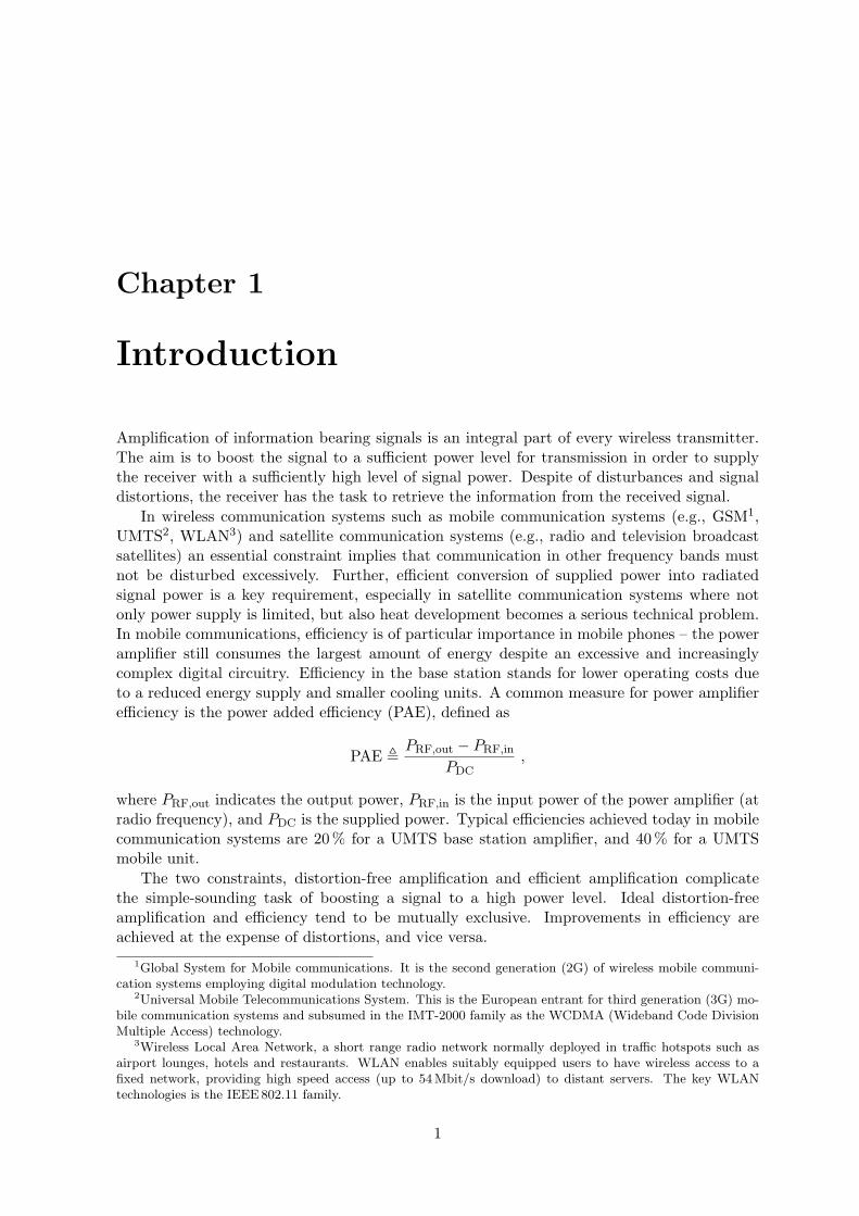
Feedforward linearisation is a very old method, dating back to 1928 [24, 25]. Nevertheless,feedforward linearisation is used extensively in nowadays base stations [2, 1], since it is amature technology and provides good linearisation performance.
3 dB div.
Delay +
Delay
� �
�
�
�
� �
�
u(t)
Main amplifier
Error amplifier−
Equal delay Equal delay� � � �
y(t)
τm τe
gm
ge
c1 c2
Coupler Coupleru1(t)
u2(t)
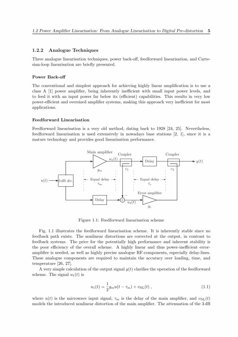
Figure 1.1: Feedforward linearisation scheme
Fig. 1.1 illustrates the feedforward linearisation scheme. It is inherently stable since nofeedback path exists. The nonlinear distortions are corrected at the output, in contrast tofeedback systems. The price for the potentially high performance and inherent stability isthe poor efficiency of the overall scheme. A highly linear and thus power-inefficient error-amplifier is needed, as well as highly precise analogue RF-components, especially delay-lines.These analogue components are required to maintain the accuracy over loading, time, andtemperature [26, 27].
A very simple calculation of the output signal y(t) clarifies the operation of the feedforwardscheme. The signal u1(t) is
u1(t) =12gmu(t− τm) + vNL(t) , (1.1)
where u(t) is the microwave input signal, τm is the delay of the main amplifier, and vNL(t)models the introduced nonlinear distortion of the main amplifier. The attenuation of the 3 dB
6 CHAPTER 1. Introduction
splitter is taken into account via the factor 12 . The signal u2(t) is
u2(t) =12(1− c1gm
)u(t− τm)− c1vNL(t) (1.2)
with the coupling-factor c1. The output signal y(t) is
y(t) = u1(t− τe) + c2geu2(t− τe) , (1.3)
where τe is the delay of the error-amplifier, g2 is the gain of the error-amplifier, and c2 is thecoupling-factor of the coupler at the output. After a simple calculation the output signal
y(t) =12(gm + c2ge − c1c2gmge
)u(t− τm − τe) +
(1− c1c2ge
)vNL(t− τ2) (1.4)
follows. If ge = 1c1c2
the distortion is completely removed and the output signal is simply
y(t) =1
2c1u(t− τm − τe) . (1.5)
The coupling-factor c1 determines the overall gain. An obvious choice is c1 = 1gm
, which resultsin
u2(t) = − 1gm
vNL(t) (1.6)
andy(t) =
gm2u(t− τm − τe) . (1.7)
In this analysis the delays of the delay lines are assumed to be perfectly matched to theintroduced delays of the amplifiers. This perfect match is in practice difficult to maintain overvarying operating conditions, reducing the performance significantly [27].
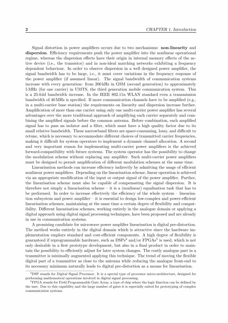
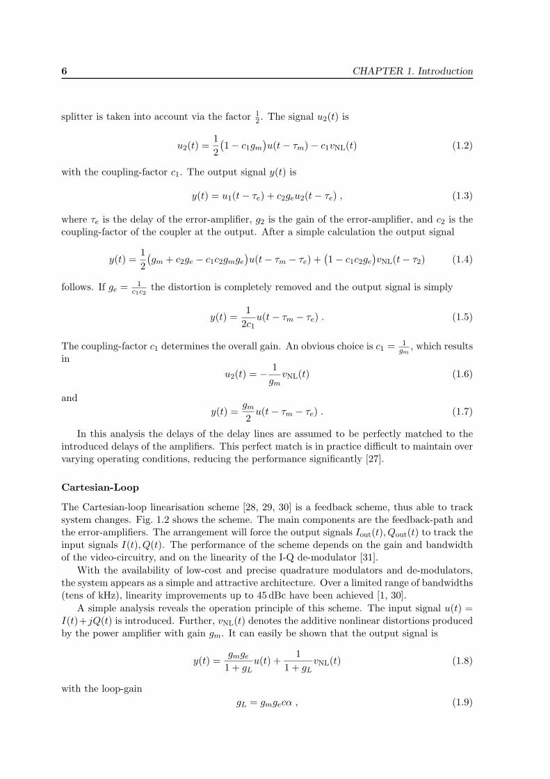
Cartesian-Loop
The Cartesian-loop linearisation scheme [28, 29, 30] is a feedback scheme, thus able to tracksystem changes. Fig. 1.2 shows the scheme. The main components are the feedback-path andthe error-amplifiers. The arrangement will force the output signals Iout(t), Qout(t) to track theinput signals I(t), Q(t). The performance of the scheme depends on the gain and bandwidthof the video-circuitry, and on the linearity of the I-Q de-modulator [31].
With the availability of low-cost and precise quadrature modulators and de-modulators,the system appears as a simple and attractive architecture. Over a limited range of bandwidths(tens of kHz), linearity improvements up to 45 dBc have been achieved [1, 30].
A simple analysis reveals the operation principle of this scheme. The input signal u(t) =I(t)+jQ(t) is introduced. Further, vNL(t) denotes the additive nonlinear distortions producedby the power amplifier with gain gm. It can easily be shown that the output signal is
y(t) =gmge
1 + gLu(t) +
11 + gL
vNL(t) (1.8)
with the loop-gaingL = gmgecα , (1.9)
1.2 Power Amplifier Linearisation: From Analogue Linearisation to Digital Pre-distortion 7
composed of the coupling-factor c, the attenuation α, the gain of the error-amplifiers ge, andthe gain of the main power amplifier gm. For a large loop-gain, (1.8) reduces to
y(t) ≈ 1cαu(t) + vNL(t)
1gL
. (1.10)
If 1cα = gm, this simplifies further to
y(t) ≈ gmu(t) + vNL(t)1ge. (1.11)
The suppression of the nonlinear disturbance depends in this case on the gain of the error-amplifiers ge.
+
+
�
��
�
LO
ATT
I(t)
Q(t)
�
�
� �
�
� ge
ge��
Coupler
�
−
−
�
Error amplifier
Error amplifier
Iout(t)
Qout(t)
I-Q
mod
ulat
orI-
Qde
-mod
ulat
or
Power amplifier
y(t)
fc
gmc
α
Figure 1.2: Cartesian-loop linearisation scheme
1.2.3 Digital Pre-distortion
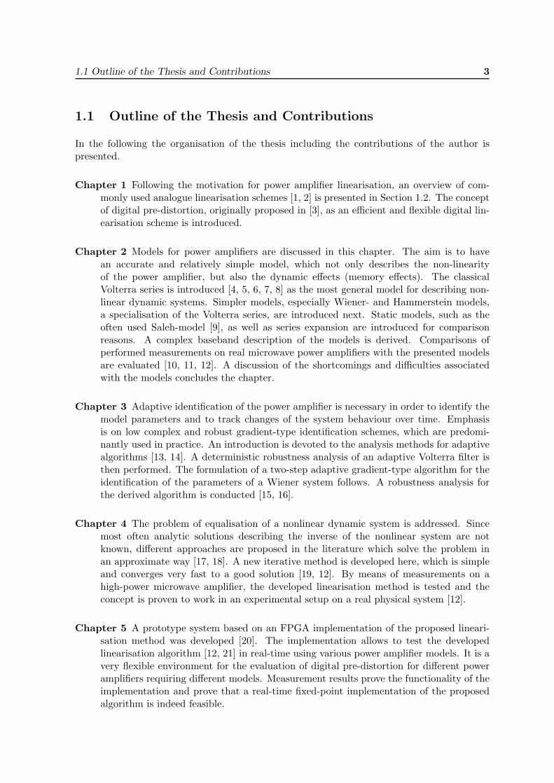
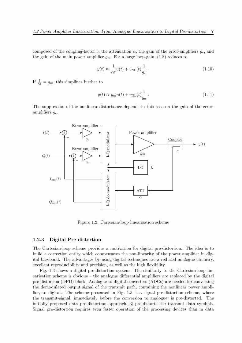
The Cartesian-loop scheme provides a motivation for digital pre-distortion. The idea is tobuild a correction entity which compensates the non-linearity of the power amplifier in dig-ital baseband. The advantages by using digital techniques are a reduced analogue circuitry,excellent reproducibility and precision, as well as the high flexibility.
Fig. 1.3 shows a digital pre-distortion system. The similarity to the Cartesian-loop lin-earisation scheme is obvious – the analogue differential amplifiers are replaced by the digitalpre-distortion (DPD) block. Analogue-to-digital converters (ADCs) are needed for convertingthe demodulated output signal of the transmit path, containing the nonlinear power ampli-fier, to digital. The scheme presented in Fig. 1.3 is a signal pre-distortion scheme, wherethe transmit-signal, immediately before the conversion to analogue, is pre-distorted. Theinitially proposed data pre-distortion approach [3] pre-distorts the transmit data symbols.Signal pre-distortion requires even faster operation of the processing devices than in data
8 CHAPTER 1. Introduction
pre-distortion systems, since the signal data-rate is in general higher than the symbol rate.Signal pre-distortion is further independent of the used modulation scheme, whereas in datapre-distortion the pre-distortion algorithm depends on the modulation format.
DAC
DAC
DPD
ADC
ADC
LO
ATT
� �
��
I-Q
mod
.I-
Qde
-mod
.
� �
�
�
�
�
��
�
�
�
�
I[n]
Q[n]
Ipd[n]
Qpd[n]y(t)
Iout[n]
Qout[n]
Power amplifier
fc
Figure 1.3: Digital pre-distortion linearisation scheme
Digital Pre-distortion: Building Blocks
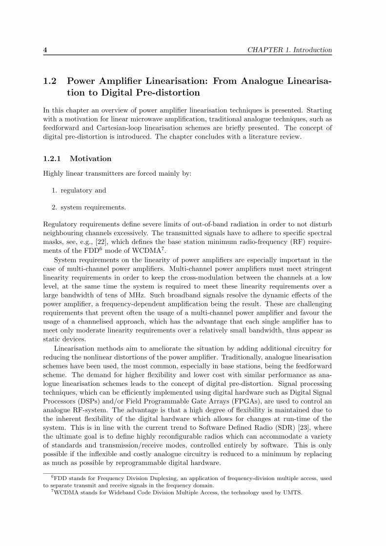
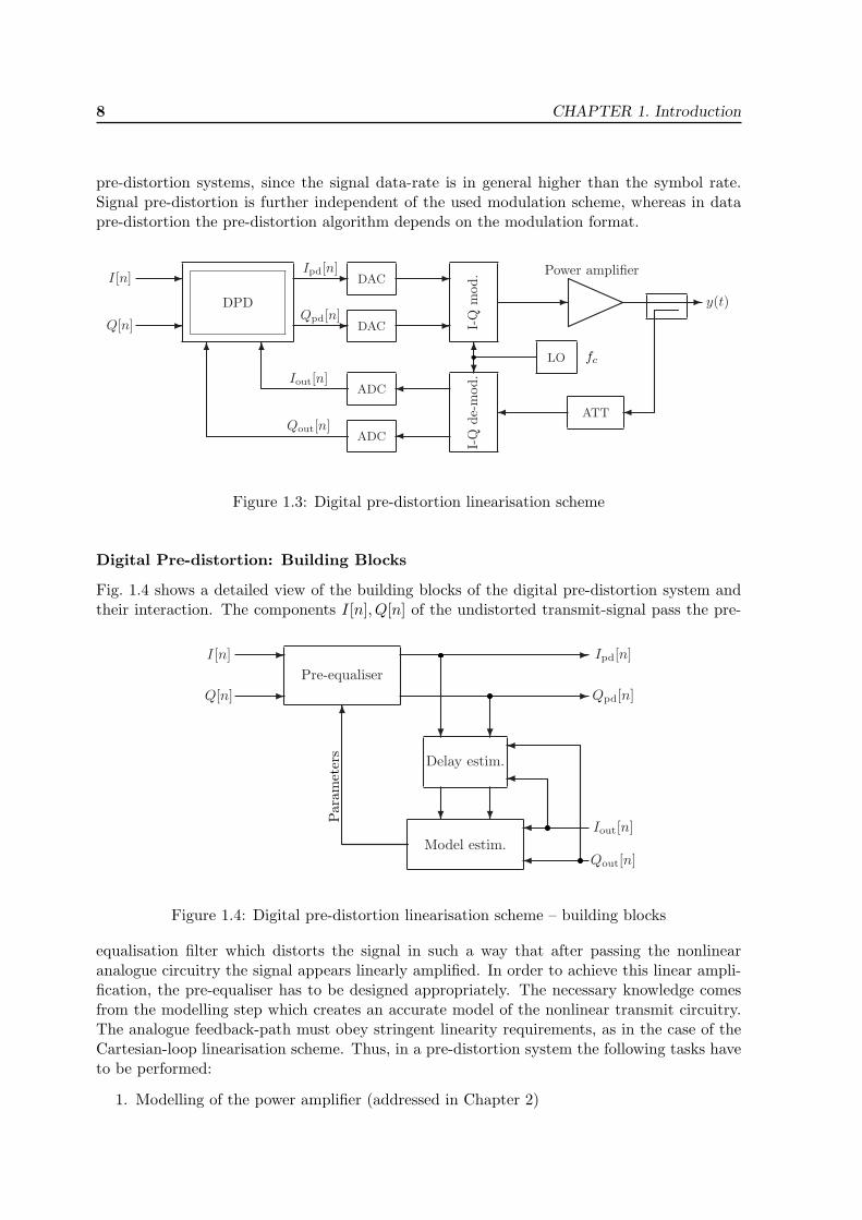
Fig. 1.4 shows a detailed view of the building blocks of the digital pre-distortion system andtheir interaction. The components I[n], Q[n] of the undistorted transmit-signal pass the pre-
Delay estim.
Pre-equaliser
�I[n]
Q[n] �
�
�
� �
� � �
�
�
Model estim.Qout[n]
Ipd[n]
Qpd[n]
Iout[n]
�
�
Par
amet
ers
Figure 1.4: Digital pre-distortion linearisation scheme – building blocks
equalisation filter which distorts the signal in such a way that after passing the nonlinearanalogue circuitry the signal appears linearly amplified. In order to achieve this linear ampli-fication, the pre-equaliser has to be designed appropriately. The necessary knowledge comesfrom the modelling step which creates an accurate model of the nonlinear transmit circuitry.The analogue feedback-path must obey stringent linearity requirements, as in the case of theCartesian-loop linearisation scheme. Thus, in a pre-distortion system the following tasks haveto be performed:
1. Modelling of the power amplifier (addressed in Chapter 2)
1.2 Power Amplifier Linearisation: From Analogue Linearisation to Digital Pre-distortion 9
2. Adaptive identification of the power amplifier model-parameters (addressed in Chapter 3)
3. Design of the pre-distortion filter (addressed in Chapter 4)
4. Realisation of the pre-distortion unit (addressed in Chapter 5).
The first task is the modelling of the nonlinear transmit path. Nonlinear systems are basicallyall systems which behave nonlinear. Infinitely many possibilities for models exist, makingthis task difficult. A model has to be found that is capable of describing the behaviourof a composite of systems (mixed-signal devices such as DACs, analogue circuitry such asI-Q modulators, filters, pre-amplifiers, and power amplifiers) and that is at the same timereasonably low-complex.
Once a candidate model has been found the model-parameters have to be estimated. Anadaptive identification algorithm, in its nature an on-line optimisation method, can performthis task.
The next task is then to design a pre-equaliser that compensates the nonlinear and dynamiceffects (memory effects) of the transmit path. Analytic solutions for the pre-equaliser are ingeneral not achievable. At least a method which provides an approximate solution for the pre-equaliser has to be found. It would be further desirable that this method provides solutionsfor the pre-equaliser for a variety of power amplifier models.
Finally, the system has to be realised and tested in an experimental setup. This is not onlya proof-of-principle, but shows also the technical feasibility of the method under technologicalconstraints.
Digital Pre-distortion – Brief Literature Review
Digital pre-distortion of microwave power amplifiers is a relatively young technique, initiated inthe early 1980s with the paper of A. A. M. Saleh and J. Salz [3]. This and other early contribu-tions consider data pre-distortion, i.e., the data symbols are distorted, not the transmit signalafter transmit filtering. The pulse-shaping is thus performed after the pre-distortion stage.The spectral broadening due to the nonlinear amplifier cannot be avoided, but the nonlineardistortion of the data is compensated. These contributions consider nonlinear memorylesspower amplifiers.
Data pre-distortion considering also memory effects appear in the late 1980s [32, 33, 34,35], using Volterra filters as models for the nonlinear channel and for the pre-equaliser [36].Nonlinear equalisation at the receiver, compensating for a nonlinear travelling wave tubeamplifier and a linear channel, are considered in [37], whereas linearisation at the satellitetransmitter is considered in [32], making the task easier since the amplifier can be consideredas memoryless and the channel, which makes post-equalisation complicated, has no impact.
Pre-distortion of the transmit signal after the transmit filters appeared in the late 1980s [38,39, 40], introducing a look-up table based pre-distortion concept, based on a memorylessnonlinear power amplifier model. Since then, a vast amount of literature has been published,based on memoryless as well as dynamic models for the power amplifier, see e.g., [41, 17, 42, 43],mostly based on computer simulations.

10 CHAPTER 1. Introduction

Chapter 2
Power Amplifier Modelling
The modelling task in the context of power amplifier pre-distortion is essential. Withoutknowledge of the system behaviour at a relatively high level of abstraction – in digital pre-distortion, parametric black-box models are used – equalisation will be an impossible challenge.The quality of the modelling has a great influence on the quality of the equalisation, since thepre-distortion unit is built based on the used power amplifier model, as observed in detail inChapter 4. Therefore, modelling is a key element for pre-distortion techniques.
Models used commonly in power amplifier design and analysis range from detailed physicaldescriptions of the active device, the transistor, e.g., in power amplifier design, to relativelyabstract models, incorporating equivalent circuits, e.g., for power amplifier characterisation.Here, the most abstract approach will be taken – the power amplifier is modelled as a para-metric black box1. This brings several advantages, but has its drawbacks, too:
➾ Modelling at a high level of abstraction does not require specific and detailed knowledgeof the functionality of the power amplifier. On the other hand, specific knowledge canimprove the quality of the modelling.
➾ Gaining physical insight into system behaviour from abstract black box models is rarelypossible. In the context of pre-distortion the aim is not to gain physical insight into theoperation of power amplifiers.
➾ If performed in a smart way, black box models of complex dynamic systems can lead tocompact descriptions. Few parameters can suffice to characterise a complex system witha large number of interconnected subsystems. This is especially important in systemsimulation – fast and accurate simulators can be realised.
The most often used approach to deal with a nonlinear system is its linearisation arounda certain operating point; in other words, the nonlinear aspects of the problem are avoided.Approximating the power amplifier behaviour in some neighbourhood of an operating pointusing a linear model is not feasible in the pre-distortion context – the identification of thenonlinear aspects is essential for being able to compensate them.
In this chapter parametric nonlinear models for power amplifiers are presented. TheVolterra series [45] is presented – it is the most widely investigated model for nonlinear dy-namic systems. As it is capable of modelling a very large class of systems, it serves as a
1A model-set whose parameters are a vehicle for adjusting the fit to the data is called a black box [44]. Theparameters do not reflect physical entities in the system. Accordingly, model-sets with adjustable parametersadmitting physical interpretations are called grey boxes.
11
12 CHAPTER 2. Power Amplifier Modelling
performance measure for the modelling capabilities of low complex models, such as Wiener-and Hammerstein models, which are presented thereafter. It is not the scope of this work topresent a detailed analysis of the capabilities and difficulties associated with each presentedmodel. The modelling is viewed from a practically relevant position, mostly with respect toperformance and complexity.
The modelling capabilities of each model structure are tested against measured input/out-put data from power amplifiers, as well as against data obtained with a widely used simulationtool, ADS 2. This simulation tool incorporates vendor-specific power amplifier models at circuitlevel. The advantage by using such an environment is that no equipment limitations, e.g.,with respect to a maximum allowed signal bandwidth, have to be taken into consideration, aswell as detrimental effects, such as measurement noise and accuracy limitations (e.g. limitedresolution of analogue-to-digital converters), have no effect on the modelling. This environmentis suited to test different model structures against each other and to gain insight in algorithmiclimitations by excluding undesired effects from the measurement process. On the other hand,simulations can provide only a very special and restricted picture of reality, where detrimentaleffects and limitations have to be taken into account.
In order to prevent wrong conclusions on power amplifier models based only on simu-lated data, measurements on microwave power amplifiers have been performed. Therefore,the presented models in the following sections are compared with respect to their modellingcapabilities, i.e., the capability to reproduce the measured output data given the input data.
2.1 The Volterra Series
The Volterra series as a means for describing nonlinear systems was first used by NorbertWiener [47, 4]. It is a functional power series of the form
y(t) = H(x(t)
)= h0 +
∞∑p=1
∫· · ·∫hp(t, τ1, . . . , τp)x(τ1) · · ·x(τp)dτ1 · · · dτp , (2.1)
in which H(x(t)
)is a nonlinear functional of the continuous function x(t), h0 is a constant, t
is a parameter, and hp(· · · ) for p ≥ 1 are continuous functions, called the Volterra kernels.In the context of modelling of a dynamic nonlinear system such as a power amplifier in
wireless communications, x(t) is the input time-signal and t is (continuous) time. The basicquestions are whether it is possible to approximate the behaviour of a physical nonlineardynamic system with a series of the form in (2.1) and for which systems and which inputsignals does this series converge. These questions can be answered affirmatively for a largeclass of systems, i.e., any time-invariant continuous nonlinear system, and a wide class of inputsignals, i.e., signals extending over a finite time interval and belonging to a compact set3 [5,pp. 34-37]. The basis for proving this is the Stone-Weierstrass theorem, see [49].
2ADS [46] stands for Advanced Design System, a simulation environment developed by Agilent Technologies.It is capable to simulate microwave designs, as well as complex communication systems.
3A set S in a normed space is compact, if for an arbitrary sequence {xi} in S there is a subsequence{xin} converging to an element x ∈ S. In finite dimensions, compactness is equivalent to being closed andbounded [48]. An example of a noncompact set is the unit ball in L2(0, T ), the set of all u(t) such that‖u(t)‖ ≤ 1, easily verified by an example, violating Weierstrass’ theorem [48] which states that a continuousfunctional on a compact subset of a normed vector space achieves a maximum: The continuous functional
f(u) =R 1/2
0u(t)dt −
R 1
1/2u(t)dt does not achieve the supremum of 1 (|f(u)| ≤ ‖u(t)‖ ≤ 1) for continuous
functions u(t), thus proves that the unit ball is not compact.
2.1 The Volterra Series 13
In [8] the range of the input signals for which the Volterra series approximation convergesis enlarged to signals extending over the whole time-axis and belonging to non-compact sets,to which more practical signals belong to. This is achieved by limiting the class of systemsto only those with fading memory. Roughly speaking, this means that the memory of thesystem “fades” or that the system is “forgetting”. These strong theoretical results provide thebackground for the attempts in representing nonlinear dynamic systems with Volterra series.
The input/output relation of the Volterra model of the power amplifier used in this workis a truncated and stationary (time-invariant) Volterra series
y(t) =2P+1∑p=1
∫· · ·∫hp(τ1, . . . , τp)x(t− τ1) · · · x(t− τp)dτ1 · · · dτp (2.2)
=2P+1∑p=1
∫hp(τττp)
p∏i=1
x(t− τi)dτττp , (2.3)
where, for notational compactness, the vector τττp = [τ1, . . . , τp]T for the set of time-argumentsfor the p−dimensional kernel hp(τ1, . . . , τp) and dτττp = dτ1 · · · dτp is used. The multiple integralsare compactly described. The constant term h0 is assumed to be zero. The tilde marks thesignals and the kernels as real-valued bandpass, see (2.4) further ahead. In the following, anequivalent discrete-time complex baseband input/output representation of (2.2) is deduced.This follows the derivation in [50], where the equivalent complex baseband Volterra kernels ofa real-valued bandpass Wiener model are determined, see also Section 2.2 for more details.
2.1.1 Complex Baseband Volterra Series
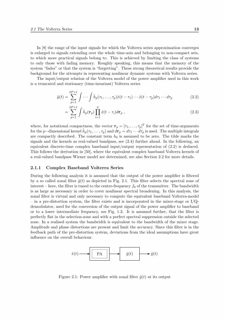
During the following analysis it is assumed that the output of the power amplifier is filteredby a so called zonal filter g(t) as depicted in Fig. 2.1. This filter selects the spectral zone ofinterest – here, the filter is tuned to the centre-frequency f0 of the transmitter. The bandwidthis as large as necessary in order to cover nonlinear spectral broadening. In this analysis, thezonal filter is virtual and only necessary to compute the equivalent baseband Volterra-model– in a pre-distortion system, the filter exists and is incorporated in the mixer-stage or I/Q-demodulator, used for the conversion of the output signal of the power amplifier to basebandor to a lower intermediate frequency, see Fig. 1.3. It is assumed further, that the filter isperfectly flat in the selection-zone and with a perfect spectral suppression outside the selectedzone. In a realised system the bandwidth is equivalent to the bandwidth of the mixer stage.Amplitude and phase distortions are present and limit the accuracy. Since this filter is in thefeedback path of the pre-distortion system, deviations from the ideal assumptions have greatinfluence on the overall behaviour.
PA g(t)- - -x(t) y(t)
Figure 2.1: Power amplifier with zonal filter g(t) at its output
14 CHAPTER 2. Power Amplifier Modelling
The real-valued bandpass signal, centred at f0 and input to the amplifier or Volterra model,is
x(t) = <{x(t)ej2πf0t
}. (2.4)
The equivalent complex baseband signal is x(t). Inserting the expression (2.4) into the firstorder term in the Volterra series (2.2) gives the output of the first order (linear) term
y1(t) =∫h1(τ1)<
{x(t− τ1)ej2πf0(t−τ1)
}dτ1 = <
{∫h1(τ1)x(t− τ1)dτ1ej2πf0t
}(2.5)
with the first order baseband kernel h1(t) = h1(t)e−j2πf0t. The (ideal) zonal filter is centred atf0, the signal passes unchanged. The equivalent complex baseband output signal is thereforesimply obtained by the convolution of h1(t) and x(t).
For the quadratic part insertion of (2.4) into
y2(t) =∫h2(τττ2)
2∏i=1
x(t− τi)dτττ2 (2.6)
yields already a much more complex behaviour:
y2(t) =∫h2(τττ2)
2∏i=1
<{x(t− τi)ej2πf0(t−τi)
}dτττ2
=14
∫h2(τττ2)e−j2πf0τ1e−j2πf0τ2x(t− τ1)x(t− τ2)dτττ2e
j2π2f0t
+14
∫h2(τττ2)ej2πf0τ1ej2πf0τ2x∗(t− τ1)x∗(t− τ2)dτττ2e
−j2π2f0t
+14
∫h2(τττ2)ej2πf0τ1e−j2πf0τ2x∗(t− τ1)x(t− τ2)dτττ2
+14
∫h2(τττ2)e−j2πf0τ1ej2πf0τ2x(t− τ1)x∗(t− τ2)dτττ2
=12<
{∫h2(τττ2)e−j2πf0(τ1+τ2)
2∏i=1
x(t− τi)dτττ2ej2π2f0t
}
+12<{∫
h2(τττ2)e−j2πf0(τ1−τ2)x(t− τ1)x∗(t− τ2)dτττ2
}. (2.7)
The second order part produces signals that are centred at f = 2f0 and f = 0. The zonalfilter, centred at f0 with a bandwidth assumed to be small compared with f0, suppresses theoutput of the second order term completely.
In a similar manner, the output signal of the third order part of (2.2) can be computed.The resulting expression is
y3(t) =14<
{∫h3(τττ3)e−j2πf0(τ1+τ2+τ3)
3∏i=1
x(t− τi) dτττ3 ej2π3f0t
}
+14<{∫
h3(τττ3)e−j2πf0(τ1+τ2−τ3) x(t− τ1)x(t− τ2)x∗(t− τ3) dτττ3 ej2πf0t
}+
14<{∫
h3(τττ3)e−j2πf0(τ1−τ2+τ3) x(t− τ1)x∗(t− τ2)x(t− τ3) dτττ3 ej2πf0t
}+
14<{∫
h3(τττ3) e−j2πf0(−τ1+τ2+τ3)x∗(t− τ1)x(t− τ2)x(t− τ3) dτττ3 ej2πf0t
}. (2.8)
2.1 The Volterra Series 15
Only symmetric kernels hp(tp) = hp(t1, t2 . . . , tp) are considered – the arguments t1, t2, . . . , tpcan therefore be permuted in every order without affecting the output signal. This is no lossof generality since every asymmetric Volterra kernel can easily be converted into a symmetrickernel, see [4, pp. 80-81]. The three last parts of (2.8) at f0 yield therefore the same result.Since the zonal filter is centred at f0, the first component at 3f0 is assumed to be suppressedperfectly. The only remaining term, written in the equivalent baseband form, is thus
y3(t) =∫h3(τττ3)x(t− τ1)x(t− τ2)x∗(t− τ3)dτττ3 (2.9)
with the third order baseband kernel
h3(t3) =34h3(t3)e−j2πf0(t1+t2−t3) . (2.10)
By induction it can be shown that the terms of even order 2p do not contribute to the outputsignal if the zonal filter is centred at f0. Only the uneven terms in (2.2) produce componentsat f0. The output for the 2p+ 1-th homogeneous part is (in the equivalent baseband form)
y2p+1(t) =∫h2p+1(τττ2p+1)
p+1∏i=1
x(t− τi)2p+1∏i=p+2
x∗(t− τi)dτττ2p+1 (2.11)
with the equivalent baseband kernel
h2p+1(t2p+1) =(
12
)2p(2p+ 1p
)h2p+1 (t2p+1) e−j2πf0(
Pp+1i=1 ti−
P2p+1i=p+2 ti) , (2.12)
h2p+1 (t2p+1) being the real-valued 2p+ 1-dimensional bandpass kernel.The equivalent complex baseband Volterra series of order 2P − 1 (with the zonal filter
centred at the centre frequency f0) is thus
y(t) =P−1∑p=0
∫h2p+1(τττ2p+1)
p+1∏i=1
x(t− τi)2p+1∏i=p+2
x∗(t− τi)dτττ2p+1 . (2.13)
It has to be noted that in (2.12) the equivalent baseband kernel h2p+1(t2p+1) is invariant withrespect to a permutation of the first p+1 arguments and with respect to a permutation of thesecond p arguments. A permutation of members between these two sets is allowed only if thecorresponding conjugation of the input signal x(t) in (2.13) is also considered.
2.1.2 Frequency Domain Representation of a Volterra Series
Further insight into the behaviour of a nonlinear system, represented by the Volterra se-ries (2.13), can be gained if the output spectrum is computed. In the following, this calculationis performed exemplarily for the third order part (see [4, pp.104-108] for the real valued case).The extension to arbitrary orders is straightforward.
Consider (2.9), the third order homogeneous part. For the calculation of
y(3)(t1, t2, t3) =∫h3(τττ3)x(t1 − τ1)x(t2 − τ2)x∗(t3 − τ3)dτττ3 (2.14)
16 CHAPTER 2. Power Amplifier Modelling
is introduced. Three dimensional Fourier transform yields
Y(3)(f1, f2, f3) = H3(f1, f2, f3)X(f1)X(f2)X∗(−f3) . (2.15)
Inverse Fourier transformation of (2.15) and setting of t = t1 = t2 = t3 gives
y3(t) = y(3)(t, t, t) =∫∫∫
H3(f1, f2, f3)X(f1)X(f2)X∗(−f3)ej2π(f1+f2+f3)tdf1df2df3 . (2.16)
With substitution of f2 + f3 = ν1
y3(t) =∫∫∫
H3(f1, ν1 − f3, f3)X(f1)X(ν1 − f3)X∗(−f3)ej2π(f1+ν1)tdf1dν1df3 (2.17)
is obtained. Further substitution of f = f1 + ν1 results in
y3(t) =∫∫∫
H3(f − ν1, ν1 − f3, f3)X(f − ν1)X(ν1 − f3)X∗(−f3)ej2πftdν1df3df , (2.18)
which provides the desired result for the spectrum Y3(f)
Y3(f) =∫∫
H3(f − ν1, ν1 − ν2, ν2)X(f − ν1)X(ν1 − ν2)X∗(−ν2)dν1dν2 . (2.19)
For the general case of the 2p+ 1-th homogeneous part it can easily be shown that
Y2p+1(f) =∫Y(2p+1)(f − ν1, ν1 − ν2, ν2 − ν3, . . . , ν2p)dν1 · · · dν2p , (2.20)
with
Y(2p+1)(f1, . . . , f2p+1) = H2p+1(f1, . . . , f2p+1)p+1∏i=1
X(fi)2p+1∏i=p+2
X∗(−fi) . (2.21)
The frequency domain representation of the Volterra series (2.13) is therefore
Y (f) =P−1∑p=0
Y2p+1(f) . (2.22)
Equation (2.20) is very similar to a multi-dimensional convolution integral. From thisintegral form the spectral broadening of a signal passing through a Volterra system can easilybe understood. This becomes very clear in the case of a Wiener- or Hammerstein system,considered in Section 2.2 and Section 2.3 in more detail.
2.1.3 Discrete-time Volterra Series
A discrete-time representation of the Volterra series (2.13), used to model the nonlinear system,is essential for digital signal processing. In digital pre-distortion, the output of the amplifier(after attenuation, down-conversion and eventual demodulation) is sampled. This gives adiscrete-time signal, together with the discrete-time input signal it is used to extract theparameters of the power amplifier model, here, the Volterra kernels. The selection of thesampling rate is essential – in order to reconstruct the analogue output signal, the samplingrate must be at least twice the signal bandwidth, see e.g., [51, 52], as requested by the sampling
2.1 The Volterra Series 17
theorem. Since nonlinear systems spread the signal in bandwidth, see (2.20), selecting thesampling rate twice the output bandwidth is challenging in practice, since very fast analogue-to-digital converters with a high resolution (typically 12-14 bits supporting a dynamic rangeof up to 70 dB) have to be used. For system identification it can be shown that it is sufficientto sample the output with the same rate as used for the input signal [53, 54, 55].
The input signal X(f) is assumed to be bandlimited4 in I = [−B,B]. As can be seenfrom (2.21), the kernels H2p+1(f1, . . . , f2p+1), p = 0, . . . , P − 1, can be assumed to be band-limited. The form of the kernels outside of the hypercube C = I × I × . . .× I is of no impor-tance, since in this region the kernels will not be excited by the input signal. The spectrumY(2p+1)(f1, . . . , f2p+1) is zero outside the hypercube C and therefore strictly bandlimited5.
It is assumed that the input signal is sampled at the Nyquist-rate T = 12B yielding x[n] =
x(nT ) = x( n2B ), n ∈ Z. Discrete Fourier transform yields
X(f) =∑n∈Z
x[n]e−jπfBn . (2.23)
Since the kernels can be assumed to be bandlimited, the spectrum of the kernel in the hyper-cube C can be determined by the multidimensional Fourier transform, e.g., for the third orderkernel
H3(f1, f2, f3) =∑
n1,n2,n3∈Zh3[n1, n2, n3]e−j
πB
(f1n1+f2n2+f3n3) , (2.24)
the Volterra kernel being sampled at the Nyquist-rate of the input signal, h3[n1, n2, n3] =h3( n1
2B ,n22B ,
n32B ). If the output is sampled, again with the rate of the input sampling y3[n] =
y( n2B ), with (2.16), (2.23) and (2.24)
y3[n] =∑
n1,n2,n3∈Z
∑r1,r2,r3∈Z
h3[n1, n2, n3]x[r1]x[r2]x∗[r3]×
12B
∫ B
−Bejπ
f1B
(n−n1−r1)df11
2B
∫ B
−Bejπ
f2B
(n−n2−r2)df21
2B
∫ B
−Bejπ
f3B
(n−n3−r3)df3
=∑n3,r3
h3[n3]x[r1]x[r2]x∗[r3]δ[n− n1 − r1]δ[n− n2 − r2]δ[n− n3 − r3]
=∑n3
h3[n3]x[n− n1]x[n− n2]x∗[n− n3] (2.25)
is obtained, showing that the output of the Volterra system, sampled with the Nyquist-rate ofthe input-signal, can be obtained by a convolution of the sampled input signal and the sampledVolterra kernel. In order to shorten the notation the argument vectors n3 = [n1, n2, n3]T andr3 = [r1, r2, r3]T are introduced. A summation with the here three dimensional argumentvectors as indices stands for a three-fold summation with the entries of the argument vectorsused as individual indices. This notation is used wherever appropriate. Higher order kernels
4It has to be emphasised that in a pre-distortion system the input signal to the power amplifier has beennonlinearly distorted by the pre-distortion filter. The bandwidth is therefore larger than the bandwidth of theundistorted input signal, e.g., P × 5MHz for one UMTS carrier and for a pre-distortion filter of nonlinear orderP .
5It has to be noted that H2p+1(f1, . . . , f2p+1) cannot be strictly bandlimited due to causality. Here, it isassumed that the spectral components of the input signal are sufficiently small outside the interval I = [−B, B].Therefore, the signal Y(2p+1)(f1, . . . , f2p+1) is assumed to be bandlimited in C.
18 CHAPTER 2. Power Amplifier Modelling
are treated equivalently. The discrete-time Volterra series of order 2P − 1 is
y[n] =P−1∑p=0
∑n2p+1∈Z
h2p+1[n2p+1]p+1∏i=1
x[n− ni]2p+1∏i=p+2
x∗[n− ni] . (2.26)
The continuous-time kernel h2p+1(t2p+1) and the discrete-time kernel h2p+1[n2p+1] are equiv-alent, since the same output-signal is reproduced exactly at the sampling points. The contin-uous-time Volterra system Vc, defined by the continuous-time kernels, and the discrete-timeVolterra system Vd, defined by the sampled continuous-time kernels, are therefore equivalent.Hence, for system identification, sampling with the Nyquist-rate of the input-signal is suffi-cient for estimating the Volterra-kernels. But it is not possible to reconstruct the continuous-time output signal y(t) from the discrete-time signal y[n], resulting from a sampling withthe Nyquist-rate of the input signal. Aliasing would occur, since Y (f) is not bandlimited inI = [−B,B], see (2.20). If the discrete-time Volterra kernels are known, the continuous-timekernels can be reconstructed, thus, with the knowledge of the continuous-time input signalx(t), the continuous-time output signal y(t) can be produced. Hence, the knowledge of thediscrete-time kernel and the input signal, either in continuous-time or discrete-time, is sufficientto reproduce all signals. The commutative diagram [53]
x(t) Vc//
OO
��
y(t)
��x[n] Vd
// y[n]
(2.27)
visualises this situation: Taking the path x(t) Vc//y(t) //y[n] is equivalent to taking the
path x(t) //x[n] Vd//y[n] .
The consequence is that for modelling a nonlinear system which can be represented by aVolterra series, it is not necessary to sample the output signal at its Nyquist rate – samplingwith the Nyquist-rate of the input signal is sufficient for estimating the Volterra kernels.
2.1.4 Series Representation of a Static Non-linearity
From the Volterra series (2.26) it is straightforward to specialise to a static non-linearity. Thekernels are assumed to vanish, except if all indices are equal to zero, h2p+1[n2p+1] = 0 ifn2p+1 6= 0, p = 0, . . . , P − 1. The equivalent discrete-time baseband representation of a staticnon-linearity, represented by a power series, is therefore
y[n] =P−1∑p=0
h2p+1[0]x[n]∣∣x[n]
∣∣2p = x[n]P−1∑p=0
θ2p+1
∣∣x[n]∣∣2p = x[n]gθ
(∣∣x[n]∣∣) . (2.28)
The 2p + 1-th order kernel reduces to a simple (complex) scalar θp. A signal-dependent gaingθ(∣∣x[n]
∣∣) distorts the input signal. Since this gain is complex, it introduces amplitude andphase distortions which depend on the amplitude of the input signal. The amplitude distortion(AM-AM conversion) is ∣∣y[n]
∣∣∣∣x[n]∣∣ =
∣∣∣gθ(∣∣x[n]∣∣)∣∣∣ , (2.29)
2.1 The Volterra Series 19
whereas the phase distortion (AM-PM conversion) is
arg(y[n]
)− arg
(x[n]
)= arg
(gθ
(∣∣x[n]∣∣)) . (2.30)
If instead of a power series a set of orthogonal polynomials{φp(·)
}with the real argument∣∣x[n]
∣∣ is used, only even order polynomials will contribute,
y[n] = x[n]P−1∑p=0
θ′2p+1 φ2p
(∣∣x[n]∣∣) . (2.31)
E.g., for{φp(·)
}the even Hermite polynomials can be used. Another possibility is to use
linear splines, see [21, 43].
2.1.5 Parameter Estimation for the Volterra Model
The Volterra series is linear-in-parameters – standard least-squares techniques can thereforebe used to estimate the kernels. The composition of the regression matrix is, due to thespecial form of (2.26), different from the standard real-valued Volterra series: the kernels aresymmetric with respect to the first p + 1 arguments, e.g., h3[0, 1, 1] = h3[1, 0, 1] since thesekernels are associated with the signal products x[n]x[n− 1]x∗[n− 1] and x[n− 1]x[n]x∗[n− 1],which are symmetric with respect to the first two components. The kernels are symmetricalso with respect to the second p arguments. These terms are associated with the conjugatedsignals. The difference to the real-valued standard formulation of the Volterra series is thatpermutations across these two sets, i.e., the kernel arguments corresponding to the product ofthe first p+ 1 not conjugated signals and the kernel arguments corresponding to the productof the second p conjugated signals, are not allowed.
The kernels can be arranged in vectors, e.g., the third order kernel with a one-tap memorycomprises six elements, h3 =
[h[0, 0, 0], h[0, 0, 1], h[0, 1, 0], h[0, 1, 1], h[1, 1, 0], h[1, 1, 1]
]T , sym-metries already taken into account. The parameter vector of a Volterra series of order 2P − 1,containing only uneven components, can therefore be written as
θθθ = [hT1 ,hT3 , . . . ,h
T2P−1]
T . (2.32)
A specific signal matrix H, associated with this parameter vector, is composed of sub-matricesXp, which are associated with the kernels hp,
H = [X1,X3, . . . ,X2P−1] . (2.33)
Here, e.g., the sub-matrix X3, considering a time window of M samples, is
X3 = [x3,n,x3,n−1, . . . ,x3,n−M ]T , (2.34)
whereby the vectors
x3,n =[x[n]
∣∣x[n]∣∣2, x2[n]x∗[n− 1], . . . , x[n−N3 + 1]
∣∣x[n−N3 + 1]∣∣2]T , (2.35)
N3 being the memory-length of the kernel, are used.The output signal of a Volterra system of order 2P − 1, see (2.26), over the finite time-
horizon n, n− 1, . . . , n−M is thusyn = Hθθθ (2.36)
20 CHAPTER 2. Power Amplifier Modelling
with yn =[y[n], . . . , y[n−M ]
]T .
Having available a set of measured output data dn =[d[n], d[n − 1], . . . , d[n −M ]
]T , theparameters (kernels) of a specific Volterra model can be estimated with the least-squaresmethod:
θθθ = (HHH)−1HHdn . (2.37)
2.2 The Wiener Model
The Wiener model used here is a series connection of a linear finite-impulse response (FIR)filter and a static (memoryless) non-linearity f(·), see Fig. 2.2. It is not the general Wienermodel, resulting from a construction of orthogonal functionals (Wieners G-functionals) fromthe Volterra functionals via a Gram-Schmidt procedure [4, pp. 199ff.]. The general Wienermodel has the advantage to incorporate a larger class of nonlinear systems than a Volterraseries, but is not less complex (in terms of numbers of parameters) as the Volterra series. Thesimple Wiener model [44] used here requires substantially fewer parameters compared to aVolterra model and achieves good modelling results, see Section 2.6.
As in the case of the Volterra model, at the output of the power amplifier a zonal filterselects the spectral zone around the carrier frequency. The linear filter in the Wiener model isassumed to be an FIR filter G(q−1) =
∑N−1i=0 giq
−i, the nonlinear function is represented via aseries as in (2.31). Hence, the discrete-time input/output representation of the Wiener modelis
y[n] = G(x[n]
) P−1∑p=0
θ2p+1 φ2p
(∣∣∣G(x[n])∣∣∣) . (2.38)
In contrast to the Volterra series (and the static nonlinear function represented by a series)the Wiener model is not linear with respect to the parameters {gi}N−1
i=0 of the linear filter, itis only linear with respect to the parameters of the static non-linearity {θp}P−1
p=0 .
G f(·)- - -x[n] y[n]
Figure 2.2: The Wiener model.
Further insight can be gained in the frequency domain. For this, the static non-linearityis represented using a power series. In continuous time, the input/output relation reads
y(t) =P−1∑p=0
θ2p+1G(x(t)
)∣∣∣G(x(t))∣∣∣2p . (2.39)
Exemplarily, the third order part is considered,
y(3)(t1, t2, t3) = θ3G(x(t1)
)G(x(t2)
)G∗(x(t3)
). (2.40)
2.2 The Wiener Model 21
Fourier transform yields
Y(3)(f1, f2, f3) = θ3G(f1)X(f1)G(f2)X(f2)G∗(−f3)X∗(−f3)= θ3H(f1, f2, f3)X(f1)X(f2)X∗(−f3)= θ3Z(f1)Z(f2)Z∗(−f3) , (2.41)
with Z(f) = G(f)X(f). The Volterra kernel in the frequency domain is H(f1, f2, f3) =θ3G(f1)G(f2)G∗(−f3). Again, X(f) is considered exactly bandlimited in I = [−B,B]. There-fore, Y (f1, f2, f3) is exactly bandlimited in the 3-dimensional cube C = I × I × I. InverseFourier transform yields
y(t) = y(3)(t, t, t) = θ3
∫∫∫Z(f − ν1)Z(ν1 − ν2)Z∗(−ν2)dν1dν2e
2πftdf , (2.42)
where Y (f) can be recognised to be
Y (f) = θ3
∫∫Z(f − ν1)Z(ν1 − ν2)Z∗(−ν2)dν1dν2 = θ3Z(f) ∗ Z(f) ∗ Z∗(−f) , (2.43)
a twofold convolution of Z(f) = H(f)X(f) with itself, producing the spectral broadening,Y (f) ∈ [−3B, 3B]. Via the convolution, the spectrum Y(3)(f1, f2, f3) ∈ C is mapped intoY (f) ∈ [−3B, 3B].
Again, as in the case of a Volterra system, for system identification input rate samplingat the output of the Wiener system suffices, i.e., even if the signal is spread in the frequencydomain during the passage through the nonlinear system, no larger sampling rate at the outputis required.
2.2.1 Parameter Estimation for the Wiener Model
The Wiener model is partially linear-in-parameters – the parameters of the static non-linearity{θp} – and partially nonlinear-in-parameters – the parameters of the linear filter G. Parame-ter estimation using the conventional least-squares approach is therefore not applicable in astraightforward manner. For the parameter estimation with the measured and simulated datathe following simple heuristic method is proposed:
1. First, the measured or simulated input/output data is fitted to a purely linear modelusing the least squares method:
g =(HHg Hg
)−1HHg dn , (2.44)
with the estimated parameter vector g = [g0, g1, . . . , gN−1]T , the input-signal matrix
Hg =
x[n] x[n− 1] · · · x[n−N + 1]
x[n− 1] x[n− 2] . . . x[n−N ]...
.... . .
...x[n−M ] x[n−M − 1] · · · x[n−M −N + 1]
, (2.45)
and dn =[d[n], d[n − 1], . . . , d[n − M ]
]T , which is the measured output signal. Thenonlinear distortions act here as an additional disturbance.
22 CHAPTER 2. Power Amplifier Modelling
2. After the estimation of the parameters of the linear filter, the input signal is passedthrough this estimated linear filter, producing the input signal for the estimation of thestatic nonlinear filter
z[n] = G(x[n]
). (2.46)
3. Using this signal, the parameters of the nonlinear filter are estimated with the leastsquares technique
θθθ =(HHθ Hθ
)−1HHθ dn , (2.47)
with the estimated parameter vector θθθ =[θ1, θ3, . . . , θ2P−1
]T , the signal matrix
Hθ =
z[n]φ0
(|z[n]|
)· · · z[n]φ2(P−1)
(|z[n]|
)z[n− 1]φ0
(|z[n− 1]|
). . . z[n− 1]φ2(P−1)
(|z[n− 1]|
)...
. . ....
z[n−M ]φ0
(|z[n−M ]|
)· · · z[n−M ]φ2(P−1)
(|z[n−M ]|
) , (2.48)
and dn =[d[n], d[n− 1], . . . , d[n−M ]
]T , which is again the measured output signal. Inthis last step a new data set is used, meaning that the input/output signals are not thesame as those used in the estimation of the linear filter parameters.
If, e.g., φ2p(x) = x2p,
y[n] = θ1G(x[n]
)+ G
(x[n]
) P−1∑p=1
θ2p+1
∣∣∣G(x[n])∣∣∣2p︸ ︷︷ ︸
nonlinear distortion
(2.49)
the nonlinear parts can be seen as a disturbance term for the estimation of the parameters ofthe linear filter. If the nonlinear disturbances are not too strong, which is the case for weaklynonlinear systems, the estimation of the parameters of the linear filter is accurate.
2.3 The Hammerstein Model
The Hammerstein model [44] investigated here is a static non-linearity f(·), followed by alinear FIR filter, see. Fig. 2.3. Also here, a zonal filter selects the spectral zone around thecarrier frequency at the output of the power amplifier.
Gf(·)- - -x[n] y[n]
Figure 2.3: The Hammerstein model.
If the nonlinear function f(·) is represented by a series, the input/output representationreads
y[n] = G
x[n]P−1∑p=0
θ2p+1 φ2p
(∣∣x[n]∣∣) , (2.50)
2.3 The Hammerstein Model 23
with the linear filter G(q−1) =∑N−1
i=0 giq−i. Similar as in the case of the Wiener model,
the description is linear in a part of the parameters (the parameters of the linear filter), butnonlinear in the parameters of the static nonlinear function.
As in the case of the Wiener model, the continuous-time representation
y(t) = G
P−1∑p=0
θ2p+1x(t)∣∣x(t)∣∣2p
= G(z(t)
)(2.51)
is transformed into frequency domain
Y (f) = G(f)Z(f) , (2.52)
where, again only for the third-order term,
Z(f) = θ3X(f) ∗X(f) ∗X∗(−f) . (2.53)
Here, Z(f) ∈ [−3B, 3B], G(f) extends in general also over [−3B, 3B], in contrast to theWiener model, where the linear filter G(f) can be considered bandlimited in [−B,B].
2.3.1 Parameter Estimation for the Hammerstein Model
Similar as in the case of the Wiener model also the Hammerstein model is linear in part ofthe parameters – the parameters of the linear filter – and nonlinear in the parameters of thestatic nonlinear filter. A similar two-step estimation procedure is adopted also here:
1. The parameters of the static nonlinear filter are estimated first using the least squaresmethod,
θθθ =(HHθ Hθ
)−1HHθ dn , (2.54)
whereby
Hθ =
φ0
(|x[n]|
)· · · φ2(P−1)
(|x[n]|
)φ0
(|x[n− 1]|
). . . φ2(P−1)
(|x[n− 1]|
)...
. . ....
φ0
(|x[n−M ]|
)· · · φ2(P−1)
(|x[n−M ]|
) , (2.55)
θθθ = [θ1, . . . , θ2P−1]T is the estimated parameter vector and dn =[d[n], . . . , d[n −M ]
]Tis the measured output signal.
2. The input signal is then passed through the estimated nonlinear filter producing the newsignal
z[n] = f(θθθ, x[n]
). (2.56)
3. Using this signal as the input signal for the linear filter, the parameters of the linearfilter are estimated, again using the least squares technique
g =(HHg Hg
)−1HHg dn , (2.57)
with the estimated parameter vector g = [g0, g1, . . . , gN−1]T , the input-signal matrix
Hg =
z[n] z[n− 1] · · · z[n−N + 1]
z[n− 1] z[n− 2] . . . z[n−N ]...
.... . .
...z[n−M ] z[n−M − 1] · · · z[n−M −N + 1]
, (2.58)
24 CHAPTER 2. Power Amplifier Modelling
and dn =[d[n], d[n − 1], . . . , d[n −M ]
]T , which is the measured output signal. Alsohere, a new set the input and measured output data is used for the second step of theparameter estimation.
Equivalently as in the case of the Wiener model, the estimation of the first set of parameters(the parameters of the non-linearity) is not accurate due to the linear filter after that block.From
y[n] =P−1∑p=0
θ2p+1G(x[n]
∣∣x[n]∣∣2p) = (2.59)
g0
P−1∑p=0
θ2p+1x[n]∣∣x[n]
∣∣2p + g1
P−1∑p=0
θ2p+1x[n− 1]∣∣x[n− 1]
∣∣2p + . . .︸ ︷︷ ︸memory effects
(2.60)
can be seen that the estimation of the parameters {θp} would be accurate if no dynamic partwould exist, g1 = g2 = . . . = gM = 0. Since the memory lengths of the power amplifiers simu-lated and measured are not very long (|g0| is large compared to |g1|, |g2|, . . ., see Section 2.6),the estimation of the parameters {θp} is not disturbed exceedingly.
2.4 The Saleh Model
A simple static power amplifier model requiring only four parameters is the Saleh model [9].Originally, it is used to model traveling-wave tube amplifiers but it is often used to model solid-state power amplifiers, too. Both, amplitude distortions and phase distortions are modelledwith simple two-parameter formulas.
If the (real-valued bandpass) input signal of the power amplifier is
x(t) = <{x(t)ej2πf0t
}= r(t) cos
(2πf0t+ ψ(t)
)(2.61)
with x(t) = r(t)ejψ(t) describing the equivalent low-pass signal, r(t) being the amplitude andψ(t) being the phase of the this signal, the output signal of the power amplifier is modelled as
y(t) = A[r(t)
]cos(2πf0t+ ψ(t) + Φ
[r(t)
])(2.62)
with the nonlinear functions
A(r) =αar
1 + βar2and (2.63)
Φ(r) =αφr
2
1 + βφr2. (2.64)
If r is very large, A(r) is proportional to 1/r and Φ(r) approaches a constant. The function A(r)describes the conversion of the input amplitude to the output amplitude (AM-AM conversion),whereas the function Φ(r) describes the influence of the input amplitude on the output phase(AM-PM conversion).
2.5 Model-Structure Selection and Model Validation 25
2.4.1 Parameter Estimation for the Saleh Model
The equations (2.63) and (2.64) are reorganised for the estimation of the parameters αa, βa, αφand βφ:
r[n]A[n]
=1αa
+βaαar2[n] (2.65)
r2[n]Φ[n]
=1αφ
+βφαφr2[n] . (2.66)
Here, A[n] = A(r[n]) and Φ[n] = Φ(r[n]) are the measured output amplitude and phase-difference, r[n] is the amplitude of the input signal. The so transformed model allows toapply the standard least-squares technique for estimating the parameters, summarised in theparameter-vectors θθθa =
[1αa, βa
αa
]T and θθθφ =[
1αφ,αφ
βφ
]T :
θθθa =(HHa Ha
)−1HHa wa , (2.67)
θθθφ =(HHφ Hφ
)−1HHφ wφ , (2.68)
where
Ha = Hφ =
1 r2[n]1 r2[n− 1]...
...1 r2[n−N + 1]
(2.69)
and
wa =[r[n]A[n]
,r[n− 1]A[n− 1]
, . . . ,r[n−N + 1]A[n−N + 1]
]T(2.70)
wφ =[r2[n]Φ[n]
,r2[n− 1]Φ[n− 1]
, . . . ,r2[n−N + 1]Φ[n−N + 1]
]T. (2.71)
Once θθθa and θθθφ are computed, αa = 1
θθθa(1), βa = θθθa(2)
θθθa(1), αφ = 1
θθθφ(1), and βφ = θθθφ(1)
θθθφ(2)can easily
be computed.
2.5 Model-Structure Selection and Model Validation
So far, different kinds of nonlinear models with various complexity have been introduced. TheVolterra model is the most powerful model and comprises a large class of nonlinear dynamicsystems. Wiener-and Hammerstein models are special cases of the Volterra series, as well asthe static nonlinearities – the power series and Saleh’s model. The models can be related toeach other in terms of the size of the model class M : The model class contains all models of aparticular class, e.g., the class (set) MVolterra embraces all models which can be expressed asa Volterra series, a particular model out of that class is determined by the parameter-vectorθθθ of a certain dimension dM (θθθ) = dimθθθ, which is a measure of the model-complexity. Thedescribed models can be ordered according to
MSaleh ⊂ MPower series ⊂ MWiener,MHammerstein ⊂ MVolterra . (2.72)
26 CHAPTER 2. Power Amplifier Modelling
The aim is to describe the input/output behaviour of the power amplifier with a sufficientlypowerful model with the smallest dimension (dM (θθθ)) possible. The evaluation criterion ofchoice for a particular model m = M (θθθ) is the mean squared-error between system outputd[n] and model output ym[n]
J(m) =1N
N∑n=1
∣∣d[n]− ym[n]∣∣2 =
1N
N∑n=1
∣∣em[n]∣∣2 , (2.73)
where an observation interval of length N samples is chosen and system and model are excitedwith the same signal. The least-squares parameter estimation minimises this measure – butcare has to be taken with respect to the number of parameters: using more parameters, theerror will decrease monotonically. Unnecessary parameters will adjust themselves to the par-ticular realisation of the noise (e.g., measurement noise). This is known as overfit – parameterswhich are adjusted to the specific noise realisation do not reflect features of the system andare thus useless.
2.5.1 Model-Structure Selection
Two standard criteria (tailored for least-squares parameter estimation and modifying thesquared-error J(m)) for determining the model structure, i.e., the dimension of the model-parameter vector θθθ of a model in a particular model class M , are of the form [44]
W (m) = J(m)(1 + U(m)) , (2.74)
where W (m) is a modified least-squares error. The function U(m) measures the dimension ofthe model structure and can be interpreted as a penalty-term. In Akaike’s “Final Prediction-Error Criteria (FPE)” [56], the complexity-penalty is defined as
UFPE(m) =2N
dimθθθ , (2.75)
whereas in Rissanen’s “Minimum Description Length Criteria (MDL)” [57], the data length isalso taken into account
UMDL(m) =ln(N)N
dimθθθ . (2.76)
This form of the penalty-term is obtained by requiring to achieve the shortest possible descrip-tion of the observed data.
2.5.2 Model Validation
It is obvious that the derived model is capable of reproducing the data which has been usedfor the estimation. In order to test the model and being able to compare with other models,the models must be tested with different data sets – the validation data [44]. Comparingtwo different models m1 and m2 consists thus of computing J(m1) and J(m2), cf. (2.73),with a data set which is different from the data set used for the parameter estimation. Themodel which yields a better performance (smaller mean-squared error) and which complexityis reasonable for implementation, is favoured. The models are thus cross-validated againsteach other in terms of modelling capability and complexity. The comparison does not use anyassumptions about the true system or other probabilistic arguments. The disadvantage of this
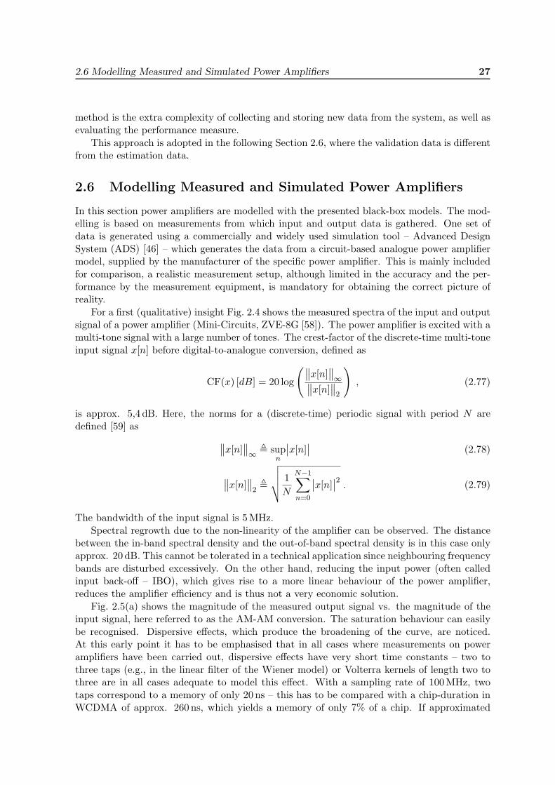
2.6 Modelling Measured and Simulated Power Amplifiers 27
method is the extra complexity of collecting and storing new data from the system, as well asevaluating the performance measure.
This approach is adopted in the following Section 2.6, where the validation data is differentfrom the estimation data.
2.6 Modelling Measured and Simulated Power Amplifiers
In this section power amplifiers are modelled with the presented black-box models. The mod-elling is based on measurements from which input and output data is gathered. One set ofdata is generated using a commercially and widely used simulation tool – Advanced DesignSystem (ADS) [46] – which generates the data from a circuit-based analogue power amplifiermodel, supplied by the manufacturer of the specific power amplifier. This is mainly includedfor comparison, a realistic measurement setup, although limited in the accuracy and the per-formance by the measurement equipment, is mandatory for obtaining the correct picture ofreality.
For a first (qualitative) insight Fig. 2.4 shows the measured spectra of the input and outputsignal of a power amplifier (Mini-Circuits, ZVE-8G [58]). The power amplifier is excited with amulti-tone signal with a large number of tones. The crest-factor of the discrete-time multi-toneinput signal x[n] before digital-to-analogue conversion, defined as
CF(x) [dB] = 20 log
(∥∥x[n]∥∥∞∥∥x[n]∥∥
2
), (2.77)
is approx. 5,4 dB. Here, the norms for a (discrete-time) periodic signal with period N aredefined [59] as ∥∥x[n]
∥∥∞ , sup
n
∣∣x[n]∣∣ (2.78)
∥∥x[n]∥∥
2,
√√√√ 1N
N−1∑n=0
∣∣x[n]∣∣2 . (2.79)
The bandwidth of the input signal is 5 MHz.Spectral regrowth due to the non-linearity of the amplifier can be observed. The distance
between the in-band spectral density and the out-of-band spectral density is in this case onlyapprox. 20 dB. This cannot be tolerated in a technical application since neighbouring frequencybands are disturbed excessively. On the other hand, reducing the input power (often calledinput back-off – IBO), which gives rise to a more linear behaviour of the power amplifier,reduces the amplifier efficiency and is thus not a very economic solution.
Fig. 2.5(a) shows the magnitude of the measured output signal vs. the magnitude of theinput signal, here referred to as the AM-AM conversion. The saturation behaviour can easilybe recognised. Dispersive effects, which produce the broadening of the curve, are noticed.At this early point it has to be emphasised that in all cases where measurements on poweramplifiers have been carried out, dispersive effects have very short time constants – two tothree taps (e.g., in the linear filter of the Wiener model) or Volterra kernels of length two tothree are in all cases adequate to model this effect. With a sampling rate of 100MHz, twotaps correspond to a memory of only 20 ns – this has to be compared with a chip-duration inWCDMA of approx. 260 ns, which yields a memory of only 7% of a chip. If approximated
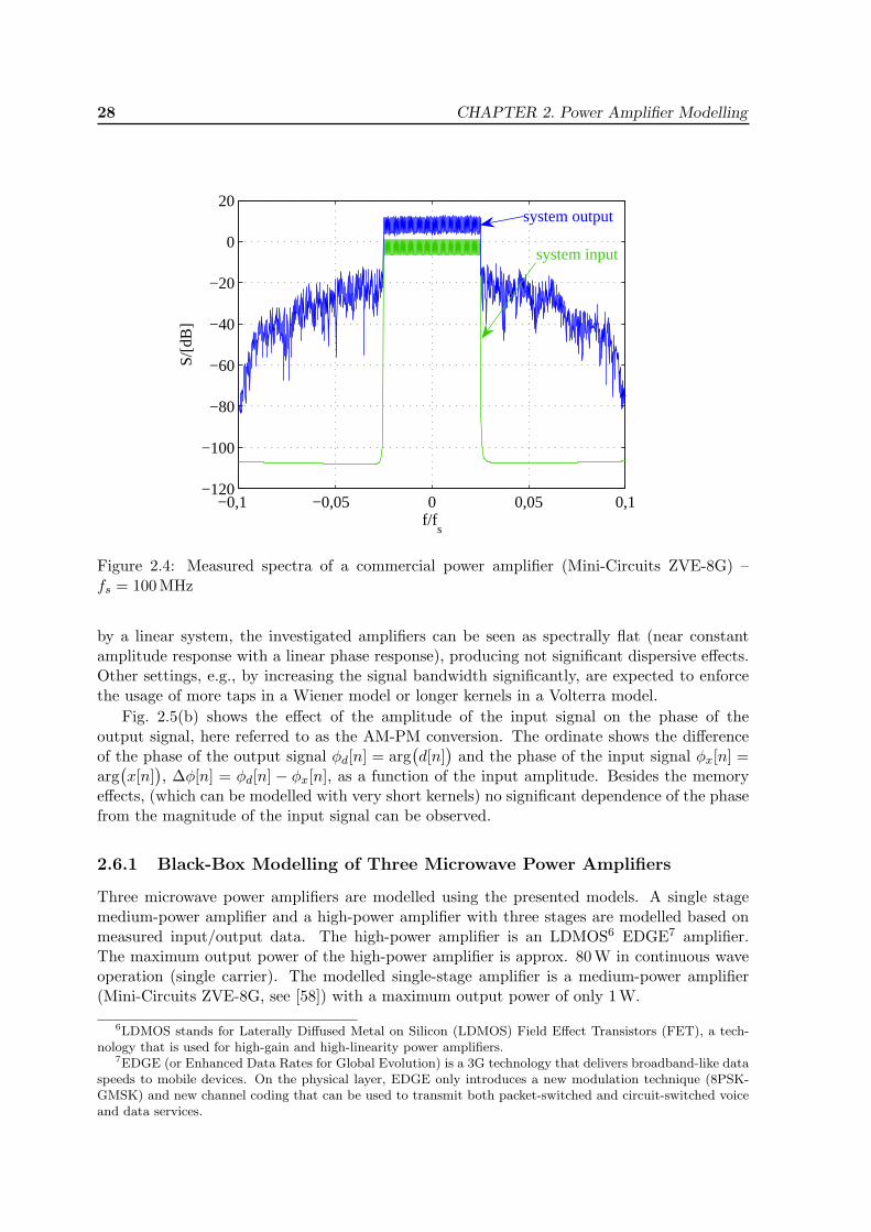
28 CHAPTER 2. Power Amplifier Modelling
−0,1 −0,05 0 0,05 0,1−120
−100
−80
−60
−40
−20
0
20
f/fs
S/[d
B]
system output
system input
Figure 2.4: Measured spectra of a commercial power amplifier (Mini-Circuits ZVE-8G) –fs = 100MHz
by a linear system, the investigated amplifiers can be seen as spectrally flat (near constantamplitude response with a linear phase response), producing not significant dispersive effects.Other settings, e.g., by increasing the signal bandwidth significantly, are expected to enforcethe usage of more taps in a Wiener model or longer kernels in a Volterra model.
Fig. 2.5(b) shows the effect of the amplitude of the input signal on the phase of theoutput signal, here referred to as the AM-PM conversion. The ordinate shows the differenceof the phase of the output signal φd[n] = arg
(d[n]
)and the phase of the input signal φx[n] =
arg(x[n]
), ∆φ[n] = φd[n] − φx[n], as a function of the input amplitude. Besides the memory
effects, (which can be modelled with very short kernels) no significant dependence of the phasefrom the magnitude of the input signal can be observed.
2.6.1 Black-Box Modelling of Three Microwave Power Amplifiers
Three microwave power amplifiers are modelled using the presented models. A single stagemedium-power amplifier and a high-power amplifier with three stages are modelled based onmeasured input/output data. The high-power amplifier is an LDMOS6 EDGE7 amplifier.The maximum output power of the high-power amplifier is approx. 80 W in continuous waveoperation (single carrier). The modelled single-stage amplifier is a medium-power amplifier(Mini-Circuits ZVE-8G, see [58]) with a maximum output power of only 1 W.
6LDMOS stands for Laterally Diffused Metal on Silicon (LDMOS) Field Effect Transistors (FET), a tech-nology that is used for high-gain and high-linearity power amplifiers.
7EDGE (or Enhanced Data Rates for Global Evolution) is a 3G technology that delivers broadband-like dataspeeds to mobile devices. On the physical layer, EDGE only introduces a new modulation technique (8PSK-GMSK) and new channel coding that can be used to transmit both packet-switched and circuit-switched voiceand data services.
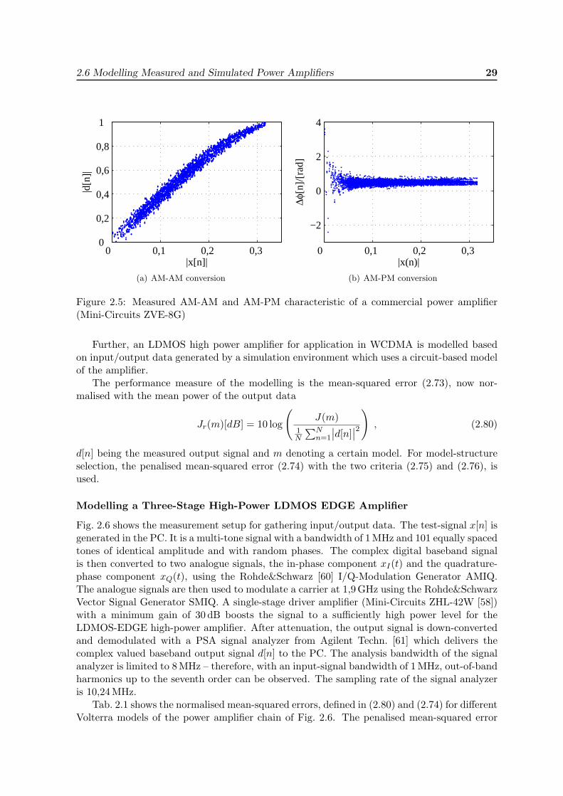
2.6 Modelling Measured and Simulated Power Amplifiers 29
0 0,1 0,2 0,3 0
0,2
0,4
0,6
0,8
1
|x[n]|
|d[n
]|
(a) AM-AM conversion
0 0,1 0,2 0,3
−2
0
2
4
|x(n)|
∆φ[n
]/[r
ad]
(b) AM-PM conversion
Figure 2.5: Measured AM-AM and AM-PM characteristic of a commercial power amplifier(Mini-Circuits ZVE-8G)
Further, an LDMOS high power amplifier for application in WCDMA is modelled basedon input/output data generated by a simulation environment which uses a circuit-based modelof the amplifier.
The performance measure of the modelling is the mean-squared error (2.73), now nor-malised with the mean power of the output data
Jr(m)[dB] = 10 log
(J(m)
1N
∑Nn=1
∣∣d[n]∣∣2), (2.80)
d[n] being the measured output signal and m denoting a certain model. For model-structureselection, the penalised mean-squared error (2.74) with the two criteria (2.75) and (2.76), isused.
Modelling a Three-Stage High-Power LDMOS EDGE Amplifier
Fig. 2.6 shows the measurement setup for gathering input/output data. The test-signal x[n] isgenerated in the PC. It is a multi-tone signal with a bandwidth of 1 MHz and 101 equally spacedtones of identical amplitude and with random phases. The complex digital baseband signalis then converted to two analogue signals, the in-phase component xI(t) and the quadrature-phase component xQ(t), using the Rohde&Schwarz [60] I/Q-Modulation Generator AMIQ.The analogue signals are then used to modulate a carrier at 1,9 GHz using the Rohde&SchwarzVector Signal Generator SMIQ. A single-stage driver amplifier (Mini-Circuits ZHL-42W [58])with a minimum gain of 30 dB boosts the signal to a sufficiently high power level for theLDMOS-EDGE high-power amplifier. After attenuation, the output signal is down-convertedand demodulated with a PSA signal analyzer from Agilent Techn. [61] which delivers thecomplex valued baseband output signal d[n] to the PC. The analysis bandwidth of the signalanalyzer is limited to 8MHz – therefore, with an input-signal bandwidth of 1 MHz, out-of-bandharmonics up to the seventh order can be observed. The sampling rate of the signal analyzeris 10,24 MHz.
Tab. 2.1 shows the normalised mean-squared errors, defined in (2.80) and (2.74) for differentVolterra models of the power amplifier chain of Fig. 2.6. The penalised mean-squared error
30 CHAPTER 2. Power Amplifier Modelling
PA
HPA
-SMIQx[n]
d[n]
AMIQ
-
-
ATT ��PSA �
PC
-
�
Vec. Sig. Gen.I/Q Mod. Gen.
Sig. Analyzer
xI(t)
xQ(t)xRF (t)
dRF (t)
LDMOS-EDGE
Driver
Figure 2.6: Measurement setup for input/output data generation
is normalised with the penalised mean-squared error of the model with the lowest complexity.First, the order p is increased stepwise – the specification of the Volterra model is defined bythe vector mV = [N1, N3, N5, N7, N9], Np denoting the length of the kernel hp[n1, . . . , np] ineach dimension.
mV order Jr(m)[dB] Wr,FPE(m)[dB] Wr,MDL(m)[1,1] 3 -33,04 0 0
[1,1,1] 5 -34,5 -1,85 -1,81[1,1,1,1] 7 -35,07 -2,33 -2,26
[1,1,1,1,1] 9 -35,1 -2,34 -2,23
Table 2.1: Normalised mean-squared errors of static Volterra models – nonlinear order selection
From Tab. 2.1 it can be seen that a seventh order model is sufficient – however, the mean-squared error does not increase significantly even if only a fifth order model is selected.
Now the length of the linear kernel is increased stepwise in the seventh order model. Again,the penalised mean-squared errors are normalised with the lowest-complex model.
mV order Jr(m)[dB] Wr,FPE(m)[dB] Wr,MDL(m)[1,1,1,1] 7 -35,07 0 0[2,1,1,1] 7 -35,43 -0,54 -0,51[3,1,1,1] 7 -35,45 -0,58 -0,51[4,1,1,1] 7 -35,46 -0,58 -0,48
Table 2.2: Normalised mean-squared errors of Volterra models of order seven with memoryonly in the linear kernel
From Tab. 2.2 it can be seen that two taps for the linear kernel are sufficient, adding moretaps reduces the error only marginally, if the memory-length is increased to four, WMDL beginsto increase, indicating an overfit. For the estimation of the length of the third-order kernel theprocedure is repeated, with the reference-model mV = [2, 1, 1, 1]. Adding only one tap is alsohere enough. Adding taps in the higher-order kernels does not improve the estimation. The
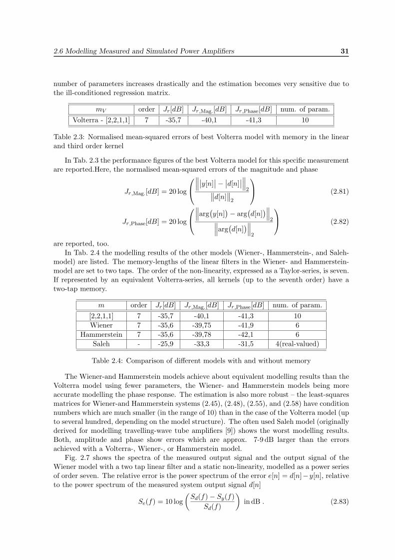
2.6 Modelling Measured and Simulated Power Amplifiers 31
number of parameters increases drastically and the estimation becomes very sensitive due tothe ill-conditioned regression matrix.
mV order Jr[dB] Jr,Mag.[dB] Jr ,Phase[dB] num. of param.Volterra - [2,2,1,1] 7 -35,7 -40,1 -41,3 10
Table 2.3: Normalised mean-squared errors of best Volterra model with memory in the linearand third order kernel
In Tab. 2.3 the performance figures of the best Volterra model for this specific measurementare reported.Here, the normalised mean-squared errors of the magnitude and phase
Jr ,Mag.[dB] = 20 log
∥∥∥∣∣y[n]
∣∣− ∣∣d[n]∣∣∥∥∥
2∥∥d[n]∥∥
2
(2.81)
Jr ,Phase[dB] = 20 log
∥∥∥arg
(y[n]
)− arg
(d[n]
)∥∥∥2∥∥∥arg
(d[n]
)∥∥∥2
(2.82)
are reported, too.In Tab. 2.4 the modelling results of the other models (Wiener-, Hammerstein-, and Saleh-
model) are listed. The memory-lengths of the linear filters in the Wiener- and Hammerstein-model are set to two taps. The order of the non-linearity, expressed as a Taylor-series, is seven.If represented by an equivalent Volterra-series, all kernels (up to the seventh order) have atwo-tap memory.
m order Jr[dB] Jr,Mag.[dB] Jr ,Phase[dB] num. of param.[2,2,1,1] 7 -35,7 -40,1 -41,3 10Wiener 7 -35,6 -39,75 -41,9 6
Hammerstein 7 -35,6 -39,78 -42,1 6Saleh - -25,9 -33,3 -31,5 4(real-valued)
Table 2.4: Comparison of different models with and without memory
The Wiener-and Hammerstein models achieve about equivalent modelling results than theVolterra model using fewer parameters, the Wiener- and Hammerstein models being moreaccurate modelling the phase response. The estimation is also more robust – the least-squaresmatrices for Wiener-and Hammerstein systems (2.45), (2.48), (2.55), and (2.58) have conditionnumbers which are much smaller (in the range of 10) than in the case of the Volterra model (upto several hundred, depending on the model structure). The often used Saleh model (originallyderived for modelling travelling-wave tube amplifiers [9]) shows the worst modelling results.Both, amplitude and phase show errors which are approx. 7-9 dB larger than the errorsachieved with a Volterra-, Wiener-, or Hammerstein model.
Fig. 2.7 shows the spectra of the measured output signal and the output signal of theWiener model with a two tap linear filter and a static non-linearity, modelled as a power seriesof order seven. The relative error is the power spectrum of the error e[n] = d[n]−y[n], relativeto the power spectrum of the measured system output signal d[n]
Se(f) = 10 log(Sd(f)− Sy(f)
Sd(f)
)in dB . (2.83)
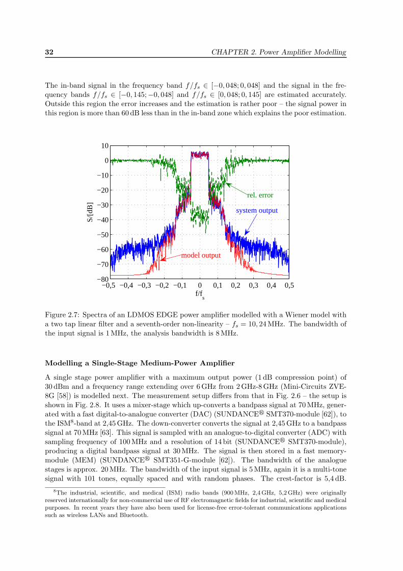
32 CHAPTER 2. Power Amplifier Modelling
The in-band signal in the frequency band f/fs ∈ [−0, 048; 0, 048] and the signal in the fre-quency bands f/fs ∈ [−0, 145;−0, 048] and f/fs ∈ [0, 048; 0, 145] are estimated accurately.Outside this region the error increases and the estimation is rather poor – the signal power inthis region is more than 60 dB less than in the in-band zone which explains the poor estimation.
−0,5 −0,4 −0,3 −0,2 −0,1 0 0,1 0,2 0,3 0,4 0,5−80
−70
−60
−50
−40
−30
−20
−10
0
10
f/fs
S/[d
B]
rel. error
system output
model output
Figure 2.7: Spectra of an LDMOS EDGE power amplifier modelled with a Wiener model witha two tap linear filter and a seventh-order non-linearity – fs = 10, 24 MHz. The bandwidth ofthe input signal is 1 MHz, the analysis bandwidth is 8 MHz.
Modelling a Single-Stage Medium-Power Amplifier
A single stage power amplifier with a maximum output power (1 dB compression point) of30 dBm and a frequency range extending over 6 GHz from 2GHz-8 GHz (Mini-Circuits ZVE-8G [58]) is modelled next. The measurement setup differs from that in Fig. 2.6 – the setup isshown in Fig. 2.8. It uses a mixer-stage which up-converts a bandpass signal at 70 MHz, gener-ated with a fast digital-to-analogue converter (DAC) (SUNDANCEr SMT370-module [62]), tothe ISM8-band at 2,45 GHz. The down-converter converts the signal at 2,45 GHz to a bandpasssignal at 70MHz [63]. This signal is sampled with an analogue-to-digital converter (ADC) withsampling frequency of 100MHz and a resolution of 14 bit (SUNDANCEr SMT370-module),producing a digital bandpass signal at 30 MHz. The signal is then stored in a fast memory-module (MEM) (SUNDANCEr SMT351-G-module [62]). The bandwidth of the analoguestages is approx. 20MHz. The bandwidth of the input signal is 5 MHz, again it is a multi-tonesignal with 101 tones, equally spaced and with random phases. The crest-factor is 5,4 dB.
8The industrial, scientific, and medical (ISM) radio bands (900MHz, 2,4 GHz, 5,2 GHz) were originallyreserved internationally for non-commercial use of RF electromagnetic fields for industrial, scientific and medicalpurposes. In recent years they have also been used for license-free error-tolerant communications applicationssuch as wireless LANs and Bluetooth.
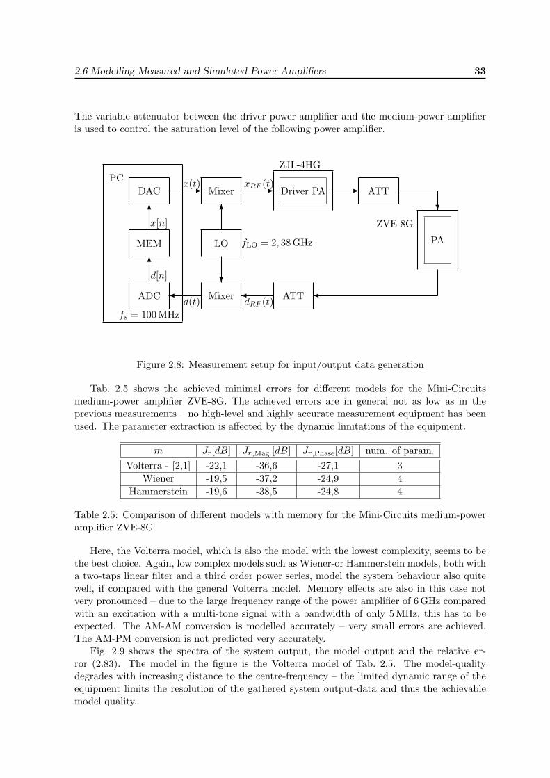
2.6 Modelling Measured and Simulated Power Amplifiers 33
The variable attenuator between the driver power amplifier and the medium-power amplifieris used to control the saturation level of the following power amplifier.
Driver PA-Mixer
Mixer
ATT
LO
DAC
ATT
-
6 6
��
MEM
�
?
dRF (t)
6
-
PA
?
ADC
PCxRF (t)x(t)
x[n]
d[n]
d(t)
ZJL-4HG
ZVE-8G
fLO = 2, 38 GHz
fs = 100MHz
Figure 2.8: Measurement setup for input/output data generation
Tab. 2.5 shows the achieved minimal errors for different models for the Mini-Circuitsmedium-power amplifier ZVE-8G. The achieved errors are in general not as low as in theprevious measurements – no high-level and highly accurate measurement equipment has beenused. The parameter extraction is affected by the dynamic limitations of the equipment.
m Jr[dB] Jr,Mag.[dB] Jr ,Phase[dB] num. of param.Volterra - [2,1] -22,1 -36,6 -27,1 3
Wiener -19,5 -37,2 -24,9 4Hammerstein -19,6 -38,5 -24,8 4
Table 2.5: Comparison of different models with memory for the Mini-Circuits medium-poweramplifier ZVE-8G
Here, the Volterra model, which is also the model with the lowest complexity, seems to bethe best choice. Again, low complex models such as Wiener-or Hammerstein models, both witha two-taps linear filter and a third order power series, model the system behaviour also quitewell, if compared with the general Volterra model. Memory effects are also in this case notvery pronounced – due to the large frequency range of the power amplifier of 6GHz comparedwith an excitation with a multi-tone signal with a bandwidth of only 5 MHz, this has to beexpected. The AM-AM conversion is modelled accurately – very small errors are achieved.The AM-PM conversion is not predicted very accurately.
Fig. 2.9 shows the spectra of the system output, the model output and the relative er-ror (2.83). The model in the figure is the Volterra model of Tab. 2.5. The model-qualitydegrades with increasing distance to the centre-frequency – the limited dynamic range of theequipment limits the resolution of the gathered system output-data and thus the achievablemodel quality.
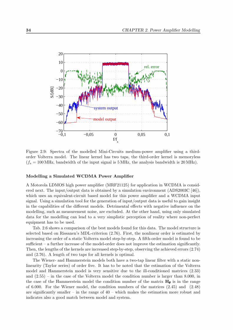
34 CHAPTER 2. Power Amplifier Modelling
−0,1 −0,05 0 0,05 0,1−70
−60
−50
−40
−30
−20
−10
0
10
20
f/fs
S/[d
B]
model output
system output
rel. error
Figure 2.9: Spectra of the modelled Mini-Circuits medium-power amplifier using a third-order Volterra model. The linear kernel has two taps, the third-order kernel is memoryless(fs = 100MHz, bandwidth of the input signal is 5 MHz, the analysis bandwidth is 20 MHz).
Modelling a Simulated WCDMA Power Amplifier
A Motorola LDMOS high power amplifier (MRF21125) for application in WCDMA is consid-ered next. The input/output data is obtained by a simulation environment (ADS2003C [46]),which uses an equivalent-circuit based model for this power amplifier and a WCDMA inputsignal. Using a simulation tool for the generation of input/output data is useful to gain insightin the capabilities of the different models. Detrimental effects with negative influence on themodelling, such as measurement noise, are excluded. At the other hand, using only simulateddata for the modelling can lead to a very simplistic perception of reality where non-perfectequipment has to be used.
Tab. 2.6 shows a comparison of the best models found for this data. The model structure isselected based on Rissanen’s MDL-criterion (2.76). First, the nonlinear order is estimated byincreasing the order of a static Volterra model step-by-step. A fifth-order model is found to besufficient – a further increase of the model-order does not improve the estimation significantly.Then, the lengths of the kernels are increased step-by-step, observing the achieved errors (2.74)and (2.76). A length of two taps for all kernels is optimal.
The Wiener- and Hammerstein models both have a two-tap linear filter with a static non-linearity (Taylor series) of order five. It has to be noted that the estimation of the Volterramodel and Hammerstein model is very sensitive due to the ill-conditioned matrices (2.33)and (2.55) – in the case of the Volterra model the condition number is larger than 8.000, inthe case of the Hammerstein model the condition number of the matrix Hθθθ is in the rangeof 6.000. For the Wiener model, the condition numbers of the matrices (2.45) and (2.48)are significantly smaller – in the range of 40 – which makes the estimation more robust andindicates also a good match between model and system.
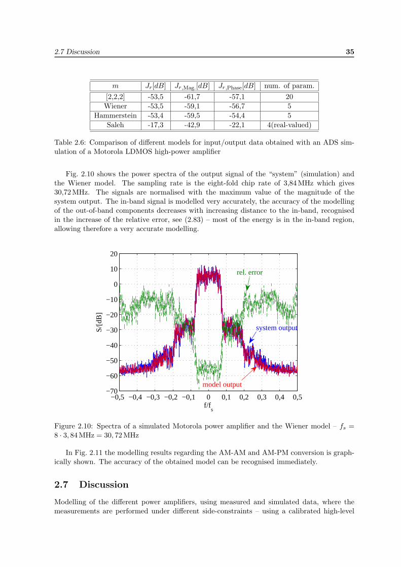
2.7 Discussion 35
m Jr[dB] Jr,Mag.[dB] Jr ,Phase[dB] num. of param.[2,2,2] -53,5 -61,7 -57,1 20Wiener -53,5 -59,1 -56,7 5
Hammerstein -53,4 -59,5 -54,4 5Saleh -17,3 -42,9 -22,1 4(real-valued)
Table 2.6: Comparison of different models for input/output data obtained with an ADS sim-ulation of a Motorola LDMOS high-power amplifier
Fig. 2.10 shows the power spectra of the output signal of the “system” (simulation) andthe Wiener model. The sampling rate is the eight-fold chip rate of 3,84 MHz which gives30,72MHz. The signals are normalised with the maximum value of the magnitude of thesystem output. The in-band signal is modelled very accurately, the accuracy of the modellingof the out-of-band components decreases with increasing distance to the in-band, recognisedin the increase of the relative error, see (2.83) – most of the energy is in the in-band region,allowing therefore a very accurate modelling.
−0,5 −0,4 −0,3 −0,2 −0,1 0 0,1 0,2 0,3 0,4 0,5−70
−60
−50
−40
−30
−20
−10
0
10
20
f/fs
S/[d
B]
rel. error
model output
system output
Figure 2.10: Spectra of a simulated Motorola power amplifier and the Wiener model – fs =8 · 3, 84 MHz = 30, 72 MHz
In Fig. 2.11 the modelling results regarding the AM-AM and AM-PM conversion is graph-ically shown. The accuracy of the obtained model can be recognised immediately.
2.7 Discussion
Modelling of the different power amplifiers, using measured and simulated data, where themeasurements are performed under different side-constraints – using a calibrated high-level
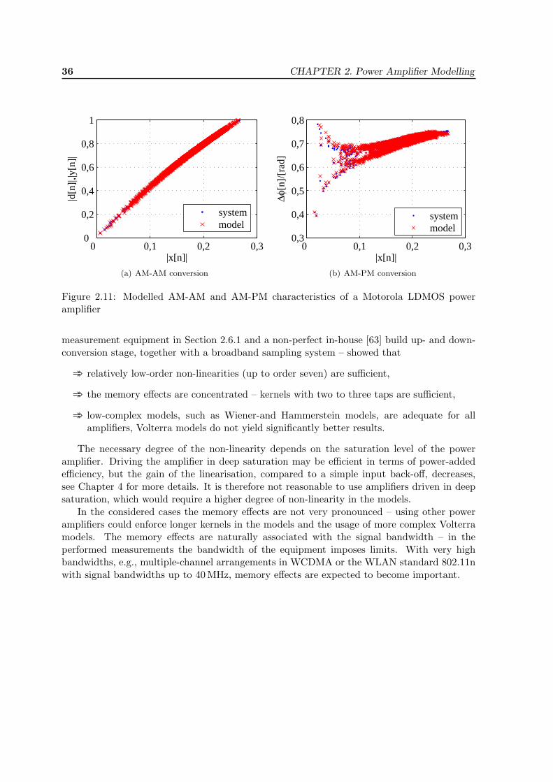
36 CHAPTER 2. Power Amplifier Modelling
0 0,1 0,2 0,30
0,2
0,4
0,6
0,8
1
|x[n]|
|d[n
]|,|y
[n]|
systemmodel
(a) AM-AM conversion
0 0,1 0,2 0,30,3
0,4
0,5
0,6
0,7
0,8
|x[n]|
∆φ[n
]/[r
ad]
systemmodel
(b) AM-PM conversion
Figure 2.11: Modelled AM-AM and AM-PM characteristics of a Motorola LDMOS poweramplifier
measurement equipment in Section 2.6.1 and a non-perfect in-house [63] build up- and down-conversion stage, together with a broadband sampling system – showed that
➾ relatively low-order non-linearities (up to order seven) are sufficient,
➾ the memory effects are concentrated – kernels with two to three taps are sufficient,
➾ low-complex models, such as Wiener-and Hammerstein models, are adequate for allamplifiers, Volterra models do not yield significantly better results.
The necessary degree of the non-linearity depends on the saturation level of the poweramplifier. Driving the amplifier in deep saturation may be efficient in terms of power-addedefficiency, but the gain of the linearisation, compared to a simple input back-off, decreases,see Chapter 4 for more details. It is therefore not reasonable to use amplifiers driven in deepsaturation, which would require a higher degree of non-linearity in the models.
In the considered cases the memory effects are not very pronounced – using other poweramplifiers could enforce longer kernels in the models and the usage of more complex Volterramodels. The memory effects are naturally associated with the signal bandwidth – in theperformed measurements the bandwidth of the equipment imposes limits. With very highbandwidths, e.g., multiple-channel arrangements in WCDMA or the WLAN standard 802.11nwith signal bandwidths up to 40 MHz, memory effects are expected to become important.
Chapter 3
Adaptive Identification
In this chapter low complex stochastic-gradient algorithms for the adaptive identification of theparameters of the Volterra and Wiener models presented in Chapter 2 are developed. A deter-ministic robustness analysis of an adaptive gradient algorithm for the parameter identificationof a Volterra system and Wiener system is presented. The Wiener model requires significantlyless parameters than a general Volterra model and is thus very attractive. The main disad-vantage of this model consists of the fact that the description is nonlinear with respect to apart of the model-parameters, namely the linear filter parameter. The consequence is that aquadratic cost-function, which is minimised by the adaptive algorithm during the search of theoptimal model-parameters, may be non-convex. This can result in a poor estimation quality ifthe adaptive gradient algorithm locates only a local minimum of the cost-function. Whetherthe algorithm finds only a local minimum or the global minimum of the cost-function dependson the initial values for the parameters which are used to start the iterative search.
Here, a two step procedure for the identification of a Wiener system is proposed and an-alysed in a deterministic context [15, 16]. A stochastic analysis of such an adaptive gradientidentification method for a Wiener system is in practice rarely possible. The signal charac-teristics are most often not known and even if the signal characteristics are known, furtherinformation regarding the system, especially some knowledge about the static nonlinear func-tion, must be available. Even if all this is known, a very restrictive convergence analysisgiving only information about convergence-in-the mean assuming a small step-size can be per-formed [64, 65]. The deterministic approach does not rely on such a-priori knowledge makingit a very general analysis approach. On the other hand, the drawback of this method is thatit provides only sufficient but not necessary conditions for convergence which may be veryconservative.
This chapter begins with a short introduction of the gradient identification algorithm. Thedeterministic analysis method for stability is presented briefly for a general adaptive Volterrafilter which is linear-in-parameters. Following this introduction the gradient identificationmethod is applied for the identification of a Wiener system. Following an idea of [66], a two-step procedure is proposed: First, an estimation of the parameters which enter nonlinearly inthe description, namely the parameters of the linear filter, based on a gradient identification,is performed. A deterministic robustness analysis [13, 67] of this identification algorithmis performed [16]. In the next step, an identification algorithm for the estimation of theparameters of the static nonlinear output-filter is presented and analysed.
37
38 CHAPTER 3. Adaptive Identification
3.1 The Stochastic-Gradient Algorithm
Stochastic-gradient algorithms are widely used as a tool for model-parameter identification.Linear-in-parameter models lead to various variants, e.g., least-mean-squares (LMS) algorithmand normalised LMS (NLMS) algorithm. All these algorithms are obtained from the steepest-decent method by replacing the required gradient vectors with different approximations [68,14]. By replacing these deterministic quantities by approximations, the update directionsbecome subject to stochastic fluctuations (gradient noise).
Using these approximations for the gradient there is no need to know the signal statistics(e.g., first or second order moments) for the implementation of the algorithm. These sta-tistical quantities are furthermore rarely available in practice. For a statistical convergenceanalysis these quantities must be known. Consequently, if the signal statistics are not knowna stochastic analysis of these algorithms is not possible. A deterministic analysis requires farless a-priori knowledge and is thus, at least in principle, often possible, see Section 3.1.1 andSection 3.1.2 further ahead.
The stochastic gradient algorithms possess a learning mechanism which enables them toestimate the required signal statistics. Further, stochastic-gradient algorithms are able totrack the signal statistics and thus system variations. They inherently possess a trackingcapability. Their learning and tracking capability, together with a low-complex and robustimplementation, make these algorithms very attractive for practical applications.
3.1.1 Stochastic-Gradient Identification for Linear-in-Parameter Models
Volterra models are linear-in-parameters. The input-output relation can be stated as an innervector product
y[n] = xnθθθ , (3.1)
where xn is the (row) input-signal vector
xn = [x1,n,x3,n, . . . ,x2P−1,n] , (3.2)
composed of all necessary parts corresponding to the specific Volterra model of nonlinear order2P − 1, e.g.,
x1,n = [x[n], x[n− 1], . . . , x[n−N1 + 1]] (3.3)
x3,n =[x[n]
∣∣x[n]∣∣2, x2[n]x∗[n− 1], . . . , x[n−N3 + 1]
∣∣x[n−N3 + 1]∣∣2] . (3.4)
Here, x1,n denotes the signal-vector for the linear part and x3,n is the signal-vector for thethird-order part, N1 is the length of the linear kernel, N3 is the length of the third-orderkernel (assumed to be equal in all three dimensions), cf. also Section 2.1.5. The correspondingfilter-parameter (column-) vector comprises of
θθθ =[θθθT1 , θθθ
T3 , . . . , θθθ
T2P−1
]T, (3.5)
with the linear and third order parts
θθθ1 =[h1[0], h1[1], . . . , h1[N1 − 1]
]T (3.6)
θθθ3 =[h3[0, 0, 0], h3[0, 0, 1], . . . , h3[N3 − 1, N3 − 1, N3 − 1]
]T. (3.7)
3.1 The Stochastic-Gradient Algorithm 39
If the observed output-signal from the system is denoted by d[n], the optimal weight-vectorθθθW minimising the mean-squared error
J = E{∣∣d[n]− xnθθθ
∣∣2} , (3.8)
where E{·} denotes the expectation operator, is the Wiener-solution, (cf., e.g., [14])
θθθW = R−1xx rdx . (3.9)
Here,
Rxx = E{xHn xn
}(3.10)
rdx = E{d[n]xHn
}, (3.11)
Rxx is the auto-correlation matrix of the input signal and rdx is the cross-correlation vectorbetween the output sample d[n] and input signal-vector xn. The optimal weight vector resultsin a minimum mean-square error
JW = σ2d − rxdR−1
xx rdx (3.12)
with σ2d = E
{∣∣d[n]∣∣2}.
The difficulty is the computation of the correlation matrix Rxx, resp. the correlation vec-tor rdx. Even if the statistics of the signals x[n] and d[n] are known, due to the complicatedstructure of the signal-vector xn, which comprises various products, see, e.g., (3.4), the com-putation of the expectation is in practice not feasible. Therefore, a direct solution (3.9) or asteepest-decent approach, which does not require the inversion of the correlation matrix,
θθθi = θθθi−1 + µ [rdx −Rxxθθθi−1] , i ≥ 0 , θθθ−1 = initial guess (3.13)
with a (small) step-size µ are not feasible. Further, in practice the statistics of the signals andthus the quantities Rxx and rdx tend to vary with time, e.g., due to a system change (in thiscase the power amplifier). Therefore, the optimal model-parameters θθθW will also change. Asteepest-decent approach (3.13) or a direct solution (3.9) cannot track system changes.
Stochastic-gradient algorithms provide approximations to the steepest-decent method byintroducing approximations to the non-computable quantities Rxx and rdx. Further, thesealgorithms possess a tracking capability which enables them to track signal and/or systemchanges. The most popular and widely used algorithm is the least-mean-squares (LMS) algo-rithm. Here, the deterministic quantities Rxx and rdx are approximated with the instantaneousestimates
Rxx ≈ xHn xn (3.14)
rdx ≈ d[n]xHn (3.15)
resulting in the LMS-algorithm
θθθn = θθθn−1 + µ[n]xHn (d[n]− xnθθθn−1) , n ≥ 0 , θθθ−1 = initial guess . (3.16)
The iteration index i used in the steepest-descent method has been changed to the time indexn – with each new data sample d[n] and associated signal vector xn a new estimate for theparameter-vector θθθ is formed by adding a specific correction term to the old estimate θθθn−1. Thefixed step-size µ has also been changed to a time-variant step-size µ[n]. Various selections forthe step-size exist, giving rise to several variants of the classical LMS-algorithm. In Tab. 3.1the most common modifications for the step-size are listed, together with the name of thealgorithm.
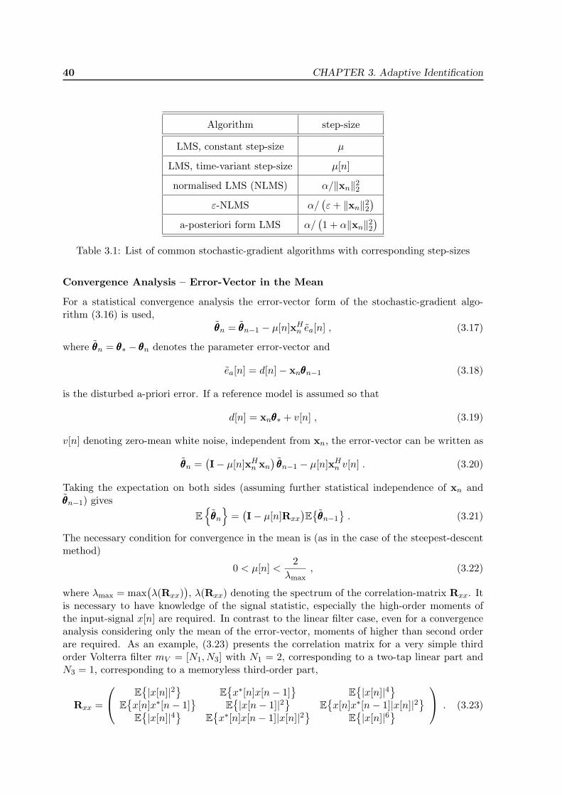
40 CHAPTER 3. Adaptive Identification
Algorithm step-size
LMS, constant step-size µ
LMS, time-variant step-size µ[n]
normalised LMS (NLMS) α/‖xn‖22ε-NLMS α/
(ε+ ‖xn‖22
)a-posteriori form LMS α/
(1 + α‖xn‖22
)Table 3.1: List of common stochastic-gradient algorithms with corresponding step-sizes
Convergence Analysis – Error-Vector in the Mean
For a statistical convergence analysis the error-vector form of the stochastic-gradient algo-rithm (3.16) is used,
θθθn = θθθn−1 − µ[n]xHn ea[n] , (3.17)
where θθθn = θθθ∗ − θθθn denotes the parameter error-vector and
ea[n] = d[n]− xnθθθn−1 (3.18)
is the disturbed a-priori error. If a reference model is assumed so that
d[n] = xnθθθ∗ + v[n] , (3.19)
v[n] denoting zero-mean white noise, independent from xn, the error-vector can be written as
θθθn =(I− µ[n]xHn xn
)θθθn−1 − µ[n]xHn v[n] . (3.20)
Taking the expectation on both sides (assuming further statistical independence of xn andθθθn−1) gives
E{θθθn
}=(I− µ[n]Rxx
)E{θθθn−1
}. (3.21)
The necessary condition for convergence in the mean is (as in the case of the steepest-descentmethod)
0 < µ[n] <2
λmax, (3.22)
where λmax = max(λ(Rxx)
), λ(Rxx) denoting the spectrum of the correlation-matrix Rxx. It
is necessary to have knowledge of the signal statistic, especially the high-order moments ofthe input-signal x[n] are required. In contrast to the linear filter case, even for a convergenceanalysis considering only the mean of the error-vector, moments of higher than second orderare required. As an example, (3.23) presents the correlation matrix for a very simple thirdorder Volterra filter mV = [N1, N3] with N1 = 2, corresponding to a two-tap linear part andN3 = 1, corresponding to a memoryless third-order part,
Rxx =
E{|x[n]|2
}E{x∗[n]x[n− 1]
}E{|x[n]|4
}E{x[n]x∗[n− 1]
}E{|x[n− 1]|2
}E{x[n]x∗[n− 1]|x[n]|2
}E{|x[n]|4
}E{x∗[n]x[n− 1]|x[n]|2
}E{|x[n]|6
} . (3.23)
3.1 The Stochastic-Gradient Algorithm 41
Moments up to the sixth-order are required. For a Volterra system of order P , moments upto the order 2P are required for this convergence analysis. In most cases it is not feasible tocompute these moments. Thus, it is not possible to compute the upper bound for the step-sizeas given in (3.22). Since in general no upper bound for the step-size can be computed, smallstep-sizes are used in order to guarantee convergence.
Furthermore, the terms involving products of the input signal in the correlation matrixhave the negative effect to enlarge the eigenvalue spread of the correlation matrix significantly.If, e.g., x[n] ∼ B(±1), i.e., x[n] takes on values +1 or −1 with equal probability, and theprocess is white, the correlation matrix Rxx becomes simply
Rxx =
1 0 10 1 01 0 1
. (3.24)
This matrix is singular, thus having an eigenvalue spread which is infinity.Since the convergence-speed is small if the eigenvalue spread is large, the convergence-
speed of nonlinear adaptive Volterra filters can in general be expected to be small comparedto adaptive linear filters.
Deterministic Robustness Analysis – Local Passivity
The difficulty in computing the high-order moments prevents a statistical analysis (convergencein-the-mean, mean-square behaviour) of the stochastic-gradient algorithm (3.16) for Volterrafilters in most cases. A deterministic approach involving energy relations provides a method toanalyse whether the gradient-algorithm (3.16) is guaranteed to converge [13] to a final estimatefor the optimal parameter-vector θθθ∗ or not.
Rewriting the error-vector update-equation (3.17)
θθθn = θθθn−1 − µ[n]xHn (ea[n] + v[n]) (3.25)
with the undisturbed a-priori error ea[n] = xnθθθn−1 and taking the squared `2-norm on bothsides gives, after rearranging terms,
‖θθθn‖22 − ‖θθθn−1‖22 + µ[n]∣∣ea[n]
∣∣2 − µ[n]∣∣v[n]
∣∣2 = µ[n]∣∣ea[n] + v[n]
∣∣2(µ[n]‖xn‖22 − 1). (3.26)
Whether the right-hand side is positive, negative or zero depends on the quantity µ[n]‖xn‖22−1.Compactly, the energy relation can be written as [13]
‖θθθn‖22 + µ[n]∣∣ea[n]
∣∣2‖θθθn−1‖22 + µ[n]
∣∣v[n]∣∣2
< 1, if µ[n]‖xn‖22 < 1= 1, if µ[n]‖xn‖22 = 1> 1, if µ[n]‖xn‖22 > 1
. (3.27)
The first inequality guarantees that, no matter what the value of v[n] is and no matter howfar away the estimate θθθn−1 from the optimal value θθθ∗ is, it holds that
‖θθθn‖22 + µ[n]∣∣ea[n]
∣∣2 < ‖θθθn−1‖22 + µ[n]∣∣v[n]
∣∣2 . (3.28)
The map Tn, mapping the signals{θθθn−1,
õ[n]v[n]
}to the output signals
{θθθn,√µ[n]ea[n]
}is therefore passive, i.e.,[
θθθn√µ[n]ea[n]
]= Tn
[θθθn−1√µ[n]v[n]
], with ‖Tn‖22 < 1 . (3.29)
42 CHAPTER 3. Adaptive Identification
The step-size selection according to an NLMS and an ε-NLMS with α < 1 and the a-posteriori LMS with α > 0, cf. Tab. 3.1, guarantees local stability since the step-sizes areguaranteed to be smaller than the limit
µ[n] =1
‖xn‖22. (3.30)
Deterministic Robustness Analysis – Global Passivity
In the previous analysis, local passivity of the map Tn, i.e., from time-index n − 1 to n, wasguaranteed if µ[n] < µ[n]. For the stability-analysis over the finite time-horizon n = 0, . . . , N ,the sum on both sides of (3.28) is performed
N∑n=0
(‖θθθn‖22 + µ[n]
∣∣ea[n]∣∣2) < N∑
n=0
(‖θθθn−1‖22 + µ[n]
∣∣v[n]∣∣2) , (3.31)
resulting in
‖θθθN‖22 +N∑n=0
µ[n]∣∣ea[n]
∣∣2 ≤ ‖θθθ−1‖22 +N∑n=0
µ[n]∣∣v[n]
∣∣2 . (3.32)
Ifµ[n]‖xn‖22 < 1 for 0 ≤ n ≤ N , (3.33)
the algorithm behaves also globally passive, i.e., the error-energy ‖θθθN‖22 +∑N
n=0 µ[n]∣∣ea[n]
∣∣2,comprising the final remaining distance from the optimal vector θθθ∗ and the accumulated sumof the undisturbed a-priori errors is guaranteed to be smaller than the energy of the initialweight-distance and the noise, ‖θθθ−1‖22 +
∑Nn=0 µ[n]
∣∣v[n]∣∣2.
Feedback Structure – Local and Global Passivity
Equation (3.25) can easily be transformed to
θθθn = θθθn−1 − µ[n]xHn (ea[n] + v[n]) (3.34)
with the abbreviation
v[n] =µ[n]µ[n]
v[n]−(
1− µ[n]µ[n]
)ea[n] . (3.35)
Since now the step-size is µ[n], the forward map Tn, mapping {θθθn−1,√µ[n]v[n]} to the output
signals {θθθn,√µ[n]ea[n]}, is lossless, ‖Tn‖22 = 1. A feedback path exists, which produces the
modified noise signal v[n]. Together with the forward map, the system equations read[θθθn√
µ[n]ea[n]
]= Tn
[θθθn−1√µ[n]v[n]
], with ‖Tn‖22 = 1 (3.36)
õ[n]v[n] =
µ[n]µ[n]
√µ[n]v[n]−
(1− µ[n]
µ[n]
)õ[n]ea[n] . (3.37)
This feedback-system is illustrated in Fig. 3.1.For local stability it suffices that the magnitude of the gain of the feedback loop gFB, which
isgFB = 1− µ[n]
µ[n], (3.38)
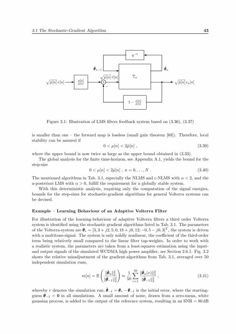
3.1 The Stochastic-Gradient Algorithm 43
Tn
q−1
1− µ[n]µ[n]
+µ[n]µ[n]
� � � ��
�
�
θθθnθθθn−1
õ[n] ea[n]
õ[n] v[n]
−
õ[n] v[n]
Figure 3.1: Illustration of LMS filters feedback system based on (3.36), (3.37)
is smaller than one – the forward map is lossless (small gain theorem [69]). Therefore, localstability can be assured if
0 < µ[n] < 2µ[n] , (3.39)
where the upper bound is now twice as large as the upper bound obtained in (3.33).The global analysis for the finite time-horizon, see Appendix A.1, yields the bound for the
step-size0 < µ[n] < 2µ[n] , n = 0, . . . , N . (3.40)
The mentioned algorithms in Tab. 3.1, especially the NLMS and ε-NLMS with α < 2, and thea-posteriori LMS with α > 0, fulfill the requirement for a globally stable system.
With this deterministic analysis, requiring only the computation of the signal energies,bounds for the step-sizes for stochastic-gradient algorithms for general Volterra systems canbe devised.
Example – Learning Behaviour of an Adaptive Volterra Filter
For illustration of the learning-behaviour of adaptive Volterra filters a third order Volterrasystem is identified using the stochastic gradient algorithms listed in Tab. 3.1. The parametersof the Volterra-system are θθθ∗ = [3, 3 + j2, 5; 0, 18 + j0, 12;−0, 5− j0, 3]T , the system is drivenwith a multitone-signal. The system is only mildly nonlinear, the coefficient of the third-orderterm being relatively small compared to the linear filter tap-weights. In order to work witha realistic system, the parameters are taken from a least-squares estimation using the input-and output signals of the simulated WCDMA high power amplifier, see Section 2.6.1. Fig. 3.2shows the relative misadjustment of the gradient-algorithms from Tab. 3.1, averaged over 50independent simulation runs,
m[n] = E
(‖θθθn‖22‖θθθ−1‖22
)≈ 1
50
50∑r=1
‖θθθn(r)‖22‖θθθ−1‖22
, (3.41)
whereby r denotes the simulation run, θθθ−1 = θθθ∗ − θθθ−1 is the initial error, where the starting-guess θθθ−1 = 0 in all simulations. A small amount of noise, drawn from a zero-mean, whitegaussian process, is added to the output of the reference system, resulting in an SNR = 80 dB
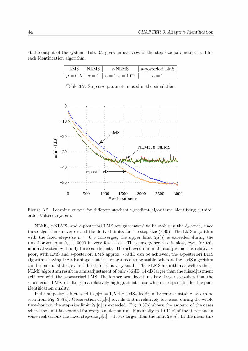
44 CHAPTER 3. Adaptive Identification
at the output of the system. Tab. 3.2 gives an overview of the step-size parameters used foreach identification algorithm.
LMS NLMS ε-NLMS a-posteriori LMSµ = 0, 5 α = 1 α = 1, ε = 10−4 α = 1
Table 3.2: Step-size parameters used in the simulation
0 500 1000 1500 2000 2500 3000
−50
−40
−30
−20
−10
0
# of iterations n
m[n
] / [
dB]
NLMS, ε−NLMS
LMS
a−post. LMS
Figure 3.2: Learning curves for different stochastic-gradient algorithms identifying a third-order Volterra-system.
NLMS, ε-NLMS, and a-posteriori LMS are guaranteed to be stable in the `2-sense, sincethese algorithms never exceed the derived limits for the step-size (3.40). The LMS-algorithmwith the fixed step-size µ = 0, 5 converges, the upper limit 2µ[n] is exceeded during thetime-horizon n = 0, . . . , 3000 in very few cases. The convergence-rate is slow, even for thisminimal system with only three coefficients. The achieved minimal misadjustment is relativelypoor, with LMS and a-posteriori LMS approx. -50 dB can be achieved, the a-posteriori LMSalgorithm having the advantage that it is guaranteed to be stable, whereas the LMS algorithmcan become unstable, even if the step-size is very small. The NLMS algorithm as well as the ε-NLMS algorithm result in a misadjustment of only -36 dB, 14 dB larger than the misadjustmentachieved with the a-posteriori LMS. The former two algorithms have larger step-sizes than thea-posteriori LMS, resulting in a relatively high gradient-noise which is responsible for the pooridentification quality.
If the step-size is increased to µ[n] = 1, 5 the LMS-algorithm becomes unstable, as can beseen from Fig. 3.3(a). Observation of µ[n] reveals that in relatively few cases during the wholetime-horizon the step-size limit 2µ[n] is exceeded. Fig. 3.3(b) shows the amount of the caseswhere the limit is exceeded for every simulation run. Maximally in 10-11 % of the iterations insome realisations the fixed step-size µ[n] = 1, 5 is larger than the limit 2µ[n]. In the mean this
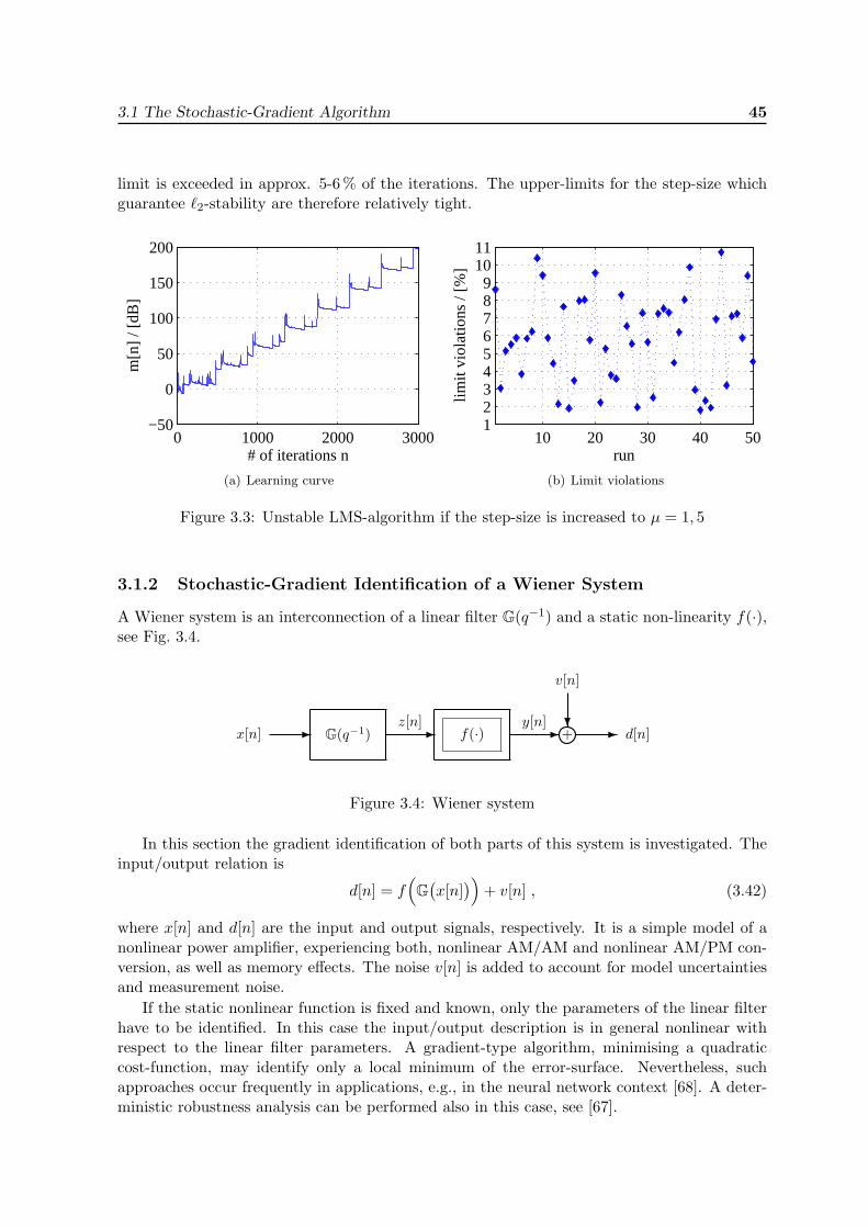
3.1 The Stochastic-Gradient Algorithm 45
limit is exceeded in approx. 5-6 % of the iterations. The upper-limits for the step-size whichguarantee `2-stability are therefore relatively tight.
0 1000 2000 3000−50
0
50
100
150
200
# of iterations n
m[n
] / [
dB]
(a) Learning curve
10 20 30 40 50123456789
1011
limit
viol
atio
ns /
[%]
run
(b) Limit violations
Figure 3.3: Unstable LMS-algorithm if the step-size is increased to µ = 1, 5
3.1.2 Stochastic-Gradient Identification of a Wiener System
A Wiener system is an interconnection of a linear filter G(q−1) and a static non-linearity f(·),see Fig. 3.4.
G(q−1) f(·)� � � +�
v[n]
x[n]z[n] y[n]
d[n]�
Figure 3.4: Wiener system
In this section the gradient identification of both parts of this system is investigated. Theinput/output relation is
d[n] = f(G(x[n]
))+ v[n] , (3.42)
where x[n] and d[n] are the input and output signals, respectively. It is a simple model of anonlinear power amplifier, experiencing both, nonlinear AM/AM and nonlinear AM/PM con-version, as well as memory effects. The noise v[n] is added to account for model uncertaintiesand measurement noise.
If the static nonlinear function is fixed and known, only the parameters of the linear filterhave to be identified. In this case the input/output description is in general nonlinear withrespect to the linear filter parameters. A gradient-type algorithm, minimising a quadraticcost-function, may identify only a local minimum of the error-surface. Nevertheless, suchapproaches occur frequently in applications, e.g., in the neural network context [68]. A deter-ministic robustness analysis can be performed also in this case, see [67].
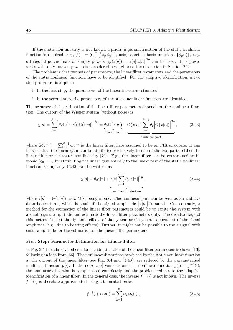
46 CHAPTER 3. Adaptive Identification
If the static non-linearity is not known a-priori, a parametrisation of the static nonlinearfunction is required, e.g., f(·) =
∑P−1p=0 θp φp(·), using a set of basis functions {φp(·)}, e.g.,
orthogonal polynomials or simply powers φp (z[n]) = z[n]∣∣z[n]
∣∣2p can be used. This powerseries with only uneven powers is considered here, cf. also the discussion in Section 2.2.
The problem is that two sets of parameters, the linear filter parameters and the parametersof the static nonlinear function, have to be identified. For the adaptive identification, a twostep procedure is applied:
1. In the first step, the parameters of the linear filter are estimated.
2. In the second step, the parameters of the static nonlinear function are identified.
The accuracy of the estimation of the linear filter parameters depends on the nonlinear func-tion. The output of the Wiener system (without noise) is
y[n] =P−1∑p=0
θpG(x[n]
)∣∣∣G(x[n])∣∣∣2p = θ0G
(x[n]
)︸ ︷︷ ︸linear part
+ G(x[n]
) P−1∑p=1
θp
∣∣∣G(x[n])∣∣∣2p︸ ︷︷ ︸
nonlinear part
, (3.43)
where G(q−1) =∑N−1
i=0 giq−i is the linear filter, here assumed to be an FIR structure. It can
be seen that the linear gain can be attributed exclusively to one of the two parts, either thelinear filter or the static non-linearity [70]. E.g., the linear filter can be constrained to bemonic (g0 = 1) by attributing the linear gain entirely to the linear part of the static nonlinearfunction. Compactly, (3.43) can be written as
y[n] = θ0z[n] + z[n]P−1∑p=1
θp∣∣z[n]
∣∣2p︸ ︷︷ ︸nonlinear distortion
, (3.44)
where z[n] = G(x[n]
), now G(·) being monic. The nonlinear part can be seen as an additive
disturbance term, which is small if the signal amplitude∣∣z[n]
∣∣ is small. Consequently, amethod for the estimation of the linear filter parameters could be to excite the system witha small signal amplitude and estimate the linear filter parameters only. The disadvantage ofthis method is that the dynamic effects of the system are in general dependent of the signalamplitude (e.g., due to heating effects). Further, it might not be possible to use a signal withsmall amplitude for the estimation of the linear filter parameters.
First Step: Parameter Estimation for Linear Filter
In Fig. 3.5 the adaptive scheme for the identification of the linear filter parameters is shown [16],following an idea from [66]. The nonlinear distortions produced by the static nonlinear functionat the output of the linear filter, see Fig. 3.4 and (3.43), are reduced by the parameterisednonlinear function g(·). If the noise v[n] vanishes and the nonlinear function g(·) = f−1(·),the nonlinear distortion is compensated completely and the problem reduces to the adaptiveidentification of a linear filter. In the general case, the inverse f−1(·) is not known. The inversef−1(·) is therefore approximated using a truncated series
f−1(·) ≈ g(·) =K∑k=1
wkψk(·) , (3.45)
3.1 The Stochastic-Gradient Algorithm 47
G(q−1) g(·)
e[n]
� � �+ � d[n]x[n]zL[n]
−zN [n]
Adaptive algorithm
�
�
�
Figure 3.5: Adaptive identification of the linear filter of a Wiener system
where {ψk(·)}Kk=1 is a set of basis functions. For adjusting the parameters of the linear filterand the approximated inverse of the static non-linearity f(·), the error
e[n] = G(x[n]
)− g(d[n]
)= zL[n]− zN [n] (3.46)
is used. Both signals, x[n] and d[n] are accessible for the identification. The quadratic objectivefunction
J [n] = E{∣∣e[n]
∣∣2} (3.47)
is defined. Since both parts, the linear filter G(·) and the nonlinear function g(·) are linear-in-parameters, the objective function is convex with respect to both parameter sets. Therefore,no local minima occur. Explicitly, the objective function is
J [n] = E{∣∣zL[n]− zN [n]
∣∣2} = E{|xng −ψψψnw|2
}. (3.48)
The parameters of the linear filter are subsumed in the (column-) vector g = [g0, g1, . . . , gN−1]T ,the input signal for the linear filter is a row-vector xn =
[x[n], x[n− 1], . . . , x[n−N + 1]
], the
parameters of the nonlinear map g(·) are subsumed in the column-vector w = [w1, w2, . . . , wK ]T
and the input signal for this map is ψψψn =[ψ1
(d[n]
), ψ2
(d[n]
), . . . , ψK
(d[n]
)]. The trivial
solution g = w = 0 has to be excluded. This can be achieved by assuming a monic linearfilter, therefore fixing g0 = 1. The linear gain is entirely attributed to the static non-linearityf(·). Therefore, the error is
e[n] = x[n] + x′ng
′ −ψψψnw , (3.49)
using the reduced vectors x′n =
[x[n− 1], x[n− 2], . . . , x[n−N + 1]
]and g
′= [g1, . . . , gN−1]
T .The optimal solution minimising (3.48) is
{g′∗,w∗} = arg ming′ ,w
J [n] . (3.50)
A direct solution is not feasible since the required signal statistics are not known. Even ifthe statistics of the input signal xn are known, the statistical properties of the output signald[n], required to determine the statistics of the signal ψψψn, cannot be known since the nonlinearfunction f(·) is not known. Therefore, a stochastic-gradient algorithm is conceived whichapproximates the optimal solution and does not require knowledge of the signal statistics.
Derivation of the objective function with respect to the parameter vectors g′and w and
simplification of the expectation leads to the following adaptive gradient-algorithm:
g′n = g
′n−1 − µg[n]ea[n]x
′Hn , n ≥ 0 ,g
′−1 given, (3.51)
wn = wn−1 + µw[n]ea[n]ψψψHn , n ≥ 0 ,w−1 given . (3.52)
48 CHAPTER 3. Adaptive Identification
Here,ea[n] = x[n] + x
′ng
′n−1 −ψψψnwn−1 (3.53)
is the disturbed a-priori error. Differently to the cases considered before, the disturbance v[n]is indirectly contained in this error, i.e., via the signal ψψψn.
For the subsequent analysis, the update-equations are defined in the error-vector form.With the optimal values for the parameter-vectors g
′∗ and w∗, the parameter error-vectors
g′n = g
′∗−g
′n and wn = w∗−wn are defined. The update equations for the error-vectors read
g′n = g
′n−1 + µg[n]ea[n]x
′Hn (3.54)
wn = wn−1 − µw[n]ea[n]ψψψHn . (3.55)
The update equations (3.54) and (3.55) are coupled via the disturbed a-priori error. Thetask is to analyse the stability of the update equations and possibly device bounds for the step-sizes µw[n] and µg[n] which guarantee a stable operation of the algorithm. In the following, adeterministic convergence analysis providing bounds for the step-sizes is carried out.
Local Passivity Relations For the derivation of the local passivity relations the disturbeda-priori error is decomposed into
ea[n] = ea,w[n]− ea,g[n] + ve[n] (3.56)
with ea,w[n] = ψψψnwn−1, ea,g[n] = x′ng
′n−1, and ve[n] = vf [n] + vv[n], where
vf [n] = f−1(d[n]
)−w∗ψψψn (3.57)
vv[n] = f−1(y[n]
)− f−1
(d[n]
)(3.58)
are reflecting the errors due to the approximation of f−1(·) using g(·), see (3.45), and theinfluence of the noise v[n]. Assuming that f−1(·) is analytic, it can be represented by a Taylorseries. Thus, (3.58) can be simplified to
vv[n] = f−1(y[n]
)− f−1
(y[n] + v[n]
)= −∂yf−1
(y[n]
)v[n] + O
(v[n]2
), (3.59)
which reveals that, assuming small disturbances, the noise vv[n] depends on the first derivativeof the inverse at the point y[n], ∂yf−1
(y[n]
). Depending on this function the noise can be
amplified or attenuated. This disturbance term vanishes if the noise v[n] vanishes, in contrastto the disturbance term vf [n].
The disturbed a-priori error can be written as
ea[n] = ea,w[n] + vw[n] = −(ea,g[n] + vg[n]
)(3.60)
introducing the new noise terms
vw[n] = −ea,g[n] + ve[n] (3.61)vg[n] = −ea,w[n]− ve[n] . (3.62)
The update equations in the error-vector form read now
g′n = g
′n−1 − µg[n]
(ea,g[n] + vg[n]
)x′Hn (3.63)
wn = wn−1 − µw[n](ea,w[n] + vw[n]
)ψψψHn . (3.64)
3.1 The Stochastic-Gradient Algorithm 49
The equations are coupled via the noise terms vg[n] and vw[n], which depend on the undis-turbed a-priori errors ea,w[n] and ea,g[n], respectively, see (3.61) and (3.62). The local passivityrelations can now easily be devised, see Appendix A.2: If
0 < µg[n] <1
‖x′n‖22= µg[n] (3.65)
0 < µw[n] <1
‖ψψψn‖22= µw[n] , (3.66)
then
‖g′n‖22 + µg[n]∣∣ea,g[n]
∣∣2‖g′n−1‖22 + µg[n]
∣∣vg[n]∣∣2 < 1 (3.67)
‖wn‖22 + µw[n]∣∣ea,w[n]
∣∣2‖wn−1‖22 + µw[n]
∣∣vw[n]∣∣2 < 1 . (3.68)
Again, the two relations are coupled via the noise terms – the adaptation processes are notindependent. As long as the step-sizes are smaller than the limits µg[n] and µw[n], localstability is guaranteed no matter how large the noise terms vg[n] and vw[n] are.
In each iteration step the error-energies, the `2-norm of the parameter error-vector andthe squared undisturbed a-priori error are guaranteed to remain smaller than the disturbanceenergy, the `2-norm of the parameter error-vector at the previous iteration-step with thesquared noise terms. The noise terms contain the undisturbed a-priori errors of the respectivelyother system, cf. (3.61) and (3.62). Therefore, no matter how large these errors are, the error-energies remain bounded if the conditions (3.65) and (3.66) are satisfied.
Feedback Structure – Local Passivity For the derivation of the feedback structure andthe global stability analysis, the update equations in the error-vector form (3.54) and (3.55)are combined by defining the following vectors
ϕϕϕn , [−x′n,ψψψn] , (3.69)
hn , [g′Tn , w
Tn ]T , (3.70)
and the positive definite and symmetric step-size matrix Mn. The update equation in error-vector form reads
hn = hn−1 −Mn
(ea[n] + ve[n]
)ϕϕϕHn , (3.71)
whereby the undisturbed a-priori error is
ea[n] = −ea,g + ea,w[n] = ϕϕϕnhn−1 . (3.72)
The passivity relation is (derivation see Appendix A.3)
hHn M−1n hn +
∣∣ea[n]∣∣2
hHn−1M−1n hn−1 +
∣∣ve[n]∣∣2 < 1 if 0 < ϕϕϕnMnϕϕϕ
Hn < 1 . (3.73)
It is assumed that the time-variant step-size matrix Mn can be decomposed in a (positive)time-variant scalar α[n] and a constant, symmetric and positive definite matrix M, i.e.,
Mn = α[n]M . (3.74)
50 CHAPTER 3. Adaptive Identification
The update equation ishn = hn−1 + α[n]Mea[n]ϕϕϕHn , (3.75)
with ea[n] = ϕϕϕnhn−1 − x[n] = ea[n] + ve[n]. With the special step-size matrix Mn = α[n]M,whereby M is, e.g., a diagonal matrix with positive entries, and α[n] satisfies the condition
α[n] =1
ϕϕϕnMϕϕϕHn= ‖ϕϕϕn‖−2
M , (3.76)
the update equation in error-vector form reads
hn = hn−1 − α[n]M︸ ︷︷ ︸=Mn
(ea[n] + ve[n]
)ϕϕϕHn . (3.77)
Here,
ve[n] =α[n]α[n]
ve[n]−(
1− α[n]α[n]
)ea[n]︸ ︷︷ ︸
feedback path
(3.78)
is a new noise term, which defines the feedback path. The local passivity relation is
hHn M−1hn + α[n]∣∣ea[n]
∣∣2hHn−1M−1hn−1 + α[n]
∣∣ve[n]∣∣2 = 1 (3.79)
since the step-size in (3.77) is Mn which satisfies the condition ϕϕϕnMnϕϕϕHn = 1.
The forward map Tn, which maps the input signals{M−1/2hn−1,
√α[n]ve[n]
}to the out-
put signals{M−1/2hn,
√α[n]ea[n]
}, is lossless,
∥∥Tn∥∥2= 1, as the passivity relation (3.79)
shows. The feedback path is defined in (3.78). Since the gain of the forward path is one, thealgorithm (3.71) with the step-size matrix Mn = α[n]M is locally stable if the gain of thefeedback path is less than one. Hence, for local stability∣∣∣∣1− α[n]
α[n]
∣∣∣∣ < 1 , (3.80)
which yields the bounds0 < αn < 2α[n] . (3.81)
Global Passivity Relations The stability of the algorithm (3.71) with the step-size Mn =α[n]M considering the time horizon n = 0, . . . , N is investigated now. Rewriting the localrelation (3.79)
hHn M−1hn + α[n]∣∣ea[n]
∣∣2 = hHn−1M−1hn−1 + α[n]
∣∣ve[n]∣∣2 (3.82)
and summation of both sides over the finite time horizon n = 0, . . . , N gives
hHNM−1hN +N∑n=0
α[n]∣∣ea[n]
∣∣2 = hH−1M−1h−1 +
N∑n=0
α[n]∣∣ve[n]
∣∣2 . (3.83)
Since the quadratic form hHNM−1hN > 0 (M is positive definite) it holds that
N∑n=0
α[n]∣∣ea[n]
∣∣2 ≤ hH−1M−1h−1 +
N∑n=0
α[n]∣∣ve[n]
∣∣2 , (3.84)
3.1 The Stochastic-Gradient Algorithm 51
which, using the triangle inequality, yields√√√√ N∑n=0
α[n]∣∣ea[n]
∣∣2 ≤√hH−1M−1h−1 +
√√√√ N∑n=0
α[n]∣∣ve[n]
∣∣2 . (3.85)
Insertion of the expression (3.78) for the modified noise term yields the energy-relation (seeAppendix A.4)√√√√ N∑
n=0
α[n]∣∣ea[n]
∣∣2 ≤ 11− γN
√hH−1M−1h−1 + δN
√√√√ N∑n=0
α[n]∣∣ve[n]
∣∣2 , (3.86)
with
δN = maxn=0,...,N
α[n]α[n]
(3.87)
γN = maxn=0,...,N
∣∣∣∣1− α[n]α[n]
∣∣∣∣ . (3.88)
Equation (3.86) relates the error energy (left hand side) to the disturbance energy (right handside). If
γN < 1 (3.89)
the algorithm is globally stable. Hence, the bounds
0 < α[n] < 2α[n] n = 0, . . . , N (3.90)
yield also a globally stable behaviour of the algorithm (3.75) with the step-size Mn = α[n]M.
Example 1: Identification of the Linear Part of a Wiener System – Local StabilityIn this example the linear filter (FIR) of a Wiener-system with real valued input signal andreal valued system parameters is identified with the proposed method. The algorithm in (3.51)and (3.52) is used for identification. Different step-sizes are chosen and their effect on thestability of the algorithm is determined.
The reference Wiener-system is a linear FIR-filter with 17 taps defining a bandpass filterand a static nonlinear function with a linear and a third order part, f
(z[n]
)= z[n] − 1
9z[n]3.The nonlinear filter g
(d[n]
)is also a power series with only uneven terms up to the third order,
g(d[n]
)= w1d[n] + w2d[n]3. The input signal x[n] is drawn from a white, zero-mean gaussian
process, x[n] ∼ N(0, σ2x = 1) with unit variance. It is assured that significant nonlinear
distortion occurs, i.e., the magnitude of the linear filter output-signal z[n] is large enough tofall in the saturation region of the nonlinear output-function. The algorithm is run 50 timesand averages are taken to approximate the relative misadjustment
mg[n] = E
(‖g′n‖22‖g′−1‖22
)≈ 1
50
50∑r=1
‖g′n(r)‖22‖g′−1‖22
. (3.91)
Here, g′−1 denotes the initial error-vector. The initial estimate is g
′−1 = 0, g
′n(r) denotes the
error-vector at iteration-step n for the realisation r. The initial estimate for the nonlinearadaptive filter g(·) is w−1 = [1, 0]T . No measurement noise v[n] is added, the remainingmisadjustment of the linear filter parameter is therefore entirely due to the nonlinear saturationcharacteristic at the output of the Wiener system.
52 CHAPTER 3. Adaptive Identification
Case 1 In this case the step-sizes are µg[n] = 0, 001 and µw[n] = 0, thus effectively nononlinear filter g(·) is placed at the output of the Wiener system, the nonlinear distortionsremain uncompensated. A relative misadjustment of approx. -20 dB is achieved, seeFig. 3.6. The system is stable. Since no measurement noise is added at the output ofthe Wiener-system, the misadjustment is only due to the nonlinear effects.
Case 2 The step-size µw = 0, 01 in this case, the step-size µg[n] = µg[n]. The adaptivenonlinear filter g(·) compensates the effects of the non-linearity f(·) and a significantlybetter system identification of the linear filter is achieved. A relative misadjustmentof approx. -30 dB is achieved, an improvement of approx. 10 dB, compared to case1. The system is on the stability bound for guaranteed locally stable behaviour. Thelearning-curves for this case and case 1 are illustrated in Fig. 3.6. A significantly differentlearning behaviour, compared to case 1, can be observed. After a very fast initial phase,the learning becomes slower but continues, whereas in case 1 the learning process reachesthe steady-state after approx. 5000 iterations.
Case 3 The time-variant step-size µg[n] is reduced to µg[n] = 0, 5µg[n], the step-size µw[n] =0, 01. The identification is not as accurate as in case 2, but the learning-process issmoother due to the smaller step-size µg[n] and the algorithm is guaranteed to be locallystable. The achieved misadjustment of approx. −26 dB is still significantly smaller thanthe misadjustment achieved in case 1. Fig. 3.7 shows the learning curve for this case,together with the learning-curve for case 2.
Case 4 The step-size µg[n] = 0, 01 again, but now µg[n] = 1, 5µg[n]. The algorithm is notguaranteed to be locally stable. Compared with case 2 a larger misadjustment results,together with a relatively turbulent learning behaviour, see Fig. 3.8.
Case 5 Further increase of the step-size µg[n] to the µg[n] = 2µg[n] results in an unstablesystem, see Fig. 3.8.
Case 6 A step-size µw[n] = 1, 5 together with the step-size µg[n] = µg[n] results also in anunstable system (without illustration).
Example 2: Identification of the Linear Part of a Wiener System – Global StabilityIn this example a Wiener system with a complex-valued input signal x[n], drawn from a zeromean, white gaussian process x[n] ∼ N(0,Rxx = I) is identified with the algorithm (3.75).The correlation matrix of the complex-valued input signal is given as Rxx = E
{xHx
}with
xT =[<{x[n]
},={x[n]
}]. The linear filter of the reference Wiener system is a 17 taps linear
FIR bandpass filter, the static nonlinear filter of the reference system is given as f(z[n]
)=
z[n]− 120
(1+j0, 01
)z[n]
∣∣z[n]∣∣2. Nonlinear AM/AM and AM/PM conversion occur in the static
nonlinear filter. The nonlinear filter intended to compensate these nonlinear effects if also oforder three, g
(d[n]
)= w1d[n] + w2d[n]
∣∣d[n]∣∣2. The constant step-size matrix is given as
M =(cgI 00 cwI
). (3.92)
Different constants cg and cw define the adaptation behaviour of the linear part g′
and thenonlinear part w, respectively. The initial values for the adaptive algorithm are hT−1 =
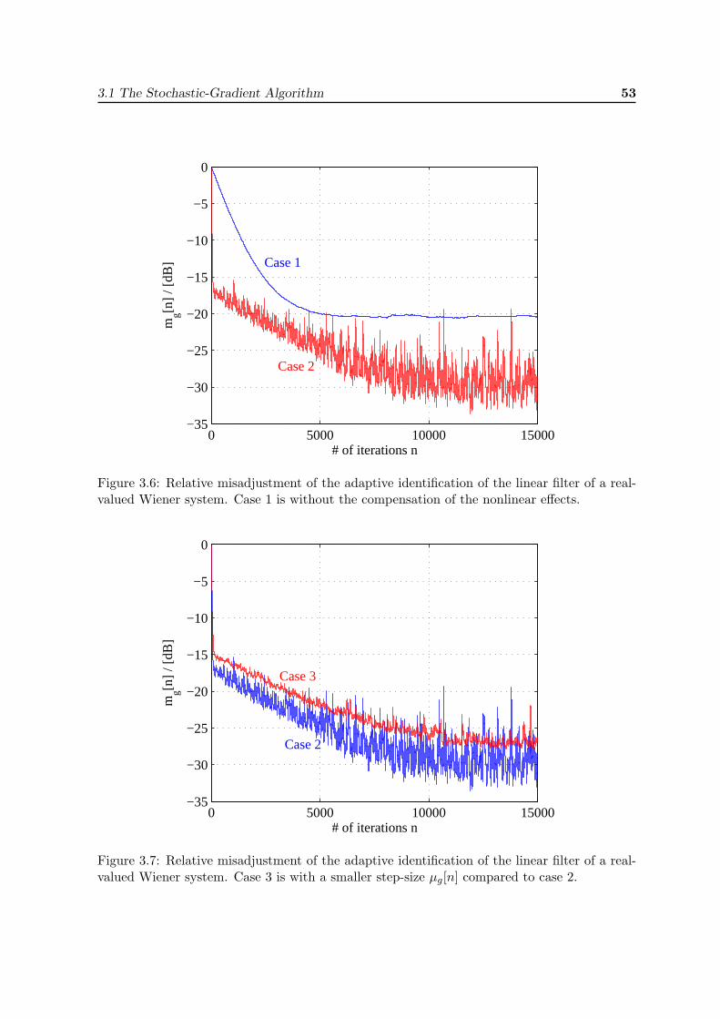
3.1 The Stochastic-Gradient Algorithm 53
0 5000 10000 15000−35
−30
−25
−20
−15
−10
−5
0
# of iterations n
mg[n
] / [
dB] Case 1
Case 2
Figure 3.6: Relative misadjustment of the adaptive identification of the linear filter of a real-valued Wiener system. Case 1 is without the compensation of the nonlinear effects.
0 5000 10000 15000−35
−30
−25
−20
−15
−10
−5
0
# of iterations n
mg[n
] / [
dB]
Case 2
Case 3
Figure 3.7: Relative misadjustment of the adaptive identification of the linear filter of a real-valued Wiener system. Case 3 is with a smaller step-size µg[n] compared to case 2.
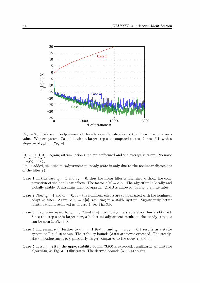
54 CHAPTER 3. Adaptive Identification
0 5000 10000 15000−35
−30
−25
−20
−15
−10
−5
0
5
10
15
20
# of iterations n
mg[n
] / [
dB]
Case 2
Case 4
Case 5
Figure 3.8: Relative misadjustment of the adaptive identification of the linear filter of a real-valued Wiener system. Case 4 is with a larger step-size compared to case 2, case 5 is with astep-size of µg[n] = 2µg[n].
[0, . . . , 0︸ ︷︷ ︸
=g′T−1
, 1, 0︸︷︷︸=wT
−1
]. Again, 50 simulation runs are performed and the average is taken. No noise
v[n] is added, thus the misadjustment in steady-state is only due to the nonlinear distortionsof the filter f(·).
Case 1 In this case cg = 1 and cw = 0, thus the linear filter is identified without the com-pensation of the nonlinear effects. The factor α[n] = α[n]. The algorithm is locally andglobally stable. A misadjustment of approx. -24 dB is achieved, as Fig. 3.9 illustrates.
Case 2 Now cg = 1 and cw = 0, 08 – the nonlinear effects are compensated with the nonlinearadaptive filter. Again, α[n] = α[n], resulting in a stable system. Significantly betteridentification is achieved as in case 1, see Fig. 3.9.
Case 3 If cw is increased to cw = 0, 2 and α[n] = α[n], again a stable algorithm is obtained.Since the step-size is larger now, a higher misadjustment results in the steady-state, ascan be seen in Fig. 3.9.
Case 4 Increasing α[n] further to α[n] = 1, 99 α[n] and cg = 1, cw = 0, 1 results in a stablesystem as Fig. 3.10 shows. The stability bounds (3.90) are never exceeded. The steady-state misadjustment is significantly larger compared to the cases 2, and 3.
Case 5 If α[n] = 2 α[n] the upper stability bound (3.90) is exceeded, resulting in an unstablealgorithm, as Fig. 3.10 illustrates. The derived bounds (3.90) are tight.
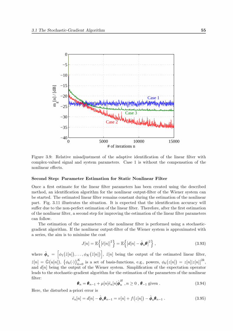
3.1 The Stochastic-Gradient Algorithm 55
0 5000 10000 15000−40
−35
−30
−25
−20
−15
−10
−5
0
# of iterations n
mg[n
] / [
dB]
Case 1
Case 2
Case 3
Figure 3.9: Relative misadjustment of the adaptive identification of the linear filter withcomplex-valued signal and system parameters. Case 1 is without the compensation of thenonlinear effects.
Second Step: Parameter Estimation for Static Nonlinear Filter
Once a first estimate for the linear filter parameters has been created using the describedmethod, an identification algorithm for the nonlinear output-filter of the Wiener system canbe started. The estimated linear filter remains constant during the estimation of the nonlinearpart. Fig. 3.11 illustrates the situation. It is expected that the identification accuracy willsuffer due to the non-perfect estimation of the linear filter. Therefore, after the first estimationof the nonlinear filter, a second step for improving the estimation of the linear filter parameterscan follow.
The estimation of the parameters of the nonlinear filter is performed using a stochastic-gradient algorithm. If the nonlinear output-filter of the Wiener system is approximated witha series, the aim is to minimise the cost
J [n] = E{∣∣e[n]
∣∣2} = E{∣∣d[n]− φφφnθθθ
∣∣2} , (3.93)
where φφφn =[φ1
(z[n]
), . . . , φK
(z[n]
)], z[n] being the output of the estimated linear filter,
z[n] = G(u[n]
),{φk(·)
}Kk=0
is a set of basis-functions, e.g., powers, φk(z[n]
)= z[n]|z[n]
∣∣2k,and d[n] being the output of the Wiener system. Simplification of the expectation operatorleads to the stochastic-gradient algorithm for the estimation of the parameters of the nonlinearfilter:
θθθn = θθθn−1 + µ[n]ea[n]φφφH
n , n ≥ 0 , θθθ−1 given . (3.94)
Here, the disturbed a-priori error is
ea[n] = d[n]− φφφnθθθn−1 = v[n] + f(z[n]
)− φφφnθθθn−1 . (3.95)
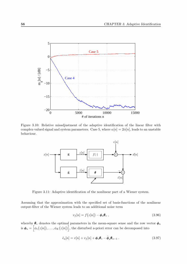
56 CHAPTER 3. Adaptive Identification
0 5000 10000 15000−20
−15
−10
−5
0
5
# of iterations n
mg[n
] / [
dB]
Case 4
Case 5
Figure 3.10: Relative misadjustment of the adaptive identification of the linear filter withcomplex-valued signal and system parameters. Case 5, where α[n] = 2α[n], leads to an unstablebehaviour.
g f(·)
g θθθ
+
+
� � � �d[n]
�
�
��
x[n] z[n]
z[n]
v[n]
�−
�e[n]
Figure 3.11: Adaptive identification of the nonlinear part of a Wiener system.
Assuming that the approximation with the specified set of basis-functions of the nonlinearoutput-filter of the Wiener system leads to an additional noise term
vf [n] = f(z[n]
)−φφφnθθθ∗ , (3.96)
whereby θθθ∗ denotes the optimal parameters in the mean-square sense and the row vector φφφnis φφφn =
[φ1
(z[n]
), . . . , φK
(z[n]
)], the disturbed a-priori error can be decomposed into
ea[n] = v[n] + vf [n] +φφφnθθθ∗ − φφφnθθθn−1 . (3.97)
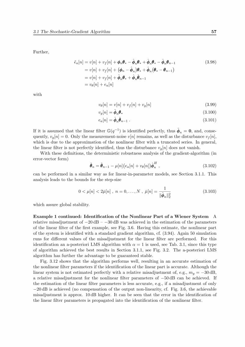
3.1 The Stochastic-Gradient Algorithm 57
Further,
ea[n] = v[n] + vf [n] +φφφnθθθ∗ − φφφnθθθ∗ + φφφnθθθ∗ − φφφnθθθn−1 (3.98)
= v[n] + vf [n] +(φφφn − φφφn
)θθθ∗ + φφφn
(θθθ∗ − θθθn−1
)= v[n] + vf [n] + φφφnθθθ∗ + φφφnθθθn−1
= vθ[n] + ea[n]
with
vθ[n] = v[n] + vf [n] + vg[n] (3.99)
vg[n] = φφφnθθθ∗ (3.100)
ea[n] = φφφnθθθn−1 . (3.101)
If it is assumed that the linear filter G(q−1) is identified perfectly, thus φφφn = 0, and, conse-quently, vg[n] = 0. Only the measurement-noise v[n] remains, as well as the disturbance vf [n],which is due to the approximation of the nonlinear filter with a truncated series. In general,the linear filter is not perfectly identified, thus the disturbance vg[n] does not vanish.
With these definitions, the deterministic robustness analysis of the gradient-algorithm (inerror-vector form)
θθθn = θθθn−1 − µ[n](ea[n] + vθ[n]
)φφφH
n , (3.102)
can be performed in a similar way as for linear-in-parameter models, see Section 3.1.1. Thisanalysis leads to the bounds for the step-size
0 < µ[n] < 2µ[n] , n = 0, . . . , N , µ[n] =1
‖φφφn‖22(3.103)
which assure global stability.
Example 1 continued: Identification of the Nonlinear Part of a Wiener System Arelative misadjustment of −20 dB – −30 dB was achieved in the estimation of the parametersof the linear filter of the first example, see Fig. 3.6. Having this estimate, the nonlinear partof the system is identified with a standard gradient algorithm, cf. (3.94). Again 50 simulationruns for different values of the misadjustment for the linear filter are performed. For thisidentification an a-posteriori LMS algorithm with α = 1 is used, see Tab. 3.1, since this typeof algorithm achieved the best results in Section 3.1.1, see Fig. 3.2. The a-posteriori LMSalgorithm has further the advantage to be guaranteed stable.
Fig. 3.12 shows that the algorithm performs well, resulting in an accurate estimation ofthe nonlinear filter parameters if the identification of the linear part is accurate. Although thelinear system is not estimated perfectly with a relative misadjustment of, e.g., mg = −30 dB,a relative misadjustment for the nonlinear filter parameters of −50 dB can be achieved. Ifthe estimation of the linear filter parameters is less accurate, e.g., if a misadjustment of only−20 dB is achieved (no compensation of the output non-linearity, cf. Fig. 3.6, the achievablemisadjustment is approx. 10 dB higher. It can be seen that the error in the identification ofthe linear filter parameters is propagated into the identification of the nonlinear filter.
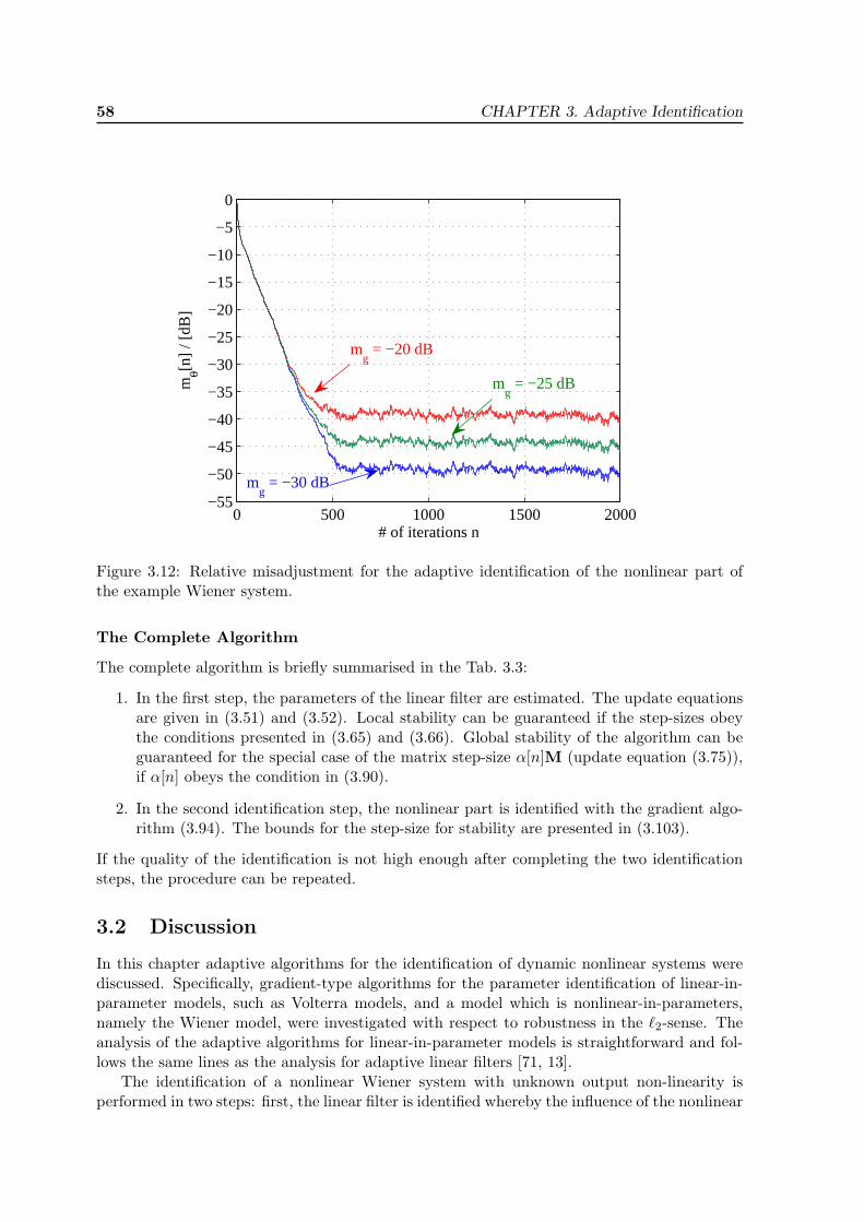
58 CHAPTER 3. Adaptive Identification
0 500 1000 1500 2000−55
−50
−45
−40
−35
−30
−25
−20
−15
−10
−5
0
# of iterations n
mθ[n
] / [
dB]
mg = −20 dB
mg = −25 dB
mg = −30 dB
Figure 3.12: Relative misadjustment for the adaptive identification of the nonlinear part ofthe example Wiener system.
The Complete Algorithm
The complete algorithm is briefly summarised in the Tab. 3.3:
1. In the first step, the parameters of the linear filter are estimated. The update equationsare given in (3.51) and (3.52). Local stability can be guaranteed if the step-sizes obeythe conditions presented in (3.65) and (3.66). Global stability of the algorithm can beguaranteed for the special case of the matrix step-size α[n]M (update equation (3.75)),if α[n] obeys the condition in (3.90).
2. In the second identification step, the nonlinear part is identified with the gradient algo-rithm (3.94). The bounds for the step-size for stability are presented in (3.103).
If the quality of the identification is not high enough after completing the two identificationsteps, the procedure can be repeated.
3.2 Discussion
In this chapter adaptive algorithms for the identification of dynamic nonlinear systems werediscussed. Specifically, gradient-type algorithms for the parameter identification of linear-in-parameter models, such as Volterra models, and a model which is nonlinear-in-parameters,namely the Wiener model, were investigated with respect to robustness in the `2-sense. Theanalysis of the adaptive algorithms for linear-in-parameter models is straightforward and fol-lows the same lines as the analysis for adaptive linear filters [71, 13].
The identification of a nonlinear Wiener system with unknown output non-linearity isperformed in two steps: first, the linear filter is identified whereby the influence of the nonlinear
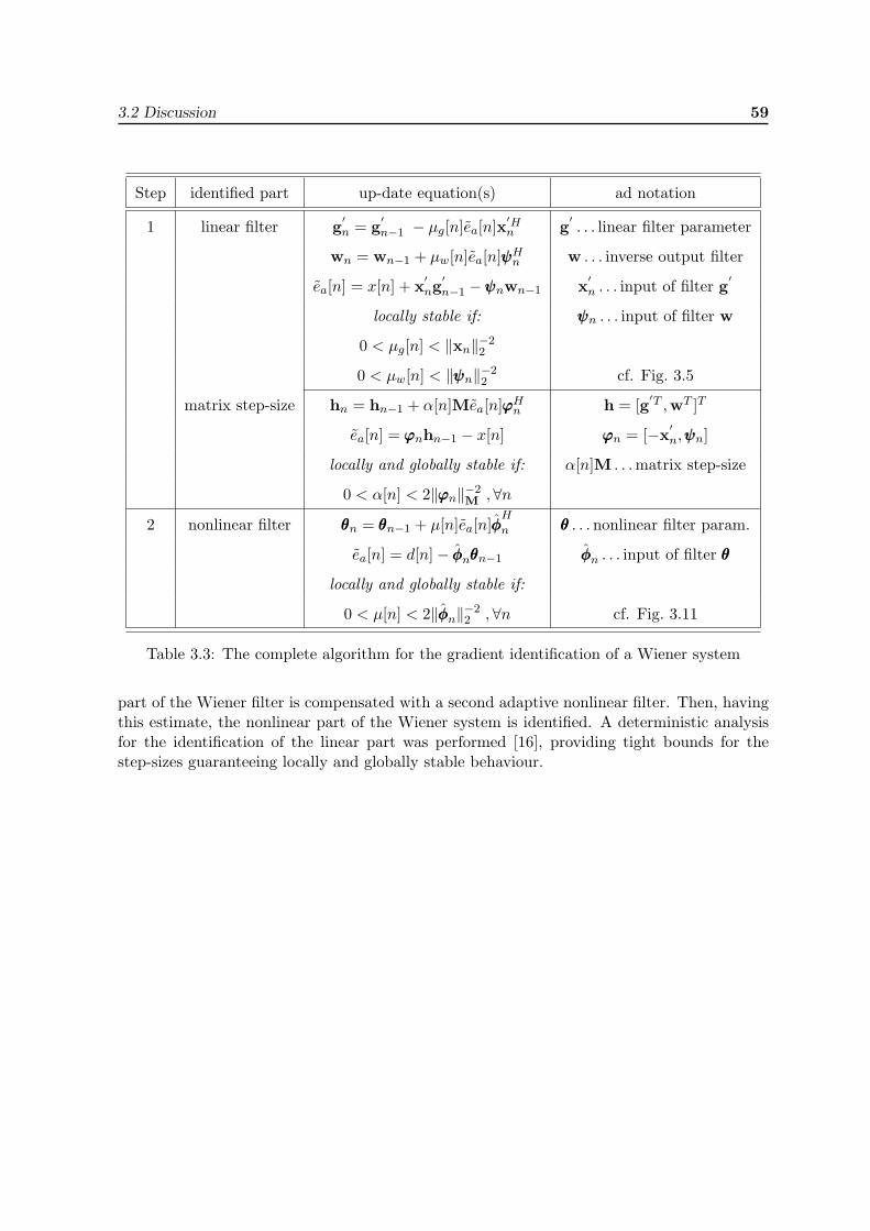
3.2 Discussion 59
Step identified part up-date equation(s) ad notation
1 linear filter g′n = g
′n−1 − µg[n]ea[n]x
′Hn g
′. . . linear filter parameter
wn = wn−1 + µw[n]ea[n]ψψψHn w . . . inverse output filter
ea[n] = x[n] + x′ng
′n−1 −ψψψnwn−1 x
′n . . . input of filter g
′
locally stable if: ψψψn . . . input of filter w
0 < µg[n] < ‖xn‖−22
0 < µw[n] < ‖ψψψn‖−22 cf. Fig. 3.5
matrix step-size hn = hn−1 + α[n]Mea[n]ϕϕϕHn h = [g′T ,wT ]T
ea[n] = ϕϕϕnhn−1 − x[n] ϕϕϕn = [−x′n,ψψψn]
locally and globally stable if: α[n]M . . .matrix step-size
0 < α[n] < 2‖ϕϕϕn‖−2M ,∀n
2 nonlinear filter θθθn = θθθn−1 + µ[n]ea[n]φφφH
n θθθ . . .nonlinear filter param.
ea[n] = d[n]− φφφnθθθn−1 φφφn . . . input of filter θθθ
locally and globally stable if:
0 < µ[n] < 2‖φφφn‖−22 ,∀n cf. Fig. 3.11
Table 3.3: The complete algorithm for the gradient identification of a Wiener system
part of the Wiener filter is compensated with a second adaptive nonlinear filter. Then, havingthis estimate, the nonlinear part of the Wiener system is identified. A deterministic analysisfor the identification of the linear part was performed [16], providing tight bounds for thestep-sizes guaranteeing locally and globally stable behaviour.

60 CHAPTER 3. Adaptive Identification
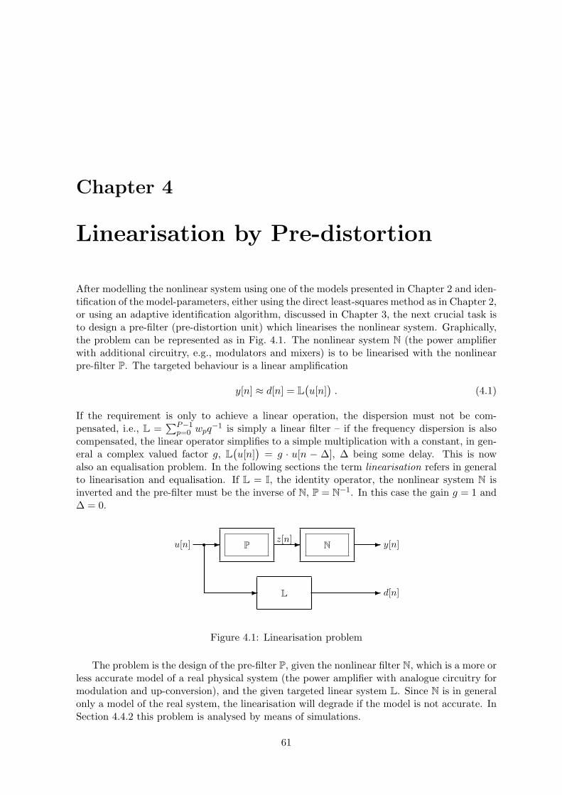
Chapter 4
Linearisation by Pre-distortion
After modelling the nonlinear system using one of the models presented in Chapter 2 and iden-tification of the model-parameters, either using the direct least-squares method as in Chapter 2,or using an adaptive identification algorithm, discussed in Chapter 3, the next crucial task isto design a pre-filter (pre-distortion unit) which linearises the nonlinear system. Graphically,the problem can be represented as in Fig. 4.1. The nonlinear system N (the power amplifierwith additional circuitry, e.g., modulators and mixers) is to be linearised with the nonlinearpre-filter P. The targeted behaviour is a linear amplification
y[n] ≈ d[n] = L(u[n]
). (4.1)
If the requirement is only to achieve a linear operation, the dispersion must not be com-pensated, i.e., L =
∑P−1p=0 wpq
−1 is simply a linear filter – if the frequency dispersion is alsocompensated, the linear operator simplifies to a simple multiplication with a constant, in gen-eral a complex valued factor g, L
(u[n]
)= g · u[n − ∆], ∆ being some delay. This is now
also an equalisation problem. In the following sections the term linearisation refers in generalto linearisation and equalisation. If L = I, the identity operator, the nonlinear system N isinverted and the pre-filter must be the inverse of N, P = N−1. In this case the gain g = 1 and∆ = 0.
P N
L
� � �
� �
u[n] z[n]y[n]
d[n]
Figure 4.1: Linearisation problem
The problem is the design of the pre-filter P, given the nonlinear filter N, which is a more orless accurate model of a real physical system (the power amplifier with analogue circuitry formodulation and up-conversion), and the given targeted linear system L. Since N is in generalonly a model of the real system, the linearisation will degrade if the model is not accurate. InSection 4.4.2 this problem is analysed by means of simulations.
61
62 CHAPTER 4. Linearisation by Pre-distortion
In general, since the filter N is nonlinear, an analytical solution for the linearisation problemis not possible. Local solutions, i.e., a pre-filter P that linearises or inverts the nonlinear systemN for a restricted class of input signals, can often be found. Formally, the nonlinear system Nis linearised around a point u0[n] – the linearisation is accurate in a certain neighbourhood ofthis point, i.e.,∥∥∥N(P
(u[n]
))− L
(u[n]
)∥∥∥ < δ if u[n] ∈{u[n]
∣∣∣∥∥u0[n]− u[n]∥∥ < ε
}. (4.2)
E.g., for static nonlinearities and real-valued signals u[n], the linearisation is accurate in acertain interval on the real line. In this case, the pre-filter can be implemented as a look-uptable, see e.g., [72, 73]. The table entries are pre-calculated based on the model of the nonlinearsystem. The accuracy of the method is heavily dependent on the resolution of the look-uptable – if the input signal is quantised using Q levels, the look-up table has Q entries. Forcomplex signals Q2 values have to be stored, which can be very large if the resolution is high,e.g., if Q = 212 = 4096, corresponding to a 12 bit analogue-to-digital converter, the size of thelook-up table is 16, 8 · 106, requiring approx. 34 MB of storage if 2 bytes per sample are used.If memory effects have to be considered the size of the look-up table becomes very large – forthe linearisation of dynamic nonlinear systems, look-up tables are prohibitively complex.
The inversion of general dynamic nonlinearities, expressed by a Volterra series, was pio-neered by M. Schetzen in [4, 36], where a pth-order inverse of a Volterra system is derived. Thesystem response of the tandem connection of the pth order inverse and the Volterra system is
N(P(u[n]
))= u[n] + Q
(u[n]
), (4.3)
where Q(u[n]
)=∑∞
i=p+1 Qi
(u[n]
)is a Volterra filter with the second through the pth-order
homogeneous parts Qi
(u[n]
)(cf., e.g., (2.26)) equal to zero. Thus, the nonlinear effects up to
the pth order are compensated, but not the higher order nonlinear terms. The drawback ofthis approach is the relatively high complexity of the pre-inverse and the appearance of thehigh-order nonlinear terms beginning with the p+ 1th term.
In this chapter, two iterative methods for the linearisation of a general Volterra filter areinvestigated – the first method is based on a fixed-point approach, presented in [18], the secondapproach is based on an alternative formulation of the linearisation problem [19, 74, 12]. Here,the idea is to modify the formulation of the linearisation problem to a root-search problemand to solve this problem iteratively. The advantage of this formulation is that fast iterativealgorithms can be used, which reduce the required complexity compared with the fixed-pointapproach. The drawback of the two methods is the complex analysis of convergence. For thefixed-point approach a sufficient condition for convergence of the iterative procedure can bedevised using the contraction-mapping theorem. Since this provides only sufficient conditionsfor convergence, they are in general too conservative – even if the conditions are not met,the algorithm may converge. Further, the verification of the convergence criterion is rathercomplex. In the investigated cases, based on models derived from measurements on poweramplifiers, see Chapter 2, both methods showed good convergence behaviour with obviousrestrictions on the targeted linear behaviour L. A further alleviation is that the power amplifiernonlinearities are usually mild and the linearisation task is “easy” to achieve for the iterativetechniques.
The iterative techniques are investigated with respect to convergence and speed usingsimulations. Here, realistic power amplifier models, either obtained from measurements or
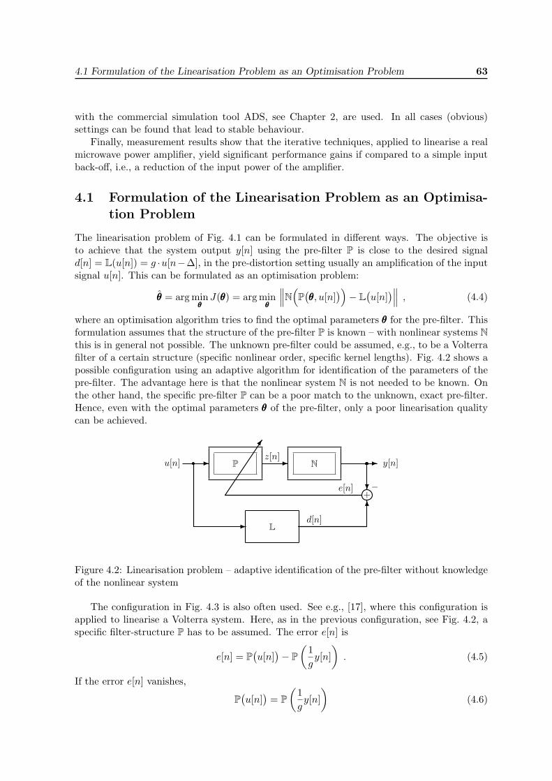
4.1 Formulation of the Linearisation Problem as an Optimisation Problem 63
with the commercial simulation tool ADS, see Chapter 2, are used. In all cases (obvious)settings can be found that lead to stable behaviour.
Finally, measurement results show that the iterative techniques, applied to linearise a realmicrowave power amplifier, yield significant performance gains if compared to a simple inputback-off, i.e., a reduction of the input power of the amplifier.
4.1 Formulation of the Linearisation Problem as an Optimisa-tion Problem
The linearisation problem of Fig. 4.1 can be formulated in different ways. The objective isto achieve that the system output y[n] using the pre-filter P is close to the desired signald[n] = L(u[n]) = g ·u[n−∆], in the pre-distortion setting usually an amplification of the inputsignal u[n]. This can be formulated as an optimisation problem:
θθθ = arg minθθθJ(θθθ) = arg min
θθθ
∥∥∥N(P(θθθ, u[n]
))− L
(u[n]
)∥∥∥ , (4.4)
where an optimisation algorithm tries to find the optimal parameters θθθ for the pre-filter. Thisformulation assumes that the structure of the pre-filter P is known – with nonlinear systems Nthis is in general not possible. The unknown pre-filter could be assumed, e.g., to be a Volterrafilter of a certain structure (specific nonlinear order, specific kernel lengths). Fig. 4.2 shows apossible configuration using an adaptive algorithm for identification of the parameters of thepre-filter. The advantage here is that the nonlinear system N is not needed to be known. Onthe other hand, the specific pre-filter P can be a poor match to the unknown, exact pre-filter.Hence, even with the optimal parameters θθθ of the pre-filter, only a poor linearisation qualitycan be achieved.
P N
L
� � �
�
+
u[n]z[n]
y[n]
d[n]
−e[n] �
�
�
Figure 4.2: Linearisation problem – adaptive identification of the pre-filter without knowledgeof the nonlinear system
The configuration in Fig. 4.3 is also often used. See e.g., [17], where this configuration isapplied to linearise a Volterra system. Here, as in the previous configuration, see Fig. 4.2, aspecific filter-structure P has to be assumed. The error e[n] is
e[n] = P(u[n]
)− P
(1gy[n]
). (4.5)
If the error e[n] vanishes,
P(u[n]
)= P
(1gy[n]
)(4.6)
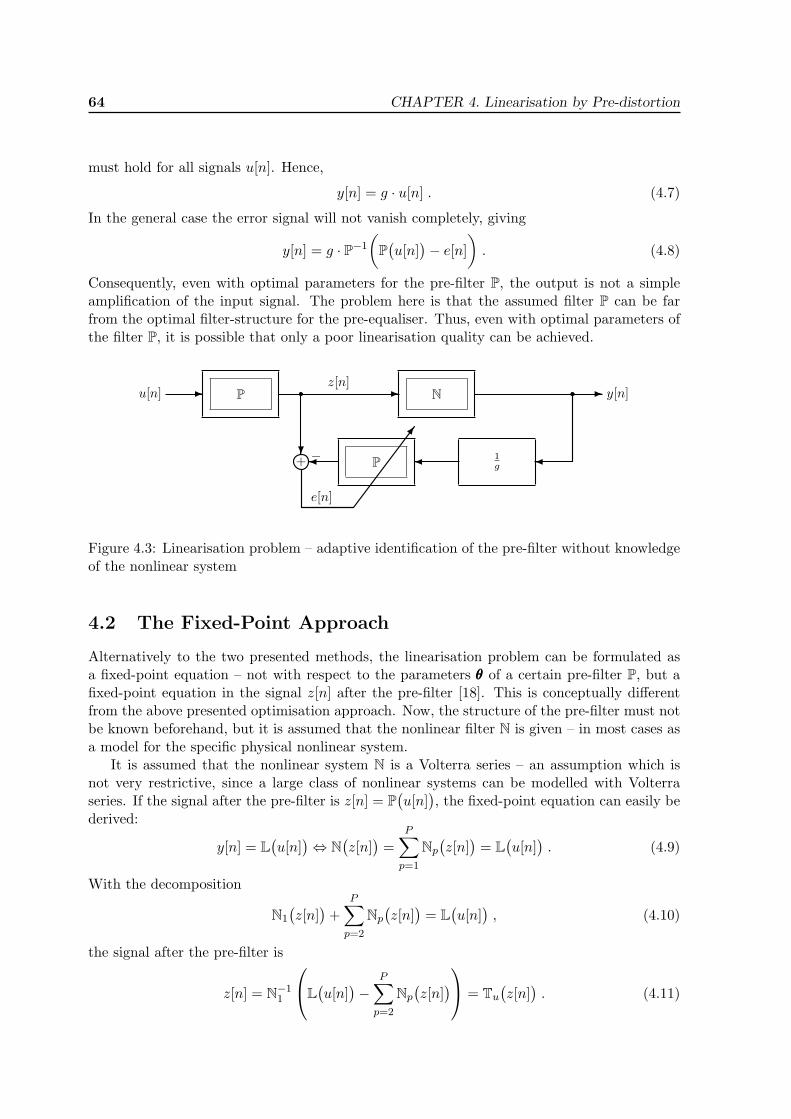
64 CHAPTER 4. Linearisation by Pre-distortion
must hold for all signals u[n]. Hence,
y[n] = g · u[n] . (4.7)
In the general case the error signal will not vanish completely, giving
y[n] = g · P−1
(P(u[n]
)− e[n]
). (4.8)
Consequently, even with optimal parameters for the pre-filter P, the output is not a simpleamplification of the input signal. The problem here is that the assumed filter P can be farfrom the optimal filter-structure for the pre-equaliser. Thus, even with optimal parameters ofthe filter P, it is possible that only a poor linearisation quality can be achieved.
P N
1g
z[n]
−P+
u[n] � y[n]
�
e[n]
�
�
�
� � �
Figure 4.3: Linearisation problem – adaptive identification of the pre-filter without knowledgeof the nonlinear system
4.2 The Fixed-Point Approach
Alternatively to the two presented methods, the linearisation problem can be formulated asa fixed-point equation – not with respect to the parameters θθθ of a certain pre-filter P, but afixed-point equation in the signal z[n] after the pre-filter [18]. This is conceptually differentfrom the above presented optimisation approach. Now, the structure of the pre-filter must notbe known beforehand, but it is assumed that the nonlinear filter N is given – in most cases asa model for the specific physical nonlinear system.
It is assumed that the nonlinear system N is a Volterra series – an assumption which isnot very restrictive, since a large class of nonlinear systems can be modelled with Volterraseries. If the signal after the pre-filter is z[n] = P
(u[n]
), the fixed-point equation can easily be
derived:
y[n] = L(u[n]
)⇔ N
(z[n]
)=
P∑p=1
Np
(z[n]
)= L
(u[n]
). (4.9)
With the decomposition
N1
(z[n]
)+
P∑p=2
Np
(z[n]
)= L
(u[n]
), (4.10)
the signal after the pre-filter is
z[n] = N−11
L(u[n]
)−
P∑p=2
Np
(z[n]
) = Tu(z[n]
). (4.11)
4.2 The Fixed-Point Approach 65
Here, Np are the homogeneous Volterra operators of order p and it is assumed that the first-order operator N1 (a linear filter) is invertible. The transformation T is indexed with the inputsignal u[n] to emphasise the dependence on it (it depends also on L). Here, in contrast to theabove mentioned two methods, the nonlinear Volterra system N, which is in practice the modelfor the nonlinear power amplifier, needs to be known. The essential difference in this approachis, that the signal z[n] after the pre-filter P is identified, not the parameters θθθ of a specificpre-filter. In (4.11) the signal z[n] is a fixed-point of the transformation Tu. Searching thefixed-point is thus equivalent to determining the pre-filter P itself. Since an analytic solutionto the above fixed-point equation is rarely available, the fixed-point z[n] is searched iterativelywith successive approximation:
zi+1[n] = Tu(zi[n]
), z0[n] given . (4.12)
Whether the method converges to a solution z[n] or not depends on the transformation T,which depends on the input signal u[n] and the targeted linear operation L. Here a simplelinear amplification with a delay ∆, L
(u[n]
)= g · u[n−∆] is used. Applying the Contraction
Mapping Theorem [49, 48], which states basically that the method of successive approximationconverges if T is contractive (see Appendix B), it can be determined whether the method ofsuccessive approximation (4.12) is guaranteed to converge. If the transformation T is furtherdifferentiable and
∥∥T′(z)∥∥ ≤ α < 1 on a convex set1 K , the transformation is a contraction
mapping, since∥∥T(z1) − T(z2)
∥∥ ≤ sup∥∥T′
(z)∥∥‖z1 − z2‖ ≤ α‖z1 − z2‖, using the mean-value
inequality [48]. Therefore, it is guaranteed that the method converges.For applying the Contraction Mapping Theorem for the linearisation problem, the problem
must be formulated in a Banach space and, therefore, a specific norm has to be chosen. Manychoices of norms are possible, e.g., any of the `p-sequence norms may be chosen. Once a normhas been chosen, it must be confirmed that the transformation Tu is contractive. In order toconfirm this, the norms of the homogeneous Volterra operators Np, induced by the chosen sig-nal norm, have to be computed. In practice, these norms cannot be computed – computableupper bounds have to be used, which may be tight or loose. Hence, using different signalnorms, different restrictions, necessary to guarantee the contractiveness, are produced [18].Since the Contraction Mapping Theorem gives sufficient conditions for convergence, the ob-tained convergence results may be very loose and seldom possible to fulfill in practice. Thecomplicated nature for proving convergence and the loose bounds obtained are not very helpfulin applications – therefore, the convergence is investigated in Section 4.4 using simulations.
Regarding the convergence rate of the successive approximation procedure applied to acontraction mapping T with the fixed-point z[n] the inequality∥∥∥T(zi−1[n]
)− T
(z[n]
)∥∥∥ =∥∥zi[n]− z[n]
∥∥ ≤ α∥∥zi−1[n]− z[n]
∥∥ (4.13)
results. The sequence {zi[n]} converges thus only linearly to the fixed-point z[n] since
limj→∞
supi≥j
∥∥zi[n]− z[n]∥∥∥∥zi−1[n]− z[n]∥∥ = α (4.14)
for some 0 < α < 1. The slow convergence is the main drawback of this linearisation method.Slow convergence means that for good accuracy of linearisation a large number of iterations
has to be performed. A large number of iterations means a high complexity – either a pipelined1A set K in a linear vector space is said to be convex if, given x1, x2 ∈ K , all points of the form βx1+(1−β)x2
with 0 ≤ β < 1 are in K .
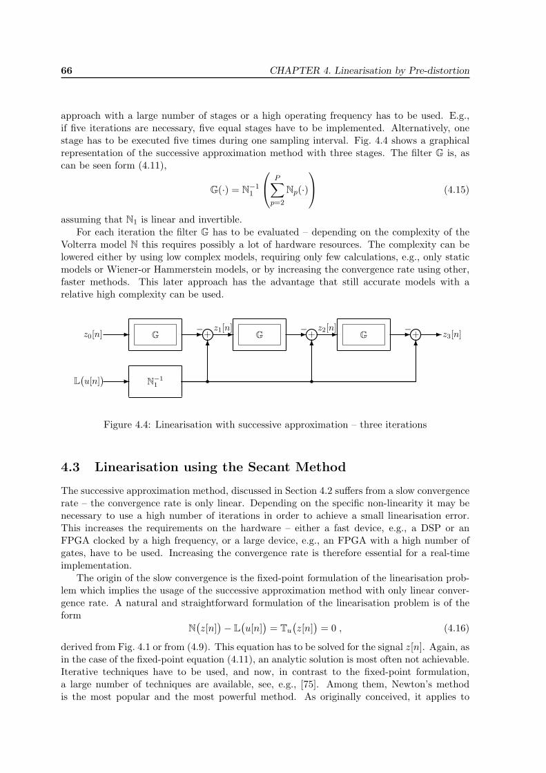
66 CHAPTER 4. Linearisation by Pre-distortion
approach with a large number of stages or a high operating frequency has to be used. E.g.,if five iterations are necessary, five equal stages have to be implemented. Alternatively, onestage has to be executed five times during one sampling interval. Fig. 4.4 shows a graphicalrepresentation of the successive approximation method with three stages. The filter G is, ascan be seen form (4.11),
G(·) = N−11
P∑p=2
Np(·)
(4.15)
assuming that N1 is linear and invertible.For each iteration the filter G has to be evaluated – depending on the complexity of the
Volterra model N this requires possibly a lot of hardware resources. The complexity can belowered either by using low complex models, requiring only few calculations, e.g., only staticmodels or Wiener-or Hammerstein models, or by increasing the convergence rate using other,faster methods. This later approach has the advantage that still accurate models with arelative high complexity can be used.
G G
N−11
� − � G+
�
z0[n] +�� �− +�
L(u[n]
)
�−� � �
z1[n] z2[n]z3[n]
Figure 4.4: Linearisation with successive approximation – three iterations
4.3 Linearisation using the Secant Method
The successive approximation method, discussed in Section 4.2 suffers from a slow convergencerate – the convergence rate is only linear. Depending on the specific non-linearity it may benecessary to use a high number of iterations in order to achieve a small linearisation error.This increases the requirements on the hardware – either a fast device, e.g., a DSP or anFPGA clocked by a high frequency, or a large device, e.g., an FPGA with a high number ofgates, have to be used. Increasing the convergence rate is therefore essential for a real-timeimplementation.
The origin of the slow convergence is the fixed-point formulation of the linearisation prob-lem which implies the usage of the successive approximation method with only linear conver-gence rate. A natural and straightforward formulation of the linearisation problem is of theform
N(z[n]
)− L
(u[n]
)= Tu
(z[n]
)= 0 , (4.16)
derived from Fig. 4.1 or from (4.9). This equation has to be solved for the signal z[n]. Again, asin the case of the fixed-point equation (4.11), an analytic solution is most often not achievable.Iterative techniques have to be used, and now, in contrast to the fixed-point formulation,a large number of techniques are available, see, e.g., [75]. Among them, Newton’s methodis the most popular and the most powerful method. As originally conceived, it applies to
4.3 Linearisation using the Secant Method 67
equations of a single real variable but it can be extended to nonlinear transformations onnormed spaces [48]. In order to solve the above equation (4.16) with Newton’s method, thenonlinear transformation Tu must be differentiable. If this is assured, Newton’s method reads
zi+1[n] = zi[n]−[∂zTu
(zi[n]
)]−1 Tu(zi[n]
), (4.17)
using some starting value z0[n]. Newton’s method converges quadratically, meaning that∥∥zi+1[n]− z[n]∥∥ ≤ c
∥∥zi[n]− z[n]∥∥2, (4.18)
z[n] denoting a solution of (4.16).The Newton step
δzi[n] = −[∂zTu
(zi[n]
)]−1 Tu(zi[n]
), (4.19)
where δzi[n] = zi+1[n]− zi[n], decreases also the cost function
J(z[n]
)=∥∥∥Tu(z[n]
)∥∥∥2
2= THu
(z[n]
)Tu(z[n]
). (4.20)
This can be seen if the Newton step is multiplied with the gradient of the cost function∂zJ
(z[n]
), which is
∂zJ(z[n]
)= ∂z
[THu(z[n]
)Tu(z[n]
)]= THu
(z[n]
)∂zTu
(z[n]
). (4.21)
Multiplication of the gradient at the point zi[n] with the Newton step δzi[n] yields
∂zJ(zi[n]
)δzi[n] =
(THu(z[n]
)∂zTu
(zi[n]
))(−[∂zTu
(zi[n]
)]−1Tu(zi[n]
))= −THu
(zi[n]
)Tu(zi[n]
)< 0 ,
(4.22)
proving that the cost (4.20) is indeed reduced with every step. This means that every solutionof (4.16) minimises also the cost function (4.20). But the converse is not necessarily true, sincethere might be local minima of (4.20) which are not solutions of (4.16). This is the fundamentaland important difference between the optimisation approach where an objective function isminimised and the direct approach presented above, where a solution for a nonlinear (systemof) equation(s) is searched for.
The fast convergence rate of Newton’s method has a price attached: its large complex-ity [74]. Now, for one iteration, not only the transformation Tu has to be evaluated at zi[n].Additionally, the Jacobian ∂zTu
(zi[n]
)has to be evaluated and inverted. The principal prob-
lem with this method is the computation of the Jacobian, which might not be easy or evenpossible – the transformation T has to be differentiable, which, for the specific nonlinear modelsdiscussed in Chapter 2 is not the case, since terms involving the magnitude of the signal
∣∣z[n]∣∣
are appearing – these terms are only analytic for z[n] = 0. See, e.g., the general equivalentbaseband Volterra series in (2.26). A solution could be to exclude these terms in the modelling,but this results in a poor model-system match. It is expected that the output is dependent onthe actual magnitude of the input signal, the restriction being thus not well-founded.
The main difficulty in applying the fast Newton’s method for solving (4.16) is thus thedetermination and evaluation of the Jacobian. Every simplification will further result in aslower procedure. The aim is thus to simplify Newton’s method but keep the convergence rate
68 CHAPTER 4. Linearisation by Pre-distortion
as high as possible. A practical and for the purpose well-suited method is the secant method.The secant method for the specific problem (4.16) is
zi+1[n] = zi[n]− zi[n]− zi−1[n]N(zi[n]
)− N
(zi−1[n]
)Tu(zi[n]), (4.23)
with two (different) starting values z−1[n] and z0[n]. A convenient choice is z−1[n] = 0 andz0[n] = u[n], since it is expected that the signal after the pre-filter differs only slightly fromthe original input signal u[n].
The computation of the Jacobian is thus no longer required. The only condition on thetransformation N is to be continuous, a requirement which is naturally fulfilled for the modelsdiscussed in Chapter 2. The above equation (4.23) calculates the output of the pre-filter Pfor each time instant n. If the nonlinear transformations N and Tu have memory, they aretime-variant since the outputs N
(zi[n]
), N(zi−1[n]
), and Tu
(zi[n]
)depend on the previously
calculated pre-filter outputs z[n − 1], . . . , z[n − M + 1] (assuming a memory length of Msamples), as well as the pre-filter input signal u[n].
For a formal derivation of the secant method, the general case with signals of length M ,e.g., z[n] =
{z[n], z[n− 1], . . . , z[n−M + 1]
}, M being larger or equal to the memory length
of the nonlinear transformation N, is used. The Newton step in (4.19), whose computation isthe main contribution to the complexity of the method, can be approximated by a so-calledquasi-Newton step [75], which is the solution of
Biδzi[n] = −Tu(zi[n]
). (4.24)
The secant condition requires [75] that
Bi+1δzi[n] = δTu(zi[n]
), (4.25)
with δTu(zi[n]
)= Tu
(zi+1[n]
)− Tu
(zi[n]
). Considering the general case with M dimensions
and thus avoiding the time-variant formulation of (4.23), a multidimensional secant methodmust be used. The problem here is that in more than one dimension the matrix Bi+1 in (4.25)cannot be uniquely determined, which gives additional degrees of freedom. The most popularand in practice best performing algorithm is Broyden’s method [76, 75]. For the implementa-tion in real-time, where the output of the pre-filter must be calculated on a sample-by-samplebasis, the time-variant formulation in (4.23) is adequate. Broyden’s method is block-based,and thus not applicable for a real-time implementation.
In one dimension, Bi+1 is simply a scalar bi+1 and is for the transformation in (4.16)
bi+1 =N(zi+1[n]
)− N
(zi[n]
)zi+1[n]− zi[n]
, (4.26)
as can easily be verified. Thus, the secant step from (4.24)
δzi[n] = −b−1i Tu
(zi[n]
)= − zi[n]− zi−1[n]
N(zi[n]
)− N
(zi−1[n]
)Tu(zi[n])
(4.27)
results.If the algorithm converges, the convergence rate of the secant method is superlinear [75]∥∥zi[n]− z[n]
∥∥ ≤ c∥∥zi−1[n]− z[n]
∥∥φ , (4.28)
with the golden ratio φ = 12
(1 +
√5)≈ 1, 618. The convergence order is smaller than that
of the Newton method, but still much larger than the convergence order of the successiveapproximation method.
4.4 Applying the Linearisation Methods 69
4.4 Applying the Linearisation Methods
In Sections 4.4.1 and 4.4.2 the two presented linearisation methods, namely the successive ap-proximation method, discussed in Section 4.2 and the secant method, discussed in Section 4.3,are compared with respect to convergence rate and robustness against model uncertainties. Ahigh convergence rate is essential for a practical real-time implementation of the pre-distortionfilter, e.g., in an FPGA or a DSP, since few iterations are required for a good approximationof the ideal pre-filter. Further, in a practical implementation the system (power-amplifierwith analogue circuitry such as modulators, demodulators, and mixers) cannot be modelledperfectly. Various types of disturbances affect the modelling:
➾ At the output of the system, measurement noise affects the estimation of the modelparameters. The noise comes from various sources, e.g., due to the limited resolution ofthe analogue-to-digital converters, quantisation noise is introduced. Other components,such as mixers, demodulators, and amplifiers add thermal noise.
➾ The model-structure does not equal the system-structure. The power-amplifier is not aspecific Volterra-, Wiener-, or Hammerstein system, the model being thus only a moreor less accurate approximation to the system.
These disturbances will ultimately limit the achievable linearisation quality, since the designof the pre-filter is based on the model.
The following situations are investigated:
1. Model-parameter errors due to measurement noise
2. Memory effects are neglected in the model
3. Underestimation of the nonlinear order of the system
This investigation is performed using simulations since a direct control of the system outputis necessary, e.g., for adding measurement noise. The “test-system” in this section is theVolterra model of the Motorola power-amplifier of Section 2.6. It can be considered as realistic.The different situations are then simulated and their influence on the linearisation quality isinvestigated.
First, the parameters of the test-system S, see Fig. 4.5, are estimated using the in-put/output data obtained from the ADS simulation. This test-system replaces the “real”,physical system in the following simulations. Then, noise is added to the output data ob-tained from the ADS simulation of the power-amplifier. The noise is white, zero-mean andwith a gaussian amplitude distribution. The model has the same structure as the test-system,i.e., it is also a Volterra system of order five with kernels of length two. The implication of theadded noise is a higher modelling error.
Subsequently, the effect of model-system mismatch, i.e., a structural difference of systemand model, is investigated. In this case, no measurement noise is added to the output dataobtained by the ADS simulation. The error signal due to imperfect modelling is
emod[n] = y[n]− x[n] = S(z[n]
)+ v[n]− N
(z[n]
). (4.29)
The modelling quality is measured by
Jmod [dB] = 10 log
(∥∥emod[n]∥∥2
2∥∥y[n]∥∥2
2
). (4.30)
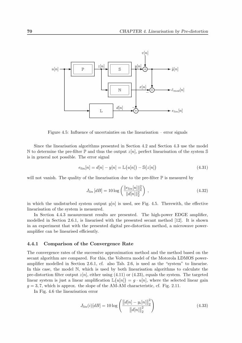
70 CHAPTER 4. Linearisation by Pre-distortion
P S
L
�
N
� y[n]u[n]z[n]
d[n]
+
+
+
�
�
�
�
�
�
�
�x[n]
�
� emod[n]
elin[n]
v[n]
�
−
−
y[n]
Figure 4.5: Influence of uncertainties on the linearisation – error signals
Since the linearisation algorithms presented in Section 4.2 and Section 4.3 use the modelN to determine the pre-filter P and thus the output z[n], perfect linearisation of the system Sis in general not possible. The error signal
elin[n] = d[n]− y[n] = L(u[n]
)− S(z[n]
)(4.31)
will not vanish. The quality of the linearisation due to the pre-filter P is measured by
Jlin [dB] = 10 log(‖elin[n]‖22‖d[n]‖22
), (4.32)
in which the undisturbed system output y[n] is used, see Fig. 4.5. Therewith, the effectivelinearisation of the system is measured.
In Section 4.4.3 measurement results are presented. The high-power EDGE amplifier,modelled in Section 2.6.1, is linearised with the presented secant method [12]. It is shownin an experiment that with the presented digital pre-distortion method, a microwave power-amplifier can be linearised efficiently.
4.4.1 Comparison of the Convergence Rate
The convergence rates of the successive approximation method and the method based on thesecant algorithm are compared. For this, the Volterra model of the Motorola LDMOS power-amplifier modelled in Section 2.6.1, cf. also Tab. 2.6, is used as the “system” to linearise.In this case, the model N, which is used by both linearisation algorithms to calculate thepre-distortion filter output z[n], either using (4.11) or (4.23), equals the system. The targetedlinear system is just a linear amplification L
(u[n]
)= g · u[n], where the selected linear gain
g = 3, 7, which is approx. the slope of the AM-AM characteristic, cf. Fig. 2.11.In Fig. 4.6 the linearisation error
Jlin(i)[dB] = 10 log
(∥∥d[n]− yi[n]∥∥2
2∥∥d[n]∥∥2
2
)(4.33)
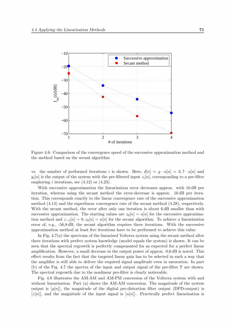
4.4 Applying the Linearisation Methods 71
1 2 3 4−70
−60
−50
−40
−30
−20
−10
# of iterations
J lin(i
)/[d
B]
Successive approximationSecant method
Figure 4.6: Comparison of the convergence speed of the successive approximation method andthe method based on the secant algorithm
vs. the number of performed iterations i is shown. Here, d[n] = g · u[n] = 3, 7 · u[n] andyi[n] is the output of the system with the pre-filtered input zi[n], corresponding to a pre-filteremploying i iterations, see (4.12) or (4.23).
With successive approximation the linearisation error decreases approx. with 10 dB periteration, whereas using the secant method the error-decrease is approx. 16 dB per itera-tion. This corresponds exactly to the linear convergence rate of the successive approximationmethod (4.14) and the superlinear convergence rate of the secant method (4.28), respectively.With the secant method, the error after only one iteration is about 6 dB smaller than withsuccessive approximation. The starting values are z0[n] = u[n] for the successive approxima-tion method and z−1[n] = 0, z0[n] = u[n] for the secant algorithm. To achieve a linearisationerror of, e.g., -56,8 dB, the secant algorithm requires three iterations. With the successiveapproximation method at least five iterations have to be performed to achieve this value.
In Fig. 4.7(a) the spectrum of the linearised Volterra system using the secant method afterthree iterations with perfect system knowledge (model equals the system) is shown. It can beseen that the spectral regrowth is perfectly compensated for as expected for a perfect linearamplification. However, a small decrease in the output power of approx. 0,6 dB is noted. Thiseffect results from the fact that the targeted linear gain has to be selected in such a way thatthe amplifier is still able to deliver the required signal amplitude even in saturation. In part(b) of the Fig. 4.7 the spectra of the input and output signal of the pre-filter P are shown.The spectral regrowth due to the nonlinear pre-filter is clearly noticeable.
Fig. 4.8 illustrates the AM-AM and AM-PM conversion of the Volterra system with andwithout linearisation. Part (a) shows the AM-AM conversion. The magnitude of the systemoutput is
∣∣y[n]∣∣, the magnitude of the digital pre-distortion filter output (DPD-output) is∣∣z[n]
∣∣, and the magnitude of the input signal is∣∣u[n]
∣∣. Practically perfect linearisation is
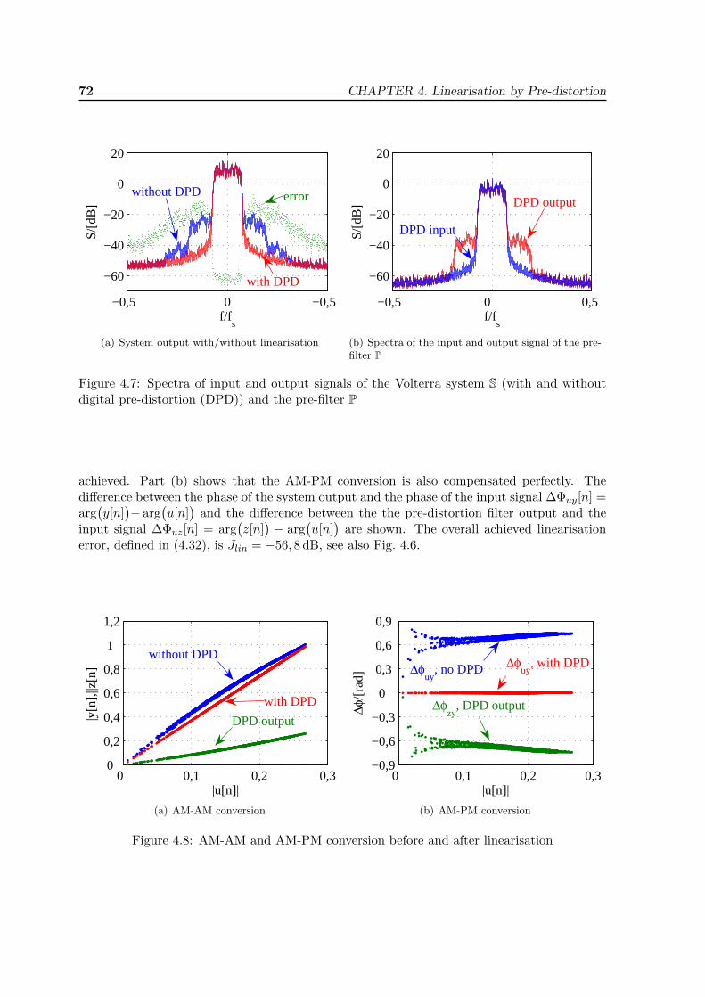
72 CHAPTER 4. Linearisation by Pre-distortion
−0,5 0 −0,5
−60
−40
−20
0
20
f/fs
S/[d
B]
errorwithout DPD
with DPD
(a) System output with/without linearisation
−0,5 0 0,5
−60
−40
−20
0
20
f/fs
S/[d
B] DPD output
DPD input
(b) Spectra of the input and output signal of the pre-filter P
Figure 4.7: Spectra of input and output signals of the Volterra system S (with and withoutdigital pre-distortion (DPD)) and the pre-filter P
achieved. Part (b) shows that the AM-PM conversion is also compensated perfectly. Thedifference between the phase of the system output and the phase of the input signal ∆Φuy[n] =arg(y[n]
)− arg
(u[n]
)and the difference between the the pre-distortion filter output and the
input signal ∆Φuz[n] = arg(z[n]
)− arg
(u[n]
)are shown. The overall achieved linearisation
error, defined in (4.32), is Jlin = −56, 8 dB, see also Fig. 4.6.
0 0,1 0,2 0,30
0,2
0,4
0,6
0,8
1
1,2
|u[n]|
|y[n
],||z
[n]|
without DPD
with DPD
DPD output
(a) AM-AM conversion
0 0,1 0,2 0,3−0,9
−0,6
−0,3
0
0,3
0,6
0,9
|u[n]|
∆φ/[
rad]
∆φuy
, no DPD ∆φuy
, with DPD
∆φzy
, DPD output
(b) AM-PM conversion
Figure 4.8: AM-AM and AM-PM conversion before and after linearisation
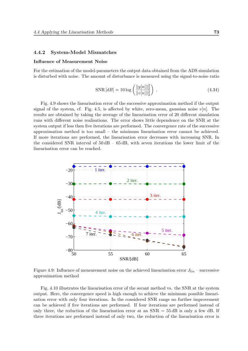
4.4 Applying the Linearisation Methods 73
4.4.2 System-Model Mismatches
Influence of Measurement Noise
For the estimation of the model-parameters the output data obtained from the ADS simulationis disturbed with noise. The amount of disturbance is measured using the signal-to-noise ratio
SNR [dB] = 10 log(‖y[n]‖22‖v[n]‖22
). (4.34)
Fig. 4.9 shows the linearisation error of the successive approximation method if the outputsignal of the system, cf. Fig. 4.5, is affected by white, zero-mean, gaussian noise v[n]. Theresults are obtained by taking the average of the linearisation error of 20 different simulationruns with different noise realisations. The error shows little dependence on the SNR at thesystem output if less then five iterations are performed. The convergence rate of the successiveapproximation method is too small – the minimum linearisation error cannot be achieved.If more iterations are performed, the linearisation error decreases with increasing SNR. Inthe considered SNR interval of 50 dB – 65 dB, with seven iterations the lower limit of thelinearisation error can be reached.
50 55 60 65−80
−70
−60
−50
−40
−30
−20
SNR/[dB]
J lin/[
dB]
1 iter.
2 iter.
3 iter.
4 iter.
5 iter.6 iter.7 iter.
Figure 4.9: Influence of measurement noise on the achieved linearisation error Jlin – successiveapproximation method
Fig. 4.10 illustrates the linearisation error of the secant method vs. the SNR at the systemoutput. Here, the convergence speed is high enough to achieve the minimum possible lineari-sation error with only four iterations. In the considered SNR range no further improvementcan be achieved if five iterations are performed. If four iterations are performed instead ofonly three, the reduction of the linearisation error at an SNR = 55 dB is only a few dB. Ifthree iterations are performed instead of only two, the reduction of the linearisation error is
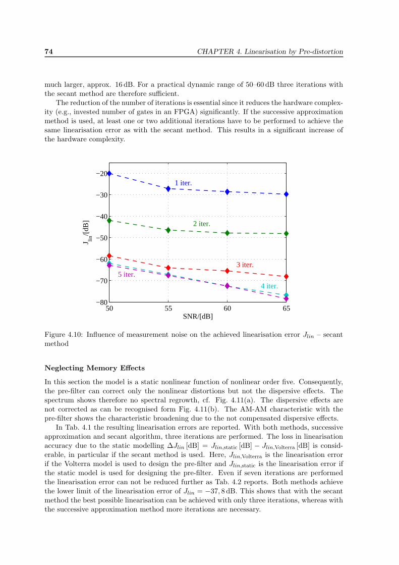
74 CHAPTER 4. Linearisation by Pre-distortion
much larger, approx. 16 dB. For a practical dynamic range of 50–60 dB three iterations withthe secant method are therefore sufficient.
The reduction of the number of iterations is essential since it reduces the hardware complex-ity (e.g., invested number of gates in an FPGA) significantly. If the successive approximationmethod is used, at least one or two additional iterations have to be performed to achieve thesame linearisation error as with the secant method. This results in a significant increase ofthe hardware complexity.
50 55 60 65−80
−70
−60
−50
−40
−30
−20
SNR/[dB]
J lin/[
dB]
1 iter.
2 iter.
3 iter.
4 iter.
5 iter.
Figure 4.10: Influence of measurement noise on the achieved linearisation error Jlin – secantmethod
Neglecting Memory Effects
In this section the model is a static nonlinear function of nonlinear order five. Consequently,the pre-filter can correct only the nonlinear distortions but not the dispersive effects. Thespectrum shows therefore no spectral regrowth, cf. Fig. 4.11(a). The dispersive effects arenot corrected as can be recognised form Fig. 4.11(b). The AM-AM characteristic with thepre-filter shows the characteristic broadening due to the not compensated dispersive effects.
In Tab. 4.1 the resulting linearisation errors are reported. With both methods, successiveapproximation and secant algorithm, three iterations are performed. The loss in linearisationaccuracy due to the static modelling ∆Jlin [dB] = Jlin,static [dB] − Jlin,Volterra [dB] is consid-erable, in particular if the secant method is used. Here, Jlin,Volterra is the linearisation errorif the Volterra model is used to design the pre-filter and Jlin,static is the linearisation error ifthe static model is used for designing the pre-filter. Even if seven iterations are performedthe linearisation error can not be reduced further as Tab. 4.2 reports. Both methods achievethe lower limit of the linearisation error of Jlin = −37, 8 dB. This shows that with the secantmethod the best possible linearisation can be achieved with only three iterations, whereas withthe successive approximation method more iterations are necessary.
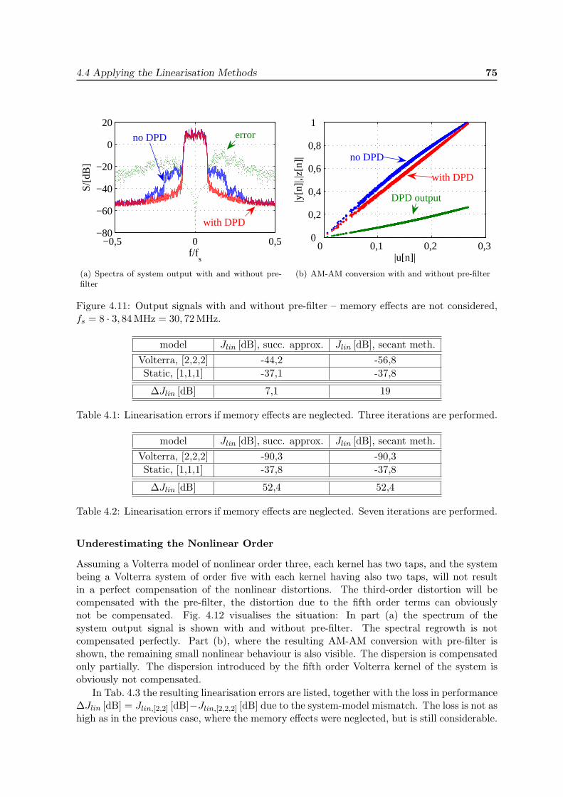
4.4 Applying the Linearisation Methods 75
−0,5 0 0,5−80
−60
−40
−20
0
20
f/fs
S/[d
B]
errorno DPD
with DPD
(a) Spectra of system output with and without pre-filter
0 0,1 0,2 0,3 0
0,2
0,4
0,6
0,8
1
|u[n]|
|y[n
]|,|z
[n]| no DPD
with DPD
DPD output
(b) AM-AM conversion with and without pre-filter
Figure 4.11: Output signals with and without pre-filter – memory effects are not considered,fs = 8 · 3, 84 MHz = 30, 72 MHz.
model Jlin [dB], succ. approx. Jlin [dB], secant meth.Volterra, [2,2,2] -44,2 -56,8Static, [1,1,1] -37,1 -37,8
∆Jlin [dB] 7,1 19
Table 4.1: Linearisation errors if memory effects are neglected. Three iterations are performed.
model Jlin [dB], succ. approx. Jlin [dB], secant meth.Volterra, [2,2,2] -90,3 -90,3Static, [1,1,1] -37,8 -37,8
∆Jlin [dB] 52,4 52,4
Table 4.2: Linearisation errors if memory effects are neglected. Seven iterations are performed.
Underestimating the Nonlinear Order
Assuming a Volterra model of nonlinear order three, each kernel has two taps, and the systembeing a Volterra system of order five with each kernel having also two taps, will not resultin a perfect compensation of the nonlinear distortions. The third-order distortion will becompensated with the pre-filter, the distortion due to the fifth order terms can obviouslynot be compensated. Fig. 4.12 visualises the situation: In part (a) the spectrum of thesystem output signal is shown with and without pre-filter. The spectral regrowth is notcompensated perfectly. Part (b), where the resulting AM-AM conversion with pre-filter isshown, the remaining small nonlinear behaviour is also visible. The dispersion is compensatedonly partially. The dispersion introduced by the fifth order Volterra kernel of the system isobviously not compensated.
In Tab. 4.3 the resulting linearisation errors are listed, together with the loss in performance∆Jlin [dB] = Jlin,[2,2] [dB]−Jlin,[2,2,2] [dB] due to the system-model mismatch. The loss is not ashigh as in the previous case, where the memory effects were neglected, but is still considerable.
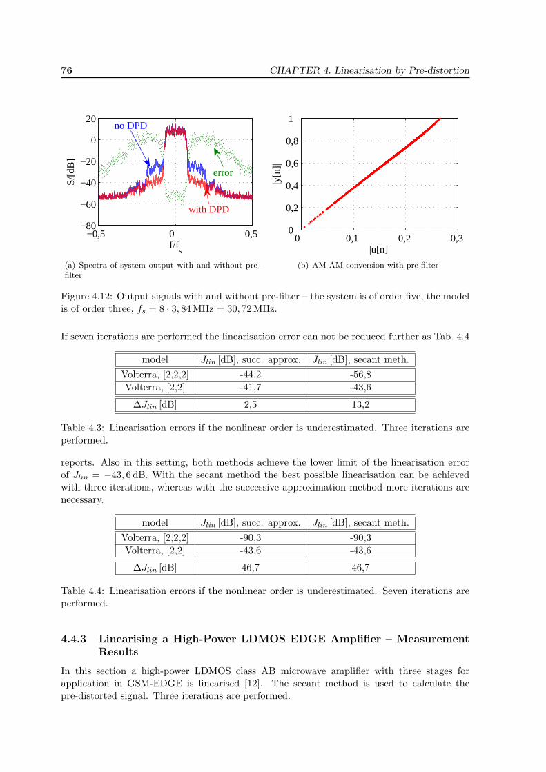
76 CHAPTER 4. Linearisation by Pre-distortion
−0,5 0 0,5 −80
−60
−40
−20
0
20
f/fs
S/[d
B]
error
no DPD
with DPD
(a) Spectra of system output with and without pre-filter
0 0,1 0,2 0,3 0
0,2
0,4
0,6
0,8
1
|u[n]|
|y[n
]|(b) AM-AM conversion with pre-filter
Figure 4.12: Output signals with and without pre-filter – the system is of order five, the modelis of order three, fs = 8 · 3, 84 MHz = 30, 72 MHz.
If seven iterations are performed the linearisation error can not be reduced further as Tab. 4.4
model Jlin [dB], succ. approx. Jlin [dB], secant meth.Volterra, [2,2,2] -44,2 -56,8Volterra, [2,2] -41,7 -43,6
∆Jlin [dB] 2,5 13,2
Table 4.3: Linearisation errors if the nonlinear order is underestimated. Three iterations areperformed.
reports. Also in this setting, both methods achieve the lower limit of the linearisation errorof Jlin = −43, 6 dB. With the secant method the best possible linearisation can be achievedwith three iterations, whereas with the successive approximation method more iterations arenecessary.
model Jlin [dB], succ. approx. Jlin [dB], secant meth.Volterra, [2,2,2] -90,3 -90,3Volterra, [2,2] -43,6 -43,6
∆Jlin [dB] 46,7 46,7
Table 4.4: Linearisation errors if the nonlinear order is underestimated. Seven iterations areperformed.
4.4.3 Linearising a High-Power LDMOS EDGE Amplifier – MeasurementResults
In this section a high-power LDMOS class AB microwave amplifier with three stages forapplication in GSM-EDGE is linearised [12]. The secant method is used to calculate thepre-distorted signal. Three iterations are performed.
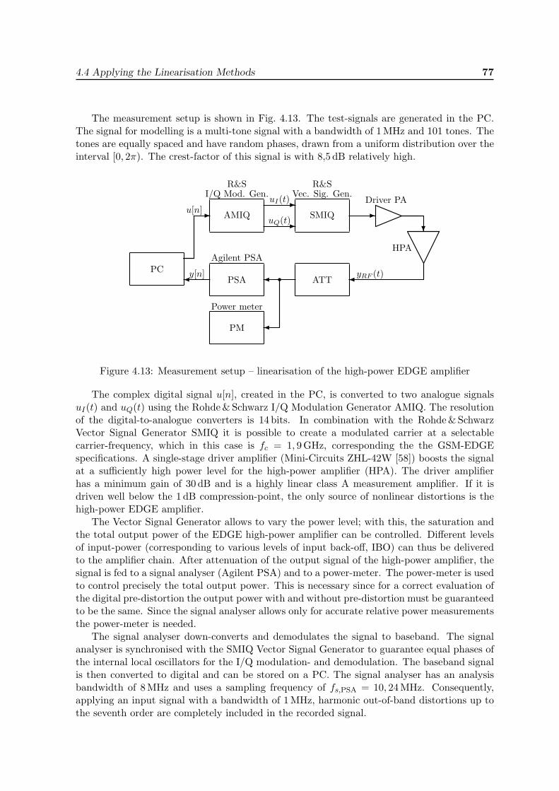
4.4 Applying the Linearisation Methods 77
The measurement setup is shown in Fig. 4.13. The test-signals are generated in the PC.The signal for modelling is a multi-tone signal with a bandwidth of 1 MHz and 101 tones. Thetones are equally spaced and have random phases, drawn from a uniform distribution over theinterval [0, 2π). The crest-factor of this signal is with 8,5 dB relatively high.
AMIQ SMIQu[n]
PCPSA �
PM
�
ATT
�
�
�� �
�
�
R&S R&SI/Q Mod. Gen. Vec. Sig. Gen.
Driver PA
HPAAgilent PSA
Power meter
y[n] yRF (t)
uI(t)
uQ(t)
Figure 4.13: Measurement setup – linearisation of the high-power EDGE amplifier
The complex digital signal u[n], created in the PC, is converted to two analogue signalsuI(t) and uQ(t) using the Rohde & Schwarz I/Q Modulation Generator AMIQ. The resolutionof the digital-to-analogue converters is 14 bits. In combination with the Rohde &SchwarzVector Signal Generator SMIQ it is possible to create a modulated carrier at a selectablecarrier-frequency, which in this case is fc = 1, 9 GHz, corresponding the the GSM-EDGEspecifications. A single-stage driver amplifier (Mini-Circuits ZHL-42W [58]) boosts the signalat a sufficiently high power level for the high-power amplifier (HPA). The driver amplifierhas a minimum gain of 30 dB and is a highly linear class A measurement amplifier. If it isdriven well below the 1 dB compression-point, the only source of nonlinear distortions is thehigh-power EDGE amplifier.
The Vector Signal Generator allows to vary the power level; with this, the saturation andthe total output power of the EDGE high-power amplifier can be controlled. Different levelsof input-power (corresponding to various levels of input back-off, IBO) can thus be deliveredto the amplifier chain. After attenuation of the output signal of the high-power amplifier, thesignal is fed to a signal analyser (Agilent PSA) and to a power-meter. The power-meter is usedto control precisely the total output power. This is necessary since for a correct evaluation ofthe digital pre-distortion the output power with and without pre-distortion must be guaranteedto be the same. Since the signal analyser allows only for accurate relative power measurementsthe power-meter is needed.
The signal analyser down-converts and demodulates the signal to baseband. The signalanalyser is synchronised with the SMIQ Vector Signal Generator to guarantee equal phases ofthe internal local oscillators for the I/Q modulation- and demodulation. The baseband signalis then converted to digital and can be stored on a PC. The signal analyser has an analysisbandwidth of 8 MHz and uses a sampling frequency of fs,PSA = 10, 24 MHz. Consequently,applying an input signal with a bandwidth of 1 MHz, harmonic out-of-band distortions up tothe seventh order are completely included in the recorded signal.
78 CHAPTER 4. Linearisation by Pre-distortion
The procedure is now as follows:
1. First, the multi-tone test signal is applied to the power-amplifier chain. Here, threedifferent levels of input power, corresponding to different levels of saturation, are used.
2. With the input-signal and the recorded output-signal, a black-box model of the amplifieris created. A Volterra model and a Wiener model are compared for all three levels ofsaturation.
3. Since, as is shown in the following, the Wiener model results in a comparable modellingerror, it is used to calculate the pre-distorted signal with the secant method.
4. The pre-distorted signal is then used to excite the power amplifier chain. The outputsignal is stored in the PC. The power level is measured with the power-meter.
5. Since the power level with pre-distortion is smaller than in the first step, the undistortedsignal has to be applied once more. The output power of the SMIQ is slightly reduced,compared to step one, in order to guarantee the same output power of the amplifier chainas with pre-distortion. This corresponds to an input back-off.
Modelling
Two models are compared using three different degrees of saturation of the high-power ampli-fier: A Volterra model and a Wiener model. The amplifier input power is adjusted to differentlevels with the SMIQ. The models are then fitted to the measured data. Both models havea nonlinear order of seven. For the Volterra model, the least modelling error was found witha linear kernel of length five, a third-order kernel with three taps, a fifth-order kernel withtwo taps and a seventh-order kernel with one tap (memoryless). The corresponding structuralnotation is mV = [5, 3, 2, 1]T . The best Wiener model is a four tap FIR filter followed by a sev-enth order static non-linearity. In Tab. 4.5 the three different cases, corresponding to the threedifferent power levels, are compared. The modelling error, defined in (4.30), of the Wienermodel is approx. 1,6 dB higher as the modelling error of the Volterra model. The advantageof the Wiener model is the small number of parameters: only eight complex parameters arerequired whereas the Volterra model requires 36 parameters. The modelling quality decreasesfurther with increasing output power. This is reasonable, since with increasing output powerthe high-power amplifier is driven more and more into saturation, corresponding to a relativelyhard non-linearity, which is difficult to fit with only a seventh order model. On the other hand,out-of-band distortions higher than seventh-order cannot be analysed by the signal analyserdue to the limited bandwidth of 8 MHz. Only the weak in-band distortions are available forthe modelling, making thus the task of fitting higher nonlinear terms difficult. Therefore, thenonlinear model-order is kept constant, even if the amplifier is driven in higher saturation.
case Pout/[dBm] Jmod,Wiener/[dB] Jmod,Volterra/[dB]1 42,3 -37,3 -38,92 43,9 -35,5 -37,13 45,4 -33,8 -35,3
Table 4.5: Modelling errors – high-power EDGE amplifier
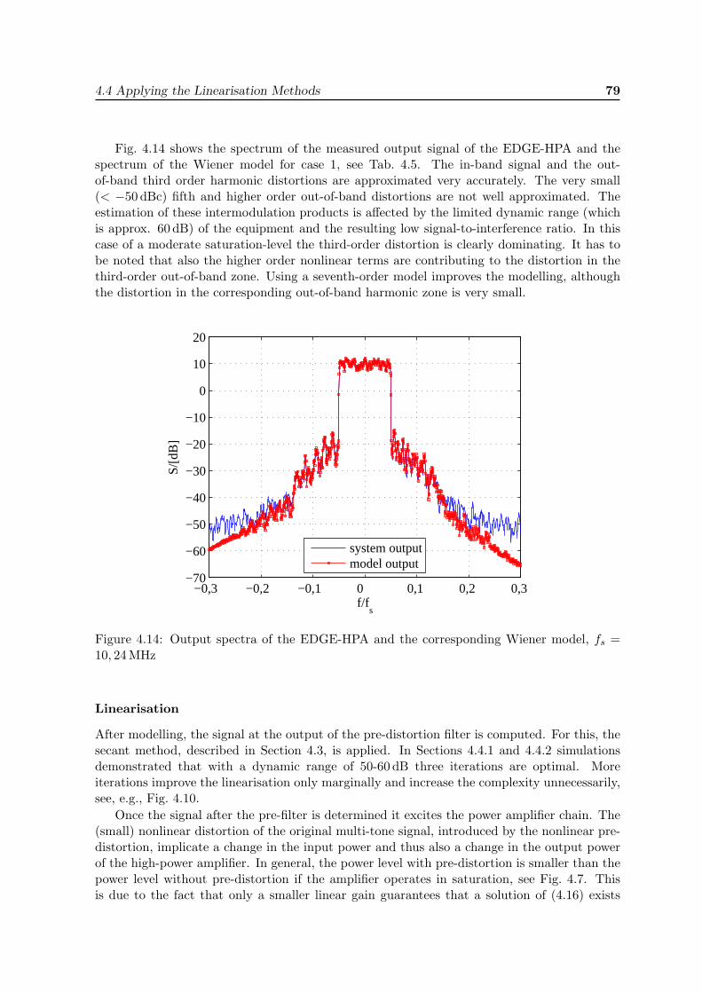
4.4 Applying the Linearisation Methods 79
Fig. 4.14 shows the spectrum of the measured output signal of the EDGE-HPA and thespectrum of the Wiener model for case 1, see Tab. 4.5. The in-band signal and the out-of-band third order harmonic distortions are approximated very accurately. The very small(< −50 dBc) fifth and higher order out-of-band distortions are not well approximated. Theestimation of these intermodulation products is affected by the limited dynamic range (whichis approx. 60 dB) of the equipment and the resulting low signal-to-interference ratio. In thiscase of a moderate saturation-level the third-order distortion is clearly dominating. It has tobe noted that also the higher order nonlinear terms are contributing to the distortion in thethird-order out-of-band zone. Using a seventh-order model improves the modelling, althoughthe distortion in the corresponding out-of-band harmonic zone is very small.
−0,3 −0,2 −0,1 0 0,1 0,2 0,3 −70
−60
−50
−40
−30
−20
−10
0
10
20
f/fs
S/[d
B]
system outputmodel output
Figure 4.14: Output spectra of the EDGE-HPA and the corresponding Wiener model, fs =10, 24 MHz
Linearisation
After modelling, the signal at the output of the pre-distortion filter is computed. For this, thesecant method, described in Section 4.3, is applied. In Sections 4.4.1 and 4.4.2 simulationsdemonstrated that with a dynamic range of 50-60 dB three iterations are optimal. Moreiterations improve the linearisation only marginally and increase the complexity unnecessarily,see, e.g., Fig. 4.10.
Once the signal after the pre-filter is determined it excites the power amplifier chain. The(small) nonlinear distortion of the original multi-tone signal, introduced by the nonlinear pre-distortion, implicate a change in the input power and thus also a change in the output powerof the high-power amplifier. In general, the power level with pre-distortion is smaller than thepower level without pre-distortion if the amplifier operates in saturation, see Fig. 4.7. Thisis due to the fact that only a smaller linear gain guarantees that a solution of (4.16) exists
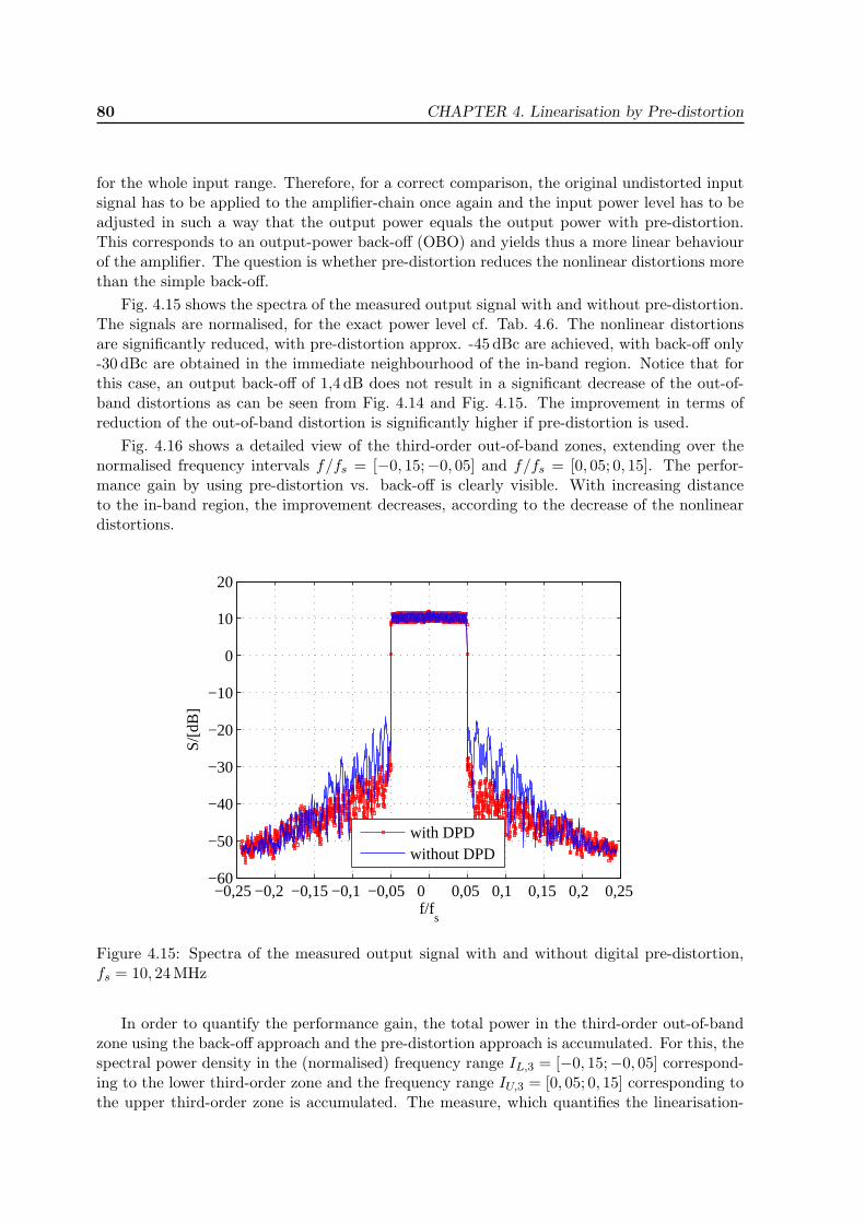
80 CHAPTER 4. Linearisation by Pre-distortion
for the whole input range. Therefore, for a correct comparison, the original undistorted inputsignal has to be applied to the amplifier-chain once again and the input power level has to beadjusted in such a way that the output power equals the output power with pre-distortion.This corresponds to an output-power back-off (OBO) and yields thus a more linear behaviourof the amplifier. The question is whether pre-distortion reduces the nonlinear distortions morethan the simple back-off.
Fig. 4.15 shows the spectra of the measured output signal with and without pre-distortion.The signals are normalised, for the exact power level cf. Tab. 4.6. The nonlinear distortionsare significantly reduced, with pre-distortion approx. -45 dBc are achieved, with back-off only-30 dBc are obtained in the immediate neighbourhood of the in-band region. Notice that forthis case, an output back-off of 1,4 dB does not result in a significant decrease of the out-of-band distortions as can be seen from Fig. 4.14 and Fig. 4.15. The improvement in terms ofreduction of the out-of-band distortion is significantly higher if pre-distortion is used.
Fig. 4.16 shows a detailed view of the third-order out-of-band zones, extending over thenormalised frequency intervals f/fs = [−0, 15;−0, 05] and f/fs = [0, 05; 0, 15]. The perfor-mance gain by using pre-distortion vs. back-off is clearly visible. With increasing distanceto the in-band region, the improvement decreases, according to the decrease of the nonlineardistortions.
−0,25 −0,2 −0,15 −0,1 −0,05 0 0,05 0,1 0,15 0,2 0,25 −60
−50
−40
−30
−20
−10
0
10
20
f/fs
S/[d
B]
with DPDwithout DPD
Figure 4.15: Spectra of the measured output signal with and without digital pre-distortion,fs = 10, 24 MHz
In order to quantify the performance gain, the total power in the third-order out-of-bandzone using the back-off approach and the pre-distortion approach is accumulated. For this, thespectral power density in the (normalised) frequency range IL,3 = [−0, 15;−0, 05] correspond-ing to the lower third-order zone and the frequency range IU,3 = [0, 05; 0, 15] corresponding tothe upper third-order zone is accumulated. The measure, which quantifies the linearisation-
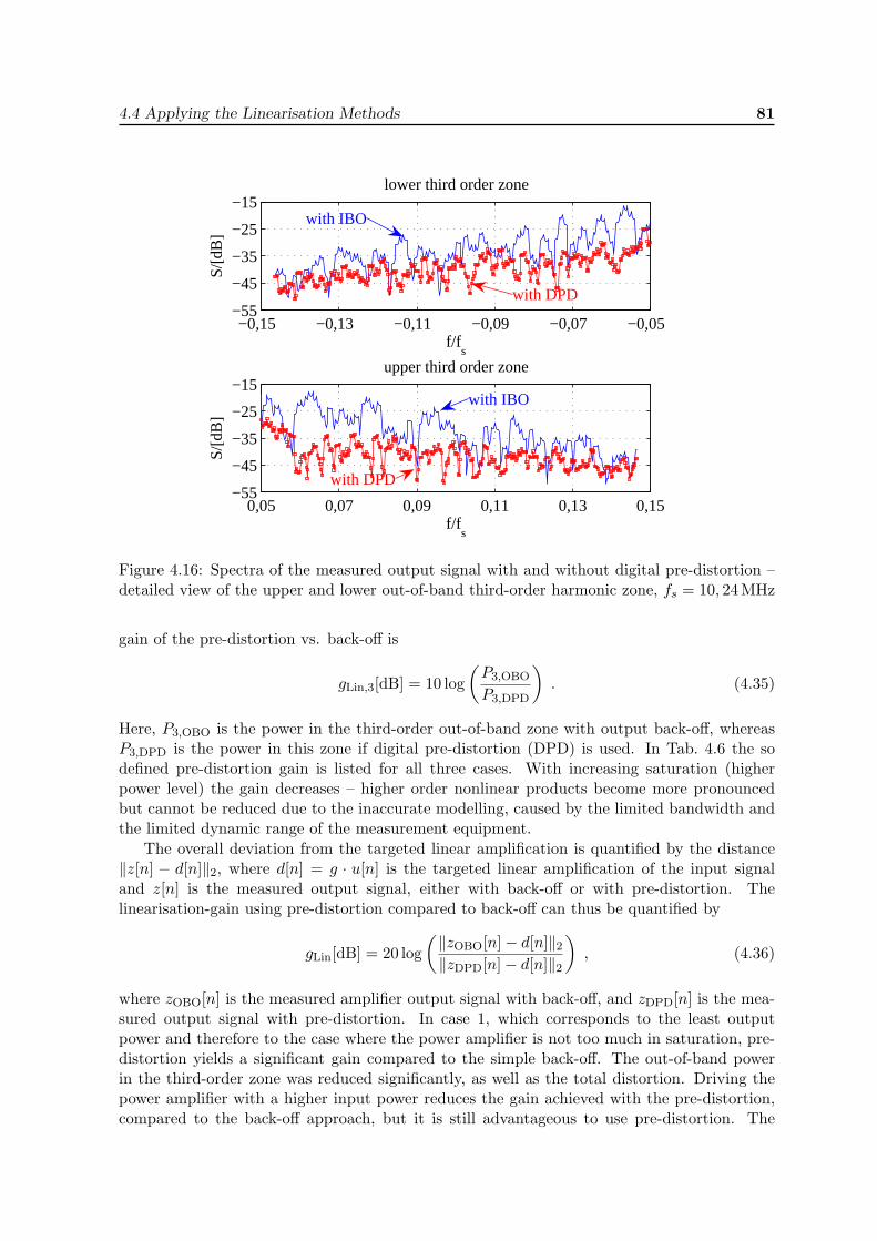
4.4 Applying the Linearisation Methods 81
−0,15 −0,13 −0,11 −0,09 −0,07 −0,05−55
−45
−35
−25
−15
f/fs
S/[d
B]
lower third order zone
0,05 0,07 0,09 0,11 0,13 0,15−55
−45
−35
−25
−15
f/fs
S/[d
B]
upper third order zone
with DPD
with IBO
with IBO
with DPD
Figure 4.16: Spectra of the measured output signal with and without digital pre-distortion –detailed view of the upper and lower out-of-band third-order harmonic zone, fs = 10, 24 MHz
gain of the pre-distortion vs. back-off is
gLin,3[dB] = 10 log(P3,OBO
P3,DPD
). (4.35)
Here, P3,OBO is the power in the third-order out-of-band zone with output back-off, whereasP3,DPD is the power in this zone if digital pre-distortion (DPD) is used. In Tab. 4.6 the sodefined pre-distortion gain is listed for all three cases. With increasing saturation (higherpower level) the gain decreases – higher order nonlinear products become more pronouncedbut cannot be reduced due to the inaccurate modelling, caused by the limited bandwidth andthe limited dynamic range of the measurement equipment.
The overall deviation from the targeted linear amplification is quantified by the distance‖z[n] − d[n]‖2, where d[n] = g · u[n] is the targeted linear amplification of the input signaland z[n] is the measured output signal, either with back-off or with pre-distortion. Thelinearisation-gain using pre-distortion compared to back-off can thus be quantified by
gLin[dB] = 20 log(‖zOBO[n]− d[n]‖2‖zDPD[n]− d[n]‖2
), (4.36)
where zOBO[n] is the measured amplifier output signal with back-off, and zDPD[n] is the mea-sured output signal with pre-distortion. In case 1, which corresponds to the least outputpower and therefore to the case where the power amplifier is not too much in saturation, pre-distortion yields a significant gain compared to the simple back-off. The out-of-band powerin the third-order zone was reduced significantly, as well as the total distortion. Driving thepower amplifier with a higher input power reduces the gain achieved with the pre-distortion,compared to the back-off approach, but it is still advantageous to use pre-distortion. The
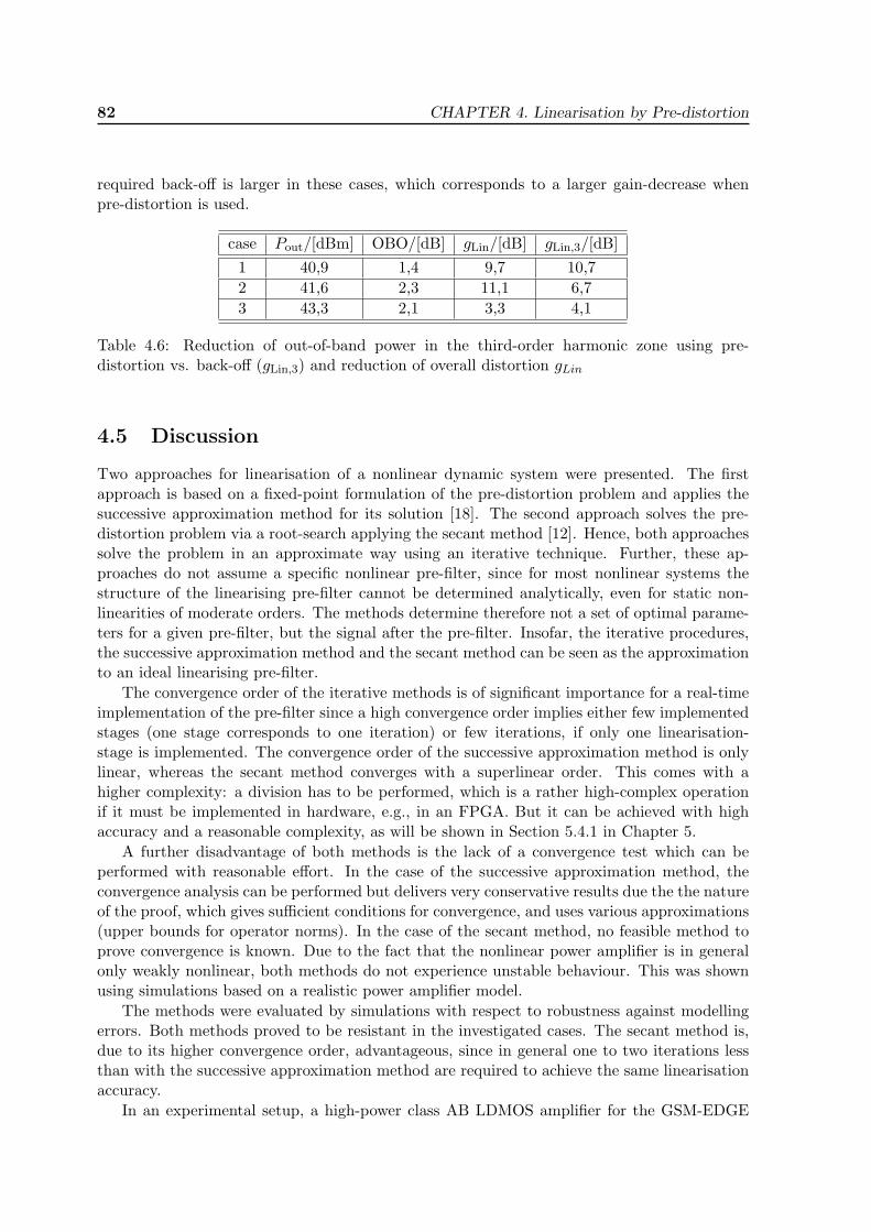
82 CHAPTER 4. Linearisation by Pre-distortion
required back-off is larger in these cases, which corresponds to a larger gain-decrease whenpre-distortion is used.
case Pout/[dBm] OBO/[dB] gLin/[dB] gLin,3/[dB]1 40,9 1,4 9,7 10,72 41,6 2,3 11,1 6,73 43,3 2,1 3,3 4,1
Table 4.6: Reduction of out-of-band power in the third-order harmonic zone using pre-distortion vs. back-off (gLin,3) and reduction of overall distortion gLin
4.5 Discussion
Two approaches for linearisation of a nonlinear dynamic system were presented. The firstapproach is based on a fixed-point formulation of the pre-distortion problem and applies thesuccessive approximation method for its solution [18]. The second approach solves the pre-distortion problem via a root-search applying the secant method [12]. Hence, both approachessolve the problem in an approximate way using an iterative technique. Further, these ap-proaches do not assume a specific nonlinear pre-filter, since for most nonlinear systems thestructure of the linearising pre-filter cannot be determined analytically, even for static non-linearities of moderate orders. The methods determine therefore not a set of optimal parame-ters for a given pre-filter, but the signal after the pre-filter. Insofar, the iterative procedures,the successive approximation method and the secant method can be seen as the approximationto an ideal linearising pre-filter.
The convergence order of the iterative methods is of significant importance for a real-timeimplementation of the pre-filter since a high convergence order implies either few implementedstages (one stage corresponds to one iteration) or few iterations, if only one linearisation-stage is implemented. The convergence order of the successive approximation method is onlylinear, whereas the secant method converges with a superlinear order. This comes with ahigher complexity: a division has to be performed, which is a rather high-complex operationif it must be implemented in hardware, e.g., in an FPGA. But it can be achieved with highaccuracy and a reasonable complexity, as will be shown in Section 5.4.1 in Chapter 5.
A further disadvantage of both methods is the lack of a convergence test which can beperformed with reasonable effort. In the case of the successive approximation method, theconvergence analysis can be performed but delivers very conservative results due the the natureof the proof, which gives sufficient conditions for convergence, and uses various approximations(upper bounds for operator norms). In the case of the secant method, no feasible method toprove convergence is known. Due to the fact that the nonlinear power amplifier is in generalonly weakly nonlinear, both methods do not experience unstable behaviour. This was shownusing simulations based on a realistic power amplifier model.
The methods were evaluated by simulations with respect to robustness against modellingerrors. Both methods proved to be resistant in the investigated cases. The secant method is,due to its higher convergence order, advantageous, since in general one to two iterations lessthan with the successive approximation method are required to achieve the same linearisationaccuracy.
In an experimental setup, a high-power class AB LDMOS amplifier for the GSM-EDGE

4.5 Discussion 83
standard was linearised with the secant method. It was shown that the proposed methodachieves also very good results in an experimental setup and delivers significantly better resultsthan the usual back-off approach.

84 CHAPTER 4. Linearisation by Pre-distortion
Chapter 5
Prototype Implementation
This chapter presents a prototype implementation of the pre-distortion algorithm discussedin Chapter 4. Here, a memoryless power amplifier model with only AM/AM conversion isconsidered in order to keep the implementation-complexity very low. The aim is to have aflexible and extendable first implementation of the presented linearisation algorithm runningin real-time in hardware, concretely on an FPGA. Although the developed pre-distortionmethod itself proved to be capable of linearising a high-power microwave amplifier, as shownin Section 4.4.3, an implementation is necessary to prove that the algorithm can also be realisedusing a fixed-point environment with a limited amount of resources. These resource-limitationscan be of different nature:
➾ maximal speed, e.g., maximal clock-frequency of the FPGA,
➾ limited resolution, e.g., 12 bit AD/DA converters, fixed-point arithmetic in the FPGA,
➾ limited number of arithmetic and/or logic units in the FPGA,
➾ maximal bus data-rates, and
➾ maximal allowed power consumption.
If the algorithm can be implemented and proves to be working, further optimisations and/orextensions are to be performed to satisfy product constraints.
In a prototyping implementation several aspects regarding the future product realisationcan be neglected, e.g., the amount of hardware resources invested. The first principal aimis to prove the feasibility of the algorithm, without placing the emphasis on implementationefficiency. If the principal operation in hardware has been shown, the design can be extendedand optimised to satisfy the constraints of a future product. The implementation of a prototypehelps therefore not only to understand and possibly solve implementation problems, but toprevent a future production from unexpected difficulties and possibly non-realisable parts ofthe algorithm. Further, costly parts, as well as parts which are difficult to realise due to highquality constraints, are detected.
In the following, an overview of the realised pre-distortion prototype is presented. After thesystem concept has been introduced, the required hardware-components are briefly discussed.The realised implementation is then described in a more detailed fashion, before measurementresults from this real-time implementation are presented and conclude this chapter.
85
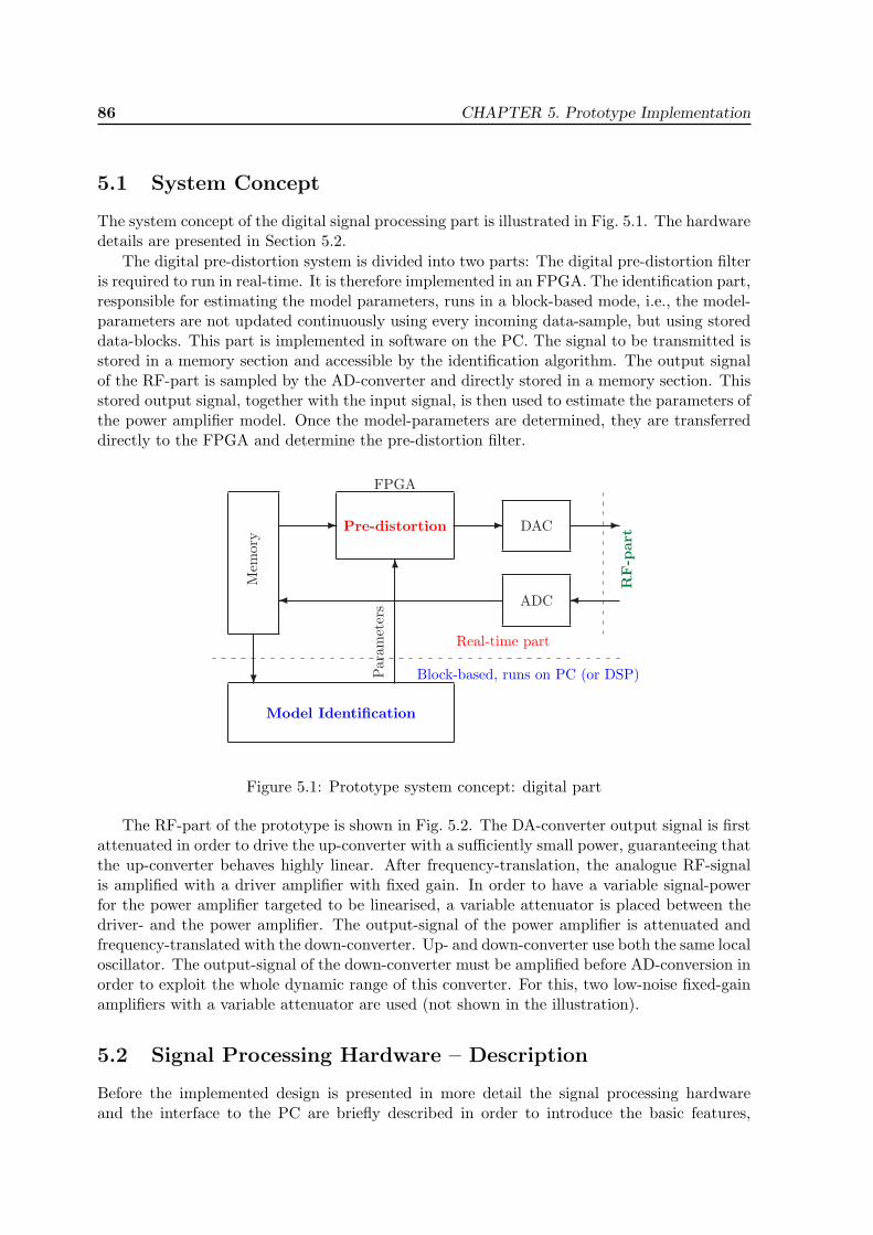
86 CHAPTER 5. Prototype Implementation
5.1 System Concept
The system concept of the digital signal processing part is illustrated in Fig. 5.1. The hardwaredetails are presented in Section 5.2.
The digital pre-distortion system is divided into two parts: The digital pre-distortion filteris required to run in real-time. It is therefore implemented in an FPGA. The identification part,responsible for estimating the model parameters, runs in a block-based mode, i.e., the model-parameters are not updated continuously using every incoming data-sample, but using storeddata-blocks. This part is implemented in software on the PC. The signal to be transmitted isstored in a memory section and accessible by the identification algorithm. The output signalof the RF-part is sampled by the AD-converter and directly stored in a memory section. Thisstored output signal, together with the input signal, is then used to estimate the parameters ofthe power amplifier model. Once the model-parameters are determined, they are transferreddirectly to the FPGA and determine the pre-distortion filter.
Mem
ory
Pre-distortion DAC
ADC
Model Identification
� � �
��
�
�
Par
amet
ers
Real-time part
Block-based, runs on PC (or DSP)
RF-p
art
FPGA
Figure 5.1: Prototype system concept: digital part
The RF-part of the prototype is shown in Fig. 5.2. The DA-converter output signal is firstattenuated in order to drive the up-converter with a sufficiently small power, guaranteeing thatthe up-converter behaves highly linear. After frequency-translation, the analogue RF-signalis amplified with a driver amplifier with fixed gain. In order to have a variable signal-powerfor the power amplifier targeted to be linearised, a variable attenuator is placed between thedriver- and the power amplifier. The output-signal of the power amplifier is attenuated andfrequency-translated with the down-converter. Up- and down-converter use both the same localoscillator. The output-signal of the down-converter must be amplified before AD-conversion inorder to exploit the whole dynamic range of this converter. For this, two low-noise fixed-gainamplifiers with a variable attenuator are used (not shown in the illustration).
5.2 Signal Processing Hardware – Description
Before the implemented design is presented in more detail the signal processing hardwareand the interface to the PC are briefly described in order to introduce the basic features,
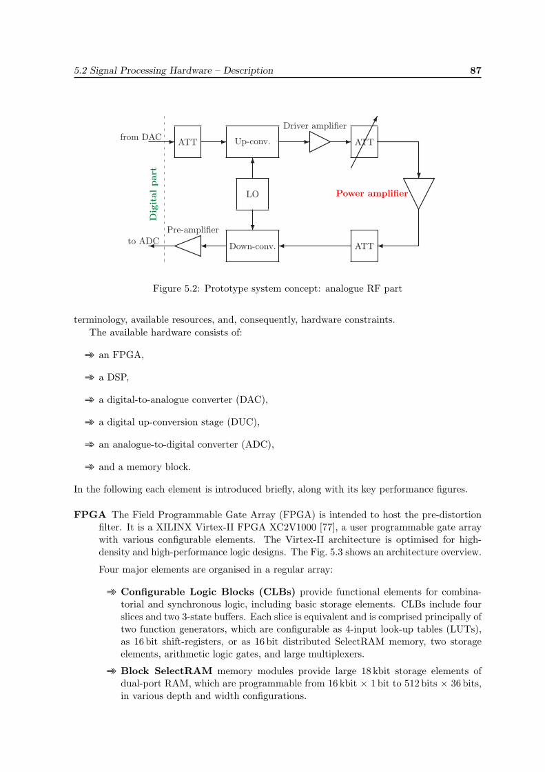
5.2 Signal Processing Hardware – Description 87
ATT Up-conv.
Down-conv.
ATT
ATT
LO
�
�
�
� � � �
�
����
from DAC
to ADCPre-amplifier
Driver amplifier
Power amplifier
Dig
ital
par
t
Figure 5.2: Prototype system concept: analogue RF part
terminology, available resources, and, consequently, hardware constraints.The available hardware consists of:
➾ an FPGA,
➾ a DSP,
➾ a digital-to-analogue converter (DAC),
➾ a digital up-conversion stage (DUC),
➾ an analogue-to-digital converter (ADC),
➾ and a memory block.
In the following each element is introduced briefly, along with its key performance figures.
FPGA The Field Programmable Gate Array (FPGA) is intended to host the pre-distortionfilter. It is a XILINX Virtex-II FPGA XC2V1000 [77], a user programmable gate arraywith various configurable elements. The Virtex-II architecture is optimised for high-density and high-performance logic designs. The Fig. 5.3 shows an architecture overview.
Four major elements are organised in a regular array:
➾ Configurable Logic Blocks (CLBs) provide functional elements for combina-torial and synchronous logic, including basic storage elements. CLBs include fourslices and two 3-state buffers. Each slice is equivalent and is comprised principally oftwo function generators, which are configurable as 4-input look-up tables (LUTs),as 16 bit shift-registers, or as 16 bit distributed SelectRAM memory, two storageelements, arithmetic logic gates, and large multiplexers.
➾ Block SelectRAM memory modules provide large 18 kbit storage elements ofdual-port RAM, which are programmable from 16 kbit × 1 bit to 512 bits × 36 bits,in various depth and width configurations.
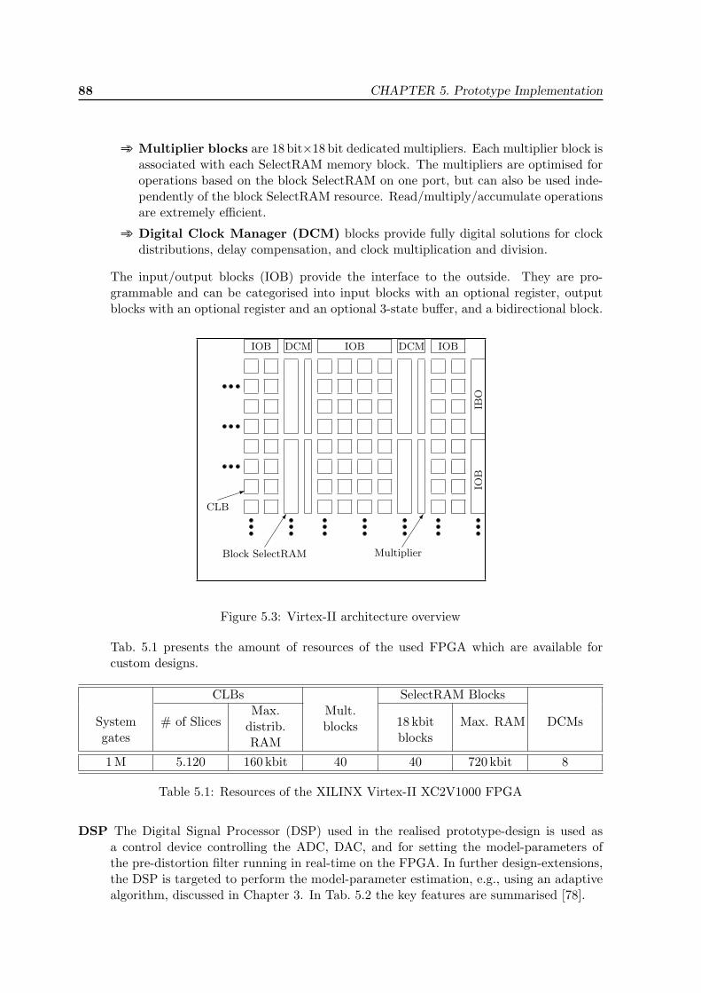
88 CHAPTER 5. Prototype Implementation
➾ Multiplier blocks are 18 bit×18 bit dedicated multipliers. Each multiplier block isassociated with each SelectRAM memory block. The multipliers are optimised foroperations based on the block SelectRAM on one port, but can also be used inde-pendently of the block SelectRAM resource. Read/multiply/accumulate operationsare extremely efficient.
➾ Digital Clock Manager (DCM) blocks provide fully digital solutions for clockdistributions, delay compensation, and clock multiplication and division.
The input/output blocks (IOB) provide the interface to the outside. They are pro-grammable and can be categorised into input blocks with an optional register, outputblocks with an optional register and an optional 3-state buffer, and a bidirectional block.
DCM DCMIOBIOB
CLB
�
Block SelectRAM Multiplier
� �
IOB
IBO
IOB
Figure 5.3: Virtex-II architecture overview
Tab. 5.1 presents the amount of resources of the used FPGA which are available forcustom designs.
CLBs SelectRAM Blocks
Systemgates
# of SlicesMax.
distrib.RAM
Mult.blocks 18 kbit
blocksMax. RAM DCMs
1 M 5.120 160 kbit 40 40 720 kbit 8
Table 5.1: Resources of the XILINX Virtex-II XC2V1000 FPGA
DSP The Digital Signal Processor (DSP) used in the realised prototype-design is used asa control device controlling the ADC, DAC, and for setting the model-parameters ofthe pre-distortion filter running in real-time on the FPGA. In further design-extensions,the DSP is targeted to perform the model-parameter estimation, e.g., using an adaptivealgorithm, discussed in Chapter 3. In Tab. 5.2 the key features are summarised [78].
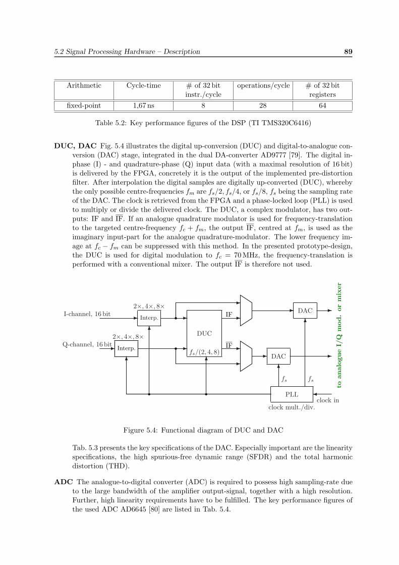
5.2 Signal Processing Hardware – Description 89
Arithmetic Cycle-time # of 32 bitinstr./cycle
operations/cycle # of 32 bitregisters
fixed-point 1,67 ns 8 28 64
Table 5.2: Key performance figures of the DSP (TI TMS320C6416)
DUC, DAC Fig. 5.4 illustrates the digital up-conversion (DUC) and digital-to-analogue con-version (DAC) stage, integrated in the dual DA-converter AD9777 [79]. The digital in-phase (I) - and quadrature-phase (Q) input data (with a maximal resolution of 16 bit)is delivered by the FPGA, concretely it is the output of the implemented pre-distortionfilter. After interpolation the digital samples are digitally up-converted (DUC), wherebythe only possible centre-frequencies fm are fs/2, fs/4, or fs/8, fs being the sampling rateof the DAC. The clock is retrieved from the FPGA and a phase-locked loop (PLL) is usedto multiply or divide the delivered clock. The DUC, a complex modulator, has two out-puts: IF and IF. If an analogue quadrature modulator is used for frequency-translationto the targeted centre-frequency fc + fm, the output IF, centred at fm, is used as theimaginary input-part for the analogue quadrature-modulator. The lower frequency im-age at fc − fm can be suppressed with this method. In the presented prototype-design,the DUC is used for digital modulation to fc = 70MHz, the frequency-translation isperformed with a conventional mixer. The output IF is therefore not used.
Interp.
DUC
� DAC
PLL
�
�
�
�
�
�
� DAC �
�
�
�
�
�
�
2×, 4×, 8×
I-channel, 16 bit
�
�
clock mult./div.
2×, 4×, 8×
Q-channel, 16 bit
�
fs fs
clock in
fs/(2, 4, 8)
IF
IFto
anal
ogue
I/Q
mod.
orm
ixer
Interp.
Figure 5.4: Functional diagram of DUC and DAC
Tab. 5.3 presents the key specifications of the DAC. Especially important are the linearityspecifications, the high spurious-free dynamic range (SFDR) and the total harmonicdistortion (THD).
ADC The analogue-to-digital converter (ADC) is required to possess high sampling-rate dueto the large bandwidth of the amplifier output-signal, together with a high resolution.Further, high linearity requirements have to be fulfilled. The key performance figures ofthe used ADC AD6645 [80] are listed in Tab. 5.4.
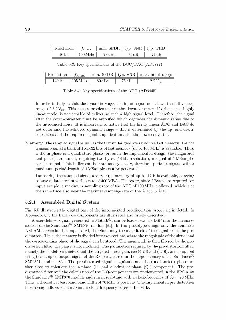
90 CHAPTER 5. Prototype Implementation
Resolution fs,max min. SFDR typ. SNR typ. THD16 bit 400 MHz 73 dBc 75 dB -71 dB
Table 5.3: Key specifications of the DUC/DAC (AD9777)
Resolution fs,max min. SFDR typ. SNR max. input range14 bit 105 MHz 89 dBc 75 dB 2,2Vss
Table 5.4: Key specifications of the ADC (AD6645)
In order to fully exploit the dynamic range, the input signal must have the full voltagerange of 2,2 Vss. This causes problems since the down-converter, if driven in a highlylinear mode, is not capable of delivering such a high signal level. Therefore, the signalafter the down-converter must be amplified which degrades the dynamic range due tothe introduced noise. It is important to notice that the highly linear ADC and DAC donot determine the achieved dynamic range – this is determined by the up- and down-converters and the required signal-amplification after the down-converter.
Memory The sampled signal as well as the transmit-signal are saved in a fast memory. For thetransmit-signal a bank of 1 M×32 bits of fast memory (up to 166 MHz) is available. Thus,if the in-phase and quadrature-phase (or, as in the implemented design, the magnitudeand phase) are stored, requiring two bytes (14 bit resolution), a signal of 1 MSamplescan be stored. This buffer can be read-out cyclically, therefore, periodic signals with amaximum period-length of 1 MSamples can be generated.
For storing the sampled signal a very large memory of up to 2 GB is available, allowingto save a data stream with a rate of 400 MB/s. Therefore, since 2 Bytes are required perinput sample, a maximum sampling rate of the ADC of 100 MHz is allowed, which is atthe same time also near the maximal sampling-rate of the AD6645 ADC.
5.2.1 Assembled Digital System
Fig. 5.5 illustrates the digital part of the implemented pre-distortion prototype in detail. InAppendix C.3 the hardware components are illustrated and briefly described.
A user-defined signal, generated in Matlab R©, can be loaded via the DSP into the memory-section of the Sundance R© SMT370 module [81]. In this prototype-design only the nonlinearAM-AM conversion is compensated, therefore, only the magnitude of the signal has to be pre-distorted. Thus, the memory is divided into two sections where the magnitude of the signal andthe corresponding phase of the signal can be stored. The magnitude is then filtered by the pre-distortion filter, the phase is not modified. The parameters required by the pre-distortion filter,namely the model-parameters and the targeted linear gain, see (4.23) and (4.16), are computedusing the sampled output signal of the RF-part, stored in the large memory of the Sundance R©
SMT351 module [82]. The pre-distorted signal magnitude and the (undistorted) phase arethen used to calculate the in-phase (I-) and quadrature-phase (Q-) component. The pre-distortion filter and the calculation of the I/Q-components are implemented in the FPGA onthe Sundance R© SMT370 module and run in real-time with a clock-frequency of fT = 70MHz.Thus, a theoretical baseband bandwidth of 70 MHz is possible. The implemented pre-distortionfilter design allows for a maximum clock-frequency of fT = 133MHz.
5.2Sign
alP
rocessin
gH
ardw
are–
Descrip
tion91
DPD-filter
to I/Q
Interp.
Interp.DUC DAC
ADC2 GB MemoryDSP Matlab
� �
�
�
�
�
�
� �
MemoryFPGA DUC/DAC
Mag.
Phase
�
��
� � � �
Sundance SMT370
Sundance SMT365 PC Sundance SMT351
Tx
sign
alup
load
Mod
elpa
ram
.se
t
Model param. estim.
4×
4×
fm =fs/4=70 MHz
fs =280 MHz
fT =70 MHz
fT =70 MHz
fT =70 MHz
z(t)
y(t)
zI [n]
zQ[n]
fs =100 MHz
16 bit
14 bit
�configure
u[n]
PC
Ibus
PC
Ibus
Figure 5.5: Digital part of the pre-distortion prototype in detail
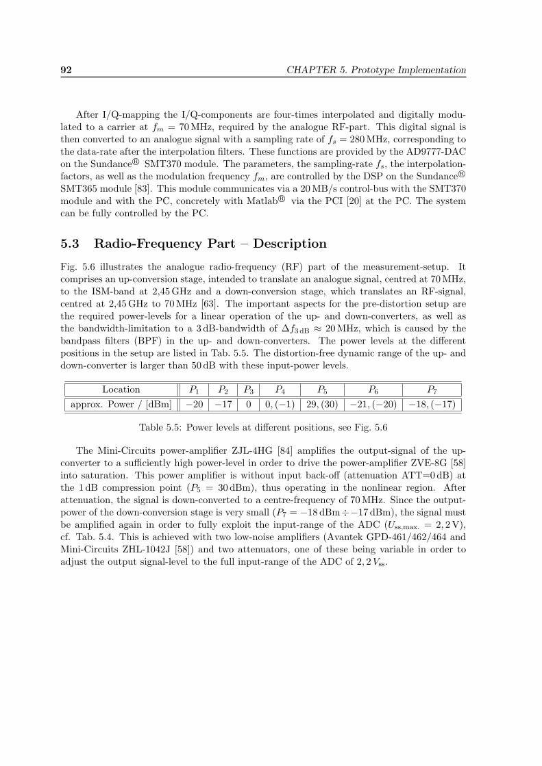
92 CHAPTER 5. Prototype Implementation
After I/Q-mapping the I/Q-components are four-times interpolated and digitally modu-lated to a carrier at fm = 70MHz, required by the analogue RF-part. This digital signal isthen converted to an analogue signal with a sampling rate of fs = 280MHz, corresponding tothe data-rate after the interpolation filters. These functions are provided by the AD9777-DACon the Sundance R© SMT370 module. The parameters, the sampling-rate fs, the interpolation-factors, as well as the modulation frequency fm, are controlled by the DSP on the Sundance R©
SMT365 module [83]. This module communicates via a 20 MB/s control-bus with the SMT370module and with the PC, concretely with Matlab R© via the PCI [20] at the PC. The systemcan be fully controlled by the PC.
5.3 Radio-Frequency Part – Description
Fig. 5.6 illustrates the analogue radio-frequency (RF) part of the measurement-setup. Itcomprises an up-conversion stage, intended to translate an analogue signal, centred at 70 MHz,to the ISM-band at 2,45 GHz and a down-conversion stage, which translates an RF-signal,centred at 2,45 GHz to 70MHz [63]. The important aspects for the pre-distortion setup arethe required power-levels for a linear operation of the up- and down-converters, as well asthe bandwidth-limitation to a 3 dB-bandwidth of ∆f3 dB ≈ 20 MHz, which is caused by thebandpass filters (BPF) in the up- and down-converters. The power levels at the differentpositions in the setup are listed in Tab. 5.5. The distortion-free dynamic range of the up- anddown-converter is larger than 50 dB with these input-power levels.
Location P1 P2 P3 P4 P5 P6 P7
approx. Power / [dBm] −20 −17 0 0, (−1) 29, (30) −21, (−20) −18, (−17)
Table 5.5: Power levels at different positions, see Fig. 5.6
The Mini-Circuits power-amplifier ZJL-4HG [84] amplifies the output-signal of the up-converter to a sufficiently high power-level in order to drive the power-amplifier ZVE-8G [58]into saturation. This power amplifier is without input back-off (attenuation ATT=0 dB) atthe 1 dB compression point (P5 = 30 dBm), thus operating in the nonlinear region. Afterattenuation, the signal is down-converted to a centre-frequency of 70 MHz. Since the output-power of the down-conversion stage is very small (P7 = −18 dBm÷−17 dBm), the signal mustbe amplified again in order to fully exploit the input-range of the ADC (Uss,max. = 2, 2 V),cf. Tab. 5.4. This is achieved with two low-noise amplifiers (Avantek GPD-461/462/464 andMini-Circuits ZHL-1042J [58]) and two attenuators, one of these being variable in order toadjust the output signal-level to the full input-range of the ADC of 2, 2Vss.
5.3R
adio-F
requen
cyPart
–D
escription
93
ATT BPF ATT MIX Amp BPF
LO
MIX Amp BPFAmpBPF
ATT
ATT�
� � � � � � � �
�� �����
�
�
�
�
z(t)
y(t)
ATT = 50 dB
PA, ZVE-8G
PA, ZJL-4HG
fLO =2380MHz
∆f3 dB≈20 MHz ∆f3 dB≈20MHz
∆f3 dB≈20MHz∆f3 dB≈20 MHzPre-Amp.
up-conversion: 70 MHz to 2,45 GHz
down-conversion: 2,45 GHz to 70 MHz
P1 P2 P3
ATT = 0 dB, 1 dB
P4
G ≈ 17 dB
G ≈ 30 dBP1 dB = 30dBm
P5
P6P7�
Figure 5.6: Analogue RF-part of the pre-distortion prototype
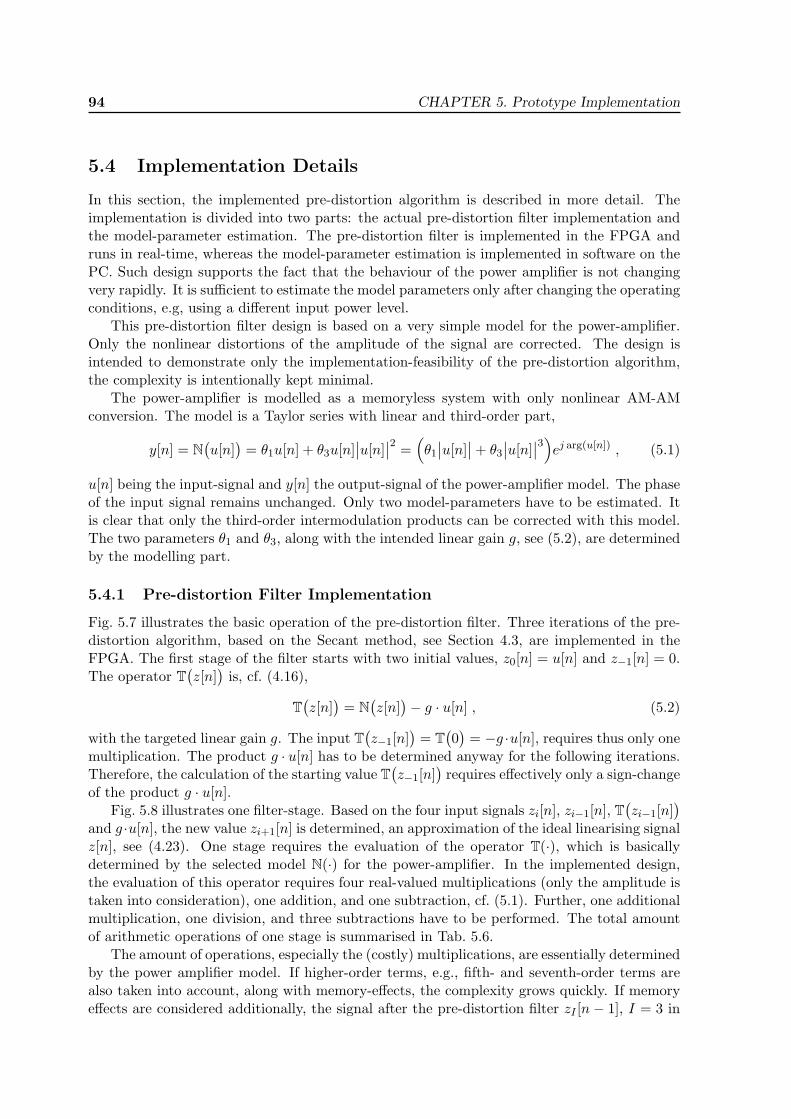
94 CHAPTER 5. Prototype Implementation
5.4 Implementation Details
In this section, the implemented pre-distortion algorithm is described in more detail. Theimplementation is divided into two parts: the actual pre-distortion filter implementation andthe model-parameter estimation. The pre-distortion filter is implemented in the FPGA andruns in real-time, whereas the model-parameter estimation is implemented in software on thePC. Such design supports the fact that the behaviour of the power amplifier is not changingvery rapidly. It is sufficient to estimate the model parameters only after changing the operatingconditions, e.g, using a different input power level.
This pre-distortion filter design is based on a very simple model for the power-amplifier.Only the nonlinear distortions of the amplitude of the signal are corrected. The design isintended to demonstrate only the implementation-feasibility of the pre-distortion algorithm,the complexity is intentionally kept minimal.
The power-amplifier is modelled as a memoryless system with only nonlinear AM-AMconversion. The model is a Taylor series with linear and third-order part,
y[n] = N(u[n]
)= θ1u[n] + θ3u[n]
∣∣u[n]∣∣2 =
(θ1∣∣u[n]
∣∣+ θ3∣∣u[n]
∣∣3)ej arg(u[n]) , (5.1)
u[n] being the input-signal and y[n] the output-signal of the power-amplifier model. The phaseof the input signal remains unchanged. Only two model-parameters have to be estimated. Itis clear that only the third-order intermodulation products can be corrected with this model.The two parameters θ1 and θ3, along with the intended linear gain g, see (5.2), are determinedby the modelling part.
5.4.1 Pre-distortion Filter Implementation
Fig. 5.7 illustrates the basic operation of the pre-distortion filter. Three iterations of the pre-distortion algorithm, based on the Secant method, see Section 4.3, are implemented in theFPGA. The first stage of the filter starts with two initial values, z0[n] = u[n] and z−1[n] = 0.The operator T
(z[n]
)is, cf. (4.16),
T(z[n]
)= N
(z[n]
)− g · u[n] , (5.2)
with the targeted linear gain g. The input T(z−1[n]
)= T
(0)
= −g ·u[n], requires thus only onemultiplication. The product g · u[n] has to be determined anyway for the following iterations.Therefore, the calculation of the starting value T
(z−1[n]
)requires effectively only a sign-change
of the product g · u[n].Fig. 5.8 illustrates one filter-stage. Based on the four input signals zi[n], zi−1[n], T
(zi−1[n]
)and g ·u[n], the new value zi+1[n] is determined, an approximation of the ideal linearising signalz[n], see (4.23). One stage requires the evaluation of the operator T(·), which is basicallydetermined by the selected model N(·) for the power-amplifier. In the implemented design,the evaluation of this operator requires four real-valued multiplications (only the amplitude istaken into consideration), one addition, and one subtraction, cf. (5.1). Further, one additionalmultiplication, one division, and three subtractions have to be performed. The total amountof arithmetic operations of one stage is summarised in Tab. 5.6.
The amount of operations, especially the (costly) multiplications, are essentially determinedby the power amplifier model. If higher-order terms, e.g., fifth- and seventh-order terms arealso taken into account, along with memory-effects, the complexity grows quickly. If memoryeffects are considered additionally, the signal after the pre-distortion filter zI [n− 1], I = 3 in
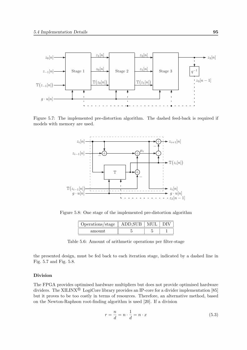
5.4 Implementation Details 95
Stage 1 Stage 2 Stage 3
�
�
�
� �
� � q−1
� �
��� � � �
�
�z0[n]
z0[n]z−1[n]
z1[n]
z1[n]
z2[n]z3[n]
T(z−1[n]
) T(z0[n]
)T
(z1[n]
) z3[n − 1]
g · u[n]
Figure 5.7: The implemented pre-distortion algorithm. The dashed feed-back is required ifmodels with memory are used.
T
+
�
� +�
+�
�
÷ µi��
·��
�
��
�
�
−
−
−zi[n]
zi−1[n]
T(zi−1[n]
)�
�g · u[n]
zi+1[n]
T(zi[n]
)
zi[n]g · u[n]
�
zI [n− 1]
Figure 5.8: One stage of the implemented pre-distortion algorithm
Operations/stage ADD,SUB MUL DIVamount 5 5 1
Table 5.6: Amount of arithmetic operations per filter-stage
the presented design, must be fed back to each iteration stage, indicated by a dashed line inFig. 5.7 and Fig. 5.8.
Division
The FPGA provides optimised hardware multipliers but does not provide optimised hardwaredividers. The XILINX R© LogiCore library provides an IP-core for a divider implementation [85]but it proves to be too costly in terms of resources. Therefore, an alternative method, basedon the Newton-Raphson root-finding algorithm is used [20]. If a division
r =n
d= n · 1
d= n · x (5.3)
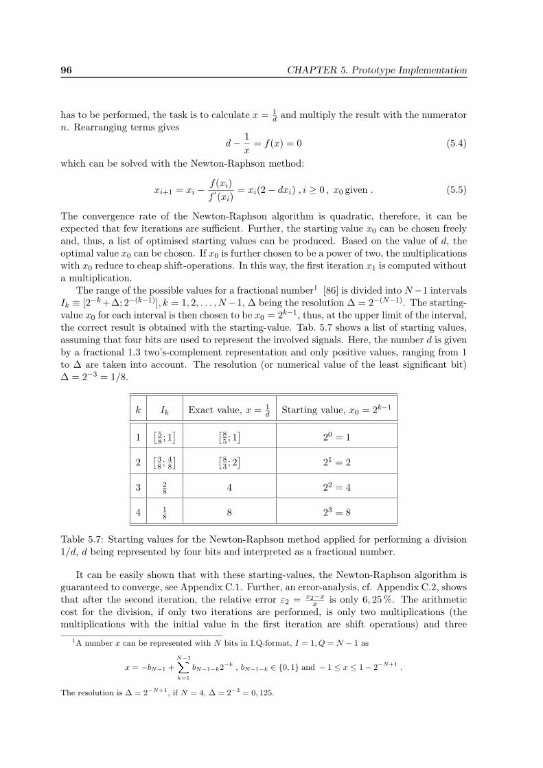
96 CHAPTER 5. Prototype Implementation
has to be performed, the task is to calculate x = 1d and multiply the result with the numerator
n. Rearranging terms gives
d− 1x
= f(x) = 0 (5.4)
which can be solved with the Newton-Raphson method:
xi+1 = xi −f(xi)f ′(xi)
= xi(2− dxi) , i ≥ 0 , x0 given . (5.5)
The convergence rate of the Newton-Raphson algorithm is quadratic, therefore, it can beexpected that few iterations are sufficient. Further, the starting value x0 can be chosen freelyand, thus, a list of optimised starting values can be produced. Based on the value of d, theoptimal value x0 can be chosen. If x0 is further chosen to be a power of two, the multiplicationswith x0 reduce to cheap shift-operations. In this way, the first iteration x1 is computed withouta multiplication.
The range of the possible values for a fractional number1 [86] is divided into N−1 intervalsIk ≡ [2−k+∆; 2−(k−1)], k = 1, 2, . . . , N−1, ∆ being the resolution ∆ = 2−(N−1). The starting-value x0 for each interval is then chosen to be x0 = 2k−1, thus, at the upper limit of the interval,the correct result is obtained with the starting-value. Tab. 5.7 shows a list of starting values,assuming that four bits are used to represent the involved signals. Here, the number d is givenby a fractional 1.3 two’s-complement representation and only positive values, ranging from 1to ∆ are taken into account. The resolution (or numerical value of the least significant bit)∆ = 2−3 = 1/8.
k Ik Exact value, x = 1d Starting value, x0 = 2k−1
1[
58 ; 1] [
85 ; 1]
20 = 1
2[
38 ; 4
8
] [83 ; 2]
21 = 2
3 28 4 22 = 4
4 18 8 23 = 8
Table 5.7: Starting values for the Newton-Raphson method applied for performing a division1/d, d being represented by four bits and interpreted as a fractional number.
It can be easily shown that with these starting-values, the Newton-Raphson algorithm isguaranteed to converge, see Appendix C.1. Further, an error-analysis, cf. Appendix C.2, showsthat after the second iteration, the relative error ε2 = x2−x
x is only 6, 25 %. The arithmeticcost for the division, if only two iterations are performed, is only two multiplications (themultiplications with the initial value in the first iteration are shift operations) and three
1A number x can be represented with N bits in I.Q-format, I = 1, Q = N − 1 as
x = −bN−1 +
N−1X
k=1
bN−1−k2−k , bN−1−k ∈ {0, 1} and − 1 ≤ x ≤ 1− 2−N+1 .
The resolution is ∆ = 2−N+1, if N = 4, ∆ = 2−3 = 0, 125.
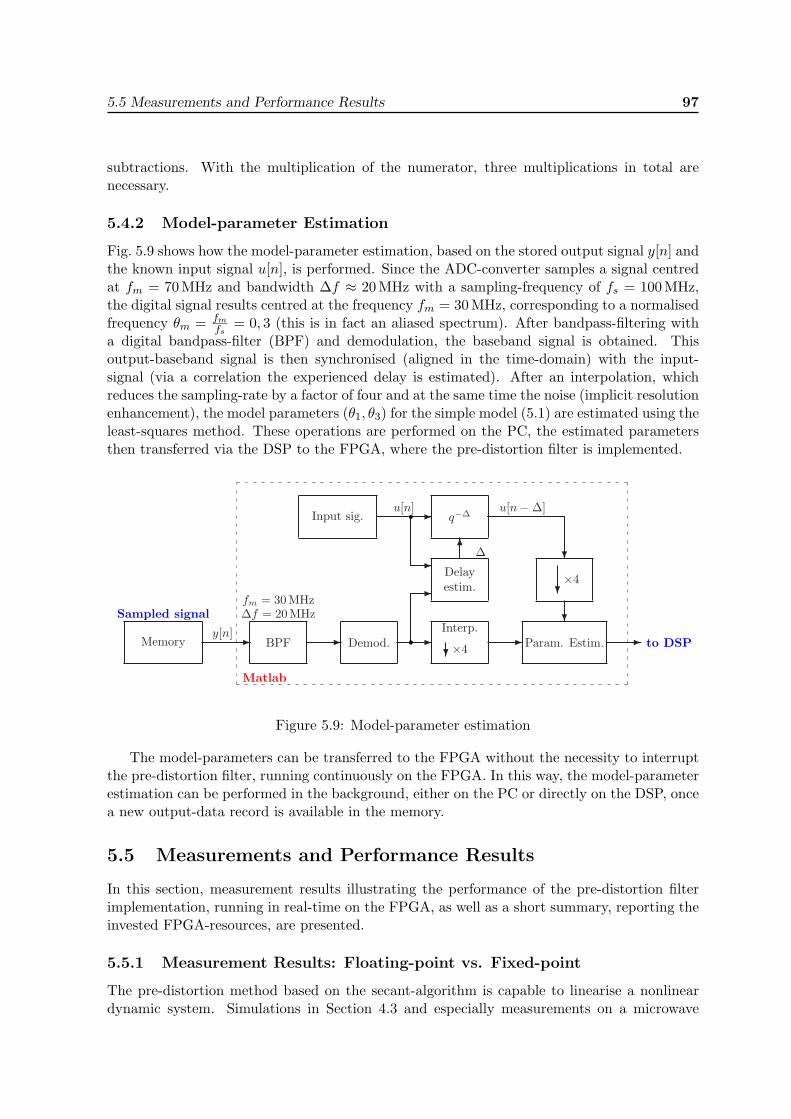
5.5 Measurements and Performance Results 97
subtractions. With the multiplication of the numerator, three multiplications in total arenecessary.
5.4.2 Model-parameter Estimation
Fig. 5.9 shows how the model-parameter estimation, based on the stored output signal y[n] andthe known input signal u[n], is performed. Since the ADC-converter samples a signal centredat fm = 70 MHz and bandwidth ∆f ≈ 20 MHz with a sampling-frequency of fs = 100 MHz,the digital signal results centred at the frequency fm = 30MHz, corresponding to a normalisedfrequency θm = fm
fs= 0, 3 (this is in fact an aliased spectrum). After bandpass-filtering with
a digital bandpass-filter (BPF) and demodulation, the baseband signal is obtained. Thisoutput-baseband signal is then synchronised (aligned in the time-domain) with the input-signal (via a correlation the experienced delay is estimated). After an interpolation, whichreduces the sampling-rate by a factor of four and at the same time the noise (implicit resolutionenhancement), the model parameters (θ1, θ3) for the simple model (5.1) are estimated using theleast-squares method. These operations are performed on the PC, the estimated parametersthen transferred via the DSP to the FPGA, where the pre-distortion filter is implemented.
Memory BPF Demod.
Delayestim.
Input sig.
Param. Estim.� � � � �
�
�
�×4
q−∆
to DSPy[n]
u[n] u[n−∆]
�×4
�
�
Matlab
Sampled signalfm = 30MHz∆f = 20MHz
Interp.
∆�
�
Figure 5.9: Model-parameter estimation
The model-parameters can be transferred to the FPGA without the necessity to interruptthe pre-distortion filter, running continuously on the FPGA. In this way, the model-parameterestimation can be performed in the background, either on the PC or directly on the DSP, oncea new output-data record is available in the memory.
5.5 Measurements and Performance Results
In this section, measurement results illustrating the performance of the pre-distortion filterimplementation, running in real-time on the FPGA, as well as a short summary, reporting theinvested FPGA-resources, are presented.
5.5.1 Measurement Results: Floating-point vs. Fixed-point
The pre-distortion method based on the secant-algorithm is capable to linearise a nonlineardynamic system. Simulations in Section 4.3 and especially measurements on a microwave
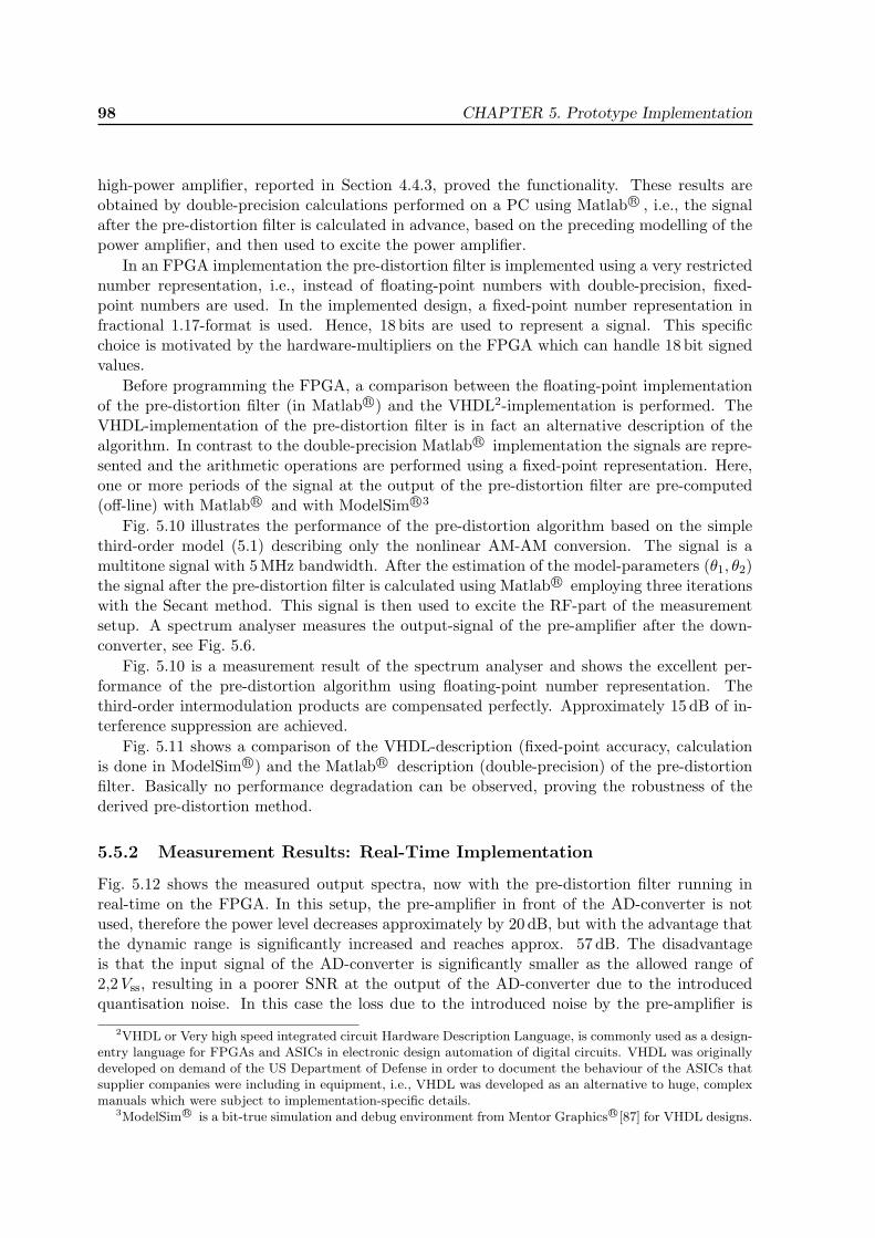
98 CHAPTER 5. Prototype Implementation
high-power amplifier, reported in Section 4.4.3, proved the functionality. These results areobtained by double-precision calculations performed on a PC using Matlab R© , i.e., the signalafter the pre-distortion filter is calculated in advance, based on the preceding modelling of thepower amplifier, and then used to excite the power amplifier.
In an FPGA implementation the pre-distortion filter is implemented using a very restrictednumber representation, i.e., instead of floating-point numbers with double-precision, fixed-point numbers are used. In the implemented design, a fixed-point number representation infractional 1.17-format is used. Hence, 18 bits are used to represent a signal. This specificchoice is motivated by the hardware-multipliers on the FPGA which can handle 18 bit signedvalues.
Before programming the FPGA, a comparison between the floating-point implementationof the pre-distortion filter (in Matlab R©) and the VHDL2-implementation is performed. TheVHDL-implementation of the pre-distortion filter is in fact an alternative description of thealgorithm. In contrast to the double-precision Matlab R© implementation the signals are repre-sented and the arithmetic operations are performed using a fixed-point representation. Here,one or more periods of the signal at the output of the pre-distortion filter are pre-computed(off-line) with Matlab R© and with ModelSim R©3
Fig. 5.10 illustrates the performance of the pre-distortion algorithm based on the simplethird-order model (5.1) describing only the nonlinear AM-AM conversion. The signal is amultitone signal with 5MHz bandwidth. After the estimation of the model-parameters (θ1, θ2)the signal after the pre-distortion filter is calculated using Matlab R© employing three iterationswith the Secant method. This signal is then used to excite the RF-part of the measurementsetup. A spectrum analyser measures the output-signal of the pre-amplifier after the down-converter, see Fig. 5.6.
Fig. 5.10 is a measurement result of the spectrum analyser and shows the excellent per-formance of the pre-distortion algorithm using floating-point number representation. Thethird-order intermodulation products are compensated perfectly. Approximately 15 dB of in-terference suppression are achieved.
Fig. 5.11 shows a comparison of the VHDL-description (fixed-point accuracy, calculationis done in ModelSim R©) and the Matlab R© description (double-precision) of the pre-distortionfilter. Basically no performance degradation can be observed, proving the robustness of thederived pre-distortion method.
5.5.2 Measurement Results: Real-Time Implementation
Fig. 5.12 shows the measured output spectra, now with the pre-distortion filter running inreal-time on the FPGA. In this setup, the pre-amplifier in front of the AD-converter is notused, therefore the power level decreases approximately by 20 dB, but with the advantage thatthe dynamic range is significantly increased and reaches approx. 57 dB. The disadvantageis that the input signal of the AD-converter is significantly smaller as the allowed range of2,2Vss, resulting in a poorer SNR at the output of the AD-converter due to the introducedquantisation noise. In this case the loss due to the introduced noise by the pre-amplifier is
2VHDL or Very high speed integrated circuit Hardware Description Language, is commonly used as a design-entry language for FPGAs and ASICs in electronic design automation of digital circuits. VHDL was originallydeveloped on demand of the US Department of Defense in order to document the behaviour of the ASICs thatsupplier companies were including in equipment, i.e., VHDL was developed as an alternative to huge, complexmanuals which were subject to implementation-specific details.
3ModelSimR© is a bit-true simulation and debug environment from Mentor GraphicsR©[87] for VHDL designs.
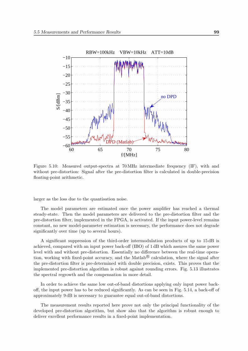
5.5 Measurements and Performance Results 99
60 65 70 75 80−60
−55
−50
−45
−40
−35
−30
−25
−20
−15
−10 RBW=100kHz VBW=10kHz ATT=10dB
f/[MHz]
S/[d
Bm
]
no DPD
DPD (Matlab)
Figure 5.10: Measured output-spectra at 70 MHz intermediate frequency (IF), with andwithout pre-distortion: Signal after the pre-distortion filter is calculated in double-precisionfloating-point arithmetic.
larger as the loss due to the quantisation noise.
The model parameters are estimated once the power amplifier has reached a thermalsteady-state. Then the model parameters are delivered to the pre-distortion filter and thepre-distortion filter, implemented in the FPGA, is activated. If the input power-level remainsconstant, no new model-parameter estimation is necessary, the performance does not degradesignificantly over time (up to several hours).
A significant suppression of the third-order intermodulation products of up to 15 dB isachieved, compared with an input power back-off (IBO) of 1 dB which assures the same powerlevel with and without pre-distortion. Essentially no difference between the real-time opera-tion, working with fixed-point accuracy, and the Matlab R© calculation, where the signal afterthe pre-distortion filter is pre-determined with double precision, exists. This proves that theimplemented pre-distortion algorithm is robust against rounding errors. Fig. 5.13 illustratesthe spectral regrowth and the compensation in more detail.
In order to achieve the same low out-of-band distortions applying only input power back-off, the input power has to be reduced significantly. As can be seen in Fig. 5.14, a back-off ofapproximately 9 dB is necessary to guarantee equal out-of-band distortions.
The measurement results reported here prove not only the principal functionality of thedeveloped pre-distortion algorithm, but show also that the algorithm is robust enough todeliver excellent performance results in a fixed-point implementation.
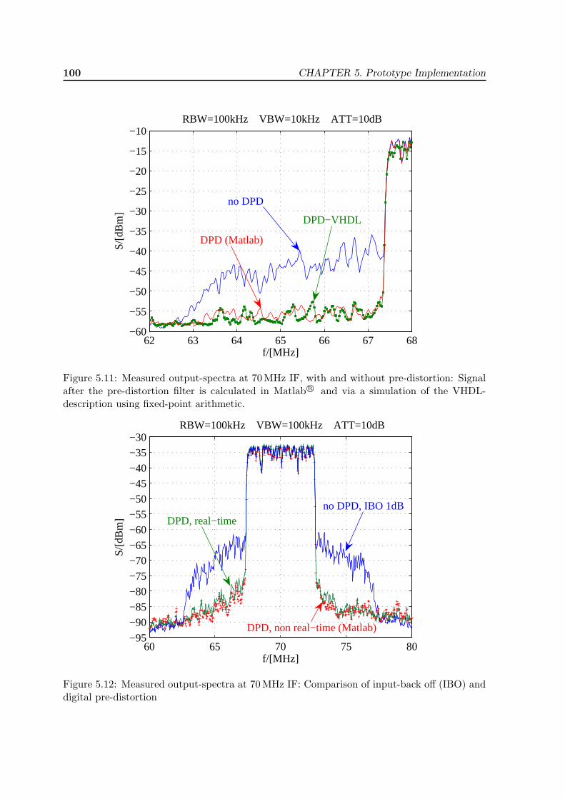
100 CHAPTER 5. Prototype Implementation
62 63 64 65 66 67 68−60
−55
−50
−45
−40
−35
−30
−25
−20
−15
−10 RBW=100kHz VBW=10kHz ATT=10dB
f/[MHz]
S/[d
Bm
]
no DPD
DPD (Matlab)
DPD−VHDL
Figure 5.11: Measured output-spectra at 70MHz IF, with and without pre-distortion: Signalafter the pre-distortion filter is calculated in Matlab R© and via a simulation of the VHDL-description using fixed-point arithmetic.
60 65 70 75 80−95
−90
−85
−80
−75
−70
−65
−60
−55
−50
−45
−40
−35
−30 RBW=100kHz VBW=100kHz ATT=10dB
f/[MHz]
S/[d
Bm
]
no DPD, IBO 1dB
DPD, non real−time (Matlab)
DPD, real−time
Figure 5.12: Measured output-spectra at 70 MHz IF: Comparison of input-back off (IBO) anddigital pre-distortion
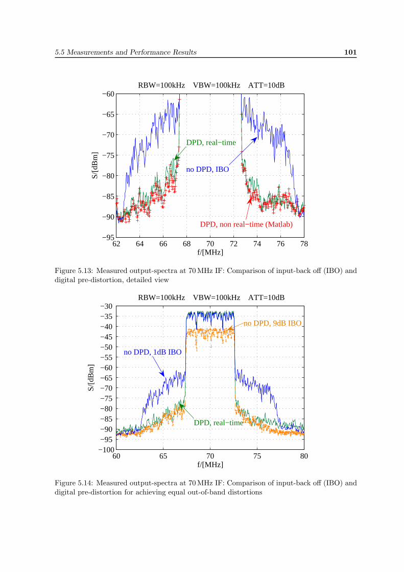
5.5 Measurements and Performance Results 101
62 64 66 68 70 72 74 76 78−95
−90
−85
−80
−75
−70
−65
−60 RBW=100kHz VBW=100kHz ATT=10dB
f/[MHz]
S/[d
Bm
]
no DPD, IBO
DPD, non real−time (Matlab)
DPD, real−time
Figure 5.13: Measured output-spectra at 70 MHz IF: Comparison of input-back off (IBO) anddigital pre-distortion, detailed view
60 65 70 75 80−100−95 −90 −85 −80 −75 −70 −65 −60 −55 −50 −45 −40 −35 −30
RBW=100kHz VBW=100kHz ATT=10dB
f/[MHz]
S/[d
Bm
]
no DPD, 1dB IBO
no DPD, 9dB IBO
DPD, real−time
Figure 5.14: Measured output-spectra at 70 MHz IF: Comparison of input-back off (IBO) anddigital pre-distortion for achieving equal out-of-band distortions
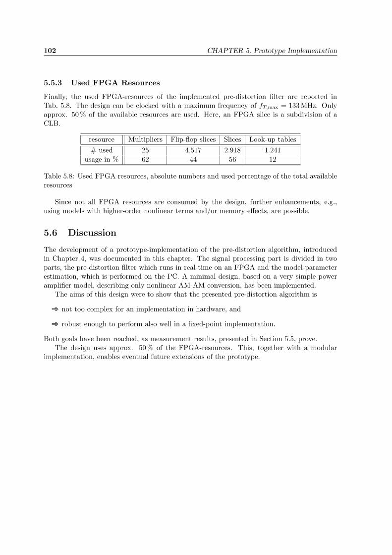
102 CHAPTER 5. Prototype Implementation
5.5.3 Used FPGA Resources
Finally, the used FPGA-resources of the implemented pre-distortion filter are reported inTab. 5.8. The design can be clocked with a maximum frequency of fT,max = 133 MHz. Onlyapprox. 50 % of the available resources are used. Here, an FPGA slice is a subdivision of aCLB.
resource Multipliers Flip-flop slices Slices Look-up tables# used 25 4.517 2.918 1.241
usage in % 62 44 56 12
Table 5.8: Used FPGA resources, absolute numbers and used percentage of the total availableresources
Since not all FPGA resources are consumed by the design, further enhancements, e.g.,using models with higher-order nonlinear terms and/or memory effects, are possible.
5.6 Discussion
The development of a prototype-implementation of the pre-distortion algorithm, introducedin Chapter 4, was documented in this chapter. The signal processing part is divided in twoparts, the pre-distortion filter which runs in real-time on an FPGA and the model-parameterestimation, which is performed on the PC. A minimal design, based on a very simple poweramplifier model, describing only nonlinear AM-AM conversion, has been implemented.
The aims of this design were to show that the presented pre-distortion algorithm is
➾ not too complex for an implementation in hardware, and
➾ robust enough to perform also well in a fixed-point implementation.
Both goals have been reached, as measurement results, presented in Section 5.5, prove.The design uses approx. 50% of the FPGA-resources. This, together with a modular
implementation, enables eventual future extensions of the prototype.
Chapter 6
Conclusions
This thesis addressed digital pre-distortion for linearisation of nonlinear and dynamic mi-crowave power amplifiers. The aim was the development of a linearisation algorithm which iscapable of linearising a variety of power amplifiers. Such algorithm had to be implemented ina prototype system in order to prove its practical value.
The devised linearisation method can be considered as very flexible, capable of being ap-plied in a plurality of applications with different degrees of complexity. These applications canrange from power amplifier linearisation in mobile communication base-stations of the secondgeneration to multichannel arrangements in base-stations of the third- and future generations,as well as applications in high data-rate wireless local area networks.
En route to the implementation of a prototype pre-distortion system, four main tasks havebeen addressed:
1. Modelling of the microwave power amplifier
2. Low complex and robust identification of the model parameters
3. Development of a pre-distortion algorithm
4. Implementation in signal processing hardware
Various models for nonlinear and dynamic microwave power amplifies have been evalu-ated. The aim was to identify possible accurate and low-complex candidates for power am-plifier models. Based on time-domain measurements on different microwave power amplifiersit was shown that low-order nonlinearities, i.e., up to nonlinear order seven, are sufficient foran accurate description of the nonlinear effects. The investigated power amplifiers showedfurther that memory effects are rather concentrated, meaning that the kernel-lengths of, e.g.,a Volterra model, are short. It was further shown that low complex models, such as Wiener-or Hammerstein models, are adequate.
Adaptive gradient-type identification schemes for the identification of the parameters ofa Volterra- and Wiener systems have been presented. The stability analysis of the derivedadaptive algorithms was performed in a deterministic context. The common stochastic analysisfails because important information regarding the statistics of the signals and required partialknowledge of system characteristics is in practical applications missing. The deterministicanalysis provided furthermore very strong results about the stability of the devised algorithmswhich cannot be provided by a conventional stochastic analysis.
To develop an analytical solution for the pre-equaliser is rarely possible in practice. There-fore, an iterative procedure for the determination of the output signal of the pre-distortion
103

104 CHAPTER 6. Conclusions
filter has been devised. It is based on the Secant method for root-finding and applicable for allinvestigated power amplifier models, providing an approximation to the exact solution for thepre-equaliser. The presented method is therefore a powerful tool for solving the equalisationproblem in an approximate way. The derived method proved further to be advantageous interms of accuracy and complexity if compared with a known method based on a fixed-pointformulation of the pre-distortion problem.
A pre-distortion prototype system, based on the devised linearisation algorithm, has beendeveloped. The core of this hardware system is a real-time implementation of the linearisationalgorithm in an FPGA. With this experimental setup it has been shown that the derivedpre-distortion method admits also a practical implementation where only a limited amount ofresources and limited arithmetic accuracy is available. Measurement results with microwavepower amplifiers proved the excellent performance of the implemented algorithm.
Appendix A
Appendix: Adaptive Identification
Various definitions and derivations for Chapter 3 are presented.
A.1 Derivation of (3.40)
The local energy relation reads
‖θθθn‖22 +∣∣ea[n]
∣∣2 = ‖θθθn−1‖22 +∣∣¯v[n]
∣∣2 , (A.1)
using the definitions
ea[n] =õ[n]ea[n] (A.2)
¯v[n] =√µ[n]v[n] . (A.3)
The finite time-horizon n = 0, . . . , N is considered. For a derivation of the global passivityrelation using the feedback structure, the following vectors-signals are defined:
ea,N =[√
µ[0]ea[0],√µ[1]ea[1], . . . ,
õ[N ]ea[N ]
]T(A.4)
¯vN =[√
µ[0]v[0],√µ[1]v[1], . . . ,
õ[N ]v[N ]
]T. (A.5)
Summation over the time-horizon n = 0, . . . , N of (A.1) gives
‖θθθN‖22 + ‖ea,N‖22 = ‖θθθ−1‖22 + ‖¯vN‖22 . (A.6)
A lossless map T, with ‖T‖22 = 1, transforms the input-vectors θθθ−1 and ¯vN to the output-vectors θθθN and ea,N .
With the definitions
vN =[√
µ[0]v[0],√µ[1]v[1], . . . ,
õ[N ]v[N ]
]T(A.7)
GN = diag{(
1− µ[0]µ[0]
), . . . ,
(1− µ[N ]
µ[N ]
)}(A.8)
AN = diag{µ[0]µ[0]
, . . . ,µ[N ]µ[N ]
}, (A.9)
105
106 CHAPTER A. Appendix: Adaptive Identification
the system equations read[θθθNea,N
]= T
[θθθ−1
¯vN
], with ‖T‖22 = 1 (A.10)
¯vN = AN vN −GN ea,N . (A.11)
The gain of the feedback path is
gFB = ‖GN‖22 = max∣∣λ(GN )
∣∣2 = maxn=0,...,N
∣∣∣∣1− µ[n]µ[n]
∣∣∣∣2 , (A.12)
where λ(GN ) is the spectrum of the matrix GN . Using the small gain theorem [69], the systemis guaranteed to be stable if
gFB gFF < 1 , (A.13)
and, since gFF = ‖T‖22 = 1, global stability is assured if
maxn=0,...,N
∣∣∣∣1− µ[n]µ[n]
∣∣∣∣ < 1 . (A.14)
Thus, if0 < µ[n] < 2µ[n] , n = 0, . . . , N , (A.15)
the gradient algorithm is globally stable [13, 14].
A.2 Derivation of (3.67) and (3.68)
Taking the norm on both sides of the update-equation (the derivation of the passivity relationfor the update-equation (3.64) is similar)
g′n = g
′n−1 − µg[n]
(ea,g[n] + vg[n]
)x′Hn (A.16)
and simple manipulation results in
‖g′n‖22 − ‖g′n−1‖22 + µg[n]
∣∣ea,g[n]∣∣2 − µg[n]
∣∣vg[n]∣∣2 =
µg[n]∣∣ea,g[n]− vg[n]
∣∣2 (µg[n]‖x′n‖22 − 1) (A.17)
which gives, if (µg[n]‖x′n‖22 − 1
)< 0 , (A.18)
(cf. (3.65)) the passivity relation (3.67).
A.3 Derivation of (3.73)
Multiplication of the update-equation
hn = hn−1 −Mn
(ea[n] + ve[n]
)ϕϕϕHn , (A.19)
with M−1/2n yields
M−1/2n hn = M−1/2
n hn−1 −M1/2n
(ea[n] + ve[n]
)ϕϕϕHn . (A.20)
A.4 Derivation of (3.86) 107
Taking the squared `2-norm on both sides results in
hHn M−1n hn = hHn−1M
−1n hn−1 +ϕϕϕnMnϕϕϕ
Hn
∣∣ea[n] + ve[n]∣∣2 (A.21)
− 2∣∣ea[n]
∣∣2 − ea[n]v∗e [n]− e∗a[n]ve[n] .
If0 < ϕϕϕnMnϕϕϕ
Hn < 1 (A.22)
hHn M−1n hn ≤ hHn−1M
−1n hn−1 −
∣∣ea[n]∣∣2 +
∣∣ve[n]∣∣2 (A.23)
results. This gives the local passivity relation (3.73).
A.4 Derivation of (3.86)
Insertion of the modified noise
ve[n] =α[n]α[n]
ve[n]−(
1− α[n]α[n]
)ea[n] (A.24)
in √√√√ N∑n=0
α[n]∣∣ve[n]
∣∣2 =
√√√√ N∑n=0
α[n]∣∣∣∣α[n]α[n]
ve[n]−(
1− α[n]α[n]
)ea[n]
∣∣∣∣2 (A.25)
results in the upper bound√√√√ N∑n=0
α[n]∣∣ve[n]
∣∣2 ≤√√√√ N∑
n=0
α[n]∣∣∣∣α[n]α[n]
ve[n]∣∣∣∣2 +
√√√√ N∑n=0
α[n]∣∣∣∣(1− α[n]
α[n]
)ea[n]
∣∣∣∣2 . (A.26)
This can be upper bounded further√√√√ N∑n=0
α[n]∣∣∣∣α[n]α[n]
ve[n]∣∣∣∣2 +
√√√√ N∑n=0
α[n]∣∣∣∣(1− α[n]
α[n]
)ea[n]
∣∣∣∣2 (A.27)
≤ δN
√√√√ N∑n=0
α[n]∣∣ve[n]
∣∣2 + γN
√√√√ N∑n=0
α[n]∣∣ea[n]
∣∣2 ,whereby
δN = maxn=0,...,N
α[n]α[n]
(A.28)
γN = maxn=0,...,N
∣∣∣∣1− α[n]α[n]
∣∣∣∣ . (A.29)
Insertion of the upper bound (A.27) in√√√√ N∑n=0
α[n]∣∣ea[n]
∣∣2 ≤√hH−1M−1h−1 +
√√√√ N∑n=0
α[n]∣∣ve[n]
∣∣2 . (A.30)
yields after simple manipulations the global passivity relation (3.86).

108 CHAPTER A. Appendix: Adaptive Identification
Appendix B
Appendix: Linearisation byPre-distortion
B.1 The Contraction Mapping Theorem
The contraction mapping theorem can be stated as follows [49, 48]:
Contraction Mapping Theorem. If T is a contraction mapping on a closed subset S ofa Banach space1, there is a unique vector z ∈ S satisfying z = T(z). Furthermore, z can beobtained with the method of successive approximation starting from an arbitrary initial vectorin S .
The definition of a contraction mapping is
Definition. Let S be a subset of a normed space S and let T be a transformation mappingS into S . Then T is said to be a contraction mapping if there is an α, 0 ≤ α < 1 such that‖T(z1)− T(z2)‖ ≤ α‖z1 − z2‖ for all z1, z2 ∈ S .
1A Banach space is a complete normed linear vector space. A normed linear vector space X is said to becomplete if every Cauchy sequence from X has a limit in X.
109

110 CHAPTER B. Appendix: Linearisation by Pre-distortion
Appendix C
Appendix: PrototypeImplementation
C.1 Convergence of the Newton-Raphson Method Applied forDivision
A method to prove the convergence for the Newton-Raphson algorithm is based on the Con-traction Mapping Theorem, see Appendix B.1. Starting point is the iteration-rule (5.5),
xi+1 = xi −f(xi)f ′(xi)
= xi(2− d · xi) , i ≥ 0 , x0 given . (C.1)
This can be viewed as a method of successive approximation applied to the function
g(x) ≡ x− f(x)f ′(x)
= x(2− d · x). (C.2)
A fixed-point of g(x) is thus a solution to f(x) = 0. Differentiating with respect to x gives
g′d(x) = 2(1− d · x). (C.3)
The index d denotes that g′(x) is parameterised by d. For convergence,∣∣g′d(x)∣∣ < 1 , (C.4)
resulting in the limits for x12d
< x <32d
. (C.5)
If x is in this interval, g(x) is contractive. If, e.g., d ∈[
38 ; 1
2
], corresponding to the second row
in Tab. 5.7, the starting value x0 = 2 is in the corresponding intervals I1 : 43 < x < 4 for d = 3
8and I2 : 1 < x < 3 for d = 1
2 , thus being in the contractive region of g(x). It has further to beshown that the function g(x) maps the intervals also in regions where g(x) is contractive. Ascan easily be shown,
I1g(·),d=3/8−−−−−−→
[2;
83
]∈ I1 (C.6)
I2g(·),d=1/2−−−−−−→
[32; 2]∈ I2 , (C.7)
g(x) remains therefore contractive. This can be done also for the first row of Tab. 5.7, thus,the method converges for all four possibilities.
111

112 CHAPTER C. Appendix: Prototype Implementation
C.2 Error-Analysis of the Newton-Raphson Method Appliedfor Division
The relative error εi at each iteration, assuming that x = 1d is the correct value, is easily
computed as
εi =xi − x
x= d · xi − 1 . (C.8)
Corresponding to Tab. 5.7, the worst-case values of d are the lower limits in each interval, i.e.,dwc = 2−k + ∆ with k ∈ {1, N − 1} if N bits are used for the number representation, and∆ = 2−(N−1). The correct value would be x = 1
dwc= 1
2−k+∆≈ 1
2−k = 2k, assuming that ∆ issmall (large N) and k � N . The initial value is x0 = 2k−1, thus, if k � N and N �, thelargest errors result. With only the initial value, the relative error is
ε0 = dwc · x0 − 1 =(2−k + ∆
)2k−1 − 1 ≈ 2−1 − 1 = −50 % . (C.9)
The first iteration results in
x1 = x0(2− dwc · x0) = 2k−1(2− (2−k + ∆)2k−1
)≈ 2k
(1− 2−2
), (C.10)
the relative error being thus
ε1 =x1 − x
x= −2−2 = −1
4= −25 % . (C.11)
The second iterations reduces the error to
ε2 =x2 − x
x= −2−4 = − 1
16= −6, 25 % , (C.12)
according to the quadratic convergence rate of the Newton-Raphson method.
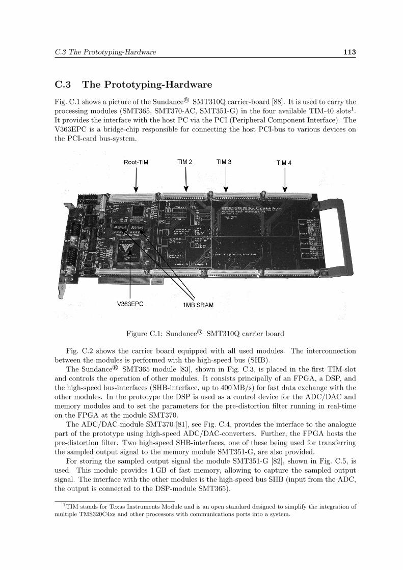
C.3 The Prototyping-Hardware 113
C.3 The Prototyping-Hardware
Fig. C.1 shows a picture of the Sundance R© SMT310Q carrier-board [88]. It is used to carry theprocessing modules (SMT365, SMT370-AC, SMT351-G) in the four available TIM-40 slots1.It provides the interface with the host PC via the PCI (Peripheral Component Interface). TheV363EPC is a bridge-chip responsible for connecting the host PCI-bus to various devices onthe PCI-card bus-system.
Figure C.1: Sundance R© SMT310Q carrier board
Fig. C.2 shows the carrier board equipped with all used modules. The interconnectionbetween the modules is performed with the high-speed bus (SHB).
The Sundance R© SMT365 module [83], shown in Fig. C.3, is placed in the first TIM-slotand controls the operation of other modules. It consists principally of an FPGA, a DSP, andthe high-speed bus-interfaces (SHB-interface, up to 400 MB/s) for fast data exchange with theother modules. In the prototype the DSP is used as a control device for the ADC/DAC andmemory modules and to set the parameters for the pre-distortion filter running in real-timeon the FPGA at the module SMT370.
The ADC/DAC-module SMT370 [81], see Fig. C.4, provides the interface to the analoguepart of the prototype using high-speed ADC/DAC-converters. Further, the FPGA hosts thepre-distortion filter. Two high-speed SHB-interfaces, one of these being used for transferringthe sampled output signal to the memory module SMT351-G, are also provided.
For storing the sampled output signal the module SMT351-G [82], shown in Fig. C.5, isused. This module provides 1 GB of fast memory, allowing to capture the sampled outputsignal. The interface with the other modules is the high-speed bus SHB (input from the ADC,the output is connected to the DSP-module SMT365).
1TIM stands for Texas Instruments Module and is an open standard designed to simplify the integration ofmultiple TMS320C4xs and other processors with communications ports into a system.
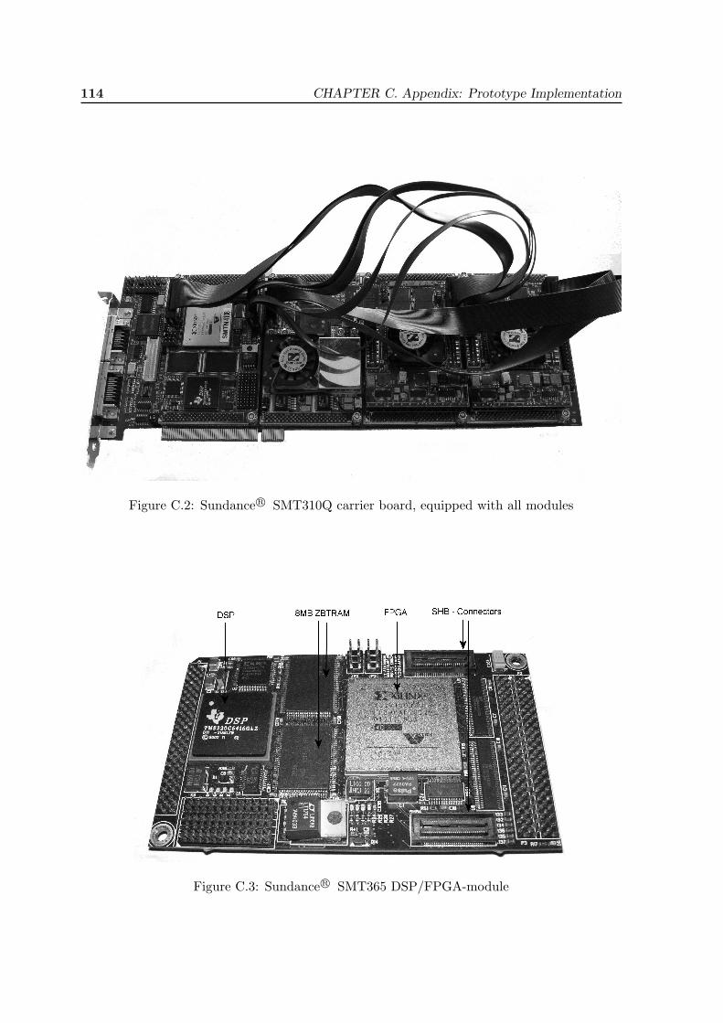
114 CHAPTER C. Appendix: Prototype Implementation
Figure C.2: Sundance R© SMT310Q carrier board, equipped with all modules
Figure C.3: Sundance R© SMT365 DSP/FPGA-module

C.3 The Prototyping-Hardware 115
Figure C.4: Sundance R© SMT370 ADC/DAC-module
Figure C.5: Sundance R© SMT351 memory-module
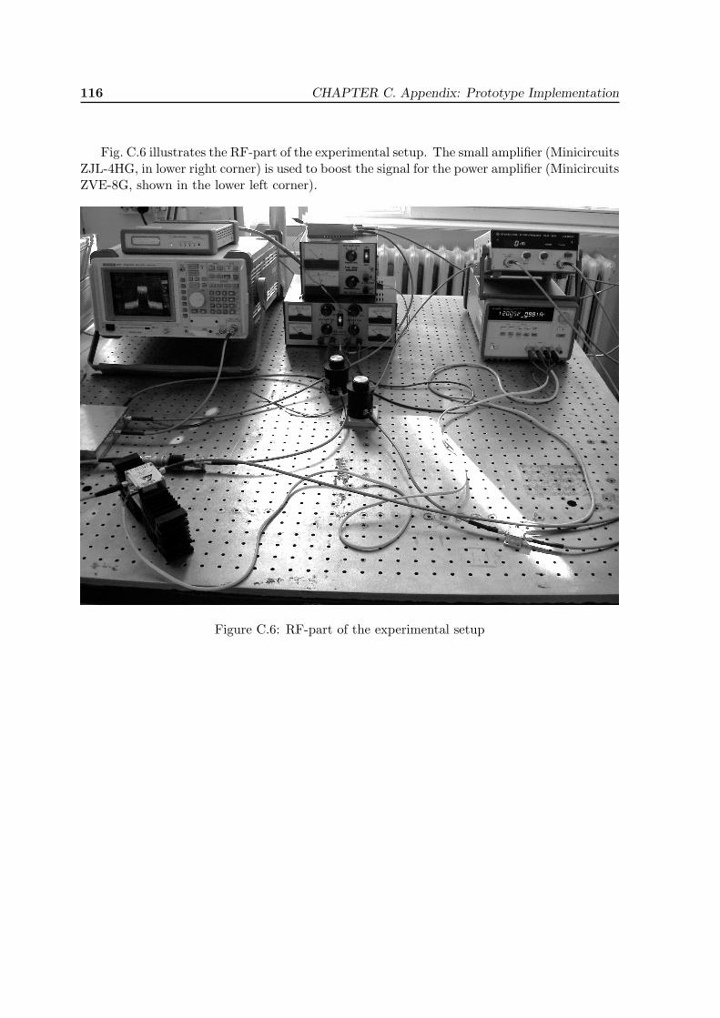
116 CHAPTER C. Appendix: Prototype Implementation
Fig. C.6 illustrates the RF-part of the experimental setup. The small amplifier (MinicircuitsZJL-4HG, in lower right corner) is used to boost the signal for the power amplifier (MinicircuitsZVE-8G, shown in the lower left corner).
Figure C.6: RF-part of the experimental setup

Appendix D
Appendix: Abbreviations andSymbols
D.1 List of Abbreviations
ADS advanced design system (Agilent Technologies)AM-AM amplitude-to-amplitude conversionAM-PM amplitude-to-phase conversionADC analogue-to-digital converterASIC application specific integrated circuitBPF bandpass filterCDMA code division multiple accessDAC digital-to-analogue converterDUC digital up-conversionDPD digital pre-distortionDSP digital signal processorEDGE enhanced data rates for global evolutionε-NLMS epsilon-normalised least-mean-squaresFDD frequency division duplexFIR finite impulse responseFPGA field programmable gate arrayGSM global system for mobile communicationHPA high-power amplifierIBO input power back-offIF intermediate frequencyISM industrial, scientific, medicalLMS least-mean-squaresLDMOS laterally diffused metal on siliconNLMS normalised least-mean-squaresOBO output power back-offPA power amplifierPC personal computerRBW resolution bandwidthRF radio frequency
117

118 CHAPTER D. Appendix: Abbreviations and Symbols
SDR software defined radioSNR signal-to-noise ratioVBW video bandwidthVHDL very high speed integrated circuit hardware description languageUMTS universal mobile telecommunications systemWCDMA wideband code division multiple accessWLAN wireless local area network
D.2 List of Mathematical Symbols
a, α scalar constantx(t) function, parameter is tx[n] sequence, parameter is nX(f) Fourier-transformx vectorX matrixV operator<{y} real part of y={y} imaginary part of yθθθ parameter vectorJ(·) cost functionJr(·) relative costM setf frequency‖·‖ norm‖·‖2 `2-norm
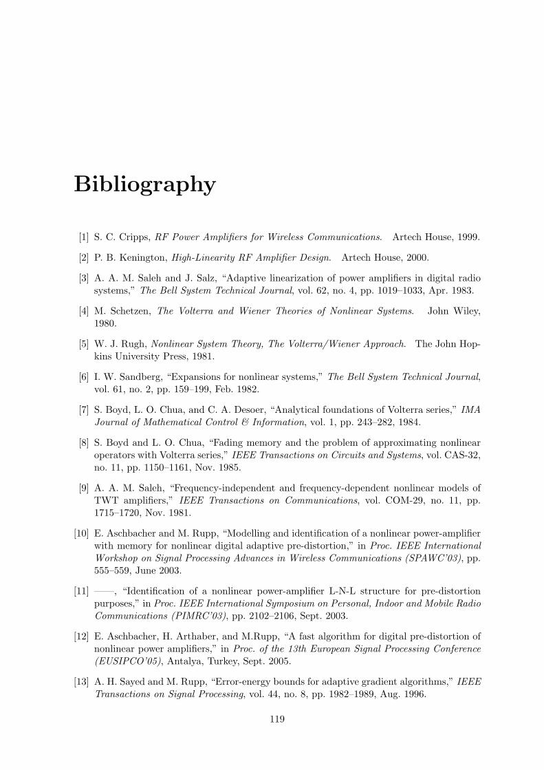
Bibliography
[1] S. C. Cripps, RF Power Amplifiers for Wireless Communications. Artech House, 1999.
[2] P. B. Kenington, High-Linearity RF Amplifier Design. Artech House, 2000.
[3] A. A. M. Saleh and J. Salz, “Adaptive linearization of power amplifiers in digital radiosystems,” The Bell System Technical Journal, vol. 62, no. 4, pp. 1019–1033, Apr. 1983.
[4] M. Schetzen, The Volterra and Wiener Theories of Nonlinear Systems. John Wiley,1980.
[5] W. J. Rugh, Nonlinear System Theory, The Volterra/Wiener Approach. The John Hop-kins University Press, 1981.
[6] I. W. Sandberg, “Expansions for nonlinear systems,” The Bell System Technical Journal,vol. 61, no. 2, pp. 159–199, Feb. 1982.
[7] S. Boyd, L. O. Chua, and C. A. Desoer, “Analytical foundations of Volterra series,” IMAJournal of Mathematical Control & Information, vol. 1, pp. 243–282, 1984.
[8] S. Boyd and L. O. Chua, “Fading memory and the problem of approximating nonlinearoperators with Volterra series,” IEEE Transactions on Circuits and Systems, vol. CAS-32,no. 11, pp. 1150–1161, Nov. 1985.
[9] A. A. M. Saleh, “Frequency-independent and frequency-dependent nonlinear models ofTWT amplifiers,” IEEE Transactions on Communications, vol. COM-29, no. 11, pp.1715–1720, Nov. 1981.
[10] E. Aschbacher and M. Rupp, “Modelling and identification of a nonlinear power-amplifierwith memory for nonlinear digital adaptive pre-distortion,” in Proc. IEEE InternationalWorkshop on Signal Processing Advances in Wireless Communications (SPAWC’03), pp.555–559, June 2003.
[11] ——, “Identification of a nonlinear power-amplifier L-N-L structure for pre-distortionpurposes,” in Proc. IEEE International Symposium on Personal, Indoor and Mobile RadioCommunications (PIMRC’03), pp. 2102–2106, Sept. 2003.
[12] E. Aschbacher, H. Arthaber, and M.Rupp, “A fast algorithm for digital pre-distortion ofnonlinear power amplifiers,” in Proc. of the 13th European Signal Processing Conference(EUSIPCO’05), Antalya, Turkey, Sept. 2005.
[13] A. H. Sayed and M. Rupp, “Error-energy bounds for adaptive gradient algorithms,” IEEETransactions on Signal Processing, vol. 44, no. 8, pp. 1982–1989, Aug. 1996.
119
120 BIBLIOGRAPHY
[14] A. H. Sayed, Fundamentals of Adaptive Filtering. J. Wiley, 2003.
[15] E. Aschbacher and M. Rupp, “Robust identification of an L-N-L system,” in ConferenceRecord of the 37th Asilomar Conference on Signals, Systems, and Computers (Asilo-mar’03), vol. 2, pp. 1298–1302, Nov. 2003.
[16] ——, “Robustness analysis of a gradient identification method for a nonlinear Wienersystem,” in Proceedings of the 2005 IEEE Workshop on Statistical Signal Processing(SSP’05), July 2005.
[17] C. Eun and E. J. Powers, “A new Volterra predistorter based on the indirect learningarchitecture,” IEEE Transactions on Signal Processing, vol. 45, no. 1, pp. 223–227, Jan.1997.
[18] R. D. Nowak and B. D. V. Veen, “Volterra filter equalization: A fixed point approach,”IEEE Transactions on Signal Processing, vol. 45, no. 2, pp. 377–387, Feb. 1997.
[19] E. Aschbacher, M. Steinmair, and M. Rupp, “Iterative linearization methods suited fordigital pre-distortion of power amplifiers,” in Conf. Record of the 38th Asilomar Conf. onSignals, Systems, and Computers, vol. 2, pp. 2198–2202, Nov. 2004.
[20] P. Brunmayr, “Implementation of a nonlinear digital pre-distortion algorithm,” Master’sthesis, Institute of Communications and Radio-Frequency Eng., Vienna University ofTechnology, 2005.
[21] M. Y. Cheong, E. Aschbacher, P. Brunmayr, M. Rupp, and T. I. Laakso, “Comparisonand experimental verification of two low-complex digital predistortion methods,” in Conf.Record of the 39th Asilomar Conf. on Signals, Systems, and Computers, Nov. 2005.
[22] 3rd Generation Partnership Project; Technical Specification Group Radio AccessNetwork; Base Station (BS) radio transmission and reception (FDD) (Release 6), TS25.104. [Online]. Available: http://www.3gpp.org
[23] Software Defined Radio Forum. [Online]. Available: http://www.sdrforum.org
[24] H. S. Black, “Translating system,” U.S. Patents 1.686.792 and 2.102.671, Oct.,Dec.1928,1937.
[25] H. Seidel, “A microwave feedforward experiment,” Bell Systems Technical Journal, vol. 50,pp. 22 879–2916, Nov. 1971.
[26] K. J. Parsons and P. B. Kenington, “The efficiency of a feedforward amplifier with delayloss,” IEEE Transactions on Vehicular Technology, vol. 43, no. 2, pp. 407–412, May 1994.
[27] ——, “Effect of delay mismatch on a feedforward amplifier,” IEE Proceedings on Circuits,Devices, and Systems, vol. 141, no. 2, pp. 140–144, April 1994.
[28] V. Petrovic and C. N. Smith, “Reduction of intermodulation distortion by means of mod-ulation feedback,” in Proceedings of the IEE Conference on Radio Spectrum ConservationTechniques, pp. 44–49, Sept. 1983.
[29] A. Bateman and D. M. Haines, “Direct conversion tranceiver design for compact lowcost portable mobile terminals,” in Proceedings of the 39th IEEE Vehicular TechnologyConference, vol. 1, pp. 57–62, May 1989.
BIBLIOGRAPHY 121
[30] M. Johanson and T. Mattson, “Linearised high-efficiency power amplifier for PCN,” Elec-tronics Letters, vol. 27, no. 9, pp. 762–764, 1991.
[31] P. B. Kenington, R. J. Wilkinson, and K. J. Parsons, “Noise performance of a cartesianloop transmitter,” IEEE Transactions on Vehicular Technology, vol. 46, no. 2, pp. 467–476, May 1997.
[32] E. Biglieri, S. Barberis, and M. Catena, “Analysis and compensation of nonlinearitiesin digital transmission systems,” IEEE Journal on Selected Areas in Communications,vol. 6, no. 1, pp. 42–51, Jan. 1988.
[33] G. Karam and H. Sari, “Improved data predistortion using intersymbol interpolation,”in Proceedings of the IEEE International Conference on Communications, vol. 1, pp.286–291, June 1989.
[34] S. Pupolin, A. Sarti, and H. Fu, “Performance analysis of digital radio links with nonlin-ear transmit amplifier and data predistorter with memory,” in Proceedings of the IEEEInternational Conference on Communications, vol. 1, pp. 292–296, June 1989.
[35] G. Lazzarin, S. Pupolin, and A. Sarti, “Nonlinearity compensation in digital radiosystems,” IEEE Transactions on Communications, vol. 42, no. 2/3/4, pp. 988–999,Feb./March/April 1994.
[36] M. Schetzen, “Theory of pth-order inverses of nonlinear systems,” IEEE Transactions onCircuits and Systems, vol. CAS-23, no. 5, pp. 285–291, May 1976.
[37] S. Benedetto and E. Biglieri, “Nonlinear equalization of digital satellite channels,” IEEEJournal on Selected Areas in Communications, vol. SAC-1, no. 1, pp. 57–62, Jan. 1983.
[38] A. Bateman, D. M. Haines, and R. J. Wilkinson, “Linear transceiver architectures,” inProceedings of the 38th IEEE Vehicular Technology Conference, pp. 478–484, May 1988.
[39] Y. Nagata, “Linear amplification technique for digital mobile communication,” in Pro-ceedings of the 39th IEEE Vehicular Technology Conference, vol. 1, pp. 159–164, May1989.
[40] J. Cavers, “Amplifier linearization using a digital predistorter with fast adaptation andlow memory requirements,” IEEE Transactions on Vehicular Technology, vol. 39, no. 4,pp. 374–382, Nov. 1990.
[41] J. Kim and K. Konstantinou, “Digital predistortion of wideband signals based on poweramplifier model with memory,” Electron. Lett., vol. 37, no. 23, pp. 1417–1418, Nov. 2001.
[42] J. W. Wustenberg, H. J. Xing, and J. R. Cruz, “Complex gain and fixed-point predistortersfor CDMA power amplifiers,” IEEE Transactions on Vehicular Technology, vol. 53, no. 2,pp. 469–478, March 2004.
[43] M. Y. Cheong, S. Werner, J. Cousseau, and T. I. Laakso, “Predistorter identificationusing the simplicial canonical piecewise linear function,” in Proc. of the 12th InternationalConference on Telecommunications ICT2005, Cape Town, South Africa, pp. 2102–2106,May 2005.
[44] L. Ljung, System Identification, Theory for the User, 2nd ed. Prentice Hall, 1999.
122 BIBLIOGRAPHY
[45] V. Volterra, Theory of Functions and of Integral and Integro-Differential Equations. NewYork: Dover Publ., 1959.
[46] Advanced Design System (ADS), Agilent Technologies. [Online]. Available: http://eesof.tm.agilent.com/products/ads main.html
[47] N. Wiener, Nonlinear Problems in Random Theory. John Wiley, 1958.
[48] D. G. Luenberger, Optimization by Vector Space Methods. J. Wiley, 1968.
[49] J. A. Dieudonne, Foundations of Modern Analysis. Academic Press, 1967.
[50] D. R. Hummels and R. D. Gitchell, “Equivalent low-pass representations for bandpassvolterra systems,” IEEE Transactions on Communications, vol. COM-28, no. 1, pp. 140–142, Jan. 1980.
[51] J. I. Churkin, C. P. Jakowlew und G. Wunsch, Theorie und Anwendung der Signalabtas-tung. VEB Verlag Technik Berlin, 1966.
[52] M. Unser, “Sampling - 50 years after Shannon,” Proceedings of the IEEE, vol. 88, no. 4,pp. 569–587, April 2000.
[53] R. J. Martin, “Volterra system identification and Kramer’s sampling theorem,” IEEETransactions on Signal Processing, vol. 47, no. 11, pp. 3152–3155, Nov. 1999.
[54] Y.-M. Zhu, “Generalized sampling theorem,” IEEE Transactions on Circuits andSystems—Part II: Analog and Digital Signal Processing, vol. 39, no. 8, pp. 587–588, Aug.1992.
[55] J. Tsimbinos and K. V. Lever, “Input Nyquist sampling suffices to identify and compen-sate nonlinear systems,” IEEE Transactions on Signal Processing, vol. 46, no. 10, pp.2833–2837, Oct. 1998.
[56] H. Akaike, “Fitting autoregressive models for prediction,” Annals of the Institute of Sta-tistical Mathematics, vol. 21, pp. 243–247, 1969.
[57] J. Rissanen, “Modelling by shortest data description,” Automatica, vol. 14, no. 5, pp.465–471, Sept. 1978.
[58] Mini-Circuits Medium to High Power Amplifiers: Data sheet. [Online]. Available:http://www.minicircuits.com/dg03-176.pdf
[59] S. Boyd, “Multitone signals with low crest factor,” IEEE Transactions on Circuits andSystems, vol. CAS-33, no. 10, pp. 1018–1022, Oct. 1986.
[60] Rohde&Schwarz. [Online]. Available: http://www.rohde-schwarz.com/
[61] Agilent Technologies. [Online]. Available: http://www.agilent.com/
[62] Sundance Multiprocessor Technology Ltd. [Online]. Available: http://www.sundance.com
[63] R. Langwieser, “Entwicklung von HF-Baugruppen fur ein Echtzeit MIMO-Ubertra-gungssystem,” Master’s thesis, Institut fur Nachrichten- und Hochfrequenztechnik, Tech-nische Universitat Wien, 2004.
BIBLIOGRAPHY 123
[64] N. J. Bershad, S. Bouchired, and F. Castanie, “Stochastic analysis of adaptive gradientidentification of Wiener-Hammerstein systems for gaussian inputs,” IEEE Transactionson Signal Processing, vol. 48, no. 2, pp. 557–560, Feb. 2000.
[65] N. J. Bershad, P. Celka, and S. McLaughlin, “Analysis of stochastic gradient identificationof Wiener-Hammerstein systems for nonlinearities with Hermite polynomial expansions,”IEEE Transactions on Signal Processing, vol. 49, no. 5, pp. 1060–1072, May 2001.
[66] A. D. Kalafatis, L. Wang, and W. Cluett, “Identification of Wiener-type nonlinear systemsin a noisy environment,” International Journal of Control, vol. 66, no. 6, pp. 923–941,April 1997.
[67] M. Rupp and A. H. Sayed, “Supervised learning of perceptron and output feedback dy-namic networks: A feedback analysis via the small gain theorem,” IEEE Transactions onNeural Networks, vol. 8, no. 3, pp. 612–622, May 1997.
[68] S. Haykin, Adaptive Filter Theory, 4th ed. Prentice Hall, 2002.
[69] H. K. Khalil, Nonlinear Systems. Macmillan Pub., 1992.
[70] S. Boyd and L. O. Chua, “Uniquiness of a basic nonlinear structure,” IEEE Transactionson Circuits and Systems, vol. CAS-30, no. 9, pp. 648–651, Sept. 1983.
[71] M. Rupp and A. H. Sayed, “Robustness of Gauss-Newton recursive methods: A deter-ministic feedback analysis,” Signal Processing, vol. 50, pp. 165–187, 1996.
[72] K. J. Muhonen, M. Kavehrad, and R. Krishnamoorthy, “Look-up table techniques foradaptive digital predistortion: A development and comparison,” IEEE Transactions onVehicular Technology, vol. 49, no. 5, pp. 1995–2002, Sept. 2000.
[73] P. Andreani, L. Sundstrom, N. Karlsson, and M. Svensson, “A chip for linearization ofRF power amplifiers using digital predistortion with a bit-parallel complex multiplier,” inProc. of the1999 IEEE Intern. Symp. on Circuits and Systems (ISCAS ’99), vol. 1, pp.346–349, Mai 1999.
[74] M. Steinmair, “Identifikation und Linearisierung nichtlinearer Verstarker mit Volterrarei-hen,” Master’s thesis, Insitut fur Nachrichten- und Hochfrequenztechnik, Technische Uni-versitat Wien, 2004.
[75] W. H. Press, B. P. Flannery, S. A. Teukolsky, and W. T. Vetterling, Numerical Recipesin C: The Art of Scientific Computing. Cambridge University Press, 1992. [Online].Available: http://www.nr.com
[76] C. G. Broyden, “A class of methods for solving nonlinear simultaneous equations,” Math-ematics of Computation, vol. 19, no. 92, pp. 577–593, Oct. 1965.
[77] XILINX Virtex-II Platform FPGAs: Complete data sheet. [Online]. Available:http://www.xilinx.com/partinfo/ds031.pdf
[78] TMS320C64xx fixed-point Digital Signal Processors: Complete data sheet. [Online].Available: http://focus.ti.com/lit/ds/symlink/tms320c6416.pdf

124 BIBLIOGRAPHY
[79] Analog Devices D/A converter AD9777: Complete data sheet. [Online]. Available: http://www.analog.com/UploadedFiles/Data Sheets/3229938536490156500AD9777 b.pdf
[80] Analog Devices A/D converter AD6645: Complete datasheet. [Online]. Available: http://www.analog.com/UploadedFiles/Data Sheets/39459366394038040210399061519954AD6645 b .pdf
[81] Sundance SMT370-AC module: Data sheet. [Online]. Available: http://www.sundance.com/edge/files/productpage.asp?STRFilter=SMT370-AC
[82] Sundance SMT351-G module: Data sheet. [Online]. Available: http://www.sundance.com/edge/files/productpage.asp?STRFilter=SMT351-VP7-5-G
[83] Sundance SMT365-16-2 module: Data sheet. [Online]. Available: http://www.sundance.com/edge/files/productpage.asp?STRFilter=SMT365-16-2
[84] Mini-Circuits Low to Medium Power Amplifiers: Data sheet. [Online]. Available:http://www.minicircuits.com/dg03-174.pdf
[85] XILINX IP Core Pipelined Divider: Data Sheet. [Online]. Available: http://www.xilinx.com/bvdocs/ipcenter/data sheet/sdivider.pdf
[86] G. Doblinger, Signalprozessoren - Architekturen, Algorithmen, Anwendungen. J. Schlem-bach Fachverlag, 2000.
[87] Mentor Graphics. [Online]. Available: http://www.mentor.com
[88] Sundance SMT310Q PCI Carrier Board: Data sheet. [Online]. Available: http://www.sundance.com/docs/SMT310Q%20User%20Manual.pdf

Curriculum Vitae
Personal Details
Name Ernst AschbacherMarital status SingleCitizenship ItalianDate of birth 04.09.1970
Education
09/1984 – 06/1986 Full-time vocational school for Electrical Engineering,Bruneck (IT)
09/1987 – 06/1990 Technical college (Gewerbeoberschule), Bozen (IT)Branch: Informatics
09/1991 – 07/1993 Technical college (Gewerbeoberschule), Bozen (IT)Branch: Informatics
09/1993 – 06/2000 Master studies at Vienna University of Technology(AUT)Electrical Engineering and Information Technology
06/2000 Graduation with highest honours (Diplomingenieur)09/2001 – 09/2005 Ph.D. studies at Vienna University of Technology (AUT)
Field: Signal Processing for Mobile Communications
Military Service
09/1990 – 09/1991 Military service in Meran (IT), military music
Professional Experience
07/1986 – 09/1990 Full-time millwright, GKN Birfield, Bruneck (IT)
10/2000 – 09/2001 Project assistant at the Institute of Communicationsand Radio-Frequency Eng.Vienna University of TechnologyField: Optical Communications
09/2001 – 09/2005 Assistant (Universitatsassistent) at the Institute ofCommunications and Radio-Frequency Eng.Vienna University of Technology
Language Skills
German (mother tongue)English (business fluent)Italian (business fluent)Spanish (basics)


![Spin waves in coupled YIG/Co heterostructuresexcitation of exchange spin waves by microwave magnetic fields requires nanolithographically defined microwave an-tennas [11] that have](https://img.pdfslide.org/doc/110x75/6068fa3a8fa72b2c5a423f16/spin-waves-in-coupled-yigco-heterostructures-excitation-of-exchange-spin-waves.jpg)