Embed Size (px)
Citation preview
Diplomarbeit
Analysis and Visualisation of Social Networks
Keyan Mahmoud Ghazi-Zahedi

Diplomarbeit im Fach Informatik
Analysis and Visualisation of Social Networks
vorgelegt von
Keyan Mahmoud Ghazi-Zahedi
April 2001
Betreuer: Prof. Dr. Michael Kaufmann
Wilhelm-Schickard-InstitutArbeitsbereich Paralleles Rechnen
Eberhard-Karls-Universitat TubingenSand 13 · 72076 Tubingen
Erklarung
Hiermit versichere ich, diese Arbeitselbstandig verfaßt und nur dieangegebenen Quellen benutzt zu haben.
(Keyan Zahedi)
Contents
1 Introduction 5
2 Social Networks 92.1 History . . . . . . . . . . . . . . . . . . . . . . . . . . . . . . . 92.2 Modern social network analysis . . . . . . . . . . . . . . . . . 102.3 Data and resources . . . . . . . . . . . . . . . . . . . . . . . . 11
2.3.1 Actors . . . . . . . . . . . . . . . . . . . . . . . . . . . 112.3.2 Relations . . . . . . . . . . . . . . . . . . . . . . . . . 11
2.4 Why formal methods? . . . . . . . . . . . . . . . . . . . . . . 13
3 Mathematical Foundations 153.1 Definitions . . . . . . . . . . . . . . . . . . . . . . . . . . . . . 15
4 Clustering 194.1 Clustering Algorithms . . . . . . . . . . . . . . . . . . . . . . 20
4.1.1 Top-Down Approaches . . . . . . . . . . . . . . . . . . 204.1.2 Bottom-Up Approaches . . . . . . . . . . . . . . . . . 21
4.2 The Clustering Algorithm . . . . . . . . . . . . . . . . . . . . 234.2.1 Overview . . . . . . . . . . . . . . . . . . . . . . . . . 234.2.2 Clustering . . . . . . . . . . . . . . . . . . . . . . . . . 244.2.3 Calculating the residual graph . . . . . . . . . . . . . . 274.2.4 Merging clusters . . . . . . . . . . . . . . . . . . . . . 30
5 Centrality 335.1 Overview . . . . . . . . . . . . . . . . . . . . . . . . . . . . . . 33
5.1.1 Degree Centrality . . . . . . . . . . . . . . . . . . . . . 345.1.2 Betweenness Centrality . . . . . . . . . . . . . . . . . . 355.1.3 Flow-betweenness Centrality . . . . . . . . . . . . . . . 35
3
4 CONTENTS
5.1.4 Closeness Centrality . . . . . . . . . . . . . . . . . . . 365.1.5 The Bonacich’s power index . . . . . . . . . . . . . . . 37
5.2 Group centrality . . . . . . . . . . . . . . . . . . . . . . . . . 375.2.1 General Principles . . . . . . . . . . . . . . . . . . . . 37
5.3 Method . . . . . . . . . . . . . . . . . . . . . . . . . . . . . . 385.4 Algorithms . . . . . . . . . . . . . . . . . . . . . . . . . . . . . 39
5.4.1 Degree centrality . . . . . . . . . . . . . . . . . . . . . 395.4.2 Betweenness centrality . . . . . . . . . . . . . . . . . . 395.4.3 Flow-betweenness centrality . . . . . . . . . . . . . . . 42
6 Visualisation 456.1 Data and Properties . . . . . . . . . . . . . . . . . . . . . . . 45
6.1.1 Data . . . . . . . . . . . . . . . . . . . . . . . . . . . . 456.1.2 Properties . . . . . . . . . . . . . . . . . . . . . . . . . 46
6.2 Problems . . . . . . . . . . . . . . . . . . . . . . . . . . . . . . 476.2.1 Types of Nodes . . . . . . . . . . . . . . . . . . . . . . 476.2.2 Types of Clusters . . . . . . . . . . . . . . . . . . . . . 486.2.3 Type B Analysis . . . . . . . . . . . . . . . . . . . . . 49
6.3 Conclusion . . . . . . . . . . . . . . . . . . . . . . . . . . . . . 546.4 Single Cluster Layout . . . . . . . . . . . . . . . . . . . . . . . 546.5 Multi cluster visualisation . . . . . . . . . . . . . . . . . . . . 56
6.5.1 Shared actors . . . . . . . . . . . . . . . . . . . . . . . 596.5.2 Group layout . . . . . . . . . . . . . . . . . . . . . . . 59
6.6 Conclusion . . . . . . . . . . . . . . . . . . . . . . . . . . . . . 59
7 Conclusions & Future Work 63
A YSocNet 65A.1 Requirements . . . . . . . . . . . . . . . . . . . . . . . . . . . 65A.2 Application Properties . . . . . . . . . . . . . . . . . . . . . . 66A.3 Architecture . . . . . . . . . . . . . . . . . . . . . . . . . . . . 66
A.3.1 Data Input . . . . . . . . . . . . . . . . . . . . . . . . 66A.4 Modules . . . . . . . . . . . . . . . . . . . . . . . . . . . . . . 68
A.4.1 SocNetData . . . . . . . . . . . . . . . . . . . . . . . . 68A.4.2 SocNet-Interface . . . . . . . . . . . . . . . . . . . . . 68A.4.3 Clustering . . . . . . . . . . . . . . . . . . . . . . . . . 69A.4.4 Centrality . . . . . . . . . . . . . . . . . . . . . . . . . 69A.4.5 Visualisation . . . . . . . . . . . . . . . . . . . . . . . 69
CONTENTS 5
A.4.6 SocNetAnalysis . . . . . . . . . . . . . . . . . . . . . . 69A.5 Framework . . . . . . . . . . . . . . . . . . . . . . . . . . . . . 70
B Related Work 71B.1 Social Network Analysis Programs . . . . . . . . . . . . . . . . 71
B.1.1 UCINET . . . . . . . . . . . . . . . . . . . . . . . . . . 71B.1.2 KrackPlot . . . . . . . . . . . . . . . . . . . . . . . . . 72

6 CONTENTS
Chapter 1
Introduction
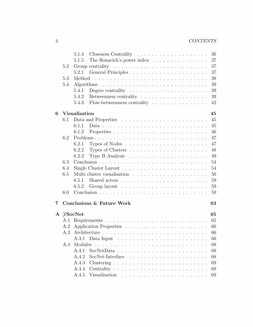
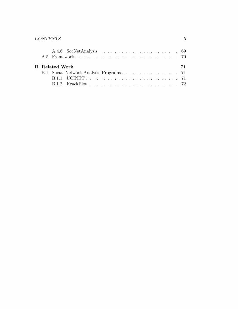
Firms exchanging information forming a social network (Knoke InformationExchange Data)
A social network is a formal representation of actors and the relationsbetween them. Actors, in this context, can be persons, like students ina classroom, or companies, having economic relations (see Figure above).Representing a social structure by a (social) network allows the analysis bygraph theoretical methods. In a social network, or more precise the graph ofa social network, actors are represented by nodes, and the relations betweenactors are represented by edges between the according nodes. In the Chap-ter Social Networks we briefly review the history of social network analysis,discussing the data we have, and the advantages of formal methods.
7
8 CHAPTER 1. INTRODUCTION
In the Figure above, we see companies that have an information exchangenetwork. Having a brief look at the Figure, one can see, that there are actorshaving a lot of direct connections to others, some receiving more or lessinformation as they offer, and some only having very few direct connectionsto others. Social scientists are interested in determining the structure of asocial network, as well as determining the distribution of power among theactors. The power of an actor arises from the structure of the relations inthe social network.
The structure of network is best shown using clustering methods. Acluster is a group of actors in the network, that have more relations amongeach other, then to actors that are not a member of the group. The networkis divided into distinguishable sub-networks. We assume, that an actor canbe part of more then one group. The clustering method must therefor beable to extract overlapping clusters. In the Chapter Clustering we discussdifferent approaches of clustering, finally choosing the k-plex approach as itallows overlapping of the extracted clusters.
The next step in our analysis of the social network is to calculate thedistribution of power. An actors is said to have power, if he has an advan-tageous position compared to others. The power of an actor is modelled bycentrality measures. The degree centrality, as an example, implies, that anactor with more direct connections to other actors has more power, or ismore important, as he has access to more resources. In the picture abovethe actor labelled with WRO would be said to be less powerful than the ac-tor labelled with COMM, as WRO has less direct connections, and thereforless access to information. In the Chapter Centrality we discuss differentapproaches to model power, discussing in detail the algorithms to calculatetwo basic (degree and betweenness) and one extension of a basic centrality(flow-betweenness).
After analysing the data, the next step is a good visualisation of theextracted information. We say that a visualisation is good, if the information,extracted clusters and centrality of the actors, can bee seen by the viewerwithout much interpretation needed. The result of the visualisation shouldbe able to support the analysis of a social network done by a social scientist,as well as the presentation of the results. In the chapter Visualisation wefirst discuss the problems that occur visualising overlapping clusters. Wethen develop a method, starting with the visualisation of only one cluster,extending it to handle multiple overlapping or non-overlapping clusters.
In the chapter Mathematical Foundations we introduce some definitions

9
and the terminology that is needed to describe and discuss the algorithmsused here.
In the Appendix A we discuss the architecture of the application YSocNet,and related work is discussed in the Appendix B.
Acknowledgement
I would like to thank Prof. Dr. M. Kaufmann for giving me the chance towork on this subject under his direction and for his help. My thanks also goto Monika Lanik, from the Ethnological Institute of Tubingen, for helping inany aspect concerning the usage of the application as well as helping in anysocial scientific question, and to Markus Eiglsperger, Roland Wiese, BorisDiebold and Frank Eppinger for their help, as well as to Olaf Peisker for hishelp.

10 CHAPTER 1. INTRODUCTION
Chapter 2
Social Networks
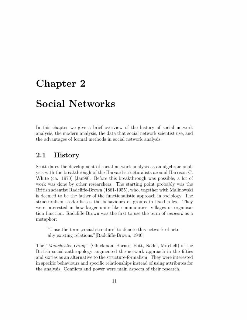
In this chapter we give a brief overview of the history of social networkanalysis, the modern analysis, the data that social network scientist use, andthe advantages of formal methods in social network analysis.
2.1 History
Scott dates the development of social network analysis as an algebraic anal-ysis with the breakthrough of the Harvard-structuralists around Harrison C.White (ca. 1970) [Jan99]. Before this breakthrough was possible, a lot ofwork was done by other researchers. The starting point probably was theBritish scientist Radcliffe-Brown (1881-1955), who, together with Malinowskiis deemed to be the father of the functionalistic approach in sociology. Thestructuralism stadardisises the behaviours of groups in fixed roles. Theywere interested in how larger units like communities, villages or organisa-tion function. Radcliffe-Brown was the first to use the term of network as ametaphor:
”I use the term ,social structure’ to denote this network of actu-ally existing relations.”[Radcliffe-Brown, 1940]
The ”Manchester-Group” (Gluckman, Barnes, Bott, Nadel, Mitchell) of theBritish social-anthropology augmented the network approach in the fiftiesand sixties as an alternative to the structure-formalism. They were interestedin specific behaviours and specific relationships instead of using attributes forthe analysis. Conflicts and power were main aspects of their research.
11
12 CHAPTER 2. SOCIAL NETWORKS
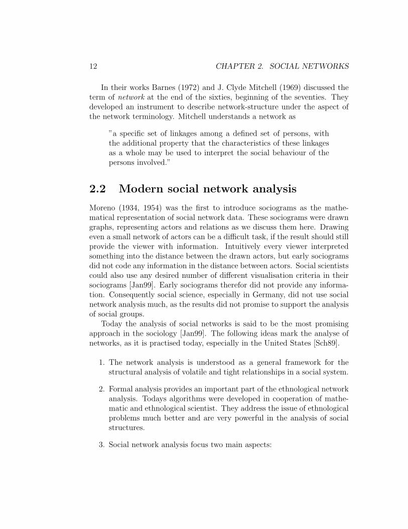
In their works Barnes (1972) and J. Clyde Mitchell (1969) discussed theterm of network at the end of the sixties, beginning of the seventies. Theydeveloped an instrument to describe network-structure under the aspect ofthe network terminology. Mitchell understands a network as
”a specific set of linkages among a defined set of persons, withthe additional property that the characteristics of these linkagesas a whole may be used to interpret the social behaviour of thepersons involved.”
2.2 Modern social network analysis
Moreno (1934, 1954) was the first to introduce sociograms as the mathe-matical representation of social network data. These sociograms were drawngraphs, representing actors and relations as we discuss them here. Drawingeven a small network of actors can be a difficult task, if the result should stillprovide the viewer with information. Intuitively every viewer interpretedsomething into the distance between the drawn actors, but early sociogramsdid not code any information in the distance between actors. Social scientistscould also use any desired number of different visualisation criteria in theirsociograms [Jan99]. Early sociograms therefor did not provide any informa-tion. Consequently social science, especially in Germany, did not use socialnetwork analysis much, as the results did not promise to support the analysisof social groups.
Today the analysis of social networks is said to be the most promisingapproach in the sociology [Jan99]. The following ideas mark the analyse ofnetworks, as it is practised today, especially in the United States [Sch89].
1. The network analysis is understood as a general framework for thestructural analysis of volatile and tight relationships in a social system.
2. Formal analysis provides an important part of the ethnological networkanalysis. Todays algorithms were developed in cooperation of mathe-matic and ethnological scientist. They address the issue of ethnologicalproblems much better and are very powerful in the analysis of socialstructures.
3. Social network analysis focus two main aspects:
2.3. DATA AND RESOURCES 13
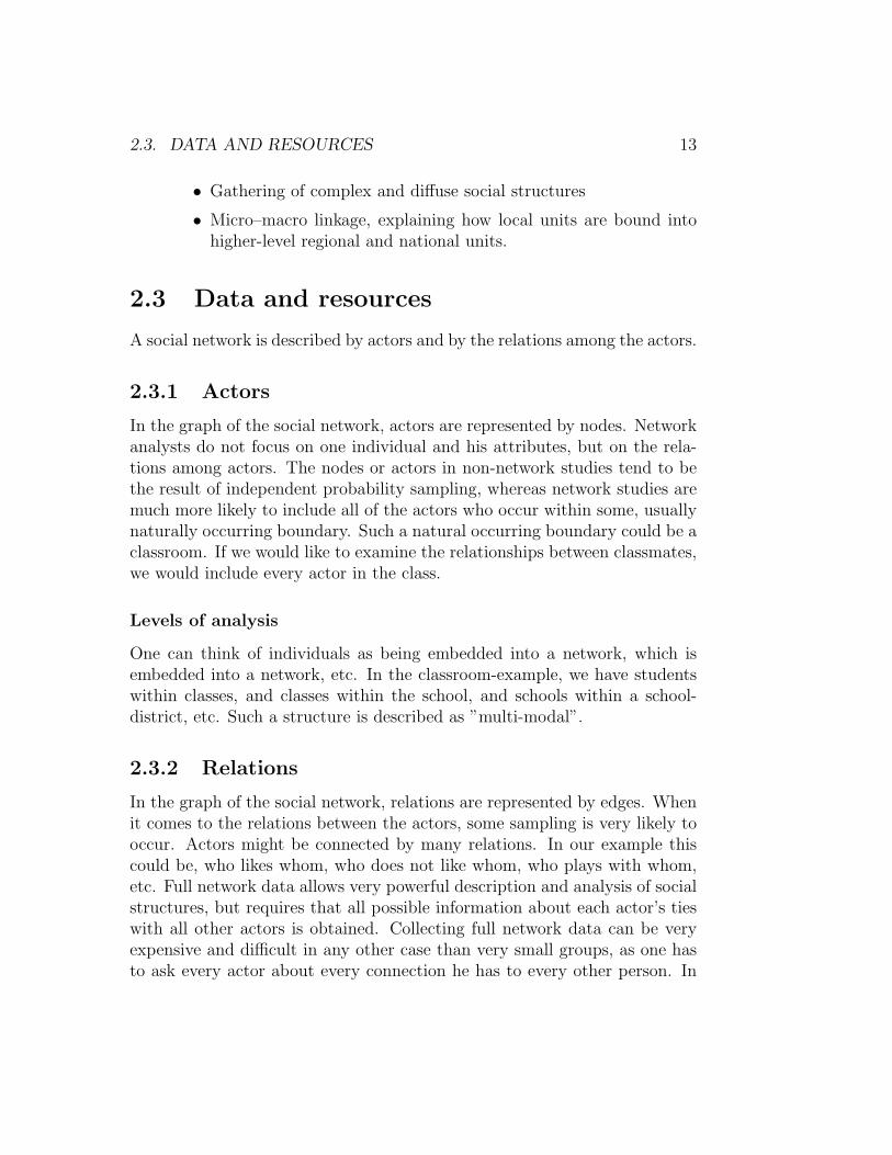
• Gathering of complex and diffuse social structures
• Micro–macro linkage, explaining how local units are bound intohigher-level regional and national units.
2.3 Data and resources
A social network is described by actors and by the relations among the actors.
2.3.1 Actors
In the graph of the social network, actors are represented by nodes. Networkanalysts do not focus on one individual and his attributes, but on the rela-tions among actors. The nodes or actors in non-network studies tend to bethe result of independent probability sampling, whereas network studies aremuch more likely to include all of the actors who occur within some, usuallynaturally occurring boundary. Such a natural occurring boundary could be aclassroom. If we would like to examine the relationships between classmates,we would include every actor in the class.
Levels of analysis
One can think of individuals as being embedded into a network, which isembedded into a network, etc. In the classroom-example, we have studentswithin classes, and classes within the school, and schools within a school-district, etc. Such a structure is described as ”multi-modal”.
2.3.2 Relations
In the graph of the social network, relations are represented by edges. Whenit comes to the relations between the actors, some sampling is very likely tooccur. Actors might be connected by many relations. In our example thiscould be, who likes whom, who does not like whom, who plays with whom,etc. Full network data allows very powerful description and analysis of socialstructures, but requires that all possible information about each actor’s tieswith all other actors is obtained. Collecting full network data can be veryexpensive and difficult in any other case than very small groups, as one hasto ask every actor about every connection he has to every other person. In
14 CHAPTER 2. SOCIAL NETWORKS
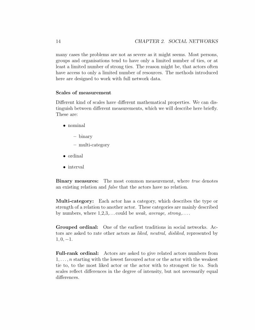
many cases the problems are not as severe as it might seems. Most persons,groups and organisations tend to have only a limited number of ties, or atleast a limited number of strong ties. The reason might be, that actors oftenhave access to only a limited number of resources. The methods introducedhere are designed to work with full network data.
Scales of measurement
Different kind of scales have different mathematical properties. We can dis-tinguish between different measurements, which we will describe here briefly.These are:
• nominal
– binary
– multi-category
• ordinal
• interval
Binary measures: The most common measurement, where true denotesan existing relation and false that the actors have no relation.
Multi-category: Each actor has a category, which describes the type orstrength of a relation to another actor. These categories are mainly describedby numbers, where 1,2,3,. . . could be weak, average, strong,. . . .
Grouped ordinal: One of the earliest traditions in social networks. Ac-tors are asked to rate other actors as liked, neutral, disliked, represented by1, 0,−1.
Full-rank ordinal: Actors are asked to give related actors numbers from1, . . . , n starting with the lowest favoured actor or the actor with the weakesttie to, to the most liked actor or the actor with to strongest tie to. Suchscales reflect differences in the degree of intensity, but not necessarily equaldifferences.
2.4. WHY FORMAL METHODS? 15
Interval measures: A more precise level of measurement as the full-rankordinal measure. The difference between a ”1” and ”2” denotes the sameamount of real difference as between ”24” and ”25”.
2.4 Why formal methods?
There are three main reasons for using formal methods to analyse socialnetworks [Han98].
Systematic representation: For a small population of actors, the pat-terns of relationships can be described completely and effectively usingwords. For a large number of actors and/or relations between the ac-tors, this can get very tedious. Formal representation ensures that allthe necessary information is systematically represented.
Computational Analysis: To analyse a large social network large amountsof data must be manipulated. By hand this would take too long. Theusage of computers reduces the time needed significantly.
Patterns: The technique of graphing and the rules of mathematics them-selves suggest things that we might look for in our data, that might nothave been seen if the data was presented using a description in words.Describing the relations of actors by a matrix can show patterns of therelations that otherwise may not have been seen. This can lead us toask other questions, which then may lead us to new insights.

16 CHAPTER 2. SOCIAL NETWORKS
Chapter 3
Mathematical Foundations
In this chapter we introduce some graph theoretical definitions, needed todescribe and discuss the algorithms of this work.
3.1 Definitions
The definitions are taken from [dBETT99],[CLR99] and [Har69]. The formalrepresentation of a social network is called a graph.
Definition 3.1 (graph)A graph G = (V,E) consists of a finite set V of vertices and a finite multi-set E of edges, that is, unordered pairs (u, v) or vertices. The vertices of agraph are sometimes called nodes, edges are sometimes called links, arcs orconnections.
Here a node represents an actor, and an edge indicates a relationship betweentwo actors.
This definition is too general, as relations are directed. If an actor A callsactor B , this does not automatically imply, that actor B will also call actorA. So we have to regard directed relations between actors.
Definition 3.2 (digraph)A directed graph, or digraph, is a graph, which elements of E are orderedpairs of vertices, called directed edges. The directed edge (u, v) is an outgo-ing edge of u and an incoming edge of v. Vertices without outgoing (resp.incoming) edges are called sinks or targets (resp. sources).
17
18 CHAPTER 3. MATHEMATICAL FOUNDATIONS
If we talk about graphs in the following chapters, we always mean digraphs.Given an undirected graph G = (V,E), the directed version of G is thedirected graph G′ = (V,E ′), where (u, v) ∈ E ′ if and only if (u, v) ∈ E. Thatis, each undirected edge (u, v) ∈ E is replaced in the directed version bythe two directed edges (u, v) ∈ E ′ and (v, u) ∈ E ′. Given a directed graphG = (V,E), the undirected version of G is the undirected graph G′ = (V,E ′),where (u, v) ∈ E ′ if and only if u 6= v and (u, v) ∈ E or (v, u) ∈ E.
Now we need a notation for the direct neighbourhood of a node, concern-ing the relations and the neighbours a node can have.
Definition 3.3 (incident)If (u, v) is and edge in a directed graph G = (V,E), we say that (u, v) isincident from or leaves vertex u and is incident to or enter vertex u. If (u, v)is an edge in an undirected graph G = (V,E), we say that (u, v) is incidenton vertices u and v.
Definition 3.4 (adjacent)If (u, v) is an edge in a graph G = (V,E), we say that vertex v is adjacent tovertex u. When the graph is undirected, the adjacency relation is symmetric.
Definition 3.5 (neighbour)In a directed graph G = (V,E), a neighbour of a vertex u is any vertex thatis adjacent to u in the undirected version of G. That is, v is a neighbourof u if either (u, v) ∈ E or (v, u) ∈ E. In an undirected graph, u and v areneighbours if they are adjacent.
Definition 3.6 (degree)The degree of a vertex in an undirected graph is the number of edges incidenton it. In a directed graph, the out-degree of a vertex is the number of edgesleaving it, and the in-degree of a vertex is the number of edges entering it.The degree of a vertex in a directed graph is its in-degree plus its out-degree.
Definition 3.7 (path)A path of length k from a vertex u to a vertex u′ in a graph G = (V,E) is asequence 〈v0, v1, . . . , vk〉 of vertices such that u = v0, u
′ = vk, and (vi−1, vi) ∈E for i = 1, 2, . . . , k. The length of the path is the number of edges in thepath. The path contains the vertices v0, v1, . . . , vk and the correspondingedges (v0, v1), (v1, v2), . . . , (vk−1, vk). If there is a path p from u to u′, we
say u′ is reachable from u via p, which we sometimes write as up v if G is
directed. A path is simple if all vertices in the path are distinct. A shortest
3.1. DEFINITIONS 19
path u, u′ is often called a geodesic. The diameter d(G) of a connected graphG is the length of any longest geodesic. A undirected graph is connected ifevery pair of vertices is connected by a path.
Definition 3.8 (complete graph)A complete graph is an undirected graph in which every pair of vertices isadjacent.
Definition 3.9 (flow network)A flow network G = (V,E) is a directed graph in which each edge (u, v) ∈E has a nonnegative capacity c(u, v) ≥ 0. If (u, v) 6∈ E, we assume thatc(u, v) = 0. We distinguish two vertices in a flow network: a source s ∈ Vand a sink t ∈ V .
Definition 3.10 (flow)A flow in G is a real-valued function f : V × V 7→ R that satisfies thefollowing three properties:
Capacity constraint: For all u, v ∈ V , we require f(u, v) ≤ c(u, v).
Skew symmetry: For all u, v ∈ V , we require f(u, v) = −f(v, u).
Flow conservation: For all u ∈ V \s, t, we require∑v∈V
f(u, v) = 0.

20 CHAPTER 3. MATHEMATICAL FOUNDATIONS
Chapter 4
Clustering
Social scientists are interested in the structure of relations between actors.By grouping the actors, that have more relations among each other, thestructure of the social network can be presented well, as we divide the graphinto distinguishable sub-graphs. Actors are understood as strategists, andtheir position in the network as well as their power allows a social scientistto draw conclusions about the tactics and possibilities of acting. Thereforthe first step in our social network analysis is the clustering of nodes. Butbefore we discuss the clustering, we should first define what a cluster is.
Definition 4.1 (cluster)Let G = (V,E) be a graph, where V is the set of nodes, and E is the setof edges. A cluster Ci is a list of nodes vi ∈ V , where the elements ofCi are sorted by their degree in an increasing order. The set of clustersC = {C0, C1, . . . , Ck} is called a clustering of G, if
⋃Ci∈C Ci = V . A cluster
Ci ∈ C includes all sub-cluster, so that Cj 6∈ C, if Cj ⊂ Ci.
We have 2 main goals in clustering:
1. Finding the maximum number of clusters
2. Maximise each cluster in size
To be sure not to find just a single cluster, we would like to have the maximalnumber of clusters. This would be fulfilled, if every node declares a clusteron its own. In order to prevent this, we also require that each group ismaximised in size.
Overlapping of clusters is wanted, as we assume that a single actor canbe part of more than just one group.
21
22 CHAPTER 4. CLUSTERING
4.1 Clustering Algorithms
There are two main categories of clustering algorithms, bottom-up and top-down. The bottom-up methods start with a single node, trying to find dyads,which is a cluster formed by only two nodes. The dyads are then extendedto triads and higher-numbered clusters, if possible.
The top-down methods divide the graph into clusters, by analysing thestructure of the graph, identifying sub-structures as parts that are locallydenser than the graph as a whole.
4.1.1 Top-Down Approaches
Components
A component of a graph G is a completely connected sub-graph. It does notmatter how closely connected the nodes are. Each component determines acluster.
Blocks and Cut-points
A cut-point of a graph G is a node, which, if removed, divides the graph intoan unconnected system. The sets of nodes into which the graph is dividedare called blocks.
Lambda Sets and Bridges
Each relationship in the network is ranked in terms of importance by evalu-ating how much of the flow among the actors in the network is going througheach link. The network is divided by the set of actors who, if disconnected,would significantly disrupt the flow among all actors. These actors arecalled bridges and the resulting sets are called Lambda sets. One property ofLambda sets is that each node in the set has more edge independent pathsto every other node in the set than to nodes outside the set.
Conclusion
The top-down algorithms divide the complete graph into non-overlappingsub-graphs. As we would like to allow overlapping, none of the algorithmsintroduced above seem appropriate.
4.1. CLUSTERING ALGORITHMS 23
4.1.2 Bottom-Up Approaches
Cliques
A clique in a graph G is a maximal complete sub-graph of G. That is, a setof nodes C ⊆ V is a clique, if
∀v ∈ C : degC(v) = |C| − 1,
where degC(v) is the degree of the node v ∈ V in the cluster C:
degC(v) = |{u|u ∈ C, (u, v) ∈ E ∨ (v, u) ∈ E}|.
N-Cliques
The N -clique loosens the very hard constraint of a maximal fully connectedsub-graph to form a cluster. We could say, an actor is part of a group, if heknows everyone in the group through someone else, which would correspondto being a ”friend of a friend”. This approach of defining sub-structures iscalled N -clique, where N stands for the length of the path allowed to makea connection to all other members. A set of nodes C ⊆ V is a N -clique, if
∀v ∈ C : ∀u ∈ C : distC(u, v) ≤ N.
N-Clan
The N -clique approach tends to find long and stringy groupings rather thanthe tight and discrete ones of the maximal sub-graph approach. In somecases, N -cliques can be found, that have a property that is probably unde-sirable for many purposes: it is possible for a member of N -cliques to beconnected by actors who are not members of the clique themselves.
Therefor some analysts have suggested to insert a restriction of the totalspan or diameter of a N -clique. This forces all ties among members of aN -clique to pass only over actors, who are themselves members of the group.N -Clans are also known as distance k-cliques [ESB99]. A set of nodes C ⊆ Vis a N -clan, if
∀v ∈ C : ∀u ∈ C : distC(u, v) ≤ N
and
diameterC(C) ≤ N.
24 CHAPTER 4. CLUSTERING
1−plex
5−plex
4−plex
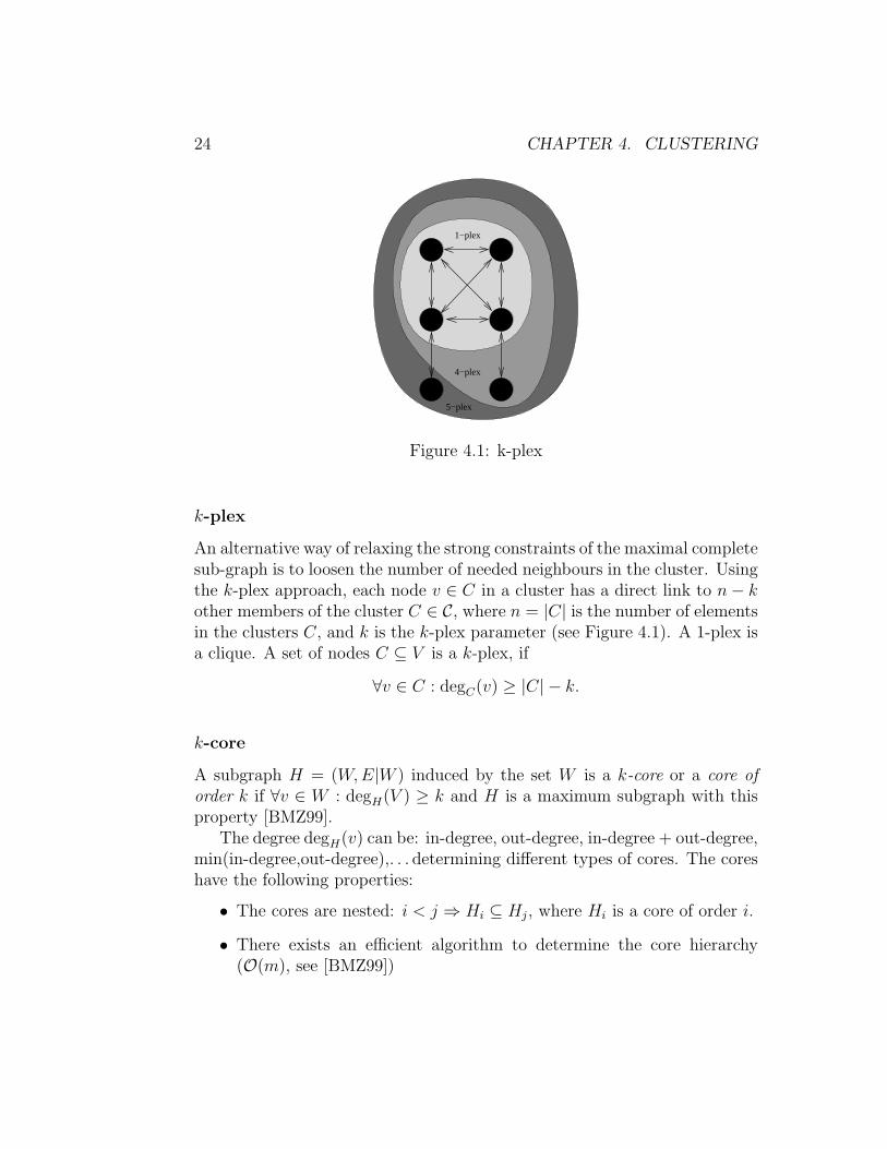
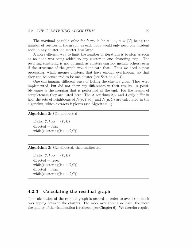
Figure 4.1: k-plex
k-plex
An alternative way of relaxing the strong constraints of the maximal completesub-graph is to loosen the number of needed neighbours in the cluster. Usingthe k-plex approach, each node v ∈ C in a cluster has a direct link to n− kother members of the cluster C ∈ C, where n = |C| is the number of elementsin the clusters C, and k is the k-plex parameter (see Figure 4.1). A 1-plex isa clique. A set of nodes C ⊆ V is a k-plex, if
∀v ∈ C : degC(v) ≥ |C| − k.
k-core
A subgraph H = (W,E|W ) induced by the set W is a k-core or a core oforder k if ∀v ∈ W : degH(V ) ≥ k and H is a maximum subgraph with thisproperty [BMZ99].
The degree degH(v) can be: in-degree, out-degree, in-degree + out-degree,min(in-degree,out-degree),. . . determining different types of cores. The coreshave the following properties:
• The cores are nested: i < j ⇒ Hi ⊆ Hj, where Hi is a core of order i.
• There exists an efficient algorithm to determine the core hierarchy(O(m), see [BMZ99])
4.2. THE CLUSTERING ALGORITHM 25
• Cores are not necessarily connected sub-graphs
Conclusion
From all bottom-up approaches only the N -clan, N -clique and the k-plexalgorithm would allow overlapping of the resulting clusters. Using the N -clan/-clique, we would demand, that every node has a limited path to everyother node in the cluster, but the path may have a length greater than one.The k-plex on the other hand emphasises the direct connection a node hasin a cluster. Which algorithm to choose is a personal decision, as they justhighlight different aspects. In consultation with the Ethnological Institute ofTubingen, we decided, that the number of direct neighbours an actor musthave would better match our understanding of a group.
4.2 The Clustering Algorithm
4.2.1 Overview
The clustering algorithm used here is based on the k-plex algorithm. Thatis, each cluster fulfils the k-plex constraint
∀v ∈ Ci : degCi(v) ≥ ni − k (4.1)
during the clustering, where ni = |Ci| is the size of the cluster Ci, and k isgiven externally. With degCi(v) we denote the degree of the node v ∈ V inthe cluster Ci ∈ C. If k = 1, then each node has a link to every other nodein the cluster. We have two goals for the clustering:
1. maximise the number of clusters
2. maximise each cluster in size
In order to achieve these goals, we declare every node as a cluster on its own.In every clustering-step, the cluster will be extended by all neighbours, thatobey the Constraint 4.1. So at the beginning we receive every possible dyadas a initial cluster-core. As we will see later, the dyads are very importantfor the overlapping between clusters, consequently we will keep them, andonly copies will be extended. If no nodes which can be added are found, k isincreased by one, until the increasing of k does not change the set of clusters
26 CHAPTER 4. CLUSTERING
anymore. At the beginning we are looking for highly connected clusters. Atevery clustering-step, k is increased, which means, every new member needsless direct neighbours in order to be added to the cluster. While maximisingthe number of nodes for each cluster, we check if a cluster is equal to orcompletely part of another cluster. If we find such a cluster, we delete itfrom the list of clusters, as the size of the set of clusters is a very criticalfactor in the running time of the clustering. At the end, we give up the k-plexconstraint to perform a post processing, which merges clusters, that have asignificant percentage of shared nodes in respect of the smaller cluster. Whythe merging of the clusters is needed is explained in the Section 4.2.4 at theend of this chapter.
4.2.2 Clustering
The first step of the clustering algorithm is to create a cluster from everynode v ∈ V . After that, we only need an algorithm capable of extending acluster in respect of a given parameter k.
Finding k-plex
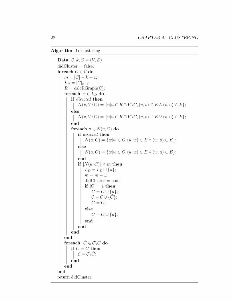
The algorithm introduced here (see Algorithm 1) is inspired by the clusteringalgorithm introduced in ”Improved Graph Drawing Via Clustering” by Sixand Tolles in [ST] regarding the Constraint 4.1.
The input of the algorithm is a set of clusters C(k−1) in respect of k − 1.The output is the set of clusters C(k) in respect of k.
For every cluster Ci ∈ C we need to find new members in the set ofneighbours of the nodes v ∈ Ci. The goal is to perform this without checkingevery neighbour of every node in each cluster as a potential new member.The good thing is, that we do not have to. As a new member needs atleast n − k − 1 direct neighbours in the cluster, we only have to check forneighbours of k + 1 members of each cluster. If none of the k + 1 membershas a neighbour, that has enough direct connections into the cluster, we canstop, as for any potentially new member the maximal number of possibleneighbours in the clusters is n − k − 2. If we choose the k + 1 memberswith the lowest degree, we have reduced the cost for expanding a clusterto a minimum. Let L
(k+1)D = Ci|k+1 be the set of the k + 1 lowest degree
members of the cluster Ci, which is equal to the first k + 1 elements of Ci.For every node v ∈ L
(k+1)D , we have to create the set of neighbours not in
4.2. THE CLUSTERING ALGORITHM 27
Ci of v; N(v, V \Ci) = {u|u ∈ V \Ci, (v, u) ∈ E ∧ (u, v) ∈ E}. For everyu ∈ N(v, V \Ci), we have to calculate the size of the set of neighbours of uin Ci; N(u,Ci). If |N(u,Ci)| exceeds n − k − 1 then u will be added to thecluster Ci.
A cluster Ci with size one will not be extended itself, but a copy will beadded and extended, as we need the single node to receive every possibledyad. Deleting the single nodes, if they and all their neighbours are part ofone cluster did not show any significant speed-up. The algorithm is listed inAlgorithm 1.
To avoid too much overlapping, a residual graph is calculated for everycluster (see Section 4.2.3), only including the nodes of the clusters, that thecurrent cluster does not share any nodes with. New members can only befound within the residual graph.
Worst-case runtime analysis
The first loop is calledO(|C|) times, creating the set of lowest degree membersLD in O(k) time. The time needed to create the rest-graph is discussed laterin Section 4.2.3, and is here denoted by O(R). For each member v ∈ LDwe create the set of member N(v, V \C) in O(n) time. For each node u ∈N(v, V \C) we create the set of neighbours of u in the cluster C in O(n)time. The rest of the inner loop can be approximated by O(n). At the endwe clean up after each cluster, which takes O(|C|) · O(n2) time. This sumsto an overall worst case running-time of
O(|C|) · (O(R) +O(k) · O(n2) +O(|C|) · O(n2))
Maximising the clusters
We assume, that it is not possible to find the best clustering by finding allk-plexes for a given k. Choosing a too small value for k ∈ N could yield inreceiving many small clusters (especially dyads), as each cluster has to behighly connected. On the other hand, choosing a too high value for k is verylikely to produce only a few or just one very large cluster (in respect of thesize of the graph) as each cluster is only very slightly connected. Instead itseems promising to start with the smallest possible value k = 1 and increasek after every clustering-step. A clustering-step is over, if no node can beadded to any cluster in respect to k.
28 CHAPTER 4. CLUSTERING
Algorithm 1: clustering
Data: C, k, G = (V,E)
didCluster = false;foreach C ∈ C do
m = |C| − k − 1;LD = |C|k+1;R = calcRGraph(C);foreach v ∈ LD do
if directed thenN(v, V \C) = {u|u ∈ R ∩ V \C, (u, v) ∈ E ∧ (v, u) ∈ E};
elseN(v, V \C) = {u|u ∈ R ∩ V \C, (u, v) ∈ E ∨ (v, u) ∈ E};
endforeach u ∈ N(v, C) do
if directed thenN(u,C) = {w|w ∈ C, (u,w) ∈ E ∧ (w, u) ∈ E};
elseN(u,C) = {w|w ∈ C, (u,w) ∈ E ∨ (w, u) ∈ E};
endif |N(u,C)| ≥ m then
LD = LD ∪ {u};m = m+ 1;didCluster = true;if |C| = 1 then
C = C ∪ {u};C = C ∪ {C};C = C;
elseC = C ∪ {u};
endend
endendforeach C ∈ C\C do
if C = C thenC = C\C;
endend
endreturn didCluster;
4.2. THE CLUSTERING ALGORITHM 29
The maximal possible value for k would be n − 1, n = |V | being thenumber of vertices in the graph, as each node would only need one incidentnode in any cluster, no matter how large.
A more efficient way to limit the number of iterations is to stop as soonas no node was being added to any cluster in one clustering step. Theresulting clustering is not optimal, as clusters can not include others, evenif the structure of the graph would indicate that. Thus we need a postprocessing, which merges clusters, that have enough overlapping, so thatthey can be considered to be one cluster (see Section 4.2.4).
One can imagine different ways of letting the clusters grow. They wereimplemented, but did not show any differences in their results. A possi-bly cause is the merging that is performed at the end. For the reason ofcompleteness they are listed here. The Algorithms 2,3, and 4 only differ inhow the sets of neighbours of N(v, V \C) and N(u,C) are calculated in thealgorithm, which extracts k-plexes (see Algorithm 1).
Algorithm 2: G1: undirected
Data: C, k, G = (V,E)
directed = false;while(clustering(k++,C,G));
Algorithm 3: G2: directed, then undirected
Data: C, k, G = (V,E)
directed = true;while(clustering(k++,C,G));directed = false;while(clustering(k++,C,G));
4.2.3 Calculating the residual graph
The calculation of the residual graph is needed in order to avoid too muchoverlapping between the clusters. The more overlapping we have, the morethe quality of the visualisation is reduced (see Chapter 6). We therefor require
30 CHAPTER 4. CLUSTERING
Algorithm 4: G3: directed, reset k, then undirected
Data: C, ki, G = (V,E)
directed = true;k = ki;while(clustering(k++,C,G));directed = false;k = ki;while(clustering(k++,C,G));
that two clusters, which share nodes at a certain clustering-step, denoted bythe corresponding k-plex parameter k, will not be allowed to have any furtheroverlapping for any k > k. To ensure this, the remaining graph R ⊂ G mustbe calculated once for every cluster at every clustering-step. The residualgraph R includes only nodes of clusters that have no node in common withthe current one.
To calculate the residual graph R, we need a binary array that indicates,which clusters overlap, and which do not. This array is denoted by AO andmust be re-initialised every time R is calculated, because the size of the setof clusters C may vary. New dyads are added to the set of clusters anddispensable clusters are removed. After the overlapping-array AO is createdand filled with values indicating the overlapping, the residual graph R canbe created by merging all clusters having a false entry in the array. Thealgorithm is shown in Algorithm 5.
Worst-case running time
With |Cm| we denote the size of the largest cluster in the set of clustersC. Initialising and filling of the overlap-array AO takes O(|C|) · O(|Cm|2)time, as for every cluster Cj ∈ C in the set of clusters, the intersectionwith the current cluster Ci is calculated. The residual graph R is created inO(|C|) · O(n) · O(|Cm|), as for every cluster Cj ∈ C in the set of clusters, thecluster Cj is merged with the residual graph R if it does not share any nodeswith the current cluster Ci. This gives us an overall worst case running-timeof
O(R) = O(|C|) · O(n) · (|Cm|).
4.2. THE CLUSTERING ALGORITHM 31
Algorithm 5: calculate residual graph
Data: |C|, CiResult: Rm = |C|;i = index(Ci);AO = BinArray(m);foreach Cj ∈ C do
if i = j thenAO(j) = 1;
elseif |Ci ∩ Cj| > 1 then
AO(j) = 1;
elseAO(j) = 0;
endend
endR = ∅;foreach Cj ∈ C do
if AO(j) = 0 thenR = R ∪ Ci;
endend
32 CHAPTER 4. CLUSTERING
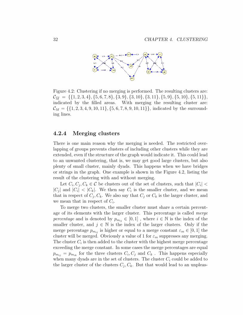
Figure 4.2: Clustering if no merging is performed. The resulting clusters are:CM = {{1, 2, 3, 4}, {5, 6, 7, 8}, {3, 9}, {3, 10}, {3, 11}, {5, 9}, {5, 10}, {5, 11}},indicated by the filled areas. With merging the resulting cluster are:CM = {{1, 2, 3, 4, 9, 10, 11}, {5, 6, 7, 8, 9, 10, 11}}, indicated by the surround-ing lines.
4.2.4 Merging clusters
There is one main reason why the merging is needed. The restricted over-lapping of groups prevents clusters of including other clusters while they areextended, even if the structure of the graph would indicate it. This could leadto an unwanted clustering, that is, we may get good large clusters, but alsoplenty of small cluster, mainly dyads. This happens when we have bridgesor strings in the graph. One example is shown in the Figure 4.2, listing theresult of the clustering with and without merging.
Let Ci, Cj, Ck ∈ C be clusters out of the set of clusters, such that |Ci| <|Cj| and |Ci| < |Ck|. We then say Ci is the smaller cluster, and we meanthat in respect of Cj, Ck. We also say that Cj or Ck is the larger cluster, andwe mean that in respect of Ci.
To merge two clusters, the smaller cluster must share a certain percent-age of its elements with the larger cluster. This percentage is called mergepercentage and is denoted by pmij ∈ [0, 1] , where i ∈ N is the index of thesmaller cluster, and j ∈ N is the index of the larger clusters. Only if themerge percentage pmij is higher or equal to a merge constant εm ∈ [0, 1] thecluster will be merged. Obviously a value of 1 for εm suppresses any merging.The cluster Ci is then added to the cluster with the highest merge percentageexceeding the merge constant. In some cases the merge percentages are equalpmij = pmik for the three clusters Ci, Cj and Ck . This happens especiallywhen many dyads are in the set of clusters. The cluster Ci could be added tothe larger cluster of the clusters Cj, Ck. But that would lead to an unpleas-
4.2. THE CLUSTERING ALGORITHM 33
ant clustering, as the shared nodes in Figure 4.2 would be added completelyto one of the two clusters {1, 2, 3, 4} or {5, 6, 7, 8}, depending which clusterwould first include one of the dyads. In this case node 3 or node 5 would bethe shared node of the resulting two clusters.
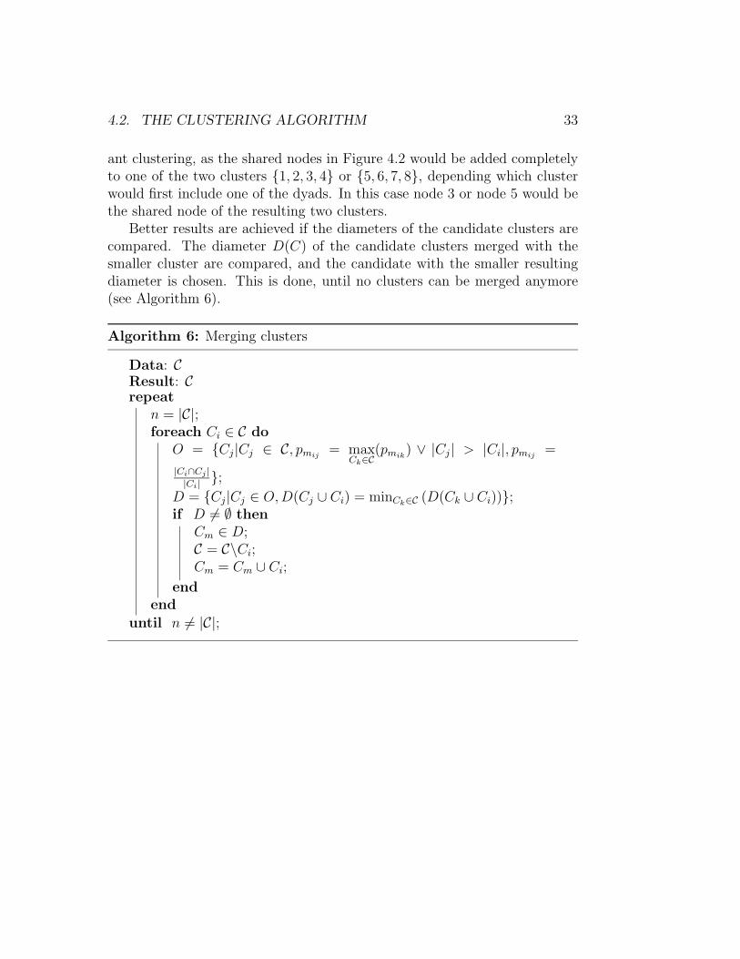
Better results are achieved if the diameters of the candidate clusters arecompared. The diameter D(C) of the candidate clusters merged with thesmaller cluster are compared, and the candidate with the smaller resultingdiameter is chosen. This is done, until no clusters can be merged anymore(see Algorithm 6).
Algorithm 6: Merging clusters
Data: CResult: Crepeat
n = |C|;foreach Ci ∈ C do
O = {Cj|Cj ∈ C, pmij = maxCk∈C
(pmik) ∨ |Cj| > |Ci|, pmij =
|Ci∩Cj ||Ci| };
D = {Cj|Cj ∈ O,D(Cj ∪ Ci) = minCk∈C (D(Ck ∪ Ci))};if D 6= ∅ then
Cm ∈ D;C = C\Ci;Cm = Cm ∪ Ci;
endend
until n 6= |C|;

34 CHAPTER 4. CLUSTERING
Chapter 5
Centrality
Once we have the clusters extracted, it is very interesting to know, how thepower is distributed within the clusters, and how the power is distributedamong the groups. The power is an index of the importance of the actorin the network and allows to draw conclusions about the activity of theactors, showing if they are passive or active. Concerning the distribution ofpower in the complete network, it shows if the network is homogeneous orheterogeneous.
5.1 Overview
Power is the consequence of patterns of relations [Han98]. We will discussthe degree-, betweenness-, closeness- and flow-betweenness-centrality, as thebasic centrality measurements. The problems of the closeness-centrality arediscussed in the Section 5.1.4. The Bonacich power index is introduced asan alternative measurement, but is not included in the analysis.
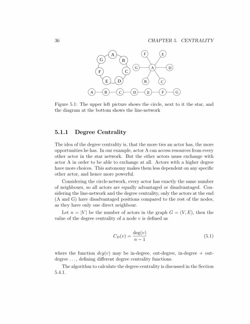
To understand the principles of a power centrality measurement, we takea look at three basic types of networks, the star, line, and circle (see Figure5.1). Having a short look at the basic networks, a viewer would probablysay, that actor A has the most power in the star-network. In the followingwe should find enough arguments that validate our assumption.
We then discuss how the centrality measurement can be adopted to calcu-late the group-centrality, ending the chapter with the algorithms to calculatethe basic centrality measurements.
35
36 CHAPTER 5. CENTRALITY
B
E D
C
A
F
G
A
B C
D
EF
G
A B C D E F G
Figure 5.1: The upper left picture shows the circle, next to it the star, andthe diagram at the bottom shows the line-network
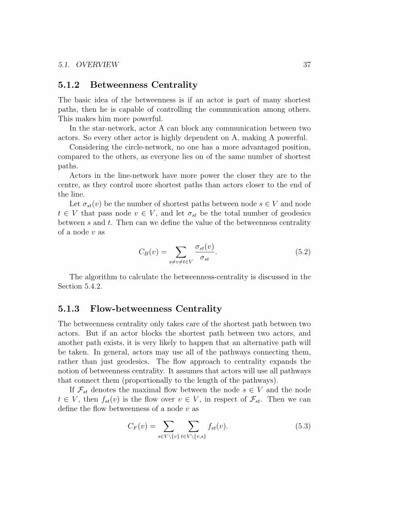
5.1.1 Degree Centrality
The idea of the degree centrality is, that the more ties an actor has, the moreopportunities he has. In our example, actor A can access resources from everyother actor in the star network. But the other actors muss exchange withactor A in order to be able to exchange at all. Actors with a higher degreehave more choices. This autonomy makes them less dependent on any specificother actor, and hence more powerful.
Considering the circle-network, every actor has exactly the same numberof neighbours, so all actors are equally advantaged or disadvantaged. Con-sidering the line-network and the degree centrality, only the actors at the end(A and G) have disadvantaged positions compared to the rest of the nodes,as they have only one direct neighbour.
Let n = |V | be the number of actors in the graph G = (V,E), then thevalue of the degree centrality of a node v is defined as
CD(v) =deg(v)
n− 1(5.1)
where the function deg(v) may be in-degree, out-degree, in-degree + out-degree . . . , defining different degree centrality functions.
The algorithm to calculate the degree-centrality is discussed in the Section5.4.1.
5.1. OVERVIEW 37
5.1.2 Betweenness Centrality
The basic idea of the betweenness is if an actor is part of many shortestpaths, then he is capable of controlling the communication among others.This makes him more powerful.
In the star-network, actor A can block any communication between twoactors. So every other actor is highly dependent on A, making A powerful.
Considering the circle-network, no one has a more advantaged position,compared to the others, as everyone lies on of the same number of shortestpaths.
Actors in the line-network have more power the closer they are to thecentre, as they control more shortest paths than actors closer to the end ofthe line.
Let σst(v) be the number of shortest paths between node s ∈ V and nodet ∈ V that pass node v ∈ V , and let σst be the total number of geodesicsbetween s and t. Then can we define the value of the betweenness centralityof a node v as
CB(v) =∑
s 6=v 6=t∈V
σst(v)
σst. (5.2)
The algorithm to calculate the betweenness-centrality is discussed in theSection 5.4.2.
5.1.3 Flow-betweenness Centrality
The betweenness centrality only takes care of the shortest path between twoactors. But if an actor blocks the shortest path between two actors, andanother path exists, it is very likely to happen that an alternative path willbe taken. In general, actors may use all of the pathways connecting them,rather than just geodesics. The flow approach to centrality expands thenotion of betweenness centrality. It assumes that actors will use all pathwaysthat connect them (proportionally to the length of the pathways).
If Fst denotes the maximal flow between the node s ∈ V and the nodet ∈ V , then fst(v) is the flow over v ∈ V , in respect of Fst. Then we candefine the flow betweenness of a node v as
CF (v) =∑
s∈V \{v}
∑t∈V \{v,s}
fst(v). (5.3)
38 CHAPTER 5. CENTRALITY
In this definition, we do not take care of the length of the pathway. Onemethod would be dividing CF by the sum of the length of the geodesicsbetween s, v and v, t divided by the length of the geodesic between s and t:
CF (v) =
∑s∈V \{v}
∑t∈V \{v,s} fst(v)
dist(s,v)+dist(v,t)dist(s,t)
. (5.4)
The algorithm to calculate the flow-betweenness is discussed in the Section5.4.3.
5.1.4 Closeness Centrality
Actors who are able to reach other actors at shorter path length, or whoare more reachable by other actors at shorter path lengths, have a favouredposition. In the star-network again actor A has the best position, as he isclosest to all other actors. Taking a look at the circle-network, we see thatall the actors have an identical distribution of closeness, as for each actorthe sum of distances to the other actors is identical. Actor D is the mostpowerful in the line network, followed by the couple of C,E, then B,F andfinally A,G. Let dist(v, t) be the length of the geodesic between the actors vand the actor t, then we can define the closeness centrality of a node v as
CC(v) =1∑
t∈V dist(v, t)(5.5)
or
CC(v) =∑t∈V
dist(v, t). (5.6)
The problem with this centrality is, it does not really handle isolated nodes,or completely separated sub-graphs. If unreachable nodes have a distanceof infinity, then it is hard to distinguish between nodes that are completelyisolated and nodes that have a few neighbours and some nodes they cannot reach. Assigning the value 0 for unreachable actors would make a dis-connected group of two actors most powerful, as it would have a closenesscentrality value of 1.
5.2. GROUP CENTRALITY 39
5.1.5 The Bonacich’s power index
Phillip Bonacich completely questions the ideas of centrality as discussedhere. His idea is, that if an actor A is connected to central others, he ismore influential, as he can reach more actors with less expense. But if theothers are themselves well connected, they are not highly dependent on theactor A. If, on the other hand, the others are not well connected, then theydepend more on the actor A, making him more powerful. Bonacich arguedthat being connected to connected others makes an actor central, but notpowerful, but being connected to others that are not well connected makesan actor powerful. Bonacich proposed that both centrality and power are afunction of the connections of the actors in one’s neighbourhood. The moreconnections the actors in the neighbourhood have, the more central an actorsis. The fewer connections the actors in the neighbourhood have, the morepowerful the actor is.
5.2 Group centrality
After we have done the clustering and calculated the centrality value for everynode in its cluster, we are interested in the distribution of power among thegroups. This should be possible using existing individual measures. Everettand Borgatti introduce a method for calculating group centralities, usingexisting measures [EB99].
5.2.1 General Principles
Any group measure is a proper generalisation of the corresponding individualmeasure, such as, when applied to a group consisting of a single individual,the measure yields the same answer as the individual version. An immediateconsequence of this requirement is that group centrality is not measured bycomputing centrality on a network of relationships among groups. Instead,the centrality of a group is computed directly from the network of relation-ships among individuals. A side benefit of this approach is that there are noproblems working with overlapping groups, where one individual can belongto many groups.
40 CHAPTER 5. CENTRALITY
A B
C
D
E
F
G
H
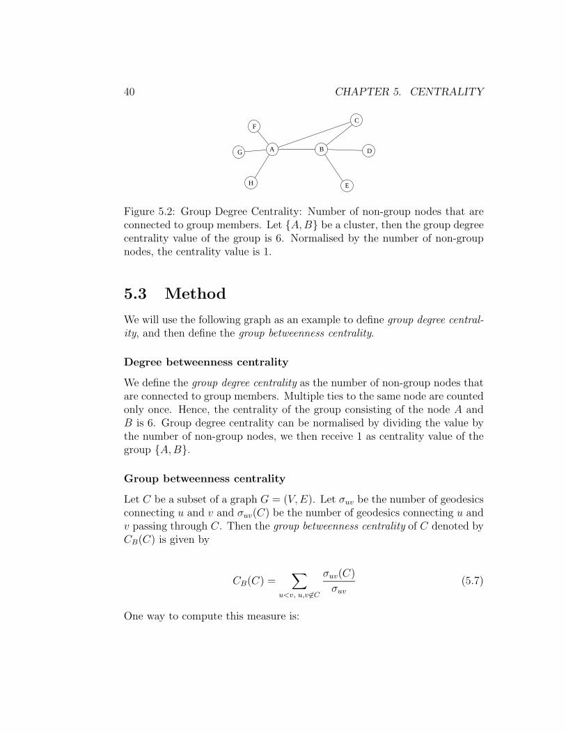
Figure 5.2: Group Degree Centrality: Number of non-group nodes that areconnected to group members. Let {A,B} be a cluster, then the group degreecentrality value of the group is 6. Normalised by the number of non-groupnodes, the centrality value is 1.
5.3 Method
We will use the following graph as an example to define group degree central-ity, and then define the group betweenness centrality.
Degree betweenness centrality
We define the group degree centrality as the number of non-group nodes thatare connected to group members. Multiple ties to the same node are countedonly once. Hence, the centrality of the group consisting of the node A andB is 6. Group degree centrality can be normalised by dividing the value bythe number of non-group nodes, we then receive 1 as centrality value of thegroup {A,B}.
Group betweenness centrality
Let C be a subset of a graph G = (V,E). Let σuv be the number of geodesicsconnecting u and v and σuv(C) be the number of geodesics connecting u andv passing through C. Then the group betweenness centrality of C denoted byCB(C) is given by
CB(C) =∑
u<v, u,v 6∈C
σuv(C)
σuv(5.7)
One way to compute this measure is:
5.4. ALGORITHMS 41
1. count the number of geodesics between every pair of non-group mem-bers, yielding a node-by-node matrix of counts
2. delete all ties involving group members and redo the calculation, cre-ating a new node-by-node matrix of counts
3. divide each cell in the new matrix by the corresponding cell in the firstmatrix
4. take the sum of all these ratios
5.4 Algorithms
We implemented the basic centrality measures of degree and betweenness cen-trality, and one alternative to betweenness, the flow betweenness centrality.
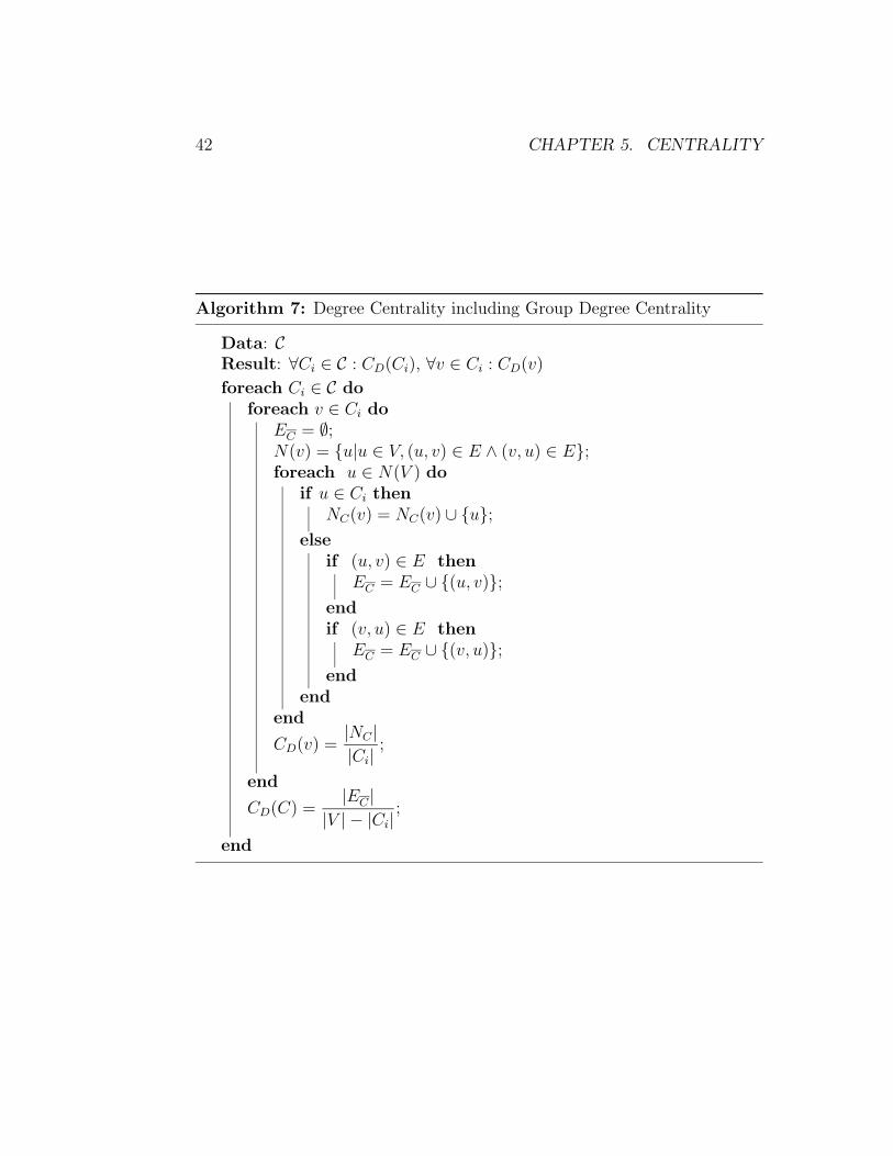
5.4.1 Degree centrality
Let G = (V,E) be a graph, and N(v) = {u|u ∈ V, (u, v) ∈ E ∨ (v, u) ∈ E}be the set of neighbours u ∈ V of v ∈ V . We define the set of edges leaving acluster EC = {(u, v)|(u, v) ∈ E, (u ∈ C∧v ∈ V \C)∨(u ∈ V \C∧v ∈ C)} andthe set of neighbours u of v that are in the same cluster NC(v) = C ∩N(v).
The values for CD(v) and CD(C) may be normalised as suggested here(see Algorithm 7). One alternative method would be to normalise the valuesby the theoretical maximum given by a star-network (see Figure 5.1) of thesame size. Normalising by the theoretical maximums allows to compare thecentrality values of different networks. As we combine the three centralitymeasures by a weighted sum, we decided to normalise each value by itsmaximum.
5.4.2 Betweenness centrality
A fast algorithm to calculate betweenness centrality was introduced by UlrikBrandes. The description in this section follows the publication ”Faster Eval-uation of Shortest-Path Based Centrality Indices” of Ulrik Brandes. Proofsare omitted here, as they give no additional information. For any proof or amore detailed description see [Bra00].
42 CHAPTER 5. CENTRALITY
Algorithm 7: Degree Centrality including Group Degree Centrality
Data: CResult: ∀Ci ∈ C : CD(Ci), ∀v ∈ Ci : CD(v)
foreach Ci ∈ C doforeach v ∈ Ci do
EC = ∅;N(v) = {u|u ∈ V, (u, v) ∈ E ∧ (v, u) ∈ E};foreach u ∈ N(V ) do
if u ∈ Ci thenNC(v) = NC(v) ∪ {u};
elseif (u, v) ∈ E then
EC = EC ∪ {(u, v)};endif (v, u) ∈ E then
EC = EC ∪ {(v, u)};end
endend
CD(v) =|NC ||Ci|
;
end
CD(C) =|EC |
|V | − |Ci|;
end
5.4. ALGORITHMS 43
The betweenness centrality is an essential measurement for the analysis ofsocial networks. The fastest known algorithms require Θ(n3) time and Θ(n2)space, where n = |V | is the number of vertices. The algorithm introducedby Ulrik Brandes requires O(n + m) space and runs in O(n(m + n)) orO(n(m + n log n)) time for unweighted or weighted graphs, where m = |E|is the number of edges.
To obtain the betweenness centrality index of a vertex v, we simply haveto sum the pair-dependencies of all pairs on that vertex
CB(v) =∑
s 6=v 6=t∈V
σst(v)
σst(5.8)
where σst is the number of shortest paths between s ∈ V and t ∈ V , andσst(v) is the number of shortest paths between s and t passing the nodev ∈ V .
Therefor betweenness centrality is traditionally determined in two steps.
1. compute the length and number of shortest paths between all pairs
2. sum all pair-dependencies
Corollary 5.1 Given a source s ∈ V , both the length and number of allshortest paths to other vertices can be determined in time O(m+n log n) forweighted, and in time O(m+ n) for unweighted graphs.
The Corollary 5.1 tells us, that the complexity of determining the be-tweenness centrality is dominated by the second step, the θ(n3) time sum-mation and θ(n2) storage of pair-dependencies. This situation is remediedby the algorithm introduced by Ulrik Brandes.
Accumulation of Pair-Dependencies
Let G = (V,E) be a graph, and let σst = σts denote the number of shortestpaths between s ∈ V and t ∈ V , where σss = 1 by convention. Then σst(v)is the number of shortest paths between s and t that pass the vertex v ∈ V .The distance between s and t is described by dG(s, t), where dG(s, s) = 0 forevery s ∈ V , and dG(s, t) = dG(t, s) for s, t ∈ V . Given pairwise distances andshortest paths counts, the pair-dependency δst(v) =
σst(v)
σstof a pair s, t ∈ V
on an intermediary v ∈ V . The lemma and theorem are taken from [Bra00].
44 CHAPTER 5. CENTRALITY
We define the dependency of a vertex s ∈ V on v ∈ V as
δs• =∑t∈V
δst(v), (5.9)
Lemma 5.1 If there is exactly one shortest path from s ∈ V to each t ∈ V ,the dependency of s on any v ∈ V obeys
δs•(v) =∑
w:v∈Ps(w)
(1 + δs•(w)) (5.10)
where
Ps(v) = {u ∈ V |(u, v) ∈ E, dG(s, v) = dG(s, u) + ω(u, v)}
is the set of predecessors of a vertex v.
Theorem 5.1 The dependency of s ∈ V on any v ∈ V obeys
δs• =∑
w:v∈Ps(w)
σsvσsw· (1 + δst(w)).
With this theorem, we can determine the betweenness centrality indexby solving the single-source shortest-paths problem for each vertex. At theend of each iteration, the dependencies of the source on each other vertexare added to the centrality score of that vertex.
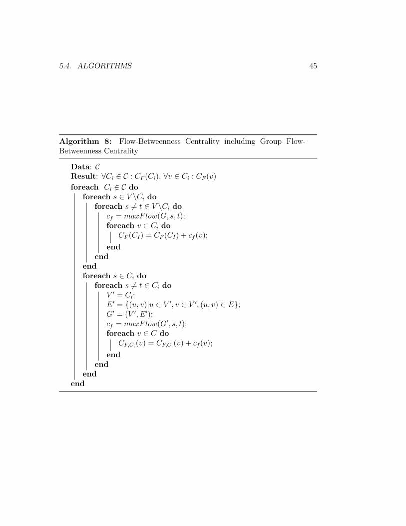
5.4.3 Flow-betweenness centrality
Let G = (V,E) be the graph, where V is the set of vertices v ∈ V andE is the set of edges. The maxFlow-function was implemented using thelift-to-front algorithm, see [CLR99] for a description of the algorithm. Withcf we describe the array of values returned by maxFlow, and with cf (v) wecan access the max-flow-value of the node v ∈ V , and CF,Ci(v) is the flow-betweenness of the node v in the cluster Ci. In this algorithm the length ofthe path the node v is part of is not taken into account. A rule to normalisethe value of CF,Ci(v) is not given here, but we normalise any centrality indexby the maximum. The flow index of each group is described by CF (Ci).
To calculate the flow index of a node in a group, the maximum flow withinthe cluster is calculated for every combination of s, t ∈ Ci, s 6= t. The flowvalues for every node in the cluster are added together, receiving the flowcentrality value.
5.4. ALGORITHMS 45
Algorithm 8: Flow-Betweenness Centrality including Group Flow-Betweenness Centrality
Data: CResult: ∀Ci ∈ C : CF (Ci), ∀v ∈ Ci : CF (v)
foreach Ci ∈ C doforeach s ∈ V \Ci do
foreach s 6= t ∈ V \Ci docf = maxFlow(G, s, t);foreach v ∈ Ci do
CF (CI) = CF (CI) + cf (v);
endend
endforeach s ∈ Ci do
foreach s 6= t ∈ Ci doV ′ = Ci;E ′ = {(u, v)|u ∈ V ′, v ∈ V ′, (u, v) ∈ E};G′ = (V ′, E ′);cf = maxFlow(G′, s, t);foreach v ∈ C do
CF,Ci(v) = CF,Ci(v) + cf (v);
endend
endend

46 CHAPTER 5. CENTRALITY
Chapter 6
Visualisation
After clustering the graph, and determining the distribution of power orcentrality, the extracted information should be visualised.
The visualisation should support the social scientist in two ways. It shouldhelp the scientist with the analysis concerning the social network and alsosupport the presentation of the results of the analysis, as a good visualisationcan provide additional comprehension aids.
The information should therefor be clearly visible, without much inter-pretation or searching needed.
6.1 Data and Properties
Before we discuss the visualisation, we should recapitulate what kind of datawe have, and define the properties of the visualisation.
6.1.1 Data
Let G = (V,E) be a graph representing the social network. We then havenodes, representing actors, and edges representing the relations between ac-tors. The relations between actors are directed. Two actors A,B havea relation, if the corresponding vertices vA, vB ∈ V are incident, that is(vA, vB) ∈ E or (vB, vA) ∈ E. The nodes are combined in clusters, whichdenote separated groups within the graph. A node can be part of more thanone group or cluster. Each node has a centrality value in its cluster. If a nodeis part of more than one cluster, it may have a different centrality value in
47
48 CHAPTER 6. VISUALISATION
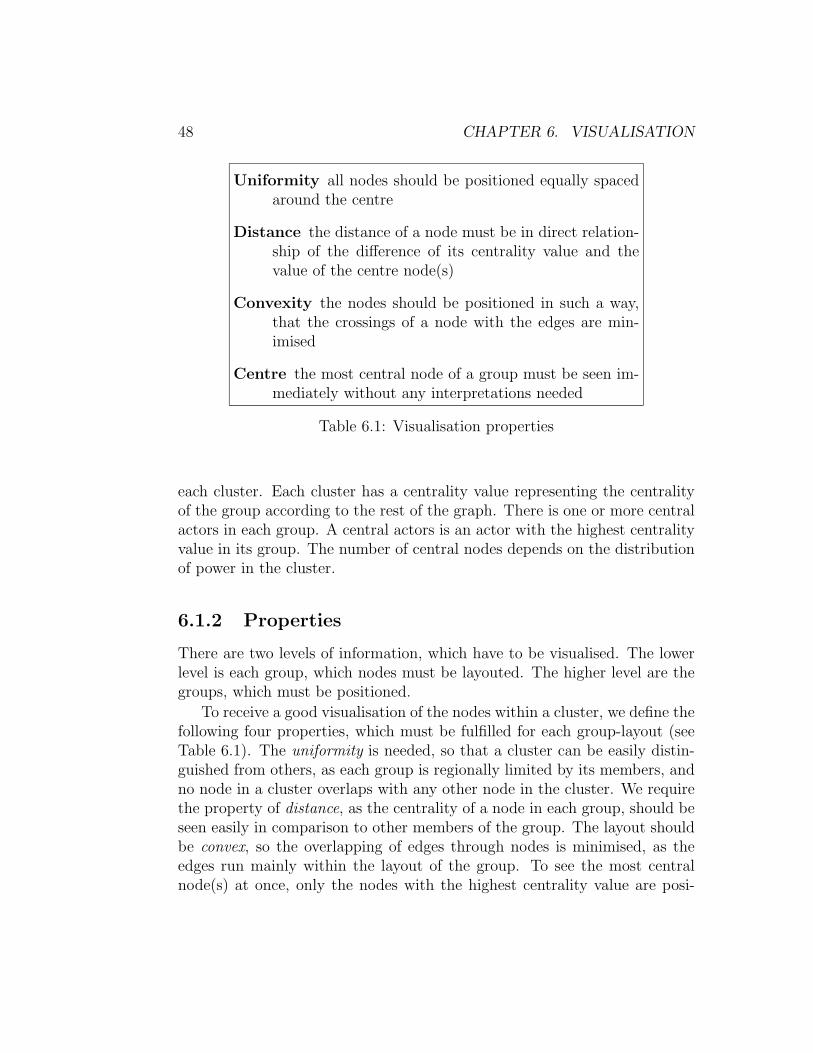
Uniformity all nodes should be positioned equally spacedaround the centre
Distance the distance of a node must be in direct relation-ship of the difference of its centrality value and thevalue of the centre node(s)
Convexity the nodes should be positioned in such a way,that the crossings of a node with the edges are min-imised
Centre the most central node of a group must be seen im-mediately without any interpretations needed
Table 6.1: Visualisation properties
each cluster. Each cluster has a centrality value representing the centralityof the group according to the rest of the graph. There is one or more centralactors in each group. A central actors is an actor with the highest centralityvalue in its group. The number of central nodes depends on the distributionof power in the cluster.
6.1.2 Properties
There are two levels of information, which have to be visualised. The lowerlevel is each group, which nodes must be layouted. The higher level are thegroups, which must be positioned.
To receive a good visualisation of the nodes within a cluster, we define thefollowing four properties, which must be fulfilled for each group-layout (seeTable 6.1). The uniformity is needed, so that a cluster can be easily distin-guished from others, as each group is regionally limited by its members, andno node in a cluster overlaps with any other node in the cluster. We requirethe property of distance, as the centrality of a node in each group, should beseen easily in comparison to other members of the group. The layout shouldbe convex, so the overlapping of edges through nodes is minimised, as theedges run mainly within the layout of the group. To see the most centralnode(s) at once, only the nodes with the highest centrality value are posi-
6.2. PROBLEMS 49
tioned in the centre of the group. The central nodes are also scaled in size,so they have a second property that distinguishes them from the non-centralnodes.
We say, a node is positioned nicely, if it fulfils the visualisation properties.A shared node is positioned nicely, if it fulfils the visualisation properties foreach cluster it is in.
6.2 Problems
We first define a clan and the different types of nodes and clusters, beforediscussing the the problems that must be handled if more than one clusterwith overlapping is to be visualised.
Definition 6.1 (clan)Let G = (V,E) be a graph. Let C = {Ci}i∈I be a valid clustering of G, suchthat
⋃i∈ICi = V but the Ci ∈ C may not be disjunct. A clan is a subset
Φ ∈ C such that the elements Ci ∈ Φ overlap, that is⋂Ci∈Φ Ci 6= ∅, and
∀Ci∈CCj 6∈ Φ : Cj ∩(⋂
Ci∈ΓCi)
= ∅. The set of clans is denoted by Φ.
6.2.1 Types of Nodes
A cluster Ci ∈ C can be divided into central ZCi and non-central nodes ZCi .So we can distinguish between four different classes of nodes.
Type A Node v ∈ V is part of only one group:
v ∈ T AA : [∃1Ci ∈ C : v ∈ Ci, v 6∈ Cj∀j 6= i ].
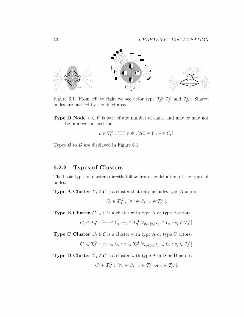
Type B Node v ∈ V is part of any number of clans, having a non-centralposition in each cluster included in the clan:
v ∈ T AB : [∃Γ ∈ Φ : ∀Ci ∈ Γ : v ∈ Z ].
Type C Node v ∈ V is part of any number of clans, having a centralposition in each cluster included in the clan:
v ∈ T AC : [∃Γ ∈ Φ : ∀Ci ∈ Γ : v ∈ Zi ].
50 CHAPTER 6. VISUALISATION
Type B
Type C
� � �� � �� � �� � �� � �
� � �� � �� � �� � �� � �
� � �� � �� � �� � �� � �
� � �� � �� � �� � �� � �
� � �� � �� � �� � �� � �
� � �� � �� � �� � �� � �� � �� � �� � �� � �� � �
� � �� � �� � �� � �� � �
� � � �� � � �� � � �
� � �� � �� � �
� � � �� � � �� � � �
� � �� � �� � �
� � �� � �� � �
� � �� � �� � �� � �� � �
� � �� � �� � �� � �� � �� � �� � �� � �� � �� � �
� � �� � �� � �� � �� � �� � �� � �� � �� � �� � �
� � �� � �� � �� � �� � �� � �� � �� � �� � �� � �
� � �� � �� � �� � �� � �
� � � � �� � � � �� � � � �
� � � � �� � � � �� � � � �
� � � � �� � � � �� � � � �
� � � � �� � � � �� � � � �
� � � � �� � � � �� � � � �
� � � � �� � � � �� � � � �
� � � � �� � � � �� � � � �
� � � � �� � � � �� � � � �
! !! !! !! !! !! !! !! !! !
" " "" " "" " "" " "
# ## ## ## #
$ $$ $$ $$ $$ $$ $$ $$ $$ $
% %% %% %% %% %% %% %% %
& & & & && & & & && & & & && & & & &
' ' ' ' '' ' ' ' '' ' ' ' '' ' ' ' '
� � � � � � � �� � � � � � � �� � � � � � � �� � � � � � � �� � � � � � � �� � � � � � � �� � � � � � � �
� � � � � � � �� � � � � � � �� � � � � � � �� � � � � � � �� � � � � � � �� � � � � � � �� � � � � � � �
Type D
Figure 6.1: From left to right we see actor type T AB , T AC and T AD . Sharednodes are marked by the filled areas.
Type D Node v ∈ V is part of any number of clans, and may or may notbe in a central position:
v ∈ T AD : [∃Γ ∈ Φ : ∀Ci ∈ Γ : v ∈ Ci ].
Types B to D are displayed in Figure 6.1.
6.2.2 Types of Clusters
The basic types of clusters directly follow from the definition of the types ofnodes.
Type A Cluster Ci ∈ C is a cluster that only includes type A actors:
Ci ∈ T GA : [∀v ∈ Ci : v ∈ T AA ].
Type B Cluster Ci ∈ C is a cluster with type A or type B actors:
Ci ∈ T GB : [∃vi ∈ Ci : vi ∈ T AB ,∀vj 6∈{vi}vj ∈ Ci : vj ∈ T AA ].
Type C Cluster Ci ∈ C is a cluster with type A or type C actors:
Ci ∈ T GC : [∃vi ∈ Ci : vi ∈ T AC ,∀vj 6∈{vi}vj ∈ Ci : vj ∈ T AA ].
Type D Cluster Ci ∈ C is a cluster with type A or type D actors:
Ci ∈ T GD : [∀v ∈ Ci : v ∈ T AA or v ∈ T AD ].
6.2. PROBLEMS 51
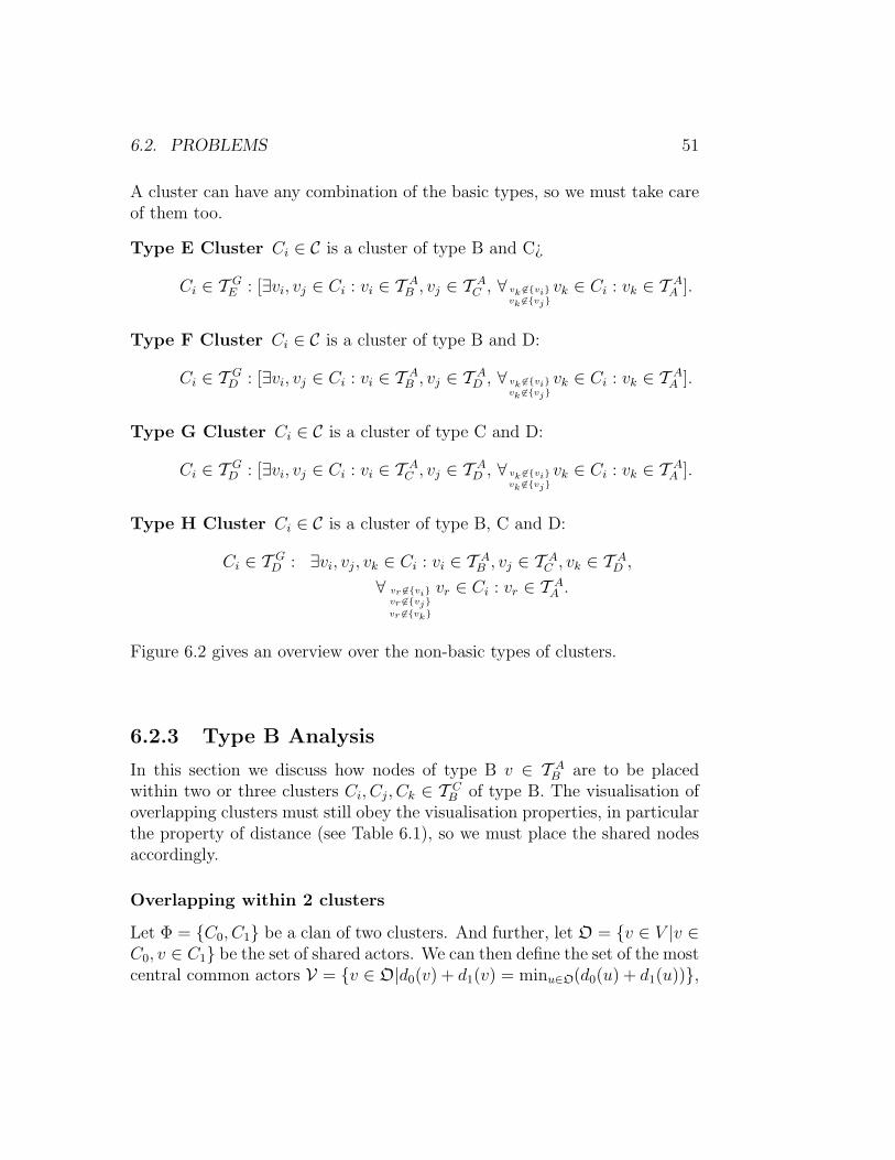
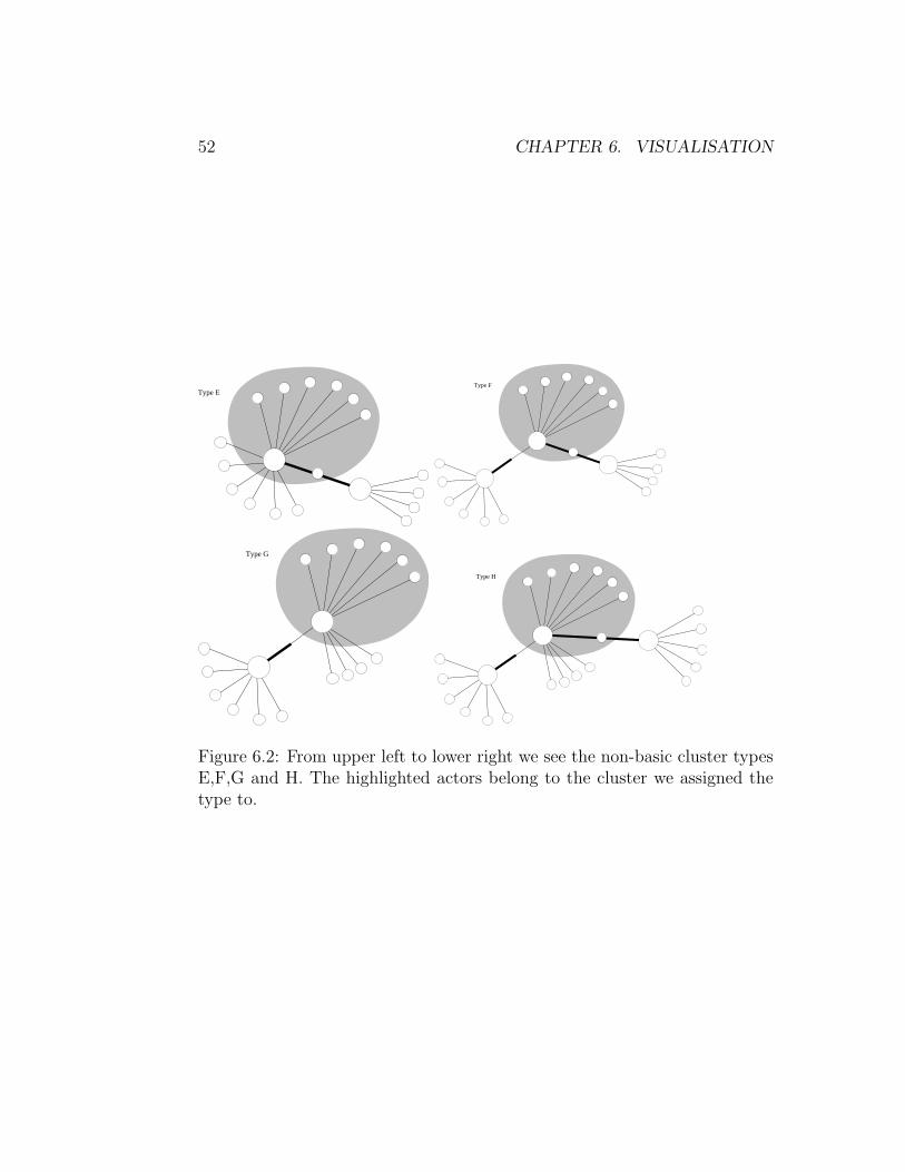
A cluster can have any combination of the basic types, so we must take careof them too.
Type E Cluster Ci ∈ C is a cluster of type B and C¿
Ci ∈ T GE : [∃vi, vj ∈ Ci : vi ∈ T AB , vj ∈ T AC , ∀ vk 6∈{vi}vk 6∈{vj}
vk ∈ Ci : vk ∈ T AA ].
Type F Cluster Ci ∈ C is a cluster of type B and D:
Ci ∈ T GD : [∃vi, vj ∈ Ci : vi ∈ T AB , vj ∈ T AD , ∀ vk 6∈{vi}vk 6∈{vj}
vk ∈ Ci : vk ∈ T AA ].
Type G Cluster Ci ∈ C is a cluster of type C and D:
Ci ∈ T GD : [∃vi, vj ∈ Ci : vi ∈ T AC , vj ∈ T AD , ∀ vk 6∈{vi}vk 6∈{vj}
vk ∈ Ci : vk ∈ T AA ].
Type H Cluster Ci ∈ C is a cluster of type B, C and D:
Ci ∈ T GD : ∃vi, vj, vk ∈ Ci : vi ∈ T AB , vj ∈ T AC , vk ∈ T AD ,∀ vr 6∈{vi}vr 6∈{vj}vr 6∈{vk}
vr ∈ Ci : vr ∈ T AA .
Figure 6.2 gives an overview over the non-basic types of clusters.
6.2.3 Type B Analysis
In this section we discuss how nodes of type B v ∈ T AB are to be placedwithin two or three clusters Ci, Cj, Ck ∈ T CB of type B. The visualisation ofoverlapping clusters must still obey the visualisation properties, in particularthe property of distance (see Table 6.1), so we must place the shared nodesaccordingly.
Overlapping within 2 clusters
Let Φ = {C0, C1} be a clan of two clusters. And further, let O = {v ∈ V |v ∈C0, v ∈ C1} be the set of shared actors. We can then define the set of the mostcentral common actors V = {v ∈ O|d0(v) + d1(v) = minu∈O(d0(u) + d1(u))},
52 CHAPTER 6. VISUALISATION
Type EType F
Type G
Type H
Figure 6.2: From upper left to lower right we see the non-basic cluster typesE,F,G and H. The highlighted actors belong to the cluster we assigned thetype to.
6.2. PROBLEMS 53
where di(v) is the distance-value of the actor v in the cluster Ci, as definedin the Algorithm 9.
The distance between the centre of the groups is then defined by
D = dist(C0, C1) = d0(v) + d1(v), v ∈ V .
The following constraint must be valid for all nodes v ∈ V if we want thedistance of v to have the same proposition as all the other nodes, that arepart of the group.
∀v ∈ O : |d0(v)− d1(v)| ≤ D
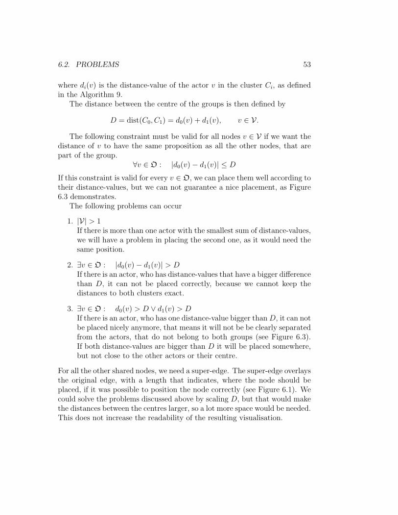
If this constraint is valid for every v ∈ O, we can place them well according totheir distance-values, but we can not guarantee a nice placement, as Figure6.3 demonstrates.
The following problems can occur
1. |V| > 1If there is more than one actor with the smallest sum of distance-values,we will have a problem in placing the second one, as it would need thesame position.
2. ∃v ∈ O : |d0(v)− d1(v)| > DIf there is an actor, who has distance-values that have a bigger differencethan D, it can not be placed correctly, because we cannot keep thedistances to both clusters exact.
3. ∃v ∈ O : d0(v) > D ∨ d1(v) > DIf there is an actor, who has one distance-value bigger thanD, it can notbe placed nicely anymore, that means it will not be be clearly separatedfrom the actors, that do not belong to both groups (see Figure 6.3).If both distance-values are bigger than D it will be placed somewhere,but not close to the other actors or their centre.
For all the other shared nodes, we need a super-edge. The super-edge overlaysthe original edge, with a length that indicates, where the node should beplaced, if it was possible to position the node correctly (see Figure 6.1). Wecould solve the problems discussed above by scaling D, but that would makethe distances between the centres larger, so a lot more space would be needed.This does not increase the readability of the resulting visualisation.
54 CHAPTER 6. VISUALISATION
C1C0
c (v)1c (v)0
c (v) > D1
D
vC1
C0
c (v)1c (v)0
c (v) > D1
D
v
Figure 6.3: Possible overlap between 2 groups. Here we see an actor, whichfulfils the constraint, but overlapping and non-overlapping actors are notseparated clearly anymore
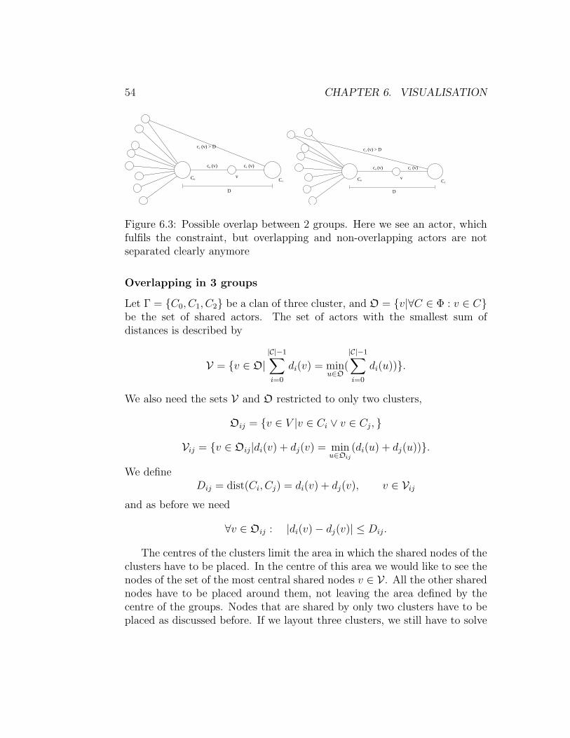
Overlapping in 3 groups
Let Γ = {C0, C1, C2} be a clan of three cluster, and O = {v|∀C ∈ Φ : v ∈ C}be the set of shared actors. The set of actors with the smallest sum ofdistances is described by
V = {v ∈ O||C|−1∑i=0
di(v) = minu∈O
(
|C|−1∑i=0
di(u))}.
We also need the sets V and O restricted to only two clusters,
Oij = {v ∈ V |v ∈ Ci ∨ v ∈ Cj, }
Vij = {v ∈ Oij|di(v) + dj(v) = minu∈Oij
(di(u) + dj(u))}.
We defineDij = dist(Ci, Cj) = di(v) + dj(v), v ∈ Vij
and as before we need
∀v ∈ Oij : |di(v)− dj(v)| ≤ Dij.
The centres of the clusters limit the area in which the shared nodes of theclusters have to be placed. In the centre of this area we would like to see thenodes of the set of the most central shared nodes v ∈ V . All the other sharednodes have to be placed around them, not leaving the area defined by thecentre of the groups. Nodes that are shared by only two clusters have to beplaced as discussed before. If we layout three clusters, we still have to solve
6.2. PROBLEMS 55
C0
1C
C2
dv
dv
dv
C0
1C
C2
v02
v12
v012
v01
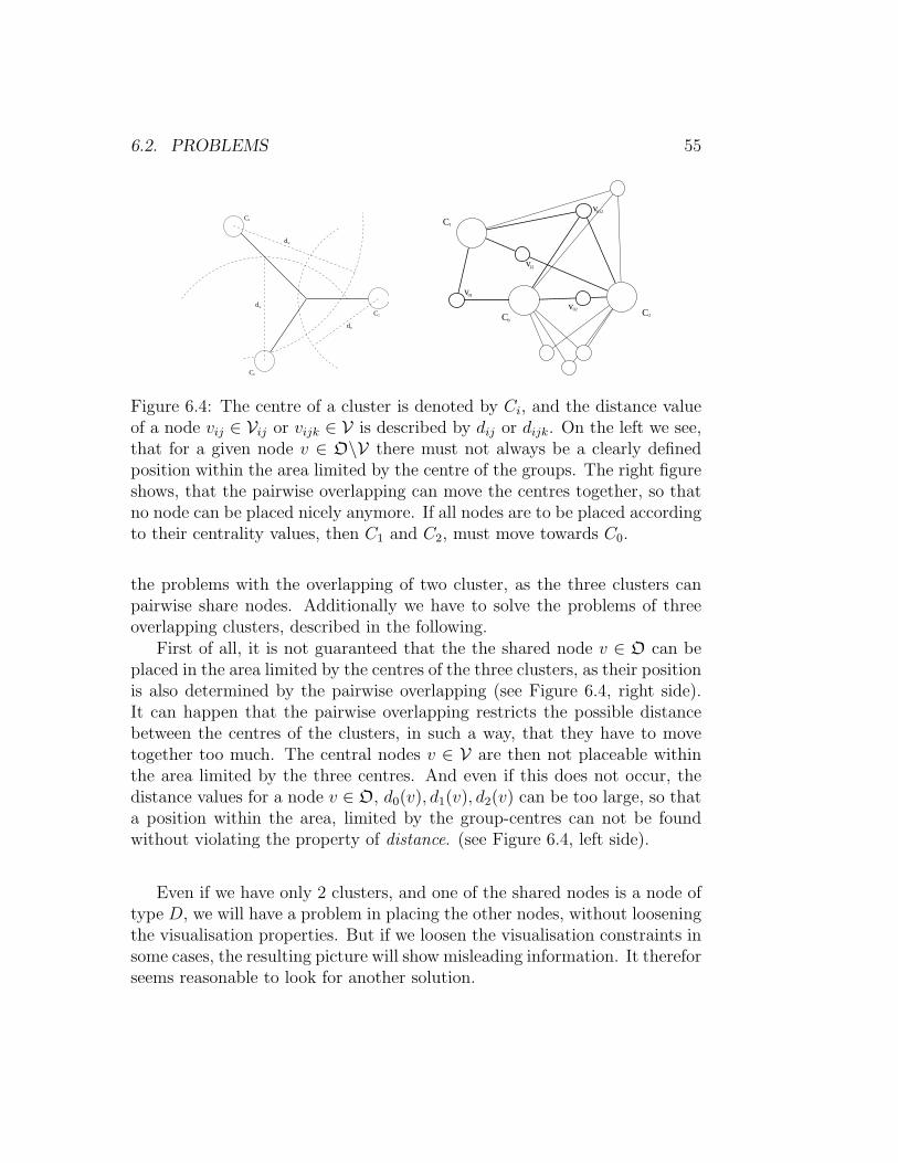
Figure 6.4: The centre of a cluster is denoted by Ci, and the distance valueof a node vij ∈ Vij or vijk ∈ V is described by dij or dijk. On the left we see,that for a given node v ∈ O\V there must not always be a clearly definedposition within the area limited by the centre of the groups. The right figureshows, that the pairwise overlapping can move the centres together, so thatno node can be placed nicely anymore. If all nodes are to be placed accordingto their centrality values, then C1 and C2, must move towards C0.
the problems with the overlapping of two cluster, as the three clusters canpairwise share nodes. Additionally we have to solve the problems of threeoverlapping clusters, described in the following.
First of all, it is not guaranteed that the the shared node v ∈ O can beplaced in the area limited by the centres of the three clusters, as their positionis also determined by the pairwise overlapping (see Figure 6.4, right side).It can happen that the pairwise overlapping restricts the possible distancebetween the centres of the clusters, in such a way, that they have to movetogether too much. The central nodes v ∈ V are then not placeable withinthe area limited by the three centres. And even if this does not occur, thedistance values for a node v ∈ O, d0(v), d1(v), d2(v) can be too large, so thata position within the area, limited by the group-centres can not be foundwithout violating the property of distance. (see Figure 6.4, left side).
Even if we have only 2 clusters, and one of the shared nodes is a node oftype D, we will have a problem in placing the other nodes, without looseningthe visualisation properties. But if we loosen the visualisation constraints insome cases, the resulting picture will show misleading information. It thereforseems reasonable to look for another solution.
56 CHAPTER 6. VISUALISATION
6.3 Conclusion
We have discussed the problems that occur, when having to layout a type Bgroup, overlapping with one or two other type B groups that have no furtheroverlapping. The complexity of visualising overlapping clusters arise fromthe range of possible combinations of clusters, that yield from the followingproperties:
1. a node can be part of any number of clusters
2. in each cluster a node can be central or non-central
3. a cluster can overlap with any number of other clusters
4. an overlapping cluster can overlap with any type of a cluster
It is therefor non-trivial to find a set of rules, that can handle all possible casesof overlapping groups. We tried to create a graph for each clan, representingthe groups and their overlapping. Groups were represented by nodes, andthe weighted edges between nodes represented different overlapping types.This graph was then layouted by a spring embedder. After that, the sharednodes were placed between the involved clusters, and the unshared nodeswere placed, so that they did not intersect with the area of the shared nodes.The result was very un-pleasing, and it was very difficult to read the desiredinformation from the resulting picture, as central nodes were moved away toofar from the centre of their groups, and overlapping of three groups couldnot be handled. We therefor had to develop an alternative layout, which isintroduced in the next section.
6.4 Single Cluster Layout
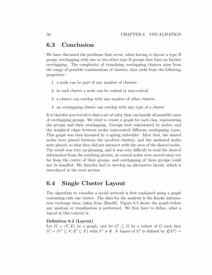
The algorithm to visualise a social network is first explained using a graphcontaining only one cluster. The data for the analysis is the Knoke informa-tion exchange data, taken from [Han98]. Figure 6.5 shows the graph beforeany analysis or visualisation is performed. We first have to define, what alayout in this context is.
Definition 6.2 (Layout)Let G = (V,E) be a graph, and let G′ ⊆ G be a subset of G such thatG′ = (V ′ ⊆ V,E ′ ⊆ E) with V ′ 6= ∅. A layout of G′ is defined by L(G′) =
6.4. SINGLE CLUSTER LAYOUT 57
Figure 6.5: Knoke information exchange data
{C,Z,Z, c(v), p, ω,∆min,∆max} where C = {(xv, yv) ∈ R2|v ∈ V ′} is the setof coordinates for every node v ∈ V ′, Z = {v ∈ G′|c(v) = maxu∈G′(c(u))} isthe list of the central nodes with c(v) ∈ R as a valid centrality measure, andZ = G′\Z is the list of non-central nodes. The elements in the list u ∈ Z areput in descending order in respect to their centrality value c(u). The centreand the orientation of the layout are given by p = (xl, yl) ∈ R2 and ω ∈ R,while the distance parameters ∆min,∆max ∈ R determine the dimension ofthe layout, in respect of the centre nodes.
The values ∆min,∆,max limit the distance of a non-central node from acentral node. In some cases, if for example the cluster has a large numberof members, the nodes must be placed further away from the centre, as∆min,∆max would indicate. In this case the distance parameters must beadopted.
The sets of central and non-central nodes Z,Z can be received using thecentrality function c(v) ∈ R. To layout a cluster, we therefor must determinethe set of coordinates C, in respect of the layout parameters Z,Z, c(v), p, ω.
58 CHAPTER 6. VISUALISATION
Algorithm
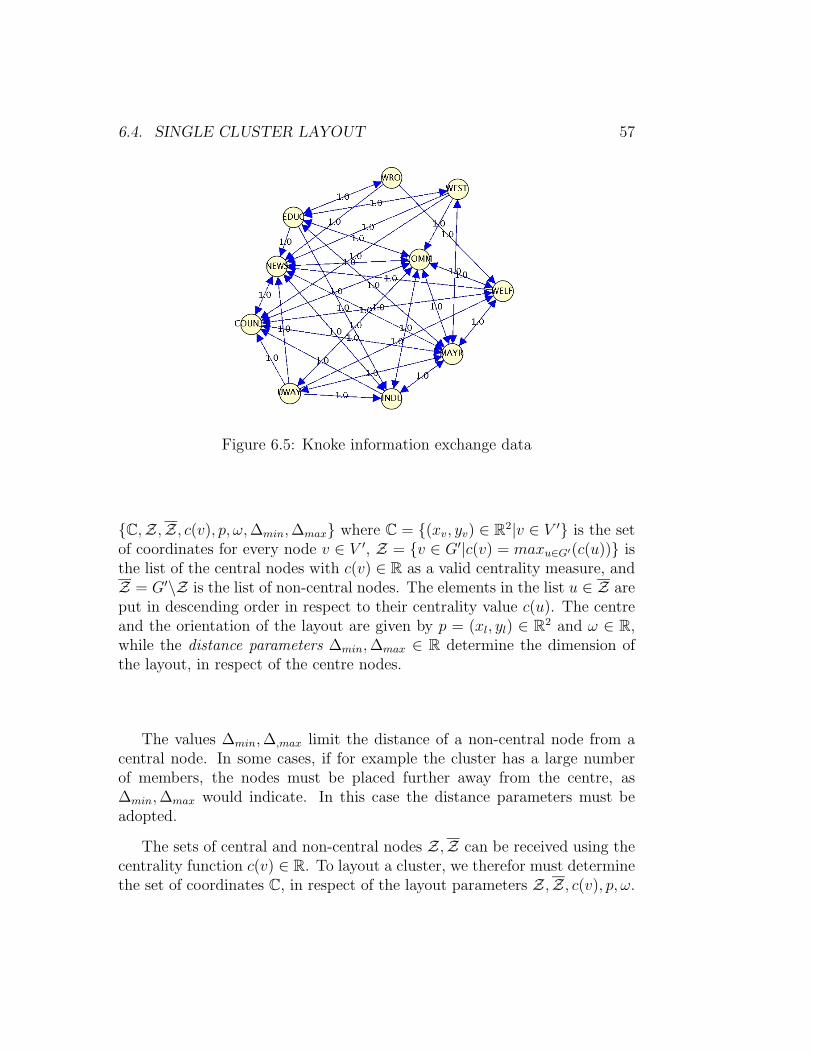
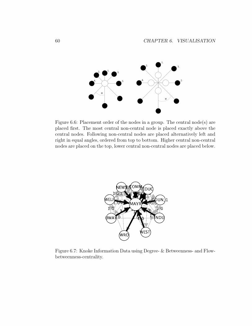
The first step in the algorithm for the layout of a group (see Algorithm 9) isto position the central nodes v ∈ Z in a circular layout. This is not discussedhere, as it would not provide any additional information. A circular layoutalgorithm is discussed in [dBETT99]. The radius of the resulting circle ofcentral nodes is denoted by rc ∈ R. After that, the radius for the non-central nodes is calculated, respecting the radius of the inner circle rc andthe number of vertices in the set of non-central nodes Z. The resulting valueis denoted by rc ∈ R, and is the minimum distance for each non-central nodefrom the centre of the layout p ∈ R2. The first non-central node is placedin the direction given by the orientation of the layout ω ∈ R. The next twonodes are placed in the same angle from the orientation, but on differentsides. This is done for every following node, so that the cluster forms akind of oval or heart (see Figure 6.6). The distance of the non-central nodevZ ∈ Z from the nearest central node vZ ∈ Z is determined by the differenceof the centrality values c(cZ)−c(vZ) mapped to the difference of the distancevalues ∆max−∆min. The result of the visualisation of the Knoke informationexchange data is shown in Figure 6.7. One can see, that if the orientation is 0,thus the first node is exactly above the centre, then there is an ordering fromtop to bottom, in which the node is placed further down, as its centralityvalue decreases. In the following we will assume that the orientation ω is 0for every layout.
Running time
The visualisation of the non-central nodes of one cluster in done in O(n)time (see Algorithm 9).
6.5 Multi cluster visualisation
The visualisation of more then just one cluster does differ only in two aspects.We have to take care of the shared actors, and each group must be positionedaccording to its group centrality value.
6.5. MULTI CLUSTER VISUALISATION 59
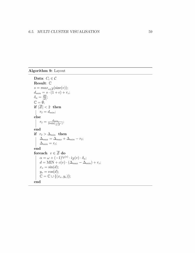
Algorithm 9: Layout
Data: Ci ∈ CResult: Cs = maxv∈Z(size(v));dmin = s · (1 + ε) + rc;δα = 2Π
|Z| ;
C = ∅;if |Z| < 2 then
rc = dmin;
elserc = dmin
2∗sin( γ
2·|Z );
endif rc > ∆min then
∆max = ∆max + ∆min − rc;∆min = rc;
endforeach v ∈ Z do
α = ω + (−1)iZ(v) · iZ(v) · δα;d = MIN + c(v) · (∆max −∆min) + rc;xv = sin(d);yv = cos(d);C = C ∪ {(xv, yv)};
end
60 CHAPTER 6. VISUALISATION
1.2. 3.
4. .5
1.2. 3.
4. .5
α
α
Figure 6.6: Placement order of the nodes in a group. The central node(s) areplaced first. The most central non-central node is placed exactly above thecentral nodes. Following non-central nodes are placed alternatively left andright in equal angles, ordered from top to bottom. Higher central non-centralnodes are placed on the top, lower central non-central nodes are placed below.
Figure 6.7: Knoke Information Data using Degree- & Betweenness- and Flow-betweenness-centrality.
6.6. CONCLUSION 61
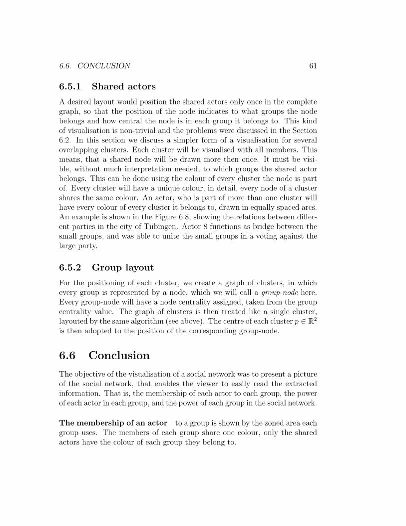
6.5.1 Shared actors
A desired layout would position the shared actors only once in the completegraph, so that the position of the node indicates to what groups the nodebelongs and how central the node is in each group it belongs to. This kindof visualisation is non-trivial and the problems were discussed in the Section6.2. In this section we discuss a simpler form of a visualisation for severaloverlapping clusters. Each cluster will be visualised with all members. Thismeans, that a shared node will be drawn more then once. It must be visi-ble, without much interpretation needed, to which groups the shared actorbelongs. This can be done using the colour of every cluster the node is partof. Every cluster will have a unique colour, in detail, every node of a clustershares the same colour. An actor, who is part of more than one cluster willhave every colour of every cluster it belongs to, drawn in equally spaced arcs.An example is shown in the Figure 6.8, showing the relations between differ-ent parties in the city of Tubingen. Actor 8 functions as bridge between thesmall groups, and was able to unite the small groups in a voting against thelarge party.
6.5.2 Group layout
For the positioning of each cluster, we create a graph of clusters, in whichevery group is represented by a node, which we will call a group-node here.Every group-node will have a node centrality assigned, taken from the groupcentrality value. The graph of clusters is then treated like a single cluster,layouted by the same algorithm (see above). The centre of each cluster p ∈ R2
is then adopted to the position of the corresponding group-node.
6.6 Conclusion
The objective of the visualisation of a social network was to present a pictureof the social network, that enables the viewer to easily read the extractedinformation. That is, the membership of each actor to each group, the powerof each actor in each group, and the power of each group in the social network.
The membership of an actor to a group is shown by the zoned area eachgroup uses. The members of each group share one colour, only the sharedactors have the colour of each group they belong to.
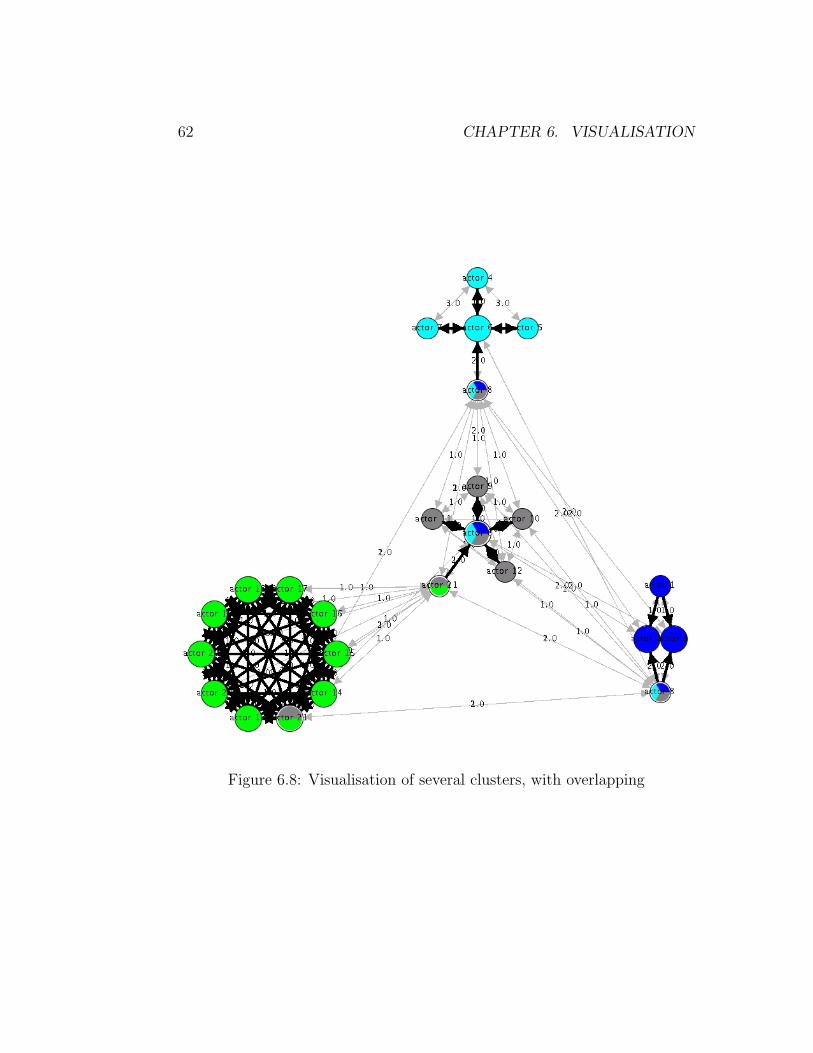
62 CHAPTER 6. VISUALISATION
Figure 6.8: Visualisation of several clusters, with overlapping
6.6. CONCLUSION 63
The centrality of each actor is displayed by the distance of an actorto the centre of its group. A node is closer to the centre of its group, thehigher its centrality value is. The centre of its group only includes the centralnode, that is, the nodes with the highest centrality value. If we have morethan one central node, the central nodes form a circle around the centre.Central nodes are also scaled in size. All non-central nodes are placed inequidistant angles around the centre. The most central non-central node isplaced exactly above the centre, then, in decreasing order of their centrality,the nodes are placed on the left and right side of the centre. The group formsa kind of oval or heart, depending on the distribution of the power within thegroup. Therefor we also have an ordering of the non-central actors, whereactors with a higher centrality value are placed above actors with a lowercentrality value.
The centrality of each group is visualised, using the same algorithmthat is used to position the actors within a cluster. Central groups are placedcentral, and the ordering of the other groups is equivalent to the non-centralnodes in a cluster.
We can therefor say, that the algorithm introduced here provides the viewerwith easy to read information about the analysed social network.

64 CHAPTER 6. VISUALISATION
Chapter 7
Conclusions & Future Work
The analysis of social networks was divided into two separated sections, theclustering and the calculation of centrality.
The first step is the clustering of the actors in the social networks, sinceclustering is a good method to analyse the structure of a social network. Theclustering must correspond to the social-scientific understanding of groups.We did introduce several clustering algorithms, that were developed underthis premise. The k-plex algorithm was chosen in consultation with the Eth-nological Institute of Tubingen, as it correlates most with our understandingof a group. The results are very pleasing, as the k-plex algorithm describedhere is capable of clustering the graph according to the requirements of thesocial scientist, including the correct analysis of bridges.
The calculation of power or centrality is the second step of the social net-work analysis. We introduced several basic concepts of centrality, finally dis-cussing three (degree-, betweenness-, flow-betweenness centrality) in detail.Ulirk Brandes introduced a method that is able to calculate the betweennessin a minimum of time and space [Bra00]. The flow-betweenness central-ity measure was implemented using the lift-to-front algorithm discussed in[CLR99]. No optimisation was found yet, as the max-flow calculation forevery combination of sources s ∈ Ci and sinks t ∈ Ci in a cluster Ci neededdid not seem to be replaceable. Future work could find new algorithms forthe calculation of flow-betweenness, reducing the high cost.
The visualisation of the social network analysis must be able to presentthe extracted information without much interpretation needed. The infor-mation, that is to be presented are the clusters, the centrality for each nodeand cluster, and the overlapping of clusters. We discussed the problems,
65
66 CHAPTER 7. CONCLUSIONS & FUTURE WORK
that occur in the visualisation of overlapping cluster, finally introducing analgorithm capable of visualising the clusters and the centrality of each nodein a cluster well. The algorithm can also be used to visualise the central-ity of each group in the cluster. Shared nodes are placed more then once.The region of each node is divided into equally spaced arcs, each sharingthe colour of a group the node belongs to. This method is good as long asa node is not part of too many clusters, as the arcs might get too small toidentify the colours. Practically this did not happen. Future work couldinclude the visualisation of overlapping clusters, placing shared nodes onlyonce. We have briefly discussed a method here, using a graph to representoverlapping clusters. Each cluster was assigned a node in the graph. Eachedge between two nodes represented one of four possible overlaps, that is, thenode is central — centre, non-central — central, non-central — non-centraland no overlap (indicated by an edge with weight 0). The graph was layoutedusing a spring embedder. Early results seemed promising, but the limitedtime did not allow any detailed evaluation of the problems that occurred.Future work could achieve good results in the visualisation of overlappingclusters.
Appendix A
YSocNet
The two standard software packages, UCINET as the analysis software, andKrackPlot (see Appendix B) mainly to visualise, are very good consideringthe results, but they are not easy to handle. The analysis is not interactiveand the usage is not very intuitive. YSocNet was created trying to compen-sate that.
A.1 Requirements
Talking to social scientist, we extracted some requirements for a social net-work analysis program:
Ethnological Methods: The methods used in the program should corre-spond to social scientific understanding of groups and power.
Good Visualisation: The visualisation should support the analysis as wellas the presentation of results.
Handling: The handling of the software should be intuitive and easy.
Interactive: A social scientist should be able to ”play” with the data, thatis, to easily be able to select what data to include/exclude from theanalysis.
In the next section we will discuss, what we mean by handling and interac-tivity.
67
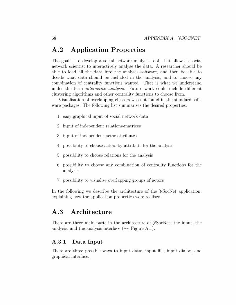
68 APPENDIX A. YSOCNET
A.2 Application Properties
The goal is to develop a social network analysis tool, that allows a socialnetwork scientist to interactively analyse the data. A researcher should beable to load all the data into the analysis software, and then be able todecide what data should be included in the analysis, and to choose anycombination of centrality functions wanted. That is what we understandunder the term interactive analysis. Future work could include differentclustering algorithms and other centrality functions to choose from.
Visualisation of overlapping clusters was not found in the standard soft-ware packages. The following list summarises the desired properties:
1. easy graphical input of social network data
2. input of independent relations-matrices
3. input of independent actor attributes
4. possibility to choose actors by attribute for the analysis
5. possibility to choose relations for the analysis
6. possibility to choose any combination of centrality functions for theanalysis
7. possibility to visualise overlapping groups of actors
In the following we describe the architecture of the YSocNet application,explaining how the application properties were realised.
A.3 Architecture
There are three main parts in the architecture of YSocNet, the input, theanalysis, and the analysis interface (see Figure A.1).
A.3.1 Data Input
There are three possible ways to input data: input file, input dialog, andgraphical interface.
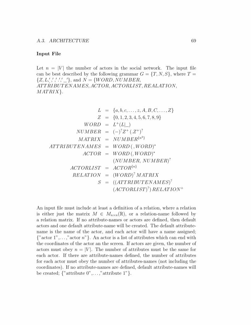
A.3. ARCHITECTURE 69
Input File
Let n = |V | the number of actors in the social network. The input filecan be best described by the following grammar G = {T,N, S}, where T ={Z,L,′, ,′ ,′ .′,′ ′}, and N = {WORD,NUMBER,ATTRIBUTENAMES,ACTOR,ACTORLIST,REALATION,MATRIX}.
L = {a, b, c, . . . , z, A,B,C, . . . , Z}Z = {0, 1, 2, 3, 4, 5, 6, 7, 8, 9}
WORD = L+(L| )
NUMBER = (−)?Z+ (.Z+)?
MATRIX = NUMBER{n2}
ATTRIBUTENAMES = WORD ( ,WORD)∗
ACTOR = WORD (,WORD)∗
(NUMBER, NUMBER)?
ACTORLIST = ACTOR{n}
RELATION = (WORD)?MATRIX
S = ((ATTRIBUTENAMES)?
(ACTORLIST )?)RELATION+
An input file must include at least a definition of a relation, where a relationis either just the matrix M ∈ Mn×n(R), or a relation-name followed bya relation matrix. If no attribute-names or actors are defined, then defaultactors and one default attribute-name will be created. The default attribute-name is the name of the actor, and each actor will have a name assigned;{”actor 1”,. . . ,”actor n”}. An actor is a list of attributes which can end withthe coordinates of the actor an the screen. If actors are given, the number ofactors must obey n = |V |. The number of attributes must be the same foreach actor. If there are attribute-names defined, the number of attributesfor each actor must obey the number of attributes-names (not including thecoordinates). If no attribute-names are defined, default attribute-names willbe created; {”attribute 0”,. . . ,”attribute 1”}.
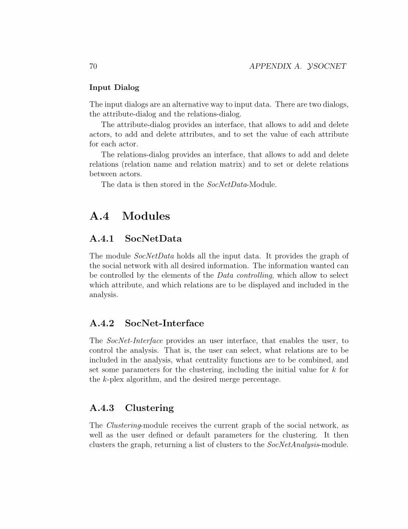
70 APPENDIX A. YSOCNET
Input Dialog
The input dialogs are an alternative way to input data. There are two dialogs,the attribute-dialog and the relations-dialog.
The attribute-dialog provides an interface, that allows to add and deleteactors, to add and delete attributes, and to set the value of each attributefor each actor.
The relations-dialog provides an interface, that allows to add and deleterelations (relation name and relation matrix) and to set or delete relationsbetween actors.
The data is then stored in the SocNetData-Module.
A.4 Modules
A.4.1 SocNetData
The module SocNetData holds all the input data. It provides the graph ofthe social network with all desired information. The information wanted canbe controlled by the elements of the Data controlling, which allow to selectwhich attribute, and which relations are to be displayed and included in theanalysis.
A.4.2 SocNet-Interface
The SocNet-Interface provides an user interface, that enables the user, tocontrol the analysis. That is, the user can select, what relations are to beincluded in the analysis, what centrality functions are to be combined, andset some parameters for the clustering, including the initial value for k forthe k-plex algorithm, and the desired merge percentage.
A.4.3 Clustering
The Clustering-module receives the current graph of the social network, aswell as the user defined or default parameters for the clustering. It thenclusters the graph, returning a list of clusters to the SocNetAnalysis-module.
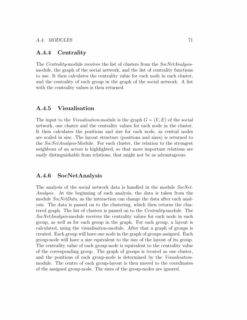
A.4. MODULES 71
A.4.4 Centrality
The Centrality-module receives the list of clusters from the SocNetAnalysis-module, the graph of the social network, and the list of centrality functionsto use. It then calculates the centrality value for each node in each cluster,and the centrality of each group in the graph of the social network. A listwith the centrality values is then returned.
A.4.5 Visualisation
The input to the Visualisation-module is the graph G = (V,E) of the socialnetwork, one cluster and the centrality values for each node in the cluster.It then calculates the positions and size for each node, as central nodesare scaled in size. The layout structure (positions and sizes) is returned tothe SocNetAnalysis-Module. For each cluster, the relation to the strongestneighbour of an actors is highlighted, so that more important relations areeasily distinguishable from relations, that might not be as advantageous.
A.4.6 SocNetAnalysis
The analysis of the social network data is handled in the module SocNet-Analysis. At the beginning of each analysis, the data is taken from themodule SocNetData, as the interaction can change the data after each anal-ysis. The data is passed on to the clustering, which then returns the clus-tered graph. The list of clusters is passed on to the Centrality-module. TheSocNetAnalysis-module receives the centrality values for each node in eachgroup, as well as for each group in the graph. For each group, a layout iscalculated, using the visualisation-module. After that a graph of groups iscreated. Each group will have one node in the graph of groups assigned. Eachgroup-node will have a size equivalent to the size of the layout of its group.The centrality value of each group-node is equivalent to the centrality valueof the corresponding group. The graph of groups is treated as one cluster,and the positions of each group-node is determined by the Visualisation-module. The centre of each group-layout is then moved to the coordinatesof the assigned group-node. The sizes of the group-nodes are ignored.
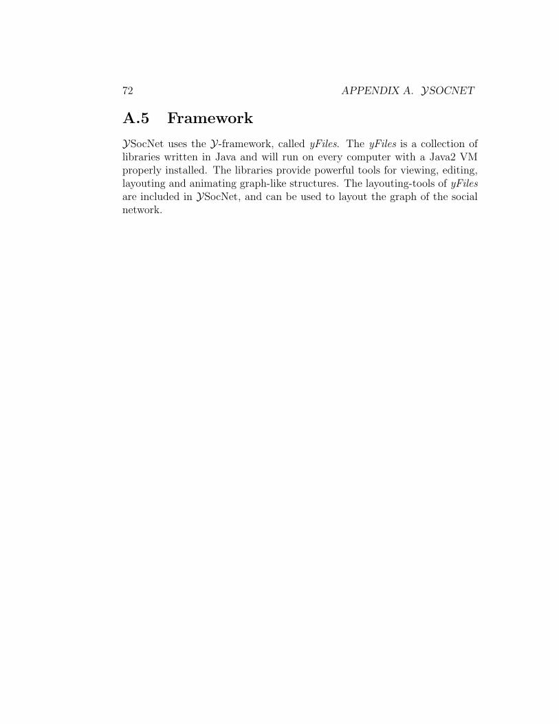
72 APPENDIX A. YSOCNET
A.5 Framework
YSocNet uses the Y-framework, called yFiles. The yFiles is a collection oflibraries written in Java and will run on every computer with a Java2 VMproperly installed. The libraries provide powerful tools for viewing, editing,layouting and animating graph-like structures. The layouting-tools of yFilesare included in YSocNet, and can be used to layout the graph of the socialnetwork.
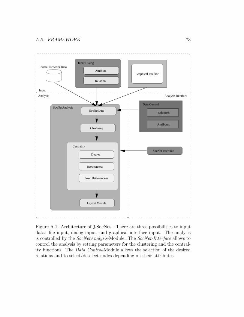
A.5. FRAMEWORK 73
Input
Analysis Analysis Interface
SocNetAnalysis
Social Network Data
Data Control
Clustering
Layout Module
SocNet Interface
SocNetData
Relation
Attribute
Input Dialog
Centrality
Flow−Betweenness
Betweenness
Degree
Relations
Attributes
Graphical Inteface
Figure A.1: Architecture of YSocNet . There are three possibilities to inputdata: file input, dialog input, and graphical interface input. The analysisis controlled by the SocNetAnalysis-Module. The SocNet-Interface allows tocontrol the analysis by setting parameters for the clustering and the central-ity functions. The Data Control-Module allows the selection of the desiredrelations and to select/deselect nodes depending on their attributes.

74 APPENDIX A. YSOCNET
Appendix B
Related Work
B.1 Social Network Analysis Programs
B.1.1 UCINET
The first version of the program UCINET was developed in 1986 under theadministration of Linton C. Freeman [BEF92],[Frea].
UCINET is a DOS program and the input is an ASCII-file. The inputfile contains matrices, that can be unlabelled or labelled. Concerning theanalysis of social networks, it offers the following centrality measures
• Degree
• Betweenness
• Flow betweenness
• Information centrality
• Eigenvector centrality
• Bonacich’s power index
and the following clustering algorithms
• Cliques
• N -cliques
75
76 APPENDIX B. RELATED WORK
• N -clans
• k-plexes
• k-cores
• Lambda sets
• Fractions
• f -groups
of which a few where described here. It can also group actors by structuralsimilarity[Han98], such as
• Structural equivalence
• Automorphic equivalence
• Regular equivalence
The output can be visualised by KrackPlot.
B.1.2 KrackPlot
The visualisation program KrackPlot was originally designed by David Krack-hardt. Jim Blythe and Cathleen McGrath are involved in the version 3 of theprogram. The program does not support network analysis, but has severallayout-functions included [Hom]:
User: the user can specify the coordinates
Circle: the nodes are positioned in a circle, so that every edge is within thecircle
Multidimensional Scaling: The main applications of factor analytic tech-niques are
1. to reduce the number of variables and
2. to detect structures in the relationships between variables, that isto classify variables
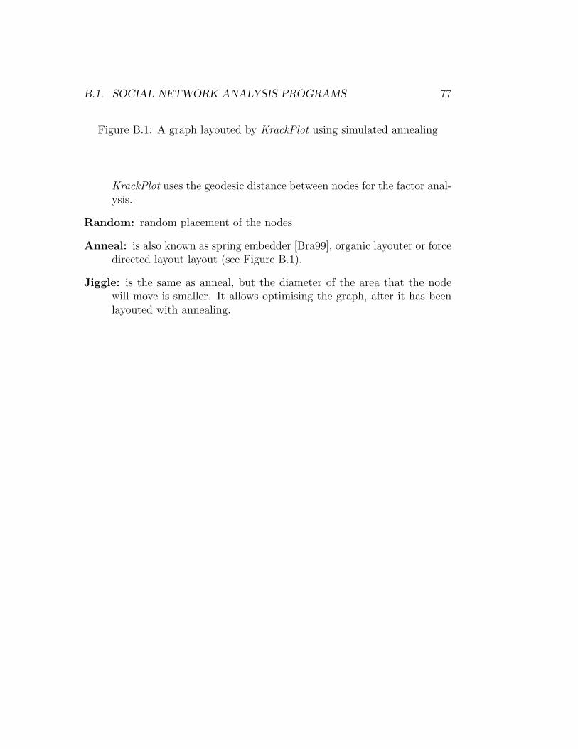
B.1. SOCIAL NETWORK ANALYSIS PROGRAMS 77
Figure B.1: A graph layouted by KrackPlot using simulated annealing
KrackPlot uses the geodesic distance between nodes for the factor anal-ysis.
Random: random placement of the nodes
Anneal: is also known as spring embedder [Bra99], organic layouter or forcedirected layout layout (see Figure B.1).
Jiggle: is the same as anneal, but the diameter of the area that the nodewill move is smaller. It allows optimising the graph, after it has beenlayouted with annealing.

78 APPENDIX B. RELATED WORK
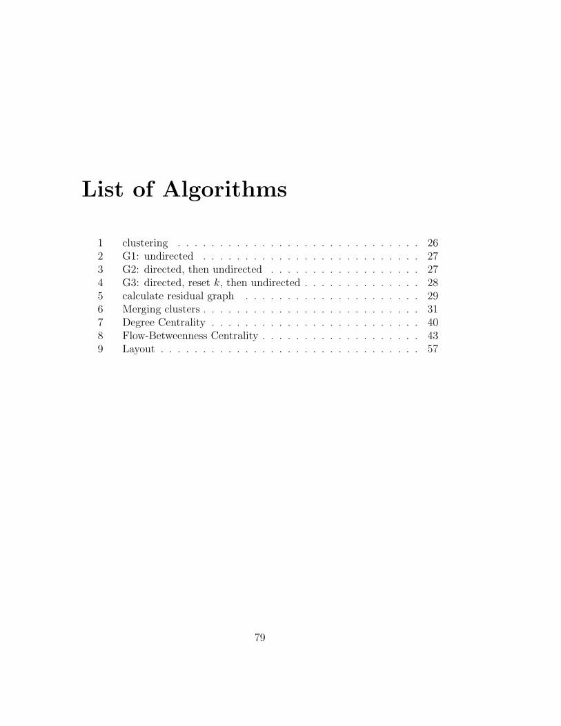
List of Algorithms
1 clustering . . . . . . . . . . . . . . . . . . . . . . . . . . . . . 262 G1: undirected . . . . . . . . . . . . . . . . . . . . . . . . . . 273 G2: directed, then undirected . . . . . . . . . . . . . . . . . . 274 G3: directed, reset k, then undirected . . . . . . . . . . . . . . 285 calculate residual graph . . . . . . . . . . . . . . . . . . . . . 296 Merging clusters . . . . . . . . . . . . . . . . . . . . . . . . . . 317 Degree Centrality . . . . . . . . . . . . . . . . . . . . . . . . . 408 Flow-Betweenness Centrality . . . . . . . . . . . . . . . . . . . 439 Layout . . . . . . . . . . . . . . . . . . . . . . . . . . . . . . . 57
79

80 LIST OF ALGORITHMS
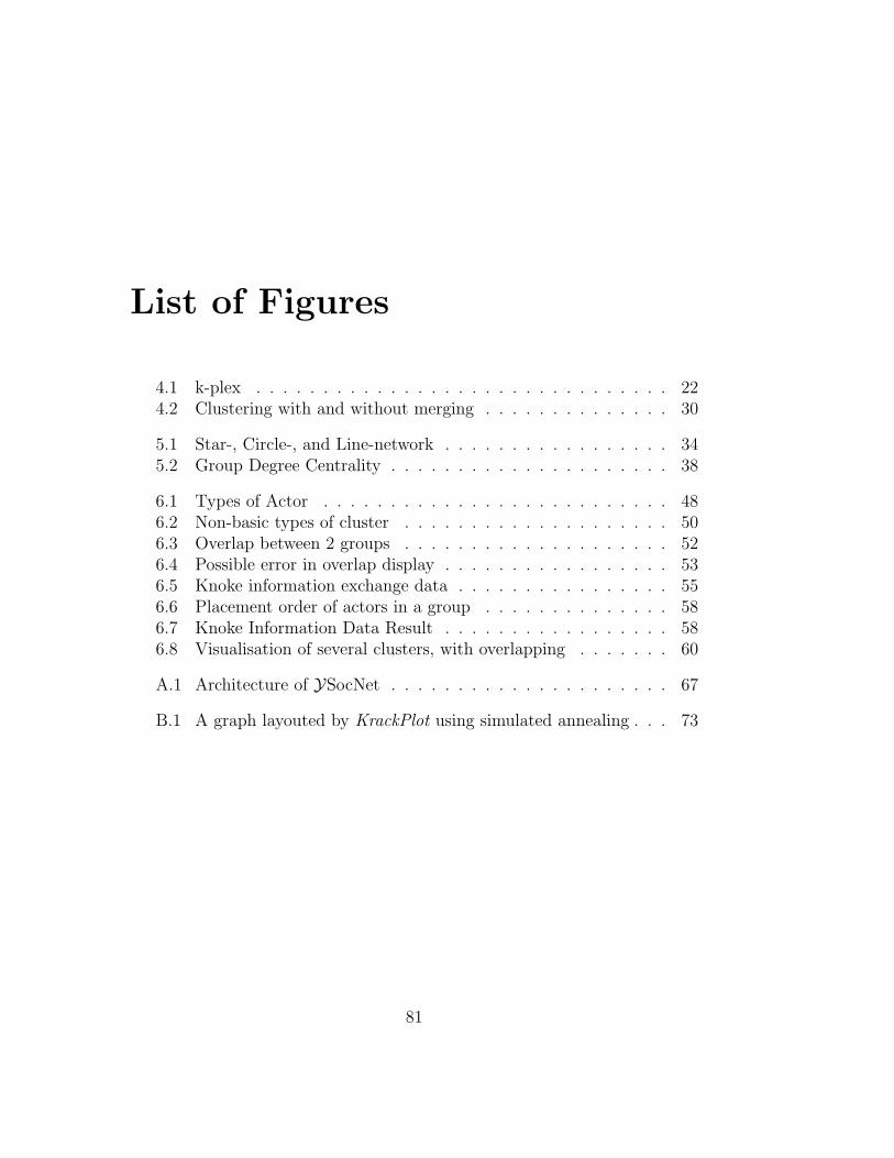
List of Figures
4.1 k-plex . . . . . . . . . . . . . . . . . . . . . . . . . . . . . . . 224.2 Clustering with and without merging . . . . . . . . . . . . . . 30
5.1 Star-, Circle-, and Line-network . . . . . . . . . . . . . . . . . 345.2 Group Degree Centrality . . . . . . . . . . . . . . . . . . . . . 38
6.1 Types of Actor . . . . . . . . . . . . . . . . . . . . . . . . . . 486.2 Non-basic types of cluster . . . . . . . . . . . . . . . . . . . . 506.3 Overlap between 2 groups . . . . . . . . . . . . . . . . . . . . 526.4 Possible error in overlap display . . . . . . . . . . . . . . . . . 536.5 Knoke information exchange data . . . . . . . . . . . . . . . . 556.6 Placement order of actors in a group . . . . . . . . . . . . . . 586.7 Knoke Information Data Result . . . . . . . . . . . . . . . . . 586.8 Visualisation of several clusters, with overlapping . . . . . . . 60
A.1 Architecture of YSocNet . . . . . . . . . . . . . . . . . . . . . 67
B.1 A graph layouted by KrackPlot using simulated annealing . . . 73
81

82 LIST OF FIGURES
Bibliography
[BEF92] S.P. Borgatti, M.G. Everett, and L.C. Freeman. UCINET IV.Analytic Technologies, 1992.
[BKW99a] Ulrik Brandes, Patrick Kenis, and Dorothea Wagner. Central-ity in Policy Network Drawings. Proc. 7th Intl. Symp. GraphDrawing (GD’99) LNCS 1731, pages 250–258, 1999.
[BKW99b] Ulrik Brandes, Patrick Kenis, and Dorothea Wagner. Explo-rations into the Visualization of Policy Networks. Journal ofTheoretical Politics, 1(11):75–106, 1999.
[BLW96] Giuseppe Di Battista, Giuseppe Liotta, and Sue H. Whitesides.The Strength of Weak Proximity. Technical report, UniversitaDegli Studi di Roma Tre, Dipartimento die Discipline Scientifice,1996.
[BM99] S.P. Borgatti and M.G.Everett. Models of Core/Periphery Struc-tures. Unpublished manuscript submitted to Social Networks,1999.
[BMZ99] Vladimir Batagelj, Andrej Mrvar, and Matjaz Zaversnik. Parti-tioning Approah to Visualization of Large Graphs. Graph Draw-ing, pages 90–97, 1999.
[Bor] Stephen P. Borgatti. A SOCNET Discussion on the Origions ofthe Term Social Capital. CONNECTIONS, 21(2):–46.
[Bra99] Ulrik Brandes. Layout of Graph Visualizations. Ph.D. Thesis.http://www.ub.uni-konstanz.de/kops/volltexte/1999/255, June1999.
83
84 BIBLIOGRAPHY
[Bra00] Ulrik Brandes. Faster Evaluation of Shortest-Path Based Cen-trality Indices. Konstanzer Schriften in Mathematik und Infor-matik 120, May 2000.
[BW00] Ulrik Brandes and Dorothea Wagner. Contextual Visualizationof Actor Status in Social Networks. In Data Visualization 2000,pages 13–22. 2nd Eurographics/IEEE TVCG Symp. Visualiza-tion (VisSym’00), Springer, 2000.
[CLR99] Thomas H. Cormen, Charles E. Leiserson, and Ronald L. Rivest.Introduction to algorithms. MIT Press, 22th edition, 1999.
[dBETT99] Giuseppe di Batitista, Peter Eades, Roberto Tamassia, and Ioan-ning G. Tollis. Graph Drawing. Prentice-Hall, Inc., 1999.
[DFK+] P. Drineas, Alan Frieze, Ravi Kannan, Santosh Vempala, andV. Vinay. Clustering in large graphs and matrices.
[EB] Martin G. Everett and Stephen P. Borgatti. Peripheries of Co-hesive Subsets.
[EB99] M.G. Everett and S.P. Borgatti. The Centrality of Groups andClasses. Joural of Mathematical Sociology, 23(3):181–201, 1999.
[ESB99] Jubin Edachery, Arunabha Sen, and Fran J. Brandenburg.Graph Clustering Using Distance-k Cliques. Graph Drawing,pages 98–106, 1999.
[Frea] Linton C. Freeman. UCINET - Network Analysis Software -Webpage. http://eclectic.ss.uci.edu/˜lin/ucinet.html.
[Freb] Linton C. Freeman. Visualizing Social Networks. Journal ofSocial Structure.
[Fre97] Linton C. Freeman. Uncovering Organizational Hierachies.Computational & Mathematical Organization Theorie, 1(3):5–18, 1997.
[FWK98] Linton C. Freeman, Cynthia M. Webster, and Deirdre M. Kirke.Exploring social structure using dynamic three-dimensionalcolor images. Social Network, 20:109–118, 1998.
BIBLIOGRAPHY 85
[GWW] Yoram Gdalyahu, Daphna Weinshall, and Michael Werman.Stochastic Clustering and its Application to Image Segmenta-tion.
[Han98] Robert A. Hanneman. Introduction to Social Network Methods.http://wizard.ucr.edu/˜rhannema/networks/text/textindex.html,1998.
[Har69] Frank Harary. Graph Theorie. Addison-Wesley, 1969.
[Hom] KrackPlot Homepage. http://www.heinz.cmu.edu/˜krack/.
[Jan99] Dorothea Jansen. Einfuhrung in die Netzwerkanalyse. leske +budrich, 1999.
[JB] Robert O. Johnson and John Boyd. e-centrality.http://eclectic.ss.uci.edu/ rjohns/ecent.htm.
[Lea] Sonia Leach. Singular Value Decomposition – A Primer.
[MBK] Cathleen McGrath, Jim Blythe, and David Krackhardt. SeeingGroups in Graph Layouts.
[MC] Peter R. Monge and Noshir S. Contractor. Emergence of Com-munication Networks. A chapter prepared for Publication inJablin, F.M., & Putnam, L.L. (Eds.) Handbook of Organiza-tional Communications (2nd Ed.). Thousand Oaks, CA. Sage.1999.
[Sch] Robby Schonfeld. k-layer Straightline Crossing Minimization bySpeeding upn Shifting.
[Sch89] Thomas Schweizer. Netzwerkanalyse. Dietrich Reimer Verlag,1989.
[ST] Janed M. Six and Ioannis G. Tollis. Improved Graph DrawingVia Clustering.
[Ved98] Balazs Vedres. Locked in Centrality. Sunbelt XVIII and 5thEuropean International Conference on Social Networks, 1998.