Diplomarbeit

Georg Rupert Müller

Betreuer: Prof. Dr. Jörg Conradt, Dominik Stengel

Ausgabe: 01.08.2011

Abgabe: 29.02.2012

AIS-Nr.: 550DA0811

Lehrstuhl für

Automatisierung und

Informationssysteme

Prof. Dr.-Ing. B. Vogel-Heuser

Technische Universität München

Boltzmannstraße 15 - Geb. 1

85748 Garching bei München

Telefon 089 / 289 – 164 00

Telefax 089 / 289 – 164 10

http://www.ais.mw.tum.de

3D Object Tracking with embedded Event Based

Vision Sensors

Erklärung:

Ich versichere hiermit eidesstattlich, dass ich die vorliegende Diplomarbeit selbstständig

verfasst und nur die angegebenen Quellen und Hilfsmittel verwendet habe. Die aus fremden

Quellen wörtlich oder sinngemäß übernommenen Gedanken sind als solche gekennzeichnet.

Die Arbeit wurde bisher keiner anderen Prüfungsbehörde vorgelegt.

München, den 29. Februar 2012

Georg Müller

Abstract

Recognizing and tracking objects is a key function in any application of robots which depends

on appropriate perception, intelligent sensing and understanding of the environment. This

thesis presents a new approach for real-time 3D-target tracking, which can be applied on

autonomous moving robots in cluttered environments for tracking multiple objects. It is based

on a vision system, which includes two new biologically inspired, high-speed asynchronous

temporal contrast vision sensors (DVS-sensors) and active target markers. The sensors, which

could be independently placed in the environment, react to illumination changes in the

environment and thus track the position of light flashing objects on the basis of events with

the use of a new algorithm running on the ARM7 microcontroller of the eDVS-sensor board.

Two sensors were added to the system to provide orientation within the 3D space based on

their observation of the target from different position angles. The sensors were mounted on

pan-tilts to extend their surveillance area and were calibrated as a device set to report accurate

actual angular positions to the tracked targets in space. A feed-forward neural network was

used to transform the observed angular positions into 3D Cartesian space. Angular positions

of three LEDs, which were placed as active markers on a target stimulus and were

simultaneously observed from both sensors, were grouped together as synchronized angular

position sets. Such angular position sets were established from moving the target along an

arbitrary trajectory in 3D Cartesian space and applied as training input data set of the neuronal

network. The trained neural network had to represent the geometry of the 3D target stimulus

with active markers at fixed defined distance on its output. This was used to adjust learning of

the network by back-propagation without the presence of output training patterns. Testing of

the performance of the trained neural network with a new undefined data set showed that it

could predict and track a moving target at any positioning in a cube with high speed and very

high precision. The neural network and the new training method have been implemented in C

for fast processing. It can be used during tracking from a computer connected online to the

DVS-sensor via an USB interface. Usually a terminal program is used which transmits

commands to the DVS-sensor. For more convenient adjustment of the parameters a Matlab

GUI has been designed which enables communication with the sensor via a COM-port and

transmits commands for different tracking algorithm coefficients from the computer

automatically. The parameters can be modified via intuitive sliders and also loaded and stored

to a text file. With this interface no commands for the terminal program have to be

remembered. The new 3D tracking algorithm requires only low-power consuming hardware

(ARM7) and thus can be applied even to small robots with high hardware and software

flexibility. The applications of this system could be, for instance, the measuring of distances

to other robots or the autonomous assemblage of marked pieces belonging to one product in

factories.

Acknowledgements

I would like to thank Prof. Jörg Conradt for permitting to join his work group at the LSR-

department in 2010 in order to perform a Bachelor thesis first and then for inviting me to do

my Diploma´s thesis. You have taught me first steps in robotic science and always kept a

keen stimulating eye over my work.

To Dominik Stengel who agreed to be my examiner from the AIS-Department within the

Faculty of Maschinenbau and has effectively volunteered to supervise, read and review this

thesis - many thanks!

Finally to my girlfriend and my family for their help in any way possible and whenever!

Contents

Page I

1. Introduction ........................................................................................................................ 1

1.1. Problems and Challenges............................................................................................. 1

1.2. Current Methods for Tracking ..................................................................................... 2

1.3. Specific Aims and Structure of this Thesis ................................................................. 2

2. Background and Conception .............................................................................................. 5

2.1. Methods for Target Detection ...................................................................................... 5

2.2. Biologically Inspired Embedded Dynamic Vision Sensor (eDVS) ............................. 6

2.3. Artificial Neural Networks .......................................................................................... 9

3. Event-Based Target Detection Algorithm ........................................................................ 17

3.1. Algorithm and Hardware Implementation ................................................................. 17

3.2. Results ....................................................................................................................... 23

4. 3D Tracking ...................................................................................................................... 25

4.1. Tracking Concept ...................................................................................................... 25

4.2. Hardware Components .............................................................................................. 27

5. Neural Network for 3D Position Estimation .................................................................... 31

5.1. Network Design ......................................................................................................... 31

5.2. Training the Neural Network ..................................................................................... 32

5.3. Evaluation of Training Success ................................................................................. 34

6. Test Data Acquisition & System Evaluation .................................................................... 37

6.1. Evaluation in a Semi-Stationary System ................................................................... 37

6.2. Prediction of Target Motion ...................................................................................... 39

6.3. Data Acquisition ........................................................................................................ 42

6.4. Performance of Learning ........................................................................................... 43

6.5. 3D Performance ......................................................................................................... 47

7. Conclusion and Perspectives ............................................................................................ 51

Appendix A .............................................................................................................................. 53

Appendix B .............................................................................................................................. 54

List of Figures .......................................................................................................................... 57

List of Tables ............................................................................................................................ 57

References ................................................................................................................................ 59

1.1 Problems and Challenges

Page 1

1. Introduction

Today´s applications of robots depend in large parts on their appropriate perception and

intelligent sensing of the environment. Humans and animals can rely on several sensory

receptors such as proprioception sensors, visual sensors and vestibular sensors dynamically

percept their surroundings. Current robotic systems usually need a large number of

exteroceptive sensors only operating with a sufficient source of high computing power.

Nevertheless significant progress has been made in robot perception by different, meanwhile

also commercially available object tracking systems which have been mainly explored by the

Computer Vision and Augmented Reality Communities, but are also applied in military

defense, assisted driving and home living. They are often built on hybrid ultrasound-inertial

tracking technology electromagnetic tracking, most frequently, however, on vision-based

techniques.

Robust object tracking systems based on computer vision with multiple cameras as sensors

and vision data recorded in the form of image frames of grayscale or color have been

developed, but are limited in real-time data processing and 3D-object detection.

While many 3D object tracking strategies have been proposed, it still remains a particular

challenging task on mobile robots. The focus of this thesis here is to introduce a new method

for real-time 3D tracking with the use of a new tracking algorithm for object recognition and

identification and implementation of a neuronal network for position measurement of objects.

A common approach is to make use of vision-based tracking devices. Such systems, however,

are usually too expensive and complex to perform real-time tracking in cluttered 3D

environments. The new proposed system is promising for wider practical use as a new vision-

based 3D tracking technique for mobile robots because of its precision, robustness, low power

consumption and low management costs. The first section of this thesis provides a short

overview on today´s still existing difficulties and challenges of object tracking in general and

on mobile robots. Section two refers to currently applied methods for object identification and

tracking on mobile robots and ends up in a final introductory paragraph with further details on

the objective and structure of this thesis.

1.1. Problems and Challenges

In recent years, robots have made a big step forward from huge machines which assemble

product parts in factories to small autonomous robots which progressively infiltrate private

homes and official environments for diverse appliances. As personal or domestic home robots

they promise to simplify annoying household chores like cleaning floors and to free up users´

time, furthermore as intelligent self-correcting robots which also can be remote controlled

they may become key elements for the success of projects which are too difficult or

dangerous to be reached by humans like collecting probes on the Mars. As these systems have

to operate more and more autonomously in the future, they must gain further abilities besides

secure collision avoidance and precise navigation through unknown environments. 3D object

recognition and position measurement in real time have to be achieved, but cannot yet be

provided on small autonomous robots. This will be an essential requirement for intelligent

autonomous robots which should be able to perform high level tasks.

Several methods have been developed to recognize and classify objects [1]. These methods,

however, demand powerful hardware for image processing and object categorization. Thus

they are difficult to apply on autonomous robots due to their excessive power consumption. In

1.2 Current Methods for Tracking

Page 2

this thesis a new, low-cost 3D tracking system is presented which runs in real time on low

computing power hardware. This system comprises two vision sensors and senses positions of

several marked objects simultaneously at 100Hz. Another special feature of this system is that

the sensors can be placed arbitrarily in the environment. After a short calibration the system

independently tracks objects in 3D with high precision.

1.2. Current Methods for Tracking

Recognizing objects or obstacles is a key function in any robotic appliances. Several different

types of sensors have been developed which help robots already to avoid collisions with other

objects or follow targets. These sensors comprise infrared sensors [2], ultrasonic sensors [3]

and laser range finders [4] and can be found on several autonomous robots. All these sensors,

however, can only recognize objects within a limited distance and angle.

Camera vision based tracking and object identification has been an interesting field of

research throughout the past years. Several image based methods for object recognition have

been developed which can be mainly classified as either geometrically based [5] or

appearance based [2] techniques. Tracking and object identification of autonomous robots

with these systems, however, had to focus on off-line computation for a long time due to the

lack of powerful hardware for processing of the recorded images in real time. Because of the

continuously increasing performance of the computer hardware, tracking algorithms

meanwhile can be also applied on mobile robots. [6] and [7] present a camera based

stereovision system used on mobile robots which track objects autonomously. Since the start

of Microsoft’s Xbox Kinect, which also offers 3D depth information of an image besides

RGB-color data, a new field of research for object recognition and identification has emerged.

This motion sensing input device, which captures video data in 3D, has also been applied for

target identification and tracking [8].

All the presently camera based tracking systems still demand powerful hardware such as a

laptop at least for tracking only. A mobile robot, however, should not assign all its computing

resources for object tracking. Therefore tracking has to become more efficient.

Recently, a completely new sensor technology has been introduced with the development of

so-called biologically inspired dynamic vision sensors (DVS-sensors). These sensors operate

with a drastically reduced amount of recorded data as they only sense and signal changes of

brightness within the environment and thus reduce the computational complexity and the

requirements of the hardware. Tracking of objects is also possible with these sensors. Some of

them even offer localization of the tracked object on their hardware output [9]. Other

developments showed tracking of cars and persons with a monocular DVS-sensor system

using a cluster algorithm [10]. Recently a dynamic stereovision system has been published

comprising two biologically inspired sensors for tracking people in 3D [11]. The performance

of this system has been shown for the fixed device in a dynamic scene and not mounted on a

mobile robot. All these biologically inspired systems also still lack reliable object recognition.

1.3. Specific Aims and Structure of this Thesis

In this thesis, a new 3D tracking method in cluttered environments is developed which can be

used on small autonomous robots with little computing power. It relies on two biologically

inspired vision sensors and an active target marker. Conventional systems, as described in

chapter 1.2, are limited in their adaptability due to high computational complexity. Recently

1.3 Specific Aims and Structure of this Thesis

Page 3

developed tracking systems, which are based on biologically inspired sensors [11], overcome

these difficulties, however, lack flexibility and capability of realigning sensors to different,

not predefined positions.

The new 3D tracking system developed in this thesis consists of two biologically inspired

vision sensors and an active marker. The sensors can be independently placed in the

environment. Each of these sensors autonomously tracks the active marker and reports its

angular positions to a trained neural network running on one of the sensors. The neural

network allows transformation of the angular positions into 3D real world positions online.

In chapter 2 of this thesis, basic aspects of object tracking are illustrated with special

references to a 3D mode as well as to benefits of biologically inspired sensors in comparison

to ordinary vision sensors in this application field. The last chapter of this section also

addresses fundamentals of neural networks and why they have been exploited for this use. In

chapter 3 a newly developed event-based tracking algorithm is described which has been

applied to the biologically inspired sensors for the detection of the active marker. The

complete, new 3D tracking system is presented in detail with the use of this new algorithm

and special focus on the hardware necessary for tracking in chapter 4. Chapter 5 describes an

advanced training method of the neural network which differs from ordinary techniques and is

applied for mapping of the 4D sensory data into 3D. In chapter 6 the complete new 3D

tracking system is presented in detail with performance tests as well as documentation of its

capabilities in practice. Chapter 7 provides an outlook on prospective fields of application and

future improvements of the system.

1.3 Specific Aims and Structure of this Thesis

Page 4

2.1 Methods for Target Detection

Page 5

2. Background and Conception

In this project a miniature, low power, standalone 3D tracking system, which could take

advantage of a new biologically inspired sensor, had to be designed and developed for real

time tracking of marker-targeted objects. Essential methods for labeling and identifying

targets are first introduced in section 2.1. Thereafter the basic constituents of a biologically

inspired sensor used in this project are presented in section 2.2 and their benefits are

expounded in compared to conventional CCD- or CMOS-sensors. Tracked marker positions

of two of these sensors are then inserted into a specifically trained neural network used to

transform these data into 3D real world coordinates. In section 2.3 a survey of the structure of

neural networks is provided and conventional training methods with reference to important

differences of the approach shown in chapter 5 are explained.

2.1. Methods for Target Detection

Precise nearby object detection and tracking are indispensable functions of many robotic

systems. They are necessary in several robotic applications to enable definition of self-

positioning and secure movement of autonomous robots in their environment as well as allow

human-robot-interactions in particular. Several highly advanced techniques for collision

avoidance that also became standard features of autonomous robots are meanwhile available.

However, object identification is still a challenging task. Therefore many different solutions

have been designed which today can be grouped into three basic configurations with respect

to the component used for the target identification, such as an active marker, an active sensor

or a marker-less passive sensor. They can be further overviewed in brief as follows:

Marker-based tracking is generally a cheap solution to detect objects. The systems usually

rely on an aligned target marker and sensor and thus can only be used to fulfill specific,

predefined tasks like homing of autonomous robots.

Active markers as one specific option of these systems are usually paired with a passive

sensor. The absolute requirement of an active marker for each identifiable object, however, is

a major drawback for a wider use of such a system in object tracking. Such devices usually

can detect only predefined objects. They are not suitable for tasks like collision avoidance in

cluttered unmarked environments. In spite of these negative aspects and deficiencies, such

systems generally detect and identify many predefined objects robustly and pretty easily [12].

Another advantage of these systems is their management on simple hardware, which makes

them applicable also for small autonomous robots and allows longer system running time on

batteries as reduced computing requirements decrease the size, the costs and the power

consumption of the whole system.

Active sensors instead are used in these systems for various scenarios for instance for airplane

navigation by radar or laser optical measurements of objects, for industrial processes with

movement recognition by motion sensors using ultrasound [13]. “Active sensors transmit a

signal from a transmitter and with a receiver detect changes or reflections of the signal” [13].

The targets usually do not need a special preparation for their detection by an active sensor.

However, it is very challenging to specifically identify such objects without any attached even

passive label. For instance, it is difficult to discriminate a flying object on the radar as a B52

or A340 airplane, whereas it is obviously much easier to identify it, if the airplane transmits

identification data by itself like through active markers. Today active sensors are in particular

used for collision avoidance. Although such a system does not require labeling of each object

2.2 Biologically Inspired Embedded Dynamic Vision Sensor (eDVS)

Page 6

in the environment, a lot of research effort still has to be put into differentiated enhancement

of object identification. Various techniques have been developed which allow optimized

usage of active sensors in combination with passive, predefined target markers. Examples of

such devices are target identification via barcode or radio frequency scanning.

Systems with a marker-less passive sensor are most prospective and preferable as they

provide facilities for operation in diverse situations without special preparation of the

environment. They rely on technically highly advanced object detection and recognition

which nowadays is still a major challenge and favored research area. Up-to-now, these

systems require specialized, expensive sensors and an enormous computing power for object

detection and specific identification. Usually an image sensor captures a scene of the relevant

surrounding, of which essential image features are extracted by specialized algorithms. The

extraction procedure is thus based on highly computerized data processing which limits the

speed of object tracking. The gained information is then compared to key views of a scene or

geometrical constraints or reference structures such as models of objects [14]. This is a

complicated task and explains why these systems on small autonomous robots still fail for fast

object identification as the amount of data which has to be processed dramatically increases,

the faster these systems operate. System configurations which include high performance

hardware for sophisticated image processing usually have to be balanced against the limited

power supply from batteries and the demand of long operating times in these systems.

2.2. Biologically Inspired Embedded Dynamic Vision Sensor (eDVS)

Current 3D tracking systems relying on ordinary CCD- or CMOS-sensors, as described in

section 1.2, need powerful hardware to process the often massively redundant data in real-

time. However, this is not possible on small, battery powered robots. For solving such a

problem of high computational requirements a biologically inspired embedded dynamic

vision sensor, a high-speed asynchronous temporal contrast vision sensor called DVS, was

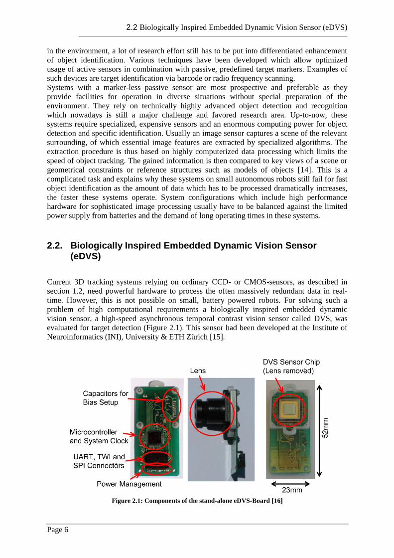
evaluated for target detection (Figure 2.1). This sensor had been developed at the Institute of

Neuroinformatics (INI), University & ETH Zürich [15].

Figure 2.1: Components of the stand-alone eDVS-Board [16]

2.2 Biologically Inspired Embedded Dynamic Vision Sensor (eDVS)

Page 7

Its main structure resembles that of ordinary CMOS-sensors. CMOS-sensors in cameras

capture full image frames usually with an update rate of 30 or 60 frames per second. Each

time a frame is captured, the brightness on all pixels is evaluated. Images are established with

the information of the sensed brightness and position of each pixel and serialized for the time

tested. The DVS-sensor also represents a light sensitive device. However, no image frames

are recorded. This sensor instead individually and continuously recognizes only illumination

changes on each pixel in the environment. This property of the DVS-sensor drastically

reduces the generated data which have to be processed, as only information of dynamic

brightness changes are recorded and passed on for fast and sensitive object detection and

recognition. “Each pixel independently and continuously quantifies local relative light

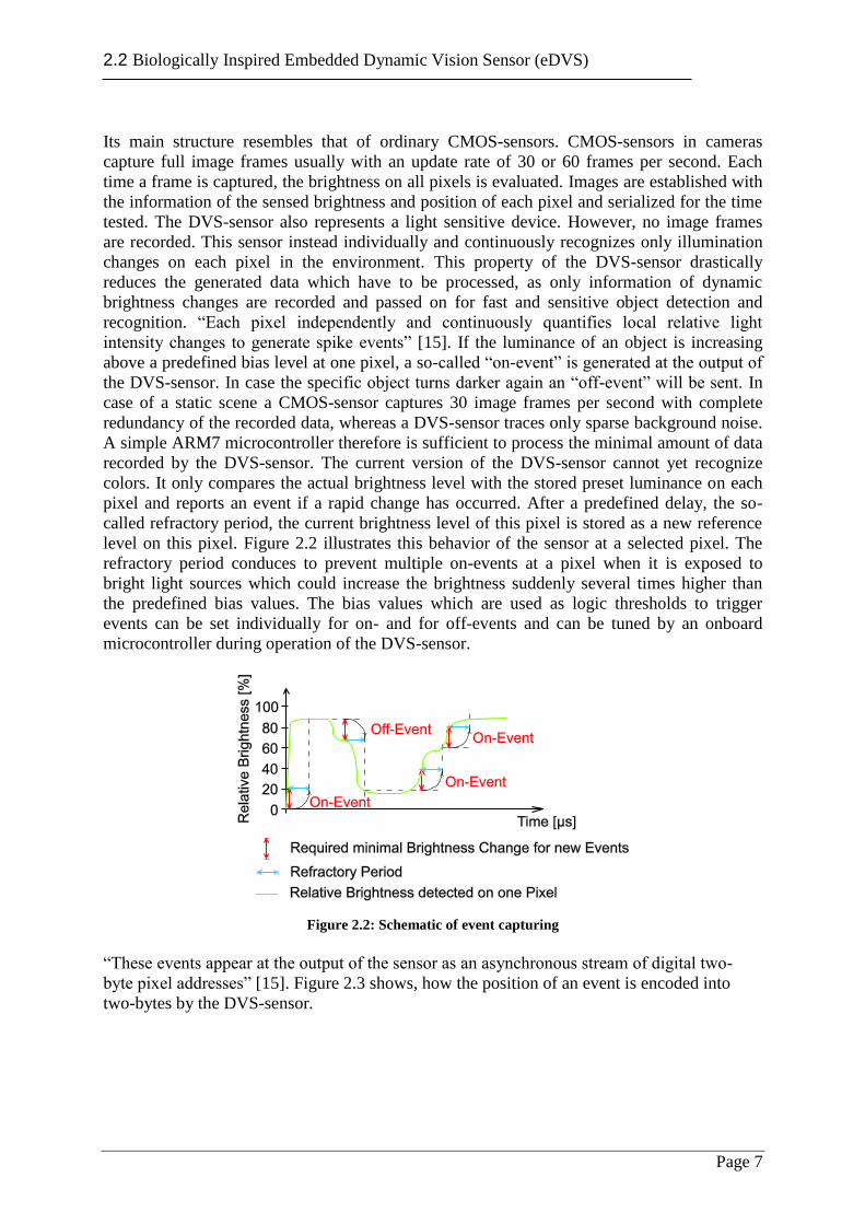
intensity changes to generate spike events” [15]. If the luminance of an object is increasing

above a predefined bias level at one pixel, a so-called “on-event” is generated at the output of

the DVS-sensor. In case the specific object turns darker again an “off-event” will be sent. In

case of a static scene a CMOS-sensor captures 30 image frames per second with complete

redundancy of the recorded data, whereas a DVS-sensor traces only sparse background noise.

A simple ARM7 microcontroller therefore is sufficient to process the minimal amount of data

recorded by the DVS-sensor. The current version of the DVS-sensor cannot yet recognize

colors. It only compares the actual brightness level with the stored preset luminance on each

pixel and reports an event if a rapid change has occurred. After a predefined delay, the so-

called refractory period, the current brightness level of this pixel is stored as a new reference

level on this pixel. Figure 2.2 illustrates this behavior of the sensor at a selected pixel. The

refractory period conduces to prevent multiple on-events at a pixel when it is exposed to

bright light sources which could increase the brightness suddenly several times higher than

the predefined bias values. The bias values which are used as logic thresholds to trigger

events can be set individually for on- and for off-events and can be tuned by an onboard

microcontroller during operation of the DVS-sensor.

Figure 2.2: Schematic of event capturing

“These events appear at the output of the sensor as an asynchronous stream of digital two-

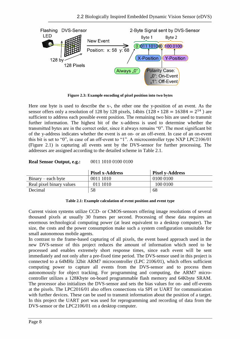
byte pixel addresses” [15]. Figure 2.3 shows, how the position of an event is encoded into

two-bytes by the DVS-sensor.

2.2 Biologically Inspired Embedded Dynamic Vision Sensor (eDVS)

Page 8

Figure 2.3: Example encoding of pixel position into two bytes

Here one byte is used to describe the x-, the other one the y-position of an event. As the

sensor offers only a resolution of 128 by 128 pixels, 14bits ( ) are

sufficient to address each possible event position. The remaining two bits are used to transmit

further information. The highest bit of the x-address is used to determine whether the

transmitted bytes are in the correct order, since it always remains “0”. The most significant bit

of the y-address indicates whether the event is an on- or an off-event. In case of an on-event

this bit is set to “0”, in case of an off-event to “1”. A microcontroller type NXP LPC2106/01

(Figure 2.1) is capturing all events sent by the DVS-sensor for further processing. The

addresses are assigned according to the detailed scheme in Table 2.1.

Real Sensor Output, e.g.: 0011 1010 0100 0100

Pixel x-Address Pixel y-Address

Binary – each byte 0011 1010 0100 0100

Real pixel binary values 011 1010 100 0100

Decimal 58 68

Table 2.1: Example calculation of event position and event type

Current vision systems utilize CCD- or CMOS-sensors offering image resolutions of several

thousand pixels at usually 30 frames per second. Processing of these data requires an

enormous technological computing power (at least equivalent to a desktop computer). The

size, the costs and the power consumption make such a system configuration unsuitable for

small autonomous mobile agents.

In contrast to the frame-based capturing of all pixels, the event based approach used in the

new DVS-sensor of this project reduces the amount of information which need to be

processed and enables extremely short response times, since each event will be sent

immediately and not only after a pre-fixed time period. The DVS-sensor used in this project is

connected to a 64MHz 32bit ARM7 microcontroller (LPC 2106/01), which offers sufficient

computing power to capture all events from the DVS-sensor and to process them

autonomously for object tracking. For programming and computing, the ARM7 micro-

controller utilizes a 128Kbyte on-board programmable flash memory and 64Kbyte SRAM.

The processor also initializes the DVS-sensor and sets the bias values for on- and off-events

at the pixels. The LPC2016/01 also offers connections via SPI or UART for communication

with further devices. These can be used to transmit information about the position of a target.

In this project the UART port was used for reprogramming and recording of data from the

DVS-sensor or the LPC2106/01 on a desktop computer.

2.3 Artificial Neural Networks

Page 9

The combination of the microcontroller with the DVS-sensor offers a low-cost embedded

stand-alone system, here referred to as eDVS-board, for 2D target detection. The eDVS-board

has a size of 52x23mm and a height of 6mm (30mm with lens). It weighs just 5g (12g with

lens). The power consumption of this embedded system (eDVS) is less than 200mW and thus

can be easily powered by a LiPo-cell [16]. Depending on the operation purpose, the DVS-

sensor can be equipped with different lenses to increase the field of view or to zoom into the

observed area. Because of the limited spatial resolution of the sensor, a distortion-free

telephoto lens, offering a view angle of just 11,3°, was used to remain a high resolution also at

far distances. With this lens the sensor could clearly identify its positioning angle to an object

within 0,088°.

2.3. Artificial Neural Networks

Current vision 3D tracking systems cannot run on small mobile robots due to their high

computing power requirements. Beside this fundamental condition a 3D tracking system also

has to be easily adaptable to the geometry of a robot for wider engineering use and should not

demand that the design of the robot has to be fitted. The biologically inspired tracking system

[11] introduced in section 1.2 still lacks this quality as it relies on a predefined, fixed design

of the detecting sensor. For gain of system flexibility, implementation of an artificial neural

network was endeavored that could transform varying angular positions of a tracked object

recorded from two DVS-sensors into 3D real-world data and allow use of a specific 3D

tracking algorithm. The following chapters introduce basic characteristics of artificial neural

networks, how their output can be calculated on a feed-forward network. Neural networks

cannot be used directly after initialization. Therefore it is explained in brief, how they can be

trained for specific application on different methods developed meanwhile.

Basics

Artificial neural networks (ANN) are programming constructs that try to mimic biological

neural networks, as they represent interconnected neurons in the nervous system of animals

and humans, for solving intelligence problems. The human brain consists of over 100 billion

neurons interconnected via synapses for exchange of information via electrical and chemical

signals. Single biological neurons are usually connected with axons and dendrites to many

other neurons forming extensive networks which function in groups of complex ordered

signaling circuits for all cognitive processes such as perception, motion, memory and learning

as major examples of only some of the tasks of the brain. With these neuronal networks

humans and animals can spontaneously adapt to new environments and perfectly and easily

perform tasks of orientation and perception of any objects that, although they look simple in

their performance, are still highly complex to be imitated by robots.

The development of artificial neural networks has been inspired by the biological structure

and behavior of the biological neural networks and was aimed at building mathematical or

computational models of the nervous system for simulation of properties and function of the

brain. Similar to the biological neurons, artificial networks are based on single operating

“units” also named “artificial neurons” or “nodes” which are interconnected in functional

groups. Various models have been developed to endow the systems with functions of the

humans’ brain.

ANNs mostly are non-linear statistical data modeling tools. They usually consist of complex

interconnections (“synapses”) of artificial neurons in different layers, which may be addressed

as input neurons, secondary layer neurons and output neurons via internal or external

2.3 Artificial Neural Networks

Page 10

information signals. Most systems use “weights” to change the parameters of information

flow and to regulate the connections between the neurons.

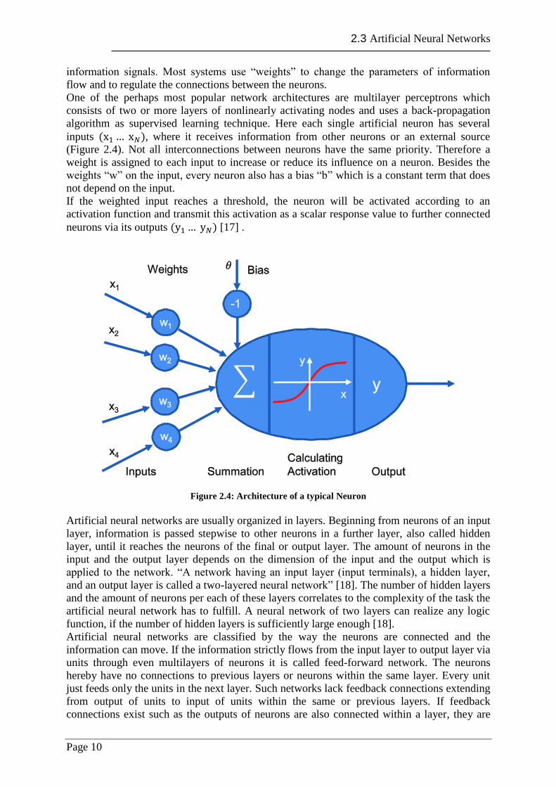
One of the perhaps most popular network architectures are multilayer perceptrons which

consists of two or more layers of nonlinearly activating nodes and uses a back-propagation

algorithm as supervised learning technique. Here each single artificial neuron has several

inputs ( ), where it receives information from other neurons or an external source

(Figure 2.4). Not all interconnections between neurons have the same priority. Therefore a

weight is assigned to each input to increase or reduce its influence on a neuron. Besides the

weights “w” on the input, every neuron also has a bias “b” which is a constant term that does

not depend on the input.

If the weighted input reaches a threshold, the neuron will be activated according to an

activation function and transmit this activation as a scalar response value to further connected

neurons via its outputs ( ) [17] .

Figure 2.4: Architecture of a typical Neuron

Artificial neural networks are usually organized in layers. Beginning from neurons of an input

layer, information is passed stepwise to other neurons in a further layer, also called hidden

layer, until it reaches the neurons of the final or output layer. The amount of neurons in the

input and the output layer depends on the dimension of the input and the output which is

applied to the network. “A network having an input layer (input terminals), a hidden layer,

and an output layer is called a two-layered neural network” [18]. The number of hidden layers

and the amount of neurons per each of these layers correlates to the complexity of the task the

artificial neural network has to fulfill. A neural network of two layers can realize any logic

function, if the number of hidden layers is sufficiently large enough [18].

Artificial neural networks are classified by the way the neurons are connected and the

information can move. If the information strictly flows from the input layer to output layer via

units through even multilayers of neurons it is called feed-forward network. The neurons

hereby have no connections to previous layers or neurons within the same layer. Every unit

just feeds only the units in the next layer. Such networks lack feedback connections extending

from output of units to input of units within the same or previous layers. If feedback

connections exist such as the outputs of neurons are also connected within a layer, they are

2.3 Artificial Neural Networks

Page 11

called lateral networks. “The structure of the interconnection network does not change over

time” [19].

The size of a neural network, the amount of layers and the number of neurons in each layer,

has major impact on its ability to reproduce complex functions. In general, increasing the

network size not only affects its complexity but also learning time and training quality, thus it

should be chosen deliberately. Increasing the size may considerably influence the capability

of the network for pattern recognition and approximation particularly for data not presented in

training sets under supervised learning conditions [20]. If the complexity and capacity of a

neural network exceeds the amount of testable free parameters in data training sets, a problem

called “over-fitting” arises. Training patterns usually include some noise values which the

network should not reproduce from the training data. In this case the network may perform

well on pattern recognition within the training set but fail to generalize or reproduce in unseen

data examples.

A network with simpler structure than necessary for correct prediction from a training data set

produces extensive bias in the output and cannot generate an optimal regression analysis even

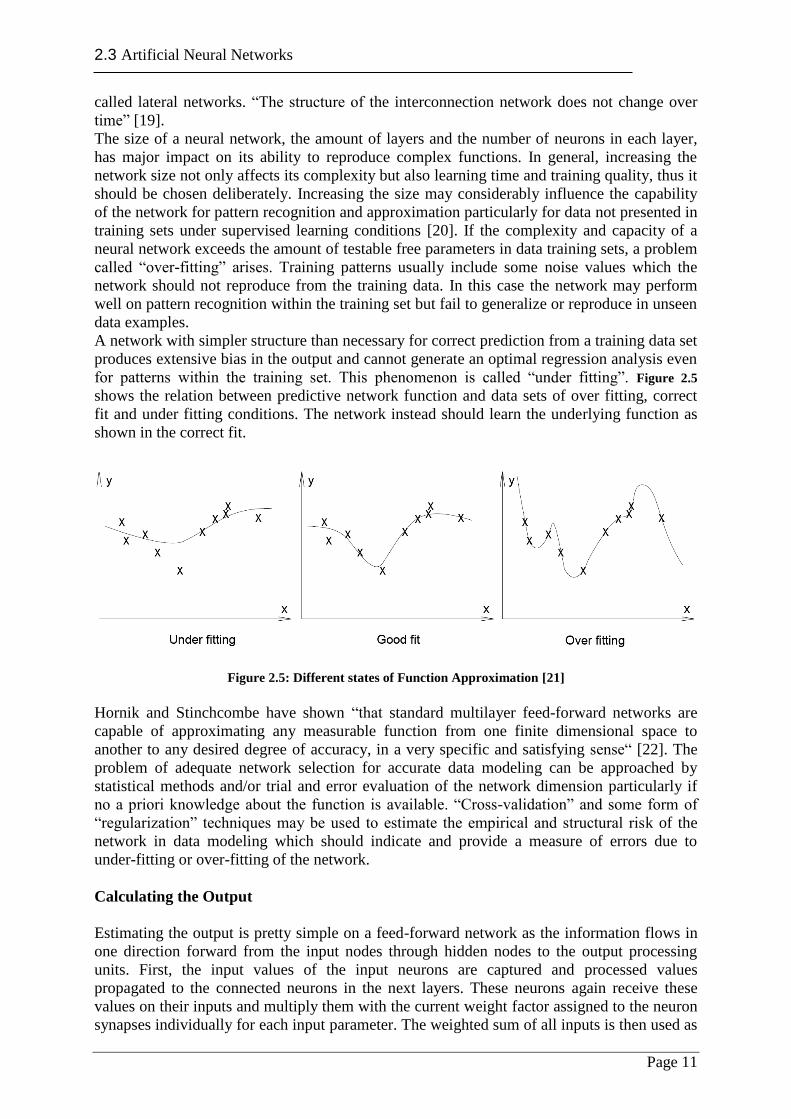
for patterns within the training set. This phenomenon is called “under fitting”. Figure 2.5

shows the relation between predictive network function and data sets of over fitting, correct

fit and under fitting conditions. The network instead should learn the underlying function as

shown in the correct fit.

Figure 2.5: Different states of Function Approximation [21]

Hornik and Stinchcombe have shown “that standard multilayer feed-forward networks are

capable of approximating any measurable function from one finite dimensional space to

another to any desired degree of accuracy, in a very specific and satisfying sense“ [22]. The

problem of adequate network selection for accurate data modeling can be approached by

statistical methods and/or trial and error evaluation of the network dimension particularly if

no a priori knowledge about the function is available. “Cross-validation” and some form of

“regularization” techniques may be used to estimate the empirical and structural risk of the

network in data modeling which should indicate and provide a measure of errors due to

under-fitting or over-fitting of the network.

Calculating the Output

Estimating the output is pretty simple on a feed-forward network as the information flows in

one direction forward from the input nodes through hidden nodes to the output processing

units. First, the input values of the input neurons are captured and processed values

propagated to the connected neurons in the next layers. These neurons again receive these

values on their inputs and multiply them with the current weight factor assigned to the neuron

synapses individually for each input parameter. The weighted sum of all inputs is then used as

2.3 Artificial Neural Networks

Page 12

input for the activation function of the neuronal network as shown in Figure 2.4. A common

nonlinear activation function can be continuous like ( ) or non-continuous like signum

functions (eq. 2.1). In each node the sum of products of the inputs and of the weights is

calculated. If it exceeds a certain threshold value, the unit fires and shows the activated value,

otherwise it takes the deactivated value. The value of activation of a neuron is then

transmitted to neurons in the next layer as their new input values.

( ) 2.1

: bias

: signum activaton function

: neuron inputs 1….n

: neuron output

This type of propagation of information is typical for neural feed-forward networks and

continuous until the final layer, the so-called output layer, which then shows the output of the

neural network. “The only significant delay within the neural system is the synaptic

delay”[19].

Training a Neural Network

When designing an artificial neural network for a specific task, its structure and topology

have to be specified such as the amount of neurons in each layer, the activation function and

the connections between the neurons. If weights and biases of the connection units are

initially set to random values, an artificial neural network cannot be immediately utilized

because of unspecific initialization. It first has to be trained to adjust weights and biases of

each neuron connection with a set of input-output data patterns. The structure of the unit

interconnections and the activation functions do not change over the training period, thus only

the weights and biases of the connections between the processing units are tuned. The goal of

the training is to find values of these adjustable parameters that for any input x the output y of

the network is a good approximation of the desired value. The training is performed via

suitable “learning” algorithms that tune the adjustable parameters so that an input training

data set maps well to corresponding outputs of the network. The output values of the system

are iteratively compared to the desired values to compute values of a predefined error function

and further adjust performance of the network by back-propagation learning. There is no a

priori knowledge to adjusts weights properly and optimally before training [23].

To train and validate a neural network a huge set of sample data has to be generated with data

values equally spread for all possible inputs and outputs. These examples are then divided

into three data subsystems, A, B and C [17]. In A the biggest amount of sample data is stored

and used for training the neural network. Training a neural network with relatively limited

numbers of training samples can lead to “over-training” or “over-fitting” of the neural

network. This means that the neural network fails generalization and pattern recognition of

the training data set. The general purpose of the training can be described as function

approximation of the network. In this context classification involves deriving a function that

will separate data into categories or classes characterized by distinct sets of features. If a

neural network can only operate on input data, it cannot be trained to produce the desired

output data on a “supervised” way, but must be able to recognize hidden structures and

patterns in the input data without “supervision” by employing so-called self-organization

capabilities. Unsupervised operating networks may be regarded as classifiers that imply

detection of constellations of clusters within the raw input data.

2.3 Artificial Neural Networks

Page 13

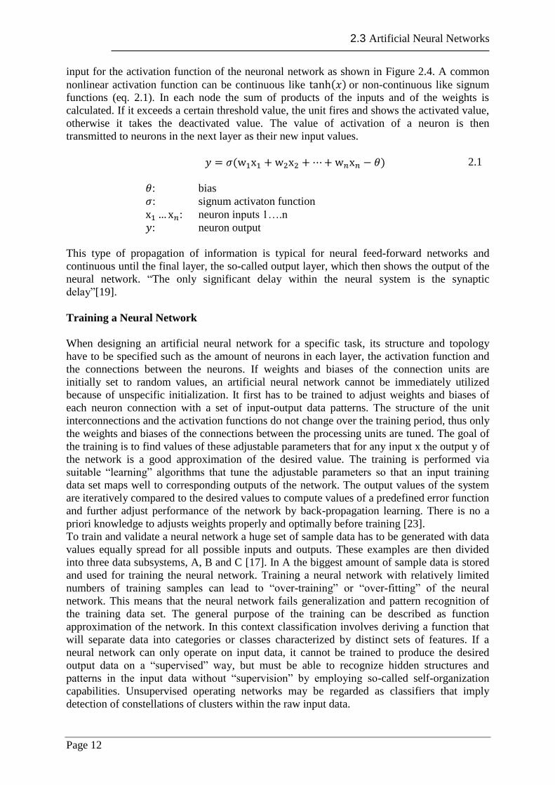
While training the artificial neural network on the data set A, its performance has to be

validated on the data of subsystem B which was generated under similar conditions as A. If

the performance of the output on dataset B becomes worse while training, the training is

stopped (Figure 2.6). If the achieved performance is not suitable enough, the network model

does not meet the desired requirements, in which case a better model could be chosen or the

training repeated with modification of the weights. Once performance of the network is

validated, it can be tested with new experimental unseen data from the subsystem C.

Figure 2.6: Learning of a Neural Network

The error function displayed in Figure 2.6, however is usually not continuous decreasing to a

global minimum, but offers several local minima. If a neural network runs into a local

minimum it can be stuck in this and cannot be removed by further training anymore.

Simulated Annealing is a probabilistic method “for finding the global minimum of a cost

function that may possess several local minima” [24]. This is being achieved by slight

modification of all weights and biases which shift the neural network to a different position

on the error-function.

Error Function

The quality of a trained network is evaluated with a predefined statistical error function. For

continuous activation functions the perhaps most important learning algorithm is called the

delta rule [25]. This means that for adjusting weights of the network properly, a general

method, the so-called gradient descent is applied. The weights are modified so that the error

decreases (delta between sample output value and true value) when it is calculated from the

error function.

The delta rule is based on gradient descent to reduce the error calculated by an error function

as shown (eq. 2.2).

2.3 Artificial Neural Networks

Page 14

∑( )

2.2

The basic principle is to find the minimum of an error surface which represents the

cumulative error over the dataset of subsystem “A” as a function of network weights and

biases as displayed in Figure 2.6. For detecting the minimum of this function, various

techniques have been developed like Levenberg Marquardt algorithm or back-propagation

which will be now explained in detail.

Back-Propagation

Back-propagation is one of the most popular methods for neural network training based on a

supervised learning method which means that the network is trained by providing it with input

and matched output patterns. The sample output is compared to the correct values to calculate

delta from a predefined error function. “The reason for the popularity is the underlying

simplicity and relative power of the algorithm” [26]. The strength of back-propagation is that

it can be used to also train nonlinear neural networks with any order of synapses between the

neurons. The simplicity is that it is based on a gradient descent of a defined error function.

The activation function of the neurons in the neural network needs to be differentiable that

back-propagation can be applied.

The back-propagation algorithm is separated into two steps, a feed-forward path and an error

back-propagation path. In the feed-forward path an input is fed into the network and the

activation of the neural network on the output calculated and the error calculated according to

an error function (eq. 2.2).

In the second step the error is back-propagated for each neuron through the whole network

beginning at the output layer. The weights and biases on each neuron are then modified in

order to reduce the value of the error function. Given for instance the error function (eq. 2.2)

the gradient can be calculated according to equation 2.3.

2.3

whereas

{ ( )( )

( )∑

2.4

2.3 Artificial Neural Networks

Page 15

Using the back-propagation algorithm the error is now reduced by modifying each weight

with the negative gradient as shown in equation 2.3. When the same data set is applied in this

training procedure to the network, it can be assured that the output error will be reduced

appropriately by this method.

2.3 Artificial Neural Networks

Page 16

3.1 Algorithm and Hardware Implementation

Page 17

3. Event-Based Target Detection Algorithm

Visual detection and tracking of objects is an essential requirement in many robotic

applications ranging from navigation and self-localization to interactive manipulation of

objects [27]. Especially in dynamic environments which can be experienced in human robot

interactions, detection of relevant objects and their reliable tracking are indispensable features

of robotic systems to avoid collision. Real-time computer vision based tracking on ordinary

CMOS- or CCD-sensors, however, relies on powerful hardware for fast extraction and

processing of key object features from each input image frame. Up to now most systems

could not incorporate full object sensing and tracking in real-time, particularly as the limited

computing power usually also has to be shared with further data processing tasks relevant for

other simultaneous functions of the robot system like grasping or navigating.

In this chapter, a new approach is presented offering high-speed visual tracking of active

markers also on autonomous robots. The algorithm was especially designed for the DVS-

sensor presented in section 2.2 and is fast enough to run on the ARM7 microcontroller of the

eDVS-sensor board. This 2D tracking algorithm is fundamental for the 3D tracking system

presented in chapter 4. The first section of this chapter introduces the event based tracking

algorithm with specific references to its advantages in comparison to ordinary visual tracking

methods. In section two application scenarios are shown, which demonstrate the performance

of the tracking algorithm.

3.1. Algorithm and Hardware Implementation

Unlike ordinary vision sensors, the DVS-sensor asynchronously records illumination changes

in the environment independently on each pixel. As no full frames of images are generated in

this vision system, standard object tracking techniques cannot be applied. A simple frame-

based tracking algorithm, which runs on the eDVS board, had been previously developed

specifically for the DVS-sensor to optimally track an active stimulus (Figure 3.1) flashing at

frequencies above 500Hz [28]. The portable, active stimulus is equipped with a Nichia

Superflux warmwhite LED which flashes at user-predefined frequencies and stimulates

continuously events on the DVS-sensor.

The previous algorithm continuously collects on-events within a predefined time period and

then assumes the target position where most events were recognized. Although this algorithm

works pretty well in this tracking setup, its limitations are that it only offers a position update

at 100Hz. In addition it is unable to reliably track and discriminate multiple flashing targets.

This, however, is a necessary feature for calibration of the 3D tracking system shown in

chapter 4.

3.1 Algorithm and Hardware Implementation

Page 18

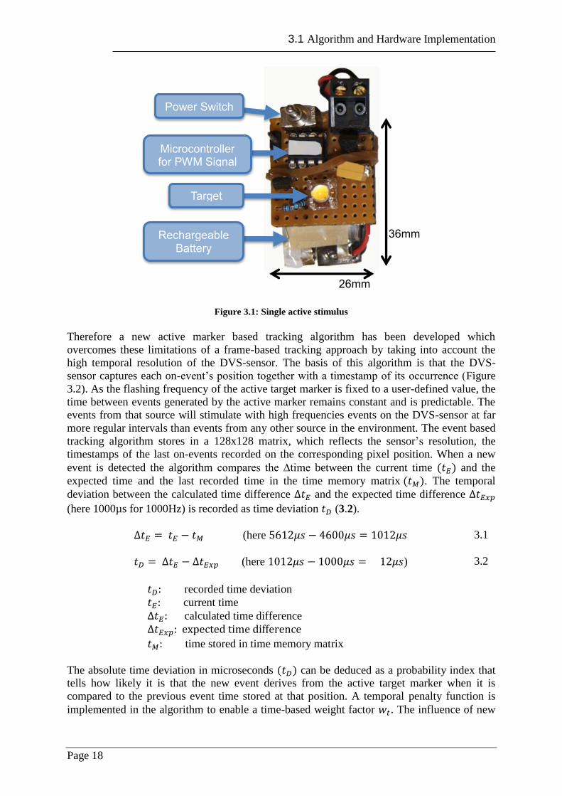
Figure 3.1: Single active stimulus

Therefore a new active marker based tracking algorithm has been developed which

overcomes these limitations of a frame-based tracking approach by taking into account the

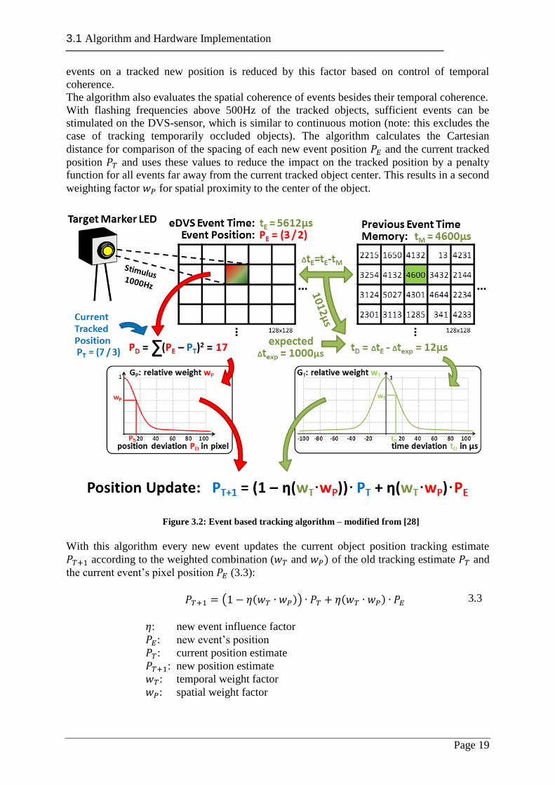
high temporal resolution of the DVS-sensor. The basis of this algorithm is that the DVS-

sensor captures each on-event’s position together with a timestamp of its occurrence (Figure

3.2). As the flashing frequency of the active target marker is fixed to a user-defined value, the

time between events generated by the active marker remains constant and is predictable. The

events from that source will stimulate with high frequencies events on the DVS-sensor at far

more regular intervals than events from any other source in the environment. The event based

tracking algorithm stores in a 128x128 matrix, which reflects the sensor’s resolution, the

timestamps of the last on-events recorded on the corresponding pixel position. When a new

event is detected the algorithm compares the ∆time between the current time ( ) and the

expected time and the last recorded time in the time memory matrix ( ). The temporal

deviation between the calculated time difference and the expected time difference

(here 1000µs for 1000Hz) is recorded as time deviation (3.2).

(here 3.1

(here ) 3.2

recorded time deviation

current time

calculated time difference

time stored in time memory matrix

The absolute time deviation in microseconds ( ) can be deduced as a probability index that

tells how likely it is that the new event derives from the active target marker when it is

compared to the previous event time stored at that position. A temporal penalty function is

implemented in the algorithm to enable a time-based weight factor . The influence of new

26mm

36mm

Target LED

Rechargeable Battery

Microcontroller for PWM Signal

Power Switch

3.1 Algorithm and Hardware Implementation

Page 19

events on a tracked new position is reduced by this factor based on control of temporal

coherence.

The algorithm also evaluates the spatial coherence of events besides their temporal coherence.

With flashing frequencies above 500Hz of the tracked objects, sufficient events can be

stimulated on the DVS-sensor, which is similar to continuous motion (note: this excludes the

case of tracking temporarily occluded objects). The algorithm calculates the Cartesian

distance for comparison of the spacing of each new event position and the current tracked

position and uses these values to reduce the impact on the tracked position by a penalty

function for all events far away from the current tracked object center. This results in a second

weighting factor for spatial proximity to the center of the object.

Figure 3.2: Event based tracking algorithm – modified from [28]

With this algorithm every new event updates the current object position tracking estimate

according to the weighted combination ( and ) of the old tracking estimate and

the current event’s pixel position (3.3):

( ( )) ( ) 3.3

: new event influence factor

: new event’s position

: current position estimate

: new position estimate

: temporal weight factor

: spatial weight factor

3.1 Algorithm and Hardware Implementation

Page 20

Each new recorded event influences the current object position estimate according to its event

significance calculated with the temporal weight factor and the spatial weight factor .

The parameter has been introduced to adapt the tracking algorithm to switch between fast

tracking for fast moving objects to slow but more robust tracking. In contrast to the frame

based algorithm [28] this new algorithm updates the tracked position asynchronously on every

new registered event. Tuning the parameters and developing suitable penalty functions for

optimal object tracking, however, is a difficult task. Optimal parameter settings are

particularly essential when different objects on several active marker LEDs flashing at

different frequencies are tracked. In spite of the use of LEDs with different preset and fixed

flashing frequencies in such a setting, the DVS-sensor recognizes and responds to slight

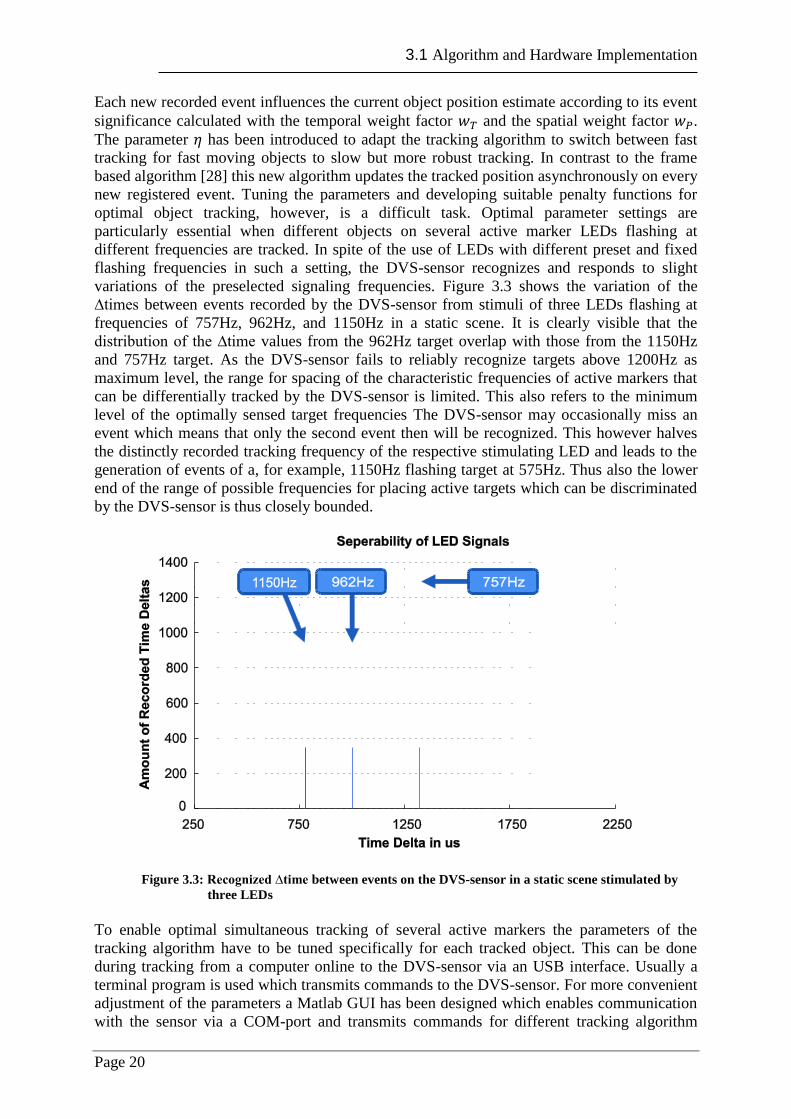
variations of the preselected signaling frequencies. Figure 3.3 shows the variation of the

∆times between events recorded by the DVS-sensor from stimuli of three LEDs flashing at

frequencies of 757Hz, 962Hz, and 1150Hz in a static scene. It is clearly visible that the

distribution of the ∆time values from the 962Hz target overlap with those from the 1150Hz

and 757Hz target. As the DVS-sensor fails to reliably recognize targets above 1200Hz as

maximum level, the range for spacing of the characteristic frequencies of active markers that

can be differentially tracked by the DVS-sensor is limited. This also refers to the minimum

level of the optimally sensed target frequencies The DVS-sensor may occasionally miss an

event which means that only the second event then will be recognized. This however halves

the distinctly recorded tracking frequency of the respective stimulating LED and leads to the

generation of events of a, for example, 1150Hz flashing target at 575Hz. Thus also the lower

end of the range of possible frequencies for placing active targets which can be discriminated

by the DVS-sensor is thus closely bounded.

Figure 3.3: Recognized ∆time between events on the DVS-sensor in a static scene stimulated by

three LEDs

To enable optimal simultaneous tracking of several active markers the parameters of the

tracking algorithm have to be tuned specifically for each tracked object. This can be done

during tracking from a computer online to the DVS-sensor via an USB interface. Usually a

terminal program is used which transmits commands to the DVS-sensor. For more convenient

adjustment of the parameters a Matlab GUI has been designed which enables communication

with the sensor via a COM-port and transmits commands for different tracking algorithm

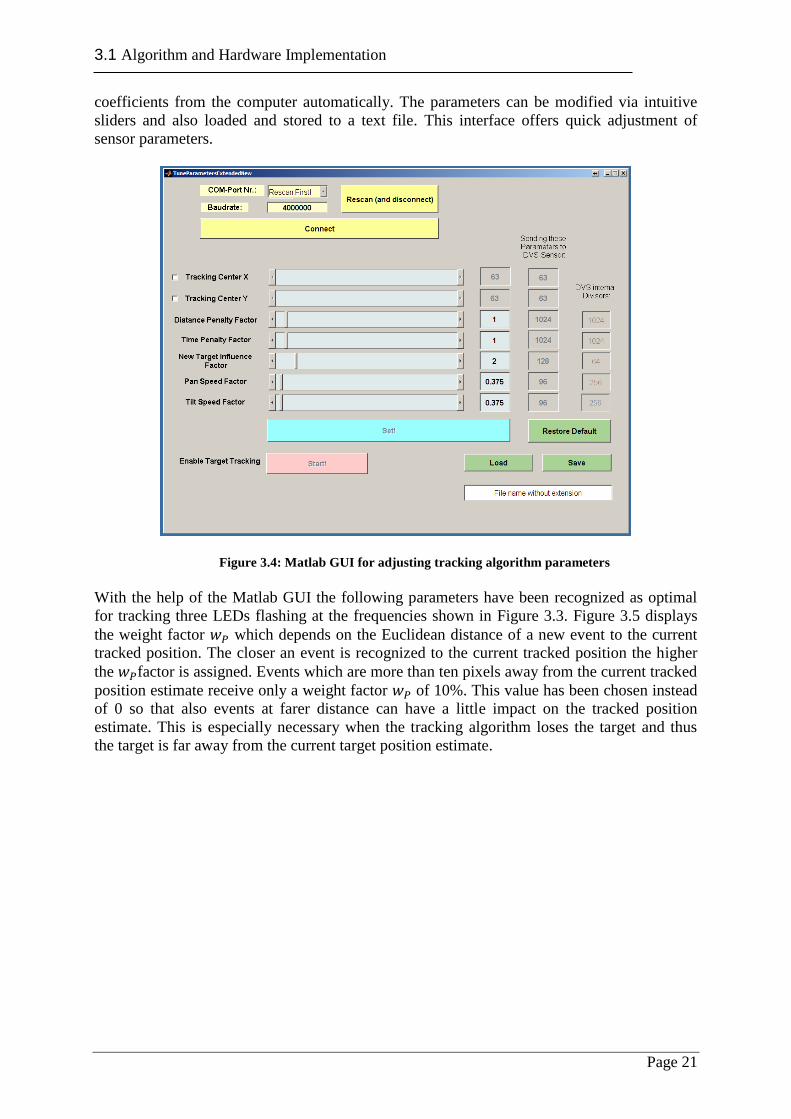
3.1 Algorithm and Hardware Implementation

Page 21

coefficients from the computer automatically. The parameters can be modified via intuitive

sliders and also loaded and stored to a text file. This interface offers quick adjustment of

sensor parameters.

Figure 3.4: Matlab GUI for adjusting tracking algorithm parameters

With the help of the Matlab GUI the following parameters have been recognized as optimal

for tracking three LEDs flashing at the frequencies shown in Figure 3.3. Figure 3.5 displays

the weight factor which depends on the Euclidean distance of a new event to the current

tracked position. The closer an event is recognized to the current tracked position the higher

the factor is assigned. Events which are more than ten pixels away from the current tracked

position estimate receive only a weight factor of 10%. This value has been chosen instead

of 0 so that also events at farer distance can have a little impact on the tracked position

estimate. This is especially necessary when the tracking algorithm loses the target and thus

the target is far away from the current target position estimate.

3.1 Algorithm and Hardware Implementation

Page 22

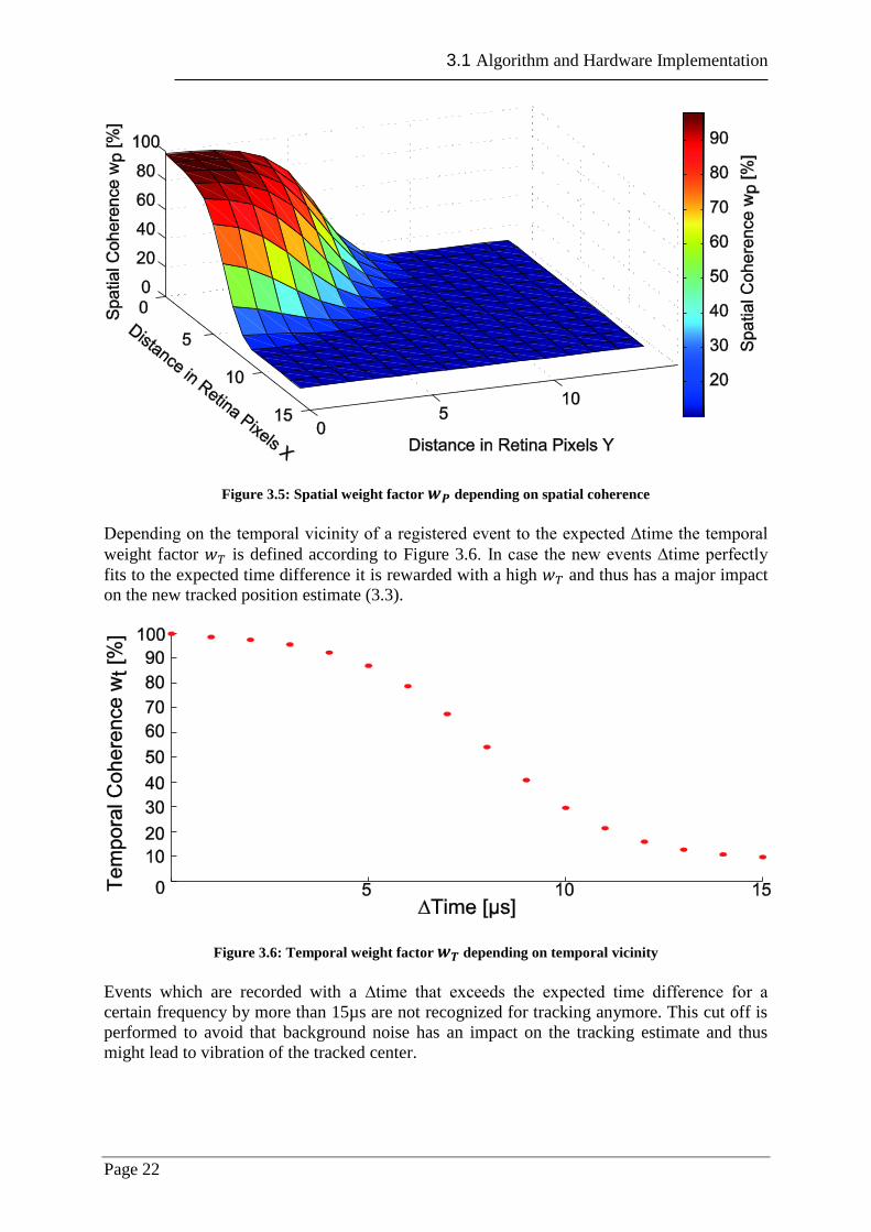
Figure 3.5: Spatial weight factor depending on spatial coherence

Depending on the temporal vicinity of a registered event to the expected ∆time the temporal

weight factor is defined according to Figure 3.6. In case the new events ∆time perfectly

fits to the expected time difference it is rewarded with a high and thus has a major impact

on the new tracked position estimate (3.3).

Figure 3.6: Temporal weight factor depending on temporal vicinity

Events which are recorded with a ∆time that exceeds the expected time difference for a

certain frequency by more than 15µs are not recognized for tracking anymore. This cut off is

performed to avoid that background noise has an impact on the tracking estimate and thus

might lead to vibration of the tracked center.

3.2 Results

Page 23

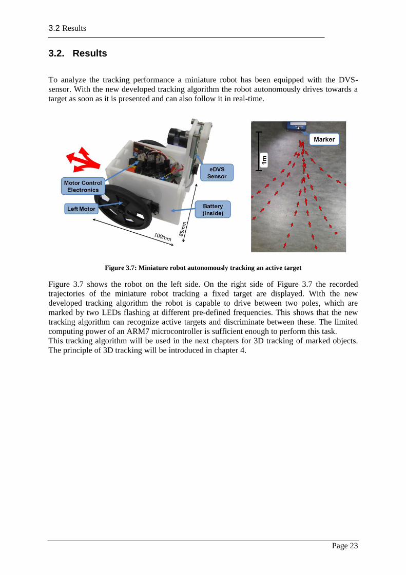
3.2. Results

To analyze the tracking performance a miniature robot has been equipped with the DVS-

sensor. With the new developed tracking algorithm the robot autonomously drives towards a

target as soon as it is presented and can also follow it in real-time.

Figure 3.7: Miniature robot autonomously tracking an active target

Figure 3.7 shows the robot on the left side. On the right side of Figure 3.7 the recorded

trajectories of the miniature robot tracking a fixed target are displayed. With the new

developed tracking algorithm the robot is capable to drive between two poles, which are

marked by two LEDs flashing at different pre-defined frequencies. This shows that the new

tracking algorithm can recognize active targets and discriminate between these. The limited

computing power of an ARM7 microcontroller is sufficient enough to perform this task.

This tracking algorithm will be used in the next chapters for 3D tracking of marked objects.

The principle of 3D tracking will be introduced in chapter 4.

3.2 Results

Page 24

4.1 Tracking Concept

Page 25

4. 3D Tracking

The first section of this chapter outlines principle ideas and basic structure of a 3D tracking

system developed in this thesis. All necessary hardware components and the software

programming are described in the following sections. The last section shows the performance

of the 3D tracking system.

4.1. Tracking Concept

Distance estimation is an essential acquirement for many applications of robots such as for

robotic product assembling, for human robot interactions or for the explorative use of

autonomous robots. Autonomous robots frequently offer only limited computing power.

Visual 3D tracking of objects in real-time, however, affords a fast computing hardware which

often cannot be sufficiently supplied with energy from batteries that are frequently the sole

power source on mobile robots.

In this project, a stand-alone 3D tracking system of lightweight and small size with low power

consumption was developed for application on mobile autonomous robots, The system

consists of two DVS-sensors. It was intended that the sensor could be flexibly positioned onto

the robot and versatile fitted to its geometry.

Two biologically inspired sensors (DVS-sensors) that could fulfill these requirements were

chosen. In comparison to ordinary CCD- or CMOS- sensors these devices had the major

advantage that they generated a very limited amount of data that had to be processed during

sensitive object detection. As shown in chapter 3 the DVS-sensor tracked marked objects at

high speed with the use of an ARM7 microcontroller only. When these sensors were used in

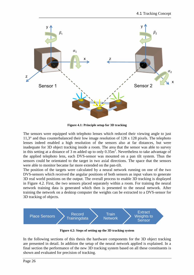
the 3D tracking system, they recorded their angular positions to specific active markers on a

traced target. Three Nichia NSSL 157T-H3 LEDs were individually selected on a specific

flashing frequency and mounted onto the target at a fixed mutual distance (Figure 4.6). The

algorithm presented in chapter 3 was trained to track each of the LEDs selectively and

calculate the angular position from the center of a fixed pan tilt coordinate system to each

LED (Figure 4.1).

4.1 Tracking Concept

Page 26

Figure 4.1: Principle setup for 3D tracking

The sensors were equipped with telephoto lenses which reduced their viewing angle to just

11,3° and thus counterbalanced their low image resolution of 128 x 128 pixels. The telephoto

lenses indeed enabled a high resolution of the sensors also at far distances, but were

inadequate for 3D object tracking inside a room. The area that the sensor was able to survey

in this setting at a distance of 3 m added up to only 0.35m2. Nevertheless to take advantage of

the applied telephoto lens, each DVS-sensor was mounted on a pan tilt system. Thus the

sensors could be orientated to the target in two axial directions. The space that the sensors

were able to monitor became far more extended on the pan-tilt.

The position of the targets were calculated by a neural network running on one of the two

DVS-sensors which received the angular positions of both sensors as input values to generate

3D real world positions on the output. The overall process to enable 3D tracking is displayed

in Figure 4.2. First, the two sensors placed separately within a room. For training the neural

network training data is generated which then is presented to the neural network. After

training the network on a desktop computer the weights can be extracted to a DVS-sensor for

3D tracking of objects.

Figure 4.2: Steps of setting up the 3D tracking system

In the following sections of this thesis the hardware components for the 3D object tracking

are presented in detail. In addition the setup of the neural network applied is explained. In a

final section the performance of the new 3D tracking system based on all these constituents is

shown and evaluated for precision of tracking.

Place Sensors Record

Trainingdata Train

Network

Extract Weights to

Sensor

x

y

z

x

y

z

𝛼

𝛽

𝛼

𝛽

Sensor 1 Sensor 2

4.2 Hardware Components

Page 27

4.2. Hardware Components

Pan Tilt

The spatial resolution of the DVS-sensor used for the new 3D tracking system was extremely

low with 128 by 128 pixels and therefore not sufficient for optimal object tracing even in the

nearer neighboring space within a room. When the DVS-sensor was equipped with a wide

angle lens to get a viewing field of 9 square meters at a two meter distance for instance, the

minimal distance between objects 2 meters away from the DVS-sensor had to be 10,99cm so

that they could be discriminated and recognized by the DVS-sensor. This discriminatory

capacity and detection accuracy was by far not sufficient for tracking or grasping objects in

3D even when two sensors were combined.

The DVS-sensors therefore have been equipped with narrow lenses that provided a viewing

angle of 11,3°, thus narrowed down the observation area of the sensors with an increase in

sensitivity and capacity for object discrimination. For regain of a larger supervision area

which was essential for any object tracking function the sensors were then mounted on pan tilt

systems which allowed the positioning of the sensors in two dimensions with a freedom of

90° at the vertical and of 120° at the horizontal axis. Two different pan tilt systems have been

setup for the orientation of the DVS-sensor. Both of them are based on serial kinematics.

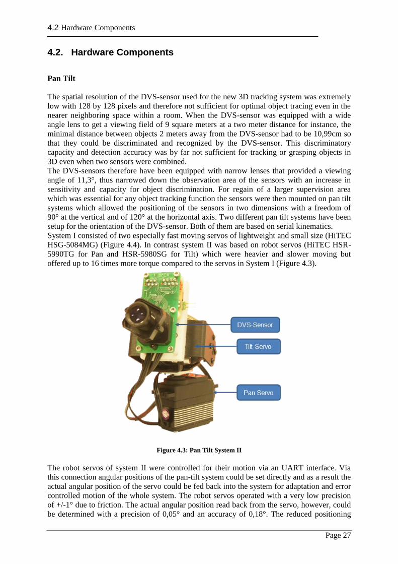
System I consisted of two especially fast moving servos of lightweight and small size (HiTEC

HSG-5084MG) (Figure 4.4). In contrast system II was based on robot servos (HiTEC HSR-

5990TG for Pan and HSR-5980SG for Tilt) which were heavier and slower moving but

offered up to 16 times more torque compared to the servos in System I (Figure 4.3).

Figure 4.3: Pan Tilt System II

The robot servos of system II were controlled for their motion via an UART interface. Via

this connection angular positions of the pan-tilt system could be set directly and as a result the

actual angular position of the servo could be fed back into the system for adaptation and error

controlled motion of the whole system. The robot servos operated with a very low precision

of +/-1° due to friction. The actual angular position read back from the servo, however, could

be determined with a precision of 0,05° and an accuracy of 0,18°. The reduced positioning

4.2 Hardware Components

Page 28

precision of the pan tilt system to reach a desired position was not a major drawback for its

use in object tracking, as the actual orientation of the servo can be read back with sufficient

precision and accuracy.

In system I the servos were controlled via PWM signals from the microcontroller on the

DVS-sensor board. The orientation of the pan tilt was determined by the PWM signal length.

No sensory feedback of the real orientation and positioning of the servos could be recorded by

this method. However, the servos themselves could detect and recognize their position with a

built-in potentiometer and correct positioning errors of the system to a tracked object with

these signals fed back into the system. Due to inherent inertia and friction of the system the

servos achieved to position the sensor on the pan tilt with a very limited precision. In specific

analyses of the motion control and positioning this pan tilt system I was shown to reach an

accuracy of about +/- 1°. This suggested that a tracking point at two meters distance to the

DVS-sensor could only be detected within +/- 3,5cm, if the sensor was tracking it perfectly.

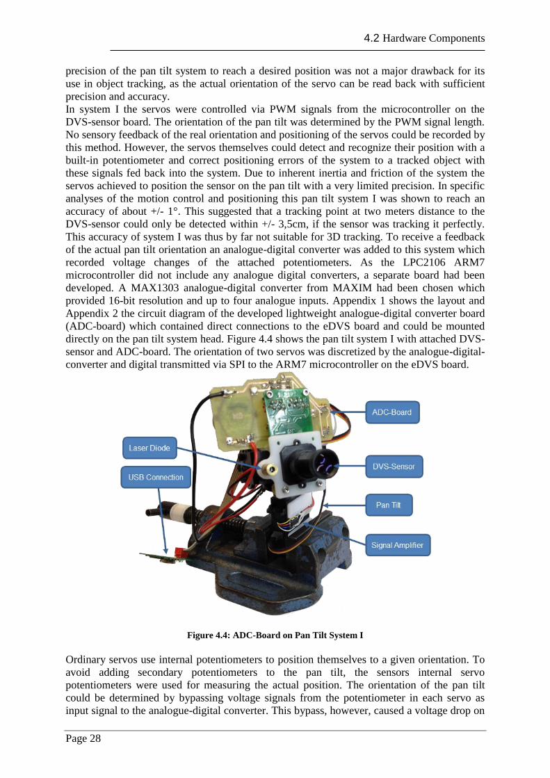
This accuracy of system I was thus by far not suitable for 3D tracking. To receive a feedback

of the actual pan tilt orientation an analogue-digital converter was added to this system which

recorded voltage changes of the attached potentiometers. As the LPC2106 ARM7

microcontroller did not include any analogue digital converters, a separate board had been

developed. A MAX1303 analogue-digital converter from MAXIM had been chosen which

provided 16-bit resolution and up to four analogue inputs. Appendix 1 shows the layout and

Appendix 2 the circuit diagram of the developed lightweight analogue-digital converter board

(ADC-board) which contained direct connections to the eDVS board and could be mounted

directly on the pan tilt system head. Figure 4.4 shows the pan tilt system I with attached DVS-

sensor and ADC-board. The orientation of two servos was discretized by the analogue-digital-

converter and digital transmitted via SPI to the ARM7 microcontroller on the eDVS board.

Figure 4.4: ADC-Board on Pan Tilt System I

Ordinary servos use internal potentiometers to position themselves to a given orientation. To

avoid adding secondary potentiometers to the pan tilt, the sensors internal servo

potentiometers were used for measuring the actual position. The orientation of the pan tilt

could be determined by bypassing voltage signals from the potentiometer in each servo as

input signal to the analogue-digital converter. This bypass, however, caused a voltage drop on

4.2 Hardware Components

Page 29

the potentiometer signal which was also recorded by the servo and interfered with its self-

positioning. The servo thus tried to reposition itself according to a falsified signal. To avoid

the consecutive unpredictable movement a signal amplifier was added to increase the input

signal strength of the analogue-digital converter without affection of the potentiometer signal

(Figure 4.4).

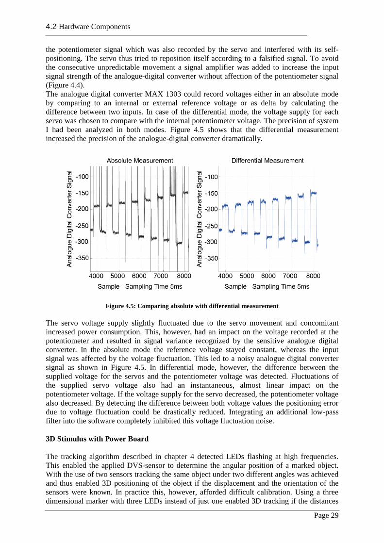
The analogue digital converter MAX 1303 could record voltages either in an absolute mode

by comparing to an internal or external reference voltage or as delta by calculating the

difference between two inputs. In case of the differential mode, the voltage supply for each

servo was chosen to compare with the internal potentiometer voltage. The precision of system

I had been analyzed in both modes. Figure 4.5 shows that the differential measurement

increased the precision of the analogue-digital converter dramatically.

Figure 4.5: Comparing absolute with differential measurement

The servo voltage supply slightly fluctuated due to the servo movement and concomitant

increased power consumption. This, however, had an impact on the voltage recorded at the

potentiometer and resulted in signal variance recognized by the sensitive analogue digital

converter. In the absolute mode the reference voltage stayed constant, whereas the input

signal was affected by the voltage fluctuation. This led to a noisy analogue digital converter

signal as shown in Figure 4.5. In differential mode, however, the difference between the

supplied voltage for the servos and the potentiometer voltage was detected. Fluctuations of

the supplied servo voltage also had an instantaneous, almost linear impact on the

potentiometer voltage. If the voltage supply for the servo decreased, the potentiometer voltage

also decreased. By detecting the difference between both voltage values the positioning error

due to voltage fluctuation could be drastically reduced. Integrating an additional low-pass

filter into the software completely inhibited this voltage fluctuation noise.

3D Stimulus with Power Board

The tracking algorithm described in chapter 4 detected LEDs flashing at high frequencies.

This enabled the applied DVS-sensor to determine the angular position of a marked object.

With the use of two sensors tracking the same object under two different angles was achieved

and thus enabled 3D positioning of the object if the displacement and the orientation of the

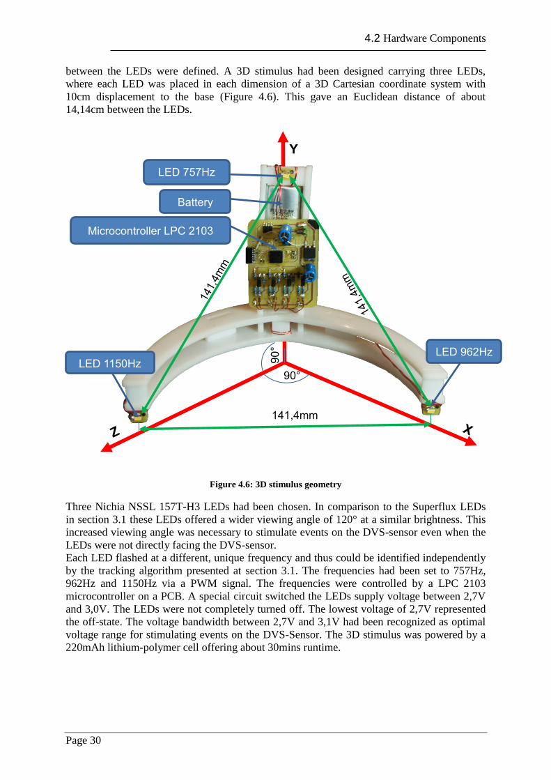
sensors were known. In practice this, however, afforded difficult calibration. Using a three

dimensional marker with three LEDs instead of just one enabled 3D tracking if the distances

4.2 Hardware Components

Page 30

between the LEDs were defined. A 3D stimulus had been designed carrying three LEDs,

where each LED was placed in each dimension of a 3D Cartesian coordinate system with

10cm displacement to the base (Figure 4.6). This gave an Euclidean distance of about

14,14cm between the LEDs.

Figure 4.6: 3D stimulus geometry

Three Nichia NSSL 157T-H3 LEDs had been chosen. In comparison to the Superflux LEDs

in section 3.1 these LEDs offered a wider viewing angle of 120° at a similar brightness. This

increased viewing angle was necessary to stimulate events on the DVS-sensor even when the

LEDs were not directly facing the DVS-sensor.

Each LED flashed at a different, unique frequency and thus could be identified independently

by the tracking algorithm presented at section 3.1. The frequencies had been set to 757Hz,

962Hz and 1150Hz via a PWM signal. The frequencies were controlled by a LPC 2103

microcontroller on a PCB. A special circuit switched the LEDs supply voltage between 2,7V

and 3,0V. The LEDs were not completely turned off. The lowest voltage of 2,7V represented

the off-state. The voltage bandwidth between 2,7V and 3,1V had been recognized as optimal

voltage range for stimulating events on the DVS-Sensor. The 3D stimulus was powered by a

220mAh lithium-polymer cell offering about 30mins runtime.

141,4mm

90°

90

°

Y

Microcontroller LPC 2103

Battery

LED 1150Hz LED 962Hz

LED 757Hz

5.1 Network Design

Page 31

5. Neural Network for 3D Position Estimation

5.1. Network Design

A neural network was applied in this project to map 4D data, consisting of tracked angular

positions of marked targets with two sensors, into 3D real world data. The advantage of using

a neural network instead of mathematic equations was that the output of a neural network

could be easily calculated, also on a less powerful hardware. For mapping, the neural network

offered four inputs for the pan and tilt angles of each sensor respectively. The output layer

consisted of three neurons, each for one dimension of the Cartesian 3D space.

Determining a proper network size, however, was difficult as described in section 2.3. Only

the amount of input and output neurons was evident. To analyze the minimal possible size of

a neural network for the mapping task, artificial input- and output-data were generated in

Matlab for a simulation. From two positions simulating sensor positioning angular positions

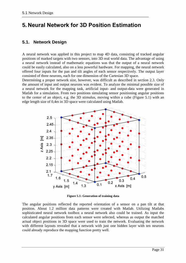
to the center of an object, e.g. the 3D stimulus, moving within a cube (Figure 5.1) with an

edge length size of 0,4m in 3D space were calculated using Matlab.

Figure 5.1: Generation of training data

The angular positions reflected the reported orientation of a sensor on a pan tilt at that

position. About 1.2 million data patterns were created with Matlab. Utilizing Matlabs

sophisticated neural network toolbox a neural network also could be trained. As input the

calculated angular positions from each sensor were selected, whereas as output the matched

actual object positions in 3D space were used to train the network. Evaluating the network

with different layouts revealed that a network with just one hidden layer with ten neurons

could already reproduce the mapping function pretty well.

5.2 Training the Neural Network

Page 32

5.2. Training the Neural Network

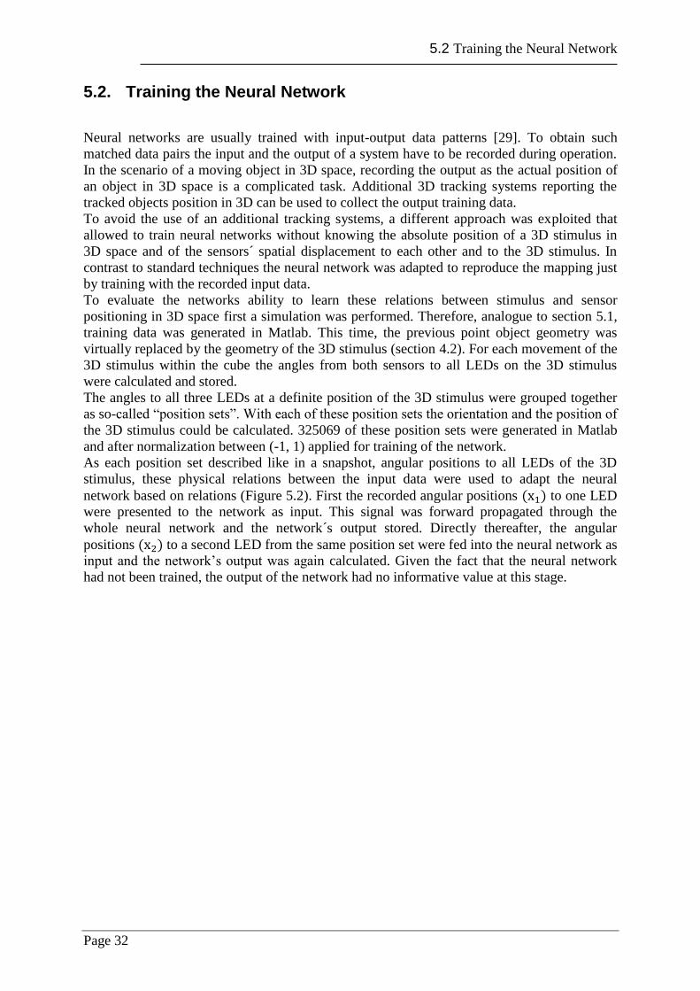
Neural networks are usually trained with input-output data patterns [29]. To obtain such

matched data pairs the input and the output of a system have to be recorded during operation.

In the scenario of a moving object in 3D space, recording the output as the actual position of

an object in 3D space is a complicated task. Additional 3D tracking systems reporting the

tracked objects position in 3D can be used to collect the output training data.

To avoid the use of an additional tracking systems, a different approach was exploited that

allowed to train neural networks without knowing the absolute position of a 3D stimulus in

3D space and of the sensors´ spatial displacement to each other and to the 3D stimulus. In

contrast to standard techniques the neural network was adapted to reproduce the mapping just

by training with the recorded input data.

To evaluate the networks ability to learn these relations between stimulus and sensor

positioning in 3D space first a simulation was performed. Therefore, analogue to section 5.1,

training data was generated in Matlab. This time, the previous point object geometry was

virtually replaced by the geometry of the 3D stimulus (section 4.2). For each movement of the

3D stimulus within the cube the angles from both sensors to all LEDs on the 3D stimulus

were calculated and stored.

The angles to all three LEDs at a definite position of the 3D stimulus were grouped together

as so-called “position sets”. With each of these position sets the orientation and the position of

the 3D stimulus could be calculated. 325069 of these position sets were generated in Matlab

and after normalization between (-1, 1) applied for training of the network.

As each position set described like in a snapshot, angular positions to all LEDs of the 3D

stimulus, these physical relations between the input data were used to adapt the neural

network based on relations (Figure 5.2). First the recorded angular positions ( ) to one LED

were presented to the network as input. This signal was forward propagated through the

whole neural network and the network´s output stored. Directly thereafter, the angular

positions ( ) to a second LED from the same position set were fed into the neural network as

input and the network’s output was again calculated. Given the fact that the neural network

had not been trained, the output of the network had no informative value at this stage.

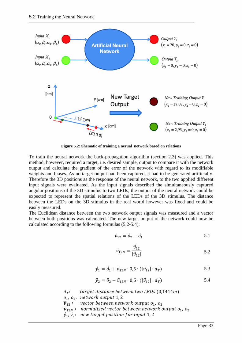
5.2 Training the Neural Network

Page 33

Figure 5.2: Shematic of training a nerual network based on relations

To train the neural network the back-propagation algorithm (section 2.3) was applied. This

method, however, required a target, i.e. desired sample, output to compare it with the network

output and calculate the gradient of the error of the network with regard to its modifiable

weights and biases. As no target output had been captured, it had to be generated artificially.

Therefore the 3D positions as the response of the neural network, to the two applied different

input signals were evaluated. As the input signals described the simultaneously captured

angular positions of the 3D stimulus to two LEDs, the output of the neural network could be

expected to represent the spatial relations of the LEDs of the 3D stimulus. The distance

between the LEDs on the 3D stimulus in the real world however was fixed and could be

easily measured.

The Euclidean distance between the two network output signals was measured and a vector

between both positions was calculated. The new target output of the network could now be

calculated according to the following formulas (5.2-5.4):

5.1

| | 5.2

(| | ) 5.3

(| | ) 5.4

( )

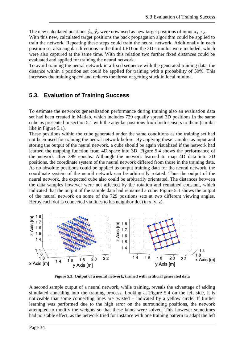
5.3 Evaluation of Training Success

Page 34

The new calculated positions were now used as new target positions of input .

With this new, calculated target positions the back propagation algorithm could be applied to

train the network. Repeating these steps could train the neural network. Additionally in each

position set also angular directions to the third LED on the 3D stimulus were included, which

were also captured at the same time. With this relation two further fixed distances could be

evaluated and applied for training the neural network.

To avoid training the neural network in a fixed sequence with the generated training data, the

distance within a position set could be applied for training with a probability of 50%. This

increases the training speed and reduces the threat of getting stuck in local minima.

5.3. Evaluation of Training Success

To estimate the networks generalization performance during training also an evaluation data

set had been created in Matlab, which includes 729 equally spread 3D positions in the same

cube as presented in section 5.1 with the angular positions from both sensors to them (similar

like in Figure 5.1).

These positions within the cube generated under the same conditions as the training set had

not been used for training the neural network before. By applying these samples as input and

storing the output of the neural network, a cube should be again visualized if the network had

learned the mapping function from 4D space into 3D. Figure 5.4 shows the performance of

the network after 399 epochs. Although the network learned to map 4D data into 3D

positions, the coordinate system of the neural network differed from those in the training data.

As no absolute positions could be applied as output training data for the neural network, the

coordinate system of the neural network can be arbitrarily rotated. Thus the output of the

neural network, the expected cube also could be arbitrarily orientated. The distances between

the data samples however were not affected by the rotation and remained constant, which

indicated that the output of the sample data had remained a cube. Figure 5.3 shows the output

of the neural network on some of the 729 positions sets at two different viewing angles.

Herby each dot is connected via lines to his neighbor dot (in x, y, z).

Figure 5.3: Output of a neural network, trained with artificial generated data

A second sample output of a neural network, while training, reveals the advantage of adding

simulated annealing into the training process. Looking at Figure 5.4 on the left side, it is

noticeable that some connecting lines are twisted – indicated by a yellow circle. If further

learning was performed due to the high error on the surrounding positions, the network

attempted to modify the weights so that these knots were solved. This however sometimes

had no stable effect, as the network tried for instance with one training pattern to adapt the left

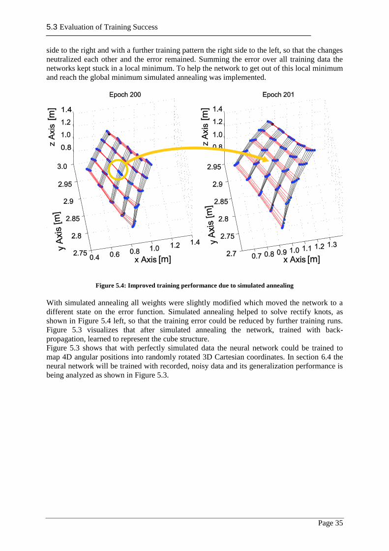
5.3 Evaluation of Training Success

Page 35

side to the right and with a further training pattern the right side to the left, so that the changes

neutralized each other and the error remained. Summing the error over all training data the

networks kept stuck in a local minimum. To help the network to get out of this local minimum

and reach the global minimum simulated annealing was implemented.

Figure 5.4: Improved training performance due to simulated annealing

With simulated annealing all weights were slightly modified which moved the network to a

different state on the error function. Simulated annealing helped to solve rectify knots, as

shown in Figure 5.4 left, so that the training error could be reduced by further training runs.

Figure 5.3 visualizes that after simulated annealing the network, trained with back-

propagation, learned to represent the cube structure.

Figure 5.3 shows that with perfectly simulated data the neural network could be trained to

map 4D angular positions into randomly rotated 3D Cartesian coordinates. In section 6.4 the

neural network will be trained with recorded, noisy data and its generalization performance is

being analyzed as shown in Figure 5.3.

5.3 Evaluation of Training Success

Page 36

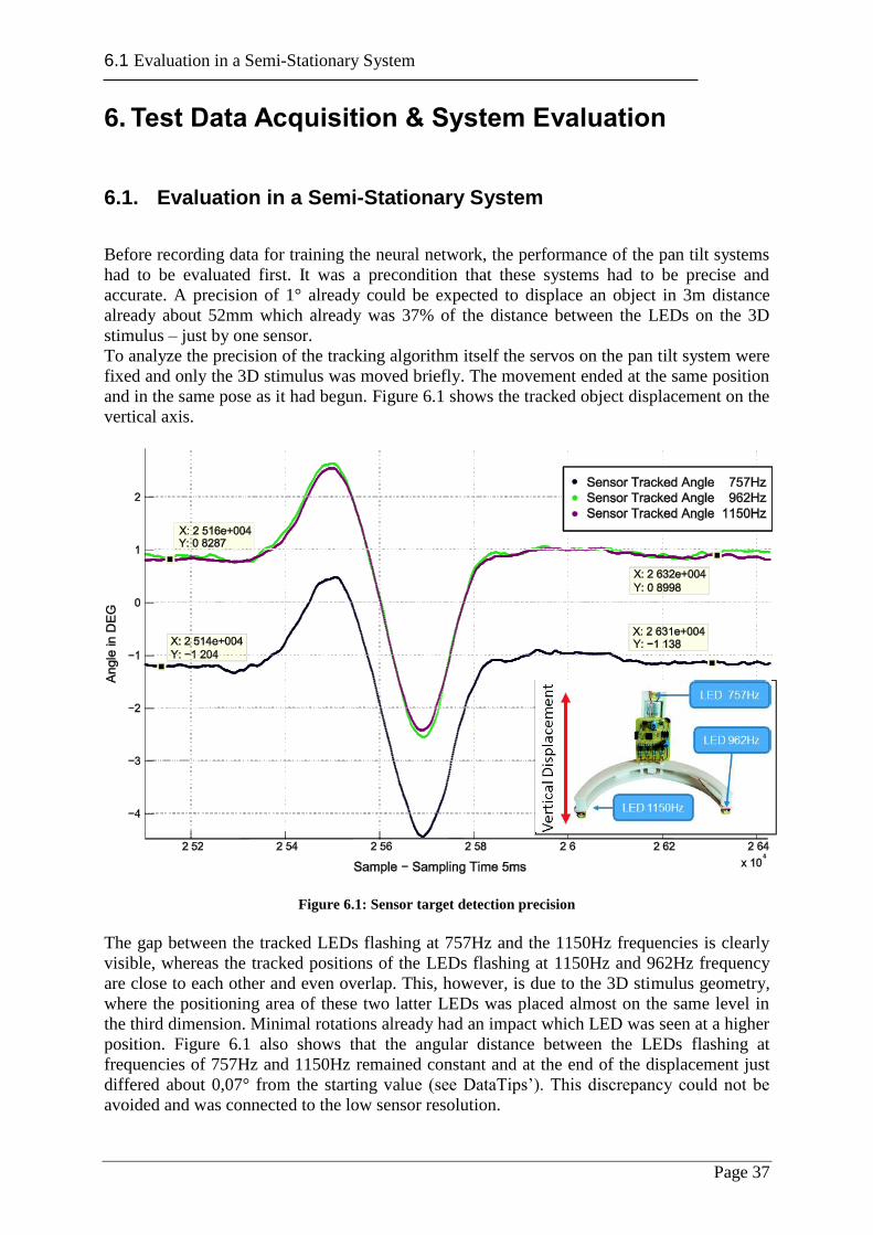
6.1 Evaluation in a Semi-Stationary System

Page 37

6. Test Data Acquisition & System Evaluation

6.1. Evaluation in a Semi-Stationary System

Before recording data for training the neural network, the performance of the pan tilt systems

had to be evaluated first. It was a precondition that these systems had to be precise and

accurate. A precision of 1° already could be expected to displace an object in 3m distance

already about 52mm which already was 37% of the distance between the LEDs on the 3D

stimulus – just by one sensor.

To analyze the precision of the tracking algorithm itself the servos on the pan tilt system were

fixed and only the 3D stimulus was moved briefly. The movement ended at the same position

and in the same pose as it had begun. Figure 6.1 shows the tracked object displacement on the

vertical axis.

Figure 6.1: Sensor target detection precision

The gap between the tracked LEDs flashing at 757Hz and the 1150Hz frequencies is clearly

visible, whereas the tracked positions of the LEDs flashing at 1150Hz and 962Hz frequency

are close to each other and even overlap. This, however, is due to the 3D stimulus geometry,

where the positioning area of these two latter LEDs was placed almost on the same level in

the third dimension. Minimal rotations already had an impact which LED was seen at a higher

position. Figure 6.1 also shows that the angular distance between the LEDs flashing at

frequencies of 757Hz and 1150Hz remained constant and at the end of the displacement just

differed about 0,07° from the starting value (see DataTips’). This discrepancy could not be

avoided and was connected to the low sensor resolution.

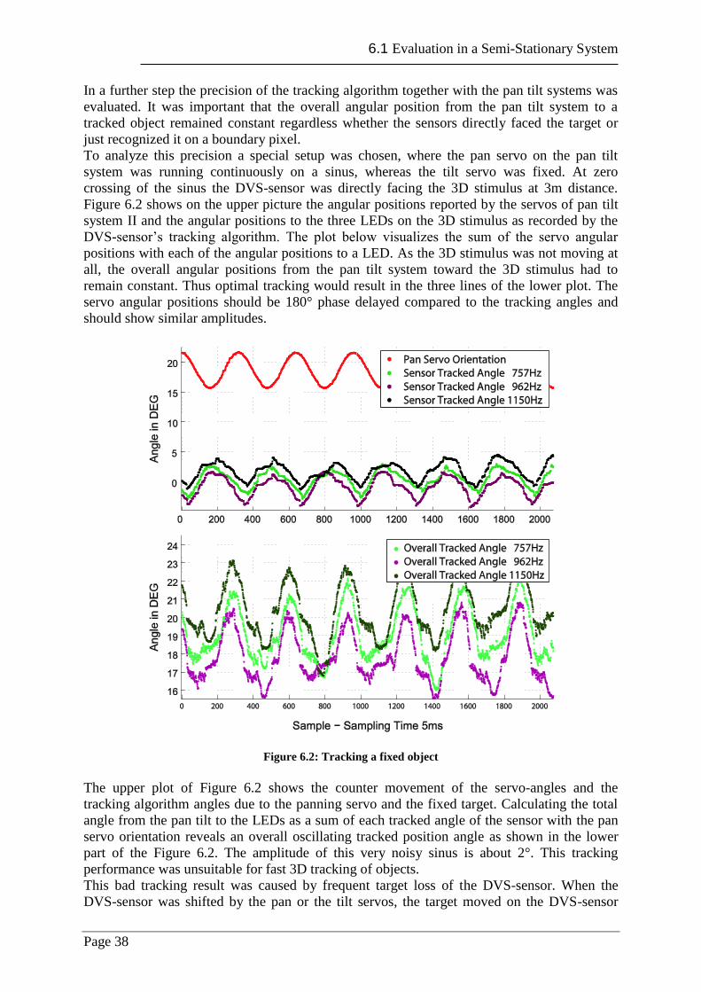
6.1 Evaluation in a Semi-Stationary System

Page 38

In a further step the precision of the tracking algorithm together with the pan tilt systems was

evaluated. It was important that the overall angular position from the pan tilt system to a

tracked object remained constant regardless whether the sensors directly faced the target or

just recognized it on a boundary pixel.

To analyze this precision a special setup was chosen, where the pan servo on the pan tilt

system was running continuously on a sinus, whereas the tilt servo was fixed. At zero

crossing of the sinus the DVS-sensor was directly facing the 3D stimulus at 3m distance.

Figure 6.2 shows on the upper picture the angular positions reported by the servos of pan tilt

system II and the angular positions to the three LEDs on the 3D stimulus as recorded by the

DVS-sensor’s tracking algorithm. The plot below visualizes the sum of the servo angular

positions with each of the angular positions to a LED. As the 3D stimulus was not moving at

all, the overall angular positions from the pan tilt system toward the 3D stimulus had to

remain constant. Thus optimal tracking would result in the three lines of the lower plot. The

servo angular positions should be 180° phase delayed compared to the tracking angles and

should show similar amplitudes.

Figure 6.2: Tracking a fixed object

The upper plot of Figure 6.2 shows the counter movement of the servo-angles and the

tracking algorithm angles due to the panning servo and the fixed target. Calculating the total

angle from the pan tilt to the LEDs as a sum of each tracked angle of the sensor with the pan

servo orientation reveals an overall oscillating tracked position angle as shown in the lower

part of the Figure 6.2. The amplitude of this very noisy sinus is about 2°. This tracking

performance was unsuitable for fast 3D tracking of objects.

This bad tracking result was caused by frequent target loss of the DVS-sensor. When the

DVS-sensor was shifted by the pan or the tilt servos, the target moved on the DVS-sensor

6.2 Prediction of Target Motion

Page 39

pixels. By moving to a neighboring pixel, two events, which were recorded with a predefined

time gap, were necessary to update the tracked position estimation. The timestamp first event

had to be stored in the time stamp matrix (Figure 3.2) so that it could be later compared with

the newer timestamp of the second event to evaluate the affiliation to one of the tracked

targets. This, however, limited the maximum angular velocity of a tracked target.

Furthermore, by far more events were stimulated on the DVS-sensor when it was panned than

the 3D stimulus was moved itself. This huge amount of events could not be completely

processed by the DVS-sensor and the microcontroller. This led to increased event drop which

falsified the recognized event frequency. The dropped events had no impact on the tracking

estimate. The tracked position update, thus could not be kept up with the angular velocity of

the panning servo. In the next section a method to overcome these difficulties will be

introduced.

6.2. Prediction of Target Motion

To improve the overall tracking performance shown in Figure 6.2, target loss due to DVS-

sensor rotation had to be avoided. Since the angular shift of the pan and the tilt servos could

be detected, the current tracked position estimated in the tracking algorithm could be

continuously counter shifted. Figure 6.3 exemplifies application of this method. The left

frame shows the 128 by 128 pixels of the DVS-sensor where the actual target position (dark

blue) is being shifted from the boundary pixels towards a pixel in the center of the DVS-

sensor (bright blue). This shift is performed by the tilt servo, which rotated the DVS-sensor

around the horizontal axis. The tracking algorithm failed to reliably track the target when the

servos were moving (section 6.1).

To improve the reliability of tracking, the angular tracked position estimate was updated

according to the angular shift of the tilt servos. With this method pixel positions of stationary

objects on the DVS-sensor which shifted due to pan or tilt servo movements could be

predicted without actually tracking the object. Figure 6.3 shows in the right frame, that the

position estimate of the target is shifted according to the measured servo movement.

This method also improved tracking of moving targets. Events which were related to the

tracked target frequency stayed closer to estimates of the tracked position with use of this

method than without consideration of the shifting variance. This was important for increasing

the maximum velocity of objects that still could be tracked by the 3D tracking algorithm.

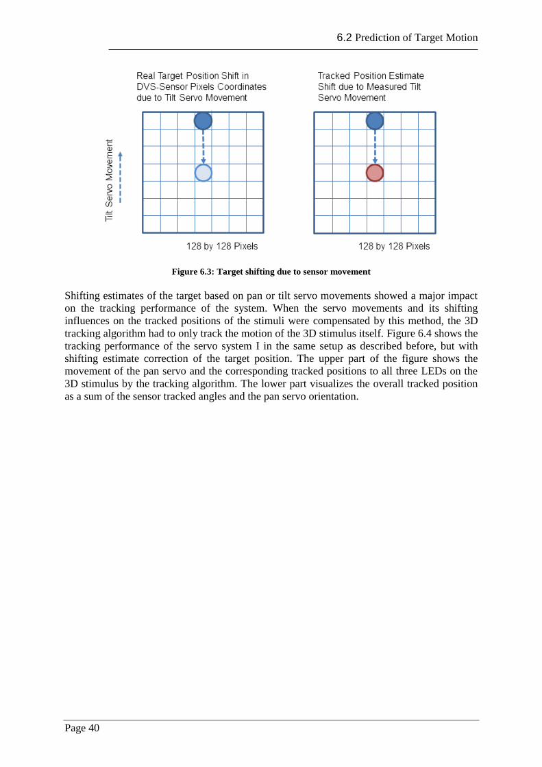
6.2 Prediction of Target Motion

Page 40

Figure 6.3: Target shifting due to sensor movement

Shifting estimates of the target based on pan or tilt servo movements showed a major impact

on the tracking performance of the system. When the servo movements and its shifting

influences on the tracked positions of the stimuli were compensated by this method, the 3D

tracking algorithm had to only track the motion of the 3D stimulus itself. Figure 6.4 shows the

tracking performance of the servo system I in the same setup as described before, but with

shifting estimate correction of the target position. The upper part of the figure shows the

movement of the pan servo and the corresponding tracked positions to all three LEDs on the

3D stimulus by the tracking algorithm. The lower part visualizes the overall tracked position

as a sum of the sensor tracked angles and the pan servo orientation.

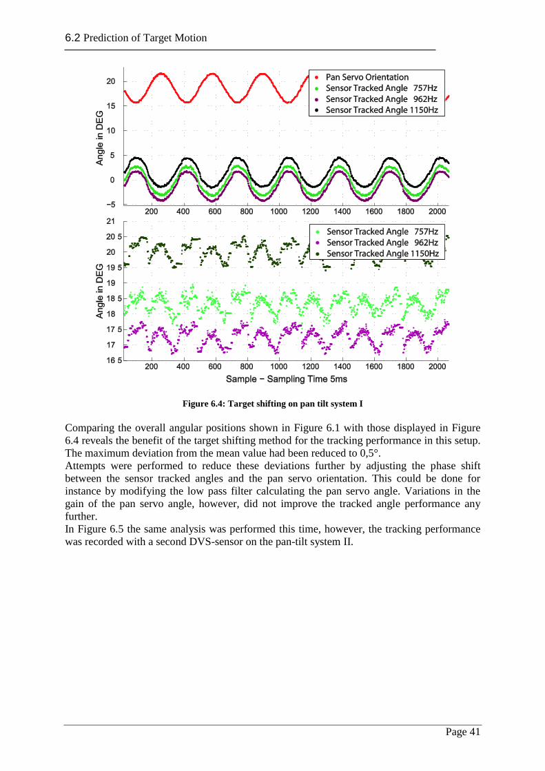
6.2 Prediction of Target Motion

Page 41

Figure 6.4: Target shifting on pan tilt system I

Comparing the overall angular positions shown in Figure 6.1 with those displayed in Figure

6.4 reveals the benefit of the target shifting method for the tracking performance in this setup.

The maximum deviation from the mean value had been reduced to 0,5°.

Attempts were performed to reduce these deviations further by adjusting the phase shift

between the sensor tracked angles and the pan servo orientation. This could be done for

instance by modifying the low pass filter calculating the pan servo angle. Variations in the

gain of the pan servo angle, however, did not improve the tracked angle performance any

further.

In Figure 6.5 the same analysis was performed this time, however, the tracking performance

was recorded with a second DVS-sensor on the pan-tilt system II.

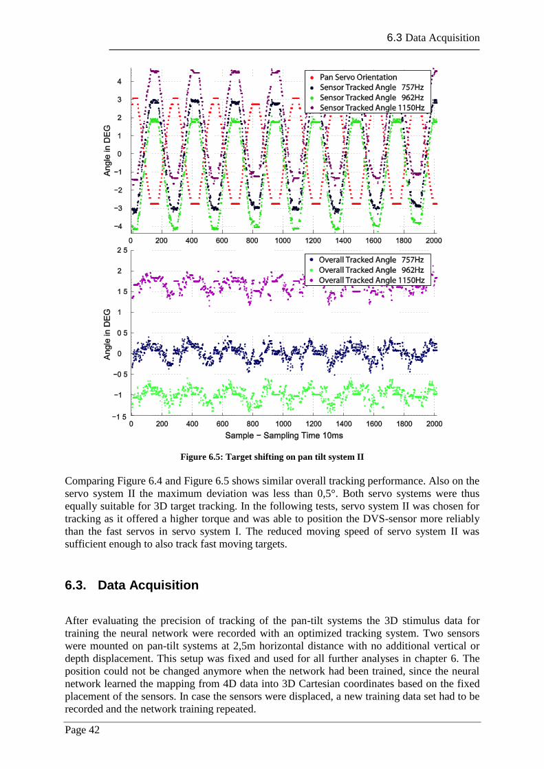
6.3 Data Acquisition

Page 42

Figure 6.5: Target shifting on pan tilt system II

Comparing Figure 6.4 and Figure 6.5 shows similar overall tracking performance. Also on the

servo system II the maximum deviation was less than 0,5°. Both servo systems were thus

equally suitable for 3D target tracking. In the following tests, servo system II was chosen for

tracking as it offered a higher torque and was able to position the DVS-sensor more reliably

than the fast servos in servo system I. The reduced moving speed of servo system II was

sufficient enough to also track fast moving targets.

6.3. Data Acquisition

After evaluating the precision of tracking of the pan-tilt systems the 3D stimulus data for

training the neural network were recorded with an optimized tracking system. Two sensors

were mounted on pan-tilt systems at 2,5m horizontal distance with no additional vertical or

depth displacement. This setup was fixed and used for all further analyses in chapter 6. The

position could not be changed anymore when the network had been trained, since the neural

network learned the mapping from 4D data into 3D Cartesian coordinates based on the fixed

placement of the sensors. In case the sensors were displaced, a new training data set had to be

recorded and the network training repeated.

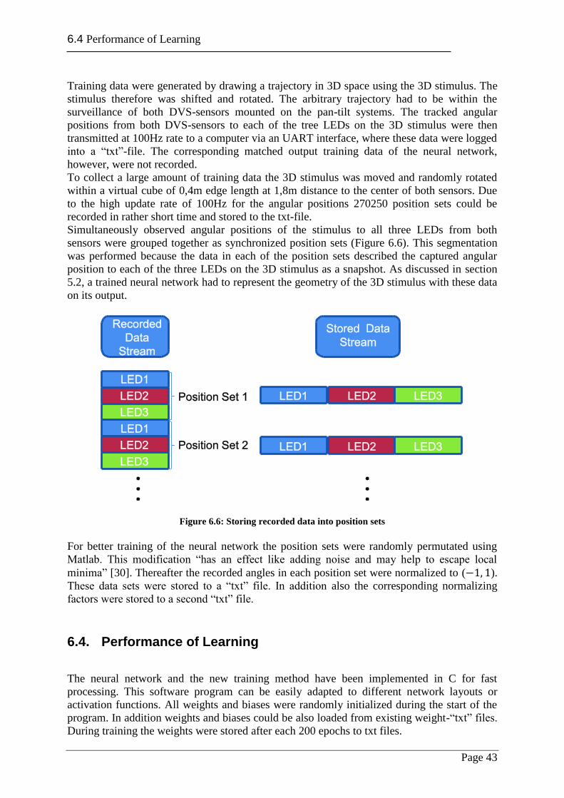
6.4 Performance of Learning

Page 43

Training data were generated by drawing a trajectory in 3D space using the 3D stimulus. The

stimulus therefore was shifted and rotated. The arbitrary trajectory had to be within the

surveillance of both DVS-sensors mounted on the pan-tilt systems. The tracked angular

positions from both DVS-sensors to each of the tree LEDs on the 3D stimulus were then

transmitted at 100Hz rate to a computer via an UART interface, where these data were logged

into a “txt”-file. The corresponding matched output training data of the neural network,

however, were not recorded.

To collect a large amount of training data the 3D stimulus was moved and randomly rotated

within a virtual cube of 0,4m edge length at 1,8m distance to the center of both sensors. Due

to the high update rate of 100Hz for the angular positions 270250 position sets could be

recorded in rather short time and stored to the txt-file.

Simultaneously observed angular positions of the stimulus to all three LEDs from both

sensors were grouped together as synchronized position sets (Figure 6.6). This segmentation

was performed because the data in each of the position sets described the captured angular

position to each of the three LEDs on the 3D stimulus as a snapshot. As discussed in section

5.2, a trained neural network had to represent the geometry of the 3D stimulus with these data

on its output.

Figure 6.6: Storing recorded data into position sets

For better training of the neural network the position sets were randomly permutated using

Matlab. This modification “has an effect like adding noise and may help to escape local

minima” [30]. Thereafter the recorded angles in each position set were normalized to ( ).

These data sets were stored to a “txt” file. In addition also the corresponding normalizing

factors were stored to a second “txt” file.

6.4. Performance of Learning

The neural network and the new training method have been implemented in C for fast

processing. This software program can be easily adapted to different network layouts or

activation functions. All weights and biases were randomly initialized during the start of the

program. In addition weights and biases could be also loaded from existing weight-“txt” files.

During training the weights were stored after each 200 epochs to txt files.

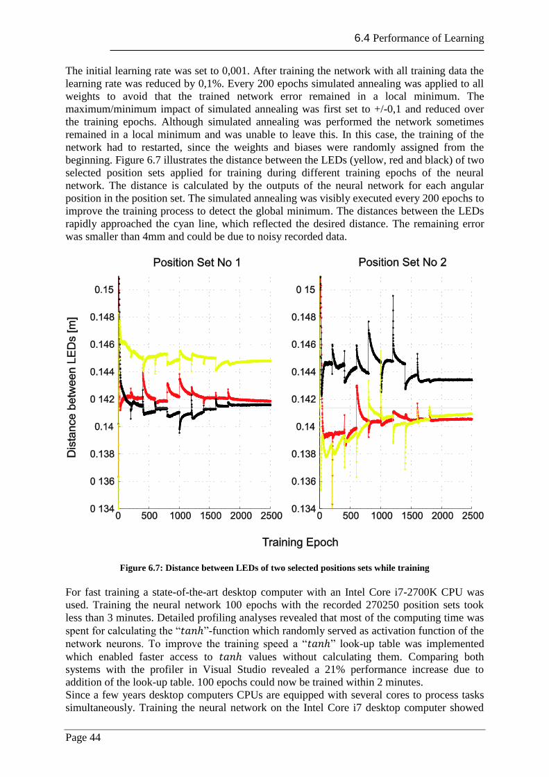
6.4 Performance of Learning

Page 44

The initial learning rate was set to 0,001. After training the network with all training data the

learning rate was reduced by 0,1%. Every 200 epochs simulated annealing was applied to all

weights to avoid that the trained network error remained in a local minimum. The

maximum/minimum impact of simulated annealing was first set to +/-0,1 and reduced over

the training epochs. Although simulated annealing was performed the network sometimes

remained in a local minimum and was unable to leave this. In this case, the training of the

network had to restarted, since the weights and biases were randomly assigned from the

beginning. Figure 6.7 illustrates the distance between the LEDs (yellow, red and black) of two

selected position sets applied for training during different training epochs of the neural

network. The distance is calculated by the outputs of the neural network for each angular

position in the position set. The simulated annealing was visibly executed every 200 epochs to

improve the training process to detect the global minimum. The distances between the LEDs

rapidly approached the cyan line, which reflected the desired distance. The remaining error

was smaller than 4mm and could be due to noisy recorded data.

Figure 6.7: Distance between LEDs of two selected positions sets while training

For fast training a state-of-the-art desktop computer with an Intel Core i7-2700K CPU was

used. Training the neural network 100 epochs with the recorded 270250 position sets took

less than 3 minutes. Detailed profiling analyses revealed that most of the computing time was

spent for calculating the “ ”-function which randomly served as activation function of the

network neurons. To improve the training speed a “ ” look-up table was implemented

which enabled faster access to values without calculating them. Comparing both

systems with the profiler in Visual Studio revealed a 21% performance increase due to

addition of the look-up table. 100 epochs could now be trained within 2 minutes.

Since a few years desktop computers CPUs are equipped with several cores to process tasks

simultaneously. Training the neural network on the Intel Core i7 desktop computer showed

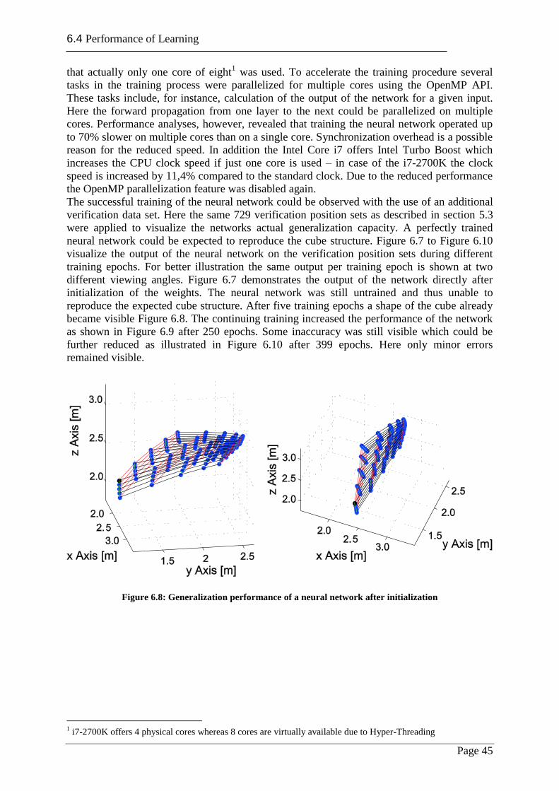
6.4 Performance of Learning

Page 45

that actually only one core of eight1 was used. To accelerate the training procedure several

tasks in the training process were parallelized for multiple cores using the OpenMP API.

These tasks include, for instance, calculation of the output of the network for a given input.

Here the forward propagation from one layer to the next could be parallelized on multiple

cores. Performance analyses, however, revealed that training the neural network operated up

to 70% slower on multiple cores than on a single core. Synchronization overhead is a possible

reason for the reduced speed. In addition the Intel Core i7 offers Intel Turbo Boost which

increases the CPU clock speed if just one core is used – in case of the i7-2700K the clock

speed is increased by 11,4% compared to the standard clock. Due to the reduced performance

the OpenMP parallelization feature was disabled again.

The successful training of the neural network could be observed with the use of an additional

verification data set. Here the same 729 verification position sets as described in section 5.3

were applied to visualize the networks actual generalization capacity. A perfectly trained

neural network could be expected to reproduce the cube structure. Figure 6.7 to Figure 6.10

visualize the output of the neural network on the verification position sets during different

training epochs. For better illustration the same output per training epoch is shown at two

different viewing angles. Figure 6.7 demonstrates the output of the network directly after

initialization of the weights. The neural network was still untrained and thus unable to

reproduce the expected cube structure. After five training epochs a shape of the cube already

became visible Figure 6.8. The continuing training increased the performance of the network

as shown in Figure 6.9 after 250 epochs. Some inaccuracy was still visible which could be

further reduced as illustrated in Figure 6.10 after 399 epochs. Here only minor errors

remained visible.

Figure 6.8: Generalization performance of a neural network after initialization

1 i7-2700K offers 4 physical cores whereas 8 cores are virtually available due to Hyper-Threading

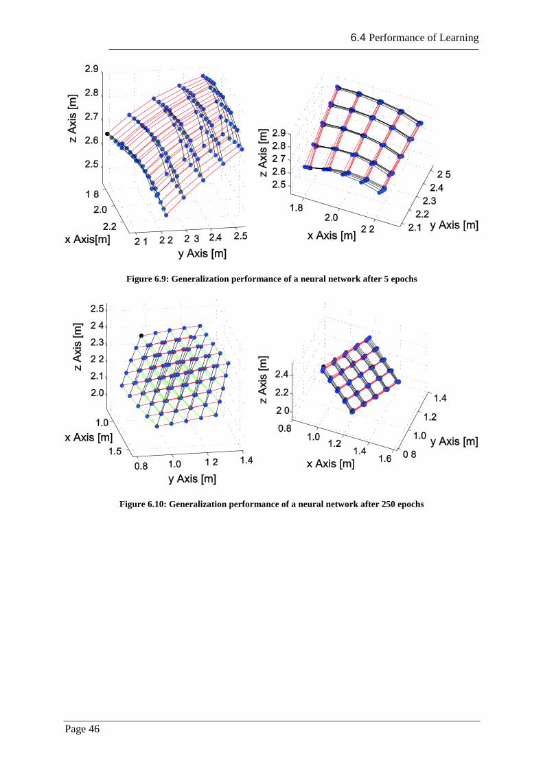
6.4 Performance of Learning

Page 46

Figure 6.9: Generalization performance of a neural network after 5 epochs

Figure 6.10: Generalization performance of a neural network after 250 epochs

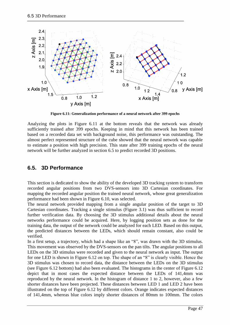
6.5 3D Performance

Page 47

Figure 6.11: Generalization performance of a neural network after 399 epochs

Analyzing the plots in Figure 6.11 at the bottom reveals that the network was already

sufficiently trained after 399 epochs. Keeping in mind that this network has been trained

based on a recorded data set with background noise, this performance was outstanding. The

almost perfect represented structure of the cube showed that the neural network was capable

to estimate a position with high precision. This state after 399 training epochs of the neural

network will be further analyzed in section 6.5 to predict recorded 3D positions.

6.5. 3D Performance

This section is dedicated to show the ability of the developed 3D tracking system to transform

recorded angular positions from two DVS-sensors into 3D Cartesian coordinates. For

mapping the recorded angular position the trained neural network, whose great generalization

performance had been shown in Figure 6.10, was selected.

The neural network provided mapping from a single angular position of the target to 3D

Cartesian coordinates. Tracking a single stimulus (Figure 3.1) was thus sufficient to record

further verification data. By choosing the 3D stimulus additional details about the neural

networks performance could be acquired. Here, by logging position sets as done for the

training data, the output of the network could be analyzed for each LED. Based on this output,

the predicted distances between the LEDs, which should remain constant, also could be

verified.

In a first setup, a trajectory, which had a shape like an “8”, was drawn with the 3D stimulus.

This movement was observed by the DVS-sensors on the pan tilts. The angular positions to all

LEDs on the 3D stimulus were recorded and given to the neural network as input. The output

for one LED is shown in Figure 6.12 on top. The shape of an “8” is clearly visible. Hence the

3D stimulus was chosen to record data, the distance between the LEDs on the 3D stimulus

(see Figure 6.12 bottom) had also been evaluated. The histograms in the center of Figure 6.12

depict that in most cases the expected distance between the LEDs of 141,4mm was

reproduced by the neural network. In the histogram of distance 1 to 2, however, also a few

shorter distances have been projected. These distances between LED 1 and LED 2 have been

illustrated on the top of Figure 6.12 by different colors. Orange indicates expected distances

of 141,4mm, whereas blue colors imply shorter distances of 80mm to 100mm. The colors

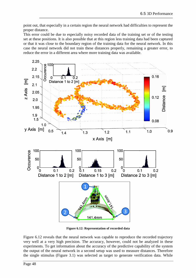
6.5 3D Performance

Page 48

point out, that especially in a certain region the neural network had difficulties to represent the

proper distance.

This error could be due to especially noisy recorded data of the training set or of the testing

set at these positions. It is also possible that at this region less training data had been captured

or that it was close to the boundary region of the training data for the neural network. In this

case the neural network did not train these distances properly, remaining a greater error, to

reduce the error in a different area where more training data was available.

Figure 6.12: Representation of recorded data

Figure 6.12 reveals that the neural network was capable to reproduce the recorded trajectory

very well at a very high precision. The accuracy, however, could not be analyzed in these

experiments. To get information about the accuracy of the predictive capability of the system

the output of the neural network in a second setup was used to measure distances. Therefore

the single stimulus (Figure 3.1) was selected as target to generate verification data. While

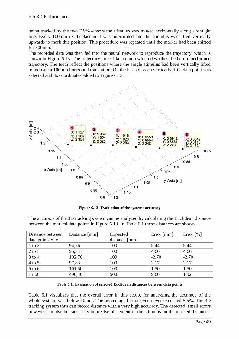
6.5 3D Performance

Page 49

being tracked by the two DVS-sensors the stimulus was moved horizontally along a straight

line. Every 100mm its displacement was interrupted and the stimulus was lifted vertically

upwards to mark this position. This procedure was repeated until the marker had been shifted

for 500mm.

The recorded data was then fed into the neural network to reproduce the trajectory, which is

shown in Figure 6.13. The trajectory looks like a comb which describes the before performed

trajectory. The teeth reflect the positions where the single stimulus had been vertically lifted

to indicate a 100mm horizontal translation. On the basis of each vertically lift a data point was

selected and its coordinates added to Figure 6.13.

Figure 6.13: Evaluation of the systems accuracy

The accuracy of the 3D tracking system can be analyzed by calculating the Euclidean distance

between the marked data points in Figure 6.13. In Table 6.1 these distances are shown.

Distance between

data points x, y

Distance [mm] Expected

distance [mm]

Error [mm] Error [%]

1 to 2 94,56 100 5,44 5,44

2 to 3 95,34 100 4,66 4,66

3 to 4 102,70 100 -2,70 -2,70

4 to 5 97,83 100 2,17 2,17

5 to 6 101,50 100 1,50 1,50

1 t o6 490,40 500 9,60 1,92

Table 6.1: Evaluation of selected Euclidean distances between data points

Table 6.1 visualizes that the overall error in this setup, for analyzing the accuracy of the

whole system, was below 10mm. The percentaged error even never exceeded 5,5%. The 3D

tracking system thus can record distance with a very high accuracy. The detected, small errors

however can also be caused by imprecise placement of the stimulus on the marked distances.

6.5 3D Performance

Page 50

The 3D tracking system therefore should be additionally evaluated by comparing the 3D

Cartesian Output to a professional 3D tracking system.

Conclusion and Perspectives

Page 51

7. Conclusion and Perspectives

A new 3D tracking system has been presented which can discriminate and track the

translation of marked objects in real-time. First an event-based tracking algorithm has been

developed for a biologically inspired sensor (DVS-sensor). This algorithm was used to track

marked objects in the environment at 100Hz.

For tracking an object in 3D, a second DVS-sensor was added to the system. The DVS-

sensors, which had a too limited resolution for 3D tracking, were equipped with telephoto

lenses which increased the sensors’ resolution at farer distances. The DVS-sensors have been

attached to pan tilt systems to increase the area of observance. The tracking precision of the

pan tilt systems with the attached DVS-sensors was evaluated and calibrated to report

accurate actual angular positions to the tracked targets.

The observed angular positions from two biologically inspired sensors to these objects were

transformed by a neural network into 3D Cartesian space. To train the neural network for

tracking and prediction of target positions an unconventional method was developed which

trained a feed-forward neural network by back propagation without the presence of output

training patterns. This drastically reduced the effort for calibrating the 3D sensor system.

Training a neural network with this method took less than 10 minutes on a desktop computer.

This training might thus also be applied directly on fast microcontrollers in the future.

The 3D tracking system has been recognized in a 2D setup to show error in measurement of

below 5,5%. Further detailed investigations should be performed to analyze the accuracy and

precision also within 3D space.

Currently the 3D tracking system reports 3D Cartesian coordinates independently for three

active markers. If these active markers are fixed on an object, e.g. the 3D stimulus, the

orientation of that object can also be estimated in addition.

The developed 3D tracking system can be applied in factories for assembling of marked

products. This stand-alone low power consuming system can also be applied on autonomous

robots to enable interaction with other robots or humans in future.

Page 52

Appendix A

Page 53

Appendix A

Used Programs

Program-Name: Visual Studio 2011

Version: 2010

Origin: Microsoft Cooperation

Program-Name: Matlab 2011b

Version: 7.13

Origin: The MathWorks

Program-Name: Eagle

Version: 5.11

Origin: CadSoft Computer GmbH

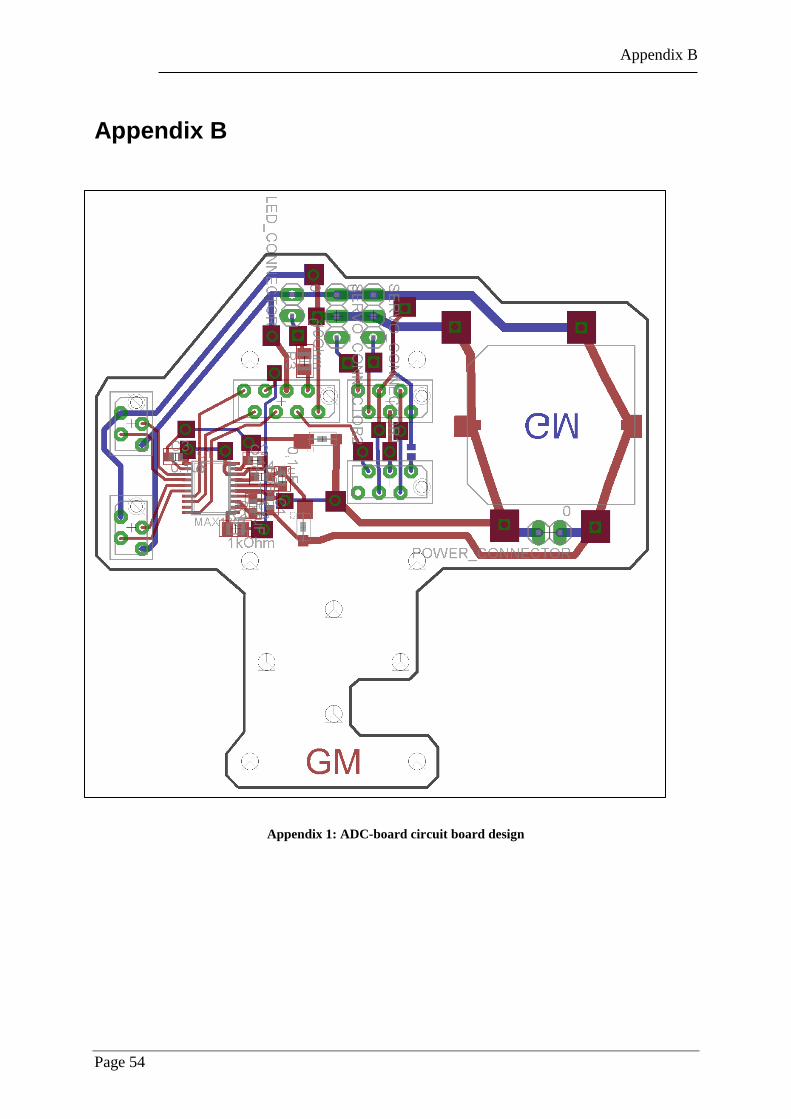
Appendix B

Page 54

Appendix B

Appendix 1: ADC-board circuit board design

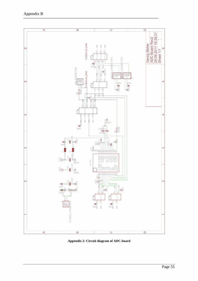
Appendix B

Page 55

Appendix 2: Circuit diagram of ADC-board

Page 56

List of Figures and Tables

Page 57

List of Figures

Figure 2.1: Components of the stand-alone eDVS-Board [16] .................................................. 6 Figure 2.2: Schematic of event capturing ................................................................................... 7 Figure 2.3: Example encoding of pixel position into two bytes ................................................. 8 Figure 2.4: Architecture of a typical Neuron ........................................................................... 10 Figure 2.5: Different states of Function Approximation [21] .................................................. 11

Figure 2.6: Learning of a Neural Network ............................................................................... 13 Figure 3.1: Single active stimulus ............................................................................................ 18 Figure 3.2: Event based tracking algorithm – modified from [28] .......................................... 19 Figure 3.3: Recognized ∆time between events on the DVS-sensor in a static scene

stimulated by three LEDs ...................................................................................... 20

Figure 3.4: Matlab GUI for adjusting tracking algorithm parameters ..................................... 21

Figure 3.5: Spatial weight factor wP depending on spatial coherence ..................................... 22

Figure 3.6: Temporal weight factor wT depending on temporal vicinity ................................. 22 Figure 3.7: Miniature robot autonomously tracking an active target ....................................... 23 Figure 4.1: Principle setup for 3D tracking .............................................................................. 26 Figure 4.2: Steps of setting up the 3D tracking system ............................................................ 26

Figure 4.3: Pan Tilt System II .................................................................................................. 27 Figure 4.4: ADC-Board on Pan Tilt System I .......................................................................... 28

Figure 4.5: Comparing absolute with differential measurement .............................................. 29 Figure 4.6: 3D stimulus geometry ............................................................................................ 30 Figure 5.1: Generation of training data .................................................................................... 31

Figure 5.2: Shematic of training a nerual network based on relations .................................... 33 Figure 5.3: Output of a neural network, trained with artificial generated data ........................ 34

Figure 5.4: Improved training performance due to simulated annealing ................................. 35 Figure 6.1: Sensor target detection precision ........................................................................... 37

Figure 6.2: Tracking a fixed object .......................................................................................... 38 Figure 6.3: Target shifting due to sensor movement ................................................................ 40 Figure 6.4: Target shifting on pan tilt system I ........................................................................ 41 Figure 6.5: Target shifting on pan tilt system II ....................................................................... 42

Figure 6.6: Storing recorded data into position sets ................................................................. 43 Figure 6.7: Distance between LEDs of two selected positions sets while training .................. 44 Figure 6.8: Generalization performance of a neural network after initialization ..................... 45 Figure 6.9: Generalization performance of a neural network after 5 epochs ........................... 46 Figure 6.10: Generalization performance of a neural network after 250 epochs ..................... 46

Figure 6.11: Generalization performance of a neural network after 399 epochs ..................... 47 Figure 6.12: Representation of recorded data .......................................................................... 48 Figure 6.13: Evaluation of the systems accuracy ..................................................................... 49

List of Tables

Table 2.1: Example calculation of event position and event type .............................................. 8 Table 6.1: Evaluation of selected Euclidean distances between data points ............................ 49

Page 58

References

Page 59

References

1. Andriluka, M., S. Roth, and B. Schiele, Monocular 3d pose estimation and

tracking by detection in IEEE Conference on Computer Vision and Pattern

Recognition (CVPR), 2010, IEEE: San Francisco, CA p. 623 - 630

2. Ponce, J., et al. Toward true 3D object recognition. in Congrès de Reconnaissance

des Formes et Intelligence Artificielle. 2004. Toulouse, France.

3. Beom, H.R. and H.S. Cho, A sensor-based navigation for a mobile robot using

fuzzy logic and reinforcement learning. IEEE Transactions on Systems, Man and

Cybernetics, 1995. 25(3): p. 464-477.

4. Hancock, J., M. Hebert, and C. Thorpe. Laser intensity-based obstacle detection.

in Proceedings of International Conference on Intelligent Robots and Systems (

IEEE/RSJ). 1998. Victoria, BC , Canada: IEEE.

5. Cyr, C.M. and B.B. Kimia. 3D object recognition using shape similiarity-based

aspect graph. in Proceedings of Eighth IEEE International Conference on

Computer Vision (ICCV). 2001. Vancouver, BC , Canada: IEEE.

6. Chao, C.H., et al., Real-time target tracking and obstacle avoidance for mobile

robots using two cameras in ICCAS-SICE, 2009, IEEE: Fukuoka, . p. 4347-4352.

7. Shibata, M. and N. Kobayashi. Image-based visual tracking for moving targets

with active stereo vision robot. in International Joint Conference SICE-ICASE.

2006. Busan: IEEE.

8. Benavidez, P. and M. Jamshidi, Mobile robot navigation and target tracking system

in 2011 6th International Conference on System of Systems Engineering (SoSE),

2011, IEEE: Albuquerque, NM. p. 299 - 304

9. Indiveri, G., P. Oswald, and J. Kramer. An adaptive visual tracking sensor with a

hysteretic winner-take-all network. in IEEE International Symposium on Circuits

and Systems (ISCAS). 2002. Phoenix-Scottsdale, AZ , USA IEEE.

10. Litzenberger, M., et al. Embedded vision system for real-time object tracking using

an asynchronous transient vision sensor. in Digital Signal Processing Workshop,

12th - Signal Processing Education Workshop, 4th. 2006. Teton National Park,

WY: IEEE.

11. Schraml, S., et al. Dynamic stereo vision system for real-time tracking. in

Proceedings of 2010 IEEE International Symposium on Circuits and Systems

(ISCAS). 2010. Paris: IEEE.

12. Chen, I., B. MacDonald, and B. Wünsche, Markerless Augmented Reality for

Robotic Helicoptor Applications, in Robot Vision, G. Sommer and R. Klette,

Editors. 2008, Springer Berlin / Heidelberg. p. 125-138.

13. Garcia, M.L., Design and evaluation of physical protection systems2007:

Butterworth-Heinemann.

14. Schreer, O., P. Kauff, and T. Sikora, 3D videocommunication. 2005: Wiley Online

Library.

15. Lichtsteiner, P., C. Posch, and T. Delbruck, A 128× 128 120 dB 15 s latency

asynchronous temporal contrast vision sensor. Solid-State Circuits, IEEE Journal

of, 2008. 43(2): p. 566-576.

16. Conradt, J., et al. An embedded AER dynamic vision sensor for low-latency pole

balancing. 2009. IEEE.

17. Leigh, J.R., Control theory. 2004: The Institution of Engineering and Technology.

18. Hirose, A., Complex-valued neural networks. IEEJ Transactions on Electronics,

Information and Systems, 2011. 131(1): p. 2-8.

References

Page 60

19. Graupe, D., Principles of artificial neural networks. 2007: World Scientific

Publishing Company.

20. Bebis, G. and M. Georgiopoulos, Optimal feed-forward neural network

architectures. IEEE Potentials, 1994: p. 27-31.

21. Lawrence, S., C.L. Giles, and A.C. Tsoi, What size neural network gives optimal

generalization? Convergence properties of backpropagation. 1998.

22. Hornik, K., M. Stinchcombe, and H. White, Multilayer feedforward networks are

universal approximators. Neural networks, 1989. 2(5): p. 359-366.

23. Antal, P., et al., Extended bayesian regression models: a symbiotic application of

belief networks and multilayer perceptrons for the classification of ovarian tumors.

Artificial Intelligence in Medicine, 2001: p. 177-187.

24. Bertsimas, D. and J. Tsitsiklis, Simulated annealing. Statistical Science, 1993: p.

10-15.

25. Luger, G.F., Artificial intelligence: Structures and strategies for complex problem

solving. 2005: Addison-Wesley Longman.

26. Rumelhart, D.E., Backpropagation: theory, architectures, and applications. 1995:

Lawrence Erlbaum.

27. DeSouza, G.N. and A.C. Kak, Vision for mobile robot navigation: A survey. IEEE

Transactions on Pattern Analysis and Machine Intelligence, 2002. 24(2): p. 237-

267.

28. Georg R. Müller, J.C. A Miniature Low-Power Sensor System for Real Time 2D

Visual Tracking of LED Markers. in Proceedings of the IEEE International

Conference on Robotics and Biomimetics (IEEE-ROBIO). 2011. Phuket, Thailand.

29. Yegnanarayana, B., Artificial neural networks. 2004: PHI Learning Pvt. Ltd.

30. Alpaydin, E., Introduction to machine learning. 2004: The MIT Press.