Embed Size (px)
Citation preview

D I S S E RTAT I O N
PAT T E R N S I N L A B E L L E D C O M B I N AT O R I A LO B J E C T S
Ausgeführt zum Zwecke der Erlangung des akademischenGrades einer Doktorin der technischen Wissenschaften unter
der Anleitung von
ao. univ. prof . dr . alois panholzer
E104, Institut fürDiskrete Mathematik und Geometrie
eingereicht an der Technischen Universität WienFakultät für Mathematik und Geoinformation
von
marie-louise bruner
Matrikelnummer 0525370
Josefstädterstraße 43-45/2/4
A-1080 Wien
Wien, am 13. Mai 2015 Marie-Louise Marie-Louise BrunerMarie-Louise Bruner
Marie-Louise BrunerAlois Panholzer
Marie-Louise BrunerVincent Vatter
Die approbierte Originalversion dieser Dissertation ist in der Hauptbibliothek der Technischen Universität Wien aufgestellt und zugänglich. http://www.ub.tuwien.ac.at
The approved original version of this thesis is available at the main library of the Vienna University of Technology.
http://www.ub.tuwien.ac.at/eng


PAT T E R N S I N L A B E L L E D C O M B I N AT O R I A L O B J E C T S
marie-louise bruner
Institute of Discrete Mathematics and GeometryVienna University of Technology
May 2015

Marie-Louise Bruner: Patterns in labelled combinatorial objects, May 2015

Dedicated to the memory of my mother, Ingela Bruner.
1952 – 2014
Thank you for always believing in me. (I U 2)∞


D E C L A R AT I O N
I herewith declare that I have completed the present thesis indepen-dently, making use only of the specified literature and aids. Sentencesor parts of sentences quoted literally are marked as quotations; identi-fication of other references with regard to the statement and scope ofthe work is quoted. The thesis in this form has not been submitted toan examination body and has not been published. This thesis drawshowever on previous publications of the author. For a complete listof my relevant scientific articles, I refer to page xi.
Vienna, May 2015
Marie-Louise Bruner


A B S T R A C T
This thesis is concerned with various types of patterns and structuralrestrictions in labelled combinatorial objects. We say that a combina-torial object A is contained in another combinatorial object B as apattern if A can be obtained by deleting parts of B. Moreover, theorder structure of the labels must be preserved.
A first part of this thesis addresses patterns in permutations. Aquestion that is of particular interest is the decision problem “Doesthe permutation τ contain the pattern π”? In general, this problemis NP-complete. We present an fpt-algorithm that solves this problemefficiently if τ has few alternating runs. We also analyse the com-putational complexity of this problem for several different types ofpermutation patterns. For a special permutation class arising in thecontext of the third part of this thesis, we solve the enumeration prob-lem. Finally, the log-concavity of a combinatorial sequence related topermutation patterns is investigated.
A second part of this work is concerned with Cayley trees, i.e.,rooted unordered trees and mappings, i.e., functions from a finiteset to itself. First, we present a new bijective proof of Cayley’s for-mula which will subsequently allow us to establish bijective corre-spondences. Next, we generalize the label patterns “ascents” and “as-cending runs” from permutations to Cayley trees and mappings andinvestigate their distribution. Another topic treated in this part is thegeneralization of the concept of parking functions to Cayley trees andmappings. The asymptotic analysis of the numbers of these objectsleads to an interesting phase transition behaviour.
A third part deals with so-called single-peaked elections that playan important role in social choice theory. We introduce the concept ofconfigurations in elections and establish a correspondence with per-mutation patterns. For the special case of single-peaked profiles weanswer the question how likely these are to occur when preferencesare chosen at random.
Some of the results presented in this thesis have already been pub-lished in scientific articles by the present author. For a complete listof the papers this thesis is based on, we refer to page xi.
ix

Z U S A M M E N FA S S U N G
Diese Dissertation beschäftigt sich mit unterschiedlichen Arten vonMustern und strukturellen Einschränkungen in markierten kombina-torischen Objekten. Ein kombinatorisches Objekt A ist in einem an-deren größeren Objekt B als Muster enthalten, falls man A erhaltenkann, indem Teile von B entfernt werden. Dabei muss auch die Ord-nungsstruktur der Marken (engl. “labels”) erhalten bleiben.
Ein erster Teil dieser Arbeit befasst sich mit Mustern in Permuta-tionen. Besondere Aufmerksamkeit wird in diesem Zusammenhangdem Entscheidungssproblem “Enthält die Permutation τ das Musterπ?” gewidmet. Dieses Problem ist bekanntlich NP-vollständig. Wirstellen einen fpt-Algorithmus für dieses Problem vor, der besonderseffizient ist, wenn die Permutation τ nur wenige “alternating runs”aufweist. Außerdem analysieren wir die Komplexität dieses Problemsfür verschiedene Typen von Permutationsmustern. Für eine beson-dere Permutationsklasse, die durch vier vermiedene Muster definiertist und im dritten Teil dieser Arbeit auftaucht, konnten wir das Abzähl-problem lösen. Weiters wird die Log-Konkavität einer kombinato-rischen Zahlenfolge, die mit Mustervermeidung zusammenhängt, un-tersucht.
Ein zweiter Teil dieser Dissertation beschäftigt sich mit Cayley Bäu-men, das sind gewurzelte ungeordnete Bäume, und mit Mappings,das sind Abbildungen einer endlichen Menge auf sich selbst. Zunächstpräsentieren wir einen neuen bijektiven Zusammenhang zwischenCayley Bäumen und Mappings, der uns im Folgenden erlauben wird,bijektive Resultate zu beweisen. Wir verallgemeinern die für Permuta-tionen definierten Muster “Aufstiege” und “aufsteigende Runs” unduntersuchen deren Verteilung für Cayley Bäume und Mappings. Einweiteres Thema sind Parkfunktionen, die wir auf Cayley Bäume undMappings verallgemeinern. Das asymptotische Verhalten der Abzähl-formeln weist dabei ein interessantes Phasenübergangsverhalten auf.
Ein dritter Teil behandelt sogenannte “Single-peaked elections”, diein der sozialen Wahltheorie eine wichtige Rolle spielen. Wir führenden allgemeinen Begriff von Konfigurationen in Präferenzen ein undstellen eine Verbindung zu Permutationsmustern her. Für die spezielleSingle-peaked-Konfiguration beantworten wir außerdem die Frage,wie wahrscheinlich es ist, dass diese in zufälligen Präferenzen auf-taucht.
Die in dieser Dissertation vorgestellten Resultate sind zum Teilschon in wissenschaftlichen Artikeln der Autorin publiziert worden.Eine Auflistung der Arbeiten, auf denen diese Dissertation aufgebautist, findet sich auf Seite xi.
x

P U B L I C AT I O N S
This thesis is based on the following publications and preprints:
[41] Marie-Louise Bruner and Martin Lackner. A fast algorithm forpermutation pattern matching based on alternating runs. In Fe-dor V. Fomin and Petteri Kaski, editors, SWAT, volume 7357 ofLecture Notes in Computer Science, pages 261–270. Springer, 2012.
[42] Marie-Louise Bruner and Martin Lackner. The computationallandscape of permutation patterns. Pure Mathematics and Appli-cations, 24(2)(2):83–101, 2013.
[30] Miklós Bóna and Marie-Louise Bruner. Log-concavity, the Ulamdistance and involutions. arXiv preprint, arXiv:1502.05438, 2015.
[44] Marie-Louise Bruner and Alois Panholzer. Parking functionsfor trees and mappings. arXiv preprint, arXiv:1504.04972, 2015.
[43] Marie-Louise Bruner and Martin Lackner. The likelihood ofstructure in preference profiles. In Proceedings of the 8th Mul-tidisciplinary Workshop on Advances in Preference Handling (MPref2014), 2014.
xi

A C K N O W L E D G M E N T S
First and foremost I wish to thank my supervisor Alois Panholzer. Hewas the one who, in his lecture on “Discrete Methods”, first sparkedmy interest for discrete mathematics and combinatorial problems.During my PhD studies, I greatly valued the substantial freedomAlois gave me to pursue my own research directions. This allowed meto explore various aspects of the combinatorial world. Also, he madeit possible for me to participate in many conferences and workshopsand to spend a month at the University of Florida. It has meant a lotto me personally to have his support in emotionally difficult timesand never having to feel under pressure. I am also most thankful thathe is not only enabling but also encouraging me to pursue my planof hiking, kayaking and bicycling from Oslo back home this summer.
I would also like to thank all the other great researchers whom Imet and interacted with during my studies. Thank you for making mefeel part of the Analysis of Algorithms and the Permutation Patternscommunity. Thank you for welcoming me into your world and for en-couraging me. In particular, my thanks go to Cyril Banderier, MiklósBóna, Michael Drmota, Danièle Gardy, Antoine Genitrini, BernhardGittenberger, Markus Kuba, Adeline Pierrot and Vincent Vatter.
To Vincent Vatter I also owe my thanks for accepting the task of re-viewing my thesis. In addition, I would like to thank him very muchfor inviting me for a second research stay at the University of Floridathis past winter.
During my daily work in Vienna, it was my colleagues as wellas my (current and former) roommates who made my days as aPhD student very enjoyable. These are in particular: Danièle Gardy,Veronika Kraus, Benoît Loridant, Johannes Morgenbesser, AdelinePierrot, Georg Seitz and Michael Wallner. My special thanks also go toour secretary Barbara Dolezal-Rainer whose open ear for all sorts ofquestions and good sense of humour always created a warm-heartedand welcoming atmosphere at our department.
The program WINA+ was started rather recently to support youngresearchers at the Vienna University of Technology. The regular meet-ings with colleagues from various disciplines and our coach StephanFaatz were very encouraging and helped to solve small and big prob-lems. Furthermore, the wonderful seminars on scientific writing ledby Katherine Tiede were very inspiring and taught me the joy of writ-ing.
I would also like to thank Gerhard Bruner, Martin Lackner, DianaNewton-Smith and Michael Wallner who helped me by proof-readingmy thesis.
xiii

If there is one thing that my mother’s illness taught me, it is howmuch my family and friends mean to me. I am very grateful for thetime we were able spend together and for the many strong memoriesI have of my mother. After her passing away last spring, my familyand friends were a tremendous support. Especially I want to thankmy father Gerhard Bruner for his generosity, patience, cheerful dis-position, trust in me and helpfulness. Also, I would like to thank my“new” family, the Lackners, for including me in their lives and mak-ing me feel so much at home in their company.
My greatest support throughout the last years has been my part-ner Martin Lackner with whom I can share not only mathematicalresearch but also crazy plans for outdoor adventures. Thank you forbeing my rain boots when it’s pouring, the hot cup of tea on a coldwinter day, the shelter when it’s stormy and for being by my side toenjoy the sunny days.
Last but not least, my thanks go to the Austrian Science Fund FWFthat supported my research throughout most of the duration of mythesis via the projects P25337-N23 “Restricted labelled combinatorialobjects: new enumerative, statistical, asymptotic and complexity the-oretical aspects” and 9608 “Combinatoric analysis of data structuresand tree-like structures”.
xiv

C O N T E N T S
1 introduction 1
2 preliminaries 13
2.1 Asymptotic notation 13
2.2 Permutations, patterns and Standard Young tableaux 14
2.3 Cayley trees and Mappings 20
2.4 Preferences and Social Choice Theory 22
2.5 Algorithms and complexity theory 24
2.6 Symbolic method and analytic combinatorics 27
2.7 Probabilistic tools 36
2.8 Method of characteristics 40
2.9 Log-concavity and combinatorial sequences 41
i permutations 45
3 efficient permutation pattern matching : the al-ternating run algorithm 47
3.1 The alternating run algorithm 49
3.2 The parameter run(π) 75
3.3 Summary of the results 79
4 the computational complexity of generalized per-mutation pattern matching 81
4.1 Types of patterns 82
4.2 The possibility of polynomial-time algorithms 86
4.3 The impact of the pattern length 89
4.4 Summary of the results 95
5 central binomial coefficients 97
6 log-concavity, longest increasing subsequences
and involutions 105
6.1 The conjecture and a first result 105
6.2 A class of permutations for which the conjecture holds 106
6.3 Lattice paths and 321-avoiding permutations 117
6.4 Summary of the results 119
ii cayley trees and mappings 121
7 a new bijective proof of cayley’s formula 123
8 ascending runs in mappings 127
8.1 A probabilistic warm-up: Ascents in mappings and trees 128
8.2 Ascending runs in mappings 131
8.3 Summary of the results 148
9 parking in trees and mappings 151
9.1 Introduction 151
9.2 Basic properties of parking functions for trees and map-pings 155
xv

xvi contents
9.3 Total number of parking functions: the number of driverscoincides with the number of parking spaces 162
9.4 Total number of parking functions: the general case 173
9.5 Summary of the results 197
iii preferences and elections 199
10 on the likelihood of single-peaked elections 201
10.1 A general result based on permutation patterns 204
10.2 Counting results and the Impartial Culture assump-tion 211
10.3 The Pólya urn model 214
10.4 Mallows model 218
10.5 Numerical Evaluations 221
10.6 Summary of the results 223
11 further research 225
notation 233
bibliography 235
curriculum vitæ 247
1I N T R O D U C T I O N
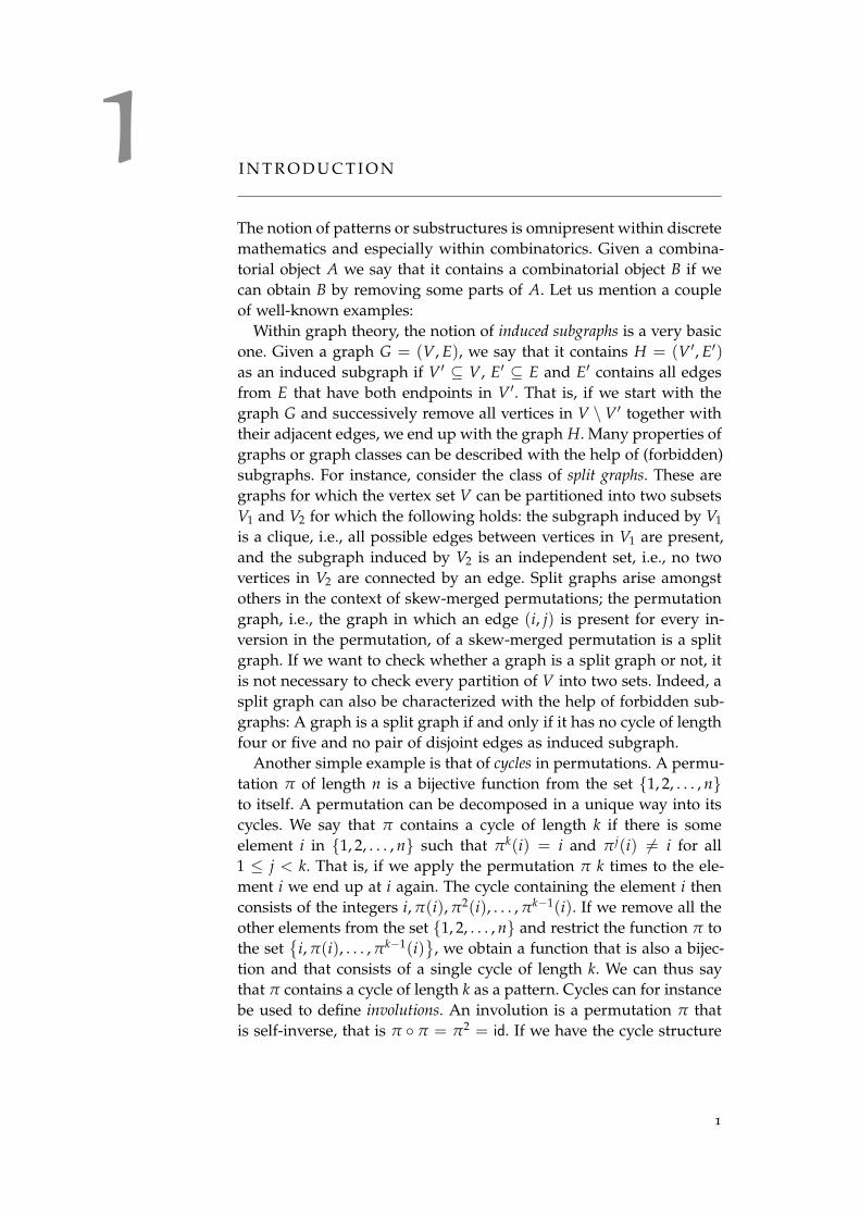
The notion of patterns or substructures is omnipresent within discretemathematics and especially within combinatorics. Given a combina-torial object A we say that it contains a combinatorial object B if wecan obtain B by removing some parts of A. Let us mention a coupleof well-known examples:
Within graph theory, the notion of induced subgraphs is a very basicone. Given a graph G = (V, E), we say that it contains H = (V ′, E′)as an induced subgraph if V ′ ⊆ V, E′ ⊆ E and E′ contains all edgesfrom E that have both endpoints in V ′. That is, if we start with thegraph G and successively remove all vertices in V \V ′ together withtheir adjacent edges, we end up with the graph H. Many properties ofgraphs or graph classes can be described with the help of (forbidden)subgraphs. For instance, consider the class of split graphs. These aregraphs for which the vertex set V can be partitioned into two subsetsV1 and V2 for which the following holds: the subgraph induced by V1
is a clique, i.e., all possible edges between vertices in V1 are present,and the subgraph induced by V2 is an independent set, i.e., no twovertices in V2 are connected by an edge. Split graphs arise amongstothers in the context of skew-merged permutations; the permutationgraph, i.e., the graph in which an edge (i, j) is present for every in-version in the permutation, of a skew-merged permutation is a splitgraph. If we want to check whether a graph is a split graph or not, itis not necessary to check every partition of V into two sets. Indeed, asplit graph can also be characterized with the help of forbidden sub-graphs: A graph is a split graph if and only if it has no cycle of lengthfour or five and no pair of disjoint edges as induced subgraph.
Another simple example is that of cycles in permutations. A permu-tation π of length n is a bijective function from the set {1, 2, . . . , n}to itself. A permutation can be decomposed in a unique way into itscycles. We say that π contains a cycle of length k if there is someelement i in {1, 2, . . . , n} such that πk(i) = i and π j(i) 6= i for all1 ≤ j < k. That is, if we apply the permutation π k times to the ele-ment i we end up at i again. The cycle containing the element i thenconsists of the integers i, π(i), π2(i), . . . , πk−1(i). If we remove all theother elements from the set {1, 2, . . . , n} and restrict the function π tothe set
{i, π(i), . . . , πk−1(i)
}, we obtain a function that is also a bijec-
tion and that consists of a single cycle of length k. We can thus saythat π contains a cycle of length k as a pattern. Cycles can for instancebe used to define involutions. An involution is a permutation π thatis self-inverse, that is π ◦ π = π2 = id. If we have the cycle structure
1

2 introduction
stack
inputoutput
5
3
1 4 2
Figure 1: Attempting to sort the permutation π = 5 3 1 4 2 with the help ofa stack. As we can see, the subsequence 3 4 2 causes trouble andcannot be sorted.
of a permutation π at hand, it is very easy to say whether it is aninvolution or not. Indeed, since π2(i) = i has to hold for all elementsi of the permutation, all cycles need to be of length one or two. Thus,involutions can be characterized as those permutations that do notcontain any k-cycles for k ≥ 3 as a pattern.
The next example is also related to permutations. Let us considerthe following sorting device called a stack. A stack is a linear list forwhich all insertions and deletions are made at one end of the list.That is, the last element inserted from the input into the stack, willbe the first to be deleted and placed in the output. Stacks are thusalso called LIFO-(Last-In-First-Out-)lists. For a graphical representa-tion of a stack, see Figure 1. The question is now: Which permutationsπ can be sorted with the help of a stack? In other words: For whichpermutations π as input is it possible to obtain the identity permu-tation π as output? Let us consider the permutation π = 5 3 1 4 2 inFigure 1 as an example. As we can see, we get stuck as soon as theelement 3 is placed in the stack and it is not possible to output theelement 2 before the element 4. Within the permutation π, it is thesubsequence 342 that cannot be sorted. This observation can be gen-eralized and one can prove that a permutation π is stack-sortable ifand only if there are no three elements `, m, n in the permutationswith ` < m < n and m stands to the left of n and n to the left of `.That is, π may not contain a subsequence of length three in which theelements are in the same order as in the permutation 2 3 1. One alsosays that a permutation is stack sortable if and only if it avoids thepattern 2 3 1.
The first two examples of patterns or substructures have a pointin common that distinguishes them from the third example. The pat-terns were defined by the underlying graph or cycle structure andthe specific labels of the involved vertices or the elements of the per-

introduction 3
mutation were of no importance. For instance, when considering agraph containing a cycle of length 4, it is of no relevance whether theelements forming this cycle are labelled 1, 2, 3, 4 or 7, 2, 1, 5. This isin contrast to the third example where we introduced 231-avoidingpermutations. Here, the involved elements of the permutation play acrucial role since they need to be in a specific order to form a 231-pattern.
This leads us to the concept of label patterns in combinatorial ob-jects that is at the heart of this thesis. First, all combinatorial objectsthat we will consider are labelled ones. This means that the “atoms”– these are for instance the vertices in a graph or the elements in apermutation – have positive integers attached to them. We call theseintegers the labels. Second, we say that a labelled combinatorial ob-ject A contains a labelled combinatorial object B if we can obtainB by removing some parts of A. Additionally, the labels of B haveto be order-isomorphic to the labels of the substructure of A thatwe obtained after deleting some parts. Returning to the example ofstack-sortable permutations, we can formalize the definition of 231-avoiding permutations as follows: A permutation π contains the pat-tern 231 if and only if there are three positions i < j < k in π suchthat π(k) < π(i) < π(j), i.e., the subsequence π(i)π(j)π(k) in π isorder-isomorphic to 231.
In this thesis, we will study different types of label patterns in var-ious combinatorial objects. Our research is devoted to a varied set ofproblems that concern algorithmical, enumerative, analytic and prob-abilistic questions. Also, the methods employed throughout this the-sis are diverse: We employ techniques from analytic combinatorics,complexity theory, probability theory as well as bijective proofs. Fig-ure 2 provides an overview of the combinatorial objects studied inthis thesis and the methods that were used. A detailed introductionto the objects studied in this thesis is given in the Preliminaries, start-ing on page 13.
Part i of this thesis is devoted to permutation patterns. The historyof permutation patterns can be traced back to the beginning of the20th century and MacMahon’s study [120] of permutations that canbe partitioned into two decreasing subsequences, i.e., 123-avoidingpermutations. Also, the studies by Erdos and Szekeres showing thata permutation of length n always contains an increasing subsequenceof length
√n− 1 or a decreasing subsequence of length
√n− 1 [67]
along with Schensted’s study of longest increasing subsequences inpermutations [139] can be seen as studies of the monotone patterns12 . . . k for some integer k. However, the birth of permutation pat-terns is mostly attributed to Knuth who published the first volumeof The Art of Computer Programming [111] in 1968. There, in an ex-ercise, he asks which permutations can be sorted with the help ofa stack and his question naturally leads to permutation patterns as

4 introduction
PERMUTATIONSof length n
bijections π : [n]→ [n]
Permutation patterns
MAPPINGSon the set [n]
arbitrary functions f : [n]→ [n]
Consecutive label patterns
Parking functions
Cayley TREESof size n
Consecutive label patterns
Parking functions
PREFERENCESon n candidates
total orders of a set C of size n
Configurations
Bijectionin Chapter 7
Connectionin Chapter 10
3 C P
4 C
5 E
6 E
10E P 8 A E P
9 A E P
9 A E P
8 A E P
remove
bijectivity
impose
bijectivity
allow cycles
& several
components
forbid cycles
& impose
connectedness
add ordered
structure to C
replace [n]
by any set C of size n
Chapters in this thesis and publications
3Efficient PPM: the alternatingrun algorithm [BL12]
4The computational complexity ofgeneralized PPM [BL13]
5A permutation class enumerated bythe central binomial coefficients
6Log-concavity, longest increasingsubsequences and involutions [BB15]
7A new bijective proof ofCayley’s formula [BP15]
8 Ascending runs in mappings
9 Parking in trees and mappings [BP15]
10Configuration avoidance inpreference profiles[BL14]
Methods employed
A Analytic combinatorics
CComputational complexityand algorithms
EEnumerative combinatoricsand bijective methods
P Probability theory
Figure 2: An overview of the objects studied and the methods employed inthis thesis. Dashed lines mark connections between combinatorialobjects and solid lines mark connections that are proved withinthis thesis.

introduction 5
we have seen above. The first systematic study of patterns in permu-tations was not performed until 1985 by Simion and Schmidt [140].Since then, the field of permutation patterns has become a vastlygrowing part of combinatorics. This is evidenced by the attentionattributed to this topic in various monographs: several chapters inBóna’s Combinatorics of Permutations are concerned with permutationpatterns[25]; a comprehensive presentation of results related to var-ious types of patterns in permutations and words can be found inKitaev’s monograph Patterns in Permutations and Words [108]; and asurvey of permutation classes and recent research directions can befound in Vatter’s Chapter 12 in the Handbook of Enumerative Combina-torics [29]. Moreover many applications of permutation patterns havebeen discovered: their relation to stack and deque sorting, genomesequences in computational biology, statistical mechanics and in gen-eral their numerous connections to other combinatorial objects [108].
So far, computational aspects of permutation patterns have receivedfar less attention than enumerative ones. The computational prob-lem of detecting permutation patterns, the Permutation Pattern
Matching (PPM) problem, can be formulated as follows: Does a per-mutation τ of length n (the text) contain a permutation π of lengthk ≤ n (the pattern)? In Chapters 3 and 4 we will take the viewpoint ofcomputational complexity and consider this algorithmical problem.
PPM has been shown to be NP-complete [31]. This implies that, un-less P = NP, we cannot hope for a polynomial time algorithm forPPM. This is however not the end of the story: even though PPM isNP-complete in general, one can hope to find polynomial time algo-rithms for special cases of the problem. For instance, if π is the iden-tity 12 . . . k, PPM consists of looking for an increasing subsequence oflength k in the text – this is a special case of the Longest Increasing
Subsequence problem. This problem can be solved inO(n log n)-timefor sequences in general [139] and in O(n log log n)-time for permu-tations [48, 122]. Another example is that of separable patterns. Theseare permutations avoiding both patterns 3142 and 2413. In this case,PPM can be solved in O(k · n4) time [99]. Another possibility thatallows to circumvent the computational hardness of PPM is to con-fine the combinatorial explosion to a certain parameter of the input(τ, σ). This is the approach of parameterized complexity theory, a rathernew branch of complexity theory that has, so far, mostly been usedfor problems on graphs [59]. In Chapter 3 we employ parameterizedcomplexity theory and construct an algorithm that has a worst-caseruntime of O(1.79run(τ) · n · k) where run(τ) denotes the number ofalternating runs in τ. This algorithm is particularly well-suited forinstances where τ has few alternating runs, i.e., few ups and downs.Moreover, since run(τ) < n, this can be seen as a O(1.79n · n · k) algo-rithm that is the first to beat the exponential 2n exponential runtime ofbrute-force search. Furthermore, we prove that under standard com-
6 introduction
plexity theoretic assumptions such a fixed-parameter tractability re-sult is not possible for run(π).
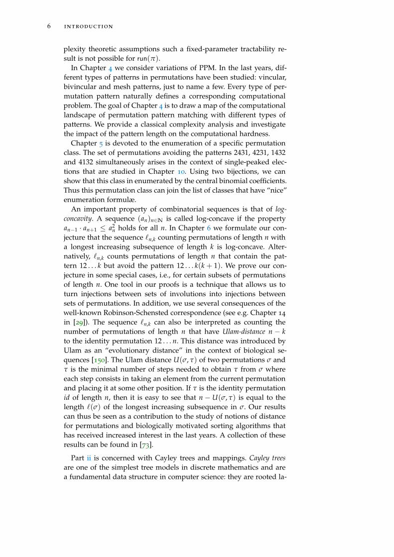
In Chapter 4 we consider variations of PPM. In the last years, dif-ferent types of patterns in permutations have been studied: vincular,bivincular and mesh patterns, just to name a few. Every type of per-mutation pattern naturally defines a corresponding computationalproblem. The goal of Chapter 4 is to draw a map of the computationallandscape of permutation pattern matching with different types ofpatterns. We provide a classical complexity analysis and investigatethe impact of the pattern length on the computational hardness.
Chapter 5 is devoted to the enumeration of a specific permutationclass. The set of permutations avoiding the patterns 2431, 4231, 1432and 4132 simultaneously arises in the context of single-peaked elec-tions that are studied in Chapter 10. Using two bijections, we canshow that this class in enumerated by the central binomial coefficients.Thus this permutation class can join the list of classes that have “nice”enumeration formulæ.
An important property of combinatorial sequences is that of log-concavity. A sequence (an)n∈N is called log-concave if the propertyan−1 · an+1 ≤ a2
n holds for all n. In Chapter 6 we formulate our con-jecture that the sequence `n,k counting permutations of length n witha longest increasing subsequence of length k is log-concave. Alter-natively, `n,k counts permutations of length n that contain the pat-tern 12 . . . k but avoid the pattern 12 . . . k(k + 1). We prove our con-jecture in some special cases, i.e., for certain subsets of permutationsof length n. One tool in our proofs is a technique that allows us toturn injections between sets of involutions into injections betweensets of permutations. In addition, we use several consequences of thewell-known Robinson-Schensted correspondence (see e.g. Chapter 14
in [29]). The sequence `n,k can also be interpreted as counting thenumber of permutations of length n that have Ulam-distance n − kto the identity permutation 12 . . . n. This distance was introduced byUlam as an “evolutionary distance” in the context of biological se-quences [150]. The Ulam distance U(σ, τ) of two permutations σ andτ is the minimal number of steps needed to obtain τ from σ whereeach step consists in taking an element from the current permutationand placing it at some other position. If τ is the identity permutationid of length n, then it is easy to see that n −U(σ, τ) is equal to thelength `(σ) of the longest increasing subsequence in σ. Our resultscan thus be seen as a contribution to the study of notions of distancefor permutations and biologically motivated sorting algorithms thathas received increased interest in the last years. A collection of theseresults can be found in [73].
Part ii is concerned with Cayley trees and mappings. Cayley treesare one of the simplest tree models in discrete mathematics and area fundamental data structure in computer science: they are rooted la-

introduction 7
1
2
1
1
2
1
2 3
2
1 3
3
1 2
1
2
3
1
3
2
2
1
3
2
3
1
3
1
2
3
2
1
Figure 3: All Cayley trees of size up to n = 3
belled unordered trees. “Rooted” means that there is one designatednode in the tree that we call the root (this node can be any one of thenodes) and we consider all the edges to be oriented toward the root.“Labelled” means that every node carries a label, which we assumeto be an integer between 1 and n, where n is the size of the tree andevery label occurs exactly once. “Unordered” means that there is noorder among the children of a given node. Figure 3 provides a rep-resentation of all Cayley trees of size n = 1, 2 and 3. The roots aredrawn on top and are marked by a black border. Cayley trees carrytheir name from the British mathematician Arthur Cayley who stud-ied them in 1889 [47]. In this paper he showed that the number Tn ofrooted unordered trees with n nodes is equal to nn−1 or, equivalently,that the number of unrooted unordered trees with n nodes is equalto nn−2. Cayley was however not the first to have stated this result.An equivalent result had already been shown earlier by Borchardt(1860) and Sylvester (1857), but Cayley was the first to use graph the-ory terms. The theorem stating that Tn = nn−1 has since been knownas Cayley’s formula. Since Cayley’s paper, various proofs have beengiven for his formula, using bijections, double counting, recursionsand even methods from linear algebra, see e.g. the collection in [2].
In Chapter 7 we present a new proof of Cayley’s formula by con-structing a bijection between pairs (T, w) where T is a Cayley treeof size n and w is a node of T and n-mappings. An n-mapping is afunction from the set {1, 2, . . . , n} into itself. Clearly, there are nn n-mappings and thus providing such a bijection is indeed a proof ofCayley’s formula. The advantage of our bijection is that it can be ap-plied to the objects studied in the subsequent two chapters and allowsus to provide combinatorial explanations for facts that we obtain withthe help of generating functions.
Besides this bijective correspondence between Cayley trees and map-pings, these combinatorial objects are also structurally linked to eachother. To see this, let us consider the functional digraph G f associ-ated with an n-mapping f . This graph is defined on the vertex set{1, 2, . . . , n} and a directed edge is present between vertex i and ver-

8 introduction
f : 1 7→ 32 7→ 23 7→ 6
4 7→ 35 7→ 26 7→ 3
2
5
3 6
1 4
Figure 4: The functional graph of the 6-mapping f
tex j whenever j = f (i). For an example, see the 6-mapping f de-picted in Figure 4. The connected components of such a functionaldigraph are Cayley trees whose root nodes have been arranged in cy-cles. In our example, the connected component containing the node 1has two cyclic elements: the node 3 and the node 6. The node 3 is theroot node of a Cayley tree of size 3 and the node 6 is the root node ofa Cayley tree of size 1. The second connected component has a singlecyclic node and simply consists of a Cayley tree of size 2 where anadditional loop edge has been attached to the root. Cayley trees withan additional edge from the root node to itself can thus be seen as aspecial case of mappings. This structural connection between Cayleytrees and mappings translates easily into the language of generatingfunctions using the symbolic method.
Random n-mappings, or simply random functions from the set{1, 2, . . . , n} into itself, appear in various applications: for instance inthe birthday paradox, the coupon collector problem and occupancyproblems, just to name a few. Structural properties of the functionaldigraphs of random mappings have widely been studied, see e.g. thework of Arney and Bender [8], Kolchin [112], Flajolet and Odlyzko [75].For instance, it is well known that the expected number of connectedcomponents in a random n-mapping is asymptotically 1/2 · log(n),the expected number of cyclic nodes is
√πn/2 and the expected
number of terminal nodes, i.e., nodes with no preimages, is e−1n. Inthe functional graphs corresponding to random mappings the labelsof nodes play an important role and thus it is somewhat surprisingthat the occurrences of label patterns have, so far, not received moreattention. In Chapter 8 we perform a first analysis of such a labelpattern in random mappings. Namely, we generalize the notion of as-cending runs from permutations to mappings and study the randomvariable counting the number of ascending runs in a random map-ping. We obtain exact enumeration formulæ and limiting distributionresults for the occurrences of ascending runs both in mappings andin Cayley trees. We also analyse the occurrence of ascents in ransommappings and Cayley trees. Some recent research in this directionhas been undertaken by Panholzer who studied alternating mappingsin [130]. These are a generalization of the concept of alternating per-mutations to mappings. They can be defined as those mappings forwhich every iteration orbit forms an alternating sequence. Alternat-
introduction 9
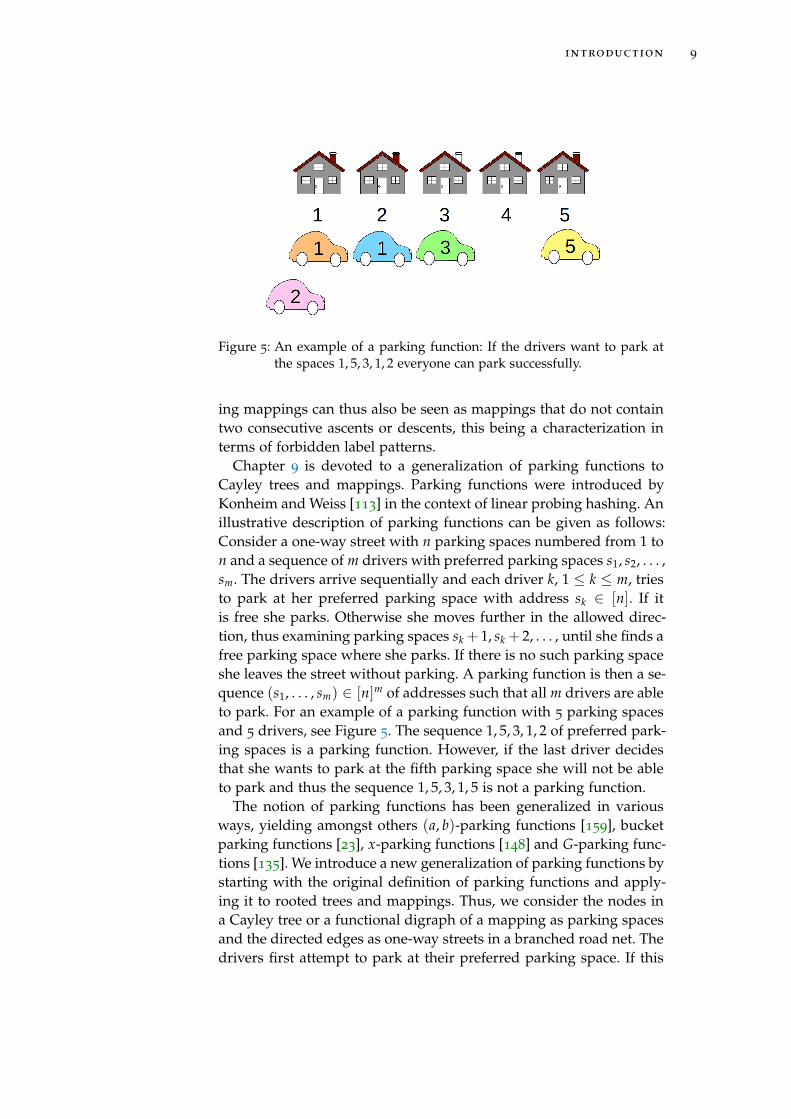
Figure 5: An example of a parking function: If the drivers want to park atthe spaces 1, 5, 3, 1, 2 everyone can park successfully.
ing mappings can thus also be seen as mappings that do not containtwo consecutive ascents or descents, this being a characterization interms of forbidden label patterns.
Chapter 9 is devoted to a generalization of parking functions toCayley trees and mappings. Parking functions were introduced byKonheim and Weiss [113] in the context of linear probing hashing. Anillustrative description of parking functions can be given as follows:Consider a one-way street with n parking spaces numbered from 1 ton and a sequence of m drivers with preferred parking spaces s1, s2, . . . ,sm. The drivers arrive sequentially and each driver k, 1 ≤ k ≤ m, triesto park at her preferred parking space with address sk ∈ [n]. If itis free she parks. Otherwise she moves further in the allowed direc-tion, thus examining parking spaces sk + 1, sk + 2, . . . , until she finds afree parking space where she parks. If there is no such parking spaceshe leaves the street without parking. A parking function is then a se-quence (s1, . . . , sm) ∈ [n]m of addresses such that all m drivers are ableto park. For an example of a parking function with 5 parking spacesand 5 drivers, see Figure 5. The sequence 1, 5, 3, 1, 2 of preferred park-ing spaces is a parking function. However, if the last driver decidesthat she wants to park at the fifth parking space she will not be ableto park and thus the sequence 1, 5, 3, 1, 5 is not a parking function.
The notion of parking functions has been generalized in variousways, yielding amongst others (a, b)-parking functions [159], bucketparking functions [23], x-parking functions [148] and G-parking func-tions [135]. We introduce a new generalization of parking functions bystarting with the original definition of parking functions and apply-ing it to rooted trees and mappings. Thus, we consider the nodes ina Cayley tree or a functional digraph of a mapping as parking spacesand the directed edges as one-way streets in a branched road net. Thedrivers first attempt to park at their preferred parking space. If this

10 introduction
one is not free, they continue their route following the directed edgesuntil they find a free parking space. For this generalization of park-ing functions, we count the total number of tree-parking functions aswell as the total number of mappings functions. Interestingly, it turnsout that these numbers are directly linked to each other which canalso be explained in a bijective manner. Furthermore, we perform anasymptotic analysis of these quantities using methods from analyticcombinatorics. Subsequently, we observe an interesting phase transi-tion behaviour at the point where the number m of drivers is equal tohalf the number of parking spaces.
Parking functions represent a structural restriction on integer se-quences but cannot directly be interpreted in terms of label patterns.However, there does exist a correspondence between parking func-tions and certain types of patterns. In order to state this correspon-dence, consider the following sorting device, called a priority queue. Ina priority queue, two possible operations can be performed: one caneither insert the next element from the input to the queue or, when-ever the queue is not empty, one can move the smallest element in thequeue to the output. With such a sorting device, the possible outputpermutations depend on the input. For instance, the identity permu-tation id = 12 . . . n will always lead to the same output, namely theidentity again. However, if the input permutation is n(n− 1) . . . 21, itcan lead to various different output permutations. The pairs (σ, τ) ofinput-output pairs that can be obtained with a priority queue – theseare called allowable pairs – can also be characterized in terms of forbid-den patterns. Indeed, a pair (σ, τ) is an allowable pair if and only if itdoes not contain the pattern-pairs (12, 21) and (321, 132). This meansthat if there are two entries σ(i) and σ(j) with i < j and σ(i) < σ(j)in the input permutation, the elements σ(i) and σ(j) may not occurin inverse order in τ. Similarly, if there are positions i < j < k inthe input permutation with σ(i) > σ(j) > σ(k), these elements maynot occur in the order σ(k), σ(i), σ(j) in the output permutation. Thisnotion of pattern avoidance is connected with pattern avoidance inpermutations but it requires patterns to occur simultaneously on thesame elements in two permutations. Now, allowable pairs of size nare in bijective correspondence with parking functions with n park-ing spaces and n drivers. In [90], such a bijection is described wherethe output permutation of the allowable pair is equal to the output ofthe corresponding parking function. For a parking function, the out-put permutation associates to each driver the parking space whereshe eventually ends up parking. Thus parking functions have a niceconnection to a certain notion of label patterns.
The last part of this thesis is devoted to so-called single-peaked elec-tions and configurations in elections. The single-peaked restriction, in-troduced by Black [22], is an extensively studied concept in socialchoice theory. A collection of preferences, i.e., total orders on a set
introduction 11
axis A18◦ 19◦ 20◦ 21◦ 22◦ 23◦
?
?
?
?
?
?
Alice
Bob
Claire
? Doug
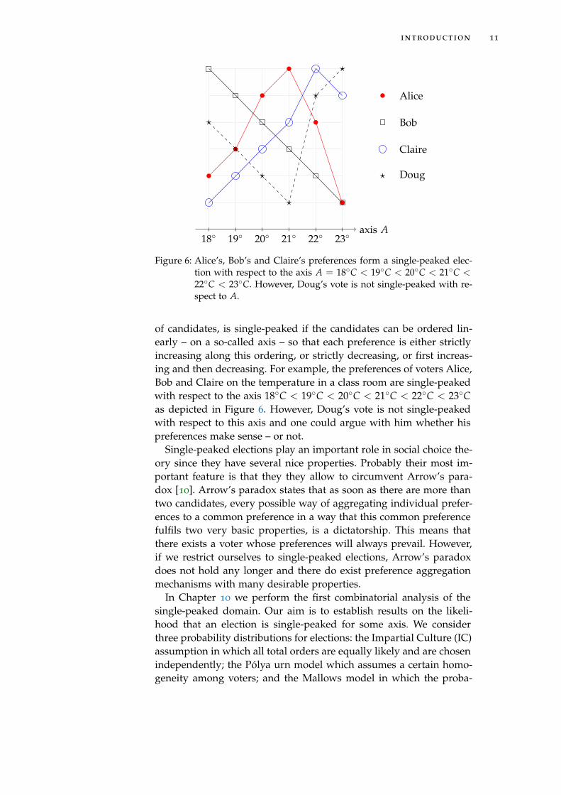
Figure 6: Alice’s, Bob’s and Claire’s preferences form a single-peaked elec-tion with respect to the axis A = 18◦C < 19◦C < 20◦C < 21◦C <22◦C < 23◦C. However, Doug’s vote is not single-peaked with re-spect to A.
of candidates, is single-peaked if the candidates can be ordered lin-early – on a so-called axis – so that each preference is either strictlyincreasing along this ordering, or strictly decreasing, or first increas-ing and then decreasing. For example, the preferences of voters Alice,Bob and Claire on the temperature in a class room are single-peakedwith respect to the axis 18◦C < 19◦C < 20◦C < 21◦C < 22◦C < 23◦Cas depicted in Figure 6. However, Doug’s vote is not single-peakedwith respect to this axis and one could argue with him whether hispreferences make sense – or not.
Single-peaked elections play an important role in social choice the-ory since they have several nice properties. Probably their most im-portant feature is that they they allow to circumvent Arrow’s para-dox [10]. Arrow’s paradox states that as soon as there are more thantwo candidates, every possible way of aggregating individual prefer-ences to a common preference in a way that this common preferencefulfils two very basic properties, is a dictatorship. This means thatthere exists a voter whose preferences will always prevail. However,if we restrict ourselves to single-peaked elections, Arrow’s paradoxdoes not hold any longer and there do exist preference aggregationmechanisms with many desirable properties.
In Chapter 10 we perform the first combinatorial analysis of thesingle-peaked domain. Our aim is to establish results on the likeli-hood that an election is single-peaked for some axis. We considerthree probability distributions for elections: the Impartial Culture (IC)assumption in which all total orders are equally likely and are chosenindependently; the Pólya urn model which assumes a certain homo-geneity among voters; and the Mallows model in which the proba-

12 introduction
bility of a vote depends on its Kendall-tau distance to a given ref-erence vote. We also define the concept of configurations in electionsand prove a general result on the probability that an election does notcontain a configuration of size (2, k).
Before we start with the actual results of this thesis, we gather themost important definitions of concepts that occur throughout this the-sis in Chapter 2. In this Chapter, we also present the methods thatwill be employed in this thesis. In Chapter 10.6 we point out variousdirections for further research.

2P R E L I M I N A R I E S
In this chapter, we introduce the objects and methods that will beused throughout this thesis. After some basic asymptotic notation wepresent the combinatorial objects that will be analysed throughoutthis thesis: permutations, Cayley trees, mappings and preference pro-files. We continue by giving a brief introduction to the methods usedto analyse these objects; these are algorithmic, analytic, probabilisticand combinatorial tools. Parts of this chapter are taken from the pub-lications this thesis is based on, see page xii for a complete list.
Some standard notation that is used throughout this thesis is gath-ered in the Notation-Section on page 233 and following pages.
2.1 asymptotic notation
Throughout this thesis we will often be interested in the asymptoticgrowth of functions, both in the context of the runtime of algorithmsand of the enumeration of combinatorial objects.
When comparing the growth rates of functions, we use the follow-ing standard asymptotic notation introduced by Bachmann and Lan-dau. The presentation here follows the one in [78]. Let x0 be someelement of a set X on which some notion of neighbourhood exists. Inthis thesis this will be: X = N∪ {∞} and x0 = ∞, X = R and x0 anyreal number or X = C and x0 = 0. Furthermore, let f and g be tworeal or complex functions defined on X \ {x0}.
• We write f (x) = O(g(x)) as x → x0, if the ratio f (x)/g(x) staysbounded as x → x0. That is, if there is a constant C > 0 and aneighbourhood U of x0 such that
| f (x)| ≤ C · |g(x)| for all x 6= x0, x ∈ U .
One says that “ f is of order at most g” or “ f is big-Oh of g”.
• We write f (x) = o(g(x)) as x → x0, if the ratio f (x)/g(x) tendsto 0 as x → x0. That is, if for every ε > 0 there is a neighbour-hood Uε of x0 such that
| f (x)| ≤ ε · |g(x)| for all x 6= x0, x ∈ Uε.
One says that “ f is of order smaller than g” or “ f is little-oh ofg”.
• We write f (x) ∼ g(x) as x → x0, if the ratio f (x)/g(x) tends to1 as x → x0. One says that “ f and g are asymptotically equiva-lent”.
13

14 preliminaries
The concepts above clearly depend very strongly on the point x0 cho-sen. Most of the time it will be clear from the context what the choiceof x0 is and we will thus omit as x → x0 from the notation.
In order to obtain asymptotic expansions we will often use the well-known Taylor expansions of the following elementary functions:
(1 + z)α = ∑n≥0
(α
n
)zn,
1(1− z)α+1 = ∑
n≥0
(n + α
n
)zn,
exp z = ∑n≥0
zn
n!, log
(1
1− z
)= ∑
n≥1
zn
n.
Moreover the following two asymptotic expansions will be used:
1. Stirling’s formula:
n! =nn
en
√2πn · (1 + λn) , where 0 < λn <
112n
. (1)
2. The harmonic numbers:
Hn :=n
∑i=1
1i= ln(n) + γ +
12n
+O(
1n2
), (2)
with the Euler-Mascheroni constant γ ≈ 0.5772 . . ..
2.2 permutations , patterns and standard young tableaux
Permutations
A permutation π is a bijective function from a finite set onto itself. Wewill denote by π−1 the inverse function of π, i.e., the unique functionthat fulfils π ◦π−1 = π−1 ◦π = id. A permutation that is self-inverse,i.e., for which it holds that π ◦ π = id, is called an involution.
If π is defined on a set of size n, we speak of a permutation oflength n or of an n-permutation. For the definition of permutationpatterns that will be given in Section 2.2 it is crucial that we have thenatural order defined by < on the elements of a permutation. We willthus assume that an n-permutation is always defined on the set [n].
An n-permutation π can thus also be seen as the sequence π(1),π(2), . . . , π(n) in which every one of the integers in [n] appears ex-actly once. We will also use the notation π1, π2, . . . , πn to refer to thissequence. This representation of a permutation is also known as theone-line notation. Given an integer m ∈ [n] we may refer to m as anelement of π and say that its position in π is i if π−1(m) = i. Everyn-permutation π defines a total order on [n] that we will denote by≺π. We write k ≺π m if π−1(k) < π−1(m), i.e., the element k lies tothe left of the element m in the sequence π. In this case, we say thatk is left of m or that m is right of k. We also use the non-strict total

2.2 permutations , patterns and standard young tableaux 15
order �π associated to π: k �π m iff k ≺π m or k = m. In this case,we say that k is not right of m or that m is not left of k.
Viewing permutations as sequences allows us to speak of subse-quences of a permutation. We speak of a contiguous subsequence of π
if the sequence consists of contiguous elements in π or, equivalently,if the corresponding positions form an interval of [n]. Given a setS ⊆ [n], we write π|S to denote the subsequence of π consisting ex-actly of the elements of S.
Graphically, a permutation π on [n] can be represented with thehelp of a plot in the integer plane in which dots are placed at the po-sitions (i, π(i)). This representation thus corresponds to the functiongraph of π when viewing permutations as bijective maps. For exam-ples, see Figure 7 on page 17 where the two permutations πex = 2 3 1 4and τex = 1 8 12 4 7 11 6 3 2 9 5 10 which will serve as running exam-ples throughout this section are represented with the help of plots.
We denote by πr := π(n)π(n− 1) . . . π(1) the reverse of π and byπc := (n− π(1) + 1)(n− π(2) + 1) . . . (n− π(n) + 1) its complement.From the plot corresponding to π one obtains πr’s plot by reflectingacross x = n/2 and πc’s plots by reflecting across y = n/2. Also, theplot of π−1 is obtained by reflecting across the line y = x.
For other possible definitions and representations of permutationswe refer to Stanley’s Enumerative combinatorics [146], especially thesection Geometric representations of permutations. Furthermore, for a ex-tensive treatment of permutations as combinatorial objects, we referto Bóna’s monograph Combinatorics of Permutations [25].
Ups and downs in permutations: various statistics
In this section, we gather various definitions related to the up-downstructure of permutations. In this thesis, three different notions ofmonotone subsequences in permutations will appear: alternating runs,ascending runs and longest increasing subsequences.
We discern two types of local extrema in permutations: valleys andpeaks. A valley of a permutation π is an element π(i) for which itholds that π(i− 1) > π(i) and π(i) < π(i + 1). If π(i− 1) or π(i + 1)is not defined, we still speak of valleys. Similarly, a peak denotes anelement π(i) for which it holds that π(i − 1) < π(i) and π(i) >
π(i + 1).Valleys and peaks partition a permutation into contiguous mono-
tone subsequences, so-called alternating runs. The first run of a givenpermutation starts with its first element (which is also the first localextremum) and ends with the second local extremum. The secondrun starts with the following element and ends with the third localextremum. Continuing in this way, every element of the permutationbelongs to exactly one alternating run. Observe that every alternat-ing run is either increasing or decreasing. We therefore distinguish

16 preliminaries
between runs up and runs down. Note that runs up always end withpeaks and runs down always end with valleys. The parameter run(π)
counts the number of alternating runs in π. Hence, run(π) + 1 equalsthe number of local extrema in π. These definitions can be analo-gously extended to subsequences of permutations.
Example 2.1. In the permutation τex = 1 8 12 4 7 11 6 3 2 9 5 10 the val-leys are 1, 4, 2 and 5 and the peaks are 12, 11, 9 and 10. A decompo-sition into alternating runs is given by: 1 8 12|4|7 11|6 3 2|9|5|10 and isgraphically represented in Figure 7. a
A permutation in which all alternating runs except the first one areof length one only is called an alternating permutation. If an alternat-ing permutation π starts with a run up it is also called an up-down-permutation and its elements have to satisfy π(1) < π(2) > π(3) <. . .. Analogously, alternating permutations starting with a run downare called down-up-permutations and have to satisfy π(1) > π(2) <
π(3) > . . .. Note that a slightly different notation is sometimes usedin the literature, calling alternating permutations in our sense zigzagpermutations and only referring to up-down permutations as alter-nating permutations.
Example 2.2. The permutation πex = 2 3 1 4 is an alternating permu-tation. To be more precise, it is an up-down permutation. a
A different way of characterizing alternating permutations is withthe help of ascents and descents. An ascent of a permutation π is aposition i for which it holds that π(i) < π(i + 1). Similarly, a descentof a permutation π is a position i for which it holds that π(i) >
π(i + 1). Thus, an alternating permutation is a permutation whereevery ascent is directly followed by a descent and vice-versa.
The descents of a permutation π partition it into so-called ascend-ing runs. These are increasing contiguous subsequences of maximallength. The following holds: if π has k descents, it is the union of k+ 1ascending runs. In order to make the difference between ascendingand alternating runs clear, let us note the following: an alternatingrun that is a run up is always also an ascending run; however, a rundown is the union of multiple ascending runs of length one.
Example 2.3. In our running example τex the five descents are the fol-lowing elements: 12, 11, 6, 3, 9. The decomposition into six ascendingruns is given as follows : 1 8 12|47 11|6|3|2 9|5 10. a
Another important concept in permutations is that of longest in-creasing and longest decreasing subsequences. A longest increasing sub-sequence of a permutation π is a monotonically increasing subse-quence that is of maximal length. Note that the longest increasing ordecreasing subsequence need not be unique and in general are notcontiguous subsequences.

2.2 permutations , patterns and standard young tableaux 17
2
3
1
4
run uprun down 1
8
12
4
7
11
6
32
9
5
10
Figure 7: The pattern πex = 2 3 1 4 (left-hand side) is contained in the per-mutation τex = 1 8 12 4 7 11 6 3 2 9 5 10 (right-hand side).
Example 2.4. In our running example τex the two increasing subse-quences of maximal length are: 146910 and 147910. a
Permutation patterns
Classical permutation patterns, or simply permutation patterns, areat the heart of Part i of this thesis.
Definition 2.5. Let π be a permutation of length k and τ = τ(1) . . . τ(n) apermutation of length n. An occurrence of the permutation pattern π inτ is a subsequence τ(i1) τ(i2) . . . τ(ik) of τ that is order-isomorphic to π.The subsequence τ(i1) τ(i2) . . . τ(ik) is order-isomorphic to π if τ(ia) <
τ(ib) holds iff π(a) < π(b). If such a subsequence exists, one says thatτ contains π or that there is a matching of π into τ. If there is no suchsubsequence one says than τ avoids the pattern π. If π is contained in τ wewrite π ≤ τ and if τ avoids π we write π � τ.
Matching π into τ thus consists in finding a monotonically increas-ing map M : [k] → [n] that maps elements in π to elements in τ insuch a way that the sequence M(π), defined as M(π(1)), M(π(2)),. . . , M(π(k)), is a subsequence of τ. We then refer to such a functionM as a matching.
Example 2.6. The pattern πex is contained in the permutation τex aswitnessed by the subsequence 4 6 2 9. The matching corresponding tothis occurrence of πex is M(1) = 2, M(2) = 4, M(3) = 6, M(4) = 9.However, τex avoids the pattern σ = 1 2 3 4 5 6 since the length of thelongest increasing subsequence of τex is 5. For an illustration see againFigure 7. a
Representing permutations with the help of plots allows for a sim-ple interpretation of pattern containment respectively avoidance in

18 preliminaries
permutations. Indeed, the pattern π is contained in the permutationτ iff the plot corresponding to π can be obtained from the one cor-responding to τ by deleting some columns and rows. Moreover, it iseasy to see that the following statements are all equivalent:
• π ≤ τ
• π−1 ≤ τ−1
• πr ≤ τr
• πc ≤ τc.
The pattern containment relation ≤ defines a partial order on theset of all permutations. This leads to the following definition:
Definition 2.7. A permutation class is a downset of permutations in thecontainment order. That is, if C is a permutation class that contains a per-mutation τ, then every π with π ≤ τ is also contained in C.
A permutation class can be defined by pattern avoidance and weuse the following notation:
Av(B) :={
τ : π � τ for all π ∈ B}
Avn(B) := {τ ∈ Av(B) : τ is of length n}Sn(B) := |Avn(B)|
If the set B is an antichain, i.e., no element of B is contained inanother on, then it is called the basis of the permutation class.
For an introduction to permutation patterns and a survey of themain results of this field we refer to the Chapters 4, 5 and 8 inBóna’s Combinatorics of Permutations [25]. A comprehensive presen-tation of results related to various types of patterns in permutationsand words can be found in Kitaev’s monograph Patterns in Permu-tations and Words [108]. A survey of permutation classes and recentresearch directions can be found in Vince Vatter’s Chapter 12 in [29].
Standard Young tableaux
The famous Robinson-Schensted correspondence establishes a bijectivecorrespondence between permutations and pairs of standard Youngtableaux of the same shape. Let us start by defining these:
Definition 2.8. Let λ = λ1, . . . , λk be a partition of n, i.e., λ1 ≥ λ2 ≥. . . ≥ λ1 ≥ 1 and ∑k
i=1 λi = n. A Young diagram of shape λ consists of nsquare boxes that are arranged in k left-justified rows such that the i-th rowcontains λi boxes. A Young tableau is obtained by filling in the boxes ofa Young diagram with elements from some ordered set. A standard YoungTableau, short SYT, of size n is a Young tableau on n boxes filled in withthe elements in [n] in such a way that every element appears exactly onceand that the rows and columns are increasing when going to the right anddown.

2.2 permutations , patterns and standard young tableaux 19
Note that we label boxes in a Young diagram in the same way asone labels entries in matrices, i.e., we say that a box is at position (i, j)if it lies in the i-th row and the j-th column.
Example 2.9. Two SYT of size 12 and of the same shape are displayedin Figure 9. The underlying partition for both Young diagrams is λ =
(5, 2, 2, 2, 1). aWe can now define the Robinson-Schensted correspondence. In a
step-by-step procedure, it associates to every n-permutation σ a pair(P(σ), Q(σ)) of SYT of size n of the same shape. In order to alleviatenotation, we will write (P, Q) instead of (P(σ), Q(σ)) whenever noconfusion is possible. The procedure constructs a sequence (P0, Q0),(P1, Q1), · · · , (Pn, Qn) = (P, Q) of pairs of Young tableaux of the sameshape, where P0 = Q0 are empty tableaux. The intermediate tableauxPi and Qi for i < n are in general not SYT since they don’t necessarilycontain all elements in [i]. However, they do have the property thatevery element occurs only once and that columns and rows are in-creasing. Having constructed Pi−1, Pi is formed by inserting σ(i) intoPi−1 according to the Schensted insertion that will be explained in amoment. The tableaux Pi are thus referred to as insertion tableaux. Atthe same time, Qi is created by adding the element i to Qi−1 in thebox that is added to the shape by the insertion of σ(i) into Pi−1. Thetableaux Qi are referred to as recording tableaux.
The Schensted insertion or row insertion of an element σ(i) into aYoung tableau Pi−1 can now be described as follows. If Pi−1 is empty,we place a box at position (1, 1) containing the element σ(i). Other-wise, proceed recursively:
1. Find the leftmost element j in the first row that is larger thanσ(i). If there is no such element, we place σ(i) at the end of thefirst row and are done. Otherwise, we replace the element j byσ(i) and proceed to the next step.
2. Using the Schensted insertion, insert the element j into the Youngtableau that is obtained by deleting the first row of Pi−1. Placethe resulting tableau under the row obtained in the first step.
Example 2.10. For the permutation τex = 1 8 12 4 7 11 6 3 2 9 5 10, theintermediate insertion tableau P6 is displayed on the left-hand sideof Figure 8. The next element to be inserted is τex(7) = 6. The in-termediate steps of the Schensted insertion of the element 6 into P6,leading to P7, are shown in the same figure. The pair (P, Q) of SYTcorresponding to τex is displayed in Figure 9. a
In the following, we list some important properties of the Robinson-Schensted correspondence that will be of use to use:
• If the permutation σ corresponds to the pair (P, Q) of SYT, theinverse permutation σ−1 corresponds to the pair (Q, P). Thus,

20 preliminaries
1 4 7 118 12
→ 1 4 6 118 12
→ 1 4 6 117 12
→ 1 4 6 117 128
insert 6 insert 7 insert 8
in row 1 in row 2 in row 3
Figure 8: The Schensted insertion of the element 6 into an insertion tableau
P =
1 2 5 9 103 64 117 128
Q =
1 2 3 6 124 57 108 119
Figure 9: The pair (P, Q) of SYT corresponding to τex under the Robinson-Schensted correspondence
if σ is an involution, it corresponds to a pair (P, P) and can beidentified with the single SYT P.
• The length of the first row in P(σ) and Q(σ) corresponds to thelength of the longest increasing subsequence in σ.
The number of SYT of size n and of a given shape can be deter-mined with the help of the so-called hooklength formula.
Definition 2.11. Let b be a box in a Young diagram. Then the hook Hb of bconsists of the box b itself, all boxes in the same row and to the right of b andall boxes in the same column and below b. The hook-length hb is the numberof cells in the hook Hb.
Example 2.12. Let b be the box at position (1, 2) in the SYT P dis-played on the left-hand side of Figure 9, i.e., the box containing theelement 2. Then hb = 3 + 3 + 1 = 7. aTheorem 2.13. Let D be a young diagram with n boxes. Then the numberof SYT of shape D is equal to
n!∏b hb
where the product is taken over all boxes b of D.
For an overview of the connections between permutations and SYT,see Chapter 7 in [25] and the references given therein. See also Chap-ter 14 of [29] for a recent survey by Ron Adin and Yuval Roichmanon Standard Young Tableaux.
2.3 cayley trees and mappings
Part ii is concerned with Cayley trees and with mappings, two closelyrelated types of combinatorial objects that we introduce in the follow-
2.3 cayley trees and mappings 21
4
1 2
3 6 5
=
4
2
5 3 6
1 6=
4
2 1
3 6 5
Figure 10: Examples of Cayley trees of size n = 6
ing. In this section, we only present the basic definitions of Cayleytrees and mappings. For analytic properties of the corresponding gen-erating functions, we refer to the examples in Section 2.6, in particularExamples 2.26, 2.27 and 2.29. For more background, we refer to [78].
Cayley trees
In a graph-theoretic sense, a tree is an acyclic undirected connectedgraph. A rooted tree is a tree in which one specific node is distin-guished; it is called the root. In this case the edges can be oriented ina natural way, either towards or away from the root. Throughout thisthesis, edges will always be oriented towards the root. Thus, the rootnode is always the unique node that has no outgoing edges. Nodeswith no incoming edges are called leaves. Let i and j be nodes in atree such that the directed edge (i, j) is present, i.e., j lies on the pathfrom i to the root. Then j is called i’s parent and i is a child of j. Fur-thermore, unordered trees are rooted trees in which there is no orderon the children of any node. Such trees are sometimes also referredto as non-plane trees.
The main family of trees studied in this thesis is the following:
Definition 2.14. A Cayley tree of size n is a unordered labelled tree withn nodes. In a labelled tree of size n every node carries a distinct integer fromthe set [n] as a label.
In the following, we will simply refer to Cayley trees as trees andindicate if we speak about other types of trees. Throughout this thesiswe will always identify nodes with their labels.
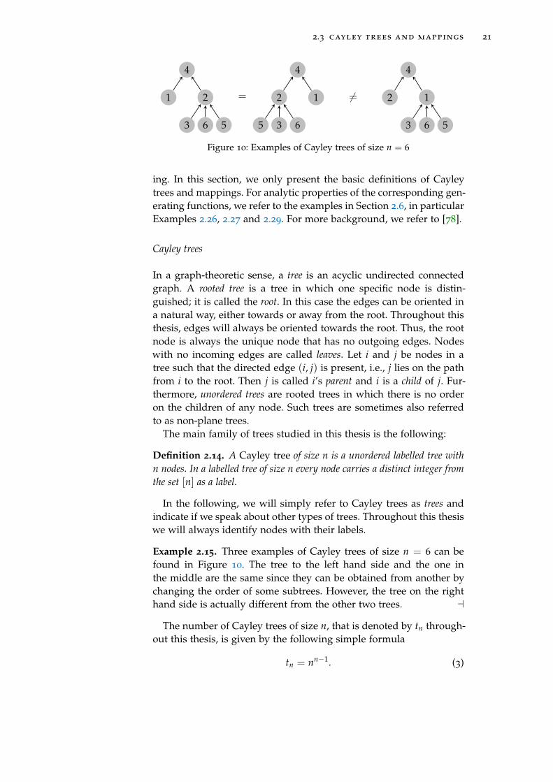
Example 2.15. Three examples of Cayley trees of size n = 6 can befound in Figure 10. The tree to the left hand side and the one inthe middle are the same since they can be obtained from another bychanging the order of some subtrees. However, the tree on the righthand side is actually different from the other two trees. a
The number of Cayley trees of size n, that is denoted by tn through-out this thesis, is given by the following simple formula
tn = nn−1. (3)
22 preliminaries
This formula is attributed to Arthur Cayley and thus also referred toas “Cayley’s formula”. It is sometimes also stated in the followingform: the number of (unrooted) labelled trees of size n is equal tonn−2. Many proofs of this formula have been given since Cayley’sproof in 1889, using various different methods. See for instance thecollection of proofs in Proofs from THE BOOK [2]. In Chapter 7 we willpresent a new bijective proof of Cayley’s formula.
Mappings
Definition 2.16. A function f from the set [n] into itself is called an n-mapping. Given an n-mapping f , its functional digraph G f is definedto be the directed graph on the vertex set [n] where a directed edge (i, j) isdrawn whenever f maps i to j.
In this thesis we will always identify a mapping with its functionaldigraph and will not make any distinction between the objects f andG f . Sometimes, mappings are also referred to as functional graphs orfunctional digraphs in the literature.
Note that an n-mapping can alternatively also be interpreted as asequence ( fi)i∈[n] of length n over the alphabet [n] by setting fi = f (i).
The structure of mappings is simple and is well described in [78]:the weakly connected components of their digraphs are simply cyclesof Cayley trees. That is, each connected component consists of rootedlabelled trees whose root nodes are connected by directed edges suchthat they form a cycle. In this context, we will call a node j that lieson a cycle in a mapping f , i.e., for which there exists a k ≥ 1 suchthat f k(j) = j, a cyclic node.
How this structural connection to trees can be translated into thelanguage of generating functions using the symbolic method is de-scribed in Example 2.27 on page 30.
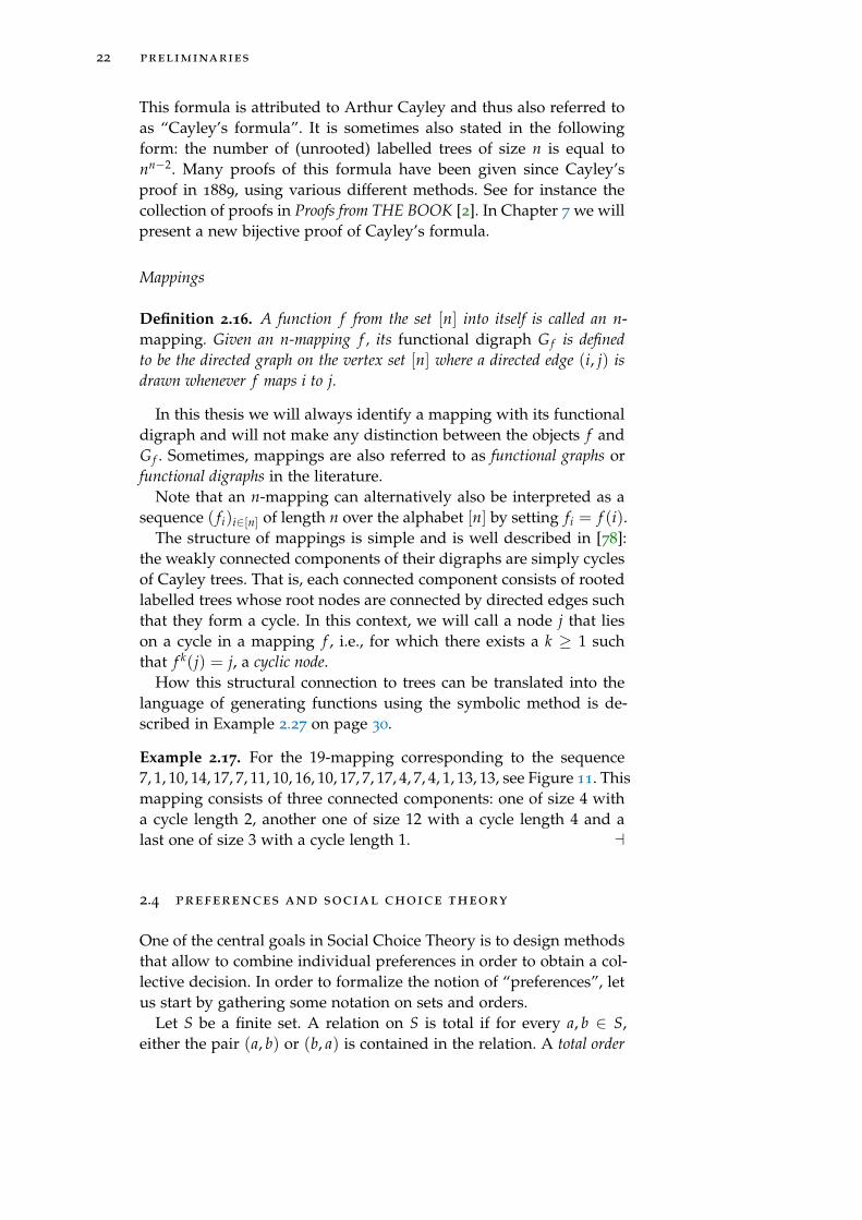
Example 2.17. For the 19-mapping corresponding to the sequence7, 1, 10, 14, 17, 7, 11, 10, 16, 10, 17, 7, 17, 4, 7, 4, 1, 13, 13, see Figure 11. Thismapping consists of three connected components: one of size 4 witha cycle length 2, another one of size 12 with a cycle length 4 and alast one of size 3 with a cycle length 1. a
2.4 preferences and social choice theory
One of the central goals in Social Choice Theory is to design methodsthat allow to combine individual preferences in order to obtain a col-lective decision. In order to formalize the notion of “preferences”, letus start by gathering some notation on sets and orders.
Let S be a finite set. A relation on S is total if for every a, b ∈ S,either the pair (a, b) or (b, a) is contained in the relation. A total order

2.4 preferences and social choice theory 23
1
7
11
17
5
2
612
15
13
15
1918
10
3 8
4 14
16
9
Figure 11: Functional graph of a 19-mapping
on S is a reflexive, antisymmetric, transitive and total relation. Let Tbe a total order of S. Instead of writing (a, b) ∈ T, we write a ≤T b orb ≥T a. We write a <T b or b >T a to state that a ≤T b and a 6= b. Asa short form, we write T : s1s2s3 . . . si instead of s1 >T s2 >T s3 >T
. . . >T si for s1, s2, . . . , si in S. We write T(i) to denote the i-th largestelement with respect to T.
Every pair (T1, T2) of total orders on a set with m elements canbe identified with the m-permutation p(T1, T2), which is defined asfollows: i is the i-th largest element in T1 maps to the j-th largestelement in T2. For T1 : bac and T2 : cab we have p(T1, T2) = 321. Notethat p(T1, T2) = p(T2, T1)
−1.We can now define elections:
Definition 2.18. An (n, m)-election (C,P) consists of a size-m set C andan n-tuple (V1, . . . , Vn) of total orders on C. The set C is referred to as thecandidate set. The total orders V1, . . . , Vn are votes or preferences.
We write V ∈ P to denote that there exists an index i ∈ [n] suchthat V = Vi. Given a vote Vi ∈ P with Vi : cicj, this means that thei-th voter prefers candidate ci to candidate cj.
When counting elections we do not care about the specific namesthat candidates have. Thus, if the candidate set C consists of m ele-ments, we assume that the candidates are c1, c2, . . . , cm. This impliesthat the number of (n, m)-elections is (m!)n.
The most fundamental result in Social Choice Theory is an impos-sibility result. Namely, it states that there is no way of aggregatingindividual preference in a way that three very basic and desirableproperties are fulfilled simultaneously. In order to state the theorem,let us introduce the notion of a social welfare function: a social welfarefunction is a function that associates to every election (C,P) a singlepreference on the set C. The idea is that this single preference is anaggregation of all the preferences that are present in the election.

24 preliminaries
Theorem 2.19 (Arrow’s paradox [10]). Let f be a social welfare functionand (C,P) an election with preferences V1, . . . , Vn. As soon as |C| > 2 thefollowing three conditions are incompatible:
• unanimity, or Pareto efficiency: If Vi : ab holds for all preferences,then f ((C,P)) : ab.
• independence of irrelevant alternatives: Consider a second election(C,Q) with preferences W1, . . . , Wn. If for all voters i it holds thatcandidates a and b have the same order in Vi as in Wi, candidates aand b have the same order in f ((C,P)) as in f ((C,Q))
• non-dictatorship: There is no voter i whose preferences always pre-vail. That is, there is no i ∈ [n] such that for all elections (C,P) itholds that f ((C,P)) = Vi.
If we make the task easier and do not ask for a total ordering ofall candidates but only for a winner of the election, this leads to theconcept of voting rules. However, this only seemingly decreases thedifficulty of the problem since the Gibbard-Satterthwaite theorem [89,137] states a similar impossibility result as Arrow’s paradox.
2.5 algorithms and complexity theory
This thesis classifies several permutation pattern matching problemsby proving membership in complexity classes, see Chapters 4 and3. We thus give a brief introduction to classical and parameterizedcomplexity theory in the following.
Classical complexity theory
The two fundamental classes in classical complexity theory are P andNP. The class P contains all decision problems that can be solved inpolynomial time on a deterministic Turing machine. A decision prob-lem is a computational problem that takes as input some string overan alphabet Σ and outputs either “YES” or “NO”. A subset L ⊆ Σ∗
defines a decision problem in the following sense: the strings in L arethe YES-instances of the problem and all other strings in Σ∗ are NO-instances. If there exists an algorithm that outputs the correct answerfor any input string of length n in O(nc) steps, where c is a constantthat is independent of the input, then one says that the problem canbe solved in polynomial time. Many natural problems are containedin P. For instance, consider the following decision problem related topermutation patterns (see Definition 2.5):
2.5 algorithms and complexity theory 25
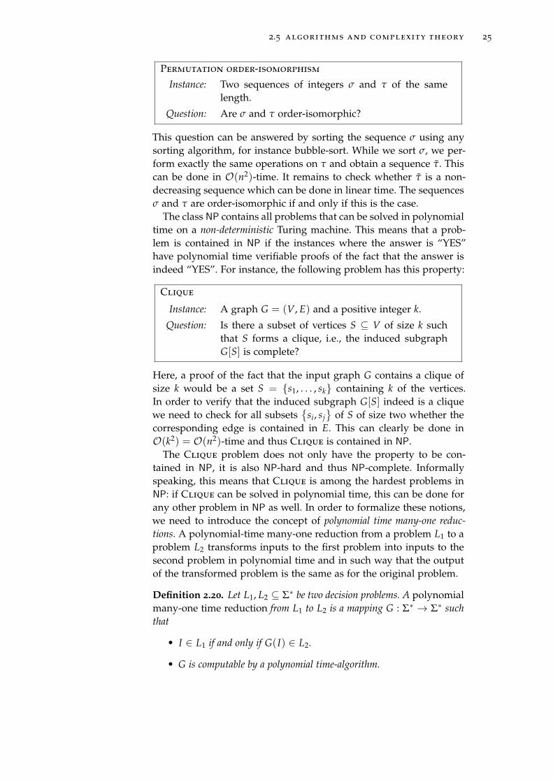
Permutation order-isomorphism
Instance: Two sequences of integers σ and τ of the samelength.
Question: Are σ and τ order-isomorphic?
This question can be answered by sorting the sequence σ using anysorting algorithm, for instance bubble-sort. While we sort σ, we per-form exactly the same operations on τ and obtain a sequence τ. Thiscan be done in O(n2)-time. It remains to check whether τ is a non-decreasing sequence which can be done in linear time. The sequencesσ and τ are order-isomorphic if and only if this is the case.
The class NP contains all problems that can be solved in polynomialtime on a non-deterministic Turing machine. This means that a prob-lem is contained in NP if the instances where the answer is “YES”have polynomial time verifiable proofs of the fact that the answer isindeed “YES”. For instance, the following problem has this property:
Clique
Instance: A graph G = (V, E) and a positive integer k.
Question: Is there a subset of vertices S ⊆ V of size k suchthat S forms a clique, i.e., the induced subgraphG[S] is complete?
Here, a proof of the fact that the input graph G contains a clique ofsize k would be a set S = {s1, . . . , sk} containing k of the vertices.In order to verify that the induced subgraph G[S] indeed is a cliquewe need to check for all subsets
{si, sj
}of S of size two whether the
corresponding edge is contained in E. This can clearly be done inO(k2) = O(n2)-time and thus Clique is contained in NP.
The Clique problem does not only have the property to be con-tained in NP, it is also NP-hard and thus NP-complete. Informallyspeaking, this means that Clique is among the hardest problems inNP: if Clique can be solved in polynomial time, this can be done forany other problem in NP as well. In order to formalize these notions,we need to introduce the concept of polynomial time many-one reduc-tions. A polynomial-time many-one reduction from a problem L1 to aproblem L2 transforms inputs to the first problem into inputs to thesecond problem in polynomial time and in such way that the outputof the transformed problem is the same as for the original problem.
Definition 2.20. Let L1, L2 ⊆ Σ∗ be two decision problems. A polynomialmany-one time reduction from L1 to L2 is a mapping G : Σ∗ → Σ∗ suchthat
• I ∈ L1 if and only if G(I) ∈ L2.
• G is computable by a polynomial time-algorithm.

26 preliminaries
A problem is called NP-hard if every problem in NP can be reducedto it by a polynomial time reduction. Note that this can also be thecase for decision problems that are not in NP. Furthermore, a problemis NP-complete if it is contained in NP and NP-hard. The Clique de-cision problem was one of the 21 problems shown to be NP-completeby Richard Karp in 1972 [106]. Under standard complexity-theoreticalassumptions, namely P 6= NP, this result implies that Clique cannotbe solved in polynomial time.
For a formal definition of Turing machines and the complexityclasses mentioned above, see e.g. [97]. A detailed introduction tocomplexity theory can be found in the monographs by Papadim-itriou [132], Goldreich [91], and Arora and Barak [9].
Parameterized complexity theory
Many problems that have practical relevance are known to be NP-complete. Thus, unless P = NP, there is no hope for polynomial timealgorithms for a large class of problems. If such problems need tobe solved efficiently anyhow, methods such as approximation algo-rithms or heuristics can be used. Another, relatively new approachthat originated in the work of Downey and Fellows [59] is to try toconfine the combinatorial explosion to a parameter of the input. Forinstance, if the treewidth of the input graph is bounded, Clique canbe solved in O(nc)-time with a constant c that is independent of thetreewidth [53]. Finding such parameters that allow to handle NP-hardproblems efficiently is the key idea of parametrized complexity the-ory.
In contrast to classical complexity theory, a parameterized complex-ity analysis studies the runtime of an algorithm with respect to anadditional parameter and not just the input size |I|. Therefore everyparameterized problem is considered as a subset of Σ∗ ×N. An in-stance of a parameterized problem consequently consists of an inputstring together with a positive integer p, the parameter.
Definition 2.21. A parameterized problem is fixed-parameter tractable(or in FPT) if there is a computable function f and an integer c such thatthere is an algorithm solving the problem in O(|I|c · f (p)) time.
The algorithm itself is also called fixed-parameter tractable (fpt).A central concept in parameterized complexity theory are fixed-
parameter tractable reductions.
Definition 2.22. Let L1, L2 ⊆ Σ∗ ×N be two parameterized problems. Anfpt-reduction from L1 to L2 is a mapping R : Σ∗ ×N → Σ∗ ×N suchthat
• (I, k) ∈ L1 iff R(I, k) ∈ L2.
• R is computable by an fpt-algorithm.

2.6 symbolic method and analytic combinatorics 27
• There is a computable function g such that for R(I, k) = (I′, k′), k′ ≤g(k) holds.
Other important complexity classes in the framework of parame-terized complexity are W[1] ⊆ W[2] ⊆ . . ., the W-hierarchy. For ourpurpose, only the class W[1] is relevant. It can be defined as follows:
Definition 2.23. The class W[1] is the class of all problems that are fpt-reducible to the following parameterized version of the Clique problem.
Clique
Instance: A graph G = (V, E) and a positive integer k.
Parameter: k
Question: Is there a subset of vertices S ⊆ V of size k suchthat S forms a clique, i.e., the induced subgraphG[S] is complete?
It is conjectured (and widely believed) that W[1] 6= FPT. Thereforeshowing W[1]-hardness can be considered as evidence that the prob-lem is not fixed-parameter tractable.
Definition 2.24. A parameterized problem is in XP if it can be solved intime O(|I| f (k)) where f is a computable function.
All the aforementioned classes are closed under fpt-reductions. Thefollowing relations between these complexity classes are known:
FPT ⊆ W[1] ⊆ W[2] ⊆ . . . ⊆ XP as well as
FPT ⊂ XP.
Further details can be found, for example, in the monographs byDowney and Fellows [59], Niedermeier [127] and Flum and Grohe [80].
2.6 symbolic method and analytic combinatorics
For an extensive introduction to the field of Analytic Combinatorics anda thorough treatment of the underlying theory, we refer to the mono-graph be Flajolet and Sedgewick [78]. Also, for a vivid presentationof generating functions as a bridge between discrete mathematics andcontinuous analysis we refer to Herbert Wilf’s generatingfunctionol-ogy [158].
Generating functions
Throughout this thesis we consider various combinatorial sequences(an)n≥0, i.e., an = |An| is the number of objects of size n in somecombinatorial class A. The size of an object α in A, denoted by |α|,

28 preliminaries
is a non-negative integer assigned to the object α. Throughout thisthesis, it will always be clear from the context how the concept of sizeis to be understood. For instance, the size of a Cayley tree is simplyits number of nodes.
The (ordinary) generating function (OGF) of A is the (formal) powerseries
A(z) = ∑n≥0
anzn = ∑n≥0|An|zn = ∑
α∈Azα. (4)
The combinatorial objects in this thesis are always labelled ones.That is, every object of size n of A consists of n “atoms” (e.g., thenodes in a tree) to which the integers in [n] are associated in a bijec-tive manner. In this context one considers the exponential generatingfunction (EGF) associated with the class A:
A(z) = ∑n≥0
anzn
n!= ∑
n≥0|An|
zn
n!= ∑
α∈A
z|α|
|α|! . (5)
Note that the concepts presented here are also applicable to a moregeneral setting where sequences (an)n≥0 are merely required to besequences of real numbers.
The symbolic method
The symbolic method is a powerful tool in the context of generatingfunctions. It allows to translate certain combinatorial constructionsdirectly to equations for generating functions. Since all objects anal-ysed in this thesis are labelled ones, we present the symbolic methodfor the case of exponential generating functions only. For the case ofordinary generating functions and even more combinatorial construc-tions, we refer to Chapters I and II of [78].
In what follows we collect some of the so-called admissible construc-tions that will be used in this thesis and which make it possible tobuild complex combinatorial classes from simpler ones.
∪ Disjoint union: If A and B are two disjoint labelled classes, thenA ∪ B denotes the union of A and B in the set-theoretic sense.However, ∪ can also be defined for not necessarily disjointclasses: If A and B are two arbitrary labelled classes, then A ∪Bdenotes the union of two disjoint copies of A and B. Such disjointcopies can, e.g., be constructed by choosing two distinct colours,and colouring the elements of A with the first colour, and theelements of B with the second one.
? Labelled product: The labelled product β ? γ of two labelled ob-jects β and γ of respective sizes |β| = m and |γ| = n is a set ofpairs, defined as follows
β ? γ :={(β′, γ′) |distinct labels in [m + n]
:= (β′, γ′) s.t. ρ(β′) = β, ρ(γ′) = γ}
,

2.6 symbolic method and analytic combinatorics 29
where ρ relabels each labelled object of size k such that exactlythe integers {1, . . . , k} are used, while preserving the relativeorder of all labels. The labelled product B ? C of two labelledclasses B and C is defined by
B ? C :=⋃
β∈B,γ∈C(β ? γ).
Seq Sequences: The sequence class of B is defined by
Seq (B) := {ε} ∪ B ∪ B ? B ∪ B ? B ? B ∪ . . . =⋃
k≥0
Bk,
where ε denotes the empty sequence.
Set Sets: Let the equivalence relation R identify sequences of equallength whenever the components of one are a permutation ofthe components of the other. Then the set class of B is definedas the quotient Seq (B) /R.
Cyc Cycles: Let the equivalence relation S identify sequences of equallength whenever one can be obtained from the other by cycli-cally shifting the components of the other, i.e., βSγ for β =
(β1, . . . , βn) and γ = (γ1, . . . , γm) iff (βk, . . . , βn, β1, . . . , βk−1) =
(γ1, . . . , γm) for some k. The cycle class of B is then defined asthe quotient (Seq (B) \ {ε}) /S.
The following theorem states how these admissible constructionsallow for a direct translation into equations for the associated expo-nential generating functions:
Theorem 2.25 (Symbolic method [78]). Let A, B, C be classes of labelledobjects, and A(z), B(z), C(z) their associated exponential generating func-tions. Then the following holds:
If A = B ∪ C, then A(z) = B(z) + C(z),
if A = B ? C, then A(z) = B(z) · C(z),
if A = Seq (B) and B0 = ∅, then A(z) =1
1− B(z),
if A = Set (B) and B0 = ∅, then A(z) = exp B(z),
if A = Cyc (B) and B0 = ∅, then A(z) = log(
11− B(z)
).
Example 2.26. As defined in Section 2.3, a Cayley tree consists of aroot node and a set of Cayley trees attached to it as children. If Tdenotes the labelled combinatorial class of Cayley trees its combina-torial construction can thus be described as follows
T = Z ? Set (T )
30 preliminaries
where Z is an atom, i.e., a single node carrying the label 1. We thusimmediately obtain that T(z), the EGF of T , is implicitly defined bythe following functional equation
T(z) = zeT(z). (6)
This function is known as the (Cayley) tree function and will appear atseveral occasions in this thesis.
The tree function is closely related to the so-called (Lambert) W-function [51] that is defined by the following functional equation:
z = W(z)eW(z).
The simple connection between the Cayley tree function and theLambert W-function is:
T(z) = −W(−z).
aExample 2.27. Using the symbolic method, the structural connectionbetween Cayley trees and mappings can also easily be taken to thelevel of generating functions. Indeed, if T , C andM denote the com-binatorial classes of Cayley trees, connected mappings and mappings,respectively, and if T(z), C(z) and M(z) denote their exponential gen-erating functions we have the following connection:
C = Cyc (T ) =⇒ C(z) = log(
11− T(z)
)
M = Set (C) =⇒ M(z) = exp(C(z)) =1
1− T(z)
aIn this thesis we will often be interested in enumerating combinato-
rial objects of a class A not only according to size but also accordingto some parameter χ. A d-dimensional parameter χ = (χ1, . . . , χd) isa function that maps an object α ∈ A to a tuple χ(α) of non-negativeintegers. In our studies, we will mostly have d = 1.
Given a labelled combinatorial class A and a d-dimensional param-eter χ on A, the multivariate exponential generating function of the pair〈A, χ〉 is defined by
A(z, u) := ∑α∈A
uχ(α) z|α|
|α|! ,
where u := (u1, . . . , ud) and u(k1,...,kd) := uk11 · · · u
kdd .
In case of a 1-dimensional parameter χ, the bivariate exponential gen-erating function of the pair 〈A, χ〉 is defined by
A(z, u) := ∑n≥0
∑k≥0
An,k
n!ukzn, (7)

2.6 symbolic method and analytic combinatorics 31
where An,k is the number of combinatorial objects in A of size n andfor which χ = k. One says that the variable z in A(z, u) marks thesize whereas u marks χ.
When working with multivariate generating functions, one can usean extension of the symbolic method. This will not be detailed hereand we refer again to [78] as well as to the new monograph AnalyticCombinatorics in Several Variables by Pemantle and Wilson [133].
Extracting coefficients
Once we have computed the generating function A(z) of some com-binatorial class A, we need to know how to get our hands on thecoefficients An (or An/n! for EGF) since this is what we are actu-ally interested in. In this context, we will denote by [zn] the operatorwhich extracts the coefficient of zn from a (formal) power series, i.e.[zn]A(z) = an, if A(z) = ∑n≥0 anzn. Sometimes, the generating func-tions will take simple forms and extracting coefficients can be doneeasily by using the Taylor expansions of well-known functions suchas those in Section 2.1.
If this is not the case, it can be helpful to apply Cauchy’s integralformula. If the radius of convergence of A(z) is positive the coefficient[zn]A(z) can be obtained as follows
[zn]A(z) =1
2πi
∮ A(z)zn+1 dz, (8)
where the integral is taken in counter-clockwise direction along asimple closed curve around the origin that lies completely inside thecircle of convergence of A(z).
Moreover, we will often deal with generating functions F(z) whichare implicitly given by a functional equation of the form F(z) =
zϕ(F(z)). This is for instance the case for the Cayley tree functiondefined in Equation (6) where ϕ(u) = exp(u). When extracting coef-ficients of such an implicitly defined function, the following theoremproves useful:
Theorem 2.28 (Lagrange’s inversion formula [78]). Let F(z) and ϕ(u)be formal power series which satisfy F(z) = zϕ(F(z)) and ϕ0 = [u0]ϕ(u) 6=0. Then one has
[zn]g(F(z)) =
1n [F
n−1]g′(x)(ϕ(F))n, n > 0
[F0]g(F), n = 0,
for every formal power series g(x).
Example 2.29. Let us consider the Cayley tree function T(z). Its func-tional equation is of the form described in Theorem 2.28 with ϕ(u) =exp(u) = ∑n≥0 un/n!. Thus ϕ0 = 1 and the conditions are fulfilled. If

32 preliminaries
we are interested in the coefficients of T(z), i.e., tn/n! where tn is thenumber of Cayley trees of size n, we have g(x) = x.
We thus obtain
tn =n! · [zn]T(z) = n! · 1n[Tn−1](exp(T))n = n! · 1
n[Tn−1](exp(T))n
=n!1n[Tn−1] ∑
k≥0
nkTk
k!= nn−1
and t0 = [F0]F = 0. We have thus rediscovered Cayley’s formula,using the symbolic method and Lagrange inversion. a
Singularity analysis
Singularity analysis is one of the most prominent techniques presentedin Flajolet and Sedgewick’s monograph Analytic combinatorics [78]. Itallows to give asymptotic expansions for the coefficients of generatingfunctions that have isolated singularities on the boundary of theirdisc of convergence. Singularity analysis is based on the followingtwo statements:
First Principle of Coefficient Asymptotics. The locationof a function’s singularities dictates the exponential growthof its coefficients.
Second Principle of Coefficient Asymptotics. The natureof a function’s singularities determines the associate subex-ponential factor.
In the following, let us assume that the generating function f (z)has a unique dominant singularity ρ, i.e., ρ is the unique singularitythat lies on the boundary of f ’s disc of convergence. Then one can ofcourse make use of the scaling rule
[zn] f (z) = ρ−n[zn] f (ρz),
and hence consider the case where ρ = 1 only. In this case, the follow-ing theorem can be applied:
Theorem 2.30 (Big-Oh transfer [76]). Let R > 1 and 0 < φ < π2 , and
assume that f (z) is analytic in a so-called ∆-domain
∆ = ∆(φ, R) := {z | |z| < R, z 6= 1, |Arg(z− 1)| > φ} .
Furthermore, assume that, as z→ 1 in ∆,
f (z) = O (|1− z|α) ,
for some constant α ∈ R. Then, as n→ ∞,
[zn] f (z) = O(
n−α−1)
.

2.6 symbolic method and analytic combinatorics 33
As a consequence, one obtains the following:
Theorem 2.31 (Singularity analysis [76]). Assume that f (z) is analyticin the domain ∆ from Theorem 2.30, and that, as z→ 1 in ∆,
f (z) =m
∑j=0
cj(1− z)αj +O(|1− z|A
),
for real numbers α0 ≤ α1 ≤ . . . ≤ αm < A and a sequence of complexnumbers (cj)0≤j≤m. Then, as n→ ∞,
[zn] f (z) =m
∑j=0
cj
(n− αj − 1
n
)+O
(n−A−1
).
In case f has a finite number of dominant singularities, a similarresult can be applied and the contributions of each singularity areadded up. We won’t detail this here and refer to [78].
As we will often encounter generating functions that are definedby a functional equation of the type F(z) = z · ϕ
(F(z)
)as in Theo-
rem 2.28, the following theorem will be useful:
Theorem 2.32 (Singular Inversion, Theorem VI.6 in [76]). Let F = F(z)be a function satisfying the functional equation
F = z · ϕ(
F), and F(0) = 0,
where ϕ(u) = ∑n≥0 ϕnun with ϕn ∈ R. Assume that ϕ(u) fulfils thefollowing conditions:
• ϕ(u) is analytic at u = 0, ϕ0 6= 0 and ϕ(u) 6≡ ϕ0 + ϕ1u
• Within the open disc of convergence of ϕ(u), |u| < R, there existsa (then necessarily unique) solution to the so-called characteristicequation
∃τ : 0 < τ < R, ϕ(τ)− τ · ϕ′(τ) = 0. (9)
• ϕ(u) is aperiodic, i.e., there does not exist an integer p ≥ 2 such thatϕ(u) = ψ(up) for some function ψ
Then it follows that
ρ =τ
ϕ(τ)=
1ϕ′(τ)
is the radius of convergence of F and f has a unique dominant singularityat z = ρ, where it admits a local expansion:
F(z) = τ −√
2ϕ(τ)
ϕ′′(τ)·√
1− zρ+ ∑
j≥2(−1)jdj
(1− z
ρ
)j/2
,
where the dj are some computable constants. Thus, F(z) is analytic in a∆-domain.
34 preliminaries
Example 2.33. The above theorem can easily be applied to the Cayleytree function (6) in order to obtain an asymptotic expansion of T(z).Here, the function ϕ(u) is simply exp(u) and clearly fulfils the threeconditions of the theorem. The characteristic equation is
eu − τ · eu = 0,
implying that τ = 1 and ρ = e−1. Thus T(z) has its unique dominantsingularity at e−1 and admits the following local expansion:
T(z) = 1−√
2 ·√
1− ez + d2(1− ez) +O((1− ez)3/2
), (10)
where the constant d2 can be determined as follows. With help of theTaylor expansion of T exp(−T) around T = 1, we obtain:
z =1e− 1
2e(T − 1)2 +
13e(T − 1)3 − 1
8e(T − 1)4 + . . .
Solving for T gives
T − 1 = −√
2 ·√
1− ez +23(1− ez) +O
((1− ez)3/2
)
and thus d2 = 2/3. A further expansion could be obtained using thesame idea. a
Saddle point method
The saddle point method allows to investigate the asymptotic be-haviour of the coefficients of generating functions. It is especially use-ful when the generating function is free of singularities and othermethods such as singularity analysis presented in the previous sec-tion cannot be applied. We shall present this method with the helpof an example and will follow the presentation in Chapter VIII ofAnalytic combinatorics [78]. We also refer to [57] for an instructive ex-position of this method.
A saddle point of a surface is a point that resembles the inner partof a saddle or of a pass between two mountains. If the surface isdefined by the modulus of an analytic function, saddle points aresimply the zeros of the derivative of the function.
The main idea of the saddle point method is to express the coef-ficients with the help of Cauchy’s Integral formula and to choose asuitable integration contour passing through or at least close to thedominant saddle point, i.e., the saddle point lying closest to the ori-gin. Thus, one chooses the contour in such a way that, locally aroundthe saddle point, it follows the steepest descents and steepest ascentlines. This ensures that the main contribution of the integral comesfrom a small part of the curve containing the saddle point.
This technique is detailed and illustrated in the following example.

2.6 symbolic method and analytic combinatorics 35
Example 2.34. In the following, we shall use the saddle point methodin order to prove Stirling’s formula (1) for the asymptotic equivalentof the factorials. The goal is thus to estimate 1
n! = [zn] exp(z). UsingCauchy’s Integral formula (8), we obtain
1n!
= In =1
2πi
∮ exp(z)zn+1 dz,
where the integration is performed along a circle centred at the origin.The saddle points can be found where the derivative of the integrandvanishes, i.e., at:
(exp(z)
zn+1
)′=
exp(z)(z− (n + 1))zn+2 = 0⇔ z = n + 1.
We thus expect to obtain an asymptotic estimate of n! by adopting acircle passing through the saddle point or close to it. Thus, we passto polar coordinates and set z = neiφ:
In =1
2π· en
nn
∫ π
−πexp
(n(eiφ − 1− iφ)
)dφ,
where we will denote by h(φ) the function eiφ − 1− iφ. We now needto split the integral in two parts: a central part that corresponds to theintegral for a small angle φ ∈ [−φ0, φ0] and that will deliver the maincontribution as well as the remaining tails that will be asymptoticallynegligible.
I(0)n =∫ φ0
−φ0
exp (nh(φ)) dφ and I(1)n =∫ 2π−φ0
φ0
exp (nh(φ)) dφ.
In order to satisfy the desired tail and central approximation, one canmake use of the saddle point dimensioning heuristic. For the case of anintegral of the form
∮exp( f (z))dz and a saddle point at z = ζ, it
states that the angle φ0 has to satisfy the following:
f ′′(ζ)(φ0)2 n→∞−−→ ∞ and f ′′′(ζ)(φ0)
3 n→∞−−→ 0
where the choice of φ0 clearly depends on n. Here, φ0 needs to satisfy
nh′′(0)(φ0)2 = −n(φ0)
2 n→∞−−→ ∞ and nh′′′(0)(φ0)3 = −i · n(φ0)
3 n→∞−−→ 0
and we can choose φ0 = nα where α is a number between −1/2 and−1/3. Let us thus fix
φ0 = n−2/5.
In particular, this implies that the angle of the central region of theintegral tends to zero when n tends to infinity.
The asymptotic approximation of In now consists of three parts:tails pruning, central approximation and tails completion.

36 preliminaries
1) Tails pruning: With z = neiφ, one has | exp(z)| = exp(n cos(φ)).Since the cosine is a unimodal function on [−π, π] with its peak atφ = 0, we have:
∣∣∣I(1)n
∣∣∣ = O (exp(n cos(φ0)− 1)) = O(
exp(−Cn1/5
))(11)
for some constant C > 0. The tail integral is thus exponentially small.2) Central approximation: Around φ = 0 we have the following ex-
pansion of h(φ):
h(φ) = −12
φ2 +O(φ3).
For φ ∈ [−φ0, φ0], the integrand can thus be approximated as follows:
exp(nh(φ)) = exp(−n
2φ2 +O(nφ3)
)= exp
(−n
2φ2) (
1 +O(nφ3))
and the central integral becomes
I(0)n =∫ n−2/5
−n−2/5exp
(−n
2φ2)
dφ ·(
1 +O(n−1/5))
=1√n
∫ n1/10
−n1/10exp
(− t2
2
)dt ·
(1 +O(n−1/5)
), (12)
where the latter expression is obtained by the change of variablest = φ
√n.
3) Tails completion: What remains to be done is to show that thetails can be completed back in the integral (12). For tails of Gaussianintegrals we have for every c > 0 that
∫ +∞
cexp
(− t2
2
)dt = O
(exp
(− c2
2
)).
It follows that, for n → ∞ we have the following asymptotic equiva-lent:
I(0)n ∼ 1√n
∫ ∞
−∞exp
(− t2
2
)dt =
√2π
n.
Finally, putting (11) and (12) together, we obtain
I(0)n + I(1)n ∼√
2π
nand thus In ∼
en
nn√
2πn.
Of course, using a refined Taylor expansion for h(φ), one could obtainfurther coefficients in the asymptotic expansion of n! using the samemethod. a
2.7 probabilistic tools
In this section we collect some probabilistic concepts and techniqueswe will use throughout this thesis. For a detailed introduction to thesetopics as well as for proofs we refer to the monographs by Billings-ley [21] and Klenke [109].
2.7 probabilistic tools 37
Basics
Let A be a labelled combinatorial class, An the subset of A consistingof objects of size n and An the cardinality of An. If we speak about arandom object in An, we will always mean the uniform probability dis-tribution over An. That is, every object in An has the same probability,namely 1/An. Whenever we consider other probability distributionsthis will be stated explicitly.
Often we are interested in some parameter χ of A, see the remarkon bivariate generating functions in Section 2.6. For every n ∈ N, itdefines a discrete random variable Xn:
P(Xn = k) =An,k
An,
where An,k denotes the number of objects in An for which χ = k.Let us recall the following two elementary definitions: The expecta-
tion or mean of the discrete random variable X is defined as
E(X) = µ = ∑k
P(X = k) · k
and is a linear functional. Note that From the second moment E(X2),one obtains the variance
V(X) = E((X− µ)2) = E(X2)− µ2
and the standard deviation σ =√
V(X).Let X be a discrete random variable supported by N with a given
distribution. If one needs to calculate the expected value of a functiong(X) of X when one does not explicitly know the distribution of g(X),the Law of the Unconscious Statistician or Change of Variables Theoremcomes in handy. It states that, if the expected value of g(X) exists,then the following holds:
E(g(X)) = ∑n∈N
g(n)P(X = n).
One of the most fundamental discrete probability distributions isthe Bernoulli distribution. It is the distribution of a random variableX that takes the value 1 with probability p, where 0 ≤ p ≤ 1, andthe value 0 with probability (1− p); one writes X ∼ B(p). Clearly,E(X) = p and V(X) = p(1− p).
The normal distribution or Gaussian distribution is a continuous prob-ability distribution that occurs very commonly in various contexts. Itwill appear as limiting distribution of discrete random variables inthis thesis. A random variable X is normally distributed with meanµ and standard deviation σ, noted as X ∼ N (µ, σ), iff it has the prob-ability density function
fX(x) =1
σ√
2πe−
(x−µ)2
2σ2 .

38 preliminaries
The distribution function of the standard normal distribution N (0, 1) isdenoted by Φ(x).
Probability and moment generating functions
In the following we introduce two generating functions that are closelyrelated to the distribution of Xn.
1. The probability generating function (PGF) of Xn is the functionpXn(v) := pn(v) := E(vXn). It is the ordinary generating func-tion of the sequence of probabilities:
pn(v) = ∑k≥0
P(Xn = k)vk.
If A(z, v) is the bivariate generating function of the parameterχ over A, i.e.,
A(z, v) = ∑n≥0
∑k≥0
An,kzn
n!vk,
then there is a close relation between pn(v) and the coefficientsof A(z, v). Indeed, it holds that
pn(v) =n!An
[zn]A(z, v) =[zn]A(z, v)[zn]A(z, 1)
.
If pn(v) exists in a neighbourhood of v = 1 it can be helpful inorder to compute the factorial moments
E(Xr) = E(X(X− 1) · · · (X− r + 1))
of X = Xn. The factorial moments can be obtained by r-folddifferentiation followed by evaluation at v = 1:
E(Xr) =∂r pn(v)
∂vr
∣∣∣∣v=1
.
If the random variable X can be written as a sum of indepen-dent random variables Xi, i.e., X = ∑r
i=1 aiXi where the ai areconstants, the probability generating function has a particularlysimple form:
pX(v) =r
∏i=1
pXi(vai).
2. The moment generating function of Xn is the function gXn(s) :=gn(s) is defined by :
gn(s) := pn (es) = E(esXn) = ∑k≥0
P(Xn = k)esk.
2.7 probabilistic tools 39
It is the exponential generating function of the sequence of mo-ments, i.e.,
gn(s) = ∑k≥0
E(Xk)sk
k!
and thus the moments E(Xr) can be obtained by r-fold differen-tiation followed by evaluation at v = 1:
E(Xr) =∂rgn(s)
∂sr
∣∣∣∣s=0
.
Convergence in distribution
Let (Xn)n∈N be a sequence of random variables, and (Fn(x))n∈N therespective distribution functions. Furthermore, let X be another ran-dom variable with distribution function F(x). The sequence (Xn)n∈N
is said to converge in distribution to X iff
limn→∞
Fn(x) = F(x),
for every x ∈ R where F is continuous. One then also says that(Xn)n∈N converges weakly to X, and writes
Xn(d)−→ X.
If the random variable X can be written as a sum of indepen-dent and identically distributed (short: iid) random variables Xi, i.e.,X = ∑n
i=1 Xi whit E(Xi) = µ < ∞ and V(Xi) = σ2 < ∞, then the Cen-tral limit theorem (CLT) implies that the standardized random variableconverges in distribution to the standard normal distribution:
X− nµ
σ√
n(d)−→ N (0, 1).
In case the random variable X is the sum of independent but not nec-essarily identically distributed random variables the following strongerversion of the CLT can be used:
Theorem 2.35 (Ljapunov CLT). Let X1, X2, . . . , Xn be a sequence of inde-pendent random variables, with finite mean µi and variance σ2
i each. More-over, let s2
n = ∑ni=1 σ2
i . If there exists a δ > 0 such that the Ljapunovcondition
1s2+δ
n
n
∑i=1
E(|Xi − µi|2+δ
)→ 0 as n→ ∞ (13)
is fulfilled, then X = ∑ni=1 Xi converges to a normal distribution:
X−n
∑i=1
µi
sn
(d)−→ N (0, 1).
40 preliminaries
Often we will encounter sequences of random variables (Xn)n∈N
that are not independent. In order to show that such a sequence haslinear mean and variance and that it is asymptotically normal dis-tributed when suitably standardized, a useful theorem is the follow-ing:
Theorem 2.36 (Hwang’s quasi-power theorem [98]). Let (Xn)n∈N bea sequence of discrete random variables supported by N0. Assume that themoment generating functions (gn(s))n∈N are analytic in a fixed complexneighbourhood of s = 0 in which they have an expansion of the form
gn(s) = exp(φnU(s) + V(s)
)·(
1 +O(
1κn
)),
where φn, κn → ∞ and U(s), V(s) do not depend of n and are analytic ats = 0. Assume finally that U(s) satisfies the so-called “variability condition”U′′(0) 6= 0. Under these conditions, the mean and variance of Xn satisfy
E(Xn) =φnU′(0) + V ′(0) +O(κ−1n ),
V(Xn) =φnU′′(0) + V ′′(0) +O(κ−1n ).
Furthermore, Xn is after standardization asymptotically normally distributed,with speed of convergence O(κ−1
n + φ−1/2n ):
P
{Xn −E(Xn)√
V(Xn)≤ x
}= Φ(x) +O
(1κn
+1√φn
),
where Φ(x) is the distribution function of the standard normal distribution.
2.8 method of characteristics
The method of characteristics is a technique for solving linear partialdifferential equations. We will use this method in order to solve someof the differential equations that occur in this thesis. We thus givea brief introduction to it; for details and more background we referto [69].
In what follows we consider homogeneous quasilinear first orderPDEs for a function f (x, y) in two variables. These are of the followingform
a(x, y, f ) fx(x, y) + b(x, y, f ) fy(x, y) = c(x, y, f ), (14)
with an initial condition f (x, 0) = u(x). The idea behind the methodof characteristics is to convert this PDE to a system of ordinary differ-ential equations along so-called characteristic curves.
Let us first note that the following holds:
(a, b, c) · ( fx, fy,−1) = 0.
This can be understood geometrically as follows: A plot of z = f (x, y)corresponds to a surface in (x, y, z)-space. The vector ( fx, fy,−1) isnormal to this solution surface and (a, b, c) is tangent.

2.9 log-concavity and combinatorial sequences 41
Starting with any point of the initial curve f (x, 0) = u(x), we followthe vector (a, b, c) in order to construct a curve on the solution surface.Such a curve is then called a characteristic curve. Once we have foundall the characteristic curves, the solution f (x, y) is fully characterized.
We parametrize our characteristic curves by an auxiliary parametert. Then, given a characteristic curve (x(t), y(t), f (t)) its tangent vectoris (
∂x∂t
,∂y∂t
,∂ f∂t
)
However, as described above, we chose our curves in such a way that(a, b, c) is tangent. We thus obtain the following system of characteristicequations,
x′ =dxdt
= a(x, y, f ),
y′ =dydt
= b(x, y, f ), (15)
f ′ =d fdt
= c(x, y, f ).
The next step is then to find first integrals of the system (15), i.e.,functions ζ(x, y, F) that are constant along any characteristic curve.This is usually done by considering the equations
∂x∂y
=a(x, y, f )b(x, y, f )
,∂x∂ f
=a(x, y, f )c(x, y, f )
or∂y∂ f
=b(x, y, f )b(x, y, f )
.
If one has found two independent first integrals ζ1(x, y, F) and ζ2(x, y, F)of (15), the general solution is given by:
G(ζ1(x, y, f ), ζ2(x, y, f )) = const.,
where G is an arbitrary differentiable function in two variables. Us-ing the initial condition f (x, 0) = u(x), this function G can then bespecified.
2.9 log-concavity and combinatorial sequences
Log-concavity
Log-concave sequences play an important role in Combinatorics; seethe extensive surveys by Stanley [147] and Brenti [40] as well Chapter7 of [29] for a recent survey by Petter Brändén on the subject.
Definition 2.37. Let a1, a2, · · · , an be a sequence of positive real numbers.We say that the sequence is log-concave if for all indices k, the inequalityak−1ak+1 ≤ a2
k holds.
Note that a sequence (ak)1≤k≤n is log-concave if and only if thesequence (bk)1≤k≤n := (log(ak))1≤k≤n is concave.
Log-concavity implies another important property of combinatorialsequences:

42 preliminaries
Proposition 2.38. If the sequence a1, a2, · · · , an is log-concave then it isunimodal, i.e., there exists an index 0 ≤ k ≤ n such that a1 ≤ a2 ≤ . . . ≤ akand an ≤ an−1 ≤ . . . ≤ ak.
The following property is even stronger than log-concavity:
Definition 2.39. We say that the sequence a1, a2, · · · , an has real rootsonly or real zeros only if the corresponding polynomial A(x) = ∑n
i=1 aixi
has real roots only.
The following holds:
Proposition 2.40. If the sequence a1, a2, · · · , an has real roots only then itis log-concave as well.
Note that the converse of this statement does not hold. For instancethe sequence 1, 1, 1 is log-concave but the polynomial 1 + x + x2 hastwo complex roots.
Example 2.41. A combinatorial sequence for which it is straightfor-ward to prove real-rootedness for every fixed n is the sequence ofbinomial coefficients:
bn,k =
(nk
)with 0 ≤ k ≤ n.
It follows, that this sequence is log-concave and unimodal. Indeed, weknow that the binomial coefficients (n
k) have a unique peak at k = n/2in case n is even and have two maximal elements at k = (n − 1)/2and k = (n + 1)/2 in case n is odd.
Another prominent example of a combinatorial sequence that hasreal roots only is the sequence of Eulerian numbers A(n, k). The Eu-lerian numbers count permutations of length n with exactly k as-cents. Equivalently, A(n, k) counts n-permutations that are the unionof (k + 1) ascending runs. a
Various combinatorial sequences appearing in this thesis
In the following Table 1 we give an overview of the most importantcombinatorial sequences appearing in this thesis and gather some oftheir properties.
Table 1 only contains univariate combinatorial sequences. A fa-mous bivariate sequence that appears in this thesis in Chapter 8 isthe sequence of Stirling numbers of the second kind. The sequence Sn,kcounts partitions of the set [n] into m nonempty subsets and we willsee that it is closely related to the number of n-mappings with m runs(see Chapter 8). The following holds for the Stirling numbers of thesecond kind:
{nm
}:= Sn,k =
1m!
m
∑`=0
(m`
)(−1)m−``n

2.9 log-concavity and combinatorial sequences 43
This sequence is the entry A008277 in Sloane’s OEIS [128].For a detailed introduction to these combinatorial sequences we
refer the reader to the monographs by Bóna [27] and Stanley [146].For the viewpoint of analytical combinatorics, we refer to Flajolet andSedgewick’s monograph [78].

Formula Combinatorial objects counted by thesenumbers and appearing in this thesis
Exponential (EGF) orOrdinary (OGF) GF
Asymptotics Entry inOEIS[128]
pn = n! n-permutations (Part i) EGF: P(z) =1
1− zpn ∼
√2πn
(ne
)nA000142
Catn =1
n + 1
(2nn
)sorted n-parking functions (Chapter 9),
321-avoiding n-permutations (Chapter 5)OGF: C(z) =
1−√
1− 4z2z
Catn ∼4n
n3/2√
πA000108
bn =
(2nn
)(n + 1)-permutations avoiding
2431, 4231, 1432, 4132 (Chapter 5)OGF: B(z) =
1√1− 4z
bn ∼4n√
nπA000984
in =bn/2c∑k=0
n!(n− 2k)!2kk!
involutions of length n (Chapter 6),SYT with n boxes (Chapter 6)
EGF: I(z) = exp(
z +z2
2
)in ∼
nn/2e√
n−n/2−1/4√
2A000085
tn = nn−1 Cayley trees with n nodes (Part ii) EGF: T(z) = zeT(z) tn = nn−1 A000169
mn = nn n-mappings (Part ii) EGF: M(z) =1
1− T(z)mn = nn A000312
fn = (n + 1)n−1 ordinary n-parking functions(Chapter 9)
EGF: F(z) =T(z)
zfn = (n + 1)n−1 A000272
Table 1: An overview of famous combinatorial sequences appearing in this thesis.

Part I
P E R M U TAT I O N S
This part is concerned with various aspects of patternsin permutations. Chapters 3 and 4 focus on the computa-tional problem of Permutation Pattern Matching, thefirst one with the design of an fpt algorithm for this prob-lem and the second one dealing with the computationalcomplexity of this problem for different types of patterns.Chapter 5 deals with a permutation class that arises withinthe study of domain restrictions and that has a nice enu-meration formula. Chapter 6 deals with the conjecturedlog-concavity of the combinatorial sequence enumeratingpermutations by the length of their longest increasing sub-sequence. Especially, it provides two examples of permu-tation classes for which the conjecture holds.


3E F F I C I E N T P E R M U TAT I O N PAT T E R N M AT C H I N G :T H E A LT E R N AT I N G R U N A L G O R I T H M
This chapter is based on joint work with Martin Lackner which haslead to the article A Fast Algorithm for Permutation Pattern MatchingBased on Alternating Runs which has recently been accepted for publi-cation in Algorithmica. A preliminary version of this paper appearedin the proceedings of the 13th Scandinavian Symposium and Work-shops on Algorithm , SWAT 2012 [41].
The main goal of this chapter is the design of an efficient algorithmfor the following computational problem:
Permutation Pattern Matching (PPM)
Instance: A permutation τ (the text) of length n and a per-mutation π (the pattern) of length k ≤ n.
Question: Is there a matching of π into τ?
Bose, Buss and Lubiw [31] showed that PPM is in general NP-complete.The trivial brute-force algorithm checking every subsequence of lengthk of τ has a runtime of O(2n · n). So far, no algorithm has been discov-ered that improves the exponential runtime to cn for some constantc < 2. Improving exponential time algorithms is a major topic in algo-rithmics, as witnessed by the monograph of Fomin and Kratsch [81].
In this chapter we tackle the problem of solving PPM faster thanO(2n · n) for arbitrary π and τ. We achieve this by exploiting the de-composition of permutations into alternating runs. Note that when-ever we speak of runs in this Section, we will always mean alternatingruns and not ascending runs (see Section 2.2 for a distinction of thesetwo concepts). The number of alternating runs in a permutation π
is denoted by run(π) throughout this chapter. Alternating runs area fundamental permutation statistic and were studied already in thelate 19th century by André [7]. Despite the importance of alternatingruns within the study of permutations, the connection to PPM has sofar not been explored.
This chapter is organized as follows: The main section, Section 3.1,describes the alternating run algorithm and is divided into the follow-ing subsections. Section 3.1 introduces matching functions. Section 3.1describes the alternating run algorithm in detail. Section GetMatchingcontains proof details necessary to verify the correctness of the alter-nating run algorithm. Section GetMatching proves the correspondingruntime bounds. Our results concerning the parameter run(π) can befound in Section 3.2. The contributions of this chapter to the PPMproblem are summarized in Section 3.3.
47
48 efficient permutation pattern matching
Throughout this chapter the pattern permutation πex = 2 3 1 4 andthe text permutation τex = 1 8 12 4 7 11 6 3 2 9 5 10, as introduced in thePreliminaries, will serve as a running example. A graphical represen-tation can be found in Figure 13 on page 51.
related work . The most relevant paper is the recent break-through result by Guillemot and Marx [93] showing that PPM is FPTwith respect to the length of the pattern. Their algorithm has a run-time of 2O(k
2·logk) · n. This FPT result is anteceeded by algorithms witha runtime of O(n1+2k/3 · log n) [3] and O(n0.47k+o(k)) [1].
Although PPM is NP-complete in general, there are polynomialtime algorithms if only certain permutations are allowed as patterns.The most important example are separable permutations: these are per-mutations that contain neither 3142 nor 2413. If the pattern is separa-ble, PPM can be solved in polynomial time [3, 31, 99, 138]. In case P isthe identity 1 2 . . . k, PPM consists of looking for an increasing subse-quence of length k in the text T – this is a special case of the Longest
Increasing Subsequence problem. This problem can be solved inO(n log n)-time for sequences in general [139] and in O(n log log n)-time for permutations [48, 122]. An O(k2n6)-time algorithm is pre-sented in [94] for the case that both the text and the pattern that donot contain 321. If the pattern is required to be matched to consecu-tive elements in the text, a O(n + k) algorithm has been found [114].A similar result has been found independently in [107]. This work hasbeen extended to the cases where some mismatches are tolerated [84];also suffix trees have recently been generalized to be applicable in thissetting [55].
The related Longest Common Pattern problem is to find a longestcommon pattern between two permutations T1 and T2, i.e., a patternP of maximal length that can be matched both into T1 and T2. Thisproblem is a generalization of PPM since determining whether T1
is the longest common pattern between T1 and T2 is equivalent tochecking whether T2 contains T1 as a pattern. In [34] a polynomialtime algorithm for the Longest Common Pattern problem is pre-sented for the case that one of the two permutations T1 and T2 isseparable. A generalization of this problem, the so called Longest
Common C-Pattern problem was introduced in [35]. This problemconsists of finding the longest common pattern among several permu-tations belonging to a class C of permutations. For the case that C isthe class of all separable permutations and that the number of inputpermutations is fixed, the problem was shown to be polynomial timesolvable [35].
For a class of permutations X, the Longest X-Subsequence (LXS)problem is to identify in a given permutation T its longest subse-quence that is isomorphic to a permutation of X. Polynomial time al-gorithms for many classes X exist, but in general LXS is NP-hard [4].
3.1 the alternating run algorithm 49
notation. To avoid confusion, we introduce the following nota-tion for this chapter: Capital letters are used for functions, sets andlists; lower case letters for natural numbers. The letters i and j areexclusively used to denote positions or indices such as positions inpermutations or indices in lists. We use greek letters only in the fol-lowing cases: π (the pattern) and τ (the text) are permutations; κ ∈ [k]as well as ν ∈ [n] are the main variables in the algorithm. In this chap-ter, tuples always have length run(π) and are denoted with bars, e.g.,~x. The elements of ~x are x1, . . . , xrun(π).
3.1 the alternating run algorithm
We start with an outline of the alternating run algorithm. Its descrip-tion consists of two parts. In Part 1 we introduce so-called matchingfunctions. These functions map runs in π to sequences of adjacent runsin τ. The intention behind matching functions is to restrict the searchspace to certain subsequences of length k, namely to those where allelements in a run in π are mapped to elements in the correspondingsequences of runs in τ. In Part 2 a dynamic programming algorithmis described. It checks for every matching function whether it is pos-sible to find a compatible matching. This is done by finding a smallset of representative elements to which the element 1 can be mappedto, then – for a given choice for 1 – finding representative elementsfor 2, and so on.
Theorem 3.1. The alternating run algorithm solves the PPM problem intime O(1.79run(τ) · n · k). Therefore, PPM parameterized by run(τ) is inFPT.
Since run(τ) < n, we obtain as an immediate consequence:
Corollary 3.2. The alternating run algorithm solves the PPM problem intime O(1.79n · n · k).
Before we start with the description of the alternating run algo-rithm, we introduce two functions which play an important role.
Definition 3.3. Let u ∈ [k]. The run predecessor pre(u) denotes thelargest element smaller than u that is contained in the same run as u in π
(if such an element exists). Moreover, the run index function ri is defined asfollows: ri(u) = i if u is contained in the i-th run in π.
Note that both functions concern only the pattern π.
Matching functions.
We introduce the concept of matching functions. These are functionsfrom the interval [run(π)] to sequences of adjacent runs in τ. For a

50 efficient permutation pattern matching
P:
T:
F
= F(1)= F(2)
= F(3)= F(4)
Figure 12: A sketch of a matching function and its M- and W-shaped subse-quences
given matching function F the search space in τ is restricted to match-ings where an element κ contained in the i-th run in π is matched toan element in F(i). As we will see later on in Lemma 3.7, this re-striction of the search space does not influence whether a matchingcan be found or not: if a matching exists, a corresponding matchingfunction can be found. In addition, Lemma 3.27 will show that it ispossible to iterate over all matching functions in fpt time. Thus, ouralgorithm verifies for all matching functions whether a compatiblematching exists.
Let us now give a formal definition of matching functions.
Definition 3.4. A matching function F maps an element of [run(π)] toa subsequence of τ. It has to satisfy the following properties for all i ∈[run(π)].
(P1) F(i) is a contiguous subsequence of τ.
(P2) If the i-th run in π is a run up (down), F(i) starts with an elementfollowing a valley (peak) or the first element in τ and ends with avalley (peak) or the last element in τ.
(P3) F(1) starts with the first and F(run(π)) ends with the last element inτ.
(P4) F(i) and F(i + 1) have one run in common: F(i + 1) starts with theleftmost element in the last run in F(i).
Property (P2) implies that every run up is matched into an M-shaped sequence of runs of the form up–down–up–...–up–down (ifthe run up is the first or the last run in π the sequence might startor end differently) and every run down is matched into a W-shapedsequence of runs of the form down–up–down–...–down–up (again, ifthe run down is the first or the last run in π, the sequence might startor end differently). These M- and W-shaped sequences are sketchedin Figure 12.
Property (P4) implies that two adjacent runs in π are mapped to se-quences of runs that overlap with exactly one run, as is also sketched

3.1 the alternating run algorithm 51
2
3
1
4
1
8
12
4
7
11
6
3
2
9
5
10
= F(ri(2)) = F(ri(3)) = F(1)
= F(ri(1)) = F(2)
= F(ri(4)) = F(3)
Figure 13: πex and τex together with a matching function F and the compat-ible matching witnessed by the subsequence 4 6 2 9
in Figure 12. This overlap is necessary since elements in different runsin π may be matched to elements in the same run in τ. More precisely,valleys and peaks in π might be matched to the same run in τ as theirsuccessors (see the following example).
Example 3.5. In Figure 13, πex (left-hand side) and τex (right-handside) are depicted together with a matching function F. A matchingcompatible with F is given by 4 6 2 9. We can see that the elements6 and 2 lie in the same run in τex even though 3 (a peak) and 1 (itssuccessor) lie in different runs in πex. a
Note that there are no matching functions if run(π) > run(τ). Thiscorresponds to the fact that in such a case no matching from π intoτ exists either. The properties (P1)-(P4) guarantee that the number of
functions we have to consider is less than (√
2)run(τ)
, as will be provenin Section GetMatching, Lemma 3.27. This allows us to iterate over allmatching functions in fpt time.
Let us formalize what we mean by compatible matchings.
Definition 3.6. A matching M is compatible with a matching function Fif M(κ) ∈ F(ri(κ)) for every κ ∈ [k], i.e., M matches each element containedin the i-th run in π to an element in F(i).
Lemma 3.7. For every matching M of π into τ there exists a matchingfunction F such that M is compatible with F.
The proof of this lemma can be found in Section GetMatchingon page 61. We continue with the observation that, when searchingfor a compatible matching by looking for the possible values thatM(1), M(2) and so on can take, we do not have to remember all theprevious choices we made. Let us have a look at an example first:

52 efficient permutation pattern matching
Example 3.8. In Figure 13, assume that we already have a partialmatching: M(1) = 2 and M(2) = 4. We now have to decide whereto map 3. There are two constraints that have to be satisfied: First,M(3) > M(2). Second, M(3) has to be to the right of M(2), since2 ≺π 3. Since our choices for M(3) are limited to F(ri(3)) = F(1), wedo not have to check whether M(3) is left of M(1) but only whetherM(3) > M(2). Later, when deciding where to map 4, we will onlyhave to verify that M(4) > M(3).
In more generality, we observe that given a matching function anda partial matching M defined on [κ − 1], deciding where to map κ
only requires the knowledge of M(κ − 1) and of M(κ′), where κ′ isthe previous element in the same run as κ. a
Let us now make this observation more precise:
Lemma 3.9. Let F be a matching function. A function M:[k] → [n] is amatching of π into τ compatible with F if and only if for every κ ∈ [k]:
1. M(κ) ∈ F(ri(κ)),
2. M(κ) > M(κ − 1) and
3. if pre(κ) exists, then pre(κ) ≺π κ if and only if M(pre(κ)) ≺τ M(κ),i.e., if κ is contained in a run up (down), then M(κ) is right (left) ofM(pre(κ)).
As we will see soon, this lemma is essential for our algorithm. Itsproof can be found in Section GetMatching on page 62.
Algorithm description
Before we start explaining the actual fpt algorithm, let us considera simple algorithm based on alternating runs. This simple algorithm(Algorithm 1) does not have fpt runtime but has the same basic struc-ture as the fpt algorithm. In particular, this simple algorithm willalready demonstrate the importance of Lemma 3.9.
From Lemma 3.7 we know that when checking whether τ containsπ as a pattern, it is sufficient to test for all matching functions whetherthere exists a compatible matching. Let us fix a matching function F.We first find suitable elements to which 1 can be mapped, then suit-able elements for 2, and so on. Observe that we can use Lemma 3.9to verify what suitable elements are. In addition, Lemma 3.9 tellsus that when finding suitable elements for κ ∈ [k], we only requirethe values of M(κ − 1) and M(pre(κ)). This means in particular thatwe do not have to store all values of a possible partial matching(M(1), . . . , M(κ)) but only the values of M for the largest element ≤ κ
in each run in π. For example, when trying to match π = 2 3 5 7 4 1 6into some text and looking for the possible elements for κ = 4, weonly have to consider possibilities for M(3) and M(pre(4)) = M(1).

3.1 the alternating run algorithm 53
Algorithm 1: A Simple Alternating Run Algorithm
1 XF0 ← {(0, . . . , 0)} // The tuple (0, . . . , 0) has run(π)
elements.
2 foreach matching function F do3 for κ ← 1 . . . k do // κ is the element to be matched.
4 XFκ ← ∅
5 foreach ~x ∈ XFκ−1 do
6 R← {ν ∈ [n] : ν ∈ F(ri(κ)) ∧ ν >
xri(κ−1) ∧ (pre(κ) ≺π κ ↔ xri(pre(κ)) ≺τ ν)}// Conditions according to Lemma 3.9
7 foreach ν ∈ R do8 XF
κ ←XF
κ ∪ {(x1, . . . , xri(κ)−1, ν, xri(κ)+1, . . . , xrun(π))}9 if XF
k 6= ∅ then10 return “π can be matched into τ.”11 return “π cannot be matched into τ.”
In this simple algorithm, we want to keep track of all possible par-tial matchings (M(1), . . . , M(κ)) for every κ ∈ [k]. Since such partialmatchings can be described by storing a single value per run in π,every one of them can be stored as a tuple ~x of length run(π). Thefirst element of ~x contains a possible choice for the largest element≤ κ in the first run of π, the second element of ~x contains a possi-ble choice for the largest element ≤ κ in the second run of π, etc.We formalize this notion of “tuples encoding partial matchings” as(κ, F)-matchings:
Definition 3.10. Let κ be an integer in [k]. A tuple~x = (x1, x2, . . . , xrun(π))
with xi ∈ [0, n] for all i ∈ [run(π)] is called a (κ, F)-matching of π into τ ifthe following holds: There exists a function M : [κ]→ [n] that is a matchingof π|[κ] into τ that is compatible with F and for which it additionally holdsthat for every xi 6= 0, M(max{κ′ ≤ κ : ri(κ′) = i}) = xi, i.e., M maps thelargest element ≤ κ in the i-th run of π to the i-th element of ~x.
The following lemma states that XFκ – as constructed by Algorithm 1
– indeed contains only tuples that are (κ, F)-matchings:
Lemma 3.11. Let XFκ be the set of tuples as constructed by Algorithm 1.
Then every ~x ∈ XFκ is a (κ, F)-matching.
The proof can be found in Section GetMatching on page 63. Asan immediate consequence of this lemma, we know that if XF
k 6= ∅then there exists a matching from π into τ that is compatible with F.Observe that XF
k is always empty if a previous XFκ was empty. If for
every F the set XFk = ∅, we know from Lemma 3.7 that π cannot be
matched into τ.
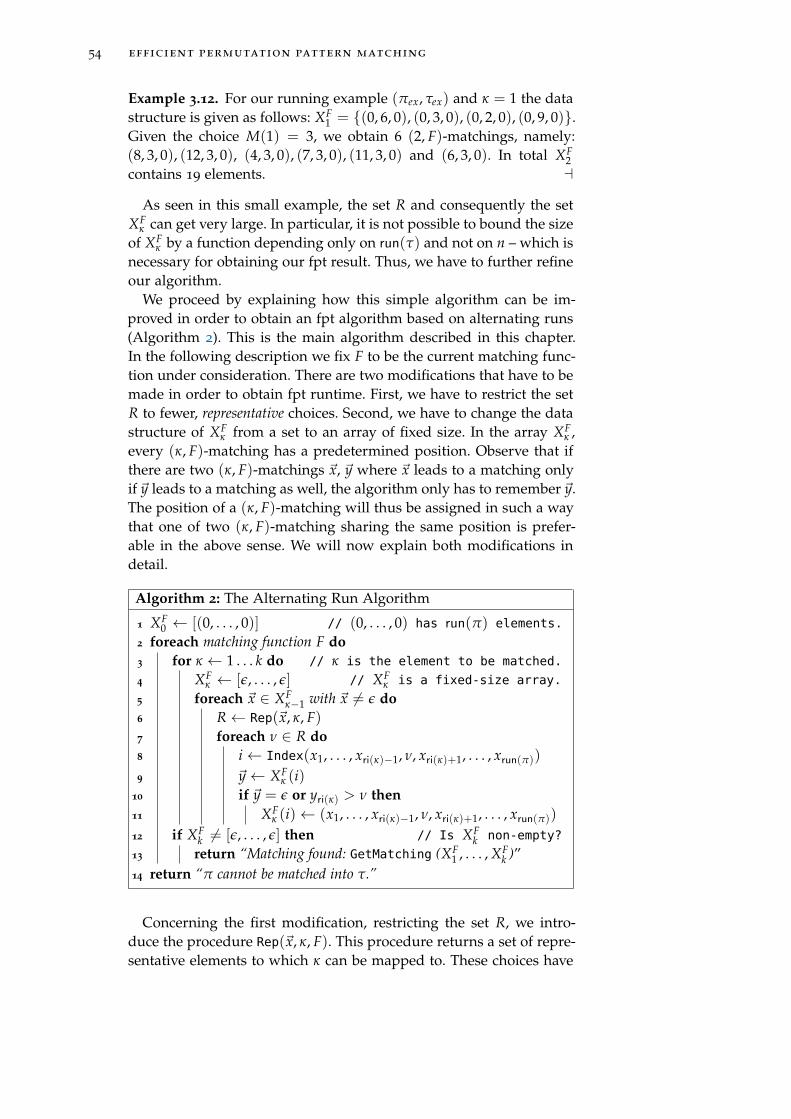
54 efficient permutation pattern matching
Example 3.12. For our running example (πex, τex) and κ = 1 the datastructure is given as follows: XF
1 = {(0, 6, 0), (0, 3, 0), (0, 2, 0), (0, 9, 0)}.Given the choice M(1) = 3, we obtain 6 (2, F)-matchings, namely:(8, 3, 0), (12, 3, 0), (4, 3, 0), (7, 3, 0), (11, 3, 0) and (6, 3, 0). In total XF
2contains 19 elements. a
As seen in this small example, the set R and consequently the setXF
κ can get very large. In particular, it is not possible to bound the sizeof XF
κ by a function depending only on run(τ) and not on n – which isnecessary for obtaining our fpt result. Thus, we have to further refineour algorithm.
We proceed by explaining how this simple algorithm can be im-proved in order to obtain an fpt algorithm based on alternating runs(Algorithm 2). This is the main algorithm described in this chapter.In the following description we fix F to be the current matching func-tion under consideration. There are two modifications that have to bemade in order to obtain fpt runtime. First, we have to restrict the setR to fewer, representative choices. Second, we have to change the datastructure of XF
κ from a set to an array of fixed size. In the array XFκ ,
every (κ, F)-matching has a predetermined position. Observe that ifthere are two (κ, F)-matchings ~x, ~y where ~x leads to a matching onlyif ~y leads to a matching as well, the algorithm only has to remember ~y.The position of a (κ, F)-matching will thus be assigned in such a waythat one of two (κ, F)-matching sharing the same position is prefer-able in the above sense. We will now explain both modifications indetail.
Algorithm 2: The Alternating Run Algorithm
1 XF0 ← [(0, . . . , 0)] // (0, . . . , 0) has run(π) elements.
2 foreach matching function F do3 for κ ← 1 . . . k do // κ is the element to be matched.
4 XFκ ← [ε, . . . , ε] // XF
κ is a fixed-size array.
5 foreach ~x ∈ XFκ−1 with ~x 6= ε do
6 R← Rep(~x, κ, F)7 foreach ν ∈ R do8 i← Index(x1, . . . , xri(κ)−1, ν, xri(κ)+1, . . . , xrun(π))
9 ~y← XFκ (i)
10 if ~y = ε or yri(κ) > ν then11 XF
κ (i)← (x1, . . . , xri(κ)−1, ν, xri(κ)+1, . . . , xrun(π))
12 if XFk 6= [ε, . . . , ε] then // Is XF
k non-empty?
13 return “Matching found: GetMatching (XF1 , . . . , XF
k )”14 return “π cannot be matched into τ.”
Concerning the first modification, restricting the set R, we intro-duce the procedure Rep(~x, κ, F). This procedure returns a set of repre-sentative elements to which κ can be mapped to. These choices have
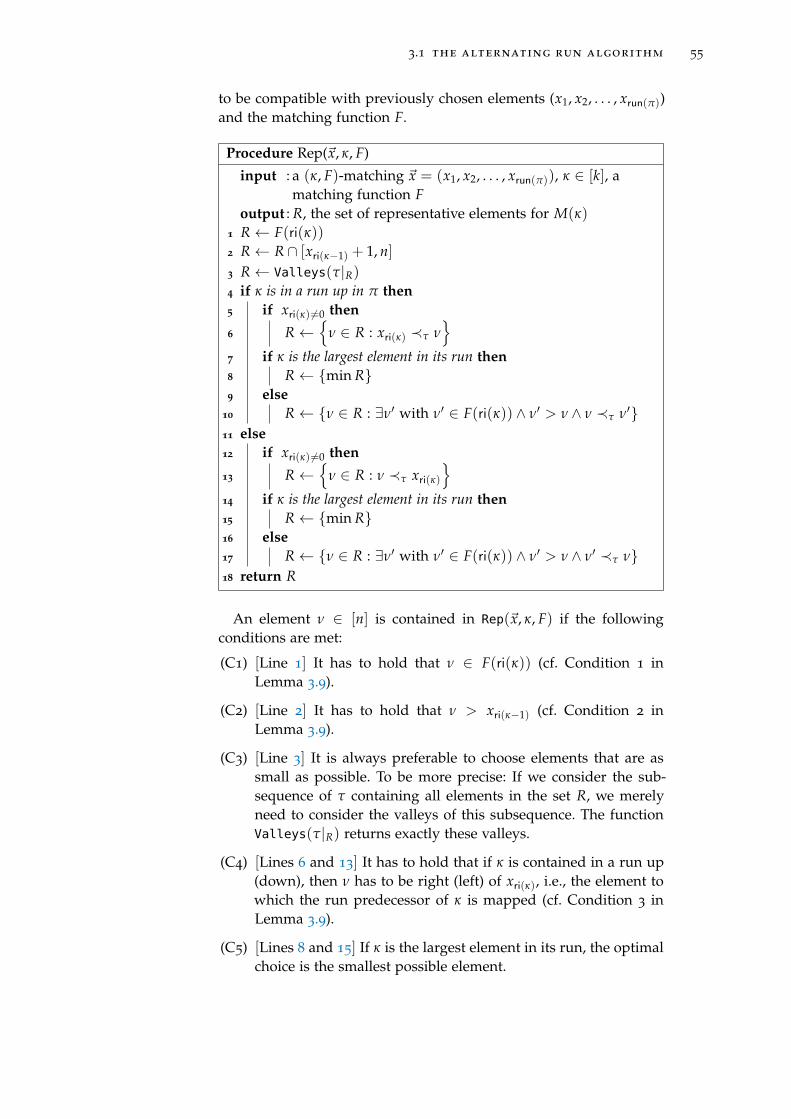
3.1 the alternating run algorithm 55
to be compatible with previously chosen elements (x1, x2, . . . , xrun(π))and the matching function F.
Procedure Rep(~x, κ, F)
input : a (κ, F)-matching ~x = (x1, x2, . . . , xrun(π)), κ ∈ [k], amatching function F
output : R, the set of representative elements for M(κ)
1 R← F(ri(κ))2 R← R ∩ [xri(κ−1) + 1, n]3 R← Valleys(τ|R)4 if κ is in a run up in π then5 if xri(κ) 6=0 then
6 R←{
ν ∈ R : xri(κ) ≺τ ν}
7 if κ is the largest element in its run then8 R← {min R}9 else
10 R← {ν ∈ R : ∃ν′ with ν′ ∈ F(ri(κ)) ∧ ν′ > ν ∧ ν ≺τ ν′}11 else12 if xri(κ) 6=0 then
13 R←{
ν ∈ R : ν ≺τ xri(κ)}
14 if κ is the largest element in its run then15 R← {min R}16 else17 R← {ν ∈ R : ∃ν′ with ν′ ∈ F(ri(κ)) ∧ ν′ > ν ∧ ν′ ≺τ ν}18 return R
An element ν ∈ [n] is contained in Rep(~x, κ, F) if the followingconditions are met:
(C1) [Line 1] It has to hold that ν ∈ F(ri(κ)) (cf. Condition 1 inLemma 3.9).
(C2) [Line 2] It has to hold that ν > xri(κ−1) (cf. Condition 2 inLemma 3.9).
(C3) [Line 3] It is always preferable to choose elements that are assmall as possible. To be more precise: If we consider the sub-sequence of τ containing all elements in the set R, we merelyneed to consider the valleys of this subsequence. The functionValleys(τ|R) returns exactly these valleys.
(C4) [Lines 6 and 13] It has to hold that if κ is contained in a run up(down), then ν has to be right (left) of xri(κ), i.e., the element towhich the run predecessor of κ is mapped (cf. Condition 3 inLemma 3.9).
(C5) [Lines 8 and 15] If κ is the largest element in its run, the optimalchoice is the smallest possible element.
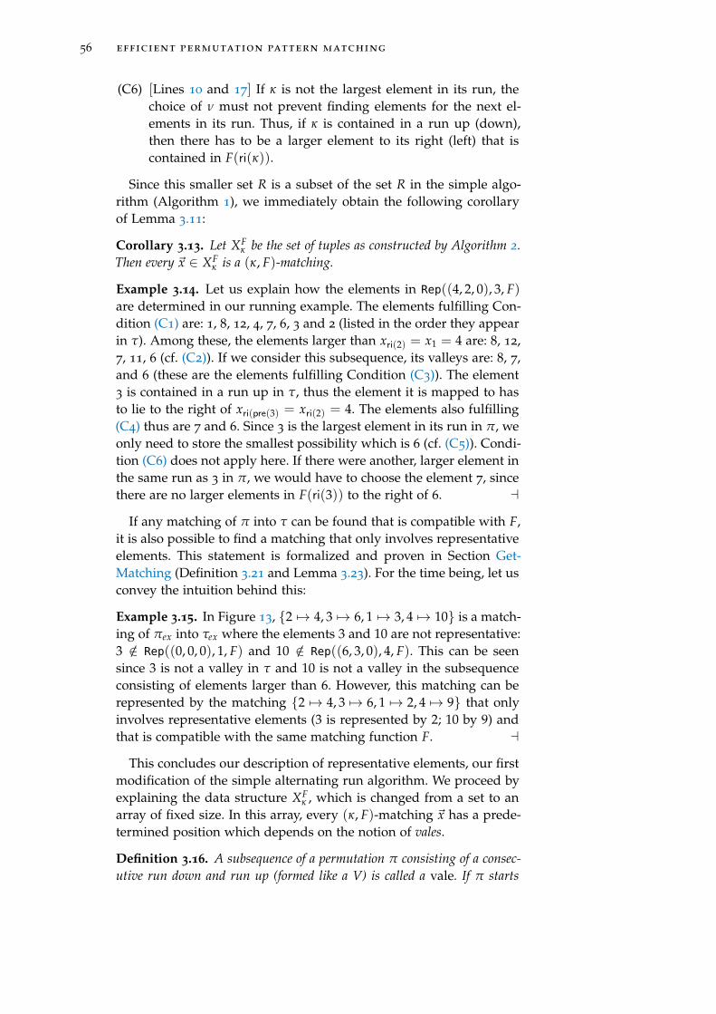
56 efficient permutation pattern matching
(C6) [Lines 10 and 17] If κ is not the largest element in its run, thechoice of ν must not prevent finding elements for the next el-ements in its run. Thus, if κ is contained in a run up (down),then there has to be a larger element to its right (left) that iscontained in F(ri(κ)).
Since this smaller set R is a subset of the set R in the simple algo-rithm (Algorithm 1), we immediately obtain the following corollaryof Lemma 3.11:
Corollary 3.13. Let XFκ be the set of tuples as constructed by Algorithm 2.
Then every ~x ∈ XFκ is a (κ, F)-matching.
Example 3.14. Let us explain how the elements in Rep((4, 2, 0), 3, F)are determined in our running example. The elements fulfilling Con-dition (C1) are: 1, 8, 12, 4, 7, 6, 3 and 2 (listed in the order they appearin τ). Among these, the elements larger than xri(2) = x1 = 4 are: 8, 12,7, 11, 6 (cf. (C2)). If we consider this subsequence, its valleys are: 8, 7,and 6 (these are the elements fulfilling Condition (C3)). The element3 is contained in a run up in τ, thus the element it is mapped to hasto lie to the right of xri(pre(3) = xri(2) = 4. The elements also fulfilling(C4) thus are 7 and 6. Since 3 is the largest element in its run in π, weonly need to store the smallest possibility which is 6 (cf. (C5)). Condi-tion (C6) does not apply here. If there were another, larger element inthe same run as 3 in π, we would have to choose the element 7, sincethere are no larger elements in F(ri(3)) to the right of 6. a
If any matching of π into τ can be found that is compatible with F,it is also possible to find a matching that only involves representativeelements. This statement is formalized and proven in Section Get-Matching (Definition 3.21 and Lemma 3.23). For the time being, let usconvey the intuition behind this:
Example 3.15. In Figure 13, {2 7→ 4, 3 7→ 6, 1 7→ 3, 4 7→ 10} is a match-ing of πex into τex where the elements 3 and 10 are not representative:3 /∈ Rep((0, 0, 0), 1, F) and 10 /∈ Rep((6, 3, 0), 4, F). This can be seensince 3 is not a valley in τ and 10 is not a valley in the subsequenceconsisting of elements larger than 6. However, this matching can berepresented by the matching {2 7→ 4, 3 7→ 6, 1 7→ 2, 4 7→ 9} that onlyinvolves representative elements (3 is represented by 2; 10 by 9) andthat is compatible with the same matching function F. a
This concludes our description of representative elements, our firstmodification of the simple alternating run algorithm. We proceed byexplaining the data structure XF
κ , which is changed from a set to anarray of fixed size. In this array, every (κ, F)-matching ~x has a prede-termined position which depends on the notion of vales.
Definition 3.16. A subsequence of a permutation π consisting of a consec-utive run down and run up (formed like a V) is called a vale. If π starts

3.1 the alternating run algorithm 57
3
1
2
10
2
8
9
5
= F(ri(1)) = F(ri(3))
4
7
= F(ri(2))
Figure 14: Schematic representation of the permutations occurring in Exam-ple 3.17: to the left the pattern π and to the right the text τ
with a run up, this run is also considered as a vale and analogously if π
ends with a run down. Let vale(π) denote the number of vales in π. Fi-nally, we define the vale index function vi(u): given a matching functionF and u ∈ F(i), let vi(u) = j if u is contained in the j-th vale in F(i). Fornotational convenience we set vi(0) = 1.
The main idea is the following: Two (κ, F)-matchings ~x and ~y in XFκ
with vi(xi) = vi(yi) for all i ∈ [run(π)] are comparable in the sensethat one of these is less likely to lead to a matching. More precisely,the (κ, F)-matching containing the larger element at the ri(κ)-th po-sition (this is also the largest element of the entire tuple) leads to amatching only if the other one leads to a matching as well. Thus, theformer (κ, F)-matching can be discarded and only the latter (κ, F)-matching has to be stored. The following example illustrates this no-tion of comparability:
Example 3.17. Consider the two permutations π and τ schematicallyrepresented in Figure 14. We are searching for representative ele-ments for κ = 3 which lies in a run down in π. Which elements κ
may be matched to depends on the choices for its run predecessorpre(3) = 1 and for κ− 1 = 2. For the element 1, two representative el-ements are 2 (circle) and 5 (square), the valleys in F(ri(1)) in τ. Theylead to one representative element for 2 each: if 2 has been chosenthen 4 is a representative element (circle) and if 5 has been chosenthen 7 (square) is one. At this point, we have the following two (2, F)-matchings: ~x = (. . . , 0, 2, 4, 0, . . .) and ~y = (. . . , 0, 5, 7, 0, . . .). On theone hand, ~x seems to be preferable since it involves smaller elementsthan ~y and this leaves more possibilities for the following elements.On the other hand, ~y seems to be preferable since it involves 5 inF(ri(1)), which is further to the right than 2. This is advantageoussince F(ri(1)) corresponds to a run down and this means that largerelements in the same run will have to be chosen to the left. All to-

58 efficient permutation pattern matching
gether we cannot say which of ~x and ~y is preferable and thus have tostore both of them.
When we now turn to the element 3 in π, there are three represen-tative elements: if we have chosen ~x the only possible choice is the el-ement 10; if we have chosen ~y there are two possible choices namely 8and 9. We thus obtain three (3, F) matchings: ~x′ = (. . . , 0, 10, 4, 0, . . .),~y′ = (. . . , 0, 8, 7, 0, . . .) and ~y′′ = (. . . , 0, 9, 7, 0, . . .). We can now ob-serve that we do not have to keep track of all three possibilities. In-deed, the two (3, F)-matchings ~x′ and ~y′ have coinciding vales and ~x′
can be discarded in favour of ~y′ since ~x′ will only lead to a matchingof π into τ if ~y′ does. This is due to the fact that x′ri(3) = 10 > 8 = y′ri(3)and can be seen as follows:
Let u be an element in the same run as 3 in π that is larger than 3(which means that it lies to the left of 3). All elements to the left ofand larger than 10 in F(ri(u)) are clearly also to the left of and largerthan 8. Thus, if there exists an element in Rep(~x′, u, F) there also existsa smaller element in Rep(~y′, u, F). This means that from the point ofview of the run containing 3, ~y′ is to be preferred over ~x′. Now letv > 3 be an element in the same run in π as 2 (which means that itlies to the right of 2). Representative elements for v have to both lieto the right of the element chosen for 2 (4 or 7) and be larger thanthe element chosen for 3 (10 or 8). Since 4 and 7 lie in the same valein τ there are no larger elements in between them. This implies thatelements that are to the right of 4 in F(ri(2)) and larger than 10 areautomatically to the right of 7 and larger than 8. From the point ofview of the run containing 2, ~y′ it also to be preferred over ~x′. Thesame argument also holds for any other element in π that is largerthan 3.
To put this example in a nutshell: if we have two (κ, F)-matchings~x and ~y with coinciding vales and yri(κ) ≤ xri(κ) we only need to store~y. For a formal proof of this statement, we refer to Lemma 3.25 onpage 67 in Section GetMatching. a
If we store only one (κ, F)-matching out of those with identicalvales, the question arises how many vales there are in F(i), i ∈ [run(π)].The answer is that at most brun(F(i))/2c + 1 exist: all vales but thetwo outermost consist of two runs and the two outermost may consistof only one run (cf. Definition 3.16). This would yield that we haveto store at most ∏run(π)
i=1
(b run(F(i)
2 c+ 1)
many (κ, F)-matchings. Thisnumber is still too large to show our desired runtime bounds. How-ever, it suffices to distinguish between brun(F(i))/2c many vales inF(i) with i ∈ [run(π)− 1]. This is achieved by not distinguishing be-tween the first and the last vale in F(i) for i < run(π). We only brieflymention that this is correct due to the Conditions (C5) and (C6); a for-mal proof will follow with Lemma 3.25 in Section GetMatching. Fori = run(π), the last run in π, we still consider all vales occurring inF(run(π)).

3.1 the alternating run algorithm 59
Recall that our goal is to assign a position in the array XFκ to every
(κ, F)-matching ~x. For every one of the run(π) values of the (κ, F)-matching there are at most brun(F(i)/2c vales that need to be dis-tinguished, except for the last one where we have to distinguishbetween brun(F(run(π)))/2c + 1 vales. Thus, it is natural to use amixed radix numeral system with bases b1 = brun(F(1)/2c, b2 =
brun(F(2)/2c, . . . , brun(π)−1 = brun(F(run(π) − 1)/2c and brun(π) isequal to the number of vales in F(run(π)). Let Index be the func-tion that assigns a position in the array to each (κ, F)-matching ~x =
(x1, . . . , xrun(π)):
Index(
x1, . . . , xrun(π)
)= 1 +
run(π)
∑i=1
(vi(xi)− 1 mod bi) ·i−1
∏j=1
bj.
The mod operator is required since for x ∈ F(i), vi(x) ∈ [bi + 1] – asexplained above.
Example 3.18. Let us discuss what the Index function looks like forour running example πex and τex (cf. Figure 13). The subsequenceF(1) contains four runs. Thus, b1 = 2. Since both F(2) and F(3) con-tain two runs, b2 = b3 = 1. Consequently, in our running example,XF
κ contains at most two elements for every κ ∈ [k]. For example,Index(8, 3, 10) = 1, Index(6, 3, 10) = 1 and Index(11, 3, 10) = 2. a
From the definition of the Index-function, it follows that the lengthof our array is ∏run(π)
i=1 bi. We will show in Lemma 3.28 that ∏run(π)i=1 bi =
O(
1.2611run(τ))
. At this point, we see the huge advantage of this ar-ray data structure over the set data structure in the simple algorithm:the set XF
κ has a potential size of nrunπ – too large for an fpt algorithm.This concludes the description of the array data structure. Let us
now – once again – return to our running example and see how thiswould be dealt with by the alternating run algorithm.
Example 3.19. Let us demonstrate how the alternating run algorithmworks. As before, consider τex, πex and the matching function F as rep-resented in Figure 13. We already know from the last example thatXF
κ has size 2, i.e., the Index function has range {1, 2}. We start withXF
0 = {(0, 0, 0)}. Refer to Table 2 for an overview. For the element1 in π the only representative element is 2. Since Index(0, 2, 0) = 1,we store this (1, F)-matching at position 1 in XF
1 . Position 2 remainsempty (symbolized by ε). For the element 2, we have more representa-tive elements: Rep((0, 2, 0), 2, F) = {4, 8}. Note that 3 is not a represen-tative element since there is no larger element to its right in F(ri(2)) =F(1) (cf. (C6)). Since Index(8, 2, 0) = 1 and Index(4, 2, 0) = 2, both(2, F)-matchings are stored in XF
2 . For placing the element 3, observethat 3 is the largest element in its run in π. Thus, Condition (C5)applies. We obtain Rep((8, 2, 0), 3, F) = min{11, 12} = {11} as well

60 efficient permutation pattern matching
Index(., ., .) = 1 Index(., ., .) = 2
XF1 (0, 2, 0) ε
XF2 (8, 2, 0) (4, 2, 0)
XF3 (6, 2, 0) (11, 2, 0)
XF4 (6, 2, 9) ε
Table 2: The arrays XF1 , . . . , XF
4 for our running example (cf. Figure 13)
as Rep((4, 2, 0), 3, F) = min{7, 6} = {6}. Thus, we have two (3, F)-matchings to store in XF
3 : (11, 2, 0) and (6, 2, 0) with Index(11, 2, 0) =2 and Index(6, 2, 0) = 1. Finally, we have to place the element 4. SinceRep((11, 2, 0), 4, F) = ∅ the (3, F)-matching (11, 2, 0) does not leadto a matching. However, Rep((6, 2, 0), 3, F) = {9}. Thus, XF
4 containsthe (4, F)-matching (6, 2, 9). This (4, F)-matching corresponds to thematching {2 7→ 4, 3 7→ 6, 1 7→ 2, 4 7→ 9}. a
Finally, it only remains to explain the GetMatching procedure. From
Procedure GetMatching(XF1 , . . . , XF
k )
input : k arrays XF1 , XF
2 , . . . , XFk generated by Algorithm 2
output : M, a matching of π into τ that is compatible with F1 for κ ← k . . . 1 do2 if κ = k then3 ~x ← some element in XF
k4 else5 ~x ← some element ~y in XF
κ with xi = yi for all i 6= ri(κ)
6 M(κ)← xri(κ)7 return M = (M(1), M(2), . . . , M(k))
Lemma 3.11 we know that if there is an element in XFk , a matching
from π into τ that is compatible with F exists. However, we havenot yet shown how a matching can be constructed from an elementin XF
k . This is what the GetMatching procedure does: it extracts anactual matching M : [k] → [n] out of the arrays XF
1 , . . . , XFk . We con-
struct M recursively: First, we pick some element ~x ∈ XFk and set
M(k) := xri(k). Now, suppose the matching has been determined forκ ∈ [k] and M(κ) = xri(κ) for some ~x ∈ XF
κ . Then there must exist anelement ~y ∈ XF
κ−1 that has led to the element ~x ∈ XFκ , i.e., ~y differs
from ~x only at the ri(κ)-th element. We define M(κ − 1) := yri(κ−1).This defines the function M : [k] → [n]. It can easily be seen with thehelp of Lemma 3.9 that the function M returned by the GetMatching
procedure is indeed a matching of π into τ that is compatible with F.This concludes our description of the alternating run algorithm. We
would like to remark that this description omits two minor details

3.1 the alternating run algorithm 61
necessary for obtaining the polynomial factor O(n · k) of the desiredruntime. The one detail concerns the calculation of the Index function.The second details concerns how data is stored in the array. Thesedetails are described in the proof of the runtime, Proposition 3.29.
Correctness
We start by providing the proof of Lemma 3.7, which states that forevery matching M there exists a matching function F such that M iscompatible with F.
Lemma 3.7. Given a matching M from π to τ, we will construct amatching function F such that M is compatible with F. In order todescribe F, it is enough to determine the first (=leftmost) elementlF(i) of every F(i), where i ∈ [run(π)]. In order to specify the last(=rightmost) element rF(i) of F(i) for i ∈ [run(π)], we simply need toapply the properties (P3) and (P4): rF(i) is either the last element in τ
or the leftmost valley (peak) in F(i + 1) in case that the i-th run is arun up (down). Clearly, lF(1) = τ(1), the first element in τ – cf. (P3).When determining lF(i), let lπ,i be the first element in the i-th run in π
and rπ,i be the last element in the i-th run in π. If the i-th run is a runup (down), lF(i) is the right-most element in τ not lying to the rightof M(lπ,i) and following a valley (peak). This construction guaranteesthat F is a matching function.
In order to prove that M is compatible with F, we need to showfor all i ∈ [run(π)] that lF(i) �τ M(lπ,i) and M(rπ,i) �τ rF(i). The firststatement holds by construction. For i = run(π), the second state-ment clearly also holds by construction. Let i ∈ [run(π)− 1]. Let usassume that the i-th run is a run up – the proof for runs down is anal-ogous. We distinguish between the following cases that are depictedin Figure 15:
• M(rπ,i) and M(lπ,i+1) lie in the same run in τ. Since we haveassumed that the i-th run in π is a run up, rπ,i is a peak in π.Hence, this case is only possible if M(rπ,i) is in a run down inτ and rπ,i > lπ,i+1. Thus, lF(i+1) is the first element in this run,which implies that rF(i) is the last element of this run and thusM(rπ,i) �τ rF(i).
• M(rπ,i) and M(lπ,i+1) do not lie in the same run in τ and theelement M(lπ,i+1) is in a run up in τ. In this case, rF(i) is the lastelement in the run down preceding this run and thus it clearlyholds that M(rπ,i) �τ rF(i).
• M(rπ,i) and M(lπ,i+1) do not lie in the same run in τ and the ele-ment M(lπ,i+1) is in a run down in τ. In this case, rF(i) is the lastelement in this run and again it clearly holds that M(rπ,i) �τ
rF(i).

62 efficient permutation pattern matching
� and ◦ in the samerun
� and ◦ not in thesame run; ◦ in a
run up
� and ◦ not in thesame run; ◦ in a
run down
LF(i+1)RF(i)
LF(i+1)RF(i)
LF(i+1)RF(i)
Figure 15: Three cases that have to be distinguished in the proof ofLemma 3.7 when showing that M(rπ,i) �τ rF(i) for all i ∈[run(π)− 1] under the assumption that the i-th run in π is a runup. The element M(rπ,i) is represented by a � and the elementM(lπ,i+1) by a ◦.
Example 3.20. Constructing F as described in the proof of Lemma 3.7for the matching 4 6 2 9 of πex into τex yields the matching functionrepresented in Figure 13. a
Next, we prove Lemma 3.9. This lemma states that a function Mfrom the set [k] into the set [n] is a matching of π into τ compatiblewith F if and only if for every κ ∈ [k]:
1. M(κ) ∈ F(ri(κ)),
2. M(κ) > M(κ − 1) and
3. if pre(κ) exists, then pre(κ) ≺π κ if and only if M(pre(κ)) ≺τ
M(κ), i.e., if κ is contained in a run up (down), then M(κ) isright (left) of M(pre(κ)).
Lemma 3.9. Let M:[k] → [n] be a matching of π into τ that is com-patible with F. Recall Definition 2.5 which states that M has to be amonotonically increasing function. This implies the second condition.Moreover, the sequence M(π) = M(π(1)), M(π(2)), . . . , M(π(k)) hasto be a subsequence of τ. This means nothing else than M(π(1)) ≺τ
M(π(2)) ≺τ . . . ≺τ M(π(k)). In particular it must hold that M(u) ≺τ
M(v), where u and v are two neighbouring elements in the same runin π with u ≺π v. This implies the third condition. Finally, the firstcondition follows directly from the definition of compatibility (Defi-nition 3.6).
Let M:[k] → [n] be a function fulfilling the three conditions statedabove. The second condition implies that M is monotonically increas-ing. In order to show that M is indeed a matching of π into τ, we

3.1 the alternating run algorithm 63
have to show that M(π) = M(π(1)), M(π(2)), . . . , M(π(k)) is a sub-sequence of τ. In other words, we have to show that for all i ∈ [k− 1]it holds that M(π(i)) ≺τ M(π(i + 1)). We distinguish three cases:
• The elements π(i) and π(i + 1) lie in the same run in π. Thus,for the case of a run up (down) we have π(i) = pre(π(i + 1))(π(i + 1) = pre(π(i))). With κ = π(i + 1) (κ = π(i)) it followsfrom the third condition that M(π(i)) ≺τ M(π(i + 1)) (in bothcases).
• The elements π(i) and π(i + 1) do not lie in the same run in π
and M(π(i)) and M(π(i + 1)) do not lie in the same run in τ.If π(i) lies in the j-th run in π, the first condition implies thatM(π(i)) lies in F(j) and that M(π(i + 1)) lies in F(j + 1) in τ.Then property (P4) of matching functions (the leftmost run ofF(j + 1) is the rightmost run of F(j)) implies that M(π(i)) liesto the left of M(π(i + 1)) in τ.
• The elements π(i) and π(i + 1) do not lie in the same run in π
but M(π(i)) and M(π(i + 1)) lie in the same run in τ. By thedefinition of matching functions and since it holds that M(κ) ∈F(ri(κ)) for all κ ∈ [k], this can only be possible if M(π(i)) isin the last run of F(j) and M(π(i + 1)) is in the first run ofF(j + 1) for some j ∈ [run(π)]. Thus, if π(i) lies in a run up(down) in π both M(π(i)) and M(π(i + 1)) are contained ina run down (up) in τ. On the other hand, if π(i) is in a runup (down) it must be a peak (valley) and thus it holds thatπ(i) > π(i + 1) (π(i) < π(i + 1)). The second condition thenensures that M(π(i)) > M(π(i + 1)) (M(π(i)) < M(π(i + 1))),which implies that M(π(i)) lies to the left of M(π(i + 1)) in τ.
The function M is thus a matching of π into τ additionally fulfillingthat M(κ) ∈ F(ri(κ)) which means that M is a matching compatiblewith F.
Lemma 3.11 states that in Algorithm 1, ~x ∈ XFκ is a (κ, F)-matching.
This can be shown as follows:
Lemma 3.11. We prove this statement by induction over κ. For κ =
1 this is easy: An element ~x ∈ XF1 looks as follows: xi = 0 for all
i 6= ri(1) and xri(1) is equal to some u ∈ F(ri(1)). Thus, the functionM : [1]→ [n] with M(1) = u is clearly a (1, F)-matching.
Now suppose we have proven the statement of Lemma 3.11 forκ − 1 and we want to prove it for κ. If ~x ∈ XF
κ , then there mustexist an element ~y ∈ XF
κ−1 and an element ν ∈ [n] such that ~x =
(y1, . . . , yri(κ)−1, ν, yri(κ)+1, . . . , yrun(π)) (see lines 5 to 8 in Algorithm 1).This element ν may not be any arbitrary element, it must fulfil thefollowing conditions (see Algorithm 1, Line 6): ν ∈ F(ri(κ)), ν >
xri(κ−1)) and pre(κ) ≺π κ if and only if xri(pre(κ)) ≺τ ν. Since ~y ∈ XFκ−1 it

64 efficient permutation pattern matching
is a (κ− 1, F)-matching and thus there exists a function M : [κ− 1]→[n] that is a matching of π|[κ−1] into τ that is compatible with F andfor which it additionally holds that for every yi 6= 0, M(max{κ′ ≤κ − 1 : ri(κ′) = i}) = yi.
We now define a function M : [κ] → [n] as follows: M(u) = M(u)for all u ∈ [κ − 1] and M(κ) = ν. We will see that this function Mis a witness for the fact that ~x is a (κ, F)-matching. For this purposewe have to check that the three conditions in Lemma 3.9 are fulfilledfor every u ∈ [κ]. For u < κ these conditions are necessarily fulfilledsince we then have M(i) = M(i) and M is a matching of π|[κ−1]into τ that is compatible with F. For u = κ, i.e., M(u) = ν, theseconditions are exactly those stated above that must be fulfilled bythe element ν ∈ [n]. The last condition in Definition 3.10, namelythat for every xi 6= 0, M(max{κ′ ≤ κ : ri(κ′) = i}) = xi, is fulfilledsince M is a witness for the fact that ~y is a (κ − 1, F)-matching andsince we defined M(κ) to be equal to ν = xri(κ). Thus, ~x is a (κ, F)-matching.
The next lemma shows that it is sound to consider elements re-turned by the Rep procedure only.
Definition 3.21. Let F be a matching function and~x = (x1, x2, . . . , xrun(π))
be a (κ, F)-matching for some κ ∈ [k]. A matching M (κ, F)-extends ~x ifM is compatible with F and if for every xi 6= 0, M(max{κ′ ≤ κ : ri(κ′) =i}) = xi, i.e., M maps the largest element ≤ κ in the i-th run of π to thei-th element of ~x.
Definition 3.22. Let ~x = (x1, . . . , xrun(π)). In the following, we write~x(ri(κ)← ν) instead of (x1, . . . , xri(κ)−1, ν, xri(κ)+1, . . . , xrun(π)).
Lemma 3.23. Let κ ∈ [k] and ~x ∈ XFκ . If there exists a matching M that
(κ, F)-extends ~x, then there exist an element ν ∈ Rep(~x, κ + 1, F) and amatching M that (κ + 1, F)-extends ~x(ri(κ + 1)← ν).
Proof. Let us first explicitly show how to pick the element ν. Then wewill prove that it indeed holds that ν is in Rep(~x, κ + 1, F). We defineM as follows: M(κ + 1) := ν and M(u) := M(u) otherwise. Finally,we will see that M is a matching that (κ + 1, F)-extends ~x(ri(κ + 1)←ν).
In order to increase legibility, let i ∈ [k] be the position for whichπ(i) = κ + 1. Let us then consider the set S consisting of all elementsin τ that lie to the right of M(π(i− 1)) and to the left of M(π(i + 1)),that are contained in F(ri(κ + 1)) and that are larger than M(κ) =
xri(κ). More formally, we have
S :={u ∈ [n] : M(π(i− 1)) ≺τ u ≺τ M(π(i + 1))}∩ F(ri(κ + 1)) ∩ [M(κ) + 1, n].
This set is never empty: Especially, M(κ + 1) is contained in S sinceM is a matching that (κ, F)-extends ~x. We now define ν := min(S).
3.1 the alternating run algorithm 65
We have to check that it indeed holds that ν ∈ Rep(~x, κ + 1, F). Werefer the reader to the definition of Rep(~x, κ + 1, F) on page 55.
• (C1) is fulfilled by construction of S.
• (C2) is fulfilled since ν > M(κ − 1) = xri(κ−1).
• (C3) is fulfilled: ν is a valley in the subsequence of τ consistingof elements larger than M(κ) by construction of S.
• (C4) If the run predecessor of κ + 1 exists and κ + 1 lies in a runup (down), pre(κ + 1) = π(i− 1) (pre(κ + 1) = π(i + 1)). More-over, note that M(pre(κ + 1)) = xri(κ+1) since M (κ, F)-extends~x. Since S ⊆ {u ∈ [n] : M(π(i− 1)) ≺τ u ≺τ M(π(i + 1))}, it isguaranteed that ν lies on the correct side of xri(κ+1).
• (C5) In case κ + 1 is the largest element in its run in π, there isonly a single element in Rep(~x, κ + 1, F) which is exactly ν.
• (C6) In case κ + 1 is not the largest element in its run in π
and κ + 1 lies in a run up (down), the element M(π(i + 1))(M(π(i − 1))) is an element larger than ν that lies to the right(left) of ν in F(ri(κ + 1)) since M is compatible with F.
Now let us show that M as defined above is a matching that (κ +
1, F)-extends ~x(ri(κ + 1) ← ν). First we need to show that the func-tion M is a matching of π into τ that is compatible with F. HereLemma 3.9 comes in handy since it tells us that we only have to checkthe following three conditions for all u ∈ [k]:
1. M(u) ∈ F(ri(u)): For u = κ + 1 this holds by construction of ν
and for u 6= κ + 1 this holds since we then have M(u) = M(u)and M is a matching that is compatible with F.
2. M(u + 1) > M(u) for u 6= k: For u /∈ {κ, κ + 1} this again holdssince M is a matching.
u = κ: By the construction of S, M(κ + 1) = ν > M(κ) = M(κ).
u = κ + 1: Again by the construction of S we know that ν ≤M(κ + 1). Since M is a matching M(κ + 1) < M(κ + 2) = M(κ +
2) it follows that ν = M(κ + 1) < M(κ + 2).
3. If pre(u) exists, then pre(u) ≺π u if and only if M(pre(u)) ≺τ
M(u): Since M is a matching, we only have to check this condi-tion for κ + 1 and its run predecessor pre(κ + 1) as well as for κ +
1 and κ′, the next largest element in the same run in π (we couldcall this element the run successor of κ + 1), i.e., pre(κ′) = κ + 1.If κ + 1 lies in a run up (down), we have pre(κ + 1) = π(i− 1)and κ′ = π(i + 1) (pre(κ + 1) = π(i + 1) and κ′ = π(i− 1) ). Byconstruction of S we have that M(π(i− 1)) = M(π(i− 1)) ≺τ
ν = M(κ + 1) ≺τ M(π(i + 1)) = M(π(i + 1)) and thus thiscondition is also fulfilled.
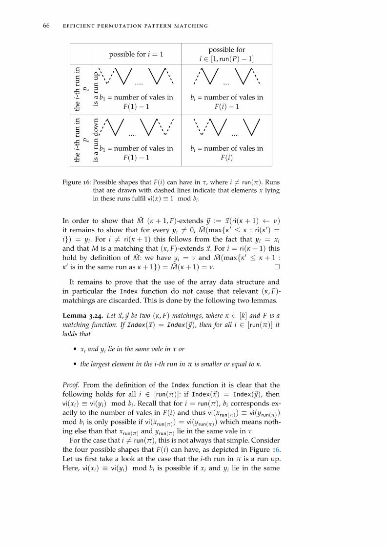
66 efficient permutation pattern matching
possible for i = 1possible for
i ∈ [1, run(P)− 1]
the
i-th
run
inP
isa
run
upb1 = number of vales in
F(1)− 1bi = number of vales in
F(i)− 1
the
i-th
run
inP
isa
run
dow
n
b1 = number of vales inF(1)− 1
bi = number of vales inF(i)
Figure 16: Possible shapes that F(i) can have in τ, where i 6= run(π). Runsthat are drawn with dashed lines indicate that elements x lyingin these runs fulfil vi(x) ≡ 1 mod bi.
In order to show that M (κ + 1, F)-extends ~y := ~x(ri(κ + 1) ← ν)
it remains to show that for every yi 6= 0, M(max{κ′ ≤ κ : ri(κ′) =
i}) = yi. For i 6= ri(κ + 1) this follows from the fact that yi = xiand that M is a matching that (κ, F)-extends ~x. For i = ri(κ + 1) thishold by definition of M: we have yi = ν and M(max{κ′ ≤ κ + 1 :κ′ is in the same run as κ + 1}) = M(κ + 1) = ν.
It remains to prove that the use of the array data structure andin particular the Index function do not cause that relevant (κ, F)-matchings are discarded. This is done by the following two lemmas.
Lemma 3.24. Let ~x,~y be two (κ, F)-matchings, where κ ∈ [k] and F is amatching function. If Index(~x) = Index(~y), then for all i ∈ [run(π)] itholds that
• xi and yi lie in the same vale in τ or
• the largest element in the i-th run in π is smaller or equal to κ.
Proof. From the definition of the Index function it is clear that thefollowing holds for all i ∈ [run(π)]: if Index(~x) = Index(~y), thenvi(xi) ≡ vi(yi) mod bi. Recall that for i = run(π), bi corresponds ex-actly to the number of vales in F(i) and thus vi(xrun(π)) ≡ vi(yrun(π))
mod bi is only possible if vi(xrun(π)) = vi(yrun(π)) which means noth-ing else than that xrun(π) and yrun(π) lie in the same vale in τ.
For the case that i 6= run(π), this is not always that simple. Considerthe four possible shapes that F(i) can have, as depicted in Figure 16.Let us first take a look at the case that the i-th run in π is a run up.Here, vi(xi) ≡ vi(yi) mod bi is possible if xi and yi lie in the same

3.1 the alternating run algorithm 67
vale in τ or if xi lies in the first vale in F(i) and yi lies in the last runin F(i) (or vice-versa). Now recall the definition of the Rep procedure:an element in the last run (which is always a run down) may only bechosen for the largest element in its run in π (Condition (C6)). Thismeans that the largest element in the i-th run in π must be smaller orequal to κ. Now let us consider the case that the i-th run in π is a rundown. Here, if xi and yi do not lie in the same vale in τ, vi(xi) ≡ vi(yi)
mod bi is only possible for i = 1 and if τ starts with a run up: xi hasto then lie in this first run of τ and yi in the last vale of F(1) (or vice-versa). Again, because of Condition (C6), this is only possible for thelargest element in its run in π. Thus, we can again conclude that thelargest element in the i-th run in π must be smaller or equal to κ.
Lemma 3.25. Let ~x,~y be two (κ, F)-matchings, where κ ∈ [k] and F isa matching function. In addition to that, let νx ∈ Rep(~x, κ + 1, F) andνy ∈ Rep(~y, κ + 1, F). If
Index(~x(ri(κ + 1)← νx)) = Index(~y(ri(κ + 1)← νy))
and νy ≤ νx the following holds: if there exists a matching that (κ + 1, F)-extends ~x(ri(κ + 1) ← νx), then there exists a matching that (κ + 1, F)-extends ~y(ri(κ + 1)← νy). Thus, the alternating run algorithm only has tokeep track of the (κ + 1, F)-matching ~y(ri(κ + 1)← νy).
Proof. Let Mx be a matching of π into τ that (κ + 1, F)-extends ~x(ri(κ +1) ← νx). We shall construct a function My : [k] → [n] and show thatit is a matching that (κ + 1, F)-extends ~y(ri(κ + 1)← νy).
Since ~y is a (κ, F)-matching (Recall Definition 3.10) there exists apartial matching M : [κ]→ [n] of π|[κ] into τ for which it additionallyholds that for every yi 6= 0, M(max{κ′ ≤ κ : ri(κ′) = i}) = yi. Wedefine the function My as follows:
My(u) =
M(u), for u ∈ [κ]
νy, for u = κ + 1
Mx(u), for u ∈ [κ + 2, k]
We now need to show that My is indeed a matching that (κ + 1, F)-extends ~y(ri(κ + 1) ← νy). As in the proof of Lemma 3.23, we shalluse Lemma 3.9 to show that My is a matching that is compatible withF. We have to check the following three conditions for all u ∈ [k]:
1. My(u) ∈ F(ri(u)): For u = κ + 1 this holds since νy ∈ Rep(~y, κ +
1, F) (Condition (C1)) and for u 6= κ + 1 this holds since Mx andM are matchings that are compatible with F.
2. My(u + 1) > My(u) for u 6= k: For u /∈ {κ, κ + 1} this againholds since Mx and M are matchings.

68 efficient permutation pattern matching
a) My(κ + 1) > My(κ) or equivalently νy > M(κ) = yri(κ):This holds since νy ∈ Rep(~y, κ + 1, F) (Condition (C2)).
b) My(κ + 2) > My(κ + 1) or equivalently Mx(κ + 2) > νy:Since Mx is a matching that (κ+ 1, F)-extends ~x(ri(κ+ 1)←νx) it has to hold that Mx(κ + 2) > Mx(κ + 1) = νx. Sincewe have νy ≤ νx, this condition is fulfilled.
3. If pre(u) exists, then pre(u) ≺π u if and only if My(pre(u)) ≺τ
My(u): Since Mx and M are matchings, this condition is fulfilledfor all u ∈ [k] such that both u < κ + 1 and pre(u) < κ + 1 orsuch that both u > κ + 1 and pre(u) > κ + 1. Thus, we onlyhave to check this condition for u = κ + 1 and for all κ′ ∈[κ + 2, k] that satisfy pre(κ′) ≤ κ + 1. Let K be the set of all suchκ′. Observe that such a κ′ is the smallest element in the ri(κ′)-thrun in π that is strictly larger than κ + 1. This means that pre(κ′),if it exists, is the largest element in the ri(κ′)-th run in π that issmaller or equal to κ + 1. We only consider the case that u iscontained in a run up – the proof for the case that u lies in arun down works analogously. We have to check the conditionfor the following three situations:
a) u = κ + 1: If pre(κ + 1) exists it has to hold that My(pre(κ +
1)) = yri(κ+1) ≺τ νy. This condition is fulfilled since νy ∈Rep(~y, κ + 1, F) (Condition (C4)).
b) u = κ′ ∈ K such that pre(κ′) = κ + 1: If this element κ′
exists we have to show that νy ≺τ My(κ′) = Mx(κ′). Sinceκ + 1 is not the largest element in its run in π, we knowfrom Lemma 3.24 that νx and νy lie in the same vale in τ.Moreover we know that νx ≥ νy – but what does this implyfor the right-left order of νx and νy within this vale? Twocases may occur: νx may lie in the run up or in the rundown of this vale. If νx lies in the run up, then it has tohold that νy ≺τ νx. Since Mx is a matching, it has to holdthat νx = Mx(κ + 1) ≺τ Mx(κ′) and thus νy ≺τ Mx(κ′). Ifνx lies in the run down, νx ≺τ νy and all elements betweenνx and νy in τ are smaller than vx. This implies that Mx(κ′)which is larger than νx and lies to the right of νx also hasto lie to the right of νy in τ.
c) u = κ′ ∈ K with pre(κ′) < κ + 1: We need to show thatyri(pre(κ′)) = yri(κ′) = M(pre(κ′)) ≺τ Mx(κ′). Since Mx isa matching that (κ + 1, F)-extends ~x(ri(κ + 1) ← νx), weknow that Mx(pre(κ′)) = xri(κ′) and that xri(κ′) ≺τ Mx(κ′).Moreover, since Index(~x(ri(κ + 1)← νx)) = Index(~y(ri(κ +
1) ← νy)) and pre(κ′) is not the largest element in its runin π we know from Lemma 3.24 that xri(κ′) and yri(κ′) lie inthe same vale in τ. However, nothing is known about therelative positions of these two elements within this vale

3.1 the alternating run algorithm 69
and we have to distinguish two cases. If yri(κ′) ≺τ xri(κ′) thestatement follows easily since yri(κ′) ≺τ xri(κ′) ≺τ Mx(κ′). Ifxri(κ′) ≺τ yri(κ′) we have to collect a few more arguments inorder to prove that the condition holds. By transitivity andthe condition checked in Point 2. of this proof we knowthat yri(κ′) < νy = My(κ + 1) < Mx(κ′). Now note thatthe elements that lie in τ between xri(κ′) and yri(κ′) are allsmaller than max(xri(κ′), yri(κ′)) (since both are contained inthe same vale). Thus, the element Mx(κ′) – that is to theright of xri(κ′) and larger than yri(κ′) – has to lie to the rightof yri(κ′). This is what we wanted to prove.
Let ~y′ = ~y(ri(κ + 1) ← νy). It remains to show that for every i ∈[run(π)] with y′i 6= 0, My(max{κ′ ≤ κ + 1 : ri(κ′) = i}) = y′i. Thisfollows directly from the definition of My(κ + 1) and the fact that Mis a witness for ~y being a (κ, F)-matching.
Finally, we have gathered all necessary information to prove thecorrectness of the alternating run algorithm.
Proposition 3.26. π can be matched into τ if and only if XFk is non-empty
for some matching function F.
Proof. (⇒) If there is a matching of π into τ, then there is at least onematching function F for which XF
k is nonempty:Since there exists a matching M, we know from Lemma 3.7 that thereexists some matching function F such that M is compatible with F.Let us fix this F. We prove by induction over κ ∈ [k] that there is an~x ∈ XF
κ and a matching Mκ that (κ, F)-extends ~x. For κ = 1 this iseasy. Let ν be the valley in τ that lies in the same vale as M(1). Itis clear that ν ∈ Rep((0, . . . , 0), 1, F). Consequently, the tuple ~x withxi = 0 for i 6= ri(1) and xri(1) = ν is contained in XF
1 . Observe thatM1 being defined by M1(u) = M(u) for u 6= 1 and M1(1) = ν is amatching that (1, F)-extends ~x.
Now, let κ ∈ [k] and assume that ~x ∈ XFκ and Mκ κ-extends ~x. We
show that there exist an ~x′ ∈ XFκ+1 and a Mκ+1 that (κ + 1)-extends
~x′. By Lemma 3.23, there exists a ν ∈ Rep(~x, κ + 1, F) and a matchingMκ+1 that (κ + 1)-extends ~x(ri(κ + 1) ← ν). At this point, we can-not be sure that ~x(ri(κ + 1) ← ν) ∈ XF
κ+1 since XFκ+1 may contain
another (κ, F)-matching ~y with Index(~x) = Index(~y). However, thisis only possible if yri(κ+1) ≤ xri(κ+1) (see Line 10 in Algorithm 2). ByLemma 3.25 we know that, in this case, there exists a matching that(κ + 1)-extends ~y. So, no matter whether ~x(ri(κ + 1) ← ν) ∈ XF
κ+1or not, we can conclude that there is an ~x′ ∈ XF
κ+1 and a matchingfunction Mκ+1 that (κ + 1)-extends ~x′. By induction, we have shownthat XF
k 6= ∅.(⇐) If there is a matching function F such that the corresponding XF
kis non-empty, then a matching of π into τ can be found: This is animmediate consequence of Corollary 3.13.
70 efficient permutation pattern matching
Finally, let us remark that the function M returned by the proce-dure GetMatching(XF
1 , . . . , XFk ) is indeed a matching, as can easily be
seen with the help of Lemma 3.9: The first condition in the lemma issatisfied because of Condition (C1) for representative elements. Thesecond condition holds because of Condition (C2). The third condi-tion corresponds to Condition (C4). Note that(C3), (C5) and (C6) areonly required for improving the runtime.
Runtime
We are now going to prove the promised fpt runtime bounds. First,we bound the number of matching functions.
Lemma 3.27. There are less than (√
2)run(τ)
functions from [runπ] to sub-sequences of τ that satisfy (P1) to (P4).
Proof. A matching function F can be uniquely characterized by fixingthe position of the first run up in every F(i) for i ∈ [run(π)]. Thisis because the last run of F(i) is the first run of F(i + 1) for all i ∈[run(π) − 1]. Moreover the first run up in F(1) is always the firstrun up in τ. Thus, the number of matching functions is equal to thenumber of possibilities of picking run(π)− 1 runs (for the first run inπ no choice has to be made) among the at most drun(τ)/2e runs upin τ. Hence, we obtain
(drun(τ)/2erun(π)− 1
)≤ 2drun(τ)/2e−1 < (
√2)
run(τ).
The first inequality holds since (nk) < 2n−1 for all n, k ∈ N as can
easily be proven by induction over n.
Now we bound the size of XFκ , which is the main step to achieve
the 1.79run(τ) runtime bound.
Lemma 3.28. For any given matching function F and every κ ∈ [k]
|XFκ | ≤ 2 ·
run(π)
∏i=1
run(F(i))2
≤ 1.6 · 1.261071run(τ).
Proof. Recall that each (κ, F)-matching in XFκ has a position as deter-
mined by the function Index, defined by
Index(x1, . . . , xrun(π)) = 1 +run(π)
∑i=1
(vi(xi) mod bi) ·i−1
∏j=1
bj.
For i ∈ [run(π) − 1] we have bi = brun(F(i)/2c and for i = run(π)
brun(π) ≤ brun(F(run(π))/2c+ 1 since brun(π) is equal to the number

3.1 the alternating run algorithm 71
of vales in F(run(π))1. The range of Index is{
1, . . . , ∏run(π)i=1 bi
}. Since
the function Index determines the positions in the array XFκ , we obtain
|XFκ | =
run(π)
∏i=1
bi ≤run(π)−1
∏i=1
⌊run(F(i))
2
⌋·(⌊
run(F(run(π)))
2
⌋+ 1)
and consequently
|XFκ | ≤ 2 ·
run(π)
∏i=1
run(F(i))2
. (16)
We want to bound XFκ and thus want to know when the product in
Equation (16) is maximal. The maximum of this product has to bedetermined under the condition that
run(π)
∑i=1
run(F(i)) = run(τ) + run(π)− 1, (17)
since two subsequent F(i)’s have one run in common (cf. Defini-tion 3.4). The inequality of geometric and arithmetic means impliesthat the product in Equation (16) is maximal if all run(F(i)) are equal,i.e., for every i ∈ run(π), run(F(i)) = run(τ)+run(π)−1
run(π). Therefore, XF
κ
has at most 2 ·(run(τ)+run(π)−1
2·run(π)
)run(π)elements. To shorten the proof,
we write in the following p for run(π) and t for run(τ).Thus, we want to determine the maximum of the function
g(p) =(
t + p− 12p
)p
(we omit the factor 2 for the calculation). The derivative of g(p) is:
g′(p) =1p
(2−p
( p + t− 1p
)p−1· h(p)
)
where h(p) =(p + t− 1)(
log(
p + t− 1p
)− log(2)
)− t + 1.
And thus:
g′(p) = 0→ h(p) = 0→ log(
p + t− 12p
)=
t− 1p + t− 1
.
The solutions are:
p1(t) = (−1 + t)/(−1 + 2e1+W0(−1/(2e)))
p2(t) = (−1 + t)/(−1 + 2e1+W−1(−1/(2e))),
1 The reason why we do not set brun(π) = brun(F(run(π))/2c is a rather technical one:F(run(π)) may end with a run up if the last run in π is a run up and may endwith a run down if the last run in π is a run down. This would lead to unwantedcollisions concerning the Index function and consequently would prohibit the proofof Lemma 3.24.
72 efficient permutation pattern matching
where W0 is the principal branch of the Lambert function (defined byx = W(x) · eW(x)) and W−1 its lower branch. It holds that
(−1 + t)/3.311071 ≤ p1(t) ≤ (−1 + t)/3.311070
(−1 + t)/− 0.62663 ≤ p2(t) ≤ (−1 + t)/− 0.62664,
The second solution p2(t) is negative and therefore of no interest tous. The first solution p1(t) is a local maximum as can be checkedeasily and yields
g(p1) ≤(
t + (−1 + t)/3.311070− 12(−1 + t)/3.311071
)(−1+t)/3.311070
≤ 0.80 · (1.261071)t .
It therefore holds that |XFκ | ≤ 1.6 · 1.261071run(τ).
Proposition 3.29. The runtime of the alternating run algorithm (Algo-rithm 2) is O(1.784run(τ) · n · k).
Proof. The main structure of the algorithm is the following: for ev-ery matching function F and for every κ ∈ [k] the array XF
κ is com-
puted. There are (√
2)run(τ)
matching functions (Lemma 3.27). Themaximal number of elements in XF
κ is 1.6 · 1.2611run(τ) (Lemma 3.28).Given a matching function and an element κ ∈ [k], the algorithm hasto execute Lines 6 to 11 for every ~x ∈ XF
κ−1. Once we have shownthat the runtime of these lines is O(n), we obtain a total runtime of
O((√
2)run(τ) · 1.2611run(τ) · k · n
)= O(1.784run(τ) · k · n).
So it remains to show that the runtime of the Lines 6 to 11 is O(n).First, observe that determining the set R with the help of the Rep
procedure requires O(n) time. Second, for every element in R theLines 8, 10 and 11 are executed. Since R only contains valleys (ofsome subsequence of τ), its size is less than run(τ). Assuming unitcost for arithmetic operations, computing Index requires O(run(π))
time. However, note that it is not necessary to repeat all calculationsfor Index for every element ν in R. Indeed, for a fixed ~x ∈ XF
κ , theelements for which Index is computed at Line 8 only differ at theri(κ)-th position. Assume that we have already computed Index(~x)for some ~x. Computing Index(~y) for a ~y that is identical to ~x exceptat the ri(κ)-th position can be done as follows:
Index(~y) =Index(~x)
+(vi(yri(κ))− vi(xri(κ)) mod bri(κ)
)·ri(κ)−1
∏j=1
bj.
Consequently, Line 8 requires (amortized) constant time.Checking the condition in Line 10 requires only constant time. How-
ever, Line 11 requires O(run(π)) time to write the (κ, F)-matching

3.1 the alternating run algorithm 73
to its position in XFκ . This is too much time to obtain the desired
runtime bound – we can only afford amortized O(n) time per ~x ∈XF
κ−1. This can be achieved by executing Line 11 at most once per~x ∈ XF
κ−1. Let ν ∈ R be the first element for which the conditionat Line 10 is fulfilled. For this element Line 11 is executed and apointer p′ to the position Index(~x(ri(κ) ← ν)) is created. (Recallthe ~x(ri(κ) ← ν) notation from Definition 3.22.) If the condition atLine 10 is fulfilled for the same ~x and some other ν′ ∈ R, we donot execute Line 11. Instead we only store the pointer p′ and theelement ν′. This is sufficient information since two (κ, F)-matchingsin Line 11 that originate from the same ~x are identical except forthe ri(κ)-th element. It might be that Line 11 is executed for someother element ~y ∈ XF
κ−1 and νy ∈ Rep(~y, κ, F) at a later point. It isthen possible that a (κ, F)-matching ~x(ri(κ) ← ν) is overwritten thathas other (κ, F)-matchings ~x(ri(κ)← ν′) pointing to it. However, thiscan only happen in the following situation: ~x(ri(κ) ← ν′) is (κ, F)-extendable only if ~y(ri(κ) ← ν′) is (κ, F)-extendable. (It holds thatIndex(~x(ri(κ)← ν′)) = Index(~y(ri(κ)← ν′)). Lemma 3.25 shows thatif ~x(ri(κ) ← ν′) is (κ, F)-extendable, then so is ~y(ri(κ) ← ν′). Strictlyspeaking Lemma 3.25 is not applicable since it is not guaranteed thatν′ ∈ Rep(~y, κ, F) because ν′ might not be a valley in the correspondingsubsequence of τ (cf. Condition (C3)). However, all other conditionsare satisfied and this suffices to prove Lemma 3.25.) Therefore, thismodified array data structure is equivalent to the original data struc-ture described in Section 3.1. Thus, we have shown that Lines 6 to 11
have a runtime of O(n), if we modify the array data structure to alsoallow for pointers. This concludes our proof.
We conclude this section about the runtime of the alternating runalgorithm by proving that an even smaller constant than 1.784 can beexpected. Indeed, the following holds:
Theorem 3.30. Let Rn be the random variable counting the number of al-ternating runs in an n-permutation chosen uniformly at random amongstall n-permutations. Then for n ≥ 2 we have: E
(1.784Rn
)= O (1.515n).
Proof. In the following, let Rn,m denote the number of n-permutationswith exactly m alternating runs. Then the mean of Rn is given asfollows:
E(Rn) = ∑m≥1
m · Rn,m
n!.
By the law of the unconscious statistician we then have that:
E(
1.784Rn)= ∑
m≥11.784m · Rn,m
n!.
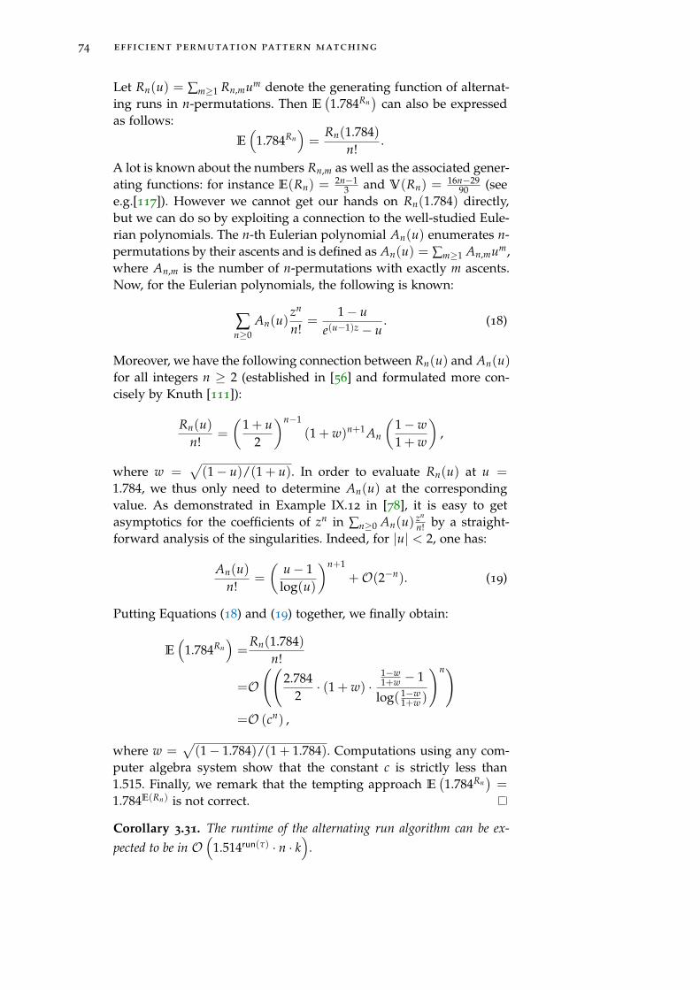
74 efficient permutation pattern matching
Let Rn(u) = ∑m≥1 Rn,mum denote the generating function of alternat-ing runs in n-permutations. Then E
(1.784Rn
)can also be expressed
as follows:
E(
1.784Rn)=
Rn(1.784)n!
.
A lot is known about the numbers Rn,m as well as the associated gener-ating functions: for instance E(Rn) =
2n−13 and V(Rn) =
16n−2990 (see
e.g.[117]). However we cannot get our hands on Rn(1.784) directly,but we can do so by exploiting a connection to the well-studied Eule-rian polynomials. The n-th Eulerian polynomial An(u) enumerates n-permutations by their ascents and is defined as An(u) = ∑m≥1 An,mum,where An,m is the number of n-permutations with exactly m ascents.Now, for the Eulerian polynomials, the following is known:
∑n≥0
An(u)zn
n!=
1− ue(u−1)z − u
. (18)
Moreover, we have the following connection between Rn(u) and An(u)for all integers n ≥ 2 (established in [56] and formulated more con-cisely by Knuth [111]):
Rn(u)n!
=
(1 + u
2
)n−1
(1 + w)n+1An
(1− w1 + w
),
where w =√(1− u)/(1 + u). In order to evaluate Rn(u) at u =
1.784, we thus only need to determine An(u) at the correspondingvalue. As demonstrated in Example IX.12 in [78], it is easy to getasymptotics for the coefficients of zn in ∑n≥0 An(u) zn
n! by a straight-forward analysis of the singularities. Indeed, for |u| < 2, one has:
An(u)n!
=
(u− 1
log(u)
)n+1
+O(2−n). (19)
Putting Equations (18) and (19) together, we finally obtain:
E(
1.784Rn)=
Rn(1.784)n!
=O((
2.7842· (1 + w) ·
1−w1+w − 1
log( 1−w1+w )
)n)
=O (cn) ,
where w =√(1− 1.784)/(1 + 1.784). Computations using any com-
puter algebra system show that the constant c is strictly less than1.515. Finally, we remark that the tempting approach E
(1.784Rn
)=
1.784E(Rn) is not correct.
Corollary 3.31. The runtime of the alternating run algorithm can be ex-pected to be in O
(1.514run(τ) · n · k
).

3.2 the parameter run(π ) 75
2
5
9
7
4
6
8
3
1
1
2
3
4
5
6
7
8
9
Figure 17: To the left is a graphical representation of the permutation π in-troduced in Example 3.33, to the right the corresponding inci-dence graph Gπ .
3.2 the parameter run(π )
The aim of this section is twofold: First, we want to show that PPMcan be solved in time O (n1+run(π ) ). This result builds upon an algo-rithm by Ahal and Rabinovich [1] and a novel connection between thepathwidth of the incidence graph of a permutation [1] and the numberof alternating runs in that permutation. Second, we show that thisruntime cannot be improved to an fpt result unless FPT = W[1]. Letus start by defining incidence graphs:
Definition 3.32. Given an m-permutation π, the incidence graph Gπ =
(V, E) of π is defined as follows: The vertices V := [m] represent positionsin π. There are edges between adjacent positions, i.e., E1 :=
{{i, i+ 1} | i ∈
[m − 1]}
. There are also edges between positions where the correspondingelements have a difference of 1, i.e., E2 :=
{{i, j} | π(i)− π(j) = 1
}. The
edge set is defined as E := E1 ∪ E2.
Example 3.33. Consider the permutation
π =
(1 2 3 4 5 6 7 8 9
2 5 9 7 4 6 8 3 1
)
written in two-line representation. A graphical representation of π
can be found on the left-hand side of Figure 17. The correspondinggraph Gπ is represented on the right-hand side of the same figure.The solid lines correspond to the edges in E1 and the dashed lines tothe ones in E2. a
Definition 3.34. Let G = (V, E) be a simple graph, i.e., E is a set ofcardinality 2 subsets of V. A path decomposition of G is a sequence of subsetsSi ⊆ V such that
1. Every vertex appears in at least one Si.

76 efficient permutation pattern matching
2. Every edge is a subset of at least one Si.
3. Let three indices h < i < j be given. If a vertex is contained both inSh and Sj then it is also contained in Si.
The width of a path decomposition is defined as maxi(|Si|) − 1. The path-width of a graph G, written pw(G), is the minimum width of any pathdecomposition.
In [1], Theorem 2.7 and Proposition 3.5, the authors present an algo-rithm that solves PPM in time O
(n1+pw(Gπ)
). The following lemma
relates pw(Gπ) and the number of alternating runs in π.
Lemma 3.35. For all permutations π, it holds that pw(Gπ) ≤ run(π).
Proof. Given an m-permutation π we will define a sequence S1, . . . , Sm.We then show that this sequence is a path decomposition of Gπ =
(V, E) with width at most run(π).In order to define the sequence S1, . . . , Sm of subsets of V, we shall
extend alternating runs to maximal monotone subsequences. Thismeans that we add the preceding valley to a run up and the pre-ceding peak to a run down. For any i ∈ [run(π)], Ri then denotesthe set of elements in the i-th run in π together with the precedingvalley or peak. Note that this implies that |Ri ∩ Ri+1| = 1 for alli ∈ [run(π)− 1].
We define S′1 := {1} and for every v ∈ [2, m],
S′v :={
max(Rj ∩ [v− 1]) | j ∈ [run(π)] and Rj ∩ [v− 1] 6= ∅}∪{
v}
,
i.e., S′v contains v and the largest element of every run that is smallerthan v. Since Sv should contain positions in π (and not elements), wedefine
Sv := {π−1(w) | w ∈ S′v}.For an example of this construction, see Example 3.37. We now
check that S1, . . . , Sm indeed is a path decomposition.
1. The vertex i appears in Sπ(i).
2. First we consider edges of the form {i, i + 1}. Without loss ofgenerality let π(i) < π(i + 1). Then {i, i + 1} is a subset ofSπ(i+1). Clearly, i + 1 ∈ Sπ(i+1). Since π(i) and π(i + 1) are adja-cent in π there has to be an s ∈ [run(π)] such that {π(i), π(i +1)} ⊆ Rs. It then holds that max(Rs ∩ [π(i + 1) − 1]) = π(i)since π(i) ∈ Rs ∩ [π(i + 1)− 1] and π(i) is the largest elementin Rs smaller than π(i + 1). Consequently i ∈ Sπ(i+1).
Second, every edge {i, j} ∈ E with π(i)−π(j) = 1 is a subset ofSπ(i): As before i ∈ Sπ(i). Let s be any element of [run(π)] suchthat j ∈ Rs. Then max(Rs ∩ [π(i) − 1]) = max(Rs ∩ [π(j)]) =
π(j) and hence j ∈ Sπ(i).
Only these two types of edges exists.
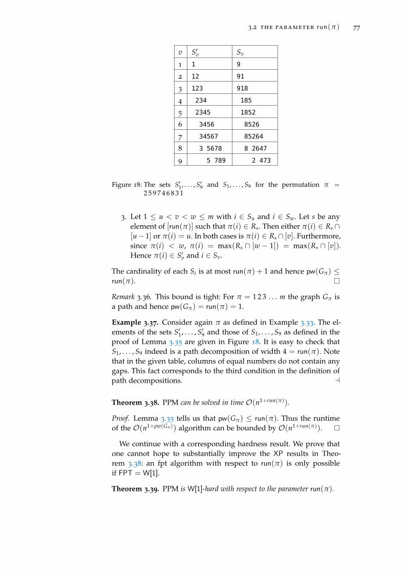
3.2 the parameter run(π ) 77
v S′v Sv
1 1 9
2 12 91
3 123 918
4 234 185
5 2345 1852
6 3456 8526
7 34567 85264
8 3 5678 8 2647
9 5 789 2 473
Figure 18: The sets S′1, . . . , S′9 and S1, . . . , S9 for the permutation π =2 5 9 7 4 6 8 3 1
3. Let 1 ≤ u < v < w ≤ m with i ∈ Su and i ∈ Sw. Let s be anyelement of [run(π)] such that π(i) ∈ Rs. Then either π(i) ∈ Rs ∩[u− 1] or π(i) = u. In both cases is π(i) ∈ Rs ∩ [v]. Furthermore,since π(i) < w, π(i) = max(Rs ∩ [w − 1]) = max(Rs ∩ [v]).Hence π(i) ∈ S′v and i ∈ Sv.
The cardinality of each Si is at most run(π) + 1 and hence pw(Gπ) ≤run(π).
Remark 3.36. This bound is tight: For π = 1 2 3 . . . m the graph Gπ isa path and hence pw(Gπ) = run(π) = 1.
Example 3.37. Consider again π as defined in Example 3.33. The el-ements of the sets S′1, . . . , S′9 and those of S1, . . . , S9 as defined in theproof of Lemma 3.35 are given in Figure 18. It is easy to check thatS1, . . . , S9 indeed is a path decomposition of width 4 = run(π). Notethat in the given table, columns of equal numbers do not contain anygaps. This fact corresponds to the third condition in the definition ofpath decompositions. a
Theorem 3.38. PPM can be solved in time O(n1+run(π)).
Proof. Lemma 3.35 tells us that pw(Gπ) ≤ run(π). Thus the runtimeof the O(n1+pw(Gπ)) algorithm can be bounded by O(n1+run(π)).
We continue with a corresponding hardness result. We prove thatone cannot hope to substantially improve the XP results in Theo-rem 3.38: an fpt algorithm with respect to run(π) is only possibleif FPT = W[1].
Theorem 3.39. PPM is W[1]-hard with respect to the parameter run(π).

78 efficient permutation pattern matching
Proof. We give an fpt-reduction from the W[1]-hard Segregated Per-mutation Pattern Matching Problem [42] to PPM. This problemis defined on page 90 in Section 4.3.
In this problem we are looking for matchings M where for all u ≤ pit holds that M(u) ∈ [t] and for all u > p it holds that M(u) ∈[t + 1, n]. Let (π, τ, p, t) be a SPPM instance, where |π| = k ≤ n = |τ|.We are going to construct a PPM instance (π, τ) as follows:
π = (p + 0.5) (k + 1)(k + 2) . . . (k + n + 1)︸ ︷︷ ︸=Rπ
π
τ = (t + 0.5) (n + 1)(n + 2) . . . . . . (2n + 1)︸ ︷︷ ︸=Rτ
τ
Note that the increasing runs R{π} and Rτ both consist of (n + 1)elements. The element placed at the beginning of π, p + 0.5, is largerthan p but smaller than p+ 1. Analogously, t+ 0.5 in τ is larger than tbut smaller than t + 1. Note that π and τ are not permutations in theclassical sense, since they contain elements that are not integers. How-ever, in order to obtain permutations on [k + n + 2] and [2n + 2], wesimply need to relabel the respective elements order-isomorphically.
Given this construction of π and τ the following holds: In everymatching of π into τ the element p + 0.5 has to be mapped to t + 0.5.Indeed, the increasing run of elements Rπ = (k + 1)(k + 2) . . . (k +n + 1) in π has to be mapped to the increasing run of elementsRτ = (n + 1)(n + 2) . . . . . . (2n + 1) in τ and consequently π has tobe matched into τ. This holds because of the following observation:If the element (k+ 1) in π is mapped to an element (n+ u) with u > 1in τ, some of the elements of Rπ have to be matched into τ since Rπ
and Rτ have the same length. This is however not possible, since allelements in τ are smaller than (n+ u). If (k + 1) is instead mapped toone of the elements of τ, then all remaining elements of Rπ also haveto be matched into τ which is not possible since Rπ is longer than τ.Therefore, the element (k + 1) in π is always mapped to the element(n + 1) in τ. Both in π and in τ there is only one element lying to theleft of (k + 1) and one to left of (n + 1): (p + 0.5) and (t + 0.5), respec-tively. Thus, (p + 0.5) has to be mapped to (t + 0.5). This implies thatall elements smaller than (p+ 0.5), i.e., elements in the interval [p], inπ have to be mapped to elements smaller than t+ 0.5, i.e., elements inthe interval [t], in τ. We have shown that (π, τ, p, t) is a YES-instanceof SPPM if and only if (π, τ) is a YES-instance of PPM.
It remains to show that this reduction can be done in fpt-time.Clearly run(π) = 2 + run(π) = O(k). Moreover the length of τ isbounded by a polynomial in the size of G since |τ| = n + 2 + |τ| =2n + 2 = O(n).

3.3 summary of the results 79
3.3 summary of the results
Let us sum up the contributions of this chapter:
• Our main result is a fixed-parameter algorithm for PPM with aruntime of O(1.79run(τ) · n · k). Since the combinatorial explosionis confined to run(τ), this algorithm performs especially wellwhen τ has few alternating runs.
• Since run(τ) ≤ n, the alternating run algorithm also solves PPMin time O(1.79n · n · k). This is a major improvement over thebrute-force algorithm with a runtime of O(2n · n).
• Since the number of runs in a random permutation is unlikelyto be n, one can expect an even smaller constant than 1.79 onaverage. Indeed, we prove that the expected runtime of our al-gorithm is in O(1.52n · n · k).
• We also show that an algorithm by Ahal and Rabinovich [1]has a runtime of O(n1+run(π)). This is achieved by proving thatthe pathwidth of a certain graph generated by a permutation isbounded by the number of alternating runs of this permutation.
• Finally, we prove that – under standard complexity theoreticassumptions – no fixed-parameter algorithm exists with respectto run(π), i.e., we cannot hope for an algorithm with runtimeO(crun(π) · poly(n)) for some constant c. Thus, the runtime of theaforementioned O(n1+run(π)) algorithm cannot be substantiallyimproved.


4T H E C O M P U TAT I O N A L C O M P L E X I T Y O FG E N E R A L I Z E D P E R M U TAT I O N PAT T E R NM AT C H I N G
This chapter is based on the publication The computational landscape ofpermutation patterns [42] which is joint work with Martin Lackner.
Permutation patterns, which we will refer to as classical permu-tation patterns in this chapter, have become well-established combi-natorial objects and are widely studied in the combinatorial liter-ature. In recent years, several other types of permutation patternswere introduced and have received increased interest, such as vincu-lar [13], bivincular [33], mesh [36], boxed mesh [12] and consecutivepatterns [62]. All these pattern types are introduced in Section 4.1.
Every type of permutation pattern naturally defines a correspond-ing computational problem. Let C denote any type of permutationpattern, i.e., let C ∈ {classical, vincular, bivincular, mesh, boxed mesh,consecutive}.
C Permutation Pattern Matching (C PPM)
Instance: A permutation τ (the text) and a C pattern π
Question: Does the C pattern π occur in τ?
In this chapter we study the classical, vincular, bivincular, mesh, boxedmesh and consecutive pattern matching problem. Often we abbrevi-ate Classical Permutation Pattern Matching with PPM and theother problems with C PPM, where C is the corresponding patterntype.
While the combinatorial structure of permutation patterns is beingextensively studied, the computational perspective has so far receivedless attention. Related work to computational aspects of permutationpatterns has been gathered on page 48 in the preceding Chapter 3.This chapter draws a map of the computational landscape of per-mutation patterns and thus aims at paving the way for a detailedcomputational analysis of these problems.
The contents of this chapter are the following:
• In Section 4.1, we survey different types of permutation pat-terns. Our focus lies on classical, vincular, bivincular, mesh,boxed mesh and consecutive patterns. The hierarchy of thesepatterns with the most general one at the top is displayed inFigure 19.
• In Section 4.2, we study the computational complexity of everycorresponding decision problem. We strengthen the result that
81

82 the computational complexity of generalized ppm
mesh
boxed mesh bivincular
vincular
consecutive classical
NP-complete
inP
Figure 19: Hierarchy of pattern types
Classical Permutation Pattern Matching is NP-complete [31]and also show in which cases C PPM can be solved in polyno-mial time.
• In Section 4.3, we offer a more fine-grained complexity analy-sis by employing the framework of parameterized complexity.For most NP-complete problems we provide a more detailedcomplexity classification by showing W[1]-completeness with re-spect to the parameter length of π.
• Both the classical as well as the parameterized complexity re-sults are summarized in Section 4.4 and in the two Tables 3 and4 on pages 83 and 84, respectively.
4.1 types of patterns
In this section we give an overview of several different types of per-mutation patterns that have been introduced in the last years andthat will be of interest in this paper. Besides classical permutationpatterns that were defined in the Preliminaries (see Section 2.2, weconsider the following types of patterns: vincular, bivincular, mesh,boxed mesh and consecutive patterns. A schematic representation oftheir hierarchy can be found in Figure 19 and examples can be foundin Tables 3 and 3. For details, we refer to the Chapters 1 and 5-7 inKitaev’s monograph Patterns in Permutations and Words [108].
Before we introduce non-classical types of patterns, we extend thedefinition of matchings from classical to other types of patterns:
Definition 4.1. Let C ∈ {classical, vincular, bivincular, mesh, boxed mesh,consecutive}. A matching of a C pattern π of length k into a permutation τ
of length n is an increasing mapping M : [k] → [n] such that the sequenceM(P(1)), M(P(2)), . . . , M(P(k)) is an occurrence of the C pattern π in τ.
Matchings are denoted by M throughout this chapter.

4.1 types of patterns 83
Classical Vincular Bivincular
Pattern
π = 132 =ooo
π = 1 3 2 =blub
cols(π) = 1
π =11
23
32 =
cols(π) = 1rows(π) = 2
Text
Classicalcomplexity
NP-complete [31]NP-completeCorollary 4.8
NP-completeCorollary 4.8
Parameterizedcomplexity
FPT [93]W[1]-completeTheorem 4.15
W[1]-completeTheorem 4.16
Table 3: Examples of classical, vincular and bivincular permutation patterns
Vincular patterns
Let τ(i1)τ(i2) . . . τ(ik) be an occurrence of the classical pattern π inthe text τ. Then there are no requirements on the elements in τ ly-ing in between τ(ij) and τ(ij+1). It is however natural to ask foroccurrences of patterns in which certain elements are forced to beadjacent in the text, i.e., τ(ij+1) = τ(ij + 1). Vincular patterns are ageneralization of classical patterns capturing these requirements onadjacency in the text. They were introduced under the name of gener-alized patterns in 2000 by Babson and Steingrímsson in [13], where itwas shown that essentially all Mahonian permutation statistics in theliterature can be written as linear combinations of vincular patterns.For a survey of this topic, see [149].
Here we use the name of vincular patterns as it was introduced byKitaev in [108]. We also use the notation introduced there, since it isconsistent with the notation for classical patterns.
Definition 4.2. A vincular pattern π is a permutation in which certainconsecutive entries may be underlined. An occurrence of π in a permutationτ is then an occurrence of the corresponding classical pattern for which un-derlined elements are matched to adjacent elements. To be more formal: Anoccurrence of π in τ corresponds to a subsequence τ(i1)τ(i2) . . . τ(ik) of τ
that is order-isomorphic to π and for which τ(ij+1) = τ(ij + 1) whenever π
contains π(j)π(j + 1). Furthermore, if π starts with π(1) an occurrenceof π in τ must start with the first entry in τ, i.e., τ(i1) = τ(1). Similarly,if π ends with π(k) it must hold that τ(ik) = τ(n).
When using plots in a [0, n + 1] × [0, n + 1]-grid to represent n-permutations, adjacency of positions clearly corresponds to adjacencyof columns. In order to represent the underlined elements in vincularpatterns in the corresponding grids, one shades the columns which
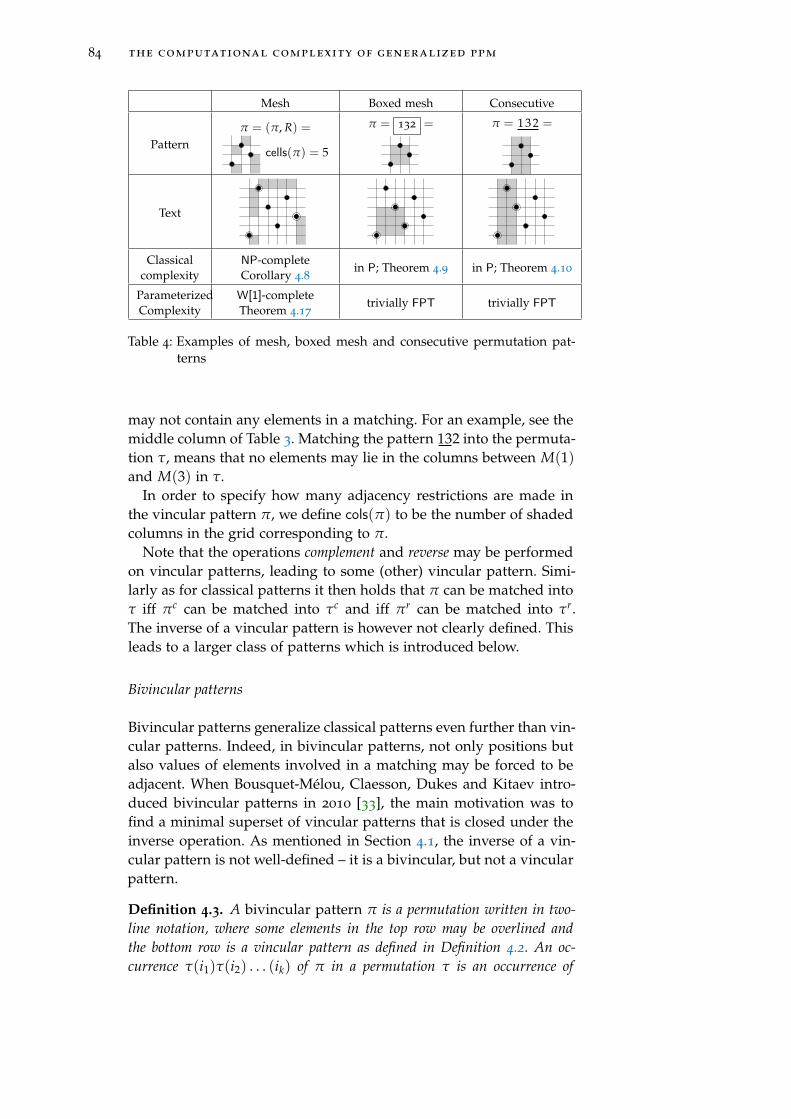
84 the computational complexity of generalized ppm
Mesh Boxed mesh Consecutive
Patternπ = (π, R) =
cells(π) = 5
π = 132 = π = 1 3 2 =ooo
Text
Classicalcomplexity
NP-completeCorollary 4.8
in P; Theorem 4.9 in P; Theorem 4.10
ParameterizedComplexity
W[1]-completeTheorem 4.17
trivially FPT trivially FPT
Table 4: Examples of mesh, boxed mesh and consecutive permutation pat-terns
may not contain any elements in a matching. For an example, see themiddle column of Table 3. Matching the pattern 132 into the permuta-tion τ, means that no elements may lie in the columns between M(1)and M(3) in τ.
In order to specify how many adjacency restrictions are made inthe vincular pattern π, we define cols(π) to be the number of shadedcolumns in the grid corresponding to π.
Note that the operations complement and reverse may be performedon vincular patterns, leading to some (other) vincular pattern. Simi-larly as for classical patterns it then holds that π can be matched intoτ iff πc can be matched into τc and iff πr can be matched into τr.The inverse of a vincular pattern is however not clearly defined. Thisleads to a larger class of patterns which is introduced below.
Bivincular patterns
Bivincular patterns generalize classical patterns even further than vin-cular patterns. Indeed, in bivincular patterns, not only positions butalso values of elements involved in a matching may be forced to beadjacent. When Bousquet-Mélou, Claesson, Dukes and Kitaev intro-duced bivincular patterns in 2010 [33], the main motivation was tofind a minimal superset of vincular patterns that is closed under theinverse operation. As mentioned in Section 4.1, the inverse of a vin-cular pattern is not well-defined – it is a bivincular, but not a vincularpattern.
Definition 4.3. A bivincular pattern π is a permutation written in two-line notation, where some elements in the top row may be overlined andthe bottom row is a vincular pattern as defined in Definition 4.2. An oc-currence τ(i1)τ(i2) . . . (ik) of π in a permutation τ is an occurrence of

4.1 types of patterns 85
the corresponding vincular pattern where additionally the following holds:τ(ij+1) = (ij) + 1 whenever the top row of π contains j(j + 1). Further-more, if the top row starts with 1, an occurrence of π in τ must start withthe smallest entry in τ, i.e., τ(i1) = 1. Similarly, if the top row ends with k ,it must hold that τ(ik) = n.
This definition gets a lot less cumbersome when representing per-mutations with the help of grids: As remarked earlier, underlinedelements in the bottom row are translated into forbidden columnsin which no elements may occur in a matching. Similarly, overlinedelements in the top row are translated into forbidden rows. For anexample, see the right column in Table 3.
Again, in order to specify how many adjacency restrictions aremade in the bivincular pattern π, we define – in addition to cols(π) –rows(π) to be the number of shaded rows in the grid correspondingto π.
Mesh patterns
A further generalization of bivincular patterns was given by Brändénand Claesson who introduced mesh patterns in [36] in 2011. Mesh pat-terns allow further restrictions on the relative positions of the entriesin an occurrence of a pattern. Several permutation statistics can be for-mulated as the number of occurrences of certain mesh patterns [36].
Definition 4.4. A mesh pattern is a pair π = (π, R) where π is a per-mutation of length k and R ⊂ [0, k]× [0, k] is a relation. An occurrence ofπ in a permutation τ is an occurrence of the classical pattern π fulfillingadditional restrictions defined by R. That is to say there is a subsequenceτ(i1)τ(i2) . . . τ(ik) of τ that is order-isomorphic to π and for which holds:
(x, y) ∈ R =⇒@i ∈ [n] : ix < i < ix+1
∧ τ(
iπ−1(y)
)< τ(i) < τ
(iπ−1(y+1)
).
This definition is again a lot easier to capture when representingpermutations as grids. Indeed, the relation R can be translated veryeasily into the graphical representation of π = (π, R), by shading theunit square with bottom left corner (x, y) for every (x, y) ∈ R. Anoccurrence of π in a permutation τ is then a classical occurrence of π
in τ such that no elements of τ lie in the shaded regions of the grid.Again, in order to specify how many adjacency restrictions are
made in the mesh pattern π, we define cells(π) to be the numberof shaded cells in the corresponding grid. Thus cells(π, R) := |R|. Foran example where π = 132 and R = {(1, 0), (1, 2), (2, 3), (3, 0), (3, 1)}see the left column in Table 4.
86 the computational complexity of generalized ppm
Boxed mesh patterns
A special case of mesh patterns, so called boxed mesh patterns, wasvery recently introduced by Avgustinovich, Kitaev and Valyuzhenichin [12].
Definition 4.5. A boxed mesh pattern, or simply boxed pattern, is a meshpattern π = (π, R) where π is a permutation of length k and R = [1, k−1]× [1, k− 1]. π is then denoted by π .
In the grid representing a boxed pattern all but the boundary squaresare shaded. For an example, see the middle column of Table 4.
It is straightforward to see that the set of boxed patterns is closedunder taking complements, reverses and inverses and that these oper-ations are compatible with pattern containment. Interestingly, it wasshown [12] that the statement “π can be matched into τ iff π can bematched into τ” is only true if π is one of the following permutations:1, 12, 21, 132, 213, 231, 312.
Consecutive patterns
Consecutive patterns are a special case of vincular patterns, namelythose where all entries are underlined. In an occurrence of a consecu-tive pattern it is thus necessary that all entries are adjacent. Findingan occurrence of a consecutive pattern therefore consists in findinga contiguous subsequence of τ that is order-isomorphic to π. For anexample, see the right column of Table 4.
Several well-known enumeration problems for permutations canbe formulated in terms of forbidden consecutive patterns; Elizaldeand Noy [62] provide examples. Chapter 5 in [108] is devoted to andgives an overview of different methods employed in the literature forthe study of consecutive patterns.
4.2 the possibility of polynomial-time algorithms
The results of this Section are summarized in Figure 19 in which thestudied problems are partitioned into those that are in P and thosethat are NP-complete.
NP-completeness
At the 1992 SIAM Discrete Mathematics meeting Herbert Wilf askedwhether it is possible to solve the permutation pattern matching prob-lem in polynomial time. The answer is no unless P=NP, as shown bythe NP-completeness result of Bose, Buss and Lubiw [31]. This resultimmediately yields NP-hardness for all generalizations of classicalpermutation pattern matching. In this section we are going to show
4.2 the possibility of polynomial-time algorithms 87
that NP-hardness holds for these problems even in a more restrictedcase. Indeed,NP-hardness can be shown for instances in which allalternating runs are as short as possible, i.e., for alternating permuta-tions.
Theorem 4.6. Every Mesh Permutation Pattern Matching instance(π, τ) = ((π, R), τ) can be transformed into an instance (π′, τ′) with π′ =(π′, R) and the following properties: (π′, τ′) is a yes-instance iff (π, τ) isyes-instance, |π′| = 2|π|, |τ′| = 2|τ| and both π′ and τ′ are alternatingpermutations. This transformation can be done in polynomial time.
Proof. Let π = π1 . . . πk and τ = τ1 . . . τn. We define
π′ = (k + 1) π1 (k + 2) π2 (k + 3) . . . (2k) πk
τ′ = (n + 1) τ1 (n + 2) τ2 (n + 3) . . . (2n) τn.
Clearly, |π′| = 2|π|, |τ′| = 2|τ| and both permutations π′ and τ′ arealternating. We are now going to show that there is a matching fromπ into τ iff there is a matching from π′ into τ′. Assume that M is amatching from π into τ, i.e., a map from [k] to [n]. We extend thismap to a map M′ from [2k + 1] to [2n + 1] in the following way:
M′(i) =
M(i), if i ∈ [k],
τ(j), where M(i− k) = τ(j + 1) if i > k.
In other words, M′ maps (i + k) to the element in τ left of M(i). Forexample if M(π3) = τ5 then π3 ∈ π′ is matched to τ5 ∈ τ′ and(k + 3) ∈ π′ is matched to n + 5 ∈ τ′ (which is the element in τ lyingdirectly to the left of τ5). Observe that the function M′ is a matchingfrom π′ into τ′.
Now let us assume that M′ is a matching from π′ into τ′. If werestrict the domain of M′ to [k] then we obtain a matching from π
into τ.
Theorem 4.7. PPM is NP-complete even when both π and τ are alternatingpermutations.
Proof. We apply the transformation in Theorem 4.6 to show NP-hard-ness. NP-membership holds for this restricted class of input instancesas well.
Corollary 4.8. Vincular, Bivincular and Mesh PPM are NP-completeeven when both π and τ are alternating permutations.
Proof. NP-hardness follows from Theorem 4.6 as well as from Theo-rem 4.7. NP-membership holds since checking whether the additionalrestrictions imposed by the vincular, bivincular or mesh pattern arefulfilled can clearly be done in polynomial time.
88 the computational complexity of generalized ppm
Polynomial time algorithms
We have seen that polynomial time algorithms are unlikely to existfor PPM and its generalizations. However, this is not the case for thespecial cases of boxed mesh and consecutive pattern matching.
Theorem 4.9. Boxed Mesh Permutation Pattern Matching can besolved in O(n3) time.
Proof. Let π be a boxed pattern of length k and τ a permutation oflength n. For every pair (i, j) where i ∈ [n] and i + k ≤ j ≤ n checkwhether there is a matching M of the boxed pattern π into τ wherethe smallest element in π is matched to i and the largest one to j, i.e.,M(1) = i and M(k) = j.
Checking whether such a matching exists can be done in the fol-lowing way: From the permutation τ, construct the permutation τ bydeleting all elements that are smaller than i and larger than j. Clearly,the matching that we are looking for must be contained in τ, it couldotherwise not be an occurrence of a boxed pattern. Moreover, it hasto consist of k consecutive elements in τ. Since the positions of thesmallest and the largest element are fixed, the positions for all otherelements of π are equally determined. Thus there is only one sub-sequence of τ that could possibly be a matching of π into τ withM(1) = i and M(k) = j. Deleting the elements that are too smallor too large and checking whether this subsequence actually corre-sponds to an occurrence of π in τ, i.e., whether it is order-isomorphicto π, can be checked in at most n steps. Note that this subsequencemight consist of less than k elements in which case it clearly does notcorrespond to an occurrence.
In total, there are (n− k+ 1) · (n− k+ 2)/2 = O(n2) pairs (i, j) thathave to be checked which leads to the runtime bound O(n3).
Theorem 4.10. Consecutive Permutation Pattern Matching canbe solved in O((n− k) · k) time.
Proof. Let π be a consecutive pattern of length k and τ a permuta-tion of length n. For every i ∈ [n − k + 1] check whether there is amatching of π into τ where the first element of π is mapped to i.Since we are looking for an occurrence of a consecutive pattern, theonly possible subsequence of τ then consists of the element i andthe following (k − 1) elements of τ. Whether this sequence is order-isomorphic to π can be checked in k steps which leads to the runtimebound O((n− k) · k).
As was recently shown by Kubica et.al. in [114], this simple resultcan be improved by an algorithm with runtime O(n + k).

4.3 the impact of the pattern length 89
mesh
boxed mesh bivincular
vincular
consecutive classical
FPT
W[1]-complete
inP
Figure 20: The influence of the pattern length on the computational hard-ness: parameterized complexity of permutation pattern matching
4.3 the impact of the pattern length
PPM can be solved in O(nk) time by exhaustive search, where k isthe length of π. This trivial upper bound has been improved first byAlbert et al. to O(n1+2k/3 · log n) [3] and then to O(n0.47k+o(k)) by Ahaland Rabinovich [1]. In a recent breakthrough result, Guillemot andMarx have shown that PPM can be solved by an FPT algorithm [93].Its runtime is 2O(k
2·log k) · n. In this section we are going to show thatsuch a result is likely not to be achievable for Vincular, Bivincular
and Mesh PPM. This is done by showing W[1]-hardness with respectto the parameter k. First, we show that Mesh PPM and therefore allother problems studied in this paper are contained in W[1].
All results in this section are summarized in Figure 20.
Theorem 4.11. Mesh Permutation Pattern Matching is containedin W[1].
Proof. For showing membership we encode Mesh PPM as a modelchecking problem of an existential first order formula. W[1]-member-ship is then a consequence of the fact that the following problem isW[1]-complete [79].
Existential first-order model checking
Instance: A structure A and an existential first-order for-mula ϕ
Parameter: |ϕ|Question: Is A a model for ϕ?
Let ((π, R), τ) be a Mesh PPM instance. We compute a structureA = (A,<,≺τ, E), where the domain set A = {1, . . . , n} representsindices in the text. The binary relation≺τ is defined as follows: x ≺τ yholds iff τ(x) < τ(y). E is a quaternary relation where E(w, x, y, z) istrue iff there are no elements in τ that are left of w, right of x, largerthan y and smaller than z. Intuitively, w, x, y and z describe a forbid-den rectangle in the permutation grid of τ which may not contain

90 the computational complexity of generalized ppm
any elements of τ. The relations ≺τ, E and < can be computed inpolynomial time. The formula ϕ we want to check is
ϕ =∃x1 . . . ∃xk x1 < x2 ∧ x2 < x3 ∧ . . . ∧ xk−1 < xk ∧∧
P(i)<P(j)for i,j∈[k]
xi ≺T xj
︸ ︷︷ ︸ϕ1
∧∧
P(i)>P(j)for i,j∈[k]
¬(xi ≺T xj)
︸ ︷︷ ︸ϕ2
∧
∧
i,j∈[k] andR(i,j) is true.
E(xi, xi+1, xj, xj+1)
︸ ︷︷ ︸ϕ3
.
Observe that the length of ϕ is in O(k2). The two sub-formulæ ϕ1
and ϕ2 are true exactly when a subsequence τ(x1)τ(x2) . . . τ(xk) of τ
can be found such that τ(xi) < τ(xj) iff π(i) < π(j). Thus ϕ1 ∧ ϕ2 istrue iff there is a matching of the classical pattern π into τ. The sub-formula ϕ3 encodes the relation R and is true iff no elements lie inthe forbidden regions of τ, as can be seen by recalling Definition 4.4.Thus ϕ is true iff ((π, R), τ) is a yes-instance of Mesh PPM.
We now want to prove W[1]-hardness for vincular, bivincular andmesh pattern matching. For this purpose, we introduce Segregated
Permutation Pattern Matching, a generalization of PPM. All sub-sequent hardness theorems use reductions from this problem.
Segregated Permutation Pattern Matching (SPPM)
Instance: A permutation τ (the text) of length n, a permuta-tion π (the pattern) of length k ≤ n and two posi-tive integers p ∈ [k], t ∈ [n].
Parameter: k
Question: Is there a matching M of π into τ such that M(i) ≤t iff i ≤ p?
Example 4.12. Consider the pattern π = 132 and the text τ = 53142.As shown by the matching M(2) = 3, M(1) = 1 and M(3) = 4, theinstance (π, τ, 2, 3) is a yes-instance of the SPPM problem. However,(π, τ, 2, 4) is a NO-instance, since no matching of π into τ can befound where M(3) > 4. aTheorem 4.13. Segregated Permutation Pattern Matching is W[1]-hard with respect to the parameter k.
Proof. We show W[1]-hardness by giving an fpt-reduction from theW[1]-complete Clique problem (see Section 2.5 in the Preliminaries)to SPPM.
The reduction has three parts. First, we will show that we are ableto reduce a Clique instance to a pair (π′, τ′), where π′ and τ′ are two

4.3 the impact of the pattern length 91
permutations on multisets, i.e., permutations in which elements mayoccur more than once. Applying Definition 2.5 to permutations onmultisets means that in a matching repeated elements in the patternhave to be mapped to repeated elements in the text. In addition torepeated elements, π′ and τ′ contain so-called guard elements. Theirfunction is explained below. Second, we will show how to get rid ofrepetitions. The method used in this step has already been used in theNP-completeness proof of PPM provided by Bose, Buss and Lubiwin [31]. Third, we implement the guards by using the segregationproperty and have thus reduced Clique to SPPM.
Let (G, k) be a Clique instance, where V = {v1, v2, . . . , vl} is the setof vertices and E = {e1, e2, . . . , em} the set of edges. Both the patternand the text consist of a single substring coding vertices (π resp. τ)and substrings coding edges (πi resp. τi for the i-th substring). Thesesubstrings are listed one after the other, with guard elements placed inbetween them. These guard elements have the function of separatingsubstrings in a matching: guard elements will have to be mapped toguard elements and substrings embraced by two consecutive guard-elements will also have to be mapped to substrings embraced by twoconsecutive guard-elements. For the moment, we will simply writebrackets to indicate where guard elements are placed. The meaningof these brackets is then the following: a block of elements enclosed bya 〈 to the left and a 〉 to the right has to be matched into another blockof elements between two such brackets. How the guard-elements areimplemented as elements of a permutation is explained at the end ofthe proof after Claim 2.
We define the pattern to be
π′ := 〈π〉〈π1〉〈π2〉〈. . .〉〈πk(k−1)/2〉= 〈123 . . . k〉〈12〉〈13〉〈. . .〉〈1k〉〈23〉〈. . .〉〈2k〉〈. . .〉〈(k− 1)k〉.
π corresponds to a list of (indices of) k vertices. The πi’s represent allpossible edges between the k vertices (in lexicographic order).
For the textτ′ := 〈τ〉〈τ1〉〈τ2〉〈. . .〉〈τm〉
we proceed similarly. τ is a list of the (indices of the) l vertices of G.The τi’s represent all edges in G (again in lexicographic order). Let usgive an example:
Example 4.14. Let l = 6 and k = 3. Then the pattern permutation isgiven by
π′ = 〈123〉〈12〉〈13〉〈23〉.Consider for instance the graph G with six vertices v1, . . . , v6 andedge-set
{{1, 2} , {1, 6} , {2, 3} , {2, 4} , {2, 5} , {3, 5} , {4, 5} , {4, 6}} .
represented in Figure 21 (we write {i, j} instead of{
vi, vj}
).

92 the computational complexity of generalized ppm
v1v6
v4
v2v5
v3
Pattern: 1 2 3 12 13 23
Text: 1 4 6 12 16 24 45 462 3 5 23 25 35
Figure 21: An example for the reduction of an Independent Set instance toa PPM instance
Then the text permutation is given by:
τ′ = 〈123456〉〈12〉〈16〉〈23〉〈24〉〈25〉〈35〉〈45〉〈46〉.
aClaim 1. A clique of size k can be found in G iff there is a simultaneousmatching of π into τ and of every πi into some τj.
Example 4.14 (continuation). In our example {v2, v3, v5} is a cliqueof size three. Indeed, the pattern π′ can be matched into τ′ as can beseen by matching the elements 1, 2 and 3 onto 2, 3 and 5 respectively.See again Figure 21 where the involved vertices respectively elementsof the text permutation have been marked in gray. a
Proof of Claim 1. A matching of π into τ corresponds to a selection ofk vertices amongst the l vertices of G. If it is possible to additionallymatch every one of the π’s into a τ this means that all possible edgesbetween the selected vertices appear in G. This is because τ′ onlycontains pairs of indices that correspond to edges appearing in thegraph. The selected k vertices thus form a clique in G. Conversely, iffor every possible matching of π into τ defined by a monotone mapM : [k] → [l] some πi = xy cannot be matched into τ′, this meansthat {M(x), M(y)} does not appear as an edge in G. Thus, for everyselection of k vertices there will always be at least one pair of verticesthat are not connected by an edge and therefore there is no clique ofsize k in G.
In order to get rid of repeated elements, we identify every variablewith a real interval: 1 corresponds to the interval [1, 1.9], 2 to [2, 2.9]and so on until finally k corresponds to [k, k+ 0.9] (resp. l to [l, l + 0.9]).In π and τ we shall therefore replace every element j by the pair ofelements (j + 0.9, j) (in this order). The occurrences of j in the πi’s(resp. τi’s) shall then successively be replaced by real numbers in theinterval [j, j + 0.9]. For every j, these values are chosen one after theother (from left to right), always picking a real number that is largerthan all the previously chosen ones in the interval [j, j + 0.9].

4.3 the impact of the pattern length 93
Observe the following: The obtained sequence is not a permutationin the classical sense since it consists of real numbers. However, byreplacing the smallest number by 1, the second smallest by 2 andso on, we do obtain an ordinary permutation. This defines π and τ
(except for the guard elements).
Example 4.14 (continuation). Getting rid of repetitions in the patternof the above example could for instance be done in the following way:
π = 〈1.9 1 2.9 2 3.9 3〉〈1.1 2.1〉〈1.2 3.1〉〈2.2 3.2〉
This permutation of real numbers is order-isomorphic to the follow-ing ordinary permutation:
π = 〈4 1 8 5 12 9〉〈2 6〉〈3 10〉〈7 11〉.
aClaim 2. π can be matched into τ iff π′ can be matched into τ′.
Proof of Claim 2. Suppose that π′ can be matched into τ′. When match-ing π into τ, we have to make sure that elements in π that were copiesof some repeated element in π′ may still be mapped to elements inτ that were copies themselves in τ′. Indeed this is possible since wehave chosen the real numbers replacing repeated elements in increas-ing order. If i in π′ was matched to j in τ′, then the pair (i + 0.9, i)in π may be matched to the pair (j + 0.9, j) in τ and the increasingsequence of elements in the interval [i, i + 0.9] may be matched intothe increasing sequence of elements in the interval [j, j + 0.9].
Now suppose that π can be matched into τ. In order to prove thatthis implies that π′ can be matched into τ′, we merely need to showthat elements in π that were copies of some repeated element in π′
have to be mapped to elements in τ that were copies themselves in τ′.Then returning to repeated elements clearly preserves the matching.Firstly, it is clear that a pair of consecutive elements i + 0.9 and i in π
has to be matched to some pair of consecutive elements j + 0.9 and jin τ, since j is the only element smaller than j + 0.9 and appearing toits right. Thus intervals are matched to intervals. Secondly, an elementx in π for which it holds that i < x < i + 0.9 must be matched to anelement y in τ for which it holds that j < y < j + 0.9. Thus copies ofan element are still matched to copies of some other element.
Finally, replacing real numbers by integers does not change thepermutations in any relevant way.
It remains to implement the guards in order to ensure that sub-strings are matched to corresponding substrings. Let πmax and τmax
denote the largest integer that is contained in π respectively τ at thispoint. We now replace all guards with integers larger than πmax re-spectively τmax and will choose the segregating elements p and t suchthat guards and “original” pattern/text elements are separated. We

94 the computational complexity of generalized ppm
insert the guard elements in the designated positions (previouslymarked by 〈 and 〉) in the following order: πmax + 2 (instead of thefirst 〈), πmax + 1 (instead of the first 〉), πmax + 4 (instead of the sec-ond 〈), πmax + 3 (instead of the second 〉), . . . , πmax + 2i (instead ofthe i-th 〈), πmax + 2i− 1 (instead of the i-th 〉), . . ., and so on until wereach the last guard-position. The guard elements are inserted in thisspecific order to ensure that two neighbouring guard elements 〈 and〉 in π have to be mapped to two neighbouring guard elements 〈 and〉 in τ. We proceed analogously in τ. To ensure that guards in π arematched to guards in τ and pattern elements of π are matched to textelements in τ, we set p to πmax and t to τmax.
This finally yields that (G, k) is a yes-instance of Clique iff (π, τ, p, t)is a yes-instance of SPPM. It can easily be verified that this reductioncan be done in fpt-time.
As can easily be seen, the reduction performed in the proof of The-orem 4.13 can be done in polynomial time. Thus this proof immedi-ately yields NP-hardness for SPPM.
Now, that we have obtained this result, we are able to show W[1]-hardness for PPM with vincular, bivincular and mesh patterns. Asbefore, the parameter is the length of the pattern.
Theorem 4.15. Vincular Permutation Pattern Matching is W[1]-complete with respect to k. This holds even when restricting the problem toinstances (π, τ) with cols(π) = 1.
Proof. We reduce from Segregated PPM. Let (π, τ, p, t) be an SPPMinstance. The Vincular PPM instance (π′, τ′) constructed from (π, τ)
will have have an additional element in π′ and an additional elementin τ′. The new element in π, denoted by p′, is p + 0.5, i.e., p′ is largerthan p but smaller than p + 1. Analogously, t′ = t + 0.5 is the newelement in τ. We define π′ = p ′π and τ′ = t′ τ. In order to obtaina permutation π on [k + 1] and τ on [n + 1], we simply need to rela-bel the respective elements order-isomorphically. In every matchingof π′ into τ′ the element p′ has to be mapped to t′. Consequently, allelements larger than p′ in π′ have to be mapped to elements largerthan t′ in τ′ and all elements smaller than p′ have to be mapped toelements smaller than t′. This implies that (π, τ, p, t) is a Segregated
PPM yes-instance iff (π′, τ′) is a Vincular PPM yes-instance. Thisreduction is done in linear time which proves W[1]-hardness of Vin-cular PPM. Membership follows from Theorem 4.11.
Theorem 4.16. Bivincular Permutation Pattern Matching is W[1]-complete with respect to k. This holds even when restricting the problem toinstances (π, τ) with rows(π) = 1.
Proof. As in the previous proof we reduce from Segregated PPM. Let(π, τ, p, t) be an SPPM instance. Identically to the previous proof, wedefine p′ = p + 0.5 and t′ = t + 0.5. The Bivincular PPM instance

4.4 summary of the results 95
consists of a permutation π′ with elements in [k + 1] ∪ {p′} and τ′, apermutation on [n+ 1]∪{t′}. The permutation π′, written in two-linenotation, is given as follows:
π′ =
(1 2 3 . . . p′ . . . (k+1)
p′ (k + 1) π(1) . . . π(k)
)
and τ′ is defined to be t′(n + 1)τ. In order to obtain permutationson [k + 2] respectively [n + 2] we again relabel the elements order-isomorphically.
In any matching of π′ into τ′ the element (k + 1) has to be mappedto (n + 1) and therefore p′ has to be mapped to t′. Thus all elementslarger than p′ in π′ have to be mapped to elements larger than t′ inτ′ and all elements smaller than p′ have to be mapped to elementssmaller than t′. This implies that (π, τ, p, t) is a Segregated PPMyes-instance iff (π′, τ′) is a Bivincular PPM yes-instance. Since thisreduction can again be done in linear time, Bivincular PPM is W[1]-hard. Membership follows again from Theorem 4.11.
Theorem 4.17. Mesh Permutation Pattern Matching is W[1]-completewith respect to k. This holds even if cells(π) = 1.
Proof. Let (π, τ, p, t) be a Segregated PPM instance. As before, wedefine p′ = p + 0.5 and t′ = t + 0.5. The Mesh PPM instance consistsof a permutation π′ with elements in [k]∪ {p′} and τ′, a permutationon [n + 1] ∪ {t′}. Again, permutations on [k + 1] respectively [n + 2]can be obtained by relabelling the elements order-isomorphically. Wedefine π′ = p′ π and τ′ = t′ (n + 1) τ. Furthermore, we define:R = {(0, (k + 1))}. This means that for every matching M of π′ intoτ′ the following must hold: to the left of M(p′) in τ′, there are no ele-ments larger than M(k). However, it surely holds that M(k) ≤ (n+ 1).Consequently, p′ has to be mapped to t′. This implies that (π, τ, p, t)is a Segregated PPM yes-instance iff (π′, τ′) is a Mesh PPM yes-instance. Since this reduction can again be done in linear time, Mesh
PPM is W[1]-hard. Membership follows from Theorem 4.11.
These hardness results show that we cannot hope for a fixed-parametertractable algorithm for Vincular/Bivincular/Mesh Permutation
Pattern Matching.
4.4 summary of the results
Let us briefly sum up the contributions of this chapter. We analysedseveral versions of Permutation Pattern Matching, based on var-ious types of permutation patterns that were recently introduced inthe literature. This allows us to draw a picture of the computationallandscape of generalized PPM:

96 the computational complexity of generalized ppm
We performed a classical complexity analysis and could show thatthe only cases where C PPM can be solved in polynomial time areConsecutive PPM and Boxed Mesh PPM. All other versions of PPMare NP-complete, even if the input instances are reduced to the casewhere both the pattern and the text are alternating permutations. Thispartition of the C PPM problems is represented in Figure 19 on page82.
We offered a more fine-grained complexity analysis of the NP-hardversions of C PPM by employing the framework of parameterizedcomplexity. We were able to show that Mesh, Bivincular and Vin-cular PPM are W[1]-complete with respect to the length of the pat-tern. This is in strong contrast to the case of classical PPM, that isfpt with respect to this parameter [93]. This partition of the C PPMproblems that are NP-complete is represented in Figure 20 on page89.

5A P E R M U TAT I O N C L A S S E N U M E R AT E D B Y T H EC E N T R A L B I N O M I A L C O E F F I C I E N T S
This short chapter is concerned with the enumeration of permuta-tions avoiding the patterns 2431, 4231, 1432 and 4132 simultaneously.This permutation class arises in the context of single-peaked electionsthat are introduced and studied in Chapter 10 of this thesis. To bemore precise, we can show that permutations of length n that avoidthe four patterns above are in bijective correspondence with elections{V1, V2} on a candidate set C = {c1, c2, . . . , cn} that are single-peakedand where V1 is the vote c1 > c2 > . . . > cn. This allows us to derivean upper bound on the number of single-peaked elections with anarbitrary number of votes. For definitions, the precise statements ofour results and their proofs, we refer to Chapter 10 and in particularto Theorem 10.17 therein.
The study of this permutation class leads to a surprisingly simpleexact enumeration formula, namely the central binomial coefficients:
Theorem 5.1. For all n ∈N the following holds:
Sn(2431, 4231, 1432, 4132) =(
2 · (n− 1)n− 1
)= bn−1.
In the following, let us denote the set of permutations avoiding theforbidden patterns 2431, 4231, 1432 and 4132 by S and the subset ofS consisting of permutations of length n by Sn.
We shall prove this theorem by identifying every permutation inSn by a certain code word of length (n− 1). Later on we count thesecode words and show that they are precisely enumerated by the cen-tral binomial coefficients. This is done by identifying the non-initialsegments of code words with certain lattice paths.
The set of code words corresponding to permutations in S is de-fined in the following way:
Definition 5.2. W ⊆ ({2, 3, . . .} ∪ {B, E})N is the set of words W =
w1w2 . . . fulfilling the following conditions:
1. wi ∈ {B, E} ∪ {j ∈N : 2 ≤ j ≤ i},
2. if wi 6= B, E then wi+1 6= B, E,
3. if wi 6= B, E then wi+1 ≥ wi.
We shall denote by Wn the set of all code words of length n and by Wn itscardinality.
97
98 central binomial coefficients
In a code word, the letters B and E stand for beginning and end,respectively. Integers in a code word represent positions in the corre-sponding permutation. The precise meaning of this will become clearin the proof of the following Lemma 5.4.
Form the definition above it follows that code words contain aninitial segment of letters B and E (conditions 1 and 3). This initialsegment is followed by a non-decreasing sequence of not too largeintegers (conditions 1 and 2).
Example 5.3. The six code words of length two are: BB, BE, EB, EE,B2, E2. For an example of a code word of length 8, see Figure 22 onpage 101. a
Lemma 5.4. There is a bijection between code words in Wn−1 and permu-tations in Sn.
The approach used to prove the lemma above can be seen as a gen-erating trees approach. This is a technique introduced in the study ofBaxter permutations and systematized by Julian West [157] in the con-text of pattern avoidance. It is frequently used for the enumeration ofpermutation classes, see e.g. [32]. However, we decided not to intro-duce the generating trees terminology here: The following argumentsand especially the enumeration of code words can be done in a bijec-tive manner and do not require the use of rewriting rules and of theassociated generating functions.
Proof. Given a permutation π in Sn, we can associate with it the se-quence π|[1], π|[2], . . . π|[n−1], π|[n], where π|[i] is the permutation π
restricted to the elements in [i]–as defined in Section 2.2. Note that ifπ is in S , all π|[i] are as well. Thus, a permutation π in Sn is createdby inserting the element n in some allowed position in the permutationπ|[n−1]. In the following, we will use this observation in order to iden-tify every permutation π|[i], i ∈ [n], with an element of the alphabet{2, 3, . . .} ∪ {B, E} that encodes where the largest element of π|[i] wasinserted in π|[i−1]. This will be done in such a way that the resultingword bijectively encodes the permutation π.
For this purpose, let us consider a permutation π of length n− 1that lies in S . Where are we allowed to insert the element n withoutcreating one of the forbidden patterns?
• If π contains a 132-pattern on the elements abc, then the elementn may not be inserted to the left of a since this would create a4132-pattern and not between a and b since this would createa 1432-pattern. In other words, the element n must be insertedsomewhere to the right of b.
• Similarly, if π contains a 231-pattern on the elements abc, theelement n must be inserted somewhere to the right of b. Other-wise a 4231- or a 2431-pattern would be created.

central binomial coefficients 99
Thus the position of the rightmost element b that plays the role of the3 in a 132- or a 231-pattern in π tells us where the element n may beinserted without creating any of the forbidden patterns. Indeed, if theelement b is at the i-th position in π, the element n can be inserted atany of the positions i + 1 up to n.
Example 5.5. In the permutation π = 2413 the elements 241 form a231-pattern and the elements 243 form a 132-pattern. In both patternsthe element 4 plays the role of the 3 and thus all positions to the rightof 4 are allowed. Indeed, we can insert 5 at the third, fourth and fifthposition in π and obtain the following permutations in S5: 24513,24153 and 24135. a
Since this position will be the key to describing a permutation in Sby a code word in a unique way, let us set up the following notation:
p(π) := max {i ∈ [n] : ∃j < i < k s.t. π(j) < π(i) and π(k) < π(i)} ,
where we set max(∅) := 0.Now, given a permutation π and its associated sequence of permu-
tations π|[2], . . . , π|[n], we identify it with a word w = w1 . . . wn−1 onthe alphabet {2, 3, . . .}∪ {B, E} in the following way. For all i ∈ [n− 1]we define:
wi :=
p(π|[i+1]) if p(π|[i+1]) 6= 0
B if p(π|[i+1]) = 0 and
(i + 1) lies at the beginning of π|[i+1]
E if p(π|[i+1]) = 0 and
(i + 1) lies at the end of π|[i+1]
Example 5.6. Consider the permutation π = 245178396 in S9. Asshown in the table on the left hand side of Figure 22 on page 101, itcan be identified with the word w = BE233568 in W8. a
Let us note that two distinct permutations can never be identifiedwith the same code word. Indeed, if the permutation π|[i] is givenand if we know that p(π|[i+1]) is equal to some element in {2, 3, . . .} ∪{B, E}, there is only a single possibility for placing the element (i + 1)in π|[i] in order to obtain π|[i+1]. Thus the map that sends an elementin Sn to a word of length n− 1 is injective.
Now we need to show that this map actually associates permu-tations in S with code words as described in Definition 5.2. The firstcondition of code words is clearly fulfilled: First, w1 = B for π|[2] = 21and w1 = E for π|[2] = 12. Second, if wi 6= B, E we have 2 ≤ wi ≤ isince 2 ≤ p(π|[i+1]) ≤ i. In order to show that the second and thirdcondition are also fulfilled we need to identify at which positions new132- or 231-patterns can be created when the element i is inserted ina permutation in Ci−1.

100 central binomial coefficients
• If the element i is inserted at some position j with 1 < j < ithen it automatically creates a 132- or 231-pattern in which theelement i plays the role of the 3. Thus, irrespective of the valueof wi−1, we have p(π|[i]) = j. Since i can only be inserted intoπ|[i−1] to the right of the p(π|[i−1]-th position, we always havethat p(π|[i]) = wi > p(π|[i−1]).
• If the element i is inserted at the beginning or at the end of thepermutation, no new 132- or 231-patterns are created. Thus ifthere were no occurrences of such patterns before, we have thatwi+1 is equal to B or E, depending on whether i is inserted atthe beginning or at the end.
However, if p(π|[i−1]) 6= 0, that is if wi−1 is neither B nor E, wehave p(π|[i]) = p(π|[i−1]) + 1 if the element i is inserted at thebeginning and p(π|[i]) = p(π|[i−1]) if it is inserted at the end.Together with the fact that wi 6= B, E whenever i is not insertedat the first or last position, this implies that the second conditionof code words is fulfilled. Furthermore, we also have in this casethat wi ≥ wi−1 whenever wi−1 is an integer and thus the thirdcondition of code words is also fulfilled.
Finally, it remains to show that this map is surjective. Given a codeword w of length n − 1 it is straightforward how to construct thecorresponding permutation π in a recursive manner. Start with theelement 1 and then place the elements 2 up to n one after the other atthe positions prescribed by w: if wi = B the element i + 1 is placed atthe beginning of the permutation, if wi = E it is placed at the end ofthe permutation and if wi = j for some integer 2 ≤ j ≤ i it is placed atthe j-th position of the permutation. That the resulting permutationπ is an element of S and avoids all forbidden patterns follows fromthe discussion at the beginning of this proof.
Lemma 5.7. For all n ∈N the following statement holds:
Wn =
(2nn
).
Proof. First of all, let us note that
Wn =n
∑i=1
2i · w(n− i, i)
where i corresponds to the length of the initial segment consisting ofletters B and E and where w(n − i, i) is the number of words w =
w1 . . . wn−i of length (n − i) where 2 ≤ wj ≤ j + i and wj ≤ wj+1.These numbers w(n − i, i) can be easily computed by viewing thewords that they count as certain lattice paths.
First, let us remark that we can decrease every integer in such aword by 2 and counts the number of words of length (n− i) where

central binomial coefficients 101
i π|[i+1] wi
1 21 B
2 213 E
3 2413 2
4 24513 3
5 245136 3
6 2451736 5
7 24517836 6
8 245178396 8 x
y
y = x + 2
(6, 7)
(0, 0)0 1 1 3 4 6
1
2
3
4
5
6
7
Figure 22: The permutation π = 245178396 in S9 can be identified withthe word w = BE233568 in W8 as shown in the table on the lefthand side. The sequence of integers that remains when the initialsegment BE has been removed from w and when all integers aredecreased by 2 is 011346. It can be represented as the lattice pathshown on the right-hand side that starts at (0, 0) and ends at (6, 7)without ever touching the dashed line.
0 ≤ wj ≤ j + i− 2 and wj ≤ wj+1. Now we can represent each suchword by a lattice path starting at (0, 0), ending at (n− i, n− 1) andconsisting of unit steps to the East or the North as follows: If wj = kfor some integer k, the j-th step to the East is at height k, i.e., wetake a step from (j− 1, k) to (j, k). Since it holds that wj ≤ wj+1, theremaining gaps can simply be filled in with North-steps and there isno need for South-steps. The condition that wj ≤ j + i − 2 is easilytranslated into the condition that the lattice path must always staybelow and never touch the line y = x + i.
It is now easy to convince oneself that this correspondence betweenwords of length (n − i) where 2 ≤ wj ≤ j + i and wj ≤ wj+1 andNorth-East-lattice paths from (0, 0) to (n− i, n− 1) that never touchthe line y = x + i is one-to-one.
Example 5.8. For an example of this correspondence, see the pathcorresponding to 011346 that is represented on the right-hand side ofFigure 22. a
Such lattice paths have been widely studied in the literature and itis shown, for instance in the first chapter of Mohanty’s monographon lattice path counting [125], that their number is:
w(n− i, i) =(
2n− i− 1n− 1
)· i
n

102 central binomial coefficients
Since it is so simple and beautiful, let us briefly repeat the argumentof the bijective proof here. It is known as Andrés reflection principle.First, let us remark that
w(n− i, i) =(
2n− i− 1n− 1
)− r(n− i, i), (20)
where the binomial coefficient counts all North-East-lattice paths from(0, 0) to (n− i, n− 1) and r(n− i, i) is the number of such paths thatdo touch the line y = x + i at some point. Given such a “bad” pathfrom (0, 0) to (n− i, n− 1), we denote by X the point where it touchesthe forbidden line for the first time. From this path we now constructa new path as follows: The part to the left of X is reflected about theline y = x+ i, thus turning North-steps into East-steps and vice-versa;the part to the right of X stays the same. The new path is then a pathfrom (−i, i) to (n− i, n− 1) and this transformation is a one-to-onecorrespondence to all such paths. Therefore, we have
w(n− i, i) =(
2n− i− 1n− 1
)−(
2n− i− 1n
),
and thus the enumeration formula stated in Equation (20). Finally,this leads to:
Wn =n
∑i=1
2i ·(
2n− i− 1n− i
)· i
n
=1n·
n−1
∑j=0
2n−j ·(
n + j− 1j
)· (n− j)
In order to prove that Wn = (2nn ) let us first remark that a more general
statement holds. It holds thatn−1
∑j=0
2m−j ·(
m + j− 1j
)· (m− j) = n · 2m−n+1
(m + n− 1
n
)(21)
for all m, n ∈ N as can be showed very easily by induction over nand every fixed m. The induction start for n = 1 is trivially truesince the left hand side of Equation (21) is equal to 2m · m and theright hand side to 2m · (m
1 ). For the induction step, let us assume thatEquation (21) has been proven for n. For n + 1, we have:
n
∑j=0
2m−j ·(
m + j− 1j
)· (m− j) =
= n · 2m−n+1(
m + n− 1n
)+ 2m−n
(m + n− 1
n
)· (m− n)
=2m−n(
m + n− 1n
)· (2n + m− n)
=2m−n(
m + nn + 1
)· n + 1
m + n· (m + n),

central binomial coefficients 103
which proves Equation (21) for n + 1.Setting m = n in Equation (21) leads to the central binomial coeffi-
cients and finishes the proof.
Let us very briefly sum up the results of this Chapter: We consid-ered a permutation class that arises in the context of domain restric-tions in preference profiles (see Chapter 10) and showed that its ele-ments are enumerated by the central binomial coefficients. The proofused bijective methods and establishes a link to certain lattice paths.


6L O G - C O N C AV I T Y, L O N G E S T I N C R E A S I N GS U B S E Q U E N C E S A N D I N V O L U T I O N S
This chapter in based on joint work with Miklós Bóna that has re-cently been submitted to a journal. A preprint of the article can befound on arXiv.org [30].
At the heart of this chapter lie two important concepts in combi-natorics: First, the notion of log-concave sequences and second, thatof longest increasing subsequences in permutations. Throughout thischapter we will denote by `(σ) the length of the longest increasingsubsequence in the permutation σ. Moreover, we will denote by Ln,kthe set of all permutations of length n that satisfy `(σ) = k. The car-dinality of Ln,k will be denoted by `n,k.
The algorithmic question of determining the length of the longestincreasing subsequence can be answered in O(n log(n))-time for se-quences in general [139] and in O(n log(log(n)))-time for permuta-tions of length n [48]. The distribution of the parameter `(σ) has beenthe subject of vigorous study for over 60 years. See [14] for strongestresults on this subject, and see [6] for a history of the problem. How-ever, it is still not known whether the sequence `n,1, `n,2, · · · , `n,n islog-concave for each fixed n.
Supported by numerical evidence, we state our conjecture that thissequence indeed is log-concave for every fixed value of n (Section 6.1).Then, in Sections 6.2 and 6.3 we proceed to prove the conjecture insome special cases, that is, for certain subsets of permutations oflength n, as opposed to the entire set of n! permutations of lengthn. One tool in our proofs will be a technique that allows us to turninjections between sets of involutions into injections between sets ofpermutations. In addition, we will use several consequences of thewell-known Robinson-Schensted correspondence. The results of thischapter are summed up in Section 6.4.
6.1 the conjecture and a first result
Supported by the data that we computed for permutations of lengthup to n = 15, we conjecture the following:
Conjecture 6.1. For every positive integer n the sequence `n,k where 1 ≤k ≤ n is log-concave.
Let In,k denote the set of all involutions of length n with longestincreasing subsequence of length k. The cardinality of In,k will bedenoted by in,k.
105
106 log-concavity, longest increasing subsequences and involutions
Theorem 6.2. For every positive integer n the following holds: If the se-quence (in,k)1≤k≤n is log-concave, then so is the sequence (`n,k)1≤k≤n.
Proof. In order to show that the sequence (`n,k) is log-concave it wouldsuffice to find an injection from Ln,k−1 × Ln,k+1 to Ln,k × Ln,k for alln ≥ 1 and 2 ≤ k ≤ n− 1.
Assume that the statement of log-concavity is true for involutions.Then there is an injection fn,k from In,k−1 × In,k+1 to In,k × In,k for alln ≥ 1 and 2 ≤ k ≤ n− 1. Now let π1 ∈ Ln,k−1 and π2 ∈ Ln,k−2. Then,they correspond to the pairs (P1, Q1) and (P2, Q2) of Standard YoungTableaux. Define F(π1, π2) = (σ1, σ2), where σ1 is the permutationin Ln,k whose pair of SYT is f (P1, P2), and σ2 is the permutation inLn,k whose pair of SYT is f (Q1, Q2). Then F is injective since f isinjective.
In the following, we will apply this result to specific classes of per-mutations and show that our conjecture indeed holds there.
6.2 a class of permutations for which the conjecture
holds
First we show that the conjecture holds for permutations whose cor-responding SYT are hooks. This implies that the conjecture is true forthe class of skew-merged involutions. Then we will define a general-ization of hooks, introducing (l, m)-protected SYT. We will see thatthe conjecture holds for these much larger classes of SYT respectivelypermutations as well, for every pair (l, m) of non-negative integers.
Hook-shaped SYT and skew-merged involutions
Definition 6.3. We call a SYT a hook if it consists of exactly one row andone column.
In the following, let Hn,k denote the set of all hooks of size n withfirst row of length k. The cardinality of Hn,k will be denoted by hn,k.
Theorem 6.4. For every positive integer n the sequence (hn,k)1≤k≤n is log-concave.
Proof. First, let us remark than it is straightforward to determine thenumbers hn,k. Indeed, in order to create a hook with n boxes with k ofthem in the first row, we simply need to choose the (n− 1) elementslarger than 1 that will be in the first row. The remaining elements arethen placed in increasing order in the first column. Thus
hn,k =
(n− 1k− 1
)
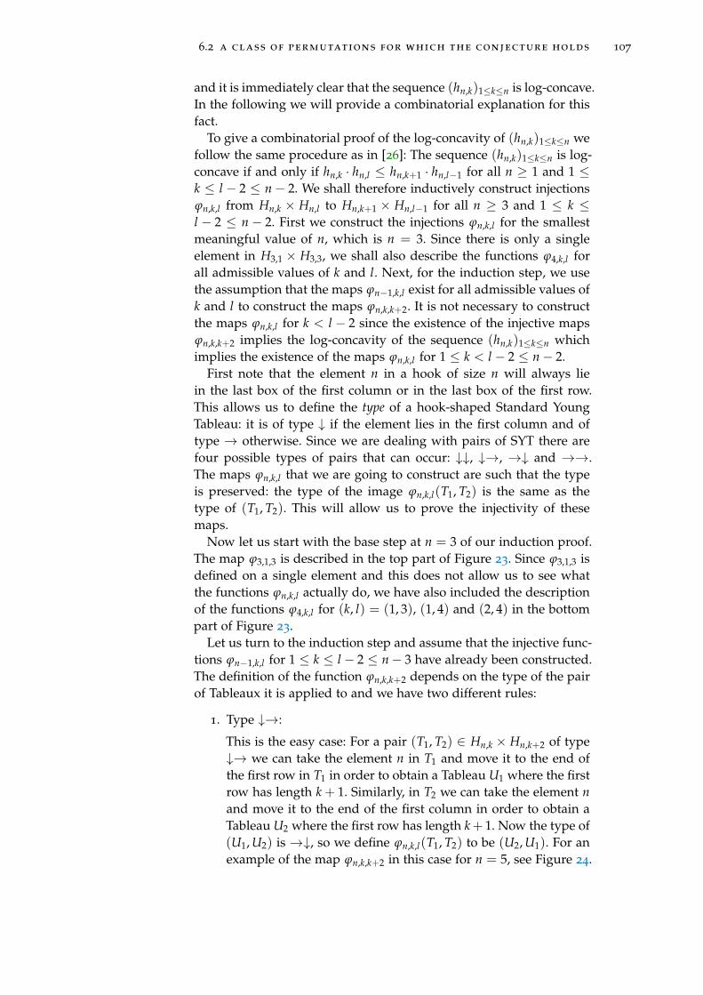
6.2 a class of permutations for which the conjecture holds 107
and it is immediately clear that the sequence (hn,k)1≤k≤n is log-concave.In the following we will provide a combinatorial explanation for thisfact.
To give a combinatorial proof of the log-concavity of (hn,k)1≤k≤n wefollow the same procedure as in [26]: The sequence (hn,k)1≤k≤n is log-concave if and only if hn,k · hn,l ≤ hn,k+1 · hn,l−1 for all n ≥ 1 and 1 ≤k ≤ l − 2 ≤ n− 2. We shall therefore inductively construct injectionsϕn,k,l from Hn,k × Hn,l to Hn,k+1 × Hn,l−1 for all n ≥ 3 and 1 ≤ k ≤l − 2 ≤ n− 2. First we construct the injections ϕn,k,l for the smallestmeaningful value of n, which is n = 3. Since there is only a singleelement in H3,1 × H3,3, we shall also describe the functions ϕ4,k,l forall admissible values of k and l. Next, for the induction step, we usethe assumption that the maps ϕn−1,k,l exist for all admissible values ofk and l to construct the maps ϕn,k,k+2. It is not necessary to constructthe maps ϕn,k,l for k < l − 2 since the existence of the injective mapsϕn,k,k+2 implies the log-concavity of the sequence (hn,k)1≤k≤n whichimplies the existence of the maps ϕn,k,l for 1 ≤ k < l − 2 ≤ n− 2.
First note that the element n in a hook of size n will always liein the last box of the first column or in the last box of the first row.This allows us to define the type of a hook-shaped Standard YoungTableau: it is of type ↓ if the element lies in the first column and oftype → otherwise. Since we are dealing with pairs of SYT there arefour possible types of pairs that can occur: ↓↓, ↓→, →↓ and →→.The maps ϕn,k,l that we are going to construct are such that the typeis preserved: the type of the image ϕn,k,l(T1, T2) is the same as thetype of (T1, T2). This will allow us to prove the injectivity of thesemaps.
Now let us start with the base step at n = 3 of our induction proof.The map ϕ3,1,3 is described in the top part of Figure 23. Since ϕ3,1,3 isdefined on a single element and this does not allow us to see whatthe functions ϕn,k,l actually do, we have also included the descriptionof the functions ϕ4,k,l for (k, l) = (1, 3), (1, 4) and (2, 4) in the bottompart of Figure 23.
Let us turn to the induction step and assume that the injective func-tions ϕn−1,k,l for 1 ≤ k ≤ l− 2 ≤ n− 3 have already been constructed.The definition of the function ϕn,k,k+2 depends on the type of the pairof Tableaux it is applied to and we have two different rules:
1. Type ↓→:
This is the easy case: For a pair (T1, T2) ∈ Hn,k × Hn,k+2 of type↓→ we can take the element n in T1 and move it to the end ofthe first row in T1 in order to obtain a Tableau U1 where the firstrow has length k + 1. Similarly, in T2 we can take the element nand move it to the end of the first column in order to obtain aTableau U2 where the first row has length k+ 1. Now the type of(U1, U2) is →↓, so we define ϕn,k,l(T1, T2) to be (U2, U1). For anexample of the map ϕn,k,k+2 in this case for n = 5, see Figure 24.

108 log-concavity, longest increasing subsequences and involutions
n = 3(k, l) = (1, 3)
123
, 1 2 3 7−→
(1 23
, 1 32
)
n = 4(k, l) = (1, 3)
1234
, 1 2 34
7−→
1 234
, 1 324
1234
, 1 2 43
7−→
1 234
, 1 423
1234
, 1 3 42
7−→
1 324
, 1 423
(k, l) = (1, 4)
1234
, 1 2 3 4 7−→
1 234
, 1 2 43
(k, l) = (2, 4)
1 234
, 1 2 3 4 7−→
(1 2 34
, 1 2 43
)
1 423
, 1 2 3 4 7−→
(1 2 43
, 1 3 42
)
1 324
, 1 2 3 4 7−→
(1 2 34
, 1 3 42
)
Figure 23: The base step of the induction in the proof of Theorem 6.4: themaps ϕn,k,l for n = 3 and n = 4 and all allowed values for k and l.The box containing the largest element is marked in gray in everySYT and we can see that a pair of SYT of a given type is alwaysmapped to a pair of SYT of the same type.
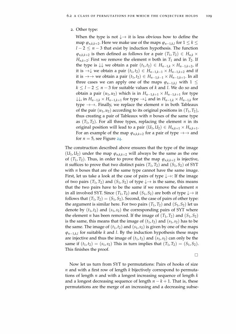
6.2 a class of permutations for which the conjecture holds 109
2. Other type:
When the type is not ↓→ it is less obvious how to define themap ϕn,k,k+2. Here we make use of the maps ϕn−1,k,l for 1 ≤ k ≤l − 2 ≤ n− 3 that exist by induction hypothesis. The functionϕn,k,k+2 is then defined as follows for a pair (T1, T2) ∈ Hn,k ×Hn,k+2: First we remove the element n both in T1 and in T2. Ifthe type is ↓↓ we obtain a pair (t1, t2) ∈ Hn−1,k × Hn−1,k+2, ifit is →↓ we obtain a pair (t1, t2) ∈ Hn−1,k−1 × Hn−1,k+2 and ifit is →→ we obtain a pair (t1, t2) ∈ Hn−1,k−1 × Hn−1,k+1. In allthree cases we can apply one of the maps ϕn−1,k,l with 1 ≤k ≤ l − 2 ≤ n− 3 for suitable values of k and l. We do so andobtain a pair (u1, u2) which is in Hn−1,k+1 × Hn−1,k+1 for type↓↓, in Hn−1,k × Hn−1,k+1 for type →↓ and in Hn−1,k × Hn−1,k fortype →→. Finally, we replace the element n in both Tableauxof the pair (u1, u2) according to its original positions in (T1, T2),thus creating a pair of Tableaux with n boxes of the same typeas (T1, T2). For all three types, replacing the element n in itsoriginal position will lead to a pair (U1, U2) ∈ Hn,k+1 × Hn,k+1.For an example of the map ϕn,k,k+2 for a pair of type →→ andfor n = 5, see Figure 24.
The construction described above ensures that the type of the image(U1, U2) under the map ϕn,k,k+2 will always be the same as the oneof (T1, T2). Thus, in order to prove that the map ϕn,k,k+2 is injective,it suffices to prove that two distinct pairs (T1, T2) and (S1, S2) of SYTwith n boxes that are of the same type cannot have the same image.First, let us take a look at the case of pairs of type ↓→: If the imageof two pairs (T1, T2) and (S1, S2) of type ↓→ is the same, this meansthat the two pairs have to be the same if we remove the element nin all involved SYT. Since (T1, T2) and (S1, S2) are both of type ↓→ itfollows that (T1, T2) = (S1, S2). Second, the case of pairs of other type:the argument is similar here. For two pairs (T1, T2) and (S1, S2) let usdenote by (t1, t2) and (s1, s2) the corresponding pairs of SYT wherethe element n has been removed. If the image of (T1, T2) and (S1, S2)
is the same, this means that the image of (t1, t2) and (s1, s2) has to bethe same. The image of (t1, t2) and (s1, s2) is given by one of the mapsϕn−1,k,l for suitable k and l. By the induction hypothesis these mapsare injective and thus the image of (t1, t2) and (s1, s2) can only be thesame if (t1, t2) = (s1, s2) This in turn implies that (T1, T2) = (S1, S2).This finishes the proof.
Now let us turn from SYT to permutations: Pairs of hooks of sizen and with a first row of length k bijectively correspond to permuta-tions of length n and with a longest increasing sequence of length kand a longest decreasing sequence of length n− k + 1. That is, thesepermutations are the merge of an increasing and a decreasing subse-
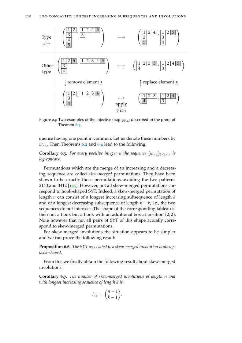
110 log-concavity, longest increasing subsequences and involutions
Type↓→
1 2345
, 1 2 4 53
7−→
1 2 435
, 1 2 534
Othertype
1 2 534
, 1 2 3 4 5 7−→
(1 2 3 54
, 1 2 4 53
)
99K remove element 5
99K replace element 5
1 234
, 1 2 3 4 799K
applyϕ4,2,4
(1 2 34
, 1 2 43
)
Figure 24: Two examples of the injective map ϕ5,k,l described in the proof ofTheorem 6.4.
quence having one point in common. Let us denote these numbers bymn,k. Then Theorems 6.2 and 6.4 lead to the following:
Corollary 6.5. For every positive integer n the sequence (mn,k)1≤k≤n islog-concave.
Permutations which are the merge of an increasing and a decreas-ing sequence are called skew-merged permutations. They have beenshown to be exactly those permutations avoiding the two patterns2143 and 3412 [145]. However, not all skew-merged permutations cor-respond to hook-shaped SYT. Indeed, a skew-merged permutation oflength n can consist of a longest increasing subsequence of length kand of a longest decreasing subsequence of length n− k, i.e., the twosequences do not intersect. The shape of the corresponding tableau isthen not a hook but a hook with an additional box at position (2, 2).Note however that not all pairs of SYT of this shape actually corre-spond to skew-merged permutations.
For skew-merged involutions the situation appears to be simplerand we can prove the following result:
Proposition 6.6. The SYT associated to a skew-merged involution is alwayshook-shaped.
From this we finally obtain the following result about skew-mergedinvolutions:
Corollary 6.7. The number of skew-merged involutions of length n andwith longest increasing sequence of length k is:
in,k =
(n− 1k− 1
).
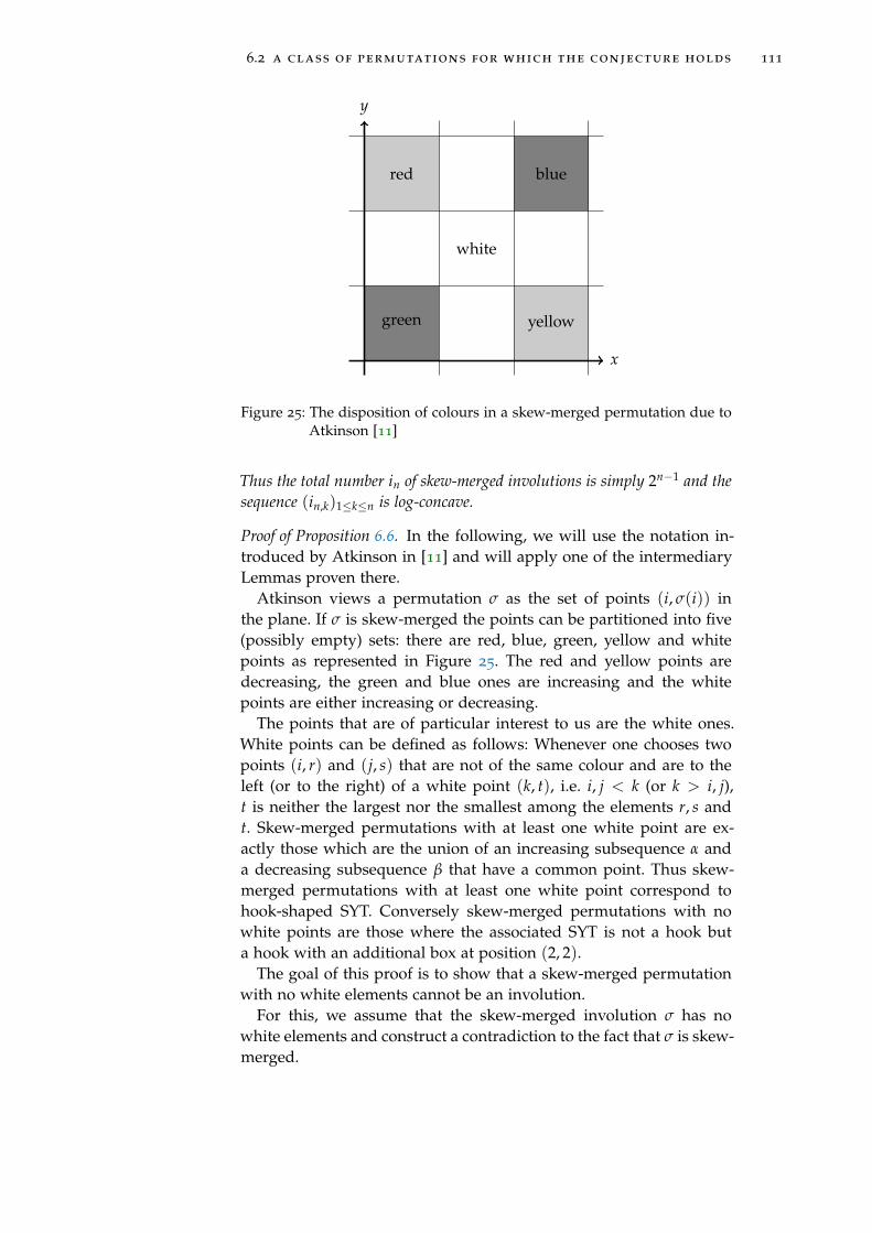
6.2 a class of permutations for which the conjecture holds 111
x
y
green
red
white
yellow
blue
Figure 25: The disposition of colours in a skew-merged permutation due toAtkinson [11]
Thus the total number in of skew-merged involutions is simply 2n−1 and thesequence (in,k)1≤k≤n is log-concave.
Proof of Proposition 6.6. In the following, we will use the notation in-troduced by Atkinson in [11] and will apply one of the intermediaryLemmas proven there.
Atkinson views a permutation σ as the set of points (i, σ(i)) inthe plane. If σ is skew-merged the points can be partitioned into five(possibly empty) sets: there are red, blue, green, yellow and whitepoints as represented in Figure 25. The red and yellow points aredecreasing, the green and blue ones are increasing and the whitepoints are either increasing or decreasing.
The points that are of particular interest to us are the white ones.White points can be defined as follows: Whenever one chooses twopoints (i, r) and (j, s) that are not of the same colour and are to theleft (or to the right) of a white point (k, t), i.e. i, j < k (or k > i, j),t is neither the largest nor the smallest among the elements r, s andt. Skew-merged permutations with at least one white point are ex-actly those which are the union of an increasing subsequence α anda decreasing subsequence β that have a common point. Thus skew-merged permutations with at least one white point correspond tohook-shaped SYT. Conversely skew-merged permutations with nowhite points are those where the associated SYT is not a hook buta hook with an additional box at position (2, 2).
The goal of this proof is to show that a skew-merged permutationwith no white elements cannot be an involution.
For this, we assume that the skew-merged involution σ has nowhite elements and construct a contradiction to the fact that σ is skew-merged.

112 log-concavity, longest increasing subsequences and involutions
In order to so, we will need a slightly weaker version of one of thetwo assertions in Lemma 11 in [11]. We shall state it here in the formwe need it:
Lemma [11]: Suppose that σ is a skew-merged permutation oflength n with no white points. Then there exist indices 1 ≤i < j < j + 1 < k ≤ n such that one of the following twostatements holds:
• σ(i)σ(j)σ(j + 1)σ(k) forms a 3142-pattern in σ
• σ(i)σ(j)σ(j + 1)σ(k) forms a 2413-pattern in σ
We will now show the following: If σ(i)σ(j)σ(j + 1)σ(k) forms a3142-pattern then σ also contains the pattern 3412 or 2143 and is thusnot skew-merged. In order to do so we distinguish three differentcases. To alleviate notation, we will write cadb instead of σ(i)σ(j)σ(j+1)σ(k) and will keep in mind that a < b < c < d.
1. d ≤ j + 1:
This implies that a ≤ d− 3 ≤ j− 2 and that b ≤ d− 2 ≤ j− 1.Especially this means that a and b cannot be fixed points in σ.Since σ is an involution we thus have σ(a) = j and σ(b) = k.Since a < b < j < k, we have jkab as a subsequence of σ thatforms a 3412-pattern.
2. a ≥ j:
This implies that c ≥ a + 2 ≥ j + 2 and that d ≥ a + 3 ≥ j + 3.Especially this means that c and d cannot be fixed points in σ.Since σ is an involution we thus have σ(c) = i and σ(d) = j + 1.Since i < j + 1 < c < d, we have cda(j + 1) as a subsequence ofσ that forms a 3412-pattern.
3. d > j + 1 and a < j:
In this case a and d aren’t fixed points and since σ is an involu-tion we have σ(a) = j and σ(d) = j + 1. Since a < j < j + 1 < d,we have jad(j + 1) as a subsequence of σ that forms a 2143-pattern.
Note that it is crucial in the arguments above that the elements a andd are adjacent in σ which is due to the fact that there are no whitepoints in σ.
If the second statement of the Lemma above is fulfilled, that is ifσ(i)σ(j) σ(j + 1)σ(k) forms a 2413-pattern, we consider the reversedpermutation σr, i.e., the permutation σ read from right to left. Thepermutation σr then contains the pattern 3142 at the positions (n +
1 − k), (n − j), (n + 1 − j) and (n + 1 − i). This implies that σr alsocontains 3412 or 2143 as a pattern and is not skew-merged. Remarkthat a permutation is skew-merged exactly then when its reverse is

6.2 a class of permutations for which the conjecture holds 113
1
m elements
l elements
the eastern surplus
the southern surplus
the protected area
ac
db
Figure 26: The decomposition of a SYT into its surplus and protected area. Theprotected area consists of m elements of which l are in the firstrow.
skew-merged. Thus we conclude that σ is not skew-merged in thiscase either.
We have thus proven that a skew-merged involution must containat least one white point and the shape of its associated SYT is a hook.
The set of (l, m)-protected SYT
Definition 6.8. Given an arbitrary SYT T, it can be decomposed into twoparts in a unique way as follows: The protected area of T is obtained fromT by removing as many boxes as possible in the first row and in the firstcolumn of T without creating a shape that is no longer a Young diagram.The removed elements form the surplus of T. The elements that have beenremoved in the first row are referred to as the eastern surplus and the onesin the first column as the southern surplus.
Example 6.9. For an illustration of this decomposition of a SYT intoprotected area and surplus, see Figure 26. Note that if T is a hook inthe sense of Definition 6.3, then the protected area of T consists of thebox containing the element 1 only. a
We can now define the following class of SYT:
Definition 6.10. Let T be a SYT in which all elements contained in its sur-plus are larger than all elements contained in the first row and first columnof its protected area. If T has a protected area of size m of which l elementsare contained in the first row it is called (l, m)-protected.

114 log-concavity, longest increasing subsequences and involutions
Example 6.11. For an example of an (l, m)-protected SYT with l = 4and m = 12, see the top part of Figure 27 where the protected areashave been marked in gray. a
Let a, b, c and d be the elements of T as displayed in Figure 26,i.e., a is the smallest element in the eastern surplus and c is its leftneighbour in T, b is the smallest element in the southern surplus andd is its top neighbour in T. Then the condition that all elements in thesurplus are larger than those in the first row and first column of theprotected area is equivalent to:
min(a, b) > max(c, d). (22)
Before we tackle our conjecture for the set of (l, m)-protected SYT,let us consider the special case of (2, 4)-protected SYT and take acloser look at the set of these SYT. For (2, 4)-protected SYT, i.e., SYTwhose shape is a hook with an additional box at the position (2, 2),condition (22) is fulfilled if and only if the elements 1, 2, and 3 are con-tained in the protected area. Equivalently, the elements 1, 2, and 3 maynot be contained in the same row or column of the SYT. Turning toinvolutions, this translates as follows: Involutions that correspond to(2, 4)-protected SYT have the property that the lengths of the longestincreasing and of the longest decreasing sequence add up to the totallength of the permutation and the elements 1, 2, and 3 do not form a123- or a 321- pattern.
A question that is of interest here is the following: how many SYTwhose shape is a hook with an additional box at the position (2, 2) ac-tually fulfil condition (22)? We will see that this is the case for roughlyhalf of the SYT of this shape.
Proposition 6.12. Let pn denote the number of (2, 4)-protected SYT ofsize n and let bn denote the number of SYT whose shape is a hook with anadditional box at the position (2, 2). Then the following holds for all n ≥ 4:
pn = (n− 3)2n−3, bn = (n− 4)2n−2 + 2 and thus limn→∞
pn
bn=
12
.
Proof. Let us start by counting (2, 4)-protected SYT. We know that theelements 1, 2 and 3 have to be present in the protected area and thereare two different possibilities of arranging them. Moreover we canchoose the element i that will lie in the box at position (2, 2) amongthe integers 4, . . . , n. The remaining entries are then inserted one afterthe other in increasing order. For every element we can choose toplace it either in the eastern or in the southern surplus of the tableauwhich gives us a total of 2n−4 possibilities. In total we have:
pn = 2 · (n− 3)2n−4 = (n− 3)2n−3.
Now let us count SYT whose shape is a hook with an additionalbox at the position (2, 2) but that are not (2, 4)-protected. That is,
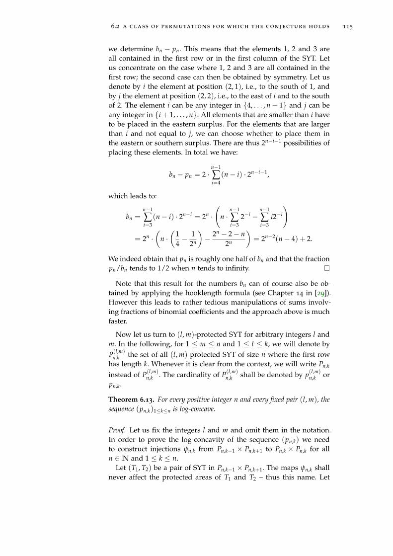
6.2 a class of permutations for which the conjecture holds 115
we determine bn − pn. This means that the elements 1, 2 and 3 areall contained in the first row or in the first column of the SYT. Letus concentrate on the case where 1, 2 and 3 are all contained in thefirst row; the second case can then be obtained by symmetry. Let usdenote by i the element at position (2, 1), i.e., to the south of 1, andby j the element at position (2, 2), i.e., to the east of i and to the southof 2. The element i can be any integer in {4, . . . , n− 1} and j can beany integer in {i + 1, . . . , n}. All elements that are smaller than i haveto be placed in the eastern surplus. For the elements that are largerthan i and not equal to j, we can choose whether to place them inthe eastern or southern surplus. There are thus 2n−i−1 possibilities ofplacing these elements. In total we have:
bn − pn = 2 ·n−1
∑i=4
(n− i) · 2n−i−1,
which leads to:
bn =n−1
∑i=3
(n− i) · 2n−i = 2n ·(
n ·n−1
∑i=3
2−i −n−1
∑i=3
i2−i
)
= 2n ·(
n ·(
14− 1
2n
)− 2n − 2− n
2n
)= 2n−2(n− 4) + 2.
We indeed obtain that pn is roughly one half of bn and that the fractionpn/bn tends to 1/2 when n tends to infinity.
Note that this result for the numbers bn can of course also be ob-tained by applying the hooklength formula (see Chapter 14 in [29]).However this leads to rather tedious manipulations of sums involv-ing fractions of binomial coefficients and the approach above is muchfaster.
Now let us turn to (l, m)-protected SYT for arbitrary integers l andm. In the following, for 1 ≤ m ≤ n and 1 ≤ l ≤ k, we will denote byP(l,m)
n,k the set of all (l, m)-protected SYT of size n where the first rowhas length k. Whenever it is clear from the context, we will write Pn,k
instead of P(l,m)n,k . The cardinality of P(l,m)
n,k shall be denoted by p(l,m)n,k or
pn,k.
Theorem 6.13. For every positive integer n and every fixed pair (l, m), thesequence (pn,k)1≤k≤n is log-concave.
Proof. Let us fix the integers l and m and omit them in the notation.In order to prove the log-concavity of the sequence (pn,k) we needto construct injections ψn,k from Pn,k−1 × Pn,k+1 to Pn,k × Pn,k for alln ∈N and 1 ≤ k ≤ n.
Let (T1, T2) be a pair of SYT in Pn,k−1 × Pn,k+1. The maps ψn,k shallnever affect the protected areas of T1 and T2 – thus this name. Let
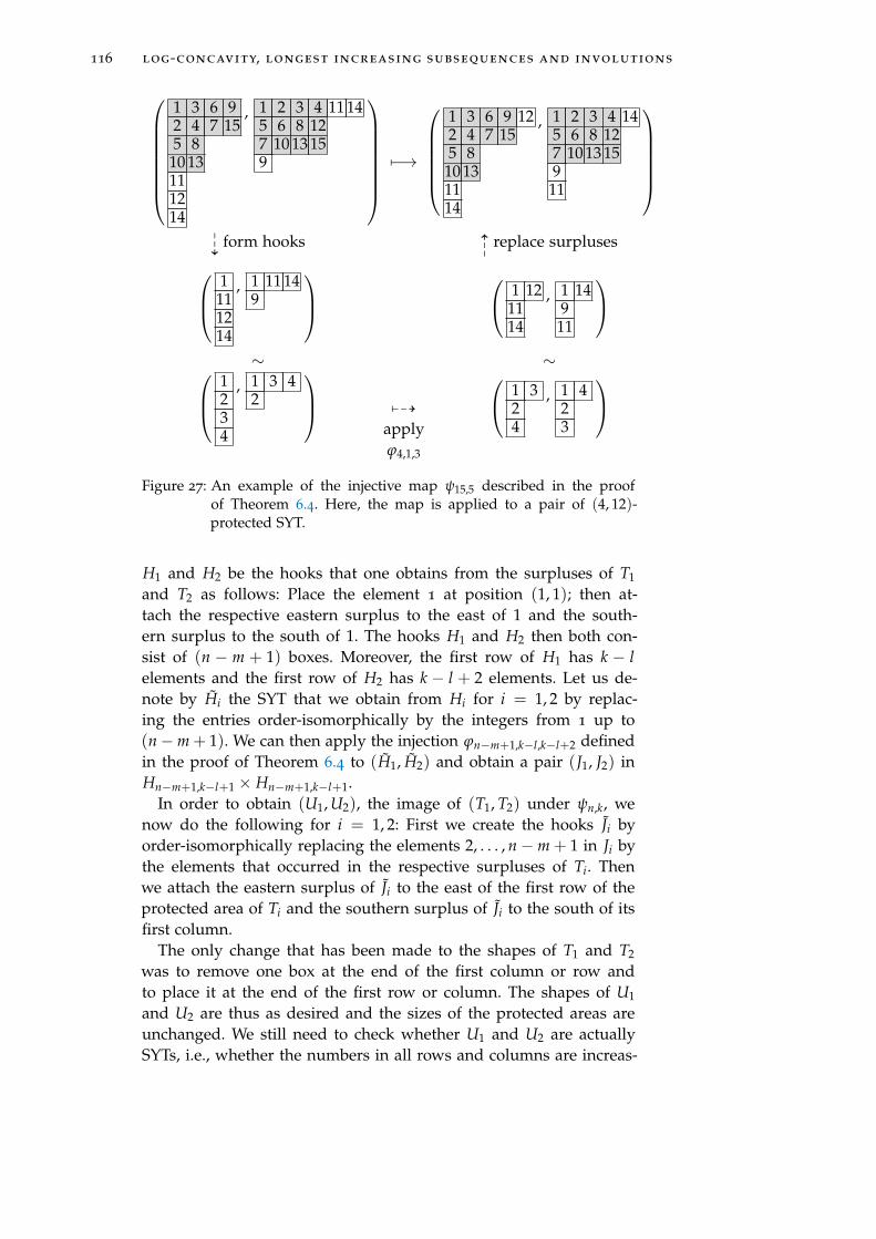
116 log-concavity, longest increasing subsequences and involutions
1 3 6 92 4 7 155 810 13111214
, 1 2 3 4 11 145 6 8 127 10 13 159
7−→
1 3 6 9 122 4 7 155 810 131114
, 1 2 3 4 145 6 8 127 10 13 15911
99K form hooks
99K replace surpluses
1111214
, 1 11 149
1 121114
, 1 149
11
∼ ∼
1234
, 1 3 42
799K
applyϕ4,1,3
1 324
, 1 423
Figure 27: An example of the injective map ψ15,5 described in the proofof Theorem 6.4. Here, the map is applied to a pair of (4, 12)-protected SYT.
H1 and H2 be the hooks that one obtains from the surpluses of T1
and T2 as follows: Place the element 1 at position (1, 1); then at-tach the respective eastern surplus to the east of 1 and the south-ern surplus to the south of 1. The hooks H1 and H2 then both con-sist of (n − m + 1) boxes. Moreover, the first row of H1 has k − lelements and the first row of H2 has k − l + 2 elements. Let us de-note by Hi the SYT that we obtain from Hi for i = 1, 2 by replac-ing the entries order-isomorphically by the integers from 1 up to(n−m + 1). We can then apply the injection ϕn−m+1,k−l,k−l+2 definedin the proof of Theorem 6.4 to (H1, H2) and obtain a pair (J1, J2) inHn−m+1,k−l+1 × Hn−m+1,k−l+1.
In order to obtain (U1, U2), the image of (T1, T2) under ψn,k, wenow do the following for i = 1, 2: First we create the hooks Ji byorder-isomorphically replacing the elements 2, . . . , n−m + 1 in Ji bythe elements that occurred in the respective surpluses of Ti. Thenwe attach the eastern surplus of Ji to the east of the first row of theprotected area of Ti and the southern surplus of Ji to the south of itsfirst column.
The only change that has been made to the shapes of T1 and T2
was to remove one box at the end of the first column or row andto place it at the end of the first row or column. The shapes of U1
and U2 are thus as desired and the sizes of the protected areas areunchanged. We still need to check whether U1 and U2 are actuallySYTs, i.e., whether the numbers in all rows and columns are increas-
6.3 lattice paths and 321-avoiding permutations 117
ing. Clearly, we only need to do so for the first row and the firstcolumn since the other parts have not been affected. By definition ofthe maps ϕn−m+1,k−l,k−l+2, the elements in the surpluses of U1 andU2 are increasing. Moreover, the elements in the surpluses of U1 andU2 are all larger than the elements contained in the first row and firstcolumn of the corresponding protected areas. Thus we indeed obtaina pair of tableaux (U1, U2) in Pn,k × Pn,k with the same values for land m as for (T1, T2). The injectivity of the maps ψn,k clearly followsfrom the injectivity of the maps ϕn−m+1,k−l,k−l+2.
Example 6.14. For an example of the map ψn,k with n = 15, k = 5and (l, m) = (4, 12), see Figure 27. a
6.3 lattice paths and 321-avoiding permutations
In the following, let An ,k denote the set of all 321-avoiding involu-tions of length n with longest increasing sequence of length k. Thecardinality of An ,k will be denoted by an ,k . The Robinson-Schenstedcorrespondence maps elements of An ,k into SYT that consist of atmost two rows such that the length of the first row is k ≥ dn/2e.Then the hooklength formula yields that
an ,k =
(nk
)2k − n + 1
k + 1.
Using this formula, it is routine to prove that for any fixed n, thesequence an ,k is log-concave if k ∈ [dn/2e , n ], but that proof is notparticularly elucidating. In what follows, we provide a more elegant,injective proof.
There is a natural bijection f = f n between the set of such SYT andlattice paths using steps (0, 1) and (1, 0) that start at (0, 0), consistof n steps, and never go above the diagonal x = y. We will refer tothese steps as East and North steps. Indeed, if i1 , i2 , · · · , ik are thenumbers in the first row of the SYT T , and j1 , j2 , · · · , jn−k are thenumbers in the second row of T , then we can set f (T ) to be the latticepath starting at (0, 0) whose East steps are in positions i1 , i2 , · · · , ik ,and whose North steps are in positions j1 , j2 , · · · , jn−k . The fact thatT is a SYT means that i t < jt for all t ≤ n − k, so f (T ) will indeedstay below the diagonal x = y since its t-th North step will comesome time after its t-th East step. Note that elements of An ,k will bemapped into paths that end in (k , n − k).
Example 6.15. The SYT with elements 1, 3, 4, 5, 6, 7 in the first rowand the element 2 in the second row corresponds to the path Q con-sisting of the following steps: E, N, E, E, E, E, E. It is representedby circles on the left hand side of Figure 28. Similarly, the SYT withelements 1, 2, 4, 7 in the first and elements 3, 5, 6 in the second rowcorresponds to the path P : E, E, N, E, N, N, E. a

118 log-concavity, longest increasing subsequences and involutions
P′1
P′2
Q1
Q2X
P′1
P′2
Q1
Q2X
Figure 28: The main step in the construction of the map φ
Let L(n , k) be the set of lattice paths using steps (0, 1) and (1, 0)that start at (0, 0), never go above the diagonal x = y, and end in(k , n − k), where n − k ≤ k ≤ n − 2. We define a map
φ : L(n , k) × L(n , k + 2) → L(n , k + 1) × L(n , k + 1)
as follows.Let (P, Q) ∈ L(n, k)× L(n, k + 2). Let us translate P by the vector
(1,−1) to obtain the path P′ that starts at (1,−1), ends in (k + 1, n−k − 1), and never goes above the diagonal x − 2 = y. As Q starts Westof P′ and ends East of P′, the paths P′ and Q will have at least onepoint in common. Let X be the last such point. Note that X is not theendpoint of P′ or Q, since those two paths do not end in the samepoint. We now “flip” the paths at X, which means the following. LetP′1 and Q1 denote the parts of P′ and Q that end in X, and let P′2 andQ2 denote the parts of P′ and Q that start in X. Then we define φ(P, Q)
as ((P′1Q2)∗, Q1P′2), where (P′1Q2)∗ denotes the path P′1Q2 translatedback by the vector (−1, 1) so that it starts at (0, 0). See Figure 28 foran illustration.
Proposition 6.16. The map φ described above indeed maps into the setL(n, k + 1) × L(n, k + 1) and is an injection from L(n, k) × L(n, k + 2)into L(n, k + 1)× L(n, k + 1).
Proof. It is a direct consequence of the definitions that both (P′1Q2)∗and Q1P′2 will indeed start at (0, 0) and end in (k+ 1, n− k+ 1). So, allwe need to do in order to prove that φ(P, Q) ∈ L(n, k+ 1)× L(n, k+ 1)is to show that neither (P′1Q2)∗ and Q1P′2 ever goes above the diagonalx = y.
• To show that (P′1Q2)∗ does not go above the diagonal x = y isequivalent to showing that P′1Q2 does not go above the diagonalx− 2 = y. This is true for P′1 by its definition (it is a part of P′),and this is true for Q2 since Q2 is entirely below P′2, and P′2, byits definition (it is a part of P′), never goes above the diagonalx− 2 = y.
• It is clear that Q1P′2 never goes above the diagonal x = y, sinceneither Q1 (a part of Q) nor P′2 (a part of P) do.

6.4 summary of the results 119
Finally, in order to prove that the map φ is injective, let (R, S) bein L(n, k + 1) × L(n, k + 1). If R and S have no points in common(other than their starting and ending points), (R, S) has no preimageunder φ. Otherwise, we can recover X as the last point that R andS have in common other than their endpoint, and then reversing the“flipping” operation described in the construction of φ we can recoverthe unique preimage of (R, S).
Corollary 6.17. For any fixed n, the sequence (an,k)n/2≤k≤n is log-concave.
Therefore, it follows by the principle that we used to prove Theo-rem 6.2 that we have an injective proof of the following corollary aswell.
Corollary 6.18. Let bn,k denote the number of 321-avoiding permutationsof length n in which the longest increasing subsequence is of length k. Thenfor any fixed n, the sequence (bn,k)n/2≤k≤n is log-concave.
6.4 summary of the results
Let us briefly summarize the results of this chapter. First we statedour conjecture that the sequence (`n,k)1≤k≤n is log-concave for fixedn ∈ N and showed that it suffices to prove this conjecture for invo-lutions in order to obtain a result for permutations in general. Sec-ond, we proved that our conjecture holds for SYT whose shape is ahook which implies that it holds for skew-merged involutions. Thisresult could be extended to a larger class of permutations, based onthe concept of (l, m)-protected SYT. Third, we showed that our con-jecture holds for 321-avoiding permutations. For all our results weprovided combinatorial proofs and exploited the Robinson-Schenstedcorrespondence between permutations and pairs of SYT.


Part II
C AY L E Y T R E E S A N D M A P P I N G S
This part treats two seemingly unrelated topics on Cayleytrees and mappings. First, Chapter 7 provides a new bijec-tive proof of Cayley’s formula that will be applied in thefollowing chapters. Second, Chapter 8 deals with ascend-ing runs in trees and mappings, analysing the occurrenceof a specific pattern that involves the labels of the combi-natorial object. Third, Chapter 9 generalizes the concept ofparking functions to trees and to mappings. Even thoughthese two topics have little in common at first sight, a simi-lar decomposition approach leading to PDEs is fruitful fortackling the enumeration task.

7A N E W B I J E C T I V E P R O O F O F C AY L E Y ’ S F O R M U L A
We start this part by presenting a new bijective proof of Cayley’s for-mula. This bijection will be used in the following two chapters thatconcern ascending runs in trees and mappings (Chapter 8) and a gen-eralization of the concept of parking functions to trees and mappings(Chapter 9).
Theorem 7.1. For each n ≥ 1, there exists a bijection ϕ from the set of pairs(T, w), with T ∈ Tn a tree of size n and w ∈ T a node of T, to the set ofn-mappings. Thus
n · Tn = Mn, for n ≥ 1.
Proof. In the following, we will denote by T(v) the parent of node vin the tree T. That is, for v 6= root(T), T(v) is the unique node suchthat (v, T(v)) is an edge in T.
Given a pair (T, w), we consider the unique path w root(T)from the node w to the root of T. It consists of the nodes v1 = w,v2 = T(v1), . . . , vi+1 = T(vi), . . . , vr = root(T) for some r ≥ 1. Wedenote by I = (i1, . . . , it), with i1 < i2 < · · · < it for some t ≥ 1, theindices of the right-to-left maxima in the sequence v1, v2, . . . , vr, i.e.,
i ∈ I ⇐⇒ vi > vj, for all j > i.
The corresponding set of nodes in the path w root(T) will be de-noted by VI := {vi : i ∈ I}. Of course, if follows from the definitionthat the root node is always contained in VI , i.e., vr ∈ VI .
We can now describe the function ϕ by constructing an n-mappingf . The t right-to-left maxima in the sequence v1, v2, . . . , vr will giverise to t connected components in the functional digraph G f . More-over, the nodes on the path w root(T) in T will correspond to thecyclic nodes in G f . We describe f by defining f (v) for all v ∈ [n],where we distinguish whether v ∈ VI or not.
(a) Case v /∈ VI : We set f (v) := T(v).
(b) Case v ∈ VI : Setting T(vi0) := v1 = w, we define
f (vi`) := T(vi`−1
).
This means that the nodes on the path w root(T) in T form tcycles C1 := (v1, . . . , vi1), . . . , Ct := (T(vit−1), . . . , vr = vit) in G f .
It is now easy to describe the inverse function ϕ−1. Given a map-ping f , we sort the connected components of G f in decreasing order
123
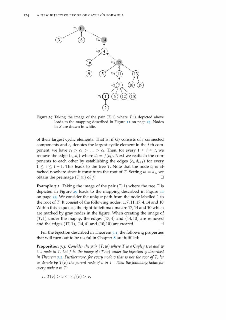
124 a new bijective proof of cayley’s formula
10
3 8 14
4
16
9
17
5 11
7
1
2
6 12 15
13
18 19
v1
v2
v3
v4
v5
v6
v7
Figure 29: Taking the image of the pair (T, 1) where T is depicted aboveleads to the mapping described in Figure 11 on page 23. Nodesin S are drawn in white.
of their largest cyclic elements. That is, if G f consists of t connectedcomponents and ci denotes the largest cyclic element in the i-th com-ponent, we have c1 > c2 > . . . > ct. Then, for every 1 ≤ i ≤ t, weremove the edge (ci, di) where di = f (ci). Next we reattach the com-ponents to each other by establishing the edges (ci, di+1) for every1 ≤ i ≤ t − 1. This leads to the tree T. Note that the node ct is at-tached nowhere since it constitutes the root of T. Setting w = d1, weobtain the preimage (T, w) of f .
Example 7.2. Taking the image of the pair (T, 1) where the tree T isdepicted in Figure 29 leads to the mapping described in Figure 11
on page 23. We consider the unique path from the node labelled 1 tothe root of T. It consist of the following nodes: 1, 7, 11, 17, 4, 14 and 10.Within this sequence, the right-to-left maxima are 17, 14 and 10 whichare marked by gray nodes in the figure. When creating the image of(T, 1) under the map ϕ, the edges (17, 4) and (14, 10) are removedand the edges (17, 1), (14, 4) and (10, 10) are created. a
For the bijection described in Theorem 7.1, the following propertiesthat will turn out to be useful in Chapter 8 are fulfilled:
Proposition 7.3. Consider the pair (T, w) where T is a Cayley tree and wis a node in T. Let f be the image of (T, w) under the bijection ϕ describedin Theorem 7.1. Furthermore, for every node v that is not the root of T, letus denote by T(v) the parent node of v in T . Then the following holds forevery node v in T:
1. T(v) > v⇐⇒ f (v) > v,

a new bijective proof of cayley’s formula 125
2. There exists a node x < v in T with T(x) = v
⇐⇒ There exists an element x < v in f with f (x) = v.
Proof. The main reason why these properties hold is the following:When creating the image of some (T, w) under the map ϕ, the onlyedges that are removed are decreasing ones. That is, the only edgesthat are present in T but not in G f , are of the form (v, x) where v > x.The edges that are created instead in G f are also decreasing ones. Inthe following, we prove the two statements of the theorem in moredetail:
1. As in the proof of Theorem 7.1 we distinguish whether the nodev in T is contained in VI or not: If v is not contained in VI ,f (v) = T(v) and thus the statement is clearly true. If v ∈ VI , vis a right-to-left maximum in the unique path from w to the rootof T. It thus holds v = vi` for some ` and clearly T(v) < v. Weneed to show that this implies that f (v) ≤ v. By definition, wehave f (vi`) = T
(vi`−1
). T(vi`−1
)is either equal to vi` or it is not a
right-to left maximum in which case it is clearly strictly smallerthan vi` . This proves the first statement of this proposition.
2. (=⇒) : If the node v has a child x with x < v, then x cannotbelong to the set of nodes VI . Thus f (x) = T(x) = v and in themapping f the node v has a preimage x with x < v.
(⇐=) : Let x be an element with x < v and f (x) = v. Supposex = vi` for some `. Then v = f (x) = T(vi`−1) ≤ x. Thus x /∈ VI
and we have f (x) = T(x). Therefore x is a child of v in T thatfulfils x < v.


8A S C E N D I N G R U N S I N M A P P I N G S
This chapter is based on joint work with Alois Panholzer.Random mappings, i.e., random functions from the set [n] into it-
self, arise in many applications and are very well-studied objects bothfrom a combinatorial and a probabilistic point of view. For examplesof situations where random mappings occur, see e.g. the introductionof [75]. Previous research has concentrated on structural parametersof the corresponding functional graphs. Structural parameters suchas the number of connected components, the size of the largest tree,the number of terminal nodes, etc. are well-studied objects. Exem-plarily, we would like to mention the work of Arney and Bender [8],Kolchin [112], Flajolet and Odlyzko [75], Drmota and Soria [61] (givenin chronological order).
In the functional graphs corresponding to random mappings, thelabels of nodes play an important role and thus it is somewhat sur-prising that, despite the many studies of mappings concerning struc-tural quantities, the occurrences of label patterns have received farless attention so far.
Some recent research in this direction has been performed by Pan-holzer who studied alternating mappings in [130]. These are a gen-eralization of the concept of alternating permutations to mappings;they can be defined as those mappings for which every iteration orbitforms an alternating sequence. Alternating mappings can thus alsobe seen as mappings that do not contain two consecutive ascents ordescents; this is a characterization in terms of forbidden label pat-terns. Also, we would like to mention the PhD thesis of Okoth [129]who has very recently studied local extrema in trees (called sourcesand sinks there). His studies also lead to results for the correspondingquantities in mappings.
In this chapter, we study the occurrence of a specific label patternin mappings by generalizing the concept of ascending runs from per-mutations to mappings. See Section 2.2 in the Preliminaries, for adefinition and a distinction between ascending and alternating runs.Since the only types of runs encountered in this chapter are ascendingruns, we will also use runs for short. As we will see in Section 32,counting runs in mappings is equivalent to counting the number ofnodes that form the label pattern on the left-hand side in Figure 30.Our goal is to enumerate mappings by their size and by their numberof ascending runs and to characterize the typical behaviour of thislabel pattern in random mappings. Since connected mappings can be
127
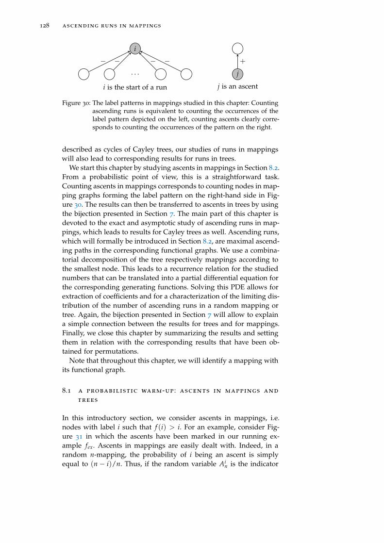
128 ascending runs in mappings
i
. . .
− −− −
i is the start of a run
j
+
j is an ascent
Figure 30: The label patterns in mappings studied in this chapter: Countingascending runs is equivalent to counting the occurrences of thelabel pattern depicted on the left, counting ascents clearly corre-sponds to counting the occurrences of the pattern on the right.
described as cycles of Cayley trees, our studies of runs in mappingswill also lead to corresponding results for runs in trees.
We start this chapter by studying ascents in mappings in Section 8.2.From a probabilistic point of view, this is a straightforward task.Counting ascents in mappings corresponds to counting nodes in map-ping graphs forming the label pattern on the right-hand side in Fig-ure 30. The results can then be transferred to ascents in trees by usingthe bijection presented in Section 7. The main part of this chapter isdevoted to the exact and asymptotic study of ascending runs in map-pings, which leads to results for Cayley trees as well. Ascending runs,which will formally be introduced in Section 8.2, are maximal ascend-ing paths in the corresponding functional graphs. We use a combina-torial decomposition of the tree respectively mappings according tothe smallest node. This leads to a recurrence relation for the studiednumbers that can be translated into a partial differential equation forthe corresponding generating functions. Solving this PDE allows forextraction of coefficients and for a characterization of the limiting dis-tribution of the number of ascending runs in a random mapping ortree. Again, the bijection presented in Section 7 will allow to explaina simple connection between the results for trees and for mappings.Finally, we close this chapter by summarizing the results and settingthem in relation with the corresponding results that have been ob-tained for permutations.
Note that throughout this chapter, we will identify a mapping withits functional graph.
8.1 a probabilistic warm-up : ascents in mappings and
trees
In this introductory section, we consider ascents in mappings, i.e.nodes with label i such that f (i) > i. For an example, consider Fig-ure 31 in which the ascents have been marked in our running ex-ample fex. Ascents in mappings are easily dealt with. Indeed, in arandom n-mapping, the probability of i being an ascent is simplyequal to (n − i)/n. Thus, if the random variable Ai
n is the indicator

8.1 a probabilistic warm-up : ascents in mappings and trees 129
1
7
11
17
5
2
612
15
13
1918
10
3 8
4 14
16
9
Figure 31: In our running example fex, 10 out of 19 nodes are ascents. Theseare marked by square nodes.
variable for the event “node i is an ascent in a random n-mapping”Ai
n follows a Bernoulli distribution with parameter p = (n − i)/n:Ai
n ∼ B((n − i)/n). Moreover, An = ∑ni=1 Ai
n and since the Ain’s
are independent random variables we easily obtain An’s probability-generating function
mAn(t) =∞
∑k=0
tkP {An = k}
=n
∏i=1
mAin(t)
=n
∏i=1
i + t(n− i)n
.
Thus, An follows a so-called Poisson binomial distribution (see e.g. [21]).The number An,m of n-mappings with exactly m ascents is thus simplygiven as:
An,m = [tm]n
∏k=1
k + t(n− k)
= ∑I⊆[n]|I|=m
(∏i∈I
(n− i) ∏j∈Ic
j
).

130 ascending runs in mappings
Clearly, the sequence (An,m)m=0...n is symmetric: An,m = An,n−1−m.It is also easily shown to be unimodal since mAn(t) has real roots only.Moreover, one readily sees that
E(An) =n
∑i=1
E(Ain) and V(An) =
n
∑i=1
(1−E(Ai
n))
E(Ain)
=n
∑i=1
n− in
=n
∑i=1
in· n− i
n
=n− 1
2=
n2 − 16n
.
Using the Ljupanov-version of the Central Limit Theorem, Theorem 2.35,we can show even more:
Theorem 8.1. Let An denote the random variable counting the number ofascents in a random n-mapping. Then the standardized random variable
An −E(An)√V(An)
converges in distribution to a standard normal distribution.
Proof. The result follows by a basic application of the Ljapunov CLT.Similar proofs can be found in any textbook on probability theory. Weneed to check whether there exists a δ > 0 such that
1√
V(An)2+δ
n
∑i=1
E(|Ai
n −E(Ain)|2+δ
)→ 0 as n→ ∞
is fulfilled. Let δ > 0. Then the following holds:
1 ≥ n− in· i
n= E
((Ai
n −n− i
n
)2)
= V
(Ai
n −n− i
n
)≥ E
((Ai
n −n− i
n
)2+δ)
.
Thus we obtain
1√
V(An)2+δ
E
((Ai
n −n− i
n
)2+δ)
≤ 1√
V(An)2+δ
V
(Ai
n −n− i
n
)
=1
√V(An)
δ=
(6n
n2 − 1
)δ/2
and since the right hand side tends to zero as n → ∞ we obtain thedesired statement.

8.2 ascending runs in mappings 131
These results themselves are maybe not particularly surprising, butwhat is less straightforward is that they can be transferred to thecorresponding enumeration problem for trees. Indeed, as shown inTheorem 7.1 and Proposition 7.3, we can identify every pair (T, w)
where T is a Cayley tree of size n with m ascents and w is a node in Twith an n-mapping f with m ascents. We thus obtain the following:
An,m = n · Bn,m,
where Bn,m denotes the number of trees with n nodes and exactly mascents. Thus, if Bn is the random variable counting ascents in a treeof size n, An and Bn have exactly the same probability-generatingfunction for every integer n.
Corollary 8.2. Let Bn denote the random variable counting the number ofascents in a random Cayley tree of size n. Then the expectation and variancesatisfy
E(Bn) =n− 1
2and V(Bn) =
n2 − 16n
.
Furthermore, the standardized random variable
Bn −E(Bn)√V(Bn)
converges in distribution to a standard normal distribution.
A similar result for ascents in trees seems to have been obtainedin [49]. However, this simple approach via the detour of ascents inmappings is, to the best of our knowledge, new.
8.2 ascending runs in mappings
We consider here the number of ascending runs of a mapping. Gen-eralizing the definition of ascending runs for permutations (see Sec-tion 2.2), an ascending run in a mapping f is a maximal ascendingsequence i < f (i) < f 2(i) < · · · < f k(i), i.e., an ascending sequencewhich is not contained in a longer such sequence. The only type of“runs” studied in this chapter are ascending runs, we will thus alsouse the shorter term run when speaking of ascending runs. These arenot to be confused with alternating runs as studied in Chapter 3 (seeSection 2.2 for a distinction of these two concepts).
Given a specific mapping f and its functional graph G f , the numberof runs in f can be counted easily by considering the first element ofa run: Indeed, an element j is the first element of a run iff each label iof a preimage of j is not smaller than j, i.e., ( f (i) = j) ⇒ (i ≥ j). Wethus need to count nodes in the mapping that form the label patterndepicted on the left-hand side of Figure 30. Note that elements with

132 ascending runs in mappings
1
7
11
17
5
2
612
15
13
1918
10
3 8
4 14
16
9
Figure 32: In fex there are 13 ascending runs. If an element is the first ele-ment in a run, its node is white; otherwise it is gray. Increasingedges, i.e., edges (i, j) with i < j, are marked by dashed lines.
no preimages at all, i.e., terminal nodes in the graph, are of coursealways at the beginning of a run.
Recall that for permutations the following simple connection be-tween descents and ascending runs holds: if a permutation π has kdescents, i.e., positions i for which it holds that π(i) > π(i + 1), it canbe decomposed into (k + 1) ascending runs. Moreover, by taking thecomplement πc of π one obtains a permutation with k ascents. Thus,studying the distribution of the following parameters in permutationsis equivalent: ascents, descents, ascending runs and descending runs.This is clearly not the case for mappings: The presence of k descentsdoes not yield a decomposition into (k + 1) ascending runs. For ex-ample, in fex there are 10 ascents and thus 9 descents but the numberof ascending runs is equal to 13. Thus, the study of ascending runshas to be performed separately and requires, as we will see, far moreinvolved techniques than the one of ascents.
Example 8.3. In Figure 32, our running example fex of a 19-mappingis depicted. In its functional graph, the nodes that correspond to firstelements of an ascending run are marked by white nodes. There are13 such nodes and thus our mapping has 13 ascending runs. More-over, edges (i, j) where i < j are marked with dashed lines and edgeswith j > i are marked with full lines. An ascending run is thus a pathof maximal length consisting of dashed edges only (or no edges at all).An element that is the start of an ascending run can be characterizedas a node where no incoming edges are dashed. a
In the following, Rn will denote the r.v. that counts the number ofascending runs in a random n-mapping. Because of the combinatorialstructure of mappings as presented in Example 2.27, we will firstanalyse the corresponding random variable for trees before we studyRn.

8.2 ascending runs in mappings 133
...T1 T2 Tr...T1 TrT2
T0
i
1
1
Figure 33: Decomposition of a tree with respect to its smallest node
Runs in trees
To study Rn we first consider the corresponding quantity in trees,where the edges are oriented towards the root node of the tree. Thus,we introduce the random variable Fn which counts the number ofruns in a random Cayley tree of size n. Let us further introduce thegenerating function
F(z, v) = ∑n≥1
∑m≥0
P{Fn = m}Tnzn
n!vm
= ∑n≥1
∑m≥0
Fn,mzn
n!vm,
where Tn = nn−1 is the number of trees of size n and Fn,m is thenumber of trees of size n with exactly m ascending runs.
Clearly, F1,m = δm,1. In order to establish a recurrence relation forthe numbers Fn,m, we decompose a tree of size n ≥ 2 with respect tothe node labelled 1. Two different cases, as shown in Figure 33, haveto be considered:
Case (1): The node 1 is the root node. In this case a set of r ≥ 1subtrees T1, T2, . . . , Tr is attached to the root 1. Since the root has thesmallest of all labels, it will always constitute a run of its own. Thus,if the subtrees Ti have respective sizes ni and mi runs each, the entiretree will consist of n nodes and have m runs iff ∑r
i=1 ni = n− 1 and∑r
i=1 mi = m− 1. The contribution to Fn,m is therefore:
F(1)n,m = ∑
r≥1
1r! ∑
∑ ni=n−1∑ mi=m−1
Fn1,m1 · · · Fnr ,mr ·(
n− 1n1, . . . , nr
),
where the multinomial coefficient reflects the number of possibilitiesof redistributing the labels in [n− 1] order-isomorphically to the sub-trees.
Case (2): The node 1 is not the root node. In this case the node 1 isattached to some node labelled i of a tree T0 of size n0 and with m0
runs and has itself a set of r ≥ 0 subtrees T1, T2, . . . , Tr attached to

134 ascending runs in mappings
it. Depending on where in T0 the node 1 is attached, a new run iscreated or not. If 1 is attached at the begin of a run in T0 no new runis created – there are m0 possibilities of attaching 1 in this way. If 1is however attached somewhere in the middle of a run, a new runwill be created – for this case there are (n0 − m0) possibilities. Thecontribution to Fn,m is therefore:
F(2a)n,m = ∑
1≤n0·≤n−11≤m0≤m
m0 ·∑r≥0
1r! ∑
∑ ni=n−n0−1∑ mi=m−m0
Fn0,m0 · · · Fnr ,mr
(n− 1
n0, . . . , nr
)
for the case that the node 1 is attached to the beginning of a run in T0
and
F(2b)n,m =∑
1≤n0≤n−11≤m0≤m
(n0 −m0) ·∑r≥0
1r! ∑
∑ ni=n−n0−1∑ mi=m−m0−1
Fn0,m0 · · · Fnr ,mr
(n− 1
n0, . . . , nr
)
in the other cases.The goal is now to translate this recurrence relation for Fn,m =
F(1)n,m + F(2a)
n,m + F(2b)n,m into the language of generating functions. In order
to alleviate notation we write F for F(z, v), Fz and Fv for the partialderivatives of F with respect to z and v.
First, let us note that for F(1)n,m we have the following:
F(1)n,m = ∑
r≥1
(n− 1)!r! ∑
∑ ni=n−1∑ mi=m−1
[zn1 vm1 ]F · · · [znr vmr ]F
= (n− 1)![zn−1vm−1] exp(F)
= (n− 1)![znvm]zv exp(F).
Recall that m0 · Fn0,m0 /(n0)! = [zn0 vm0 ]vFv. We then obtain for F(2a)n,m :
F(2a)n,m = (n− 1)! ∑
n0,m0
([zn0 vm0 ]vFv) ·([zn−n0−1vm−m0 ] exp(F)
)
= (n− 1)![znvm]zvFv exp(F).
Similarly, for F(2b)n,m :
F(2b)n,m = (n− 1)![znvm]zv (zFz − vFv) exp(F).
Thus, we can write Fn,m as follows:
Fn,m =n![znvm]F
=(n− 1)![znvm]zv exp(F) (1 + zFz + (1− v)Fv) ,
or equivalently,
∑n≥1
∑m≥1
n[znvm]F = zFz = zv exp(F) (1 + zFz + (1− v)Fv) .

8.2 ascending runs in mappings 135
Thus the bivariate generating function F(z, v) is defined by the fol-lowing following partial differential equation:
(1− zveF(z,v)
)Fz(z, v) = v(1− v)eF(z,v)Fv(z, v) + veF(z,v),
with the initial condition F(0, v) = 0.This PDE can be solved using the method of characteristics (see
Section 2.8). Let us thus regard z, v and F as variables dependingon t. We then obtain the following system of ordinary differentialequations, the so-called system of characteristic differential equations:
dzdt
= 1− zv · eF(z,v), (23a)
dvdt
= eF(z,v) · v(v− 1), (23b)
dFdt
= v · eF(z,v). (23c)
We are now looking for first integrals of the system (23), i.e., forfunctions ζ(z, v, F) that are constant along any solution curve – a so-called characteristic curve – of (23). From (23b) and (23c) one obtainsthe following differential equation
dvdF
= v− 1
which has the general solution
v = c1 · eF + 1.
Thus a first integral of (23) is given by:
ζ1(z, v, F) = c1 = e−F · (v− 1). (24)
From (23a) and (23c) one obtains, after substituting v = c1 · eF + 1, thefollowing differential equation
dzdF
=1
(c1eF + 1) · eF − z.
The general solution of this first order linear differential equation is
z =F− ln
(c1 · eF + 1
)+ c2
eF .
After backsubstituting c1 = e−F · (v − 1) one obtains the followingfirst integral of (23) which is independent of (24):
ζ2(z, v, F) = c2 = z · eF − F + ln(v). (25)
The general solution of (23) is thus given by:
G(ζ1(z, v, F), ζ2(z, v, F)) = const.,

136 ascending runs in mappings
where G is an arbitrary differentiable function in two variables. Onecan also solve this equation with respect to the variable z and obtains:
z = e−F ·(
F− ln(v) + g(
v− 1eF
)),
where g is an arbitrary differentiable function in one variable. In orderto specify this function g, we plug the initial condition F(0, v) = 0 intothis equation. This leads to:
g(v− 1) = ln(v),
and finally we obtain that the solution of (23) is given by the followingfunctional equation:
z =ln(
eF(z,v)−1+vv
)
eF(z,v). (26)
Extracting coefficients can now be done by applying Lagrange’s in-version formula with ϕ(F) = exp(F)F/ ln
(eF−1+v
v
)and twice Cauchy’s
integral formula:
[zn]F(z, v) =1n[Fn−1]
enF · Fn
ln(
eF−1+vv
)n
=1
n · 2πi
∮ enF
ln(
eF−1+vv
)n dF
=1
n · 2πi
∮(eS · v− 1 + v)n−1 · eSv
Sn dS
=1n[Sn−1](eS · v− 1 + v)n−1 · eSv
=vn
n−1
∑k=0
1(n− 1− k)!
n−1
∑`=0
(n− 1`
)`kv`
k!(v− 1)n−1−`
=vn
n−1
∑`=0
(n− 1`
)v`(v− 1)n−1−` (l + 1)n−1
(n− 1)!
When passing form the second to the third line above we use thesubstitution S = ln
(eR−1+v
v
)for which it holds that dR = eR−1+v
eR dS =
veS
veS−1+v dS.What remains to do now is to extract the coefficients in v:
Fn,m =n![vmzn]F(z, v)
=n−1
∑`=0
(n− 1`
)(`+ 1)n−1[vm−`−1](1− v)n−1−`
=n−1
∑`=0
(n− 1`
)(`+ 1)n−1
(n− `− 1m− `− 1
)(−1)m−`−1
8.2 ascending runs in mappings 137
Finally, we obtain the following explicit solution for the numbersFn,m = TnP{Fn = m} = n![znvm]F(z, v) of size-n trees with exactly mruns:
Fn,m =
(n− 1m− 1
) m−1
∑`=0
(`+ 1)n−1(−1)m−1−`(
m− 1`
).
These numbers can also be described with the help of the Stirlingnumbers of second kind. Indeed, since the Stirling numbers of secondkind {n
m} satisfy{
nm
}=
1m!
m
∑`=0
(m`
)(−1)m−``n, (27)
we obtain the following for n ≥ 1:
Fn,m =
(n− 1m− 1
) m
∑`=1
`n−1(−1)m−`(
m− 1`− 1
)
=
(n− 1m− 1
) m
∑`=1
`n−1(−1)m−` ·((
m`
)−(
m− 1`
))
=
(n− 1m− 1
)(m!{
n− 1m
}+ (m− 1)!
{n− 1m− 1
})
=
(n− 1m− 1
)· (m− 1)!
(m{
n− 1m
}+
{n− 1m− 1
})
=
(n− 1m− 1
)· (m− 1)!
{nm
}
= (n− 1)m−1{
nm
}(28)
In our studies of runs in mappings and of the numbers Rn we willhowever not use these exact numbers, we only require the generatingfunction F(z, v) computed above in (26).
Runs in (connected) mappings
Having computed the generating functions F(z, v) of ascending runsin trees in the previous section, we now turn to our actual problem,namely the enumeration of mappings by size and number of ascend-ing runs. We introduce the following bivariate generating function
R(z, v) = ∑n≥0
∑m≥0
P{Rn = m}Mnzn
n!vm, (29)
with Mn = nn the number of n-mappings. Actually, it is easier tostudy the quantity for connected mapping graphs first. We thus in-troduce the corresponding g.f. C(z, v). Due to the combinatorial con-struction of mappings as sets of connected mappings (see Example 2.27),it holds that
R(z, v) = eC(z,v).

138 ascending runs in mappings
...T1 TrT2
C0
...T1 TrT2
T0i i
1 1
Figure 34: Decomposition of a connected mapping with respect to its small-est node
As for trees, we decompose a connected mapping graph accordingto the node labelled 1. Here, we have to consider three different cases,two of which are depicted in Figure 34.Case (1): The node 1 is a cyclic node in a cycle of length one. In thiscase the mapping graph is simply a tree with root node 1 and anadditional loop-edge (1, 1). We thus have exactly the same situationas in the first case for trees. See the left hand side of Figure 33. Thecontribution to Cn,m is therefore:
C(1)n,m = ∑
r≥1
1r! ∑
∑ ni=n−1∑ mi=m−1
Fn1,m1 · · · Fnr ,mr ·(
n− 1n1, . . . , nr
),
Case (2): The node 1 is a cyclic node in a cycle containing more thanone element; this case is depicted on the left hand side of Figure 34.The structure of such a mapping can be understood as follows: Thereis a (non-empty) tree T0 in which the node 1 has been attached tosome node i. Moreover, the root of T0 is attached to the node 1, thusforming a cycle consisting of the path from i to the root of T0 andi. Since 1 can have arbitrarily many children, we pick a set of r ≥ 0subtrees and attach them to 1. Whether the node 1 contributes to anew run or not depends on whether it is attached at the beginningor somewhere in the middle of a run (as in the second case for trees).Indeed, if T0 is of size n0 and has m0 runs itself, there are m0 pos-sibilities of attaching 1 at the begin of a run in T0 thus not creatinga new run. Moreover, there are (n0 − m0) possibilities of attaching 1somewhere in the middle of a run and of creating a new run. Thecontribution to Cn,m is therefore:
C(2)n,m =∑
1≤n0≤n−11≤m0≤m
m0 ∑r≥0
1r! ∑
∑ ni=n−n0−1∑ mi=m−m0
Fn0,m0 · · · Fnr ,mr
(n− 1
n0, . . . , nr
)
+ ∑1≤n0≤n−11≤m0≤m
(n0 −m0) ·∑r≥0
1r! ∑
∑ ni=n−n0−1∑ mi=m−m0−1
Fn0,m0 · · · Fnr ,mr
(n− 1
n0, . . . , nr
)
8.2 ascending runs in mappings 139
Case (3): The node 1 is not a cyclic node; this case is depicted onthe right hand side of Figure 34. Here, the node 1 is attached to somenode i of a connected mapping C0 and a set of r ≥ 0 trees are attachedto 1. Again, the node 1 contributes to a new run or not depending onwhere it is attached. Similarly as in the second case, we obtain thatthe contribution to Cn,m is:
C(3)n,m =∑
1≤n0≤n−11≤m0≤m
m0 ∑r≥0
Cn0,m0
r! ∑∑ ni=n−n0−1∑ mi=m−m0
Fn1,m1 · · · Fnr ,mr
(n− 1
n0, . . . , nr
)
+ ∑1≤n0≤n−11≤m0≤m
(n0 −m0) ·∑r≥0
Cn0,m0
r! ∑∑ ni=n−n0−1
∑ mi=m−m0−1
Fn1,m1 · · · Fnr ,mr
(n− 1
n0, . . . , nr
)
=(n− 1)![znvm]zv exp(F) (zCz + (1− v)Cv)
Adding up the contributions of these three cases and summing overn ≥ 1 and m ≥ 1 we obtain the following:
Cz = v exp(F) · (1 + (1− v)Fv + zFz + (1− v)Cv + zCz)
Thus, the bivariate generating function C(z, v) is defined by the fol-lowing partial differential equation:
Cz (1− zv · exp(F)) = v(1− v) exp(F)Cv + Fz
where Fz(z, v) is defined by Equation (26).Using the auxiliary function H(z, v) that is defined by
exp(H) =exp(F)− 1 + v
v(30)
and that satisfies the following functional equation
z =H
veH + 1− v(31)
we can solve this PDE. We do not provide details here, since the ap-proach is very similar to the one used for parking functions in Sec-tion 9.4 in Chapter 9. We find that the solution is given as follows:
C(z, v) = ln
(veH(z,v) + 1− v
veH(z,v)(1− H(z, v)
)+ 1− v
),
with H(z, v) as given above. Checking that this function indeed is a so-lution to the partial differential equation can be done easily by usingimplicit differentiation in order to compute the partial derivatives.
We thus also obtain the solution for ascending runs in arbitrarymappings:
R(z, v) =veH(z,v) + 1− v
veH(z,v)(1− H(z, v)
)+ 1− v
=H/z
H/z− Hv exp(H)=
11− zv · exp(H(z, v))
(32)
with H(z, v) defined above.
140 ascending runs in mappings
Exact enumeration formula and asymptotic distribution
Having found the generating functions F(z, v) and R(z, v) for treesand mappings, respectively, we can prove the following interestingconnection between ascending runs in trees and in mappings:
Theorem 8.4. Let Fn,m denote the number of Cayley trees of size n withexactly m ascending runs and Rn,m the number of n-mappings with exactlym ascending runs. Then for all n ≥ 1 and m ≥ 1 the following identityholds:
Rn,m = n · Fn,m.
Proof. We will prove the assertion above at the level of generatingfunctions. Combining Equation (30) and (32) we have:
R(z, v) =1
1− z · (exp(F(z, v)− 1 + v)).
Moreover, implicit differentiation of (26) with respect to z leads to:
Fz(z, v) =exp(F(z, v))− 1 + v
1− z · (exp(F(z, v)− 1 + v)).
Thus one easily sees that
R(z, v) = 1 + z · Fz(z, v)
Extracting coefficients for n ≥ 1 and m ≥ 1 leads to
Rn,m = n![znvm]R(z, v) = n![zn−1vm]Fz(z, v) = n · Fn,m
A combinatorial proof of this result can be found in Section 8.2.Combining this result with the formula obtained for Fn,m in Equa-
tion (28) on page 137, we obtain the following.
Theorem 8.5. The number Rn,m of n-mappings with exactly m runs isgiven as follows:
Rn,m = nm{
nm
}=
n!(n−m)!
{nm
}. (33)
In order to show that the random variable Rn has linear meanand variance and that it is asymptotically normal distributed whensuitably standardized, we apply H.-K. Hwang’s quasi-power theo-rem [98]. We then obtain the following:

8.2 ascending runs in mappings 141
Theorem 8.6. Let Rn denote the random variable counting the number ofascending runs in a random n-mapping. Then the expectation and variancesatisfy
E(Rn) = (1− e−1)n +O(1) and
V(Rn) = (e−1 − 2e−2)n +O(1).
Furthermore, the standardized random variable
Rn −E(Rn)√V(Rn)
is asymptotically Gaussian distributed with a rate of convergence of orderO(n−1/2).
Note that Theorem 8.4 implies that the random variable Rn count-ing the number of runs in n-mappings and the random variable Fn
counting the number of runs in trees of size n follow exactly the samedistribution. The theorem above thus holds for Fn as well.
Proof. Before we get our hands on the bivariate generating functionR(z, v) defined in Equation (29), we will need to take a closer look atthe function H(z, v) from Equation (31) that is involved in the func-tional equation (32) for R(z, v). Once we have a singular expansionof H(z, v), we can obtain an expansion of R(z, v). Extracting coeffi-cients [zn] in R(z, v) will then then allow us to obtain an asymptoticexpansion of the probability generating function pn(v) and the mo-ment generating function gn(s) = pn(es). This will finally allow usto apply the quasi-power theorem (Theorem 2.36) and to obtain thestatement of this Theorem.
Asymptotic expansion of H. The function H = H(z, v) is defined by afunctional equation of the form H = zϕ(H) where the function ϕ isdefined as ϕ(u) = v · eu + 1− v. It is thus amenable to the Singular-Inversion theorem (Theorem 2.32). The first and third condition onthe function ϕ(u) can easily be checked. Since the constant term ϕ0
is equal to 1 and ϕ1 = v they are clearly fulfilled. For the second con-dition, we need the characteristic equation (see Equation (9)). Sinceϕ′(u) = veu it is given as:
ϕ(τ)− τ · ϕ′(τ) = 0
⇔ veτ + 1− v− τ · veτ = 0
⇔ τ = 1 +1− vveτ
. (34)
For v = 1 we have τ = 1 and whenever v is close to 1 a uniquesolution to Equation (34) exists as can be seen by applying the ImplicitFunction Theorem. Note that τ is a function of v. This will howeverbe omitted in the notation and in the following, τ will always denotethe unique solution of Equation (34). Theorem 2.32 then implies that
142 ascending runs in mappings
the unique dominant singularity of H, seen as a function in z, is atz = ρ, with:
ρ =1
ϕ′(τ)=
1veτ
(35)
(34)=
1e , if v = 1,τ−11−v , if v 6= 1.
(36)
Before we continue by giving the asymptotic expansion of H, we wantto characterize its unique dominant singularity ρ with the help of afunctional equation. From (34) and ρ = τ/ϕ(τ) it follows that:
τ = 1 + ρ(1− v) and
τ = ρ · (veτ + 1− v)
= ρ ·(
ve1+ρ(1−v) + 1− v)
.
Dividing by ρ then leads to
1ρ+ 1− v = ve1+ρ(1−v) + 1− v,
or, equivalently,
ρ =1
v · e · eρ(1−v).
Thus
(1− v)ρeρ(1−v) =1− vv · e (37)
and ρ can be expressed with the help of the Lambert W function forv 6= 1 but in a neighbourhood of 1:
ρ =1
1− vW(
1− vev
).
Note that the above expression is not defined for v = 1. However,taking limits as v tends to 1, the right-hand side tends to exp(−1) asexpected from Equation (36).
According to Theorem 2.32 the function H admits the followingasymptotic expansion around its unique dominant singularity ρ, i.e,for z→ ρ:
H(z, v) =τ −√
2ϕ(τ)
ϕ′′(τ)·√
1− zρ+ K ·
(1− z
ρ
)+O
(1− z
ρ
)3/2
,
=τ −√
2τ
√1− z
ρ+ K ·
(1− z
ρ
)+O
(1− z
ρ
)3/2
,
where K is a computable constant that will not be needed explicitlyin the following.

8.2 ascending runs in mappings 143
Asymptotic expansion of R. We can now use this result in order to de-scribe the analytic behaviour of the function R(z, v). Indeed, R inher-its a unique dominant singularity at z = ρ from H. This can be seenas follows: Let us first recall that (R(z, v))−1 = 1− zv · exp(H(z, v)).Thus, R has a singularity whenever zv · exp(H) = 1 or equivalently,whenever H = − ln(zv). Using the functional equation for H givenin Equation (31), this is equivalent to:
z =− ln(zv)
v · exp(− ln(zv)) + 1− v
⇔1 =− ln(zv)
1 + z− zv
⇔z exp(z(1− v)) =1ev
which is exactly the same as Equation (37) for ρ. Thus z = ρ is theunique dominant singularity of R.
In order to provide the asymptotic expansion of R for z→ ρ, let uswrite z as (z− ρ) + ρ and H as (H − τ) + τ:
1R
= 1− vρeτ · eH−τ + vρ
(1− z
ρ
)eτ · eH−τ
= 1− eH−τ +
(1− z
ρ
)· eH−τ
since vρeτ = 1 by definition of ρ (see Equation (35)). Using the powerseries expansion of exp and the asymptotic expansion for H(z, v) weobtain the following (for z→ ρ):
eH−τ = 1 + (H − τ) +O((H − τ)2)
= 1−√
2τ
√1− z
ρ+O(1− z
ρ)
and thus
1R
= 1− 1 +√
2τ
√1− z
ρ+O(1− z
ρ).
Finally, with τ = 1 + ρ(1− v), we obtain
R(z, v) =1
√2τ√
1− zρ +O
(1− z
ρ
)
=1√
2√
1 + ρ(1− v)√
1− zρ
·(
1 +O(√
1− zρ
)). (38)
144 ascending runs in mappings
Asymptotic expansion of pn(v). Let us first apply Theorem 2.31 (Sin-gularity Analysis) in order to obtain the asymptotics of the coeffi-cients of R(z, v). It yields
[zn]R(z, v) =1ρn [z
n]R(zρ, v)
=1ρn ·
[1√
2√
1 + ρ(1− v)·(
n + 12 − 1n
)+O
(1n
)]
=1ρn ·
1√2√
1 + ρ(1− v)· 1√
πn·(
1 +√
nO(
1n
)).
Since pn(v) = n!/nn · [zn]R(z, v), we obtain the following expansionof the probability generating function by applying Stirling’s formula:
pn(v) =n!nn
1ρn ·
1√2√
1 + ρ(1− v)· 1√
πn·(
1 +O(
1√n
))
=nn√
2πnennn ·
(1 +O
(1n
))1ρn
· 1√2√
1 + ρ(1− v)· 1√
πn·(
1 +O(
1√n
))
=1
(e · ρ)n ·√
1 + ρ(1− v)·(
1 +O(
1√n
))(39)
Applying the quasi-power theorem. The expansion (39) now immedi-ately gives an asymptotic expansion for the moment generating func-tion:
gn(s) =1
(e · ρ)n ·√
1 + ρ(1− es)·(
1 +O(
1√n
))
= exp(−n · ln(e · ρ)− ln
(√1 + ρ(1− es)
))
·(
1 +O(
1√n
))
This is precisely the situation where the quasi-power theorem, Theo-rem 2.36, can be applied. The involved functions are here defined asfollows:
φn = n, U(s) = − ln(e · ρ),κn =
√n and V(s) = − ln
(√1 + ρ(1− es)
).
Note once again that ρ is not a constant but depends on es. We onlyneed to check the variability condition U′′(0) 6= 0; the other condi-tions are clearly fulfilled. For this purpose, let us use Equation (35)and write U(s) as follows:
U(s) = − ln( e
eseτ
)= −1 + s + τ.

8.2 ascending runs in mappings 145
We thus obtain that the first and second derivative of U(s) are givenas follows:
U′(s) = 1 + τ′(es) · es
U′′(s) = es ·(τ′′(es) + τ′(es)
),
where τ is viewed as a function in v = es. In order to determine τ′
and τ′′, we will make use of implicit differentiation and the functionalequation for τ given in (34):
τ′ = − 1v2eτ
− 1− vveτ
· τ′, implying τ′ =1
v · (v− 1− veτ).
Furthermore,
τ′′ =− (v− 1− veτ) + v · (1− eτ − veτ · τ′)v2(v− 1− veτ)2
=eτ
v(v− 1− veτ)3 +2veτ + 1− 2v
v2(v− 1− veτ)2 .
Recalling that τ = 1 for es = v = 1, we obtain:
U′(0) = 1 + τ′(1) = 1 +1
−eτ(1)
= 1− e−1 ≈ 0.632 . . . ,
U′′(0) = τ′′(1) + τ′(1) =e−e3 +
2e− 1e2 − e−1
= −2e−2 + e−1 ≈ 0.0972 . . . .
In a similar way, we could also determine V ′(0) and V ′′(0). Sincethe calculations are rather tedious and we are not interested in theadditive constants in E(Rn) and V(Rn)), we omit this here. It sufficesto note that V ′(0) and V ′′(0) are both real constants. This finally givesus the desired result that
E(Rn) = (1− e−1)n +O(1) and V(Rn) = (e−1 − 2e−2)n +O(1),
and that the standardized random variable (Rn − E(Rn))/√
V(Rn)
converges to a standard normal distribution. Moreover, since κ−1n =
n−1/2 = φ−1/2n , the speed of convergence is of order O(n−1/2).
Bijective proofs
In the previous section, we proved two results about ascending runsin trees and mappings where a combinatorial, i.e., bijective explana-tion would be very desirable. First, the fact that Rn,m = n · Fn,m andsecond the fact that the numbers Rn,m can very easily be expressedwith the help of the Stirling numbers of the second kind. In this Sec-tion we will thus provide bijective proofs for these statements.
146 ascending runs in mappings
Theorem 8.7. There is a bijection between pairs (T, w) where T is a tree ofsize n with exactly m ascending runs and w is a node in T and n-mappingsf with exactly m ascending runs.
Proof. This statement follows quite directly form Proposition 7.3. Fora pair (T, w), let f be its image under the bijection described in The-orem 7.1. We need to show the following: A node v is at the start ofa run in T if and only if v is at the start of a run in f . As remarkedearlier, a node v is at the start of a run in a tree or mapping if and onlyif all children or preimages x of v have labels larger than x. Then thestatement of this theorem follows by negating the second property inProposition 7.3.
Example 8.8. As described in Chapter 7, the pair (T, 1) where T isdepicted in Figure 29 is identified with the mapping fex as depicted inFigure 32. As can be seen very easily both T and fex have 13 ascendingruns and the nodes that are at the start of a run are the following:1, 2, 3, 4, 5, 6, 8, 9, 12, 13, 15, 18 and 19. a
Now let us turn to the second interesting fact that asks for a bijec-tive proof, namely that the number Rn,m of n-mappings with m as-cending runs can be expressed with the help of the Stirling numbersof the second kind as in Theorem 33. We shall prove the following:
Theorem 8.9. There is a bijection between the set of n-mappings with ex-actly m runs and the set of pairs (S, x), where S is a set-partition of [n]into m parts and x = (n1, . . . , nm) is an integer sequence of length m.The set partition is given as S = (S1, S2, . . . , Sm) where the parts are or-dered decreasingly according to the largest element in each part, i.e., it holdsmax(S1) > max(S2) > · · · > max(Sm). The sequence x then has to fulfilthe following restriction: nj ∈ [n] \
(⋃j−1i=1 min{` ∈ Si : ` > max(Sj)}
).
The idea of the bijection is to successively decompose the mappinginto ascending runs. This is done by starting with a run ending at thelargest element of the mapping, then one ending at the next-largestelement that has not been involved yet aso. The runs then correspondto blocks of the partition. In order to keep track of how these runswhere “glued” together and to be able to reconstruct the mapping,we additionally store the image of the last element of each run in thesequence x.
Proof. First we remark that this indeed will prove that
Rn,m = nm{
nm
}
since the number of set-partitions of [n] into m parts is given by {nm}
and the number of sequences x satisfying the restrictions is given byn · (n− 1) · · · (n−m + 1) = nm.
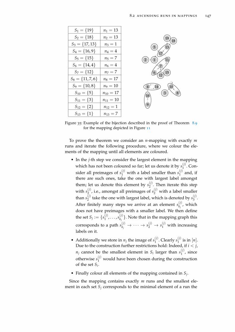
8.2 ascending runs in mappings 147
S1 = {19} n1 = 13
S2 = {18} n2 = 13
S3 = {17, 13} n3 = 1
S4 = {16, 9} n4 = 4
S5 = {15} n5 = 7
S6 = {14, 4} n6 = 4
S7 = {12} n7 = 7
S8 = {11, 7, 6} n8 = 17
S9 = {10, 8} n9 = 10
S10 = {5} n10 = 17
S11 = {3} n11 = 10
S12 = {2} n12 = 1
S13 = {1} n13 = 7
1
7
11
17
5
2
612
15
13
15
1918
10
3 8
4 14
16
9
Figure 35: Example of the bijection described in the proof of Theorem 8.9for the mapping depicted in Figure 11
To prove the theorem we consider an n-mapping with exactly mruns and iterate the following procedure, where we colour the ele-ments of the mapping until all elements are coloured.
• In the j-th step we consider the largest element in the mappingwhich has not been coloured so far; let us denote it by s(j)
1 . Con-
sider all preimages of s(j)1 with a label smaller than s(j)
1 and, ifthere are such ones, take the one with largest label amongstthem; let us denote this element by s(j)
2 . Then iterate this stepwith s(j)
2 , i.e., amongst all preimages of s(j)2 with a label smaller
than s(j)2 take the one with largest label, which is denoted by s(j)
3 .
After finitely many steps we arrive at an element s(j)k j
, whichdoes not have preimages with a smaller label. We then definethe set Sj := {s(j)
1 , . . . , s(j)k j}. Note that in the mapping graph this
corresponds to a path s(j)k j→ · · · → s(j)
2 → s(j)1 with increasing
labels on it.
• Additionally we store in nj the image of s(j)1 . Clearly s(j)
1 is in [n].Due to the construction further restrictions hold: Indeed, if i < j,nj cannot be the smallest element in Si larger than s(j)
1 , since
otherwise s(j)1 would have been chosen during the construction
of the set Si.
• Finally colour all elements of the mapping contained in Sj.
Since the mapping contains exactly m runs and the smallest ele-ment in each set Sj corresponds to the minimal element of a run the

148 ascending runs in mappings
procedure stops after exactly m steps. It thus defines a pair of a setpartition S = (S1, . . . , Sm) and a sequence x = (n1, . . . , nm) with thegiven restrictions.
If the pair (S, x) is given, the corresponding mapping can easily bereconstructed. Indeed, the partition S gives us a decomposition of themapping into ascending runs and the sequence x tells us how theseruns have to be linked to each other. The inverse of this bijection cantherefore be defined in a straightforward way.
Example 8.10. The construction of the partition S and the sequence xfor the mapping described in Figure 11 can be found in Figure 35. Letus exemplarily explain how the set S8 is constructed. At this point,the elements in ∪7
i=1Si, i.e., 19, 18, 17, 13, 16, 9, 15, 14, 4 and 12, havealready been coloured. Thus, the largest element that has not beencoloured so far is 11 = s(8)1 . For s(8)2 , we consider the preimages of 11that have a label smaller than 11. The only such element is 7 and thuss(8)2 = 7. Next, the preimages of 7 are 6, 12 and 15 and thus s(8)3 = 6.Since 6 does not have any preimages, we stop here and S8 = {11, 7, 6}.Since the image of 11 is 17, we set n8 = 17. a
8.3 summary of the results
Let us briefly discuss the results of this chapter.We started with a study of ascents in mappings – which is easy
since the probability of a node i being an ascent in a random n-mapping is simply (n− i)/n. The results obtained here can be trans-lated to trees, where the study of ascents is less straightforward.
As can be seen very easily a permutation with k ascents consistsof exactly k + 1 descending runs and thus the study of these twopermutation statistics is equivalent. This is in contrast to the case ofmappings, where results on ascents can not directly be translated toresults on descending or ascending runs. We thus proceeded withthe study of ascending runs in mappings which was the main focusof this chapter. Using a PDE we obtained exact enumeration formulæinvolving the Stirling numbers of the second kind.
Both for ascents and for ascending runs in mappings (and trees), wecould also obtain limiting distribution results and show convergenceto a normal distribution. Let us compare this to the known results forthe Eulerian numbers that enumerate permutations by their lengthand their number of ascents.
In [46] it is shown that the random variable Xn counting the num-ber of ascents in a random permutation of length n satisfies a centrallimit theorem. Indeed, with E(Xn) =
n−12 and V(Xn) =
n+112 it holds
that the standardized random variable (Xn − E(Xn))/√
V(Xn) con-verges in distribution to a standard normal distribution. Equivalently,the random variable Yn = Xn + 1 counting the number of ascending

8.3 summary of the results 149
runs in a random permutation of length n satisfies a central limit the-orem with E(Yn) =
n+12 and V(Yn) = V(Xn). Thus, both for ascents
and for ascending runs we have E ∼ n/2 and V ∼ n/12 = 0.083 · n.Here, we could show similar results for ascending runs and ascents
in trees and mappings. Indeed, we also obtained a linear mean andvariance and convergence in distribution to a standard normal distri-bution of the standardized random variable. However, the involvedcoefficients are not the same:
• E(An) ∼ n/2 as well as V(An) ∼ n/6 for ascents and
• E(Rn) ∼ (1− e−1)n with 1− e−1 ≈ 0.632 . . . as well as V(Rn) ∼(e−1 − 2e−2)n with e−1 − 2e−2 ≈ 0.0972 . . . for ascending runs.


9PA R K I N G I N T R E E S A N D M A P P I N G S
This chapter is based on joint work with Alois Panholzer. A manuscripthas recently been submitted to a journal and a preprint can be foundon arxiv.org [44].
In this chapter, we apply the well-known concept of parking func-tions to Cayley trees and to mappings by considering the nodes asparking spaces and the directed edges as one-way streets: Each driverhas a preferred parking space and starting with this node she1 followsthe edges in the graph until she either finds a free parking space orall reachable parking spaces are occupied. If all drivers are successfulwe speak about a parking function for the tree or mapping.
A more detailed introduction to the topic of this chapter, relatedliterature and the organization of this chapter can be found in thefollowing section.
9.1 introduction
Parking functions are combinatorial objects originally introduced byKonheim and Weiss [113] during their studies of the so-called linearprobing collision resolution scheme for hash tables. Since then, park-ing functions have been studied extensively and many connectionsto various other combinatorial objects such as forests, hyperplane ar-rangements, acyclic functions and non-crossing partitions have beenrevealed, see, e.g., [146].
An illustrative description of parking functions is as follows: con-sider a one-way street with n parking spaces numbered from 1 to nand a sequence of m drivers with preferred parking spaces s1, s2, . . . ,sm. The drivers arrive sequentially and each driver k, 1 ≤ k ≤ m, triesto park at her preferred parking space with address sk ∈ [n]. If it isfree she parks. Otherwise she moves further in the allowed direction,thus examining parking spaces sk + 1, sk + 2, . . . , until she finds a freeparking space where she parks. If there is no such parking space sheleaves the street without parking. A parking function is then a se-quence (s1, . . . , sm) ∈ [n]m of addresses such that all m drivers areable to park. It has been shown already in [113] that there are exactlyPn,m = (n+ 1−m) · (n+ 1)m−1 parking functions for n parking spacesand 0 ≤ m ≤ n drivers.
The notion of parking functions has been generalized in variousways, yielding, e.g., (a, b)-parking functions [159], bucket parkingfunctions [23], x-parking functions [148], or G-parking functions [135].
1 In the following we use “she” as a generic pronoun.
151

152 parking in trees and mappings
3
8 1
4
2 7
6
5
(2, 8, 7, 2)⇒
3
8 1
4
2 7
6
5
Figure 36: An example of a (8, 4)-tree parking function
Another natural generalization that has however not been consideredyet is the following: Starting with the original definition of park-ing functions as a vivid description of a simple collision resolutionscheme, we apply it to other objects of interest, namely, to rootedtrees and mappings.
First, when allowing branches in the road net, this collision reso-lution scheme leads to a natural generalization of parking functionsto rooted labelled trees, i.e., Cayley trees. Consider a Cayley tree Tof size |T| = n. As usual, we assume that the edges of the treeare oriented towards the root node, which we will often denote byroot(T). We thus view edges as “one-way streets”. Now, we considera sequence of m drivers, where again each driver has her preferredparking space which in this case is a node in the tree, respectively itslabel. The drivers arrive sequentially and each driver k, 1 ≤ k ≤ m,tries to park at her preferred parking space with address sk ∈ [n]. Ifit is free she parks. Otherwise she follows the edges towards the rootnode and parks at the first empty node, if there is such one. If there isno empty node, she leaves the road net, i.e., the tree without parking.A sequence s ∈ [n]m of addresses is then called a parking functionfor the tree T, if all drivers are successful, i.e., if all drivers are ableto find a parking space. More precisely, we will call a pair (T, s) an(n, m)-tree parking function, if T is a rooted labelled tree of size n ands ∈ [n]m is a parking function for T with m drivers.
Example 9.1. Consider the tree T of size 8 depicted in Figure 36.Moreover, consider the sequence s = (2, 8, 7, 2) of addresses of pre-ferred parking spaces for 4 drivers. All drivers are successful, thus(T, s) yields a (8, 4)-tree parking function. Conversely, the sequence(2, 8, 8, 2) is not a parking function for T, since the fourth driver is notable to park. a
Second, one can go a step further and consider structures in generalfor which the simple collision resolution scheme is applicable, i.e., forwhich a driver reaching an occupied parking space can move on ina unique way to reach a new parking space. This naturally leads toa generalization of parking functions to mappings: Consider the set[n] of addresses and a mapping f : [n] → [n]. If a driver reaches

9.1 introduction 153
5
1
18
1315
118
12
2
17
10
6
4
1619
7 14
3
9
(10, 5, 14, 10, 13, 14)
⇓
5
1
18
1315
118
12
2
17
10
6
4
1619
7 14
3
9
Figure 37: An example of a (19, 6)-mapping parking function
address i and is unable to park there, she moves on to the parkingspace with address j = f (i) for her next trial. The road net is then thefunctional digraph G f of the mapping f . Again, the drivers arrive se-quentially and each driver has her preferred parking space which is anode in the graph. If it is empty she will park, otherwise she followsthe edges and parks at the first empty node, if such one exists. Oth-erwise she cannot park since she would be caught in an endless loop.A sequence s ∈ [n]m of addresses is then called a parking functionfor the mapping f if all drivers are successful, i.e., all drivers finda parking space. A pair ( f , s) is called an (n, m)-mapping parkingfunction, if f is an n-mapping and s ∈ [n]m is a parking function forf with m drivers. Note that we will always identify mappings withtheir functional digraphs in the course of this chapter.
Example 9.2. Consider the mapping f of size 19 depicted in Fig-ure 37 and the sequence s = (10, 5, 14, 10, 13, 14) of addresses of pre-ferred parking spaces for 6 drivers. All drivers are successful, thus( f , s) yields a (19, 6)-mapping parking function. When a new driverwith preferred parking space 7 arrives, she is not able to park. Thus(10, 5, 14, 10, 13, 14, 7) is not a parking function for f . a
To each (n, m)-tree parking function (T, s) (or (n, m)-mapping park-ing function ( f , s)), we associate the corresponding output-functionπ := π(T,s) (or π := π( f ,s)), with π : [m] → [n], where π(k) is theaddress of the parking space (i.e., the label of the node) in which thek-th driver ends up parking. Of course, π is an injection and for theparticular case m = n a bijection; thus in the latter case one may speakabout the output-permutation π. This notion will be useful in subse-quent considerations describing characterizations and bijections fortree and mapping parking functions.
154 parking in trees and mappings
Example 9.3. Consider again the tree parking function representedin Figure 36. The parking positions of the drivers are given by thesequence (2, 8, 7, 4) defining the output-function π(T,s). a
Obviously, both concepts of parking functions generalize ordinaryparking functions: first, each ordinary parking function on [n] can beidentified with a parking function for the linear tree (i.e., the chain)1 − 2 − · · · − n with root n, and second, each parking function fora tree T of size n can be identified with a parking function for thefunctional digraph which is obtained from T by adding a loop-edgeto the root.
We start our studies of tree and mapping parking functions by giv-ing some of their basic properties and characterizations in Section 9.2.This extends corresponding properties and characterizations for or-dinary parking functions. As an application we can characterize theextremal values for the number of parking functions with 0 ≤ m ≤ ndrivers amongst all size-n trees.
The main focus of this chapter lies on the exact and asymptoticenumeration of the total number of (n, m)-tree parking functions and(n, m)-mapping parking functions. This is done in Sections 9.3 and9.4. We are interested in the exact and asymptotic behaviour of thequantities
Fn,m := |{(T, s) : T ∈ Tn, s ∈ [n]m a parking function for T}|,Mn,m := |{( f , s) : f ∈ Mn, s ∈ [n]m a parking function for f }|,
counting the total number of (n, m)-tree parking functions and (n, m)-mapping parking functions.
In order to get exact enumeration results we use suitable combi-natorial decompositions of the objects which give recursive descrip-tions of the quantities of interest. The recurrences occurring can betreated by a generating functions approach yielding partial differen-tial equations. These differential equations allow for implicit charac-terizations of the generating functions. This treatment is divided intotwo main steps: First, in Section 9.3 we treat the important particularcase m = n, i.e., we consider parking functions where the number ofdrivers is equal to the number of parking spaces. Second, the generalcase in which the number of drivers m is less than or equal to thenumber of parking spaces n is then treated in Section 9.4.
To give a complete picture of the asymptotic behaviour of Mn,m
(and thus also Fn,m) depending on the growth of m w.r.t. n requires amore detailed study using saddle point methods. In Section 9.4, weconsider the probability pn,m := Mn,m/nn+m = Fn,m/nn+m−1 that arandomly chosen pair ( f , s) of an n-mapping f and a sequence s of maddresses is indeed a parking function and thus the probability thatall drivers are successful.
In Section 9.5 we summarize the results of this chapter.
9.2 basic properties of parking functions for trees and mappings 155
9.2 basic properties of parking functions for trees and
mappings
In this section we will state and prove some basic facts on parkingfunctions for trees and mappings. The following notation will turnout to be useful: Given an n-mapping f , we define a binary relation� f on [n] via
i � f j :⇐⇒ ∃k ∈N : f k(i) = j.
Thus i � f j holds if there exists a directed path from i to j in thefunctional digraph G f , and we say that j is a successor of i or that i isa predecessor of j. In this context a one-way street represents a totalorder, a tree represents a certain partial order, where the root nodeis the maximal element (to be precise, a partially ordered set withmaximal element, where every interval is a chain – this is also calledtree in set theory) and a mapping represents a certain pre-order (i.e.,binary relation that is transitive and reflexive).
Changing the order in a parking function
For ordinary parking functions the following holds: changing the or-der of the elements of a sequence does not affect its property of beinga parking function or not. This fact can easily be generalized to park-ing functions for mappings (which might also be trees).
Lemma 9.4. A function s : [m] → [n] is a parking function for a mappingf : [n] → [n] if and only if s ◦ σ is a parking function for f for anypermutation σ on [m].
Proof. Since each permutation σ on [m] can be obtained by a sequenceof transpositions of consecutive elements, i.e., σ = τr ◦ τr−1 ◦ · · · ◦ τ1,with τi = (ki ki + 1), 1 ≤ ki ≤ m− 1, 1 ≤ i ≤ r, it suffices to provethe following: if s is a parking function for f , then s ◦ σ is a parkingfunction for f for any transposition σ of consecutive elements, i.e., forany permutation σ on [m] that swaps two consecutive elements andleaves the other elements fixed. The statement for general σ followsfrom this by iteration.
Thus, let s : [m] → [n] be a parking function for f : [n] → [n] ands′ = s ◦ σ, where σ = (k k + 1), with 1 ≤ k ≤ m− 1, i.e., σ(k) = k + 1,σ(k + 1) = k, and σ(j) = j otherwise. In other words, s′ is the parkingsequence obtained from s by changing the order of the k-th and the(k + 1)-th car.
In the following the mapping f is fixed and we denote by πs =
π( f ,s) the output-function of the parking function s and consider theparking paths of the drivers: the path yj = sj ; πs(j) denotes theparking path of the j-th driver of s in the mapping graph G f start-ing with the preferred parking space sj and ending with the parkingposition πs(j). In order to show that s′ is still a parking function, we

156 parking in trees and mappings
have to show that all cars can successfully be parked using s′. In thefollowing we do this and also determine the output-function πs′ ofs′ (and thus the parking paths y′j = s′j ; πs′(j), 1 ≤ j ≤ m, of thedrivers of s′).
Clearly, the parking paths of the first (k− 1) cars are not affectedby the swapping of the k-th and the (k + 1)-th car and we have thatπs′(1) = πs(1), . . . , πs′(k− 1) = πs(k− 1). For the k-th and the (k+ 1)-th car we will distinguish between two cases according to the parkingpaths yk = sk ; πs(k) and yk+1 = sk+1 ; πs(k + 1).
(a) Case yk ∩ yk+1 = ∅: Since the parking paths yk and yk+1 are dis-joint, swapping the k-th and the (k+ 1)-th car simply also swapsthe corresponding parking paths, i.e., y′k = yk+1 and y′k+1 = yk,and in particular πs′(k) = πs(k + 1) and πs′(k + 1) = πs(k).
(b) Case yk ∩ yk+1 6= ∅: Let us denote by v the first node in thepath yk that also occurs in yk+1. Then, according to the parkingprocedure, the parking paths can be decomposed as follows:
yk = sk ; v ; πs(k) and
yk+1 = sk+1 ; v ; πs(k) ; πs(k + 1),
i.e. πs(k + 1) is a proper successor of πs(k), i.e., πs(k) ≺ f πs(k +1). Thus, when swapping the k-th and the (k + 1)-th car, bothcars can also be parked yielding the parking paths
y′k = sk+1 ; v ; πs(k) and
y′k+1 = sk ; v ; πs(k) ; πs(k + 1).
In particular, we obtain πs′(k) = πs(k) and πs′(k + 1) = πs(k +1).
Thus, in any case we get {πs(k), πs(k + 1)} = {πs′(k), πs′(k + 1)},and consequently swapping the k-th and the (k + 1)-th car does notchange the parking paths of the subsequent cars and we obtain πs′(j) =πs(j), k + 2 ≤ j ≤ m. So all drivers in the parking sequence s′ are suc-cessful and s′ is indeed a parking function for f .
Alternative characterizations of parking functions
Using the fact that reordering the elements of a function does nothave any influence on whether it is a parking function or not, onecan obtain the following well-known simpler characterization of or-dinary parking functions (see, e.g., [146]): A sequence s ∈ [n]n is aparking function if and only if it is a major function, i.e., the sortedrearrangement s′ of the sequence s satisfies:
s′j ≤ j, for all j ∈ [n].

9.2 basic properties of parking functions for trees and mappings 157
s = (1, 1, 2, 3, 3, 4, 7)
5
3 2
71 6
4
[1] s = (2, 4, 4, 4, 5, 6, 7)
5
3 2
71 6
4
[2]
j 1 2 3 4 5 6 7
p(j) 2 2 4 1 7 1 1
q1(j) 3 2 5 1 7 0 1
q2(j) 3 2 4 3 7 1 1
Figure 38: Exemplifying the characterization of generalized parking func-tions given in Lemma 9.5 for a tree T of size 7. The sequence s[1]
represented on the left-hand-side does not give a parking func-tion for T, whereas the sequence s[2] represented on the right-hand-side does.
This statement can be reformulated in the following way: A se-quence s ∈ [n]n is a parking function if and only if for every j ∈ [n],it does not contain more than (n− j) elements that are larger than j.Or again in other words, there must be at least j elements that are notlarger than j:
| {k ∈ [n] : sk ≤ j} | ≥ j, for all j ∈ [n]. (40)
Now, this characterization of parking functions can easily be gen-eralized to parking functions for trees and mappings. Indeed, in (40)we merely need to replace the ≤ and ≥ relation which come from theorder on the elements 1, 2, . . . , n represented by the one-way street oflength n by the binary relation given by the respective tree or map-ping. The following characterization of (n, n)-mapping parking func-tions (which might also be trees) is now possible.
Lemma 9.5. Given an n-mapping f and a sequence s ∈ [n]n, let p(j) :=|{
i ∈ [n] : i � f j}| denote the number of predecessors of j and q(j) :=
|{
k ∈ [n] : sk � f j}| the number of drivers whose preferred parking spaces
are predecessors of j. Then s is a mapping parking function for f if and onlyif
q(j) ≥ p(j), for all j ∈ [n].
Example 9.6. Consider the two pairs (T, s[1]) and (T, s[2]) representedin Figure 38. The sequence s[1] = (1, 1, 2, 3, 3, 4, 7) does not give a park-ing function for T, whereas the sequence s[2] = (2, 4, 4, 4, 5, 6, 7) repre-sented on the right-hand-side does. This can be seen in the followingway, where we denote by q1(j) and q2(j) the quantity q(j) for s[1] and

158 parking in trees and mappings
s[2], respectively: for the sequence s[1] we have q1(6) = 0 < 1 = p(6)thus violating the condition q(j) ≥ p(j), whereas each element p(j) issmaller or equal to the corresponding element q2(j). aProof of Lemma 9.5. First, assume that q(j) < p(j) holds for some j ∈[n]. Let us denote by P(j) := {i ∈ [n] : i �j j} the set of predecessorsof j. Obviously, if sk 6∈ P(j) then the k-th driver will not get a parkingspace in P(j). Thus, at most q(j) = |{k ∈ [n] : sk ∈ P(j)}| drivers areable to park in P(j). In other words, at least p(j)− q(j) > 0 parkingspaces in P(j) remain free. Since there is the same number of cars andof parking spaces, this means that at least one driver will not be ableto park successfully. Thus s is not a parking function for f .
Next, assume that q(j) ≥ p(j) holds for all j ∈ [n]. It will be suffi-cient to show the following: Let s ∈ [n]n be a parking sequence suchthat q(j) ≥ p(j) for some j, then node j will be occupied after ap-plying the parking procedure. Due to the assumption above we maythen conclude that all nodes will be occupied after applying the park-ing procedure and thus that all n drivers are successful, which meansthat s indeed is a parking function for f .
To prove the assertion above we distinguish between two cases:
(a) j is not a cyclic node: Then the set P(j) of predecessors of j isa tree. If there is a driver k with preferred parking space sk = jthen in any case node j will be occupied. Thus let us assume thatsk 6= j, for all j ∈ [n]. Let us further assume that i1, . . . , ir are thepreimages of j, i.e., f (it) = j, 1 ≤ t ≤ r. Since q(j) ≥ p(j), but nodriver wishes to park at j, it holds that there exists a preimagei`, such that q(i`) > p(i`). This means that there must be at leastone driver appearing in P(i`) that is not able to get a parkingspace in P(i`) and thus, according to the parking procedure,she has to pass the edge (i`, j). Consequently, node j will beoccupied.
(b) j is a cyclic node: If the edge (j, f (j)) is passed by some driverduring the application of the parking procedure this necessarilyimplies that the node j is occupied. Thus let us assume thatthe edge (j, f (j)) will never be passed while carrying out theparking procedure. Then we may remove the edge (j, f (j)) fromG f without influencing the outcome of the parking procedure.By doing so, node j becomes a non-cyclic node and accordingto case (a), node j will be occupied.
Now let us turn to parking functions, where the number of driversdoes not necessarily coincide with the number of parking spaces. Itis well-known and easy to see that a parking sequence s : [m] → [n]on a one-way street is a parking function if and only if
| {k ∈ [m] : sk ≥ j} | ≤ n− j + 1, for all j ∈ [n]. (41)
9.2 basic properties of parking functions for trees and mappings 159
This characterization can be generalized to (n, m)-tree parking func-tions as follows.
Lemma 9.7. Given a rooted labelled tree T of size |T| = n and a sequences ∈ [n]m. Then s is a tree parking function for T if and only if
|{
k ∈ [m] : sk ∈ T′}| ≤ |T′|, for all subtrees T′ of T containing root(T).
Proof. First, let us assume that there exists a subtree T′ of T containingroot(T), such that q(T′) := |Q(T′)| := | {k ∈ [m] : sk ∈ T′} | > |T′|.Clearly, the possible parking spaces for any driver k with preferredparking space sk ∈ T′ form a subset of T′. Here, the number of suchdrivers q(T′) exceeds the amount of parking spaces |T′| and thus atleast one of the drivers in Q(T′) will be unsuccessful. Thus s is not aparking function for T.
Next, let us assume that s is not a parking function for T. Let us fur-ther assume that ` ∈ [m] is the first unsuccessful driver in s when ap-plying the parking procedure. We consider the situation after the first` drivers: Define T′ as the maximal subtree of T containing root(T)and only such nodes that are occupied by one of the first `− 1 cars.Of course, since the `-th driver is unsuccessful, the root(T) has to beoccupied by one of the first `− 1 cars, anyway. Due to the maximal-ity condition of T′, it holds that each driver ` that has parked in T′
must have had her preferred parking space in T′, thus |{k ∈ [`− 1] :sk ∈ T′}| = |T′|. Since the `-th driver is unsuccessful, her preferredparking space is also in T′, yielding |{k ∈ [`] : sk ∈ T′}| > |T′|. Ofcourse, this implies |{k ∈ [m] : sk ∈ T′}| > |T′|, for the subtree T′ ofT containing root(T).
We remark that the characterization above could be also extendedto mapping parking functions (where one has to consider connectedsubgraphs of G f containing all cyclic nodes of the respective compo-nent). Since we will not make use of it in the remainder of this chapterwe omit it here.
Extremal cases for the number of parking functions
Given an n-mapping f : [n] → [n] (which might be a tree), let usdenote by S( f , m) the number of parking functions s ∈ [n]m for fwith m drivers. So far we are not aware of enumeration formulæ forthe numbers S( f , m) for general f . In Sections 9.3 and 9.4 however,we will compute the total number Fn,m := ∑T∈Tn
S(T, m) and Mn,m :=∑ f∈Mn
S( f , m) of (n, m)-tree and (n, m)-mapping parking functions.Before continuing, we first state the obvious fact that isomorphic
mappings (or trees) yield the same number of mapping (or tree) park-ing functions, since one simply has to adapt the preferred parkingspaces of the drivers according to the relabelling.
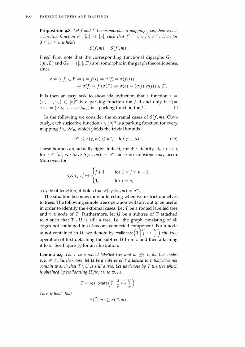
160 parking in trees and mappings
Proposition 9.8. Let f and f ′ two isomorphic n-mappings, i.e., there existsa bijective function σ : [n] → [n], such that f ′ = σ ◦ f ◦ σ−1. Then for0 ≤ m ≤ n it holds
S( f , m) = S( f ′, m).
Proof. First note that the corresponding functional digraphs G f =
([n], E) and G f ′ = ([n], E′) are isomorphic in the graph theoretic sense,since
e = (i, j) ∈ E⇔ j = f (i)⇔ σ(j) = σ( f (i))
⇔ σ(j) = f ′(σ(i))⇔ σ(e) = (σ(i), σ(j)) ∈ E′.
It is then an easy task to show via induction that a function s =
(s1, . . . , sm) ∈ [n]m is a parking function for f if and only if s′;=σ ◦ s = (σ(s1), . . . , σ(sm)) is a parking function for f ′.
In the following we consider the extremal cases of S( f , m). Obvi-ously, each surjective function s ∈ [n]m is a parking function for everymapping f ∈ Mn, which yields the trivial bounds
nm ≤ S( f , m) ≤ nm, for f ∈ Mn. (42)
These bounds are actually tight. Indeed, for the identity idn : j 7→ j,for j ∈ [n], we have S(idn, m) = nm since no collisions may occur.Moreover, for
cyclen : j 7→
j + 1, for 1 ≤ j ≤ n− 1,
1, for j = n,
a cycle of length n, it holds that S(cyclen, m) = nm.The situation becomes more interesting when we restrict ourselves
to trees. The following simple tree operation will turn out to be usefulin order to identify the extremal cases. Let T be a rooted labelled treeand v a node of T. Furthermore, let U be a subtree of T attachedto v such that T \ U is still a tree, i.e., the graph consisting of alledges not contained in U has one connected component. For a node
w not contained in U, we denote by reallocate(
T∣∣∣ U↓v7→ U
↓w
)the tree
operation of first detaching the subtree U from v and then attachingit to w. See Figure 39 for an illustration.
Lemma 9.9. Let T be a rooted labelled tree and w �T v, for two nodesv, w ∈ T. Furthermore, let U be a subtree of T attached to v that does notcontain w such that T \U is still a tree. Let us denote by T the tree whichis obtained by reallocating U from v to w, i.e.,
T = reallocate(
T∣∣∣ U↓v7→ U
↓w
).
Then it holds thatS(T, m) ≥ S(T, m).
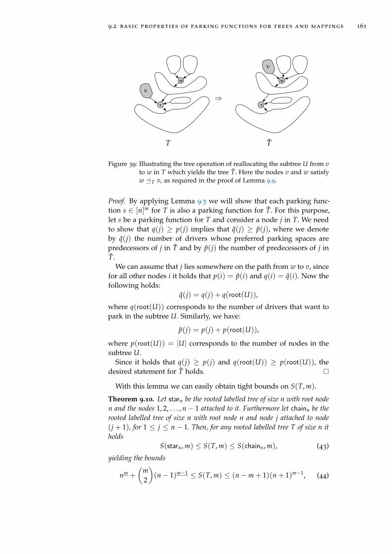
9.2 basic properties of parking functions for trees and mappings 161
v
w
U
T
⇒v
w
U
T
Figure 39: Illustrating the tree operation of reallocating the subtree U from vto w in T which yields the tree T. Here the nodes v and w satisfyw �T v, as required in the proof of Lemma 9.9.
Proof. By applying Lemma 9.5 we will show that each parking func-tion s ∈ [n]m for T is also a parking function for T. For this purpose,let s be a parking function for T and consider a node j in T. We needto show that q(j) ≥ p(j) implies that q(j) ≥ p(j), where we denoteby q(j) the number of drivers whose preferred parking spaces arepredecessors of j in T and by p(j) the number of predecessors of j inT.
We can assume that j lies somewhere on the path from w to v, sincefor all other nodes i it holds that p(i) = p(i) and q(i) = q(i). Now thefollowing holds:
q(j) = q(j) + q(root(U)),
where q(root(U)) corresponds to the number of drivers that want topark in the subtree U. Similarly, we have:
p(j) = p(j) + p(root(U)),
where p(root(U)) = |U| corresponds to the number of nodes in thesubtree U.
Since it holds that q(j) ≥ p(j) and q(root(U)) ≥ p(root(U)), thedesired statement for T holds.
With this lemma we can easily obtain tight bounds on S(T, m).
Theorem 9.10. Let starn be the rooted labelled tree of size n with root noden and the nodes 1, 2, . . . , n− 1 attached to it. Furthermore let chainn be therooted labelled tree of size n with root node n and node j attached to node(j + 1), for 1 ≤ j ≤ n− 1. Then, for any rooted labelled tree T of size n itholds
S(starn, m) ≤ S(T, m) ≤ S(chainn, m), (43)
yielding the bounds
nm +
(m2
)(n− 1)m−1 ≤ S(T, m) ≤ (n−m + 1)(n + 1)m−1, (44)
162 parking in trees and mappings
for 0 ≤ m ≤ n.
Proof. Each tree T of size n can be constructed from a tree T0, which isisomorphic to starn, by applying a sequence of reallocations Ti+1 :=
reallocate(
Ti
∣∣∣∣Ui↓vi7→ Ui
↓wi
), with wi �Ti vi, for 0 ≤ i ≤ k, with k ≥ 0.
Furthermore, starting with T =: T0, there always exists a sequence
of reallocations Ti+1 := reallocate(
Ti
∣∣∣∣Ui↓vi
7→ Ui↓wi
), with wi �Ti
vi, for
0 ≤ i ≤ k, with k ≥ 0, such that the resulting tree is isomorphic tochainn. Thus, equation (43) follows immediately from Lemma 9.9.
The upper bound in (44) is the well-known formula for the num-ber parking functions in a one-way street (which corresponds to thenumber of tree parking functions for chainn). For the lower bound onehas to compute the number of parking functions with m drivers forstarn: there are only two possible cases, namely either s is injective orexactly two drivers have the same non-root node as preferred parkingspace, whereas all remaining drivers have different non-root nodes aspreferred parking spaces. Elementary combinatorics yields the statedresult.
9.3 total number of parking functions : the number of
drivers coincides with the number of parking spaces
In this section, we consider the total number of parking functions fortrees and mappings for the case that the number of drivers m is equalto the number of parking spaces n. As for ordinary parking functions,this case is not only interesting in its own. It will also occur during thestudies of the general case via initial values for recurrence relations.
Tree parking functions
We study the total number Fn := Fn,n of (n, n)-tree parking functions,i.e., the number of pairs (T, s), with T ∈ Tn a Cayley tree of size nand s ∈ [n]n a parking sequence of length n for the tree T, such thatall drivers are successful. To obtain a recursive description of the totalnumber Fn of tree parking functions we use the decomposition of aCayley tree T ∈ Tn w.r.t. the last empty node. We thus consider thesituation just before the last driver starts searching a parking space.
Two different situations have to be considered for the last emptynode: it might be the root node of the tree T as depicted in Figure 40
or a non-root node as in Figure 41.
Case (1): The last empty node is the root node. In this case the lastdriver will always find a free parking space regardless of the n possi-ble choices of her preferred parking space.

9.3 total number of parking functions : m = n 163
sdfjhsiudfhsiudfhisuhdfiushjgduifffffffffffffffffffffff︸ ︷︷ ︸
... kr nodesk1 nodes k2 nodes
r subtrees with a total of n− 1 nodes
Figure 40: Schematic representation of the first case that can occur whenconsidering parking functions with n drivers for a Cayley treewith n nodes. The last empty node which is marked in white inthe tree is the root node of the tree.
sdfjhsiudfhsiudfhisuhdfius︸ ︷︷ ︸
T ′ of size k
...k1 kr
T ′′ of size n− k
r ≥ 0 subtrees
Figure 41: Schematic representation of the second case that can occur whenconsidering parking functions with n drivers for a Cayley treewith n nodes. The last empty node which is marked in white inthe tree is a non-root node.

164 parking in trees and mappings
Case (2): The last empty node is a non-root node. Here, the last driverwill only find a free parking space if her preferred parking space iscontained in the subtree (call it T′′) rooted at the node correspondingto the free parking space. If we detach the edge linking this subtreeT′′ with the rest of the tree we get two unordered trees. Let us as-sume the tree containing the original root of the tree (denote it withT′) has size k, whereas the remaining tree T′′ has size n − k. Thenthere are n − k choices for the preferred parking space of the lastdriver such that she is successful. Furthermore, it is important to takeinto account that, given T′ and T′′, the original tree T cannot be re-constructed, since there are always k different trees in Tn leading tothe same pair (T′, T′′); in other words, given T′ and T′′, we have kchoices of constructing trees T ∈ Tn by attaching the root of T′′ toany of the k nodes of T′.
Taking into account the order-preserving relabellings of the sub-trees and also the merging of the parking sequences for the subtrees,we obtain the following recursive description of Fn.
Fn = ∑r≥1
1r! ∑
∑ ki=n−1ki≥1
Fk1 · Fk2 · · · · · Fkr n(
nk1, k2, . . . , kr, 1
)(n− 1
k1, k2, . . . , kr
)
+ ∑r≥0
1r! ∑
k+∑ ki=n−1k≥1,ki≥1
Fk · Fk1 · Fk2 · · · · · Fkr k(n− k)· (45)
·(
nk, k1, k2, . . . , kr, 1
)(n− 1
k, k1, k2, . . . , kr
), for n ≥ 2,
with initial value F1 = 1. Here r denotes the number of subtrees ofthe free parking space (i.e., of the empty node), thus the factor 1
r!occurs, since each of the r! orderings of the subtrees of the emptynode represent the same tree. In order to treat this recurrence weintroduce the following generating function
F(z) := ∑n≥1
Fn
(n!)2 zn.
Then, after straightforward computations which are omitted here, (45)can be transferred into the following differential equation:
F′(z) = exp(F(z)) ·(1 + zF′(z)
)2 , F(0) = 0. (46)
This differential equation can be solved by standard methods and itcan be checked easily that the solution of (46) is given as follows:
F(z) = T(2z) + ln(
1− T(2z)2
), (47)
where T(z) denotes the Cayley tree function.We shall not extract coefficients from (47) at this point yet, since
we will soon see in Theorem 9.12 that the total number Fn of parking
9.3 total number of parking functions : m = n 165
functions for trees of size n is directly linked to the total number Mn
of parking functions for mappings of size n. The latter quantity istreated in the next section and thus also yields exact and asymptoticenumeration formulæ for Fn.
Mapping parking functions
Now we study the total number Mn := Mn,n of (n, n)-mapping park-ing functions, i.e., the number of pairs ( f , s), with f ∈ Mn an n-mapping and s ∈ [n]n a parking sequence of length n for the map-ping f , such that all drivers are successful. Recall the structure offunctional graphs of mappings: the connected components are cyclesof Cayley trees. It is thus natural to introduce connected mappingsas auxiliary objects and study parking functions for them first. It willthen be easy to treat the general situation for mappings when wehave obtained results for connected mappings.
Whereas the relation between mappings and connected mappingscan be translated immediately into connections between parking func-tions for these objects, this is not the case for connected mappings andtrees. Indeed, the decomposition of connected mappings C into Cay-ley trees T is not consistent with the parking procedure. Instead ofusing this composition, we will therefore apply a decomposition ofconnected mappings w.r.t. the last empty node in the parking proce-dure. So, let us introduce the total number Cn of parking functionsof length n for connected n-mappings, i.e., the number of pairs ( f , s),with f ∈ Cn a connected n-mapping and s ∈ [n]n a parking sequenceof length n for f , such that all drivers are successful. We will then ob-tain a recursive description of Cn in which the quantity Fn countingthe number of (n, n)-tree parking functions which was introduced inSection 9.3 appears.
Here, we have to distinguish three different situations. To treatthese cases only slight adaptions to the considerations made in Sec-tion 9.3 have to be done:
Case (1): The last empty node is the root node of the Cayley tree thatforms a length-1 cycle. This situation is the same as the first case forparking functions for trees and has been depicted in Figure 40.
Case (2): The last empty node is the root node of a Cayley tree lyingin a cycle of at least two trees. This case is depicted in Figure 42. Here,the last driver will always find a free parking space regardless of then possible choices of her preferred parking space. Let us denote byT′′ the tree whose root node is the last free parking space. When wedetach the two edges linking T′′ with the rest of the mapping graph,we cut the cycle and the graph decomposes into two trees: the treeT′′ and the unordered tree (call it T′), which we may consider rootedat the former predecessor of the free parking space in the cycle ofthe original graph. Let us assume that T′ has size k, whereas T′′ has
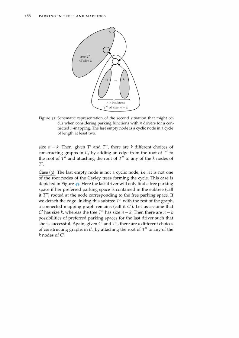
166 parking in trees and mappings
...
tree T ′
of size k
sdfjhsiudfhsiuduhdfius︸ ︷︷ ︸
T ′′ of size n− k
r ≥ 0 subtrees
k1 kr
Figure 42: Schematic representation of the second situation that might oc-cur when considering parking functions with n drivers for a con-nected n-mapping. The last empty node is a cyclic node in a cycleof length at least two.
size n − k. Then, given T′ and T′′, there are k different choices ofconstructing graphs in Cn by adding an edge from the root of T′ tothe root of T′′ and attaching the root of T′′ to any of the k nodes ofT′.
Case (3): The last empty node is not a cyclic node, i.e., it is not oneof the root nodes of the Cayley trees forming the cycle. This case isdepicted in Figure 43. Here the last driver will only find a free parkingspace if her preferred parking space is contained in the subtree (callit T′′) rooted at the node corresponding to the free parking space. Ifwe detach the edge linking this subtree T′′ with the rest of the graph,a connected mapping graph remains (call it C′). Let us assume thatC′ has size k, whereas the tree T′′ has size n− k. Then there are n− kpossibilities of preferred parking spaces for the last driver such thatshe is successful. Again, given C′ and T′′, there are k different choicesof constructing graphs in Cn by attaching the root of T′′ to any of thek nodes of C′.

9.3 total number of parking functions : m = n 167
...
sdfjh
siudhsiudfhfhsiuggggggfffffffdfhihdfifffffff
︸︷︷
︸
sdfjhsiudfhsiudfhisuhdfifffffff︸ ︷︷ ︸r subtrees
k1 nodes k2 nodes kr nodes...
tree T ′′ of size n− k
connected
of size kmapping C ′
Figure 43: Schematic representation of the third situation that might occurwhen considering parking functions with n drivers for a con-nected n-mapping. The last empty node is a non-cyclic node.
Again, taking into account the order-preserving relabellings of thesubstructures and also the merging of the parking sequences for them,we obtain the following recursive description of Cn, valid for all n ≥ 1:
Cn = ∑r≥0
1r! ∑
∑ ki=n−1Fk1 Fk2 · · · Fkr · n
(n
k1, k2, . . . , kr
)(n− 1
k1, k2, . . . , kr
)
+ ∑r≥0
1r! ∑
k+∑ ki=n−1FkFk1 Fk2 · · · Fkr · kn
(n
k, k1, . . . , kr
)(n− 1
k, k1, . . . , kr
)
+ ∑r≥0
1r! ∑
k+∑ ki=n−1CkFk1 Fk2 · · · Fkr · k(n− k)· (48)
·(
nk, k1, . . . , kr
)(n− 1
k, k1, . . . , kr
).
Now we introduce the generating function
C(z) := ∑n≥1
Cn
(n!)2 zn.
Then, recurrence (48) yields the following differential equation forC(z),
C′(z) ·(1− z exp(F(z))− z2F′(z) exp(F(z))
)
=((
1 + zF′(z))2
+ zF′(z) + z2F′′(z))
exp(F(z)), C(0) = 0, (49)

168 parking in trees and mappings
where F(z) denotes the generating function of the number of treeparking functions given in (47). This differential equation has the fol-lowing simple solution:
C(z) = ln
(1
1− T(2z)2
), (50)
as can be checked easily by using the functional equation of the treefunction T(z) (Equation (6)).
Extracting coefficients from (50) gives the following auxiliary result.
Lemma 9.11. The total number Cn of parking functions of length n forconnected n-mappings is, for n ≥ 1, given as follows:
Cn = n!(n− 1)!n−1
∑j=0
(2n)j
j!.
Proof. Using the functional equation of the tree function T(z) in Equa-tion (6), a standard application of the Lagrange inversion formulayields
[zn] ln
(1
1− T(2z)2
)= 2n[zn] ln
(1
1− T(z)2
)=
2n
n[Tn−1]
enT
2(1− T2 )
=2n−1
n
n−1
∑j=0
nn−1−j
2j(n− 1− j)!=
1n
n−1
∑j=0
(2n)j
j!,
and further
Cn = (n!)2[zn]C(z) = (n!)2[zn] ln
(1
1− T(2z)2
)= n!(n− 1)!
n−1
∑j=0
(2n)j
j!.
Now we are in the position to study the total number Mn of (n, n)-mapping parking functions. Again we introduce the generating func-tion
M(z) := ∑n≥0
Mnzn
(n!)2 .
Since the functional digraph of a mapping can be considered as theset of its connected components and furthermore a parking functionfor a mapping can be considered as a shuffle of the correspondingparking functions for the connected components, we get the followingsimple relation between the generating functions M(z) and C(z) ofparking functions for mappings and connected mappings:
M(z) = exp(C(z)).

9.3 total number of parking functions : m = n 169
Thus, by using (50), the generating function M(z) is given as follows:
M(z) =1
1− T(2z)2
. (51)
Next, we remark that the following relation between M(z) and F(z),the generating functions for the number of parking functions for map-pings and trees, holds:
1 + zF′(z) = 1 +T(2z)
1− T(2z)·(
1− 12− T(2z)
)
= 1 +T(2z)
2
1− T(2z)2
= M(z),
where we used T′(z) = T(z)/(z · (1− T(z))) obtained by differentiat-ing Equation (6). At the level of coefficients, this immediately showsthe following somewhat surprising connection between Fn and Mn.
Theorem 9.12. For all n ≥ 1 it holds that the total numbers Fn and Mn of(n, n)-tree parking functions and (n, n)-mapping parking functions, respec-tively, satisfy:
Mn = n · Fn.
Since it also holds that the number of mappings of size n is exactlyn times the number of Cayley trees of size n, this implies that theaverage number of parking functions per mapping of a given sizeis exactly equal to the average number of parking functions per treeof the same size. Later, in Section 9.3 we establish a combinatorialexplanation for this interesting fact.
Extracting coefficients from the generating function solution (51) ofM(z) easily yields exact formulæ for Mn and, due to Theorem 9.12,also for Fn.
Theorem 9.13. The total number Mn of (n, n)-mapping parking functionsis for n ≥ 1 given as follows:
Mn = n!(n− 1)! ·n−1
∑j=0
(n− j) · (2n)j
j!.
Corollary 9.14. The total number Fn of (n, n)-tree parking functions is forn ≥ 1 given as follows:
Fn = ((n− 1)!)2 ·n−1
∑j=0
(n− j) · (2n)j
j!.
Proof of Theorem 9.13. Again, using (6) and the Lagrange inversion for-mula, we obtain
[zn]1
1− T(2z)2
= 2n[zn]1
1− T(z)2
=2n
n[Tn−1]
enT
2(1− T
2
)2
=2n−1
n
n−1
∑k=0
(k + 1)nn−1−k
2k(n− 1− k)!=
1n
n−1
∑j=0
(n− j)(2n)j
j!,

170 parking in trees and mappings
and thus
Mn = (n!)2[zn]M(z) = (n!)2[zn]1
1− T(2z)2
= n!(n− 1)!n−1
∑j=0
(n− j) · (2n)j
j!.
The asymptotic behaviour of the numbers Mn and Fn for n → ∞could be deduced from these exact formulæ; however, it seems eas-ier to start with the generating function solution (51) of M(z). Us-ing the asymptotic expansion of the tree function T(z) in a complexneighbourhood of its unique dominant singularity 1
e (as derived inExample 2.33),
T(z) = 1−√
2√
1− ez +23(1− ez) +O
((1− ez)
32
), (52)
one immediately obtains that M(z) inherits a singularity from T(z)at ρ = 1
2e . According to (51), there might be another singularity at thepoint z0 where T(2z0) = 2. Due to the functional equation of T(z)(6), this would imply 2 = 2z0e2, i.e. z0 = 1/e2. It is easy to checkthat T(2/e2) ≈ 0.4 6= 2. Therefore, M(z) has its unique dominantsingularity at ρ = 1
2e . Its local expansion in a complex neighbourhoodof ρ can easily be obtained as follows:
M(z) =2
2− T(2z)=
2
1 +√
2√
1− 2ez− 23 (1− 2ez) +O((1− 2ez)
32 )
= 2
(1−√
2√
1− 2ez +23(1− 2ez)
+
(−√
2√
1− 2ez +23(1− 2ez) +O((1− 2ez)
32 )
)2
+O((1− 2ez)32 )
)
= 2− 2√
2√
1− 2ez +163(1− 2ez) +O((1− 2ez)
32 ).
A standard application of Theorem 2.31 shows the following asymp-totic equivalent of the numbers Mn. We get
[zn]M(z) ∼√
2√π
(2e)n
n32
and the following corollary, which follows directly when applyingStirling’s approximation formula for the factorials [78].

9.3 total number of parking functions : m = n 171
3
8 1
4
2 7
6
5
(7, 3, 3, 6, 8, 5, 6, 1)
ranks⇒3
8 1
4
2 7
6
5
4
3
2 1
5
6 7
8
ϕ⇒
ϕ⇒3
8 1
4 2
7
6
5
43
2 1
5
6
7
8
(ranks)−1
⇒3
8 1
4 2
7
6
5
(7, 3, 3, 6, 8, 5, 6, 1)
Figure 44: The bijection ψ described in Theorem 9.16 is applied to thetriple (T, s, w) with T the tree depicted in the top left corner,s = (7, 3, 3, 6, 8, 5, 6, 1) a parking function for T and the nodew = 6. It yields the mapping parking function ( f , s) representedin the bottom right corner. The function ϕ is the bijection de-scribed in Theorem 7.1.
Corollary 9.15. The total number Mn of (n, n)-mapping parking functionsand the total number Fn of (n, n)-tree parking functions, respectively, areasymptotically, for n→ ∞, given as follows:
Mn ∼√
2π 2n+1n2n√
n en , and Fn ∼√
2π 2n+1n2n
n32 en
.
Bijective relation between parking functions for trees and mappings
The simple relation between the total number of parking functionsof a given size for trees and mappings stated in Theorem 9.12 wasproved by algebraic manipulations of the corresponding generatingfunctions. This does not provide a combinatorial explanation of thisfact.
Of course, the numbers Tn := |Tn| = nn−1 of Cayley trees of size nand the numbers |Mn| = nn of n-mappings themselves satisfy sucha relationship. However, standard constructions such as Prüfer codesdo not seem to give a simple explanation why this carries over to thetotal number of parking functions. We thus present a bijective proofof this result in the following. An example of the bijection ψ is givenafter the proof in Example 9.18 and illustrated in Figure 44.

172 parking in trees and mappings
Theorem 9.16. For each n ≥ 1, there exists a bijection ψ from the set oftriples (T, s, w), with T ∈ Tn a tree of size n, s ∈ [n]n a parking functionfor T with n drivers, and w ∈ T a node of T, to the set of pairs ( f , s) wheref ∈ Mn is an n-mapping and s ∈ [n]n is a parking function for f with ndrivers. Thus
n · Fn = Mn, for n ≥ 1.
Remark 9.17. The parking function s remains unchanged under thebijection ϕ. Thus, when denoting by Fn(s) and Mn(s) the number oftrees T ∈ Tn and mappings f ∈ Mn, respectively, such that a givens ∈ [n]n is a parking function for T and f , respectively, it holds:
n · Fn(s) = Mn(s), for n ≥ 1.
Proof of Theorem 9.16. Let us start by defining the rank of a node vin T: the rank k(v) is defined as π−1(v), where the output-functionπ of (T, s) is a bijection since s is a parking function for T with ndrivers. That is, k(v) = i if and only if the i-th car in the parkingsequence ends up parking at node v in T. For an example, see thesecond picture in Figure 44.
The ranks associated to every node in T define a new tree T that hasthe same shape as T but different labels. We now apply the bijectionϕ described in Theorem 7.1 to the pair (T, k(w)) in order to obtaina mapping f . From this mapping f we construct the mapping f byassociating to every node i in f the label j if and only if k(j) = i, i.e.,j = π(v).
What needs to be shown now is that s is a parking function for fas well. For this purpose, let us use the notation introduced in theproof of Theorem 7.1: v1, v2, . . . , vr are the nodes in T constituting theunique path from w to the root of T and the ranks k1, . . . , kr are thelabels of corresponding nodes in T. Furthermore, i1 < i2 < · · · < it
are the positions of right-to-left maxima in the sequence k1, . . . , kr.Recall that the only edges that are deleted in T are those between
the nodes ki` and their parents T (ki`) for 1 ≤ ` ≤ t. Equivalently,the edges that are removed in T are those between vi` and their par-ents T (vi`) The crucial observation is that these edges (ki` , T (ki`)) arenever used by any of the drivers of s. Since ki` is a right-to-left max-imum in the sequence k1, . . . , kr, all nodes that lie on the path fromki` to the root are already occupied when the ki`-th driver parks at ki` .Thus, no driver before ki` (then she would have parked at ki`) nor afterki` (then she would not be able to park anywhere) could have reachedand thus left the node ki` . We may thus delete this edge and attachthe node ki` to an arbitrary node without violating the property that sis a parking function. Having defined the mapping f in this way, thesequence s is also a parking function for f and it holds that the park-ing paths of the drivers coincide for T and f . In particular, it holdsthat π( f ,s) = π(T,s) for the corresponding output-functions.

9.4 total number of parking functions : the general case 173
Example 9.18. Consider the tree T of size 8 depicted in the top leftcorner of Figure 44. The sequence s = 7, 3, 3, 6, 8, 5, 6, 1 is a parkingfunction for T. In the top right corner of the figure, the ranks of everynode in T can be found. With w = 6, the path from w to the rootconsists of the nodes 6, 2, 8, 4 with respective ranks 4, 7, 3, 5. Withinthis sequence of ranks, the right-to-left maxima are 7 and 5. The map-ping f associated to the triple (T, s, w) thus consists of two connectedcomponents, as depicted in the bottom left corner of the figure. In thefunctional graph of f , the cyclic elements are 6, 2, 8, 4. It can easily bechecked that s is a parking function for f as well. a
9.4 total number of parking functions : the general case
In this section we study the exact and asymptotic behaviour of thetotal number of tree and mapping parking functions for the generalcase of n parking spaces and 0 ≤ m ≤ n drivers. In what followswe will always use m := n−m, i.e., m denotes the number of emptyparking spaces (i.e., empty nodes) in the tree or mapping graph afterall m drivers have parked. The case m = 0 has already been treatedin Section 9.3 and the results obtained there will be required here.
Tree parking functions
We analyse the total number Fn,m of (n, m)-tree parking functions, i.e.,the number of pairs (T, s), with T ∈ Tn a Cayley tree of size n ands ∈ [n]m a parking sequence of length m for the tree T, such thatall drivers are successful. Furthermore, as introduced in Section 9.3,Fn = Fn,n denotes the number of tree parking functions when thenumber of parking spaces n coincides with the number of drivers m.
Let us now consider tree parking functions for the case that m park-ing spaces will remain free. In the following it is advantageous to usethe abbreviation Fn,m := Fn,n−m, thus Fn,0 = Fn. Let us assume that1 ≤ m ≤ n. To get a recursive description for the numbers Fn,m, weuse the combinatorial decomposition of a Cayley tree T ∈ Tn w.r.t.the free node which has the largest label amongst all m empty nodesin the tree.
Again, the two situations depicted in Figures 40 and 41 have to beconsidered. The argumentation given in Section 9.3 for the case m = 0can be adapted easily:
Case (1): The root node is the empty node with largest label and weassume that the r subtrees of the root are of sizes k1, . . . , kr (with∑i ki = n− 1) and contain `1, . . . , `r (with ∑i `i = m− 1) empty nodes,respectively.
Case (2): Here, a non-root node is the empty node with largest label.We denote by T′′ the subtree of T rooted at this empty node. After de-

174 parking in trees and mappings
taching T′′ from the remaining tree we obtain a tree T′ that is of sizek and has ` empty nodes for some 1 ≤ k ≤ n− 1 and 0 ≤ ` ≤ m− 1.Furthermore, we assume that the r subtrees of the root of T′′ are ofsizes k1, . . . , kr (with k + ∑i ki = n − 1) and contain `1, . . . , `r (with` + ∑i `i = m − 1) empty nodes, respectively. In the latter case onehas to take into account that there are k possibilities of attaching theroot of T′′ to one of the k nodes in T′ yielding the same decomposi-tion. The following recursive description of the numbers Fn,m followsby considering the order-preserving relabellings of the subtrees andalso the merging of the parking sequences for the subtrees. Moreover,one uses the simple fact that, when fixing an empty node v and con-sidering all possible labellings of the m empty nodes, only a fractionof 1
m of all labellings leads to v having the largest label amongst allempty nodes.
We then get the following recurrence for 1 ≤ m ≤ n
Fn,m =1m ∑
r≥0
1r! ∑
∑ ki=n−1∑
∑ `i=m−1Fk1,`1 · Fk2,`2 · · · Fkr ,`r ·
·(
nk1, k2, . . . , kr
)(n− m
k1 − `1, k2 − `2, . . . , kr − `r
)(53)
+1m ∑
r≥0
1r! ∑
k+∑ ki=n−1· ∑`+∑ `i=m−1
Fk,` Fk1,`1 · · · Fkr ,`r · k·
·(
nk, k1, . . . , kr
)(n− m
k− `, k1 − `1, . . . , kr − `r
),
with initial values Fn,0 = Fn. It is advantageous to introduce the gen-erating function
F(z, u) := ∑n≥1
∑m≥0
Fn,mznum
n!(n− m)!= ∑
n≥1∑
0≤m≤nFn,n−m
znun−m
n!m!. (54)
The recurrence relation (53) then yields, after straightforward compu-tations, the following partial differential equation for F(z, u):
Fu(z, u) = z2Fz(z, u) exp(F(z, u)) + z exp(F(z, u)), (55)
with initial condition F(z, 0) = F(z) and F(z) = ∑n≥1 Fnzn
(n!)2 givenby (47). A suitable representation of the solution of this PDE as givennext is crucial for further studies.
Proposition 9.19. The generating function F(z, u) defined in (54) is givenby
F(z, u) = Q · (2 + u(1−Q)) + ln (1−Q) = ln(
Q(1−Q)
z
),
where the function Q = Q(z, u) is given implicitly as the solution of thefunctional equation
Q = z · eQ·(2+u(1−Q)). (56)
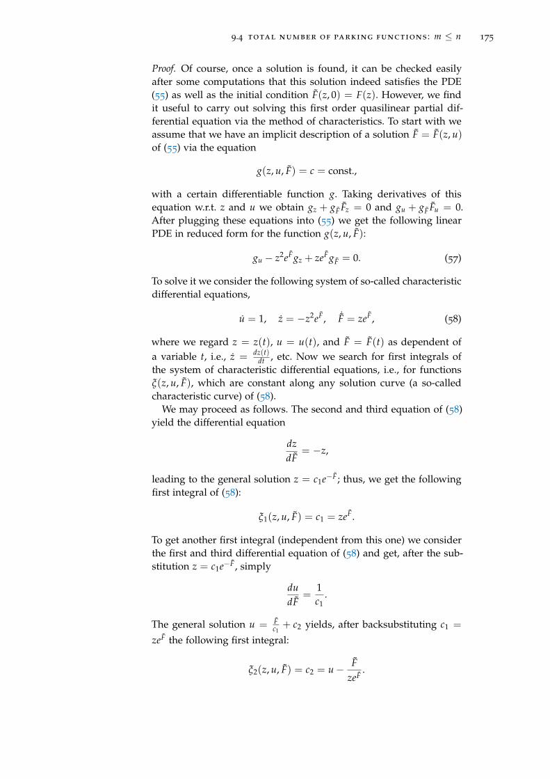
9.4 total number of parking functions : m ≤ n 175
Proof. Of course, once a solution is found, it can be checked easilyafter some computations that this solution indeed satisfies the PDE(55) as well as the initial condition F(z, 0) = F(z). However, we findit useful to carry out solving this first order quasilinear partial dif-ferential equation via the method of characteristics. To start with weassume that we have an implicit description of a solution F = F(z, u)of (55) via the equation
g(z, u, F) = c = const.,
with a certain differentiable function g. Taking derivatives of thisequation w.r.t. z and u we obtain gz + gF Fz = 0 and gu + gF Fu = 0.After plugging these equations into (55) we get the following linearPDE in reduced form for the function g(z, u, F):
gu − z2eFgz + zeFgF = 0. (57)
To solve it we consider the following system of so-called characteristicdifferential equations,
u = 1, z = −z2eF, ˙F = zeF, (58)
where we regard z = z(t), u = u(t), and F = F(t) as dependent ofa variable t, i.e., z = dz(t)
dt , etc. Now we search for first integrals ofthe system of characteristic differential equations, i.e., for functionsξ(z, u, F), which are constant along any solution curve (a so-calledcharacteristic curve) of (58).
We may proceed as follows. The second and third equation of (58)yield the differential equation
dzdF
= −z,
leading to the general solution z = c1e−F; thus, we get the followingfirst integral of (58):
ξ1(z, u, F) = c1 = zeF.
To get another first integral (independent from this one) we considerthe first and third differential equation of (58) and get, after the sub-stitution z = c1e−F, simply
dudF
=1c1
.
The general solution u = Fc1+ c2 yields, after backsubstituting c1 =
zeF the following first integral:
ξ2(z, u, F) = c2 = u− FzeF
.

176 parking in trees and mappings
Thus the general solution of (57) is given as follows:
g(z, u, F) = H(ξ1(z, u, F), ξ2(z, u, F)
)
= H(
zeF, u− FzeF
)= const., (59)
with H an arbitrary differentiable function in two variables. We cansolve (59) w.r.t. the variable u and obtain that the general solution ofthe PDE (55) is implicitly given by
u =F(z, u)zeF(z,u)
+ h(
zeF(z,u))
, (60)
with h(x) an arbitrary differentiable function in one variable. It re-mains to characterize the function h(x) by adapting the general solu-tion (60) to the initial condition F(z, 0) = F(z). First, we obtain
h(zeF(z)) = − F(z)zeF(z)
,
with F(z) given by (47). To get an explicit description of h(x) werequire some manipulations. Using the abbreviations F = F(z), T =
T(2z) and introducing R = R(z) := zeF(z), we get
R = zeF = zeT+ln(1− T2 ) = zeT
(1− T
2
)=
T2
(1− T
2
),
where we applied (3) for the last identity. Thus
T = 1−√
1− 4R,
since T(0) = R(0) = 0 determines the correct branch for the solution.We can characterize the function h(x) via
h(R) = − FR
= −T + ln(1− T2 )
R= −1−
√1− 4R + ln(1− 1−
√1−4R2 )
R.
Therefore, plugging this characterization of h(x) into (60), the gener-ating function F = F(z, u) is given implicitly as follows:
uzeF − F +(
1−√
1− 4zeF)+ ln
(1− 1−
√1− 4zeF
2
)= 0. (61)
To get a more amenable representation we introduce Q = Q(z, u) via
Q :=1−
√1− 4zeF
2.
First, we get
eF =Q(1−Q)
z, (62)

9.4 total number of parking functions : m ≤ n 177
and, after plugging this into (61),
F = uQ(1−Q) + 2Q + ln(1−Q).
Exponentiating the latter equation shows then the functional equationcharacterizing Q,
Q = zeuQ(1−Q)+2Q,
finishing the proof.
As for the case where the number of drivers coincides with the sizeof the tree, we do not extract coefficients at this point yet. We willsee in Theorem 9.22 that the numbers Fn,m are again linked directlyto the numbers Mn,m counting mapping parking functions and weshall therefore content ourselves with extracting coefficients for thecorresponding generating function M(z, u).
Mapping parking functions
We continue our studies on mapping parking functions by consider-ing the total number Mn,m of (n, m)-mapping parking functions, i.e.,the number of pairs ( f , s) with f ∈ Mn an n-mapping and s ∈ [n]m aparking sequence of length m for the mapping f , such that all driversare successful.
As pointed out already in Section 9.3, it suffices to provide the rele-vant considerations for the subfamily Cn of connected n-mappings,since results for the general situation can then be deduced easily.Thus, let us introduce the total number Cn,m of parking functionsof length m for connected n-mappings, i.e., the number of pairs ( f , s),with f ∈ Cn a connected n-mapping and s ∈ [n]m a parking sequenceof length m for f , such that all drivers are successful. Additionally,we require the numbers Fn, Cn and Fn,m as introduced in the Sections9.3, 9.3 and 9.4, respectively.
Let us consider parking functions for connected mappings for thecase that m = n − m parking spaces remain free after all drivershave parked successfully. In what follows it is advantageous to de-fine Cn,m := Cn,n−m and also to use Fn,m := Fn,n−m as done previ-ously. Then it holds that Cn,0 = Cn and Fn,0 = Fn. Let us assume that1 ≤ m ≤ n. To obtain a recursive description of the numbers Cn,m weuse the combinatorial decomposition of a connected mapping f ∈ Cn
w.r.t. the free node which has the largest label amongst all m emptynodes in the mapping graph.
Three situations may occur when using this decomposition: in thefirst case the empty node with largest label is the root node of theCayley tree which forms a length-1 cycle (depicted in Figure 40), inthe second case the empty node with largest label is the root nodeof a Cayley tree forming a cycle of at least two trees (depicted inFigure 42) and in the third case the empty node with largest label is

178 parking in trees and mappings
not a cyclic node (depicted in Figure 43). Analogous considerationsto the ones given for tree parking function in Section 9.4 show thefollowing recursive description of the number of parking functionsfor connected mappings for 1 ≤ m ≤ n:
Cn,m =1m ∑
r≥0
1r! ∑
∑ ki=n−1∑
∑ `i=m−1Fk1,`1 · Fk2,`2 · · · Fkr ,`r ·
·(
nk1, k2, . . . , kr
)(n− m
k1 − `1, k2 − `2, . . . , kr − `r
)
+1m ∑
r≥0
1r! ∑
k+∑ ki=n−1∑
`+∑ `i=m−1Fk,` Fk1,`1 · · · Fkr ,`r · k· (63)
·(
nk, k1, . . . , kr
)(n− m
k− `, k1 − `1, . . . , kr − `r
)
+1m ∑
r≥0
1r! ∑
k+∑ ki=n−1∑
`+∑ `i=m−1Ck,` Fk1,`1 · · · Fkr ,`r · k·
·(
nk, k1, . . . , kr
)(n− m
k− `, k1 − `1, . . . , kr − `r
),
with initial values Cn,0 = Cn. When introducing the generating func-tion
C(z, u) := ∑n≥1
∑m≥0
Cn,mznum
n!(n− m)!, (64)
recurrence (63) yields the following first order linear partial differen-tial equation for the function C(z, u):
Cu(z, u) =z2Cz(z, u) exp(F(z, u)) + z exp(F(z, u)) (65)
+ z2Fz(z, u) exp(F(z, u)),
with F(z, u) = ∑n,m Fn,mznum
n!(n−m)! the corresponding generating func-tion for the number of tree parking functions given in Proposition 9.19,and initial condition C(z, 0) = C(z), with C(z) = ∑n≥1 Cn
zn
(n!)2 givenby (50). A suitable representation of the solution of the PDE (65) isgiven in the following proposition.
Proposition 9.20. The generating function C(z, u) defined in (64) is givenas follows:
C(z, u) = ln(
1(1−Q)(1− uQ)
),
where the function Q = Q(z, u) is given implicitly as the solution of thefollowing functional equation:
Q = z · eQ·(2+u(1−Q)).
Proof. To solve equation (65) we first consider the partial derivativesof the function Q = Q(z, u) occurring in the characterization of the

9.4 total number of parking functions : m ≤ n 179
function F = F(z, u) given in Proposition 9.19. Starting with (56),implicit differentiation yields
Qz =Q
z(1− 2Q)(1− uQ)and Qu =
Q2(1−Q)
(1− 2Q)(1− uQ). (66)
Thus, due to (62), it holds
Qu(z, u) = z2Qz(z, u)eF(z,u),
i.e., Q(z, u) solves the reduced PDE corresponding to (65). This sug-gests the substitution z = z(Q) := Q
eQ(2+u(1−Q)) and we introduce
C(Q, u) := C(z(Q), u) = C(
QeQ(2+u(1−Q))
, u)
.
After straightforward computations, which are thus omitted, equa-tion (65) reads as
Cu(Q, u) =Q
1− uQ.
Thus, after backsubstituting z and C(z, u), the general solution of thisequation is given by
C(z, u) = ln(
11− uQ(z, u)
)+ h(Q(z, u)), (67)
with an arbitrary differentiable function h(x). To characterize it, weevaluate (67) at u = 0 and use the initial condition C(z, u) = C(z),with C(z) given by (50). Using the abbreviation T := T(2z)
2 , one easilygets Q(z, 0) = T and further
h(T) = h(Q(z, u)) = C(z, 0) = C(z) = ln(
11− T
),
which characterizes the function h(x). The proposition follows imme-diately.
We are now able to treat the total number Mn,m of (n, m)-mappingparking functions. We introduce Mn,m := Mn,n−m and the generatingfunction
M(z, u) := ∑n≥0
∑m≥0
Mn,mznum
n!(n− m)!. (68)
The decomposition of mapping parking functions into parking func-tions for their connected components immediately gives the relation
M(z, u) = exp(C(z, u)
)
for the respective generating functions. According to Proposition 9.20
we obtain the following solution of M(z, u).
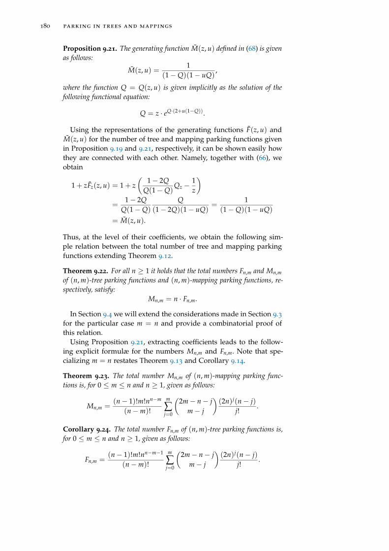
180 parking in trees and mappings
Proposition 9.21. The generating function M(z, u) defined in (68) is givenas follows:
M(z, u) =1
(1−Q)(1− uQ),
where the function Q = Q(z, u) is given implicitly as the solution of thefollowing functional equation:
Q = z · eQ·(2+u(1−Q)).
Using the representations of the generating functions F(z, u) andM(z, u) for the number of tree and mapping parking functions givenin Proposition 9.19 and 9.21, respectively, it can be shown easily howthey are connected with each other. Namely, together with (66), weobtain
1 + zFz(z, u) = 1 + z(
1− 2QQ(1−Q)
Qz −1z
)
=1− 2Q
Q(1−Q)
Q(1− 2Q)(1− uQ)
=1
(1−Q)(1− uQ)
= M(z, u).
Thus, at the level of their coefficients, we obtain the following sim-ple relation between the total number of tree and mapping parkingfunctions extending Theorem 9.12.
Theorem 9.22. For all n ≥ 1 it holds that the total numbers Fn,m and Mn,m
of (n, m)-tree parking functions and (n, m)-mapping parking functions, re-spectively, satisfy:
Mn,m = n · Fn,m.
In Section 9.4 we will extend the considerations made in Section 9.3for the particular case m = n and provide a combinatorial proof ofthis relation.
Using Proposition 9.21, extracting coefficients leads to the follow-ing explicit formulæ for the numbers Mn,m and Fn,m. Note that spe-cializing m = n restates Theorem 9.13 and Corollary 9.14.
Theorem 9.23. The total number Mn,m of (n, m)-mapping parking func-tions is, for 0 ≤ m ≤ n and n ≥ 1, given as follows:
Mn,m =(n− 1)!m!nn−m
(n−m)!
m
∑j=0
(2m− n− j
m− j
)(2n)j(n− j)
j!.
Corollary 9.24. The total number Fn,m of (n, m)-tree parking functions is,for 0 ≤ m ≤ n and n ≥ 1, given as follows:
Fn,m =(n− 1)!m!nn−m−1
(n−m)!
m
∑j=0
(2m− n− j
m− j
)(2n)j(n− j)
j!.

9.4 total number of parking functions : m ≤ n 181
Proof of Theorem 9.23. In view of the representation of M(z, u) givenin Proposition 9.21 containing the function Q = Q(z, u), we makea change of variables in order to extract coefficients. Using the func-tional equation (56) and the derivative (66) of Q w.r.t. z, an applicationof Cauchy’s integral formula gives
[zn]M(z, u) =1
2πi
∮ M(z, u)zn+1 dz =
12πi
∮ 1zn+1
1(1−Q)(1− uQ)
dQ
=1
2πi
∮ e(uQ(1−Q)+2Q)(n+1)
(1−Q)(1− uQ)Qn+1(1− 2Q)(1− uQ)
euQ(1−Q)+2QdQ
= [Qn]en(uQ(1−Q)+2Q)(1− 2Q)
1−Q.
Further, for 0 ≤ m ≤ n,
[znun−m]M(z, u) = [Qnun−m]eunQ(1−Q)e2nQ(1− 2Q)
1−Q
=nn−m
(n−m)n−m−1e2nQ(1− 2Q).
(69)
We get
Mn,m = n!m![znun−m]M(z, u)
=n!m!nn−m
(n−m)n−m−1e2nQ(1− 2Q) (70)
=n!m!nn−m
(n−m)!
m
∑j=0
(n−m− 1
j
)(−1)j[Qm−j]e2nQ(1− 2Q)
=n!m!nn−m
(n−m)!
m
∑j=0
(n−m− 1
j
)(−1)j 2(n−m + j)(2n)m−j−1
(m− j)!
=(n− 1)!m!nn−m
(n−m)!
m
∑j=0
(j + m− n
j
)(n−m + j) (2n)m−j
(m− j)!
=(n− 1)!m!nn−m
(n−m)!
m
∑j=0
(2m− n− j
m− j
)(n− j) (2n)j
j!.
From Theorem 9.23 we can easily derive exact values for the totalnumber of (n, m)-mapping parking functions for a moderate size of n.However, due to the alternating sign of the summands in the explicitformula of Mn,m that is inherent in the binomial coefficient, it is notwell suited to deduce the asymptotic behaviour of these numbersand thus to give answers to questions concerning the probability pn,m
that a random pair ( f , s) of an n-mapping f and a sequence s ∈[n]m of addresses of length m is a parking function, when n → ∞.Starting from (69), such asymptotic considerations will be carried outin Section 9.4 using saddle point methods.
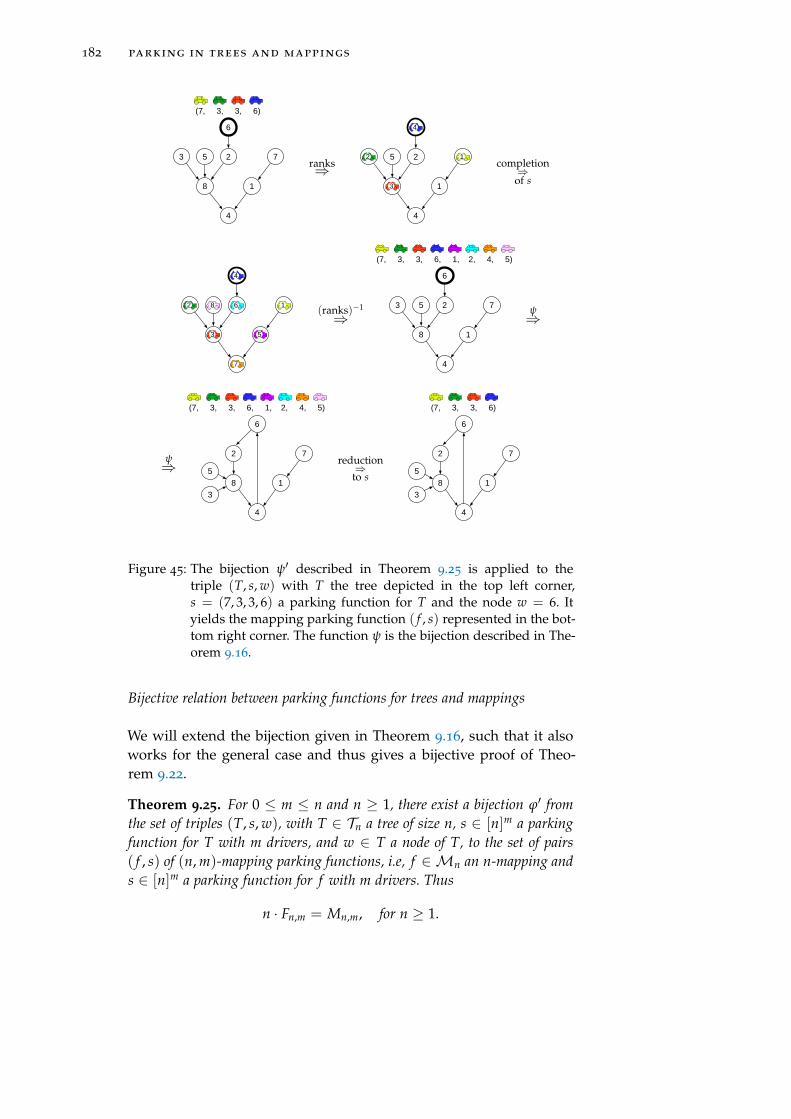
182 parking in trees and mappings
3
8 1
4
2 7
6
5
(7, 3, 3, 6)
ranks⇒3
8 1
4
2 7
6
5
4
3
2 1completion⇒
of s
3
8 1
4
2 7
6
5
4
3
2 1
5
6
7
8(ranks)−1
⇒3
8 1
4
2 7
6
5
(7, 3, 3, 6, 1, 2, 4, 5)
ψ⇒
ψ⇒3
8 1
4
2 7
6
5
(7, 3, 3, 6, 1, 2, 4, 5)
reduction⇒to s
38 1
4
2 7
6
5
(7, 3, 3, 6)
Figure 45: The bijection ψ′ described in Theorem 9.25 is applied to thetriple (T, s, w) with T the tree depicted in the top left corner,s = (7, 3, 3, 6) a parking function for T and the node w = 6. Ityields the mapping parking function ( f , s) represented in the bot-tom right corner. The function ψ is the bijection described in The-orem 9.16.
Bijective relation between parking functions for trees and mappings
We will extend the bijection given in Theorem 9.16, such that it alsoworks for the general case and thus gives a bijective proof of Theo-rem 9.22.
Theorem 9.25. For 0 ≤ m ≤ n and n ≥ 1, there exist a bijection ϕ′ fromthe set of triples (T, s, w), with T ∈ Tn a tree of size n, s ∈ [n]m a parkingfunction for T with m drivers, and w ∈ T a node of T, to the set of pairs( f , s) of (n, m)-mapping parking functions, i.e, f ∈ Mn an n-mapping ands ∈ [n]m a parking function for f with m drivers. Thus
n · Fn,m = Mn,m, for n ≥ 1.

9.4 total number of parking functions : m ≤ n 183
Remark 9.26. It holds that the parking function s remains unchangedunder the bijection ϕ′. Thus, also the general case satisfies the relation
n · Fn(s) = Mn(s), for n ≥ 1,
where again Fn(s) and Mn(s) denote the number of trees T ∈ Tn andmappings f ∈ Mn, respectively, such that a given sequence s ∈ [n]m
is a parking function for T and f , respectively.
Proof of Theorem 9.25. In order to a establish a bijection ψ′ from the setof triples (T, s, w) to pairs ( f , s), we will first extend the tree parkingfunction s ∈ [n]m to a tree parking function s′ ∈ [n]n with n drivers.Then we apply the bijection ψ described in the proof of Theorem 9.16
Finally, we reduce s′ to the original parking function s. We only needto ensure that the extension from s to s′ is done in such a way that thewhole procedure can be reversed in a unique way. This can be doneas follows.
Starting with a triple (T, s, w), let us denote by Vπ the set of nodeswhich are occupied after the parking procedure, i.e., Vπ := π([m]) =
{π(k) : 1 ≤ k ≤ m}, where π = π(T,s) is the output-function of (T, s).Let us arrange the n − m free nodes in ascending order w.r.t. theirlabels: V \Vπ = {x1, x2, . . . , xn−m}, with x1 < x2 < · · · < xn−m. Thenwe define the sequence s′ = (s′1, . . . , s′n) ∈ [n]n as follows:
s′i := si, 1 ≤ i ≤ m,
s′m+i := xi, 1 ≤ i ≤ n−m.
Of course s′ is a parking function for T since s is a parking function forT and every one of the drivers m+ 1, . . . , n can park at their preferredparking space. Applying ψ from Theorem 9.16 gives an n-mappingf , such that s′ is a parking function for f . Thus the sequence s =
(s1, . . . , sm) = (s′1, . . . , s′m), which contains the preferences of the firstm drivers of s′, is a parking function for f . We define the pair ( f , s) tobe the outcome of ψ′.
As for the case m = n, it holds that the parking paths of the driverscoincide for T and f . In particular, it holds π( f ,s) = π(T,s) for thecorresponding output-functions. Thus, ψ′ can be reversed easily, sincethe extension from s to s′ can also be constructed when starting withf .
Example 9.27. Consider the tree T of size 8 depicted in the top leftcorner of Figure 45. The sequence s = (7, 3, 3, 6) is a parking functionfor T with 4 drivers. In the top right corner of the figure, the ranks ofthe nodes in T that are occupied by a car can be found. Completing sto a parking function with 8 drivers leads to the ranks in the middleleft and the sequence s′ = 7, 3, 3, 6, 1, 2, 4, 5 as described in the middleright of the figure. Applying the mapping ψ described in the proof ofTheorem 9.16 to (T, s′, w) yields the mapping parking function ( f , s′)

184 parking in trees and mappings
as depicted in the bottom left corner. Reducing s′ to the first 4 driversleads to the original parking function s. The image ( f , s) of (T, s, w)
under ψ′ is depicted in the bottom right. It can be checked very easilythat s is indeed a parking function for f . a
Asymptotic considerations
Let us now turn to the asymptotic analysis of the number Mn,m of(n, m)-mapping parking functions. Due to Theorem 9.22, our resultsfor parking functions for mappings can automatically be translatedto results for parking functions for trees. In this context the followingquestion will be of particular interest to us: How does the probabilitypn,m := Mn,m
nn+m that a randomly chosen sequence of length m on theset [n] is a parking function for a randomly chosen n-mapping swapfrom being equal to 1 (which is the case for m=1) to being close to 0(which is the case for m = n) when the ratio ρ := m
n increases?In order to get asymptotic results for Mn,m (and so for Fn,m and pn,m,
too) we start with the representation (70), which can be written as
Mn,m =n!m!nn−m
(n−m)!An,m, (71)
with
An,m = [wm](1− 2w)e2nw(1− w)n−m−1
=1
2πi
∮(1− 2w)e2nw(1− w)n−m−1
wm+1 dw, (72)
where, in the latter expression, we choose as contour a suitable sim-ple positively oriented closed curve around the origin, e.g., for eachchoice of m and n, we may choose any such curve in the dotted disk0 < |w| < 1.
Next we will use the integral representation (72) of An,m and makeuse of the saddle point method. We write the integral as follows:
An,m =1
2πi
∫
Γ
g(w)enh(w)dw, (73)
with Γ a suitable contour and
g(w) :=1− 2w
(1− w)wand (74)
h(w) = hn,m(w) := 2w +(
1− mn
)log(1− w)− m
nlog w.
In the terminology of [78] the integral (73) has the form of a “largepower integral” and saddle points of the relevant part enh(w) of theintegrand can thus be found as the zeros of the derivative h′(w). Theresulting equation
h′(w) = 2−(
1− mn
) 11− w
− mn
1w
= 0
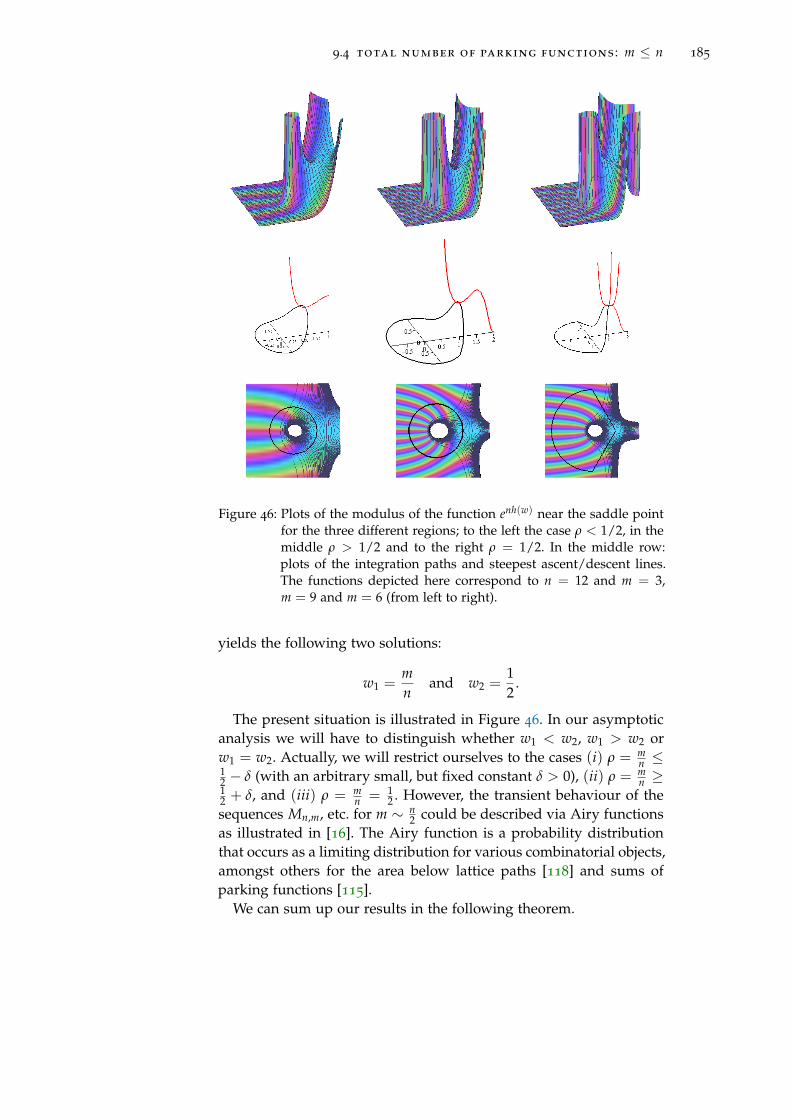
9.4 total number of parking functions : m ≤ n 185
Figure 46: Plots of the modulus of the function enh(w) near the saddle pointfor the three different regions; to the left the case ρ < 1/2, in themiddle ρ > 1/2 and to the right ρ = 1/2. In the middle row:plots of the integration paths and steepest ascent/descent lines.The functions depicted here correspond to n = 12 and m = 3,m = 9 and m = 6 (from left to right).
yields the following two solutions:
w1 =mn
and w2 =12
.
The present situation is illustrated in Figure 46. In our asymptoticanalysis we will have to distinguish whether w1 < w2, w1 > w2 orw1 = w2. Actually, we will restrict ourselves to the cases (i) ρ = m
n ≤12 − δ (with an arbitrary small, but fixed constant δ > 0), (ii) ρ = m
n ≥12 + δ, and (iii) ρ = m
n = 12 . However, the transient behaviour of the
sequences Mn,m, etc. for m ∼ n2 could be described via Airy functions
as illustrated in [16]. The Airy function is a probability distributionthat occurs as a limiting distribution for various combinatorial objects,amongst others for the area below lattice paths [118] and sums ofparking functions [115].
We can sum up our results in the following theorem.

186 parking in trees and mappings
Theorem 9.28. The total number Mn,m of (n, m)-mapping parking func-tions is asymptotically, for n → ∞, given as follows (where δ denotes anarbitrary small, but fixed, constant):
Mn,m ∼
nn+m+ 12√
n−2mn−m , for 1 ≤ m ≤ ( 1
2 − δ)n,
Γ( 2
3
)√ 2π 3
16 n
3n2 − 1
6 , for m = n2 ,
m!(n−m)! · n2n−m+ 3
2 22m−n+1
(2m−n)52
, for ( 12 + δ)n ≤ m ≤ n.
Let us fix the ratio ρ = m/n. This ratio can be interpreted as a “loadfactor” – a term used in open addressing hashing. Then the asymp-totic behaviour of the probabilities pn,m = pn,ρn follows immediately.
Corollary 9.29. The probability pn,m that a randomly chosen pair ( f , s),with f an n-mapping and s a sequence in [n]m, represents a parking functionis asymptotically, for n → ∞ and m = ρn with 0 < ρ < 1 fixed, given asfollows:
pn,m ∼
C<(ρ), for 0 < ρ < 12 ,
C1/2 · n−1/6, for ρ = 1/2,
C>(ρ) · n−1 · (D>(ρ))n, for 1/2 < ρ < 1,
with
C<(ρ) =
√1− 2ρ
1− ρ, C1/2 =
√6π
Γ(2/3)31/3 ≈ 1.298 . . . ,
C>(ρ) = 2 ·√
ρ
(1− ρ)(2ρ− 1)5 , D>(ρ) =
(4ρ
e2
)ρ e2(1− ρ)1−ρ
.
From Corollary 9.29 it follows that the limiting probability L(ρ) :=limn→∞ pn,ρn that all drivers can park successfully for a load factor ρ
is given as follows :
L(ρ) =
√1−2ρ
1−ρ , for 0 ≤ ρ ≤ 12 ,
0, for 12 ≤ ρ ≤ 1.
See Figure 47 for an illustration: On the left hand-side the limitingdistribution L(ρ) is plotted and on the right hand-side the exact prob-abilities pn,ρn for some values of n can be found.
The proof of Theorem 9.28 is given in Sections 9.4-9.4. As we cansee from Theorem 9.28 and Corollary 9.29, the most interesting regionfor us is case (i), i.e., where less than half of the parking spaces are oc-cupied. We will thus provide the calculations for this region in detail,whereas the application of the saddle point method is only sketchedfor the other two regions. Before we continue with the computations,we want to comment on relations between mapping parking func-tions and ordered forests of unrooted trees.

9.4 total number of parking functions : m ≤ n 187
Figure 47: To the left: The limiting probability L(ρ) that all drivers areable to park successfully in a mapping, for a load factor 0 ≤ρ ≤ 1. To the right: The exact probabilities pn,ρn for n =20, 50, 200, 500, 1000, 5000.
Remark 9.30. Qualitatively, the transient behaviour at m ∼ n2 is the
same as observed previously in other combinatorial contexts, such as,e.g., in the analysis of random graphs. The study of random graphsG(n, m) with n nodes and m edges was initiated by Erdos and Rényiin the late 1950s [66]. The structure of G(n, m) has three differentphases depending on the ratio m
n :
• When m = µn for some µ < 12 , the graph G(n, m) consists
with high probability, i.e., with probability tending to one whenn → ∞, only of trees and of unicyclic components. Moreover,the size of the largest component is of order O(log n).
• For m = 12 n +O(n2/3, there appear with high probability one
or several semi-giant components of size O(n2/3).
• When m = µn for some µ > 12 , the graph G(n, m) consists with
high probability of a unique giant component of size propor-tional to n.
For each case refined estimates that are obtained with the help ofanalytic techniques can be found in [74] and [104].
Such phase transition phenomena have for instance also been ob-served for random planar maps, see [16].
Remark 9.31. Let Gn,m denote the number of ordered forests, i.e., se-quences of m unrooted labelled trees and comprised of n nodes intotal. The problem of evaluating Gn,m asymptotically by using saddlepoint techniques has been considered in [78, p. 603f.]; as has beenmentioned there, it is also relevant to the analysis of random graphsduring the phase where a giant component has not yet emerged [74].
Since there are nn−2 unrooted labelled trees of size n ≥ 1, the expo-nential generating function U(z) = ∑n≥1 nn−2 zn
n! is given by U(z) =
188 parking in trees and mappings
T(z)− T2(z)2 , with T(z) the tree-function. Thus the numbers Gn,m can
be obtained as follows:
Gn,m = n![zn]U(z)m = n![zn]
(T(z)− T2(z)
2
)m
= n!1
2πi
∮ (T(z)− T2(z)
2
)m dzzn+1 ,
by using a suitable contour around the origin. The substitution z = TeT
leads to
Gn,m = n!1
2πi
∮ enT (1− T2
)m(1− T)
Tn−m+1 dT.
After substituting T = 2w, one obtains
Gn,m = n!1
2πi
∮ e2nw (1− w)m (1− 2w)
2n−mwn−m+1 dw
=n!
2n−m [wn−m](1− 2w)e2nw(1− w)m,
and so[wm](1− 2w)e2nw(1− w)n−m =
2m
n!Gn,n−m. (75)
Comparing Equation (75) with Equation (72) for An,m suggests thatthe same phase change behaviour occurs for An,m (and thus also Mn,m)and for Gn,n−m as studied in [78].
Remark 9.32. By slightly adapting the considerations made in the pre-vious remark we can even express the numbers Mn,m directly via thenumber of ordered forests. Namely, let Gn,m denote the number ofordered forests made of one rooted labelled tree followed by m − 1unrooted labelled trees and comprised of n nodes in total. This yields
Gn,m = n![zn]T(z)U(z)m−1 = n![zn]T(z)(
T(z)− T2(z)2
)m−1
= n!1
2πi
∮T(z)
(T(z)− T2(z)
2
)m−1 dzzn+1 ,
and, after the substitutions z = TeT and T = 2w, we end up with
Gn,m =n!
2n−m
∮ e2nw(1− w)m−1(1− 2w)
wn−m+1 dw
=n!
2n−m [wn−m](1− 2w)e2nw(1− w)m−1.
We get
An,m =2m
n!Gn,n−m,
and thus we are able to express Mn,m by counting a certain numberof ordered forests:
Mn,m =m!2mnn−m
(n−m)!Gn,n−m.
9.4 total number of parking functions : m ≤ n 189
The region ρ ≤ 12 − δ
The geometry of the modulus of the integrand of (73) as depicted inFigure 46 is easily described: There is a simple dominant saddle pointat w = w1, where the surface resembles an ordinary horse saddleor a mountain pass. There are two steepest ascent/steepest ascentlines: one following the real axis and one parallel to the imaginaryaxis. It is thus natural to adopt an integration contour that lies closeto the steepest ascent and steepest descent line perpendicular to thereal axis. In Equation (73) we thus choose the contour Γ to be a circlecentered at the origin and passing through the dominant saddle pointw1, i.e., it has radius r = ρ.
Using the parametrization Γ = {w = ρeiφ : φ ∈ [−π, π]}, we obtainfrom (73) the representation
An,m =1
2π
∫ π
−πρeiφg(ρeiφ)enh(ρeiφ)dφ. (76)
Next we want to find a suitable splitting of the integral into the cen-tral approximation and the remainder. That is , we need to choosea proper value φ0 = φ0(n, m) to write the contour as Γ = Γ1 ∪ Γ2,with Γ1 := {w = ρeiφ : φ ∈ [−φ0, φ0]} and Γ2 := {w = ρeiφ : φ ∈[−π,−φ0] ∪ [φ0, π]} yielding the representation An,m = I(1)n,m + I(2)n,m,such that I(2)n,m = o
(I(1)n,m
), where
I(1)n,m :=1
2π
∫
Γ1
ρeiφg(ρeiφ)enh(ρeiφ)dφ and
I(2)n,m :=1
2π
∫
Γ2
ρeiφg(ρeiφ)enh(ρeiφ)dφ.
To do this we consider the local expansion of the integral around φ =
0; the following results are obtained by straightforward computations,which are thus omitted:
ρeiφg(ρeiφ) =1− 2m
n eiφ
1− mn eiφ =
1− 2mn
1− mn·(
1 +O(
mφ
n
)),
nh(ρeiφ) =n(
2mn
eiφ +(
1− mn
)log(
1− mn
eiφ)− m
nlog(m
neiφ))
=2m + (n−m) log(
1− mn
)−m log
(mn
)
− mφ2
2+
m2
2(n−m)φ2 +O(mφ3),
yielding
ρeiφg(ρeiφ)enh(ρeiφ) =
(1− 2m
n
)( nm
)me2m(
1− mn
)n−m−1· (77)
· e−(
m2 − m2
2(n−m)
)φ2(
1 +O(mφ3)+O
(mφ
n
)).
190 parking in trees and mappings
From the latter expansion we obtain that we shall choose φ0, suchthat mφ2
0 → ∞ (then the central approximation contains the maincontributions) and mφ3
0 → 0 (then the remainder term is asymptot-ically negligible). E.g., we may choose φ0 = m−
12+
ε3 , for a constant
0 < ε < 12 . With such a choice of φ0 we obtain for the integral I(1)n,m the
following asymptotic expansion:
I(1)n,m =1
2π
(1− 2m
n
)( nm
)me2m(
1− mn
)n−m−1·
·∫ φ0
−φ0
e−(
m2 − m2
2(n−m)
)φ2
dφ ·(
1 +O(
m−12+ε))
=1
2π
(1− 2m
n
)( nm
)me2m(
1− mn
)n−m−1 1√m·
·∫ m
ε3
−mε3
e−12 (1− m
n−m )t2dt ·
(1 +O
(m−
12+ε))
,
where we used the substitution φ = t√m for the latter expression.
For the so-called tail completion we use that∫ ∞
ce−αt2
dt = O(
e−αc2)
, for c > 0 and α > 0,
which can be shown, e.g., via
∫ ∞
ce−αt2
dt ≤∞
∑i=0
e−α(c+i)2= e−αc2 ·
∞
∑i=0
e−αi(2c+i) = O(
e−αc2)
,
since ∑∞i=0 e−α(c+i)2
converges.Thus we obtain
∫ ∞
mε3
e−12 (1− m
n−m )t2dt = O
(e−
12 (1− m
n−m )m2ε3
),
which yields a subexponentially small and thus negligible error term.Using this we may proceed in the asymptotic evaluation of I(1)n,m andget
I(1)n,m =1
2π
(1− 2m
n
)( nm
)me2m(
1− mn
)n−m−1 1√m·
∫ ∞
−∞e−
12 (1− m
n−m )t2dt(
1 +O(
m−12+ε))
.
Using ∫ ∞
−∞e−αt2
dt =√
π√α
, for α > 0,

9.4 total number of parking functions : m ≤ n 191
the Gaussian integral occurring can be evaluated easily, which yields
I(1)n,m =1
2π
(1− 2m
n
)( nm
)me2m(
1− mn
)n−m−1 1√m·
·√
2π√1− m
n−m
·(
1 +O(
m−12+ε))
=(n−m)n−m− 1
2√
n− 2me2m√
2πmm+ 12 nn−2m
·(
1 +O(
m−12+ε))
.
Next we consider the remainder integral
I(2)n,m =1
2π
(1− 2m
n
)·
·∫
Γ2
1− 2mn eiφ
1− mn eiφ en(2 m
n eiφ+(1−mn ) log(1−m
n eiφ)−mn log(m
n )−mn iφ)dφ.
To estimate the integrand we use the obvious bounds∣∣∣∣1−
2mn
eiφ∣∣∣∣ ≤ 1 +
2mn
and1∣∣1− mn eiφ
∣∣ ≤1
1− mn
,
as well as the following:∣∣∣en(2 m
n eiφ+(1−mn ) log(1−m
n eiφ)−mn log(m
n )−mn iφ)
∣∣∣
=( n
m
)men(2ρ cos φ+ 1−ρ
2 log(1−2ρ cos φ+ρ2)).
This yields∣∣∣I(2)n,m
∣∣∣ ≤ 12π
(1− 2mn )(1 + 2m
n )
1− mn
·( n
m
)m·
·∫
Γ2
en(2ρ cos φ+ 1−ρ2 log(1−2ρ cos φ+ρ2))dφ.
Considering the function
H(x) := 2ρx +1− ρ
2log(1− 2ρx + ρ2),
it can be shown by applying standard calculus that H(x) is a mono-tonically increasing function for x ∈ [−1, 1]. Setting x = cos φ it fol-lows that amongst all points of the contour Γ2 the integrand reachesits maximum at φ = φ0. Thus, we obtain∣∣∣I(2)n,m
∣∣∣ ≤ (1− 2mn )(1 + 2m
n )
1− mn
·( n
m
)m· e2m cos φ0+
n−m2 log(1− 2m
n cos φ0+(mn )
2)
≤2 ·( n
m
)m· e2m cos φ0+
n−m2 log(1− 2m
n cos φ0+(mn )
2)
=2( n
m
)me2me
n−m2 log
(1− 2m
n +(mn )
2)·
· e2m(cos φ0−1)+ n−m
2 log(
1− 2mn cos φ0+(
mn )
2
1− 2mn +(m
n )2
)
=2( n
m
)me2m(
1− mn
)n−m· e2m(cos φ0−1)+ n−m
2 log(
1−2mn (cos φ0−1)(1−m
n )2
)
.

192 parking in trees and mappings
Using the estimates
log(1− x) ≤ −x, for x < 1, and cos x− 1 ≤ − x2
6, for x ∈ [−π, π],
we may proceed f as follows:
|I(2)n,m| ≤ 2( n
m
)me2m(
1− mn
)n−m· em(cos φ0−1)·
(2− 1
1−mn
)
≤ 2( n
m
)me2m(
1− mn
)n−m· e−
φ206 m
(2− 1
1−mn
)
= 2( n
m
)me2m(
1− mn
)n−m· e−
16
(2− 1
1−mn
)m
2ε3
.
Thus we obtain
|I(2)n,m| = |I(1)n,m| · O(√
me−cm2ε3
), with c =
16
(2− 1
1− mn
),
i.e., I(2)n,m is subexponentially small compared to I(1)n,m.Combining these results we get
An,m =(n−m)n−m− 1
2√
n− 2me2m√
2πmm+ 12 nn−2m
·(
1 +O(
m−12+ε))
and, by using (71) and applying Stirling’s approximation formula forthe factorials,
Mn,m =n!m!nn−m(n−m)n−m− 1
2√
n− 2me2m√
2π(n−m)!mm+ 12 nn−2m
·(
1 +O(
m−12+ε))
=nn+m
√1− 2m
n
1− mn
·(
1 +O(
m−12+ε))
. (78)
Note that according to the remainder term in (78) we have onlyshown the required result for m → ∞. However, again starting with(76), we can easily show a refined bound on the error term for smallm. Namely, we may write the integral as follows:
An,m =1
2π
( nm
)m·∫ π
−π
e2meiφ(1− m
n eiφ)n−m−1(1− 2mn eiφ)
eimφdφ,
and use for m = o(√
n) the expansions
(1− m
neiφ)n−m−1
= e−meiφ ·(
1 +O(
m2
n
))and
1− 2mn
eiφ = 1 +O(m
n
),
which gives
An,m =1
2π
( nm
)m·∫ π
−π
emeiφ
eimφdφ ·
(1 +O
(m2
n
)).

9.4 total number of parking functions : m ≤ n 193
Using the substitution z = eiφ this yields for m = o(√
n)
An,m =1
2πi
( nm
)m·∮ emz
zm+1 dz ·(
1 +O(
m2
n
))=
nm
m!·(
1 +O(
m2
n
))
and, again by using (71) and applying Stirling’s approximation for-mula for the factorials, furthermore
Mn,m =n!nn
(n−m)!·(
1 +O(
m2
n
))= nn+m ·
(1 +O
(m2
n
))
=nn+m
√1− 2m
n
1− mn
·(
1 +O(
m2
n
)).
The region ρ ≥ 12 + δ
For this region we choose in (73) the contour Γ to be a circle centredat the origin and passing through the dominant saddle point w2, i.e.,it has radius r = 1
2 . Using the parametrization Γ = {w = 12 eiφ : φ ∈
[−π, π]}, we obtain from (73) the representation
An,m =1
2π
∫ π
−π
12
eiφg(12
eiφ)enh( 12 eiφ)dφ, (79)
with functions g(w) and h(w) defined in (74).As in the previous region we expand the integrand in (79) around
φ = 0 to find a suitable choice for φ0 to split the integral. However,due to cancellations, we require a more refined expansion which canagain be obtained by straightforward computations. Namely, we ob-tain
12
eiφg(
12
eiφ)=− 2iφ + 3φ2 +O(φ3),
nh(
12
eiφ)=n + (2m− n) log 2−
(m− n
2
)φ2
+ i(
5n6−m
)φ3 +O(nφ4),
which gives
12
eiφg(
12
eiφ)
enh( 12 eiφ) =en22m−ne−(m−
n2 )φ
2 ·
·(− 2iφ + 3φ2 +
(5n− 6m
3
)φ4+
+O(φ3) +O(nφ5) +O(n2φ7)
).
Thus we may choose φ0 = n−12+ε, with 0 < ε < 1
6 to split the contourΓ = Γ1 ∪ Γ2, with Γ1 = {w = 1
2 eiφ : φ ∈ [−φ0, φ0]} and Γ2 = {w =12 eiφ : φ ∈ [−π,−φ0] ∪ [φ0, π]}. Let us again denote by I(1)n,m and I(2)n,m
194 parking in trees and mappings
the contribution of the integral in the representation (79) over Γ1 andΓ2, respectively.
For I(1)n,m we use the above expansion for the integrand and obtainafter simple manipulations
I(1)n,m = cn,m
∫ φ0
−φ0
e−(m−n2 )φ
2 ·
·(−2iφ + 3φ2 +
(5n− 6m
3
)φ4 +O(n− 3
2+7ε)
)dφ,
where the multiplicative factor cn,m is equal to en22m−n 12π . Again it
holds that completing the tails only gives a subexponentially smallerror term and we obtain
I(1)n,m = cn,m
∫ ∞
−∞e−(m−
n2 )φ
2 ·
·(−2iφ + 3φ2 +
(5n− 6m
3
)φ4 +O(n− 3
2+7ε)
)dφ
=cn,m√
n
∫ ∞
−∞e−(
mn − 1
2 )t2 ·
·(−2i
t√n+
3t2
n+
5n− 6m3
t4
n2 +O(
n−32+7ε
))dt,
where we used the substitution φ = t√n to get the latter expression.
Using the integral evaluations (with α > 0):∫ ∞
−∞te−αt2
dt = 0,∫ ∞
−∞t2e−αt2
dt =√
π
2α32
,∫ ∞
−∞t4e−αt2
dt =3√
π
4α52
,
we obtain
I(1)n,m =cn,m
n32
3
√π
2(m
n − 12
) 32+
(5− 6m
n
)√π
4(m
n − 12
) 52
·
(1 +O
(n−
12+7ε
))
=en22m−n+1
√2πn
32( 2m
n − 1) 5
2·(
1 +O(
n−12+7ε
)).
Again, it can be shown that the main contribution of An,m comesfrom I(1)n,m, i.e., that it holds
I(2)n,m =1
2π
∫
Γ2
12
eiφg(
12
eiφ)
enh( 12 eiφ)dφ = o
(I(1)n,m
),
but here we omit these computations. Thus we obtain
An,m =en22m−n+1
√2πn
32( 2m
n − 1) 5
2·(
1 +O(
n−12+7ε
)),
and
Mn,m =m!
(n−m)!· n2n−m−122m−n+1
( 2mn − 1
) 52
·(
1 +O(
n−12+7ε
)).

9.4 total number of parking functions : m ≤ n 195
The monkey saddle for ρ = 1/2
For ρ = mn = 1
2 , the situation is slightly different to the previousregions since the two otherwise distinct saddle points coalesce to aunique double saddle point. The difference in the geometry of thesurface, i.e., of the modulus of the large power en·h(w) in (73), is thatthere are now three steepest descent lines and three steepest ascentslines departing from the saddle point (in contrast to two steepestdescent lines and two steepest ascents lines for the case of a simplesaddle point). This explains why such saddle points are also referredto as “monkey saddles”: they do not only offer space for two legs butalso for a tail. In this particular case the three steepest descent andsteepest ascent lines departing from the saddle point at w = w1 =
w2 = 12 have angles 0, 2π/3 and −2π/3 as can be seen in the middle
right of Figure 46. This also follows from a local expansion of h(w) asdefined in (74) around w = 1
2 :
h(w) = 1− 83
(w− 1
2
)3
+O((
w− 12
)4)
.
Thus, we may choose as integration contour two line segmentsjoining the point w = 1
2 with the imaginary axis at an angle of−2π/3 and 2π/3, respectively, as well as a half circle centred atthe origin and joining the two line segments. See the bottom rightof Figure 46. This yields Γ = Γ1 ∪ Γ2 ∪ Γ3 and An,m = I(1)n,m + I(2)n,m +
I(3)n,m for the corresponding integrals, where we use the parametriza-tions Γ1 :=
{12 − e−
2πi3 t : t ∈ [−1, 0]
}, Γ2 :=
{12 + e
2πi3 t : t ∈ [0, 1]
},
and Γ3 :={√
32 eit : t ∈ [π
2 , 3π2 ]}
.We first treat
I(1)n,m =1
2πi
∫ 0
−1
(−e−
2πi3
)g(
12− e−
2πi3 t)
enh(
12−e−
2πi3 t)
dt
=1
2πi
∫ 1
0
(−e−
2πi3
)g(
12+ e−
2πi3 t)
enh(
12+e−
2πi3 t)
dt.
In order to find a suitable choice t0 for splitting the integral for thecentral approximation and the remainder we consider the expansionof the integrand around t = 0, which can be obtained easily:
−e−2πi
3
2πig(
12+ e−
2πi3 t)
enh(
12+e−
2πi3 t)
=4ene−
4πi3
πite−
83 nt3 ·
(1 +O(t2) +O(nt5)
). (80)
Thus we obtain the restrictions nt30 → ∞ and nt5
0 → 0 which are, e.g.,satisfied when choosing t0 = n−
14 . This splitting yields I(1)n,m = I(1,1)
n,m +
I(1,2)n,m , for the integration paths t ∈ [0, t0] and t ∈ [t0, 1], respectively.

196 parking in trees and mappings
Using the local expansion of the integrand (80) as well as the before-mentioned choice for t0, the central approximation I(1,1)
n,m gives
I(1,1)n,m =
4ene−4πi
3
πi
∫ t0
0te−
83 nt3
dt ·(
1 +O(n− 14 ))
=4ene−
4πi3
πi
∫ ∞
0te−
83 nt3
dt ·(
1 +O(n− 14 ))
,
since one can show easily that completing the integral only yields asubexponentially small error term. Moreover, also the remainder
I(1,2)n,m =
12πi
∫ 1
t0
(−e−
2πi3
)g(
12+ e−
2πi3 t)
enh(
12+e−
2πi3 t)
dt
only yields a subexponentially small error term compared to I(1,1)n,m .
Thus, we get the contribution
I(1)n,m =4ene−
4πi3
πi
∫ ∞
0te−
83 nt3
dt ·(
1 +O(n− 14 ))
.
The integral
I(2)n,m =1
2πi
∫ 1
0
(e
2πi3
)g(
12+ e
2πi3 t)
enh(
12+e
2πi3 t)
dt,
can be treated in an analogous manner which gives the contribution
I(2)n,m = −4ene4πi
3
πi
∫ ∞
0te−
83 nt3
dt ·(
1 +O(n− 14 ))
.
Moreover, one can show that the contribution of
I(3)n,m =1
2πi
∫ 3π2
π2
√3
2ieitg
(√3
2eit
)enh
(√3
2 eit)
dt
is asymptotically negligible compared to I(1)n,m and I(2)n,m.Collecting the contributions and evaluating the integral yields
An,m ∼4en
πi
(e−
4πi3 − e
4πi3
)·∫ ∞
0te−
83 nt3
dt =4√
3en
π
∫ ∞
0te−
83 nt3
dt
=3
16 enn−
23
πΓ(
23
),
and thus by using (71):
Mn,m ∼√
2 316 Γ( 2
3 )n3n2
√π n
16
.

9.5 summary of the results 197
9.5 summary of the results
This chapter constitutes the first treatment of parking functions fortrees and mappings. Let us summarize our contributions:
• We have provided several different characterizations of parkingfunctions on trees and mappings, showing that results for ordi-nary parking functions may be extended. Also, we were able tocharacterize the extremal cases for the number of parking func-tions for trees, i.e., the types of trees which allow for a maximalor a minimal number of parking functions.
• The main task of this chapter was to count the number of pairs(T, s) where T is a tree of size n and s a parking function for sas well as the number of pairs ( f , s) that are mapping parkingfunctions. This was first done for the case that the number ofdrivers m coincides with the number n of parking spaces andlater on for the general case m = n. The generating functionsapproach also led to the surprising result that n · Fn,m = Mn,m.We were able to provide a bijective proof for this result, thusproviding a combinatorial explanation of this interesting fact.
• The numbers Fn,m and Mn,m of tree and mapping parking func-tions were also analysed from an asymptotic point of view. Us-ing the saddle point method, we could show that these numbersexhibit a phase transition behaviour for m = n/2, i.e., whenhalf of the parking spaces are occupied. Similar phase transi-tion phenomena have for instance been observed in the analysisof random graphs during the phase where a giant componenthas not yet emerged.


Part III
P R E F E R E N C E S A N D E L E C T I O N S
This part deals with patterns in elections which are re-ferred to as so-called configurations and occur within theconcept of domain restrictions. We establish a connectionto permutation patterns and study the likelihood of thesingle-peaked domain restriction under several probabil-ity models.

10O N T H E L I K E L I H O O D O F S I N G L E - P E A K E DE L E C T I O N S
This chapter is based on joint work with Martin Lackner. A prelimi-nary version of the results presented here has been published in theProceedings of the 8th Multidisciplinary Workshop on Advances inPreference Handling (MPref 2014) [43].
The single-peaked restriction [22] is an extensively studied prefer-ence domain in social choice theory. A collection of preferences, i.e.,total orders on a set of candidates, is single-peaked if the candidatescan be ordered linearly – on a so-called axis – so that each preferenceis either strictly increasing along this ordering, or strictly decreasing,or first increasing and then decreasing. See Figure 48 for examples.Intuitively, the axis reflects the society’s ordering of the candidatesand voters always prefer candidates that are closer to their ideal can-didate over those farther away. In political elections, for example, thisaxis could reflect the left-right spectrum of the candidates or a naturalordering of political issues such as the maximum income tax.
Single-peaked preferences have several nice properties. First, theyguarantee that a Condorcet winner exists and further that the pair-wise majority relation is transitive [100]. Let us explain this briefly:The pairwise majority relation ≺M is obtained by considering allpairs of candidates (ci, cj). If a majority of voters ranks ci above cj,then we set cj ≺M ci. The relation obtained in this way is not nec-essarily transitive since cycles can occur. However, for single-peakedelections cycles are not possible and ≺M is indeed transitive whichimplies that it can serve as output for a social welfare function. Thehighest ranked candidate with respect to ≺M is called the Condorcetwinner and is the candidate that wins most pairwise comparisons.Thus single-peaked preferences are a way to escape Arrow’s para-dox, Theorem 2.19. Second, non-manipulable voting rules exist forsingle-peaked preferences (Moulin 1980) and hence the single-peakedrestriction also offers a way to circumvent the Gibbard-Satterthwaiteparadox [89, 137]. By adopting an algorithmic viewpoint, a third ad-vantage becomes apparent. Restricting the input to single-peakedpreferences often allows for faster algorithms for computationallyhard voting problems [20, 37, 71, 154].
In this chapter we perform the first combinatorial analysis of thesingle-peaked domain. Our aim is to establish results on the likeli-hood that a collection of preferences – which we call an election – issingle-peaked for some axis. To be more precise, we allow the axis tobe chosen depending on the preferences and do not assume that it is
201

202 on the likelihood of single-peaked elections
axisc1 c2 c3 c4 c5 c6 c7
?
?
?
?
?
?
?
Figure 48: The vote V1 : c4 > c5 > c6 > c3 > c2 > c7 > c1, shown as a solidline, is single-peaked with respect to the axis c1 < c2 < c3 < c4 <c5 < c6 < c7. The vote V2 : c3 > c5 > c4 > c2 > c6 > c1 > c7,depicted as a dashed line, is not single-peaked with respect tothis axis since both c3 and c5 form a peak. However, note thatboth votes are single-peaked with respect to the axis c1 < c2 <c3 < c5 < c4 < c6 < c7.
given together with the election. We consider three probability distri-butions for elections: the Impartial Culture (IC) assumption in whichall total orders are equally likely and are chosen independently, thePólya urn model which assumes a certain homogeneity among votersand Mallows model in which the probability of a vote depends on itsKendall-tau distance to a given reference vote.
This chapter is organized as follows: We start by presenting somerelated work as well as the studied probability models and give aformal definition of single-peaked elections. The results on configu-ration definable restrictions can be found in Section 10.1, results oncounting single-peaked elections in Section 10.2, results on the Pólyaurn model in Section 10.3 and results on the Mallows model in Sec-tion 10.4. In Section 10.5 we provide numerical evaluations of ourresults and discuss their implications. We summarize our results inSection 10.6.
related work . Computing the likelihood of properties relatedto voting has been the focus of a large body of research. The mostfundamental question in this line of research is the choice of appro-priate probability distributions, see [54] for a survey. We would like tomention two particular properties of elections that have been studiedfrom a probability theoretic point of view: the likelihood of manipu-lability and the likelihood of having a Condorcet winner.
An election is manipulable if a voter or a coalition of voters is betteroff by not voting sincerely but by misrepresenting their true prefer-ences. The Gibbard-Satterthwaite paradox [89, 137] states that everyreasonable voting system for more than two candidates is susceptible

on the likelihood of single-peaked elections 203
to manipulation. However, the Gibbard-Satterthwaite does not offerinsight into how likely it is that manipulation is possible. Determin-ing this likelihood both for single manipulators and coalitions of ma-nipulators has been the focus of intensive research. Results have beenobtained under a variety of probability distributions: for example un-der the Independent Culture assumption [82, 101, 141, 142], the Pólyaurn model [116], the Independent Anonymous Culture [72, 143].
The likelihood that an election has a Condorcet winner or, its con-verse, the likelihood of the Condorcet paradox has been the focusof many publications (see [86] for a survey and [87, 88] for morerecent research). In particular, we would like to mention a result ofGehrlein [85] who determined that the likelihood of an election withthree candidates having a Condorcet winner under the Impartial Cul-ture assumption is 15(n + 3)2/[16(n + 2)(n + 4)]. We will commenton the relation between this result and our results in Chapter 10.6.
probability distributions over elections . In this chapterwe consider three probability distributions. The first and simplest isthe Impartial Culture (IC) which assumes that in an election all votes,i.e., total orders of candidates, are equally likely and are chosen inde-pendently. Thus, the IC assumption can be seen as the uniform distri-bution over all elections of a given size. Our results concerning IC donot state probabilities but rather count the number of elections. If, e.g.,the number of single-peaked (n, m)-elections is a(n, m, SP), then theprobability under the IC assumption that an (n, m)-election is single-peaked is a(n,m,SP)
(m!)n . It is important to note that elections contain anordered list of votes. Thus, we distinguish elections that consists ofthe same votes but appearing in a different order. This is in contrastto the Impartial Anonymous Culture assumption, in which electionscontain a multiset of votes and thus elections are not ordered. We donot consider the Impartial Anonymous Culture assumption here.
In addition to the IC assumption, we consider the Pólya urn modeland the Mallows model. Both distributions are generalizations of theIC assumption and generate more structured elections. We are goingto define the Pólya urn and the Mallows model in Section 10.3 and10.4, respectively.
single-peaked preferences The single-peaked restriction as-sumes that the candidates can be ordered linearly on a so-called axisand voters prefer candidates close to their ideal point to candidatesthat are further away.
Definition 10.1. Let (C,P) be an election and A a total order of C. Avote V on C contains a valley with respect to A on the candidatesc1, c2, c3 ∈ C if A : c1 c2 c3 and V ranks c2 below c1 and c3. The election(C,P) is single-peaked with respect to A if for every V ∈ P and forall candidates c1, c2, c3 ∈ C, V does not contain a valley with respect to
204 on the likelihood of single-peaked elections
A on c1, c2, c3. We then call the total order A the axis. The election (C,P)is single-peaked if there exists a total order A of C such that (C,P) issingle-peaked with respect to A.
Remark 10.2. Given an axis on m candidates, there are 2m−1 votesthat are single-peaked with respect to this axis. This has been shownin [68] and can be seen as follows: The last ranked candidate has tobe one of the two outermost candidates on the axis and hence thereare two possibilities. Once we have picked this last candidate, we caniterate the argument for the next lowest ranked candidate, where weagain have two possibilities. Thus, for all positions in the total order(except for the top ranked candidate), there are two candidates tochoose from – which yields 2m−1 possibilities in total.
10.1 a general result based on permutation patterns
Before we study the single-peaked domain in detail, we prove a gen-eral result that is applicable to a large class of domain restrictionsincluding the single-peaked domain. To precisely define this class ofdomain restrictions, we require the notion of configuration definabil-ity.
Configuration definable domain restrictions
Single-peaked elections may also be defined in the following way:
Theorem 10.3 (15). An (n, m)-election (C,P) is single-peaked if and onlyif there do not exist candidates a, b, c, d ∈ C and indices i, j ∈ [n] such that
• Vi : abc, Vi : db,
• Vj : cba and Vj : db holds
and there do not exist candidates a, b, c ∈ C and indices i, j, k ∈ [n] suchthat
• Vi : ba, ca (i.e., a is ranked below b and c),
• Vj : ab, cb and
• Vk : ac, bc holds.
Note that this theorem defines single-peakedness without referringto an axis. Indeed, single-peakedness is now defined as a local prop-erty in the sense that certain configurations must not be contained inthe election. Similar definitions have also been found for the single-crossing [39] and group-separable [15] domain. Our aim is to provea theorem that is applicable to arbitrary domain restrictions that canbe defined in such a way. Thus, we give a precise definition of whatit means for a domain to be configuration definable.

10.1 a general result based on permutation patterns 205
Configuration:
d > a > b > c
c d b a> > >
f
f
Election:
u v w x y
w y v u x
y u x w v
> > > >
> > > >
> > > >
Figure 49: The configuration on the left-hand side is contained in the elec-tion on the right-hand side as witnessed by f : {1 7→ 1, 2 7→ 3}and g : {a 7→ v, b 7→ x, c 7→ y, d 7→ u}.
Definition 10.4. An (l, k)-configuration (S, T ) consists of a finite set Sof cardinality k and a tuple T = (T1, . . . , Tl), where T1, . . . , Tl are totalorders on S. An election (C,P) contains configuration C if there exist aninjective function f from [l] into [n] and an injective function g from S intoC such that, for any x, y ∈ S and i ∈ [l], it holds that Ti : xy impliesVf (i) : g(x)g(y).
We use (S, T ) v (C,P) as a shorthand notation to denote that theelection (C,P) contains the configuration (S, T ). An election (C,P)avoids a configuration (S, T ) if (C,P) does not contain (S, T ). In sucha case we say that (C,P) is (S, T )-restricted. If the set S is clear fromthe context, we omit it and just use T to describe a configuration.
Example 10.5. Let us consider an election (C,P) with C = {u, v, w, x, y}and P = (uvwxy, wyvux, yuxwv) and a configuration (S, T ) withS = {a, b, c, d} and T = (dabc, cdba). Election (C,P) contains theconfiguration (S, T ) as witnessed by the functions f : {1 7→ 1, 2 7→ 3}and g : {a 7→ v, b 7→ x, c 7→ y, d 7→ u}. In Figure 49, the functions fand g are depicted graphically.
By considering all linearizations of the partial orders appearing inTheorem 10.3 we can now restate it as follows.
Theorem 10.6 (15). An election is single-peaked if and only if it avoids
• the following (2, 4)-configurations:
(dabc, dcba), (adbc, dcba), (dabc, cdba) and (adbc, cdba)
• as well as the following (3, 3)-configurations:
(bca, acb, abc), (cba, acb, abc), (bca, cab, abc), (cba, cab, abc),
(bca, acb, bac), (cba, acb, bac), (bca, cab, bac), (cba, cab, bac).
The first four configurations correspond to the first condition inTheorem 10.3, the remaining eight correspond to the second condi-tion.
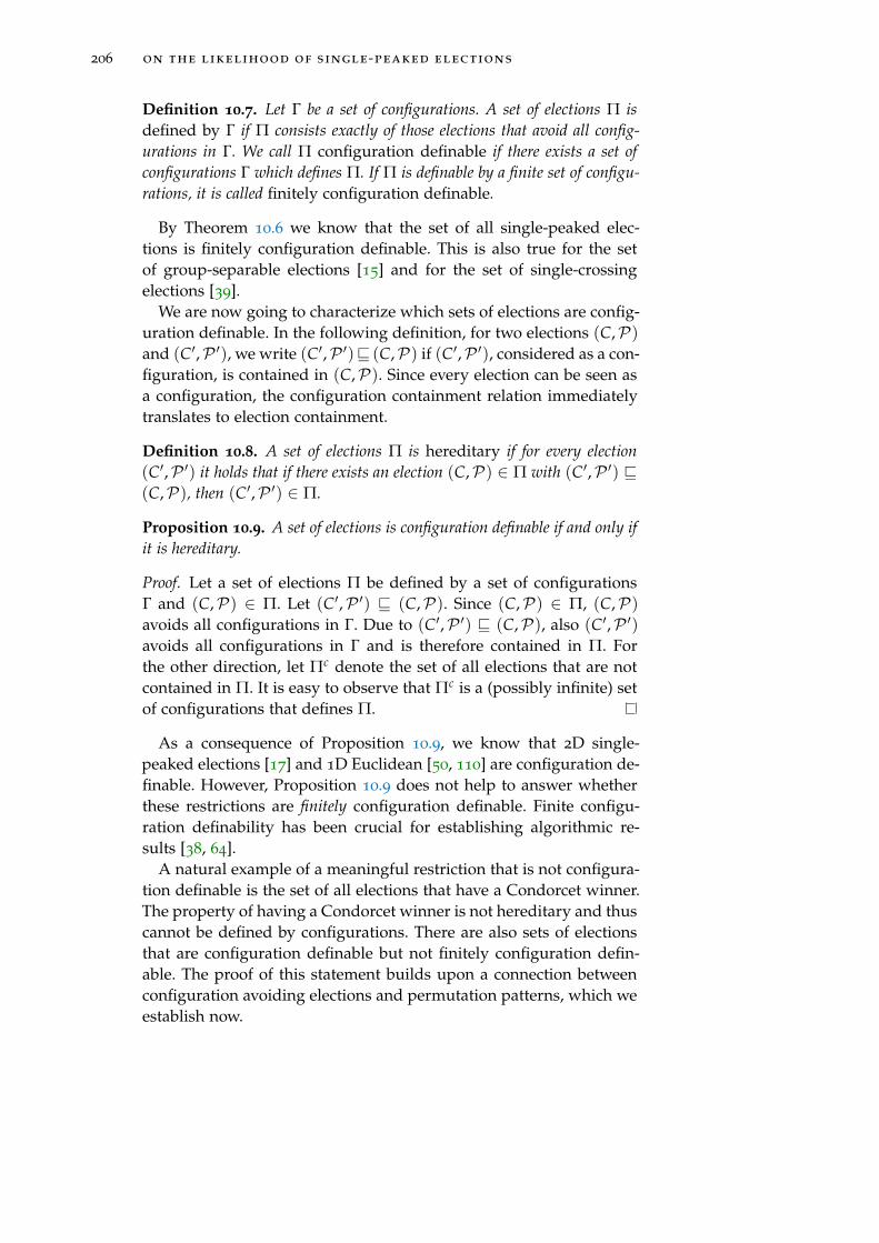
206 on the likelihood of single-peaked elections
Definition 10.7. Let Γ be a set of configurations. A set of elections Π isdefined by Γ if Π consists exactly of those elections that avoid all config-urations in Γ. We call Π configuration definable if there exists a set ofconfigurations Γ which defines Π. If Π is definable by a finite set of configu-rations, it is called finitely configuration definable.
By Theorem 10.6 we know that the set of all single-peaked elec-tions is finitely configuration definable. This is also true for the setof group-separable elections [15] and for the set of single-crossingelections [39].
We are now going to characterize which sets of elections are config-uration definable. In the following definition, for two elections (C,P)and (C′,P ′), we write (C′,P ′)v (C,P) if (C′,P ′), considered as a con-figuration, is contained in (C,P). Since every election can be seen asa configuration, the configuration containment relation immediatelytranslates to election containment.
Definition 10.8. A set of elections Π is hereditary if for every election(C′,P ′) it holds that if there exists an election (C,P) ∈ Π with (C′,P ′) v(C,P), then (C′,P ′) ∈ Π.
Proposition 10.9. A set of elections is configuration definable if and only ifit is hereditary.
Proof. Let a set of elections Π be defined by a set of configurationsΓ and (C,P) ∈ Π. Let (C′,P ′) v (C,P). Since (C,P) ∈ Π, (C,P)avoids all configurations in Γ. Due to (C′,P ′) v (C,P), also (C′,P ′)avoids all configurations in Γ and is therefore contained in Π. Forthe other direction, let Πc denote the set of all elections that are notcontained in Π. It is easy to observe that Πc is a (possibly infinite) setof configurations that defines Π.
As a consequence of Proposition 10.9, we know that 2D single-peaked elections [17] and 1D Euclidean [50, 110] are configuration de-finable. However, Proposition 10.9 does not help to answer whetherthese restrictions are finitely configuration definable. Finite configu-ration definability has been crucial for establishing algorithmic re-sults [38, 64].
A natural example of a meaningful restriction that is not configura-tion definable is the set of all elections that have a Condorcet winner.The property of having a Condorcet winner is not hereditary and thuscannot be defined by configurations. There are also sets of electionsthat are configuration definable but not finitely configuration defin-able. The proof of this statement builds upon a connection betweenconfiguration avoiding elections and permutation patterns, which weestablish now.

10.1 a general result based on permutation patterns 207
The connection to permutation patterns
In this section, we establish a strong link between the concept of con-figuration containment and the concept of pattern containment inpermutations. We are going to prove two lemmas. The first lemma(Lemma 10.10) states that every permutation pattern matching querycan naturally be translated in a configuration containment query. Thesecond lemma (Lemma 10.12) states that for (2, k)-configurations, aconfiguration containment query can naturally be translated in a per-mutation pattern query.
Lemma 10.10. Let π be a k-permutation and τ an m-permutation. Wedefine the corresponding configuration and election as follows: Let (C,P) bea (3, m)-election with C = {c1, . . . , cm}, P = (V1, V2, V3) and
V1 : c1c2 · · · cm V2 : c1c2 · · · cm V3 : cτ(1)cτ(2) · · · cτ(m).
Furthermore, let (S, T ) be a (3, k)-configuration with S = {x1, . . . , xk},T = (T1, T2, T3) and
T1 : x1x2 · · · xm T2 : x1x2 · · · xm T3 : xπ(1)xπ(2) · · · xπ(k).
Then (C,P) contains (S, T ) if and only if τ contains π.
Proof. Assume that we have a matching µ from π into τ. We have tofind an injective function f from {1, 2, 3} into {1, 2, 3} and an injectivefunction g from S into C such that, for any x, y ∈ S and i ∈ {1, 2, 3},it holds that Ti : xy implies Vf (i) : g(x)g(y). Let f be the function{1 7→ 1, 2 7→ 2, 3 7→ 3} and g = µ. It holds for xi, xj ∈ S that T1 : xi xjif and only if V1 : cµ(i) cµ(j) since µ is monotone. The same holds forT2 and V2. For T3 and V3 observe that T3 : xi xj implies V3 : cµ(i) cµ(j)since µ is a matching. Thus, the election fulfils (S, T ) v (C,P).
For the other direction, assume that (C,P) contains (S, T ). Conse-quently, there exists an injective function f from {1, 2, 3} into {1, 2, 3}and an injective function g from S into C such that, for any x, y ∈ Sand i ∈ {1, 2, 3}, it holds that Ti : xy implies Vf (i) : g(x)g(y). First,we claim that f (3) = 3. Observe that f has to map T1 and T2 toidentical total orders. Thus, unless V1 = V2 = V3, f (3) = 3. In thecase that V1 = V2 = V3, we can assume without loss of generalitythat f (3) = 3. We will construct a function µ and show that µ is amatching from π into τ. Let us define µ(i) = j if g(xi) = cj. Ob-serve that µ is strictly increasing since for i < j, V1 : cg(i) cg(j) andV1 : c1c2 · · · cm. In addition, µ(π) =
(µ(π(1)), µ(π(2)), . . . , µ(π(k))
)
is a subsequence of τ since, by definition of T3 and V3 and the factthat f (3) = 3,
(g(xπ(1)), g(xπ(2)), . . . , g(xπ(k))
)is a subsequence of(
cτ(1), cτ(2), . . . , cτ(m)
).
We can now state our first result that builds upon the connectionbetween configuration avoiding elections and permutation patterns.

208 on the likelihood of single-peaked elections
Proposition 10.11. There are sets of elections that are configuration defin-able but not finitely configuration definable.
Proof. Take an infinite set of permutations that pairwise avoid eachother [25]. Then use the construction in Lemma 10.10 to generate cor-responding configurations. There are no two configurations that pair-wise contain each other. Thus the set of elections defined by avoid-ing these configurations is not definable by a finite set of configura-tions.
Next, we will prove the second lemma, which is essential for Theo-rem 10.13. As of now, we shall denote by Sm(π1, . . . , πl) the cardinal-ity of the set of m-permutations that avoid the patterns π1, . . . , πl .
Lemma 10.12. Let (S, T ) be a (2, k)-configuration with T = (T1, T2).Furthermore, let V1 be a total order on the candidate set C = {c1, . . . , cm}.Then the number of total orders V2 such that the election (C,P) with P =
(V1, V2) avoids (S, T ) is equal to Sm(π, π−1), where π = p(C1, C2).
Proof. Let us start by proving the following statement: The configu-ration (S, T ) is contained in an election (C,P) with P = (V1, V2) ifand only if the permutation π or the permutation π−1 is contained inp(V1, V2). In order to alleviate notation, we will assume in the follow-ing that C = {1, 2, . . . m} and S = {1, 2, . . . k}.
”⇐” We can assume without loss of generality that T1 : 12 . . . k andV1 : 12 . . . m. If π is contained in p(V1, V2) as witnessed by a matchingµ, then the functions f = {1 7→ 1, 2 7→ 2} and g = µ show that(S, T ) v (C,P) (cf. Definition 10.4). If π−1 is contained in p(V1, V2)
as witnessed by a matching µ, then the functions f = {1 7→ 2, 2 7→ 1}and g = µ show that (S, T ) v (C,P).
”⇒” Let (S, T ) v (C,P). Without loss of generality we assumethat T1 : 12 . . . k. Note that renaming C does not change whether(S, T ) v (C,P). Thus, it is safe to rename the candidates accordingto the f function: If f = {1 7→ 1, 2 7→ 2}, let V1 : 12 . . . n. Sincef (1) = 1, g is monotonic. It is easy to verify that g is a matching fromπ into p(V1, V2). If f = {1 7→ 2, 2 7→ 1}, let V2 : 12 . . . n. Now, g is amatching from π into p(V2, V1) = (p(V1, V2))−1. This is equivalent tog being a matching from π−1 into p(V1, V2).
It follows that (C,P) avoids the configuration (S, T ) if and only ifthe permutation p(V1, V2) avoids both the patterns π and π−1. More-over, for the fixed total order V1 and a fixed m-permutation τ, thereis a single total order V2 such that p(V1, V2) = τ. Thus the numberof votes V2 such that p(V1, V2) avoids π and π−1 (and equivalentlythe number of votes V2 such that (C,P) avoids (S, T )) is equal toSm(π, π−1), the number of m-permutations avoiding π and π−1.
From this lemma follows the main theorem of this section that isapplicable to any set of configurations that contains at least one con-figuration of cardinality two.
10.1 a general result based on permutation patterns 209
Elections that avoid a (2, k)-configuration
With the help of Lemma 10.12, we are able to establish the followingresult.
Theorem 10.13. Let a(n, m, Γ) be the number of (n, m)-elections avoidinga set of configurations Γ. Let k ≥ 2. If a set of configurations Γ contains a(2, k)-configuration, then it holds for all n, m ∈N that
a(n, m, Γ) ≤ m! · c(n−1)mk ,
where ck is a constant depending only on k.
This result shows that forbidding any (2, k)-configuration is a verystrong restriction. Indeed, m! · c(n−1)m
k is very small compared to thetotal number of (n, m)-elections which is (m!)n. This result allows usto bound the number of single-peaked and group-separable elections.However, let us prove this result first before we explore its conse-quences.
In order to prove this result we make use of the link between con-figuration avoiding elections and pattern avoiding permutations es-tablished in Lemma 10.12 and profit from a very strong result withinthe theory of pattern avoidance in permutations, the Marcus-Tardostheorem (former Stanley-Wilf conjecture).
Proof. We will provide an upper bound on the number of (n, m)-elections avoiding a (2, k)-configuration (S, T ) with T = (T1, T2). Letus start by choosing the first vote V1 of the election at random. Forthis there are m! possibilities. When choosing the remaining (n− 1)votes V2, . . . , Vn, we have to make sure that no selection of two votescontains the forbidden configuration (S, T ). We relax this conditionand only demand that for none of the pairs (V1, Vi) with i 6= 1, theelection (C, (V1, Vi)) contains the forbidden configuration. Hereby weobtain an upper bound for a(n, m, {C}). Now Lemma 10.12 tells usthat there are – under this relaxed condition – Sm(π, π−1) choices forevery Vi where π = p(C1, C2). Thus we have the following upperbound:
a(n, m, {C}) ≤ m!Sm(π, π−1)n−1 ≤ m!Sm(π)n−1, (81)
where the second inequality follows since all permutations avoidingboth π and π−1 clearly avoid π.
Now we apply the famous Marcus-Tardos theorem [124]: For everypermutation π of length k there exists a constant ck such that forall positive integers m we have Sm(π) ≤ ck
m. Putting this togetherwith Equation (81) and noting that a(n, m, {C}) is an upper boundfor a(n, m, Γ), we obtain the desired upper bound.
210 on the likelihood of single-peaked elections
The proof of the Marcus-Tardos theorem provides an explicit expo-nential formula for the constants ck. Indeed, it holds that
Sm(π) ≤(
152k4(k2k )
)m
.
These constants are however far from being optimal and there is anongoing effort to find minimal values for ck with fixed k. In particularit has been shown that c2 = 1, c3 = 4 [140] and c4 ≤ 13.738 [28].
Let us discuss the implications of this theorem. It is applicableto all (not necessarily finite) configuration definable domain restric-tions that contain a configuration of cardinality two. In particular,we obtain the following upper bounds for single-peaked and group-separable elections.
Corollary 10.14. Let a(n, m, Γsp) denote the number of single-peaked (n, m)-elections. For n, m ≥ 2 it holds that
a(n, m, Γsp) ≤ m! · 4(m−1)(n−1).
Proof. We know from Theorem 10.3 that the single-peaked domainavoids the (2, 4)-configurations (dabc, dcba), (adbc, dcba), (dabc, cdba)and (adbc, cdba). We can use Equation (81) in the proof of Theo-rem 10.13 to bound a(n, m, Γsp).
For this, we have to compute the permutations and their inversescorresponding to the four configurations. We obtain the permuta-tions π1 = p(dabc, dcba) = 1432, π2 = p(adbc, dcba) = 4132, π3 =
p(dabc, cdba) = 2431 and π4 = p(adbc, cdba) = 4231. Their inversesare π−1
1 = π1, π−12 = π3, π−1
3 = π2 and π−14 = π4. Hence it holds that
the number of (n, m)-elections that avoid these four configurationsis bounded by m! · Sm(π1, π2, π3, π4)
n−1. As shown in Theorem 5.1,Sm(π1, π2, π3, π4) = (2m−2
m−1 ), which, in turn, is bounded by 4m−1.
In the next section, we will see that the growth rate of a(n, m, Γsp)
is indeed of the form m! · c(m−1)(n−1) for some constant c. However,the constant found in Corollary 10.14 is not optimal as we will seeby providing a better bound for the single-peaked restriction that iseven asymptotically optimal.
As another corollary of Theorem 10.13, we prove a bound on thenumber of group-separable elections. An election is group separableif for every subset of candidates C′ there exists a partition C1, C2 ofC′ such that in every vote either all candidates in C1 are preferredto all candidates in C2 or vice versa. In [15] it is shown that thegroup-separable domain is finitely configuration definable. In par-ticular, this domain avoids the configuration (abcd, bdac). Therefore,Theorem 10.13 is applicable.

10.2 counting results and the impartial culture assumption 211
Corollary 10.15. Let a(n, m, Γgs) denote the number of group-separable(n, m)-elections. For n, m ≥ 2 it holds that
a(n, m, Γgs) ≤ m! · (3 + 2√
2)m(n−1).
Proof. The proof is similar to the one of Corollary 10.14. We useEquation (81) in the proof of Theorem 10.13 to bound a(n, m, Γgs),i.e., a(n, m, Γgs) ≤ m! · Sm(π, π−1)n−1, where π = p(abcd, bdac) =
2413 and π−1 = 3142. Permutations avoiding these two patterns areknown under the name of separable permutations. It is known that sepa-rable permutations are counted by the large Schröder numbers (OEISA006318) and that Sm(π, π−1) ≤ (3 + 2
√2)m [156].
10.2 counting results and the impartial culture assump-tion
As in the previous section, let a(n, m, Γsp) denote the number of single-peaked elections. In this section, we prove a lower and upper boundon a(n, m, Γsp). These two bounds are asymptotically optimal, i.e.,the lower bound converges to the upper bound for every fixed mand n → ∞. In addition, we prove exact enumeration results fora(2, m, Γsp), a(n, 3, Γsp) and a(n, 4, Γsp).
Our results immediately imply derive bounds on the probabilitythat an (n, m)-election is single-peaked assuming that elections aredrawn uniformly at random, i.e., according to the Impartial Cultureassumption. The probability is simply a(n, m, Γsp)/(m!)n.
Theorem 10.16. It holds that
m!2· 2(m−1)·n · (1− ε(n, m)) ≤ a(n, m, Γsp) ≤
m!2· 2(m−1)·n,
where ε(n, m)→ 0 for every fixed m and n→ ∞.
Proof. First observe that an election is single-peaked with respect toan axis if and only if it is single-peaked with respect to its reverse, i.e.,the axis read from right to left. Thus the total number of axes on mcandidates that need to be considered is m!/2. Second, recall that thenumber of votes that are single-peaked with respect to a given axis is2m−1 (cf. Remark 10.2).
Now we have gathered all facts necessary for the upper bound. Forevery one of the m!/2 axes considered, select an ordered set of votesfrom the 2m−1 votes that are single-peaked with respect to this axis.There are exactly 2(m−1)·n such possibilities, which yields the upperbound. Since an election may be single-peaked with respect to morethan two axes, this number is only an upper bound for a(n, m, Γsp).
Let us turn to the lower bound. Given a vote V, there are only twoaxes with respect to which both V and its reverse V are single-peaked,
212 on the likelihood of single-peaked elections
namely the total orders V and V themselves. Thus the presence of thevotes V and V in an election forces the axis to be equal to either V orV. If we fix a vote V, the number of single-peaked elections containingboth V and V can thus be determined exactly. Multiplying this by thenumber of possible choices for V leads to:
m!2· ∑
1≤i,ji+j≤n
(ni
)·(
n− ij
)(2m−1 − 2
)n−i−j, (82)
where i denotes the number of times the vote V appears in the elec-tions and j the number of times the vote V appears. The other votesmay be any of the 2m−1 votes that are single-peaked with respect tothe axis V respectively V – except V and V themselves – and n− i− jof them must be chosen.
Setting k = i + j in equation (82) leads to:
n
∑k=2
k−1
∑i=1
(ni
)·(
n− ik− i
)(2m−1 − 2
)n−k
=n
∑k=2
(2m−1 − 2
)n−k(
nk
) k−1
∑i=1
(ki
)
=n
∑k=2
(2m−1 − 2
)n−k(
nk
)(2k − 2
)
=(
2m−1)n− 2 · n
(2m−1 − 2
)n−1−(
2m−1 − 2)n
− 2 ·((
2m−1 − 1)n− n ·
(2m−1 − 2
)n−1−(
2m−1 − 2)n)
= 2(m−1)·n +(
2m−1 − 2)n− 2 ·
(2m−1 − 1
)n
= 2(m−1)·n · (1− ε(n, m)) ,
where ε(n, m) =2 · (2m−1 − 1)n −
(2m−1 − 2
)n
2(m−1)n.
Since ε(n, m) ≤ 2 ·(
2m−1−12m−1
)n, ε(n, m) tends to 0 for every fixed m and
n→ ∞. Clearly, not all single-peaked elections contain a pair of voteswhere one is the reverse of the other. Thus this number is indeed onlya lower bound.
In the next theorem we prove exact enumeration formulæ for thenumber of (n, m)-single-peaked elections for n = 2, m = 3 and m = 4.Note that for m ≤ 2 and for n = 1 all (n, m)-elections are single-peaked. For n > 2 and for m > 4 we have not been able to find exactenumeration formulæ.
Theorem 10.17. It holds that
(i.) a(2, m, Γsp) = m! · (2m−2m−1 ) for m ≥ 1,

10.2 counting results and the impartial culture assumption 213
(ii.) a(n, 3, Γsp) = 6 · 2n−1 (2n − 1) and
(iii.) a(n, 4, Γsp) = 24 · 4n−1 ·(2n+1 − 3
).
Proof. (i.) a(2, m, Γsp) = m! · (2m−2m−1 ): This follows from Lemma 10.12.
We choose the first vote arbitrarily (m! possibilities). The second votehas to be chosen in such a way that all configurations that characterizesingle-peakedness are avoided. Since we consider only elections withtwo votes, the relevant configurations are (dabc, dcba), (adbc, dcba),(dabc, cdba) and (adbc, cdba) (Theorem 10.6). We obtain the permuta-tions π1 = p(dabc, dcba) = 1432, π2 = p(adbc, dcba) = 4132, π3 =
p(dabc, cdba) = 2431 and π4 = p(adbc, cdba) = 4231. Their inversesare π−1
1 = π1, π−12 = π3, π−1
3 = π2 and π−14 = π4. Thus, the num-
ber of a(2, m, Γsp) = Sm(π1, π2, π3, π4). As shown in Theorem 5.1,Sm(π1, π2, π3, π4) = (2m−2
m−1 ).(ii.) a(n, 3, Γsp) = m! · 2n−1 (2n − 1): We consider all elections with
three candidates. There are m! many possibilities for the first voteV1. Without loss of generality, let us consider only the vote V1 : abc.Since we have only three candidates, single-peakedness boils downto having at most two last ranked candidates (cf. Theorem 10.3). Dueto our assumption that V1 : abc, we distinguish three cases: electionsin which the votes rank either a or c last, elections in which the votesrank either b or c last and elections in which all votes rank c last.The number of elections in which the votes rank either a or c lastcan be determined as follows: every vote can either be abc, bac, cba orbca. Hence, there are 4n−1 possibilities for elections in which the votesrank either a or c last and where V1 : abc holds. By the same argument,the number of elections in which the votes rank either b or c last is4n−1 as well. The number of elections where c is always ranked lastis 2n−1. We obtain a total number of single-peaked elections with afixed first vote of 4n−1 + 4n−1− 2n−1 = 2n−1 · (2 · 2n−1− 1). Given that6 options for the first vote exist, we obtain the stated enumerationresult.
(iii.) a(n, 4, Γsp) = m! · 4n−1 ·(2n+1 − 3
): As in the previous proof,
we fix V1 : abcd. This vote V1 already rules out some possible axes.Indeed, only eight axes are single-peaked axes for V1, namely A1 :abcd, A2 : bacd, A3 : cabd, A4 : cbad, and their reverses. Since thereverse of an axis permits the same single-peaked votes, we have toconsider only A1, A2, A3, A4. For 1 ≤ i ≤ 4, let Wi denote the set offour-candidate votes that are single-peaked with respect to axis Ai.

214 on the likelihood of single-peaked elections
We count the number of single-peaked elections with four candidatesby using the inclusion-exclusion principle, i.e.,
a(n, 4, Γsp) =m! · (|W1|+ |W2|+ |W3|+ |W4|− |W1 ∩W2| − |W1 ∩W3| − |W1 ∩W4|−− |W2 ∩W3| − |W2 ∩W4| − |W3 ∩W4|+ |W1 ∩W2 ∩W3|+ |W1 ∩W2 ∩W4|+ |W2 ∩W3 ∩W4|− |W1 ∩W2 ∩W3 ∩W4|)
It is easy to verify that W1 ∩W2 = W1 ∩W4 = W2 ∩W3 = {abcd, bacd}.Consequently, all intersections of three or four sets consist also ofthese two votes. The remaining intersections look as follows:
W1 ∩W3 = {abcd, bacd, cbad, bcad},W2 ∩W4 = {abcd, bacd, cabd, acbd},W3 ∩W4 = {abcd, bacd, badc, abdc}.
The number of votes single-peaked with respect to one axis is 2m−1
(see Remark 10.2), i.e., in our case 8. We obtain
a(n, 4, Γsp) = 4! · (4 · 8n−1 − 3 · 2n−1 − 3 · 4n−1 + 4 · 2n−1 − 2n−1) =
= 24 · (4 · 8n−1 − 3 · 4n−1).
10.3 the pólya urn model
The Pólya urn model (also refereed to as the Pólya-Eggenberger urnmodel) [19, 105, 121] is an approach to sample elections with a vari-able degree of social homogeneity, i.e., where preferences are not inde-pendent but voters tend to have the same preferences as other voters.In the following the parameter a, a non-negative integer, describesthe degree of social homogeneity. As we will see in a moment, thecase a = 0 corresponds to the Impartial Culture assumption, i.e., apopulation with no homogeneity.
The setting of the Pólya urn model for an election with n votesand m candidates can be described as follows. Consider a large urncontaining m! balls. Every ball represents one of the m! possible voteson the candidate set and has a different colour. An election is thencreated by subsequently pulling n balls out of the urn according tothe following rule. The first ball is pulled at random and constitutesthe first vote of the election. Then the pulled ball is returned to theurn and a other balls of the same colour are added to the urn. Thisprocedure is repeated n times until an election consisting of n votesis created.
At a first glance, it might seem that the probability assigned to acertain election within the Pólya urn model depends on the order

10.3 the pólya urn model 215
of the votes. However this is not the case: Any election that can beobtained by rearranging a given election (C,P), i.e, by changing theorder of the votes, has exactly the same probability of occurring asthe election (C,P) itself. First, when the i-th ball is drawn from theurn, i.e., when the i-th vote is chosen, there are always m! + (i− 1) ·a balls present in the urn. Second, for any vote V the number ofballs corresponding to V, i.e., the number of favourable cases, onlydepends on how often the vote V has already been pulled out of theurn and is equal to (1 + k · a) where k is the number of times V hasalready been pulled.
It is now easy to give a concise characterization of this discretedistribution. In order to alleviate notation, let us use the so calledPochhammer k-symbol as introduced in [58].
Definition 10.18. The Pochhammer k-symbol is defined as
(x)n,k =n
∏i=1
(x + (i− 1) · k)
where in our context x ∈ R and n, k are non-negative integers. Note that(x)n,1 = x(x + 1)(x + 2) . . . (x + n− 1) is the ordinary Pochhammer sym-bol (also known as rising factorial) and (1)n,1 = n!.
We can now define the probability of a given (n, m)-election with `
distinct votes. Let ni, i ∈ [m!] be non-negative integers with ∑m!i=1 ni =
n such that, for all i ∈ [`] vote Vi appears ni times. The probability ofsuch an election is given by:
(n
n1, . . . , n`
)· ∏`
i=1(1)ni ,a
(m!)n,a=
n!
∏`i=1 ni!
· ∏`i=1(1)ni ,a
(m!)n,a. (83)
Note that setting a = 0 corresponds to the case where every oneof the n votes is drawn from exactly the same urn, namely the urncontaining every one of the m! balls exactly once. Thus, the votesare chosen independently and every vote has the same probability ofoccurring; this corresponds to the Impartial Culture assumption.
Theorem 10.19. Let pP(n, m, a) denote the probability of an (n, m)-electionbeing single-peaked if it is created according to the Pólya urn model withhomogeneity a. It holds that:
pP(n, m, a) ≥ m!(n− 1)!a(m!
a
)n,1
·[
1 +2a
(2m− 2m− 1
)Hn−1+
+na
n−1
∑l=2
(2m−1 − 2)n−l,a
an−l · Hl−1
l(n− l)!
],
where Hk denotes the k-th harmonic number ∑ki=1
1i .

216 on the likelihood of single-peaked elections
Proof. Before we start with the actual proof, let us collect a few usefulobservations. In the following we will use that
(m!)n,a = an ·n
∏i=1
(m!a
+ (i− 1))= an
(m!a
)
n,1. (84)
Moreover, we will use the following bound:
(1)k,a =k
∏i=1
(1 + (i− 1) · a) ≥k
∏i=2
(i− 1) · a = (k− 1)! · ak−1. (85)
Since it holds that
1i · (l − i)
=1l·(
l − i + ii · (l − i)
)=
1l·(
1i+
1l − i
)
the following sum can be expressed with the help of the harmonicnumbers:
l−1
∑i=1
1i · (l − i)
=1l·(
l−1
∑i=1
1i+
l−1
∑i=1
1l − i
)=
2l·
l−1
∑i=1
1i=
2l
Hl−1. (86)
The proof of the theorem is now split in three parts: First, we con-sider elections with only one distinct vote. Then, we determine alower bound on the probability of single-peaked elections that con-sist of exactly two distinct votes. Third, we give a lower bound on thenumber of single-peaked elections that contain at least three distinctvotes.
Let us now start with the first part of the lower bound. Clearly, anelection in which all votes are identical is single-peaked. Let us denotethe probability of this event by p1 – in the following we fix m, n, aan omit them in the notation. According to the discrete probabilitydistribution of the Pólya urn model (83), the probability of this eventis:
p1 = m! · (1)n,a
(m!)n,a≥ m!(n− 1)!an−1
an(m!
a
)n,1
=m!(n− 1)!a(m!
a
)n,1
,
where we used Equations (84) and (85).Next, we want to determine the probability that an election is sam-
pled that is single-peaked and consists of exactly two distinct votes.Let us denote the probability of this event by p2. From the third state-ment of Theorem 10.17 we know that there are exactly m! · (2m−2
m−1 )elections with two voters and m candidates that are single-peaked.That is, if we pick a first vote V1 at random, there are (2m−2
m−1 ) votes V2
that form a single-peaked election together with V1. We thus have thefollowing (again according to (83)):
p2 = m!(
2m− 2m− 1
)·
n−1
∑i=1
P(i votes equal to V1; n− i votes equal to V2︸ ︷︷ ︸=p′(i)
)

10.3 the pólya urn model 217
According to (83) the probability p′(i) is equal to
p′(i) =(
ni
)(1)i,a · (1)n−i,a
(m!)n,a.
Using the bound in Equation (85) and the equality in Equation (84),p′(i) can be bounded from below as follows:
p′(i) ≥(
ni
)(i− 1)! · ai−1 · (n− i− 1)! · an−i−1
(m!)n,a.
=n! · an−2
an(m!
a
)n,1 · i(n− i)
.
For p2 we thus obtain
p2 ≥ m! ·(
2m− 2m− 1
)n!
a2(m!
a
)n,1
n−1
∑i=1
1i(n− i)
=m!(n− 1)!(m!
a
)n,1
·(
2m− 2m− 1
)2a2 Hn−1,
where the transformation from the first to the second line is donewith the identity in Equation (86).
Finally, for single-peaked elections that have more than two distinctvotes, we only consider elections that contain a vote V and also itsreverse V. Let us denote the probability of this event by p3. As in theproof of the bounds under the IC assumption this idea is based onthe following fact about single-peakedness: If a vote V and its reversevote V are both present within an election, then there are at most twoaxes with respect to which this election can be single-peaked, namelythe axes V and V. Thus, if a single-peaked election contains both thevote V and V, all the other votes must be among the 2m−1 − 2 votesthat are also single-peaked with respect to the axis V (respectively V).Let us denote this set of votes that are not equal to V or V and thatare single-peaked with respect to the axis V by SV .
The probability p3 is then given as follows:
p3 =m!2
n−1
∑l=2
l−1
∑i=1
P(i votes equal to V, l − i votes equal to V, rest in SV)
=m!2
n−1
∑l=2
l−1
∑i=1
(ni
)(n− il − i
)(1)i,a · (1)l−i,a · (2m−1 − 2)n−l,a
(m!)n,a,
where m!/2 stands for the number of possible choices for the vote V,i is the number of times the vote V appears and l − i is the numberof times the vote V appears.
By using the bound in Equation (85) as well as the identity in Equa-tion (86), we obtain the following:

218 on the likelihood of single-peaked elections
p3 ≥m!
2(m!)n,a
n−1
∑l=2
(2m−1 − 2)n−l,a
l−1
∑i=1
(ni
)(n− il − i
)(i− 1)!(l − i− 1)!al−2
=m!
2(m!)n,a
n−1
∑l=2
(2m−1 − 2)n−l,a · al−2l−1
∑i=1
n!(n− i)!(i− 1)!(l − i− 1)!i!(n− i)!(l − i)!(n− l)!
=m!n!
2(m!)n,a
n−1
∑l=2
(2m−1 − 2)n−l,a ·al−2
(n− l)!
l−1
∑i=1
1i(l − i)
=m!n!(m!a
)n,1
n−1
∑l=2
(2m−1 − 2)n−l,a
an+2−l · 1l(n− l)!
Hl−1.
Since p1 + p2 + p3 ≤ pP(n, m, a), we obtain the desired lower bound.
Corollary 10.20. If a = m! we have:
pP(n, m, a) ≥ 1n·(
1 + 2ln(n− 1)
m!· (2m− 2)!((m− 1)!)2
).
10.4 mallows model
The Mallows model [123] assumes that there is a reference vote andvotes are more likely to appear in an election if they are close tothis reference vote. Closeness is measured by the Kendall tau rankdistance, defined as follows.
Definition 10.21. Given two votes V and W contained in an election(C,P), the Kendall tau rank distance κ(V, W) is a metric that countsthe number of pairwise disagreements between V and W. To be more precise:
κ(V, W) = |{{c, c′} ⊆ C : (V : cc′ ∧W : c′c) ∨ (V : c′c ∧W : cc′)}|.
Note that κ(V, W) is also the minimum number of transpositions,i.e., swaps, of adjacent elements, needed to transform V into W orvice versa. We can now define the Mallows model.
Definition 10.22. Let C be a set of candidates with |C| = m and let T(C)be the set of all total orders on C. Given a reference vote V and a real num-ber φ ∈ (0, 1], the so-called dispersion parameter, the Mallows model isdefined as follows. Every vote W of an (n, m)-election is determined indepen-dently from the others according to the following probability distribution:
PV,φ(W) =1Z· φκ(V,W), (87)
where the normalization constant Z = ∑W∈T(C) φκ(V,W) fulfils Z = 1 · (1+φ) · (1 + φ + φ2) · · · (1 + . . . + φm−1).

10.4 mallows model 219
axis Ac7 c5 c3 c1 c2 c4 c6
?
?
?
?
?
?
?
Figure 50: The axis A and the reference vote V : c1c2c3c4c5c6c7, shown as asolid line. The dashed line represents the vote W : c1c4c2c3c6c7and is not single-peaked with respect to A. The Kendall tau dis-tance of V and W is 2. Note that all votes with a Kendall taudistance to V of 1 are single-peaked with respect to A.
Note that choosing φ = 1 corresponds the Impartial Culture as-sumption and as φ → ∞ one obtains a distribution that concentratesall mass on V.
Theorem 10.23. Let pM(n, m, φ) denote the probability of an (n, m)-electionbeing single-peaked if it is created according to the Mallows model with dis-persion parameter φ. Then the following lower bound holds:
pM(n, m, φ) ≥(
1 + φ · (m− 1) + φ2 · (m− 2)(m− 3)/2Z
)n
.
Proof. Without loss of generality, we can assume that the referencevote is V : c1c2 . . . cm. We define a total order A which will serve asaxis as follows: A : . . . c6c4c2c1c3c5 . . .. Clearly, V is single-peaked withrespect to A and it will turn out that “many” other votes that are closeto V with respect to the Kendall tau distance are also single-peakedwith respect to this axis. See Figure 50 for a representation of the axisA and the reference vote V for the case of seven candidates. In thefollowing, we will write “W is SP” as a shortform of “the total orderW on C is single-peaked with respect to axis A”.
The idea of this proof is to bound the probability pM(n, m, φ) frombelow as follows:
pM(n, m, φ) ≥(PV,φ(W : W is SP )
)n .
Moreover, we use the following bound:
PV,φ(W : W is SP) ≥ PV,φ(V) + ∑W is SP andκ(V,W)=1
PV,φ(W) + ∑W is SP andκ(V,W)=2
PV,φ(W)
First, it is clear that P(V) = 1/Z.

220 on the likelihood of single-peaked elections
Second, we need to compute the number of votes W that are single-peaked with respect to A and that fulfil κ(V, W) = 1. Votes W withκ(V, W) = 1 are votes in which the order of exactly one pair of can-didates (ci, ci+1) has been changed in V. Since there are (m− 1) pairsof adjacent candidates in V, there are exactly (m− 1) votes W withκ(V, W) = 1. All these votes are single-peaked with respect to theaxis A since:
• If c1 and c2 are interchanged, the position of the peak on theaxis A is changed, but clearly no new peaks arise.
• If two other candidates ci and ci+1 are interchanged, one of thesetwo candidates lies to the left of the peak on A and the otherone to the right of the peak. Thus, interchanging only these twocandidates does not create a new peak either.
Therefore we have the following:
∑W is SP andκ(V,W)=1
PV,φ(W) = (m− 1) · φ
Z.
Third, we need to compute the number of votes W that are single-peaked with respect to A and that fulfil κ(V, W) = 2. Here we have adifferent situation: Not all votes that can be obtained by exactly twoswaps of adjacent candidates in V are single-peaked with respect toA. For instance, first swapping the candidates (c3, c4) and then swap-ping (c2, c4) in V, does not lead to a vote that is single-peaked withrespect to A. For this example, see the vote shown as a dashed linein Figure 50. The problem here is that the swapping of these twopairs changes the order of c2 and c4, two elements that both lie on thesame side of the peak on A, and thus a valley is created by the ele-ments c1, c2 and c4. In general, a pair of swaps (ci, ci+1) and (cj, cj+1)
is always allowed if the two pairs of candidates do not have any ele-ments in common. Note that the order of the two (disjoint) swaps isof no importance and without loss of generality we can assume thati + 1 < j.
Knowing this, we can bound the number of votes W with κ(V, W) =
2 that are single-peaked with respect to A as follows: If the first swapis (ci, ci+1) for some i ∈ [1, m− 3] and the second swap (cj, cj+1) is dis-joint from the first one, j has to fulfil j ∈ [i + 2, m− 1] and thus thereare (m− i− 2) possibilities for (cj, cj+1). Summing over all possible iwe obtain that there are at least
m−3
∑i=1
m− i− 2 =(m− 2)(m− 3)
2
many votes W with κ(V, W) = 2 that are single-peaked with respectto A. Thus we have
∑W is SP andκ(V,W)=2
PV,φ(W) ≥ φ2
Z· (m− 2)(m− 3)
2.
10.5 numerical evaluations 221
Putting the results for Kendall tau distance equal to 0, 1 and 2
together we obtain the desired lower bound.
Corollary 10.24. Assuming φ = 1m , it holds that
pM(n, m, φ) ≥1.5
(1− 1
m
1−( 1
m
)m
)m−1
n
>
(1− 1
m
)(m−1)n
.
Proof. Inserting φ = 1m in the lower bound of Theorem 10.23 yields
pM(n, m, φ) ≥(
1 + m−1m + (m−2)(m−3)
2m2(1 + 1
m
)·(1 + 1
m + 1m2
)· · ·(1 + 1
m + · · ·+ 1mm−1
))n
.
As can be checked easily, the numerator is larger than 1.5. Moreoverthe finite geometric sums in the denominator are all bounded fromabove by
1−( 1
m
)m
1− 1m
.
We thus obtain
pM(n, m, φ) ≥1.5
(1− 1
m
1−( 1
m
)m
)m−1
n
.
Replacing the numerator by 1 and every one of the finite geometricsums in the denominator by an infinite geometric row leads the sec-ond, much rougher lower bound. Note that this is simply a bound onthe probability of sampling an (n, m)-election in which all votes areequal to the reference vote.
Comparing this bound with the asymptotic tight bound for theprobability of an (n, m)-election being single peaked under the ICassumption that is given in Theorem 10.16 and is of the form
m!2·(
2m−1
m!
)n
,
we see that the likelihood of single-peakedness is far larger in theMallows model with dispersion parameter φ = 1
m .
10.5 numerical evaluations
In this section we provide numerical evaluations of our probabilityresults from the previous sections. In Table 51, we list exact probabil-ities that an (n, m)-election is single-peaked assuming the ImpartialCulture assumptions for small values of m and bounds for these prob-abilities for a larger number of candidates. These probabilities illus-trate how unlikely it is that an election drawn uniformly at random

222 on the likelihood of single-peaked elections
(n, m) exactprobability
(2, 3) 1
(5, 3) 0.38
(10, 3) 0.05
(25, 3) 1.19 · 10−4
(50, 3) 4.70 · 10−9
(2, 4) 0.83
(5, 4) 0.05
(10, 4) 2.03 · 10−4
(25, 4) 1.42 · 10−11
(50, 4) 1.67 · 10−23
(n, m) lowerbound
upperbound
(2, 5) 0.58 (via Thm 10.17)
(5, 5) 1.6 · 10−4 2.6 · 10−3
(10, 5) 2.2 · 10−8 1.1 · 10−7
(25, 5) 5.0 · 10−21 8.0 · 10−21
(50, 5) 9.7 · 10−43 1.1 · 10−42
(2, 10) 1.3 · 10−2 (via Thm 10.17)
(5, 10) 7.6 · 10−18 1.1 · 10−13
(10, 10) 1.9 · 10−36 5.7 · 10−33
(25, 10) 2.3 · 10−93 1.0 · 10−90
(50, 10) 4.6 · 10−189 5.5 · 10−187
Figure 51: The likelihood that an (n, m)-election is single-peaked whendrawn uniformly at random (Impartial Culture assumption). Theprobabilities in the left table are obtained via Theorem 10.17;those in the right table are obtained via Theorem 10.16 (exceptfor n = 2).
(n, m) a = 10 a = m!/2 a = m!
(10, 5) 1.6 · 10−4 0.13 0.43
(25, 5) 8.4 · 10−8 3.0 · 10−2 0.21
(50, 5) 1.5 · 10−10 9.1 · 10−3 0.12
(10, 10) 3.6 · 10−36 2.0 · 10−2 0.10
(25, 10) 2.3 · 10−91 3.6 · 10−3 4.4 · 10−2
(50, 10) 2.6 · 10−181 9.7 · 10−4 2.2 · 10−2
Figure 52: Lower bounds obtained from Theorem 10.19 on the likelihoodthat an (n, m)-election is single-peaked when sampled accordingto the Pólya urn model with homogeneity a
(n, m) φ = 0.2 φ = 0.1 φ = 0.05 φ = 0.01
(10, 5) 0.15 0.59 0.86 0.99
(25, 5) 8.7 · 10−3 0.26 0.70 0.98
(50, 5) 7.6 · 10−5 7.2 · 10−2 0.49 0.97
(10, 10) 2.7 · 10−3 0.20 0.66 0.98
(25, 10) 3.7 · 10−7 1.9 · 10−2 0.36 0.96
(50, 10) 1.4 · 10−13 3.7 · 10−4 0.13 0.92
Figure 53: Lower bounds via Theorem 10.23 on the likelihood that an (n, m)-election is single-peaked when sampled according to the Mallowsmodel with dispersion parameter φ

10.6 summary of the results 223
is single-peaked – even for small n and m. The probability that an(n, m)-election is single-peaked is considerably higher if we assumethat votes are drawn subject to the Pólya urn and Mallows models.Table 52 shows lower bounds for the Pólya urn model and Table 53
shows lower bounds for the Mallows model. Note that Table 53 alsoincludes results for φ = 1
m : for m = 5 these can be found in the col-umn φ = 0.2 and for m = 10 in the column φ = 0.1. Our resultsindicate that the Mallows model with small φ is a very restrictiveprobability distribution, since it generates single-peaked preferenceswith rather high probability.
10.6 summary of the results
In this chapter we performed the first combinatorial study of the like-lihood of single-peakedness in random elections. Our main resultsare the following:
• Configuration definable restrictions: Many domain restrictions canbe characterized by forbidden configurations, in particular thesingle-peaked domain. We proved a close connection betweenconfigurations and permutations patterns. This novel connec-tion allowed us to obtain a very general result (Theorem 10.13),showing that many domain restrictions characterized by forbid-den configurations are very unlikely to appear in a random elec-tion chosen according to the Impartial Culture assumption.
• Counting single-peaked elections: We performed a detailed com-binatorial analysis of the single-peaked domain by countingthe number of single-peaked elections. We established an upperbound for single-peaked elections which asymptotically matchesour lower bound result (Theorem 10.16). In addition, we showedexact enumeration results for elections with two voters or up tofour candidates (Theorem 10.17). Our results rigorously showthat the single-peaked restriction is highly unlikely to appear inrandom elections chosen according to the IC assumption. Thisholds even for elections with few votes and candidates (cf. Sec-tion 10.5).
• Pólya urn model: In contrast to the IC assumption, single-peakedelections are considerably more likely if elections are chosen ac-cording to the Pólya urn model. We provided a lower bound onthe corresponding likelihood (Theorem 10.19) and showed that,if a sufficiently strong homogeneity is assumed, the probabilityof an election with n votes being single-peaked is larger than1/n (Corollary 10.20).
• Mallows model: We encountered the most likely occurrence ofsingle-peaked elections under Mallows model. As for the Pólya

224 on the likelihood of single-peaked elections
urn model we established a lower bound result on the likeli-hood (Theorem 10.23). If the dispersion parameter φ is suffi-ciently small, we were able to show that single-peaked electionsare likely to appear (Corollary 10.24 and Table 53).
11F U RT H E R R E S E A R C H
Let us conclude this thesis by pointing out some directions for fur-ther research. These suggestions are based on the Future research-sections in the respective publications, see page xi.
efficient permutation pattern matching
In Chapter 3 we performed a parameterized complexity analysis ofthe PPM problem and constructed an fpt-algorithm for the parame-ter run(τ), the number of alternating runs in the text permutation τ
(Theorem 3.1). This fpt-algorithm performs particularly well for PPMinstances with few alternating runs.
An immediate consequence of this theorem is that any PPM in-stance can be reduced by polynomial time preprocessing to an equiv-alent instance – a kernel – of size depending solely on run(τ). Thisraises the question whether even a polynomial-sized kernel exists.Such kernels, and in particular polynomial kernels, have been thefocus of intensive research in algorithmics [95]. In [24], it has beenshown that no such polynomial-sized kernel exists for the parameterk = |π|. Thus a positive result for the parameter run(τ) would be ofgreat interest.
Another research direction is the study of further parameters suchas the permutation statistics listed in the Appendix A of [108].
At this point, several algorithms exist that solve PPM without im-posing restrictions on π and τ. The algorithms by Guillemot andMarx [93], Albert et al. [3] and Ahal and Rabinovich [1] seem to beparticularly well-suited for small patterns. In contrast, the runtimeof our algorithm does not depend that critically on |π|. Thus, it maybe expected that our algorithm is preferable for large patterns. How-ever, only implementations and benchmarks could allow to settle thisquestion and compare these algorithms.
generalized permutation pattern matching
In Chapter 4 we analysed the PPM problem for several different typesof permutation patterns. We strengthened the previously known NP-hardness result for PPM and proved NP-completeness for its gener-alizations. We also provided simple polynomial time algorithms forboxed mesh and consecutive PPM. Furthermore, we performed a pa-rameterized complexity analysis, which shows that for vincular, bivin-cular and mesh PPM a fixed-parameter tractable algorithm is unlikelyto exist.
225

226 further research
In Section 4.2 we have listed several special cases for which PPM isin P. This list, however, is certainly far from being complete. In par-ticular, polynomial time fragments of vincular, bivincular and meshpermutation pattern matching are not known at all.
In Section 4.3 we studied the influence of the length of the patternon the complexity of the different types of Permutation Pattern
Matching problems. For the cases where W[1]-hardness was shownas well as for PPM which is solvable by an FPT algorithm, it is ofinterest to find out whether other parameters of the input instanceslead to fixed parameter tractability results. For future work any per-mutation statistic could be taken into account for a parameterizedcomplexity analysis of all versions of PPM. An analysis of PPM withrespect to several different parameters would then allow to draw amore detailed picture of the computational landscape of permutationpattern matching.
Another type of patterns was introduced by West [155]: barred pat-terns. A barred pattern π is a permutation where some letters arebarred. One denotes by π the underlying permutation without anybars and by π′ the permutation obtained by removing all barred let-ters. A permutation τ then avoids the barred pattern π if every oc-currence of π′ in τ is part of an occurrence of π in τ. For details andresults on barred patterns, see Chapter 7 in [108]. Brändén and Claes-son [36] showed that mesh patterns can easily be used to write anybarred pattern with only one barred letter.
There exist further generalizations of mesh patterns: marked meshand decorated patterns. These two types of patterns were introducedby Úlfarsson in [151] and [152], respectively. They allow a finer con-trol over whether certain regions in a permutation may contain ele-ments. Mesh patterns permit to specify regions in a permutation thatmay not contain elements in a matching. Marked mesh patterns allowmore, namely to specify how many elements may be contained in cer-tain regions (exactly, at most or at least). Decorated patterns go evenfurther: they allow to detail in which order these elements may lie bydescribing forbidden patterns. These forbidden patterns may againbe decorated patterns. Since both marked mesh and decorated pat-terns are generalizations of mesh patterns, the W[1]-hardness resultgiven in Theorem 4.17 can be extended to these two types of patterns.
We considered patterns in permutations. However, the concept ofpattern avoidance respectively containment can easily be extended topatterns in words over ordered alphabets (or permutations on multi-sets). In a matching of a word W into another word V, copies of thesame letter have to be mapped to copies of some letter in the text. Thetopic of patterns in words has received quite some attention in thelast years, see e.g. Heubach and Mansour’s monograph Combinatoricsof compositions and words [96]. The corresponding pattern matchingproblems have not yet been studied.

further research 227
a permutation class enumerated by the central bino-mial coefficients
Chapter 5 was devoted to the study of a special permutation class,namely the class of permutations avoiding the patterns 2431, 4231,1432 and 4132 simultaneously. We could show that this class is enu-merated by the central binomial coefficients.
The proof presented in Chapter 5 first constructs a bijection to acertain set of words and then counts these words by establishing acorrespondence of certain segments of these words to lattice paths.However, it remains open to construct a direct bijection to some com-binatorial object that is also counted by the central binomial coef-ficients. For instance, it would be nice to have a direct bijection togranny walks which are direct routes from the pint (0, 0) to the point(n, n) in an integer grid.
The permutation class studied in this chapter is not the only oneknown to be enumerated by the central binomial coefficients. Indeed,in [5] the authors describe a general scheme to enumerate permuta-tion classes. As an example, they give the permutation class avoidingthe patterns 3124, 4123, 3142 and 4132 that is also enumerated by thecentral binomial coefficients.
Preliminary studies show that there are in total nine permutationclasses that are defined by four forbidden patterns of length four andthat are enumerated by the central binomial coefficients. It would bedesirable to develop a general framework that can be used to provethat all these classes are indeed counted by the central binomial coef-ficients and that no other such classes exist.
log-concavity, longest increasing subsequences and in-volutions
Chapter 6 was devoted to the sequence `n,k counting permutations oflength n and with a longest increasing subsequence of length k. Weconjectured that this sequence is log-concave for every fixed n andcharacterized several sets of permutations for which our conjectureholds. One main tool was to first prove our results for involutionsand then to transfer them to arbitrary permutations. A next step inthis line of research and towards proving our conjecture in generalwould be to find larger sets of permutations for which this methodcan be applied. Also, it would be interesting to find applications ofthis technique to other permutation statistics than the length of thelongest increasing subsequence.

228 further research
ascending runs in mappings
In Chapter 8 we generalized the patterns “ascents” and “ascendingruns” from permutations to Cayley trees and to mappings. We pro-vided exact enumeration formulæ that are linked to the Stirling num-bers of the second kind and showed that the random variables count-ing ascents and ascending runs in random mappings is asymptoti-cally normal distributed.
The combinatorial decomposition of Cayley trees and mappingsemployed there can also be used to study other label patterns. Indeed,our method can also be applied to count the number of local minimaor maxima, thus generalizing the notion of valleys and peaks in per-mutations. However, the results contained in Okoth’s thesis [129] aremore general and thus the study of local minima and maxima was notincluded in Chapter 8. Moreover, preliminary studies show that ourmethod can also be applied to what we call up-ups. For an n-mappingf , these are elements i in [n] for which it holds that i < f (i) < f 2(i).The notion of up-ups thus generalizes consecutive 123-patterns in per-mutations. Permutations avoiding this pattern have been studied in[62].
All label patterns mentioned so far were consecutive patterns, i.e.,they concerned the images or preimages of nodes in the mappingsgraph. A probably more involved task would be to study non-conse-cutive label patterns in mappings. For instance, the non-consecutivepattern 21 corresponds to an inversion in the mapping. Of course,one could also study longer non-consecutive patterns in mappings orCayley trees.
parking in trees and mappings
In Chapter 9 we generalized the concept of parking functions to Cay-ley trees and mappings. As this is the first study of such parkingfunctions, several possible directions for further research arise:
Given a tree T or a mapping f , we obtained general, but sim-ple bounds for the number of tree and mapping parking functionsS(T, m) and S( f , m). It is possible to obtain explicit formula for somesimple classes of trees (or mappings), e.g., for “chain-like” trees withonly few branchings. However, the following question remains open:Is it possible in general to give some “simple characterization” of thenumbers S(T, m) and S( f , m)?
With the approach presented, one can also study the total numberof parking functions for other important tree families such as labelledbinary trees or labelled ordered trees. We already performed somepreliminary work for these tree families and according to our consid-erations, the results are considerably more involved than for labelledunordered trees and mappings. However, they do not seem to lead to
further research 229
new phase change phenomena. Thus we did not comment on thesestudies here.
In contrast to the previous comment, the problem of determiningthe total number of parking functions seems to be interesting for so-called increasing (or decreasing) tree families (see, e.g., [60, 131]). Thatis, the labels along all leaf-to-root-paths form an increasing (or, de-creasing) sequence. For so-called recursive trees (see, e.g., [83, 144]),i.e., unordered increasing trees, the approach presented could be ap-plied, but the differential equations occurring do not seem to yield“tractable” solutions. For such tree families quantities such as the“sums of parking functions” as studied in [115] could be worthwhiletreating as well.
As for ordinary parking functions one could analyse importantquantities for tree and mapping parking functions. E.g., the so-called“total displacement” (which is of particular interest in problems re-lated to hashing algorithms, see [77, 102]), i.e., the total driving dis-tance of the drivers, or “individual displacements” (the driving dis-tance of the k-th driver, see [103, 153]) seem to lead to interestingquestions.
A refinement of parking functions can be obtained by studyingwhat has been called “defective parking functions” in [45], or “over-flow” in [92], i.e., pairs (T, s) or ( f , s), such that exactly k driversare unsuccessful. Preliminary studies indicate that the approach pre-sented is suitable to obtain results in this direction as well.
Again, as for ordinary parking functions, one could consider enu-meration problems for some restricted parking functions for trees (ormappings). E.g., we call (T, s), with T a size-n tree and s ∈ [n]n aparking function for T, an ordered tree parking function, if π−1(v) <π−1(w), whenever v ≺ w (i.e., if the k-th driver parks at parking spacew, all predecessors of w are already occupied by earlier drivers). Thenit is easy to show that for any size-n tree T there are exactly n! orderedtree parking functions.
Let us denote by Xn the random variable measuring the numberof parking functions s with n drivers for a randomly chosen labelledunordered tree T of size n. Then, due to our previous results, we getthe expected value of Xn via
E(Xn) =Fn
Tn∼√
2√
π2n+1nn− 12
en .
However, with the approach presented here, it seems that we are notable to obtain higher moments or other results on the distribution ofXn.
The rather simple exact enumeration formulæ for perking func-tions for Cayley trees, connected mappings or arbitrary mappingsfor the case that the number of drivers coincides with the numberof parking spaces also allow for other combinatorial interpretations.
230 further research
For instance, recall that the number of such parking functions forconnected mappings was given by (Lemma 9.11):
Cn = n!(n− 1)!n−1
∑j=0
(2n)j
j!.
Compare this with the number of connected mappings Cn that can bederived easily using the symbolic method and Lagrange inversion:
Cn = (n− 1)! ·n−1
∑k=0
nk
k!.
In this formula, k corresponds to the number of elements not ly-ing on the cycle. Thus Cn/n! can also be interpreted as the num-ber of connected n-mappings in which the non-cyclic elements arecoloured either blue or red. It would thus be interesting to find a bi-jection between parking functions for connected mappings and pairs(π, C) where π is a permutation of length n and C is connected map-ping with coloured non-cyclic elements. Similar interpretations canbe given for the numbers Fn of tree-parking functions and Mn ofmappings parking functions and could also allow for bijective cor-respondences.
As mentioned in the Introduction of this thesis on page 10, ordi-nary parking functions can bijectively be identified with allowableinput-output pairs of priority queues. It would be interesting to finda generalization of this result to parking functions for trees and map-pings, thus providing an interpretation of these in terms of forbiddenpatterns. Such a generalization might be possible by replacing the nat-ural order on the numbers 1, . . . , n by the order induced by the treeor mapping.
on the likelihood of single-peaked elections
In Chapter 10 we studied the likelihood of single-peakedness in ran-dom elections. This was the first combinatorial study of single-peakedelections and we see various directions for future research.
Theorem 10.13 requires that the domain restriction avoids a (2, k)-configuration and thus is not applicable to domain restrictions suchas the single-crossing restriction [39, 136]. It remains open whetherthis result can be extended to such domain restrictions as well andhow the corresponding bound would look like. It would also be in-teresting to complement Theorem 10.13 with a corresponding lowerbound result.
In general, the likelihood of other domain restrictions such as thesingle-crossing [136] or the 2D single-peaked restriction [17] has yetto be studied.
In Section 10.2 we obtained counting results for the number ofsingle-peaked elections. In particular, it follows from Theorem 10.17

further research 231
that under the IC assumption the likelihood that an (n, 3)-electionis single-peaked is (2n−1 − 1)/3n−1. The likelihood that such an elec-tion has a Condorcet winner is 15(n + 3)2/[16(n + 2)(n + 4)] [85].Note that the former probability is significantly smaller than the lat-ter and, in particular, the former converges to 0 whereas the latterconverges to 15/16 for n→ ∞. Recently, the top monotonicity restric-tion has been proposed [18] which is a generalization of the single-peaked and single-crossing domain but still guarantees a Condorcetwinner. It would be highly interesting to know the likelihood of topmonotonicity restricted preferences and whether this probability isnon-zero for n→ ∞.
Another direction is to consider other probability distributions suchas the Plackett-Luce model [119, 134] or Mallows mixture modelswhere more than one reference vote is considered [126]. One couldalso analyse the probability distribution that arises when assumingthat all elections are single-peaked and that all elections of the samesize are equally likely. This would allow to ask questions such as“How likely is it that a single-peaked election is also single-crossing?”.Finally, a recent research direction is to consider elections that arenearly single-peaked, i.e., elections that have a small distance to be-ing single-peaked according to some notion of distance [38, 52, 63, 65,70]. The likelihood that elections are nearly single-peaked remains aworthwhile direction for future research.


N O TAT I O N
[n] the set of integers {1, . . . , n}
[m, n] for m ≤ n, the interval of integers {m, m + 1, . . . , n}
n! factorial of a nonnegative integer n
0! = 1, n! = n · (n− 1)! = n(n− 1) · 1
Γ(z) Gamma function: Γ(z) =∫ ∞
o tz−1e−tdt
Γ(n) = (n− 1) for a nonnegative integer n
αk falling factorial of α for a real α and a nonnegative k:
α0 = 1, αk = α · (α− 1)k−1 = α(α− 1) · (α− k + 1)
(x)n,k Pochhammer k-symbol: (x)n,k = ∏ni=1(x + (i− 1) · k)
where x ∈ R and n, k ∈N(α
k
)binomial coefficient for real α and nonnegative k:(
α
k
)=
αk
k!, for n ∈N :
(nk
)=
n!(n− k)!k!{
nm
}Stirling numbers of the second kind
E(X) expected value of X
V(X) variance of X
π, σ, τ permutations
|T| size of the combinatorial object T
iff if and only if
w.r.t with respect to
� end of proof
a end of example
233


B I B L I O G R A P H Y
[1] S. Ahal and Y. Rabinovich. On complexity of the subpatternproblem. SIAM Journal on Discrete Mathematics, 22(2):629–649,2008.
[2] M. Aigner and G. M. Ziegler. Proofs from the Book. Springer,2014.
[3] M. Albert, R. Aldred, M. Atkinson, and D. Holton. Algorithmsfor pattern involvement in permutations. In P. Eades andT. Takaoka, editors, Algorithms and Computation, volume 2223 ofLecture Notes in Computer Science, pages 355–367. Springer, 2001.
[4] M. H. Albert, R. E. L. Aldred, M. D. Atkinson, H. P. van Dit-marsch, B. D. Handley, C. C. Handley, and J. Opatrny. Longestsubsequences in permutations. Australasian Journal of Combina-torics, 28:225–238, 2003.
[5] M. H. Albert, S. Linton, and N. Ruškuc. The insertion encodingof permutations. The Electronic Journal of Combinatorics, 12(1):31,2005.
[6] D. Aldous and P. Diaconis. Longest increasing subsequences:from patience sorting to the Baik-Deift-Johansson theorem. Bull.Amer. Math. Soc. (N.S.), 36(4):413–432, 1999.
[7] D. André. Étude sur les maxima, minima et séquences despermutations. Annales scientifiques de l’École normale supérieure,3(1):121–135, 1884.
[8] J. Arney and E. Bender. Random mappings with constraints oncoalescence and number of origins. Pacific Journal of Mathemat-ics, 103(2):269–294, 1982.
[9] S. Arora and B. Barak. Computational complexity: a modern ap-proach. Cambridge University Press, 2009.
[10] K. J. Arrow. A difficulty in the concept of social welfare. TheJournal of Political Economy, 58(4):328–346, 1950.
[11] M. D. Atkinson. Permutations which are the union of an in-creasing and a decreasing subsequence. The Electronic Journal ofCombinatorics, 5:87–100, 1998.
[12] S. Avgustinovich, S. Kitaev, and A. Valyuzhenich. Avoidance ofboxed mesh patterns on permutations. Discrete Applied Mathe-matics, 161(1-2):43–51, 2013.
235
236 bibliography
[13] E. Babson and E. Steingrímsson. Generalized permutation pat-terns and a classification of the mahonian statistics. SéminaireLotharingien de Combinatoire, 44:117, 2000.
[14] J. Baik, P. Deift, and K. Johansson. On the distribution of thelength of the longest increasing subsequence of random permu-tations. J. Amer. Math. Soc., 12(4):1119 – 1178, 1999.
[15] M. A. Ballester and G. Haeringer. A characterization of thesingle-peaked domain. Social Choice and Welfare, 36(2):305–322,2011.
[16] C. Banderier, P. Flajolet, G. Schaeffer, and M. Soria. Randommaps, coalescing saddles, singularity analysis, and Airy phe-nomena. Random Structures & Algorithms, 19:194–246, 2001.
[17] S. Barberà, F. Gul, and E. Stacchetti. Generalized median voterschemes and committees. Journal of Economic Theory, 61(2):262–289, 1993.
[18] S. Barberà and B. Moreno. Top monotonicity: A common rootfor single peakedness, single crossing and the median voter re-sult. Games and Economic Behavior, 73(2):345–359, Nov. 2011.
[19] S. Berg. Paradox of voting under an urn model: The effect ofhomogeneity. Public Choice, 47(2):377–387, 1985.
[20] N. Betzler, A. Slinko, and J. Uhlmann. On the computation offully proportional representation. Journal of Artificial IntelligenceResearch (JAIR), 47:475–519, 2013.
[21] P. Billingsley. Probability and Measure. John Wiley & Sons, sec-ond edition edition, 1984.
[22] D. Black. On the rationale of group decision making. Journal ofPolitical Economy, 56(1):23–34, 1948.
[23] I. F. Blake and A. G. Konheim. Big buckets are (are not) better!Journal of the Association for Computing Machinery, 24:591–606,1977.
[24] I. Bliznets, M. Cygan, P. Komosa, and L. Mach. Kernelizationlower bound for permutation pattern matching. Information Pro-cessing Letters, 2015.
[25] M. Bóna. Combinatorics of permutations. Discrete Mathematicsand Its Applications. Chapman & Hall/CRC, 2004.
[26] M. Bóna. A combinatorial proof of the log-concavity of a fa-mous sequence counting permutations. The Electronic Journal ofCombinatorics, 11, 2005.

bibliography 237
[27] M. Bóna. A walk through combinatorics: an introduction to enumer-ation and graph theory. World Scientific, 2011.
[28] M. Bóna. A new record for 1324-avoiding permutations. Euro-pean Journal of Mathematics, pages 1–9, 2014.
[29] M. Bóna, editor. Handbook of Enumerative Combinatorics. CRCPress – Chapman Hall, 2015.
[30] M. Bóna and M.-L. Bruner. Log-concavity, the Ulam distanceand involutions. arXiv preprint, arXiv:1502.05438, 2015.
[31] P. Bose, J. F. Buss, and A. Lubiw. Pattern matching for permu-tations. Information Processing Letters, 65(5):277 – 283, 1998.
[32] M. Bousquet-Mélou. Four classes of pattern-avoiding permu-tations under one roof: Generating trees with two labels. TheElectronic Journal of Combinatorics, 9(2), 2003.
[33] M. Bousquet-Mélou, A. Claesson, M. Dukes, and S. Kitaev. (2+2)-free posets, ascent sequences and pattern avoiding permu-tations. Journal of Combinatorial Theory Series A, 117(7):884–909,2010.
[34] M. Bouvel and D. Rossin. The longest common pattern problemfor two permutations. Pure Mathematics and Applications, 17(1-2):55–69, 2006.
[35] M. Bouvel, D. Rossin, and S. Vialette. Longest common sep-arable pattern among permutations. In B. Ma and K. Zhang,editors, Combinatorial Pattern Matching, Lecture Notes in Com-puter Science, pages 316–327. Springer, 2007.
[36] P. Brändén and A. Claesson. Mesh patterns and the expansionof permutation statistics as sums of permutation patterns. TheElectronic Journal of Combinatorics, 18(2):P5, 2011.
[37] F. Brandt, M. Brill, E. Hemaspaandra, and L. A. Hemaspaan-dra. Bypassing combinatorial protections: Polynomial-time al-gorithms for single-peaked electorates. In Proceedings of the 24thAAAI Conference on Artificial Intelligence (AAAI 2010), pages 715–722, 2010.
[38] R. Bredereck, J. Chen, and G. J. Woeginger. Are there any nicelystructured preference profiles nearby? In Proceedings of the 23rdInternational Joint Conference on Artificial Intelligence (IJCAI 2013),pages 62–68, 2013.
[39] R. Bredereck, J. Chen, and G. J. Woeginger. A characteriza-tion of the single-crossing domain. Social Choice and Welfare,41(4):989–998, 2013.

238 bibliography
[40] F. Brenti. Log-concave and unimodal sequences in algebra, com-binatorics, and geometry: an update. Contemporary Mathematics,178:71–89, 1994.
[41] M.-L. Bruner and M. Lackner. A fast algorithm for permutationpattern matching based on alternating runs. In F. V. Fominand P. Kaski, editors, SWAT, volume 7357 of Lecture Notes inComputer Science, pages 261–270. Springer, 2012.
[42] M.-L. Bruner and M. Lackner. The computational landscapeof permutation patterns. Pure Mathematics and Applications,24(2)(2):83–101, 2013.
[43] M.-L. Bruner and M. Lackner. The likelihood of structure inpreference profiles. In Proceedings of the 8th MultidisciplinaryWorkshop on Advances in Preference Handling (MPref 2014), 2014.
[44] M.-L. Bruner and A. Panholzer. Parking functions for trees andmappings. arXiv preprint, arXiv:1504.04972, 2015.
[45] P. J. Cameron, D. Johannsen, T. Prellberg, and P. Schweitzer.Counting defective parking functions. The Electronic Journal ofCombinatorics, 15:R92, 2008.
[46] L. Carlitz, D. Kurtz, R. Scoville, and O. Stackelberg. Asymptoticproperties of eulerian numbers. Zeitschrift für Wahrscheinlichkeit-stheorie und Verwandte Gebiete, 23(1):47–54, 1972.
[47] A. Cayley. A theorem on trees. Quart. J. Math, 23(376-378):69,1889.
[48] M.-S. Chang and F.-H. Wang. Efficient algorithms for the max-imum weight clique and maximum weight independent setproblems on permutation graphs. Information Processing Letters,43(6):293–295, 1992.
[49] L. Clark. Ascents and descents in random trees. Journal of Dis-crete Mathematical Sciences and Cryptography, 11(4):483–492, 2008.
[50] C. H. Coombs. A Theory of Data. John Wiley & Sons, 1964.
[51] R. M. Corless, G. H. Gonnet, D. E. Hare, D. J. Jeffrey, and D. E.Knuth. On the Lambert W function. Advances in ComputationalMathematics, 5(1):329–359, 1996.
[52] D. Cornaz, L. Galand, and O. Spanjaard. Bounded single-peaked width and proportional representation. In Proceedings ofthe 20th European Conference on Artificial Intelligence (ECAI 2012),volume 242, pages 270–275. IOS Press, 2012.

bibliography 239
[53] B. Courcelle. The monadic second-order logic of graphs. i.recognizable sets of finite graphs. Information and computation,85(1):12–75, 1990.
[54] D. E. Critchlow, M. A. Fligner, and J. S. Verducci. Probabil-ity models on rankings. Journal of Mathematical Psychology,35(3):294–318, Sept. 1991.
[55] M. Crochemore, C. S. Iliopoulos, T. Kociumaka, M. Kubica,A. Langiu, S. P. Pissis, J. Radoszewski, W. Rytter, and T. Walen.Order-preserving incomplete suffix trees and order-preservingindexes. In O. Kurland, M. Lewenstein, and E. Porat, editors,String Processing and Information Retrieval, volume 8214 of Lec-ture Notes in Computer Science, pages 84–95. Springer, 2013.
[56] F. N. David and D. E. Barton. Combinatorial chance. Griffin, 1962.
[57] N. de Bruijn. Asymptotic methods in analysis. North-HollandPublishing Co., 1958.
[58] R. Díaz and E. Pariguan. On hypergeometric functions andpochhammer k-symbol. Divulgaciones Matemáticas, 15(2):179–192, 2007.
[59] R. G. Downey and M. R. Fellows. Parameterized Complexity.Springer, 1999.
[60] M. Drmota. Random trees. Springer, 2009.
[61] M. Drmota and M. Soria. Images and preimages in randommappings. SIAM Journal on Discrete Mathematics, 10(2):246–269,1997.
[62] S. Elizalde and M. Noy. Consecutive patterns in permutations.Advances in Applied Mathematics, 30(1):110–125, 2003.
[63] E. Elkind, P. Faliszewski, and A. M. Slinko. Clone structures invoters’ preferences. In Proceedings of the 13th ACM Conference onElectronic Commerce (EC 2012), pages 496–513. ACM, 2012.
[64] E. Elkind and M. Lackner. On detecting nearly structured pref-erence profiles. In Proceedings of the 28th AAAI Conference onArtificial Intelligence (AAAI 2014), 2014.
[65] G. Erdélyi, M. Lackner, and A. Pfandler. Computational as-pects of nearly single-peaked electorates. In Proceedings of the26th AAAI Conference on Artificial Intelligence (AAAI 2013). AAAIPress, 2013.
[66] P. Erdos and A. Rényi. On random graphs. Publicationes Mathe-maticae Debrecen, 6:290–297, 1959.

240 bibliography
[67] P. Erdös and G. Szekeres. A combinatorial problem in geometry.Compositio Mathematica, 2:463–470, 1935.
[68] B. Escoffier, J. Lang, and M. Öztürk. Single-peaked consistencyand its complexity. In Proceedings of the 18th European Conferenceon Artificial Intelligence (ECAI 2008), volume 178 of FAIA, pages366–370. IOS Press, 2008.
[69] L. C. Evans. Partial differential equations. American Mathemati-cal Society, 2010.
[70] P. Faliszewski, E. Hemaspaandra, and L. A. Hemaspaandra.The complexity of manipulative attacks in nearly single-peakedelectorates. Artificial Intelligence, 207(0):69 – 99, 2014.
[71] P. Faliszewski, E. Hemaspaandra, L. A. Hemaspaandra, andJ. Rothe. The shield that never was: Societies with single-peakedpreferences are more open to manipulation and control. Infor-mation and Computation, 209(2):89 – 107, 2011.
[72] P. Favardin, D. Lepelley, and J. Serais. Borda rule, copelandmethod and strategic manipulation. Review of Economic Design,7(2):213–228, 2002.
[73] G. Fertin, A. Labarre, I. Rusu, E. Tannier, and S. Vialette. Com-binatorics of Genome Rearrangments. MIT Press, 2009.
[74] P. Flajolet, D. E. Knuth, and B. Pittel. The first cycles in anevolving graph. Discrete Mathematics, 75:167–215, 1989.
[75] P. Flajolet and A. M. Odlyzko. Random mapping statis-tics. In Advances in cryptology-EUROCRYPT’89, pages 329–354.Springer, 1990.
[76] P. Flajolet and A. M. Odlyzko. Singularity analysis of generat-ing functions. SIAM Journal on Discrete Mathematics, 3:216–240,1990.
[77] P. Flajolet, P. Poblete, and A. Viola. On the analysis of linearprobing hashing. Algorithmica, 22:490–515, 1998.
[78] P. Flajolet and R. Sedgewick. Analytic combinatorics. CambridgeUniversity press, 2009.
[79] J. Flum and M. Grohe. Model-checking problems as a basis forparameterized intractability. Logical Methods in Computer Science,1(1), 2005.
[80] J. Flum and M. Grohe. Parameterized complexity theory. Springer,2006.
bibliography 241
[81] F. Fomin and D. Kratsch. Exact Exponential Algorithms. Textsin Theoretical Computer Science. An EATCS Series. Springer,2010.
[82] E. Friedgut, G. Kalai, N. Keller, and N. Nisan. A quantitativeversion of the gibbard-satterthwaite theorem for three alterna-tives. SIAM Journal of Computation, 40:934–952, 2011.
[83] M. Fuchs, H.-K. Hwang, and R. Neininger. Profiles of randomtrees: limit theorems for random recursive trees and binarysearch trees. Algorithmica, 46:367–407, 2006.
[84] P. Gawrychowski and P. Uznanski. Order-preserving patternmatching with k mismatches. arXiv preprint, arXiv:1309.6453,2013.
[85] W. V. Gehrlein. The expected probability of Condorcet’s para-dox. Economics Letters, 7(1):33–37, 1981.
[86] W. V. Gehrlein. Condorcet’s Paradox. Springer, 2006.
[87] W. V. Gehrlein, D. Lepelley, and I. Moyouwou. Voters’ prefer-ence diversity, concepts of agreement and condorcet’s paradox.Quality & Quantity, pages 1–24, 2014.
[88] W. V. Gehrlein, I. Moyouwou, and D. Lepelley. The impact ofvoters’ preference diversity on the probability of some electoraloutcomes. Mathematical Social Sciences, 66(3):352–365, 2013.
[89] A. Gibbard. Manipulation of voting schemes. Econometrica,41(4):587–601, 1973.
[90] J. D. Gilbey and L. H. Kalikow. Parking functions, valet func-tions and priority queues. Discrete mathematics, 197:351–373,1999.
[91] O. Goldreich. Computational Complexity: A Conceptual Perspective.Cambridge University Press, 2008.
[92] G. H. Gonnet and J. I. Munro. The analysis of linear probingsort by the use of a new mathematical transform. Journal ofAlgorithms, 5:451–470, 1984.
[93] S. Guillemot and D. Marx. Finding small patterns in permu-tations in linear time. In Proceedings of the Twenty-Fifth AnnualACM-SIAM Symposium on Discrete Algorithms, SODA 2014, Port-land, Oregon, USA, January 5-7, 2014, SODA’14, pages 82–101.SIAM, 2014.
[94] S. Guillemot and S. Vialette. Pattern matching for 321-avoidingpermutations. In Y. Dong, D.-Z. Du, and O. Ibarra, editors, Al-gorithms and Computation, volume 5878 of Lecture Notes in Com-puter Science, pages 1064–1073. Springer, 2009.
242 bibliography
[95] J. Guo and R. Niedermeier. Invitation to data reduction andproblem kernelization. SIGACT News, 38(1):31–45, Mar. 2007.
[96] S. Heubach and T. Mansour. Combinatorics of compositions andwords. Chapman & Hall/CRC, 2009.
[97] J. E. Hopcroft and J. D. Ullman. Introduction to Automata Theory,Languages and Computation. Addison-Wesley, 1979.
[98] H.-K. Hwang. On convergence rates in the central limit theo-rems for combinatorial structures. European Journal of Combina-torics, 19(3):329–343, 1998.
[99] L. Ibarra. Finding pattern matchings for permutations. Informa-tion Processing Letters, 61(6):293–295, 1997.
[100] K.-i. Inada. The simple majority decision rule. Econometrica,37(3):490–506, 1969.
[101] M. Isaksson, G. Kindler, and E. Mossel. The geome-try of manipulation—a quantitative proof of the Gibbard-Satterthwaite theorem. Combinatorica, 32(2):221–250, 2012.
[102] S. Janson. Asymptotic distribution for the cost of linear probinghashing. Random Structures & Algorithms, 19:438–471, 2001.
[103] S. Janson. Individual displacements for linear probing hash-ing with different insertion policies. ACM Transactions on Algo-rithms, 1:177–213, 2005.
[104] S. Janson, D. E. Knuth, T. Łuczak, and B. Pittel. The birth of thegiant component. Random Structures & Algorithms, 4(3):233–358,1993.
[105] N. L. Johnson and S. Kotz. Urn models and their application. Wiley,1977.
[106] R. M. Karp. Reducibility among combinatorial problems. InR. Miller, J. Thatcher, and J. Bohlinger, editors, Complexity ofComputer Computations, The IBM Research Symposia Series,pages 85–103. Springer, 1972.
[107] J. Kim, P. Eades, R. Fleischer, S.-H. Hong, C. S. Iliopoulos,K. Park, S. J. Puglisi, and T. Tokuyama. Order preserving match-ing. arxiv preprint, arxiv:1302.4064, 2013.
[108] S. Kitaev. Patterns in Permutations and Words. Springer, 2011.
[109] A. Klenke. Probability Theory: A Comprehensive Course. Springer,2008.
[110] V. Knoblauch. Recognizing one-dimensional Euclidean prefer-ence profiles. Journal of Mathematical Economics, 46(1):1 – 5, 2010.

bibliography 243
[111] D. E. Knuth. The Art of Computer Programming, Volume I: Funda-mental Algorithms. Addison-Wesley, 1968.
[112] V. F. Kolchin. Random mappings. Optimization Software, 1986.
[113] A. G. Konheim and B. Weiss. An occupancy discipline and ap-plications. SIAM Journal on Applied Mathematics, 14:1266–1274,1966.
[114] M. Kubica, T. Kulczynski, J. Radoszewski, W. Rytter, andT. Walen. A linear time algorithm for consecutive permutationpattern matching. Information Processing Letters, 113(12):430 –433, 2013.
[115] J. P. Kung and C. Yan. Exact formulas for moments of sumsof classical parking functions. Advances in Applied Mathematics,31(1):215–241, 2003.
[116] D. Lepelley and F. Valognes. Voting rules, manipulability andsocial homogeneity. Public Choice, 116(1-2):165–184, 2003.
[117] H. Levene and J. Wolfowitz. The covariance matrix of runsup and down. The Annals of Mathematical Statistics, 15(1):58–69,1944.
[118] G. Louchard. Kac’s formula, levy’s local time and brownianexcursion. Journal of Applied Probability, 21(3):pp. 479–499, 1984.
[119] R. D. Luce. Individual choice behavior. Wiley, 1959.
[120] P. A. MacMahon. Combinatory Analysis. Cambridge UniversityPress, 1915–16.
[121] H. Mahmoud. Pólya urn models. Texts in Statistical Science.Chapman & Hall/CRC, 2008.
[122] E. Mäkinen. On the longest upsequence problem for permuta-tions. International Journal of Computer Mathematics, 77(1):45–53,2001.
[123] C. L. Mallows. Non-null ranking models. I. Biometrika,44(1/2):114–130, 1957.
[124] A. Marcus and G. Tardos. Excluded permutation matrices andthe stanley–wilf conjecture. Journal of Combinatorial Theory, Se-ries A, 107(1):153–160, 2004.
[125] S. G. Mohanty. Lattice path counting and applications. AcademicPress, 1979.
[126] T. B. Murphy and D. Martin. Mixtures of distance-based mod-els for ranking data. Computational Statistics & Data Analysis,41(3–4):645 – 655, 2003.
244 bibliography
[127] R. Niedermeier. Invitation to Fixed-Parameter Algorithms. Ox-ford Lecture Series in Mathematics And Its Applications. Ox-ford University Press, 2006.
[128] The On-Line Encyclopedia of Integer Sequences. Publishedelectronically at http://oeis.org, 2015.
[129] I. O. Okoth. Combinatorics of oriented trees and tree-like structures.PhD thesis, University of Stellenbosch, South Africa, 2015.
[130] A. Panholzer. Alternating mapping functions. Journal of Combi-natorial Theory, Series A, 120(7):1835–1850, 2013.
[131] A. Panholzer and H. Prodinger. Level of nodes in increas-ing trees revisited. Random Structures & Algorithms, 31:203–226,2007.
[132] C. H. Papadimitriou. Computational complexity. John Wiley andSons Ltd., 2003.
[133] R. Pemantle and M. C. Wilson. Analytic Combinatorics in SeveralVariables. Cambridge University Press, 2013.
[134] R. L. Plackett. The analysis of permutations. Journal of the RoyalStatistical Society. Series C (Applied Statistics), 24(2):193–202, 1975.
[135] A. Postnikov and B. Shapiro. Trees, parking functions, syzy-gies, and deformations of monomial ideals. Transactions of theAmerican Mathematical Society, 356:3109–3142, 2004.
[136] K. W. Roberts. Voting over income tax schedules. Journal ofPublic Economics, 8(3):329–340, 1977.
[137] M. Satterthwaite. Strategy-proofness and Arrow’s conditions:Existence and correspondence theorems for voting proceduresand social welfare functions. Journal of Economic Theory,10(2):187–217, 1975.
[138] S. Saxena and V. Yugandhar. Parallel algorithms for separa-ble permutations. Discrete Applied Mathematics, 146(3):343–364,2005.
[139] C. Schensted. Longest increasing and decreasing subsequences.Classic Papers in Combinatorics, pages 299–311, 1987.
[140] R. Simion and F. W. Schmidt. Restricted permutations. EuropeanJournal of Combinatorics, 6:383–406, 1985.
[141] A. Slinko. On asymptotic strategy-proofness of classical socialchoice rules. Theory and Decision, 52(4):389–398, June 2002.

bibliography 245
[142] A. Slinko. On asymptotic strategy-proofness of the pluralityand the run-off rules. Social Choice and Welfare, 19(2):313–324,2002.
[143] A. Slinko. How the size of a coalition affects its chances toinfluence an election. Social Choice and Welfare, 26(1):143–153,Dec. 2005.
[144] R. T. Smythe and H. M. Mahmoud. A survey of recursive trees.Theory of Probability and Mathematical Statistics, 51:1–27, 1996.
[145] Z. E. Stankova. Forbidden subsequences. Discrete Mathematics,132(1):291–316, 1994.
[146] R. Stanley. Enumerative combinatorics, volume I & II. CambridgeUniversity press, 1997 & 1999.
[147] R. P. Stanley. Log-concave and unimodal sequences in algebra,combinatorics, and geometrya. Annals of the New York Academyof Sciences, 576(1):500–535, 1989.
[148] R. P. Stanley and J. Pitman. A polytope related to empiricaldistributions, plane trees, parking functions, and the associahe-dron. Discrete & Computational Geometry, 27:603–634, 2002.
[149] E. Steingrímsson. Generalized permutation patterns - a shortsurvey. Permutation Patterns, 376:137–152, 2010.
[150] S. Ulam. Some ideas and prospects in biomathematics. AnnualReview of Biophysics and Bioengineering, 1(1):277–292, 1972.
[151] H. Úlfarsson. A unification of permutation patterns related toSchubert varieties. In Formal power series and algebraic combi-natorics (FPSAC 2010), DMTCS Proceedings, pages 1057–1068,2010.
[152] H. Úlfarsson. Describing west-3-stack-sortable permutationswith permutation patterns. Séminaire Lotharingien de Combina-toire, 67:20, 2012.
[153] A. Viola. Exact distribution of individual displacements in lin-ear probing hashing. ACM Transactions on Algorithms, 1:214–242,2005.
[154] T. Walsh. Uncertainty in preference elicitation and aggregation.In Proceedings of the 22nd National Conference on Artificial Intelli-gence (AAAI 2007), pages 3–8. AAAI Press, 2007.
[155] J. West. Permutations with forbidden subsequences, and, stack-sortable permutations. PhD thesis, Massachusetts Institute ofTechnology, 1990.

246 bibliography
[156] J. West. Generating trees and the Catalan and Schröder num-bers. Discrete Mathematics, 146(1-3):247–262, 1995.
[157] J. West. Generating trees and forbidden subsequences. DiscreteMathematics, 157(1):363–374, 1996.
[158] H. S. Wilf. generatingfunctionology. A K Peters/CRC Press, thirdedition, 2006.
[159] C. H. Yan. Generalized parking functions, tree inversions, andmulticolored graphs. Advances in Applied Mathematics, 27:641–670, 2001.

C U R R I C U L U M V I T Æ – M A R I E - L O U I S E B R U N E R
personal information
Address Josefstädterstraße 43-35/2/10, 1080 Vienna, Austria
Email [email protected]
Web http://dmg.tuwien.ac.at/mbruner/
Born July 27th 1987 in Vienna
Citizenship Austrian
education
Oct 2011–Jun 2015
PHD studies, Vienna University of Technology, underthe supervision of Alois Panholzer
Jun 2012 “Dr. Maria Schaumayer”-prize, awarded for thediploma thesis
Oct 2005–Jun 2011
Studies of “Technische Mathematik”, Vienna Univer-sity of Technology
Jun 2011 Master’s degree (Dipl.-Ing.), Vienna University ofTechnology, Master thesis “Restricted Permutationson Multisets” supervised by Alois Panholzer, passedwith distinction
Aug 2008–Dec 2008
Erasmus exchange term, Royal Institute of Technologyin Stockholm (KTH), Sweden
Aug 1993–Jun 2005
Lycée Français de Vienne, Ecole primaire, collège, lycée,Section S (scientifique/sciences)
Jun 2005 French Baccalauréat, Lycée Français de Vienne, passedwith distinction
Jun 2005 Austrian Matura, Lycée Français de Vienne, passedwith distinction
academic career
All positions so far at the Institute for Discrete Mathematics and Ge-ometry at the Vienna University of Technology.
247

248 curriculum vitæ
Feb 2013–present
Research fellow, FWF-project P25337-N23 “Restrictedlabelled combinatorial objects: new enumerative, statis-tical, asymptotic and complexity theoretical aspects”,Project director: Prof. Alois Panholzer
Mar 2012–Jul 2013
Graduate teaching and research assistant, Underthe responsibility of Prof. Michael Drmota and Prof.Monika Ludwig
Jun 2011–Feb 2012
Research fellow, FWF-project S9608 “Combinatoricanalysis of data structures and tree-like structures”, partof the national research network (NFN) “AnalyticCombinatorics and Probabilistic Number Theory”,Project director: Prof. Alois Panholzer
Oct 2010–Jun 2011
Undergraduate teaching assistant, Under the re-sponsibility of Prof. Monika Ludwig
Mar 2009–Jun 2010
Tutor, Exercises for mechanical engineering and civil en-gineering students, Under the responsibility of Prof.Peter M. Gruber
research areas to date
◦ Combinatorics: Enumeration of labelled combinato-rial objects - exact and asymptotic results; generatingfunctions and bijective proofs
◦ Complexity analysis of combinatorial problems: clas-sical and parametrized complexity theory; design of(FPT)-algorithms
◦ Computational Social Choice: combinatorial andcomplexity theoretic properties of domain restric-tions
scientific articles
2015 Parking functions for trees and mappings, with AloisPanholzer, submitted.
2015 Log-concavity, the Ulam distance and involutions, withMiklós Bóna, submitted.
2015 A Fast Algorithm for Permutation Pattern MatchingBased on Alternating Runs, with Martin Lackner, ac-cepted for publication in Algorithmica

curriculum vitæ 249
2014 The Likelihood of Structure in Preference Profiles, withMartin Lackner, in Proceedings of the 8th Multidis-ciplinary Workshop on Advances in Preference Han-dling (MPref 2014)
2013 On restricted permutations on regular multisets, in Per-mutation Patterns 2012 Proceedings, special issue ofPure Mathematics and Applications
2013 The computational landscape of permutation patterns,with Martin Lackner, in Permutation Patterns 2012
Proceedings, special issue of Pure Mathematics andApplications.
2012 From Peaks to Valleys, Running Up and Down: Fast Per-mutation Pattern Matching, with Martin Lackner, TinyTransactions on Computer Science
2012 A Fast Algorithm for Permutation Pattern MatchingBased on Alternating Runs, with Martin Lackner, Al-gorithm Theory – SWAT 2012
talks
2015 The likelihood of single-peaked preference profiles: a combi-natorial approachCombinatorics Seminar, University of Florida,Gainesville, USA.
2015 A combinatorial approach to structure in preference pro-filesSeminar of the “Arbeitsgemeinschaft Diskrete Math-ematik”, Vienna University of Technology, Austria.
2014 The Likelihood of Structure in Preference ProfilesWorkshop on Challenges in Algorithmic SocialChoice, Bad Belzig, Germany.
2014 Permutation Pattern Matching: From separable permuta-tions to fixed-parameter algorithmsCombinatorics Seminar, University of Florida,Gainesville, USA.
2013 The computational landscape of permutation patterns11th Permutation Patterns conference, UniversityParis Diderot, Paris, France.
250 curriculum vitæ
2013 Parking in trees4th biennial Canadian Discrete and AlgorithmicMathematics Conference, CanaDAM 2013, MemorialUniversity of Newfoundland, St. John’s, Canada.
2013 Label patterns in mappings24th International Meeting on Probabilistic, Combi-natorial and Asymptotic Methods for the Analysisof Algorithms, AofA 2013, Cala Galdana, Menorca,Spain.
2013 Parking arborescentJournées Aléa 2013, CIRM, Marseille, France.
2012 A Fast Algorithm for Permutation Pattern MatchingBased on Alternating RunsSeminar of the “Arbeitsgemeinschaft Diskrete Math-ematik”, Vienna University of Technology, Austria.
2012 A Fast Algorithm for Permutation Pattern MatchingBased on Alternating Runs10th Permutation Patterns conference, University ofStrathclyde, Glasgow, Scotland.
2011 Counting multiset-permutations avoiding the pattern 122and another pattern of length three30th Colloquium on Combinatorics, Magdeburg,Germany.
2011 Enumerative formulae for multiset-permutations avoidingthe pattern 122 and another pattern of length threeJoint Mathematical Conference of the Austrian, Cata-lan, Czech, Slovak and Slovenian Mathematical Soci-eties, Krems, Austria.

colophon
This document was typeset using the typographical look-and-feelclassicthesis developed by André Miede. The style was inspiredby Robert Bringhurst’s seminal book on typography “The Elements ofTypographic Style”. classicthesis is available for both LATEX and LYX:
http://code.google.com/p/classicthesis/
Happy users of classicthesis usually send a real postcard to theauthor, a collection of postcards received so far is featured here:
http://postcards.miede.de/