Embed Size (px)
Citation preview
UN
IVE R S IT A
S
SA
RA V I E N
SI S
Universitat des SaarlandesMax-Planck-Institut fur Informatik
Diploma Thesis in Computer Science
Time-series Rule Discovery onGene Expression Data
by
Isabell Schu
supervised by
Prof. Dr. Gerhard Weikum
and
Prof. Dr. Hans-Peter Lenhof
Saarbrucken, 30. 03. 2006
ii
Eidesstattliche Erklarung
Ich versichere hiermit an Eides statt, dass ich die von mir eingereichteDiplomarbeit selbstandig verfasst, ausschließlich die angegebenen Quellen undHilfsmittel benutzt und die Arbeit noch keinem anderen Prufungsamt vorgelegthabe.
Saarbrucken, den 30.03.2006,
Isabell Schu
iii
Abstract
Gene expression data capture which genes are activated or inhibited at a par-ticular point in time. The mechanism of gene expression depends on transcriptionfactors that work as promoters or enhancers of the gene expression. However, thecontrol mechanism of gene expression is partly unknown.
We aim at finding dependencies between genes of the form if gene A is ac-tive then gene B becomes active or inactive within a certain time with the goalto constitute new and important biological information about gene expression. Toreach this goal we model the dependencies, described above, as association rules.We extend the most efficient algorithm for finding association rules, the A-priorialgorithm [2], to discover rules with a certain time offset from the given gene ex-pression data. We have to handle the problem of finding an immense number ofrules and false positive rules, i.e. rules that are marked as ’good’ rules but are notrelevant in biology. To keep track of all these rules we provide an interactive toolkitthat guides the user in finding relevant rules with different types of visualizationsthat allows to control the quality of the rules. The user can improve the search re-sults by changing the required parameters depending on the quality of the retrievedrules.
Although we do not use any prior knowledge, we are able to extract known re-lations between genes from the public available gene expression data of the baker’syeast (Saccharomyces cerevisiae) examined by Cho [12] and Spellman [42]. Ap-plying our extended version of the A-priori algorithm we are able to find genes thatare involved in the regulation of the same biological processes, for example the cellcycle and DNA replication. This indicates that many of the other identified rulesmay represent real regulatory interactions.
iv
Zusammenfassung
Wir betrachten die Genexpressionsdaten der Backerhefe (Saccharomyces cere-visiae) um die Funktionsweise und das Zusammenspiel der Gene zur Bildungvon Proteinen zu verstehen. Genexpressionsdaten werden aus sogenannten DNA-Microarrays gewonnen und beschreiben, welche Gene einer Zelle zu einem be-stimmten Zeitpunkt aktiv sind, und exprimiert werden. Transkriptionsfaktorenregulieren diese Genexpression, der genaue Vorgang ist allerdings noch teilweiseunbekannt.
Unsere Aufgabe ist es, Abhangigkeiten folgender Form zu erkennen: wennGen A aktiv ist, dann wird auch Gen B innerhalb einer bestimmter Zeit aktivoder inaktiv. Dazu verwenden wir sogenannte Assoziationsregeln. Wir erwei-tern den effizientesten Algorithmus zum Finden von Assoziationsregeln, den A-priori Algorithmus [2], so, dass er auch nach Assoziationsregeln suchen kann, dieeinen gewissen Zeitfaktor berucksichtigen. Trotz der Einschrankung des Ergeb-nisraums durch verschiedene benutzerdefinierte Parameter liefert der Algorithmusublicherweise eine unuberschaubar große Menge an Regeln. Zusatzlich konnen indieser Ergebnismenge Regeln auftauchen, die keine wesentliche biologische Be-deutung haben. Daher bieten wir eine interaktive Benutzeroberflache, die es demBenutzer ermoglicht, die Qualitat der gefundenen Regeln nochmals zu testen unddie Ergebnissmenge nach anderen Kriterien zusatzlich einzuschranken.
Unser Algorithmus ist ohne jegliches Vorwissen in der Lage bereits bekannteZusammenhange zwischen den Genen zu entdecken. Mit den Geneexpressions-daten von Cho [12] und Spellman [42] als Eingabe, hat unser Algorithmus mehrerehundert Gene gefunden, die an der Regulierung derselben biologischen Prozessebeteiligt sind (z.B.: Zellzyklus oder DNA Replikation). Das lasst uns hoffen, dassauch die anderen Regeln biologische Zusammenhange widerspiegeln.

Dank
Ich mochte mich bei Herrn Prof. Gerhard Weikum und Herrn Prof. Hans-PeterLenhof fur die ausgezeichnete Betreuung bedanken. Fur Hilfestellungen bei derEinrichtung der Datenbank danke ich Andreas Kaster und Sebastian Michel. Ichdanke Andreas Karrenbauer fur erste Korrekturen und Verbesserungsvorschlage.Ganz besonders danke ich Andreas Keller fur hilfreiche Tipps bei der Auswertungder Ergebnisse und letzte Korrekturen.
Ich danke meinen Eltern, dass sie mich zu einem Studium der Informatik er-mutigt haben und dieses auch finanziert haben.
Weiterhin danke ich meinem Freund Michael Backes, meiner Familie und mei-nen Freunden fur ein schones Privatleben und etwas Abwechslung neben demStudium.

vi
Contents
1 Introduction 11.1 Motivation . . . . . . . . . . . . . . . . . . . . . . . . . . . . . . 11.2 Our aim . . . . . . . . . . . . . . . . . . . . . . . . . . . . . . . 21.3 Related Work . . . . . . . . . . . . . . . . . . . . . . . . . . . . 31.4 Outline . . . . . . . . . . . . . . . . . . . . . . . . . . . . . . . 5
2 Genetic Fundamentals 72.1 Introduction . . . . . . . . . . . . . . . . . . . . . . . . . . . . . 72.2 Cell Cycle . . . . . . . . . . . . . . . . . . . . . . . . . . . . . . 72.3 DNA . . . . . . . . . . . . . . . . . . . . . . . . . . . . . . . . . 82.4 Gene Expression . . . . . . . . . . . . . . . . . . . . . . . . . . 92.5 Genetic Networks . . . . . . . . . . . . . . . . . . . . . . . . . . 112.6 DNA-Microarrays . . . . . . . . . . . . . . . . . . . . . . . . . . 122.7 Time-series of Expression Profiles . . . . . . . . . . . . . . . . . 132.8 Biological Data Sources . . . . . . . . . . . . . . . . . . . . . . 15
2.8.1 Gene Expression Omnibus . . . . . . . . . . . . . . . . . 152.8.2 Saccharomyces Genome Database . . . . . . . . . . . . . 15
3 Computational Foundations 173.1 Informal Overview . . . . . . . . . . . . . . . . . . . . . . . . . 173.2 Formal Model . . . . . . . . . . . . . . . . . . . . . . . . . . . . 18
3.2.1 Support . . . . . . . . . . . . . . . . . . . . . . . . . . . 183.2.2 Confidence . . . . . . . . . . . . . . . . . . . . . . . . . 19
3.3 A-priori Algorithm . . . . . . . . . . . . . . . . . . . . . . . . . 203.3.1 Find Frequent Itemsets . . . . . . . . . . . . . . . . . . . 213.3.2 Generate Strong Association Rules . . . . . . . . . . . . 21
3.4 Association Rules with Time Offset . . . . . . . . . . . . . . . . 223.4.1 Discretization . . . . . . . . . . . . . . . . . . . . . . . . 223.4.2 Formal Model . . . . . . . . . . . . . . . . . . . . . . . . 22
4 Mining Association Rules on Gene Expression Data 25
vii
viii CONTENTS
4.1 Introduction . . . . . . . . . . . . . . . . . . . . . . . . . . . . . 254.2 Naive Approach . . . . . . . . . . . . . . . . . . . . . . . . . . . 254.3 Run A-priori Algorithm on Gene Expression Data . . . . . . . . . 264.4 Mining Association Rules with Time Offset . . . . . . . . . . . . 28
4.4.1 Extended A-priori Algorithm . . . . . . . . . . . . . . . . 294.5 Find Inhibition Rules with Time Offset . . . . . . . . . . . . . . . 314.6 Time Offsets . . . . . . . . . . . . . . . . . . . . . . . . . . . . . 324.7 Syntactic Constraints on Rules . . . . . . . . . . . . . . . . . . . 334.8 Mining co-regulated Genes . . . . . . . . . . . . . . . . . . . . . 33
5 Implementation 375.1 Introduction . . . . . . . . . . . . . . . . . . . . . . . . . . . . . 375.2 Overview . . . . . . . . . . . . . . . . . . . . . . . . . . . . . . 375.3 Parse and Preprocess Gene Expression Data . . . . . . . . . . . . 385.4 Database Schema . . . . . . . . . . . . . . . . . . . . . . . . . . 395.5 Extended A-priori Algorithm . . . . . . . . . . . . . . . . . . . . 41
5.5.1 Global Properties . . . . . . . . . . . . . . . . . . . . . . 415.5.2 Genesets and Rules . . . . . . . . . . . . . . . . . . . . . 415.5.3 Algorithm . . . . . . . . . . . . . . . . . . . . . . . . . . 425.5.4 Generate frequent k-rules . . . . . . . . . . . . . . . . . . 455.5.5 Return Strong Association Rules with Time Offset . . . . 475.5.6 Rule Format . . . . . . . . . . . . . . . . . . . . . . . . 475.5.7 Mining Rules of co-regulated genes . . . . . . . . . . . . 49
5.6 Graphical Interface . . . . . . . . . . . . . . . . . . . . . . . . . 515.6.1 Menubar and Toolbar . . . . . . . . . . . . . . . . . . . . 51
6 Results 576.1 Influence of Parameter on Rule Mining . . . . . . . . . . . . . . . 57
6.1.1 Finding Frequent 1-genesets . . . . . . . . . . . . . . . . 586.1.2 Finding Frequent 1-rules with Time Offset . . . . . . . . 596.1.3 Finding Frequent k-rules with Time Offset . . . . . . . . 606.1.4 Output Strong Association Rules . . . . . . . . . . . . . . 61
6.2 Biological Interpretation of Rule Mining Results . . . . . . . . . 62
7 Conclusion 77
A User Manual 79
B Additional Results 83B.1 Influence of Parameter . . . . . . . . . . . . . . . . . . . . . . . 83
Chapter 1
Introduction
1.1 Motivation
Working for the last decades, scientists discovered the structure of the genetic ma-terial that specify all characteristics of a living organism. The genetic material canbe interpreted as a construction plan that essentially influences the appearance, life-time, living space, and social behavior of a single organism from simple bacteriato remarkably complex human beings.
The genetic material is called genome and is stored in the form of deoxyribonu-cleid acid (DNA). We are interested in the functionality of genes that are segmentsof the DNA and build the basic physical units of heredity. In the process of geneexpression, the cell takes information from the genes that finally leads to the pro-duction of proteins. Proteins perform most of the critical functions of a cell andtherefore control nearly all functions in a living organism.
Gene expression begins with the transcription of the base sequence of the DNAinto single stranded molecules of /em messenger ribonucleic acid (mRNA). Thetranscription is regulated by transcription factors, proteins that binds DNA at aspecific promoter or enhancer region. Transcription factors can be selectively ac-tivated or deactivated by other proteins. A cell, in which specific genes shouldbecome activated or inhibited, contains specific transcript factors that define whichgenes should be activated or inhibited.
We consider the mechanism that responds to the transcription factors as an onand off switch. On means that the gene becomes expressed (active), and off meansthat the gene becomes inhibited (inactive). However, the control mechanism of thetranscription factors is partly unknown.
We aim at finding dependencies between genes of the form if gene A is activethen gene B becomes active or inactive within a certain period of time with the goalto constitute new and important biological information about gene expression. Toreach this goal we model the dependencies, described above, as association rules.
1
2 CHAPTER 1. INTRODUCTION
1.2 Our aim
Studying the gene expression benefits from DNA-microarrays that are small glassslides on which thousands of complementary DNA fragments (cDNA) are spottedat fixed positions and are used to detect the expression level of a gene. The ex-tracted data is called gene expression data and yields an expression profile of allknown genes in the genome at a particular time. We use the word time-series todescribe a set of expression profiles measured at fixed intervals over a period oftime. The goal is to derive biological knowledge from the gene expression data.Handling this vast amount of data requires extensive use of computers, which inreturn are confronted with issues such as modeling and computer-aided analysis ofthe data.
The challenge of our work is to discover interactions like activations and in-hibitions between genes in a time-series of expression profiles. We model theseinteractions as association rules that give detailed information about the similari-ties and dependencies under certain conditions between the genes of such a rule.Association rules are of the form X ⇒ Y that is interpreted as: if X satisfy thegiven conditions, than it is also likely that Y satisfy the same conditions. The mainapplication area for association rules is the prediction of an event, e.g. marketbasket analysis. Market basket analysis studies the buying habits of customers bysearching for sets of items that are frequently associated or purchased together andconclude rules of the kind: if a customer buys bread then he will also buy butter.In a similar way, we define activation and inhibition rules: if gene A is active thengene B becomes active or inactive, respectively. However, it can take time untilan activation or inhibition between genes occurs. Therefore, we define associationrules that include a certain time aspect: if gene A is active then gene B becomesactive or inactive within a certain period of time.
We use data mining techniques to discover such interactions and especiallyfocus on the A-priori algorithm introduced by Agrawal et. al in 1993 [2]. TheA-priori algorithm was originally used to solve the problem of mining associationrules over basket data. In the first step, the algorithm finds sets of items that are fre-quently bought together, and in the second step it generates association rules fromthe previous found sets of items. To define whether a given rule is interesting ornot the algorithm uses the measures support and confidence. The support measurecounts how often the considered rule occurs in the given database; and the confi-dence is defined as the quotient of the support over the number of occurrences ofthe rule’s left side. If both values are greater than specified thresholds for supportand confidence the rule is considered interesting.
The main part of our work is to suitably augment the A-priori algorithm withtiming information to find association rules with time offset. We are interestedin genes that are similar expressed during the time course. Therefore, we haveto adapt the definition of support and confidence to our problem definition. Thismeans that the support counts how often a rule occurs within a certain time off-set. In the first part, our extended A-priori algorithm examine all genes that are
1.3. RELATED WORK 3
frequently active and inactive. From these frequent genes we build rules with onegene on each side, and compute the support and confidence of each rule. The al-gorithm requires two minimum thresholds for support and confidence. If a rulesatisfies these values, it is used to build other rules with more than one gene on oneor both sides. Rules with more genes on a side are constructed iteratively by com-bining two rules if they have the same consequence or antecedence, respectively.For example, we are given the rules A⇒C and B⇒C. Both rules have the sameconsequence, therefore we join the antecedence of both rules and construct a newrule {A,B} ⇒ C. If support and confidence are satisfied then the rule is used tobuild iteratively rules with three genes on the left side.
For data mining to be effective we provide an interactive toolkit that providesassistance in interacting with the available gene expression data and visualizes theretrieved association rules in multiple formats such as tables, networks [4], andcharts. Allowing this kind of visualization can help users with different back-grounds to identify rules of interest and to improve the search results.
We evaluate the results of our algorithm and validate the algorithm by usingthe public available data sets of the baker’s yeast (Saccharomyces cerevisiae) 1
examined by Cho [12] and Spellman [42]. Although, we do not use any priorknowledge, we are able to extract known relations between genes from the givendata sets. We are able to find more than 100 genes that are indeed involved in theregulation of the same biological processes.
1.3 Related Work
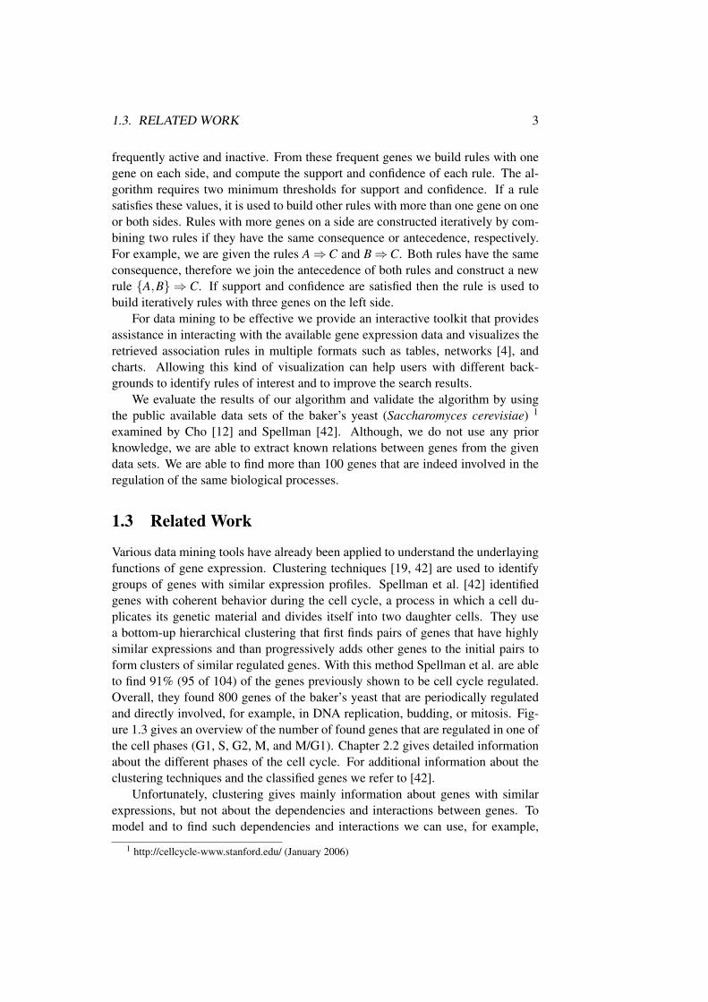
Various data mining tools have already been applied to understand the underlayingfunctions of gene expression. Clustering techniques [19, 42] are used to identifygroups of genes with similar expression profiles. Spellman et al. [42] identifiedgenes with coherent behavior during the cell cycle, a process in which a cell du-plicates its genetic material and divides itself into two daughter cells. They usea bottom-up hierarchical clustering that first finds pairs of genes that have highlysimilar expressions and than progressively adds other genes to the initial pairs toform clusters of similar regulated genes. With this method Spellman et al. are ableto find 91% (95 of 104) of the genes previously shown to be cell cycle regulated.Overall, they found 800 genes of the baker’s yeast that are periodically regulatedand directly involved, for example, in DNA replication, budding, or mitosis. Fig-ure 1.3 gives an overview of the number of found genes that are regulated in one ofthe cell phases (G1, S, G2, M, and M/G1). Chapter 2.2 gives detailed informationabout the different phases of the cell cycle. For additional information about theclustering techniques and the classified genes we refer to [42].
Unfortunately, clustering gives mainly information about genes with similarexpressions, but not about the dependencies and interactions between genes. Tomodel and to find such dependencies and interactions we can use, for example,
1 http://cellcycle-www.stanford.edu/ (January 2006)
4 CHAPTER 1. INTRODUCTION
Cluster SizeG1 300S 71G2 121M 195M/G1 113
Table 1.1: The five clusters of co-regulated genes with similar expression profiles.
Bayesian networks [22], Probabilistic Boolean networks [41], or association rules [13].In the following we give a short overview of these models.
Friedman et al. [22] describe interactions between genes with Bayesian net-works. A Bayesian network [37] is a graph-based model of joint probability dis-tributions that captures properties of conditional independences between variables.Such models are used to describe statistical dependencies. Friedman et al. intro-duce an efficient algorithm that is capable of building such networks using neitherprior biological knowledge nor constraints. They applied their algorithm to thegene expression data of Spellman et al. [42]. The results that contain the learnednetworks and interactions between the groups of genes are public available 2.
Shmulevich et al. [41] have introduced a new model for genetic regulatory net-works that constitutes a probabilistic generalization of the Boolean network modelof Kauffman [31, 25, 32]. A Boolean network [4] is a graph G(V,F) defined by aset of nodes V = {x1, ...,xn} and a list of Boolean functions F = f1, ..., fn. A nodexi represents the state of expression of a gene i, where xi = 1 or xi = 0 means thatthe gene is expressed or not, respectively. A Boolean function fi(xi1 , ...,xik) with kinput nodes is assigned to node xi that represents an interactions between genes. Alist of all Boolean functions F specifies the whole regulatory network of the genes.
The basic idea of Probabilistic Boolean networks was to overcome the deter-ministic rigidity of Boolean networks by allowing more than one possible functionfor each node. Thus, every node contains a set of possible functions that coulddetermine the value of this node. With this non-deterministic model, one can buildmany simple networks to different but specific contexts, in contrast to the deter-ministic Boolean networks that model the whole and therefore complex regulatorynetwork of the given data set. To determine those genes and functions that have themajor impact of other genes, the method of Shmulevich et al. is based on the coeffi-cient of determination [17, 18] that produces a number of good candidate functionsfor each gene. The implementation of this algorithm is described in [44].
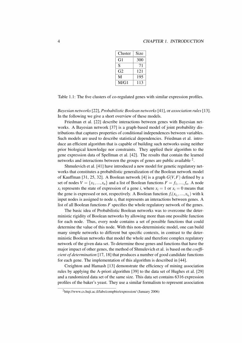
Creighton and Hamash [13] demonstrate the efficiency of mining associationrules by applying the A-priori algorithm [39] to the data set of Hughes et al. [29]and a randomized data set of the same size. This data set contains 6316 expressionprofiles of the baker’s yeast. They use a similar formalism to represent association
2http://www.cs.huji.ac.il/labs/compbio/expression/ (January 2006)
1.4. OUTLINE 5
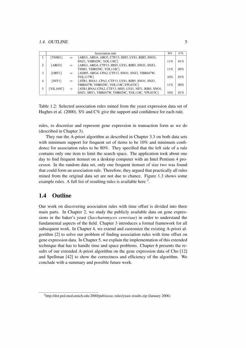
Association rule S% C%1 {YHM1} ⇒ {ARG1, ARG4, ARO3, CTF13, HIS5, LYS1, RIB5, SNO1,
SNZ1, YHR029C, YOL118C} 11% 81%2 {ARO3} ⇒ {ARG1, ARG4, CTF13, HIS5, LYS1, RIB5, SNO1, SNZ1,
YHM1, YHR029C, YOL118C} 11% 89%3 {ORT1} ⇒ {ADH5, ARG4, CPA2, CTF13, SNO1, SNZ1, YBR047W,
YGL117W} 10% 83%4 {NIT1} ⇒ {ATR1, BNA1, CPA2, CTF13, LYS1, RIB5, SNO1, SNZ1,
YBR047W, YHR029C, YOL118C,YPL033C} 11% 80%5 {YIL165C} ⇒ {ATR1,BNA1,CPA2, CTF13, HIS5, LYS1, NIT1, RIB5, SNO1,
SNZ1, SRY1, YBR047W, YHR029C, YOL118C, YPL033C} 10% 81%
Table 1.2: Selected association rules mined from the yeast expression data set ofHughes et al. (2000). S% and C% give the support and confidence for each rule.
rules, to discretize and represent gene expression in transaction form as we do(described in Chapter 3).
They run the A-priori algorithm as described in Chapter 3.3 on both data setswith minimum support for frequent set of items to be 10% and minimum confi-dence for association rules to be 80%. They specified that the left side of a rulecontains only one item to limit the search space. The application took about oneday to find frequent itemset on a desktop computer with an Intel Pentium 4 pro-cessor. In the random data set, only one frequent itemset of size two was foundthat could form an association rule. Therefore, they argued that practically all rulesmined from the original data set are not due to chance. Figure 1.3 shows someexample rules. A full list of resulting rules is available here 3.
1.4 Outline
Our work on discovering association rules with time offset is divided into threemain parts. In Chapter 2, we study the publicly available data on gene expres-sions in the baker’s yeast (Saccharomyces cerevisae) in order to understand thefundamental aspects of the field. Chapter 3 introduces a formal framework for allsubsequent work. In Chapter 4, we extend and customize the existing A-priori al-gorithm [2] to solve our problem of finding association rules with time offset ongene expression data. In Chapter 5, we explain the implementation of this extendedtechnique that has to handle time and space problems. Chapter 6 presents the re-sults of our extended A-priori algorithm on the gene expression data of Cho [12]and Spellman [42] to show the correctness and efficiency of the algorithm. Weconclude with a summary and possible future work.
3http://dot.ped.med.umich.edu:2000/pub/assoc rules/yeast results.zip (January 2006)

6 CHAPTER 1. INTRODUCTION
Chapter 2
Genetic Fundamentals
2.1 Introduction
All organisms contain a construction plan that defines the cellular structure andactivities during the lifetime of a single cell and the whole organism. This con-struction plan is called genome, and encodes all the information necessary to buildand maintain life, from bacteria to human beings. All cells of an organism containa copy of the same genome that is distributed by heredity to all cells. Thereby,a cell makes a copy of all its components and the genome and divides into twodaughter cells.
In 1953, Francis Crick and James Watson discovered the structure of the de-oxyribonucleic acid (DNA), that encodes the information of a genome and per-forms the heredity of the genetic information. DNA molecules are normally pack-aged in the form of multiple large macromolecules called chromosomes. Thegenome of an organism is a complete DNA sequence of one set of chromosomes.The DNA forms a double helix that can unzip to make copies of itself, and there-fore, a copy of the whole genome.
Understanding the functions of heredity requires more knowledge of the struc-ture and organization of the DNA. In the following, we give a short introduction inthe fundamental aspects of genetics. For more details we refer the interested readerto [28, 36, 43].
2.2 Cell Cycle
The lifetime of a cell is characterized by four distinct phases during which a grow-ing cell replicates all its components and divides into two daughter cells, called cellcycle (see Figure 2.1). After the cell division each daughter cell contains an exactcopy of the genetic material and the machinery to repeat the process of replication.The cell cycle is characterized by an alternation between the cell growing (G1), theDNA replication (S), the preparation to divide the DNA (G2), and the cell division,called mitosis (M). Mitosis separates the duplicated genome into two individual
7
8 CHAPTER 2. GENETIC FUNDAMENTALS
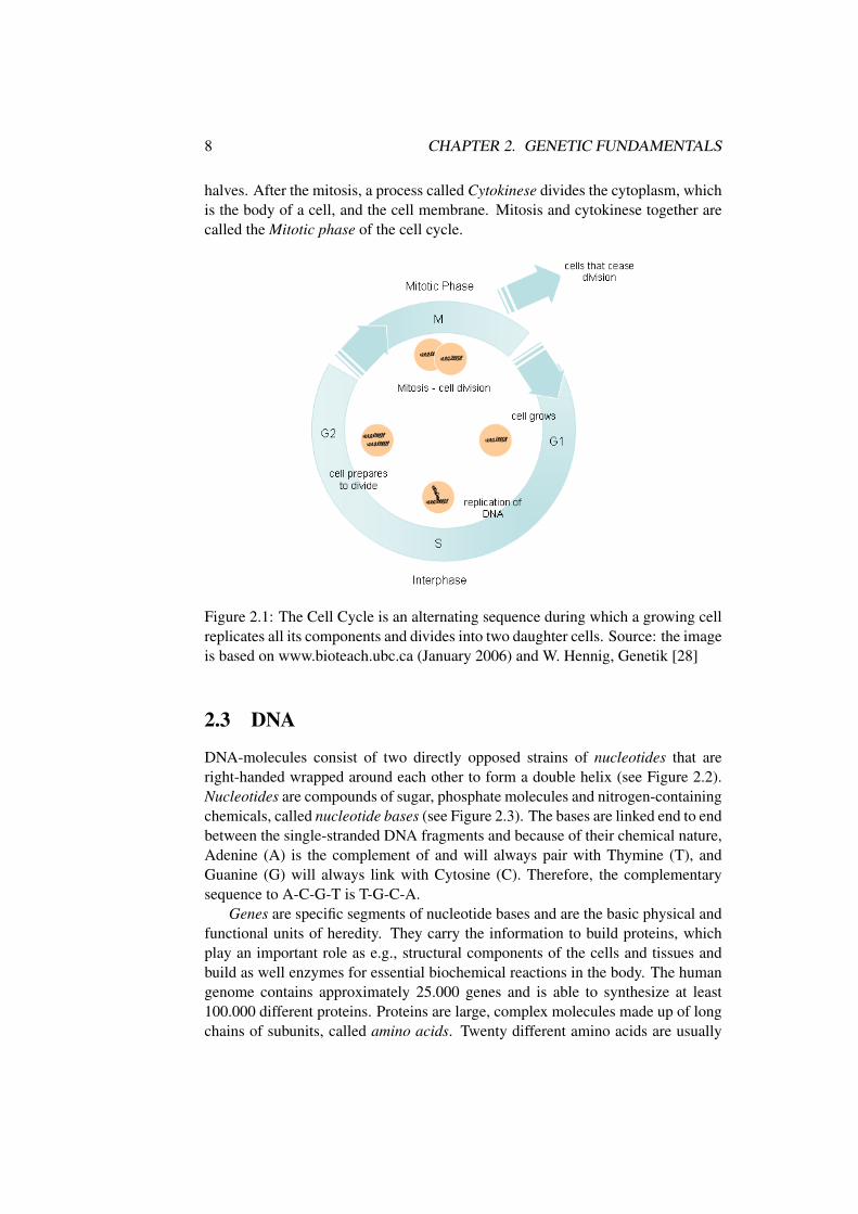
halves. After the mitosis, a process called Cytokinese divides the cytoplasm, whichis the body of a cell, and the cell membrane. Mitosis and cytokinese together arecalled the Mitotic phase of the cell cycle.
Figure 2.1: The Cell Cycle is an alternating sequence during which a growing cellreplicates all its components and divides into two daughter cells. Source: the imageis based on www.bioteach.ubc.ca (January 2006) and W. Hennig, Genetik [28]
2.3 DNA
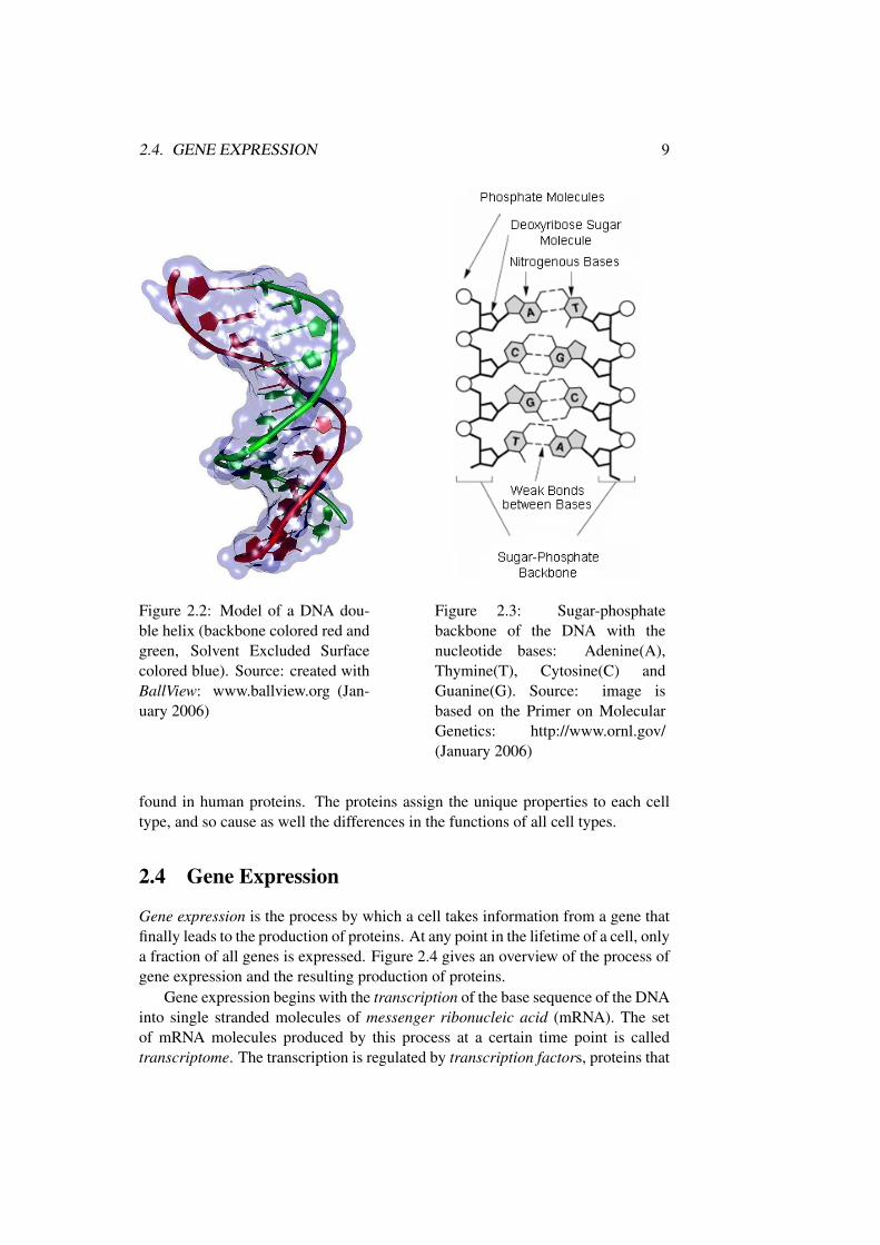
DNA-molecules consist of two directly opposed strains of nucleotides that areright-handed wrapped around each other to form a double helix (see Figure 2.2).Nucleotides are compounds of sugar, phosphate molecules and nitrogen-containingchemicals, called nucleotide bases (see Figure 2.3). The bases are linked end to endbetween the single-stranded DNA fragments and because of their chemical nature,Adenine (A) is the complement of and will always pair with Thymine (T), andGuanine (G) will always link with Cytosine (C). Therefore, the complementarysequence to A-C-G-T is T-G-C-A.
Genes are specific segments of nucleotide bases and are the basic physical andfunctional units of heredity. They carry the information to build proteins, whichplay an important role as e.g., structural components of the cells and tissues andbuild as well enzymes for essential biochemical reactions in the body. The humangenome contains approximately 25.000 genes and is able to synthesize at least100.000 different proteins. Proteins are large, complex molecules made up of longchains of subunits, called amino acids. Twenty different amino acids are usually
2.4. GENE EXPRESSION 9
Figure 2.2: Model of a DNA dou-ble helix (backbone colored red andgreen, Solvent Excluded Surfacecolored blue). Source: created withBallView: www.ballview.org (Jan-uary 2006)
Figure 2.3: Sugar-phosphatebackbone of the DNA with thenucleotide bases: Adenine(A),Thymine(T), Cytosine(C) andGuanine(G). Source: image isbased on the Primer on MolecularGenetics: http://www.ornl.gov/(January 2006)
found in human proteins. The proteins assign the unique properties to each celltype, and so cause as well the differences in the functions of all cell types.
2.4 Gene Expression
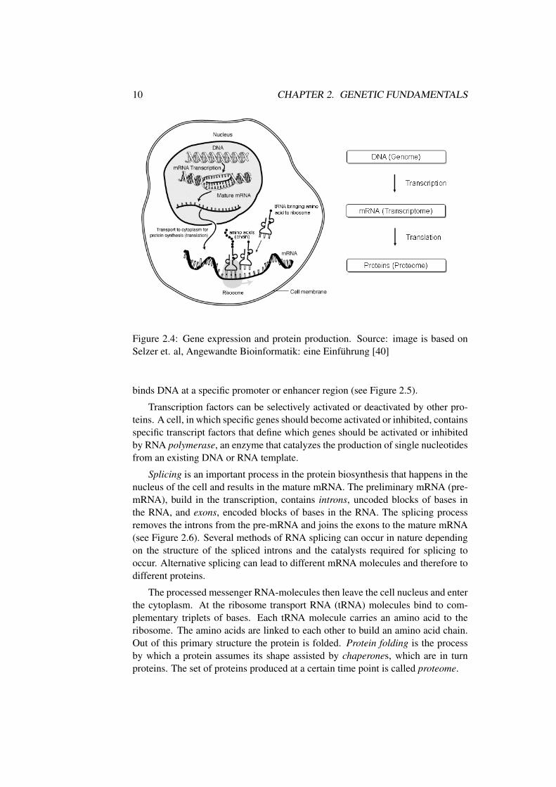
Gene expression is the process by which a cell takes information from a gene thatfinally leads to the production of proteins. At any point in the lifetime of a cell, onlya fraction of all genes is expressed. Figure 2.4 gives an overview of the process ofgene expression and the resulting production of proteins.
Gene expression begins with the transcription of the base sequence of the DNAinto single stranded molecules of messenger ribonucleic acid (mRNA). The setof mRNA molecules produced by this process at a certain time point is calledtranscriptome. The transcription is regulated by transcription factors, proteins that
10 CHAPTER 2. GENETIC FUNDAMENTALS
Figure 2.4: Gene expression and protein production. Source: image is based onSelzer et. al, Angewandte Bioinformatik: eine Einfuhrung [40]
binds DNA at a specific promoter or enhancer region (see Figure 2.5).
Transcription factors can be selectively activated or deactivated by other pro-teins. A cell, in which specific genes should become activated or inhibited, containsspecific transcript factors that define which genes should be activated or inhibitedby RNA polymerase, an enzyme that catalyzes the production of single nucleotidesfrom an existing DNA or RNA template.
Splicing is an important process in the protein biosynthesis that happens in thenucleus of the cell and results in the mature mRNA. The preliminary mRNA (pre-mRNA), build in the transcription, contains introns, uncoded blocks of bases inthe RNA, and exons, encoded blocks of bases in the RNA. The splicing processremoves the introns from the pre-mRNA and joins the exons to the mature mRNA(see Figure 2.6). Several methods of RNA splicing can occur in nature dependingon the structure of the spliced introns and the catalysts required for splicing tooccur. Alternative splicing can lead to different mRNA molecules and therefore todifferent proteins.
The processed messenger RNA-molecules then leave the cell nucleus and enterthe cytoplasm. At the ribosome transport RNA (tRNA) molecules bind to com-plementary triplets of bases. Each tRNA molecule carries an amino acid to theribosome. The amino acids are linked to each other to build an amino acid chain.Out of this primary structure the protein is folded. Protein folding is the processby which a protein assumes its shape assisted by chaperones, which are in turnproteins. The set of proteins produced at a certain time point is called proteome.
2.5. GENETIC NETWORKS 11
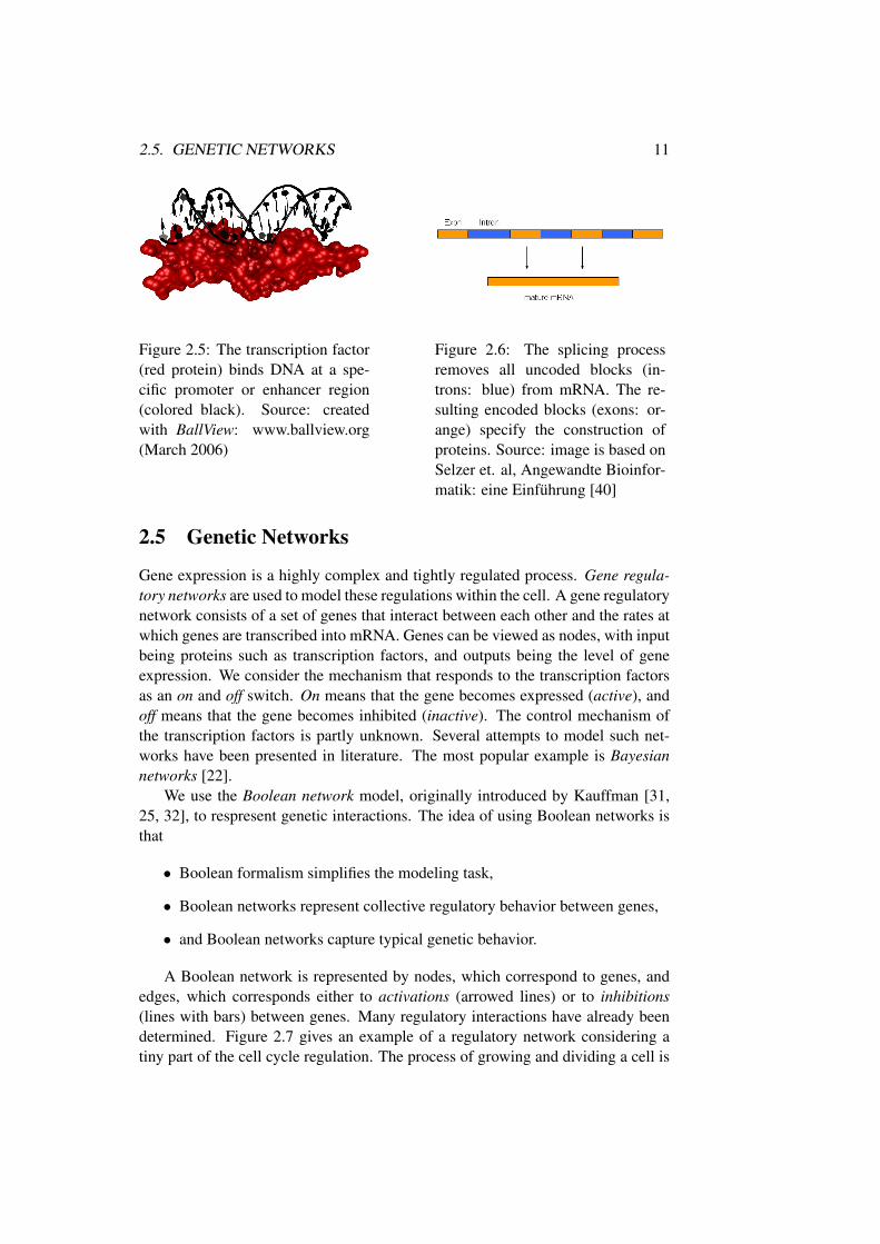
Figure 2.5: The transcription factor(red protein) binds DNA at a spe-cific promoter or enhancer region(colored black). Source: createdwith BallView: www.ballview.org(March 2006)
Figure 2.6: The splicing processremoves all uncoded blocks (in-trons: blue) from mRNA. The re-sulting encoded blocks (exons: or-ange) specify the construction ofproteins. Source: image is based onSelzer et. al, Angewandte Bioinfor-matik: eine Einfuhrung [40]
2.5 Genetic Networks
Gene expression is a highly complex and tightly regulated process. Gene regula-tory networks are used to model these regulations within the cell. A gene regulatorynetwork consists of a set of genes that interact between each other and the rates atwhich genes are transcribed into mRNA. Genes can be viewed as nodes, with inputbeing proteins such as transcription factors, and outputs being the level of geneexpression. We consider the mechanism that responds to the transcription factorsas an on and off switch. On means that the gene becomes expressed (active), andoff means that the gene becomes inhibited (inactive). The control mechanism ofthe transcription factors is partly unknown. Several attempts to model such net-works have been presented in literature. The most popular example is Bayesiannetworks [22].
We use the Boolean network model, originally introduced by Kauffman [31,25, 32], to respresent genetic interactions. The idea of using Boolean networks isthat
• Boolean formalism simplifies the modeling task,
• Boolean networks represent collective regulatory behavior between genes,
• and Boolean networks capture typical genetic behavior.
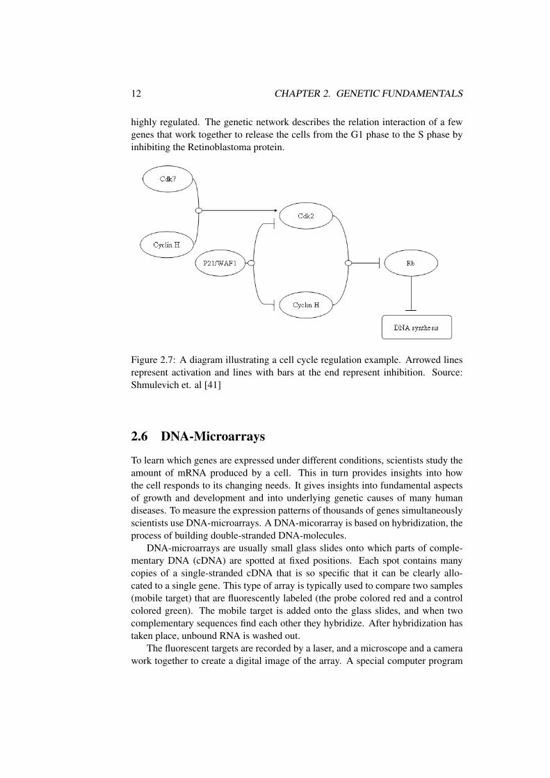
A Boolean network is represented by nodes, which correspond to genes, andedges, which corresponds either to activations (arrowed lines) or to inhibitions(lines with bars) between genes. Many regulatory interactions have already beendetermined. Figure 2.7 gives an example of a regulatory network considering atiny part of the cell cycle regulation. The process of growing and dividing a cell is
12 CHAPTER 2. GENETIC FUNDAMENTALS
highly regulated. The genetic network describes the relation interaction of a fewgenes that work together to release the cells from the G1 phase to the S phase byinhibiting the Retinoblastoma protein.
Figure 2.7: A diagram illustrating a cell cycle regulation example. Arrowed linesrepresent activation and lines with bars at the end represent inhibition. Source:Shmulevich et. al [41]
2.6 DNA-Microarrays
To learn which genes are expressed under different conditions, scientists study theamount of mRNA produced by a cell. This in turn provides insights into howthe cell responds to its changing needs. It gives insights into fundamental aspectsof growth and development and into underlying genetic causes of many humandiseases. To measure the expression patterns of thousands of genes simultaneouslyscientists use DNA-microarrays. A DNA-micorarray is based on hybridization, theprocess of building double-stranded DNA-molecules.
DNA-microarrays are usually small glass slides onto which parts of comple-mentary DNA (cDNA) are spotted at fixed positions. Each spot contains manycopies of a single-stranded cDNA that is so specific that it can be clearly allo-cated to a single gene. This type of array is typically used to compare two samples(mobile target) that are fluorescently labeled (the probe colored red and a controlcolored green). The mobile target is added onto the glass slides, and when twocomplementary sequences find each other they hybridize. After hybridization hastaken place, unbound RNA is washed out.
The fluorescent targets are recorded by a laser, and a microscope and a camerawork together to create a digital image of the array. A special computer program
2.7. TIME-SERIES OF EXPRESSION PROFILES 13
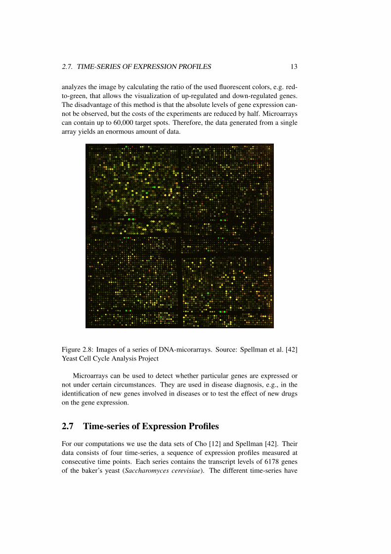
analyzes the image by calculating the ratio of the used fluorescent colors, e.g. red-to-green, that allows the visualization of up-regulated and down-regulated genes.The disadvantage of this method is that the absolute levels of gene expression can-not be observed, but the costs of the experiments are reduced by half. Microarrayscan contain up to 60,000 target spots. Therefore, the data generated from a singlearray yields an enormous amount of data.
Figure 2.8: Images of a series of DNA-micorarrays. Source: Spellman et al. [42]Yeast Cell Cycle Analysis Project
Microarrays can be used to detect whether particular genes are expressed ornot under certain circumstances. They are used in disease diagnosis, e.g., in theidentification of new genes involved in diseases or to test the effect of new drugson the gene expression.
2.7 Time-series of Expression Profiles
For our computations we use the data sets of Cho [12] and Spellman [42]. Theirdata consists of four time-series, a sequence of expression profiles measured atconsecutive time points. Each series contains the transcript levels of 6178 genesof the baker’s yeast (Saccharomyces cerevisiae). The different time-series have
14 CHAPTER 2. GENETIC FUNDAMENTALS
been measured under different experimental conditions. All experiments startedwith a cell population that has been synchronized, i.e. the cells are arrested inthe same state of the cell cycle. The studies applied four independent methodsto perform synchronization. The used methods are cdc15, cdc28, α factor, andelutriation (elu). These approaches arrested the cells by introducing external sub-stances, changing environmental conditions, or selecting cells of the same size thatare likely in the same state. For a full description of the methods and data sets, werefer the interested reader to the original papers [12] [42]1.
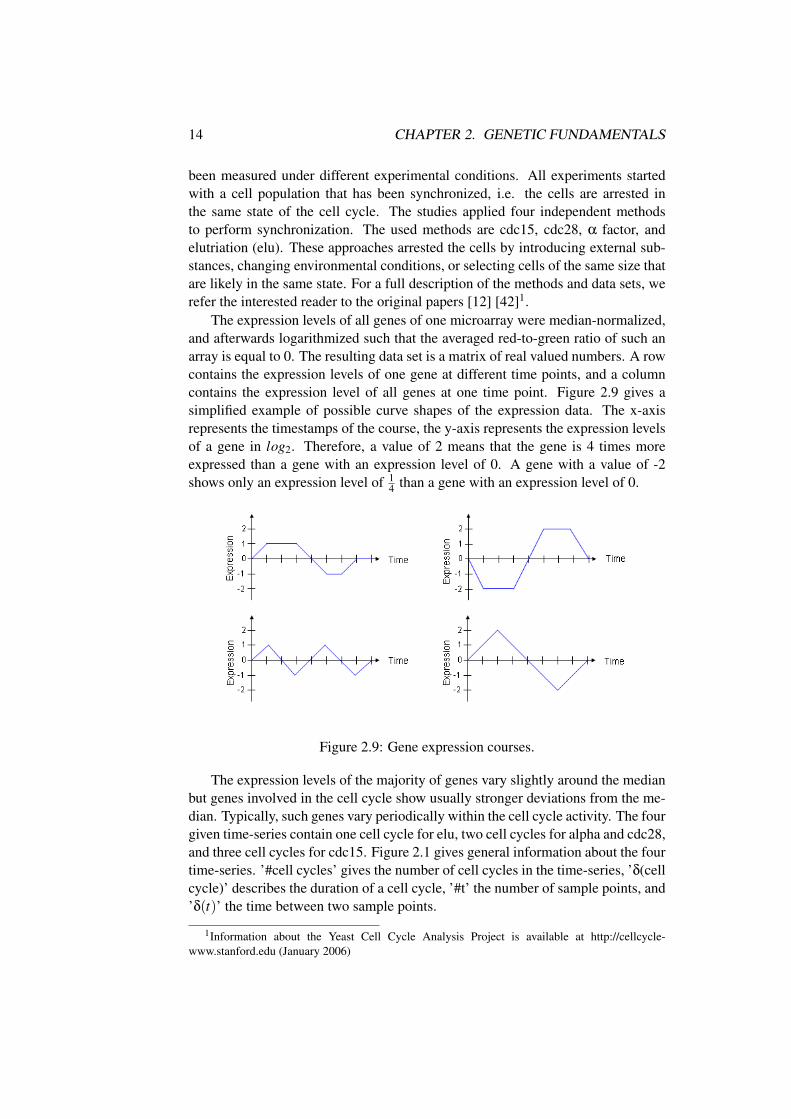
The expression levels of all genes of one microarray were median-normalized,and afterwards logarithmized such that the averaged red-to-green ratio of such anarray is equal to 0. The resulting data set is a matrix of real valued numbers. A rowcontains the expression levels of one gene at different time points, and a columncontains the expression level of all genes at one time point. Figure 2.9 gives asimplified example of possible curve shapes of the expression data. The x-axisrepresents the timestamps of the course, the y-axis represents the expression levelsof a gene in log2. Therefore, a value of 2 means that the gene is 4 times moreexpressed than a gene with an expression level of 0. A gene with a value of -2shows only an expression level of 1
4 than a gene with an expression level of 0.
Figure 2.9: Gene expression courses.
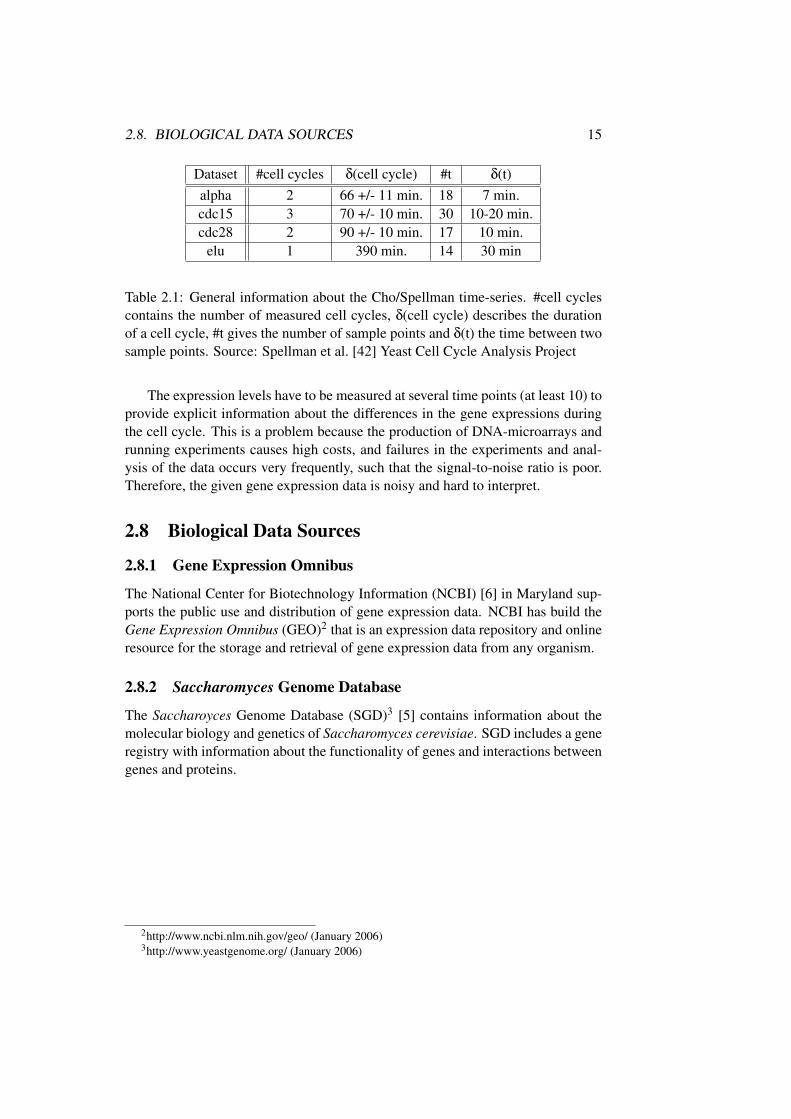
The expression levels of the majority of genes vary slightly around the medianbut genes involved in the cell cycle show usually stronger deviations from the me-dian. Typically, such genes vary periodically within the cell cycle activity. The fourgiven time-series contain one cell cycle for elu, two cell cycles for alpha and cdc28,and three cell cycles for cdc15. Figure 2.1 gives general information about the fourtime-series. ’#cell cycles’ gives the number of cell cycles in the time-series, ’δ(cellcycle)’ describes the duration of a cell cycle, ’#t’ the number of sample points, and’δ(t)’ the time between two sample points.
1Information about the Yeast Cell Cycle Analysis Project is available at http://cellcycle-www.stanford.edu (January 2006)
2.8. BIOLOGICAL DATA SOURCES 15
Dataset #cell cycles δ(cell cycle) #t δ(t)alpha 2 66 +/- 11 min. 18 7 min.cdc15 3 70 +/- 10 min. 30 10-20 min.cdc28 2 90 +/- 10 min. 17 10 min.
elu 1 390 min. 14 30 min
Table 2.1: General information about the Cho/Spellman time-series. #cell cyclescontains the number of measured cell cycles, δ(cell cycle) describes the durationof a cell cycle, #t gives the number of sample points and δ(t) the time between twosample points. Source: Spellman et al. [42] Yeast Cell Cycle Analysis Project
The expression levels have to be measured at several time points (at least 10) toprovide explicit information about the differences in the gene expressions duringthe cell cycle. This is a problem because the production of DNA-microarrays andrunning experiments causes high costs, and failures in the experiments and anal-ysis of the data occurs very frequently, such that the signal-to-noise ratio is poor.Therefore, the given gene expression data is noisy and hard to interpret.
2.8 Biological Data Sources
2.8.1 Gene Expression Omnibus
The National Center for Biotechnology Information (NCBI) [6] in Maryland sup-ports the public use and distribution of gene expression data. NCBI has build theGene Expression Omnibus (GEO)2 that is an expression data repository and onlineresource for the storage and retrieval of gene expression data from any organism.
2.8.2 Saccharomyces Genome Database
The Saccharoyces Genome Database (SGD)3 [5] contains information about themolecular biology and genetics of Saccharomyces cerevisiae. SGD includes a generegistry with information about the functionality of genes and interactions betweengenes and proteins.
2http://www.ncbi.nlm.nih.gov/geo/ (January 2006)3http://www.yeastgenome.org/ (January 2006)

16 CHAPTER 2. GENETIC FUNDAMENTALS
Chapter 3
Computational Foundations
3.1 Informal Overview
We want to discover relationships among genes in a large data set. We representthese relationships in the form of implications, called association rules. Associ-ation rule mining is a popular data mining task to find interesting relationshipsamong any items in a database. Here, interesting means relationships that satisfycertain desirables specified by parameters. Our goal is to find such associationrules to verify existing gene regulatory networks and to discover new interactions.We focus on the problem that an activation or inhibition of a gene can occur withina certain amount of time. The information that a gene X activates or inhibits a geneY with a delay of τ time units in a given data set constituted the association rulethat we are interested in analyzing.
Association rules have been extensively studied in the literature [2, 3, 13, 24,26] due to their usefulness in many application domains. A typical example is themarket basket analysis, which focus on the customer habits in super markets, andretrieves associations between the different items that customers frequently pur-chase together. The discovery of such association rules help marketers to developretail strategies to structure their shelf space to optimally meet the shopping behav-ior of the costumers, e.g. to place items close to each other if they are frequentlysold together. This strategy should encourage the customers to buy more itemswithin a single visit to the store.
Due to the given number of genes, the number of possible association rules isvery large; however, only a small fraction of rules is actually of interest. Thereforethe next task is to identify and concentrate on interesting cases.
In the following sections we specify the terminology to represent the geneexpression data and association rules with time offset. We describe the problemof mining association rules with time offset on gene expression data in a formalmanner thereby relying on the so-called A-priori Algorithm introduced in 1993 byAgrawal et al. [2, 3]. The name of the algorithm is based on the fact that it usesprior knowledge to retrieve association rules, as we shall see below. We will briefly
17
18 CHAPTER 3. COMPUTATIONAL FOUNDATIONS
review this data mining technique and extend it that it is suited for our more specificproblem definition.
3.2 Formal Model
First, we need to introduce some basic definitions. Let I be a set of literals, calleditems, and T a multi set of transactions. In the case of market basket analysis atransaction t is a set of items bought in one visit to the marketplace, i.e. t ⊆ I.In most of the data mining literature a set of items is called itemset. To specifywhether a given itemset is contained in a transaction we use the following defini-tion.
Definition 3.1 (Contains) Let x be an item in I, and t a transaction. Then,
Contains(x, t) :=
{1 if x ∈ t0 if x /∈ t
For an itemset X we define Contains(X , t) := ∏x∈X Contains(x, t). 3
An association rule is an implication of the following form.
Definition 3.2 (Association Rule) Let X and Y be subsets of I with X∩Y = /0, andt a transaction. An implication
X ⇒ Y
is called association rule if Contains(X , t) and Contains(Y, t). X is called an-tecedence of the rule and Y consequence of the rule. 3
The definition of association rules is more general than the one presented in thepaper of Agrawal et al.[2] in that they restrict the consequences to singletons. Weuse the measures support and confidence to estimate the utility and certainty of arule. Such objective measures are based on the structure and underlying statisticsof the rules.
3.2.1 Support
Support [3, 26] is a utility function that counts how often the considered rule occursin the given transactions. The higher the value of the support the more importantthe rule is considered. In other words, the support of a rule corresponds to thepercentage of transactions that contain the rule.
Definition 3.3 (Rule Support) Let X and Y be subsets of I, T a multiset of trans-actions, and r := X⇒Y an association rule. The support of r with respect to T ,denoted Support(r), is defined as
Support(r) :=1T
T
∑t=0
Contains(X ∪Y, t).
3.2. FORMAL MODEL 19
3
Note, that Support(A⇒B) = Support(B⇒A) for all itemsets A and B. Rules with lowsupport represent rare or exceptional cases; they can have more random coherence.
3.2.2 Confidence
Confidence[15, 26] is a measure of certainty or rule quality that gives hints of thestrength of the association rule. The confidence defines the level of correlationbetween itemsets, i.e. the confidence of a rule X⇒Y is the fraction of transactionsthat contain both X and Y . The confidence of a rule is defined by dividing thesupport of a rule by the support of the antecedence of the itemset. Analogue to thedefinition of rule support we define the support of genesets.
Definition 3.4 (Support) Let X be a subset of I, and T a multiset of transactions.The support of X with respect to T , denoted Support(X), is defined as
Support(X) :=1T
T
∑t=0
Contains(X , t).
3
The definition of confidence is as follows.
Definition 3.5 (Confidence) Let X and Y be subsets in I, and r := X⇒Y an asso-ciation rule. Then the confidence of r with respect to X, denoted Confidence(r), isdefined as
Confidence(r) :=Support(r)Support(X)
.
3
A confidence of 1.0 indicates that the rule is always true on the analyzed data.A small confidence value indicates that the antecedence is not strongly connectedto the consequence. Therefore, we are interested in finding rules having supportgreater than a minimum support threshold called minSupport and a confidencegreater than a minimum confidence threshold called minConfidence. Rules thatsatisfy both are called strong association rules.
Definition 3.6 (Strong Association Rules) Let X and Y be disjoint subsets of I,and r := X⇒Y be an association rule. Then, r is a strong association rule if Sup-port(r) ≥ minSupport and Confidence(r) ≥ minConfidence. 3
20 CHAPTER 3. COMPUTATIONAL FOUNDATIONS
3.3 A-priori Algorithm
The number of possible strong association rules in a data set is very large. For adata set of n genes we can construct
( nk
)sets with k items. So we have a total num-
ber of ∑nk=2
( nk
)= 2n−n−1 sets with k-items. Altogether, by combining these sets
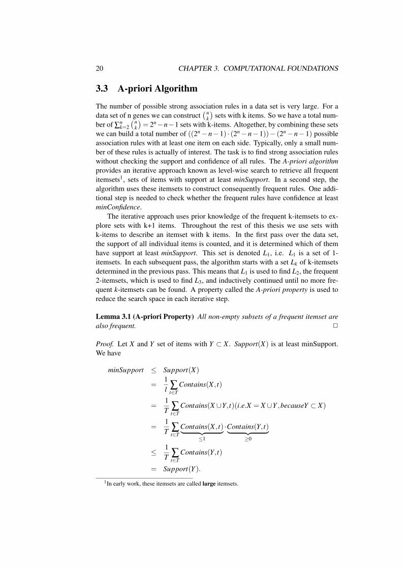
we can build a total number of ((2n−n−1) · (2n−n−1))− (2n−n−1) possibleassociation rules with at least one item on each side. Typically, only a small num-ber of these rules is actually of interest. The task is to find strong association ruleswithout checking the support and confidence of all rules. The A-priori algorithmprovides an iterative approach known as level-wise search to retrieve all frequentitemsets1, sets of items with support at least minSupport. In a second step, thealgorithm uses these itemsets to construct consequently frequent rules. One addi-tional step is needed to check whether the frequent rules have confidence at leastminConfidence.
The iterative approach uses prior knowledge of the frequent k-itemsets to ex-plore sets with k+1 items. Throughout the rest of this thesis we use sets withk-items to describe an itemset with k items. In the first pass over the data set,the support of all individual items is counted, and it is determined which of themhave support at least minSupport. This set is denoted L1, i.e. L1 is a set of 1-itemsets. In each subsequent pass, the algorithm starts with a set Lk of k-itemsetsdetermined in the previous pass. This means that L1 is used to find L2, the frequent2-itemsets, which is used to find L3, and inductively continued until no more fre-quent k-itemsets can be found. A property called the A-priori property is used toreduce the search space in each iterative step.
Lemma 3.1 (A-priori Property) All non-empty subsets of a frequent itemset arealso frequent. 2
Proof. Let X and Y set of items with Y ⊂ X . Support(X) is at least minSupport.We have
minSupport ≤ Support(X)
=1l ∑
t∈TContains(X , t)
=1T ∑
t∈TContains(X ∪Y, t)(i.e.X = X ∪Y ,becauseY ⊂ X)
=1T ∑
t∈TContains(X , t)︸ ︷︷ ︸
≤1
·Contains(Y, t)︸ ︷︷ ︸≥0
≤ 1T ∑
t∈TContains(Y, t)
= Support(Y ).
1In early work, these itemsets are called large itemsets.
3.3. A-PRIORI ALGORITHM 21
The A-priori property is based on the following observation. By definition, if anitemset X does not satisfy the minimum support threshold, then X is not frequent(Support(X) ≤ minSupport). If an item i is added to the itemset X , then the re-sulting itemset X ∪{i} cannot occur more frequently than X . Therefore X ∪{i} isnot frequent either, that is Support(X ∪{i})≤ minSupport. This property is calledanti-monotone because it is monotonic in the context of being not frequent. Thismeans that if a set is not frequent all of its supersets are not frequent as well.
The A-priori Algorithm is decomposed into two subproblems. First, we com-pute all frequent k-itemsets, and then we generate all strong association rules.
3.3.1 Find Frequent Itemsets
Because of the A-priori assumption k-itemsets can be generated by joining frequent(k-1)-itemsets, and deleting those that contain any subset that does not satisfy min-Support:
1. Join Step: Join all disjoint pairs of itemsets of the same size that differ inexact one element. Let A,B ∈ I. Then, A and B can be joined if
∃a ∈ A,∃b ∈ B : A\{a}= B\{b}
This condition simply ensures that no duplicates are generated.
2. Prune Step: Delete all created k-itemsets that contain a (k-1)-itemset that isnot frequent, because any (k-1)-itemset that is not frequent cannot be a subsetof a frequent k-itemset. This subset testing can be done quickly by maintain-ing a hash table of trees of frequent itemsets. The database is scanned againand the support of all created k-itemsets is counted.
3.3.2 Generate Strong Association Rules
Once the frequent itemsets are found, it is straightforward to generate strong asso-ciation rules from them.
1. For all nonempty subsets A of itemset X generate all rules A⇒ (X \A).
2. Since the rules are generated from frequent itemsets, each one automaticallysatisfies minSupport.
3. Compute the confidence of all rules support(A⇒(X\A))support(A) and remove those that
do not satisfy minConfidence.
22 CHAPTER 3. COMPUTATIONAL FOUNDATIONS
3.4 Association Rules with Time Offset
The previous definition of association rules considers interactions of genes that oc-cur at the same timestamp. Our challenge is to discover interactions that occur aftera certain amount of time. We apply the previous definition of strong associationrules directly to our problem definition.
To simplify matters we say in the following genes and timestamps instead ofitems and transactions. Respectively, we use k-geneset to denote a set of k genes.
3.4.1 Discretization
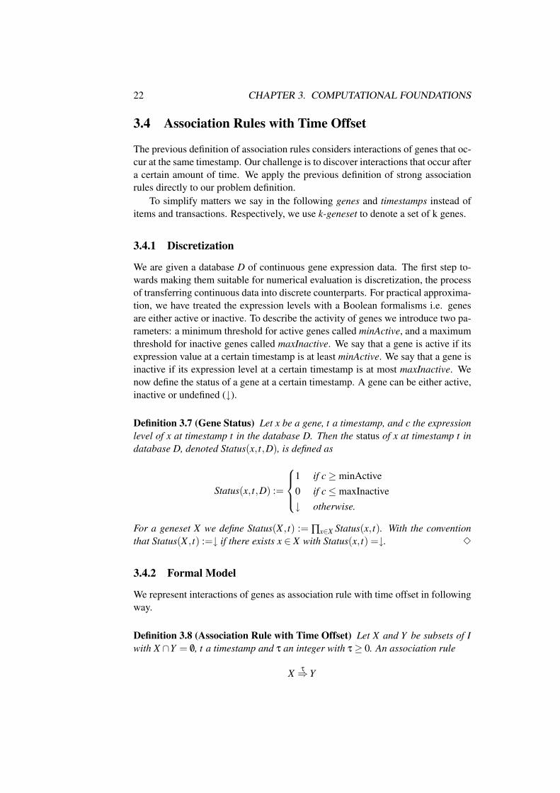
We are given a database D of continuous gene expression data. The first step to-wards making them suitable for numerical evaluation is discretization, the processof transferring continuous data into discrete counterparts. For practical approxima-tion, we have treated the expression levels with a Boolean formalisms i.e. genesare either active or inactive. To describe the activity of genes we introduce two pa-rameters: a minimum threshold for active genes called minActive, and a maximumthreshold for inactive genes called maxInactive. We say that a gene is active if itsexpression value at a certain timestamp is at least minActive. We say that a gene isinactive if its expression level at a certain timestamp is at most maxInactive. Wenow define the status of a gene at a certain timestamp. A gene can be either active,inactive or undefined (↓).
Definition 3.7 (Gene Status) Let x be a gene, t a timestamp, and c the expressionlevel of x at timestamp t in the database D. Then the status of x at timestamp t indatabase D, denoted Status(x, t,D), is defined as
Status(x, t,D) :=
1 if c≥ minActive0 if c≤ maxInactive↓ otherwise.
For a geneset X we define Status(X , t) := ∏x∈X Status(x, t). With the conventionthat Status(X , t) :=↓ if there exists x ∈ X with Status(x, t) =↓. 3
3.4.2 Formal Model
We represent interactions of genes as association rule with time offset in followingway.
Definition 3.8 (Association Rule with Time Offset) Let X and Y be subsets of Iwith X ∩Y = /0, t a timestamp and τ an integer with τ≥ 0. An association rule
X τ⇒ Y
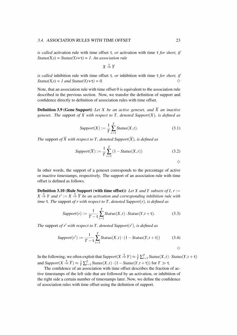
3.4. ASSOCIATION RULES WITH TIME OFFSET 23
is called activation rule with time offset τ, or activation with time τ for short, ifStatus(X,t) = Status(Y,t+τ) = 1. An association rule
X τ⇒ Y
is called inhibition rule with time offset τ, or inhibition with time τ for short, ifStatus(X,t) = 1 and Status(Y,t+τ) = 0. 3
Note, that an association rule with time offset 0 is equivalent to the association ruledescribed in the previous section. Now, we transfer the definition of support andconfidence directly to definition of association rules with time offset.
Definition 3.9 (Gene Support) Let X be an active geneset, and X an inactivegeneset. The support of X with respect to T , denoted Support(X), is defined as
Support(X) :=1T
T
∑t=1
Status(X , t). (3.1)
The support of X with respect to T , denoted Support(X), is defined as
Support(X) :=1T
T
∑t=1
(1−Status(X , t)) (3.2)
3
In other words, the support of a geneset corresponds to the percentage of activeor inactive timestamps, respectively. The support of an association rule with timeoffset is defined as follows.
Definition 3.10 (Rule Support (with time offset)) Let X and Y subsets of I, r :=X τ⇒ Y and r′ := X τ⇒ Y be an activation and corresponding inhibition rule withtime τ. The support of r with respect to T , denoted Support(r), is defined as
Support(r) :=1
T − τ
T
∑t=1
Status(X , t) ·Status(Y, t + τ). (3.3)
The support of r′ with respect to T , denoted Support(r′), is defined as
Support(r′) :=1
T − τ
T
∑t=1
Status(X , t) · (1−Status(Y, t + τ)) (3.4)
3
In the following, we often exploit that Support(X τ⇒Y )≈ 1T ∑
Tt=1 Status(X , t) ·Status(Y, t + τ)
and Support(X τ⇒ Y )≈ 1T ∑
Tt=1 Status(X , t) · (1−Status(Y, t + τ)) for T � τ.
The confidence of an association with time offset describes the fraction of ac-tive timestamps of the left side that are followed by an activation, or inhibition ofthe right side a certain number of timestamps later. Now, we define the confidenceof association rules with time offset using the definition of support.
24 CHAPTER 3. COMPUTATIONAL FOUNDATIONS
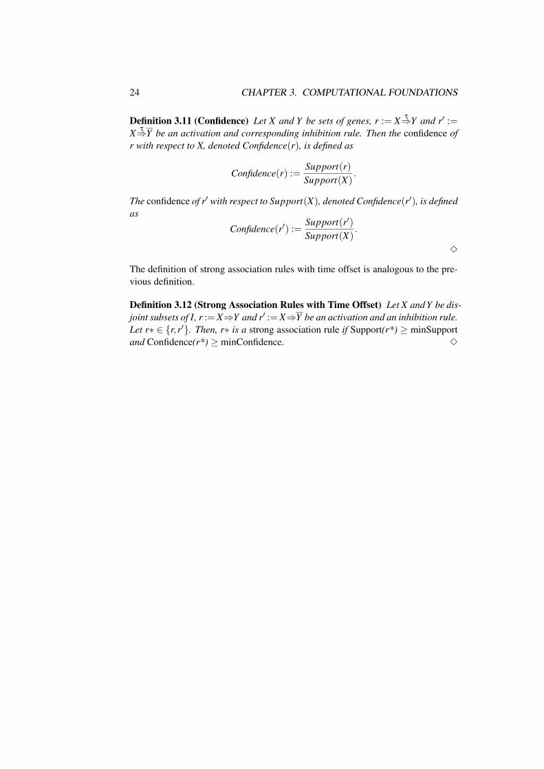
Definition 3.11 (Confidence) Let X and Y be sets of genes, r := X τ⇒Y and r′ :=X τ⇒Y be an activation and corresponding inhibition rule. Then the confidence ofr with respect to X, denoted Confidence(r), is defined as
Confidence(r) :=Support(r)Support(X)
.
The confidence of r′ with respect to Support(X), denoted Confidence(r′), is definedas
Confidence(r′) :=Support(r′)Support(X)
.
3
The definition of strong association rules with time offset is analogous to the pre-vious definition.
Definition 3.12 (Strong Association Rules with Time Offset) Let X and Y be dis-joint subsets of I, r := X⇒Y and r′ := X⇒Y be an activation and an inhibition rule.Let r∗ ∈ {r,r′}. Then, r∗ is a strong association rule if Support(r*) ≥ minSupportand Confidence(r*) ≥ minConfidence. 3
Chapter 4
Mining Association Rules onGene Expression Data
4.1 Introduction
The ultimate goal of this work is to discover genes that regulate each other. Wewant to discover dependencies between genes without any prior knowledge of co-regulated genes or existing rules. In particular we want to find genes involved in aregulatory network and appropriate to form rules from the given discretized geneexpression data in the context of rule discovery. Our main challenge is to providean algorithm that is able to find activation and inhibition rules with a certain timeoffset between two and more genes. In this chapter we describe our algorithm forfinding strong association rules with time offset.
4.2 Naive Approach
The intuitive approach for finding strong association rules with time offset is asfollows. We start by selecting the two threshold minSupport and minConfidence(see Chapter 3.2.2) and then generate all possible combinations of rules. While theresults found by this naive approach make sense in biology, the search space andrunning time constitute two major disadvantages, since this approach generates animmense number of possible strong association rules. We discussed before that wecan build O(2n) activation and inhibition rules. To find interesting rules out of thisexploding number we need to compute the support and confidence of each rule.This computation requires an immense amount of space and time. Therefore weneed a better approach to retrieve strong association rules.
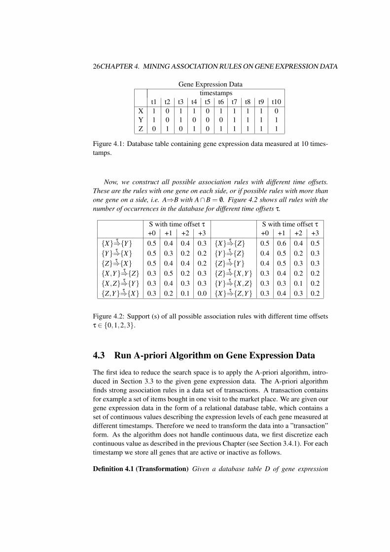
Example 4.1 (Naive approach) Consider a concrete example for this Naive Ap-proach. Figure 4.2 shows the gene expression data of three genes, i.e. |I| = 3. Arow represents the expression levels of a single gene, and a column the expressionlevels of all genes measured at one timestamp.
25
26CHAPTER 4. MINING ASSOCIATION RULES ON GENE EXPRESSION DATA
Gene Expression Datatimestamps
t1 t2 t3 t4 t5 t6 t7 t8 t9 t10X 1 0 1 1 0 1 1 1 1 0Y 1 0 1 0 0 0 1 1 1 1Z 0 1 0 1 0 1 1 1 1 1
Figure 4.1: Database table containing gene expression data measured at 10 times-tamps.
Now, we construct all possible association rules with different time offsets.These are the rules with one gene on each side, or if possible rules with more thanone gene on a side, i.e. A⇒B with A∩B = /0. Figure 4.2 shows all rules with thenumber of occurrences in the database for different time offsets τ.
S with time offset τ S with time offset τ
+0 +1 +2 +3 +0 +1 +2 +3{X} τ⇒{Y} 0.5 0.4 0.4 0.3 {X} τ⇒{Z} 0.5 0.6 0.4 0.5{Y} τ⇒{X} 0.5 0.3 0.2 0.2 {Y} τ⇒{Z} 0.4 0.5 0.2 0.3{Z} τ⇒{X} 0.5 0.4 0.4 0.2 {Z} τ⇒{Y} 0.4 0.5 0.3 0.3{X ,Y} τ⇒{Z} 0.3 0.5 0.2 0.3 {Z} τ⇒{X ,Y} 0.3 0.4 0.2 0.2{X ,Z} τ⇒{Y} 0.3 0.4 0.3 0.3 {Y} τ⇒{X ,Z} 0.3 0.3 0.1 0.2{Z,Y} τ⇒{X} 0.3 0.2 0.1 0.0 {X} τ⇒{Z,Y} 0.3 0.4 0.3 0.2
Figure 4.2: Support (s) of all possible association rules with different time offsetsτ ∈ {0,1,2,3}.
4.3 Run A-priori Algorithm on Gene Expression Data
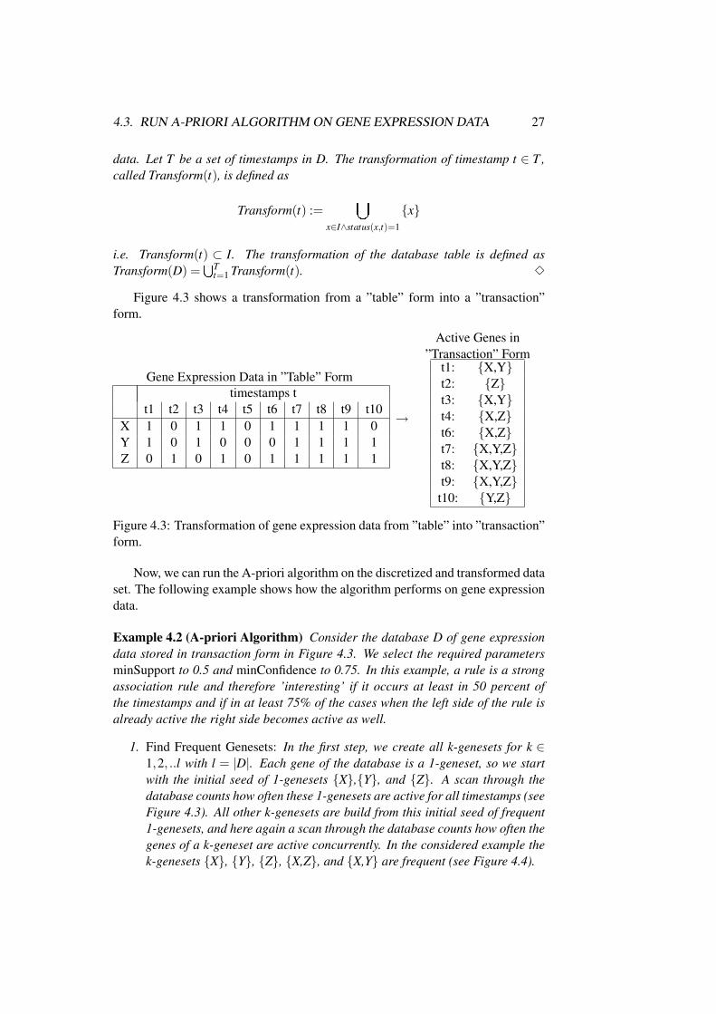
The first idea to reduce the search space is to apply the A-priori algorithm, intro-duced in Section 3.3 to the given gene expression data. The A-priori algorithmfinds strong association rules in a data set of transactions. A transaction containsfor example a set of items bought in one visit to the market place. We are given ourgene expression data in the form of a relational database table, which contains aset of continuous values describing the expression levels of each gene measured atdifferent timestamps. Therefore we need to transform the data into a ”transaction”form. As the algorithm does not handle continuous data, we first discretize eachcontinuous value as described in the previous Chapter (see Section 3.4.1). For eachtimestamp we store all genes that are active or inactive as follows.
Definition 4.1 (Transformation) Given a database table D of gene expression
4.3. RUN A-PRIORI ALGORITHM ON GENE EXPRESSION DATA 27
data. Let T be a set of timestamps in D. The transformation of timestamp t ∈ T ,called Transform(t), is defined as
Transform(t) :=[
x∈I∧status(x,t)=1
{x}
i.e. Transform(t) ⊂ I. The transformation of the database table is defined asTransform(D) =
STt=1 Transform(t). 3
Figure 4.3 shows a transformation from a ”table” form into a ”transaction”form.
Gene Expression Data in ”Table” Formtimestamps t
t1 t2 t3 t4 t5 t6 t7 t8 t9 t10X 1 0 1 1 0 1 1 1 1 0Y 1 0 1 0 0 0 1 1 1 1Z 0 1 0 1 0 1 1 1 1 1
→
Active Genes in”Transaction” Form
t1: {X,Y}t2: {Z}t3: {X,Y}t4: {X,Z}t6: {X,Z}t7: {X,Y,Z}t8: {X,Y,Z}t9: {X,Y,Z}t10: {Y,Z}
Figure 4.3: Transformation of gene expression data from ”table” into ”transaction”form.
Now, we can run the A-priori algorithm on the discretized and transformed dataset. The following example shows how the algorithm performs on gene expressiondata.
Example 4.2 (A-priori Algorithm) Consider the database D of gene expressiondata stored in transaction form in Figure 4.3. We select the required parametersminSupport to 0.5 and minConfidence to 0.75. In this example, a rule is a strongassociation rule and therefore ’interesting’ if it occurs at least in 50 percent ofthe timestamps and if in at least 75% of the cases when the left side of the rule isalready active the right side becomes active as well.
1. Find Frequent Genesets: In the first step, we create all k-genesets for k ∈1,2, ..l with l = |D|. Each gene of the database is a 1-geneset, so we startwith the initial seed of 1-genesets {X},{Y}, and {Z}. A scan through thedatabase counts how often these 1-genesets are active for all timestamps (seeFigure 4.3). All other k-genesets are build from this initial seed of frequent1-genesets, and here again a scan through the database counts how often thegenes of a k-geneset are active concurrently. In the considered example thek-genesets {X}, {Y}, {Z}, {X,Z}, and {X,Y} are frequent (see Figure 4.4).
28CHAPTER 4. MINING ASSOCIATION RULES ON GENE EXPRESSION DATA
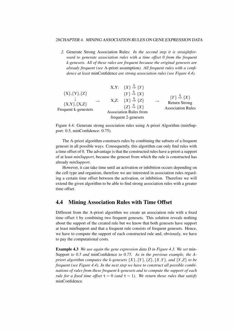
2. Generate Strong Association Rules: In the second step it is straightfor-ward to generate association rules with a time offset 0 from the frequentk-genesets. All of these rules are frequent because the original genesets arealready frequent (see A-priori assumption). All frequent rules with a confi-dence at least minConfidence are strong association rules (see Figure 4.4).
{X},{Y},{Z}↓
{X,Y},{X,Z}Frequent k-genestets
→
X,Y: {X} 0⇒{Y}{Y} 0⇒{X}
X,Z: {X} 0⇒{Z}{Z} 0⇒{X}
Association Rules fromfrequent 2-genesets
→{Y} 0⇒{X}
Return StrongAssociation Rules
Figure 4.4: Generate strong association rules using A-priori Algorithm (minSup-port: 0.5, minConfidence: 0.75).
The A-priori algorithm constructs rules by combining the subsets of a frequentgeneset in all possible ways. Consequently, this algorithm can only find rules witha time offset of 0. The advantage is that the constructed rules have a-priori a supportof at least minSupport, because the geneset from which the rule is constructed hasalready minSupport.
However, it can take time until an activation or inhibition occurs depending onthe cell type and organism, therefore we are interested in association rules regard-ing a certain time offset between the activation, or inhibition. Therefore we willextend the given algorithm to be able to find strong association rules with a greatertime offset.
4.4 Mining Association Rules with Time Offset
Different from the A-priori algorithm we create an association rule with a fixedtime offset τ by combining two frequent genesets. This solution reveals nothingabout the support of the created rule but we know that both genesets have supportat least minSupport and that a frequent rule consists of frequent genesets. Hence,we have to compute the support of each constructed rule and, obviously, we haveto pay the computational costs.
Example 4.3 We use again the gene expression data D in Figure 4.3. We set min-Support to 0.5 and minConfidence to 0.75. As in the previous example, the A-priori algorithm computes the k-genesets {X},{Y},{Z},{X ,Y}, and {Y,Z} to befrequent (see Figure 4.4). In the next step we have to construct all possible combi-nations of rules from these frequent k-genesets and to compute the support of eachrule for a fixed time offset τ = 0 (and τ = 1). We return those rules that satisfyminConfidence.
4.4. MINING ASSOCIATION RULES WITH TIME OFFSET 29
{X},{Y},{Z}↓
{X,Y},{X,Z}Frequent
k-genestets
→
{X},{Y}: {X} 0(1)⇒ {Y}{Y} 0(1)⇒ {X}
{X},{Z}: {X} 0(1)⇒ {Z}{Z} 0(1)⇒ {X}
{Y},{Z}: {Y} 0(1)⇒ {Z}{Z} 0(1)⇒ {Y}
{Y},{X,Z} {Y} 0(1)⇒ {X ,Z}{X ,Z} 0(1)⇒ {Y}
{Z},{X,Y} {Z} 0(1)⇒ {X ,Y}{X ,Y} 0(1)⇒ {Z}
Combine frequent k-genesetsto rules with τ = 0 (τ = 1)
→
{Y} 0⇒{X}({Y} 1⇒{Z})({X} 1⇒{Z})
({X ,Z} 1⇒{Y})Strong AssociationRules with τ = 0
(τ = 1)
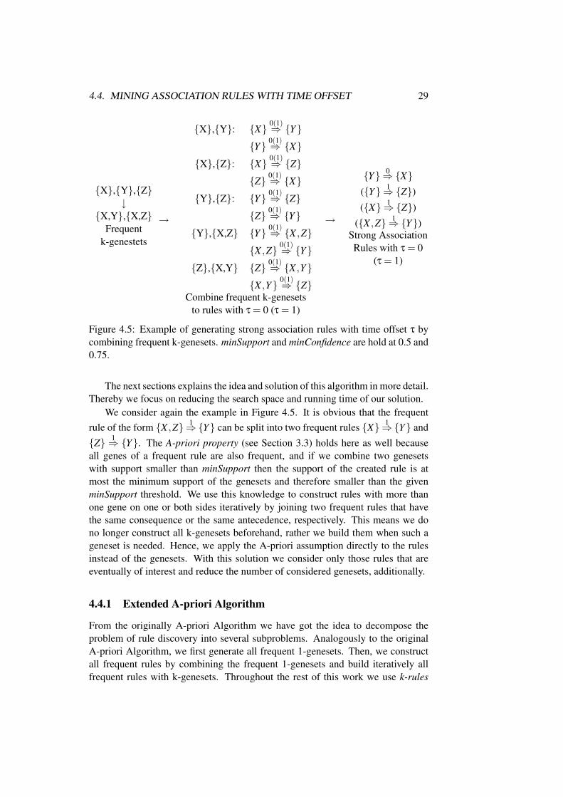
Figure 4.5: Example of generating strong association rules with time offset τ bycombining frequent k-genesets. minSupport and minConfidence are hold at 0.5 and0.75.
The next sections explains the idea and solution of this algorithm in more detail.Thereby we focus on reducing the search space and running time of our solution.
We consider again the example in Figure 4.5. It is obvious that the frequentrule of the form {X ,Z} 1⇒{Y} can be split into two frequent rules {X} 1⇒{Y} and{Z} 1⇒ {Y}. The A-priori property (see Section 3.3) holds here as well becauseall genes of a frequent rule are also frequent, and if we combine two genesetswith support smaller than minSupport then the support of the created rule is atmost the minimum support of the genesets and therefore smaller than the givenminSupport threshold. We use this knowledge to construct rules with more thanone gene on one or both sides iteratively by joining two frequent rules that havethe same consequence or the same antecedence, respectively. This means we dono longer construct all k-genesets beforehand, rather we build them when such ageneset is needed. Hence, we apply the A-priori assumption directly to the rulesinstead of the genesets. With this solution we consider only those rules that areeventually of interest and reduce the number of considered genesets, additionally.
4.4.1 Extended A-priori Algorithm
From the originally A-priori Algorithm we have got the idea to decompose theproblem of rule discovery into several subproblems. Analogously to the originalA-priori Algorithm, we first generate all frequent 1-genesets. Then, we constructall frequent rules by combining the frequent 1-genesets and build iteratively allfrequent rules with k-genesets. Throughout the rest of this work we use k-rules
30CHAPTER 4. MINING ASSOCIATION RULES ON GENE EXPRESSION DATA
to describe a rule that has k-genesets on one or both sides. We apply the A-prioriproperty as described before directly to the rulesets. This procedure results in amuch smaller number of considered genesets and rules.
Step 1 Generation of frequent 1-genesets: First, the set of frequent 1-genesets isfound. The seach space of the considered genesets is reduced by removingthose genes that obvious cannot occur in a frequent rule.
Step 2 Generation of frequent 1-rules: Now, we construct association rules witha fixed time offset τ by combining two frequent 1-genesets. We cannot con-clude immediately that these rules have minSupport rather we have to checkhow often the left side of the rule (frequent 1-geneset) is active and exact τ
time units later the right side of the rule (the second frequent 1-geneset) be-comes active as well. Rules having minSupport are used as as seed to buildk-rules in the next step.
Step 3 Generation of frequent k-rules: In the third part, we use the A-priori prop-erty to construct rules with more than one gene on the left or right side. Giventwo rules that have the same consequence (or antecedence, respectively,) wejoin the genesets of the antecedence (or consequence) by using the A-prioriproperty. Because of the A-priori property we know that all subsets of thejoined geneset are frequent, but we have to check whether the joined genesetitself has minSupport. If this is the case, we need an additional step to checkas well if the support of the new rule is at least minSupport. This means wehave to count how often the antecedence (or consequence) is active followedby an activation of the joined right side (or left side) exactly τ time unitslater. k-rules having minSupport are used to build k+1-rules.
Step 4 Output Strong Association Rules If no more rules can be build we haveto compute the confidence of each rule. If this value is greater or equalto the appropriate parameter minConfidence the rule is returned as a strongassociation rule.
Example 4.4 (Extended A-priori Algorithm) We use again the gene expressiondata in Figure 4.3. We want to discover strong association rules with a time offsetτ = 0 (τ = 1) that fulfill a minSupport of 0.5 and a minConfidence of 0.75.
1. The initial frequent 1-genesets are {X},{Y}, and {Z} that are active at least5 times.
2. We contruct association rules with time offset τ = 0 (τ = 1) that have onegene on each side by combining the frequent 1-genesets. Figure 4.6 showsall frequent rules that are used as a seed in the next iterative step.
3. We join all frequent rules that have the same consequence (or antecedence,respectively). In this example the rules {X} 1⇒ {Z} and {Y} 1⇒ {Z} have
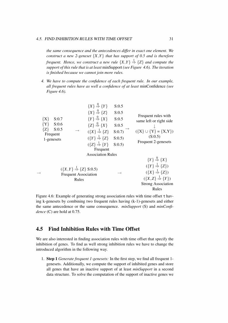
4.5. FIND INHIBITION RULES WITH TIME OFFSET 31
the same consequence and the antecedences differ in exact one element. Weconstruct a new 2-geneset {X ,Y} that has support of 0.5 and is therefore
frequent. Hence, we construct a new rule {X ,Y} 1⇒ {Z} and compute thesupport of this rule that is at least minSupport (see Figure 4.6). The iterationis finished because we cannot join more rules.
4. We have to compute the confidence of each frequent rule. In our example,all frequent rules have as well a confidence of at least minConfidence (seeFigure 4.6).
{X} S:0.7{Y} S:0.6{Z} S:0.5
Frequent1-genesets
→
{X} 0⇒{Y} S:0.5
{X} 0⇒{Z} S:0.5
{Y} 0⇒{X} S:0.5
{Z} 0⇒{X} S:0.5
({X} 1⇒{Z} S:0.7)
({Y} 1⇒{Z} S:0.5)
({Z} 1⇒{Y} S:0.5)Frequent
Association Rules
→
Frequent rules withsame left or right side
↓({X} ∪ {Y} = {X,Y})
(S:0.5)Frequent 2-genesets
→({X ,Y} 1⇒{Z} S:0.5)Frequent Association
Rules
→
{Y} 0⇒{X}({Y} 1⇒{Z})({X} 1⇒{Z})
({X ,Z} 1⇒{Y})Strong Association
Rules
Figure 4.6: Example of generating strong association rules with time offset τ hav-ing k-genesets by combining two frequent rules having (k-1)-genesets and eitherthe same antecedence or the same consequence. minSupport (S) and minConfi-dence (C) are hold at 0.75.
4.5 Find Inhibition Rules with Time Offset
We are also interested in finding association rules with time offset that specify theinhibition of genes. To find as well strong inhibition rules we have to change theintroduced algorithm in the following way.
1. Step 1 Generate frequent 1-genesets: In the first step, we find all frequent 1-genesets. Additionally, we compute the support of inhibited genes and storeall genes that have an inactive support of at least minSupport in a seconddata structure. To solve the computation of the support of inactive genes we
32CHAPTER 4. MINING ASSOCIATION RULES ON GENE EXPRESSION DATA
provide a second set of transactions that contains all inactive genes at onetimestamp (see Section 4.3). Now we can compute the inactive support of agene by counting in how many timestamps the gene is contained.
2. Step 2 Generate frequent 1-rules: To build inhibition rules we combine a 1-geneset with active support (left side) and a 1-geneset with inactive support(right side) at least minSupport. The support counts how often the left sideis active and exactly τ time units later the right side becomes inactive.
3. Step 3 Generate frequent k-rules: We use the frequent k-1-rules from theprevious step to build frequent inhibition rules with k-genesets. Analogueto the algorithm for building frequent activation rules we combine two rulesif they have the same antecedence (or consequence) and the right side (orleft side) differs in exact one element. The support is computed by countinghow often the antecedence is active and exact τ time units later the right sidebecomes inactive.
4. Step 4 Output Strong Association Rules Computing the confidence of inhi-bition rules works in the same way as for activation rules by dividing thesupport of the rule by the support of the left side.
In the same way we can adapt this algorithm to find as well a second type ofactivation and inhibition rules that occur after an inhibition of a gene i.e. activationrules of the form X τ⇒ Y and inhibition rules of the form X τ⇒ Y .
4.6 Time Offsets
In the previous examples it is obvious that a time offset of 4 or 5 is not significantto find good association rules. On gene expression data with 10 sample points sucha rule can occur only five or six times and gives no evidence of its correctness.There can be a failure in the gene expression data, or an activation or inhibition ofthe left and right side of the rule at random. Therefore, the time offset have to bechosen wise depending on the number of the considered sample points. We providea parameter, called timeT that defines the time offset and has to be specified by theuser.
The occurrences of a rule depends on the current phase of the cell cycle. Un-fortunately, such a rule can occur between two sample points, or not exactly aftera given number of time points. To enhance our search results and to find strongerassociation rules, we define our time offset τ more weakly. This means we do nolonger compute how often a rule occurs after exact τ time points but how often itoccurs approximately after τ time points.
We introduce a second parameter called windowW, also specified by the user,that defines the interval in which a rule can occur. This interval includes the naturalnumbers between timeT - windowW and timeT + windowW, i.e.
τ ∈ [timeT−windowW, timeT +windowW]
4.7. SYNTACTIC CONSTRAINTS ON RULES 33
.
4.7 Syntactic Constraints on Rules
The new algorithm constructs rules with any number of genes on the left and rightside. Sometimes, we are interested in rules with a single gene on one or maybe bothsides. Therefore, we provide upper bounds called maxA and maxB that restrict thenumber of genes on the left and right side.
The algorithm constructs only those rules with at most maxA genes on the leftside and maxB genes on the right side. The advantage of this solution is that thealgorithm need to compute only those k-genesets with k≤max {maxA, maxB} thatreduces the number of possible strong association rules for example by 50 percentif we allow only one gene on one side.
4.8 Mining co-regulated Genes
It is important to know that a various number of genes are co-regulated. Theirexpression levels are often related to each other, this means they are concurrentlyactive or inactive. We define activation and inhibition rules for co-regulated genesas follows. An activation rule of co-regulated genes occurs in two cases if bothsides of the rule are active or if both sides are inactive. An inhibition rule of co-regulated genes occurs if one of the sides is active and the other one is inactive.
The data sets of Cho and Spellman [42, 12] contain expression levels of genesmeasured during the different phases of a cell cycle. For finding interactions ofco-regulated genes within this data set it is straightforward to count both how oftena gene or geneset is active and inactive for all timestamps. Hence, for activationrules we have to compute both, how often a geneset is active and followed by anactive geneset and how often a geneset is inactive followed by an inactive geneset.Analogously for inhibition rules we have to compute how often a geneset is activefollowed by an inactive geneset and how often a geneset is inactive followed by anactive geneset.
These changes influence the introduced algorithm and the definition of min-Support and minConfidence. We discussed in Section 4.5 how we can adapt ouralgorithm to find as well these kind of rules. The support of co-regulated genes isdefined as the sum of the active (Equation 3.1) and inactive (Equation 3.2) support(see Definition 3.9).
Definition 4.2 (Support co-regulated Genes) Let X be a subset of I. The supportof a co-regulated geneset X, denoted Supportco−regulated(X), is defined as
Supportco−regulated(X) = Support(X)+Support(X).
3
34CHAPTER 4. MINING ASSOCIATION RULES ON GENE EXPRESSION DATA
The support of activation rules of co-regulated genes is defined as the sumof the active rule support(Equation 3.3) (see Definition 3.10), which counts howoften both sides are active, and the inactive rule support, which counts how oftenboth sides are inactive. The support of inhibition rules of co-regulated genes isdefined as the sum of the active rule support (Equation 3.4) (see Definition 3.10),which counts how often the left side is active and the right side is inactive, and theinactive rule support ,which counts how often the left side is inactive and the rightside is active. We represent inactive activation and inactive inhibition rules withtime offset in the following way.
Definition 4.3 (Inactive Association Rule with Time Offset) Let X and Y be sub-sets of I with X ∩Y = /0, t a timestamp and τ an integer with τ≥ 0. An associationrule
X τ⇒ Y
is called inactive activation rule with time offset τ, or inactive activation rule withtime τ for short if Status(X,t) = Status(Y,t+τ) = 0. An association rule
X τ⇒ Y
is called inactive inhibition rule with time offset τ, or inactive inhibition with timeτ for short, if Status(X,t) = 0 and Status(Y,t+τ) = 1. 3
To compute the support of activation and inhibition rules of co-regulated geneswe need two additional definitions of rule support. Definition 4.4 defines the sup-port of inactive activation and inhibition rules.
Definition 4.4 (Rule Support extended) Let X and Y be subsets of I, T a multisetof transactions, r := X τ⇒Y an inactive activation rule and r′ := X τ⇒Y an inactiveinhibition rule.
The support of r with respect to T , denoted Support(r), is defined as
Support(r) :=1T
T
∑t=1
(1−Status(X , t)) · (1−Status(Y, t + τ)).
The support of the inhibition rule r′ with respect to T , denoted Support(r′), isdefined as
Support(r′) :=1T
T
∑t=1
(1−Status(X , t)) ·Status(Y, t + τ).
3
Using the definition of active (Definition 3.10) and inactive (Definition 4.4)support of activation and inhibitions rules we can compute the support of rules ofco-regulated genes in the following way.
4.8. MINING CO-REGULATED GENES 35
Definition 4.5 (Rule Support of co-regulated Genes) Let X and Y be co-regulatedgenesets, i.e. X ,Y ∈ I, r := X τ⇒Y and r′ := X τ⇒Y activation and inhibition rules.The support of the activation rule, denoted Supportco−regulated(r), is defined as
Supportco−regulated(r) = Support(X τ⇒ Y )+Support(X τ⇒ Y )
The support of the inhibition rule, denoted Supportco−regulated(r′), is defined as
Supportco−regulated(r′) = Support(X τ⇒ Y )+Support(X τ⇒ Y ).
3
Before running the algorithm the user can select whether he wants to searchfor co-regulated genes or not. This additional parameter is called strategy (searchstrategy).

36CHAPTER 4. MINING ASSOCIATION RULES ON GENE EXPRESSION DATA
Chapter 5
Implementation
5.1 Introduction
To assess the applicability and feasibility of the described algorithm we devel-oped a database application that implements our extended A-priori algorithm asdescribed in Chapter 4. We provide an interactive toolkit that allows the user to in-teract with the algorithm by modifying different parameters, e.g. minSupport andminConfidence. Allowing different kind of visualizations of the available genesand retrieved rules facilitates effective data mining by allowing the user to identifyrules of interest in a comfortable manner, and to improve the future search resultsby suitably adapting the parameters.
In the following we explain the implementation of the extended A-priori algo-rithm, the underlying functionality of the program and the helpful features of theuser interface with its various possibilities to represent genes and rules.
5.2 Overview
The program is implemented in Java 5.0 using the graphical library SWT/JFace todesign the interactive toolkit (see Section 5.6). The given gene expression data andthe retrieved rules are stored in an relational database. We are using the Oracle10g 1
database. The program mainly consists of the following components:
1. Parser and preprocessor of the gene expression data: loads the time seriesfrom a text file into the database, and removes genes that have too manymissing points.
2. Connection to the database: builds the interface between the program andthe database, loads gene expression data and stores the retrieved rules.
3. Extended A-priori algorithm: searches for strong association rules with timeoffset in the gene expression data.
1http://www.oracle.com/index.html (January 2006)
37
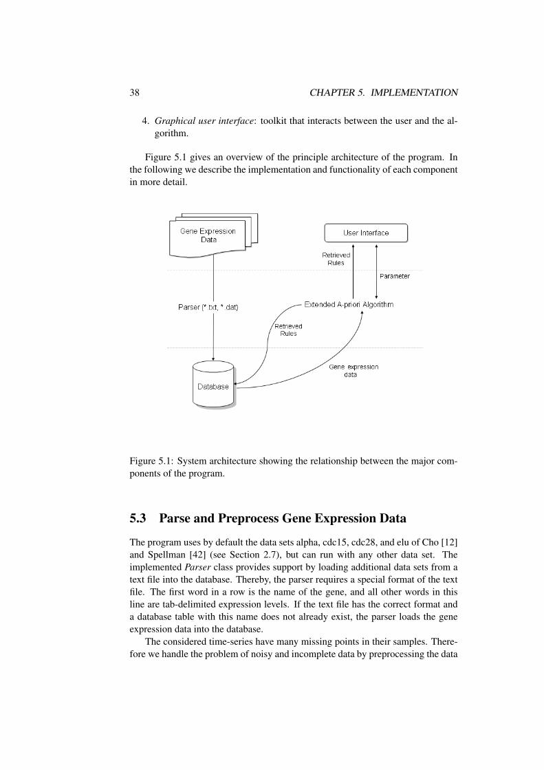
38 CHAPTER 5. IMPLEMENTATION
4. Graphical user interface: toolkit that interacts between the user and the al-gorithm.
Figure 5.1 gives an overview of the principle architecture of the program. Inthe following we describe the implementation and functionality of each componentin more detail.
Figure 5.1: System architecture showing the relationship between the major com-ponents of the program.
5.3 Parse and Preprocess Gene Expression Data
The program uses by default the data sets alpha, cdc15, cdc28, and elu of Cho [12]and Spellman [42] (see Section 2.7), but can run with any other data set. Theimplemented Parser class provides support by loading additional data sets from atext file into the database. Thereby, the parser requires a special format of the textfile. The first word in a row is the name of the gene, and all other words in thisline are tab-delimited expression levels. If the text file has the correct format anda database table with this name does not already exist, the parser loads the geneexpression data into the database.
The considered time-series have many missing points in their samples. There-fore we handle the problem of noisy and incomplete data by preprocessing the data
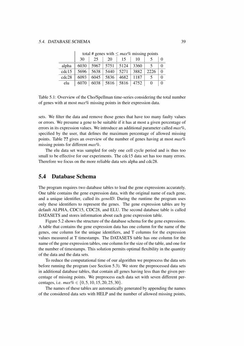
5.4. DATABASE SCHEMA 39
total # genes with ≤ max% missing points30 25 20 15 10 5 0
alpha 6030 5967 5751 5124 3360 5 0cdc15 5696 5638 5440 5271 3882 2226 0cdc28 6093 6045 5836 4682 1187 5 0
elu 6070 6038 5816 5816 4752 0 0
Table 5.1: Overview of the Cho/Spellman time-series considering the total numberof genes with at most max% missing points in their expression data.
sets. We filter the data and remove those genes that have too many faulty valuesor errors. We presume a gene to be suitable if it has at most a given percentage oferrors in its expression values. We introduce an additional parameter called max%,specified by the user, that defines the maximum percentage of allowed missingpoints. Table ?? gives an overview of the number of genes having at most max%missing points for different max%.
The elu data set was sampled for only one cell cycle period and is thus toosmall to be effective for our experiments. The cdc15 data set has too many errors.Therefore we focus on the more reliable data sets alpha and cdc28.
5.4 Database Schema
The program requires two database tables to load the gene expressions accurately.One table contains the gene expression data, with the original name of each gene,and a unique identifier, called its geneID. During the runtime the program usesonly these identifiers to represent the genes. The gene expression tables are bydefault ALPHA, CDC15, CDC28, and ELU. The second database table is calledDATASETS and stores information about each gene expression table.
Figure 5.2 shows the structure of the database schema for the gene expressions.A table that contains the gene expression data has one column for the name of thegenes, one column for the unique identifiers, and T columns for the expressionvalues measured at T timestamps. The DATASETS table has one column for thename of the gene expression tables, one column for the size of the table, and one forthe number of timestamps. This solution permits optimal flexibility in the quantityof the data and the data sets.
To reduce the computational time of our algorithm we preprocess the data setsbefore running the program (see Section 5.3). We store the preprocessed data setsin additional database tables, that contain all genes having less than the given per-centage of missing points. We preprocess each data set with seven different per-centages, i.e. max% ∈ {0,5,10,15,20,25,30}.
The names of these tables are automatically generated by appending the namesof the considered data sets with HELP and the number of allowed missing points,
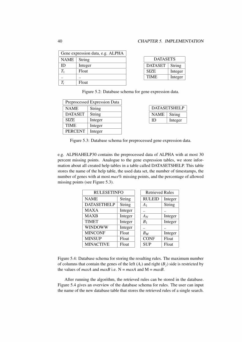
40 CHAPTER 5. IMPLEMENTATION
Gene expression data, e.g. ALPHANAME StringID IntegerT1 Float.. ..Ti Float
DATASETSDATASET StringSIZE IntegerTIME Integer
Figure 5.2: Database schema for gene expression data.
Preprocessed Expression DataNAME StringDATASET StringSIZE IntegerTIME IntegerPERCENT Integer
DATASETSHELPNAME StringID Integer
Figure 5.3: Database schema for preprocessed gene expression data.
e.g. ALPHAHELP30 contains the preprocessed data of ALPHA with at most 30percent missing points. Analogue to the gene expression tables, we store infor-mation about all created help tables in a table called DATASETSHELP. This tablestores the name of the help table, the used data set, the number of timestamps, thenumber of genes with at most max% missing points, and the percentage of allowedmissing points (see Figure 5.3).
RULESETINFONAME StringDATASETHELP StringMAXA IntegerMAXB IntegerTIMET IntegerWINDOWW IntegerMINCONF FloatMINSUP FloatMINACTIVE Float
Retrieved RulesRULEID IntegerA1 String.. ..AN IntegerB1 Integer.. ..BM IntegerCONF FloatSUP Float
Figure 5.4: Database schema for storing the resulting rules. The maximum numberof columns that contain the genes of the left (Ai) and right (B j) side is restricted bythe values of maxA and maxB i.e. N = maxA and M = maxB.
After running the algorithm, the retrieved rules can be stored in the database.Figure 5.4 gives an overview of the database schema for rules. The user can inputthe name of the new database table that stores the retrieved rules of a single search.
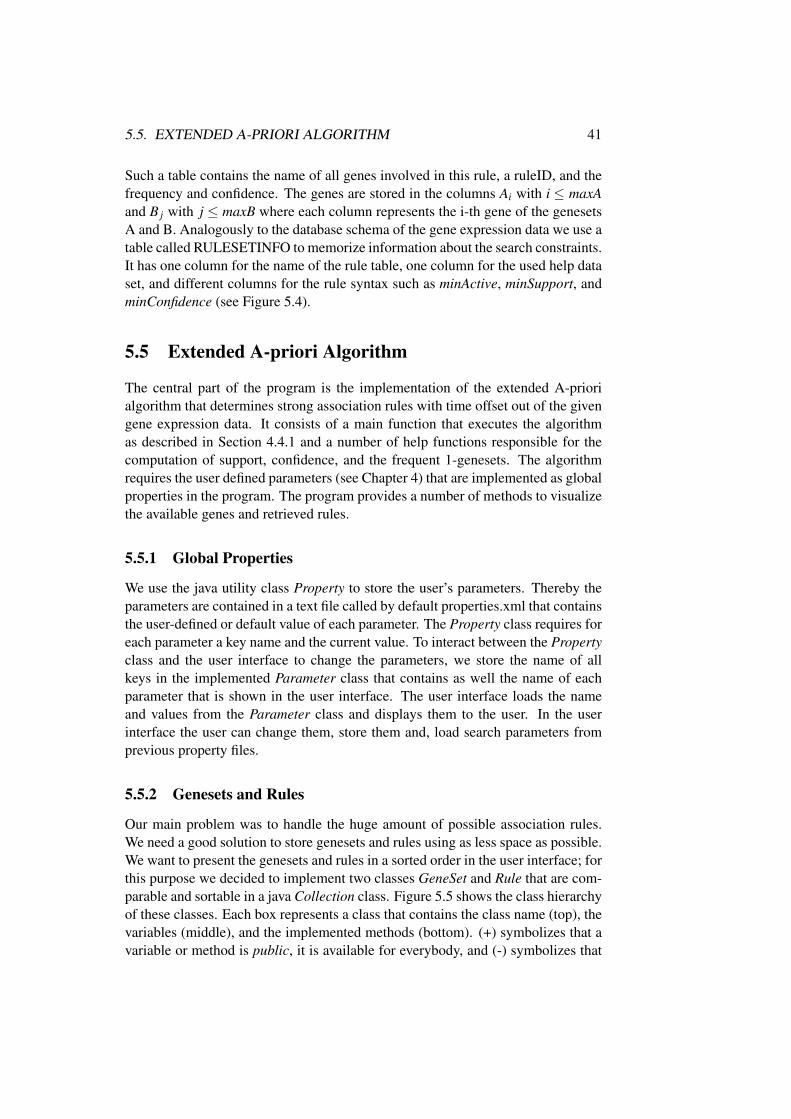
5.5. EXTENDED A-PRIORI ALGORITHM 41
Such a table contains the name of all genes involved in this rule, a ruleID, and thefrequency and confidence. The genes are stored in the columns Ai with i ≤ maxAand B j with j ≤ maxB where each column represents the i-th gene of the genesetsA and B. Analogously to the database schema of the gene expression data we use atable called RULESETINFO to memorize information about the search constraints.It has one column for the name of the rule table, one column for the used help dataset, and different columns for the rule syntax such as minActive, minSupport, andminConfidence (see Figure 5.4).
5.5 Extended A-priori Algorithm
The central part of the program is the implementation of the extended A-priorialgorithm that determines strong association rules with time offset out of the givengene expression data. It consists of a main function that executes the algorithmas described in Section 4.4.1 and a number of help functions responsible for thecomputation of support, confidence, and the frequent 1-genesets. The algorithmrequires the user defined parameters (see Chapter 4) that are implemented as globalproperties in the program. The program provides a number of methods to visualizethe available genes and retrieved rules.
5.5.1 Global Properties
We use the java utility class Property to store the user’s parameters. Thereby theparameters are contained in a text file called by default properties.xml that containsthe user-defined or default value of each parameter. The Property class requires foreach parameter a key name and the current value. To interact between the Propertyclass and the user interface to change the parameters, we store the name of allkeys in the implemented Parameter class that contains as well the name of eachparameter that is shown in the user interface. The user interface loads the nameand values from the Parameter class and displays them to the user. In the userinterface the user can change them, store them and, load search parameters fromprevious property files.
5.5.2 Genesets and Rules
Our main problem was to handle the huge amount of possible association rules.We need a good solution to store genesets and rules using as less space as possible.We want to present the genesets and rules in a sorted order in the user interface; forthis purpose we decided to implement two classes GeneSet and Rule that are com-parable and sortable in a java Collection class. Figure 5.5 shows the class hierarchyof these classes. Each box represents a class that contains the class name (top), thevariables (middle), and the implemented methods (bottom). (+) symbolizes that avariable or method is public, it is available for everybody, and (-) symbolizes that
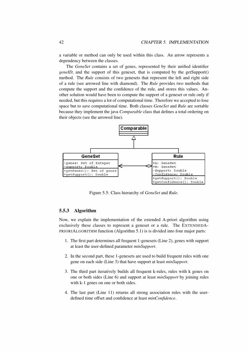
42 CHAPTER 5. IMPLEMENTATION
a variable or method can only be used within this class. An arrow represents adependency between the classes.
The GeneSet contains a set of genes, represented by their unified identifiergeneID, and the support of this geneset, that is computed by the getSupport()method. The Rule consists of two genesets that represent the left and right sideof a rule (see arrowed line with diamond). The Rule provides two methods thatcompute the support and the confidence of the rule, and stores this values. An-other solution would have been to compute the support of a geneset or rule only ifneeded, but this requires a lot of computational time. Therefore we accepted to losespace but to save computational time. Both classes GeneSet and Rule are sortablebecause they implement the java Comparable class that defines a total ordering ontheir objects (see the arrowed line).
Figure 5.5: Class hierarchy of GeneSet and Rule.
5.5.3 Algorithm
Now, we explain the implementation of the extended A-priori algorithm usingexclusively these classes to represent a geneset or a rule. The EXTENDEDA-PRIORIALGORITHM function (Algorithm 5.1) is is divided into four major parts:
1. The first part determines all frequent 1-genesets (Line 2), genes with supportat least the user-defined parameter minSupport.
2. In the second part, these 1-genesets are used to build frequent rules with onegene on each side (Line 3) that have support at least minSupport.
3. The third part iteratively builds all frequent k-rules, rules with k genes onone or both sides (Line 6) and support at least minSupport by joining ruleswith k-1 genes on one or both sides.
4. The last part (Line 11) returns all strong association rules with the user-defined time offset and confidence at least minConfidence.
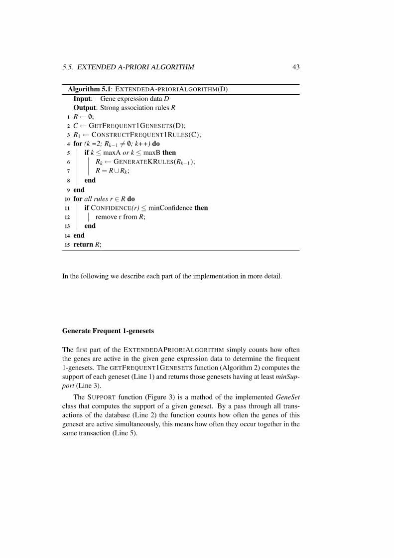
5.5. EXTENDED A-PRIORI ALGORITHM 43
Algorithm 5.1: EXTENDEDA-PRIORIALGORITHM(D)Input: Gene expression data DOutput: Strong association rules RR← /0;1
C← GETFREQUENT1GENESETS(D);2
R1← CONSTRUCTFREQUENT1RULES(C);3
for (k =2; Rk−1 6= /0; k++) do4
if k ≤ maxA or k ≤ maxB then5
Rk← GENERATEKRULES(Rk−1);6
R = R∪Rk;7
end8
end9
for all rules r ∈ R do10
if CONFIDENCE(r) ≤ minConfidence then11
remove r from R;12
end13
end14
return R;15
In the following we describe each part of the implementation in more detail.
Generate Frequent 1-genesets
The first part of the EXTENDEDAPRIORIALGORITHM simply counts how oftenthe genes are active in the given gene expression data to determine the frequent1-genesets. The GETFREQUENT1GENESETS function (Algorithm 2) computes thesupport of each geneset (Line 1) and returns those genesets having at least minSup-port (Line 3).
The SUPPORT function (Figure 3) is a method of the implemented GeneSetclass that computes the support of a given geneset. By a pass through all trans-actions of the database (Line 2) the function counts how often the genes of thisgeneset are active simultaneously, this means how often they occur together in thesame transaction (Line 5).
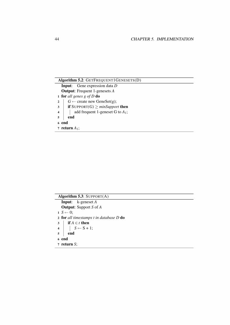
44 CHAPTER 5. IMPLEMENTATION
Algorithm 5.2: GETFREQUENT1GENESETS(D)Input: Gene expression data DOutput: Frequent 1-genesets Afor all genes g of D do1
G← create new GeneSet(g);2
if SUPPORT(G) ≥ minSupport then3
add frequent 1-geneset G to A1;4
end5
end6
return A1;7
Algorithm 5.3: SUPPORT(A)Input: k-geneset AOutput: Support S of AS← 0;1
for all timestamps t in database D do2
if A ∈ t then3
S← S + 1;4
end5
end6
return S;7
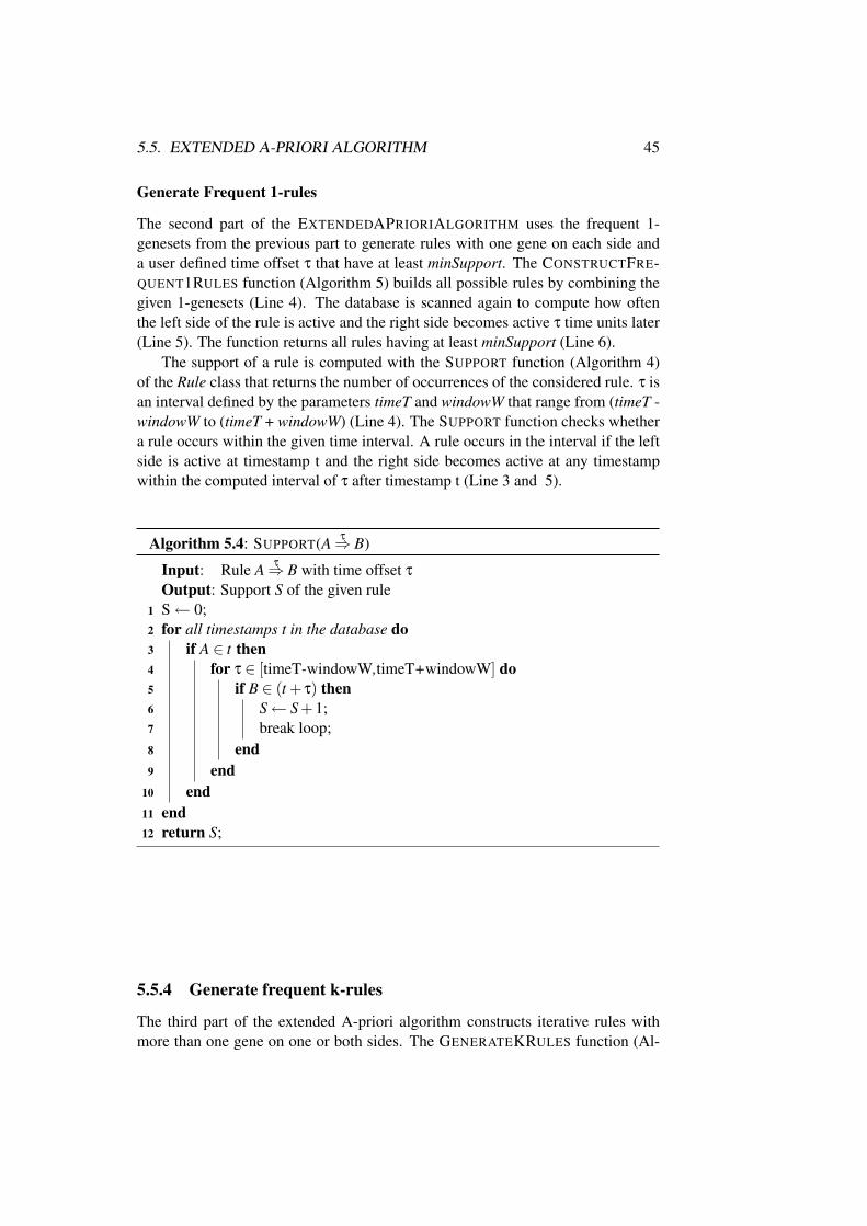
5.5. EXTENDED A-PRIORI ALGORITHM 45
Generate Frequent 1-rules
The second part of the EXTENDEDAPRIORIALGORITHM uses the frequent 1-genesets from the previous part to generate rules with one gene on each side anda user defined time offset τ that have at least minSupport. The CONSTRUCTFRE-QUENT1RULES function (Algorithm 5) builds all possible rules by combining thegiven 1-genesets (Line 4). The database is scanned again to compute how oftenthe left side of the rule is active and the right side becomes active τ time units later(Line 5). The function returns all rules having at least minSupport (Line 6).
The support of a rule is computed with the SUPPORT function (Algorithm 4)of the Rule class that returns the number of occurrences of the considered rule. τ isan interval defined by the parameters timeT and windowW that range from (timeT -windowW to (timeT + windowW) (Line 4). The SUPPORT function checks whethera rule occurs within the given time interval. A rule occurs in the interval if the leftside is active at timestamp t and the right side becomes active at any timestampwithin the computed interval of τ after timestamp t (Line 3 and 5).
Algorithm 5.4: SUPPORT(A τ⇒ B)
Input: Rule A τ⇒ B with time offset τ
Output: Support S of the given ruleS← 0;1
for all timestamps t in the database do2
if A ∈ t then3
for τ ∈ [timeT-windowW,timeT+windowW] do4
if B ∈ (t + τ) then5
S← S +1;6
break loop;7
end8
end9
end10
end11
return S;12
5.5.4 Generate frequent k-rules
The third part of the extended A-priori algorithm constructs iterative rules withmore than one gene on one or both sides. The GENERATEKRULES function (Al-
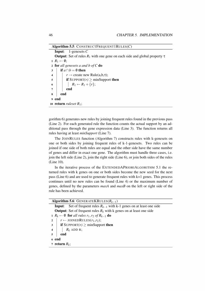
46 CHAPTER 5. IMPLEMENTATION
Algorithm 5.5: CONSTRUCTFREQUENT1RULES(C)Input: 1-genesets COutput: Set of rules R1 with one gene on each side and global property τ
R1← /0;1
for all genesets a and b of C do2
if a∩b = /0 then3
r→ create new Rule(a,b,τ);4
if SUPPORT(r) ≥ minSupport then5
R1← R1 +{r};6
end7
end8
end9
return ruleset R1;10
gorithm 6) generates new rules by joining frequent rules found in the previous pass(Line 2). For each generated rule the function counts the actual support by an ad-ditional pass through the gene expression data (Line 3). The function returns allrules having at least minSupport (Line 7).
The JOINRULES function (Algorithm 7) constructs rules with k-genesets onone or both sides by joining frequent rules of k-1-genesets. Two rules can bejoined if one side of both rules are equal and the other side have the same numberof genes and differ in exact one gene. The algorithm must handle three cases, i.e.join the left side (Line 2), join the right side (Line 6), or join both sides of the rules(Line 10).
In the iterative process of the EXTENDEDAPRIORIALGORITHM 5.1 the re-turned rules with k genes on one or both sides become the new seed for the nextpass (Line 6) and are used to generate frequent rules with k+1 genes. This processcontinues until no new rules can be found (Line 4) or the maximum number ofgenes, defined by the parameters maxA and maxB on the left or right side of therule has been achieved.
Algorithm 5.6: GENERATEKRULES(Rk−1)Input: Set of frequent rules Rk−1 with k-1 genes on at least one sideOutput: Set of frequent rules Rk with k genes on at least one sideRk← /0 for all rules r1,r2 of Rk−1 do1
r← JOINEDRULES(r1,r2);2
if SUPPORT(r) ≥ minSupport then3
Rk ADD R;4
end5
end6
return Rk;7
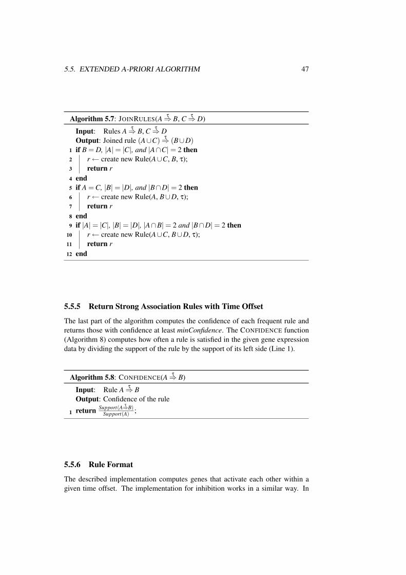
5.5. EXTENDED A-PRIORI ALGORITHM 47
Algorithm 5.7: JOINRULES(A τ⇒ B, C τ⇒ D)
Input: Rules A τ⇒ B, C τ⇒ DOutput: Joined rule (A∪C) τ⇒ (B∪D)if B = D, |A|= |C|, and |A∩C|= 2 then1
r← create new Rule(A∪C, B, τ);2
return r3
end4
if A = C, |B|= |D|, and |B∩D|= 2 then5
r← create new Rule(A, B∪D, τ);6
return r7
end8
if |A|= |C|, |B|= |D|, |A∩B|= 2 and |B∩D|= 2 then9
r← create new Rule(A∪C, B∪D, τ);10
return r11
end12
5.5.5 Return Strong Association Rules with Time Offset
The last part of the algorithm computes the confidence of each frequent rule andreturns those with confidence at least minConfidence. The CONFIDENCE function(Algorithm 8) computes how often a rule is satisfied in the given gene expressiondata by dividing the support of the rule by the support of its left side (Line 1).
Algorithm 5.8: CONFIDENCE(A τ⇒ B)
Input: Rule A τ⇒ BOutput: Confidence of the rule
return Support(A τ⇒B)Support(A) ;1
5.5.6 Rule Format
The described implementation computes genes that activate each other within agiven time offset. The implementation for inhibition works in a similar way. In
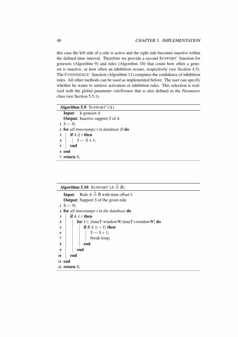
48 CHAPTER 5. IMPLEMENTATION
this case the left side of a rule is active and the right side becomes inactive withinthe defined time interval. Therefore we provide a second SUPPORT’ function forgenesets (Algorithm 9) and rules (Algorithm 10) that count how often a gene-set is inactive, or how often an inhibition occurs, respectively (see Section 4.5).The CONFIDENCE’ function (Algorithm 11) computes the confidence of inhibitionrules. All other methods can be used as implemented before. The user can specifywhether he wants to retrieve activation or inhibition rules. This selection is real-ized with the global parameter ruleFormat that is also defined in the Parameterclass (see Section 5.5.1).
Algorithm 5.9: SUPPORT’(A)Input: k-geneset AOutput: Inactive support S of AS← 0;1
for all timestamps t in database D do2
if A /∈ t then3
S← S + 1;4
end5
end6
return S;7
Algorithm 5.10: SUPPORT’(A τ⇒ B)
Input: Rule A τ⇒ B with time offset τ
Output: Support S of the given ruleS← 0;1
for all timestamps t in the database do2
if A ∈ t then3
for τ ∈ [timeT-windowW,timeT+windowW] do4
if B /∈ (t + τ) then5
S← S +1;6
break loop;7
end8
end9
end10
end11
return S;12
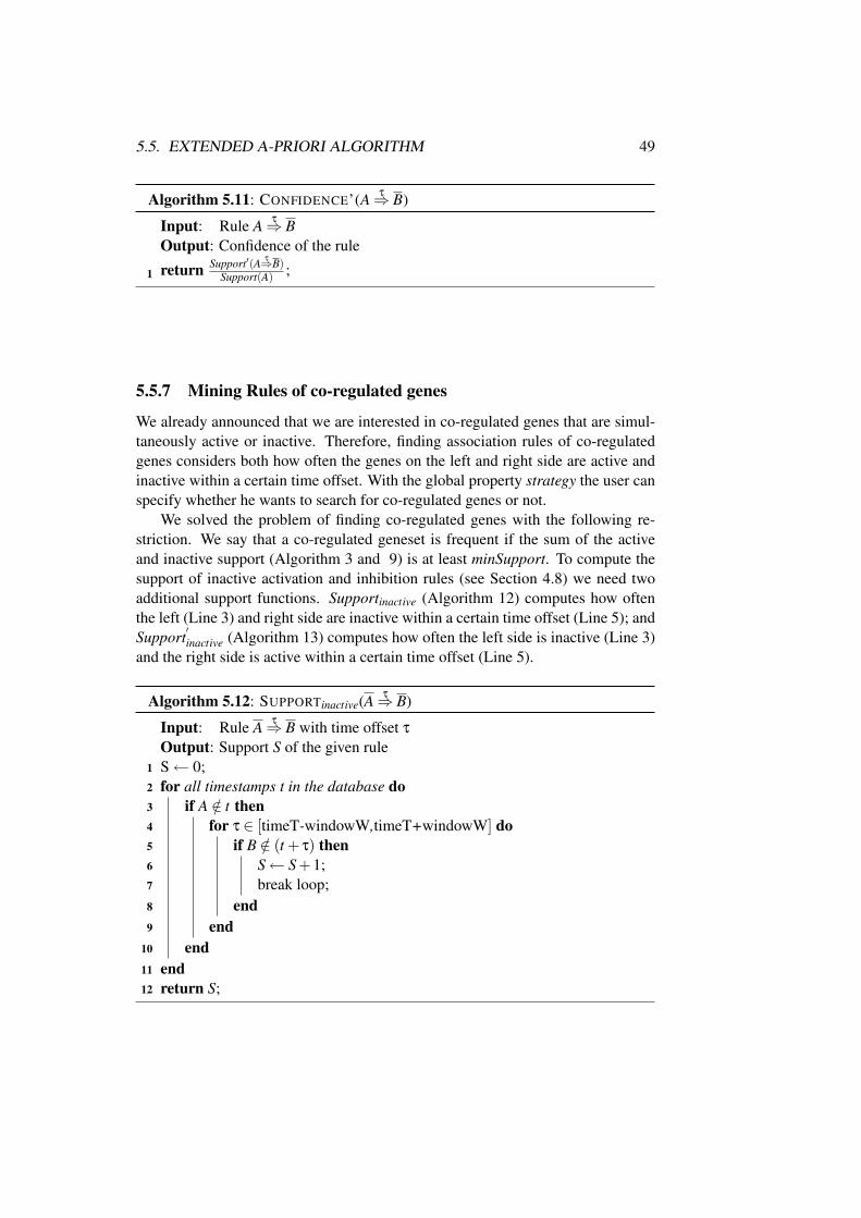
5.5. EXTENDED A-PRIORI ALGORITHM 49
Algorithm 5.11: CONFIDENCE’(A τ⇒ B)
Input: Rule A τ⇒ BOutput: Confidence of the rule
return Support′(A τ⇒B)Support(A) ;1
5.5.7 Mining Rules of co-regulated genes
We already announced that we are interested in co-regulated genes that are simul-taneously active or inactive. Therefore, finding association rules of co-regulatedgenes considers both how often the genes on the left and right side are active andinactive within a certain time offset. With the global property strategy the user canspecify whether he wants to search for co-regulated genes or not.
We solved the problem of finding co-regulated genes with the following re-striction. We say that a co-regulated geneset is frequent if the sum of the activeand inactive support (Algorithm 3 and 9) is at least minSupport. To compute thesupport of inactive activation and inhibition rules (see Section 4.8) we need twoadditional support functions. Supportinactive (Algorithm 12) computes how oftenthe left (Line 3) and right side are inactive within a certain time offset (Line 5); andSupport
′inactive (Algorithm 13) computes how often the left side is inactive (Line 3)
and the right side is active within a certain time offset (Line 5).
Algorithm 5.12: SUPPORTinactive(A τ⇒ B)
Input: Rule A τ⇒ B with time offset τ
Output: Support S of the given ruleS← 0;1
for all timestamps t in the database do2
if A /∈ t then3
for τ ∈ [timeT-windowW,timeT+windowW] do4
if B /∈ (t + τ) then5
S← S +1;6
break loop;7
end8
end9
end10
end11
return S;12
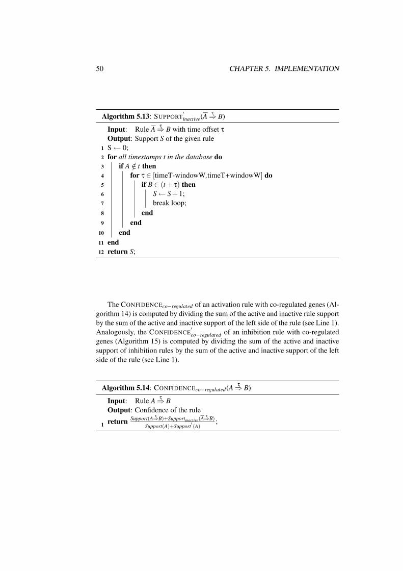
50 CHAPTER 5. IMPLEMENTATION
Algorithm 5.13: SUPPORT′inactive(A τ⇒ B)
Input: Rule A τ⇒ B with time offset τ
Output: Support S of the given ruleS← 0;1
for all timestamps t in the database do2
if A /∈ t then3
for τ ∈ [timeT-windowW,timeT+windowW] do4
if B ∈ (t + τ) then5
S← S +1;6
break loop;7
end8
end9
end10
end11
return S;12
The CONFIDENCEco−regulated of an activation rule with co-regulated genes (Al-gorithm 14) is computed by dividing the sum of the active and inactive rule supportby the sum of the active and inactive support of the left side of the rule (see Line 1).Analogously, the CONFIDENCE
′co−regulated of an inhibition rule with co-regulated
genes (Algorithm 15) is computed by dividing the sum of the active and inactivesupport of inhibition rules by the sum of the active and inactive support of the leftside of the rule (see Line 1).
Algorithm 5.14: CONFIDENCEco−regulated(A τ⇒ B)
Input: Rule A τ⇒ BOutput: Confidence of the rule
return Support(A τ⇒B)+Supportinactive(Aτ⇒B)
Support(A)+Support′ (A)
;1
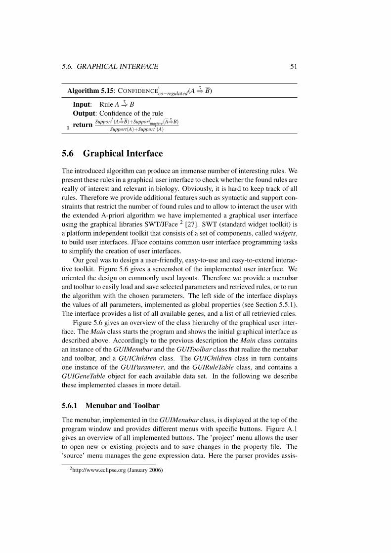
5.6. GRAPHICAL INTERFACE 51
Algorithm 5.15: CONFIDENCE′co−regulated(A τ⇒ B)
Input: Rule A τ⇒ BOutput: Confidence of the rule
return Support′(A τ⇒B)+Support
′inactive(A
τ⇒B)Support(A)+Support
′ (A)1
5.6 Graphical Interface
The introduced algorithm can produce an immense number of interesting rules. Wepresent these rules in a graphical user interface to check whether the found rules arereally of interest and relevant in biology. Obviously, it is hard to keep track of allrules. Therefore we provide additional features such as syntactic and support con-straints that restrict the number of found rules and to allow to interact the user withthe extended A-priori algorithm we have implemented a graphical user interfaceusing the graphical libraries SWT/JFace 2 [27]. SWT (standard widget toolkit) isa platform independent toolkit that consists of a set of components, called widgets,to build user interfaces. JFace contains common user interface programming tasksto simplify the creation of user interfaces.
Our goal was to design a user-friendly, easy-to-use and easy-to-extend interac-tive toolkit. Figure 5.6 gives a screenshot of the implemented user interface. Weoriented the design on commonly used layouts. Therefore we provide a menubarand toolbar to easily load and save selected parameters and retrieved rules, or to runthe algorithm with the chosen parameters. The left side of the interface displaysthe values of all parameters, implemented as global properties (see Section 5.5.1).The interface provides a list of all available genes, and a list of all retrievied rules.
Figure 5.6 gives an overview of the class hierarchy of the graphical user inter-face. The Main class starts the program and shows the initial graphical interface asdescribed above. Accordingly to the previous description the Main class containsan instance of the GUIMenubar and the GUIToolbar class that realize the menubarand toolbar, and a GUIChildren class. The GUIChildren class in turn containsone instance of the GUIParameter, and the GUIRuleTable class, and contains aGUIGeneTable object for each available data set. In the following we describethese implemented classes in more detail.
5.6.1 Menubar and Toolbar
The menubar, implemented in the GUIMenubar class, is displayed at the top of theprogram window and provides different menus with specific buttons. Figure A.1gives an overview of all implemented buttons. The ’project’ menu allows the userto open new or existing projects and to save changes in the property file. The’source’ menu manages the gene expression data. Here the parser provides assis-
2http://www.eclipse.org (January 2006)
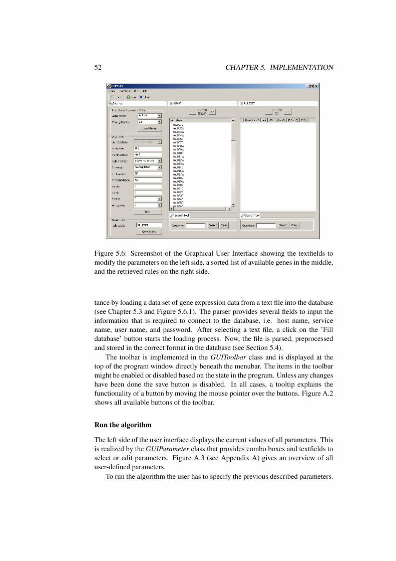
52 CHAPTER 5. IMPLEMENTATION
Figure 5.6: Screenshot of the Graphical User Interface showing the textfields tomodify the parameters on the left side, a sorted list of available genes in the middle,and the retrieved rules on the right side.
tance by loading a data set of gene expression data from a text file into the database(see Chapter 5.3 and Figure 5.6.1). The parser provides several fields to input theinformation that is required to connect to the database, i.e. host name, servicename, user name, and password. After selecting a text file, a click on the ’Filldatabase’ button starts the loading process. Now, the file is parsed, preprocessedand stored in the correct format in the database (see Section 5.4).
The toolbar is implemented in the GUIToolbar class and is displayed at thetop of the program window directly beneath the menubar. The items in the toolbarmight be enabled or disabled based on the state in the program. Unless any changeshave been done the save button is disabled. In all cases, a tooltip explains thefunctionality of a button by moving the mouse pointer over the buttons. Figure A.2shows all available buttons of the toolbar.
Run the algorithm
The left side of the user interface displays the current values of all parameters. Thisis realized by the GUIParameter class that provides combo boxes and textfields toselect or edit parameters. Figure A.3 (see Appendix A) gives an overview of alluser-defined parameters.
To run the algorithm the user has to specify the previous described parameters.
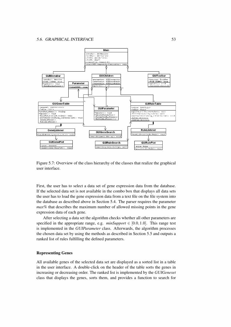
5.6. GRAPHICAL INTERFACE 53
Figure 5.7: Overview of the class hierarchy of the classes that realize the graphicaluser interface.
First, the user has to select a data set of gene expression data from the database.If the selected data set is not available in the combo box that displays all data setsthe user has to load the gene expression data from a text file on the file system intothe database as described above in Section 5.4. The parser requires the parametermax% that describes the maximum number of allowed missing points in the geneexpression data of each gene.
After selecting a data set the algorithm checks whether all other parameters arespecified in the appropriate range, e.g. minSupport ∈ [0.0,1.0]. This range testis implemented in the GUIParameter class. Afterwards, the algorithm processesthe chosen data set by using the methods as described in Section 5.5 and outputs aranked list of rules fulfilling the defined parameters.
Representing Genes
All available genes of the selected data set are displayed as a sorted list in a tablein the user interface. A double-click on the header of the table sorts the genes inincreasing or decreasing order. The ranked list is implemented by the GUIGenesetclass that displays the genes, sorts them, and provides a function to search for
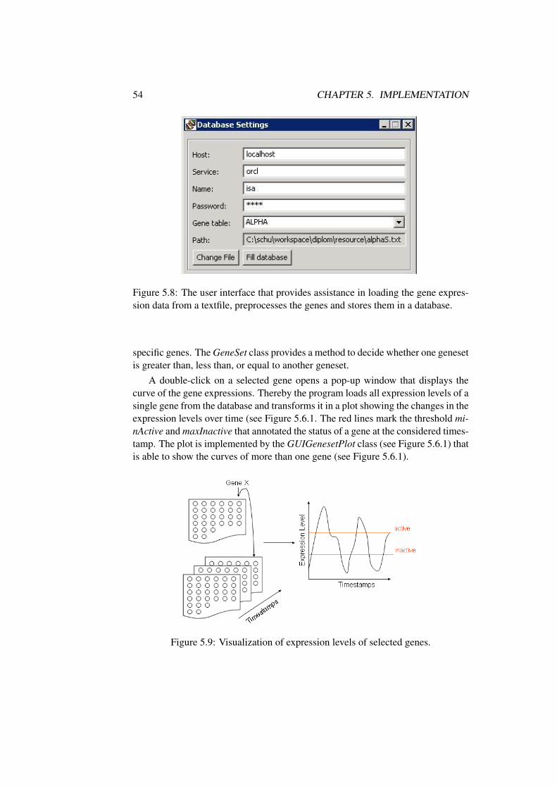
54 CHAPTER 5. IMPLEMENTATION
Figure 5.8: The user interface that provides assistance in loading the gene expres-sion data from a textfile, preprocesses the genes and stores them in a database.
specific genes. The GeneSet class provides a method to decide whether one genesetis greater than, less than, or equal to another geneset.
A double-click on a selected gene opens a pop-up window that displays thecurve of the gene expressions. Thereby the program loads all expression levels of asingle gene from the database and transforms it in a plot showing the changes in theexpression levels over time (see Figure 5.6.1. The red lines mark the threshold mi-nActive and maxInactive that annotated the status of a gene at the considered times-tamp. The plot is implemented by the GUIGenesetPlot class (see Figure 5.6.1) thatis able to show the curves of more than one gene (see Figure 5.6.1).
Figure 5.9: Visualization of expression levels of selected genes.
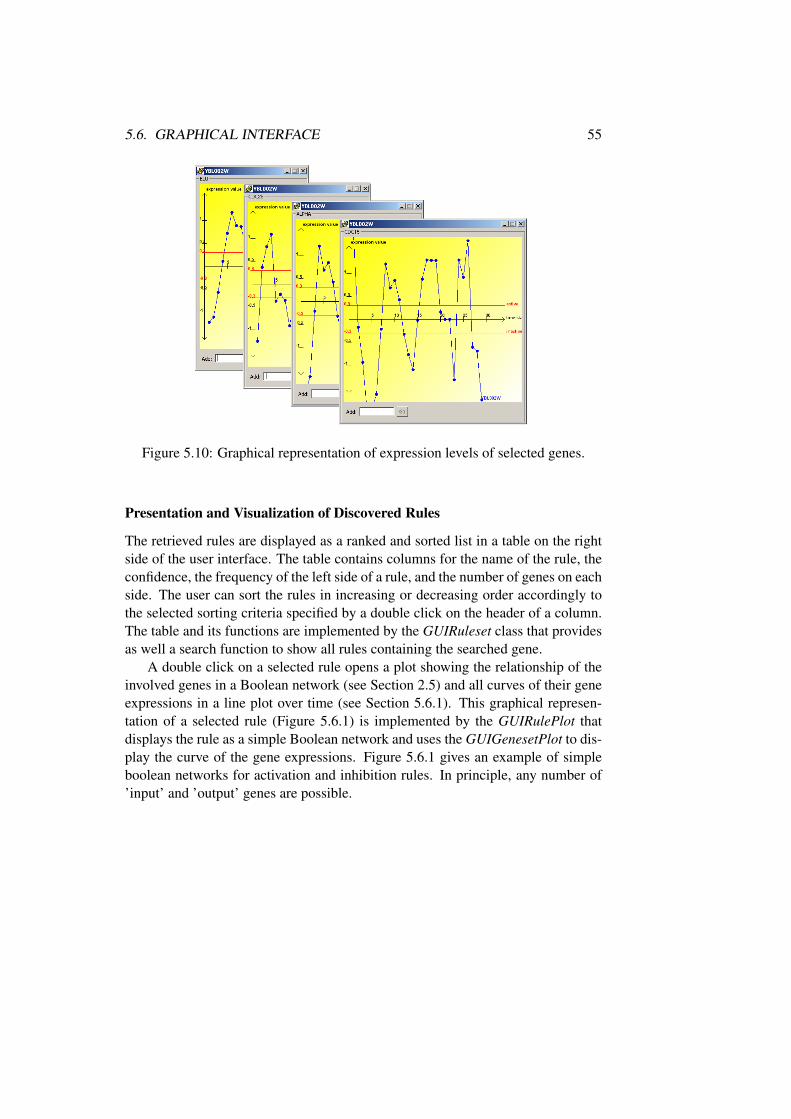
5.6. GRAPHICAL INTERFACE 55
Figure 5.10: Graphical representation of expression levels of selected genes.
Presentation and Visualization of Discovered Rules
The retrieved rules are displayed as a ranked and sorted list in a table on the rightside of the user interface. The table contains columns for the name of the rule, theconfidence, the frequency of the left side of a rule, and the number of genes on eachside. The user can sort the rules in increasing or decreasing order accordingly tothe selected sorting criteria specified by a double click on the header of a column.The table and its functions are implemented by the GUIRuleset class that providesas well a search function to show all rules containing the searched gene.
A double click on a selected rule opens a plot showing the relationship of theinvolved genes in a Boolean network (see Section 2.5) and all curves of their geneexpressions in a line plot over time (see Section 5.6.1). This graphical represen-tation of a selected rule (Figure 5.6.1) is implemented by the GUIRulePlot thatdisplays the rule as a simple Boolean network and uses the GUIGenesetPlot to dis-play the curve of the gene expressions. Figure 5.6.1 gives an example of simpleboolean networks for activation and inhibition rules. In principle, any number of’input’ and ’output’ genes are possible.
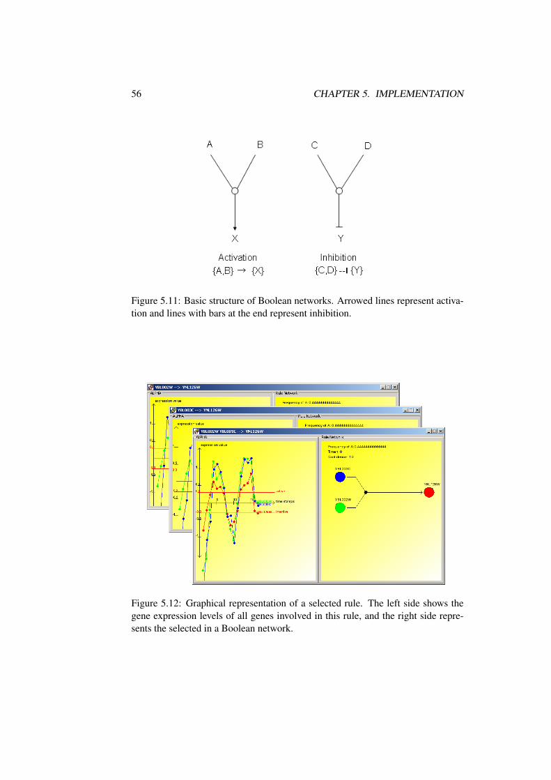
56 CHAPTER 5. IMPLEMENTATION
Figure 5.11: Basic structure of Boolean networks. Arrowed lines represent activa-tion and lines with bars at the end represent inhibition.
Figure 5.12: Graphical representation of a selected rule. The left side shows thegene expression levels of all genes involved in this rule, and the right side repre-sents the selected in a Boolean network.
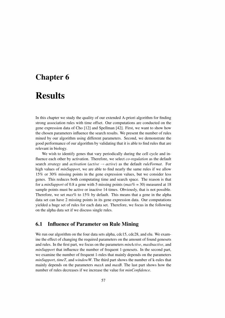
Chapter 6
Results
In this chapter we study the quality of our extended A-priori algorithm for findingstrong association rules with time offset. Our computations are conducted on thegene expression data of Cho [12] and Spellman [42]. First, we want to show howthe chosen parameters influence the search results. We present the number of rulesmined by our algorithm using different parameters. Second, we demonstrate thegood performance of our algorithm by validating that it is able to find rules that arerelevant in biology.
We wish to identify genes that vary periodically during the cell cycle and in-fluence each other by activation. Therefore, we select co-regulation as the defaultsearch strategy and activation (active→ active) as the default ruleFormat. Forhigh values of minSupport, we are able to find nearly the same rules if we allow15% or 30% missing points in the gene expression values, but we consider lessgenes. This reduces both computating time and search space. The reason is thatfor a minSupport of 0.8 a gene with 5 missing points (max% = 30) measured at 18sample points must be active or inactive 14 times. Obviously, that is not possible.Therefore, we set max% to 15% by default. This means that a gene in the alphadata set can have 2 missing points in its gene expression data. Our computationsyielded a huge set of rules for each data set. Therefore, we focus in the followingon the alpha data set if we discuss single rules.
6.1 Influence of Parameter on Rule Mining
We run our algorithm on the four data sets alpha, cdc15, cdc28, and elu. We exam-ine the effect of changing the required parameters on the amount of found genesetsand rules. In the first part, we focus on the parameters minActive, maxInactive, andminSupport that influence the number of frequent 1-genesets. In the second part,we examine the number of frequent 1-rules that mainly depends on the parametersminSupport, timeT, and windowW. The third part shows the number of k-rules thatmainly depends on the parameters maxA and maxB. The last part shows how thenumber of rules decreases if we increase the value for minConfidence.
57
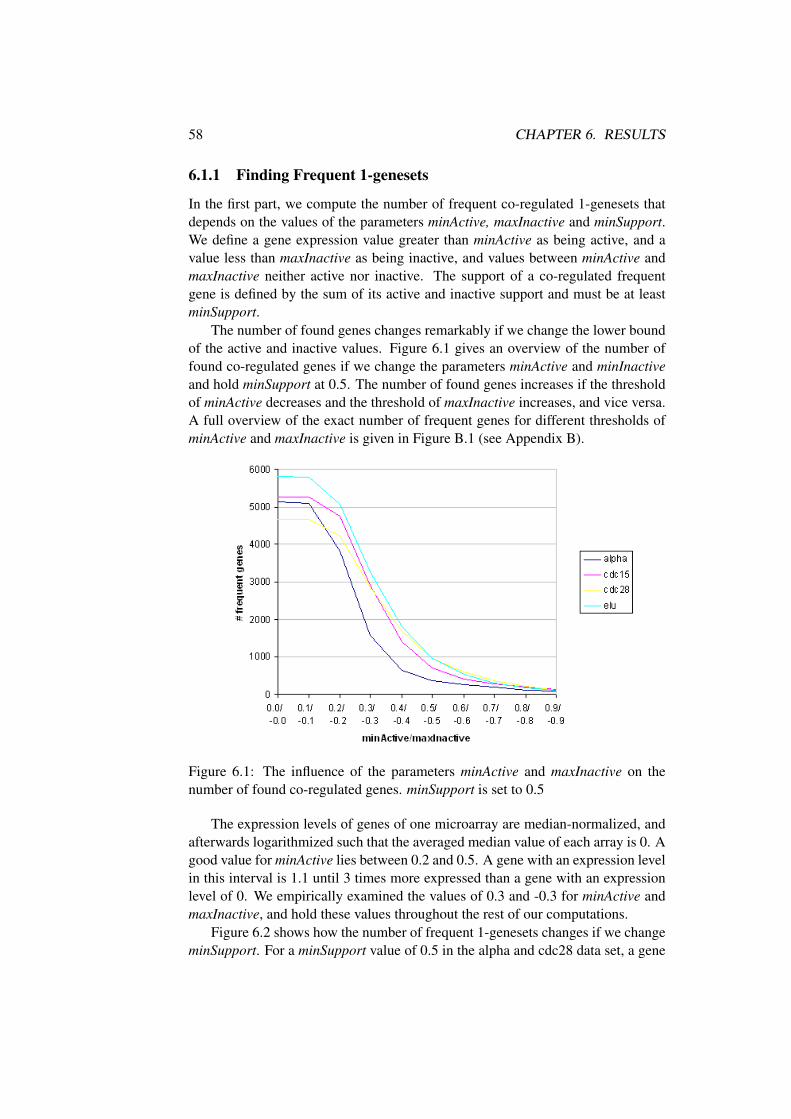
58 CHAPTER 6. RESULTS
6.1.1 Finding Frequent 1-genesets
In the first part, we compute the number of frequent co-regulated 1-genesets thatdepends on the values of the parameters minActive, maxInactive and minSupport.We define a gene expression value greater than minActive as being active, and avalue less than maxInactive as being inactive, and values between minActive andmaxInactive neither active nor inactive. The support of a co-regulated frequentgene is defined by the sum of its active and inactive support and must be at leastminSupport.
The number of found genes changes remarkably if we change the lower boundof the active and inactive values. Figure 6.1 gives an overview of the number offound co-regulated genes if we change the parameters minActive and minInactiveand hold minSupport at 0.5. The number of found genes increases if the thresholdof minActive decreases and the threshold of maxInactive increases, and vice versa.A full overview of the exact number of frequent genes for different thresholds ofminActive and maxInactive is given in Figure B.1 (see Appendix B).
Figure 6.1: The influence of the parameters minActive and maxInactive on thenumber of found co-regulated genes. minSupport is set to 0.5
The expression levels of genes of one microarray are median-normalized, andafterwards logarithmized such that the averaged median value of each array is 0. Agood value for minActive lies between 0.2 and 0.5. A gene with an expression levelin this interval is 1.1 until 3 times more expressed than a gene with an expressionlevel of 0. We empirically examined the values of 0.3 and -0.3 for minActive andmaxInactive, and hold these values throughout the rest of our computations.
Figure 6.2 shows how the number of frequent 1-genesets changes if we changeminSupport. For a minSupport value of 0.5 in the alpha and cdc28 data set, a gene
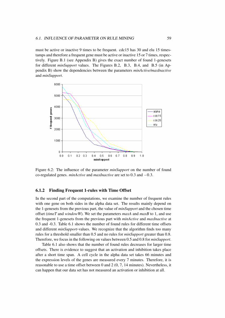
6.1. INFLUENCE OF PARAMETER ON RULE MINING 59
must be active or inactive 9 times to be frequent. cdc15 has 30 and elu 15 times-tamps and therefore a frequent gene must be active or inactive 15 or 7 times, respec-tively. Figure B.1 (see Appendix B) gives the exact number of found 1-genesetsfor different minSupport values. The Figures B.2, B.3, B.4, and B.5 (in Ap-pendix B) show the dependencies between the parameters minActive/maxInactiveand minSupport.
Figure 6.2: The influence of the parameter minSupport on the number of foundco-regulated genes. minActive and maxInactive are set to 0.3 and −0.3.
6.1.2 Finding Frequent 1-rules with Time Offset
In the second part of the computations, we examine the number of frequent ruleswith one gene on both sides in the alpha data set. The results mainly depend onthe 1-genesets from the previous part, the value of minSupport and the chosen timeoffset (timeT and windowW). We set the parameters maxA and maxB to 1, and usethe frequent 1-genesets from the previous part with minActive and maxInactive at0.3 and -0.3. Table 6.1 shows the number of found rules for different time offsetsand different minSupport-values. We recognize that the algorithm finds too manyrules for a threshold smaller than 0.5 and no rules for minSupport greater than 0.8.Therefore, we focus in the following on values between 0.5 and 0.8 for minSupport.
Table 6.1 also shows that the number of found rules decreases for larger timeoffsets. There is evidence to suggest that an activation and inhibition takes placeafter a short time span. A cell cycle in the alpha data set takes 66 minutes andthe expression levels of the genes are measured every 7 minutes. Therefore, it isreasonable to use a time offset between 0 and 2 (0, 7, 14 minutes). Nevertheless, itcan happen that our data set has not measured an activation or inhibition at all.
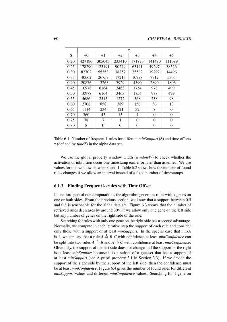
60 CHAPTER 6. RESULTS
τ
S +0 +1 +2 +3 +4 +50.20 427190 305045 233410 171873 141480 1110890.25 178290 123191 90249 63141 49297 385260.30 82702 55353 38257 25582 19292 144960.35 40662 26757 17213 10978 7712 53050.40 20876 13263 7929 4590 2890 18060.45 10978 6164 3463 1754 978 4990.50 10978 6164 3463 1754 978 4990.55 5686 2515 1272 568 238 980.60 2708 858 389 156 36 130.65 1114 234 121 32 8 00.70 360 43 15 4 0 00.75 78 7 1 0 0 00.80 8 0 0 0 0 0
Table 6.1: Number of frequent 1-rules for different minSupport (S) and time offsetsτ (defined by timeT) in the alpha data set.
We use the global property window width (windowW) to check whether theactivation or inhibition occur one timestamp earlier or later than assumed. We usevalues for this window between 0 and 1. Table 6.2 shows how the number of foundrules changes if we allow an interval instead of a fixed number of timestamps.
6.1.3 Finding Frequent k-rules with Time Offset
In the third part of our computations, the algorithm generates rules with k genes onone or both sides. From the previous section, we know that a support between 0.5and 0.8 is reasonable for the alpha data set. Figure 6.3 shows that the number ofretrieved rules decreases by around 30% if we allow only one gene on the left sidebut any number of genes on the right side of the rule.
Searching for rules with only one gene on the right side has a second advantage.Normally, we compute in each iterative step the support of each rule and consideronly those with a support of at least minSupport. In the special case that maxAis 1, we can say that a rule A τ⇒ B,C with confidence at least minConfidence canbe split into two rules A τ⇒ B and A τ⇒C with confidence at least minConfidence.Obviously, the support of the left side does not change and the support of the rightis at least minSupport because it is a subset of a geneset that has a support ofat least minSupport (see A-priori property 3.1 in Section 3.3). If we devide thesupport of the right side by the support of the left side, then the confidence mustbe at least minConfidence. Figure 6.4 gives the number of found rules for differentminSupport-values and different minConfidence-values. Searching for 1 gene on
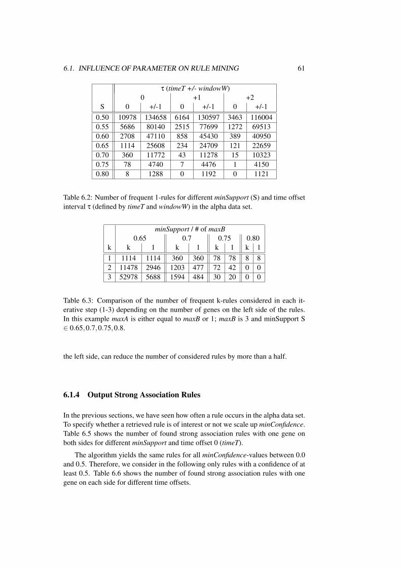
6.1. INFLUENCE OF PARAMETER ON RULE MINING 61
τ (timeT +/- windowW)0 +1 +2
S 0 +/-1 0 +/-1 0 +/-10.50 10978 134658 6164 130597 3463 1160040.55 5686 80140 2515 77699 1272 695130.60 2708 47110 858 45430 389 409500.65 1114 25608 234 24709 121 226590.70 360 11772 43 11278 15 103230.75 78 4740 7 4476 1 41500.80 8 1288 0 1192 0 1121
Table 6.2: Number of frequent 1-rules for different minSupport (S) and time offsetinterval τ (defined by timeT and windowW) in the alpha data set.
minSupport / # of maxB0.65 0.7 0.75 0.80
k k 1 k 1 k 1 k 11 1114 1114 360 360 78 78 8 82 11478 2946 1203 477 72 42 0 03 52978 5688 1594 484 30 20 0 0
Table 6.3: Comparison of the number of frequent k-rules considered in each it-erative step (1-3) depending on the number of genes on the left side of the rules.In this example maxA is either equal to maxB or 1; maxB is 3 and minSupport S∈ 0.65,0.7,0.75,0.8.
the left side, can reduce the number of considered rules by more than a half.
6.1.4 Output Strong Association Rules
In the previous sections, we have seen how often a rule occurs in the alpha data set.To specify whether a retrieved rule is of interest or not we scale up minConfidence.Table 6.5 shows the number of found strong association rules with one gene onboth sides for different minSupport and time offset 0 (timeT).
The algorithm yields the same rules for all minConfidence-values between 0.0and 0.5. Therefore, we consider in the following only rules with a confidence of atleast 0.5. Table 6.6 shows the number of found strong association rules with onegene on each side for different time offsets.
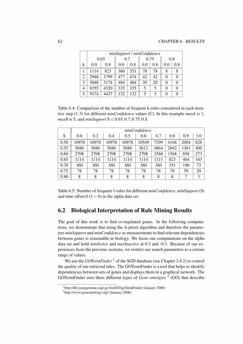
62 CHAPTER 6. RESULTS
minSupport / minConfidence0.65 0.7 0.75 0.8
k 0.0 0.8 0.0 0.8 0.0 0.8 0.0 0.81 1114 823 360 351 78 78 8 82 2946 1799 477 474 42 42 0 03 5688 3174 484 484 20 20 0 04 8355 4320 335 335 5 5 0 05 9174 4437 132 132 5 5 0 0
Table 6.4: Comparison of the number of frequent k-rules considered in each itera-tive step (1-3) for different minConfidence-values (C). In this example maxA is 1,maxB is 5, and minSupport S ∈ 0.65,0.7,0.75,0.8.
minConfidenceS 0.0 0.2 0.4 0.5 0.6 0.7 0.8 0.9 1.0
0.50 10978 10978 10978 10978 10549 7299 4168 2084 6280.55 5686 5686 5686 5686 5612 4864 2642 1361 4000.60 2708 2708 2708 2708 2708 2568 1568 856 2730.65 1114 1114 1114 1114 1114 1111 823 464 1630.70 360 360 360 360 360 360 351 190 730.75 78 78 78 78 78 78 78 59 200.80 8 8 8 8 8 8 8 7 3
Table 6.5: Number of frequent 1-rules for different minConfidence, minSupport (S)and time offset 0 (τ = 0) in the alpha data set.
6.2 Biological Interpretation of Rule Mining Results
The goal of this work is to find co-regulated genes. In the following computa-tions, we demonstrate that using the A-priori algorithm and therefore the parame-ters minSupport and minConfidence as measurements to find relevant dependenciesbetween genes is reasonable in biology. We focus our computations on the alphadata set and hold minActive and maxInactive at 0.3 and -0.3. Because of our ex-periences from the previous sections, we restrict our search parameters to a certainrange of values.
We use the GOTermFinder 1 of the SGD database (see Chapter 2.8.2) to controlthe quality of our retrieved rules. The GOTermFinder is a tool that helps to identifydependencies between sets of genes and displays them in a graphical network. TheGOTermFinder uses three different types of Gene ontolgies 2 (GO) that describe
1http://db.yeastgenome.org/cgi-bin/GO/goTermFinder (January 2006)2http://www.geneontology.org/ (January 2006)
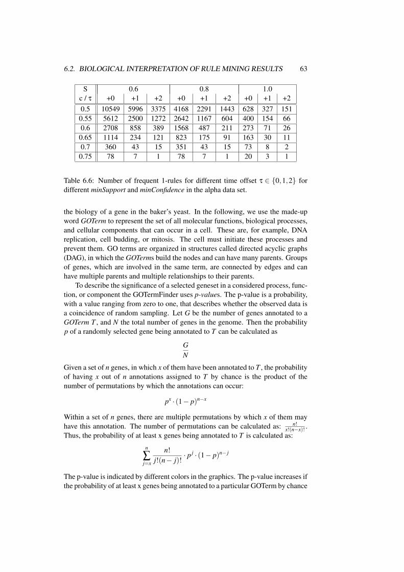
6.2. BIOLOGICAL INTERPRETATION OF RULE MINING RESULTS 63
S 0.6 0.8 1.0c / τ +0 +1 +2 +0 +1 +2 +0 +1 +20.5 10549 5996 3375 4168 2291 1443 628 327 151
0.55 5612 2500 1272 2642 1167 604 400 154 660.6 2708 858 389 1568 487 211 273 71 26
0.65 1114 234 121 823 175 91 163 30 110.7 360 43 15 351 43 15 73 8 2
0.75 78 7 1 78 7 1 20 3 1
Table 6.6: Number of frequent 1-rules for different time offset τ ∈ {0,1,2} fordifferent minSupport and minConfidence in the alpha data set.
the biology of a gene in the baker’s yeast. In the following, we use the made-upword GOTerm to represent the set of all molecular functions, biological processes,and cellular components that can occur in a cell. These are, for example, DNAreplication, cell budding, or mitosis. The cell must initiate these processes andprevent them. GO terms are organized in structures called directed acyclic graphs(DAG), in which the GOTerms build the nodes and can have many parents. Groupsof genes, which are involved in the same term, are connected by edges and canhave multiple parents and multiple relationships to their parents.
To describe the significance of a selected geneset in a considered process, func-tion, or component the GOTermFinder uses p-values. The p-value is a probability,with a value ranging from zero to one, that describes whether the observed data isa coincidence of random sampling. Let G be the number of genes annotated to aGOTerm T , and N the total number of genes in the genome. Then the probabilityp of a randomly selected gene being annotated to T can be calculated as
GN
Given a set of n genes, in which x of them have been annotated to T , the probabilityof having x out of n annotations assigned to T by chance is the product of thenumber of permutations by which the annotations can occur:
px · (1− p)n−x
Within a set of n genes, there are multiple permutations by which x of them mayhave this annotation. The number of permutations can be calculated as: n!
x!(n−x)! .Thus, the probability of at least x genes being annotated to T is calculated as:
n
∑j=x
n!j!(n− j)!
· p j · (1− p)n− j
The p-value is indicated by different colors in the graphics. The p-value increases ifthe probability of at least x genes being annotated to a particular GOTerm by chance
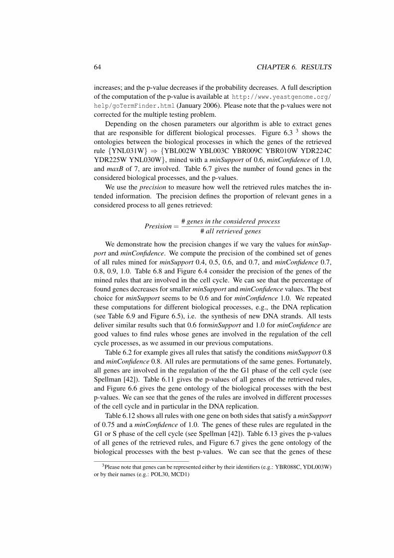
64 CHAPTER 6. RESULTS
increases; and the p-value decreases if the probability decreases. A full descriptionof the computation of the p-value is available at http://www.yeastgenome.org/help/goTermFinder.html (January 2006). Please note that the p-values were notcorrected for the multiple testing problem.
Depending on the chosen parameters our algorithm is able to extract genesthat are responsible for different biological processes. Figure 6.3 3 shows theontologies between the biological processes in which the genes of the retrievedrule {YNL031W} ⇒ {YBL002W YBL003C YBR009C YBR010W YDR224CYDR225W YNL030W}, mined with a minSupport of 0.6, minConfidence of 1.0,and maxB of 7, are involved. Table 6.7 gives the number of found genes in theconsidered biological processes, and the p-values.
We use the precision to measure how well the retrieved rules matches the in-tended information. The precision defines the proportion of relevant genes in aconsidered process to all genes retrieved:
Presision =# genes in the considered process
# all retrieved genes
We demonstrate how the precision changes if we vary the values for minSup-port and minConfidence. We compute the precision of the combined set of genesof all rules mined for minSupport 0.4, 0.5, 0.6, and 0.7, and minConfidence 0.7,0.8, 0.9, 1.0. Table 6.8 and Figure 6.4 consider the precision of the genes of themined rules that are involved in the cell cycle. We can see that the percentage offound genes decreases for smaller minSupport and minConfidence values. The bestchoice for minSupport seems to be 0.6 and for minConfidence 1.0. We repeatedthese computations for different biological processes, e.g., the DNA replication(see Table 6.9 and Figure 6.5), i.e. the synthesis of new DNA strands. All testsdeliver similar results such that 0.6 forminSupport and 1.0 for minConfidence aregood values to find rules whose genes are involved in the regulation of the cellcycle processes, as we assumed in our previous computations.
Table 6.2 for example gives all rules that satisfy the conditions minSupport 0.8and minConfidence 0.8. All rules are permutations of the same genes. Fortunately,all genes are involved in the regulation of the the G1 phase of the cell cycle (seeSpellman [42]). Table 6.11 gives the p-values of all genes of the retrieved rules,and Figure 6.6 gives the gene ontology of the biological processes with the bestp-values. We can see that the genes of the rules are involved in different processesof the cell cycle and in particular in the DNA replication.
Table 6.12 shows all rules with one gene on both sides that satisfy a minSupportof 0.75 and a minConfidence of 1.0. The genes of these rules are regulated in theG1 or S phase of the cell cycle (see Spellman [42]). Table 6.13 gives the p-valuesof all genes of the retrieved rules, and Figure 6.7 gives the gene ontology of thebiological processes with the best p-values. We can see that the genes of these
3Please note that genes can be represented either by their identifiers (e.g.: YBR088C, YDL003W)or by their names (e.g.: POL30, MCD1)
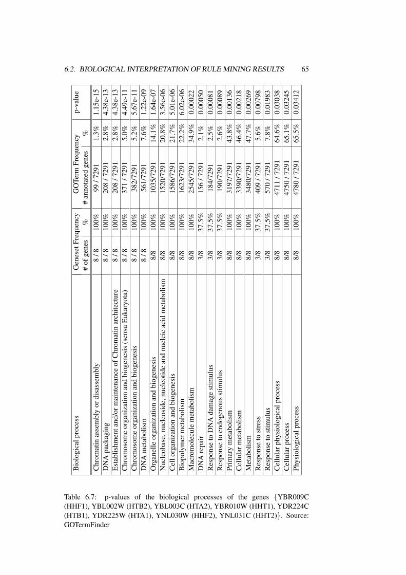
6.2. BIOLOGICAL INTERPRETATION OF RULE MINING RESULTS 65B
iolo
gica
lpro
cess
Gen
eset
Freq
uenc
yG
OTe
rmFr
eque
ncy
p-va
lue
#of
gene
s%
#an
nota
ted
gene
s%
Chr
omat
inas
sem
bly
ordi
sass
embl
y8
/810
0%99
/729
11.
3%1.
15e-
15D
NA
pack
agin
g8
/810
0%20
8/7
291
2.8%
4.38
e-13
Est
ablis
hmen
tand
/orm
aint
enan
ceof
Chr
omat
inar
chite
ctur
e8
/810
0%20
8/7
291
2.8%
4.38
e-13
Chr
omos
ome
orga
niza
tion
and
biog
enes
is(s
ensu
Euk
aryo
ta)
8/8
100%
371
/729
15.
0%4.
49e-
11C
hrom
osom
eor
gani
zatio
nan
dbi
ogen
esis
8/8
100%
382/
7291
5.2%
5.67
e-11
DN
Am
etab
olis
m8
/810
0%56
1/72
917.
6%1.
22e-
09O
rgan
elle
orga
niza
tion
and
biog
enes
is8/
810
0%10
35/7
291
14.1
%1.
64e-
07N
ucle
obas
e,nu
cleo
side
,nuc
leot
ide
and
nucl
eic
acid
met
abol
ism
8/8
100%
1520
/729
120
.8%
3.56
e-06
Cel
lorg
aniz
atio
nan
dbi
ogen
esis
8/8
100%
1586
/729
121
.7%
5.01
e-06
Bio
poly
mer
met
abol
ism
8/8
100%
1623
/729
122
.2%
6.02
e-06
Mac
rom
olec
ule
met
abol
ism
8/8
100%
2545
/729
134
.9%
0.00
022
DN
Are
pair
3/8
37.5
%15
6/7
291
2.1%
0.00
050
Res
pons
eto
DN
Ada
mag
est
imul
us3/
837
.5%
184/
7291
2.5%
0.00
081
Res
pons
eto
endo
geno
usst
imul
us3/
837
.5%
190/
7291
2.6%
0.00
089
Prim
ary
met
abol
ism
8/8
100%
3197
/729
143
.8%
0.00
136
Cel
lula
rmet
abol
ism
8/8
100%
3390
/729
146
.4%
0.00
218
Met
abol
ism
8/8
100%
3480
/729
147
.7%
0.00
269
Res
pons
eto
stre
ss3/
837
.5%
409
/729
15.
6%0.
0079
8R
espo
nse
tost
imul
us3/
837
.5%
570
/729
17.
8%0.
0198
3C
ellu
larp
hysi
olog
ical
proc
ess
8/8
100%
4711
/729
164
.6%
0.03
038
Cel
lula
rpro
cess
8/8
100%
4750
/729
165
.1%
0.03
245
Phys
iolo
gica
lpro
cess
8/8
100%
4780
/729
165
.5%
0.03
412
Table 6.7: p-values of the biological processes of the genes {YBR009C(HHF1), YBL002W (HTB2), YBL003C (HTA2), YBR010W (HHT1), YDR224C(HTB1), YDR225W (HTA1), YNL030W (HHF2), YNL031C (HHT2)}. Source:GOTermFinder
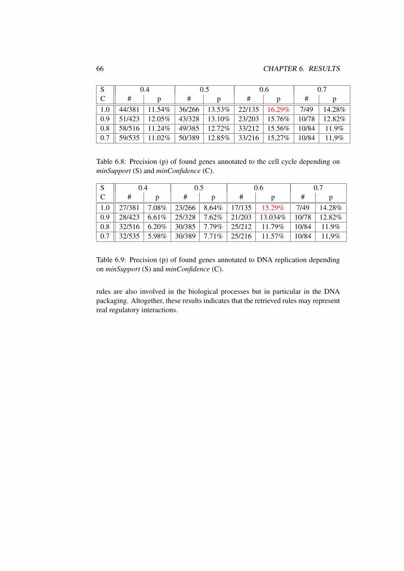
66 CHAPTER 6. RESULTS
S 0.4 0.5 0.6 0.7C # p # p # p # p1.0 44/381 11.54% 36/266 13.53% 22/135 16.29% 7/49 14.28%0.9 51/423 12.05% 43/328 13.10% 23/203 15.76% 10/78 12.82%0.8 58/516 11.24% 49/385 12.72% 33/212 15.56% 10/84 11.9%0.7 59/535 11.02% 50/389 12.85% 33/216 15,27% 10/84 11,9%
Table 6.8: Precision (p) of found genes annotated to the cell cycle depending onminSupport (S) and minConfidence (C).
S 0.4 0.5 0.6 0.7C # p # p # p # p1.0 27/381 7.08% 23/266 8.64% 17/135 15.29% 7/49 14.28%0.9 28/423 6.61% 25/328 7.62% 21/203 13.034% 10/78 12.82%0.8 32/516 6.20% 30/385 7.79% 25/212 11.79% 10/84 11.9%0.7 32/535 5.98% 30/389 7.71% 25/216 11.57% 10/84 11,9%
Table 6.9: Precision (p) of found genes annotated to DNA replication dependingon minSupport (S) and minConfidence (C).
rules are also involved in the biological processes but in particular in the DNApackaging. Altogether, these results indicates that the retrieved rules may representreal regulatory interactions.
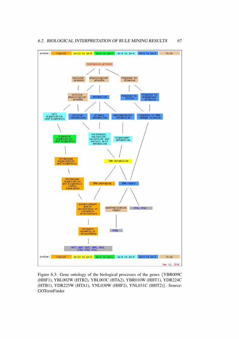
6.2. BIOLOGICAL INTERPRETATION OF RULE MINING RESULTS 67
Figure 6.3: Gene ontology of the biological processes of the genes {YBR009C(HHF1), YBL002W (HTB2), YBL003C (HTA2), YBR010W (HHT1), YDR224C(HTB1), YDR225W (HTA1), YNL030W (HHF2), YNL031C (HHT2)}. Source:GOTermFinder
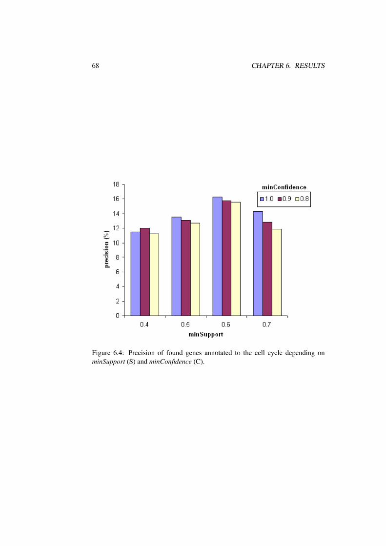
68 CHAPTER 6. RESULTS
Figure 6.4: Precision of found genes annotated to the cell cycle depending onminSupport (S) and minConfidence (C).
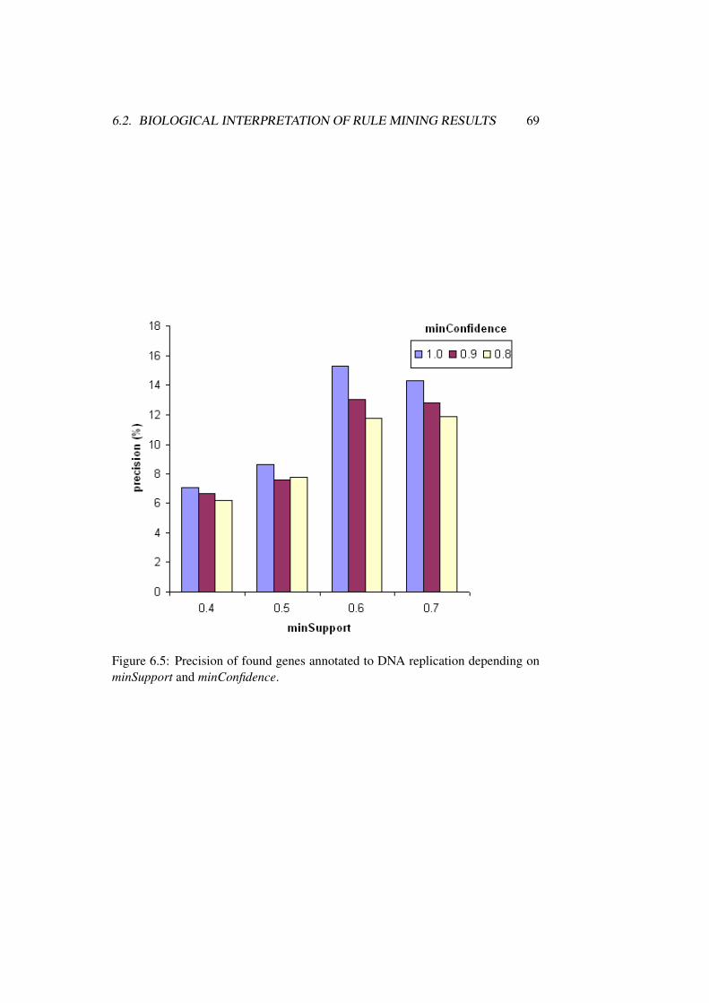
6.2. BIOLOGICAL INTERPRETATION OF RULE MINING RESULTS 69
Figure 6.5: Precision of found genes annotated to DNA replication depending onminSupport and minConfidence.
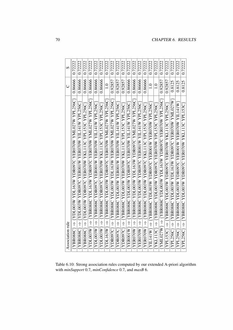
70 CHAPTER 6. RESULTS
Ass
ocia
tion
rule
CS
{YB
R08
8C}⇒{Y
DL
003W
YD
L16
3WY
DR
097C
YE
R07
0WY
ML
027W
YPL
256C}
0.86
666
0.72
222
{YB
R08
8C}⇒{Y
DL
003W
YD
R09
7CY
ER
001W
YE
R07
0WY
IL14
1WY
PL25
6C}
0.86
666
0.72
222
{YB
R08
8C}⇒{Y
DL
003W
YD
R09
7CY
ER
070W
YK
L11
3CY
PL15
3CY
PL25
6C}
0.86
666
0.72
222
{YD
L00
3W}⇒{Y
BR
088C
YD
L16
3WY
DR
097C
YE
R07
0WY
ML
027W
YPL
256C}
0.86
666
0.72
222
{YD
L00
3W}⇒{Y
BR
088C
YD
R09
7CY
ER
001W
YE
R07
0WY
IL14
1WY
PL25
6C}
0.86
666
0.72
222
{YD
L00
3W}⇒{Y
BR
088C
YD
R09
7CY
ER
070W
YK
L11
3CY
PL15
3CY
PL25
6C}
0.86
666
0.72
222
{YD
L16
3W}⇒{Y
BR
088C
YD
L00
3WY
DR
097C
YE
R07
0WY
ML
027W
YPL
256C}
1.0
0.72
222
{YD
R09
7C}⇒{Y
BR
088C
YD
L00
3WY
DL
163W
YE
R07
0WY
ML
027W
YPL
256C}
0.92
857
0.72
222
{YD
R09
7C}⇒{Y
BR
088C
YD
L00
3WY
ER
001W
YE
R07
0WY
IL14
1WY
PL25
6C}
0.92
857
0.72
222
{YD
R09
7C}⇒{Y
BR
088C
YD
L00
3WY
ER
070W
YK
L11
3CY
PL15
3CY
PL25
6C}
0.92
857
0.72
222
{YE
R00
1W}⇒{Y
BR
088C
YD
L00
3WY
DR
097C
YE
R07
0WY
IL14
1WY
PL25
6C}
0.86
666
0.72
222
{YE
R07
0W}⇒{Y
BR
088C
YD
L00
3WY
DL
163W
YD
R09
7CY
ML
027W
YPL
256C}
0.86
666
0.72
222
{YE
R07
0W}⇒{Y
BR
088C
YD
L00
3WY
DR
097C
YE
R00
1WY
IL14
1WY
PL25
6C}
0.86
666
0.72
222
{YE
R07
0W}⇒{Y
BR
088C
YD
L00
3WY
DR
097C
YK
L11
3CY
PL15
3CY
PL25
6C}
0.86
666
0.72
222
{YIL
141W}⇒{Y
BR
088C
YD
L00
3WY
DR
097C
YE
R00
1WY
ER
070W
YPL
256C}
1.0
0.72
222
{YK
L11
3C}⇒{Y
BR
088C
YD
L00
3WY
DR
097C
YE
R07
0WY
PL15
3CY
PL25
6C}
1.0
0.72
222
{YM
L02
7W}⇒{Y
BR
088C
YD
L00
3WY
DL
163W
YD
R09
7CY
ER
070W
YPL
256C}
0.92
857
0.72
222
{YPL
153C}⇒{Y
BR
088C
YD
L00
3WY
DR
097C
YE
R07
0WY
KL
113C
YPL
256C}
0.92
857
0.72
222
{YPL
256C}⇒{Y
BR
088C
YD
L00
3WY
DL
163W
YD
R09
7CY
ER
070W
YM
L02
7W}
0.81
250.
7222
2{Y
PL25
6C}⇒{Y
BR
088C
YD
L00
3WY
DR
097C
YE
R00
1WY
ER
070W
YIL
141W}
0.81
250.
7222
2{Y
PL25
6C}⇒{Y
BR
088C
YD
L00
3WY
DR
097C
YE
R07
0WY
KL
113C
YPL
153C}
0.81
250.
7222
2
Table 6.10: Strong association rules computed by our extended A-priori algorithmwith minSupport 0.7, minConfidence 0.7, and maxB 6.
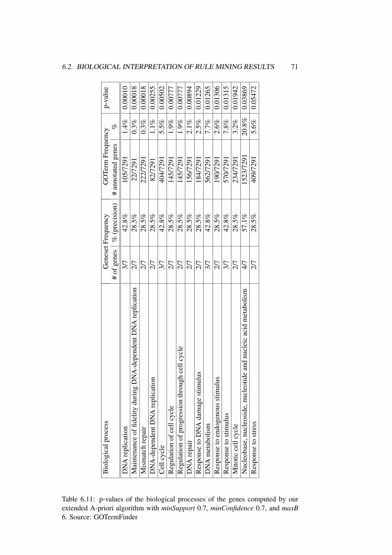
6.2. BIOLOGICAL INTERPRETATION OF RULE MINING RESULTS 71
Bio
logi
calp
roce
ssG
enes
etFr
eque
ncy
GO
Term
Freq
uenc
yp-
valu
e#
ofge
nes
%(p
reci
sion
)#
anno
tate
dge
nes
%D
NA
repl
icat
ion
3/7
42.8
%10
5/72
911.
4%0.
0001
0M
aint
enan
ceof
fidel
itydu
ring
DN
A-d
epen
dent
DN
Are
plic
atio
n2/
728
.5%
22/7
291
0.3%
0.00
018
Mis
mat
chre
pair
2/7
28.5
%22
2/72
910.
3%0.
0001
8D
NA
-dep
ende
ntD
NA
repl
icat
ion
2/7
28.5
%82
/729
11.
1%0.
0025
5C
ellc
ycle
3/7
42.8
%40
4/72
915.
5%0.
0050
2R
egul
atio
nof
cell
cycl
e2/
728
.5%
145/
7291
1.9%
0.00
777
Reg
ulat
ion
ofpr
ogre
ssio
nth
roug
hce
llcy
cle
2/7
28.5
%14
5/72
911.
9%0.
0077
7D
NA
repa
ir2/
728
.5%
156/
7291
2.1%
0.00
894
Res
pons
eto
DN
Ada
mag
est
imul
us2/
728
.5%
184/
7291
2.5%
0.01
229
DN
Am
etab
olis
m3/
742
.8%
562/
7291
7.7%
0.01
265
Res
pons
eto
endo
geno
usst
imul
us2/
728
.5%
190/
7291
2.6%
0.01
306
Res
pons
eto
stim
ulus
3/7
42.8
%57
0/72
917.
8%0.
0131
5M
itotic
cell
cycl
e2/
728
.5%
234/
7291
3.2%
0.01
942
Nuc
leob
ase,
nucl
eosi
de,n
ucle
otid
ean
dnu
clei
cac
idm
etab
olis
m4/
757
.1%
1523
/729
120
.8%
0.03
869
Res
pons
eto
stre
ss2/
728
.5%
409/
7291
5.6%
0.05
472
Table 6.11: p-values of the biological processes of the genes computed by ourextended A-priori algorithm with minSupport 0.7, minConfidence 0.7, and maxB6. Source: GOTermFinder
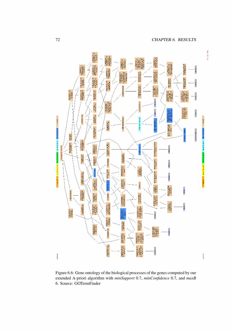
72 CHAPTER 6. RESULTS
Figure 6.6: Gene ontology of the biological processes of the genes computed by ourextended A-priori algorithm with minSupport 0.7, minConfidence 0.7, and maxB6. Source: GOTermFinder
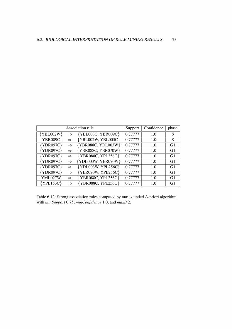
6.2. BIOLOGICAL INTERPRETATION OF RULE MINING RESULTS 73
Association rule Support Confidence phase{YBL002W} ⇒ {YBL003C, YBR009C} 0.77777 1.0 S{YBR009C} ⇒ {YBL002W, YBL003C} 0.77777 1.0 S{YDR097C} ⇒ {YBR088C, YDL003W} 0.77777 1.0 G1{YDR097C} ⇒ {YBR088C, YER070W} 0.77777 1.0 G1{YDR097C} ⇒ {YBR088C, YPL256C} 0.77777 1.0 G1{YDR097C} ⇒ {YDL003W, YER070W} 0.77777 1.0 G1{YDR097C} ⇒ {YDL003W, YPL256C} 0.77777 1.0 G1{YDR097C} ⇒ {YER070W, YPL256C} 0.77777 1.0 G1{YML027W} ⇒ {YBR088C, YPL256C} 0.77777 1.0 G1{YPL153C} ⇒ {YBR088C, YPL256C} 0.77777 1.0 G1
Table 6.12: Strong association rules computed by our extended A-priori algorithmwith minSupport 0.75, minConfidence 1.0, and maxB 2.
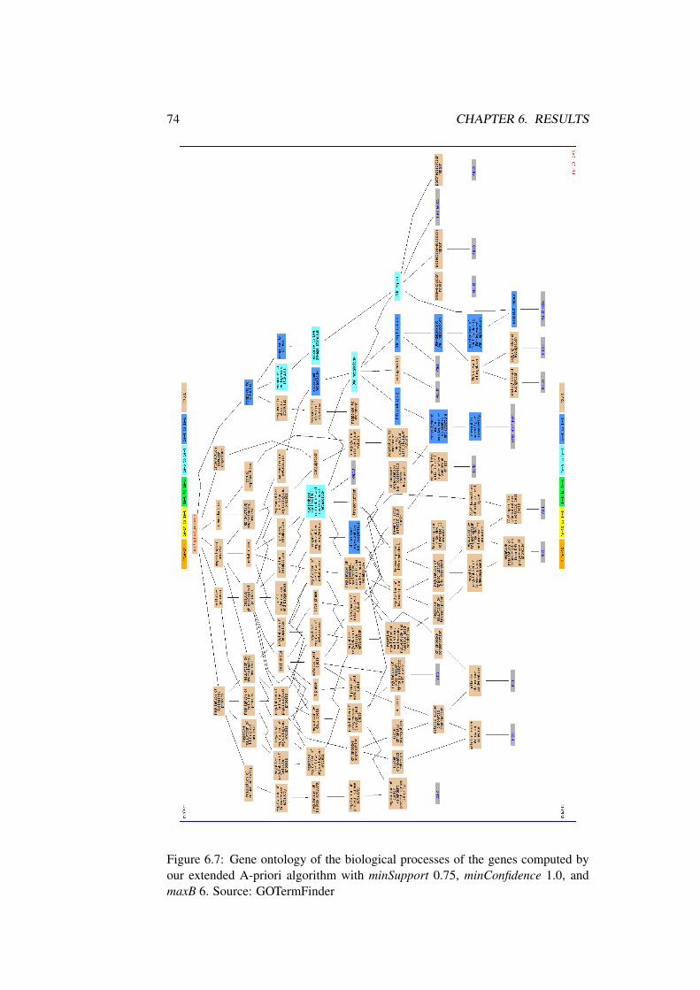
74 CHAPTER 6. RESULTS
Figure 6.7: Gene ontology of the biological processes of the genes computed byour extended A-priori algorithm with minSupport 0.75, minConfidence 1.0, andmaxB 6. Source: GOTermFinder
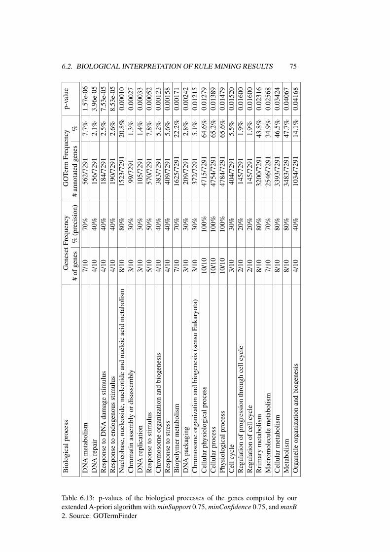
6.2. BIOLOGICAL INTERPRETATION OF RULE MINING RESULTS 75B
iolo
gica
lpro
cess
Gen
eset
Freq
uenc
yG
OTe
rmFr
eque
ncy
p-va
lue
#of
gene
s%
(pre
cisi
on)
#an
nota
ted
gene
s%
DN
Am
etab
olis
m7/
1070
%56
2/72
917.
7%1.
57e-
06D
NA
repa
ir4/
1040
%15
6/72
912.
1%3.
96e-
05R
espo
nse
toD
NA
dam
age
stim
ulus
4/10
40%
184/
7291
2.5%
7.53
e-05
Res
pons
eto
endo
geno
usst
imul
us4/
1040
%19
0/72
912.
6%8.
53e-
05N
ucle
obas
e,nu
cleo
side
,nuc
leot
ide
and
nucl
eic
acid
met
abol
ism
8/10
80%
1523
/729
120
.8%
0.00
010
Chr
omat
inas
sem
bly
ordi
sass
embl
y3/
1030
%99
/729
11.
3%0.
0002
7D
NA
repl
icat
ion
3/10
30%
105/
7291
1.4%
0.00
033
Res
pons
eto
stim
ulus
5/10
50%
570/
7291
7.8%
0.00
052
Chr
omos
ome
orga
niza
tion
and
biog
enes
is4/
1040
%38
3/72
915.
2%0.
0012
3R
espo
nse
tost
ress
4/10
40%
409/
7291
5.6%
0.00
158
Bio
poly
mer
met
abol
ism
7/10
70%
1625
/729
122
.2%
0.00
171
DN
Apa
ckag
ing
3/10
30%
209/
7291
2.8%
0.00
242
Chr
omos
ome
orga
niza
tion
and
biog
enes
is(s
ensu
Euk
aryo
ta)
3/10
30%
372/
7291
5.1%
0.01
215
Cel
lula
rphy
siol
ogic
alpr
oces
s10
/10
100%
4715
/729
164
.6%
0.01
279
Cel
lula
rpro
cess
10/1
010
0%47
54/7
291
65.2
%0.
0138
9Ph
ysio
logi
calp
roce
ss10
/10
100%
4784
/729
165
.6%
0.01
479
Cel
lcyc
le3/
1030
%40
4/72
915.
5%0.
0152
0R
egul
atio
nof
prog
ress
ion
thro
ugh
cell
cycl
e2/
1020
%14
5/72
911.
9%0.
0160
0R
egul
atio
nof
cell
cycl
e2/
1020
%14
5/72
911.
9%0.
0160
0R
rim
ary
met
abol
ism
8/10
80%
3200
/729
143
.8%
0.02
316
Mac
rom
olec
ule
met
abol
ism
7/10
70%
2546
/729
134
.9%
0.02
568
Cel
lula
rmet
abol
ism
8/10
80%
3393
/729
146
.5%
0.03
424
Met
abol
ism
8/10
80%
3483
/729
147
.7%
0.04
067
Org
anel
leor
gani
zatio
nan
dbi
ogen
esis
4/10
40%
1034
/729
114
.1%
0.04
168
Table 6.13: p-values of the biological processes of the genes computed by ourextended A-priori algorithm with minSupport 0.75, minConfidence 0.75, and maxB2. Source: GOTermFinder

76 CHAPTER 6. RESULTS
Chapter 7
Conclusion
In this thesis we presented a new approach for analyzing gene expression data. Thechallenge was to find dependencies between genes studying time-series expressiondata. Our new technique is based on the A-priori algorithm, introduced in 1993by Agrawal et. al. [2]. We described how to apply this technique to the real worldexpression data sets of Saccharomyces cerevisiae (Cho [12] and Spellman [42]).Although, we did not use any prior knowledge, we were able to extract alreadyknown relations between genes. We showed how the chosen parameters can in-fluence and improve the search results. This comes with small loss of quality butreduces both the search space and computing time.
The first version of our algorithm only considered the active timestamps incontrast to our new solution where we consider active and inactive timestamps.We applied the first version of our algorithm to the alpha data set of Spellmanand recognized immediately that the algorithm yielded no or at most a few relevantrules. A distinctive feature of these rules was that the amplitude of the course of thegene expressions was very small. Therefore, it was appropriate to consider both theactive and inactive timestamps. This solution preferred genes that are often activeand inactive at the same time point. We have modified the definition of support(see Definition 3.9) that counts now both how often the considered genes are activeand inactive (see Definition 4.2), and how often both sides of a rule are active orinactive, respectively (see Definition 4.5).
Our resulting sets of retrieved rules were so large that the discussion of allrules would be out of the scope of this work. It was necessary to visualize theexpression levels of the genes that are involved in our retrieved rules. With thiskind of visualization we were able to control the quality of a considered rule andto improve the search results.
One remaining problem is still the discretization of the expression values. Here,we decided to use the values 0.3 and -0.3 as thresholds for active and inactivegenes (see Section 6.1). We empirically determined these parameters. Therefore,they may perhaps not be the optimal choice. Instead of a discretization of theexpression levels into three categories (active, inactive, and none of both), a finer
77
78 CHAPTER 7. CONCLUSION
discretization into more categories may improve the results.Finally, our interactive toolkit on finding dependencies between genes assists
the user in understanding and determining the causal structure of the underlyinggenetic functions of the cells. Applying our extended version of the A-priori al-gorithm we were able to find genes that are involved in the regulation of the samebiological processes, as for example the cell cycle and DNA replication. This indi-cates that many of other identified rules may represent real regulatory interactions.
Appendix A
User Manual
This Appendix gives an overview and a description of the available buttons inthe GUIMenubar(Table A.1) and GUIToolbar(Table A.2) (see Figure 5.6), and anoverview of the user-specific parameters (Figure A.3) required to run our extendedA-priori algorithm (see Section 4.4.1).
79
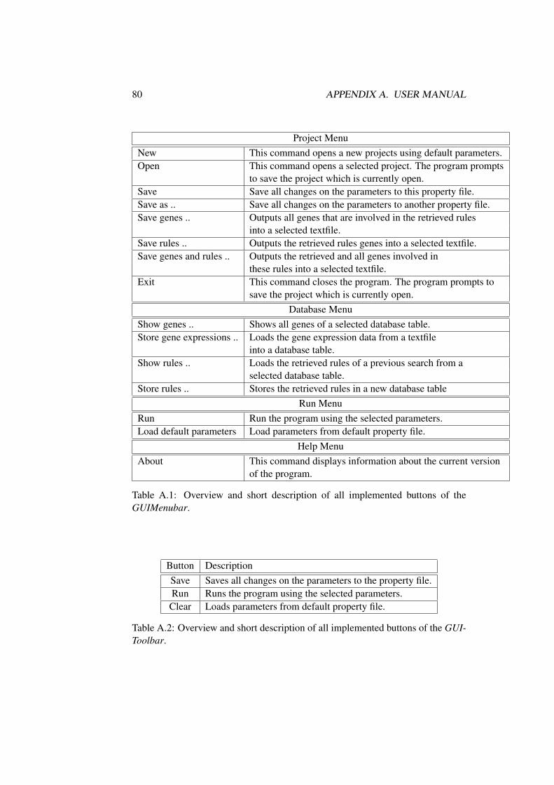
80 APPENDIX A. USER MANUAL
Project MenuNew This command opens a new projects using default parameters.Open This command opens a selected project. The program prompts
to save the project which is currently open.Save Save all changes on the parameters to this property file.Save as .. Save all changes on the parameters to another property file.Save genes .. Outputs all genes that are involved in the retrieved rules
into a selected textfile.Save rules .. Outputs the retrieved rules genes into a selected textfile.Save genes and rules .. Outputs the retrieved and all genes involved in
these rules into a selected textfile.Exit This command closes the program. The program prompts to
save the project which is currently open.Database Menu
Show genes .. Shows all genes of a selected database table.Store gene expressions .. Loads the gene expression data from a textfile
into a database table.Show rules .. Loads the retrieved rules of a previous search from a
selected database table.Store rules .. Stores the retrieved rules in a new database table
Run MenuRun Run the program using the selected parameters.Load default parameters Load parameters from default property file.
Help MenuAbout This command displays information about the current version
of the program.
Table A.1: Overview and short description of all implemented buttons of theGUIMenubar.
Button DescriptionSave Saves all changes on the parameters to the property file.Run Runs the program using the selected parameters.Clear Loads parameters from default property file.
Table A.2: Overview and short description of all implemented buttons of the GUI-Toolbar.
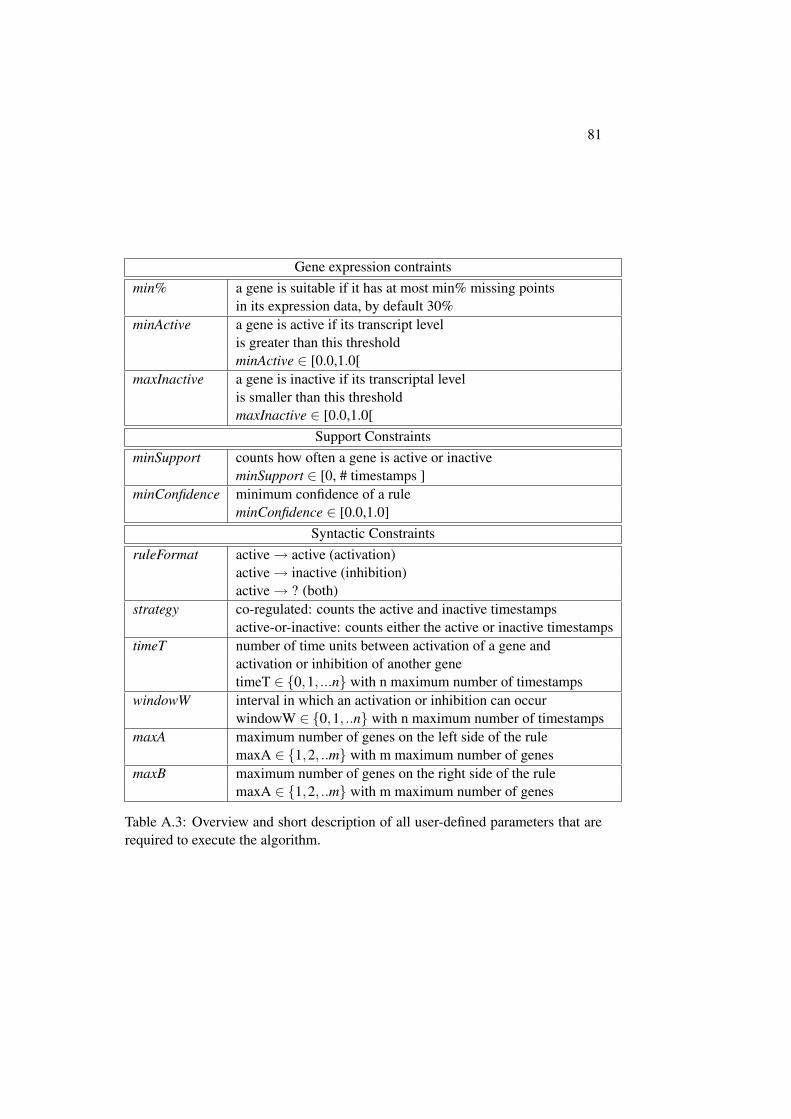
81
Gene expression contraintsmin% a gene is suitable if it has at most min% missing points
in its expression data, by default 30%minActive a gene is active if its transcript level
is greater than this thresholdminActive ∈ [0.0,1.0[
maxInactive a gene is inactive if its transcriptal levelis smaller than this thresholdmaxInactive ∈ [0.0,1.0[
Support ConstraintsminSupport counts how often a gene is active or inactive
minSupport ∈ [0, # timestamps ]minConfidence minimum confidence of a rule
minConfidence ∈ [0.0,1.0]Syntactic Constraints
ruleFormat active→ active (activation)active→ inactive (inhibition)active→ ? (both)
strategy co-regulated: counts the active and inactive timestampsactive-or-inactive: counts either the active or inactive timestamps
timeT number of time units between activation of a gene andactivation or inhibition of another genetimeT ∈ {0,1, ...n} with n maximum number of timestamps
windowW interval in which an activation or inhibition can occurwindowW ∈ {0,1, ..n} with n maximum number of timestamps
maxA maximum number of genes on the left side of the rulemaxA ∈ {1,2, ..m} with m maximum number of genes
maxB maximum number of genes on the right side of the rulemaxA ∈ {1,2, ..m} with m maximum number of genes
Table A.3: Overview and short description of all user-defined parameters that arerequired to execute the algorithm.

82 APPENDIX A. USER MANUAL
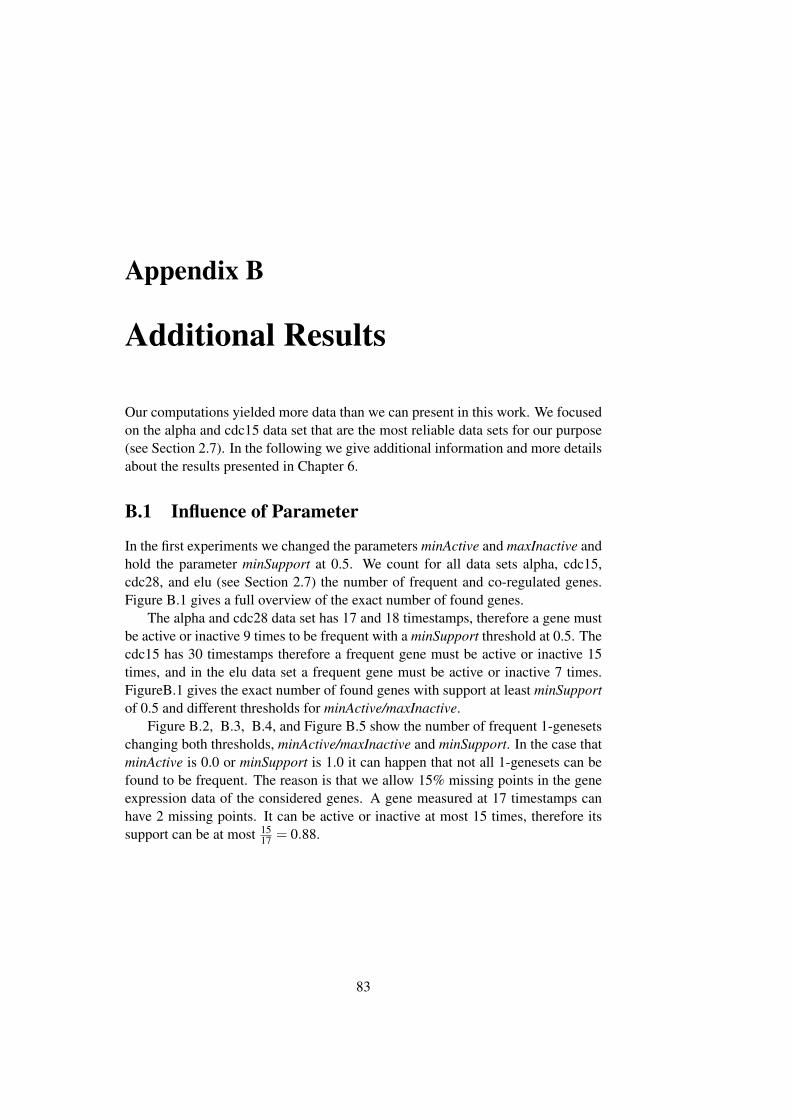
Appendix B
Additional Results
Our computations yielded more data than we can present in this work. We focusedon the alpha and cdc15 data set that are the most reliable data sets for our purpose(see Section 2.7). In the following we give additional information and more detailsabout the results presented in Chapter 6.
B.1 Influence of Parameter
In the first experiments we changed the parameters minActive and maxInactive andhold the parameter minSupport at 0.5. We count for all data sets alpha, cdc15,cdc28, and elu (see Section 2.7) the number of frequent and co-regulated genes.Figure B.1 gives a full overview of the exact number of found genes.
The alpha and cdc28 data set has 17 and 18 timestamps, therefore a gene mustbe active or inactive 9 times to be frequent with a minSupport threshold at 0.5. Thecdc15 has 30 timestamps therefore a frequent gene must be active or inactive 15times, and in the elu data set a frequent gene must be active or inactive 7 times.FigureB.1 gives the exact number of found genes with support at least minSupportof 0.5 and different thresholds for minActive/maxInactive.
Figure B.2, B.3, B.4, and Figure B.5 show the number of frequent 1-genesetschanging both thresholds, minActive/maxInactive and minSupport. In the case thatminActive is 0.0 or minSupport is 1.0 it can happen that not all 1-genesets can befound to be frequent. The reason is that we allow 15% missing points in the geneexpression data of the considered genes. A gene measured at 17 timestamps canhave 2 missing points. It can be active or inactive at most 15 times, therefore itssupport can be at most 15
17 = 0.88.
83
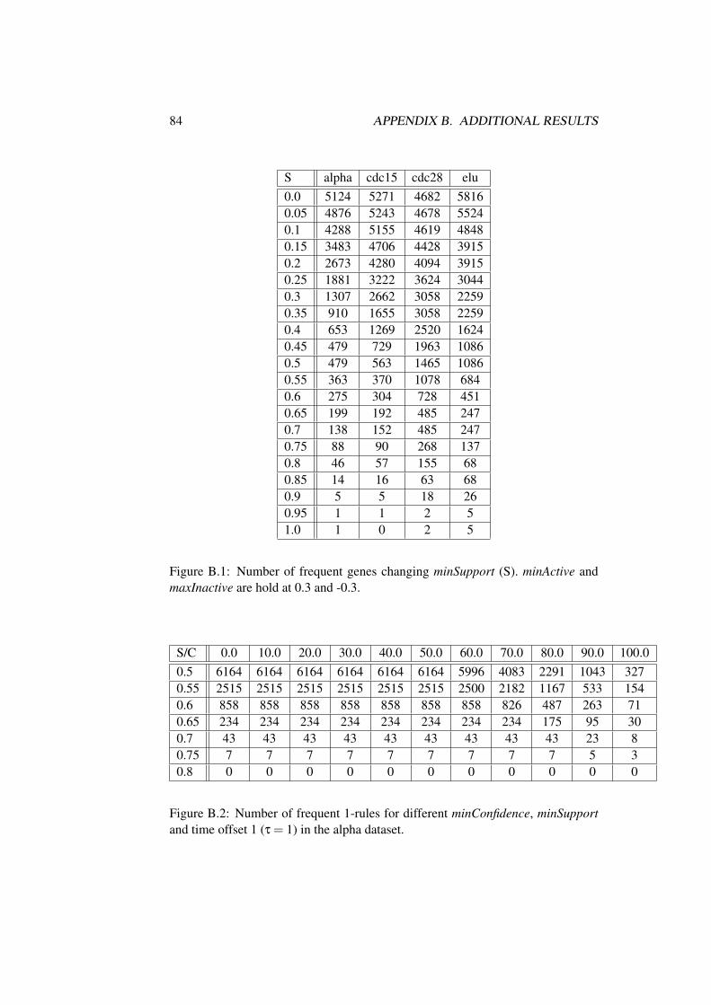
84 APPENDIX B. ADDITIONAL RESULTS
S alpha cdc15 cdc28 elu0.0 5124 5271 4682 58160.05 4876 5243 4678 55240.1 4288 5155 4619 48480.15 3483 4706 4428 39150.2 2673 4280 4094 39150.25 1881 3222 3624 30440.3 1307 2662 3058 22590.35 910 1655 3058 22590.4 653 1269 2520 16240.45 479 729 1963 10860.5 479 563 1465 10860.55 363 370 1078 6840.6 275 304 728 4510.65 199 192 485 2470.7 138 152 485 2470.75 88 90 268 1370.8 46 57 155 680.85 14 16 63 680.9 5 5 18 260.95 1 1 2 51.0 1 0 2 5
Figure B.1: Number of frequent genes changing minSupport (S). minActive andmaxInactive are hold at 0.3 and -0.3.
S/C 0.0 10.0 20.0 30.0 40.0 50.0 60.0 70.0 80.0 90.0 100.00.5 6164 6164 6164 6164 6164 6164 5996 4083 2291 1043 3270.55 2515 2515 2515 2515 2515 2515 2500 2182 1167 533 1540.6 858 858 858 858 858 858 858 826 487 263 710.65 234 234 234 234 234 234 234 234 175 95 300.7 43 43 43 43 43 43 43 43 43 23 80.75 7 7 7 7 7 7 7 7 7 5 30.8 0 0 0 0 0 0 0 0 0 0 0
Figure B.2: Number of frequent 1-rules for different minConfidence, minSupportand time offset 1 (τ = 1) in the alpha dataset.
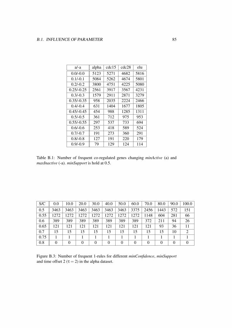
B.1. INFLUENCE OF PARAMETER 85
a/-a alpha cdc15 cdc28 elu0.0/-0.0 5123 5271 4682 58160.1/-0.1 5084 5262 4674 58010.2/-0.2 3800 4751 4225 5080
0.25/-0.25 2561 3917 3567 42310.3/-0.3 1579 2911 2871 3279
0.35/-0.35 958 2035 2224 24660.4/-0.4 631 1404 1677 1805
0.45/-0.45 454 988 1285 13110.5/-0.5 361 712 975 953
0.55/-0.55 297 537 733 6940.6/-0.6 253 418 589 5240.7/-0.7 191 273 360 2910.8/-0.8 127 191 220 1790.9/-0.9 79 129 124 114
Table B.1: Number of frequent co-regulated genes changing minActive (a) andmaxInactive (-a). minSupport is hold at 0.5.
S/C 0.0 10.0 20.0 30.0 40.0 50.0 60.0 70.0 80.0 90.0 100.00.5 3463 3463 3463 3463 3463 3463 3375 2456 1443 572 1510.55 1272 1272 1272 1272 1272 1272 1272 1148 604 281 660.6 389 389 389 389 389 389 389 372 211 94 260.65 121 121 121 121 121 121 121 121 93 36 110.7 15 15 15 15 15 15 15 15 15 10 20.75 1 1 1 1 1 1 1 1 1 1 10.8 0 0 0 0 0 0 0 0 0 0 0
Figure B.3: Number of frequent 1-rules for different minConfidence, minSupportand time offset 2 (τ = 2) in the alpha dataset.
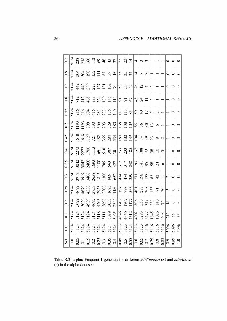
86 APPENDIX B. ADDITIONAL RESULTS
S/a
0.0
0.1
0.2
0.25
0.3
0.35
0.4
0.45
0.5
0.55
0.6
0.7
0.8
0.9
0.0
5124
5124
5124
5124
5124
5124
5124
5124
5124
5124
5124
5124
5124
5124
0.05
5124
5124
5029
4679
3919
3042
2273
1618
1193
916
712
442
304
238
0.1
5124
5124
5029
4679
3919
3042
2273
1618
1193
916
712
442
304
238
0.15
5124
5124
4939
4338
3406
2466
1700
1127
798
604
465
299
198
160
0.2
5124
5124
4692
3753
2658
1693
1113
721
530
416
333
227
152
112
0.25
5124
5118
4203
2953
1812
1100
691
482
366
281
224
167
111
690.
351
2451
1136
9823
0813
0078
551
036
629
323
318
913
187
480.
3551
2450
8930
3316
8390
956
338
728
422
917
614
510
259
430.
451
2450
2523
4211
8065
242
730
123
418
014
011
470
4637
0.45
5123
4846
1707
797
474
317
233
180
138
113
9153
3523
0.5
5123
4846
1707
797
474
317
233
180
138
113
9153
3523
0.55
5123
4512
1177
565
359
248
185
139
109
8567
4222
140.
651
2340
0280
640
127
119
313
710
485
5948
2614
40.
6551
2332
9353
028
819
814
110
874
5640
2412
73
0.7
5116
2477
347
208
133
9572
4930
1711
43
30.
7551
1616
4523
813
583
5838
2313
73
21
10.
851
1610
2614
071
4224
108
62
11
11
0.85
5116
508
7530
116
32
11
11
11
0.9
5096
213
185
21
11
11
10
00
0.95
5096
556
00
00
00
00
00
01.
050
9655
60
00
00
00
00
00
Table B.2: alpha: Frequent 1-genesets for different minSupport (S) and minActive(a) in the alpha data set.
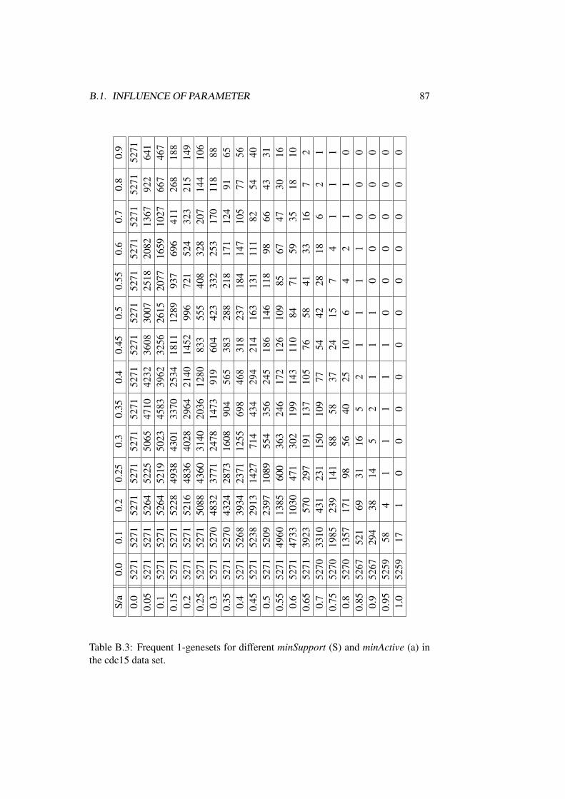
B.1. INFLUENCE OF PARAMETER 87
S/a
0.0
0.1
0.2
0.25
0.3
0.35
0.4
0.45
0.5
0.55
0.6
0.7
0.8
0.9
0.0
5271
5271
5271
5271
5271
5271
5271
5271
5271
5271
5271
5271
5271
5271
0.05
5271
5271
5264
5225
5065
4710
4232
3608
3007
2518
2082
1367
922
641
0.1
5271
5271
5264
5219
5023
4583
3962
3256
2615
2077
1659
1027
667
467
0.15
5271
5271
5228
4938
4301
3370
2534
1811
1289
937
696
411
268
188
0.2
5271
5271
5216
4836
4028
2964
2140
1452
996
721
524
323
215
149
0.25
5271
5271
5088
4360
3140
2036
1280
833
555
408
328
207
144
106
0.3
5271
5270
4832
3771
2478
1473
919
604
423
332
253
170
118
880.
3552
7152
7043
2428
7316
0890
456
538
328
821
817
112
491
650.
452
7152
6839
3423
7112
5569
846
831
823
718
414
710
577
560.
4552
7152
3829
1314
2771
443
429
421
416
313
111
182
5440
0.5
5271
5209
2397
1089
554
356
245
186
146
118
9866
4331
0.55
5271
4960
1385
600
363
246
172
126
109
8567
4730
160.
652
7147
3310
3047
130
219
914
311
084
7159
3518
100.
6552
7139
2357
029
719
113
710
576
5841
3316
72
0.7
5270
3310
431
231
150
109
7754
4228
186
21
0.75
5270
1985
239
141
8858
3724
157
41
11
0.8
5270
1357
171
9856
4025
106
42
11
00.
8552
6752
169
3116
52
11
11
00
00.
952
6729
438
145
21
11
00
00
00.
9552
5958
41
11
11
00
00
00
1.0
5259
171
00
00
00
00
00
0
Table B.3: Frequent 1-genesets for different minSupport (S) and minActive (a) inthe cdc15 data set.
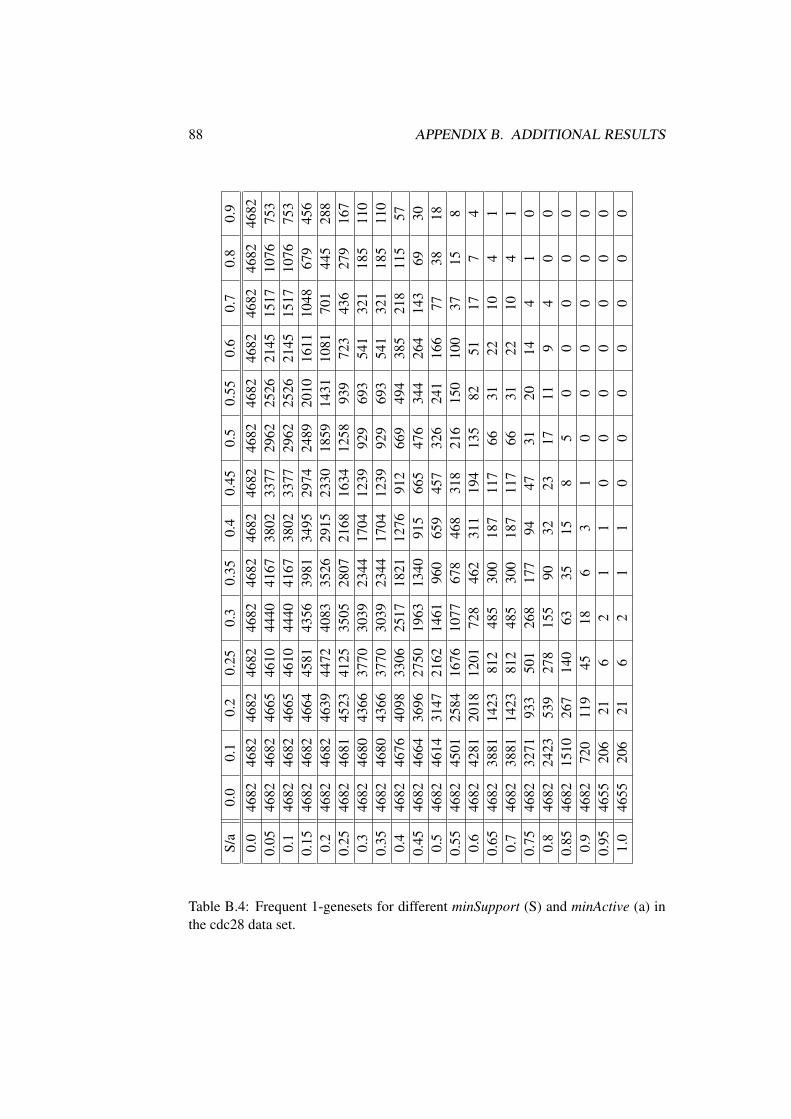
88 APPENDIX B. ADDITIONAL RESULTS
S/a
0.0
0.1
0.2
0.25
0.3
0.35
0.4
0.45
0.5
0.55
0.6
0.7
0.8
0.9
0.0
4682
4682
4682
4682
4682
4682
4682
4682
4682
4682
4682
4682
4682
4682
0.05
4682
4682
4665
4610
4440
4167
3802
3377
2962
2526
2145
1517
1076
753
0.1
4682
4682
4665
4610
4440
4167
3802
3377
2962
2526
2145
1517
1076
753
0.15
4682
4682
4664
4581
4356
3981
3495
2974
2489
2010
1611
1048
679
456
0.2
4682
4682
4639
4472
4083
3526
2915
2330
1859
1431
1081
701
445
288
0.25
4682
4681
4523
4125
3505
2807
2168
1634
1258
939
723
436
279
167
0.3
4682
4680
4366
3770
3039
2344
1704
1239
929
693
541
321
185
110
0.35
4682
4680
4366
3770
3039
2344
1704
1239
929
693
541
321
185
110
0.4
4682
4676
4098
3306
2517
1821
1276
912
669
494
385
218
115
570.
4546
8246
6436
9627
5019
6313
4091
566
547
634
426
414
369
300.
546
8246
1431
4721
6214
6196
065
945
732
624
116
677
3818
0.55
4682
4501
2584
1676
1077
678
468
318
216
150
100
3715
80.
646
8242
8120
1812
0172
846
231
119
413
582
5117
74
0.65
4682
3881
1423
812
485
300
187
117
6631
2210
41
0.7
4682
3881
1423
812
485
300
187
117
6631
2210
41
0.75
4682
3271
933
501
268
177
9447
3120
144
10
0.8
4682
2423
539
278
155
9032
2317
119
40
00.
8546
8215
1026
714
063
3515
85
00
00
00.
946
8272
011
945
186
31
00
00
00
0.95
4655
206
216
21
10
00
00
00
1.0
4655
206
216
21
10
00
00
00
Table B.4: Frequent 1-genesets for different minSupport (S) and minActive (a) inthe cdc28 data set.
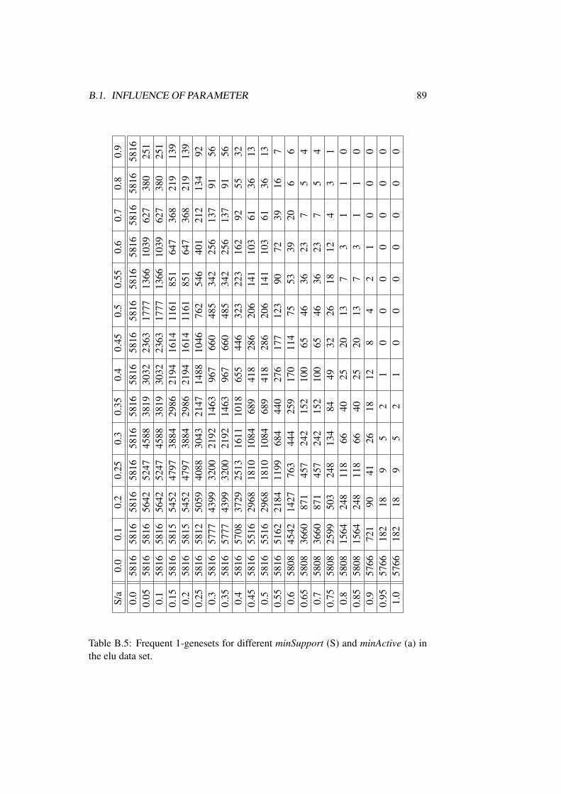
B.1. INFLUENCE OF PARAMETER 89
S/a
0.0
0.1
0.2
0.25
0.3
0.35
0.4
0.45
0.5
0.55
0.6
0.7
0.8
0.9
0.0
5816
5816
5816
5816
5816
5816
5816
5816
5816
5816
5816
5816
5816
5816
0.05
5816
5816
5642
5247
4588
3819
3032
2363
1777
1366
1039
627
380
251
0.1
5816
5816
5642
5247
4588
3819
3032
2363
1777
1366
1039
627
380
251
0.15
5816
5815
5452
4797
3884
2986
2194
1614
1161
851
647
368
219
139
0.2
5816
5815
5452
4797
3884
2986
2194
1614
1161
851
647
368
219
139
0.25
5816
5812
5059
4088
3043
2147
1488
1046
762
546
401
212
134
920.
358
1657
7743
9932
0021
9214
6396
766
048
534
225
613
791
560.
3558
1657
7743
9932
0021
9214
6396
766
048
534
225
613
791
560.
458
1657
0837
2925
1316
1110
1865
544
632
322
316
292
5532
0.45
5816
5516
2968
1810
1084
689
418
286
206
141
103
6136
130.
558
1655
1629
6818
1010
8468
941
828
620
614
110
361
3613
0.55
5816
5162
2184
1199
684
440
276
177
123
9072
3916
70.
658
0845
4214
2776
344
425
917
011
475
5339
206
60.
6558
0836
6087
145
724
215
210
065
4636
237
54
0.7
5808
3660
871
457
242
152
100
6546
3623
75
40.
7558
0825
9950
324
813
484
4932
2618
124
31
0.8
5808
1564
248
118
6640
2520
137
31
10
0.85
5808
1564
248
118
6640
2520
137
31
10
0.9
5766
721
9041
2618
128
42
10
00
0.95
5766
182
189
52
10
00
00
00
1.0
5766
182
189
52
10
00
00
00
Table B.5: Frequent 1-genesets for different minSupport (S) and minActive (a) inthe elu data set.

90 APPENDIX B. ADDITIONAL RESULTS
List of Figures
2.1 The Cell Cycle . . . . . . . . . . . . . . . . . . . . . . . . . . . 82.2 Model of a DNA double helix . . . . . . . . . . . . . . . . . . . 92.3 Sugar-phosphate backbone of the DNA . . . . . . . . . . . . . . 92.4 Gene expression and protein production . . . . . . . . . . . . . . 102.5 Transcription factor binds DNA at a specific promoter or enhancer
region . . . . . . . . . . . . . . . . . . . . . . . . . . . . . . . . 112.6 The splicing process . . . . . . . . . . . . . . . . . . . . . . . . 112.7 A cell cycle regulation example . . . . . . . . . . . . . . . . . . . 122.8 DNA-microarray . . . . . . . . . . . . . . . . . . . . . . . . . . 132.9 Gene expression courses . . . . . . . . . . . . . . . . . . . . . . 14
4.1 Database table of gene expression data . . . . . . . . . . . . . . . 264.2 Naive approach to find association rules with time offset τ . . . . 264.3 Transformation of the gene expression data . . . . . . . . . . . . 274.4 Example of the A-priori algorithm . . . . . . . . . . . . . . . . . 284.5 Example of generating strong association rules with time offset by
combining frequent k-genesets . . . . . . . . . . . . . . . . . . . 294.6 Example of generating strong association (k-)rules with time offset
by combining two frequent (k-1-)rules . . . . . . . . . . . . . . . 31
5.1 Overview of the system architecture . . . . . . . . . . . . . . . . 385.2 Database schema for gene expression data . . . . . . . . . . . . . 405.3 Database schema for preprocessed gene expression data . . . . . . 405.4 Database schema for storing the resulting rules . . . . . . . . . . 405.5 Class hierarchy of GeneSet and Rule . . . . . . . . . . . . . . . . 425.6 Screenshot of the Graphical User Interface . . . . . . . . . . . . . 525.7 Class hierarchy of the classes that realize the graphical user interface 535.8 User interface’s assistance to load gene expressions into the database 545.9 Visualization of expression levels of selected genes . . . . . . . . 545.10 Graphical representation of expression levels of selected genes . . 555.11 Basic structure of Boolean networks . . . . . . . . . . . . . . . . 565.12 Graphical representation of a selected rules . . . . . . . . . . . . 56
6.1 Influence of minActive and maxInactive on the search result . . . . 58
91
92 LIST OF FIGURES
6.2 Influence of minSupport on the search result . . . . . . . . . . . . 596.3 Gene Ontology of {YBR009C, YBL002W, YBL003C, YBR010W,
YDR224C, YDR225W, YNL030W, YNL031C} . . . . . . . . . . 676.4 Precision of found genes annotated to the cell cycle . . . . . . . . 686.5 Precision of found genes annotated to DNA replication . . . . . . 696.6 Gene ontology for genes mined with minSupport 0.7, minConfi-
dence 0.7, maxB 6 . . . . . . . . . . . . . . . . . . . . . . . . . . 726.7 Gene ontology of genes mined with minSupport 0.75, minConfi-
dence 1.0, maxB 2 . . . . . . . . . . . . . . . . . . . . . . . . . . 74
B.1 Frequent co-regulated genes changing minSupport . . . . . . . . . 84B.2 Frequent 1-rules with time offset 1 in the alpha dataset . . . . . . 84B.3 Frequent 1-rules with time offset 2 in the alpha dataset . . . . . . 85
List of Tables
1.1 Five clusters of co-regulated genes . . . . . . . . . . . . . . . . . 41.2 Association rules mined from yeast expression data . . . . . . . . 5
2.1 General information about the Cho/Spellman data sets . . . . . . 15
5.1 Number of missing points in the Cho/Spellman time-series . . . . 39
6.1 Frequent 1-rules changing minSupport and time offset . . . . . . . 606.2 Frequent 1-rules changing minSupport and time offset interval . . 616.3 Frequent k-rules in each iterative step changing maxA . . . . . . . 616.4 Frequent k-rules in each iterative step changing minConfidence . . 626.5 Frequent 1-rules with time offset 2 in the alpha data set . . . . . . 626.6 Frequent 1-rules with different time offsets . . . . . . . . . . . . . 636.7 p-values of {YBR009C, YBL002W, YBL003C, YBR010W, YDR224C,
YDR225W, YNL030W, YNL031C} . . . . . . . . . . . . . . . . 656.8 Precision of found genes annotated to the cell cycle . . . . . . . . 666.9 Precision of found genes annotated to DNA replication . . . . . . 666.10 Strong association rules mined with minSupport 0.7, minConfi-
dence 0.7, maxB 6 . . . . . . . . . . . . . . . . . . . . . . . . . . 706.11 p-values for genes mined with minSupport 0.7, minConfidence 0.7,
maxB 6 . . . . . . . . . . . . . . . . . . . . . . . . . . . . . . . 716.12 Strong association rules mined with minSupport 0.75, minConfi-
dence 1.0, maxB 2 . . . . . . . . . . . . . . . . . . . . . . . . . . 736.13 p-values of genes mined with minSupport 0.75, minConfidence 1.0,
maxB 2 . . . . . . . . . . . . . . . . . . . . . . . . . . . . . . . 75
A.1 Overview of the buttons of the GUIMenubar . . . . . . . . . . . . 80A.2 Overview of the buttons of the GUIToolbar . . . . . . . . . . . . 80A.3 Overview of all user-defined parameters . . . . . . . . . . . . . . 81
B.1 Frequent co-regulated genes changing minActive and maxInactive 85B.2 Frequent 1-genesets in the alpha data set . . . . . . . . . . . . . . 86B.3 Frequent 1-genesets in the cdc15 data set . . . . . . . . . . . . . . 87B.4 Frequent 1-genesets in the cdc28 data set . . . . . . . . . . . . . . 88
93

94 LIST OF TABLES
B.5 Frequent 1-genesets in the elu data set . . . . . . . . . . . . . . . 89
Bibliography
[1] R. Agrawal, K.-I. Lin, H. S. Sawhney, and K. Shim. Fast similarity searchin the presence of noise, scaling, and translation in time-series databases. InTwenty-First International Conference on Very Large Data Bases, pages 490–501, Zurich, Switzerland, 1995. Morgan Kaufmann.
[2] Rakesh Agrawal, Tomasz Imielinski, and Arun N. Swami. Mining associationrules between sets of items in large databases. In Peter Buneman and SushilJajodia, editors, Proceedings of the 1993 ACM SIGMOD International Con-ference on Management of Data, pages 207–216, Washington, D.C., 1993.
[3] Rakesh Agrawal and Ramakrishnan Srikant. Fast algorithms for mining asso-ciation rules. In Jorge B. Bocca, Matthias Jarke, and Carlo Zaniolo, editors,Proc. 20th Int. Conf. Very Large Data Bases, VLDB, pages 487–499. MorganKaufmann, 1994.
[4] Tatsuya Akutsu, Satoru Miyano, and Satoru Kuhara. Identification of geneticnetworks from a small number of gene expression patterns under the booleannetwork model. Proc. Pacific Symposium on Biocomputing, 1999.
[5] R. Balakrishnan, K.R. Christie M.C., Costanzo, K. Dolinski, S.S. Dwight,S.R. Engel, D.G. Fisk, J.E. Hirschman, E.L. Hong, R. Nash, R. Oughtred,M. Skrzypek, C.L. Theesfeld, G. Binkley, C. Lane, M. Schroeder, A. Sethu-raman, S. Dong, S. Weng, S. Miyasato, R. Andrada, D. Botstein, and J.M.Cherry. Saccharomyces genome database. http://www.yeastgenome.org/.
[6] T. Barrett, T. O. Suzek, D. B. Troup, S. E. Wilhite, W. C. Ngau, P. Ledoux,D. Rudnev, A. E. Lash, W. Fujibuchi, and R. Edgar. Ncbi geo: min-ing millions of expression profiles–database and tools. Nucleic Acids Res,33(Database issue), January 2005.
[7] N. P. Boghossian, O. Kohlbacher, and H.-P. Lenhof. Rapid software proto-typing in molecular modeling using the biochemical algorithms library (ball).Journal of Experimental Algorithmics (JEA), 5:16, 2000.
[8] N.P. Boghossian, O. Kohlbacher, and H.-P. Lenhof. Ball: Biochemical algo-rithms library. In J. Vitter and C. Zaroliagis, editors, Algorithm Engineering- Proc. 3rd Intern. Workshop, pages 330–344. Springer, Berlin, 1999.
95
96 BIBLIOGRAPHY
[9] George Casella and Roger L. Berger. Statistical Inference. Second Edition.Duxbury, 2002.
[10] Soumen Chakrabarti. Mining the Web: Discovering Knowledge from Hyper-text Data. Morgan-Kauffman, 2002.
[11] Katherine C. Chen, Laurence Calzone, Attila Csikasz-Nagy, Frederick R.Cross, Bela Novak, and John J. Tyson. Integrative analysis of cell cycle con-trol in budding yeast. Mol. Biol. of the Cell, August 2004.
[12] Raymond J. Cho, Michael J. Campbell, Elizabeth A. Winzeler, Lars Stein-metz, Andrew Conway, Lisa Wodicka, Tyra G. Wolfsberg, Andrei E.Gabrielian, David Landsman, David J. Lockhart, and Ronald W. Davis. Agenome wide transcriptional analysis of the mitotic cell cycle. Mol. Cell,1998.
[13] Chad Creighton and Samir Hanash. Mining gene expression databases forassociation rules. Bioinformatics, 19(1):79–86, 2003.
[14] Gautam Das, Dimitrios Gunopulos, and Heikki Mannila. Finding similartime series. In Principles of Data Mining and Knowledge Discovery, pages88–100, 1997.
[15] Gautam Das, King-Ip Lin, Heikki Mannila, Gopal Renganathan, and PadhraicSmyth. Rule discovery from time series. In Knowledge Discovery and DataMining, pages 16–22, 1998.
[16] Eric H. Davidson. Genomic Regulatory Systems: Development and Evolu-tion. Academic Press, first edition, February 2001.
[17] E.R. Dougherty, S. Kim, and Y. Chen. Coefficient of determination in non-linear signal processing. Signal Process., 80, 2219–2235, 2000.
[18] E.R. Dougherty, S. Kim, Y. Chen, K. Sivakumar, P. Meltzer, J.M. Trent, andM. Bittner. Multivariate measurement of gene expression relationships. Ge-nomics, 67, 201–209, 2000.
[19] Michael B. Eisen, Paul T. Spellman, Patrick O. Brown, and David Botstein.Cluster analysis and display of genome-wide expression patterns. Proc. Natl.Acad. Sci. USA, 95:14863–14868, December 1998.
[20] Vladimir Filkov, Steven Skiena, and Jizu Zhi. Analysis techniques for mi-croarray time-series data. In RECOMB ’01: Proceedings of the fifth annualinternational conference on Computational biology, pages 124–131, NewYork, NY, USA, 2001. ACM Press.
[21] Christophe Fiorio. algorithm2e.sty - package for algorithms. (c) 1996 - 2005Christophe Fiorio, LIRM Montpellier, France, release 3.6, January 2005.
BIBLIOGRAPHY 97
[22] Nir Friedman, Michal Linial, Iftach Nachman, and Dana Pe’er. Usingbayesian networks to analyze expression data. In RECOMB, pages 127–135,2000.
[23] Nir Friedman, Iftach Nachman, and Dana Pe’er. Learning bayesian networkstructures from massive datasets: The sparse candidate algorithm. In Proc.UAI, 1999.
[24] Elisabeth Georgii, Lothar Richter, Ulrich Ruckert, and Stefan Kramer. Ana-lyzing microarray data using quantitative association rules. In Bioinformatics2005 21(Suppl 2), pages ii123–ii129. Oxford University Press, 2005.
[25] L. Glass and S.A. Kauffman. The logical analysis of continuous, nonlinearbiochemical control networks. Theoret. Biol. 39, 1973.
[26] Jiawei Han and Micheline Kamber. Data Mining: Concepts and Techniques.Morgan Kaufmann, 2001.
[27] Robert Harris and Rob Warner. The Definitive Guide to SWT and JFace.Apress, June 2004.
[28] Wolfgang Hennig. Genetik. Springer-Lehrbuch. Springer, 2002. HEN w 02:11.P-Ex.
[29] Timothy R. Hughes, Matthew J. Marton, Allan R. Jones, Christopher J.Roberts, Roland Stoughton, and Chirstopher D. Armour. Functional discov-ery via a compendium of expression profiles. Cell, 102:109–126, 2000.
[30] Vishwanath R. Iyer, Michael B. Eisenand Douglas T. Ross, Greg Schuler,Troy Moore, Jeffrey C. F. Lee, Jeffrey M. Trent, Louis M. Staudt, James Hud-son Jr., Mark S. Boguski, Deval Lashkari, Dari Shalon, David Botstein, andPatrick O. Brown. The transcriptional program in the response of humanfibroblasts to serum. Science 1 Vol. 283. no. 5398, January 1999.
[31] S.A. Kauffman. Metabolic stability and epigenesis in randomly constructedgenetic nets. Theoret. Biol. 22, 1969.
[32] S.A. Kauffman. Origins of order: Self-organization and selection in evolu-tion. Oxford University Press, New York, 1993.
[33] Andreas Keller. A statistical framework for the diagnosis of meningiomacancer. Master’s thesis, Saarland University, 2005.
[34] Heikki Mannila, Jaakko Hollmn, Jouni K. Seppanen, Kalle Korpiaho, Jo-hanna Tikanmaki, and Ella Bingham. From data to knowledge research unit:Applications in bioinformatics. In K. Puolamki and L. Koivisto, editors, Bi-ennial report 2000-2001, pages 195–202. Otaniemi, April 2002.
98 BIBLIOGRAPHY
[35] Christopher D. Manning and Hinrich Schuze. Foundations of statistical nat-ural language processing. MIT Press, Cambridge, MA, USA, 1999.
[36] U.S. Department of Energy by Denise Casey. Primer on molecular genetics.1991-1992 DOE Human Genome Program Report, 1992.
[37] Judea Pearl. Probabilistic Reasoning in Intelligent Systems: networks of plau-sible inference. Morgan Kaufmann, 1988.
[38] Dana Pe’er, Aviv Regev, Gal Elidan, and Nir Friedman. Inferring subnet-works from perturbed expression profiles. Proceedings of the Ninth Inter-national Conference on Intelligent Systems for Molecular Biology, ISMB,17(90001):S215–S224, 2001.
[39] Raghu Ramakrishnan and Johannes Gehrke. Database Management Systems.McGraw-Hill Higher Education, 2000.
[40] P. M. Selzer, R. J. Marhfer, and A. Rohwer. Angewandte Bioinformatik: eineEinfuhrung. Springer-Lehrbuch. Springer, 2004.
[41] Ilya Shmulevich, Edward R. Dougherty, Seungchan Kim, and Wei Zhang.Probabilistic boolean networks: a rule-based uncertainty model for gene reg-ulatory networks. Bioinformatics 2002 18 (Suppl 2), 2001.
[42] Paul T. Spellman, Gavin Sherlock, Michael Q. Zhang, Vishwanath R. Iyer,Kirk Anders, Michael B. Eisen, Patrick O. Brown, David Botstein, and BruceFutcher. Comprehensive identification of cell cycle-regulated genes of theyeast saccharomyces cerevisiae by microarray hybridization. Mol. Biol. ofthe Cell, 1998.
[43] Lubert Stryer. Biochemie. Spektrum Akademischer Verlag, 1991. Translatedfrom the English by Brigitte Pfeiffer and Johannes Guglielmi.
[44] E.B. Suh, E.R. Dougherty, S. Kim, D.E. Russ, and R.L. Martino. Parallelcomputing methods for analyzing gene expression relationships. In Proc.SPIE Vol. 4266, p. 213-221, Microarrays: Optical Technologies and Infor-matics, pages 213–221, June 2001.
[45] Larry Wasserman. All of Statistics. Springer, 2004.
[46] J. D. Watson and F. H. C. Crick. Molecular structure of nucleic acids: Astructure for deoxyribose nucleic acid. Nature, 171:737–738, 1953.


![Einsatz von Satellitenbildern im Bevölkerungsschutz · charter-activations [Stand: 02.11.2018] eingesehen werden. 4.2 ZKI-DE ZKI-DE ist der Name eines Projektes. Hierbei handelt](https://img.pdfslide.org/doc/110x75/605cb21072a0554c462ec53a/einsatz-von-satellitenbildern-im-bevlkerungsschutz-charter-activations-stand.jpg)