Efficient Modelling, Generationand Analysis of Markov Automata

Mark Timmer

Graduation committee:

Chairman: Prof. dr. ir. Anton J. MouthaanPromotors: Prof. dr. ir. Joost-Pieter Katoen, PDEng

Prof. dr. Jaco C. van de PolCo-promotor: Dr. Marielle I. A. Stoelinga

Members:Prof. dr. ir. Boudewijn R. Haverkort University of TwenteProf. dr. Richard J. Boucherie University of TwenteProf. dr. ir. Jan Friso Groote Eindhoven University of TechnologyProf. dr. Wan Fokkink VU University AmsterdamProf. dr. ing. Holger Hermanns Universitat des Saarlandes

CTITCTIT Ph.D. Thesis Series No. 13-261Centre for Telematics and Information TechnologyUniversity of Twente, The NetherlandsP.O. Box 217 – 7500 AE Enschede

IPA Dissertation Series No. 2013-13The work in this thesis has been carried out under the aus-pices of the research school IPA (Institute for Programmingresearch and Algorithmics).

Netherlands Organisation for Scientific ResearchThe work in this thesis was supported by the SYRUPproject (SYmbolic RedUction of Probabilistic Models),funded by NWO grant 612.063.817.

ISBN 978-90-365-0592-5ISSN 1381-3617 (CTIT Ph.D. Thesis Series No. 13-261)Available online at http://dx.doi.org/10.3990/1.9789036505925

Typeset with LATEXPrinted by Ipskamp Drukkers

Cover design by Thomas van den Berg and Mark Timmer(Image designed originally by Kaj Gardemeister, bought from Dreamstime)

Copyright c© 2013 Mark Timmer, Enschede, The Netherlands

EFFICIENT MODELLING, GENERATIONAND ANALYSIS OF MARKOV AUTOMATA

DISSERTATION

to obtainthe degree of doctor at the University of Twente,

on the authority of the rector magnificus,prof. dr. H. Brinksma,

on account of the decision of the graduation committee,to be publicly defended

on Friday, September 13th, 2013 at 16:45 o’clock.

by

Mark Timmer

born on 15 April 1984in Apeldoorn, The Netherlands

This dissertation has been approved by:

Prof. dr. ir. Joost-Pieter Katoen, PDEng (promotor)Prof. dr. Jaco van de Pol (promotor)Dr. Marielle Stoelinga (co-promotor)

To my parents (in memoriam)

Acknowledgements

“A noble person is mindful and thankfulfor the favours he receives from others.”

Buddha

First, I would like to thank my supervisors Jaco van de Pol, Joost-PieterKatoen and Marielle Stoelinga, who were most influential regarding the

contents of this work. Thank you all so much for enabling me to experiencethe journey that resulted in this thesis. It taught me a lot about computerscience as well as myself, and it allowed me to meet people from more countriesthan I could ever have expected.

Jaco, you were always enthusiastic to talk about technical matters, discuss-ing definitions or proofs and often immediately spotting mistakes or possibledifficulties that I may otherwise have missed. Your eye for detail greatly helpedto shape and improve this work. As a boss, you gave me the freedom to work ona variety of topics, and allowed me to participate in the “promovendi voor deklas” project. This impacted my life significantly, enabling me to pursue a careerin teaching. You recently even gave a guest lecture at the school where I teach,explaining twelve-year-olds about the fascinating aspects of model checking andexperiencing how rewarding secondary school teaching is. I can never thank youenough for being a decisive factor in making it possible that I can now experiencethis joy every day.

Joost-Pieter, even though Aachen is not around the corner, we quite oftenmanaged to discuss my work. I really enjoyed the visits to Aachen, allowing me toget to know your other PhD students as well. Thank you for the many motivatingtalks and emails, and the extremely precise feedback on my papers and thisbook—you always managed to suggest several interesting and relevant conceptsto mention or include in my work, checked several proofs very thoroughly andnever failed to notice a missing closing parenthesis. When I was in doubt whichdirection to go or to which conference to submit next, I could always rely onyour confidence and great advice.

Marielle, as my daily supervisor you were the one who has taught me the most.While working on my MSc thesis you already spent many hours educating me inthe fine art of scientific writing. I learned to be concise and use short and simplesentences where possible—although I do still appreciate some more complicatedstructures. I learned to use ‘may’ instead of ‘might’ more often, and to stopusing ‘would’ in conditional statements that require a second conditional or thirdconditional grammatical construct instead. You taught me how to structure anexplanation, how to write an introduction and how to define concepts as simple

viii Acknowledgements

as possible. Your quest for clean theory sometimes made me slightly desperate,but also greatly helped me to improve my work. When I knew that a certainconcept could be explained a bit better but I had not forced myself to do so, Icould always count on you to point this out. In the end, of course, I was happythat you did. Also on a more personal level, we had many interesting talks.You always know more gossip than I do and often have several suggestions forinteresting books, my favorite being “Eats, shoots and leaves”. I also like tothank you for allowing me to co-organise the Dutch testing day and one of theROCKS meetings—a lot of fun!

Regarding the work in this thesis, in addition to my supervisors, I want tothank several other people. First of all, a big thanks to Henri Hansen and ArndHartmanns for collaborating with me on the work that resulted in Chapters 7and 8. Luis Marıa Ferrer Fioriti, thanks for your help in analysing the behaviourof the partial order check on the case studies discussed in Chapter 8. I also wantto thank Erik de Vink and Michel Reniers for their many helpful commentson a draft of one of the papers on which Chapter 4 is based, as well as Pedrod’Argenio for his useful insights in stochastic process algebras. A big thanks toDave Parker from Oxford University for useful discussions about the functionalityof my tool and several of the underlying theoretical ideas, and Axel Belinfantefor implementing a web-based interface. I thank Jan Friso Groote for hisspecification of the handshake register, upon which one of the case studies inChapter 9 is based. Furthermore, I thank Michael Weber for fruitful discussionsabout Hesselink’s protocol. Stefan Blom, thank you so much for your manyhelpful suggestions regarding several aspects of my work. Dennis Guck, thanksfor all your invaluable help regarding the case studies and tool support.

I would like to thank my thesis committee for their extensive efforts, readingthis book and providing numerous points of improvement. Boudewijn Haverkort,Holger Hermanns, Jan Friso Groote, Richard Boucherie, Wan Fokkink, thankyou for all your hard work during the summer!

An important part of my PhD experience consisted of my collaboration with thepeople from the research group I was part of: Formal Methods & Tools (FMT).Over the years, I had many colleagues that were interesting coworkers and goodfriends as well. For approximately 4.5 years I shared office 5078 with EduardoZambon. We had a perfect atmosphere for working and having some fun as well,mostly working hard but helping each other when needed and having a laughevery now and then. Eduardo, you showed me that the final months of writinga PhD thesis can be hell—but also that it is not impossible to make it throughand that the result is very rewarding. I replicated this process, going throughhell as well though with the advantage of having seen that indeed everythingcan be completed as long as we continue gradually. Thanks for all the goodtimes! And, sorry again for using your desk as additional storage space forall my stuff when you were on holiday or a conference visit. After Eduardograduated, Paul Bonsma took his place (and hence my storage space). Paul, Ienjoyed your company. Thanks for putting up with me in these last few monthswhen I was stressing to finish the thesis and therefore may not have been the

Acknowledgements ix

most pleasant office mate.

Theo Ruys, your passion for teaching really impressed me, and your (some-times hard to interpret) sarcasm and cynicism often resulted in a (sometimessomewhat delayed) smile on my face. I was in doubt for quite a while aboutwhether or not to pursue the teaching degree in parallel to my PhD work. Youquitting your job at FMT to study for primary school teaching was precisely thetrigger I needed to decide (even though in the end you did not pursue this—Iam still expecting at least some teaching degree from you in the coming years),thank you so much for that! Thanks as well for being quite perplexed when atsome point I had neglected my right to vote for the European Parliament—Ivoted for every election since then.

Arend Rensink, thanks for all your enthusiasm organising Floor Five Filmmarathons, dutifully buying crisps for BOCOM (Floor Five’s Friday afternoonget-together), and for organising a wonderful barbecue every year—allowing meto be lazy last time and not bring any salad in exchange for this acknowledgement.Elise Rensink, you are always great company at the barbecues and one of thecoolest women I know!

Thanks to Rom Langerak for being a great office neighbour, and for stressingeven more on your educational self-evaluation than I did on my thesis these lastmonths (that made me feel slightly better). Marieke Huisman, thank you forhaving us over several times, allowing us to practice babysitting. Also, thanksfor always being so relaxed, putting things in perspective, and for persistentlytrying to get our foreign colleagues to speak Dutch. Hajo Broersma, thanks foryour stories about mathematics and for lending me a great calendar with puzzlesthat I may use in secondary school.

Axel Belinfante, thank you so much for providing the puptol framework! Itmajorly improved the visibility of my work, impressed quite some colleagues atconferences and even helped me to more easily experiment with my own tool.Also, thanks for all the great collaborations regarding the Testing Techniquescourse over the years and the organisation of the Dutch testing day! MichaelWeber, I was amazed by your positivity when some bad things happened. I wasalso amazed by your resistance to Marieke’s attempts to try to have you speakDutch, even though you secretly can do this perfectly fine! Stefan Blom, thanksfor being our most reliable BOCOM supplier, buying beer at the lowest priceand introducing the cans of soft drinks (that have become very popular overthe last year!). Also, thanks for always making time to give great tips when Ihad a confluence-related problem, and for still being nice to me even thoughI had little time to assist you while you were working on a great embeddingof my tool SCOOP in the LTSmin toolset (which, by the way, still deserves abetter name in my opinion—Jaco, you managed to rename FMG to FMT, sothis should be possible too!).

Maarten de Mol, even though (or maybe even because) we are so differentin many ways, I always had a great time having coffee with you in the rappa.It was funny seeing you walk circles to come up with new ideas, or seeing youpassionate about functional programming. I was impressed by your work ethicand your persistence in travelling to work all the way from Westervoort everyday. Thank you for the many lovely conversations we had! Alfons Laarman,

x Acknowledgements

first of all thanks for always being in the office so late that I never had to feelbad if I was sometimes late as well—I could always count on you being evenlater! Also, thanks for the great company you and Laura Grana-Suarez wereduring our Western USA within a week trip! I actually had not expected you tosurvive and/or enjoy our minute-to-minute planning on Mark & Thijs speed (or,as Laura phrased it, the German schedule). I had an amazing time, thanks forbeing there to share this experience!

Dennis Guck, first of all, thank you so much for developing algorithms forMarkov automata and for implementing IMCA! I remember being absolutelythrilled when Joost-Pieter told me about your accomplishments; they reallygive purpose to my work that would otherwise not have been there. FlorianArnold, Dennis, thanks for an amazing Rome experience at ETAPS this year! Iseldom had so much fun at a karaoke bar. Florian, once more my apologies forpersuading you to stay up so long that the next day you actually missed yourplane! I felt a bit bad the next day, but on the other hand this does make agreat story (for me as well as for you, I hope).

Tri Minh Ngo, thanks for very persistently forcing me to take the stairsinstead of the elevator and constantly reminding me that I should exercise more!Of course, you were completely right. Actually, I recently even took the stairswhile you were in Vietnam so that I could proudly send you an email about this!(I did forget to send this email though.) Also, thanks for having your luggage getlost while travelling to the Netherlands for your job interview and then presentingyour work in shorts and a rather crappy T-shirt—this story always makes mefeel better when my luggage gets lost at the airport; things can always be worse!

Stefano Schivo, thanks for motivating several people (including me sometimes)to go running every week and get some exercise; we really need it. MarinaZaharieva-Stojanovski, you are one of the friendliest people I have ever met—thanks for always being so involved and interested in other people’s lives. Also,I am very happy to have you as a paranymph! Gijs Kant, thanks for youromnipresent enthusiasm to go out and have a drink at conferences, for yourgreat participation in making songs for colleagues, and for sometimes organisingnice events in the lunch breaks. Ed Brinksma, thanks for taking some timeout of your extremely busy schedule to work on a nice paper on model-basedtesting together with Marielle and me. Afshin Amighi, Lesley Wevers, MohsinDanish, Steven te Brinke, Tom van Dijk, Waheed Ahmad, Wojciech Mostowski,you are all great colleagues! Amir Ghamarian, Jeroen Ketema, I was sad to seeyou leave, thanks for the great times we had. Amir, I’m still counting on youto drive a camel some day.

Joke Lammerink, Jeanette Rebel-de Boer, thanks for your administrativesupport during the last five year, but even more for the many long and interestingtalks we had. If I had something I wanted to talk to somebody about, I wasalways welcome in your offices.

I also owe a great deal to the lovely people of DACS. Aiko Pras and Pieter-Tjerkde Boer, thank you so much for your great supervision of my BSc thesis in 2005!You really gave me confidence to seriously consider pursuing a PhD. Withoutyou, this thesis may never have been written! I also really want to thank you

Acknowledgements xi

for encouraging me to write a paper on my BSc work and helping me a lot byproviding feedback and writing parts of that paper. Boudewijn, a big thanks toyou as well, for allowing me to present the paper at the E2EMON workshop inVancouver, Canada—additionally, thank you so much for informing me aboutthe possibility to take a return flight from a different airport! This enabled meto make a memorable trip from Vancouver to San Francisco and Los Angeles.Anne Remke, thanks for our many great talks and for offering me to work withyou and Rom next year!

Dave Parker, Marta Kwiatkowska, Joel Ouaknine, thank you so much forreceiving me at Oxford University ComLab for two months in the autumn of2010. Marta, once more my apologies for spilling my soup all over the chair whilewalking back to the lunch table in Trinity College’s professor’s lounge. As it alllooked so fancy I was so nervously trying to avoid doing anything stupid thatof course my clumsiness caused me to make a big mess. The change of scenerydue to my stay in Oxford inspired me to majorly improve my tool SCOOP,and it taught me a lot about Apex and PRISM (no dear reader, not the NSAsurveillance programme). Most importantly, it got me in contact with so manynice people. Bjorn Wachter, Christian Dehnert, Hristina Palikareva, I had thebest time on our trip to Stonehenge, Salisbury, Bath and some castle just overthe border of Wales. Christian, thanks for being great company in Oxford, forjoining me to Windsor Castle and Cambridge, and for showing me around inAachen. Vojtech Forejt, Stefan Kiefer, you also quickly became good friendduring my visit. Together with the rest of the gang, I greatly enjoyed our visitsto evensongs, the opera, the gamelan concert, the Jan Tiersen concert, and alarge variety of pubs and restaurants.

Henri Hansen, thanks for accompanying Christian and me on a great trip toStratford-upon-Avon, and for making every lunch break a delight. Also, manythanks for our wonderful collaborations, resulting in a journal paper that makesme proud and that is presented in Chapter 7 of this thesis. Our collaborationwas very fruitful; we both contributed ideas and meticulously checked and ifneeded improved the other’s input. I always felt that I could opt every idea thatcame to mind, surely receiving constructive criticism. You still have many greatideas on the topics that we worked on, and I hope that we may still publishsome nice results together. I also still have to visit you in Finland someday, andwould really like to do so some day!

Alexandru Mereacre, Arpit Sharma, Christian Dehnert, Erika Abraham,Friedrich Gretz, Falak Sher, Henrik Bohnenkamp, Martin Neuhaußer, Sabrinavon Styp, Souy Chakraborty, Tingting Han, Viet Yen Nguyen, thanks for makingme feel right at home in Aachen. You were great to be around during my researchvisits and the Aachen Concurrency and Dependability week. Tingting, I thoughtwe were a great Aladdin and Jasmin on SingStar!

I would like to thank all the students that I supervised during my PhD. VincentBloemen, you were a pleasure to work with, and I am very proud that youmanaged to work on several quite difficult concepts as part of your BSc thesis.Martijn Adolfsen, you worked hard on an interesting topic and obtained severalrelevant results. No wonder that the company you did the research at wanted

xii Acknowledgements

to keep you! Elodie Venezia, you were one of the best students in the TestingTechniques course. Your research project on coverage measures demonstratedgreat perseverance! Gerjan Stokkink, I was very impressed by the amount ofwork you managed to complete. We don’t often see so many scientific resultsfrom one MSc project. It was great fun too, exploring the bad neighbourhoodsof Tallinn together! Rob Bamberg, thanks for choosing me for your MSc thesison a topic very related to my work; I enjoyed it a lot. Ferry Olthuis, at themoment of writing you are still working on your MSc thesis. Good work so far!I was very honoured to hear that you wanted to do your thesis on a projectfurther investigating some of my work. You are a pleasure to work with.

During the last few years I visited several conferences, sometimes at far-awaydestinations. It is infeasible to thank all the people that made these experiencesas memorable as they were, but I do like to mention a few. In York, England(ETAPS 2009), I had many nice dinners and a remarkable Ghost Tour, mostlywith the Aachen people from Joost-Pieter’s group. Thanks for a great initiationto enjoying conferences, guys! In Tianjin, China (TASE 2009), I had an awesometime sightseeing the city together with Richard Banach and Moritz Martens,thank you for that! This conference also resulted in Thijs and me travellingthrough China for three weeks, showing us how great far-away holidays canbe and inspiring us to have many more afterwards. I owe this to a couple ofFOSSACS 2009 reviewers; thank you for rejecting my paper so that I couldresubmit to TASE, travel to China and have all these amazing experiences!

Macao (ATVA 2009) was also fairly spectacular, bungee jumping the MacaoTower (233 meters) together with Christian Dax. A big thanks to Yael Mellerfor making pictures during the bungee jump and for teaching me a lot aboutIsrael. And a big apology to Thijs for almost giving you a heart attack uponseeing the video of this jump. ETAPS 2010 brought me to Paphos, Cyprus,where I had a great time with Miguel Andres, Trajce Dimkov and Petur Olsen.Besides drinking cocktails and enjoying a swim in the ocean or the swimmingpool, we spent a free afternoon discovering the underwater world through anintroduction dive. Thanks for sharing this with me! Rather impulsively Trajceand me even took a road trip to the north of Denmark, visiting Petur duringthe Aalborg carnival. Great trip, thanks guys for the awesome weekend!

The summer of 2010 took me to Braga, Portugal for ACSD. Anton Wijs,thanks for accompanying me during the Sao Joao festival, which to our greatamusement mainly seemed to consist of people smashing each other on theheads with plastic hammers (martelinhos) and leek. A big thanks to all theBraga inhabitants for indeed allowing us to smash them on their heads; that’sgood stuff! I also like to thank Matthias Raffelsieper for spending a great dayin Porto with me.

ETAPS 2011 in Saarbrucken, Germany was nice, but I enjoyed the 2012destination even more: Tallinn, Estonia. As mentioned before, it encompassedan interesting walking tour with Gerjan, but also a shamefully funny evening ina karaoke bar with Arend, Gerjan, Gijs and Sander Bruggink (video material isavailable upon request). Also, thanks to Arend, Maarten, Marina and Antonfor joining me to visit Helsinki, Finland during this week. Although Marina

Acknowledgements xiii

observed that Helsinki is a place where you would rather be found dead thanalive (I could see her point), I really enjoyed the trip. Later that year, I spent awonderful weekend in York with James Williams and Chris Poskitt for mentalpreparation for CONCUR 2012, taking place in Newcastle, England. DanielGebler and Michel Reniers, thanks for joining me to see the (rather unimpressive,as it turned out) Hadrian’s wall. Daniel, thanks as well for inviting me to give atalk at your group in Amsterdam!

This year’s ETAPS in Rome, Italy was a pleasure as well. Although I wasalready stressing a bit about finishing this thesis and I could only be there brieflydue to teaching responsibilities, the karaoke bar visit with Dennis and Florianmade me forget all my worries for a while—fortunately, I did manage to completemy slides the next day. Thanks to Arnd Hartmanns as well for joining me forsightseeing through Rome. Mieke Massink, Erik de Vink, thanks for alwaysproviding great companionship at QAPL events.

Even more fun than conferences are summer schools. Katharina Spies, SilkeMuller, thank you for organising the best summer school there is, the Marktober-dorf summer school! I had the most amazing time there in the summer of 2010.Hristina Mihajloska, Magdalena Kostoska, you already became good friends ofmine there before the first night was over! Yuriy Solodkyy, thanks for teachingus many great salsa moves; this always brought about a perfect atmosphere.Chris Poskitt (Harry!), David Williams, James Sharp, James Williams (Ron!),Luke Herbert, Tuomas Kuismin, go Team GB! You all were so funny and a blastto be around. I had a great time during our visits to Neuschwanstein Castleand Munich, and it was awesome when you came to see me during my Oxfordvisit (unfortunately without Tuomas), and when we met up in Amsterdam afterDavid moved there. James Sharp, you are one of the best Disney song singersI know! I think we annoyed most of Amsterdam and all of the professors inthe bus to the hike near Marktoberdorf, a good accomplishment. Luke, youare one of the strangest persons I have ever met (in a good way)! Aws Albarg-houthi, Ken Madlener, it was also very nice to meet you in Marktoberdorf andat other occasions.

In the summer of 2011 I spent a wonderful week in the hilly town of Bertinoro,Italy, for the SFM summer school. Marco Bernardo, thanks for organising thisevent! Also, a big thanks to my room mate Nuno Oliveira, and to Peter Drabik,Jaroslav Keznikl, Amel Bennaceur, Gianina Ganceanu, Bojana Bislimovska,Pankesh Patel, Sara Hachem, Sergio Di Sebenico, Imen Ben Hafaiedh Marzoukfor several great dinners, long evening talks and a great visit to the beach ofRimini. I had loads of fun! Christel Baier, my (kind of late) apologies for leavingand re-entering the room several times during your lectures. After having had anice talk with you in the bus from the airport, I felt a bit bad about it. Therewas a good reason, though; I was negotiating the price of the house we currentlyown, and we managed to reduce it by approximately 10% during your talk!

Maybe even more fun than summer schools, the IPA (Instituut voor Program-matuurkunde en Algoritmiek) Spring Days and Autumn Days were amongthe highlights of each year. Thanks to Tijn Borghuis, Michel Reniers and

xiv Acknowledgements

Tim Willemse for subsequently organising these wonderful events together withMeivan Cheng! We learned a lot during the days on various topics, but also(most importantly?) enjoyed the socialising aspects that took place during theevenings. I made many great friends during these events and we had so muchfun, even resulting in two IPAZoP (IPA Zonder Praatjes) weekends organisedby ourselves (big thanks to Ze Pedro Magalhaes!). A huge thanks to AlexandraSilva, Atze van der Ploeg, Carst Tankink, Cynthia Kop, David Costa, FaranakHeidarian, Felienne Hermans, Frank Stappers, Frank Takes, Jeroen Keiren, JoostWinter, Marijn Schraagen, Michiel Helvesteijn, Paul van Tilburg, Ze PedroMagalhaes, Sjoerd Cranen, Stephanie Kemper, Tijs van der Storm and manyothers for making these events so much more than just work.

Besides the conferences, summer schools and IPA events, I also visited alarge number of ROCKS and QUASIMODO meetings. At these events I met somany nice people, among which some of the ones already mentioned above. Aspecial thanks to Arnd Hartmanns, who gave an interesting talk at one particularROCKS meeting that resulted in a fruitful collaboration. We are both equallyperfectionistic (Arnd maybe even slightly more than I am), which actually workedout really well; it got us to the NASA Ames Research Center in Moffett Field,California, and resulted in Chapter 8 of this thesis. Arnd, thank you for thecollaboration, for taking me to see Volklinger Hutte, and for your great schedulingskills and companionship regarding our Western USA within a week trip!

Nico van Diepen, you were the first person to inform me about the “Promovendivoor de klas” project. Thank you for thinking about me and being the initial stepin my journey towards the most interesting job I can imagine! Nellie Verhoef,you are a great inspiration regarding mathematics teaching and a lovely person!Thank you for always believing in me and my teaching skills, allowing me tocollaborate with you on several interesting projects and papers, and for invitingme to the Community of Learners for mathematics teachers! Bert Booltink, Daanvan Smaalen, Fokke Hoeksema, Gerard Jeurnink, Jan Keemink, John Heijmans,Nico Alink, Roelf Haverkamp, Ronnie Koolenbrander, Tom Coenen, thanks formaking this such an inspiring experience! Petra Hendrikse, thank you for thenumerous tips and advice and your guidance during my internship at a secondaryschool. Henri Ruizenaar, thanks for lending me one of your groups of studentsat the Stedelijk Lyceum Kottenpark for one chapter to allow me to perform theresearch project that resulted in several papers, workshops and a nomination forthe OnderwijsTopTalentPrijs. Without you, this would not have been possible!

Marita Groote Schaarsberg, you immediately made me feel at home at theCarmel College Salland. I really admire your enthusiasm, passion and dedicationfor both your work and your personal life. When I was busy, you were alwayswilling to help and support me even though you were busy yourself just as well.I hope we can keep working together for a long time, and that you will enjoyand excell at your new position as much as at teaching mathematics. I also liketo express my gratitude towards the rest of the mathematics section. GerardTenhagen, Gerrit van Wijk, Harrie Thoben, Henk de Waal, Henk Langbroek,Henri van der Meijden, Jan Swart, Karin Hafkamp, Marcel Hagen, MarianVelding, Marita Groote Schaarsberg, Marjan Schutmaat, Reina Voogd, I could

Acknowledgements xv

not have hoped for a better group of colleagues. You all value mathematics justas much as I do, provide an amazing setting to work in and all are such nicepeople. Thank you for receiving me in such a positive way!

Jacqueline Maatman, Ingrid Hegeman, you both fought hard to be able to hireme in a time of budget cuts and downsizing. I am very happy about the positiveoutcome of your efforts, and want to thank you for your trust in me. I also like tothank team 3, headed by Jacqueline, for the way they made me feel at home rightaway. Amanda Mulder, Dieuwertje Kuppens, Gemma de Breet, Gert Katgert,Henk Loevering, Jan van Zon, Jeroen Koene, Jolanthe Beenders, Loes Luurs,Louis Bakkenes, Hans Roeland, Mark van Dasler, Marjolein Gerritsen, MirjamVrijma, Rene Schiphorst, Sander Alferink, Siebrich Siemens, Reina Voogd, YttjeSipma, it has been a pleasure! I am very happy that I can work with you in ateam for another year! Mark, it was great fun developing the curriculum forour new course on technologies with you. Our ideas often complemented eachother, and your relaxed and seemingly carefree attitude helped me to put thingsin perspective. Thanks! I would also like to thank Mark Schrijver, TerrenceBos and Harriet Lemstra-Dijk for their collaborations in the excellence workinggroup, which helped shape the Technology course in many ways. Nicola Buthker,thanks so much for coaching me for the last year. Dieuwertje, Marjolein, whenyou were in our team room, it was always hard to focus since we had such goodtimes. Thanks for making work so much fun! Jolanthe, thanks for introducingme to the world of mentoring! I am really looking forward to sharing A1A3 withyou for the coming year.

A big thanks to my friends, and my apologies for having so little time thisyear; I really hope to make this up to you! Andre Foeken, Liang Hiah, WilcoHendriksen, Hester Bruikman, George Onderdijk, Veronique Wendt, Thomas vanden Berg, Marit Hoekman, Keith Davelaar, Randy Klaassen, Frank Halfwerk,Martijn Schouwstra, Auke Been, Laura Vos, Melissa Martos, Lina Baranowski,Johannes van Wijngaarden, Jasmien de Vette, Maarten Eykelhoff, Fenna Janssen,Mark Kruidenier, Marieke van Amstel, Luuk Pasman, Emilie Klaver, VincentKroeze, Koen Blom, Carmen de Schutter, Erik Slomp, Michel Jansen, RemkoNolten, Wim Bos, you all are amazing people! Lina, I as so happy that youintroduced me to a mindfulness workshop during the last months of writingthis thesis; that really helped me to relax! Thomas, a big thanks for designingthe cover of this thesis. You contributed to the part of this book that mostpeople will (only?) see.

Thanks to all the people from Stichting Neverland, for organising the mostamazing summer camps for children! Sophie van Baalen, Mieke Boon, Febe vander Zwan, Tianne Numan, Ilona Meij, Teska Numan, Theuntje Steemers, thankyou for perfectly arranging a big change in the organisation this year withoutme having to do much while I was busy finishing this thesis.

I would like to thank my family for supporting me and always being there for me.Mom, dad, you always told me that talents are to be used to their fullest. Youtaught me a good work ethic that eventually culminated in the accomplishmentrepresented by this thesis. You also often tried to save me from myself a bit when

xvi Acknowledgements

I was working too hard, a lesson I am still trying to apply (although regularlyfailing at this). Most importantly, you provided me with the best childhoodanyone can ask for. We did a lot of things together, watching movies, going tothe zoo, theme parks, the swimming pool, or to France. You always put myneeds before yours, and I cannot thank you enough for being the best parents Ican imagine. I know you would have been very proud of me if you could havewitnessed me finishing my PhD.

Grandma, I cannot think of a better way to spend my Monday evenings thanto have dinner with you and watch Lingo together. You always know exactly whatto say, and I am so happy that you are still able to watch me defend my thesis.Thank you for always taking an interest in my life and for being an amazinggrandma! Grandpa (in memoriam), Edward, Arnold, Gerrie, Bas, Eva, Marloes,Emiliano, Carolien, Marc, Sander, Wies, Jan, Beppie, Wim, Plony, Annemarie,Ralf, Stado, Marjolein, Peter, Jacques (in memoriam), Hans, Gerien, Sander,Emy, Hugo, David, Noortje, Edwin, Bram, you all supported me in one way oranother to make me survive these last five years, thank you all for being there!

Thijs, I saved the best for last. Thank you for putting up with me over the lastmonths, when I was often busy and cranky. Thanks for being busy yourself,finishing your MSc in Pedagogical Sciences parallel to your work, which mademe feel less guilty about not having so much time myself. Thanks for alwaysremembering everything that I forget, for doing many chores that I hate, formaking me buy new clothes when the old ones have holes in them, for makingour home a lovely place to live in, for being able to give me so much greatadvice for helping children with learning disabilities at school, and for enjoyingthe same type of holidays that I do (labelled by Marcel Hagen as “plannen enrennen”—plan and run). Thanks for sometimes being just as strange as I am,and for enjoying a well-placed semicolon just as much as I do; it just makes asentence so much prettier! Thanks for knowing what to do when I don’t anymore,for often knowing me better than I do myself, and for always being there for me!

Formalities

In addition to all the personal thanks above, I would also like to thank theNederlandse Organisatie voor Wetenschappelijk Onderzoek (NWO) for support-ing my work by means of funding provided by the SYRUP project (SymbolicRedUction of Probabilistic Models); this project paid for the majority of mysalary. The first year was funded by the STOP project, paid from our universitybudget. Thank you for this, University of Twente! Many of my travels werepartly funded by the DFG/NWO Bilateral Research Programme ROCKS (Dn63-257), and by the EU FP7-ICT-2007-1 project QUASIMODO (grant 214755).Many thanks to Jaco and Joost-Pieter for arranging the STOP and SYRUPprojects, for Marielle for being involved in the acquisition of the ROCKS project,and for a whole bunch of people for setting up QUASIMODO.

A final thanks to all the Dutch tax payers for actually (probably unknowingly)providing the money that is distributed by these agencies!

Abstract

Quantitative model checking is concerned with the verification of bothquantitative and qualitative properties over models incorporating quant-itative information. Increases in expressivity of the models involved allow

more types of systems to be analysed, but also raise the difficulty of their efficientanalysis.

Three years ago, the Markov automaton (MA) was introduced as a general-isation of probabilistic automata and interactive Markov chains, supporting non-determinism, discrete probabilistic choice as well as stochastic timing (Markovianrates). Later, the tool IMCA was developed to compute time-bounded reachab-ility probabilities, expected times and long-run averages for sets of goal stateswithin an MA. However, an efficient formalism for modelling and generatingMAs was still lacking. Additionally, the omnipresent state space explosion alsothreatened the analysability of these models. This thesis solves the first problemand contributes significantly to the solution of the second.

First, we introduce the process-algebraic language MAPA for modelling MAs.It incorporates the use of static as well as dynamic data (such as lists), allowingsystems to be modelled efficiently. A transformation of MAPA specifications toa restricted part of the language—enabled through an encoding of Markovianrates in action—allows for easy parallel composition, state space generation andsyntactic optimisations (also known as reduction techniques).

Second, we introduce five reduction techniques for MAPA specifications:constant elimination, expression simplification, summation elimination, deadvariable reduction and confluence reduction. The first three aim to speed up statespace generation by simplifying the specification, while the last two aim to speedup analysis by reductions in the size of the state space. Dead variable reductionresets data variables the moment their value becomes irrelevant, while confluencereduction detects and resolves spurious nondeterminism often arising in thepresence of loosely coupled parallel components. Since MAs generalise labelledtransition systems, discrete-time Markov chains, continuous-time Markov chains,probabilistic automata and interactive Markov chains, our techniques and resultsare also applicable to all these subclasses.

Third, we thoroughly compare confluence reduction to the ample set variantof partial order reduction. Since partial order reduction has not yet beendefined for MAs, we restrict both to the context of probabilistic automata. Weprecisely pinpoint the differences between the two methods on a theoreticallevel, resolving the long-standing uncertainty about the relation between thesetwo concepts: when preserving branching-time properties, confluence reduction

xviii Abstract

strictly subsumes partial order reduction and hence is slightly more powerful.Also, we compare the techniques in the practical setting of statistical modelchecking, demonstrating that the additional potential of confluence indeed mayprovide larger reductions (even compared to a variant of the ample set methodthat only preserves linear-time properties).

We developed a tool called SCOOP, which contains all our techniques and isable to export to the IMCA tool. Together, these tools for the first time allowthe analysis of MAs. Case studies on a handshake register, a leader electionprotocol, a polling system and a processor grid demonstrate the large varietyof systems that can be modelled using MAPA. Experiments additionally showsignificant reductions by all our techniques, sometimes reducing state spacesto less than a percent of their original size. Moreover, our results enable us toprovide guidelines that indicate for each technique the aspects of case studiesthat predict large reductions.

In the end, MAPA indeed enables us to efficiently specify systems incorpor-ating nondeterminism, discrete probabilistic choice and stochastic timing. It alsoallows several advanced reduction techniques to be applied rather easily, leadingus to define a variety of such techniques. Our comparison of confluence reductionand partial order reduction provides several novel insights in their relation. Also,experiments show that our techniques greatly reduce the impact of the statespace explosion: a major step forward in efficient quantitative verification.

Table of Contents

Acknowledgements vii

Abstract xvii

1 Introduction 11.1 Formal methods . . . . . . . . . . . . . . . . . . . . . . . . . . . 1

1.1.1 Formal methods in the development process . . . . . . . . 21.2 Model checking . . . . . . . . . . . . . . . . . . . . . . . . . . . . 3

1.2.1 Logics for model checking . . . . . . . . . . . . . . . . . . 41.2.2 Quantitative model checking . . . . . . . . . . . . . . . . 51.2.3 Previous limitations and current contributions . . . . . . 9

1.3 Process algebras . . . . . . . . . . . . . . . . . . . . . . . . . . . 91.3.1 Previous limitations and current contributions . . . . . . 11

1.4 Reduction techniques . . . . . . . . . . . . . . . . . . . . . . . . . 121.4.1 Previous limitations and current contributions . . . . . . 13

1.5 Main contributions . . . . . . . . . . . . . . . . . . . . . . . . . . 141.6 Organisation of the thesis . . . . . . . . . . . . . . . . . . . . . . 15

I Background 17

2 Preliminaries 192.1 Set theory . . . . . . . . . . . . . . . . . . . . . . . . . . . . . . . 19

2.1.1 Building and comparing sets . . . . . . . . . . . . . . . . 192.1.2 Relations and functions . . . . . . . . . . . . . . . . . . . 202.1.3 Summations and sequences . . . . . . . . . . . . . . . . . 22

2.2 Probability theory . . . . . . . . . . . . . . . . . . . . . . . . . . 222.2.1 Probability spaces . . . . . . . . . . . . . . . . . . . . . . 232.2.2 Random variables . . . . . . . . . . . . . . . . . . . . . . 242.2.3 Discrete probability theory . . . . . . . . . . . . . . . . . 262.2.4 Continuous probability theory . . . . . . . . . . . . . . . . 27

3 Modelling with Automata 313.1 Automata for modelling system behaviour . . . . . . . . . . . . . 32

3.1.1 Informal overview . . . . . . . . . . . . . . . . . . . . . . 323.2 Markov automata . . . . . . . . . . . . . . . . . . . . . . . . . . . 34

3.2.1 Interpretation . . . . . . . . . . . . . . . . . . . . . . . . . 35

xx Table of Contents

3.2.2 Behavioural notions . . . . . . . . . . . . . . . . . . . . . 383.2.3 Parallel composition . . . . . . . . . . . . . . . . . . . . . 443.2.4 Probabilistic automata and interactive Markov chains . . 45

3.3 Isomorphism and bisimulation relations . . . . . . . . . . . . . . 463.3.1 Strong equivalences . . . . . . . . . . . . . . . . . . . . . 463.3.2 Weak equivalences . . . . . . . . . . . . . . . . . . . . . . 473.3.3 Property preservation by our notions of bisimulation . . . 52

3.4 Contributions . . . . . . . . . . . . . . . . . . . . . . . . . . . . . 54

II MAPA: Markov Automata Process Algebra 55

4 Process Algebra for Markov Automata 574.1 Process algebras . . . . . . . . . . . . . . . . . . . . . . . . . . . 60

4.1.1 Syntax: signatures and process terms . . . . . . . . . . . 604.1.2 Semantics . . . . . . . . . . . . . . . . . . . . . . . . . . . 624.1.3 Alternative syntax descriptions . . . . . . . . . . . . . . . 64

4.2 Markov Automata Process Algebra . . . . . . . . . . . . . . . . . 654.2.1 Syntax . . . . . . . . . . . . . . . . . . . . . . . . . . . . . 654.2.2 Static semantics . . . . . . . . . . . . . . . . . . . . . . . 694.2.3 Operational semantics . . . . . . . . . . . . . . . . . . . . 714.2.4 Markovian Linear Process Equations . . . . . . . . . . . . 754.2.5 Probabilistic Common Representation Language . . . . . 80

4.3 Linearisation . . . . . . . . . . . . . . . . . . . . . . . . . . . . . 844.3.1 Transforming from prCRL to IRF . . . . . . . . . . . . . 864.3.2 Transforming from IRF to LPPE . . . . . . . . . . . . . . 934.3.3 Complexity . . . . . . . . . . . . . . . . . . . . . . . . . . 94

4.4 Parallel composition . . . . . . . . . . . . . . . . . . . . . . . . . 954.4.1 Linearisation of parallel processes . . . . . . . . . . . . . . 984.4.2 Linearisation of hiding, encapsulation and renaming . . . 100

4.5 Basic reduction techniques . . . . . . . . . . . . . . . . . . . . . . 1024.5.1 Constant elimination . . . . . . . . . . . . . . . . . . . . . 1024.5.2 Expression simplification . . . . . . . . . . . . . . . . . . 1034.5.3 Summation elimination . . . . . . . . . . . . . . . . . . . 104

4.6 Contributions . . . . . . . . . . . . . . . . . . . . . . . . . . . . . 105

5 Dead Variable Reduction 1075.1 Reconstructing the control flow graphs . . . . . . . . . . . . . . . 109

5.1.1 Basic control flow analysis . . . . . . . . . . . . . . . . . . 1095.1.2 Control flow parameters . . . . . . . . . . . . . . . . . . . 1115.1.3 Removing dead code using CFPs . . . . . . . . . . . . . . 113

5.2 Simultaneous data flow analysis . . . . . . . . . . . . . . . . . . . 1135.2.1 Data relevance analysis . . . . . . . . . . . . . . . . . . . 1145.2.2 Changing the initial state . . . . . . . . . . . . . . . . . . 119

5.3 State space reduction using data flow analysis . . . . . . . . . . . 1195.3.1 Syntactic transformation . . . . . . . . . . . . . . . . . . . 1195.3.2 Lack of idempotency . . . . . . . . . . . . . . . . . . . . . 120

Table of Contents xxi

5.4 Failing alternatives . . . . . . . . . . . . . . . . . . . . . . . . . . 1215.4.1 Allowing CFPs to belong to other CFPs . . . . . . . . . . 1215.4.2 Relaxing the definition of belongs-to . . . . . . . . . . . . 122

5.5 Case study . . . . . . . . . . . . . . . . . . . . . . . . . . . . . . 1235.6 Contributions . . . . . . . . . . . . . . . . . . . . . . . . . . . . . 124

III Confluence Reduction 127

6 Confluence Reduction 1296.1 Informal introduction . . . . . . . . . . . . . . . . . . . . . . . . 131

6.1.1 Checking for mimicking behaviour . . . . . . . . . . . . . 1326.1.2 State space reduction based on confluence . . . . . . . . . 1326.1.3 Traditional notions of confluence . . . . . . . . . . . . . . 134

6.2 Confluence for Markov automata . . . . . . . . . . . . . . . . . . 1356.2.1 Limitations of probabilistic confluence . . . . . . . . . . . 1356.2.2 Confluence classifications and confluent sets . . . . . . . . 1386.2.3 Properties of confluent sets . . . . . . . . . . . . . . . . . 141

6.3 State space reduction using confluence . . . . . . . . . . . . . . . 1426.3.1 Representation maps . . . . . . . . . . . . . . . . . . . . . 1426.3.2 Quotienting using a representation map . . . . . . . . . . 143

6.4 Symbolic detection of Markovian confluence . . . . . . . . . . . . 1456.4.1 Characterisation of confluent summands . . . . . . . . . . 1466.4.2 Heuristics for confluent summands . . . . . . . . . . . . . 150

6.5 Failing alternatives . . . . . . . . . . . . . . . . . . . . . . . . . . 1546.5.1 Convertible confluent connectivity . . . . . . . . . . . . . 1556.5.2 Joinable confluent connectivity . . . . . . . . . . . . . . . 1556.5.3 Diamond-shaped mimicking . . . . . . . . . . . . . . . . . 1566.5.4 Explicit confluent mimicking . . . . . . . . . . . . . . . . 157

6.6 Contributions . . . . . . . . . . . . . . . . . . . . . . . . . . . . . 158

7 Confluence Reduction versus Partial Order Reduction 1597.1 Preliminaries . . . . . . . . . . . . . . . . . . . . . . . . . . . . . 1617.2 Ample sets and confluence for MDPs . . . . . . . . . . . . . . . . 165

7.2.1 Ample sets . . . . . . . . . . . . . . . . . . . . . . . . . . 1677.2.2 Confluence . . . . . . . . . . . . . . . . . . . . . . . . . . 169

7.3 Comparing ample sets and confluence . . . . . . . . . . . . . . . 1717.3.1 Why confluence is strictly more powerful . . . . . . . . . 1727.3.2 Closing the gap between confluence and ample sets . . . . 1747.3.3 Practical implications . . . . . . . . . . . . . . . . . . . . 178

7.4 Contributions . . . . . . . . . . . . . . . . . . . . . . . . . . . . . 179

8 Confluence Reduction in Statistical Model Checking 1818.1 Statistical model checking in a nutshell . . . . . . . . . . . . . . . 184

8.1.1 Basics of statistical model checking . . . . . . . . . . . . . 1848.1.2 Dealing with nondeterminism . . . . . . . . . . . . . . . . 185

8.2 Preliminaries . . . . . . . . . . . . . . . . . . . . . . . . . . . . . 187

xxii Table of Contents

8.3 Confluence for statistical model checking . . . . . . . . . . . . . . 188

8.3.1 Confluence sets for statistical model checking . . . . . . . 188

8.3.2 Confluence reduction . . . . . . . . . . . . . . . . . . . . . 190

8.4 On-the-fly detection of probabilistic confluence . . . . . . . . . . 191

8.4.1 Detailed description of the algorithm . . . . . . . . . . . . 192

8.4.2 Correctness . . . . . . . . . . . . . . . . . . . . . . . . . . 194

8.5 Evaluation . . . . . . . . . . . . . . . . . . . . . . . . . . . . . . . 196

8.5.1 Dining cryptographers . . . . . . . . . . . . . . . . . . . . 196

8.5.2 IEEE 802.3 CSMA/CD . . . . . . . . . . . . . . . . . . . 197

8.5.3 Binary exponential backoff . . . . . . . . . . . . . . . . . 198

8.6 Contributions . . . . . . . . . . . . . . . . . . . . . . . . . . . . . 199

IV Practical Validation 201

9 Implementation and Case Studies 203

9.1 Implementation . . . . . . . . . . . . . . . . . . . . . . . . . . . . 204

9.1.1 Input . . . . . . . . . . . . . . . . . . . . . . . . . . . . . 204

9.1.2 Output . . . . . . . . . . . . . . . . . . . . . . . . . . . . 205

9.1.3 The MaMa tool chain . . . . . . . . . . . . . . . . . . . . 205

9.1.4 Coupling SCOOP with LTSmin . . . . . . . . . . . . . . . 206

9.1.5 Confluence implementation . . . . . . . . . . . . . . . . . 207

9.1.6 Compositional analysis . . . . . . . . . . . . . . . . . . . . 207

9.2 Analysing MAs with the MaMa tool chain . . . . . . . . . . . . 208

9.2.1 Analysis techniques . . . . . . . . . . . . . . . . . . . . . 208

9.2.2 Zeno behaviour . . . . . . . . . . . . . . . . . . . . . . . . 208

9.3 Case studies . . . . . . . . . . . . . . . . . . . . . . . . . . . . . . 209

9.3.1 Handshake register . . . . . . . . . . . . . . . . . . . . . . 210

9.3.2 Leader election protocol . . . . . . . . . . . . . . . . . . . 214

9.3.3 Polling system . . . . . . . . . . . . . . . . . . . . . . . . 219

9.3.4 Processor grid . . . . . . . . . . . . . . . . . . . . . . . . 223

9.4 Contributions . . . . . . . . . . . . . . . . . . . . . . . . . . . . . 228

9.4.1 Reduction potential . . . . . . . . . . . . . . . . . . . . . 229

9.4.2 Individual reduction techniques . . . . . . . . . . . . . . . 230

9.4.3 Reductions in analysis time . . . . . . . . . . . . . . . . . 232

10 Conclusions 233

10.1 Summary . . . . . . . . . . . . . . . . . . . . . . . . . . . . . . . 233

10.1.1 The MAPA language: efficient modelling . . . . . . . . . 233

10.1.2 Reduction techniques: efficient generation and analysis . . 233

10.1.3 Implementation and validation . . . . . . . . . . . . . . . 234

10.2 Discussion . . . . . . . . . . . . . . . . . . . . . . . . . . . . . . . 235

10.3 Future work . . . . . . . . . . . . . . . . . . . . . . . . . . . . . . 236

10.3.1 Reduction techniques . . . . . . . . . . . . . . . . . . . . 236

10.3.2 Long-term perspective . . . . . . . . . . . . . . . . . . . . 237

Table of Contents xxiii

V Appendices 239

A Proofs 241A.1 Proofs for Chapter 3 . . . . . . . . . . . . . . . . . . . . . . . . . 241

A.1.1 Proof of Proposition 3.32 . . . . . . . . . . . . . . . . . . 241A.1.2 Proof of Proposition 3.33 . . . . . . . . . . . . . . . . . . 243

A.2 Proofs for Chapter 4 . . . . . . . . . . . . . . . . . . . . . . . . . 246A.2.1 Proof of Proposition 4.18 . . . . . . . . . . . . . . . . . . 246A.2.2 Proof of Theorem 4.35 . . . . . . . . . . . . . . . . . . . . 246A.2.3 Proof of Theorem 4.36 . . . . . . . . . . . . . . . . . . . . 251A.2.4 Proof of Theorem 4.45 . . . . . . . . . . . . . . . . . . . . 259A.2.5 Proof of Theorem 4.48 . . . . . . . . . . . . . . . . . . . . 263A.2.6 Proof of Proposition 4.51 . . . . . . . . . . . . . . . . . . 265A.2.7 Proof of Proposition 4.56 . . . . . . . . . . . . . . . . . . 266A.2.8 Proof of Proposition 4.59 . . . . . . . . . . . . . . . . . . 267A.2.9 Proof of Proposition 4.61 . . . . . . . . . . . . . . . . . . 268A.2.10 Proof of Proposition 4.65 . . . . . . . . . . . . . . . . . . 269

A.3 Proofs for Chapter 5 . . . . . . . . . . . . . . . . . . . . . . . . . 269A.3.1 Proof of Proposition 5.11 . . . . . . . . . . . . . . . . . . 270A.3.2 Proof of Theorem 5.21 . . . . . . . . . . . . . . . . . . . . 270A.3.3 Proof of Theorem 5.23 . . . . . . . . . . . . . . . . . . . . 274A.3.4 Proof of Proposition 5.24 . . . . . . . . . . . . . . . . . . 276A.3.5 Proof of Theorem 5.25 . . . . . . . . . . . . . . . . . . . . 277

A.4 Proofs for Chapter 6 . . . . . . . . . . . . . . . . . . . . . . . . . 279A.4.1 Proof of Proposition 6.10 . . . . . . . . . . . . . . . . . . 279A.4.2 Proof of Theorem 6.11 . . . . . . . . . . . . . . . . . . . . 280A.4.3 Proof of Theorem 6.13 . . . . . . . . . . . . . . . . . . . . 281A.4.4 Proof of Proposition 6.18 . . . . . . . . . . . . . . . . . . 283

A.5 Proofs for Chapter 7 . . . . . . . . . . . . . . . . . . . . . . . . . 287A.5.1 Proof of Theorem 7.21 . . . . . . . . . . . . . . . . . . . . 287A.5.2 Proof of Theorem 7.31 . . . . . . . . . . . . . . . . . . . . 289

A.6 Proofs for Chapter 8 . . . . . . . . . . . . . . . . . . . . . . . . . 291A.6.1 Proof of Theorem 8.11 . . . . . . . . . . . . . . . . . . . . 291A.6.2 Proof of Theorem 8.12 . . . . . . . . . . . . . . . . . . . . 291

B List of papers by the author 295

References 299

Index 317

Samenvatting 323

CHAPTER 1

Introduction

“Joy in looking and comprehending is nature’s most beautiful gift.”

Albert Einstein

Our society heavily depends on computer systems. Although some peopleassociate these mainly with the desktop computer in their office, com-puters are used much more ubiquitously. They allow us to watch digital

television, call a friend, play games on our consoles, listen to music on ourMP3 players and record our favorite movies on DVD. Embedded computersystems can even be found in our microwaves, washing machines, dishwashersand thermostats. Failure of any of such systems would be inconvenient.

Computers are ubiquitous in our financial infrastructure, libraries, and datastorage centers—unavailability may have a severe impact on our economy.Maybe even more importantly, computer systems are of vital importance for ourtransport infrastructure, controlling cars, airplanes, trains, railway crossings andspace shuttles. Also, they are present in medical equipment such defibrillators,CT scanners and radiation devices. Failure of any of such systems could very wellbe life-threatening. Erroneous behaviour by systems operating nuclear powerplants may even result in a number of casualties we would rather not imagine.

1.1 Formal methods

“Software engineers want to be real engineers.Real engineers use mathematics.

Formal methods are the mathematics of software engineering.Therefore, software engineers should use formal methods.”

Michael Holloway [BH06]

The omnipresence of computer systems and the accompanying increasing dangerof their failure clearly necessitates methods to verify their correctness: we wantto be sure that they are dependable. A wide variety of techniques can and shouldbe applied to achieve this goal, and due to the complexity and importanceof hardware and software we strongly advocate to include the use of formalmethods : mathematical techniques for system specification and analysis. Formermember of the NASA formal methods team Michael Holloway justifies the useof formal methods in an interesting way, as cited above. Recent work at Philips

2 1. Introduction

Healthcare even indicated a possible tenfold reduction in the number of errorsand a threefold increase of productivity in software development when usingformal techniques [Osa12], illustrating their strength.

Traditionally, formal methods only dealt with qualitative aspects of behaviour,verifying for instance that a certain undesirable event (e.g., a buffer overflowing)can never occur, or that a certain desirable event (e.g., a message arriving)is guaranteed to eventually occur. Often, these questions are answered in thepresence of nondeterminism: unquantified freedom for a system to choose froma set of possible alternative behaviours.

More recently, the focus shifted towards quantitative aspects of behaviour,verifying for instance that the probability of an undesirable event occurringwithin a certain amount of time is below a given threshold. This asks for moreexpressive models, that in addition to (1) nondeterminism are also able to model(2) discrete probabilistic behaviour as well as (3) continuous (stochastic) timing.The Markov automaton [EHZ10b, EHZ10a] was recently introduced to modelprecisely those three dimensions.

1.1.1 Formal methods in the development process

The field of formal methods is based on the idea that quality is improved bymeans of thoroughness through formalisation (i.e., mathematisation). Hence,preferably, formal methods are applied to the specification, testing as well asthe verification of hardware and software systems [WLBF09, BH06, ABW10,SSBM11]. We briefly discuss the application of formal methods in these threestages, before zooming in on our subfield within verification in the next section.For all applications of formal methods, tool support is essential—formal methodsshould be (and are more and more) integrated in model-driven engineeringprocesses [BCP12, BCK+11].

Formal methods for system specification. Software engineers may use model-ling languages with formal semantics (for instance, Z [ASM80], SDL [FO94] ormCRL2 [CGK+13]) to specify parts of a system that is to be developed. Oneadvantage of using formal methods during this stage in the software engineeringprocess is that formalisation forces us to be precise, thereby hopefully reducingthe number of mistakes. Additionally, some languages allow for the automaticgeneration of (parts of) an implementation that satisfies the formalised specific-ation. Finally, a formal specification allows for easier and more thorough testingmethods as well as formal verification, as discussed below.

Formal methods for system testing. Once a formal model of a system hasbeen developed, it can be used for model-based testing [TBS11]: evaluating thebehaviour of a system by means of a large number of executions. Test tools suchas TGV [JJ05] and JTorX [Bel10] are able to automatically generate and runmany test cases and evaluate the correctness of an implementation in accordanceto the formal model of the specification.

1.2. Model checking 3

Formal methods for system verification. Although testing is applied often,Dijkstra already stated many years ago that it can only be used to show thepresence of bugs, but never to show their absence [Dij70]. Hence, especially formission-critical and safety-critical systems this may not yield sufficient confidence.Formal verification of its specification can then be used as an additional techniqueto check for any remaining imperfections to improve our trust in a system.

Formal verification can roughly be categorised into two main categories:theorem proving and model checking. The field of theorem proving is mostlybuilt on the work of Hoare [Hoa69], who proposed to use preconditions andpostconditions to reason about the correctness of a program. Although beingapplicable to infinite-state systems, an important disadvantage is that theoremproving can only partly be automated, resulting in the fact that theorem provers(such as PVS [ORR+96] and Coq [Ber08]) are often called interactive theoremprovers or proof assistants. The user has to provide the structure of the proof,while the theorem prover assists by validating all steps and possibly automaticallycompleting easy parts of the proof [Duf91, KM04]. We discuss the field of modelchecking in more detail in the next section.

This thesis focuses on formal verification of quantitative behaviour by meansof model checking.

1.2 Model checking

“Model checking algorithms prior to submitting

them for publication should become the norm.”

Leslie Lamport [Lam06]

“Many notions of models in computer science provide

quantitative information, or uncertainties, which

necessitate a quantitative model checking paradigm.”

Michael Huth and Marta Kwiatkowska [HK97]

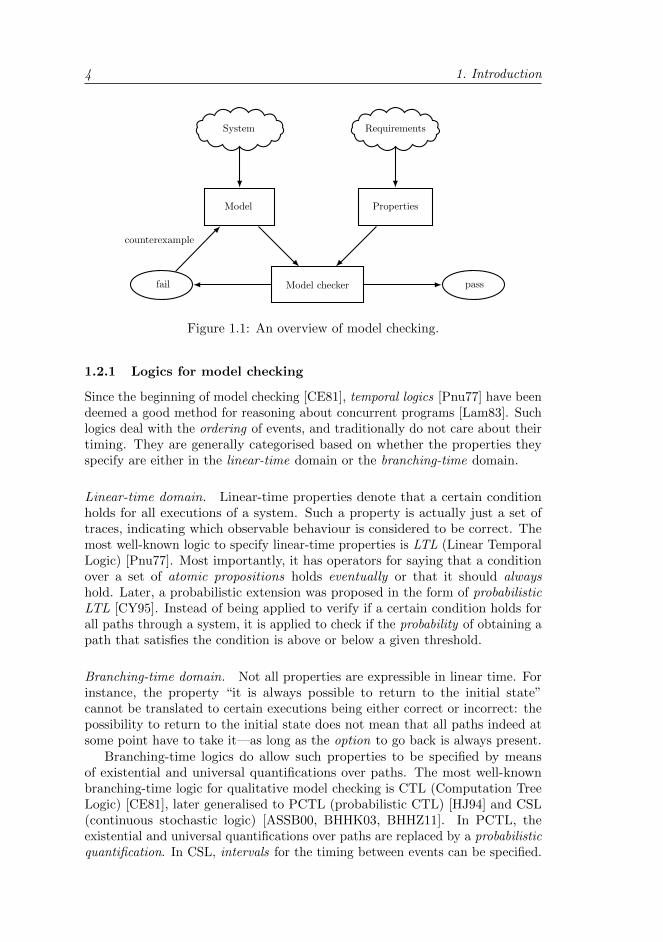
This thesis is positioned in the field of model checking, a topic that started withtwo seminal papers, written independently by Clarke and Emerson [CE81] andby Queille and Sifakis [QS82]. The basic idea is to construct a finite-state modelof a system, to specify some properties in a (temporal) logic and to automaticallyverify the validity of these properties by means of an exhaustive search throughthe state space. In case the system satisfies all properties we are done, otherwisea counterexample is provided to either improve the system or maybe change theproperty. Figure 1.1 summarises the approach.

Due to a combinatorial explosion of the size of the state space in the numberof variables and parallel components, model checking has shown to be ratherdifficult to scale to real-life applications. Therefore, methods for reducing thestate space have been given quite some attention.

4 1. Introduction

System

Model

Requirements

Properties

Model checkerfail pass

counterexample

Figure 1.1: An overview of model checking.

1.2.1 Logics for model checking

Since the beginning of model checking [CE81], temporal logics [Pnu77] have beendeemed a good method for reasoning about concurrent programs [Lam83]. Suchlogics deal with the ordering of events, and traditionally do not care about theirtiming. They are generally categorised based on whether the properties theyspecify are either in the linear-time domain or the branching-time domain.

Linear-time domain. Linear-time properties denote that a certain conditionholds for all executions of a system. Such a property is actually just a set oftraces, indicating which observable behaviour is considered to be correct. Themost well-known logic to specify linear-time properties is LTL (Linear TemporalLogic) [Pnu77]. Most importantly, it has operators for saying that a conditionover a set of atomic propositions holds eventually or that it should alwayshold. Later, a probabilistic extension was proposed in the form of probabilisticLTL [CY95]. Instead of being applied to verify if a certain condition holds forall paths through a system, it is applied to check if the probability of obtaining apath that satisfies the condition is above or below a given threshold.

Branching-time domain. Not all properties are expressible in linear time. Forinstance, the property “it is always possible to return to the initial state”cannot be translated to certain executions being either correct or incorrect: thepossibility to return to the initial state does not mean that all paths indeed atsome point have to take it—as long as the option to go back is always present.

Branching-time logics do allow such properties to be specified by meansof existential and universal quantifications over paths. The most well-knownbranching-time logic for qualitative model checking is CTL (Computation TreeLogic) [CE81], later generalised to PCTL (probabilistic CTL) [HJ94] and CSL(continuous stochastic logic) [ASSB00, BHHK03, BHHZ11]. In PCTL, theexistential and universal quantifications over paths are replaced by a probabilisticquantification. In CSL, intervals for the timing between events can be specified.

1.2. Model checking 5

Moreover, it can specify steady-state properties that hold in the long run.

There is an ongoing debate about whether LTL or CTL is best [Hol04, Var01].Luckily, they can be combined into an overarching logic CTL∗. Similarly,probabilistic LTL and PCTL can be combined into the logic PCTL∗ [BdA95]that is able to express linear-time as well as branching-time properties. Sinceall techniques presented in this work preserve at least a variant of PCTL∗, thedebate between LTL and CTL does not concern us much.

1.2.2 Quantitative model checking

Over the last two decades, much effort has gone into the field of quantitativemodel checking . This field includes powerful techniques to analyse both qual-itative properties and quantitative properties over models featuring discreteprobabilities and/or timing (and often still also nondeterminism). They allow usto verify probabilistic as well as hard and soft real-time systems, modelled bytimed automata (TAs), discrete-time Markov chains (DTMCs), Markov decisionprocess (MDPs), probabilistic automata (PAs), continuous-time Markov chains(CTMCs), interactive Markov chains (IMCs), and Markov automata (MAs).Other notable extensions are the annotation of models with rewards or costs,yielding priced timed automata and Markov reward models, and enabling theverification of multi-objective problems [FKN+11].

Software tools such as UPPAAL [BDL+06], LiQuor [CB06], MRMC [KKZ05,KZH+11], PRISM [KNP11], APMC [HLP06], and FHP-Murϕ [PIM+06] arededicated quantitative model checkers that have been applied to a wide range ofapplications. The success of quantitative model checking is also witnessed by itsadoption as a major analysis technique by tools that originate from performanceanalysis, such as GreatSPN [BBC+09], Mobius [BCD+03], PEPA WB [GH94],and SMART [CJMS06].

In this work we focus on the extension of traditional model checking bydiscrete-time probabilistic behaviour and continuous-time stochastic behaviour.As all extensions are based on labelled transition systems (LTSs), we first discusstheir main feature: nondeterminism. Then, we discuss the three main extensions,as well as their practical applications. Finally, we discuss the main limitationsof quantitative model checking and our contributions to the field.

Nondeterminism. As mentioned in the beginning of this chapter, nondetermin-ism is the unquantified uncertainty about a system’s behaviour. Stated differently,a system is nondeterministic if at some point its precise behaviour is unknownto us (although the possible alternatives are specified). While probabilistic ap-proaches specify the likelihood of each of the alternatives, nondeterminism leavesthe choice completely open. A system nondeterministically choosing betweenproviding coffee or tea may always provide coffee, serve coffee on Wednesdays andtea on the other days, throw a coin to decide between the two, or do somethingeven different.

Nondeterminism may arise from the unspecified ordering of events of twoor more (partly) independent parallel components, from interaction with an

6 1. Introduction

unpredictable environment or just from underspecification. It is a invaluabletool in the presence of uncertainty that cannot be resolved probabilistically.Traditional model checking tools are often able to compute whether a certainproperty holds for all possible ways to resolve the nondeterministic choices,whereas quantitative model checking tools often provide minimal and maximalprobabilities for satisfying a given property (quantifying over all possible waysto resolve the nondeterministic choices in a probabilistic manner).

Probabilistic automata

When adding probabilistic behaviour to traditional labelled transition systems,we obtain Segala’s probabilistic automata (PAs) [Seg95]—or discrete-time Markovchains (DTMCs) when restricting to deterministic systems (i.e., systems that donot allow multiple actions from the same state). These models allow us to specifytransitions that do not have a unique target state anymore, but probabilisticallydecide on their continuation. This is highly practical, as discrete probabilisticbehaviour is omnipresent:

Randomisation by design. Several protocols use randomisation to break theirsymmetry. For instance, the Itah-Rodeh leader election protocol uses prob-ability to decide on a leader between identical nodes [IR90] and the IEEE802.11 standard for wireless networks applies random backoffs to avoidcollisions when multiple nodes try to access the network [IEE97]. Random-isation is also present in many board and card games, for instance due tothe use of dice or because cards are drawn from a randomly shuffled deck.

Involuntary randomisation. Many practical systems also feature some naturaluncertainty due to erroneous behaviour. For instance, congestion in theinternet results in packet loss happening with a certain probability [KR01].Additionally, many biological and physical systems behave in an unpre-dictable way. For instance, we do not know upon conception whether ababy will be a boy or a girl, we do not know which side of a coin will beon top when we toss it, and we do not know for sure if a medicine is goingto work on a specific individual.

Note that, in fact, most of these phenomena are not really randomanymore if we zoom in to an extremely precise level: in theory, it maybe predicted which side of a coin will end up on top. We would need toconsider the exact location of the coin, the precise hand movement, thenon-perfect shape of the coin, the wind, etc—clearly, this is not feasible inpractice (even if we ignore Heisenberg’s uncertainty principle). Similarly,packet loss in the internet may be predicted by modelling the entire stateof the network. Since such fine-grained analysis if often far from realistic,abstraction is applied and probability arises.

All of these phenomena can be modelled effectively as PAs, allowing us to verifyproperties in PCTL or probabilistic LTL and answer questions such as

• What is the probability of electing a leader within 5 rounds?• What is the probability that a message in a network is lost at least once?

1.2. Model checking 7

• What is the probability that a customer’s demand can be satisfied fromstock on hand, given a certain inventory management strategy?

Interactive Markov Chains

When adding stochastic behaviour to labelled transition systems, we obtain Her-manns’ interactive Markov chains (IMCs) [Her02]—or continuous-time Markovchains (CTMCs) when restricting to deterministic systems. In addition to theaction-labelled transitions of traditional model checking (an IMC’s interactivepart), this model also supports transitions that take a certain amount of time,determined by an exponential distribution—sometimes we also say that a statehas a certain rate of going to another state. Instead of moving in discrete timesteps, these models work in continuous time. This feature also allows us tomodel several phenomena that often occur in practice:

Waiting times. When standing in line for a cash register or waiting for someoneto finish a phone call, the remaining waiting time may be unknown. Suchwaiting times are often modelled by exponentially distributed delays inthe field of queueing theory [Hav98].

Failure rates. In dependability analysis, it is common to describe failure usinga mean time to failure (MTTF). Often, for instance in dynamic faulttrees [BCS10], the distribution of such failures is assumed to be determinedby an exponential distribution.

All of these phenomena can effectively be modelled as IMCs, allowing us toverify properties in CSL and answer questions such as

• What is the probability that it is my turn at the cash register within 5time units?

• What is the probability that a hard disk drive crashes within 10,000 hoursof operation?

• What is the expected time until a phone call ends?• What is the fraction of time that a processor will be idle in the long run?• What is the probability that an emergency cooling system in a nuclear

power plant does not switch on in time?

Markov Automata

PAs are great for modelling discrete probabilistic behaviour and IMCs formodelling continuous stochastic behaviour, but they have their separate domainof operation. In this thesis, we like to be as general of possible, and hence workwith a recent combination of these two models: the Markov automaton [EHZ10b,EHZ10a]. By generalising PAs and IMCs, it also generalises the DTMC, CTMCand LTS. Hence, MAs can be used as a semantic model for a wide range offormalisms, such as generalised stochastic Petri nets (GSPNs) [ACB84], dynamicfault trees [BCS10], Arcade [BCH+08] and the domain-specific ArchitectureAnalysis and Design Language (AADL) [BCK+11]. MAs are very general and,

8 1. Introduction

0, 0, 0

1, 0, 0

0, 1, 0

0, 0, 1

1, 0, 1

0, 1, 1

1, 1, 1 1, 1, 0

λ1

λ2

910

110

τ

910

110τ

µ λ1

λ2

λ2

µ

µ

λ1

µ

910

110 τ

910

110

τ

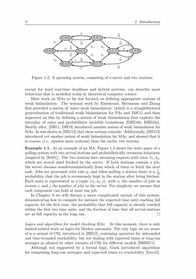
Figure 1.2: A queueing system, consisting of a server and two stations.

except for hard real-time deadlines and hybrid systems, can describe mostbehaviour that is modelled today in theoretical computer science.

Most work on MAs so far has focused on defining appropriate notions ofweak bisimulation. The seminal work by Eisentraut, Hermanns and Zhangfirst provided a notion of ‘naive weak bisimulation’ (which is a straightforwardgeneralisation of traditional weak bisimulation for PAs and IMCs) and thenimproved on this by defining a notion of weak bisimulation that exploits theinterplay of rates and probabilistic invisible transitions [EHZ10b, EHZ10a].Shortly after, [DH11, DH13] introduced another notion of weak bisimulation forMAs. In was shown in [SZG12] that these notions coincide. Additionally, [SZG12]introduced yet another notion of weak bisimulation for MAs, and showed that itis coarser (i.e., equates more systems) than the earlier two notions.

Example 1.1. As an example of an MA, Figure 1.2 shows the state space of apolling system with two arrival stations and probabilistically erroneous behaviour(inspired by [Sri91]). The two stations have incoming requests with rates λ1, λ2,which are stored until fetched by the server. If both stations contain a job,the server chooses nondeterministically from which of them to fetch the nexttask. Jobs are processed with rate µ, and when polling a station there is a 1

10probability that the job is erroneously kept in the station after being fetched.Each state is represented as a tuple (s1, s2, j), with si the number of jobs instation i, and j the number of jobs in the server. For simplicity we assume thateach component can hold at most one job.

In Chapter 9 we will discuss a more complicated variant of this system,demonstrating how to compute for instance the expected time until reaching fullcapacity for the first time, the probability that full capacity is already reachedwithin the first two time units, and the fraction of time that all arrival stationsare at full capacity in the long run.

Logics and algorithms for model checking MAs. At this moment, there is onlylimited related work on logics for Markov automata. The only logic we are awareof is a variant of CSL introduced in [HH12], containing operators for unboundedand time-bounded reachability, but not dealing with expected times or long-runaverages as allowed by other variants of CSL for different models [BHHZ11].

Although not supported by a formal logic, Guck introduced algorithmsfor computing long-run averages and expected times to reachability [Guc12].

1.3. Process algebras 9

Also, Hafeti and Hermanns showed how to do time-bounded reachability ana-lysis [HH12]. These results were unified in [GHH+13a], also providing toolsupport by means of the IMCA tool.

1.2.3 Previous limitations and current contributions

No full-fledged formal modelling languages aimed at specifying MAs existed thusfar. As it is often infeasible to manually write down a low-level transition system,this greatly limited the applicability of MAs. Additionally, model checkingis prone to the state space explosion: data variables and interleavings due toparallel composition quickly yield a large number of states. In quantitative modelchecking the effects of this explosion are even worse [KKZJ07], as the numericalalgorithms for computing quantitative properties are more time-consuming thantheir non-probabilistic counterparts.

Contributions. We contribute to both issues by providing a process-algebraicmodelling language targeted specifically at MAs. It allows MAs to be modelledefficiently by means of data, and enables reduction technique to be defined easilydue to its simplicity. The next sections go into more details on both issues.

This thesis aims at efficient modelling of Markov automata, as well asreducing the state space explosion during their formal verification.

1.3 Process algebras

“Process algebra became an underlying theory of all paralleland distributed systems, extending formal language and

automata theory with the central ingredient of interaction.”

Jos Baeten [Bae05]

While model checking algorithms are mostly defined on models such as PAs,IMCs and MAs, it would be rather inconvenient to explicitly provide such models.After all, model-based system specifications tend to get incredibly large evenfor simple systems. Therefore, it is more common to specify systems in sometype of higher-level language that is mapped to a formal model. For efficientspecification, such a language should have compositionality features, allowingthe user to model several components independently. In addition to simplifyingthe specification phase, higher-level languages also allow us to perform syntacticoptimisations on the language level to generate reduced models without evenhaving to generate the unreduced variant in the first place.

In this work, we focus on process-algebraic modelling languages (also calledprocess calculi) [Fok07, Bae05]. An important feature of such languages istheir mathematical thoroughness, describing behaviour by means of algebraicterms. Additionally, a characterising feature of process algebras is the parallelcomposition operator: a powerful method to compose a system by specifying itsvarious subsystems and their interaction.

10 1. Introduction

Traditionally—in addition to having an operational semantics defined in termsof a model such as the IMC or MA—process algebras are often accompanied by aset of algebraic laws. Preferably this set is an axiomatisation for some notion ofequivalence. That is, two process-algebraic descriptions yield equivalent modelsif and only if they themselves are equivalent according to the algebraic laws.In this work, we rather employ process algebra to specify systems formally andgenerate the underlying models1. We do perform syntactical transformationson the process-algebraic descriptions, but prove them correct by showing abisimulation relation between the original and the transformed specification.

The framework for working with MAs introduced in this thesis is relatedto several existing formalisms. Mainly, it is based on µCRL, a process algebrafor specifying labelled transition systems. Also, it has been influenced by thelanguage TPCCS that extended CCS with discrete probabilistic choice, and thelanguage IML for specifying IMCs. It shows similarities to the mCCS languagefor specifying MAs. We discuss these languages in some detail, and explain inthe next section how these languages have been used in our framework.

µCRL [GP95] The language µCRL was developed to more easily specify com-municating processes in the presence of data, by adding equational abstractdata types to the process algebra ACP [BK89]. Data can be used to para-meterise processes as well as actions, and in conditions to affect a process’behaviour. Also, it can be used to concisely specify behaviour due to thepossibility of summing over (possibly infinite) data types—generalising thewell-known process-algebraic alternative composition operator.

In µCRL, the LPE (linear process equation) [BG94b] was introduced asa restricted part of the language for easier formal manipulation. It is similarto the Greibach normal form in formal language theory, specifications inthe language UNITY [CM88], and the precondition-effect style used fordescribing I/O automata [LT89]. Usenko showed how to linearise a generalµCRL specification into an LPE [GPU01, Use02], based on ideas firstproposed in [BP95].

TPCCS [HJ90] The language TPCCS added a discrete probabilistic operator tothe CCS process algebra, introducing the notation

∑• that we also apply.

TPCCS has its semantics defined in the so-called alternating model , havingdisjoint sets of nondeterministic and probabilistic states. During the courseof execution of the alternating model, there is a strict alternation between

1One may therefore argue about whether or not our language is actually a process algebra,depending on the definition that is used. According to [HJ90], process algebras are “structureddescription languages for concurrent systems, in which a few simple constructs (e.g., sequentialand parallel composition, nondeterministic choice, and recursion) lead to languages capable ofdescribing the various aspects of distributed systems”. Similarly, [Fok07] states that processalgebra is “a mathematical framework in which system behaviour is expressed in the form ofalgebraic terms, enhancing the available techniques for manipulation”. Our language preciselysatisfies the first definition, and could satisfy the second depending on the interpretationof the word ‘algebraic’. On the other hand, according to [Bae05] a process algebra is “anymathematical structure satisfying the axioms given for the basic operators”. When applyingthis definition, our work should not be called a process algebra due to the absence of axioms.We could also just call it a process calculus, like Milner [Mil80].

1.3. Process algebras 11

these types of states. As mentioned in [Sto02a], any alternating model canbe transformed to an equivalent probabilistic automaton.

IML [Her02] The language IML was developed to model IMCs. It containsoperators to specify actions and well as Markovian rates. Its operationalrules that prescribe how each IML specification is mapped to an IMC takeinto account the multiplicity of each transition. This is vital for stochasticprocess algebras, since additional occurrences of the same rate increasethe speed of a process. There is a wide variety of other stochastic processalgebras featuring similar properties; an overview of the foundational onesis provided in [HHK02].

mCCS [DH11, DH13] The language mCCS is the only other process algebrawe are aware of that also aims at constructing MAs. It contains discreteprobabilistic choice in the same way as defined first in [HJ90], and canspecify Markovian rates in the same way as IML. However, as alreadystated in [DH11], it is incomplete due to the ignorance of multiplicities.

1.3.1 Previous limitations and current contributions

None of the existing languages discussed in the previous section serves thepurpose of providing a basis for efficient modelling, generation and analysis ofMAs. Except for mCCS, none of them is able to construct MAs. Except forµCRL, none of them is able to deal with data or easily allows reduction techniquesto be defined. Still, together these languages contain all the ingredients for aprocess algebra to efficiently work with MAs.

We note that the Modest language [BDHK06] is in principle also able tomodel MAs, but it has not yet specifically been applied in this context. It is avery expressive language, but does not contain a restricted form such as µCRL’sLPE. Additionally, it does not allow MAs to be reduced for efficient analysis.

Contributions. We took from µCRL its way of dealing with data, as well asthe idea of first linearising each specification to a restricted part of the languagefor easier formal manipulation. We extended this with an operator for discreteprobabilistic choice, similar to the one introduced in TPCCS [HJ90] but fullyintegrated in the language in such a way that probabilistic behaviour can alsodepend on data. Finally, we took from IML the operator for modelling Markovianrates (and also allow these rates to depend on data parameters), as well as the ideaof taking into account the number of derivations for each Markovian transition.

The result is MAPA (Markov Automata Process Algebra): a language richenough to efficiently model nondeterminism, discrete probabilistic choice andstochastic timing. MAPA improves on mCCS—the only other process algebrafor MAs—by the incorporation of data and a linear format (in MAPA calledthe MLPE) that allows reduction techniques to be defined in a rather simplemanner, as well as by its proper way of dealing with multiplicities of rates.MAPA includes operators for parallel composition and hiding, allowing systemsto be modelled in a compositional manner.

We introduce a novel notion of bisimulation: derivation-preserving bisimula-tion. It is defined on a subset of MAPA (called prCRL), obtained by omitting

12 1. Introduction

the stochastic timing. We show how to encode MAPA specifications in prCRL,and prove that transformations of prCRL that preserve our new notion of bisim-ulation can be applied safely before decoding back—the result then is a MAPAspecification that is bisimilar to the specification we started with. This procedureallows us to reuse techniques defined on prCRL immediately to the full rangeof MAPA. We apply it for the transformation from MAPA to MLPE and formultiple reduction techniques.

MAPA can be seen as a maximal analysable subset of Modest (only dis-regarding its realtime features). By specialising our language to this subset weare able to generalise µCRL’s LPE format to the MLPE, enabling reductiontechniques that have not been defined yet for the Modest language.

This thesis introduces the process-algebraic language MAPA, allowingefficient modelling of MAs using data and enabling their efficient generationand analysis by supporting several reduction techniques via the MLPE.

1.4 Reduction techniques

“A clever person solves a problem.A wise person avoids it.”

Albert Einstein

As mentioned before, the applicability of model checking is bound by thestate space explosion: the number of states that has to be visited often growsexponentially with the size of the system. Much research has been devoted totechniques that battle this omnipresent state space explosion [Pel08].

These techniques focus on either reducing the amount of time needed formodel checking large systems, the amount of memory, or both. Three differenttypes of approaches can be observed, depending on whether they focus on efficientrepresentation, efficient computation or efficient generation. For all techniques,the significance of their reductions depends on the model at hand.

Efficient representation. One way is to more efficiently store state spaces bymeans of techniques such as state compression [Hol97, LLPY97, LvdPW11],or to use symbolic representations like binary decision diagrams [McM93,BvdP08]. Although these techniques aim at improved memory usage, theymay also reduce analysis time.

Efficient computation. Another approach is to more effectively use the increasingnumber of cores in today’s hardware via smart parallelisations [Web06]or to use multiple machines for distributed model checking [BvdPW10].These techniques are mostly aimed at speeding up model checking; however,the distribution of work over several machines may also partly solve thememory problem.

Efficient generation. Finally, both memory usage and analysis time may beimproved by using techniques that reduce the number of states or onlyexplore part of a state space. There are several techniques that do so

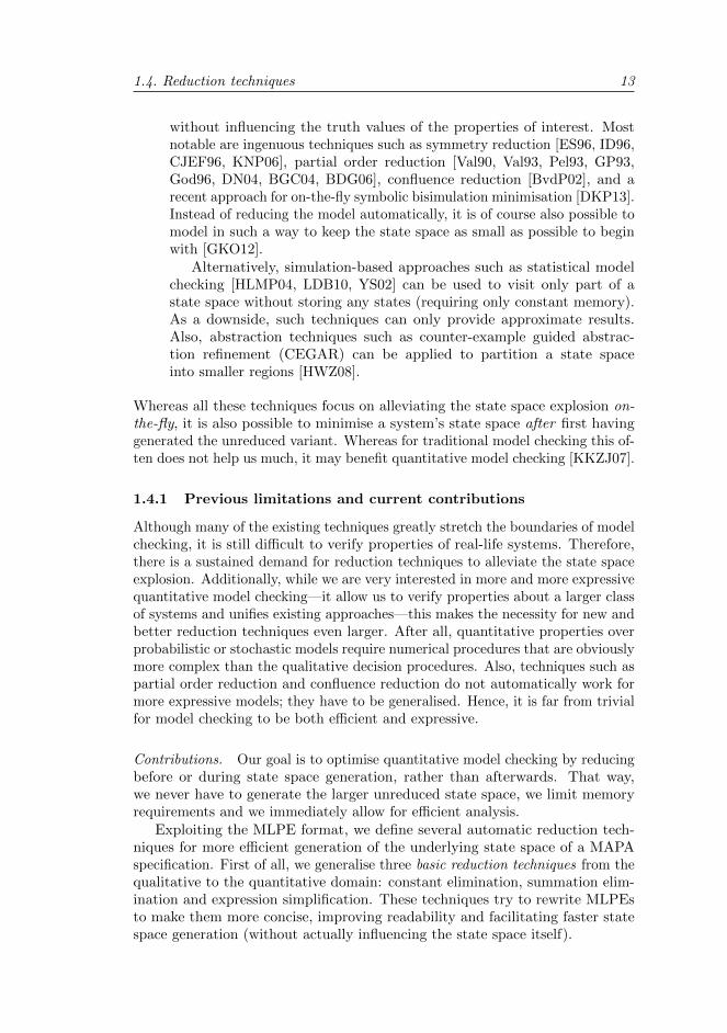
1.4. Reduction techniques 13

without influencing the truth values of the properties of interest. Mostnotable are ingenuous techniques such as symmetry reduction [ES96, ID96,CJEF96, KNP06], partial order reduction [Val90, Val93, Pel93, GP93,God96, DN04, BGC04, BDG06], confluence reduction [BvdP02], and arecent approach for on-the-fly symbolic bisimulation minimisation [DKP13].Instead of reducing the model automatically, it is of course also possible tomodel in such a way to keep the state space as small as possible to beginwith [GKO12].

Alternatively, simulation-based approaches such as statistical modelchecking [HLMP04, LDB10, YS02] can be used to visit only part of astate space without storing any states (requiring only constant memory).As a downside, such techniques can only provide approximate results.Also, abstraction techniques such as counter-example guided abstrac-tion refinement (CEGAR) can be applied to partition a state spaceinto smaller regions [HWZ08].

Whereas all these techniques focus on alleviating the state space explosion on-the-fly, it is also possible to minimise a system’s state space after first havinggenerated the unreduced variant. Whereas for traditional model checking this of-ten does not help us much, it may benefit quantitative model checking [KKZJ07].

1.4.1 Previous limitations and current contributions

Although many of the existing techniques greatly stretch the boundaries of modelchecking, it is still difficult to verify properties of real-life systems. Therefore,there is a sustained demand for reduction techniques to alleviate the state spaceexplosion. Additionally, while we are very interested in more and more expressivequantitative model checking—it allow us to verify properties about a larger classof systems and unifies existing approaches—this makes the necessity for new andbetter reduction techniques even larger. After all, quantitative properties overprobabilistic or stochastic models require numerical procedures that are obviouslymore complex than the qualitative decision procedures. Also, techniques such aspartial order reduction and confluence reduction do not automatically work formore expressive models; they have to be generalised. Hence, it is far from trivialfor model checking to be both efficient and expressive.

Contributions. Our goal is to optimise quantitative model checking by reducingbefore or during state space generation, rather than afterwards. That way,we never have to generate the larger unreduced state space, we limit memoryrequirements and we immediately allow for efficient analysis.

Exploiting the MLPE format, we define several automatic reduction tech-niques for more efficient generation of the underlying state space of a MAPAspecification. First of all, we generalise three basic reduction techniques from thequalitative to the quantitative domain: constant elimination, summation elim-ination and expression simplification. These techniques try to rewrite MLPEsto make them more concise, improving readability and facilitating faster statespace generation (without actually influencing the state space itself).

14 1. Introduction

Second, we present a state space reduction technique based on dead variables ,resetting variables to their initial value in case they will always be overwrittenbefore being used again. It is especially powerful due to a novel method fordetecting control flow. This technique detects which state parameters act asprogram counters. Liveness analysis is then performed based on these recon-structed program counters, and hence even takes into account control flow thatwas manually encoded in a system’s global parameters. Dead variable reductionpreserves strong bisimulation, and hence leaves invariant all properties in PCTL∗

when restricting to PAs and in CSL when restricting to IMCs.Third, we generalise confluence reduction to the Markovian realm and show

how apply it on MAPA specifications. This technique reduces spurious in-terleavings, often arising from the parallel composition of largely independentprocesses. We investigate confluence reduction in great detail by comparing itto its competitor partial order reduction. As partial order reduction has not yetbeen introduced for MAs, we restrict confluence for the subclass of MDPs andtheoretically show that it strictly subsumes the partial order reduction variantthat preserves branching time properties [BDG06]. We also define confluencereduction for the context of statistical model checking , and compare partial orderreduction to confluence reduction on a practical level. It turns our that our con-fluence implementation is able to reduce more than the previous implementationbased on partial order reduction, allowing more systems to be analysed withthis promising technique. Confluence reduction preserves divergence-sensitivebranching bisimulation, and hence leaves invariant all properties in PCTL∗\Xwhen restricting to PAs and all time-bounded reachability properties whenrestricting to IMCs.

We implemented all our reduction techniques in the tool SCOOP, and provideseveral case studies that show significant reductions. No such reductions haveever been obtained for MAs before. As MAs generalise LTSs, DTMCs, CTMCs,PAs and IMCs, all our reduction techniques are also applicable to these models.

This thesis introduces dead variable reduction, confluence reduction andsome basic reduction techniques for the MLPE. Additionally, it investigatesconfluence reduction in-depth by comparing it to partial order reductionfrom a theoretical as well as practical perspective.

1.5 Main contributions

Summarising, this thesis contributes to the field of quantitative verificationin several ways. Our main goal was to enable more expressive models tobe specified, generated and analysed in an efficient manner. While initiallyworking on probabilistic automata—extending existing techniques with discreteprobabilistic choice—we generalised this even further to Markov automata whenthese were introduced. As this formalism subsumes a large variety of importantmodels, its generality allows our techniques to be applied to an equally largevariety of systems. Our main contributions are threefold:

• We enable the efficient modelling of MAs, by providing the new process

1.6. Organisation of the thesis 15

algebra MAPA. It treats data as a first-class citizen, allowing complicatedbehaviour involving data-dependent probabilistic branching or delays to bemodelled quite easily. MAPA includes operators for parallel compositionand hiding, allowing systems to be modelled in a compositional manner.Since MAs generalise a wide variety of simpler models, MAPA allowssystems of all these types to be modelled in a uniform manner.

• We present an encoding of MAPA into prCRL, a restricted part of the lan-guage obtained by omitting its stochastic timing aspect. We also introducea novel notion of bisimulation for prCRL. We show that transformationson prCRL preserving this notion of bisimulation can safely be used onencoded MAPA specifications—this still guarantees a strongly bisimilarsystem after decoding back to MAPA. Based on this approach, we alsopresent an algorithm for rephrasing each MAPA specification in a stripped-down (but equally expressive) version of the language: the MLPE. Due toits simplicity, this format allows reduction techniques to be defined muchmore easily.

We enable the efficient generation and analysis of MAs by defining sev-eral reduction techniques on the MLPE. Three basic reduction techniquesspeedup state space generation, while dead variable reduction and conflu-ence reduction additionally speedup analysis. Case studies demonstratethe usefulness of these techniques through significant reductions.

• We provide new understanding about the relation between confluencereduction and partial order reduction, by providing both a theoreticalcomparison, and a practical comparison in the context of statistical modelchecking. We show that confluence reduction is more powerful in theorywhen restricting to the preservation of branching-time properties, andthat its on-the-fly detection may even beat partial order reduction in thelinear-time context of statistical model checking.

1.6 Organisation of the thesis

The remainder of this thesis is organised in the following way:

Chapter 2 recalls the necessarily mathematical backgrounds for this work fromset theory and probability theory.

Chapter 3 presents the MA and discusses several behavioural equivalencerelations for this model and its subclasses.

Chapter 4 introduces the MAPA language, shows how to safely define trans-formations on a restricted version of the language and introduces theMLPE including its linearisation procedure. Also, it defines three basicreduction techniques on the MLPE.

Chapter 5 introduces our dead variable reduction technique, including themethod for control flow reconstruction.

Chapter 6 generalises confluence reduction, formally defining confluence onMAs, presenting heuristics for detecting it on MLPEs and demonstratinghow to apply confluence for generating reduced state spaces.

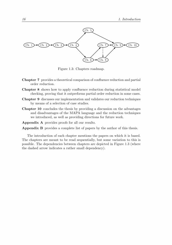
16 1. Introduction

Ch. 1 Ch. 2 Ch. 3 Ch. 4

Ch. 6

Ch. 7

Ch. 8

Ch. 5

Ch. 9 Ch. 10

Figure 1.3: Chapters roadmap.

Chapter 7 provides a theoretical comparison of confluence reduction and partialorder reduction.

Chapter 8 shows how to apply confluence reduction during statistical modelchecking, proving that it outperforms partial order reduction in some cases.

Chapter 9 discusses our implementation and validates our reduction techniquesby means of a selection of case studies.

Chapter 10 concludes the thesis by providing a discussion on the advantagesand disadvantages of the MAPA language and the reduction techniqueswe introduced, as well as providing directions for future work.

Appendix A provides proofs for all our results.

Appendix B provides a complete list of papers by the author of this thesis.

The introduction of each chapter mentions the papers on which it is based.The chapters are meant to be read sequentially, but some variation to this ispossible. The dependencies between chapters are depicted in Figure 1.3 (wherethe dashed arrow indicates a rather small dependency).

Part I

Background

CHAPTER 2

Preliminaries

“Pure mathematics is, in its way, the poetry of logical ideas.”

Albert Einstein

Most of the technicalities in the next chapters rely on set theory andprobability theory. As formal treatments of both topics are ratherinvolved, we restrict ourselves to informally recalling the relevant notions

and introducing the notations that are used throughout the rest of this thesis.All material in this chapter is well known. The set-theoretical notions we dis-

cuss can be found in almost any textbook on discrete mathematics (e.g., [Gri03]).The basics from probability theory can for instance be found in [Ros11, CK04].

Organisation of the chapter. Section 2.1 discusses the basics of set theory, andSection 2.2 the basics of probability theory.

2.1 Set theory

One of the most fundamental concepts in mathematics is the notion of a set : anabstract collection of objects. Finite sets can be described explicitly, enumeratingall of their elements: X = 1, 3, 5, 7, 9. We use 3 ∈ X to indicate that theelement 3 is contained in X, and 4 6∈ X to indicate that 4 is not. The emptyset is denoted by ∅. Moreover, the set of natural numbers is denoted byN = 0, 1, 2, . . . , the set of positive natural numbers by N+ = 1, 2, . . . , theset of real numbers by R, the set of nonnegative real numbers by R≥0 and theset of positive real numbers by R>0 (also known as R+).

The elements of a set do not have a multiplicity and are unordered: thesets 1, 2, 3 and 1, 3, 2, 1 are identical. In a multiset , elements do have amultiplicity. We denote multisets like |1, 1, 2|, indicating the multiplicity ofeach element by the number of times it is written.

2.1.1 Building and comparing sets

Sets can be defined using the set-builder notation (also called set comprehension),given a certain universe of all possible elements and a condition. For instance,we write x ∈ N | x < 5 = 0, 1, 2, 3, 4 for all natural numbers smaller than 5.

Often, the universe is implied by the context and an expression is used at theleft-hand side of the vertical bar. In that case, the condition at the right-hand

20 2. Preliminaries

side of the vertical bar specifies for which values from the universe, the valueobtained by evaluating the expression on its left-hand side is present in theresulting set. For instance, we could write x2 | x < 5 = 0, 1, 4, 9, 16.

Given two sets X,Y , we use X ∩ Y = x | x ∈ X ∧ x ∈ Y to denote theintersection of X and Y , i.e., the set of all elements that are both in X andin Y . We say that X and Y are disjoint if X ∩ Y = ∅. We write X ∪ Y =x | x ∈ X ∨ x ∈ Y for the set of all elements that are in either X or Y (or inboth): their union. We use X \Y = x ∈ X | x 6∈ Y to denote the difference ofX and Y , i.e., the set of elements from X that are not in Y . Finally, the disjointunion of two sets X,Y is given by X ] Y = (x, 1) | x ∈ X ∪ (y, 2) | y ∈ Y .

The concepts of intersection, union and disjoint union are lifted naturally tobe applied to more than two sets. For intersections, we let⋂

i∈1,2,3,...

Xi =⋂X1, X2, X3, . . . = X1 ∩ X2 ∩ X3 ∩ . . .

Unions and disjoint unions are generalised in the same manner.

A set X is a subset of a set Y , denoted by X ⊆ Y , if every element in X isalso in Y , i.e., X ⊆ Y ⇐⇒ ∀x ∈ X . x ∈ Y . It is easy to see that this coincideswith X \ Y = ∅. If X ⊆ Y and X 6= Y , we write X ⊂ Y and say that X is astrict subset of Y . If X is a (strict) subset of Y , then Y is a (strict) supersetof X, denoted by Y ⊇ X in general and Y ⊃ X for the strict version. We useX 6⊆ Y to denote that X is not a subset of Y , and apply similar negations ofthe other symbols.

Given a set X, we use P(X) to denote its powerset , i.e., the set of all itssubsets (including the empty set and X itself).

2.1.2 Relations and functions

The Cartesian product of two sets X,Y , denoted by X ×Y , is the set of all pairs(x, y) such that x ∈ X and y ∈ Y . A binary relation between two sets X,Y is asubset of X × Y . If X = Y , it is called a binary relation on X. Given a binaryrelation R, we sometimes write xRy to indicate that (x, y) ∈ R.

Given two binary relations R1 and R2 over a set X, we use R2 R1 to denotetheir composition:

R2 R1 = (x, z) ∈ X ×X | ∃y ∈ X . (x, y) ∈ R1 ∧ (y, z) ∈ R2

Equivalence relations. A binary relation R on a set X is called reflexive if(x, x) ∈ R for every x ∈ X, symmetric if (x, y) ∈ R implies (y, x) ∈ R andtransitive if (x, y) ∈ R and (y, z) ∈ R together imply (x, z) ∈ R. Binary relationsthat have all these properties are called equivalence relations.

Given an equivalence relation R ⊆ X ×X, we write [x]R for the equivalenceclass induced by x, i.e., [x]R = y ∈ X | (x, y) ∈ R. We denote the set of allsuch equivalence classes by X/R. Due to the nature of equivalence relations, theequivalence classes partition X. That is, two equivalence classes [x]R, [y]R eithercoincide or are disjoint, and the union of the equivalence classes equals X.

2.1. Set theory 21

Example 2.1. Let X = 1, 2, 3, 4, 5, 6, 7, 8, then the relation

R = (x, y) ∈ X ×X | x and y are both even or both odd

is an equivalence relation. To see why R is transitive, note that (x, y) ∈ R and(y, z) ∈ R imply that x, y, z are all even or all odd, and hence (x, z) ∈ R isimmediate. Reflexivity and symmetry are shown similarly.

We find that, for instance, [1]R = [3]R = 1, 3, 5, 7 and [4]R = 2, 4, 6, 8.As these are the only equivalence classes, X/R = 1, 3, 5, 7, 2, 4, 6, 8.

Functions. A (total) function from a set X (its domain) to a set Y (its range)is a relation R ⊆ X × Y such that (x, y) ∈ R and (x, z) ∈ R imply y = z, andfor each x ∈ X there is a pair (x, y) ∈ R. Hence, a function from X to Y mapseach element of X to precisely one element of Y . If (x, y) ∈ R for a function R,we also write R(x) = y and say that y is the image of x under R. Often, wewrite f : X → Y to indicate that f is a function from X to Y .

A function f : X → Y is injective if f(x) = f(y) implies x = y for allx, y ∈ X. Hence, it never maps two different values from X to the same valuefrom Y . It is surjective if it uses its complete range, i.e., if for every y ∈ Ythere exists an x ∈ X such that f(x) = y. A function that is both injective andsurjective is said to be bijective. Such functions represent a one-to-one mappingbetween the elements of X and Y , and hence can only exist if X and Y havethe same number of elements.

Given a function f : X → Y and an element y ∈ Y , the inverse image of yunder f is denoted by f−1(y) and given by the set x ∈ X | f(x) = y. Notethat f−1(y) contains at most one value if f is injective and at least one value if fis surjective. Hence, for bijective functions it always contains precisely one value.

Example 2.2. The function f : N→ N given by f(n) = n2 is injective, but notsurjective (and hence not bijective). The image of 3 under f is 9, and the inverseimage of 10 is f−1(10) = ∅.

The function f : R→ R given by f(n) = n2 is neither surjective nor injective.After all, the negative numbers do not appear as the image of any value fromthe domain, and f−1(4) = −2, 2 contains more than one value.

The function f : R→ R given by f(x) = x3 is both injective and surjective,and hence bijective.

A partial function f : X Y is similar to a function from X to Y , exceptthat it does not necessarily assign a value from Y to each element in X. Hence,it behaves like a function f ′ : X ′ → Y for some set X ′ ⊆ X. We use dom(f) todenote this domain X ′.

Set cardinality. The size or cardinality of a set X, denoted by |X|, is its numberof elements. Obviously, |X × Y | = |X| · |Y |. Any set with a finite number ofelements is called a finite set. We define a set to be countable if it containsat most as many elements as the set N of natural numbers. Formally, a set Xis countable if there exists an injective function f : X → N. A set that is notcountable is called uncountable.

22 2. Preliminaries

Note that our definition allows countable sets to be finite. Countable setsthat are infinite are called countably infinite.

Example 2.3. Let X = x ∈ R | 2x ∈ N, i.e., X = 0, 12 , 1,

32 , . . . . Although

intuitively this sets seems to be bigger than N, there does exist an injectivefunction f : X → N. After all, take f(x) = 2x for every x ∈ X. This clearly isa function from X to N, and no element in N is the image of more than oneelement from X. Hence, it is injective.

It can be shown that the set of real numbers R, as well as any nontrivialinterval [a, b] ∈ R, is uncountable.

2.1.3 Summations and sequences

Summations. Given a function f : X → Y and a countable set X ′ ⊆ X, suchthat Y ⊆ R and either X ′ is finite or f is nonnegative (i.e., f(x) ≥ 0 for everyx ∈ X), we use

∑x∈X′ f(x) to denote the summation of the image under f of all

elements of X ′. Given a countable set X ⊆ R such that |X| <∞ or X ⊆ R≥0,we use

∑X as an abbreviation for

∑x∈X x. Similarly, for a multiset Y satisfying

the same conditions, we let∑Y be the sum of its elements (taking into account

their multiplicities).We note that the finiteness or nonnegativity constraints are needed for

the summation order to be irrelevant and a summation to either diverge orconverge (and thus not oscillate), and hence for the notion

∑x∈X f(x) to be

well-defined [Bro08]. Often we do not explicitly provide the function f , butwrite an expression that implicitly captures it. For instance, we write x2 todenote the function f : R→ R such that f(x) = x2.

Sequences. For a sequence σ = a1a2a3 . . . ak of elements from some set L(sometimes also written as 〈a1, a2, a3 . . . , ak〉), we write |σ| = k to denote itslength. Given an element a ∈ L, we use aσ to denote the sequence aa1a2a3 . . . ak.The empty sequence is denoted by ε. Given a subset L′ ⊆ L, we let σ \L′ denotethe sequence σ′ obtained by removing every occurrence of elements from L′ in σ.

2.2 Probability theory

When systems behave in an uncertain manner, probability theory can be usedto formalise this behaviour. The basis of probability theory is the experiment :some real-world procedure with a predetermined set of possible outcomes . Eachexecution of the experiment will result in one specific outcome; the next executionmay have a different one. A standard example is the roll of a die; it has sixdifferent outcomes, corresponding to which side ends up on top.

For a fair die, the probability of rolling a six is 16 . Intuitively, this means that

if the experiment is repeated N times (with N going to infinity), the outcomewill be six approximately 1

6 ·N times. This intuition immediately explains whyprobabilities have to be nonnegative and have to sum up to one. After all, anevent cannot be expected to occur a negative number of times, and together theoutcomes should account for all N experiments.

2.2. Probability theory 23

2.2.1 Probability spaces

Mathematically, an experiment is modelled by a probability space, consisting ofa sample space, a set of events and a probability measure.

The sample space Ω is just a non-empty set consisting of all possible outcomesof the experiment modelled by the probability space. We want to assign prob-abilities to the occurrence of the elements of this sample space, but in generalit does not suffice to do so only for each individual outcome. After all, for anexperiment yielding a value from a continuous domain, we often find that theprobability of each individual outcome is 0; still, there is a positive probabilityof an outcome within a certain set of outcomes. Therefore, events are defined assets of outcomes—i.e., subsets of the sample space—and the probability spacecontains a set F of all events to which a probability is assigned by the probabilitymeasure P .

Formally, a probability space is a tuple (Ω,F , P ), where

1. Ω 6= ∅ is the sample space2. F ⊆P(Ω) is the set of events, such that

• Ω ∈ F• E ∈ F implies Ω \ E ∈ F• Ei ∈ F for i = 1, 2, . . . implies

⋃∞i=1Ei ∈ F

3. P : F → [0, 1] is the probability measure, such that

• P (Ω) = 1• P (

⋃∞i=1Ei) =

∑∞i=1 P (Ei), if Ej ∩ Ek = ∅ for all j 6= k.

Example 2.4. Consider the experiment of rolling a die. We may model thisexperiment by the probability space (Ω,F , P ), with Ω = 1, 2, 3, 4, 5, 6, F =

P(Ω) and P (E) = |E|6 for every E ∈ F . It is easy to check that F and P indeed

satisfy their constraints.The event O = 1, 3, 5 ∈ F represents the scenario that the experiment

yields an odd outcome. We easily compute P (O) = 36 = 1

2 .

Probability measures. To understand the restrictions on the probability measure,first note that the event Ω corresponds to the occurrence of any outcome of thesample space. As this is unavoidable, clearly P (Ω) = 1 has to hold. Additionally,if we know the probabilities of two or more disjoint events, then the probability ofthe union of these events intuitively indeed should be the sum of their probabilities(this property is called countable additivity). Any function with range [0, 1]satisfying these two properties is called a probability measure.

Measurable spaces and σ-algebras. To understand the restrictions on the setof events, note that the first and third are obviously needed for the probabilitymeasure to be well-defined. The second corresponds to the intuition that if weknow the probability p of a certain event, we also know the probability of itscomplement: 1− p. Hence, for each event in F , also its complement should bein F . Any set satisfying these properties is called a σ-algebra. A pair (Ω, F )

24 2. Preliminaries

of a sample space and an associated σ-algebra is called a measurable space. Awell-known example of a measurable space is (R,B), with R the set of realnumbers and B the Borel σ-algebra over R, i.e., the smallest σ-algebra over thereal numbers containing all intervals.

Although it may seem that we can take F = P(Ω) for every Ω, it is wellknown from measure theory that this is impossible in general. There are sets(e.g., the Vitali sets1) that are so inherently complicated, that no probability canbe assigned to them in a satisfactory way while satisfying the constraints above.Hence, they must be excluded from the domain of the probability measure, inorder to still be able to define useful measures. This is precisely the purpose ofthe set F . However, if Ω is countable, F = P(Ω) can always be used.

2.2.2 Random variables

Instead of dealing with a probability space (Ω,F , P ) directly, it is more commonto work with an additional layer of random variables. These are just functionsX : Ω → S from the sample space to some other domain S, under the (oftenimplicit) restriction that S is part of some measurable space (S,S). For acountable set S we can always take S = P(S), and for S = R the Borelσ-algebra often suffices.

As a random variable assigns a value to each outcome of an experiment, wecan ask for the probability that this value is in a certain set E ∈ S, defined by

Pr(X ∈ E) = P (X−1(E)) = P (w ∈ Ω | X(w) ∈ E)

Similarly, we use notations like Pr(X < 5) and Pr(X = s4). Note that, for suchprobabilities to be well-defined, we need X−1(E) ∈ F for every E ∈ S. We thensay that X is (F ,S)-measurable.

Example 2.5. Consider again the rolling of a die, represented earlier by aprobability space (Ω,F , P ). We define a random variable X : Ω→ even, odd,given by X(1) = X(3) = X(5) = odd and X(2) = X(4) = X(6) = even.

1To understand the intricacies, consider a probability distribution P over the sample spaceΩ = [0, 1], assigning to each interval [a, b] in Ω a probability equal to its length b − a. Forunions of disjoint intervals, it takes the sum of their lengths. Additionally, we require thatP (X) = P (x + c (mod 1) | x ∈ X) for every set X and real number c. These are veryreasonable assumptions for a probability distribution, as for instance satisfied by the uniformdistribution introduced in Example 2.9. Note that P (Ω) = 1, and that for unions of disjointintervals the requirement of countable additivity is fulfilled; indeed, for all sets in the Borelσ-algebra, everything works fine.

Now consider an equivalence relation R over Ω equating all real numbers x, y such thatx−y ∈ Q. A Vitali set A is then obtained by choosing precisely one value from each equivalenceclass of R. To see why A cannot be given a probability, consider the family of sets definedby Aq = a + q (mod 1) | a ∈ A for every q ∈ Q. Since the sets Aq form a partitioning of[0, 1], countable additivity prescribes that

∑q∈Q P (Aq) = P ([0, 1]) = 1. Because each Aq is

identical to A except for a translation, we find that P (Aq) = P (A) for every q ∈ Q and hence∑q∈Q P (A) = 1. This is clearly impossible, since an infinite sum of a nonnegative constant is

either 0 or ∞. Therefore, no probability can be assigned to the set A under the restrictionsof P , and indeed it is not present in the Borel σ-algebra B that can be used for such measures.

2.2. Probability theory 25

We can now compute, for instance,

Pr(X = odd) = P (ω ∈ Ω | X(ω) = odd) = P (1, 3, 5) =1

2

The question may rise why to use this additional layer, and not just directlywork with probability spaces. Although that indeed would be possible, themain argument is that we may be interested in several different observationsbased on a probabilistic experiment. For instance, whereas someone may beinterested in the parity of the outcome of a die, as given by the random variablein Example 2.5, someone else may be interested in the fact whether or not it isa 5 or higher. Then, the same probability space may be reused, just definingan additional random variable over it. This corresponds to the philosophicalargument that ‘chance’ only does its work once, and that we may have severaldifferent observers of it.

Conditional probabilities. A well-known concept when dealing with randomvariables is the conditional probability : the probability that a certain event E1

occurs, given that we know that an event E2 occurs. It is defined by

Pr(X ∈ E1 | X ∈ E2) =Pr(X ∈ E1 ∩ E2)

Pr(X ∈ E2)

Example 2.6. Again considering the probability space defined in Example 2.4,let X : Ω → S be given by X(ω) = ω (i.e., S = 1, 2, 3, 4, 5, 6 as well). Then,obviously, we find that Pr(X = ω) = 1

6 for every ω ∈ Ω. Given that someonetells us that an odd number was rolled, we can compute the probability that a 1or 2 was rolled:

Pr(X ∈ 1, 2 | X ∈ 1, 3, 5) =Pr(X ∈ 1, 2 ∩ 1, 3, 5)

Pr(X ∈ 1, 3, 5)

=Pr(X = 1)

Pr(X ∈ 1, 3, 5) =1612

=1

3

Distribution functions for random variables. Often, it is more convenient tospecify the probabilities for the outcomes of a random variable directly, embracingthe underlying probability space and basically forgetting about it. Traditionally,for this to be specified feasibly, random variables are classified to be eitherdiscrete (having a countable domain) or continuous (having an uncountablereal-valued domain). Although in general more complicated random variablesare possible, we restrict to these two basic cases.

From now on, we do not refer to underlying probability spaces anymore.Also, we will use the common standard of referring to the domain of the randomvariables we consider as their sample spaces.

26 2. Preliminaries

2.2.3 Discrete probability theory

A discrete random variable has a countable sample space S, and a correspondingσ-algebra of events P(S). Its behaviour can easily be specified by a discreteprobability distribution (often just called a probability distribution or distribution)over S. Such a distribution is a function µ : S → [0, 1] such that

∑s∈S µ(s) = 1.

That is, it assigns a probability to the occurrence of each possible outcome in Sin such a way that the total probability is 1. The behaviour of X is then simplygiven by Pr(X = s) = µ(s) and Pr(X ∈ S′) =

∑s∈S′ µ(s′), for s ∈ S and

S′ ⊆ S.Sometimes, we use the notation µ = s1 7→ p1, s2 7→ p2, . . . , sn 7→ pn to

denote that µ(s1) = p1, µ(s2) = p2, . . . , µ(sn) = pn. Also, we often write µ(S′)as an abbreviation of

∑s∈S′ µ(s′) if S′ ⊆ S.

Example 2.7. The random variable from Example 2.6 is specified by the dis-tribution µ : S → [0, 1] with µ(s) = 1

6 for every s ∈ S.

Given a countable set S, we use Distr(S) to denote the (uncountable) setof all discrete probability distributions over S. We use SDistr(S) for the setof all substochastic discrete probability distributions over S, i.e., all functionsµ : S → [0, 1] such that

∑s∈S µ(s) ≤ 1.

Discrete probability distributions. For a discrete probability distribution µ overS and a function f : S → T , we let µf ∈ Distr(T ) be the lifting of µ over f , i.e.,µf (t) = µ(f−1(t)) for all t ∈ T . Hence, µf assigns the same probability to anelement t ∈ T as µ assigns to the corresponding elements s ∈ S. We write 1sfor the Dirac distribution over s, given by 1s(s) = 1 (and hence 1s(t) = 0 forevery t ∈ S such that t 6= s).

For any distribution µ over a countable set S, we write supp(µ) = s ∈ S |µ(s) > 0 for the support of µ. Given two distributions µ, ν ∈ Distr(S), we letµ × ν ∈ Distr(S × S) be their joint distribution, defined by (µ × ν)((s, t)) =µ(s) · ν(t).

Given two probability distributions µ, µ′ over a set S and an equivalencerelation R over S, we write µ ≡R µ′ to denote that µ and µ′ assign the sameprobability to each equivalence class of S under R. Formally, µ([s]R) = µ′([s]R)for every s ∈ S. Obviously, ≡R is an equivalence relation itself.

Example 2.8. Let S = 1, 2, 3, . . . , 10, and let R relate all odd and all evennumbers, i.e.,

S/R = 1, 3, 5, 7, 9, 2, 4, 6, 8, 10Also, let µ : S → [0, 1] and ν : S → [0, 1] be the distributions given by

µ(1) =1

2µ(2) =

1

4µ(3) =

1

4

ν(5) =1

8ν(9) =

5

8ν(4) =

1

4

Then, µ ≡R ν, since both assign probability 34 to the equivalence class 1, 3, 5,

7, 9 and 14 to 2, 4, 6, 8, 10.

2.2. Probability theory 27

2.2.4 Continuous probability theory

A continuous random variable has an uncountable real-valued sample space S,with the Borel σ-algebra as its set of events. It is often assumed that theprobability of each individual outcome is 0, but that a probability can beassigned to an interval of the sample space. We adopt this assumption, and donot consider random variables with a more complicated structure that cannotbe captured by the techniques discussed below.

A probability density function (often just called a density function or density)f(x) : R→ R≥0 is employed to specify the probabilities of a continuous randomvariable X, in such a way that

Pr(X ∈ [a, b]) = Pr(X ∈ (a, b)) =

∫ b

a

f(x) dx

for every interval [a, b] ⊂ R. As every set in the Borel σ-algebra can be construc-ted from intervals, this completely specifies X. Obviously, any density functionshould satisfy

∫∞−∞ f(x) dx = 1.

Example 2.9. Consider a web service that is available to its customers duringa 200 minutes time interval. Each customer will access it at some point duringthis period, but will choose its timing randomly (in the sense that arriving withinevery equally sized interval in [0, 200] is equally likely). Since time is continuous,the probability of access at a specific time (for instance, t = 83.6) is 0, as thereare infinitely many other times. However, the probability of access within thefirst 50 minutes is 1

4 .

This behaviour can be described by a random variable W with probabilitydensity function

f(x) =

0.005 if 0 ≤ x ≤ 200

0 otherwise

In general, this is called the uniform distribution over the interval [0, 200], andW is said to be distributed uniformly.

Indeed, Pr(W ∈ [0, 50]) =∫ 50

0f(x) dx = [0.005x]50

0 = 0.005 · 50 = 0.25.

It is often more convenient to use a cumulative distribution function: afunction F : R → [0, 1] assigning to each value x ∈ R the probability that theoutput of the experiment is at most equal to x. Hence,

F (x) = Pr(X < x) = Pr(X ∈ (−∞, x)) =

∫ x

−∞f(t) dt

Example 2.10. For the density function f(x) of the previous example, we findfor 0 ≤ x ≤ 200 that

F (x) =

∫ x

−∞f(t) dt =

∫ 0

−∞0 dt+

∫ x

0

0.005 dt = 0 + [0.005t]x0 = 0.005x

28 2. Preliminaries

Hence, it is easy to see that

F (x) =

0 if x < 0

0.005x if 0 ≤ x ≤ 200

1 if x > 200

Indeed, F (50) = 0.005 · 50 = 0.25, as before.

Expected values. The expected value E(X) of a continuous random variable Xis the weighted average of all possible values it can attain. It can be computedby the integral E(X) =

∫∞−∞ xf(x) dx.

Example 2.11. For the web service described in the previous example, we find

E(W ) =

∫ ∞−∞

xf(x) dx =

∫ 200

0

0.005x dx = [0.0025x2]2000 = 0.0025 · 2002 = 100

Hence, as was to be expected, the average arrival of a customer who arrivesuniformly within the interval [0,200] is at time 100.

Remark 2.12. The expected value of a random variable does not necessarilyexist. Like integrals in general, it may be infinite or even undefined (due tooscillation). As an example of a random variable X with expected value ∞,consider the probability density function

g(x) =

1x2 if x ≥ 1

0 otherwise

Indeed, as required

Pr(−∞ ≤ X ≤ ∞) =

∫ ∞−∞

g(x) dx =

∫ ∞1

1

x2dx =

[− 1

x

]∞1

= 1

However, we find that

E(X) =

∫ ∞−∞

xg(x) dx =

∫ ∞1

1

xdx = [lnx]

∞1 =∞

The exponential distribution. The most important continuous probability dis-tribution for this work is the exponential distribution. It is parameterised by avalue λ > 0, and given by either the probability density function f(x) belowleft, or alternatively the cumulative distribution function F (x) below right:

f(x) =

λe−λx if x > 0

0 otherwiseF (x) =

1− e−λx if x > 0

0 otherwise

2.2. Probability theory 29

The parameter λ of an exponentially distributed random variable X dictates itsrate, which is the reciprocal of its expected value:

E(X) =

∫ ∞−∞

xλe−λx dx = λ

∫ ∞0

xe−λx dx =1

λ

where the last step is obtained using integration by parts. Hence, the larger λ,the smaller the expected outcome of an exponentially distributed experiment.Note that each exponentially distributed random variable has a finite expectedvalue (since we disallow λ = 0).

The exponential distribution is the only memoryless continuous probabilitydistribution, as explained in the following example.

Example 2.13. The duration of telephone calls is often assumed to be ex-ponentially distributed, with its parameter λ the average duration of a call.The probability that a call takes at least t time units is easily computed by1 − F (t) = e−λt. Now, given that a call has already taken s time units, theprobability that it will take at most an additional t time units is computed asfollows (where T is an exponentially distributed random variable):

Pr(T > s+ t | T > s) =Pr(T > s+ t)

Pr(T > s)=e−λ(t+s)

e−λs= e−λt

Hence, the duration someone was already on the phone does not influence theprobability that the call will take an additional t time units. This is called thememoryless property of the exponential distribution.

It is well known that the minimum of two independent exponentially dis-tributed random variables X,Y with rates λ1 and λ2 is again an exponentiallydistributed random variable Z, with rate λ1 + λ2. To see why, we compute theprobability that min(X,Y ) yields a value larger than t:

Pr(min(X,Y ) > t) = Pr(X > t ∧ Y > t)

= Pr(X > t) · Pr(Y > t)

= e−λ1t · e−λ2t

= e−(λ1+λ2)t = Pr(Z > t)

where the second step follows by independence. Since these probabilities coincidefor min(X,Y ) and Z, their cumulative distribution functions also coincide. Thisimmediately implies that indeed min(X,Y ) = Z. This naturally generalisesto the observation that min(X1, X2, . . . , Xn) = Z ′, with Z ′ an exponentiallydistributed random variable with a rate equal to the sum of the rates of theconstituents X1, X2, . . . , Xn.

On the other hand, the maximum of two exponentially distributed randomvariables is not exponentially distributed, and neither is their sum.

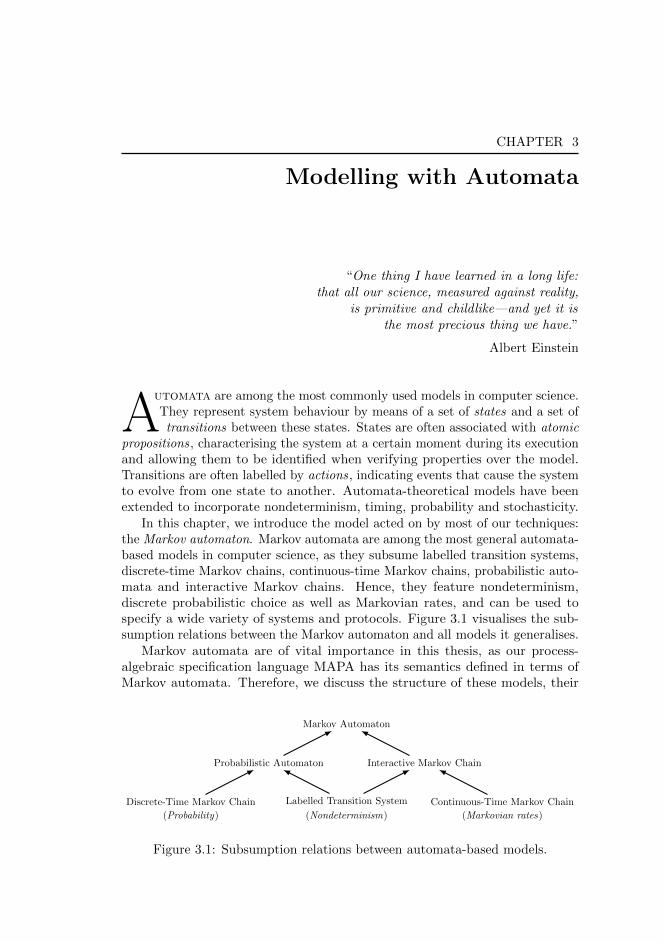
CHAPTER 3

Modelling with Automata

“One thing I have learned in a long life:that all our science, measured against reality,

is primitive and childlike—and yet it isthe most precious thing we have.”

Albert Einstein

Automata are among the most commonly used models in computer science.They represent system behaviour by means of a set of states and a set oftransitions between these states. States are often associated with atomic

propositions , characterising the system at a certain moment during its executionand allowing them to be identified when verifying properties over the model.Transitions are often labelled by actions , indicating events that cause the systemto evolve from one state to another. Automata-theoretical models have beenextended to incorporate nondeterminism, timing, probability and stochasticity.

In this chapter, we introduce the model acted on by most of our techniques:the Markov automaton. Markov automata are among the most general automata-based models in computer science, as they subsume labelled transition systems,discrete-time Markov chains, continuous-time Markov chains, probabilistic auto-mata and interactive Markov chains. Hence, they feature nondeterminism,discrete probabilistic choice as well as Markovian rates, and can be used tospecify a wide variety of systems and protocols. Figure 3.1 visualises the sub-sumption relations between the Markov automaton and all models it generalises.

Markov automata are of vital importance in this thesis, as our process-algebraic specification language MAPA has its semantics defined in terms ofMarkov automata. Therefore, we discuss the structure of these models, their

Markov Automaton

Probabilistic Automaton Interactive Markov Chain

Labelled Transition SystemDiscrete-Time Markov Chain Continuous-Time Markov Chain

(Probability) (Nondeterminism) (Markovian rates)

Figure 3.1: Subsumption relations between automata-based models.

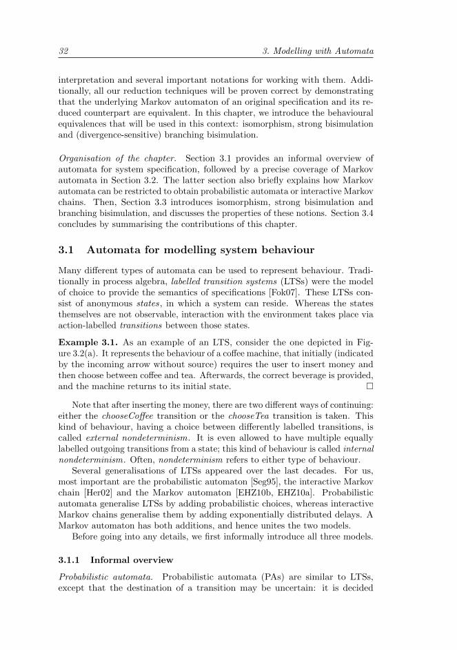
32 3. Modelling with Automata

interpretation and several important notations for working with them. Addi-tionally, all our reduction techniques will be proven correct by demonstratingthat the underlying Markov automaton of an original specification and its re-duced counterpart are equivalent. In this chapter, we introduce the behaviouralequivalences that will be used in this context: isomorphism, strong bisimulationand (divergence-sensitive) branching bisimulation.

Organisation of the chapter. Section 3.1 provides an informal overview ofautomata for system specification, followed by a precise coverage of Markovautomata in Section 3.2. The latter section also briefly explains how Markovautomata can be restricted to obtain probabilistic automata or interactive Markovchains. Then, Section 3.3 introduces isomorphism, strong bisimulation andbranching bisimulation, and discusses the properties of these notions. Section 3.4concludes by summarising the contributions of this chapter.

3.1 Automata for modelling system behaviour

Many different types of automata can be used to represent behaviour. Tradi-tionally in process algebra, labelled transition systems (LTSs) were the modelof choice to provide the semantics of specifications [Fok07]. These LTSs con-sist of anonymous states, in which a system can reside. Whereas the statesthemselves are not observable, interaction with the environment takes place viaaction-labelled transitions between those states.

Example 3.1. As an example of an LTS, consider the one depicted in Fig-ure 3.2(a). It represents the behaviour of a coffee machine, that initially (indicatedby the incoming arrow without source) requires the user to insert money andthen choose between coffee and tea. Afterwards, the correct beverage is provided,and the machine returns to its initial state.

Note that after inserting the money, there are two different ways of continuing:either the chooseCoffee transition or the chooseTea transition is taken. Thiskind of behaviour, having a choice between differently labelled transitions, iscalled external nondeterminism. It is even allowed to have multiple equallylabelled outgoing transitions from a state; this kind of behaviour is called internalnondeterminism. Often, nondeterminism refers to either type of behaviour.

Several generalisations of LTSs appeared over the last decades. For us,most important are the probabilistic automaton [Seg95], the interactive Markovchain [Her02] and the Markov automaton [EHZ10b, EHZ10a]. Probabilisticautomata generalise LTSs by adding probabilistic choices, whereas interactiveMarkov chains generalise them by adding exponentially distributed delays. AMarkov automaton has both additions, and hence unites the two models.

Before going into any details, we first informally introduce all three models.

3.1.1 Informal overview

Probabilistic automata. Probabilistic automata (PAs) are similar to LTSs,except that the destination of a transition may be uncertain: it is decided

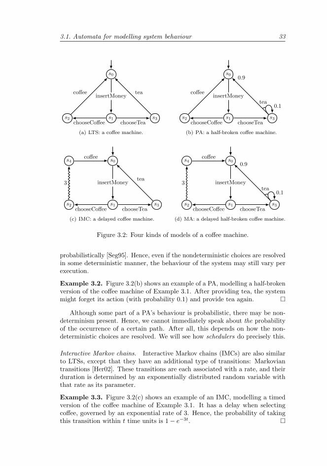
3.1. Automata for modelling system behaviour 33

s0

s1s2 s3

insertMoney

chooseCoffee chooseTea

coffee tea

(a) LTS: a coffee machine.

s0

s1s2 s3

insertMoney

chooseCoffee chooseTea

coffee

tea0.1

0.9

(b) PA: a half-broken coffee machine.

s0

s1s2 s3

s4

insertMoney

chooseCoffee chooseTea

3

coffee

tea

(c) IMC: a delayed coffee machine.

s0

s1s2 s3

s4

insertMoney

chooseCoffee chooseTea

3

coffee

tea0.1

0.9

(d) MA: a delayed half-broken coffee machine.

Figure 3.2: Four kinds of models of a coffee machine.

probabilistically [Seg95]. Hence, even if the nondeterministic choices are resolvedin some deterministic manner, the behaviour of the system may still vary perexecution.

Example 3.2. Figure 3.2(b) shows an example of a PA, modelling a half-brokenversion of the coffee machine of Example 3.1. After providing tea, the systemmight forget its action (with probability 0.1) and provide tea again.

Although some part of a PA’s behaviour is probabilistic, there may be non-determinism present. Hence, we cannot immediately speak about the probabilityof the occurrence of a certain path. After all, this depends on how the non-deterministic choices are resolved. We will see how schedulers do precisely this.

Interactive Markov chains. Interactive Markov chains (IMCs) are also similarto LTSs, except that they have an additional type of transitions: Markoviantransitions [Her02]. These transitions are each associated with a rate, and theirduration is determined by an exponentially distributed random variable withthat rate as its parameter.

Example 3.3. Figure 3.2(c) shows an example of an IMC, modelling a timedversion of the coffee machine of Example 3.1. It has a delay when selectingcoffee, governed by an exponential rate of 3. Hence, the probability of takingthis transition within t time units is 1− e−3t.

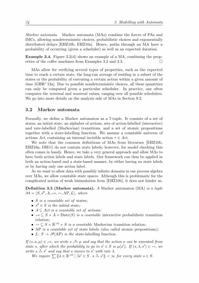
34 3. Modelling with Automata

Markov automata. Markov automata (MAs) combine the forces of PAs andIMCs, allowing nondeterministic choices, probabilistic choices and exponentiallydistributed delays [EHZ10b, EHZ10a]. Hence, paths through an MA have aprobability of occurring (given a scheduler) as well as an expected duration.

Example 3.4. Figure 3.2(d) shows an example of a MA, combining the prop-erties of the coffee machines from Examples 3.2 and 3.3.

MAs allow for verifying several types of properties, such as the expectedtime to reach a certain state, the long-run average of residing in a subset of thestates or the probability of executing a certain action within a given amount oftime [GHH+13a]. Due to possible nondeterministic choices, all these quantitiescan only be computed given a particular scheduler. In practice, one oftencomputes the minimal and maximal values, ranging over all possible schedulers.We go into more details on the analysis side of MAs in Section 9.2.

3.2 Markov automata

Formally, we define a Markov automaton as a 7-tuple. It consists of a set ofstates, an initial state, an alphabet of actions, sets of action-labelled (interactive)and rate-labelled (Markovian) transitions, and a set of atomic propositionstogether with a state-labelling function. We assume a countable universe ofactions Act, containing an internal invisible action τ ∈ Act.

We note that the common definitions of MAs from literature [EHZ10b,EHZ10a, DH11] do not contain state labels; however, for model checking thisoften comes in handy. Hence, we take a very general approach and allow MAs tohave both action labels and state labels. Our framework can thus be applied inboth an action-based and a state-based manner, by either having no state labelsor by having only one action label.

As we want to allow data with possibly infinite domains in our process algebraover MAs, we allow countable state spaces. Although this is problematic for thecomplicated notion of weak bisimulation from [EHZ10b], it does not hinder us.

Definition 3.5 (Markov automata). A Markov automaton (MA) is a tupleM = 〈S, s0, A, −→, ,AP, L〉, where

• S is a countable set of states;• s0 ∈ S is the initial state;• A ⊆ Act is a countable set of actions;• −→ ⊆ S ×A×Distr(S) is a countable interactive probabilistic transition

relation;• ⊆ S × R>0 × S is a countable Markovian transition relation;• AP is a countable set of state labels (also called atomic propositions);• L : S →P(AP) is the state-labelling function.

If (s, a, µ) ∈ −→, we write s a−→ µ and say that the action a can be executed fromstate s, after which the probability to go to s′ ∈ S is µ(s′). If (s, λ, s′) ∈ , wewrite s λ s′ and say that s moves to s′ with rate λ.

We require∑ |λ ∈ R>0 | ∃s′ ∈ S . s λ s′| <∞ for every state s ∈ S.

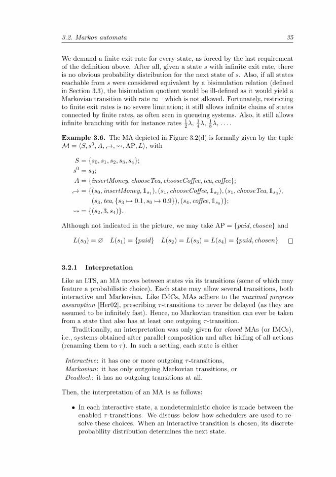
3.2. Markov automata 35

We demand a finite exit rate for every state, as forced by the last requirementof the definition above. After all, given a state s with infinite exit rate, thereis no obvious probability distribution for the next state of s. Also, if all statesreachable from s were considered equivalent by a bisimulation relation (definedin Section 3.3), the bisimulation quotient would be ill-defined as it would yield aMarkovian transition with rate∞—which is not allowed. Fortunately, restrictingto finite exit rates is no severe limitation; it still allows infinite chains of statesconnected by finite rates, as often seen in queueing systems. Also, it still allowsinfinite branching with for instance rates 1

2λ, 14λ, 1

8λ, . . . .

Example 3.6. The MA depicted in Figure 3.2(d) is formally given by the tupleM = 〈S, s0, A, −→, ,AP, L〉, with

S = s0, s1, s2, s3, s4;s0 = s0;

A = insertMoney, chooseTea, chooseCoffee, tea, coffee;−→ = (s0, insertMoney,1s1), (s1, chooseCoffee,1s2), (s1, chooseTea,1s3),

(s3, tea, s3 7→ 0.1, s0 7→ 0.9), (s4, coffee,1s0); = (s2, 3, s4).

Although not indicated in the picture, we may take AP = paid, chosen and

L(s0) = ∅ L(s1) = paid L(s2) = L(s3) = L(s4) = paid, chosen

3.2.1 Interpretation

Like an LTS, an MA moves between states via its transitions (some of which mayfeature a probabilistic choice). Each state may allow several transitions, bothinteractive and Markovian. Like IMCs, MAs adhere to the maximal progressassumption [Her02], prescribing τ -transitions to never be delayed (as they areassumed to be infinitely fast). Hence, no Markovian transition can ever be takenfrom a state that also has at least one outgoing τ -transition.

Traditionally, an interpretation was only given for closed MAs (or IMCs),i.e., systems obtained after parallel composition and after hiding of all actions(renaming them to τ). In such a setting, each state is either

Interactive: it has one or more outgoing τ -transitions,

Markovian: it has only outgoing Markovian transitions, or

Deadlock : it has no outgoing transitions at all.

Then, the interpretation of an MA is as follows:

• In each interactive state, a nondeterministic choice is made between theenabled τ -transitions. We discuss below how schedulers are used to re-solve these choices. When an interactive transition is chosen, its discreteprobability distribution determines the next state.

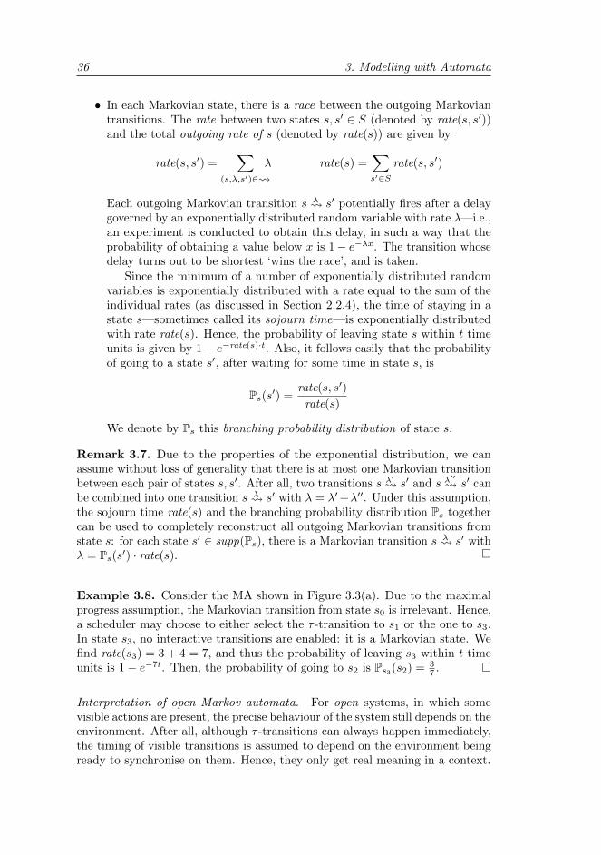
36 3. Modelling with Automata

• In each Markovian state, there is a race between the outgoing Markoviantransitions. The rate between two states s, s′ ∈ S (denoted by rate(s, s′))and the total outgoing rate of s (denoted by rate(s)) are given by

rate(s, s′) =∑

(s,λ,s′)∈ λ rate(s) =

∑s′∈S

rate(s, s′)

Each outgoing Markovian transition s λ s′ potentially fires after a delaygoverned by an exponentially distributed random variable with rate λ—i.e.,an experiment is conducted to obtain this delay, in such a way that theprobability of obtaining a value below x is 1− e−λx. The transition whosedelay turns out to be shortest ‘wins the race’, and is taken.

Since the minimum of a number of exponentially distributed randomvariables is exponentially distributed with a rate equal to the sum of theindividual rates (as discussed in Section 2.2.4), the time of staying in astate s—sometimes called its sojourn time—is exponentially distributedwith rate rate(s). Hence, the probability of leaving state s within t timeunits is given by 1− e−rate(s)·t. Also, it follows easily that the probabilityof going to a state s′, after waiting for some time in state s, is

Ps(s′) =rate(s, s′)

rate(s)

We denote by Ps this branching probability distribution of state s.

Remark 3.7. Due to the properties of the exponential distribution, we canassume without loss of generality that there is at most one Markovian transitionbetween each pair of states s, s′. After all, two transitions s λ

′ s′ and s λ

′′ s′ can

be combined into one transition s λ s′ with λ = λ′+λ′′. Under this assumption,the sojourn time rate(s) and the branching probability distribution Ps togethercan be used to completely reconstruct all outgoing Markovian transitions fromstate s: for each state s′ ∈ supp(Ps), there is a Markovian transition s λ s′ withλ = Ps(s′) · rate(s).

Example 3.8. Consider the MA shown in Figure 3.3(a). Due to the maximalprogress assumption, the Markovian transition from state s0 is irrelevant. Hence,a scheduler may choose to either select the τ -transition to s1 or the one to s3.In state s3, no interactive transitions are enabled: it is a Markovian state. Wefind rate(s3) = 3 + 4 = 7, and thus the probability of leaving s3 within t timeunits is 1− e−7t. Then, the probability of going to s2 is Ps3(s2) = 3

7 .

Interpretation of open Markov automata. For open systems, in which somevisible actions are present, the precise behaviour of the system still depends on theenvironment. After all, although τ -transitions can always happen immediately,the timing of visible transitions is assumed to depend on the environment beingready to synchronise on them. Hence, they only get real meaning in a context.

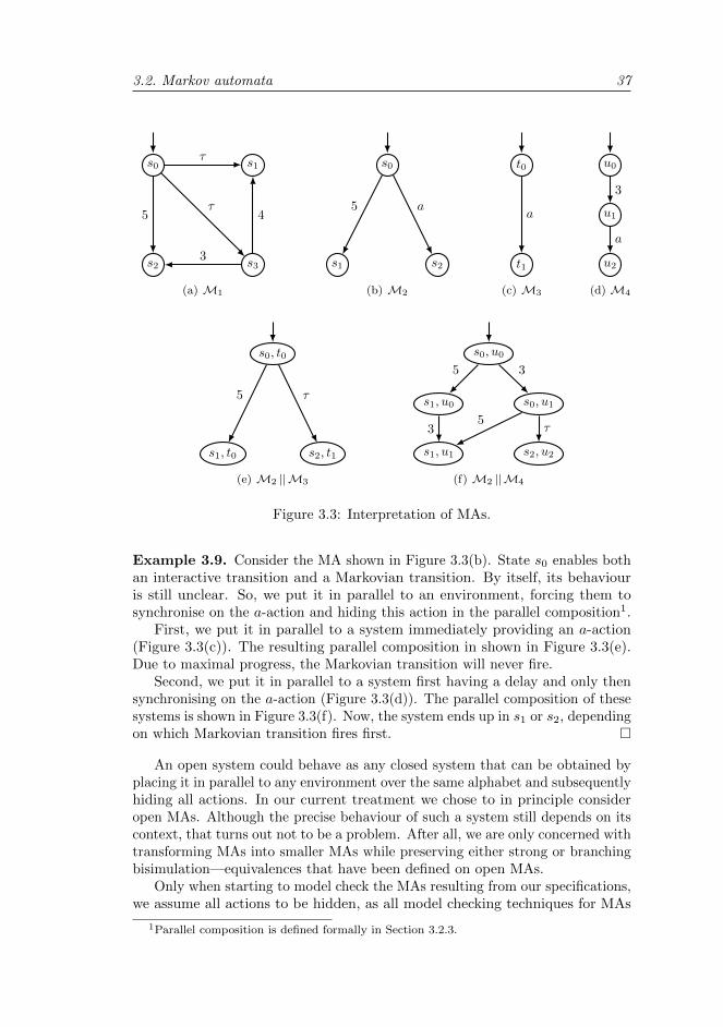
3.2. Markov automata 37

s0 s1

s3s2

τ

τ5 4

3

(a) M1

s0

s1 s2

5 a

(b) M2

t0

t1

a

(c) M3

u0

u1

u2

3

a

(d) M4

s0, t0

s1, t0 s2, t1

5 τ

(e) M2 ||M3

s0, u0

s0, u1s1, u0

s1, u1 s2, u2

35

τ5

3

(f) M2 ||M4

Figure 3.3: Interpretation of MAs.

Example 3.9. Consider the MA shown in Figure 3.3(b). State s0 enables bothan interactive transition and a Markovian transition. By itself, its behaviouris still unclear. So, we put it in parallel to an environment, forcing them tosynchronise on the a-action and hiding this action in the parallel composition1.

First, we put it in parallel to a system immediately providing an a-action(Figure 3.3(c)). The resulting parallel composition in shown in Figure 3.3(e).Due to maximal progress, the Markovian transition will never fire.

Second, we put it in parallel to a system first having a delay and only thensynchronising on the a-action (Figure 3.3(d)). The parallel composition of thesesystems is shown in Figure 3.3(f). Now, the system ends up in s1 or s2, dependingon which Markovian transition fires first.

An open system could behave as any closed system that can be obtained byplacing it in parallel to any environment over the same alphabet and subsequentlyhiding all actions. In our current treatment we chose to in principle consideropen MAs. Although the precise behaviour of such a system still depends on itscontext, that turns out not to be a problem. After all, we are only concerned withtransforming MAs into smaller MAs while preserving either strong or branchingbisimulation—equivalences that have been defined on open MAs.

Only when starting to model check the MAs resulting from our specifications,we assume all actions to be hidden, as all model checking techniques for MAs

1Parallel composition is defined formally in Section 3.2.3.

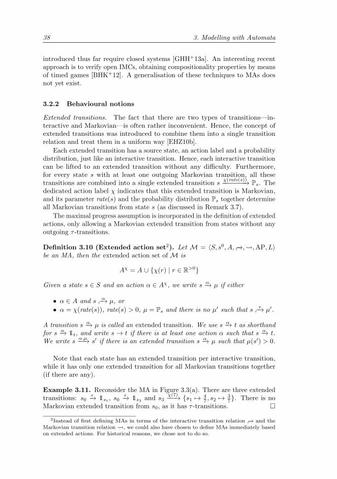
38 3. Modelling with Automata

introduced thus far require closed systems [GHH+13a]. An interesting recentapproach is to verify open IMCs, obtaining compositionality properties by meansof timed games [BHK+12]. A generalisation of these techniques to MAs doesnot yet exist.

3.2.2 Behavioural notions

Extended transitions. The fact that there are two types of transitions—in-teractive and Markovian—is often rather inconvenient. Hence, the concept ofextended transitions was introduced to combine them into a single transitionrelation and treat them in a uniform way [EHZ10b].

Each extended transition has a source state, an action label and a probabilitydistribution, just like an interactive transition. Hence, each interactive transitioncan be lifted to an extended transition without any difficulty. Furthermore,for every state s with at least one outgoing Markovian transition, all thesetransitions are combined into a single extended transition s −χ(rate(s))−−−−−−→ Ps. Thededicated action label χ indicates that this extended transition is Markovian,and its parameter rate(s) and the probability distribution Ps together determineall Markovian transitions from state s (as discussed in Remark 3.7).

The maximal progress assumption is incorporated in the definition of extendedactions, only allowing a Markovian extended transition from states without anyoutgoing τ -transitions.

Definition 3.10 (Extended action set2). Let M = 〈S, s0, A, −→, ,AP, L〉be an MA, then the extended action set of M is

Aχ = A ∪ χ(r) | r ∈ R>0

Given a state s ∈ S and an action α ∈ Aχ, we write s −α→ µ if either

• α ∈ A and s α−→ µ, or

• α = χ(rate(s)), rate(s) > 0, µ = Ps and there is no µ′ such that s τ−→ µ′.

A transition s −α→ µ is called an extended transition. We use s −α→ t as shorthandfor s −α→ 1t, and write s→ t if there is at least one action α such that s −α→ t.We write s −α,µ−−→ s′ if there is an extended transition s −α→ µ such that µ(s′) > 0.

Note that each state has an extended transition per interactive transition,while it has only one extended transition for all Markovian transitions together(if there are any).

Example 3.11. Reconsider the MA in Figure 3.3(a). There are three extendedtransitions: s0 −τ→ 1s1 , s0 −τ→ 1s3 and s3 −χ(7)−−→ s1 7→ 4

7 , s2 7→ 37. There is no

Markovian extended transition from s0, as it has τ -transitions.

2Instead of first defining MAs in terms of the interactive transition relation −→ and theMarkovian transition relation , we could also have chosen to define MAs immediately basedon extended actions. For historical reasons, we chose not to do so.

3.2. Markov automata 39

Paths, traces and connectivity. As for LTSs and other types of automata, wecan define paths and traces through an MA. We define these concepts, andprovide notations to work with them. Basically, a path is just a traversalthrough an MA, indicating which transitions were taken and which states werechosen probabilistically. Paths abstract from timing: they do not contain anyinformation on the precise duration of these steps. As paths are based onextended transitions, they may contain interactive as well as Markovian steps.Traces are obtained from paths by only listing the observable aspects of a path:the state labels and the visible action labels.

Definition 3.12 (Paths and traces). LetM = 〈S, s0, A, −→, ,AP, L〉 be anMA. Then,

• A path in M is a finite sequence

πfin = s0 −α1,µ1−−−→ s1 −α2,µ2−−−→ s2 −α3,µ3−−−→ . . . −αn,µn−−−→ sn,

possibly with n = 0, or an infinite sequence

πinf = s0 −α1,µ1−−−→ s1 −α2,µ2−−−→ s2 −α3,µ3−−−→ . . . ,

with si ∈ S for all 0 ≤ i ≤ n and all i ≥ 0, respectively, and such that eachextended transition si −αi+1,µi+1−−−−−−→ si+1 is indeed present in M. We refer toπfin as a path from s0 to sn.

• For any path π as above, we define

trace(π) = L(s0)α1L(s1)α2L(s2)α3 . . .

to be its sequence of state labellings and action labels. Additionally, wewrite

actionTrace(π) = α1α2α3 . . . \ τstateTrace(π) = L(s0)L(s1)L(s2) . . .

for the sequences of visible actions and state labellings of π, respectively.• Given an infinite or sufficiently long finite path π, we use prefix(π, i)

to denote the path fragment s0 −α1,µ1−−−→ . . . −αi,µi−−−→ si, and step(π, i) for thetransition si−1 −αi−→ µi. When π is finite we define |π| = n and last(π) = sn,otherwise |π| =∞ and no final state exists.

• We use finpathsM for the set of all finite paths in M (not necessarilybeginning in the initial state), and finpathsM(s) for all such paths withs0 = s.

• We say that a path π is invisible (denoted by invisible(π)) if it neveralters the state labelling and only consists of invisible actions. That is,actionTrace(π) = ε and stateTrace(π) is a sequence of identical labellings.

Example 3.13. Again, consider the MA M in Figure 3.3(a). A possible pathin M is

π = s0 −τ,1s3−−−→ s3 −χ(7),µ−−−→ s1

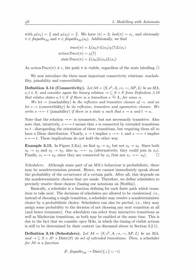
40 3. Modelling with Automata

with µ(s1) = 47 and µ(s2) = 3

7 . We have |π| = 2, last(π) = s1, and obviouslyπ ∈ finpathsM and π ∈ finpathsM(s0). Additionally, we find

trace(π) = L(s0)τL(s3)χ(7)L(s1)

actionTrace(π) = χ(7)

stateTrace(π) = L(s0)L(s3)L(s1)

As actionTrace(π) 6= ε, the path π is visible, regardless of the state labelling.

We now introduce the three most important connectivity relations: reachab-ility, joinability and convertibility.

Definition 3.14 (Connectivity). LetM = 〈S, s0, A, −→, ,AP, L〉 be an MA,s, t ∈ S, and consider again the binary relation → ⊆ S × S from Definition 3.10that relates states s, t ∈ S if there is a transition s −α→ 1t for some α.

We let (reachability) be the reflexive and transitive closure of →, and welet (convertibility) be its reflexive, transitive and symmetric closure. Wewrite s t (joinability) if there is a state u such that s u and t u.

Note that the relation is symmetric, but not necessarily transitive. Alsonote that, intuitively, s t means that s is connected by extended transitionsto t—disregarding the orientation of these transitions, but requiring them all tohave a Dirac distribution. Clearly, s t implies s t, and s t impliess t. These implications do not hold the other way.

Example 3.15. In Figure 3.3(a), we find s0 s2, but not s2 s0. Since boths0 s2 and s3 s2, also s0 s3 (alternatively, they could join in s3).Finally, s1 s2, since they are connected by s3 (but not s1 s2).

Schedulers. Although some part of an MA’s behaviour is probabilistic, theremay be nondeterminism present. Hence, we cannot immediately speak aboutthe probability of the occurrence of a certain path. After all, this depends onthe nondeterministic choices that are made. Therefore, we define schedulers toprecisely resolve these choices (basing our notations on [Sto02a]).

Basically, a scheduler is a function defining for each finite path which trans-ition to take next. The decisions of schedulers are allowed to be randomised , i.e.,instead of choosing a single transition, a scheduler may resolve a nondeterministicchoice by a probabilistic choice. Schedulers can also be partial , i.e., they mayassign some probability to the decision of not choosing any next transition at all(and hence terminate). Our schedulers can select from interactive transitions aswell as Markovian transitions, as both may be enabled at the same time. This isdue to the fact that we consider open MAs, in which the timing of visible actionsis still to be determined by their context (as discussed above in Section 3.2.1).

Definition 3.16 (Schedulers). Let M = 〈S, s0, A, −→, ,AP, L〉 be an MA,and → ⊆ S ×Aχ ×Distr(S) its set of extended transitions. Then, a schedulerfor M is a function

S : finpathsM → Distr(⊥ ∪ →)

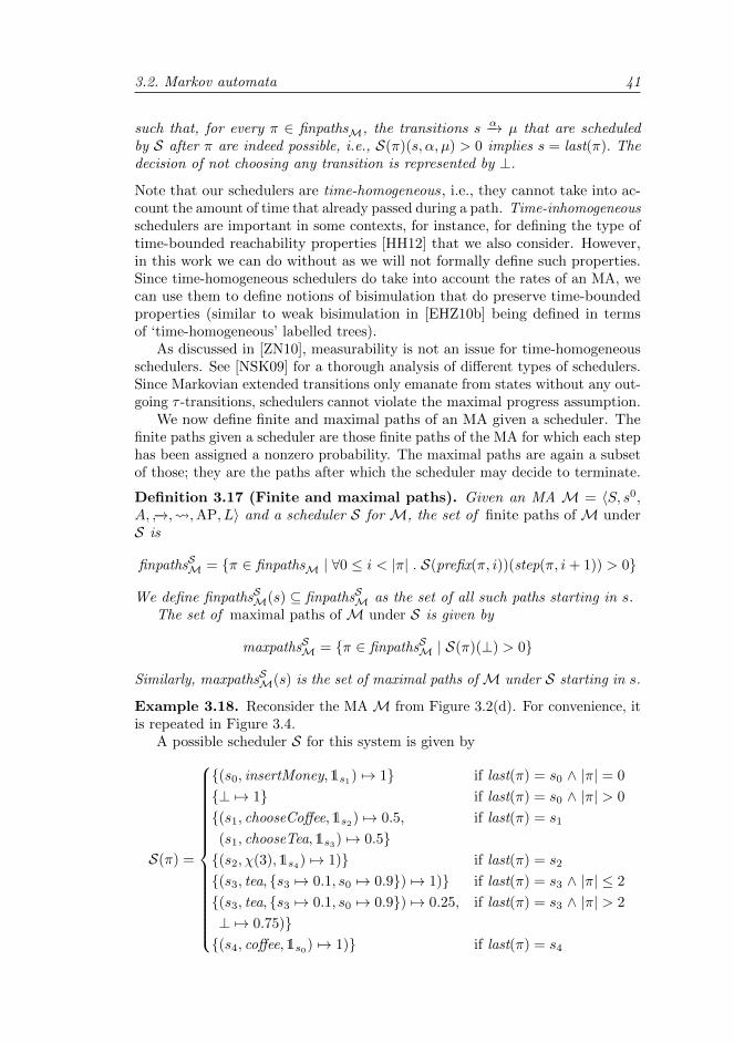
3.2. Markov automata 41

such that, for every π ∈ finpathsM, the transitions s −α→ µ that are scheduledby S after π are indeed possible, i.e., S(π)(s, α, µ) > 0 implies s = last(π). Thedecision of not choosing any transition is represented by ⊥.

Note that our schedulers are time-homogeneous, i.e., they cannot take into ac-count the amount of time that already passed during a path. Time-inhomogeneousschedulers are important in some contexts, for instance, for defining the type oftime-bounded reachability properties [HH12] that we also consider. However,in this work we can do without as we will not formally define such properties.Since time-homogeneous schedulers do take into account the rates of an MA, wecan use them to define notions of bisimulation that do preserve time-boundedproperties (similar to weak bisimulation in [EHZ10b] being defined in termsof ‘time-homogeneous’ labelled trees).

As discussed in [ZN10], measurability is not an issue for time-homogeneousschedulers. See [NSK09] for a thorough analysis of different types of schedulers.Since Markovian extended transitions only emanate from states without any out-going τ -transitions, schedulers cannot violate the maximal progress assumption.

We now define finite and maximal paths of an MA given a scheduler. Thefinite paths given a scheduler are those finite paths of the MA for which each stephas been assigned a nonzero probability. The maximal paths are again a subsetof those; they are the paths after which the scheduler may decide to terminate.

Definition 3.17 (Finite and maximal paths). Given an MA M = 〈S, s0,A, −→, ,AP, L〉 and a scheduler S for M, the set of finite paths of M underS is

finpathsSM = π ∈ finpathsM | ∀0 ≤ i < |π| . S(prefix(π, i))(step(π, i+ 1)) > 0

We define finpathsSM(s) ⊆ finpathsSM as the set of all such paths starting in s.The set of maximal paths of M under S is given by

maxpathsSM = π ∈ finpathsSM | S(π)(⊥) > 0

Similarly, maxpathsSM(s) is the set of maximal paths ofM under S starting in s.

Example 3.18. Reconsider the MA M from Figure 3.2(d). For convenience, itis repeated in Figure 3.4.

A possible scheduler S for this system is given by

S(π) =

(s0, insertMoney,1s1) 7→ 1 if last(π) = s0 ∧ |π| = 0

⊥ 7→ 1 if last(π) = s0 ∧ |π| > 0

(s1, chooseCoffee,1s2) 7→ 0.5, if last(π) = s1

(s1, chooseTea,1s3) 7→ 0.5(s2, χ(3),1s4) 7→ 1) if last(π) = s2

(s3, tea, s3 7→ 0.1, s0 7→ 0.9) 7→ 1) if last(π) = s3 ∧ |π| ≤ 2

(s3, tea, s3 7→ 0.1, s0 7→ 0.9) 7→ 0.25, if last(π) = s3 ∧ |π| > 2

⊥ 7→ 0.75)(s4, coffee,1s0) 7→ 1) if last(π) = s4

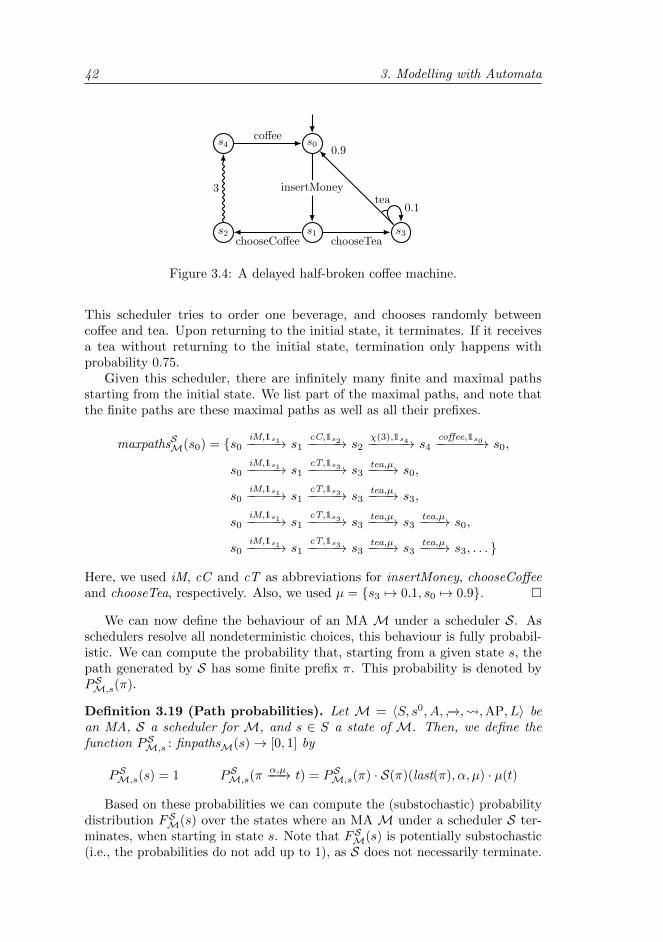
42 3. Modelling with Automata

s0

s1s2 s3

s4

insertMoney

chooseCoffee chooseTea

3

coffee

tea0.1

0.9

Figure 3.4: A delayed half-broken coffee machine.

This scheduler tries to order one beverage, and chooses randomly betweencoffee and tea. Upon returning to the initial state, it terminates. If it receivesa tea without returning to the initial state, termination only happens withprobability 0.75.

Given this scheduler, there are infinitely many finite and maximal pathsstarting from the initial state. We list part of the maximal paths, and note thatthe finite paths are these maximal paths as well as all their prefixes.

maxpathsSM(s0) = s0 −iM,1s1−−−−→ s1 −

cC,1s2−−−−→ s2 −χ(3),1s4−−−−−→ s4 −

coffee,1s0−−−−−−→ s0,

s0 −iM,1s1−−−−→ s1 −

cT,1s3−−−−→ s3 −tea,µ−−−→ s0,

s0 −iM,1s1−−−−→ s1 −

cT,1s3−−−−→ s3 −tea,µ−−−→ s3,

s0 −iM,1s1−−−−→ s1 −

cT,1s3−−−−→ s3 −tea,µ−−−→ s3 −tea,µ−−−→ s0,

s0 −iM,1s1−−−−→ s1 −

cT,1s3−−−−→ s3 −tea,µ−−−→ s3 −tea,µ−−−→ s3, . . .

Here, we used iM, cC and cT as abbreviations for insertMoney, chooseCoffeeand chooseTea, respectively. Also, we used µ = s3 7→ 0.1, s0 7→ 0.9.

We can now define the behaviour of an MA M under a scheduler S. Asschedulers resolve all nondeterministic choices, this behaviour is fully probabil-istic. We can compute the probability that, starting from a given state s, thepath generated by S has some finite prefix π. This probability is denoted byPSM,s(π).

Definition 3.19 (Path probabilities). Let M = 〈S, s0, A, −→, ,AP, L〉 bean MA, S a scheduler for M, and s ∈ S a state of M. Then, we define thefunction PSM,s : finpathsM(s)→ [0, 1] by

PSM,s(s) = 1 PSM,s(π −α,µ−−→ t) = PSM,s(π) · S(π)(last(π), α, µ) · µ(t)

Based on these probabilities we can compute the (substochastic) probabilitydistribution FSM(s) over the states where an MA M under a scheduler S ter-minates, when starting in state s. Note that FSM(s) is potentially substochastic(i.e., the probabilities do not add up to 1), as S does not necessarily terminate.

3.2. Markov automata 43

Definition 3.20 (Final state probabilities). Given an MA M = 〈S, s0, A,−→, ,AP, L〉 and a scheduler S for M, we define FSM : S → SDistr(S) by

FSM(s) =s′ 7→

∑π∈maxpathsSM(s)

last(π)=s′

PSM,s(π) · S(π)(⊥) | s′ ∈ S

∀s ∈ S

Example 3.21. We continue with Example 3.18. Since all maximal paths endin either state s3 or state s0, FSM(s0) will be a probability distribution over thesetwo states.

For the scheduler S defined before, we compute PSM,s0(πi) · S(πi)(⊥) for the

following three paths (again with µ = s3 7→ 0.1, s0 7→ 0.9):

π1 = s0 −iM,1s1−−−−→ s1 −

cC,1s2−−−−→ s2 −χ(3),1s4−−−−−→ s4 −

coffee,1s0−−−−−−→ s0

π2 = s0 −iM,1s1−−−−→ s1 −

cT,1s3−−−−→ s3 −tea,µ−−−→ s0

π3 = s0 −iM,1s1−−−−→ s1 −

cT,1s3−−−−→ s3 −tea,µ−−−→ s3

Using the definition of path probabilities, we find

PSM,s0(π1) · S(π1)(⊥) = (1 · 1) · ( 12 · 1) · (1 · 1) · (1 · 1) · 1 = 0.5

PSM,s0(π2) · S(π2)(⊥) = (1 · 1) · ( 12 · 1) · (1 · 0.9) · 1 = 0.45

PSM,s0(π3) · S(π3)(⊥) = (1 · 1) · ( 12 · 1) · (1 · 0.1) · 0.75 = 0.0375

As π3 ends in s3, its path probability 0.0375 contributes to the total probabilityof terminating in s3. To precisely obtain the probability of terminating in s3, weneed to sum the probabilities of all paths ending in s3. Note that these pathsalways first have to take the chooseTea transition (probability 0.5). Then, thetea transition should be taken (probability 1) and it should fail (probability0.1). Due to independence of these probabilities, this combination happens withprobability 0.5 · 1 · 0.1 = 0.05.

Then, either we immediately terminate (probability 0.75), or we terminateafter any number of times continuing and failing again (probability 0.25 · 0.1 =0.025 per time). So, this happens with probability

0.75 + 0.025 · 0.75 + 0.0252 · 0.75 + · · · = 0.75 ·∞∑i=0

0.025i =0.75

1− 0.025=

10

13

Combining these results, the total probability of terminating in state s3 is foundto be 0.05 · 10

13 = 126 . In the same way, we can compute that the probability of

terminating in s0 is 2526 . Hence,

FSM(s0) =

s0 7→

25

26, s3 7→

1

26

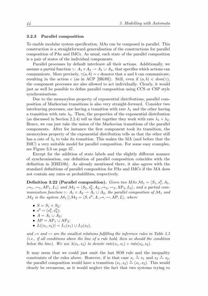
44 3. Modelling with Automata

3.2.3 Parallel composition

To enable modular system specification, MAs can be composed in parallel. Thisconstruction is a straightforward generalisation of the constructions for parallelcomposition of PAs and IMCs. As usual, each state of the parallel compositionis a pair of states of the individual components.

Parallel processes by default interleave all their actions. Additionally, weassume a partial function γ : A1×A2 A1 ∪ A2, that specifies which actions cancommunicate. More precisely, γ(a, b) = c denotes that a and b can communicate,resulting in the action c (as in ACP [BK89]). Still, even if (a, b) ∈ dom(γ),the component processes are also allowed to act individually. Clearly, it wouldjust as well be possible to define parallel composition using CCS or CSP stylesynchronisations.

Due to the memoryless property of exponential distributions, parallel com-position of Markovian transitions is also very straight-forward. Consider twointerleaving processes, one having a transition with rate λ1 and the other havinga transition with rate λ2. Then, the properties of the exponential distribution(as discussed in Section 2.2.4) tell us that together they work with rate λ1 + λ2.Hence, we can just take the union of the Markovian transitions of the parallelcomponents. After for instance the first component took its transition, thememoryless property of the exponential distribution tells us that the other stillhas a rate of λ2 to take its transition. This makes the MA (and before that theIMC) a very suitable model for parallel composition. For some easy examples,see Figure 3.3 on page 37.

Except for the addition of state labels and the slightly different mannerof synchronisation, our definition of parallel composition coincides with thedefinition in [EHZ10b]. As already mentioned there, it also agrees with thestandard definitions of parallel composition for PAs and IMCs if the MA doesnot contain any rates or probabilities, respectively.

Definition 3.22 (Parallel composition). Given two MAs M1 = 〈S1, s01, A1,

−→1, 1,AP1, L1〉 and M2 = 〈S2, s02, A2, −→2, 2,AP2, L2〉, and a partial com-

munication function γ : A1×A2 A1 ∪ A2, the parallel composition of M1 andM2 is the system M1 ||M2 = 〈S, s0, A, −→, ,AP, L〉, where

• S = S1 × S2;• s0 = (s0

1, s02);

• A = A1 ∪ A2;• AP = AP1 ∪ AP2;• L((s1, s2)) = L1(s1) ∪ L2(s2),

and −→ and are the smallest relations fulfilling the inference rules in Table 3.5(i.e., if all conditions above the line of a rule hold, then so should the conditionbelow the line). We use λ(s1, s2) to denote rate(s1, s1) + rate(s2, s2).

It may seem that we could just omit the last SOS rule and the inequalityconstraints of the rules above. However, if in that case s1

λ s1 and s2λ s2,

the parallel composition would have a transition (s1, s2) λ (s1, s2). This wouldclearly be erroneous, as it would neglect the fact that two systems trying to

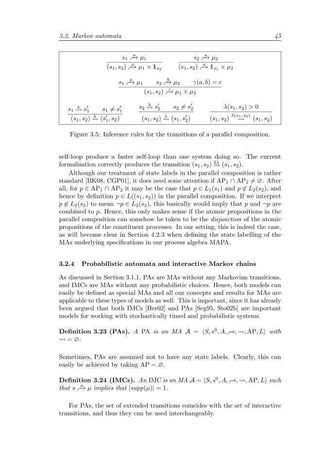
3.2. Markov automata 45

s1a−→ µ1

(s1, s2) a−→ µ1 × 1s2s2

a−→ µ2

(s1, s2) a−→ 1s1 × µ2

s1a−→ µ1 s2

b−→ µ2 γ(a, b) = c

(s1, s2) c−→ µ1 × µ2

s1λ s′1 s1 6= s′1

(s1, s2) λ (s′1, s2)

s2λ s′2 s2 6= s′2

(s1, s2) λ (s1, s′2)

λ(s1, s2) > 0

(s1, s2)λ(s1, s2) (s1, s2)

Figure 3.5: Inference rules for the transitions of a parallel composition.

self-loop produce a faster self-loop than one system doing so. The currentformalisation correctly produces the transition (s1, s2) 2λ (s1, s2).

Although our treatment of state labels in the parallel composition is ratherstandard [BK08, CGP01], it does need some attention if AP1 ∩ AP2 6= ∅. Afterall, for p ∈ AP1 ∩ AP2 it may be the case that p ∈ L1(s1) and p 6∈ L2(s2), andhence by definition p ∈ L((s1, s2)) in the parallel composition. If we interpretp 6∈ L2(s2) to mean ¬p ∈ L2(s2), this basically would imply that p and ¬p arecombined to p. Hence, this only makes sense if the atomic propositions in theparallel composition can somehow be taken to be the disjunction of the atomicpropositions of the constituent processes. In our setting, this is indeed the case,as will become clear in Section 4.2.3 when defining the state labelling of theMAs underlying specifications in our process algebra MAPA.

3.2.4 Probabilistic automata and interactive Markov chains

As discussed in Section 3.1.1, PAs are MAs without any Markovian transitions,and IMCs are MAs without any probabilistic choices. Hence, both models caneasily be defined as special MAs and all our concepts and results for MAs areapplicable to these types of models as well. This is important, since it has alreadybeen argued that both IMCs [Her02] and PAs [Seg95, Sto02b] are importantmodels for working with stochastically timed and probabilistic systems.

Definition 3.23 (PAs). A PA is an MA A = 〈S, s0, A, −→, ,AP, L〉 with = ∅.

Sometimes, PAs are assumed not to have any state labels. Clearly, this caneasily be achieved by taking AP = ∅.

Definition 3.24 (IMCs). An IMC is an MA A = 〈S, s0, A, −→, ,AP, L〉 suchthat s a−→ µ implies that |supp(µ)| = 1.

For PAs, the set of extended transitions coincides with the set of interactivetransitions, and thus they can be used interchangeably.

46 3. Modelling with Automata

3.3 Isomorphism and bisimulation relations

It is often important to be able to say that two models are equivalent, forinstance when reducing a model before analysing it. After all, we do not wantto lose behaviour or change the properties of the model. Several behaviouralequivalences have already been defined for MAs, most importantly notions ofbisimulation. There is one important criterion that distinguishes them: someequivalences require internal transitions to be mimicked (strong equivalences),while others abstract from them (weak equivalences). Both types of bisimulationrelations have their own merits [BK08].

Strong equivalences preserve more properties; most importantly, they preserveproperties involving the length of a computation. Weak equivalences on the otherhand allow more aggressive state space reductions, but preserve only propertiesthat are oblivious to stuttering (repetition) of state labels and do not refer tointernal actions or computation length. For most of our techniques we are ableto prove a strong equivalence, showing that they can safely be applied whilepreserving a large set of properties. For confluence reduction, we explicitly aim atreducing the amount of internal behaviour; hence, a weak equivalence is needed.

3.3.1 Strong equivalences

We first discuss the two most important strong equivalences: isomorphism andstrong bisimulation.

Isomorphism. Isomorphism is the strongest equivalence on MAs that we con-sider. For two models to be isomorphic, they have to be identical except forstate names.

Definition 3.25 (Isomorphism). Given an MA M = 〈S, s0, A, −→, ,AP,L〉, two states s, t ∈ S are isomorphic (denoted by s ≈iso t) if there exists abijection f : S → S such that f(s) = t and

∀s′ ∈ S, α ∈ Aχ, µ ∈ Distr(S) . L(f(s′)) = L(s′) ∧ s′ −α→ µ⇐⇒ f(s′) −α→ µf

with µf as defined in Section 2.2.3. Two MAs M,M′ are isomorphic (denotedby M≈iso M′) if their initial states are isomorphic in their disjoint union.

Strong bisimulation. The notion of strong bisimulation we introduce is takenfrom [EHZ10b], while adding support for state labels. Based on the traditionalnotions of strong bisimulation [Mil89, LS91, SL95], it is the most straightforwardkind of bisimulation, equating any two states that cannot be distinguished. Thesystem is considered to be quite transparant, in the sense that it can observestate labels, action labels and even internal transitions. Hence, bisimilar statesshould have the same state label. Moreover, any α-labelled transition enabledby one state should also be enabled by all bisimilar states, and all target statesof these transitions should again be bisimilar. More precisely, the probabilitydistributions of a transition and its mimicking transitions should assign the same

3.3. Isomorphism and bisimulation relations 47

probabilities to the equivalence classes of the state space under bisimulation (asformalised by the relation ≡R, defined in Section 2.2.3).

Definition 3.26 (Strong bisimulation). Given an MA M = 〈S, s0, A, −→, ,AP, L〉, an equivalence relation R ⊆ S × S is a strong bisimulation for M iffor every (s, t) ∈ R and all α ∈ Aχ, µ ∈ Distr(S), it holds that L(s) = L(t) and

s −α→ µ =⇒ ∃µ′ ∈ Distr(S) . t −α→ µ′ ∧ µ ≡R µ′

Two states s, t ∈ S are strongly bisimilar (denoted by s ≈s t) if there exists astrong bisimulation R for M such that (s, t) ∈ R. Two MAs M,M′ are stronglybisimilar (denoted by M≈s M′) if their initial states are strongly bisimilar intheir disjoint union.

It is easy to see that strong bisimulation is implied by isomorphism, by takingR = (s, t) ∈ S × S | t = f(s) as the bisimulation relation associated withan isomorphism f . We note that there are also notions of strong bisimulationallowing convex combinations of transitions [Seg95]; we do not need to considerthese notions, as our procedures already preserve the current (stronger) variantof strong bisimulation. As future work, it might be beneficial to define morepowerful reduction techniques that do take advantage of such a more liberalnotion of bisimulation.

The following proposition (taken from [EHZ10b]) states that strong bisimu-lation is a congruence for parallel composition. It is of vital importance to therest of this thesis, since we will often transform components while preservingstrong bisimulation, prior to composing them in parallel.

Proposition 3.27. LetM1,M2 andM3 be MAs such thatM1 ≈s M2. Then,

M1 ||M3 ≈s M2 ||M3

It is easy to see that the validity of this proposition is not influenced by the factthat our notion of strong bisimulation also requires state labels to coincide or byour slightly different manner of synchronisation.

3.3.2 Weak equivalences

Often, from an outside perspective not all behaviour of a system is observable.In action-based process algebras, the τ -action is used to model unobservablebehaviour. In state-based model checking, stuttering transitions (i.e., transitionsleaving the state labelling invariant) are assumed to be invisible. Since ourdefinition of MAs contains both action and state labels, we assume transitionsto be invisible if they are labelled by τ and their source state and all possibletarget states have the same state labelling.

As mentioned before, it is often desirable to abstract from internal be-haviour and consider systems to be equivalent if the visible transitions co-incide. This insight resulted in many weak equivalences for LTSs and PAs,among which weak bisimulation [Mil89, SL95, BH97, BS00, PLS00], and branch-ing bisimulation [vGW96, SL95]. Weak bisimulation was also generalised to

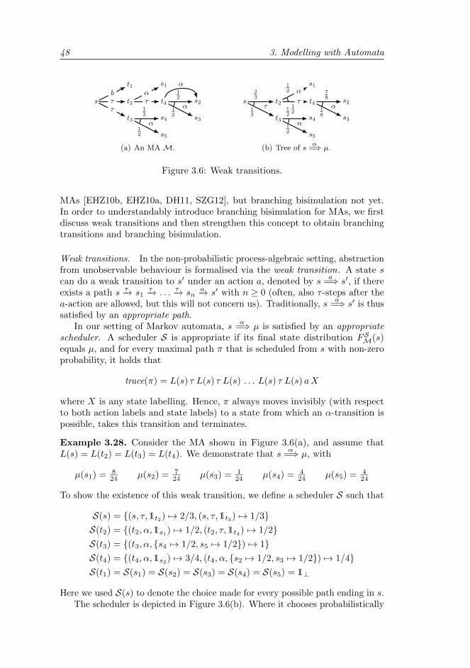
48 3. Modelling with Automata

s t2

t3

t1

ττ

bt4

s1

s2

s4 s3

s5

τα

α

12

12

α

12

12

α

(a) An MA M.

s t2

t3

τ

23

13

t4

s1

s2

s4 s3

s5

12

12

τ

α

12

12

α

78

18

α

(b) Tree of sα

=⇒ µ.

Figure 3.6: Weak transitions.

MAs [EHZ10b, EHZ10a, DH11, SZG12], but branching bisimulation not yet.In order to understandably introduce branching bisimulation for MAs, we firstdiscuss weak transitions and then strengthen this concept to obtain branchingtransitions and branching bisimulation.

Weak transitions. In the non-probabilistic process-algebraic setting, abstractionfrom unobservable behaviour is formalised via the weak transition. A state scan do a weak transition to s′ under an action a, denoted by s

a=⇒ s′, if there

exists a path s −τ→ s1 −τ→ . . . −τ→ sn −a→ s′ with n ≥ 0 (often, also τ -steps after thea-action are allowed, but this will not concern us). Traditionally, s

a=⇒ s′ is thus

satisfied by an appropriate path.In our setting of Markov automata, s

α=⇒ µ is satisfied by an appropriate

scheduler. A scheduler S is appropriate if its final state distribution FSM(s)equals µ, and for every maximal path π that is scheduled from s with non-zeroprobability, it holds that

trace(π) = L(s) τ L(s) τ L(s) . . . L(s) τ L(s) aX

where X is any state labelling. Hence, π always moves invisibly (with respectto both action labels and state labels) to a state from which an α-transition ispossible, takes this transition and terminates.

Example 3.28. Consider the MA shown in Figure 3.6(a), and assume thatL(s) = L(t2) = L(t3) = L(t4). We demonstrate that s

α=⇒ µ, with

µ(s1) = 824 µ(s2) = 7

24 µ(s3) = 124 µ(s4) = 4

24 µ(s5) = 424

To show the existence of this weak transition, we define a scheduler S such that

S(s) = (s, τ,1t2) 7→ 2/3, (s, τ,1t3) 7→ 1/3S(t2) = (t2, α,1s1) 7→ 1/2, (t2, τ,1t4) 7→ 1/2S(t3) = (t3, α, s4 7→ 1/2, s5 7→ 1/2) 7→ 1S(t4) = (t4, α,1s2) 7→ 3/4, (t4, α, s2 7→ 1/2, s3 7→ 1/2) 7→ 1/4S(t1) = S(s1) = S(s2) = S(s3) = S(s4) = S(s5) = 1⊥

Here we used S(s) to denote the choice made for every possible path ending in s.The scheduler is depicted in Figure 3.6(b). Where it chooses probabilistically

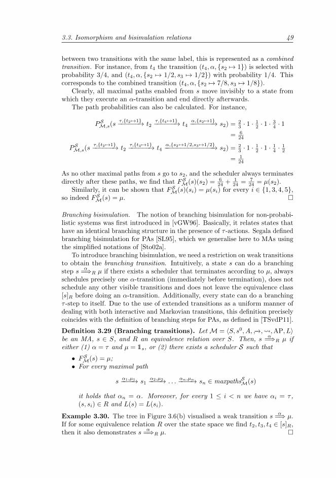
3.3. Isomorphism and bisimulation relations 49

between two transitions with the same label, this is represented as a combinedtransition. For instance, from t4 the transition (t4, α, s2 7→ 1) is selected withprobability 3/4, and (t4, α, s2 7→ 1/2, s3 7→ 1/2) with probability 1/4. Thiscorresponds to the combined transition (t4, α, s2 7→ 7/8, s3 7→ 1/8).

Clearly, all maximal paths enabled from s move invisibly to a state fromwhich they execute an α-transition and end directly afterwards.

The path probabilities can also be calculated. For instance,

PSM,s(s −τ,t2 7→1−−−−−→ t2 −τ,t4 7→1−−−−−→ t4 −α,s2 7→1−−−−−−→ s2) = 2

3 · 1 · 12 · 1 · 3

4 · 1= 6

24

PSM,s(s −τ,t2 7→1−−−−−→ t2 −τ,t4 7→1−−−−−→ t4 −α,s2 7→1/2,s3 7→1/2−−−−−−−−−−−−−→ s2) = 2

3 · 1 · 12 · 1 · 1

4 · 12

= 124

As no other maximal paths from s go to s2, and the scheduler always terminatesdirectly after these paths, we find that FSM(s)(s2) = 6

24 + 124 = 7

24 = µ(s2).Similarly, it can be shown that FSM(s)(si) = µ(si) for every i ∈ 1, 3, 4, 5,

so indeed FSM(s) = µ.

Branching bisimulation. The notion of branching bisimulation for non-probabi-listic systems was first introduced in [vGW96]. Basically, it relates states thathave an identical branching structure in the presence of τ -actions. Segala definedbranching bisimulation for PAs [SL95], which we generalise here to MAs usingthe simplified notations of [Sto02a].

To introduce branching bisimulation, we need a restriction on weak transitionsto obtain the branching transition. Intuitively, a state s can do a branchingstep s

α=⇒R µ if there exists a scheduler that terminates according to µ, always

schedules precisely one α-transition (immediately before termination), does notschedule any other visible transitions and does not leave the equivalence class[s]R before doing an α-transition. Additionally, every state can do a branchingτ -step to itself. Due to the use of extended transitions as a uniform manner ofdealing with both interactive and Markovian transitions, this definition preciselycoincides with the definition of branching steps for PAs, as defined in [TSvdP11].

Definition 3.29 (Branching transitions). Let M = 〈S, s0, A, −→, ,AP, L〉be an MA, s ∈ S, and R an equivalence relation over S. Then, s

α=⇒R µ if

either (1) α = τ and µ = 1s, or (2) there exists a scheduler S such that

• FSM(s) = µ;• For every maximal path

s −α1,µ1−−−→ s1 −α2,µ2−−−→ . . . −αn,µn−−−→ sn ∈ maxpathsSM(s)

it holds that αn = α. Moreover, for every 1 ≤ i < n we have αi = τ ,(s, si) ∈ R and L(s) = L(si).

Example 3.30. The tree in Figure 3.6(b) visualised a weak transition sα

=⇒ µ.If for some equivalence relation R over the state space we find t2, t3, t4 ∈ [s]R,then it also demonstrates s

α=⇒R µ.

50 3. Modelling with Automata

Based on branching transitions, we define branching bisimulation for MAs asa natural extension of the notion of naive weak bisimulation from [EHZ10b]3.Naive weak bisimulation is an intuitive generalisation of weak bisimulation fromPAs and IMCs to MAs. Naive weak bisimulation is implied by our notionof branching bisimulation, as it is obtained by omitting the requirement that(s, si) ∈ R for all 1 ≤ i < n, and allowing convex combinations of transitions.

Definition 3.31 (Branching bisimulation). Given an MA M = 〈S, s0, A,−→, ,AP, L〉, an equivalence relation R ⊆ S × S is a branching bisimulationfor M if for every (s, t) ∈ R and all α ∈ Aχ, µ ∈ Distr(S), it holds thatL(s) = L(t) and

s −α→ µ =⇒ ∃µ′ ∈ Distr(S) . tα

=⇒R µ′ ∧ µ ≡R µ′

Two states s, t ∈ S are branching bisimilar (denoted by s ≈b t) if there existsa branching bisimulation R for M such that (s, t) ∈ R. Two MAs M,M′ arebranching bisimilar (denoted by M≈b M′) if their initial states are branchingbisimilar in their disjoint union.

Note that, since each branching bisimulation relation R has the property that(s, t) ∈ R implies L(s) = L(t), the condition “L(s) = L(si) for every 1 ≤ i < n”in Definition 3.29 is already implied by (s, si) ∈ R, and hence does not explicitlyneed to be checked for t

α=⇒R µ

′.This notion of branching bisimulation has some appealing properties. First,

the definition is robust in the sense that it can be adapted to using sα

=⇒R µinstead of s −α→ µ in its condition. It turns out that this altered definition equatesexactly the same systems. Second, the relation ≈b induced by the definition isan equivalence relation.

Proposition 3.32. Let M = 〈S, s0, A, −→, ,AP, L〉 be an MA. Then, an equi-valence relation R ⊆ S × S is a branching bisimulation for M if and only if forevery (s, t) ∈ R and all α ∈ Aχ, µ ∈ Distr(S), it holds that L(s) = L(t) and

sα

=⇒R µ =⇒ ∃µ′ ∈ Distr(S) . tα

=⇒R µ′ ∧ µ ≡R µ′

Proposition 3.33. The relation ≈b is an equivalence relation.

Divergence sensitivity. If infinite paths of τ -actions can be scheduled withnon-zero probability, then minimal probabilities (e.g., of eventually seeing ana-action) are not preserved by branching bisimulation. Consider for instance thetwo systems in Figure 3.7.

Note that, for the system on the left, the a-transition is not necessarily evertaken. After all, it is possible to indefinitely and invisibly loop through state

3Since our notion of branching bisimulation for MAs is just as naive as naive weak bisimu-lation for MAs, we could have called it naive branching bisimulation. However, since naiveweak bisimulation for MAs is actually very related to weak bisimulation for PAs and IMCs, weargue that it would have made more sense to omit the ‘naive’ in the existing notion of naiveweak bisimulation for MAs and prefix ‘smart’ to the existing notion of weak bisimulation forMAs. Our terminology still leaves room for a notion of smart branching bisimulation.

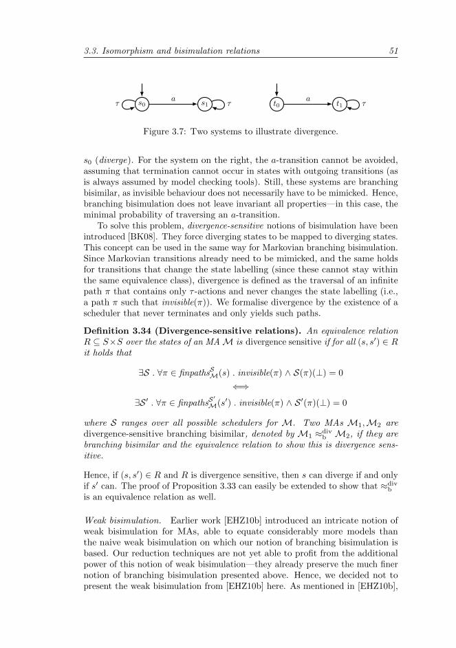
3.3. Isomorphism and bisimulation relations 51

s0 s1a

τ τ t0 t1a

τ

Figure 3.7: Two systems to illustrate divergence.

s0 (diverge). For the system on the right, the a-transition cannot be avoided,assuming that termination cannot occur in states with outgoing transitions (asis always assumed by model checking tools). Still, these systems are branchingbisimilar, as invisible behaviour does not necessarily have to be mimicked. Hence,branching bisimulation does not leave invariant all properties—in this case, theminimal probability of traversing an a-transition.

To solve this problem, divergence-sensitive notions of bisimulation have beenintroduced [BK08]. They force diverging states to be mapped to diverging states.This concept can be used in the same way for Markovian branching bisimulation.Since Markovian transitions already need to be mimicked, and the same holdsfor transitions that change the state labelling (since these cannot stay withinthe same equivalence class), divergence is defined as the traversal of an infinitepath π that contains only τ -actions and never changes the state labelling (i.e.,a path π such that invisible(π)). We formalise divergence by the existence of ascheduler that never terminates and only yields such paths.

Definition 3.34 (Divergence-sensitive relations). An equivalence relationR ⊆ S×S over the states of an MAM is divergence sensitive if for all (s, s′) ∈ Rit holds that

∃S . ∀π ∈ finpathsSM(s) . invisible(π) ∧ S(π)(⊥) = 0

⇐⇒∃S ′ . ∀π ∈ finpathsS

′

M(s′) . invisible(π) ∧ S ′(π)(⊥) = 0

where S ranges over all possible schedulers for M. Two MAs M1,M2 aredivergence-sensitive branching bisimilar, denoted by M1 ≈div

b M2, if they arebranching bisimilar and the equivalence relation to show this is divergence sens-itive.

Hence, if (s, s′) ∈ R and R is divergence sensitive, then s can diverge if and onlyif s′ can. The proof of Proposition 3.33 can easily be extended to show that ≈div

b

is an equivalence relation as well.

Weak bisimulation. Earlier work [EHZ10b] introduced an intricate notion ofweak bisimulation for MAs, able to equate considerably more models thanthe naive weak bisimulation on which our notion of branching bisimulation isbased. Our reduction techniques are not yet able to profit from the additionalpower of this notion of weak bisimulation—they already preserve the much finernotion of branching bisimulation presented above. Hence, we decided not topresent the weak bisimulation from [EHZ10b] here. As mentioned in [EHZ10b],

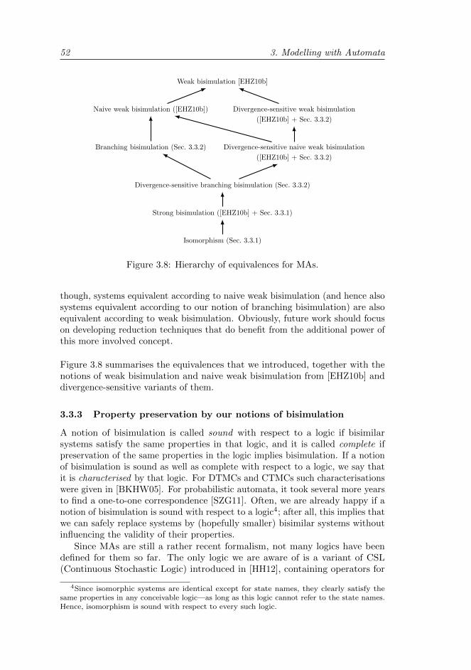
52 3. Modelling with Automata

Weak bisimulation [EHZ10b]

Naive weak bisimulation ([EHZ10b]) Divergence-sensitive weak bisimulation

([EHZ10b] + Sec. 3.3.2)

Branching bisimulation (Sec. 3.3.2) Divergence-sensitive naive weak bisimulation

([EHZ10b] + Sec. 3.3.2)

Divergence-sensitive branching bisimulation (Sec. 3.3.2)

Strong bisimulation ([EHZ10b] + Sec. 3.3.1)

Isomorphism (Sec. 3.3.1)

Figure 3.8: Hierarchy of equivalences for MAs.

though, systems equivalent according to naive weak bisimulation (and hence alsosystems equivalent according to our notion of branching bisimulation) are alsoequivalent according to weak bisimulation. Obviously, future work should focuson developing reduction techniques that do benefit from the additional power ofthis more involved concept.

Figure 3.8 summarises the equivalences that we introduced, together with thenotions of weak bisimulation and naive weak bisimulation from [EHZ10b] anddivergence-sensitive variants of them.

3.3.3 Property preservation by our notions of bisimulation

A notion of bisimulation is called sound with respect to a logic if bisimilarsystems satisfy the same properties in that logic, and it is called complete ifpreservation of the same properties in the logic implies bisimulation. If a notionof bisimulation is sound as well as complete with respect to a logic, we say thatit is characterised by that logic. For DTMCs and CTMCs such characterisationswere given in [BKHW05]. For probabilistic automata, it took several more yearsto find a one-to-one correspondence [SZG11]. Often, we are already happy if anotion of bisimulation is sound with respect to a logic4; after all, this implies thatwe can safely replace systems by (hopefully smaller) bisimilar systems withoutinfluencing the validity of their properties.

Since MAs are still a rather recent formalism, not many logics have beendefined for them so far. The only logic we are aware of is a variant of CSL(Continuous Stochastic Logic) introduced in [HH12], containing operators for

4Since isomorphic systems are identical except for state names, they clearly satisfy thesame properties in any conceivable logic—as long as this logic cannot refer to the state names.Hence, isomorphism is sound with respect to every such logic.

3.3. Isomorphism and bisimulation relations 53

unbounded and time-bounded reachability, but not dealing with expected timesor long-run averages as allowed by other variants of CSL for different mod-els [BHHZ11] (see Section 9.2.1 for an explanation of these types of properties).Additionally, there are no results yet on the relation between notions of bisim-ulation for MAs and the logic of [HH12]. Instead, the notions of bisimulationthat have been defined were motivated by the fact that they coincide with theircorresponding notions for PAs and IMCs in case an MA does not have any ratesor probabilities, respectively [EHZ10b]. Hence, in these cases there does exista logic that is preserved. We discuss the preservation of logical properties bystrong bisimulation and branching bisimulation, for the subclass of PAs as wellas for IMCs.

Strong bisimulation. In the degenerate case of an MA actually being an IMC,our notion of strong bisimulation coincides with the notion of strong bisimulationfor IMCs [HK09]. It is well-known that strongly bisimilar IMCs satisfy exactly thesame properties in the logic CSL, including time-bounded and unbounded reach-ability probabilities, expected reachability times and long-run averages [NK07].

When restricting to action-based probabilistic automata, our notion of strongbisimulation coincides with the notion of strong bisimulation from [SL95]. It wasshown there that systems that are equivalent according to this notion satisfyexactly the same properties in an action-based variant of PCTL (ProbabilisticComputation Tree Logic). Additionally, when restricting to a state-based setting,our notion is a strengthening of the strong bisimulation in [SZG11]. There, it wasshown that strongly bisimilar systems satisfy the same properties in state-basedPCTL∗ [BdA95].

Branching bisimulation. When restricting MAs to IMCs, we find that our notionof branching bisimulation almost coincides with the notion of weak bisimulationfor IMCs [HK09]—our notion being slightly more restrictive with the branchingrequirement. It was shown in [HK09] that this notion preserves maximal time-bounded reachability properties (i.e., the probability of reaching a certain setof goal states within a certain time bound, under the most optimal schedulermaximising this probability, remains invariant). As always, minimal probabilitiesare not preserved due to divergences. This problem was solved in [Her02] byrequiring bisimulation relations to be divergence sensitive, as later also usedin [SZG12] for MAs to deal with the indefinite ignoring of behaviour. Hence, ifwe restrict our notion of branching bisimulation to be applied in a divergence-sensitive manner, then we also preserve minimal reachability properties of IMCs.

When restricting to action-based probabilistic automata, our branching bi-simulation coincides with Segala’s notion. He showed that branching bisimulationpreserves all properties that can be expressed in the probabilistic temporal logicWPCTL (Weak Probabilistic Computation Tree Logic), provided that no infinitepath of τ -actions can be scheduled with non-zero probability [SL95]. Again, itis well-known that this limitation to systems without divergences can be liftedby introducing divergence sensitivity, as for instance used in [BDG06]. Whenrestricting to state-based probabilistic automata, our branching bisimulationcoincides with the notion of probabilistic visible bisimulation [Gro08] (except that

54 3. Modelling with Automata

we only require invisibility of transitions, whereas [Gro08] requires invisibility ofactions—i.e., they consider a transition invisible only if all transitions with thesame action label are invisible as well). In [Gro08], it was stated that systemsequivalent according to this notion preserve PCTL∗\X (PCTL∗ without the ‘next’

operator).All these logics that are preserved by weak or branching bisimulation are very

expressive, with the only limitation that a property cannot take into account theaction or state labelling in the next state. After all, trace lengths are cut back byomitting irrelevant internal transitions. However, many interesting properties canstill be specified without a next operator, such as time-bounded and unboundedreachability probabilities, expected reachability times and long-run averages.

We are mostly interested in time-bounded and unbounded reachability probabil-ities, expected times to reachability and long-run averages for MAs. Althoughnot yet published, Sergey Sazonov from RWTH Aachen University showed thatstrong bisimulation and branching bisimulation indeed preserve expected timesto reachability and long-run averages for MAs (in the absence of divergences).For unbounded reachability probabilities it follows easily from the fact thateach MA can be transformed into a PA by changing rates to probabilities.Since unbounded reachability probabilities in an MA correspond to reachabil-ity probabilities in such an associated PA, and since branching bisimilar MAsyield branching bisimilar PAs, the fact that branching bisimulation preservesreachability probabilities in PAs implies that it preserves unbounded reachabilityprobabilities in MAs. We conjecture that time-bounded reachability probabilitiesare preserved as well. For the subclass of IMCs it is a known result, and allour case studies confirm this conjecture also for MAs containing probabilities.It is additionally supported by the observation that our notion of branchingbisimulation is a strengthening of all notions of weak bisimulation for MAsintroduced thus far [EHZ10b, EHZ10a, DH11, SZG12].

3.4 Contributions

The main concepts concerning Markov automata, probabilistic automata andinteractive Markov chains are well-established in the field. Relevant citationswere already made throughout the section. Our presentation of these conceptswas inspired by the way Stoelinga rephrased Segala’s theory on probabilisticautomata [Sto02a].

The definition of branching bisimulation for MAs, introduced in Section 3.3,and the corresponding Propositions 3.32 and 3.33, are original work, as well asthe discussion in Section 3.3.3.

Part II

MAPA: Markov AutomataProcess Algebra

CHAPTER 4

Process Algebra for Markov Automata

“Whatever mathematical models are studied,I believe that process calculi provide an

essential perspective for the study.”

Robin Milner

While the models described in Chapter 3 are well-suited for formal

verification, they tend to be very large for any non-trivial system.Hence, it is rather inconvenient and error-prone to model a specification

directly as an MA or one of its subclasses. Instead, many specification languageshave been introduced to model systems on a much higher level—just like pro-gramming languages. Among the most prominent specification techniques inmodel checking are process algebras: formal languages to describe behaviour interms of actions, allowing compositional modelling using parallel composition.

Related work. No full-fledged process algebra for MAs existed thus far. Therewere already some modelling formalisms for probabilistic systems, but they oftensuffer from two major deficiencies:

Restricted treatment of data. The focus of probabilistic process algebras hasmainly been on understanding random phenomena and the interplaybetween randomness and nondeterminism. Data is mostly treated in arestricted manner: probabilistic process algebras typically only allow a ran-dom choice over a fixed distribution, and input languages for probabilisticmodel checkers such as the reactive module language of PRISM [KNP11] orthe probabilistic variant of Promela [BCG04] only support basic data types,but neither support more advanced data structures. To model realisticsystems, however, convenient means for data modelling are indispensable.In the non-probabilistic world, µCRL [GP95] and LOTOS NT [GS98] areable to handle advanced data structures.

State space explosion. In addition to the problem of a restricted treatmentof data, the state space explosion is always threatening the feasibilityof most model-based analysis techniques (including model checking).After all, although parameterised probabilistic choice is semantically well-defined [BDHK06], the incorporation of data yields a significant increaseof, or even an infinite, state space. However, current probabilistic min-imisation techniques are not well-suited to be applied in the presence

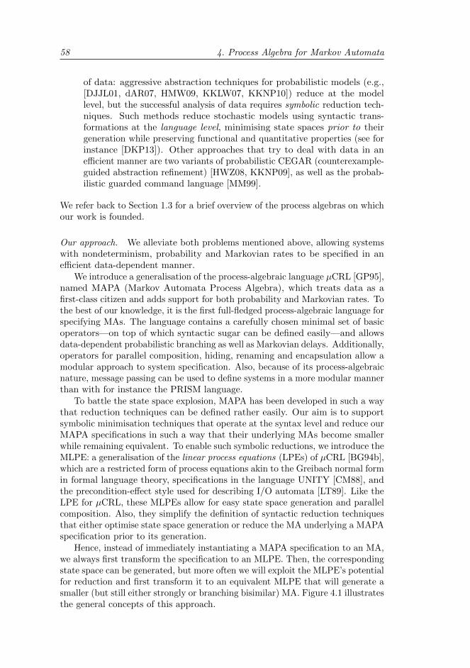
58 4. Process Algebra for Markov Automata

of data: aggressive abstraction techniques for probabilistic models (e.g.,[DJJL01, dAR07, HMW09, KKLW07, KKNP10]) reduce at the modellevel, but the successful analysis of data requires symbolic reduction tech-niques. Such methods reduce stochastic models using syntactic trans-formations at the language level, minimising state spaces prior to theirgeneration while preserving functional and quantitative properties (see forinstance [DKP13]). Other approaches that try to deal with data in anefficient manner are two variants of probabilistic CEGAR (counterexample-guided abstraction refinement) [HWZ08, KKNP09], as well as the probab-ilistic guarded command language [MM99].

We refer back to Section 1.3 for a brief overview of the process algebras on whichour work is founded.

Our approach. We alleviate both problems mentioned above, allowing systemswith nondeterminism, probability and Markovian rates to be specified in anefficient data-dependent manner.

We introduce a generalisation of the process-algebraic language µCRL [GP95],named MAPA (Markov Automata Process Algebra), which treats data as afirst-class citizen and adds support for both probability and Markovian rates. Tothe best of our knowledge, it is the first full-fledged process-algebraic language forspecifying MAs. The language contains a carefully chosen minimal set of basicoperators—on top of which syntactic sugar can be defined easily—and allowsdata-dependent probabilistic branching as well as Markovian delays. Additionally,operators for parallel composition, hiding, renaming and encapsulation allow amodular approach to system specification. Also, because of its process-algebraicnature, message passing can be used to define systems in a more modular mannerthan with for instance the PRISM language.

To battle the state space explosion, MAPA has been developed in such a waythat reduction techniques can be defined rather easily. Our aim is to supportsymbolic minimisation techniques that operate at the syntax level and reduce ourMAPA specifications in such a way that their underlying MAs become smallerwhile remaining equivalent. To enable such symbolic reductions, we introduce theMLPE: a generalisation of the linear process equations (LPEs) of µCRL [BG94b],which are a restricted form of process equations akin to the Greibach normal formin formal language theory, specifications in the language UNITY [CM88], andthe precondition-effect style used for describing I/O automata [LT89]. Like theLPE for µCRL, these MLPEs allow for easy state space generation and parallelcomposition. Also, they simplify the definition of syntactic reduction techniquesthat either optimise state space generation or reduce the MA underlying a MAPAspecification prior to its generation.

Hence, instead of immediately instantiating a MAPA specification to an MA,we always first transform the specification to an MLPE. Then, the correspondingstate space can be generated, but more often we will exploit the MLPE’s potentialfor reduction and first transform it to an equivalent MLPE that will generate asmaller (but still either strongly or branching bisimilar) MA. Figure 4.1 illustratesthe general concepts of this approach.

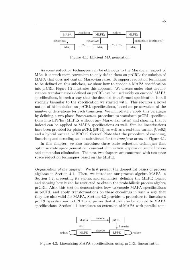
59

MAPA

MA0

MLPE1

MA1

MLPE2

MA2

instantiate

reducetransform

instantiate

≈s ≈s / ≈b

instantiate (optimised)

Figure 4.1: Efficient MA generation.

As some reduction techniques can be oblivious to the Markovian aspect ofMAs, it is much more convenient to only define them on prCRL: the subclass ofMAPA that does not contain Markovian rates. To support reduction techniquesto be defined on this subclass, we show how to encode a MAPA specificationinto prCRL. Figure 4.2 illustrates this approach. We discuss under what circum-stances transformations defined on prCRL can be used safely on encoded MAPAspecifications, in such a way that the decoded transformed specification is stillstrongly bisimilar to the specification we started with. This requires a novelnotion of bisimulation on prCRL specifications, based on preservation of thenumber of derivations for each transition. We immediately apply this paradigmby defining a two-phase linearisation procedure to transform prCRL specifica-tions into LPPEs (MLPEs without any Markovian rates) and showing that itindeed can be applied to MAPA specifications as well. Similar linearisationshave been provided for plain µCRL [BP95], as well as a real-time variant [Use02]and a hybrid variant [vdBRC06] thereof. Note that the procedure of encoding,linearising and decoding can be substituted for the transform arrow in Figure 4.1.

In this chapter, we also introduce three basic reduction techniques thatoptimise state space generation: constant elimination, expression simplificationand summation elimination. The next two chapters are concerned with two statespace reduction techniques based on the MLPE.

Organisation of the chapter. We first present the theoretical basics of processalgebras in Section 4.1. Then, we introduce our process algebra MAPA inSection 4.2, presenting its syntax and semantics, defining the MLPE formatand showing how it can be restricted to obtain the probabilistic process algebraprCRL. Also, this section demonstrates how to encode MAPA specificationsin prCRL and apply transformations on these encodings in such a way thatthey are also valid for MAPA. Section 4.3 provides a procedure to linearise aprCRL specification to LPPE and proves that it can also be applied to MAPAspecifications. Section 4.4 introduces an extension of MAPA with parallel com-

MAPA

MLPE

prCRL

LPPE

≈s

encode

linearise

decodereducereduce

Figure 4.2: Linearising MAPA specifications using prCRL linerarisation.

60 4. Process Algebra for Markov Automata

position, encapsulation, hiding and renaming, and shows how systems specifiedusing these constructs can be linearised as well. In Section 4.5 we exploit theMLPE format to define the three basic reduction techniques. Finally, Section 4.6concludes by summarising the contributions of this chapter.

Origins of the chapter. The results in this chapter on prCRL were first pub-lished in the proceedings of the 10th International Conference on Applicationof Concurrency to System Design (ACSD) [KvdPST10a] and a correspondingtechnical report [KvdPST10b]. Later, they were published more extensively inthe journal Theoretical Computer Science [KvdPST12]. The language MAPAwas introduced afterwards, in the proceedings of the 23rd International Con-ference on Concurrency Theory (CONCUR) [TKvdPS12a] and a correspondingtechnical report [TKvdPS12b].

4.1 Process algebras

Before discussing our process algebra for MAs, we give a brief introduction to thefield of process algebras. We based our concepts and notations on the treatmentin [Fok07], and refer to that work for a more detailed discussion.

Each process algebra basically consists of two parts: a definition of its syntax(the process terms that are allowed) and a definition of its semantics (themeaning of its syntactic elements in terms of automata). Together, these twoaspects combine to allow us to specify automata more efficiently by means ofprocess-algebraic descriptions. Often, additionally axioms are introduced tomore easily equate process terms that yield bisimilar automata. We are notconcerned with such axioms, since we will justify our reduction techniques definedon process-algebraic descriptions by proving that the underlying automata of anoriginal process term and its reduced variant are bisimilar.

4.1.1 Syntax: signatures and process terms

Process algebras are defined over a signature Σ = f, g, . . . , consisting of afinite set of operators. Each operator f is equipped with an arity , denoted byar(f), indicating its number of arguments. Operators with arity zero are oftencalled constants, and operators with arity two are called binary operators.

In addition to the signature, a countable set of variables V = x, y, z, . . . ,disjoint from Σ, is assumed. Based on a signature Σ and set of variables V ,process terms can be constructed. Basically, they consist of operators applied toas many arguments as prescribed by their arity.

Definition 4.1 (Process terms). Given a finite signature Σ and a countableset of variables V , process terms over Σ and V are constructed recursively asfollows:

• Any variable v ∈ V is a process term;• If f ∈ Σ and p1, p2, . . . , pn are process terms, with n = ar(f), then alsof(p1, p2, . . . , pn) is a process term.

4.1. Process algebras 61

A process term is said to be open if it contains at least one variable, and closedif it does not. Process terms containing binary operators, such as f(p1, p2), areoften written in infix notation, as in p1 f p2 or (p1 f p2). Constants in processterms are often written without parentheses, i.e., as f instead of f().

Note that this is a rather simple view on process algebra. It provides abasic and thorough framework for process algebras without any data, bindingoperators or recursion; our MAPA language does contain such more complicatedconstructs. Still, the current treatment provides a solid basis for understandingvarious concepts such as SOS rules and proof trees.

Example 4.2. We define the syntax of a very simple process algebra, based onCCS [Mil80]. It consists of one constant ∅ for the deadlock process, a binaryoperator + for alternative composition and two unary operators a· and b· foraction prefix.

Formally, the signature of our process algebra is Σ = ∅,+, a·, b·, withar(∅) = 0, ar(+) = 2 and ar(a·) = ar(b·) = 1. We assume a set of variablesV = x, x′, y, y′. Often, we just write an action name a to abbreviate a · ∅.

An infinite number of process terms can be constructed for this processalgebra, such as:

• a · ∅ (also written as a);

• +(a · ∅, b · ∅) (also written as a+ b);

• +(b · ∅, x) (also written as b+ x);

• +(a · (b · x),+(b, ∅)) (also written as (a · b · x) + (b+ ∅)).

The first two process terms are closed, whereas the last two are open.

To transform an open process term into a closed one, substitutions can beapplied. This entails renaming variables to (either closed or open) process terms.

Definition 4.3 (Substitutions). Given a signature Σ and a countable set Vof variables, a substitution is a list σ = [x1 := q1, . . . , xn := qn], where xi ∈ Vand qi is a process term for each 1 ≤ i ≤ n.

Given a process term p and a substitution σ = [x1 := q1, . . . , xn := qn], wedefine σ(p) inductively on the structure of p:

σ(x) =

qi if x = xi for some 1 ≤ i ≤ nx otherwise

σ(f(p1, . . . , pn)) = f(σ(p1), . . . , σ(pn))

for any variable x ∈ V , process terms p1, . . . , pn and operator f ∈ Σ. We liftthis to sets of process terms P in the obvious way: σ(P ) = σ(p) | p ∈ P.

Given two vectors x = (x1, . . . , xn) and q = (q1, . . . , qn), we write [x := q]as an abbreviation for the substitution σ = [x1 := q1, . . . , xn := qn].

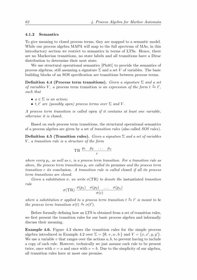
62 4. Process Algebra for Markov Automata

4.1.2 Semantics

To give meaning to closed process terms, they are mapped to a semantic model.While our process algebra MAPA will map to the full spectrum of MAs, in thisintroductory section we restrict to semantics in terms of LTSs. Hence, thereare no Markovian transitions, no state labels and all transitions have a Diracdistribution to determine their next state.

We use structural operational semantics [Plo81] to provide the semantics ofprocess algebras, still assuming a signature Σ and a set V of variables. The basicbuilding blocks of an SOS specification are transitions between process terms.

Definition 4.4 (Process term transitions). Given a signature Σ and a setof variables V , a process term transition is an expression of the form t −a→ t′,such that

• a ∈ Σ is an action;• t, t′ are (possibly open) process terms over Σ and V .

A process term transition is called open if it contains at least one variable,otherwise it is closed.

Based on such process term transitions, the structural operational semanticsof a process algebra are given by a set of transition rules (also called SOS rules).

Definition 4.5 (Transition rules). Given a signature Σ and a set of variablesV , a transition rule is a structure of the form

TRp1 p2 . . . pn

c

where every pi, as well as c, is a process term transition. For a transition rule asabove, the process term transitions pi are called its premises and the process termtransition c its conclusion. A transition rule is called closed if all its processterm transitions are closed.

Given a substitution σ, we write σ(TR) to denote the instantiated transitionrule

σ(TR)σ(p1) σ(p2) . . . σ(pn)

σ(c)

where a substitution σ applied to a process term transition t −a→ t′ is meant to bethe process term transition σ(t) −a→ σ(t′).

Before formally defining how an LTS is obtained from a set of transition rules,we first present the transition rules for our basic process algebra and informallydiscuss their meaning.

Example 4.6. Figure 4.3 shows the transition rules for the simple processalgebra introduced in Example 4.2 over Σ = ∅,+, a·, b· and V = x, x′, y, y′.We use a variable v that ranges over the actions a, b, to prevent having to includea copy of each rule. However, technically we just assume each rule to be presenttwice, once with v = a and once with v = b. Due to the simplicity of our algebra,all transition rules have at most one premise.

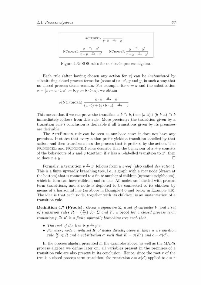
4.1. Process algebras 63

ActPrefixv · x −v−→ x

NChoiceLx −v−→ x′

x+ y −v−→ x′NChoiceR

y −v−→ y′

x+ y −v−→ y′

Figure 4.3: SOS rules for our basic process algebra.

Each rule (after having chosen any action for v) can be instantiated bysubstituting closed process terms for (some of) x, x′, y and y, in such a way thatno closed process terms remain. For example, for v = a and the substitutionσ = [x := a · b, x′ := b, y := b · b · a], we obtain

σ(NChoiceL)a · b −a−→ b

(a · b) + (b · b · a) −a−→ b

This means that if we can prove the transition a ·b −a→ b, then (a ·b)+(b ·b ·a) −a→ bimmediately follows from this rule. More precisely: the transition given by atransition rule’s conclusion is derivable if all transitions given by its premisesare derivable.

The ActPrefix rule can be seen as our base case: it does not have anypremises. It states that every action prefix yields a transition labelled by thataction, and then transforms into the process that is prefixed by the action. TheNChoiceL and NChoiceR rules describe that the behaviour of x+ y consistsof the behaviours of x and y together: if x has a v-labelled transition to x′, thenso does x+ y.

Formally, a transition p −v→ p′ follows from a proof (also called derivation).This is a finite upwardly branching tree, i.e., a graph with a root node (drawn atthe bottom) that is connected to a finite number of children (upwards neighbours),which in turn can have children, and so one. All nodes are labelled with processterm transitions, and a node is depicted to be connected to its children bymeans of a horizontal line (as above in Example 4.6 and below in Example 4.8).The idea is that each node, together with its children, is an instantiation of atransition rule.

Definition 4.7 (Proofs). Given a signature Σ, a set of variables V and a setof transition rules R = Pici for Σ and V , a proof for a closed process term

transition p −a→ p′ is a finite upwardly branching tree such that

• The root of the tree is p −a→ p′;• For every node c, with set K of nodes directly above it, there is a transition

rule K′

c′ ∈ R and a substitution σ such that K = σ(K ′) and c = σ(c′).

In the process algebra presented in the examples above, as well as the MAPAprocess algebra we define later on, all variables present in the premises of atransition rule are also present in its conclusion. Hence, since the root r of thetree is a closed process term transition, the restriction c = σ(c′) applied to c = r

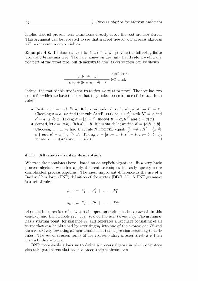
64 4. Process Algebra for Markov Automata

implies that all process term transitions directly above the root are also closed.This argument can be repeated to see that a proof tree for our process algebraswill never contain any variables.

Example 4.8. To show (a · b) + (b · b · a) −a→ b, we provide the following finiteupwardly branching tree. The rule names on the right-hand side are officiallynot part of the proof tree, but demonstrate how its correctness can be shown.

a · b −a→ b

(a · b) + (b · b · a) −a→ bNChoiceL

ActPrefix

Indeed, the root of this tree is the transition we want to prove. The tree has twonodes for which we have to show that they indeed arise for one of the transitionrules:

• First, let c = a · b −a→ b. It has no nodes directly above it, so K = ∅.Choosing v = a, we find that rule ActPrefix equals K′

c′ with K ′ = ∅ and

c′ = a · x −a→ x. Taking σ = [x := b], indeed K = σ(K ′) and c = σ(c′).

• Second, let c = (a·b)+(b·b·a) −a→ b. It has one child; we find K = a·b −a→ b.Choosing v = a, we find that rule NChoiceL equals K′

c′ with K ′ = x −a→x′ and c′ = x + y −a→ x′. Taking σ = [x := a · b, x′ := b, y := b · b · a],indeed K = σ(K ′) and c = σ(c′).

4.1.3 Alternative syntax descriptions

Whereas the notations above—based on an explicit signature—fit a very basicprocess algebra, we often apply different techniques to easily specify morecomplicated process algebras. The most important difference is the use of aBackus-Naur form (BNF) definition of the syntax [BBG+63]. A BNF grammaris a set of rules

p1 ::= P 11 | P 2

1 | . . . | P k11

. . .

pn ::= P 1n | P 2

n | . . . | P knn

where each expression P ij may contain operators (often called terminals in thiscontext) and the symbols p1, . . . , pn (called the non-terminals). The grammarhas a starting point, for instance p1, and generates a language consisting of allterms that can be obtained by rewriting p1 into one of the expressions P i1 andthen recursively rewriting all non-terminals in this expression according to theirrules. The set of process terms of the corresponding process algebra is thenprecisely this language.

BNF more easily allows us to define a process algebra in which operatorsalso take parameters that are not process terms themselves.

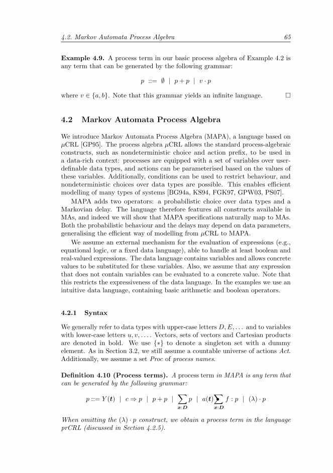
4.2. Markov Automata Process Algebra 65

Example 4.9. A process term in our basic process algebra of Example 4.2 isany term that can be generated by the following grammar:

p ::= ∅ | p+ p | v · p

where v ∈ a, b. Note that this grammar yields an infinite language.

4.2 Markov Automata Process Algebra

We introduce Markov Automata Process Algebra (MAPA), a language based onµCRL [GP95]. The process algebra µCRL allows the standard process-algebraicconstructs, such as nondeterministic choice and action prefix, to be used ina data-rich context: processes are equipped with a set of variables over user-definable data types, and actions can be parameterised based on the values ofthese variables. Additionally, conditions can be used to restrict behaviour, andnondeterministic choices over data types are possible. This enables efficientmodelling of many types of systems [BG94a, KS94, FGK97, GPW03, PS07].

MAPA adds two operators: a probabilistic choice over data types and aMarkovian delay. The language therefore features all constructs available inMAs, and indeed we will show that MAPA specifications naturally map to MAs.Both the probabilistic behaviour and the delays may depend on data parameters,generalising the efficient way of modelling from µCRL to MAPA.

We assume an external mechanism for the evaluation of expressions (e.g.,equational logic, or a fixed data language), able to handle at least boolean andreal-valued expressions. The data language contains variables and allows concretevalues to be substituted for these variables. Also, we assume that any expressionthat does not contain variables can be evaluated to a concrete value. Note thatthis restricts the expressiveness of the data language. In the examples we use anintuitive data language, containing basic arithmetic and boolean operators.

4.2.1 Syntax

We generally refer to data types with upper-case letters D,E, . . . and to variableswith lower-case letters u, v, . . . . Vectors, sets of vectors and Cartesian productsare denoted in bold. We use ∗ to denote a singleton set with a dummyelement. As in Section 3.2, we still assume a countable universe of actions Act.Additionally, we assume a set Proc of process names.

Definition 4.10 (Process terms). A process term in MAPA is any term thatcan be generated by the following grammar:

p ::= Y (t) | c⇒ p | p+ p |∑x:D

p | a(t)∑•x:D

f : p | (λ) · p

When omitting the (λ) · p construct, we obtain a process term in the languageprCRL (discussed in Section 4.2.5).

66 4. Process Algebra for Markov Automata

Here, Y ∈ Proc is a process name, t a vector of data expressions, c a booleanexpression, x a vector of variables ranging over a countable1 type D, a ∈ Acta (parameterised) atomic action, f a real-valued expression yielding values in[0, 1], and λ an expression yielding positive real numbers (rates). All expressionsare allowed to contain variables—although later we will put some restrictionson them, requiring each data variable to either be a process variable or to bebound by a nondeterministic or probabilistic choice operator.

We write p = p′ only for syntactically identical process terms, not to relateprocess terms with identical meaning but different syntax.

Remark 4.11. Not all possible process terms have meaning. Since this dependson their context, we defer this issue to Section 4.2.2, where we specify severalwell-formedness criteria.

Given an expression t, a process term p, a vector of variable names x =(x1, . . . , xn) and a vector of closed data expressions d = (d1, . . . , dn), we uset[x := d] to denote the result of simultaneously substituting every xi in tby di, and p[x := d] for the result of applying this to every expression in p(only substituting each xi by di in expressions in p that do not occur within aconstruct

∑x:D or

∑•

x:D such that xi is an element of x (not considering thecontext of p)).

Example 4.12. The grammar above provides the MAPA language with aninfinite number of process terms. One of these is∑

n:Nn < 3⇒ (2 · n+ 1) · send(n)

∑•

x:1,2

x

3: (Y (n+ x) + Z(n+ x))

For the expression t = x3 we find t[x := 2] = 2

3 , and for the process termp′ = Y (x) + Z(x) we find p′[x := 2] = Y (2) + Z(2).

Note that two of our operators (∑

and∑• ) range over vectors of data

parameters. If a vector x is indeed nontrivial (i.e., it has more than oneelement), then its accompanying data type D is a Cartesian product. This isthe case in the following process term:∑

(m,i):m1,m2×1,2,3

send(m, i) · Y ()

To make it easier to understand the rest of this section, we already give avery informal idea of the meaning of the operators. In Section 4.2.3 we will gointo more details, after having completed our discussion on the syntax.

In a process term, Y (t) denotes process instantiation, where t instantiatesY ’s process variables as defined below. The term c ⇒ p behaves as p if thecondition c holds, and cannot do anything otherwise. The + operator denotesnondeterministic choice, and

∑x:D p a (possibly infinite) nondeterministic choice

over data type D. The term a(t)∑•

x:D f : p performs the action a(t) and then

1Although uncountable choice may be well-defined process-algebraically, this would notwork out for us as we want to provide semantics in terms of MAs.

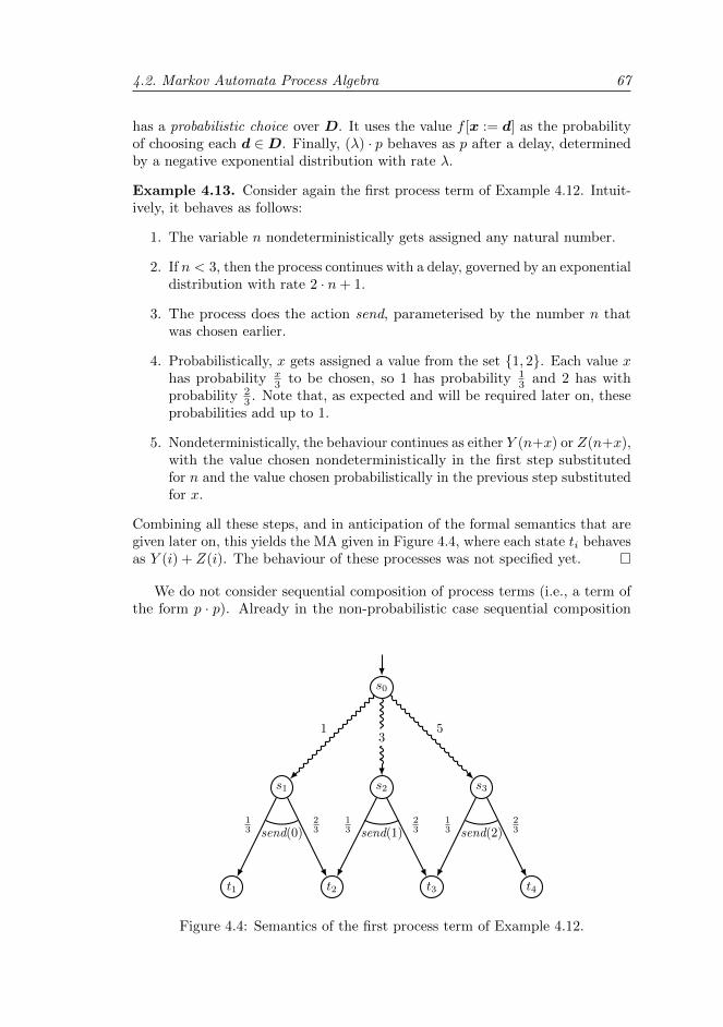
4.2. Markov Automata Process Algebra 67

has a probabilistic choice over D. It uses the value f [x := d] as the probabilityof choosing each d ∈D. Finally, (λ) · p behaves as p after a delay, determinedby a negative exponential distribution with rate λ.

Example 4.13. Consider again the first process term of Example 4.12. Intuit-ively, it behaves as follows:

1. The variable n nondeterministically gets assigned any natural number.

2. If n < 3, then the process continues with a delay, governed by an exponentialdistribution with rate 2 · n+ 1.

3. The process does the action send, parameterised by the number n thatwas chosen earlier.

4. Probabilistically, x gets assigned a value from the set 1, 2. Each value xhas probability x

3 to be chosen, so 1 has probability 13 and 2 has with

probability 23 . Note that, as expected and will be required later on, these

probabilities add up to 1.

5. Nondeterministically, the behaviour continues as either Y (n+x) or Z(n+x),with the value chosen nondeterministically in the first step substitutedfor n and the value chosen probabilistically in the previous step substitutedfor x.

Combining all these steps, and in anticipation of the formal semantics that aregiven later on, this yields the MA given in Figure 4.4, where each state ti behavesas Y (i) + Z(i). The behaviour of these processes was not specified yet.

We do not consider sequential composition of process terms (i.e., a term ofthe form p · p). Already in the non-probabilistic case sequential composition

s0

s2s1 s3

t2t1 t3 t4

31 5

13

23

13

23

13

23send(0) send(1) send(2)

Figure 4.4: Semantics of the first process term of Example 4.12.

68 4. Process Algebra for Markov Automata

significantly increases the difficulty of linearisation (especially when using recur-sion) [Use02]. Therefore, it would distract from our main purpose: combiningprobabilities and Markovian rates with data. Moreover, many specificationscan easily be written without sequential composition (as long as action prefix ispresent). Actually, [Use02] even showed that all sequential composition can beencoded by means of data.

We now formally introduce MAPA specifications. They consist of a set ofprocess equations (defining behaviour for processes that can again be instantiatedby other processes) and an initial process.

Definition 4.14 (Specifications). A MAPA specification is given by a tupleM = (Xi(xi : Di) = pi, Xj(t)) consisting of a finite set of uniquely-namedprocesses Xi, each defined by a process equation Xi(xi : Di) = pi, and an initialprocess Xj(t) with t a vector of closed data expressions. Here, xi is a vector ofprocess variables2 with type Di, and pi (the right-hand side) is a process termspecifying the behaviour of Xi.

A variable v in an expression in a right-hand side pi is bound if it is anelement of xi or it occurs within a construct

∑x:D or

∑•

x:D such that v is anelement of x. Variables that are not bound are said to be free.

We generally refer to process terms with lower-case letters p, q, r, and toprocesses with capitals X,Y, Z. Also, we write X(x1 : D1, . . . , xn : Dn) instead ofX((x1, . . . , xn) : (D1×· · ·×Dn)). Finally, for brevity we often abuse notation byinterpreting a single process equation as a specification (additionally mentioningthe initial state if this is not clear from the context).

Example 4.15. The first process term introduced in Example 4.12 can be madeinto a proper MAPA specification by using it as a right-hand side of a process,adding behaviour for the processes Y and Z, and specifying an initial state.Hence, we obtain for instance the specification M = (Procs, X), where Procs isthe set of process equations

X =∑n:N

n < 3⇒ (2 · n+ 1) · send(n)∑•

x:1,2

x

3: (Y (n+ x) + Z(n+ x))

Y (y : N) = beep(y)∑•

x:1

1 : Y (y)

Z(z : N) = ring(z)∑•

x:1

1 : Z(z)

Syntactic sugar. For notational ease, we define some syntactic sugar. First,given a process name X and an action a, we write X instead of X() and a insteadof a(). Second, given a process p and a (possibly parameterised) action a(t), wewrite a(t) · p as an abbreviation for the process term a(t)

∑•x:1 1 : p, where x is

2Note that we use the term process variables to denote data variables within a process (likea class variable is a variable within a class in object-oriented programming), not to denotevariables referencing processes.

4.2. Markov Automata Process Algebra 69

a fresh variable, not occurring freely in p. Third, for finite probabilistic sums weintroduce the notation

a(t)(u1 : p1 ⊕ u2 : p2 ⊕ · · · ⊕ un : pn)

for the process term that executes the action a(t) and then behaves as processterm pi with probability ui. This could be modelled in MAPA as the processterm a(t)

∑•x:1,...,n f : p, where x is chosen such that it does not occur freely

in any pi, the probability expression f is such that f [x := i] = ui for every1 ≤ i ≤ n, and p is given by (x = 1⇒ p1) + (x = 2⇒ p2) + · · ·+ (x = n⇒ pn).

4.2.2 Static semantics

Not all syntactically correct MAPA specifications are meaningful. The follow-ing definition formulates additional well-formedness conditions. The first twoconstraints ensure that a specification does not refer to undefined variablesor processes, the third is needed to obtain valid probability distributions, andthe fourth ensures that the specification has a unique solution (modulo strongprobabilistic bisimulation).

Additionally, all outgoing rates should be finite. This requirement is discussedin Remark 4.28, after providing the operational semantics and MLPE format—it is not easily defined statically, since it cannot be checked locally due toMarkovian delays possibly being nested within several nondeterministic choicesand conditions and hence depending on the operational semantics of theseoperators.

To define well-formedness, we require the concept of unguardedness. Wesay that a process term Y (t) can go unguarded to Y . Moreover, c⇒ p can gounguarded to Y if p can, p+ q if either p or q can, and

∑x:D p if p can, whereas

a(t)∑•

x:D f : p and (λ) · p cannot go unguarded anywhere.

Definition 4.16 (Well-formedness). A MAPA specification

M = (Xi(xi : Di) = pi, Xj(t))

is well-formed if the following four constraints are all satisfied:

1. None of the right-hand sides pi contains a free variable.

2. There are no instantiations to undefined processes. That is, for everyinstantiation Y (t′) occurring in some right-hand side pi, there exists aprocess equation (Xk(xk : Dk) = pk) such that Xk = Y and t′ is oftype Dk. Also, the vector t used in the initial process is of type Dj .

3. The probabilistic choices are well-defined. That is, for every constructa(t)

∑•

x:D f : p occurring in a right-hand side pi we have∑d∈D

f [x := d] = 1

70 4. Process Algebra for Markov Automata

for every possible valuation of the free variables in f [x := d] (the summationnow used in the mathematical sense)3.

4. There is no unguarded recursion4. That is, for every process Y , there is nosequence of processes X1, X2, . . . , Xn (with n ≥ 2) such that Y = X1 = Xn

and pj can go unguarded to Xj+1 for every 1 ≤ j < n.

We assume from now on that every MAPA specification is well-formed.

Note that the first two and the last requirement are easily checked statically.The third requirement is undecidable in general, but could of course simply bechecked on-the-fly during state space generation.

Example 4.17. As an example of a well-formed MAPA specification, we con-sider a system that first writes the number 1, and then continuously writesnatural numbers (excluding zero) in such a way that the probability of writ-ing n is each time given by 1

2n . This system can be modelled by the MAPAspecification M = (X, X(1)), where X is given by

X(n : N+) = write(n)∑•

m:N+

12m : X(m)

We demonstrate that all four well-formedness rules are satisfied:

1. The right-hand side contains two variables: n and m. The variable n isbound since it is a process variable of X. The variable m is bound since itonly occurs within the construct

∑•m:N+ .

2. There is one process instantiation: X(m). Indeed, there is a processequation for this process, namely X(n : N+) = . . . , and m is of type N+.Also, the initial parameter value 1 is of type N+, as required.

3. There is one probabilistic choice in the specification:∑•m:N+

12m . Indeed,∑

d∈N+

12m [m := d] =

∑d∈N+

12d

= 1

where the last step is well-known in mathematics since it concerns thegeometric series.

4. There is one process: X. The only way for this process to yield unguardedrecursion, would be to go unguarded to itself. However, X always startswith an action, and hence cannot go anywhere unguarded.

Note that the data types in MAPA specifications can be countably infinite.Also, probabilistic choices over countably infinite domains are allowed. Hence,countably infinite branching may occur, as long as no infinite exit rates arepresent. Since this is a semantic well-formedness rule, we will come back toit in Remark 4.28.

3We could be slightly more liberal, only requiring this for all reachable valuations of thefree variables in f [x := d].

4This constraint could be relaxed a bit, as contradictory conditions of the processes maymake an unguarded cycle harmless.

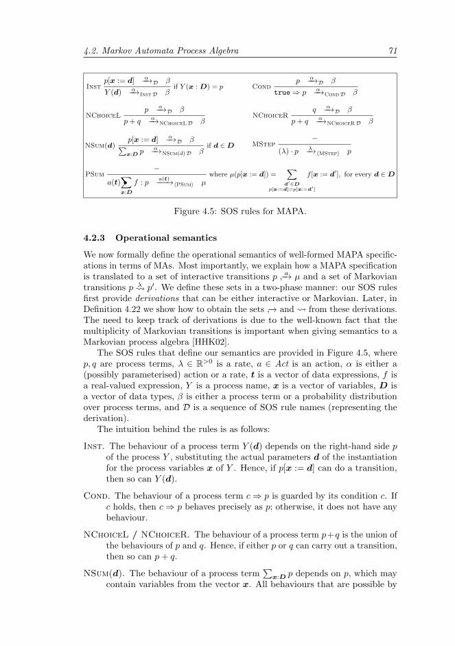
4.2. Markov Automata Process Algebra 71

Instp[x := d] −α−→D β

Y (d) −α−→InstD βif Y (x : D) = p Cond

p −α−→D β

true⇒ p −α−→CondD β

NChoiceLp −α−→D β

p+ q −α−→NChoiceLD βNChoiceR

q −α−→D β

p+ q −α−→NChoiceRD β

NSum(d)p[x := d] −α−→D β∑x:D p −α−→NSum(d)D β

if d ∈ D MStep−

(λ) · p −λ−→〈MStep〉 p

PSum−

a(t)∑•x:D

f : p −a(t)−−→〈PSum〉 µwhere µ(p[x := d]) =

∑d′∈D

p[x:=d]=p[x:=d′]

f [x := d′], for every d ∈ D

Figure 4.5: SOS rules for MAPA.

4.2.3 Operational semantics

We now formally define the operational semantics of well-formed MAPA specific-ations in terms of MAs. Most importantly, we explain how a MAPA specificationis translated to a set of interactive transitions p a−→ µ and a set of Markoviantransitions p λ p′. We define these sets in a two-phase manner: our SOS rulesfirst provide derivations that can be either interactive or Markovian. Later, inDefinition 4.22 we show how to obtain the sets −→ and from these derivations.The need to keep track of derivations is due to the well-known fact that themultiplicity of Markovian transitions is important when giving semantics to aMarkovian process algebra [HHK02].

The SOS rules that define our semantics are provided in Figure 4.5, wherep, q are process terms, λ ∈ R>0 is a rate, a ∈ Act is an action, α is either a(possibly parameterised) action or a rate, t is a vector of data expressions, f isa real-valued expression, Y is a process name, x is a vector of variables, D isa vector of data types, β is either a process term or a probability distributionover process terms, and D is a sequence of SOS rule names (representing thederivation).

The intuition behind the rules is as follows:

Inst. The behaviour of a process term Y (d) depends on the right-hand side pof the process Y , substituting the actual parameters d of the instantiationfor the process variables x of Y . Hence, if p[x := d] can do a transition,then so can Y (d).

Cond. The behaviour of a process term c⇒ p is guarded by its condition c. Ifc holds, then c⇒ p behaves precisely as p; otherwise, it does not have anybehaviour.

NChoiceL / NChoiceR. The behaviour of a process term p+q is the union ofthe behaviours of p and q. Hence, if either p or q can carry out a transition,then so can p+ q.

NSum(d). The behaviour of a process term∑

x:D p depends on p, which maycontain variables from the vector x. All behaviours that are possible by

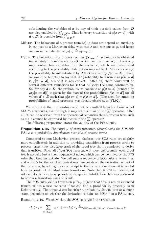
72 4. Process Algebra for Markov Automata

substituting the variables of x by any of their possible values from Dare also enabled by

∑x:D p. That is, every transition of p[x := d], with

d ∈D, is possible from∑

x:D p.

MStep. The behaviour of a process term (λ) · p does not depend on anything.It can just do a Markovian delay with rate λ and continue as p, and hence

we can immediate derive (λ) · p −λ→〈MStep〉 p.

PSum. The behaviour of a process term a(t)∑•

x:D f : p can also be obtainedimmediately. It can execute its a(t) action, and continue as p. However, pmay contain free variables from the vector x, which are instantiatedaccording to the probability distribution implied by f . More concretely:the probability to instantiate x by d ∈ D is given by f [x := d]. Hence,we would be tempted to say that the probability to continue as p[x := d]is f [x := d], but that is not correct. After all, there could well beseveral different valuations for x that all yield the same continuation.So, for any d ∈ D, the probability to continue as p[x := d] (denoted byµ(p[x := d])) is given by the sum of the probabilities f [x := d′] for allvalues d′ ∈ D such that p[x := d] = p[x := d′]. (The need for summingprobabilities of equal processes was already observed in [YL92].)

We note that the + operator could not be omitted from the basic set ofMAPA constructs, even though it may seem similar to the

∑operator. After

all, it can be observed from the operational semantics that a process term suchas a+ b cannot be expressed by means of the

∑operator.

The following proposition states the validity of the PSum rule.

Proposition 4.18. The target µ of every transition derived using the SOS-rulePSum is a probability distribution over closed process terms.

Compared to non-Markovian process algebras, our SOS rules are slightlymore complicated: in addition to providing transitions from process terms toprocess terms, they also keep track of the proof tree that is employed to derivethat transition. Since all of our SOS rules have at most one premise, each prooftree is actually just a linear sequence of nodes, which can be identified by the SOSrules that they instantiate. We call such a sequence of SOS rules a derivation,and write ∆ for the set of all derivations. We construct the derivation as part ofthe transition, by adding it as a subscript to the transition relation—it is neededlater to construct the Markovian transitions. Note that NSum is instantiatedwith a data element to keep track of the specific substitution that was performedto obtain a transition using this rule.

The SOS rules yield a transition p −α→D β (note that this is not an extendedtransition but a new concept) if we can find a proof for it, precisely as inDefinition 4.7. The target β can be either a probability distribution or a singlestate, depending on whether the derivation contains an MStep or a PSum rule.

Example 4.19. We show that the SOS rules yield the transition

(λ1) · q +∑

n:1,2,3

n < 3⇒ (λ2) · q −λ2−→〈NChoiceR,NSum(1),Cond,MStep〉 q

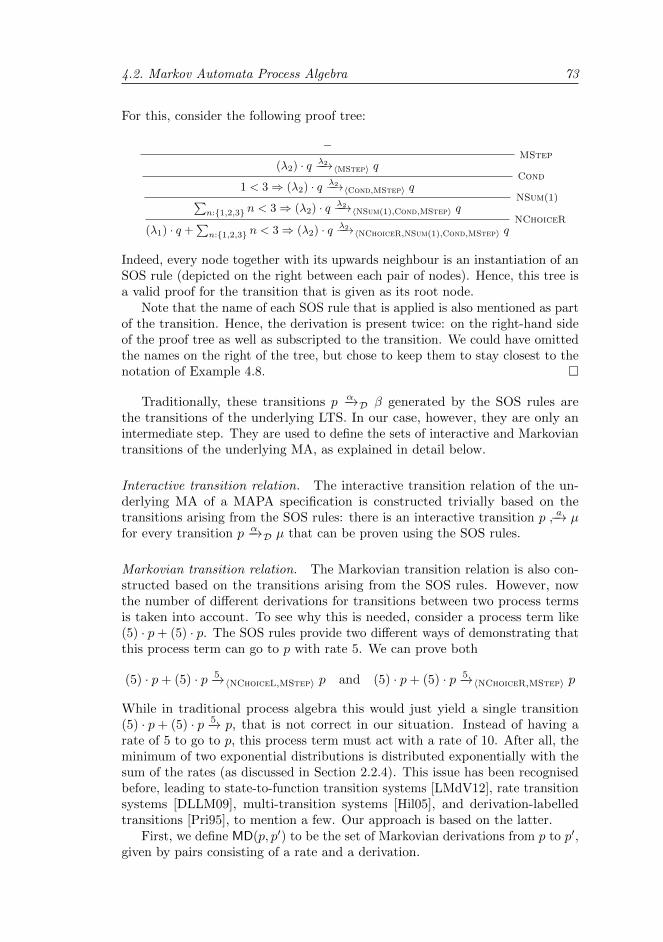
4.2. Markov Automata Process Algebra 73

For this, consider the following proof tree:

−(λ2) · q −λ2−→〈MStep〉 q

1 < 3⇒ (λ2) · q −λ2−→〈Cond,MStep〉 q∑n:1,2,3 n < 3⇒ (λ2) · q −λ2−→〈NSum(1),Cond,MStep〉 q

(λ1) · q +∑n:1,2,3 n < 3⇒ (λ2) · q −λ2−→〈NChoiceR,NSum(1),Cond,MStep〉 q

NChoiceR

NSum(1)

Cond

MStep

Indeed, every node together with its upwards neighbour is an instantiation of anSOS rule (depicted on the right between each pair of nodes). Hence, this tree isa valid proof for the transition that is given as its root node.

Note that the name of each SOS rule that is applied is also mentioned as partof the transition. Hence, the derivation is present twice: on the right-hand sideof the proof tree as well as subscripted to the transition. We could have omittedthe names on the right of the tree, but chose to keep them to stay closest to thenotation of Example 4.8.

Traditionally, these transitions p −α→D β generated by the SOS rules arethe transitions of the underlying LTS. In our case, however, they are only anintermediate step. They are used to define the sets of interactive and Markoviantransitions of the underlying MA, as explained in detail below.

Interactive transition relation. The interactive transition relation of the un-derlying MA of a MAPA specification is constructed trivially based on thetransitions arising from the SOS rules: there is an interactive transition p a−→ µfor every transition p −α→D µ that can be proven using the SOS rules.

Markovian transition relation. The Markovian transition relation is also con-structed based on the transitions arising from the SOS rules. However, nowthe number of different derivations for transitions between two process termsis taken into account. To see why this is needed, consider a process term like(5) · p+ (5) · p. The SOS rules provide two different ways of demonstrating thatthis process term can go to p with rate 5. We can prove both

(5) · p+ (5) · p −5→〈NChoiceL,MStep〉 p and (5) · p+ (5) · p −5→〈NChoiceR,MStep〉 p

While in traditional process algebra this would just yield a single transition(5) · p+ (5) · p −5→ p, that is not correct in our situation. Instead of having arate of 5 to go to p, this process term must act with a rate of 10. After all, theminimum of two exponential distributions is distributed exponentially with thesum of the rates (as discussed in Section 2.2.4). This issue has been recognisedbefore, leading to state-to-function transition systems [LMdV12], rate transitionsystems [DLLM09], multi-transition systems [Hil05], and derivation-labelledtransitions [Pri95], to mention a few. Our approach is based on the latter.

First, we define MD(p, p′) to be the set of Markovian derivations from p to p′,given by pairs consisting of a rate and a derivation.

74 4. Process Algebra for Markov Automata

Definition 4.20 (Derivations). Given two process terms p, p′, we define

MD(p, p′) = (λ,D) ∈ R>0 ×∆ | p −λ→D p′

to be the set of pairs (λ,D) such that there is a transition p −λ→D p′ that can beproven by our SOS rules.

Example 4.21. Consider again the process term

p = (λ1) · q +∑

n:1,2,3

n < 3⇒ (λ2) · q

In Example 4.19 we already showed that p −λ2−→D q, with

D = 〈NChoiceR,NSum(1),Cond,MStep〉

In the same way, we can find one other derivation D′ with rate λ2 using NSum(2),

and finally p −λ1−→D′′ q with D′′ = 〈NChoiceL,MStep〉. Since these are the onlyMarkovian derivations from p to q, we find

MD(p, q) = (λ2,D), (λ2,D′), (λ1,D′′)

Now, the total rate from a process term p to a process term q can easily beobtained by summing all rates in MD(p, q).

Based on the observations above, we now formally define the operational se-mantics of a well-formed MAPA specification.

Definition 4.22 (Operational semantics). The semantics of a MAPA spe-cification

M = (Xi(xi : Di) = pi, Xj(t))

is an MA M = 〈S, s0, A, −→, ,AP, L〉, where

• s0 = Xj(t);• −→ is the smallest relation such that p α−→ µ if there exists a D ∈ ∆ for

which p −α→D µ holds;• is the smallest relation such that p λ p′ if MD(p, p′) 6= ∅ and

λ =∑

(λ′,D)∈MD(p,p′)

λ′

• L(s) = a ∈ A \ τ | ∃s′ ∈ S . s a−→ s′,

and S, A and AP are the smallest sets such that s0, −→ and are well-defined.

Note that we cannot give S explicitly based on a specification, as its reachablestates cannot be determined statically. Therefore, also the set of actions Aand hence the set of atomic propositions AP can only be constructed by firstcomputing the reachable state space.

4.2. Markov Automata Process Algebra 75

Also note that we may obtain infinite rates, if the MAPA specification is notconstructed carefully. We discuss in Remark 4.28 how to check for this.

Remark 4.23. We chose the state labelling in such a way that each state is la-belled by the set of actions that it enables. This may seem restrictive, since duringmodel checking we may also be interested in the values of some of the global vari-ables. However, we will see in Section 4.2.4 that any condition over the global vari-ables can easily be encoded by the enabledness of an action (see Remark 4.29).

Note that this implies that none of the proofs showing strong bisimulation forMAPA need to be concerned with the state labelling. After all, since (s, t) ∈ Rimplies that all transitions from s can be mimicked by t and vice versa, clearly sand t enable the same actions and hence L(s) = L(t).

Example 4.24. Continuing with Example 4.21, we find that there is a transitionfrom p to q with rate λ = λ1 + 2λ2.

Equivalent MAPA specifications. Given a MAPA specification M and its under-lying MAM, two process terms in M are isomorphic if their corresponding statesin M are isomorphic. Two specifications with underlying MAs M1,M2 areisomorphic ifM1 is isomorphic toM2. Bisimilar process terms and specificationsare defined in the same way.

Associativity of nondeterministic sums. It can easily be seen from our opera-tional semantics that nondeterministic sums are associative, i.e., (p+ q) + r andp+ (q + r) yield the same transitions. The derivations differ, having for instance〈NChoiceR,NChoiceL〉 instead of 〈NChoiceL,NChoiceR〉 for choosing q,but the resulting MAs will not be any different as the number of derivations doesnot change. Hence, instead of writing 〈NChoiceL,NChoiceR〉 for choosing qin (p+ q) + r, we could also omit the parentheses and write 〈NChoice(2)〉 forchoosing q in p+ q+ r. So, we will often just write p+ q+ r without parentheses.

Congruences. Although not specifically needed for the results in this work, itcan be shown that strong bisimulation is a congruence for all MAPA operators,along the same lines as the proof of Proposition 4.35. Just like weak bisimulationis not a congruence for IML [Her02], branching bisimulation is not a congruencefor MAPA. After all, while a · p ≈b τ · a · p, we have a · p+λ · p 6≈b τ · a · p+λ · p.We leave it for future work to consider weak congruences for MAPA (as alreadysuggested in [EHZ10b]).

4.2.4 Markovian Linear Process Equations

In the non-probabilistic setting, a restricted version of µCRL is captured bythe LPE format [BG94b]. It is well-suited for formal manipulation, state spacegeneration and parallel composition. In the purely functional setting of LTSs,LPEs provided a uniform and simple format for the data-rich process algebraµCRL. As a consequence of this simplicity, the LPE format was essential fortheory development and tool construction. It led to elegant proof methods, like

76 4. Process Algebra for Markov Automata

the use of invariants for process algebra [BG94b], and the cones and foci methodfor proof checking process equivalence [GS01, FPvdP06]. It also enabled theapplication of model checking techniques to process algebra, such as optimisationsfrom static analysis [GL01] (including dead variable reduction [vdPT09a]), dataabstraction [VvdP07], distributed model checking [BLvdPW11], symbolic modelchecking (either with BDDs [BvdP08] or by constructing the product of anLPE and a parameterised µ-calculus formula [GM98, GW05]), and confluencereduction [BvdP02] (a variant of partial order reduction). In all these cases, theLPE format enabled a smooth theoretical development with rigorous correctnessproofs (often checked in PVS), and a unifying tool implementation. It alsoallowed the cross-fertilisation of the various techniques by composing them asLPE to LPE transformations.

A µCRL specification is in LPE format if it consists of only one process andhas the following structure:

X(g : G) =∑

d:Dc1 ⇒ a1(b) ·X(n)

+∑

d:Dc2 ⇒ a2(b) ·X(n)

. . .

+∑

dk:Dkck ⇒ ak(bk) ·X(nk)

Each of the k components is called a summand . The conditions ci, action para-meters bi and next-state vectors ni may all depend on the process variables g andon di. The LPE corresponds to the well-known precondition-effect style [LT89].

As each summand contains only one action and then immediately has arecursive call, the values of the process variables g completely characterise thestate of an LPE. Hence, a valuation of g is often called a state vector (possiblyempty), and the process variables are also called the LPE’s global variables. Thevariables di are often called a summand’s local variables; these may be absent.

Each summand potentially gives rise to several transitions: it may be enabledfor many different valuations of the global variables g, and hence producetransitions in multiple states. Additionally, even per state a summand may yieldmore than one transition, due to its local nondeterministic choice.

Sometimes, the LPE format is more compactly represented as

X(g : G) =∑i∈I

∑di:Di

ci ⇒ ai(bi) ·X(ni)

Example 4.25. Consider a system consisting of two buffers, B1 and B2. Con-tinuously, buffer B1 reads a message of type D from the environment, andsends it synchronously to buffer B2. Then, B2 writes the message back to theenvironment. The following LPE has exactly this behaviour when initialisedwith a = 1 and b = 1 (x and y can be chosen arbitrarily):

X(a : 1, 2, b : 1, 2, x : D, y : D) =∑d:D a = 1 ⇒ read(d) ·X(2, b, d, y) (1)

+ a = 2 ∧ b = 1⇒ comm(x) ·X(1, 2, x, x) (2)

4.2. Markov Automata Process Algebra 77

+ b = 2 ⇒ write(y) ·X(a, 1, x, y) (3)

The first summand models B1’s reading, the second the inter-buffer commu-nication, and the third B2’s writing. The global variables a and b are used asprogram counters for B1 and B2, and x and y for their local memory.

We generalise the LPE format to a restricted format for our MAPA language.As it should easily be mapped onto MAs, it should follow the concept of non-deterministically choosing between rates and actions. Hence, we need Markovianand interactive summands, mirroring the fact that MAs have Markovian andinteractive transitions. The rate transitions should have unique target states,whereas the state after an interactive transition should be determined probabil-istically. Therefore, a natural generalisation of the LPE to the Markovian worldis the format given by the following definition.

Definition 4.26 (MLPEs). A Markovian linear process equation (MLPE) isa MAPA specification of the following format:

X(g : G) =∑i∈I

∑di:Di

ci ⇒ ai(bi)∑•

ei:Ei

fi : X(ni)

+∑j∈J

∑dj :Dj

cj ⇒ (λj) ·X(nj)

The first |I| nondeterministic choices are referred to as interactive summands,the last |J | as Markovian summands.

The expressions ci, bi, fi and ni may depend on g and di, and fi and ni alsoon ei. Similarly, cj , λj and nj may depend on g and dj . Often, we write ci(g

′,d′i)for ci[(g,di) := (g′,d′i)], and we use similar shorthands for the other expressions.

As an MLPE consists of only one process, an initial process X(v) can berepresented by its initial vector v. Often, we will use the same name for thespecification of an MLPE and the single process it contains. Also, we sometimesuse X(v) to refer to the specification X = (X(g : G) = . . . , X(v)).

Operational semantics. Since a state vector g′ ∈ G completely characterise thestate of an MLPE, we can simplify the underlying MA by identifying each stateby g′ instead of X(g′). The initial state is the initial vector.

Since an MLPE is a MAPA specification, its semantics are given by the SOSrules in Table 4.5. However, due to the strict structure of an MLPE, we cansimplify to explicit non-recursive semantics. It immediately follows from theSOS rules that for all g′ ∈ G, there is a transition g′ a(q)−−−→ µ if and only if forat least one summand i ∈ I there is a local choice d′i ∈Di such that5

ci ∧ ai(bi) = a(q) ∧ ∀e′i ∈ Ei . µ(ni[ei := e′i]) =∑

e′′i ∈Ei

ni[ei:=e′i]=ni[ei:=e′′i ]

fi[ei := e′′i ]

5Note that for the variables g, di and ei we use the primed notations g′, d′i, e′i and e′′i todenote specific values for these variables. We will often use this convention of having unprimedletters denote variables and primed letters denote possible valuations for them.

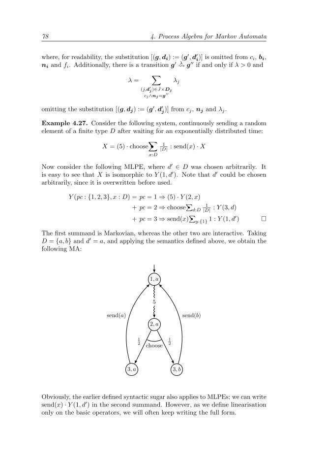
78 4. Process Algebra for Markov Automata

where, for readability, the substitution [(g,di) := (g′,d′i)] is omitted from ci, bi,ni and fi. Additionally, there is a transition g′ λ g′′ if and only if λ > 0 and

λ =∑

(j,d′j)∈J×Dj

cj∧nj=g′′

λj

omitting the substitution [(g,dj) := (g′,d′j)] from cj , nj and λj .

Example 4.27. Consider the following system, continuously sending a randomelement of a finite type D after waiting for an exponentially distributed time:

X = (5) · choose∑•x:D

1|D| : send(x) ·X

Now consider the following MLPE, where d′ ∈ D was chosen arbitrarily. Itis easy to see that X is isomorphic to Y (1, d′). Note that d′ could be chosenarbitrarily, since it is overwritten before used.

Y (pc : 1, 2, 3, x : D) = pc = 1⇒ (5) · Y (2, x)

+ pc = 2⇒ choose∑•d:D

1|D| : Y (3, d)

+ pc = 3⇒ send(x)∑•y:1 1 : Y (1, d′)

The first summand is Markovian, whereas the other two are interactive. TakingD = a, b and d′ = a, and applying the semantics defined above, we obtain thefollowing MA:

1, a

2, a

3, a 3, b

5

12

12choose

send(a) send(b)

Obviously, the earlier defined syntactic sugar also applies to MLPEs; we can writesend(x) · Y (1, d′) in the second summand. However, as we define linearisationonly on the basic operators, we will often keep writing the full form.

4.2. Markov Automata Process Algebra 79

Remark 4.28. We already noted in Section 4.2.2 that MAPA specifications arenot allowed to have infinite outgoing rates (since this is not allowed by MAs),although at that point we could not yet make this precise. With the MLPEformat, though, it is much easier to define and heuristically check this.

For the semantics to be an MA with finite outgoing rates, we can now requirethat for every Markovian summand j ∈ J and every reachable state g′ ∈ G,∑

d′j∈Dj

cj(g′,d′j)

λj(g′,d′j) <∞

That is, for each reachable state g′ ∈ G and each Markovian summand j, theMarkovian transitions that may be generated in g′ ∈ G by j should add up to afinite number.

One way of enforcing this syntactically is to require all data types inMarkovian summands to be finite. For the MLPE in Example 4.27, this isindeed the case. Note, however, that this restriction would disallow an MLPEhaving a Markovian summand such as∑

n:N( 1

2n ) ·X(n)

even though it is well-formed.

Remark 4.29. For any MAPA specification in the MLPE format, it is trivial toencode a condition c over its global variables g by the enabledness of an action,as mentioned in Remark 4.23. We just add a single summand to the MLPE,having c as its enabling condition, obtaining

X(g : G) =∑i∈I

∑di:Di

ci ⇒ ai(bi)∑•

ei:Ei

fi : X(ni)

+∑j∈J

∑dj :Dj

cj ⇒ (λj) ·X(nj)

+ c ⇒ conditionReached∑•

x:∗

1 : X(g)

Clearly, X behaves precisely the same as without the final summand, exceptthat there is a selfloop labelled conditionReached in every state such that theglobal variables satisfy condition c. Of course we should be careful never tohide the action conditionReached (renaming it to τ), as in combination withthe maximal progress assumption this would disable all Markovian summands.Actually, in our implementation we only use such actions for finding a set ofgoal states; during state space generation, they are omitted to get precisely thesame MA as we would have obtained without the additional summand.

80 4. Process Algebra for Markov Automata

4.2.5 Probabilistic Common Representation Language

The MAPA specification language we just presented can be used to modelsystems with nondeterminism, probability and Markovian rates. If a systemdoes not contain any rates, a subset of MAPA suffices. In fact, before definingMAPA in [TKvdPS12a], we had already introduced such a subset under thename probabilistic Common Representation Language (prCRL) in [KvdPST10a,KvdPST12]. The syntax of prCRL coincides with the syntax of MAPA, exceptthat it does not contain the (λ) · p construct.

Definition 4.30 (Process terms in prCRL). A process term in prCRL isany term that can be generated by the following grammar:

p ::= Y (t) | c⇒ p | p+ p |∑x:D

p | a(t)∑•x:D

f : p

Assuming this restricted syntax, all MAPA concepts defined before (specific-ations, well-formedness, operational semantics, syntactic sugar) can be appliedunchanged. Note that for prCRL the SOS rule MStep is never used, and thatthe concept of derivations is rendered superfluous.

It is often more convenient to define and prove correct a (reduction) tech-nique on prCRL than on MAPA, due to the absence of Markovian transitions.Therefore, we present an encoding scheme that allows us to encode a MAPAspecification M into a prCRL specification enc (M), apply some transforma-tion f on it and then decode back to a MAPA specification dec (f(enc (M))) (seeFigure 4.2 on page 59). For a transformation f on prCRL specification to beapplicable to MAPA specifications in this manner, we often need to take care thatdec (f(enc (M))) is strongly bisimilar to M for every MAPA specification M . Toachieve this, we introduce a novel notion of derivation-preserving bisimulationon prCRL terms and show that, for any prCRL transformation f that respectsthis notion, dec f enc indeed preserves strong bisimulation.

Encoding and decoding. The encoding of MAPA terms is straightforward. Theconstruct (λ) · p of MAPA is the only one that has to be encoded, since the otherconstructs all are also present in prCRL. We chose to encode each exponentialrate λ by a parameterised action rate(λ) (which is assumed not to occur in theoriginal specification). Since actions in prCRL require a probabilistic choice forthe next state, we use

∑•x:1 1 : p such that x is not used in p. Figure 4.6 shows

the appropriate encoding and decoding functions.

Remark 4.31. We only provide a decoding rule for rate-actions in a constructof the form rate(λ)

∑•

x:∗ 1 : p, and cannot decode any construct of the formrate(λ)

∑•

x:D f : p with D 6= ∗ or f 6= 1. We say that a prCRL specification Pis decodable if it can be decoded, otherwise it is non-decodable.

Note that the encoding of a MAPA specification without any rate actions isalways decodable. Also note that transformations on encoded MAPA specifica-tions are not allowed to modify the data types D or probability expressions fof the existing rate-constructs or add additional rate-constructs of a different

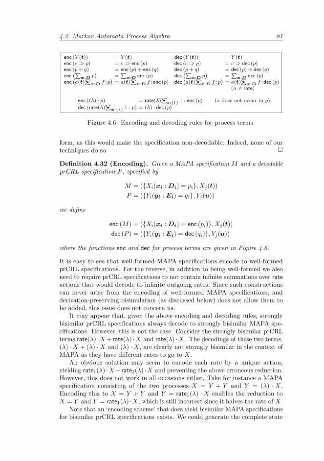
4.2. Markov Automata Process Algebra 81

enc (Y (t)) = Y (t)enc (c⇒ p) = c⇒ enc (p)enc (p+ q) = enc (p) + enc (q)enc(∑

x:D p)

=∑

x:D enc (p)enc(a(t)

∑•

x:D f :p)

= a(t)∑•

x:D f :enc (p)

dec (Y (t)) = Y (t)dec (c⇒ p) = c⇒ dec (p)dec (p+ q) = dec (p) + dec (q)dec(∑

x:D p)

=∑

x:D dec (p)dec(a(t)

∑•

x:D f :p)

= a(t)∑•

x:D f :dec (p)(a 6= rate)

enc ((λ) · p) = rate(λ)∑•x:1 1 : enc (p) (x does not occur in p)

dec (rate(λ)∑•

x:∗ 1 : p) = (λ) · dec (p)

Figure 4.6: Encoding and decoding rules for process terms.

form, as this would make the specification non-decodable. Indeed, none of ourtechniques do so.

Definition 4.32 (Encoding). Given a MAPA specification M and a decodableprCRL specification P , specified by

M = (Xi(xi : Di) = pi, Xj(t))

P = (Yi(yi : Ei) = qi, Yj(u))

we define

enc (M) = (Xi(xi : Di) = enc (pi), Xj(t))

dec (P ) = (Yi(yi : Ei) = dec (qi), Yj(u))

where the functions enc and dec for process terms are given in Figure 4.6.

It is easy to see that well-formed MAPA specifications encode to well-formedprCRL specifications. For the reverse, in addition to being well-formed we alsoneed to require prCRL specifications to not contain infinite summations over rateactions that would decode to infinite outgoing rates. Since such constructionscan never arise from the encoding of well-formed MAPA specifications, andderivation-preserving bisimulation (as discussed below) does not allow them tobe added, this issue does not concern us.

It may appear that, given the above encoding and decoding rules, stronglybisimilar prCRL specifications always decode to strongly bisimilar MAPA spe-cifications. However, this is not the case. Consider the strongly bisimilar prCRLterms rate(λ) ·X+ rate(λ) ·X and rate(λ) ·X. The decodings of these two terms,(λ) ·X + (λ) ·X and (λ) ·X, are clearly not strongly bisimilar in the context ofMAPA as they have different rates to go to X.

An obvious solution may seem to encode each rate by a unique action,yielding rate1(λ) ·X+ rate2(λ) ·X and preventing the above erroneous reduction.However, this does not work in all occasions either. Take for instance a MAPAspecification consisting of the two processes X = Y + Y and Y = (λ) · X.Encoding this to X = Y + Y and Y = rate1(λ) · X enables the reduction toX = Y and Y = rate1(λ) ·X, which is still incorrect since it halves the rate of X.

Note that an ‘encoding scheme’ that does yield bisimilar MAPA specificationsfor bisimilar prCRL specifications exists. We could generate the complete state

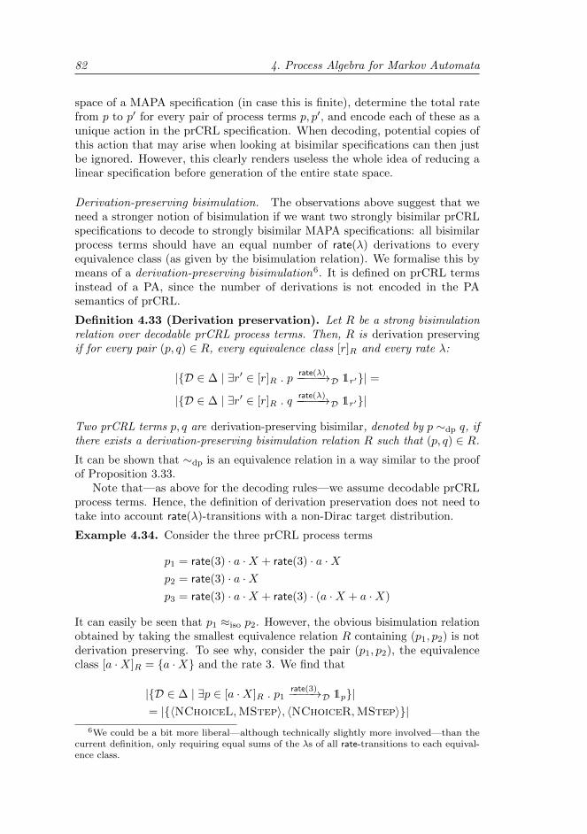
82 4. Process Algebra for Markov Automata

space of a MAPA specification (in case this is finite), determine the total ratefrom p to p′ for every pair of process terms p, p′, and encode each of these as aunique action in the prCRL specification. When decoding, potential copies ofthis action that may arise when looking at bisimilar specifications can then justbe ignored. However, this clearly renders useless the whole idea of reducing alinear specification before generation of the entire state space.

Derivation-preserving bisimulation. The observations above suggest that weneed a stronger notion of bisimulation if we want two strongly bisimilar prCRLspecifications to decode to strongly bisimilar MAPA specifications: all bisimilarprocess terms should have an equal number of rate(λ) derivations to everyequivalence class (as given by the bisimulation relation). We formalise this bymeans of a derivation-preserving bisimulation6. It is defined on prCRL termsinstead of a PA, since the number of derivations is not encoded in the PAsemantics of prCRL.

Definition 4.33 (Derivation preservation). Let R be a strong bisimulationrelation over decodable prCRL process terms. Then, R is derivation preservingif for every pair (p, q) ∈ R, every equivalence class [r]R and every rate λ:

|D ∈ ∆ | ∃r′ ∈ [r]R . p −rate(λ)−−−−→D 1r′| =

|D ∈ ∆ | ∃r′ ∈ [r]R . q −rate(λ)−−−−→D 1r′|

Two prCRL terms p, q are derivation-preserving bisimilar, denoted by p ∼dp q, ifthere exists a derivation-preserving bisimulation relation R such that (p, q) ∈ R.

It can be shown that ∼dp is an equivalence relation in a way similar to the proofof Proposition 3.33.

Note that—as above for the decoding rules—we assume decodable prCRLprocess terms. Hence, the definition of derivation preservation does not need totake into account rate(λ)-transitions with a non-Dirac target distribution.

Example 4.34. Consider the three prCRL process terms

p1 = rate(3) · a ·X + rate(3) · a ·Xp2 = rate(3) · a ·Xp3 = rate(3) · a ·X + rate(3) · (a ·X + a ·X)

It can easily be seen that p1 ≈iso p2. However, the obvious bisimulation relationobtained by taking the smallest equivalence relation R containing (p1, p2) is notderivation preserving. To see why, consider the pair (p1, p2), the equivalenceclass [a ·X]R = a ·X and the rate 3. We find that

|D ∈ ∆ | ∃p ∈ [a ·X]R . p1 −rate(3)−−−→D 1p|= |〈NChoiceL,MStep〉, 〈NChoiceR,MStep〉|

6We could be a bit more liberal—although technically slightly more involved—than thecurrent definition, only requiring equal sums of the λs of all rate-transitions to each equival-ence class.

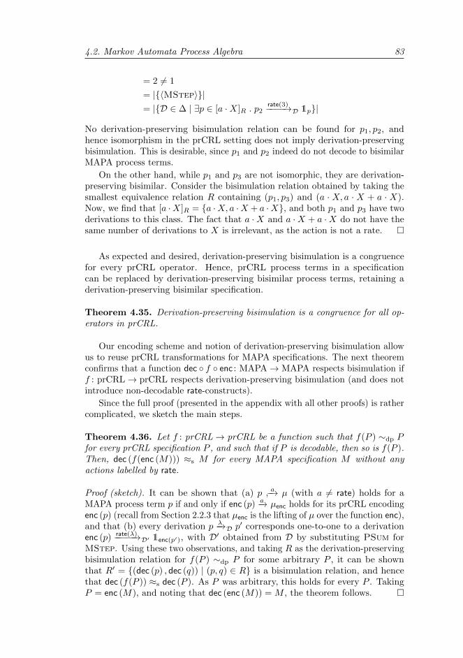
4.2. Markov Automata Process Algebra 83

= 2 6= 1

= |〈MStep〉|= |D ∈ ∆ | ∃p ∈ [a ·X]R . p2 −rate(3)−−−→D 1p|

No derivation-preserving bisimulation relation can be found for p1, p2, andhence isomorphism in the prCRL setting does not imply derivation-preservingbisimulation. This is desirable, since p1 and p2 indeed do not decode to bisimilarMAPA process terms.

On the other hand, while p1 and p3 are not isomorphic, they are derivation-preserving bisimilar. Consider the bisimulation relation obtained by taking thesmallest equivalence relation R containing (p1, p3) and (a · X, a · X + a · X).Now, we find that [a ·X]R = a ·X, a ·X + a ·X, and both p1 and p3 have twoderivations to this class. The fact that a ·X and a ·X + a ·X do not have thesame number of derivations to X is irrelevant, as the action is not a rate.

As expected and desired, derivation-preserving bisimulation is a congruencefor every prCRL operator. Hence, prCRL process terms in a specificationcan be replaced by derivation-preserving bisimilar process terms, retaining aderivation-preserving bisimilar specification.

Theorem 4.35. Derivation-preserving bisimulation is a congruence for all op-erators in prCRL.

Our encoding scheme and notion of derivation-preserving bisimulation allowus to reuse prCRL transformations for MAPA specifications. The next theoremconfirms that a function dec f enc : MAPA→ MAPA respects bisimulation iff : prCRL→ prCRL respects derivation-preserving bisimulation (and does notintroduce non-decodable rate-constructs).

Since the full proof (presented in the appendix with all other proofs) is rathercomplicated, we sketch the main steps.

Theorem 4.36. Let f : prCRL→ prCRL be a function such that f(P ) ∼dp Pfor every prCRL specification P , and such that if P is decodable, then so is f(P ).Then, dec (f(enc (M))) ≈s M for every MAPA specification M without anyactions labelled by rate.

Proof (sketch). It can be shown that (a) p a−→ µ (with a 6= rate) holds for aMAPA process term p if and only if enc (p) −a→ µenc holds for its prCRL encodingenc (p) (recall from Section 2.2.3 that µenc is the lifting of µ over the function enc),and that (b) every derivation p −λ→D p′ corresponds one-to-one to a derivationenc (p) −rate(λ)−−−−→D′ 1enc(p′), with D′ obtained from D by substituting PSum forMStep. Using these two observations, and taking R as the derivation-preservingbisimulation relation for f(P ) ∼dp P for some arbitrary P , it can be shownthat R′ = (dec (p) , dec (q)) | (p, q) ∈ R is a bisimulation relation, and hencethat dec (f(P )) ≈s dec (P ). As P was arbitrary, this holds for every P . TakingP = enc (M), and noting that dec (enc (M)) = M , the theorem follows.

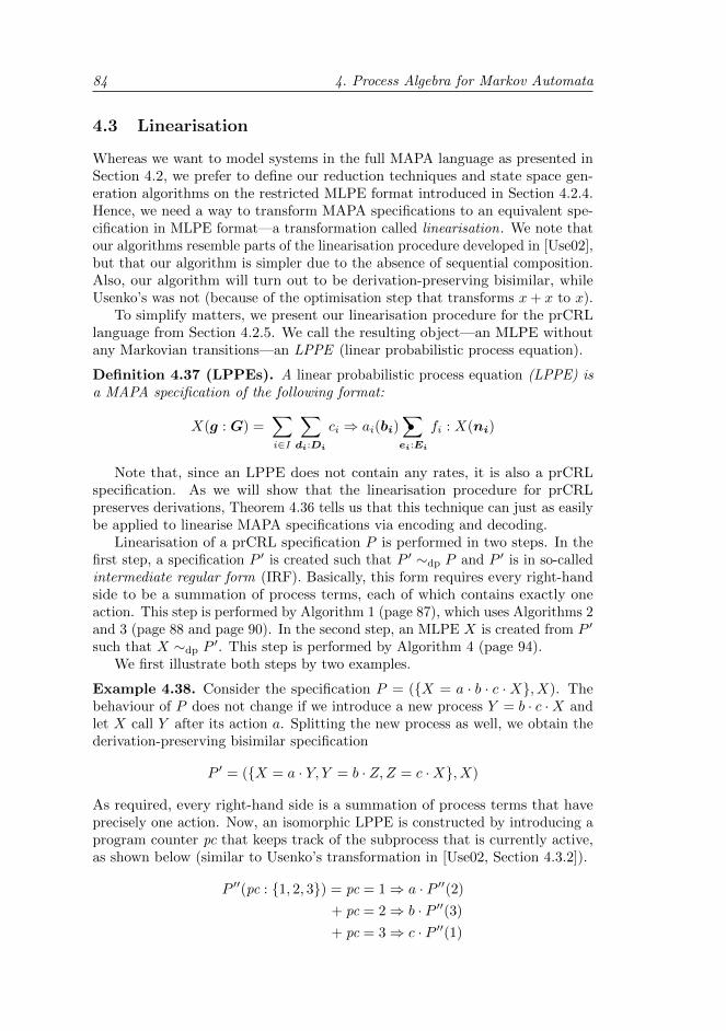
84 4. Process Algebra for Markov Automata

4.3 Linearisation

Whereas we want to model systems in the full MAPA language as presented inSection 4.2, we prefer to define our reduction techniques and state space gen-eration algorithms on the restricted MLPE format introduced in Section 4.2.4.Hence, we need a way to transform MAPA specifications to an equivalent spe-cification in MLPE format—a transformation called linearisation. We note thatour algorithms resemble parts of the linearisation procedure developed in [Use02],but that our algorithm is simpler due to the absence of sequential composition.Also, our algorithm will turn out to be derivation-preserving bisimilar, whileUsenko’s was not (because of the optimisation step that transforms x+ x to x).

To simplify matters, we present our linearisation procedure for the prCRLlanguage from Section 4.2.5. We call the resulting object—an MLPE withoutany Markovian transitions—an LPPE (linear probabilistic process equation).

Definition 4.37 (LPPEs). A linear probabilistic process equation (LPPE) isa MAPA specification of the following format:

X(g : G) =∑i∈I

∑di:Di

ci ⇒ ai(bi)∑•

ei:Ei

fi : X(ni)

Note that, since an LPPE does not contain any rates, it is also a prCRLspecification. As we will show that the linearisation procedure for prCRLpreserves derivations, Theorem 4.36 tells us that this technique can just as easilybe applied to linearise MAPA specifications via encoding and decoding.

Linearisation of a prCRL specification P is performed in two steps. In thefirst step, a specification P ′ is created such that P ′ ∼dp P and P ′ is in so-calledintermediate regular form (IRF). Basically, this form requires every right-handside to be a summation of process terms, each of which contains exactly oneaction. This step is performed by Algorithm 1 (page 87), which uses Algorithms 2and 3 (page 88 and page 90). In the second step, an MLPE X is created from P ′

such that X ∼dp P′. This step is performed by Algorithm 4 (page 94).

We first illustrate both steps by two examples.

Example 4.38. Consider the specification P = (X = a · b · c ·X, X). Thebehaviour of P does not change if we introduce a new process Y = b · c ·X andlet X call Y after its action a. Splitting the new process as well, we obtain thederivation-preserving bisimilar specification

P ′ = (X = a · Y, Y = b · Z,Z = c ·X, X)

As required, every right-hand side is a summation of process terms that haveprecisely one action. Now, an isomorphic LPPE is constructed by introducing aprogram counter pc that keeps track of the subprocess that is currently active,as shown below (similar to Usenko’s transformation in [Use02, Section 4.3.2]).

P ′′(pc : 1, 2, 3) = pc = 1⇒ a · P ′′(2)

+ pc = 2⇒ b · P ′′(3)

+ pc = 3⇒ c · P ′′(1)

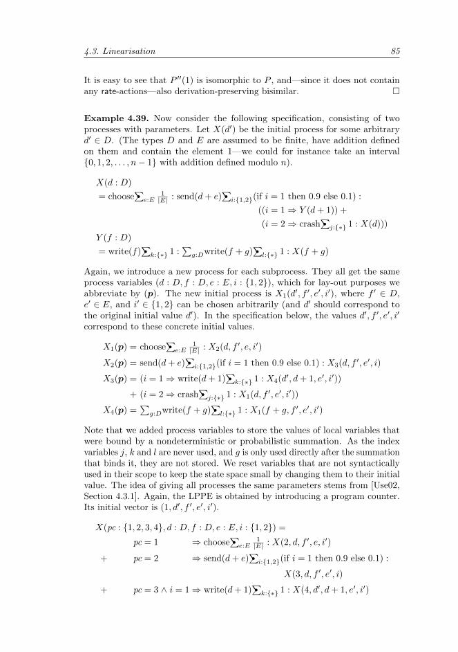
4.3. Linearisation 85

It is easy to see that P ′′(1) is isomorphic to P , and—since it does not containany rate-actions—also derivation-preserving bisimilar.

Example 4.39. Now consider the following specification, consisting of twoprocesses with parameters. Let X(d′) be the initial process for some arbitraryd′ ∈ D. (The types D and E are assumed to be finite, have addition definedon them and contain the element 1—we could for instance take an interval0, 1, 2, . . . , n− 1 with addition defined modulo n).

X(d : D)

= choose∑•e:E

1|E| : send(d+ e)

∑•i:1,2(if i = 1 then 0.9 else 0.1) :

((i = 1⇒ Y (d+ 1)) +

(i = 2⇒ crash∑•j:∗ 1 : X(d)))

Y (f : D)

= write(f)∑•k:∗ 1 :

∑g:Dwrite(f + g)

∑•l:∗ 1 : X(f + g)

Again, we introduce a new process for each subprocess. They all get the sameprocess variables (d : D, f : D, e : E, i : 1, 2), which for lay-out purposes weabbreviate by (p). The new initial process is X1(d′, f ′, e′, i′), where f ′ ∈ D,e′ ∈ E, and i′ ∈ 1, 2 can be chosen arbitrarily (and d′ should correspond tothe original initial value d′). In the specification below, the values d′, f ′, e′, i′

correspond to these concrete initial values.

X1(p) = choose∑•e:E

1|E| : X2(d, f ′, e, i′)

X2(p) = send(d+ e)∑•i:1,2(if i = 1 then 0.9 else 0.1) : X3(d, f ′, e′, i)

X3(p) = (i = 1⇒ write(d+ 1)∑•k:∗ 1 : X4(d′, d+ 1, e′, i′))

+ (i = 2⇒ crash∑•j:∗ 1 : X1(d, f ′, e′, i′))

X4(p) =∑g:Dwrite(f + g)

∑•l:∗ 1 : X1(f + g, f ′, e′, i′)

Note that we added process variables to store the values of local variables thatwere bound by a nondeterministic or probabilistic summation. As the indexvariables j, k and l are never used, and g is only used directly after the summationthat binds it, they are not stored. We reset variables that are not syntacticallyused in their scope to keep the state space small by changing them to their initialvalue. The idea of giving all processes the same parameters stems from [Use02,Section 4.3.1]. Again, the LPPE is obtained by introducing a program counter.Its initial vector is (1, d′, f ′, e′, i′).

X(pc : 1, 2, 3, 4, d : D, f : D, e : E, i : 1, 2) =

pc = 1 ⇒ choose∑•e:E

1|E| : X(2, d, f ′, e, i′)

+ pc = 2 ⇒ send(d+ e)∑•i:1,2(if i = 1 then 0.9 else 0.1) :

X(3, d, f ′, e′, i)

+ pc = 3 ∧ i = 1⇒ write(d+ 1)∑•k:∗ 1 : X(4, d′, d+ 1, e′, i′)

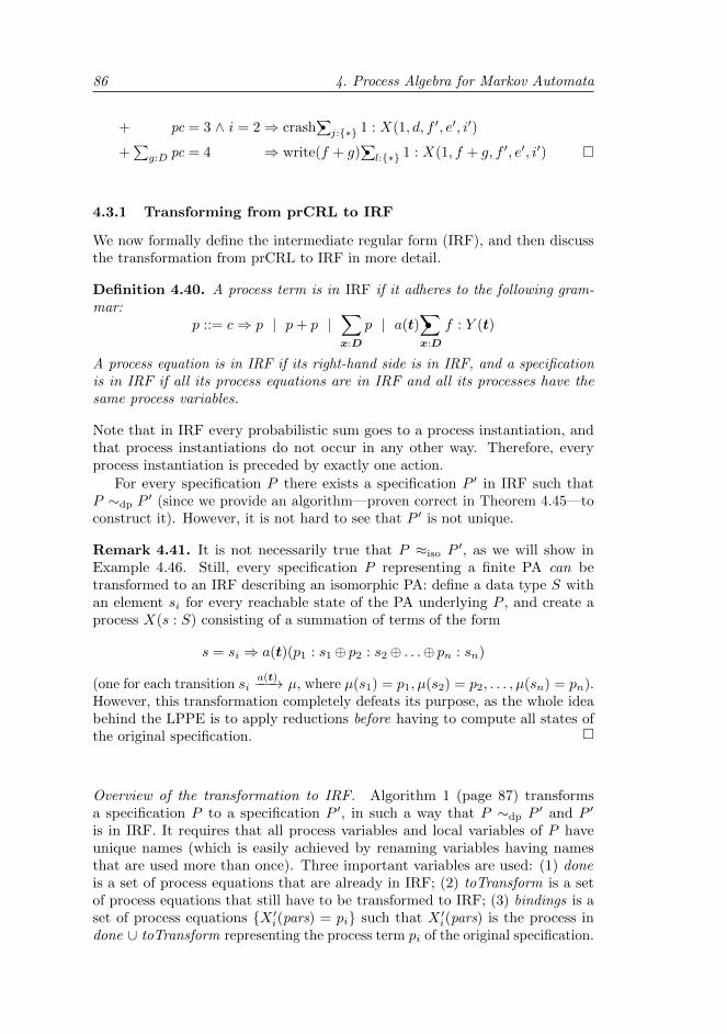
86 4. Process Algebra for Markov Automata

+ pc = 3 ∧ i = 2⇒ crash∑•j:∗ 1 : X(1, d, f ′, e′, i′)

+∑g:D pc = 4 ⇒ write(f + g)

∑•l:∗ 1 : X(1, f + g, f ′, e′, i′)

4.3.1 Transforming from prCRL to IRF

We now formally define the intermediate regular form (IRF), and then discussthe transformation from prCRL to IRF in more detail.

Definition 4.40. A process term is in IRF if it adheres to the following gram-mar:

p ::= c⇒ p | p+ p |∑x:D

p | a(t)∑•x:D

f : Y (t)

A process equation is in IRF if its right-hand side is in IRF, and a specificationis in IRF if all its process equations are in IRF and all its processes have thesame process variables.

Note that in IRF every probabilistic sum goes to a process instantiation, andthat process instantiations do not occur in any other way. Therefore, everyprocess instantiation is preceded by exactly one action.

For every specification P there exists a specification P ′ in IRF such thatP ∼dp P

′ (since we provide an algorithm—proven correct in Theorem 4.45—toconstruct it). However, it is not hard to see that P ′ is not unique.

Remark 4.41. It is not necessarily true that P ≈iso P′, as we will show in

Example 4.46. Still, every specification P representing a finite PA can betransformed to an IRF describing an isomorphic PA: define a data type S withan element si for every reachable state of the PA underlying P , and create aprocess X(s : S) consisting of a summation of terms of the form

s = si ⇒ a(t)(p1 : s1⊕ p2 : s2⊕ . . .⊕ pn : sn)

(one for each transition si −a(t)−−→ µ, where µ(s1) = p1, µ(s2) = p2, . . . , µ(sn) = pn).However, this transformation completely defeats its purpose, as the whole ideabehind the LPPE is to apply reductions before having to compute all states ofthe original specification.

Overview of the transformation to IRF. Algorithm 1 (page 87) transformsa specification P to a specification P ′, in such a way that P ∼dp P ′ and P ′

is in IRF. It requires that all process variables and local variables of P haveunique names (which is easily achieved by renaming variables having namesthat are used more than once). Three important variables are used: (1) doneis a set of process equations that are already in IRF; (2) toTransform is a setof process equations that still have to be transformed to IRF; (3) bindings is aset of process equations X ′i(pars) = pi such that X ′i(pars) is the process indone ∪ toTransform representing the process term pi of the original specification.

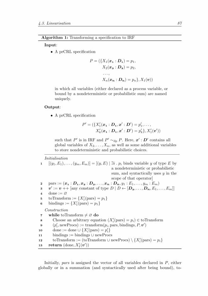
4.3. Linearisation 87

Algorithm 1: Transforming a specification to IRF

Input:

• A prCRL specification

P = (X1(x : D) = p1,

X2(x : D) = p2,

. . . ,

Xn(xn : Dn) = pn, X1(v))

in which all variables (either declared as a process variable, orbound by a nondeterministic or probabilistic sum) are nameduniquely.

Output:

• A prCRL specification

P ′ = (X ′1(x : D,x′ : D′) = p′1, . . . ,

X ′k(x : D,x′ : D′) = p′k, X ′1(v′))

such that P ′ is in IRF and P ′ ∼dp P . Here, x′ : D′ contains allglobal variables of X2, . . . , Xn, as well as some additional variablesto store nondeterministic and probabilistic choices.

Initialisation1 [(y1, E1), . . . , (ym, Em)] = [(y,E) | ∃i . pi binds variable y of type E by

a nondeterministic or probabilisticsum, and syntactically uses y in thescope of that operator]

2 pars := (x : D,x : D, . . . ,xn : Dn, y1 : E1, . . . , ym : Em)3 v′ := v ++ [any constant of type D | D ← [D, . . . ,Dn, E1, . . . , Em]]4 done := ∅5 toTransform := X ′1(pars) = p16 bindings := X ′1(pars) = p1

Construction7 while toTransform 6= ∅ do8 Choose an arbitrary equation (X ′i(pars) = pi) ∈ toTransform9 (p′i,newProcs) := transform(pi,pars,bindings, P,v′)

10 done := done ∪ X ′i(pars) = p′i11 bindings := bindings ∪ newProcs12 toTransform := (toTransform ∪ newProcs) \ X ′i(pars) = pi13 return (done, X ′1(v′))

Initially, pars is assigned the vector of all variables declared in P , eitherglobally or in a summation (and syntactically used after being bound), to-

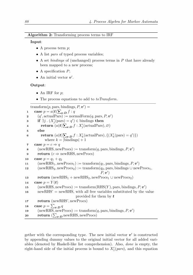
88 4. Process Algebra for Markov Automata

Algorithm 2: Transforming process terms to IRF

Input:

• A process term p;

• A list pars of typed process variables;

• A set bindings of (unchanged) process terms in P that have alreadybeen mapped to a new process;

• A specification P ;

• An initial vector v′.

Output:

• An IRF for p;

• The process equations to add to toTransform.

transform(p,pars,bindings, P,v′) =1 case p = a(t)

∑•

x:D f : q2 (q′, actualPars) := normalForm(q,pars, P,v′)3 if ∃j . (X ′j(pars) = q′) ∈ bindings then4 return (a(t)

∑•

x:D f : X ′j(actualPars),∅)

5 else6 return (a(t)

∑•

x:D f : X ′k(actualPars), (X ′k(pars) = q′))where k = |bindings|+ 1

7 case p = c⇒ q8 (newRHS,newProcs) := transform(q,pars,bindings, P,v′)9 return (c⇒ newRHS,newProcs)

10 case p = q1 + q2

11 (newRHS1,newProcs1) := transform(q1,pars,bindings, P,v′)12 (newRHS2,newProcs2) := transform(q2,pars,bindings ∪ newProcs1,

P,v′)13 return (newRHS1 + newRHS2,newProcs1 ∪ newProcs2)

14 case p = Y (t)15 (newRHS,newProcs) := transform(RHS(Y ),pars,bindings, P,v′)16 newRHS’ = newRHS, with all free variables substituted by the value

provided for them by t17 return (newRHS’,newProcs)

18 case p =∑

x:D q19 (newRHS,newProcs) := transform(q,pars,bindings, P,v′)20 return (

∑x:D newRHS,newProcs)

gether with the corresponding type. The new initial vector v′ is constructedby appending dummy values to the original initial vector for all added vari-ables (denoted by Haskell-like list comprehension). Also, done is empty, theright-hand side of the initial process is bound to X ′1(pars), and this equation

4.3. Linearisation 89

is added to toTransform and bindings. Then, we repeatedly take an equationX ′i(pars) = pi from toTransform, transform pi to a strongly probabilisticallybisimilar IRF p′i using Algorithm 2, add the equation X ′i(pars) = p′i to done, andremove X ′i(pars) = pi from toTransform. The transformation may introduce newprocesses, which are added to toTransform, and bindings is updated accordingly.

Remark 4.42. The use of the set bindings makes sure that multiple occur-rences of the same process term are linearised only once. For instance, whentransforming a process term such as x · b · c ·X + y · b · c ·X, we want to makeuse of the duplication, transforming to x ·X ′2 + y ·X ′2, with X ′2 = b · c ·X (whichis initially put in toTransform and later transformed itself). To this end, we addthe equation X ′2 = b · c ·X to bindings after transforming the left-hand side ofthe nondeterministic choice to x ·X ′2. Then, when transforming the right-handside, this information is used to transform to y ·X ′2 instead of introducing a newprocess X ′3.

Additionally, the bindings set makes sure that process instantiations aretransformed correctly while still terminating. For instance, when transforming aprocess such as X = a · b · c ·X, the algorithm starts by putting the equationX ′1 = a · b · c · X in both bindings and toTransform. When transforming theright-hand side of this equation, at some point we will have to transform theprocess term c ·X. It is then checked whether the right-hand side of X, in thiscase a · b · c · X, is already present in bindings. This is the case (in the formX ′1 = a · b · c ·X), so the instantiation X is changed to X ′1.

In a more complicated situation where X has data parameters, the algorithmstill works in the same way. For instance, consider the process X(n : N) =a ·b ·X(n+1)+b ·X(5). In the initialisation, X ′1(n : N) = a ·b ·X(n+1)+b ·X(5)is put in bindings. When later on b ·X(n + 1) needs to be transformed, it isrecognised that X(n+ 1) is an instantiation of a process with right-hand sidea · b ·X(n+ 1) + b ·X(5). This process term is already present in bindings, sothe algorithm transforms b ·X(n+ 1) to b ·X ′1(n+ 1).

Transforming single process terms to IRF. Algorithm 2 transforms individualprocess terms to IRF recursively by means of a case distinction over the structureof the terms (using Algorithm 3). Its base case is the action prefix, which isalways reached in a finite number of steps due to the requirement of guarded-ness (Definition 4.16).

For a summation q1 + q2, the IRF is q′1 + q′2 (with q′i an IRF of qi). For thecondition c⇒ q1 it is c⇒ q′1, and for

∑x:D q1 it is

∑x:D q′1. Finally, the IRF

for Y (t) is the IRF for the right-hand side of Y , where the global variables of Yoccurring in this term have been substituted by the expressions given by t.

The base case is a probabilistic choice a(t)∑•

x:D f : q. The correspondingprocess term in IRF depends on whether or not there already is a process nameX ′j mapped to q (as stored in bindings). If this is the case, apparently q hasbeen linearised before and the result simply is a(t)

∑•

x:D f : X ′j(actualPars),with actualPars as explained below. If q was not linearised before, a new processname X ′k is chosen, the result is a(t)

∑•

x:D f : X ′k(actualPars) and X ′k is mapped

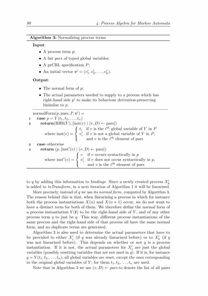
90 4. Process Algebra for Markov Automata

Algorithm 3: Normalising process terms

Input:

• A process term p;

• A list pars of typed global variables;

• A prCRL specification P ;

• An initial vector v′ = (v′1, v′2, . . . , v

′k).

Output:

• The normal form of p;

• The actual parameters needed to supply to a process which hasright-hand side p′ to make its behaviour derivation-preservingbisimilar to p.

normalForm(p,pars, P,v′) =1 case p = Y (t1, t2, . . . , tn)2 return(RHS(Y ), [inst(v) | (v,D)← pars])

where inst(v) =

ti if v is the ith global variable of Y in Pv′i if v is not a global variable of Y in P ,

and v is the ith element of pars

3 case otherwise4 return (p, [inst′(v) | (v,D)← pars])

where inst′(v) =

v if v occurs syntactically in pv′i if v does not occur syntactically in p,

and v is the ith element of pars

to q by adding this information to bindings. Since a newly created process X ′kis added to toTransform, in a next iteration of Algorithm 1 it will be linearised.

More precisely, instead of q we use its normal form, computed by Algorithm 3.The reason behind this is that, when linearising a process in which for instanceboth the process instantiations X(n) and X(n + 1) occur, we do not want tohave a distinct term for both of them. We therefore define the normal form ofa process instantiation Y (t) to be the right-hand side of Y , and of any otherprocess term q to just be q. This way, different process instantiations of thesame process and the right-hand side of that process all have the same normalform, and no duplicate terms are generated.

Algorithm 3 is also used to determine the actual parameters that have tobe provided to either X ′j (if q was already linearised before) or to X ′k (if qwas not linearised before). This depends on whether or not q is a processinstantiation. If it is not, the actual parameters for X ′j are just the globalvariables (possibly resetting variables that are not used in q). If it is, for instanceq = Y (t1, t2, . . . , tn), all global variables are reset, except the ones correspondingto the original global variables of Y ; for them t1, t2, . . . , tn are used.

Note that in Algorithm 3 we use (v,D)← pars to denote the list of all pairs

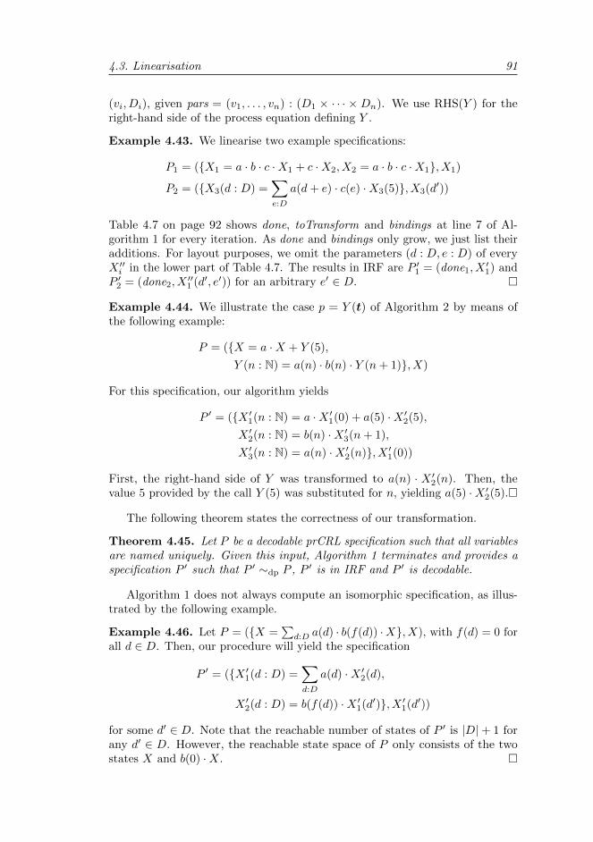
4.3. Linearisation 91

(vi, Di), given pars = (v1, . . . , vn) : (D1 × · · · × Dn). We use RHS(Y ) for theright-hand side of the process equation defining Y .

Example 4.43. We linearise two example specifications:

P1 = (X1 = a · b · c ·X1 + c ·X2, X2 = a · b · c ·X1, X1)

P2 = (X3(d : D) =∑e:D

a(d+ e) · c(e) ·X3(5), X3(d′))

Table 4.7 on page 92 shows done, toTransform and bindings at line 7 of Al-gorithm 1 for every iteration. As done and bindings only grow, we just list theiradditions. For layout purposes, we omit the parameters (d : D, e : D) of everyX ′′i in the lower part of Table 4.7. The results in IRF are P ′1 = (done1, X

′1) and

P ′2 = (done2, X′′1 (d′, e′)) for an arbitrary e′ ∈ D.

Example 4.44. We illustrate the case p = Y (t) of Algorithm 2 by means ofthe following example:

P = (X = a ·X + Y (5),

Y (n : N) = a(n) · b(n) · Y (n+ 1), X)

For this specification, our algorithm yields

P ′ = (X ′1(n : N) = a ·X ′1(0) + a(5) ·X ′2(5),

X ′2(n : N) = b(n) ·X ′3(n+ 1),

X ′3(n : N) = a(n) ·X ′2(n), X ′1(0))

First, the right-hand side of Y was transformed to a(n) · X ′2(n). Then, thevalue 5 provided by the call Y (5) was substituted for n, yielding a(5) ·X ′2(5).

The following theorem states the correctness of our transformation.

Theorem 4.45. Let P be a decodable prCRL specification such that all variablesare named uniquely. Given this input, Algorithm 1 terminates and provides aspecification P ′ such that P ′ ∼dp P , P ′ is in IRF and P ′ is decodable.

Algorithm 1 does not always compute an isomorphic specification, as illus-trated by the following example.

Example 4.46. Let P = (X =∑d:D a(d) · b(f(d)) ·X, X), with f(d) = 0 for

all d ∈ D. Then, our procedure will yield the specification

P ′ = (X ′1(d : D) =∑d:D

a(d) ·X ′2(d),

X ′2(d : D) = b(f(d)) ·X ′1(d′), X ′1(d′))

for some d′ ∈ D. Note that the reachable number of states of P ′ is |D|+ 1 forany d′ ∈ D. However, the reachable state space of P only consists of the twostates X and b(0) ·X.

92 4. Process Algebra for Markov Automata

don

e1

toT

ran

sform

1bi

ndin

gs1

0∅

X′ 1

=a·b·c·X

1+c·X

2X′ 1

=a·b·c·X

1+c·X

2

1X′ 1

=a·X′ 2

+c·X′ 3

X′ 2

=b·c·X

1,X′ 3

=a·b·c·X

1X′ 2

=b·c·X

1,X′ 3

=a·b·c·X

1

2X′ 2

=b·X′ 4

X′ 3

=a·b·c·X

1,X′ 4

=c·X

1X′ 4

=c·X

1

3X′ 3

=a·X′ 2

X′ 4

=c·X

1

4X′ 4

=c·X′ 1

∅

don

e2

toT

ran

sform

2bi

ndin

gs2

0∅

X′′ 1

=∑ e

:Da(d

+e)·c

(e)·X

3(5

)X′′ 1

=∑ e

:Da(d

+e)·c

(e)·X

3(5

)

1X′′ 1

=∑ e

:Da(d

+e)·X′′ 2(d′ ,e)

X′′ 2

=c(e)·X

3(5

)X′′ 2

=c(e)·X

3(5

)

2X′′ 2

=c(e)·X′′ 1(5,e′ )

∅

Table

4.7

:T

ransf

orm

ingP

1=

(X

1=

a·b·c·X

1+c·X

2,X

2=

a·b·c·X

1,X

1)

(ab

ove)

andP

2=

(X

3(d

:D

)=

∑ e:Da(d

+e)·c

(e)·X

3(5

),X

3(d′ )

)(b

elow

)to

IRF

.

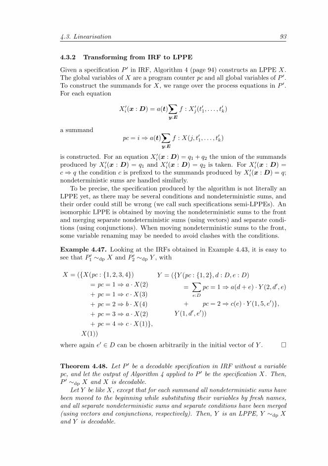
4.3. Linearisation 93

4.3.2 Transforming from IRF to LPPE

Given a specification P ′ in IRF, Algorithm 4 (page 94) constructs an LPPE X.The global variables of X are a program counter pc and all global variables of P ′.To construct the summands for X, we range over the process equations in P ′.For each equation

X ′i(x : D) = a(t)∑•y:E

f : X ′j(t′1, . . . , t

′k)

a summandpc = i⇒ a(t)

∑•y:E

f : X(j, t′1, . . . , t′k)

is constructed. For an equation X ′i(x : D) = q1 + q2 the union of the summandsproduced by X ′i(x : D) = q1 and X ′i(x : D) = q2 is taken. For X ′i(x : D) =c⇒ q the condition c is prefixed to the summands produced by X ′i(x : D) = q;nondeterministic sums are handled similarly.

To be precise, the specification produced by the algorithm is not literally anLPPE yet, as there may be several conditions and nondeterministic sums, andtheir order could still be wrong (we call such specifications semi-LPPEs). Anisomorphic LPPE is obtained by moving the nondeterministic sums to the frontand merging separate nondeterministic sums (using vectors) and separate condi-tions (using conjunctions). When moving nondeterministic sums to the front,some variable renaming may be needed to avoid clashes with the conditions.

Example 4.47. Looking at the IRFs obtained in Example 4.43, it is easy tosee that P ′1 ∼dp X and P ′2 ∼dp Y , with

X = (X(pc : 1, 2, 3, 4)= pc = 1⇒ a ·X(2)

+ pc = 1⇒ c ·X(3)

+ pc = 2⇒ b ·X(4)

+ pc = 3⇒ a ·X(2)

+ pc = 4⇒ c ·X(1),X(1))

Y = (Y (pc : 1, 2, d : D, e : D)

=∑e:D

pc = 1⇒ a(d+ e) · Y (2, d′, e)

+ pc = 2⇒ c(e) · Y (1, 5, e′),Y (1, d′, e′))

where again e′ ∈ D can be chosen arbitrarily in the initial vector of Y .

Theorem 4.48. Let P ′ be a decodable specification in IRF without a variablepc, and let the output of Algorithm 4 applied to P ′ be the specification X. Then,P ′ ∼dp X and X is decodable.

Let Y be like X, except that for each summand all nondeterministic sums havebeen moved to the beginning while substituting their variables by fresh names,and all separate nondeterministic sums and separate conditions have been merged(using vectors and conjunctions, respectively). Then, Y is an LPPE, Y ∼dp Xand Y is decodable.

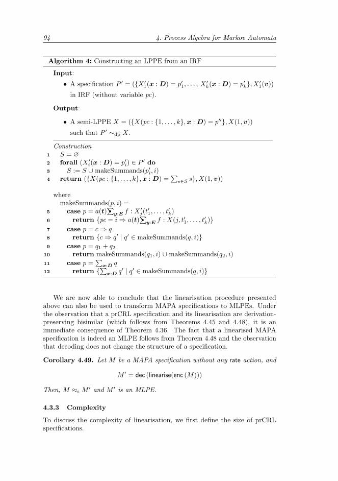
94 4. Process Algebra for Markov Automata

Algorithm 4: Constructing an LPPE from an IRF

Input:

• A specification P ′ = (X ′1(x : D) = p′1, . . . , X′k(x : D) = p′k, X ′1(v))

in IRF (without variable pc).

Output:

• A semi-LPPE X = (X(pc : 1, . . . , k,x : D) = p′′, X(1,v))

such that P ′ ∼dp X.

Construction1 S = ∅2 forall (X ′i(x : D) = p′i) ∈ P ′ do3 S := S ∪ makeSummands(p′i, i)4 return (X(pc : 1, . . . , k,x : D) =

∑s∈S s, X(1,v))

wheremakeSummands(p, i) =

5 case p = a(t)∑•

y:E f : X ′j(t′1, . . . , t

′k)

6 return pc = i⇒ a(t)∑•

y:E f : X(j, t′1, . . . , t′k)

7 case p = c⇒ q8 return c⇒ q′ | q′ ∈ makeSummands(q, i)9 case p = q1 + q2

10 return makeSummands(q1, i) ∪ makeSummands(q2, i)

11 case p =∑

x:D q12 return ∑x:D q′ | q′ ∈ makeSummands(q, i)

We are now able to conclude that the linearisation procedure presentedabove can also be used to transform MAPA specifications to MLPEs. Underthe observation that a prCRL specification and its linearisation are derivation-preserving bisimilar (which follows from Theorems 4.45 and 4.48), it is animmediate consequence of Theorem 4.36. The fact that a linearised MAPAspecification is indeed an MLPE follows from Theorem 4.48 and the observationthat decoding does not change the structure of a specification.

Corollary 4.49. Let M be a MAPA specification without any rate action, and

M ′ = dec (linearise(enc (M)))

Then, M ≈s M′ and M ′ is an MLPE.

4.3.3 Complexity

To discuss the complexity of linearisation, we first define the size of prCRLspecifications.

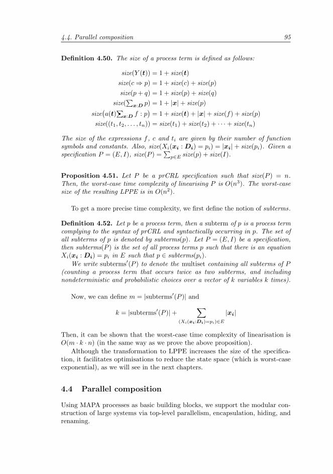
4.4. Parallel composition 95

Definition 4.50. The size of a process term is defined as follows:

size(Y (t)) = 1 + size(t)

size(c⇒ p) = 1 + size(c) + size(p)

size(p+ q) = 1 + size(p) + size(q)

size(∑

x:D p) = 1 + |x|+ size(p)

size(a(t)

∑•

x:D f : p)

= 1 + size(t) + |x|+ size(f) + size(p)

size((t1, t2, . . . , tn)) = size(t1) + size(t2) + · · ·+ size(tn)

The size of the expressions f , c and ti are given by their number of functionsymbols and constants. Also, size(Xi(xi : Di) = pi) = |xi|+ size(pi). Given aspecification P = (E, I), size(P ) =

∑p∈E size(p) + size(I).

Proposition 4.51. Let P be a prCRL specification such that size(P ) = n.Then, the worst-case time complexity of linearising P is O(n3). The worst-casesize of the resulting LPPE is in O(n2).

To get a more precise time complexity, we first define the notion of subterms .

Definition 4.52. Let p be a process term, then a subterm of p is a process termcomplying to the syntax of prCRL and syntactically occurring in p. The set ofall subterms of p is denoted by subterms(p). Let P = (E, I) be a specification,then subterms(P ) is the set of all process terms p such that there is an equationXi(xi : Di) = pi in E such that p ∈ subterms(pi).

We write subterms′(P ) to denote the multiset containing all subterms of P(counting a process term that occurs twice as two subterms, and includingnondeterministic and probabilistic choices over a vector of k variables k times).

Now, we can define m = |subterms′(P )| and

k = |subterms′(P )|+∑

(Xi(xi:Di)=pi)∈E

|xi|

Then, it can be shown that the worst-case time complexity of linearisation isO(m · k · n) (in the same way as we prove the above proposition).

Although the transformation to LPPE increases the size of the specifica-tion, it facilitates optimisations to reduce the state space (which is worst-caseexponential), as we will see in the next chapters.

4.4 Parallel composition

Using MAPA processes as basic building blocks, we support the modular con-struction of large systems via top-level parallelism, encapsulation, hiding, andrenaming.

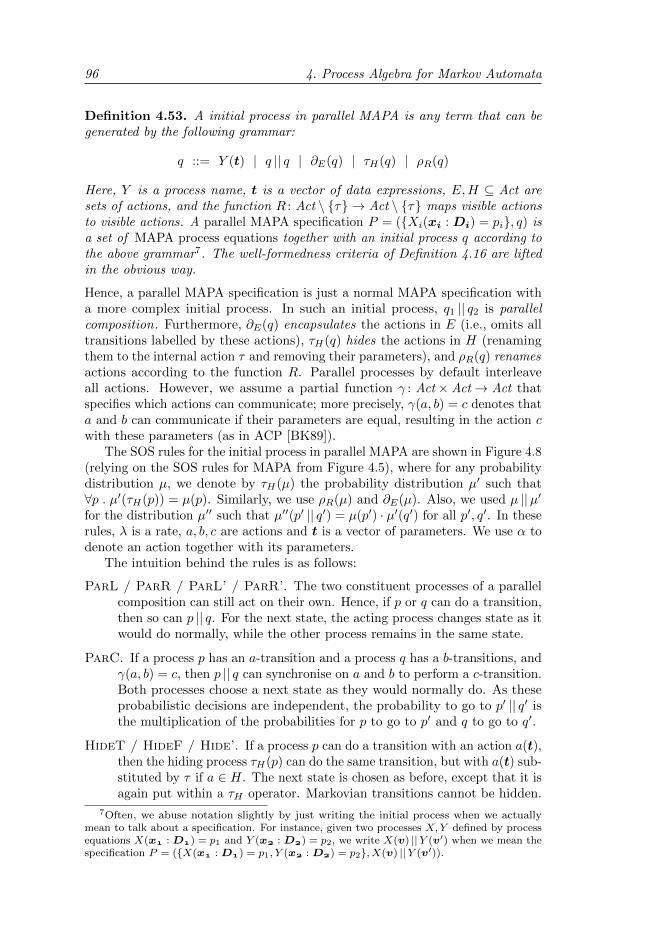
96 4. Process Algebra for Markov Automata

Definition 4.53. A initial process in parallel MAPA is any term that can begenerated by the following grammar:

q ::= Y (t) | q || q | ∂E(q) | τH(q) | ρR(q)

Here, Y is a process name, t is a vector of data expressions, E,H ⊆ Act aresets of actions, and the function R : Act \ τ → Act \ τ maps visible actionsto visible actions. A parallel MAPA specification P = (Xi(xi : Di) = pi, q) isa set of MAPA process equations together with an initial process q according tothe above grammar7. The well-formedness criteria of Definition 4.16 are liftedin the obvious way.

Hence, a parallel MAPA specification is just a normal MAPA specification witha more complex initial process. In such an initial process, q1 || q2 is parallelcomposition. Furthermore, ∂E(q) encapsulates the actions in E (i.e., omits alltransitions labelled by these actions), τH(q) hides the actions in H (renamingthem to the internal action τ and removing their parameters), and ρR(q) renamesactions according to the function R. Parallel processes by default interleaveall actions. However, we assume a partial function γ : Act×Act→ Act thatspecifies which actions can communicate; more precisely, γ(a, b) = c denotes thata and b can communicate if their parameters are equal, resulting in the action cwith these parameters (as in ACP [BK89]).

The SOS rules for the initial process in parallel MAPA are shown in Figure 4.8(relying on the SOS rules for MAPA from Figure 4.5), where for any probabilitydistribution µ, we denote by τH(µ) the probability distribution µ′ such that∀p . µ′(τH(p)) = µ(p). Similarly, we use ρR(µ) and ∂E(µ). Also, we used µ ||µ′for the distribution µ′′ such that µ′′(p′ || q′) = µ(p′) · µ′(q′) for all p′, q′. In theserules, λ is a rate, a, b, c are actions and t is a vector of parameters. We use α todenote an action together with its parameters.

The intuition behind the rules is as follows:

ParL / ParR / ParL’ / ParR’. The two constituent processes of a parallelcomposition can still act on their own. Hence, if p or q can do a transition,then so can p || q. For the next state, the acting process changes state as itwould do normally, while the other process remains in the same state.

ParC. If a process p has an a-transition and a process q has a b-transitions, andγ(a, b) = c, then p || q can synchronise on a and b to perform a c-transition.Both processes choose a next state as they would normally do. As theseprobabilistic decisions are independent, the probability to go to p′ || q′ isthe multiplication of the probabilities for p to go to p′ and q to go to q′.

HideT / HideF / Hide’. If a process p can do a transition with an action a(t),then the hiding process τH(p) can do the same transition, but with a(t) sub-stituted by τ if a ∈ H. The next state is chosen as before, except that it isagain put within a τH operator. Markovian transitions cannot be hidden.

7Often, we abuse notation slightly by just writing the initial process when we actuallymean to talk about a specification. For instance, given two processes X,Y defined by processequations X(x : D) = p1 and Y (x : D) = p2, we write X(v) ||Y (v′) when we mean thespecification P = (X(x : D) = p1, Y (x : D) = p2, X(v) ||Y (v′)).

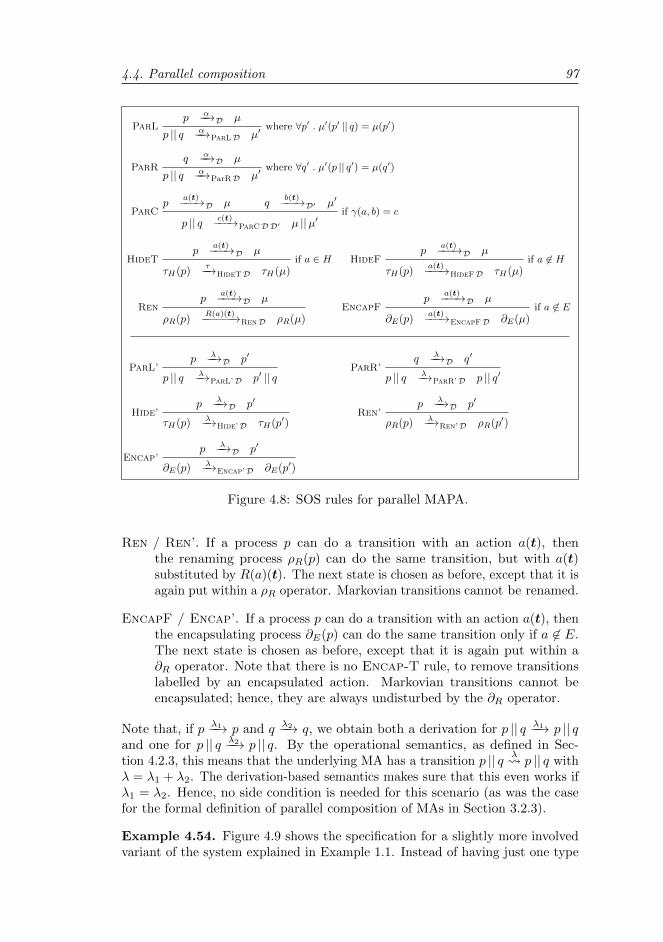
4.4. Parallel composition 97

ParLp −α−→D µ

p || q −α−→ParLD µ′where ∀p′ . µ′(p′ || q) = µ(p′)

ParRq −α−→D µ

p || q −α−→ParRD µ′where ∀q′ . µ′(p || q′) = µ(q′)

ParCp −a(t)−−→D µ q −b(t)−−→D′ µ′

p || q −c(t)−−→ParCDD′ µ ||µ′if γ(a, b) = c

HideTp −a(t)−−→D µ

τH(p) −τ−→HideTD τH(µ)if a ∈ H HideF

p −a(t)−−→D µ

τH(p) −a(t)−−→HideFD τH(µ)if a 6∈ H

Renp −a(t)−−→D µ

ρR(p) −R(a)(t)−−−−−→RenD ρR(µ)EncapF

p −a(t)−−→D µ

∂E(p) −a(t)−−→EncapFD ∂E(µ)if a 6∈ E

ParL’p −λ−→D p′

p || q −λ−→ParL’D p′ || qParR’

q −λ−→D q′

p || q −λ−→ParR’D p || q′

Hide’p −λ−→D p′

τH(p) −λ−→Hide’D τH(p′)Ren’

p −λ−→D p′

ρR(p) −λ−→Ren’D ρR(p′)

Encap’p −λ−→D p′

∂E(p) −λ−→Encap’D ∂E(p′)

Figure 4.8: SOS rules for parallel MAPA.

Ren / Ren’. If a process p can do a transition with an action a(t), thenthe renaming process ρR(p) can do the same transition, but with a(t)substituted by R(a)(t). The next state is chosen as before, except that it isagain put within a ρR operator. Markovian transitions cannot be renamed.

EncapF / Encap’. If a process p can do a transition with an action a(t), thenthe encapsulating process ∂E(p) can do the same transition only if a 6∈ E.The next state is chosen as before, except that it is again put within a∂R operator. Note that there is no Encap-T rule, to remove transitionslabelled by an encapsulated action. Markovian transitions cannot beencapsulated; hence, they are always undisturbed by the ∂R operator.

Note that, if p −λ1−→ p and q −λ2−→ q, we obtain both a derivation for p || q −λ1−→ p || qand one for p || q −λ2−→ p || q. By the operational semantics, as defined in Sec-tion 4.2.3, this means that the underlying MA has a transition p || q λ

p || q withλ = λ1 + λ2. The derivation-based semantics makes sure that this even works ifλ1 = λ2. Hence, no side condition is needed for this scenario (as was the casefor the formal definition of parallel composition of MAs in Section 3.2.3).

Example 4.54. Figure 4.9 shows the specification for a slightly more involvedvariant of the system explained in Example 1.1. Instead of having just one type

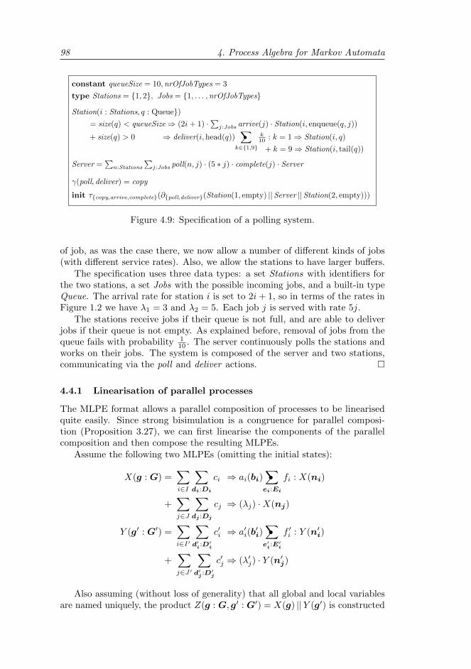
98 4. Process Algebra for Markov Automata

constant queueSize = 10,nrOfJobTypes = 3

type Stations = 1, 2, Jobs = 1, . . . ,nrOfJobTypes

Station(i : Stations, q : Queue)= size(q) < queueSize⇒ (2i+ 1) ·∑j:Jobs arrive(j) · Station(i, enqueue(q, j))

+ size(q) > 0 ⇒ deliver(i,head(q))∑•

k∈1,9

k10 : k = 1⇒ Station(i, q)

+ k = 9⇒ Station(i, tail(q))

Server =∑n:Stations

∑j:Jobs poll(n, j) · (5 ∗ j) · complete(j) · Server

γ(poll, deliver) = copy

init τcopy,arrive,complete(∂poll,deliver(Station(1, empty) ||Server ||Station(2, empty)))

Figure 4.9: Specification of a polling system.

of job, as was the case there, we now allow a number of different kinds of jobs(with different service rates). Also, we allow the stations to have larger buffers.

The specification uses three data types: a set Stations with identifiers forthe two stations, a set Jobs with the possible incoming jobs, and a built-in typeQueue. The arrival rate for station i is set to 2i+ 1, so in terms of the rates inFigure 1.2 we have λ1 = 3 and λ2 = 5. Each job j is served with rate 5j.

The stations receive jobs if their queue is not full, and are able to deliverjobs if their queue is not empty. As explained before, removal of jobs from thequeue fails with probability 1

10 . The server continuously polls the stations andworks on their jobs. The system is composed of the server and two stations,communicating via the poll and deliver actions.

4.4.1 Linearisation of parallel processes

The MLPE format allows a parallel composition of processes to be linearisedquite easily. Since strong bisimulation is a congruence for parallel composi-tion (Proposition 3.27), we can first linearise the components of the parallelcomposition and then compose the resulting MLPEs.

Assume the following two MLPEs (omitting the initial states):

X(g : G) =∑i∈I

∑di:Di

ci ⇒ ai(bi)∑•

ei:Ei

fi : X(ni)

+∑j∈J

∑dj :Dj

cj ⇒ (λj) ·X(nj)

Y (g′ : G′) =∑i∈I′

∑d′i:D′i

c′i ⇒ a′i(b′i)∑•

e′i:E′i

f ′i : Y (n′i)

+∑j∈J′

∑d′j :D′j

c′j ⇒ (λ′j) · Y (n′j)

Also assuming (without loss of generality) that all global and local variablesare named uniquely, the product Z(g : G, g′ : G′) = X(g) ||Y (g′) is constructed

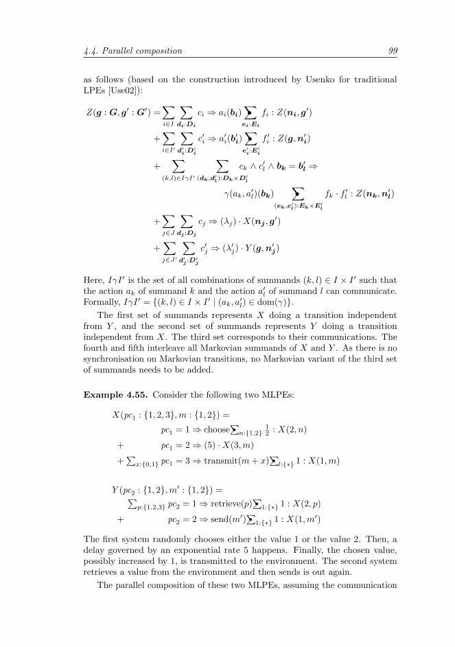
4.4. Parallel composition 99

as follows (based on the construction introduced by Usenko for traditionalLPEs [Use02]):

Z(g : G, g′ : G′) =∑i∈I

∑di:Di

ci ⇒ ai(bi)∑•

ei:Ei

fi : Z(ni, g′)

+∑i∈I′

∑d′i:D′i

c′i ⇒ a′i(b′i)∑•

e′i:E′i

f ′i : Z(g,n′i)

+∑

(k,l)∈IγI′

∑(dk,d′l):Dk×D′l

ck ∧ c′l ∧ bk = b′l ⇒

γ(ak, a′l)(bk)

∑•

(ek,e′l):Ek×E′l

fk · f ′l : Z(nk,n′l)

+∑j∈J

∑dj :Dj

cj ⇒ (λj) ·X(nj , g′)

+∑j∈J′

∑d′j :D′j

c′j ⇒ (λ′j) · Y (g,n′j)

Here, IγI ′ is the set of all combinations of summands (k, l) ∈ I × I ′ such thatthe action ak of summand k and the action a′l of summand l can communicate.Formally, IγI ′ = (k, l) ∈ I × I ′ | (ak, a′l) ∈ dom(γ).

The first set of summands represents X doing a transition independentfrom Y , and the second set of summands represents Y doing a transitionindependent from X. The third set corresponds to their communications. Thefourth and fifth interleave all Markovian summands of X and Y . As there is nosynchronisation on Markovian transitions, no Markovian variant of the third setof summands needs to be added.

Example 4.55. Consider the following two MLPEs:

X(pc1 : 1, 2, 3,m : 1, 2) =

pc1 = 1⇒ choose∑•n:1,2

12 : X(2, n)

+ pc1 = 2⇒ (5) ·X(3,m)

+∑x:0,1 pc1 = 3⇒ transmit(m+ x)

∑•l:∗ 1 : X(1,m)

Y (pc2 : 1, 2,m′ : 1, 2) =∑p:1,2,3 pc2 = 1⇒ retrieve(p)

∑•

1:∗ 1 : X(2, p)

+ pc2 = 2⇒ send(m′)∑•

1:∗ 1 : X(1,m′)

The first system randomly chooses either the value 1 or the value 2. Then, adelay governed by an exponential rate 5 happens. Finally, the chosen value,possibly increased by 1, is transmitted to the environment. The second systemretrieves a value from the environment and then sends is out again.

The parallel composition of these two MLPEs, assuming the communication

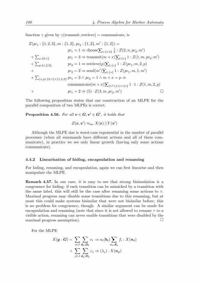
100 4. Process Algebra for Markov Automata

function γ given by γ(transmit, retrieve) = communicate, is

Z(pc1 : 1, 2, 3,m : 1, 2, pc2 : 1, 2,m′ : 1, 2) =

pc1 = 1⇒ choose∑•n:1,2

12 : Z(2, n, pc2,m

′)

+∑x:0,1 pc1 = 3⇒ transmit(m+ x)

∑•l:∗ 1 : Z(1,m, pc2,m

′)

+∑p:1,2,3 pc2 = 1⇒ retrieve(p)

∑•

1:∗ 1 : Z(pc1,m, 2, p)

+ pc2 = 2⇒ send(m′)∑•

1:∗ 1 : Z(pc1,m, 1,m′)

+∑

(x,p):0,1×1,2,3 pc1 = 3 ∧ pc2 = 1 ∧ m+ x = p⇒communicate(m+ x)

∑•

(l,l′):∗×∗ 1 · 1 : Z(1,m, 2, p)

+ pc1 = 2⇒ (5) · Z(3,m, pc2,m′)

The following proposition states that our construction of an MLPE for theparallel composition of two MLPEs is correct.

Proposition 4.56. For all v ∈ G,v′ ∈ G′, it holds that

Z(v,v′) ≈iso X(v) ||Y (v′)

Although the MLPE size is worst-case exponential in the number of parallelprocesses (when all summands have different actions and all of them com-municate), in practice we see only linear growth (having only some actionscommunicate).

4.4.2 Linearisation of hiding, encapsulation and renaming

For hiding, renaming, and encapsulation, again we can first linearise and thenmanipulate the MLPE.

Remark 4.57. In our case, it is easy to see that strong bisimulation is acongruence for hiding: if each transition can be mimicked by a transition withthe same label, this will still be the case after renaming some actions to τ .Maximal progress may disable some transitions due to this renaming, but atmost this could make systems bisimilar that were not bisimilar before; thisis no problem for congruence, though. A similar argument can be made forencapsulation and renaming (note that since it is not allowed to rename τ to avisible action, renaming can never enable transitions that were disabled by themaximal progress assumption).

For the MLPE

X(g : G) =∑i∈I

∑di:Di

ci ⇒ ai(bi)∑•

ei:Ei

fi : X(ni)

+∑j∈J

∑dj :Dj

cj ⇒ (λj) ·X(nj)

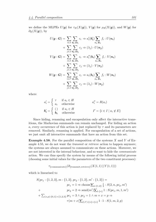
4.4. Parallel composition 101

we define the MLPEs U(g) for τH(X(g)), V (g) for ρR(X(g)), and W (g) for∂E(X(g)), by

U(g : G) =∑i∈I

∑di:Di

ci ⇒ a′i(b′i)∑•

ei:Ei

fi : U(ni)

+∑j∈J

∑dj :Dj

cj ⇒ (λj) · U(nj)

V (g : G) =∑i∈I

∑di:Di

ci ⇒ a′′i (bi)∑•

ei:Ei

fi : V (ni)

+∑j∈J

∑dj :Dj

cj ⇒ (λj) · V (nj)

W (g : G) =∑i∈I′

∑di:Di

ci ⇒ ai(bi)∑•

ei:Ei

fi : W (ni)

+∑j∈J

∑dj :Dj

cj ⇒ (λj) ·W (nj)

where

a′i =

τ if ai ∈ Hai otherwise

a′′i = R(ai)

b′i =

( ) if ai ∈ Hbi otherwise

I ′ = i ∈ I | ai 6∈ E

Since hiding, renaming and encapsulation only affect the interactive trans-itions, the Markovian summands can remain unchanged. For hiding an actiona, every occurrence of this action is just replaced by τ and its parameters areremoved. Similarly, renaming is applied. For encapsulation of a set of actions,we just omit all interactive summands that have an action from this set.

Example 4.58. For the parallel composition of the systems X and Y of Ex-ample 4.55, we do not want the transmit or retrieve action to happen anymore;the systems are always assumed to communicate on these actions. Moreover, weare not interested in the internal behaviour, and so want to hide the communicateaction. We can thus specify the system by means of the following initial process(choosing some initial values for the parameters of the two constituent processes):

τcommunicate(∂transmit,retrieve(X(1, 1) ||Y (1, 1)))

which is linearised to

S(pc1 : 1, 2, 3,m : 1, 2, pc2 : 1, 2,m′ : 1, 2) =

pc1 = 1⇒ choose∑•n:1,2

12 : S(2, n, pc2,m

′)

+ pc2 = 2⇒ send(m′)∑•

1:∗ 1 : S(pc1,m, 1,m′)

+∑

(x,p):0,1×1,2,3 pc1 = 3 ∧ pc2 = 1 ∧ m+ x = p⇒τ(m+ x)

∑•

(l,l′):∗×∗ 1 · 1 : S(1,m, 2, p)

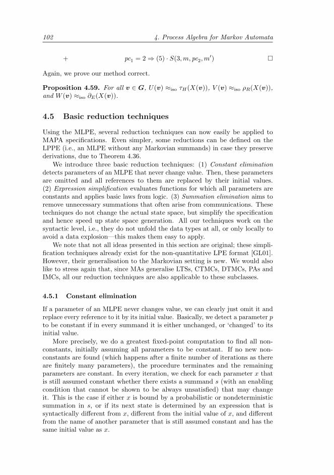
102 4. Process Algebra for Markov Automata

+ pc1 = 2⇒ (5) · S(3,m, pc2,m′)

Again, we prove our method correct.

Proposition 4.59. For all v ∈ G, U(v) ≈iso τH(X(v)), V (v) ≈iso ρR(X(v)),and W (v) ≈iso ∂E(X(v)).

4.5 Basic reduction techniques

Using the MLPE, several reduction techniques can now easily be applied toMAPA specifications. Even simpler, some reductions can be defined on theLPPE (i.e., an MLPE without any Markovian summands) in case they preservederivations, due to Theorem 4.36.

We introduce three basic reduction techniques: (1) Constant eliminationdetects parameters of an MLPE that never change value. Then, these parametersare omitted and all references to them are replaced by their initial values.(2) Expression simplification evaluates functions for which all parameters areconstants and applies basic laws from logic. (3) Summation elimination aims toremove unnecessary summations that often arise from communications. Thesetechniques do not change the actual state space, but simplify the specificationand hence speed up state space generation. All our techniques work on thesyntactic level, i.e., they do not unfold the data types at all, or only locally toavoid a data explosion—this makes them easy to apply.

We note that not all ideas presented in this section are original; these simpli-fication techniques already exist for the non-quantitative LPE format [GL01].However, their generalisation to the Markovian setting is new. We would alsolike to stress again that, since MAs generalise LTSs, CTMCs, DTMCs, PAs andIMCs, all our reduction techniques are also applicable to these subclasses.

4.5.1 Constant elimination

If a parameter of an MLPE never changes value, we can clearly just omit it andreplace every reference to it by its initial value. Basically, we detect a parameter pto be constant if in every summand it is either unchanged, or ‘changed’ to itsinitial value.

More precisely, we do a greatest fixed-point computation to find all non-constants, initially assuming all parameters to be constant. If no new non-constants are found (which happens after a finite number of iterations as thereare finitely many parameters), the procedure terminates and the remainingparameters are constant. In every iteration, we check for each parameter x thatis still assumed constant whether there exists a summand s (with an enablingcondition that cannot be shown to be always unsatisfied) that may changeit. This is the case if either x is bound by a probabilistic or nondeterministicsummation in s, or if its next state is determined by an expression that issyntactically different from x, different from the initial value of x, and differentfrom the name of another parameter that is still assumed constant and has thesame initial value as x.

4.5. Basic reduction techniques 103

Example 4.60. Consider the specification

P = (X(id : one, two) = say(id) ·X(id), X(one))

Clearly, the process variable id never changes value, so the specification can besimplified to P ′ = (X = say(one) ·X, X).

Proposition 4.61. The underlying MAs of an MLPE before and after constantelimination are isomorphic.

Actually, we initially implemented constant elimination for prCRL by havingit operate on the LPPE. It is easy to see that constant elimination is derivationpreserving. Hence, by Theorem 4.36 we can just use this implementation foroptimising MAPA specifications as well: first encode as prCRL, then linearise toan LPPE, then apply constant elimination, and then decode back to an MLPE(as depicted earlier in Figure 4.2).

Since every iteration goes through the MLPE once, and the number ofiterations is limited by the number of parameters m, the worst-case time-complexity is O(m ·N) (with N the size of the MLPE).

4.5.2 Expression simplification

Expressions occurring as enabling conditions, action parameters or next stateparameters can often be simplified. We apply two kinds of simplifications(recursively): (1) functions for which all parameters are constants are evaluated,and (2) basic laws from logic are applied.

Additionally, summands for which the enabling condition simplified to falseare removed, as they cannot contribute to the behaviour of an LPPE any-way. More thoroughly, we also check for each summand whether every localand global parameter with a finite type has at least one possible value forwhich the enabling condition does not simplify to false. If there exists a para-meter without at least one such a value, the summand apparently can never betaken and hence is removed.

Example 4.62. Consider the expression 3 = 1+2 ∨ x > 5. As all parameters ofthe addition function are given, the expression is first simplified to 3 = 3 ∨ x > 5.Then, the equality function can be evaluated, obtaining true ∨ x > 5. Finally,logic tells us that we can simplify once more, obtaining the expression true.

The following proposition is trivial: replacing expressions by equivalent onesdoes not change anything.

Proposition 4.63. The underlying MAs of an MLPE before and after expres-sion simplification are isomorphic.

Again, we actually employ an implementation on LPPEs via the encodingdiscussed earlier. After all, it is immediately clear that expression simplificationdoes not influence a process’s derivations.

Expression simplification is linear in the size of the MLPE, as it just processesall expressions one by one to simplify them.

104 4. Process Algebra for Markov Automata

4.5.3 Summation elimination

When composing parallel components that communicate based on messagepassing actions, often this results in summations that can be eliminated. Forinstance, summands with a nondeterministic choice of the form

∑d:D and a

condition d = e may arise, which can obviously be simplified by omitting thesummation and substituting e for every occurrence of d.

More precisely, to eliminate a sum∑d:D in a summand that has the enabling

condition c, we compute the set S of possible values that c allows for d (anduse the empty set if we cannot establish specific values). When c is given byd = e or e = d, where e is a value or an expression (in which d does not occurfreely) that can be evaluated, we take S to be the singleton set containing thisvalue. When c is a conjunction e1 ∧ e2, we take S = S1 ∩ S2, where Si is the setof possible values for c given by ei. For a disjunction, we take a union (unlessS1 = ∅ or S2 = ∅; in that case also S = ∅). If it turns out that S is a singletonset d′, we omit the summation and substitute every free occurrence of d by d′.

Example 4.64. Consider the specification X =∑d:1,2,3 d = 2⇒ send(d) ·X.

As the summand is only enabled for d = 2, the specification can be simplified toX = 2 = 2⇒ send(2) ·X. Expression simplification may further reduce this toX = send(2) ·X.

The concept of summation elimination described above, as well as the notionsof constant elimination and expression simplification, could be generalised tothe Markovian setting without any trouble. They all could be implemented forLPPEs and applied to MAPA by means of our encoding. Their procedures asdescribed here are basically no different from the way they were defined earlierfor the non-quantitative LPEs [GL01].

For the second part of summation elimination, which we define next, thisis not the case anymore: we have to be slightly more careful. In the contextof LPEs and LPPEs we reduced summands such as

∑d:1,2 a ·X to a ·X, as

the summation variable is not used anyway. This, however, does influence thenumber of derivations to take the action a. Hence, if this were an encoded rate,the reduction would be erroneous. Therefore, we have to define summationelimination directly on MLPEs. Interactive summands can be handled as before,but for Markovian summands the second kind of reduction is altered. Instead ofreducing

∑d:D(λ) ·X to (λ) ·X, we now reduce to (|D| × λ) ·X. That way, the

total rate to X remains the same.In fact, we can even reduce summations over a variable that also appears

in the condition and the rate of a Markovian summand, as long as it does notoccur in the probabilities and next state expressions and there are no othervariables that occur in the condition. For instance, we automatically reduce∑d:2..5 d < 4⇒ (di) ·X to (2i + 3i) ·X. To be precise, we reduce∑

d:D

c⇒ (λ) ·X to( ∑

d′∈Dc[d:=d′]

λ[d := d′])·X

where the second summation is meant in the mathematical sense. If the sum-

4.6. Contributions 105

mation variable d does not occur in the condition, we can just sum over all itsvalues and leave the condition intact.

Proposition 4.65. The underlying MAs of an MLPE before and after summa-tion elimination are isomorphic.

Summation elimination is linear in the size of the MLPE.

4.6 Contributions

We introduced a new process-algebraic framework—called MAPA (MarkovAutomata Process Algebra)—for modelling and generating MAs. It can beused to specify systems incorporating both nondeterminism, probability andMarkovian rates. Key ingredient is the combined treatment of data and data-dependent probabilistic choice in a fully symbolic manner. Since MAs generaliseLTSs, DTMCs, CTMCs, IMCs and PAs, the MAPA framework is applicable tospecifying systems in any of these domains.

We defined a restricted format of MAPA, the MLPE, that allows easy statespace generation and parallel composition. Also, its basic structure enables muchsimpler definitions of many reduction techniques, as will become apparent in thenext three chapters. We showed how MAPA specifications can be encoded in arestriction of itself, prCRL, and defined the novel concept of derivation-preservingbisimulation to prove under which circumstances MAPA transformations cansafely—that is, while preserving strong bisimulation—be defined solely on prCRL.

We showed how to linearise prCRL specifications to a restricted variant of theMLPE, while indeed obtaining derivation-preserving bisimilar results. Hence,the encoding scheme allows this procedure to be lifted to transform MAPAspecifications to MLPEs without any effort. That way, techniques defined onthe MLPE can be automatically applied to the full spectrum of MAPA.

The results show that the treatment of probabilities and Markovian ratesis simple and elegant, and rather orthogonal to the traditional setting [Use02].This is very desirable, as it simplifies the generalisation of existing techniquesto the Markovian setting. We did this for three existing reduction techniques:constant elimination, expression simplification and summation elimination. Thecase studies in Chapter 9 will demonstrate their significance, sometimes speedingup state space generation by more than an order of magnitude.

Although the CADP [CGH+10, GLMS13] and Modest [BDHK06] frame-works are also able to model rates and probabilistic choices in the presence ofdata, the MAPA framework is much simpler. None of the other quantitativeapproaches features a restricted format such as the MLPE, which allows us toeasily define reduction techniques that are not available in the other toolsets.CADP does implement bisimulation minimisation, but not for systems thatfeature both discrete probabilistic choice and stochastic timing—hence, it is notapplicable to MAs. As already discussed in Section 1.3 and in the introductionof this chapter, all other related specification languages cannot handle the fullspectrum of MAs and/or are not able to deal with data.

CHAPTER 5

Dead Variable Reduction

“Everything should be madeas simple as possible,

but no simpler.”

Albert Einstein

Section 4.5 introduced three techniques for MAPA that simplify the MLPErepresentation of specifications, without influencing the state space. Thecurrent chapter provides a different type of technique: dead variable reduc-

tion. This technique does not necessarily simplify MLPEs, but rather reducesthe number of states of the underlying MA while preserving strong bisimulation.We define this reduction technique on LPPEs, show that it yields derivation-preserving bisimilar systems, and apply Theorem 4.36 to show that it can be usedon MLPEs just as well. The linearisation procedure introduced in Section 4.3makes the technique applicable to all MAPA specifications. The idea of ourtechnique is to analyse when certain global variables of an LPPE are dead, alsocalled irrelevant. Basically, this means that for all continuations of the process,these variables are overwritten before they are used again. Hence, they can justas well be reset to their initial value, reducing the number of states.

Our approach. Due to the structure of an LPPE, it is not obvious whenvariables are irrelevant; this relies on the order in which summands can beexecuted. The explicit control flows of the original parallel processes have beenlost, though, since they were merged into one linear form. Therefore, it is notimmediately clear which values a variable may get in the future, or when it willbe overwritten. Moreover, some control flow could already have been encodedin the state parameters of the original specification. To solve this problem, wefirst present a technique to (re)construct the control flow graphs of an LPPE.This technique is based on detecting which state parameters act as programcounters for the underlying parallel processes; we call these counters control flowparameters (CFPs). We analyse which summands of the LPPE correspond toeach CFP, similar to the ideas of program slicing [Wei84].

Using the reconstructed control flow, we define a parameter to be relevantin a given state if, before being overwritten, it may be used by an enablingcondition, action parameter or probability distribution, or by an expression todetermine the value of another parameter that will be relevant in the next state.Based on this notion of relevance, we present a syntactic reduction technique

108 5. Dead Variable Reduction

that resets variables that are not relevant to their initial value. This is justified,because these variables will anyway be overwritten before ever being read. Weshow that our technique may only shrink the state space and that it neverenlarges it, and discuss a couple of our technical design choices. A case study ona handshake register shows its applicability in practice.

Related work. Liveness analysis techniques are well-known in compiler the-ory [ASU86]. However, their focus is often not on handling the multiple controlflows arising from parallelism. Moreover, these techniques generally work onlylocally for each block of program code, and aim at reducing execution timeinstead of state space size.

The concept of resetting dead variables for state space reduction was firstformalised by Bozga et al. [BFG99, FBG03], but in their analysis relevance ofvariables was only dealt with locally, such that a variable that is passed to aqueue or written to another variable was considered relevant, even if it is neverused afterwards. A similar technique was presented in [YG04], using analysisof control flow graphs. It suffers from the same locality restriction as [BFG99].Most recent is [GS06], which applies data flow analysis to value-passing processalgebras. It uses Petri nets as its intermediate format, featuring concurrencyand taking into account global liveness information. We improve on this workby providing a thorough formal foundation including bisimulation preservationproofs, and by showing that our transformation never increases the state space.Additionally, none of the aforementioned techniques works in the context of MAs.Most importantly, they do not attempt to reconstruct control flow informationthat is hidden in the state variables, missing opportunities for reduction—theycan only reduce based on control flow resulting from the structure of the parallelcomponents, whereas we can exploit user-induced control flow as well.

The µCRL toolkit already contained a tool parelm, implementing a basicvariant of our methods. Instead of resetting state parameters that are dead givensome context, it simply removes parameters that are dead in all contexts [GL01].That is, it marks all parameters that either occur in some condition or actionargument, and also (recursively and iteratively) all parameters that are usedin some summand to determine one of the marked parameters. Unmarkedparameters are then deleted. As it does not take into account the control flow,parameters that are sometimes relevant and sometimes not will never be reset.

Organisation of the chapter. We discuss the construction of control flow graphsin Section 5.1, the data flow analysis in Section 5.2, and the LPPE transformationin Section 5.3. Some potential adaptations to the framework, including examplesillustrating our choice for the current variant, are discussed in Section 5.4.In Section 5.5 we demonstrate our technique on a larger example. Finally,Section 5.6 concludes by summarising the contributions of this chapter.

Origins of the chapter. The ideas of dead variable reduction for non-probabilisticLPEs were developed by Jaco van de Pol, and published together with the authorin the proceedings of the 7th International Symposium on Automated Technology

5.1. Reconstructing the control flow graphs 109

for Verification and Analysis (ATVA) [vdPT09a] and a corresponding technicalreport [vdPT09b]. For this chapter, the author generalised the framework towork with LPPEs, and added correctness proofs for derivation preservation tobe able to apply the technique to MAPA specifications as well.

5.1 Reconstructing the control flow graphs

The techniques introduced in this chapter all work on LPPEs. As discussed inChapter 4, these are MLPEs without any Markovian summands (and hence theyare also part of the prCRL language):

Definition 4.37 (LPPEs). A linear probabilistic process equation (LPPE) isa MAPA specification of the following format:

X(g : G) =∑i∈I

∑di:Di

ci ⇒ ai(bi)∑•

ei:Ei

fi : X(ni)

Throughout this chapter we assume the existence of such an LPPE, withvariable names as indicated and an initial state vector init, and we assumethat it is decodable (see Remark 4.31). We use the indices i ∈ I to refer to itssummands. Without loss of generality, we assume that all variables in g (theparameters or global variables), di (the local variables) and ei (the probabilisticvariables) are unique—this can easily be achieved by renaming duplicates.

Given a vector of formal state parameters g, we use gj to refer to its jth

parameter. An actual state is a vector of values, which we often denote by v; weuse vj to refer to its jth value. We use Gj to denote the type of gj , and J for theset of all parameters gj . Furthermore, ni,j denotes the jth element of ni, andpars(t) the set of all parameters gj that syntactically occur in the expression t.

5.1.1 Basic control flow analysis

To construct the control flow of an LPPE, we detect which of its global parametersare acting as program counters for the system or a part of it. We take this to bethe case for a parameter gj ∈ J if each summand either leaves it unchanged (sincethat summand deals with a part of the system not governed by gj) or changes itfrom a specific value to another specific value (since that summand does dealwith a part of the system governed by gj). Of course, we could just rememberwhich parameters were introduced as program counters during the linearisationprocedure of Section 4.3. However, the approach we take here is more general: itdoes not only detect these parameters, but may additionally detect user-definedparameters to also act as program counters for (a part of) the system.

First, we define a parameter to be changed in a summand i if its value aftertaking i may be different from its current value. Clearly, this can only be thecase if the expression ni,j is different from gj .

Definition 5.1 (Changed parameters). Given a summand i, a parametergj ∈ J is changed in i if ni,j 6= gj, otherwise it is unchanged in i.

110 5. Dead Variable Reduction

Note that parameters that are changed according to this definition may stillkeep the same value. However, since this is not easily decidable in practice, wechose to take a safe overapproximation. Parameters that are unchanged in asummand i according to this definition indeed will never be changed by i.

For a summand i to change a parameter gj from one specific value to another,there should be one value s such that the enabling condition of i can only holdif gj has that value. We call this value the source of gj for i.

Definition 5.2 (Source functions). A function f : I × J → ⋃j∈J Gj ∪ ⊥

is a source function if, for every i ∈ I, gj ∈ J , and s ∈ Gj, f(i, gj) = s impliesthat

∀v ∈ G,d′i ∈Di . ci(v,d′i) =⇒ vj = s

Furthermore, f(i, gj) = ⊥ is always allowed; it indicates that no unique value scomplying to the above could be found.

From now on we assume a given source function source.

We note that source(i, gj) is allowed to be ⊥ even though there may be somesource s, as computing the source is in general undecidable—so, in practice heur-istics are used that sometimes yield ⊥ when in fact a source is present. However,we will see that this does not result in any errors. It may limit the effects of thereduction, though. The same holds for the destination functions defined below.

The heuristics we apply in our implementation (see Chapter 9) to find asource can handle equations, disjunctions and conjunctions, as well as negationsof boolean expressions. For an equational condition gj = c the source of gjis obviously c, for a disjunction of such terms we apply set union, and forconjunction intersection. If for some summand i a set of sources is obtained, itcan be split into multiple summands, such that each again has a unique source.

Example 5.3. Let ci be given by (gj = 3 ∨ gj = 5) ∧ gj = 3 ∧ gk = 10, thenobviously source(i, gj) = 3 is valid (because (3 ∪ 5) ∩ 3 = 3), but also(as always) source(i, gj) = ⊥ is allowed.

For a summand to change a parameter from one specific value to another,in addition to having a unique source it also should have a unique destination.We define the destination of a parameter gj for a summand i to be the uniquevalue gj obtains after taking i, regardless of the values of the global, local andprobabilistic variables. Again, we only specify a minimal requirement, since sucha value may not always easily be found.

Definition 5.4 (Destination functions). A function f : I×J → ⋃gj∈J Gj ∪

⊥ is a destination function if, for every i ∈ I, gj ∈ J , and s ∈ Gj , f(i, gj) = simplies that

∀v ∈ G,d′i ∈Di, e′i ∈ Ei . ci(v,d

′i) =⇒ ni,j(v,d

′i, e′i) = s

Furthermore, f(i, gj) = ⊥ is always allowed, indicating that no unique destinationvalue could be derived.

5.1. Reconstructing the control flow graphs 111

From now on we assume a given destination function dest.1

The heuristics in our implementation for computing dest(i, gj) substitutesource(i, gj) for gj in ni,j , and try to rewrite the result to a closed term.

Example 5.5. If ci is given by gj = 8 and ni,j by gj +5, then dest(i, gj) = 13 isvalid, but also (as always) dest(i, gj) = ⊥ is allowed. If for instance ci is gj = 5and ni,j equals e3, then dest(i, gj) can only yield ⊥, since the value of gj aftertaking i is not fixed (it depends on the value of e3).

We say that a parameter gj rules a summand i if both its source and itsdestination for that summand can be computed, i.e., are different from ⊥. Thisimplies that i indeed changes gj from one specific value to another, and hencethat i belongs to the part of the system governed by gj .

Definition 5.6 (The rules relation). A parameter gj ∈ J rules a summandi if

source(i, gj) 6= ⊥ and dest(i, gj) 6= ⊥The set of all summands ruled by gj is denoted by Rgj = i ∈ I | gj rules i.Furthermore, Vgj denotes the set of all possible values that gj can take before andafter taking one of the summands that it rules, plus its initial value. Formally,

Vgj = source(i, gj) | i ∈ Rgj ∪ dest(i, gj) | i ∈ Rgj ∪ initj

Examples will show that summands can be ruled by several parameters.

5.1.2 Control flow parameters

We now define a parameter to be a control flow parameter if it rules all summandsin which it is changed. Stated differently, in every summand a control flowparameter is either left alone or we know what happens to it. As discussedbefore, such a parameter can be seen as a program counter for the summands itrules, and therefore its values can be seen as locations. All other parameters arecalled data parameters.

Definition 5.7 (Control flow and data parameters). A parameter gj ∈ Jis a control flow parameter (CFP) if for all i ∈ I, either gj rules i or gj isunchanged in i. A parameter that is not a CFP is called a data parameter (DP).

We call the set of all summands i ∈ I ruled by gj its cluster (denoted aboveby Rgj ). The set of all CFPs is denoted by C, the set of all DPs by D.

Example 5.8. Consider the following LPPE, based on the specification inExample 4.25. It still consists of two buffers that continuously read and write

1Note that we could be a bit more liberal than the current definition, only requiringni,j(v,d

′i,e′i) = s for values e′i ∈ Ei such that fi(v,d

′i,e′i) > 0. We chose not to do so, to

keep the presentation simple. However, clearly all our results still hold for this more liberaldefinition.

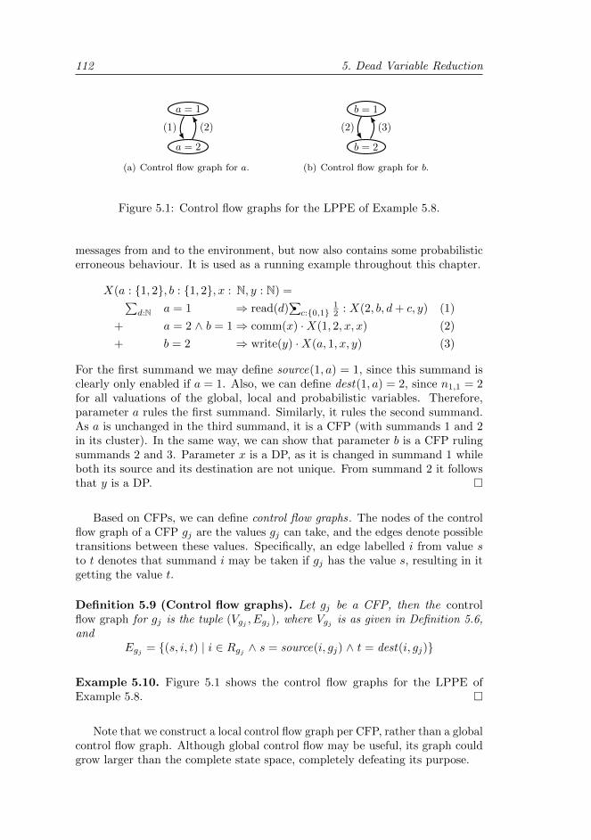
112 5. Dead Variable Reduction

a = 1

a = 2

(1) (2)

(a) Control flow graph for a.

b = 1

b = 2

(2) (3)

(b) Control flow graph for b.

Figure 5.1: Control flow graphs for the LPPE of Example 5.8.

messages from and to the environment, but now also contains some probabilisticerroneous behaviour. It is used as a running example throughout this chapter.

X(a : 1, 2, b : 1, 2, x : N, y : N) =∑d:N a = 1 ⇒ read(d)

∑•c:0,1

12 : X(2, b, d+ c, y) (1)

+ a = 2 ∧ b = 1⇒ comm(x) ·X(1, 2, x, x) (2)

+ b = 2 ⇒ write(y) ·X(a, 1, x, y) (3)

For the first summand we may define source(1, a) = 1, since this summand isclearly only enabled if a = 1. Also, we can define dest(1, a) = 2, since n1,1 = 2for all valuations of the global, local and probabilistic variables. Therefore,parameter a rules the first summand. Similarly, it rules the second summand.As a is unchanged in the third summand, it is a CFP (with summands 1 and 2in its cluster). In the same way, we can show that parameter b is a CFP rulingsummands 2 and 3. Parameter x is a DP, as it is changed in summand 1 whileboth its source and its destination are not unique. From summand 2 it followsthat y is a DP.

Based on CFPs, we can define control flow graphs. The nodes of the controlflow graph of a CFP gj are the values gj can take, and the edges denote possibletransitions between these values. Specifically, an edge labelled i from value sto t denotes that summand i may be taken if gj has the value s, resulting in itgetting the value t.

Definition 5.9 (Control flow graphs). Let gj be a CFP, then the controlflow graph for gj is the tuple (Vgj , Egj ), where Vgj is as given in Definition 5.6,and

Egj = (s, i, t) | i ∈ Rgj ∧ s = source(i, gj) ∧ t = dest(i, gj)

Example 5.10. Figure 5.1 shows the control flow graphs for the LPPE ofExample 5.8.

Note that we construct a local control flow graph per CFP, rather than a globalcontrol flow graph. Although global control flow may be useful, its graph couldgrow larger than the complete state space, completely defeating its purpose.

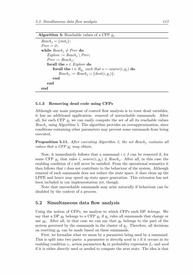
5.2. Simultaneous data flow analysis 113

Algorithm 5: Reachable values of a CFP gj .

Reachj = initj;Prev = ∅;while Reachj 6= Prev do

Explore := Reachj \Prev ;Prev := Reachj ;forall the s ∈ Explore do

forall the i ∈ Rgj such that s = source(i, gj) doReachj := Reachj ∪ dest(i, gj);

end

end

end

5.1.3 Removing dead code using CFPs

Although our main purpose of control flow analysis is to reset dead variables,it has an additional application: removal of unreachable summands. Afterall, for each CFP gj we can easily compute the set of all its reachable valuesReachj using Algorithm 5. The algorithm provides an overapproximation, sinceconditions containing other parameters may prevent some summands from beingexecuted.

Proposition 5.11. After executing Algorithm 5, the set Reachj contains allvalues that a CFP gj may obtain.

Now, it immediately follows that a summand i ∈ I can be removed if, forsome CFP gj that rules i, source(i, gj) 6∈ Reachj . After all, in this case theenabling condition of i will never be satisfied. From the operational semantics itthen follows that i does not contribute to the behaviour of the system. Althoughremoval of such summands does not reduce the state space, it does clean up theLPPE and hence may speed up state space generation. This extension has notbeen included in our implementation yet, though.

Note that unreachable summands may arise naturally if behaviour can bedisabled by the context of a process.

5.2 Simultaneous data flow analysis

Using the notion of CFPs, we analyse to which CFPs each DP belongs. Wesay that a DP gk belongs to a CFP gj if gj rules all summands that change oruse gk. After all, in that case we can say that gk belongs to the part of thesystem governed by the summands in the cluster of gj . Therefore, all decisionson resetting gk can be made based on these summands.

First, we formalise what we mean by a parameter being used by a summand.This is split into two parts: a parameter is directly used in i if it occurs in itsenabling condition ci, action parameters bi or probability expression fi, and usedif it is either directly used or needed to compute the next state. The idea is that

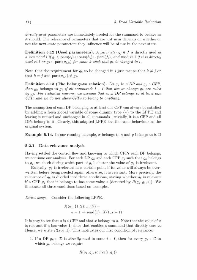
114 5. Dead Variable Reduction

directly used parameters are immediately needed for the summand to behave asit should. The relevance of parameters that are just used depends on whether ornot the next-state parameters they influence will be of use in the next state.

Definition 5.12 (Used parameters). A parameter gj ∈ J is directly used ina summand i if gj ∈ pars(ci) ∪ pars(bi) ∪ pars(fi), and used in i if it is directlyused in i or gj ∈ pars(ni,k) for some k such that gk is changed in i.

Note that the requirement for gk to be changed in i just means that k 6= j orthat k = j and pars(ni,j) 6= gj .

Definition 5.13 (The belongs-to relation). Let gk be a DP and gj a CFP,then gk belongs to gj if all summands i ∈ I that use or change gk are ruledby gj. For technical reasons, we assume that each DP belongs to at least oneCFP, and we do not allow CFPs to belong to anything.

The assumption of each DP belonging to at least one CFP can always be satisfiedby adding a fresh global variable of some dummy type ∗ to the LPPE andleaving it unused and unchanged in all summands—trivially, it is a CFP and allDPs belong to it. Clearly, this adapted LPPE has the same behaviour as theoriginal system.

Example 5.14. In our running example, x belongs to a and y belongs to b.

5.2.1 Data relevance analysis

Having settled the control flow and knowing to which CFPs each DP belongs,we continue our analysis. For each DP gk and each CFP gj such that gk belongsto gj , we check during which part of gj ’s cluster the value of gk is irrelevant.

Basically, gk is irrelevant at a certain point if its value will always be over-written before being needed again; otherwise, it is relevant. More precisely, therelevance of gk is divided into three conditions, stating whether gk is relevantif a CFP gj that it belongs to has some value s (denoted by R(gk, gj , s)). Weillustrate all three conditions based on examples.

Direct usage. Consider the following LPPE.

X(a : 1, 2, x : N) =

a = 1⇒ send(x) ·X(1, x+ 1)

It is easy to see that a is a CFP and that x belongs to a. Note that the value of xis relevant if a has value 1, since that enables a summand that directly uses x.Hence, we write R(x, a, 1). This motivates our first condition of relevance:

1. If a DP gk ∈ D is directly used in some i ∈ I, then for every gj ∈ C towhich gk belongs we require

R(gk, gj , source(i, gj))

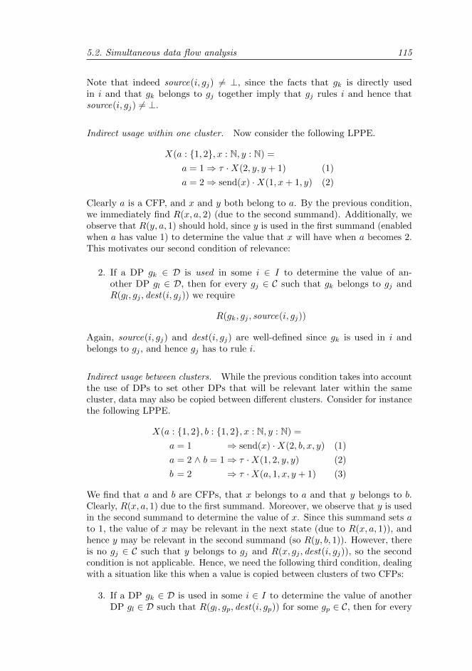
5.2. Simultaneous data flow analysis 115

Note that indeed source(i, gj) 6= ⊥, since the facts that gk is directly usedin i and that gk belongs to gj together imply that gj rules i and hence thatsource(i, gj) 6= ⊥.

Indirect usage within one cluster. Now consider the following LPPE.

X(a : 1, 2, x : N, y : N) =

a = 1⇒ τ ·X(2, y, y + 1) (1)

a = 2⇒ send(x) ·X(1, x+ 1, y) (2)

Clearly a is a CFP, and x and y both belong to a. By the previous condition,we immediately find R(x, a, 2) (due to the second summand). Additionally, weobserve that R(y, a, 1) should hold, since y is used in the first summand (enabledwhen a has value 1) to determine the value that x will have when a becomes 2.This motivates our second condition of relevance:

2. If a DP gk ∈ D is used in some i ∈ I to determine the value of an-other DP gl ∈ D, then for every gj ∈ C such that gk belongs to gj andR(gl, gj , dest(i, gj)) we require

R(gk, gj , source(i, gj))

Again, source(i, gj) and dest(i, gj) are well-defined since gk is used in i andbelongs to gj , and hence gj has to rule i.

Indirect usage between clusters. While the previous condition takes into accountthe use of DPs to set other DPs that will be relevant later within the samecluster, data may also be copied between different clusters. Consider for instancethe following LPPE.

X(a : 1, 2, b : 1, 2, x : N, y : N) =

a = 1 ⇒ send(x) ·X(2, b, x, y) (1)

a = 2 ∧ b = 1⇒ τ ·X(1, 2, y, y) (2)

b = 2 ⇒ τ ·X(a, 1, x, y + 1) (3)

We find that a and b are CFPs, that x belongs to a and that y belongs to b.Clearly, R(x, a, 1) due to the first summand. Moreover, we observe that y is usedin the second summand to determine the value of x. Since this summand sets ato 1, the value of x may be relevant in the next state (due to R(x, a, 1)), andhence y may be relevant in the second summand (so R(y, b, 1)). However, thereis no gj ∈ C such that y belongs to gj and R(x, gj , dest(i, gj)), so the secondcondition is not applicable. Hence, we need the following third condition, dealingwith a situation like this when a value is copied between clusters of two CFPs:

3. If a DP gk ∈ D is used in some i ∈ I to determine the value of anotherDP gl ∈ D such that R(gl, gp, dest(i, gp)) for some gp ∈ C, then for every

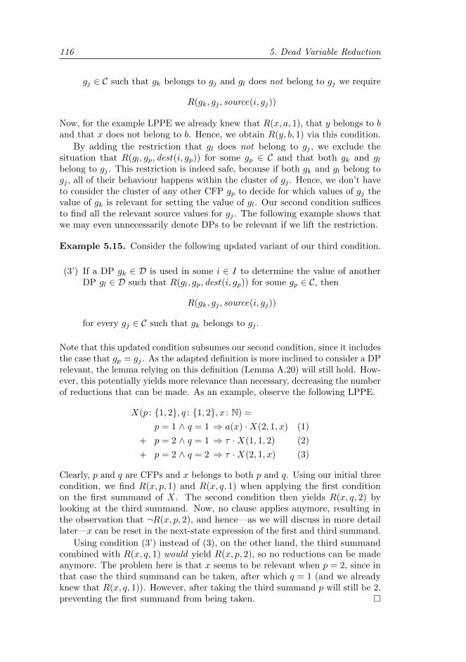
116 5. Dead Variable Reduction

gj ∈ C such that gk belongs to gj and gl does not belong to gj we require

R(gk, gj , source(i, gj))

Now, for the example LPPE we already knew that R(x, a, 1), that y belongs to band that x does not belong to b. Hence, we obtain R(y, b, 1) via this condition.

By adding the restriction that gl does not belong to gj , we exclude thesituation that R(gl, gp, dest(i, gp)) for some gp ∈ C and that both gk and glbelong to gj . This restriction is indeed safe, because if both gk and gl belong togj , all of their behaviour happens within the cluster of gj . Hence, we don’t haveto consider the cluster of any other CFP gp to decide for which values of gj thevalue of gk is relevant for setting the value of gl. Our second condition sufficesto find all the relevant source values for gj . The following example shows thatwe may even unnecessarily denote DPs to be relevant if we lift the restriction.

Example 5.15. Consider the following updated variant of our third condition.

(3’) If a DP gk ∈ D is used in some i ∈ I to determine the value of anotherDP gl ∈ D such that R(gl, gp, dest(i, gp)) for some gp ∈ C, then

R(gk, gj , source(i, gj))

for every gj ∈ C such that gk belongs to gj .

Note that this updated condition subsumes our second condition, since it includesthe case that gp = gj . As the adapted definition is more inclined to consider a DPrelevant, the lemma relying on this definition (Lemma A.20) will still hold. How-ever, this potentially yields more relevance than necessary, decreasing the numberof reductions that can be made. As an example, observe the following LPPE.

X(p : 1, 2, q : 1, 2, x : N) =

p = 1 ∧ q = 1 ⇒ a(x) ·X(2, 1, x) (1)

+ p = 2 ∧ q = 1 ⇒ τ ·X(1, 1, 2) (2)

+ p = 2 ∧ q = 2 ⇒ τ ·X(2, 1, x) (3)

Clearly, p and q are CFPs and x belongs to both p and q. Using our initial threecondition, we find R(x, p, 1) and R(x, q, 1) when applying the first conditionon the first summand of X. The second condition then yields R(x, q, 2) bylooking at the third summand. Now, no clause applies anymore, resulting inthe observation that ¬R(x, p, 2), and hence—as we will discuss in more detaillater—x can be reset in the next-state expression of the first and third summand.

Using condition (3’) instead of (3), on the other hand, the third summandcombined with R(x, q, 1) would yield R(x, p, 2), so no reductions can be madeanymore. The problem here is that x seems to be relevant when p = 2, since inthat case the third summand can be taken, after which q = 1 (and we alreadyknew that R(x, q, 1)). However, after taking the third summand p will still be 2,preventing the first summand from being taken.

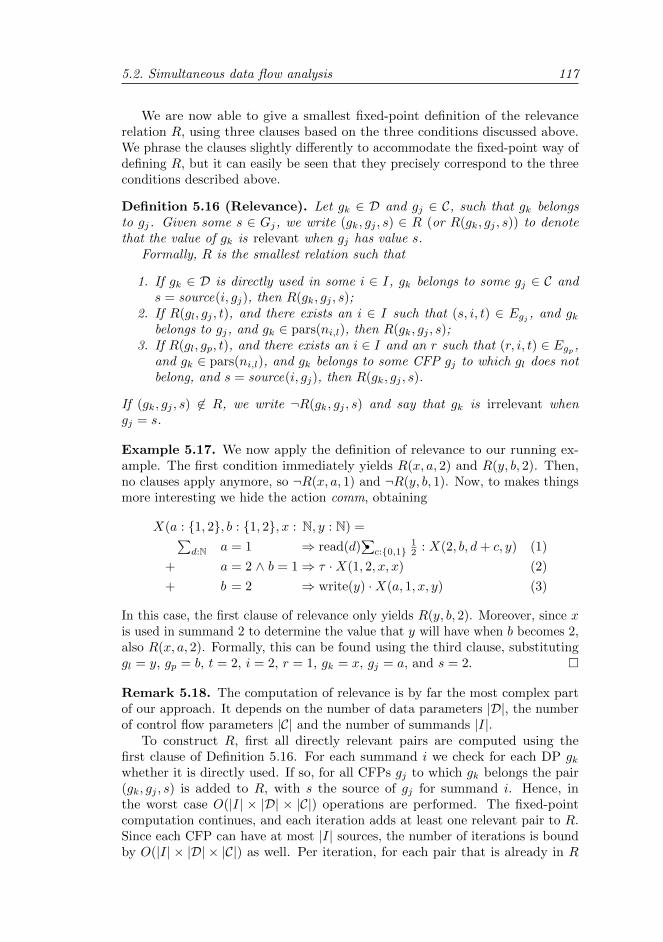
5.2. Simultaneous data flow analysis 117

We are now able to give a smallest fixed-point definition of the relevancerelation R, using three clauses based on the three conditions discussed above.We phrase the clauses slightly differently to accommodate the fixed-point way ofdefining R, but it can easily be seen that they precisely correspond to the threeconditions described above.

Definition 5.16 (Relevance). Let gk ∈ D and gj ∈ C, such that gk belongsto gj. Given some s ∈ Gj, we write (gk, gj , s) ∈ R (or R(gk, gj , s)) to denotethat the value of gk is relevant when gj has value s.

Formally, R is the smallest relation such that

1. If gk ∈ D is directly used in some i ∈ I, gk belongs to some gj ∈ C ands = source(i, gj), then R(gk, gj , s);

2. If R(gl, gj , t), and there exists an i ∈ I such that (s, i, t) ∈ Egj , and gkbelongs to gj, and gk ∈ pars(ni,l), then R(gk, gj , s);

3. If R(gl, gp, t), and there exists an i ∈ I and an r such that (r, i, t) ∈ Egp ,and gk ∈ pars(ni,l), and gk belongs to some CFP gj to which gl does notbelong, and s = source(i, gj), then R(gk, gj , s).

If (gk, gj , s) 6∈ R, we write ¬R(gk, gj , s) and say that gk is irrelevant whengj = s.

Example 5.17. We now apply the definition of relevance to our running ex-ample. The first condition immediately yields R(x, a, 2) and R(y, b, 2). Then,no clauses apply anymore, so ¬R(x, a, 1) and ¬R(y, b, 1). Now, to makes thingsmore interesting we hide the action comm, obtaining

X(a : 1, 2, b : 1, 2, x : N, y : N) =∑d:N a = 1 ⇒ read(d)

∑•c:0,1

12 : X(2, b, d+ c, y) (1)

+ a = 2 ∧ b = 1⇒ τ ·X(1, 2, x, x) (2)

+ b = 2 ⇒ write(y) ·X(a, 1, x, y) (3)

In this case, the first clause of relevance only yields R(y, b, 2). Moreover, since xis used in summand 2 to determine the value that y will have when b becomes 2,also R(x, a, 2). Formally, this can be found using the third clause, substitutinggl = y, gp = b, t = 2, i = 2, r = 1, gk = x, gj = a, and s = 2.

Remark 5.18. The computation of relevance is by far the most complex partof our approach. It depends on the number of data parameters |D|, the numberof control flow parameters |C| and the number of summands |I|.

To construct R, first all directly relevant pairs are computed using thefirst clause of Definition 5.16. For each summand i we check for each DP gkwhether it is directly used. If so, for all CFPs gj to which gk belongs the pair(gk, gj , s) is added to R, with s the source of gj for summand i. Hence, inthe worst case O(|I| × |D| × |C|) operations are performed. The fixed-pointcomputation continues, and each iteration adds at least one relevant pair to R.Since each CFP can have at most |I| sources, the number of iterations is boundby O(|I| × |D| × |C|) as well. Per iteration, for each pair that is already in R

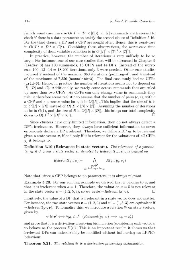
118 5. Dead Variable Reduction

(which worst case has size O(|I| × |D| × |C|)), all |I| summands are traversed tocheck if there is a data parameter to satisfy the second clause of Definition 5.16.For the third clause, a DP and a CFP are sought after. Hence, this is worst-casein O(|I|2 × |D|2 × |C|2). Combining these observations, the worst-case timecomplexity of dead variable reduction is in O(|I|3 × |D|3 × |C|3).

In practice, however, the number of iterations is very unlikely to be solarge. For instance, one of our case studies that will be discussed in Chapter 9(leader-3) has 100 summands, 13 CFPs and 14 DPs. Instead of the worst-case 100 · 13 · 14 = 18,200 iterations, only 3 were needed. Other case studiesrequired 2 instead of the maximal 360 iterations (polling-4), and 4 insteadof the maximum of 7,350 (hesselink-3). The final case study had no CFPs(grid-3). Hence, in practice the number of iterations seems not to depend on|I|, |D| and |C|. Additionally, we rarely come across summands that are ruledby more than two CFPs. As CFPs can only change value in summands theyrule, it therefore seems realistic to assume that the number of pairs (c, s), with ca CFP and s a source value for c, is in O(|I|). This implies that the size of R isin O(|I| × |D|) instead of O(|I| × |D| × |C|). Assuming the number of iterationsto be in O(1), and the size of R in O(|I| × |D|), this brings our total complexitydown to O(|I|2 × |D|2 × |C|).

Since clusters have only limited information, they do not always detect aDP’s irrelevance. However, they always have sufficient information to nevererroneously declare a DP irrelevant. Therefore, we define a DP gk to be relevantgiven a state vector v, if and only if it is relevant for the valuations of all CFPsgj it belongs to.

Definition 5.19 (Relevance in state vectors). The relevance of a parame-ter gk ∈ J given a state vector v, denoted by Relevant(gk,v), is defined by

Relevant(gk,v) =∧gj∈C

gk belongs to gj

R(gk, gj , vj)

Note that, since a CFP belongs to no parameters, it is always relevant.

Example 5.20. For our running example we derived that x belongs to a, andthat it is irrelevant when a = 1. Therefore, the valuation x = 5 is not relevantin the state vector v = (1, 2, 5, 3), so we write ¬Relevant(x,v).

Intuitively, the value of a DP that is irrelevant in a state vector does not matter.For instance, the two state vectors v = (1, 2, 3) and v′ = (1, 5, 3) are equivalent if¬Relevant(g2,v). To formalise this, we introduce a relation ∼= on state vectors,given by

v ∼= v′ ⇐⇒ ∀gk ∈ J : (Relevant(gk,v) =⇒ vk = v′k)

and prove that it is a derivation-preserving bisimulation (considering each vector vto behave as the process X(v). This is an important result: it shows us thatirrelevant DPs can indeed safely be modified without influencing an LPPE’sbehaviour.

Theorem 5.21. The relation ∼= is a derivation-preserving bisimulation.

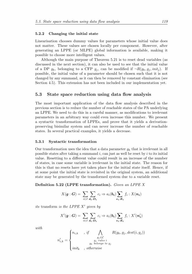
5.3. State space reduction using data flow analysis 119

5.2.2 Changing the initial state

Linearisation chooses dummy values for parameters whose initial value doesnot matter. These values are chosen locally per component. However, aftergenerating an LPPE (or MLPE) global information is available, making itpossible to choose more intelligent values.

Although the main purpose of Theorem 5.21 is to reset dead variables (asdiscussed in the next section), it can also be used to see that the initial valueof a DP gk, belonging to a CFP gj , can be modified if ¬R(gk, gj , initj). Ifpossible, the initial value of a parameter should be chosen such that it is notchanged by any summand, as it can then be removed by constant elimination (seeSection 4.5). This extension has not been included in our implementation yet.

5.3 State space reduction using data flow analysis

The most important application of the data flow analysis described in theprevious section is to reduce the number of reachable states of the PA underlyingan LPPE. We need to do this in a careful manner, as modifications to irrelevantparameters in an arbitrary way could even increase this number. We presenta syntactic transformation of LPPEs, and prove that it yields a derivation-preserving bisimilar system and can never increase the number of reachablestates. In several practical examples, it yields a decrease.

5.3.1 Syntactic transformation

Our transformation uses the idea that a data parameter gk that is irrelevant in allpossible states after taking a summand i, can just as well be reset by i to its initialvalue. Resetting to a different value could result in an increase of the numberof states, in case some variable is irrelevant in the initial state. The reason forthis is that no resets have yet taken place for the initial state itself. Hence, ifat some point the initial state is revisited in the original system, an additionalstate may be generated by the transformed system due to a variable reset.

Definition 5.22 (LPPE transformation). Given an LPPE X

X(g : G) =∑i∈I

∑di:Di

ci ⇒ ai(bi)∑•

ei:Ei

fi : X(ni)

its transform is the LPPE X ′ given by

X ′(g : G) =∑i∈I

∑di:Di

ci ⇒ ai(bi)∑•

ei:Ei

fi : X ′(n′i)

with

n′i,k =

ni,k , if

∧gj∈C

gj rules igk belongs to gj

R(gk, gj , dest(i, gj))

initk , otherwise

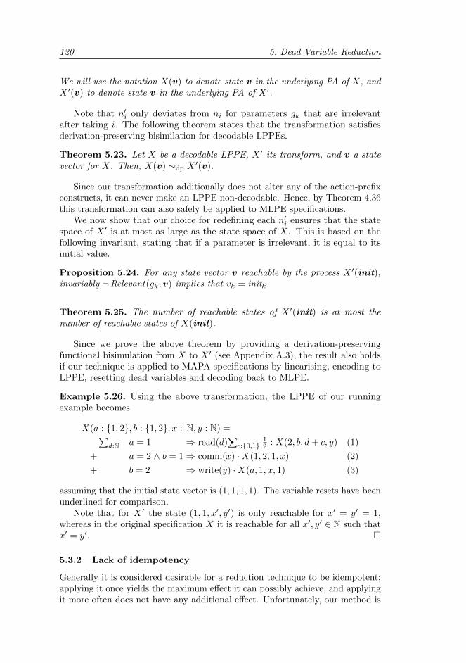
120 5. Dead Variable Reduction

We will use the notation X(v) to denote state v in the underlying PA of X, andX ′(v) to denote state v in the underlying PA of X ′.

Note that n′i only deviates from ni for parameters gk that are irrelevantafter taking i. The following theorem states that the transformation satisfiesderivation-preserving bisimilation for decodable LPPEs.

Theorem 5.23. Let X be a decodable LPPE, X ′ its transform, and v a statevector for X. Then, X(v) ∼dp X

′(v).

Since our transformation additionally does not alter any of the action-prefixconstructs, it can never make an LPPE non-decodable. Hence, by Theorem 4.36this transformation can also safely be applied to MLPE specifications.

We now show that our choice for redefining each n′i ensures that the statespace of X ′ is at most as large as the state space of X. This is based on thefollowing invariant, stating that if a parameter is irrelevant, it is equal to itsinitial value.

Proposition 5.24. For any state vector v reachable by the process X ′(init),invariably ¬Relevant(gk,v) implies that vk = initk.

Theorem 5.25. The number of reachable states of X ′(init) is at most thenumber of reachable states of X(init).

Since we prove the above theorem by providing a derivation-preservingfunctional bisimulation from X to X ′ (see Appendix A.3), the result also holdsif our technique is applied to MAPA specifications by linearising, encoding toLPPE, resetting dead variables and decoding back to MLPE.

Example 5.26. Using the above transformation, the LPPE of our runningexample becomes

X(a : 1, 2, b : 1, 2, x : N, y : N) =∑d:N a = 1 ⇒ read(d)

∑•c:0,1

12 : X(2, b, d+ c, y) (1)

+ a = 2 ∧ b = 1⇒ comm(x) ·X(1, 2, 1, x) (2)

+ b = 2 ⇒ write(y) ·X(a, 1, x, 1) (3)

assuming that the initial state vector is (1, 1, 1, 1). The variable resets have beenunderlined for comparison.

Note that for X ′ the state (1, 1, x′, y′) is only reachable for x′ = y′ = 1,whereas in the original specification X it is reachable for all x′, y′ ∈ N such thatx′ = y′.

5.3.2 Lack of idempotency

Generally it is considered desirable for a reduction technique to be idempotent;applying it once yields the maximum effect it can possibly achieve, and applyingit more often does not have any additional effect. Unfortunately, our method is

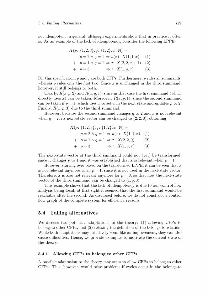
5.4. Failing alternatives 121

not idempotent in general, although experiments show that in practice it oftenis. As an example of the lack of idempotency, consider the following LPPE.

X(p : 1, 2, 3, q : 1, 2, x : N) =

p = 2 ∧ q = 1 ⇒ a(x) ·X(1, 1, x) (1)

+ p = 1 ∧ q = 1 ⇒ τ ·X(2, 2, x+ 1) (2)

+ p = 3 ⇒ τ ·X(1, q, x) (3)

For this specification, p and q are both CFPs. Furthermore, p rules all summands,whereas q rules only the first two. Since x is unchanged in the third summand,however, it still belongs to both.

Clearly, R(x, p, 2) and R(x, q, 1), since in that case the first summand (whichdirectly uses x) can be taken. Moreover, R(x, p, 1), since the second summandcan be taken if p = 1, which uses x to set x in the next state and updates p to 2.Finally, R(x, p, 3) due to the third summand.

However, because the second summand changes q to 2 and x is not relevantwhen q = 2, its next-state vector can be changed to (2, 2, 0), obtaining

X(p : 1, 2, 3, q : 1, 2, x : N) =

p = 2 ∧ q = 1 ⇒ a(x) ·X(1, 1, x) (1)

+ p = 1 ∧ q = 1 ⇒ τ ·X(2, 2, 0) (2)

+ p = 3 ⇒ τ ·X(1, q, x) (3)

The next-state vector of the third summand could not (yet) be transformed,since it changes p to 1 and it was established that x is relevant when p = 1.

However, starting over based on the transformed LPPE, it can be seen that xis not relevant anymore when p = 1, since it is not used in the next-state vector.Therefore, x is also not relevant anymore for p = 3, so that now the next-statevector of the third summand can be changed to (1, q, 0).

This example shows that the lack of idempotency is due to our control flowanalysis being local; at first sight it seemed that the first summand would bereachable after the second. As discussed before, we do not construct a controlflow graph of the complete system for efficiency reasons.

5.4 Failing alternatives

We discuss two potential adaptations to the theory: (1) allowing CFPs tobelong to other CFPs, and (2) relaxing the definition of the belongs-to relation.While both adaptations may intuitively seem like an improvement, they can alsocause difficulties. Hence, we provide examples to motivate the current state ofthe theory.

5.4.1 Allowing CFPs to belong to other CFPs

A possible adaptation to the theory may seem to allow CFPs to belong to otherCFPs. This, however, would raise problems if cycles occur in the belongs-to

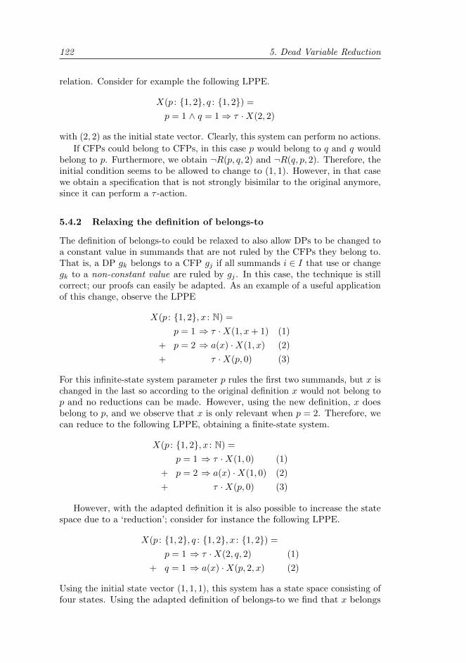
122 5. Dead Variable Reduction

relation. Consider for example the following LPPE.

X(p : 1, 2, q : 1, 2) =

p = 1 ∧ q = 1⇒ τ ·X(2, 2)

with (2, 2) as the initial state vector. Clearly, this system can perform no actions.

If CFPs could belong to CFPs, in this case p would belong to q and q wouldbelong to p. Furthermore, we obtain ¬R(p, q, 2) and ¬R(q, p, 2). Therefore, theinitial condition seems to be allowed to change to (1, 1). However, in that casewe obtain a specification that is not strongly bisimilar to the original anymore,since it can perform a τ -action.

5.4.2 Relaxing the definition of belongs-to

The definition of belongs-to could be relaxed to also allow DPs to be changed toa constant value in summands that are not ruled by the CFPs they belong to.That is, a DP gk belongs to a CFP gj if all summands i ∈ I that use or changegk to a non-constant value are ruled by gj . In this case, the technique is stillcorrect; our proofs can easily be adapted. As an example of a useful applicationof this change, observe the LPPE

X(p : 1, 2, x : N) =

p = 1 ⇒ τ ·X(1, x+ 1) (1)

+ p = 2 ⇒ a(x) ·X(1, x) (2)

+ τ ·X(p, 0) (3)

For this infinite-state system parameter p rules the first two summands, but x ischanged in the last so according to the original definition x would not belong top and no reductions can be made. However, using the new definition, x doesbelong to p, and we observe that x is only relevant when p = 2. Therefore, wecan reduce to the following LPPE, obtaining a finite-state system.

X(p : 1, 2, x : N) =

p = 1 ⇒ τ ·X(1, 0) (1)

+ p = 2 ⇒ a(x) ·X(1, 0) (2)

+ τ ·X(p, 0) (3)

However, with the adapted definition it is also possible to increase the statespace due to a ‘reduction’; consider for instance the following LPPE.

X(p : 1, 2, q : 1, 2, x : 1, 2) =

p = 1 ⇒ τ ·X(2, q, 2) (1)

+ q = 1 ⇒ a(x) ·X(p, 2, x) (2)

Using the initial state vector (1, 1, 1), this system has a state space consisting offour states. Using the adapted definition of belongs-to we find that x belongs

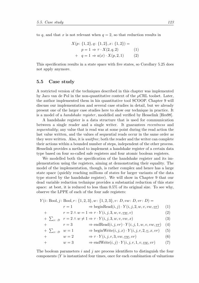
5.5. Case study 123

to q, and that x is not relevant when q = 2, so that reduction results in

X(p : 1, 2, q : 1, 2, x : 1, 2) =

p = 1 ⇒ τ ·X(2, q, 2) (1)

+ q = 1 ⇒ a(x) ·X(p, 2, 1) (2)

This specification results in a state space with five states, so Corollary 5.25 doesnot apply anymore.

5.5 Case study

A restricted version of the techniques described in this chapter was implementedby Jaco van de Pol in the non-quantitative context of the µCRL toolset. Later,the author implemented them in his quantitative tool SCOOP. Chapter 9 willdiscuss our implementation and several case studies in detail, but we alreadypresent one of the larger case studies here to show our technique in practice. Itis a model of a handshake register , modelled and verified by Hesselink [Hes98].

A handshake register is a data structure that is used for communicationbetween a single reader and a single writer. It guarantees recentness andsequentiality ; any value that is read was at some point during the read action thelast value written, and the values of sequential reads occur in the same order asthey were written. Also, it is waitfree; both the reader and the writer can completetheir actions within a bounded number of steps, independent of the other process.Hesselink provides a method to implement a handshake register of a certain datatype based on four so-called safe registers and four atomic boolean registers.

We modelled both the specification of the handshake register and its im-plementation using the registers, aiming at demonstrating their equality. Themodel of the implementation, though, is rather complex and hence has a largestate space (quickly reaching millions of states for larger variants of the datatype stored by the handshake register). We will show in Chapter 9 that ourdead variable reduction technique provides a substantial reduction of this statespace: at best, it is reduced to less than 0.5% of its original size. To see why,observe the LPPE of each of the four safe registers:

Y (i : Bool, j : Bool, r : 1, 2, 3, w : 1, 2, 3, v : D, vw : D, vr : D) =

r = 1 ⇒ beginRead(i, j) · Y (i, j, 2, w, v, vw, vr) (1)

+ r = 2 ∧ w = 1⇒ τ · Y (i, j, 3, w, v, vw, v) (2)

+∑x : D r = 2 ∧ w 6= 1⇒ τ · Y (i, j, 3, w, v, vw, x) (3)

+ r = 3 ⇒ endRead(i, j, vr) · Y (i, j, 1, w, v, vw, vr) (4)

+∑x : D w = 1 ⇒ beginWrite(i, j, x) · Y (i, j, r, 2, v, x, vr) (5)

+ w = 2 ⇒ τ · Y (i, j, r, 3, vw, vw, vr) (6)

+ w = 3 ⇒ endWrite(i, j) · Y (i, j, r, 1, v, vw, vr) (7)

The boolean parameters i and j are process identifiers to distinguish the fourcomponents (Y is instantiated four times, once for each combination of valuations

124 5. Dead Variable Reduction

for i and j). The parameter r denotes the read status, and w the write status.Reading consists of a beginRead action, a τ step, and an endRead action.

During the τ step either the contents of v is copied into vr (summand 2), or,when writing is taking place at the same time, a random value is copied to vr(summand 3). In the final step, the endRead action is taken with the value ofvr as a parameter (summand 4). Writing works by first storing the value to bewritten in vw (summand 5), and then copying vw to v (summand 6).

Our dead variable technique automatically detects several possibilities forvariable resets, indicated by the underlined variables in the specification. Theseare due to r and w being recognised as manually encoded control flow parameters.Based on these CFPs, our implementation detects that the value of vr is irrelevantafter summand 4, since it will not be used before summand 4 is reached again.This is always preceded by summand 2 or 3, both overwriting vr. Thus, vr canbe reset to its initial value in the next-state expression of summand 4. Theseresets drastically decrease the size of the state space, as our experiments willshow in Section 9.3.1. The CADP tool [GS06] was not able to make thesereductions, since it does not contain control flow reconstruction.

Note that the use of parallel processes for the reader and the writer insteadof our solution of encoding control flow in the data parameters—which wouldlimit the need for control flow reconstruction—would be difficult, because of theshared variables. Additionally, although the example may seem artificial, it isan almost one-to-one formalisation of its description in [Hes98]. Without ourmethod for control flow reconstruction, useful variable resets could not be foundautomatically. Manual optimisation would be hard and error-prone.

5.6 Contributions

We presented a novel method for reconstructing the local control flow of linearprocesses. The reconstruction process enables us to interpret some variablesas program counters. Especially when specifications are translated betweenlanguages, their control flow may be hidden in the state parameters (as showedby the case study presented in this chapter). To the best of our knowledge, nosuch reconstruction method appeared in literature before, and hence other toolsare not able to do this analysis. As an exception, our techniques have recentlybeen used and adapted [KWW13] to the context of PBESs (parameterisedBoolean equation systems). This now allows dead variable reduction to also beapplied in the mCRL2 toolset [CGK+13].

The reconstructed control flow is used for data flow analysis, aiming at statespace reduction by resetting variables that are irrelevant given a certain state. Weintroduced a transformation and proved its correctness with regard to derivation-preserving bisimilarity, as well as its property to never increase the state space.

By finding useful variable resets automatically, users can focus on modellingsystems in an intuitive way, instead of formulating models such that a toolsetcan handle them best. This idea of automatic syntactic transformations forimproving the efficiency of formal verification (not relying on users to maketheir models as efficient as possible) already proved to be a fruitful concept inearlier work [WH00]. Our case studies in Chapter 9 will show that significant

5.6. Contributions 125

reductions can indeed be obtained, sometimes shrinking state spaces to less than1% of their original size.

Part III

Confluence Reduction

CHAPTER 6

Confluence Reduction

“Art is the elimination of the unnecessary.”

Pablo Picasso

The previous chapters presented techniques for reducing MAPA specific-

ations while preserving strong bisimulation. Although these are all veryuseful, we can do much better in many cases: we can abstract from in-

ternal behaviour, reducing more while preserving divergence-sensitive branchingbisimulation1.

This chapter therefore generalises confluence reduction from LTSs to MAs.It is a powerful state space reduction technique based on commutativity oftransitions, removing spurious nondeterminism often arising from the parallelcomposition of largely independent components. The core is a confluent set ofinvisible transitions; these are chosen in such a way that they always connectbisimilar states. Confluence therefore paves the way for state space reductions,by giving confluent transitions priority over their neighbouring transitions.

The aim of our analysis is to efficiently approximate which invisible transitionsare confluent, and hence do not influence the observable behaviour. Althoughit may be beneficial to know all confluent transitions, this is often infeasiblein practice as it may require the entire state space—however, generating theunreduced system is precisely what we want to prevent. Hence, we settle for anunderapproximation. To the best of our knowledge, it is the first technique ofthis kind for MAs.

Our approach. In the probabilistic setting, transitions do not necessarily havea unique target state. Using an example, we argue that only τ -transitions witha unique target state can be considered confluent. Additionally, we generalisethe concept of commutativity to the probabilistic realm, taking into account theprobability of commuting paths. Based on these ideas, we define our novel notionof confluence for MAs. As in the non-probabilistic case, it specifies sufficientconditions for invisible transitions to not alter the behaviour of an MA; i.e., if atransition is found to be confluent in a state s, it may be given priority over allother transitions emanating from s.

We prove that confluent transitions connect divergence-sensitive branchingbisimilar states, and present a mapping of states to representatives to efficiently

1Since this chapter is only concerned with divergence-sensitive branching bisimulation, wewill often abbreviate this concept by just the term bisimulation.

130 6. Confluence Reduction

generate a reduced MA. We explain how confluence can be detected symbolicallyon specifications in the MAPA language, and provide a detailed exposition of ourheuristics to do so efficiently. Case studies in Chapter 9 applying these heuristicswill demonstrate state space reduction up to more than 90%, with decreases inanalysis time of sometimes more than 98%. We conclude with a discussion onpossible alternatives to our notions and show why these fail.

Related work. Compared to the earlier approach on confluence reduction forprocess algebras [BvdP02], the notion of confluence we present in this chapter isdifferent in three important ways:

• We can handle MAs, lifting confluence reduction to a significantly largerclass of systems (including the subclasses of PAs and IMCs).• We discuss a subtle flaw in the earlier work [BvdP02], and solve it by

introducing an underlying classification of the interactive transitions. Thisway we guarantee closure under unions, something that was not guaranteedbefore2. It is key to the way we detect confluence on MAPA specifications.• We preserve divergence and hence minimal reachability probabilities.

Outside the domain of confluence reduction, our technique is most relatedto partial order reduction (POR). Several types of POR have been defined,both for non-probabilistic [Val90, Val93, Pel93, GP93, God96] and probabilisticsystems [DN04, BGC04, BDG06]. These techniques are based on ideas similar toconfluence, choosing a subset of the outgoing transitions per state to reduce thestate space while preserving a certain notion of bisimulation or trace equivalence.None of these techniques is capable of reducing MAs. For the subclass of PAs,we provide a detailed comparison in Chapters 7 and 8, showing confluencereduction to be more powerful in theory as well as practice when restricting tothe preservation of branching-time properties.

Since none of the existing techniques is able to deal with MAs, we believe thatour generalisation—the first on-the-fly reduction technique for MAs abstract-ing from internal transitions—is a major step forward in efficient quantitativeverification.

Organisation of the chapter. We start in Section 6.1 by presenting an informalintroduction to the concept of confluence reduction. Since the additional technicaldifficulties due to probabilities and Markovian rates may distract from theunderlying ideas, we just consider confluence for LTSs in this introduction.Section 6.2 then discusses the additional difficulties when defining confluencefor probabilistic systems, introduces our novel notion of confluence for MAs,

2Actually, the approach taken in [BvdP02] resembles our approach to a large degree (exceptthat they consider a less expressive model and do not preserve divergence). While their claimof being able to take the union of confluent sets is faulty in general, their implementation workscorrectly. We show in this chapter that an additional technical restriction (the confluenceclassification) is needed to remedy the theoretical mistake, and this restriction happens to besatisfied in their implementation (in the same way as in ours). Since the confluence reductiontechnique described in [BvdP02] is a restricted variant of our notion, it could be fixed byintroducing a confluence classification precisely in the same way as we do in this chapter.

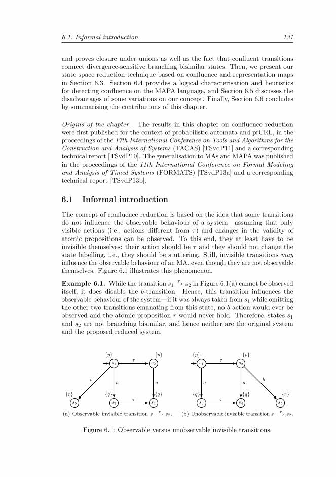
6.1. Informal introduction 131

and proves closure under unions as well as the fact that confluent transitionsconnect divergence-sensitive branching bisimilar states. Then, we present ourstate space reduction technique based on confluence and representation mapsin Section 6.3. Section 6.4 provides a logical characterisation and heuristicsfor detecting confluence on the MAPA language, and Section 6.5 discusses thedisadvantages of some variations on our concept. Finally, Section 6.6 concludesby summarising the contributions of this chapter.

Origins of the chapter. The results in this chapter on confluence reductionwere first published for the context of probabilistic automata and prCRL, in theproceedings of the 17th International Conference on Tools and Algorithms for theConstruction and Analysis of Systems (TACAS) [TSvdP11] and a correspondingtechnical report [TSvdP10]. The generalisation to MAs and MAPA was publishedin the proceedings of the 11th International Conference on Formal Modelingand Analysis of Timed Systems (FORMATS) [TSvdP13a] and a correspondingtechnical report [TSvdP13b].

6.1 Informal introduction

The concept of confluence reduction is based on the idea that some transitionsdo not influence the observable behaviour of a system—assuming that onlyvisible actions (i.e., actions different from τ) and changes in the validity ofatomic propositions can be observed. To this end, they at least have to beinvisible themselves: their action should be τ and they should not change thestate labelling, i.e., they should be stuttering. Still, invisible transitions mayinfluence the observable behaviour of an MA, even though they are not observablethemselves. Figure 6.1 illustrates this phenomenon.

Example 6.1. While the transition s1 −τ→ s2 in Figure 6.1(a) cannot be observeditself, it does disable the b-transition. Hence, this transition influences theobservable behaviour of the system—if it was always taken from s1 while omittingthe other two transitions emanating from this state, no b-action would ever beobserved and the atomic proposition r would never hold. Therefore, states s1

and s2 are not branching bisimilar, and hence neither are the original systemand the proposed reduced system.

s1

s3

s2

s4s5

p

q

p

qr

τ

a

τ

ab

(a) Observable invisible transition s1 −τ→ s2.

s1

s3

s2

s4 s5

p

q

p

q r

τ

a

τ

ab

(b) Unobservable invisible transition s1 −τ→ s2.

Figure 6.1: Observable versus unobservable invisible transitions.

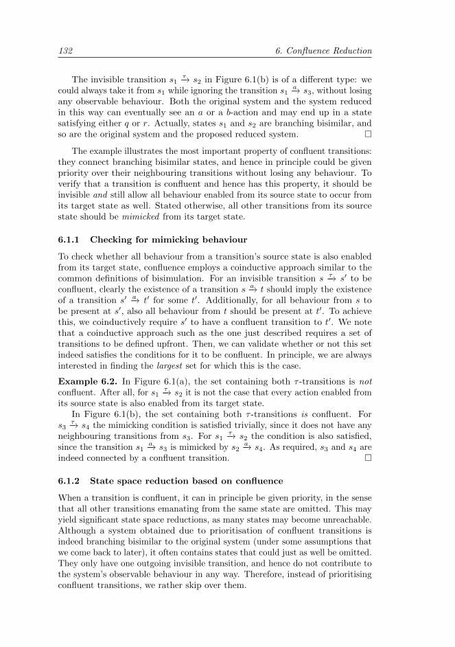
132 6. Confluence Reduction

The invisible transition s1 −τ→ s2 in Figure 6.1(b) is of a different type: wecould always take it from s1 while ignoring the transition s1 −a→ s3, without losingany observable behaviour. Both the original system and the system reducedin this way can eventually see an a or a b-action and may end up in a statesatisfying either q or r. Actually, states s1 and s2 are branching bisimilar, andso are the original system and the proposed reduced system.

The example illustrates the most important property of confluent transitions:they connect branching bisimilar states, and hence in principle could be givenpriority over their neighbouring transitions without losing any behaviour. Toverify that a transition is confluent and hence has this property, it should beinvisible and still allow all behaviour enabled from its source state to occur fromits target state as well. Stated otherwise, all other transitions from its sourcestate should be mimicked from its target state.

6.1.1 Checking for mimicking behaviour

To check whether all behaviour from a transition’s source state is also enabledfrom its target state, confluence employs a coinductive approach similar to thecommon definitions of bisimulation. For an invisible transition s −τ→ s′ to beconfluent, clearly the existence of a transition s −a→ t should imply the existenceof a transition s′ −a→ t′ for some t′. Additionally, for all behaviour from s tobe present at s′, also all behaviour from t should be present at t′. To achievethis, we coinductively require s′ to have a confluent transition to t′. We notethat a coinductive approach such as the one just described requires a set oftransitions to be defined upfront. Then, we can validate whether or not this setindeed satisfies the conditions for it to be confluent. In principle, we are alwaysinterested in finding the largest set for which this is the case.

Example 6.2. In Figure 6.1(a), the set containing both τ -transitions is notconfluent. After all, for s1 −τ→ s2 it is not the case that every action enabled fromits source state is also enabled from its target state.

In Figure 6.1(b), the set containing both τ -transitions is confluent. Fors3 −τ→ s4 the mimicking condition is satisfied trivially, since it does not have anyneighbouring transitions from s3. For s1 −τ→ s2 the condition is also satisfied,since the transition s1 −a→ s3 is mimicked by s2 −a→ s4. As required, s3 and s4 areindeed connected by a confluent transition.

6.1.2 State space reduction based on confluence

When a transition is confluent, it can in principle be given priority, in the sensethat all other transitions emanating from the same state are omitted. This mayyield significant state space reductions, as many states may become unreachable.Although a system obtained due to prioritisation of confluent transitions isindeed branching bisimilar to the original system (under some assumptions thatwe come back to later), it often contains states that could just as well be omitted.They only have one outgoing invisible transition, and hence do not contribute tothe system’s observable behaviour in any way. Therefore, instead of prioritisingconfluent transitions, we rather skip over them.

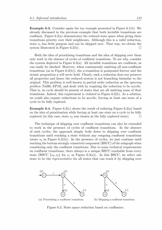
6.1. Informal introduction 133

Example 6.3. Consider again the toy example presented in Figure 6.1(b). Wealready discussed in the previous example that both invisible transitions areconfluent. Figure 6.2(a) demonstrates the reduced state space when giving thesetransitions priority over their neighbours. Although this is a valid reduction,state s1 has little purpose and can be skipped over. That way, we obtain thesystem illustrated in Figure 6.2(b).

Both the idea of prioritising transitions and the idea of skipping over themonly work in the absence of cycles of confluent transitions. To see why, considerthe system depicted in Figure 6.3(a). All invisible transitions are confluent, ascan easily be checked. However, when continuously omitting all non-confluenttransitions (as in Figure 6.3(b)), the a-transition is postponed forever and theatomic proposition q will never hold. Clearly, such a reduction does not preserveall properties and hence the reduced system is not branching bisimilar to theoriginal. This problem is well known in partial order reduction as the ignoringproblem [Val90, EP10], and dealt with by requiring the reduction to be acyclic.That is, no cycle should be present of states that are all omitting some of theirtransitions. Indeed, this requirement is violated in Figure 6.3(b). As a solution,we could also require reductions to be acyclic, forcing at least one state of acycle to be fully explored.

Example 6.4. Figure 6.3(c) shows the result of reducing Figure 6.3(a) basedon the idea of prioritisation while forcing at least one state on a cycle to be fullyexplored (in this case, state s2 was chosen as the fully explored state).

The technique of skipping over confluent transitions can also be extendedto work in the presence of cycles of confluent transitions. In the absenceof such cycles, the approach simply boils down to skipping over confluenttransitions until reaching a state without any outgoing confluent transitions(state s2 in Figure 6.2(b)). In the presence of cycles, we just continue untilreaching the bottom strongly connected component (BSCC) of the subgraph whenconsidering only the confluent transitions. Due to some technical requirementson confluent transitions, there always is a unique BSCC reachable from everystate (BSCC s2, s3 for s1 in Figure 6.3(a)). In this BSCC, we select onestate to be the representative for all states that can reach it by skipping over

s1 s2

s4 s5

p p

q r

τ

ab

(a) Prioritising a confluent transition.

s2

s4 s5

p

q r

ab

(b) Skipping a confluent transition.

Figure 6.2: State space reduction based on confluence.

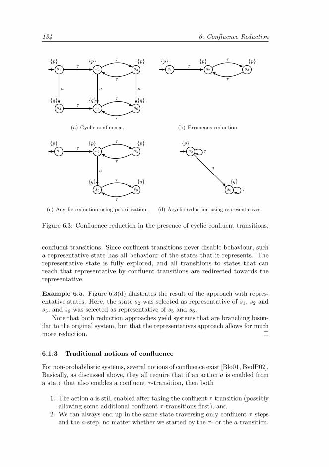
134 6. Confluence Reduction

s1

s4

s2

s5

s3

s6

p

q

p

q

p

q

τ

τ

a

τ

τ

τ

τ

a a

(a) Cyclic confluence.

s1 s2 s3

p p pτ

τ

τ

(b) Erroneous reduction.

s1 s2

s5

s3

s6

p p

q

p

q

τ

τ

τ

τ

τ

a

(c) Acyclic reduction using prioritisation.

s2

s6

τ

p

qτ

a

(d) Acyclic reduction using representatives.

Figure 6.3: Confluence reduction in the presence of cyclic confluent transitions.

confluent transitions. Since confluent transitions never disable behaviour, sucha representative state has all behaviour of the states that it represents. Therepresentative state is fully explored, and all transitions to states that canreach that representative by confluent transitions are redirected towards therepresentative.

Example 6.5. Figure 6.3(d) illustrates the result of the approach with repres-entative states. Here, the state s2 was selected as representative of s1, s2 ands3, and s6 was selected as representative of s5 and s6.

Note that both reduction approaches yield systems that are branching bisim-ilar to the original system, but that the representatives approach allows for muchmore reduction.

6.1.3 Traditional notions of confluence

For non-probabilistic systems, several notions of confluence exist [Blo01, BvdP02].Basically, as discussed above, they all require that if an action a is enabled froma state that also enables a confluent τ -transition, then both

1. The action a is still enabled after taking the confluent τ -transition (possiblyallowing some additional confluent τ -transitions first), and

2. We can always end up in the same state traversing only confluent τ -stepsand the a-step, no matter whether we started by the τ - or the a-transition.

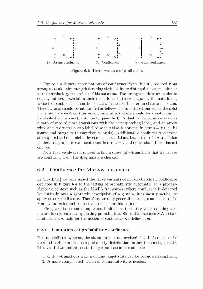
6.2. Confluence for Markov automata 135

•

•

•

•

a

τc

a

τc

(a) Strong confluence.

•

•

•

•

•

a

τc

a

τcτc

(b) Confluence.

•

•

•

•

•

•

a

τc

τc

a

τcτc

(c) Weak confluence.

Figure 6.4: Three variants of confluence.

Figure 6.4 depicts three notions of confluence from [Blo01], ordered fromstrong to weak—the strength denoting their ability to distinguish systems, similarto the terminology for notions of bisimulation. The stronger notions are easier todetect, but less powerful in their reductions. In these diagrams, the notation τcis used for confluent τ -transitions, and a can either be τ or an observable action.The diagrams should be interpreted as follows: for any state from which the solidtransitions are enabled (universally quantified), there should be a matching forthe dashed transitions (existentially quantified). A double-headed arrow denotesa path of zero of more transitions with the corresponding label, and an arrowwith label a denotes a step labelled with a that is optional in case a = τ (i.e., itssource and target state may then coincide). Additionally, confluent transitionsare required to be mimicked by confluent transitions; i.e., if the solid a-transitionin these diagrams is confluent (and hence a = τ), then so should the dashedone be.

Note that we always first need to find a subset of τ -transitions that we believeare confluent; then, the diagrams are checked.

6.2 Confluence for Markov automata

In [TSvdP11] we generalised the three variants of non-probabilistic confluencedepicted in Figure 6.4 to the setting of probabilistic automata. In a process-algebraic context such as the MAPA framework, where confluence is detectedheuristically over a syntactic description of a system, it is most practical toapply strong confluence. Therefore, we only generalise strong confluence to theMarkovian realm and from now on focus on this notion.

First, we discuss some important limitations that arise when defining con-fluence for systems incorporating probabilities. Since this includes MAs, theselimitations also hold for the notion of confluence we define later.

6.2.1 Limitations of probabilistic confluence

For probabilistic systems, the situation is more involved than before, since thetarget of each transition is a probability distribution, rather than a single state.This yields two limitations to the generalisation of confluence:

1. Only τ -transitions with a unique target state can be considered confluent;2. A more complicated notion of commutativity is needed.

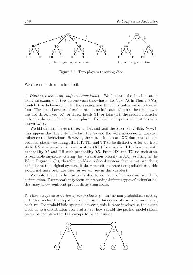
136 6. Confluence Reduction

XX

XHTXHX XT

HH THTH TT HT TTHH HT

12

12

τ 12

12t2

12

12t2

12

12t2

12

12τ

12

12τ

(a) The original specification.

XX

TXHX

TH TTHH HT

12

12τ

12

12t2

12

12t2

(b) A wrong reduction.

Figure 6.5: Two players throwing dice.

We discuss both issues in detail.

1. Dirac restriction on confluent transitions. We illustrate the first limitationusing an example of two players each throwing a die. The PA in Figure 6.5(a)models this behaviour under the assumption that it is unknown who throwsfirst. The first character of each state name indicates whether the first playerhas not thrown yet (X), or threw heads (H) or tails (T); the second characterindicates the same for the second player. For lay-out purposes, some states weredrawn twice.

We hid the first player’s throw action, and kept the other one visible. Now, itmay appear that the order in which the t2- and the τ -transition occur does notinfluence the behaviour. However, the τ -step from state XX does not connectbisimilar states (assuming HH, HT, TH, and TT to be distinct). After all, fromstate XX it is possible to reach a state (XH) from where HH is reached withprobability 0.5 and TH with probability 0.5. From HX and TX no such stateis reachable anymore. Giving the τ -transition priority in XX, resulting in thePA in Figure 6.5(b), therefore yields a reduced system that is not branchingbisimilar to the original system. If the τ -transitions were non-probabilistic, thiswould not have been the case (as we will see in this chapter).

We note that this limitation is due to our goal of preserving branchingbisimulation. Future work may focus on preserving different types of bisimulation,that may allow confluent probabilistic transitions.

2. More complicated notion of commutativity. In the non-probabilistic settingof LTSs it is clear that a path aτ should reach the same state as its correspondingpath τa. For probabilistic systems, however, this is more involved as the a-stepleads us to a distribution over states. So, how should the partial model shownbelow be completed for the τ -steps to be confluent?

s t

s1 s2

12

12

a

τ

t2t1 t3

16

13

12

a

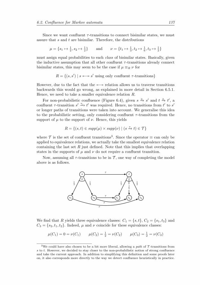
6.2. Confluence for Markov automata 137

Since we want confluent τ -transitions to connect bisimilar states, we mustassure that s and t are bisimilar. Therefore, the distributions

µ = s1 7→ 12 , s2 7→ 1

2 and ν = t1 7→ 13 , t2 7→ 1

6 , t3 7→ 12

must assign equal probabilities to each class of bisimilar states. Basically, giventhe inductive assumption that all other confluent τ -transitions already connectbisimilar states, this may seem to be the case if µ ≡R ν for

R = (s, s′) | s s′ using only confluent τ -transitions

However, due to the fact that the relation allows us to traverse transitionsbackwards this would go wrong, as explained in more detail in Section 6.5.1.Hence, we need to take a smaller equivalence relation R.

For non-probabilistic confluence (Figure 6.4), given s −a→ s′ and t −a→ t′, aconfluent τ -transition s′ −τc−→ t′ was required. Hence, no transitions from t′ to s′

or longer paths of transitions were taken into account. We generalise this ideato the probabilistic setting, only considering confluent τ -transitions from thesupport of µ to the support of ν. Hence, this yields

R = (s, t) ∈ supp(µ)× supp(ν) | (s −τ→ t) ∈ T

where T is the set of confluent transitions3. Since the operator ≡ can only beapplied to equivalence relations, we actually take the smallest equivalence relationcontaining the last set R just defined. Note that this implies that overlappingstates in the supports of µ and ν do not require a confluent transition.

Now, assuming all τ -transitions to be in T , one way of completing the modelabove is as follows.

s t

s1 s2

12

12

a

τ

t2t1 t3

16

13

12

a

τ

τ

τ

We find that R yields three equivalence classes: C1 = s, t, C2 = s1, t3 andC3 = s2, t1, t2. Indeed, µ and ν coincide for these equivalence classes:

µ(C1) = 0 = ν(C1) µ(C2) = 12 = ν(C2) µ(C3) = 1

2 = ν(C3)

3We could have also chosen to be a bit more liberal, allowing a path of T -transitions froms to t. However, we decided to stay closer to the non-probabilistic notion of strong confluenceand take the current approach. In addition to simplifying this definition and some proofs lateron, it also corresponds more directly to the way we detect confluence heuristically in practice.

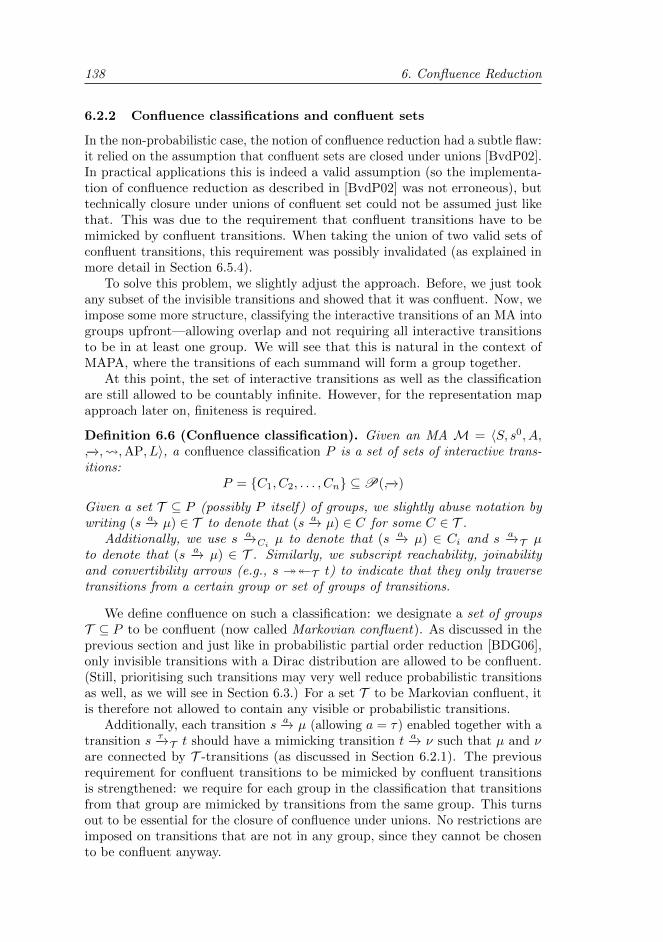
138 6. Confluence Reduction

6.2.2 Confluence classifications and confluent sets

In the non-probabilistic case, the notion of confluence reduction had a subtle flaw:it relied on the assumption that confluent sets are closed under unions [BvdP02].In practical applications this is indeed a valid assumption (so the implementa-tion of confluence reduction as described in [BvdP02] was not erroneous), buttechnically closure under unions of confluent set could not be assumed just likethat. This was due to the requirement that confluent transitions have to bemimicked by confluent transitions. When taking the union of two valid sets ofconfluent transitions, this requirement was possibly invalidated (as explained inmore detail in Section 6.5.4).

To solve this problem, we slightly adjust the approach. Before, we just tookany subset of the invisible transitions and showed that it was confluent. Now, weimpose some more structure, classifying the interactive transitions of an MA intogroups upfront—allowing overlap and not requiring all interactive transitionsto be in at least one group. We will see that this is natural in the context ofMAPA, where the transitions of each summand will form a group together.

At this point, the set of interactive transitions as well as the classificationare still allowed to be countably infinite. However, for the representation mapapproach later on, finiteness is required.

Definition 6.6 (Confluence classification). Given an MA M = 〈S, s0, A,−→, ,AP, L〉, a confluence classification P is a set of sets of interactive trans-itions:

P = C1, C2, . . . , Cn ⊆P(−→)

Given a set T ⊆ P (possibly P itself) of groups, we slightly abuse notation bywriting (s −a→ µ) ∈ T to denote that (s −a→ µ) ∈ C for some C ∈ T .

Additionally, we use s −a→Ci µ to denote that (s −a→ µ) ∈ Ci and s −a→T µto denote that (s −a→ µ) ∈ T . Similarly, we subscript reachability, joinabilityand convertibility arrows (e.g., s T t) to indicate that they only traversetransitions from a certain group or set of groups of transitions.

We define confluence on such a classification: we designate a set of groupsT ⊆ P to be confluent (now called Markovian confluent). As discussed in theprevious section and just like in probabilistic partial order reduction [BDG06],only invisible transitions with a Dirac distribution are allowed to be confluent.(Still, prioritising such transitions may very well reduce probabilistic transitionsas well, as we will see in Section 6.3.) For a set T to be Markovian confluent, itis therefore not allowed to contain any visible or probabilistic transitions.

Additionally, each transition s −a→ µ (allowing a = τ) enabled together with atransition s −τ→T t should have a mimicking transition t −a→ ν such that µ and νare connected by T -transitions (as discussed in Section 6.2.1). The previousrequirement for confluent transitions to be mimicked by confluent transitionsis strengthened: we require for each group in the classification that transitionsfrom that group are mimicked by transitions from the same group. This turnsout to be essential for the closure of confluence under unions. No restrictions areimposed on transitions that are not in any group, since they cannot be chosento be confluent anyway.

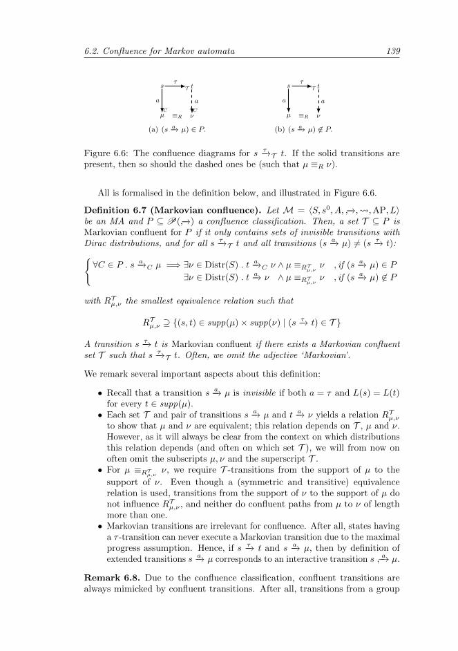
6.2. Confluence for Markov automata 139

s tT

µ νC C

τ

a a

≡R(a) (s −a→ µ) ∈ P.

s tT

µ ν

τ

a a

≡R(b) (s −a→ µ) 6∈ P.

Figure 6.6: The confluence diagrams for s −τ→T t. If the solid transitions arepresent, then so should the dashed ones be (such that µ ≡R ν).

All is formalised in the definition below, and illustrated in Figure 6.6.

Definition 6.7 (Markovian confluence). Let M = 〈S, s0, A, −→, ,AP, L〉be an MA and P ⊆ P(−→) a confluence classification. Then, a set T ⊆ P isMarkovian confluent for P if it only contains sets of invisible transitions withDirac distributions, and for all s −τ→T t and all transitions (s −a→ µ) 6= (s −τ→ t):∀C ∈ P . s −a→C µ =⇒ ∃ν ∈ Distr(S) . t −a→C ν ∧ µ ≡RTµ,ν ν , if (s −a→ µ) ∈ P

∃ν ∈ Distr(S) . t −a→ ν ∧ µ ≡RTµ,ν ν , if (s −a→ µ) 6∈ P

with RTµ,ν the smallest equivalence relation such that

RTµ,ν ⊇ (s, t) ∈ supp(µ)× supp(ν) | (s −τ→ t) ∈ T

A transition s −τ→ t is Markovian confluent if there exists a Markovian confluentset T such that s −τ→T t. Often, we omit the adjective ‘Markovian’.

We remark several important aspects about this definition:

• Recall that a transition s −a→ µ is invisible if both a = τ and L(s) = L(t)for every t ∈ supp(µ).

• Each set T and pair of transitions s −a→ µ and t −a→ ν yields a relation RTµ,νto show that µ and ν are equivalent; this relation depends on T , µ and ν.However, as it will always be clear from the context on which distributionsthis relation depends (and often on which set T ), we will from now onoften omit the subscripts µ, ν and the superscript T .

• For µ ≡RTµ,ν ν, we require T -transitions from the support of µ to the

support of ν. Even though a (symmetric and transitive) equivalencerelation is used, transitions from the support of ν to the support of µ donot influence RTµ,ν , and neither do confluent paths from µ to ν of lengthmore than one.

• Markovian transitions are irrelevant for confluence. After all, states havinga τ -transition can never execute a Markovian transition due to the maximalprogress assumption. Hence, if s −τ→ t and s −a→ µ, then by definition ofextended transitions s −a→ µ corresponds to an interactive transition s a−→ µ.

Remark 6.8. Due to the confluence classification, confluent transitions arealways mimicked by confluent transitions. After all, transitions from a group

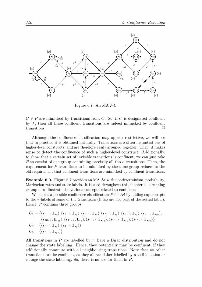
140 6. Confluence Reduction

s1

s0

s2

s3

s4

s5

s6 s17

s8

s7

s9

s11

s10s12

s13 s14

s15

s16

p

p

q

qτ1

910

910

a

a

τ1

τ1

τ2

τ2

τ1

b

b

b

b110

110

q

q

qr

s

s

s

st

s

s

ss

q

τ

τ3

τ1 τ1

τ1τ1

c

c

c

c

τ

τ1

5

7

τ1

τ1

Figure 6.7: An MA M.

C ∈ P are mimicked by transitions from C. So, if C is designated confluentby T , then all these confluent transitions are indeed mimicked by confluenttransitions.

Although the confluence classification may appear restrictive, we will seethat in practice it is obtained naturally. Transitions are often instantiations ofhigher-level constructs, and are therefore easily grouped together. Then, it makessense to detect the confluence of such a higher-level construct. Additionally,to show that a certain set of invisible transitions is confluent, we can just takeP to consist of one group containing precisely all those transitions. Then, therequirement for P -transitions to be mimicked by the same group reduces to theold requirement that confluent transitions are mimicked by confluent transitions.

Example 6.9. Figure 6.7 provides an MAM with nondeterminism, probability,Markovian rates and state labels. It is used throughout this chapter as a runningexample to illustrate the various concepts related to confluence.

We depict a possible confluence classification P forM by adding superscriptsto the τ -labels of some of the transitions (these are not part of the actual label).Hence, P contains three groups:

C1 = (s0, τ,1s1), (s2, τ,1s3), (s3, τ,1s4), (s5, τ,1s6), (s8, τ,1s9), (s9, τ,1s10),

(s10, τ,1s11), (s11, τ,1s8), (s13, τ,1s14), (s16, τ,1s15), (s15, τ,1s10)C2 = (s3, τ,1s5), (s4, τ,1s6)C3 = (s6, τ,1s17)

All transitions in P are labelled by τ , have a Dirac distribution and do notchange the state labelling. Hence, they potentially may be confluent, if theyadditionally commute with all neighbouring transitions. Note that no othertransitions can be confluent, as they all are either labelled by a visible action orchange the state labelling. So, there is no use for them in P .

6.2. Confluence for Markov automata 141

Now, we take T = C1 and show that it is a Markovian confluent set.We have to show that each transition in T is confluent as defined above. Weillustrate this for a couple of transitions.

First, consider s0 −τ→T s1. There is one other transition from s0, namelys0 −a→ µ with µ(s2) = 9

10 and µ(s0) = 110 . Since s0 −a→ µ 6∈ P , we need to show

that ∃ν ∈ Distr(S) . s1 −a→ ν ∧ µ ≡R ν. We take s1 −a→ ν with ν(s3) = 910 and

ν(s1) = 110 . This yields

R = Id ∪ (s0, s1), (s1, s0), (s2, s3), (s3, s2)

with Id the identity relation. Indeed, µ and ν assign the same probability toeach equivalence class of R, so µ ≡R ν.

Second, consider s2 −τ→T s3. Since there are no other transitions from s2,there is nothing to check. The same holds for several other transitions in T .

Finally, consider s3 −τ→T s4. There are two other transitions from s3, namely

s3 −b→ 1s7 and s3 −τ→ 1s5 . The first one can be mimicked by s4 −b→ 1s7 . Clearly1s7 ≡R 1s7 , due to reflexivity. The second can be mimicked by s4 −τ→ 1s6 . Then,

R = Id ∪ (s5, s6), (s6, s5)

and hence indeed 1s5 ≡R 1s6 . Since s3 −τ→ 1s5 ∈ C2, we additionally need tocheck that also s4 −τ→ 1s6 ∈ C2. This is indeed the case.

The remaining transitions can be shown to satisfy the requirements in thesame manner.

6.2.3 Properties of confluent sets

Since confluent transitions are always mimicked by confluent transitions, confluentpaths (i.e., paths following only transitions from a confluent set) are alwaysjoinable. This is captured by the following proposition.

Proposition 6.10. Let M = 〈S, s0, A, −→, ,AP, L〉 be an MA, P ⊆P(−→) aconfluence classification for M and T a Markovian confluent set for P . Then,

s T t if and only if sT t

Due to the confluence classification, we now also do have a closure result.Closure under union tells us that it is safe to show confluence of multiple setsof transitions in isolation, and then just take their union as one confluent set.Also, it implies that there exists a unique maximal confluent set.

Theorem 6.11. Let M = 〈S, s0, A, −→, ,AP, L〉 be an MA, P ⊆ P(−→) aconfluence classification for M and T1, T2 two Markovian confluent sets for P .Then, T1 ∪ T2 is also a Markovian confluent set for P .

Example 6.12. Example 6.9 demonstrated that T = C1 is confluent for ourrunning example. In the same way, it can be shown that T ′ = C2 is confluent.Hence, T ′′ = C1, C2 is also confluent.

142 6. Confluence Reduction

The final result of this section shows that confluent transitions indeed connectdivergence-sensitive branching bisimilar states. This is a key result; it impliesthat confluent transitions can be given priority over other transitions withoutlosing behaviour—when being careful not to indefinitely ignore any behaviour.

Theorem 6.13. Let M = 〈S, s0, A, −→, ,AP, L〉 be an MA, s, s′ ∈ S two ofits states, P ⊆ P(−→) a confluence classification for M and T a Markovianconfluent set for P . Then,

sT s′ implies s ≈div

b s′

6.3 State space reduction using confluence

We can reduce state spaces by giving priority to confluent transitions, i.e.,omitting all other transitions from a state that also enables a confluent transition(as long as no behaviour is ignored indefinitely). Better still, we aim at omittingall intermediate states on a confluent path altogether; after all, they are allbisimilar anyway by Theorem 6.13. Confluence even dictates that all visibletransitions and divergences enabled from a state s can directly be mimicked fromanother state t if sT t. Hence, during state space generation we can just keepfollowing a confluent path and only retain the last state. To avoid getting stuckin an infinite confluent loop, we detect entering a bottom strongly connectedcomponent (BSCC) of confluent transitions and choose a unique representativefrom this BSCC for all states that can reach it. This technique was proposedfirst in [Blo01], and later used in [BvdP02] for the non-probabilistic setting. Ahighly similar construction was used in [DJJL02] for representing sets of statesfor the so-called essential state abstraction for probabilistic transition systems.

Since confluent joinability is transitive (as implied by Proposition 6.10), itfollows immediately that all confluent paths emanating from a certain state salways end up in a unique BSCC (as long as the system is finite).

6.3.1 Representation maps

Formally, we use the notion of a representation map, assigning a representativestate ϕ(s) to every state s. We make sure that ϕ(s) indeed exhibits all behaviourof s due to being in a BSCC reachable from s.

Definition 6.14 (Representation map). Let M = 〈S, s0, A, −→, ,AP, L〉be an MA and T a Markovian confluent set forM. Then, a function ϕT : S → Sis a representation map for M under T if for all s, s′ ∈ S• sT ϕT (s);• s→T s′ =⇒ ϕT (s) = ϕT (s′).

Note that the first requirement ensures that every representative is reachablefrom all states it represents, while the second takes care that all T -related stateshave the same representative. Together, they imply that every representative isin a BSCC. Since all T -related states have the same BSCC, as discussed above,it is indeed always possible to find a representation map. We refer to [Blo01]

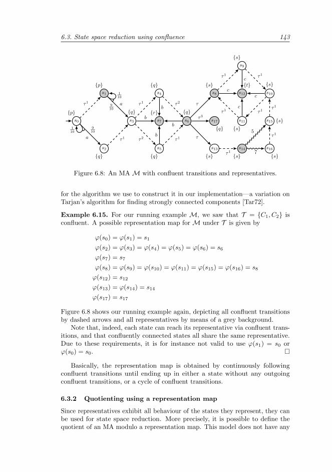
6.3. State space reduction using confluence 143

s1

s0

s2

s3

s4

s5

s6 s17

s8

s7

s9

s11

s10s12

s13 s14

s15

s16

p

p

q

qτ1

910

910

a

a

τ1

τ1

τ2

τ2

τ1

b

b

b

b110

110

q

q

qr

s

s

s

st

s

s

ss

q

τ

τ3

τ1 τ1

τ1τ1

c

c

c

c

τ

τ1

5

7

τ1

τ1

Figure 6.8: An MA M with confluent transitions and representatives.

for the algorithm we use to construct it in our implementation—a variation onTarjan’s algorithm for finding strongly connected components [Tar72].

Example 6.15. For our running example M, we saw that T = C1, C2 isconfluent. A possible representation map for M under T is given by

ϕ(s0) = ϕ(s1) = s1

ϕ(s2) = ϕ(s3) = ϕ(s4) = ϕ(s5) = ϕ(s6) = s6

ϕ(s7) = s7

ϕ(s8) = ϕ(s9) = ϕ(s10) = ϕ(s11) = ϕ(s15) = ϕ(s16) = s8

ϕ(s12) = s12

ϕ(s13) = ϕ(s14) = s14

ϕ(s17) = s17

Figure 6.8 shows our running example again, depicting all confluent transitionsby dashed arrows and all representatives by means of a grey background.

Note that, indeed, each state can reach its representative via confluent trans-itions, and that confluently connected states all share the same representative.Due to these requirements, it is for instance not valid to use ϕ(s1) = s0 orϕ(s0) = s0.

Basically, the representation map is obtained by continuously followingconfluent transitions until ending up in either a state without any outgoingconfluent transitions, or a cycle of confluent transitions.

6.3.2 Quotienting using a representation map

Since representatives exhibit all behaviour of the states they represent, they canbe used for state space reduction. More precisely, it is possible to define thequotient of an MA modulo a representation map. This model does not have any

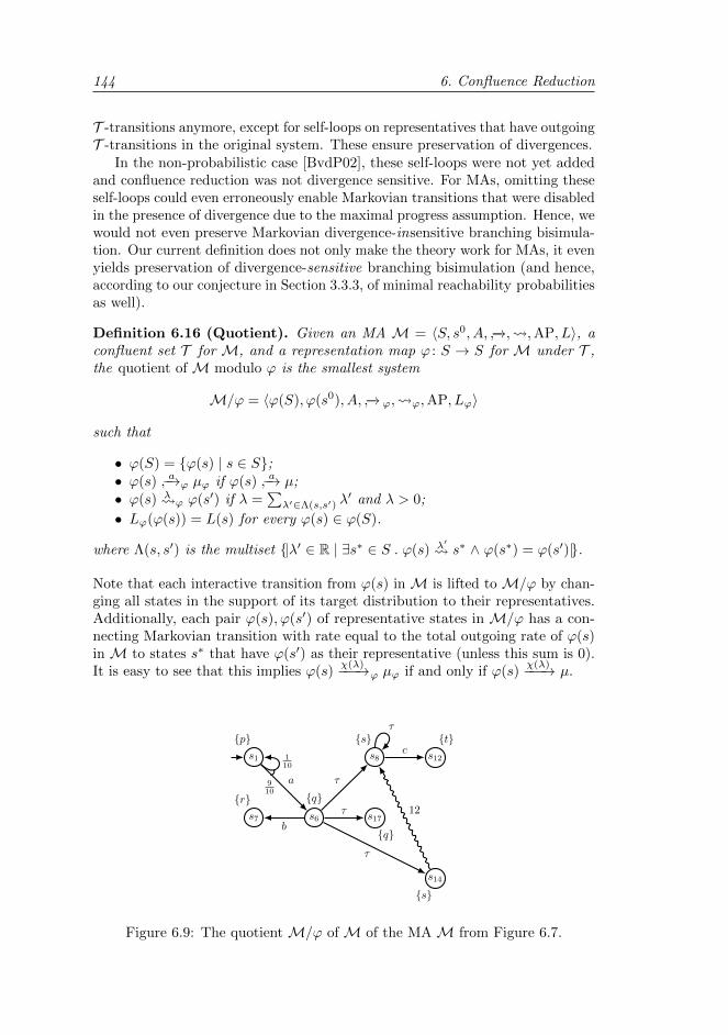
144 6. Confluence Reduction

T -transitions anymore, except for self-loops on representatives that have outgoingT -transitions in the original system. These ensure preservation of divergences.

In the non-probabilistic case [BvdP02], these self-loops were not yet addedand confluence reduction was not divergence sensitive. For MAs, omitting theseself-loops could even erroneously enable Markovian transitions that were disabledin the presence of divergence due to the maximal progress assumption. Hence, wewould not even preserve Markovian divergence-insensitive branching bisimula-tion. Our current definition does not only make the theory work for MAs, it evenyields preservation of divergence-sensitive branching bisimulation (and hence,according to our conjecture in Section 3.3.3, of minimal reachability probabilitiesas well).

Definition 6.16 (Quotient). Given an MA M = 〈S, s0, A, −→, ,AP, L〉, aconfluent set T for M, and a representation map ϕ : S → S for M under T ,the quotient of M modulo ϕ is the smallest system

M/ϕ = 〈ϕ(S), ϕ(s0), A, −→ ϕ, ϕ,AP, Lϕ〉

such that

• ϕ(S) = ϕ(s) | s ∈ S;• ϕ(s) a−→ϕ µϕ if ϕ(s) a−→ µ;• ϕ(s) λ ϕ ϕ(s′) if λ =

∑λ′∈Λ(s,s′) λ

′ and λ > 0;

• Lϕ(ϕ(s)) = L(s) for every ϕ(s) ∈ ϕ(S).

where Λ(s, s′) is the multiset |λ′ ∈ R | ∃s∗ ∈ S . ϕ(s) λ′ s∗ ∧ ϕ(s∗) = ϕ(s′)|.

Note that each interactive transition from ϕ(s) in M is lifted to M/ϕ by chan-ging all states in the support of its target distribution to their representatives.Additionally, each pair ϕ(s), ϕ(s′) of representative states in M/ϕ has a con-necting Markovian transition with rate equal to the total outgoing rate of ϕ(s)in M to states s∗ that have ϕ(s′) as their representative (unless this sum is 0).It is easy to see that this implies ϕ(s) −χ(λ)−−→ϕ µϕ if and only if ϕ(s) −χ(λ)−−→ µ.

s1

s6 s17

s8

s7

s12

s14

p

910

a

b

110

qr

s t

s

q

τ

τ

c

τ

12

τ

Figure 6.9: The quotient M/ϕ of M of the MA M from Figure 6.7.

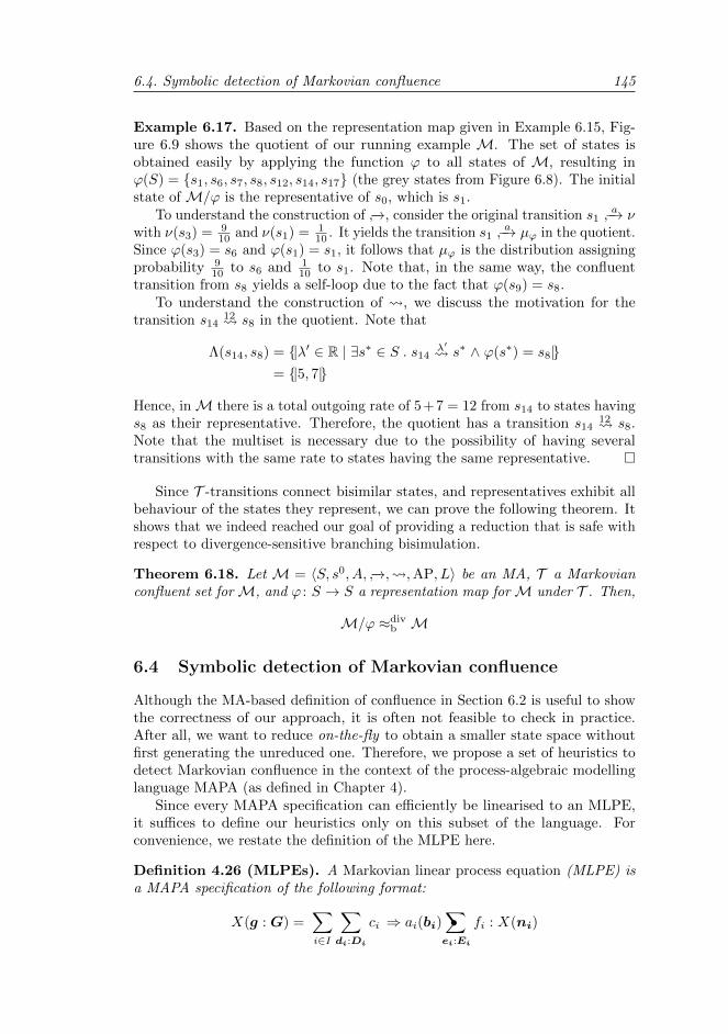
6.4. Symbolic detection of Markovian confluence 145

Example 6.17. Based on the representation map given in Example 6.15, Fig-ure 6.9 shows the quotient of our running example M. The set of states isobtained easily by applying the function ϕ to all states of M, resulting inϕ(S) = s1, s6, s7, s8, s12, s14, s17 (the grey states from Figure 6.8). The initialstate of M/ϕ is the representative of s0, which is s1.

To understand the construction of −→, consider the original transition s1a−→ ν

with ν(s3) = 910 and ν(s1) = 1

10 . It yields the transition s1a−→ µϕ in the quotient.

Since ϕ(s3) = s6 and ϕ(s1) = s1, it follows that µϕ is the distribution assigningprobability 9

10 to s6 and 110 to s1. Note that, in the same way, the confluent

transition from s8 yields a self-loop due to the fact that ϕ(s9) = s8.To understand the construction of , we discuss the motivation for the

transition s1412 s8 in the quotient. Note that

Λ(s14, s8) = |λ′ ∈ R | ∃s∗ ∈ S . s14λ′ s∗ ∧ ϕ(s∗) = s8|

= |5, 7|

Hence, inM there is a total outgoing rate of 5+7 = 12 from s14 to states havings8 as their representative. Therefore, the quotient has a transition s14

12 s8.Note that the multiset is necessary due to the possibility of having severaltransitions with the same rate to states having the same representative.

Since T -transitions connect bisimilar states, and representatives exhibit allbehaviour of the states they represent, we can prove the following theorem. Itshows that we indeed reached our goal of providing a reduction that is safe withrespect to divergence-sensitive branching bisimulation.

Theorem 6.18. Let M = 〈S, s0, A, −→, ,AP, L〉 be an MA, T a Markovianconfluent set forM, and ϕ : S → S a representation map forM under T . Then,

M/ϕ ≈divb M

6.4 Symbolic detection of Markovian confluence

Although the MA-based definition of confluence in Section 6.2 is useful to showthe correctness of our approach, it is often not feasible to check in practice.After all, we want to reduce on-the-fly to obtain a smaller state space withoutfirst generating the unreduced one. Therefore, we propose a set of heuristics todetect Markovian confluence in the context of the process-algebraic modellinglanguage MAPA (as defined in Chapter 4).

Since every MAPA specification can efficiently be linearised to an MLPE,it suffices to define our heuristics only on this subset of the language. Forconvenience, we restate the definition of the MLPE here.

Definition 4.26 (MLPEs). A Markovian linear process equation (MLPE) isa MAPA specification of the following format:

X(g : G) =∑i∈I

∑di:Di

ci ⇒ ai(bi)∑•

ei:Ei

fi : X(ni)

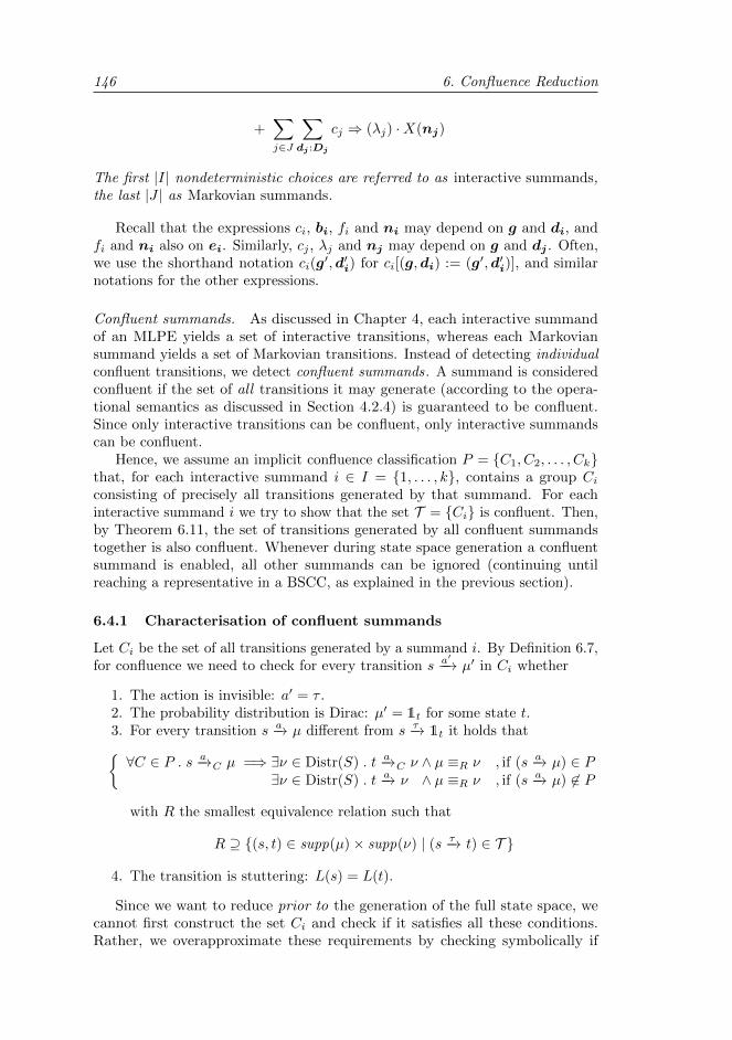
146 6. Confluence Reduction

+∑j∈J

∑dj :Dj

cj ⇒ (λj) ·X(nj)

The first |I| nondeterministic choices are referred to as interactive summands,the last |J | as Markovian summands.

Recall that the expressions ci, bi, fi and ni may depend on g and di, andfi and ni also on ei. Similarly, cj , λj and nj may depend on g and dj . Often,we use the shorthand notation ci(g

′,d′i) for ci[(g,di) := (g′,d′i)], and similarnotations for the other expressions.

Confluent summands. As discussed in Chapter 4, each interactive summandof an MLPE yields a set of interactive transitions, whereas each Markoviansummand yields a set of Markovian transitions. Instead of detecting individualconfluent transitions, we detect confluent summands . A summand is consideredconfluent if the set of all transitions it may generate (according to the opera-tional semantics as discussed in Section 4.2.4) is guaranteed to be confluent.Since only interactive transitions can be confluent, only interactive summandscan be confluent.

Hence, we assume an implicit confluence classification P = C1, C2, . . . , Ckthat, for each interactive summand i ∈ I = 1, . . . , k, contains a group Ciconsisting of precisely all transitions generated by that summand. For eachinteractive summand i we try to show that the set T = Ci is confluent. Then,by Theorem 6.11, the set of transitions generated by all confluent summandstogether is also confluent. Whenever during state space generation a confluentsummand is enabled, all other summands can be ignored (continuing untilreaching a representative in a BSCC, as explained in the previous section).

6.4.1 Characterisation of confluent summands

Let Ci be the set of all transitions generated by a summand i. By Definition 6.7,for confluence we need to check for every transition s −a′−→ µ′ in Ci whether

1. The action is invisible: a′ = τ .2. The probability distribution is Dirac: µ′ = 1t for some state t.3. For every transition s −a→ µ different from s −τ→ 1t it holds that∀C ∈ P . s −a→C µ =⇒ ∃ν ∈ Distr(S) . t −a→C ν ∧ µ ≡R ν , if (s −a→ µ) ∈ P

∃ν ∈ Distr(S) . t −a→ ν ∧ µ ≡R ν , if (s −a→ µ) 6∈ P

with R the smallest equivalence relation such that

R ⊇ (s, t) ∈ supp(µ)× supp(ν) | (s −τ→ t) ∈ T

4. The transition is stuttering: L(s) = L(t).

Since we want to reduce prior to the generation of the full state space, wecannot first construct the set Ci and check if it satisfies all these conditions.Rather, we overapproximate these requirements by checking symbolically if

6.4. Symbolic detection of Markovian confluence 147

summand i is such that all transitions it may ever generate satisfy the conditions.In this section, we characterise confluent summands, by explaining how these fourconditions can be derived from their specification. Examples will be provided inthe next section, when we discuss heuristics for checking these characterisationspractically.

1. Action-invisible summands. We can easily check if all transitions that canbe generated by a summand have an invisible action: the summand should justhave τ as its action.

Definition 6.19 (Action-invisible summands). A summand i is action-in-visible if ai(bi) = τ .

It is immediately clear from the operational semantics of the MLPE that action-invisible summands fulfill the first requirement of confluence.

2. Non-probabilistic summands. To check if a summand can only yield Diracdistributions, there should be only one possible next state for each valuation ofthe global and local parameters that enables its condition.

Definition 6.20 (Non-probabilistic summands). A summand i is non-probabilistic if for every v ∈ G and d′i ∈Di such that ci(v,d

′i), there exists a

unique state v′ ∈ G such that ni(v,d′i, e′i) = v′ for every e′i ∈ Ei

4.

It should also be immediately clear from the operational semantics of the MLPEthat non-probabilistic summands fulfill the second requirement of confluence.

3. Commuting summands. For a summand i to satisfy the third condition,we need to check if every transition s −a→ µ enabled together with a transitions −τ→ 1t generated by i can be mimicked from state t. Additionally, the mim-icking transition t −a→ ν should be from the same group as s −a→ µ. Since eachgroup precisely consists of all transitions generated by one summand, this boilsdown to the requirement that if s −a→ µ is generated by summand j, then soshould t −a→ ν be.

To check if all transitions generated by a summand i commute in this waywith all other transitions, we check for each summand j if all transitions thatit may generate commute with all transitions that summand i may generate.In that case, we say that the two summands commute. Again, we look at thespecification of the summands and not at the actual transitions they generate.

Clearly, two summands i, j commute if they cannot disable each other anddo not influence each other’s action parameters, probabilities and next states.After all, in that case any transition s −a→ µ enabled from state s by summand j

4We could also weaken this condition slightly to

∀e′i ∈ Ei . fi(v,d′i,e′i) > 0 =⇒ ni(v,d′i,e

′i) = v′

However, in that case we would need to be more strict later on, requiring the probabilitiesof a confluent summand to remain invariant. For the current formulation, the probabilityexpression can be changed without influencing the next state.

148 6. Confluence Reduction

must still be enabled from state t as a transition t −a→ ν, the τ -transition fromsummand i is still enabled in all states in the support of µ and the order of theexecution of the two transitions does not influence the observable behaviour orthe final state. Hence, µ ≡R ν. Since Definition 6.7 does not require transitionsto commute with themselves, a summand can also commute with itself bygenerating only one transition per state.

To formally define commuting summands, we already assume that one ofthem is action-invisible and non-probabilistic. Hence, we can write ni(v,d

′i) for

its unique next state given v and d′i. For an action-invisible non-probabilisticsummand i to commute with a summand j, we have to investigate their behaviourfor all state vectors v ∈ G and local variable vectors d′i ∈ Di,d

′j ∈ Dj such

that both summands are enabled: ci(v,d′i) ∧ cj(v,d′j). The maximal progress

assumption dictates that interactive summands and Markovian summands cannever be enabled at the same time, so we only need to check commutativityamong the interactive summands.

Definition 6.21 (Commuting summands). An action-invisible non-probab-ilistic summand i commutes with a summand j (possibly i = j) if for all v ∈ G,d′i ∈Di,d

′j ∈Dj such that ci(v,d

′i) ∧ cj(v,d′j):

• Summand i cannot not disable summand j, and vice versa:

cj(ni(v,d′i),d

′j) ∧ ci(nj(v,d′j , e

′j),d′i)

for every e′j ∈ Ej such that fj(v,d′j , e′j) > 0.

• Summand i cannot influence the action parameters of summand j:

bj(v,d′j) = bj(ni(v,d

′i),d

′j)

Note that summand i was already assumed to have no action parameters (asits action is always τ), so these cannot be influenced by j anyway—hence,no converse equality has to be checked.

• Summand i cannot influence the probability expression of summand j:

fj(v,d′j , e′j) = fj(ni(v,d

′i),d

′j , e′j)

for every e′j ∈ Ej .

Note that summand i was already assumed to have a unique next statev′ ∈ G for any state vector v ∈ G and local variable vector d′i ∈ Di, sono converse equality has to be checked. (Under the adapted condition forpotentially confluent summands discussed in Footnote 4 on page 147, thiswould not be the case anymore.)

• Execution of summands i and j in either order yield the same next state:

nj(ni(v,d′i),d

′j , e′j) = ni(nj(v,d′j , e

′j),d′i)

for every e′j ∈ Ej such that fj(v,d′j , e′j) > 0.

or, alternatively, if i = j ∧ ni(v,d′i) = nj(v,d′j).

6.4. Symbolic detection of Markovian confluence 149

From the discussion above, it follows that if i commutes with all summandsincluding itself, it satisfies the third requirement of confluence.

Remark 6.22. Definition 6.21 can be phrased as one formula, characterisingthe commutativity of two summands. An action-invisible and non-probabilisticsummand i commutes with a summand j (possibly i = j) if:

ci(v,d′i) ∧ cj(v,d′j)

=⇒fj(v,d

′j , e′j) > 0 =⇒ cj(ni(v,d

′i),d

′j) ∧ ci(nj(v,d′j , e

′j),d′i)

∧ bj(v,d′j) = bj(ni(v,d

′i),d

′j)

∧ fj(v,d′j , e′j) = fj(ni(v,d

′i),d

′j , e′j)

∧ fj(v,d′j , e′j) > 0 =⇒ nj(ni(v,d

′i),d

′j , e′j) = ni(nj(v,d′j , e

′j),d′i)

∨(i = j ∧ ni(v,d

′i) = nj(v,d′j)

)where v,d′i,d

′j and e′j universally quantify over G, Di, Dj and Ej , respect-

ively.

As these formulas are quantifier-free and in practice often either trivially falseor true, they can generally be solved using an SMT solver for the data typesinvolved. For n summands, n2 formulas need to be solved; the complexity ofthis procedure depends on the data types.

4. Stuttering summands. Finally, a confluence summand should only generatetransitions that do not change change the state labelling. Hence, for all v ∈ Gand d′i ∈Di:

ci(v,d′i) =⇒ L(v) = L(ni(v,d

′i))

Recall that we defined the state labelling of the MA corresponding to aMAPA specification such that each state is labelled by the set of visible actionsit immediately enables (Definition 4.22). Hence, for a summand to be invisiblewith respect to the state labelling it should leave invariant the set of enabledvisible actions. This requirement can be alleviated by hiding all actions that arenot used in the properties of interest.

If a summand i is action-invisible and commutes with all summands, wealready know that it can never disable another summand (if it disables itselfthat is fine, since it cannot produce any visible actions). Hence, we only stillneed to verify whether it can never enable a summand having a visible action.

Definition 6.23 (Stuttering summands). An action-invisible non-probab-ilistic summand i that commutes with all summands is stuttering if, for eachsummand j,

• The condition of j can never be enabled by i if j has a visible action, i.e.,

ci(v,d′i) ∧ aj 6= τ ∧ ¬cj(v,d′j) =⇒ ¬cj(ni(v,d

′i),d

′j)

for all v ∈ G, d′i ∈Di and d′j ∈Dj .

150 6. Confluence Reduction

Clearly, stuttering summands satisfy the fourth requirement of confluence.Concluding, a summand that is action-invisible, non-probabilistic and stut-

tering, and that also commutes with all summands including itself, generatesonly confluent transitions.

6.4.2 Heuristics for confluent summands

Although the symbolic characterisation introduced in the previous section issound, it may not always be feasible or efficient to apply. Only action invisibilitycan easily be checked syntactically, so we introduce heuristics for checking if asummand is non-probabilistic, commuting and stuttering. Although our heurist-ics are rather simple and intuitive, they are widely applicable (as demonstratedby our case studies in Chapter 9).

2. Non-probabilistic summands. In Definition 6.20 we discussed a minimalcondition for a summand i to be non-probabilistic. We check this heuristicallyin the following way.

P . Instead of checking for all possible valuations of the global and localvariables whether indeed ni(v,d

′i, e′i) = v′ for every e′i ∈ Ei, we just

check if |Ei| = 1. After all, summands that do have a probabilistic choiceare very likely to indeed have different next states—otherwise, this choicecould easily be eliminated. On the other hand, if there is no probabilisticchoice, indeed there is a unique next state for every v ∈ G and d′i ∈Di.

3. Commuting summands. To check for commutativity according to Defini-tion 6.21, we define several heuristics. As mentioned before, these are only neededfor the interactive summands; all Markovian summands are trivially disabled dueto the maximal progress assumption. Each heuristic individually is a sufficientcondition for the requirements of Definition 6.21. Hence, only one of them hasto hold. They are based on (1) two summands never being enabled at the sametime, (2) two summands coinciding and not having any local nondeterministicchoice, and (3) two summands never influencing each other’s conditions, actionparameters, probabilities and next states due to disjoint variable use.

C1. Never enabled at the same time. If two summands are never enabled atthe same time, i.e., ci(v,d

′i) ∧ cj(v,d′j) does not hold for any possible

combination of valuations v ∈ G, d′i ∈ Di and d′j ∈ Dj , then thecommutativity requirements hold vacuously. Since the variables d′i andd′j are only used locally per summand (and hence cannot disable anothersummand), we focus on the global variables.

Our heuristics range over the global variables g that have a finitedomain, and check if there is at least one gk that disables either i or j foreach of its valuations. That is, we check if

∀vk ∈ Gk . ¬ci[gk := vk] ∨ ¬cj [gk := vk]

applying the expression simplification heuristics described in Section 4.5to try to rewrite the conditions to false. If this indeed succeeds for all

6.4. Symbolic detection of Markovian confluence 151

vk ∈ Gk for some global variable gk, then apparently ci(v,d′i) ∧ cj(v,d′j)

can never occur. Hence, the commutativity requirements hold due to thefact that their premise never holds.

Example 6.24. Consider the following MLPE:

X(pc : 1, . . . , 10, x : 1, 2, 3, 4) =

pc = 3 ∧ x < 3⇒ τ ·X(4, 2) (1)

+ pc = 3 ∧ x ≥ 3⇒ τ ·X(5, x) (2)

+ . . .

Clearly, these two summands commute. To see why, note that for everyvalue of x either ci or cj can be rewritten to false. Hence, since eachstate vector v ∈ G must contain one of these values, the two summandsare never enabled at the same time and thus ci(v,d

′i) ∧ cj(v,d′j) can never

hold.

C2. Coinciding summands without local choice. If the two summands forwhich commutativity is analysed coincide (i.e., i = j), we can satisfy therequirements by showing that ni(v,d

′i) = nj(v,d′j) for every v ∈ G and

all d′i,d′j ∈Di. We do so by checking whether |Di| = 1. Since this implies

that d′i = d′j , the condition reduces to ni(v,d′i) = ni(v,d

′i), with d′i the

single element of Di. Obviously, this holds for all v ∈ G.

Example 6.25. Consider the following MLPE:

X(x : N, y : N, z : N) =∑i:1,25 < x < 10⇒ τ ·X(x+ i, y + 1) (1)

+ y > 2⇒ τ ·X(x, y − 1) (2)

The second summand clearly commutes with itself, since it does not containa nondeterministic choice and hence only produces at most one transitionin each state. The first summand, though, may produce two transitions.Hence, it is not immediately clear anymore if these commute.

C3. Disjoint variables. If the global variables that are used by summand i(according to Definition 5.12) are disjoint from the global variables thatare changed by summand j (according to Definition 5.1), and the globalvariables that are used by summand j are disjoint from the global variablesthat are changed by summand i, then clearly the order of their executiondoes not matter. For instance, bj(v,d

′j) = bj(ni(v,d

′i),d

′j) trivially holds

since all variables needed to decide bj are used in j and hence unchanged byi; i.e., they do not differ between v and ni(v,d

′i). The other requirements

hold by a similar argument.We implemented some additional heuristics that for instance take into

account that an update x := x+ 1 cannot disable a condition x > 5, andthat updates like x := x + 2, x := x + 5 and x := x − 3 commute dueto their linearity. More precisely, our heuristics that check for disjoint

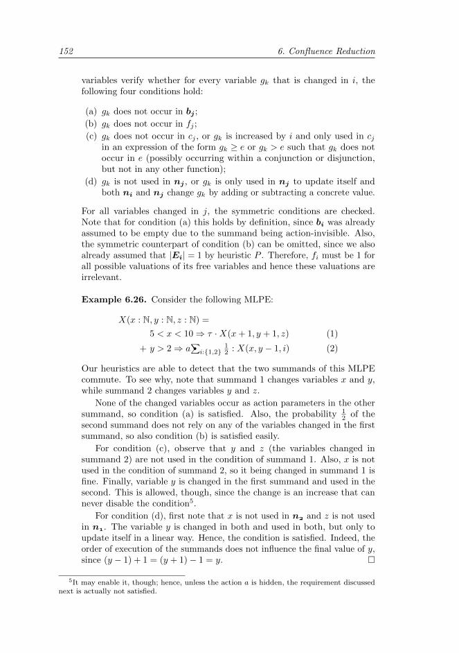
152 6. Confluence Reduction

variables verify whether for every variable gk that is changed in i, thefollowing four conditions hold:

(a) gk does not occur in bj ;

(b) gk does not occur in fj ;

(c) gk does not occur in cj , or gk is increased by i and only used in cjin an expression of the form gk ≥ e or gk > e such that gk does notoccur in e (possibly occurring within a conjunction or disjunction,but not in any other function);

(d) gk is not used in nj , or gk is only used in nj to update itself andboth ni and nj change gk by adding or subtracting a concrete value.

For all variables changed in j, the symmetric conditions are checked.Note that for condition (a) this holds by definition, since bi was alreadyassumed to be empty due to the summand being action-invisible. Also,the symmetric counterpart of condition (b) can be omitted, since we alsoalready assumed that |Ei| = 1 by heuristic P . Therefore, fi must be 1 forall possible valuations of its free variables and hence these valuations areirrelevant.

Example 6.26. Consider the following MLPE:

X(x : N, y : N, z : N) =

5 < x < 10⇒ τ ·X(x+ 1, y + 1, z) (1)

+ y > 2⇒ a∑•i:1,2

12 : X(x, y − 1, i) (2)

Our heuristics are able to detect that the two summands of this MLPEcommute. To see why, note that summand 1 changes variables x and y,while summand 2 changes variables y and z.

None of the changed variables occur as action parameters in the othersummand, so condition (a) is satisfied. Also, the probability 1

2 of thesecond summand does not rely on any of the variables changed in the firstsummand, so also condition (b) is satisfied easily.

For condition (c), observe that y and z (the variables changed insummand 2) are not used in the condition of summand 1. Also, x is notused in the condition of summand 2, so it being changed in summand 1 isfine. Finally, variable y is changed in the first summand and used in thesecond. This is allowed, though, since the change is an increase that cannever disable the condition5.

For condition (d), first note that x is not used in n and z is not usedin n. The variable y is changed in both and used in both, but only toupdate itself in a linear way. Hence, the condition is satisfied. Indeed, theorder of execution of the summands does not influence the final value of y,since (y − 1) + 1 = (y + 1)− 1 = y.

5It may enable it, though; hence, unless the action a is hidden, the requirement discussednext is actually not satisfied.

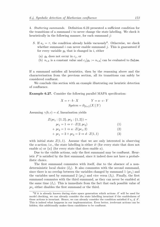
6.4. Symbolic detection of Markovian confluence 153

4. Stuttering summands. Definition 6.23 presented a sufficient condition forthe transitions of a summand i to never change the state labelling. We check itheuristically in the following manner, for each summand j:

S. If aj = τ , the condition already holds vacuously6. Otherwise, we checkwhether summand i can never enable summand j. This is guaranteed iffor every variable gk that is changed in i, either

(a) gk does not occur in cj , or(b) ni,k is a constant value and cj [gk := ni,k] can be evaluated to false.

If a summand satisfies all heuristics, then by the reasoning above and thecharacterisation from the previous section, all its transitions can safely beconsidered confluent.

We conclude this section with an example illustrating our heuristic detectionof confluence.

Example 6.27. Consider the following parallel MAPA specification:

X = τ · b ·X Y = a · c · YSystem = ∂b,c(X ||Y )

Assuming γ(b, c) = d, linearisation yields

Z(pc1 : 1, 2, pc2 : 1, 2) =

pc1 = 1⇒ τ · Z(2, pc2) (1)

+ pc2 = 1⇒ a · Z(pc1, 2) (2)

+ pc1 = 2 ∧ pc2 = 2⇒ d · Z(1, 1) (3)

with initial state Z(1, 1). Assume that we are only interested in observingthe a-action; i.e., the state labelling is either ∅ (for every state that does notenable a) or a (for every state that does enable a).

Due to the visible actions, only the first summand may be confluent. Heur-istic P is satisfied by the first summand, since it indeed does not have a probab-ilistic choice.

The first summand commutes with itself, due to the absence of a non-deterministic local choice (I2). It also commutes with the second summand,since there is no overlap between the variables changed by summand 1 (pc1) andthe variables used by summand 2 (pc2) and vice versa (I3). Finally, the firstsummand commutes with the third summand, as they can never be enabled atthe same time (I1). This is immediate from the fact that each possible value ofpc1 either disables the first summand or the third.

6If it is already known during state space generation which actions A′ will be used formodel checking, we can already consider the state labelling invariant if the enabledness ofthese actions is invariant. Hence, we can already consider the condition satisfied if aj 6∈ A′.This is indeed what happens in our implementation. Even better, irrelevant actions can behidden; this additionally makes them candidates to be confluent.

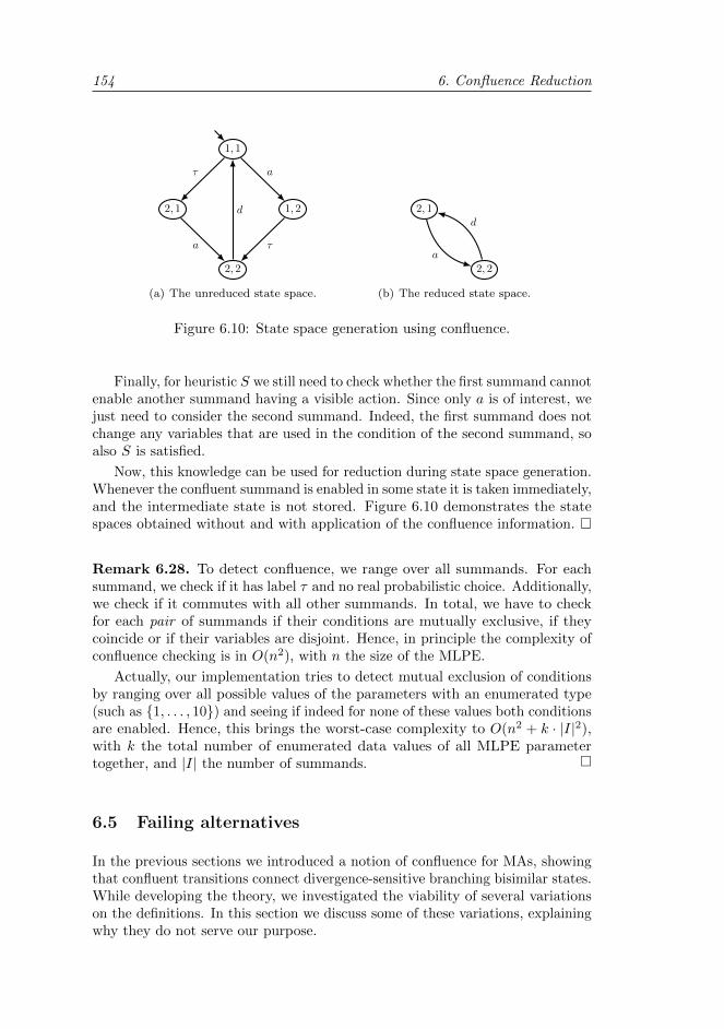
154 6. Confluence Reduction

1, 1

1, 22, 1

2, 2

τ a

a τ

d

(a) The unreduced state space.

2, 1

2, 2

a

d

(b) The reduced state space.

Figure 6.10: State space generation using confluence.

Finally, for heuristic S we still need to check whether the first summand cannotenable another summand having a visible action. Since only a is of interest, wejust need to consider the second summand. Indeed, the first summand does notchange any variables that are used in the condition of the second summand, soalso S is satisfied.

Now, this knowledge can be used for reduction during state space generation.Whenever the confluent summand is enabled in some state it is taken immediately,and the intermediate state is not stored. Figure 6.10 demonstrates the statespaces obtained without and with application of the confluence information.

Remark 6.28. To detect confluence, we range over all summands. For eachsummand, we check if it has label τ and no real probabilistic choice. Additionally,we check if it commutes with all other summands. In total, we have to checkfor each pair of summands if their conditions are mutually exclusive, if theycoincide or if their variables are disjoint. Hence, in principle the complexity ofconfluence checking is in O(n2), with n the size of the MLPE.

Actually, our implementation tries to detect mutual exclusion of conditionsby ranging over all possible values of the parameters with an enumerated type(such as 1, . . . , 10) and seeing if indeed for none of these values both conditionsare enabled. Hence, this brings the worst-case complexity to O(n2 + k · |I|2),with k the total number of enumerated data values of all MLPE parametertogether, and |I| the number of summands.

6.5 Failing alternatives

In the previous sections we introduced a notion of confluence for MAs, showingthat confluent transitions connect divergence-sensitive branching bisimilar states.While developing the theory, we investigated the viability of several variationson the definitions. In this section we discuss some of these variations, explainingwhy they do not serve our purpose.

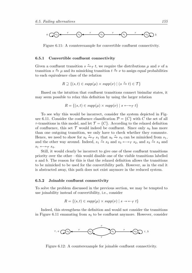
6.5. Failing alternatives 155

s0 s1 s2s3s4τ τ

baττ

Figure 6.11: A counterexample for convertible confluent connectivity.

6.5.1 Convertible confluent connectivity

Given a confluent transition s −τ→T t, we require the distributions µ and ν of atransition s −a→ µ and its mimicking transition t −a→ ν to assign equal probabilitiesto each equivalence class of the relation

R ⊇ (s, t) ∈ supp(µ)× supp(ν) | (s −τ→ t) ∈ T

Based on the intuition that confluent transitions connect bisimilar states, itmay seem possible to relax this definition by using the larger relation

R = (s, t) ∈ supp(µ)× supp(ν) | sT t

To see why this would be incorrect, consider the system depicted in Fig-ure 6.11. Consider the confluence classification P = C with C the set of allτ -transitions in this model, and let T = C. According to the relaxed definitionof confluence, this set T would indeed be confluent. Since only s0 has morethan one outgoing transition, we only have to check whether they commute.Hence, we need to show for s0 −τ→T s1 that s0 −τ→ s3 can be mimicked from s1,and the other way around. Indeed, s1 −τ→ s2 and s3 T s2, and s3 −τ→ s4 ands1 T s4.

Still, it would clearly be incorrect to give one of these confluent transitionspriority over the other—this would disable one of the visible transitions labelleda and b. The reason for this is that the relaxed definition allows the transitionsto be mimicked to be used for the convertibility path. However, as in the end itis abstracted away, this path does not exist anymore in the reduced system.

6.5.2 Joinable confluent connectivity

To solve the problem discussed in the previous section, we may be tempted touse joinability instead of convertibility, i.e., consider

R = (s, t) ∈ supp(µ)× supp(ν) | s T t

Indeed, this strengthens the definition and would not consider the transitionsin Figure 6.11 emanating from s0 to be confluent anymore. However, consider

s0 s1 s2s4

τ

τ

τττ , a τ , b

Figure 6.12: A counterexample for joinable confluent connectivity.

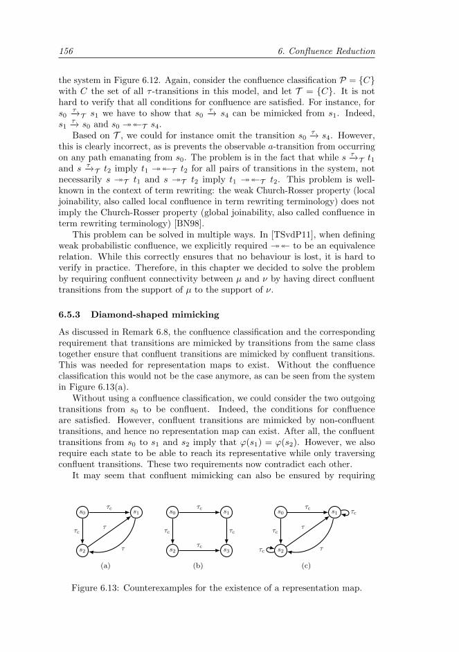
156 6. Confluence Reduction

the system in Figure 6.12. Again, consider the confluence classification P = Cwith C the set of all τ -transitions in this model, and let T = C. It is nothard to verify that all conditions for confluence are satisfied. For instance, fors0 −τ→T s1 we have to show that s0 −τ→ s4 can be mimicked from s1. Indeed,s1 −τ→ s0 and s0 T s4.

Based on T , we could for instance omit the transition s0 −τ→ s4. However,this is clearly incorrect, as is prevents the observable a-transition from occurringon any path emanating from s0. The problem is in the fact that while s −τ→T t1and s −τ→T t2 imply t1 T t2 for all pairs of transitions in the system, notnecessarily s T t1 and s T t2 imply t1 T t2. This problem is well-known in the context of term rewriting: the weak Church-Rosser property (localjoinability, also called local confluence in term rewriting terminology) does notimply the Church-Rosser property (global joinability, also called confluence interm rewriting terminology) [BN98].

This problem can be solved in multiple ways. In [TSvdP11], when definingweak probabilistic confluence, we explicitly required to be an equivalencerelation. While this correctly ensures that no behaviour is lost, it is hard toverify in practice. Therefore, in this chapter we decided to solve the problemby requiring confluent connectivity between µ and ν by having direct confluenttransitions from the support of µ to the support of ν.

6.5.3 Diamond-shaped mimicking

As discussed in Remark 6.8, the confluence classification and the correspondingrequirement that transitions are mimicked by transitions from the same classtogether ensure that confluent transitions are mimicked by confluent transitions.This was needed for representation maps to exist. Without the confluenceclassification this would not be the case anymore, as can be seen from the systemin Figure 6.13(a).

Without using a confluence classification, we could consider the two outgoingtransitions from s0 to be confluent. Indeed, the conditions for confluenceare satisfied. However, confluent transitions are mimicked by non-confluenttransitions, and hence no representation map can exist. After all, the confluenttransitions from s0 to s1 and s2 imply that ϕ(s1) = ϕ(s2). However, we alsorequire each state to be able to reach its representative while only traversingconfluent transitions. These two requirements now contradict each other.

It may seem that confluent mimicking can also be ensured by requiring

s0 s1

s2

τc

τc

τ

τ

(a)

s0 s1

s2 s3

τc

τc τc

τc

(b)

s0 s1

s2

τc

τc

τ

τ

τc

τc

(c)

Figure 6.13: Counterexamples for the existence of a representation map.

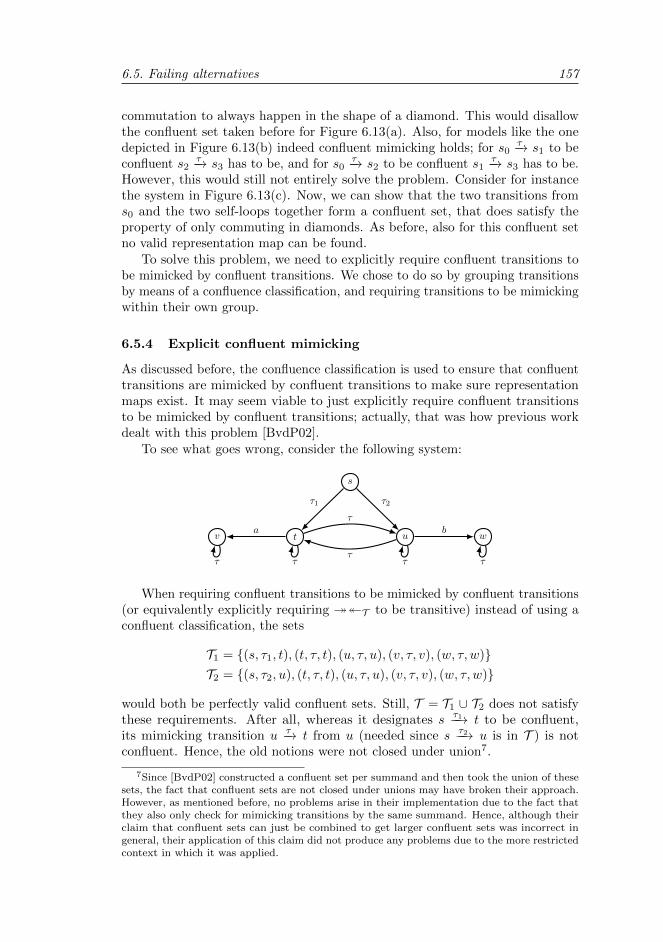
6.5. Failing alternatives 157

commutation to always happen in the shape of a diamond. This would disallowthe confluent set taken before for Figure 6.13(a). Also, for models like the onedepicted in Figure 6.13(b) indeed confluent mimicking holds; for s0 −τ→ s1 to beconfluent s2 −τ→ s3 has to be, and for s0 −τ→ s2 to be confluent s1 −τ→ s3 has to be.However, this would still not entirely solve the problem. Consider for instancethe system in Figure 6.13(c). Now, we can show that the two transitions froms0 and the two self-loops together form a confluent set, that does satisfy theproperty of only commuting in diamonds. As before, also for this confluent setno valid representation map can be found.

To solve this problem, we need to explicitly require confluent transitions tobe mimicked by confluent transitions. We chose to do so by grouping transitionsby means of a confluence classification, and requiring transitions to be mimickingwithin their own group.

6.5.4 Explicit confluent mimicking

As discussed before, the confluence classification is used to ensure that confluenttransitions are mimicked by confluent transitions to make sure representationmaps exist. It may seem viable to just explicitly require confluent transitionsto be mimicked by confluent transitions; actually, that was how previous workdealt with this problem [BvdP02].

To see what goes wrong, consider the following system:

s

t uv w

τ1 τ2

a bτ

ττ ττ τ

When requiring confluent transitions to be mimicked by confluent transitions(or equivalently explicitly requiring T to be transitive) instead of using aconfluent classification, the sets

T1 = (s, τ1, t), (t, τ, t), (u, τ, u), (v, τ, v), (w, τ, w)T2 = (s, τ2, u), (t, τ, t), (u, τ, u), (v, τ, v), (w, τ, w)

would both be perfectly valid confluent sets. Still, T = T1 ∪ T2 does not satisfythese requirements. After all, whereas it designates s −τ1−→ t to be confluent,its mimicking transition u −τ→ t from u (needed since s −τ2−→ u is in T ) is notconfluent. Hence, the old notions were not closed under union7.

7Since [BvdP02] constructed a confluent set per summand and then took the union of thesesets, the fact that confluent sets are not closed under unions may have broken their approach.However, as mentioned before, no problems arise in their implementation due to the fact thatthey also only check for mimicking transitions by the same summand. Hence, although theirclaim that confluent sets can just be combined to get larger confluent sets was incorrect ingeneral, their application of this claim did not produce any problems due to the more restrictedcontext in which it was applied.

158 6. Confluence Reduction

By using a confluence classification and requiring transitions to be mimickedby the same group, we ascertain that this kind of bad compositionality behaviourdoes not occur. After all, for T1 to be a valid confluent set, the confluenceclassification should be such that s −τ2−→ u and its mimicking transition t −τ→ u arein the same group. So, for s −τ2−→ u to be confluent (as prescribed by T2), alsot −τ→ u would need to be confluent. The latter is impossible, since the b-transitionfrom u cannot be mimicked from t, and hence T2 is disallowed.

6.6 Contributions

We introduced confluence reduction for MAs: the first practical reductiontechnique for this model that abstracts from invisible transitions. We showedthat it preserves divergence-sensitive branching bisimulation, and hence yieldsquantitatively behavioural equivalent models. In addition to working on MAs,our novel notion of confluence reduction has two additional advantages overprevious notions. First, it preserves divergences, and hence does not alterminimal reachability probabilities. Second, it is closed under unions, enablingus to separately detect confluence of different sets of transitions and combinethe results. We also showed that a representation map approach can be usedsafely to reduce systems on-the-fly, and discussed how to detect confluencesyntactically on the process-algebraic language MAPA—both using a symbolic(logical) characterisation and a set of heuristics.

Our case studies in Chapter 9 will demonstrate that significant reductionscan be obtained, reducing state spaces sometimes by an order of magnitude.A decrease in the degree of nondeterminism, as is to be expected from con-fluence reduction, often yields even better reductions in analysis time thanin state space size.

We conjecture that our technique can also be applied in different settings,for instance in the PRISM model checker [KNP11]. Due to the fact that thistool employs MTBDDs to do its analysis, an application of confluence duringmodel checking may be difficult. However, we could detect confluence on itsmodelling language in quite the same way as described in this chapter, and usethis information to syntactically optimise specifications. For instance, we mayadd guards to non-confluent commands to disable them in case at least oneconfluent command is enabled. Since the representation map approach cannotbe applied in this context, it would require acyclicity of the confluent commandsto avoiding the ignoring problem.

CHAPTER 7

Confluence Reduction versus

Partial Order Reduction

A Theoretical Comparison

“In theory, theory and practice are the same.In practice, they are not.”

Albert Einstein

The previous chapter introduced confluence reduction for MAs. As men-

tioned before, this technique is most closely related to the concept ofpartial order reduction (POR). Both use a notion of independence between

transitions of a system, either explicitly or implicitly, and try to reduce the statespace by eliminating redundant paths in the system.

In the non-probabilistic setting, partial order reduction techniques havebeen defined for a range of property classes, most notably LTL\X and CTL∗\X[GKPP95, GKPP99, WW96, Val96, Pel98]. Most work on confluence reductionhas been designed to guarantee that the reduced system is branching bisimilarto the original system; thus, these techniques preserve virtually all branchingproperties (in particular, CTL∗\X). There is not so much work on weaker variantsof confluence, though [LM09] explores a variant that makes no distinction betweenvisible and invisible actions and does not require acyclicity—hence, it preservesonly deadlocks, similar to weaker versions of ample and stubborn sets [Val96].

While POR has not yet been defined for MAs, it was already generalised tothe probabilistic setting. In [BGC04] and [DN04], the ample sets approach waslifted from labelled transition systems to Markov decision processes (MDPs),providing reductions that preserve probabilistic LTL\X . These techniques wererefined in [BDG06] to also preserve PCTL∗\X , a branching logic. Later, arevision of partial order reduction for distributed schedulers was introduced andimplemented in PRISM [GDF09]. In [BGC09], the use of fairness constraintsin combination with ample sets for the quantitative analysis of MDPs was firstintroduced. Later, the so-called weak stubborn set method was defined for aclass of safety properties of MDPs under fairness constraints [HKQ11].

Ample sets and confluent transitions are defined and detected quite differently:ample sets are defined by first giving an independence relation for the actionlabels, whereas confluence is a property of a set of (invisible) transitions in thefinal state space. Even so, the underlying ideas are similar on the intuitive level.

160 7. Confluence Reduction versus Partial Order Reduction

Indeed, [LM09] even describes them as ‘two lines of work’ in the area of partialorder reduction. Since both techniques are in general not able to achieve optimalreductions as compared to the bisimulation-minimal quotient, we are interestedto see if there are scenarios that can be handled by one technique but not by theother, or whether their reduction capabilities are equally powerful. Therefore,an obvious question is: to what extent do ample sets and confluent transitionscoincide? This chapter addresses that question by comparing the notion ofprobabilistic ample sets from [BDG06] to a slightly reformulated variant on thenotion of confluence from Chapter 6. We restrict to ample sets, because they arecurrently the most well-established notion of partial order reduction for MDPs.

Our approach. We introduce MDPs as a restriction of MAs, and recall someof their basic terminology. Then, we present the theory on ample set reductionfrom [BDG06] by means of the concept of a reduction function. Such functionsspecify for each state which actions (and hence which transitions) are enabled.We reformulate confluence reduction in the same way, taking into account thatMDPs are insensitive to action visibility—i.e., there is no notion of τ -actions;only the state labelling is assumed to be observable.

We compare the two notions and show that, when preserving branchingtime behaviour, confluence reduction is strictly more powerful than ample setreduction. For this purpose, we prove that every nontrivial ample set can bemimicked by a confluent set, while also providing examples where confluenttransitions do not qualify as ample sets. In such cases, confluence reduction isable to reduce more than ample set reduction. Mainly, confluence imposes fewerrestrictions on the independence of actions. To continue, we pinpoint preciselyin what way confluence is more general than ample sets, and show how thedefinitions of both can be adjusted to make them coincide.

While revealing exactly where the extra reduction potential with confluencecomes from, the results we present support the idea that confluence reductionis a well-suited alternative to the thus far more often used partial order reduc-tion methods. In particular, this is a major consideration in contexts where(1) detection of confluence using heuristics that make use of these more relaxedconditions is possible, or where (2) the conditions of confluence are just easier tocheck than their partial order reduction counterparts.

1. The first situation seems to occur in the context of statistical modelchecking and simulation. In this context, [BFHH11] used partial orderreduction to remove spurious nondeterminism from models to allow themto be analysed statistically. As the reduction is applied directly to explicitmodels rather than high-level specifications, the more relaxed confluenceconditions may come in handy. Indeed, the next chapter shows thatconfluence reduction is able to remove nondeterminism that partial orderreduction could not, thereby allowing more models to be analysed usingstatistical model checking techniques. Our results in this chapter providetheoretical support for this intuition.

2. The second situation seems to arise when working with process-algebraicmodelling languages. As demonstrated in [Blo01, BvdP02] for the non-

7.1. Preliminaries 161

probabilistic setting and in the previous chapter for the setting of Markovautomata, it is quite natural to detect confluence in such a context.Although it is also possible to work with POR in this setting (see forinstance [FTW10]), the way confluence is phrased seems to be more closelyrelated to the models involved, making its detection more straightforward.

Alternatively, our results (in particular Theorem 7.31) allow for the use ofmore relaxed definitions—incorporating a notion of local independence—if partialorder reduction is used. In addition to providing these practical opportunities,our precise comparison of confluence and partial order reduction fills a significantgap in the theoretical understanding of the two notions.

The theory is presented in such a way that the results hold for non-probabi-listic automata as well, as they form a special case of the theory where allprobability distributions are deterministic. Hence, as a side effect we also answerthe question of how the non-probabilistic variants of ample set reduction andconfluence reduction relate.

Our findings imply that results and techniques applicable to confluencecan be used in conjunction with ample sets—for instance, the state spacegeneration technique based on representative states, already known in the contextof confluence reduction as shown in [BvdP02] and in the previous chapter.Applying this technique to POR replaces explicit checking of the cycle condition,in addition to further reducing the number of states and transitions. The latteris important, especially if the MDP is to be subjected to further analysis.

Organisation of the chapter. After recalling some basic preliminaries in Sec-tion 7.1, we present the notions of ample set reduction and confluence reductionin Section 7.2. Then, in Section 7.3 we discuss how ample set reduction canbe thought of as a special case of confluence reduction. We show what kindof restrictions and relaxations are needed to make them coincide, thereby pin-pointing the exact differences of the methods. Finally, Section 7.4 concludes bysummarising the contributions of this chapter.

Origins of the chapter. This chapter is based on a journal paper that willsoon be published in Theoretical Computer Science [HT13a]. That paper waswritten in collaboration with Henri Hansen from the Institute of Mathematics atTampere University of Technology, Tampere, Finland (working at the TemasekLaboratories of the National University of Singapore, Singapore during someof the work). The author updated the definitions slightly, replacing the morecomplicated notion of equivalence of probability distributions used in [HT13a]by the more simple way of dealing with this as presented in the previous chapter(and first published in [HT13b]).

7.1 Preliminaries

Probabilistic ample set reduction has been defined on the Markov decisionprocess. This model is a subclass of the MA, having no Markovian rates andfinite sets of states and actions, and allowing each action to occur only once per

162 7. Confluence Reduction versus Partial Order Reduction

state. Because of the latter restriction, the transition relation is often formalisedslightly different from what we have done in the previous chapters. In thischapter, we conform to MDP terminology [Put05] and formalise the transitionrelation as a function assigning to each pair of a state and action the probabilitydistribution for the next state. To allow actions to be disabled, we now use the setDistr⊥(S) = Distr(S) ∪ ⊥ that not only contains all probability distributionsover the set of states S, but also the subdistribution ⊥ that assigns probability 0to every state s ∈ S.

Hence, an MDP consists of states that are labelled by atomic propositions,an initial state, and a probabilistic action-labelled transition function. Fromeach state s, a subset of the actions is enabled; for every enabled action a, aprobability distribution P (s, a) specifies for every other state s′ the probabilityP (s, a)(s′) of ending up in s′ after taking a from s.

Recall from Section 3.2 that we assume a countable universe of actions Act.

Definition 7.1 (MDPs). A Markov decision process (MDP) is tuple M =(S, s0, A, P,AP, L), where

• S is a finite set of states;• s0 ∈ S is the initial state;• A ⊆ Act is a finite set of actions;• P : (S ×A)→ Distr⊥(S) is the probabilistic transition function;• AP is a finite set of state labels;• L : S →P(AP) is the state-labelling function.

If P (s, a) = ⊥, the action a is not enabled from s. Otherwise, P (s, a)(s′) is theprobability of going to s′ when executing a from s.

We still like to be able to speak about transitions of an MDP, and henceintroduce the notation (s, a, µ) for a transition from s, taking an action a andhaving a next-state distribution µ. Note that such a transition is present ifP (s, a) = µ. As before, we often write s −a→ µ instead of (s, a, µ).

Definition 7.2 (Supporting notations for MDPs). Given an MDP M =(S, s0, A, P,AP, L), we denote the set of all possible transitions of M by

∆M = (s, a, µ) ∈ S ×A×Distr(S) | P (s, a) = µ

Additionally,

• We write s −a→ µ if (s, a, µ) ∈ ∆M , and s −a→ if s −a→ µ for some µ ∈Distr(S). Also, we define en(s) = a ∈ A | s −a→ to be the set of actionsenabled from state s.• We reuse all notations defined in Chapter 3 for extended transitions also

for transitions in an MDP—including the notations for paths, reachability,joinability and convertibility—and subscript them with a set of transitionsT ⊆ ∆M to restrict to using only transitions from this set.• We write s −a1a2...an−−−−−→ s′ if there exists a path

s0 −a1,µ1−−−→ s1 −a2,µ2−−−→ . . . −an,µn−−−→ sn

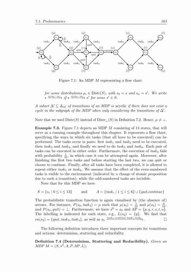
7.1. Preliminaries 163

s1

s0

s2

s3

s4

s5

s6 s8s7

s9

s10

s11

s12

s13

p

p

q

q

task1

910

910

task2

task2

task1

task3

task4

task4

task3

quit

quit

quit

quit110

110

q

s

sr s

s

t

t

t

u

continue

task6

task5

task5

task6 task5

task6

Figure 7.1: An MDP M representing a flow chart.

for some distributions µi ∈ Distr(S), with s0 = s and sn = s′. We writes −a1a2...an−−−−−→ if s −a1a2...an−−−−−→ s′ for some s′ ∈ S.

A subset ∆′ ⊆ ∆M of transitions of an MDP is acyclic if there does not exist acycle in the subgraph of the MDP when only considering the transitions of ∆′.

Note that we used Distr(S) instead of Distr⊥(S) in Definition 7.2. Hence, µ 6= ⊥.

Example 7.3. Figure 7.1 depicts an MDP M consisting of 14 states, that willserve as a running example throughout this chapter. It represents a flow chart,specifying the ways in which six tasks (that all have to be executed) can beperformed. The tasks occur in pairs: first task1 and task2 need to be executed,then task3 and task4, and finally we need to do task5 and task6. Each pair oftasks can be executed in either order. Furthermore, the execution of task2 failswith probability 1

10 , in which case it can be attempted again. Moreover, afterfinishing the first two tasks and before starting the last two, we can quit orchoose to continue. Finally, after all tasks have been completed, it is allowed torepeat either task5 or task6. We assume that the effect of the even-numberedtasks is visible to the environment (indicated by a change of atomic propositiondue to such a transition), while the odd-numbered tasks are invisible.

Note that for this MDP we have

S = si | 0 ≤ i ≤ 13 and A = task i | 1 ≤ i ≤ 6 ∪ quit,continue

The probabilistic transition function is again visualised by (the absence of)arrows. For instance, P (s0, task2) = µ such that µ(s0) = 1

10 and µ(s2) = 910 ,

and P (s0, quit) = ⊥. Furthermore, we have s0 = s0 and AP = p, q, r, s, t, u.The labelling is indicated for each state, e.g., L(s2) = q. We find that

en(s3) = quit , task3, task4, as well as s5 −task3 continue task5 task6−−−−−−−−−−−−−−−−→.

The following definition introduces three important concepts for transitionsand actions: determinism, stuttering and reducibility.

Definition 7.4 (Determinism, Stuttering and Reducibility). Given anMDP M = (S, s0, A, P,AP, L),

164 7. Confluence Reduction versus Partial Order Reduction

• A transition s −a→ µ is deterministic if µ is deterministic (i.e., assignsprobability 1 to a single state), and an action a ∈ A is a deterministic actionin M if all a-labelled transitions in ∆M are deterministic. Assuming animplicit MDP, we denote the set of all deterministic actions by Adet ⊆ A.Given a deterministic transition s −a→ 1t, we write target(s, a) = t;• A transition s −a→ µ is stuttering if L(s′) = L(s) for each s′ ∈ supp(µ),

and an action a ∈ A is a stuttering action in M if all a-labelled transitionsin ∆M are stuttering. We denote the set of all stuttering actions byAst ⊆ A;• A transition s −a→ µ is reducible if it is both deterministic and stuttering,

and an action a ∈ A is a reducible action if all a-labelled transitions in ∆M

are reducible. We denote the set of all reducible actions by Ared = Ast ∩Adet;• A finite path s −a1a2...an−−−−−→ s′ or infinite path s −a1a2...−−−−→ is reducible if every

action ai on it is reducible.

As before, we sometimes abuse notation a little by writing s −a→ s′ instead ofs −a→ 1s′ for deterministic transitions.

Note that s −a→ µ may be a reducible transition even if a is not a reducibleaction, but not vice versa. Finally, given a sequence of reducible (and thusdeterministic) actions a1a2 . . . an, talking about “the” path of this sequence fromsome state s makes sense, because the states that are visited are unique. We doso for the rest of this chapter.

Example 7.5. In the MDP M in Figure 7.1, all transitions except for the oneslabelled by task2 are deterministic. Hence, all actions except for task2 aredeterministic. All transitions labelled by odd tasks are stuttering, as well asthe continue transition, since the atomic propositions in their source and targetstates all correspond. Hence, all odd-labelled task actions and the continueaction are stuttering. Combining this, we obtain

Ared = task i | i ∈ 1, 3, 5 ∪ continue

A wide class of reductions for an MDP can be defined using the constructcalled a reduction function. Such a function determines a sub-MDP by decidingfor each state which outgoing actions are enabled in the reduced MDP. Thetransition function of the reduced MDP then consists of all transitions that arestill enabled after the reduction function is applied, and the set of states consistsof all states that are still reachable using the reduced transition function.

Definition 7.6 (Reduction functions). Given an MDP M = (SM , s0M , A,

PM ,AP, LM ), a reduction function for M is any function R : SM →P(A) withR(s) ⊆ en(s) for every s ∈ SM . Given a reduction function R, the reducedMDP for M with respect to R is the minimal MDP MR = (SR, s

0R, A, PR,AP,

LR) such that s0R = s0

M and

• If s ∈ SR and a ∈ R(s), then PR(s, a) = PM (s, a) (and hence by definitionof PR also supp(PM (s, a)) ⊆ SR);

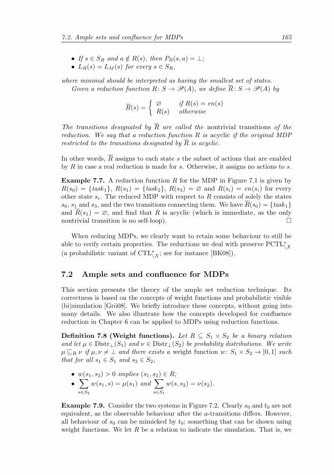
7.2. Ample sets and confluence for MDPs 165

• If s ∈ SR and a /∈ R(s), then PR(s, a) = ⊥;• LR(s) = LM (s) for every s ∈ SR,

where minimal should be interpreted as having the smallest set of states.Given a reduction function R : S →P(A), we define R : S →P(A) by

R(s) =

∅ if R(s) = en(s)R(s) otherwise

The transitions designated by R are called the nontrivial transitions of thereduction. We say that a reduction function R is acyclic if the original MDPrestricted to the transitions designated by R is acyclic.

In other words, R assigns to each state s the subset of actions that are enabledby R in case a real reduction is made for s. Otherwise, it assigns no actions to s.

Example 7.7. A reduction function R for the MDP in Figure 7.1 is given byR(s0) = task1, R(s1) = task2, R(s3) = ∅ and R(si) = en(si) for everyother state si. The reduced MDP with respect to R consists of solely the statess0, s1 and s3, and the two transitions connecting them. We have R(s0) = task1and R(s1) = ∅, and find that R is acyclic (which is immediate, as the onlynontrivial transition is no self-loop).

When reducing MDPs, we clearly want to retain some behaviour to still beable to verify certain properties. The reductions we deal with preserve PCTL∗\X(a probabilistic variant of CTL∗\X ; see for instance [BK08]).

7.2 Ample sets and confluence for MDPs

This section presents the theory of the ample set reduction technique. Itscorrectness is based on the concepts of weight functions and probabilistic visible(bi)simulation [Gro08]. We briefly introduce these concepts, without going intomany details. We also illustrate how the concepts developed for confluencereduction in Chapter 6 can be applied to MDPs using reduction functions.

Definition 7.8 (Weight functions). Let R ⊆ S1 × S2 be a binary relationand let µ ∈ Distr⊥(S1) and ν ∈ Distr⊥(S2) be probability distributions. We writeµ vR ν if µ, ν 6= ⊥ and there exists a weight function w : S1 × S2 → [0, 1] suchthat for all s1 ∈ S1 and s2 ∈ S2,

• w(s1, s2) > 0 implies (s1, s2) ∈ R;

•∑s∈S2

w(s1, s) = µ(s1) and∑s∈S1

w(s, s2) = ν(s2).

Example 7.9. Consider the two systems in Figure 7.2. Clearly s0 and t0 are notequivalent, as the observable behaviour after the a-transitions differs. However,all behaviour of s0 can be mimicked by t0; something that can be shown usingweight functions. We let R be a relation to indicate the simulation. That is, we

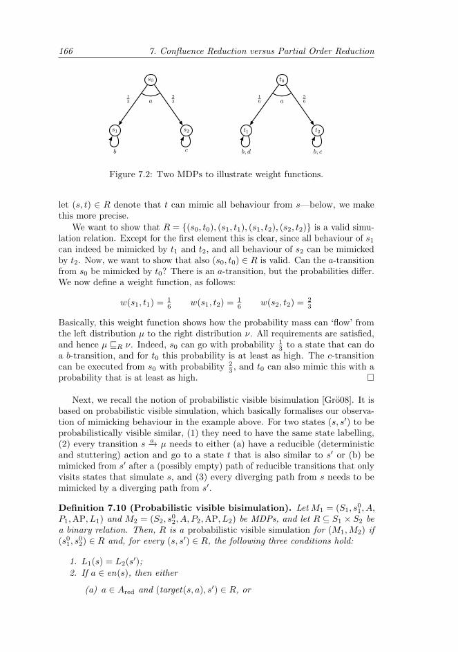
166 7. Confluence Reduction versus Partial Order Reduction

s0

s1 s2

t0

t1 t2

13

23

16

56a a

b c b, d b, c

Figure 7.2: Two MDPs to illustrate weight functions.

let (s, t) ∈ R denote that t can mimic all behaviour from s—below, we makethis more precise.

We want to show that R = (s0, t0), (s1, t1), (s1, t2), (s2, t2) is a valid simu-lation relation. Except for the first element this is clear, since all behaviour of s1

can indeed be mimicked by t1 and t2, and all behaviour of s2 can be mimickedby t2. Now, we want to show that also (s0, t0) ∈ R is valid. Can the a-transitionfrom s0 be mimicked by t0? There is an a-transition, but the probabilities differ.We now define a weight function, as follows:

w(s1, t1) = 16 w(s1, t2) = 1

6 w(s2, t2) = 23

Basically, this weight function shows how the probability mass can ‘flow’ fromthe left distribution µ to the right distribution ν. All requirements are satisfied,and hence µ vR ν. Indeed, s0 can go with probability 1

3 to a state that can doa b-transition, and for t0 this probability is at least as high. The c-transitioncan be executed from s0 with probability 2

3 , and t0 can also mimic this with aprobability that is at least as high.

Next, we recall the notion of probabilistic visible bisimulation [Gro08]. It isbased on probabilistic visible simulation, which basically formalises our observa-tion of mimicking behaviour in the example above. For two states (s, s′) to beprobabilistically visible similar, (1) they need to have the same state labelling,(2) every transition s −a→ µ needs to either (a) have a reducible (deterministicand stuttering) action and go to a state t that is also similar to s′ or (b) bemimicked from s′ after a (possibly empty) path of reducible transitions that onlyvisits states that simulate s, and (3) every diverging path from s needs to bemimicked by a diverging path from s′.

Definition 7.10 (Probabilistic visible bisimulation). Let M1 = (S1, s01, A,

P1,AP, L1) and M2 = (S2, s02, A, P2,AP, L2) be MDPs, and let R ⊆ S1 × S2 be

a binary relation. Then, R is a probabilistic visible simulation for (M1,M2) if(s0

1, s02) ∈ R and, for every (s, s′) ∈ R, the following three conditions hold:

1. L1(s) = L2(s′);

2. If a ∈ en(s), then either

(a) a ∈ Ared and (target(s, a), s′) ∈ R, or

7.2. Ample sets and confluence for MDPs 167

(b) there is a reducible path s′ −b1...bn−−−−→ s′′ in M2 such that (s, s′i) ∈ R forevery state s′i on this path, a ∈ en(s′′) and P1(s, a) vR P2(s′′, a);

3. If there is an infinite reducible path s −b1b2...−−−→ in M1 such that (si, s′) ∈ R

for every si on this path, then there is a finite reducible path s′ −a1...an−−−−→ s′nin M2, n ≥ 1, such that (s, s′i) ∈ R for every s′i on this path (possiblyexcluding s′n), and (sk, s

′n) ∈ R for at least one sk (with k > 0) on the

path s −b1b2...−−−→.

A binary relation R is a probabilistic visible bisimulation for (M1,M2) if it isa probabilistic visible simulation for (M1,M2) and R−1 is a probabilistic visiblesimulation for (M2,M1).

We say that two MDPs M1,M2 are probabilistically visibly bisimilar, denotedby M1 ≈pvb M2, if there is a probabilistic visible bisimulation that relates them.

We note that probabilistic visible bisimulation is very much related to our notionof divergence-sensitive branching bisimulation. The only real difference is thatprobabilistic visible bisimulation requires transitions to be labelled by actionsthat are deterministic and stuttering globally in conditions 2a and 2b, while thebranching step only requires the transitions to be this themselves.

7.2.1 Ample sets

Although there are many techniques that are called “partial order reduction”,we focus on the ample set method as presented in [BDG06]. This is the onlypartial order reduction technique we are aware of that preserves all probabilisticbranching time properties. To present the definition, we first need to introducethe notion of independence. Intuitively, two actions a, b are independent if theydon’t disable each other, and if the probability of ending up at any state by firsttaking a and then taking b is the same as when the actions are taken the otherway around.

Definition 7.11 (Independence). Given an MDP M = (S, s0, A, P,AP, L),two actions a, b ∈ A are independent if a 6= b and for every state s ∈ S witha, b ⊆ en(s) the following conditions hold:

• If s′ ∈ supp(P (s, a)), then b ∈ en(s′) (and symmetrically);• We have∑

s′∈SP (s, a)(s′) · P (s′, b)(t) =

∑s′∈S

P (s, b)(s′) · P (s′, a)(t)

for every t ∈ S.

If a and b are not independent, we say that they are dependent. An action a isdependent on a set B if there exists at least one b ∈ B on which a depends.

Example 7.12. In the MDP M given in Figure 7.1, the actions task1 and task2

are independent. After all, there is only one state in which both are enabled:s0. From there, indeed, these two actions do not disable each other. Moreover,

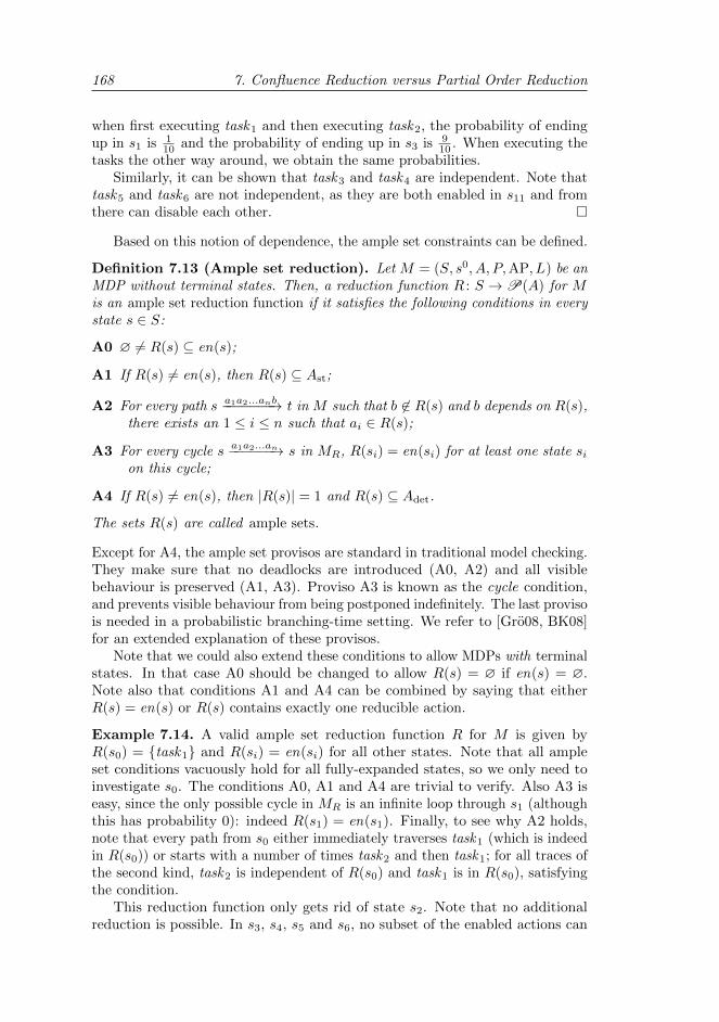
168 7. Confluence Reduction versus Partial Order Reduction

when first executing task1 and then executing task2, the probability of endingup in s1 is 1

10 and the probability of ending up in s3 is 910 . When executing the

tasks the other way around, we obtain the same probabilities.Similarly, it can be shown that task3 and task4 are independent. Note that

task5 and task6 are not independent, as they are both enabled in s11 and fromthere can disable each other.

Based on this notion of dependence, the ample set constraints can be defined.

Definition 7.13 (Ample set reduction). Let M = (S, s0, A, P,AP, L) be anMDP without terminal states. Then, a reduction function R : S →P(A) for Mis an ample set reduction function if it satisfies the following conditions in everystate s ∈ S:

A0 ∅ 6= R(s) ⊆ en(s);

A1 If R(s) 6= en(s), then R(s) ⊆ Ast;

A2 For every path s −a1a2...anb−−−−−−→ t in M such that b 6∈ R(s) and b depends on R(s),there exists an 1 ≤ i ≤ n such that ai ∈ R(s);

A3 For every cycle s −a1a2...an−−−−−→ s in MR, R(si) = en(si) for at least one state sion this cycle;

A4 If R(s) 6= en(s), then |R(s)| = 1 and R(s) ⊆ Adet.

The sets R(s) are called ample sets.

Except for A4, the ample set provisos are standard in traditional model checking.They make sure that no deadlocks are introduced (A0, A2) and all visiblebehaviour is preserved (A1, A3). Proviso A3 is known as the cycle condition,and prevents visible behaviour from being postponed indefinitely. The last provisois needed in a probabilistic branching-time setting. We refer to [Gro08, BK08]for an extended explanation of these provisos.

Note that we could also extend these conditions to allow MDPs with terminalstates. In that case A0 should be changed to allow R(s) = ∅ if en(s) = ∅.Note also that conditions A1 and A4 can be combined by saying that eitherR(s) = en(s) or R(s) contains exactly one reducible action.

Example 7.14. A valid ample set reduction function R for M is given byR(s0) = task1 and R(si) = en(si) for all other states. Note that all ampleset conditions vacuously hold for all fully-expanded states, so we only need toinvestigate s0. The conditions A0, A1 and A4 are trivial to verify. Also A3 iseasy, since the only possible cycle in MR is an infinite loop through s1 (althoughthis has probability 0): indeed R(s1) = en(s1). Finally, to see why A2 holds,note that every path from s0 either immediately traverses task1 (which is indeedin R(s0)) or starts with a number of times task2 and then task1; for all traces ofthe second kind, task2 is independent of R(s0) and task1 is in R(s0), satisfyingthe condition.

This reduction function only gets rid of state s2. Note that no additionalreduction is possible. In s3, s4, s5 and s6, no subset of the enabled actions can

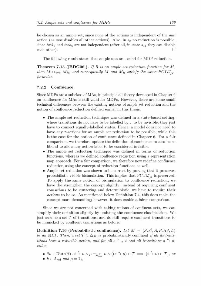
7.2. Ample sets and confluence for MDPs 169

be chosen as an ample set, since none of the actions is independent of the quitaction (as quit disables all other actions). Also, in s8 no reduction is possible,since task5 and task6 are not independent (after all, in state s11 they can disableeach other).

The following result states that ample sets are sound for MDP reduction.

Theorem 7.15 ([BDG06]). If R is an ample set reduction function for M ,then M ≈pvb MR, and consequently M and MR satisfy the same PCTL∗\X-formulae.

7.2.2 Confluence

Since MDPs are a subclass of MAs, in principle all theory developed in Chapter 6on confluence for MAs is still valid for MDPs. However, there are some smalltechnical differences between the existing notions of ample set reduction and thenotion of confluence reduction defined earlier in this thesis:

• The ample set reduction technique was defined in a state-based setting,where transitions do not have to be labelled by τ to be invisible; they justhave to connect equally-labelled states. Hence, a model does not need tohave any τ -actions for an ample set reduction to be possible, while thisis the case for the notion of confluence defined in Chapter 6. For a faircomparison, we therefore update the definition of confluence to also be soliberal to allow any action label to be considered invisible.

• The ample set reduction technique was defined in terms of reductionfunctions, whereas we defined confluence reduction using a representationmap approach. For a fair comparison, we therefore now redefine confluencereduction using the concept of reduction functions as well.

• Ample set reduction was shown to be correct by proving that it preservesprobabilistic visible bisimulation. This implies that PCTL∗\X is preserved.To apply the same notion of bisimulation to confluence reduction, wehave the strengthen the concept slightly: instead of requiring confluenttransitions to be stuttering and deterministic, we have to require theiractions to be so. As mentioned below Definition 7.4, this does make theconcept more demanding; however, it does enable a fairer comparison.

Since we are not concerned with taking unions of confluent sets, we cansimplify their definition slightly by omitting the confluence classification. Wejust assume a set T of transitions, and do still require confluent transitions tobe mimicked by confluent transitions as before.

Definition 7.16 (Probabilistic confluence). Let M = (S, s0, A, P,AP, L)be an MDP. Then, a set T ⊆ ∆M is probabilistically confluent if all its trans-

itions have a reducible action, and for all s −a→T t and all transitions s −b→ µ,either

• ∃ν ∈ Distr(S) . t −b→ ν ∧ µ ≡RTµ,ν ν ∧((s −b→ µ) ∈ T =⇒ (t −b→ ν) ∈ T

), or

• b ∈ Ared and µ = 1t,

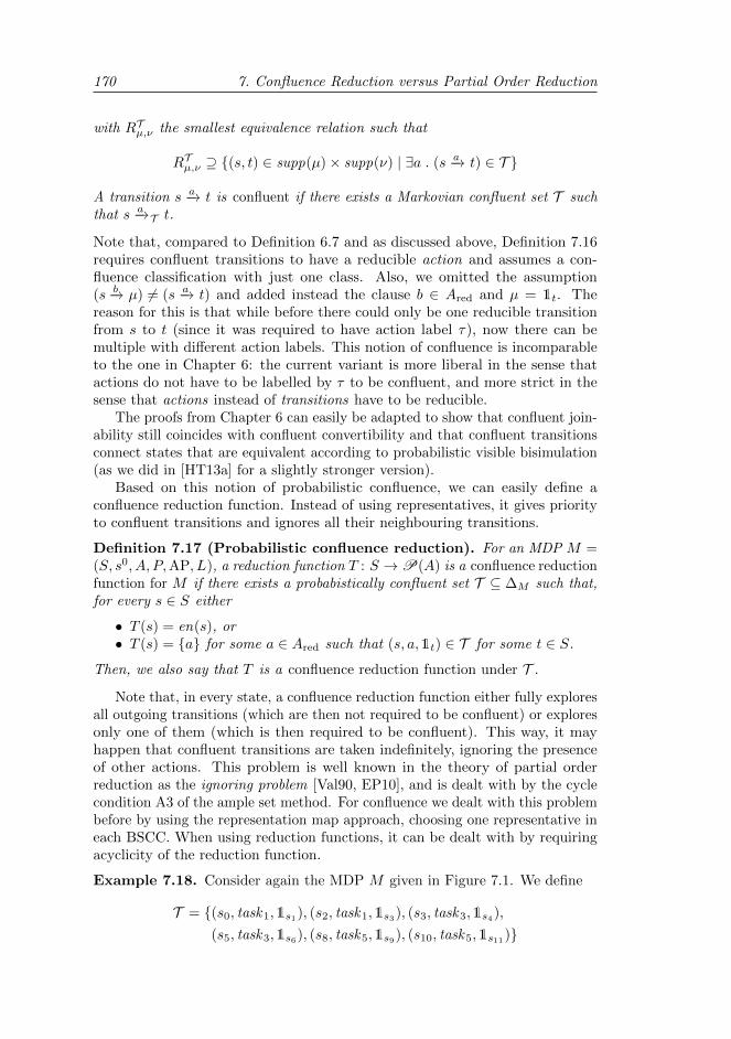
170 7. Confluence Reduction versus Partial Order Reduction

with RTµ,ν the smallest equivalence relation such that

RTµ,ν ⊇ (s, t) ∈ supp(µ)× supp(ν) | ∃a . (s −a→ t) ∈ T

A transition s −a→ t is confluent if there exists a Markovian confluent set T suchthat s −a→T t.Note that, compared to Definition 6.7 and as discussed above, Definition 7.16requires confluent transitions to have a reducible action and assumes a con-fluence classification with just one class. Also, we omitted the assumption(s −b→ µ) 6= (s −a→ t) and added instead the clause b ∈ Ared and µ = 1t. Thereason for this is that while before there could only be one reducible transitionfrom s to t (since it was required to have action label τ), now there can bemultiple with different action labels. This notion of confluence is incomparableto the one in Chapter 6: the current variant is more liberal in the sense thatactions do not have to be labelled by τ to be confluent, and more strict in thesense that actions instead of transitions have to be reducible.

The proofs from Chapter 6 can easily be adapted to show that confluent join-ability still coincides with confluent convertibility and that confluent transitionsconnect states that are equivalent according to probabilistic visible bisimulation(as we did in [HT13a] for a slightly stronger version).

Based on this notion of probabilistic confluence, we can easily define aconfluence reduction function. Instead of using representatives, it gives priorityto confluent transitions and ignores all their neighbouring transitions.

Definition 7.17 (Probabilistic confluence reduction). For an MDP M =(S, s0, A, P,AP, L), a reduction function T : S →P(A) is a confluence reductionfunction for M if there exists a probabistically confluent set T ⊆ ∆M such that,for every s ∈ S either

• T (s) = en(s), or• T (s) = a for some a ∈ Ared such that (s, a,1t) ∈ T for some t ∈ S.

Then, we also say that T is a confluence reduction function under T .

Note that, in every state, a confluence reduction function either fully exploresall outgoing transitions (which are then not required to be confluent) or exploresonly one of them (which is then required to be confluent). This way, it mayhappen that confluent transitions are taken indefinitely, ignoring the presenceof other actions. This problem is well known in the theory of partial orderreduction as the ignoring problem [Val90, EP10], and is dealt with by the cyclecondition A3 of the ample set method. For confluence we dealt with this problembefore by using the representation map approach, choosing one representative ineach BSCC. When using reduction functions, it can be dealt with by requiringacyclicity of the reduction function.

Example 7.18. Consider again the MDP M given in Figure 7.1. We define

T = (s0, task1,1s1), (s2, task1,1s3), (s3, task3,1s4),

(s5, task3,1s6), (s8, task5,1s9), (s10, task5,1s11)

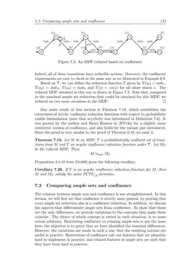
7.3. Comparing ample sets and confluence 171

s1

s0 s3

s4

s6 s8s7

s9

s11

s12

s13

p

p

q

task1910

task2 task3 task4

quit

quit

110

q

sr s

s

t

t

ucontinue

task5 task6 task5

task6

Figure 7.3: An MDP reduced based on confluence.

Indeed, all of these transitions have reducible actions. Moreover, the confluencerequirements are easy to check in the same way as we illustrated in Example 6.9.

Based on T , we can define the reduction function T given by T (s0) = task1,T (s3) = task3, T (s8) = task5 and T (s) = en(s) for all other states s. Thereduced MDP obtained in this way is shown in Figure 7.3. Note that, comparedto the maximal ample set reduction that could be obtained for this MDP, wereduced on two more occasions in the MDP.

Our main result of this section is Theorem 7.19, which establishes thecorrectness of acyclic confluence reduction functions with respect to probabilisticvisible bisimulation (note that acyclicity was introduced in Definition 7.6). Itwas proven by the author and Henri Hansen in [HT13a] for a slightly morerestrictive version of confluence, and also holds for the variant just introduced.Since the proof is very similar to the proof of Theorem 6.18, we omit it.

Theorem 7.19. Let M be an MDP, T a probabilistically confluent set of trans-itions from M and T an acyclic confluence reduction function under T . Let MT

be the reduced MDP. Then,M ≈pvb MT

Proposition 3.4.10 from [Gro08] gives the following corollary.

Corollary 7.20. If T is an acyclic confluence reduction function for M , thenM and MT satisfy the same PCTL∗\X-formulae.

7.3 Comparing ample sets and confluence

The relation between ample sets and confluence is not straightforward. In thissection, we will first see that confluence is strictly more general, by proving thatevery ample set reduction also is a confluence reduction. In addition, we discussthe aspects that differentiate ample sets from confluence. To show that theseare the only differences, we provide variations to the concepts that make themcoincide. The choice of which concept is varied in each situation, is to someextent arbitrary. Restricting confluence or relaxing ample sets is not the issuehere, the objective is to prove that we have identified the essential differences.However, the variations are made in such a way that the resulting notions areuseful in practice. Restrictions of confluence rule out features that are plausiblyhard to implement in practice, and relaxed features of ample sets are such thatthey have been used in practice.

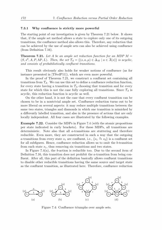
172 7. Confluence Reduction versus Partial Order Reduction

7.3.1 Why confluence is strictly more powerful

The starting point of our investigation is given by Theorem 7.21 below. It showsthat, if the ample set method allows a state to explore only one of its outgoingtransitions, the confluence method also allows this. Therefore, any reduction thatcan be achieved by the use of ample sets can also be achieved using confluence(from Definition 7.16).

Theorem 7.21. Let A be an ample set reduction function for an MDP M =(S, s0, A, P,AP, L). Then, the set TA = (s, a, µ) ∈ ∆M | a ∈ A(s) is acyclic,and consists of probabilistically confluent transitions.

This result obviously also holds for weaker notions of confluence (as forinstance presented in [TSvdP11]), which are even more powerful.

In the proof of Theorem 7.21, we construct a confluent set containing alltransitions from TA. We can use this set to define a confluence reduction function,for every state having a transition in TA choosing that transition and for everystate for which this is not the case fully exploring all transitions. Since TA isacyclic, this reduction function is acyclic as well.

On the other hand, it is not the case that every confluent transition can bechosen to be in a nontrivial ample set. Confluence reduction turns out to bemore liberal on several aspects: it may reduce multiple transitions between thesame two states, triangles and diamonds in which one transition is mimicked bya differently labelled transition, and also in the presence of actions that are onlylocally independent. All four cases are illustrated by the following examples.

Example 7.22. Consider the MDPs in Figure 7.4 (with the atomic propositionsper state indicated in curly brackets). For these MDPs, all transitions aredeterministic. Note also that all a-transitions are stuttering and thereforereducible. Even more, they are constructed in such a way that the outgoinga-transitions from every state s1 are confluent, i.e., s1 −a→ s2 is a confluent setfor all subfigures. Hence, confluence reduction allows us to omit the b-transitionfrom each state s1, thus removing six transitions and two states.

In Figure 7.4(a), the b-action is reducible too. Due to the second item ofDefinition 7.16, this transition does not prohibit the a-transition from being con-fluent. After all, this part of the definition basically allows confluent transitionsto disable other reducible transitions having the same source and target stateas the confluent transition, as illustrated here. Therefore, confluence reduction

s1

ps2

pb

a

(a)

s1

p

s2

ps3

qa b

b

(b)

s1

p

s2

ps3

q

s4

q

a b

b c

(c)

s1

p

s2

ps3

q

s4

q

a b

b a

s5

qs6

ra b

(d)

Figure 7.4: Confluence triumphs over ample sets.

7.3. Comparing ample sets and confluence 173

may choose either one of these two transitions and could for instance reducebased on T = (s1, a,1s2). The ample set conditions do not allow this; theyrequire complete independence between a and b for a to be a valid ample setfor s1. Hence, the only valid ample set for s1 is a, b.

In Figure 7.4(b), the b-transition is not reducible. Furthermore, a and b aredependent, since b disables a. However, the a-transition from s1 can still beconsidered confluent, taking T = (s1, a,1s2) as the underlying confluent setfor confluence reduction. This is due to the fact that although visible actionsmust still be enabled after a confluent transition, the confluent action does notneed to be enabled after the visible action. Again, ample set reduction cannotreduce since a and b are not independent.

Although it may seem that reduction in case of triangle constructions such asFigure 7.4(b) only removes some transitions, it can in theory make a significantdifference in the number of states. Imagine for instance a system in which everystate has a transition quit to a single deadlock state (as is partially the case inFigure 7.1). Then, not one action is independent of quit, and ample set reductionwould not be able to provide any reduction. However, such transitions wouldnot interfere with confluence. Every confluence reduction that would be possiblewithout the quit transitions is still possible with the quit transitions.

In Figure 7.4(c), the a-transition can be considered confluent since thediamond shape is closed perfectly (taking T = (s1, a,1s2), (s3, c,1s4)). Eventhough b disables a, there is a transition from s3 to s4 that can easily be shownconfluent. The ample set conditions strictly require reducible transitions to bemimicked by equally-named transitions, disallowing any reduction for this model.

In Figure 7.4(d), the outgoing a-transition from s1 is confluent since thediamond shape of independence is present (taking T = (s1, a,1s2), (s3, a,1s4)).The fact that a can disable b later on in the system does not matter for confluence.The ample set conditions, however, do require a and b to be globally independentfor a to be a valid ample set for s1. As this is not the case, no reductions canbe achieved with ample set reduction.

Confluence mainly provides more reduction since it is defined based on the actuallow-level transitions at a given state of the model, whereas the independencenotion of ample set reduction works on higher-level actions and is consideredto be global. That is, the dependency relation is assumed to be the same forevery state. In practice, however, heuristics for detecting confluent transitionssymbolically (as in [BvdP02] and in the previous chapter) often also take thismore global point of view, which diminishes the difference.

Differences and heuristics. Our implementation in SCOOP (see Chapter 9)only considers transitions to be potentially confluent if they are labelled by τ .Hence, the differences between confluence and POR depicted in Figures 7.4(a)and 7.4(c) do not occur. If differently labelled transitions were possibly con-sidered invisible as well, situation 7.4(a) could easily be detected efficientlyduring state space generation.

The heuristics implemented to decide on behaviour mimicking (basicallychecking if summands do not influence each other) do not allow any reduction in

174 7. Confluence Reduction versus Partial Order Reduction

the scenarios depicted in Figures 7.4(b) and 7.4(c). However, situations as shownin Figure 7.4(d) can occur if a = τ and the action label b is used in multiplesummands (as demonstrated below), and are indeed reduced using our heuristics.

Example 7.23. Consider the following MAPA specification:

X(pc1 : 1, 3, pc2 : 1, 3) =

pc1 = 1⇒ τ ·X(2, pc2) (1)

+ pc2 = 1⇒ b ·X(pc1, 2) (2)

+ pc2 = 2 ∧ pc2 = 2⇒ (τ ·X(3, 2) + b ·X(2, 3)) (3)

This specification yields precisely the MA of Figure 7.4(d), with a = τ . In-deed, our confluence implementation is able to reduce this system from sixto four states.

7.3.2 Closing the gap between confluence and ample sets

To show that the differences discussed above are indeed the only differencesbetween confluence and ample sets, we remove them and show that the resultingnotions indeed coincide.

As a first step, we precisely prohibit all the liberal aspects of confluence thatmake the reductions in Figure 7.4(a), 7.4(b) and 7.4(c) work—hence, disallowing‘shortcuts’ and confluent transitions relying on differently labelled confluenttransitions for the diamond shape to close.

As a second step, we loosen the independence concept of ample sets so thatit corresponds better to the more local approach of confluence, allowing amplesets to reduce Figure 7.4(d). Note that we do this safely, i.e., Theorem 7.19 isnever compromised during the process, as all these notions will still be confluentin the sense used in that theorem.

Restricted confluence. First of all, we restrict the notion of confluence bystrengthening the requirements for two distributions to be equivalent. Forthis purpose, we introduce a notion called equivalence up to T -steps to forcecommutation of transitions to occur in the diamond structure of independence.This results in a notion of confluence that can no longer reduce Figure 7.4(b).

Definition 7.24 (Equivalence up to T -steps). Let M = (S, s0, A, P,AP,L) be an MDP, T ⊆ ∆M a set of deterministic transitions of M , and letµ, ν ∈ Distr⊥(S) be two probability distributions. Then, we say that µ is equi-valent up to T -steps to ν, denoted by µ T ν, if µ, ν 6= ⊥ and there ex-ists a partitioning supp(µ) =

⊎ni=1 Si of the support of µ and an ordering

supp(ν) = 〈s1, . . . , sn〉 of the support of ν, such that

∀1 ≤ i ≤ n . µ(Si) = ν(si) ∧ ∀s ∈ Si . ∃a ∈ A . (s, a,1si) ∈ T

Example 7.25. Consider the MDP in Figure 7.5, and let

T = (s0, a,1s1), (s2, a,1s6), (s3, a,1s5), (s4, a,1s5)

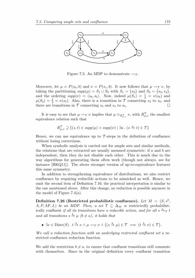
7.3. Comparing ample sets and confluence 175

s0 s1

s3s2 s4

13

13

13

b

a

s5 s6

23

13

b

a

a

a

Figure 7.5: An MDP to demonstrate T .

Moreover, let µ = P (s0, b) and ν = P (s1, b). It now follows that µ T ν, bytaking the partitioning supp(µ) = S1 ∪ S2 with S1 = s2 and S2 = s3, s4,and the ordering supp(ν) = 〈s6, s5〉. Now, indeed µ(S1) = 1

3 = ν(s6) andµ(S2) = 2

3 = ν(s5). Also, there is a transition in T connecting s2 to s6, andthere are transitions in T connecting s3 and s4 to s5.

It is easy to see that µ T ν implies that µ ≡RTµ,ν ν, with RTµ,ν the smallestequivalence relation such that

RTµ,ν ⊇ (s, t) ∈ supp(µ)× supp(ν) | ∃a . (s −a→ t) ∈ T

Hence, we can use equivalence up to T -steps in the definition of confluencewithout losing correctness.

When symbolic analysis is carried out for ample sets and similar methods,the relations that are extracted are usually assumed symmetric: if a and b areindependent, then they do not disable each other. This is much due to theway algorithms for generating them often work (though not always, see forinstance [HKQ11]). The above stronger version of up-to-equivalence featuresthis same symmetry.

In addition to strengthening equivalence of distributions, we also restrictconfluence by requiring reducible actions to be mimicked as well. Hence, weomit the second item of Definition 7.16; the practical interpretation is similar tothe one mentioned above. After this change, no reduction is possible anymore inthe model of Figure 7.4(a).

Definition 7.26 (Restricted probabilistic confluence). Let M = (S, s0,A, P,AP, L) be an MDP. Then, a set T ⊆ ∆M is restrictedly probabilist-ically confluent if all its transitions have a reducible action, and for all s −a→T tand all transitions s −b→ µ (b 6= a), it holds that

• ∃ν ∈ Distr(S) . t −b→ ν ∧ µ T ν ∧((s −b→ µ) ∈ T =⇒ (t −b→ ν) ∈ T

).

We call a reduction function with an underlying restricted confluent set a re-stricted confluence reduction function.

We add the restriction b 6= a, to ensure that confluent transitions still commutewith themselves. Since in the original definition every confluent transition

176 7. Confluence Reduction versus Partial Order Reduction

also already commuted with itself, this does not weaken the concept. Hence,Definition 7.26 is a true restriction of Definition 7.16.

Finally, we saw in Figure 7.4(c) that confluence allows reducible transitionsto be mimicked by actions with different names. If we want confluence reductionand ample sets to coincide, we need to make sure that actions are not allowedto rely on other actions to ‘close their diamonds’. From the point of view ofsymbolic analysis, this restriction matches the practical heuristics used for ampleset reduction: only pairwise analysis of actions is required, and the algorithmsfor generating ample sets or similar notions mostly rely on these sort of binaryrelations. For this purpose we introduce the concept of action-separability ,requiring that each subset of T that can be obtained by only keeping one specificaction, is confluent. That way, confluence reduction functions such as the one inFigure 7.4(c) are not allowed anymore.

Definition 7.27 (Action-separable confluence). Let M = (S, s0, A, P,AP,L) be an MDP, then a confluent set T ⊆ ∆M of transitions of M is action-separable if for every action a ∈ A the subset

Ta = (s, a, µ) ∈ S × a ×Distr(S) | (s, a, µ) ∈ T

of a-labelled confluent transitions is confluent (so possibly empty).

A confluence reduction function T : S → P(A) is action-separable if itsunderlying confluent set T is.

Relaxing ample sets. Independence is judged by the ample set constraintsin a global manner, whereas confluence deals with the notion of equivalentdistributions, which is much more local.

To make confluence and ample sets coincide, independence should also bedetermined locally, i.e., given a state, dependency of a and b makes a differenceonly in parts of the MDP that can be reached without executing the ampleaction first. This corresponds to the fact that confluence only puts restrictionson commutation of actions before a confluent transition.

The practical side of this change lies in dynamic analysis. We can, forinstance, initially consider that a and b are dependent due to symbolic analysis.However, after finishing exploring some part of the possible states following astate s, we may come to the conclusion that the dependency never manifestsanywhere where a has not been executed yet, and thus declare a independent of blocally in s. This idea originates from [KP92] and [GP93], and also correspondsexactly to the way the stubborn set definitions (see, e.g., [Val96]) deal withdependency in the non-probabilistic case: only executions starting from thecurrent state that do not include any stubborn actions, are relevant from thepoint of view of commutativity.

To define local independence, let Ra(s) ⊆ S be the set of states s′ such thats −c1...cn−−−−→ s′ for some path where there is no i such that ci = a.

Definition 7.28 (Local independence). Given an MDP M = (S, s0, A, P,AP, L), a state s ∈ S, and two actions a, b ∈ A, we say that a is independent

7.3. Comparing ample sets and confluence 177

of b at s if a 6= b and for every state s′ ∈ Ra(s) such that a, b ⊆ en(s′) thefollowing conditions hold:

• If s∗ ∈ supp(P (s′, a)), then b ∈ en(s∗) (and symmetrically);

• We have∑s∗∈S

P (s′, a)(s∗) · P (s∗, b)(t) =∑s∗∈S

P (s′, b)(s∗) · P (s∗, a)(t)

for every t ∈ S.

If a is not independent of b at s, we say that it is dependent of b at s.

Note that this definition coincides with the original definition of independence,except that the conditions only have to hold for all states in Ra(s) instead of allstates in S.

Also note that local (in)dependence is not a symmetric relation. For a to beindependent of b at s we only consider the states in Ra(s); this is in general aset different from Rb(s).

Example 7.29. In Example 7.12 we noticed that the actions task5 and task6

in Figure 7.1 were not independent, since there is a state (namely s11) inwhich they can disable each other. However, taking local independence, wesee that Rtask5(s8) = s8, s10 and Rtask6(s8) = s8, s9, and we can verifythat the independence conditions are satisfied by all of these states. Hence,task5 is independent of task6 at s8 and also task6 is independent of task5 at s8.Therefore, if the ample set conditions used local independence instead of globalindependence, it would be allowed to take either task5 or task6 as an ample setfor s8.

Under the local dependency condition, we can now relax the ample setconditions slightly.

Definition 7.30 (Relaxed ample sets). A set A(s) is a relaxed ample set ifit meets the criteria of Definition 7.13, except that A2 is replaced by the followingcondition:

A2∗ For every path s −a1a2...anb−−−−−−→ t in M such that b 6∈ A(s) and some a ∈ A(s)is dependent on b at s, there exists an 1 ≤ i ≤ n such that ai ∈ A(s).

Comparison. Our most important theorem of this chapter is now ready to beproven. It says that our restriction of confluence reduction and relaxation ofample set reduction indeed coincide. Hence, the differences we identified earlierindeed precisely characterise the gap between the two notions.

Theorem 7.31. Let M = (S, s0, A, P,AP, L) be an MDP. Then, T : S →P(A)is an acyclic action-separable restricted confluence reduction function if and onlyif T is a relaxed ample set reduction function.

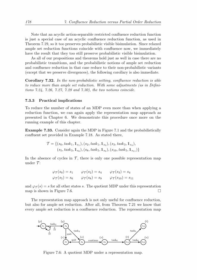
178 7. Confluence Reduction versus Partial Order Reduction

Note that an acyclic action-separable restricted confluence reduction functionis just a special case of an acyclic confluence reduction function, as used inTheorem 7.19, so it too preserves probabilistic visible bisimulation. Since relaxedample set reduction functions coincide with confluence now, we immediatelyhave the result that they too still preserve probabilistic visible bisimulation.

As all of our propositions and theorems hold just as well in case there are noprobabilistic transitions, and the probabilistic notions of ample set reductionand confluence reduction in that case reduce to their non-probabilistic variants(except that we preserve divergences), the following corollary is also immediate.

Corollary 7.32. In the non-probabilistic setting, confluence reduction is ableto reduce more than ample set reduction. With some adjustments (as in Defini-tions 7.24, 7.26, 7.27, 7.28 and 7.30), the two notions coincide.

7.3.3 Practical implications

To reduce the number of states of an MDP even more than when applying areduction function, we can again apply the representation map approach aspresented in Chapter 6. We demonstrate this procedure once more on therunning example of this chapter.

Example 7.33. Consider again the MDP in Figure 7.1 and the probabilisticallyconfluent set provided in Example 7.18. As stated there,

T = (s0, task1,1s1), (s2, task1,1s3), (s3, task3,1s4),

(s5, task3,1s6), (s8, task5,1s9), (s10, task5,1s11)

In the absence of cycles in T , there is only one possible representation mapunder T :

ϕT (s0) = s1 ϕT (s2) = s4 ϕT (s3) = s4

ϕT (s5) = s6 ϕT (s8) = s9 ϕT (s10) = s11

and ϕT (s) = s for all other states s. The quotient MDP under this representationmap is shown in Figure 7.6.

The representation map approach is not only useful for confluence reduction,but also for ample set reduction. After all, from Theorem 7.21 we know thatevery ample set reduction is a confluence reduction. The representation map

s1 s4

s6s7 s9 s11

s12

s13

p

910

task2

task4

quit

quit

110

q

sr s t

t

ucontinue task6

task5

task6

Figure 7.6: A quotient MDP under a representation map.

7.4. Contributions 179

approach serves as an alternative implementation of the cycle condition of amplesets or the acyclicity requirement used earlier in this chapter. The cycle conditionis satisfied in the sense that the quotient MDP never indefinitely ignores anybehaviour of the original MDP.

7.4 Contributions

We redefined confluence reduction in an MDP-based setting, enabling a compar-ison to probabilistic partial order reduction based on ample sets in branchingtime. We proved that every nontrivial ample set can be mimicked by a confluentset, and that in some cases reductions are possible using confluence but notusing ample sets. Therefore, at least in theory confluence reduction is able toreduce more than the ample set method. We also showed the exact way in whichconfluence and ample sets have to be modified for the two notions to coincide.This way, the gap between their expressivity is identified precisely. These resultshold for the non-probabilistic variants of the two reduction techniques as well.

Our observation that probabilistic ample set reduction can be mimicked byprobabilistic confluence reduction has additional implications, some of whichare highly practical. One such implication is that the use of a representationmap for reduced state space generation, already applied earlier in combinationwith confluence reduction, can also be applied for partial order reduction as asubstitute for the cycle condition.

As both ample sets and confluence are detected symbolically on the languagelevel, the quality of the heuristics applied there will decide which notion worksbest in practice. The results in this chapter already strengthen our theoreticalunderstanding of the two methods, and this is independent of the heuristics thatare applied. Obviously, no matter how such heuristics are improved, the resultsin this chapter will remain valid. We showed that at least one of the advantagesof confluence over POR can indeed be exploited by our heuristics.

To complement the theoretical results presented in this chapter, the nextchapter will provide a comparison of confluence reduction and partial orderreduction from a practical point of view. Although the practical difference maybe limited with regard to the number of additional reductions, we will show thatthe way confluence deals with independence allows more systems to be subjectedto statistical model checking: a significant improvement.

We conjecture that the ideas presented in this chapter can easily be used todefine a notion of branching time partial order reduction for MAs, based on ournotion of confluence for MAs presented in Chapter 6. Then, a result similar toTheorem 7.21 might be applied to prove its correctness.

CHAPTER 8

Confluence Reduction in

Statistical Model Checking

A Practical Comparison to Partial Order Reduction

“There’s no sense in being precisewhen you don’t even knowwhat you’re talking about.”

John von Neumann

As mentioned before, model checking is subject to the state space explosionproblem, with probabilistic model checking being particularly affecteddue to its additional numerical complexity. Several techniques have been

introduced to stretch the limits of model checking, while preserving its basicnature of performing state space exploration to obtain results that unconditionallyhold for the entire state space. Among these techniques are the basic reductiontechniques we introduced in Section 4.5 and the dead variable reduction techniquefrom Chapter 5, as well as confluence reduction and partial order reduction(POR) as discussed in Chapters 6 and 7. As discussed previously, partial orderreduction and confluence reduction both work by selecting a subset of thetransitions of a model—and thus a subset of the reachable states—in a way thatensures that the reduced system is equivalent to the complete system.

A much different approach for probabilistic models is statistical modelchecking (SMC) [HLMP04, LDB10, YS02]: instead of exploring—and storing inmemory—the entire state space, or even a reduced version of it, discrete-eventsimulation is used to generate traces through the state space. This comes atconstant memory usage and thus circumvents the state space explosion entirely,but can only approximate probabilities of interest. Statistical methods such assequential hypothesis testing are then used to make sure that the probability ofreturning the wrong result is below a certain threshold. As a simulation-basedapproach, however, SMC is in principle limited to fully stochastic models suchas Markov chains [Har10].

Previously, an approach based on POR was presented [BFHH11] to extendSMC and simulation to the nondeterministic model of Markov decision processes(MDPs). In that approach, simulation proceeds as usual until a nondeterministicchoice is encountered; then, an on-the-fly check is performed to find a singletonsubset of the available transitions that satisfies the ample set conditions of linear-

182 8. Confluence Reduction in Statistical Model Checking

time probabilistic POR [BGC04, DN04]. If such an ample set is found, simulationcan continue according to it, with the guarantee that ignoring the other transitionsdoes not affect the verification results—that is, the nondeterminism was spurious.Yet, the ample set conditions are based on the notion of independence of actions,which can in practice only feasibly be checked on a symbolic/syntactic level(using conditions such as J1 and J2 in [BFHH11]). This limits the approach toresolving spurious nondeterminism only when it results from the interleaving ofbehaviours of concurrently executing deterministic components.

It is absolutely vital for the search for a valid singleton subset to succeed inthe approach discussed above: one choice that cannot be resolved means thatthe entire analysis fails and SMC cannot safely be applied to the given model atall. Hence, any additional reduction power is highly welcome. In this chapter,we therefore introduce an alternative approach that uses confluence reductioninstead of POR. We demonstrate that the findings of Chapter 7—which showedthat confluence is in theory more powerful than branching time POR—indeedenable reductions that POR did not allow. That way, some models can now beanalysed using SMC whereas this was not possible before.

We note that a confluence-based approach is not better in all cases, though,since the approach in [BFHH11] in based on linear time POR with an addedrequirement of having singleton ample sets. Compared to branching time POR,this notion is more liberal in the sense that it allows ample actions to beprobabilistic. As confluence requires deterministic transitions, this also gives thePOR-based approach an advantage—at the cost of preserving less properties,though LTL\X is still more than enough for SMC.

Except for potentially reducing more in some cases, an additional advantageof confluence reduction is that it is more easily implemented on the level of theconcrete state space alone—without any need to go back to the symbolic/syntacticlevel for an independence check (as was done for POR). As opposed to theapproach in [BFHH11], it thus allows even spurious nondeterminism that isinternal to components to be ignored during simulation. Of course, modelscontaining non-spurious nondeterminism can still not be dealt with.

Our approach. While the notion of confluence from Chapter 7 is based onMDPs too, it is not yet suitable for use during SMC. After all, it required actionsinstead of transitions to be stuttering and deterministic. In SMC we cannotcheck this explicitly, as the complete state space is not available. Moreover,we especially do not want to apply syntactic heuristics, to make the techniqueas powerful as possible. Hence, we change the requirement of stuttering anddeterministic actions back to stuttering and deterministic transitions—basicallyagain taking the same approach as in Chapter 6. In addition to this alteration,we also relax the definition of confluence by allowing visible transitions to bemimicked by differently-labelled transitions. After all, simulation works with afully composed, closed system, where action labels have become irrelevant. Wethus achieve more reduction/detection power at no computational cost; yet, thisadapted notion of confluence still preserves PCTL∗ formulae [BK08] without thenext operator.

We introduce an algorithm for detecting our new notion of probabilistic

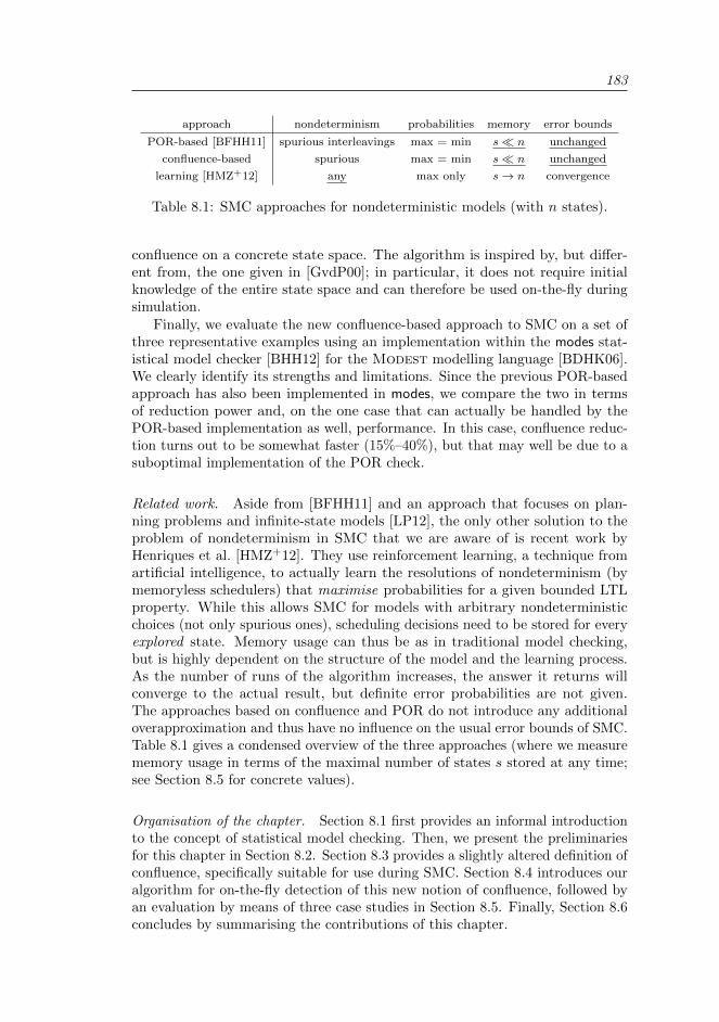
183

approach nondeterminism probabilities memory error bounds

POR-based [BFHH11] spurious interleavings max = min s n unchanged

confluence-based spurious max = min s n unchanged

learning [HMZ+12] any max only s→ n convergence

Table 8.1: SMC approaches for nondeterministic models (with n states).

confluence on a concrete state space. The algorithm is inspired by, but differ-ent from, the one given in [GvdP00]; in particular, it does not require initialknowledge of the entire state space and can therefore be used on-the-fly duringsimulation.

Finally, we evaluate the new confluence-based approach to SMC on a set ofthree representative examples using an implementation within the modes stat-istical model checker [BHH12] for the Modest modelling language [BDHK06].We clearly identify its strengths and limitations. Since the previous POR-basedapproach has also been implemented in modes, we compare the two in termsof reduction power and, on the one case that can actually be handled by thePOR-based implementation as well, performance. In this case, confluence reduc-tion turns out to be somewhat faster (15%–40%), but that may well be due to asuboptimal implementation of the POR check.

Related work. Aside from [BFHH11] and an approach that focuses on plan-ning problems and infinite-state models [LP12], the only other solution to theproblem of nondeterminism in SMC that we are aware of is recent work byHenriques et al. [HMZ+12]. They use reinforcement learning, a technique fromartificial intelligence, to actually learn the resolutions of nondeterminism (bymemoryless schedulers) that maximise probabilities for a given bounded LTLproperty. While this allows SMC for models with arbitrary nondeterministicchoices (not only spurious ones), scheduling decisions need to be stored for everyexplored state. Memory usage can thus be as in traditional model checking,but is highly dependent on the structure of the model and the learning process.As the number of runs of the algorithm increases, the answer it returns willconverge to the actual result, but definite error probabilities are not given.The approaches based on confluence and POR do not introduce any additionaloverapproximation and thus have no influence on the usual error bounds of SMC.Table 8.1 gives a condensed overview of the three approaches (where we measurememory usage in terms of the maximal number of states s stored at any time;see Section 8.5 for concrete values).

Organisation of the chapter. Section 8.1 first provides an informal introductionto the concept of statistical model checking. Then, we present the preliminariesfor this chapter in Section 8.2. Section 8.3 provides a slightly altered definition ofconfluence, specifically suitable for use during SMC. Section 8.4 introduces ouralgorithm for on-the-fly detection of this new notion of confluence, followed byan evaluation by means of three case studies in Section 8.5. Finally, Section 8.6concludes by summarising the contributions of this chapter.

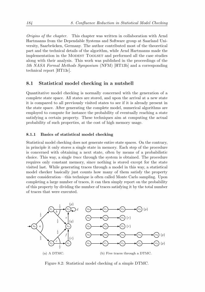
184 8. Confluence Reduction in Statistical Model Checking

Origins of the chapter. This chapter was written in collaboration with ArndHartmanns from the Dependable Systems and Software group at Saarland Uni-versity, Saarbrucken, Germany. The author contributed most of the theoreticalpart and the technical details of the algorithm, while Arnd Hartmanns made theimplementation in the Modest Toolset and performed all the case studiesalong with their analysis. This work was published in the proceedings of the5th NASA Formal Methods Symposium (NFM) [HT13b] and a correspondingtechnical report [HT13c].

8.1 Statistical model checking in a nutshell

Quantitative model checking is normally concerned with the generation of acomplete state space. All states are stored, and upon the arrival at a new stateit is compared to all previously visited states to see if it is already present inthe state space. After generating the complete model, numerical algorithms areemployed to compute for instance the probability of eventually reaching a statesatisfying a certain property. These techniques aim at computing the actualprobability of such properties, at the cost of high memory usage.

8.1.1 Basics of statistical model checking

Statistical model checking does not generate entire state spaces. On the contrary,in principle it only stores a single state in memory. Each step of the procedureis concerned with obtaining a next state, often by means of a probabilisticchoice. This way, a single trace through the system is obtained. The procedurerequires only constant memory, since nothing is stored except for the statevisited last. While generating traces through a model in this way, a statisticalmodel checker basically just counts how many of them satisfy the propertyunder consideration—this technique is often called Monte Carlo sampling. Uponcompleting a large number of traces, it can then simply report on the probabilityof this property by dividing the number of traces satisfying it by the total numberof traces that were executed.

s0

s1

s2

a

13

23

s3

s4

s5

12

12

12

12

b

c

p

q

r

e

f

d

(a) A DTMC.

s0 s1 s3 s3 p

s0 s2 s5 r

s0 s2 s5 r

s0 s2 s4 s3 s3 p

s0 s1 s4 s3 s3 p

(b) Five traces through a DTMC.

Figure 8.2: Statistical model checking of a simple DTMC.

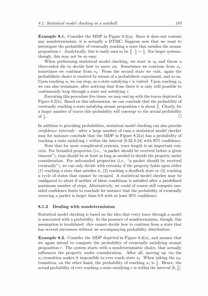
8.1. Statistical model checking in a nutshell 185

Example 8.1. Consider the MDP in Figure 8.2(a). Since it does not containany nondeterminism, it is actually a DTMC. Suppose now that we want toinvestigate the probability of eventually reaching a state that satisfies the atomicproposition r. Analytically, this is easily seen to be 2

3 · 13 = 13 . For larger systems,

though, this may not be so easy.When performing statistical model checking, we start in s0 and throw a

three-sided die to decide how to move on. Sometimes we continue from s1,sometimes we continue from s2. From the second state we visit, again theprobabilistic choice is resolved by means of a probabilistic experiment, and so on.Upon reaching s5 we can stop, as a state satisfying r is visited. Upon reaching s3

we can also terminate, after noticing that from there it is only still possible tocontinuously loop through a state not satisfying r.

Executing this procedure five times, we may end up with the traces depicted inFigure 8.2(b). Based on this information, we can conclude that the probability ofeventually reaching a state satisfying atomic proposition r is about 2

5 . Clearly, fora larger number of traces this probability will converge to the actual probabilityof 1

3 .

In addition to providing probabilities, statistical model checking can also provideconfidence intervals—after a large number of runs a statistical model checkermay for instance conclude that the MDP in Figure 8.2(a) has a probability ofreaching a state satisfying r within the interval [0.32, 0.34] with 95% confidence.

Note that for more complicated systems, trace length is an important con-cern. For bounded properties (i.e., “a packet should be received before a giventimeout”), runs should be at least as long as needed to decide the property underconsideration. For unbounded properties (i.e., “a packet should be receivedeventually”), we can only decide with certainty if the property holds upon either(1) reaching a state that satisfies it, (2) reaching a deadlock state or (3) reachinga cycle of states that cannot be escaped. A statistical model checker may beconfigured to abort if neither of these conditions is satisfied after a predefinedmaximum number of steps. Alternatively, we could of course still compute one-sided confidence limits to conclude for instance that the probability of eventuallyreceiving a packet is larger than 0.8 with at least 95% confidence.

8.1.2 Dealing with nondeterminism

Statistical model checking is based on the idea that every trace through a modelis associated with a probability. In the presence of nondeterminism, though, thisassumption is invalidated: dice cannot decide how to continue from a state thathas several successors without an accompanying probability distribution.

Example 8.2. Consider the MDP depicted in Figure 8.3(a), and assume thatwe again intend to compute the probability of eventually satisfying atomicproposition r. The system starts with a nondeterministic choice, that actuallyinfluences the property under consideration. After all, moving up via thea1-transition makes it impossible to ever reach state s5. When taking the a2-transition, on the other hand, the probability of reaching s5 is 1

2 . Hence, theactual probability of ever reaching a state satisfying r is within the interval [0, 1

2 ].

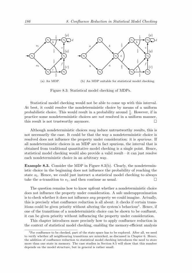
186 8. Confluence Reduction in Statistical Model Checking

s0

s1

s2

a1

a2

s3

s4

s5

12

12

12

12

b

c

p

q

r

e

f

d

(a) An MDP.

s0

s1

s2

s0

s1

s2

a

a

b

b

a

13

23

s3

s4

s5

12

12

12

12

b

c

p

q

r

e

f

d

(b) An MDP suitable for statistical model checking.

Figure 8.3: Statistical model checking of MDPs.

Statistical model checking would not be able to come up with this interval.At best, it could resolve the nondeterministic choice by means of a uniformprobabilistic choice. This would result in a probability around 1

4 . However, if inpractice some nondeterministic choices are not resolved in a uniform manner,this result is not trustworthy anymore.

Although nondeterministic choices may induce untrustworthy results, this isnot necessarily the case. It could be that the way a nondeterministic choice isresolved does not influence the property under consideration: it is spurious. Ifall nondeterministic choices in an MDP are in fact spurious, the interval that isobtained from traditional quantitative model checking is a single point. Hence,statistical model checking would also provide a valid result—it can just resolveeach nondeterministic choice in an arbitrary way.

Example 8.3. Consider the MDP in Figure 8.3(b). Clearly, the nondetermin-istic choice in the beginning does not influence the probability of reaching thestate s5. Hence, we could just instruct a statistical model checking to alwaystake the a-transition to s1, and then continue as usual.

The question remains how to know upfront whether a nondeterministic choicedoes not influence the property under consideration. A safe underapproximationis to check whether it does not influence any property we could imagine. Actually,this is precisely what confluence reduction is all about: it checks if certain trans-itions could be given priority without altering the system’s behaviour1. Hence, ifone of the transitions of a nondeterministic choice can be shown to be confluent,it can be given priority without influencing the property under consideration.

This chapter introduces more precisely how to apply confluence reduction inthe context of statistical model checking, enabling the memory-efficient analysis

1For confluence to be checked, part of the state space has to be explored. After all, we needto verify whether all neighbouring transitions are mimicked, as discussed in Chapter 6. Hence,the addition of confluence reduction to statistical model checking introduces the need to storemore than one state in memory. The case studies in Section 8.5 will show that this numberdepends on the model structure, but in general is rather small.

8.2. Preliminaries 187

of the subset of MDPs that contain only confluent nondeterministic choices.2

8.2 Preliminaries

Our investigation of confluence reduction for statistical model checking takesplace in the context of the Modest Toolset. This framework is based onMarkov decision processes (MDPs), almost identical to the variant defined inthe previous chapter (Definition 7.1), but slightly different in the sense that astate is now allowed to have multiple outgoing transitions with the same label.

For convenience of the reader—though at the cost of some repetition—we present the altered definition again instead of only explaining the (minor)differences.

Definition 8.4 (MDPs). A Markov decision process (MDP) is a tuple M =(S, s0, A, P,AP, L), where

• S is a countable set of states;• s0 ∈ S is the initial state;• A ⊆ Act is a finite set of actions;• P ⊆ S ×A×Distr(S) is the probabilistic transition relation;• AP is a finite set of state labels;• L : S →P(AP) is the state-labelling function.

Given a state s ∈ S, we define its set of enabled transitions

en(s) = (s, a, µ) ∈ s ×A×Distr(S) | s −a→ µ

We will use SM , AM , . . . , to refer to the components of an MDP M . If theMDP is clear from the context, these subscripts are omitted.

Note that the current definition of MDPs precisely coincides with the definitionof MAs (Definition 3.5) when restricting MAs to finite sets of actions and statelabels and an empty set of Markovian transitions. Hence, all notations introducedfor MAs can directly be applied to these MDPs. Also, we reuse the conceptspresented in Definition 7.4 on determinism and stuttering.

With Modest we work in a state-based verification setting where propertiesonly refer to the atomic propositions of states. The action labels are solely meantfor synchronisation during parallel composition. Since SMC is applied to theresult of parallel composition we consider closed systems only, and thereforewe can ignore the action labels. We do care about whether or not transitionschange the observable behaviour of the system, i.e., the atomic propositions.As before, transitions not changing this behaviour are called stuttering. In thischapter, we write s −τ→ µ to indicate that a transition is stuttering. Transitionslabelled by a letter different from τ can be either stuttering or not.

2In hindsight, if all nondeterministic choices turn out to be spurious, we could just as wellhave taken the old approach of just resolving nondeterministic choices in a uniform probabilisticmanner. This would indeed have provided the same result. However, the old approach wouldnot have shown us that this result indeed is a valid result under all possible schedulers. Ourapproach based on confluence does provide us with this information.

188 8. Confluence Reduction in Statistical Model Checking

As in the previous chapter, we again apply reduction functions to indicatewhich transitions to keep and which to omit. Whereas in Definition 7.6 we couldspecify the outgoing transitions of a state by listing their actions, this is now notpossible anymore due to the fact that there may be multiple transitions with thesame label. Hence, we alter the concept of a reduction function slightly, makingit select from the outgoing transitions of a state instead of its actions.

Definition 8.5 (Reduction functions). Given an MDP M = (SM , s0M , A,

PM ,AP, LM ), a reduction function is any function R : SM →P(PM ) such thatR(s) ⊆ en(s) for every s ∈ SM . Given a reduction function R, the reducedMDP for M with respect to R is the minimal MDP MR = (SR, s

0R, A, PR,AP,

LR) such that s0R = s0

M and

• if s ∈ SR and (s, a, µ) ∈ R(s), then (s, a, µ) ∈ PR and supp(µ) ⊆ SR;• LR(s) = LM (s) for every s ∈ SR,

where minimal should be interpreted as having the smallest set of states and thesmallest set of transitions.

Given a reduction function R and a state s ∈ SR, we say that s is a reducedstate if R(s) 6= en(s). All outgoing transitions of a reduced state are callednontrivial transitions. We say that a reduction function is acyclic if there areno cyclic paths when only nontrivial transitions are considered.

8.3 Confluence for statistical model checking

In this chapter we are dealing with a state-based context; only the atomicpropositions that are assigned to each state are of interest. Therefore, we baseour definition of confluence on the one introduced in Chapter 7. We adjust itslightly to adapt to the setting of SMC.

8.3.1 Confluence sets for statistical model checking

In this chapter, we apply the following definition of confluence.

Definition 8.6 (Probabilistic confluence). Let M = (S, s0, A, P,AP, L) bean MDP, then a subset T ⊆ P of transitions from M is probabilistically confluentif it only contains deterministic stuttering transitions, and for all s −a→T t and

all transitions s −b→ µ, either

• ∃c ∈ A, ν ∈ Distr(S) . t −c→ ν ∧ µ ≡RTµ,ν ν ∧((s −b→ µ) ∈ T =⇒ (t −c→ ν) ∈ T

), or

• µ = 1t,

with RTµ,ν the smallest equivalence relation such that

RTµ,ν ⊇ (s, t) ∈ supp(µ)× supp(ν) | ∃a . (s −a→ t) ∈ T

A transition is probabilistically confluent if there exists a probabilistically con-fluent set that contains it.

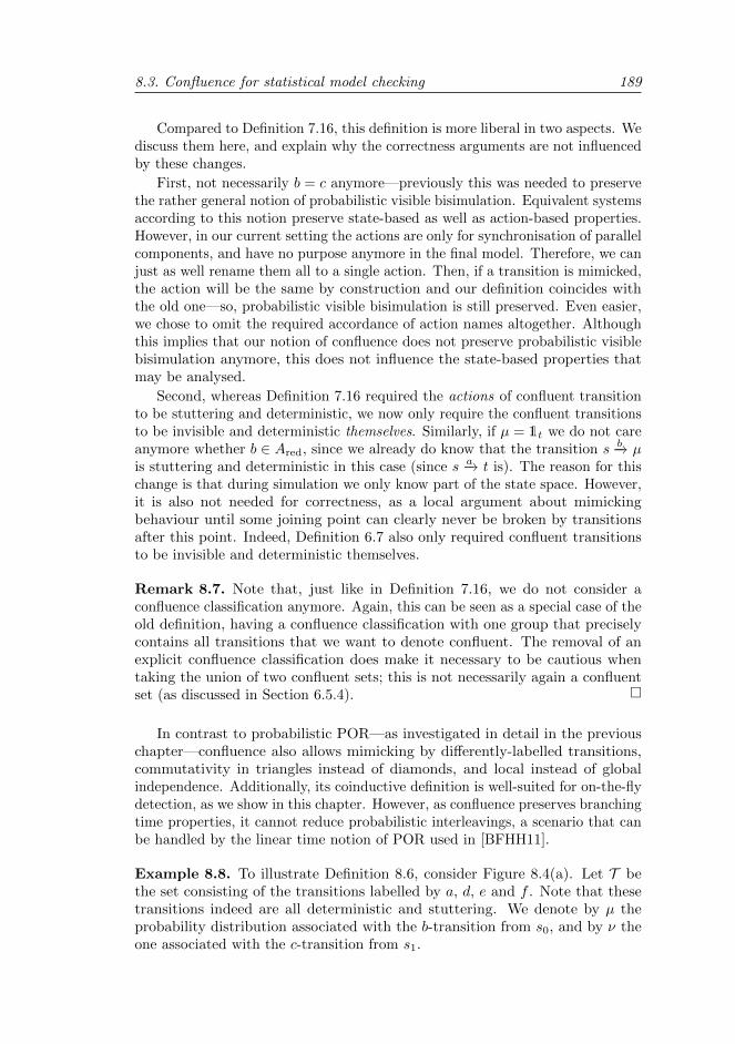
8.3. Confluence for statistical model checking 189

Compared to Definition 7.16, this definition is more liberal in two aspects. Wediscuss them here, and explain why the correctness arguments are not influencedby these changes.

First, not necessarily b = c anymore—previously this was needed to preservethe rather general notion of probabilistic visible bisimulation. Equivalent systemsaccording to this notion preserve state-based as well as action-based properties.However, in our current setting the actions are only for synchronisation of parallelcomponents, and have no purpose anymore in the final model. Therefore, we canjust as well rename them all to a single action. Then, if a transition is mimicked,the action will be the same by construction and our definition coincides withthe old one—so, probabilistic visible bisimulation is still preserved. Even easier,we chose to omit the required accordance of action names altogether. Althoughthis implies that our notion of confluence does not preserve probabilistic visiblebisimulation anymore, this does not influence the state-based properties thatmay be analysed.

Second, whereas Definition 7.16 required the actions of confluent transitionto be stuttering and deterministic, we now only require the confluent transitionsto be invisible and deterministic themselves. Similarly, if µ = 1t we do not careanymore whether b ∈ Ared, since we already do know that the transition s −b→ µis stuttering and deterministic in this case (since s −a→ t is). The reason for thischange is that during simulation we only know part of the state space. However,it is also not needed for correctness, as a local argument about mimickingbehaviour until some joining point can clearly never be broken by transitionsafter this point. Indeed, Definition 6.7 also only required confluent transitionsto be invisible and deterministic themselves.

Remark 8.7. Note that, just like in Definition 7.16, we do not consider aconfluence classification anymore. Again, this can be seen as a special case of theold definition, having a confluence classification with one group that preciselycontains all transitions that we want to denote confluent. The removal of anexplicit confluence classification does make it necessary to be cautious whentaking the union of two confluent sets; this is not necessarily again a confluentset (as discussed in Section 6.5.4).

In contrast to probabilistic POR—as investigated in detail in the previouschapter—confluence also allows mimicking by differently-labelled transitions,commutativity in triangles instead of diamonds, and local instead of globalindependence. Additionally, its coinductive definition is well-suited for on-the-flydetection, as we show in this chapter. However, as confluence preserves branchingtime properties, it cannot reduce probabilistic interleavings, a scenario that canbe handled by the linear time notion of POR used in [BFHH11].

Example 8.8. To illustrate Definition 8.6, consider Figure 8.4(a). Let T bethe set consisting of the transitions labelled by a, d, e and f . Note that thesetransitions indeed are all deterministic and stuttering. We denote by µ theprobability distribution associated with the b-transition from s0, and by ν theone associated with the c-transition from s1.

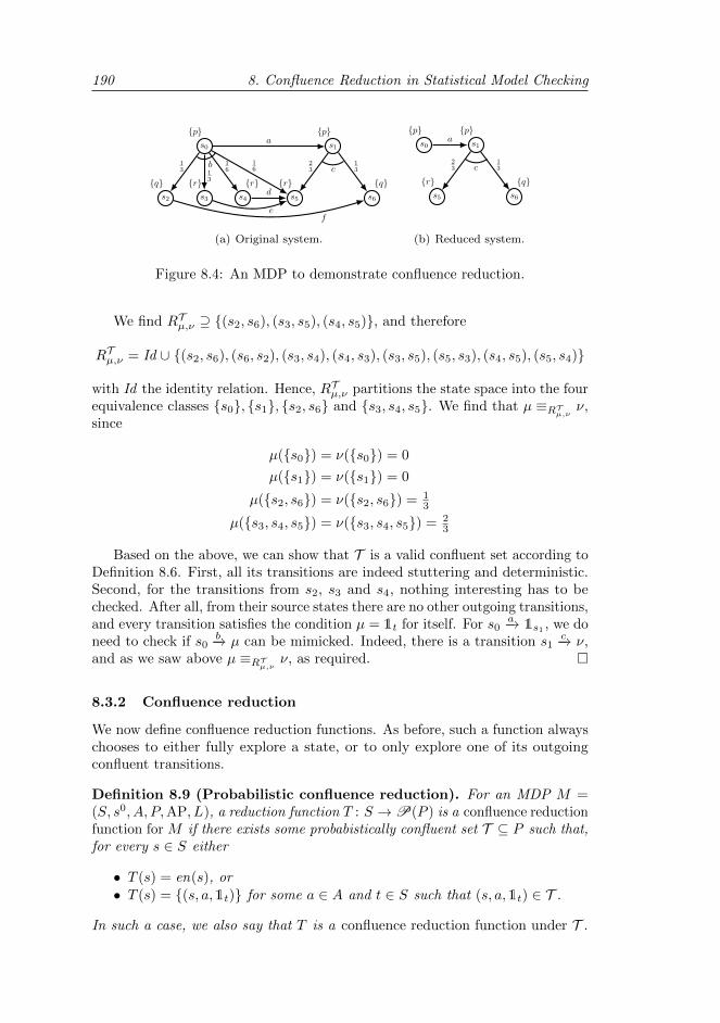
190 8. Confluence Reduction in Statistical Model Checking

s0 s1

s3s2 s4 s5 s6

13 1

3

16

16

b

a

23

13c

f

d

e

p p

rq r r q

(a) Original system.

s0 s1

s5 s6

a

23

13c

p p

r q

(b) Reduced system.

Figure 8.4: An MDP to demonstrate confluence reduction.

We find RTµ,ν ⊇ (s2, s6), (s3, s5), (s4, s5), and therefore

RTµ,ν = Id ∪ (s2, s6), (s6, s2), (s3, s4), (s4, s3), (s3, s5), (s5, s3), (s4, s5), (s5, s4)

with Id the identity relation. Hence, RTµ,ν partitions the state space into the fourequivalence classes s0, s1, s2, s6 and s3, s4, s5. We find that µ ≡RTµ,ν ν,since

µ(s0) = ν(s0) = 0

µ(s1) = ν(s1) = 0

µ(s2, s6) = ν(s2, s6) = 13

µ(s3, s4, s5) = ν(s3, s4, s5) = 23

Based on the above, we can show that T is a valid confluent set according toDefinition 8.6. First, all its transitions are indeed stuttering and deterministic.Second, for the transitions from s2, s3 and s4, nothing interesting has to bechecked. After all, from their source states there are no other outgoing transitions,and every transition satisfies the condition µ = 1t for itself. For s0 −a→ 1s1 , we doneed to check if s0 −b→ µ can be mimicked. Indeed, there is a transition s1 −c→ ν,and as we saw above µ ≡RTµ,ν ν, as required.

8.3.2 Confluence reduction

We now define confluence reduction functions. As before, such a function alwayschooses to either fully explore a state, or to only explore one of its outgoingconfluent transitions.

Definition 8.9 (Probabilistic confluence reduction). For an MDP M =(S, s0, A, P,AP, L), a reduction function T : S →P(P ) is a confluence reductionfunction for M if there exists some probabistically confluent set T ⊆ P such that,for every s ∈ S either

• T (s) = en(s), or• T (s) = (s, a,1t) for some a ∈ A and t ∈ S such that (s, a,1t) ∈ T .

In such a case, we also say that T is a confluence reduction function under T .

8.4. On-the-fly detection of probabilistic confluence 191

Note the resemblance with Definition 7.17—the only difference is that we nowselect between the transitions instead of the actions of each state.

As discussed before in earlier chapters, confluent transitions may be takenindefinitely, ignoring the presence of other actions—the ignoring problem [EP10].It was dealt with by the cycle condition of the ample set method of POR, andby the requirement of having an acyclic reduction function in the confluencereduction technique introduced in the previous chapter. In the current context,we again deal with it by requiring the reduction function to be acyclic. Acyclicitycan be checked during simulation and statistical model checking in the sameway as was done for POR in [BFHH11]: for some predefined constant l, alwayscheck whether in the last l steps at least one state was fully explored (i.e., thestate already contained only one outgoing transition)3.

Example 8.10. For the system of Figure 8.4(a), we already found a validconfluent set. Based on this set, we can define the reduction function T givenby T (s0) = (s0, a,1s1) and T (s) = en(s) for every other state s. That way,the reduced system is given by Figure 8.4(b).

Note that the two models indeed share the same properties, such as that the(minimum and maximum) probability of eventually observing r is 2

3 .

Confluence reduction preserves PCTL∗\X , and hence basically all interestingquantitative properties (including LTL\X , as was preserved in [BFHH11]).

Theorem 8.11. Let M be an MDP, T a confluent set of its transitions and Tan acyclic confluence reduction function under T . Let MT be the reduced MDP.Then, M and MT satisfy the same PCTL∗\X formulae.

8.4 On-the-fly detection of probabilistic confluence

Non-probabilistic confluence was first detected directly on concrete state spaces toreduce them modulo branching bisimulation [GvdP00]. Although the complexitywas linear in the size of the state space, the method was not very useful: itrequired the complete unreduced state space to be available, which could alreadybe too large to generate. Therefore, two directions of improvements were pursued.

The first idea was to detect confluence on higher-level process-algebraicsystem descriptions, as first done in [Blo01, BvdP02] for labelled transitionsystems and generalised to the probabilistic setting of MAs (and hence MDPs) inthis thesis. The other direction was to use the ideas from [GvdP00] to on-the-flydetect non-probabilistic weak or strong confluence [MW12, PLM03] during statespace generation. These techniques are based on boolean equation systems andhave not yet been generalised to the probabilistic setting.

We present a novel on-the-fly algorithm that works on concrete probabilisticstate spaces and does not require the unreduced state space, making it perfectlyapplicable during simulation for statistical model checking of MDPs. Given

3As mentioned in [BFHH11], the value of l does not impact the performance at all; it justdecides how long to continue before giving up on satisfying the cycle condition and terminating.By default, we therefore use a high value for l, e.g., l = 1000.

192 8. Confluence Reduction in Statistical Model Checking

a specific transition in the model it underapproximates whether or not thattransition is confluent. To do so, it explores a (generally small) part of themodel. For each state having more than one transition, we apply this algorithmto see if at least one of these transitions is confluent. If so, we continue alongthis transition; otherwise, SMC can only abort.

8.4.1 Detailed description of the algorithm

Our algorithm is presented on page 193. It assumes an implicit underlying statespace, so that it at least can request the state labelling L(s) of a given state s

and is able to iterate over all neighbours s −b→ µ of a transition s −a→ 1t.Given a deterministic transition s −a→ 1t, the result of the function call

checkConfluence(s −a→ 1t) tells us whether or not this transition is confluent. Wefirst discuss this function checkConfluence, and then the function checkEquival-ence on which it relies (which determines whether or not two distributions areequivalent up-to confluent steps).

These functions do not yet fully take into account the fact that confluenttransitions have to be mimicked by confluent transitions. Therefore, we have anadditional function checkConfluentMimicking that is called after termination ofcheckConfluence to see if indeed no violations of this condition occur.

The function checkConfluence first checks if a transition is invisible and was notalready detected to be confluent before. Then, it is added to the global set ofconfluent transitions T . To check whether this is valid, a loop checks if indeedall outgoing transitions from s commute with s −a→ 1t. If so, we return true andkeep the transition in T . Otherwise, all transitions that were added to T duringthese checks are removed again and we return false. Note that it would not besufficient to only remove s −a→ 1t from T , since during the loop some transitionsmay have been detected to be confluent (and hence added to T ) based on thefact that s −a→ 1t was in T . As s −a→ 1t turned out not to be confluent, we canalso not be sure anymore if these other transitions are indeed actually confluent.

The loop to check whether all outgoing transitions commute with s follows

directly from the definition of confluent sets, which requires for every s −b→ µ thateither µ = 1t, or that there exists a transition t −c→ ν such that µ ≡R ν, where

t −c→ ν has to be in T if s −b→ µ is. Indeed, if µ = 1t we immediately continue to

the next transition (this includes the case that s −b→ µ = s −a→ 1t). Otherwise, werange over all transitions t −c→ ν to see if there is one such that µ ≡R ν. For this,

we use the function checkEquivalence(µ, ν), described below. Also, if s −b→ µ ∈ T ,we have to check if also t −c→ ν ∈ T . We do this by checking it for confluence,which immediately returns if it is already in T , and otherwise tries to add it.

If indeed we find a mimicking transition, we continue. If s −b→ µ cannot bemimicked, confluence of s −a→ 1t cannot be established. Hence, we reset T asdiscussed above, and return false. If this did not happen for any of the outgoingtransitions of s, then s −a→ 1t is indeed confluent and we return true.

The function checkEquivalence checks whether µ ≡R ν. Since T is constructedon-the-fly, during this check some of the transitions from the support of µ mighthave not been detected to be confluent yet, even though they are. Therefore,

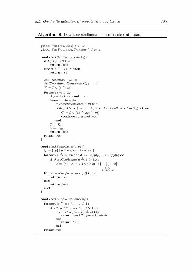
8.4. On-the-fly detection of probabilistic confluence 193

Algorithm 6: Detecting confluence on a concrete state space.

global Set〈Transition〉 T := ∅global Set〈Transition,Transition〉 C := ∅

bool checkConfluence(s −a→ 1t) if L(s) 6= L(t) then

return false

else if s −a→ 1t ∈ T thenreturn true

Set〈Transition〉 Told := TSet〈Transition,Transition〉 Cold := C

T := T ∪ s −a→ 1tforeach s −b→ µ do

if µ = 1t then continue

foreach t −c→ ν doif checkEquivalence(µ, ν) and

(s −b→ µ 6∈ T or (∃u . ν = 1u and checkConfluence(t −c→ 1u))) then

C := C ∪ (s −b→ µ, t −c→ ν)continue outermost loop

end

T := ToldC := Cold

return false

return true

bool checkEquivalence(µ, ν) Q := p | p ∈ supp(µ) ∪ supp(ν)foreach u −d→ 1v such that u ∈ supp(µ), v ∈ supp(ν) do

if checkConfluence(u −d→ 1v) then

Q := q ∈ Q | u 6∈ q ∧ v 6∈ q ∪ ⋃

q∈Qu∈q∨v∈q

q

if µ(q) = ν(q) for every q ∈ Q thenreturn true

elsereturn false

end

bool checkConfluentMimicking foreach (s −b→ µ, t −c→ ν) ∈ C do

if s −b→ µ ∈ T and t −c→ ν 6∈ T then

if checkConfluence(t −c→ ν) thenreturn checkConfluentMimicking

elsereturn false

end

return true

194 8. Confluence Reduction in Statistical Model Checking

instead of checking for connecting transitions that are already in T , we try toadd possible connecting transitions to T using a recursive call.

In accordance to Definition 8.6, we first determine the smallest equivalencerelation that relates states from the support of µ to states from the support of νin case there is a confluent transition connecting them. We do so by constructinga set of equivalence classes Q, i.e., a partitioning of the state space accordingto this equivalence relation. We start with the smallest possible equivalencerelation, in which each equivalence class is a singleton. Then, for each confluent

transition u −d→ 1v, with u ∈ supp(µ) and v ∈ supp(ν), we merge the equivalenceclasses containing u and v. Finally, we can easily compute the probability ofreaching each equivalence class of Q by either µ or ν. If all of these probabilitiescoincide, indeed µ ≡R ν and we return true; otherwise, we return false.

The function checkConfluentMimicking is called after checkConfluence designateda transition to be confluent, to verify if T satisfies the requirement that confluenttransitions are mimicked by confluent transitions. After all, when a mimicking

transition for some transition s −b→ µ was found, it may have been the case that

s −b→ µ was not yet in T while in the end it is. Hence, checkConfluence keepstrack of the mimicking transitions in a global set C. If a transition s −a→ 1t is

shown to be confluent, all pairs (s −b→ µ, t −c→ ν) of other outgoing transitionsfrom s and the transitions that were found to mimic them from t are addedto C. If s −a→ 1t turns out not to be confluent after all, the mimicking transitionsthat were found in the process are removed again.

Based on C, checkConfluentMimicking ranges over all pairs (s −b→ µ, t −c→ ν),checking if one violates the requirement. If no such pair is found, we return true.Otherwise, the current set T is not valid yet. However, it could be the case that

t −c→ ν is not in T , while it is confluent (but since s −b→ µ was not in T at themoment the pair was added to C, this was not checked earlier). Therefore, westill try to denote t −c→ ν as confluent. If we fail, we return false. Otherwise, wecheck again for confluent mimicking using the new set T .

8.4.2 Correctness

The following theorem states that the algorithm is sound. We assume that Cand T are not reset to their initial value ∅ after termination of checkConfluence.

Theorem 8.12. Given a transition p −l→ 1q, checkConfluence(p −l→ 1q) andcheckConfluentMimicking together imply that p −l→ 1q is confluent.

Note that the converse of this theorem does not always hold. To see why,consider the situation that checkConfluentMimicking fails because a transition

s −b→ µ was mimicked by a transition t −c→ ν that is not confluent, and s −b→ µ wasadded to T later on. Although we then abort, there might have been another

transition t −d→ ρ that could also have been used to mimic s −b→ µ and that isconfluent. We chose not to consider this due to the additional overhead of theimplementation. Additionally, in none of our case studies this situation occurred.

8.4. On-the-fly detection of probabilistic confluence 195

Applying the algorithm more than once. The confluence detection algorithmoften needs to be applied multiple times during SMC: every time that a non-deterministic state is visited, the algorithm is used to detect whether it is safeto restrict to only traversing one of the outgoing transitions. What we thenbasically do, is combine several confluent sets into one larger confluent set.As we saw in Chapter 6, taking unions of confluent sets can be problematic.Therefore, our definition there was based on a confluence classification. However,as mentioned in Remark 8.7, we do not take into account such a classification inour definitions in this chapter—to make the notion easier to apply in an SMCsetting.

Hence, we need to argue why multiple executions of the algorithm indeed canbe combined to reduce the same model multiple times. We do so by noting thatconfluence reduction yields an equivalent model, as can be observed by combiningTheorem 8.11 and Theorem 8.12. By transitivity of PCTL∗\X equivalence, itimmediately follows that it is perfectly fine to reduce a model once, and then toapply the same reduction technique again on the reduced model while completelyforgetting about the first reduction.

The only issue here is that this is not entirely what happens. After all, if anondeterministic state s is reached and confluence reduction allows us to removeall but one of its outgoing transitions, this is not remembered due to the natureof SMC. Hence, if the computation at some point returns to s, it again has all itsoutgoing transitions. This implies that we are not continuing with the reducedmodel, and hence that the above reasoning does not immediately apply. Thiscan be solved, though, in a rather intuitive manner—making sure that we indeedare continuing working with the actual reduced model.

Let’s say we’re trying to resolve the nondeterminism in state s. It has atransition s −a→ t, that we have shown to be confluent by a confluent set Tobtained from our algorithm. Now:

1. Make a copy s′ of s. Let s′ have all transitions of s, and let all transitionsof the original system that went to s now go to s′. Clearly, the newsystem is PCTL∗\X equivalent to the original system—for instance, by

the bisimulation relation Id ∪ (s, s′), (s′, s). Basically, due to the SMCalgorithm not remembering the reductions we will apply to s, this copyingprocess models precisely what actually happens in practice.

2. Note that s −a→ t is also confluent in the altered system, by observing thatif a transition s −b→ µ was confluent originally, then so is the correspondingtransition from s′ in the new model. All other confluent transitions alsoremain confluent, as they behave identically.

3. Reduce, by omitting all transitions from s except for s −a→ t. We know nowthat the reduced system has the same properties as the original system.So, we can forget about the confluence information and continue with thismodel. Indeed, all behaviour from s is still present (but now from s′),reflecting the fact that if simulation returns to s, the omitted transitionsare back again.

Remark 8.13. Note that if s is reachable from t, this process only increasesthe size of the state space. Although in the setting of SMC this is fine (as the

196 8. Confluence Reduction in Statistical Model Checking

size of the state space is irrelevant anyway), it would be very undesirable in thecontext of normal model checking. Hence, this is why this technique is only validas a way of arguing the correctness of our SMC method, but cannot be used tomore easily enable us to take unions of confluent sets in a setting such as theone in the previous two chapters.

8.5 Evaluation

The modes tool4 provides SMC for models specified in the Modest lan-guage [BHH12]. It allowed SMC for MDPs using the POR-based approachof [BFHH11]. We have now implemented the confluence-based approach presen-ted in this chapter in modes as well. In this section, we apply it to three examplesto evaluate its applicability and performance impact. They were selected so asto allow us to clearly identify its strengths and limitations. For each, we (1) givean overview of the model, (2) discuss, if POR fails, why it does and which, ifany, modifications were needed to apply the confluence-based approach, and (3)evaluate memory use and runtime.

The performance results are summarised in Table 8.5. For the runtimeassessment, we compare to simulation with uniformly-distributed probabilisticresolution of nondeterminism. Although such a hidden assumption cannot leadto trustworthy results in general (but is implemented in many tools), it is a goodbaseline to judge the overhead of confluence checking. We generated 10 000 runsper model instance to compute probabilities psmc for case-specific properties.Using reasoning based on the Chernoff-Hoeffding bound [PRI13], this guaranteesthe following probabilistic error bound: Prob(|p− psmc| > 0.01) < 0.017, wherep is the actual probability of the property under consideration.

We measure memory usage in terms of the maximum number of extra stateskept in memory at any time during confluence (or POR) checking, denoted by s.We also report the maximum number of “lookahead” steps (i.e., the maximalnumber of checkConfluence calls on the stack) necessary in the confluence/PORchecks as k, as well as the average length t of a simulation trace and theaverage number c of nontrivial confluence checks, i.e., of nondeterministic choicesencountered, per trace.

To get a sense for the size of the models considered, we also attempted modelchecking (using mcpta [HH09], which relies on PRISM [KNP11]). Note that wedo not intend to perform a rigorous comparison of SMC and traditional modelchecking in this section and instead refer the interested reader to dedicatedcomparison studies such as [YKNP06]. Model checking for the BEB example wasperformed on a machine with 120 GB of RAM [BFHH11]; all other measurementsused a dual-core Intel Core i5 M450 system with 4 GB of RAM running 64-bitWindows 7.

8.5.1 Dining cryptographers

First, we consider the classical dining cryptographers problem [Cha88]: Ncryptographers use a protocol that has them toss coins and communicate the

4modes is part of the Modest Toolset, available at www.modestchecker.net.

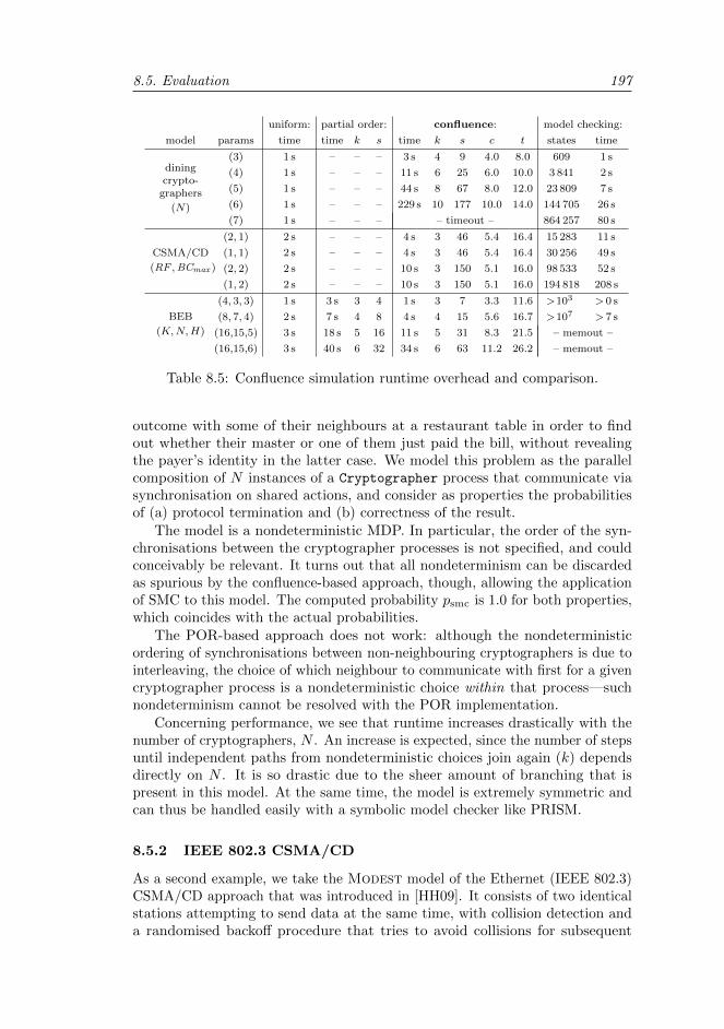
8.5. Evaluation 197

uniform: partial order: confluence: model checking:

model params time time k s time k s c t states time

diningcrypto-

graphers

(N)

(3) 1 s – – – 3 s 4 9 4.0 8.0 609 1 s

(4) 1 s – – – 11 s 6 25 6.0 10.0 3 841 2 s

(5) 1 s – – – 44 s 8 67 8.0 12.0 23 809 7 s

(6) 1 s – – – 229 s 10 177 10.0 14.0 144 705 26 s

(7) 1 s – – – – timeout – 864 257 80 s

CSMA/CD

(RF ,BCmax )

(2, 1) 2 s – – – 4 s 3 46 5.4 16.4 15 283 11 s

(1, 1) 2 s – – – 4 s 3 46 5.4 16.4 30 256 49 s

(2, 2) 2 s – – – 10 s 3 150 5.1 16.0 98 533 52 s

(1, 2) 2 s – – – 10 s 3 150 5.1 16.0 194 818 208 s

BEB

(K,N,H)

(4, 3, 3) 1 s 3 s 3 4 1 s 3 7 3.3 11.6 >103 > 0 s

(8, 7, 4) 2 s 7 s 4 8 4 s 4 15 5.6 16.7 >107 > 7 s

(16,15,5) 3 s 18 s 5 16 11 s 5 31 8.3 21.5 – memout –

(16,15,6) 3 s 40 s 6 32 34 s 6 63 11.2 26.2 – memout –

Table 8.5: Confluence simulation runtime overhead and comparison.

outcome with some of their neighbours at a restaurant table in order to findout whether their master or one of them just paid the bill, without revealingthe payer’s identity in the latter case. We model this problem as the parallelcomposition of N instances of a Cryptographer process that communicate viasynchronisation on shared actions, and consider as properties the probabilitiesof (a) protocol termination and (b) correctness of the result.

The model is a nondeterministic MDP. In particular, the order of the syn-chronisations between the cryptographer processes is not specified, and couldconceivably be relevant. It turns out that all nondeterminism can be discardedas spurious by the confluence-based approach, though, allowing the applicationof SMC to this model. The computed probability psmc is 1.0 for both properties,which coincides with the actual probabilities.

The POR-based approach does not work: although the nondeterministicordering of synchronisations between non-neighbouring cryptographers is due tointerleaving, the choice of which neighbour to communicate with first for a givencryptographer process is a nondeterministic choice within that process—suchnondeterminism cannot be resolved with the POR implementation.

Concerning performance, we see that runtime increases drastically with thenumber of cryptographers, N . An increase is expected, since the number of stepsuntil independent paths from nondeterministic choices join again (k) dependsdirectly on N . It is so drastic due to the sheer amount of branching that ispresent in this model. At the same time, the model is extremely symmetric andcan thus be handled easily with a symbolic model checker like PRISM.

8.5.2 IEEE 802.3 CSMA/CD

As a second example, we take the Modest model of the Ethernet (IEEE 802.3)CSMA/CD approach that was introduced in [HH09]. It consists of two identicalstations attempting to send data at the same time, with collision detection anda randomised backoff procedure that tries to avoid collisions for subsequent

198 8. Confluence Reduction in Statistical Model Checking

retransmissions. We consider the probability that both stations eventuallymanage to send their data without collision. The model is a probabilistic timedautomaton (PTA), but delays are fixed and deterministic, making it equivalentto an MDP (with real variables for clocks, updated on transitions that explicitlyrepresent the delays; modes does this transformation automatically and on-the-fly). The model has two parameters: a time reduction factor RF (i.e., delays of ttime units with RF = 1 correspond to delays of t

2 time units with RF = 2), andthe maximum value used in the exponential backoff part of the protocol, BCmax .

Unfortunately, modes immediately reports nondeterminism that cannot bediscarded as spurious. Inspection of the reported lines in the model quicklyshows a nondeterministic choice between two probabilistic transitions—whichconfluence cannot handle. Fortunately, this problem can easily be eliminatedthrough an additional synchronisation, leading to psmc = 1.0 (which is thecorrect result). POR still fails, for reasons similar to the previous example:initially, both stations send at the same time, the order being determinednondeterministically. In the process representing the shared medium, this mustbe an internal nondeterministic choice. In contrast to the problem for confluence,this cannot be fixed easily.

In terms of runtime, the confluence checks incur a moderate overhead forthis example. Compared to the dining cryptographers, the slowdown is muchless even where more states need to be explored in each check (s); performanceappears to more directly depend on k, which stays low in this case.

8.5.3 Binary exponential backoff

The previous two examples clearly indicate that the added power of confluencereduction pays off, allowing SMC for models where it is not possible with POR.Still, we also need a comparison of the two approaches. For this purpose, werevisit the MDP model of the binary exponential backoff (BEB) procedure thatwas used to evaluate the POR-based approach in [BFHH11]. The probability wecompute is that of some host eventually getting access to the shared medium, fordifferent values of the model parameters K (maximum backoff counter value), N(number of tries per station before giving up) and H (number of stations/hostsinvolved).

Again, for the confluence check to succeed, we first need to minimally modifythe model by making a probabilistic transition synchronise. This appears to bea recurring issue, yet the relevant model code could quite clearly be identified asa modelling artifact without semantic impact in both examples where it appears.We then obtain psmc = 0.91 for model instance (4, 3, 3), otherwise psmc = 1.0.

The runtime overhead necessary to get trustworthy results by enablingeither confluence or POR is again moderate. This is despite longer paths beingexplored in the confluence checks compared to the CSMA/CD example (k). Theconfluence-based approach is somewhat faster than POR in this implementation.As noted in [BFHH11], large instances of this model cannot be solved withclassical model checking due to the state space explosion problem.

8.6. Contributions 199

8.6 Contributions

We defined a more slightly more liberal variant of probabilistic confluence thanthe one defined in Chapter 7, tailored for the core simulation step of statisticalmodel checking. It has more reduction potential at no extra computational cost,but still preserves PCTL∗\X . We provided an algorithm for on-the-fly detectionof confluence during simulation and implemented this algorithm in the modesSMC tool5.

Compared to a previous approach based on partial order reduction [BFHH11],the use of confluence allows new kinds of nondeterministic choices to be handled,in particular lifting the limitation to spurious interleavings—now, also spuri-ous nondeterminism within a process may be resolved. Heuristics for partialorder reduction generally consider all actions within the same process to bedependent [BK08, HP95, BFHH11].

In fact, for two of the three examples we presented, SMC is only possible usingthe new confluence-based technique, showing the additional power to be relevant.In terms of performance, it is somewhat faster than the POR-based approach,but the impact relative to (unsound) simulation using an arbitrary schedulerlargely depends on the amount of lookahead that needs to be performed, forboth approaches. Again, on two of our examples, the impact was moderate andshould in general be acceptable to obtain trustworthy results. Most importantly,the memory overhead is negligible, and one of the central advantages of SMCover traditional model checking is thus retained.

As confluence preserves branching time properties, it cannot handle theinterleaving of probabilistic choices. Although—as we showed—these can oftenbe avoided, for some models POR might work while confluence does not. Hence,neither of the techniques subsumes the other, and it is best to combine them: ifone cannot be used to resolve a nondeterministic choice, the SMC algorithm canstill try to apply the other. Implementing this combination is trivial and yieldsa technique that handles the union of what confluence and POR can deal with.

5Note that, as also mentioned at the beginning of this chapter, the implementation andcase studies were not done by the author, but by Arnd Hartmanns.

Part IV

Practical Validation

CHAPTER 9

Implementation and Case Studies

“It doesn’t matter how beautiful your theory is,it doesn’t matter how smart you are.

If it doesn’t agree with experiment, it’s wrong.”

Richard P. Feynman

The previous chapters described the process-algebraic language MAPA

for modelling MAs, as well as several reduction techniques for optimisingMAPA specifications and generating their corresponding MAs.

To validate the applicability of MAPA and the significance of its reductiontechniques, we developed a prototype tool called SCOOP. It takes as input eithera MAPA specification or a generalised stochastic Petri net (GSPN), linearisesto an MLPE and applies all our reduction techniques while generating an MA.These MAs can be subjected to analysis by a tool called IMCA, developed byDennis Guck at RWTH Aachen University and Hassan Hatefi at Saarland Uni-versity [GHKN12, HH12, GHH+13a]. We briefly present the analysis techniquesthat are available for MAs, as implemented in IMCA. These techniques havenot been developed by the author, but provide purpose to the MAPA languageand the MAs that can be generated. We do not go into any technical details,but only discuss IMCA’s features from a user perspective.

Together with IMCA and the tool GEMMA for parsing GSPN specifications,SCOOP is part of the MaMa (Modelling and Analysis of Markov Automata) toolchain. We provide four case studies that illustrate the capabilities of SCOOP aspart of this tool chain: an ingenious construction of a handshake register, a well-known leader election protocol, a polling system and a processor grid architecture.We illustrate how to model such systems in MAPA and what kind of propertiescan be computed. Our results confirm that the basic reduction techniques(Section 4.5), dead variable reduction (Chapter 5) and confluence reduction(Chapter 6) all are valuable tools when generating and analysing MAPA models.

Organisation of the chapter. In Section 9.1 we introduce the tool SCOOP,describing its input and output formats and discussing the MaMa tool chain inwhich it is embedded. Section 9.2 presents the analysis techniques implementedby IMCA. Then, Section 9.3 presents our case studies and discusses their indi-vidual results. Finally, Section 9.4 concludes by summarising the contributionsof this chapter and providing an overarching discussion on the merits of ourreduction techniques as illustrated by the case studies.

204 9. Implementation and Case Studies

Origins of the chapter. An earlier version of SCOOP was introduced by a toolpaper in the proceedings of the 8th International Conference on QuantitativeEvaluation of Systems (QEST) [Tim11], whereas the last version was describedby a regular paper in the proceedings of the 10th International Conference onQuantitative Evaluation of Systems (QEST) [GHH+13a] and a correspondingtechnical report [GHH+13b]). Additionally, part of the case studies alreadyappeared throughout the papers that introduced the techniques described in theprevious chapters.

9.1 Implementation

We developed the prototype tool SCOOP1 in Haskell, based on a simple datalanguage that allows the modelling of several kinds of protocols and systems.Excluding the generated parser, it has just over 3,100 lines of code.

A web-based interface (developed by Axel Belinfante using his Puptol tool2)makes the tool convenient to use, but it can also be used stand-alone. Thetool is capable of linearising MAPA specifications, as well as applying parallelcomposition, hiding, encapsulation and renaming (as explained in Chapter 4).Since Haskell is a functional language, the algorithms in our implementation arealmost identical to their mathematical representations presented in this thesis.The tool also implements all reduction techniques introduced in Section 4.5,Chapter 5 and Chapter 6. Where applicable, it encodes MLPEs as LPPEs asexplained in Section 4.2.5.

9.1.1 Input

SCOOP takes as input any specification in the MAPA language, and allowsthe use of a couple of built-in data types and several built-in functions forthese data types. By default it supports booleans, integers, rational numbers,lists and stacks. Additionally, users can define enumerative types for modellingconvenience.

For booleans, we support the basic operations: negation, conjunction anddisjunction. Also, we include conditional expressions. For integers and rationals,we support the standard numerical operations: addition, subtraction, multi-plication, division and exponentiation. Additionally, we implemented functionsfor obtaining the minimum or maximum of two numbers and for modulo com-putation. Finally, integers and rationals can be compared using the standardmathematical operators <, ≤, =, ≥ and >. For lists and stacks we allow elementsto be appended, read, updated, deleted, pushed or popped, and we can obtaintheir size.

The syntax expected by SCOOP largely corresponds to the notations weintroduced in Chapter 4. The most important concepts are presented in Table 9.1,linking the MAPA notations introduced in Chapter 4 to the corresponding textual

1The implementation, including a web-based interface, can be found at http://fmt.

cs.utwente.nl/~timmer/scoop. A list of all features and the way to use them is shownat http://fmt.cs.utwente.nl/~timmer/scoop/manual.html.

2See http://fmt.ewi.utwente.nl/puptol/.

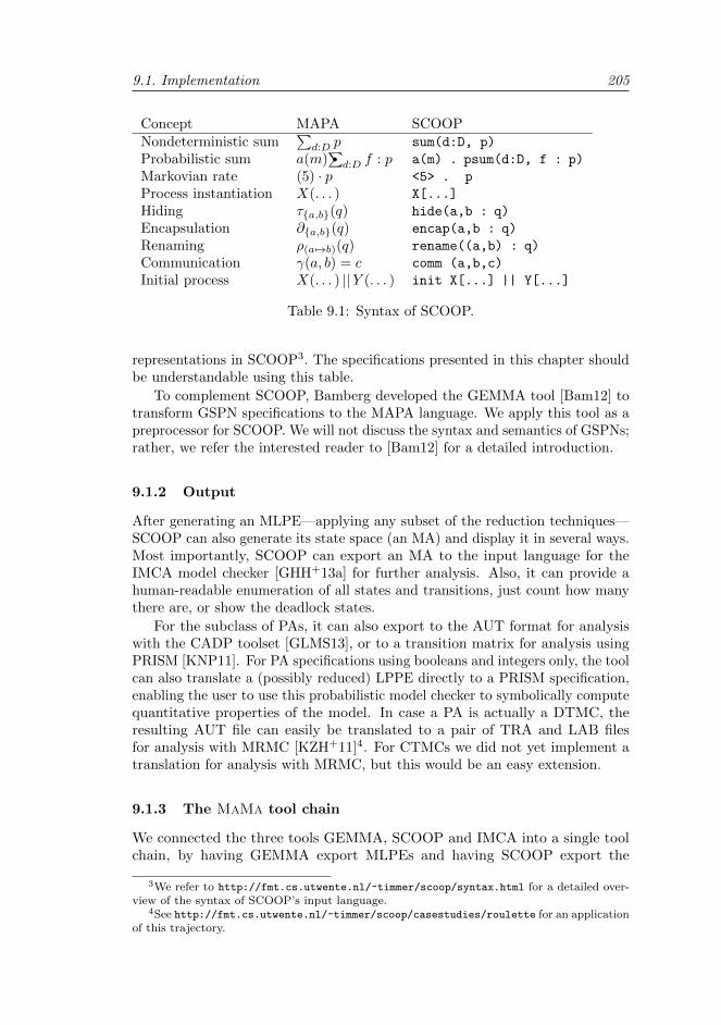
9.1. Implementation 205

Concept MAPA SCOOPNondeterministic sum

∑d:D p sum(d:D, p)

Probabilistic sum a(m)∑•d:D f : p a(m) . psum(d:D, f : p)

Markovian rate (5) · p <5> . p

Process instantiation X(. . . ) X[...]

Hiding τa,b(q) hide(a,b : q)

Encapsulation ∂a,b(q) encap(a,b : q)

Renaming ρ(a7→b)(q) rename((a,b) : q)

Communication γ(a, b) = c comm (a,b,c)

Initial process X(. . . ) ||Y (. . . ) init X[...] || Y[...]

Table 9.1: Syntax of SCOOP.

representations in SCOOP3. The specifications presented in this chapter shouldbe understandable using this table.

To complement SCOOP, Bamberg developed the GEMMA tool [Bam12] totransform GSPN specifications to the MAPA language. We apply this tool as apreprocessor for SCOOP. We will not discuss the syntax and semantics of GSPNs;rather, we refer the interested reader to [Bam12] for a detailed introduction.

9.1.2 Output

After generating an MLPE—applying any subset of the reduction techniques—SCOOP can also generate its state space (an MA) and display it in several ways.Most importantly, SCOOP can export an MA to the input language for theIMCA model checker [GHH+13a] for further analysis. Also, it can provide ahuman-readable enumeration of all states and transitions, just count how manythere are, or show the deadlock states.

For the subclass of PAs, it can also export to the AUT format for analysiswith the CADP toolset [GLMS13], or to a transition matrix for analysis usingPRISM [KNP11]. For PA specifications using booleans and integers only, the toolcan also translate a (possibly reduced) LPPE directly to a PRISM specification,enabling the user to use this probabilistic model checker to symbolically computequantitative properties of the model. In case a PA is actually a DTMC, theresulting AUT file can easily be translated to a pair of TRA and LAB filesfor analysis with MRMC [KZH+11]4. For CTMCs we did not yet implement atranslation for analysis with MRMC, but this would be an easy extension.

9.1.3 The MaMa tool chain

We connected the three tools GEMMA, SCOOP and IMCA into a single toolchain, by having GEMMA export MLPEs and having SCOOP export the

3We refer to http://fmt.cs.utwente.nl/~timmer/scoop/syntax.html for a detailed over-view of the syntax of SCOOP’s input language.

4See http://fmt.cs.utwente.nl/~timmer/scoop/casestudies/roulette for an applicationof this trajectory.

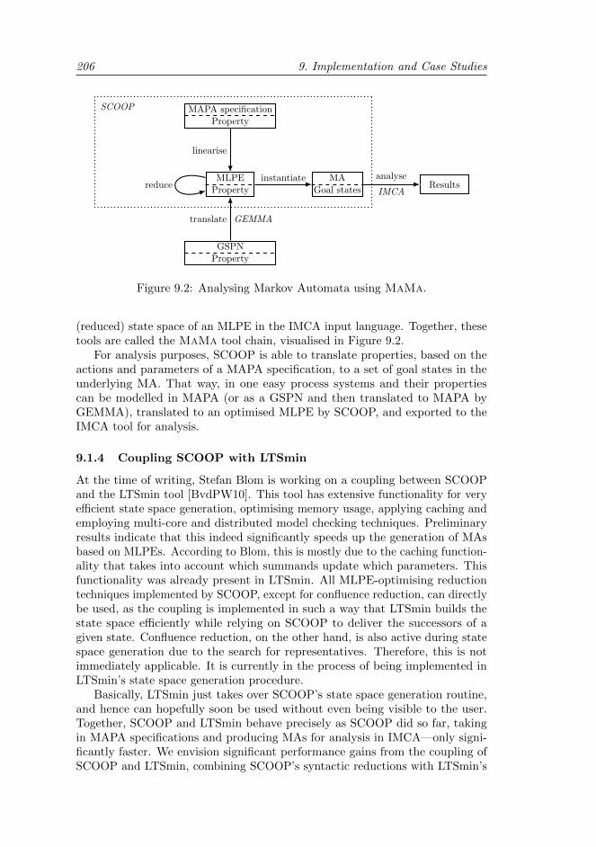
206 9. Implementation and Case Studies

MLPEProperty

MA

Goal statesResults

instantiatereduce

GSPNProperty

MAPA specificationProperty

linearise

GEMMAtranslate

IMCA

analyse

SCOOP

Figure 9.2: Analysing Markov Automata using MaMa.

(reduced) state space of an MLPE in the IMCA input language. Together, thesetools are called the MaMa tool chain, visualised in Figure 9.2.

For analysis purposes, SCOOP is able to translate properties, based on theactions and parameters of a MAPA specification, to a set of goal states in theunderlying MA. That way, in one easy process systems and their propertiescan be modelled in MAPA (or as a GSPN and then translated to MAPA byGEMMA), translated to an optimised MLPE by SCOOP, and exported to theIMCA tool for analysis.

9.1.4 Coupling SCOOP with LTSmin

At the time of writing, Stefan Blom is working on a coupling between SCOOPand the LTSmin tool [BvdPW10]. This tool has extensive functionality for veryefficient state space generation, optimising memory usage, applying caching andemploying multi-core and distributed model checking techniques. Preliminaryresults indicate that this indeed significantly speeds up the generation of MAsbased on MLPEs. According to Blom, this is mostly due to the caching function-ality that takes into account which summands update which parameters. Thisfunctionality was already present in LTSmin. All MLPE-optimising reductiontechniques implemented by SCOOP, except for confluence reduction, can directlybe used, as the coupling is implemented in such a way that LTSmin builds thestate space efficiently while relying on SCOOP to deliver the successors of agiven state. Confluence reduction, on the other hand, is also active during statespace generation due to the search for representatives. Therefore, this is notimmediately applicable. It is currently in the process of being implemented inLTSmin’s state space generation procedure.

Basically, LTSmin just takes over SCOOP’s state space generation routine,and hence can hopefully soon be used without even being visible to the user.Together, SCOOP and LTSmin behave precisely as SCOOP did so far, takingin MAPA specifications and producing MAs for analysis in IMCA—only signi-ficantly faster. We envision significant performance gains from the coupling ofSCOOP and LTSmin, combining SCOOP’s syntactic reductions with LTSmin’s

9.1. Implementation 207

meticulously optimised state space generation.

9.1.5 Confluence implementation

When applying confluence reduction, the target states of each transition aresubstituted by their representatives. These representatives are found by followingconfluent transitions until arriving in a BSCC, as discussed earlier in Chapter 6.During this search, several states are visited but not stored in the reducedstate space. The actual number of states that are visited during state spacegeneration is therefore larger than the number displayed in our tables—thenumber presented there is the actual number of states in the reduced state space.

To keep memory usage in the order of the reduced state space, the represent-ation map is deliberately not stored by default. Therefore, if non-representativestates are visited for the second time they are not recognised and their repres-entative is recomputed. In principle, the number of states visited during statespace generation may thus even be larger than the original number of states.

For models with a lot of cyclicity, not remembering anything may not bethe most efficient approach. Therefore, SCOOP also allows to store part of therepresentation map, trading speed for memory usage. Whenever a state s isreached and its representative t is computed, the pair (s, t) is then stored in ahash table. That way, whenever s is visited again, its representative t does notneed to be recomputed. For one of our case studies (the leader election protocol)this variant of confluence reduction is applied. This is also indicated in the tablepresenting its results. We investigated the possibility of additionally storingpairs (s′, t) for all states s′ visited on the path from s to t while looking for arepresentative for s. However, that did not turn out to be beneficial.

Depending on the model structure and the specific confluence implementationthat is used, confluence reduction sometimes only marginally improves or evenslows down state space generation time. Nonetheless, the reduction in statespace size is still useful if the model is subject to further analysis, as it often is.

9.1.6 Compositional analysis

An interesting approach is to generate state spaces by building them compos-itionally [BCS10, LM09]. That is, first, two components are generated andcomposed and the result is minimised. Then, the minimised composition is againcomposed with a third component and the result is minimised. This continues,until the complete system has been generated in a compositional manner.

Although in principle this approach seems to be applicable to MAPA spe-cifications as well, we did not implement it yet. One important reason for notchoosing such an approach is that some reduction techniques benefit from thefact that an MLPE contains information about the full system. For instance,dead variable reduction may reset variables based on a global specification; thosevariables may not have been reset in the individual components. Therefore,compositional state space generation may even yield larger (intermediate) statespaces than we obtain in our approach. Still, compositional state space genera-tion (including for instance compositional confluence detection) is an interestingdirection for future work.

208 9. Implementation and Case Studies

9.2 Analysing MAs with the MaMa tool chain

With the MaMa tool chain, four types of properties of an MA can be computed.All are defined based on a subset of the states of the MA: the set of goal states.As mentioned before, SCOOP allows for a set of goal states to be generated basedon the actions and properties of a MAPA specification. More specifically, wehave two options for generating goal states: either (1) we provide SCOOP witha list of actions, or (2) we provide SCOOP with a condition over the MLPE’svariables. In the first case, the set of goal states will consist of all states thatenable at least one of the actions in the list. Hence, goal states in general havenot executed the specified action(s) yet, but they are always able to execute atleast one. In the second case, the set of goal states will consist of all states thatsatisfy the condition that was specified.

9.2.1 Analysis techniques

SCOOP’s job is to provide an MA together with a set of goal states. Based onthis information, IMCA is able to compute the following properties:

Unbounded reachability This type of analysis computes the probability ofeventually reaching at least one of the goal states. It ignores all timinginformation, as if the MA were a PA. Unbounded reachability analysismay be used to compute properties that are not concerned with timing,but for instance with valid termination of a protocol.

Time-bounded reachability This type of analysis does take timing into ac-count. Parameterised in a lower bound l and an upper bound u, it computesthe probability that at least one goal state is visited within the interval[l, u]. It is not concerned with the question whether one or more goal statesare also already visited before time l. Time-bounded reachability analysismay be used for properties to investigate for instance how likely a systemcompletes a certain task within a given amount of time.

Expected time This type of analysis computes the expected time until reachinga goal state for the first time. Expected time analysis may be used forperformance analysis, computing for instance how long a system is expectedto work on a set of tasks.

Long-run average This type of analysis computes the fraction of time, in thelong run, that an MA resides in a goal state. Long-run average analysismay be used to compute throughput, for instance, or to see how often asystem is idling.

We note that time-bounded reachability grows to unbounded reachability if l = 0and u goes to ∞.

9.2.2 Zeno behaviour

In principle, MAs are not allowed to have any Zeno behaviour . That is, no loopof internal transitions may be present. After all, since such transitions take no

9.3. Case studies 209

time and prevent Markovian delays from happening, they would prevent timefrom progressing—this is often not allowed.

SCOOP and IMCA do not check their input for this restriction. Hence,in contrast to many theoretical papers they do allow MAs to contain Zenobehaviour. In many cases, such MAs still allow valid reasoning. For instance,for a system first delaying according to a rate of 1, then executing an action aand then looping indefinitely, we can say that the expected time until reachingthe action a is 1. On the other hand, the long-run average of being in theinfinite loop may be counterintuitive. Although from some point on we staythere indefinitely, time does not progress anymore. Hence, the long-run averagecomputed by IMCA is 0.

Both tools also allow MAs to have deadlock states. IMCA prevents Zenobehaviour by adding Markovian self-loops to such states.

9.3 Case studies

The modelling power of MAPA in combination with the reduction techniquesimplemented by SCOOP allow a wide variety of systems to be modelled andanalysed. We worked on several, such as a handshake register, a leader electionprotocol, a polling system, a processor grid architecture, a perfect strategyfor roulette5, the gambler’s ruin problem [Blo12], a stripped-down version ofYahtzee [Blo12], the game of the goose [Blo12], and a mutual exclusion al-gorithm [TKvdPS12a].

In this section we describe the first four studies mentioned above. They aremodelled in the MAPA language and optimised by the latest version of SCOOPusing the reduction techniques introduced in this thesis. Except for the firstcase study, all are also analysed by means of the IMCA tool (version 1.5 beta).These case studies should be interpreted as a proof-of-concept for our modellinglanguage and reduction techniques. They show that all our techniques workreally well in some cases, and maybe less in others. To fully investigate howwell our techniques work, how scalable they are and precisely what modellingartifacts influence their impact, many more experiments are needed—we leavethis for future work. Still, the current treatment is sufficient for concluding thatall our techniques are valuable contributions to the field of quantitative modelchecking.

Measurements. All measurements were taken on a 2.4 GHz 4 GB Intel Core 2Duo MacBook running Mac OS X 10.6.8. For each case study we first presentthe number of states and transitions obtained using SCOOP when not applyingany of our reduction techniques. We also present the time to generate thesestate spaces, both with and without our basic reduction techniques. The timingmeasurements include the whole process of parsing, linearisation, optimisationand generation: we just measure the real time SCOOP takes to display the statespace size after being invoked6.

5http://wwwhome.cs.utwente.nl/~timmer/scoop/casestudies/roulette/roulette.html.6Since our Haskell-implementation is rather inefficient in I/O at the moment, we excluded

the time to write the state space to disk from our measurements.

210 9. Implementation and Case Studies

We also present the effects of our reduction techniques on the state spacesizes and the generation and analysis times. We perform three categoriesof measurements: one applying only dead variable reduction in combinationwith the basic reduction techniques, one applying only confluence reduction incombination with the basic reduction techniques, and one applying all at thesame time. Increases and decreases are presented as reduction percentages withrespect to the setting of only applying the basic reduction techniques.

Since all algorithms implemented by SCOOP and IMCA are deterministic, weran all experiments only once. All other user processes were killed, for accuracyof our results. When rerunning some of the experiments to check if this approachis indeed valid, we noticed at most deviations of a few percent in the timingresults.

9.3.1 Handshake register

Our first case study is a model of a handshake register , modelled and verifiedby Hesselink [Hes98]. A handshake register is a data structure that is usedfor communication between a single reader and a single writer. It guaranteesrecentness and sequentiality ; any value that is read was at some point duringthe read action the last value written, and the values of sequential reads occurin the same order as they were written. Also, it is waitfree; both the readerand the writer can complete their actions within a bounded number of steps,independent of the other process.

Hesselink provided a method to implement a handshake register of an arbit-rary data type based on four so-called safe registers and four atomic booleanregisters. Each safe register can be used to store one value, and only guaranteesto provide the actual value to the reader if no write action is in progress at thesame time. Hence, the safe registers on their own do not satisfy the recentnessrequirement: if a safe register is read during a write operation, this may resultin any value. Still, Hesselink managed to combine four copies of such a saferegister with four atomic boolean registers in such a way that the result doeshave all the required properties for a handshake register. The algorithm is farfrom trivial, and Hesselink’s correctness proof involves several invariants.

As an alternative to the manual proof, we present a model checking approachto show the correctness of this construction. The handshake register’s specifica-tion and its construction based on the four safe register were already modelledin µCRL by Arjan Mooij, Aad Mathijssen and Jan Friso Groote. We translatedthese models to MAPA, generated their state spaces and compared these moduloτ∗a equivalence7 [FM91] using µCRL’s ltscmp tool. Indeed, as expected, thespecification and implementation yield identical minimal quotients. Therefore,the construction satisfies its requirements. Below, we go into more details aboutthe models and their analysis.

7The concept of τ∗a equivalence is similar to weak bisimulation. For two states p, q to beτ∗a-equivalent, each path p −τ...τa−−−→ p′ has to be mimicked by a path q −τ...τa−−−→ q′ such that p′

and q′ are again τ∗a-equivalent. Here, the sequences τ . . . τ may be of distinct length and areallowed to be empty; hence, the term τ∗a equivalence.

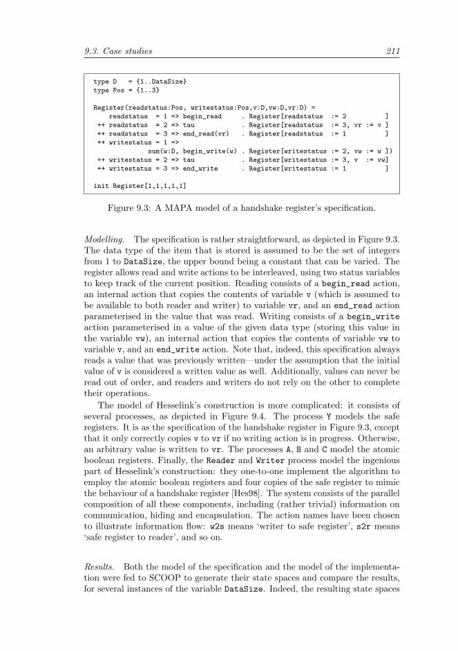
9.3. Case studies 211

type D = 1..DataSize

type Pos = 1..3

Register(readstatus:Pos, writestatus:Pos,v:D,vw:D,vr:D) =

readstatus = 1 => begin_read . Register[readstatus := 2 ]

++ readstatus = 2 => tau . Register[readstatus := 3, vr := v ]

++ readstatus = 3 => end_read(vr) . Register[readstatus := 1 ]

++ writestatus = 1 =>

sum(w:D, begin_write(w) . Register[writestatus := 2, vw := w ])

++ writestatus = 2 => tau . Register[writestatus := 3, v := vw]

++ writestatus = 3 => end_write . Register[writestatus := 1 ]

init Register[1,1,1,1,1]

Figure 9.3: A MAPA model of a handshake register’s specification.

Modelling. The specification is rather straightforward, as depicted in Figure 9.3.The data type of the item that is stored is assumed to be the set of integersfrom 1 to DataSize, the upper bound being a constant that can be varied. Theregister allows read and write actions to be interleaved, using two status variablesto keep track of the current position. Reading consists of a begin_read action,an internal action that copies the contents of variable v (which is assumed tobe available to both reader and writer) to variable vr, and an end_read actionparameterised in the value that was read. Writing consists of a begin_write

action parameterised in a value of the given data type (storing this value inthe variable vw), an internal action that copies the contents of variable vw tovariable v, and an end_write action. Note that, indeed, this specification alwaysreads a value that was previously written—under the assumption that the initialvalue of v is considered a written value as well. Additionally, values can never beread out of order, and readers and writers do not rely on the other to completetheir operations.

The model of Hesselink’s construction is more complicated: it consists ofseveral processes, as depicted in Figure 9.4. The process Y models the saferegisters. It is as the specification of the handshake register in Figure 9.3, exceptthat it only correctly copies v to vr if no writing action is in progress. Otherwise,an arbitrary value is written to vr. The processes A, B and C model the atomicboolean registers. Finally, the Reader and Writer process model the ingeniouspart of Hesselink’s construction: they one-to-one implement the algorithm toemploy the atomic boolean registers and four copies of the safe register to mimicthe behaviour of a handshake register [Hes98]. The system consists of the parallelcomposition of all these components, including (rather trivial) information oncommunication, hiding and encapsulation. The action names have been chosento illustrate information flow: w2s means ‘writer to safe register’, s2r means‘safe register to reader’, and so on.

Results. Both the model of the specification and the model of the implementa-tion were fed to SCOOP to generate their state spaces and compare the results,for several instances of the variable DataSize. Indeed, the resulting state spaces

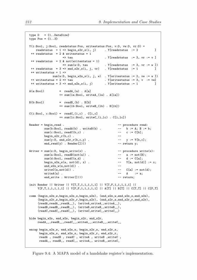
212 9. Implementation and Case Studies

type D = 1..DataSize

type Pos = 1..3

Y(i:Bool, j:Bool, readstatus:Pos, writestatus:Pos, v:D, vw:D, vr:D) =

readstatus = 1 => begin_s2r_s(i, j) . Y[readstatus := 2 ]

++ readstatus = 2 & writestatus = 1

=> tau . Y[readstatus := 3, vr := v ]

++ readstatus = 2 & not(writestatus = 1)

=> sum(w:D, tau . Y[readstatus := 3, vr := w ])

++ readstatus = 3 => end_s2r_s(i, j, vr) . Y[readstatus := 1 ]

++ writestatus = 1 =>

sum(w:D, begin_w2s_s(i, j, w) . Y[writestatus := 2, vw := w ])

++ writestatus = 2 => tau . Y[writestatus := 3, v := vw]

++ writestatus = 3 => end_w2s_s(i, j) . Y[writestatus := 1 ]

A(a:Bool) = readA_(a) . A[a]

++ sum(la:Bool, writeA_(la) . A[la])

B(b:Bool) = readB_(b) . B[b]

++ sum(lb:Bool, writeB_(lb) . B[lb])

C(i:Bool, c:Bool) = readC_(i,c) . C[i,c]

++ sum(lc:Bool, writeC_(i,lc) . C[i,lc])

Reader = begin_read . -- procedure read:

sum(b:Bool, readA(b) . writeB(b) . -- b := A; B := b;

sum(c:Bool, readC(b,c) . -- c := C[b];

begin_s2r_r(b,c) . --

sum(y:D, end_s2r_r(b,c,y) . -- y := Y[b,c];

end_read(y) . Reader[]))) -- return y;

Writer = sum(x:D, begin_write(x) . -- procedure write(x):

sum(a:Bool, readB(not(a)) . -- a := not(B);

sum(d:Bool, readC(a,d) . -- d := C[a];

begin_w2s_w(a, not(d), x) . -- Y[a, not(d)] := x;

end_w2s_w(a,not(d)) . --

writeC(a,not(d)) . -- C[a] := not(d);

writeA(a) . -- A := a;

end_write . Writer[]))) -- return;

init Reader || Writer || Y[T,T,1,1,1,1,1] || Y[T,F,1,1,1,1,1] ||

Y[F,T,1,1,1,1,1] || Y[F,F,1,1,1,1,1] || A[T] || B[T] || C[T,T] || C[F,T]

comm (begin_w2s_w,begin_w2s_s,begin_w2s), (end_w2s_w,end_w2s_s,end_w2s),

(begin_s2r_s,begin_s2r_r,begin_s2r), (end_s2r_s,end_s2r_r,end_s2r),

(readA,readA_,readA__), (writeA,writeA_,writeA__),

(readB,readB_,readB__), (writeB,writeB_,writeB__),

(readC,readC_,readC__), (writeC,writeC_,writeC__)

hide begin_w2s, end_w2s, begin_s2r, end_s2r,

readA__,readB__,readC__,writeA__,writeB__,writeC__

encap begin_w2s_w, end_w2s_w, begin_s2r_s, end_s2r_s,

begin_w2s_s, end_w2s_s, begin_s2r_r, end_s2r_r,

readA , readB , readC , writeA , writeB ,writeC ,

readA_, readB_, readC_, writeA_, writeB_,writeC_

Figure 9.4: A MAPA model of a handshake register’s implementation.

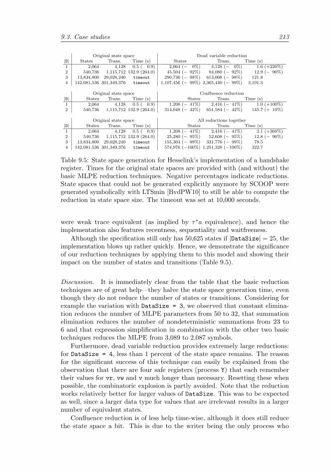
9.3. Case studies 213

Original state space Dead variable reduction|D| States Trans. Time (s) States Trans. Time (s)1 2,064 4,128 0.5 ( 0.9) 2,064 (− 0%) 4,128 (− 0%) 1.6 (+220%)2 540,736 1,115,712 132.9 (264.0) 45,504 (− 92%) 94,080 (− 92%) 12.9 (− 90%)3 13,834,800 29,028,240 timeout 290,736 (− 98%) 613,008 (− 98%) 121.84 142,081,536 301,349,376 timeout 1,107,456 (− 99%) 2,365,440 (− 99%) 3,101.3

Original state space Confluence reduction|D| States Trans. Time (s) States Trans. Time (s)1 2,064 4,128 0.5 ( 0.9) 1,208 (− 41%) 2,416 (− 41%) 1.0 (+100%)2 540,736 1,115,712 132.9 (264.0) 314,048 (− 42%) 651,584 (− 42%) 145.7 (+ 10%)

Original state space All reductions together|D| States Trans. Time (s) States Trans. Time (s)1 2,064 4,128 0.5 ( 0.9) 1,208 (− 41%) 2,416 (− 41%) 2.1 (+360%)2 540,736 1,115,712 132.9 (264.0) 25,280 (− 95%) 52,608 (− 95%) 12.8 (− 90%)3 13,834,800 29,028,240 timeout 155,304 (− 99%) 331,776 (− 99%) 78.54 142,081,536 301,349,376 timeout 574,976 (−100%) 1,251,328 (−100%) 322.7

Table 9.5: State space generation for Hesselink’s implementation of a handshakeregister. Times for the original state spaces are provided with (and without) thebasic MLPE reduction techniques. Negative percentages indicate reductions.State spaces that could not be generated explicitly anymore by SCOOP weregenerated symbolically with LTSmin [BvdPW10] to still be able to compute thereduction in state space size. The timeout was set at 10,000 seconds.

were weak trace equivalent (as implied by τ∗a equivalence), and hence theimplementation also features recentness, sequentiality and waitfreeness.

Although the specification still only has 50,625 states if |DataSize| = 25, theimplementation blows up rather quickly. Hence, we demonstrate the significanceof our reduction techniques by applying them to this model and showing theirimpact on the number of states and transitions (Table 9.5).

Discussion. It is immediately clear from the table that the basic reductiontechniques are of great help—they halve the state space generation time, eventhough they do not reduce the number of states or transitions. Considering forexample the variation with DataSize = 3, we observed that constant elimina-tion reduces the number of MLPE parameters from 50 to 32, that summationelimination reduces the number of nondeterministic summations from 23 to6 and that expression simplification in combination with the other two basictechniques reduces the MLPE from 3,089 to 2,087 symbols.

Furthermore, dead variable reduction provides extremely large reductions:for DataSize = 4, less than 1 percent of the state space remains. The reasonfor the significant success of this technique can easily be explained from theobservation that there are four safe registers (process Y) that each remembertheir values for vr, vw and v much longer than necessary. Resetting these whenpossible, the combinatoric explosion is partly avoided. Note that the reductionworks relatively better for larger values of DataSize. This was to be expectedas well, since a larger data type for values that are irrelevant results in a largernumber of equivalent states.

Confluence reduction is of less help time-wise, although it does still reducethe state space a bit. This is due to the writer being the only process who

214 9. Implementation and Case Studies

writes to atomic boolean register C. Therefore, when it is reading a value fromthis register, it may interleave in any order with the system’s other possibletransitions without influencing the result. Confluence reduction detects thisand gives priority to the τ -transition obtained from hiding readC(a,d). Thesame holds for the τ -transitions corresponding to the actions begin_s2r_s andend_s2r_s(i, j, vr). The former does not use or change any variables (exceptfor using the constants i and j—but they are removed by constant eliminationfirst). The latter does use vr, but this variable can only be updated in statesthat can never be enabled at the same time (since it requires a different value forreadstatus). No write actions are confluent, as they change the writestate

variable, which is used to decide whether or not to provide the correct resultduring a (possibly simultaneous) read action. Due to the excessive growth ofthe model, confluence reduction alone is not sufficient to analyze the model for|D| ≥ 3. However, the impact of confluence on larger models can be seen fromits effect in combination with dead variable reduction. Then, for |D| ≥ 3, it doessignificantly reduce the state space generation time compared to the situation ofonly applying dead variable reduction.

The reason for dead variable reduction not always positively affecting thestate space generation time for the smallest model is the additional overhead ofdeciding which variables can be reset (taking about 1.0 second for each model).For confluence reduction, there is the overhead to check which summands areconfluent (taking about 0.5 seconds) and the additional overhead of recomputingrepresentatives, as discussed above. For the larger models, though, these concernscompletely vanish compared to the significant reductions that are obtained.

9.3.2 Leader election protocol

For our second case study, we investigate a leader election protocol: Algorithm Bfrom [FP05]. It is an adaptation of the Itai-Rodeh protocol [IR81, IR90] fordeciding on a leader in an asynchronous ring with an arbitrary number of nodes.Basically, the algorithm breaks the symmetry by rolling dice, choosing the nodethat rolled highest as leader. If multiple nodes roll the same high number, theprocess is repeated.

More precisely, each node is either active (still in the running to become theleader) or passive (only passing on messages). Initially, all nodes are active andthey randomly choose a natural number within a certain interval 1, . . . , k, i.e.,they roll a k-sided die. We assume that this takes some time, governed by anexponential distribution with rate 1. After having chosen a value c, each nodesends a message (c, 1) to the channel on its right-hand side, with 1 representingthe number of hops the message has taken. The hop count is included to beable to notice that a message makes it all the way around the ring, back to itsoriginal sender.

After having sent its message, each node ni keeps reading messages (o, h)from the channel on its left-hand side. Upon receiving a message, four conditionsapply from the point of view of node ni:

• If o < c, then apparently a node on the left of ni rolled a lower numberthan ni did, so the message is discarded.

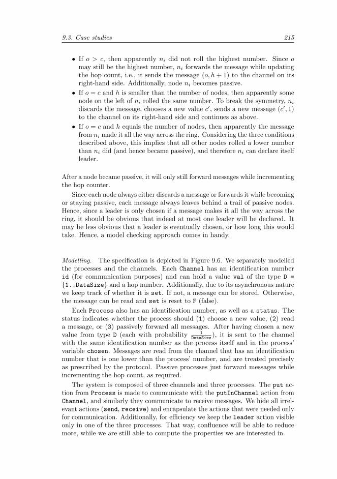
9.3. Case studies 215

• If o > c, then apparently ni did not roll the highest number. Since omay still be the highest number, ni forwards the message while updatingthe hop count, i.e., it sends the message (o, h + 1) to the channel on itsright-hand side. Additionally, node ni becomes passive.

• If o = c and h is smaller than the number of nodes, then apparently somenode on the left of ni rolled the same number. To break the symmetry, nidiscards the message, chooses a new value c′, sends a new message (c′, 1)to the channel on its right-hand side and continues as above.

• If o = c and h equals the number of nodes, then apparently the messagefrom ni made it all the way across the ring. Considering the three conditionsdescribed above, this implies that all other nodes rolled a lower numberthan ni did (and hence became passive), and therefore ni can declare itselfleader.

After a node became passive, it will only still forward messages while incrementingthe hop counter.

Since each node always either discards a message or forwards it while becomingor staying passive, each message always leaves behind a trail of passive nodes.Hence, since a leader is only chosen if a message makes it all the way across thering, it should be obvious that indeed at most one leader will be declared. Itmay be less obvious that a leader is eventually chosen, or how long this wouldtake. Hence, a model checking approach comes in handy.

Modelling. The specification is depicted in Figure 9.6. We separately modelledthe processes and the channels. Each Channel has an identification numberid (for communication purposes) and can hold a value val of the type D =

1..DataSize and a hop number. Additionally, due to its asynchronous naturewe keep track of whether it is set. If not, a message can be stored. Otherwise,the message can be read and set is reset to F (false).

Each Process also has an identification number, as well as a status. Thestatus indicates whether the process should (1) choose a new value, (2) reada message, or (3) passively forward all messages. After having chosen a newvalue from type D (each with probability 1

DataSize), it is sent to the channel

with the same identification number as the process itself and in the process’variable chosen. Messages are read from the channel that has an identificationnumber that is one lower than the process’ number, and are treated preciselyas prescribed by the protocol. Passive processes just forward messages whileincrementing the hop count, as required.

The system is composed of three channels and three processes. The put ac-tion from Process is made to communicate with the putInChannel action fromChannel, and similarly they communicate to receive messages. We hide all irrel-evant actions (send, receive) and encapsulate the actions that were needed onlyfor communication. Additionally, for efficiency we keep the leader action visibleonly in one of the three processes. That way, confluence will be able to reducemore, while we are still able to compute the properties we are interested in.

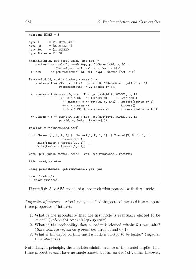
216 9. Implementation and Case Studies

constant NODES = 3

type D = 1..DataSize

type Id = 0..NODES-1

type Hop = 1..NODES

type Status = 1..3

Channel(id:Id, set:Bool, val:D, hop:Hop) =

not(set) => sum(v:D, sum(h:Hop, putInChannel(id, v, h) .

Channel[set := T, val := v, hop := h]))

++ set => getFromChannel(id, val, hop) . Channel[set := F]

Process(id:Id, status:Status, chosen:D) =

status = 1 => <1> . roll(id) . psum(c:D, 1/DataSize : put(id, c, 1) .

Process[status := 2, chosen := c])

++ status = 2 => sum(o:D, sum(h:Hop, get(mod(id-1, NODES), o, h) .

( h = NODES => leader(id) . Deadlock[]

++ chosen < o => put(id, o, h+1) . Process[status := 3]

++ o < chosen => Process[]

++ h < NODES & o = chosen => Process[status := 1])))

++ status = 3 => sum(o:D, sum(h:Hop, get(mod(id-1, NODES), o, h) .

put(id, o, h+1) . Process[]))

Deadlock = finished.Deadlock[]

init Channel[0, F, 1, 1] || Channel[1, F, 1, 1] || Channel[2, F, 1, 1] ||

Process[0,1,1] ||

hide(leader : Process[1,1,1]) ||

hide(leader : Process[2,1,1])

comm (put, putInChannel, send), (get, getFromChannel, receive)

hide send, receive

encap putInChannel, getFromChannel, get, put

reach leader(0)

-- reach finished

Figure 9.6: A MAPA model of a leader election protocol with three nodes.

Properties of interest. After having modelled the protocol, we used it to computethree properties of interest:

1. What is the probability that the first node is eventually elected to beleader? (unbounded reachability objective)

2. What is the probability that a leader is elected within 5 time units?(time-bounded reachability objective, error bound 0.01)

3. What is the expected time until a node is elected to be leader? (expectedtime objective)

Note that, in principle, the nondeterministic nature of the model implies thatthese properties each have no single answer but an interval of values. However,

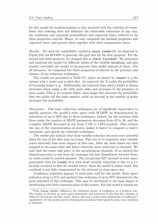
9.3. Case studies 217

for this model the nondeterminism is only involved with the ordering of events.Since this ordering does not influence the observable behaviour in any way,the minimum and maximal probabilities and expected times referred to bythese properties coincide. Hence, we only computed the minimal properties andexpected times, and present these together with their computation times.

Results. We used the reachability condition reach leader(0) (as depicted inFigure 9.6) for SCOOP to generate the goal sets for the first property. For thesecond and third property, we changed this to reach finished8. We generatedand analysed the model for different values of the variable DataSize, and also(easily) extended the model to incorporate four nodes instead of three. Forall instances, we computed the three properties of interest in the presence andabsence of our reduction techniques.

The results are presented in Table 9.7, where we denote by leader-i-j thevariant with i nodes and j-sided dice. As expected, for N nodes the probabilityof becoming leader is 1

N . Additionally, the expected time until a leader is chosendecreases when using a die with more sides and increases in the presence ofmore nodes. This is no surprise either, since larger dice decrease the probabilitythat two nodes roll the same number, while an increase in the number of nodesincreases this probability.

Discussion. Our basic reduction techniques are of significant importance toquickly generate the model’s state space with SCOOP, as demonstrated byreductions of up to 98% due to these techniques. Indeed, for the variation withthree nodes the number of MLPE parameters decreases from 42 to 26, and thecomplete MLPE decreases in size from 7,576 to 1,678 symbols. This reducesthe size of the representation of states, makes it faster to compute a state’ssuccessors, and speeds up reduction techniques.

The results also indicate that dead variable reduction becomes more powerfulwhen the size of the data type increases. This was to be expected, since variableresets obviously have more impact in this case. After all, more states are thenmapped to the same state and hence relatively more reduction is obtained. Wenote that the resets take place in the asynchronous channels. If we altered thechannel processes to not store the messages but just immediately forward them,no resets would be needed anymore. The exceptional 32% increase in state spacegeneration time for leader-4-2 with dead variable reduction is due to a 1.1seconds overhead to find all variable resets. Since the model is rather small, thisoverhead is not fully compensated by the decrease in state space size.

Confluence reduction appears to work quite well for this model. State spacereduction of up to 91% and analysis time reduction of up to 97% demonstrate thegreat potential of this technique. This may be attributed to the large degree ofinterleaving with little communication of this system. For this model it turned out

8This change slightly influences the reduction power of confluence in a positive way.The results we present on state space generation and reduction in the first few columns ofTable 9.7 all concern the first model. Hence, they are a conservative illustration of confluence’scapabilities—for the model used for checking the second and third property some more reductionis obtained.

218 9. Implementation and Case Studies

Ori

gin

al

state

space

Pro

per

ty1

Pro

per

ty2

Pro

per

ty3

Sp

ecifi

cati

on

Sta

tes

Tra

nsi

tion

sS

CO

OP

(s)

Res

ult

IMC

A(s

)R

esu

ltIM

CA

(s)

Res

ult

IMC

A(s

)leader-3-4

11,7

14

14,8

14

2.0

(64.1

)0.3

30.5

0.8

751.8

2.9

22.0

leader-3-6

51,2

53

65,2

08

8.8

(400.7

)0.3

31.9

0.9

2226.9

2.4

97.1

leader-3-8

148,5

12

189,6

06

26.3

(1,5

07.5

)0.3

35.2

0.9

4725.8

2.3

119.9

leader-3-10

342,1

79

437,8

56

60.9

(4,2

81.5

)0.3

312.1

0.9

51,7

70.8

2.2

045.2

leader-4-2

9,8

43

13,3

72

2.5

(85.1

)0.2

50.7

0.3

687.7

6.6

73.6

leader-4-3

68,7

72

96,6

40

17.1

(827.6

)0.2

54.4

0.6

6816.6

4.4

921.9

leader-4-4

271,7

73

388,4

60

68.1

(4,1

90.8

)0.2

519.0

0.7

74,0

62.7

3.7

287.9

Dea

dvari

ab

lere

du

ctio

nP

rop

erty

1P

rop

erty

2P

rop

erty

3S

pec

ifica

tion

Sta

tes

Tra

nsi

tion

sS

CO

OP

(s)

Res

ult

IMC

A(s

)R

esu

ltIM

CA

(s)

Res

ult

IMC

A(s

)leader-3-4

7,2

65

(−38%

)9,3

39

(−37%

)1.6

(−20%

)0.3

30.3

(−40%

)0.8

730.8

(−41%

)2.9

21.2

(−40%

)leader-3-6

25,2

58

(−51%

)32,6

88

(−50%

)4.7

(−47%

)0.3

30.9

(−53%

)0.9

2109.5

(−52%

)2.4

93.4

(−52%

)leader-3-8

60,7

95

(−59%

)78,9

57

(−58%

)10.8

(−59%

)0.3

32.0

(−62%

)0.9

4270.5

(−63%

)2.3

17.4

(−63%

)leader-3-10

119,8

52

(−65%

)155,9

94

(−64%

)21.1

(−65%

)0.3

34.0

(−67%

)0.9

5595.7

(−66%

)2.2

014.9

(−67%

)leader-4-2

8,4

67

(−14%

)11,6

00

(−13%

)3.3

(+32%

)0.2

50.6

(−14%

)0.3

674.8

(−15%

)6.6

73.1

(−14%

)leader-4-3

50,7

20

(−26%

)72,0

36

(−25%

)13.9

(−19%

)0.2

53.0

(−32%

)0.6

6573.3

(−30%

)4.4

915.2

(−31%

)leader-4-4

175,4

01

(−35%

)253,7

60

(−35%

)46.1

(−32%

)0.2

512.1

(−36%

)0.7

72,6

08.1

(−36%

)3.7

255.6

(−37%

)

Con

flu

ence

red

uct

ion

(sto

rere

pre

senta

tion

map

)P

rop

erty

1P

rop

erty

2P

rop

erty

3S

pec

ifica

tion

Sta

tes

Tra

nsi

tion

sS

CO

OP

(s)

Res

ult

IMC

A(s

)R

esu

ltIM

CA

(s)

Res

ult

IMC

A(s

)leader-3-4

2,2

32

(−81%

)2,5

24

(−83%

)1.7

(−15%

)0.3

30.1

(−80%

)0.8

72.8

(−95%

)2.9

20.1

(−95%

)leader-3-6

7,4

40

(−85%

)8,3

21

(−87%

)6.1

(−31%

)0.3

30.3

(−84%

)0.9

29.5

(−96%

)2.4

90.3

(−96%

)leader-3-8

17,5

64

(−88%

)19,5

54

(−90%

)16.8

(−36%

)0.3

30.6

(−88%

)0.9

423.2

(−97%

)2.3

10.8

(−96%

)leader-3-10

34,2

44

(−90%

)38,0

31

(−91%

)38.0

(−38%

)0.3

31.2

(−90%

)0.9

562.8

(−96%

)2.2

01.8

(−96%

)leader-4-2

2,4

62

(−75%

)3,1

20

(−77%

)2.4

(−4%

)0.2

50.1

(−86%

)0.3

65.8

(−93%

)6.6

70.2

(−94%

)leader-4-3

12,5

88

(−82%

)15,6

24

(−84%

)12.0

(−30%

)0.2

50.4

(−91%

)0.6

639.6

(−95%

)4.4

90.9

(−96%

)leader-4-4

40,7

90

(−85%

)50,6

14

(−87%

)42.4

(−38%

)0.2

51.4

(−93%

)0.7

7138.4

(−97%

)3.7

22.6

(−97%

)

All

red

uct

ion

tech

niq

ues

Pro

per

ty1

Pro

per

ty2

Pro

per

ty3

Sp

ecifi

cati

on

Sta

tes

Tra

nsi

tion

sS

CO

OP

(s)

Res

ult

IMC

A(s

)R

esu

ltIM

CA

(s)

Res

ult

IMC

A(s

)leader-3-4

1,6

89

(−86%

)1,9

81

(−87%

)1.6

(−20%

)0.3

30.0

(−99%

)0.8

72.2

(−96%

)2.9

20.1

(−95%

)leader-3-6

5,2

50

(−90%

)6,1

31

(−91%

)4.0

(−55%

)0.3

30.1

(−95%

)0.9

26.5

(−97%

)2.4

90.2

(−97%

)leader-3-8

11,9

15

(−92%

)13,9

05

(−93%

)8.7

(−67%

)0.3

30.3

(−94%

)0.9

413.8

(−98%

)2.3

10.4

(−98%

)leader-3-10

22,6

52

(−93%

)26,4

39

(−94%

)16.6

(−73%

)0.3

30.6

(−95%

)0.9

527.2

(−98%

)2.2

00.7

(−98%

)leader-4-2

2,2

04

(−78%

)2,8

59

(−79%

)3.3

(+32%

)0.2

50.1

(−86%

)0.3

65.2

(−94%

)6.6

70.2

(−94%

)leader-4-3

10,3

94

(−85%

)13,3

66

(−86%

)10.8

(−37%

)0.2

50.4

(−91%

)0.6

633.1

(−96%

)4.4

90.7

(−97%

)leader-4-4

31,9

34

(−88%

)41,3

44

(−89%

)31.9

(−53%

)0.2

51.1

(−94%

)0.7

7107.2

(−97%

)3.7

22.0

(−98%

)

Table 9.7: State space generation and analysis for a leader election protocol.

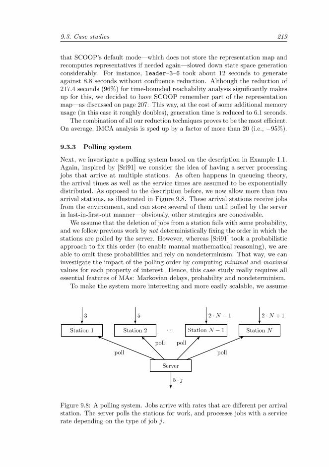
9.3. Case studies 219

that SCOOP’s default mode—which does not store the representation map andrecomputes representatives if needed again—slowed down state space generationconsiderably. For instance, leader-3-6 took about 12 seconds to generateagainst 8.8 seconds without confluence reduction. Although the reduction of217.4 seconds (96%) for time-bounded reachability analysis significantly makesup for this, we decided to have SCOOP remember part of the representationmap—as discussed on page 207. This way, at the cost of some additional memoryusage (in this case it roughly doubles), generation time is reduced to 6.1 seconds.

The combination of all our reduction techniques proves to be the most efficient.On average, IMCA analysis is sped up by a factor of more than 20 (i.e., −95%).

9.3.3 Polling system

Next, we investigate a polling system based on the description in Example 1.1.Again, inspired by [Sri91] we consider the idea of having a server processingjobs that arrive at multiple stations. As often happens in queueing theory,the arrival times as well as the service times are assumed to be exponentiallydistributed. As opposed to the description before, we now allow more than twoarrival stations, as illustrated in Figure 9.8. These arrival stations receive jobsfrom the environment, and can store several of them until polled by the serverin last-in-first-out manner—obviously, other strategies are conceivable.

We assume that the deletion of jobs from a station fails with some probability,and we follow previous work by not deterministically fixing the order in which thestations are polled by the server. However, whereas [Sri91] took a probabilisticapproach to fix this order (to enable manual mathematical reasoning), we areable to omit these probabilities and rely on nondeterminism. That way, we caninvestigate the impact of the polling order by computing minimal and maximalvalues for each property of interest. Hence, this case study really requires allessential features of MAs: Markovian delays, probability and nondeterminism.

To make the system more interesting and more easily scalable, we assume

Station 1 Station 2 · · · Station N − 1 Station N

3 5 2 ·N − 1 2 ·N + 1

Server

poll

poll poll

poll

5 · j

Figure 9.8: A polling system. Jobs arrive with rates that are different per arrivalstation. The server polls the stations for work, and processes jobs with a servicerate depending on the type of job j.

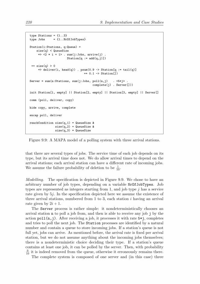
220 9. Implementation and Case Studies

type Stations = 1..3

type Jobs = 1..NrOfJobTypes

Station(i:Stations, q:Queue) =

size(q) < QueueSize

=> <2 * i + 1> . sum(j:Jobs, arrive(j) .

Station[q := add(q,j)])

++ size(q) > 0

=> deliver(i, head(q)) . psum(0.9 -> Station[q := tail(q)]

++ 0.1 -> Station[])

Server = sum(n:Stations, sum(j:Jobs, poll(n,j) . <5*j> .

complete(j) . Server[]))

init Station[1, empty] || Station[2, empty] || Station[3, empty] || Server[]

comm (poll, deliver, copy)

hide copy, arrive, complete

encap poll, deliver

reachCondition size(q_1) = QueueSize &

size(q_2) = QueueSize &

size(q_3) = QueueSize

Figure 9.9: A MAPA model of a polling system with three arrival stations.

that there are several types of jobs. The service time of each job depends on itstype, but its arrival time does not. We do allow arrival times to depend on thearrival stations; each arrival station can have a different rate of incoming jobs.We assume the failure probability of deletion to be 1

10 .

Modelling. The specification is depicted in Figure 9.9. We chose to have anarbitrary number of job types, depending on a variable NrOfJobTypes. Jobtypes are represented as integers starting from 1, and job type j has a servicerate given by 5j. In the specification depicted here we assume the existence ofthree arrival stations, numbered from 1 to 3, each station i having an arrivalrate given by 2i+ 1.

The Server process is rather simple: it nondeterministically chooses anarrival station n to poll a job from, and then is able to receive any job j by theaction poll(n,j). After receiving a job, it processes it with rate 5*j, completesand tries to poll the next job. The Station processes are identified by a naturalnumber and contain a queue to store incoming jobs. If a station’s queue is notfull yet, jobs can arrive. As mentioned before, the arrival rate is fixed per arrivalstation, but we do not assume anything about the incoming jobs themselves;there is a nondeterministic choice deciding their type. If a station’s queuecontains at least one job, it can be polled by the server. Then, with probability910 it is indeed removed from the queue, otherwise it erroneously remains there.

The complete system is composed of one server and (in this case) three

9.3. Case studies 221

arrival stations. Since our properties will be concerned with the situation that allarrival stations have reached their full capacity, we added a reachability condition(using the keyword reachCondition) that checks for precisely this situation. AreachCondition is specified over the global state space of the system; hence,we must refer to the q variables of the individual arrival stations. SCOOP hasbeen implemented in such a way that each variable gets suffixed by an index,indicating the position of its process in the init specification. Hence, we canrefer to the first arrival station’s queue by q_1, and so on.

Properties of interest. Our analysis is focused on the situation that all arrivalbuffers are full, as in this case no jobs can arrive anymore. We use IMCA tocompute three properties concerning this situation:

1. What is the expected time until reaching full capacity for the first time?(expected time objective)

2. What is the probability that full capacity is already reached within the firsttwo time units? (time-bounded reachability objective, error bound 0.01)

3. What is the fraction of time that all arrival stations are at full capacity inthe long run? (long run objective)

Due to nondeterminism in both the polling order and the job types that arrive,none of these properties has one definite answer. They all depend on how thesetwo nondeterministic choices are resolved. Clearly, to keep the long-run averagefraction of reaching full capacity low, the server should always first poll thearrival station with the lowest arrival rate. Additionally, the environment couldhelp keeping this fraction low by only providing jobs that have a high servicerate. Hence, for each property we provide an interval [min,max] that containsall values that may be obtained for different schedulings.

Results. We investigate the effect of changes in the number of job types, thequeue sizes in the arrival stations, and the number of arrival stations. For eachdimension we provide three experiments, showing the intervals computed byIMCA for all three properties of interest, the time to generate and analysethese models and the reductions in these times as well as the state space sizes.Additionally, since confluence reduction seemed to be particularly powerful inthe presence of many arrival stations and little data, we included a variation withnine stations all having just a single-element buffer and one type of incomingjob. The results are presented in Table 9.10, where polling-i-j-k denotes asystem with i stations, all having buffers of size of j and k types of jobs.

Discussion. It turns out that the model does not allow for much reductionby our main techniques dead variable reduction and confluence reduction, butstill they decrease analysis time slightly. Dead variable reduction automaticallydeduces that the job type is irrelevant after the delay 5j in the Server process,due to the complete(j) action being hidden.

Confluence reduction automatically detects that the hidden complete(j)

action is confluent and hence does not need to interleave with other actions.

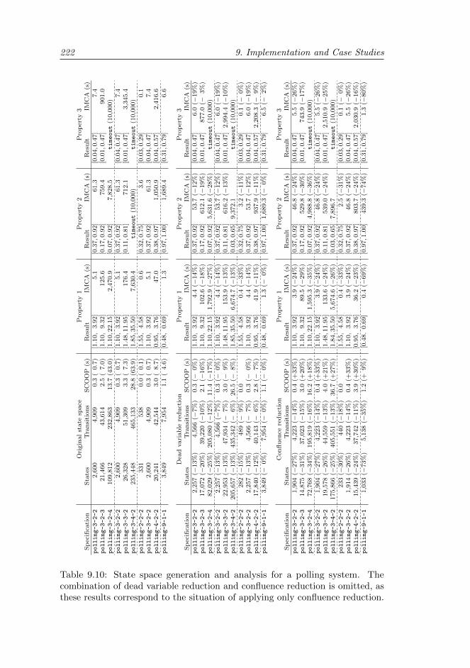
222 9. Implementation and Case Studies

Ori

gin

al

state

space

Pro

per

ty1

Pro

per

ty2

Pro

per

ty3

Sp

ecifi

cati

on

Sta

tes

Tra

nsi

tion

sS

CO

OP

(s)

Res

ult

IMC

A(s

)R

esu

ltIM

CA

(s)

Res

ult

IMC

A(s

)polling-3-2-2

2,6

00

4,9

09

0.3

(0.7

)[1.1

0,

3.9

2]

5.1

[0.3

7,0.9

2]

61.3

[0.0

4,0.4

7]

7.4

polling-3-2-3

21,4

66

43,6

14

2.5

(7.0

)[1.1

0,

9.3

2]

125.6

[0.1

7,0.9

2]

759.4

[0.0

1,0.4

7]

901.0

polling-3-2-4

109,8

12

232,8

63

13.7

(43.0

)[1.1

0,2

2.1

5]

2,4

70.9

[0.0

7,0.9

2]

7,8

28.5

timeout

(10,0

00)

polling-3-2-2

2,6

00

4,9

09

0.3

(0.7

)[1.1

0,

3.9

2]

5.1

[0.3

7,0.9

2]

61.3

[0.0

4,0.4

7]

7.4

polling-3-3-2

26,3

28

51,3

09

3.3

(7.3

)[1.4

8,1

1.9

5]

176.4

[0.1

1,0.8

1]

712.1

[0.0

1,0.4

7]

3,3

45.4

polling-3-4-2

235,4

48

465,1

33

28.8

(63.9

)[1.8

5,3

5.5

0]

7,6

30.4

timeout

(10,0

00)

timeout

(10,0

00)

polling-2-2-2

331

538

0.0

(0.1

)[1.5

5,

4.5

8]

0.6

[0.3

2,0.7

5]

3.6

[0.0

3,0.2

9]

0.1

polling-3-2-2

2,6

00

4,9

09

0.3

(0.7

)[1.1

0,

3.9

2]

5.1

[0.3

7,0.9

2]

61.3

[0.0

4,0.4

7]

7.4

polling-4-2-2

20,2

41

42,5

44

3.0

(8.7

)[0.9

5,

3.7

6]

47.0

[0.3

8,0.9

7]

1,0

50.9

[0.0

4,0.5

7]

2,4

16.6

polling-9-1-1

3,8

49

7,9

54

1.1

(4.6

)[0.4

8,

0.6

9]

1.3

[0.9

7,1.0

0]

1,6

89.4

[0.3

1,0.7

9]

6.6

Dea

dvari

ab

lere

du

ctio

nP

rop

erty

1P

rop

erty

2P

rop

erty

3S

pec

ifica

tion

Sta

tes

Tra

nsi

tion

sS

CO

OP

(s)

Res

ult

IMC

A(s

)R

esu

ltIM

CA

(s)

Res

ult

IMC

A(s

)polling-3-2-2

2,2

57

(−13%

)4,5

66

(−7%

)0.3

(−0%

)[1.1

0,

3.9

2]

4.4

(−14%

)[0.3

7,0.9

2]

53.7

(−12%

)[0.0

4,0.4

7]

6.0

(−19%

)polling-3-2-3

17,0

72

(−20%

)39,2

20

(−10%

)2.1

(−16%

)[1.1

0,

9.3

2]

102.6

(−18%

)[0.1

7,0.9

2]

612.1

(−19%

)[0.0

1,0.4

7]

877.0

(−3%

)polling-3-2-4

82,0

29

(−25%

)205,0

80

(−12%

)11.4

(−17%

)[1.1

0,2

2.1

5]

1,7

92.9

(−27%

)[0.0

7,0.9

2]

5,6

31.6

(−28%

)timeout

(10,0

00)

polling-3-2-2

2,2

57

(−13%

)4,5

66

(−7%

)0.3

(−0%

)[1.1

0,

3.9

2]

4.4

(−14%

)[0.3

7,0.9

2]

53.7

(−12%

)[0.0

4,0.4

7]

6.0

(−19%

)polling-3-3-2

22,9

53

(−13%

)47,9

34

(−7%

)3.0

(−9%

)[1.4

8,1

1.9

5]

153.9

(−13%

)[0.1

1,0.8

1]

616.2

(−13%

)[0.0

1,0.4

7]

2,9

94.4

(−10%

)polling-3-4-2

205,6

57

(−13%

)435,3

42

(−6%

)26.5

(−8%

)[1.8

5,3

5.5

0]

6,6

74.7

(−13%

)[0.0

3,0.6

5]

9,3

72.1

timeout

(10,0

00)

polling-2-2-2

282

(−15%

)489

(−9%

)0.0

[1.5

5,

4.5

8]

0.4

(−33%

)[0.3

2,0.7

5]

3.2

(−11%

)[0.0

3,0.2

9]

0.1

(−0%

)polling-3-2-2

2,2

57

(−13%

)4,5

66

(−7%

)0.3

(−0%

)[1.1

0,

3.9

2]

4.4

(−14%

)[0.3

7,0.9

2]

53.7

(−12%

)[0.0

4,0.4

7]

6.0

(−19%

)polling-4-2-2

17,8

40

(−12%

)40,1

43

(−6%

)2.8

(−7%

)[0.9

5,

3.7

6]

41.9

(−11%

)[0.3

8,0.9

7]

937.9

(−11%

)[0.0

4,0.5

7]

2,2

08.3

(−9%

)polling-9-1-1

3,8

49

(−0%

)7,9

54

(−0%

)1.1

(−0%

)[0.4

8,

0.6

9]

1.3

(−0%

)[0.9

7,1.0

0]

1,6

89.3

(−0%

)[0.3

1,0.7

9]

6.5

(−2%

)

Con

flu

ence

red

uct

ion

Pro

per

ty1

Pro

per

ty2

Pro

per

ty3

Sp

ecifi

cati

on

Sta

tes

Tra

nsi

tion

sS

CO

OP

(s)

Res

ult

IMC

A(s

)R

esu

ltIM

CA

(s)

Res

ult

IMC

A(s

)polling-3-2-2

1,9

04

(−27%

)4,2

23

(−14%

)0.4

(+33%

)[1.1

0,

3.9

2]

3.9

(−24%

)[0.3

7,0.9

2]

46.8

(−24%

)[0.0

4,0.4

7]

5.5

(−26%

)polling-3-2-3

14,8

75

(−31%

)37,0

23

(−15%

)3.0

(+20%

)[1.1

0,

9.3

2]

89.5

(−29%

)[0.1

7,0.9

2]

529.8

(−30%

)[0.0

1,0.4

7]

743.9

(−17%

)polling-3-2-4

72,7

68

(−34%

)195,8

19

(−16%

)16.2

(+18%

)[1.1

0,2

2.1

5]

1,5

95.3

(−35%

)[0.0

7,0.9

2]

4,9

88.8

(−36%

)timeout

(10,0

00)

polling-3-2-2

1,9

04

(−27%

)4,2

23

(−14%

)0.4

(+33%

)[1.1

0,

3.9

2]

3.9

(−24%

)[0.3

7,0.9

2]

46.8

(−24%

)[0.0

4,0.4

7]

5.5

(−26%

)polling-3-3-2

19,5

78

(−26%

)44,5

59

(−13%

)4.0

(+21%

)[1.4

8,1

1.9

5]

133.6

(−24%

)[0.1

1,0.8

1]

539.0

(−24%

)[0.0

1,0.4

7]

2,5

10.9

(−25%

)polling-3-4-2

175,8

66

(−25%

)405,5

51

(−13%

)36.7

(+27%

)[1.8

4,3

5.5

0]

5,6

74.6

(−26%

)[0.0

3,0.6

5]

7,8

96.7

timeout

(10,0

00)

polling-2-2-2

233

(−30%

)440

(−18%

)0.0

[1.5

5,

4.5

8]

0.4

(−33%

)[0.3

2,0.7

5]

2.5

(−31%

)[0.0

3,0.2

9]

0.1

(−0%

)polling-3-2-2

1,9

14

(−26%

)4,2

23

(−14%

)0.4

(+33%

)[1.1

0,

3.9

2]

3.9

(−24%

)[0.3

7,0.9

2]

46.8

(−24%

)[0.0

4,0.4

7]

5.5

(−26%

)polling-4-2-2

15,4

39

(−24%

)37,7

42

(−11%

)3.9

(+30%

)[0.9

5,

3.7

6]

36.2

(−23%

)[0.3

8,0.9

7]

803.7

(−24%

)[0.0

4,0.5

7]

2,0

30.9

(−16%

)polling-9-1-1

1,0

33

(−73%

)5,1

38

(−35%

)1.2

(+9%

)[0.4

8.

0.6

9]

0.4

(−69%

)[0.9

7,1.0

0]

439.3

(−74%

)[0.3

1,0.7

9]

1.3

(−80%

)

Table 9.10: State space generation and analysis for a polling system. Thecombination of dead variable reduction and confluence reduction is omitted, asthese results correspond to the situation of applying only confluence reduction.

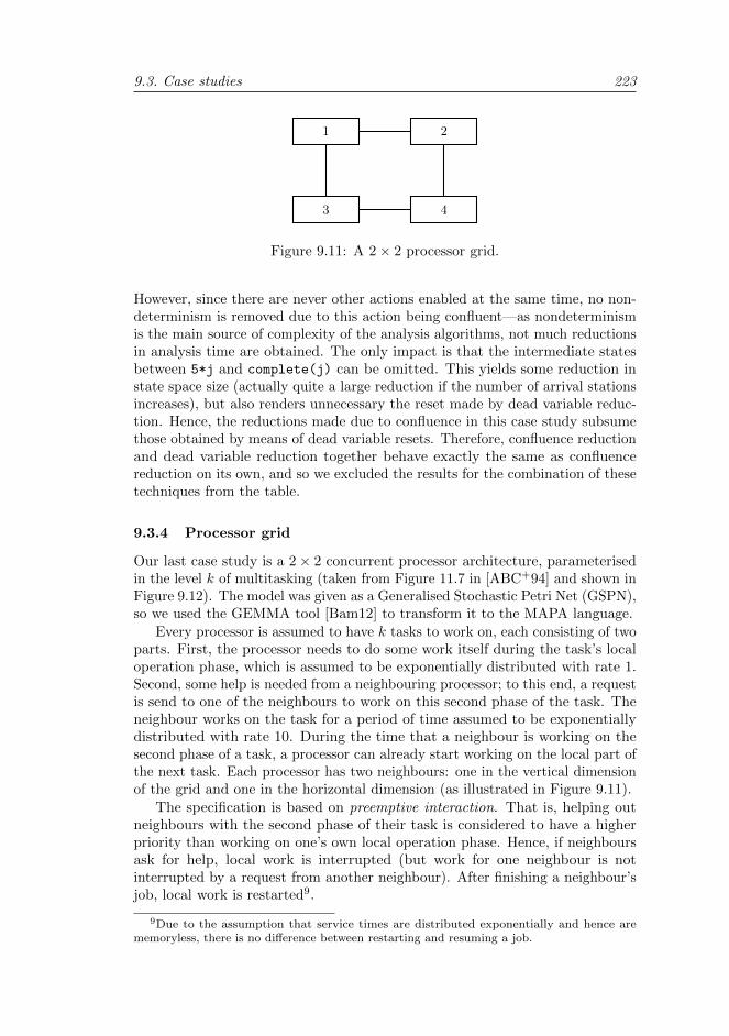
9.3. Case studies 223

1 2

3 4

Figure 9.11: A 2× 2 processor grid.

However, since there are never other actions enabled at the same time, no non-determinism is removed due to this action being confluent—as nondeterminismis the main source of complexity of the analysis algorithms, not much reductionsin analysis time are obtained. The only impact is that the intermediate statesbetween 5*j and complete(j) can be omitted. This yields some reduction instate space size (actually quite a large reduction if the number of arrival stationsincreases), but also renders unnecessary the reset made by dead variable reduc-tion. Hence, the reductions made due to confluence in this case study subsumethose obtained by means of dead variable resets. Therefore, confluence reductionand dead variable reduction together behave exactly the same as confluencereduction on its own, and so we excluded the results for the combination of thesetechniques from the table.

9.3.4 Processor grid

Our last case study is a 2× 2 concurrent processor architecture, parameterisedin the level k of multitasking (taken from Figure 11.7 in [ABC+94] and shown inFigure 9.12). The model was given as a Generalised Stochastic Petri Net (GSPN),so we used the GEMMA tool [Bam12] to transform it to the MAPA language.

Every processor is assumed to have k tasks to work on, each consisting of twoparts. First, the processor needs to do some work itself during the task’s localoperation phase, which is assumed to be exponentially distributed with rate 1.Second, some help is needed from a neighbouring processor; to this end, a requestis send to one of the neighbours to work on this second phase of the task. Theneighbour works on the task for a period of time assumed to be exponentiallydistributed with rate 10. During the time that a neighbour is working on thesecond phase of a task, a processor can already start working on the local part ofthe next task. Each processor has two neighbours: one in the vertical dimensionof the grid and one in the horizontal dimension (as illustrated in Figure 9.11).

The specification is based on preemptive interaction. That is, helping outneighbours with the second phase of their task is considered to have a higherpriority than working on one’s own local operation phase. Hence, if neighboursask for help, local work is interrupted (but work for one neighbour is notinterrupted by a request from another neighbour). After finishing a neighbour’sjob, local work is restarted9.

9Due to the assumption that service times are distributed exponentially and hence arememoryless, there is no difference between restarting and resuming a job.

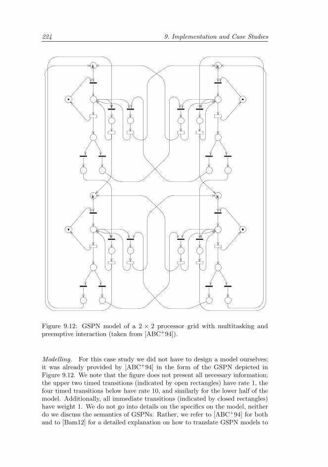
224 9. Implementation and Case Studies

MODELS OF MESH STRUCTURES 255

k

kk

k

Figure 11.7: GSPN model of a 2 × 2 mesh in the case of preemptive interaction and

multitasking

the time between two successive reschedulings of a given task and is computed by

multiplying the cycle time by the number of tasks. Latency corresponds to the

total delay that a task experiences in the following steps: execution on its local

processor, and waiting for service from the remote processor, receiving service from

the remote processor, waiting in the ready-task queue until the next rescheduling.

Individual waiting times may also be readily computed by applying Little’s formula,

since the mean number of tokens in each place and transition rates can be directly

computed by GreatSPN.

The analysis of the 2 × 2 models seems to reach the computational limits of the

Figure 9.12: GSPN model of a 2 × 2 processor grid with multitasking andpreemptive interaction (taken from [ABC+94]).

Modelling. For this case study we did not have to design a model ourselves;it was already provided by [ABC+94] in the form of the GSPN depicted inFigure 9.12. We note that the figure does not present all necessary information;the upper two timed transitions (indicated by open rectangles) have rate 1, thefour timed transitions below have rate 10, and similarly for the lower half of themodel. Additionally, all immediate transitions (indicated by closed rectangles)have weight 1. We do not go into details on the specifics on the model, neitherdo we discuss the semantics of GSPNs. Rather, we refer to [ABC+94] for bothand to [Bam12] for a detailed explanation on how to translate GSPN models to

9.3. Case studies 225

MAPA. For this chapter it suffices to say that the GSPN represents the systemdescribed above, and that we used the PIPE (Platform Independent Petri netEditor) tool [PIP13] to draw this model and the GEMMA tool to obtain anequivalent MAPA specification (actually, an MLPE). That way, every place ofthe GSPN is modelled as a variable and every transition as a summand.

The GSPN community is used to assign weights to immediate transitions,basically resolving nondeterminism by changing it into probabilistic branching.Hence, previous analysis always required weights for all immediate transitions,requiring complete knowledge of the mutual behaviour of all these transitions.That way, GSPNs reduce to CTMCs and relatively simple calculations can beemployed to compute for instance the long-run average fraction of time thata GSPN is in a certain state or set of states. Analysis in [ABC+94] on theGSPN of the processor grid described above indeed assumed all nondeterministicchoices to be resolved uniformly. That is, if N immediate transitions are enabledsimultaneously, only one of them is taken and the probability for each of themto be chosen is 1

N . For the 2× 2 processor grid, this most importantly specifiesthat a processor randomly chooses between its two neighbours for requestingwork on the second phase of its tasks. This, however, may not always be thebest strategy, neither may it accurately represent actual behaviour in a practicalscenario.

When translating GSPNs to MAPA, we now are able to retain nondetermin-ism [Kat12, EHKZ13]. We actually even allow a weight assignment to just a(possibly empty) subset of the immediate transitions—reflecting the practicalscenario of only knowing the mutual behaviour for a selection of the transitions.

Properties of interest. As in [ABC+94], we are interested in computing thethroughput of one of the processors (say processor 1 in Figure 9.11), given bythe long-run average of having a token in a certain place of the GSPN (the placebelow the one on the top-left containing the letter k in Figure 9.12). In [ABC+94],symmetry dictated that all processors have exactly the same behaviour. Hence, itdid not matter which processor was under investigation. However, when breakingthe symmetry by giving one processor a nondeterministic choice between itsneighbours for service requests, differences may occur. Hence, we compute threeproperties for various instances of the system:

1. What is the throughput of processor 1? (long run objective)2. What is the throughput of processor 2? (long run objective)3. What is the throughput of processor 4? (long run objective)

To investigate the impact of the amount of nondeterminism on the throughputas well as the effects of the reduction techniques, we consider three variations inthe assumptions on the behaviour of the grid:

• All nondeterministic choices are resolved uniformly. That is, we retain allweights from the original specification [ABC+94]. This variation has nonondeterminism, only probability.

• Processors 2, 3 and 4 still use a uniform distribution to decide on theirneighbour to send a service request to. Hence, these weights are retained.

226 9. Implementation and Case Studies

All other nondeterministic behaviour, including processor 1’s choice ofneighbour, stays nondeterministic.• No nondeterministic choices are resolved uniformly. That is, all weights

from the original specification are omitted. This variation has no probab-ility, only nondeterminism.

The second variation still has three of the four processors choose their neighbourto send a service request to uniformly, while the remaining processor has theliberty of choosing in any way it wants to. This situation contains nondeterminismas well as probability (and Markovian delays), and hence asks for the full spectrumof MAs. Clearly, the introduction of nondeterminism for the second and thirdvariation implies that each answer will again be an interval instead of a singlevalue. Also, note that all processors are completely equivalent in the first andthird variation. Therefore, we only compute the first property for these twoscenarios; processor 2 and 4 have the same throughput anyway.

Results. Table 9.13 presents the results of this case study. We denote bygrid-o-k the original model (with all weights retained and hence all non-deterministic choices resolved probabilistically) and k concurrent tasks. Similarly,grid-i-k is the intermediate model with some weights retained and k concurrenttasks, and grid-n-k is the fully nondeterministic model with k concurrent tasks.The results for grid-o-2, grid-o-3 and grid-o-4 indeed correspond to theresults in Table 11.5 from [ABC+94]. However, existing work was not yet able toindicate the accuracy of these results in case processors do not resolve their non-deterministic choices uniformly. We now were able to investigate this, resultingin the intervals presented for the moderately and fully nondeterministic variantsof the model. This shows us that for instance in the presence of two tasks, thethroughput of our first processor is at least 0.81 and at most 1.00, dependingon the processors’ behaviour. This information is much more trustworthy thanthe original result of 0.903, which tells us nothing if the strong assumption onuniform resolutions is violated.

The results also indicate that the intermediate situation where only pro-cessor 1 can choose freely allows just a slight variation in throughput. This can beexplained by noticing that it could send its service requests to the neighbour thatis currently not already working on another service request (either coincidentallyor maybe due to some shared information on who is working on what). Thatway, work immediately starts and no additional waiting is necessary. As servicerequests are dealt with rather quickly, the potential increase or decrease inthroughput for processor 1 is rather small. However, the neighbouring processorsmay endure a much larger decrease in throughput as a result of processor 1slightly increasing its throughput. This is explained by the fact that processor 1may try to preempt neighbours that are working on their local operation phase.Since that phase on average takes much longer than the service requests, thepreemptions may severely impact their throughput (as the memoryless aspectof the exponential distribution dictates that preempted work basically startsall over). If all processors can choose freely, processor 1 may obtain an almostperfect throughput. This presumably is due to its possibility of selecting a

9.3. Case studies 227

Ori

gin

al

state

space

Pro

per

ty1

Pro

per

ty2

Pro

per

ty3

Sp

ecifi

cati

on

Sta

tes

Tra

nsi

tion

sS

CO

OP

(s)

Res

ult

IMC

A(s

)R

esu

ltIM

CA

(s)

Res

ult

IMC

A(s

)grid-o-2

2,5

08

3,2

15

14.5

(17.7

)0.9

031

2.0

grid-o-3

10,8

52

14,3

79

64.7

(79.5

)0.9

086

32.8

grid-o-4

31,8

32

42,8

79

193.0

(236.7

)0.9

090

249.7

grid-i-2

2,5

08

4,2

54

0.8

(0.9

)[0.9

001,0.9

055]

3.0

[0.8

585,0.9

479]

2.6

[0.9

029,0.9

032]

3.1

grid-i-3

10,8

52

19,0

99

3.2

(3.9

)[0.9

081,0.9

089]

84.4

[0.8

633,0.9

541]

67.1

[0.9

086,0.9

087]

77.2

grid-i-4

31,8

32

56,7

04

9.8

(11.9

)[0.9

089,0.9

091]

868.2

[0.8

636,0.9

545]

765.2

[0.9

090,0.9

091]

937.3

grid-n-2

2,5

08

4,6

08

0.6

(0.6

)[0.8

110,0.9

953]

2.7

grid-n-3

10,8

52

20,8

72

2.7

(2.6

)[0.8

173,0.9

998]

64.4

grid-n-4

31,8

32

62,3

56

7.9

(8.0

)[0.8

181,1.0

000]

914.4

Con

flu

ence

red

uct

ion

Th

rou

gh

pu

tT

hro

ugh

pu

tn

eighb

ou

rsT

hro

ugh

pu

tn

on

-nei

ghb

ou

rS

pec

ifica

tion

Sta

tes

Tra

nsi

tion

sS

CO

OP

(s)

Res

ult

IMC

A(s

)R

esu

ltIM

CA

(s)

Res

ult

IMC

A(s

)grid-o-2

1,9

50

(−22%

)2,6

57

(−17%

)18.3

(+26%

)0.9

031

1.2

(−40%

)grid-o-3

8,5

68

(−21%

)12,0

95

(−16%

)81.9

(+27%

)0.9

086

22.0

(−33%

)grid-o-4

25,1

77

(−21%

)36,2

24

(−16%

)243.8

(+26%

)0.9

090

162.5

(−35%

)grid-i-2

1,5

14

(−40%

)2,7

67

(−35%

)0.8

(−0%

)[0.9

001,0.9

055]

1.4

(−53%

)[0.8

585,0.9

479]

1.2

(−54%

)[0.9

029,0.9

032]

1.5

(−52%

)grid-i-3

6,5

09

(−40%

)12,5

23

(−34%

)3.5

(+9%

)[0.9

081,0.9

089]

30.3

(−64%

)[0.8

633,0.9

541]

25.2

(−62%

)[0.9

086,0.9

087]

38.6

(−50%

)grid-i-4

19,0

25

(−40%

)37,4

18

(−34%

)10.1

(+3%

)[0.9

089,0.9

091]

398.8

(−54%

)[0.8

636,0.9

545]

348.2

(−54%

)[0.9

090,0.9

091]

555.7

(−41%

)grid-n-2

1,5

14

(−40%

)3,0

43

(−34%

)0.7

(−30%

)[0.8

110,0.9

953]

1.1

(−59%

)grid-n-3

6,5

09

(−40%

)13,7

38

(−34%

)3.0

(+11%

)[0.8

173,0.9

998]

22.4

(−65%

)grid-n-4

19,0

25

(−40%

)41,0

18

(−34%

)8.8

(+11%

)[0.8

181,1.0

000]

361.4

(−60%

)

Table 9.13: State space generation and analysis for a processor grid.

228 9. Implementation and Case Studies

neighbour that is currently not already working on a service request, and on theneighbours’ possibility of sparing processor 1 from any work. On the other hand,the neighbours 2 and 3 may also direct all their work to processor 1, lowering itsthroughput significantly.

Discussion. Based on the results, we can conclude that the basic reductiontechniques do not help us much. This is understandable, as the construction ofan MLPE based on a GSPN does not introduce any summations or constants;hence, at most some very basic expression simplifications may be possible.Additionally, dead variable reduction has no impact—therefore, these resultshave even been omitted. This was to be expected as well, since the only variablesin an MLPE based on a GSPN are the ones that represent the number of tokensin each place. This number can only become irrelevant for places that have nooutgoing transitions or that are somehow reset at some point. As neither ofthese situations occurs in the model at hand, indeed dead variable reduction isnot applicable.

Confluence reduction may only reduce in the presence of invisible non-probabilistic transitions. Hence, in the original model not much reduction ispossible. The fact that some state space reduction is still obtained is due tothe fact that states having only one outgoing τ -transition may sometimes beomitted. As expected, more reduction is possible if more nondeterminism ispresent (since indeed some of this nondeterminism turns out to be spurious).State space reductions of about 40% and decreases in analysis time around 60%save a significant amount of time.

9.4 Contributions

In this chapter we presented our tool SCOOP, implementing the MAPA linearisa-tion procedure, a state space generation algorithm and all reduction techniques in-troduced for MAPA in this thesis. We discussed four case studies, showing how tomodel and analyse them and illustrating the power of our reduction techniques.

Our case studies show that several types of systems can easily be modelledin MAPA. Enabling the full spectrum of MAs, and supported by IMCA, ourtechniques for the first time allow the efficient modelling, generation and ana-lysis of systems incorporating both nondeterminism, probabilistic choice andMarkovian delays. For the GSPN case study on a processor grid, this made itpossible to compute intervals of probabilities, taking into account the effects ofhow nondeterministic choices are resolved. This was not possible in earlier work.

Our results also clearly show the significant potential of confluence reduction,dead variable reduction and the basic reduction techniques. We demonstratedthat all of them may greatly reduce state space generation time. Additionally,dead variable reduction and confluence reduction often cut back the state spaceitself and hence the analysis time. In the remainder of this section we discuss towhat extent our reduction techniques approach the smallest possible representa-tions of our case studies. Additionally, we touch upon some trends regardingthe reduction power of the individual techniques. Finally, we briefly discuss thereductions in analysis time.

9.4. Contributions 229

9.4.1 Reduction potential

Although our techniques reduce state spaces significantly, they in general do notobtain the smallest possible model that still satisfies the same properties. Afterall, in general this would require the entire state space to be known upfront.

Hence, we are interested to know how much of the potential reductions areindeed obtained by means of our techniques. Since there are no tools available yetto compute the branching bisimulation minimal quotient for MAs, we actuallyhave no means to derive the maximal possible reduction for models that exhibitnondeterminism, probability as well as Markovian delays at the same time.However, for subsets of these features we can rely on older tools that computetraditional branching bisimulation in the presence of only nondeterminism (asis the case for the handshake register), probabilistic branching bisimulation inthe presence of only nondeterminism and probabilistic choice (as is the casefor a slight variation of the leader election protocol) and stochastic branchingbisimulation in the presence of only nondeterminism and Markovian delays (asis the case for one of the variations of the processor grid).

Handshake register. The case study of the handshake register contains noquantitative information; hence, we can just apply µCRL’s ltsmin tool forcomputing its minimal quotient with respect to branching bisimulation.

For the handshake register with |D| = 2, the state space went down from540,736 to 25,280 states due to our techniques. In the minimal quotient, it turnsout to have only 72 states. Hence, some additional reduction is still possible.Nonetheless, we managed to cut back over 95% of the maximum number of statesthat could have been omitted (515,456 of the maximum number of 540,664).For |D| = 3, we went down from 13,834,800 to 155,304 states, while the minimalquotient has 189 states.

Leader election protocol. We omitted the Markovian delay from the specificationof the leader election protocol to make it into a PA. Then, CADP’s bcg_min

tool can be applied to obtain a minimal quotient with respect to probabilisticbranching bisimulation. Since CADP represents each probabilistic transition bymeans of an intermediate state with outgoing probabilistic edges, the number ofstates and transitions is not fully comparable to the numbers we provide. Still,we can report that the number of states in CADP of leader-3-4 in the absenceof Markovian delays is 21,232 without our reduction techniques, 2,939 whenapplying all reduction techniques and 242 in the branching bisimulation minimalquotient. This again shows that some additional reduction may be achieved,but also that we were able to reduce quite significantly: we omitted 87% ofthe maximum number of states that could be removed (18,293 out of 20,990).For leader-3-8 the number of states without any reduction was 274,476, withreductions 21,151 and after minimisation 666—hence, here we found 93% of themaximal reduction.

Processor grid. For the GSPN case study of the processor grid, we took thevariation without any weights (and hence without any discrete probabilitistic

230 9. Implementation and Case Studies

behaviour). Since that model is an IMC, we are able to apply CADP’s bcg_mintool to obtain the minimal quotient with respect to stochastic branching bisimu-lation. For grid-n-4 the number of states without any transitions was 31,832,which went down to 19,025 when applying all reduction techniques. The minimalquotient turned out to consist of 11,901 states. So, for this model our techniquesmanaged to find 64% of the maximal reduction possible.

9.4.2 Individual reduction techniques

Based on the results for the four case studies, we draw conclusions aboutthe applicability of the individual reduction techniques (the basic reductiontechniques, dead variable reduction and confluence reduction). For each of thesethree categories, we also conjecture some model properties that seem to beindicators to expect a lot of reduction.

As demonstrated by the case studies, often the combination of all our tech-niques is most efficient. After all, this combines their forces (which are mostlyrather orthogonal).

Basic reduction techniques. We noticed from the processor grid case study thatthe basic reduction techniques do not influence state space generation much forMAPA models generated from GSPNs. This was to be expected, due to the factthat the translation procedure does not introduce any real data. No summationsare introduced and no variables can ever be constant (unless a place in the GSPNis never used). Hence, summation elimination and constant elimination are notapplicable.

For the handshake register and polling system generation times roughlyhalved, while for the leader election protocol reduction factors of more than70 were observed (requiring less than 1.5% of the original time to generatethe state space). This could be explained from the relatively large number ofparallel components, introducing a lot of constant parameters and reduciblenondeterministic summations.

The reduction of the number of MLPE parameters reduces the size of thestates that need to be stored in memory (vectors of values of these parameters).Additionally, smaller states and smaller specifications make it easier to checkwhich summands are enabled for a given state. Both aspects speed up statespace generation, and this speed up can be quite significant—as illustrated byour case studies.

Best results if a model is constructed as the parallel composition of manycomponents having extensive interactions based on data parameters (in-troducing reducible summation and constant parameters), and if a modelhas lots of data and expressions over this data (introducing reducibleexpressions).

Dead variable reduction. The potential of dead variable reduction is mostconvincingly shown by the handshake register case study. There, state spaceswere reduced by more than a factor of 100, leaving less than a percent of the

9.4. Contributions 231

original number of states and transitions. This way, a model could be generatedthat would have been much too big without dead variable reduction. On theother hand, the processor grid confirmed our expectation that GSPN-basedmodels are not suitable for dead variable reduction. After all, these only containvariables storing the number of tokens in each place; often, this informationnever becomes irrelevant (as it basically encodes the control flow) and hence novariable resets are possible.

For the leader election protocol and the polling system, dead variable reduc-tion was able to achieve significant reductions. As expected, these reductionsbecome more powerful in case larger data types are used. After all, this impliesthat variable resets map more states on the same state than when using onlysmall data types. For the polling systems moderate results were found, redu-cing analysis times by about 10%. This can be explained by the fact that thismodel only allowed one variable reset of rather limited influence. For the leaderelection protocol, on the other hand, more impressive reduction were obtained.Depending on the model parameters, dead variable reduction sometimes cutback analysis time to less than 3% of the time needed to analyse the unreducedmodel. This made the analysis of much larger models feasible in reasonableamounts of time (minutes instead of hours).

Best results if a model has many parameters with large data types, storingvalues that regularly become irrelevant.

Confluence reduction. Like dead variable reduction, also confluence reductiondepends heavily on the structure of the model under consideration. For thehandshake register state spaces reduced by approximately 40%, for the leaderelection protocol by approximately 80%–90%, for the polling system by approx-imately 25%-30% and for the processor grid by approximately 20%–40%. Thecase studies show little difference in the effect of confluence reduction whenvarying the parameters of the model. The processor grid did show that, as wasto be expected, a nondeterministic model allows for more confluence reductionthan a probabilistic model.

For the leader election protocol and the processor grid analysis times droppedeven more significantly than the number of states of the model due to con-fluence reduction. This can be explained by the observation that the degreeof nondeterminism reduced more than the number of states. For instance, forleader-3-6 without confluence reduction there are 51,253 states of which 13,599have a nondeterministic choice. With confluence reduction, 6,880 states remain, ofwhich only 120 have a nondeterministic choice. Hence, the degree of nondetermin-ism goes down from 27% to 2%—apparently confluence reduction is able to detectthat almost all nondeterministic choices are spurious. Since nondeterminism isthe main source of complexity in the algorithms, this explains why the reductionin analysis time is even larger than the reduction in state space size.

The generation times by SCOOP are not reduced as much, due to the addi-tional overhead of (re)computing representative states. To keep memory usage inthe order of the reduced state space, the representation map is deliberately notstored by default and therefore potentially recomputed for some states. As ex-

232 9. Implementation and Case Studies

plained in Section 9.3.2, we did store the representation map for the leader electionprotocol case study to save time at the cost of some additional memory usage.

Best results if a model is constructed as the parallel composition of manyloosely connected components, all having many internal transitions thatmay interleave in any order. Since probabilistic transitions cannot be conflu-ent, confluence reduction prefers nondeterminism over probabilistic choice.

Our heuristics underapproximate the confluent transitions, and hence maynot find them all. Since no algorithm has yet been implemented to find thecomplete set of confluent transitions on a concrete state space, it is at this pointinfeasible to say if all confluent transitions were discovered. We can, however,take the state space when applying dead variable reduction as our baseline, andcompare confluence reduction’s performance to the maximal obtainable reductionwith respect to branching bisimulation. For the handshake register with |D| = 2,confluence brought the state space down from 45,504 to 25,280 states, with aminimal quotient of 72 states. Hence, 45% of the maximal reduction is obtained.Since confluence is more strict than branching bisimulation, we can reasonablyexpect more than 45% of the confluent transitions to have been detected.

For leader-3-6 confluence got the number of states down from 44,581 to9,267, with 430 as the absolute minimum. Hence, for this model at least 80%of the maximal possible reduction was obtained. For grid-4 no dead variablereduction was possible, and hence the 64% discussed earlier is completely due toconfluence reduction.

9.4.3 Reductions in analysis time

For the three case studies that were analysed with IMCA, we noticed (asexpected) that decreases in the number of states resulted in decreases in thetime needed for the computation of the various properties that we checked.Most of the algorithms used by IMCA (linear programming, value iteration)are rather expensive regarding their worst-case time complexity [ZN10], but areoften reasonably fast in practice—as shown by our experiments. Therefore, nostrong theoretical statements can be made about the impact of our reductiontechniques on IMCA’s analysis.

However, we did observe that if models were reduced by dead variable reduc-tion, the relative reductions in analysis time corresponded quite well to the relat-ive reductions in state space size. For the models where confluence reduction wasable to actually decrease the amount of nondeterminism (leader election protocoland processor grid), the reduction in analysis time was relatively even larger.

In addition to (mostly) reducing state space generation time, our reductiontechniques always reduced IMCA’s analysis time. With only a few excep-tions, this decrease was at least as large as the decrease in the number ofstates, relatively. Hence, especially if a model is to be analysed by IMCA,our techniques really pay off.

CHAPTER 10

Conclusions

“A moral being is one who is capable of reflectingon his past actions and their motives—

of approving of some and disapproving of others.”

Charles Darwin

We introduced MAPA: a novel process-algebraic language for specifying

Markov automata (MAs). The MA is a recently introduced state-basedmodelling formalism incorporating nondeterminism, probabilistic choice

and stochastic timing—all these features are also supported by MAPA. Wedefined several reduction techniques, working symbolically on specifications tooptimise state space generation and analysis without ever having to generate anunreduced state space. Experimental validation shows that significant reductionsare obtained, reducing the larger models between 35% and 99%.

10.1 Summary

10.1.1 The MAPA language: efficient modelling

The MAPA language is data driven, even allowing specifications that rely ondynamic data types such as stacks or lists. To simplify symbolic translations ofMAPA specifications, we presented the notion of derivation-preserving bisimula-tion. We used it to show under which circumstances techniques can be definedfor our language without even taking into account stochastic timing, while stillbeing applicable to all specifications by means of an encoding of rates in actions.

We defined the MLPE as a restricted part of MAPA, easy to use for statespace generation, parallel composition and symbolic optimisations. We demon-strated how to transform (linearise) each MAPA specification into an equivalentrepresentation as MLPE, allowing MLPE-based reduction techniques to be ap-plied to all specifications. The linearisation procedure is defined only on thesubset of MAPA not including stochastic timing, but can be applied to the fulllanguage by means of our encoding scheme.

10.1.2 Reduction techniques: efficient generation and analysis

MAPA specifications often generate large state spaces—a well-known problem in(quantitative) model checking. This may be due to the presence of data, or due

234 10. Conclusions

to a large number of parallel components. To alleviate this state space explosion,we presented five reduction techniques. All are defined on the MLPE, as henceare enabled through our linearisation procedure.

First we defined three basic reduction techniques: constant elimination,expression simplification and summation elimination. They syntactically clean-up an MLPE, making it more human friendly to read and speeding up statespace generation. However, they do not influence the underlying state space.Our two other reduction techniques—dead variable reduction and confluencereduction—do aim to shrink a specification’s MA, while preserving all propertiesof interest. As they work on the MLPE instead of the actual models, theyprevent having to generate the unreduced state space.

Dead variable reduction automatically performs variable resets, reducing statespaces by merging several equivalent states. It incorporates a control flow analysistechnique on MLPEs that does not only take into account control flow dictatedby the program counters of the constituent processes, but also by control flowencoded in the data parameters. Although some of these resets may also beintroduced manually, our technique relieves the user of that burden. Additionally,while manual optimisations are error-prone, our technique guarantees to onlyprovide a bisimilar state space that is at most as large as the unreduced one.

Confluence reduction focusses on spurious interleavings. It basically gives priorityto invisible transitions that do not disable any observable behaviour and hencecan always be taken at the cost of other transitions emanating from the samestate. We generalised a non-quantitative variant of this technique, while at thesame time fixing a subtle mistake in the old definitions concerning closure underunions. We showed how to apply confluence to reduce state spaces on-the-fly,and discussed how to detect confluence symbolically based on the MLPE.

Additionally, we compared confluence reduction to partial order reduction intwo ways. First, we provided a theoretical comparison between the two notionsin branching time, demonstrating that confluence is slightly more powerful inthat setting. We pinpointed precisely how the two techniques can be altered tomake them coincide, showing that the differences we observed indeed completelycharacterise the gap. Second, we provided a practical comparison betweenconfluence reduction an partial order reduction in the context of statistical modelchecking. We demonstrated how to apply confluence to its full potential onthe partial concrete state spaces that are available during this type of modelchecking, and indeed showed that the advantages over partial order reductioncan make a difference in practice.

10.1.3 Implementation and validation

We developed a tool called SCOOP, implementing a parser, lineariser and statespace generator for our language MAPA. The tool applies all five reductiontechniques presented in this thesis. It is linked to the preprocessor GEMMA towork with GSPNs as well, and to the model checker IMCA for the verificationof time-bounded and unbounded reachability properties, expected times andlong-run averages. Together, this tool chain (called MaMa) for the first time

10.2. Discussion 235

enables the efficient specification, generation and analysis of Markov automata.We presented four case studies, on a handshake register, a leader election

protocol, a polling system and a processor grid. They demonstrated thatMAPA can be used to specify a large variety of systems. The fact that systemsare represented as MAs allowed for the computation of minimal and maximalprobabilities in the presence of stochastic timing, discrete probabilistic choiceand nondeterminism, whereas earlier work required all nondeterminism to beresolved and hence always yielded single probabilities.

Experimental results showed that our techniques significantly reduce statespace generation and analysis times. As expected, all reduction techniquesturned out to have their own strengths. We were able to provide guidelinesindicating for what type of systems each reduction technique is most applicable.

10.2 Discussion

The framework we presented enables the efficient modelling, generation andanalysis of MAs. It contributes in several ways to the state of the art inquantitative model checking:

• The data-driven language MAPA supports the efficient modelling of systemsincorporating nondeterminism, probabilistic choice and stochastic timing.

• The notion of derivation-preserving bisimulation provides the opportunityto reuse techniques developed for PAs also for specifications of MAs.

• The basic reduction techniques contribute to the efficient generation ofMAs based on MAPA specifications.

• Dead variable reduction and confluence reduction alleviate the state spaceexplosion by means of reductions in the number of states and transitions,allowing faster analysis.

• Our comparison of confluence reduction and partial order reduction resolvesthe long-standing uncertainty about the relation between these two conceptsin branching time.

The practical applicability of our approach for specific case studies mainlydepends on two aspects: (1) how accurate can the case study be represented asan MA, and (2) how severe is the state space explosion?

Accuracy of the model. Since MAs generalise LTSs, DTMCs, CTMCs, PAs andIMCs, all systems that can be modelled as one of these can also be modelledas an MA. Based on the abundant number of case studies that indeed havebeen modelled in one of these formalisms (for instance, [BG94a, KS94, FGK97,SvdZ98, GPW03, PS07, HHK00, FG06, KNP12, QWP99, YKNP06, KNP08,HKN+08, KNS03, NS06, NM10, BCS10, BHH+09]), we can conclude that thereis a large target set of cases.

Already for CTMCs and IMCs, the main concern is whether the exponentialdistribution accurately describes the timing in a system. This is often assumed,for instance in queueing systems [BB96] and systems biology [Wil11, KNP08].Additionally, it is well-known that every probability distribution can be approx-imated arbitrarily well by a phase-type distribution, i.e., a network of exponential

236 10. Conclusions

distributions [BGdMT06, Nel95]. Although this is not always easy to achieve inpractice [Bla05], a combination of exponential distributions may still be used toat least partly improve the accuracy of the model.

Surviving the state space explosion. Although our techniques mitigate the statespace explosion to quite some extent, this does not yet fully solve the problem.In the presence of large data that cannot be reset, or multiple interleavingsthat do make a difference, the state space may still grow rather quickly. Hence,although we did lift the bar significantly, quantitative model checking of systemsrepresentable as MAs remains to be bound by the complexity of these systems.Nonetheless, our case studies (as well as many other case studies in quantitativemodel checking) demonstrated that interesting results can still be obtained, forinstance by abstracting systems or protocols to their core or by only consideringpart of a system.

10.3 Future work

Our work gives rise to several directions for future work. Most obviously,the development of additional minimisation techniques preserving strong orbranching bisimulation could be very useful. As our case studies demonstratedthat a large fraction of the potential reduction is often already obtained by ourcurrent techniques, it would also be interesting to investigate the possibilitiesfor reductions techniques preserving less properties, for instance only traces oreven only deadlocks.

Instead of developing additional reduction techniques, future work may alsofocus on conducting more case studies, to evaluate the effects of our currentreduction techniques and verify the generalisability of our results. Also, thepotential of compositional state space generation may be explored. Additionally,the existing techniques may be investigated some more, as discussed below.

10.3.1 Reduction techniques

Dead variable reduction. It would be interesting to find additional applicationsfor the control flow reconstructed as part of our dead variable reduction technique.One possibility is to use it for invariant generation, another is to visualise itsuch that process structure can be understood better. Also, it might be used tooptimise confluence detection, since it could assist in determining which pairs ofsummands may be confluent. As also conjectured by [Pel08], such collaborationbetween reduction techniques could be useful.

Another direction for future work is based on the insight that the controlflow graph is an abstraction of the state space. It could be investigated whetherother abstractions, such as a control flow graph containing also the values ofimportant data parameters, may result in more accurate data flow analysis.

Confluence reduction. As future work on confluence reduction we envisionto search for even more powerful ways of using commutativity for state spacereduction, for instance by allowing confluent transitions to be probabilistic.

10.3. Future work 237

Preferably, such extensions will enable more aggressive reductions that, insteadof preserving the rather conservative notion of bisimulation we used, preservethe more powerful weak bisimulation from [EHZ10b]. Future work may alsofocus on finding more powerful heuristics for detecting confluence based on theMLPE, enabling more reduction in practice.

Another obvious direction of future work is to generalise the ample set methodof partial order reduction to MAs, and prove its correctness by demonstratingagain the subsumption by confluence reduction.

Finally, although we already showed that confluence reduction preservesbranching bisimulation, it is still unknown precisely what types of propertiesare left invariant by this notion of equivalence. We conjectured (and confirmedempirically by all our experiment) that this is the case for all properties that canbe verified by IMCA. Ongoing work in the Software Modeling and Verificationgroup at RWTH Aachen University already formally showed this for strongbisimulation, and is currently concerned with also showing this for weak andbranching bisimulation.

10.3.2 Long-term perspective

From a more long-term perspective, we would be interested to see if our modellinglanguage and reduction techniques can be extended to include even more features,such as deterministic timing or non-exponential distributions.

Also, it would be useful to incorporate our techniques in a larger variety oftools. We already discussed the coupling with LTSmin, but for instance alsoforesee useful applications of dead variable reduction and confluence reductionin PRISM. The symbolic (BDD / MTBDD) aspect of these tools complicatesmatters, but in combination with our techniques may also open up even morepossibilities.

Finally, whereas we now only focused on techniques based on equivalences,another interesting direction for future work is to consider abstraction. Thatis, instead of preserving all behaviour of the original system, only a subset ispreserved. In some cases this may already be enough to show that a certainproperty is violated, while reducing more significantly than the type of reductiontechniques discussed in this thesis.

Part V

Appendices

APPENDIX A

Proofs

“Very impressive, colleague . . . but does it also work in theory?”

Fokke & Sukke

In many of the proofs in this appendix we use the fact that, given a countableset S, two distributions µ, ν ∈ Distr(S) and two equivalence relations R,R′

over S such that R′ ⊇ R, it holds that µ ≡R µ′ implies µ ≡R′ µ′. This resultimmediately follows from Propositions 5.2.1.1 and 5.2.1.5 from [Sto02a]. We usethis result in the proofs, without every time referring to these propositions again.

Many proofs of the propositions and theorems presented throughout thethesis rely on some auxiliary lemmas. These are each time presented directlybefore the results in which they are applied for the first time.

A.1 Proofs for Chapter 3

A.1.1 Proof of Proposition 3.32

Lemma A.1. Let M = 〈S, s0, A, −→, ,AP, L〉 be an MA, and let s ∈ S,α ∈ Aχ, and µ ∈ Distr(S). Then,

s −α→ µ =⇒ sα

=⇒R µ

for any equivalence relation R over S.

Proof. Assume that s −α→ µ. To show that sα

=⇒R µ, we need to provide ascheduler S such that

• FSM(s) = µ• For every maximal path

s −α1,µ1−−−→ s1 −α2,µ2−−−→ . . . −αn,µn−−−→ sn ∈ maxpathsSM(s)

it holds that αn = α. Moreover, for every 1 ≤ i < n we have αi = τ ,(s, si) ∈ R and L(s) = L(si).

Let S be defined by S(s) = (s, α, µ) 7→ 1 and S(π) = 1⊥ for every path π 6= s.Clearly, FSM(s) = µ. Also, all maximal path in

maxpathsSM(s) = s −α,µ−−→ s′ | s′ ∈ supp(µ)

242 A. Proofs

indeed trivially satisfy the requirements above for any equivalence relation Rover S (since n = 1 for all of these maximal paths).

Lemma A.2. Let M = 〈S, s0, A, −→, ,AP, L〉 be an MA, R ⊆ S × S abranching bisimulation for M, and R′ ⊇ R an equivalence relation such thatL(p) = L(q) for every (p, q) ∈ R′. Then, for every (s, t) ∈ R and all α ∈ Aχ, µ ∈Distr(S), it holds that

sα

=⇒R′ µ =⇒ ∃µ′ ∈ Distr(S) . tα

=⇒R′ µ′ ∧ µ ≡R′ µ′.

Proof. Let (s, t) ∈ R, and assume that sα

=⇒R′ µ. If α = τ and µ = 1s, then thetrivial branching transition t

τ=⇒R′ 1t completes the proof. Otherwise, assume

that there exists a scheduler S such that

• FSM(s) = µ• For every maximal path

s −α1,µ1−−−→ s1 −α2,µ2−−−→ . . . −αn,µn−−−→ sn ∈ maxpathsSM(s)

it holds that αn = α. Moreover, for every 1 ≤ i < n we have αi = τ ,(s, si) ∈ R′ and L(s) = L(si).

As every single transition of s can be mimicked by t (due to (s, t) being in abisimulation relation R), we can define a scheduler S ′ that mimics every choiceof S. So, assume that S(s) = s −α1−→ µ1 7→ p1, . . . , s −αn−→ µn 7→ pn. Then, welet S ′ schedule the transitions necessary for t

αi=⇒R µ′i (with µi ≡R µ′i) withprobability pi. That is, if for instance t −α2−→ ν1 and t −α3−→ ν2 should both beassigned probability 0.5 as a first step to obtaining t

α1=⇒R µ′1, we let S ′ schedule

them each with probability 0.5p1. This way, with probability p1 the tree startingfrom t reaches a distribution over states that is R-equivalent to µ1. As wecan then again mimic the transitions of S from there, and this can continueuntil the end of each maximal path of S, we obtain a scheduler S ′ for whichFS′

M(t) = µ′ with µ ≡R µ′. Moreover, all states visited before the α-actions inthe tree starting from t also remain in the same R′ equivalence class because ofthe restrictions of the =⇒R′ relation and the fact that the mimicked steps yieldan R-equivalent distribution. Therefore, indeed t

α=⇒R′ µ

′ ∧ µ ≡R µ′. SinceR′ ⊇ R, this implies µ ≡R′ µ′.

Figure 1.1 illustrates the proof for a simplified non-probabilistic setting.

Proposition 3.32. Let M = 〈S, s0, A, −→, ,AP, L〉 be an MA. Then, an equi-valence relation R ⊆ S × S is a branching bisimulation for M if and only if forevery (s, t) ∈ R and all α ∈ Aχ, µ ∈ Distr(S), it holds that L(s) = L(t) and

sα

=⇒R µ =⇒ ∃µ′ ∈ Distr(S) . tα

=⇒R µ′ ∧ µ ≡R µ′

Proof. (if) First, assume that R is an equivalence relation satisfying the re-quirements of this proposition. Hence, if (s, t) ∈ R, then L(s) = L(t) andevery branching transition s

α=⇒R µ can be mimicked by t. By Lemma A.1,

this immediately implies that also every transition s −α→ µ can be mimicked.Therefore, R is a bisimulation relation.

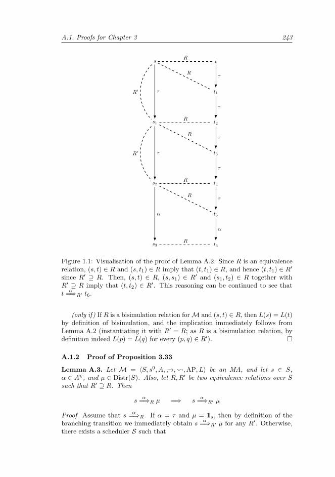
A.1. Proofs for Chapter 3 243

s t

s1

s2

s3

R

τ

τ

α

R′

R′

t1

t2

t3

t4

t5

t6

τ

τ

τ

τ

τ

α

R

R

R

R

R

R

Figure 1.1: Visualisation of the proof of Lemma A.2. Since R is an equivalencerelation, (s, t) ∈ R and (s, t1) ∈ R imply that (t, t1) ∈ R, and hence (t, t1) ∈ R′since R′ ⊇ R. Then, (s, t) ∈ R, (s, s1) ∈ R′ and (s1, t2) ∈ R together withR′ ⊇ R imply that (t, t2) ∈ R′. This reasoning can be continued to see thatt

α=⇒R′ t6.

(only if) If R is a bisimulation relation forM and (s, t) ∈ R, then L(s) = L(t)by definition of bisimulation, and the implication immediately follows fromLemma A.2 (instantiating it with R′ = R; as R is a bisimulation relation, bydefinition indeed L(p) = L(q) for every (p, q) ∈ R′).

A.1.2 Proof of Proposition 3.33

Lemma A.3. Let M = 〈S, s0, A, −→, ,AP, L〉 be an MA, and let s ∈ S,α ∈ Aχ, and µ ∈ Distr(S). Also, let R,R′ be two equivalence relations over Ssuch that R′ ⊇ R. Then

sα

=⇒R µ =⇒ sα

=⇒R′ µ

Proof. Assume that sα

=⇒R. If α = τ and µ = 1s, then by definition of thebranching transition we immediately obtain s

α=⇒R′ µ for any R′. Otherwise,

there exists a scheduler S such that

244 A. Proofs

• FSM(s) = µ• For every maximal path

s −α1,µ1−−−→ s1 −α2,µ2−−−→ . . . −αn,µn−−−→ sn ∈ maxpathsSM(s)

it holds that αn = α. Moreover, for every 1 ≤ i < n we have αi = τ ,(s, si) ∈ R and L(s) = L(si).

The same scheduler proofs the validity of sα

=⇒R′ µ. After all, the only thingthat has to be checked is that (s, si) ∈ R′ still holds for all 1 ≤ i < n. As(s, si) ∈ R is assumed and R′ ⊇ R, this is immediate.

Proposition 3.33. The relation ≈b is an equivalence relation.

Proof. Let M = 〈S, s0, A, −→, ,AP, L〉 be an MA. We show that ≈b is anequivalence relation, by showing reflexivity, symmetry and transitivity.

Reflexivity holds, as the identity relation (s, s) | s ∈ S is a branchingbisimulation. This immediately follows by definition of branching bisimulation,Lemma A.1 and the fact that ≡R is reflexive.

For symmetry, let s, t ∈ S and assume that s ≈b t. Then, there must exista branching bisimulation R ⊆ S × S such that (s, t) ∈ R. As every branchingbisimulation is an equivalence relation, also (t, s) ∈ R, and hence t ≈b s.

For transitivity, let (p, q) ∈ S and assume that p ≈b q as well as q ≈b r.Then, using Proposition 3.32, there exists an equivalence relation R1 ⊆ S × Ssuch that (p, q) ∈ R1, and for all (s, t) ∈ R1 it holds that

sα

=⇒R1µ =⇒ ∃µ′ ∈ Distr(S) . t

α=⇒R1

µ′ ∧ µ ≡R1µ′.

Similarly, there exists an equivalence relation R2 ⊆ S × S such that (q, r) ∈ R2,and for all (s, t) ∈ R2 it holds that

sα

=⇒R2µ =⇒ ∃µ′ ∈ Distr(S) . t

α=⇒R2

µ′ ∧ µ ≡R2µ′.

We define R3 = (R2 R1) ∪ (R1 R2), and let R be the transitive closureof R3. We first prove that R is an equivalence relation by showing (1) reflexivity,(2) symmetry, and (3) transitivity.

(1) As R1 are R2 are equivalence relations, they are reflexive; thus, for everystate s ∈ S it holds that (s, s) ∈ R1 and (s, s) ∈ R2. Therefore, also(s, s) ∈ R2 R1 and thus (s, s) ∈ R.

2) First observe that when (x, z) ∈ R2 R1, then there must be a state y ∈ Ssuch that (x, y) ∈ R1 and (y, z) ∈ R2, and therefore by symmetry of R1

and R2 also (y, x) ∈ R1 and (z, y) ∈ R2, and thus (z, x) ∈ R1 R2.Now let (s, t) ∈ R. Then there is an integer n ≥ 2 such that there exists

a sequence of states s1, s2, . . . , sn such that s1 = s and sn = t, and for all1 ≤ i < n it holds that (si, si+1) ∈ (R2 R1) or (si, si+1) ∈ (R1 R2).By the observation above we can reverse the order of the states, obtainingthe sequence sn, sn−1, . . . , s1 such that still sn = t and s1 = s, and for all1 ≤ i < n it holds that (si, si+1) ∈ (R2 R1) or (si, si+1) ∈ (R1 R2). To

A.1. Proofs for Chapter 3 245

be precise, when (si, si+1) ∈ (R2 R1), then (si+1, si) ∈ (R1 R2), andwhen (si, si+1) ∈ (R1 R2), then (si+1, si) ∈ (R2 R1). The sequenceobtained in this way proves that (t, s) ∈ R.

(3) By definition.

We now prove that p ≈b r, by showing that (p, r) ∈ R, and that for all (s, u) ∈ R

s −α→ µ =⇒ ∃µ′ ∈ Distr(S) . uα

=⇒R µ′ ∧ µ ≡R µ′

As (p, q) ∈ R1 and (q, r) ∈ R2, it follows immediately that (p, r) ∈ R2 R1

and therefore indeed (p, r) ∈ R. We prove the second part by induction on thenumber of transitive steps needed to include (s, u) in R.

Base case. Let (s, u) ∈ R because (s, u) ∈ R2 R1 (the case that (s, u) ∈ Rbecause (s, u) ∈ R1 R2 can be proven symmetrically). This impliesthat there exists a state t such that (s, t) ∈ R1 and (t, u) ∈ R2. Lets −α→ µ. Then, by definition of bisimulation we know that there exists aµ′ ∈ Distr(S) such that t

α=⇒R1 µ

′ and µ ≡R1 µ′. By Lemma A.3 it follows

that tα

=⇒R µ′, and since R ⊇ R1, we obtain µ ≡R µ′.

Note that R ⊇ R2 and L(p) = L(q) for every (p, q) ∈ R. The latterfollows from the fact that, if (p, q) ∈ R, there is a sequence of statess1, s2, . . . , sn such that s1 = s and sn = t, and for all 1 ≤ i < n it holdsthat (si, si+1) ∈ (R2 R1) or (si, si+1) ∈ (R1 R2). Since R1 and R2

only relate equally-labelled states, this immediately implies that also pand q are equally labelled. Now, Lemma A.2 applies, and hence for all(t, u) ∈ R2 it holds that

tα

=⇒R µ′ =⇒ ∃µ′′ ∈ Distr(S) . u

α=⇒R µ

′′ ∧ µ′ ≡R µ′′.

We thus showed that s −α→ µ implies tα

=⇒R µ′ (with µ ≡R µ′), andthat t

α=⇒R µ′ implies u

α=⇒R µ′′ (with µ′ ≡R µ′′). Therefore, it follows

that if s −α→ µ, indeed there exists a µ′′ ∈ Distr(S) such that uα

=⇒R µ′′.As ≡R is an equivalence relation, µ ≡R µ′′ follows by transitivity.

Inductive step. Assume that if (s, t) ∈ R by k transitive steps,

s −α→ µ =⇒ ∃µ′ ∈ Distr(S) . tα

=⇒R µ′ ∧ µ ≡R µ′.

Now, let (s, u) ∈ R by k + 1 transitive steps. That is, there exists a t suchthat (s, t) ∈ R by means of k transitive steps, and either (t, u) ∈ R2 R1

or (t, u) ∈ R1 R2. We then need to show that

s −α→ µ =⇒ ∃µ′′ ∈ Distr(S) . uα

=⇒R µ′′ ∧ µ ≡R µ′′.

By the induction hypothesis we already know that s −α→ µ impliest

α=⇒R µ′ for some µ′ ≡R µ. Moreover, using the same reasoning as for

the base case, we know that ta

=⇒R µ′ implies that ua

=⇒R µ′′ for someµ′′ ≡R µ. Therefore, by transitivity of ≡R the statement holds.

246 A. Proofs

A.2 Proofs for Chapter 4

A.2.1 Proof of Proposition 4.18

Proposition 4.18. The target µ of every transition derived using the SOS-rulePSum is a probability distribution over closed process terms.

Proof. For µ to be a probability distribution function over closed process terms,it should hold that µ : S → [0, 1] such that

∑s∈S µ(s) = 1, where the sample

space S consists of all process terms without free variables.Note that µ is only defined to be nonzero for process terms p′ that can be

found by evaluating p[x := d] for some d ∈D. Since we assumed a(t)∑•

x:D f : pto be a closed process term, the only variables in p that are allowed to be freeare variables from x. Hence, every process term p[x := d] is again closed. LetP = p[x := d] | d ∈D be the set of these process terms. Now, indeed,∑

p′∈Pµ(p′) =

∑p′∈P

∑d′∈D

p′=p[x:=d′]

f [x := d′]

=∑d′∈D

∑p′∈P

p′=p[x:=d′]

f [x := d′]

=∑d′∈D

f [x := d′] = 1

In the first step we apply the definition of µ from Figure 4.5; in the secondwe interchange the summand indices (which is allowed because f [x := d′] isalways non-negative); in the third we omit the second summation as for everyd′ ∈ D there is exactly one p′ ∈ P satisfying p′ = p[x := d′]; in the fourthwe use the fact that f is a real-valued expression yielding values in [0, 1] suchthat

∑d∈D f [x := d] = 1 (due to Definitions 4.10 and 4.16 on syntax and

well-formedness).

A.2.2 Proof of Theorem 4.35

Lemma A.4. Let S be any set and R,R′ two equivalence relations over S × Ssuch that R ⊆ R′. Let [r]R′ ∈ S/R′ be an arbitrary equivalence class of R′.Then, [r]R′ ∈ S/R′ can be partitioned into equivalence classes of R.

Proof. Let [p]R ∈ S/R be one of the equivalence classes of R. We show thateither [p]R ⊆ [r]R′ or [p]R ∩ [r]R′ = ∅. To see this, let s ∈ [p]R, so (s, p) ∈ R.Since R ⊆ R′, this implies (s, p) ∈ R′. Now, we make a case distinction basedon whether or not p ∈ [r]R′ .

• Let p ∈ [r]R′ , and hence, (p, r) ∈ R′. Since (s, p) ∈ R′, by transitivity weobtain (s, r) ∈ R′ and thus s ∈ [r]R′ .• Let p 6∈ [r]R′ . If s ∈ [r]R′ , then (s, r) ∈ R′ and hence by transitivity also

(p, r) ∈ R′ and thus p ∈ [r]R′ . As this is a contradiction, s 6∈ [r]R′ .

A.2. Proofs for Chapter 4 247

Hence, if p ∈ [r]R′ then every element of [p]R is in [r]R′ and thus [p]R ⊆ [r]R′ ,and if p 6∈ [r]R′ then no element of [p]R is in [r]R′ and thus [p]R ∩ [r]R′ = ∅.Since every equivalence class of R is either fully contained in [r]R′ or does notoverlap with it at all, [r]R′ indeed can be partitioned into equivalence classesof R.

We now show that derivation-preserving bisimulation is a congruence for allprCRL operators. We allow prCRL process terms to contain free variables. Inthat case, we require the bisimulation relation to be valid under all possiblevaluations for these variables. For instance, d > 5⇒ p and d > 5 ∧ d > 3⇒ pare clearly bisimilar for every value of d, but d > 5⇒ p and d > 3⇒ p are notbisimilar if for example d is substituted by 4.

Theorem 4.35. Derivation-preserving bisimulation is a congruence for all op-erators in prCRL.

Proof. Let p, p′, q, and q′ be prCRL process terms (possibly containing unbounddata variables) such that p ∼dp p

′ and q ∼dp q′ for every valuation of their free

variables. We show that, for every such valuation and every D, c, a, t and f ,also

p+ q ∼dp p′ + q′ (A.1)∑x:D

p ∼dp

∑x:D

p′ (A.2)

c⇒ p ∼dp c⇒ p′ (A.3)

a(t)∑•x:D

f : p ∼dp a(t)∑•x:D

f : p′ (A.4)

Y (t) ∼dp Y ′(t) (A.5)

where Y (g : G) = p and Y ′(g : G) = p′ (assuming that no non-decodableconstruct is introduced).

Let Rp and Rq be the derivation-preserving bisimulation relations relating pand p′, and q and q′, respectively. Also, assume some arbitrary valuation for allfree variables of p, p′, q and q′.

For each of the statements above, we construct a relation R and show that itis a derivation-preserving bisimulation relation. In each case, we first prove that(a) R is a bisimulation relation relating the left-hand side and right-hand side ofthe equation, and then that (b) it is derivation preserving.

(A.1). We choose R to be the symmetric, reflexive, transitive closure of the set

Rp ∪ Rq ∪ (p+ q, p′ + q′)

(a) Let p+ q −α→ µ. We show that p′ + q′ −α→ µ′ such that µ ≡R µ′. By theoperational semantics, either p −α→ µ or q −α→ µ. We assume the first possibilitywithout loss of generality. Since p ∼dp p′ (by the bisimulation relation Rp),we know that p′ −α→ µ′ for some µ′ such that µ ≡Rp µ′, and therefore, by the

248 A. Proofs

operational semantics, also p′ + q′ −α→ µ′. Since Rp ⊆ R, by Proposition 5.2.1of [Sto02a] we obtain that µ ≡R µ′. The fact that transitions of p′ + q′ can bemimicked by p+ q follows by symmetry.

For any other element (s, t) ∈ R, the required implications follow from theassumption that Rp and Rq are bisimulation relations. Since R is the smallestset containing Rp, Rq and (p + q, p′ + q′) such that (s, s) ∈ R, (s, t) ∈ R =⇒(t, s) ∈ R and (s, t) ∈ R ∧ (t, u) ∈ R =⇒ (s, u) ∈ R, we can do induction overthe number of applications of these closure rules for (s, t) to be in R. The basecase, (s, t) ∈ Rp or (s, t) ∈ Rq, follows immediate from the fact that Rp and Rqare bisimulation relations and Proposition 5.2.1 of [Sto02a]. Otherwise, (s, t) ∈ Ris due to reflexivity, symmetry or transitivity. For reflexivity, s = t, and theytrivially mimic each other. For symmetry, (t, s) ∈ R can mimic each other by theinduction hypothesis, and therefore (s, t) also satisfy the requirements becauseof symmetry of mimicking. If (s, t) ∈ R since (s, u) ∈ R and (u, t) ∈ R, then bythe induction hypothesis any transition s −α→ µ can be mimicked by a transitionu −α→ µ′ such that µ ≡R µ′, which in turn can be mimicked by a transitiont −α→ µ′′ such that µ′ ≡R µ′′. By transitivity of ≡R, indeed µ ≡R µ′′.

(b) Let [r]R be any equivalence class of R, and λ an arbitrary rate. Also, let

X = D ∈ ∆ | ∃r′ ∈ [r]R . p + q −rate(λ)−−−−→D 1r′

X ′ = D ∈ ∆ | ∃r′ ∈ [r]R . p′ + q′ −rate(λ)−−−−→D 1r′

be the sets of all derivations from p + q and p′ + q′, respectively, with actionrate(λ) to a state in [r]R. We need to show that |X| = |X ′|. Note that |X| <∞and |X ′| <∞ since infinite outgoing rates are prohibited.

Note that X can be partitioned into two sets: X = Xp ∪ Xq, where Xp

contains all derivations that start with NChoiceL (and hence correspond totransitions of p), and Xq contains all derivations that start with NChoiceR(corresponding to transitions of q). That is:

Xp = D ∈ ∆ | ∃D′ ∈ ∆ . D = NChoiceL +D′ ∧ ∃r′ ∈ [r]R . p −rate(λ)−−−−→D′ 1r′

Xq = D ∈ ∆ | ∃D′ ∈ ∆ . D = NChoiceR +D′ ∧ ∃r′ ∈ [r]R . q −rate(λ)−−−−→D′ 1r′

Similarly, we can partition X ′ into two sets X ′p and X ′q. Since every derivationin Xp corresponds to exactly one derivation of p, it follows that the size of Xp isgiven by

|Xp| = |D ∈ ∆ | ∃r′ ∈ [r]R . p −rate(λ)−−−−→D 1r′|and similarly for Xq, X

′p and X ′q.

Since Rp ⊆ R, by Lemma A.4 we know that [r]R can be partitioned into[p1]Rp , [p2]Rp , . . . , [pn]Rp for some p1, p2, . . . pn. Therefore:

|Xp| =n∑i=1

|D ∈ ∆ | ∃r′ ∈ [pi]Rp . p −rate(λ)−−−−→D 1r′|

A.2. Proofs for Chapter 4 249

=

n∑i=1

|D ∈ ∆ | ∃r′ ∈ [pi]Rp . p′ −rate(λ)−−−−→D 1r′| = |X ′p|

where the second equality is due to the fact that (p, p′) ∈ Rp and Rp is derivationpreserving. In the same way, we find that |Xq| = |X ′q|, and hence |X| = |X ′|.

The fact that all other elements of R satisfy the derivation preservationproperty follows from an easy inductive argument and the fact that Rp and Rqare derivation preserving (in the same way as above for (a)).

(A.2). We choose R to be the symmetric, reflexive, and transitive closure ofthe set

Rp ∪(∑

x:D

p,∑x:D

p′

)

(a) Let∑

x:D p −α→ µ. Then, by the operational semantics, there is a d ∈Dsuch that p[x := d] −α→ µ. From the assumption that p ∼dp p

′ for all valuations,it immediately follows that p[x := d] ∼dp p

′[x := d] for any d ∈ D, so if wehave p[x := d] −α→ µ, then also p′[x := d] −α→ µ′ and hence

∑x:D p′ −α→ µ′ with

µ ≡Rp µ′ and thus µ ≡R µ′ due to R ⊇ Rp and Proposition 5.2.1 of [Sto02a].The fact that transitions of

∑x:D p′ can be mimicked by

∑x:D p follows by

symmetry. For all other elements of R, the required implications follow from theassumption that Rp is a bisimulation relation as above.

(b) Let [r]R be any equivalence class of R, and λ an arbitrary rate. Also, let

X = D ∈ ∆ | ∃r′ ∈ [r]R .∑x:D

p −rate(λ)−−−−→D 1r′

X ′ = D ∈ ∆ | ∃r′ ∈ [r]R .∑x:D

p −rate(λ)−−−−→D 1r′

be the sets of all derivations from∑

x:D p and∑

x:D p′, respectively, with actionrate(λ) to a state in [r]R. We need to show that |X| = |X ′|. Again, neither Xnor X ′ can be infinite.

Note that X can be partitioned into as many sets as there are elements inthe set D: X =

⋃d∈DXd, where Xd contains all derivations that start with

NSum(d) (and hence correspond to transitions of p with d substituted for x).That is:

Xd = D ∈ ∆ | ∃D′ ∈ ∆ . D = NSum(d) +D′ ∧

∃r′ ∈ [r]R . p[x := d] −rate(λ)−−−−→D′ 1r′

Similarly, we can partition X ′ into sets X ′d. Since every derivation in Xd

corresponds precisely to one derivation of p[x := d], it follows that the size ofXd is given by

|Xd| = |D ∈ ∆ | ∃r′ ∈ [r]R . p[x := d] −rate(λ)−−−−→D 1r′|

250 A. Proofs

and similarly for X ′d.

Since Rp ⊆ R, by Lemma A.4 we know that [r]R can be partitioned into[p1]Rp , [p2]Rp , . . . , [pn]Rp for some p1, p2, . . . pn. Therefore:

|Xd| =n∑i=1

|D ∈ ∆ | ∃r′ ∈ [pi]Rp . p [x := d] −rate(λ)−−−−→D 1r′|

=

n∑i=1

|D ∈ ∆ | ∃r′ ∈ [pi]Rp . p′[x := d] −rate(λ)−−−−→D 1r′| = |X ′d|

where the second equality is due to the fact that (p, p′) ∈ Rp and Rp is derivationpreserving for every valuation. As this holds for all Xd, we obtain |X| = |X ′|.

The fact that all other elements of R satisfy the derivation preservationproperty follows again from the fact that Rp is derivation preserving.

(A.3). We choose R to be the symmetric, reflexive, and transitive closure ofthe set

Rp ∪ (c⇒ p, c⇒ p′)(a) Let (c⇒ p) −α→ µ. By the operational semantics, this implies that c holds

for the given valuation and p −α→ µ. Now, since p ∼dp p′ (by the bisimulation

relation Rp), we know that p′ −α→ µ′, and therefore also (c⇒ p′) −α→ µ′, suchthat µ ≡Rp µ′. Since Rp ⊆ R, by Proposition 5.2.1 of [Sto02a] we obtain thatµ ≡R µ′. The fact that transitions of c⇒ p′ can be mimicked by c⇒ p followsby symmetry. For all other elements of R, the required implications follow fromthe assumption that Rp is a bisimulation relation, as above.

(b) If c does not hold for the given valuation, then both c⇒ p and c⇒ p′

have no derivations at all. If c does hold, the proof is analogous to the proof of1(b) and 2(b).

(A.4). We choose R to be the symmetric, reflexive, and transitive closure ofthe set

Rp ∪(

a(t)∑•x:D

f : p, a(t)∑•x:D

f : p′

)(a) Let (a(t)

∑•

x:D f : p) −α→ µ. Then, by the operational semantics α = a(t),and

∀d ∈D . µ(p[x := d]) =∑d′∈D

p[x:=d]=p[x:=d′]

f [x := d′]

Then, also (a(t)∑•

x:D f : p′) −α→ µ′, where α = a(t) and

∀d ∈D . µ′(p′[x := d]) =∑d′∈D

p′[x:=d]=p′[x:=d′]

f [x := d′]

From the assumption that p ∼dp p′ for all valuations (by the bisimulation

A.2. Proofs for Chapter 4 251

relation Rp), it immediately follows that p[x := d] ∼dp p′[x := d] for any d ∈D,

so (p[x := d], p′[x := d]) ∈ Rp. Since µ and µ′ both assign probability f [x := d]to these process terms, they assign equal probabilities to each equivalence classof Rp; hence, µ ≡Rp µ′ and thus µ ≡R µ′ due to R ⊇ Rp and Proposition 5.2.1of [Sto02a]. (Note that for instance µ might have p[x := d] = p[x := d′] andtherefore assign probability f [x := d] + f [x := d′] to this term. However, evenif p′[x := d] 6= p′[x := d′] and therefore µ′ does not combine these probabilities,still all terms are in the same equivalence class, and therefore everything stillmatches.)

Again, the mimicking the other way around follows by symmetry. For allother elements of R, the required implications follow from the assumption thatRp is a bisimulation relation, as above.

(b) The proof is analogous to the proof of 1(b) and 2(b).

(A.5). We choose R to be the symmetric, reflexive, transitive closure of the set

Rp ∪ (Y (t), Y ′(t)

Recall that Y (g : G) = p, Y ′(g : G) = p′ and p ∼dp p′ for all valuations.

(a) Let Y (t) −α→ µ. Then, by the operational semantics, also p[x := t] −α→ µ.From the assumption that p ∼dp p

′ for all valuations, it immediately followsthat p[x := t] ∼dp p

′[x := t]. Therefore, also p′[x := t] −α→ µ′ with µ ≡Rp µ′ andthus µ ≡R µ′ due to R ⊇ Rp and Proposition 5.2.1 of [Sto02a]. The fact thattransitions of Y ′(t) can be mimicked by Y (t) follows by symmetry. For all otherelements of R, the required implications follow from the assumption that Rp isa bisimulation relation.

(b) The proof is analogous to the proof of 1(b) and 2(b).

A.2.3 Proof of Theorem 4.36

The following lemma states that, if µ ≡R µ′, then also µf ≡Rf µ′f , where Rf isthe lifting of R over a bijective function f .

Lemma A.5. Let S, T be countable sets, µ, µ′ ∈ Distr(S), and R ⊆ S × S anequivalence relation such that µ ≡R µ′. Given a bijective function f : S → T ,the set

Rf = (t, t′) ∈ T 2 | (f−1(t)), f−1(t′)) ∈ Ris an equivalence relation and µf ≡Rf µ′f .

Proof. For any t ∈ T , we have (t, t) ∈ Rf since (f−1(t), f−1(t)) ∈ R due toreflexivity of R; hence, Rf is also reflexive. For any (t, t′) ∈ Rf it holds that(f−1(t), f−1(t′)) ∈ R, so by symmetry of R also (f−1(t′), f−1(t)) ∈ R andhence (t′, t) ∈ Rf . Therefore, Rf is also symmetric. For any (t, t′) ∈ Rfand (t′, t′′) ∈ Rf , we find (f−1(t), f−1(t′)) ∈ R and (f−1(t′), f−1(t′′)) ∈ R, so(f−1(t), f−1(t′′)) ∈ R by transitivity of R, and hence also (t, t′′) ∈ Rf . Therefore,Rf is also transitive.

252 A. Proofs

Now, let [t]Rf be an arbitrary equivalence class of Rf , then

µf ([t]Rf ) Def. of probability of sets

=∑

t′∈[t]Rf

µf (t′) Def. of lifting of distributions

=∑

t′∈[t]Rf

µ(f−1(t′)) Disjointness of inverses

= µ(⋃

t′∈[t]Rf

f−1(t′)) Def. of inverse

= µ(⋃

t′∈[t]Rf

s ∈ S | f(s) = t′) Easy rewriting

= µ(s ∈ S | f(s) ∈ [t]Rf ) See below

=∑

[s]R∈S/Rf(s)∈[t]Rf

µ([s]R)

To see why the final equality holds, we show that f(s) ∈ [t]Rf if and onlyif f(s′) ∈ [t]Rf for every s′ ∈ [s]R (note that the ‘if’ part of this statement istrivial, since s ∈ [s]R). Then, the total probability of all states s such thatf(s) ∈ [t]Rf clearly corresponds to the total probability of all classes of statesfor which at least one state has this property.

Let s ∈ S such that f(s) ∈ [t]Rf , and let s′ ∈ [s]R. So, by definition ofequivalence classes, (s, s′) ∈ R. Hence, by definition of Rf also (f(s), f(s′)) ∈ Rf .Since f(s) ∈ [t]Rf , therefore by definition of equivalence classes (f(s), t) ∈ Rf .Finally, by symmetry and transitivity of Rf we obtain (f(s′), t) ∈ Rf and thusf(s′) ∈ [t]Rf .

In exactly the same way as above, we can show that

µ′f ([t]Rf ) =∑

[s]R∈S/Rf(s)∈[t]Rf

µ′([s]R)

Now, since µ([s]R) = µ′([s]R) for every s ∈ S (by definition of ≡ and due to theassumption µ ≡R µ′), we obtain µf ([t]Rf ) = µ′f ([t]Rf ) and hence µf ≡Rf µ′f .

Based on the encoding and decoding rules, we can prove the following results.Note that the Lemma A.6 implies that dec and enc are bijective (when restrictingto decodable prCRL specifications).

Lemma A.6. Restricting to MAPA specifications without any rate-actions anddecodable prCRL specifications, the functions dec and enc are each others’ inverse.That is,

dec enc = idm and enc dec = idp

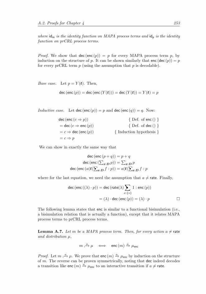
A.2. Proofs for Chapter 4 253

where idm is the identity function on MAPA process terms and idp is the identityfunction on prCRL process terms.

Proof. We show that dec (enc (p)) = p for every MAPA process term p, byinduction on the structure of p. It can be shown similarly that enc (dec (p)) = pfor every prCRL term p (using the assumption that p is decodable).

Base case. Let p = Y (t). Then,

dec (enc (p)) = dec (enc (Y (t))) = dec (Y (t)) = Y (t) = p

Inductive case. Let dec (enc (p)) = p and dec (enc (q)) = q. Now:

dec (enc (c⇒ p)) Def. of enc () = dec (c⇒ enc (p)) Def. of dec () = c⇒ dec (enc (p)) Induction hypothesis = c⇒ p

We can show in exactly the same way that

dec (enc (p+ q)) = p+ q

dec (enc (∑

x:D p)) =∑

x:D p

dec (enc (a(t)∑•

x:D f : p)) = a(t)∑•

x:D f : p

where for the last equation, we need the assumption that a 6= rate. Finally,

dec (enc ((λ) · p)) = dec (rate(λ)∑•

x:∗

1 : enc (p))

= (λ) · dec (enc (p)) = (λ) · p

The following lemma states that enc is similar to a functional bisimulation (i.e.,a bisimulation relation that is actually a function), except that it relates MAPAprocess terms to prCRL process terms.

Lemma A.7. Let m be a MAPA process term. Then, for every action a 6= rateand distribution µ,

m a−→ µ ⇐⇒ enc (m) −a→ µenc

Proof. Let m a−→ µ. We prove that enc (m) −a→ µenc by induction on the structureof m. The reverse can be proven symmetrically, noting that dec indeed decodesa transition like enc (m) −a→ µenc to an interactive transition if a 6= rate.

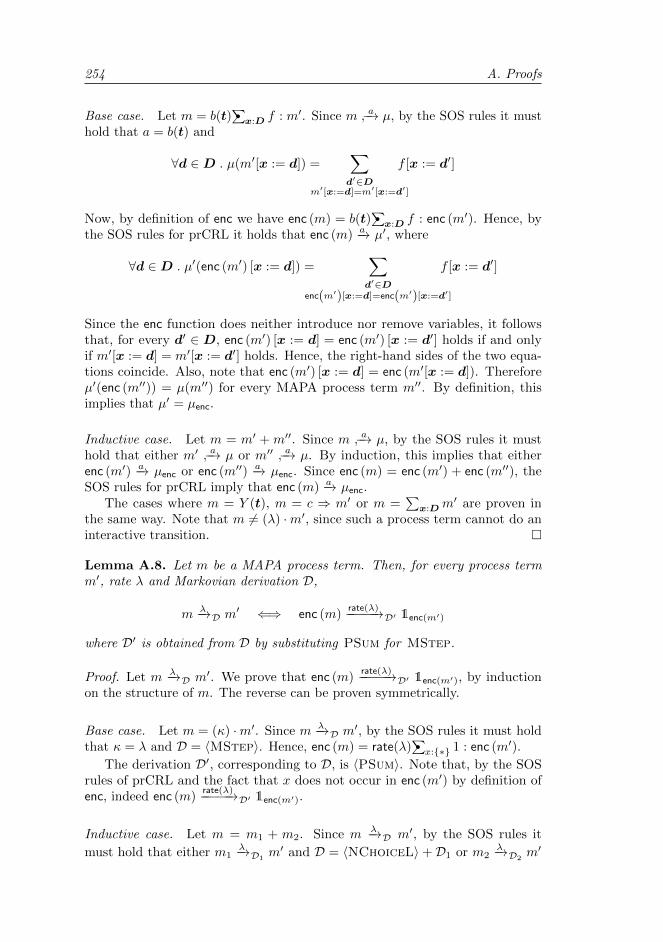
254 A. Proofs

Base case. Let m = b(t)∑•

x:D f : m′. Since m a−→ µ, by the SOS rules it musthold that a = b(t) and

∀d ∈D . µ(m′[x := d]) =∑d′∈D

m′[x:=d]=m′[x:=d′]

f [x := d′]

Now, by definition of enc we have enc (m) = b(t)∑•

x:D f : enc (m′). Hence, bythe SOS rules for prCRL it holds that enc (m) −a→ µ′, where

∀d ∈D . µ′(enc (m′) [x := d]) =∑d′∈D

enc(m′)[x:=d]=enc(m′)[x:=d′]

f [x := d′]

Since the enc function does neither introduce nor remove variables, it followsthat, for every d′ ∈ D, enc (m′) [x := d] = enc (m′) [x := d′] holds if and onlyif m′[x := d] = m′[x := d′] holds. Hence, the right-hand sides of the two equa-tions coincide. Also, note that enc (m′) [x := d] = enc (m′[x := d]). Thereforeµ′(enc (m′′)) = µ(m′′) for every MAPA process term m′′. By definition, thisimplies that µ′ = µenc.

Inductive case. Let m = m′ + m′′. Since m a−→ µ, by the SOS rules it musthold that either m′ a−→ µ or m′′ a−→ µ. By induction, this implies that eitherenc (m′) −a→ µenc or enc (m′′) −a→ µenc. Since enc (m) = enc (m′) + enc (m′′), theSOS rules for prCRL imply that enc (m) −a→ µenc.

The cases where m = Y (t), m = c ⇒ m′ or m =∑

x:Dm′ are proven inthe same way. Note that m 6= (λ) ·m′, since such a process term cannot do aninteractive transition.

Lemma A.8. Let m be a MAPA process term. Then, for every process termm′, rate λ and Markovian derivation D,

m −λ→D m′ ⇐⇒ enc (m) −rate(λ)−−−−→D′ 1enc(m′)

where D′ is obtained from D by substituting PSum for MStep.

Proof. Let m −λ→D m′. We prove that enc (m) −rate(λ)−−−−→D′ 1enc(m′), by inductionon the structure of m. The reverse can be proven symmetrically.

Base case. Let m = (κ) ·m′. Since m −λ→D m′, by the SOS rules it must holdthat κ = λ and D = 〈MStep〉. Hence, enc (m) = rate(λ)

∑•x:∗ 1 : enc (m′).

The derivation D′, corresponding to D, is 〈PSum〉. Note that, by the SOSrules of prCRL and the fact that x does not occur in enc (m′) by definition ofenc, indeed enc (m) −rate(λ)−−−−→D′ 1enc(m′).

Inductive case. Let m = m1 + m2. Since m −λ→D m′, by the SOS rules it

must hold that either m1 −λ→D1m′ and D = 〈NChoiceL〉+D1 or m2 −λ→D2

m′

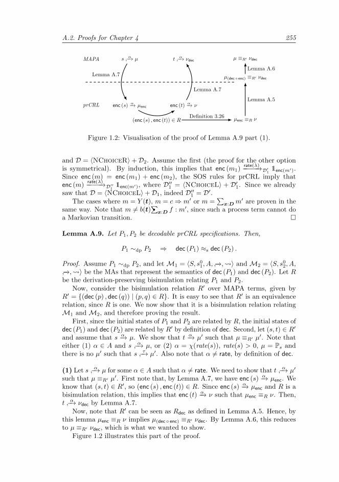
A.2. Proofs for Chapter 4 255

s α−→ µ

enc (s) −α→ µenc enc (t) −α→ ν

t α−→ νdecMAPA

prCRL

µ ≡R′ νdec

µenc ≡R ν

µ(dec enc) ≡R′ νdecLemma A.7

(enc (s) , enc (t)) ∈ R

Lemma A.7

Definition 3.26

Lemma A.5

Lemma A.6

Figure 1.2: Visualisation of the proof of Lemma A.9 part (1).

and D = 〈NChoiceR〉+D2. Assume the first (the proof for the other optionis symmetrical). By induction, this implies that enc (m1) −rate(λ)−−−−→D′1 1enc(m′).Since enc (m) = enc (m1) + enc (m2), the SOS rules for prCRL imply thatenc (m) −rate(λ)−−−−→D′′1 1enc(m′), where D′′1 = 〈NChoiceL〉 + D′1. Since we alreadysaw that D = 〈NChoiceL〉+D1, indeed D′′1 = D′.

The cases where m = Y (t), m = c⇒ m′ or m =∑

x:Dm′ are proven in thesame way. Note that m 6= b(t)

∑•

x:D f : m′, since such a process term cannot doa Markovian transition.

Lemma A.9. Let P1, P2 be decodable prCRL specifications. Then,

P1 ∼dp P2 ⇒ dec (P1) ≈s dec (P2) .

Proof. Assume P1 ∼dp P2, and let M1 = 〈S, s01, A, −→, 〉 and M2 = 〈S, s0

2, A,−→, 〉 be the MAs that represent the semantics of dec (P1) and dec (P2). Let Rbe the derivation-preserving bisimulation relating P1 and P2.

Now, consider the bisimulation relation R′ over MAPA terms, given byR′ = (dec (p) , dec (q)) | (p, q) ∈ R. It is easy to see that R′ is an equivalencerelation, since R is one. We now show that it is a bisimulation relation relatingM1 and M2, and therefore proving the result.

First, since the initial states of P1 and P2 are related by R, the initial states ofdec (P1) and dec (P2) are related by R′ by definition of dec. Second, let (s, t) ∈ R′and assume that s −α→ µ. We show that t −α→ µ′ such that µ ≡R′ µ′. Note thateither (1) α ∈ A and s α−→ µ, or (2) α = χ(rate(s)), rate(s) > 0, µ = Ps andthere is no µ′ such that s τ−→ µ′. Also note that α 6= rate, by definition of dec.

(1) Let s α−→ µ for some α ∈ A such that α 6= rate. We need to show that t α−→ µ′

such that µ ≡R′ µ′. First note that, by Lemma A.7, we have enc (s) −α→ µenc. Weknow that (s, t) ∈ R′, so (enc (s) , enc (t)) ∈ R. Since enc (s) −α→ µenc and R is abisimulation relation, this implies that enc (t) −α→ ν such that µenc ≡R ν. Then,t α−→ νdec by Lemma A.7.

Now, note that R′ can be seen as Rdec as defined in Lemma A.5. Hence, bythis lemma µenc ≡R ν implies µ(dec enc) ≡R′ νdec. By Lemma A.6, this reducesto µ ≡R′ νdec, which is what we wanted to show.

Figure 1.2 illustrates this part of the proof.

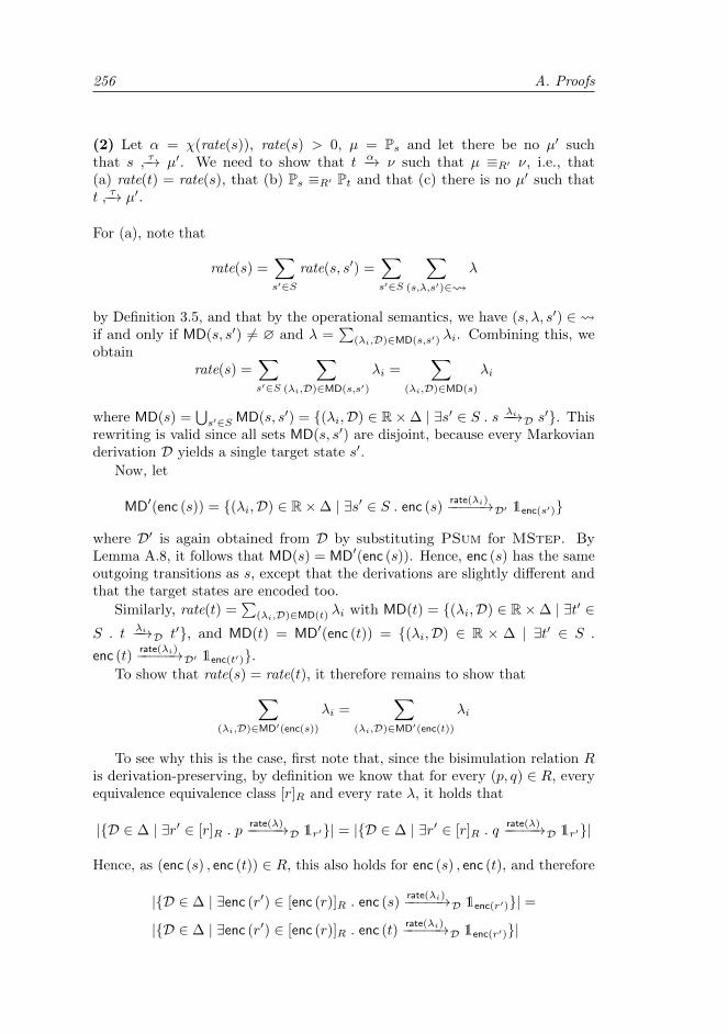
256 A. Proofs

(2) Let α = χ(rate(s)), rate(s) > 0, µ = Ps and let there be no µ′ suchthat s τ−→ µ′. We need to show that t −α→ ν such that µ ≡R′ ν, i.e., that(a) rate(t) = rate(s), that (b) Ps ≡R′ Pt and that (c) there is no µ′ such thatt τ−→ µ′.

For (a), note that

rate(s) =∑s′∈S

rate(s, s′) =∑s′∈S

∑(s,λ,s′)∈

λ

by Definition 3.5, and that by the operational semantics, we have (s, λ, s′) ∈ if and only if MD(s, s′) 6= ∅ and λ =

∑(λi,D)∈MD(s,s′) λi. Combining this, we

obtainrate(s) =

∑s′∈S

∑(λi,D)∈MD(s,s′)

λi =∑

(λi,D)∈MD(s)

λi

where MD(s) =⋃s′∈SMD(s, s′) = (λi,D) ∈ R×∆ | ∃s′ ∈ S . s −λi−→D s′. This

rewriting is valid since all sets MD(s, s′) are disjoint, because every Markovianderivation D yields a single target state s′.

Now, let

MD′(enc (s)) = (λi,D) ∈ R×∆ | ∃s′ ∈ S . enc (s) −rate(λi)−−−−→D′ 1enc(s′)

where D′ is again obtained from D by substituting PSum for MStep. ByLemma A.8, it follows that MD(s) = MD′(enc (s)). Hence, enc (s) has the sameoutgoing transitions as s, except that the derivations are slightly different andthat the target states are encoded too.

Similarly, rate(t) =∑

(λi,D)∈MD(t) λi with MD(t) = (λi,D) ∈ R×∆ | ∃t′ ∈S . t −λi−→D t′, and MD(t) = MD′(enc (t)) = (λi,D) ∈ R × ∆ | ∃t′ ∈ S .

enc (t) −rate(λi)−−−−→D′ 1enc(t′).To show that rate(s) = rate(t), it therefore remains to show that∑

(λi,D)∈MD′(enc(s))

λi =∑

(λi,D)∈MD′(enc(t))

λi

To see why this is the case, first note that, since the bisimulation relation Ris derivation-preserving, by definition we know that for every (p, q) ∈ R, everyequivalence equivalence class [r]R and every rate λ, it holds that

|D ∈ ∆ | ∃r′ ∈ [r]R . p −rate(λ)−−−−→D 1r′| = |D ∈ ∆ | ∃r′ ∈ [r]R . q −rate(λ)−−−−→D 1r′|

Hence, as (enc (s) , enc (t)) ∈ R, this also holds for enc (s) , enc (t), and therefore

|D ∈ ∆ | ∃enc (r′) ∈ [enc (r)]R . enc (s) −rate(λi)−−−−→D 1enc(r′)| =

|D ∈ ∆ | ∃enc (r′) ∈ [enc (r)]R . enc (t) −rate(λi)−−−−→D 1enc(r′)|

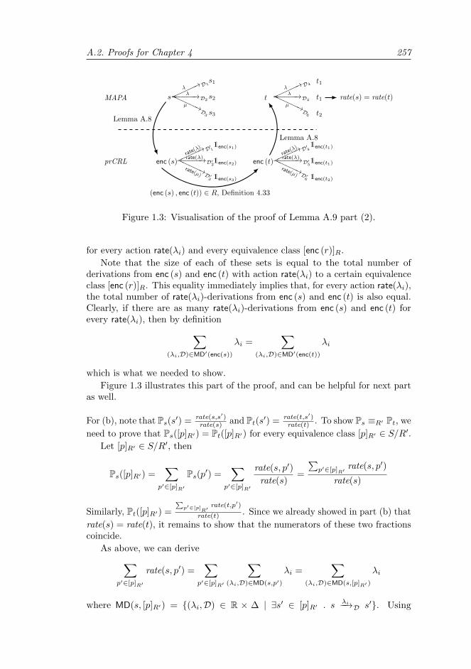
A.2. Proofs for Chapter 4 257

s s2

s1

s3

− λ−−−−−→D2−λ

−−−−−−→D1

−µ

−−−−−−→D

3

enc (s) 1enc(s2)

1enc(s1)

1enc(s3)

− rate(λ)−−−−−→D′2−rate

(λ)

−−−−−→D

′1

−rate(µ)

−−−−−→D ′3

enc (t) 1enc(t1)

1enc(t1)

1enc(t2)

− rate(λ)−−−−−→D′5−rate

(λ)

−−−−−→D

′4

−rate(µ)

−−−−−→D ′6

t t1

t1

t2

− λ−−−−−→D4−λ

−−−−−−→D4

−µ

−−−−−−→D

6

MAPA

prCRL

rate(s) = rate(t)

Lemma A.8

(enc (s) , enc (t)) ∈ R, Definition 4.33

Lemma A.8

Figure 1.3: Visualisation of the proof of Lemma A.9 part (2).

for every action rate(λi) and every equivalence class [enc (r)]R.

Note that the size of each of these sets is equal to the total number ofderivations from enc (s) and enc (t) with action rate(λi) to a certain equivalenceclass [enc (r)]R. This equality immediately implies that, for every action rate(λi),the total number of rate(λi)-derivations from enc (s) and enc (t) is also equal.Clearly, if there are as many rate(λi)-derivations from enc (s) and enc (t) forevery rate(λi), then by definition∑

(λi,D)∈MD′(enc(s))

λi =∑

(λi,D)∈MD′(enc(t))

λi

which is what we needed to show.

Figure 1.3 illustrates this part of the proof, and can be helpful for next partas well.

For (b), note that Ps(s′) = rate(s,s′)rate(s) and Pt(s′) = rate(t,s′)

rate(t) . To show Ps ≡R′ Pt, we

need to prove that Ps([p]R′) = Pt([p]R′) for every equivalence class [p]R′ ∈ S/R′.Let [p]R′ ∈ S/R′, then

Ps([p]R′) =∑

p′∈[p]R′

Ps(p′) =∑

p′∈[p]R′

rate(s, p′)

rate(s)=

∑p′∈[p]R′

rate(s, p′)

rate(s)

Similarly, Pt([p]R′) =

∑p′∈[p]

R′rate(t,p′)

rate(t) . Since we already showed in part (b) that

rate(s) = rate(t), it remains to show that the numerators of these two fractionscoincide.

As above, we can derive∑p′∈[p]R′

rate(s, p′) =∑

p′∈[p]R′

∑(λi,D)∈MD(s,p′)

λi =∑

(λi,D)∈MD(s,[p]R′ )

λi

where MD(s, [p]R′) = (λi,D) ∈ R × ∆ | ∃s′ ∈ [p]R′ . s −λi−→D s′. Using

258 A. Proofs

Lemma A.8 we find that MD(s, [p]R′) = MD′(enc (s) , [enc (p)]R), where

MD′(enc (s) , [enc (p)]R)

= (λi,D) ∈ R×∆ | ∃enc (p′) ∈ [enc (p)]R . enc (s) −rate(λi)−−−−→D′ 1enc(p′)

Similar derivations can be made for t, so it remains to show that∑(λi,D)∈MD′(enc(s),[enc(p)]R)

λi =∑

(λi,D)∈MD′(enc(t),[enc(p)]R)

λi

Just as in part (b), by assumption we have

|D ∈ ∆ | ∃enc (p′) ∈ [enc (p)]R . enc (s) −rate(λi)−−−−→D 1enc(p′)| =

|D ∈ ∆ | ∃enc (p′) ∈ [enc (p)]R . enc (t) −rate(λi)−−−−→D 1enc(p′)|

for every action rate(λi).

Note again that the size of each of these sets is equal to the total number ofderivations from enc (s) and enc (t) with action rate(λi) to a certain equivalenceclass [enc (p)]R. Hence, the fact that these two sets are of equal size implies thatevery transition enc (s) −rate(λi)−−−−→D 1enc(s′) with enc (s′) ∈ [enc (p)]R correspondsone-to-one to a transition enc (t) −rate(λi)−−−−→D′ 1enc(t′) such that enc (t′) ∈ [enc (p)]R.

This immediately implies that, for every action rate(λi), the total number ofrate(λi)-derivations to [enc (p)]R from enc (s) and enc (t) is also equal. Therefore,by definition ∑

(λi,D)∈MD′(enc(s),[enc(p)]R)

λi =∑

(λi,D)∈MD′(enc(t),[enc(p)]R)

λi

which is what we needed to show.

For (c), note that (enc (s) , enc (t)) ∈ R since (s, t) ∈ R′. As there is no τ -transition from s, by Lemma A.7 there is also no τ -transition from enc (s).Since R is a bisimulation relation, also enc (t) does not have a τ -transition, andapplying Lemma A.7 again also t does not have a τ -transition.

Theorem 4.36. Let f : prCRL→ prCRL be a function such that f(P ) ∼dp Pfor every prCRL specification P , and such that if P is decodable, then so is f(P ).Then, dec (f(enc (M))) ≈s M for every MAPA specification M without anyactions labelled by rate.

Proof. Let M be an arbitrary MAPA specification without any rate action. Sincef(P ) ∼dp P for every prCRL specification P , also f(enc (M)) ∼dp enc (M). Ad-ditionally, since enc (M) is decodable by construction, by the assumption on f alsof(enc (M)) is. Lemma A.9 therefore yields dec (f(enc (M))) ≈s dec (enc (M)).Moreover, M = dec (enc (M)) by Lemma A.6, and thus also M ≈s dec (enc (M)).By transitivity of strong bisimulation, the result follows.

A.2. Proofs for Chapter 4 259

A.2.4 Proof of Theorem 4.45

Lemma A.10. Algorithm 1 terminates for every finite specification P .

Proof. The algorithm terminates when toTransform eventually becomes empty.Note that every iteration removes exactly one element from toTransform. So, ifthe total number of additions to toTransform is finite (and the call to Algorithm 2never goes into an infinite recursion), the algorithm will terminate.

The elements that are added to toTransform are of the form X ′i(pars) = pi,where pi ∈ subterms(P ) (recall that subterms were introduced in Definition 4.52).Since P has a finite set of equations with finite right-hand sides, there existsonly a finite number of such pi. Moreover, every process equation X ′i(pars) = pithat is added to toTransform is also added to bindings. This makes sure thatno process equation X ′k(pars) = pi is ever added to toTransform again, as canbe observed from line 3 of Algorithm 2. Hence, the total number of possibleadditions to toTransform is finite.

The fact that Algorithm 2 always terminates relies on not allowing specifica-tions with unguarded recursion. After all, the base case of Algorithm 2 is theaction prefix. Therefore, when every recursion in a specification is guarded atsome point by an action prefix, this base case is always reached eventually.

Lemma A.11. Let P = (E,X1(v)) be a decodable input prCRL specificationfor Algorithm 1 (having unique variable names), and let v′ be the computed newinitial vector. Then, before and after an arbitrary iteration of the algorithm’swhile loop,

(E ∪ done ∪ toTransform, X ′1(v′)) ∼dp P

and (E ∪ done ∪ toTransform, X ′1(v′)) is decodable.

Proof. The fact that (E ∪ done ∪ toTransform, X ′1(v′)) stays decodable isimmediate from the observation that the algorithm uses the process termsfrom P (which is assumed to be decodable) and never changes or introduces anynew probabilistic sums. Hence, from now on we only focus on the ∼dp part ofthe lemma.

For brevity, in this proof we write ‘bisimilar’ if we actually mean ‘derivation-preserving bisimilar for all valuations’ (since there may be unbound variables).Also, the notation p ∼dp q will be used for this.

We prove that (E ∪ done ∪ toTransform, X ′1(v′)) ∼dp P before and after anarbitrary iteration of the algorithm’s while loop, by induction on the number ofiterations that have already been performed. We let

E = X1(x : D) = p1, . . . , Xn(xn : Dn) = pn

and hence we have

P = (X1(x : D) = p1, . . . , Xn(xn : Dn) = pn, X1(v))

260 A. Proofs

Base case. Before the first iteration, the parameters of the new processes aredetermined. Every process will have the same parameters: x : D,x

′ : D′.This is the union of all process variables of the original processes, extended with aparameter for every nondeterministic or probabilistic sum binding a variable thatis used later on. Also, the new initial state vector v′ is computed by taking theoriginal initial vector v, and appending dummy values for all added parameters.Furthermore, done is set to ∅ and toTransform to X ′1(x : D,x

′ : D′) = p1.Clearly, X ′1(v′) is identical to X1(v), except that it has more global variables

(without overlap, as we assumed specifications to have unique variable names).However, these additional global variables are not used in p1, otherwise theywould be free in X1(x : D) = p1 (which is not allowed by Definition 4.16).Therefore, (E ∪ done ∪ toTransform, X ′1(v′)) and P are obviously bisimilar (bythe smallest equivalence relation that relates X1(v) to X ′1(v′) and contains theidentity relation).

Since the additional unused variables do not affect the possible derivationsin any way, this bisimulation is derivation preserving.

Inductive case. Now assume that k ≥ 0 iterations have passed. Without loss ofgenerality, assume that each time a process (X ′i(pars) = pi) ∈ toTransform hadto be chosen, it was the one with the smallest i. Then, after these k iterations,

done = X ′1(x : D,x′ : D′) = p′1, . . . , X

′k(x : D,x

′ : D′) = p′k

Also,

toTransform = X ′k+1(x : D,x′ : D′) = p′k+1, . . . , X

′l(x : D,x

′ : D′) = p′l

for some l ≥ k. We have (E ∪ done ∪ toTransform, X ′1(v′)) ∼dp P by theinduction hypothesis.

We prove that after k + 1 iterations, (E ∪ done ∪ toTransform, X ′1(v′)) isstill derivation-preserving bisimilar to P . During iteration k + 1 three thingshappen:

1. The process equation X ′k+1(x : D,x′ : D′) = p′k+1 is removed from

toTransform;

2. An equation X ′k+1(x : D,x′ : D′) = p′′k+1 is added to done;

3. potentially, one or more equations of the form

X ′l+1(x : D,x′ : D′) = p′l+1, . . . , X

′m(x : D,x

′ : D′) = p′m

are added to toTransform.

As the other equations in E ∪ done ∪ toTransform do not change, The-orem 4.35 implies that (E ∪ done ∪ toTransform, X ′1(v′)) ∼dp P still holds ifp′k+1 ∼dp p′′k+1. We show this by induction on the number of recursive callsto Algorithm 2 (which depends on the structure of p′k+1). Since unguardedrecursion is not allowed by our well-formedness criteria, indeed every processterm needs only a finite number of recursive calls.

A.2. Proofs for Chapter 4 261

The base case is when Algorithm 2 terminates without any recursive calls;this is when p′k+1 = a(t)

∑•

x:D f : q. We now make a case distinction based onwhether there already is a process equation in either done or toTransform whoseright-hand side is an IRF corresponding to the normal form of q (which is just qwhen q is not a process instantiation, otherwise it is the right-hand side of theprocess it instantiates), as indicated by the variable bindings.

Case 1a. There does not already exist a process equation X ′j(pars) = q′ inbindings such that q′ is the normal form of q.

A new process equation X ′l+1(pars) = q′ is added to toTransform via line 6of Algorithm 2, and p′′k+1 = a(t)

∑•

x:D f : X ′l+1(actualPars).When q was not a process instantiation, the actual parameters for X ′l+1

are just the unchanged global variables, with those that are not used inq reset (line 4 of Algorithm 3). Since (by definition of the normal form)the right-hand side of X ′l+1 is identical to q and actualPars takes carethat all data parameters keep the same value, clearly X ′l+1(actualPars) isderivation-preserving bisimilar to q: every derivation D of q corresponds tothe derivation Inst +D of X ′l+1(actualPars). Therefore, by Theorem 4.35indeed also p′′k+1 ∼dp p

′k+1.

When q = Y (t1, t2, . . . , tn), there should occur some substitutions toascertain that X ′l+1(actualPars) is bisimilar to q. Since we know thatX ′l+1(actualPars) = q′, with q′ the right-hand side of Y , the actual para-meters to be provided to X ′l+1 should include t1, t2, . . . , tn for the globalvariables of X ′l+1 that correspond to the original global variables of Y .All other global variables can be reset, as they cannot be used by Yanyway. This indeed happens in line 2 of Algorithm 3, so all behavioursof q are present in X ′l+1(actualPars) are vice versa, and all derivationsof q map one-to-one to the derivations of X ′l+1(actualPars). So, we findthat q ∼dp X

′l+1(actualPars), and therefore, by Theorem 4.35, indeed also

p′′k+1 ∼dp p′k+1.

Case 1b. There exists a process equation X ′j(pars) = q′ in bindings such thatq′ is the normal form of q.

We obtainp′′k+1 = a(t)

∑•x:D

f : X ′j(actualPars)

from line 4 of Algorithm 2. By Theorem 4.35, we only need to show that qis derivation-preserving bisimilar to X ′j(actualPars).

Note that the fact that X ′j(pars) = q′ is in bindings implies that atsome point X ′j(pars) = q′ was in toTransform. In case it was alreadytransformed in an earlier iteration there is now a process X ′j(pars) = q′′

in done such that q′′ ∼dp q′ (by induction). Otherwise, X ′j(pars) = q′

is still in toTransform. In both cases, done ∪ toTransform ∪ P containsa process X ′j(pars) = q′′ such that q′′ ∼dp q

′, and therefore it is correctto take p′′k+1 = a(t)

∑•

x:D f : X ′j(actualPars). The reasoning to see that

262 A. Proofs

indeed p′′k+1 ∼dp p′k+1 then only depends on the choice of actualPars, and

is the same as for Case 1a.

Now, we assume that Algorithm 2 functions correctly (i.e., provides aderivation-preserving bisimilar result) for all process terms that require k or lessrecursive calls. Let q1 and q2 be two such process terms, for which Algorithm 2provided the bisimilar process terms p′′′k+1 and p′′′′k+1 in k steps. Also, assumethat p′k+1 yields k + 1 recursive calls. We prove that p′′k+1 (as obtained fromAlgorithm 2) is bisimilar to p′k+1 by means of a case distinction over the possiblestructures of p′k+1. (Note that p′k+1 cannot be an action prefix, since that wouldnot require any recursive calls.)

Case 2. p′k+1 = c⇒ q1.

Algorithm 2 yields p′′k+1 = c⇒ p′′′k+1, which according to Theorem 4.35 isbisimilar to p′k+1, since q1 ∼dp p

′′′k+1.

Case 3. p′k+1 = q1 + q2.

Algorithm 2 yields p′′k+1 = p′′′k+1 + p′′′′k+1, which according to Theorem 4.35is bisimilar to p′k+1, since q1 ∼dp p

′′′k+1 and q2 ∼dp p

′′′′k+1.

Case 4. p′k+1 = Y (t), where we assume that Y (x : D) = q1.

Algorithm 2 yields p′′k+1 = p′′′k+1, with x substituted by t, which is bisimilarto p′k+1 (as it precisely follows the SOS rule Inst). To see that thebisimulation preserves derivations, note that every derivation D of p′′′k+1

corresponds one-to-one to a derivation Inst +D of p′k+1.

Case 5. p′k+1 =∑x:D q1.

In this case, Algorithm 2 yields p′′k+1 =∑x:D p

′′′k+1, which according to

Theorem 4.35 is bisimilar to p′k+1, since q1 ∼dp p′′′k+1.

Since in all cases the process term p′′k+1 obtained from Algorithm 2 is derivation-preserving bisimilar to p′k+1 for all valuations, the lemma holds.

Theorem 4.45. Let P be a decodable prCRL specification such that all variablesare named uniquely. Given this input, Algorithm 1 terminates and provides aspecification P ′ such that P ′ ∼dp P , P ′ is in IRF and P ′ is decodable.

Proof. Let P = (E,X1(v)) be an arbitrary input prCRL specification for Al-gorithm 1 (having unique variable names), and let v′ be the computed newinitial vector. Lemma A.10 already provided termination, and Lemma A.11provided the invariant that (E ∪ done ∪ toTransform, X ′1(v′)) ∼dp P and that(E ∪ done ∪ toTransform, X ′1(v′)) is decodable. As at the end of the algorithmonly the equations in done are returned, it remains to prove that upon ter-mination X ′1(v′) in done does not depend on any of the process equations inE ∪ toTransform, and that done is in IRF.

A.2. Proofs for Chapter 4 263

First of all, note that upon termination toTransform = ∅ by the condition ofthe while loop. Moreover, note that the processes that are added to done all havea right-hand side determined by Algorithm 2, which only produces process termsthat refer to processes in done or toTransform (in line 4 and line 6). Therefore,X ′1(v′) in done indeed can only depend on process equations in done.

Finally, to show that done is indeed in IRF, we need to prove that allprobabilistic sums immediately go to a process instantiation, and that processinstantiations do not occur in any other way. This is immediately clear fromAlgorithm 2, as process instantiations are only constructed in line 4 and line 6;there, they indeed are always preceded by a probabilistic sum. Moreover,probabilistic sums are also only constructed by these lines, and are, as required,always succeeded by a process instantiation. Finally, all processes clearly have thesame list of global variables (because they are created on line 10 on Algorithm 1using pars, and pars never changes).

A.2.5 Proof of Theorem 4.48

Theorem 4.48. Let P ′ be a decodable specification in IRF without a variablepc, and let the output of Algorithm 4 applied to P ′ be the specification X. Then,P ′ ∼dp X and X is decodable.

Let Y be like X, except that for each summand all nondeterministic sums havebeen moved to the beginning while substituting their variables by fresh names,and all separate nondeterministic sums and separate conditions have been merged(using vectors and conjunctions, respectively). Then, Y is an LPPE, Y ∼dp Xand Y is decodable.

Proof. The fact that X and Y stay decodable is immediate from the observationthat the algorithm uses the process terms from P ′ (which is assumed to bedecodable) and never changes or introduces any new probabilistic sums. Hence,from now on we only focus on the ∼dp part of the theorem.

Algorithm 4 transforms a specification

P ′ = (X ′1(x : D) = p′1, . . . , X′k(x : D) = p′k, X ′1(v))

to an LPPEX = (X(pc : 1, . . . , k,x : D), X(1,v))

by constructing one or more summands for X for every process in P ′. Basically,the algorithm just introduces a program counter pc to keep track of the processthat is currently active. That is, instead of starting in X ′1(v), the system willstart in X(1,v). Moreover, instead of advancing to X ′j(v), the system willadvance to X(j,v).

The bisimulation relation R to prove the theorem is the smallest equivalencerelation containing

R = (X ′i(u), X(i,u)) | 1 ≤ i ≤ k,u ∈D

By definition the initial states are related: (X ′1(v), X(1,v)) ∈ R. We addi-

264 A. Proofs

tionally need to prove that

X ′i(u) −α→ µ =⇒ ∃µ′ . X(i,u) −α→ µ′ ∧ µ ≡R µ′

and vice versa, for all 1 ≤ i ≤ k and u ∈D, and that these pairs (X ′i(u), X(i,u))have the same number of rate(λ)-transitions to each equivalence class. We doso by assuming an arbitrary X ′l(u), and showing that each derivation (andhence each transition) of X ′l(u) maps one-to-one to a derivation of X(l,u), byinduction over the structure of X ′l(x : D).

The base case is X ′l(x : D) = a(t)∑•

y:E f : X ′j(t′1, . . . , t

′k). For this process,

Algorithm 4 constructs the summand pc = l⇒ a(t)∑•

y:E f : X(j, t′1, . . . , t′k). As

every summand constructed by the algorithm contains a condition pc = i, andthe summands produced for X ′l(x : D) are the only ones producing a summandwith i = l (all others require pc to have a different value), it follows that X ′l(u)and X(l,u) have precisely the same derivations, except that each target stateX ′j(u

′) of X ′l(u) is mimicked by X(l,u) using a target state X(j,u′). Sincethese are all R-related, indeed X ′l(u) and X(l,u) have the same derivations (andhence transitions) modulo R.

Now assume that X ′l(x : D) = c⇒ q. By induction, X ′′l (x : D) = q wouldresult in the construction of one or more summands such that X ′′l (u) and X(l,u)have the same derivations. For X ′l(x : D) the algorithm takes those summands,and adds the condition c to all of them. Therefore, X ′l(u) and X(l,u) also havethe same derivations (and hence transitions). Similar arguments can be used forX ′l(x : D) = q1 + q2 or X ′l(x : D) =

∑x:D q. Hence, P ′ ∼dp X.

Now, let Y be equal to X, except that within each summand all nondetermin-istic sums have been moved to the beginning while substituting their variablesby fresh names, and all separate nondeterministic sums and separate conditionshave been merged (using vectors and conjunctions, respectively).

To see that Y is an LPPE, first observe that X already was a single processequation consisting of a set of summands. Each of these contains a number ofnondeterministic sums and conditions, followed by a probabilistic sum. Further-more, each probabilistic sum is indeed followed by a process instantiation, ascan be seen from line 6 of Algorithm 4.

The only discrepancy for X to be an LPPE is that the nondeterministic sumsand the conditions are not yet necessarily in the right order, and there may beseveral of them. For instance, we may have something like

d > 0⇒∑d:D1

e > 0⇒∑f :D2

act(d).X(d, f)

However, since the nondeterministic sums and conditions are swapped in Y suchthat all nondeterministic sums precede all conditions, and since conditions aremerged using conjunctions, and summations using vectors, Y is an LPPE. Incase of the example before, we obtain∑

(d′,f):D1×D2

d > 0 ∧ e > 0⇒ act(d′).X(d′, f)

A.2. Proofs for Chapter 4 265

Note that, indeed, some renaming had to be done such that Y ∼dp X. After all,by renaming the summation variables, we can rely on the obvious equality of theprocess terms c⇒∑

d:D p and∑d:D c⇒ p, given that d is not a free variable in

c. Thus, swapping the conditions and nondeterministic sums this way does notmodify the process’ semantics in any way. Also, it is easy to see from the SOSrules in Table 4.5 that merging nondeterministic sums and conditions does notinfluence the transitions or the number of rate(λ)-derivations of the process inany way. Therefore, indeed Y ∼dp X.

A.2.6 Proof of Proposition 4.51

Proposition 4.51. Let P be a prCRL specification such that size(P ) = n.Then, the worst-case time complexity of linearising P is O(n3). The worst-casesize of the resulting LPPE is in O(n2).

Proof. Let P = (E, I) be a specification such that size(P ) = n. First of all, notethat ∣∣pars

∣∣ ≤ ∑(Xi(xi:Di)=pi)∈E

|xi|+∣∣subterms′(P )

∣∣ ≤ n (A.6)

after the initialisation of Algorithm 1, where |pars| denotes the numbers of newglobal variables and subterms′(P ) denotes the multiset containing all subtermsof P (counting a process term that occurs twice as two subterms, and includingnondeterministic and probabilistic choices over a vector of k variables k times).When mentioning the subterms of P in this proof, we will be referring to thismultiset (for a formal definition of subterms, see Definition 4.52 on page 95).

The first inequality follows from the fact that pars is defined to be thesequence of all xi appended by all local variables of P (that are syntacticallyused), and the observation that there are at most as many local variables asthere are subterms. The second inequality follows from the definition of size andthe observation that size(pi) counts the number of subterms of p plus the size oftheir expressions.

Time complexity. We first determine the worst-case time complexity of Al-gorithm 1. As the function transform is called at most once for every subtermof P , it follows from Equation (A.6) that the number of times this happensis in O(n). The time complexity of every such call is governed by the call tonormalForm.

The function normalForm checks for each global variable in pars whetheror not it can be reset; from Equation (A.6) we know that the number of suchvariables is in O(n). To check whether a global variable can be reset givena process term p, we have to examine every expression in p; as the size ofthe expressions is accounted for by n, this is also in O(n). So, the worst-casetime complexity of normalForm is in O(n2). Therefore, the worst-case timecomplexity of Algorithm 1 is in O(n3).

As the transformation from IRF to LPPE by Algorithm 4 is easily seen tobe in O(n), we find that, in total, linearisation has a worst-case time complexityin O(n3).

266 A. Proofs

LPPE size complexity. Every summand of the LPPE X that is constructed hasa size in O(n). After all, each contains a process instantiation with an expressionfor every global variable in pars, and we already saw that the number of themis in O(n). Furthermore, the number of summands is bound from above bythe number of subterms of P , so this is in O(n). Therefore, the size of X is inO(n2).

A.2.7 Proof of Proposition 4.56

Proposition 4.56. For all v ∈ G,v′ ∈ G′, it holds that

Z(v,v′) ≈iso X(v) ||Y (v′)

Proof. The only processes an MLPE Z(v,v′) can become, are of the formZ(v, v′), and the only processes a parallel composition X(v) ||Y (v′) can become,are of the form X(v) ||Y (v′). Therefore, the isomorphism h needed to prove theproposition is as follows:

h(X(v) ||Y (v′)) = Z(v,v′) and h(Z(v,v′)) = X(v) ||Y (v′)

for all v ∈ G,v′ ∈ G′, and h(p) = p for every process term p of a different form.Clearly, h is bijective. We will now show that indeed X(v) ||Y (v′) −α→ µ if andonly if Z(v,v′) −α→ µh. We do so by showing that

X(v) ||Y (v′) a(q)−−−→ µ if and only if Z(v,v′) a(q)−−−→ µh

and

X(v) ||Y (v′) λ X(v′) ||Y (v′) if and only if Z(v,v′) λ µ(X(v′) ||Y (v′))

Let v ∈ G and v′ ∈ G′ be arbitrary global variables vectors for X and Y . Then,by the operational semantics of parallel MAPA, X(v) ||Y (v′) a(q)−−−→ µ is enabledif and only if at least one of the following three conditions holds.

(1) X(v) a(q)−−−→ µ′ ∧ ∀v ∈ G . µ(X(v) ||Y (v′)) = µ′(v)

(2) Y (v′) a(q)−−−→ µ′ ∧ ∀v′ ∈ G′ . µ(X(v) ||Y (v′)) = µ′(v′)

(3) X(v) a′(q)−−−→ µ′ ∧ Y (v′) a′′(q)−−−−→ µ′′ ∧ γ(a′, a′′) = a ∧∀v ∈ G, v′ ∈ G′ . µ(X(v) ||Y (v′)) = µ′(v) · µ′′(v′)

It immediately follows from the construction of Z that Z(v,v′) a(q)−−−→ µh isenabled under exactly the same conditions, as condition (1) is covered by thefirst set of summands of Z, condition (2) is covered by the second set of summandsof Z, and condition (3) is covered by the third set of summands of Z.

We now show that X(v) ||Y (v′) λ X(v) ||Y (v′) if and only if Z(v,v′) λ h(X(v) ||Y (v′)), by making a case distinction between (1) v = v and v′ = v′,(2) v 6= v and v′ = v′, (3) v = v and v′ 6= v′, and (4) v 6= v and v′ 6= v′.

(1) If v = v and v′ = v′, then by the operational semantics a transitionX(v) ||Y (v′) λ X(v) ||Y (v′) is enabled if λ is the sum of all rates λi

A.2. Proofs for Chapter 4 267

such that there is a derivation X(v) −λi−→D X(v) or Y (v′) −λi−→D Y (v′). Byconstruction of Z, it follows immediately that Z(v,v′) has precisely thesame number of derivations with the same rates to go to Z(v,v′), via itsfourth and fifth set of summands. Hence, Z(v,v′) λ Z(v,v′) is enabledunder exactly the same conditions as X(v) ||Y (v′) λ X(v) ||Y (v′). SinceZ(v,v′) = h(X(v) ||Y (v′)) = h(X(v) ||Y (v′)), this completes the proof.

(2) If v 6= v and v′ = v′, then by the operational semantics a transitionX(v) ||Y (v′) λ X(v) ||Y (v′) is enabled if λ is the sum of all rates λi suchthat there is a derivation X(v) −λi−→D X(v). By construction of Z, it followsimmediately that Z(v,v′) has precisely the same number of derivationswith the same rates to go to Z(v,v′), via its fourth set of summands.Hence, Z(v,v′) λ Z(v,v′) is enabled under exactly the same conditionsas X(v) ||Y (v′) λ X(v) ||Y (v′). Since Z(v,v′) = h(X(v) ||Y (v′)) =h(X(v) ||Y (v′)), this completes the proof.

(3) Symmetric to the previous case.(4) It immediately follows from the operational semantics and the construction

of Z that neither X(v) ||Y (v′) nor Z(v,v′) has any Markovian transitionsthat change both v and v′. So, if v 6= v and v′ 6= v′, then triviallyX(v) ||Y (v′) λ X(v) ||Y (v′) if and only if Z(v,v′) λ h(X(v) ||Y (v′)).

A.2.8 Proof of Proposition 4.59

Proposition 4.59. For all v ∈ G, U(v) ≈iso τH(X(v)), V (v) ≈iso ρR(X(v)),and W (v) ≈iso ∂E(X(v)).

Proof. We will prove that U(v) ≈iso τH(X(v)) for all v ∈ G; the other twostatements are proven similarly.

The only processes an MLPE X(v) can become are of the form X(v′).Moreover, as hiding does not change the process structure, the only processesthat τH(X(v)) can become, are processes of the form τH(X(v′)). Therefore, theisomorphism h needed to prove the proposition is easy: for all v ∈ G, we defineh(τH(X(v))) = U(v) and h(U(v)) = τH(X(v)), and h(p) = p for every p of adifferent form. Clearly, h is bijective.

We now show that h indeed is an isomorphism. To do so, we first show that(1) τH(X(v)) a(q)−−−→ µ if and only if h(τH(X(v))) a(q)−−−→ µh, i.e., if and only ifU(v) a(q)−−−→ µh. Second, we show that (2) τH(X(v)) λ τH(X(v′)) if and only ifU(v) λ U(v′).

(1) First, recall that X(v) a(q)−−−→ µ is enabled if and only if there is a summandi ∈ I and a local variables vector d′i ∈Di such that

ci(v,d′i) ∧ ai(bi(v,d′i)) = a(q) ∧ µ = target i(v,di)

where target i(v,d′i) is the distribution µ′ such that

∀e′i ∈ Ei . µ′(ni(v,d

′i, e′i)) =

∑e′′i ∈Ei

ni(v,d′i,e′i)=ni(v,d′i,e

′′i )

fi(v,d′i, e′′i )

268 A. Proofs

We now make a case distinction between (a) a 6= τ or q 6= ( ), and (b) a = τand q = ( ).

(a) If a 6= τ or q 6= ( ), then the operational semantics imply thatτH(X(v)) a(q)−−−→ µ is enabled if and only if X(v) a(q)−−−→ µ ∧ a 6∈ H.Moreover, U(v) a(q)−−−→ µh is enabled if and only if there is a summandi ∈ I and a local variables vector d′i ∈Di such that

ci(v,d′i) ∧ a′i(b′i(v,d′i)) = a(q) ∧ µ = target i(v,di)

which indeed corresponds to X(v) a(q)−−−→ µ ∧ a 6∈ H by definition ofa′i and b′i and the assumption that a 6= τ or q 6= ( ).

(b) If a = τ and q = ( ), then the operational semantics imply thatτH(X(v)) τ−→ µ is enabled if and only if X(v) τ−→ µ is enabled orthere exists some a ∈ H with parameters q′ such that X(v) a(q′)−−−→ µis enabled. It immediately follows by definition of a′i and b′i thatU(v) τ−→ µh is enabled under exactly these conditions.

(2) Second, note that, since Markovian transitions cannot be hidden, we haveτH(X(v)) λ τH(X(v′)) if and only if X(v) λ X(v′) and there is no µsuch that τH(X(v)) τ−→ µ. Additionally, as X(g : G) and U(g : G) haveexactly the same Markovian summands, we find that U(v) λ U(v′) if andonly if X(v) λ X(v′) and there is no µ such that U(v) τ−→ µ (the ‘onlyif’ part is due to the fact that X(v) τ−→ µ implies that there is a µ′ suchthat U(v) τ−→ µ′).

By the first part of this proof, there is no µ such that τH(X(v)) τ−→ µif and only if there is no µ such that U(v) τ−→ µ. Hence, when combiningthis with the findings above, we see that

τH(X(v)) λ τH(X(v′)) if and only if U(v) λ U(v′)

Since we defined U(v′) = h(τH(X(v′)), this completes the proof.

A.2.9 Proof of Proposition 4.61

Proposition 4.61. The underlying MAs of an MLPE before and after constantelimination are isomorphic.

Proof (sketch). We first show that every parameter that is marked constant bythe procedure, indeed has the same value in every reachable state of the statespace. Let x be a parameter with initial value x0 that is not constant, so thereexists a state v where x is not equal to x0. Then there must be a summandthat semantically changes x to a value different from x0. If the next state of xin this summand is syntactically given by the expression x, and x is changedbecause it is bound to a value x′ 6= x0 by a nondeterministic or probabilisticsum, this is detected by the procedure in the first iteration. If the next stateis given by an expression e not equal to x, then e must also be different fromx0 (otherwise the value of x would still not change). This will also be detectedin the first iteration, except if e is the name of another parameter y that is

A.3. Proofs for Chapter 5 269

initially, but not constantly, equal to x0. Either the first iteration detects y to benon-constant and the second iteration will then see that x is also non-constant,or y is also non-constant because of a valuation based on another parameter.In the latter case, it may take some more iterations, but as y is non-constantthis recursion clearly ends at some point (as a cyclicity would imply that x isconstant, violating our assumption).

Now, as the procedure correctly computes the parameters of an MLPE thatare constant, it is trivial that changing all their occurrences to their initial valuesis a valid transformation; it does not change the semantics of the MLPE andtherefore leaves the reachable state space (including its transitions) untouched.Moreover, as the constant parameters are not used anymore after this step,they have no influence on the semantics of the MLPE, and removing them alsodoes also not change anything (except for state names, which is allowed byisomorphism).

A.2.10 Proof of Proposition 4.65

Proposition 4.65. The underlying MAs of an MLPE before and after summa-tion elimination are isomorphic.

Proof (sketch). Assume a summand with a summation∑d:D and a condition c.

Clearly, when c is given by d = e or e = d, and e does not contain d, the conditioncan indeed only be satisfied when d is equal to e, so, for any other value thesummand would not be enabled. Given a condition e1 ∧ e2, the summand isonly enabled when both e1 and e2 hold, so clearly indeed only when d has avalue in the intersection of the sets containing the values for those two conditionsto hold. For a disjunction e1 ∨ e2, knowing that for ei to hold d should have avalue in Si, clearly it should have a value in S1 ∪ S2 for the disjunction to hold.However, when either S1 or S2 is empty, this implies that we don’t know thevalues that satisfy this disjunct, so then we also don’t know anything about thecomplete disjunction.

If in the end there is precisely one value d′ that enables the condition c, thismeans that the summand can only be taken for this value. Therefore, clearlywe can just as well omit the nondeterministic choice and substitute d′ for everyfree occurrence of d in the resulting summand. This obviously changes nothingabout the underlying MA, so the transformation preserves isomorphism.

It should also be immediately obvious from the operational semantics thatsummations over unused variables can be omitted in interactive summands, andthat summations in Markovian summands over variables that are only useddirectly after the summation can be changed as explained in Section 4.5.3.

A.3 Proofs for Chapter 5

To simplify the proofs for this chapter, we first define a notation for the target of asummand. As in Section 4.2.4, we sometimes use state vectors v as abbreviationsfor process terms X(v) when the process is clear from the context.

270 A. Proofs

Definition A.12 (LPPE target function). Given an LPPE

X(g : G) =∑i∈I

∑di:Di

ci ⇒ ai(bi)∑•

ei:Ei

fi : X(ni)

we define, for each i ∈ I, the function target i : G×Di → Distr(G) by

target i(v,d′i) = µ such that

∀e′i ∈ Ei . µ(ni(v,d′i, e′i)) =

∑e′′i ∈Ei

ni(v,d′i,e′i)=ni(v,d′i,e

′′i )

fi(v,d′i, e′′i )

Hence, target i(v,d′i) provides the next-state distribution of X(v) after taking

summand i with a local variable vector d′i (assuming that summand i is indeedenabled given v and d′i).

A.3.1 Proof of Proposition 5.11

Proposition 5.11. After executing Algorithm 5, the set Reachj contains allvalues that a CFP gj may obtain.

Proof. The proof is by induction on the number of transitions by summands inthe cluster of gj that have to be taken to reach a value. We prove that all valuesthat gj may take in n such transitions are included before or during iteration n(where the first iteration has index 0). Note that the number of values gj cantake is finite, as it is limited by the number of summands.

The only value gj can have after 0 transitions is initj . By the first line of thealgorithm, this value is indeed included, so all values gj may take in 0 transitionsare included in Reachj before or during iteration 0.

Now assume that all values gj may take in k transitions are included inReachj before or during iteration k. Furthermore, let v be a value gj can obtainin k + 1 transitions, so initj = v0 → v1 → · · · → vk → vk+1 = v. By theinduction hypothesis vk ∈ Reachj during iteration k + 1. Furthermore, sincevk → v, there must be some summand i ∈ Rgj such that vk = source(i, gj) andv = dest(i, gj). Also, vk 6∈ Prev during iteration k + 1, otherwise v would havebeen reachable in less than k + 1 steps. Hence, vk+1 is added during iterationk + 1 by the innermost statement of the algorithm.

Termination of the algorithm immediately follows from the observation thatthe number of values a CFP may take is finite.

A.3.2 Proof of Theorem 5.21

Lemma A.13. Given a decodable LPPE

X(g : G) =∑i∈I

∑di:Di

ci ⇒ ai(bi)∑•

ei:Ei

fi : X(ni)

A.3. Proofs for Chapter 5 271

and an equivalence relation R ⊆ G×G, if

ci(v,d′i) =⇒ ci(v

′,d′i) ∧ bi(v,d′i) = bi(v

′,d′i) ∧target i(v,d

′i) ≡R target i(v

′,d′i)

for every (v,v′) ∈ R, i ∈ I and d′i ∈ Di, then R is a derivation-preservingbisimulation.

Proof. To see that R is a strong bisimulation relation, take an arbitrary pair(v,v′) ∈ R and let v α−→ µ. Note that, by the operational semantics, this impliesthat for at least one summand i ∈ I, there is a local choice d′i ∈Di such thatci(v,d

′i) holds, α = ai(bi(v,d

′i)) and target i(v,d

′i) = µ.

Then, by the assumption on R, we have

ci(v′,d′i) ∧ bi(v,d

′i) = bi(v

′,d′i) ∧ target i(v,d′i) ≡R target i(v

′,d′i)

By the operational semantics this immediately implies that v′ α−→ µ′ such thatµ ≡R µ′, which is what we needed to show for strong bisimulation.

It remains to show that for every equivalence equivalence class [w]R andevery rate λ:

|D ∈ ∆ | ∃w′ ∈ [w]R . v −rate(λ)−−−−→D 1w′| =

|D ∈ ∆ | ∃w′′ ∈ [w]R . v′ −rate(λ)−−−−→D 1w′′|

It is easy to see from the LPPE’s structure and the operational semantics thatevery derivation v −rate(λ)−−−−→D 1w′ corresponds to selecting a summand i and alocal variable vector d′i such that ci(v,d

′i) holds, rate(λ) = ai(bi(v,d

′i)) and

target i(v,d′i) = 1w′ . Hence, we can specify a derivation by a pair (i,d′i).

Given such a derivation (i,d′i), the assumption on R implies that (i,d′i) isalso a derivation for v′, yielding a transition v′ −rate(λ)−−−−→D µ such that µ ≡R 1w′ .Since we assumed that the LPPE is decodable, this implies that µ = 1w′′ forsome w′′ ∈ [w′]R. Hence, every derivation for a transition v −rate(λ)−−−−→D 1w′ forsome w′ ∈ [w]R is also a derivation for v′ −rate(λ)−−−−→D 1w′′ for some w′′ ∈ [w]R.Therefore,

|D ∈ ∆ | ∃w′ ∈ [w]R . v −rate(λ)−−−−→D 1w′| ≤

|D ∈ ∆ | ∃w′′ ∈ [w]R . v′ −rate(λ)−−−−→D 1w′′|

Now, by symmetry we obtain the inequality in the other direction, and hencethese two sets have the same cardinality.

The next lemma states that if a CFP gj rules a summand i, and i is enabledfor some state vector v = (v1, . . . , vj , . . . , vn) and local variable vector d′i ∈Di,then the control flow graph of gj contains an edge from vj to ni,j(v,d

′i, e′i) (where

e′i ∈ Ei can be taken arbitrarily due to the uniqueness of the destination).

Lemma A.14. Let gj be a CFP, v a state vector, d′i ∈ Di a local variablevector and e′i ∈ Ei a probabilistic choice. Then, if gj rules i and ci(v,d

′i) holds,

272 A. Proofs

it follows that(vj , i, ni,j(v,d

′i, e′i)) ∈ Egj

Proof. Since gj rules i, by definition source(i, gj) 6= ⊥. Then, by definitionof source, ci(v,d

′i) implies that vj = source(i, gj). By definition of rules also

dest(i, gj) 6= ⊥, and by the definition of dest we then know that ci(v,d′i) implies

that dest(i, gj) = ni,j(v,d′i, e′i). Thus, using the definition of the control flow

graph, indeed (vj , i, ni,j(v,d′i, e′i)) ∈ Egj .

Lemma A.15. Let v and v′ be state vectors such that v ∼= v′, and assume thatRelevant(gk,v

′) for some gk. Then, also Relevant(gk,v).

Proof. If gk is a CFP, then Relevant(gk,v) by definition. From now on wetherefore assume that it is a DP.

Assume that v ∼= v′ and Relevant(gk,v′). Let gj be one of the CFPs gk

belongs to. Then, by definition of Relevant , we have R(gk, gj , v′j). Because gj is

a CFP we know that Relevant(gj ,v), so by the definition of ∼= we have vj = v′j .Since R(gk, gj , v

′j), this immediately implies R(gk, gj , vj). Since this argument

holds for all gj that gk belongs to, we obtain Relevant(gk,v).

Lemma A.16. The relation ∼= is an equivalence relation.

Proof. Reflexivity is trivial. For symmetry, assume that v ∼= v′. For all gk ∈ J ,if Relevant(gk,v

′), then by Lemma A.15 also Relevant(gk,v). Therefore, bydefinition of ∼= and the assumption that v ∼= v′, we obtain vk = v′k, hence v′ ∼= v.

For transitivity, assume that v ∼= v′ and v′ ∼= v′′. If Relevant(gk,v),then by definition vk = v′k. Using symmetry and Lemma A.15 it follows thatRelevant(gk,v

′), and hence v′k = v′′k . Therefore, v ∼= v′′.

Now, we show that if a summand i is enabled given some state vector v,then it is also enabled given a state vector v′ such that v ∼= v′.

Lemma A.17. Let v and v′ be state vectors such that v ∼= v′, i ∈ I a summandand d′i ∈Di a local variable vector for i. Then, ci(v,d

′i) implies ci(v

′,d′i).

Proof. It has to be shown that for all gk ∈ pars(ci) it holds that vk = v′k. Sincethis is trivially true for CFPs, we from now on assume that gk is a DP. Assumethat ci(v,d

′i) holds. Let an arbitrary gk ∈ pars(ci) be given, and let gj be a CFP

that gk belongs to. Then, since gk is directly used in i, by definition of belongs-togj rules i. Therefore, by Lemma A.14 and Definition 5.9, vj = source(i, gj), andbecause gk is used directly in i by definition R(gk, gj , vj). Since this holds for allgj to which gk belongs, we obtain Relevant(gk,v), and, using the definition of ∼=,also vk = v′k. Since gk was chosen arbitrary, this is the case for all gk ∈ pars(ci),so ci(v

′,d′i) also holds.

We can also show that if a summand i is taken given some state vector v,the resulting action parameters are identical to when i is taken given a statevector v′ such that v ∼= v′.

A.3. Proofs for Chapter 5 273

Lemma A.18. Let v and v′ be state vectors such that v ∼= v′, i ∈ I a summandand d′i ∈Di a local variable vector for i. Then, bi(v,d

′i) = bi(v

′,d′i).

Proof. Identical to the proof of Lemma A.17, when taking the elements of biinstead of ci.

Lemma A.19. Let v and v′ be state vectors such that v ∼= v′, i ∈ I a summand,d′i ∈ Di a local variable vector for i and e′i ∈ Ei a probabilistic choice for i.Then, fi(v,d

′i, e′i) = fi(v

′,d′i, e′i).

Proof. Identical to the proof of Lemma A.17, when taking the elements of fiinstead of ci.

Finally, we show that taking a summand i given some state vector v andtaking it given a state vector v′ such that v ∼= v′ yield next-state vectors thatare equivalent with respect to ∼=.

Lemma A.20. Let v and v′ be state vectors such that v ∼= v′, i ∈ I a summand,d′i ∈ Di a local variable vector for i and e′i ∈ Ei a probabilistic choice for i.Then, ci(v,d

′i) implies that

ni(v,d′i, e′i)∼= ni(v

′,d′i, e′i)

Proof. By definition of ∼=, it has to be shown that for all parameters gk suchthat Relevant(gk, ni(v,d

′i, e′i)), it holds that ni,k(v,d′i, e

′i) = ni,k(v′,d′i, e

′i). For

CFPs this is immediate, since by definition these are either unchanged or have aunique destination in each summand; hence, from now on we assume that gk isa DP.

To show that ni,k(v,d′i, e′i) = ni,k(v′,d′i, e

′i), we show that vm = v′m for all

parameters gm ∈ pars(ni,k). Since CFPs are always relevant they cannot differbetween v and v′, therefore we also assume that gm is a DP from now on.

So, let gk, gm ∈ D such that Relevant(gk, ni(v,d′i, e′i)) and gm ∈ pars(ni,k).

Furthermore, let gl be a CFP that gm belongs to. Now, we distinguish betweenwhether gk belongs to gl or not.

• Suppose that gk belongs to gl. Because Relevant(gk, ni(v,d′i, e′i)) and gk

belongs to gl, by definition of Relevant we have R(gk, gl, ni,l(v,d′i, e′i)).

Now, if gl rules gi, then by Lemma A.14 (and the initial assumptionthat ci(v,d

′i) holds), we have (vl, i, ni,l(v,d

′i, e′i)) ∈ Egl . Now it imme-

diately follows from the second clause of the definition of relevance thatR(gm, gl, vl).

On the other hand, if gl does not rule i, then by definition of belongs-to gk is unchanged in i, so ni,k = gk. This implies that gm = gk.Since gl does not rule i, but it is a CFP, it follows that ni,l = gl. So,R(gk, gl, ni,l(v,d

′i, e′i)) = R(gm, gl, vl), and therefore R(gm, gl, vl) follows

trivially.• Suppose that gk does not belong to gl. Since gm does belong to gl, gm 6= gk.

So, i uses gm (because gm occurs in pars(ni,k) and gm 6= gk), hence gl rulesi. Using Lemma A.14, we obtain (vl, i, ni,l(v,d

′i, e′i)) ∈ Egl , which implies

274 A. Proofs

that vl = source(i, gl). Next, let gp be some CFP that gk belongs to. Then,by definition of Relevant and the fact that Relevant(gk, ni(v,d

′i, e′i)), we

know that R(gk, gp, ni,p(v,d′i, e′i)). Because gm 6= gk and gm ∈ pars(ni,k)

we know that gk is changed by i, and because gk belongs to gp it followsthat gp rules i. Applying Lemma A.14 again, (vp, i, ni,p(v,d

′i, e′i)) ∈ Egp .

Then, by the third clause of the definition of relevance, R(gm, gl, vl).

Since in all cases we have shown that R(gm, gl, vl) for an arbitrary gl that gmbelongs to, by definition Relevant(gm,v). Therefore, since v ∼= v′, by definitionof ∼= it follows that vm = v′m.

Theorem 5.21. The relation ∼= is a derivation-preserving bisimulation.

Proof. As we assumed the LPPE X to be decodable, derivation-preservingbisimulation can indeed be defined for its state vectors. Also, we already saw inLemma A.16 that ∼= indeed is an equivalence relation.

Let v and v′ be state vectors such that v ∼= v′. We show that

ci(v,d′i) =⇒ ci(v

′,d′i) ∧ bi(v,d′i) = bi(v

′,d′i) ∧target i(v,d

′i) ≡∼= target i(v

′,d′i)

for every i ∈ I and d′i ∈ Di. Then, by Lemma A.13 it follows that ∼= is aderivation-preserving bisimulation.

So, take an arbitrary i ∈ I and d′i ∈Di and assume that ci(v,d′i). Now, by

Lemma A.17 we know that ci(v′,d′i) holds, and by Lemma A.18 that bi(v,d

′i) =

bi(v′,d′i). Finally, Lemma A.20 tells us that

ni(v,d′i, e′i)∼= ni(v

′,d′i, e′i)

for every e′i, and hence target i(v,d′i) ≡∼= target i(v

′,d′i) since additionallyfi(v,d

′i, e′i) = fi(v

′,d′i, e′i) for every e′i (by Lemma A.19).

A.3.3 Proof of Theorem 5.23

In the following lemmas, we use n′i to refer to the transformed next state asgiven in Definition 5.22.

Lemma A.21. For every summand i ∈ I, state vector v and local variablevector d′i ∈Di such that ci(v,d

′i) holds, we have ni(v,d

′i, e′i)∼= n′i(v,d

′i, e′i) for

every probabilistic choice e′i ∈ Ei.

Proof. To show that ni(v,d′i, e′i)∼= n′i(v,d

′i, e′i), by definition of ∼= we need to

show that for all parameters gk such that Relevant(gk, ni(v,d′i, e′i)), it holds

that ni,k(v,d′i, e′i) = n′i,k(v′,d′i, e

′i). Assume such a gk ∈ J . Then, by definition

of Relevant we have ∧gj∈C

gk belongs to gj

R(gk, gj , ni,j(v,d′i, e′i))

A.3. Proofs for Chapter 5 275

and thus also ∧gj∈C

gj rules igk belongs to gj

R(gk, gj , ni,j(v,d′i, e′i))

By definition of n′ and the fact that dest(i, gj) = ni,j(v,d′i, e′i) when gj rules i

and ci(v,d′i) holds (as is the case), we obtain n′i,k(v,d′i, e

′i) = ni,k(v,d′i, e

′i).

Lemma A.22. Let u be the smallest equivalence relation such that

v ∼= v′ =⇒ X(v) u X ′(v′)

where the relation ∼= is used as it was defined for X. Then, u is a derivation-preserving bisimulation.

Proof. In this proof, we use primed notations c′i, n′i and so on to refer to the

elements of X ′. It is easy to see that the reasoning behind Lemma A.13 stillapplies, except for the symmetric argument. It now suffices to show for anarbitrary pair of state vectors v,v′ such that X(v) u X ′(v′), that both

ci(v,d′i) =⇒ c′i(v

′,d′i) ∧ bi(v,d′i) = b′i(v

′,d′i) ∧X(target i(v,d

′i)) ≡u X ′(target ′i(v

′,d′i))

and

c′i(v,d′i) =⇒ ci(v

′,d′i) ∧ bi(v,d′i) = b′i(v

′,d′i) ∧X(target i(v,d

′i)) ≡u X ′(target ′i(v

′,d′i))

for every i ∈ I and d′i ∈ Di, where we use X(target i(v,d′i)) to denote the

probability distribution µ such that µ(X(v′)) = target i(v,d′i)(v

′). We prove thefirst statement; the second follows by an almost-identical reasoning. Note thatX(v) u X ′(v′) implies v ∼= v′, due to the fact that ∼= is an equivalence relation.

So, take an arbitrary i ∈ I and d′i ∈ Di and assume that ci(v,d′i). Now,

by Lemma A.17 we know that ci(v′,d′i) holds, and since c′i = ci also c′i(v

′,d′i).Similarly, Lemma A.18 yields bi(v,d

′i) = bi(v

′,d′i), and due to b′i = bi we findbi(v,d

′i) = b′i(v

′,d′i). Finally, Lemma A.20 yields ni(v,d′i, e′i)∼= ni(v

′,d′i, e′i)

for every e′i, and combining this with Lemma A.21 and the fact that ∼= is anequivalence relation, shows that

ni(v,d′i, e′i)∼= n′i(v

′,d′i, e′i)

Hence, since f ′i = fi and fi(v,d′i, e′i) = fi(v

′,d′i, e′i) for every e′i (as shown by

Lemma A.19), also target i(v,d′i) ≡∼= target ′i(v

′,d′i), and by definition of u and ≡this directly implies that X(target i(v,d

′i)) ≡u X ′(target ′i(v

′,d′i)), completingthe proof.

Theorem 5.23. Let X be a decodable LPPE, X ′ its transform, and v a statevector for X. Then, X(v) ∼dp X

′(v).

Proof. Immediate from Lemma A.22.

276 A. Proofs

A.3.4 Proof of Proposition 5.24

Proposition 5.24. For any state vector v reachable by the process X ′(init),invariably ¬Relevant(gk,v) implies that vk = initk.

Proof. For the initial state the invariant is trivially true. Now assume that theinvariant holds for an arbitrary gk for some reachable state vector v. We proveby induction that it still holds for all states reachable by an arbitrary summand igiven a local state vector d′i ∈Di such that ci(v,d

′i) holds and a probabilistic

choice e′i ∈ Ei. If ∧gj∈C

gj rules igk belongs to gj

R(gk, gj , dest(i, gj)) (A.7)

is false, then by definition we have n′i,k = initk and the invariant holds. From nowon we therefore assume that this conjunction is true, so n′i,k = ni,k by definition.We make a case distinction between Relevant(gk,v) and ¬Relevant(gk,v), i.e.,whether or not gk is relevant in the current state.

• Assume that Relevant(gk,v), so by definition∧gj∈C

gk belongs to gj

R(gk, gj , vj)

For gj ∈ C such that gk belongs to gj and gj does not rule i, by definitiongj is unchanged in i, so from R(gk, gj , vj) it immediately follows thatR(gk, gj , ni,j(v,d

′i, e′i)). Now we easily obtain∧

gj∈Cgk belongs to gj

R(gk, gj , ni,j(v,d′i, e′i))

since we already assumed R(gk, gj , dest(i, gj)) for all gj ∈ C such that gkbelongs to gj and gj does rule i (and for those gj by definition dest(i, gj) =ni,j(v,d

′i, e′i)). Since CFPs do not belong to any CFPs, n′i,j = ni,j for all

gj ∈ C, and therefore ∧gj∈C

gk belongs to gj

R(gk, gj , n′i,j(v,d

′i, e′i))

Now, by definition we have Relevant(gk, n′i(v,d

′i, e′i)), so the invariant

holds.• Assume that ¬Relevant(gk,v). If there exists a gj such that gk belongs togj and gj does not rule i, then by definition of belongs-to gk is unchangedin i. By the induction hypothesis vk = initk, and since n′i,k = ni,k we findthat

n′i,k(v,d′i, e′i) = ni,k(v,d′i, e

′i) = vk = initk

A.3. Proofs for Chapter 5 277

and the invariant holds.From now on assume that all gj that gk belongs to rule i. Therefore,

by the assumed truth of Equation (A.7) and the fact that dest(i, gj) =ni,j(v,d

′i, e′i) for all gj that rule i, it follows that∧

gj∈Cgk belongs to gj

R(gk, gj , ni,j(v,d′i, e′i))

and, since n′i,j = ni,j for all gj ∈ C, we obtain∧gj∈C

gk belongs to gj

R(gk, gj , n′i,j(v,d

′i, e′i))

Hence, by definition Relevant(gk, n′i(v,d

′i, e′i)) and the invariant holds.

A.3.5 Proof of Theorem 5.25

Lemma A.23. Let h be a function over state vectors, given for any v by

hk(v) =

vk if Relevant(gk,v)

initk otherwise

and let H be the smallest equivalence relation H such that

h(v) = v′ =⇒ (X(v), X ′(v′)) ∈ H

Then, H is a derivation-preserving bisimulation relating the reachable states ofX(init) and X ′(init).

Proof. Note that indeed (X(init), X ′(init)) ∈ H, since each element of a statevector is either left alone by h or reset to its initial value. Since all values of initare already equal to their initial value, we find that h(init) = init.

To see that H is a derivation-preserving bisimulation, we first note thatLemma A.22 already provided a derivation-preserving bisimulation u, relatingall states X(v) and X ′(v′) such that v ∼= v′. To see how H and u relate, wefirst show that H ⊆ u:

• If (X(v), X ′(v′)) ∈ H, then this must be due to h(v) = v′. Hence, bydefinition v ∼= v′ and thus X(v) u X ′(v′).

• If (X ′(v′), X(v)) ∈ H, then by symmetry of H also (X(v), X ′(v′)) ∈ Hand hence X(v) u X ′(v′) as in the previous case. Applying symmetry ofu, this yields X ′(v′) u X(v).

• If (X ′(v′), X ′(v′)) ∈ H, then it can only be the case that v′ = v′ (sinceh is a function). Hence, v′

∼= v′ and thus X(v′) u X ′(v′). Since ∼=is an equivalence relation, also v′

∼= v′ and thus X(v′) u X ′(v′). Bysymmetry and transitivity of u, we obtain X ′(v′) u X ′(v′).

278 A. Proofs

• If (X(v), X(v)) ∈ H, then this must be due to h(v) = h(v). We knowthat v

∼= h(v) and v∼= h(v). Using h(v) = h(v) and the fact that ∼=

is an equivalence relation, this yields v∼= v and thus X(v) u X ′(v).

Since X(v) u X ′(v) by reflexivity of ∼=, this yields X(v) u X(v).

So, indeed H ⊆ u.

Now, consider an arbitrary equivalence class C of u, given by

C = X(v), X(v), . . . , X(vn), X ′(w), X ′(w), . . . , X ′(wm)

As mentioned in the proof of Lemma A.22, X(v) u X ′(v′) implies v ∼= v′.Hence, vi

∼= wj for all i, j. Due to the fact that ∼= is an equivalence relation,this implies that also vi

∼= vj and wi∼= wj for all i, j.

Let w = h(v). By definition of h and ∼=, this implies that v∼= w. By

definition of u, this in turn implies that X(v) u X ′(w). Hence, it must be thecase that wj = w = h(v) for some j. Without loss of generality, we assume thatw = h(v). It is easy to see that v ∼= v′ implies h(v) = h(v′). Hence, actuallyw = h(vi) for all i. For all other states wj with j > 1, we find wj 6= h(vi) forall i since each vi can only be associated with one h(vi).

Hence, in H the above equivalence class will be split into the following classes:

C1 = X(v), X(v), . . . , X(vn), X ′(w)C2 = X ′(w)

...

Cm = X ′(wm)

Note that for each state vector wj with j > 1, there also cannot be a statevector z different from any of the vectors vi such that h(z) = wj . After all, thiswould imply that (X(z), X ′(wj)) ∈ H, while X(z) 6u X ′(wj) and we alreadyshowed that H ⊆ u. As we took an arbitrary equivalence class, the samesplitting as above happens for all equivalence classes of u.

We first show that H is a strong bisimulation. Let v and v′ be state vectorssuch that h(v) = v′. Assuming X(v) −a→ µ, we show that there exists a transitionX ′(v′) −a→ ν such that µ ≡H ν (the other direction can be shown symmetrically).Since u is a strong bisimulation relation and h(v) = v′ implies v ∼= v′ and henceX(v) u X ′(v′), we already know that there exists a transition X ′(v′) −a→ ν suchthat µ ≡u ν. It remains to show that also µ ≡H ν.

So, take an arbitrary equivalence class of H. It will be like one of theequivalence classes Ci discussed above. Without loss of generality, we assumethat m = 2. We find µ(C2) = 0, since it only contains an X ′-process. Now, weshow by contradiction that also ν(C2) = 0, so assume that ν(C2) 6= 0, and henceν(X ′(w)) > 0. Since µ ≡u ν, there must be at least one state u such thatµ(X(u)) > 0 and X(u) u X ′(w), and hence u ∼= w. Since Proposition 5.24tells us that every reachable state of X ′ has all its irrelevant variables reset(and we do not care about unreachable states), this implies that h(u) = w.This is a contradiction, since we already concluded that there is no state z

A.4. Proofs for Chapter 6 279

such that h(z) = w. So, ν(C2) = 0. Since µ(C) = ν(C) due to µ ≡u ν, andµ(C2) = ν(C2), the fact that C = C1 ∪ C2 yield µ(C1) = ν(C1).

As the argument above can be repeated for all equivalence classes of H, wecan indeed conclude that µ ≡H ν.

Finally, to see why H is derivation preserving, note that u was already shownto be derivation preserving. Also, recall that we showed above that H and uare very similar; the only difference is that some equivalence classes of H are abit smaller due to some unreachable states having been separated. Since thesenew equivalence classes are all singletons, nothing about derivation preservationhas to be proven for the states that they contain. For the equivalence classessuch as C1 above, all states have the same number of derivations to for instancean equivalence class D1 of H as to the equivalence class D of u (using the samenaming convention as above). Hence, since u was derivation preserving, sois H.

Theorem 5.25. The number of reachable states of X ′(init) is at most thenumber of reachable states of X(init).

Proof. The bisimulation relation H provided by Lemma A.23 relates each stateof X to precisely one state of X ′ (due to its functional aspect). Hence, thenumber of reachable states of X ′ cannot be larger than the number of reachablestates of X, otherwise some reachable states of X ′ would be unrelated to X andhence H could not have been a bisimulation relation.

A.4 Proofs for Chapter 6

In the proofs for this chapter, whenever a confluent set T is given, we abusenotation by writing confluent transition to denote a transition in this set T .Note that, in general, there may also be confluent transitions that are not in T .

A.4.1 Proof of Proposition 6.10

Proposition 6.10. Let M = 〈S, s0, A, −→, ,AP, L〉 be an MA, P ⊆P(−→) aconfluence classification for M and T a Markovian confluent set for P . Then,

s T t if and only if sT t

Proof. We separately prove both directions of the equivalence.

(=⇒) Let s T t. Then, by definition there is a state u such that s T uand tT u. This immediately implies that sT t.

(⇐=) Let sT t. This means that there is a path from s to t such as

s0 ← s1 → s2 → s3 ← s4 ← s5 → s6,

where s0 = s, s6 = t and each of the transitions is in T . Note that si T si+1

for all si, si+1 on this path. After all, if si → si+i then they can join at si+1,

280 A. Proofs

otherwise they can join at si. Hence, to show that s T t, it suffices to showthat T is transitive.

Let s′ T s and s T s′′. We show that s′ T s′′. Let t′ be astate such that s T t′ and s′ T t′, and likewise, let t′′ be a similar statefor s and s′′. If we can show that there is some state t such that t′ T t andt′′ T t, we have the result. Let a minimal confluent path from s to t′ be givenby s0 →T s1 →T · · · →T sn, with s0 = s and sn = t′. By induction on thelength of this path, we show that for each state si on it, there is some statet such that si T t and t′′ T t. Since t′ is also on the path, this completesthe argument.

Base case. There clearly is a state t such that s0 T t and t′′ T t, namely t′′

itself. After all, s0 = s and sT t′′, and T is reflexive.

Inductive case. Let there be a state tk such that sk T tk and t′′ T tk. Weshow that there exists a state tk+1 such that sk+1 T tk+1 and t′′ T tk+1.Let sk −τ→ u be the first transition on the T -path from sk to tk. Let sk −τ→ sk+1

be the T -transition between sk and sk+1. Since it is in T , there must be at leastone group C ∈ P ∩ T such that sk −τ→C sk+1.

By definition of confluence, since (sk −τ→ u) ∈ T and sk −τ→C sk+1 for someC ∈ P , either (1) sk+1 = u (the transitions coincide), or (2) there is a transitionu −τ→C u′ such that 1sk+1

≡R 1u′ , with R the equivalence relation given inDefinition 6.7.

In case (1), we directly find sk+1 T tk. Hence, we can just take tk+1 = tk.In case (2), either sk+1 = u′ or sk+1 −τ→T u′. In both cases, if u = tk, we cantake tk+1 = u′ and indeed sk+1 T tk+1 and t′′ T tk+1. Otherwise, we canuse the same reasoning to show that there is a state tk+1 such that u′ T tk+1

and t′′ T tk+1, based on u T tk, t′′ T tk and u −τ→T u′. Since the pathfrom u to tk is one transition shorter than the path from sk to tk, this argumentterminates.

A.4.2 Proof of Theorem 6.11

Theorem 6.11. Let M = 〈S, s0, A, −→, ,AP, L〉 be an MA, P ⊆ P(−→) aconfluence classification for M and T1, T2 two Markovian confluent sets for P .Then, T1 ∪ T2 is also a Markovian confluent set for P .

Proof. Let T = T1 ∪ T2. Clearly, T still only contain invisible transitions withDirac distributions, since T1 and T2 do. Consider a transition (s −τ→T t), andanother transition s −a→ µ. We need to show that∀C ∈ P . s −a→C µ =⇒ ∃ν ∈ Distr(S) . t −a→C ν ∧ µ ≡R ν , if (s −a→ µ) ∈ P

∃ν ∈ Distr(S) . t −a→ ν ∧ µ ≡R ν , if (s −a→ µ) 6∈ P

where R is the smallest equivalence relation such that

R ⊇ (s, t) ∈ supp(µ)× supp(ν) | (s −τ→ t) ∈ T .

Without loss of generality, assume that s −τ→T1 t. Hence, by definition of

A.4. Proofs for Chapter 6 281

Markovian confluence, we find that∀C ∈ P . s −a→C µ =⇒ ∃ν ∈ Distr(S) . t −a→C ν ∧ µ ≡R1 ν , if (s −a→ µ) ∈ P

∃ν ∈ Distr(S) . t −a→ ν ∧ µ ≡R1 ν , if (s −a→ µ) 6∈ P

where R1 is the smallest equivalence relation such that

R1 ⊇ (s, t) ∈ supp(µ)× supp(ν) | (s −τ→ t) ∈ T1

Note that R ⊇ R1 since T ⊇ T1. Therefore, µ ≡R1 ν implies µ ≡R ν (usingProposition 5.2.1.5 from [Sto02a]). The result now immediately follows.

A.4.3 Proof of Theorem 6.13

Lemma A.24. Let M = 〈S, s0, A, −→, ,AP, L〉 be an MA, s, s′ ∈ S two of itsstates, a ∈ A, µ ∈ Distr(S), P ⊆P(−→) a confluence classification for M andT a Markovian confluent set for P . Then,

sT s′ ∧ s −a→ µ =⇒ (a = τ ∧ µ ≡R 1s′) ∨

(∃ν ∈ Distr(S) . s′ −a→ ν ∧ µ ≡R ν

)where R = (u, v) | u T v.

Proof. First of all, we note that R is indeed an equivalence relation, as shown inProposition 6.10.

Let s, s′ ∈ S be such that s T s′, and assume a transition s −a→ µ. LetR = (u, v) | u T v. We show that either a = τ ∧ µ ≡R 1s′ or that thereexists a transition s′ −a→ ν such that µ ≡R ν, by induction on the length of theconfluent path from s to s′. Let s0 −τ→T s1 −τ→T . . . −τ→T sn−1 −τ→T sn, withs0 = s and sn = s′, denote this path. Then, we show that

(a = τ ∧ µ ≡R 1s′) ∨(∃ν ∈ Distr(S) . si −a→ ν ∧ µ ≡R ν

)holds for every state si on this path. For the base case s this is immediate, sinces −a→ µ and the relation ≡R is reflexive.

As induction hypothesis, assume that the formula holds for some state si(0 ≤ i < n). We show that it still holds for state si+1. If the above formula wastrue for si due to the clause a = τ ∧ µ ≡R 1s′ , then this still holds for si+1. So,assume that si −a→ ν such that µ ≡R ν.

Since si −τ→T si+1 and si −a→ ν, by definition of confluence either (1) a = τand ν = 1si+1 , or (2) there is a transition si+1 −a→ ν′ such that ν ≡R′ ν′, whereR′ is the smallest equivalence relation such that

R′ ⊇ (s, t) ∈ supp(ν)× supp(ν′) | (s −τ→ t) ∈ T

(1) In the first case, ν = 1si+1implies that ν ≡R 1s′ as there is a T -path from

si+1 to s′ and hence (si+1, s′) ∈ R. Since we assumed that µ ≡R ν, and

the relation ≡R is transitive, this yields µ ≡R 1s′ . Together with a = τ ,this completes the proof.

282 A. Proofs

(2) In the second case, note that R ⊇ R′. After all, R = T =T (byProposition 6.10), and obviously (s, t) ∈ R′ implies that sT t. Hence,ν ≡R′ ν′ implies ν ≡R ν′ (using Proposition 5.2.1.5 from [Sto02a]). Sincewe assumed that µ ≡R ν, by transitivity of ≡R we obtain µ ≡R ν′. Hence,there is a transition si+1 −a→ ν′ such that µ ≡R ν′, which completes theproof.

Theorem 6.13. Let M = 〈S, s0, A, −→, ,AP, L〉 be an MA, s, s′ ∈ S two ofits states, P ⊆ P(−→) a confluence classification for M and T a Markovianconfluent set for P . Then,

sT s′ implies s ≈div

b s′

Proof. We show that s T s′ implies s ≈divb s′. By Proposition 6.10, this is

equivalent to the theorem. So, assume that s T s′. To show that s ≈divb s′,

consider the relationR = (u, v) | u T v

Clearly (s, s′) ∈ R, and from Proposition 6.10 and the obvious fact that Tis an equivalence relation, it follows that R is an equivalence relation as well.

It remains to show that R is a divergence-sensitive branching bisimulation.First, (p, q) ∈ R indeed implies L(p) = L(q) by the requirements that confluenttransitions are invisible (Definition 6.7). Second, let (p, q) ∈ R, i.e., p T q.We need to show that for every extended transition p −a→ µ there is a transitionq

a=⇒R µ

′ such that µ ≡R µ′.So, assume such a transition p −a→ µ. Let r be a state such that p T r

and q T r. By Lemma A.24, either (1) a = τ ∧ µ ≡R 1r or (2) there is adistribution ν ∈ Distr(S) such that r −a→ ν ∧ µ ≡R ν.

(1) In the first case, note that q T r immediately implies that qτ

=⇒R 1r.After all, we can schedule the (invisible) confluent transitions from q tor and then terminate. Indeed, all intermediate states are clearly relatedby R. Together with the assumption that µ ≡R 1r, this completes theargument.

(2) In the second case, note that q T r and r −a→ ν together immediatelyimply that q

a=⇒R ν. After all, we can schedule the (invisible) confluent

transitions from q to r, perform the transition r −a→ ν and then terminate.Indeed, all intermediate states before the a-transition are clearly relatedby R. Together with the assumption that µ ≡R ν, this completes theargument.

It remains to show that R is divergence sensitive. So, let (s, s′) ∈ R (and hences T s′) and assume that there is a scheduler S such that

∀π ∈ finpathsSM(s) . Ared(π) ∧ S(π)(⊥) = 0

It is well known that we can assume that such diverging schedulers are memorylessand deterministic.

A.4. Proofs for Chapter 6 283

We show that there also is a diverging scheduler from s′. First, note thatsince s T s′, there is a state t such that sT t and s′ T t. We show thatthere is a diverging scheduler from t; then, the result follows as from s′ we canschedule to first follow the confluent (and hence invisible) transitions to t andthen continue with the diverging scheduler from t.

Let s0 −τ→T s1 −τ→T s2 −τ→T . . . −τ→T sn be the confluent path from s to t;hence, s0 = s and sn = t. It might be the case that some states on this path alsooccur on the tree associated with S; hence, for those states a diverging scheduleralready exists. Let si be the last state on the path from s0 to sn that occurs onthe tree of S. We show that sn also has a diverging scheduler by induction onthe length of the path from si to sn; note that the base case is immediate.

Assume that sj (with i ≤ j < n) has a diverging scheduler S ′. We showthat sj+1 has one too. If sj+1 occurs on the tree associated with S ′ this isimmediate, so from now on assume that it does not. From sj there now is aconfluent transition sj −τ→T sj+1 and an invisible (not necessarily confluent)transition sj −τ→ µ (chosen by S ′ as first step of the diverging path form sj). Bydefinition of confluence, either these transitions coincide or there is a transitionsj+1 −τ→ ν such that µ ≡R′ ν, with R′ the smallest equivalence relation such thatR ⊇ (s, t) ∈ supp(µ)× supp(ν) | (s −τ→ t) ∈ T . The first option is impossible,since we assumed that sj+1 is not on the tree associated with S ′. Therefore,there is a transition sj+1 −τ→ ν such that µ ≡R′ ν.

Since sj −τ→ µ is invisible, L(u) = L(sj) for all states u ∈ supp(µ). Ad-ditionally, by definition of R′, µ ≡R′ ν implies that each state v ∈ supp(ν)is either (1) in supp(µ) as well or (2) has an incoming confluent transitionu −τ→T v with u ∈ supp(µ). Hence, since confluent transitions are invisible, alsoL(v) = L(sj) for all states v ∈ supp(ν). Finally, since sj −τ→ sj+1 is confluent,also L(sj) = L(sj+1). Together, these facts imply that L(v) = L(sj+1) for allstates v ∈ supp(ν), and hence that sj+1 −τ→ ν is invisible. We schedule thistransition from sj+1 in order to diverge. So, we still need to show that it ispossible to diverge from all states q ∈ supp(ν).

By definition of R′, µ ≡R′ ν implies that each state v ∈ supp(ν) is either(1) in supp(µ) as well or (2) has an incoming confluent transition u −τ→T v withu ∈ supp(µ). In the first case, we can diverge from v using S ′. In the second case,we have reached the situation of a state v with an incoming confluent transitionfrom a state u that has a diverging scheduler. Now, the above reasoning canbe applied again, taking sj = u and sj+1 = v. Either at some point overlapwith the scheduler of u occurs, or this argument is repeated indefinitely; in bothcases, divergence is obtained.

A.4.4 Proof of Proposition 6.18

Theorem 6.18. Let M = 〈S, s0, A, −→, ,AP, L〉 be an MA, T a Markovianconfluent set forM, and ϕ : S → S a representation map forM under T . Then,

M/ϕ ≈divb M

Proof. We denote the extended transition relation of M by →, and the one of

284 A. Proofs

M/ϕ by →ϕ. We take the disjoint union M′ of M and M/ϕ, to provide abisimulation relation over this state space that contains their initial states. Wedenote the transition relation ofM′ by −→′. Note that, based on whether s ∈Mor s ∈M/ϕ, a transition s −a→′ µ corresponds to either s −a→ µ or s −a→ϕ µ.

To distinguish between for instance a state ϕ(s) ∈M and the correspondingstate ϕ(s) ∈M/ϕ, we denote all states s, ϕ(s) from M just by s, ϕ(s), and allstates s, ϕ(s) from M/ϕ by s, ϕ(s).

Let R be the smallest equivalence relation containing the set

(s, ϕ(s)) | s ∈ S,

i.e., R relates all states from M that have the same representative to eachother and to this mutual representative from M/ϕ. Clearly, (s0, ϕ(s0)) ∈ R.Also, (p, q) ∈ R implies L(p) = L(q) by definition of the representation map(prescribing all states that have the same representative to be connected byconfluent transitions), the fact that confluent transitions are invisible and theconstruction of the quotient (leaving the state labelling invariant).

Note that given this equivalence relation R, for every probability distribu-tion µ we have µ ≡R µϕ (no matter whether µϕ is in M or in M/ϕ). After all,the lifting over ϕ just changes the states in the support of µ to their represent-atives; as R relates precisely such states, clearly µ ≡R µϕ. This observation isused several times in the proof below.

Now, let (s, s′) ∈ R and assume that there is an extended transition s −a→′ µ.We show that also s′

a=⇒′R µ′ such that µ ≡R µ′. Note that there are four

possible cases to consider with respect to the origin of s and s′, indicated by thepresence or absence of hats:

• Case 1: (s, s′). Since every equivalence class of R contains preciselyone representative from M/ϕ, we find that s = s′. Hence, the resultfollows directly by the scheduler that takes the transition s −a→′ µ and thenterminates.

• Case 2: (s, s′). If both states are inM, then the quotient is not involved andϕ(s) = ϕ(s′). By definition of the representation map, we find s T s′.Using Theorem 6.13, this immediately implies that s′

a=⇒R′ µ

′ such thatµ ≡R′ µ′ for R′ = (u, v) | u T v. Since all states connected by T -transitions are required to have the same representative, we have R ⊇ R′.Hence, also s′

a=⇒R µ

′, as this is then less restrictive. Moreover, µ ≡R µ′by Proposition 5.2.1.5 from [Sto02a]. Finally, note that s′

a=⇒R µ

′ impliess′

a=⇒′R µ′.

• Case 3: (s, s′). Since s is in M/ϕ and s′ is not, by definition of R wefind that s = ϕ(s′). Hence, by assumption ϕ(s′) −a→ϕ µ, and thus bydefinition of the extended arrow either (1) a ∈ A and ϕ(s′) a−→ϕ µ, or (2)a = χ(λ) for λ = rate(ϕ(s′)), λ > 0, µ = Pϕ(s′) and there is no µ′ suchthat ϕ(s′) τ−→ϕ µ

′. We make a case distinction based on this.

(1) Let a ∈ A and ϕ(s′) a−→ϕ µ. By definition of the quotient, thisimplies that there is a transition ϕ(s′) a−→ µ′ in M such that µ = µ′ϕ. By

A.4. Proofs for Chapter 6 285

definition of the representation map, there is a T -path (which is invisibleand deterministic) from s′ to ϕ(s′) inM. Hence, s′

a=⇒R µ

′ (and thereforealso s′

a=⇒′R µ′) by the scheduler from s′ that first goes to ϕ(s′) and then

executes the ϕ(s′) a−→ µ′ transition. Note that the transition is indeedbranching, as all steps in between have the same representative and thusare related by R.

It remains to show that µ ≡R µ′. We already saw that µ = µ′ϕ; hence,the result follows from the observation that µ ≡R µϕ for every µ.

(2) Let a = χ(λ) for λ = rate(ϕ(s′)), λ > 0, µ = Pϕ(s′) and there is noµ′ such that ϕ(s′) τ−→ϕ µ

′. Note that this means that from ϕ(s′) there is atotal outgoing rate of λ, spreading out according to µ. Hence, given anarbitrary state u in M/ϕ, we have

µ(u) =rate(ϕ(s′), u)

λ

By definition of the quotient there is at most one Markovian transitionbetween any pair of states in M/ϕ, so for every u ∈ supp(µ), thereis precisely one Markovian transition ϕ(s′) λ′ ϕ u with λ′ = µ(u) · λ. Bydefinition of the quotient we then also find that λ′ is the sum of all outgoingMarkovian transitions in M from ϕ(s′) to states t such that ϕ(t) = u.Since each state in M has precisely one representative and ϕ(s′) has aMarkovian transition to all representatives of states reached from ϕ(s′) byMarkovian transitions, it follows that the total outgoing rate of ϕ(s′) isalso λ.

Additionally, there is no outgoing τ -transition from ϕ(s′), since bydefinition of the quotient this would have resulted in a τ -transition fromϕ(s′), which we assumed is not present. Hence, there is an extendedtransition ϕ(s′) −χ(λ)−−→ µ′ in M. As the total outgoing rates of ϕ(s′) andϕ(s′) are equal, and the sum of all outgoing Markovian transitions fromϕ(s′) to states t such that ϕ(t) = u equals the rate from ϕ(s′) to u, we findthat µ ≡R µ′ since R equates states to their representative and to otherstates with the same representative.

By definition of the representation map, there is a T -path (which isinvisible and deterministic) from s′ to ϕ(s′) in M. Hence, ϕ(s′) −χ(λ)−−→ µ′

implies that s′χ(λ)=⇒R µ

′ and therefore also s′χ(λ)=⇒′R µ′. As χ(λ) = a and

we already saw that µ ≡R µ′, this completes this part of the proof.

• Case 4: (s, s′). Since s′ is in M/ϕ and s is not, by definition of R we findthat s′ = ϕ(s). By definition of the representation map, there is a T -pathfrom s to ϕ(s) in M. Hence, since s −a→ µ, by Lemma A.24 we have either(1) a = τ ∧ µ ≡R′ 1ϕ(s), or (2) there exists a transition ϕ(s) −a→ ν suchthat µ ≡R′ ν, for R′ = (u, v) | u T v. Again, as in case 2 we cansafely substitute R′ by R.

(1) We need to show that ϕ(s)τ

=⇒′R µ′ such that 1ϕ(s) ≡R µ′. Bydefinition of branching steps, we trivially have ϕ(s)

τ=⇒′R 1ϕ(s). Note that

indeed 1ϕ(s) ≡R 1ϕ(s), since (ϕ(s), ϕ(s)) ∈ R.

286 A. Proofs

(2) If ϕ(s) −a→ ν, by definition of the extended arrow either (2.a) a ∈ Aand ϕ(s) a−→ µ, or (2.b) a = χ(λ) for λ = rate(ϕ(s)), λ > 0, µ = Pϕ(s) andthere is no µ′ such that ϕ(s) τ−→ µ′.

In case of (2.a), by definition of the quotient we find that ϕ(s) a−→ϕ νϕ.

Hence, also ϕ(s)a

=⇒′R νϕ. As observed above, νϕ ≡R ν. Also, sinceµ ≡R ν by assumption, transitivity of ≡R yields µ ≡R νϕ.

In case of (2.b), ϕ(s) has a total outgoing rate of λ and this is spreadout according to µ. That is, for each state t, there is a rate of λ · µ(t) fromϕ(s) to t. Let C = [t]R for some state t, and let λ′ be the total rate fromϕ(s) to C. By definition of the quotient, this implies that there is a rate ofλ′ from ϕ(s) to ϕ(t) inM/ϕ as well. Since the only element of C reachablefrom ϕ(s) is ϕ(t), this implies that there is a rate from ϕ(s) to C of λ′.Hence, for an arbitrary equivalence class C we find identical rates fromϕ(s) to C and from ϕ(s) to C. This immediately implies that the outgoingrates of ϕ(s) and ϕ(s) coincide, and that Pϕ(s) ≡R Pϕ(s). By definition ofextended transitions now ϕ(s) −χ(λ)−−→ϕ Pϕ(s), and hence ϕ(s)

a=⇒′R Pϕ(s).

Since µ = Pϕ(s) and Pϕ(s) ≡R Pϕ(s), this completes this part of the proof.

It remains to show that R is divergence sensitive. So, let (s, s′) ∈ R. Again,we make a case distinction based on the origin of s and s′. Like before, if bothstates are in M/ϕ then they coincide, and hence the result immediately follows.Also, if both states are in M, then divergence of s′ is implied by divergenceof s. After all, having the same representative they must be connected byconfluent transitions, and hence Theorem 6.13 and the fact that the quotient isnot involved give the result.

So, we only need to show (1) whether divergence in a state s in M impliesdivergence in its representative ϕ(s) in M/ϕ, and (2) whether divergence in astate t ∈M/ϕ implies divergence in all states s in M such that ϕ(s) = t.

(1) Assume that there is a diverging scheduler for some state s inM. We needto show that there also is a diverging scheduler for ϕ(s) in M/ϕ. First ofall note that, by Theorem 6.13, divergence of s implies divergence of ϕ(s)in M. Hence, we can assume that there is a scheduler S such that

∀π ∈ finpathsSM(ϕ(s)) . Ared(π) ∧ S(π)(⊥) = 0

It is well known that we can assume that this diverging scheduler ismemoryless and deterministic.

By the existence of S, there must be some transition ϕ(s) τ−→ µsuch that every state t ∈ supp(µ) is also diverging and has the samelabelling as ϕ(s). By the definition of the quotient, then there also is atransition ϕ(s) τ−→ϕ µϕ inM/ϕ. Since µϕ is obtained from µ by taking therepresentatives of all states in its support, ϕ(s) τ−→ϕ µϕ is also invisible bydefinition of the representation map, the fact that confluent transitions areinvisible and the fact that the quotient leaves the state labelling invariant.

We can now construct a diverging scheduler for ϕ(s) that starts withthis transition. Then, it invisibly ends up in either one of a set of statesthat are all representatives of diverging states. From all those states, the

A.5. Proofs for Chapter 7 287

above argument can be repeated to take the next invisible transition. Asthis process can be extended indefinitely, indeed ϕ(s) is diverging too.

(2) Assume that there is a scheduler S such that

∀π ∈ finpathsSM/ϕ(s) . Ared(π) ∧ S(π)(⊥) = 0

for some state s in M/ϕ. It is well known that we can assume that thisdiverging scheduler is memoryless and deterministic.

We need to show that there also is a diverging scheduler for every states′ in M such that ϕ(s′) = s. First of all note that, by Theorem 6.13,divergence of ϕ(s′) implies divergence of s′ in M. Hence, it suffices toshow divergence of ϕ(s′) based on divergence of ϕ(s′) (= s).

By the existence of S, there must be an invisible transition ϕ(s′) τ−→ϕ µsuch that every state t ∈ supp(µ) is also diverging. By the definition of thequotient, then there also is a transition ϕ(s′) τ−→ ν inM such that νϕ = µ.Again, it can easily be seen that ϕ(s′) τ−→ ν is also invisible. Hence, wecan now construct a diverging scheduler for ϕ(s′) that starts with thistransition. Then, it invisibly ends up in either one of a set of states that allhave a diverging representative. From all those states, the above argumentcan be repeated to take the next invisible transition. As this process canbe extended indefinitely, indeed ϕ(s′) (and hence s′) is diverging too.

A.5 Proofs for Chapter 7

A.5.1 Proof of Theorem 7.21

Lemma A.25. Let M = (S, s0, A, P,AP, L) be an MDP, and a, b ∈ A twoindependent actions such that a ∈ Adet. Let s ∈ S such that a, b ⊆ en(s), and

assume that s −a→ s′ and s −b→ µ.

If T contains all outgoing a-transitions from states in the support of µ, i.e.,

T ⊇ (t, a, µ) ∈ ∆M | t ∈ supp(µ)

then there is a distribution ν ∈ Distr(S) such that s′ −b→ ν and µ ≡R ν, with Rthe smallest equivalence relation such that

R ⊇ (s, t) ∈ supp(µ)× supp(ν) | (s −a→ t) ∈ T

Proof. Since a and b are independent, by definition a, b ⊆ en(s) and s −a→ s′

imply that there is a distribution ν ∈ Distr(S) such that s′ −b→ ν.

For any t ∈ supp(ν), let Rt = r ∈ supp(µ) | r −a→ t be the set of states fromthe support of µ that can reach t by an a-action. As a and b are independent, Rtis not empty, and when taking into account the assumption that a is deterministic

288 A. Proofs

it follows that Rt | t ∈ supp(ν) is a partitioning of supp(µ). Note that

ν(t) =∑s′′∈S

P (s, a)(s′′) · P (s′′, b)(t) =∑s′′∈S

P (s, b)(s′′) · P (s′′, a)(t)

=∑s′′∈Rt

P (s, b)(s′′) · P (s′′, a)(t) = P (s, b)(Rt) = µ(Rt).

The first equality follows from the fact that a is deterministic, the second fromthe independence of a and b, the third from the definition of Rt and the fourthfrom the fact that a is deterministic.

Note that R is the smallest equivalence relation relating each state t ∈ supp(ν)to all states in Rt. From the above it follows that µ ≡R ν.

Recall that A(s) contains the actions that are enabled from s by a reductionfunction A in case s is not fully explored (the nontrivial transitions); otherwise,A(s) is the empty set (Definition 7.6).

Theorem 7.21. Let A be an ample set reduction function for an MDP M =(S, s0, A, P,AP, L). Then, the set TA = (s, a, µ) ∈ ∆M | a ∈ A(s) is acyclic,and consists of probabilistically confluent transitions.

Proof. Firstly, the fact that TA is acyclic follows from the ample set condition A3:a cycle of nontrivial transitions would violate the condition. Secondly, to showthat all the transitions in TA are confluent, we need to find a confluent set oftransitions T ∗A ⊇ TA in which they are contained. Let T ∗A be defined as theminimal set that satisfies the following:

• TA∗ ⊇ TA;

• If (s, a,1t) ∈ T ∗A and b ∈ en(s) (b 6= a), then

(s0, a, µ) ∈ ∆M | s0 ∈ supp(P (s, b)) ⊆ T ∗A

To prove that T ∗A is confluent, first note that by conditions A1 and A4 of thedefinition of ample sets and by construction of T ∗A , only transitions with invisibleactions are ever added to the set. Second, let (s −a→ t) ∈ T ∗A and let s −b→ µ bea transition of M . If b equals a, then the condition for confluence is triviallyfulfilled, so assume that b 6= a. If we can prove that a and b are independent,confluence follows from Lemma A.25. Note that this lemma is indeed applicable,since by construction T ∗A contains all a-transitions from the support of P (s, b).

By definition of T ∗A , there must be some state s∗ and a (possibly trivial)path s∗ −b1...bn−−−−→ s such that bi 6= a for each i, and a ∈ A(s∗). Then, A(s∗) = a,by condition A4 of ample sets. Condition A2 guarantees that if b depends ona, we would have at least one bi ∈ A(s∗), contradicting A4. Thus, a and b areindependent.

Also note that, if (s −b→ µ) ∈ T ∗A too, then for confluence it has to be mim-icked by a confluent transition. Indeed, since (s −b→ µ) ∈ T ∗A and a ∈ en(s), byconstruction also the b-transition from t is in T ∗A.

A.5. Proofs for Chapter 7 289

A.5.2 Proof of Theorem 7.31

Lemma A.26. Let M = (S, s0, A, P,AP, L) be an MDP, a ∈ Adet a determin-istic action, s ∈ S a state, and T ⊇ (t, a, µ) ∈ ∆M | t ∈ Ra(s) a set containingall a-labelled transitions enabled from some state that is reachable from s withoutdoing any a-transitions. For any action b ∈ A such that b 6= a, the implication

a, b ⊆ en(s′) =⇒ P (s′, b) T P (target(s′, a), b)

holds for every s′ ∈ Ra(s) if and only if a is independent of b at s.

Proof. (⇒) To prove the “only if” part of this lemma, take an arbitrary actionb 6= a and consider any state s′ ∈ Ra(s) such that a, b ⊆ en(s′). Accordingto the assumptions of the lemma the a-transition from s′ has to be in T , so let(s′, a,1t) ∈ T .

Due to the implication assumed by this lemma, P (s′, b) T P (t, b). Now,from this and the fact that T only contains a-transitions, using the part∀s∗ ∈ Si . ∃a ∈ A . (s∗, a,1si) ∈ T of the conjunction in the definition of T ,the first condition for independence is satisfied. For the second condition, observethat∑s∗∈S

P (s′, a)(s∗) · P (s∗, b)(u) = P (t, b)(u) =∑s∗∈Su

P (s′, b)(s∗)

=∑s∗∈Ss∗−a→u

P (s′, b)(s∗) =∑s∗∈S

P (s′, b)(s∗) · P (s∗, a)(u)

where the first and last step follow from the fact that a is deterministic, thesecond and third from the definition of T . We used Su to denote the class inthe partitioning according to T , corresponding to state u.

(⇐) For the “if” part of this lemma, assume that a is independent of b ats, and let s′ ∈ Ra(s) be an arbitrary state such that a, b ⊆ en(s′). Carryingout exactly the same calculations as in Lemma A.25 for s′ (note that T indeedcontains all a-transitions from the support of P (s′, b) since all these states arealso in Ra(s)), we see that P (s′, b) T P (target(s′, a), b).

Theorem 7.31. Let M = (S, s0, A, P,AP, L) be an MDP. Then, T : S →P(A)is an acyclic action-separable restricted confluence reduction function if and onlyif T is a relaxed ample set reduction function.

Proof. (⇒) To prove the “only if” part of the theorem, let T be the action-separable restricted confluent set underlying T , and let s ∈ S be an arbitrarystate. In this proof, when we write that a transition is confluent we mean thatit is confluent and that it is in T . If T (s) = en(s), then all ample set conditionshold vacuously, so assume that T (s) 6= en(s). Thus, by definition of confluencereduction functions, T (s) = a for some action a ∈ Ared such that (s, a,1t) ∈ Tfor some state t ∈ S.

Condition A0 is clearly satisfied. Moreover, A1 follows from fact that onlytransitions with invisible (and thus stuttering) actions can be confluent, A3 from

290 A. Proofs

the acyclicity of T and A4 by construction and from the fact that all confluenttransitions are deterministic.

For condition A2∗, we prove the contrapositive: given an arbitrary path

s −a1a2...anb−−−−−−→ t in M such that b 6∈ T (s) and ai 6∈ T (s) for every i, we show thatT (s) is independent of b at s. For each action ai on this path, let si be thestate reached immediate after taking this action. Due to Lemma A.26, it isenough to prove that (s′, a,1target(s′,a)) ∈ T for every s′ ∈ Ra(s) and additionallyP (s′, b) T P (target(s′, a), b) if a, b ⊆ en(s′).

Let s′ ∈ Ra(s), so there is a path s −a1a2...am−−−−−−→ sm such that ai 6= a forevery i and sm = s′. Again, for each action ai on this path, let si be thestate reached immediate after taking this action. Since there is a confluenta-transition from s and also a1 ∈ en(s) and a1 6= a, by definition of restrictedconfluence P (s, a1) T P (target(s, a), a1). Now, by definition of and usingaction-separability, there has to be a confluent a-labelled transition from s1.Repeating this argument from s1 we find that P (s1, a2) T P (target(s1, a), a2)and that there is a confluent a-labelled transition from s2, and continuing thisway that P (sm−1, am) T P (target(sm−1, a), am) and that there is a confluenta-labelled transition from sm. So, since sm = s′, indeed (s′, a,1target(s′,a)) ∈ T .Now, if a, b ⊆ en(s′), then the same argument can be applied once more froms′, obtaining P (s′, b) T P (target(s′, a), b). (b 6= a since it was assumed thatb 6∈ T (s).)

(⇐) To prove the “if” part of the theorem, let Ta be the set of nontrivialactions of the relaxed ample set reduction function that are labelled by a. Now,the construction and proof of confluence of a set T ∗a ⊇ Ta works almost exactlyas in Theorem 7.21: the construction never adds actions that have a label thatis different from a to the set (so action-separability is guaranteed), and the proofof confluence does not rely in any way on the liberal parts that we removed fromthe definitions.

The only difference is that now, due to the relaxed condition A2∗, a and bare not necessarily globally independent anymore. However, confluence can still

be proven. To see this, let (s, a,1t) ∈ T ∗a and let s −b→ µ be a transition of M .If b equals a, then again the condition for confluence is trivially fulfilled, soassume that b 6= a. Now, by definition of T ∗a , there must be some state s∗ and a(possibly empty) path s∗ −b1...bn−−−−→ s such that bi 6= a for each i, and a ∈ T (s∗).Then, T (s∗) = a, by condition A4 of ample sets. Condition A2∗ guaranteesthat if a depends on b at s∗, we would have at least one bi ∈ T (s∗), contradictingA4. Thus, a is independent of b at s∗. As s ∈ Ra(s∗), the conditions of localindependence hold at s. Now, confluence follows from Lemma A.25. (Notethat, technically, this lemma is not applicable: although by construction T ∗acontains all a-transitions from the support of P (s, b), a and b are not globallyindependent. However, the fact that the independence equations hold at s is theonly thing that is used in the proof of Lemma A.25, so the result is still valid.)

Note that the union of these confluent sets Ta is an action-separable confluentset, as the action-specific subsets are exactly the sets Ta constructed above. Thus,we get the result by taking the union of every Ta, as a ranges over all (invisible)actions: the resulting action-separable confluent set T contains all nontrivialtransitions of T and therefore proves that T is an acyclic action-separable

A.6. Proofs for Chapter 8 291

restricted confluence reduction function.

The fact that we indeed can take the union of these sets Ta follows from thesame argument as discussed in the end of Theorem 7.21.

A.6 Proofs for Chapter 8

A.6.1 Proof of Theorem 8.11

Theorem 8.11. Let M be an MDP, T a confluent set of its transitions and Tan acyclic confluence reduction function under T . Let MT be the reduced MDP.Then, M and MT satisfy the same PCTL∗\X formulae.

Proof. This theorem precisely corresponds to Corollary 7.20. That corollary isbased on Theorem 7.19, which states that M ≡pvb MT . Although those resultswere for MDPs where each state can have only one outgoing transition for eachaction label, this property is not used in any of the proofs. Hence, the resultsapply just as well for our type of MDPs. Additionally, we now allow countablestate spaces, while in Chapter 7 finiteness was assumed. However, as we onlyconsider finite subparts of an MDP during simulation, this also does not matter.

More importantly, the results in Chapter 7 were based on a slightly morerestrictive notion of confluence. Although technically probabilistic visible bisim-ulation is not preserved anymore under the new definition of Chapter 8, thebisimulation notion could be altered to also just require invisible transitionsinstead of invisible actions, and also allow transitions to be mimicked by trans-itions with a different action. As discussed in detail in Section 8.3, this wouldnot change anything to the fact that PCTL∗\X properties are preserved.

A.6.2 Proof of Theorem 8.12

Lemma A.27. Given two distributions µ, ν,

checkEquivalence(µ, ν) =⇒ µ ≡RTµ,ν ν

where T is the set of confluent transitions at termination of checkEquivalence.

Proof. First of all, note that T only grows during checkEquivalence. After all,each call to checkConfluence may only add transitions to it, or leave it unchanged.

Assume that checkEquivalence(µ, ν) yields true. Hence, µ(q) = ν(q) for everyq ∈ Q, using the set Q after the loop. Note that Q is a partitioning of the setsupp(µ) ∪ supp(ν), since initially it contains all singletons, and the loop onlymerges some of its elements. Now let Q′ = Q ∪ q | q 6∈ supp(µ) ∪ supp(ν)be a partitioning of the complete set of states S. We also have µ(q) = ν(q) forevery q ∈ Q′, as both µ and ν assign probability 0 to all newly added classes.Let Q′′ be the equivalence relation associated with Q′, i.e., (s, t) ∈ Q′′ if andonly if there is a set q′ ∈ Q′ such that s, t ∈ q′. Since the function returns true,by definition we have µ ≡Q′′ ν.

292 A. Proofs

It remains to show that Q′′ ⊆ RTµ,ν ; by Proposition 5.2.1.5 of [Sto02a], then

indeed µ ≡RTµ,ν ν. Recall that RTµ,ν is the smallest equivalence relation containingthe set

R′ = (s, t) | s ∈ supp(µ), t ∈ supp(ν),∃ a . s −a→ t ∈ T

where we chose T to be the set at termination of checkEquivalence. Hence,(s, t) ∈ RTµ,ν if and only if s = t or there are states s0, s1, . . . , sn such that s0 = s,sn = t and either (si, si+1) ∈ R′ or (si+1, si) ∈ R′ for every 0 ≤ i < n.

So, let (s, t) ∈ Q′′. We show that also (s, t) ∈ RTµ,ν . If s = t, this is immediate,so assume that s 6= t. By construction, there is a set q′ ∈ Q such that s, t ∈ q′.For s and t to be in the same set, some merges must have taken place in the loop.

If s ∈ supp(µ), s1 ∈ supp(ν) and s −a→ s1 ∈ T (at some point, so since T onlygrows also at the end), then s and s1 are merged. Hence, this correspondsto (s, s1) ∈ R′. Alternatively, the same merge also happens if s ∈ supp(ν),s1 ∈ supp(µ) and s1 −a→ s ∈ T , hence, (s1, s) ∈ R′. The set s, s1 can growfurther in the same way, until it at some point contains t. This procedurecorresponds exactly to the requirement that (s, t) ∈ RTµ,ν .

(In this proof we used s −a→ µ ∈ T and checkConfluence(s −a→ µ) inter-changeably; after all, if checkConfluence(s −a→ µ) returns true then indeed alsos −a→ µ ∈ T , and if s −a→ µ ∈ T then checkConfluence(s −a→ µ) returns true.)

Theorem 8.12. Given a transition p −l→ 1q, checkConfluence(p −l→ 1q) andcheckConfluentMimicking together imply that p −l→ 1q is confluent.

Proof. We need to show that there exists a confluent set of transitions containing

p −l→ 1q. We show that, upon termination of the algorithm and returning true,

the set T fulfills this condition. Clearly, p −l→ 1q ∈ T , since it is always addedimmediately at the beginning of checkConfluence (except in case that false isreturned due to it being visible), and only removed before returning false. Since

we assumed that true is returned, indeed p −l→ 1q ∈ T .To show that T is a confluent set, let s −a→ 1t ∈ T be an arbitrary element.

Note that indeed any element of T is deterministic, since the inner foreachloop of checkConfluence ascertains that only for such transitions the functioncheckConfluence is called (and hence only they are potentially added to T ). We

have to prove that s −a→ 1t is invisible and that, for every s −b→ µ we have eitherµ = 1t or there exists a transition t −c→ ν such that µ ≡RTµ,ν ν. Also, we need to

show that t −c→ ν is in T if s −b→ µ is. We postpone this last part to the end.Since s −a→ 1t ∈ T , at some point checkConfluence(s −a→ 1t) must have been

called, s −a→ 1t was added to T and subsequently not removed. This impliesthat L(s) = L(t) (and hence indeed the transition is invisible) and that thealgorithm terminated with the final return true statement. Hence, the outermostforeach loop never reached the end of its body, but was always cut short before

by a continue statement. So, for each s −b→ µ it holds that either µ = 1t orthere exists a transition t −c→ ν for which the second foreach loop reached itscontinue statement. In the second case, checkEquivalence(µ, ν) yielded true,and by Lemma A.27, this implies that µ ≡RTµ,ν ν was true at the end of each

A.6. Proofs for Chapter 8 293

iteration of the loop. Since T can only grow during the loop, and also afterwards

no transitions are removed from T anymore (because otherwise p −l→ 1q wouldhave been removed too), the set T at the end of the algorithm is a superset ofthe set T at the moment that µ ≡RTµ,ν ν was established. Hence, we also have

µ ≡RTµ,ν ν for the final T (based on Proposition 5.2.1.5 of [Sto02a]), as required.

Finally, we show that if s −b→ µ is mimicked by t −c→ ν and s −b→ µ ∈ T ,then so is t −c→ ν. This follows from checkConfluentMimicking. After all, eachtransition and its mimicking transition that are found, are added to C in thebody of checkConfluence. Only when T is reset also C is, since the mimickingsthat were found in that call are then clearly not relevant anymore. At the end,checkConfluentMimicking checks all of the mimicking pairs. If one fails the test,the function checks to see if it can still add t −c→ ν to T to make things right. Sincewe assumed that it returns true, apparently no irreparable violation was found,and indeed all confluent transitions are mimicked by confluent transitions.

APPENDIX B

List of papers by the author

Formal Verification

[1] D. Guck, H. Hatefi, H. Hermanns, J.-P. Katoen, and M. Timmer. Modelling,reduction and analysis of Markov automata. In Proceedings of the 10th Interna-tional Conference on Quantitative Evaluation of Systems (QEST), volume 8054 ofLecture Notes in Computer Science, pages 55–71. Springer, 2013.

[2] H. Hansen and M. Timmer. A comparison of confluence and ample sets inprobabilistic and non-probabilistic branching time. Theoretical Computer Science,2013. In press.

[3] A. Hartmanns and M. Timmer. On-the-fly confluence detection for statisticalmodel checking. In Proceedings of the 5th International NASA Formal MethodsSymposium (NFM), volume 7871 of Lecture Notes in Computer Science, pages337–351. Springer, 2013.

[4] J.-P. Katoen, J. C. van de Pol, M. I. A. Stoelinga, and M. Timmer. A linearprocess-algebraic format for probabilistic systems with data. In Proceedings of the10th International Conference on Application of Concurrency to System Design(ACSD), pages 213–222. IEEE, 2010.

[5] J.-P. Katoen, J. C. van de Pol, M. I. A. Stoelinga, and M. Timmer. A linear process-algebraic format with data for probabilistic automata. Theoretical ComputerScience, 413(1):36–57, 2012.

[6] M. Timmer. SCOOP: A tool for symbolic optimisations of probabilistic processes.In Proceedings of the 8th International Conference on Quantitative Evaluation ofSystems (QEST), pages 149–150. IEEE, 2011.

[7] M. Timmer, J.-P. Katoen, J. C. van de Pol, and M. I. A. Stoelinga. Efficientmodelling and generation of Markov automata. In Proceedings of the 23rd Inter-national Conference on Concurrency Theory (CONCUR), volume 7454 of LectureNotes in Computer Science, pages 364–379. Springer, 2012.

[8] M. Timmer, M. I. A. Stoelinga, and J. C. van de Pol. Confluence reduction forprobabilistic systems. In Proceedings of the 17th International Conference on Toolsand Algorithms for the Construction and Analysis of Systems (TACAS), volume6605 of Lecture Notes in Computer Science, pages 311–325. Springer, 2011.

[9] M. Timmer, M. I. A. Stoelinga, and J. C. van de Pol. Confluence reduction forMarkov automata. In Proceedings of the 11th International Conference on FormalModeling and Analysis of Timed Systems (FORMATS), volume 8053 of LectureNotes in Computer Science, pages 243–257. Springer, 2013.

[10] J. C. van de Pol and M. Timmer. State space reduction of linear processes usingcontrol flow reconstruction. In Proceedings of the 7th International Symposium

296 Telematics

on Automated Technology for Verification and Analysis (ATVA), volume 5799 ofLecture Notes in Computer Science, pages 54–68. Springer, 2009.

Model-Based Testing

[11] M. I. A. Stoelinga and M. Timmer. Interpreting a successful testing process: Riskand actual coverage. In Proceedings the of 3rd IEEE International Symposium onTheoretical Aspects of Software Engineering (TASE), pages 251–258. IEEE, 2009.

[12] W. G. J. Stokkink, M. Timmer, and M. I. A. Stoelinga. Talking quiescence: arigorous theory that supports parallel composition, action hiding and determ-inisation. In Proceedings of the 7th Workshop on Model-Based Testing (MBT),volume 80 of Electronic Proceedings in Theoretical Computer Science, pages 73–87.Open Publishing Association, 2012.

[13] W. G. J. Stokkink, M. Timmer, and M. I. A. Stoelinga. Divergent quiescenttransition systems. In Proceedings the of 7th International Conference on Tests &Proofs (TAP), volume 7942 of Lecture Notes in Computer Science, pages 214–231.Springer, 2013.

[14] M. Timmer, H. Brinksma, and M. I. A. Stoelinga. Model-based testing. In Softwareand Systems Safety - Specification and Verification, volume 30 of NATO Sciencefor Peace and Security Series - D: Information and Communication Security,pages 1–32. IOS Press, 2011.

Mathematics Teaching

[15] M. Alberink, H. Muijlwijk, and M. Timmer. De sinus: van meetkundige definitienaar analytisch begrip (The sine: from geometrical definition to analytical concept).Euclides, 86(6):250–252, 2011.

[16] M. I. A. Stoelinga and M. Timmer. Efficient zoeken in grote tekstbestanden(Searching efficiently in large text files). Nieuwe Wiskrant, 30(4):35–38, 2011.

[17] M. Timmer and N. C. Verhoef. Analytische meetkunde door een synthetische bril(Analytical geometry through a synthetic eye). Nieuwe Wiskrant, 31(4):13–18,2012.

[18] M. Timmer and N. C. Verhoef. Increasing insightful thinking in analytic geometry.Nieuw Archief voor Wiskunde, 5/13(3):217–219, 2012.

[19] N. C. Verhoef and M. Timmer. Lesson study, deel 3: ervaringen bij de introductievan periodieke bewegingen (Lesson study, part 3: experiences with the introductionof periodic movements). Euclides, 88(4):173–176, 2013.

Telematics

[20] M. Timmer, P.-T. de Boer, and A. Pras. How to identify the speed limiting factorof a TCP flow. In Proceedings of the 4th IEEE/IFIP Workshop on End-to-EndMonitoring Techniques and Services (E2EMON), pages 17–24. IEEE, 2006.

Technical reports 297

Technical reports

[21] D. Guck, H. Hatefi, H. Hermanns, J.-P. Katoen, and M. Timmer. Modelling,reduction and analysis of Markov automata (extended version). Technical Report1305.7050, ArXiv e-prints, 2013.

[22] A. Hartmanns and M. Timmer. On-the-fly confluence detection for statisticalmodel checking (extended version). Technical Report TR-CTIT-13-04, Centre forTelematics and Information Technology, University of Twente, 2013.

[23] J.-P. Katoen, J. C. van de Pol, M. I. A. Stoelinga, and M. Timmer. A linear processalgebraic format for probabilistic systems with data (extended version). Tech-nical Report TR-CTIT-10-11, Centre for Telematics and Information Technology,University of Twente, 2010.

[24] M. I. A. Stoelinga and M. Timmer. Interpreting a successful testing process: Riskand actual coverage. Technical Report TR-CTIT-09-17, Centre for Telematicsand Information Technology, University of Twente, 2009.

[25] W. G. J. Stokkink, M. Timmer, and M. I. A. Stoelinga. Talking quiescence: arigorous theory that supports parallel composition, action hiding and determinisa-tion (extended version). Technical Report TR-CTIT-12-05, Centre for Telematicsand Information Technology, University of Twente, 2012.

[26] W. G. J. Stokkink, M. Timmer, and M. I. A. Stoelinga. Divergent quiescenttransition systems. Technical Report TR-CTIT-13-08, Centre for Telematics andInformation Technology, University of Twente, 2013.

[27] M. Timmer, J.-P. Katoen, J. C. van de Pol, and M. I. A. Stoelinga. Efficient mod-elling and generation of Markov automata (extended version). Technical ReportTR-CTIT-12-16, Centre for Telematics and Information Technology, University ofTwente, 2012.

[28] M. Timmer, M. I. A. Stoelinga, and J. C. van de Pol. Confluence reductionfor probabilistic systems (extended version). Technical Report 1011.2314, ArXive-prints, 2010.

[29] M. Timmer, M. I. A. Stoelinga, and J. C. van de Pol. Confluence reduction forMarkov automata (extended version). Technical Report TR-CTIT-13-14, Centrefor Telematics and Information Technology, University of Twente, 2013.

[30] J. C. van de Pol and M. Timmer. State space reduction of linear processesusing control flow reconstruction. Technical Report TR-CTIT-09-24, Centre forTelematics and Information Technology, University of Twente, 2009.

References

[ABC+94] M. Ajmone Marsan, G. Balbo, G. Conte, S. Donatelli, andG. Franceschinis. Modelling with Generalized Stochastic Petri Nets.John Wiley & Sons, 1994.

[ABW10] Y. Aıt Ameur, F. Boniol, and V. Wiels. Toward a wider use of formalmethods for aerospace systems design and verification. InternationalJournal on Software Tools for Technology Transfer, 12(1):1–7, 2010.

[ACB84] M. Ajmone Marsan, G. Conte, and G. Balbo. A class of generalizedstochastic Petri nets for the performance evaluation of multiprocessorsystems. ACM Transactions on Computer Systems, 2(2):93–122, 1984.

[ASM80] J.-R. Abrial, S. A. Schuman, and B. Meyer. Specification language. InOn the Construction of Programs, pages 343–410. Cambridge UniversityPress, 1980.

[ASSB00] A. Aziz, K. Sanwal, V. Singhal, and R. K. Brayton. Model-checkingcontinous-time Markov chains. ACM Transactions on ComputationalLogic (TOCL), 1(1):162–170, 2000.

[ASU86] A. V. Aho, R. Sethi, and J. D. Ullman. Compilers: Principles, Tech-niques, and Tools. Addison-Wesley, 1986.

[Bae05] J. C. M. Baeten. A brief history of process algebra. Theoretical ComputerScience, 335(2-3):131–146, 2005.

[Bam12] R. Bamberg. Non-deterministic generalised stochastic Petri nets: Mod-elling and analysis. Master’s thesis, University of Twente, 2012.

[BB96] N. Balakrishnan and A. P. Basu, editors. The Exponential Distribu-tion: Theory, Methods and Applications. Gorden and Breach SciencePublishers, 1996.

[BBC+09] S. Baarir, M. Beccuti, D. Cerotti, M. De Pierro, S. Donatelli, andG. Franceschinis. The GreatSPN tool: recent enhancements. SIGMET-RICS Performance Evaluation Review, 36(4):4–9, 2009.

[BBG+63] J. W. Backus, F. L. Bauer, J. Green, C. Katz, J. McCarthy, A. J.Perlis, H. Rutishauser, K. Samelson, B. Vauquois, J. H. Wegstein,A. van Wijngaarden, M. Woodger, and P. Naur. Revised report onthe algorithm language ALGOL 60. Communications of the ACM,6(1):1–17, 1963.

[BCD+03] H. C. Bohnenkamp, T. Courtney, D. Daly, S. Derisavi, H. Hermanns,J.-P. Katoen, R. Klaren, V. Vi Lam, and W. H. Sanders. On integratingthe Mobius and Modest modeling tools. In Proceedings of the 33rdInternational Conference on Dependable Systems and Networks (DSN),page 671. IEEE, 2003.

[BCG04] C. Baier, F. Ciesinski, and M. Großer. PROBMELA: a modelinglanguage for communicating probabilistic processes. In Proceedings of

300 References

the 2nd ACM/IEEE International Conference on Formal Methods andModels for Co-Design (MEMOCODE), pages 57–66. IEEE, 2004.

[BCH+08] H. Boudali, P. Crouzen, B. R. Haverkort, M. Kuntz, and M. I. A.Stoelinga. Architectural dependability evaluation with Arcade. InProceedings of the 38th Annual IEEE/IFIP International Conference onDependable Systems and Networks (DSN), pages 512–521. IEEE, 2008.

[BCK+11] M. Bozzano, A. Cimatti, J.-P. Katoen, V. Y. Nguyen, T. Noll, andM. Roveri. Safety, dependability and performance analysis of extendedAADL models. The Computer Journal, 54(5):754–775, 2011.

[BCP12] M. Bernardo, V. Cortellessa, and A. Pierantonio, editors. Proceedingsof the 12th International School on Formal Methods for the Design ofComputer, Communication, and Software Systems: Formal Methodsfor Model-Driven Engineering (SFM), volume 7320 of Lecture Notes inComputer Science. Springer, 2012.

[BCS10] H. Boudali, P. Crouzen, and M. I. A. Stoelinga. A rigorous, composi-tional, and extensible framework for dynamic fault tree analysis. IEEETransactions on Dependable and Secure Computing, 7(2):128–143, 2010.

[BdA95] A. Bianco and L. de Alfaro. Model checking of probabilistic andnondeterministic systems. In Proceedings of the 15th Conference onFoundations of Software Technology and Theoretical Computer Science(FSTTCS), volume 1026 of Lecture Notes in Computer Science, pages499–513. Springer, 1995.

[BDG06] C. Baier, P. R. D’Argenio, and M. Großer. Partial order reductionfor probabilistic branching time. In Proceedings of the 3rd Workshopon Quantitative Aspects of Programming Languages (QAPL), volume153(2) of Electronic Notes in Theoretical Computer Science, pages 97–116. Elsevier, 2006.

[BDHK06] H. C. Bohnenkamp, P. R. D’Argenio, H. Hermanns, and J.-P. Katoen.MODEST: A compositional modeling formalism for hard and softlytimed systems. IEEE Transactions on Software Engineering, 32(10):812–830, 2006.

[BDL+06] G. Behrmann, A. David, K. G. Larsen, J. Hakansson, P. Pettersson,W. Yi, and M. Hendriks. Uppaal 4.0. In Proceedings of the 3rd Inter-national Conference on Quantitative Evaluation of Systems (QEST),pages 125–126. IEEE, 2006.

[Bel10] A. F. E. Belinfante. JTorX: A tool for on-line model-driven test deriva-tion and execution. In Proceedings of the 16th International Conferenceon Tools and Algorithms for the Construction and Analysis of Systems(TACAS), volume 6015 of Lecture Notes in Computer Science, pages266–270. Springer, 2010.

[Ber08] Y. Bertot. A short presentation of Coq. In Proceedings of the 21stInternational Conference on Theorem Proving in Higher Order Logics(TPHOLs), volume 5170 of Lecture Notes in Computer Science, pages12–16. Springer, 2008.

[BFG99] M. Bozga, J.-C. Fernandez, and L. Ghirvu. State space reductionbased on live variables analysis. In Proceedings of the 6th InternationalSymposium on Static Analysis (SAS), volume 1694 of Lecture Notes inComputer Science, pages 164–178. Springer, 1999.

References 301

[BFHH11] J. Bogdoll, L. M. F. Fioriti, A. Hartmanns, and H. Hermanns. Par-tial order methods for statistical model checking and simulation. InProceedings of the Joint 13th IFIP International Conference on FormalMethods for Open Object-based Distributed Systems (FMOODS) and31st IFIP International Conference on FORmal TEchniques for Net-worked and Distributed Systems (FORTE), volume 6722 of Lecture Notesin Computer Science, pages 59–74. Springer, 2011.

[BG94a] M. Bezem and J. F. Groote. A correctness proof of a one-bit slidingwindow protocol in µCRL. The Computer Journal, 37(4):289–307, 1994.

[BG94b] M. Bezem and J. F. Groote. Invariants in process algebra with data. InProceedings of the 5th International Conference on Concurrency Theory(CONCUR), volume 836 of Lecture Notes in Computer Science, pages401–416. Springer, 1994.

[BGC04] C. Baier, M. Großer, and F. Ciesinski. Partial order reduction forprobabilistic systems. In Proceedings of the 1st International Conferenceon Quantitative Evaluation of Systems (QEST), pages 230–239. IEEE,2004.

[BGC09] C. Baier, M. Großer, and F. Ciesinski. Quantitative analysis underfairness constraints. In Proceedings of the 7th International Symposiumon Automated Technology for Verification and Analysis (ATVA), volume5799 of Lecture Notes in Computer Science, pages 135–150. Springer,2009.

[BGdMT06] G. Bolch, S. Greiner, H. de Meer, and K. S. Trivedi. Queueing Net-works and Markov Chains - Modeling and Performance Evaluation withComputer Science Applications; 2nd Edition. John Wiley & Sons, 2006.

[BH97] C. Baier and H. Hermanns. Weak bisimulation for fully probabilistic pro-cesses. In Proceedings of the 9th International Conference on ComputerAided Verification (CAV), volume 1254 of Lecture Notes in ComputerScience, pages 119–130. Springer, 1997.

[BH06] J. P. Bowen and M. G. Hinchey. Ten commandments of formal methods...ten years later. IEEE Computer, 39(1):40–48, 2006.

[BHH+09] E. Bode, M. Herbstritt, H. Hermanns, S. Johr, T. Peikenkamp, R. Pulun-gan, J. Rakow, R. Wimmer, and B. Becker. Compositional dependabilityevaluation for STATEMATE. IEEE Transactions on Software Engin-eering, 35(2):274–292, 2009.

[BHH12] J. Bogdoll, A. Hartmanns, and H. Hermanns. Simulation and statisticalmodel checking for Modestly nondeterministic models. In Proceedings ofthe 16th International GI/ITG Conference on Measurement, Modelling,and Evaluation of Computing Systems and Dependability and FaultTolerance (MMB/DFT), volume 7201 of Lecture Notes in ComputerScience, pages 249–252. Springer, 2012.

[BHHK03] C. Baier, B. R. Haverkort, H. Hermanns, and J.-P. Katoen. Model-checking algorithms for continuous-time markov chains. IEEE Transac-tions on Software Engineering, 29(6):524–541, 2003.

[BHHZ11] P. Buchholz, E. M. Hahn, H. Hermanns, and L. Zhang. Model checkingalgorithms for CTMDPs. In Proceedings of the 23rd InternationalConference on Computer Aided Verification (CAV), volume 6806 ofLecture Notes in Computer Science, pages 225–242. Springer, 2011.

302 References

[BHK+12] T. Brazdil, H. Hermanns, J. Krcal, J. Kretınsky, and V. Rehak. Verific-ation of open interactive Markov chains. In Proceedings of the IARCSAnnual Conference on Foundations of Software Technology and Theor-etical Computer Science (FSTTCS), volume 18 of Leibniz InternationalProceedings in Informatics, pages 474–485. Schloss Dagstuhl - Leibniz-Zentrum fur Informatik, 2012.

[BK89] J. A. Bergstra and J. W. Klop. ACPτ : A universal axiom system forprocess specification. In Proceedings of the 1st Workshop on AlgebraicMethods: Theory, Tools and Applications, volume 394 of Lecture Notesin Computer Science, pages 447–463. Springer, 1989.

[BK08] C. Baier and J.-P. Katoen. Principles of Model Checking. MIT Press,2008.

[BKHW05] C. Baier, J.-P. Katoen, H. Hermanns, and V. Wolf. Comparativebranching-time semantics for Markov chains. Information and Compu-tation, 200(2):149–214, 2005.

[Bla05] M. Bladt. A review on phase-type distributions and their use in risktheory. ASTIN bulletin, 35(1):145–161, 2005.

[Blo01] S. C. C. Blom. Partial τ -confluence for efficient state space generation.Technical Report SEN-R0123, Centrum voor Wiskunde en Informatica,2001.

[Blo12] V. Bloemen. Analyzing old games with modern techniques: Probabilisticmodel checking using SCOOP and PRISM. Bachelor’s thesis, Universityof Twente, 2012.

[BLvdPW11] S. C. C. Blom, B. Lisser, J. C. van de Pol, and M. Weber. A databaseapproach to distributed state-space generation. Journal of Logic andComputation, 21:45–62, 2011.

[BN98] F. Baader and T. Nipkow. Term Rewriting and All That. CambridgeUniversity Press, 1998.

[BP95] D. Bosscher and A. Ponse. Translating a process algebra with symbolicdata values to linear format. In Proceedings of the 1st Workshop on Toolsand Algorithms for the Construction and Analysis of Systems (TACAS),volume NS-95-2 of BRICS Notes Series, pages 119–130. University ofAarhus, 1995.

[Bro08] T. Bromwich. An Introduction to the Theory of Infinite Series. Mac-millan, 1908.

[BS00] C. Baier and M. I. A. Stoelinga. Norm functions for probabilisticbisimulations with delays. In Proceedings of the 3rd International Con-ference on Foundations of Software Science and Computation Structures(FOSSACS), volume 1784 of Lecture Notes in Computer Science, pages1–16. Springer, 2000.

[BvdP02] S. C. C. Blom and J. C. van de Pol. State space reduction by provingconfluence. In Proceedings of the 14th International Conference onComputer Aided Verification (CAV), volume 2404 of Lecture Notes inComputer Science, pages 596–609. Springer, 2002.

[BvdP08] S. C. C. Blom and J. C. van de Pol. Symbolic reachability for processalgebras with recursive data types. In Proceedings of the 5th InternationalColloquium on Theoretical Aspects of Computing (ICTAC), volume 5160of Lecture Notes in Computer Science, pages 81–95. Springer, 2008.

References 303

[BvdPW10] S. C. C. Blom, J. C. van de Pol, and M. Weber. LTSmin: Distributedand symbolic reachability. In Proceedings of the 22nd InternationalConference on Computer Aided Verification (CAV), volume 6174 ofLecture Notes in Computer Science, pages 354–359. Springer, 2010.

[CB06] F. Ciesinski and C. Baier. LiQuor: A tool for qualitative and quant-itative linear time analysis of reactive systems. In Proceedings of the3rd International Conference on Quantitative Evaluation of Systems(QEST), pages 131–132. IEEE, 2006.

[CE81] E. M. Clarke and E. A. Emerson. Design and synthesis of synchronizationskeletons using branching-time temporal logic. In Proceedings of the3rd Workshop on Logics of Programs, volume 131 of Lecture Notes inComputer Science, pages 52–71. Springer, 1981.

[CGH+10] N. Coste, H. Garavel, H. Hermanns, F. Lang, R. Mateescu, andW. Serwe. Ten years of performance evaluation for concurrent sys-tems using CADP. In Proceedings of the 4th International Symposiumon Leveraging Applications of Formal Methods, Verification, and Val-idation (ISoLA), Part II, volume 6416 of Lecture Notes in ComputerScience, pages 128–142. Springer, 2010.

[CGK+13] S. Cranen, J. F. Groote, J. J. A. Keiren, F. P. M. Stappers, E. P.de Vink, W. Wesselink, and T. A. C. Willemse. An overview of themCRL2 toolset and its recent advances. In Proceedings of the 19thInternational Conference on Tools and Algorithms for the Constructionand Analysis of Systems (TACAS), volume 7795 of Lecture Notes inComputer Science, pages 199–213. Springer, 2013.

[CGP01] E. M. Clarke, O. Grumberg, and D. Peled. Model Checking. MIT Press,2001.

[Cha88] D. Chaum. The dining cryptographers problem: Unconditional senderand recipient untraceability. Journal of Cryptology, 1(1):65–75, 1988.

[CJEF96] E. M. Clarke, S. Jha, R. Enders, and T. Filkorn. Exploiting symmetryin temporal logic model checking. Formal Methods in System Design,9(1/2):77–104, 1996.

[CJMS06] G. Ciardo, R. L. Jones, A. S. Miner, and R. Siminiceanu. Logic andstochastic modeling with Smart. Performance Evaluation, 63(6):578–608, 2006.

[CK04] M. Capinski and P. E. Kopp. Measure, Integral and Probability. Springer,2004.

[CM88] K. M. Chandy and J. Misra. Parallel Program Design: a Foundation.Addison-Wesley, 1988.

[CY95] C. Courcoubetis and M. Yannakakis. The complexity of probabilisticverification. Journal of the ACM, 42(4):857–907, 1995.

[dAR07] L. de Alfaro and P. Roy. Magnifying-lens abstraction for Markov de-cision processes. In Proceedings of the 19th International Conference onComputer Aided Verification (CAV), volume 4590 of Lecture Notes inComputer Science, pages 325–338. Springer, 2007.

[DH11] Y. Deng and M. Hennessy. On the semantics of Markov automata. InProceedings of the 38th International Colloquium on Automata, Lan-guages and Programming (ICALP), volume 6756 of Lecture Notes inComputer Science, pages 307–318. Springer, 2011.

304 References

[DH13] Y. Deng and M. Hennessy. On the semantics of Markov automata.Information and Computation, 222:139–168, 2013.

[Dij70] E. W. Dijkstra. Structured programming. In Software EngineeringTechniques. NATO Science Committee, 1970.

[DJJL01] P. R. D’Argenio, B. Jeannet, H. E. Jensen, and K. G. Larsen. Reach-ability analysis of probabilistic systems by successive refinements. InProceedings of the 1st Joint International Workshop on Process Al-gebra and Probabilistic Methods, Performance Modeling and Verification(PAPM-PROBMIV), volume 2165 of Lecture Notes in Computer Science,pages 39–56. Springer, 2001.

[DJJL02] P. R. D’Argenio, B. Jeannet, H. E. Jensen, and K. G. Larsen. Reduc-tion and refinement strategies for probabilistic analysis. In Proceed-ings of the 2nd Joint International Workshop on Process Algebra andProbabilistic Methods, Performance Modeling and Verification (PAPM-PROBMIV), volume 2399 of Lecture Notes in Computer Science, pages57–76. Springer, 2002.

[DKP13] C. Dehnert, J.-P. Katoen, and D. Parker. SMT-based bisimulationminimisation of Markov models. In Proceedings of the 14th InternationalConference on Verification, Model Checking, and Abstract Interpretation(VMCAI), volume 7737 of Lecture Notes in Computer Science, pages28–47. Springer, 2013.

[DLLM09] R. De Nicola, D. Latella, M. Loreti, and M. Massink. Rate-based trans-ition systems for stochastic process calculi. In Proceedings of the 36thInternational Colloquium on Automata, Languages and Programming(ICALP), part II, volume 5556 of Lecture Notes in Computer Science,pages 435–446. Springer, 2009.

[DN04] P. R. D’Argenio and P. Niebert. Partial order reduction on concurrentprobabilistic programs. In Proceedings of the 1st International Confer-ence on Quantitative Evaluation of Systems (QEST), pages 240–249.IEEE, 2004.

[Duf91] D. A. Duffy. Principles of Automated Theorem Proving. John Wiley &Sons, 1991.

[EHKZ13] C. Eisentraut, H. Hermanns, J.-P. Katoen, and L. Zhang. A semanticsfor every GSPN. In Proceedings of the 34th International Conference onApplication and Theory of Petri Nets and Other Models of Concurrency(ICATPN), volume 7927 of Lecture Notes in Computer Science, pages90–109. Springer, 2013.

[EHZ10a] C. Eisentraut, H. Hermanns, and L. Zhang. Concurrency and com-position in a stochastic world. In Proceedings of the 21st InternationalConference on Concurrency Theory (CONCUR), volume 6269 of LectureNotes in Computer Science, pages 21–39. Springer, 2010.

[EHZ10b] C. Eisentraut, H. Hermanns, and L. Zhang. On probabilistic automatain continuous time. In Proceedings of the 25th Annual IEEE Symposiumon Logic in Computer Science (LICS), pages 342–351. IEEE, 2010.

[EP10] S. Evangelista and C. Pajault. Solving the ignoring problem for partialorder reduction. International Journal on Software Tools for TechnologyTransfer, 12(2):155–170, 2010.

References 305

[ES96] E. A. Emerson and A. P. Sistla. Symmetry and model checking. FormalMethods in System Design, 9(1/2):105–131, 1996.

[FBG03] J.-C. Fernandez, M. Bozga, and L. Ghirvu. State space reductionbased on live variables analysis. Science of Computer Programming,47(2-3):203–220, 2003.

[FG06] A. Fehnker and P. Gao. Formal verification and simulation for per-formance analysis for probabilistic broadcast protocols. In Proceedingsof the 5th International Conference on Ad-Hoc, Mobile, and WirelessNetworks (ADHOC-NOW), volume 4104 of Lecture Notes in ComputerScience, pages 128–141. Springer, 2006.

[FGK97] L. Fredlund, J. F. Groote, and H. Korver. Formal verification of a leaderelection protocol in process algebra. Theoretical Computer Science,177(2):459–486, 1997.

[FKN+11] V. Forejt, M. Z. Kwiatkowska, G. Norman, D. Parker, and H. Qu. Quant-itative multi-objective verification for probabilistic systems. In Proceed-ings of the 17th International Conference on Tools and Algorithms forthe Construction and Analysis of Systems (TACAS), volume 6605 ofLecture Notes in Computer Science, pages 112–127. Springer, 2011.

[FM91] J.-C. Fernandez and L. Mounier. “On the Fly” Verification of Behavi-oural Equivalences and Preorders. In Proceedings of the 3rd InternationalWorkshop on Computer Aided Verification (CAV), volume 575 of LectureNotes in Computer Science, pages 181–191. Springer, 1991.

[FO94] O. Færgemand and A. Olsen. Introduction to SDL-92. ComputerNetworks and ISDN Systems, 26(9):1143–1167, 1994.

[Fok07] W. Fokkink. Introduction to Process Algebra. Springer, 2007.

[FP05] W. Fokkink and J. Pang. Simplifying Itai-Rodeh leader election foranonymous rings. In Proceedings of the 4th International Workshop onAutomated Verification of Critical Systems (AVOCS), volume 128(6) ofElectronic Notes in Theoretical Computer Science, pages 53–68. Elsevier,2005.

[FPvdP06] W. Fokkink, J. Pang, and J. C. van de Pol. Cones and foci: A mechanicalframework for protocol verification. Formal Methods in System Design,29(1):1–31, 2006.

[FTW10] W. Fokkink, M. Torabi Dashti, and A. Wijs. Partial order reduction forbranching security protocols. In Proceedings of the 10th InternationalConference on Application of Concurrency to System Design (ACSD),pages 191–200. IEEE, 2010.

[GDF09] S. Giro, P. R. D’Argenio, and L. Marıa Ferrer Fioriti. Partial orderreduction for probabilistic systems: A revision for distributed schedulers.In Proceedings of the 20th International Conference on ConcurrencyTheory (CONCUR), volume 5710 of Lecture Notes in Computer Science,pages 338–353. Springer, 2009.

[GH94] S. Gilmore and J. Hillston. The PEPA workbench: A tool to supporta process algebra-based approach to performance modelling. In Pro-ceedings of the 7th International Conference on Computer PerformanceEvaluation, Modeling Techniques and Tools (TOOLS), volume 794 ofLecture Notes in Computer Science, pages 353–368. Springer, 1994.

306 References

[GHH+13a] D. Guck, H. Hatefi, H. Hermanns, J.-P. Katoen, and M. Timmer.Modelling, reduction and analysis of Markov automata. In Proceedingsof the 10th International Conference on Quantitative Evaluation ofSystems (QEST), volume 8054 of Lecture Notes in Computer Science,pages 55–71. Springer, 2013.

[GHH+13b] D. Guck, H. Hatefi, H. Hermanns, J.-P. Katoen, and M. Timmer. Mod-elling, reduction and analysis of Markov automata (extended version).Technical Report 1305.7050, ArXiv e-prints, 2013.

[GHKN12] D. Guck, T. Han, J.-P. Katoen, and M. R. Neuhaußer. Quantitativetimed analysis of interactive Markov chains. In Proceedings of the 4thInternational NASA Formal Methods Symposium (NFM), volume 7226of Lecture Notes in Computer Science, pages 8–23. Springer, 2012.

[GKO12] J. F. Groote, T. W. D. M. Kouters, and A. Osaiweran. Specificationguidelines to avoid the state space explosion problem. In Proceedingsof the 4th IPM International Conference on Fundamentals of SoftwareEngineering (FSEN), volume 7141 of Lecture Notes in Computer Science,pages 112–127. Springer, 2012.

[GKPP95] R. Gerth, R. Kuiper, D. Peled, and W. Penczek. A partial orderapproach to branching time logic model checking. In Proceedings of the3rd Israel Symposium on Theory of Computing and Systems (ISTCS),pages 130–139. IEEE, 1995.

[GKPP99] R. Gerth, R. Kuiper, D. Peled, and W. Penczek. A partial order approachto branching time logic model checking. Information and Computation,150(2):132–152, 1999.

[GL01] J. F. Groote and B. Lisser. Computer assisted manipulation of algebraicprocess specifications. Technical Report SEN-R0117, Centrum voorWiskunde en Informatica, 2001.

[GLMS13] H. Garavel, F. Lang, R. Mateescu, and W. Serwe. CADP 2011: a toolboxfor the construction and analysis of distributed processes. InternationalJournal on Software Tools for Technology Transfer, 15(2):89–107, 2013.

[GM98] J. F. Groote and R. Mateescu. Verification of temporal properties ofprocesses in a setting with data. In Proceedings of the 7th Interna-tional Conference on Algebraic Methodology and Software Technology(AMAST), volume 1548 of Lecture Notes in Computer Science, pages74–90. Springer, 1998.

[God96] P. Godefroid. Partial-order Methods for the Verification of ConcurrentSystems: an Approach to the State-explosion Problem, volume 1032 ofLecture Notes in Computer Science. Springer, 1996.

[GP93] P. Godefroid and D. Pirottin. Refining dependencies improves partial-order verification methods. In Proceedings of the 5th InternationalConference on Computer Aided Verification (CAV), volume 697 ofLecture Notes in Computer Science, pages 438–449. Springer, 1993.

[GP95] J. F. Groote and A. Ponse. The syntax and semantics of µCRL. InProceedings of the 1st Workshop on the Algebra of CommunicatingProcesses (ACP), Workshops in Computing, pages 26–62. Springer,1995.

References 307

[GPU01] J. F. Groote, A. Ponse, and Y. S. Usenko. Linearization in parallelpCRL. Journal of Logic and Algebraic Programming, 48(1-2):39–70,2001.

[GPW03] J. F. Groote, J. Pang, and A. G. Wouters. Analysis of a distributedsystem for lifting trucks. Journal of Logic and Algebraic Programming,55(1-2):21–56, 2003.

[Gri03] R. P. Grimaldi. Discrete and Combinatorial Mathematics — An AppliedIntroduction, 5th Edition. Pearson, 2003.

[Gro08] M. Großer. Reduction Methods for Probabilistic Model Checking. PhDthesis, Technische Universitat Dresden, 2008.

[GS98] H. Garavel and M. Sighireanu. Towards a second generation of formaldescription techniques - rationale for the design of E-LOTOS. In Pro-ceedings of the 3rd International Workshop on Formal Methods forIndustrial Critical Systems (FMICS), pages 198–230. Centrum voorWiskunde en Informatica, 1998.

[GS01] J. F. Groote and J. Springintveld. Focus points and convergent processoperators: a proof strategy for protocol verification. Journal of Logicand Algebraic Programming, 49(1-2):31–60, 2001.

[GS06] H. Garavel and W. Serwe. State space reduction for process algebraspecifications. Theoretical Computer Science, 351(2):131–145, 2006.

[Guc12] D. Guck. Quantitative analysis of Markov automata. Master’s thesis,RWTH Aachen University, 2012.

[GvdP00] J. F. Groote and J. C. van de Pol. State space reduction using partialτ -confluence. In Proceedings of the 25th International Symposium onMathematical Foundations of Computer Science (MFCS), volume 1893of Lecture Notes in Computer Science, pages 383 – 393. Springer, 2000.

[GW05] J. F. Groote and T. A. C. Willemse. Model-checking processes withdata. Science of Computer Programming, 56(3):251–273, 2005.

[Har10] A. Hartmanns. Model-checking and simulation for stochastic timedsystems. In Proceedings of the 9th International Symposium on FormalMethods for Components and Objects (FMCO), volume 6957 of LectureNotes in Computer Science, pages 372–391. Springer, 2010.

[Hav98] B. R. Haverkort. Performance of Computer Communication Systems -a Model-Based Approach. John Wiley & Sons, 1998.

[Her02] H. Hermanns. Interactive Markov Chains: The Quest for QuantifiedQuality, volume 2428 of Lecture Notes in Computer Science. Springer,2002.

[Hes98] W. H. Hesselink. Invariants for the construction of a handshake register.Information Processing Letters, 68(4):173–177, 1998.

[HH09] A. Hartmanns and H. Hermanns. A Modest approach to checkingprobabilistic timed automata. In Proceedings of the 6th InternationalConference on Quantitative Evaluation of Systems (QEST), pages 187–196. IEEE, 2009.

[HH12] H. Hatefi and H. Hermanns. Model checking algorithms for Markovautomata. In Proceedings of the 12th International Workshop on Auto-mated Verification of Critical Systems (AVOCS), volume 53 of ElectronicCommunications of the EASST, 2012.

308 References

[HHK00] B. R. Haverkort, H. Hermanns, and J.-P. Katoen. On the use of modelchecking techniques for dependability evaluation. In Proceedings of the19th IEEE Symposium on Reliable Distributed Systems (SRDS), pages228–237. IEEE, 2000.

[HHK02] H. Hermanns, U. Herzog, and J.-P. Katoen. Process algebra for per-formance evaluation. Theoretical Computer Science, 274(1-2):43–87,2002.

[Hil05] J. Hillston. Process algebras for quantitative analysis. In Proceedings ofthe 20th IEEE Symposium on Logic in Computer Science (LICS), pages239–248. IEEE, 2005.

[HJ90] H. Hansson and B. Jonsson. A calculus for communicating systemswith time and probabilities. In Proceedings of the 11th IEEE Real-TimeSystems Symposium (RTSS), pages 278–287. IEEE, 1990.

[HJ94] H. Hansson and B. Jonsson. A logic for reasoning about time andreliability. Formal Aspects of Computing, 6(5):512–535, 1994.

[HK97] M. Huth and M. Z. Kwiatkowska. Quantitative analysis and modelchecking. In Proceedings of the 12th Annual IEEE Symposium on Logicin Computer Science (LICS), pages 111–122. IEEE, 1997.

[HK09] H. Hermanns and J.-P. Katoen. The how and why of interactive Markovchains. In Proceedings of the 8th International Symposium on FormalMethods for Components and Objects (FMCO), volume 6286 of LectureNotes in Computer Science, pages 311–337. Springer, 2009.

[HKN+08] J. Heath, M. Z. Kwiatkowska, G. Norman, D. Parker, and O. Tymchy-shyn. Probabilistic model checking of complex biological pathways.Theoretical Computer Science, 391(3):239–257, 2008.

[HKQ11] H. Hansen, M. Z. Kwiatkowska, and H. Qu. Partial order reduction formodel checking Markov decision processes under unconditional fairness.In Proceedings of the 8th International Conference on QuantitativeEvaluation of Systems (QEST), pages 203–212. IEEE, 2011.

[HLMP04] T. Herault, R. Lassaigne, F. Magniette, and S. Peyronnet. Approximateprobabilistic model checking. In Proceedings of the 5th InternationalConference on Verification, Model Checking, and Abstract Interpretation(VMCAI), volume 2937 of Lecture Notes in Computer Science, pages73–84. Springer, 2004.

[HLP06] T. Herault, R. Lassaigne, and S. Peyronnet. APMC 3.0: Approximateverification of discrete and continuous time Markov chains. In Proceed-ings of the 3rd International Conference on Quantitative Evaluation ofSystems (QEST), pages 129–130. IEEE, 2006.

[HMW09] T. A. Henzinger, M. Mateescu, and V. Wolf. Sliding window abstractionfor infinite Markov chains. In Proceedings of the 21st InternationalConference on Computer Aided Verification (CAV), volume 5643 ofLecture Notes in Computer Science, pages 337–352. Springer, 2009.

[HMZ+12] D. Henriques, J. Martins, P. Zuliani, A. Platzer, and E. M. Clarke. Stat-istical model checking for Markov decision processes. In Proceedings ofthe 9th International Conference on Quantitative Evaluation of Systems(QEST), pages 84–93. IEEE, 2012.

[Hoa69] C. A. R. Hoare. An axiomatic basis for computer programming. Com-munications of the ACM, 12(10):576–580, 1969.

References 309

[Hol97] G. J. Holzmann. State compression in SPIN: Recursive indexing andcompression training runs. In Proceedings of the 3rd International SPINworkshop, 1997.

[Hol04] G. J. Holzmann. The SPIN Model Checker - Primer and ReferenceManual. Addison-Wesley, 2004.

[HP95] G. J. Holzmann and D. Peled. An improvement in formal verification.In Proceedings of the 7th IFIP WG6.1 International Conference onFormal Description Techniques (FORTE), volume 6 of IFIP ConferenceProceedings, pages 197–211. Chapman & Hall, 1995.

[HT13a] H. Hansen and M. Timmer. A comparison of confluence and amplesets in probabilistic and non-probabilistic branching time. TheoreticalComputer Science, 2013. In press.

[HT13b] A. Hartmanns and M. Timmer. On-the-fly confluence detection forstatistical model checking. In Proceedings of the 5th InternationalNASA Formal Methods Symposium (NFM), volume 7871 of LectureNotes in Computer Science, pages 337–351. Springer, 2013.

[HT13c] A. Hartmanns and M. Timmer. On-the-fly confluence detection for stat-istical model checking (extended version). Technical Report TR-CTIT-13-04, Centre for Telematics and Information Technology, University ofTwente, 2013.

[HWZ08] H. Hermanns, B. Wachter, and L. Zhang. Probabilistic CEGAR. InProceedings of the 20th International Conference on Computer AidedVerification (CAV), volume 5123 of Lecture Notes in Computer Science,pages 162–175. Springer, 2008.

[ID96] C. N. Ip and D. L. Dill. Better verification through symmetry. FormalMethods in System Design, 9(1/2):41–75, 1996.

[IEE97] IEEE Standards Department. 802.11: IEEE Standard for Wireless LANMedium Access Control (MAC) and Physical Layer (PHY) Specification,1997.

[IR81] A. Itai and M. Rodeh. Symmetry breaking in distributive networks. InProceedings of the 22nd Annual Symposium on Foundations of ComputerScience (FOCS), pages 150–158. IEEE, 1981.

[IR90] A. Itai and M. Rodeh. Symmetry breaking in distributed networks.Information and Computation, 88(1):60–87, 1990.

[JJ05] C. Jard and T. Jeron. TGV: theory, principles and algorithms. Interna-tional Journal on Software Tools for Technology Transfer, 7(4):297–315,2005.

[Kat12] J.-P. Katoen. GSPNs revisited: Simple semantics and new analysisalgorithms. In Proceedings of the 12th International Conference onApplication of Concurrency to System Design (ACSD), pages 6–11.IEEE, 2012.

[KKLW07] J.-P. Katoen, D. Klink, M. Leucker, and V. Wolf. Three-valued ab-straction for continuous-time Markov chains. In Proceedings of the19th International Conference on Computer Aided Verification (CAV),volume 4590 of Lecture Notes in Computer Science, pages 311–324.Springer, 2007.

310 References

[KKNP09] M. Kattenbelt, M. Z. Kwiatkowska, G. Norman, and D. Parker. Ab-straction refinement for probabilistic software. In Proceedings of the 19thInternational Conference on Verification, Model Checking, and AbstractInterpretation (VMCAI), volume 5403 of Lecture Notes in ComputerScience, pages 182–197. Springer, 2009.

[KKNP10] M. Kattenbelt, M. Z. Kwiatkowska, G. Norman, and D. Parker. A game-based abstraction-refinement framework for Markov decision processes.Formal Methods in System Design, 36(3):246–280, 2010.

[KKZ05] J.-P. Katoen, M. Khattri, and I. S. Zapreev. A Markov reward modelchecker. In Proceedings of the 2nd International Conference on Quant-itative Evaluation of Systems (QEST), pages 243–244. IEEE, 2005.

[KKZJ07] J.-P. Katoen, T. Kemna, I. S. Zapreev, and D. N. Jansen. Bisimulationminimisation mostly speeds up probabilistic model checking. In Pro-ceedings of the 13th International Conference on Tools and Algorithmsfor the Construction and Analysis of Systems (TACAS), volume 4424of Lecture Notes in Computer Science, pages 87–101. Springer, 2007.

[KM04] M. Kaufmann and J. S. Moore. Some key research problems in automatedtheorem proving for hardware and software verification. Ciencias de laComputacion, 98(1):181–195, 2004.

[KNP06] M. Z. Kwiatkowska, G. Norman, and D. Parker. Symmetry reduction forprobabilistic model checking. In Proceedings of the 18th InternationalConference on Computer Aided Verification (CAV), volume 4144 ofLecture Notes in Computer Science, pages 234–248. Springer, 2006.

[KNP08] M. Z. Kwiatkowska, G. Norman, and D. Parker. Using probabilisticmodel checking in systems biology. SIGMETRICS Performance Evalu-ation Review, 35(4):14–21, 2008.

[KNP11] M. Z. Kwiatkowska, G. Norman, and D. Parker. PRISM 4.0: Verificationof probabilistic real-time systems. In Proceedings of the 23rd Interna-tional Conference on Computer Aided Verification (CAV), volume 6806of Lecture Notes in Computer Science, pages 585–591. Springer, 2011.

[KNP12] M. Z. Kwiatkowska, G. Norman, and D. Parker. Probabilistic verificationof Herman’s self-stabilisation algorithm. Formal Aspects of Computing,24(4-6):661–670, 2012.

[KNS03] M. Z. Kwiatkowska, G. Norman, and J. Sproston. Probabilistic modelchecking of deadline properties in the IEEE 1394 FireWire root conten-tion protocol. Formal Aspects of Computing, 14(3):295–318, 2003.

[KP92] S. Katz and D. Peled. Defining conditional independence using collapses.Theoretical Computer Science, 101(2):337–359, 1992.

[KR01] J. F. Kurose and K. W. Ross. Computer Networking - a Top-downApproach Featuring the Internet. Addison-Wesley-Longman, 2001.

[KS94] H. Korver and J. Springintveld. A computer-checked verification ofMilner’s scheduler. In Proceedings of the 2nd International Conferenceon Theoretical Aspects of Computer Software (TACS), volume 789 ofLecture Notes in Computer Science, pages 161–178. Springer, 1994.

[KvdPST10a] J.-P. Katoen, J. C. van de Pol, M. I. A. Stoelinga, and M. Timmer.A linear process-algebraic format for probabilistic systems with data.In Proceedings of the 10th International Conference on Application ofConcurrency to System Design (ACSD), pages 213–222. IEEE, 2010.

References 311

[KvdPST10b] J.-P. Katoen, J. C. van de Pol, M. I. A. Stoelinga, and M. Timmer. Alinear process algebraic format for probabilistic systems with data (exten-ded version). Technical Report TR-CTIT-10-11, Centre for Telematicsand Information Technology, University of Twente, 2010.

[KvdPST12] J.-P. Katoen, J. C. van de Pol, M. I. A. Stoelinga, and M. Timmer. Alinear process-algebraic format with data for probabilistic automata.Theoretical Computer Science, 413(1):36–57, 2012.

[KWW13] J. J. A. Keiren, W. Wesselink, and T. A. C. Willemse. Improved staticanalysis of parameterised boolean equation systems using control flowreconstruction. Technical Report 1304.6482, ArXiv e-prints, 2013.

[KZH+11] J.-P. Katoen, I. S. Zapreev, E. M. Hahn, H. Hermanns, and D. N.Jansen. The ins and outs of the probabilistic model checker MRMC.Performance Evaluation, 68(2):90–104, 2011.

[Lam83] L. Lamport. What good is temporal logic? In Proceedings of theIFIP 9th World Computer Congress on Information Processing, pages657–668. Elsevier, 1983.

[Lam06] L. Lamport. Checking a multithreaded algorithm with +CAL. In Pro-ceedings of the 20th International Symposium on Distributed Computing(DISC), volume 4167 of Lecture Notes in Computer Science, pages151–163. Springer, 2006.

[LDB10] A. Legay, B. Delahaye, and S. Bensalem. Statistical model checking:An overview. In Proceedings of the 1st International Conference onRuntime Verification (RV), volume 6418 of Lecture Notes in ComputerScience, pages 122–135. Springer, 2010.

[LLPY97] K. G. Larsen, F. Larsson, P. Pettersson, and W. Yi. Efficient verificationof real-time systems: compact data structure and state-space reduction.In Proceedings of the 18th IEEE Real-Time Systems Symposium (RTSS),pages 14–24. IEEE, 1997.

[LM09] F. Lang and R. Mateescu. Partial order reductions using compositionalconfluence detection. In Proceedings of the 16th International Symposiumon Formal Methods (FM), volume 5850 of Lecture Notes in ComputerScience, pages 157–172. Springer, 2009.

[LMdV12] D. Latella, M. Massink, and E. P. de Vink. Bisimulation of labeledstate-to-function transition systems of stochastic process languages. InProceedings of the 7th Workshop on Applied and Computational CategoryTheory (ACCAT), volume 93 of Electronic Proceedings in TheoreticalComputer Science, pages 23–43. Open Publishing Association, 2012.

[LP12] R. Lassaigne and S. Peyronnet. Approximate planning and verificationfor large Markov decision processes. In Proceedings of the 27th ACMSymposium on Applied Computing (SAC), pages 1314–1319. ACM, 2012.

[LS91] K. G. Larsen and A. Skou. Bisimulation through probabilistic testing.Information and Computation, 94(1):1–28, 1991.

[LT89] N. A. Lynch and M. R. Tuttle. An introduction to Input/Outputautomata. CWI Quarterly, 2(3):219–246, 1989.

[LvdPW11] A. Laarman, J. C. van de Pol, and M. Weber. Parallel recursive statecompression for free. In Proceedings of the 18th International SPINWorkshop on Model Checking Software (SPIN), volume 6823 of LectureNotes in Computer Science, pages 38–56. Springer, 2011.

312 References

[McM93] K. L. McMillan. Symbolic Model Checking. Kluwer, 1993.

[Mil80] R. Milner. A Calculus of Communicating Systems, volume 92 of LectureNotes in Computer Science. Springer, 1980.

[Mil89] R. Milner. Communication and Concurrency. Prentice Hall, 1989.

[MM99] C. Morgan and A. McIver. pGCL: formal reasoning for random al-gorithms. South African Computer Journal, 22:14–27, 1999.

[MW12] R. Mateescu and A. Wijs. Sequential and distributed on-the-fly com-putation of weak tau-confluence. Science of Computer Programming,77(10-11):1075–1094, 2012.

[Nel95] R. D. Nelson. Probability, Stochastic Processes, and Queueing Theory -the Mathematics of Computer Performance Modeling. Springer, 1995.

[NK07] M. R. Neuhaußer and J.-P. Katoen. Bisimulation and logical preservationfor continuous-time Markov decision processes. In Proceedings of the18th International Conference on Concurrency Theory (CONCUR),volume 4703 of Lecture Notes in Computer Science, pages 412–427.Springer, 2007.

[NM10] U. Ndukwu and A. McIver. An expectation transformer approach topredicate abstraction and data independence for probabilistic programs.In Proceedings of the 8th Workshop on Quantitative Aspects of Pro-gramming Languages (QAPL), volume 28 of Electronic Proceedings inTheoretical Computer Science, pages 129–143. Open Publishing Associ-ation, 2010.

[NS06] G. Norman and V. Shmatikov. Analysis of probabilistic contract signing.Journal of Computer Security, 14(6):561–589, 2006.

[NSK09] M. R. Neuhaußer, M. I. A. Stoelinga, and J.-P. Katoen. Delayed non-determinism in continuous-time Markov decision processes. In Proceed-ings of the 12th International Conference on Foundations of SoftwareScience and Computational Structures (FOSSACS), volume 5504 ofLecture Notes in Computer Science, pages 364–379. Springer, 2009.

[ORR+96] S. Owre, S. Rajan, J. M. Rushby, N. Shankar, and M. K. Srivas.PVS: Combining specification, proof checking, and model checking. InProceedings of the 8th International Conference on Computer AidedVerification (CAV), volume 1102 of Lecture Notes in Computer Science,pages 411–414. Springer, 1996.

[Osa12] A. Osaiweran. Formal Development of Control Software in the MedicalSystems Domain. PhD thesis, Eindhoven University of Technology,2012.

[Pel93] D. Peled. All from one, one for all: on model checking using represent-atives. In Proceedings of the 5th International Conference on ComputerAided Verification (CAV), volume 697 of Lecture Notes in ComputerScience, pages 409–423. Springer, 1993.

[Pel98] D. Peled. Ten years of partial order reduction. In Proceedings ofthe 10th International Conference on Computer Aided Verification(CAV), volume 1427 of Lecture Notes in Computer Science, pages17–28. Springer, 1998.

References 313

[Pel08] R. Pelanek. Fighting state space explosion: Review and evaluation. InProceedings of the 13th International Workshop on Formal Methods forIndustrial Critical Systems (FMICS), volume 5596 of Lecture Notes inComputer Science, pages 37–52. Springer, 2008.

[PIM+06] G. Della Penna, B. Intrigila, I. Melatti, E. Tronci, and M. VenturiniZilli. Finite horizon analysis of Markov chains with the Murphi verifier.International Journal on Software Tools for Technology Transfer, 8(4-5):397–409, 2006.

[PIP13] Platform independent Petri net editor 2, 2013. http://pipe2.

sourceforge.net/.

[PLM03] G. J. Pace, F. Lang, and R. Mateescu. Calculating τ -confluence com-positionally. In Proceedings of the 15th International Conference onComputer Aided Verification (CAV), volume 2725 of Lecture Notes inComputer Science, pages 446–459. Springer, 2003.

[Plo81] G. D. Plotkin. A structural approach to operational semantics. Tech-nical Report DAIMI FN-19, Computer Science Department, AarhusUniversity, 1981.

[PLS00] A. Philippou, I. Lee, and O. Sokolsky. Weak bisimulation for prob-abilistic systems. In Proceedings of the 11th International Conferenceon Concurrency Theory (CONCUR), volume 1877 of Lecture Notes inComputer Science, pages 334–349. Springer, 2000.

[Pnu77] A. Pnueli. The temporal logic of programs. In Proceedings of the 18thAnnual Symposium on Foundations of Computer Science (FOCS), pages46–57. IEEE, 1977.

[Pri95] C. Priami. Stochastic pi-calculus. The Computer Journal, 38(7):578–589,1995.

[PRI13] PRISM manual: The APMC method, 2013. http:

//www.prismmodelchecker.org/manual/RunningPRISM/

ApproximateModelChecking.

[PS07] B. Ploeger and L. J. Somers. Analysis and verification of an automaticdocument feeder. In Proceedings of the 2007 ACM Symposium on AppliedComputing (SAC), pages 1499–1505. ACM, 2007.

[Put05] M. L. Puterman. Markov Decision Processes: Discrete Stochastic Dy-namic Programming. John Wiley & Sons, 2005.

[QS82] J.-P. Queille and J. Sifakis. Specification and verification of concurrentsystems in CESAR. In Proceedings of the 5th International Symposiumon Programming, volume 137 of Lecture Notes in Computer Science,pages 337–351. Springer, 1982.

[QWP99] Q. Qiu, Q. Wu, and M. Pedram. Stochastic modeling of a power-managed system: construction and optimization. In Proceedings of the1999 International Symposium on Low Power Electronics and Design(ISLPED), pages 194–199. ACM, 1999.

[Ros11] S. M. Ross. Introduction to Probability Models, 10th Revised Edition.Academic Press, 2011.

[Seg95] R. Segala. Modeling and Verification of Randomized Distributed Real-Time Systems. PhD thesis, Massachusetts Institute of Technology,1995.

314 References

[SL95] R. Segala and N. A. Lynch. Probabilistic simulations for probabilisticprocesses. Nordic Journal of Computation, 2(2):250–273, 1995.

[Sri91] M. M. Srinivasan. Nondeterministic polling systems. ManagementScience, 37(6):667–681, 1991.

[SSBM11] M. Sijtema, M. I. A. Stoelinga, A. F. E. Belinfante, and L. Marinelli.Experiences with formal engineering: Model-based specification, im-plementation and testing of a software bus at Neopost. In Proceedingsof the 16th International Workshop on Formal Methods for IndustrialCritical Systems (FMICS), volume 6959 of Lecture Notes in ComputerScience, pages 117–133. Springer, 2011.

[Sto02a] M. I. A. Stoelinga. Alea jacta est: Verification of Probabilistic, Real-timeand Parametric Systems. PhD thesis, University of Nijmegen, 2002.

[Sto02b] M. I. A. Stoelinga. An introduction to probabilistic automata. Bulletinof the EATCS, 78:176–198, 2002.

[SvdZ98] C. Shankland and M. van der Zwaag. The tree identify protocol of IEEE1394 in µCRL. Formal Aspects of Computing, 10(5-6):509–531, 1998.

[SZG11] L. Song, L. Zhang, and J. C. Godskesen. Bisimulations meet PCTLequivalences for probabilistic automata. In Proceedings of the 22ndInternational Conference on Concurrency Theory (CONCUR), volume6901 of Lecture Notes in Computer Science, pages 108–123. Springer,2011.

[SZG12] L. Song, L. Zhang, and J. C. Godskesen. Late weak bisimulation forMarkov automata. Technical report, ArXiv e-prints, 2012.

[Tar72] R. E. Tarjan. Depth-first search and linear graph algorithms. SIAMJournal on Computing, 1(2):146–160, 1972.

[TBS11] M. Timmer, H. Brinksma, and M. I. A. Stoelinga. Model-based test-ing. In Software and Systems Safety - Specification and Verification,volume 30 of NATO Science for Peace and Security Series - D: Inform-ation and Communication Security, pages 1–32. IOS Press, 2011.

[Tim11] M. Timmer. SCOOP: A tool for symbolic optimisations of probab-ilistic processes. In Proceedings of the 8th International Conferenceon Quantitative Evaluation of Systems (QEST), pages 149–150. IEEE,2011.

[TKvdPS12a] M. Timmer, J.-P. Katoen, J. C. van de Pol, and M. I. A. Stoelinga.Efficient modelling and generation of Markov automata. In Proceedings ofthe 23rd International Conference on Concurrency Theory (CONCUR),volume 7454 of Lecture Notes in Computer Science, pages 364–379.Springer, 2012.

[TKvdPS12b] M. Timmer, J.-P. Katoen, J. C. van de Pol, and M. I. A. Stoelinga.Efficient modelling and generation of Markov automata (extended ver-sion). Technical Report TR-CTIT-12-16, Centre for Telematics andInformation Technology, University of Twente, 2012.

[TSvdP10] M. Timmer, M. I. A. Stoelinga, and J. C. van de Pol. Confluencereduction for probabilistic systems (extended version). Technical Report1011.2314, ArXiv e-prints, 2010.

References 315

[TSvdP11] M. Timmer, M. I. A. Stoelinga, and J. C. van de Pol. Confluence reduc-tion for probabilistic systems. In Proceedings of the 17th InternationalConference on Tools and Algorithms for the Construction and Ana-lysis of Systems (TACAS), volume 6605 of Lecture Notes in ComputerScience, pages 311–325. Springer, 2011.

[TSvdP13a] M. Timmer, M. I. A. Stoelinga, and J. C. van de Pol. Confluencereduction for Markov automata. In Proceedings of the 11th Interna-tional Conference on Formal Modeling and Analysis of Timed Systems(FORMATS), volume 8053 of Lecture Notes in Computer Science, pages243–257. Springer, 2013.

[TSvdP13b] M. Timmer, M. I. A. Stoelinga, and J. C. van de Pol. Confluencereduction for Markov automata (extended version). Technical ReportTR-CTIT-13-14, Centre for Telematics and Information Technology,University of Twente, 2013.

[Use02] Y. S. Usenko. Linearization in µCRL. PhD thesis, Eindhoven Universityof Technology, 2002.

[Val90] A. Valmari. Stubborn sets for reduced state space generation. In Proceed-ings of the 10th International Conference on Applications and Theoryof Petri Nets (ICATPN), volume 483 of Lecture Notes in ComputerScience, pages 491–515. Springer, 1990.

[Val93] A. Valmari. On-the-fly verification with stubborn sets. In Proceedingsof the 5th International Conference on Computer Aided Verification(CAV), volume 697 of Lecture Notes in Computer Science, pages 397–408. Springer, 1993.

[Val96] A. Valmari. Stubborn set methods for process algebras. In Proceed-ings of the DIMACS workshop on Partial order methods in verification(POMIV), pages 213–231. AMS Press, 1996.

[Var01] M. Y. Vardi. Branching vs. linear time: Final showdown. In Proceedingsof the 7th International Conference on Tools and Algorithms for theConstruction and Analysis of Systems (TACAS), volume 2031 of LectureNotes in Computer Science, pages 1–22. Springer, 2001.

[vdBRC06] P. C. W. van den Brand, M. A. Reniers, and P. J. L. Cuijpers. Lineariz-ation of hybrid processes. Journal of Logic and Algebraic Programming,68(1-2):54–104, 2006.

[vdPT09a] J. C. van de Pol and M. Timmer. State space reduction of linearprocesses using control flow reconstruction. In Proceedings of the 7thInternational Symposium on Automated Technology for Verification andAnalysis (ATVA), volume 5799 of Lecture Notes in Computer Science,pages 54–68. Springer, 2009.

[vdPT09b] J. C. van de Pol and M. Timmer. State space reduction of linearprocesses using control flow reconstruction. Technical Report TR-CTIT-09-24, Centre for Telematics and Information Technology, University ofTwente, 2009.

[vGW96] R. J. van Glabbeek and W. P. Weijland. Branching time and abstractionin bisimulation semantics. Journal of the ACM, 43(3):555–600, 1996.

[VvdP07] M. Valero Espada and J. C. van de Pol. An abstract interpretationtoolkit for µCRL. Formal Methods in System Design, 30(3):249–273,2007.

316 References

[Web06] M. Weber. Parallel Algorithms for Verification of Large Systems. PhDthesis, RWTH Aachen University, 2006.

[Wei84] M. Weiser. Program slicing. IEEE Transactions on Software Engineering,10(4):352–357, 1984.

[WH00] B. D. Winters and A. J. Hu. Source-level transformations for improvedformal verification. In Proceedings of the 18th IEEE InternationalConference On Computer Design (ICCD), pages 599–602. IEEE, 2000.

[Wil11] D. J. Wilkinson. Stochastic Modelling for Systems Biology, volume 44 ofChapman & Hall/CRC Mathematical & Computational Biology Series.CRC Press, 2011.

[WLBF09] J. Woodcock, P. G. Larsen, J. Bicarregui, and J. S. Fitzgerald. Formalmethods: Practice and experience. ACM Computing Surveys, 41(4),2009.

[WW96] B. Willems and P. Wolper. Partial-order methods for model checking:From linear time to branching time. In Proceedings of the 11th AnnualIEEE Symposium on Logic in Computer Science (LICS), pages 294–303.IEEE, 1996.

[YG04] K. Yorav and O. Grumberg. Static analysis for state-space reductionspreserving temporal logics. Formal Methods in System Design, 25(1):67–96, 2004.

[YKNP06] H. L. S. Younes, M. Z. Kwiatkowska, G. Norman, and D. Parker.Numerical vs. statistical probabilistic model checking. InternationalJournal on Software Tools for Technology Transfer, 8(3):216–228, 2006.

[YL92] W. Yi and K. G. Larsen. Testing probabilistic and nondeterministicprocesses. In Proceedings of the 12th International Symposium on Pro-tocol Specification, Testing and Verification (PSTV), IFIP Transactions,pages 47–61. North-Holland, 1992.

[YS02] H. L. S. Younes and R. G. Simmons. Probabilistic verification ofdiscrete event systems using acceptance sampling. In Proceedings of the14th International Conference on Computer Aided Verification (CAV),volume 2404 of Lecture Notes in Computer Science, pages 223–235.Springer, 2002.

[ZN10] L. Zhang and M. R. Neuhaußer. Model checking interactive Markovchains. In Proceedings of the 16th International Conference on Toolsand Algorithms for the Construction and Analysis of Systems (TACAS),volume 6015 of Lecture Notes in Computer Science, pages 53–68.Springer, 2010.

Index

Symbolsτ∗a equivalence, 210

AACP, 10action, 31, 34action independence, 159, 167, 182

local independence, 176action-separability, 176action-separable confluence reduction func-

tion, 176acyclic reduction function, 165, 191acyclicity, 133, 170alternating model, 10alternative composition, 10ample set, 159, 168, 181ample set reduction, 168arity, 60associativity, 75atomic proposition, 4, 31, 34, 162, 187axiom, 60axiomatisation, 10

Bbasic reduction techniques, 102, 209, 230bijection, 21binary decision diagram, 12, 76binary operator, 60binary relation, 20BNF grammar, 64boolean equation system, 191Borel σ-algebra, 24bottom strongly connected component, 142bound variable, 68branching bisimulation, 47, 50, 53

divergence sensitivity, 51branching probability distribution, 36branching transition, 49branching-time domain, 4BSCC, see bottom strongly connected com-

ponent

CCADP, 105, 205

cardinality, 21

Cartesian product, 20

changed parameter, 109

characterising logic, 52

closed MA, 35

closed MDP, 187

closed process term, 61

combinatorial explosion, see state spaceexplosion

combined transition, 49

communication function, 96

commutativity, 129, 136

completeness, 52

compositional analysis, 207

Computation Tree Logic, see CTL

condition, 66

conditional probability, 25

cones and foci, 76

confidence interval, 185

confluence, 135, 207

closure under union, 138, 141, 157,189, 280

coincidence with POR, 177, 289

divergence preservation, 144

heuristics, 145, 150, 160

on-the-fly detection, 191

preservation of divergence-sensitivebranching bisimulation, 142, 145

relation with POR, 171

confluence classification, 138, 146, 189

confluence reduction, 13, 14, 76, 129, 131,143, 159, 181, 209, 231

confluence reduction function, 170, 190

confluent action, 169

confluent set, 129, 132, 139

confluent summand, 146

confluent transition, 139, 170

constant elimination, 13, 102

continuous probability theory, 27

continuous random variable, 27

continuous stochastic logic, see CSL

continuous-time Markov chain, see CTMC

318 Index

contributions, 14, 54, 105, 124, 158, 179,199, 228

control flow graph, 107, 112control flow parameter, 107, 111

belonging to, 114, 122convertibility, 40, 141, 155, 162countable additivity, 23countable set, 21countably infinite set, 22CSL, 4, 52CTL, 4CTL∗\X , 159CTL∗, 5CTMC, 5, 7, 31, 225cumulative distribution function, 27cycle condition, 133, 161, 170, 191

Ddata parameter, 111

relevance for CFP value, 117relevance in state vector, 118

dead variable, 107dead variable reduction, 14, 76, 120, 209,

230idempotency, 120

deadlock state, 35decodable, 109decoding, 81density, see probability density functiondensity function, see probability density

functionderivation, 59, 63, 71, 72derivation preservation, 82derivation-labelled transition, 73derivation-preserving bisimulation, 82, 118,

274destination function, 110

heuristics, 111determinism, 164, 187Dirac distribution, 26, 138directly used parameter, 113discrete probability distribution, 26discrete probability theory, 26discrete random variable, 26discrete-time Markov chain, see DTMCdisjoint sets, 20disjoint union, 20distributed model checking, 12, 76distributed scheduler, 159distribution, see discrete probability dis-

tribution

divergence, 51divergence-sensitive branching bisimula-

tion, 51domain, 21DTMC, 5, 6, 31dynamic fault tree, 7

Eempty sequence, 22empty set, 19enabled action, 162enabled transition, 187encapsulation, 96encoding, 81equivalence class, 20equivalence relation, 20equivalence up to T -steps, 174essential state abstraction, 142event, 23exit rate, see outgoing rateexpected time, 208expected value, 28experiment, 22exponential distribution, 28expression simplification, 13, 103extended action set, 38extended transition, 38external nondeterminism, 32

Ffinal state probability, 43finite path under a scheduler, 41finite set, 21formal methods, 1formal verification, 3free variable, 68function, 21

GGEMMA, 205, 223generalised stochastic Petri net, see GSPNglobal variable, 76goal state, 208GSPN, 7, 203, 205, 223

Hhandshake register, 123, 210hiding, 96hypothesis testing, 181

Iignoring problem, 133, 170, 191

Index 319

image, 21IMC, 5, 7, 31, 33, 45, 53IMCA, 9, 203, 205, 232IML, 10, 11independence, see action independenceinitial process, 68, 96initial state, 34initial vector, 77, 109injection, 21instantiated transition rule, 62interactive Markov chain, see IMCinteractive state, 35interactive summand, 77interactive transition, 34interactive transition relation, 73intermediate regular form, see IRFinternal action, 34internal nondeterminism, 32invariant, 76inverse image, 21invisibility, 39, 139, 160invisible action, see internal actionIRF, 84

process equation, 86process term, 86specification, 86

isomorphism, 46Itai-Rodeh, 214

Jjoinability, 40, 141, 155, 162joint distribution, 26

Lleader election protocol, 214lifting, 26linear probabilistic process equation, see

LPPElinear process equation, see LPELinear Temporal Logic, see LTLlinear-time domain, 4linearisation, 59, 84, 109

complexity, 94LiQuor, 5local variable, 76long-run average, 208lookahead, 196LOTOS NT, 57LPE, 10, 58, 75LPPE, 84, 109, 204

decodable, 120

global variable, 109initial state, 119local variable, 109parameter, 109probabilistic variable, 109transformation, 120

LTL, 4LTL\X , 159, 182, 191LTS, 31, 32LTSmin, 206

Mµ-calculus, 76µCRL, 10, 57, 65, 210MA, 2, 5, 7, 34

goal state, see goal stateMaMa, 205MAPA, 11, 31, 58, 65, 203

bisimulation, 75built-in data types, 204built-in functions, 204data, 204encapsulation, 96, 204hiding, 96, 204isomorphism, 75operational semantics, 74parallel composition, 96, 204process equation, 96process term, 65renaming, 96, 204semantics, 71SOS rules, 71specification, 68well-formedness, 69

Markov Automata Process Algebra, seeMAPA

Markov automaton, see MAMarkov decision process, see MDPMarkov reward model, 5Markovian confluence, 138Markovian derivation, 73Markovian linear process equation, see

MLPEMarkovian state, 35Markovian summand, 77Markovian transition, 34Markovian transition relation, 73maximal path under a scheduler, 41maximal progress assumption, 35mCCS, 10, 11mcpta, 196

320 Index

MDP, 5, 161, 187acyclicity, 163probabilistic confluence, 169

measurable random variable, 24measurable space, 24memorylessness, 29mimicking, 132MLPE, 15, 58, 77, 145, 204

encapsulation, 101hiding, 101operational semantics, 77parallel composition, 98renaming, 101

model checking, 3model-based testing, 2modes, 183, 196Modest, 11, 105, 183, 187Monte Carlo sampling, 184MRMC, 5multi-transition system, 73multiset, 19

Nnaive weak bisimulation, 8, 50natural number, 19non-terminal, 64nondeterminism, 2, 5, 32, 185, 225nondeterministic choice, 66nontrivial transition, 165, 188normal form, 90

Oon-the-fly confluence detection, 191open MA, 36open process term, 61operator, 60outcome, 22outgoing rate, 36, 69, 79

PPA, 5, 6, 31, 32, 45, 53parallel composition, 9, 44, 96, 187

congruence, 47parallel MAPA, 96

parallel composition, 96process term, 96SOS rules, 96specification, 96well-formedness, 96

parallelisation, 12partial function, 21

partial order reduction, 13, 14, 76, 130,159, 167, 181

partial schedulers, 40partition, 20path, 39, 162path prefix, 39path probability, 42PCTL, 53PCTL∗\X , 54, 165, 182, 191PCTL∗, 5, 53Petri net, 108polling system, 219POR, see partial order reductionpowerset, 20prCRL, 59, 80

congruence, 83decodable, 80non-decodable, 80operational semantics, 80process term, 65, 80specification, 80well-formedness, 80

priced timed automaton, 5PRISM, 5, 57, 205probabilistic automaton, see PAprobabilistic choice, 67probabilistic Common Representation Lan-

guage, see prCRLprobabilistic confluence, 135, 169, 188probabilistic confluence reduction, 190probabilistic LTL, 4probabilistic visible bisimulation, 53, 166,

189probabilistically confluent transition, 188probability, 22probability density function, 27probability distribution, see discrete prob-

ability distributionprobability measure, 23probability space, 23probability theory, 22Probmela, 57process, 68process algebra, 9, 60process equation, 68process instantiation, 66process term, 60process term transition, 62processor grid, 223program counter, 109, 111program slicing, 107

Index 321

proof, see derivationPuptol, 204pvb, see probabilistic visible bisimulation

Qquantitative model checking, 3, 5

Rrace, 36random variable, 24randomisation, 6randomised schedulers, 40range, 21rate, 29reachability, 40, 162reachability condition, 208real number, 19recentness, 123, 210reducible action, 164reducible path, 164reducible transition, 164reduction function, 160, 164, 188

acyclicity, 188reflexivity, 20reinforcement learning, 183relation composition, 20relaxed ample set, 177relevant variable, 107renaming, 96representation map, 142, 143, 156, 178

quotienting, 143representative state, 133, 142, 231restricted confluence, 174restricted confluence reduction function,

175restricted probabilistic confluence, 175ruling parameter, 111

Sσ-algebra, 23safe register, 210sample space, 23scheduler, 33, 40SCOOP, 203, 204

case studies, 209results, 228

confluence implementation, 207input, 204measurements, 209notation, 204output, 205web-based interface, 204

semantics, 60semi-LPPE, 93sequence, 22sequential composition, 67sequentiality, 123, 210set, 19set comprehension, see set-builder nota-

tionset difference, 20set intersection, 20set theory, 19set union, 20set-builder notation, 19signature, 60simulation, 160size, see cardinalitySMC, see statistical model checkingsojourn time, 36SOS rule, see transition rulesoundness, 52source function, 110

heuristics, 110specification, see MAPA specificationspurious nondeterminism, 129, 160, 181,

186state, 31, 32state compression, 12state space, 3state space explosion, 3, 12, 57, 181state vector, 76state-labelling function, 34state-to-function transition system, 73static analysis, 76statistical model checking, 13, 14, 160, 181,

184, 191steady state, 5strong bisimulation, 47, 53, 75strong confluence, 135stubborn set, 159stuttering, 164, 187stuttering transition, 47subset, 20substitution, 61substochastic discrete probability distri-

bution, 26subterm, 95summand, 76

commutativity, 147, 150unreachable, 113

summation, 22summation elimination, 13, 104

322 Index

superset, 20support, 26surjection, 21symbolic model checking, 76symmetry, 20symmetry reduction, 13syntactic sugar, 68syntax, 60

TTA, 5temporal logic, 3, 4terminal, 64terminal state, 168theorem proving, 3time-bounded reachability, 208time-homogeneous scheduler, 41time-inhomogeneous scheduler, 41timed automaton, see TAtotal function, see functionTPCCS, 10trace, 39, 162, 184transformation to IRF, 86, 89transition, 31, 32transition rule, 62transitivity, 20

Uunbounded reachability, 208unchanged parameter, 109uncountable set, 21unguardedness, 69uniform distribution, 27universe, 19upwardly branching tree, 63used parameter, 113

Vvariable, 60

disjointness, 151Vitali set, 24

Wwaitfreeness, 123, 210weak bisimulation, 8, 47, 51weak confluence, 135Weak Probabilistic Computation Tree Lo-

gic, see WPCTLweak transition, 48weight function, 165WPCTL, 53

ZZeno behaviour, 208

Samenvatting

Kwantitatief model checking houdt zich bezig met de verificatie van zowelkwantitatieve als kwalitatieve eigenschappen van modellen die kwantita-tieve informatie bevatten. Een toename in expressiviteit van de modellen

waar aan gerekend wordt zorgt ervoor dat meer soorten systemen geanalyseerdkunnen worden, maar vergroot ook de moeilijkheid van de berekeningen.

Drie jaar geleden werd de Markov-automaat (MA) geıntroduceerd. Dit modelis een generalisatie van de probabilistische automaat (PA) en de interactieveMarkov-keten (IMC). Het bevat nondeterminisme, discrete probabilistischekeuze en stochastische tijd. Later werd bovendien de tool IMCA ontwikkeld,waarmee tijdsgebonden bereikbaarheidseigenschappen, tijdsverwachtingswaardenen langetermijngemiddelden bepaald kunnen worden voor een verzameling vandoeltoestanden in een MA. Echter, tot nu toe was er nog geen efficient formalismevoor het modelleren en genereren van MAs. Bovendien loert de toestandsruimte-explosie altijd om de hoek, waardoor modellen al snel te groot worden om teanalyseren. Dit proefschrift lost het eerste probleem op, en levert een significantebijdrage aan het verminderen van het tweede.

Ten eerste introduceren we de procesalgebraısche taal MAPA voor het model-leren van MAs. Deze taal kan gebruikmaken van zowel statische als dynamischedata (zoals lijsten), zodat systemen efficient gemodelleerd kunnen worden. Eentransformatie van MAPA-specificaties naar een beperking van de taal—mogelijkgemaakt door een codering van Markoviaanse snelheden in acties—vereenvoudigtparallelle compositie, toestandsruimtegeneratie en syntactische optimalisaties(reductietechnieken).

Ten tweede introduceren we vijf reductietechnieken voor MAPA-specificaties:constanteneliminatie, expressievereenvoudiging, sommatie-eliminatie, dodeva-riabelenreductie en confluentiereductie. De eerste drie hebben als doel om detoestandsruimtegeneratie te versnellen door het vereenvoudigen van de spe-cificatie, terwijl de laatste twee zich richten op efficientere analyse door eenvermindering van het aantal toestanden. Dodevariabelenreductie reset datavaria-belen op het moment dat hun waarde niet meer relevant is, en confluentiereductiedetecteert en vermindert oneigenlijk nondeterminisme (dat vaak ontstaat doorde parallelle compositie van beperkt samenwerkende componenten). AangezienMAs zowel gelabelde transitiesystemen, Markov-ketens, Markov-processen, pro-babilistische automaten als interactive Markov-ketens generaliseren, zijn onzetechnieken en resultaten ook van toepassen op al deze deelmodellen.

Ten derde vergelijken we confluentiereductie met de ‘ample set’-variant vanpartial order reduction (POR). Aangezien POR nog niet gedefinieerd was voorMAs, vindt onze vergelijking plaats in de context van probabilistische automaten.

324 Samenvatting

We stellen exact vast hoe de twee methoden theoretisch verschillen, en lossendaarmee een langdurige onzekerheid op over hoe deze concepten verband houden.Als we ons richten op ‘branching-time’ eigenschappen, blijkt confluentiereductiestrikt krachtiger te zijn dan POR. Aansluitend hierop vergelijken we de tweetechnieken ook in praktische zin, in de context van statistische model checking.We demonstreren dat de aanvullende kracht van confluentie inderdaad tot extrareducties kan leiden (zelfs vergeleken met de POR-methode die slechts ‘linear-time’ eigenschappen bewaart).

We hebben een tool genaamd SCOOP ontwikkeld, waarin alle zojuist be-schreven reductietechnieken zijn verwerkt. SCOOP kan exporteren naar deIMCA-tool, en vormt samen daarmee de eerste softwareketen voor de analysevan MAs. Case studies omtrent een handshake-register, een verkiezingsprotocol,een polling-systeem en een processorarchitectuur demonstreren de varieteit aansystemen die gemodelleerd kunnen worden met MAPA. Experimentele resultatenlaten bovendien zien dat significante reducties behaald kunnen worden met onzetechnieken, waarmee de toestandsruimten soms krimpen tot minder dan eenprocent van hun oorspronkelijke grootte. Onze resultaten stellen ons bovendienin staat om richtlijnen te geven die voor iedere techniek aangeven wat vooreigenschappen in een case study indicatoren zijn voor grote reducties.

Uiteindelijk biedt MAPA ons de mogelijkheid om efficient systemen te model-leren met nondeterminisme, discrete probabilistische keuze en stochastische tijd.De taal staat ons bovendien toe om geavanceerde reductietechnieken eenvoudigte definieren, wat inderdaad tot een aantal nieuwe technieken heeft geleid. Onzevergelijkingen tussen confluentiereductie en POR verschaffen nieuwe inzichtenin hun relatie. Experimenten laten bovendien zien dat onze technieken vangrote waarde kunnen zijn ter voorkoming van de toestandsruimte-explosie: eenbelangrijke stap voorwaards in efficiente kwantitatieve verificatie.

Kan je dit ook uitleggen aan niet-informatici?

Het laatste gedeelte van dit proefschrift is bedoeld voor mijn oma—en voor alleandere lezers die weinig weten van informatica, maar wel enigszins benieuwdzijn wat ik de afgelopen jaren heb gedaan1. Ik zal beginnen met een versimpeldeinleiding in mijn vakgebied, en vervolgens kort proberen uit te leggen wat mijnbijdrage hieraan is geweest. In de praktijk worden de technieken waar wij aanwerken vaak gebruikt voor de kwaliteitsverbetering van ingewikkelde en essentielecomputersystemen. Ik heb de voorbeelden echter bewust eenvoudig en binnende belevingswereld van velen gehouden, om het een en ander begrijpelijker uit tekunnen leggen dan als ik realistische voorbeelden zou hebben gebruikt.

1Met dank aan ‘wiskundemeisje’ Ionica Smeets voor de tip om hier op het eind toch nogeven wat aandacht aan te besteden.

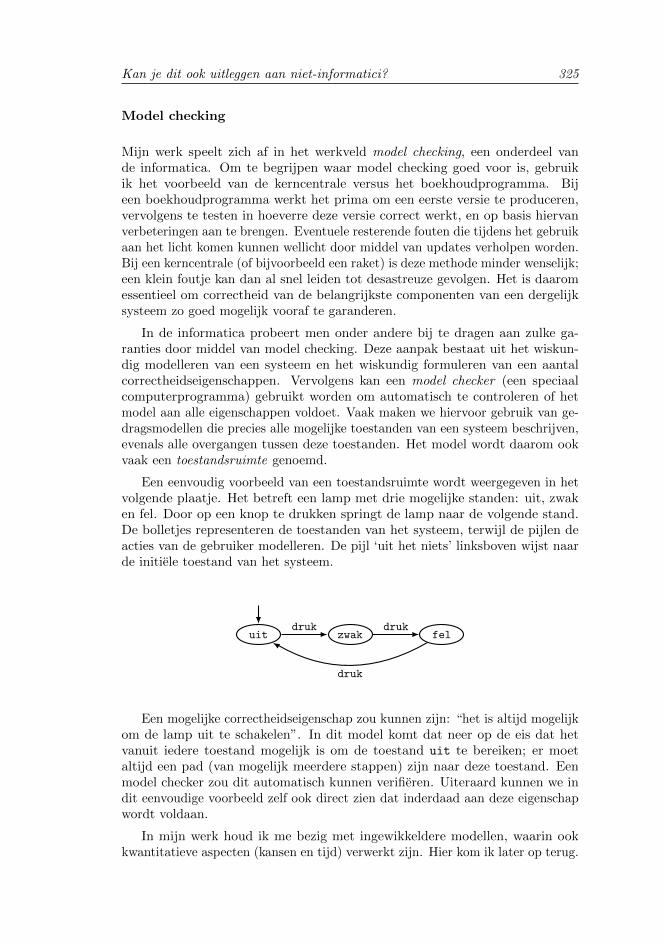
Kan je dit ook uitleggen aan niet-informatici? 325

Model checking

Mijn werk speelt zich af in het werkveld model checking, een onderdeel vande informatica. Om te begrijpen waar model checking goed voor is, gebruikik het voorbeeld van de kerncentrale versus het boekhoudprogramma. Bijeen boekhoudprogramma werkt het prima om een eerste versie te produceren,vervolgens te testen in hoeverre deze versie correct werkt, en op basis hiervanverbeteringen aan te brengen. Eventuele resterende fouten die tijdens het gebruikaan het licht komen kunnen wellicht door middel van updates verholpen worden.Bij een kerncentrale (of bijvoorbeeld een raket) is deze methode minder wenselijk;een klein foutje kan dan al snel leiden tot desastreuze gevolgen. Het is daaromessentieel om correctheid van de belangrijkste componenten van een dergelijksysteem zo goed mogelijk vooraf te garanderen.

In de informatica probeert men onder andere bij te dragen aan zulke ga-ranties door middel van model checking. Deze aanpak bestaat uit het wiskun-dig modelleren van een systeem en het wiskundig formuleren van een aantalcorrectheidseigenschappen. Vervolgens kan een model checker (een speciaalcomputerprogramma) gebruikt worden om automatisch te controleren of hetmodel aan alle eigenschappen voldoet. Vaak maken we hiervoor gebruik van ge-dragsmodellen die precies alle mogelijke toestanden van een systeem beschrijven,evenals alle overgangen tussen deze toestanden. Het model wordt daarom ookvaak een toestandsruimte genoemd.

Een eenvoudig voorbeeld van een toestandsruimte wordt weergegeven in hetvolgende plaatje. Het betreft een lamp met drie mogelijke standen: uit, zwaken fel. Door op een knop te drukken springt de lamp naar de volgende stand.De bolletjes representeren de toestanden van het systeem, terwijl de pijlen deacties van de gebruiker modelleren. De pijl ‘uit het niets’ linksboven wijst naarde initiele toestand van het systeem.

uit zwak feldruk druk

druk

Een mogelijke correctheidseigenschap zou kunnen zijn: “het is altijd mogelijkom de lamp uit te schakelen”. In dit model komt dat neer op de eis dat hetvanuit iedere toestand mogelijk is om de toestand uit te bereiken; er moetaltijd een pad (van mogelijk meerdere stappen) zijn naar deze toestand. Eenmodel checker zou dit automatisch kunnen verifieren. Uiteraard kunnen we indit eenvoudige voorbeeld zelf ook direct zien dat inderdaad aan deze eigenschapwordt voldaan.

In mijn werk houd ik me bezig met ingewikkeldere modellen, waarin ookkwantitatieve aspecten (kansen en tijd) verwerkt zijn. Hier kom ik later op terug.

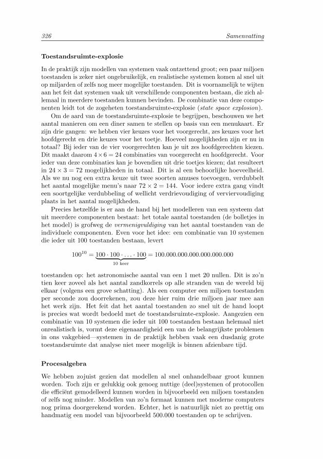
326 Samenvatting

Toestandsruimte-explosie

In de praktijk zijn modellen van systemen vaak ontzettend groot; een paar miljoentoestanden is zeker niet ongebruikelijk, en realistische systemen komen al snel uitop miljarden of zelfs nog meer mogelijke toestanden. Dit is voornamelijk te wijtenaan het feit dat systemen vaak uit verschillende componenten bestaan, die zich al-lemaal in meerdere toestanden kunnen bevinden. De combinatie van deze compo-nenten leidt tot de zogeheten toestandsruimte-explosie (state space explosion).

Om de aard van de toestandsruimte-explosie te begrijpen, beschouwen we hetaantal manieren om een diner samen te stellen op basis van een menukaart. Erzijn drie gangen: we hebben vier keuzes voor het voorgerecht, zes keuzes voor hethoofdgerecht en drie keuzes voor het toetje. Hoeveel mogelijkheden zijn er nu intotaal? Bij ieder van de vier voorgerechten kan je uit zes hoofdgerechten kiezen.Dit maakt daarom 4×6 = 24 combinaties van voorgerecht en hoofdgerecht. Voorieder van deze combinaties kan je bovendien uit drie toetjes kiezen; dat resulteertin 24× 3 = 72 mogelijkheden in totaal. Dit is al een behoorlijke hoeveelheid.Als we nu nog een extra keuze uit twee soorten amuses toevoegen, verdubbelthet aantal mogelijke menu’s naar 72× 2 = 144. Voor iedere extra gang vindteen soortgelijke verdubbeling of wellicht verdrievoudiging of verviervoudigingplaats in het aantal mogelijkheden.

Precies hetzelfde is er aan de hand bij het modelleren van een systeem datuit meerdere componenten bestaat: het totale aantal toestanden (de bolletjes inhet model) is grofweg de vermenigvuldiging van het aantal toestanden van deindividuele componenten. Even voor het idee: een combinatie van 10 systemendie ieder uit 100 toestanden bestaan, levert

10010 = 100 · 100 · . . . · 100︸ ︷︷ ︸10 keer

= 100.000.000.000.000.000.000

toestanden op: het astronomische aantal van een 1 met 20 nullen. Dit is zo’ntien keer zoveel als het aantal zandkorrels op alle stranden van de wereld bijelkaar (volgens een grove schatting). Als een computer een miljoen toestandenper seconde zou doorrekenen, zou deze hier ruim drie miljoen jaar mee aanhet werk zijn. Het feit dat het aantal toestanden zo snel uit de hand looptis precies wat wordt bedoeld met de toestandsruimte-explosie. Aangezien eencombinatie van 10 systemen die ieder uit 100 toestanden bestaan helemaal nietonrealistisch is, vormt deze eigenaardigheid een van de belangrijkste problemenin ons vakgebied—systemen in de praktijk hebben vaak een dusdanig grotetoestandsruimte dat analyse niet meer mogelijk is binnen afzienbare tijd.

Procesalgebra

We hebben zojuist gezien dat modellen al snel onhandelbaar groot kunnenworden. Toch zijn er gelukkig ook genoeg nuttige (deel)systemen of protocollendie efficient gemodelleerd kunnen worden in bijvoorbeeld een miljoen toestandenof zelfs nog minder. Modellen van zo’n formaat kunnen met moderne computersnog prima doorgerekend worden. Echter, het is natuurlijk niet zo prettig omhandmatig een model van bijvoorbeeld 500.000 toestanden op te schrijven.

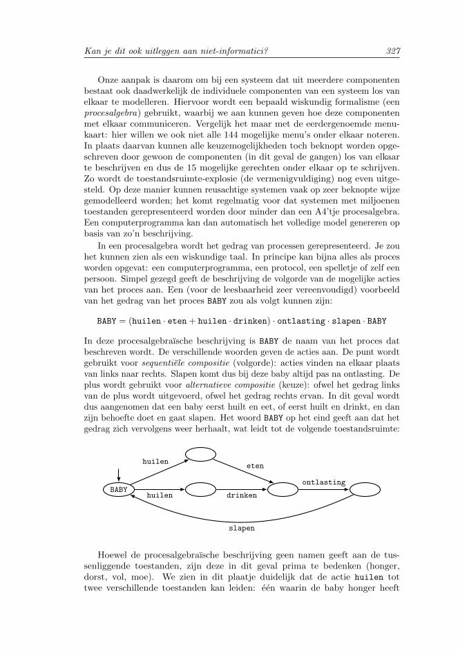
Kan je dit ook uitleggen aan niet-informatici? 327

Onze aanpak is daarom om bij een systeem dat uit meerdere componentenbestaat ook daadwerkelijk de individuele componenten van een systeem los vanelkaar te modelleren. Hiervoor wordt een bepaald wiskundig formalisme (eenprocesalgebra) gebruikt, waarbij we aan kunnen geven hoe deze componentenmet elkaar communiceren. Vergelijk het maar met de eerdergenoemde menu-kaart: hier willen we ook niet alle 144 mogelijke menu’s onder elkaar noteren.In plaats daarvan kunnen alle keuzemogelijkheden toch beknopt worden opge-schreven door gewoon de componenten (in dit geval de gangen) los van elkaarte beschrijven en dus de 15 mogelijke gerechten onder elkaar op te schrijven.Zo wordt de toestandsruimte-explosie (de vermenigvuldiging) nog even uitge-steld. Op deze manier kunnen reusachtige systemen vaak op zeer beknopte wijzegemodelleerd worden; het komt regelmatig voor dat systemen met miljoenentoestanden gerepresenteerd worden door minder dan een A4’tje procesalgebra.Een computerprogramma kan dan automatisch het volledige model genereren opbasis van zo’n beschrijving.

In een procesalgebra wordt het gedrag van processen gerepresenteerd. Je zouhet kunnen zien als een wiskundige taal. In principe kan bijna alles als procesworden opgevat: een computerprogramma, een protocol, een spelletje of zelf eenpersoon. Simpel gezegd geeft de beschrijving de volgorde van de mogelijke actiesvan het proces aan. Een (voor de leesbaarheid zeer vereenvoudigd) voorbeeldvan het gedrag van het proces BABY zou als volgt kunnen zijn:

BABY = (huilen · eten + huilen · drinken) · ontlasting · slapen · BABY

In deze procesalgebraısche beschrijving is BABY de naam van het proces datbeschreven wordt. De verschillende woorden geven de acties aan. De punt wordtgebruikt voor sequentiele compositie (volgorde): acties vinden na elkaar plaatsvan links naar rechts. Slapen komt dus bij deze baby altijd pas na ontlasting. Deplus wordt gebruikt voor alternatieve compositie (keuze): ofwel het gedrag linksvan de plus wordt uitgevoerd, ofwel het gedrag rechts ervan. In dit geval wordtdus aangenomen dat een baby eerst huilt en eet, of eerst huilt en drinkt, en danzijn behoefte doet en gaat slapen. Het woord BABY op het eind geeft aan dat hetgedrag zich vervolgens weer herhaalt, wat leidt tot de volgende toestandsruimte:

BABY

huilen

huilen

eten

drinken

ontlasting

slapen

Hoewel de procesalgebraısche beschrijving geen namen geeft aan de tus-senliggende toestanden, zijn deze in dit geval prima te bedenken (honger,dorst, vol, moe). We zien in dit plaatje duidelijk dat de actie huilen tottwee verschillende toestanden kan leiden: een waarin de baby honger heeft

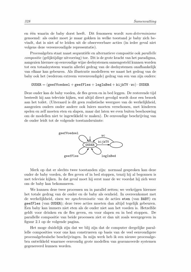
328 Samenvatting

en een waarin de baby dorst heeft. Dit fenomeen wordt non-determinismegenoemd: als ouder moet je maar gokken in welke toestand je baby zich be-vindt, dat is niet af te leiden uit de observeerbare acties (in ieder geval nietvolgens deze vereenvoudigde representatie).

Procesalgebra staat naast sequentiele en alternatieve compositie ook parallellecompositie (gelijktijdige uitvoering) toe. Dit is de grote kracht van het paradigma,aangezien hiermee op eenvoudige wijze deelsystemen samengesteld kunnen wordentot een totaalsysteem waarin allerlei gedrag van de deelsystemen onafhankelijkvan elkaar kan gebeuren. Als illustratie modelleren we naast het gedrag van debaby ook het (wederom extreem vereenvoudigde) gedrag van een van zijn ouders:

OUDER = (geefVoedsel + geefFles + legInBed + kijkTV · wc) · OUDER

Deze ouder kan de baby voeden, de fles geven en in bed leggen. De resterende tijdbesteedt hij aan televisie kijken, wat altijd direct gevolgd wordt door een bezoekaan het toilet. (Uiteraard is dit geen realistische weergave van de werkelijkheid,aangezien ouders onder andere ook luiers moeten verschonen, met kinderenspelen en zelf moeten eten en slapen, maar dat laten we even buiten beschouwingom de modellen niet te ingewikkeld te maken). De eenvoudige beschrijving vande ouder leidt tot de volgende toestandsruimte:

OUDER

geefVoedsel

geefFles legInBed

kijkTV

wc

Merk op dat er slechts twee toestanden zijn: normaal gesproken kan dezeouder de baby voeden, de fles geven of in bed stoppen, tenzij hij al begonnen ismet televisie kijken. In dat geval moet hij eerst naar de wc voordat hij zich weerom de baby kan bekommeren.

We kunnen deze twee processen nu in parallel zetten; we verkrijgen hiermeehet totale gedrag van de ouder en de baby als eenheid. In overeenkomst metde werkelijkheid, eisen we synchronisatie van de acties eten (van BABY) engeefFles (van OUDER); deze twee acties moeten dan altijd tegelijk gebeuren.Een baby kan immers niet eten als de ouder niet aan het voeden is. Hetzelfdegeldt voor drinken en de fles geven, en voor slapen en in bed stoppen. Deparallelle compositie van beide processen ziet er dan uit zoals weergegeven infiguur 2.1 op de volgende pagina.

Het moge duidelijk zijn dat we blij zijn dat de computer dergelijke paral-lelle composities voor ons kan construeren op basis van de veel eenvoudigereprocesalgebraısche beschrijvingen. In mijn werk heb ik een nieuwe procesalge-bra ontwikkeld waarmee eenvoudig grote modellen van geavanceerde systemengegenereerd kunnen worden.

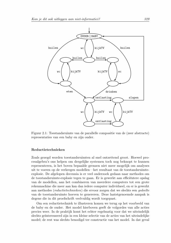
Kan je dit ook uitleggen aan niet-informatici? 329

OUDER || BABY

kijkTVwc

huilen huilen

wc wckijkTV kijkTV

huilen huilen

eten drinken

ontlasting

kijkTVwc

ontlasting

wc kijkTV

slapen

Figuur 2.1: Toestandsruimte van de parallelle compositie van de (zeer abstracte)representaties van een baby en zijn ouder.

Reductietechnieken

Zoals gezegd worden toestandsruimten al snel ontzettend groot. Hoewel pro-cesalgebra’s ons helpen om dergelijke systemen toch nog beknopt te kunnenrepresenteren, is het boven bepaalde grenzen niet meer mogelijk om analysesuit te voeren op de verkregen modellen—het resultaat van de toestandsruimte-explosie. De afgelopen decennia is er veel onderzoek gedaan naar methodes omde toestandsruimte-explosie tegen te gaan. Er is gewerkt aan efficientere opslagvan de modellen, aan het combineren van meerdere computers tot een groterekenmachine die meer aan kan dan iedere computer individueel, en er is gewerktaan methodes (reductietechnieken) die ervoor zorgen dat we slechts een gedeeltevan de toestandsruimte hoeven te genereren. Deze laatstgenoemde aanpak isdegene die in dit proefschrift veelvuldig wordt toegepast.

Om een reductietechniek te illustreren komen we terug op het voorbeeld vande baby en de ouder. Het model hierboven geeft de volgordes van alle actiesprecies weer. In de praktijk komt het echter regelmatig voor dat we uiteindelijkslechts geınteresseerd zijn in een kleine selectie van de acties van het uiteindelijkemodel; de rest was slechts benodigd ter constructie van het model. In dat geval

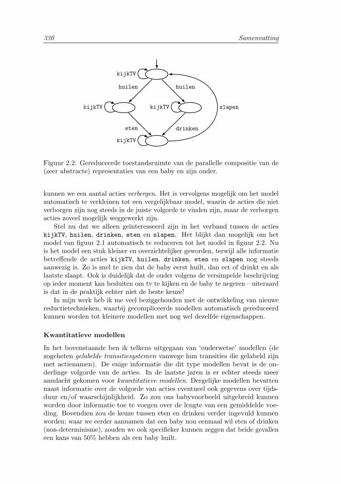
330 Samenvatting

huilen huilen

eten drinken

slapen

kijkTV

kijkTV

kijkTV

kijkTV

Figuur 2.2: Gereduceerde toestandsruimte van de parallelle compositie van de(zeer abstracte) representaties van een baby en zijn ouder.

kunnen we een aantal acties verbergen. Het is vervolgens mogelijk om het modelautomatisch te verkleinen tot een vergelijkbaar model, waarin de acties die nietverborgen zijn nog steeds in de juiste volgorde te vinden zijn, maar de verborgenacties zoveel mogelijk weggewerkt zijn.

Stel nu dat we alleen geınteresseerd zijn in het verband tussen de actieskijkTV, huilen, drinken, eten en slapen. Het blijkt dan mogelijk om hetmodel van figuur 2.1 automatisch te reduceren tot het model in figuur 2.2. Nuis het model een stuk kleiner en overzichtelijker geworden, terwijl alle informatiebetreffende de acties kijkTV, huilen, drinken, eten en slapen nog steedsaanwezig is. Zo is snel te zien dat de baby eerst huilt, dan eet of drinkt en alslaatste slaapt. Ook is duidelijk dat de ouder volgens de versimpelde beschrijvingop ieder moment kan besluiten om tv te kijken en de baby te negeren—uiteraardis dat in de praktijk echter niet de beste keuze!

In mijn werk heb ik me veel beziggehouden met de ontwikkeling van nieuwereductietechnieken, waarbij gecompliceerde modellen automatisch gereduceerdkunnen worden tot kleinere modellen met nog wel dezelfde eigenschappen.

Kwantitatieve modellen

In het bovenstaande ben ik telkens uitgegaan van ‘ouderwetse’ modellen (dezogeheten gelabelde transitiesystemen vanwege hun transities die gelabeld zijnmet actienamen). De enige informatie die dit type modellen bevat is de on-derlinge volgorde van de acties. In de laatste jaren is er echter steeds meeraandacht gekomen voor kwantitatieve modellen. Dergelijke modellen bevattennaast informatie over de volgorde van acties eventueel ook gegevens over tijds-duur en/of waarschijnlijkheid. Zo zou ons babyvoorbeeld uitgebreid kunnenworden door informatie toe te voegen over de lengte van een gemiddelde voe-ding. Bovendien zou de keuze tussen eten en drinken verder ingevuld kunnenworden; waar we eerder aannamen dat een baby nou eenmaal wil eten of drinken(non-determinisme), zouden we ook specifieker kunnen zeggen dat beide gevalleneen kans van 50% hebben als een baby huilt.

Kan je dit ook uitleggen aan niet-informatici? 331

De toevoeging van kansen maakt het mogelijk om processen te modelleren diezich niet altijd op dezelfde manier gedragen, zoals een geboorte (ongeveer 50%kans op een jongen) of het versturen van een ansichtkaart vanuit een ver landnaar Nederland (enige kans dat de kaart kwijtraakt). Bovendien kunnen we voordit soort modellen ook kwantitatieve eigenschappen formuleren en deze door eenmodel checker op waarheid laten controleren. Te denken aan eigenschappen zoals“de kans dat het programma een correct resultaat produceert is tenminste 99%”.

De toevoeging van tijdsinformatie maakt het mogelijk om eigenschappente controleren betreffende prestaties en betrouwbaarheid: “de kans dat decassieres gezamenlijk minder dan 100 klanten in een uur kunnen helpen is kleinerdan 5%”, of “de kans dat het systeem pas kapot gaat meer dan 1,000 uurgebruik is tenminste 95%”.

Mijn bijdrage

Door het lezen van het bovenstaande heeft u een klein kijkje gekregen in dekeuken van een gedeelte van mijn vakgebied. Tot zover is alles nog redelijkstandaard, in de zin dat de meeste mensen in mijn vakgebied dit al weten ener ook niks genoemd is wat door mij bedacht is. Hoofdstuk 2 en 3 vatten dezeachtergrondinformatie samen op een wiskundigere manier.

Wat heb ik dan wel zelf gedaan? Mijn bijdrage is grofweg op te splitsen indrie delen.

Nieuwe procesalgebra. Ten eerste heb ik een nieuwe procesalgebra (MAPA)ontwikkeld om modellen te genereren die zowel non-determinisme, kansen alstijdsduren bevatten (de zogeheten Markov-automaten). Ik heb voortgeborduurdop een eerdere niet-kwantitatieve aanpak die gebruikmaakte van data: eenmethode om op een efficientere manier nog complexere toestandsruimtes tekunnen genereren. Tot dusver bestond er nog geen procesalgebra die dit kondoen; het was daarom zonder mijn werk nog niet mogelijk om op een eenvoudigewijze Markov-automaten te genereren.

Ik heb bovendien een variant op MAPA ontwikkeld (de MLPE), die ergbeperkt is en daarom voor computers handiger is om mee te werken. Zo heeftde MLPE geen parallelle compositie en moet iedere actie direct gevolgd wordendoor een procesnaam—onze voorbeelden hierboven zouden dus al niet eensvoldoen. Aangezien de volledige procesalgebra handiger is voor mensen om meete werken, heb ik een algoritme (een soort recept) ontwikkeld dat automatischieder model van de gebruiksvriendelijke procesalgebra MAPA omzet in eensimpelere representatie in de taal MLPE. Daar kan de computer vervolgensmakkelijker mee overweg.

Dit alles is beschreven in hoofdstuk 4.

Nieuwe reductietechnieken. Ten tweede heb ik verscheidene reductietechnie-ken ontwikkeld, die ervoor zorgen dat het aantal toestanden van een modelbinnen de perken blijft. Hoewel het theoretisch mogelijk zou zijn om eerstde originele toestandsruimte van een systeem te genereren, is dat natuurlijkniet zo efficient. Mijn aanpak maakt daarom gebruik van de eenvoud van de

332 Samenvatting

MLPE (een procesalgebraısche beschrijving). Er worden allerlei analyses op dezebeknopte representaties uitgevoerd, waarna ze automatisch herschreven wordentot specificaties die uiteindelijk een veel kleinere toestandsruimte opleveren. Zoproberen we de toestandsruimte-explosie enigszins te omzeilen.

Om een idee te krijgen van hoe dergelijke technieken werken pakken we nogeenmaal de menukaart erbij. Stel dat er aan de kassa berekend moet wordenwat een gekozen menu kost, en dat we weten dat alle toetjes even duur zijn. Indat geval maakt het niets uit welk toetje er gekozen wordt, en kunnen we netzo goed doen alsof iedereen de verse vruchtjes heeft genomen. Dat beperkt hetaantal mogelijkheden, en maakt het model van de situatie kleiner (terwijl hetvoor de eigenschappen die bekeken worden—in dit geval de totale kosten—nogidentiek functioneert).

Drie van zulke door mij ontwikkelde technieken worden besproken in hoofd-stuk 4, en twee uitgebreidere technieken in hoofdstuk 5 en hoofdstuk 6.

Vergelijking van reductietechnieken. Ten derde heb ik een van de door mij ont-wikkelde technieken (confluence reduction) vergeleken met een eerdere reductie-techniek voor kwantitatieve systemen (partial order reduction). Een overduidelijkvoordeel van mijn techniek is dat deze de enige techniek in zijn soort is die werktvoor systemen met zowel kansen als tijdsduren. Dus, als een dergelijk modelgebruikt wordt, is er geen andere keus—partial order reduction werkt alleen alser hooguit kansen gebruikt worden, maar niet in de aanwezigheid van tijdsduren.Om toch meer inzicht te krijgen in het verband tussen de technieken, heb ikgekeken in hoeverre ze overeenkomen als we ons beperken tot systemen zondertijdsduren. Ik heb bovendien precies de verschillen ertussen geıdentificeerd.Hierdoor is ook direct duidelijk hoe de niet-kwantitatieve varianten van de tech-nieken (die al wel eerder bestonden) relateren; dat was ook nog niet bekend. Hetblijkt dat mijn techniek net iets beter presteert voor systemen die al dan nietvoorzien zijn van kansen—onder de aanname dat we een bepaalde verzamelingvan eigenschappen willen bewaren. De vergelijkingen tussen confluence reductionen partial order reduction zijn te vinden in hoofdstuk 7 en hoofdstuk 8.

Het proefschrift wordt afgerond in hoofdstuk 9 met een bespreking van hetprogramma dat ik heb gemaakt om automatisch en efficient modellen met kansenen tijdsduren te genereren op basis van procesalgebraısche beschrijvingen. Ookbespreek ik daar case studies die laten zien dat mijn procesalgebra hier inderdaadprima voor gebruikt kan worden, en laat ik zien dat mijn reductietechnieken ookin de praktijk voor aanzienlijke snelheidswinst zorgen.

Titles in the IPA Dissertation Series since 2007

H.A. de Jong. Flexible Heteroge-neous Software Systems. Faculty ofNatural Sciences, Mathematics, andComputer Science, UvA. 2007-01

N.K. Kavaldjiev. A run-time recon-figurable Network-on-Chip for strea-ming DSP applications. Faculty ofElectrical Engineering, Mathematics& Computer Science, UT. 2007-02

M. van Veelen. Considerations onModeling for Early Detection of Ab-normalities in Locally AutonomousDistributed Systems. Faculty of Ma-thematics and Computing Sciences,RUG. 2007-03

T.D. Vu. Semantics and Applica-tions of Process and Program Alge-bra. Faculty of Natural Sciences,Mathematics, and Computer Science,UvA. 2007-04

L. Brandan Briones. Theories forModel-based Testing: Real-time andCoverage. Faculty of Electrical En-gineering, Mathematics & ComputerScience, UT. 2007-05

I. Loeb. Natural Deduction: Sharingby Presentation. Faculty of Science,Mathematics and Computer Science,RU. 2007-06

M.W.A. Streppel. MultifunctionalGeometric Data Structures. Faculty ofMathematics and Computer Science,TU/e. 2007-07

N. Trcka. Silent Steps in TransitionSystems and Markov Chains. Facultyof Mathematics and Computer Sci-ence, TU/e. 2007-08

R. Brinkman. Searching in encryp-ted data. Faculty of Electrical En-gineering, Mathematics & ComputerScience, UT. 2007-09

A. van Weelden. Putting typesto good use. Faculty of Science,Mathematics and Computer Science,RU. 2007-10

J.A.R. Noppen. Imperfect Infor-mation in Software Development Pro-cesses. Faculty of Electrical Enginee-ring, Mathematics & Computer Sci-ence, UT. 2007-11

R. Boumen. Integration and Testplans for Complex Manufacturing Sys-tems. Faculty of Mechanical Enginee-ring, TU/e. 2007-12

A.J. Wijs. What to do Next?: Ana-lysing and Optimising System Beha-viour in Time. Faculty of Sciences,Division of Mathematics and Compu-ter Science, VUA. 2007-13

C.F.J. Lange. Assessing and Impro-ving the Quality of Modeling: A Seriesof Empirical Studies about the UML.Faculty of Mathematics and Compu-ter Science, TU/e. 2007-14

T. van der Storm. Component-based Configuration, Integration andDelivery. Faculty of Natural Scien-ces, Mathematics, and Computer Sci-ence,UvA. 2007-15

B.S. Graaf. Model-Driven Evolutionof Software Architectures. Faculty ofElectrical Engineering, Mathematics,and Computer Science, TUD. 2007-16

A.H.J. Mathijssen. Logical Calculifor Reasoning with Binding. Facultyof Mathematics and Computer Sci-ence, TU/e. 2007-17

D. Jarnikov. QoS framework for Vi-deo Streaming in Home Networks. Fa-culty of Mathematics and ComputerScience, TU/e. 2007-18

M. A. Abam. New Data Structuresand Algorithms for Mobile Data. Fa-culty of Mathematics and ComputerScience, TU/e. 2007-19

W. Pieters. La Volonte Machi-nale: Understanding the ElectronicVoting Controversy. Faculty of Sci-ence, Mathematics and Computer Sci-ence, RU. 2008-01

A.L. de Groot. Practical Automa-ton Proofs in PVS. Faculty of Science,Mathematics and Computer Science,RU. 2008-02

M. Bruntink. Renovation of Idio-matic Crosscutting Concerns in Em-bedded Systems. Faculty of ElectricalEngineering, Mathematics, and Com-puter Science, TUD. 2008-03

A.M. Marin. An Integrated Systemto Manage Crosscutting Concerns inSource Code. Faculty of Electrical En-gineering, Mathematics, and Compu-ter Science, TUD. 2008-04

N.C.W.M. Braspenning. Model-based Integration and Testing ofHigh-tech Multi-disciplinary Systems.Faculty of Mechanical Engineering,TU/e. 2008-05

M. Bravenboer. Exercises in FreeSyntax: Syntax Definition, Parsing,and Assimilation of Language Con-glomerates. Faculty of Science,UU. 2008-06

M. Torabi Dashti. Keeping Fair-ness Alive: Design and Formal Veri-fication of Optimistic Fair ExchangeProtocols. Faculty of Sciences, Divi-sion of Mathematics and ComputerScience, VUA. 2008-07

I.S.M. de Jong. Integration andTest Strategies for Complex Manufac-turing Machines. Faculty of Mechani-cal Engineering, TU/e. 2008-08

I. Hasuo. Tracing Anonymity withCoalgebras. Faculty of Science, Ma-thematics and Computer Science,RU. 2008-09

L.G.W.A. Cleophas. Tree Algo-rithms: Two Taxonomies and a Tool-kit. Faculty of Mathematics and Com-puter Science, TU/e. 2008-10

I.S. Zapreev. Model CheckingMarkov Chains: Techniques andTools. Faculty of Electrical Enginee-ring, Mathematics & Computer Sci-ence, UT. 2008-11

M. Farshi. A Theoretical and Ex-perimental Study of Geometric Net-works. Faculty of Mathematics andComputer Science, TU/e. 2008-12

G. Gulesir. Evolvable BehaviorSpecifications Using Context-SensitiveWildcards. Faculty of Electrical En-gineering, Mathematics & ComputerScience, UT. 2008-13

F.D. Garcia. Formal and Computa-tional Cryptography: Protocols, Has-hes and Commitments. Faculty of Sci-ence, Mathematics and Computer Sci-ence, RU. 2008-14

P. E. A. Durr. Resource-based Ve-rification for Robust Composition ofAspects. Faculty of Electrical Enginee-ring, Mathematics & Computer Sci-ence, UT. 2008-15

E.M. Bortnik. Formal Methodsin Support of SMC Design. Fa-culty of Mechanical Engineering,TU/e. 2008-16

R.H. Mak. Design and Perfor-mance Analysis of Data-IndependentStream Processing Systems. Faculty ofMathematics and Computer Science,TU/e. 2008-17

M. van der Horst. Scalable BlockProcessing Algorithms. Faculty of

Mathematics and Computer Science,TU/e. 2008-18

C.M. Gray. Algorithms for Fat Ob-jects: Decompositions and Applica-tions. Faculty of Mathematics andComputer Science, TU/e. 2008-19

J.R. Calame. Testing Reactive Sys-tems with Data - Enumerative Me-thods and Constraint Solving. Facultyof Electrical Engineering, Mathema-tics & Computer Science, UT. 2008-20

E. Mumford. Drawing Graphs forCartographic Applications. Faculty ofMathematics and Computer Science,TU/e. 2008-21

E.H. de Graaf. Mining Semi-structured Data, Theoretical and Ex-perimental Aspects of Pattern Evalu-ation. Faculty of Mathematics andNatural Sciences, UL. 2008-22

R. Brijder. Models of Natural Com-putation: Gene Assembly and Mem-brane Systems. Faculty of Mathema-tics and Natural Sciences, UL. 2008-23

A. Koprowski. Termination of Re-writing and Its Certification. Facultyof Mathematics and Computer Sci-ence, TU/e. 2008-24

U. Khadim. Process Algebras forHybrid Systems: Comparison and De-velopment. Faculty of Mathematicsand Computer Science, TU/e. 2008-25

J. Markovski. Real and Stochas-tic Time in Process Algebras for Per-formance Evaluation. Faculty ofMathematics and Computer Science,TU/e. 2008-26

H. Kastenberg. Graph-Based Soft-ware Specification and Verification.Faculty of Electrical Engineering,Mathematics & Computer Science,UT. 2008-27

I.R. Buhan. Cryptographic Keysfrom Noisy Data Theory and Applica-tions. Faculty of Electrical Enginee-ring, Mathematics & Computer Sci-ence, UT. 2008-28

R.S. Marin-Perianu. Wireless Sen-sor Networks in Motion: ClusteringAlgorithms for Service Discovery andProvisioning. Faculty of Electrical En-gineering, Mathematics & ComputerScience, UT. 2008-29

M.H.G. Verhoef. Modeling and Va-lidating Distributed Embedded Real-Time Control Systems. Faculty ofScience, Mathematics and ComputerScience, RU. 2009-01

M. de Mol. Reasoning about Func-tional Programs: Sparkle, a proof as-sistant for Clean. Faculty of Science,Mathematics and Computer Science,RU. 2009-02

M. Lormans. Managing Require-ments Evolution. Faculty of ElectricalEngineering, Mathematics, and Com-puter Science, TUD. 2009-03

M.P.W.J. van Osch. AutomatedModel-based Testing of Hybrid Sys-tems. Faculty of Mathematics andComputer Science, TU/e. 2009-04

H. Sozer. Architecting Fault-Tolerant Software Systems. Faculty ofElectrical Engineering, Mathematics& Computer Science, UT. 2009-05

M.J. van Weerdenburg. EfficientRewriting Techniques. Faculty ofMathematics and Computer Science,TU/e. 2009-06

H.H. Hansen. Coalgebraic Model-ling: Applications in Automata The-ory and Modal Logic. Faculty of Sci-ences, Division of Mathematics andComputer Science, VUA. 2009-07

A. Mesbah. Analysis and Testing ofAjax-based Single-page Web Applicati-ons. Faculty of Electrical Engineering,Mathematics, and Computer Science,TUD. 2009-08

A.L. Rodriguez Yakushev. To-wards Getting Generic ProgrammingReady for Prime Time. Faculty ofScience, UU. 2009-9

K.R. Olmos Joffre. Strategiesfor Context Sensitive Program Trans-formation. Faculty of Science,UU. 2009-10

J.A.G.M. van den Berg. Rea-soning about Java programs in PVSusing JML. Faculty of Science, Ma-thematics and Computer Science,RU. 2009-11

M.G. Khatib. MEMS-Based Stor-age Devices. Integration in Energy-Constrained Mobile Systems. Facultyof Electrical Engineering, Mathema-tics & Computer Science, UT. 2009-12

S.G.M. Cornelissen. EvaluatingDynamic Analysis Techniques for Pro-gram Comprehension. Faculty of Elec-trical Engineering, Mathematics, andComputer Science, TUD. 2009-13

D. Bolzoni. Revisiting Anomaly-based Network Intrusion DetectionSystems. Faculty of Electrical En-gineering, Mathematics & ComputerScience, UT. 2009-14

H.L. Jonker. Security Matters: Pri-vacy in Voting and Fairness in Digi-tal Exchange. Faculty of Mathematicsand Computer Science, TU/e. 2009-15

M.R. Czenko. TuLiP - ReshapingTrust Management. Faculty of Elec-trical Engineering, Mathematics &Computer Science, UT. 2009-16

T. Chen. Clocks, Dice and Proces-ses. Faculty of Sciences, Division of

Mathematics and Computer Science,VUA. 2009-17

C. Kaliszyk. Correctness and Avai-lability: Building Computer Algebraon top of Proof Assistants and makingProof Assistants available over theWeb. Faculty of Science, Mathematicsand Computer Science, RU. 2009-18

R.S.S. O’Connor. Incompleteness& Completeness: Formalizing Logicand Analysis in Type Theory. Facultyof Science, Mathematics and Compu-ter Science, RU. 2009-19

B. Ploeger. Improved VerificationMethods for Concurrent Systems. Fa-culty of Mathematics and ComputerScience, TU/e. 2009-20

T. Han. Diagnosis, Synthesisand Analysis of Probabilistic Mo-dels. Faculty of Electrical Enginee-ring, Mathematics & Computer Sci-ence, UT. 2009-21

R. Li. Mixed-Integer Evolution Stra-tegies for Parameter Optimization andTheir Applications to Medical ImageAnalysis. Faculty of Mathematics andNatural Sciences, UL. 2009-22

J.H.P. Kwisthout. The Com-putational Complexity of Probabilis-tic Networks. Faculty of Science,UU. 2009-23

T.K. Cocx. Algorithmic Tools forData-Oriented Law Enforcement. Fa-culty of Mathematics and Natural Sci-ences, UL. 2009-24

A.I. Baars. Embedded Compilers.Faculty of Science, UU. 2009-25

M.A.C. Dekker. Flexible AccessControl for Dynamic CollaborativeEnvironments. Faculty of ElectricalEngineering, Mathematics & Compu-ter Science, UT. 2009-26

J.F.J. Laros. Metrics and Visua-lisation for Crime Analysis and Ge-nomics. Faculty of Mathematics andNatural Sciences, UL. 2009-27

C.J. Boogerd. Focusing AutomaticCode Inspections. Faculty of ElectricalEngineering, Mathematics, and Com-puter Science, TUD. 2010-01

M.R. Neuhaußer. Model CheckingNondeterministic and Randomly Ti-med Systems. Faculty of ElectricalEngineering, Mathematics & Compu-ter Science, UT. 2010-02

J. Endrullis. Termination and Pro-ductivity. Faculty of Sciences, Divi-sion of Mathematics and ComputerScience, VUA. 2010-03

T. Staijen. Graph-Based Specifi-cation and Verification for Aspect-Oriented Languages. Faculty of Elec-trical Engineering, Mathematics &Computer Science, UT. 2010-04

Y. Wang. Epistemic Modelling andProtocol Dynamics. Faculty of Sci-ence, UvA. 2010-05

J.K. Berendsen. Abstraction, Pri-ces and Probability in Model CheckingTimed Automata. Faculty of Science,Mathematics and Computer Science,RU. 2010-06

A. Nugroho. The Effects of UMLModeling on the Quality of Software.Faculty of Mathematics and NaturalSciences, UL. 2010-07

A. Silva. Kleene Coalgebra. Facultyof Science, Mathematics and Compu-ter Science, RU. 2010-08

J.S. de Bruin. Service-OrientedDiscovery of Knowledge - Foundati-ons, Implementations and Applicati-ons. Faculty of Mathematics and Na-tural Sciences, UL. 2010-09

D. Costa. Formal Models for Com-ponent Connectors. Faculty of Sci-ences, Division of Mathematics andComputer Science, VUA. 2010-10

M.M. Jaghoori. Time at Your Ser-vice: Schedulability Analysis of Real-Time and Distributed Services. Fa-culty of Mathematics and Natural Sci-ences, UL. 2010-11

R. Bakhshi. Gossiping Models: For-mal Analysis of Epidemic Protocols.Faculty of Sciences, Department ofComputer Science, VUA. 2011-01

B.J. Arnoldus. An Illumination ofthe Template Enigma: Software CodeGeneration with Templates. Faculty ofMathematics and Computer Science,TU/e. 2011-02

E. Zambon. Towards Optimal ITAvailability Planning: Methods andTools. Faculty of Electrical Enginee-ring, Mathematics & Computer Sci-ence, UT. 2011-03

L. Astefanoaei. An Executable The-ory of Multi-Agent Systems Refine-ment. Faculty of Mathematics andNatural Sciences, UL. 2011-04

J. Proenca. Synchronous coordina-tion of distributed components. Fa-culty of Mathematics and Natural Sci-ences, UL. 2011-05

A. Moralı. IT Architecture-BasedConfidentiality Risk Assessment inNetworks of Organizations. Faculty ofElectrical Engineering, Mathematics& Computer Science, UT. 2011-06

M. van der Bijl. On changing mo-dels in Model-Based Testing. Facultyof Electrical Engineering, Mathema-tics & Computer Science, UT. 2011-07

C. Krause. Reconfigurable Com-ponent Connectors. Faculty ofMathematics and Natural Sciences,UL. 2011-08

M.E. Andres. Quantitative Analy-sis of Information Leakage in Probabi-listic and Nondeterministic Systems.Faculty of Science, Mathematics andComputer Science, RU. 2011-09

M. Atif. Formal Modeling and Ve-rification of Distributed Failure De-tectors. Faculty of Mathematics andComputer Science, TU/e. 2011-10

P.J.A. van Tilburg. From Compu-tability to Executability – A process-theoretic view on automata theory. Fa-culty of Mathematics and ComputerScience, TU/e. 2011-11

Z. Protic. Configuration manage-ment for models: Generic methodsfor model comparison and model co-evolution. Faculty of Mathematicsand Computer Science, TU/e. 2011-12

S. Georgievska. Probability and Hi-ding in Concurrent Processes. Facultyof Mathematics and Computer Sci-ence, TU/e. 2011-13

S. Malakuti. Event CompositionModel: Achieving Naturalness in Run-time Enforcement. Faculty of Electri-cal Engineering, Mathematics & Com-puter Science, UT. 2011-14

M. Raffelsieper. Cell Libraries andVerification. Faculty of Mathematicsand Computer Science, TU/e. 2011-15

C.P. Tsirogiannis. Analysis of Flowand Visibility on Triangulated Ter-rains. Faculty of Mathematics andComputer Science, TU/e. 2011-16

Y.-J. Moon. Stochastic Models forQuality of Service of Component Con-nectors. Faculty of Mathematics andNatural Sciences, UL. 2011-17

R. Middelkoop. Capturing andExploiting Abstract Views of Sta-tes in OO Verification. Faculty of

Mathematics and Computer Science,TU/e. 2011-18

M.F. van Amstel. Assessing andImproving the Quality of Model Trans-formations. Faculty of Mathematicsand Computer Science, TU/e. 2011-19

A.N. Tamalet. Towards CorrectPrograms in Practice. Faculty of Sci-ence, Mathematics and Computer Sci-ence, RU. 2011-20

H.J.S. Basten. Ambiguity De-tection for Programming LanguageGrammars. Faculty of Science,UvA. 2011-21

M. Izadi. Model Checking ofComponent Connectors. Faculty ofMathematics and Natural Sciences,UL. 2011-22

L.C.L. Kats. Building Blocks forLanguage Workbenches. Faculty ofElectrical Engineering, Mathematics,and Computer Science, TUD. 2011-23

S. Kemper. Modelling and Analysisof Real-Time Coordination Patterns.Faculty of Mathematics and NaturalSciences, UL. 2011-24

J. Wang. Spiking Neural P Systems.Faculty of Mathematics and NaturalSciences, UL. 2011-25

A. Khosravi. Optimal Geome-tric Data Structures. Faculty ofMathematics and Computer Science,TU/e. 2012-01

A. Middelkoop. Inference of Pro-gram Properties with Attribute Gram-mars, Revisited. Faculty of Science,UU. 2012-02

Z. Hemel. Methods and Techniquesfor the Design and Implementationof Domain-Specific Languages. Fa-culty of Electrical Engineering, Ma-thematics, and Computer Science,TUD. 2012-03

T. Dimkov. Alignment of Organiza-tional Security Policies: Theory andPractice. Faculty of Electrical En-gineering, Mathematics & ComputerScience, UT. 2012-04

S. Sedghi. Towards Provably Se-cure Efficiently Searchable Encryp-tion. Faculty of Electrical Enginee-ring, Mathematics & Computer Sci-ence, UT. 2012-05

F. Heidarian Dehkordi. Studies onVerification of Wireless Sensor Net-works and Abstraction Learning forSystem Inference. Faculty of Science,Mathematics and Computer Science,RU. 2012-06

K. Verbeek. Algorithms for Car-tographic Visualization. Faculty ofMathematics and Computer Science,TU/e. 2012-07

D.E. Nadales Agut. A Compositi-onal Interchange Format for HybridSystems: Design and Implementation.Faculty of Mechanical Engineering,TU/e. 2012-08

H. Rahmani. Analysis of Protein-Protein Interaction Networks byMeans of Annotated Graph Mining Al-gorithms. Faculty of Mathematics andNatural Sciences, UL. 2012-09

S.D. Vermolen. Software LanguageEvolution. Faculty of Electrical Engi-neering, Mathematics, and ComputerScience, TUD. 2012-10

L.J.P. Engelen. From Napkin Sket-ches to Reliable Software. Faculty ofMathematics and Computer Science,TU/e. 2012-11

F.P.M. Stappers. Bridging FormalModels – An Engineering Perspective.Faculty of Mathematics and Compu-ter Science, TU/e. 2012-12

W. Heijstek. Software ArchitectureDesign in Global and Model-CentricSoftware Development. Faculty ofMathematics and Natural Sciences,UL. 2012-13

C. Kop. Higher Order Termination.Faculty of Sciences, Department ofComputer Science, VUA. 2012-14

A. Osaiweran. Formal Develop-ment of Control Software in the Me-dical Systems Domain. Faculty ofMathematics and Computer Science,TU/e. 2012-15

W. Kuijper. Compositional Synthe-sis of Safety Controllers. Faculty ofElectrical Engineering, Mathematics& Computer Science, UT. 2012-16

H. Beohar. Refinement of Com-munication and States in Models ofEmbedded Systems. Faculty of Ma-thematics and Computer Science,TU/e. 2013-01

G. Igna. Performance Analysis ofReal-Time Task Systems using Ti-med Automata. Faculty of Science,Mathematics and Computer Science,RU. 2013-02

E. Zambon. Abstract Graph Trans-formation – Theory and Practice.Faculty of Electrical Engineering,Mathematics & Computer Science,UT. 2013-03

B. Lijnse. TOP to the Rescue –Task-Oriented Programming for In-cident Response Applications. Facultyof Science, Mathematics and Compu-ter Science, RU. 2013-04

G.T. de Koning Gans. Outsmar-ting Smart Cards. Faculty of Science,Mathematics and Computer Science,RU. 2013-05

M.S. Greiler. Test Suite Compre-hension for Modular and Dynamic

Systems. Faculty of Electrical Engi-neering, Mathematics, and ComputerScience, TUD. 2013-06

L.E. Mamane. Interactive ma-thematical documents: creation andpresentation. Faculty of Science,Mathematics and Computer Science,RU. 2013-07

M.M.H.P. van den Heuvel. Com-position and synchronization of real-time components upon one processor.Faculty of Mathematics and Compu-ter Science, TU/e. 2013-08

J. Businge. Co-evolution of theEclipse Framework and its Third-partyPlug-ins. Faculty of Mathematics andComputer Science, TU/e. 2013-09

S. van der Burg. A Reference Ar-chitecture for Distributed Software De-

ployment. Faculty of Electrical Engi-neering, Mathematics, and ComputerScience, TUD. 2013-10

J.J.A. Keiren. Advanced ReductionTechniques for Model Checking. Fa-culty of Mathematics and ComputerScience, TU/e. 2013-11

D.H.P. Gerrits. Pushing and Pul-ling: Computing push plans for disk-shaped robots, and dynamic labe-lings for moving points. Faculty ofMathematics and Computer Science,TU/e. 2013-12

M. Timmer. Efficient Modelling,Generation and Analysis of MarkovAutomata. Faculty of Electrical En-gineering, Mathematics & ComputerScience, UT. 2013-13