Embed Size (px)
Citation preview

Einführung inWeb- und Data-Science
Prof. Dr. Ralf MöllerUniversität zu Lübeck
Institut für Informationssysteme
Tanya Braun (Übungen)
Inductive Learning
Chapter 18
Material adopted from Yun Peng, Chuck Dyer, Gregory Piatetsky-Shapiro & Gary Parker
2
Chapters 3 and 4
3
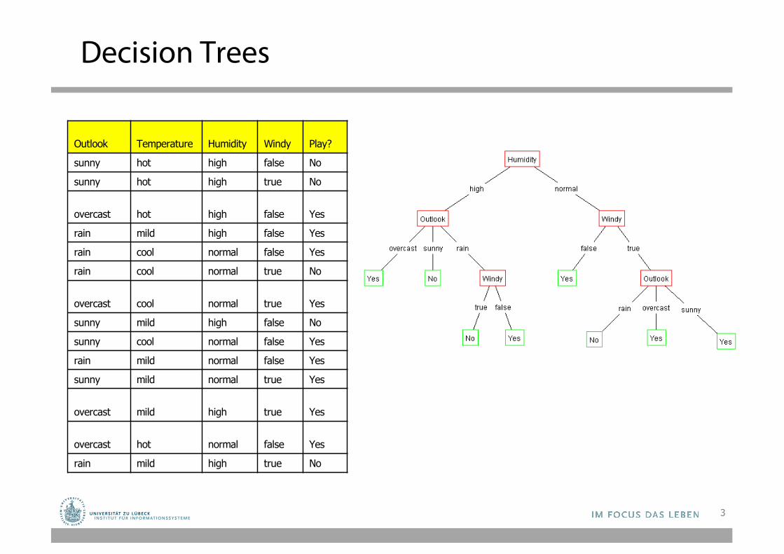
Decision Trees
Outlook Temperature Humidity Windy Play?
sunny hot high false No
sunny hot high true No
overcast hot high false Yes
rain mild high false Yes
rain cool normal false Yes
rain cool normal true No
overcast cool normal true Yes
sunny mild high false No
sunny cool normal false Yes
rain mild normal false Yes
sunny mild normal true Yes
overcast mild high true Yes
overcast hot normal false Yes
rain mild high true No
Decision trees
• An internal node is a test on an attribute.• A branch represents an outcome of the test, e.g.,
Color=red.• A leaf node represents a class label or class label
distribution.• At each node, one attribute is chosen to split training
examples into distinct classes as much as possible• A new case is classified by following a matching path to
a leaf node.
4
Building Decision Trees
• Top-down tree construction– At start, all training examples are at the root.– Partition the examples recursively by choosing one
attribute each time.
• Bottom-up tree pruning– Remove subtrees or branches, in a bottom-up manner, to
improve the estimated accuracy on new cases.
R. Quinlan, Learning efficient classification procedures, Machine Learning: an artificial intelligence approach, Michalski, Carbonell & Mitchell (eds.), Morgan Kaufmann, p. 463-482., 1983 5
6
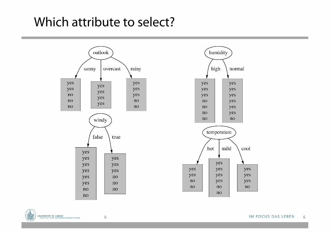
Which attribute to select?
6
7
Choosing the Best Attribute
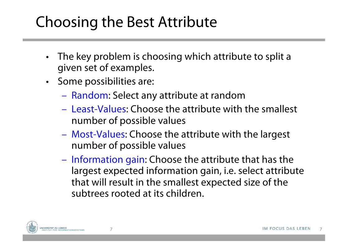
• The key problem is choosing which attribute to split a given set of examples.
• Some possibilities are:– Random: Select any attribute at random – Least-Values: Choose the attribute with the smallest
number of possible values – Most-Values: Choose the attribute with the largest
number of possible values – Information gain: Choose the attribute that has the
largest expected information gain, i.e. select attribute that will result in the smallest expected size of the subtrees rooted at its children.
7
Information Theory
8
Huffman code example
.5.5
1
.125.125
.25
A
C
B
D.25
0 1
0
0 1
1
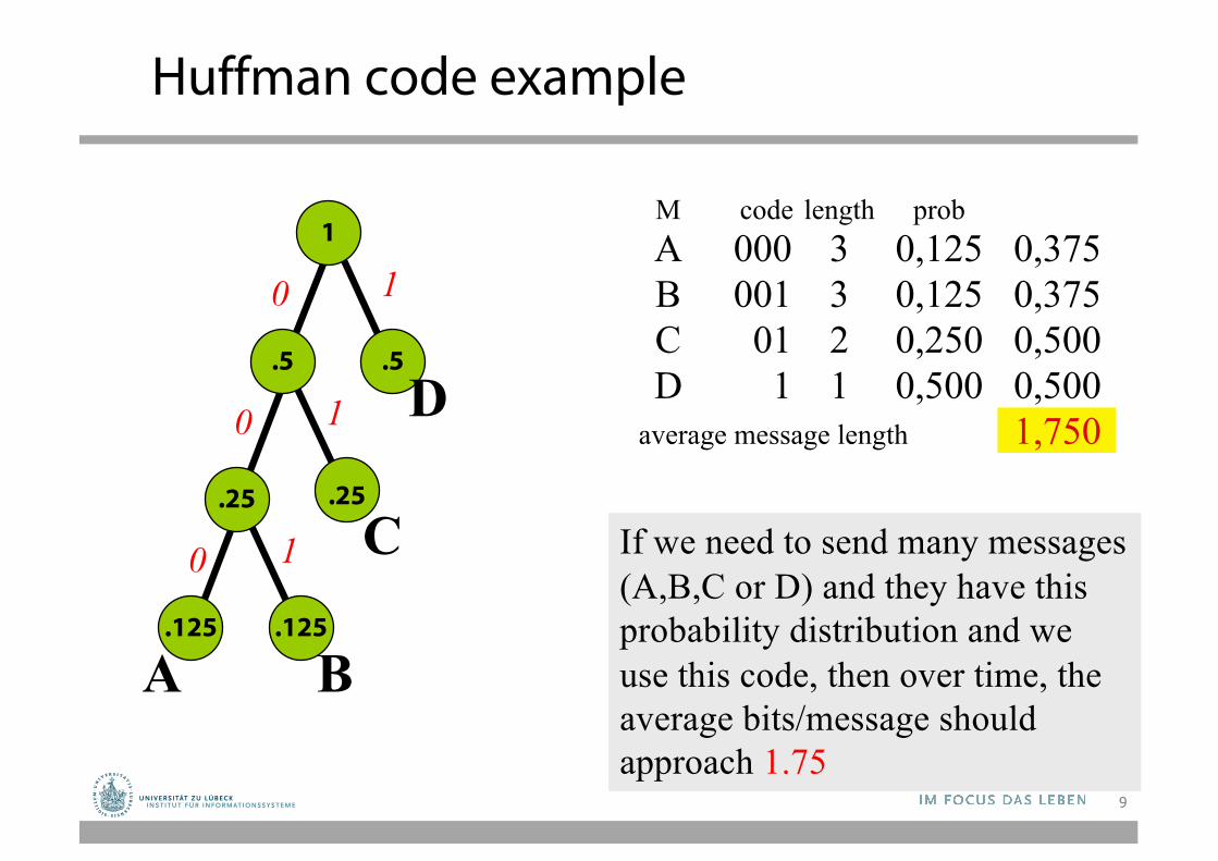
M code length probA 000 3 0,125 0,375B 001 3 0,125 0,375C 01 2 0,250 0,500D 1 1 0,500 0,500
average message length 1,750
If we need to send many messages (A,B,C or D) and they have this probability distribution and we use this code, then over time, the average bits/message should approach 1.75
9
Information Theory Background
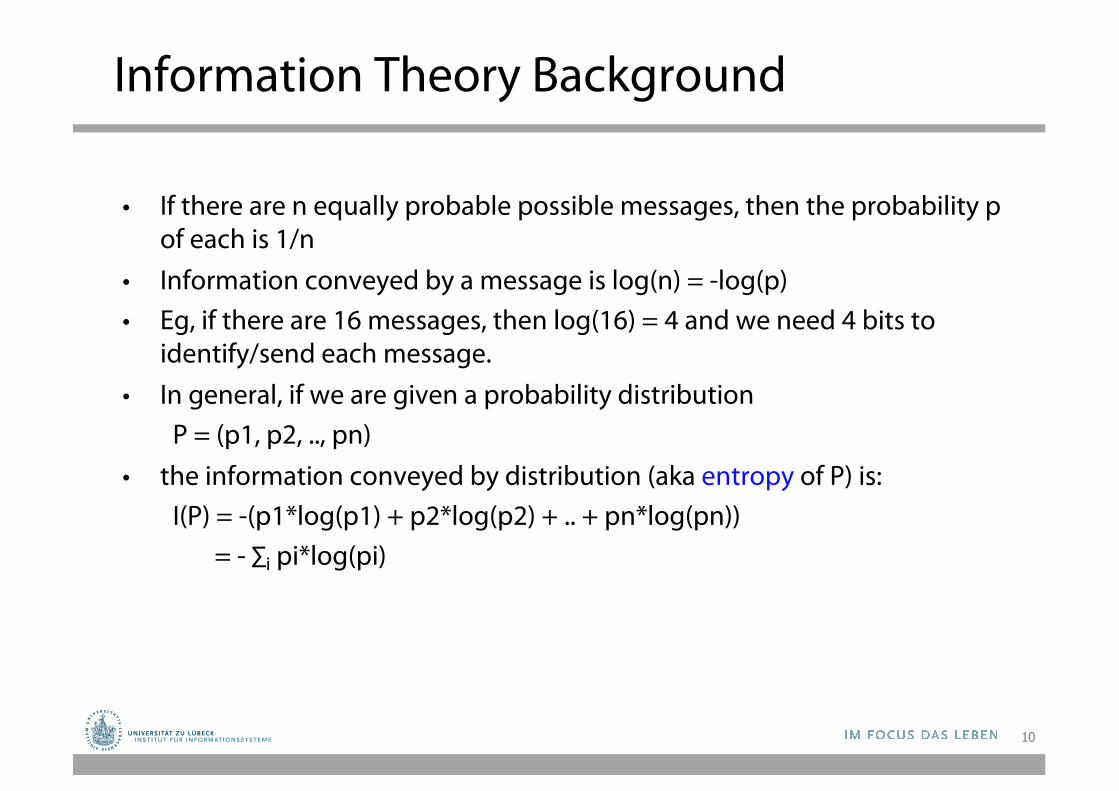
• If there are n equally probable possible messages, then the probability p of each is 1/n
• Information conveyed by a message is log(n) = -log(p)• Eg, if there are 16 messages, then log(16) = 4 and we need 4 bits to
identify/send each message.• In general, if we are given a probability distribution
P = (p1, p2, .., pn)• the information conveyed by distribution (aka entropy of P) is:
I(P) = -(p1*log(p1) + p2*log(p2) + .. + pn*log(pn))= - ∑i pi*log(pi)
10
Information Theory Background
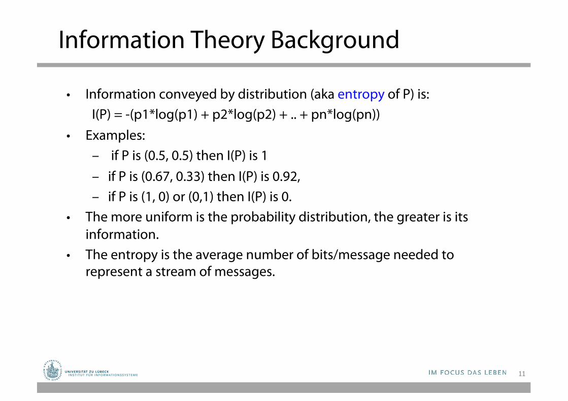
• Information conveyed by distribution (aka entropy of P) is: I(P) = -(p1*log(p1) + p2*log(p2) + .. + pn*log(pn))
• Examples:– if P is (0.5, 0.5) then I(P) is 1– if P is (0.67, 0.33) then I(P) is 0.92, – if P is (1, 0) or (0,1) then I(P) is 0.
• The more uniform is the probability distribution, the greater is its information.
• The entropy is the average number of bits/message needed to represent a stream of messages.
11
12
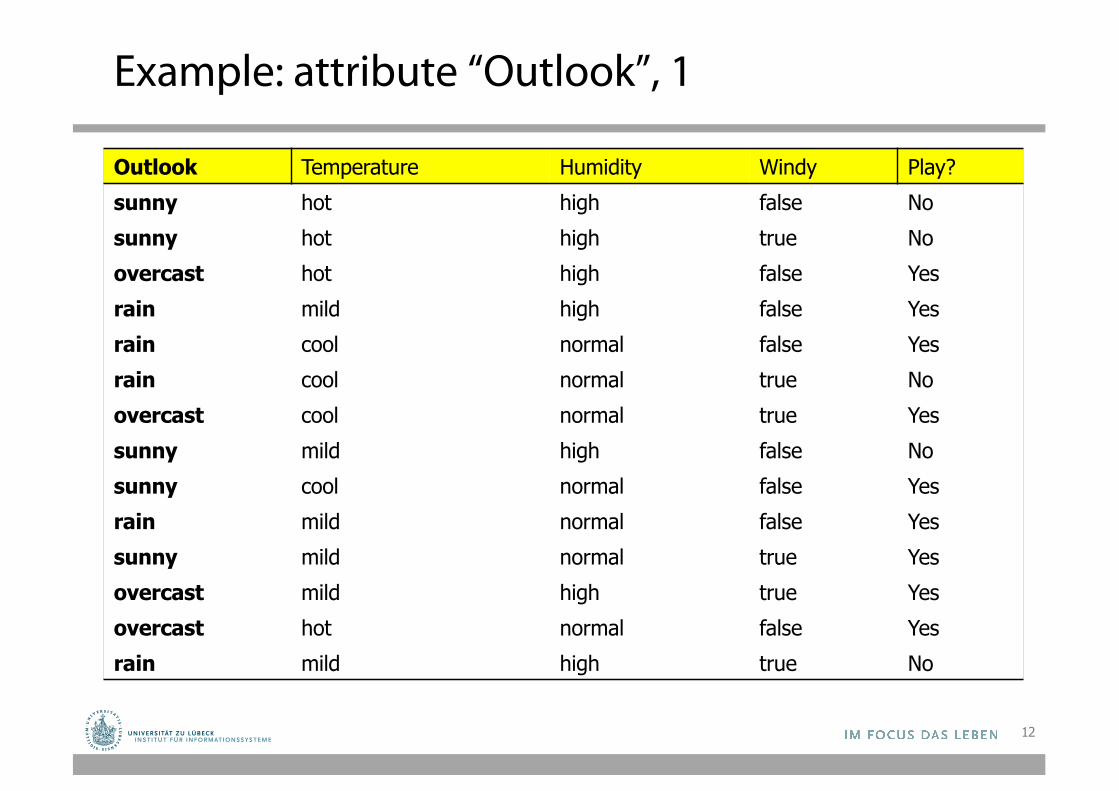
Example: attribute “Outlook”, 1
Outlook Temperature Humidity Windy Play?sunny hot high false Nosunny hot high true Noovercast hot high false Yesrain mild high false Yesrain cool normal false Yesrain cool normal true Noovercast cool normal true Yessunny mild high false Nosunny cool normal false Yesrain mild normal false Yessunny mild normal true Yesovercast mild high true Yesovercast hot normal false Yesrain mild high true No
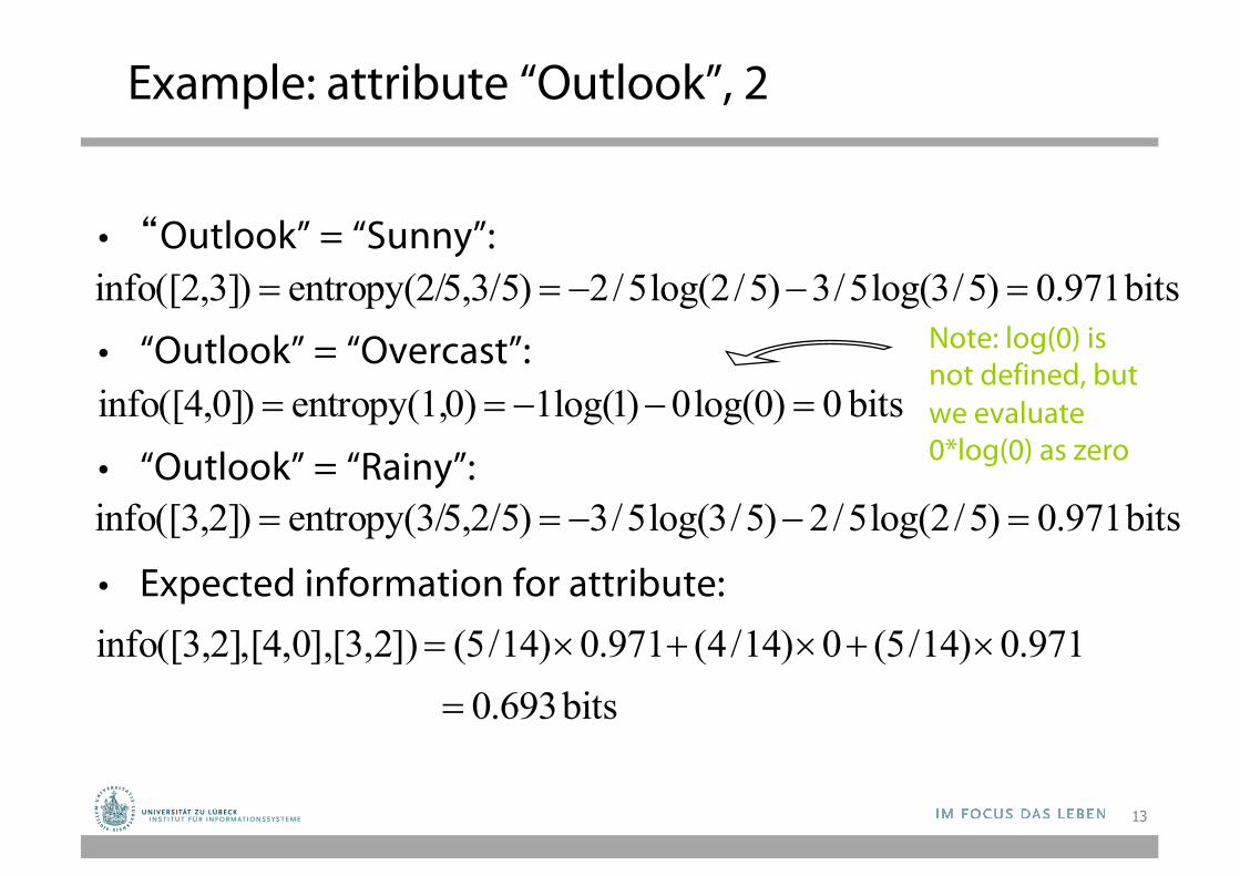
Example: attribute “Outlook”, 2
• “Outlook” = “Sunny”:
• “Outlook” = “Overcast”:
• “Outlook” = “Rainy”:
• Expected information for attribute:
bits 971.0)5/3log(5/3)5/2log(5/25,3/5)entropy(2/)info([2,3] =--==
bits 0)0log(0)1log(10)entropy(1,)info([4,0] =--==
bits 971.0)5/2log(5/2)5/3log(5/35,2/5)entropy(3/)info([3,2] =--==
Note: log(0) is not defined, but we evaluate 0*log(0) as zero
971.0)14/5(0)14/4(971.0)14/5([3,2])[4,0],,info([3,2] ´+´+´=
bits 693.0=
13
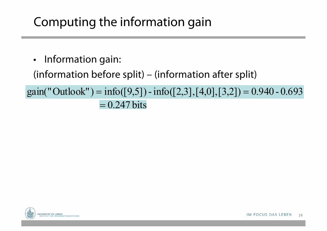
Computing the information gain
• Information gain: (information before split) – (information after split)
0.693-0.940[3,2])[4,0],,info([2,3]-)info([9,5])Outlook"gain(" ==bits 247.0=
14
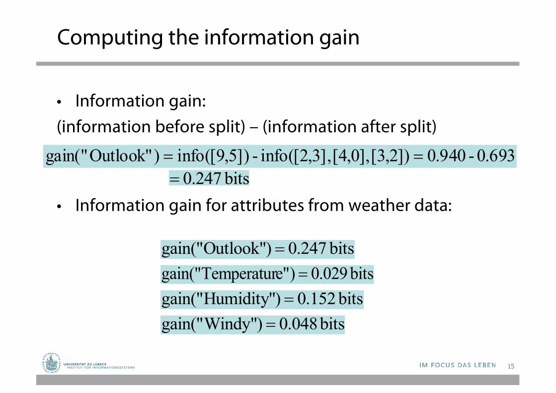
Computing the information gain
• Information gain: (information before split) – (information after split)
• Information gain for attributes from weather data:
0.693-0.940[3,2])[4,0],,info([2,3]-)info([9,5])Outlook"gain(" ==bits 247.0=
bits 247.0)Outlook"gain(" =bits 029.0)e"Temperaturgain(" =
bits 152.0)Humidity"gain(" =bits 048.0)Windy"gain(" =
15
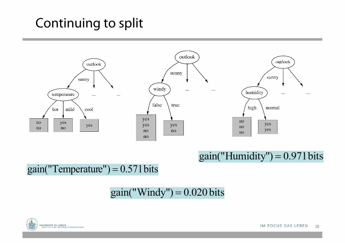
Continuing to split
bits 571.0)e"Temperaturgain(" =bits 971.0)Humidity"gain(" =
bits 020.0)Windy"gain(" =
16
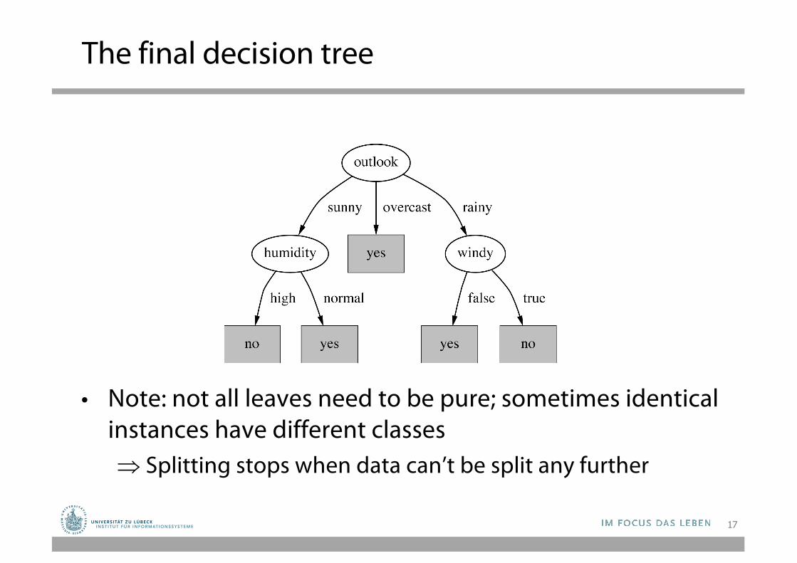
The final decision tree
• Note: not all leaves need to be pure; sometimes identical instances have different classesÞ Splitting stops when data can’t be split any further
17
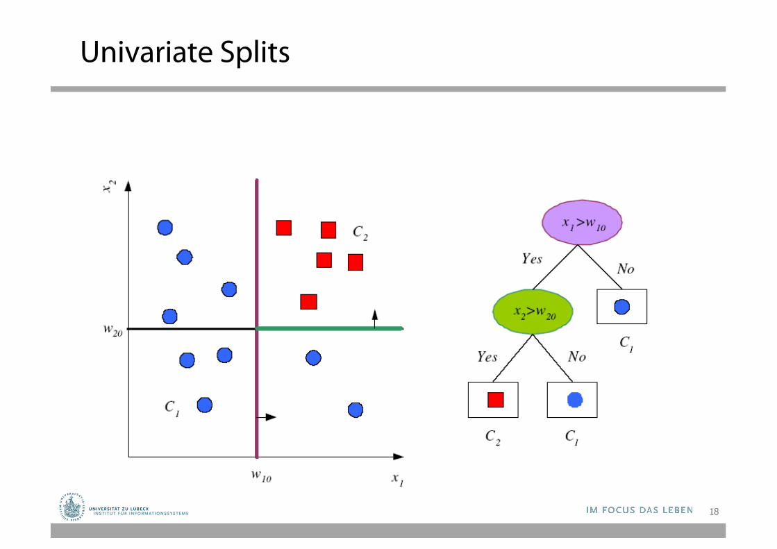
Univariate Splits
18
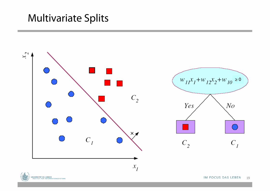
Multivariate Splits
19
≥ 0
1R – Simplicity First!
20
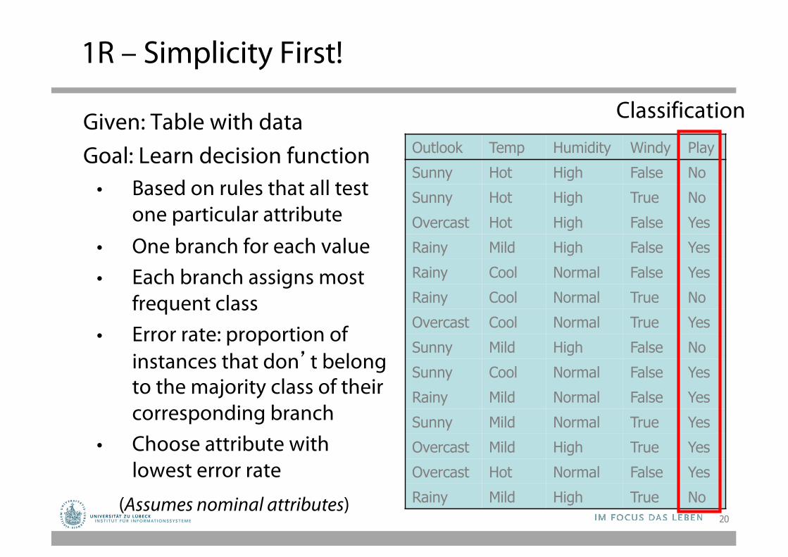
Outlook Temp Humidity Windy PlaySunny Hot High False NoSunny Hot High True NoOvercast Hot High False YesRainy Mild High False YesRainy Cool Normal False YesRainy Cool Normal True NoOvercast Cool Normal True YesSunny Mild High False NoSunny Cool Normal False YesRainy Mild Normal False YesSunny Mild Normal True YesOvercast Mild High True YesOvercast Hot Normal False YesRainy Mild High True No
ClassificationGiven: Table with dataGoal: Learn decision function
• Based on rules that all test one particular attribute
• One branch for each value• Each branch assigns most
frequent class• Error rate: proportion of
instances that don’t belong to the majority class of their corresponding branch
• Choose attribute with lowest error rate
(Assumes nominal attributes)
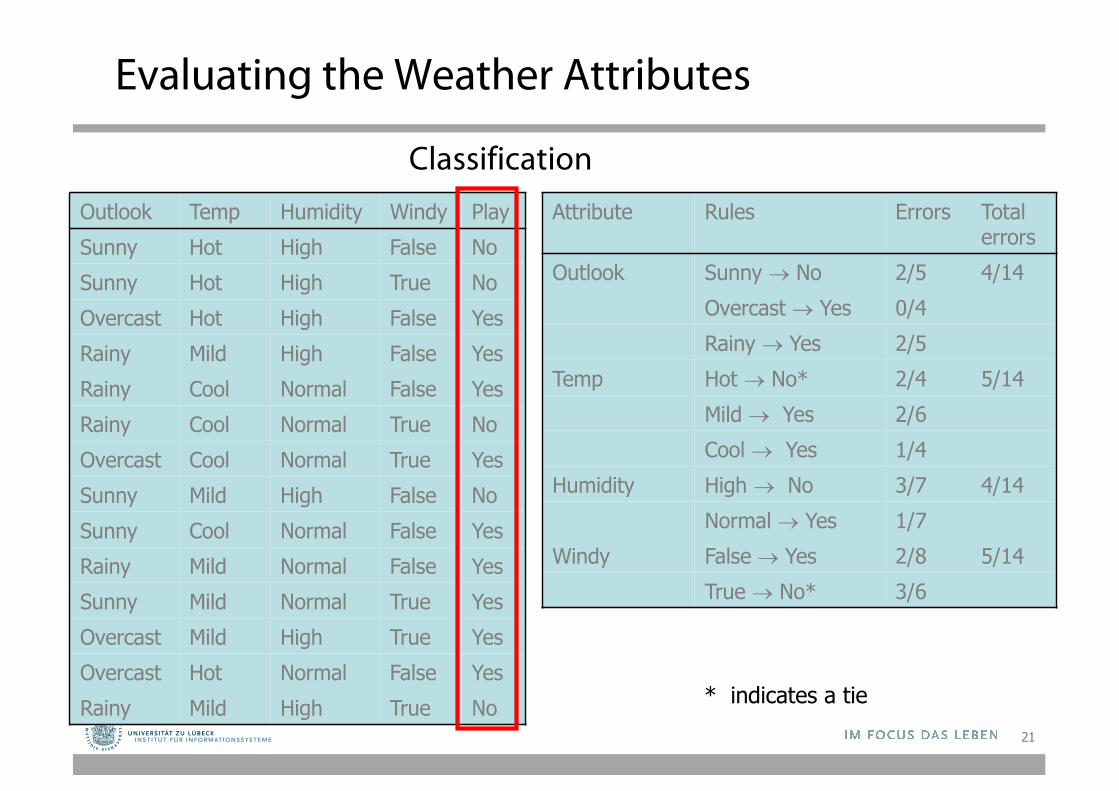
Evaluating the Weather Attributes
Attribute Rules Errors Total errors
Outlook Sunny ® No 2/5 4/14Overcast ® Yes 0/4Rainy ® Yes 2/5
Temp Hot ® No* 2/4 5/14Mild ® Yes 2/6Cool ® Yes 1/4
Humidity High ® No 3/7 4/14Normal ® Yes 1/7
Windy False ® Yes 2/8 5/14True ® No* 3/6
Outlook Temp Humidity Windy PlaySunny Hot High False NoSunny Hot High True NoOvercast Hot High False YesRainy Mild High False YesRainy Cool Normal False YesRainy Cool Normal True NoOvercast Cool Normal True YesSunny Mild High False NoSunny Cool Normal False YesRainy Mild Normal False YesSunny Mild Normal True YesOvercast Mild High True YesOvercast Hot Normal False YesRainy Mild High True No * indicates a tie
Classification
21
Assessing Performance of a Learning Algorithm
• Take out some of the training set– Train on the remaining training set– Test on the excluded instances– Cross-validation
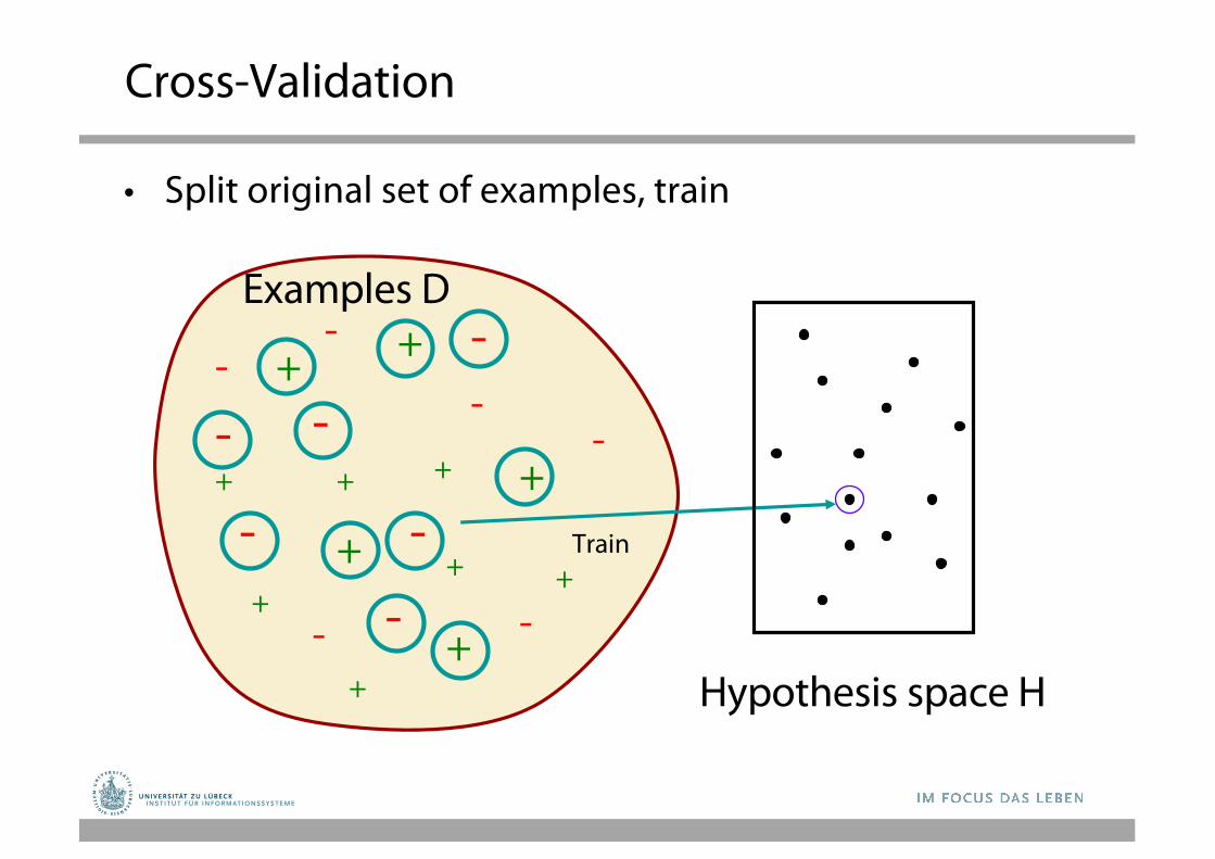
Cross-Validation
• Split original set of examples, train
+
+
+
+
++
+
-
-
-
--
-
+
+
+
+
+
-
-
-
-
-
-Hypothesis space H
Train
Examples D
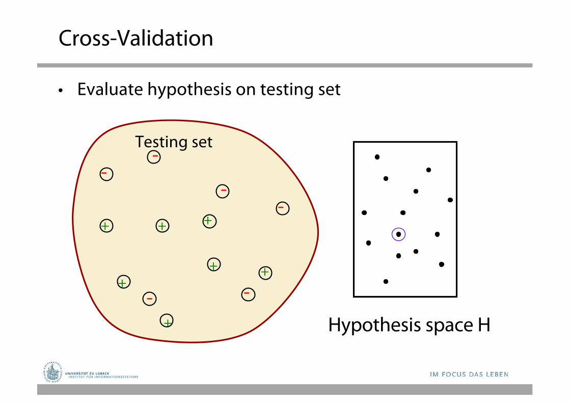
Cross-Validation
• Evaluate hypothesis on testing set
+
+
+
+
++
+
-
-
-
--
-
Hypothesis space H
Testing set
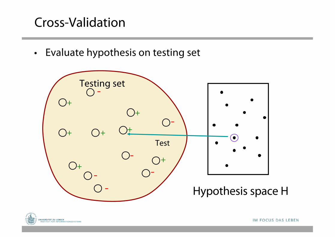
Cross-Validation
• Evaluate hypothesis on testing set
Hypothesis space H
Testing set
++
++
+
--
-
-
-
-
++
Test
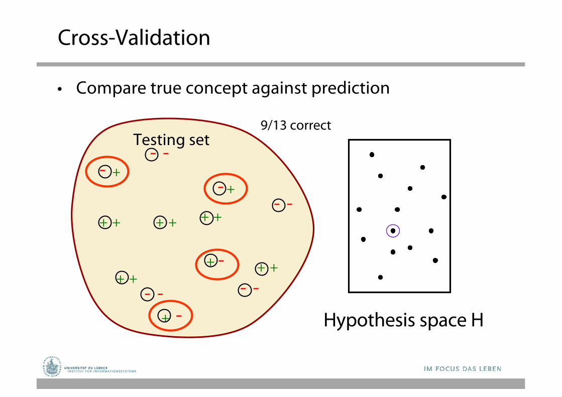
Cross-Validation
• Compare true concept against prediction
+
+
+
+
++
+
-
-
-
--
-
Hypothesis space H
Testing set
++
++
+
--
-
-
-
-
++
9/13 correct
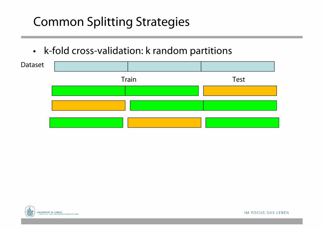
Common Splitting Strategies
• k-fold cross-validation: k random partitions
Train Test
Dataset
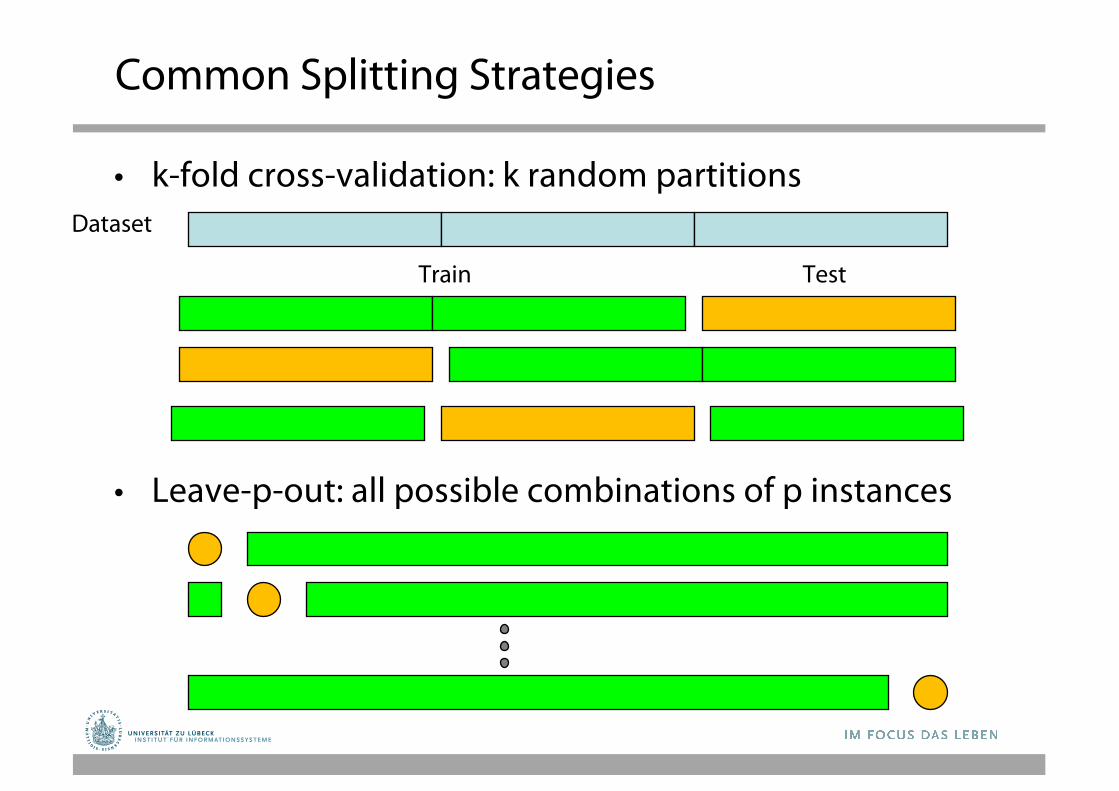
Common Splitting Strategies
• k-fold cross-validation: k random partitions
• Leave-p-out: all possible combinations of p instances
Train Test
Dataset
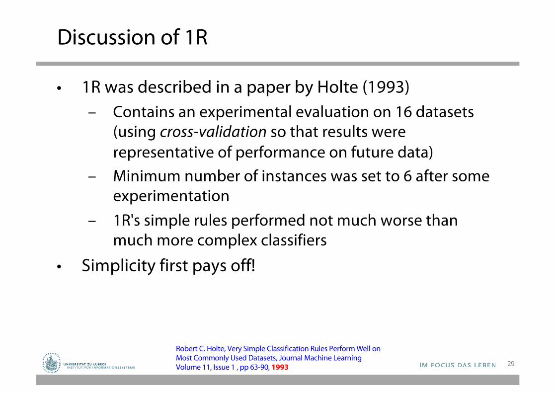
Discussion of 1R
• 1R was described in a paper by Holte (1993)– Contains an experimental evaluation on 16 datasets
(using cross-validation so that results were representative of performance on future data)
– Minimum number of instances was set to 6 after some experimentation
– 1R's simple rules performed not much worse than much more complex classifiers
• Simplicity first pays off!
29
Robert C. Holte, Very Simple Classification Rules Perform Well on Most Commonly Used Datasets, Journal Machine Learning Volume 11, Issue 1 , pp 63-90, 1993
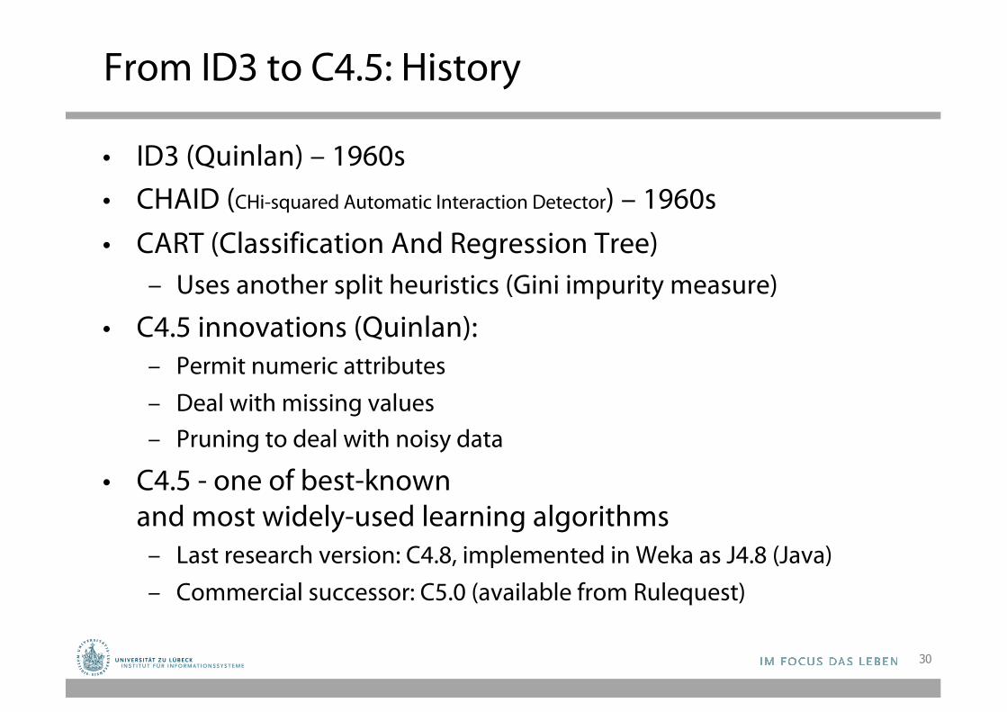
From ID3 to C4.5: History
• ID3 (Quinlan) – 1960s• CHAID (CHi-squared Automatic Interaction Detector) – 1960s• CART (Classification And Regression Tree)
– Uses another split heuristics (Gini impurity measure)
• C4.5 innovations (Quinlan):– Permit numeric attributes– Deal with missing values– Pruning to deal with noisy data
• C4.5 - one of best-known and most widely-used learning algorithms
– Last research version: C4.8, implemented in Weka as J4.8 (Java)– Commercial successor: C5.0 (available from Rulequest)
30
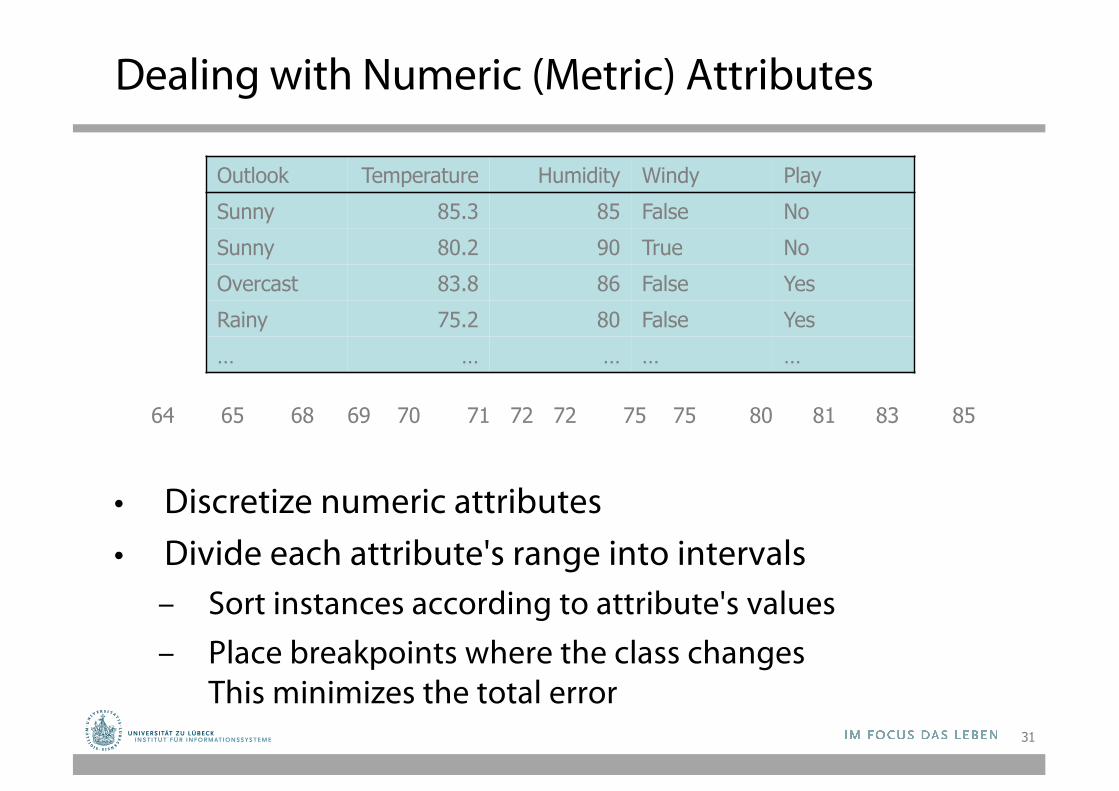
Dealing with Numeric (Metric) Attributes
• Discretize numeric attributes• Divide each attribute's range into intervals
– Sort instances according to attribute's values– Place breakpoints where the class changes
This minimizes the total error
64 65 68 69 70 71 72 72 75 75 80 81 83 85Yes | No | Yes Yes Yes | No No | Yes Yes Yes | No | Yes Yes | No
31
Outlook Temperature Humidity Windy PlaySunny 85.3 85 False NoSunny 80.2 90 True NoOvercast 83.8 86 False YesRainy 75.2 80 False Yes… … … … …
The problem of Overfitting
• This procedure is very sensitive to noise– One instance with an incorrect class label will probably
produce a separate interval• Also: time stamp attribute will have zero errors• Simple solution:
enforce minimum number of instances in majority class per interval
32
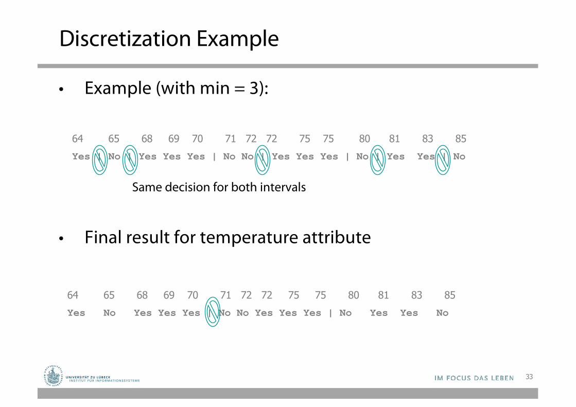
Discretization Example
• Example (with min = 3):
• Final result for temperature attribute
33
64 65 68 69 70 71 72 72 75 75 80 81 83 85Yes | No | Yes Yes Yes | No No | Yes Yes Yes | No | Yes Yes | No
64 65 68 69 70 71 72 72 75 75 80 81 83 85Yes No Yes Yes Yes | No No Yes Yes Yes | No Yes Yes No
Same decision for both intervals
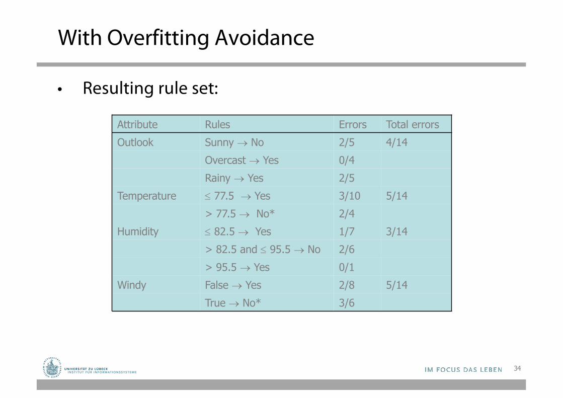
With Overfitting Avoidance
• Resulting rule set:
34
Attribute Rules Errors Total errorsOutlook Sunny ® No 2/5 4/14
Overcast ® Yes 0/4Rainy ® Yes 2/5
Temperature £ 77.5 ® Yes 3/10 5/14> 77.5 ® No* 2/4
Humidity £ 82.5 ® Yes 1/7 3/14> 82.5 and £ 95.5 ® No 2/6> 95.5 ® Yes 0/1
Windy False ® Yes 2/8 5/14True ® No* 3/6
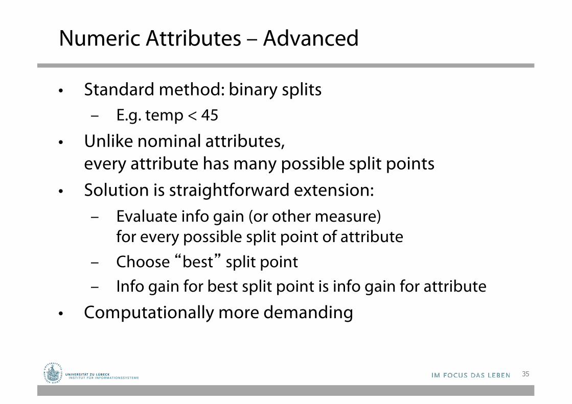
Numeric Attributes – Advanced
• Standard method: binary splits– E.g. temp < 45
• Unlike nominal attributes,every attribute has many possible split points
• Solution is straightforward extension: – Evaluate info gain (or other measure)
for every possible split point of attribute– Choose “best” split point– Info gain for best split point is info gain for attribute
• Computationally more demanding
35
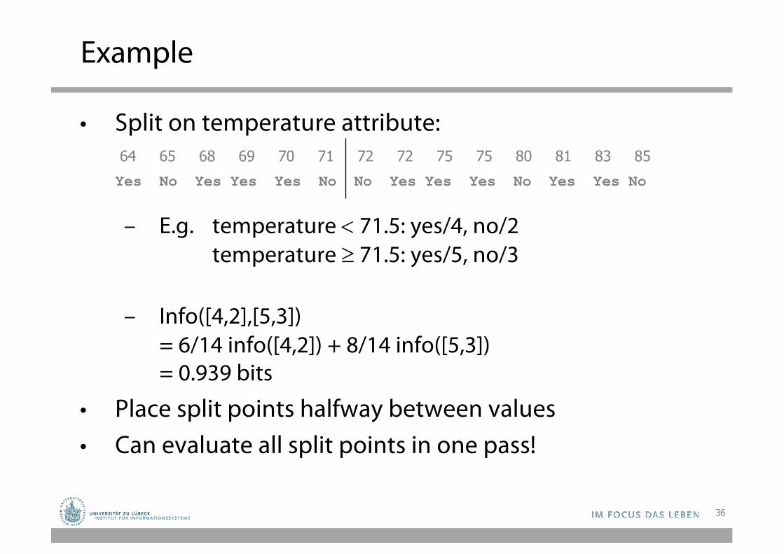
Example
• Split on temperature attribute:
– E.g. temperature < 71.5: yes/4, no/2temperature ³ 71.5: yes/5, no/3
– Info([4,2],[5,3])= 6/14 info([4,2]) + 8/14 info([5,3]) = 0.939 bits
• Place split points halfway between values• Can evaluate all split points in one pass!
36
64 65 68 69 70 71 72 72 75 75 80 81 83 85Yes No Yes Yes Yes No No Yes Yes Yes No Yes Yes No
Missing as a Separate Value
• Missing value denoted “?” in C4.X (Null value)• Simple idea: treat missing as a separate value• Q: When is this not appropriate?• A: When values are missing due to different reasons
– Example 1: blood sugar value could be missing when it is very high or very low
– Example 2: field IsPregnant missing for a male patient should be treated differently (no) than for a female patient of age 25 (unknown)
37
Missing Values – Advanced
Questions:- How should tests on attributes with different unknown
values be handled?- How should the partitioning be done in case of examples
with unknown values?- How should an unseen case with missing values be
handled?
38
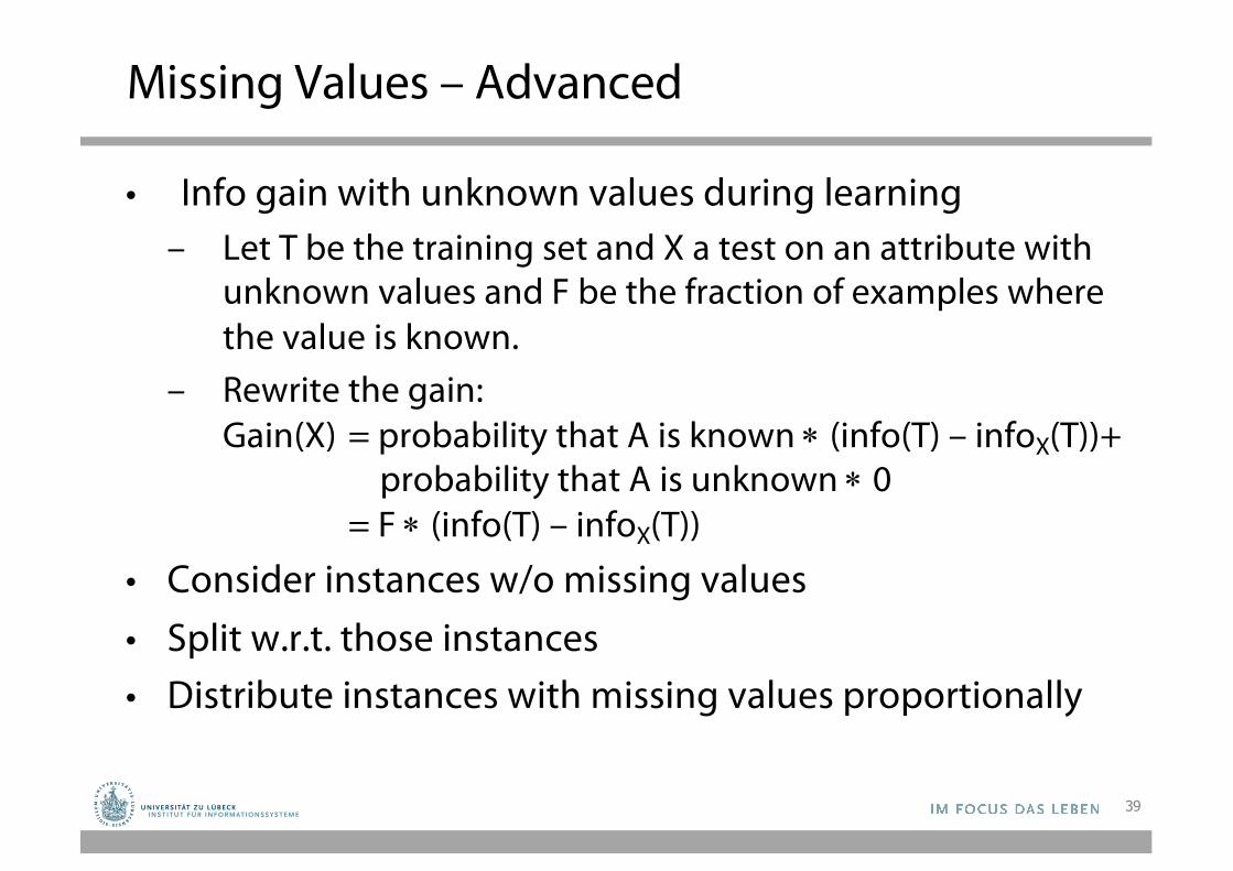
Missing Values – Advanced
• Info gain with unknown values during learning– Let T be the training set and X a test on an attribute with
unknown values and F be the fraction of examples where the value is known.
– Rewrite the gain:Gain(X) = probability that A is known * (info(T) – infoX(T))+
probability that A is unknown * 0= F * (info(T) – infoX(T))
• Consider instances w/o missing values• Split w.r.t. those instances• Distribute instances with missing values proportionally
39
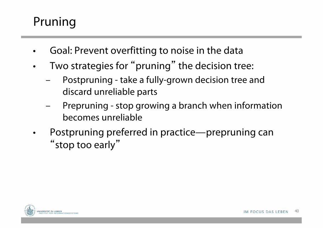
Pruning
• Goal: Prevent overfitting to noise in the data• Two strategies for “pruning” the decision tree:
– Postpruning - take a fully-grown decision tree and discard unreliable parts
– Prepruning - stop growing a branch when information becomes unreliable
• Postpruning preferred in practice—prepruning can “stop too early”
40
Post-pruning
• First, build full tree• Then, prune it
– Fully-grown tree shows all attribute interactions
→ Expected Error Pruning
44
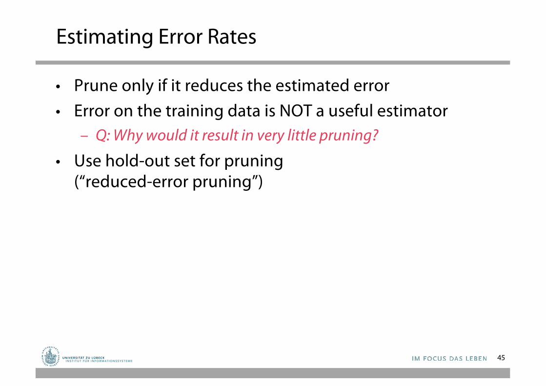
Estimating Error Rates
• Prune only if it reduces the estimated error• Error on the training data is NOT a useful estimator
– Q: Why would it result in very little pruning?
• Use hold-out set for pruning (“reduced-error pruning”)
45
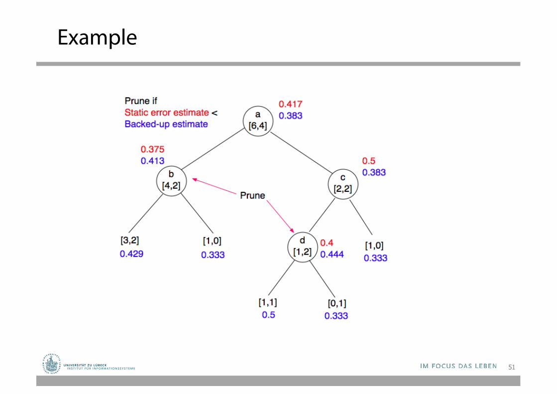
Expected Error Pruning
• Approximate expected error assuming that we prune at a particular node.
• Approximate backed-up error from children assuming we did not prune.
• If expected error is less than backed-up error, prune.
46
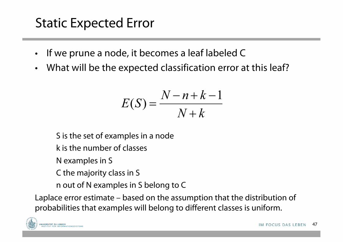
Static Expected Error
• If we prune a node, it becomes a leaf labeled C• What will be the expected classification error at this leaf?
S is the set of examples in a nodek is the number of classesN examples in SC the majority class in Sn out of N examples in S belong to C
Laplace error estimate – based on the assumption that the distribution of probabilities that examples will belong to different classes is uniform.
47
kNknNSE
+-+-
=1)(
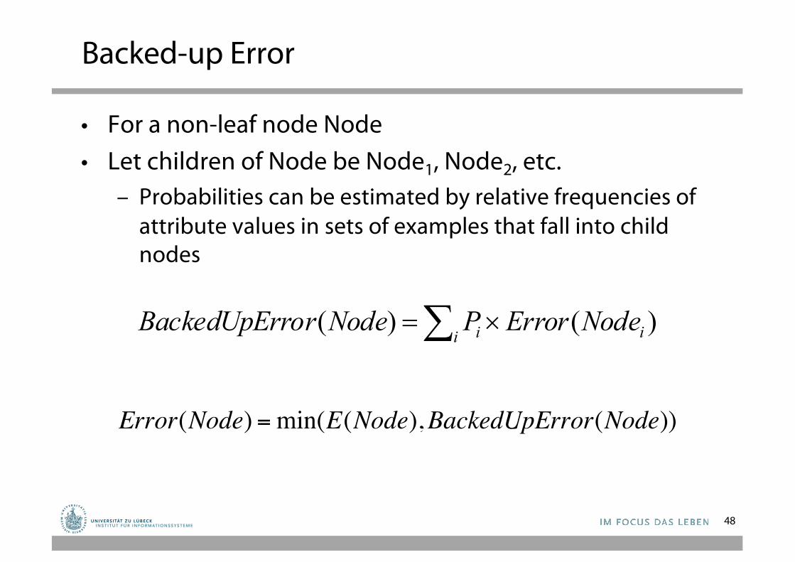
Backed-up Error
• For a non-leaf node Node• Let children of Node be Node1, Node2, etc.
– Probabilities can be estimated by relative frequencies of attribute values in sets of examples that fall into child nodes
48
)()( ii i NodeErrorPNoderorBackedUpEr ´=å
Error(Node) =min(E(Node),BackedUpError(Node))
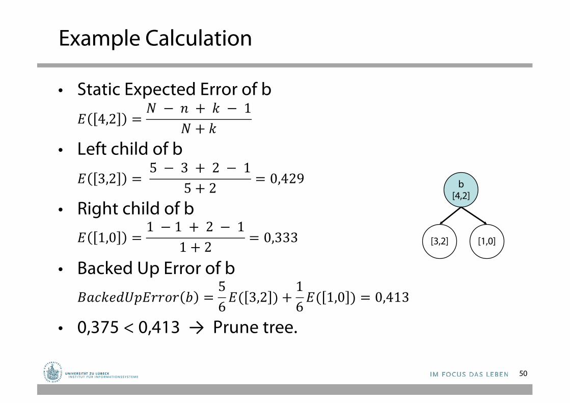
Example Calculation
• Static Expected Error of b
𝐸 4,2 =𝑁 − 𝑛 + 𝑘 − 1
𝑁 + 𝑘 =6 − 4 + 2 − 1
6 + 2 = 0,375
• Left child of b
𝐸 3,2 = 5 − 3 + 2 − 1
5 + 2 = 0,429
• Right child of b
𝐸 1,0 =1 − 1 + 2 − 1
1 + 2 = 0,333
• Backed Up Error of b
𝐵𝑎𝑐𝑘𝑒𝑑𝑈𝑝𝐸𝑟𝑟𝑜𝑟 𝑏 =56𝐸( 3,2 ) +
16𝐸( 1,0 ) = 0,413
• 0,375 < 0,413 → Prune tree.
50
b[4,2]
[3,2] [1,0]
Example
51
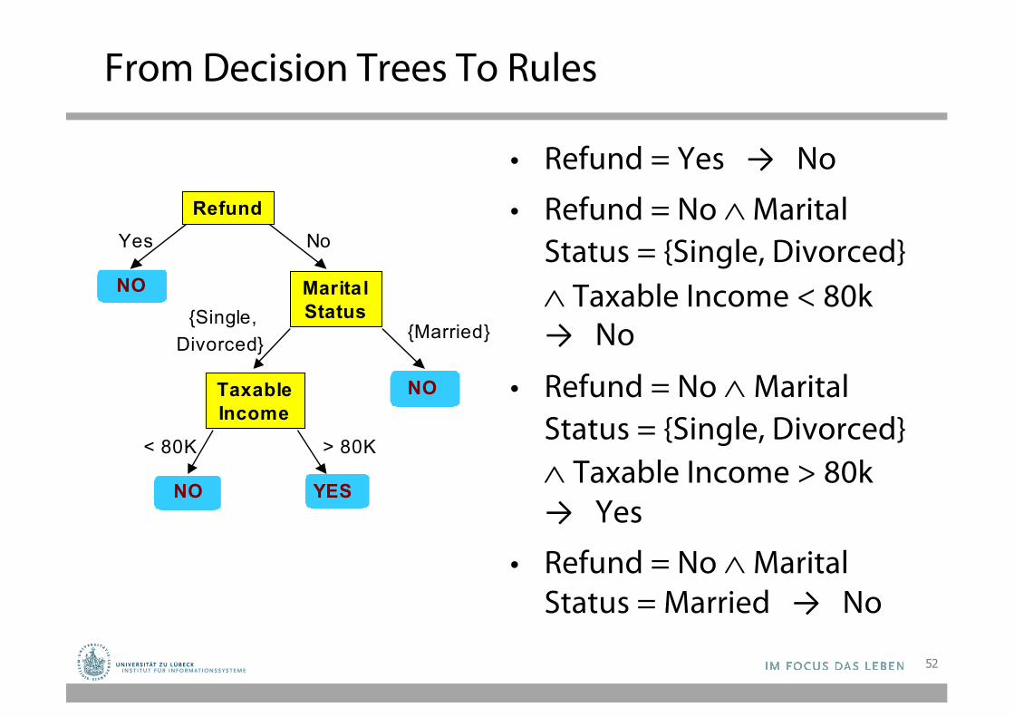
From Decision Trees To Rules
• Refund = Yes → No
• Refund = No ÙMarital Status = {Single, Divorced}Ù Taxable Income < 80k → No
• Refund = No ÙMarital Status = {Single, Divorced}Ù Taxable Income > 80k → Yes
• Refund = No ÙMarital Status = Married → No
52
YESYESNONO
NONO
NONO
Yes No
{Married}{Single,
Divorced}
< 80K > 80K
Taxable Income
Marital Status
Refund
From Decision Trees to Rules
• Derive a rule set from a decision tree: Write a rule for each path from the root to a leaf. – The left-hand side is easily built from the label of the
nodes and the labels of the arcs.
• Rules are mutually exclusive and exhaustive.• Rule set contains as much information as the tree
53
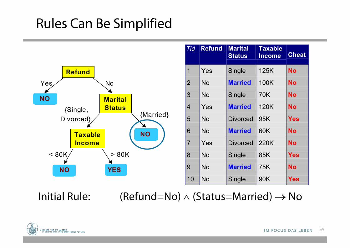
Rules Can Be Simplified
54
Tid Refund Marital Status
Taxable Income Cheat
1 Yes Single 125K No
2 No Married 100K No
3 No Single 70K No
4 Yes Married 120K No
5 No Divorced 95K Yes
6 No Married 60K No
7 Yes Divorced 220K No
8 No Single 85K Yes
9 No Married 75K No
10 No Single 90K Yes 10
Initial Rule: (Refund=No) Ù (Status=Married) ® NoSimplified Rule: (Status=Married) ® No
YESYESNONO
NONO
NONO
Yes No
{Married}{Single,
Divorced}
< 80K > 80K
Taxable Income
Marital Status
Refund
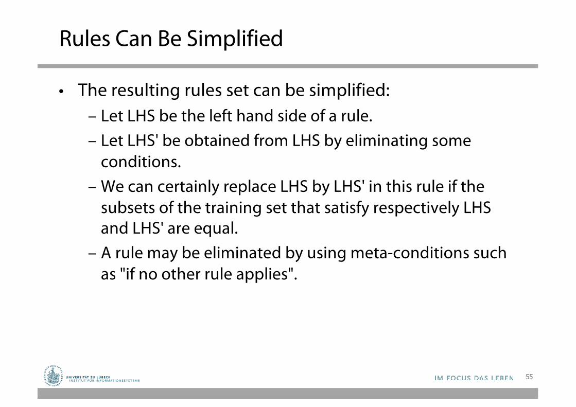
Rules Can Be Simplified
• The resulting rules set can be simplified:– Let LHS be the left hand side of a rule. – Let LHS' be obtained from LHS by eliminating some
conditions. – We can certainly replace LHS by LHS' in this rule if the
subsets of the training set that satisfy respectively LHS and LHS' are equal.
– A rule may be eliminated by using meta-conditions such as "if no other rule applies".
55
Incremental Inductive Learning
56
Chapter 19
Slides for Ch. 19 by J.C. Latombe
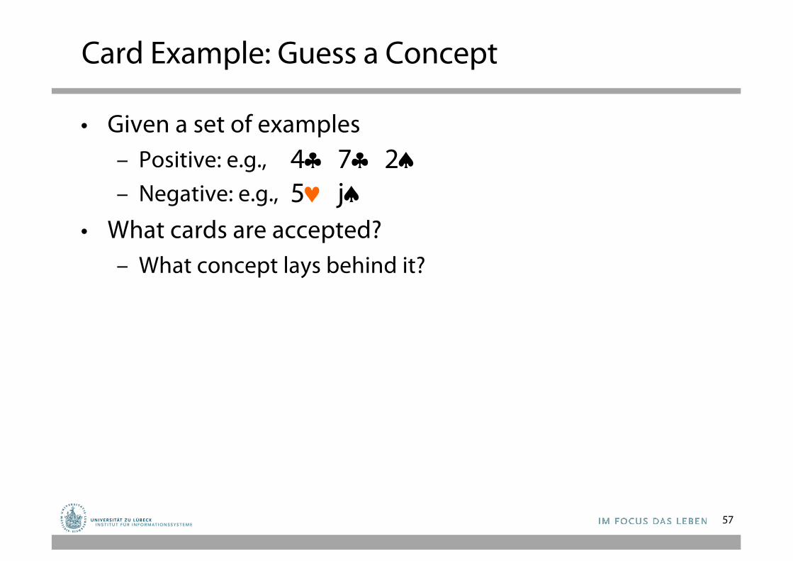
Card Example: Guess a Concept
• Given a set of examples– Positive: e.g.,– Negative: e.g.,
• What cards are accepted?– What concept lays behind it?
57
4§ 7§ 2ª5© jª
Card Example: Guess a Concept
58
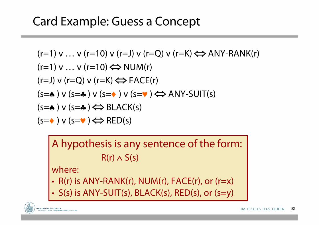
(r=1) v … v (r=10) v (r=J) v (r=Q) v (r=K) Û ANY-RANK(r)(r=1) v … v (r=10) ÛNUM(r) (r=J) v (r=Q) v (r=K) Û FACE(r)(s=ª) v (s=§) v (s=¨) v (s=©) Û ANY-SUIT(s)(s=ª) v (s=§) Û BLACK(s)(s=¨) v (s=©) Û RED(s)
A hypothesis is any sentence of the form:R(r) Ù S(s)
where:• R(r) is ANY-RANK(r), NUM(r), FACE(r), or (r=x)• S(s) is ANY-SUIT(s), BLACK(s), RED(s), or (s=y)
Simplified Representation
59
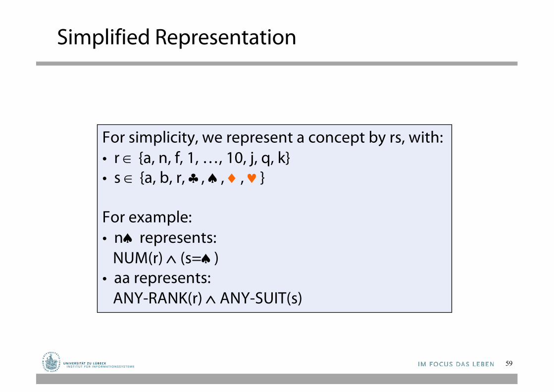
For simplicity, we represent a concept by rs, with:• r Î {a, n, f, 1, …, 10, j, q, k}• s Î {a, b, r, §, ª, ¨, ©}
For example:• nª represents:
NUM(r) Ù (s=ª)• aa represents:
ANY-RANK(r) Ù ANY-SUIT(s)
Extension of a Hypothesis
60
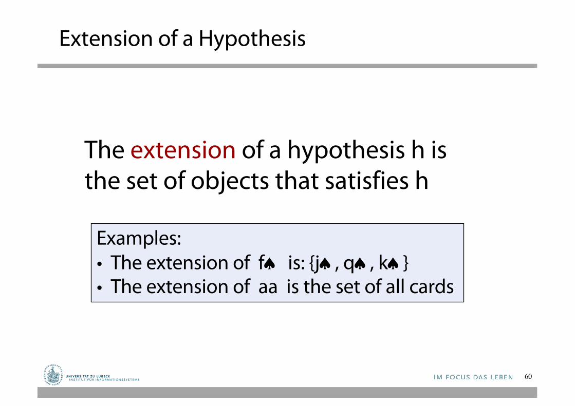
The extension of a hypothesis h is the set of objects that satisfies h
Examples: • The extension of fª is: {jª, qª, kª}• The extension of aa is the set of all cards
More General/Specific Relation
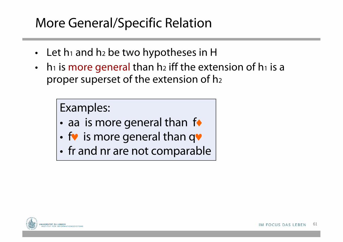
• Let h1 and h2 be two hypotheses in H• h1 is more general than h2 iff the extension of h1 is a
proper superset of the extension of h2
61
Examples: • aa is more general than f¨• f© is more general than q©• fr and nr are not comparable
More General/Specific Relation
• Let h1 and h2 be two hypotheses in H• h1 is more general than h2 iff the extension of h1 is a
proper superset of the extension of h2
• The inverse of the “more general” relation is the “more specific” relation
• The “more general” relation defines a partial orderingon the hypotheses in H
62
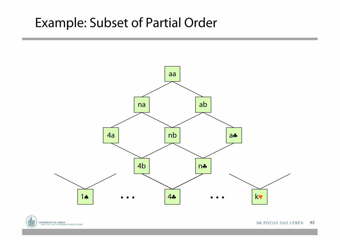
Example: Subset of Partial Order
63
aa
na ab
nb
n§
4§
4b
a§4a
1ª k©… …
G-Boundary / S-Boundary of V
64
• A hypothesis in V is most generaliff no hypothesis in V is more general
• G-boundary G of V: Set of most general hypotheses in V
G-Boundary / S-Boundary of V
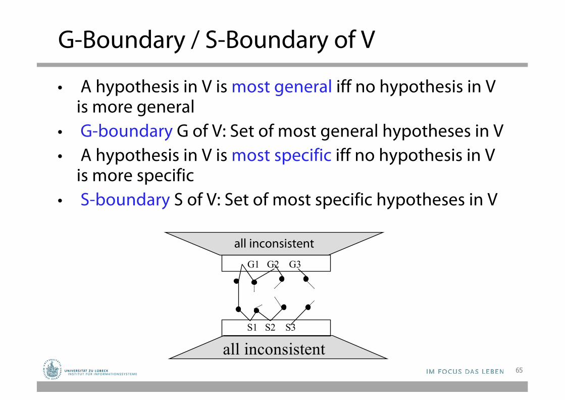
• A hypothesis in V is most general iff no hypothesis in V is more general
• G-boundary G of V: Set of most general hypotheses in V• A hypothesis in V is most specific iff no hypothesis in V
is more specific• S-boundary S of V: Set of most specific hypotheses in V
65
all inconsistent
all inconsistent
G1 G2 G3
S1 S2 S3
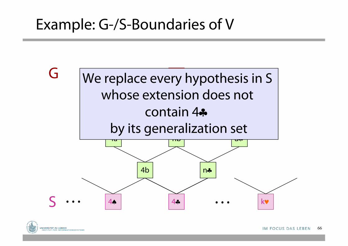
Example: G-/S-Boundaries of V
66
aa
na ab
nb
n§
4§
4b
a§4a
aa
4§ k©… …
Now suppose that 4§ is given as a positive example
S
G We replace every hypothesis in S whose extension does not
contain 4§by its generalization set
4ª
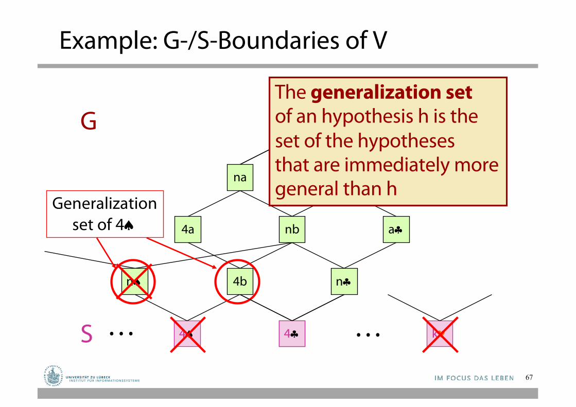
Example: G-/S-Boundaries of V
67
aa
na ab
nb
n§
4§
4b
a§4a
aa
S
G
4ª
Generalizationset of 4ª
The generalization setof an hypothesis h is theset of the hypotheses that are immediately moregeneral than h
nª
4§ k©… …
Example: G-/S-Boundaries of V
68
aa
na ab
nb
n§
4§
4b
a§4a
aa
S
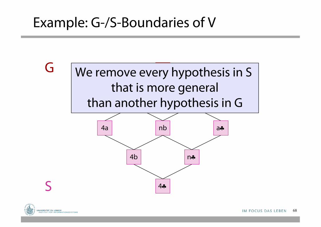
G We remove every hypothesis in S that is more general
than another hypothesis in G
Example: G-/S-Boundaries of V
69
aa
na ab
nb
n§
4§
4b
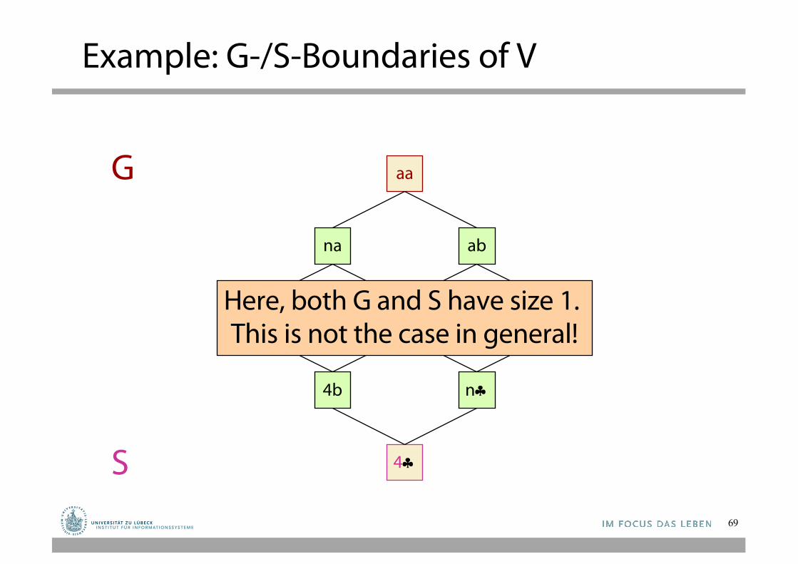
a§4aHere, both G and S have size 1. This is not the case in general!
S
G
Example: G-/S-Boundaries of V
70
aa
na ab
nb
n§
4§
4b
a§4a
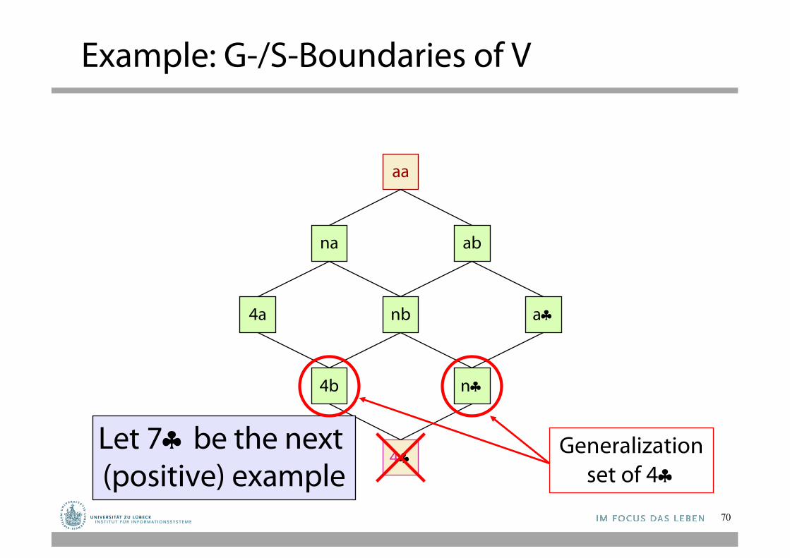
Let 7§ be the next (positive) example
Generalizationset of 4§
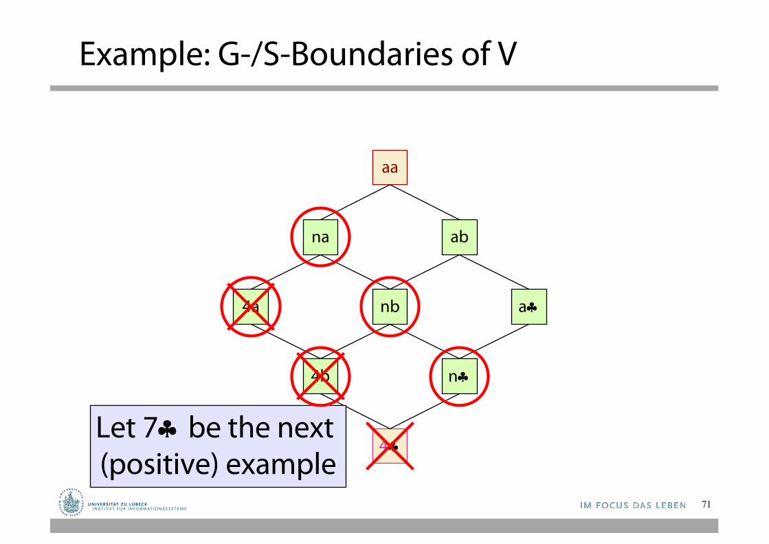
Example: G-/S-Boundaries of V
71
aa
na ab
nb
n§
4§
4b
a§4a
Let 7§ be the next (positive) example
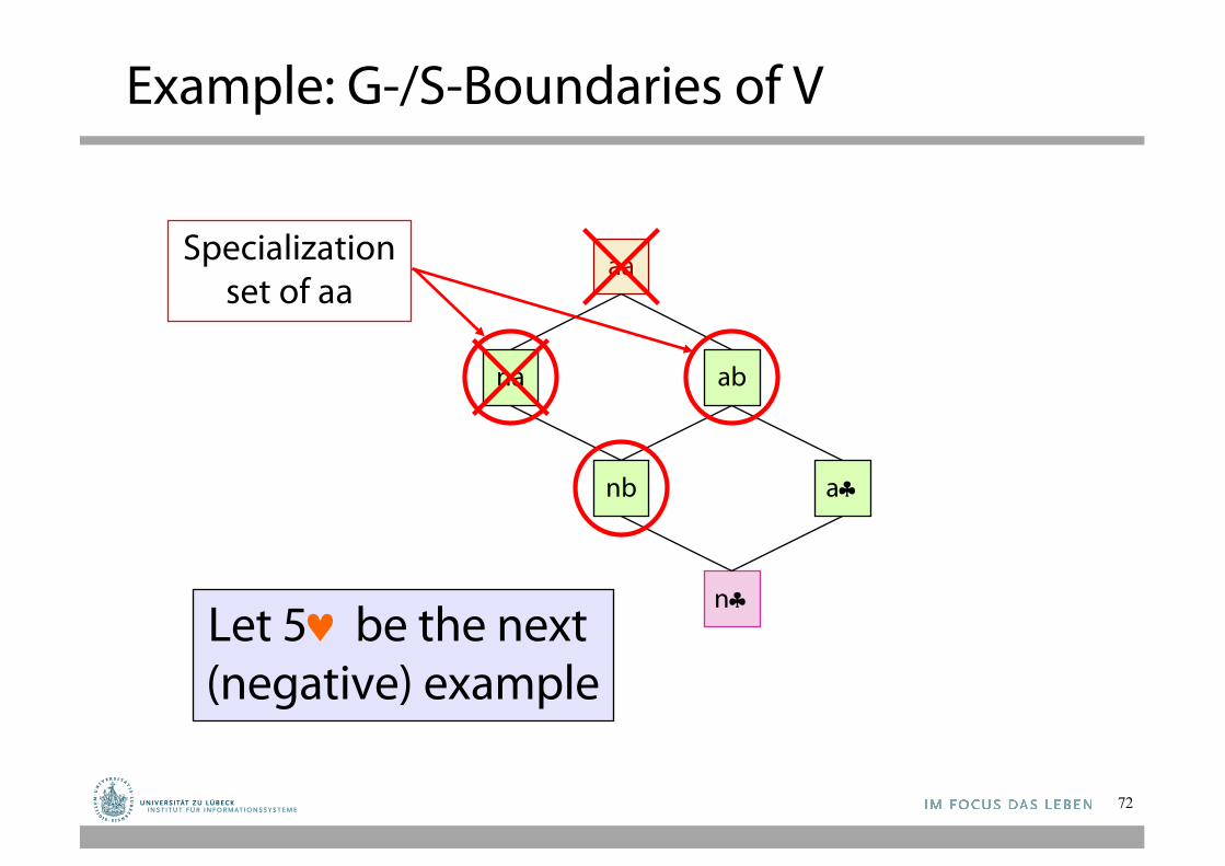
Example: G-/S-Boundaries of V
72
aa
na ab
nb
n§
a§
Let 5© be the next (negative) example
Specializationset of aa
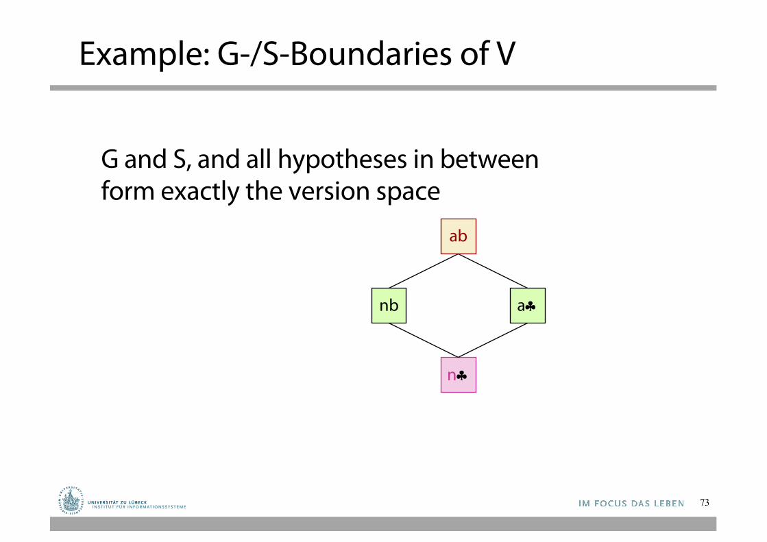
Example: G-/S-Boundaries of V
73
ab
nb
n§
a§
G and S, and all hypotheses in between form exactly the version space
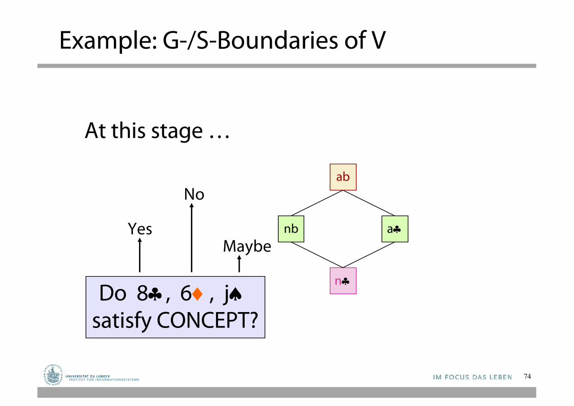
Example: G-/S-Boundaries of V
74
ab
nb
n§
a§
Do 8§, 6¨, jªsatisfy CONCEPT?
Yes
No
Maybe
At this stage …
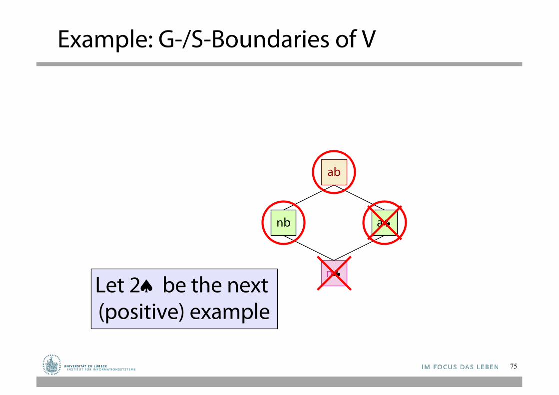
Example: G-/S-Boundaries of V
75
ab
nb
n§
a§
Let 2ª be the next (positive) example
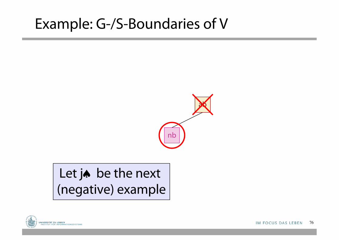
Example: G-/S-Boundaries of V
76
ab
nb
Let jª be the next (negative) example
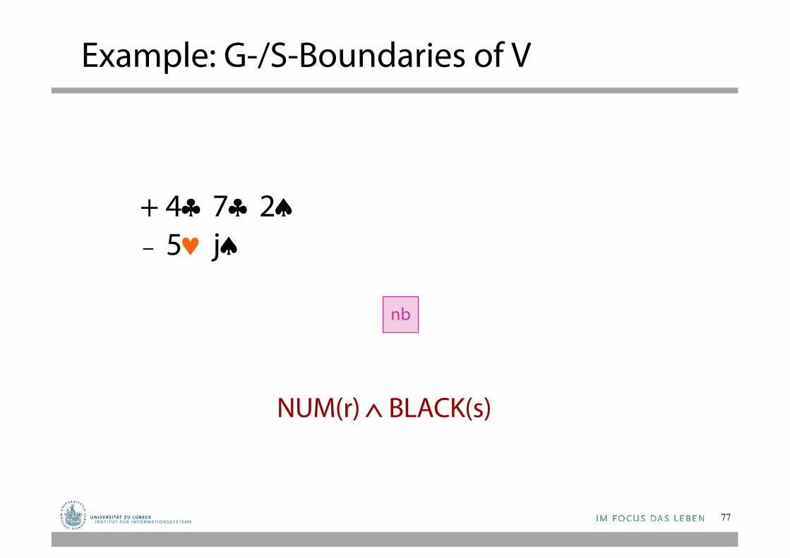
Example: G-/S-Boundaries of V
77
nb
+ 4§ 7§ 2ª– 5© jª
NUM(r) Ù BLACK(s)
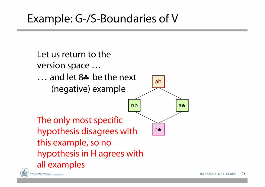
Example: G-/S-Boundaries of V
78
ab
nb
n§
a§
… and let 8§ be the next (negative) example
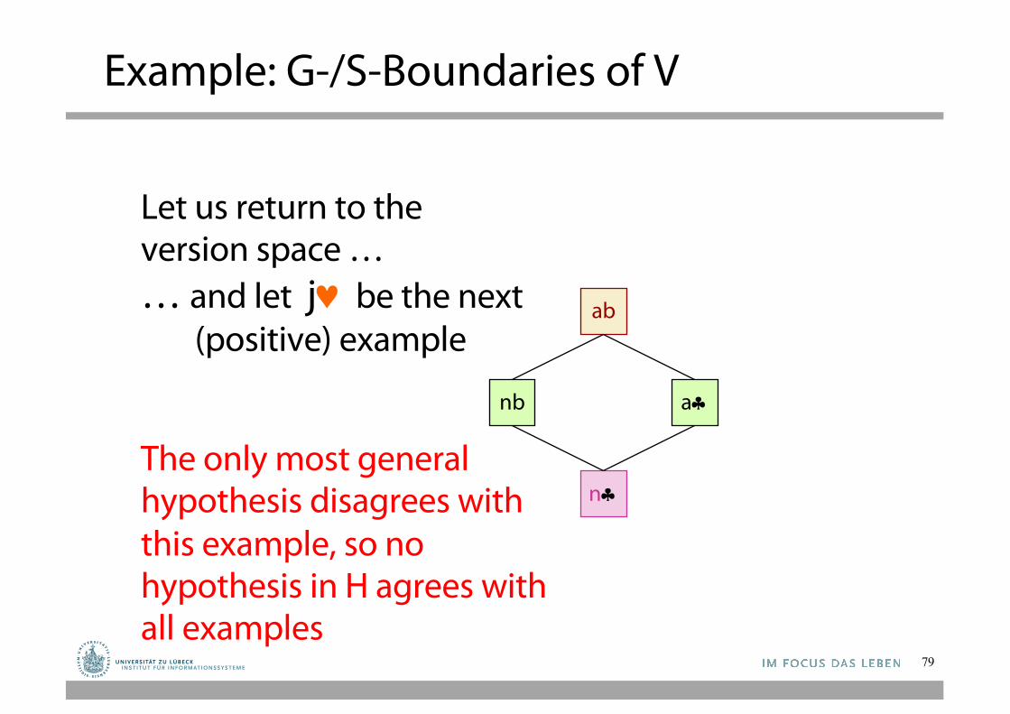
Let us return to the version space …
The only most specific hypothesis disagrees withthis example, so nohypothesis in H agrees with all examples
Example: G-/S-Boundaries of V
79
ab
nb
n§
a§
… and let j© be the next (positive) example
Let us return to the version space …
The only most general hypothesis disagrees withthis example, so nohypothesis in H agrees with all examples
Example-Selection Strategy
• Suppose that at each step the learning procedure has the possibility to select the object (card) of the next example
• Let it pick the object such that, whether the example is positive or not, it will eliminate one-half of the remaining hypotheses
• Then a single hypothesis will be isolated in O(log |H|) steps
80
81
aa
na ab
nb
n§
a§
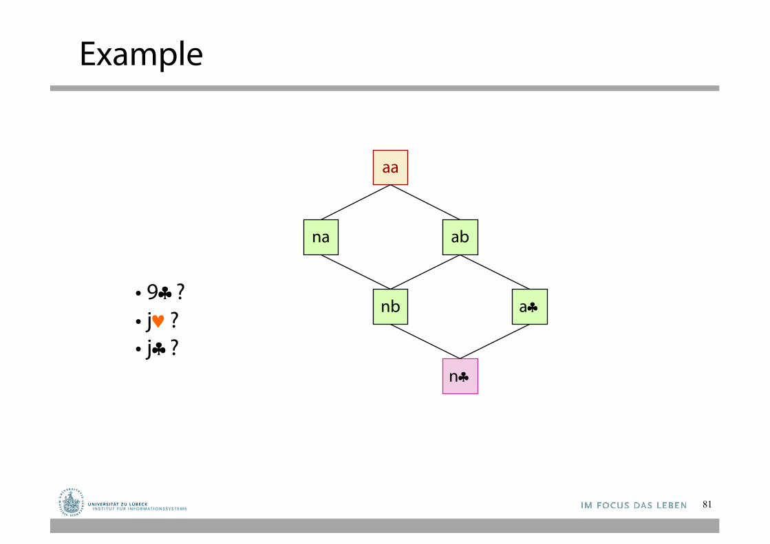
Example
• 9§?• j©?• j§?
Example-Selection Strategy
• Suppose that at each step the learning procedure has the possibility to select the object (card) of the next example
• Let it pick the object such that, whether the example is positive or not, it will eliminate one-half of the remaining hypotheses
• Then a single hypothesis will be isolated in O(log |H|) steps
• But picking the object that eliminates half the version space may be expensive
82
Noise
• If some examples are misclassified, the version space may collapse
• Possible solution:Maintain several G- and S-boundaries, e.g., consistent with all examples, all examples but one, etc…
83
VSL vs DTL
• Decision tree learning (DTL) is more efficient if all examples are given in advance; else, it may produce successive hypotheses, each poorly related to the previous one
• Version space learning (VSL) is incremental• DTL can produce simplified hypotheses that do not
agree with all examples• DTL has been more widely used in practice
84