Electronic Supplementary Information · Electronic Supplementary Information ... Ac susceptibility measurements were carried out using an oscillating field of 0.3 mT and static dc

1

Electronic Supplementary Information

Direct observation of a ferri-to-ferromagnetic transition

in a fluoride-bridged 3d-4f molecular cluster

Jan Dreiser,*a Kasper S. Pedersen,*b Cinthia Piamonteze,a Stefano Rusponi,c Zaher Salman,d Md.

Ehesan Ali,e Magnus Schau-Magnussen,b Christian Aa. Thuesen,b Stergios Piligkos,b Høgni

Weihe,b Hannu Mutka,f Oliver Waldmann,g Peter Oppeneer,h Jesper Bendix,*b Frithjof Nolting,a

and Harald Brunec

a Swiss Light Source, Paul Scherrer Institut, CH-5232 Villigen PSI, Switzerland. E-mail: [email protected]

b Department of Chemistry, University of Copenhagen, DK-2100 Copenhagen, Denmark. E-mail: [email protected] (K.S.P.), [email protected] (J.B.)

c Institute of Condensed Matter Physics, Ecole Polytechnique Fédérale de Lausanne, CH-1015 Lausanne, Switzerland.

d Laboratory for Muon Spin Spectroscopy, Paul Scherrer Institut, CH-5232 Villigen PSI, Switzerland.

e Center for Theoretical Chemistry, Ruhr-Universität Bochum, D-44801, Bochum, Germany.

f Institut Laue-Langevin, F-38042 Grenoble Cedex 9, France.

g Physikalisches Institut, Universität Freiburg, D-79104 Freiburg, Germany.

h Department of Physics and Astronomy, Uppsala University, Box 516, S-751 20 Uppsala, Sweden.

.

Electronic Supplementary Material (ESI) for Chemical ScienceThis journal is © The Royal Society of Chemistry 2012

2

Table of contents

Experimental Section _____________________________________________________________________________________ 3

General Procedures and Materials ______________________________________________________________________ 3 Syntheses ____________________________________________________________________________________________________ 3 Crystallography _____________________________________________________________________________________________ 3 SQUID magnetometer measurements ___________________________________________________________________ 4 X-ray magnetic circular dichroism ______________________________________________________________________ 5 Muon-spin relaxation ______________________________________________________________________________________ 5 Inelastic neutron scattering ______________________________________________________________________________ 5 Density-functional theory calculations _________________________________________________________________ 6 Spin-Hamiltonian simulations and fits __________________________________________________________________ 6

Supplementary Information to the Results Section of the Main Article ________________________ 7 Crystallography: Thermal ellipsoid plots of the crystal structures of 1 and 2 ____________________ 7 X-ray absorption spectroscopy ___________________________________________________________________________ 8 Ligand-field multiplet calculations ______________________________________________________________________ 9 SQUID magnetometry ____________________________________________________________________________________ 10 Inelastic neutron scattering ____________________________________________________________________________ 12 Muon-spin relaxation ____________________________________________________________________________________ 14 Spin-Hamiltonian models _______________________________________________________________________________ 15 Density-functional theory _______________________________________________________________________________ 17

References ________________________________________________________________________________________________ 17


3

Experimental Section

General Procedures and Materials

All chemicals and solvents were purchased from commercial sources and used without further

purification. [Dy(hfac)3(H2O)2] and trans-[CrF2(py)4]NO3 were prepared as described in the

literature.1

Syntheses

Synthesis of 1: To a solution of [Dy(hfac)3(H2O)2] (4.0 g, 4.9 mmol) in chloroform (60 ml,

LabScan; stabilized by 1% ethanol) was added a solution of trans-[CrF2(py)4]NO3 (0.5 g, 1.0 mmol)

in chloroform (10 ml). The resulting solution was left standing for 12 h to yield needles of

[Dy(hfac)3(H2O)–CrF2(py)4–Dy(hfac)3(NO3)] which were filtered off and washed with chloroform.

Yield: 62% (based on Cr). Anal. Calc. (found) for H28C50N5O16F38CrDy2: C: 29.24% (29.13%), H:

1.37% (1.26%), N: 3.41% (3.33%)

Synthesis of 2: To a solution of trans-[CrF2(py)4]NO3 (1.2 g, 2.6 mmol) in chloroform (25 ml) was

added a solution of one equivalent [Dy(hfac)3(H2O)2] (2.1 g, 2.6 mmol) in chloroform (40 ml). Red-

violet, block-shaped crystals of [Dy(hfac)4–CrF2(py)4]⋅ ½CHCl3 were filtered off after several hours

and washed with successive aliquots of chloroform. The samples were stored in closed vials in a

freezer to suppress solvent loss. Yield: 36% (based on Cr), Anal. calc. (found) for

H24.5C40.5N4O8F26Cl1.5CrDy: C: 33.39% (33.02%), H: 1.70% (1.49%), N: 3.85% (3.90%).

Crystallography

Single-crystal X-ray diffraction data were acquired at 122 K on a Nonius KappaCCD area-detector

diffractometer, equipped with an Oxford Cryostreams low-temperature device, using graphite-

monochromated Mo Kα radiation (λ = 0.71073 Å). The structures were solved using direct methods

(SHELXS97) and refined using the SHELXL97 software package.2 All non-hydrogen atoms were

refined anisotropically, whereas H-atoms were isotropic and constrained. Crystal structure and

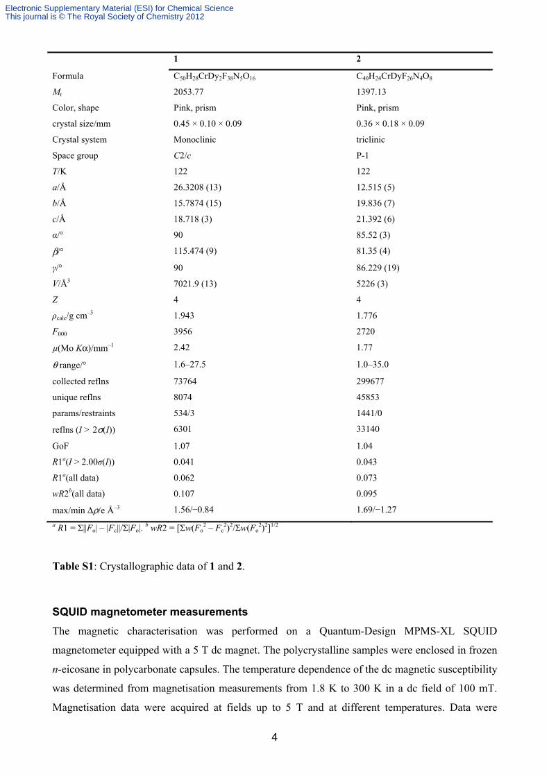
refinement data for 1 and 2 are summarised in Table S1. The structure of 2 contains a highly

disordered solvent CHCl3 molecule and no satisfactory model that describes this solvent could be

achieved. Hence the PLATON SQUEEZE3 procedure was used in the refinement to calculate a

solvent-accessible void of 311 Å3. It was confirmed that the disordered solvent is located in the void

volume.


4

1 2

Formula C50H28CrDy2F38N5O16 C40H24CrDyF26N4O8

Mr 2053.77 1397.13

Color, shape Pink, prism Pink, prism

crystal size/mm 0.45 × 0.10 × 0.09 0.36 × 0.18 × 0.09

Crystal system Monoclinic triclinic

Space group C2/c P-1

T/K 122 122

a/Å 26.3208 (13) 12.515 (5)

b/Å 15.7874 (15) 19.836 (7)

c/Å 18.718 (3) 21.392 (6)

α/° 90 85.52 (3)

β/° 115.474 (9) 81.35 (4)

γ/° 90 86.229 (19)

V/Å3 7021.9 (13) 5226 (3)

Z 4 4

ρcalc/g cm–3 1.943 1.776

F000 3956 2720

µ(Mo Kα)/mm–1 2.42 1.77

θ range/° 1.6–27.5 1.0–35.0

collected reflns 73764 299677

unique reflns 8074 45853

params/restraints 534/3 1441/0

reflns (I > 2σ(I)) 6301 33140

GoF 1.07 1.04

R1a(I > 2.00σ(I)) 0.041 0.043

R1a(all data) 0.062 0.073

wR2b(all data) 0.107 0.095

max/min Δρ/e Å–3 1.56/−0.84 1.69/−1.27

a R1 = Σ||Fo| – |Fc||/Σ|Fo|. b wR2 = [Σw(Fo

2 – Fc2)2/Σw(Fo

2)2]1/2

Table S1: Crystallographic data of 1 and 2.

SQUID magnetometer measurements

The magnetic characterisation was performed on a Quantum-Design MPMS-XL SQUID

magnetometer equipped with a 5 T dc magnet. The polycrystalline samples were enclosed in frozen

n-eicosane in polycarbonate capsules. The temperature dependence of the dc magnetic susceptibility

was determined from magnetisation measurements from 1.8 K to 300 K in a dc field of 100 mT.

Magnetisation data were acquired at fields up to 5 T and at different temperatures. Data were


5

corrected for diamagnetic contributions from the sample, n-eicosane and the sample holder by

means of Pascal´s constants. Ac susceptibility measurements were carried out using an oscillating

field of 0.3 mT and static dc fields of up to 1 T.

X-ray magnetic circular dichroism

X-ray magnetic circular dichroism (XMCD) measurements were performed at the X-Treme

beamline at the Swiss Light Source, Paul Scherrer Institut, Switzerland. To prepare the sample,

polycrystalline powder of 1 was pressed into a piece of Indium mounted on a sample holder. X-ray

absorption spectra were recorded at a temperature of 2 K in total electron yield mode at the Dy M4,5

and Cr L2,3 edges. Magnetic fields of up to B = ±6 T along the beam propagation direction were

applied. The beam was defocused (spot size ~1 × 1 mm2) and kept at very low intensity to avoid

radiation damage. Scans were taken “on-the-fly”, i.e. the monochromator and insertion device were

moving continuously while the data were acquired.4 To obtain magnetisation curves, a full

magnetic-field loop was performed at one polarisation while measuring X-ray absorption at the

energy of maximum dichroism and at the baseline. Hereafter, the polarisation was changed and

another loop was run.

Muon-spin relaxation

The µSR measurements were performed on the GPS spectrometer at the Paul Scherrer Institute in

Switzerland. In these experiments spin-polarised positive muons are implanted in the sample. Each

implanted muon decays (lifetime 2.2 µsec) emitting a positron preferentially in the direction of its

spin polarisation at the time of decay. Using appropriately positioned detectors, one measures the

asymmetry of positron emission as a function of time, A(t), which is proportional to the time

evolution of the muon spin polarisation. A(t) depends on the distribution of internal magnetic fields

and their temporal fluctuations. Further details on the µSR technique may be found in ref. 5.

Inelastic neutron scattering

Inelastic neutron scattering (INS) experiments were carried out using the direct-geometry time-of-

flight neutron spectrometer IN5 located at the Institut Laue-Langevin, Grenoble, France.

Approximately 1 g of crystalline material was loaded into a 10 mm-diameter double-wall, hollow

aluminum cylinder. Spectra were acquired with incident neutron wavelengths of 3 Å, 4.8 Å and

6.5 Å at temperatures from 1.5 K to 15 K. The detector efficiency correction was performed using

data collected from Vanadium and the background was subtracted. The data were processed and

analysed using the LAMP program package.6


6

Density-functional theory calculations

Density-functional theory (DFT) calculations were performed on two levels of sophistication. To

investigate the exchange coupling in complex 1 we considered the truncated model cluster

[Dy(hfac)3(NO3)–CrF2(py)4]. Geometrical optimisation of this model cluster was performed using

the VASP full-potential plane-wave code in scalar-relativistic approximation, in which pseudo-

potentials together within the projector augmented wave method are used.7 A kinetic energy cutoff

of 400 eV was employed for the plane waves. For the DFT exchange-correlation functional the

generalised gradient approximation (GGA) in the Perdew-Wang parameterisation8 was used for the

geometrical optimisation. A cubic simulation box of 30×30×30 Å3 and the Γ point in reciprocal

space were used. The magnetic properties of the optimised geometries as well as the experimental

crystallographic structure were furthermore investigated using the atom-centered localized basis set

approach as implemented in the NWChem package9 in combination with hybrid functionals. In the

latter calculations the segmented all-electron relativistic contracted basis sets for zeroth-order

regular approximation (SARC-ZORA)10 scalar-relativistic Hamiltonians were used for Dy and all-

electron 6-31G* basis sets for all other atoms including Cr.

Isotropic magnetic exchange interactions were calculated within the localised basis set approach,

using the hybrid meta-GGA M06-2X functional11 in combination with applying the spin-polarized

broken symmetry approach. The magnetic interaction of the model complex was expressed as

CrDyˆˆˆ SS ⋅−= jH where the exchange constant j can be extracted from the Noodleman-Ginsberg-

Davidson expression12 j=2(EBS−EHS)/Smax2 (with EBS the broken-symmetry energy and EHS the high-

symmetry energy). In the literature an alternative expression by Ruiz et al.13

[j=2(EBS−EHS)/Smax(Smax+1)] is popular and provides computationally better results in most cases.

However no theoretical basis to prefer Ruiz et al.’s expression over the other one was established so

far, therefore both expressions were explored here.

Spin-Hamiltonian simulations and fits

The spin-Hamiltonian simulations used to reproduce local and cluster magnetization curves, dc

magnetic susceptibility and INS spectra are based on full diagonalization of the respective

Hamiltonians. To take into account the powder nature of the sample, local and cluster magnetization

curves were averaged over different directions of the magnetic field according to the equation

⋅=φθ

φθθφθφθπ ,

powder sin),(),,(4

1)( ddBBm ii, nm (S1)

Here, mi is the magnetic moment of element i, depending on the magnitude and orientation of the

applied magnetic field which is expressed in spherical coordinates B = (B,θ,φ). Further, n is the unit


7

vector pointing along the B-field direction. This integral was realized numerically using a 16-point

Lebedev-Laikov grid.14 All fits shown in this work are least-squares fits which were obtained by

minimizing the sum of squared deviations between the measured and calculated curves. The

calculations were performed using home-written Matlab® and C codes.

Supplementary Information to the Results Section of

the Main Article

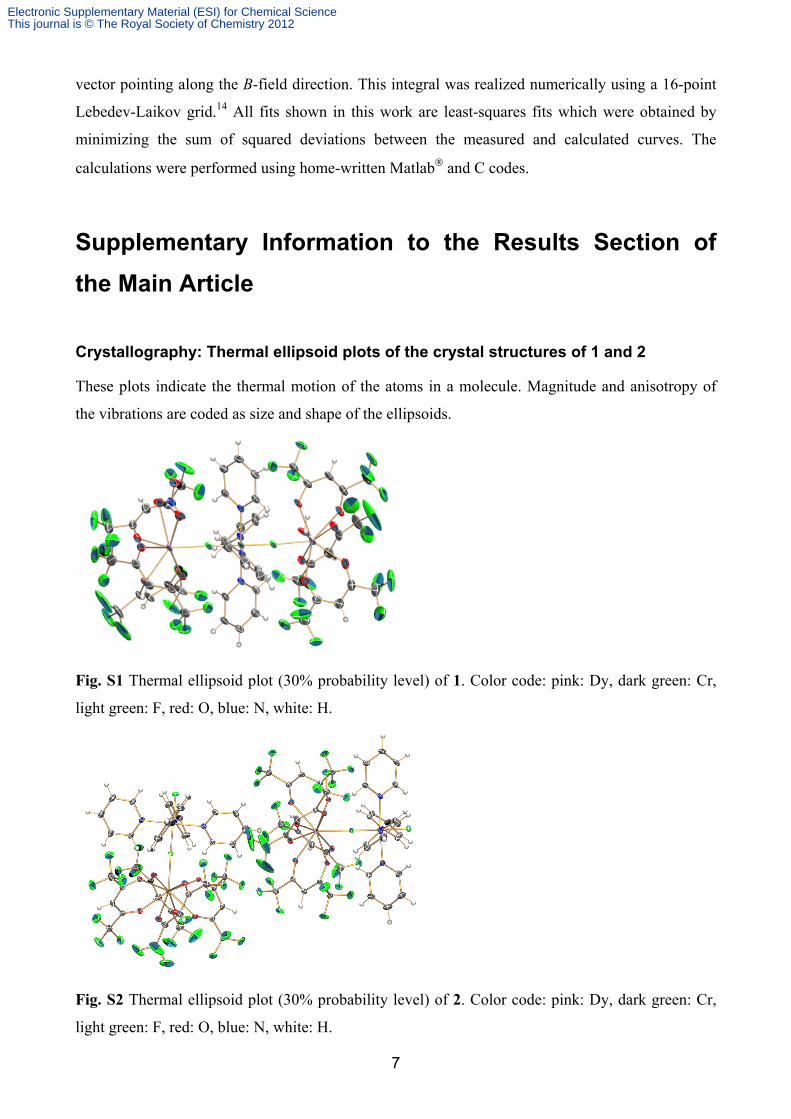
Crystallography: Thermal ellipsoid plots of the crystal structures of 1 and 2

These plots indicate the thermal motion of the atoms in a molecule. Magnitude and anisotropy of

the vibrations are coded as size and shape of the ellipsoids.

Fig. S1 Thermal ellipsoid plot (30% probability level) of 1. Color code: pink: Dy, dark green: Cr,

light green: F, red: O, blue: N, white: H.

Fig. S2 Thermal ellipsoid plot (30% probability level) of 2. Color code: pink: Dy, dark green: Cr,

light green: F, red: O, blue: N, white: H.


8

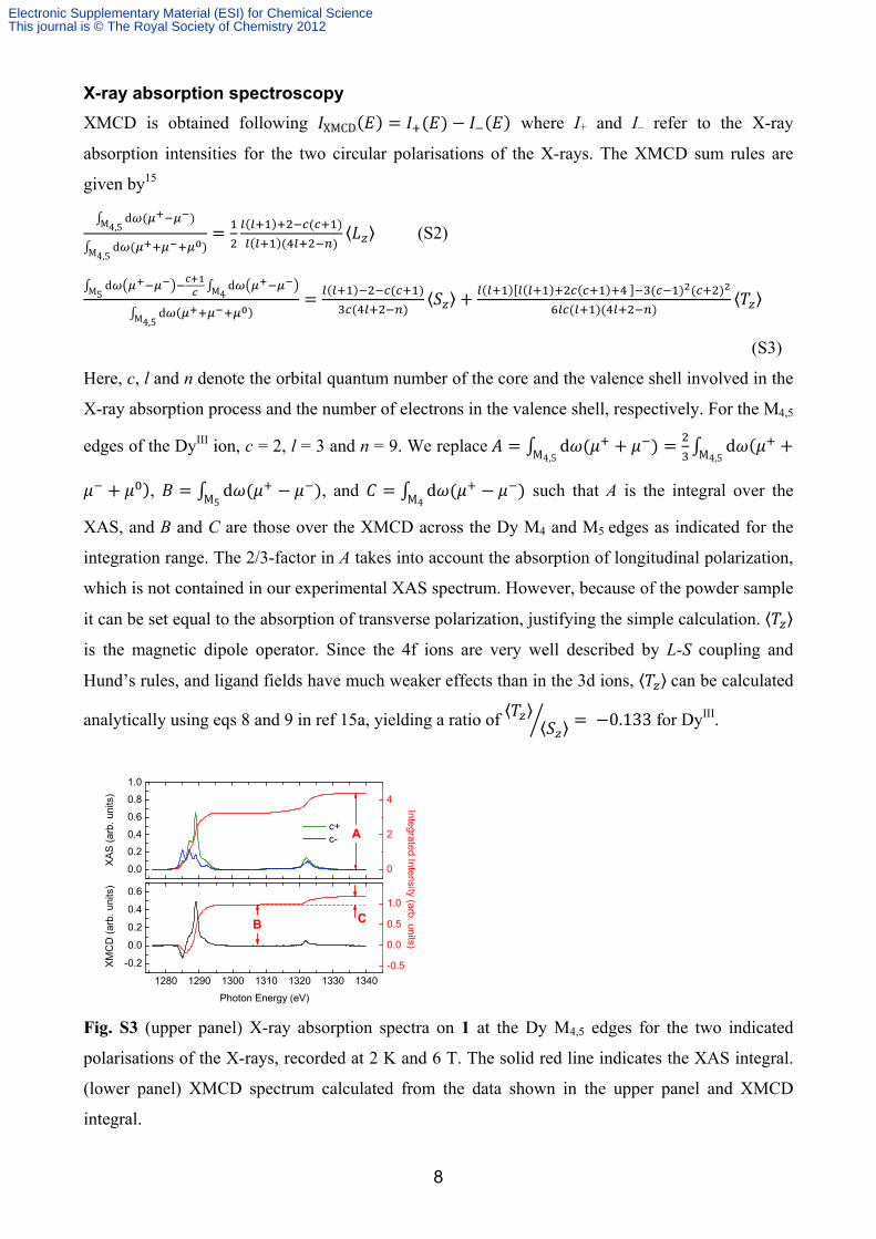
X-ray absorption spectroscopy

XMCD is obtained following XMCD( ) = ( ) − ( ) where I+ and I– refer to the X-ray

absorption intensities for the two circular polarisations of the X-rays. The XMCD sum rules are

given by15 d ( )M4,5d ( )M4,5 = ( ) ( )( )( ) ⟨ ⟩ (S2)

dM5 dM4d ( )M4,5 = ( ) ( )( ) ⟨ ⟩ + ( )[ ( ) ( ) ] ( ) ( )( )( ) ⟨ ⟩ (S3)

Here, c, l and n denote the orbital quantum number of the core and the valence shell involved in the

X-ray absorption process and the number of electrons in the valence shell, respectively. For the M4,5

edges of the DyIII ion, c = 2, l = 3 and n = 9. We replace = d ( + )M4,5 = d ( +M4,5+ ), = d ( − )M5 , and = d ( − )M4 such that A is the integral over the

XAS, and B and C are those over the XMCD across the Dy M4 and M5 edges as indicated for the

integration range. The 2/3-factor in A takes into account the absorption of longitudinal polarization,

which is not contained in our experimental XAS spectrum. However, because of the powder sample

it can be set equal to the absorption of transverse polarization, justifying the simple calculation. ⟨ ⟩ is the magnetic dipole operator. Since the 4f ions are very well described by L-S coupling and

Hund’s rules, and ligand fields have much weaker effects than in the 3d ions, ⟨ ⟩ can be calculated

analytically using eqs 8 and 9 in ref 15a, yielding a ratio of ⟨ ⟩ ⟨ ⟩ = −0.133 for DyIII.

Fig. S3 (upper panel) X-ray absorption spectra on 1 at the Dy M4,5 edges for the two indicated

polarisations of the X-rays, recorded at 2 K and 6 T. The solid red line indicates the XAS integral.

(lower panel) XMCD spectrum calculated from the data shown in the upper panel and XMCD

integral.

0.0

0.2

0.4

0.6

0.8

1.0

C

c+ c-

XA

S (

arb.

uni

ts)

A

1280 1290 1300 1310 1320 1330 1340

-0.2

0.0

0.2

0.4

0.6

XM

CD

(ar

b. u

nits

)

Photon Energy (eV)

B

0

2

4

Integrated Intensity (arb. units)

-0.5

0.0

0.5

1.0


9

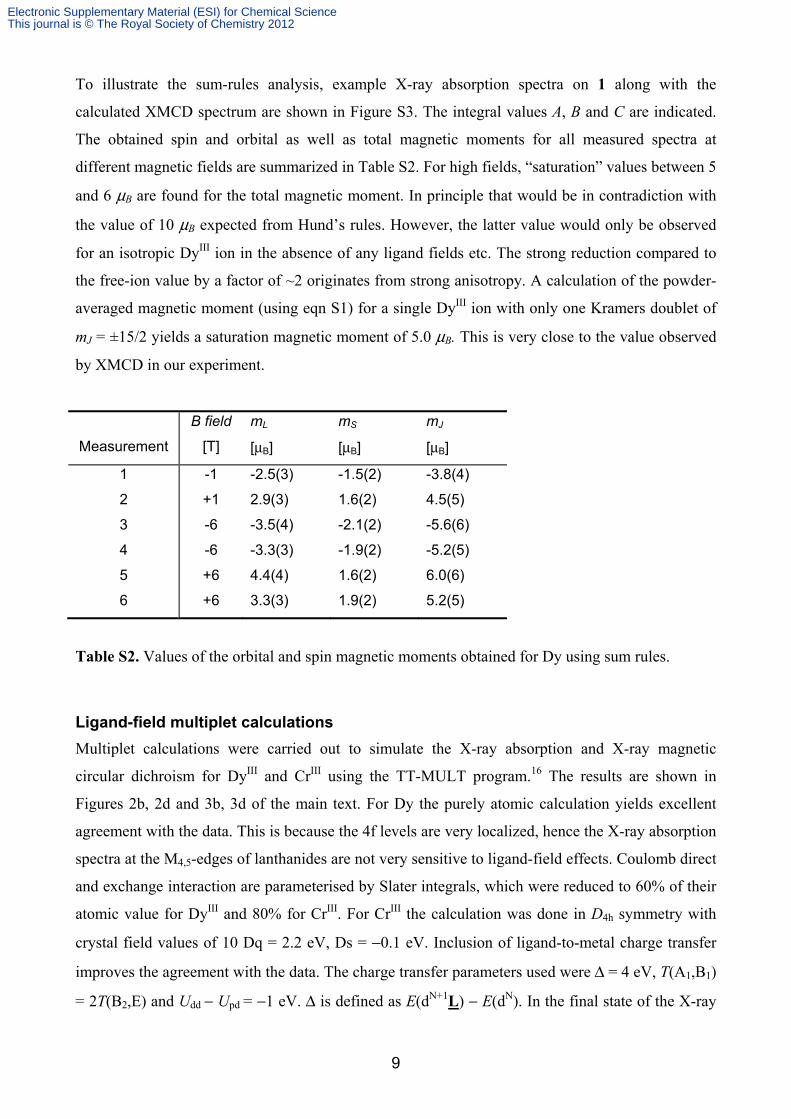
To illustrate the sum-rules analysis, example X-ray absorption spectra on 1 along with the

calculated XMCD spectrum are shown in Figure S3. The integral values A, B and C are indicated.

The obtained spin and orbital as well as total magnetic moments for all measured spectra at

different magnetic fields are summarized in Table S2. For high fields, “saturation” values between 5

and 6 μB are found for the total magnetic moment. In principle that would be in contradiction with

the value of 10 μB expected from Hund’s rules. However, the latter value would only be observed

for an isotropic DyIII ion in the absence of any ligand fields etc. The strong reduction compared to

the free-ion value by a factor of ~2 originates from strong anisotropy. A calculation of the powder-

averaged magnetic moment (using eqn S1) for a single DyIII ion with only one Kramers doublet of

mJ = ±15/2 yields a saturation magnetic moment of 5.0 μB. This is very close to the value observed

by XMCD in our experiment.

Measurement

B field

[T]

mL

[μB]

mS

[μB]

mJ

[μB]

1

2

3

4

5

6

-1

+1

-6

-6

+6

+6

-2.5(3)

2.9(3)

-3.5(4)

-3.3(3)

4.4(4)

3.3(3)

-1.5(2)

1.6(2)

-2.1(2)

-1.9(2)

1.6(2)

1.9(2)

-3.8(4)

4.5(5)

-5.6(6)

-5.2(5)

6.0(6)

5.2(5)

Table S2. Values of the orbital and spin magnetic moments obtained for Dy using sum rules.

Ligand-field multiplet calculations

Multiplet calculations were carried out to simulate the X-ray absorption and X-ray magnetic

circular dichroism for DyIII and CrIII using the TT-MULT program.16 The results are shown in

Figures 2b, 2d and 3b, 3d of the main text. For Dy the purely atomic calculation yields excellent

agreement with the data. This is because the 4f levels are very localized, hence the X-ray absorption

spectra at the M4,5-edges of lanthanides are not very sensitive to ligand-field effects. Coulomb direct

and exchange interaction are parameterised by Slater integrals, which were reduced to 60% of their

atomic value for DyIII and 80% for CrIII. For CrIII the calculation was done in D4h symmetry with

crystal field values of 10 Dq = 2.2 eV, Ds = −0.1 eV. Inclusion of ligand-to-metal charge transfer

improves the agreement with the data. The charge transfer parameters used were Δ = 4 eV, T(A1,B1)

= 2T(B2,E) and Udd − Upd = −1 eV. Δ is defined as E(dN+1L) − E(dN). In the final state of the X-ray


10

absorption process, the energy difference between the ionic and charge transfer configurations is

given by E(p5dN+2L) – E(p5dN+1) = Δ + Udd − Upd. T is the transfer integral between the metal d shell

and the ligand p shell and is usually taken as being two times larger for the orbitals pointing along

the bonding direction (A1,B1). At a field of –6 T, the expectation values <Sz> = −1.49 and <Lz> = 0

are found, in agreement with CrIII. Simulations for both CrIII and DyIII were done considering a

temperature of 2 K.

The above-mentioned parameters which were employed to simulate the CrIII X-ray spectra can be

compared to the values reported for {CrIIIF2(py)4}+ in the literature.17 From this, we obtain 10Dq =

2.3 eV, Ds = –0.125 eV and Dt = 0.0375 eV. These values are in excellent agreement with the

parameters found from the multiplet calculations. Setting Dt = 0 in the calculations is justified

because the observed X-ray absorption peaks are too broad (FWHM ~ 500 meV) to observe the

associated energy splittings.

SQUID magnetometry

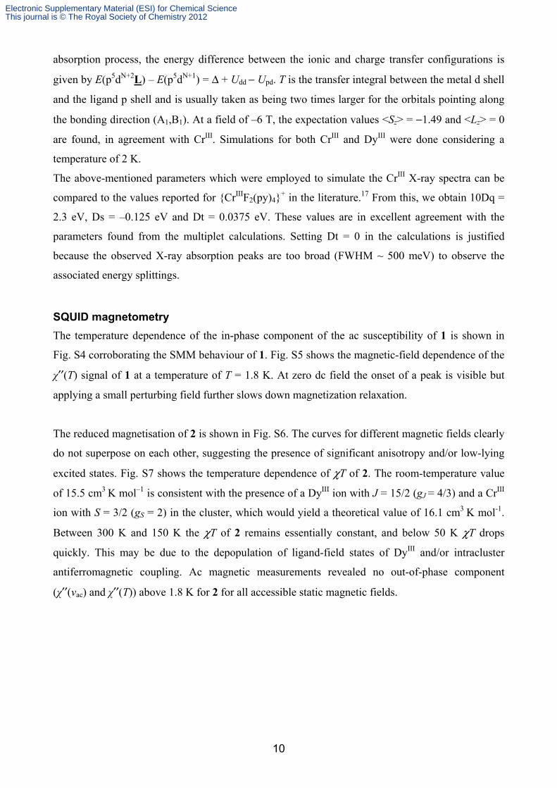
The temperature dependence of the in-phase component of the ac susceptibility of 1 is shown in

Fig. S4 corroborating the SMM behaviour of 1. Fig. S5 shows the magnetic-field dependence of the

χ′′(T) signal of 1 at a temperature of T = 1.8 K. At zero dc field the onset of a peak is visible but

applying a small perturbing field further slows down magnetization relaxation.

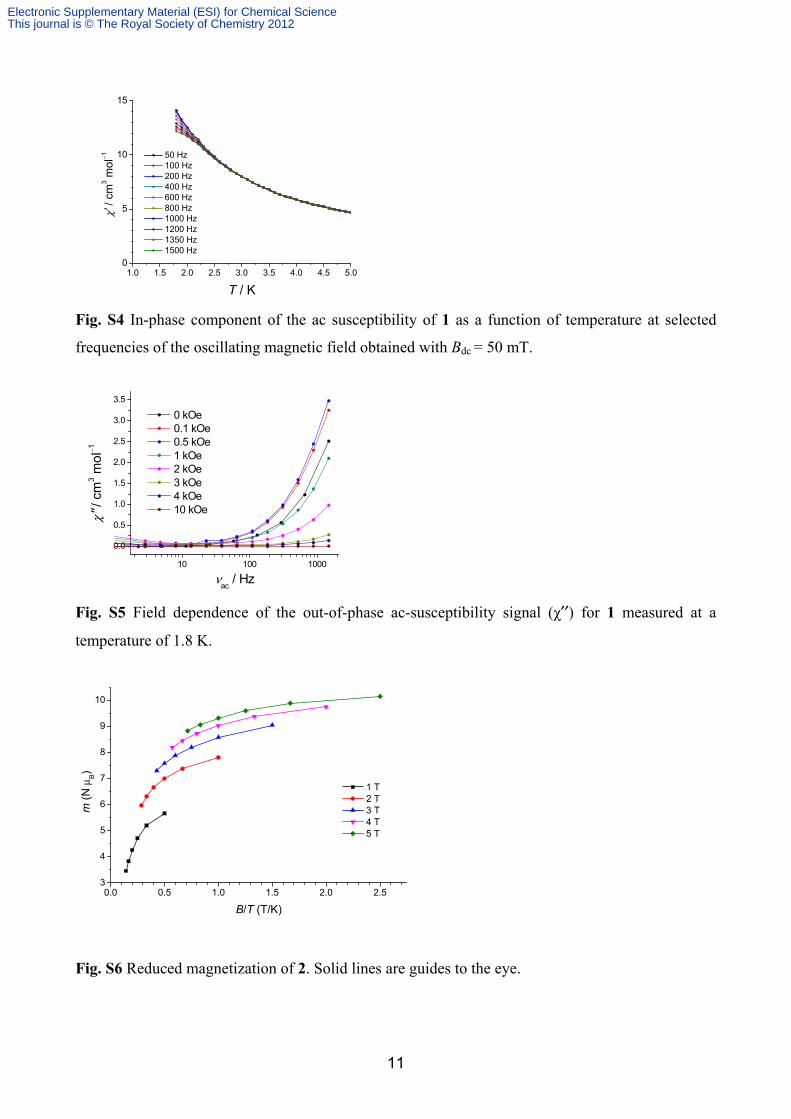
The reduced magnetisation of 2 is shown in Fig. S6. The curves for different magnetic fields clearly

do not superpose on each other, suggesting the presence of significant anisotropy and/or low-lying

excited states. Fig. S7 shows the temperature dependence of χT of 2. The room-temperature value

of 15.5 cm3 K mol–1 is consistent with the presence of a DyIII ion with J = 15/2 (gJ = 4/3) and a CrIII

ion with S = 3/2 (gS = 2) in the cluster, which would yield a theoretical value of 16.1 cm3 K mol-1.

Between 300 K and 150 K the χT of 2 remains essentially constant, and below 50 K χT drops

quickly. This may be due to the depopulation of ligand-field states of DyIII and/or intracluster

antiferromagnetic coupling. Ac magnetic measurements revealed no out-of-phase component

(χ′′(νac) and χ′′(T)) above 1.8 K for 2 for all accessible static magnetic fields.


11

1.0 1.5 2.0 2.5 3.0 3.5 4.0 4.5 5.00

5

10

15

50 Hz 100 Hz 200 Hz 400 Hz 600 Hz 800 Hz 1000 Hz 1200 Hz 1350 Hz 1500 Hz

χ' /

cm3 m

ol−1

T / K

Fig. S4 In-phase component of the ac susceptibility of 1 as a function of temperature at selected

frequencies of the oscillating magnetic field obtained with Bdc = 50 mT.

10 100 1000

0.0

0.5

1.0

1.5

2.0

2.5

3.0

3.5

χ'' /

cm

3 m

ol−1

νac

/ Hz

0 kOe 0.1 kOe 0.5 kOe 1 kOe 2 kOe 3 kOe 4 kOe 10 kOe

Fig. S5 Field dependence of the out-of-phase ac-susceptibility signal (χ′′) for 1 measured at a

temperature of 1.8 K.

0.0 0.5 1.0 1.5 2.0 2.53

4

5

6

7

8

9

10

m (

N μ

B)

B/T (T/K)

1 T 2 T 3 T 4 T 5 T

Fig. S6 Reduced magnetization of 2. Solid lines are guides to the eye.


12

0 50 100 150 200 250 3007

8

9

10

11

12

13

14

15

16χT

(cm

3 mol

-1K

)

T (K)

Fig. S7 Temperature dependence of the χT product of 2. The solid line is a guide to the eye.

Inelastic neutron scattering

Information about the magnetic origin of INS features can be derived from their temperature and Q

dependence. Upon increasing the temperature, magnetic excited energy levels become populated at

the expense of ground-state-level population. This reduction of ground-state population leads to a

decrease of INS transitions that correspond to excitation of the molecular magnet from the ground

state to an excited state by a neutron, commonly referred to as “cold magnetic transition”. In

contrast, for harmonic vibrational modes the neutron energy loss response at a certain energy = ℏ is proportional to the Bose factor18 1/[1 − exp (− ℏ )], which implies that the intensity

can only stay constant or increase with increasing temperature. Furthermore, the Q-dependence

contains relevant information, too. Here, Q is the absolute value of the momentum transfer, Q = |Q|.

At a constant energy E, for magnetic scattering the Q dependence is ruled by the magnetic form

factors of the magnetic ions present in the cluster, and by their spatial coordinates.19 Altogether, this

leads to a decay of the scattering intensity with increasing Q. For incoherent scattering from

vibrational modes the Q dependence is entirely different and the intensity is proportional to Q2.19

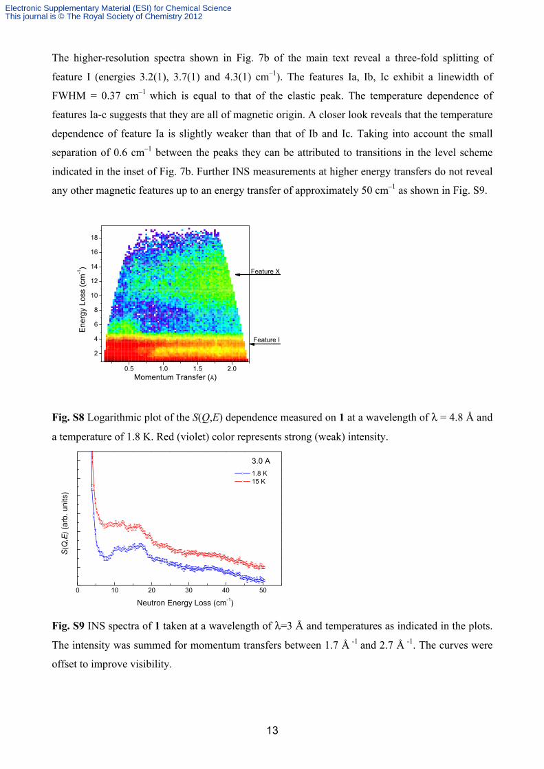
In Figure 7a of the main text, features I and X were observed. Peak I appears at an energy of

3.4(2) cm–1 and possesses a full width at half maximum (FWHM) of 0.9 cm–1 which is close to that

of the elastic peak of 0.8 cm–1. The broad feature X is located at energy transfers from 9 to 16 cm–1.

Peak I shrinks with increasing temperature, while feature X is temperature independent. These

features appear in the S(Q,E) dependence shown in Figure S8, where they are indicated by black

arrows. Whereas the scattering intensity S(Q,E) at the energy of feature I decreases with Q, it

exhibits opposite behaviour at the energy of the broad feature X. The latter is therefore proven to

originate from a nonmagnetic excitation and can therefore be neglected in the further analysis of the

magnetic properties of 1. In contrast, feature I is inferred to be a cold magnetic transition.


13

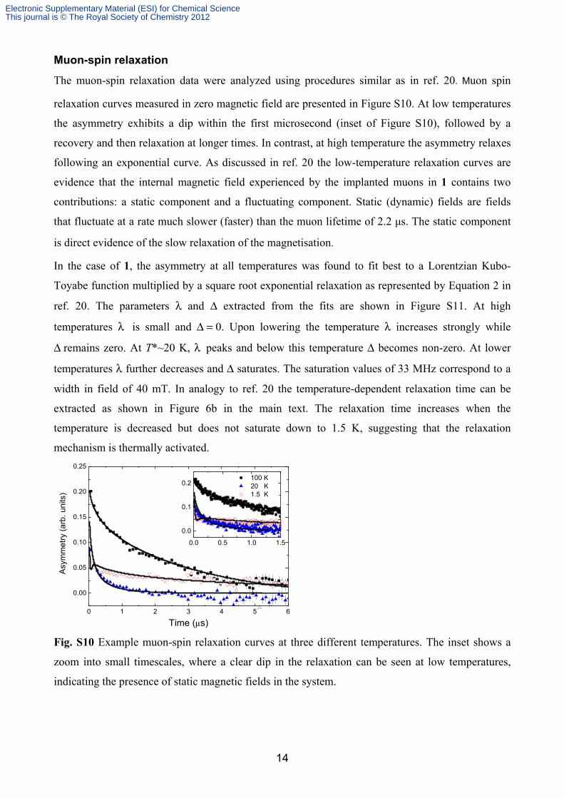
The higher-resolution spectra shown in Fig. 7b of the main text reveal a three-fold splitting of

feature I (energies 3.2(1), 3.7(1) and 4.3(1) cm–1). The features Ia, Ib, Ic exhibit a linewidth of

FWHM = 0.37 cm–1 which is equal to that of the elastic peak. The temperature dependence of

features Ia-c suggests that they are all of magnetic origin. A closer look reveals that the temperature

dependence of feature Ia is slightly weaker than that of Ib and Ic. Taking into account the small

separation of 0.6 cm–1 between the peaks they can be attributed to transitions in the level scheme

indicated in the inset of Fig. 7b. Further INS measurements at higher energy transfers do not reveal

any other magnetic features up to an energy transfer of approximately 50 cm–1 as shown in Fig. S9.

0.5 1.0 1.5 2.0

2

4

6

8

10

12

14

16

18

Feature X

Momentum Transfer (Å)

Ene

rgy

Los

s (c

m-1)

Feature I

Fig. S8 Logarithmic plot of the S(Q,E) dependence measured on 1 at a wavelength of λ = 4.8 Å and

a temperature of 1.8 K. Red (violet) color represents strong (weak) intensity.

0 10 20 30 40 50

1.8 K 15 K

3.0 A

Neutron Energy Loss (cm-1)

S(Q

,E)

(arb

. un

its)

Fig. S9 INS spectra of 1 taken at a wavelength of λ=3 Å and temperatures as indicated in the plots.

The intensity was summed for momentum transfers between 1.7 Å -1 and 2.7 Å -1. The curves were

offset to improve visibility.


14

Muon-spin relaxation

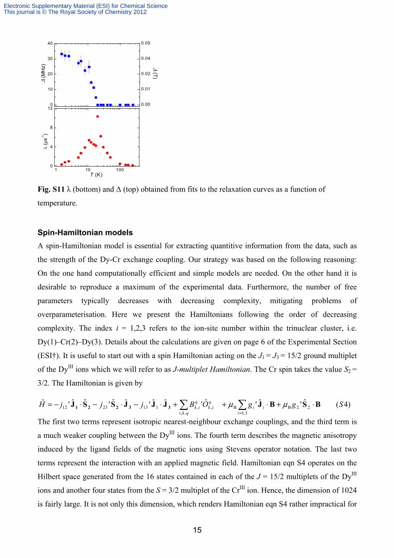
The muon-spin relaxation data were analyzed using procedures similar as in ref. 20. Muon spin

relaxation curves measured in zero magnetic field are presented in Figure S10. At low temperatures

the asymmetry exhibits a dip within the first microsecond (inset of Figure S10), followed by a

recovery and then relaxation at longer times. In contrast, at high temperature the asymmetry relaxes

following an exponential curve. As discussed in ref. 20 the low-temperature relaxation curves are

evidence that the internal magnetic field experienced by the implanted muons in 1 contains two

contributions: a static component and a fluctuating component. Static (dynamic) fields are fields

that fluctuate at a rate much slower (faster) than the muon lifetime of 2.2 μs. The static component

is direct evidence of the slow relaxation of the magnetisation.

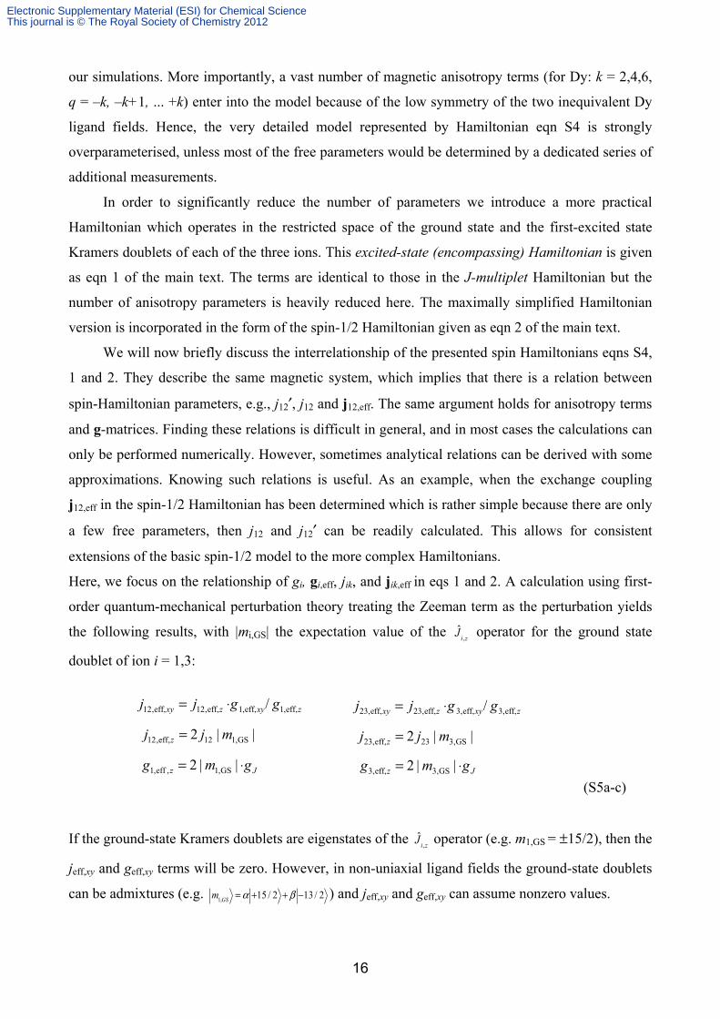
In the case of 1, the asymmetry at all temperatures was found to fit best to a Lorentzian Kubo-

Toyabe function multiplied by a square root exponential relaxation as represented by Equation 2 in

ref. 20. The parameters λ and Δ extracted from the fits are shown in Figure S11. At high

temperatures λ is small and Δ = 0. Upon lowering the temperature λ increases strongly while

Δ remains zero. At T*~20 K, λ peaks and below this temperature Δ becomes non-zero. At lower

temperatures λ further decreases and Δ saturates. The saturation values of 33 MHz correspond to a

width in field of 40 mT. In analogy to ref. 20 the temperature-dependent relaxation time can be

extracted as shown in Figure 6b in the main text. The relaxation time increases when the

temperature is decreased but does not saturate down to 1.5 K, suggesting that the relaxation

mechanism is thermally activated.

0 1 2 3 4 5 6

0.00

0.05

0.10

0.15

0.20

0.25

100 K 20 K 1.5 K

Asy

mm

etry

(ar

b. u

nits

)

Time (μs)

0.0 0.5 1.0 1.5

0.0

0.1

0.2

Fig. S10 Example muon-spin relaxation curves at three different temperatures. The inset shows a

zoom into small timescales, where a clear dip in the relaxation can be seen at low temperatures,

indicating the presence of static magnetic fields in the system.


15

1 10 1000

4

8

12

λ (μ

s-1)

T (K)

0

10

20

30

40

0.00

0.01

0.02

0.04

0.05

Δ (T

)

Δ

(MH

z)

Fig. S11 λ (bottom) and Δ (top) obtained from fits to the relaxation curves as a function of

temperature.

Spin-Hamiltonian models

A spin-Hamiltonian model is essential for extracting quantitive information from the data, such as

the strength of the Dy-Cr exchange coupling. Our strategy was based on the following reasoning:

On the one hand computationally efficient and simple models are needed. On the other hand it is

desirable to reproduce a maximum of the experimental data. Furthermore, the number of free

parameters typically decreases with decreasing complexity, mitigating problems of

overparameterisation. Here we present the Hamiltonians following the order of decreasing

complexity. The index i = 1,2,3 refers to the ion-site number within the trinuclear cluster, i.e.

Dy(1)–Cr(2)–Dy(3). Details about the calculations are given on page 6 of the Experimental Section

(ESI†). It is useful to start out with a spin Hamiltonian acting on the J1 = J3 = 15/2 ground multiplet

of the DyIII ions which we will refer to as J-multiplet Hamiltonian. The Cr spin takes the value S2 =

3/2. The Hamiltonian is given by

The first two terms represent isotropic nearest-neighbour exchange couplings, and the third term is

a much weaker coupling between the DyIII ions. The fourth term describes the magnetic anisotropy

induced by the ligand fields of the magnetic ions using Stevens operator notation. The last two

terms represent the interaction with an applied magnetic field. Hamiltonian eqn S4 operates on the

Hilbert space generated from the 16 states contained in each of the J = 15/2 multiplets of the DyIII

ions and another four states from the S = 3/2 multiplet of the CrIII ion. Hence, the dimension of 1024

is fairly large. It is not only this dimension, which renders Hamiltonian eqn S4 rather impractical for

)4(ˆˆ ˆˆˆˆˆˆˆˆ22B

3,1B

,,,,1132312 S'g'gO'B'j'j'jH

iii

qki

qik

qik BSBJJJJSSJ 33221 ⋅+⋅++⋅−⋅−⋅−=

=

μμ


16

our simulations. More importantly, a vast number of magnetic anisotropy terms (for Dy: k = 2,4,6,

q = –k, –k+1, ... +k) enter into the model because of the low symmetry of the two inequivalent Dy

ligand fields. Hence, the very detailed model represented by Hamiltonian eqn S4 is strongly

overparameterised, unless most of the free parameters would be determined by a dedicated series of

additional measurements.

In order to significantly reduce the number of parameters we introduce a more practical

Hamiltonian which operates in the restricted space of the ground state and the first-excited state

Kramers doublets of each of the three ions. This excited-state (encompassing) Hamiltonian is given

as eqn 1 of the main text. The terms are identical to those in the J-multiplet Hamiltonian but the

number of anisotropy parameters is heavily reduced here. The maximally simplified Hamiltonian

version is incorporated in the form of the spin-1/2 Hamiltonian given as eqn 2 of the main text.

We will now briefly discuss the interrelationship of the presented spin Hamiltonians eqns S4,

1 and 2. They describe the same magnetic system, which implies that there is a relation between

spin-Hamiltonian parameters, e.g., j12′, j12 and j12,eff. The same argument holds for anisotropy terms

and g-matrices. Finding these relations is difficult in general, and in most cases the calculations can

only be performed numerically. However, sometimes analytical relations can be derived with some

approximations. Knowing such relations is useful. As an example, when the exchange coupling

j12,eff in the spin-1/2 Hamiltonian has been determined which is rather simple because there are only

a few free parameters, then j12 and j12′ can be readily calculated. This allows for consistent

extensions of the basic spin-1/2 model to the more complex Hamiltonians.

Here, we focus on the relationship of gi, gi,eff, jik, and jik,eff in eqs 1 and 2. A calculation using first-

order quantum-mechanical perturbation theory treating the Zeeman term as the perturbation yields

the following results, with |mi,GS| the expectation value of the Ji ,z

operator for the ground state

doublet of ion i = 1,3:

(S5a-c)

If the ground-state Kramers doublets are eigenstates of the Ji ,z

operator (e.g. m1,GS = ±15/2), then the

jeff,xy and geff,xy terms will be zero. However, in non-uniaxial ligand fields the ground-state doublets

can be admixtures (e.g. m1,GS

= α +15 / 2 + β −13 / 2 ) and jeff,xy and geff,xy can assume nonzero values.

zxyzxy ggjj eff,,1eff,,1eff,,12eff,,12 /⋅=zxyzxy ggjj eff,,3eff,,3eff,,23eff,,23 /⋅=

||2 GS,112eff,,12 mjj z = ||2 GS,323eff,,23 mjj z =

Jz gmg ⋅= ||2 GS,1,eff,1 Jz gmg ⋅= ||2 GS,3eff,,3


17

Density-functional theory

Geometrical optimisation of the truncated model cluster as described on page 6 of the Experimental

Section (ESI†) on the GGA level in scalar-relativistic approximation yields the Dy–F and F–Cr

distances as 2.396 Å (exp. 2.321(2) Å) and 1.925 Å (exp. 1.903(2) Å). The non-bridging Cr–F

distance is 1.862 Å (exp. in 2: 1.8440(15) Å and 1.8416(15) Å), the computed value is closer to that

in the trans-[CrF2(py)4]PF6 complex21 (1.853(2) Å). The average Cr–N and Dy–O distances are

2.097 and 2.436 Å. The Cr–F–Dy bond-angle is 175.15° (exp. 176.49(13)°). Hence, the geometry is

well reproduced.

References

1 (a) J. Glerup, J. Josephsen, K. Michelsen, E. Pedersen and C. E. Schäffer, Acta. Chem. Scand., 1970, 24, 247, (b) M. F. Richardson, W. F. Wagner and D. E. J. Sands, Inorg. Nucl. Chem., 1968, 30, 1275.

2 G. M. Sheldrick, Acta Cryst., 2008, A64, 112.

3 A. L. Spek, PLATON, A Multipurpose Crystallographic Tool, Utrecht University, Utrecht, The Netherlands, 2005.

4 J. Krempasky, U. Flechsig, T. Korhonen, D. Zimoch, C. Quitmann and F. Nolting, AIP Conf. Proc., 2010, 1234, 705.

5 S. L. Lee, S. H. Kilcoyne and R. Cywinski, Muon Science; SUSSP and Institute of Physics Publishing, 1998.

6 (a) LAMP, the Large Array Manipulation Program. http://www.ill.fr/data_treat/lamp/lamp.html; (b) D. Richard, M. Ferrand and G. J. Kearley, J. Neutron Research, 1996, 4, 33.

7 (a) G. Kresse and J. Hafner, Phys. Rev. B, 1993, 47, 558; (b) G. Kresse and J. Furthmüller, Phys. Rev. B, 1996, 54, 11169; (c) P. E. Blöchl, Phys. Rev. B, 1994, 50, 17953; (d) G. Kresse and J. Furthmüller, Phys. Rev. B, 1996, 54, 11169.

8 J. P. Perdew and J. Wang, Phys. Rev. B, 1992, 45, 13244.

9 M. Valiev, E. J. Bylaska, N. Govind, K. Kowalski, T. P. Straatsma, H. J. J. van Dam, D. Wang, J. Nieplocha, E. Apra, T. L. Windus and W. A. de Jong, Comput. Phys. Commun., 2010, 181, 1477.

10 D. A. Pantazis, X.-Y. Chen, C. R. Landis and F. Neese, J. Chem. Theory Comput., 2008, 4, 908.

11 Y. Zhao and D. Truhlar, Theor. Chem. Acc., 2008, 120, 215.

12 (a) A. P. Ginsberg, J. Am. Chem. Soc., 1980, 102, 111; (b) L. Noodleman, J. Chem. Phys., 1981, 74, 5737; (c) L. Noodleman and E. R. Davidson, Chem. Phys., 1986, 109, 131.


18

13 E. Ruiz, J. Cano, S. Alvarez and P. Alemany, J. Comput. Chem., 1999, 20, 1391.

14 V. I. Lebedev and D. N. Laikov, Dokl. Math., 1999, 59, 477.

15 (a) P. Carra, B. T. Thole, M. Altarelli and X. Wang, Phys. Rev. Lett., 1993, 70, 694; (b) B. T. Thole, P. Carra, F. Sette and G. van der Laan, Phys. Rev. Lett., 1992, 68, 1943.

16 (a) B. T. Thole, G. van der Laan, J. C. Fuggle, G. A. Sawatzky, R. C. Karnatak and J.-M. Esteva, Phys. Rev. B, 1985, 32, 5107; (b) F. M. F. Groot, Coord. Chem. Rev., 2005, 249, 31.

17 J. Glerup, O. Moensted and C. E. Schaeffer, Inorg. Chem., 1976, 15, 1399.

18 G. Shirane, S. M. Shapiro and J. M. Tranquada, Neutron Scattering with a Triple-Axis Spectrometer, Cambridge University Press, Cambridge, England, 2002.

19 (a) W. Marshall and S. W. Lovesey, Theory of Thermal Neutron Scattering, Oxford Clarendon Press, 1971; (b) Furrer, A., Güdel, H. U. Phys. Rev. Lett. 1977, 39, 657; (c) Waldmann, O. Phys. Rev. B 2003, 68, 174406.

20 Z. Salman, S. R. Giblin, Y. Lan, A. K. Powell, R. Scheuermann, R. Tingle, and R. Sessoli, Phys. Rev. B, 2010, 82, 174427.

21 G. Fochi, J. Strähle and F. Gingl., Inorg. Chem., 1991, 30, 4669.


Documents

Electronic Supplementary Information · Electronic Supplementary Information ... Ac susceptibility measurements were carried out using an oscillating field of 0.3 mT and static dc