Enumerating Maximal Cliques

in Temporal Graphs

Bachelorarbeit im Studiengang Informatik

an der Technischen Universitat Berlin

vorgelegt von

Anne-Sophie Himmel

Matrikelnummer: 320296

Berlin, den 19. Januar 2016

Erstgutachter: Prof. Dr. Rolf Niedermeier

Zweitgutachterin: Prof. Dr. Sabine Glesner

Betreuer: Manuel Sorge, Hendrik Molter, Prof. Dr. Rolf Niedermeier

Zusammenfassung

In vielen komplexen Systemen spielt die Dynamik der Interaktionen zwischen den einzel-nen Einheiten des Systems eine wichtige Rolle. Eine Modellierungsumgebung, die dieseDynamik erfasst, sind temporelle Graphen. Der Fokus wird auf der Erweiterung desKonzepts von Cliquen auf temporelle Graphen liegen: fur eine gegebene Zeitperiode∆, ist eine ∆-Clique eine Menge aus Knoten und ein Zeitintervall fur die gilt, dassdie Knoten spatestens nach allen ∆ Zeiteinheiten innerhalb des gegebenen Zeitinter-valls paarweise in Kontakt zueinander stehen. Eine Aufzahlung aller maximaler Cliquenin temporellen Graphen wird bereits durch einen Greedyalgorithmus abgehandelt. ImKontrast zu diesem Ansatz wird in dieser Arbeit eine Anpassung des Bron-KerboschAlgorithmus—ein effizienter, rekursiver Backtracking-Algorithmus zur Aufzahlung allerCliquen in einfachen Graphen—auf das Problem angewandt. In Experimenten mit realenDatensatzen wird gezeigt, dass im Vergleich zu dem ersten Ansatz eine signifikanteVerbesserung der Laufzeit erreicht wird.

2

Abstract

In many complex systems, interactive dynamics play a very important role in the analysisof such systems. A modeling framework to capture these dynamics are temporal graphs.Our main focus lies on the extension of the concept of cliques to temporal graphs: for agiven time period ∆, a ∆-clique in temporal graphs is a set of vertices and a time interval,such that all vertices interact with each other at least after every ∆ time steps within thetime interval. A greedy algorithm which enumerates all maximal ∆-cliques in a temporalgraph was already introduced. In contrast to this approach, this thesis applies the Bron-Kerbosch algorithm—an efficient, recursive backtracking algorithm which enumerates allmaximal cliques in simple graphs—to this problem. Experiments on real-world datasetsshow that there is a significant improvement in the running time in comparison to thegreedy algorithm approach.

3

Contents

1 Introduction 51.1 Temporal Graphs . . . . . . . . . . . . . . . . . . . . . . . . . . . . . . . 51.2 ∆-Cliques . . . . . . . . . . . . . . . . . . . . . . . . . . . . . . . . . . . 51.3 Our Contribution . . . . . . . . . . . . . . . . . . . . . . . . . . . . . . . 71.4 Preliminaries . . . . . . . . . . . . . . . . . . . . . . . . . . . . . . . . . 7

2 Bron-Kerbosch Algorithm 102.1 Pivoting . . . . . . . . . . . . . . . . . . . . . . . . . . . . . . . . . . . . 102.2 Degeneracy Ordering . . . . . . . . . . . . . . . . . . . . . . . . . . . . . 11

3 Bron-Kerbosch Algorithm in Temporal Graphs 133.1 Description of the Algorithm . . . . . . . . . . . . . . . . . . . . . . . . . 143.2 Properties of the Recursion Tree . . . . . . . . . . . . . . . . . . . . . . . 163.3 Proof of Theorem 3.1 . . . . . . . . . . . . . . . . . . . . . . . . . . . . . 163.4 Pivoting . . . . . . . . . . . . . . . . . . . . . . . . . . . . . . . . . . . . 20

4 Implementation and Experiments 234.1 Implementation Design . . . . . . . . . . . . . . . . . . . . . . . . . . . . 234.2 Experiments . . . . . . . . . . . . . . . . . . . . . . . . . . . . . . . . . . 25

4.2.1 Datasets . . . . . . . . . . . . . . . . . . . . . . . . . . . . . . . . 254.2.2 Viard, Latapy, and Magnien Algorithm . . . . . . . . . . . . . . . 264.2.3 Comparison of the Algorithms . . . . . . . . . . . . . . . . . . . . 264.2.4 Behavior for Different ∆-Values . . . . . . . . . . . . . . . . . . . 27

5 Conclusion 30

Literature 31

4

1 Introduction

Many complex, real-world systems can be modeled as simple graphs. These consist ofvertices representing the units in the system and edges representing the interactionsbetween these units. This abstraction helps to reduce the complexity of the system andmakes it more accessible for analysis. However, such a crude modeling framework isprone to lose important information, making the model less meaningful. One possibilityto make these representations more expressive is by including additional levels of detail,a widely used extension to simple graph models is the use of edge weights [HS12]. Inthis work, however, we want to concentrate on another parameter worth studying: thetime dimension. In a plethora of systems, dynamics play a very important role: socialnetworks, communication networks, transportation networks, and epidemic networks aresome of the fields worth mentioning. In these systems, the interactions among units arerarely persistent over time and the non-temporal interpretation is an “oversimplifyingapproximation” [Nic+13]. Consequently, whenever we deal with a networked systemthat evolves over time, the concept of interaction needs to be redefined appropriately.One approach of dealing with these dynamics is the use of so-called temporal graphs.

1.1 Temporal Graphs

A temporal graph can be informally described as a graph that changes over time. Tempo-ral graphs—also referred to as time-varying graphs [Nic+13], temporal networks [HS12],or link streams [VLM15]—not only consider the edges between vertices but also thepoints in time when these edges occur during the observation time of the dynamic sys-tem. Literature commonly defines temporal graphs as a sequence of static graphs overa fixed set of vertices [EHK15; Mic15; MS14]. The definition that we want to use isessentially the same: instead of having a static graph for every point in time, the edgesof the temporal graph are not only a set of two vertices indicating an interaction betweenthese vertices but also consist of a time stamp that indicates the time of the interaction.

Definition 1.1. A temporal graph G = (T, V,E) is defined as a triple consisting of atime interval T = [α, ω], where α, ω ∈ N, T ⊆ N and ω−α is the lifetime of the temporalgraph G, a set of vertices V , and a set of time-edges E ⊆

(V2

)× T .

The notation(V2

)describes the set of all possible undirected edges {v1, v2} with v1 6= v2

and v1, v2 ∈ V . A time-edge e = ({v1, v2}, t) ∈ E can be interpreted as an interactionbetween v1 and v2 at time t. Note that we will restrict our attention to discretizedtime, implying that changes only occur at discrete points in time. This seems close toa natural abstraction of real-world dynamic systems and “gives the problems a purelycombinatorial flavor” [MS14].

1.2 ∆-Cliques

Many concepts and problem definitions of static graphs can be easily adapted to temporalgraphs. We want to have a look at a concept that has not received much attention

5

in studies even though it seems to be a very conclusive concept in temporal graphs,especially in dynamic communication and social networks: the clique. A clique in astatic graph is a subset of vertices in which all vertices are pairwise connected by anedge. We want to adapt this definition to temporal graphs. First off, we have to addressthe question of what a clique in temporal graphs is meant to express.

The result of simply examining consecutive points in time and determining whichvertices form a clique at these points would hardly be meaningful: if the subject matter ofexamination is e-mail traffic and the dataset includes e-mails with time stamps accurateto the second, we are not interested in people who sent e-mails to each other everysecond over a certain time interval, but would like to know which groups of people werein contact with each other at least after every seven days over months. One possibleapproach would be to generalize the time stamps, taking into account only the week ane-mail was sent, resulting in a loss of accuracy in the dataset. In order to achieve our goalwithout forfeiting data accuracy, we have to set a period of time—let us call it ∆—inwhich we are looking for cliques in the original dataset, whilst entirely maintaining itsaccuracy. We can define a so-called ∆-clique as follows:

Definition 1.2. For a given time period ∆ ∈ N, a ∆-clique in a temporal graph G =(T, V,E) is a tuple C = (X, I = [a, b]) with X ⊆ V and I ⊆ T such that for allτ ∈ [a, b − ∆] and for all v, w ∈ X with v 6= w there exists ({v, w}, t) ∈ E witht ∈ [τ, τ + ∆].

In other words, for a ∆-clique C = (X, I) all pairs of vertices in X interact with eachother at least after every ∆ time units during the time interval I. We implicitly exclude∆-cliques with time intervals smaller than ∆.

It is evident that the parameter ∆ is a measurement of the intensity of interactionsin ∆-cliques. Small ∆-values imply that the interaction between vertices in a ∆-cliquehas to be more frequent than in the case of large ∆-values. The choice of ∆ depends onthe dataset and the purpose of the analysis.

We can also consider ∆-cliques from another point of view. For a given temporal graphG = (T, V,E) and a ∆ ∈ N, the static graph G∆

τ = (Vτ , Eτ ) describes all contacts thatappear within the ∆-sized time window [τ, τ + ∆] with τ ∈ [α, ω −∆] in the temporalgraph G—that is Vτ = V and for every {v1, v2} ∈ Eτ it holds that a t ∈ [τ, τ + ∆] with({v1, v2}, t) ∈ E exists. The existence of a ∆-clique C = (X, I = [a, b]) indicates that allvertices in X form a clique in all static graphs G∆

τ with τ ∈ [a, b−∆]. This implies thatall vertices in X are pairwise connected to each other in the static graphs of all sliding,∆-sized time windows from time a until b−∆.

A closer look at these definitions reveals that a ∆-clique always exists at least over atime interval of size ∆. Furthermore, by setting ∆ to the length of the whole lifetimeof the temporal graph, every ∆-clique corresponds to a normal clique in the underlyingstatic graph that results from ignoring the time stamps of the time-edges. This impliesthat for every ∆-clique it holds that there is at least one interaction between the verticesduring the whole lifetime of the graph.

We are not interested in all possible ∆-cliques of a temporal graph, but in the maximalones: A ∆-clique X is maximal if it is not contained in any other ∆-clique. In other

6

words, the time interval can not be increased nor can a vertex be added to the setwithout losing the properties of a ∆-clique. In this thesis, when we talk about ∆, wewill always consider a fixed value ∆ ∈ N.

1.3 Our Contribution

Viard, Latapy, and Magnien [VLM15] have already published an algorithm for findingmaximal ∆-cliques in temporal graphs. In contrast to their approach, we adapt the ideaof the Bron-Kerbosch algorithm [BK73]—an efficient, recursive algorithm for findingmaximal cliques in static graphs [ELS13]—to the problem. We show that there is anotable improvement in the running time of the Bron-Kerbosch adaption in comparisonto the first algorithm proposed for enumerating maximal ∆-cliques in temporal graphson real-world datasets.

After introducing the main definitions and notations used in this thesis, we present themain idea of the original Bron-Kerbosch algorithm in Section 2. We explain the idea ofpivoting: a procedure to reduce the recursive calls of the Bron-Kerbosch algorithm andshortly introduce degeneracy—a measure of sparsity in non-temporal graphs—and howthis parameter can be exploited to upper-bound the running time of the Bron-Kerboschalgorithm. In Section 3, we propose an adaption of the Bron-Kerbosch algorithm toenumerate all maximal ∆-cliques in a temporal graph and prove the correctness of thealgorithm. Furthermore, we adapt the idea of pivoting to the algorithm to reduce thenumber of recursive calls. In Section 4, we present the most important details of theimplementation design and show the main results of the test runs on real-world datasets.We observe the efficiency of the algorithm and compare the running time to the algo-rithm introduced by Viard, Latapy, and Magnien [VLM15]. Additionally, we study thebehavior of the algorithm for different ∆-values.

1.4 Preliminaries

In this subsection we sum up the most important notations and definitions used. Wealready mentioned the definition of temporal graphs:

Temporal Graph A temporal graph G = (T, V,E) is defined as a triple consisting of atime interval T = [α, ω], where α, ω ∈ N and ω − α is the lifetime of a temporal graphG, a set of vertices V , and a set of time-edges E ⊆

(V2

)× T .

∆-Neighborhood We define a tuple (v, I) with v ∈ V and I ⊆ T as a vertex-intervalpair of a temporal graph. We need this definition to adapt the idea of a neighborhoodto temporal graphs with respect to a time period ∆: For a vertex v ∈ V and a timeinterval I ⊆ T in a temporal graph, we define the ∆-neighborhood N∆(v, I) as the set ofall vertex-interval pairs (w, I ′ = [a, b]) with the property that for every τ ∈ [a, b−∆] atleast one edge ({v, w}, t) ∈ E with t ∈ [τ, τ +∆] exists. Furthermore, it holds b−a ≥ ∆,I ′ ⊆ I and I ′ is maximal—that is, a time interval I ′′ ⊆ I with I ′ ⊆ I ′′ satisfying the

7

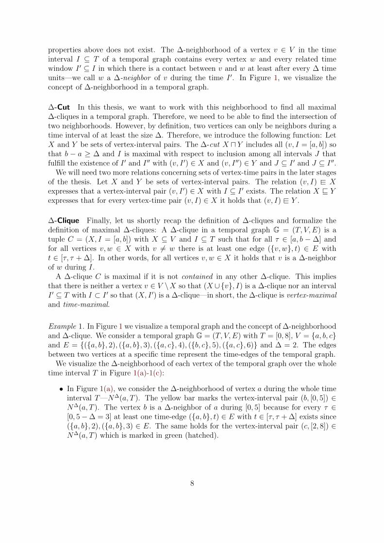
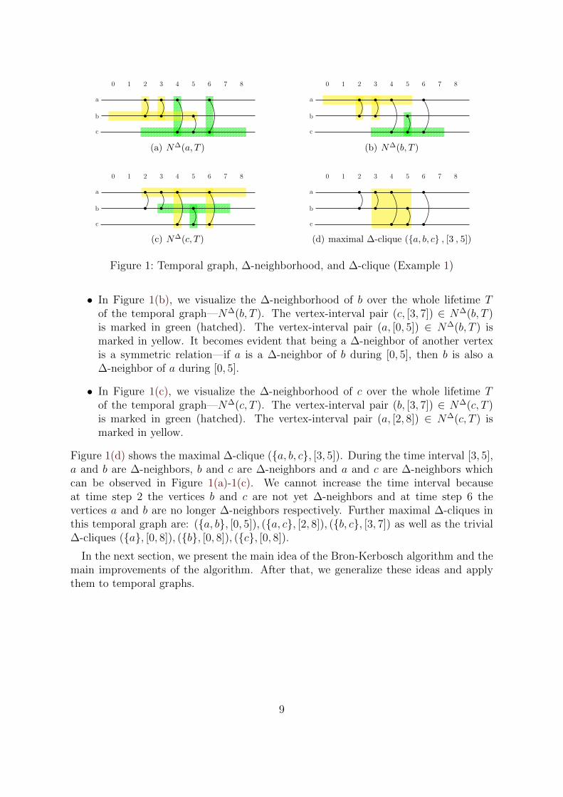
properties above does not exist. The ∆-neighborhood of a vertex v ∈ V in the timeinterval I ⊆ T of a temporal graph contains every vertex w and every related timewindow I ′ ⊆ I in which there is a contact between v and w at least after every ∆ timeunits—we call w a ∆-neighbor of v during the time I ′. In Figure 1, we visualize theconcept of ∆-neighborhood in a temporal graph.

∆-Cut In this thesis, we want to work with this neighborhood to find all maximal∆-cliques in a temporal graph. Therefore, we need to be able to find the intersection oftwo neighborhoods. However, by definition, two vertices can only be neighbors during atime interval of at least the size ∆. Therefore, we introduce the following function: LetX and Y be sets of vertex-interval pairs. The ∆-cut X u Y includes all (v, I = [a, b]) sothat b − a ≥ ∆ and I is maximal with respect to inclusion among all intervals J thatfulfill the existence of I ′ and I ′′ with (v, I ′) ∈ X and (v, I ′′) ∈ Y and J ⊆ I ′ and J ⊆ I ′′.

We will need two more relations concerning sets of vertex-time pairs in the later stagesof the thesis. Let X and Y be sets of vertex-interval pairs. The relation (v, I) @− Xexpresses that a vertex-interval pair (v, I ′) ∈ X with I ⊆ I ′ exists. The relation X v Yexpresses that for every vertex-time pair (v, I) ∈ X it holds that (v, I) @− Y .

∆-Clique Finally, let us shortly recap the definition of ∆-cliques and formalize thedefinition of maximal ∆-cliques: A ∆-clique in a temporal graph G = (T, V,E) is atuple C = (X, I = [a, b]) with X ⊆ V and I ⊆ T such that for all τ ∈ [a, b − ∆] andfor all vertices v, w ∈ X with v 6= w there is at least one edge ({v, w}, t) ∈ E witht ∈ [τ, τ + ∆]. In other words, for all vertices v, w ∈ X it holds that v is a ∆-neighborof w during I.

A ∆-clique C is maximal if it is not contained in any other ∆-clique. This impliesthat there is neither a vertex v ∈ V \X so that (X ∪{v}, I) is a ∆-clique nor an intervalI ′ ⊆ T with I ⊂ I ′ so that (X, I ′) is a ∆-clique—in short, the ∆-clique is vertex-maximaland time-maximal.

Example 1. In Figure 1 we visualize a temporal graph and the concept of ∆-neighborhoodand ∆-clique. We consider a temporal graph G = (T, V,E) with T = [0, 8], V = {a, b, c}and E = {({a, b}, 2), ({a, b}, 3), ({a, c}, 4), ({b, c}, 5), ({a, c}, 6)} and ∆ = 2. The edgesbetween two vertices at a specific time represent the time-edges of the temporal graph.

We visualize the ∆-neighborhood of each vertex of the temporal graph over the wholetime interval T in Figure 1(a)-1(c):

• In Figure 1(a), we consider the ∆-neighborhood of vertex a during the whole timeinterval T—N∆(a, T ). The yellow bar marks the vertex-interval pair (b, [0, 5]) ∈N∆(a, T ). The vertex b is a ∆-neighbor of a during [0, 5] because for every τ ∈[0, 5−∆ = 3] at least one time-edge ({a, b}, t) ∈ E with t ∈ [τ, τ + ∆] exists since({a, b}, 2), ({a, b}, 3) ∈ E. The same holds for the vertex-interval pair (c, [2, 8]) ∈N∆(a, T ) which is marked in green (hatched).

8

0 1 2 3 4 5 6 7 8

a

b

c

(a) N∆(a, T )

0 1 2 3 4 5 6 7 8

a

b

c

(b) N∆(b, T )

0 1 2 3 4 5 6 7 8

a

b

c

(c) N∆(c, T )

0 1 2 3 4 5 6 7 8

a

b

c

(d) maximal ∆-clique ({a, b, c} , [3 , 5])

Figure 1: Temporal graph, ∆-neighborhood, and ∆-clique (Example 1)

• In Figure 1(b), we visualize the ∆-neighborhood of b over the whole lifetime Tof the temporal graph—N∆(b, T ). The vertex-interval pair (c, [3, 7]) ∈ N∆(b, T )is marked in green (hatched). The vertex-interval pair (a, [0, 5]) ∈ N∆(b, T ) ismarked in yellow. It becomes evident that being a ∆-neighbor of another vertexis a symmetric relation—if a is a ∆-neighbor of b during [0, 5], then b is also a∆-neighbor of a during [0, 5].

• In Figure 1(c), we visualize the ∆-neighborhood of c over the whole lifetime Tof the temporal graph—N∆(c, T ). The vertex-interval pair (b, [3, 7]) ∈ N∆(c, T )is marked in green (hatched). The vertex-interval pair (a, [2, 8]) ∈ N∆(c, T ) ismarked in yellow.

Figure 1(d) shows the maximal ∆-clique ({a, b, c}, [3, 5]). During the time interval [3, 5],a and b are ∆-neighbors, b and c are ∆-neighbors and a and c are ∆-neighbors whichcan be observed in Figure 1(a)-1(c). We cannot increase the time interval becauseat time step 2 the vertices b and c are not yet ∆-neighbors and at time step 6 thevertices a and b are no longer ∆-neighbors respectively. Further maximal ∆-cliques inthis temporal graph are: ({a, b}, [0, 5]), ({a, c}, [2, 8]), ({b, c}, [3, 7]) as well as the trivial∆-cliques ({a}, [0, 8]), ({b}, [0, 8]), ({c}, [0, 8]).

In the next section, we present the main idea of the Bron-Kerbosch algorithm and themain improvements of the algorithm. After that, we generalize these ideas and applythem to temporal graphs.

9

Algorithm 1 Enumerating all maximal cliques in a graph1: function BronKerbosch(P,R,X)2: if P ∪X = ∅ then3: add R as maximal clique to the solution4: end if5: for v ∈ P do6: BronKerbosch(P ∩N(v), R ∪ {v}, X ∩N(v)))7: P ← P \ {v}8: X ← X ∪ {v}9: end for

10: end function

2 Bron-Kerbosch Algorithm

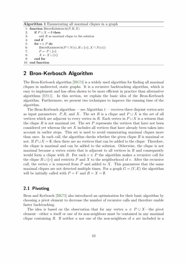
The Bron-Kerbosch algorithm [BK73] is a widely used algorithm for finding all maximalcliques in undirected, static graphs. It is a recursive backtracking algorithm, which iseasy to implement and has often shown to be more efficient in practice than alternativealgorithms [ES11]. In this section, we explain the basic idea of the Bron-Kerboschalgorithm. Furthermore, we present two techniques to improve the running time of thealgorithm.

The Bron-Kerbosch algorithm–––see Algorithm 1–––receives three disjoint vertex-setsas input parameters: P,R, and X. The set R is a clique and P ∪ X is the set of allvertices which are adjacent to every vertex in R. Each vertex in P ∪X is a witness thatthe clique R is not maximal yet. The set P represents the vertices that have not beenconsidered yet whereas the set X includes all vertices that have already been taken intoaccount in earlier steps. This set is used to avoid enumerating maximal cliques morethan once. In each call, the algorithm checks whether the given clique R is maximal ornot. If P ∪X = ∅, then there are no vertices that can be added to the clique. Therefore,the clique is maximal and can be added to the solution. Otherwise, the clique is notmaximal because a vertex exists that is adjacent to all vertices in R and consequentlywould form a clique with R. For each v ∈ P the algorithm makes a recursive call forthe clique R ∪ {v} and restricts P and X to the neighborhood of v. After the recursivecall, the vertex v is removed from P and added to X. This guarantees that the samemaximal cliques are not detected multiple times. For a graph G = (V,E) the algorithmwill be initially called with P = V and R = X = ∅.

2.1 Pivoting

Bron and Kerbosch [BK73] also introduced an optimization for their basic algorithm bychoosing a pivot element to decrease the number of recursive calls and therefore enablefaster backtracking.

The idea is based on the observation that for any vertex u ∈ P ∪ X—the pivotelement—either u itself or one of its non-neighbors must be contained in any maximalclique containing R. If neither u nor one of the non-neighbors of u are included in a

10

Algorithm 2 Enumerating all maximal cliques in a graph with pivoting1: function BronKerboschPivot(P,R,X)2: if P ∪X = ∅ then3: add R as maximal clique to the solution4: end if5: choose pivot vertex u ∈ P ∪X with |P ∩N(u)| = max

v∈P∪X| P ∩N(v) |

6: for v ∈ P \N(u) do7: BronKerboschPivot(P ∩N(v), R ∪ {v}, X ∩N(v)))8: P ← P \ {v}9: X ← X ∪ {v}

10: end for11: end function

Algorithm 3 Enumerating all maximal cliques in a graph with degeneracy ordering1: function BronKerboschDeg(P,R,X)2: for vi in a degeneracy odering v0, v1, . . . , vn of G = (V,E) do3: P ← N(vi) ∩ {vi+1, . . . , vn−1}4: X ← N(vi) ∩ {v0, . . . , vi−1}5: BronKerboschPivot(P, {vi}, X)6: end for7: end function

maximal clique containing R, this clique cannot be maximal because u can be added tothis clique due to the fact that only neighbors of u were added to the original clique R.

Therefore, choosing an arbitrary pivot element u ∈ P ∪ X and iterating just over uand all its non-neighbors decreases the number of recursive calls in the for-loop that leadto non-maximal cliques. Tomita, Tanaka, and Takahashi [TTT06] have shown that inthe case that u is chosen from P ∪X in a way that u has the most neighbors in P—seeAlgorithm 2—then the running time for a graph G = (V,E) is in O(3|V |/3).

2.2 Degeneracy Ordering

A possibility to influence the running time and provide a fixed-parameter tractablemodification of the basic Bron-Kerbosch algorithm is by exploiting the degeneracy ofthe graph, which is a measure of sparsity:

A graph G is called k-degenerated if every non-empty subgraph G′ of G contains avertex v with deg(v) ≤ k. The degeneracy of a graph G is defined as the smallest value ksuch that G is k-degenerated. If the degeneracy of a graph is d, then the maximal cliquesize of the graph is at most d + 1. In case there is a clique of the size of at least d + 2,the vertices of this clique would form a subgraph in which every vertex v of the cliquehas deg(v) ≥ d + 1. For each k-degenerated graph there is a degeneracy ordering, suchthat for every vertex v there are at most k of its neighbors later on in the ordering.The degeneracy d and a corresponding degeneracy ordering for a graph G = (V,E) canbe computed efficiently in O(|V | + |E|) time [ELS10]: For graph G, the vertex withthe smallest degree is taken in each step and removed from the graph until no vertexis left. The degeneracy of the graph is the highest degree of a vertex at the time the

11

vertex has been removed from the graph—a corresponding degeneracy ordering is theorder in which the vertices were removed from the graph. For a graph G = (V,E) withdegeneracy d, using the degeneracy ordering of G in the outer-most recursive call andafterwards using pivoting—see Algorithm 3—the algorithm runs in O(d · |V | · 3d/3) timeaccording to Eppstein, Loffler, and Strash [ELS10].

In the preceding section, the basic idea of the Bron-Kerbosch algorithm to find maxi-mal cliques in an undirected graph was introduced. In the following sections, an attemptis made to adapt the idea of the Bron-Kerbosch algorithm in order to find maximal ∆-cliques in temporal graphs. In addition, the idea of pivoting is adapted to the proposedalgorithm.

12

Algorithm 4 Enumerating all maximal ∆-cliques in a temporal graph1: function BronKerboschDelta(P, Pmax, R = (C, I), X,Xmax)

. R = (C, I) : time-maximal ∆-clique

. P ∪X : set of all (v, I ′) that fulfill that I ′ ⊆ I and (C ∪ {v}, I ′) is a time-maximal ∆-clique

. Pmax ∪Xmax : set of all (v, I) that fulfill that (C ∪ {v}, I) is a time-maximal ∆-clique

. if Pmax = ∅ and Xmax = ∅ then there exists no vertex that can be added to C without downsizingthe interval I R is vertex-maximal R is a maximal ∆-clique

2: if Pmax ∪Xmax = ∅ then3: add R as maximal clique to solution4: end if5: for (v, I ′) ∈ P do

. create new time-maximal ∆-clique by adding v to C and downsizing the interval to I ′ ⊆ I6: R′ ← (C ∪ {v}, I ′)

. find all intersections between the sets P,X and the ∆-neighborhood N∆(v, I ′)7: P ′ ← P uN∆(v, I ′)8: X ′ ← X uN∆(v, I ′)

. find all (w, I ′) in P ′, X ′ such that w can be added to R′ without downsizing the interval I ′

9: P ′max ← {(w, I ′) | (w, I ′) ∈ P ′}10: X ′max ← {(w, I ′) | (w, I ′) ∈ X ′}

. check new clique R′ with the adapted sets P ′, P ′max, X′, and X ′max

11: BronKerboschDelta(P ′, P ′max, R′, X ′, X ′max)

. remove the vertex-time pair that created the new clique R′ from set P and add it to set X toavoid multiple enumerations of cliques generated from R.

12: P ← P \ {(v, I ′)}13: X ← X ∪ {(v, I ′)}14: end for15: end function

3 Bron-Kerbosch Algorithm in Temporal Graphs

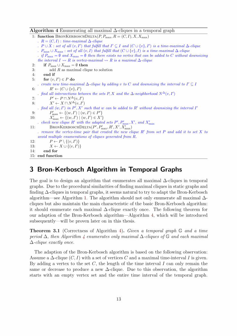
The goal is to design an algorithm that enumerates all maximal ∆-cliques in temporalgraphs. Due to the procedural similarities of finding maximal cliques in static graphs andfinding ∆-cliques in temporal graphs, it seems natural to try to adapt the Bron-Kerboschalgorithm—see Algorithm 1. The algorithm should not only enumerate all maximal ∆-cliques but also maintain the main characteristic of the basic Bron-Kerbosch algorithm:it should enumerate each maximal ∆-clique exactly once. The following theorem forour adaption of the Bron-Kerbosch algorithm—Algorithm 4, which will be introducedsubsequently—will be proven later on in this thesis.

Theorem 3.1 (Correctness of Algorithm 4). Given a temporal graph G and a timeperiod ∆, then Algorithm 4 enumerates only maximal ∆-cliques of G and each maximal∆-clique exactly once.

The adaption of the Bron-Kerbosch algorithm is based on the following observation:Assume a ∆-clique (C, I) with a set of vertices C and a maximal time-interval I is given.By adding a vertex to the set C, the length of the time interval I can only remain thesame or decrease to produce a new ∆-clique. Due to this observation, the algorithmstarts with an empty vertex set and the entire time interval of the temporal graph.

13

In each recursion step, the number of vertices increases while the length of the timeintervals monotonically decreases.

3.1 Description of the Algorithm

As shown in Algorithm 4, the function receives five parameters P, Pmax, X,Xmax, and R.The tuple R = (C, I) contains a set of vertices C and a time interval I. As we will provebelow, this tuple forms a ∆-clique with a maximal time interval I with respect to C.The sets P, Pmax, X, and Xmax contain vertex-interval pairs and it holds Pmax ⊆ P andXmax ⊆ X by definition of these sets. We will also prove below that P ∪X includes allvertex-interval pairs (v, I ′) for which (C∪{v}, I ′) is a time-maximal ∆-clique because v isa ∆-neighbor of every vertex w ∈ C during the time I ′ ⊆ I. For each (v, I) ∈ Pmax∪Xmax

the vertices C ∪ {v} form a ∆-clique over the whole time interval I of the original ∆-clique R = (C, I). While each vertex-interval pair in P still has to be combined withR to ensure that every maximal ∆-clique will be found, for every vertex-interval pair(v, I ′) ∈ X every possible ∆-clique (C ′, I ′′) with C ∪ {v} ⊆ C ′ and I ′′ ⊆ I ′ has alreadybeen detected in earlier steps. The same holds for Pmax and Xmax.

If Pmax ∪Xmax = ∅, there is no vertex v that forms a ∆-clique together with C overthe whole time interval I of the original ∆-clique R = (C, I). Due to the maximality ofthe time interval I of R, we therefore know that R is a maximal ∆-clique and has to beadded to the solution.

In the next step, for every vertex-interval pair (v, I ′) ∈ P a recursive call is initiated forthe ∆-clique R′ = (C ∪ {v}, I ′) with all parameters restricted to the ∆-neighborhood ofv in the time interval I ′—P uN∆(v, I ′) and X uN∆(v, I ′). For the set P ′ for example,we get a set of all time-maximal vertex-interval pairs (w, I ′′) for which it holds that(w, I ′′) @− N∆(v, I ′) and (w, I ′′) @− P . This restriction is made so that for all (w, I ′′) ∈ P ′

of the recursive call the vertex w is not only a ∆-neighbor of all x ∈ C but also of thevertex v during the time I ′′ ⊆ I ′.

After the recursive call for ∆-clique (C ∪ {v}, I ′), the tuple (v, I ′) is removed fromthe set P and added to the set X to avoid that the same cliques are found multipletimes. For a temporal graph G = (T, V,E) and a given time period ∆, the initialcall for Algorithm 4 to enumerate all maximal ∆-cliques in graph G is made withP = {(v, T ) | v ∈ V }, Pmax = {(v, T ) | v ∈ V }, R = (∅, T ), X = ∅, and Xmax = ∅.

Before we try to improve the running time of the algorithm by adapting the idea ofpivoting—see Subsection 3.4—we prove the correctness of Algorithm 4: it must be shownthat all elements in the output are ∆-cliques, that all elements are maximal ∆-cliques,that all maximal ∆-cliques are in the output, and that no maximal ∆-clique is foundmore than once. To present these proofs, we have to formally define the correspondingrecursion tree that is built by the recursive calls of the initial call of Algorithm 4.

14

0 1 2 3 4 5 6 7 8

a

b

c

(a) Temporal graph G

R : ({a, b, c}, [3, 5])P : ∅X : ∅Pmax, Xmax : ∅

R : ({a, b}, [0, 5])P : {(c, [3, 5])}X : ∅Pmax, Xmax : ∅

R : ({a, c}, [2, 8])P : ∅X = {(b, [3, 5])}Pmax, Xmax : ∅

R : ({a}, [0, 8])P : {(b, [0, 5]), (c, [2, 8])}X : ∅Pmax, Xmax : ∅

R : ({b, c}, [3, 7])P : ∅X = {(a, [3, 5])}Pmax, Xmax : ∅

R : ({b}, [0, 8])P : {(c, [3, 7])}X : {(a, [0, 5])}Pmax, Xmax : ∅

R : ({c}, [0, 8])P : ∅X : {(a, [3, 7]), (b, [2, 8])}Pmax, Xmax : ∅

R : (∅, [0, 8])P : {(a, [0, 8]), (b, [0, 8]), (c, [0, 8])}X : ∅Pmax : {(a, [0, 8]), (b, [0, 8]), (c, [0, 8])}Xmax : ∅

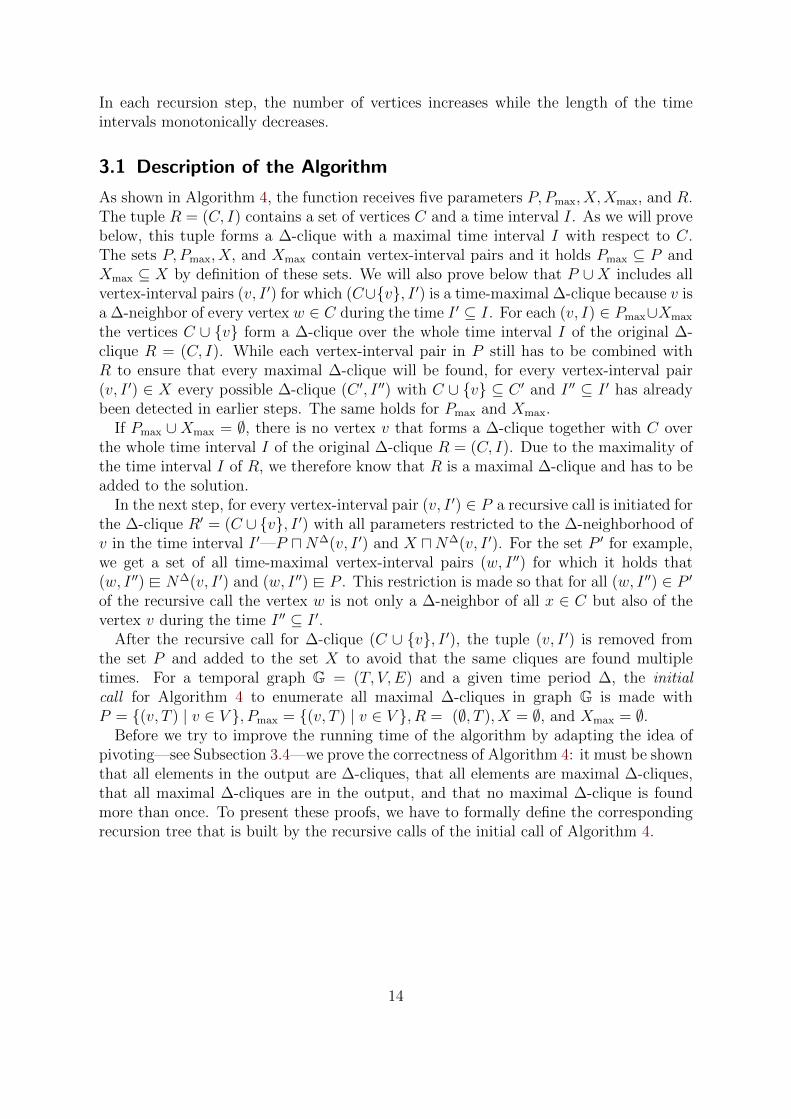
(b) Recursion tree of Algorithm 4 for temporal graph G and ∆ = 2

Figure 2: A recursion tree of the temporal graph of Figure 2(a) for ∆=2 generated bythe initial call of Algorithm 4. All nodes—except the root—signal maximal∆-cliques.

15

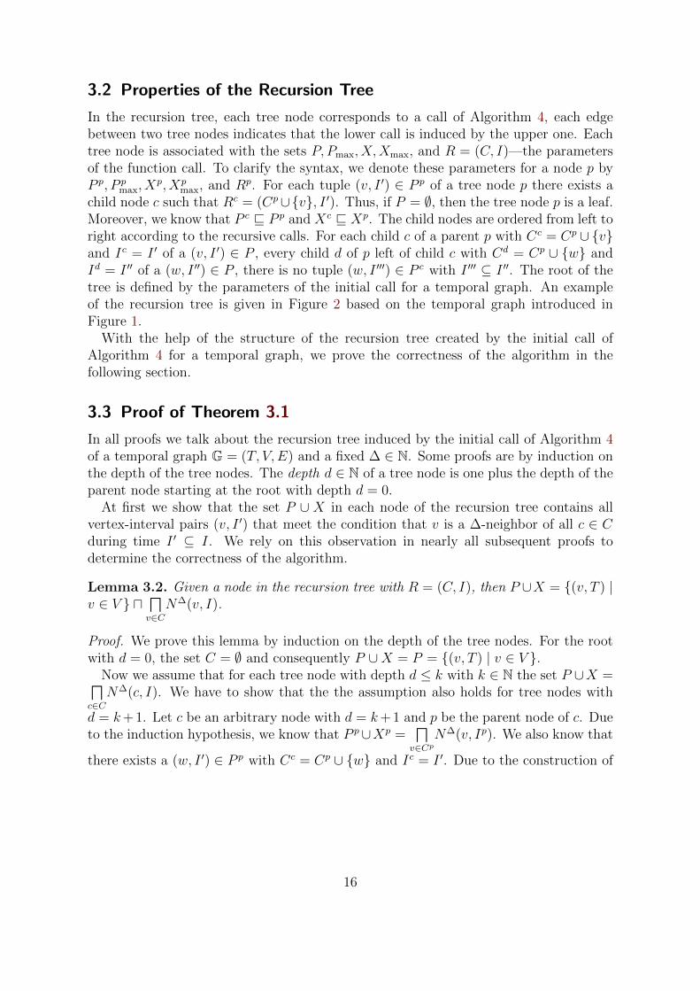
3.2 Properties of the Recursion Tree

In the recursion tree, each tree node corresponds to a call of Algorithm 4, each edgebetween two tree nodes indicates that the lower call is induced by the upper one. Eachtree node is associated with the sets P, Pmax, X,Xmax, and R = (C, I)—the parametersof the function call. To clarify the syntax, we denote these parameters for a node p byP p, P p

max, Xp, Xp

max, and Rp. For each tuple (v, I ′) ∈ P p of a tree node p there exists achild node c such that Rc = (Cp∪{v}, I ′). Thus, if P = ∅, then the tree node p is a leaf.Moreover, we know that P c v P p and Xc v Xp. The child nodes are ordered from left toright according to the recursive calls. For each child c of a parent p with Cc = Cp ∪ {v}and Ic = I ′ of a (v, I ′) ∈ P , every child d of p left of child c with Cd = Cp ∪ {w} andId = I ′′ of a (w, I ′′) ∈ P , there is no tuple (w, I ′′′) ∈ P c with I ′′′ ⊆ I ′′. The root of thetree is defined by the parameters of the initial call for a temporal graph. An exampleof the recursion tree is given in Figure 2 based on the temporal graph introduced inFigure 1.

With the help of the structure of the recursion tree created by the initial call ofAlgorithm 4 for a temporal graph, we prove the correctness of the algorithm in thefollowing section.

3.3 Proof of Theorem 3.1

In all proofs we talk about the recursion tree induced by the initial call of Algorithm 4of a temporal graph G = (T, V,E) and a fixed ∆ ∈ N. Some proofs are by induction onthe depth of the tree nodes. The depth d ∈ N of a tree node is one plus the depth of theparent node starting at the root with depth d = 0.

At first we show that the set P ∪ X in each node of the recursion tree contains allvertex-interval pairs (v, I ′) that meet the condition that v is a ∆-neighbor of all c ∈ Cduring time I ′ ⊆ I. We rely on this observation in nearly all subsequent proofs todetermine the correctness of the algorithm.

Lemma 3.2. Given a node in the recursion tree with R = (C, I), then P ∪X = {(v, T ) |v ∈ V } u

d

v∈CN∆(v, I).

Proof. We prove this lemma by induction on the depth of the tree nodes. For the rootwith d = 0, the set C = ∅ and consequently P ∪X = P = {(v, T ) | v ∈ V }.

Now we assume that for each tree node with depth d ≤ k with k ∈ N the set P ∪X =d

c∈CN∆(c, I). We have to show that the the assumption also holds for tree nodes with

d = k+ 1. Let c be an arbitrary node with d = k+ 1 and p be the parent node of c. Dueto the induction hypothesis, we know that P p∪Xp =

d

v∈Cp

N∆(v, Ip). We also know that

there exists a (w, I ′) ∈ P p with Cc = Cp ∪ {w} and Ic = I ′. Due to the construction of

16

Algorithm 4, the following holds:

P c ∪Xc =l

v∈Cp

N∆(v, I) uN∆(w, Ic)

=l

v∈Cp

N∆(v, Ic) uN∆(w, Ic)

=l

v∈Cp∪{w}

N∆(v, Ic)

=l

v∈Cc

N∆(v, Ic)

Hence, for every node of the recursion tree with R = (C, I) it holds that P ∪ X =d

v∈CN∆(v, I).

The proof of Lemma 3.2 does not only show us that for a given node in the recursiontree with a ∆-clique R = (C, I) for all (v, I ′) ∈ P ∪ X and for all c ∈ C it holds that(v, I ′) @− N∆(c, I), but also shows that all elements (v, I ′) that can expand the ∆-clique Rare in these sets. Furthermore, it gives us the certainty that the time interval I ′ of every(v, I ′) ∈ P ∪X is maximal. This observation relies on the fact that the ∆-cut (‘u’) andthe ∆-neighborhood (‘N∆’) always return sets with vertex-interval pairs that consist ofmaximal time intervals by definition.

We continue by showing that the tuple R = (C, I) is a ∆-clique in each node of therecursion tree and that this ∆-clique is time-maximal. We will need these proofs to showthat all elements that will be added to the solution are in fact maximal ∆-cliques.

Lemma 3.3. The tuple R = (C, I) of a node in the recursion tree is a ∆-clique.

Proof. We prove the lemma by induction on the depth of the tree nodes. For the rootwith d = 0, the parameter R = (C = ∅, I = T ) of this initial call is a trivial ∆-clique.Furthermore, due to the set P of this initial call, for each v ∈ V there exists a child nodeof the root with R = (C = {v}, I = T )—a trivial ∆-clique. These nodes are the onlychild nodes of the root and consequently the only tree nodes with d = 1. Thus, everytree node with d = 1 is also a ∆-clique.

Now we assume that for each tree node with depth d ≤ k with k ∈ N the tupleR = (C, I) is a ∆-clique. We have to show that for a tree node with depth d = k + 1the tuple R is also a ∆-clique. Let c be any node with d = k + 1 and let p be theparent of this node. Due to the induction hypothesis, we know that Rp = (Cp, Ip) is a∆-clique. Let (v, I ′) ∈ P p be the vertex-interval pair with Cc = Cp ∪ {v} and Ic = I ′.By Lemma 3.2 we know that the vertex v is a ∆-neighbor of all vertices in the set Cp

during time I ′. Consequently, Rc = (Cc, Ic) is a ∆-clique. Ergo, for every tree node inthe recursion tree with d = k + 1 the tuple R = (C, I) is a ∆-clique.

We have shown that R = (C, I) is a ∆-clique in all nodes of the recursion tree. Wenow have to prove that these ∆-cliques are also time-maximal. This means that wecannot increase the time interval I of R without losing the properties of a ∆-clique.

17

Lemma 3.4. Each ∆-clique R = (C, I) of a node in the recursion tree is time-maximal.

Proof. We will, again, prove the lemma by induction on the depth of the tree nodes. Forthe root with d = 0, the ∆-clique R = (C = ∅, I = T ) is time-maximal because thereis no I ′ ⊆ T with I = T ⊂ I ′. The same holds for every tree node with d = 1 whereR = (C = {v}, I = T ) for a v ∈ V .

Now we assume that for each tree node with depth d ≤ k with k ∈ N the ∆-cliqueR = (C, I) is time-maximal. We have to show that for every tree node with d = k + 1the ∆-clique R = (C, I) is time-maximal. Let c be any node with d = k+ 1 and let p bethe parent node of c. Let (v, I ′) ∈ P p be the vertex-interval pair with Cc = Cp∪{v} andIc = I ′. We know that the ∆-clique Rp = (Cp, Ip) is time-maximal due to the inductionhypothesis. Furthermore, we have proven in Lemma 3.2 that the time intervals of thevertex-interval pairs in P p and Xp are maximal. Hence, the ∆-clique Rc is time-maximalas well.

We can now easily prove, that all ∆-cliques that are added to the solution by Algo-rithm 4 are maximal ∆-cliques.

Lemma 3.5. Each ∆-clique of a node in the recursion tree that is added to the solutionis a maximal ∆-clique.

Proof. Let R = (C, I) be a ∆-clique that is added to the solution and P, Pmax andX,Xmax be the corresponding sets of vertex-interval pairs in the tree node of this ∆-clique. We already know by Lemma 3.3 that the ∆-clique R is time-maximal. Fur-thermore, according to the Algorithm 4, Pmax = ∅ and Xmax = ∅ so that R is addedto the solution. In Lemma 3.2 we have proven that the set P ∪ X contains all vertex-interval pairs (v, I ′) for which v is a ∆-neighbor of all vertices in C during time I ′. IfPmax ∪ Xmax = ∅, then there is no vertex v ∈ V \ C that will form a ∆-clique with Cover the whole time interval I. Thus, R = (C, I) is vertex-maximal as well as time-maximal and consequently not contained in any other ∆-clique. Hence, R is a maximal∆-clique.

We now prove that all maximal cliques are found by Algorithm 4. The proof isconducted by showing that every maximal ∆-clique is represented in a node of therecursion tree. In order to conclude from this proof that all maximal ∆-cliques areadded to the solution, we have to show first that every maximal ∆-clique that appearsin a node of the recursion tree is added to the solution.

Lemma 3.6. Each ∆-clique of a node in the recursion tree that is a maximal ∆-cliqueis added to the solution.

Proof. Assume there is a maximal ∆-clique R = (C, I) in a node of the recursion tree.Let P, Pmax and X,Xmax be the corresponding sets of vertex-interval pairs in this treenode. This ∆-clique R is time-maximal and, more importantly, vertex-maximal. Thus,no vertex v ∈ V \C exists such that (C ∪{v}, I) is a ∆-clique. Ergo, there is no vertex-interval pair (∗, I) ∈ P ∪X. Consequently, Pmax ∪Xmax = ∅ and R has been added tothe solution.

18

After proving that all maximal ∆-cliques that are represented in a node of the recur-sion tree are added to the solution, it remains to show that every maximal ∆-clique isrepresented in a tree node. This proof is made by contradiction, showing that for allmaximal ∆-cliques a path to a node exists representing the ∆-clique.

Lemma 3.7. Each maximal ∆-clique of the temporal graph has at least one node withinthe recursion tree.

Proof. The proof is conducted by contradiction. Assume there is a ∆-clique R = (C, I)that does not appear in any node of the recursion tree. Let s be the tree node with thegreatest depth d of the recursion tree which the clique R can still be generated from,that is, Cs ⊆ C, I ⊆ Is, and for every v ∈ C \Cs it holds that (v, I) @− P s. We considerhereby the set P s at the beginning of the function call. These conditions are definitelygiven in the root of the recursion tree with d = 0. Let t be the leftmost tree node that isgenerated by a vertex-interval pair (v, I ′) ∈ P s with v ∈ C \ Cs and I ⊆ I ′ ⊆ T . Thus,all vertex-interval pairs (w, I ′′) with w ∈ C \Cs and I ⊆ I ′′ ⊆ T have not been removedfrom P s yet. It holds Cs ⊂ Ct ⊆ C. Due to the fact that R = (C, I) is a ∆-clique, weknow that every w ∈ C \Ct is a ∆-neighbor of vertex v at least during I. Consequently,for every w ∈ C \ Ct there exists a (w, I) @− P s u N∆(v, I ′) = P t. Thus, the ∆-cliquecan also be generated from node t which is a child of the node s and thus has a greaterdepth d than its parent s. This is a contradiction to the assumption that s is the treenode with the greatest depth from which the ∆-clique R can be generated.

Additionally, Algorithm 4 also ensures that every maximal ∆-clique is added to thesolution only once. This proof is conducted again by contradiction, proving that every∆-clique appears not at least but exactly once in a node of the recursion tree.

Lemma 3.8. Each maximal ∆-clique of the temporal graph has exactly one node withinthe recursion tree.

Proof. Assume there are two nodes in the recursion tree with the same maximal ∆-cliqueR = (C, I). Let p be the last node that the paths from the root to these nodes have incommon. It holds Cp ⊂ C, I ⊆ Ip, and for every v ∈ C \Cp it holds that (v, I) @− P p atthe beginning of the function call. Let s be the child of p and the next node in the leftpath, let t also be a child of p and the next node in the right path. The node s is theleftmost node that is generated from a vertex-interval pair (v, I ′) ∈ P p with v ∈ C \ Cp

and I ⊆ I ′ ⊆ T . Recall that the nodes are ordered from left to right according tothe recursive calls. This means that the recursive call for node s is induced by node pbefore the recursive call for node t is induced. The vertex-interval pair (v, I ′) is removedfrom P p and added to Xp after the recursive call for node s. Hence, at the time whenthe recursive call for node t is made, the ∆-clique can not be generated from set P p anylonger because (v, I ′) 6∈ P p and consequently (v, I) 6@− P t. Ergo, the right path does notlead to a node that represents R = (C, I) and consequently there is no second node thatrepresents R. This is a contradiction to our assumption and therefore there is exactlyone node for each maximal ∆-clique in the recursion tree.

19

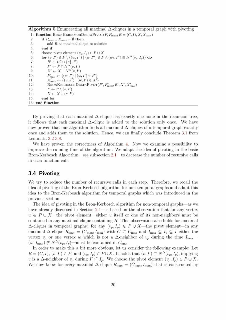
Algorithm 5 Enumerating all maximal ∆-cliques in a temporal graph with pivoting1: function BronKerboschDeltaPivot(P, Pmax, R = (C, I), X,Xmax)2: if Pmax ∪Xmax = ∅ then3: add R as maximal clique to solution4: end if5: choose pivot element (vp, Ip) ∈ P ∪X6: for (v, I ′) ∈ P \ {(w, I ′′) | (w, I ′′) ∈ P ∧ (w2, I

′′) @− N∆(vp, Ip)} do7: R′ ← (C ∪ {v}, I ′)8: P ′ ← P uN∆(v, I ′)9: X ′ ← X uN∆(v, I ′)

10: P ′max ← {(w, I ′) | (w, I ′) ∈ P ′}11: X ′max ← {(w, I ′) | (w, I ′) ∈ X ′}12: BronKerboschDeltaPivot(P ′, P ′max, R

′, X ′, X ′max)13: P ← P \ (v, I ′)14: X ← X ∪ (v, I ′)15: end for16: end function

By proving that each maximal ∆-clique has exactly one node in the recursion tree,it follows that each maximal ∆-clique is added to the solution only once. We havenow proven that our algorithm finds all maximal ∆-cliques of a temporal graph exactlyonce and adds them to the solution. Hence, we can finally conclude Theorem 3.1 fromLemmata 3.2-3.8.

We have proven the correctness of Algorithm 4. Now we examine a possibility toimprove the running time of the algorithm. We adapt the idea of pivoting in the basicBron-Kerbosch Algorithm—see subsection 2.1—to decrease the number of recursive callsin each function call.

3.4 Pivoting

We try to reduce the number of recursive calls in each step. Therefore, we recall theidea of pivoting of the Bron-Kerbosch algorithm for non-temporal graphs and adapt thisidea to the Bron-Kerbosch algorithm for temporal graphs which was introduced in theprevious section.

The idea of pivoting in the Bron-Kerbosch algorithm for non-temporal graphs—as wehave already discussed in Section 2.1—is based on the observation that for any vertexu ∈ P ∪ X—the pivot element—either u itself or one of its non-neighbors must becontained in any maximal clique containing R. This observation also holds for maximal∆-cliques in temporal graphs: for any (vp, Ip) ∈ P ∪ X—the pivot element—in anymaximal ∆-clique Rmax = (Cmax, Imax) with C ⊂ Cmax and Imax ⊆ Ip ⊆ I either thevertex vp or one vertex w which is not a ∆-neighbor of vp during the time Imax—(w, Imax) 6@− N∆(vp, Ip)—must be contained in Cmax.

In order to make this a bit more obvious, let us consider the following example: LetR = (C, I), (v, I ′) ∈ P , and (vp, Ip) ∈ P ∪X. It holds that (v, I ′) @− N∆(vp, Ip), implyingv is a ∆-neighbor of vp during I ′ ⊆ Ip. We choose the pivot element (vp, Ip) ∈ P ∪ X.We now know for every maximal ∆-clique Rmax = (Cmax, Imax) that is constructed by

20

expanding R by (v, I ′) it either holds that vp ∈ Cmax or w ∈ Cmax with (w, I ′′) ∈ P ∪X,Imax ⊆ I ′′, and (w, Imax) 6@− N∆(vp, Ip). Consequently (w, I ′′) 6@− N∆(vp, Ip) because if wis not a ∆-neighbor of vp during Imax, then it can not be a ∆-neighbor of vp during I ′′

which contains Imax. In both cases, we would also find the maximal ∆-clique Rmax bythe recursive calls for (vp, Ip) expanding R or (w, I ′′) expanding R.

The previous paragraph provided an example for pivoting in the Bron-Kerbosch algo-rithm for enumerating maximal ∆-cliques in temporal graphs. We now prove that ourintuition is correct in the following lemma:

Lemma 3.9. For each ∆-clique R = (C, I) in a node of the recursion tree and a pivotelement (vp, Ip) ∈ P ∪ X the following holds: for every Rmax = (Cmax, Imax) with C ⊂Cmax and Imax ⊆ Ip ⊆ I it either holds that vp ∈ Cmax or there is a vertex w ∈ Cmax

that satisfies (w, I ′) ∈ P ∪ X, Imax ⊆ I ′, and (w, Imax) 6@− N∆(vp, Ip) and consequently(w, I ′) 6@− N∆(vp, Ip).

Proof. Let Rmax = (Cmax, Imax) be a maximal ∆-clique with C ⊂ Cmax and Imax ⊆ Ip ⊆I. Assume all w ∈ Cmax hold (w, Imax) @− N∆(vp, Ip). Consequently, for all w ∈ Cmax \Ca (w, I ′) ∈ P ∪ X with Imax ⊆ I ′ must exist. Because v is a ∆-neighbor of all verticesin Cmax \ C at least during Imax and a ∆-neighbor of all vertices in C during Ip, thevertex vp can be added to the ∆-clique Rmax. This shows that Rmax is not vertex-maximal, and consequently not maximal—this is a contradiction to the assumption thatRmax is maximal.

Conversely, by choosing a pivot element (vp, Ip) ∈ X ∪ P we only have to iterate overall elements in P which are not in the ∆-neighborhood of the pivot element. In otherwords, we do not have to make a recursive call for any (w, I ′) ∈ P which holds (w, I ′) @−N∆(vp, Ip). Due to Lemma 3.9, we know that Algorithm 5—the implementation ofpivoting—also enumerates all maximal ∆ cliques in a temporal graph.

The pivot element must be chosen in such a way that minimizes the number of recursivecalls. The optimal pivot element is the element in the set P ∪ X of which the mostelements in P are in its ∆-neighborhood. We have seen that the whole procedure isquite similar to pivoting in the basic Bron-Kerbosch algorithm but with one difference:we are able to choose more than one pivot element. The only condition that has to besatisfied is that the time intervals of the pivot elements cannot overlap. This might notbe obvious at first glance but a closer look at Lemma 3.9 sheds some light:

For each ∆-clique R = (C, I) in a node of the recursion tree, choosing a pivot element(vp, Ip) ∈ P ∪X only affects maximal ∆-cliques Rmax = (Cmax, Imax) fulfilling Imax ⊆ Ip.Furthermore, for all elements (w, I ′) ∈ P satisfying (w, I ′) @− N∆(vp, Ip) it holds I ′ ⊆ Ip.Consequently, a further pivot element (v′p, I

′p) ∈ P ∪X fulfilling that I ′p does not overlap

with Ip, neither interferes with the considered maximal ∆-cliques nor with the vertex-interval pairs in P that are in the ∆-neighborhood of the pivot element (vp, Ip).

Now we face the problem that choosing the optimal set of pivot elements is no longera simple task. We have to find the optimal subset of vertex-interval pairs in P ∪ Xthat fulfill the condition that the time intervals do not intersect and that maximizes thenumber of elements in P for which we do not have to make a recursive call due to the

21

previous argumentation in Lemma 3.9. The problem of finding the optimal set of pivotelements in P ∪ X can be formulated as a weighted interval scheduling maximizationproblem:

Weighted Interval Scheduling Maximization ProblemInput: A set J of jobs j with a time interval Ij and a weight wjTask: Find a subset of jobs J ′ ⊆ J that maximizes

∑j∈J ′

wj while fulfilling that for

all i, j ∈ J ′ with i 6= j, the time intervals Ii and Ij do not overlap!

In our problem, the jobs are the elements of P∪X and the weight of an element is therebythe number of all elements that are in P and lie in the ∆-neighborhood of this element.Formally, the jobs are the elements (v, I ′) ∈ P ∪X, the corresponding time interval is I ′

of the element (v, I ′) and the corresponding weight w(v,I′) =| {(v, I) | (v, I) ∈ P∧(v, I) @−N∆(v, I ′)} |. This problem can be solved efficiently in O(n log n) time by using dynamicprogramming under the assumption that the weights of the potential pivot elements areknown.

We have shown that by choosing a set of pivot elements, we can reduce the number ofrecursive calls in our algorithm and therefore enable faster backtracking. The selectionof an optimal set of pivot elements can thereby be done efficiently in O(n log n) time.To complete this thesis, we test our algorithm on real-world datasets to examine therunning time of our adaption of the Bron-Kerbosch algorithm to temporal graphs. Weconcentrate on the implementation of Algorithm 4 to explore the efficiency of the basicalgorithm idea.

22

4 Implementation and Experiments

We implemented Algorithm 4 to explore the efficiency of our algorithm on differentdatasets and to compare our algorithm to the first approach for computing maximal ∆-cliques in temporal graphs. This approach was presented by Viard, Latapy, and Magnien[VLM16]. The source code in Python was provided by the authors on GitHub [VL14]. Toensure comparability, we decided to implement our algorithm in the same programminglanguage. The algorithm itself is very short and straightforward to program. For thisreason, we decided to limit our elaborations to choice design decisions concerning therepresentation of the dataset as ∆-neighborhoods and data structures. Furthermore,we look into the implementation of the ∆-cut-function (‘u’), the only non-obvious andtime-consuming function in the algorithm.

4.1 Implementation Design

After importing the dataset of the temporal graph, we compute the whole ∆-neighbor-hood of every vertex throughout its entire lifetime. The algorithm only works on these ∆-neighborhoods. The dataset itself is no longer needed. As a result of the ∆-neighborhoodrepresentation of the graph we lose some information in respect to the detailed time-edgesbetween the vertices. Thus, if the value of ∆ changes, then the new ∆-neighborhoodhas to be computed again with the help of the original dataset. This implies a trade-offbetween storing the original dataset and its repeated re-importation in order to computethe ∆-neighborhoods for changing values of ∆.

∆-Neighborhood Let us shortly recap the ∆-neighborhood in a temporal graph G =(T, V,E): For a vertex v ∈ V and a time interval I ⊆ T the ∆-neighborhood N∆(v, I)is the set of all vertex-interval pairs (w, I ′ = [a, b]) with the property that for everyτ ∈ [a, b−∆] at least one edge ({v, w}, t) ∈ E with t ∈ [τ, τ + ∆] exists. Furthermore,it holds that b− a ≥ ∆, I ′ ⊆ I and I ′ is maximal.

Computing the ∆-neighborhood of all vertices v over the whole lifetime of the graph—N∆(v, T )—is doable in polynomial time. After importing the dataset, we have a set ofall vertices, the beginning and end of the lifetime and a hash map representing the time-edges of the temporal graph. Thereby, every pair of vertices that has at least one contactrepresents a key in this hash map. The value of the key is a set of all points in time wherea contact between these two vertices appeared. To compute the ∆-neighborhoods of agiven temporal graph, we have to iterate over all keys in the hash map and compute thetime intervals during which the two vertices of the key are ∆-neighbors. Therefore, wesimply have to sort the set of time stamps, iterate over the resulting ascending list, andcompute all maximal time intervals during which the two vertices have a contact at leastafter every ∆ time steps, implying they are ∆-neighbors during these time intervals.

Data Structures Due to the symmetry of the ∆-neighbor relation, we can also use ahash map data structure to store the ∆-neighborhoods. The set of two vertices—let uscall them v and w—represents a key in the hash map and an ascending list L of time

23

intervals represents the corresponding value of the key. For all time intervals I ∈ L itholds that the vertices v and w are ∆-neighbors during I.

The sets P and X are also represented as hash maps. Let us consider the set P : Avertex v is the key and an ascending list L of time intervals is the corresponding value.For all I ∈ L it holds (v, I) ∈ P . The same holds for the set X.

Two important properties have to be highlighted concerning the lists of intervals inboth, the ∆-neighborhoods and the sets P and X: These lists of intervals are always inascending order relative to the starting points of the intervals. Furthermore, due to themaximality of the time intervals in the ∆-neighborhoods as well as in the sets P and X,the intervals in the list can only overlap in less than ∆ time steps. The reader shouldkeep this in mind to understand the implementation of the ∆-cut-function. The choiceof this data structure will be justified when we discuss the ∆-cut function.

∆-Cut We shortly recap the definition of this function before we discuss the imple-mentation: Let X and Y be sets of vertex-interval pairs. The ∆-cut X u Y includes all(v, I = [a, b]) so that b − a ≥ ∆ and I is maximal with respect to inclusion among allintervals J that fulfill the existence of I ′ and I ′′ with (v, I ′) ∈ X and (v, I ′′) ∈ Y andJ ⊆ I ′ and J ⊆ I ′′.

The ∆-cut function appears twice in the code of Algorithm 4: When the ∆-cliqueis expanded by adding the vertex v to the clique and when reducing the time intervalto I ′ for (v, I ′) ∈ P , the sets X and P also have to be adapted to the new vertex v andthe new time interval I ′. Let us consider the set P : the ∆-cut of the set P and theneighborhood N∆(v, I ′) has to be found. We now present an efficient way of computingthis ∆-cut—P uN∆(v, I ′):

To find the ∆-cut of P and N∆(v, I ′), we only have to examine the vertices that existin a vertex-time pair of P since a vertex that does not already exist in P cannot exist inthe resulting set of this ∆-cut. Consequently, we proceed to go through each vertex wthat exists in a vertex-time pair of P—the keys of the hash map of P :

• get list Lw of the vertex w in the hash map of the set P .The list Lw contains all time intervals I such that (w, I) ∈ P holds in ascendingorder relative to the starting points.

• get list L{v,w} of the set {v, w} in the hash map of the ∆-neighborhoods.The list L{v,w} contains all time intervals during which v and w are ∆-neighborsin ascending order relative to the starting points.

• find all intersections of the time intervals in the lists L{v,w} and Lw during thetime I ′ with at least size ∆.The time intervals within these lists only overlap in less than ∆ time steps. Thus,we can go through these lists concurrently without regression to find all overlapsduring time I ′ with at least size ∆. The new list L′

w containing these overlaps isautomatically sorted in ascending order relative to the starting points of the timeintervals.

24

• replace Lw with the new list L′w.

If list L′w is empty, then we delete the vertex/key w from the hash map of the

set P .

We not only get an ascending list L′w of time intervals such that for all I ′′ ∈ L′

w itholds that I ′′ ⊆ I ′ and it holds that the vertex w is a ∆-neighbor of all vertices in thenew, expanded ∆-clique during time I ′′, but can also compute this list in linear time.Thanks to the data structure of the hash maps and the lists of time intervals presortedin ascending order, the whole operation works efficiently in polynomial time.

We have shortly described the main design decisions that were made to guaranteean efficient implementation of Algorithm 4. In the following subsection, we begin totest our algorithm using different datasets. We shortly introduce the three datasets andpresent the main results of our test runs.

4.2 Experiments

We decided to conduct the test runs of our algorithm on three different real worlddatasets. We ran the experiments on a computer running a 64-bit version of Ubuntu15.10 with a 2.9 GHz Intel Core i5 4300Ua processor and 8 GB RAM.

4.2.1 Datasets

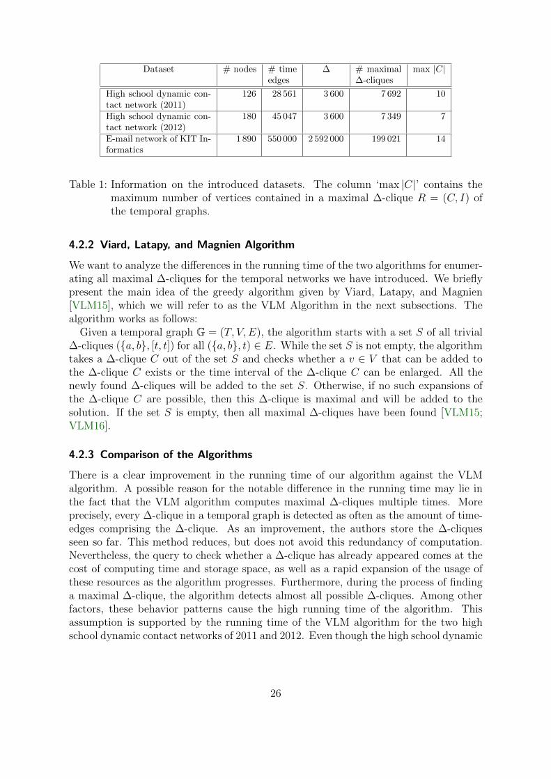
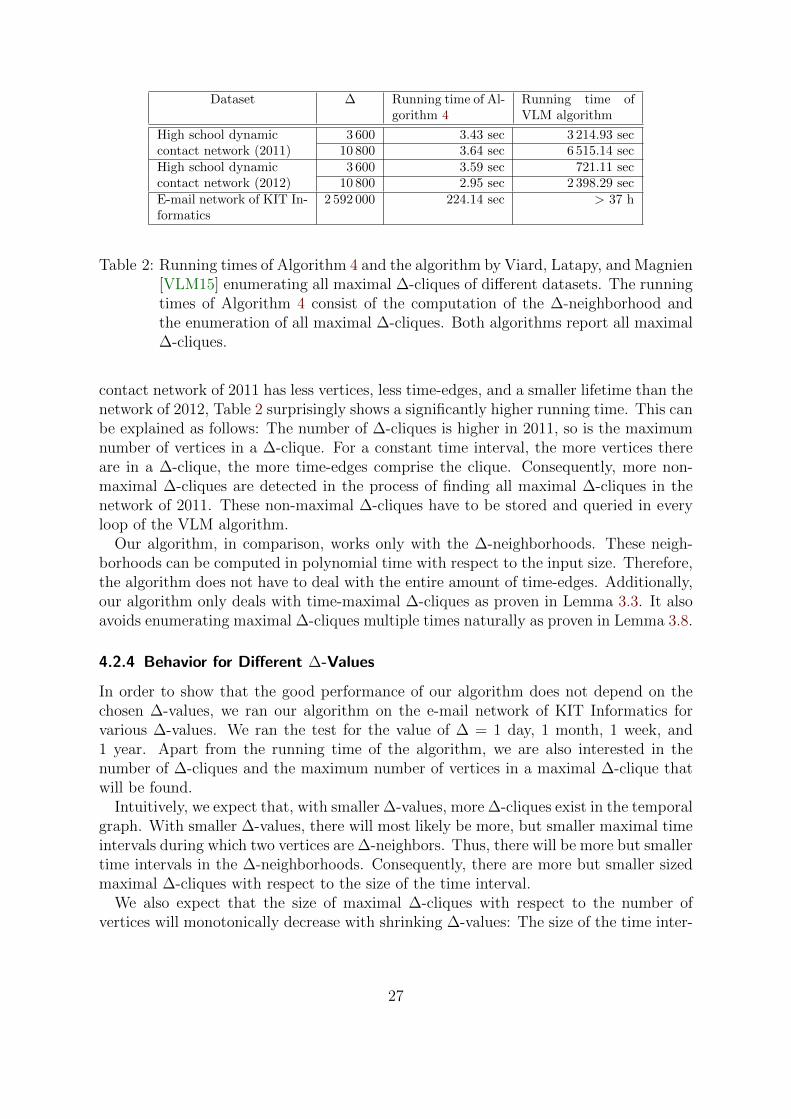
The first two datasets are high school dynamic contact networks. Both temporal net-works contain contact data between high school students in Marseilles, France. In 2011,three classes participated in the experiment which lasted for four consecutive schooldays. In 2012, five classes participated over a period of seven days from Monday untilTuesday of the following week. The contact time stamps are accurate to the second. Thedataset of 2012 was also used by Viard, Latapy, and Magnien [VLM15] to illustrate therelevance of ∆-cliques in temporal graphs. Both datasets are available on the website‘SocioPatterns’ [BF14b] and analyzed by Barrat and Fournet [BF14a]. Another datasetis the e-mail network of KIT Informatics released on the KIT website [Goe11]. It con-tains the e-mail traffic of 1 890 persons between September 2006 and August 2010. Thetime stamps of the e-mails are also accurate to the second. In Table 1 the reader canfind detailed information concerning the number of nodes and the number of time-edgesin the temporal graphs as well as the number of ∆-cliques and the maximum number ofvertices in a maximal ∆-clique for a selected ∆. For the high school contact network,the value ∆ = 3 600 (1 hour) seems like a suitable value to extract study groups. For thee-mail network of KIT Informatics, the value ∆ = 2 592 000 (1 month) seems suitableto extract research groups. The running time of our algorithm and the running timeof the algorithm by Viard, Latapy, and Magnien [VLM15] for a given ∆ is listed inTable 2. For the e-mail network of KIT Informatics, we had to stop the test run of thealgorithm by Viard, Latapy, and Magnien [VLM15] after roughly 37 hours due to thelack of computing resources.

25

Dataset # nodes # timeedges

∆ # maximal∆-cliques

max |C|

High school dynamic con-tact network (2011)

126 28 561 3 600 7 692 10

High school dynamic con-tact network (2012)

180 45 047 3 600 7 349 7

E-mail network of KIT In-formatics

1 890 550 000 2 592 000 199 021 14

Table 1: Information on the introduced datasets. The column ‘max |C|’ contains themaximum number of vertices contained in a maximal ∆-clique R = (C, I) ofthe temporal graphs.

4.2.2 Viard, Latapy, and Magnien Algorithm

We want to analyze the differences in the running time of the two algorithms for enumer-ating all maximal ∆-cliques for the temporal networks we have introduced. We brieflypresent the main idea of the greedy algorithm given by Viard, Latapy, and Magnien[VLM15], which we will refer to as the VLM Algorithm in the next subsections. Thealgorithm works as follows:

Given a temporal graph G = (T, V,E), the algorithm starts with a set S of all trivial∆-cliques ({a, b}, [t, t]) for all ({a, b}, t) ∈ E. While the set S is not empty, the algorithmtakes a ∆-clique C out of the set S and checks whether a v ∈ V that can be added tothe ∆-clique C exists or the time interval of the ∆-clique C can be enlarged. All thenewly found ∆-cliques will be added to the set S. Otherwise, if no such expansions ofthe ∆-clique C are possible, then this ∆-clique is maximal and will be added to thesolution. If the set S is empty, then all maximal ∆-cliques have been found [VLM15;VLM16].

4.2.3 Comparison of the Algorithms

There is a clear improvement in the running time of our algorithm against the VLMalgorithm. A possible reason for the notable difference in the running time may lie inthe fact that the VLM algorithm computes maximal ∆-cliques multiple times. Moreprecisely, every ∆-clique in a temporal graph is detected as often as the amount of time-edges comprising the ∆-clique. As an improvement, the authors store the ∆-cliquesseen so far. This method reduces, but does not avoid this redundancy of computation.Nevertheless, the query to check whether a ∆-clique has already appeared comes at thecost of computing time and storage space, as well as a rapid expansion of the usage ofthese resources as the algorithm progresses. Furthermore, during the process of findinga maximal ∆-clique, the algorithm detects almost all possible ∆-cliques. Among otherfactors, these behavior patterns cause the high running time of the algorithm. Thisassumption is supported by the running time of the VLM algorithm for the two highschool dynamic contact networks of 2011 and 2012. Even though the high school dynamic

26

Dataset ∆ Running time of Al-gorithm 4

Running time ofVLM algorithm

High school dynamiccontact network (2011)

3 600 3.43 sec 3 214.93 sec10 800 3.64 sec 6 515.14 sec

High school dynamiccontact network (2012)

3 600 3.59 sec 721.11 sec10 800 2.95 sec 2 398.29 sec

E-mail network of KIT In-formatics

2 592 000 224.14 sec > 37 h

Table 2: Running times of Algorithm 4 and the algorithm by Viard, Latapy, and Magnien[VLM15] enumerating all maximal ∆-cliques of different datasets. The runningtimes of Algorithm 4 consist of the computation of the ∆-neighborhood andthe enumeration of all maximal ∆-cliques. Both algorithms report all maximal∆-cliques.

contact network of 2011 has less vertices, less time-edges, and a smaller lifetime than thenetwork of 2012, Table 2 surprisingly shows a significantly higher running time. This canbe explained as follows: The number of ∆-cliques is higher in 2011, so is the maximumnumber of vertices in a ∆-clique. For a constant time interval, the more vertices thereare in a ∆-clique, the more time-edges comprise the clique. Consequently, more non-maximal ∆-cliques are detected in the process of finding all maximal ∆-cliques in thenetwork of 2011. These non-maximal ∆-cliques have to be stored and queried in everyloop of the VLM algorithm.

Our algorithm, in comparison, works only with the ∆-neighborhoods. These neigh-borhoods can be computed in polynomial time with respect to the input size. Therefore,the algorithm does not have to deal with the entire amount of time-edges. Additionally,our algorithm only deals with time-maximal ∆-cliques as proven in Lemma 3.3. It alsoavoids enumerating maximal ∆-cliques multiple times naturally as proven in Lemma 3.8.

4.2.4 Behavior for Different ∆-Values

In order to show that the good performance of our algorithm does not depend on thechosen ∆-values, we ran our algorithm on the e-mail network of KIT Informatics forvarious ∆-values. We ran the test for the value of ∆ = 1 day, 1 month, 1 week, and1 year. Apart from the running time of the algorithm, we are also interested in thenumber of ∆-cliques and the maximum number of vertices in a maximal ∆-clique thatwill be found.

Intuitively, we expect that, with smaller ∆-values, more ∆-cliques exist in the temporalgraph. With smaller ∆-values, there will most likely be more, but smaller maximal timeintervals during which two vertices are ∆-neighbors. Thus, there will be more but smallertime intervals in the ∆-neighborhoods. Consequently, there are more but smaller sizedmaximal ∆-cliques with respect to the size of the time interval.

We also expect that the size of maximal ∆-cliques with respect to the number ofvertices will monotonically decrease with shrinking ∆-values: The size of the time inter-

27

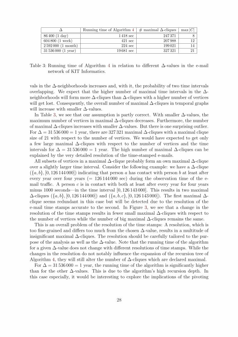
∆ Running time of Algorithm 4 # maximal ∆-cliques max |C|86 400 (1 day) 1 418 sec 247 371 8604 800 (1 week) 421 sec 207 988 122 592 000 (1 month) 224 sec 199 021 1431 536 000 (1 year) 19 681 sec 327 321 21

Table 3: Running time of Algorithm 4 in relation to different ∆-values in the e-mailnetwork of KIT Informatics.

vals in the ∆-neighborhoods increases and, with it, the probability of two time intervalsoverlapping. We expect that the higher number of maximal time intervals in the ∆-neighborhoods will form more ∆-cliques than ∆-cliques with a higher number of verticeswill get lost. Consequently, the overall number of maximal ∆-cliques in temporal graphswill increase with smaller ∆-values.

In Table 3, we see that our assumption is partly correct. With smaller ∆-values, themaximum number of vertices in maximal ∆-cliques decreases. Furthermore, the numberof maximal ∆-cliques increases with smaller ∆-values. But there is one surprising outlier.For ∆ = 31 536 000 = 1 year, there are 327 321 maximal ∆-cliques with a maximal cliquesize of 21 with respect to the number of vertices. We would have expected to get onlya few large maximal ∆-cliques with respect to the number of vertices and the timeintervals for ∆ = 31 536 000 = 1 year. The high number of maximal ∆-cliques can beexplained by the very detailed resolution of the time-stamped e-mails.

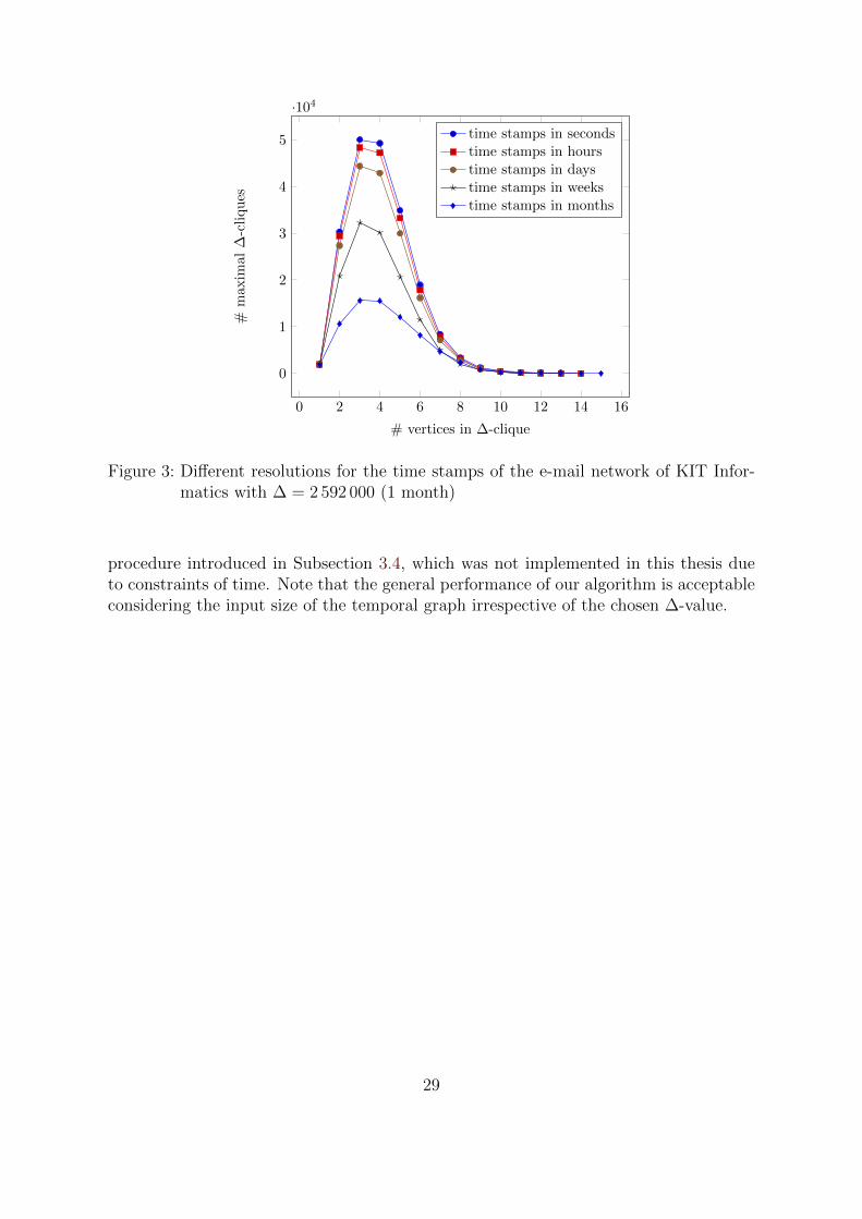
All subsets of vertices in a maximal ∆-clique probably form an own maximal ∆-cliqueover a slightly larger time interval. Consider the following example: we have a ∆-clique({a, b}, [0, 126 144 000]) indicating that person a has contact with person b at least afterevery year over four years (= 126 144 000 sec) during the observation time of the e-mail traffic. A person c is in contact with both at least after every year for four yearsminus 1000 seconds—in the time interval [0, 126 143 000]. This results in two maximal∆-cliques ({a, b}, [0, 126 144 000]) and ({a, b, c}, [0, 126 143 000]). The first maximal ∆-clique seems redundant in this case but will be detected due to the resolution of thee-mail time stamps accurate to the second. In Figure 3, we see that a change in theresolution of the time stamps results in fewer small maximal ∆-cliques with respect tothe number of vertices while the number of big maximal ∆-cliques remains the same.

This is an overall problem of the resolution of the time stamps: A resolution, which istoo fine-grained and differs too much from the chosen ∆-value, results in a multitude ofinsignificant maximal ∆-cliques. The resolution should be carefully tailored to the pur-pose of the analysis as well as the ∆-value. Note that the running time of the algorithmfor a given ∆-value does not change with different resolutions of time stamps. While thechanges in the resolution do not notably influence the expansion of the recursion tree ofAlgorithm 4, they will still alter the number of ∆-cliques which are declared maximal.

For ∆ = 31 536 000 = 1 year, the running time of the algorithm is significantly higherthan for the other ∆-values. This is due to the algorithm’s high recursion depth. Inthis case especially, it would be interesting to explore the implications of the pivoting

28

0 2 4 6 8 10 12 14 16

0

1

2

3

4

5

·104

# vertices in ∆-clique

#m

axim

al∆

-cli

qu

es

time stamps in secondstime stamps in hourstime stamps in daystime stamps in weekstime stamps in months

Figure 3: Different resolutions for the time stamps of the e-mail network of KIT Infor-matics with ∆ = 2 592 000 (1 month)

procedure introduced in Subsection 3.4, which was not implemented in this thesis dueto constraints of time. Note that the general performance of our algorithm is acceptableconsidering the input size of the temporal graph irrespective of the chosen ∆-value.

29

5 Conclusion

In this thesis, we studied the concept of cliques in temporal graphs: so-called ∆-cliques.In order to enumerate all maximal ∆-cliques in temporal graphs, we adapted the idea ofthe Bron-Kerbosch algorithm, including the procedure of pivoting to reduce the numberof recursion calls. We were able to maintain the main characteristic of the original Bron-Kerbosch algorithm: all maximal ∆-cliques are naturally enumerated exactly once. Inexperiments, we could show that our algorithm is notably faster than the first approachfor enumerating all maximal ∆-cliques in temporal graphs introduced by Viard, Latapy,and Magnien [VLM16] in real-world datasets.

We introduced the idea of pivoting for ∆-cliques and how this idea can be exploitedto reduce the number of recursive calls and therefore enable faster backtracking in ouralgorithm. Nevertheless, we did not consider this procedure in our test runs. The effectsof pivoting are interesting to examine, especially in large datasets such as the e-mailtraffic of KIT Informatics. Additionally, different heuristics for choosing a set of pivotelements can be tested to avoid solving a weighted interval scheduling maximizationproblem in each call of our algorithm.

We mentioned degeneracy—a measure of sparsity in non-temporal graphs—and howthis parameter can be exploited to upper-bound the running time of the original Bron-Kerbosch algorithm. A promising perspective could be using degeneracy as a role modelto define a measurement of sparsity in temporal graphs. This parameter can be exploitedto upper-bound the number of maximal ∆-cliques in temporal graphs and to design afixed-parameter tractable algorithm for enumerating all maximal ∆-cliques in temporalgraphs based on our approach.

30

Literature

[BF14a] A. Barrat and J. Fournet. “Contact Patterns among High School Students”.In: PLoS ONE 9.9 (Sept. 2014), e107878 (cit. on p. 25).

[BF14b] A. Barrat and J. Fournet. DATASET: High school dynamic contact networks.http: / /www .sociopatterns .org /datasets /high - school - dynamic-

contact-networks/. 2014 (cit. on p. 25).

[BK73] C. Bron and J. Kerbosch. “Algorithm 457: finding all cliques of an undirectedgraph”. In: Communications of the ACM 16.9 (1973), pp. 575–577 (cit. onpp. 7, 10).

[EHK15] T. Erlebach, M. Hoffmann, and F. Kammer. “On Temporal Graph Explo-ration”. English. In: Automata, Languages, and Programming. Ed. by M. M.Halldorsson, K. Iwama, N. Kobayashi, and B. Speckmann. Vol. 9134. LectureNotes in Computer Science. Springer Berlin Heidelberg, 2015, pp. 444–455(cit. on p. 5).

[ELS10] D. Eppstein, M. Loffler, and D. Strash. “Listing All Maximal Cliques inSparse Graphs in Near-Optimal Time”. English. In: Algorithms and Com-putation. Ed. by O. Cheong, K.-Y. Chwa, and K. Park. Vol. 6506. LectureNotes in Computer Science. Springer Berlin Heidelberg, 2010, pp. 403–414(cit. on pp. 11, 12).

[ELS13] D. Eppstein, M. Loffler, and D. Strash. “Listing All Maximal Cliques inLarge Sparse Real-World Graphs in Near-Optimal Time”. In: ACM Journalof Experimental Algorithmics 18.3 (2013), 3.1:1–3.1:21 (cit. on p. 7).

[ES11] D. Eppstein and D. Strash. “Listing All Maximal Cliques in Large SparseReal-World Graphs”. English. In: Experimental Algorithms. Ed. by P. Parda-los and S. Rebennack. Vol. 6630. Lecture Notes in Computer Science. SpringerBerlin Heidelberg, 2011, pp. 364–375 (cit. on p. 10).

[Goe11] R. Goerke. Email Network of KIT Informatics. http://i11www.iti.uni-karlsruhe.de/en/projects/spp1307/emaildata. 2011 (cit. on p. 25).

[HS12] P. Holme and J. Saramaki. “Temporal networks”. In: Physics Reports 519.3(2012), pp. 97–125 (cit. on p. 5).

[Mic15] O. Michail. “An Introduction to Temporal Graphs: An Algorithmic Perspec-tive”. English. In: Algorithms, Probability, Networks, and Games. Ed. by C.Zaroliagis, G. Pantziou, and S. Kontogiannis. Vol. 9295. Lecture Notes inComputer Science. Springer International Publishing, 2015, pp. 308–343 (cit.on p. 5).

[MS14] O. Michail and P. Spirakis. “Traveling Salesman Problems in Temporal Graphs”.English. In: Mathematical Foundations of Computer Science 2014. Ed. by E.Csuhaj-Varju, M. Dietzfelbinger, and Z. Esik. Vol. 8635. Lecture Notes inComputer Science. Springer Berlin Heidelberg, 2014, pp. 553–564 (cit. onp. 5).

31

[Nic+13] V. Nicosia, J. Tang, C. Mascolo, M. Musolesi, G. Russo, and V. Latora.“Graph Metrics for Temporal Networks”. English. In: Temporal Networks.Ed. by P. Holme and J. Saramaki. Understanding Complex Systems. SpringerBerlin Heidelberg, 2013, pp. 15–40 (cit. on p. 5).

[TTT06] E. Tomita, A. Tanaka, and H. Takahashi. “The worst-case time complex-ity for generating all maximal cliques and computational experiments”. In:Theoretical Computer Science 363.1 (2006), pp. 28–42 (cit. on p. 11).

[VL14] J. Viard and M. Latapy. Source code in Python for computing cliques in linkstreams. https://github.com/JordanV/delta- cliques. 2014 (cit. onp. 23).

[VLM15] J. Viard, M. Latapy, and C. Magnien. “Revealing Contact Patterns AmongHigh-school Students Using Maximal Cliques in Link Streams”. In: Proceed-ings of the 2015 IEEE/ACM International Conference on Advances in SocialNetworks Analysis and Mining 2015. ASONAM ’15. Paris, France: ACM,2015, pp. 1517–1522 (cit. on pp. 5, 7, 25–27).

[VLM16] J. Viard, M. Latapy, and C. Magnien. “Computing maximal cliques in linkstreams”. In: Theoretical Computer Science 609, Part 1 (2016), pp. 245 –252(cit. on pp. 23, 26, 30).

32