Embed Size (px)
Citation preview
Essays on spatial econometrics:Hodges-Lehmann estimators and
hospital efficiency
Inaugural-Dissertationzur Erlangung des akademischen Grades eines Doktors
der Wirtschafts- und Sozialwissenschaftender Wirtschafts- und Sozialwissenschaftlichen Fakultat
der Christian-Albrechts-Universitat zu Kiel
vorgelegt vonDipl. Volkswirt Christoph Strumann
aus Oelde
Kiel, 2013
Gedruckt mit Genehmigung derWirtschafts- und Sozialwissenschaftlichen Fakultat
der Christian-Albrechts-Universitat zu Kiel
Dekan:Prof. Horst Raff, Ph.D.
Erstberichterstattender:Prof. Dr. Helmut Herwartz
Zweitberichterstattender:Prof. Dr. Carsten Schultz
Tag der Abgabe der Arbeit:27. Mai 2013
Tag der mundlichen Prufung:10. Oktober 2013

Fur meine Frau und unsere kleine Familie
VorwortDie vorliegende Dissertation entstand wahrend meiner Tatigkeit als wissenschaft-
licher Mitarbeiter am Institut fur Statistik und Okonometrie sowie am Lehrstuhlfur Grundungs- und Innovationsmanagement der Christian-Albrechts-Universitat zuKiel. Mein besonderer Dank gilt meinem Doktorvater Professor Dr. Helmut Herwartz,dessen erstklassige Betreuung entscheidend zum Gelingen dieser Arbeit beigetragenhat. Herrn Professor Dr. Carsten Schultz danke ich herzlich fur die Ubernahme desZweitgutachtens.
Des Weiteren danke ich allen (ehemaligen) Kollegen am Institut fur Statistik undOkonometrie und am Lehrstuhl fur Grundungs- und Innovationsmanagement fur hilf-reiche Kommentare und eine angenehme Zusammenarbeit in freundschaftlicher Atmo-sphare, vor allem Herrn Professor Dr. Uwe Jensen, Herrn Dr. Matthias Hartmann,Herrn Dr. Bastian Gribisch und Herrn Albrecht Mengel. Ich bedanke mich außer-dem bei Herrn Dr. Alexander Vogel vom Forschungsdatenzentrum der StatistischenLandesamter - Standort Kiel/Hamburg fur die sehr gute Zusammenarbeit.
Vor allem die großartige Unterstutzung meiner Frau Susen Koslich-Strumann hatmir in vielen entscheidenden Momenten meiner wissenschaftlichen Arbeit die notigeKraft und Ausdauer gegeben. Ihr und unserem Sohn Gustav David danke ich ganzbesonders dafur, dass sie es immer wieder geschafft haben meinen Blick auf die wichti-gen Dinge im Leben, jenseits der Wissenschaft zu lenken. Dadurch ist es mir gelungenneuen Gedanken Raum zu verschaffen, was mir die notige Ruhe und Kreativitat furdie wissenschaftliche Arbeit gegeben haben.
Kiel, am 20. Mai 2013 Christoph Strumann
4
Contents
1 Introduction 1
2 Implementation and performance of Hodges-Lehmann estimators in staticpanel models with spatially correlated disturbances 42.1 Introduction . . . . . . . . . . . . . . . . . . . . . . . . . . . . . . . . . 52.2 Model representation and diagnostics . . . . . . . . . . . . . . . . . . . 7
2.2.1 The spatial panel model . . . . . . . . . . . . . . . . . . . . . . 72.2.2 Test statistics . . . . . . . . . . . . . . . . . . . . . . . . . . . . 8
2.3 Test based estimation . . . . . . . . . . . . . . . . . . . . . . . . . . . . 112.3.1 Interval estimation . . . . . . . . . . . . . . . . . . . . . . . . . 112.3.2 Test based point estimation . . . . . . . . . . . . . . . . . . . . 122.3.3 Monte Carlo test . . . . . . . . . . . . . . . . . . . . . . . . . . 12
2.4 Simulation study . . . . . . . . . . . . . . . . . . . . . . . . . . . . . . 132.4.1 Simulation design . . . . . . . . . . . . . . . . . . . . . . . . . . 142.4.2 Small sample properties of correlation tests . . . . . . . . . . . . 202.4.3 Point estimation . . . . . . . . . . . . . . . . . . . . . . . . . . 272.4.4 Interval estimation . . . . . . . . . . . . . . . . . . . . . . . . . 322.4.5 Sensitivity analysis . . . . . . . . . . . . . . . . . . . . . . . . . 35
2.5 Conclusions . . . . . . . . . . . . . . . . . . . . . . . . . . . . . . . . . 352.6 References . . . . . . . . . . . . . . . . . . . . . . . . . . . . . . . . . . 37
3 On the effect of prospective payment on local hospital competition inGermany 41
4 Hospital efficiency under prospective reimbursement schemes: An empir-ical assessment for the case of Germany 42
5 Concluding Remarks 43
5
List of Figures
2.1 Power features under SAR disturbances . . . . . . . . . . . . . . . . . . 222.2 Power features under SMA disturbances . . . . . . . . . . . . . . . . . 232.3 Estimation properties under SAR disturbances . . . . . . . . . . . . . . 282.4 Estimation properties under SMA disturbances . . . . . . . . . . . . . 29
6
List of Tables
2.1 Definitions of explanatory SR dummy variables . . . . . . . . . . . . . 192.2 Empirical size of tests on spatial correlation (in %) . . . . . . . . . . . 212.3 Absolute and relative size adjusted power estimates . . . . . . . . . . . 252.4 Surface response analysis (power) . . . . . . . . . . . . . . . . . . . . . 262.5 Performance of ML and HL point estimates (bias & RMSE) . . . . . . 302.6 Surface response analysis (point and interval estimation) . . . . . . . . 312.7 Performance of ML and HL interval estimates . . . . . . . . . . . . . . 332.8 Sensitivity Analysis . . . . . . . . . . . . . . . . . . . . . . . . . . . . . 36
7
Chapter 1
Introduction
Spatial econometrics deals with spatial interaction and spatial structure in regressionmodels. Spatial econometric techniques have been increasingly applied in almostall fields of economics. Anselin (2001) points out two main factors for the growingpopularity of spatial econometrics. On the one hand, there is an increasing interest inmodeling explicitly the interaction of economic agents with other heterogenous agents.On the other hand, more and more spatial data are available and need to be handledby appropriate techniques.
This dissertation consists of three articles considering spatial econometrics. Thefirst article in Chapter 2 proposes an alternative estimation procedure of spatial errorpanel regression models, while the other articles in Chapter 3 and 4 apply spatialeconometrics for the analysis of hospital efficiency in Germany. To be more precisely,the focus of Chapter 3 is to estimate spatial spillovers of hospital efficiency. In Chapter4, spatial econometric techniques are applied in order to handle appropriately thespatial dependence in the data as detected in Chapter 3.
In the following a more detailed description of the articles of this cumulative disser-tation is given. Moreover, the author’s contribution of the articles in Chapter 3 and4 is described.
Chapter 2 - Implementation and performance of Hodges-Lehmann estimatorsin static panel models with spatially correlated disturbances
To estimate spatial regression models Maximum Likelihood (ML) estimation is typ-ically applied, although ML spatial parameter estimates are characterized by a sub-stantial downward bias (e.g. Mizruchi and Neuman, 2008, Neuman and Mizruchi,2010, Farber et al., 2009, Smith, 2009). In Chapter 2, Hodges-Lehmann (HL) typepoint (Hodges and Lehmann, 1983) and interval estimators for the spatial parameterare proposed. The estimators are based on the inversion of common spatial correlationtests. While the actual coverage of ML interval estimates might violate the nominaltarget due to the estimation bias, the application of Monte Carlo testing offers exactHL confidence intervals in finite samples under any spatial structure. To identify mostappropriate test statistics for the HL procedure size and power features of a variety
1
Chapter 1 - Introduction
of diagnostics for spatial correlation are investigated by means of a simulation studyin a first step. Secondly, the empirical performance of HL point and interval estima-tors are compared with their ML counterparts. Simulation results show that the biasof the HL estimator is markedly smaller than its ML counterpart. In addition, HLconfidence intervals are characterized by less size distortions and appear more robustagainst spatial connectivity in comparison with ML interval estimates.
Chapter 3 - On the effect of prospective payment on local hospital competitionin Germany
In recent years, German hospitals have experienced a dramatic change in their incen-tive structure due to the introduction of prospective reimbursement based on diagnosisrelated groups (DRG) in 2004. One of the main goals of this financial reform has beento reduce the steady increase of hospital expenditures by encouraging hospitals to raisetheir efficiency. In contrast to the former per diem payments, under prospective pay-ment it is profitable for hospitals to treat their patients efficiently. As a byproducthospitals face the incentive to preferably treat cases with high reimbursement ratesand a low level of complexity (Bocking et al., 2005) potentially leading to an increasedcompetition for this so called low cost patients. In the study of Chapter 3, the compe-tition between hospitals, quantified as spatial spillover estimates of hospital efficiency,is analyzed for periods before and after the reform. A two-stage efficiency model thatallows for spatial interdependence among hospitals is implemented. Hospital efficiencyis determined by means of non-parametric and parametric econometric frontier mod-els. A significant increase of negative spatial spillovers of hospital performance isdiagnosed, and thus, confirm the expected rise of competition.
While the idea of this study and the framework of the empirical model have beendeveloped jointly with my co-author Helmut Herwartz, I was writing the text of themanuscript with editing help of Helmut Herwartz and carrying out the implementationof the preparation and descriptive analysis of the data, and of the estimation of theeconometric model.
The article has been published in Health Care Management Science, 2012, Vol. 15,No. 1, pp. 48-62.
Chapter 4 - Hospital efficiency under prospective reimbursement schemes: Anempirical assessment for the case of Germany
In Chapter 4, the effect of the DRG reform on overall hospital efficiency is addressedby two complementary testing approaches. On the one hand, a two-stage procedurebased on non-parametric efficiency measurement is applied. On the other hand, astochastic frontier model is employed that allows a one-step estimation of both pro-duction frontier parameters and inefficiency effects. Efficiency gains are identified asa consequence of changes in the hospital incentive structure because technological
2
Chapter 1 - Introduction
progress, spatial dependence and hospital heterogeneity are taken into account. Con-trary to the goal of prospective payments, the results of both approaches do not revealany increase in overall efficiency after the DRG reform. Instead, a significant declinein overall hospital efficiency over time is observed.
Similar to the article of the previous chapter, together with my co-author HelmutHerwartz we have developed jointly the idea of this study and the framework of theempirical model. I have written the text of the manuscript with editing help of HelmutHerwartz. Moreover, the implementation of the data analysis and the estimation ofthe econometric model have been done by myself.
The article has been accepted for publication in The European Journal of HealthEconomics.
ReferencesAnselin, L. (2001). Spatial econometrics. In Baltagi B.: A companion to theoreticaleconometrics. (Oxford: Blackwell), 310-330.
Bocking, W., U. Ahrens, W. Kirch and M. Milakovic (2005). First results of the intro-duction of DRGs in Germany and overview of experience from other DRG countries.Journal of Public Health 13(3), 128-137.
Farber, S., A. Paez and E. Volz (2009). Topology, dependency tests and estimationbias in network autoregressive models. In Paez, A., J. Le Gallo, R. Buliung and S.Dall’Erba: Advances in Spatial Sciences (Berlin: Spinger Verlag), 29-57.
Hodges Jr., J.L., and E.L. Lehmann (1983). Hodges-Lehmann estimators. In John-son, N.L., S. Kotz and C. Read: Encyclopedia of Statistical Sciences, vol. 3. (Wiley,New York), 642-645.
Mizruchi, M.S. and E.J. Neuman (2008). The effect of density on the level of bias inthe network autocorrelation model. Social Networks 30, 190-200.
Neuman, E.J. and M.S. Mizruchi (2010). Structure and bias in the network autocor-relation model. Social Networks 32(4), 290-300.
Smith, T.E. (2009). Estimation bias in spatial models with strongly connected weightmatrices. Geographical Analysis 41(3), 307-332.
3
Chapter 2
Implementation and performance ofHodges-Lehmann estimators in staticpanel models with spatially correlateddisturbances
Christoph Strumann1
Abstract
Several studies point out a substantial downward bias of the Maximum Likelihood(ML) estimator of the spatial correlation parameter under strongly connected spatialstructures. This paper proposes Hodges-Lehmann (HL) type point and interval esti-mators for the spatial parameter in static panel models with spatially autoregressive ormoving average disturbances. HL estimators are implemented by means of ’inverting’common diagnostics for spatial correlation. Exact inference is implemented by meansof Monte Carlo testing. A simulation study covering models with distinct degrees ofspatial connectivity shows that the bias of the HL estimator is markedly smaller thanits ML counterpart. In addition, HL confidence intervals are characterized by less sizedistortions and appear more robust against spatial connectivity in comparison withML interval estimates.
JEL-Classification: C12, C15, C21, C23Keywords: Panel data, spatial correlation, specification tests, Monte Carlo test, exactconfidence sets, Hodges-Lehmann estimators
1Institut fur Statistik und Okonometrie, Christian-Albrechts-Universitat zu Kiel, Olshausenstr. 40,D-24118 Kiel, Germany, [email protected], tel.: +49 431 880 2379, fax: +49 431880 7605
4
Chapter 2 - Implementation and performance of Hodges-Lehmann estimators
2.1 IntroductionSpatial regression models are typically estimated by means of Maximum Likelihood(ML) techniques. However, several studies point out a substantial downward bias ofML estimates of the spatial correlation parameter, which increases with the degree ofspatial connectivity (e.g. Mizruchi and Neuman, 2008, Neuman and Mizruchi, 2010,Farber et al., 2009, Smith, 2009). Lee (2004) highlights a potential irregularity ofthe information matrix under strongly connected spatial structures, which affects theconvergence rate of the ML estimator. Bao and Ullah (2007) demonstrate that thebias of the ML estimator is sensitive to the structure of the spatial weights matrix.They suggest for cross sectional spatial lag models a bias corrected estimator, whichis effective under weakly connected spatial structures.
As opposed to the spatial lag model, a biased spatial parameter estimate has noimpact on the bias of regression coefficient estimates in the spatial error model. How-ever, if the spatial parameter is of particular interest, the respective bias matters.Recent applications of the spatial error model include the analysis of economic con-vergence (Fingleton and Lopez-Bazo, 2006, Lundberg, 2006, Lopez-Bazo et al., 2004,Villaverde, 2005, Rey and Montouri, 1999), house prices (Baumont, 2009), technologyadaption (Billon et al., 2009), local governments expenditure (Bivand and Szymanski,2000), and tax mimicking (Bordignon et al., 2003, Revelli, 2002). In these models adownward biased estimator leads to a systematic understatement of spatial responsesto local shocks and, thus, weakens the empirical underpinning of economic policyadvice.
This paper proposes Hodges-Lehmann (HL) type point (Hodges and Lehmann,1983) and interval estimators for the spatial autocorrelation or moving average pa-rameter in static panel models with spatially autoregressive (SAR) or moving average(SMA) disturbances. HL estimators are implemented by means of ’inverting’ commondiagnostics for spatial correlation. The particular value of the spatial parameter thatmaximizes the test p-value is interpreted as a point estimate (Coudin and Dufour,2011). Confidence sets comprise all admissible values of the spatial parameter thatdo not involve a rejection of the null hypothesis (Dufour, 1990). The inversion ofspatial correlation tests may follow three alternative strategies, first order asymptoticapproximations, bootstrap approaches and Monte Carlo (MC) techniques (Dufour,2006). In contrast to asymptotically valid bootstrap techniques (Lin et al., 2011) MCtesting can offer exact size control in finite samples under any spatial structure.
As derived from the inversion of spatial diagnostics the performance of HL estima-tors is most likely to reflect efficiency characteristics of the underlying spatial correla-tion tests. To identify most appropriate test statistics for the HL procedure size andpower features of a variety of diagnostics for spatial correlation are investigated bymeans of a simulation study in a first step. Secondly, the empirical performance ofHL point and interval estimators are compared with their ML counterparts. Noting
5
Chapter 2 - Implementation and performance of Hodges-Lehmann estimators
that the actual coverage of ML interval estimates might violate the nominal targetdue to the estimation bias, the potential merits of HL interval estimates are high-lighted for small sample scenarios with regular and irregular, correct and misspecifiedspatial weights matrices. Moreover, a potential finite sample bias reduction of the HLestimator is addressed.
As potential candidates for the construction of HL point estimates and confidenceintervals (CIs) three sorts of rival diagnostics are considered, differing with respect tothe exploitation of modeling specific assumptions on the connectivity structure. In thefirst place, Moran’s I statistic (MI) (Cliff and Ord, 1981) and the Lagrange Multiplierstatistic for spatial error autocorrelation (LME) (Burridge, 1980) are considered.Several simulation experiments recommend MI as a powerful test against spatialerror correlation (e.g. Florax and Rey, 1995). However, as simulation results inAnselin and Rey (1991) suggest, the power of both tests declines with increasingspatial connectivity. Moreover, Smith (2009) shows that for strongly connected spatialweights matrices realizations of MI are concentrated close to the mean and, thus, thetest could suffer from power weakness. Generally, the application of MI, LME andvarious other spatial diagnostics requires an a-priori guess about the spatial patternthat underlies the data. Any choice of the so called spatial weights matrix is subjectedto the risk of misspecification. To raise the robustness of the HL estimation against thespecification of the spatial layout, statistics that do not rely on a spatial weights matrixare also considered in the second place, i.e. the Lagrange Multiplier (LM) statisticproposed by Breusch and Pagan (1980), the CD test of Pesaran (2004) and twonon-parametric tests of Friedman (1937) and Frees (1995). For power improvementPesaran (2004) suggests a modification of the CD statistic capturing spatial featuresof the regression error terms. A similar modification is also achievable for the LMstatistic of Breusch and Pagan (1980). In the third place, both modified statisticsare also included in the list of potential candidates for HL estimation. While thelatter statistics exploit a-priori information about the spatial contiguity structure,the former diagnostics are fully invariant to the spatial weights matrix. On the onehand, one may expect more robust performance of these statistics against potentialmisspecification of the spatial structure. On the other hand, it is of interest to uncoverpotential power losses in comparison with more parametric diagnostics, MI and LME
say.In Section 2.2 the spatial panel model under the SAR and SMA error distribution is
introduced along with the considered tests for spatial correlation. Section 2.3 outlinespoint and interval estimation of the spatial parameter. Furthermore, the MC testprocedure is described. Section 2.4 documents design and outcomes of the simulationstudy. Section 2.5 concludes.
6
Chapter 2 - Implementation and performance of Hodges-Lehmann estimators
2.2 Model representation and diagnosticsIn this section, the spatial panel model with SAR and SMA disturbances is introduced.To concentrate on the relative merits of HL and ML estimation the entire analysisin this paper is focussed on the pooled regression as a rather stylized model in paneldata econometrics. However, if the time dimension is sufficiently large to guarantee aconsistent estimation of the model parameters, the proposed HL procedure can also beapplied to panel models with a more complex structure, e.g. heterogenous interceptsand coefficients. Moreover, test statistics that are alternatively considered for theconstruction of HL estimators are listed in this section.
2.2.1 The spatial panel modelThe considered pooled linear regression model reads as
yt = X tβ + et, t = 1, ..., T, (2.1)
where yt is an N × 1 vector of observations of the dependent variable in time t, X t
is an N × K matrix of observations of fixed (or exogenous) explanatory variablesincluding a constant, β is a K × 1 vector of parameters and et is an N × 1 vector ofspatially correlated error terms. The cross sectional and time dimension are denotedby N and T , respectively. Two specifications of et are distinguished, the SAR andSMA model, respectively
et = ρW et + ϵt and et = γW ϵt + ϵt, ϵt = σξt, E[ξt] = 0, E[ξtξ′t] = IN , ξt
iid∼ D(0, IN),
where D is a known multivariate distribution with zero mean and covariance IN ,the identity matrix. The spatial weights matrix W is of dimension N × N withzero diagonal elements and row normalized constants (such that each row sums tounity), ρ and γ are the spatial autocorrelation and spatial moving average parameter,respectively. To establish asymptotic normality of the spatial diagnostics introducedbelow, the following conditions are assumed to hold throughout (Kelejian and Prucha,2001): (i) the fourth order moments of the idiosyncratic innovations ϵit are finite, (ii)the row and column sums of W are uniformly bounded in absolute value as N → ∞and (iii) the matrices (IN − ρW ) (SAR) and (IN + γW ) (SMA) are nonsingular forall |ρ| < 1 and |γ| < 1, respectively. Assumption (ii) is satisfied if for a given crosssectional unit the maximum number of neighbors is restricted, or the spatial weightsdecline as a function of some measure of distance between neighbors (Kelejian andPrucha, 1998). Owing to (iii) the error term of the SAR model can be expressed as
et = (IN − ρW )−1ϵt, with
7
Chapter 2 - Implementation and performance of Hodges-Lehmann estimators
E[ete′t] = σ2
[IN − ρ(W + W ′) + ρ2W ′W
]−1= ΩSAR. (2.2)
For ρ = 0, ΩSAR is a non-sparse matrix, implying that a shock in one location istransmitted globally, i.e. to all locations. For the SMA specification one has
E[ete′t] = σ2
[IN + γ(W + W ′) + γ2W W ′
]= ΩSMA. (2.3)
If W is a first order contiguity matrix say, ΩSMA formalizes local linkages between firstand second order neighbors. With ‘⊗’ denoting the Kronecker product, the pooledSAR and SMA panel regression model can be written as
y = Xβ + e, e = G•ϵ, (2.4)
whereGρ =
[IT ⊗ (IN − ρW )−1
]and Gγ = [IT ⊗ (IN + γW )] , (2.5)
respectively. Specifically, y = (y′1, ..., y′
T )′, e = (e′1, ..., e′
T )′ and ϵ = (ϵ′1, ..., ϵ′
T )′ are(TN × 1) vectors, and X = (X ′
1, ..., X ′T )′ is a (TN × K) matrix independent of
ϵ with rank(X) = K. In the following θ denotes either ρ (SAR) or γ (SMA) forconvenience of notation.
2.2.2 Test statisticsSeveral alternative diagnostics are employed to test the hypotheses
H0 : θ = θ0 vs. H1 : θ = θ0. (2.6)
In a first step the panel model is respecified as y = Xβ + G•ϵ and the estimatedresiduals are obtained as
ϵ0 = M 0y∗0 = M 0ϵ, with M 0 = INT − X∗
0(X∗′0 X∗
0)−1X∗′0 , (2.7)
where X∗0 = G−1
• X and y∗0 = G−1
• y are spatially filtered according to H0. The teststatistics differ with respect to the exploitation of modeling specific assumptions onthe connectivity structure implied by W .
Tests for spatial correlation
To date, the most commonly used diagnostic for spatial dependence is the MI statistic(Cliff and Ord, 1981). It is given along with its asymptotic distribution by
MI = I − µI
σI
d−→ N(0, 1), (2.8)
8
Chapter 2 - Implementation and performance of Hodges-Lehmann estimators
where
I = ϵ′0(IT ⊗ W )ϵ0
ϵ′0ϵ0
, µI = tr(M)(NT − K)
, σI =
√√√√tr(MM′) + tr(M2) + tr(M)2
(TN − K)(TN − K + 2)− µ2
I
and M = M 0(IT ⊗ W ).As an alternative to MI the LM test for spatial error correlation (Burridge, 1980)
is considered. Extended to the panel regression model (e.g. Anselin et al., 2008) thetest reads as
LME =
[ϵ′
0(IT ⊗ W )ϵ0/(ϵ′0ϵ0/NT )
]2
T tr(W 2 + W ′W )d−→ χ2(1). (2.9)
Tests for general contemporaneous correlation
In contrast to MI and LME the following tests do not rely on a spatial weightsspecification. Instead, the statistics summarize general correlation patterns of theresiduals in (2.7) by means of the parametric Pearson correlation coefficient
ϱ0,ij =∑T
t=1 ϵ0,itϵ0,jt√∑Tt=1 ϵ2
0,it
∑Tt=1 ϵ2
0,jt
or the non-parametric Spearman’s rank correlation coefficient
τ0,ij =∑T
t=1(Rit − (T + 1/2))(Rjt − (T + 1/2))∑Tt=1(Rit − (T + 1/2))2 ,
where Rit is the rank of the estimated filtered residual ϵ0,it.The LM statistic of Breusch and Pagan (1980) is based on the average of squared
pair-wise Pearson correlation coefficients
BP = TN−1∑i=1
N∑j=i+1
ϱ20,ij
d−→ χ2N(N−1)/2. (2.10)
For small T and large N the test exhibits substantial size distortions (Pesaran, 2004).As an alternative with reasonable small sample properties Pesaran (2004) proposes
a statistic that exploits the average of non-squared pair-wise Pearson correlation co-
9
Chapter 2 - Implementation and performance of Hodges-Lehmann estimators
efficients2
CD =√
2T
N(N − 1)
N−1∑i=1
N∑j=i+1
ϱ0,ij
d−→ N(0, 1). (2.11)
The Friedman’s (1937) test of cross sectional dependence measures the correlationpattern of estimated residuals by means of the non-parametric Spearman’s rank cor-relation and is given by
FTn = (T − 1)((N − 1)RAV E + 1) d−→ χ2T −1, (2.12)
whereRAV E = 2
N(N − 1)
N−1∑i=1
N∑j=i+1
τ0,ij.
The test statistic of Frees (1995) is a quadratic version of the Friedman’s (1937)test and reads as
FTq = N(R2AV E − (T − 1)−1)
σF
d−→ N(0, 1), (2.13)
whereR2
AV E = 2N(N − 1)
N−1∑i=1
N∑j=i+1
τ 20,ij
and
σF =
√√√√3225
(T + 2)2
(T − 1)3(T + 1)2 + 45
(5T + 6)2(T − 3)T (T − 1)2(T + 1)2 .
Tests for local correlation
Unlike in the case of MI and LME, the power of the tests for general contempora-neous correlation does not increase with N . For power improvement Pesaran (2004)suggests to exploit the correlation only among contiguous residual processes. Themodified CD test is
CDW =√
2T
p
N−1∑i=1
N∑j=i+1
I(wij > 0) ϱ0,ij
d−→ N(0, 1), (2.14)
where p is the number of non-zero off diagonal elements of W and I(.) is an indicatorfunction.
2Pesaran et al. (2008) suggest corrections for the mean and variance of the BP test to addressthe size distortions for fixed T and large N . In this paper MC testing offers full control overtype I error probabilities. Moreover, simulation results of Pesaran et al. (2008) indicate the BPstatistic as a more powerful diagnostic than their bias-adjusted BP test. Therefore, the latterstatistic is not considered in this paper.
10
Chapter 2 - Implementation and performance of Hodges-Lehmann estimators
Similarly to the CDW test the BP statistic can be transformed to test for localcorrelation as
BP W = TN−1∑i=1
N∑j=i+1
I(wij>0)ϱ20,ij
d−→ χ2p/2. (2.15)
If W is a non-sparse matrix, CDW = CD and BP W = BP .3
2.3 Test based estimationIn this section HL interval and point estimation are briefly described. To assess themarginal significance of a particular test statistic an analyst can rely on first orderasymptotic approximations or MC techniques which are briefly sketched.
2.3.1 Interval estimationTo construct confidence sets for θ, one proceeds from testing (2.6) for all admissiblevalues θ0 ∈ (−1, 1). Under H0 : θ = θ0 the estimated residuals in (2.7) are spatiallyuncorrelated. In the alternative case, H1 : θ = θ0, some spatial correlation remainsand should be detected by a correlation test. Given a realization T (θ0) of any statisticT (θ0) ∈ MI, LME, BP, CD, FTn, FTq, CDW , BP W H0 is rejected if the respectivep-value, p (T (θ0)), is smaller than the nominal level α. A confidence interval for θ withcoverage probability 1 − α comprises all admissible values of θ0 that do not obtain arejection of H0 (Coudin and Dufour, 2011), i.e.
CIT (α) =[CI l
T (α), CIuT (α)
]=
θ0 ∈ S : p
(T (θ0)
)≥ α
, (2.16)
with S = θ : |θ| < 1. In (2.16) the lower CI lT (α) and upper bound CIu
T (α) are,respectively,
CI lT (α) = min
θ0
θ0 ∈ S : p
(T (θ0)
)≥ α
and
CIuT (α) = max
θ0
θ0 ∈ S : p
(T (θ0)
)≥ α
.
The determination of interval estimates in (2.16) requires (some approximation of) thedistribution of T . As an immediate approach, one might rely on asymptotic p-values.Based on exact p-values the actual coverage probability of the HL interval estimatein (2.16) is 1 − α (Dufour, 1990).
3Further test statistics can also be considered as potential candidates for HL estimation: the mul-tivariate independence test of Tsay (2004), and the statistics proposed by Dufour and Khalaf(2002), i.e. extensions of the exact independence test of Harvey and Phillips (1982). However,these tests require a sufficiently large time dimension (T > N). In order to avoid dimensionalrestrictions, these diagnostics are not considered for HL estimation here.
11
Chapter 2 - Implementation and performance of Hodges-Lehmann estimators
2.3.2 Test based point estimationIn analogy to interval estimation the HL point estimator, denoted θT , is the particularθ0 attaining the highest confidence in form of the maximum p-value of T (θ0) (Hodgesand Lehmann, 1983, Coudin and Dufour, 2011), i.e.
θT = maxθ0
p
(T (θ0)
). (2.17)
Since HL estimators relate to some underlying diagnostic in the following these es-timators are referred as HL(T ), such that, for instance, HL(MI) is short for HLestimators based on MI. If the test statistic T has reasonable power against thealternative hypothesis, H1 : θ = θ0, θT is unique (Dufour, 1990). Martellosio (2010)shows that for some combinations of X and W the power of any invariant spatialerror correlation test vanishes as θ → 1. Then, the maximum p-value, p
(T (θ0)
)= 1,
could be obtained for more than one candidate θ0. To detect a potential power trapMartellosio (2010) recommends to apply alternative tests as robustness checks.
2.3.3 Monte Carlo testIf the distribution of a test statistic T (θ0) does not depend on nuisance parameters, itis straightforward to obtain exact p-values by means of simulating the theoretical nulldistribution.4 To show pivotalness of all considered diagnostics T ∈ MI, LME, BP,
CD, FTn, FTq, CDW , BP W it is convenient to rewrite the estimated spatially filteredresiduals (2.7) as
ϵ0 = M 0ϵ = σM 0ξ.
Under H0, correct choice of W and fixed M 0 the distribution of T is free of nui-sance parameters, since it does not depend on σ2 or β. To obtain MC realizationsTr(θ0), r = 1, . . . , R, spatially filtered residuals ξ0r = M 0ξr, ξr
iid∼ D(0, IN), enter thetest statistic. Then, the MC p-value is estimated as
pR
(T (θ0)
)=
∑Rr=1 I
(T 2
r (θ0) ≥ T 2(θ0))
+ 1R + 1
.
As shown by Dufour (2006) the MC implied significance level equals the nominal levelα if the number of MC replications R is chosen such that α(R+1) is an integer. Whilealternative choices of R offer the same reliability of the test under H0, the power ofan MC test can be improved when opting for a larger R, R = 999 if α = 0.05,say. Moreover, owing to the inverse relationship between a test statistic T (θ0) and
4Notably, the exact distribution of MI can also be derived by numerical integration (Bivand et al,2009). In comparison, the MC approach is immediate to implement for all considered diagnostics,and, thus, facilitates the evaluation of simulation results over a set of rival diagnostics T ∈MI, LME, BP, CD, FTn, FTq, CDW , BP W .
12
Chapter 2 - Implementation and performance of Hodges-Lehmann estimators
the respective p-value, minimizing the former is equivalent to maximizing the latter(Coudin and Dufour, 2011). As a consequence, applying asymptotic or MC basedp-values obtains identical HL point estimates.
Regarding the scope of MC approaches in spatial panel models two remarks are inorder. Firstly, MC testing builds upon sampling from the known distribution D. Inempirical practice a misspecification of the underlying distribution is eventually detri-mental for the performance of MC testing. Thus, careful diagnostic checking of thedistributional assumptions made for (estimated) residual processes should accompanythe application of MC based critical values. Secondly, the described MC procedureis exact, since spatial correlation is restricted to the residual processes. Within thespatial lag model typical diagnostics, e.g. the LM lag test in Anselin et al. (2008),lack pivotalness since the conditional mean coefficients impact on the asymptotic dis-tribution (Martellosio, 2010). For MC testing in presence of nuisance parameters thereader may consult Dufour (2006).
2.4 Simulation studyTo shed light on the relative merits of MC testing and HL estimation under a varietyof correlation structures, a simulation study including misspecification of the spatialweights matrix is conducted. At first, the size and power features of the test statisticslisted in Section 2.2.2 are analyzed. The simulations will be informative with re-spect to potential size distortions of the asymptotic tests in finite samples and understrongly connected spatial weights matrices. With regard to the implementation ofHL estimators it is particularly important to uncover powerful tests, since the powerof a test governs HL estimation accuracy and the precision of HL interval estimates.Secondly, HL point and interval estimators are compared with their ML counterpartscommonly employed in spatial modeling. To economize on space the latter analysis isconcentrated on a set of 3 alternative test approaches, which have shown most accu-rate performance in terms of power (MI) or robustness under diverse (misspecified)spatial structures (CD, CDW ).
In the following the data generating models (DGMs) are described in detail. More-over, the considered loss functionals are listed and a few remarks are added on theprovision of simulation results before it comes to a discussion of the relative perfor-mance of rival approaches to spatial diagnosis and estimation.
13
Chapter 2 - Implementation and performance of Hodges-Lehmann estimators
2.4.1 Simulation designData generating models
Vector valued spatial data are generated according to
yt = ιNβ1 + xtβ2 + et, t = 1, . . . , T,
with β1 = β2 = 1 and ιN is a N × 1 vector of ones. The N -dimensional vector ofexplanatory variables xt is drawn once from the uniform distribution U [0, 10] andkept constant for all replications of an experiment. SAR and SMA dependence isintroduced, respectively, by means of disturbance vectors
et = (IN − θW )−1ϵt and et = (IN + θW )ϵt, ϵt ∼ N (0, IN).
In a first set of experiments four distinct sample sizes are considered: a ’small’sample (T = 10, N = 10), experiments with an increased time (T = 25, N = 10) orcross sectional (T = 10, N = 25) dimension, and a ’large’ sample scenario (T = 25,N = 25). These relatively small sample sizes are sensible to highlight the bias ofthe ML estimator and could motivate a need for exact inference or HL estimation.Notably, such sample dimensions are typical for macroeconomic panel models, whereboth the number of available time periods and cross sectional units (e.g. G7, EU orOECD members) are small to medium.
Data are generated for 9 distinct values of θ. To avoid trivial power estimates,the power analysis is concentrated on parameter settings θ ∈ −0.20, −0.15, . . . , 0.2.The empirical performance of alternative estimators is analyzed over a wider rangeof the parameter space, θ ∈ −0.8, −0.6, . . . , 0.8. As it turns out, the choice of anynominal test level α ∈ 0.01, 0.025, 0.05, 0.1 obtains performance patterns of teststatistics or HL estimators which are qualitatively equivalent. Therefore, simulationresults are only provided for α = 0.05. The number of MC replications is chosenas R = 999 to foster the discriminatory content of MC testing under the alternativehypothesis. Assuming knowledge of the true error distribution MC innovations aredrawn from the multivariate Gaussian.
As outlined so far the simulation experiments cover the ideal (or artificial) casewhere MC testing is implemented by means of the true underlying conditional distri-bution. In practice, MC testing could suffer from selecting a false innovation distri-bution. For such instances, potential losses of HL estimators implemented by meansof MC based or asymptotic p-values are of natural interest. Moreover, sample di-mensions considered so far are generally ’medium sized’ such that it is unclear ifpotential merits of HL estimation vanish in larger samples. To investigate asymptoticproperties of rival test and estimation approaches, ’large’ sample experiments with(N, T ) ∈ (10, 50), (10, 100), (50, 10), (100, 10) are designed on the one hand. On theother hand, scenarios are considered where true model innovations ϵit are skewed and
14
Chapter 2 - Implementation and performance of Hodges-Lehmann estimators
MC testing is falsely based on the Gaussian distribution. To be precise, iid innova-tions are determined as ϵit = (νit − q)/
√2q, where νit is χ2-distributed with q degrees
of freedom. Considering distinct degrees of nonnormality q is alternatively chosenas q = 5, 15. To uncover the impacts of skewness in small and large sample casesthe respective sample dimensions are (N, T ) ∈ (10, 25), (10, 100), (25, 10), (100, 10).Keeping the documentation and discussion of the sensitivity study short in space,respective simulations are concentrated on a selection of tests (MI, CD, CDW ) andDGMs with SAR disturbances.
Spatial connectivity patterns
With regard to the row normalized weights matrix W regular and irregular latticesare distinguished. Moreover, distinct degrees of connectivity are implemented to in-vestigate the sensitivity of spatial diagnostics and estimates with regard to the spatialspecification. A regular W matrix is given by a ‘circular’ state in the form of a ‘Jahead and J behind’ weights matrix. To distinguish alternative degrees of connectiv-ity, the integer J is chosen such that c = 2J/N ≈ 0.2, 0.4, 0.6.5 Further, ‘distance’weights that build upon the NUTS 3 code of European regions (Eurostat: Regions,1999) are used to implement irregular lattices. For this purpose the German financialcenter Frankfurt (code 312) jointly with its N − 1 closest neighbors are considered.As detailed in Brocker et al. (2002) economic distance is approximated by meansof the travel time by private car (in minutes) between the economic centers of thecross sectional entities i and j, denoted ζij. Prior to row normalization the ij-thelement of W is determined as w∗
ij = exp−aζij. The distance decay parameter,a ∈ 0.01, 0.05, 0.1, governs the degree of connectivity. The smaller is a, the sloweris (prior to normalization) the decline of spatial weights across units and the higheris the connectivity.
Specification of spatial weights
To implement spatial estimators or diagnostics an analyst has to select a particularweights matrix. In the simulation study a set of experiments, denoted Wc, is charac-terized by coincidence of the applied weights matrix and its counterpart underlyingthe data generation. In many empirical studies the choice of the weights matrix reliesupon ad-hoc assumptions about the underlying spatial pattern and might also dependon data availability (Bhattacharjee and Jensen-Butler, 2005). Thus, misspecification
5For this specification of W the maximum number of neighbors for a given cross sectional unit isnot restricted as N → ∞, since J increases with N . As a consequence no additional informationis gained from individual observations as N increases (Smith, 2009). Thus, the bias of the MLestimator might not vanish asymptotically and the asymptotic distributions of the consideredspatial diagnostics might not be established. However, the main focus of this paper is rather onthe estimation bias of θ than on asymptotic test and estimation properties. Moreover, even inthis case the MC approach offers full control over the stochastic model features.
15
Chapter 2 - Implementation and performance of Hodges-Lehmann estimators
of the spatial weights matrix is inevitable and an important issue in spatial economet-rics. Accordingly, two cases of misspecification are considered. In both instances, thetrue circular and distance weights matrix are specified with c ≈ 0.40 and a = 0.05,respectively, while the applied spatial weights matrix mimics scenarios of under- orover-specifying the actual connectivity. For the circular matrix, a choice of c ≈ 0.20corresponds to an underspecified weights matrix, i.e. the true number of neighborsexceeds the number of neighbors that is formalized by the applied weighting scheme.For a = 0.1 the decay of the distance based weights is faster as it is the case for thetrue DGM. Such scenarios of underspecification are denoted by Wu. Accordingly, thecase of overspecification, denoted Wo, is implemented with c ≈ 0.60 and a = 0.01.
Comments on optimization
All simulations are performed with MATLAB. The HL (restricted ML) estimator ofthe spatial parameter is obtained by maximizing the asymptotic p-value (concentratedlog-likelihood function) over θ ∈ −1, 1. Upper and lower bounds of HL CIs withnominal coverage probability (1 − α) are obtained as parameter values θ0 > θ andθ0 < θ obtaining a p-value of α, respectively. If the intended p-value is not foundin the interval [θ, 1) ((−1, θ]), the upper (lower) bound of the CI is set to the upper(lower) bound of the parameter space.
Provision of results
Most simulation experiments are implemented for 4 sample sizes, 2 families of spatialweights matrices, 3 degrees of spatial connectivity, 2 spatial error processes and 9distinct values of θ. For space considerations simulation results are not provided infull detail but, rather, in a selective and condensed manner.
Loss measures To evaluate the finite sample properties of alternative test statisticsT (θ0) ∈ MI, LME, BP, CD, FTn, FTq, CDW , BP W their rejection frequencies aredetermined under H0 : θ = 0 (size) and H1 : θ ∈ −0.20, −0.15, . . . , 0.2, θ = 0(power). As performance measures for alternative approaches to point estimation(ML and HL based on MC critical values) two common loss functions are considered,the bias and the RMSE. Following Kelejian and Prucha (1999) the bias of an estimatorθ• is estimated as the difference between the median and the true parameter
bias•i = (med(θ•
i ) − θ), (2.18)
where ’•’ is shorthand for a particular modeling approach, the index i refers to asimulation experiment, and med(θ•
i ) is just the 50% quantile of simulated estimatorsover the set of the replications. Further, Kelejian and Prucha (1999) suggest an RMSE
16
Chapter 2 - Implementation and performance of Hodges-Lehmann estimators
estimatorRMSE•
i =((bias•
i )2 + (IQ•i /1.35)2
)1/2, (2.19)
where IQ•i is the interquartile range, i.e. the difference between the 75% and 25%
quantile of simulated quantities θ•i . Notably, if the distribution of θ•
i is Gaussian theestimator in (2.19) coincides asymptotically with the standard RMSE. As a particularadvantage of the statistic in (2.19) one might consider its robustness to outliers thateventually occur when simulating scenarios of spatial misspecification. However, stan-dard bias and RMSE estimates have been also applied without detecting qualitativedifferences of simulation outcomes.
The assessment of the performance of competing interval estimators (ML and HLestimators based on asymptotic or MC critical values) is relied on two criteria: theempirical coverage frequencies of nominal 95% interval estimates and their averagelength. With CI l,•
i and CIu,•i denoting modeling specific lower and upper CI bounds,
respectively, these loss measures are determined as
cov•i = prob
[CI l,•
i ≤ θ ≤ CIu,•i
]and len•
i = E[CIu,•i − CI l,•
i ], (2.20)
where both ’prob’ and ’E’ operate over the set of simulated quantities. Notably,over a set of simulation experiments absolute coverage distortions, |cov•
i − 0.95|, areaggregated to guard against a canceling of simulation outcomes indicating overlyliberal and conservative interval estimates. The average length of the CIs is consideredas a measure of precision. Determining the length of interval estimates, their boundsare eventually truncated to be less than unity in absolute value.
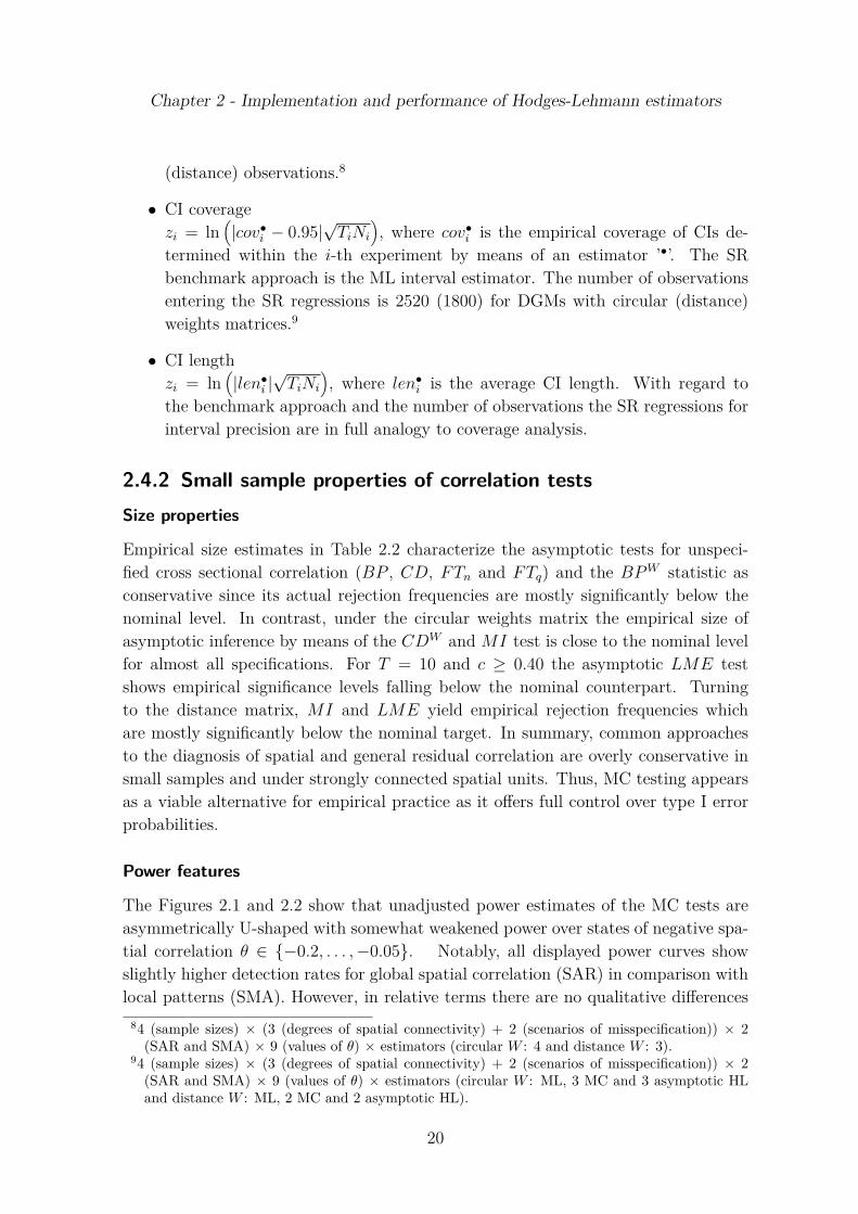
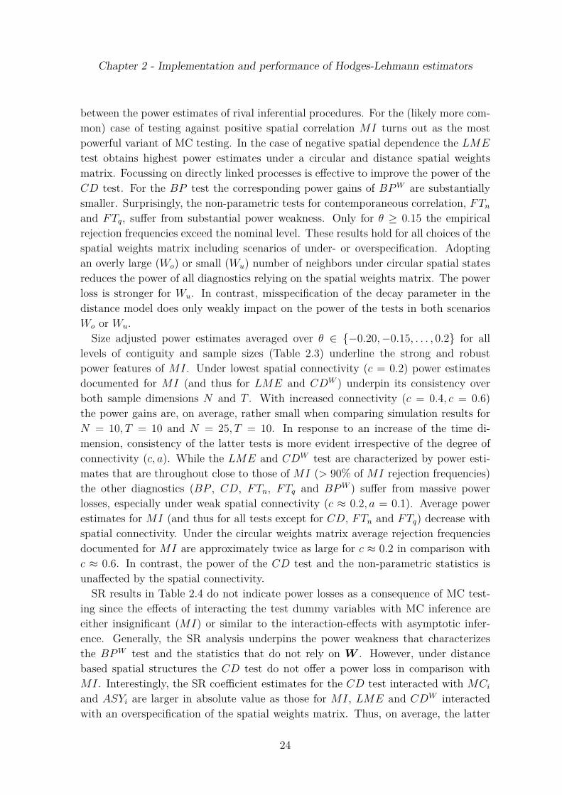
Tables and figures Size estimates of competing correlation tests are documentedin Table 2.2. Since the CDW and BP W test are identical to CD and BP under thedistance weights specification, respectively, and the latter, as well as FTn and FTq
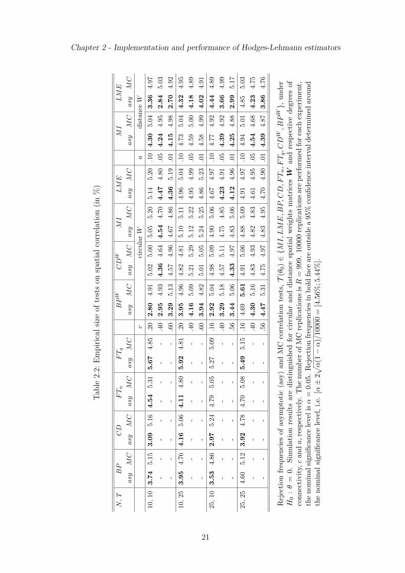
are invariant to the spatial weights matrix, size estimates under the distance matrixare only reported for MI and LME. Moreover, for SAR and SMA models withT = 10, N = 10 estimates of power are depicted as a function of the spatial parameterθ in Figure 2.1 (SAR disturbances) and Figure 2.2 (SMA). Similar plots are providedfor bias and CI coverage in Figure 2.3 (SAR) and Figure 2.4 (SMA). These figures showresults for underlying circular (left hand side panels) and distance weights (right handside) matrix with c = 0.40 and a = 0.05 (Wc), respectively, and two scenarios of spatialmisspecification (Wu, Wo). Although being restricted to the case T = 10, N = 10 thedisplayed results do not differ qualitatively over the other three combinations of sampledimensions. However, this rather small sample size highlights the discrepancies inpower of rival test statistics most clearly and demonstrates the need of HL estimationdue to the bias and coverage distortion of the ML estimator. Further simulation
17
Chapter 2 - Implementation and performance of Hodges-Lehmann estimators
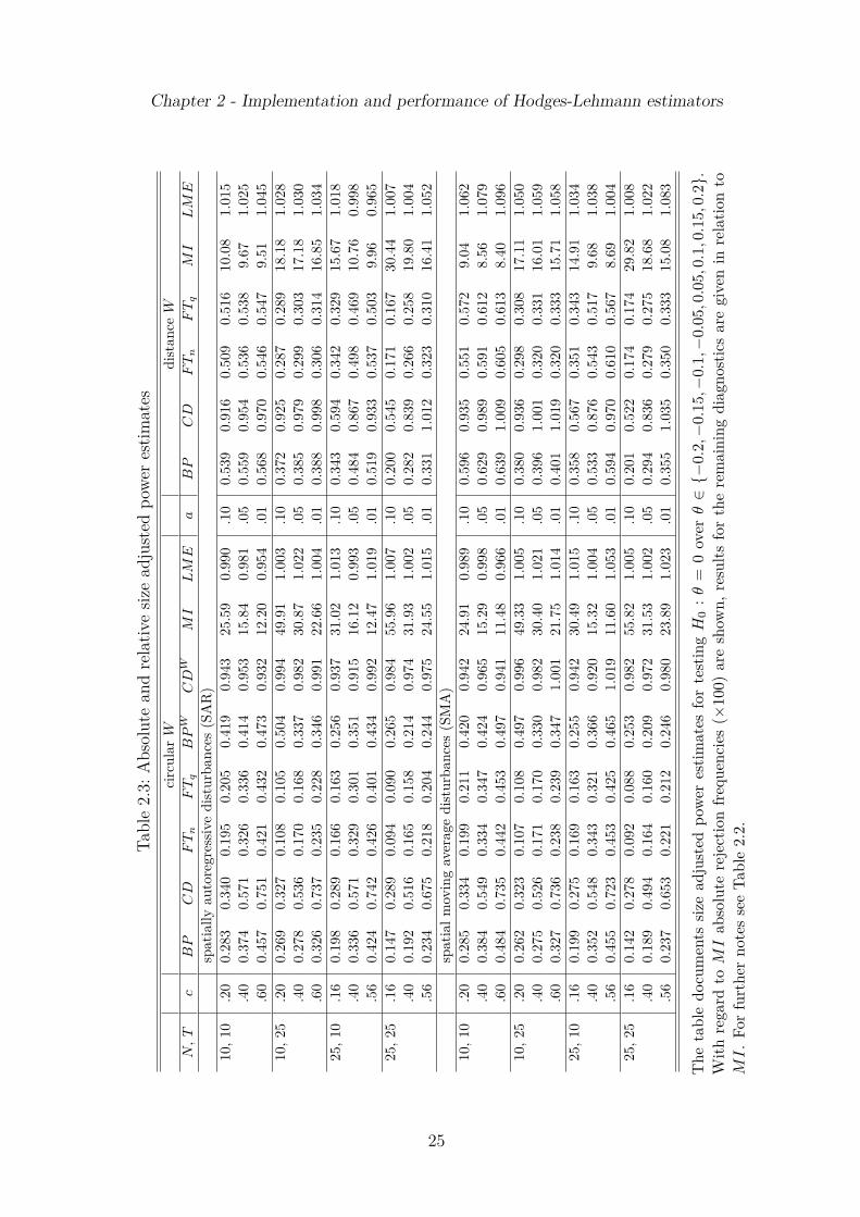
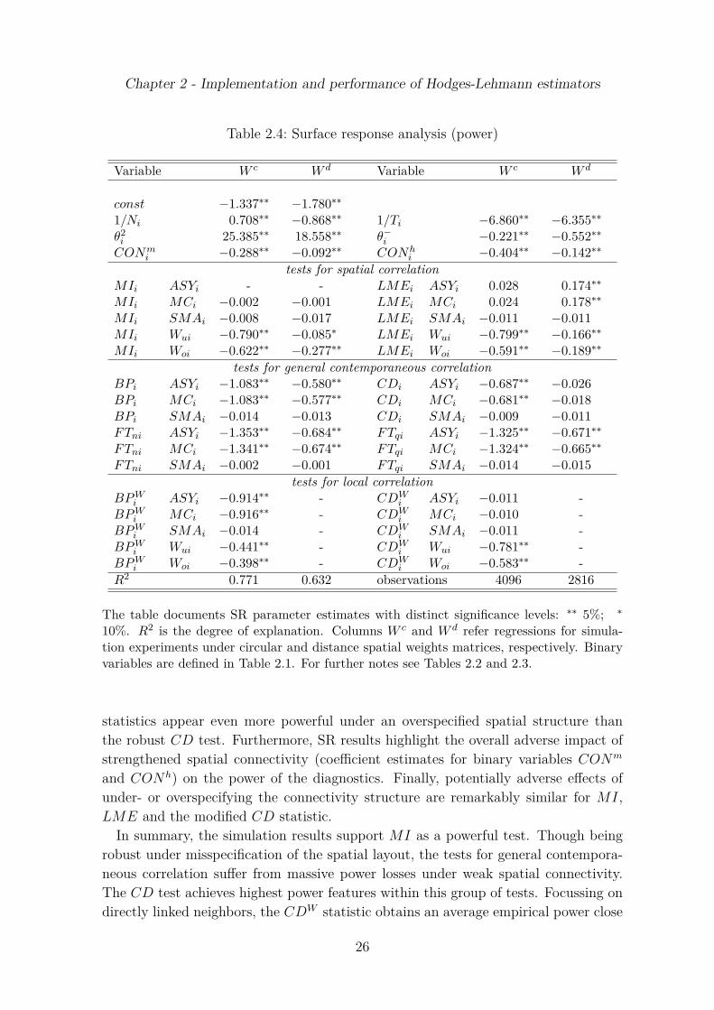
results are documented in Table 2.3 (size adjusted power6), Table 2.5 (bias/RMSE)and Table 2.7 (CI coverage/length) in the form of performance statistics averaged overθ ∈ −0.20, −0.15, . . . , 0.2 (power analysis) or θ ∈ −0.8, −0.6, . . . , 0.8 (point andinterval estimation).To facilitate the interpretation of results the entries in these tablesare given in normalized form where MI is typically the benchmark approach. Finally,at an even higher level of condensation results from surface response (SR) analysisare documented in Table 2.4 (power) and Table 2.6 (point and interval estimation).Next some implementation issues are discussed for the SR regressions.
Surface response analysis Similar to Anselin and Moreno (2003), Egger et al.(2009) or Das et al. (2003) the outcome of simulation experiments is related witheconometric tools (e.g. HL vs. ML estimators), specifications (e.g. SAR vs. SMA) ormodeling decisions (e.g. on the connectivity of spatial weight matrices). SR designsallow a rather condensed representation of simulation outcomes in response to charac-teristics of the underlying DGM and modeling decisions taken by the econometrician.Several metric variables enter the right hand side of the SR design, namely 1/Ti, 1/Ni
and θ2i . Relating the simulation outcome to θ2
i allows nonlinear performance in re-sponse to the strength of spatial dependence. Further explanatory variables, listedand defined in Table 2.1, are binary and suitable to indicate the marginal response ofloss measures to estimators and characteristics of the underlying DGM. Moreover, thebinary measures allow to uncover potential interaction effects (e.g. of applying par-ticular diagnostics in case of spatial over- (Wo) or underspecification (Wu)). Each SRregression design also includes an intercept term such that performance characteristicsare determined with regard to some benchmark modeling approach.
The dependent variables of the SR regressions are in the following denoted by zi andcorrespond to the natural logarithm of the loss measures mentioned above. The logtransformation is applied to ensure that zi is reasonably scaled (Anselin and Moreno,2003). With regard to each loss statistic two SR regressions are estimated summarizingthe simulation results obtained under circular and distance weights matrices. Thefollowing performance measures are subjected to SR regressions:
• powerzi = ln (erf •
i ), where erf •i is the empirical rejection frequency characterizing
the i-th simulation experiment (and modeling approach ’•’). For the poweranalysis the benchmark approach is MI. The number of simulation experimentsevaluated with regard to power characteristics is 4096 (circular W ) and 2816(distance W ).7
6Rejection frequencies are adjusted by tuning the critical values of the tests such that empiricalrejection frequencies are exactly 5% under H0.
74 (sample sizes) × 2 (SAR and SMA) × 8 (choices of θ under H1 : θ = 0) × 2 (MC based andasymptotic critical values) × (3 (degrees of spatial connectivity) × test statistics (circular W : 8and distance W : 6) + 2 (scenarios of misspecification) × (spatial) test statistics (circular W : 4
18
Chapter 2 - Implementation and performance of Hodges-Lehmann estimators
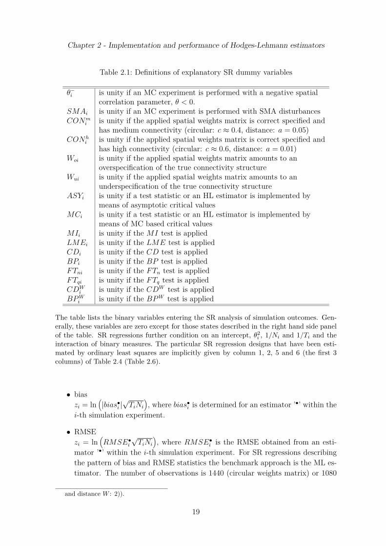
Table 2.1: Definitions of explanatory SR dummy variables
θ−i is unity if an MC experiment is performed with a negative spatial
correlation parameter, θ < 0.SMAi is unity if an MC experiment is performed with SMA disturbancesCONm
i is unity if the applied spatial weights matrix is correct specified andhas medium connectivity (circular: c ≈ 0.4, distance: a = 0.05)
CONhi is unity if the applied spatial weights matrix is correct specified and
has high connectivity (circular: c ≈ 0.6, distance: a = 0.01)Woi is unity if the applied spatial weights matrix amounts to an
overspecification of the true connectivity structureWui is unity if the applied spatial weights matrix amounts to an
underspecification of the true connectivity structureASYi is unity if a test statistic or an HL estimator is implemented by
means of asymptotic critical valuesMCi is unity if a test statistic or an HL estimator is implemented by
means of MC based critical valuesMIi is unity if the MI test is appliedLMEi is unity if the LME test is appliedCDi is unity if the CD test is appliedBPi is unity if the BP test is appliedFTni is unity if the FTn test is appliedFTqi is unity if the FTq test is appliedCDW
i is unity if the CDW test is appliedBP W
i is unity if the BP W test is applied
The table lists the binary variables entering the SR analysis of simulation outcomes. Gen-erally, these variables are zero except for those states described in the right hand side panelof the table. SR regressions further condition on an intercept, θ2
i , 1/Ni and 1/Ti and theinteraction of binary measures. The particular SR regression designs that have been esti-mated by ordinary least squares are implicitly given by column 1, 2, 5 and 6 (the first 3columns) of Table 2.4 (Table 2.6).
• biaszi = ln
(|bias•
i |√
TiNi
), where bias•
i is determined for an estimator ’•’ within thei-th simulation experiment.
• RMSEzi = ln
(RMSE•
i
√TiNi
), where RMSE•
i is the RMSE obtained from an esti-mator ’•’ within the i-th simulation experiment. For SR regressions describingthe pattern of bias and RMSE statistics the benchmark approach is the ML es-timator. The number of observations is 1440 (circular weights matrix) or 1080
and distance W : 2)).
19
Chapter 2 - Implementation and performance of Hodges-Lehmann estimators
(distance) observations.8
• CI coveragezi = ln
(|cov•
i − 0.95|√
TiNi
), where cov•
i is the empirical coverage of CIs de-termined within the i-th experiment by means of an estimator ’•’. The SRbenchmark approach is the ML interval estimator. The number of observationsentering the SR regressions is 2520 (1800) for DGMs with circular (distance)weights matrices.9
• CI lengthzi = ln
(|len•
i |√
TiNi
), where len•
i is the average CI length. With regard tothe benchmark approach and the number of observations the SR regressions forinterval precision are in full analogy to coverage analysis.
2.4.2 Small sample properties of correlation testsSize properties
Empirical size estimates in Table 2.2 characterize the asymptotic tests for unspeci-fied cross sectional correlation (BP , CD, FTn and FTq) and the BP W statistic asconservative since its actual rejection frequencies are mostly significantly below thenominal level. In contrast, under the circular weights matrix the empirical size ofasymptotic inference by means of the CDW and MI test is close to the nominal levelfor almost all specifications. For T = 10 and c ≥ 0.40 the asymptotic LME testshows empirical significance levels falling below the nominal counterpart. Turningto the distance matrix, MI and LME yield empirical rejection frequencies whichare mostly significantly below the nominal target. In summary, common approachesto the diagnosis of spatial and general residual correlation are overly conservative insmall samples and under strongly connected spatial units. Thus, MC testing appearsas a viable alternative for empirical practice as it offers full control over type I errorprobabilities.
Power features
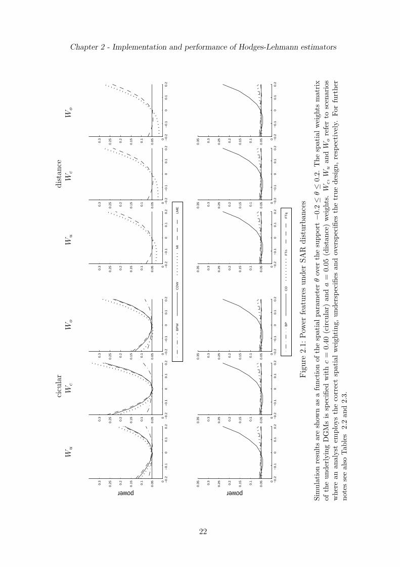
The Figures 2.1 and 2.2 show that unadjusted power estimates of the MC tests areasymmetrically U-shaped with somewhat weakened power over states of negative spa-tial correlation θ ∈ −0.2, . . . , −0.05. Notably, all displayed power curves showslightly higher detection rates for global spatial correlation (SAR) in comparison withlocal patterns (SMA). However, in relative terms there are no qualitative differences
84 (sample sizes) × (3 (degrees of spatial connectivity) + 2 (scenarios of misspecification)) × 2(SAR and SMA) × 9 (values of θ) × estimators (circular W : 4 and distance W : 3).
94 (sample sizes) × (3 (degrees of spatial connectivity) + 2 (scenarios of misspecification)) × 2(SAR and SMA) × 9 (values of θ) × estimators (circular W : ML, 3 MC and 3 asymptotic HLand distance W : ML, 2 MC and 2 asymptotic HL).
20
Chapter 2 - Implementation and performance of Hodges-Lehmann estimators
Tabl
e2.
2:Em
piric
alsiz
eof
test
son
spat
ialc
orre
latio
n(in
%)
N,
TB
PC
DF
Tn
FT
qB
PW
CD
WM
IL
ME
MI
LM
E
asy
MC
asy
MC
asy
MC
asy
MC
asy
MC
asy
MC
asy
MC
asy
MC
asy
MC
asy
MC
cci
rcul
arW
adi
stan
ceW
10,1
03.
745.
153.
095.
164.
545.
315.
674.
85.2
02.
804.
915.
025.
005.
055.
205.
145.
20.1
04.
305.
043.
364.
97-
--
--
--
-.4
02.
954.
934.
364.
644.
544.
704.
474.
80.0
54.
244.
952.
845.
03-
--
--
--
-.6
03.
295.
134.
574.
964.
674.
864.
365.
19.0
14.
154.
982.
704.
9210
,25
3.95
4.76
4.16
5.06
4.11
4.80
5.92
4.81
.20
3.95
4.96
4.82
4.81
5.10
5.11
4.96
5.04
.10
4.73
5.04
4.32
4.95
--
--
--
--
.40
4.16
5.09
5.21
5.29
5.12
5.22
4.95
4.99
.05
4.59
5.00
4.18
4.89
--
--
--
--
.60
3.94
4.82
5.01
5.05
5.24
5.25
4.86
5.23
.01
4.58
4.99
4.02
4.91
25,1
03.
534.
862.
975.
244.
795.
055.
275.
09.1
62.
925.
044.
985.
094.
905.
064.
674.
97.1
04.
774.
924.
444.
89-
--
--
--
-.4
03.
295.
184.
575.
114.
754.
854.
234.
91.0
54.
394.
923.
664.
99-
--
--
--
-.5
63.
445.
064.
334.
974.
835.
064.
124.
96.0
14.
254.
882.
995.
1725
,25
4.60
5.12
3.92
4.78
4.70
5.08
5.49
5.15
.16
4.69
5.61
4.91
5.06
4.88
5.09
4.91
4.97
.10
4.94
5.01
4.85
5.03
--
--
--
--
.40
4.30
5.16
4.83
4.93
4.82
4.83
4.61
4.95
.05
4.54
4.68
4.23
4.75
--
--
--
--
.56
4.47
5.31
4.75
4.97
4.83
4.95
4.70
4.90
.01
4.39
4.87
3.86
4.76
Rej
ectio
nfr
eque
ncie
sof
asym
ptot
ic(a
sy)
and
MC
corr
elat
ion
test
s,T
(θ0)
∈M
I,L
ME
,BP
,CD
,FT
n,F
Tq,C
DW
,BP
W,
unde
rH
0:θ
=0.
Sim
ulat
ion
resu
ltsar
edi
stin
guish
edfo
rci
rcul
aran
ddi
stan
cesp
atia
lw
eigh
tsm
atric
esW
and
resp
ectiv
ede
gree
sof
conn
ectiv
ity,c
and
a,r
espe
ctiv
ely.
The
num
bero
fMC
repl
icat
ions
isR
=99
9.10
000
repl
icat
ions
are
perf
orm
edfo
reac
hex
perim
ent,
the
nom
inal
signi
fican
cele
veli
sα=
0.05
.R
ejec
tion
freq
uenc
iesi
nbo
ldfa
cear
eou
tsid
ea
95%
confi
denc
ein
terv
alde
term
ined
arou
ndth
eno
min
alsig
nific
ance
leve
l,i.e
.[α
±2√ α
(1−
α)/
1000
0=
[4.5
6%;5
.44%
].
21
Chapter 2 - Implementation and performance of Hodges-Lehmann estimatorsci
cula
rdi
stan
ceW
uW
cW
oW
uW
cW
o
−0
.2−
0.1
00
.10
.20
0.0
5
0.1
0.1
5
0.2
0.2
5
0.3
power
−0
.2−
0.1
00
.10
.20
0.0
5
0.1
0.1
5
0.2
0.2
5
0.3
−0
.2−
0.1
00
.10
.20
0.0
5
0.1
0.1
5
0.2
0.2
5
0.3
BP
WC
DW
MI
LM
E
−0
.2−
0.1
00
.10
.20
0.0
5
0.1
0.1
5
0.2
0.2
5
0.3
−0
.2−
0.1
00
.10
.20
0.0
5
0.1
0.1
5
0.2
0.2
5
0.3
−0
.2−
0.1
00
.10
.20
0.0
5
0.1
0.1
5
0.2
0.2
5
0.3
−0
.2−
0.1
00
.10
.20
0.0
5
0.1
0.1
5
0.2
0.2
5
0.3
0.3
5
power
−0
.2−
0.1
00
.10
.20
0.0
5
0.1
0.1
5
0.2
0.2
5
0.3
0.3
5
−0
.2−
0.1
00
.10
.20
0.0
5
0.1
0.1
5
0.2
0.2
5
0.3
0.3
5
BP
CD
FT
nF
Tq
−0
.2−
0.1
00
.10
.20
0.0
5
0.1
0.1
5
0.2
0.2
5
0.3
0.3
5
−0
.2−
0.1
00
.10
.20
0.0
5
0.1
0.1
5
0.2
0.2
5
0.3
0.3
5
−0
.2−
0.1
00
.10
.20
0.0
5
0.1
0.1
5
0.2
0.2
5
0.3
0.3
5
Figu
re2.
1:Po
wer
feat
ures
unde
rSA
Rdi
stur
banc
es
Sim
ulat
ion
resu
ltsar
esh
own
asa
func
tion
ofth
esp
atia
lpar
amet
erθ
over
the
supp
ort
−0.
2≤
θ≤
0.2.
The
spat
ialw
eigh
tsm
atrix
ofth
eun
derly
ing
DG
Ms
issp
ecifi
edw
ithc
=0.
40(c
ircul
ar)
and
a=
0.05
(dist
ance
)w
eigh
ts.
Wc,W
uan
dW
ore
fer
tosc
enar
ios
whe
rean
anal
yst
empl
oys
the
corr
ect
spat
ialw
eigh
ting,
unde
rspe
cifie
san
dov
ersp
ecifi
esth
etr
uede
sign,
resp
ectiv
ely.
For
furt
her
note
sse
eal
soTa
bles
2.2
and
2.3.
22
Chapter 2 - Implementation and performance of Hodges-Lehmann estimators
cicu
lar
dist
ance
Wu
Wc
Wo
Wu
Wc
Wo
−0
.2−
0.1
00
.10
.20
0.0
5
0.1
0.1
5
0.2
0.2
5
0.3
power
−0
.2−
0.1
00
.10
.20
0.0
5
0.1
0.1
5
0.2
0.2
5
0.3
−0
.2−
0.1
00
.10
.20
0.0
5
0.1
0.1
5
0.2
0.2
5
0.3
BP
WC
DW
MI
LM
E
−0
.2−
0.1
00
.10
.20
0.0
5
0.1
0.1
5
0.2
0.2
5
0.3
−0
.2−
0.1
00
.10
.20
0.0
5
0.1
0.1
5
0.2
0.2
5
0.3
−0
.2−
0.1
00
.10
.20
0.0
5
0.1
0.1
5
0.2
0.2
5
0.3
−0
.2−
0.1
00
.10
.20
0.0
5
0.1
0.1
5
0.2
0.2
5
0.3
0.3
5
power
−0
.2−
0.1
00
.10
.20
0.0
5
0.1
0.1
5
0.2
0.2
5
0.3
0.3
5
−0
.2−
0.1
00
.10
.20
0.0
5
0.1
0.1
5
0.2
0.2
5
0.3
0.3
5
BP
CD
FT
nF
Tq
−0
.2−
0.1
00
.10
.20
0.0
5
0.1
0.1
5
0.2
0.2
5
0.3
0.3
5
−0
.2−
0.1
00
.10
.20
0.0
5
0.1
0.1
5
0.2
0.2
5
0.3
0.3
5
−0
.2−
0.1
00
.10
.20
0.0
5
0.1
0.1
5
0.2
0.2
5
0.3
0.3
5
Figu
re2.
2:Po
wer
feat
ures
unde
rSM
Adi
stur
banc
es
For
furt
her
note
sse
eFi
gure
2.1.
23
Chapter 2 - Implementation and performance of Hodges-Lehmann estimators
between the power estimates of rival inferential procedures. For the (likely more com-mon) case of testing against positive spatial correlation MI turns out as the mostpowerful variant of MC testing. In the case of negative spatial dependence the LME
test obtains highest power estimates under a circular and distance spatial weightsmatrix. Focussing on directly linked processes is effective to improve the power of theCD test. For the BP test the corresponding power gains of BP W are substantiallysmaller. Surprisingly, the non-parametric tests for contemporaneous correlation, FTn
and FTq, suffer from substantial power weakness. Only for θ ≥ 0.15 the empiricalrejection frequencies exceed the nominal level. These results hold for all choices of thespatial weights matrix including scenarios of under- or overspecification. Adoptingan overly large (Wo) or small (Wu) number of neighbors under circular spatial statesreduces the power of all diagnostics relying on the spatial weights matrix. The powerloss is stronger for Wu. In contrast, misspecification of the decay parameter in thedistance model does only weakly impact on the power of the tests in both scenariosWo or Wu.
Size adjusted power estimates averaged over θ ∈ −0.20, −0.15, . . . , 0.2 for alllevels of contiguity and sample sizes (Table 2.3) underline the strong and robustpower features of MI. Under lowest spatial connectivity (c = 0.2) power estimatesdocumented for MI (and thus for LME and CDW ) underpin its consistency overboth sample dimensions N and T . With increased connectivity (c = 0.4, c = 0.6)the power gains are, on average, rather small when comparing simulation results forN = 10, T = 10 and N = 25, T = 10. In response to an increase of the time di-mension, consistency of the latter tests is more evident irrespective of the degree ofconnectivity (c, a). While the LME and CDW test are characterized by power esti-mates that are throughout close to those of MI (> 90% of MI rejection frequencies)the other diagnostics (BP , CD, FTn, FTq and BP W ) suffer from massive powerlosses, especially under weak spatial connectivity (c ≈ 0.2, a = 0.1). Average powerestimates for MI (and thus for all tests except for CD, FTn and FTq) decrease withspatial connectivity. Under the circular weights matrix average rejection frequenciesdocumented for MI are approximately twice as large for c ≈ 0.2 in comparison withc ≈ 0.6. In contrast, the power of the CD test and the non-parametric statistics isunaffected by the spatial connectivity.
SR results in Table 2.4 do not indicate power losses as a consequence of MC test-ing since the effects of interacting the test dummy variables with MC inference areeither insignificant (MI) or similar to the interaction-effects with asymptotic infer-ence. Generally, the SR analysis underpins the power weakness that characterizesthe BP W test and the statistics that do not rely on W . However, under distancebased spatial structures the CD test do not offer a power loss in comparison withMI. Interestingly, the SR coefficient estimates for the CD test interacted with MCi
and ASYi are larger in absolute value as those for MI, LME and CDW interactedwith an overspecification of the spatial weights matrix. Thus, on average, the latter
24
Chapter 2 - Implementation and performance of Hodges-Lehmann estimators
Tabl
e2.
3:A
bsol
ute
and
rela
tive
size
adju
sted
powe
res
timat
esci
rcul
arW
dist
ance
W
N,
Tc
BP
CD
FT
nF
Tq
BP
WC
DW
MI
LM
Ea
BP
CD
FT
nF
Tq
MI
LM
E
spat
ially
auto
regr
essiv
edi
stur
banc
es(S
AR
)10
,10
.20
0.28
30.
340
0.19
50.
205
0.41
90.
943
25.5
90.
990
.10
0.53
90.
916
0.50
90.
516
10.0
81.
015
.40
0.37
40.
571
0.32
60.
336
0.41
40.
953
15.8
40.
981
.05
0.55
90.
954
0.53
60.
538
9.67
1.02
5.6
00.
457
0.75
10.
421
0.43
20.
473
0.93
212
.20
0.95
4.0
10.
568
0.97
00.
546
0.54
79.
511.
045
10,2
5.2
00.
269
0.32
70.
108
0.10
50.
504
0.99
449
.91
1.00
3.1
00.
372
0.92
50.
287
0.28
918
.18
1.02
8.4
00.
278
0.53
60.
170
0.16
80.
337
0.98
230
.87
1.02
2.0
50.
385
0.97
90.
299
0.30
317
.18
1.03
0.6
00.
326
0.73
70.
235
0.22
80.
346
0.99
122
.66
1.00
4.0
10.
388
0.99
80.
306
0.31
416
.85
1.03
425
,10
.16
0.19
80.
289
0.16
60.
163
0.25
60.
937
31.0
21.
013
.10
0.34
30.
594
0.34
20.
329
15.6
71.
018
.40
0.33
60.
571
0.32
90.
301
0.35
10.
915
16.1
20.
993
.05
0.48
40.
867
0.49
80.
469
10.7
60.
998
.56
0.42
40.
742
0.42
60.
401
0.43
40.
992
12.4
71.
019
.01
0.51
90.
933
0.53
70.
503
9.96
0.96
525
,25
.16
0.14
70.
289
0.09
40.
090
0.26
50.
984
55.9
61.
007
.10
0.20
00.
545
0.17
10.
167
30.4
41.
007
.40
0.19
20.
516
0.16
50.
158
0.21
40.
974
31.9
31.
002
.05
0.28
20.
839
0.26
60.
258
19.8
01.
004
.56
0.23
40.
675
0.21
80.
204
0.24
40.
975
24.5
51.
015
.01
0.33
11.
012
0.32
30.
310
16.4
11.
052
spat
ialm
ovin
gav
erag
edi
stur
banc
es(S
MA
)10
,10
.20
0.28
50.
334
0.19
90.
211
0.42
00.
942
24.9
10.
989
.10
0.59
60.
935
0.55
10.
572
9.04
1.06
2.4
00.
384
0.54
90.
334
0.34
70.
424
0.96
515
.29
0.99
8.0
50.
629
0.98
90.
591
0.61
28.
561.
079
.60
0.48
40.
735
0.44
20.
453
0.49
70.
941
11.4
80.
966
.01
0.63
91.
009
0.60
50.
613
8.40
1.09
610
,25
.20
0.26
20.
323
0.10
70.
108
0.49
70.
996
49.3
31.
005
.10
0.38
00.
936
0.29
80.
308
17.1
11.
050
.40
0.27
50.
526
0.17
10.
170
0.33
00.
982
30.4
01.
021
.05
0.39
61.
001
0.32
00.
331
16.0
11.
059
.60
0.32
70.
736
0.23
80.
239
0.34
71.
001
21.7
51.
014
.01
0.40
11.
019
0.32
00.
333
15.7
11.
058
25,1
0.1
60.
199
0.27
50.
169
0.16
30.
255
0.94
230
.49
1.01
5.1
00.
358
0.56
70.
351
0.34
314
.91
1.03
4.4
00.
352
0.54
80.
343
0.32
10.
366
0.92
015
.32
1.00
4.0
50.
533
0.87
60.
543
0.51
79.
681.
038
.56
0.45
50.
723
0.45
30.
425
0.46
51.
019
11.6
01.
053
.01
0.59
40.
970
0.61
00.
567
8.69
1.00
425
,25
.16
0.14
20.
278
0.09
20.
088
0.25
30.
982
55.8
21.
005
.10
0.20
10.
522
0.17
40.
174
29.8
21.
008
.40
0.18
90.
494
0.16
40.
160
0.20
90.
972
31.5
31.
002
.05
0.29
40.
836
0.27
90.
275
18.6
81.
022
.56
0.23
70.
653
0.22
10.
212
0.24
60.
980
23.8
91.
023
.01
0.35
51.
035
0.35
00.
333
15.0
81.
083
The
tabl
edo
cum
ents
size
adju
sted
pow
eres
timat
esfo
rte
stin
gH
0:θ
=0
over
θ∈
−0.
2,−
0.15
,−0.
1,−
0.05
,0.0
5,0.
1,0.
15,0
.2.
With
rega
rdto
MI
abso
lute
reje
ctio
nfr
eque
ncie
s(×
100)
are
show
n,re
sults
for
the
rem
aini
ngdi
agno
stic
sar
egi
ven
inre
latio
nto
MI.
For
furt
her
note
sse
eTa
ble
2.2.
25
Chapter 2 - Implementation and performance of Hodges-Lehmann estimators
Table 2.4: Surface response analysis (power)
Variable W c W d Variable W c W d
const −1.337∗∗ −1.780∗∗
1/Ni 0.708∗∗ −0.868∗∗ 1/Ti −6.860∗∗ −6.355∗∗
θ2i 25.385∗∗ 18.558∗∗ θ−
i −0.221∗∗ −0.552∗∗
CONmi −0.288∗∗ −0.092∗∗ CONh
i −0.404∗∗ −0.142∗∗
tests for spatial correlationMIi ASYi - - LMEi ASYi 0.028 0.174∗∗
MIi MCi −0.002 −0.001 LMEi MCi 0.024 0.178∗∗
MIi SMAi −0.008 −0.017 LMEi SMAi −0.011 −0.011MIi Wui −0.790∗∗ −0.085∗ LMEi Wui −0.799∗∗ −0.166∗∗
MIi Woi −0.622∗∗ −0.277∗∗ LMEi Woi −0.591∗∗ −0.189∗∗
tests for general contemporaneous correlationBPi ASYi −1.083∗∗ −0.580∗∗ CDi ASYi −0.687∗∗ −0.026BPi MCi −1.083∗∗ −0.577∗∗ CDi MCi −0.681∗∗ −0.018BPi SMAi −0.014 −0.013 CDi SMAi −0.009 −0.011FTni ASYi −1.353∗∗ −0.684∗∗ FTqi ASYi −1.325∗∗ −0.671∗∗
FTni MCi −1.341∗∗ −0.674∗∗ FTqi MCi −1.324∗∗ −0.665∗∗
FTni SMAi −0.002 −0.001 FTqi SMAi −0.014 −0.015tests for local correlation
BP Wi ASYi −0.914∗∗ - CDW
i ASYi −0.011 -BP W
i MCi −0.916∗∗ - CDWi MCi −0.010 -
BP Wi SMAi −0.014 - CDW
i SMAi −0.011 -BP W
i Wui −0.441∗∗ - CDWi Wui −0.781∗∗ -
BP Wi Woi −0.398∗∗ - CDW
i Woi −0.583∗∗ -R2 0.771 0.632 observations 4096 2816
The table documents SR parameter estimates with distinct significance levels: ∗∗ 5%; ∗
10%. R2 is the degree of explanation. Columns W c and W d refer regressions for simula-tion experiments under circular and distance spatial weights matrices, respectively. Binaryvariables are defined in Table 2.1. For further notes see Tables 2.2 and 2.3.
statistics appear even more powerful under an overspecified spatial structure thanthe robust CD test. Furthermore, SR results highlight the overall adverse impact ofstrengthened spatial connectivity (coefficient estimates for binary variables CONm
and CONh) on the power of the diagnostics. Finally, potentially adverse effects ofunder- or overspecifying the connectivity structure are remarkably similar for MI,LME and the modified CD statistic.
In summary, the simulation results support MI as a powerful test. Though beingrobust under misspecification of the spatial layout, the tests for general contempora-neous correlation suffer from massive power losses under weak spatial connectivity.The CD test achieves highest power features within this group of tests. Focussing ondirectly linked neighbors, the CDW statistic obtains an average empirical power close
26
Chapter 2 - Implementation and performance of Hodges-Lehmann estimators
to that of MI.To economize on space the following analysis of the empirical performance of HL
point and interval estimators is concentrated on a smaller set of alternative test ap-proaches. The empirical performance of the considered correlation tests suggests tochoose as potential candidates for HL estimation diagnostics with a rather accurateperformance in terms of power (MI) or robustness under diverse (misspecified) spatialstructures (CD). As a third alternative the CDW test is considered, gathering both,a (relatively) robust and powerful performance.
2.4.3 Point estimationAs mentioned above, the maximization of the asymptotic and the MC based p-valueto obtain HL point estimates is equivalent. Thus, each test T (θ0) ∈ MI, CD, CDW obtains one HL point estimate. In the upper panels of Figures 2.3 and 2.4 biasestimates are displayed. The HL(MI) estimator yields the smallest bias of allapproaches over the entire parameter space considered for θ. In particular, the biasof the HL(MI) estimator is markedly smaller than respective ML statistics. Whileunder correct model specification it is uniformly negative, the bias might eventuallybecome positive under misspecification of the spatial weights and scenarios of negativecorrelation. Under correct specification of the spatial weights matrix bias estimatesfor the HL(MI) estimator are markedly smaller (i.e. by a factor of ≈ 1/10) under acircular (c = 0.4) in comparison with a distance (a = 0.05) weights matrix.
The average performance measures in Table 2.5 confirm that HL(MI) estimates aremost effective with regard to bias loss. The bias of the ML and HL(CDW ) estimatorsis generally more than twice as large in comparison with the HL(MI) counterpart. Insmall samples (N = T = 10), experiments can be observed where the ML bias is by afactor of more than 7 larger in comparison with results documented for the HL(MI)estimator. ML biases are, on average, by factors 5.64 (SAR, circular W ), 4.51 (SMA,circular W ), 3.45 (SAR, distance W ) and 2.75 (SMA, distance W ) larger than lossesfeaturing the HL(MI) approach. Comparing ML and HL(CDW ) estimates, the formerappear to have a small overall lead which holds, in particular, if the cross section is’large’ (N = 25). In this case the asymptotic distribution of CDW is characterizedby a relatively large number of degrees of freedom which might adversely impact onits discriminatory content. For the same reason, under circular states the HL(CD)estimator suffers from huge average biases, such that it is not recommendable if ananalyst pays particular attention to this loss criterion.
SR results for the bias loss are documented in the fourth and fifth column of Ta-ble 2.6. For both families of spatial weights matrices the HL(MI) estimator out-performs the benchmark ML approach which is indicated by a significantly negativecoefficient estimated for the interacted MIi, MCi dummy variables. As a reflectionof power features discussed before, overall, the bias is higher over states of medium
27
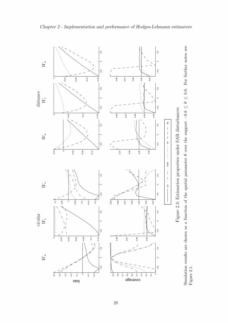
Chapter 2 - Implementation and performance of Hodges-Lehmann estimators
cicu
lar
dist
ance
Wu
Wc
Wo
Wu
Wc
Wo
−0
.50
0.5
−0
.2
−0
.10
0.1
0.2
0.3
0.4
0.5
bias
−0
.50
0.5
−0
.12
−0
.1
−0
.08
−0
.06
−0
.04
−0
.020
−0
.50
0.5
−0
.2
−0
.15
−0
.1
−0
.050
0.0
5
0.1
−0
.50
0.5
−0
.12
−0
.08
−0
.040
0.0
4
−0
.50
0.5
−0
.15
−0
.1
−0
.050
−0
.50
0.5
−0
.16
−0
.12
−0
.08
−0
.040
−0
.50
0.5
0
0.1
0.2
0.3
0.4
0.5
0.6
0.7
0.8
0.9
coverage
−0
.50
0.5
0.9
5
0.9
6
0.9
7
0.9
8
−0
.50
0.5
0.9
3
0.9
4
0.9
5
0.9
6
0.9
7
0.9
8
0.9
9
CD
CD
WM
IM
L
−0
.50
0.5
0.9
4
0.9
5
0.9
6
0.9
7
−0
.50
0.5
0.9
4
0.9
5
0.9
6
0.9
7
0.9
8
−0
.50
0.5
0.9
4
0.9
5
0.9
6
0.9
7
0.9
8
Figu
re2.
3:Es
timat
ion
prop
ertie
sun
der
SAR
dist
urba
nces
Sim
ulat
ion
resu
ltsar
esh
own
asa
func
tion
ofth
esp
atia
lpa
ram
eter
θov
erth
esu
ppor
t−
0.8
≤θ
≤0.
8.Fo
rfu
rthe
rno
tes
see
Figu
re2.
1.
28
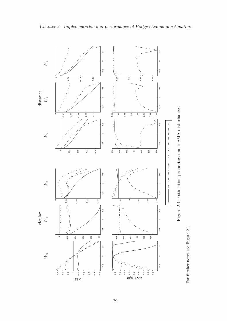
Chapter 2 - Implementation and performance of Hodges-Lehmann estimators
cicu
lar
dist
ance
Wu
Wc
Wo
Wu
Wc
Wo
−0
.50
0.5
−0
.5
−0
.4
−0
.3
−0
.2
−0
.10
0.1
0.2
0.3
bias
−0
.50
0.5
−0
.1
−0
.08
−0
.06
−0
.04
−0
.020
−0
.50
0.5
−0
.16
−0
.12
−0
.08
−0
.040
−0
.50
0.5
−0
.16
−0
.12
−0
.08
−0
.040
−0
.50
0.5
−0
.1
−0
.08
−0
.06
−0
.04
−0
.020
−0
.50
0.5
−0
.12
−0
.08
−0
.040
−0
.50
0.5
0
0.1
0.2
0.3
0.4
0.5
0.6
0.7
0.8
0.9
coverage
−0
.50
0.5
0.8
6
0.8
8
0.9
0.9
2
0.9
4
0.9
6
−0
.50
0.5
0.7
8
0.8
2
0.8
6
0.9
0.9
4
CD
CD
WM
IM
L
−0
.50
0.5
0.8
4
0.8
6
0.8
8
0.9
0.9
2
0.9
4
0.9
6
−0
.50
0.5
0.8
2
0.8
4
0.8
6
0.8
8
0.9
0.9
2
0.9
4
0.9
6
−0
.50
0.5
0.8
2
0.8
6
0.9
0.9
4
Figu
re2.
4:Es
timat
ion
prop
ertie
sun
der
SMA
dist
urba
nces
For
furt
her
note
sse
eFi
gure
2.1.
29
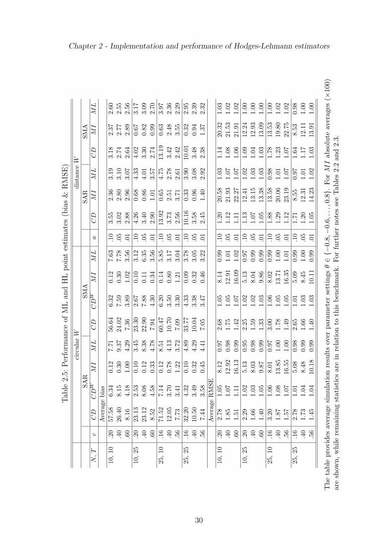
Chapter 2 - Implementation and performance of Hodges-Lehmann estimators
Tabl
e2.
5:Pe
rform
ance
ofM
Lan
dH
Lpo
int
estim
ates
(bia
s&
RM
SE)
circ
ular
Wdi
stan
ceW
SAR
SMA
SAR
SMA
N,
Tc
CD
CD
WM
IM
LC
DC
DW
MI
ML
aC
DM
IM
LC
DM
IM
L
Aver
age
bias
10,1
0.2
057
.58
6.34
0.12
7.71
56.6
46.
320.
127.
63.1
03.
552.
363.
193.
182.
372.
60.4
026
.40
8.15
0.30
9.37
24.0
27.
590.
307.
78.0
53.
022.
803.
102.
742.
772.
55.6
08.
164.
181.
004.
297.
363.
891.
023.
56.0
12.
882.
963.
072.
642.
892.
5610
,25
.20
23.1
32.
530.
103.
4523
.30
2.67
0.10
3.12
.10
4.26
0.68
4.33
4.02
0.67
3.17
.40
23.1
28.
080.
128.
3822
.90
7.88
0.11
6.35
.05
3.40
0.86
4.01
3.30
0.82
3.09
.60
8.52
4.58
0.33
4.78
7.94
4.30
0.34
3.56
.01
2.90
1.01
3.57
2.74
0.99
2.70
25,1
0.1
671
.52
7.14
0.12
8.51
60.4
76.
200.
145.
85.1
013
.92
0.65
4.75
13.1
90.
633.
97.4
012
.05
3.70
0.78
4.13
10.7
03.
500.
803.
17.0
53.
732.
512.
783.
422.
482.
36.5
67.
733.
411.
223.
727.
093.
301.
213.
04.0
12.
563.
712.
612.
423.
552.
2925
,25
.16
32.2
04.
320.
104.
8933
.77
4.33
0.09
3.78
.10
10.1
60.
333.
9010
.01
0.32
2.95
.40
10.5
03.
490.
324.
2910
.04
3.38
0.32
3.05
.05
3.58
0.96
3.08
3.48
0.94
2.39
.56
7.44
3.58
0.45
4.41
7.05
3.47
0.46
3.22
.01
2.45
1.40
2.92
2.38
1.37
2.32
Aver
age
RM
SE10
,10
.20
2.78
1.05
8.12
0.97
2.68
1.05
8.14
0.99
.10
1.20
20.5
81.
031.
1420
.32
1.03
.40
1.85
1.07
12.9
20.
981.
751.
0512
.91
1.01
.05
1.12
21.9
31.
071.
0821
.53
1.02
.60
1.51
1.11
16.1
30.
991.
421.
0716
.09
1.02
.01
1.11
22.2
71.
071.
0621
.91
1.02
10,2
5.2
02.
291.
025.
130.
952.
251.
025.
130.
97.1
01.
1312
.41
1.02
1.09
12.2
41.
00.4
01.
661.
038.
030.
981.
591.
028.
040.
99.0
51.
0713
.15
1.03
1.04
12.9
31.
00.6
01.
401.
059.
870.
991.
331.
039.
860.
99.0
11.
0513
.38
1.03
1.03
13.0
91.
0025
,10
.16
3.20
1.06
8.01
0.97
3.00
1.06
8.02
0.99
.10
1.88
13.5
80.
981.
7813
.53
1.00
.40
1.87
1.08
13.8
51.
001.
781.
0513
.71
1.00
.05
1.29
20.0
61.
011.
2319
.80
1.02
.56
1.57
1.07
16.5
51.
001.
491.
0516
.35
1.01
.01
1.12
23.1
91.
071.
0722
.75
1.02
25,2
5.1
62.
781.
015.
080.
982.
651.
015.
090.
99.1
01.
718.
550.
971.
648.
530.
98.4
01.
731.
048.
480.
991.
661.
038.
451.
00.0
51.
2012
.31
1.01
1.17
12.1
11.
00.5
61.
451.
0410
.18
0.99
1.40
1.03
10.1
10.
99.0
11.
0514
.23
1.02
1.03
13.9
11.
00
The
tabl
epr
ovid
esav
erag
esim
ulat
ion
resu
ltsov
erpa
ram
eter
sett
ings
θ∈
−0.
8,−
0.6,
...,
0.8
.Fo
rM
Iab
solu
teav
erag
es(×
100)
are
show
n,w
hile
rem
aini
ngst
atist
ics
are
inre
latio
nto
this
benc
hmar
k.Fo
rfu
rthe
rno
tes
see
Tabl
es2.
2an
d2.
3.
30
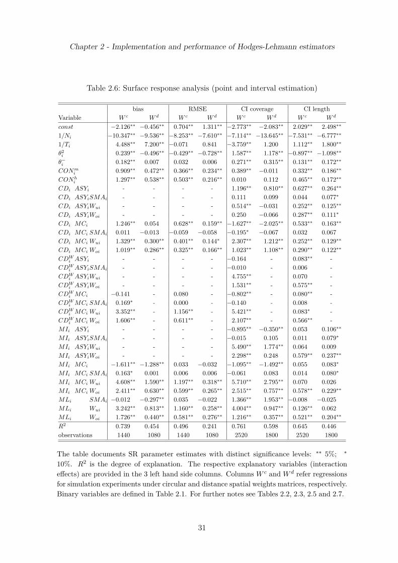
Chapter 2 - Implementation and performance of Hodges-Lehmann estimators
Table 2.6: Surface response analysis (point and interval estimation)
bias RMSE CI coverage CI lengthVariable W c W d W c W d W c W d W c W d
const −2.126∗∗ −0.456∗∗ 0.704∗∗ 1.311∗∗ −2.773∗∗ −2.083∗∗ 2.029∗∗ 2.498∗∗
1/Ni −10.347∗∗ −9.536∗∗ −8.253∗∗ −7.610∗∗ −7.114∗∗ −13.645∗∗ −7.531∗∗ −6.777∗∗
1/Ti 4.488∗∗ 7.200∗∗ −0.071 0.841 −3.759∗∗ 1.200 1.112∗∗ 1.800∗∗
θ2i 0.239∗∗ −0.496∗∗ −0.429∗∗ −0.728∗∗ 1.587∗∗ 1.178∗∗ −0.897∗∗ −1.098∗∗
θ−i 0.182∗∗ 0.007 0.032 0.006 0.271∗∗ 0.315∗∗ 0.131∗∗ 0.172∗∗
CONmi 0.909∗∗ 0.472∗∗ 0.366∗∗ 0.234∗∗ 0.389∗∗ −0.011 0.332∗∗ 0.186∗∗
CONhi 1.297∗∗ 0.538∗∗ 0.503∗∗ 0.216∗∗ 0.010 0.112 0.465∗∗ 0.172∗∗
CDi ASYi - - - - 1.196∗∗ 0.810∗∗ 0.627∗∗ 0.264∗∗
CDi ASYiSMAi - - - - 0.111 0.099 0.044 0.077∗
CDi ASYiWui - - - - 0.514∗∗ −0.031 0.252∗∗ 0.125∗∗
CDi ASYiWoi - - - - 0.250 −0.066 0.287∗∗ 0.111∗
CDi MCi 1.246∗∗ 0.054 0.628∗∗ 0.159∗∗ −1.627∗∗ −2.025∗∗ 0.533∗∗ 0.163∗∗
CDi MCi SMAi 0.011 −0.013 −0.059 −0.058 −0.195∗ −0.067 0.032 0.067CDi MCi Wui 1.329∗∗ 0.300∗∗ 0.401∗∗ 0.144∗ 2.307∗∗ 1.212∗∗ 0.252∗∗ 0.129∗∗
CDi MCi Woi 1.019∗∗ 0.286∗∗ 0.325∗∗ 0.166∗∗ 1.023∗∗ 1.108∗∗ 0.290∗∗ 0.122∗∗
CDWi ASYi - - - - −0.164 - 0.083∗∗ -
CDWi ASYiSMAi - - - - −0.010 - 0.006 -
CDWi ASYiWui - - - - 4.755∗∗ - 0.070 -
CDWi ASYiWoi - - - - 1.531∗∗ - 0.575∗∗ -
CDWi MCi −0.141 - 0.080 - −0.802∗∗ - 0.080∗∗ -
CDWi MCi SMAi 0.169∗ - 0.000 - −0.140 - 0.008 -
CDWi MCi Wui 3.352∗∗ - 1.156∗∗ - 5.421∗∗ - 0.083∗ -
CDWi MCi Woi 1.606∗∗ - 0.611∗∗ - 2.107∗∗ - 0.566∗∗ -
MIi ASYi - - - - −0.895∗∗ −0.350∗∗ 0.053 0.106∗∗
MIi ASYiSMAi - - - - −0.015 0.105 0.011 0.079∗
MIi ASYiWui - - - - 5.490∗∗ 1.774∗∗ 0.064 0.009MIi ASYiWoi - - - - 2.298∗∗ 0.248 0.579∗∗ 0.237∗∗
MIi MCi −1.611∗∗ −1.288∗∗ 0.033 −0.032 −1.095∗∗ −1.492∗∗ 0.055 0.083∗
MIi MCi SMAi 0.163∗ 0.001 0.006 0.006 −0.061 0.083 0.014 0.080∗
MIi MCi Wui 4.608∗∗ 1.590∗∗ 1.197∗∗ 0.318∗∗ 5.710∗∗ 2.795∗∗ 0.070 0.026MIi MCi Woi 2.411∗∗ 0.630∗∗ 0.599∗∗ 0.265∗∗ 2.515∗∗ 0.757∗∗ 0.578∗∗ 0.229∗∗
MLi SMAi −0.012 −0.297∗∗ 0.035 −0.022 1.366∗∗ 1.953∗∗ −0.008 −0.025MLi Wui 3.242∗∗ 0.813∗∗ 1.160∗∗ 0.258∗∗ 4.004∗∗ 0.947∗∗ 0.126∗∗ 0.062MLi Woi 1.726∗∗ 0.440∗∗ 0.581∗∗ 0.276∗∗ 1.216∗∗ 0.357∗∗ 0.521∗∗ 0.204∗∗
R2 0.739 0.454 0.496 0.241 0.761 0.598 0.645 0.446observations 1440 1080 1440 1080 2520 1800 2520 1800
The table documents SR parameter estimates with distinct significance levels: ∗∗ 5%; ∗
10%. R2 is the degree of explanation. The respective explanatory variables (interactioneffects) are provided in the 3 left hand side columns. Columns W c and W d refer regressionsfor simulation experiments under circular and distance spatial weights matrices, respectively.Binary variables are defined in Table 2.1. For further notes see Tables 2.2, 2.3, 2.5 and 2.7.
31
Chapter 2 - Implementation and performance of Hodges-Lehmann estimators
(CONm) and strong (CONh) spatial connectivity. Similarly, an underestimation ofthe spatial connectivity structure is more detrimental for bias loss in comparison withscenarios where an analyst overestimates the actual degree of connectivity.
Noting that the HL(MI) estimator offers marked bias reductions, it is of interestif this gain has to be paid with increased estimation uncertainty. Average RMSEstatistics in Table 2.5 and SR results for the RMSE loss in column 6 and 7 of Table 2.6show that the former gain does not go along with adverse second order characteristics.The ML and HL(MI) estimators are characterized by similar estimation accuracy. Insummary, with particular regard to the estimation bias, HL(MI) and to some weakerextent HL(CDW ) are viable alternatives to the ML estimator. Though being robustunder misspecification of the spatial layout, HL(CD) estimates suffer from powerweakness of the underlying diagnostic.
2.4.4 Interval estimationCoverage estimates for the ML and MC based approaches to interval estimation aredisplayed in the lower panels of Figures 2.3 and 2.4. By construction, the empiricalcoverage of HL interval estimates does not differ significantly from the nominal 95%level under correct spatial model implementation. With regard to ML interval esti-mation it appears that, in particular, SMA disturbances invoke some risk to end upwith overly liberal or falsely centered CIs even if the spatial structure presumed by ananalyst coincides with the underlying model (Wc). Again the case of underspecifyingthe spatial structure (Wu) appears most detrimental for interval estimation, since itis characterized by massive coverage distortions at least under circular spatial weight-ing. For such scenarios HL(CD) intervals still offer accurate coverage probabilitiesempirically.
Estimates of average absolute coverage distortions in Table 2.7 confirm that MLperforms markedly worse than HL(MI) implemented by means of MC critical values.For instance, regarding DGMs with distance weights matrices and SAR disturbances,average ML coverage errors exceed the benchmark statistics by factors of 1.6 (a =0.10, N = 25, T = 10) to 26 (a = 0.05, N = 10, T = 25). Notably, such large relativemeasures reflect that in nominal terms the benchmark approach shows only slightdeviations from the nominal coverage. For some instances (N = T = 25) conditioningthe HL(MI) estimator on asymptotic critical values obtains even smaller averageabsolute coverage loss in comparison with MC based implementations. The gatheringof critical values either from MC simulations or the asymptotic distribution matters,in particular, for HL(CD) and HL(CDW ). For these estimators average coveragedistortions are mostly (much) larger if critical values are taken from the asymptoticdistribution. The latter merit of MC based HL estimation, however, has to be takenwith care since the simulation of critical values is done by means of the true underlyingerror term distribution. To achieve such efficiency gains in practice, careful residual
32
Chapter 2 - Implementation and performance of Hodges-Lehmann estimators
Table 2.7: Performance of ML and HL interval estimates
circular W distance W
CD CDW MI ML CD MI ML
N, T c asy MC asy MC asy MC a asy MC asy MC
SAR: Average coverage distortions10,10 .20 19.19 2.03 4.41 2.99 1.24 0.10 5.04 .10 5.24 0.50 2.27 0.38 4.09
.40 7.20 0.55 0.83 0.39 1.18 0.27 3.08 .05 4.91 0.47 2.22 0.40 4.09
.60 19.62 1.83 4.67 0.58 1.40 0.10 11.06 .01 7.44 0.72 3.37 0.27 6.2110,25 .20 1.70 0.13 0.72 0.97 0.57 0.43 0.92 .10 16.87 1.68 5.47 0.04 17.63
.40 5.86 0.58 1.86 1.31 0.95 0.12 2.31 .05 18.40 1.89 8.89 0.04 26.71
.60 5.65 0.53 2.05 1.10 1.34 0.13 4.97 .01 12.88 1.30 6.86 0.06 19.6825,10 .16 25.05 2.36 3.12 2.69 0.92 0.09 4.01 .10 7.02 1.05 0.93 0.31 1.63
.40 15.40 2.08 4.77 2.47 2.10 0.14 5.20 .05 40.90 6.44 7.02 0.05 18.13
.56 24.15 3.33 7.40 0.78 3.11 0.09 10.70 .01 6.60 0.94 1.84 0.33 4.9825,25 .16 9.36 0.61 1.64 2.45 1.16 0.08 2.20 .10 3.45 0.20 1.00 0.23 2.03
.40 1.63 0.14 1.45 1.01 1.00 0.46 1.47 .05 6.41 0.32 1.54 0.12 5.84
.56 8.01 0.40 2.81 0.56 0.42 0.09 7.21 .01 3.28 0.14 0.92 0.23 4.00SMA: Average coverage distortions
10,10 .20 19.54 0.38 4.11 2.65 1.23 0.10 23.97 .10 4.95 0.18 2.03 0.41 18.88.40 7.46 0.14 0.85 0.39 1.27 0.27 14.30 .05 5.78 0.12 2.56 0.36 25.51.60 15.53 0.30 3.45 0.48 1.50 0.13 42.00 .01 9.22 0.20 4.06 0.22 43.25
10,25 .20 2.35 0.40 0.75 0.81 0.72 0.34 3.66 .10 19.64 3.11 7.56 0.04 70.08.40 5.93 0.83 1.89 1.18 1.23 0.13 7.79 .05 13.96 1.84 6.33 0.06 55.25.60 7.50 1.01 2.38 1.25 1.39 0.11 21.70 .01 7.21 1.11 3.41 0.11 28.80
25,10 .16 29.07 1.42 3.32 3.32 1.06 0.08 16.61 .10 7.33 2.00 0.90 0.29 12.77.40 15.27 0.71 4.75 2.30 2.16 0.15 22.87 .05 82.96 7.35 14.52 0.03 297.87.56 24.24 1.17 7.44 0.58 2.94 0.09 53.61 .01 21.64 1.01 6.13 0.10 96.93
25,25 .16 8.70 0.59 1.26 2.08 0.90 0.09 7.11 .10 3.37 0.30 1.00 0.24 7.66.40 1.84 0.13 1.50 1.07 1.04 0.43 3.28 .05 5.62 0.40 1.27 0.14 22.83.56 11.97 0.92 3.80 1.18 0.70 0.07 36.92 .01 4.46 0.33 1.48 0.18 23.71SAR: Average CI length
10,10 .20 2.69 2.36 1.05 1.06 1.00 32.56 0.96 .10 1.20 1.03 1.03 80.35 0.87.40 1.80 1.57 1.04 1.04 1.00 50.80 0.95 .05 1.10 0.95 1.05 85.42 0.85.60 1.44 1.25 1.04 1.02 1.00 64.09 0.92 .01 1.08 0.94 1.06 86.71 0.85
10,25 .20 2.32 2.25 1.00 1.02 0.99 20.22 0.96 .10 1.09 1.05 1.01 47.11 0.97.40 1.58 1.53 1.02 1.02 1.00 31.41 0.97 .05 1.04 1.00 1.01 49.47 0.96.60 1.30 1.26 1.02 1.01 1.00 38.84 0.96 .01 1.02 0.99 1.02 50.15 0.96
25,10 .16 3.13 2.64 1.05 1.05 1.00 31.51 0.98 .10 2.09 1.70 1.00 53.33 0.94.40 1.91 1.60 1.05 1.03 1.00 52.11 0.96 .05 1.39 1.13 1.02 77.25 0.88.56 1.59 1.34 1.05 1.02 1.01 62.49 0.94 .01 1.10 0.92 1.06 91.46 0.82
25,25 .16 2.62 2.52 1.02 1.02 1.00 19.82 0.99 .10 1.63 1.57 1.00 32.99 0.97.40 1.62 1.56 1.02 1.01 1.00 32.76 0.98 .05 1.17 1.12 1.01 46.18 0.96.56 1.37 1.32 1.02 1.01 1.00 38.83 0.97 .01 1.03 0.99 1.02 51.99 0.96
The table provides average simulation results over parameter settings θ ∈−0.8, −0.6, . . . , 0.8. Absolute performance statistics (×100) are shown for HL(MI) im-plemented by means of MC based critical values. All remaining results are given in relationto this benchmark. For further notes see Tables 2.2, 2.3 and 2.5.
33
Chapter 2 - Implementation and performance of Hodges-Lehmann estimators
diagnosis is required including a check of the conditional distribution of the data.Therefore, one might be more interested in a comparison of ML intervals with HLcounterparts derived from the asymptotic distribution. Doing so, it turns out thatthe latter have uniformly a clear lead over the former if the spatial weights matrix isof the circular type.
Since HL estimation can offer substantial coverage improvements in relation toML, it is immediate to investigate if this advantage comes at a cost of (markedly)less precise estimates. As documented in the lower panel of Table 2.7 ML intervalestimates are uniformly shorter than the HL(MI) benchmark with relative lengthsbetween 0.82 (a = 0.01, N = 25, T = 10) and 0.99 (c ≈ 0.2, N = T = 25). Notingan overall only slightly weakened precision of HL(MI) CIs, an analyst might preferthe benchmark approach when ’weighting’ over both loss functions, coverage errorand precision of interval estimates. Taking estimation bias into account, the moreprecise ML interval estimates do not seem to offer an attractive tradeoff, since theyprovide confidence in the wrong value. Further results in Table 2.7 indicate that theprecision of HL(MI) intervals is almost unaffected if they are based on asymptoticcritical values. Moreover, HL(CDW ) intervals are of comparable precision relative tothe HL(MI) benchmark if the spatial weighting is of circular form.
SR results for absolute coverage errors and CI lengths are documented in thecolumns 8 to 11 of Table 2.6. The response functions confirm that for both spatialweights matrices the coverage distortions of all HL approaches to interval estimationbased on MC critical values are significantly lower in comparison with the ML bench-mark. Interestingly, the effects of under- or overestimating a models connectivity aresimilar for HL interval estimation implemented with MC based or asymptotic criticalvalues, although the latter device features a slight lead over the former. Again thecase of underestimating the spatial connectivity is more detrimental for coverage per-formance as an overly general spatial specification. Explaining the average length ofinterval estimates by means of modeling characteristics underpins that HL(MI) andHL(CDW ) are moderately inferior to ML, while HL(CD) estimates are overly wideon average.
In summary, the construction of exact (MC based) or asymptotic HL interval esti-mators helps to overcome coverage biases of ML interval estimates. Noting the finitesample biases of ML estimates of the spatial parameter such distortions might bedriven by false centering of CIs. Misspecification of the spatial layout appears simi-larly detrimental for all competing approaches to interval estimation with MC testingshowing more pronounced adverse effects. Noting that HL interval estimators are onlyslightly wider than their ML counterparts, HL(MI) and HL(CDW ) interval estimateshave a clear lead over the ML estimation.
34
Chapter 2 - Implementation and performance of Hodges-Lehmann estimators
2.4.5 Sensitivity analysisAs documented in Table 2.8 the sensitivity analysis largely confirms the relative meritsof MC testing and HL estimation. Over both ’directions’ (large samples and skewedinnovations) RMSE estimates are similar for HL(MI) and ML estimation, while thelatter shows bias estimates being 2 to 12 times larger in comparison with the former.Average ML coverage errors are mostly larger than the benchmark statistics. As onemight expect, under centered and standardized χ2-distributed innovations the bias ofthe HL(MI) estimator shrinks for larger sample sizes and less pronounced skewness.Interestingly, HL interval estimates based on MC critical values are not characterizedby markedly larger coverage distortions in comparison with their asymptotic coun-terparts. In summary, the estimation bias and CI coverage error reduction of HLinference are also effective in larger sample dimensions and under skewed innovations.
2.5 ConclusionsIn this paper, Hodges-Lehmann (HL) point and interval estimators for the spatialparameter in static panel models with spatially autoregressive or moving average errorterms are proposed. Since such estimators are obtained from the inversion of spatialcorrelation diagnostics, several implementation issues as, for instance, the choice ofspatial correlation tests or the gathering of critical values are discussed. By meansof a simulation study the finite sample characteristics of HL estimation are describedand contrasted against their commonly used ML counterparts.
The simulation results reveal a likelihood of distorted type one error probabilities ofcommon correlation tests in finite samples, especially under strongly connected spa-tial units. MC testing is suggested for the diagnosis of spatial correlation. Moran’s I
(MI) obtains higher power in comparison with rival diagnostics. While it is charac-terized by similar RMSE loss, the HL point estimator based on the inversion of MI
outperforms the ML estimator in terms of estimation bias. Moreover, opposite to MLinterval estimates, the coverage of MC interval estimates appears largely unaffectedby variations of the spatial parameter.
As a main caveat of MC based critical values one could regard the requirement ofa fully correct stochastic model used for simulation purposes. Although, simulationresults reveal a robust performance of MC testing under misspecification of the con-ditional distribution, the approach is at risk to deliver false critical values in suchsituations. Thus, an analyst should accompany MC testing with thorough residualdiagnosis, including a test of a model’s conditional distribution. As an alternative toexact MC based testing, however, HL estimation can be based on asymptotic p-valueswhich also improves upon the bias of ML estimation. Moreover, one might derive HLestimators from parametric or even non-parametric bootstrap procedures as proposedby Lin et al. (2011) for the case of MI. The potential merits of resampling seems to
35
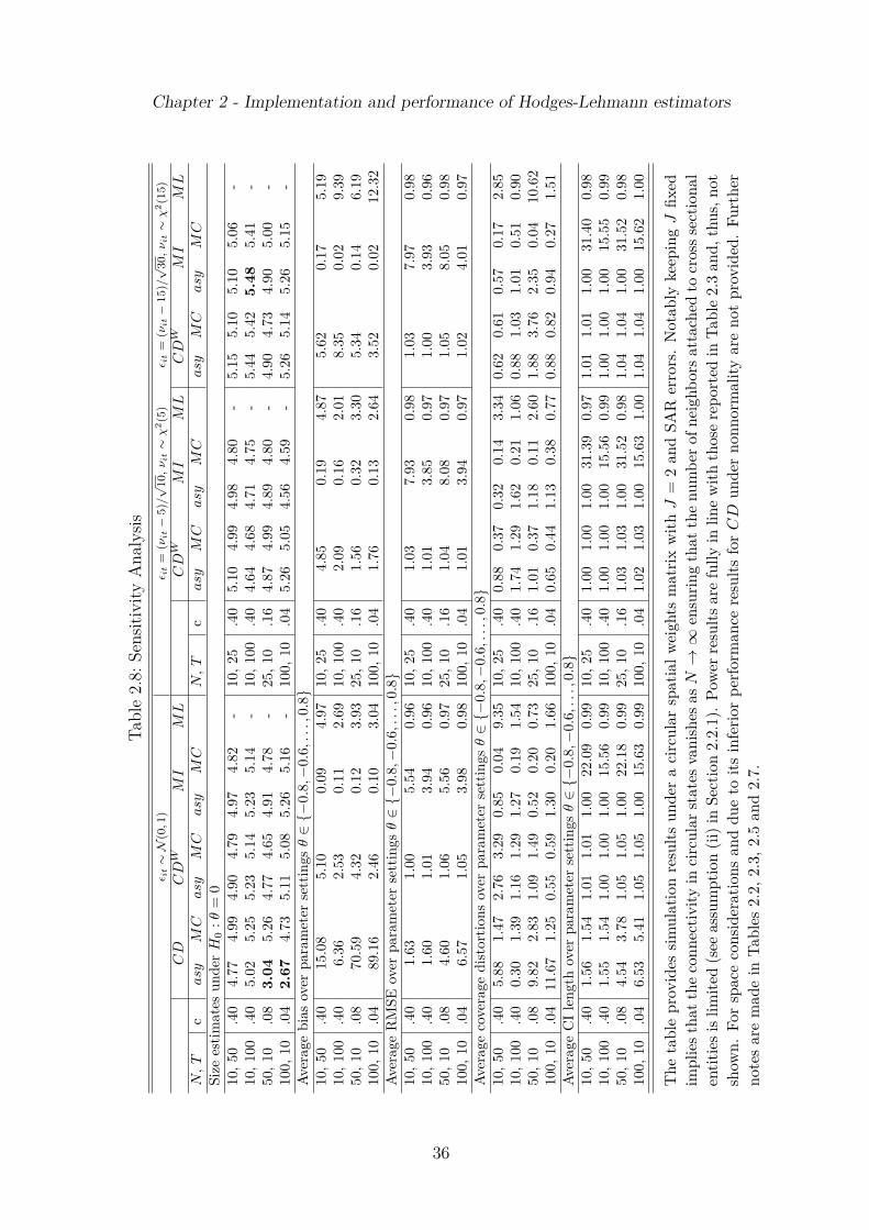
Chapter 2 - Implementation and performance of Hodges-Lehmann estimators
Tabl
e2.
8:Se
nsiti
vity
Ana
lysis
ϵ it
∼N
(0,1
)ϵ i
t=
(νit
−5)
/√
10,ν
it∼
χ2(5
)ϵ i
t=
(νit
−15
)/√
30,ν
it∼
χ2(1
5)C
DC
DW
MI
ML
CD
WM
IM
LC
DW
MI
ML
N,
Tc
asy
MC
asy
MC
asy
MC
N,
Tc
asy
MC
asy
MC
asy
MC
asy
MC
Size
estim
ates
unde
rH
0:θ
=0
10,5
0.4
04.
774.
994.
904.
794.
974.
82-
10,2
5.4
05.
104.
994.
984.
80-
5.15
5.10
5.10
5.06
-10
,100
.40
5.02
5.25
5.23
5.14
5.23
5.14
-10
,100
.40
4.64
4.68
4.71
4.75
-5.
445.
425.
485.
41-
50,1
0.0
83.
045.
264.
774.
654.
914.
78-
25,1
0.1
64.
874.
994.
894.
80-
4.90
4.73
4.90
5.00
-10
0,10
.04
2.67
4.73
5.11
5.08
5.26
5.16
-10
0,10
.04
5.26
5.05
4.56
4.59
-5.
265.
145.
265.
15-
Aver
age
bias
over
para
met
erse
ttin
gsθ
∈−
0.8,
−0.
6,..
.,0.
810
,50
.40
15.0
85.
100.
094.
9710
,25
.40
4.85
0.19
4.87
5.62
0.17
5.19
10,1
00.4
06.
362.
530.
112.
6910
,100
.40
2.09
0.16
2.01
8.35
0.02
9.39
50,1
0.0
870
.59
4.32
0.12
3.93
25,1
0.1
61.
560.
323.
305.
340.
146.
1910
0,10
.04
89.1
62.
460.
103.
0410
0,10
.04
1.76
0.13
2.64
3.52
0.02
12.3
2Av
erag
eR
MSE
over
para
met
erse
ttin
gsθ
∈−
0.8,
−0.
6,..
.,0.
810
,50
.40
1.63
1.00
5.54
0.96
10,2
5.4
01.
037.
930.
981.
037.
970.
9810
,100
.40
1.60
1.01
3.94
0.96
10,1
00.4
01.
013.
850.
971.
003.
930.
9650
,10
.08
4.60
1.06
5.56
0.97
25,1
0.1
61.
048.
080.
971.
058.
050.
9810
0,10
.04
6.57
1.05
3.98
0.98
100,
10.0
41.
013.
940.
971.
024.
010.
97Av
erag
eco
vera
gedi
stor
tions
over
para
met
erse
ttin
gsθ
∈−
0.8,
−0.
6,..
.,0.
810
,50
.40
5.88
1.47
2.76
3.29
0.85
0.04
9.35
10,2
5.4
00.
880.
370.
320.
143.
340.
620.
610.
570.
172.
8510
,100
.40
0.30
1.39
1.16
1.29
1.27
0.19
1.54
10,1
00.4
01.
741.
291.
620.
211.
060.
881.
031.
010.
510.
9050
,10
.08
9.82
2.83
1.09
1.49
0.52
0.20
0.73
25,1
0.1
61.
010.
371.
180.
112.
601.
883.
762.
350.
0410
.62
100,
10.0
411
.67
1.25
0.55
0.59
1.30
0.20
1.66
100,
10.0
40.
650.
441.
130.
380.
770.
880.
820.
940.
271.
51Av
erag
eC
Ile
ngth
over
para
met
erse
ttin
gsθ
∈−
0.8,
−0.
6,..
.,0.
810
,50
.40
1.56
1.54
1.01
1.01
1.00
22.0
90.
9910
,25
.40
1.00
1.00
1.00
31.3
90.
971.
011.
011.
0031
.40
0.98
10,1
00.4
01.
551.
541.
001.
001.
0015
.56
0.99
10,1
00.4
01.
001.
001.
0015
.56
0.99
1.00
1.00
1.00
15.5
50.
9950
,10
.08
4.54
3.78
1.05
1.05
1.00
22.1
80.
9925
,10
.16
1.03
1.03
1.00
31.5
20.
981.
041.
041.
0031
.52
0.98
100,
10.0
46.
535.
411.
051.
051.
0015
.63
0.99
100,
10.0
41.
021.
031.
0015
.63
1.00
1.04
1.04
1.00
15.6
21.
00
The
tabl
epr
ovid
essim
ulat
ion
resu
ltsun
der
aci
rcul
arsp
atia
lwei
ghts
mat
rixw
ithJ
=2
and
SAR
erro
rs.
Not
ably
keep
ing
Jfix
edim
plie
stha
tthe
conn
ectiv
ityin
circ
ular
stat
esva
nish
esas
N→
∞en
surin
gth
atth
enu
mbe
rofn
eigh
bors
atta
ched
tocr
osss
ectio
nal
entit
iesi
slim
ited
(see
assu
mpt
ion
(ii)i
nSe
ctio
n2.
2.1)
.Po
wer
resu
ltsar
efu
llyin
line
with
thos
ere
port
edin
Tabl
e2.
3an
d,th
us,n
otsh
own.
For
spac
eco
nsid
erat
ions
and
due
toits
infe
rior
perf
orm
ance
resu
ltsfo
rC
Dun
der
nonn
orm
ality
are
not
prov
ided
.Fu
rthe
rno
tes
are
mad
ein
Tabl
es2.
2,2.
3,2.
5an
d2.
7.
36
Chapter 2 - Implementation and performance of Hodges-Lehmann estimators
be an interesting future direction of research on the implementation of HL estimators.
Acknowledgements I thank Helmut Herwartz and the participants at the 3rd WorldConference 2009 of the Spatial Econometrics Association in Barcelona for helpful commentson an earlier version of this manuscript.
2.6 ReferencesAnselin, L. and S. Rey (1991). Properties of tests for spatial dependence in linearregression models. Geographical Analysis 23, 112-131.
Anselin, L. and R. Moreno (2003). Properties of tests for spatial error components.Regional Science and Urban Economics 33(5), 595-618.
Anselin, L., J. Le Gallo, and H. Jayet (2008). Spatial panel econometrics. In Matyas,L. and P. Sevestre: The econometrics of panel data, fundamentals and recent develop-ments in theory and practice (3rd Edition ed.) (Berlin Heidelberg: Springer - Verlag),625-660.
Bao, Y. and A. Ullah (2007). Finite sample properties of maximum likelihood esti-mator. Journal of Econometrics 137, 396-413.
Baumont C. (2009). Spatial effects of urban public policies on housing values. Papersin Regional Science 88, 301-326.
Billon M., R. Ezcurra and F. Lera-Lopez (2009). Power calculations for global andlocal Moran’s. Growth and Change 40(1), 54-84.
Bivand, R., W.G. Muller, and M. Reder (2009). Power calculations for global andlocal Moran’s. Computational Statistics & Data Analysis 53(8), 2859-2872.
Bivand, R. and S. Szymanski (2000). Modelling the spatial impact of the introductionof Compulsory Competitive Tendering. Regional Science and Urban Economics 30(2),203-219.
Bordignon, M., F. Cerniglia and F. Revelli (2003). In search of yardstick competi-tion: a spatial analysis of Italian municipality property tax setting. Journal of UrbanEconomics 54(2), 199-217.
Breusch, T.S. and A.R. Pagan (1980). The Lagrange Multiplier test and its appli-cations to model specification in econometrics. Review of Economic Studies 47(1),239-254.
37
Chapter 2 - Implementation and performance of Hodges-Lehmann estimators
Brocker, J., U. Kretschmer, C. Schurmann, K. Spiekermann, D. Stelder and M. We-gener (2002). The IASON common spatial database. IASON Deliverable 3, Institutefor Regional Research, Christian Albrechts University Kiel, Institute for Spatial Plan-ning, University Dortmund.
Burridge, P. (1980). On the Cliff-Ord-Test for spatial autocorrelation. Journal of theRoyal Statistical Society B 42, 107-108.
Cliff, A. and J. Ord (1981). Spatial process: Models and applications (London: Pion).
Coudin E. and Dufour J.-M. (2011). Robust sign-based and Hodges-Lehmann es-timators in linear median regressions with heterogenous serially dependent errors.CIRANO Scientific Publication No. 2011s-24.
Das, D., H.H. Kelejian and I.R. Prucha (2003). Finite sample properties of estimatorsof spatial autoregressive models with autoregressive disturbances. Papers in RegionalScience 82(1), 1-26.
Dufour, J.-M. (2006). Monte Carlo tests with nuisance parameters: A general ap-proach to finite-sample inference and nonstandard asymptotics. Journal of Econo-metrics 133(2), 443-477.
Dufour, J.-M. (1990). Exact tests and confidence sets in linear regressions with auto-correlated errors. Econometrica 58(2), 475-94.
Dufour, J.-M. and L. Khalaf (2002). Exact tests for contemporaneous correlation ofdisturbances in seemingly unrelated regressions. Journal of Econometrics 106, 143-170.
Egger, P., M. Larch, M. Pfaffermayr and J. Walde (2009). Small sample properties ofmaximum likelihood versus generalized method of moments based tests for spatiallyautocorrelated errors. Regional Science and Urban Economics 39(6), 670-678.
Eurostat: Regions (1999). Nomenclature of territorial units for statistics-NUTS. Of-fice for Official Publications of the European Communities, Luxembourg.
Farber, S., A. Paez and E. Volz (2009). Topology, dependency tests and estimationbias in network autoregressive models. In Paez, A., J. Le Gallo, R. Buliung and S.Dall’Erba: Advances in Spatial Sciences (Berlin: Spinger Verlag), 29-57.
Fingleton, B. and E. Lopez-Bazo (2006). Empirical growth models with spatial ef-fects. Papers in Regional Science 85(2), 177-198.
Florax, R. and S. Rey (1995). The impacts of misspecified spatial interaction in lin-ear regression modles. In Anselin, L. and R.J.G.M. Florax: New Directions in spatialeconometrics (Berlin: Spinger Verlag), 111-135.
Frees, E.W. (1995). Assessing cross-sectional correlation in panel data. Journal of
38
Chapter 2 - Implementation and performance of Hodges-Lehmann estimators
Econometrics 69, 393-414.
Friedman, M. (1937). The use of ranks to avoid the assumption of normality implicitin the analysis of variance. Journal of the American Statistical Association 32, 675-701.
Harvey, A.C. and G.D.A. Phillips (1982). Testing for contemporaneous correlation ofdisturbances in systems of regression equations. Bulletin of Economic Research 34(2),79-81.
Hodges Jr., J.L., and E.L. Lehmann (1983). Hodges-Lehmann estimators. In John-son, N.L., S. Kotz and C. Read: Encyclopedia of Statistical Sciences, vol. 3. (Wiley,New York), 642-645.
Kelejian and I.R. Prucha (2001). On the asymptotic distribution of the Moran I teststatistic with applications. Journal of Econometrics 104(2), 219-257.
Kelejian, H.H. and I.R. Prucha (1999). A generalized moments estimator for theautoregressive parameter in a spatial model. International Economic Review 40(2),97-130.
Kelejian and I.R. Prucha (1998). A generalized spatial two-stage least squares proce-dure for estimating a spatial autoregressive model with autoregressive disturbances.The Journal of Real Estate Finance and Economics 17(1), 99-121.
Lee, L.-F. (2004). Asymptotic distributions of Quasi-Maximum Likelihood estimatorsfor spatial autoregressive models. Econometrica 72(6), 1899-1925.
Lin, K.-P., Z.-H. Long and B. Ou (2011). The size and power of bootstrap tests forspatial dependence in a linear regression model. Computational Economics 38(2),153-171.
Lopez-Bazo, E., E. Vaya and M. Artıs (2004). Externalities and growth: Evidencefrom european regions. Journal of Regional Science 44(1), 43-73.
Lundberg J. (2006). Using spatial econometrics to analyse local growth in Sweden.Regional Studies 40(3), 303-316.
Martellosio, F. (2010). Power properties of invariant tests for spatial autocorrelationin linear regression. Econometric Theory 26, 152-186.
Mizruchi, M.S. and E.J. Neuman (2008). The effect of density on the level of bias inthe network autocorrelation model. Social Networks 30, 190-200.
Neuman, E.J. and M.S. Mizruchi (2010). Structure and bias in the network autocor-relation model. Social Networks 32(4), 290-300.
Pesaran, M.H. (2004). General diagnostic tests for cross section dependence in panels.Cambridge Working Papers in Economics No. 1229, Faculty of Economics University
39
Chapter 2 - Implementation and performance of Hodges-Lehmann estimators
of Cambridge.
Pesaran M.H., A. Ullah and T. Yamagata (2008). A bias-adjusted LM test of errorcross-section independence. The Econometrics Journal 11(1), 105-127.
Revelli, F. (2002). Testing the tax mimicking versus expenditure spill-over hypothesesusing English data. Applied Economics 34(14), 1723-31.
Rey, S.J. and B.D. Montouri (1999). US regional income convergence: A spatialeconometric perspective. Regional Studies 33(2), 143-156.
Smith, T.E. (2009). Estimation bias in spatial models with strongly connected weightmatrices. Geographical Analysis 41(3), 307-332.
Tsay, W.-J. (2004). Testing for contemporaneous correlation of disturbances in seem-ingly unrelated regressions with serial dependence. Economics Letters 83, 69-76.
Villaverde, J. (2005). Provincial convergence in Spain: a spatial econometric ap-proach. Applied Economics Letters 12(11), 697-700.
40
Chapter 3
On the effect of prospective paymenton local hospital competition inGermany
Helmut Herwartz1 Christoph Strumann2
Published in Health Care Management Science, 2012, Vol. 15, No. 1, pp. 48-62.Available at http://link.springer.com/article/10.1007%2Fs10729-011-9180-9.
Abstract
The introduction of prospective hospital reimbursement based on diagnosis relatedgroups (DRG) in 2004 has been a conspicuous attempt to increase hospital efficiencyin the German health sector. As a consequence of the reform a rise of competition for(low cost) patients could be expected. In this paper the competition between hospitals,quantified as spatial spillover estimates of hospital efficiency, is analyzed for periodsbefore and after the reform. We implement a two-stage efficiency model that allows forspatial interdependence among hospitals. Hospital efficiency is determined by means ofnon-parametric and parametric econometric frontier models. We diagnose a significantincrease of negative spatial spillovers characterizing hospital performance in Germany,and thus, confirm the expected rise of competition.
JEL-Classification: C21, D61, I11, I18Keywords: Hospital efficiency, stochastic frontier analysis, data envelopment analysis,spatial analysis, diagnosis related groups
1Department VWL, Georg-August-Universitat zu Gottingen, Platz der Gottinger Sieben 5, 37073Gottingen, Germany, [email protected], tel.: +49 551 397 350, fax: +49 551 397 279
2Corresponding author. Institut fur Statistik und Okonometrie, Christian-Albrechts-Universitat zuKiel, Olshausenstr. 40, D-24118 Kiel, Germany, [email protected], tel.: +49 431880 2379, fax: +49 431 880 7605
41
Chapter 4
Hospital efficiency under prospectivereimbursement schemes: An empiricalassessment for the case of Germany
Helmut Herwartz1 Christoph Strumann2
Accepted for publication in The European Journal of Health Economics.Available at http://link.springer.com/article/10.1007%2Fs10198-013-0464-5.
Abstract
The introduction of prospective hospital reimbursement based on diagnosis relatedgroups (DRG) has been a conspicuous attempt to decelerate the steady increase ofhospital expenditures in the German health sector. In this work, the effect of thefinancial reform on hospital efficiency is subjected to empirical testing by means oftwo complementary testing approaches. On the one hand, we apply a two-stageprocedure based on non-parametric efficiency measurement. On the other hand, astochastic frontier model is employed that allows a one-step estimation of both pro-duction frontier parameters and inefficiency effects. To identify efficiency gains asa consequence of changes in the hospital incentive structure, we account for techno-logical progress, spatial dependence and hospital heterogeneity. The results of bothapproaches do not reveal any increase in overall efficiency after the DRG reform. Incontrast, a significant decline in overall hospital efficiency over time is observed.
JEL-Classification: C21, D61, I11, I18Keywords: Hospital efficiency, stochastic frontier analysis, data envelopment analysis,spatial analysis, diagnosis related groups
1Department VWL, Georg-August-Universitat zu Gottingen, Platz der Gottinger Sieben 5, 37073Gottingen, Germany, [email protected], tel.: +49 551 397 350, fax: +49 551 397 279
2Corresponding author. Institut fur Statistik und Okonometrie, Christian-Albrechts-Universitat zuKiel, Olshausenstr. 40, D-24118 Kiel, Germany, [email protected], tel.: +49 431880 2379, fax: +49 431 880 7605
42
Chapter 5
Concluding Remarks
This dissertation consists of three articles considering spatial econometrics. While thefirst article in Chapter 2 is dealing with methodological aspects of the estimation ofspatial error models, the articles in the Chapters 3 and 4 apply spatial econometrictechniques to either estimate spatial spillovers of hospital efficiency or handle appro-priately the spatial dependence in the hospital data.
In Chapter 2, Hodges-Lehmann (HL) type point and interval estimators for the spa-tial parameter in static panel models with spatially autoregressive or moving averagedisturbances are proposed. HL estimators are implemented by means of ’inverting’common diagnostics for spatial correlation. Exact inference is implemented by meansof Monte Carlo (MC) testing. A simulation study shows that HL confidence inter-vals are characterized by less size distortions and appear more robust against spatialconnectivity in comparison with Maximum Likelihood (ML) interval estimates. More-over, the bias of the HL estimator is markedly smaller than its ML counterpart. Asopposed to the spatial lag model, a reduced bias of the spatial parameter estimatehas no impact on the bias of regression coefficient estimates in the considered spatialerror model. The implementation of HL estimation on the spatial lag model can beregarded as an interesting future direction of research. As mentioned in the paperwithin the spatial lag model typical diagnostics, e.g. the Lagrange Multiplier lag testin Anselin et al. (2008), lack pivotalness. Alternatively to MC testing, HL estimationcan be based on asymptotic p-values or critical values determined by parametric oreven non-parametric bootstrap procedures.
In Chapter 3, the effect of prospective payment system based on diagnosis relatedgroups (DRG) on local competition of hospitals is analyzed. The robustness of the em-pirical findings is addressed by comparative applications of the non-parametric DataEnvelopment Analysis (DEA) and parametric Stochastic Frontier Analysis (SFA).The results reveal an increase in the magnitude of negative spatial spillovers after theDRG reform. This is in line with an expected rise of competition for low cost patientsinvoked by the announcement or advent of the new financing system. For future re-search it might be important to analyze the effects of the increased competition on thetreatment of patients and the overall hospital efficiency. If the competitive behaviorin the hospital market encourage hospitals to select the most lucrative patients, an
43
Chapter 5 - Concluding Remarks
equal access to inpatient care is no longer guaranteed. Moreover, if higher compe-tition does not lead to a better hospital performance (as theoretically expected in awell functioning market), the justification of the DRG reform should be reconsidered.
The study of Chapter 4 might obtain some insights for the latter issue. In thiswork, the effect of prospective payment on overall hospital efficiency is subjectedto empirical testing. To identify efficiency gains as a consequence of changes in thehospital incentive structure, technological progress, spatial dependence and hospitalheterogeneity are taken into account. Similar to the previous study in Chapter 3, twocomplementary testing approaches are applied, i.e. a two-stage procedure based onnon-parametric efficiency measurement and a parametric stochastic frontier modelthat allows a one-step estimation of both production frontier parameters and ineffi-ciency effects. The results of both approaches do not reveal any increase in overallefficiency after the DRG reform. In contrast, a significant decline in overall hospitalefficiency over time is observed. This might suggest that the increased competitionhas not a positive effect on hospital efficiency. However, there might be various al-ternative reasons to explain the decline of hospital performance, e.g. a dominanceof opportunistic practices. The identification of these practices and their effects onhospital efficiency, the treatment of patients and the quality of care could deliver im-portant guidelines for future political reforms targeting a reduction of inefficiencies,and an equal and qualitative treatment of patients in the hospital sector.
From an econometric perspective some remarks regarding the adopted efficiencyapproaches are in order. Firstly, the two-stage approach of SFA efficiency scores ap-plied in the study of Chapter 3 is generally not recommended because of an inherentbias problem on both stages (Kim and Schmidt, 2008, Wang and Schmidt, 2002).Secondly, the applied second-stage treatment of DEA efficiency scores (in Chapter 3)and its Malmquist index decomposition (Chapter 4) might be inefficient (Simar andWilson, 2007). Finally, the one-step treatment of the SFA model in Chapter 4 in-corporates spatial dependence in form of spatial clusters by specifying region-specificrandom effects. However, the SFA model does not account for two distinct channelsof spatial dependence simultaneously as it is observed in the two-stage models withspatial error terms and lag dependence (SARAR). Hence, it would be a valuable di-rection of future research to focus on the development of SARAR stochastic frontiermodels. However, for the present studies in Chapter 3 and Chapter 4 the clear re-sults regarding the increase in the magnitude of negative spatial spillovers and thedecline in overall hospital efficiency over time suggest that the inherent problems ofthe employed approaches do not have a significant influence on the empirical outcomeof these studies.
44
Chapter 5 - Concluding Remarks
ReferencesKim, M. and P. Schmidt (2008). Valid tests of whether technical inefficiency dependson firm characteristics. Journal of Econometrics 144(2), 409-427.
Simar, L. and P. W. Wilson (2007). Estimation and inference in two-stage, semi-parametric models of production processes. Journal of Econometrics 136(1), 31-64.
Wang, H.-J., and P. Schmidt (2002). One-Step and Two-Step estimation of the effectsof exogenous variables on technical efficiency levels. Journal of Productivity Analysis18(2), 129-144.
45

Eidesstattliche Erklarung
Ich erklare hiermit an Eides Statt, dass ich, abgesehen von den in der Einleitungprazisierten Kooperationen mit Herrn Herwartz meine Doktorarbeit “Essays on spatialeconometrics: Hodges-Lehmann estimators and hospital efficiency” selbstandig undohne fremde Hilfe angefertigt habe und dass ich alle von anderen Autoren wortlichubernommenen Stellen, wie auch die sich an die Gedanken anderer Autoren eng an-lehnenden Ausfuhrungen meiner Arbeit, besonders gekennzeichnet und die Quellennach den mir angegebenen Richtlinien zitiert habe.
Kiel, den 23.05.2013(Christoph Strumann)
Lebenslauf
Personliche Daten
Familienname StrumannVorname ChristophGeburtsdatum 13.4.1983Geburtsort OeldeStaatsangehorigkeit deutschE-Mail [email protected]
Lebenslauf
1989 - 2002 Allgemeine Hochschulreife09/2002 - 08/2003 Anderer Dienst im Ausland:
Kinderheim, Schineni in Rumanien10/2003 - 01/2009 Studium der Volkswirtschaftslehre an der
Christian-Albrechts-Universitat zu KielSchwerpunkt: Quantitative WirtschaftsforschungAbschluss: Diplom-Volkswirt
10/2008 - 10/2013 Wissenschaftlicher Mitarbeiter am Institut fur Statistikund Okonometrie der Christian-Albrechts-Universitatzu Kiel
seit 01/2009 Doktorandenstudium im Rahmen des Programms”Quantitative Economics” der Christian-Albrechts-Universitat zu Kiel
06/2011 - 10/2013 Wissenschaftlicher Mitarbeiter am Lehrstuhl furGrundungs- und Innovationsmanagement der Christian-Albrechts-Universitat zu Kiel