Extension and Parameter Calibration of a Multi-Lane

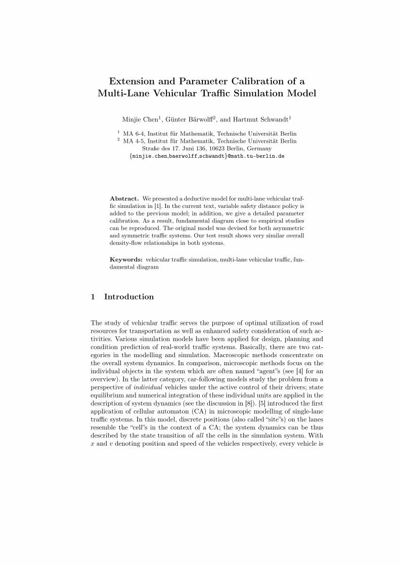
Extension and Parameter Calibration of a

Multi-Lane Vehicular Traffic Simulation Model

Minjie Chen1, Günter Bärwolff2, and Hartmut Schwandt1

1 MA 6-4, Institut für Mathematik, Technische Universität Berlin2 MA 4-5, Institut für Mathematik, Technische Universität Berlin

Straße des 17. Juni 136, 10623 Berlin, Germany{minjie.chen,baerwolff,schwandt}@math.tu-berlin.de

Abstract. We presented a deductive model for multi-lane vehicular traf-fic simulation in [1]. In the current text, variable safety distance policy isadded to the previous model; in addition, we give a detailed parametercalibration. As a result, fundamental diagram close to empirical studiescan be reproduced. The original model was devised for both asymmetricand symmetric traffic systems. Our test result shows very similar overalldensity-flow relationships in both systems.

Keywords: vehicular traffic simulation, multi-lane vehicular traffic, fun-damental diagram

1 Introduction

The study of vehicular traffic serves the purpose of optimal utilization of roadresources for transportation as well as enhanced safety consideration of such ac-tivities. Various simulation models have been applied for design, planning andcondition prediction of real-world traffic systems. Basically, there are two cat-egories in the modelling and simulation. Macroscopic methods concentrate onthe overall system dynamics. In comparison, microscopic methods focus on theindividual objects in the system which are often named “agent”s (see [4] for anoverview). In the latter category, car-following models study the problem from aperspective of individual vehicles under the active control of their drivers; stateequilibrium and numerical integration of these individual units are applied in thedescription of system dynamics (see the discussion in [8]). [5] introduced the firstapplication of cellular automaton (CA) in microscopic modelling of single-lanetraffic systems. In this model, discrete positions (also called “site”s) on the lanesresemble the “cell”s in the context of a CA; the system dynamics can be thusdescribed by the state transition of all the cells in the simulation system. Withx and v denoting position and speed of the vehicles respectively, every vehicle is

2

subject to a set of four simple transition rules:

v ⇐ min(v + 1, vmax), (1a)

v ⇐ min(x′ − x− 1, v), (1b)

v ⇐ max(0, v − 1), executed with a given probability, (2)

x ⇐ x+ v. (3)

The superscript ′, as seen in (1b), is used to denote a vehicle’s immediate neigh-bour (the leader of the current vehicle) in the flow direction. Let x′ denotethe position of the leading vehicle. (1a) describes the possible acceleration ofthe current vehicle. In comparison, (1b) shows the maximum possible positiontransition without risk of collision with the leading vehicle ahead. The final po-sition transition of this vehicle is given in (3). The rule of (2) is introduced asa stochastic element; it reflects the random “dawdling” behaviour of the driverswhich most of them are unaware of. Without this element, the simulation wouldbecome deterministic. A simulation cycle consists of application of these fourrules on all vehicles in the system. In the original model [5] and many of itsextensions (for example, the two-lane extension [7]) each site in the traffic lanehas a length of 7.5m; this value has been selected to be slightly larger than thelength of an average passenger vehicle. The simulation cycle has a time length∆t = 1 s, with this, a discrete maximum speed vmax = 5 renders a maximumphysical speed of 135 km · h−1.

2 A Deductive Multi-lane Model

lc − lv

lc

2lc − lv

2lc

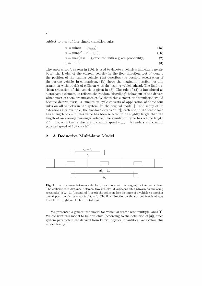
Fig. 1. Real distance between vehicles (drawn as small rectangles) in the traffic lane.The collision-free distance between two vehicles at adjacent sites (drawn as enclosingrectangles) is lc−lv (instead of lc or 0); the collision-free distance of a vehicle to anotherone at position d sites away is d · lc− lv. The flow direction in the current text is alwaysfrom left to right in the horizontal axis.

We presented a generalized model for vehicular traffic with multiple lanes [1].We consider this model to be deductive (according to the definition of [3]), sincesystem parameters are derived from known physical quantities. We explain thismodel briefly.

3

2.1 System Settings

In our model, safety distance will play a significant role, so first we take a closerlook of the distance between the vehicles. The traffic lane will be divided intosites with an equal length lc. Let lv denote the average length of a typical vehi-cle. The collision-free distance of two vehicles at the x-th site and the (x+ d)-thsite would be d · lc − lv, cf. Fig. 1. A very realistic estimate for an average pas-senger car would be lv = 5m. Respecting this measurement and the site lengthlc = 7.5m, it is almost for sure that in the model of [5] the distance between thevehicles is too small.

We start with lc = 15m and ∆t = 2.4 s. In this case, position change ofone site in the lane in each simulation cycle refers to a temporary speed of22.5 km · h−1, whereas the speed change (acceleration) is 9.375 km · h−1 everysecond (approximately eleven seconds from 0 to 100 km · h−1), which resemblesthe capacity of an average modern passenger car.

2.2 Safety distance

>From a practical perspective, it is suggested that a minimum safety distancein metres as the half of vehicle speed measured in kilometres per hour should beattended. In Germany, this is sometimes even obligatory. We introduce a safetydistance coefficient c (c ≥ 1) which is to be understood as a multiplier of theminimum safety distance.

Respecting a discrete speed v (v = 0, . . . , vmax), we have the discrete safetydistance:

sc,v =c2· v · lc ·

1 h

∆t· 10−3

lc. (4)

For ∆t = 2.4 s, (4) becomes

sc,v =3cv

4. (5)

Given a discrete distance d to the immediate leading vehicle, a collision-freespeed v requests

v + sc,v ≤d · lc − lv

lc= d−

lv

lc. (6)

The safety distance sc,v can be shortened as sv, if the safety distance coeffi-cient c is clear in the context.

2.3 Driving Strategy

We notice that in the two border lanes lane changing is allowed only in one di-rection, whereas in the middle lanes lane changing is possible in both directions.Without loss of generality, we consider exactly these three types of lanes andthey will be given indices l = 0, 1, 2, counted from the inner side. Furthermore,

4

positions on the lanes l = 0, 1, 2 will be written in x, y and z respectively. Asin (1b), we use the superscript ′ to address the immediate leading vehicle in theflow direction: respecting a vehicle at position y, the vehicle directly ahead of itwill be at position y′; by x′ and z′ we mean the positions of the leading vehiclesin the neighbouring lanes. In addition, the speed of the vehicle at position x willbe written as vx.

Same as (1a), local vehicle speed will always be increased whenever possible.After this, lane changing will be considered.

Check inner lane This is the case when a vehicle at position y′ seeks to changeinto the inner lane. This step is mandatory in an asymmetric traffic system.Obviously, this driving manoeuvre is only possible when l > 0. With

x′′ − y′ − 1− svy′

≥ vy′ , (7a)

and

vy′ > vx, (7b)

a lane changing ∆l = −1 will be possible for the current vehicle with a speed vy′ .(7a) is the forward causality taking into consideration of safety distance (4). (7b)refers to the backward causality: a higher speed of the current vehicle guaranteesa collision-free lane changing.

Check current lane This is the case when the vehicle inspects the situationin the current lane. With

y′′ − y′ − 1− svy′

≥ vy′ , (8)

no lane changing will be necessary (∆l = 0) and the current speed vy′ can bemaintained. Since no lane changing is involved, backward causality will not beconsidered, since this will be covered by the forward causality of the immediatefollowing vehicle in the same lane. In an asymmetric traffic system, (8) is gen-erally easier than (7a) to meet, since vehicles in outer lanes usually have higherspeeds and consequently the density should be lower, the latter further leads toy′′− y′ > x′′− y′. This explains why vehicles have no reason to change lanes toooften.

Check outer lane Now the current vehicle—still at position y′, since the above-mentioned two operations have been without success—seeks to change into theouter lane. To perform this operation, there must be l < 2 and

z′′ − y′ − 1− svy′

≥ vy′ , (9a)

5

and

y′ − z ≥ vmax. (9b)

In such a case, a lane changing ∆l = +1 can be performed at the current speedvy′ . In addition to the forward causality (9a), backward causality is now recov-ered in (9b). We do not request vy′ > vz, since a reliable estimate of the speedis difficult with the increasing vehicle speed in the outer lane (in an asymmetrictraffic system). Instead, we apply vmax in (9b) to ensure maximum safety.

Move in current lane In the current lane, by (5) (if ∆t is configured to be2.4 s) and (6), the maximum local speed with consideration of safety distancecan be deduced:

v ⇐ min

(

4

4 + 3c·(

y′′ − y − lvlc

)

, v

)

. (10)

The value of v is in general not an integer. Yet it is still unknown whether thespace y′′ − y′ − 1 is sufficient for the current vehicle to move forward in the flowdirection. For this, we propose:

v ⇐

{

y′′ − y′ − 1, if v ≥ y′′ − y′ − 1,

v∗, otherwise,

with

v∗ =

{

⌊v⌋+ 1, if p < v − ⌊v⌋,

⌊v⌋, otherwise,

where p is a random number from [0, 1) and ⌊·⌋ refers to the largest integer nogreater than the argument. With the construction of v∗, the position update ofthe vehicle can be performed exactly.

The above-mentioned four steps refer to the asymmetric case. In a symmet-ric traffic system, the vehicles are requested—partly owing to the heavy trafficloads—to stay in their lanes whenever possible. On the other side, when a lanechanging is necessary, it is allowed on both sides. Hence, lane changing in thesymmetric case will be considered on an equal basis; apart from this, anothersignificant change concerns the forward causality (9b), which is to be revisedinto

vy′ > vz.

for the sake of symmetric behaviour.

2.4 Space-time diagram

To test our model, periodical boundary of the lanes has been applied. Since thevehicles are now placed in a closed circulating traffic system, the actual physi-cal length of the lanes is no longer relevant for test results. We start with our

6

Lane 0v0=3v =0..6c =1.00p0=0.20p1=0.20p2=0.20p3=0.20asymmetric




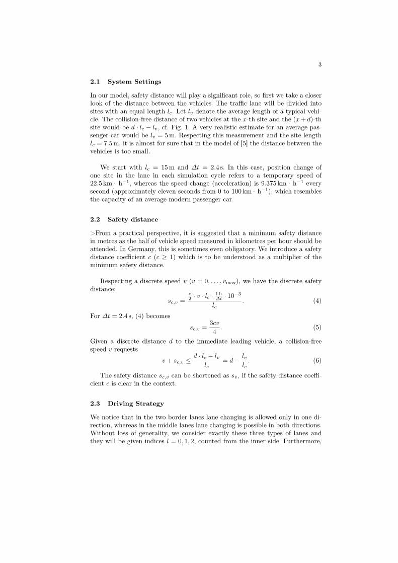
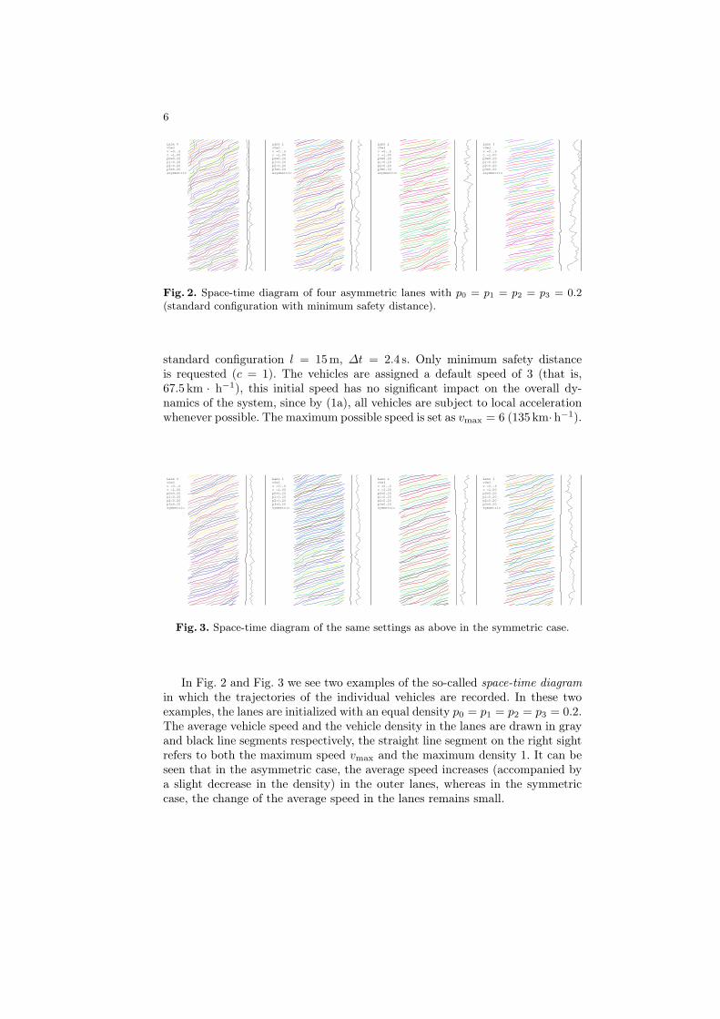
Fig. 2. Space-time diagram of four asymmetric lanes with p0 = p1 = p2 = p3 = 0.2

(standard configuration with minimum safety distance).

standard configuration l = 15m, ∆t = 2.4 s. Only minimum safety distanceis requested (c = 1). The vehicles are assigned a default speed of 3 (that is,67.5 km · h−1), this initial speed has no significant impact on the overall dy-namics of the system, since by (1a), all vehicles are subject to local accelerationwhenever possible. The maximum possible speed is set as vmax = 6 (135 km· h−1).

Lane 0v0=3v =0..6c =1.00p0=0.20p1=0.20p2=0.20p3=0.20symmetric




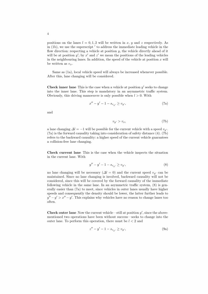
Fig. 3. Space-time diagram of the same settings as above in the symmetric case.

In Fig. 2 and Fig. 3 we see two examples of the so-called space-time diagram

in which the trajectories of the individual vehicles are recorded. In these twoexamples, the lanes are initialized with an equal density p0 = p1 = p2 = p3 = 0.2.The average vehicle speed and the vehicle density in the lanes are drawn in grayand black line segments respectively, the straight line segment on the right sightrefers to both the maximum speed vmax and the maximum density 1. It can beseen that in the asymmetric case, the average speed increases (accompanied bya slight decrease in the density) in the outer lanes, whereas in the symmetriccase, the change of the average speed in the lanes remains small.

7

3 Model Calibration

3.1 Density and Flow

Now we have a look of the fundamental diagram of density and flow, the latterof which is defined as the product of vehicle density and average speed in the lane.

max. density: 67 per kmmax. speed : 135 km per hour

0 1

1

asymmetricc=1.00

Lane 0Lane 1Lane 2Lane 3


0 1

1

symmetricc=1.00

Lane 0Lane 1Lane 2Lane 3

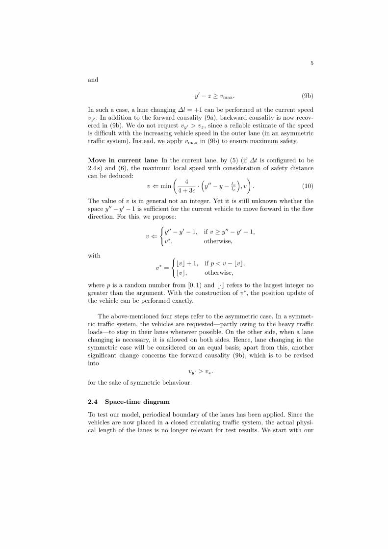
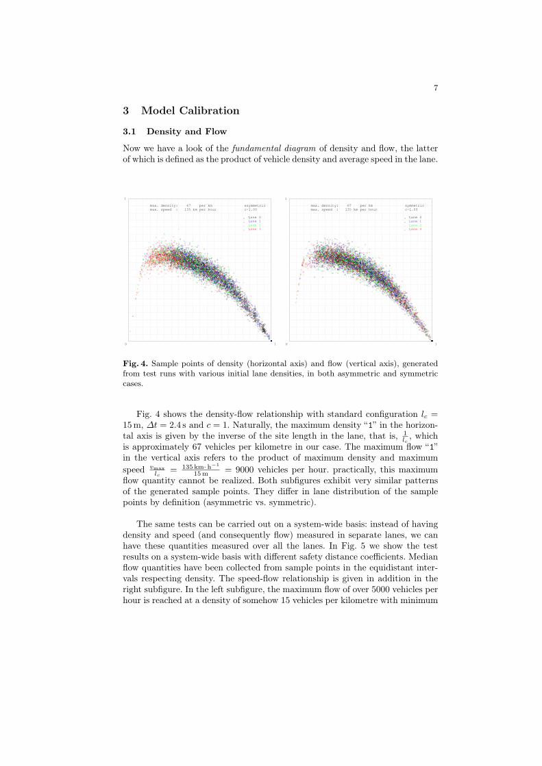
Fig. 4. Sample points of density (horizontal axis) and flow (vertical axis), generatedfrom test runs with various initial lane densities, in both asymmetric and symmetriccases.

Fig. 4 shows the density-flow relationship with standard configuration lc =15m, ∆t = 2.4 s and c = 1. Naturally, the maximum density “1” in the horizon-tal axis is given by the inverse of the site length in the lane, that is, 1

lc, which

is approximately 67 vehicles per kilometre in our case. The maximum flow “1”in the vertical axis refers to the product of maximum density and maximum

speed vmax

lc= 135 km· h

−1

15m= 9000 vehicles per hour. practically, this maximum

flow quantity cannot be realized. Both subfigures exhibit very similar patternsof the generated sample points. They differ in lane distribution of the samplepoints by definition (asymmetric vs. symmetric).

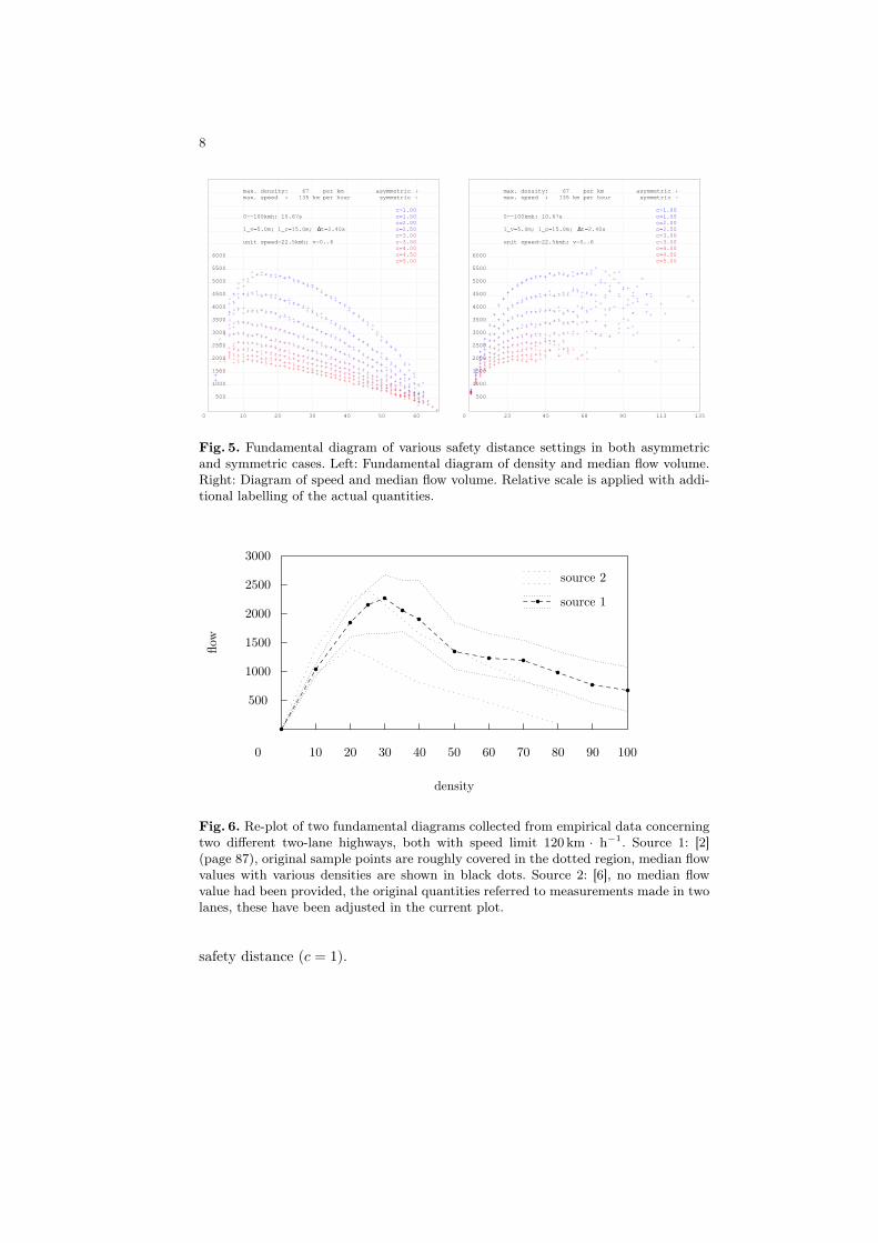
The same tests can be carried out on a system-wide basis: instead of havingdensity and speed (and consequently flow) measured in separate lanes, we canhave these quantities measured over all the lanes. In Fig. 5 we show the testresults on a system-wide basis with different safety distance coefficients. Medianflow quantities have been collected from sample points in the equidistant inter-vals respecting density. The speed-flow relationship is given in addition in theright subfigure. In the left subfigure, the maximum flow of over 5000 vehicles perhour is reached at a density of somehow 15 vehicles per kilometre with minimum

8


0

0--100kmh: 10.67s

l_v=5.0m; l_c=15.0m; ∆t=2.40s

unit speed=22.5kmh; v=0..6

asymmetric symmetric

c=1.00c=1.50c=2.00c=2.50c=3.00c=3.50c=4.00c=4.50c=5.00

500

1000

1500

2000

2500

3000

3500

4000

4500

5000

5500

6000

10 20 30 40 50 60


0

0--100kmh: 10.67s

l_v=5.0m; l_c=15.0m; ∆t=2.40s



c=1.00c=1.50c=2.00c=2.50c=3.00c=3.50c=4.00c=4.50c=5.00

500

1000

1500

2000

2500

3000

3500

4000

4500

5000

5500

6000

23 45 68 90 113 135

Fig. 5. Fundamental diagram of various safety distance settings in both asymmetricand symmetric cases. Left: Fundamental diagram of density and median flow volume.Right: Diagram of speed and median flow volume. Relative scale is applied with addi-tional labelling of the actual quantities.

density

flow

0

source 1

source 2

10 20 30 40 50 60 70 80 90 100

500

1000

1500

2000

2500

3000

Fig. 6. Re-plot of two fundamental diagrams collected from empirical data concerningtwo different two-lane highways, both with speed limit 120 km · h

−1. Source 1: [2](page 87), original sample points are roughly covered in the dotted region, median flowvalues with various densities are shown in black dots. Source 2: [6], no median flowvalue had been provided, the original quantities referred to measurements made in twolanes, these have been adjusted in the current plot.

safety distance (c = 1).

9

When the relative scale (with “1” as maximum) is applied, the overall shapeof the fundamental diagram of density and flow becomes “flatter” with the in-crease of the safety distance coefficient c. We also notice that given constant lv,lc, ∆t and c, the length of the lanes and the discrete maximum speed vmax haveno impact on the overall density-flow diagram. vmax affects only the scale in thevertical axis.

In comparison, Fig. 6 presents results acquired from empirical data. There wesee an average peak flow of roughly 2300 vehicles per hour at a density of 20 to 30vehicles per kilometre. Source 2 of Fig. 6 documented that 13% of the recordedvehicles had been trucks (of larger sizes and lower speeds), this would suggest ahigher density and flow volume, if only passenger cars were to be considered.


0

0--100kmh: 10.67s

l_v=4.7m; l_c=10.0m; ∆t=1.96s



c=1.00c=1.50c=2.00c=2.50c=3.00c=3.50c=4.00c=4.50c=5.00

500

1000

1500

2000

2500

3000

3500

4000

4500

5000

5500

6000

6500

7000

7500

10 20 30 40 50 60 70 80 90 100


0

0--100kmh: 10.67s

l_v=4.7m; l_c=10.0m; ∆t=1.96s



c=1.00c=1.50c=2.00c=2.50c=3.00c=3.50c=4.00c=4.50c=5.00

500

1000

1500

2000

2500

3000

3500

4000

4500

5000

5500

6000

6500

7000

7500

18 37 55 73 92 110 129

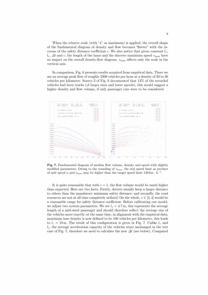
Fig. 7. Fundamental diagram of median flow volume, density and speed with slightlymodified parameters. Owing to the rounding of vmax, the real speed limit as productof unit speed u and vmax may be higher than the target speed limit 120 km · h

−1.

It is quite reasonable that with c = 1, the flow volume would be much higherthan expected. Here are two facts. Firstly, drivers usually keep a larger distanceto others than the mandatory minimum safety distance; and secondly, the roadresources are not at all time completely utilized. On the whole, c ∈ [2, 4] would bea reasonable range for safety distance coefficient. Before calibrating our model,we adjust two system parameters. We set lv = 4.7m, this represents the averagelength of a mid-sized passenger and should therefore reflect the average size ofthe vehicles more exactly; at the same time, in alignment with the empirical data,maximum lane density is now defined to be 100 vehicles per kilometre, this leadsto lc = 10m. The result of this configuration is given in Fig. 7. Unlike lv andlc, the average acceleration capacity of the vehicles stays unchanged in the testcase of Fig. 7, therefore we need to calculate the new ∆t (see below). Compared

10

to empirical data, it seems that in this test case the peak flow is reached too early.


0

0--100kmh: 20.00s

l_v=4.7m; l_c=10.0m; ∆t=2.68s



c=1.00c=1.50c=2.00c=2.50c=3.00c=3.50c=4.00c=4.50c=5.00

500

1000

1500

2000

2500

3000

3500

4000

4500

5000

5500

6000

6500

7000

7500

10 20 30 40 50 60 70 80 90 100


0

0--100kmh: 20.00s

l_v=4.7m; l_c=10.0m; ∆t=2.68s



c=1.00c=1.50c=2.00c=2.50c=3.00c=3.50c=4.00c=4.50c=5.00

500

1000

1500

2000

2500

3000

3500

4000

4500

5000

5500

6000

6500

7000

7500

13 27 40 54 67 80 94 107 121


0

0--100kmh: 6.25s

l_v=4.7m; l_c=10.0m; ∆t=1.50s



c=1.00c=1.50c=2.00c=2.50c=3.00c=3.50c=4.00c=4.50c=5.00

500

1000

1500

2000

2500

3000

3500

4000

4500

5000

5500

6000

6500

10 20 30 40 50 60 70 80 90 100


0

0--100kmh: 6.25s

l_v=4.7m; l_c=10.0m; ∆t=1.50s



c=1.00c=1.50c=2.00c=2.50c=3.00c=3.50c=4.00c=4.50c=5.00

500

1000

1500

2000

2500

3000

3500

4000

4500

5000

5500

6000

6500

24 48 72 96 120

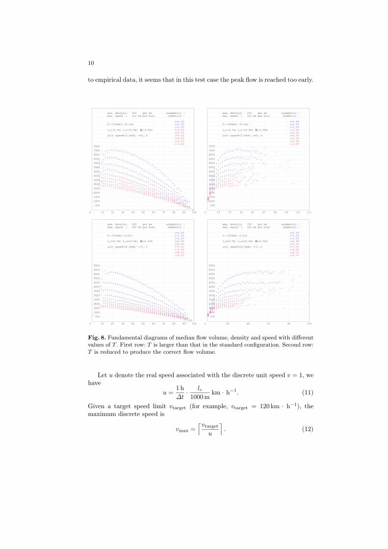
Fig. 8. Fundamental diagrams of median flow volume, density and speed with differentvalues of T . First row: T is larger than that in the standard configuration. Second row:T is reduced to produce the correct flow volume.

Let u denote the real speed associated with the discrete unit speed v = 1, wehave

u =1h

∆t·

lc

1000mkm · h−1. (11)

Given a target speed limit vtarget (for example, vtarget = 120 km · h−1), themaximum discrete speed is

vmax =⌈vtarget

u

⌉

. (12)

11

whereas ⌈·⌉ refers to the smallest integer no less than the argument.

Let T denote the time length of acceleration from 0 to 100 km · h−1 undermaximum power, there is

T =100 km · h−1

u∆t

.

By (11), we have100

T=

1h

(∆t)2·

lc

1000m,

this gives

∆t =

√

3.6 s · lc · T

100m. (13)

Although it may sound strange, increasing T leads to a higher flow volume,since larger T implies weaker acceleration capability of the vehicles. The reasonfor this is that in the flow diagram with axes of relative scale, the actual flowvolume concerning a specific configuration (of lv, lc and ∆t) is related with theshape (flatness) of the density-flow curve represented by the sample points. Aswe have pointed out earlier, with a constant configuration, varying vmax has noeffect on the shape of the density-flow curve, yet the flow volume changes, sincethe maximum flow on the vertical axis is the product of maximum density andmaximum speed. By (13), we know that ∆t is correlated with the square root ofT ; by (11) and (12), vmax is correlated with ∆t. Consequently, with a larger T

the actual flow volume increases, this can be verified by the test cases in Fig. 8as well.

In comparison to our initial configuration of ∆t = 2.4 s, ∆t = 1.5 s seems tobe quite reasonable (along with modified lv and lc) to produce flow volume in asuitable range. However, ∆t = 1.5 s would lead to T = 6.25 s which representsa much too high acceleration capacity, see the second test case in Fig. 8. As asolution for this, we introduce an additional acceleration multiplier s (s > 1) thatthe vehicle should have a simulated acceleration capacity from 0 to 100 km · h−1

in a time length of Ts. To achieve this, we request that (1a) will be carried outwith a probability of qv, for v = 0, . . . , vmax − 1. Translated into discrete form,the acceleration from v = 0 to v = vmax should then take vmax · s steps, that is

vmax−1∑

i=0

1

qi= vmax · s. (14)

In the trivial case vmax = 1 we may set: q0 = 1

s. Otherwise, we request

q0 = 1, (15)

qi+1 = qi · q, for i = 0, . . . , vmax − 2. (16)

(15) says that acceleration from a stationary state will always be carried out(apart from the trivial case); and with (16), acceleration decays with a proba-bility q (0 < q < 1). With the solution of (14), postponed acceleration can be

12


0

0--100kmh: 6.25s

l_v=4.7m; l_c=10.0m; ∆t=1.50s



q0=1.00q1=0.74q2=0.55q3=0.40q4=0.30s =2.00

c=1.00c=1.50c=2.00c=2.50c=3.00c=3.50c=4.00c=4.50c=5.00

500

1000

1500

2000

2500

3000

3500

4000

4500

5000

5500

10 20 30 40 50 60 70 80 90 100


0

0--100kmh: 6.25s

l_v=4.7m; l_c=10.0m; ∆t=1.50s



q0=1.00q1=0.74q2=0.55q3=0.40q4=0.30s =2.00

c=1.00c=1.50c=2.00c=2.50c=3.00c=3.50c=4.00c=4.50c=5.00

500

1000

1500

2000

2500

3000

3500

4000

4500

5000

5500

24 48 72 96 120


0

0--100kmh: 4.00s

l_v=4.7m; l_c=10.0m; ∆t=1.20s



q0=1.00q1=0.55q2=0.31q3=0.17s =3.00

c=1.00c=1.50c=2.00c=2.50c=3.00c=3.50c=4.00c=4.50c=5.00

500

1000

1500

2000

2500

3000

3500

4000

4500

10 20 30 40 50 60 70 80 90 100


0

0--100kmh: 4.00s

l_v=4.7m; l_c=10.0m; ∆t=1.20s



q0=1.00q1=0.55q2=0.31q3=0.17s =3.00

c=1.00c=1.50c=2.00c=2.50c=3.00c=3.50c=4.00c=4.50c=5.00

500

1000

1500

2000

2500

3000

3500

4000

4500

30 60 90 120

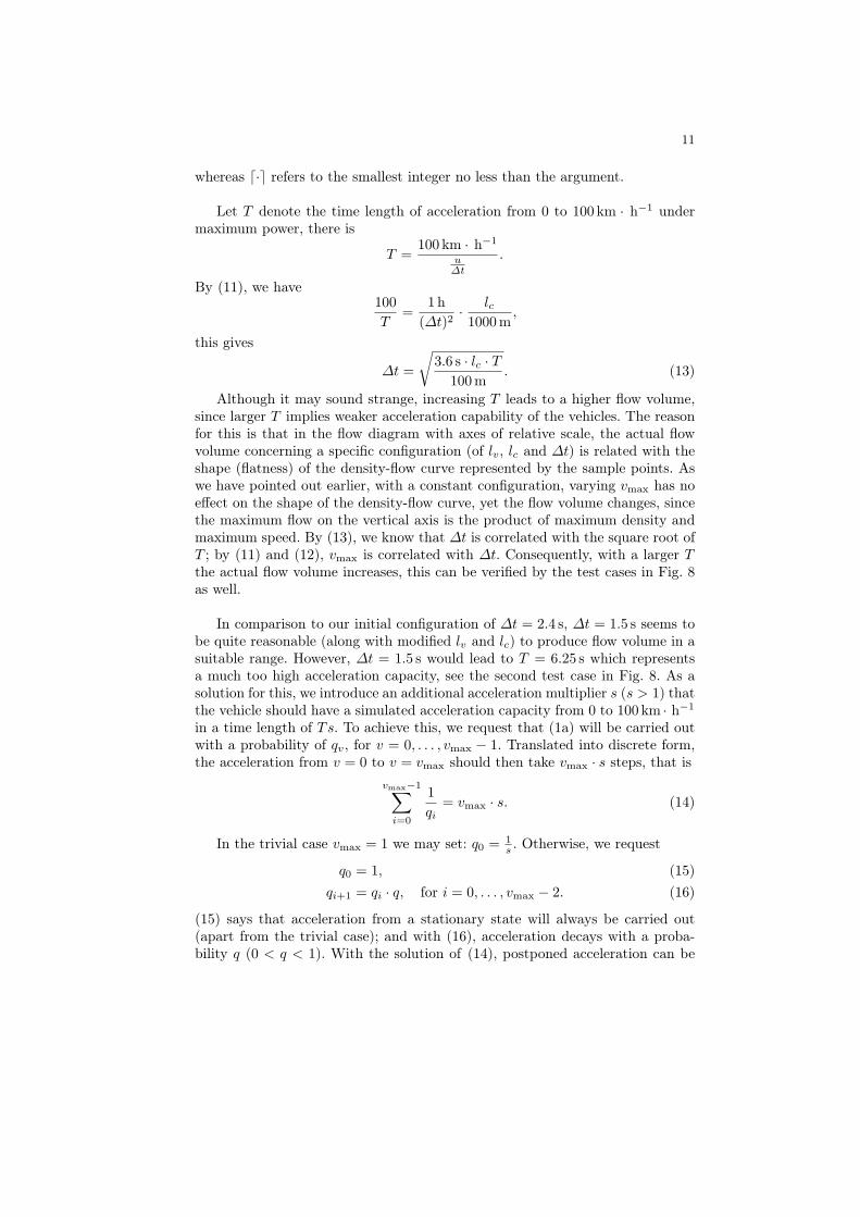
Fig. 9. Calibrated diagrams of median flow volume, density and speed with additionalacceleration multipliers.

simulated. Two further test cases are shown in Fig. 9. For the configuration ofT = 6.25 s and s = 2, c = 3 or 3.5 seems to produce maximum flow volumein the range of 2300 to 2600 vehicles per hour; for T = 4 s and s = 3, s = 2.5gives the maximum flow volume of approximately 2300 per hour at a densityslightly above 20 vehicles per kilometre. These two parameter settings representa reasonable acceleration capacity (0 to 100 km · h−1 in 12 and 12.5 secondsrespectively) and at the same time, vmax in (12) has integer solution.

13

Acknowledgement

The authors gratefully acknowledge the support of Federal Ministry for Eco-nomic Affairs and Energy of Germany for the project VP2653402RR1 and federalstate of Berlin/Investitionsbank Berlin for the project 10153525.

References

1. M.-J. Chen, G. Bärwolff, and H. Schwandt. A deductive model for multi-lane vehic-ular traffic. In 18th IEEE International Conference on Intelligent Transportation

Systems, pages 900–905, 2015.2. D. Helbing. Verkehrsdynamik: Neue physikalische Modellierungskonzepte. Springer-

Verlag Berlin Heidelberg, 1997. ISBN 978-3-642-63834-3.3. S. P. Hoogendoorn and P. H. L. Bovy. State-of-the-art of vehicular traffic flow

modelling. Proceedings of the Institution of Mechanical Engineers, Part I: Journal

of Systems and Control Engineering, 215(4): 283–303, 2001.4. A. Kesting, M. Treiber, and D. Helbing. Agents for traffic simulation. In A. Uhrma-

cher and D. Weyns, editors, Multi-Agent Systems: Simulation and Applications,pages 325–356, CRC Press, 2009. ISBN 978-1-4200-6023-1.

5. K. Nagel and M. Schreckenberg. A cellular automaton model for freeway traffic. J.

Phys. I France, 2:2221–2229, 1992.6. K. Nagel, D. E. Wolf, P. Wagner, and P. Simon. Two-lane traffic rules for cellular

automata: A systematic approach. Physical Review E, 58(2):1425–1437, 1998.7. M. Rickert, K. Nagel, M. Schreckenberg, and A. Latour. Two lane traffic simulations

using cellular automata. Physica A, 231:534–550, 1996.8. M. Treiber and A. Kesting. Traffic Flow Dynamics. Springer-Verlag Berlin Heidel-

berg, 2013. ISBN 978-3-642-32459-8.

Documents

Extension and Parameter Calibration of a Multi-Lane