Fine Structure in Distortion Product Otoacoustic Emissions and Auditory Perception

Vom Institut für Physik an der Fakultät für Mathematik und Naturwissenschaften

der Carl von Ossietzky Universität Oldenburg

zur Erlangung des Grades eines Doktors der Naturwissenschaften (Dr. rer. nat.)

angenommene Dissertation

Manfred Dieter Mauermann geb. am 26.12.1967

in Frankfurt am Main

Erstreferent: Prof. Dr. Dr. Birger Kollmeier Koreferent: Prof. Dr. Volker Mellert Tag der Disputation: 4.2.2004

Contents

1 General Introduction 4

2 Evidence for the distortion product frequency place as a source of DPOAE fine structure in humans. I. Fine structure and higher order DPOAE as a function of the frequency ratio f2/f1 9

INTRODUCTION 10 I. METHODS 12

A. Subjects 12 B. Instrumentation and signal processing 12 C. Experimental Paradigms 13 D. Analysis 14

II. EXPERIMENTAL RESULTS 16 A. Experiment 1: Dependence on f2/f1 16 B. Experiment 2: Fine structure of different order DPOAE 16 C. Experiment 3: Fixed f2 vs. fixed fDP 16

III. SIMULATIONS IN A NONLINEAR AND ACTIVE COCHLEA MODEL 18 A. Description of the model 18 B. Simulations 20

IV. DISCUSSION 22 V. CONCLUSIONS 25 ACKNOWLEDGMENTS 25 ENDNOTES 25

3 Evidence for the distortion product frequency place as a source of DPOAE fine structure in humans. II. Fine structure for different shapes of cochlear hearing loss 27

INTRODUCTION 28 I. METHODS 29

A. Subjects 29 B. Instrumentation and experimental procedures 29

II. RESULTS 32 III. SIMULATIONS IN A NONLINEAR AND ACTIVE MODEL OF THE COCHLEA 34 IV. DISCUSSION 36 V. CONCLUSIONS 38 ACKNOWLEDGEMENTS 38 APPENDIX 39

Contents II

4 The influence of the second source of distortion product otoacoustic emissions (DPOAE) on DPOAE input/output functions 41

INTRODUCTION 42 I. EXPERIMENTAL METHODS 45

A. Subjects 45 B. Instrumentation and signal processing 45 C. Calibration 46 D. DPOAE measurements 46

II. DATA ANALYSIS 47 A. Separation of DPOAE components via time windowing 47 B. DPOAE threshold according to Boege and Janssen 50

III. RESULTS 52 A. Contribution of the second source to the DPOAE at different levels 52 B. Variability of DPOAE I/O functions vs. DCOAE I/O functions 54 C. Variability of threshold prediction from DPOAE I/O and DCOAE I/O functions 56 D. Influence of the calibration paradigm in comparison to the influence of the second source on threshold estimation 59

IV. DISCUSSION 61 V. CONCLUSION 65 ACKNOWLEDGEMENTS 66 ENDNOTES 66

5 Fine structure of Hearing-Threshold and Loudness Perception 69

INTRODUCTION 70 I. GENERAL METHODS 73

A. Subjects 73 B. Instrumentation and Software 73

II. EXPERIMENT 1: PRESERVATION OF THRESHOLD FINE STRUCTURE IN EQUAL

LOUDNESS CONTOURS 74 A. Methods 74 B. Results 76

III. EXPERIMENT 2: LOUDNESS LEVEL GROWTH AT FREQUENCIES IN THRESHOLD

MAXIMA AND MINIMA - LOUDNESS MATCHING 83 A. Methods 84 B. Results 84

Contents III

IV. EXPERIMENT 3: LOUDNESS GROWTH AT FREQUENCIES IN THRESHOLD MAXIMA AND

MINIMA – CATEGORICAL LOUDNESS SCALING 87 A. Methods 87 B. Results 89

V. DISCUSSION 90 VI. SUMMARY 93 ACKNOWLEDGEMENTS 94 ENDNOTES 94

6 Summary and Outlook 95

References 97

Chapter 1

General Introduction

Hearing has a key function for social life. The auditory sensory system allows us to communicate with each other and to realize dangers around us. Therefore hearing impairment is a serious handicap. Several psychoacoustical tests are used to qualify and quantify a hearing loss in general. The auditory threshold e.g. is usually quantified by a pure tone audiogram. Sinusoidal tones are presented at different frequencies and levels and the patient has to indicate whether a tone is audible or not. However these psychoacoustical procedures always assume that the patient is able and willing to perform the necessary tasks. This is not always the case. Especially neonates or young children are not capable to understand the task and to answer in a correct way. But especially for these persons it is very important to identify and quantify an existent hearing damage as early as possible to compensate for the hearing loss e.g. with an appropriate hearing aid. This is highly relevant to allow an almost normal language development and a normal integration into social life. But also for adults who are able to follow the psychoacoustical tasks these tests have to be verified by independent objective methods (e.g. for the assessment of a pension request due to a hearing damage). Therefore it would be very useful to have a set of easy-to-handle and reliable objective tools to identify and quantify a hearing loss, in addition to the psychoacoustical set of tests. One possible method - already established for the screening of hearing function - is the measurement of otoacoustic emissions (OAE). The healthy inner ear does not only receive sound. Due to the active and nonlinear processing in the cochlea it produces weak acoustic signals as a byproduct. These sounds are sent back through the middle ear and can be recorded in the occluded ear canal, the healthy inner ear produces otoacoustic emissions (OAE). There are different types of OAE identified by the type of stimulation used for their generation: 1. Spontaneous otoacoustic emissions (SOAE) are unique because they can be

recorded without any external stimulation in about 30% of all normal hearing subjects. The measurement of SOAE is based on the averaging of power spectra of the noise recorded in the ear canal. SOAE can be detected as peak(s) that stick out the background noise spectrum. Although SOAE are related to minima in subjective auditory thresholds, they have no clinical relevance so far. The initial hope of an objective correlate for subjective tinnitus could not be confirmed (Penner and Burns, 1987; Uppenkamp et al. 1990).

DPOAE fine structure I 5

2. Transiently evoked otoacoustic emissions (TEOAE) are usually evoked by short broadband stimuli like clicks or chirps, but narrowband tone bursts are also used in some studies. Stimulus and delayed ear response can be separated in time. TEOAE measurements are established in hearing screening procedures. The existence of TEOAE indicates a healthy ear. TEOAE in general are not detectable in ears with a hearing loss above 30 dB HL.

3. Stimulus frequency otoacoustic emissions (SFOAE) are emissions evoked by a sinusoid or slowly changing sweep signals. Stimulus and ear response are present at the same time and frequency. A separation of both is possible by utilizing the nonlinear I/O characteristic of the emissions.

4. Distortion product otoacoustic emissions (DPOAE). DPOAE are a series of combination tones generated in the inner ear when stimulated with two sinusoids with frequencies f1 and f2 (f1 < f2). The most prominent distortion product is the cubic difference tone at 2f1-f2 for a frequency ratio f2/f1 = 1.2. DPOAE can be recorded in ears with an hearing loss up to 50 dB.

A miss or reduction of OAE can indicate a cochlea dysfunction. The intact mechanisms of the cochlea play a crucial role in the hearing process. The frequency analysis of the auditory system is performed in the cochlea. The frequency selectivity is assumed to be closely related to the mechanical tuning of the cochlea, and the nonlinear properties of the cochlea are responsible for most of the dynamic compression in the auditory system. The compression in the auditory system is essential to allow us perceiving sounds within a wide dynamic range of about 120 dB and is closely related to the way we perceive loudness. The most cases of hearing impairment are caused by inner ear dysfunctions. For all these reasons the functionality of the cochlea is of great interest in auditory research as well as for clinical practice. OAE provide the only noninvasive tool to get direct information out of the cochlea. Therefore OAE experiments are very useful for the development and verification of cochlea models. But since their discovery in 1978 by Kemp they have also been used as an indicator of hearing loss in clinical studies. Although OAE are now established as clinical tool for hearing screening in neonates, the clinical use in general does not go beyond the statement whether an ear is working or not - if OAE are present - or whether further clinical investigation might be required for a clear diagnosis. Several studies tried to establish a quantitative relation between OAE and clinical audiogram (for review on audiometric outcomes of OAE see e.g. Harris and Probst, 2002). These studies show a varying degree of success in relating the two measures. Most of these studies end in separating a group of impaired ears from healthy ears without a detailed quantification of individual hearing loss. There are indications, however, that the recording of DPOAE has more potential for objective

DPOAE fine structure I 6

diagnosis than just a bivalent decision. Distortion product OAE still appear to be the most promising candidates for a quantitative prediction of hearing status not at least because they are still detectable at a hearing loss up to 50 dB. There are different approaches to use DPOAE for the prediction of hearing status. In most studies, DP-Gram (DPOAE level in dependence frequency) data at moderate stimulation levels are correlated with audiogram data. Other attempts investigate the changes in DPOAE suppression tuning curves to indicate a hearing damage (e.g. Abdala and Fitzgerald, 2003). However a change in the cochlear nonlinearity is most probably reflected in a change of the I/O characteristic of the distortion produced by the underlying nonlinearity. Therefore DPOAE input/output (I/O) functions are tried to be used as an indicator of a loss of compression (recruitment) (Neely et al. 2003) or to identify basilar membrane I/O functions (Buus et al., 2001). A promising approach to predict individual auditory thresholds by the use of DPOAE input/output (I/O) functions was suggested by Kummer et al. (1998) and was further improved by Boege and Janssen (2002) (for more detail see Chapter 4). This approach shows good results on average. But estimated thresholds and behaviorally measured thresholds still differ too much to predict individual auditory thresholds reliably. It is obvious that a deeper insight into the properties of DPOAE, auditory threshold and loudness perception is still needed to improve (or possibly reject) existing approaches for a prediction (and possibly find new ones) and a detailed quantitative diagnosis of cochlear and hearing status from DPOAE measurements. To allow a correct interpretation of DPOAE measurements with regard to frequency specific damage of the cochlea a sufficient detailed understanding of the underlying mechanisms of DPOAE is needed. Especially it has to be clarified at which cochlear sites DPOAE are generated. Several studies trying to identify cochlear or hearing status from DPOAE (e.g. Buus et al. 2001; Boege and Janssen,2002; Neely et al. 2003) assume that the DPOAE I/O functions indicates the basilar membrane (BM) status in the region of maximum overlap of the excitation pattern of the two primaries near the characteristic site of f2 on the BM. But this is not the complete story. Two competing models on DPOAE generation give relevant different views. In the first model DPOAE measured in the sealed ear canal are assumed to be generated within a single region (see e.g. Sun et al.; 1994a,b) within the cochlea, while in the other model (e.g. Talmadge et. al, 1998) DPOAE are treated as the resulting interference of contributions from mainly two sources at different places in the cochlea. The first view would allow an almost direct link between the measured DPOAE and the cochlea status at a characteristic site, whereas the two-source model requires a more intricate interpretation in order to identify a frequency specific hearing loss. At this stage the detailed investigation of a phenomenon called DPOAE-fine structure (quasi periodic variations of the DPOAE

DPOAE fine structure I 7

level with frequency of up to 20 dB) is of special interest for two reasons: (1) The variability in DPOAE level may lead to misinterpretations when using DPOAE level for the prediction of auditory threshold (Heitmann et al., 1998) and (2) a comprehensive understanding of the frequency and level dependent properties of DPOAE-fine structure can be used to verify or falsify the two competing cochlea models. To determine which of both models gives a more realistic description of DPOAE properties (Mauermann et al., 1999a), in Chapter 2 several experiments on the properties of DPOAE fine structure of normal hearing subjects are performed and are simulated in an active and nonlinear cochlea model. The results strongly support the two-source model. The two-source model is further supported by the study in Chapter 3 (Mauermann et al.,1999b) investigating the DPOAE fine structure in subjects with a frequency specific hearing loss. Overall, one reason for large variability in predicting individual thresholds from DPOAE most probably is the often misleading interpretation of the DPOAE data to reflect mainly the status of characteristic BM site of f2. From these results we conclude that in further studies on prediction of hearing status from DPOAE, the knowledge about DPOAE generation mechanisms has to be considered in more detail. Since DPOAE I/O functions appear to be the most promising tool for the prediction of hearing status from DPOAE measurements we investigate in Chapter 4 the influence of the second source on DPOAE I/O functions and the potential improvement of prediction methods using DPOAE I/O functions when the second source is eliminated. The contributions of the two DPOAE sources are separated using a method of time windowing (Knight and Kemp, 2001; Kaluri and Shera 2001), and “standard” DPOAE I/O functions are compared with I/O functions for an isolated single DPOAE source (named “distortion component OAE” (DCOAE) I/O functions). The comparison shows that DPOAE I/O functions are strongly affected by the second source, i.e. the second source strongly influences shape and slope of the measured DPOAE I/O functions. Following the approach from Boege and Janssen for the prediction of auditory thresholds, a clear reduction of variability in threshold predictions between adjacent frequencies is achieved when using DCOAE I/O functions instead of DPOAE I/O functions. The exclusion of effects due to a second DPOAE source has the potential of a considerable improvement of the prediction of hearing status form DPOAE. Beside the detailed knowledge of DPOAE properties for a reliable prediction of auditory threshold or loudness perception/recruitment from DPOAE measurements the properties of the perceptual quantities themselves have to be known in detail. Therefore the properties of fine structure in auditory threshold and loudness perception is investigated in Chapter 5 (Mauermann et al., 2003). It is known from several studies (e.g. Kemp, 1979; Long, 1984) that pure tone thresholds in normal hearing subjects

DPOAE fine structure I 8

show a quasi-periodic fine structure, i.e. differ between adjacent frequencies. Although the fine structure in hearing threshold is similar to the fine structure that can be seen in DPOAE levels there is no direct transformation between the fine structure of DPOAE and the fine structure in pure tone thresholds. That means maxima in DPOAE fine structure are usually not related to minima in threshold and vice versa. This can be seen in experimental comparisons of DPOAE and threshold fine structure (e.g. Mauermann et al, 1997a, 2000a,b) and is expected from cochlea modeling (Talmadge et al, 1998). So even if fine structure effects of the DPOAE measurements are excluded as suggested in Chapter 4 the fine structure of hearing threshold itself can lead to discrepancies in the comparison between thresholds predicted from DPOAE measurements and behavioral pure tone thresholds. Therefore in Chapter 5 threshold fine structure is measured at a high frequency resolution to find out to which extent pure tone thresholds may differ for closely adjacent frequencies and such to which extent differences between threshold predictions from DPOAE measurements and directly measured behavioral thresholds are caused by the phenomenon of threshold fine structure. For prediction of loudness/recruitment it is of interest to investigate the impact of threshold fine structure on suprathreshold loudness perception, i.e. whether similar fine structure can be seen in measurements of equal loudness level contours, or whether the fine structure of auditory threshold affects the results of loudness measurements in a categorical loudness scaling procedure, that is used as psychoacoustical tool for recruitment prediction. Until now there has been only little research on suprathreshold fine structure (e.g. Kemp, 1979). Beside the potential role to explain some of the discrepancies between objective and behavioral indicators of hearing threshold there is another motivation to investigate the perceptual fine structure in more detail. A few studies indicate that the fine structure of auditory threshold perception appears to be highly vulnerable to cochlea damage (e.g. due to aspirin consumption (Long and Tubis, 1888b)) even if there is no change of auditory threshold in average. Thus in future the investigation of changes in the auditory fine structure might provide tools to indicate starting or temporal cochlea damages (e.g. after noise exposure) much more sensitive than the measurement of auditory threshold. Therefore the results of Chapter 5 provides a quantitative base on the fine structure properties of threshold and loudness perception. Finally, Chapter 6 gives a brief summary of this thesis and its implications on future studies towards a reliable prediction of hearing status from DPOAE measurements and about the role of fine structure in the auditory system.

Chapter 2

Evidence for the distortion product frequency place as a source of DPOAE fine structure in humans. I. Fine structure and higher order DPOAE as a function of the frequency ratio f2/f1

a)

Critical experiments were performed in order to validate the two-source hypothesis of DPOAE generation. Measurements of the spectral fine structure of distortion product otoacoustic emissions (DPOAE) in response to stimulation with two sinusoids have been performed with normal hearing subjects. The dependence of fine structure patterns on the frequency ratio f2/f1 was investigated by changing f1 or f2 only (fixed f2 or fixed f1 paradigm respectively), and by changing both primaries at a fixed ratio and looking at different order DPOAE. When f2/f1 is varied in the fixed ratio paradigm the patterns of 2f1-f2 fine structure vary considerably more if plotted as a function of f2 than as a function of fDP. Different order distortion products located at the same characteristic place on the basilar membrane show similar patterns for both, the fixed-f2 and fDP paradigms. Fluctuations in DPOAE level up to 20 dB can be observed. In contrast, the results from a fixed-fDP paradigm do not show any fine structure but only an overall dependence of DP level on the frequency ratio, with a maximum for 2f1-f2 at f2/f1 close to 1.2. Similar stimulus configurations used in the experiments have also been used for computer simulations of DPOAE in a nonlinear and active model of the cochlea. Experimental results and model simulations give strong evidence for a two source model of DPOAE generation: The first source is the initial nonlinear interaction of the primaries close to the f2 place. The second source is caused by coherent reflection from a re-emission site at the characteristic place of the distortion product frequency. The spectral fine structure of DPOAE observed in the ear canal reflects the interaction of both these sources.

a) This chapter is published as: Mauermann, M., Uppenkamp, S., van Hengel, P.W.J., and Kollmeier, B., (1999). “Evidence for the distortion product frequency place as a source of distortion product otoacoustic emission (DPOAE) fine structure in humans. I. Fine structure and higher-order DPOAE as a function of the frequency ratio f2/f1.” J Acoust Soc Am 106(6): 3473-3483.

DPOAE fine structure I 10

INTRODUCTION Narrow-band distortion product otoacoustic emissions (DPOAE) are low-level sinusoids recordable in the occluded ear canal at certain combination frequencies during continuous stimulation with two tones. They are the result of the nonlinear interaction of the tones in the cochlea. In human subjects DPOAE typically exhibit a pronounced spectral fine structure when varying the frequencies of both primaries simultaneously (f1, f2) at a fixed frequency ratio f2/f1 (Gaskill and Brown 1990, He and Schmiedt 1993). The variations of DPOAE level with frequency show a periodicity of about 3/32 octaves (He and Schmiedt 1993, Mauermann et al. 1997b) in a depth up to 20 dB. DPOAE can be recorded in almost any normal hearing subject and in subjects with hearing loss up to 50 dB HL (Smurzynski et al., 1990). Because of the narrow band nature of both stimuli and emissions they provide a frequency specific method to explore cochlear mechanics. Therefore, DPOAE are of great interest not only in laboratory studies but also as a diagnostic tool for clinical audiology. However, since it is as yet not completely understood, which sources along the cochlear partition contribute to the emission measured in the ear canal, the applicability of DPOAE for e.g. "objective" audiometry is limited at present. For DPOAE with frequencies below the primary frequencies (2f1-f2, 3f1-2f2 etc.), it is widely accepted that the generation site is the overlap region of the excitation patterns of the two primaries, which has a maximum close to the characteristic site around f2. Although the generation of distortion products due to the interaction of the two primaries is in principle spread over the whole cochlea, a region of about 1 mm around the characteristic place of f2 has been suggested to give the maximum contribution (van Hengel and Duifhuis, 1999). This region of maximum contribution is referred to as f2 site. It is still a point of discussion whether the generation site is the only source or to what extent other sources might also contribute to the emission. The DPOAE fine structure found in human subjects is closely related to this question of DPOAE sources. The fine structure might reflect local BM properties of either the generation site or of the re-emission site. It could also result from the interference between two or more sources or even from a combination of both local properties and interference effects. Studying the properties of DPOAE fine structure may result in further insight into BM mechanisms and the location of DP sources. The patterns of DPOAE fine structure get shifted along the frequency axis when the primary levels are increased (He and Schmiedt 1993; Mauermann et al.; 1997b) or the frequency ratio of the primaries is changed (Mauermann et al., 1997a). On one hand, these shifts may cause some problems in the interpretation of DPOAE measurements,

DPOAE fine structure I 11

especially DPOAE growth functions. Peaks may change to notches or vice versa. This is most probably the reason for the notches found in human DPOAE growth functions (He and Schmiedt 1993) and is critical for a direct correlation of DPOAE level to hearing threshold. On the other hand, the correct interpretation of these fine structure shifts can aid a detailed understanding of BM mechanisms. He and Schmiedt (1993) showed that the level-dependent shift of DPOAE fine structure is consistent with the results of Ruggero and Rich (1991) on the shift of the maximum basilar-membrane response in the chinchilla. They interpreted the fine structure as an effect of local BM properties in the region of the primaries and the level dependent shift as a result of the shift of the primary excitation on the BM (He and Schmiedt, 1993; Sun et al., 1994a, b). Varying only one primary level while holding the other fixed causes pattern shifts in different directions, dependent on whether the primary level at f1 or at f2 is varied. He and Schmiedt (1997) argued that these effects strongly support the idea that the DPOAE fine structure might reflect mechanical properties of the overlapping area of the primary excitation. However, Heitmann et al. (1998) showed that the fine structure disappears when the DPOAE is measured with a third tone close to the distortion product frequency (fDP) as a suppressor. This result is interpreted as evidence for an additional second source around the characteristic place of 2f1-f2, which has a major influence on the fine structure pattern. The contribution of a second source at the place of 2f1-f2 is also supported by several experiments on DPOAE suppression. Kummer et al. (1995) reported that in some cases a suppressor close to 2f1-f2 results in more suppression than one close to f2. Gaskill and Brown (1996) also found that the DP level is still sensitive to a suppressor near 2f1-f2 although the major suppression effects they observed were for suppressor frequencies close to f2. Brown et al. (1996) showed “that it may be legitimate to analyze DP as vector sum of two gross components” (Brown et al., 1996, p. 3263). Throughout the present paper, experimental results from normal hearing subjects and computer simulations will be presented examining in detail the properties of DPOAE fine structure for equal level primaries and varied ratios of the primary frequencies. Three "critical" experiments have been performed using different experimental paradigms, that aim to clarify where and how DPOAE fine structure is generated. Experiment 1 investigates DPOAE fine structure patterns for different f2/f1 to determine whether the fine structure is dominated by local properties of the f2 region or if a supposed reemission site around fDP is of some importance. Experiment 2 is designed to test the influence of the relative phase between the suggested emission sites by investigating the patterns of different order DPOAE. Finally in Experiment 3 the DPOAE patterns from a fDP-fixed and a f2-fixed paradigm are compared to find out if DPOAE fine structure is mainly influenced by one of these two sites. In addition to the

DPOAE fine structure I 12

recordings from subjects, all experimental paradigms were also assessed with a computer simulation of DPOAE using a nonlinear and active transmission line model of the cochlea. This model includes an impedance function as suggested by Zweig (1991) which produces excitation patterns with a broad and tall peak. Within the model, statistical fluctuations of stiffness along the cochlear partition are sufficient to create quasi-periodic OAE fine structure patterns, as reported by Zweig and Shera (1995).

I. METHODS

A. Subjects Seven normal-hearing subjects, ranging in age from 25 to 30 years, participated in this study. Their hearing thresholds were better than 15 dB HL for all audiometric frequencies in the range 250 Hz - 8 kHz, and none of the subjects had a history of any hearing problems. Spontaneous otoacoustic emissions (SOAE) were observed in only one of the subjects (subject se). DPOAE were recorded from one ear of each subject during several sessions lasting 60-90 min. During the sessions, the subjects were seated comfortably in a sound-insulated booth (IAC - 1200 CT).

B. Instrumentation and signal processing An insert ear probe, type ER-10C, was used to record DPOAE. The microphone output was connected to a low-noise amplifier, type SR560, and then converted to digital form using the 16 bit A/D converters on a signal processing board (Ariel DSP-32C) in a personal computer. All stimuli were generated digitally. After D/A conversion by the 16 bit D/A converters on the Ariel board and low pass filtering (Kemo VBF 44, 8.5 kHz) they were presented to the subjects via a computer controlled audiometer. The DSP was used for online analysis and signal-conditioning of the recorded emissions, including artifact rejection, averaging in the time domain to improve the signal-to-noise ratio, and FFT. For each signal configuration, at least 16 but usually 256 frames were averaged, using a frame-length of 186 ms (4096 samples). If required, the number of averages could be increased during the recording to get a sufficient signal-to-noise ratio for the frequencies of interest. Two sinusoids were generated as even harmonics of the frame rate (5.38 Hz) at a sampling rate of 22050 Hz. The tones were presented continuously to the subject. To compensate for the ear canal transfer function, an individual adjustment of the primaries to the desired sound pressure level of 60 dB SPL was performed automatically before each run, taking into account the transfer function of the probe microphone. The variations of attenuation within and between subjects were approximately within a range of 5 dB.

DPOAE fine structure I 13

C. Experimental Paradigms

1. Dependence of the 2f1-f2 DPOAE on frequency ratio In Experiment 1 the effect of the frequency ratio f2/f1 on the fine structure patterns of the DPOAE at 2f1-f2 was investigated. Fine structure patterns for this distortion product were recorded in all subjects for seven different frequency ratios f2/f1, fixed at 1.07, 1.1, 1.13, 1.16, 1.19, 1.22, and 1.25. Due to the additional requirement to select the primaries as harmonics of the frame rate, minor deviations up to 0.002 from the desired frequency ratio were present. Recordings were taken covering a frequency range of two octaves (f2=1-4 kHz), divided into four sessions covering half an octave each for all of the different frequency ratios specified above. The frequency step between adjacent single recordings was 1/48 octave. It is assumed that the small changes in the frequency ratio cause only small changes in the fine structure patterns, i.e. the patterns remain comparable. Consequently, if the fine structure patterns are mostly influenced by the local properties of the generation site near the characteristic place of f2 the patterns for different f2/f1 should show a high stability when plotted as a function of f2. If, however, the local properties of a presumed re-emission site near the characteristic place of the DPOAE frequency play a major role, the stability of the patterns should be greater when plotted as a function of fDP.

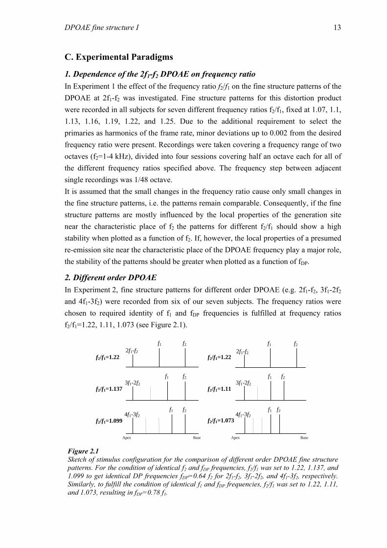
2. Different order DPOAE In Experiment 2, fine structure patterns for different order DPOAE (e.g. 2f1-f2, 3f1-2f2 and 4f1-3f2) were recorded from six of our seven subjects. The frequency ratios were chosen to required identity of f1 and fDP frequencies is fulfilled at frequency ratios f2/f1=1.22, 1.11, 1.073 (see Figure 2.1).

4f1-3f2

f1 f2

3f1-2f2

f2f1

2f1-f2

f1 f2

f2/f1=1.22

f2/f1=1.137

f2/f1=1.099

BaseApex

3f1-2f2

f1 f2

2f1-f2

f1 f2

4f1-3f2

f1 f2

f2/f1=1.22

f2/f1=1.11

f2/f1=1.073

BaseApex

Figure 2.1 Sketch of stimulus configuration for the comparison of different order DPOAE fine structure patterns. For the condition of identical f2 and fDP frequencies, f2/f1 was set to 1.22, 1.137, and 1.099 to get identical DP frequencies fDP=0.64 f2 for 2f1-f2, 3f1-2f2, and 4f1-3f2, respectively. Similarly, to fulfill the condition of identical f1 and fDP frequencies, f2/f1 was set to 1.22, 1.11, and 1.073, resulting in fDP=0.78 f1.

DPOAE fine structure I 14

If the DPOAE fine structure is mainly caused by two sources, one at the generation site and the other one at the distortion frequency site, measurements for different order DPOAE with identical f2 and fDP frequencies should result in very similar patterns, since both f2 and the observed DP frequency are the same, i.e. the characteristic places of the two assumed sources and hence the phase relation between the two is almost identical (see Figure 2.1 left column). With identical f1 and fDP frequencies a small variation in the pattern is expected indicating the influence of the change in the relative phase of the f2 and fDP components (see Figure 2.1 right column).

3. Fixed f2 vs. fixed fDP An additional test for investigating the source of the fine structure was performed during Experiment 3. DPOAE were recorded in keeping either fDP or f2 fixed. This was achieved by varying both f1 and f2 while keeping fDP fixed at 2 kHz or varying f1 and keeping f2 fixed at 3 kHz resulting in varying fDP. Both paradigms result in a varying frequency ratio f2/f1. The comparison of the two paradigms should reveal the relative contribution of the two supposed sources. If the fine structure pattern of the DPOAE is dominated by the contribution from the characteristic place of the distortion product frequency, it is expected that the observable pattern shows much less variation between minima and maxima when fDP is held constant.

D. Analysis For further analysis, the frequencies in all experiments were transformed to their characteristic places x(f) on the BM using the place-frequency map proposed by Greenwood (1991). Although the frequencies used are almost equally spaced on the Greenwood map, there are some deviations from this. These deviations are mainly due to the fact that the primaries were selected as harmonics of the frame rate. To compensate for that, the data were interpolated using a cubic spline algorithm (Matlab 5.1) and re-sampled at 1024 points equally spaced on the Greenwood map. Cross correlation functions (CCF) were calculated using the data from Experiment 1 to quantify the shift between two different fine structure patterns. The correlation lag giving the maximum of the CCF within the range ±1 mm was taken as shift between two fine structure patterns with adjacent frequency ratios. It is assumed that small changes in frequency ratio will cause only small shifts of the overall fine structure. Therefore the range to look for maxima of the CCF was limited to avoid ambiguities which could be caused by the quasi periodic shape of the patterns. The computation of CCF was always restricted to the area of actual overlap between the compared patterns.

DPOAE fine structure I 15

−20

0

20DP

leve

l − d

B S

PL

−20

0

20 DP

leve

l − d

B S

PL

1.07 to 1.07

1.07 to 1.1

1.1 to 1.13

1.13 to 1.16

1.16 to 1.19

1.19 to 1.22

1.22 to 1.25

−20

0

20DP

leve

l − d

B S

PL

−20

0

20 DP

leve

l − d

B S

PL

1.07 to 1.07

1.07 to 1.1

1.1 to 1.13

1.13 to 1.16

1.16 to 1.19

1.19 to 1.22

1.22 to 1.25

−20

0

20DP

leve

l − d

B S

PL

−20

0

20 DP

leve

l − d

B S

PL

1.07 to 1.07

1.07 to 1.1

1.1 to 1.13

1.13 to 1.16

1.16 to 1.19

1.19 to 1.22

1.22 to 1.25

10 12 14 16 18 20

−20

0

20

Distance to Base(f2) − mm

DP

leve

l − d

B S

PL

12 14 16 18 20 22

−20

0

20

Distance to Base(fDP

) − mm

DP

leve

l − d

B S

PL

−2 −1 0 1 2

1.07 to 1.07

1.07 to 1.1

1.1 to 1.13

1.13 to 1.16

1.16 to 1.19

1.19 to 1.22

1.22 to 1.25

Pattern Shift − mm

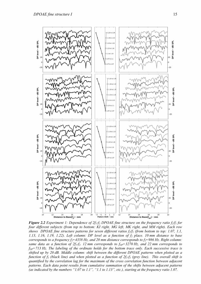
Figure 2.2 Experiment 1: Dependence of 2f1-f2 DPOAE fine structure on the frequency ratio f2/f1 for four different subjects (from top to bottom: KI right, MG left, MK right, and MM right). Each row shows DPOAE fine structure patterns for seven different ratios f2/f1 (from bottom to top: 1.07, 1.1, 1.13, 1.16, 1.19, 1.22). Left column: DP level as a function of f2 place. 10 mm distance to base corresponds to a frequency f2=4358 Hz, and 20 mm distance corresponds to f2=986 Hz. Right column: same data as a function of 2f1-f2. 12 mm corresponds to fDP=3270 Hz, and 22 mm corresponds to fDP=713 Hz. The labeling of the ordinate holds for the bottom trace only. Each successive trace is shifted up by 20 dB. Middle column: shift between the different DPOAE patterns when plotted as a function of f2 (black line) and when plotted as a function of 2f1-f2 (grey line). This overall shift is quantified by the correlation lag for the maximum of the cross correlation function between adjacent patterns. Each data point results from cumulative summation of the shifts between adjacent patterns (as indicated by the numbers “1.07 to 1.1”, “1.1 to 1.13”, etc.), starting at the frequency ratio 1.07.

DPOAE fine structure I 16

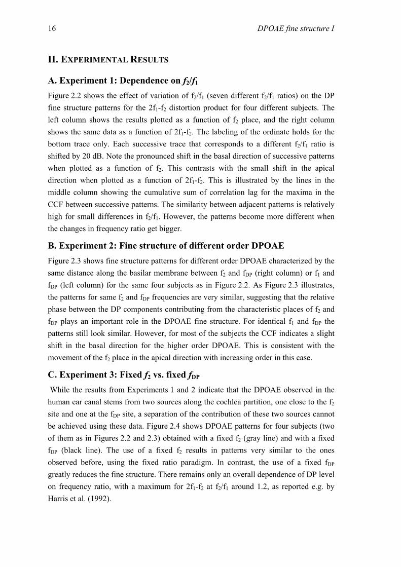
II. EXPERIMENTAL RESULTS

A. Experiment 1: Dependence on f2/f1 Figure 2.2 shows the effect of variation of f2/f1 (seven different f2/f1 ratios) on the DP fine structure patterns for the 2f1-f2 distortion product for four different subjects. The left column shows the results plotted as a function of f2 place, and the right column shows the same data as a function of 2f1-f2. The labeling of the ordinate holds for the bottom trace only. Each successive trace that corresponds to a different f2/f1 ratio is shifted by 20 dB. Note the pronounced shift in the basal direction of successive patterns when plotted as a function of f2. This contrasts with the small shift in the apical direction when plotted as a function of 2f1-f2. This is illustrated by the lines in the middle column showing the cumulative sum of correlation lag for the maxima in the CCF between successive patterns. The similarity between adjacent patterns is relatively high for small differences in f2/f1. However, the patterns become more different when the changes in frequency ratio get bigger.

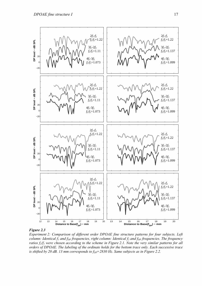
B. Experiment 2: Fine structure of different order DPOAE Figure 2.3 shows fine structure patterns for different order DPOAE characterized by the same distance along the basilar membrane between f2 and fDP (right column) or f1 and fDP (left column) for the same four subjects as in Figure 2.2. As Figure 2.3 illustrates, the patterns for same f2 and fDP frequencies are very similar, suggesting that the relative phase between the DP components contributing from the characteristic places of f2 and fDP plays an important role in the DPOAE fine structure. For identical f1 and fDP the patterns still look similar. However, for most of the subjects the CCF indicates a slight shift in the basal direction for the higher order DPOAE. This is consistent with the movement of the f2 place in the apical direction with increasing order in this case.

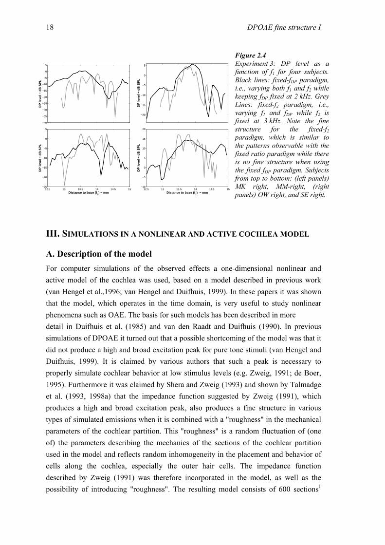
C. Experiment 3: Fixed f2 vs. fixed fDP While the results from Experiments 1 and 2 indicate that the DPOAE observed in the human ear canal stems from two sources along the cochlea partition, one close to the f2 site and one at the fDP site, a separation of the contribution of these two sources cannot be achieved using these data. Figure 2.4 shows DPOAE patterns for four subjects (two of them as in Figures 2.2 and 2.3) obtained with a fixed f2 (gray line) and with a fixed fDP (black line). The use of a fixed f2 results in patterns very similar to the ones observed before, using the fixed ratio paradigm. In contrast, the use of a fixed fDP greatly reduces the fine structure. There remains only an overall dependence of DP level on frequency ratio, with a maximum for 2f1-f2 at f2/f1 around 1.2, as reported e.g. by Harris et al. (1992).

DPOAE fine structure I 17

12 13 14 15 16 17 18 19 20

−20

0

20

c)

b)

a)

DP

leve

l − d

B S

PL

13 14 15 16 17 18 19 20

0

0

0

c)

b)

a)

12 13 14 15 16 17 18 19 20

−20

0

20 c)

b)

a)

DP

leve

l − d

B S

PL

13 14 15 16 17 18 19 20

0

0

0c)

b)

a)

12 13 14 15 16 17 18 19 20

−20

0

20

c)

b)

a)

DP

leve

l − d

B S

PL

13 14 15 16 17 18 19 20

0

0

0

c)

b)

a)

12 13 14 15 16 17 18 19 20

−20

0

20c)

b)

a)

Distance to Base(fDP

) − mm

DP

leve

l − d

B S

PL

13 14 15 16 17 18 19 20

0

0

0c)

b)

a)

Distance to Base(fDP

) − mm

2f1-f2 f2/f1=1.22

3f1-2f2 f2/f1=1.11

4f1-3f2 f2/f1=1.073

2f1-f2 f2/f1=1.22

3f1-2f2 f2/f1=1.11

4f1-3f2 f2/f1=1.073

2f1-f2 f2/f1=1.22

3f1-2f2 f2/f1=1.11

4f1-3f2 f2/f1=1.073

2f1-f2 f2/f1=1.22

3f1-2f2 f2/f1=1.11

4f1-3f2 f2/f1=1.073

2f1-f2 f2/f1=1.22 3f1-2f2 f2/f1=1.137 4f1-3f2 f2/f1=1.099

2f1-f2 f2/f1=1.22 3f1-2f2 f2/f1=1.137 4f1-3f2 f2/f1=1.099

2f1-f2 f2/f1=1.22 3f1-2f2 f2/f1=1.137 4f1-3f2 f2/f1=1.099

2f1-f2 f2/f1=1.22 3f1-2f2 f2/f1=1.137 4f1-3f2 f2/f1=1.099

Figure 2.3 Experiment 2: Comparison of different order DPOAE fine structure patterns for four subjects. Left column: Identical f1 and fDP frequencies, right column: Identical f2 and fDP frequencies. The frequency ratios f2/f1 were chosen according to the scheme in Figure 2.1. Note the very similar patterns for all orders of DPOAE. The labeling of the ordinate holds for the bottom trace only. Each successive trace is shifted by 20 dB. 13 mm corresponds to fDP=2830 Hz. Same subjects as in Figure 2.2.

DPOAE fine structure I 18

III. SIMULATIONS IN A NONLINEAR AND ACTIVE COCHLEA MODEL

A. Description of the model For computer simulations of the observed effects a one-dimensional nonlinear and active model of the cochlea was used, based on a model described in previous work (van Hengel et al.,1996; van Hengel and Duifhuis, 1999). In these papers it was shown that the model, which operates in the time domain, is very useful to study nonlinear phenomena such as OAE. The basis for such models has been described in more detail in Duifhuis et al. (1985) and van den Raadt and Duifhuis (1990). In previous simulations of DPOAE it turned out that a possible shortcoming of the model was that it did not produce a high and broad excitation peak for pure tone stimuli (van Hengel and Duifhuis, 1999). It is claimed by various authors that such a peak is necessary to properly simulate cochlear behavior at low stimulus levels (e.g. Zweig, 1991; de Boer, 1995). Furthermore it was claimed by Shera and Zweig (1993) and shown by Talmadge et al. (1993, 1998a) that the impedance function suggested by Zweig (1991), which produces a high and broad excitation peak, also produces a fine structure in various types of simulated emissions when it is combined with a "roughness" in the mechanical parameters of the cochlear partition. This "roughness" is a random fluctuation of (one of) the parameters describing the mechanics of the sections of the cochlear partition used in the model and reflects random inhomogeneity in the placement and behavior of cells along the cochlea, especially the outer hair cells. The impedance function described by Zweig (1991) was therefore incorporated in the model, as well as the possibility of introducing "roughness". The resulting model consists of 600 sections1

12.5 13 13.5 14 14.5 15−40

−35

−30

−25

−20

−15

−10

−5

0

5

DP

leve

l − d

B S

PL

12.5 13 13.5 14 14.5 15

−20

−15

−10

−5

0

5

DP

leve

l − d

B S

PL

12.5 13 13.5 14 14.5 15−25

−20

−15

−10

−5

0

5

Distance to base (f1) − mm

DP

leve

l − d

B S

PL

12.5 13 13.5 14 14.5 15

−10

−5

0

5

10

15

20

Distance to base (f1) − mm

DP

leve

l − d

B S

PL

Figure 2.4 Experiment 3: DP level as a function of f1 for four subjects. Black lines: fixed-fDP paradigm, i.e., varying both f1 and f2 while keeping fDP fixed at 2 kHz. Grey Lines: fixed-f2 paradigm, i.e., varying f1 and fDP while f2 is fixed at 3 kHz. Note the fine structure for the fixed-f2 paradigm, which is similar to the patterns observable with the fixed ratio paradigm while there is no fine structure when using the fixed fDP paradigm. Subjects from top to bottom: (left panels) MK right, MM-right, (right panels) OW right, and SE right.

DPOAE fine structure I 19

equally spaced along the length of the cochlea (35 mm). The motion of the cochlear partition in each section is described by the following equation of motion:

( ) ( , ) ( ) ( )[ ( ) ( ) ( ) | ] ( )tmy x d x v y x s x y x c v y x p xτ−+ + + =&& & (2.1)

This is a normal second order differential equation of motion for a harmonic oscillator with mass m, damping d(x,v) and stiffness s(x), driven by a pressure force p(x) (x is the position of the oscillator measured from the stapes along the cochlea, y is the displacement and yv &= the velocity of the cochlear partition in the vertical direction),

except that there is an additional "delayed feedback stiffness" term τ−txyvcxs |)()()( .

This term was derived by Zweig (1991) from fits to experimental data on BM excitation patterns. It serves to stabilize the motion of the oscillator, counteracting a negative damping term d(x,v). In order to do so and to arrive at the desired high and broad peak in the excitation caused by a pure tone, the time delay τ must depend on the resonance

frequency mxsres /)(=ω of the oscillator as resωπτ /2742.1 ⋅= (Zweig 1991). The

values of the parameters d(x,v) and c(v) determined by Zweig were )(1217.0 xms−

and 0.1416 respectively. It is important to note that these values are derived from estimated excitation patterns in the cochlea of the squirrel monkey at low levels of stimulation and in the frequency range around 8 kHz. These values can certainly not be used in the vicinity of both stapes and helicotrema, since this would lead to instability (van Hengel, 1993). It is also clear that these values do not hold for higher stimulus levels. Both the negative damping term and the stabilizing "delayed feedback stiffness" term are thought to result from active, i.e. energy producing, behavior of the outer hair cells. This active behavior must saturate at higher levels. It is therefore logical to capture the nonlinearities present in cochlear mechanics in the terms d(x,v) and c(v)2. The nonlinearity was introduced by assuming the following dependence of d(x,v) and c(v) on the velocity v of the section:

( ) | |( , ) ( )1 | |

| |( ) .1416 with .12, .51 | |

h ll

ll l l h

d d vd x v d ms xv

c vc v c c d dv

ββ

ββ

−= + + −= + = = − =+

(2.2)

In these equations the nonlinear behavior of d(x,v) and c(v) is chosen to be the same,

with the damping going to a value of )(xmsdh and the "delayed feedback stiffness"

disappearing at high excitation levels. The region in which the nonlinearity plays a role is determined by the parameter β . In all simulations presented here a value of

0.01 ms/nm was used for this parameter, leading to a compressive growth of the excitation at the characteristic place for a pure tone stimulus of around 0.3 dB/dB over the range from about 20 dB SPL to 80 dB SPL stimulus level. Because the mass m was

DPOAE fine structure I 20

chosen to be 0.375 kg/m2, independent of the position x, the stiffness controls the place-frequency map of the cochlear partition. The place-frequency map chosen was:

-1( ) , 22.508 kHz, 150 maxf x A e A a−= ⋅ = = (2.3)

Following the work of Shera and Zweig (1993) and Talmadge and Tubis (1993) the random fluctuations necessary to obtain a fine structure in the emissions were introduced in the stiffness as:

0( ) ( )[1 ( )]s x s x r r x= + (2.4)

where r(x) is a random variable with a Gaussian distribution and r0 is a scaling parameter that controls the amount of "roughness". For the results presented here a value of 1% was used for r0. The equations of motion Equation (2.1) for all sections were coupled through the fluid, which was assumed linear, incompressible and inviscid. The coupled system was solved by Gauss-elimination and integrated in time using a Runge-Kutta 4 time-integration scheme with a sampling frequency of 150 kHz. Reducing the sampling frequency could lead to instabilities in certain cases, but increasing it did not give significantly different results (differences in emission levels were below 0.5%). To simulate OAE the motion of the cochlea sections is coupled to the outside world via a simplified middle ear, consisting of a mass, stiffness and damping in combination with a transformer. This produces a sound pressure that would result at the ear drum in an open ear canal. Previous studies with this model have shown that emission levels are highly sensitive to conditions at the ear drum. SOAE level may vary up to 30 dB when different loading impedances are added (van den Raadt and Duifhuis, 1993).

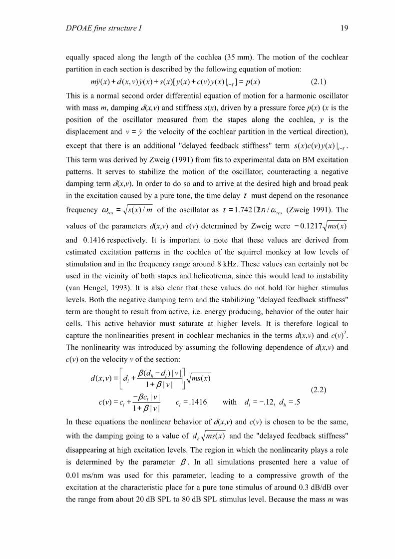
B. Simulations All the experiments described in section II (except Experiment 2 for the condition of same f1 and fDP frequencies) were simulated using this computer model. In contrast to the experiments, all simulations were performed with primary levels of 50 dB SPL. The model output is the sound pressure level at the "ear-drum" taken from a 30-ms interval beginning 20 ms after stimulus start to avoid onset effects. The data were analyzed using the least-squares-fit method described by Long and Talmadge (1997) to get an estimate of the spectral power of the frequency components of interest. The further analysis of pattern shifts was performed using cross correlation as described for the experimental data. The simulation results are given in Figures 2.5 to 2.7. Analogous to the experimental data in Figure 2.2, Figure 2.5 shows simulated DPOAE fine structure patterns for different frequency ratios of the primaries plotted as a function of f2 (left panel) and fDP (right panel). The main experimental result, i.e., the shift of fine structure patterns when varying the frequency ratio, is replicated very well, both qualitatively and quantitatively. Figure 2.6 shows fine structure patterns for three different frequency

DPOAE fine structure I 21

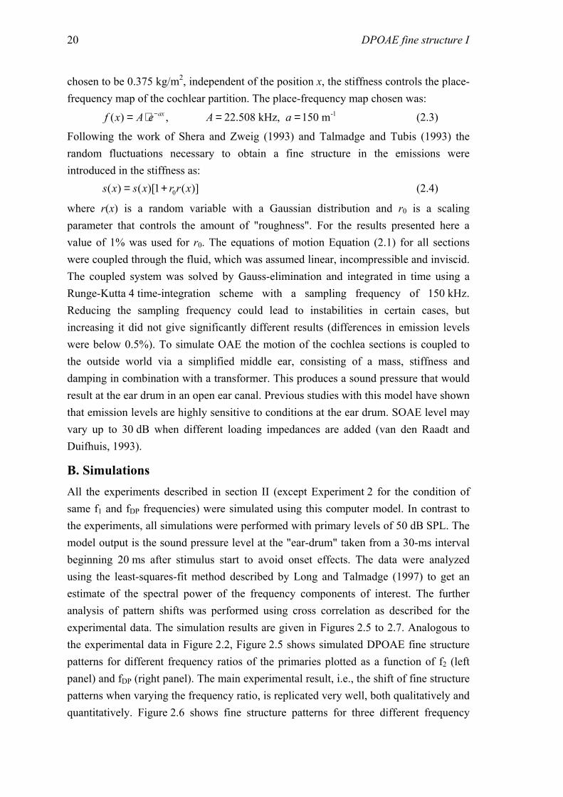
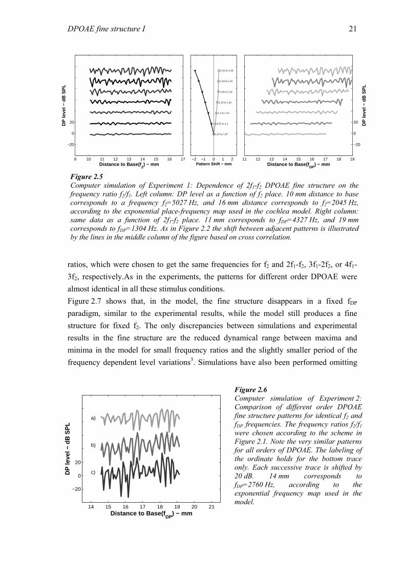
ratios, which were chosen to get the same frequencies for f2 and 2f1-f2, 3f1-2f2, or 4f1-3f2, respectively.As in the experiments, the patterns for different order DPOAE were almost identical in all these stimulus conditions. Figure 2.7 shows that, in the model, the fine structure disappears in a fixed fDP paradigm, similar to the experimental results, while the model still produces a fine structure for fixed f2. The only discrepancies between simulations and experimental results in the fine structure are the reduced dynamical range between maxima and minima in the model for small frequency ratios and the slightly smaller period of the frequency dependent level variations3. Simulations have also been performed omitting

9 10 11 12 13 14 15 16 17

−20

0

20

Distance to Base(f2) − mm

DP

leve

l − d

B S

PL

11 12 13 14 15 16 17 18 19

−20

0

20

Distance to Base(fDP

) − mm

DP

leve

l − d

B S

PL

−2 −1 0 1 2

1.07 to 1.07

1.07 to 1.1

1.1 to 1.13

1.13 to 1.16

1.16 to 1.19

1.19 to 1.22

1.22 to 1.25

Pattern Shift − mm

Figure 2.5 Computer simulation of Experiment 1: Dependence of 2f1-f2 DPOAE fine structure on the frequency ratio f2/f1. Left column: DP level as a function of f2 place. 10 mm distance to base corresponds to a frequency f2=5027 Hz, and 16 mm distance corresponds to f2=2045 Hz, according to the exponential place-frequency map used in the cochlea model. Right column: same data as a function of 2f1-f2 place. 11 mm corresponds to fDP=4327 Hz, and 19 mm corresponds to fDP=1304 Hz. As in Figure 2.2 the shift between adjacent patterns is illustrated by the lines in the middle column of the figure based on cross correlation.

14 15 16 17 18 19 20 21

−20

0

20

c)

b)

a)

Distance to Base(fDP

) − mm

DP

leve

l − d

B S

PL

Figure 2.6 Computer simulation of Experiment 2: Comparison of different order DPOAE fine structure patterns for identical f2 and fDP frequencies. The frequency ratios f2/f1 were chosen according to the scheme in Figure 2.1. Note the very similar patterns for all orders of DPOAE. The labeling of the ordinate holds for the bottom trace only. Each successive trace is shifted by 20 dB. 14 mm corresponds to fDP=2760 Hz, according to the exponential frequency map used in the model.

DPOAE fine structure I 22

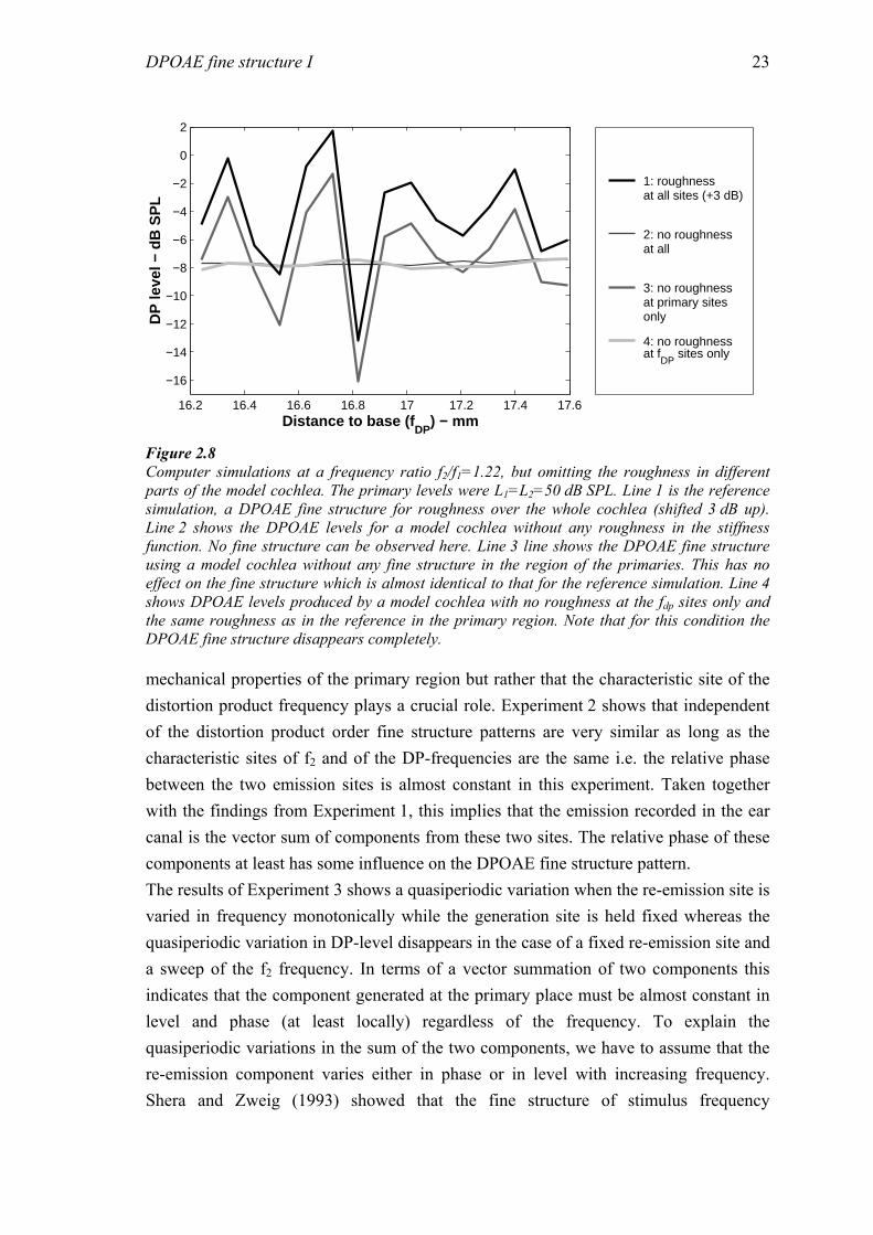
the "roughness" in the model's stiffness function in either (1) the frequency region above 2 kHz, or (2) below 2 kHz, or (3) with no roughness at all, to get a better understanding of the mechanism creating the fine structure in the model. DPOAE with a high frequency resolution were computed over a frequency range for f2 from 2483 Hz to 3084 Hz at a frequency ratio f2/f1=1.22. This ensured that the characteristic places of fDP always fell in model sections with characteristic frequencies below 2 kHz while the characteristic frequencies of the primaries always fell into sections above 2 kHz. Figure 2.8 shows the simulation results in these three conditions as well as in the reference condition with roughness over the whole length of the cochlea. The DPOAE fine structure is unaffected by the presence or absence of the "roughness" in the primary region while it disappears when the roughness is omitted in the distortion product frequency region. This emphasizes the interpretation of the experimental results that the DPOAE fine structure is mainly influenced by the re-emission components from the characteristic DP places while emission from the primary component places is almost constant in level and phase over frequency.

IV. DISCUSSION Similar to recent experimental and theoretical studies on DPOAE fine structure by other authors (e.g. Mauermann et al., 1997a; Heitmann et al., 1998; Talmadge et al., 1998a, 1999), our experiments and simulations give further evidence that the fine structure is the result of two sources. Furthermore the idea is supported that the underlying physical mechanisms of these two sources are different or at least act in a different way (e.g. Shera and Guinan, 1999). To illustrate this the results presented in this paper will be interpreted in three steps. The results of Experiment 1 show that the DPOAE fine structure is not caused by local

13.5 14 14.5 15 15.5 16−15

−10

−5

0

Distance to base (f1) − mm

DP

leve

l − d

B S

PL

Figure 2.7 Computer simulation of Experiment 3: DP level as a function of f1. Black line: fixed fDP paradigm, i.e., varying both f1 and f2 while keeping fDP fixed at 2 kHz. Grey Line: fixed f2 paradigm, i.e., varying f1 and fDP while f2 is fixed at 3 kHz. Note that, as for the experimental results, the fine structure for the fixed-f2 paradigm is similar to the patterns observable with the fixed-ratio paradigm, while there is no fine structure when using the fixed-fDP paradigm.

DPOAE fine structure I 23

mechanical properties of the primary region but rather that the characteristic site of the distortion product frequency plays a crucial role. Experiment 2 shows that independent of the distortion product order fine structure patterns are very similar as long as the characteristic sites of f2 and of the DP-frequencies are the same i.e. the relative phase between the two emission sites is almost constant in this experiment. Taken together with the findings from Experiment 1, this implies that the emission recorded in the ear canal is the vector sum of components from these two sites. The relative phase of these components at least has some influence on the DPOAE fine structure pattern. The results of Experiment 3 shows a quasiperiodic variation when the re-emission site is varied in frequency monotonically while the generation site is held fixed whereas the quasiperiodic variation in DP-level disappears in the case of a fixed re-emission site and a sweep of the f2 frequency. In terms of a vector summation of two components this indicates that the component generated at the primary place must be almost constant in level and phase (at least locally) regardless of the frequency. To explain the quasiperiodic variations in the sum of the two components, we have to assume that the re-emission component varies either in phase or in level with increasing frequency. Shera and Zweig (1993) showed that the fine structure of stimulus frequency

1: roughnessat all sites (+3 dB)

2: no roughnessat all

3: no roughnessat primary sitesonly

4: no roughnessat f

DP sites only

16.2 16.4 16.6 16.8 17 17.2 17.4 17.6

−16

−14

−12

−10

−8

−6

−4

−2

0

2

Distance to base (fDP

) − mm

DP

leve

l − d

B S

PL

Figure 2.8 Computer simulations at a frequency ratio f2/f1=1.22, but omitting the roughness in different parts of the model cochlea. The primary levels were L1=L2=50 dB SPL. Line 1 is the reference simulation, a DPOAE fine structure for roughness over the whole cochlea (shifted 3 dB up). Line 2 shows the DPOAE levels for a model cochlea without any roughness in the stiffness function. No fine structure can be observed here. Line 3 line shows the DPOAE fine structure using a model cochlea without any fine structure in the region of the primaries. This has no effect on the fine structure which is almost identical to that for the reference simulation. Line 4 shows DPOAE levels produced by a model cochlea with no roughness at the fdp sites only and the same roughness as in the reference in the primary region. Note that for this condition the DPOAE fine structure disappears completely.

DPOAE fine structure I 24

otoacoustic emissions (SFOAE) can be interpreted as interference of the incoming and outgoing traveling waves with a periodic rotating phase of the cochlear reflectance. It appears reasonable to treat the DPOAE re-emission component in a similar way to SFOAE generation. Therefore, a periodically varying phase of the re-emission component is the most likely explanation for the DPOAE fine structure. Following furthermore the arguments of the “Gedankenexperiment” described by Shera and Guinan (1998) the different characteristics of the two components (rotating phase of the fDP component, almost constant phase of the f2 component) indicate that the underlying mechanisms for these two DPOAE components are different. These authors (Shera and Guinan, 1998, 1999) distinguished two classes of OAE mechanisms, "linear coherent reflection" and "nonlinear distortion", whereby DPOAE are a combination of both a nonlinear distortion at the generation site and a coherent reflection from the characteristic site of fDP. The disappearance of fine structure during the fixed fDP experiment shows that there is no coherent reflection from the primary region because there is no rotating phase with frequency. Using the approach suggested by Zweig and Shera (1995) to explain the spectral periodicity of reflection emissions, this had to be expected because the travelling wave from the initial generation site results in constant wavelength only around the fDP site but not in the region around the primaries. Therefore the contribution from the primary region need to be generated in a different way most probably due to nonlinear distortion. This interpretation of the experiments is confirmed by the computer simulations, which show no effect on the fine structure when removing the "roughness" (which is necessary for coherent reflections) from the primary region while the fine structure disappears in simulations when removing the roughness only around the fDP region (see Figure 2.8). The overall good correspondence between simulations and experimental results gives further confirmation for a whole class of two-source interference models, like the one used here. This class of models was recently described in detail by Talmadge et al. (1998a). The simulations with partly removed roughness (see Figure 2.8) can not directly be transformed into an experimental approach because it is impossible to “flatten out” certain areas of the human cochlea. But a situation close to that might be studied. If a local area of the cochlea is damaged. Most probably no broad and tall excitation pattern can be build up there, which in addition to roughness is necessary for coherent reflections (Zweig and Shera, 1995; Talmadge et al., 1999). To get further insight into the mechanisms of DPOAE fine structure this approach is investigated in the accompanying paper (Mauermann et al. 1999b; see Chapter 3) by looking at the DPOAE fine structure of subjects with frequency specific hearing losses.

DPOAE fine structure I 25

V. CONCLUSIONS Distortion products recorded in the ear canal cannot be traced back to one single source on the basilar membrane. Instead, DPOAE fine structure reflects the interaction of two components with different underlying physical principles. The first component is due to nonlinear distortion at the primary site close to f2 and has a nearly constant phase and level. The second component is caused by a coherent reflection from the re-emission site at the characteristic place of fDP and shows a periodically varying amplitude or phase when changing the primary frequencies.

ACKNOWLEDGMENTS This study was supported by Deutsche Forschungsgemeinschaft, DFG Ko 942/11-2. Many fruitful discussions with G. Long, C. Talmadge and H. Duifhuis, as well as helpful comments by B. Moore on an earlier version of the manuscript are gratefully acknowledged.

ENDNOTES 1 The number of sections had to be increased from the original 400 to at least 600 in order to avoid "wiggles" in the excitation patterns. These "wiggles" were also found by Talmadge and Tubis in their work on a time domain model involving the "Zweig-impedance" and made them use a spatial discretisation of 4000 sections (Talmadge and Tubis, 1993; and personal communication). 2 Of course, other terms could also contain nonlinearity. For example Furst and Goldstein (1982) argue that the stiffness term should be made nonlinear. For reasons of simplicity only d(x,v) and c(v) were made nonlinear here, since these two terms must certainly change with input level. 3 There is another discrepancy between the experimental results and the simulations in the overall shape of the patterns. For the range of frequency ratios observed here, we see a maximum in DPOAE level for human subjects at a frequency ratio around 1.225 (Gaskill and Brown, 1990) while the level is reduced for smaller and larger frequency ratios. This reflects the so called “second filter” effect (e.g. Brown and Williams, 1993; Allen and Fahey, 1993), which is currently not included in our simulations. With the parameter settings used in this study the “second filter” effect produced by the model does not resemble the shapes found in the experimental data. However, as described in van Hengel and Duifhuis (1999) the “second filter” behavior can also be simulated using this kind of transmission-line model. Therefore in the near future attempts will be made to improve the model results by finding parameter values fitting both fine structure and the “second filter”.

Chapter 3

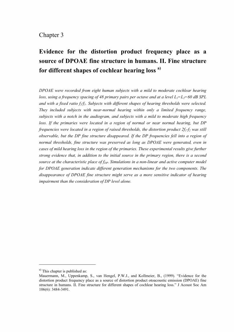
Evidence for the distortion product frequency place as a source of DPOAE fine structure in humans. II. Fine structure for different shapes of cochlear hearing loss a)

DPOAE were recorded from eight human subjects with a mild to moderate cochlear hearing loss, using a frequency spacing of 48 primary pairs per octave and at a level L1=L2=60 dB SPL and with a fixed ratio f2/f1. Subjects with different shapes of hearing thresholds were selected. They included subjects with near-normal hearing within only a limited frequency range, subjects with a notch in the audiogram, and subjects with a mild to moderate high frequency loss. If the primaries were located in a region of normal or near normal hearing, but DP frequencies were located in a region of raised thresholds, the distortion product 2f1-f2 was still observable, but the DP fine structure disappeared. If the DP frequencies fell into a region of normal thresholds, fine structure was preserved as long as DPOAE were generated, even in cases of mild hearing loss in the region of the primaries. These experimental results give further strong evidence that, in addition to the initial source in the primary region, there is a second source at the characteristic place of fDP. Simulations in a non-linear and active computer model for DPOAE generation indicate different generation mechanisms for the two components. The disappearance of DPOAE fine structure might serve as a more sensitive indicator of hearing impairment than the consideration of DP level alone.

a) This chapter is published as: Mauermann, M., Uppenkamp, S., van Hengel, P.W.J., and Kollmeier, B., (1999). “Evidence for the distortion product frequency place as a source of distortion product otoacoustic emission (DPOAE) fine structure in humans. II. Fine structure for different shapes of cochlear hearing loss.” J Acoust Soc Am 106(6): 3484-3491.

DPOAE fine structure II 28

INTRODUCTION The recording of distortion product otoacoustic emissions (DPOAE) is claimed to be useful as an objective audiometric test with a high frequency selectivity by various clinical studies. In many papers the reported correlation of audiometric thresholds and DPOAE levels is mainly based on large databases of many subjects (e.g. Nelson and Kimberley, 1992, Gorga et al., 1993; Moulin et al., 1994; Suckfüll et al., 1996). The prediction of individual thresholds based on DPOAE requires a detailed and comprehensive dataset from each individual subject including growth functions at multiple stimulus frequencies (Kummer et al, 1998). However, for extensive use as a diagnostic tool, a more detailed understanding of the DPOAE generation mechanisms is still required. In agreement with theoretical and experimental work reported by other groups (Brown et al. 1996; Gaskill and Brown, 1996; Heitmann et al., 1998; Talmadge et al., 1998, 1999), the experimental results from normal hearing subjects in the accompanying paper (Mauermann et al., 1999) showed that DPOAE should be interpreted as the vector sum of two sources, one at the initial generation site due to nonlinear distortion close to the f2 place, the other at the characteristic site of the particular DP frequency of interest. The results from simulations using a nonlinear and active model of the cochlea presented in Mauermann et al. (1999) showed that the component from the fDP site is sensitive to the existence of statistical fluctuations in the mechanical properties along the cochlea partition, i.e. roughness, while the initial generation component is not. From the model point of view this indicates different underlying mechanisms for the generation of the two DPOAE components. However, removing the roughness from certain areas along the cochlear partition - as shown in the computer simulations in Mauermann et al. (1999) - can not directly be transformed into a controlled experiment with human subjects. Other studies on modeling OAE fine structure (Zweig and Shera, 1995; Talmadge et al., 1999) showed that - in addition to the roughness - the model needs another feature to produce DPOAE fine structure: broad and tall excitation patterns have to be generated to allow coherent reflections. The generation of a broad and tall excitation pattern requires an active feedback mechanism in the model. In the real cochlea this mechanism is most probably related to the motility of outer hair cells (OHC), as found by Brownell et al. (1985) and Zenner et al. (1985). If the activity of OHC in the cochlea is reduced because of a damage to certain areas most probably no broad and tall excitation pattern can build up there. As a consequence there would be no coherent reflection from the reemission site and no DPOAE fine structure would be observable. This assumption is mainly based on the model results obtained so far (Mauermann et

DPOAE fine structure II 29

al., 1999), but can be tested in carefully selected hearing-impaired human subjects. In the present paper, results on DPOAE fine structure from subjects with different audiogram shapes will be presented to investigate the effects of damage in different regions of the cochlea in more detail. Our subjects included persons with near normal hearing only within a limited frequency range ("band pass listeners"), a notch in the audiogram ("band stop listeners"), or a hearing loss at high frequencies only ("low pass listeners"). This allowed measurement of DPOAE while restricting either fDP or the primaries to "normal" or "near normal" BM regions. It was expected that only the component generated in a region of cochlear damage would be reduced. The experiments were designed to obtain further evidence for the two-source model as discussed in the accompanying paper (Mauermann et al., 1999). To support the arguments, a "hearing-impaired" version of the computer model was also tested, simulating the "band-stop listener" situation mentioned above.

I. METHODS

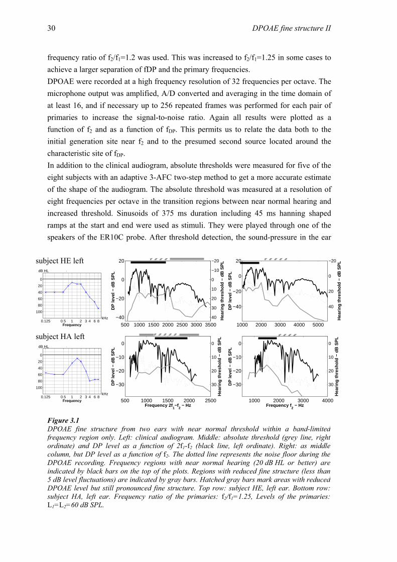
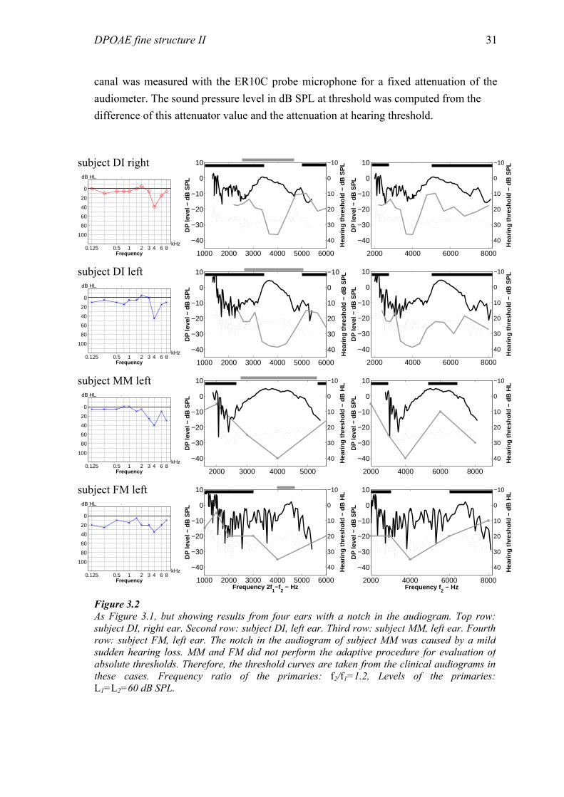
A. Subjects Eight subjects with different types of hearing loss participated in the experiments. They were selected because of the shapes of their audiograms. Subjects HE and HA (63 and 59 years old) showed a hearing loss with a bandpass characteristic, i.e., near normal threshold within only a small frequency band at 1.5 kHz with raised thresholds for frequencies above and below. The second group of subjects (DI, FM, MM, 29-50 years old) showed a notch in the hearing threshold of about 40 dB centered at 4 kHz. The third group (RH, HL, JK, 59-63 years old) showed a moderate high frequency hearing loss. All subjects except MM had a stable audiogram for at least six months. The notch in the audiogram of MM was caused by a mild sudden hearing loss. The threshold recovered almost completely over a period of six months.

B. Instrumentation and experimental procedures All instrumentation and the experimental methods for recording DPOAE fine structure are described in detail in the accompanying paper (Mauermann et al., 1999). In short, an insert ear probe type ER-10C in combination with a signal-processing board Ariel DSP-32C was used to record DPOAE. All stimuli were generated digitally at a sampling rate of 22.05 kHz and as harmonics of the inverse of the frame length (4096 samples, i.e. harmonics of 5.38 Hz). They were played continuously to the subjects via 16 bit D/A converters, a computer controlled audiometer and low pass filters at a presentation level of L1=L2=60 dB SPL. An automatic in-the-ear calibration was performed before each run to adjust the primaries to the desired sound pressure levels. In most subjects, a

DPOAE fine structure II 30

frequency ratio of f2/f1=1.2 was used. This was increased to f2/f1=1.25 in some cases to achieve a larger separation of fDP and the primary frequencies. DPOAE were recorded at a high frequency resolution of 32 frequencies per octave. The microphone output was amplified, A/D converted and averaging in the time domain of at least 16, and if necessary up to 256 repeated frames was performed for each pair of primaries to increase the signal-to-noise ratio. Again all results were plotted as a function of f2 and as a function of fDP. This permits us to relate the data both to the initial generation site near f2 and to the presumed second source located around the characteristic site of fDP. In addition to the clinical audiogram, absolute thresholds were measured for five of the eight subjects with an adaptive 3-AFC two-step method to get a more accurate estimate of the shape of the audiogram. The absolute threshold was measured at a resolution of eight frequencies per octave in the transition regions between near normal hearing and increased threshold. Sinusoids of 375 ms duration including 45 ms hanning shaped ramps at the start and end were used as stimuli. They were played through one of the speakers of the ER10C probe. After threshold detection, the sound-pressure in the ear

subject HE left

0.125 0.5 1 2 3 4 6 8

0

20

40

60

80

100

kHz

dB HL

Frequency

,

500 1000 1500 2000 2500 3000 3500

−40

−20

0

20

DP

leve

l − d

B S

PL

−20

−10

0

10

20

30

40 Hea

ring

thre

shol

d −

dB S

PL

−20

0

20

40

Hea

ring

thre

shol

d −

dB S

PL

1000 2000 3000 4000 5000

−40

−20

0

20

DP

leve

l − d

B S

PL

subject HA left

0.125 0.5 1 2 3 4 6 8

0

20

40

60

80

100

kHz

dB HL ,

Frequency

0

10

20

30

Hea

ring

thre

shol

d −

dB S

PL

500 1000 1500 2000 2500

−30

−20

−10

0

Frequency 2f1−f

2 − Hz

DP

leve

l − d

B S

PL

0

10

20

30

Hea

ring

thre

shol

d −

dB S

PL

1000 2000 3000 4000

−30

−20

−10

0

Frequency f2 − Hz

DP

leve

l − d

B S

PL

Figure 3.1 DPOAE fine structure from two ears with near normal threshold within a band-limited frequency region only. Left: clinical audiogram. Middle: absolute threshold (grey line, right ordinate) and DP level as a function of 2f1-f2 (black line, left ordinate). Right: as middle column, but DP level as a function of f2. The dotted line represents the noise floor during the DPOAE recording. Frequency regions with near normal hearing (20 dB HL or better) are indicated by black bars on the top of the plots. Regions with reduced fine structure (less than 5 dB level fluctuations) are indicated by gray bars. Hatched gray bars mark areas with reduced DPOAE level but still pronounced fine structure. Top row: subject HE, left ear. Bottom row: subject HA, left ear. Frequency ratio of the primaries: f2/f1=1.25, Levels of the primaries: L1=L2=60 dB SPL.

DPOAE fine structure II 31

canal was measured with the ER10C probe microphone for a fixed attenuation of the audiometer. The sound pressure level in dB SPL at threshold was computed from the difference of this attenuator value and the attenuation at hearing threshold.

subject DI right

0.125 0.5 1 2 3 4 6 8

0

20

40

60

80

100

kHz

dB HL

Frequency

,

−10

0

10

20

30

40

Hea

ring

thre

shol

d −

dB S

PL

1000 2000 3000 4000 5000 6000

−40

−30

−20

−10

0

10

DP

leve

l − d

B S

PL

−10

0

10

20

30

40

Hea

ring

thre

shol

d −

dB S

PL

2000 4000 6000 8000

−40

−30

−20

−10

0

10

DP

leve

l − d

B S

PL

subject DI left

0.125 0.5 1 2 3 4 6 8

0

20

40

60

80

100

kHz

dB HL

Frequency

,

−10

0

10

20

30

40H

earin

g th

resh

old

− dB

SP

L

1000 2000 3000 4000 5000 6000

−40

−30

−20

−10

0

10

DP

leve

l − d

B S

PL

−10

0

10

20

30

40

Hea

ring

thre

shol

d −

dB S

PL

2000 4000 6000 8000

−40

−30

−20

−10

0

10

DP

leve

l − d

B S

PL

subject MM left

0.125 0.5 1 2 3 4 6 8

0

20

40

60

80

100

kHz

dB HL

Frequency

,

−10

0

10

20

30

40 Hea

ring

thre

shol

d −

dB H

L

2000 3000 4000 5000

−40

−30

−20

−10

0

10

DP

leve

l − d

B S

PL

−10

0

10

20

30

40 Hea

ring

thre

shol

d −

dB H

L

2000 4000 6000 8000

−40

−30

−20

−10

0

10

DP

leve

l − d

B S

PL

subject FM left

0.125 0.5 1 2 3 4 6 8

0

20

40

60

80

100

kHz

dB HL

Frequency

,

−10

0

10

20

30

40 Hea

ring

thre

shol

d −

dB H

L

1000 2000 3000 4000 5000 6000

−40

−30

−20

−10

0

10

Frequency 2f1−f

2 − Hz

DP

leve

l − d

B S

PL

−10

0

10

20

30

40 Hea

ring

thre

shol

d −

dB H

L

2000 4000 6000 8000

−40

−30

−20

−10

0

10

Frequency f2 − Hz

DP

leve

l − d

B S

PL

Figure 3.2 As Figure 3.1, but showing results from four ears with a notch in the audiogram. Top row: subject DI, right ear. Second row: subject DI, left ear. Third row: subject MM, left ear. Fourth row: subject FM, left ear. The notch in the audiogram of subject MM was caused by a mild sudden hearing loss. MM and FM did not perform the adaptive procedure for evaluation of absolute thresholds. Therefore, the threshold curves are taken from the clinical audiograms in these cases. Frequency ratio of the primaries: f2/f1=1.2, Levels of the primaries: L1=L2=60 dB SPL.

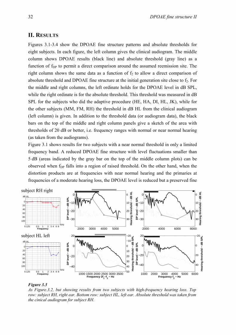
DPOAE fine structure II 32

II. RESULTS Figures 3.1-3.4 show the DPOAE fine structure patterns and absolute thresholds for eight subjects. In each figure, the left column gives the clinical audiogram. The middle column shows DPOAE results (black line) and absolute threshold (gray line) as a function of fDP to permit a direct comparison around the assumed reemission site. The right column shows the same data as a function of f2 to allow a direct comparison of absolute threshold and DPOAE fine structure at the initial generation site close to f2. For the middle and right columns, the left ordinate holds for the DPOAE level in dB SPL, while the right ordinate is for the absolute threshold. This threshold was measured in dB SPL for the subjects who did the adaptive procedure (HE, HA, DI, HL, JK), while for the other subjects (MM, FM, RH) the threshold in dB HL from the clinical audiogram (left column) is given. In addition to the threshold data (or audiogram data), the black bars on the top of the middle and right column panels give a sketch of the area with thresholds of 20 dB or better, i.e. frequency ranges with normal or near normal hearing (as taken from the audiograms). Figure 3.1 shows results for two subjects with a near normal threshold in only a limited frequency band. A reduced DPOAE fine structure with level fluctuations smaller than 5 dB (areas indicated by the gray bar on the top of the middle column plots) can be observed when fDP falls into a region of raised threshold. On the other hand, when the distortion products are at frequencies with near normal hearing and the primaries at frequencies of a moderate hearing loss, the DPOAE level is reduced but a preserved fine

subject RH right

0.125 0.5 1 2 3 4 6 8

0

20

40

60

80

100

kHz

dB HL ,

Frequency

0

10

20

30

Hea

ring

thre

shol

d −

dB H

L

2000 3000 4000 5000

−30

−20

−10

0

DP

leve

l − d

B S

PL

0

10

20

30

Hea

ring

thre

shol

d −

dB H

L

2000 4000 6000 8000

−30

−20

−10

0

DP

leve

l − d

B S

PL

subject HL left

0.125 0.5 1 2 3 4 6 8

0

20

40

60

80

100

kHz

dB HL ,

Frequency

−20

−10

0

10

20

30

40

50 Hea

ring

thre

shol

d −

dB S

PL

1000 1500 2000 2500 3000 3500

−40

−20

0

20

Frequency 2f1−f

2 − Hz

DP

leve

l − d

B S

PL

−20

0

20

40

Hea

ring

thre

shol

d −

dB S

PL

1000 2000 3000 4000 5000 6000

−40

−20

0

20

Frequency f2 − Hz

DP

leve

l − d

B S

PL

Figure 3.3 As Figure.3.2, but showing results from two subjects with high-frequency hearing loss. Top row: subject RH, right ear. Bottom row: subject HL, left ear. Absolute threshold was taken from the cinical audiogram for subject RH.

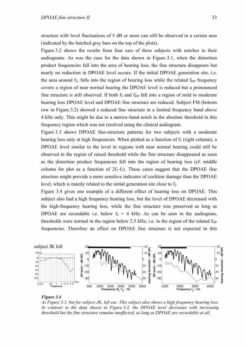
DPOAE fine structure II 33

structure with level fluctuations of 5 dB or more can still be observed in a certain area (indicated by the hatched grey bars on the top of the plots). Figure 3.2 shows the results from four ears of three subjects with notches in their audiograms. As was the case for the data shown in Figure 3.1, when the distortion product frequencies fall into the area of hearing loss, the fine structure disappears but nearly no reduction in DPOAE level occurs. If the initial DPOAE generation site, i.e. the area around f2, falls into the region of hearing loss while the related fDP frequency covers a region of near normal hearing the DPOAE level is reduced but a pronounced fine structure is still observed. If both f2 and fDP fall into a region of mild to moderate hearing loss DPOAE level and DPOAE fine structure are reduced. Subject FM (bottom row in Figure 3.2) showed a reduced fine structure in a limited frequency band above 4 kHz only. This might be due to a narrow-band notch in the absolute threshold in this frequency region which was not resolved using the clinical audiogram. Figure 3.3 shows DPOAE fine-structure patterns for two subjects with a moderate hearing loss only at high frequencies. When plotted as a function of f2 (right column), a DPOAE level similar to the level in regions with near normal hearing could still be observed in the region of raised threshold while the fine structure disappeared as soon as the distortion product frequencies fell into the region of hearing loss (cf. middle column for plot as a function of 2f1-f2). These cases suggest that the DPOAE fine structure might provide a more sensitive indicator of cochlear damage than the DPOAE level, which is mainly related to the initial generation site close to f2. Figure 3.4 gives one example of a different effect of hearing loss on DPOAE. This subject also had a high frequency hearing loss, but the level of DPOAE decreased with the high-frequency hearing loss, while the fine structure was preserved as long as DPOAE are recordable i.e. below f2 = 4 kHz. As can be seen in the audiogram, thresholds were normal in the region below 2.5 kHz, i.e. in the region of the related fDP frequencies. Therefore an effect on DPOAE fine structure is not expected in this

subject JK left

0.125 0.5 1 2 3 4 6 8

0

20

40

60

80

100

kHz

dB HL

Frequency

,

−20

−10

0

10

20

30

Hea

ring

thre

shol

d −

dB S

PL

500 1000 1500 2000 2500 3000

−30

−20

−10

0

10

20

Frequency 2f1−f

2 − Hz

DP

leve

l − d

B S

PL

−20

−10

0

10

20

30

Hea

ring

thre

shol

d −

dB S

PL

1000 2000 3000 4000

−30

−20

−10

0

10

20

Frequency f2 − Hz

DP

leve

l − d

B S

PL

Figure 3.4 As Figure 3.1, but for subject JK, left ear. This subject also shows a high frequency hearing loss. In contrast to the data shown in Figure 3.3, the DPOAE level decreases with increasing threshold but the fine structure remains unaffected, as long as DPOAE are recordable at all.

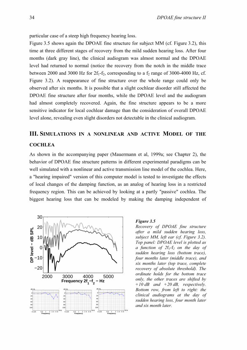
DPOAE fine structure II 34

particular case of a steep high frequency hearing loss. Figure 3.5 shows again the DPOAE fine structure for subject MM (cf. Figure 3.2), this time at three different stages of recovery from the mild sudden hearing loss. After four months (dark gray line), the clinical audiogram was almost normal and the DPOAE level had returned to normal (notice the recovery from the notch in the middle trace between 2000 and 3000 Hz for 2f1-f2, corresponding to a f2 range of 3000-4000 Hz, cf. Figure 3.2). A reappearance of fine structure over the whole range could only be observed after six months. It is possible that a slight cochlear disorder still affected the DPOAE fine structure after four months, while the DPOAE level and the audiogram had almost completely recovered. Again, the fine structure appears to be a more sensitive indicator for local cochlear damage than the consideration of overall DPOAE level alone, revealing even slight disorders not detectable in the clinical audiogram.

III. SIMULATIONS IN A NONLINEAR AND ACTIVE MODEL OF THE

COCHLEA As shown in the accompanying paper (Mauermann et al, 1999a; see Chapter 2), the behavior of DPOAE fine structure patterns in different experimental paradigms can be well simulated with a nonlinear and active transmission line model of the cochlea. Here, a "hearing impaired" version of this computer model is tested to investigate the effects of local changes of the damping function, as an analog of hearing loss in a restricted frequency region. This can be achieved by looking at a partly "passive" cochlea. The biggest hearing loss that can be modeled by making the damping independent of

2000 3000 4000 5000

−20

−10

0

10

20

30

Frequency 2f1−f

2 − Hz

DP

leve

l − d

B S

PL

0.125 0.5 1 2 3 4 6 8

0

20

40

60

80

100

kHz

dB HL ,

Frequency

0.125 0.5 1 2 3 4 6 8

0

20

40

60

80

100

kHz

dB HL ,

Frequency

0.125 0.5 1 2 3 4 6 8

0

20

40

60

80

100

kHz

dB HL

Frequency

,

Figure 3.5 Recovery of DPOAE fine structure after a mild sudden hearing loss, subject MM, left ear (cf. Figure 3.2). Top panel: DPOAE level is plotted as a function of 2f1-f2 on the day of sudden hearing loss (bottom trace), four months later (middle trace), and six months later (top trace, complete recovery of absolute threshold). The ordinate holds for the bottom trace only, the other traces are shifted by +10 dB and +20 dB, respectively. Bottom row, from left to right: the clinical audiograms at the day of sudden hearing loss, four month later and six month later.

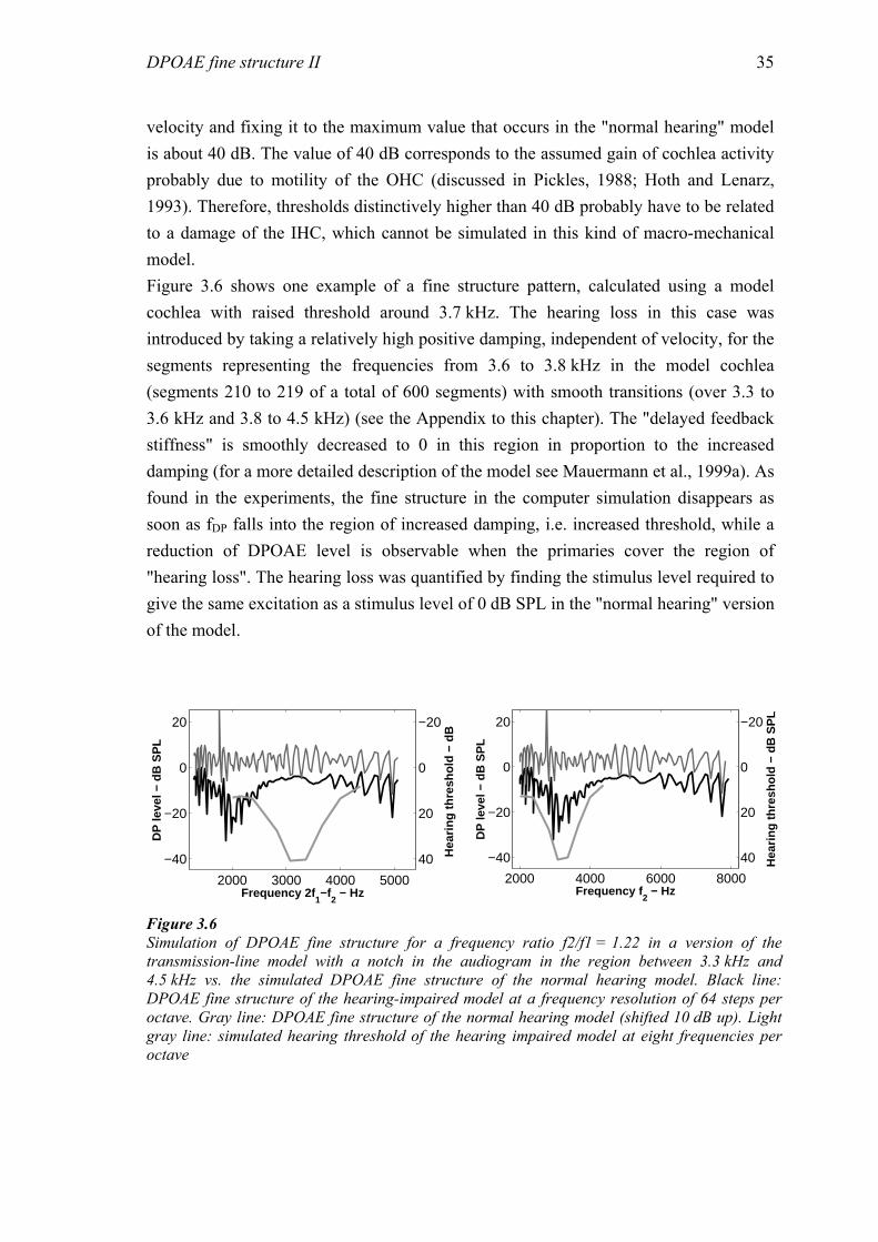
DPOAE fine structure II 35

velocity and fixing it to the maximum value that occurs in the "normal hearing" model is about 40 dB. The value of 40 dB corresponds to the assumed gain of cochlea activity probably due to motility of the OHC (discussed in Pickles, 1988; Hoth and Lenarz, 1993). Therefore, thresholds distinctively higher than 40 dB probably have to be related to a damage of the IHC, which cannot be simulated in this kind of macro-mechanical model. Figure 3.6 shows one example of a fine structure pattern, calculated using a model cochlea with raised threshold around 3.7 kHz. The hearing loss in this case was introduced by taking a relatively high positive damping, independent of velocity, for the segments representing the frequencies from 3.6 to 3.8 kHz in the model cochlea (segments 210 to 219 of a total of 600 segments) with smooth transitions (over 3.3 to 3.6 kHz and 3.8 to 4.5 kHz) (see the Appendix to this chapter). The "delayed feedback stiffness" is smoothly decreased to 0 in this region in proportion to the increased damping (for a more detailed description of the model see Mauermann et al., 1999a). As found in the experiments, the fine structure in the computer simulation disappears as soon as fDP falls into the region of increased damping, i.e. increased threshold, while a reduction of DPOAE level is observable when the primaries cover the region of "hearing loss". The hearing loss was quantified by finding the stimulus level required to give the same excitation as a stimulus level of 0 dB SPL in the "normal hearing" version of the model.

−20

0

20

40 Hea

ring

thre

shol

d −

dB

2000 3000 4000 5000

−40

−20

0

20

Frequency 2f1−f

2 − Hz

DP

leve

l − d

B S

PL

−20

0

20

40 Hea

ring

thre

shol

d −

dB S

PL

2000 4000 6000 8000

−40

−20

0

20

Frequency f2 − Hz

DP

leve

l − d

B S

PL

Figure 3.6 Simulation of DPOAE fine structure for a frequency ratio f2/f1 = 1.22 in a version of the transmission-line model with a notch in the audiogram in the region between 3.3 kHz and 4.5 kHz vs. the simulated DPOAE fine structure of the normal hearing model. Black line: DPOAE fine structure of the hearing-impaired model at a frequency resolution of 64 steps per octave. Gray line: DPOAE fine structure of the normal hearing model (shifted 10 dB up). Light gray line: simulated hearing threshold of the hearing impaired model at eight frequencies per octave

DPOAE fine structure II 36

IV. DISCUSSION Most previous studies on DPOAE from hearing-impaired subjects related DPOAE levels to hearing thresholds based on only a comparatively low number of frequencies. In the only study dealing with DPOAE from hearing impaired subjects with a high frequency resolution (He and Schmiedt, 1996) it was concluded that a fine structure would always be observable as long as DPOAE can be recorded. Their study included 14 hearing-impaired subjects, all of them had a more or less steep high-frequency hearing loss. This conclusion of unaffected fine-structure holds only for one subject (JK, Figure 3.4) from this investigation, while the others showed a substantial decrease of DPOAE fine structure when 2f1-f2 fell into a region of hearing loss. The subjects presented here were selected because of the particular shape of their audiograms with either raised thresholds or normal hearing in a limited frequency band only. This sample might not be representative for the clinical population, but it permitted measurements with either the primary frequencies or the distortion product frequencies covering a region of cochlear damage, motivated by the results and computer simulations reported in the accompanying paper (Mauermann et al., 1999a; see Chapter 2). Consequently our data will be discussed in respect to the two-source model of DPOAE generation. The experiments were not intended as a representative clinical study. Nevertheless, the results might still improve the value of DPOAE as a diagnostic tool. The initial generation of DPOAE is due to nonlinear distortion at the primary site close to f2. The cases reported in Figures 3.1 to 3.3 exhibit a coincidence of the disappearance of DPOAE fine structure with damage at the characteristic place of fDP. This strongly supports the interpretation of the data in terms of a two-source model of DPOAE generation, as discussed in the accompanying paper for normal hearing subjects (Mauermann et al., 1999a). If only the component generated in the primary region contributes to the emission measured in the ear canal, no fine structure can be observed. When there is also a contribution from the re-emission site at fDP, a quasi-periodic fine structure is observable, i.e. DPOAE can be treated as the vector sum of two different components, as suggested by Brown et al. (1996). Heitmann et al. (1998) showed that the presentation of an additional suppressor tone close to fDP (25 Hz above fDP) causes a disappearance of fine structure due to suppression of the component from the fDP place. As demonstrated here, damage in the DP frequency region has a similar effect to the suppressor. While the addition of a third tone could cause unwanted side effects when investigating the DP generation mechanisms, such as additional distortion products (Harris et al., 1992), the experiments presented here take advantage of the "naturally" reduced cochlear activity. As already reported in previous studies (e.g. Schlögel et al., 1995), it is not uncommon

DPOAE fine structure II 37

for subjects with high frequency hearing loss to have DPOAE not substantially different in level from those from normal hearing subjects, even when the primaries fall into the region of a hearing loss of 30 dB or more. Two more examples for this are the subjects RH and HL in this study (cf. Figure 3.3). However, DPOAE fine structure disappeared in both subjects as soon as fDP fell into a region of even slightly raised thresholds (i.e. above 2.5 kHz for subject HL, above 4 kHz for subject RH). This suggests that a moderate cochlear damage can already influence the reemission component of the DPOAE. A similar interpretation holds for the DPOAE fine structure during recovery from a mild sudden hearing loss shown in Figure 3.5. The reduced fine-structure after four months might indicate still some slight damage, although the threshold - as measured in the clinical audiogram with its accuracy of about ±5 dB and its limited frequency resolution - had already recovered. This high vulnerability to cochlear damage of the DPOAE fine structure has also been noticed in other studies. Engdahl and Kemp (1996) showed that noise exposure causing a temporary threshold shift results in a temporary disappearance of DPOAE fine structure. Furthermore the fine structure gets reduced during aspirin consumption before an overall DPOAE level reduction can be observed (Rao et al., 1996; Long 1999 - personal communication). Overall, it appears as if the consideration of fine structure can serve as a more sensitive tool for the detection of slight cochlear damage in certain cases than the DPOAE level alone. However, a prospective clinical study involving more subjects would be required to evaluate this possible application. In contrast to the subjects discussed so far, the DPOAE from subject JK (Figure 3.4) appears to behave differently: DPOAE level decreases with increasing hearing loss while the fine structure is unaffected. This behavior is more in line with the data reported by He and Schmiedt (1996). The seeming contradiction to our other data can be interpreted as follows. When the primary at f2 falls into a region of a distinct hearing loss, i.e. above 4 kHz for this subject, no measurable initial DPOAE component is generated. Consequently no reflection component from the reemisson site close to fDP can be recorded. However, when f2 is below 4 kHz, the corresponding fDP frequency still falls into a region of normal or near normal hearing for this subject (i.e., threshold of 20 dB HL or better), which is sufficient to create the reemission component due to coherent reflection. The interaction of the two components generates the fine structure. A similar explanation would also hold for most of the subjects described by He and Schmiedt (1996) who had a steep high frequency hearing losses. The effects of frequency specific hearing loss on DPOAE fine structure can be simulated in a realistic way using the "hearing impaired" version of the computer model of the cochlea (cf. Figure 3.2 and Figure 3.6). The very good correspondence between data and simulations even in the case of hearing impairment gives further support for a

DPOAE fine structure II 38

whole class of similar cochlea models recently described in Talmadge et al. (1999). In the model the generation mechanisms for the two sources are different. The reemission component can be interpreted as a coherent reflection sensitive (1) to the presence of "roughness" and (2) to the presence of broad and tall excitation patterns (e.g. Talmadge et al., 1998), which are generated by an active feedback mechanism. The initial generation - which is not sensitive to the presence of roughness (see Mauermann et al., 1999a; Talmadge et al., 1998) is not connected to coherent reflection but should be interpreted as a consequence of nonlinear distortion only. This view of two different mechanisms is in agreement with the conclusions drawn by Shera and Guinan (1999). They also distinguish two DPOAE mechanisms: coherent reflection from the fDP site (similar to SFOAE) and nonlinear distortion from the generation site near f2. The different effects on DPOAE fine structure and overall level caused by cochlear damage, as reported in our experiments, might reflect an experimental confirmation of two different generation mechanisms.

V. CONCLUSIONS • Distortion product emissions measured in the human ear canal are produced by two

sources, one at the characteristic place of the primaries and the second at the characteristic place of fDP.

• The DPOAE fine structure is mainly influenced by the local state of the cochlea at the characteristic place of fDP and appears to be a more sensitive indicator of cochlear damage than DPOAE level alone.

• At least from the model point of view the initial generation at the site close to f2 is caused by nonlinear interaction of the primaries while the re-emission from the characteristic site of fDP can be treated as a coherent reflection .

• The evaluation of fine structure could improve considerably the clinical use of DPOAE, e.g., for early identification of hearing loss or to monitor the recovery from a sudden hearing loss more accurately.

ACKNOWLEDGEMENTS This study was supported by Deutsche Forschungsgemeinschaft, DFG Ko 942/11-2. Helpful comments by Brian Moore and Glenis Long on an earlier version of the manuscript are gratefully acknowledged.

DPOAE fine structure II 39

APPENDIX The nonlinearity in the model is introduced by a nonlinear damping d(x,v) and a stabilizing "delayed feedback stiffness" c(v) (see Mauermann et al., 1999a).

( ) | |( , ) ( )1 | |

h ll

d d vd x v d ms xv

ββ

−= + + (A1 a)

||1||)(

vvdcvc l

l ββ+

−+= (A1 b)

where v is the velocity of basilar membrane (BM) section; m is the mass (0.375 kg/m2); x is the distance to the base of the cochlea;s is the stiffness of BM section; dl is the damping parameter, determines the damping at low BM velocities (dl is - 0.12 in the "normal hearing" model); dh is the damping parameter, determines the damping at high BM velocities (dh is 0.5 in the "normal hearing" model); cl is the parameter of delayed feedback stiffness (cl is 0.1416 in the "normal hearing" model); β is the parameter to

determine the shape of the nonlinear damping function.

The hearing loss was introduced by taking ( )d x v dh, = in the region from 3.6 kHz to

3.8 kHz with smooth transitions (over 3.3 to 3.6 kHz and 3.8 to 4.5 kHz). This could be

done in by letting β → ∞ . Because this is impossible in practice we let ( )β d dh l− go

to 0 and ld go to dh simultaneously. In correspondence to the increased damping the

"delayed feedback stiffness" c(v) is smoothly decreased to 0 in this region.

Chapter 4

The influence of the second source of distortion product otoacoustic emissions (DPOAE) on DPOAE input/output functions a)

It is widely accepted that distortion product otoacoustic emissions (DPOAE) at 2f1-f2 (f2/f1=1.2) have two components from different cochlear sources, i.e. a distortion component generated near f2 and a reflection component from the characteristic site of fDP. This may have an adulterant effect on the DPOAE input/output (I/O) functions that are used to predict auditory threshold or the compression characteristics of the basilar membrane and thus may decrease their accuracy. This study therefore investigates the influence of the contribution of the reflection component on DPOAE I/O functions. DPOAE are measured in six subjects over a frequency range for f2 from 1500-4500 Hz (18 Hz steps) at seven levels L2 from 20 to 80 dB SPL (L1 = 0.4⋅L2 + 39 dB SPL). A time windowing procedure is used to separate the components from the two DPOAE sources. With decreasing stimulus level the relative contribution of the reflection component increases and even exceeds the contribution of the distortion component at low levels for most of the subjects. I/O functions from the separated distortion component (DCOAE I/O functions) show smooth changes in shape and slope with frequency, while “standard” DPOAE I/O functions show rapid changes between adjacent frequencies indicating a strong influence from the interference with the second DPOAE source. Boege and Janssen suggested a method to predict individual pure tone threshold from DPOAE I/O functions [J. Acoust. Soc. Am. 111, 1810-1818 (2002)]. The usage of DCOAE instead of DPOAE I/O functions leads here to a clear reduction of variability in the prediction of pure tone thresholds between adjacent frequencies. This strongly indicates a clear improvement of this method when eliminating the effects of the second DPOAE source.

a) A modified version of this chapter is published as: Mauermann, M., and Kollmeier, B. (2004), “Distortion product otoacoustic emission (DPOAE) input/output functions and the influence of the second DPOAE source,” J. Acoust Soc. Am. ,in press

DPOAE I/O functions 42

INTRODUCTION Narrow-band distortion product otoacoustic emissions (DPOAE) are low-level sinusoids recordable in the occluded ear canal at certain combination frequencies during continuous stimulation with two tones at the frequencies f1 < f2. They are the result of the nonlinear interaction of the two tones in the cochlea. The recording of DPOAE is claimed to be useful as an objective audiometric test with a high frequency selectivity by various clinical studies. But in the most studies the reported correlation of audiometric thresholds and DPOAE levels is only based on large averaged databases of many subjects and allows no individual threshold prediction (e.g. Nelson and Kimberley, 1992, Gorga et al., 1993; Moulin et al., 1994; Suckfüll et al., 1996). Typically the DPOAE levels measured at moderate stimulus levels were correlated to hearing threshold. In more recent studies DPOAE I/O functions are used as tool to determine the characteristics of BM compression (Buus et al., 2001) or are discussed to be used for the prediction of loudness growth, i.e. to indicate recruitment in subjects with cochlear hearing loss (Neely et al., 2003). Boege and Janssen (2002, see also Gorga et al., 2003) suggested a method to predict thresholds based on individual DPOAE I/O functions which improves the individual and quantitative prediction of threshold remarkably although there are still large standard errors of the predicted thresholds. Both, the objective prediction of auditory threshold and the prediction of recruitment is of extended interest as audiometric tool. Especially in young children they may serve as important input parameters for a hearing aid fitting. However, in agreement with theoretical and experimental work (Brown et al. 1996; Gaskill and Brown, 1996; Heitmann et al., 1998; Talmadge et al., 1998, 1999; Mauermann, 1999 a,b; Shera and Guinan, 1999) it is widely accepted that the DPOAE at 2f1-f2 in human subjects with f2/f1 around 1.2 can be interpreted as the vector sum of two components from different cochlear sources: An initial component with its source close to f2 and a second component from the characteristic site of the distortion product frequency, e.g. 2f1-f2. Several factors indicate that the effects caused by the second source are highly relevant at least in normal or near normal hearing subjects. The two interfering DPOAE components originate at two different places on the BM and they show different phase characteristics (e.g. Shera and Guinan, 1999). The components interfere constructively when in phase at some frequencies while they cancel out each other when out of phase at other frequencies. When DPOAE are measured with a sufficiently high frequency resolution the DPOAE level shows large quasi-periodic variations (up to 20 dB) with frequency, the so called DPOAE fine structure (e.g. Mauermann et al.; 1997b). Such large interference effects occur only when both vector components have a similar magnitude. In some subjects the second or "reflection

DPOAE I/O functions 43

component" even exceeded the contribution from the initial distortion source (Talmadge et al., 1999). Furthermore, multiple reflections on the basilar membrane between the oval window and the characteristic site of fDP can add even more significant components and hence influence the observed DPOAE fine structure (Dhar et al. 2002). Furthermore DPOAE fine structure patterns show a level dependent shift in frequency (He and Schmiedt, 1993; Mauermann et al. 1997b). This shift can cause notches in DPOAE I/O functions for some frequencies especially around fine structure minima (He and Schmiedt, 1993). Overall the slope and shape of DPOAE I/O functions appears to be strongly influenced by the position of the selected frequency within DPOAE fine structure. But the maxima and minima of DPOAE fine structure are not explicitly related to the local cochlea status around the characteristic place of f2

1. All these level-dependent and frequency-dependent interference effects between the two components are probably one reason for the variability that can be observed in DPOAE I/O functions and derived predictions (see e.g. Boege and Janssen, 2002; Gorga et al., 2003). Nevertheless none of the studies (as far as known by the authors) using DPOAE I/O functions (at a fixed f2/f1 ratio) for the prediction of hearing capabilities takes those effects into account. The current study therefore investigates to what extent DPOAE I/O functions are affected by the contribution of the second source and if the variability in predictions derived from DPOAE I/O functions can possibly be reduced when considering the contribution from the second source. Until now in studies on the contribution of the second source mainly measurements at moderate primary levels had been investigated (e.g. Talmadge, 1999; Mauermann et al., 1999a, b; Kaluri and Shera, 2001) not at a whole range of different levels that is needed to characterize the influence of the second source on DPOAE I/O functions. There are some indications that the relative influence of the second source changes with stimulus level, e.g. in some subjects the DPOAE fine structure flattens out with increasing level (e.g. Mauermann et al.; 1997b). Konrad-Martin et al. (2001) investigated the energy of low and high latency components from DPOAE measurements for a fixed f2 paradigm. For a level paradigm L1=L2+10 dB they found the low latency component increasing faster than the high latency component. But there is no detailed investigation to which extent the relative contribution of the second source may change with primary levels at a fixed frequency ratio f2/f1 and therefore may affect DPOAE I/O functions. To clarify this point in a first step of this study, "standard" two source DPOAE I/O functions (L2: 20-80 dB in 10 dB steps) for frequencies f2 from 1500 to 4500 Hz are compared with I/O functions of the contribution of only the initial "distortion component" (from the f2 place). We refer to these I/O functions from the “distortion component only” as “distortion component otoacoustic emission I/O functions” (DCOAE I/O functions). To obtain

DPOAE I/O functions 44

these DCOAE I/O functions it is required to separate the DPOAE components from the two sources. Recent studies on DPOAE component separation (e.g. Knight and Kemp, 2001; Kalluri and Shera 2001) suggest two methods to unmix the DPOAE components: time windowing and selective suppression. Both methods show similar results (Kalluri and Shera, 2001): a smoothed DP-Gram (DPOAE level as function of frequency). However, in these studies only a fixed set of primary levels has been investigated, no DPOAE I/O functions. Since adequate suppressor levels for the method of selective suppression are not known yet for a whole range of primary levels that are necessary for this paradigm in the current study the method of time windowing is used. Beside the aspect that DCOAE have the theoretical advantage to be generated at a single cochlear site only (that allows a easier frequency specific interpretation of the I/O functions), the comparison of DPOAE and DCOAE I/O functions in the first step of the current study indicates a strong reduction in variability of I/O functions from adjacent frequencies. This could also lead to a reduced variability in threshold predictions derived from these I/O functions. Therefore we investigate in a second step whether methods for the prediction of pure tone thresholds from DPOAE measurements (Boege and Janssen, 2002; Gorga et al., 2003) can be improved when using DCOAE instead of DPOAE I/O functions as base for threshold predictions. Boege and Janssen (2002) and Gorga et al. (2003) exclude those DPOAE I/O functions from further use for prediction that do not satisfy certain criteria. Possibly these functions failed the inclusion criteria because of level and frequency-dependent interference effects of the two sources and even the included DPOAE I/O functions may be affected by contributions of the second DPOAE source. This may lead to an additional variation in the prediction of pure tone thresholds. For a useful prediction of hearing capabilities from DPOAE I/O functions (like hearing threshold) it should be expected that adjacent frequencies give almost similar results, i.e. show only a smooth change with frequency and a low variability between adjacent frequencies. Since there are no behavioral threshold measurement performed in this study (except standard audiogram for a rough classification of the subjects) as indication for an improvements of threshold prediction we would expect (1) a reduction in the number of rejected I/O functions and (2) a reasonably reduced variability of predicted thresholds for adjacent frequencies. To check for a potential gain by the use of DCOAE I/O functions, thresholds estimations and I/O slopes (according to Boege and Janssen, 2002) are computed and compared from both (1) "standard" DPOAE I/O functions and from (2) DCOAE I/O functions at adjacent frequencies (f2 in steps of 18 Hz). Another considerable factor most probably responsible for deviations of the threshold

DPOAE I/O functions 45

prediction from DPOAE I/O functions is the calibration of the probe speakers due to standing waves in the sealed ear canal at certain frequencies. To estimate the relevance of the expected variability in the prediction from adjacent frequencies due to the influence of the second source in relation to the influence of different calibration paradigms, the predictions from measurements with a coupler calibration are compared with predictions from measurements from an in-the-ear calibration for three subjects. The differences in the threshold predictions are compared with the assumed variability due to the influence of the second DPOAE source.

I. EXPERIMENTAL METHODS

A. Subjects DPOAE data were collected from the right ears of six subjects aged from 21 to 50 years. Five normal hearing subjects (AP, BS, IT, JF and MO) had hearing thresholds better than 15 dB HL at the standard audiometric frequencies from 125 Hz to 8 kHz and one subject (AS) showed a moderate high frequency loss (30, 35, 20 dB HL at 4, 6 and 8 kHz respectively). All subjects had normal middle ear function which was tested by tympanometric measurements (Interacoustics AZ26). During the measurement sessions of 90-120 min duration the subjects were seated comfortably in an sound-treated booth.

B. Instrumentation and signal processing An insert microphone, type ER10B+ (Etymotic Research) is used to record the DPOAE in the closed ear canal. The microphone output is connected to a low noise amplifier, type SR560 (Stanford Research) and then converted to digital form using a 24 bit ADI-8 Pro AD/DA converter (RME) which is connected optically to a Digi96/8 PAD (RME) digital I/O card in a personal computer (PC). Further on-line analysis is performed within a custom made Matlab (Vers. 6.5, Mathworks) based measurement software on a PC. All stimuli are generated and attenuated digitally. The output of the DA converters (ADI 8 Pro, 24 bit) is connected to two separate TDT-HB7 headphone buffers (Tucker Davies Technologies). These drive separately either two ER2 insert ear phones (Etymotic Research) or two encapsulated speakers of a DT48 headphone (Beyerdynamics) that are plugged with elastic sound tubes to the ER10B. The on-line analysis is used for signal conditioning of the recorded signal including artifact rejection and averaging in the time domain to improve the signal to noise ratio. Time frames of 1/3 second length are used (16000 samples at a sampling frequency of 48000 Hz or 14700 samples at 44100 Hz). This allows to select primary frequencies for continuous stimulation as harmonics of 3 Hz. Selecting f2 frequencies as harmonics of 18 Hz and the related f1 frequencies as harmonics of 15 Hz (both harmonics of 3 Hz) give primary

DPOAE I/O functions 46

frequency pairs with an exact frequency ratio f2/f1 of 1.2. The two primaries are presented via two separated speakers. For each frame the noise floor around 2f1-f2 is estimated by the average soundpressure computed from 15 samples above and below the 2f1-f2 sample in the DPOAE spectrum. The automatic artifact rejection is based on the individual noise floor computed for each frame. The rejection criteria adapts during the measurement to decrease the averaged noise floor. During each measurement all recorded frames are kept in memory. The frames to be averaged are selected from all recorded frames by the actual rejection criterion. The averaging stops automatically if the averaged noise floor is at 20 dB SPL or below and the S/N reaches 12 dB. The measurement does not stop before a minimum number of 4 averaged frames but it always stops when 128 valid averaged frames or 256 recorded frames are done. At the beginning of each measurement session the correct fit of the probe in the ear canal is checked. Therefore the ear canal response to a broadband stimulus is investigated. During a measurement session this “probefit procedure” is repeated always after 20-40 measurement points to check for the stability of the probe fit.

C. Calibration As default, level and phase characteristic of the speakers connected to the ER10B+ probe microphone system are calibrated using an artificial ear for insert probes (Bruel & Kjaer BK4152). No further individual phase correction during the measurements is performed. The overall level is slightly adjusted for each subject to compensate for the individual ear canal volume (less than ± 1dB). The microphone is calibrated as suggest by Siegel (2002) using a Bruel & Kjaer coupler microphone (B&K 4192) as reference. In the following we refer to this calibration as coupler calibration. For three of the six subjects additional measurements are performed using an in-the- ear calibration procedure for the speakers instead of the coupler calibration. In these cases the data from the probe fit procedure are used to determine the level and phase characteristics of the speakers at the probe microphone in the individual ear canal. Calibration values of intermediate frequencies not covered by the probefit signal are obtained from a cubic spline interpolation of the real and imaginary parts of the spectra recorded in the ear canal.

D. DPOAE measurements DPOAE at 2f1-f2 (f2/f1=1.2) are measured with a high frequency resolution of 12 Hz at seven levels L2 from 20 to 80 dB in 10 dB steps. The corresponding L1 levels are chosen according to the formula L1 = 0.4 · L2 + 39 dB as suggested by Kummer et al. (1998). This results in maximum DPOAE levels and an almost logarithmic

DPOAE I/O functions 47

characteristic of the DPOAE levels as function of L2 (Boege and Janssen, 2002). The DPOAE are measured over a frequency range for f2 from 1500-4500 Hz divided into four frequency bands (a) 1.5-2.25 kHz, (b) 2.25-3 kHz, (c) 3-3.75 kHz, and (d) 3.75-4.5 kHz. Within each band all 301 measurement points (43 frequencies at 7 levels) are randomized to avoid systematic effects in the data with measurement duration. In a measurement session of about 90 to 120 min duration normally one of the frequency bands is measured. The order of the bands is randomized. The results of the four frequency bands are finally joined and used for further analysis.

II. DATA ANALYSIS

A. Separation of DPOAE components via time windowing Earlier studies (e.g. Kaluri and Shera, 2001) have shown that DPOAE at a frequency ratio f2/f1 = 1.2 can be treated as the interference of two components with very different phase slope or group delay. This property is used by the method of time windowing to separate the two DPOAE components. Time windowing or spectral smoothing has been used by several authors in slightly modified form (e.g. Knight and Kemp, 2001; Kalluri and Shera, 2001). The DP-Gram data are transformed to the time or latency domain using an inverse fast Fourier transform (IFFT). In the time domain a large phase gradient with frequency, i.e. a long group delay, corresponds to a delayed peak in the resulting “time domain response”. Here we expect an “time-domain response” with mainly two peak regions indicating the different latencies of the two interfering DPOAE components that can be separated by multiplication with an adequate time window2. Transforming the low latency components back to the frequency domain by a fast Fourier transform (FFT) results in a smoothed DP-Gram representing the DPOAE levels from the initial distortion source near f2 only. The implemented evaluation procedure converts the measured pressure amplitude und phase spectra from the measured DP-Grams into their real and imaginary parts for each frequency. The array of complex values is shifted in frequency down to the lowest frequency bin above zero. The complex spectrum is extended by its negative frequencies3 using the complex conjugated values of the positive frequencies mirrored at zero. To avoid any discontinuity of the spectrum boundaries and hence to minimize artifacts in the IFFT4 for the bin at zero frequency a real value5 is used that is calculated from an interpolation between the positive and negative frequency values. For the same reason from each DP-Gram a frequency range is selected for the IFFT in the way that the lowest and highest frequency of the selected frequencies fit to a center of a maximum or minimum in the DP-Gram fine structure respectively such that a periodic continuation (due to the discrete signal processing) of the extended DP-Gram spectrum

DPOAE I/O functions 48

results in shapes at the boundaries that are almost typical for the shape of the whole DP-Gram. The IFFT of the complete complex spectrum results in a real time-signal representing the “time-domain response”6. The frequency resolution ∆f of 12 Hz in the measured DP-Grams corresponds to a resulting time frame T (T = 1/∆f) in the time domain of about 83 ms. This is sufficient since the “time-domain responses” disappear in the noise floor after about 60 ms. Therefore no aliasing in the time domain has to be expected. Due to the discrete signal processing, the resulting signal in the time domain can be seen as periodically repeated. The absolute position of the expected peaks is not exactly known due to unknown offsets in the group delay. Slight fluctuations of the absolute group delay can be expected, e.g. from individual variations of the relative phase of the two primaries at the ear drum. Therefore, the starting point of the time window to cut out the low latency region is chosen for each subject individually in a way that the rising edge of the first peak in the time signal is included, i.e. the time window can even start at “negative” times. The end of the time window is placed at a point at which the magnitude of the time signal has a dip between low and high latency peaks7. For reasons of convenience, the same time window is used at all primary levels, which is determined for the latency response of L2 = 40 dB SPL. This appears to be an adequate choice for the windowing of the “time-domain responses” of the different stimulation levels, too. As time window we use a rectangular window with cosine shaped ramps (eight samples at each end). The remaining time signal without the low-latency components gives the high-latency part of the time signal. The low-latency part of the time signal is transformed back to the frequency domain using a FFT resulting in a complex spectrum. From this the DCOAE amplitudes and phases are computed. For further spectral analysis and prediction of threshold, DCOAE are rejected which belong to frequencies affected by artifacts of the time windowing procedure. To do so at the beginning and at the end of the resulting spectrum a frequency range is cut out which is equal to the relevant spectral width of the low latency time window. As relevant spectral width of the time window we use 1/Twin with Twin as complete duration of the time window including the ramps. Figure 4.1 illustrates the time windowing procedure exemplarily for one subject (AP) at three levels. The left panels show the magnitudes8 of the “time-domain responses” (gray line) of the DP-Grams data at different levels. The low latency components are indicated as thick black lines, the high latency components as thin dotted black lines respectively. The comparison of low and high latency peaks for different stimulation levels (left panels) shows that for low stimulation levels the relative contribution of the high latency components is clearly higher. The right panels show the corresponding frequency domain representations of the low and high latency components and the originally measured DP-Gram as magnitude (b, e, h) and phase spectra (c, f, i).

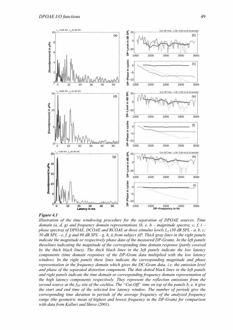
DPOAE I/O functions 49

0 10 20 30 40 500

2

4

6

8

10

|Sou

ndpr

essu

re| i

n µP

a

L1: 51dB SPL, L

2:30 dB SPL

(a)

1000 1500 2000 2500 3000

−20

0

20

DP

−Lev

el in

dB

SP

L Cut−Off Time: −1.56 / 3.65 ms (9.16 periods)

1000 1500 2000 2500 3000

−10

−5

0

DP

−Pha

se in

cyc

les

(c)

(b)

0 10 20 30 40 500

5

10

15

|Sou

ndpr

essu

re| i

n µP

a

L1: 59dB SPL, L

2:50 dB SPL

(d)

1000 1500 2000 2500 3000

−20

0

20

DP

−Lev

el in

dB

SP

L Cut−Off Time: −1.55 / 3.62 ms (9.19 periods)

1000 1500 2000 2500 3000

−10

−5

0D

P−P

hase

in c

ycle

s

(e)

(f)

0 10 20 30 40 500

5

10

15

20

25

Latency in ms

|Sou

ndpr

essu

re| i

n µP

a

L1: 71dB SPL, L

2:80 dB SPL

0 10 20 30 40 500

5

10

15

20

25

Latency in ms

|Sou

ndpr

essu

re| i

n µP

a

(g)

1000 1500 2000 2500 3000

−20

0

20

DP

−Lev

el in

dB

SP

L Cut−Off Time: −1.56 / 3.65 ms (9.16 periods)

1000 1500 2000 2500 3000

−10

−5

0

DP−Frequency in Hz

DP

−Pha

se in

cyc

les

(h)

(i)

Figure 4.1 Illustration of the time windowing procedure for the separation of DPOAE sources. Time domain (a, d, g) and frequency domain representations (b, e, h – magnitude spectra; c, f, i – phase spectra) of DPOAE, DCOAE and RCOAE at three stimulus levels L2 (30 dB SPL - a, b, c; 50 dB SPL - e, f, g and 80 dB SPL - g, h, i) from subject AP. Thick gray lines in the right panels indicate the magnitude or respectively phase data of the measured DP-Grams. In the left panels theselines indicating the magnitude of the corresponding time domain response (partly covered by the thick black lines). The thick black lines in the left panels indicate the low latency components (time domain responses of the DP-Gram data multiplied with the low latency window). In the right panels these lines indicate the corresponding magnitude and phase representation in the frequency domain which gives the DC-Gram data, i.e. the emission level and phase of the separated distortion component. The thin dotted black lines in the left panels and right panels indicate the time domain or corresponding frequency domain representation of the high latency components respectively. They represent the reflection emissions from the second source at the fDP site of the cochlea. The “Cut-Off” time on top of the panels b, e, h give the start and end time of the selected low latency window. The number of periods give the corresponding time duration in periods of the average frequency of the analyzed frequency range (the geometric mean of highest and lowest frequency in the DP-Gram) for comparison with data from Kalluri and Shera (2001).

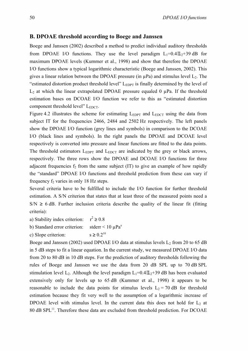
DPOAE I/O functions 50

B. DPOAE threshold according to Boege and Janssen Boege and Janssen (2002) described a method to predict individual auditory thresholds from DPOAE I/O functions. They use the level paradigm L1=0.4⋅L2+39 dB for maximum DPOAE levels (Kummer et al., 1998) and show that therefore the DPOAE I/O functions show a typical logarithmic characteristic (Boege and Janssen, 2002). This gives a linear relation between the DPOAE pressure (in µPa) and stimulus level L2. The “estimated distortion product threshold level” LEDPT is finally determined by the level of L2 at which the linear extrapolated DPOAE pressure equaled 0 µPa. If the threshold estimation bases on DCOAE I/O function we refer to this as “estimated distortion component threshold level” LEDCT. Figure 4.2 illustrates the scheme for estimating LEDPT and LEDCT using the data from subject IT for the frequencies 2466, 2484 and 2502 Hz respectively. The left panels show the DPOAE I/O function (grey lines and symbols) in comparison to the DCOAE I/O (black lines and symbols). In the right panels the DPOAE and DCOAE level respectively is converted into pressure and linear functions are fitted to the data points. The threshold estimators LEDPT and LEDCT are indicated by the grey or black arrows, respectively. The three rows show the DPOAE and DCOAE I/O functions for three adjacent frequencies f2 from the same subject (IT) to give an example of how rapidly the “standard” DPOAE I/O functions and threshold prediction from these can vary if frequency f2 varies in only 18 Hz steps. Several criteria have to be fulfilled to include the I/O function for further threshold estimation. A S/N criterion that states that at least three of the measured points need a S/N ≥ 6 dB. Further inclusion criteria describe the quality of the linear fit (fitting criteria): a) Stability index criterion: r2 ≥ 0.8 b) Standard error criterion: stderr < 10 µPa9 c) Slope criterion: s ≥ 0.210 Boege and Janssen (2002) used DPOAE I/O data at stimulus levels L2 from 20 to 65 dB in 5 dB steps to fit a linear equation. In the current study, we measured DPOAE I/O data from 20 to 80 dB in 10 dB steps. For the prediction of auditory thresholds following the rules of Boege and Janssen we use the data from 20 dB SPL up to 70 dB SPL stimulation level L2. Although the level paradigm L1=0.4⋅L2+39 dB has been evaluated extensively only for levels up to 65 dB (Kummer et al., 1998) it appears to be reasonable to include the data points for stimulus levels L2 = 70 dB for threshold estimation because they fit very well to the assumption of a logarithmic increase of DPOAE level with stimulus level. In the current data this does not hold for L2 at 80 dB SPL11. Therefore these data are excluded from threshold prediction. For DCOAE

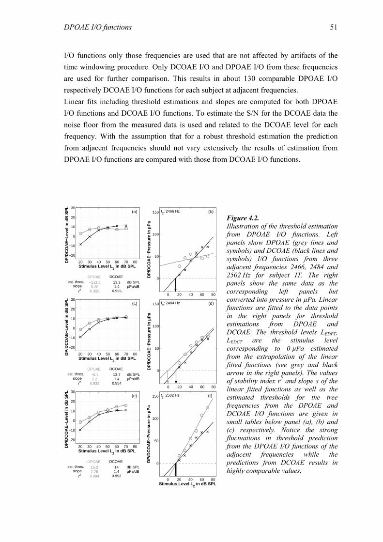
DPOAE I/O functions 51

I/O functions only those frequencies are used that are not affected by artifacts of the time windowing procedure. Only DCOAE I/O and DPOAE I/O from these frequencies are used for further comparison. This results in about 130 comparable DPOAE I/O respectively DCOAE I/O functions for each subject at adjacent frequencies. Linear fits including threshold estimations and slopes are computed for both DPOAE I/O functions and DCOAE I/O functions. To estimate the S/N for the DCOAE data the noise floor from the measured data is used and related to the DCOAE level for each frequency. With the assumption that for a robust threshold estimation the prediction from adjacent frequencies should not vary extensively the results of estimation from DPOAE I/O functions are compared with those from DCOAE I/O functions.

20 30 40 50 60 70 80

−20

−10

0

10

20

30

Stimulus Level L2 in dB SPL

(a)

0 20 40 60 80

0

50

100

150

Stimulus Level L in dB SPL

DP

/DC

OA

E−P

ress

ure

in µ

Pa

DPOAE DCOAEest. thres. slope r2

−113.30.290.326

13.31.4

0.955

dB SPLµPa/dB

(b) f2: 2466 Hz

DP

/DC

OA

E−L

evel

in d

B S

PL

20 30 40 50 60 70 80

−20

−10

0

10

20

30

Stimulus Level L2 in dB SPL

(c)

0 20 40 60 80

0

50

100

150

Stimulus Level L in dB SPL

DP

/DC

OA

E−P

ress

ure

in µ

Pa

DPOAE DCOAE est. thres. slope r2

−0.11.2

0.932

13.71.4

0.954

dB SPLµPa/dB

(d) f2: 2484 Hz

DP

/DC

OA

E−L

evel

in d

B S

PL

20 30 40 50 60 70 80

−20

−10

0

10

20

30

Stimulus Level L2 in dB SPL

DP

/DC

OA

E−L

evel

in d

B S

PL (e)

0 20 40 60 80

0

50

100

150

Stimulus Level L2 in dB SPL

DP

/DC

OA

E−P

ress

ure

in µ

Pa

DPOAE DCOAE est. thres. slope r2

15.22.260.984

141.4

0.952

dB SPLµPa/dB

(f) f2: 2502 Hz

Figure 4.2. Illustration of the threshold estimation from DPOAE I/O functions. Left panels show DPOAE (grey lines and symbols) and DCOAE (black lines and symbols) I/O functions from three adjacent frequencies 2466, 2484 and 2502 Hz for subject IT. The right panels show the same data as the corresponding left panels but converted into pressure in µPa. Linear functions are fitted to the data points in the right panels for threshold estimations from DPOAE and DCOAE. The threshold levels LEDPT, LEDCT are the stimulus level corresponding to 0 µPa estimated from the extrapolation of the linear fitted functions (see grey and black arrow in the right panels). The values of stability index r2 and slope s of the linear fitted functions as well as the estimated thresholds for the tree frequencies from the DPOAE and DCOAE I/O functions are given in small tables below panel (a), (b) and (c) respectively. Notice the strong fluctuations in threshold prediction from the DPOAE I/O functions of the adjacent frequencies while the predictions from DCOAE results in highly comparable values.

DPOAE I/O functions 52

III. RESULTS

A. Contribution of the second source to the DPOAE at different levels Figure 4.1 shows the comparison of measured DPOAE, the distortion component and the reflection component both, in the time and in the frequency domain for one subject (AP) at three stimulus levels. Analogous to the DP-Gram we refer to the magnitude of the low latency, i.e. distortion component as DC-Gram and for the reflection component as RC-Gram respectively. By comparing DC-Grams and RC-Grams, a frequency specific description of the relative contribution of the two DPOAE components is directly available. For L2 = 30 dB we see in panel (b) of Figure 4.1 that the RC-Gram clearly exceeds the contribution of the distortion component for frequencies fDP from about 1300 to 1700 Hz. For frequencies fDP up to 2400 Hz both components are almost equal while the reflection component decreases for higher frequencies. Which frequency regions are dominated by the reflection component is also directly reflected in the phase characteristic of the original DP-Gram. If the magnitude of the reflection emission exceeds the distortion component the phase of the measured DP-Gram follows the phase characteristic of the reflection emission with its strongly rotating phase, while showing almost no phase slope or group delay for frequencies dominated by the distortion component (compare Figure 4.1b and 4.1c). With increasing stimulus level the relative contribution of the reflection emission decreases for all frequencies and the phase slope of the DP-Gram data is almost identical with the phase slope of the distortion component (see Figure 4.1d). The remaining subjects show similar results as shown in Figure 4.1 for subject AP. Specifically for all subjects except IT (not shown here) the data shows that the relative contribution of the second source at lower frequencies, i.e. for fDP up to about 2200 Hz exceeds the relative contribution at higher frequencies. For subject IT the contribution from the second source appears to be almost

20 30 40 50 60 70 80−10

−5

0

5

10

Stimulus Level L2 in dB SPL

Llo

w la

t − L

high

lat i

n dB

MOJFITBSASAP

high latency dominated

low latency dominated

Figure 4.3. Differences of the levels of low and high latency components as function of stimulus level L2, derived from the time domain responses are shown for all subjects. The different lines and symbols indicate the results from the different subjects (see legend). Values below zero indicate that the DPOAEs measured in the ear canal are dominated by high latency components while positive values indicate an overall dominance of the low latency components or distortion components generated near f2. Notice the increased contribution of high latency components with decreasing stimulus level.

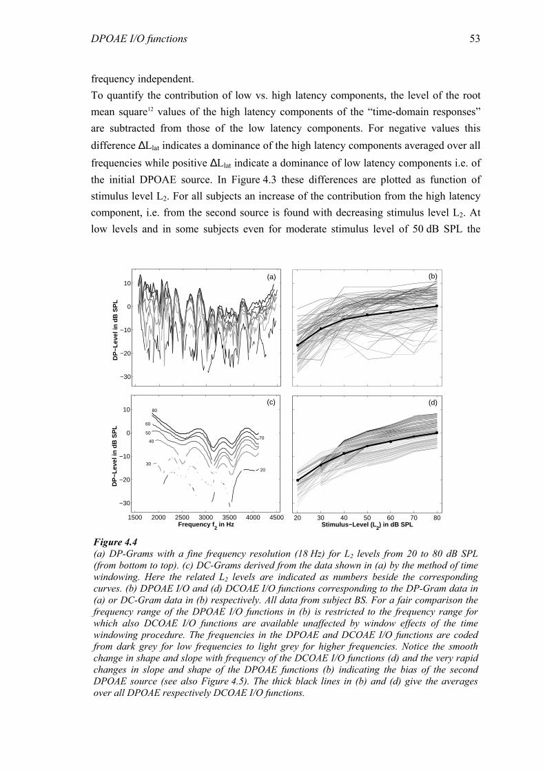
DPOAE I/O functions 53

frequency independent. To quantify the contribution of low vs. high latency components, the level of the root mean square12 values of the high latency components of the “time-domain responses” are subtracted from those of the low latency components. For negative values this difference ∆Llat indicates a dominance of the high latency components averaged over all frequencies while positive ∆Llat indicate a dominance of low latency components i.e. of the initial DPOAE source. In Figure 4.3 these differences are plotted as function of stimulus level L2. For all subjects an increase of the contribution from the high latency component, i.e. from the second source is found with decreasing stimulus level L2. At low levels and in some subjects even for moderate stimulus level of 50 dB SPL the

−30

−20

−10

0

10

DP

−Lev

el in

dB

SP

L

(a) (b)

1500 2000 2500 3000 3500 4000 4500

−30

−20

−10

0

10

Frequency f2 in Hz

DP

−Lev

el in

dB

SP

L

(c)

20 30

40

50

60

70

80

20 30 40 50 60 70 80Stimulus−Level (L

2) in dB SPL

(d)

Figure 4.4 (a) DP-Grams with a fine frequency resolution (18 Hz) for L2 levels from 20 to 80 dB SPL (from bottom to top). (c) DC-Grams derived from the data shown in (a) by the method of time windowing. Here the related L2 levels are indicated as numbers beside the corresponding curves. (b) DPOAE I/O and (d) DCOAE I/O functions corresponding to the DP-Gram data in (a) or DC-Gram data in (b) respectively. All data from subject BS. For a fair comparison the frequency range of the DPOAE I/O functions in (b) is restricted to the frequency range for which also DCOAE I/O functions are available unaffected by window effects of the time windowing procedure. The frequencies in the DPOAE and DCOAE I/O functions are coded from dark grey for low frequencies to light grey for higher frequencies. Notice the smooth change in shape and slope with frequency of the DCOAE I/O functions (d) and the very rapid changes in slope and shape of the DPOAE functions (b) indicating the bias of the second DPOAE source (see also Figure 4.5). The thick black lines in (b) and (d) give the averages over all DPOAE respectively DCOAE I/O functions.

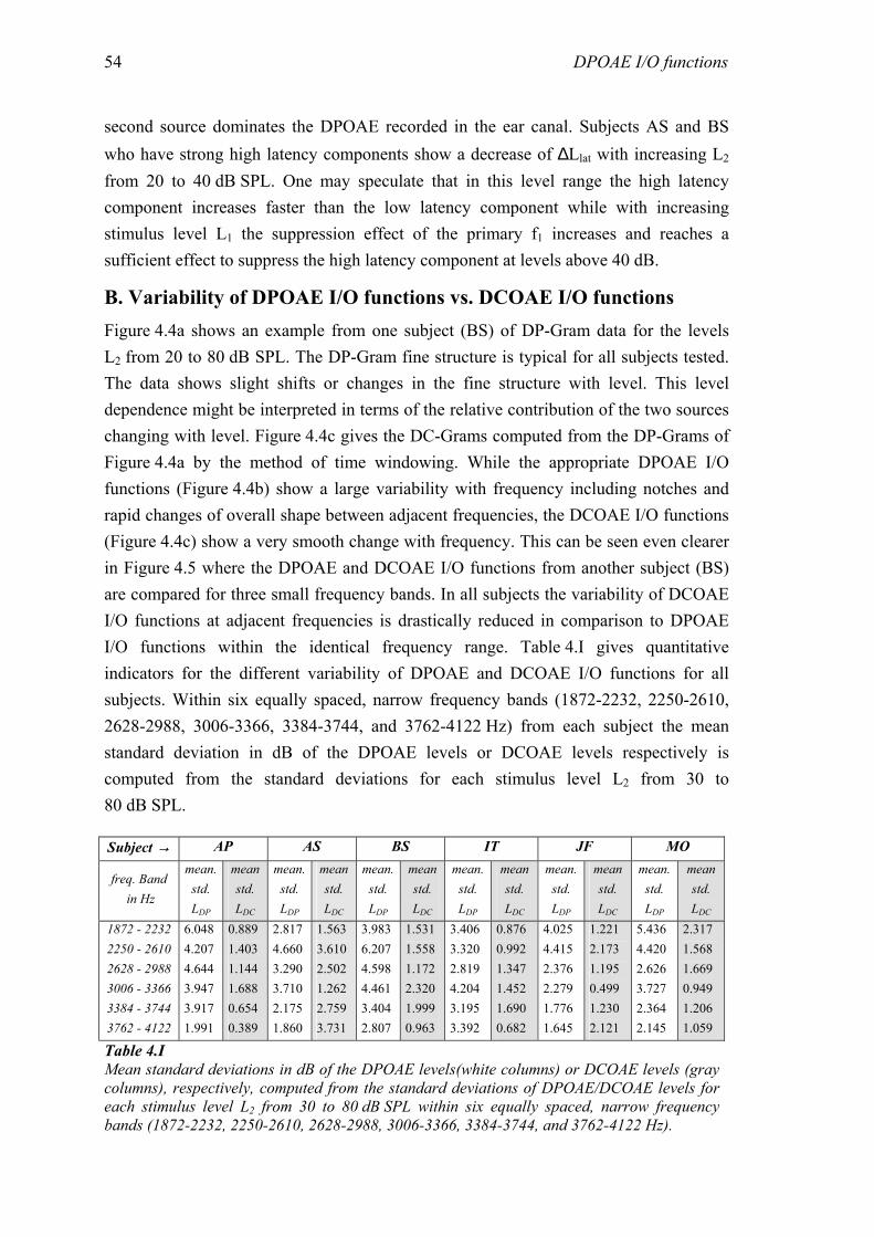
DPOAE I/O functions 54

second source dominates the DPOAE recorded in the ear canal. Subjects AS and BS who have strong high latency components show a decrease of ∆Llat with increasing L2 from 20 to 40 dB SPL. One may speculate that in this level range the high latency component increases faster than the low latency component while with increasing stimulus level L1 the suppression effect of the primary f1 increases and reaches a sufficient effect to suppress the high latency component at levels above 40 dB.

B. Variability of DPOAE I/O functions vs. DCOAE I/O functions Figure 4.4a shows an example from one subject (BS) of DP-Gram data for the levels L2 from 20 to 80 dB SPL. The DP-Gram fine structure is typical for all subjects tested. The data shows slight shifts or changes in the fine structure with level. This level dependence might be interpreted in terms of the relative contribution of the two sources changing with level. Figure 4.4c gives the DC-Grams computed from the DP-Grams of Figure 4.4a by the method of time windowing. While the appropriate DPOAE I/O functions (Figure 4.4b) show a large variability with frequency including notches and rapid changes of overall shape between adjacent frequencies, the DCOAE I/O functions (Figure 4.4c) show a very smooth change with frequency. This can be seen even clearer in Figure 4.5 where the DPOAE and DCOAE I/O functions from another subject (BS) are compared for three small frequency bands. In all subjects the variability of DCOAE I/O functions at adjacent frequencies is drastically reduced in comparison to DPOAE I/O functions within the identical frequency range. Table 4.I gives quantitative indicators for the different variability of DPOAE and DCOAE I/O functions for all subjects. Within six equally spaced, narrow frequency bands (1872-2232, 2250-2610, 2628-2988, 3006-3366, 3384-3744, and 3762-4122 Hz) from each subject the mean standard deviation in dB of the DPOAE levels or DCOAE levels respectively is computed from the standard deviations for each stimulus level L2 from 30 to 80 dB SPL.

Subject → AP AS BS IT JF MO

freq. Band in Hz

mean. std. LDP

mean std. LDC

mean. std. LDP

mean std. LDC

mean.std. LDP

mean std.LDC

mean.std. LDP

mean std. LDC

mean.std. LDP

mean std. LDC

mean. std. LDP

mean std. LDC

1872 - 2232 2250 - 2610 2628 - 2988 3006 - 3366 3384 - 3744 3762 - 4122

6.048 4.207 4.644 3.947 3.917 1.991

0.889 1.403 1.144 1.688 0.654 0.389

2.817 4.660 3.290 3.710 2.175 1.860

1.563 3.610 2.502 1.262 2.759 3.731

3.983 6.207 4.598 4.461 3.404 2.807

1.531 1.558 1.172 2.320 1.999 0.963

3.406 3.320 2.819 4.204 3.195 3.392

0.876 0.992 1.347 1.452 1.690 0.682

4.025 4.415 2.376 2.279 1.776 1.645

1.221 2.173 1.195 0.499 1.230 2.121

5.436 4.420 2.626 3.727 2.364 2.145

2.317 1.568 1.669 0.949 1.206 1.059

Table 4.I Mean standard deviations in dB of the DPOAE levels(white columns) or DCOAE levels (gray columns), respectively, computed from the standard deviations of DPOAE/DCOAE levels for each stimulus level L2 from 30 to 80 dB SPL within six equally spaced, narrow frequency bands (1872-2232, 2250-2610, 2628-2988, 3006-3366, 3384-3744, and 3762-4122 Hz).

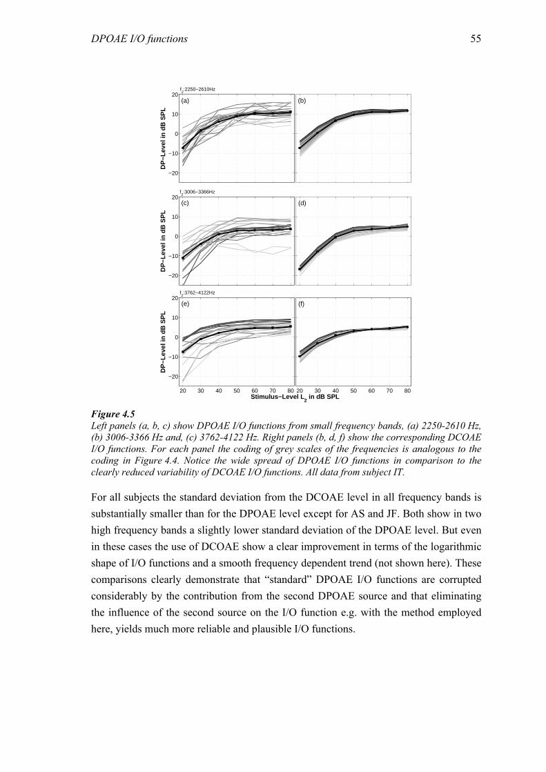
DPOAE I/O functions 55

For all subjects the standard deviation from the DCOAE level in all frequency bands is substantially smaller than for the DPOAE level except for AS and JF. Both show in two high frequency bands a slightly lower standard deviation of the DPOAE level. But even in these cases the use of DCOAE show a clear improvement in terms of the logarithmic shape of I/O functions and a smooth frequency dependent trend (not shown here). These comparisons clearly demonstrate that “standard” DPOAE I/O functions are corrupted considerably by the contribution from the second DPOAE source and that eliminating the influence of the second source on the I/O function e.g. with the method employed here, yields much more reliable and plausible I/O functions.

−20

−10

0

10

20

DP

−Lev

el in

dB

SP

L

f2:2250−2610Hz

(a) (b)

−20

−10

0

10

20

DP

−Lev

el in

dB

SP

L

f2:3006−3366Hz

(c) (d)

20 30 40 50 60 70 80

−20

−10

0

10

20

Stimulus−Level L2 in dB SPL

DP

−Lev

el in

dB

SP

L

f2:3762−4122Hz

20 30 40 50 60 70 80

(e) (f)

Figure 4.5 Left panels (a, b, c) show DPOAE I/O functions from small frequency bands, (a) 2250-2610 Hz, (b) 3006-3366 Hz and, (c) 3762-4122 Hz. Right panels (b, d, f) show the corresponding DCOAE I/O functions. For each panel the coding of grey scales of the frequencies is analogous to the coding in Figure 4.4. Notice the wide spread of DPOAE I/O functions in comparison to the clearly reduced variability of DCOAE I/O functions. All data from subject IT.

DPOAE I/O functions 56

C. Variability of threshold prediction from DPOAE I/O and DCOAE I/O functions

Figure 4.2 gives an example for the variability of threshold prediction from DPOAE I/O functions for one subject (IT). For three adjacent frequencies (2466, 2484 and 2503 Hz) the DCOAE I/O functions and the prediction of hearing threshold LEDCT are almost the same (LEDCT ≈14 dB SPL, slope =1.4). On the other hand, the DPOAE I/O functions vary remarkably. This holds as well for the derived prediction of threshold and the slope of the linear function fitted to the data. This strong fluctuation of threshold predictions from DPOAE I/O functions is quite typically for most subjects. Figure 4.6 illustrates that the threshold predictions LEDCT from DCOAE I/O functions (thin black lines) change smoothly with frequency for all subjects while LEDPT as function of frequency (grey thick lines) results in a strongly fluctuating pattern in most of the subjects. The same holds for the slope (see Figure 4.7) of the fitted linear functions, that also is used as indicator of hearing status in several studies (e.g. Kummer et al. 1998). To give quantitative indicators about the different variability in threshold estimations from DPOAE and DCOAE I/O functions, Table 4.II lists for each subject the standard

−20

0

20

40L

EDPT and L

EDCT

(a)

subject AP

LEDPT

and LEDCT

(b)

subject AS

−20

0

20

40

Les

t. th

res.

in d

B S

PL (c)

subject BS subject IT

(d)

2000 2500 3000 3500 4000

−20

0

20

40(e)

Frequency f2 in Hz

subject JF

2000 2500 3000 3500 4000Frequency f

2 in Hz

(f)

subject MO

Figure 4.6. Predicted thresholds from DPOAE I/O functions (gray lines) and DCOAE I/O functions (black lines) for all six subjects (in order of the panel indices: AP, AS, BS, IT, JF, MO). Predictions from frequencies not fitting the inclusion criteria of stability index r2 and standard error are left out in the plotted lines. Notice the reduced number of rejections and the smooth characteristics with frequency of the threshold predictions LEDCT from DCOAE I/O functions in comparison to the threshold predictions LEDPT from DPOAE I/O functions.

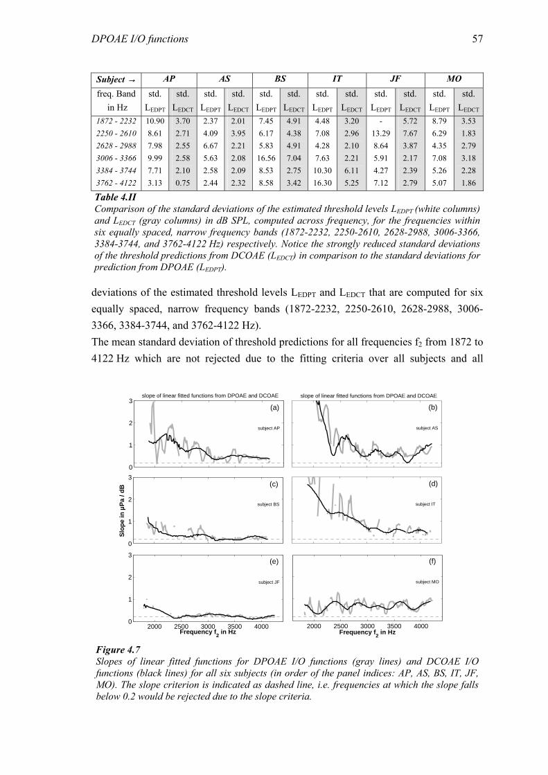
DPOAE I/O functions 57

deviations of the estimated threshold levels LEDPT and LEDCT that are computed for six equally spaced, narrow frequency bands (1872-2232, 2250-2610, 2628-2988, 3006-3366, 3384-3744, and 3762-4122 Hz). The mean standard deviation of threshold predictions for all frequencies f2 from 1872 to 4122 Hz which are not rejected due to the fitting criteria over all subjects and all

Subject → AP AS BS IT JF MO

freq. Band in Hz

std. LEDPT

std. LEDCT

std. LEDPT

std. LEDCT

std. LEDPT

std. LEDCT

std. LEDPT

std. LEDCT

std. LEDPT

std. LEDCT

std. LEDPT

std. LEDCT

1872 - 2232 2250 - 2610 2628 - 2988 3006 - 3366 3384 - 3744 3762 - 4122

10.90 8.61 7.98 9.99 7.71 3.13

3.70 2.71 2.55 2.58 2.10 0.75

2.37 4.09 6.67 5.63 2.58 2.44

2.01 3.95 2.21 2.08 2.09 2.32

7.45 6.17 5.83 16.56 8.53 8.58

4.91 4.38 4.91 7.04 2.75 3.42

4.48 7.08 4.28 7.63

10.30 16.30

3.20 2.96 2.10 2.21 6.11 5.25

- 13.29 8.64 5.91 4.27 7.12

5.72 7.67 3.87 2.17 2.39 2.79

8.79 6.29 4.35 7.08 5.26 5.07

3.53 1.83 2.79 3.18 2.28 1.86

Table 4.II Comparison of the standard deviations of the estimated threshold levels LEDPT (white columns) and LEDCT (gray columns) in dB SPL, computed across frequency, for the frequencies within six equally spaced, narrow frequency bands (1872-2232, 2250-2610, 2628-2988, 3006-3366, 3384-3744, and 3762-4122 Hz) respectively. Notice the strongly reduced standard deviations of the threshold predictions from DCOAE (LEDCT) in comparison to the standard deviations for prediction from DPOAE (LEDPT).

0

1

2

3slope of linear fitted functions from DPOAE and DCOAE

(a)

subject AP

slope of linear fitted functions from DPOAE and DCOAE

(b)

subject AS

0

1

2

3

Slo

pe in

µP

a / d

B (c)

subject BS

(d)

subject IT

2000 2500 3000 3500 40000

1

2

3(e)

Frequency f2 in Hz

subject JF

2000 2500 3000 3500 4000Frequency f

2 in Hz

(f)

subject MO

Figure 4.7 Slopes of linear fitted functions for DPOAE I/O functions (gray lines) and DCOAE I/O functions (black lines) for all six subjects (in order of the panel indices: AP, AS, BS, IT, JF, MO). The slope criterion is indicated as dashed line, i.e. frequencies at which the slope falls below 0.2 would be rejected due to the slope criteria.

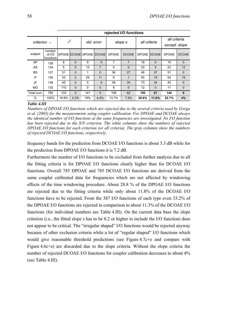
DPOAE I/O functions 58

frequency bands for the prediction from DCOAE I/O functions is about 3.3 dB while for the prediction from DPOAE I/O functions it is 7.2 dB. Furthermore the number of I/O functions to be excluded from further analysis due to all the fitting criteria is for DPOAE I/O functions clearly higher than for DCOAE I/O functions. Overall 785 DPOAE and 785 DCOAE I/O functions are derived from the same coupler calibrated data for frequencies which are not affected by windowing effects of the time windowing procedure. About 28.8 % of the DPOAE I/O functions are rejected due to the fitting criteria while only about 11.8% of the DCOAE I/O functions have to be rejected. From the 387 I/O functions of each type even 33.2% of the DPOAE I/O functions are rejected in comparison to about 11.3% of the DCOAE I/O functions (for individual numbers see Table 4.III). On the current data base the slope criterion (i.e., the fitted slope s has to be 0.2 or higher to include the I/O function) does not appear to be critical. The “irregular shaped” I/O functions would be rejected anyway because of other exclusion criteria while a lot of “regular shaped” I/O functions which would give reasonable threshold predictions (see Figure 4.7c+e and compare with Figure 4.6c+e) are discarded due to the slope criteria. Without the slope criteria the number of rejected DCOAE I/O functions for coupler calibration decreases to about 4% (see Table 4.III).

rejected I/O functions

criterion → r2 std. error slope s all criteria all criteria

except. slope

subject number of I/O

functions DPOAE DCOAE DPOAE DCOAE DPOAE DCOAE DPOAE DCOAE DPOAE DCOAE

AP 128 8 0 9 0 7 7 19 0 15 0 AS 134 5 0 15 7 0 0 23 0 23 13 BS 127 31 0 1 0 36 27 46 37 31 0 IT 130 33 2 24 11 8 1 54 19 54 19 JF 138 45 0 5 0 49 34 73 34 45 0 MO 133 110 0 0 0 8 0 12 0 11 0

Total num. 790 133 2 141 4 108 62 190 67 144 6 % 100% 16.8% 0.3% 18% 4.4% 13.7% 7.9% 28.8% 11.8% 22.7% 4%

Table 4.III Numbers of DPOAE I/O functions which are rejected due to the several criteria used by Gorga et al. (2003) for the measurements using coupler calibration. For DPOAE and DCOAE always the identical number of I/O functions at the same frequencies are investigated. No I/O function has been rejected due to the S/N criterion. The white columns show the numbers of rejected DPOAE I/O functions for each criterion (or all criteria). The gray columns show the numbers of rejected DCOAE I/O functions, respectively.

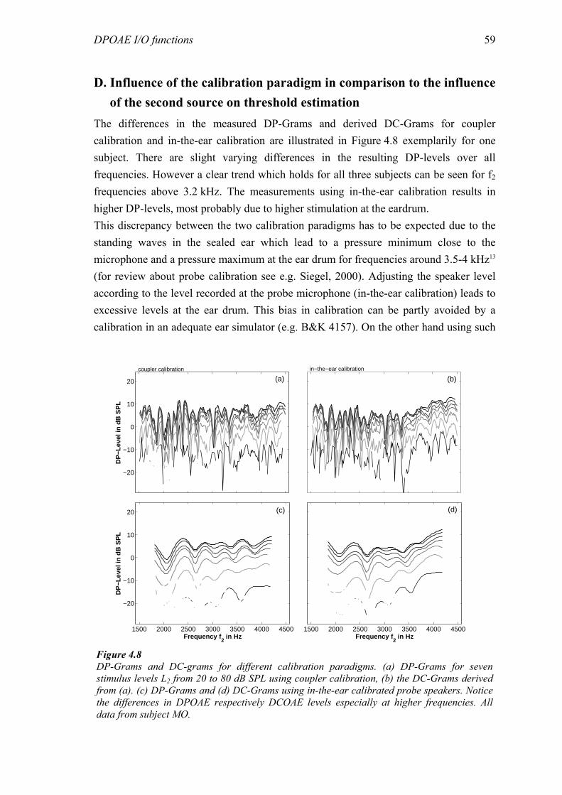
DPOAE I/O functions 59

D. Influence of the calibration paradigm in comparison to the influence of the second source on threshold estimation

The differences in the measured DP-Grams and derived DC-Grams for coupler calibration and in-the-ear calibration are illustrated in Figure 4.8 exemplarily for one subject. There are slight varying differences in the resulting DP-levels over all frequencies. However a clear trend which holds for all three subjects can be seen for f2 frequencies above 3.2 kHz. The measurements using in-the-ear calibration results in higher DP-levels, most probably due to higher stimulation at the eardrum. This discrepancy between the two calibration paradigms has to be expected due to the standing waves in the sealed ear which lead to a pressure minimum close to the microphone and a pressure maximum at the ear drum for frequencies around 3.5-4 kHz13 (for review about probe calibration see e.g. Siegel, 2000). Adjusting the speaker level according to the level recorded at the probe microphone (in-the-ear calibration) leads to excessive levels at the ear drum. This bias in calibration can be partly avoided by a calibration in an adequate ear simulator (e.g. B&K 4157). On the other hand using such

−20

−10

0

10

20

DP

−Lev

el in

dB

SP

L

coupler calibration

(a) in−the−ear calibration

(b)

1500 2000 2500 3000 3500 4000 4500

−20

−10

0

10

20

Frequency f2 in Hz

DP

−Lev

el in

dB

SP

L

(c)

1500 2000 2500 3000 3500 4000 4500Frequency f

2 in Hz

(d)

Figure 4.8 DP-Grams and DC-grams for different calibration paradigms. (a) DP-Grams for seven stimulus levels L2 from 20 to 80 dB SPL using coupler calibration, (b) the DC-Grams derived from (a). (c) DP-Grams and (d) DC-Grams using in-the-ear calibrated probe speakers. Notice the differences in DPOAE respectively DCOAE levels especially at higher frequencies. All data from subject MO.

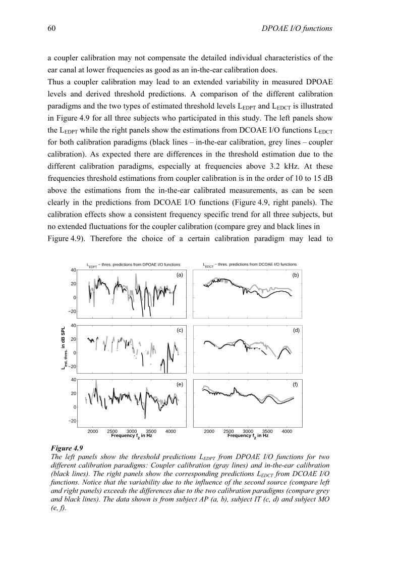
DPOAE I/O functions 60

a coupler calibration may not compensate the detailed individual characteristics of the ear canal at lower frequencies as good as an in-the-ear calibration does. Thus a coupler calibration may lead to an extended variability in measured DPOAE levels and derived threshold predictions. A comparison of the different calibration paradigms and the two types of estimated threshold levels LEDPT and LEDCT is illustrated in Figure 4.9 for all three subjects who participated in this study. The left panels show the LEDPT while the right panels show the estimations from DCOAE I/O functions LEDCT for both calibration paradigms (black lines – in-the-ear calibration, grey lines – coupler calibration). As expected there are differences in the threshold estimation due to the different calibration paradigms, especially at frequencies above 3.2 kHz. At these frequencies threshold estimations from coupler calibration is in the order of 10 to 15 dB above the estimations from the in-the-ear calibrated measurements, as can be seen clearly in the predictions from DCOAE I/O functions (Figure 4.9, right panels). The calibration effects show a consistent frequency specific trend for all three subjects, but no extended fluctuations for the coupler calibration (compare grey and black lines in Figure 4.9). Therefore the choice of a certain calibration paradigm may lead to

−20

0

20

40(a)

LEDPT

− thres. predictions from DPOAE I/O functions

(b)

LEDCT

− thres. predictions from DCOAE I/O functions

−20

0

20

40

Les

t. th

res.

in d

B S

PL (c) (d)

2000 2500 3000 3500 4000

−20

0

20

40

Frequency f2 in Hz

(e)

2000 2500 3000 3500 4000Frequency f

2 in Hz

(f)

Figure 4.9 The left panels show the threshold predictions LEDPT from DPOAE I/O functions for two different calibration paradigms: Coupler calibration (gray lines) and in-the-ear calibration (black lines). The right panels show the corresponding predictions LEDCT from DCOAE I/O functions. Notice that the variability due to the influence of the second source (compare left and right panels) exceeds the differences due to the two calibration paradigms (compare grey and black lines). The data shown is from subject AP (a, b), subject IT (c, d) and subject MO (e, f).

DPOAE I/O functions 61

systematic over- or underestimation of threshold prediction in certain frequency bands but should have little influence on the standard error of the predictions in comparison. On the other hand, the influence of the second source obviously leads to an extended variability in threshold prediction which can be reduced if the second source is eliminated (compare left and right panels of Figure 4.8). The fact that the fluctuations in threshold predictions due to effects of the second source clearly exceeds the systematic difference due to a different calibration (more than 10 dB at higher frequencies) underlines the relevance of the effects of the second source for the threshold prediction from DPOAE I/O functions.

IV. DISCUSSION Since the discovery of otoacoustic emissions by Kemp in 1978 OAE have been used to determine cochlea properties but also to clinically examine cochlea status. Nowadays OAE are well established in hearing screening procedures, e.g. in neonates, as a qualitative prediction whether a hearing loss may be present or not. From all kinds of OAE measurements DPOAE appear to have the highest potential as a tool for a quantitative auditory test, because they are measurable even for hearing losses up to 50 dB. A very promising approach for a quantitative prediction of hearing loss from OAE is the use of DPOAE I/O function for the prediction of thresholds as suggested by Boege and Janssen (2002) and verified by Gorga et al. (2003). On average, the predictions give good results but the variability in the data does not allow for a reliable prediction of individual auditory thresholds for the individual subject.

Influence of the second DPOAE source on DPOAE I/O functions and threshold predicitons Boege and Janssen (2002) discuss the close relationship between the nonlinear I/O characteristic of basilar membrane (BM) movement at the f2 site from physiological studies and the growth of DPOAE14, but they do not take possible interferences with a second DPOAE source from a different cochlear site not into account. Likewise in many studies DPOAE I/O functions are still seen as reflecting mainly the cochlea status around the f2 place. On the other hand the relevance of the second source on DPOAE at moderate to higher levels has been shown in several studies (Heitmann et al., 1998; Talmadge et al., 1999; Mauermann et al. 1999a,b; Kaluri and Shera 2001, Knight and Kemp 2001) and meanwhile is widely accepted. The current study shows that the relative contribution from this second source even increases with decreasing stimulation level (see Figure 4.2) and so leads to an increased uncertainty of DPOAE I/O characteristics as indicator for the f2 site at low levels. These results are in agreement with results from

DPOAE I/O functions 62

Konrad-Martin et al. (2001). From DPOAE measurements using a fixed f2 paradigm they also found that in normal ears the relative contribution from the second source is greater for low level primaries. The strong influence of the second source on DPOAE I/O functions can be seen in our data qualitatively in the large variation within adjacent frequencies in comparison with DCOAE I/O functions for which the second source is excluded (see Figures 3+4). Using DCOAE instead of DPOAE for the prediction of thresholds gives some practical improvements. At first the number of I/O functions rejected for threshold estimation due to the fitting criteria is drastically reduced. This is relevant for clinical applications. Gorga et al. (2003) reported that “18,4% of the total sample of DPOAE I/O functions failed to meet the inclusion criteria associated with the linear regression on DPOAE pressure (µPa) onto DPOAE stimulus level (dB SPL)”. They point out that misses due to the S/N criterion mostly are related to hearing loss, and so at least give a qualitative and clinical relevant information. On the other hand a DPOAE I/O function rejected due to a missed fitting criterion does not yield any information about hearing status. In another clinical evaluation Oswald et al. (2002) report a rejection of 46% or 26% of the I/O functions depending on whether modified fitting criteria and procedures are used or not. Thus the reduction from 28.8% to about 11.35% or even 4% rejected I/O functions (without the impractical slope criterion) in the current study contributes substantially to an improvement of the method. Another improvement of using DCOAE instead of DPOAE is the strong reduction of variation in threshold prediction between adjacent frequencies for the included I/O functions. The LEDCT follows LEDPT quite closely, similar to a moving average (see Figure 4.6). It may slightly exceed this “average” only at few frequencies. The good overall correlation and small mean difference between estimated and pure tone threshold found in other studies using LEDPT as threshold estimator (Boege and Janssen, 2002; Oswald et al., 2002; Gorga et al. 2003) is expected to be preserved if using LEDCT instead of LEDPT. However the standard error of the correlation is expected to decrease because the variability of the threshold predictions for adjacent frequencies is drastically reduced. Avoiding the influence of the second source on I/O functions (i.e. using DCOAE I/O functions instead of DPOAE I/O functions) is also necessary in order to interpret the I/O functions from DPOAE measurements as reflecting the cochlear status near f2. Thus, separating the two DPOAE sources is not only of relevance for threshold prediction but also for approaches to determine BM compression characteristics from DPOAE I/O functions (e.g. Buus et al., 2000)15 especially at low levels. Another factor which may influence the correlation of pure tone threshold and threshold estimations is the fine structure of hearing threshold. In some subjects the auditory

DPOAE I/O functions 63

threshold between adjacent frequencies varies up to 15 dB (for review see e.g. Mauermann et al. 2003 – Chapter 5). Note however, that there is only a very vague relation between OAE fine structure and threshold fine structure in humans 16. One way to avoid this uncertainty due to pure tone threshold variability might be the use of narrowband noises instead of pure tones to estimate auditory thresholds.

Relevance of the second DPOAE source in hearing impaired ears In the current study we investigated in detail five normal hearing subjects and one subject (AS) with a moderate high frequency loss. AS shows slightly reduced effects due to the second source over the whole frequency range. However the effect of the second DPOAE source in hearing impaired subjects is expected to be very individual. An influence of the second source on DPOAE I/O functions can be expected whenever DPOAE fine structure occurs, i.e. if the second source contributes in the same order as the initial distortion source. He and Schmiedt (1996) investigated fine structure in normal and hearing impaired subjects. They stated that fine structure always occur as long as DPOAE can be measured. Mauermann et al. (1999b) showed a high sensitivity of DPOAE fine structure in relation to the cochlea status around fDP, i.e. DPOAE fine structure vanishes if fDP falls in a region of hearing loss while the initial source near f2 still produces a sufficient emission (e.g. for notches in the audiogram). However the fine structure may even occurs if fDP falls in the region of normal hearing while f2 already covers a region of moderate hearing loss as can be seen in subjects with a bandpass hearing loss or a sloping high frequency loss (Mauermann et al., 1999b). Especially in those cases a strong effect on threshold estimation from the second source can be expected when using DPOAE I/O functions for the prediction. Konrad-Martin et al. (2002) investigated the relative contribution of the two DPOAE sources in hearing impaired subjects using a fixed f2 paradigm with f2 at 4 kHz. Looking at the latency domain to quantify the relative contribution of low and high latency components they found that for sloping hearing losses the high latency components are even more prominent than in normal ears while rising losses show only a low latency peak. For certain types of hearing losses the relative contribution of the second DPOAE source appears to be at least comparable to normal ears. Overall, a contribution of the second DPOAE source has to be expected even for most hearing impaired ears. Hence, the technique employed here to eliminate the influence of the second source appears to be very promising for the for the examination of hearing impaired patients. However the examination time for this method may be impractical high (see below).

Effects of Calibration Another factor most probably affecting the prediction of auditory thresholds from DPOAE I/O functions is the calibration of OAE speaker especially if the paradigm is

DPOAE I/O functions 64

very sensitive to the level ratio of the two primaries as the currently used. Individual calibration errors could lead to individually shifts in prediction of auditory threshold from DPOAE I/O functions and therefore could lead to a extended standard error when correlating both from data pooled across subjects. So individual variation of calibration errors in DPOAE measurements may partly explain the variance between behavioral and predicted thresholds. But the calibration errors for f2 frequencies below 2 kHz are assumed to be small (Siegel, 2002). A frequency specific analysis of the correlation between behavioral and predicted thresholds show no difference in the standard error for frequencies below and above 2 kHz (Gorga et al., 2003), i.e. no reduced variability at frequencies at which no or only small calibration errors are expected for the in-the-ear calibration used by Gorga et al. (2003). Looking at the predictions of auditory thresholds LEDCT from DCOAE I/O functions (Figure 4.9, right panels) for two different calibration paradigms in all three subjects the differences due to the different calibration are very similar. The comparison of these two calibration paradigms here gives no detailed information about the absolute calibration error of one or the other method. However, it yields at least a good guess about the order of magnitude of possible calibration effects17 on the DP-Grams, DPOAE I/O functions, and on the estimation of auditory threshold. A clear discrepancy of about 10 to 15 dB for the threshold estimation LEDPCT can be seen at frequencies above 3 kHz. This clearly indicates that the type of calibration is an important factor. However the differences are clearly smaller than the fluctuations of estimated threshold levels LEDPT. Therefore the bias due to the second source appears to be more relevant for prediction variability (i.e. standard error in the correlation of estimated and behavioral threshold) than the type of calibration

Outlook Overall the current studies underline that the contribution from the second DPOAE source is not negligible especially at low stimulus levels. DPOAE I/O functions are strongly affected by the interference of the two sources and therefore DPOAE I/O functions can hardly be seen as an indicator reflecting the cochlea status of the f2 site only. Beside the theoretical advantage of using DCOAE I/O functions instead of DPOAE I/O functions for estimation of behavioral thresholds it shows also relevant practical improvements such as a clearly reduced number of rejected I/O functions usable for prediction. Furthermore, strong fluctuations within threshold predictions from adjacent frequencies are almost eliminated for prediction from DCOAE as compared to DPOAE. This probably leads to a relevant reduction of the standard errors of threshold predictions. To verify this improved prediction further studies should be performed that compare the predictions from DCOAE I/O LEDCT and behavioral thresholds. Unfortunately, for a reliable use and interpretation of I/O functions from DPOAE measurements, the separation of the DPOAE components appears to be inevitable. A

DPOAE I/O functions 65

problem is the enormous measurement effort when using the method of time windowing for separation of the two DPOAE components. A significant reduction of the time effort using this procedure is not possible because (1) a high frequency resolution is needed to avoid aliasing in the time domain and (2) a sufficient frequency range is needed for this procedure to guarantee a adequate time resolution for the separation of low and high-latency components. Furthermore a lot of frequencies at the edges has to be rejected because of the window effects. Thus, the method outlined here is definitely unsuitable for clinical application. A method which might be more practicable for the separation of the DPOAE components, even for clinical use, is the method of selective suppression (e.g. Heitmann et al., 1998). A third tone presented close to fDP suppress the second source while leaving the initial distortion component intact. Kaluri and Shera (2001) have shown, that these two methods give similar results if using an appropriate suppressor level is selected which suppress the second source while keeping the initial distortion source almost unaffected. The studies on selective suppression known by the authors only investigate a set of fixed moderate primary levels (Heitmann et al; 1998; Siegel et al., 1998; Kaluri and Shera, 2001) However, for a range of different primary levels, as needed for I/O functions, the optimal suppressor levels may vary. Therefore at first appropriate suppressor levels for the different primary levels have to be found to obtain DCOAE I/O functions using selective suppression. If adequate suppressor levels can be found in future studies, the measurement effort for DCOAE I/O functions would be almost the same as for “standard” DPOAE I/O functions.

V. CONCLUSION • The second DPOAE source strongly influences DPOAE I/O functions especially at

low levels. • The use of DCOAE I/O functions instead of DPOAE I/O functions avoid influences

from a second source and so improve the interpretability of I/O functions to reflect the cochlear status at the f2 site. Furthermore it reduces the variability of I/O functions from adjacent frequencies.

• Modifying the approach of Boege and Janssen (2002) by estimating behavioral thresholds from DCOAE I/O functions instead of DPOAE I/O functions show a great potential to improve the method. The number of rejected I/O functions and the variability of the predicted thresholds is strongly reduced.

• The separation of the two DPOAE components using a time windowing procedure is to time consuming for practical applications. A significant reduction of the time effort is not possible due to the required frequency resolution.

• To use DCOAE I/O functions for studies in clinical routine tests a less time

DPOAE I/O functions 66

consuming paradigm for separation of DPOAE components is needed, i.e. adequate suppressor levels for the method of selective suppression have to be found for a sufficient range of primary levels.

ACKNOWLEDGEMENTS This study was supported by Deutsche Forschungsgemeinschaft, DFG Ko 942/11-3. Helpful comments by Stefan Uppenkamp on an earlier version of the manuscript are gratefully acknowledged.

ENDNOTES a Auditory thresholds show a similar quasi periodic fine structure as DPOAE but the periodicity is slightly different and there is no direct correspondence between the position of maxima and minima of both (e.g. Mauermann, 1997a; Talmadge, 1998). 2 This is equivalent to a convolution of the complex DP-Gram with the Fourier transform of the time window and results in a smoothing of the DP-Gram. Therefore some authors use the term “spectral smoothing” beside “time windowing” (e.g. Kaluri and Shera, 2001). 3 Kaluri and Shera (2001) performed the “spectral smoothing” as a convolution on a spectrum “wrapped” around a cylinder, i.e. taking no negative frequency into account. This is analogous to the transformation of Knight and Kemp (2001) of only positive frequencies into the time domain. The IFFT of the positive frequency bins only (negative frequencies are zero) means a transformation of the analytic signal and results in the envelope of the time-domain signal. Extending the spectrum by the complex conjugated frequencies as done in the current study results in a real signal as “time-domain response”. However for the principles of time windowing this makes no relevant difference. 4 Or if thinking in terms of spectral smoothing, to guarantee a smooth function to be convolved with the Fourier transform of the time window 5 The DC component is subtracted later from the corresponding “time-response”. 6 SFOAE and transient-evoked otoacoustic emissions show a variation in group delay with frequency (e.g. Kemp, 1978; Wilson, 1980; Neely et al., 1988). Therefore it is assumed that the high latency components show a varying latency, i.e. a spread of peaks in the latency domain. Therefore other authors (Knight and Kemp, 2001; Kalluri and Shera, 2001) suggest a transformation of the data points before the IFFT to be equidistant on an exponential frequency axis. Their aim is to linearize the underlying curve of phase as function of frequency for the reflection component. This results in clearer peaks in the time domain (Zweig and Shera, 1995). However a comparison of both – analysis with linear and exponential frequency axis – shows no practical advantage of the transformation for the further analysis. In most cases it was even easier to distinguish between low and high latency components with the “spread” of peaks for the high latency components. 7 If the definition of such a point appears to be critical we compare the time signals with data from measurements from a parallel study using a third tone close to 2f1-f2 to suppress the second source. Peaks in the latency domain which are easily affected even from low suppressor levels are seen as high latency components while peaks being almost unaffected are assumed to be low latency components, i.e. they are related to the first DPOAE source. This allows an almost complete assignment of the peaks belonging

DPOAE I/O functions 67

either to the high or low to the latency component. Suppression data for comparison is available at a couple of primary levels for all subjects in the current study except for subject AS. 8 The plots of the “time-domain response” are scaled such that they represent the soundpressure at each time per frequency component. E.g. a white spectrum with amplitudes 1 at positive and negative frequencies an zero phase would result in a peak with amplitude 1. 9 Boege and Janssen computed a linear regression of pDP onto L2 and therefore use an inclusion criterion for the standard error to be less than 10 dB (Boege, 2003). Whereas Gorga et al. (2003) computed a linear regression of pDP onto L2. As inclusion criterion here the standard error has to be less than 10 µPa. The inclusion criterion for the standard error to be less than 10 dB given in Gorga et al. (2003, Section II, E) is an typographical error an should be 10 µPa (Neely, 2003). In the current study we follow the criteria given by Gorga et al. (2003). 10 In Boege and Janssen (2002) equation (4) the criterion s ≥ 0.1 is given. However this appears to be a typographical error and the actual slope criterion was 0.2 µPa/dB as mentioned in Gorga et al. (2003) – see first Endnote there. 11 The DPOAE level at L2 = 80 dB SPL often show even a decrease in DPOAE level compared to the DPOAE level for L2 = 70 dB SPL. 12 Related for both low and high latency part of the signal to the length of the whole time domain response. 13 OAE are measured with a probe microphone in the sealed ear canal. The tips of typical ear probes are about 1.5-2 cm away from the ear drum (Siegel, 2000). Within these dimensions the incoming wave of the stimulus and the wave partly reflected at the ear drum are nearly in phase for frequencies below about 2 kHz. Such the sound pressure level in this volume of the ear canal is everywhere essentially the same. The calibration of speaker level is easily done by the calibrated probe microphone. At higher frequencies the wavelength decreases. Incoming and reflected wave interfere with different phase relationship. In the worst case the resulting standing wave shows a pressure maximum at the ear drum and a pressure null close to the microphone. In such a case the discrepancy between the sound pressure level at eardrum and microphone can be up to 20 dB (Siegel, 2000). 14 for the level paradigm L1 = 0.4 L2 +39 dB SPL 15 see also the comment of Prijs to this paper. 16 While the fine structure of pure tone threshold correlates closely with the periodicity of SOAE (Zweig and Shera, 1995; Shera, 2003) or the fine structure of low level transient evoked emissions it does not with DPOAE fine structure (Talmadge, 1998) to which the prediction of threshold from “standard” DPOAE I/O functions may be related. 17 While in-the-ear calibration makes a calibration of sound pressure at the tip of the probe microphone, the “coupler” calibration within an artificial ear is related to the sound pressure at the ear drum of an average ear. Such in cases of standing waves with a sound pressure maximum at ear drum and a minimum at the probe microphone these two types of calibration almost representing the opposite sides.

Chapter 5

Fine structure of Hearing-Threshold and Loudness Perception a)

Hearing thresholds measured with high frequency resolution show a quasi-periodic change in level called threshold fine structure (or microstructure). The effect of this fine structure on loudness perception over a range of stimulus levels was investigated in twelve subjects. Three different approaches were used. Individual hearing thresholds and equal loudness contours were measured in eight subjects using loudness-matching paradigms. In addition the loudness growth of sinusoids was observed at frequencies associated with individual minima or maxima in the hearing threshold from five subjects using a loudness-matching paradigm. At low levels loudness growth depended on the position of the test- or reference-tone frequency within the threshold fine structure. The slope of loudness growth differs by 0.2 dB/dB when an identical test tone is compared with two different reference tones. Finally loudness growth was measured for the same five subjects using categorical loudness scaling as a direct scaling technique with no reference tone instead of the loudness matching procedures. Overall, an influence of hearing-threshold fine structure on loudness perception of sinusoids was observable for stimulus levels up to 40 dB SPL - independent of the procedure used. Possible implications of fine structure for loudness measurements and other psychoacoustical experiments are discussed.

a) A modified version of this chapter is published as: Mauermann, M., Long, G. R., and Kollmeier, B. (2004), “Fine structure of Hearing-Threshold and Loudness Perception,” J. Acoust Soc. Am. 116, 1066-1080

Fine structure of Hearing-Threshold and Loudness Perception 70

INTRODUCTION When absolute hearing thresholds are evaluated with small frequency increments, consistent quasi-periodic patterns of threshold change with frequency (threshold fine structure or microstructure1) can be obtained. Regions of relatively stable poor sensitivity (hearing threshold maxima) are separated by narrow regions of greater sensitivity (threshold minima). In this study we investigated in detail the relation between hearing threshold fine structure and fine structure in loudness perception of sinusoidal signals for frequencies around 1800 Hz to receive a broader base for the understanding of loudness perception at low levels. Isolated investigations (Elliot, 1958; van den Brink, 1970; Thomas 1975) of threshold fine structure were described in the literature prior to 1979 establishing that the frequency spacing of the threshold fine structure appeared to be a constant fraction of estimates of the frequency resolution capacity of the ear (the critical band). In 1979, Kemp noted that the capacity of the healthy ear to generate sounds (known as otoacoustic emissions - OAE) could be due to the same mechanisms as those responsible for the threshold fine structure (Kemp 1979). These OAEs are generated by the processes responsible for the remarkable sensitivity of the human ear, and even small amounts of hearing loss correspond to significantly reduced levels of OAEs. All types of OAEs in humans are characterized by strikingly similar fine-structure patterns in the frequency domain with a frequency spacing between adjacent maxima or minima in the order of 0.4 bark (e.g. He and Schmiedt, 1993; Mauermann et al, 1997; Zwicker and Peisl, 1990; Zweig and Shera, 1995). Threshold minima are associated with frequencies near spontaneous OAEs (SOAEs) or large evoked OAEs (EOAEs) (Zwicker and Schloth, 1984; Long and Tubis, 1988a&b; Horst and de Kleine, 1999). The depth of the minima is not simply related to the level because high level emissions can interact with the stimuli and elevate thresholds (Long and Tubis, 1988a&b; Smurzynski and Probst, 1998). Changes in the emission frequency are associated with changes in the threshold-fine-structure frequency. (Long and Tubis, 1988a; He, 1990; Furst et al 1992). Overall the spacing of the threshold fine structure is very similar to that of otoacoustic emissions. Furthermore it can be observed that normal hearing subjects with weak otoacoustic emissions show a reduced ‘audiogram ripple’ (Kapadia and Lutman, 1999). Experimental evidence for a close link between OAE fine structure and threshold fine structure is confirmed by different cochlear models. Any sound generated in the cochlea must be conducted through the middle ear if it is to be detected in the ear canal as an OAE. But not all sound generated in the cochlea will be transmitted through the middle ear. Due to the impedance mismatch at the stapes some sound will be reflected back into the cochlea (e.g. Shera and Zweig, 1993). The returning reflection will either

Fine structure of Hearing-Threshold and Loudness Perception 71

enhance or partially cancel any energy at the original reflection site depending on the round trip travel time. If the sound was initially reflected (and is not cancelled by the returning echo) it will be reflected again unless the properties of the cochlea have changed. Multiple internal reflections of cochlear traveling waves will occur (Zweig and Shera, 1995), leading to the resonance behavior of the cochlea originally suggested by Kemp (1980) as an explanation for fine structure in stimulus frequency OAEs (SFOAE). This resonance will naturally enhance the response of the basilar membrane to sounds at some frequencies, and reduce its response to sounds at others. Frequencies at which the basilar membrane response at CF is maximal will result in threshold fine-structure minima, and frequencies at which this basilar membrane response is minimal will result in threshold fine-structure maxima. This same resonance behavior can be used to explain the origin of the pseudo-periodicity observed in all OAE fine structure with a single origin, and thus provides a common origin of the OAE fine structure and threshold (and other psychoacoustic) fine structures (see Talmadge et al., 1998). Even though OAE and psychoacoustic fine structure are based on the same underlying mechanisms and the periodicity is similar from the model point of view, the pattern of both does not need to match over all frequencies (Talmadge et al., 1998). In addition to the theoretical implications of cochlear fine structure, there are practical implications for psychoacoustic research. Except for the investigation of the relation between threshold fine structures and OAEs, there are only a small number of psychoacoustic studies investigating the dependence of suprathreshold psychoacoustic data on threshold fine structure. Variations of the psychoacoustic observations on the threshold fine structures have been found in, a) the perceived loudness of low-sensation-level tones (Kemp, 1979), b) temporal integration (Cohen, 1982), c) masked thresholds (Long, 1984), d) amplitude-modulation thresholds (Zwicker, 1986; Long 1993), e) monaural diplacusis (Kemp, 1979, Long, 1998) and f) binaural diplacusis (van den Brink, 1970, 1980). The effects of cochlear fine structure get smaller as stimulus level is increased in most paradigms and there is some indication that the spacing of the psychoacoustic fine structures can change at the highest levels tested (Long, 1984). In addition to screening of loudness maxima and minima at about 10 dB SL in 42 normal hearing ears Kemp (1979) showed equal loudness contours for one subject around a pronounced threshold minimum, which flattens out with increasing levels at about 35 dB SPL. For comparison with patterns of diplacusis van den Brink (1970) measured thresholds and isophones with a high frequency resolution, using a 1 kHz reference tone at 40, 60 and 80 dB SPL. He found “some recruitment at low SPL’s for the extreme peaks”, i.e. a flattening of threshold fine structure at 40 dB. In the example shown (van den Brink 1970, Fig.10) he linked maxima and minima in threshold with extrema in the isophones up to 80 dB SPL, which suggests a preservation of a reduced fine structure in

Fine structure of Hearing-Threshold and Loudness Perception 72

isophones (with fluctuations of about 2-3 dB) for reference tones up to 80 dB SPL. In studies taking the fine structure into account, the variance at each frequency is comparable to the within-subject variance seen in most other psychoacoustic research with well-trained subjects. The across-frequency variance is however much larger and comparable to the between-subject variance seen in many experiments. One interpretation of these results is that much of the between-subject variance seen might depend on the position of the stimuli within the cochlear fine structure. Hellman and Zwislocki (1961) found that presenting the stimuli at equal SL in comparison to equal SPL reduces the variability among listeners’ loudness judgments, especially at low levels. Any effects of cochlear fine structure on psychoacoustic research will increase the variance and thus limit our ability to evaluate the underlying impact of some stimulus manipulations. Nevertheless, with a few exceptions, most psychoacoustic research with sinusoids is done at discrete widely-spaced frequencies chosen without any attempt to determine whether these tones lie in a minimum, a maximum or a transition region within the cochlear fine structure. For studies interested in average effects over a sufficient large number of subjects it is certainly reasonable to ignore potential effects of cochlear fine structure. But it might be necessary to strengthen the consideration of cochlear fine structure effects on psychoacoustic measurements (a) to get a more detailed understanding of hearing mechanisms, (b) to investigate inter-individual variations and (c) to increase possibly the value of tools in audiology for more precise and individual diagnoses, or for diagnoses at very early states of cochlea injury. The aim of this study is to further examine the potential influences of the cochlear fine structure on perceived loudness of sinusoidal signals. Do the mechanical interference effects of cochlear mechanics - most probably responsible for threshold fine structure - effect loudness perception? To get a broader base of detailed data on loudness perception taking the threshold fine structure into account the following experiments were performed: Experiment 1 investigated the range of stimulus levels for which loudness fine structure is preserved in 8 subjects. Thresholds and equal loudness contours for different stimulus levels were measured with a high frequency resolution. Experiment 2 observed loudness growth at low to moderate levels using test tone frequencies associated with adjacent minima and maxima in individual thresholds in an attempt to describe the change in response with level for these different conditions. To check whether threshold fine structure may influence loudness matching procedures at low levels it was also examined whether the position of the reference tone within threshold fine structure affected the measured loudness growth. In Experiment 3 loudness growth was again measured for different frequencies - matching either a minimum or a maximum of threshold - but using a different paradigm.

Fine structure of Hearing-Threshold and Loudness Perception 73

Here a categorical loudness scaling was used as a direct scaling technique in addition to the loudness matching procedures used in Experiment 1 and 2. From a comparison across experiments we can determine how the effects of fine structure depend on the measurement procedures.

I. GENERAL METHODS

A. Subjects Ten normal hearing subjects (GL, GM, JO, KW, MO, MW, RH, TB, RM, SU - six male, four female) with thresholds better than 15 dB HL at the standard audiometric frequencies from 125 Hz to 8 kHz and two subjects with a slight hearing loss (MM - male, 25 dB HL at 8 kHz; DS – male, 25 dB HL at 3 and 4 kHz) participated in this study. The subjects were the authors, members of the medical physics group at the University of Oldenburg as well as students getting paid for the measurements. For all subjects the measurements were conducted on one ear. During the measurements the subjects were seated in a double-walled sound-insulated booth (IAC).

B. Instrumentation and Software Adaptive loudness matches, and most of the threshold measurements, were controlled by the signal-processing software SI running on an Indy computer system (Silicon Graphics). The signals were generated digitally at a sampling rate of 44100 Hz by the SI software, and converted by the 16 bit DA converters of the computer. They were attenuated by a computer-controlled audiometer and presented via an Etymotic Research ER2 insert ear phone. The presentation of each observation interval in one trial was marked optically by a LED, attached to the side of the computer display in the booth. For some of the interleaved adaptive threshold measurements, all of the adjustment measurements as well as the categorical loudness scaling, a PC/Matlab controlled setup was used. The signals were generated digitally at a sampling rate of 44100 Hz in the MATLAB programs and sent through a RME Digi96/8 PAD digital I/O card to a SEKD 2496 24-bit DA converter. After amplification, (Behringer headphone amplifier Powerplay II) the signals were presented via an ER2 insert phone. Each observation interval was marked optically on the computer screen instead of using the LED marker. The ER2 were calibrated using an artificial ear for insert phones (Bruel&Kjaer Type 4157).

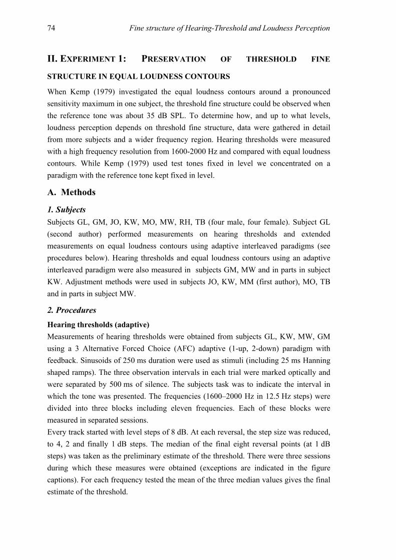
Fine structure of Hearing-Threshold and Loudness Perception 74

II. EXPERIMENT 1: PRESERVATION OF THRESHOLD FINE

STRUCTURE IN EQUAL LOUDNESS CONTOURS When Kemp (1979) investigated the equal loudness contours around a pronounced sensitivity maximum in one subject, the threshold fine structure could be observed when the reference tone was about 35 dB SPL. To determine how, and up to what levels, loudness perception depends on threshold fine structure, data were gathered in detail from more subjects and a wider frequency region. Hearing thresholds were measured with a high frequency resolution from 1600-2000 Hz and compared with equal loudness contours. While Kemp (1979) used test tones fixed in level we concentrated on a paradigm with the reference tone kept fixed in level.

A. Methods

1. Subjects Subjects GL, GM, JO, KW, MO, MW, RH, TB (four male, four female). Subject GL (second author) performed measurements on hearing thresholds and extended measurements on equal loudness contours using adaptive interleaved paradigms (see procedures below). Hearing thresholds and equal loudness contours using an adaptive interleaved paradigm were also measured in subjects GM, MW and in parts in subject KW. Adjustment methods were used in subjects JO, KW, MM (first author), MO, TB and in parts in subject MW.

2. Procedures

Hearing thresholds (adaptive) Measurements of hearing thresholds were obtained from subjects GL, KW, MW, GM using a 3 Alternative Forced Choice (AFC) adaptive (1-up, 2-down) paradigm with feedback. Sinusoids of 250 ms duration were used as stimuli (including 25 ms Hanning shaped ramps). The three observation intervals in each trial were marked optically and were separated by 500 ms of silence. The subjects task was to indicate the interval in which the tone was presented. The frequencies (1600–2000 Hz in 12.5 Hz steps) were divided into three blocks including eleven frequencies. Each of these blocks were measured in separated sessions. Every track started with level steps of 8 dB. At each reversal, the step size was reduced, to 4, 2 and finally 1 dB steps. The median of the final eight reversal points (at 1 dB steps) was taken as the preliminary estimate of the threshold. There were three sessions during which these measures were obtained (exceptions are indicated in the figure captions). For each frequency tested the mean of the three median values gives the final estimate of the threshold.

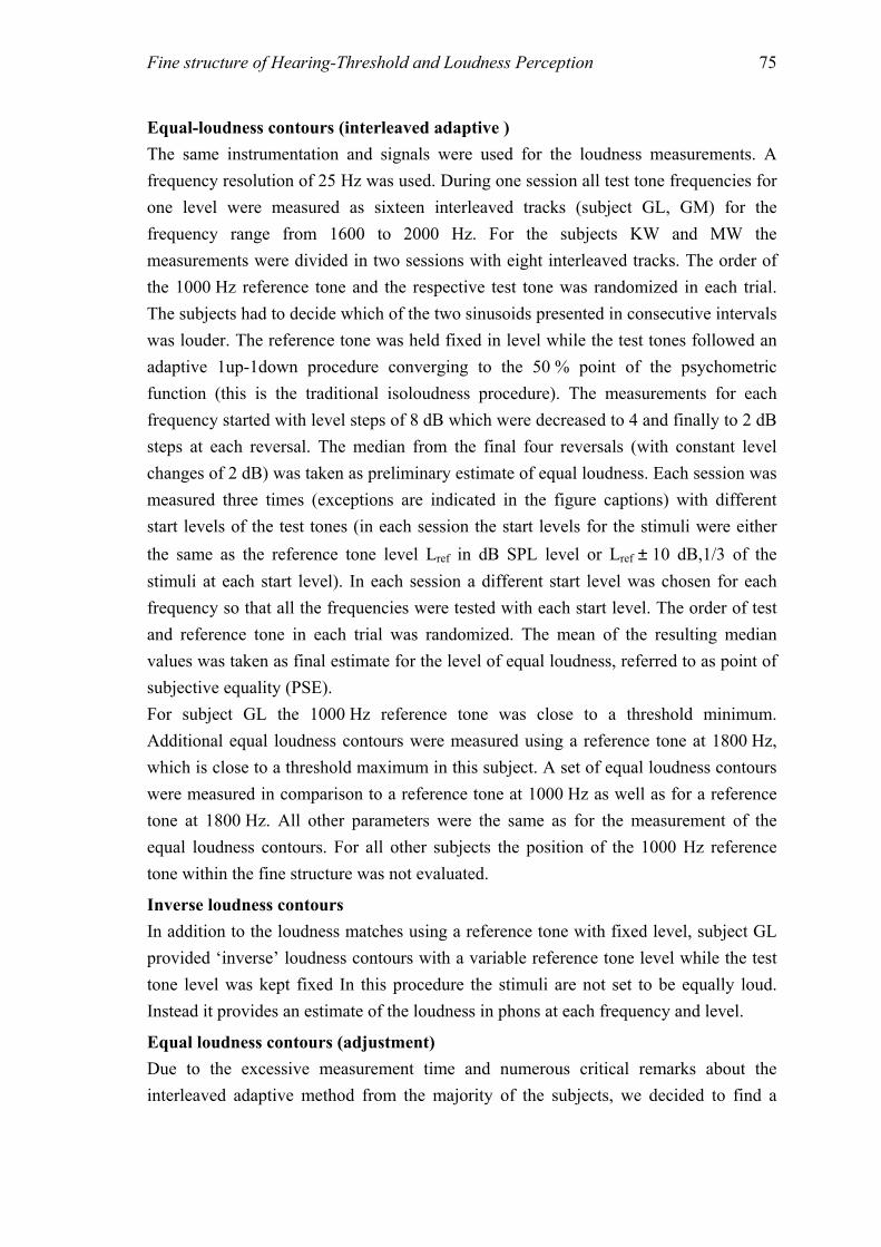
Fine structure of Hearing-Threshold and Loudness Perception 75

Equal-loudness contours (interleaved adaptive ) The same instrumentation and signals were used for the loudness measurements. A frequency resolution of 25 Hz was used. During one session all test tone frequencies for one level were measured as sixteen interleaved tracks (subject GL, GM) for the frequency range from 1600 to 2000 Hz. For the subjects KW and MW the measurements were divided in two sessions with eight interleaved tracks. The order of the 1000 Hz reference tone and the respective test tone was randomized in each trial. The subjects had to decide which of the two sinusoids presented in consecutive intervals was louder. The reference tone was held fixed in level while the test tones followed an adaptive 1up-1down procedure converging to the 50 % point of the psychometric function (this is the traditional isoloudness procedure). The measurements for each frequency started with level steps of 8 dB which were decreased to 4 and finally to 2 dB steps at each reversal. The median from the final four reversals (with constant level changes of 2 dB) was taken as preliminary estimate of equal loudness. Each session was measured three times (exceptions are indicated in the figure captions) with different start levels of the test tones (in each session the start levels for the stimuli were either the same as the reference tone level Lref in dB SPL level or Lref ± 10 dB,1/3 of the stimuli at each start level). In each session a different start level was chosen for each frequency so that all the frequencies were tested with each start level. The order of test and reference tone in each trial was randomized. The mean of the resulting median values was taken as final estimate for the level of equal loudness, referred to as point of subjective equality (PSE). For subject GL the 1000 Hz reference tone was close to a threshold minimum. Additional equal loudness contours were measured using a reference tone at 1800 Hz, which is close to a threshold maximum in this subject. A set of equal loudness contours were measured in comparison to a reference tone at 1000 Hz as well as for a reference tone at 1800 Hz. All other parameters were the same as for the measurement of the equal loudness contours. For all other subjects the position of the 1000 Hz reference tone within the fine structure was not evaluated.

Inverse loudness contours In addition to the loudness matches using a reference tone with fixed level, subject GL provided ‘inverse’ loudness contours with a variable reference tone level while the test tone level was kept fixed In this procedure the stimuli are not set to be equally loud. Instead it provides an estimate of the loudness in phons at each frequency and level.

Equal loudness contours (adjustment) Due to the excessive measurement time and numerous critical remarks about the interleaved adaptive method from the majority of the subjects, we decided to find a

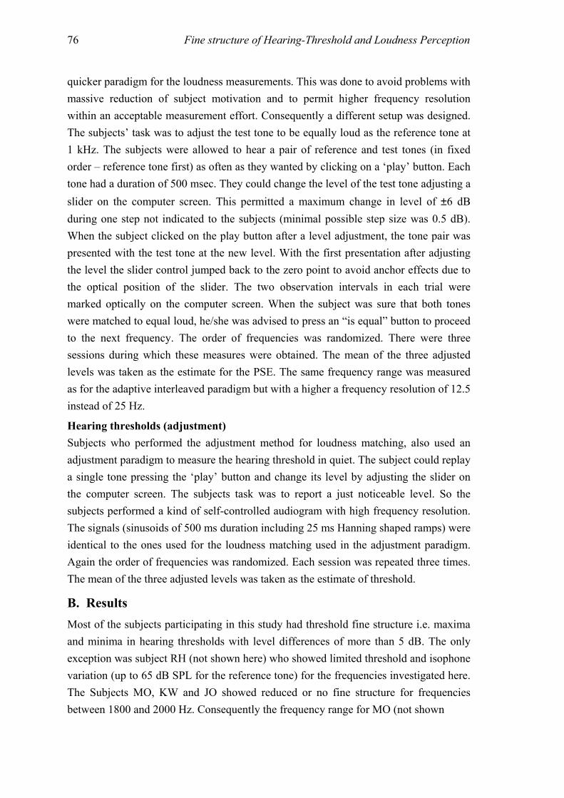
Fine structure of Hearing-Threshold and Loudness Perception 76

quicker paradigm for the loudness measurements. This was done to avoid problems with massive reduction of subject motivation and to permit higher frequency resolution within an acceptable measurement effort. Consequently a different setup was designed. The subjects’ task was to adjust the test tone to be equally loud as the reference tone at 1 kHz. The subjects were allowed to hear a pair of reference and test tones (in fixed order – reference tone first) as often as they wanted by clicking on a ‘play’ button. Each tone had a duration of 500 msec. They could change the level of the test tone adjusting a slider on the computer screen. This permitted a maximum change in level of ±6 dB during one step not indicated to the subjects (minimal possible step size was 0.5 dB). When the subject clicked on the play button after a level adjustment, the tone pair was presented with the test tone at the new level. With the first presentation after adjusting the level the slider control jumped back to the zero point to avoid anchor effects due to the optical position of the slider. The two observation intervals in each trial were marked optically on the computer screen. When the subject was sure that both tones were matched to equal loud, he/she was advised to press an “is equal” button to proceed to the next frequency. The order of frequencies was randomized. There were three sessions during which these measures were obtained. The mean of the three adjusted levels was taken as the estimate for the PSE. The same frequency range was measured as for the adaptive interleaved paradigm but with a higher a frequency resolution of 12.5 instead of 25 Hz.

Hearing thresholds (adjustment) Subjects who performed the adjustment method for loudness matching, also used an adjustment paradigm to measure the hearing threshold in quiet. The subject could replay a single tone pressing the ‘play’ button and change its level by adjusting the slider on the computer screen. The subjects task was to report a just noticeable level. So the subjects performed a kind of self-controlled audiogram with high frequency resolution. The signals (sinusoids of 500 ms duration including 25 ms Hanning shaped ramps) were identical to the ones used for the loudness matching used in the adjustment paradigm. Again the order of frequencies was randomized. Each session was repeated three times. The mean of the three adjusted levels was taken as the estimate of threshold.

B. Results Most of the subjects participating in this study had threshold fine structure i.e. maxima and minima in hearing thresholds with level differences of more than 5 dB. The only exception was subject RH (not shown here) who showed limited threshold and isophone variation (up to 65 dB SPL for the reference tone) for the frequencies investigated here. The Subjects MO, KW and JO showed reduced or no fine structure for frequencies between 1800 and 2000 Hz. Consequently the frequency range for MO (not shown

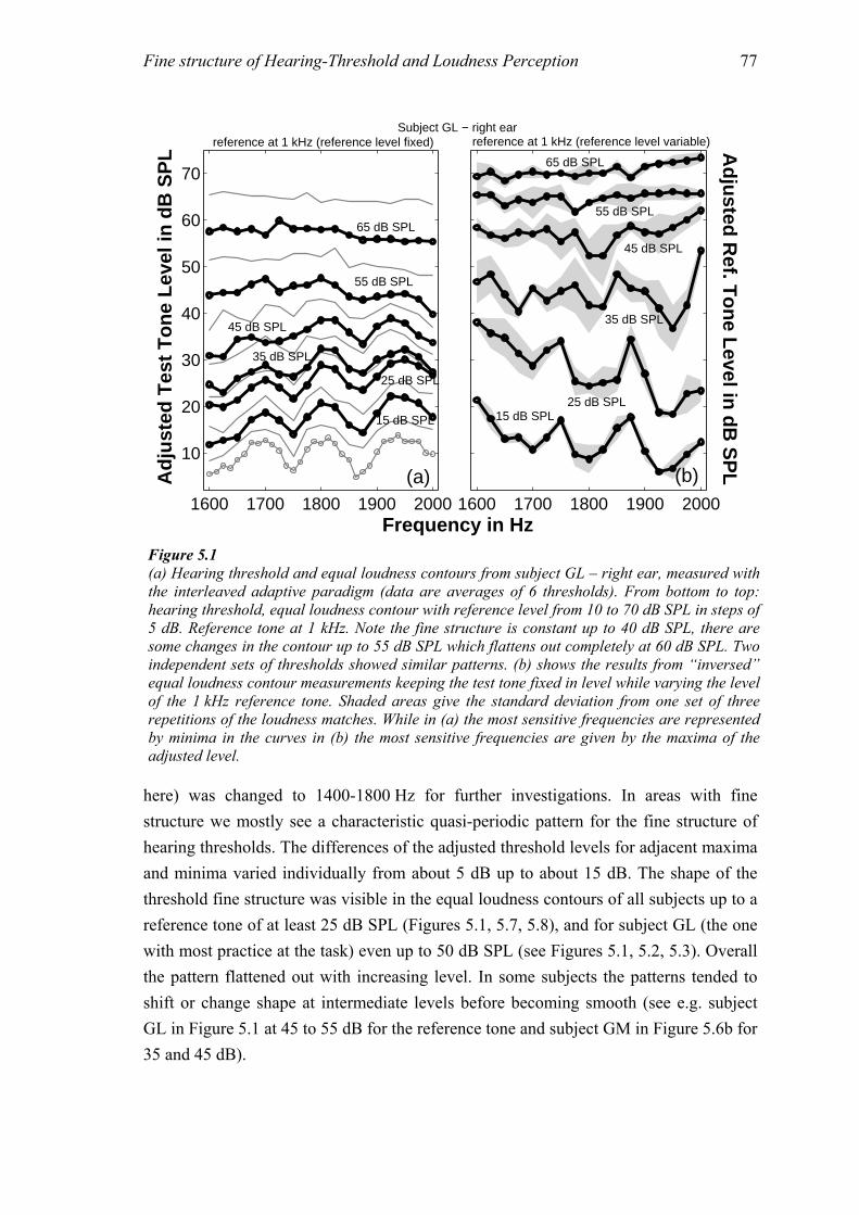
Fine structure of Hearing-Threshold and Loudness Perception 77

here) was changed to 1400-1800 Hz for further investigations. In areas with fine structure we mostly see a characteristic quasi-periodic pattern for the fine structure of hearing thresholds. The differences of the adjusted threshold levels for adjacent maxima and minima varied individually from about 5 dB up to about 15 dB. The shape of the threshold fine structure was visible in the equal loudness contours of all subjects up to a reference tone of at least 25 dB SPL (Figures 5.1, 5.7, 5.8), and for subject GL (the one with most practice at the task) even up to 50 dB SPL (see Figures 5.1, 5.2, 5.3). Overall the pattern flattened out with increasing level. In some subjects the patterns tended to shift or change shape at intermediate levels before becoming smooth (see e.g. subject GL in Figure 5.1 at 45 to 55 dB for the reference tone and subject GM in Figure 5.6b for 35 and 45 dB).

1600 1700 1800 1900 2000

10

20

30

40

50

60

70

Frequency in Hz

Adj

uste

d T

est T

one

Leve

l in

dB S

PL

reference at 1 kHz (reference level fixed)

1600 1700 1800 1900 2000

reference at 1 kHz (reference level variable) Adjusted R

ef. Tone Level in dB

SP

L

65 dB SPL

55 dB SPL

45 dB SPL

35 dB SPL

25 dB SPL15 dB SPL

(b)

15 dB SPL

25 dB SPL

35 dB SPL

45 dB SPL

55 dB SPL

65 dB SPL

(a)

Subject GL − right ear

Figure 5.1 (a) Hearing threshold and equal loudness contours from subject GL – right ear, measured with the interleaved adaptive paradigm (data are averages of 6 thresholds). From bottom to top: hearing threshold, equal loudness contour with reference level from 10 to 70 dB SPL in steps of 5 dB. Reference tone at 1 kHz. Note the fine structure is constant up to 40 dB SPL, there are some changes in the contour up to 55 dB SPL which flattens out completely at 60 dB SPL. Two independent sets of thresholds showed similar patterns. (b) shows the results from “inversed” equal loudness contour measurements keeping the test tone fixed in level while varying the level of the 1 kHz reference tone. Shaded areas give the standard deviation from one set of three repetitions of the loudness matches. While in (a) the most sensitive frequencies are represented by minima in the curves in (b) the most sensitive frequencies are given by the maxima of the adjusted level.

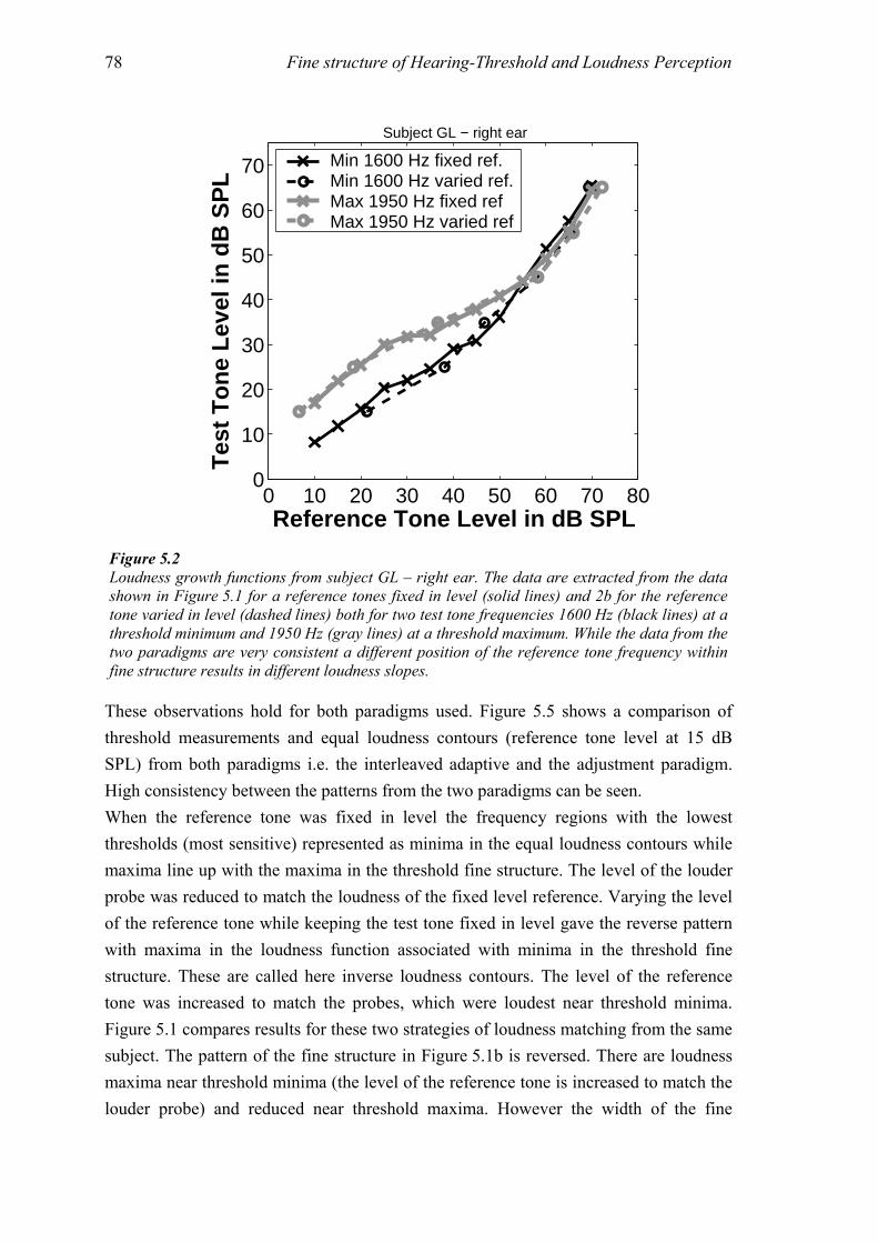
Fine structure of Hearing-Threshold and Loudness Perception 78

These observations hold for both paradigms used. Figure 5.5 shows a comparison of threshold measurements and equal loudness contours (reference tone level at 15 dB SPL) from both paradigms i.e. the interleaved adaptive and the adjustment paradigm. High consistency between the patterns from the two paradigms can be seen. When the reference tone was fixed in level the frequency regions with the lowest thresholds (most sensitive) represented as minima in the equal loudness contours while maxima line up with the maxima in the threshold fine structure. The level of the louder probe was reduced to match the loudness of the fixed level reference. Varying the level of the reference tone while keeping the test tone fixed in level gave the reverse pattern with maxima in the loudness function associated with minima in the threshold fine structure. These are called here inverse loudness contours. The level of the reference tone was increased to match the probes, which were loudest near threshold minima. Figure 5.1 compares results for these two strategies of loudness matching from the same subject. The pattern of the fine structure in Figure 5.1b is reversed. There are loudness maxima near threshold minima (the level of the reference tone is increased to match the louder probe) and reduced near threshold maxima. However the width of the fine

0 10 20 30 40 50 60 70 800

10

20

30

40

50

60

70

Reference Tone Level in dB SPL

Min 1600 Hz fixed ref. Min 1600 Hz varied ref.Max 1950 Hz fixed ref Max 1950 Hz varied ref

Tes

t Ton

e Le

vel i

n dB

SP

L

Subject GL − right ear

Figure 5.2 Loudness growth functions from subject GL – right ear. The data are extracted from the data shown in Figure 5.1 for a reference tones fixed in level (solid lines) and 2b for the reference tone varied in level (dashed lines) both for two test tone frequencies 1600 Hz (black lines) at a threshold minimum and 1950 Hz (gray lines) at a threshold maximum. While the data from the two paradigms are very consistent a different position of the reference tone frequency within fine structure results in different loudness slopes.

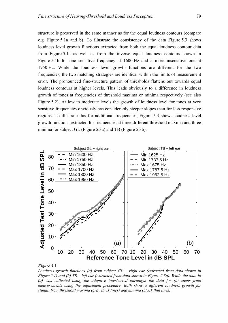
Fine structure of Hearing-Threshold and Loudness Perception 79

structure is preserved in the same manner as for the equal loudness contours (compare e.g. Figure 5.1a and b). To illustrate the consistency of the data Figure 5.3 shows loudness level growth functions extracted from both the equal loudness contour data from Figure 5.1a as well as from the inverse equal loudness contours shown in Figure 5.1b for one sensitive frequency at 1600 Hz and a more insensitive one at 1950 Hz. While the loudness level growth functions are different for the two frequencies, the two matching strategies are identical within the limits of measurement error. The pronounced fine-structure pattern of thresholds flattens out towards equal loudness contours at higher levels. This leads obviously to a difference in loudness growth of tones at frequencies of threshold maxima or minima respectively (see also Figure 5.2). At low to moderate levels the growth of loudness level for tones at very sensitive frequencies obviously has considerably steeper slopes than for less responsive regions. To illustrate this for additional frequencies, Figure 5.3 shows loudness level growth functions extracted for frequencies at three different threshold maxima and three minima for subject GL (Figure 5.3a) and TB (Figure 5.3b).

10 20 30 40 50 60 700

10

20

30

40

50

60

70

80 Min 1600 HzMin 1750 HzMin 1850 HzMax 1700 HzMax 1800 HzMax 1950 Hz

10 20 30 40 50 60 70

Min 1625 Hz Min 1737.5 HzMax 1675 Hz Max 1787.5 HzMax 1962.5 Hz

Subject GL − right ear

Adj

uste

d T

est T

one

Leve

l in

dB S

PL

Reference Tone Level in dB SPL

(a)

Subject TB − left ear

(b)

Figure 5.3 Loudness growth functions (a) from subject GL – right ear (extracted from data shown in Figure 5.1) and (b) TB – left ear (extracted from data shown in Figure 5.8a). While the data in (a) was collected using the adaptive interleaved paradigm the data for (b) stems from measurements using the adjustment procedure. Both show a different loudness growth for stimuli from threshold maxima (gray thick lines) and minima (black thin lines).

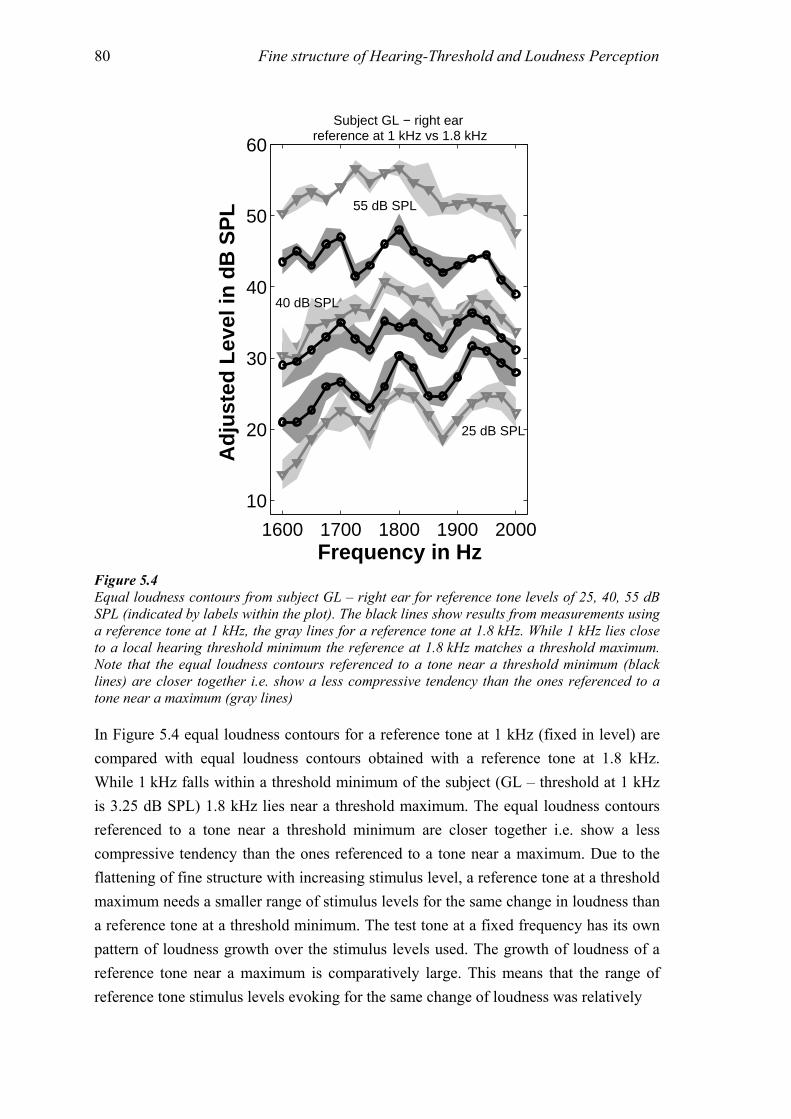
Fine structure of Hearing-Threshold and Loudness Perception 80

In Figure 5.4 equal loudness contours for a reference tone at 1 kHz (fixed in level) are compared with equal loudness contours obtained with a reference tone at 1.8 kHz. While 1 kHz falls within a threshold minimum of the subject (GL – threshold at 1 kHz is 3.25 dB SPL) 1.8 kHz lies near a threshold maximum. The equal loudness contours referenced to a tone near a threshold minimum are closer together i.e. show a less compressive tendency than the ones referenced to a tone near a maximum. Due to the flattening of fine structure with increasing stimulus level, a reference tone at a threshold maximum needs a smaller range of stimulus levels for the same change in loudness than a reference tone at a threshold minimum. The test tone at a fixed frequency has its own pattern of loudness growth over the stimulus levels used. The growth of loudness of a reference tone near a maximum is comparatively large. This means that the range of reference tone stimulus levels evoking for the same change of loudness was relatively

1600 1700 1800 1900 2000

10

20

30

40

50

60

55 dB SPL

40 dB SPL

25 dB SPL

Adj

uste

d Le

vel i

n dB

SP

L

Frequency in Hz

Subject GL − right ear reference at 1 kHz vs 1.8 kHz

Figure 5.4 Equal loudness contours from subject GL – right ear for reference tone levels of 25, 40, 55 dB SPL (indicated by labels within the plot). The black lines show results from measurements using a reference tone at 1 kHz, the gray lines for a reference tone at 1.8 kHz. While 1 kHz lies close to a local hearing threshold minimum the reference at 1.8 kHz matches a threshold maximum. Note that the equal loudness contours referenced to a tone near a threshold minimum (black lines) are closer together i.e. show a less compressive tendency than the ones referenced to a tone near a maximum (gray lines)

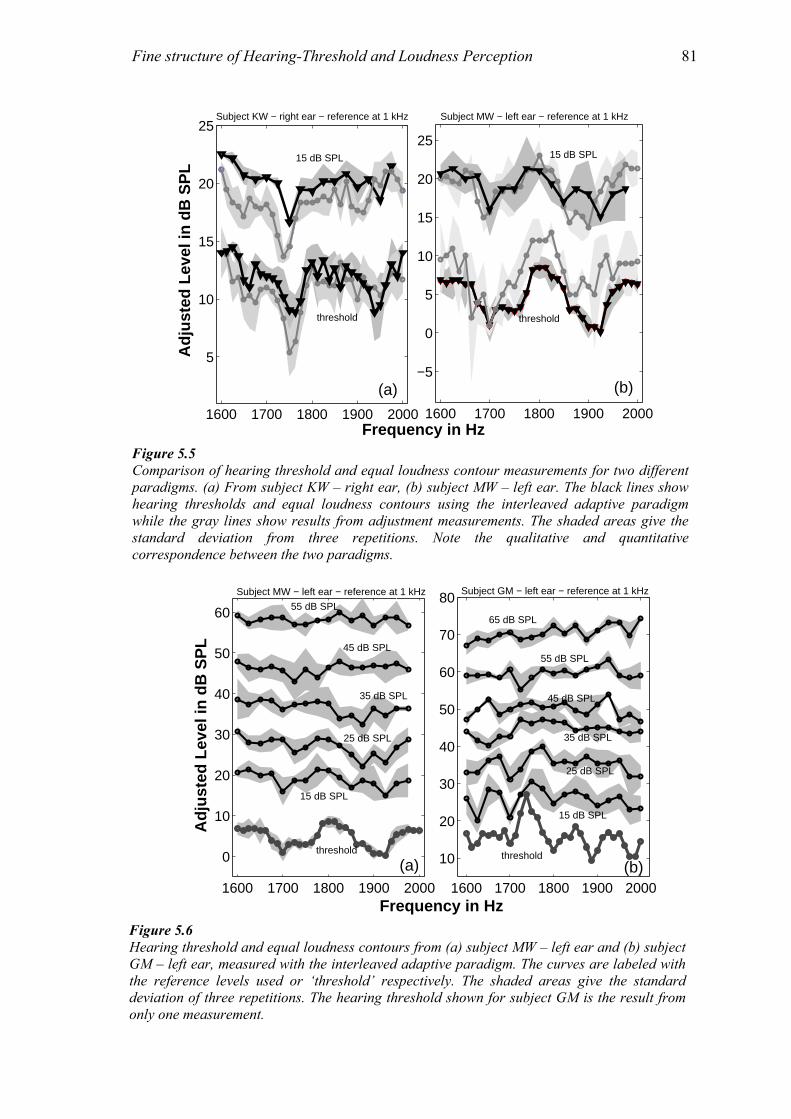
Fine structure of Hearing-Threshold and Loudness Perception 81

1600 1700 1800 1900 2000

5

10

15

20

25

1600 1700 1800 1900 2000

−5

0

5

10

15

20

25

Adj

uste

d Le

vel i

n dB

SP

L

Frequency in Hz

(a)

15 dB SPL

Subject KW − right ear − reference at 1 kHz Subject MW − left ear − reference at 1 kHz

15 dB SPL

threshold

(b)

threshold

Figure 5.5 Comparison of hearing threshold and equal loudness contour measurements for two different paradigms. (a) From subject KW – right ear, (b) subject MW – left ear. The black lines show hearing thresholds and equal loudness contours using the interleaved adaptive paradigm while the gray lines show results from adjustment measurements. The shaded areas give the standard deviation from three repetitions. Note the qualitative and quantitative correspondence between the two paradigms.

1600 1700 1800 1900 2000

0

10

20

30

40

50

60

Frequency in Hz

Subject MW − left ear − reference at 1 kHz

1600 1700 1800 1900 2000

10

20

30

40

50

60

70

8055 dB SPL

45 dB SPL

35 dB SPL

25 dB SPL

15 dB SPL

threshold

Adj

uste

d Le

vel i

n dB

SP

L

(a)

Subject GM − left ear − reference at 1 kHz

65 dB SPL

55 dB SPL

45 dB SPL

35 dB SPL

25 dB SPL

15 dB SPL

threshold (b)

Figure 5.6 Hearing threshold and equal loudness contours from (a) subject MW – left ear and (b) subject GM – left ear, measured with the interleaved adaptive paradigm. The curves are labeled with the reference levels used or ‘threshold’ respectively. The shaded areas give the standard deviation of three repetitions. The hearing threshold shown for subject GM is the result from only one measurement.

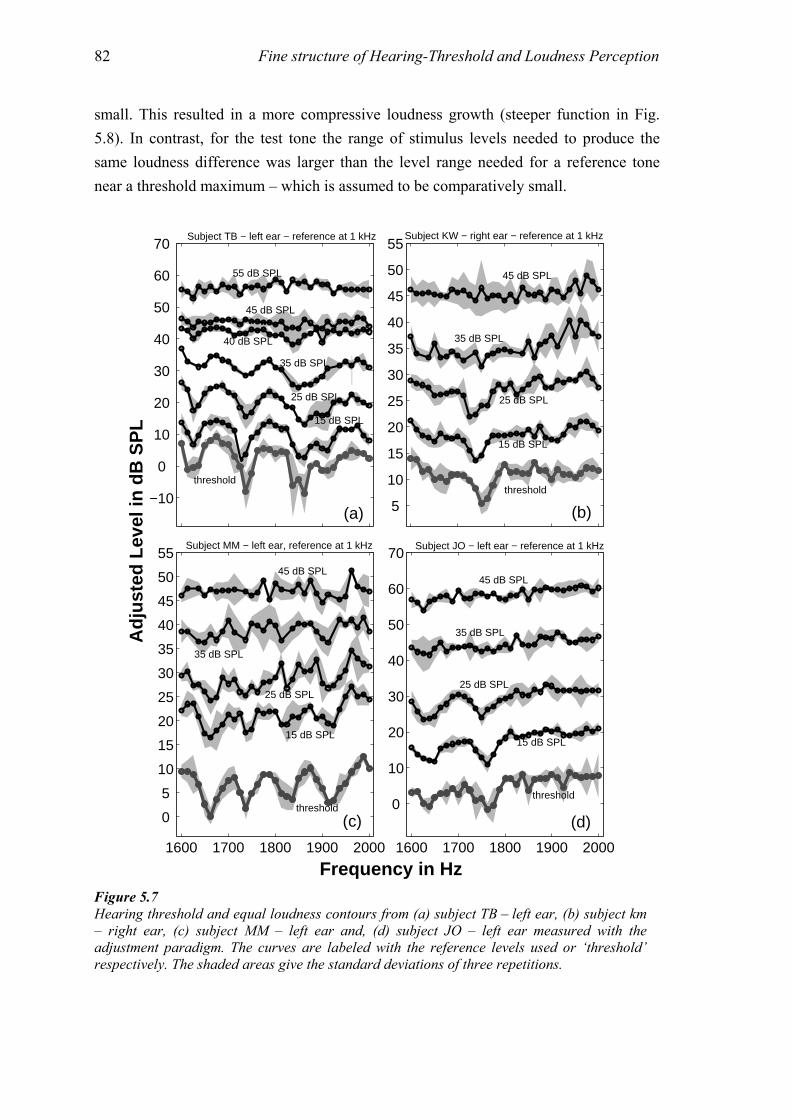
Fine structure of Hearing-Threshold and Loudness Perception 82

small. This resulted in a more compressive loudness growth (steeper function in Fig. 5.8). In contrast, for the test tone the range of stimulus levels needed to produce the same loudness difference was larger than the level range needed for a reference tone near a threshold maximum – which is assumed to be comparatively small.

−10

0

10

20

30

40

50

60

70

Adj

uste

d Le

vel i

n dB

SP

L

5

10

15

20

25

30

35

40

45

50

55

1600 1700 1800 1900 2000

0

5

10

15

20

25

30

35

40

45

50

55

Frequency in Hz1600 1700 1800 1900 2000

0

10

20

30

40

50

60

70

Subject TB − left ear − reference at 1 kHz Subject KW − right ear − reference at 1 kHz

Subject MM − left ear, reference at 1 kHz Subject JO − left ear − reference at 1 kHz

55 dB SPL

45 dB SPL

40 dB SPL

35 dB SPL

25 dB SPL

15 dB SPL

threshold

45 dB SPL

35 dB SPL

25 dB SPL

15 dB SPL

threshold

threshold threshold

15 dB SPL 15 dB SPL

25 dB SPL 25 dB SPL

35 dB SPL

35 dB SPL

45 dB SPL 45 dB SPL

(a) (b)

(c) (d)

Figure 5.7 Hearing threshold and equal loudness contours from (a) subject TB – left ear, (b) subject km – right ear, (c) subject MM – left ear and, (d) subject JO – left ear measured with the adjustment paradigm. The curves are labeled with the reference levels used or ‘threshold’ respectively. The shaded areas give the standard deviations of three repetitions.

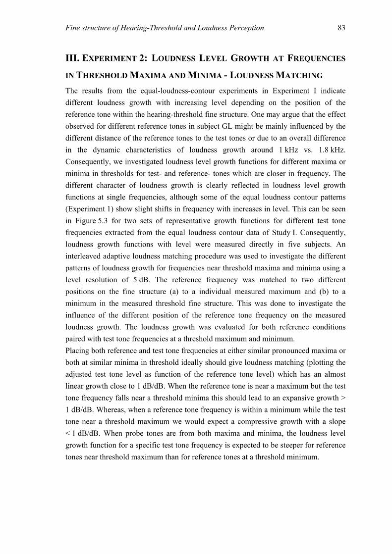
Fine structure of Hearing-Threshold and Loudness Perception 83

III. EXPERIMENT 2: LOUDNESS LEVEL GROWTH AT FREQUENCIES

IN THRESHOLD MAXIMA AND MINIMA - LOUDNESS MATCHING The results from the equal-loudness-contour experiments in Experiment I indicate different loudness growth with increasing level depending on the position of the reference tone within the hearing-threshold fine structure. One may argue that the effect observed for different reference tones in subject GL might be mainly influenced by the different distance of the reference tones to the test tones or due to an overall difference in the dynamic characteristics of loudness growth around 1 kHz vs. 1.8 kHz. Consequently, we investigated loudness level growth functions for different maxima or minima in thresholds for test- and reference- tones which are closer in frequency. The different character of loudness growth is clearly reflected in loudness level growth functions at single frequencies, although some of the equal loudness contour patterns (Experiment 1) show slight shifts in frequency with increases in level. This can be seen in Figure 5.3 for two sets of representative growth functions for different test tone frequencies extracted from the equal loudness contour data of Study I. Consequently, loudness growth functions with level were measured directly in five subjects. An interleaved adaptive loudness matching procedure was used to investigate the different patterns of loudness growth for frequencies near threshold maxima and minima using a level resolution of 5 dB. The reference frequency was matched to two different positions on the fine structure (a) to a individual measured maximum and (b) to a minimum in the measured threshold fine structure. This was done to investigate the influence of the different position of the reference tone frequency on the measured loudness growth. The loudness growth was evaluated for both reference conditions paired with test tone frequencies at a threshold maximum and minimum. Placing both reference and test tone frequencies at either similar pronounced maxima or both at similar minima in threshold ideally should give loudness matching (plotting the adjusted test tone level as function of the reference tone level) which has an almost linear growth close to 1 dB/dB. When the reference tone is near a maximum but the test tone frequency falls near a threshold minima this should lead to an expansive growth > 1 dB/dB. Whereas, when a reference tone frequency is within a minimum while the test tone near a threshold maximum we would expect a compressive growth with a slope < 1 dB/dB. When probe tones are from both maxima and minima, the loudness level growth function for a specific test tone frequency is expected to be steeper for reference tones near threshold maximum than for reference tones at a threshold minimum.

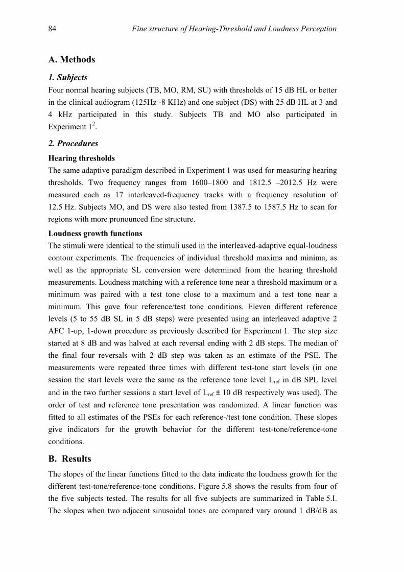
Fine structure of Hearing-Threshold and Loudness Perception 84

A. Methods

1. Subjects Four normal hearing subjects (TB, MO, RM, SU) with thresholds of 15 dB HL or better in the clinical audiogram (125Hz -8 KHz) and one subject (DS) with 25 dB HL at 3 and 4 kHz participated in this study. Subjects TB and MO also participated in Experiment 12.

2. Procedures

Hearing thresholds The same adaptive paradigm described in Experiment 1 was used for measuring hearing thresholds. Two frequency ranges from 1600–1800 and 1812.5 –2012.5 Hz were measured each as 17 interleaved-frequency tracks with a frequency resolution of 12.5 Hz. Subjects MO, and DS were also tested from 1387.5 to 1587.5 Hz to scan for regions with more pronounced fine structure.

Loudness growth functions The stimuli were identical to the stimuli used in the interleaved-adaptive equal-loudness contour experiments. The frequencies of individual threshold maxima and minima, as well as the appropriate SL conversion were determined from the hearing threshold measurements. Loudness matching with a reference tone near a threshold maximum or a minimum was paired with a test tone close to a maximum and a test tone near a minimum. This gave four reference/test tone conditions. Eleven different reference levels (5 to 55 dB SL in 5 dB steps) were presented using an interleaved adaptive 2 AFC 1-up, 1-down procedure as previously described for Experiment 1. The step size started at 8 dB and was halved at each reversal ending with 2 dB steps. The median of the final four reversals with 2 dB step was taken as an estimate of the PSE. The measurements were repeated three times with different test-tone start levels (in one session the start levels were the same as the reference tone level Lref in dB SPL level and in the two further sessions a start level of Lref ± 10 dB respectively was used). The order of test and reference tone presentation was randomized. A linear function was fitted to all estimates of the PSEs for each reference-/test tone condition. These slopes give indicators for the growth behavior for the different test-tone/reference-tone conditions.

B. Results The slopes of the linear functions fitted to the data indicate the loudness growth for the different test-tone/reference-tone conditions. Figure 5.8 shows the results from four of the five subjects tested. The results for all five subjects are summarized in Table 5.I. The slopes when two adjacent sinusoidal tones are compared vary around 1 dB/dB as

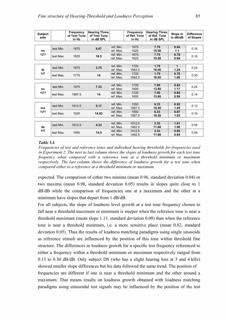
Fine structure of Hearing-Threshold and Loudness Perception 85

expected. The comparison of either two minima (mean 0.96, standard deviation 0.04) or two maxima (mean 0.98, standard deviation 0.05) results in slopes quite close to 1 dB/dB while the comparison of frequencies one at a maximum and the other at a minimum have slopes that depart from 1 dB/dB. For all subjects, the slope of loudness level growth at a test tone frequency chosen to fall near a threshold maximum or minimum is steeper when the reference tone is near a threshold maximum (mean slope 1.11, standard deviation 0.08) than when the reference tone is near a threshold minimum, i.e. a more sensitive place (mean 0.82, standard deviation 0.05). Thus the results of loudness matching paradigms using single sinusoids as reference stimuli are influenced by the position of this tone within threshold fine structure. The differences in loudness growth for a specific test frequency referenced to either a frequency within a threshold minimum or maximum respectively ranged from 0.13 to 0.30 dB/dB. Only subject DS (who has a slight hearing loss at 3 and 4 kHz) showed smaller slope differences but his data followed the same trend. The position of frequencies are different if one is near a threshold minimum and the other around a maximum. That means results on loudness growth obtained with loudness matching paradigms using sinusoidal test signals may be influenced by the position of the test

Subject side

Frequency of Test Tone

in Hz

Hearing Thres. of Test Tone

in dB SPL

Frequency of Ref. Tone

in Hz

Hearing Thres. of Ref. Tone in dB SPL

Slope m in dB/dB

Difference of Slopes

ref. Min. 1675 7.75 0.94 test Min. 1875 9.67 ref. Max. 1625 15.50 1.1 0.16

ref. Min. 1675 7.75 0.78 rm

right test Max. 1825 18.5

ref. Max. 1625 15.50 0.94 0.16

ref. Min. 1725 1.75 1 test Min. 1875 3.75 ref. Max. 1662.5 16.00 1.24 0.24

ref. Min. 1725 1.75 0.76 tb left

test Max. 1775 14 ref. Max. 1662.5 16.00 1.06 0.30

ref. Min. 1725 7.00 0.93 test Min. 1975 7.33 ref. Max. 1600 13.80 1.17 0.24

ref. Min. 1725 7.00 0.85 su

right test Max. 1887.5 14

ref. Max. 1600 13.80 0.99 0.14

ref. Min. 1550 6.33 0.92 test Min. 1612.5 5.17 ref. Max. 1587.5 16.50 1.05 0.13

ref. Min. 1550 6.33 0.87 mo right

test Max. 1525 14.83 ref. Max. 1587.5 16.50 1.03 0.16

ref. Min. 1512.5 3.33 1.01 test Min. 1612.5 4.33 ref. Max. 1462.5 11.66 1.06 0.05

ref. Min. 1512.5 3.33 0.85 ds left

test Max. 1650 14.5 ref. Max. 1462.5 11.66 0.94 0.09

Table 5.I. Frequencies of test and reference tones and individual hearing thresholds for frequencies used in Experiment 2. The next to last column shows the slopes of loudness growth for each test tone frequency when compared with a reference tone at a threshold minimum or maximum respectively. The last column shows the difference of loudness growth for a test tone when compared either to a reference at a threshold minimum or maximum.

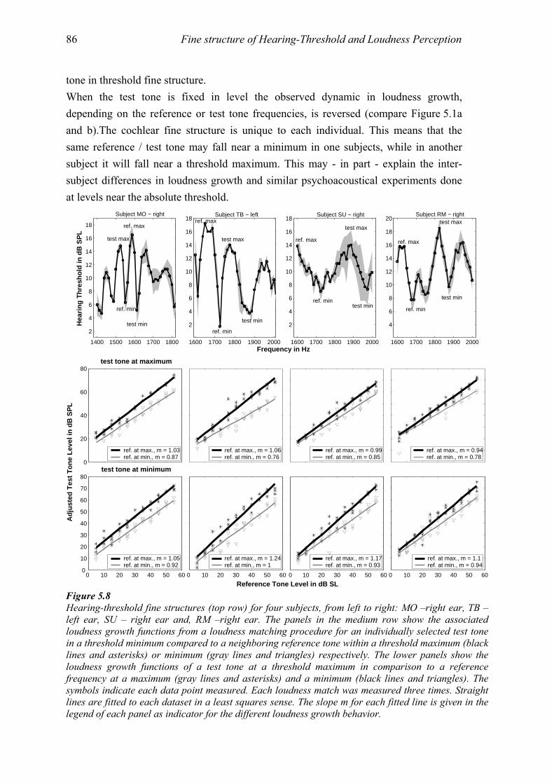
Fine structure of Hearing-Threshold and Loudness Perception 86

tone in threshold fine structure. When the test tone is fixed in level the observed dynamic in loudness growth, depending on the reference or test tone frequencies, is reversed (compare Figure 5.1a and b).The cochlear fine structure is unique to each individual. This means that the same reference / test tone may fall near a minimum in one subjects, while in another subject it will fall near a threshold maximum. This may - in part - explain the inter-subject differences in loudness growth and similar psychoacoustical experiments done at levels near the absolute threshold.

ref. min

ref. max

test max

test min

Subject MO − right

1400 1500 1600 1700 1800

2

4

6

8

10

12

14

16

18

Hea

ring

Thr

esho

ld in

dB

SP

L

ref. max

test max

test min

ref. min

Subject TB − left

1600 1700 1800 1900 2000

2

4

6

8

10

12

14

16

18

Frequency in Hz

ref. max

test max

ref. min test min

Subject SU − right

1600 1700 1800 1900 2000

2

4

6

8

10

12

14

16

18

ref. max

test max

ref. min

test min

Subject RM − right

1600 1700 1800 1900 2000

4

6

8

10

12

14

16

18

20

0 10 20 30 40 50 60

ref. at max., m = 1.1 ref. at min., m = 0.94

0 10 20 30 40 50 60

ref. at max., m = 1.17ref. at min., m = 0.93

0 10 20 30 40 50 60

Reference Tone Level in dB SL

ref. at max., m = 1.24ref. at min., m = 1

0 10 20 30 40 50 600

10

20

30

40

50

60

70

80

Adj

uste

d T

est T

one

Leve

l in

dB S

PL

test tone at minimum

ref. at max., m = 1.05ref. at min., m = 0.92

ref. at max., m = 0.94ref. at min., m = 0.78

ref. at max., m = 0.99ref. at min., m = 0.85

ref. at max., m = 1.06ref. at min., m = 0.76

0

20

40

60

80 test tone at maximum

ref. at max., m = 1.03ref. at min., m = 0.87

Figure 5.8 Hearing-threshold fine structures (top row) for four subjects, from left to right: MO –right ear, TB – left ear, SU – right ear and, RM –right ear. The panels in the medium row show the associated loudness growth functions from a loudness matching procedure for an individually selected test tone in a threshold minimum compared to a neighboring reference tone within a threshold maximum (black lines and asterisks) or minimum (gray lines and triangles) respectively. The lower panels show the loudness growth functions of a test tone at a threshold maximum in comparison to a reference frequency at a maximum (gray lines and asterisks) and a minimum (black lines and triangles). The symbols indicate each data point measured. Each loudness match was measured three times. Straight lines are fitted to each dataset in a least squares sense. The slope m for each fitted line is given in the legend of each panel as indicator for the different loudness growth behavior.

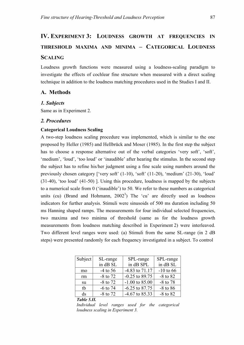
Fine structure of Hearing-Threshold and Loudness Perception 87

IV. EXPERIMENT 3: LOUDNESS GROWTH AT FREQUENCIES IN

THRESHOLD MAXIMA AND MINIMA – CATEGORICAL LOUDNESS

SCALING Loudness growth functions were measured using a loudness-scaling paradigm to investigate the effects of cochlear fine structure when measured with a direct scaling technique in addition to the loudness matching procedures used in the Studies I and II.

A. Methods

1. Subjects Same as in Experiment 2.

2. Procedures

Categorical Loudness Scaling A two-step loudness scaling procedure was implemented, which is similar to the one proposed by Heller (1985) and Hellbrück and Moser (1985). In the first step the subject has to choose a response alternative out of the verbal categories ‘very soft’, ‘soft’, ‘medium’, ‘loud’, ‘too loud’ or ‘inaudible’ after hearing the stimulus. In the second step the subject has to refine his/her judgment using a fine scale using numbers around the previously chosen category [‘very soft’ (1-10), ‘soft’ (11-20), ‘medium’ (21-30), ‘loud’ (31-40), ‘too loud’ (41-50) ]. Using this procedure, loudness is mapped by the subjects to a numerical scale from 0 (‘inaudible’) to 50. We refer to these numbers as categorical units (cu) (Brand and Hohmann, 20023) The ‘cu’ are directly used as loudness indicators for further analysis. Stimuli were sinusoids of 500 ms duration including 50 ms Hanning shaped ramps. The measurements for four individual selected frequencies, two maxima and two minima of threshold (same as for the loudness growth measurements from loudness matching described in Experiment 2) were interleaved. Two different level ranges were used: (a) Stimuli from the same SL-range (in 2 dB steps) were presented randomly for each frequency investigated in a subject. To control

Subject SL-range in dB SL

SPL-range in dB SPL

SPL-range in dB SL

mo -4 to 56 -4.83 to 71.17 -10 to 66 rm -8 to 72 -0.25 to 89.75 -8 to 82 su -8 to 72 -1.00 to 85.00 -8 to 78 tb -6 to 74 -6.25 to 87.75 -8 to 86 ds -8 to 72 -4.67 to 85.33 -8 to 82

Table 5.II. Individual level ranges used for the categorical loudness scaling in Experiment 3.

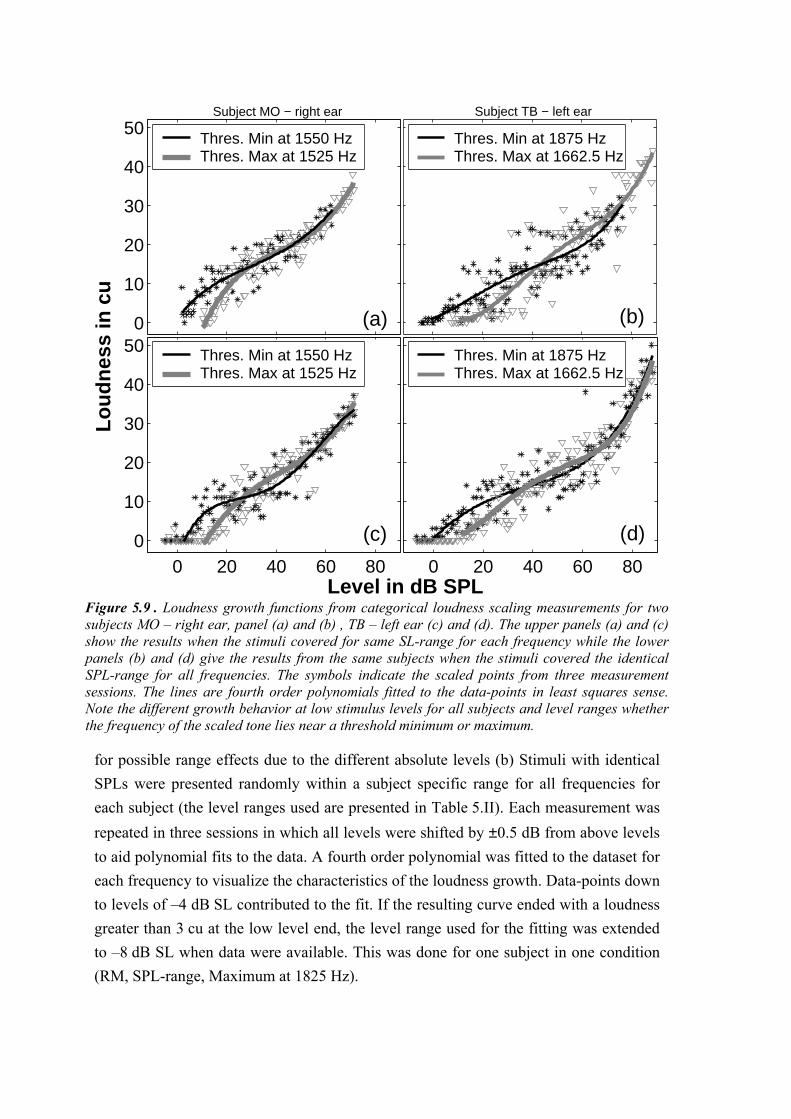
Fine structure of Hearing-Threshold and Loudness Perception 88

for possible range effects due to the different absolute levels (b) Stimuli with identical SPLs were presented randomly within a subject specific range for all frequencies for each subject (the level ranges used are presented in Table 5.II). Each measurement was repeated in three sessions in which all levels were shifted by ±0.5 dB from above levels to aid polynomial fits to the data. A fourth order polynomial was fitted to the dataset for each frequency to visualize the characteristics of the loudness growth. Data-points down to levels of –4 dB SL contributed to the fit. If the resulting curve ended with a loudness greater than 3 cu at the low level end, the level range used for the fitting was extended to –8 dB SL when data were available. This was done for one subject in one condition (RM, SPL-range, Maximum at 1825 Hz).

0

10

20

30

40

50Lo

udne

ss in

cu

Subject MO − right ear

Thres. Min at 1550 HzThres. Max at 1525 Hz

0 20 40 60 800

10

20

30

40

50

Level in dB SPL

Subject TB − left ear

0 20 40 60 80

Thres. Min at 1550 HzThres. Max at 1525 Hz

Thres. Min at 1875 Hz Thres. Max at 1662.5 Hz

Thres. Min at 1875 Hz Thres. Max at 1662.5 Hz

(a)

(c)

(b)

(d)

Figure 5.9 . Loudness growth functions from categorical loudness scaling measurements for two subjects MO – right ear, panel (a) and (b) , TB – left ear (c) and (d). The upper panels (a) and (c) show the results when the stimuli covered for same SL-range for each frequency while the lower panels (b) and (d) give the results from the same subjects when the stimuli covered the identical SPL-range for all frequencies. The symbols indicate the scaled points from three measurement sessions. The lines are fourth order polynomials fitted to the data-points in least squares sense. Note the different growth behavior at low stimulus levels for all subjects and level ranges whether the frequency of the scaled tone lies near a threshold minimum or maximum.

Fine structure of Hearing-Threshold and Loudness Perception 89

B. Results Due to technical restrictions (maximum level of the ER2) the loudness could not be scaled over the whole dynamic range of each subject. This may bias the shape of the perceived loudness growth functions. However, a ‘true’ loudness function was not the aim of this study, the aim was to investigate differences in adjacent frequencies falling either near a minimum near a maximum of cochlear fine structure. There may be range effects affecting the differences near threshold. If there was any major effect it should

0

10

20

30

40

50

60 Thres. Min. at 1550 Hz Thres. Min. at 1612.5 HzThres. Max. at 1525 Hz Thres. Max. at 1587.5 Hz

Thres. Min. at 1675 HzThres. Min. at 1875 HzThres. Max. at 1625 HzThres. Max. at 1825 Hz

0 20 40 60 800

10

20

30

40

50

60

Loud

ness

in c

u

Thres. Min. at 1725 Hz Thres. Min. at 1975 Hz Thres. Max. at 1600 Hz Thres. Max. at 1887.5 Hz

0 20 40 60 80Level in dB SPL

Thres. Min. at 1725 Hz Thres. Min. at 1875 Hz Thres. Max. at 1662.5 HzThres. Max. at 1775 Hz

Subject MO − right ear

(a) (b)

Subject RM − right ear

Subject SU − right ear

(c)

Subject TB − left ear

(d)

Figure 5.10 Each panel shows the loudness growth functions from categorical loudness scaling for frequencies at two individual fine structure maxima (thick gray lines) and minima (thin black lines). From top to bottom: subject MO – right ear, subject rm – left ear, subject SU – right ear and subject TB - left ear. Only the curves for the SPL-range measurements are shown. The SL-range measurements have very similar properties.

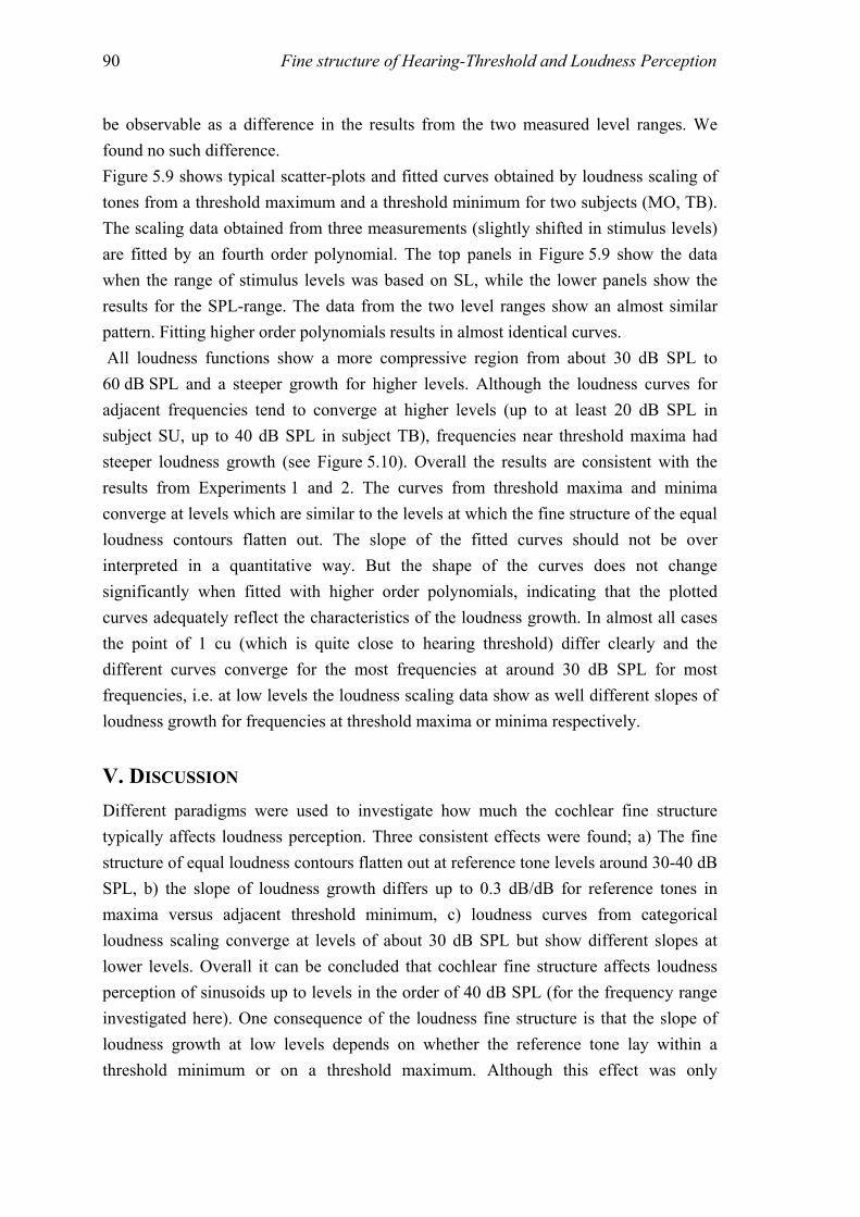
Fine structure of Hearing-Threshold and Loudness Perception 90

be observable as a difference in the results from the two measured level ranges. We found no such difference. Figure 5.9 shows typical scatter-plots and fitted curves obtained by loudness scaling of tones from a threshold maximum and a threshold minimum for two subjects (MO, TB). The scaling data obtained from three measurements (slightly shifted in stimulus levels) are fitted by an fourth order polynomial. The top panels in Figure 5.9 show the data when the range of stimulus levels was based on SL, while the lower panels show the results for the SPL-range. The data from the two level ranges show an almost similar pattern. Fitting higher order polynomials results in almost identical curves. All loudness functions show a more compressive region from about 30 dB SPL to 60 dB SPL and a steeper growth for higher levels. Although the loudness curves for adjacent frequencies tend to converge at higher levels (up to at least 20 dB SPL in subject SU, up to 40 dB SPL in subject TB), frequencies near threshold maxima had steeper loudness growth (see Figure 5.10). Overall the results are consistent with the results from Experiments 1 and 2. The curves from threshold maxima and minima converge at levels which are similar to the levels at which the fine structure of the equal loudness contours flatten out. The slope of the fitted curves should not be over interpreted in a quantitative way. But the shape of the curves does not change significantly when fitted with higher order polynomials, indicating that the plotted curves adequately reflect the characteristics of the loudness growth. In almost all cases the point of 1 cu (which is quite close to hearing threshold) differ clearly and the different curves converge for the most frequencies at around 30 dB SPL for most frequencies, i.e. at low levels the loudness scaling data show as well different slopes of loudness growth for frequencies at threshold maxima or minima respectively.

V. DISCUSSION Different paradigms were used to investigate how much the cochlear fine structure typically affects loudness perception. Three consistent effects were found; a) The fine structure of equal loudness contours flatten out at reference tone levels around 30-40 dB SPL, b) the slope of loudness growth differs up to 0.3 dB/dB for reference tones in maxima versus adjacent threshold minimum, c) loudness curves from categorical loudness scaling converge at levels of about 30 dB SPL but show different slopes at lower levels. Overall it can be concluded that cochlear fine structure affects loudness perception of sinusoids up to levels in the order of 40 dB SPL (for the frequency range investigated here). One consequence of the loudness fine structure is that the slope of loudness growth at low levels depends on whether the reference tone lay within a threshold minimum or on a threshold maximum. Although this effect was only

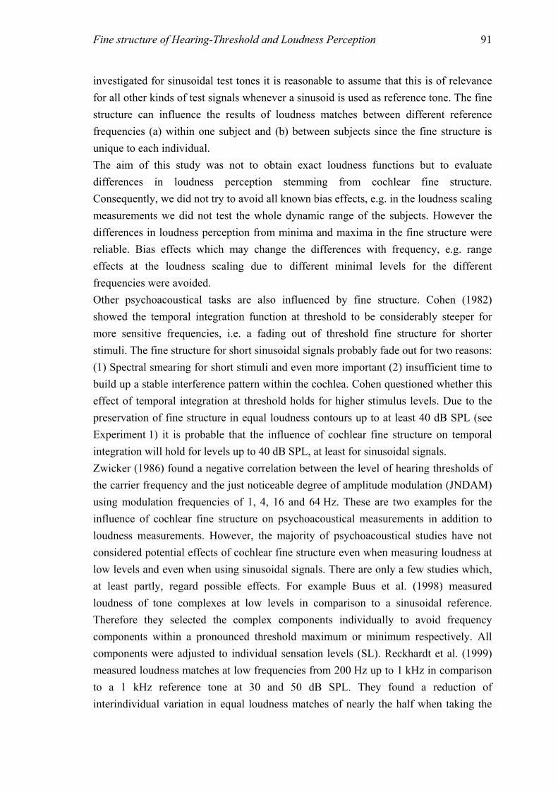
Fine structure of Hearing-Threshold and Loudness Perception 91

investigated for sinusoidal test tones it is reasonable to assume that this is of relevance for all other kinds of test signals whenever a sinusoid is used as reference tone. The fine structure can influence the results of loudness matches between different reference frequencies (a) within one subject and (b) between subjects since the fine structure is unique to each individual. The aim of this study was not to obtain exact loudness functions but to evaluate differences in loudness perception stemming from cochlear fine structure. Consequently, we did not try to avoid all known bias effects, e.g. in the loudness scaling measurements we did not test the whole dynamic range of the subjects. However the differences in loudness perception from minima and maxima in the fine structure were reliable. Bias effects which may change the differences with frequency, e.g. range effects at the loudness scaling due to different minimal levels for the different frequencies were avoided. Other psychoacoustical tasks are also influenced by fine structure. Cohen (1982) showed the temporal integration function at threshold to be considerably steeper for more sensitive frequencies, i.e. a fading out of threshold fine structure for shorter stimuli. The fine structure for short sinusoidal signals probably fade out for two reasons: (1) Spectral smearing for short stimuli and even more important (2) insufficient time to build up a stable interference pattern within the cochlea. Cohen questioned whether this effect of temporal integration at threshold holds for higher stimulus levels. Due to the preservation of fine structure in equal loudness contours up to at least 40 dB SPL (see Experiment 1) it is probable that the influence of cochlear fine structure on temporal integration will hold for levels up to 40 dB SPL, at least for sinusoidal signals. Zwicker (1986) found a negative correlation between the level of hearing thresholds of the carrier frequency and the just noticeable degree of amplitude modulation (JNDAM) using modulation frequencies of 1, 4, 16 and 64 Hz. These are two examples for the influence of cochlear fine structure on psychoacoustical measurements in addition to loudness measurements. However, the majority of psychoacoustical studies have not considered potential effects of cochlear fine structure even when measuring loudness at low levels and even when using sinusoidal signals. There are only a few studies which, at least partly, regard possible effects. For example Buus et al. (1998) measured loudness of tone complexes at low levels in comparison to a sinusoidal reference. Therefore they selected the complex components individually to avoid frequency components within a pronounced threshold maximum or minimum respectively. All components were adjusted to individual sensation levels (SL). Reckhardt et al. (1999) measured loudness matches at low frequencies from 200 Hz up to 1 kHz in comparison to a 1 kHz reference tone at 30 and 50 dB SPL. They found a reduction of interindividual variation in equal loudness matches of nearly the half when taking the

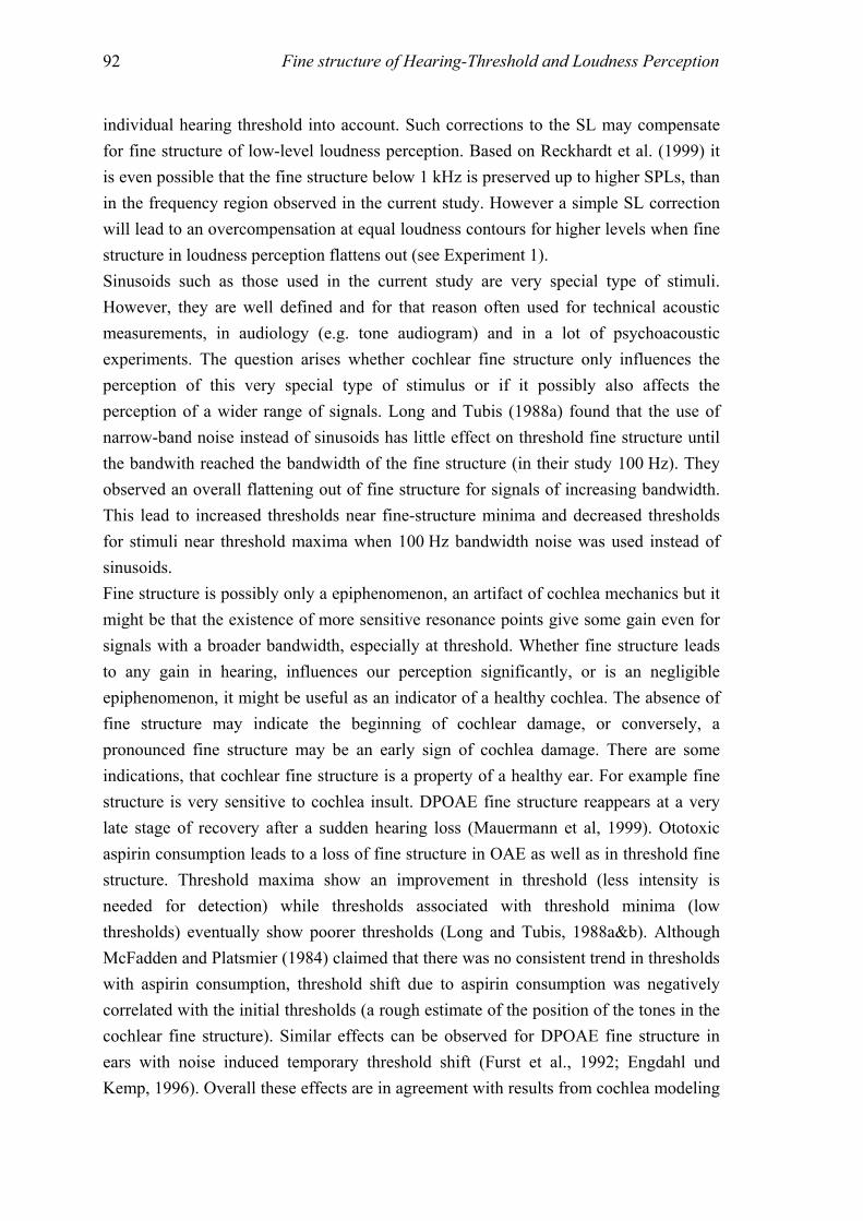
Fine structure of Hearing-Threshold and Loudness Perception 92

individual hearing threshold into account. Such corrections to the SL may compensate for fine structure of low-level loudness perception. Based on Reckhardt et al. (1999) it is even possible that the fine structure below 1 kHz is preserved up to higher SPLs, than in the frequency region observed in the current study. However a simple SL correction will lead to an overcompensation at equal loudness contours for higher levels when fine structure in loudness perception flattens out (see Experiment 1). Sinusoids such as those used in the current study are very special type of stimuli. However, they are well defined and for that reason often used for technical acoustic measurements, in audiology (e.g. tone audiogram) and in a lot of psychoacoustic experiments. The question arises whether cochlear fine structure only influences the perception of this very special type of stimulus or if it possibly also affects the perception of a wider range of signals. Long and Tubis (1988a) found that the use of narrow-band noise instead of sinusoids has little effect on threshold fine structure until the bandwith reached the bandwidth of the fine structure (in their study 100 Hz). They observed an overall flattening out of fine structure for signals of increasing bandwidth. This lead to increased thresholds near fine-structure minima and decreased thresholds for stimuli near threshold maxima when 100 Hz bandwidth noise was used instead of sinusoids. Fine structure is possibly only a epiphenomenon, an artifact of cochlea mechanics but it might be that the existence of more sensitive resonance points give some gain even for signals with a broader bandwidth, especially at threshold. Whether fine structure leads to any gain in hearing, influences our perception significantly, or is an negligible epiphenomenon, it might be useful as an indicator of a healthy cochlea. The absence of fine structure may indicate the beginning of cochlear damage, or conversely, a pronounced fine structure may be an early sign of cochlea damage. There are some indications, that cochlear fine structure is a property of a healthy ear. For example fine structure is very sensitive to cochlea insult. DPOAE fine structure reappears at a very late stage of recovery after a sudden hearing loss (Mauermann et al, 1999). Ototoxic aspirin consumption leads to a loss of fine structure in OAE as well as in threshold fine structure. Threshold maxima show an improvement in threshold (less intensity is needed for detection) while thresholds associated with threshold minima (low thresholds) eventually show poorer thresholds (Long and Tubis, 1988a&b). Although McFadden and Platsmier (1984) claimed that there was no consistent trend in thresholds with aspirin consumption, threshold shift due to aspirin consumption was negatively correlated with the initial thresholds (a rough estimate of the position of the tones in the cochlear fine structure). Similar effects can be observed for DPOAE fine structure in ears with noise induced temporary threshold shift (Furst et al., 1992; Engdahl und Kemp, 1996). Overall these effects are in agreement with results from cochlea modeling

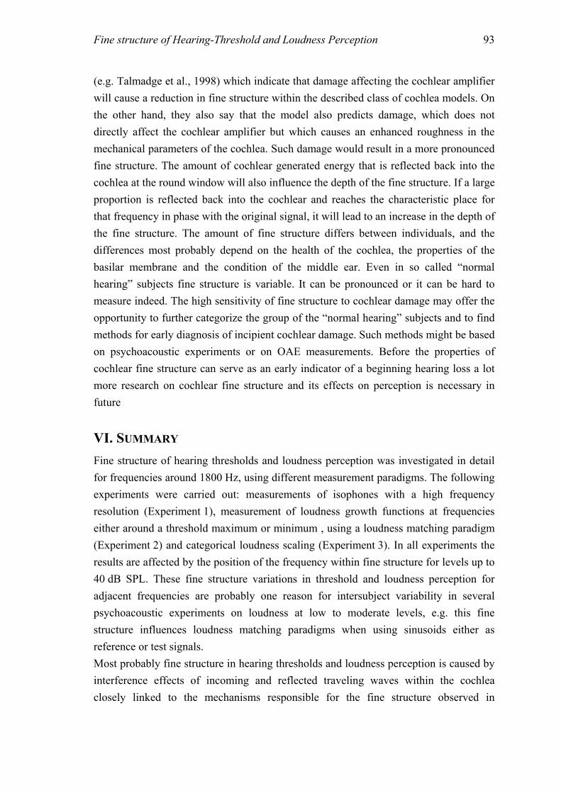
Fine structure of Hearing-Threshold and Loudness Perception 93

(e.g. Talmadge et al., 1998) which indicate that damage affecting the cochlear amplifier will cause a reduction in fine structure within the described class of cochlea models. On the other hand, they also say that the model also predicts damage, which does not directly affect the cochlear amplifier but which causes an enhanced roughness in the mechanical parameters of the cochlea. Such damage would result in a more pronounced fine structure. The amount of cochlear generated energy that is reflected back into the cochlea at the round window will also influence the depth of the fine structure. If a large proportion is reflected back into the cochlear and reaches the characteristic place for that frequency in phase with the original signal, it will lead to an increase in the depth of the fine structure. The amount of fine structure differs between individuals, and the differences most probably depend on the health of the cochlea, the properties of the basilar membrane and the condition of the middle ear. Even in so called “normal hearing” subjects fine structure is variable. It can be pronounced or it can be hard to measure indeed. The high sensitivity of fine structure to cochlear damage may offer the opportunity to further categorize the group of the “normal hearing” subjects and to find methods for early diagnosis of incipient cochlear damage. Such methods might be based on psychoacoustic experiments or on OAE measurements. Before the properties of cochlear fine structure can serve as an early indicator of a beginning hearing loss a lot more research on cochlear fine structure and its effects on perception is necessary in future

VI. SUMMARY Fine structure of hearing thresholds and loudness perception was investigated in detail for frequencies around 1800 Hz, using different measurement paradigms. The following experiments were carried out: measurements of isophones with a high frequency resolution (Experiment 1), measurement of loudness growth functions at frequencies either around a threshold maximum or minimum , using a loudness matching paradigm (Experiment 2) and categorical loudness scaling (Experiment 3). In all experiments the results are affected by the position of the frequency within fine structure for levels up to 40 dB SPL. These fine structure variations in threshold and loudness perception for adjacent frequencies are probably one reason for intersubject variability in several psychoacoustic experiments on loudness at low to moderate levels, e.g. this fine structure influences loudness matching paradigms when using sinusoids either as reference or test signals. Most probably fine structure in hearing thresholds and loudness perception is caused by interference effects of incoming and reflected traveling waves within the cochlea closely linked to the mechanisms responsible for the fine structure observed in

Fine structure of Hearing-Threshold and Loudness Perception 94

otoacoustic emissions. While fine structure effects are observable in most of the normal hearing subjects, there are some listeners with no pathological findings who show no noteworthy fine structure at all. Therefore, it might be valuable to investigate in future studies whether the presence of fine structure may indicate a very healthy ear or an initial damage already observable in most “normal hearing” adults.

ACKNOWLEDGEMENTS This study was supported by Deutsche Forschungsgemeinschaft, DFG Ko 942/11-3. Helpful comments by Stefan Uppenkamp on an earlier version of the manuscript are gratefully acknowledged.

ENDNOTES 1. In the literature, the term threshold microstructure is often used instead of fine structure. For reason of convenience here we consistently use the term fine structure. 2. The results for subject TB from Experiment 1 are about two years older than from Experiment 2/3 i.e. the thresholds measured with the simple adjustment paradigm in Study I and the adaptive interleaved in Experiment 2 and 3 are not necessarily identical 3. Brand and Hohmann used a one step procedure with eleven categories mapped to the same range of numbers (0-50)

Chapter 6

Summary and Outlook

The general aim of predicting hearing status, i.e. predicting thresholds and recruitment, from OAE recordings is not yet achieved, even though significant steps towards this aim have been taken. A reliable model has been established in this thesis, that can serve as a base for the correct interpretation of DPOAE data. The two-source model of DPOAE generation was strongly confirmed by the detailed investigations and simulations of DPOAE fine structure in Chapter 2 and also by the experiments in ears with frequency specific hearing loss in Chapter 3. DPOAE (f2/f1≈1.2) are obviously the result of two interfering components from different sources within the cochlea: (1) An initial distortion source generated in the region of the maximum overlap of BM excitation from the two primary tones (close to f2), and (2), a reflection emission from the characteristic site of the distortion product frequency fDP. A-one source model could not explain the results found here. The two-source model also provides a strategy how to use DPOAE data for prediction of hearing status, e.g. for the prediction of auditory thresholds. Following this strategy the two DPOAE components originating from different cochlear sources have to be separated in order to explicitly investigate the cochlea status at a certain frequency site. For example Boege and Janssen (2002) described a method for the prediction of individual thresholds from DPOAE I/O functions. They suggested to relate the DPAOE I/O functions to the cochlear status at the characteristic site of f2, but they did not take the effects of a second source into account. The results in Chapter 4 show that this approach should be extended for a more reliable clinical application. DPOAE I/O functions are influenced by the second DPOAE source from the fDP site. An investigation of I/O characteristics from only the initial distortion source close to f2 instead of “standard” DPOAE I/O functions results in a clear reduction of the variability in threshold predictions of adjacent frequencies. Therefore the separation of the two DPOAE sources for predicting hearing status is a necessary condition for both, a clear interpretability of the DPOAE data and the practical improvement of hearing status prediction from DPOAE measurements. At this point several extensions of the current work should be pursued in future studies. Although the time windowing method is a reliable method for the separation of DPOAE sources without affecting the measurement procedure itself - e.g. by the application of additional signals - it requires an enormous time effort to measure DPOAE at sufficiently many levels and frequencies, that are needed to allow a correct source

Summary and Outlook 96

separation. This effort (about 8 hours for a usable frequency range of about one octave) is out of question for clinical applications. Another method might be more appropriate to allow the separation of DPOAE sources for single frequencies. The method of selective suppression uses a third tone close to fDP to suppress the effect of the second source. Measurements with an additional suppressor tone need the same time effort as “standard” DPOAE I/O functions, which is acceptable for clinical use. However, this method requires adequate suppressor levels that have to be found in future studies for a whole range of primary levels that cover the required range of DPOAE I/O functions, to be able to use this method. An adequate suppressor level has to suppress the second source more or less completely while keeping the initial DPOAE source almost unchanged. With a set of appropriate suppressor levels the threshold predictions from DCOAE I/O functions have then to be evaluated in a clinical study. The results in Chapter 5 show that most “normal hearing” subjects have a considerable fine structure in hearing threshold and loudness perception, i.e. quasi-periodic variations in hearing thresholds with differences of up to 15 dB between adjacent maxima and minima in sensitivity. For a standard clinical test these fluctuations for sinusoids are not of interest, but the average hearing capability in a specific frequency band is seeked. These results therefore indicate that sinusoids as used in pure tone audiograms are not an appropriate signal to obtain a robust frequency specific clinical indication of hearing status. This holds especially for the comparison with the outcome of other audiometric tests, like DPOAE measurements, that are not affected by the cochlea resonances in the same way as hearing thresholds. Therefore narrow band noises would be more appropriate signals to quantify hearing thresholds or loudness perception for the comparison with the outcome of predictions from DPOAE measurements. Due to the fact that not all “normal hearing” subjects show a fine structure in hearing threshold, the question arises about the difference between subjects with or without threshold fine structure. Does a pronounced fine structure indicate an initial damage to the cochlea or is conversely a sign of a very healthy ear? The properties of threshold perception and possibly further psychoacoustical properties near threshold could turn out to be tools to differentiate the group of “normal hearing” subjects in more detail and could help to indicate the start of a hearing loss at very early stages. The fine structure of DPOAE shows a similar potential. As shown in Chapter 3 (see Figure 3.5) DPOAE fine structure is much more sensitive to a cochlea damage than the psychophysical hearing threshold itself. Taken together, investigations in near-threshold properties and OAE fine structure effects open a wide field for future studies on a more detailed differentiation of “normal hearing subjects”, and on early indicators of cochlear hearing loss that go far beyond the actual clinical standard.

REFERENCES Allen, J. and P. Fahey (1993). "A second cochlear-frequency map that correlates

distortion product and neural tuning measurements." J. Acoust. Soc. Am. 94, 809-816.

Boege, P. and T. Janssen (2002). "Pure-tone threshold estimation from extrapolated distortion product otoacoustic emission I/O-functions in normal and cochlear hearing loss ears," J. Acoust. Soc. Am. 111, 1810-1818.

Boege, P. (2003). Personal communication.

de Boer, E. (1995). "The 'inverse problem' solved for a three-dimensional model of the cochlea. I. Analysis," J. Acoust. Soc. Am. 98, 896-903.

Brown, A.M., Harris, F.P., and Beveridge, H.A. (1996). "Two sources of acoustic distortion products from the human cochlea," J. Acoust. Soc. Am. 100, 3260-3267.

Brown, A. and D. Williams (1993). "A second filter in the cochlea" in Biophysics of hair cell sensory systems, edited by J. H. Duifhuis, P van Dijk, SM van Netten, (World Scientific, Singapore), pp. 72-77.

Brownell, W., Bader, C.R., Bertrand, D., Ribaupierre, Y. (1985). “Evoked mechanical responses of isolated cochlear outer hair cells,” Science 227, 194-196.

Buus, S., Musch, H., and Florentine, M. (1998). „On loudness at threshold,“ J. Acoust. Soc. Am. 104, 399-410.

Buus, S., Obeling, L. and Florentine, M., (2001)."Can basilar membrane compression characterisitcs be determined from distortion-product otoacoustic emission input-output functions in humans," in Physiological and psychophysical bases of auditory function, Proceedings of the 12th International Symposium on Hearing, Mierlo August 2000, edited by D.J. Breebart, A.J.M. Houtsma, A. Kohlrausch, V.F. Prijs, R. Schoonhoven, p.373-381

Cohen, M.F. (1982). “Detection threshold microstructure and its effect on temporal integration data,“ J. Acoust. Soc. Am. 71, 1719-1733.

Dhar, S., C. L. Talmadge, G. R. Long and A. Tubis (2002). "Multiple internal reflections in the cochlea and their effect on DPOAE fine structure." J. Acoust. Soc. Am. 112, 2882-97.

References 98

Duifhuis, H., Hoogstraten, H.W., van Netten, S.M., Diependaal, R.J., and Bialek, W. (1985). "Modelling the cochlear partition with coupled van der Pol-Oscillators," in Peripherial Auditory Mechanisms, edited by J.B. Allen, J.L. Hall, A.E. Hubbard, S.T. Neely, and A. Tubis, Lecture Notes in Biomathematics 64 (Springer, Berlin), pp. 290-297.

Elliot, E. (1958). “A ripple effect in the audiogram,” Nature 81, 1076.

Engdahl, B. and D. T. Kemp (1996). "The effect of noise exposure on the details of distortion product otoacoustic emissions in humans." J. Acoust. Soc. Am. 99, 1573-1587.

Furst, M. and Goldstein, J.L. (1982) "A cochlear nonlinear transmission-line model compatible with combination tone psychophysics," J. Acoust. Soc. Am. 72, 717-726.

Furst, M., Reshef, I., and J. Attias, J. (1992). “Manifestations of intense noise stimulation of spontaneous otoacoustic emissions and threshold microstructure: experiment and model,“ J. Acoust. Soc. Am. 91, 1003-1014.

Gaskill, S.A. and Brown, A.M. (1990) "The behaviour of the acoustic distortion product, 2f1-f2, from the human ear and its relation to auditory sensitivity, " J. Acoust. Soc. Am. 88, 821-839.

Gaskill, S. A., and Brown, A.M. (1996). "Suppression of human acoustic distortion product: dual origin of 2f1-f2," J. Acoust. Soc. Am. 100, 3268-3274.

Gorga, M.P., Neely, S.T., Bergman, B., Beauchaine, K.L., Kaminski, J.R., Peters, J., and Jestaedt, W. (1993). “Otoacoustic emissions from normal-hearing and hearing-impaired subjects: Distortion product responses,” J. Acoust. Soc. Am. 93, 2050-2060.

Gorga, M. P., S. T. Neely, P. A. Dorn and B. M. Hoover (2003). "Further efforts to predict pure-tone thresholds from distortion product otoacoustic emission input/output functions." J. Acoust. Soc. Am. 113, 3275-3284.

Greenwood, D.D. (1991). "Critical bandwidth and consonance in relation to cochlear frequency-position coordinates," Hear. Res. 54, 164-208.

Harris, F.P., Probst, R., and Xu, L. (1992). "Suppression of the 2f1-f2 otoacoustic emission in humans," Hear. Res. 64, 133-141.

References 99

Harris, F. P., and Probst, R. (2002). “Otoacoustic Emissions and Audiometric Outcomes,” in Otoacoustic Emissions - Clinical Applications, 2nd ed., edited by. M. S. Robinette and T. J. Glattke. (Thieme New York, Stuttgart), pp 416-438-

He, N.-J. (1990). “Frequency shift in spontaneous otoacoustic emission and threshold fine structure. PhD thesis,” University of Iowa.

He, N.-J., and Schmiedt, R. A. (1993). "Fine structure of the 2f1-f2 acoustic distortion product: changes with primary levels," J. Acoust. Soc. Am. 94, 2659-2669.

He, N. and Schmiedt, R.A. (1996). “Effects of aging on the fine structure of the 2f1-f2 acoustic distortion product,” J. Acoust. Soc. Am. 99, 1002-1015.

He, N. and Schmiedt, R.A. (1997). "Fine structure of the 2f1-f2 acoustic distortion product: effects of primary level and frequency ratios," J. Acoust. Soc. Am. 101, 3554-3565.

Heitmann, J., Waldmann, B., Schnitzler, H.U., Plinkert, P.K., and Zenner, H.P. (1998). "Suppression of distortion product otoacoustic emissions (DPOAE) near 2f1-f2 removes DP-gram fine structure - Evidence for a secondary generator," J. Acoust. Soc. Am. 103, 1527-1531.

Hellman, R. P. and Zwislocki, J. (1961). “Some factors affecting the estimation of loudness ,” J. Acoust. Soc. Am. 33, 687-694.

Horst, W. J, and de Kleine, E. (1999). „Audiogram fine structure and spontaneous otoacoustic emissions in patients with Meniere's disease,” Audiology 38, 267-270

Hoth, S. and Lenarz, T. (1993). “Otoakustische Emissionen - Grundlagen und Anwendung,” (Thieme, Stuttgart). p. 12

van Hengel, P. (1993). Comment to paper presented by Shera and Zweig (1993), in Biophysics of hair cell sensory systems, edited by H. Duifhuis, J.W. Horst, P. van Dijk, and S.M. van Netten (World Scientific, Singapore), p. 62.

van Hengel, P.W.J., Duifhuis, H., and van den Raadt, M.P.M.G. (1996). "Spatial periodicity in the cochlea: the result of interaction of spontaneous emissions?," J. Acoust. Soc. Am. 99, 3566-3571.

References 100

van Hengel, P.W.J., Duifhuis, H. (1999). “The generation of distortion products in a nonlinear transmission line model of the cochlea” in Proceedings of the Symposium on Recent Developments in Auditory Mechanics, 25-30 july, Sendai, Japan., edited by H. Wada, T. Takasaka, K. ikeda, K. Ohyama and T.Koike. (World Scientific, Singapore),

Kalluri, R. , and Shera, C. A. (2001). "Distortion-product source unmixing: a test of the two-mechanism model for DPOAE generation," J. Acoust. Soc. Am. 109, 622-637.

Kapadia S., Lutman M.E. (1999). “Reduced audiogram ripple' in normally-hearing subjects with weak otoacoustic emissions,” Audiology 38, 257-26

Kemp, D. T. (1978). "Stimulated acoustic emissions from within the human auditory system," J. Acoust. Soc. Am. 64, 1386-1391.

Kemp, D. T. (1979). “The evoked cochlear mechanical response and auditory microstructure - evidence for a new element in cochlear mechanics,“ Scand. Audiol. Supp 9, 35-47.

Kemp, D. T. (1980). “Towards a model for the origin of cochlear echoes,“ Hear. Res. 2, 533-548.

Knight, R. D., and Kemp, D. T. (2001). "Wave and place fixed DPOAE maps of the human ear," J. Acoust. Soc. Am. 109, 1513-1525.

Konrad-Martin, D., Neely, S. T., Keefe, D. H., Dorn, P. A. , and Gorga, M. P. (2001). "Sources of distortion product otoacoustic emissions revealed by suppression experiments and inverse fast Fourier transforms in normal ears," J. Acoust. Soc. Am. 109, 2862-2879.

Konrad-Martin, D., Neely, S. T., Keefe, D. H., Dorn, P. A., Cyr, E. and Gorga, M. P. (2002). "Sources of DPOAEs revealed by suppression experiments, inverse fast Fourier transforms, and SFOAEs in impaired ears," J. Acoust. Soc. Am. 111, 1800-1809

Kummer, P., Janssen, T., and Arnold, W. (1995). "Suppression tuning characteristics of the 2f1-f2 distortion-product otoacoustic emission in humans," J. Acoust. Soc. Am. 98, 197-210.

Kummer, P., Janssen, T., and Arnold, W. (1998). “The level and growth behavior of the 2f1-f2 distortion product otoacoustic emission and its relationship to auditory sensitivity in normal hearing and cochlear hearing loss,” J. Acoust. Soc. Am. 103, 3431-3444.

References 101

Long, G. R. (1984) . “The microstructure of quiet and masked thresholds,“ Hear. Res. 15 , 73-87.

Long, G. R. (1993). Perceptual Consequences of otoacoustic emissions. In A. Schick (Eds.), Contributions to Psychological Acoustics: Results of the 6th Oldenburg Symposium on Psychological Acoustics. University of Oldenburg Press, Oldenburg. Germany. pp. 59-80.

Long G. R. (1998) “Perceptual consequences of the interactions between spontaneous otoacoustic emissions and external tones. I. Monaural diplacusis and aftertones,” Hear Res. , 119, :49-60

Long, G. R. and Tubis, A. (1988a). “Investigations into the nature of the association between threshold microstructure and otoacoustic emissions,“ Hear. Res. 36, 125-138.

Long, G. R. and Tubis, A. (1988b). “Modification of spontaneous and evoked otoacoustic emissions and associated psychoacoustic microstructure by aspirin consumption,“ J. Acoust. Soc. Am. 84, 1343-1353.

Long, G. R. and Talmadge, C.L. (1997). “Spontaneous otoacoustic emission frequency is modulated by heartbeat,” J. Acoust. Soc. Am. 102, 2831 -2848 (1997).

Mauermann, M., Uppenkamp, S., and Kollmeier, B. (1997a). "Zusammenhang zwischen unterschiedlichen otoakustischen Emissionen und deren Relation zur Ruhehörschwelle [The relation of different types of otoacoustic emissions and the threshold in quiet]," in Fortschritte der Akustik – DAGA 97, edited by P. Wille (DEGA e.V., Oldenburg), pp. 242-243.

Mauermann, M., Uppenkamp, S., and Kollmeier, B. (1997b). "Periodizität und Pegelabhängigkeit der spektralen Feinstruktur von Verzerrungsprodukt-Emissionen [Periodicity and dependence on level of the distortion product otoacoustic emission spectral fine-structure]," Audiol. Akustik 36, 92-104.

Mauermann, M., Uppenkamp, S., van Hengel, P. W., and Kollmeier, B. (1999a). "Evidence for the distortion product frequency place as a source of distortion product otoacoustic emission (DPOAE) fine structure in humans. I. Fine structure and higher-order DPOAE as a function of the frequency ratio f2/f1." J. Acoust. Soc. Am. 106, 3473-3483.

References 102

Mauermann, M., Uppenkamp, S., van Hengel, P. W., and Kollmeier, B. (1999b). "Evidence for the distortion product frequency place as a source of distortion product otoacoustic emission (DPOAE) fine structure in humans. II. Fine structure for different shapes of cochlear hearing loss." J. Acoust. Soc. Am. 106, 3484-91.

Mauermann, M., Long, G. and Kollmeier, B. (2000a). “Comparison of fine structure in isophone contours, threshold in quiet and otoacoustic emissions.” Abstracts of the 20th ARO midwinter research meeting. St. Petersburg Beach, Florida, 284 (A).

Mauermann, M., Long, G. und Kollmeier, B. (2000b). “Vergleich der Feinstruktur von Isophonen, Ruhehörschwelle und otoakustischen Emissionen.” in Fortschritte der Akustik – DAGA 2000. Oldenburg, Deutsche Gesellschaft für Akustik e.V., 292-293.

Mauermann, M., Long, G. R., and Kollmeier, B. (2003), “Fine structure of Hearing-Threshold and Loudness Perception,” J.Acoust Soc. Am. (submitted)

McFadden, D., and Plattsmier, H.S. (1984). “Apirin abolishes spontaneous oto-acoustic emissions.” J. Acoust. Soc. Am. 76, 443-448

Moulin, A., Bera, J.C., Collet, L. (1994). “Distortion product otoacoustic emissions and sensorineural hearing loss,” Audiology 33, 305-326.

Neely, S. T., Gorga, M. P., and Dorn, P. A. (2003). "Cochlear compression estimates from measurements of distortion-product otoacoustic emissions." J. Acoust. Soc. Am. 114, 1499-1507.

Neely, S. (2003). Personal communication.

Nelson, D.A. and Kimberley, B.P. (1992). “Distortion product emissions and auditory sensitivity in human ears with normal hearing and cochlear hearing loss,” J. Speech Hear. Res. 35, 1142-1159.

Oswald, J. A., Müller, J., and Janssen, T. (2002). ‘‘Audiometric threshold estimation in cochlear hearing loss ears by means of weighted extrapolated DPOAE I/O functions,’’ presented at the Twenty-Fifth Annual Midwinter Research Meeting of the Association for Research in Otolaryngology, St. Petersburg Beach, FL. #774 (A).

Penner, M. J. and Burns, E. M. (1987) "The dissociation of SOAEs and tinnitus," J. Speech Hear. Res., vol. 30, pp. 396-403.

References 103

Pickles, J. (1988). “An Introduction to the Physiology of Hearing”, 2nd edition, (Academic Press, London). p. 149

van den Raadt, M.P.M.G. and Duifhuis, H. (1990). "A generalized Van der Pol-oscillator cochlea model," in The mechanics and biophysics of hearing, edited by P. Dallos, C.D. Geisler, J.W. Matthews, M.A. Ruggero, and C.R. Steele, Lecture Notes in Biomathematics 87 (Springer, Berlin), pp. 227-234.

van den Raadt, M.P.M.G. and Duifhuis, H. (1993). "Different boundary conditions in a one-dimensional time domain model," in Biophysics of Hair Cell Sensory Systems, edited by H. Duifhuis, J.W. Horst, P. van Dijk, and S.M. van Netten, (World Scientific, Singapore), p. 103.

Rao, A., Long, G. R., Narayan, S. S., Dhar, S. (1996). "Changes in the temporal characteristics of TEOAE and the fine structure of DPOAEs with asoirin consumption," in Abstracts of the 19th ARO midwinter research meeting, abstract, p. 27.

Reckhardt, C., Mellert, V., and Kollmeier, B. (1999). “Factors influencing equal-loudness contours,“ in Psychophysics, Physiology and Models of Hearing , edited by T. Dau, V. Hohmann and B. Kollmeier (World Scientific Publishing, Singapore), pp. 113-116.

Ruggero, M.A., Rich, N.C. (1991). "Application of a commercially-manufactured Doppler-shift laser velocimeter to the measurement of basilar-membrane vibration," Hear. Res. 51, 215-230.

Schlögel, H., Stephan, K., Böheim, K., Welzl-Müller, K., (1995). “Distorsionsprodukt otoakustische Emissionen bei normalem Hörvermögen und bei sensorineuraler Schwerhörigkeit,” HNO 43, 19-24.

Shera, C.A. and Zweig, G. (1993). "Order from chaos: resolving the paradox of periodicity in evoked otoacoustic emissions," in Biophysics of hair cell sensory systems, edited by H. Duifhuis, J.W. Horst, P. van Dijk, and S.M. van Netten (World Scientific, Singapore), pp. 54-63.

Shera, C.A., Guinan, J.J. (1998). "Reflection emissions and distortion products arise from fundamentally different mechanisms," in Abstracts of the 21st ARO midwinter research meeting, abstract no. 344, p. 86.

Shera, C.A., Guinan, J.J. (1999). "Evoked otoacoustic emissions arise by two fundamentally different mechanisms: A taxonomy for mammalian OAEs," J. Acoust. Soc. Am. 105, 782-798.

References 104

Siegel, J. H. (2002). “Calibrating Otoacoustic Emission Probes,” in Otoacoustic Emissions - Clinical Applications, 2nd ed., edited by. M. S. Robinette and T. J. Glattke. (Thieme New York, Stuttgart), pp 416-438

Smurzynski, J., Leonard, G., Kim, D.O., Lafreniere, D.C., and Jung, M.D. (1990). "Distortion product otoacoustic emissions in normal and impaired adult ears," Arch. Otolaryngol. Head Neck Surg. 116, 1309-1316.

Smurzynski J, and Probst, R. (1998) “The influence of disappearing and reappearing spontaneous otoacoustic emissions on one subject’s threshold microstructure,” Hear Res. 115,197-205

Suckfüll, M., Schneeweiß, S., Dreher, A., and Schorn, K. (1996). “Evaluation of TEOAE and DPOAE measurements for the assessment of auditory thresholds in sensorineural hearing loss,” Acta Otolaryngol. (Stockh) 116, 528-533.

Sun, X., Schmiedt, R.A., He, N., and Lam, C.F. (1994a). "Modeling the fine structure of the 2f1-f2 acoustic distortion product. I. - Model development," J. Acoust. Soc. Am. 96, 2166-2174.

Sun, X., Schmiedt, R.A., He, N., and Lam, C.F. (1994b). "Modeling the fine structure of the 2f1-f2 acoustic distortion product. II. Model evaluation," J. Acoust. Soc. Am. 96, 2175-2183.

Talmadge, C.L. and Tubis, A. (1993). "On modeling the connection between spontaneous and evoked otoacoustic emissions," in Biophysics of hair cell sensory systems, edited by H. Duifhuis, J.W. Horst, P. van Dijk, and S.M. van Netten (World Scientific, Singapore), pp. 25-32.

Talmadge, C.L., Tubis, A., Long, G.R., and Piskorski, P. (1998). "Modeling otoacoustic emission and hearing threshold fine structure," J. Acoust. Soc. Am. 104, 1517-1543.

Talmadge, C.L., Long, G.R., Tubis, A., and Dhar, S. (1999). "Experimental confirmation of the two-source interference model for the fine structure of distortion product otoacoustic emissions," J. Acoust. Soc. Am.105, 275-292.

Thomas, I. B. (1975). “Microstructure of the pure tone threshold,“ J. Acoust. Soc. Am. pp. S26-27. (abstract)

Uppenkamp S, B Kollmeier, and U Eysholdt (1990) "Evozierte otoakustische Emissionen bei Tinnituspatienten [Evoked otoacoustic emissions in patients with tinnitus]," Audiol Akustik 29, 148-161.

References 105

Uppenkamp, S and M Mauermann (1999). "Effect of frequency ratio f2/f1 on spectral fine structure of distortion product otoacoustic emissions," Brit. J. Audiol. 33, 87-88 (A).

van den Brink, G. (1970) . “Experiments on binaural diplacusis and tone perception,” in Frequency Analysis and Periodicity Detection in Hearing , edited by R. Plomp and G. F. Smoorenburg (Sijthoff, Leiden), pp. 362-374.

van den Brink, G. (1980). “Cochlear mechanics as the possible cause of binaural diplacusis,“ in Psychological, Physiological and Behavioural Studies in Hearing , edited by G. van den Brink and F. Bilsen (Delft University Press, Delft), pp. 64-67.

Wilson, J. P. (1980). ‘‘Evidence for a cochlear origin for acoustic reemissions, threshold fine-structure and tonal tinnitus,’’ Hear. Res. 2, 233–252.

Zenner, H., Zimmermann, U., and Schmidt, U. (1985). “Reversible contraction of isolated mammalian cochlear hair cells,” Hear. Res. 18, 127-133.

Zweig, G. (1991). "Finding the impedance of the organ of Corti," J. Acoust. Soc. Am. 89, 1229-1254.

Zweig, G. and Shera, C. A. (1995). ”The origins of periodicity in the spectrum of oked otoacoustic emissions,“ J. Acoust. Soc. Am. 98 , 2018-2047.

Zwicker, E. (1986). “Spontaneous oto-acoustic emissions, threshold in quiet, and just noticeable amplitude modulation at low levels,“ in Auditory Frequency Selectivity, edited by B. C. J. Moore and R. D. Patterson (Plenum Press, New York), pp. 49-59.

Zwicker, E. and Peisl, W. (1990). “Cochlear processing in analog models, in digital models, and in human inner ear,” Hear. Res. 44 , 206-216.

Zwicker, E. and Schloth, E. (1984). “Interrelation of different oto-acoustic emissions,“ J. Acoust. Soc. Am. 75, 1148-1154.

ERKLÄRUNG Hiermit erkläre ich, dass ich die vorliegende Arbeit selbstständig verfasst und nur die angegebenen Quellen und Hilfsmittel verwendet habe Oldenburg, den 16. Dezember 2003 Manfred Mauermannn

DANKSAGUNG

Ich möchte mich an dieser Stelle bei all denen bedanken, die mich bei der Anfertigung dieser Dissertation unterstützt haben bzw. diese Arbeit überhaupt ermöglicht haben:

An erster Stelle gilt deshalb mein Dank Herrn Prof. Dr. Dr. Birger Kollmeier, der diese Dissertation in einem Rahmen ermöglicht hat, den man nur als rundum sehr gut bezeichnen kann.

Herrn Prof. Dr. Volker Mellert danke ich für die freundliche Übernahme des Korreferats.

Dr. Stefan Uppenkamp (Stup) gilt mein Dank für die geduldige Einarbeitung in den Themenbereich der otoakustischen Emissionen während meiner Diplomarbeit, die mich dazu verleitet hat, in diesem Bereich weiter zu forschen. Mein Dank auch für die weiterführende gute und freundschaftliche Zusammenarbeit in den Studien zu Kapitel 2 und 3. Danke auch für das Korrekturlesen der übrigen Kapitel.

Den Groningern, Prof. Dr. H. Duifhius und Dr. Peter van Hengel möchte ich danken für die intensiven Diskussionen über Cochlea Modelle und Cochleamechanik. Ohne die beiden wäre meine Vorstellung über das, was in der Cochlea passiert, weit löchriger. Peter möchte ich darüber hinaus für die gute Zusammenarbeit in Sachen Cochlea- und OAE-Modellierung im Rahmen der Studien zu Kapitel 2 und 3 danken.

Prof. Dr. Glenis Long danke ich für viele Diskussionen über alle Aspekte des Hörens und die fruchtbare Zusammenarbeit im Rahmen der Studien zu Kapitel 5.

Prof. Dr. Torsten Dau mein Dank für seine Gesangseinlagen (Mani, Mani, Mani ...), unfreiwillige Rückenmassagen, all die Spitznamen für Arbeitsgruppenmitglieder, ..., Diskussionen und Denkanstöße sowie seine ansteckende Begeisterung in Sachen Forschung, die der eigenen Motivation immer wieder auf die Sprünge half.

Junior Prof. Dr. Jesko Verhey möchte ich danken in seiner Funktion als mein „wandelndes Psychoakustik-Lexikon“ und seine Unterstützung bei der Programmierung von si-Skripten, die den Grundstein legte für die Messungen zu Kapitel 5.

Dr. Volker Hohmann mein Dank für die Beantwortung vieler vieler Signalverarbeitungsfragen.

Dr. Daniel Berg danke ich für die Programmierung von oaemex.dll und damit für die Befreiung von den Einschränkungen der Ariel-Karte sowie nur wenig flexiblen kommerziellen OAE Systemen.

Dr. Birgitta Gabriel sei gedankt für die freundliche Unterstützung bei dem Ausfindigmachen geeigneter Probanden. In diesem Zusammenhang ein Dank an alle meine Versuchspersonen für ihre Geduld und Ausdauer.

Anita Gorges, dem Herz der Arbeitsgruppe, mein Dank für die vielseitige technische Unterstützung und die Unterstützung zu den Messungen für Kapitel 4 .

Dr. Oliver Fobel (ehem. Wegner - OhWeh) danke ich für die häufige Unterstützung in Sachen Computer und Netzwerk, zu einer Zeit als die Netzwerke noch wild und die Festplatten klein waren.

Für die gute Zusammenarbeit, seine lockere Art und den Vorrat an Süßigkeiten in seiner Schreibtischschublade, der so manche Unterzuckerung zu vermeiden half, möchte ich Matthias Müller-Wehlau danken.

Meiner „Mitbewohnerin“ - in kleinen wie in großen Büroräumen - Dr. K. C. Wagener danke ich für das freundschaftliche Miteinander und das Erdulden gelegentlicher Fluchanfälle meinerseits.

Diskussionen mit Dr. Stefan Ewert, Dr. Helmut Riedel und Dr. Thomas Brand zu verschiedenen Aspekten haben mir oft weitergeholfen – Danke.

Danke auch an alle anderen Mitglieder der Arbeitsgruppe Medizinische Physik in Vergangenheit (der von mir erlebten) und Gegenwart für die unkomplizierte, konstruktive und freundschaftliche Zusammenarbeit.

Meinen Kindern Falk und Lea danke ich dafür, dass sie da sind und mir immer wieder dabei helfen, die „Wichtigkeit“ von so etwas wie einer Doktorarbeit in das rechte Licht zu rücken.

Meiner Frau Gisela danke ich für die Geduld mit mir und dieser Arbeit, vor allen in der abschließenden „Panikphase“.

LEBENSLAUF Am 26.12.1967 wurde ich, Manfred Mauermann, als Sohn von Otmar und Annegrete Mauermann, geb. Czarnecki in Frankfurt am Main geboren. Dort besuchte ich von 1974 bis 1978 die Grundschule und wechselte anschließend auf das Helmholtz Gymnasium, das ich 1987 mit Abitur abschloss. Nach meinem Zivildienst in Frankfurt und auf der Nordseeinsel Spiekeroog (September 1987 bis April 1989) folgten auf Spiekeroog verschiedene Saisontätigkeiten als Erziehungs- und Küchenhelfer bis September 1990. Zum Wintersemester 1990/91 begann ich mein Studium der Physik an der Carl-von-Ossietzky Universität Oldenburg. Meine Diplomarbeit über „die Analyse otoakustischer Emissionen und ihren Zusammenhang zur Psychoakustik“ schrieb ich in der Arbeitsgruppe Medizinische Physik bei Prof. Dr. Dr. Birger Kollmeier, um im September 1997 mein Studium mit Diplom abzuschließen. Im Zeitraum von Oktober 1997 bis Dezember 2001 war ich als wissenschaftlicher Mitarbeiter im Rahmen des Drittmittelprojektes „Otoakustische Emissionen“ an der Carl-von-Ossietzky Universität Oldenburg tätig und begann unter Anleitung von Prof. Dr. Dr. Kollmeier mit der Arbeit an der vorliegenden Dissertation. In der Zeit vom Januar 2001 bis Januar 2002 war ich an der Fachhochschule Oldenburg/Ostfriesland/Wilhelmshaven als wissenschaftlicher Mitarbeiter mit dem Aufbau des Projektpraktikums für den neu gegründeten Studiengang Hörtechnik und Audiologie betraut. In dieser Zeit ruhte der Fortgang der Promotion. Seit Februar 2003 bin ich nun wieder als wissenschaftlicher Mitarbeiter an der Carl-von-Ossietzky Universität Oldenburg tätig, wo ich im Rahmen des Drittmittelprojektes „Otoakustische Emissionen“ meine Dissertation abschließen konnte.