Embed Size (px)
Citation preview

Universitat Ulm
Fakultat fur Mathematik und
Wirtschaftswissenschaften
UN
IVERS ITÄT
U
LM
·S
CIE
ND
O
·DOCENDO
·
CU
RA
ND
O·
Form Methods
for Linear Evolution Problems
on Hilbert Spaces
Diplomarbeit zur Erlangung des akademischen Grades ”Dipl. math. oec.”
vorgelegt von
Markus Kunze

Universitat Ulm
Fakultat fur Mathematik und
Wirtschaftswissenschaften
UN
IVERS ITÄT
U
LM
·S
CIE
ND
O
·DOCENDO
·
CU
RA
ND
O·
Form Methods
for Linear Evolution Problems
on Hilbert Spaces
Diplomarbeit zur Erlangung des akademischen Grades ”Dipl. math. oec.”
vorgelegt von
Markus Kunze
1. Gutachter: Prof. Dr. W. Arendt
2. Gutachter: PD Dr. R. Chill
Januar 2005

Contents
Introduction 1
Chapter 1. Forms, Operators, Semigroups 5
1. Definitions 5
2. Closed and Closable Forms 7
3. The Relationship Between Forms and Operators 17
4. Boundedness of Universally Sectorial Operators 23
5. Pseudoresolvents and Degenerate Semigroups 27
Notes and References for Chapter 1 30
Chapter 2. Families of Forms 33
1. Convergence in the Strong Resolvent Sense 34
2. Holomorphic Families of Forms 36
3. Convergence Theorems for Forms 39
Notes and Refererences for Chapter 2 45
Chapter 3. Trotter’s Product Formula 47
1. The Proof of Trotter’s Formula 48
2. Projections 55
Notes and References for Chapter 3 61
Chapter 4. Applications to Elliptic Forms 63
1. The Principal Part of an Elliptic Form 64
2. Schrodinger Operators 67
3. Elliptic Forms with Drift 69
4. Dependence on the Domain 72
Notes and References for Chapter 4 74
Bibliography 75
Index 77
v

Introduction
Evolution means the change of a certain system with respect to time. In a more
suggestive language, one could talk of the ”motion” of a system in time. Examples
could be the movement of planets, the growth of a population, ...
From a philosophical point of view (cf. G. Nickel in [9]) it turns out, that the right
mathematical model for evolution is a one parameter (semi-)group.
By an evolution problem, we understand the problem of obtaining information about
such a motion (i.e. the semigroup) given the information how the system changes
locally. In applications, this information usually arises either from observation or
theoretical reasoning and might be expressed by an abstract Cauchy problem:
(CPA)
u′ = A(u)
u(0) = u0
Here u0 is the initial state of the system and belongs to some state space X, A ex-
presses the local change of the system.
In order to obtain an interesting mathematical theory, one often requires additional
structure on X, e.g. that X be a Banach space. Then by a linear evolution problem
we mean a Cauchy problem, where the local change A is given by a linear operator on
X.
Thus in the mathematical language of semigroup theory, a linear evolution problem is
a problem of the form:
Given a linear operator A on a Banach space X, decide whether A generates a semi-
group on X (and obtain information about the semigroup from A).
This problem was solved in 1948 by Hille and Yosida ( in the contraction case,
extendet to the general case 1952):
A is the generator of a strongly continuous semigroup if and only if A is a closed,
densely defined operator such that for some ω0 the set (ω0,∞) belongs to the resolvent
set of A and there exists a constant M such that for all λ ∈ (ω0,∞) the estimate
‖R(λ,A)n‖ ≤ M
(Reλ− ω0)n
holds.
As always with mathematical theories, there is a struggle between the generality of
the theorems and the applicability. The Hille-Yosida theorem is the most general
theorem concerning strongly continuous semigroups. However, the applications are
very limited, for only in rather special (and rare ) cases these conditions can be verified.
1
2
A characterisation which is much easier to handle is given by the Lumer-Phillips
theorem:
A closed, densely defined, dissipative operator generates a contraction semigroup if and
only if λ− A is surjective for some λ > 0.
On Hilbertspaces, the requirement that A be dissipative means that
Re (Ax x) ≤ 0 ∀x ∈ H
A possible interpretation for this is, that we may obtain information about A by
looking at the map
(x, y) 7→ (Ax y)
which will be called the form associated with A.
The idea behind all form methods for evolution equations is the following:
Instead of working with operators, work with the associated forms.
In this thesis, we will carry out this idea:
We start by investigating not operators, but closed sectorial forms. Only after this, we
will establish a one-to-one correspondence between densely defined forms and a special
class of operators, which are generators of analytic semigroups. However, we will not
require our forms to be densely defined. We will then associate not semigroups, but
degenerate semigroups directly with the forms.
This procedure is justified in chapters 2 and 3, where we will see, that operations on
the forms carry over appropriately to the semigroups:
• The degenerate semigroup associated to the sum of two forms is obtained by
the degenerate semigroups associated to the summands by Trotter’s formula.
• Corresponding to the convergence of forms, there is a convergence of the asso-
ciated semigroups under certain additional hypotheses.
This also shows, that forms are much easier to handle, than operators. In particular, it
is possible to construct closed, sectorial forms by adding up forms or using perturbation
results. This is illustrated in the last chapter on the example of elliptic forms.

3
Acknowledgements
It is a great pleasure to express my warmest thanks to the following people:
First of all, I would like to thank my supervisor Prof. Dr. Wolfgang Arendt. Not only
for suggesting this very interesting topic to me, but also for competently accompanying
me in the writing process with many stimulating suggestions and an open ear for
questions.
Dr. Ralph Chill kindly acted as second referee for this thesis. He also discussed parts
of the last chapter with me.
Next I like to thank the whole Abteilung Angewandte Analysis and our guests for
creating such a good atmosphere and also for being ready to discuss some problems
with me.
Joachim Kuebart checked the manuscript for mistakes – thank you very much. Finally,
I want to thank my parents for their encouragement and support during my time as a
student.

CHAPTER 1
Forms, Operators, Semigroups
In the following H always denotes a Hilbert space with inner product ( · · ) and norm
‖ · ‖. We start by recalling some basic notions and properties concerning sectorial
forms.
1. Definitions
A sesquilinear form on H is a mapping a : D(a) × D(a) → C which is linear in the
first component and antilinear in the second. D(a) is a subspace of H and is called
the domain of a. We say that a is densely defined if the domain of a is normdense in H .
We say that b is an extension of a (and write a ⊂ b for this) if D(a) ⊂ D(b) and
a [x, y] = b [x, y] for all x, y ∈ D(a).
The sum of two forms a and b is defined by
(a + b) [x, y] = a [x, y] + b [x, y] , D(a + b) = D(a) ∩D(b) .
If α is a scalar we define the form αa by (αa) [x, y] = α · a [x, y] and D(αa) = D(a).
We write α [x, y] for α · (x y) defined on H .
The adjoint form a∗ of a is given by
a∗ [x, y] = a [y, x] , D(a∗) = D(a) .
We easily obtain that (α · a + β · b)∗ = α · a∗ + β · b∗ for scalars α, β and forms a, b
and also a∗∗ = a. A form is called symmetric if a
∗ = a.
We define the real and imaginary part of a form a by
Re a =1
2(a + a
∗) and Im a =1
2i(a − a
∗) .
It is not hard to see, that for any form a the forms Re a and Im a are symmetric. If a
is a sesquilinear form the associated quadratic form (which we will still denote by a)
is given by a [x] = a [x, x]. The numerical range Θ (a) of a form a is given by
Θ (a) := a [x] : x ∈ D(a) , ‖x‖ = 15
6 CHAPTER 1. FORMS, OPERATORS, SEMIGROUPS
Clearly the numerical range of a symmetric form is real.
The following proposition shows, that we can reconstruct the values of a sesquilinear
form if we know the values of the associated quadratic form.
Proposition 1.1. (Polarization)
If H is a complex Hilbert space and a a sesquilinear form on H then
a [x, y] =1
4(a [x+ y] − a [x− y] + ia [x+ iy] − ia [x− iy]) ∀x, y ∈ D(a) .
Proof. This is the same computation as for inner products.
Now we impose some restrictions on the numerical range of the form. A sectorial
form is a form whose numerical range is contained in some sector Σγ(θ). Here is
γ ∈ R, θ ∈ [0, π2) and
Σγ(θ) := z ∈ C : | arg(z − γ)| ≤ θ .
We write Σ(θ) for Σ0(θ). γ is called a vertex of a and θ a corresponding semiangle.
Note that γ and θ are not uniquely determined by a.
For symmetric a any w ∈ Θ (a) is real so if γ is a vertex of a then Θ (a) is contained
in Σγ(θ) for any θ ∈ [0, π2). So being sectorial reduces to the condition a [x] ≥ γ‖x‖2
for all x ∈ D(a). We write a ≥ γ for this and say that a is semibounded. The largest
number γ with this property is called the lower bound of a and is denoted by γa. We
say that a is positive if a ≥ 0.
For a sectorial form a the condition Θ (a) ⊂ Σγ(θ) is equivalent to Re a ≥ γ and
|Im a [x]| ≤ tan θ(Re a − γ) [x] for all x ∈ D(a).
Proposition 1.2. Let a be a sectorial form on H with Θ (a) ⊂ Σγ(θ). Then for any
x, y ∈ D(a) the following hold:
a) |(Re a − γ) [x, y]| ≤ (Re a − γ) [x]12 (Re a − γ) [y]
12
b) |Im a [x, y]| ≤ tan θ(Re a − γ) [x]12 (Re a − γ) [y]
12
c) |(a − γ) [x, y]| ≤ (1 + tan θ)(Re a − γ) [x]12 (Re a − γ) [y]
12
In addition
(x y)a
:= (x y) + (Re a − γ) [x, y]
is an inner product on D(a).
Proof. Without loss of generality we may assume that γ = 0 (otherwise, we re-
place a by a+γ). Re a has all the properties of an inner product except that Re a [x] = 0
does not imply x = 0. Thus a) follows as in the proof of the Cauchy-Schwarz inequality
where this property is not needed (see [18]). We clearly have that (x x) ≤ (x x)a
2. CLOSED AND CLOSABLE FORMS 7
so that (x x)a
= 0 implies ‖x‖ = 0 and thus x = 0. So that ( · · )a
is an inner product.
To prove b) choose ψ ∈ R such that Im a[eiψx, y
]= eiψIm a [x, y] ∈ R. Since Im a [·]
is realvalued it follows from 1.1 that
|Im a [x, y]| = |14(Im a
[eiψx+ y
]− Im a
[eiψx− y
])|
≤ 1
4tan θ(Re a
[eiψx+ y
]+ Re a
[eiψx− y
])
=1
2tan θ(Re a
[eiψx
]+ Re a [y])
=1
2tan θ(Re a [x] + Re a [y])
Where we have used the fundamental estimate above in the second step. The third
equality uses the parrallelogram law, the last one |eiψ| = 1.
Now if neither Re a [x] nor Re a [y] is equal to 0, we can replace x by√αx, y by 1√
αy
where α = Re a [y]12 Re a [x]−
12 and obtain b).
If both Re a [x] and Re a [y] are zero, we are also done. So now suppose Re a [x] = 0
and Re a [y] 6= 0. We have
|Im a [x, y]| ≤ 1
2tan θRe a [y]
If we replace y by ty for some t > 0 we obtain
t|Im a [x, y]| ≤ 1
2t2 tan θRe a [y]
If we now divide by t > 0 and let t → 0 we see that Im a [x, y] = 0 so we proved b)
also in this case.
c) follows directly form a) and b).
2. Closed and Closable Forms
Look again at the inner product (x y)a
= (x y) + (Re a − γ) [x, y] defined in the last
proposition. It still depends on the vertex γ which is not uniquely determined by a.
If γ and δ are two possible vertices for a we denote the associated inner products by
( · · )γa
and ( · · )δa.
Let us assume that γ ≤ δ. Then we have:
(x x)δa
= ‖x‖2 + (Re a − δ) [x] ≤ ‖x‖2 + (Re a − γ) [x] = (x x)γa
and on the other hand
(x x)γa
= ‖x‖2 + (Re a − δ) [x] + (δ − γ)‖x‖2 ≤ (1 + δ − γ)(x x)δa,
8 CHAPTER 1. FORMS, OPERATORS, SEMIGROUPS
where we used that Re a − δ ≥ 0. Thus for two different choices of vertices, the
corresponding inner products are equivalent and the following definition makes sense.
Definition. Let a be a sectorial form and ( · · )a
be the associated inner product
defined as above. We denote the associated norm by ‖ · ‖a. Also, we often write Ha
instead of (D(a), ( · · )a). We say that a is a closed form if Ha is a Hilbert space.
Closedness behaves well with respect to summation. In fact we have:
Proposition 1.3. Let a and b be sectorial forms. Then a + b is sectorial. If a and b
are closed, then so is a + b.
Proof. Without loss of generaliy, we may assume that both forms have a vertex
0. Let θa and θb be corresponding semiangles of a resp. b. And let θ = maxθa, θb.Then for x ∈ D(a + b) = D(a) ∩D(b) we have:
|Im (a + b) [x]| = |Im a [x] + Im b [x]|≤ tan θaRe a [x] + tan θbRe b [x]
≤ tan θRe (a + b) [x]
proving that a + b is sectorial.
Now suppose that a and b are closed. We have
‖x‖2a+b
= ‖x‖2 + Re a [x] + Re b [x]
which shows that both ‖ · ‖a
and ‖ · ‖b
are dominated by ‖ · ‖a+b
. Thus if xn is a
‖ · ‖a+b
- Cauchy sequence it is as well a ‖ · ‖a
and a ‖ · ‖b
- Cauchy sequence and
hence by the closedness of a and b convergent. So suppose that ‖xn − x‖a→ 0 and
‖xn − y‖b→ 0. Since our Hilbertspace norm ‖ · ‖ is dominated by both the a and
the b - norm, x = y follows and we conclude that x = y ∈ D(a) ∩ D(b) and that
‖xn − x‖a+b
→ 0 proving that a + b is closed.
Now it is time to give some examples of closed forms.
Proposition 1.4. Let H be a Hilbertspace and V a closed subspace of H.
a) If B is a bounded operator on V and b [x, y] = (Bx y) with D(b) = V , then b
is a closed sectorial form on H. More pecicely:
We may chose any γ < −‖B‖ as a vertex for b then a corresponding semiangle
is arcsin(|γ|−1 · ‖B‖).b) If C : V → H is a closed operator and c [x, y] = (Cx Cy) with D(c) = D(C),
then c is a closed, positive form on H.
Proof. a) We have that |b [x]| ≤ ‖B‖ · ‖x‖2 and thus Θ (b) is contained in
the disk around the origin with radius ‖B‖. That the numerical range lies in
2. CLOSED AND CLOSABLE FORMS 9
the sector as claimed follows from elementary geometric considerations.
Since |Re b [x]| = |Re (Bx x)| ≤ ‖B‖‖x‖2 we easily obtain:
‖x‖2 ≤ ‖x‖2 + (Re b + ‖B‖) [x] ≤ ‖x‖2b
and ‖x‖2b≤ (1 + 2‖B‖)‖x‖2
Thus the norms ‖ · ‖ and ‖ · ‖b
are equivalent. Now V is ‖ · ‖-closed and
hence ‖ · ‖-complete and the equivalence of the norms shows, that it is ‖ · ‖b-
complete.
b) Clearly c [x] = ‖Cx‖2 ≥ 0. Thus c is a positive, symmetric form. The estimate
‖x‖c=(‖x‖2 + ‖Cx‖2)
12 ≤ ‖x‖ + ‖Cx‖
≤ 2 max ‖x‖, ‖Cx‖
≤ 2(‖x‖2 + ‖Cx‖2)
12 = 2‖x‖
c
shows that ‖ · ‖cis equivalent to the graph norm ‖ · ‖C which is defined as
‖x‖+ ‖Cx‖. Since D(C) is ‖ · ‖C-complete (because C is a closed operator) it
follows that Hc is complete.
The form in part a) of this proposition is of rather special form:
Definition. A form a is called bounded (or continuous) if there exits a constant C > 0
such that
|a [x, y]| ≤ C‖x‖‖y‖for all x, y ∈ D(a).
Remarks. a) Every bounded form is automatically sectorial which is seen as
above.
b) Every sectorial form a is a bounded form on Ha. To see this recall from 1.2
that
|(a − γ) [x, y]| ≤ (1 + tan θ)(Re a − γ) [x]12 (Re a − γ) [y]
12
≤ (1 + tan θ)‖x‖a‖y‖
a
Thus a − γ is a bounded form and since ‖ · ‖ ≤ ‖ · ‖aγ is a bounded form so
a = (a − γ) + γ is bounded.
Proposition 1.5. If a is a bounded form on H then a has a unique bounded extension
which is defined on D(a).
Proof. Let x ∈ D(a). Then there exists a sequence (xn) ⊂ D(a) converging in
norm to x. Since xn is convergent it is bounded, say ‖xn‖ ≤M for all n. Now we have
|a [xn] − a [xm]| = |a [xn, xn − xm] + a [xn − xm, xm]|≤ 2CM‖xn − xm‖ → 0 as m,n→ ∞
10 CHAPTER 1. FORMS, OPERATORS, SEMIGROUPS
So we may define a [x] = lim a [xn]. (To see that this is well defined assume having
two sequences xn, yn → x and repeat the above computation with xm replaced by yn.)
Now define the form a by polarisation. Obviously a is a bounded form that extends
a.
Next, we give some examples of forms that are not closed.
Example:
a) Let S be a positive, selfadjoint unbounded operator and define the form s by
s [x, y] := (Sx y) , D(s) = D(S) .
Then s is not closed:
We have that
‖x‖2s
= ‖x‖2 + (Sx x) = ‖x‖2 +(
S12x S
12x)
= ‖x‖2 + ‖S 12x‖2
,
which was seen to be equivalent to the graph norm of S12 in the preceding
proposition. But the domain of S is an operator core for S12 and hence dense
with respect to this graph norm. Thus if Hs was complete (and thus closed )
it would follow that D(S) = D(S12 ). This would imply that S is bounded:
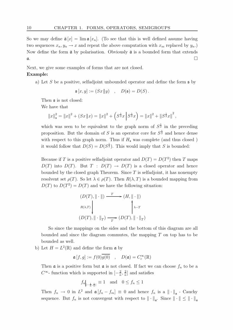
Because if T is a positive selfadjoint operator and D(T ) = D(T 2) then T maps
D(T ) into D(T ). But T : D(T ) → D(T ) is a closed operator and hence
bounded by the closed graph Theorem. Since T is selfadjoint, it has nonempty
resolvent set ρ(T ). So let λ ∈ ρ(T ). Then R(λ, T ) is a bounded mapping from
D(T ) to D(T 2) = D(T ) and we have the following situation:
(D(T ), ‖ · ‖) T //
R(λ,T )
(H, ‖ · ‖)
(D(T ), ‖ · ‖T )T
// (D(T ), ‖ · ‖T )
λ−T
OO
So since the mappings on the sides and the bottom of this diagram are all
bounded and since the diagram commutes, the mapping T on top has to be
bounded as well.
b) Let H = L2(R) and define the form a by
a [f, g] := f(0)g(0) , D(a) = C∞c (R)
Then a is a positive form but a is not closed. If fact we can choose fn to be a
C∞- function which is supported in [− 2n, 2n] and satisfies
fn[− 1
n , 1n ]
≡ 1 and 0 ≤ fn ≤ 1
Then fn → 0 in L2 and a [fn − fm] ≡ 0 and hence fn is a ‖ · ‖a
- Cauchy
sequence. But fn is not convergent with respect to ‖ · ‖a. Since ‖ · ‖ ≤ ‖ · ‖
a
2. CLOSED AND CLOSABLE FORMS 11
fn could only converge to 0. However ‖fn‖2a≥ a [fn] ≡ 1 6→ 0. Hence a is not
closed.
It turns out that these two examples are rather different. In the first example it
seems that we have only chosen the wrong domain. In fact 1.4 tells us that s0 [x, y] =(
S12x S
12x)
is a closed form on D(s0) = D(S12 ). And we know that s [x, y] = s0 [x, y]
for all x, y ∈ D(s) ⊂ D(s0). This meens that s has a closed extension.
On the other hand we will see in Theorem 1.9 that the form in the second example
has no closed extension.
Definition. A sectorial form a is called closable if it has a closed extension.
We note the following consequence of proposition 1.3:
Corollary 1.6. If a and b are closable sectorial forms, then so is a + b.
Proof. Let a and b be closed extensions of a resp. b. Then a + b is closed by 1.3
and extends a + b.
We also have the following result concerning everywhere defined forms:
Proposition 1.7. A closable form a on H with domain H is bounded.
Proof. Since a is everywhere defined it must coincide with its closed extension
and hence be closed. Thus H is complete with respect to both ‖ · ‖ and ‖ · ‖a. Since
we already know that ‖ · ‖ ≤ ‖ · ‖a
the closed graph Theorem yields that these two
norms are equivalent. But a is bounded with respect to the second norm. Thus it also
has to be bounded with respect to the equivalent ‖ · ‖-norm.
Before we go on investigation whether a given form is closable, we state a perturbation
result for sectorial forms which is very useful.
Definition. Let a be a sectorial form. A form b which need not be sectorial is
a-bounded if D(a) ⊂ D(b) and
|b [x]| ≤ α‖x‖2 + β|a [x]| ∀x ∈ D(a)
where α, β are nonnegative constants. The infimum of all possible β in this equality
is called the a-bound of b.
Theorem 1.8. Let a be a sectorial form and b be a-bounded with a-bound less than
1. Then a + b is sectorial. Furthermore the inner product ( · · )a+b
is equivalent to
( · · )a. In particular, a + b is closed if and only if a is. In this case, a subset D of
D(a) is a core for a if and only if it is a core for a + b. The sum a + b is closable if
and only if a is. In this case D(a + b) = D(a).
12 CHAPTER 1. FORMS, OPERATORS, SEMIGROUPS
Proof. If we replace a by a−γ then the β in the above inequality is not changed.
Thus we may assume that 0 is a vertex for a. Let θ be the corresponding semiangle.
Then
Re (a + b) [x] ≥ Re a [x] − |Re b [x]| ≥ (1 − β)Re a [x] − α‖x‖2 ≥ −α‖x‖2
which proves that −α is a vertex for a + b. Now we obtain
|Im (a + b) [x]| ≤ |Im a [x]| + |Im b [x]|≤ tan θRe a [x] + α‖x‖2 + βRe a [x]
≤ 1
1 − β(tan θ + β) (Re (a + b) [x] + α) + α
for ‖x‖ = 1, which proves that a + b is sectorial.
Now observe that
‖x‖a+b
≥ (1 − β)‖x‖a
and on the other hand
‖x‖2a+b
= (1 + α)‖x‖2 + Re a [x] + Re b [x]
≤ (1 + α)‖x‖2 + Re a [x] + |b [x]|≤ (1 + α)‖x‖2 + Re a [x] + α‖x‖2 + β|a [x]|≤ (1 + 2α)‖x‖2 + (1 + β(1 + tan θ))Re a [x]
≤ const. · ‖x‖2a
so that the norms ‖ · ‖a+b
and ‖ · ‖a
are equivalent. This proves the rest of the asser-
tions, considering that D(a + b) = D(a).
Example:
Let H = L2(R) and consider the forms
a [f, g] :=∫
Rf ′g′ dx D(a) = H1(R)
b [f, g] := f(0)g(0) D(b) = H1(R)
We have that a [f, g] =(ddxf d
dxg), so it follows from proposition 1.4, that a is a closed,
symmetric form, considering, that ddx
is a closed operator on L2. On the other hand,
the form b was already seen to be not closed. It will follow from Theorem 1.9, that b
is not even closable. However, b is a-bounded with bound 0:
2. CLOSED AND CLOSABLE FORMS 13
|b [f ]| ≤ |f(0)2 − f(T )2| + |f(T )|2
=
∣∣∣∣2
∫ T
0
f ′(t)f(t) dt
∣∣∣∣+ |f(T )|2
≤ |f(T )|2 + 2
∣∣∣∣
∫
R
f ′(t)f(t) dt
∣∣∣∣
≤ |f(T )|2 + 2ε
∫
R
|f ′(t)|2 dt+2
ε
∫
R
|f(t)|2 dt
→ 2ε ·∫
R
|f ′(t)|2 dt+2
ε‖f‖2 as T → ∞ .
Since here ε > 0 is arbitrary, we see that b is indeed formbounded with respect to a
with bound 0. Thus by Theorem 1.8, a + b is closed.
A tempting thing to do would be the following:
The pre-Hilbert space (D(a), ( · · )a) has a completion (Ha, ( · · )0). On this space a is
a bounded form and thus has an extension a defined on the whole of Ha by proposition
1.5. But we have that ‖ · ‖a
= ‖ · ‖01 which proves that a is closed.
The problem is of course that we obtained a closed extension of a in Ha rather than
in H . So the question is whether we can realize all this within H . The answer to this
question lies in the following observation:
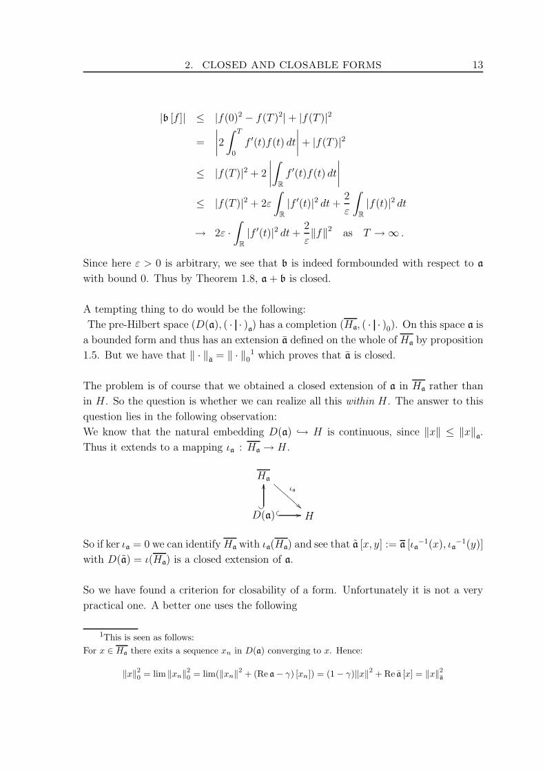
We know that the natural embedding D(a) → H is continuous, since ‖x‖ ≤ ‖x‖a.
Thus it extends to a mapping ιa : Ha → H .
Ha
ιa
!!CC
CC
CC
CC
D(a)?
OO
// H
So if ker ιa = 0 we can identifyHa with ιa(Ha) and see that a [x, y] := a [ιa−1(x), ιa
−1(y)]
with D(a) = ι(Ha) is a closed extension of a.
So we have found a criterion for closability of a form. Unfortunately it is not a very
practical one. A better one uses the following
1This is seen as follows:
For x ∈ Ha there exits a sequence xn in D(a) converging to x. Hence:
‖x‖2
0= lim ‖xn‖2
0= lim(‖xn‖2 + (Re a − γ) [xn]) = (1 − γ)‖x‖2 + Re a [x] = ‖x‖2
a
14 CHAPTER 1. FORMS, OPERATORS, SEMIGROUPS
Definition. Let a be a sectorial form. A sequence (xn) in H is said to be a -
convergent to x , we write xna−→x , if (xn) ⊂ D(a) , xn → x in H and (xn) is a ‖ · ‖
a-
Cauchy sequence.
Remarks. a) Note that x may not belong to D(a).
b) Obviously a - convergence is equivalent to both Re a - convergence and (a+α)
- convergence for any scalar α.
c) It follows from 1.2 that if xna−→x then a [xn − xm] → 0 as n,m→ ∞.
Theorem 1.9. Let a be a sectorial form and Ha and ιa be defined as above. Then the
following are equivalent:
a) a is closable.
b) For every sequence xna−→0 it follows that ‖xn‖a
→ 0.
c) ιa is injective.
Proof. a) ⇒ b) Let b be a closed extension of a and suppose that xna−→0. Since
(xn) ⊂ D(a) we have that ‖xn‖a= ‖xn‖b
for any n so that (xn) is a ‖ · ‖b
- Cauchy
sequence. Since Hb is complete xn converges to some x0 in Hb. But xn → 0 in H
implies x0 = 0, so ‖xn‖a= ‖xn‖b
→ 0.
b) ⇒ c) Let x ∈ ker ιa. Since D(a) is dense in Ha there exits a sequence (xn) in
D(a) which converges to x in the ‖ · ‖0 -norm. Since ιa is continuous it follows that
xn = ιa(xn) → ιa(x) = 0 so that xna−→0. From our assumption it follows that
‖xn‖a= ‖xn‖0 → 0 and we can conclude that x = 0.
c) ⇒ a) This was proved above.
Closed extensions are usually not unique. This shows the
Example
Let Ω ⊂ Rd be a bounded open set and H = L2(Ω, dx). Define a by
a [f, g] =
∫
Ω
∇f · ∇g dx , D(a) = C∞c (Ω) .
Then a is a positive, symmetric form and the corresponding norm is given by
‖f‖2a
= ‖f‖2 + a [f ] = ‖f‖2 + ‖∇f‖2 = ‖f‖2H1 .
Thus, the same expression is a closed form with domain H1(Ω) but also with domain
H10 (Ω).
But we see easily that the closed extension given in Theorem 1.9 has the smallest form
domain among all closed extensions. (That is because of the density of D(a) in Ha.)
2. CLOSED AND CLOSABLE FORMS 15
Definition. If a is a closable form the the closed extension with the smallest domain
is called the closure of a and denoted by a.
It is useful to characterize those domains which determine a closed form uniquely. We
define:
Definition. Let a be a sectorial form. A subset V of D(a) is called a core for a if V
is ‖ · ‖a-dense in D(a).
Proposition 1.10. Let a be a closed, sectorial form and V ⊂ D(a). Then
a) V is a core for a if and only if the closure of the form a0 = aV
is a.
b) If b is a closed sectorial form that coincides with a on some core for a then a
is an extension of b. In particular, if two closed sectorial forms coincide on a
common core, they are equal.
Proof. This is an immediate consequence of proposition 1.5.
Finally we want to introduce the notion of the regular part of a symmetric form which
is due to B. Simon and was first presented in [17]. The idea is to split up any
symmetric semibounded form a into a closable part ar and some rest as = a− ar. For
simplicity we may assume the form to be positive.
Recall the definition of Ha and ( · · )0 from above. Since the form is symmetric (and
thus Re a = a) we have not only ( · · )a
= ( · · )0 but also a [x, y] = (x y)0 − (x y)
We may decompose Ha as (ker ιa)⊕ (ker ιa)⊥ where we of course use the inner product
( · · )a.
Let P be the orthogonal projection on (ker ιa)⊥ and Q = id− P and define the forms
ar and as on D(a) as follows:
ar [x, y] = (Px y)0 − (x y)
as [x, y] = (Qx y)0
We will prove now that ar has the properties we want and furthermore characterize
ar independently of our construction above. For this we will need the
Definition. Let a and b be two symmetric semibounded forms. We say that a is
smaller then b and write a ≤ b if D(b) ⊂ D(a) and a [x] ≤ b [x] for all x ∈ D(b) 2
Theorem 1.11. Let a be a positive symmetric, semibounded form and ar , as as above.
Then:
a) ar + as = a.
b) ar is a positive closable form.
c) If b is a positive closable form smaller than a then b ≤ ar.
2Note that this is consistent with the notion of a ≥ γ introduced before.
16 CHAPTER 1. FORMS, OPERATORS, SEMIGROUPS
Proof. We have that
(ar + as) [x, y] = ((P +Q)x y)0 − (x y) = a [x, y]
for all x, y ∈ D(a) which proves a).
To see that ar is positive let x ∈ D(a) and observe that
x = ιa(x) = ιa(Px) + ιa(Qx) = ιa(Px) since Qx ∈ ker ιa. Now we obtain:
‖x‖2 = ‖ιa(Px)‖2 ≤ ‖Px‖2a
= (Px x)0 = ar [x] + (x x)
which proves that ar is positive.
We have that RgP is a closed subspace of Ha and ( · · )ar
= ( · · )0 on RgP . Since
PD(a) is ‖ · ‖0-dense in RgP we obtain thatHar is isometrically isomorphic to (RgP, ( · · )ar
).
We also can identify ιar with ιa RgPwhich is injective. Now 1.9 implies that ar is clos-
able.
To prove the last part observe that D(ar) = D(a) ⊂ D(b) so that we only need to
show that for x ∈ D(a) , b [x] ≤ ar [x] which is equivalent to show that ‖x‖b≤ ‖Px‖
a.
By hypothesis we have that ‖x‖b≤ ‖x‖
a. Thus we can extend the inclusion D(a) →
D(b) ⊂ Hb to a contraction j : Ha → Hb.
We have the following situation:
Ha
j//
ιa $$IIIII
Hb
ιbzzuuuuu
H
D(a)?
OO
// D(b)?
OO
We claim that ker ιa = ker j.
On D(a) we have that ιb j = ιa but by density this is true everywhere. Since b
closable, 1.9 implies that ιb is an injection from which ker ιa = ker j now follows. Thus
we have that j(x) = j(Px) for all x ∈ D(a) and can compute:
‖x‖b
= ‖j(x)‖b
= ‖j(Px)‖b≤ ‖Px‖
a
Definition. Let a be a symmetric semibounded form. The largest closable form
smaller than a (which exists by the preceeding theorem) is called the regular part of a
and is denoted by ar.
Corollary 1.12. Let a be a semibounded symmetric form, b a bounded form on D(a)
as defined in 1.4 and c any semibounded symmetric form smaller than a.
a) (a + b)r = ar + b
3. THE RELATIONSHIP BETWEEN FORMS AND OPERATORS 17
b) cr ≤ ar
Proof. a) follows from the fact that addition of a bounded form changes neither
closedness nor closability. b) is proved by cr ≤ c ≤ a.
3. The Relationship Between Forms and Operators
We now come back to the question whether a given form a is of the type a [x, y] =
(Ax y) for some operator A. When we define a like this on D(a) = D(A) we call a
the form associated with A. Of course the operator A should lead to a form which has
the right numerical range.
Definition. If A is an operator on a Hilbert space H then the numerical range of A
is given by
Θ (A) := (Ax x) : ‖x‖ = 1 , x ∈ D(A)A is sectorial if the numerical range of A is contained in some sector Σγ(θ). We will
use the same terminology for operators as for forms and talk of vertices etc.
A is called m-sectorial if A is sectorial and for some λ outside of the sector that contains
the numerical range of A, λ− A is surjective.
We have already seen for positive selfadjoint operators that the operator domain is
too small for the associated form to be closed. However the associated form turned
out to be closable. Here we have a similar situation.
Proposition 1.13. If A is a sectorial operator and a [x, y] = (Ax y), D(a) = D(A)
then a is closable. Furthermore, if the numerical range of a is contained in Σγ(θ), then
so is the numerical range of the closure.
Proof. We may assume that A has a vertex 0. According to Theorem 1.9 we have
to show that for any xna−→0 we have ‖xn‖a
→ 0. So let a sequence xn with xna−→0
be given. This implies that xn → 0 in H and that Re a [xn] is bounded, say by M2.
We have that
|Re a [xn]| ≤ |Re a [xn, xn − xm]| + |Re a [xn, xm]|≤ Re a [xn]
12 Re a [xn − xm]
12 + |Re (Axn xm)|
where we used 1.2.
Given ε > 0 we have for large m,n that Re a [xn − xm] < ε2 Thus for such m,n we
have
Re a [xn] ≤Mε+ |Re (Axn xm)| −→ Mε as m→ ∞So for large n we have |Re a [xn]| ≤Mε which proves that ‖xn‖a
→ 0.
M-sectorial operators have nice spectral properties. This is the reason, why they are
so interesting in the study of evolution problems. We have
18 CHAPTER 1. FORMS, OPERATORS, SEMIGROUPS
Theorem 1.14. Let A be an m- sectorial operator on a Hilbert space H. And assume
that Θ (A) ⊂ Σγ(θ) and let Ω = Σγ(θ)C. Then Ω ⊂ ρ(A) and
‖R(λ,A)‖ ≤ 1
dist(λ,Θ (A))∀λ ∈ Ω .
Proof. Let λ ∈ Ω so that d = dist(λ,Θ (A)) > 0. For x ∈ D(A) with ‖x‖ = 1 we
have
d ≤ |λ− (Ax x)| = |((λ−A)x x)| ≤ ‖(λ− A)x‖ · ‖x‖ = ‖(λ− A)x‖
which proves that λ−A is injective. Thus if λ ∈ Ω ∩ ρ(A) =: M then ‖R(λ,A)‖ ≤ 1d.
Our assumption that µ−A is surjective for some µ shows that M is not empty. Since
both Ω and ρ(A) are open M is open in Ω. We show that M is relatively closed in Ω.
Then M = Ω follows since Ω is connected and we have that Ω ⊂ ρ(A) as claimed.
So let (λn) ⊂M with λn → λ ∈ Ω. From the above it follows that
supn
‖R(λn, A)‖ ≤ supn
1
dist(λn,Θ (A))≤ C < ∞
Thus there exists some n0 ∈ N such that |λ − λn0| < 1C
≤ ‖R(λn0, A)‖−1. Now the
Neumann series shows that λ ∈ ρ(A) and we are done.
From this theorem, the following properties of m-sectorial operators follow:
Corollary 1.15. M-sectorial operators are closed and densely defined.
Proof. Let A be an m-sectorial operator and suppose that xn → x and Axn → y
and let λ ∈ ρ(A). Using the identity R(λ,A)A = λR(λ,A) − id we see that
R(λ,A)y = limR(λ,A)Axn = lim(λR(λ,A)xn − xn) = λR(λ,A)x− x
proving that x ∈ D(A) and (by multiplying with (λ− A) ) that y = Ax. Hence A is
closed.
To see that A is densely defined suppose that y ∈ D(A)⊥. We have to show, that
y = 0. By the above theorem if γ is a vertex for A then λ := γ − 1 ∈ ρ(A). So since
D(A) = RgR(λ,A) we have that, (R(λ,A)x y) = 0 for all x ∈ H . Since λ ∈ ρ(A) we
find some z ∈ D(A) such that y = (λ− A)z. Hence:
0 = Re (R(λ,A)y y) = Re (z (λ−A)z)
= Reλ‖z‖2 − Re (z Az)
≤ (γ − 1)‖z‖2 − γ‖z‖2 = −‖z‖2
which shows that z and hence y must be equal to 0.
The name m-sectorial stands for maximal sectorial meaning that an m-sectorial oper-
ator has no sectorial extensions. This is a consequence of the following

3. THE RELATIONSHIP BETWEEN FORMS AND OPERATORS 19
Lemma 1.16. If A and B are densely defined m-sectorial operators and A ⊂ B then
A = B.
Proof. Since A and B are both m-sectorial according to Theorem 1.14 there
exists a λ ∈ ρ(A) ∩ ρ(B). But then ϕ = R(λ,A)(λ− B) is a bijection from D(B) to
D(A). Since A ⊂ B we have ϕD(A)
= idD(A) we must have D(A) = D(B) and hence
A = B.
Now we come to the main theorem of this section, which links closed sectorial forms
and m-sectorial operators.
Theorem 1.17. (Representation Theorem)
Let a be a densely defined, closed sectorial form. Then there exists an m-sectorial
operator (A,D(A)) such that D(A) is a core for a and
(∗) a [x, y] = (Ax y) ∀x ∈ D(A) , y ∈ D(a)
Furthermore if x ∈ D(a) , z ∈ H and a [x, y] = (z y) holds for all y belonging to some
core for a then x ∈ D(A) and Ax = z. In particular A is uniquely determined by (∗).
Proof. Without loss of generality γ = 0.
We observe that y 7→ a [x, y] is a bounded ( |a [x, y]| ≤ (1+ tan θ)‖x‖a‖y‖
a) antilinear
functional on Ha. But so is y 7→ (z y). So the question we have to answer is which of
the first ones is actually of the second type?
Step 1: Lax-Milgram Theorem
By the Riesz representation Theorem all bounded antilinear functionals on Ha
are of the form y 7→ (x y)a. We claim that there exists a bounded bijective
function φ : D(a) → D(a) such that
(a + 1) [x, y] = (φx y)a
for all x, y ∈ D(a). Furthermore φ has a bounded inverse.
The existence of such a function φ follows directly from the Riesz representation
Theorem. φ is bounded since
‖φx‖a
= sup‖y‖
a≤1
|(φx y)a| = sup
‖y‖a≤1
|(a + 1) [x, y]| ≤ M‖x‖a
Since ‖x‖2a
= Re (a + 1) [x, x] = Re (φx x)a≤ ‖φx‖
a‖x‖
awe have ‖x‖
a≤
‖φx‖a
and thus φ is injective and has closed range. But actually Rgφ = H for
if x ∈ (Rgφ)⊥ then 0 = Re (φx x)a
= ‖x‖2a
thus x = 0.
We have shown that φ is bijective and has a bounded inverse.
Step 2: y 7→ (x y) is also a bounded antilinear functional on Ha. Again by the Riesz
representation Theorem there exists a function ψ : H → Ha such that
(x y) = (ψx y)a
∀x ∈ H, y ∈ D(a)
20 CHAPTER 1. FORMS, OPERATORS, SEMIGROUPS
We have that ψ is injective (that is because ψx1 = ψx2 implies (x1 − x2 y) = 0
for all y ∈ D(a) and now the density of D(a) in H implies x1 = x2 ) and has
‖ · ‖a-dense range (because y ∈ (ψH)⊥ implies 0 = (ψx y)
a= (x y) for all
x ∈ H which shows y = 0).
Step 3: So far we have that for any x ∈ H , y ∈ D(a)
(x y) = (ψx y)a
= (a + 1) [φ−1ψx, y] = a [φ−1ψx, y] + (φ−1ψx y)
Define A = ψ−1φ(id− φ−1ψ) = ψ−1φ− id on the domain D(A) = x ∈ D(a) :
φx ∈ Rgψ.Then D(A) is a core for a since Rgψ is and φ is bicontinuous. We have for
x ∈ D(A) and y ∈ D(a)
(Ax y) = (ψ−1φ(id− φ−1ψ)x y))
= (φ(id− φ−1ψ)x y)a
by the definition ofψ
= (a + 1) [x− φ−1ψx, y] by the definition ofφ
= (a + 1) [x, y] − (a + 1) [φ−1ψx, y]︸ ︷︷ ︸
=(x y)
= a [x, y]
In particular this shows that A is sectorial. That A is m-sectorial follows since
−1 ∈ ρ(A).
We are done except for the uniqueness assertion. If a [x, y] = (z y) holds for all y
in some core for D(a) then it holds for all y ∈ D(a) by density. Then of course
(a + 1) [x, y] = (z + x y) which shows that φx ∈ Rgψ and hence x ∈ D(A). Now
(Ax y) = (z y) for all y ∈ D(a) implies Ax = z by the density of D(a) in H .
Definition. The operator A constructed in the last theorem is called the operator
associated with a.
We now note some consequences of Theorem 1.17
Corollary 1.18. Let a be a closed,densely defined, sectorial form and A be the op-
erator associated with a. Then
a) If a0 [x, y] = (Ax y) on D(a0) = D(A), then a is the closure of a0.
b) If B is an operator with D(B) ⊂ D(A) and a [x, y] = (Bx y) for all x ∈ D(B)
and y in some core for a then B ⊂ A.
c) A∗ is the operator associated with a∗.
d) If a is symmetric, then A is selfadjoint.
e) There is a one-to-one correspondence between the set of all densely defined,
closed sectorial forms and the set of all m-sectorial operators.
Proof. a) D(a0) is a core for a. Hence the domain of any closed extension of
a0 must contian D(a), thus a = a is the smallest closed extension of a0.
3. THE RELATIONSHIP BETWEEN FORMS AND OPERATORS 21
b) This is just a reformulation of the last part of the theorem.
c) Let B be the operator associated with a∗. Then for any x ∈ D(A) ⊂ D(a∗) =
D(a), y ∈ D(B) we have
a∗ [y, x] = (By x) = (x By) and
a∗ [y, x] = a [x, y] = (Ax y)
Thus y ∈ D(A∗) and By = A∗y by uniqueness so that B ⊂ A∗. On the other
hand b) implies A∗ ⊂ B thus A∗ = B.
d) follows directly from c).
e) The mapping a → A is injective since by a) a is uniquely determined by A.
To see that it is surjective, let B be an m-sectorial operator. By proposition
1.13 the associated form is closable and densely defined. But B must be the
associated operator of that form by uniqueness.
With help of the representation Theorem we now can prove the following:
Proposition 1.19. Let a be a closed sectorial form and suppose that xn is a sequence
in D(a) such that xn → x (in H!) and a [xn] is bounded. Then x ∈ D(a) and Re a [x] ≤limRe a [xn].
Proof. Since xn is convergent and thus norm bounded, we have that if Re a [xn]
is bounded, then so is (Re a − γ) [xn], so we may assume that a has a vertex 0. Fur-
thermore we have that x ∈ D(a), so that we may assume that a be densely defined.
By hypothesis, xn is ‖ · ‖a-bounded, and thus there exists some weakly convergent
subsequence, say
(xnky)
a→ (z y) ∀ y ∈ Ha
for some z ∈ Ha. Since Re a is a symmetric, positve, densely defined closed form and
thus associated with some positive selfadjoint operator R by 1.18, we have
(xnky)
a= (xnk
(1 +R)y) → (z (1 +R)y)a
= (z y)a,
for all y ∈ Ha. But since xnk→ x in H and Rg(1 + R) = D(a) we must have
x = z ∈ D(a).
Furthermore, we have that
‖x‖a
= ‖ lim xn‖a≤ lim‖xn‖a
from which Re a [x] ≤ limRe a [xn] follows.
22 CHAPTER 1. FORMS, OPERATORS, SEMIGROUPS
The theorems of this section show that forms are excellent means of defining m-sectorial
or selfadjoint operators. Usually one is interested in those operators but properties
such as selfadjointness are hard to establish. On the other hand it is comparatively
easy to construct symmetric or sectorial forms.
However there are some differences between forms and operators. First of all, we have
seen that m-sectorial operators have no proper m-sectorial extensions. This is not true
for forms. There is no such thing as a ”maximal form” (except for everywhere defined
forms).
Recall that a symmetric operator is an operator A satisfying (Ax y) = (x Ay) for all
x, y ∈ D(A). Symmetric operators always have closed extensions (the double adjoint),
but they may not be selfadjoint. Symmetric forms may have no closed extensions at
all (see the example in the preceding section) but if they have, then the extension is
necessary associated with an selfadjoint operator.
The same holds for sectorial operators:
If A is a sectorial opererator, then the associated form is closable by proposition 1.13
and the representation Theorem shows that the closure is associated with some m-
sectorial operator B extending A. Even if A is closable, then B may differ from the
closure of A.
Definition. Let A be a sectorial operator and a be the form associated with A. The
m-sectorial operator associated with the closure of the form a is called the Friedrichs
extension of A.
Proposition 1.20. a) The Friedrichs extension of an m-sectorial operator A is
A itself.
b) Among all m-sectorial extensions of A the Friedrichs extension has the smallest
form domain.
c) The Friedrichs extension is the only m-sectorial extension of A whose domain
is contained in D(a).
Proof. Let A be a sectorial operator and denote the form associated with A by
a and the closure of this form a.
Part a) follows directly from part a) of corollary 1.18.
b) holds since by construction D(A) is a form core for a.
For the last part observe, that if A has another m-sectorial extension B with domain in
D(a) then it follows part b) of corollary 1.18 that the Friedrichs extension of A is also
an extension of B and hence they must be equal since they are both m-sectorial.
The representation Theorem has one major weakness:
The domain of the operator associated with a form is not the domain of the form.
4. BOUNDEDNESS OF UNIVERSALLY SECTORIAL OPERATORS 23
Usually the operator domain is smaller. For symmetric positive forms, this problem
can be handled and we can connect the domain of the operator with the form domain:
Proposition 1.21. Let a be a densely defined, closed, symmetric, positive form and
A be the operator associated with a. Then D(A12 ) = D(a) and for all x, y ∈ D(a) we
have:
a [x, y] =(
A12x A
12 y)
Proof. Define b on D(b) = D(A12 ) by b [x, y] =
(
A12x A
12 y)
. Then b is a densely
defined, closed form by proposition 1.4. Furthermore D(A) is a core for b since it is
an operator core for A12 and the norm ‖ · ‖
bis equivalent to the graph norm of A
12 . So
since a and b coincide on a common core, they have to be equal.
For sectorial forms a it is possible to associate an operator on a larger domain. Let
H′
abe the space of antilinear bounded functionals on Ha and recall from the proof of
the representation Theorem that we have the following situation:
H′
a
Ha
φ
OO
A
// H/ O
ψ__@@@
@@@@@
We used φ and ψ to define A in H . Another possibility would have been not to work
in H but rather in H′
aand just say y 7→ a [x, y] is an element of H
′
a, denote it by Ax
acting on Ha by
〈Ax , y〉 = a [x, y]
Then A is a continuous mapping from D(a) to H′
a. A is then precisely the part of A
in Rgψ transformed to H with the help of ψ:
D(A) = x ∈ D(A) = D(a) : Ax ∈ ψH Ax = ψ−1Ax
4. Boundedness of Universally Sectorial Operators
Now we ask the following question:
The statement that A is a sectorial operator depends on the inner product which is
defined on H . What happens if we take an equivalent inner product instead?
We will prove that if A is dissipative with respect to any equivalent inner product on
H (in particular if A happens to be sectorial for any equivalent inner product on H)
then A is necessarily bounded.
Theorem 1.22. (Matolcsi 2003) Let A be an operator on H with nonempty resolvent
set. If for any equivalent inner product ( · · )0 on H the numerical range of A is
contained in some left halfplane (i.e. there exists a constant γ0 depending on the inner
24 CHAPTER 1. FORMS, OPERATORS, SEMIGROUPS
product such that Re (Ax x)0 ≤ γ0 for all x with ‖x‖0 = 1 ) then A is a bounded
operator.
Before proving the theorem, we state some lemmata that will be used in the proof.
Lemma 1.23. Let A be an unbounded operator on a Hilbert space H and 0 ∈ ρ(A).
Then there is an orthonormal sequence xn such that A−1xn → 0.
Proof. Without loss of generality, we may assume that A (and thus A−1) is a
positive selfadjoint operator. Otherwise, we take the polar decomposition A = UR
where U is unitary and R is positive selfadjoint. Using the result for R we find an
orthonormal sequence yn with ‖R−1yn‖ → 0.
If we put xn := Uyn then xn is orthonormal since U is unitary and furthermore
‖A−1xn‖ = ‖R−1yn‖ → 0.
Courtesy of the spectral Theorem, we may assume that H = L2(Ω,Σ, µ) for some
measure space (Ω,Σ, µ) and A is a multiplication operator, say Af = hf .
If we define Mn = ω : n ≤ h(ω) < n+ 1 then for any n we have µ(Mn) > 0 (since
A is unbounded and so h has to be, thus this is true at least for a subsequence, but
for simpler notation, we assume that it is true for any n.)
Now define fn = µ(Mn)− 1
2 1lMn. Then each fn has norm 1 and since all the sets Mn are
disjoint, they are orthogonal as well. Now
‖A−1fn‖22 = µ(Mn)
−1
∫
Mn
|h(ω)|−2 dµ(ω) ≤ µ(Mn)−1µ(Mn)n
−2 → 0
Lemma 1.24. Let H be an inner product space , U, V be subspaces with dimU <
dimV <∞. Then there is a vector v ∈ V such that ‖V ‖ = 1 and v ⊥ U .
Proof. Let X = span(U ∪ V ). We extend an orthonormal basis u1, . . . uk of U to
an orthonormal basis u1, . . . , uk, uk+1, . . . uk+l of X. Note that since V ⊂ X we must
have dimX > dimU and hence l ≥ 1. Now take v = uk+1 ∈ V .
Proof of 1.22. Assume that A is not a bounded operator, and by shifting if
necessary, that 0 ∈ ρ(A). Let T = A−1.
We claim that there is a sequence xn with the following properties:
i) ‖xn‖=1 for any n.
ii) Txn → 0 with respect to the ‖ · ‖-norm
iii) spanxi, Txi ⊥ spanxj , Txj for any i 6= j
iv) There is some 1 > ε > 0 such that for any n ∈ N we have
|(xn Txn)|‖Txn‖
< ε
4. BOUNDEDNESS OF UNIVERSALLY SECTORIAL OPERATORS 25
By lemma 1.23 there is an orthonormal sequence un with Tun → 0. We construct a
sequence xn with the above properties from this sequence un.
Step 1 We construct starting from un a new orthonormal sequence un such that in
addition to the property T un → 0 we have that
un ⊥ spanu1, T u1, . . . , un−1, T un−1.
Take u1 = ui1 where the index i1 is chosen such that ‖Tui1‖ ≤ 1.
Now assume that u1, . . . , un−1 ∈ spane1, . . . eln have already been constructed
such that for any 1 ≤ k ≤ n−1 we have ‖uk‖ = 1 and ‖T uk‖ ≤ k−12 and form <
k we have uk ⊥ spanum, T um. Pick i1, . . . in > ln such that ‖Tuij‖ ≤ 1n
for
any 1 ≤ j ≤ n. Take U = spanT u1, . . . , T un−1 and V = spanui1, . . . , uin.Note that dimU ≤ n − 1 and dim V = n, so that by lemma 1.24 there exists
a vector un ∈ V with ‖un‖ = 1 and un ⊥ U . But since uk is an orthogonal
sequence, by construction un is also perpendicular to u1, . . . , un−1.
It is only left to show that ‖T un‖ ≤ n− 12 . But if un ∈ V we have un =
∑λjuij
and thus
‖T un‖2 =∑
|λj|2‖Tuij‖2 ≤ 1
n
∑
|λj|2‖uij‖2 =1
n‖un‖2 =
1
n.
Step 2 We refine the sequence uk to an orthonormal sequence vk such that
spanvk, T vk ⊥ spanvm, T vm for any k 6= m
and such that ‖Tuk‖ ≤ (2k − 1)−12 .
Let v1 = u1. For n ∈ N let v1, . . . , vn−1 ∈ spanu1, . . . uln already be chosen
with the above properties.
Pick i1, . . . , i2n−1 > ln such that ‖T uij‖ ≤ (2n− 1)−1 for any 1 ≤ j ≤ 2n− 1.
Take U = spanv1, T v1, . . . , vn−1, T vn−1 and V = T (spanui1, . . . u12n−1).Here again, we have dimU ≤ 2n − 2, whereas dimV = 2n − 1 since T =
A−1 is injective. So by applying lemma 1.24 we obtain a vector T vn ∈ V
satisfying T vn ⊥ U . If we put vn := ‖vn‖−1vn then vn has norm 1, and
spanvn, T vn ⊥ spanvk, T vk3 for any k ≤ n and a computation analog to
step 1 yields ‖Tvn‖ ≤ (2n− 1)−12 .
Step 3 In this last step, we finally establish the property iv)
Pick an index k1 such that ‖Tvk1‖ ≤ ε2
4‖Tv1‖ and put
x1 :=ε
2v1 + (1 − ε2
4)
12 vk1
3Tvn ⊥ spanvk, T vk is clear by construction. But we also have vn ⊥ spanvk, Tk since vn is
a linear combination of (uj) where these j’s are greater than those used for vk. So this follows from
the construction in Step 1.
26 CHAPTER 1. FORMS, OPERATORS, SEMIGROUPS
We then have that
‖Tx1‖ ≥ ε
2‖Tv1‖ − (1 − ε2
4)
12‖Tvk1‖
≥(ε
2− ε2
4(1 − ε2
4)
12
)
‖Tv1‖
|(x1 Tx1)| =
∣∣∣∣
ε2
4(v1 Tv1) + (1 − ε2
4)(vk1 Tvk1)
∣∣∣∣
≤(ε2
4+ (1 − ε2
4)ε2
4
)
‖Tv1‖
So we obtain that
|(x1 Tx1)|‖Tx1‖
≤ε2
4+ (1 − ε2
4) ε
2
4
ε2− ε2
4(1 − ε2
4)
12
≤ 2
ε
(ε2
4+ (1 − ε2
4)ε2
4
)
= ε− ε3
8< ε ,
which is property iv). Furthermore, we have that ‖x1‖ = 1 and ‖Tx1‖ ≤ 1.
Now suppose that vectors x1, . . . xn−1 ⊂ spanv1, . . . , vln with the properties
i), iii) and iv) have already been constructed such that ‖Txk‖ ≤ k−12 .
Choose indicesm1, m2 > ln such that ‖Tvm1‖ ≤ n− 12 and ‖A−1vm2‖ ≤ ε
4‖Tvm1‖,
and define
xn :=ε
2vm1 + (1 − ε2
4)
12 vm2
Then one showes as above, that xn also has the property iv) is satisfied. The
properties i) and iii) follow from the construction of xn and the properties of
the sequence vk. One checks that ‖Txn‖ ≤ n− 12 .
With the help of the sequence xn we will now construct an equivalent inner product on
H , so that the numerical range of A with respect to this inner product is not contained
in any left halfplane.
Take a closer look at Hn := spanxn, Txn. xn and Txn are linearly independent, since
otherwise, by the Cauchy Schwarz inequality we would have |(xn Txn)| = ‖xn‖‖Txn‖,in violation of the property iv). Thus Hn is 2-dimensional.
Extend xn to an orthonormal Basis (xn, yn) of Hn. Then Txn has a unique repersen-
tation Txn = αnxn + βnyn. Here βn 6= 0.
From the property iv) we obtain that
|(xn Txn)|2‖Txn‖2 =
|αn|2|αn|2 + |βn|2
< ε2 and thus|βn|2
|αn|2 + |βn|2> 1 − ε2
this implies on the other hand that
|αn||βn|
<ε√
1 − ε2
5. PSEUDORESOLVENTS AND DEGENERATE SEMIGROUPS 27
Define an operator Qn on Hn by having the following matrix representation with
respect to the basis (xn, yn)
Qn =
(
1 an
an 1 + |an|2
)
Q−1n =
(
1 + |an|2 −an−an 1
)
Here an = 2ε(1 − ε2)−12βn
|βn|Note, that the entry with the maximal modulus in Qn is 1+|an|2. We have |1+|an|2| <1+4ε2(1−ε2)−1 =: C. So as an operator from (Hn, ‖ · ‖1) to (Hn, ‖ · ‖∞), Qn has norm
≤ C. But since on a finite dimensional space all norms are equivalent, Qn has norm
≤ K as an operator on (Hn, ‖ · ‖2). In particular, we have that ‖Qn‖ and (similarly)
‖Q−1n ‖ are bounded independently of n.
Now define Q by
Q = P0 +∑
n∈N
QnPn
where Pn is the orthogonal projection onto Hn and H0 = (⊕
n∈NHn)
⊥. Then Q is a
positive, bounded, selfadjoint operator with bounded inverse. So (x y)0 := (x Qy) is
an equivalent scalar product on H .
Then for en = ‖Txn‖Txn we have
Re (Aen en)0 = ‖Txn‖−2Re (xn QTxn)
= ‖Txn‖−2Re (xn αn(xn + anyn) + βn(anxn + (1 + |an|2yn))= ‖Txn‖−2Re (αn + βnan)
≥ ‖Txn‖−2(−|αn| + 2ε√
1 − ε2|βn|)
≥ ‖Txn‖−2(ε√
1 − ε2|βn|)
>ε
‖A−1xn‖→ ∞
which proves, that Θ (A) is not contained in any left halfplane.
5. Pseudoresolvents and Degenerate Semigroups
Recall from Theorem 1.14 that for an m-sectorial operator A whose numerical range
is contained in the sector Σγ(θ) we have
Σγ(θ)C ⊂ ρ(A) and ‖R(λ,A)‖ ≤ 1
dist(λ,Θ (A)).
We may reformulate this as follows:
Any λ outside the sector Σγ(θ + ε) where ε ∈ (0, π − θ) is contained in the resolvent
28 CHAPTER 1. FORMS, OPERATORS, SEMIGROUPS
set of A and we have the following estimate for the resolvent:
‖R(λ,A)‖ ≤ Mε
|λ− γ|From this it follows that −A generates a quasi bounded analytic semigroup T (z) =
e−zA which is defined for z ∈ Σ(π2− θ). We refer to [4] or [9] for more details.
For nondensely defined sectorial forms a we cannot associate an m-sectorial operator.
However, we can think of a as a form on D(a) , where it is densely defined. Let Pa
be the orthogonal projection onto D(a) and A be the m-sectorial operator associated
with a as a form on D(a). We define:
e−za := e−zAPa for z ∈ Σ(π
2− θ)
.
Then e−ta is a continuous, quasibounded, degenerate, analytic semigroup on H . We
clarify the meaning:
Definition. Let X be a Banach space. A degenerate semigroup is a strongly contin-
uous mapping T : (0,∞) → L(X) satisfying
T (t+ s) = T (t)T (s) for all t, s > 0 .
If the strong limit s− limt→0 T (t) exists, we say that T is continuous. A degenerate
semigroup is bounded if there exists a constant M > 0 such that ‖T (t)‖ ≤ M for all
t > 0, and it is quasi bounded if e−ωtT (t) is a bounded degenerate semigroup for some
ω > 0. A degenerate semigoup is called analytic if it has a holomorphic extension to
some sector containing the positive real axis.
For e−ta all these properties follow directly form the properties of e−tA on D(a). We
may chose the ω in the quasi boundedness condition to be a vertex γ for a. For sim-
plicity we will frequently call e−ta the degenerate semigroup (or sometimes just the
semigroup) associated with a and understand that all the other properties hold.
When dealing with semigroups interesting objects are not only the semigroups and
their generators but also the resolvent of the generator. It turns out to be the Laplace
transform of the semigroup.
For degenerate semigroups the Laplace transform is a pseudoresolvent.
Definition. LetX be a Banach space and Ω a subset of C. A function R : Ω → L(X)
is called a pseudoresolvent if for all λ, µ ∈ Ω we have that
R(λ) − R(µ)
µ− λ= R(λ)R(µ) .
This equation is called the resolvent identity.
5. PSEUDORESOLVENTS AND DEGENERATE SEMIGROUPS 29
In our case, the Laplace transform is of rather special type. We have
T (λ) =
∫ ∞
0
e−λte−ta dt =
∫ ∞
0
e−λte−tA Padt = R(λ,−A)Pa .
Definition. Let a be a closed sectorial form and A and Pa as above. R(λ, a) :=
R(λ,−A)Pa is called the pseudoresolvent associated with a. We will also write (λ+a)−1
for R(λ, a).
We remark that we can compute e−ta directly from the pseudoresolvent with the help
of a contour integral. We have:
e−za = e−zAPa
=1
2πi
∫
Γ
ezξR(ξ,−A)dξ Pa
=1
2πi
∫
Γ
ezξR(ξ, a)dξ
Where Γ is a path around −Θ (a) ( and thus around the spectrum of −A), which is
positively oriented and avoids the vertex γ of a, such that z lies outside Γ.
Finally we want to somehow describe the form a by means of the associated semigroup
e−ta. For this we return to the operator A : D(a) → H′
aas defined at the end of section
3. We have the following result. For the proof we refer to Ouhabaz [14, Theorem
1.55].
Proposition 1.25. Let a be a densely defined closed sectorial form and A be the
operator associated with a, A as above. Then −A generates a strongly continuous
semigroup e−tA on H′
a. Furthermore
e−tAx = e−tAx = e−tax
for all x ∈ H and t ≥ 0 ( Here, we think of H as a subset of H′
awhere the embedding
is as at the end of the last section) .
With the help of this proposition it is now possible to characterize a closed sectorial
form entirely by the associated semigroup.
Theorem 1.26. Let a be a closed sectorial form. Then
D(a) = x ∈ H : supt>0
t−1Re (x− e−tax x) <∞ .
Furthermore, for all x, y ∈ D(a) we have
a [x, y] = limt→0
t−1(x− e−tax x) .
30 CHAPTER 1. FORMS, OPERATORS, SEMIGROUPS
Proof. If 0 6= x ∈ D(a)⊥ then e−tax = 0 so that t−1(x− e−tax x) = t−1‖x‖2,
which tends to ∞ as t→ 0. Hence we can assume that a is densely defined.
For x, y ∈ D(a) = D(A) we have
t−1(x− e−tax y) = t−1⟨x− e−tAx , y
⟩−→ 〈Ax , y〉 = a [x, y]
as t → 0. Here we used the above proposition and the definition of A. So the only
thing left to show is that supt>0 t−1(x− e−tax x) <∞ implies x ∈ D(a).
So suppose that supt>0 t−1Re (x− e−tax x) <∞. For λ > 0 we have λ ∈ ρ(−A) and
Re a [λ(λ+ A)−1x, λ(λ+ A)−1x]
= Re (λA(λ+ A)−1x λ(λ+ A)−1x)
= Reλ(x− λ(λ+ A)−1x λ(λ+ A)−1x)
≤ Reλ(x− λ(λ+ A)−1x x)
= Re
∫ ∞
0
λ2e−λt(x− e−tax x) dt
≤ supt>0
t−1Re (x− e−tax x)
∫ ∞
0
λ2te−λt dt
= supt>0
t−1Re (x− e−tax x)
∫ ∞
0
re−r dr <∞
This shows that λ(λ + A)−1x is uniformly bounded with respect to the ‖ · ‖a-norm
(recall that ‖λ(λ+ A)−1x‖ ≤ M‖x‖ by 1.14). Since λ(λ + A)−1x → x as λ → ∞proposition 1.19 implies x ∈ D(a).
Notes and References for Chapter 1: The material presented in this chapter is pretty
standard. Our presentation is very close to Kato [10, chapter 6]. Another possible refer-
ence is Ouhabaz [14, chapter 1]. Here, the terminology is somewhat closer to the following
approach to forms:
A form is a triplet (a, V,H), where H and V are Hilbert spaces and V is densely embedded
into H and a : V × V → C is a sectorial form. The notion of a being sectorial is equivalent
to say that a is bounded on V , the closedness of a is replaced by H-ellipticity of a, which
basically means, that the inner product associated with a is equivalent to the inner product
on V . This approach reflects the use of form methods for elliptic problems (see chapter 4).
Here H = L2 , V is a Sobolev space and a is a form associated with a differential operator.
The closedness of such a form is then proved by showing, that the associated inner product
is equivalent to the inner product in the Sobolev space. For a treatment in this spirit, see
Arendt et al [4, chapter 7].
Yet another different approach for symmetric forms is to interpret the quadratic form as
lower semicontinuous convex functionals on H, by defining a [x] = ∞ for x 6∈ D(a). This
5. PSEUDORESOLVENTS AND DEGENERATE SEMIGROUPS 31
is illustrated in Reed, Simon [16, supplement to VIII.7]. This approach is closer to the
nonlinear case, which may be found in Brezis [6].
The part of section 2 concerning closability and the regular part is inspired by Simon [17].
The description of the spectrum of m-sectorial operators may also be found in [10], but our
presentation is closer to [18, lemma VII.1.1], which deals with bounded operators. Finally
the representation Theorem is taken from [10, chapter 6.2], but the notation was changed
so that it may also be used for results concerning the semigroup generated by the operator
A associated with a on the antidual of the domain. This presentation is close to Ouhabaz
[14, chapter 1.5]. Section 4 is taken from Matolcsi [13], without many changes.
All these references are mostly concerned with densely defined forms. This caused some
minor modification to the theorems and/or the proofs in the first sections of this chapter
insofar as they concern nondensely defined forms. The real difference between the densely
defined case and the nondensely defined case lies in section 5. The terminology here is mostly
inspired by Arendt [2]. The characterisation of the degenerate semigroup in terms of the
generating forms is taken from [14].

CHAPTER 2
Families of Forms
One of the standard techniques in semigroup theory is the approximation of a (possibly
complicated) semigroup by other (possibly easier) semigroups. If one has established
the ”right” convergence of the operators, then the generated semigroups converge.
Here, the right notion of convergence is convergence in the strong resolvent sense, that
is pointwise convergence of the resolvents.
In the first section of this chapter, we define strong resolvent convergence for forms
and prove that if a sequence of forms converges in strong resolvent sense, then the
associated degenerate semigroups converge strongly.
Our next goal is to establish strong resolvent convergence from convergence of the
forms. This is a big advantage of the form methods, since in many cases this is easy
to establish.
Let an be a uniformly sectorial sequence of closed forms. Here we mean by uniformly
sectorial that the numerical range of all forms an is contained in one common sector
Σγ(θ). We define the limit by
D = x ∈ limD(an) : lim an [x] exists a [x] := lim an [x] .
If D is a vector space, we obtain by polarisation a form a on D(a) = D.
So convergence of forms is a really mild assumption on the associated operators. For
example, even if all the forms an and a are bounded (so that the associated operators
are bounded as well) form convergence means nothing more than weak convergence
of the associated operators. Often this is not enough to draw interesting conclusions
from. Therefore we have to assure that an converges to a in a certain way to conclude
strong resolvent convergence of the associated operators.
For unbounded forms, it is not even clear what form convergence means for the as-
sociated operators. This is mainly due to the fact that even if all forms an have the
same domain, the associated operators may have different, even disjoint domains.
When working with forms alone, different questions occur:
• When is the limit defined on a vector space ?
• What conditions assure that the limit form is closed as well?
33
34 CHAPTER 2. FAMILIES OF FORMS
• If the forms an are densely defined when is a ?
In section 3, we will present conditions on the sequence an , that will assure a positive
answer to these questions and establish strong resolvent convergence, so that the as-
sociated semigroup will converge as well.
Section 2 deals not with sequences of forms, but with families that are holomorphic in
a certain sense. This will provide a powerful tool to extend results for symmetric forms
to sectorial forms. This will be applied in the proof of Trotter’s formula in the next
chapter and also at the end of section 3 to obtain a convergence result for sectorial
forms from one for symmetric forms.
1. Convergence in the Strong Resolvent Sense
Definition. Let an and a be uniformly sectorial closed forms, say Θ (an),Θ (a) ⊂ Σ.
We say that an converges to a in strong resolvent sense (and write anR−→a) if for all
x ∈ H and λ ∈ (−Σ)C we have
R(λ, an)x→ R(λ, a)x
As with resolvents it is enough to check this convergence for one λ and we always
obtain uniform convergence on compact subsets of (−Σ)C :
Theorem 2.1. If an and a are closed sectorial forms and Θ (an),Θ (a) ⊂ Σ and if for
one µ ∈ Ω := (−Σ)C and all x ∈ H we have R(µ, an)x → R(µ, a)x then anR−→a and
the convergence is uniform on compact subsets of Ω.
Proof. Let λ ∈ Ω and x ∈ H and define
y = x+ (µ− λ)R(λ, a)x , yn = y + (λ− µ)R(µ, an)y .
By the resolvent identity we have R(λ, a)x = R(µ, a)y and R(λ, an)yn = R(µ, an)y.
By assumption we have that yn → y + (λ− µ)R(µ, a)y = y + (λ− µ)R(λ, a)x = x.
We further know that ‖R(λ, an)‖ ≤ (dist(λ,Σ))−1 < ∞ and we can conclude that
limR(λ, an)(yn − x) = 0. Now it follows that
limR(λ, an)x = limR(λ, an)yn
= limR(µ, an)y
= R(µ, a)y = R(λ, a)x
Which proves the required convergence for λ. Since pseudoresolvents are holomorphic
and locally bounded, the uniform convergence on compact subsets of Ω follows form
Vitali’s Theorem.
1. CONVERGENCE IN THE STRONG RESOLVENT SENSE 35
For a symmetric form a , the associated operator is selfadjoint and for real λ we also
have that the pseudoresolvents R(λ, a) are selfadjoint. In this situation even weak
convergence of the resolvents is enough:
Theorem 2.2. Let an , a be symmetric closed forms and suppose that an , a ≥ γ.
Assume that
(R(λ, an)x x) → (R(λ, a)x x)
for all x ∈ H and all λ ∈ Ω0 where Ω0 is a subset of the real line which has an
accumulation point.
Then anR−→a.
Proof. According to the preceding theorem it suffices to show strong convergence
of the pseudoresolvent in one point λ0.
We can think of (R(λ, an)x x) as a semibounded symmetric form in x and thus by
polarization obtain the convergence
(R(λ, an)x y) → (R(λ, a)x y)
for all x, y ∈ H and all λ ∈ Ω0. That is we have R(λ, an)x R(λ, a)x.
It is well known that in Hilbert spaces norm convergence is equivalent to weak con-
vergence and convergence of norms. Thus we are done if we can show for one λ0 that
‖R(λ0, an)x‖ → ‖R(λ0, a)x‖ for all x ∈ H .
Fix λ0 ∈ Ω0 ⊂ R and x ∈ H and define fn(λ) = (R(λ0, an)x R(λ, an)x). We use the
resolvent equation and the hypothesis and obtain:
fn(λ) = (R(λ, an)R(λ0, an)x x) by selfadjointness
=1
λ0 − λ((R(λ, an) −R(λ0, an))x x)
→ 1
λ0 − λ((R(λ, a) −R(λ0, a))x x)
= (R(λ0, a)x R(λ, a)x) =: f(λ)
for all λ ∈ Ω0. Since furthermore fn is holomorphic and locally bounded we obtain
from Vitali’s Theorem and the uniqueness of holomorphic functions that
fn(λ) → f(λ) ∀λ ∈ C \ (−∞, γ]
In particular we have
fn(λ0) = ‖R(λ0, an)x‖2 → f(λ0) = ‖R(λ0, a)x‖2
This finishes the proof.
We now prove, that (as for semigroups) convergence in the strong resolvent sense and
convergence of the degenerate semigroup are equivalent. We have:
36 CHAPTER 2. FAMILIES OF FORMS
Theorem 2.3. Let an be a sequence of closed sectorial forms with Θ (an) ⊂ Σγ(θ) for
all n. Then anR−→a if and only if e−zanx → e−zax for all z with | arg z| ≤ π
2− θ and
all x ∈ H.
Proof. Assume without loss that γ = 0.
First assume that anR−→a.
Fix z and x and let Γ be the positively oriented boundary of B(0, δ1) ∪ (−Σ(θ + δ2))
where δ1 and δ2 are chosen so that z is on the outside of Γ. Define C =∫
Γ|e−zξ| |dξ| <
∞. Let ε > 0 be given. By 1.14 there exists some M > 0 such that ‖R(λ, a)‖ ≤ M|λ| for
all λ ∈ Γ. Pick some R >4·C·M‖x‖
ε. By Theorem 2.1 the pseudoresolvents converge
uniformly on Γ∩B(0, R). So we find some n0 ∈ R such that ‖R(λ, an)x− R(λ, a)x‖ ≤ε
2·C for all n ≥ n0. Denote Γ1 = Γ ∩ B(0, R) and Γ2 = Γ ∩ B(0, R)C
Now we have:
‖e−zanx− e−zax‖ = ‖∫
Γezξ (R(ξ, an) − R(ξ, a))x dξ‖
≤∫
Γ1
|ezξ| · ‖R(ξ, an)x− R(ξ, a)x)‖ |dξ|
+
∫
Γ2
|ezξ| · ‖R(ξ, an)x‖ |dξ|
+
∫
Γ2
|ezξ| · ‖R(ξ, a)x‖ |dξ|
< ε
for all n ≥ n0 which proves that e−zanx→ e−zax.
The other implication follows since the pseudoresolvents are the Laplace transforms
of the degenerate semigroups.
2. Holomorphic Families of Forms
The goal of this section is to show that if a family of forms depends holomorphically on
some complex parameter then the associated pseudoresolvents are also analytic with
respect to that parameter. We start with bounded sesquilinear forms. The results are
then easily generalized to unbounded forms.
Definition. Let Ω ⊂ C be an open set. A bounded family of sesquilinear forms
(a(z))z∈Ω is called holomorphic, if for every fixed x ∈ H a(z) [x] is an analytic function
of z.
By polarization we obtain that if a(z) is a holomorphic family of bounded forms, then
also a(z) [x, y] is a holomorphic function of z for fixed x and y.
2. HOLOMORPHIC FAMILIES OF FORMS 37
Proposition 2.4. Let a(z) , z ∈ Ω ⊂ C be a holomorphic family of bounded sesquilin-
ear forms. And let A(z) ∈ L(H) be the the operator associated with a(z).
Then A(z) is a holomorphic family of operators. Furthermore if λ ∈ ρ(A(z0)) then for
|z − z0| small enough λ ∈ ρ(A(z)) and R(λ,A(z)) is holomorphic in z.
Proof. To see that A(z) is holomorphic it suffices to show that (A(z)x y) is
holomorphic for all x, y ∈ H . This is a consequence of [4, prop. A.3]. But we have
1
z − w((A(z) − A(w))x y) = a(z)−a(w)
z−w [x, y]
which converges as z → w by hypothesis.
Now suppose that λ ∈ ρ(A(z0)). We have
λ− A(z) = λ−A(z0) − (A(z) −A(z0))
=[
id− (A(z) − A(z0))R(λ,A(z0))]
(λ− A(z0))
If we choose |z − z0| small enough so that
‖A(z) − A(z0)‖ < ‖R(λ,A(z0))‖
then the first factor in the above equation is invertible and we have
[
id− (A(z) −A(z0))R(λ,A(z0))]−1
=∞∑
k=0
[
(A(z) − A(z0))R(λ,A(z0))]k
Now it follows that λ− A(z) is invertible for such z and
(λ− A(z))−1 = R(λ,A(z0))
∞∑
k=0
[
(A(z) − A(z0))R(λ,A(z0))]k
This also shows that R(λ,A(z)) is a holomorphic function of z.
Now we talk about unbounded forms. Kato develops in [10] a whole theory of holo-
morpic families of forms and their associated operators. We will only need the analyt-
icity of the pseudoresolvents of the forms and thus only present this result:
Theorem 2.5. Let a(z) for z in some open subset Ω of C be a family of closed,
sectorial forms such that D(a(z)) ≡ D and a(z) [x] is holomorphic for fixed x ∈ D1.
Then R(λ, a(z)) is holomorphic in z.
Proof. We may assume that D is dense in H since otherwise everything is just
multiplied by the orthogonal projection onto D, which does not change the analyticity.
1Kato calls this a holomorphic family of type (a) and the family of the associated operators is
called a holomorphic family of type (B)
38 CHAPTER 2. FAMILIES OF FORMS
Let z0 ∈ Ω. Assume without loss that Re a(z0) ≥ 1 and let S2 be the selfadjoint
operator associated with Re a(z0). Let λ ∈ ρ(A(z0)) and define
a(z) [x, y] = a(z) [S−1x, S−1y] − λ(x− S−1x y + S−1y)
Then a(z) is everywhere defined and closable. By proposition 1.7, a(z) is bounded and
hence by 2.4 associated with a holomorphic family of bounded operators A(z).
But we have that
(a(z) + λ) [x, y] = (a(z) + λ) [Sx, Sy]
for all x, y ∈ D(S) = D(Re a(z0)) = D. This implies that λ + A(z) = S(λ + A(z))S
and hence we have that λ + A(z) is invertible and
(λ+ A(z))−1 = S−1(λ+ A(z))−1S−1
which is holomorphic in z.
Now we apply this theorem to a rather special family of forms. But this is a really pow-
erful application of this theory, since it will allow us to generalize results for symmetric
forms to sectorial forms.
Proposition 2.6. Let a be a closed sectorial form , say Θ (a) ⊂ Σγ(θ)and let
a(z) = Re a + zIm a with D(a(z)) ≡ D(a)
Then for z ∈ Ω = (−ε, ε)×R where ε = 11+tan θ
we have that a(z) is a closed, sectorial
form. Moreover, for z ∈ [−α0, α0] × [−β0, β0] where α0 < ε and β0 are fixed positive
numbers the family a(z) is uniformly sectorial. In particular for z in such a rectangle
and suitable λ the pseudoresolvent R(λ, a(z)) is analytic in z.
Proof. We may assume that γ = 0. Fix z = α + iβ ∈ [−α0, α0] × [−β0, β0] ⊂ Ω.
Then
Re a(z) = Re a + αIm a ≥ (1 − |α| · tan θ)Re a ≥ 0
so that 0 is a vertex for a(z).
Now let x ∈ D(a) with ‖x‖ = 1. Then
Re a(z) [x] = Re a [x] + αIm a [x] =: u+ αv
Im a(z) [x] = βIm a [x] = βv
Hence we obtain that∣∣∣∣
Im a(z) [x]
Re a(z) [x]
∣∣∣∣
=
∣∣∣∣
βv
u+ αv
∣∣∣∣
=∣∣∣v
u
∣∣∣ ·∣∣∣∣
β
1 + α vu
∣∣∣∣
≤ tan θ · |β0|1 − |α0| tan θ
3. CONVERGENCE THEOREMS FOR FORMS 39
This shows that a(z) is uniformly sectorial in this rectangle with vertex 0 and corre-
sponding semingle
θ = arctan
(
tan θ|β0|
1 − |α0| tan θ
)
Since the family is clearly analytic in z the rest of the assertions follow from Theorem
2.5
3. Convergence Theorems for Forms
We begin this section with theorems about monotone convergence of symmetric forms.
Such theorems are are easier obtained than theorems about sectorial forms. This is
mainly due to the following fact:
Proposition 2.7. Let a and b be closed symmetric forms. Then:
a ≤ b ⇐⇒ (1 + b)−1 ≤ (1 + a)−1 .
Proof. Without loss of generality, we may assume that a, b ≥ 0. First, suppose
that a ≤ b.
For x ∈ H we have (1 + b)−1 ∈ D(B) ⊂ D(b) ⊂ D(a). Hence
((1 + b)−1x x) =(
(1 + a)12 (1 + b)−1x (1 + a)−
12x)
≤ ‖(1 + a)−12x‖ · ‖(1 + a)
12 (1 + b)−1x‖
= ((1 + a)−1x x)12 ((1 + a)(1 + b)−1x (1 + b)−1x)
12
≤ ((1 + a)−1x x)12 ((1 + b)(1 + b)−1x (1 + b)−1x)
12
= ((1 + a)−1x x)12 ((1 + b)−1x x)
12
This proves ((1 + b)−1x x)12 ≤ ((1 + a)−1x x)
12 which implies (1 + b)−1 ≤ (1 + a)−1.
Now suppose (1 + b)−1 ≤ (1 + a)−1.
If x ∈ D(a)⊥, then 0 = ((1 + a)−1x x) ≥ ((1 + b)−1x x), so we obtain that x ∈ D(b)
⊥.
This implies that D(b) ⊂ D(a).
Thus, for x ∈ D(a), we have that
‖(1 + b)−12 (1 + a)
12x‖2
=(
(1 + b)−1(1 + A)12x (1 + A)
12x)
≤(
(1 + a)−1(1 + A)12x (1 + A)
12x)
= ‖x‖2.
Hence (1 + b)−12 (1 + A)
12 : D(a) → D(b) ⊂ D(a) is a bounded operator with respect
to the ‖ · ‖ - norm. By density it may be extended to D(a). Denote this extension by
T .
Now let x ∈ D(b). Then x = (1 + b)−12 y for some y ∈ D(b) ⊂ D(a). Now
(
(1 + A)12 z x
)
= (Tz y) = (z T ∗y) ∀ z ∈ D(a)
40 CHAPTER 2. FAMILIES OF FORMS
which shows that x ∈ D((1 + A)12∗) = D(a) and thus D(b) ⊂ D(a).
Furthermore for x ∈ D(b) we have x = (1 + b)−12 y for some y and
(1 + a) [x] = ‖(1 + A)12 (1 + b)−
12y‖2 ≤ ‖y‖2 = (1 + b) [x]
Now we come to the first convergence theorem for forms:
Theorem 2.8. Let an be an increasing sequence of closed, symmetric forms that are
uniformly bounded from below, say by γ. Define
D(a) = x ∈⋂
D(an) : sup an [x] <∞ a [x, y] := lim an [x, y]
where the last expression exists by polarization.
Then a is closed and anR−→a.
Moreover, if an ≤ a0 for all n then the domain of a contains D(a0).
Proof. We may assume for simplicity that γ = 0.
As a concequence of the Cauchy Schwarz inequality, we obtain that an [x+ y] is
bounded if an [x] and an [y] are. Thus, in particular, D(a) is a vectorspace. Since
all forms an are closed, we have that an ≤ ar and thus also a ≤ ar from which we
conclude that a = ar is closable. We prove that it is actually closed:
Let xn be a ‖ · ‖a- Cauchy sequence. Then xn converges to some x in H . Since
‖ · ‖am
≤ ‖ · ‖a
we have that xn is a ‖ · ‖am
-Cauchy sequence for every m so that we
conclude that x ∈ D(am) for every m since am is closed.
Now, we have that
supm
am [x] = supm
limn
am [xn]
≤ supm
supn
am [xn]
= supn
supm
am [xn]
= supn
a [xn] <∞ ,
where sup a [xn] < ∞ holds since xn is a ‖ · ‖a
-Cauchy sequence and hence ‖ · ‖a-
bounded and since a [·]12 ≤ ‖ · ‖
a. This implies that x ∈ D(a). Now look at yn =
xn−x ∈ D(a). We have that yna−→0 and now since a is closable 1.9 implies ‖yn‖a
→ 0
proving that a is closed.
By 2.7 we have that ((1 + an)−1x x) is decreasing and that ((1 + an)
−1x x) ≥ ((1 + a)−1x x)
for all n. So
b [x] = lim ((1 + an)−1x x) ≥ ((1 + a)−1x x)
3. CONVERGENCE THEOREMS FOR FORMS 41
exists. b is a bounded symmetric form. Thus it is associated with a bounded selfadjoint
operator B. We have the decomposition H = kerB ⊕ kerB⊥. Clearly, B|ker B⊥
is
injective. But since B is selfadjoint, we have kerB⊥ = RgB = RgB|ker B⊥
, so that
B|ker B⊥
has dense range in kerB⊥. Hence we may think of B as (1 + c)−1 where c
is the closed form associated with the operator C = (B|ker B⊥
)−1 − 1 on the domain
D(C) = Rg(B).
We obtain an ≤ c ≤ a for all n. If we let n → ∞ we obtain a = c. This shows that
((1 + an)−1x x) → ((1 + a)−1x x) for any x ∈ H . But a similar computation can be
carried out for any λ > 0 instead of 1, so by Theorem 2.2 we obtain anR−→a.
If an ≤ a0, then we have that D(a0) ⊂ D(an) for all n and the sequence an [x] is
bounded for all x ∈ D(a0). Thus, D(a0) ⊂ D(a).
Our next theorem deals with decreasing sequences of forms. Here the situation is not
as nice as before. We still obtain strong resolvent convergence of the forms, but we
cannot conclude that the limiting form is closed. This shows the following
Example:
Let H = L2(R) and look at the sequence
an [f, g] = n−1 ·∫
R
f′
g′dx + f(0)g(0) D(an) = H1(R)
The first part of this form is clearly closed, since the associated inner product is equiv-
alent to that of the Sobolev space H1. The form an arises from this form by perturbing
with b, where b [f ] = |f(0)|2. Similar as in an earlier example, we see that b is form-
bounded with respect to the first part with bound 0, so that an is indeed a closed
form. Furthermore, the sequence an is decreasing to a [f, g] = f(0)g(0). We already
saw, that a is not closable and thus in particular not closed. However the following
theorem shows that the pseudoresolvents converge strongly to 0.
Theorem 2.9. Let an be a decreasing sequence of closed, symmetric forms that are
uniformly bounded from below, say by γ. Define
a [x, y] = lim an [x, y] on D(a) =⋃
D(an)
Then we have anR−→ar.
Proof. We suppose again, that γ = 0. By 2.7 we have that (1+an)−1 is increasing
to a limit which we can identify with some pseudoresolvent (1 + b)−1 as in the last
theorem.
We have that b ≤ an for all n and thus we obtain b ≤ a and since b is closed b ≤ ar.
On the other hand, since ar ≤ a ≤ an, we obtain that ar ≤ an and thus (1 + an)−1 ≤
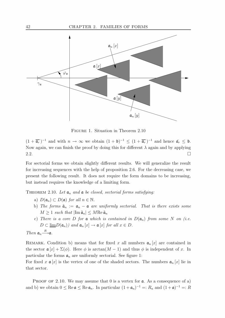
42 CHAPTER 2. FAMILIES OF FORMS
a [x]
a [y]
an [y]
an [x]
γa
ϕa
Figure 1. Situation in Theorem 2.10
(1 + ar )−1 and with n → ∞ we obtain (1 + b)−1 ≤ (1 + ar )−1 and hence ar ≤ b.
Now again, we can finish the proof by doing this for different λ again and by applying
2.2.
For sectorial forms we obtain slightly different results. We will generalize the result
for increasing sequences with the help of proposition 2.6. For the decreasing case, we
present the following result. It does not require the form domains to be increasing,
but instead requires the knowledge of a limiting form.
Theorem 2.10. Let an and a be closed, sectorial forms satisfying:
a) D(an) ⊂ D(a) for all n ∈ N.
b) The forms an := an − a are uniformly sectorial. That is there exists some
M ≥ 1 such that |Im an| ≤MRe an
c) There is a core D for a which is contained in D(an) from some N on (i.e.
D ⊂ limD(an)) and an [x] → a [x] for all x ∈ D.
Then anR−→a.
Remark. Condition b) means that for fixed x all numbers an [x] are contained in
the sector a [x] + Σ(φ). Here φ is arctan(M − 1) and thus φ is independent of x. In
particular the forms an are uniformly sectorial. See figure 1:
For fixed x a [x] is the vertex of one of the shaded sectors. The numbers an [x] lie in
that sector.
Proof of 2.10. We may assume that 0 is a vertex for a. As a consequence of a)
and b) we obtain 0 ≤ Re a ≤ Re an. In particular (1+ an)−1 =: Rn and (1+ a)−1 =: R
3. CONVERGENCE THEOREMS FOR FORMS 43
exist.
For x ∈ H we have Rnx ∈ D(An) ⊂ D(an) ⊂ D(a) and
(1 + Re a) [Rnx] ≤ (1 + Re an) [Rnx]
= Re ((1 +An)Rnx Rnx)
= Re (Panx Rnx)
≤ ‖x‖2.
From this it follows that both (1 + a) [Rnx] and anx [Rn] ≤ (1 + an) [Rnx] are uni-
formly bounded by ‖x‖2.
Now for x ∈ H and y ∈ D we have that
(1 + a) [Rnx−Rx, y] = (1 + a) [Rnx, y] − (1 + a) [Rx, y]
= (1 + an) [Rnx, y] − an [Rnx, y] − (1 + a) [Rx, y]
= (Panx y) − an [Rnx, y] − (Pax y)
= −an [Rnx, y]
The last equality holds for all n ≥ n0 where n0 is chosen such that y ∈ D(an) for all
n ≥ n0 and thus y = Pay = Pany.
For such n we have
|(1 + a) [Rnx−Rx, y]| ≤ (1 +M) an [Rnx]12
︸ ︷︷ ︸
bounded
· an [y]12
︸ ︷︷ ︸
→0
.
We have shown that (1 + a) [Rnx−Rx, y] → 0 for all x ∈ H and all y ∈ D. By the
density of D in D(a), this holds for all y ∈ D(a).
Now we have
(1 + a) [Rnx−Rx] + an [Rnx] = (1 + a) [Rnx] − (1 + a) [Rnx,Rx]
−(1 + a) [Rx,Rnx] + (1 + a) [Rx]
+(1 + an) [Rnx] − (1 + a) [Rnx]
= (1 + a) [Rx− Rnx,Rx]
− (Pax Rnx) + (Panx Rnx)︸ ︷︷ ︸
=0 sinceRnx∈D(an)⊂D(a)
→ 0 sinceRx ∈ D(a)
Taking the real part we see that
Re a [Rnx−Rx]︸ ︷︷ ︸
≥0
+‖Rnx−Rx‖2 + Re a [Rnx]︸ ︷︷ ︸
≥0
→ 0
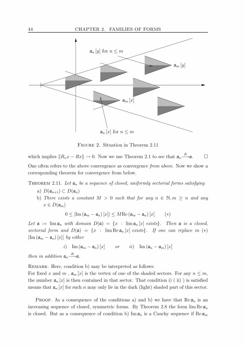
44 CHAPTER 2. FAMILIES OF FORMS
am [y]
am [x]
an [x] for n ≤ m
an [y] for n ≤ m
Figure 2. Situation in Theorem 2.11
which implies ‖Rnx−Rx‖ → 0. Now we use Theorem 2.1 to see that anR−→a.
One often refers to the above convergence as convergence from above. Now we show a
corresponding theorem for convergence from below.
Theorem 2.11. Let an be a sequence of closed, uniformly sectorial forms satisfying
a) D(an+1) ⊂ D(an)
b) There exists a constant M > 0 such that for any n ∈ N, m ≥ n and any
x ∈ D(am)
0 ≤ |Im (am − an) [x]| ≤ MRe (am − an) [x] (∗)
Let a := lim an with domain D(a) = x : lim an [x] exists. Then a is a closed,
sectorial form and D(a) = x : lim Re an [x] exists. If one can replace in (∗)|Im (am − an) [x]| by either
i) Im (am − an) [x] or ii) Im (an − am) [x]
then in addition anR−→a.
Remark. Here, condition b) may be interpreted as follows:
For fixed x and m , am [x] is the vertex of one of the shaded sectors. For any n ≤ m,
the number an [x] is then contained in that sector. That condition i) ( ii) ) is satisfied
means that an [x] for such n may only lie in the dark (light) shaded part of this sector.
Proof. As a consequence of the conditions a) and b) we have that Re an is an
increasing sequence of closed, symmetric forms. By Theorem 2.8 the form lim Re an
is closed. But as a consequence of condition b) Im an is a Cauchy sequence if Re am
3. CONVERGENCE THEOREMS FOR FORMS 45
is. In particular lim an exists if and only if lim Re an exists. This proves that D(a) =
x : lim Re an [x] exists =: D(b). It follows from Theorem 2.8 , that b := lim Re an
is a closed, symmetric form. In particular, D(a) is a vectorspace. On the other hand,
it follows from the above, that b = lim Re an = Re lim an = Re a, which implies that
a is closed, since a sectorial form is closed if and only if its real part is closed.
Now consider the forms an(z) = Re an + zIm an for n ∈ N and the form a(z) =
Re a + zIm a. These are for Re z < ε, holomorphic families of closed, sectorial forms
by proposition 2.6. (Note that because of the uniform sectoriality we can always take
the same ε .) Furthermore, for fixed z an(z) [x] → a(z) [x] for any x ∈ D(a).
For z ∈ (−ε, ε) × 0 the forms an(z) and a(z) are symmetric. Now if we assume
condition i), then an(z) is an increasing sequence of forms for z ∈ [0, ε), so that by
Theorem 2.8 R(λ, an(z))x → R(λ, a(z))x for these z, any x ∈ H and suitable λ. But
since the forms an(z) are uniformly sectorial for any n and any z in a rectangle we
obtain from Theorem 1.14 that R(λ, an(z)) is normbounded independently of n and
z. Now Vitali’s Theorem implies that we have this convergence uniformly on any rec-
tangle. By setting z = i we obtain strong convergence of R(λ, an) to R(λ, a), which
proves the claimed resolvent convergence.
If we assume condition ii), then for z ∈ (−ε, 0]× 0 the sequence an(z) is increasing,
and we obtain the resolvent convergence in the same way.
Notes and References for Chapter 2: It is a widely known fact, that the resolvent of
a generator of a strongly continuous semigroup is the Laplacetransform of that semigroup.
It is thus no surprise, that the convergence of semigroups is equivalent to the convergence of
the resolvents. This connection is discussed in Arendt et al [4].
The adaption of this to pseudoresolvents and degenerate semigroups causes little trouble.
Our presentation is close to Arendt [2].
What makes forms so much easier to handle is the observation, that for symmetric forms
weak convergence of the resolvent suffices to imply strong convergence. This fact is men-
tioned in Reed, Simon [16, chapter VIII-7]. We note, that this fact is used explicitly in the
proof of both convergence theorems for symmetric forms and thus implicitly in the proof of
Theorem 2.11.
The goal of section 2 is to establish proposition 2.6, which goes back to an idea of Simon
which appears in [11, addendum]. This is the right tool to generalize results for symmetric
forms to sectorial forms. This is illustrated in the proof of Theorem 2.11 and it will be used
again in the next chapter in the proof of Trotter’s formula. The rest of section 2 is an excerpt
of Kato [10, chapter 7-4].
46 CHAPTER 2. FAMILIES OF FORMS
The first part of section 3 concerning convergence of symmetric forms is close to Simon [17]
and was adapted to the nondensely defined case. A different proof of these theorems using
convex, lower semicontinuous functionals may be found in Reed, Simon [16, supplement to
VIII.7]. The theorem concerning convergence from above may be found in Kato [10, chapter
8-3], whereas the theorem concerning convergence from below was presented in Ouhabaz
[15] under the assumption, that the limiting form a is known to be closed and either condition
i) or ii) is satisfied.
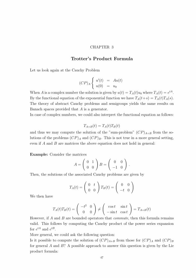
CHAPTER 3
Trotter’s Product Formula
Let us look again at the Cauchy Problem
(CP )A
u′(t) = Au(t)
u(0) = u0
When A is a complex number the solution is given by u(t) = TA(t)u0 where TA(t) = etA.
By the functional equation of the exponential function we have TA(t+s) = TA(t)TA(s).
The theory of abstract Cauchy problems and semigroups yields the same results on
Banach spaces provided that A is a generator.
In case of complex numbers, we could also interpret the functional equation as follows:
TA+B(t) = TA(t)TB(t)
and thus we may compute the solution of the ”sum-problem” (CP )A+B from the so-
lutions of the problems (CP )A and (CP )B. This is not true in a more general setting,
even if A and B are matrices the above equation does not hold in general:
Example: Consider the matrices
A =
(
0 1
0 0
)
B =
(
0 0
−1 0
)
.
Then, the solutions of the associated Cauchy problems are given by
TA(t) =
(
0 t
0 0
)
TB(t) =
(
0 0
−t 0
)
We then have
TA(t)TB(t) =
(
−t2 0
0 0
)
6=(
cos t sin t
− sin t cos t
)
= TA+B(t)
However, if A and B are bounded operators that commute, then this formula remains
valid. This follows by computing the Cauchy product of the power series expansion
for etA and etB.
More general, we could ask the following question:
Is it possible to compute the solution of (CP )A+B from those for (CP )A and (CP )Bfor general A and B? A possible approach to answer this question is given by the Lie
product formula:
47
48 CHAPTER 3. TROTTER’S PRODUCT FORMULA
Theorem 3.1. (Lie)
If A,B ∈ Cd×d, then
et(A+B) = limn→∞
(
etnAe
tnB)n
(∗)
However for unbounded operators even the meaning of A + B is not clear. It may
happen, that even though A and B are generators D(A)∩D(B) - which is the natural
domain for the sum - is not dense, so thatA+B cannot be the generator of a semigroup.
However the limit in (∗) may exist even if A+B is no generator.
In fact Chernoff investigates these phenomena in [7]. He proves that if the limit
(∗) exists, it always has the semigroup property (see [7, 2.5.3]) and uses this process
to define a generalized addition process +L.
But this generalized Lie-addition has several weaknesses:
• It is not applicable to all generators. Chernoff even proves that the only
universally addable operators are bounded (see [7, §6]).
• It is not associative ([7, prop. 5.3]).
In the case of sesquilinear forms these problems do not occur. Addition is not a
problem but it may happen that et(a+b) is degenerate even if the operators associated
with the two forms a and b generate semigroups on H . However the Trotter product
formula for forms respects this. In fact we are going to prove:
Theorem 3.2. (Trotter’s product formula)
Let a and b be closed sectorial forms. Then
s− limn→∞
(
e−tn
aetn
b
)n
= e−t(a+b)
for all t > 0, uniformly on compact subsets of (0,∞).
In the last section, we will see, that in fact Trotter’s formula as stated here characterizes
operators that are associated with sectorial forms entirely. This characterisation is due
to Matolcsi.
1. The Proof of Trotter’s Formula
A proof of this formula was given in Kato [11] under the assumption that both a and
b are densely defined. We imitate this proof and work in several steps:
Step 1 We prove an appropriate resolvent convergence under the assumption that both
a and b are symmetric.
Step 2 We use this result to prove the theorem for symmetric forms.
Step 3 We use the theorem for symmetric forms to prove the general result.
Proof of Theorem 3.2, Part 1.
Let a and b be closed symmetric forms. By adding suitable constants, we may assume
1. THE PROOF OF TROTTER’S FORMULA 49
that a and b be positive. Let c = a + b. Define for x ∈ H
S(t) =1
t(id− e−tae−tb)
In this first part of the proof, we show that for all x ∈ H
(1 + S(t))−1x→ (1 + c)−1x as t→ 0
which implies by 2.1 that the (bounded) symmetric forms associated with S(t) con-
verge to c in the strong resolvent sense.
Let A(t) = t−1(id − e−ta) , B(t) = t−1(id − e−tb) and C(t) = A(t) + B(t). We now
rewrite 1 + S(t) as
1 + S(t) = 1 + C(t) − tA(t)B(t)
= (1 + C(t))12 (1 −Q(t))(1 + C(t))
12
where Q(t) = t(1 + C(t))−12A(t)B(t)(1 + C(t))−
12 .
Lemma 3.3 shows that 1 −Q(t) is invertible. Thus we obtain
(1 + S(t))−1x = (1 + C(t))−12 (1 −Q(t))−1(1 + C(t))−
12x
= (1 + C(t))−1x+ (1 + C(t))−12 (1 −Q(t))−1Q(t)(1 + C(t))−
12x (∗)
As a consequence of Theorem 1.26 we have that (C(t)x y) converges as t → 0 if and
only if x, y ∈ D(c) and that the limit is c [x, y]. By the spectral Theorem (C(t)x x)
is increasing as t decreases, so that by Theorem 2.8 (1+C(t))−1x→ (1+c)−1x as t→ 0.
Thus it remains to show that the second summand in (∗) converges to 0. But according
to Lemma 3.3 (1+C(t))−12 (1−Q(t))−1 is bounded independently of t, so it suffices to
show that
Q(t)(1 + C(t))−12 = t(1 + C(t))−
12A(t)B(t)(1 + C(t))−1
converges to 0.
But ‖(1 + C(t))−12A(t)
12‖ = ‖A(t)
12 (1 + C(t))−
12‖ ≤ 1 by Lemma 3.31 . We also have
that tA(t)12B(t)
12 converges strongly to PaPb. By the Banach-Steinhaus Theorem,
this convergence is uniform on compact subsets of H . Now Lemma 3.4 shows that
B(t)12 (1 + C(t))−1x → B
12 (1 + c)−1x which is an element of D(b). These three facts
imply the required convergence and finish the proof.
Lemma 3.3. (1 −Q(t)) is invertible and ‖(1 −Q(t))−1‖ ≤ 2.
Furthermore ‖A(t)12 (1 + C(t))−
12‖ ≤ 1
2and ‖B(t)
12 (1 + C(t))−
12‖ ≤ 1
2.
1Note that the first operator is the adjoint of the second one
50 CHAPTER 3. TROTTER’S PRODUCT FORMULA
Proof. It suffices to show that Θ (Q(t)) ⊂ B(0, 12), since then dist
(
1,Θ ((Q(t)))
≥12
and 1.14 shows that 1 ∈ ρ(Q(t)) and ‖(1 −Q(t))−1‖ ≤ 2.
For x ∈ H we have:
|(Q(t)x x)| =∣∣∣
(
t(1 + C(t))−12A(t)B(t)(1 + C(t))−
12x x
)∣∣∣
=∣∣∣
(
tA(t)12B(t)
12B(t)
12 (1 + C(t))−
12x A(t)
12 (1 + C(t))−
12x)∣∣∣
≤ ‖tA(t)12B(t)
12‖
︸ ︷︷ ︸
≤1
·‖B(t)12 (1 + C(t))−
12x‖ · ‖A(t)
12 (1 + C(t))−
12x‖
≤ 1
2
(
‖B(t)12 (1 + C(t))−
12x‖2
+ ‖A(t)12 (1 + C(t))−
12x‖2
)
=1
2
((
B(t)(1 + C(t))−12x (1 + C(t))−
12x)
+(
A(t)(1 + C(t))−12x (1 + C(t))−
12x))
=1
2(C(t)(1 + C(t))−1x x)
=1
2
(
‖x‖2 − ((1 + C(t))−1x x))
≤ ‖x‖2
2
Here we used the selfadjointness of A(t) and (1 + C(t))−12 in the second and the
Cauchy-Schwarz inequality in the third step. The fourth inequality uses the fact that
2αβ ≤ α2 + β2. In the last equations we use again selfadjointness and the fact that
C(t) and (1 + C(t))−12 commute.
Lemma 3.4. For every x ∈ H
A(t)12 (1 + C(t))−1x → A
12 (1 + c)−1x
and B(t)12 (1 + C(t))−1x → B
12 (1 + c)−1x .
Proof.
a) By a similar manipulation as in the proof of the last lemma, we obtain that
‖(1 + C(t))−1x‖2+ ‖A(t)
12 (1 + C(t))−1x‖2
+ ‖B(t)12 (1 + C(t)−1x‖2
= ((1 + C(t))−1x x) ≤ ‖x‖2.
Thus since H is reflexive for any given sequence tn → 0 we may extract
a subsequence tk such that ya(tk) := A(tk)12 (1 + C(tk))
−1x and yb(tk) :=
B(tk)12 (1 + C(tk))
−1 are weakly convergent, say ya(tk) ya and yb(tk) yb.
1. THE PROOF OF TROTTER’S FORMULA 51
b) We clearly have that Paya(tk) Paya and similar for indices b. But on the
other hand for u ∈ D(a) = D(A12 )
(ya(tk) u) =(
(1 + C(tk))−1x A(tk)
12u)
→(
(1 + c)−1x A12u)
=(
A12 (1 + c)−1x u
)
,
since (1 + C(t))−1x → (1 + c)−1x ∈ D(c) ⊂ D(a) and since for u ∈ D(A12 ) we
have A(t)12u→ A
12u.
Now by density of D(A12 ) in D(a) = RgPa we conclude that
Paya = A12 (1 + c)−1x and similar Pbyb = B
12 (1 + c)−1x.
c) We know that ((1 + C(t))−1x x) → ((1 + c)−1x x) and since Rg(1 + c)−1 ⊂RgPc we can split up the limit as:
((1 + c)−1x x) = ((1 + c)−1x Pcx)
= ((1 + c)−1x (1 + C)(1 + c)−1x)
= ‖(1 + c)−1x‖2+ ‖A 1
2 (1 + c)−1x‖2+ ‖B 1
2 (1 + c)−1x‖2
= ‖(1 + c)−1x‖2+ ‖Paya‖2 + ‖Pbyb‖2
Now we use the first equality from a) and (1 + C(t))−1x → (1 + c)−1x and
obtain
‖ya(tk)‖2 + ‖yb(tk)‖2 → ‖Paya‖2 + ‖Pbyb‖2 ≤ ‖ya‖2 + ‖yb‖2
d) Now we exploit what we have done so far:
From the weak convergence it follows that
‖ya‖ ≤ lim‖ya(tk)‖ and ‖yb‖ ≤ lim‖yb(tk)‖
Thus given ε > 0 for all but finitely many k we have
‖ya(tk)‖2 ≥ ‖ya‖2 − ε and ‖yb(tk)‖2 ≥ ‖yb‖2 − ε
thus for these k we have
‖ya(tk)‖2 + ‖yb(tk)‖2 ≥ ‖ya‖2 + ‖yb‖2 − 2ε ≥ ‖Paya‖2 + ‖yb‖2 − 2ε
If we now let k → ∞ we obtain using c):
‖Paya‖2 + ‖yb‖2 − 2ε ≤ ‖Paya‖2 + ‖Pbyb‖2 ≤ ‖Paya‖2 + ‖yb‖2
Since ε > 0 was arbitrary, the last inequality is actually an equality and
‖Pbyb‖2 = ‖yb‖2 and hence Pbyb = yb. Similar Paya = ya.
Altogether we have showed that
‖ya(tk)‖2 + ‖yb(tk)‖2 → ‖ya‖2 + ‖yb‖2
52 CHAPTER 3. TROTTER’S PRODUCT FORMULA
e) First we show strong convergence as claimed along the sequence tk. In fact we
have:
‖ya(tk) − ya‖2 + ‖yb(tk) − yb‖2
= ‖ya(tk)‖2 + ‖ya‖2 − (ya(tk) ya) − (ya ya(tk))
+‖yb(tk)‖2 + ‖yb‖2 − (yb(tk) yb) − (yb yb(tk))
−→ 0 by d) and a)
But now we see that this convergence takes place as t→ 0 without any restric-
tion to a sequence, for otherwise, we would find ε > 0 and a sequence tn → 0
such that ‖A 12 (1 + C(tn))
−1x− A12 (1 + c)−1x‖ ≥ ε for all n. But then by what
we have done, we could extract a subsequence of tn such that the norm goes
to 0 – a contradiction.
This resolvent convergence would finish the proof if c was densely defined, by a theorem
of Chernoff [7]. We will now generalize this theorem to symmetric forms which need
not be densely defined.
Theorem 3.5. (Chernoff product formula)
Let F (t) for t ∈ (0,∞) be a family of selfadjoint, positive contractions and define
A(t) = t−1(id − F (t)). Assume that there exits a closed symmetric form a such that
(1+A(t))−1 converges strongly to (1+a)−1. Then F ( tn)n → e−ta strongly and uniformly
on intervals of the form [t0, t1].
The proof uses the following lemma. For the proof of the lemma we refer to Engel-
Nagel [9, III, Lemma 5.1]
Lemma 3.6. Let X be a Banach space, T ∈ L(X) satisfying ‖Tm‖ ≤ M for some
M ≥ 1 and all m ∈ N. Then for every n ∈ N and x ∈ X
‖en(T−id)x− T nx‖ ≤√nM‖Tx− x‖
Proof of 3.5. As a consequence of 2.1 we obtain that A(t)R−→a. Since all forms
are positive, and thus uniformly sectorial we have e−sA(t)x→ e−sax for all x by 2.3.
Decompose H = D(a) ⊕ D(a)⊥. First suppose that x ∈ D(a). By the lemma, we
obtain
‖e−tA( tn
)x− F ( tn)nx‖ = ‖en(F ( t
n)−id)x− F ( t
n)nx‖
≤√n‖F ( t
n)x− x‖
=t√n‖A( t
n)x‖ .
1. THE PROOF OF TROTTER’S FORMULA 53
For x ∈ D(A), where A is the operator associated with a as usual, we find x = (1+a)−1y
for some y ∈ D(a). Now we use that both F and e−tA( tn
) are uniformly bounded (say
by C ) and obtain:
‖e−tA( tn
)x− F ( tn)nx‖ = ‖e−tA( t
n)(1 + a)−1y − F ( t
n)n(1 + a)−1y‖
≤ 2C · ‖(1 + a)−1y − (1 + A( tn))−1y‖
+‖e−tA( tn
)(1 + A( tn))−1y − F ( t
n)n(1 + A( t
n))−1y‖
≤ 2C · ‖(1 + a)−1y − (1 + A( tn))−1y‖ +
t√n‖A( t
n)(1 + A( t
n))−1y‖
≤ 2C · ‖(1 + a)−1y − (1 + A( tn))−1y‖ +
t√n‖y − (1 + A( t
n))−1y‖
Here, since A(t)R−→a, the first term tends to zero uniformly for t in compact subsets
of R+ whereas the term in the second norm is convergent, and hence bounded. Thus
we obtain the desired convergence for x ∈ D(A) and by density also for all x ∈ D(a).
Now let x ∈ D(a)⊥. We have to show that F ( tn)nx→ 0.
By the definition of A(t) we obtain that
0 ≤ F (t) = 1 − tA(t) ≤ (1 + tA(t))−1
where the last inequality is proved this way:
((1 − tA(t))x x) = ((1 + tA(t))−1(1 − t2A(t)2)x x)
= ((1 + tA(t))−1x x) − ((1 + tA(t))−1tA(t)x tA(t)x)︸ ︷︷ ︸
≥0
≤ ((1 + tA(t))−1x x)
Using the fact that F (t) and A(t) are selfadjoint and commute we obtain inductively
that F (t)2n ≤ (1 + tA(t))−2n for all n ∈ N. But we have that
(1 + tA(t))2n =
2n∑
k=0
(2n
k
)
tkA(t)k
= 1 + 2ntA(t) + · · ·+ t2nA(t)2n
︸ ︷︷ ︸
≥0
≥ 1 + 2ntA(t)
and hence 0 ≤ F (t)2n ≤ (1 + tA(t))−2n ≤ (1 + 2ntA(t))−1 by 2.7. Hence
‖F ( tn)nx‖2
=(F ( t
n)2nx x
)
≤((1 + 2tA( t
n))−1x x
)
= (2t)−1((2t+ A( t
n))−1x x
)→ 0
54 CHAPTER 3. TROTTER’S PRODUCT FORMULA
uniformly on intervals of the form [t0, t1].
Now we are ready to finish the proof of Trotter’s product formlua for positive, sym-
metric forms. We want to apply Chernoffs formula, and we are done. The only thing
to do, is to ”symmetrize” everything2
Proof of Theorem 3.2, Part 2.
Define F (t) = e−ta
2 e−tbe−ta
2 and F (t) = e−tae−tb, S(t) = t−1(id − F (t)) and S(t) as in
Part I.
We claim that also (1 + S(t))−1 → (1 + c)−1 strongly. Note that
1 = (1 + S(t))(1 + S(t))−1
= t−1(t+ 1 − F (t))(1 + S(t))−1
so that we may conclude that
(1 + t)(1 + S(t))−1 = t+ F (t)(1 + S(t))−1
We claim that e−ta
2 (1 + S(t))−1 = (1 + S(t))−1e−ta
2 from which it then follows that
(1 + S(t))−1 = (t+ 1)−1(
t+ e−ta
2 e−tb(1 + S(t))−1e−ta
2
)
(∗)
To prove the last claim observe that
(1 + S(t))−1e−ta
2 (1 + S(t)) = (1 + S(t))−1e−ta
2 t−1(1 + ti− F (t))
= (1 + S(t))−1t−1(1 + tF (t))e−ta
2
= e−t−a
2
where we used that e−ta
2 F (t) = F (t)e−ta
2 . From this the desired equality follows im-
mediately.
Now observe that this equation for the resolvent of S implies that
(1 + S(t))−1x− (1 + S(t))−1x→ 0 + PaPb(1 + c)−1x− (1 + c)−1x
which is equal to zero, since D(c) ⊂ D(a)∩D(b) and we thus may omit the projections.
Now Chernoffs formula implies that F ( tn)nx→ e−tcx
But we have that
F (t
n)n+1 = e−t
a
2 F (t
n)ne−t
a
2 e−tb → Pae−tcPaPb = e−tc
which completes the proof.
2The reason why we didn’t start with the ”right” approximants is to have a more readable proof.
For densely defined c a direct proof of the resolvent convergence we will need in order to apply
Chernoffs formula can be found in Reed-Simon [16, Supplement VIII.8].
2. PROJECTIONS 55
Proof of Theorem 3.2, Part 3.
We now generalize our result to sectorial forms by an argument about holomorphic
functions. We let a, b be closed sectorial forms and we assume that 0 is a vertex and
θ a corresponding semiangle for both of them We define a(z) = Re a + zIm a and
b(z) = Re b + zIm b.
For z ∈ (−ε, ε) × R where ε = 11+tan θ
a(z) is a sectorial form. Moreover, for z ∈[−α0, α0] × [−β0, β0] where α0 and β0 are fixed positive numbers the family a(z) is
uniformly sectorial by Proposition 2.6. Thus, we may locally use the same integration
path for e−ta(z). This together with the analyticity of the resolvents (which also follows
from 2.6 ) implies, that the semigroups e−ta(z) and e−tb(z) depend analytically on z.
The first two parts of the proof show that
s− lim(
e−tn
a(z)e−tn
b(z))n
= e−tc
for all z ∈ (−ε, ε) since these forms are symmetric. But since in this equation all
occuring functions depend holomorphically on z. Vitali’s Theorem implies the conver-
gence for any z in the strip (−ε, ε)×R and the desired result follows by setting z = i.
Furthermore, since the left hand side is analytic in t too, Vitali’s Theorem implies
uniform convergence on compact t-subsets of (0,∞).
2. Projections
Now we consider some rather special closed sectorial forms. If U is a closed subspace
of H , then oU defined by
oU [x, y] := 0 D(o) = U
is a closed sectorial form3 . Then we have that the operator associated with oU is the
zero-operator on U , so that we obtain e−to ≡ PU where PU is the orthogonal projection
onto U .
Thus we obtain as a consequence of 3.2 the following corollary, which is a special case
of a theorem of von Neumann:
Corollary 3.7. Let U, V be closed subspaces of a Hilbert space H and PU , PV be the
orthogonal projections onto U resp. V . Then for any x ∈ H we have
lim(PUPV )nx = PU∩V x
where PU∩V is the orthogonal projection onto the intersection of U and V .
Proof. This follows immediately form 3.2 by choosing a = oU , b = oV and ob-
serving that a + b = oU∩V .
3Clearly oU is sectorial. It is closed, since ( · · )oU
= ( · · ).
56 CHAPTER 3. TROTTER’S PRODUCT FORMULA
As symmetric forms may also be viewed as subdifferentials of convex functionals it is
also interesting, that we have a Trotter formula for those as well:
If ϕ is a lower semicontinuous convex function on H then the subdifferential ∂ϕ gen-
erates a semigroup (S(t)) of nonlinear contractions on Ωϕ = D(∂ϕ) which is always
a closed, convex set. Thus we may view this as a degenerate semigroup of nonlinear
contractions on H by projecting onto Ωϕ first. We then write e−t∂ϕ = S(t)PΩϕ where
PΩϕ is the (nonlinear ) projection onto Ωϕ. We now have the following theorem of
Kato and Masuda which was proved in [12]:
Theorem 3.8. Let ϕ1, . . . , ϕk be lower semicontinuous, convex functionals on H and
ϕ :=∑ϕj. Then for any x ∈ Ωϕ we have that
lim(
e−tn∂ϕk · · · · · e− t
n∂ϕ1
)n
x = e−t∂ϕx
However, one cannot omit the requirement that x ∈ Ωϕ in this theorem (and thus
in particular obtain Theorem 3.2 from a more general theorem concerning nonlinear
semigroups). This is, because a nonlinear generalisation of corollary 3.7 does not hold.
Look at the following
Example:
Let H = R2 and let V = x : ‖x‖ ≤ 1 and U = x : x2 = 0 then U and V are
closed, convex subsets of H and the orthogonal projections onto them are given by
PUx =(x1
0
)
and PV x =
x , if ‖x‖ ≤ 1x
‖x‖ , otherwise
Figure 1 shows, that a convergence analoguous to 3.7 is not valid.
If we are given a closed sectorial form a it is also a consequence of Trotters formula,
that
s− limn→∞
(
e−tn
aP)n
exists for any orthogonal projection P . We will see, that this characterizes (operators
associated with) closed sectorial forms entirely.
But first we explore a much simpler case, namely that where P is an orthogonal
projection onto a 1-dimensional subspace.
Proposition 3.9. Let A be the generator of a strongly continuous semigroup and
define fn for x 6= 0 by
fn(x) =(
e1nAPx
)n
x
where Px is the orthogonal projection onto spanx. Then we have:
a) For any x ∈ D(A) with ‖x‖ = 1 we have lim fn(x) = e(Ax x)x.
b) Any fn is a continuous function of x.
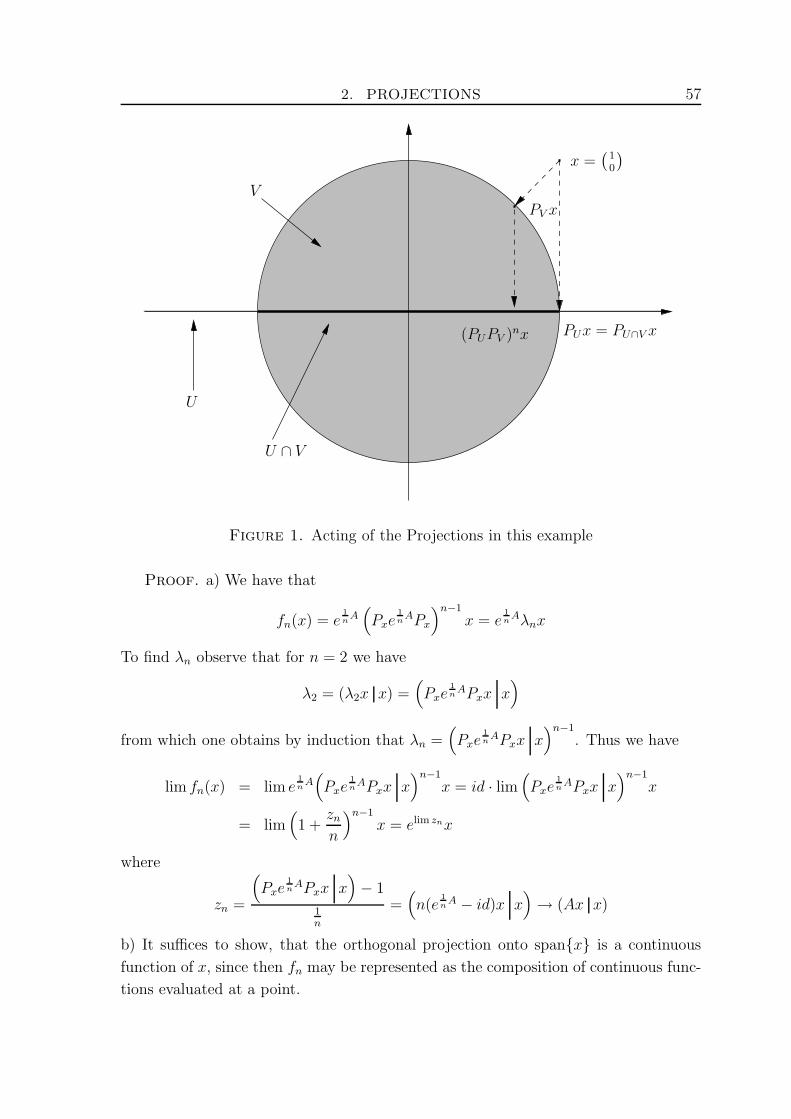
2. PROJECTIONS 57
x =(
10
)
PUx = PU∩V x
PV x
U ∩ V
V
U
(PUPV )nx
Figure 1. Acting of the Projections in this example
Proof. a) We have that
fn(x) = e1nA(
Pxe1nAPx
)n−1
x = e1nAλnx
To find λn observe that for n = 2 we have
λ2 = (λ2x x) =(
Pxe1nAPxx x
)
from which one obtains by induction that λn =(
Pxe1nAPxx x
)n−1
. Thus we have
lim fn(x) = lim e1nA(
Pxe1nAPxx x
)n−1
x = id · lim(
Pxe1nAPxx x
)n−1
x
= lim(
1 +zn
n
)n−1
x = elim znx
where
zn =
(
Pxe1nAPxx x
)
− 1
1n
=(
n(e1nA − id)x x
)
→ (Ax x)
b) It suffices to show, that the orthogonal projection onto spanx is a continuous
function of x, since then fn may be represented as the composition of continuous func-
tions evaluated at a point.
58 CHAPTER 3. TROTTER’S PRODUCT FORMULA
But we have Pxu =
(
u x‖x‖
)
x‖x‖ and thus
‖Pxu− Pyu‖ ≤∥∥∥∥
(
u x‖x‖
)x
‖x‖ −(
u x‖x‖
)y
‖y‖
∥∥∥∥
+
∥∥∥∥
(
u x‖x‖
)y
‖y‖ −(
uy
‖y‖
)y
‖y‖
∥∥∥∥
≤ 2‖u‖ ·∥∥∥∥
x
‖x‖ − y
‖y‖
∥∥∥∥
which implies that ‖Px − Py‖ ≤ 2
∥∥∥∥x
‖x‖ − y‖y‖
∥∥∥∥. This shows the continuous depen-
dence of Px on x. Moreover, we can estimate this difference by
‖ x‖x‖ − y
‖y‖‖ ≤ 1
‖x‖ · ‖y‖∥∥∥ ‖y‖x− ‖x‖y
∥∥∥
=1
‖x‖ · ‖y‖(∥∥∥ ‖y‖x− ‖y‖y
∥∥∥+
∥∥∥ ‖y‖y − ‖x‖y
∥∥∥
)
≤ 2
‖x‖‖x− y‖
So that for x, y outside a ball B(0, r) the projection Px is Lipschitz continuous with
Lipschitz constant 2r−1.
Theorem 3.10. Let A be the generator of a C0-semigroup etA on a Hilbert space H.
Then the following are equivalent:
a) −A is associated with a closed, densely defined sectorial form.
b) (etnAP )nx converges for any orthogonal projection P and any t > 0, x ∈ H.
Proof. a) ⇒ b) follows directly from Theorem 3.2
b) ⇒ a) We adopt the notation fn(x) = (e1nAPx)
nx from proposition 3.9 and put
f∞(x) = lim fn(x) = e(Ax x)x for x ∈ D(A) with ‖x‖ = 1. We also use the abbrevi-
ation yo for y
‖y‖ .
We prove this implication by contradiction and consider two cases:
1st case: Θ (A) is not bounded from the right.
Let ε > 0 be given. We construct sequences xk ⊂ D(A), nk ⊂ N and δk ⊂ (0,∞) as
follows:
Choose x1 ∈ D(A) such that ‖x1‖ = 1 and Re (Ax1 x1) ≥ 1. Now pick n1 ∈ N such
that ‖fn1(x1) − f∞(x1)‖ < ε. By continuity, there exists δ1 <12
such that
‖fn1(yo) − f∞(x1)‖ < 2ε
for all y ∈ B(x1, δ1).
Now let x1, . . . , xk , n1, . . . nk and δ1, . . . δk already be chosen such that for any 1 ≤ l ≤k
2. PROJECTIONS 59
i) ‖xl+1 − xl‖ < min δj2l+1−j : 1 ≤ j ≤ l
ii) Re (Axl xl) ≥ l
iii) ‖fnl(yo) − f∞(xol )‖ < 2ε for all y ∈ B(xl, δl).
Since Θ (A) is not bounded from the right, we can find u ∈ D(A), such that
‖u‖ < min‖Axk‖−1,
δl
2k+1−l : 1 ≤ l ≤ k and Re (Au u) ≥ 2
Now choose real α such that Re (Aeiαu xk) ≥ 0 and put xk+1 = xk + eiαu. Then by
construction condition i) is fulfilled, so we check condition ii):
We have
Re (Axk+1 xk+1) = Re (Axk xk) + Re (Axk eiαu)
+Re (Aeiαu xk) + Re (Aeiαu eiαu)
≥ k − ‖Axk‖ · ‖u‖ + 0 + 2
≥ k − 1 + 2 = k + 1
And we may find nk+1 and δk+1 such that iii) is satisfied as above.
Now observe, that for m > n we have
‖xm − xn‖ ≤m−1∑
k=n
‖xk+1 − xk‖ ≤m−1∑
k=n
δ1
2k→ 0 as m,n→ ∞
Thus xn is a Cauchy sequence and hence convergent, say to x. But we also have for
m > n that
‖xm − xn‖ ≤m−1∑
k=n
‖xk+1 − xk‖ <m−1∑
k=n
δn
2k+1−n = δn
m−n−1∑
k=1
2k = δn1 − 2−(m−n)
1 − 12
≤ δn
So that xm ∈ B(xn, δn) for all m ≥ n. This implies in particular, that x ∈ B(xn, δn)
for all n and thus
‖fnk(xo) − f∞(xok)‖ < 2ε .
But since ‖xk‖ ∈ (12, 3
2) we have
‖f∞(xok)‖ = eRe(Axk xk)
‖xk‖2 > e4k9 → ∞ .
This shows that fn(xo) = (e
1nAPx0)nxo cannot converge, since the subsequence fnk
(xo)
has unbounded norms.
2nd case: We assume that Θ (A) is bounded from the right but Θ (A) is not contained
in any sector. By rescaling, we may assume, that Re (Ax x) ≤ −1. We also assume,
that the upper half of the numerical range is not contained in any sector.
Again, we construct sequences xk ⊂ D(A), nk ⊂ N and δk ⊂ (0,∞) as follows:
60 CHAPTER 3. TROTTER’S PRODUCT FORMULA
Let x1 ∈ D(A) with ‖x1‖ = 1 be arbitrary and put α1 = (Ax1 x1) = a1 + b1i.
Let 0 < ε < e2a1
5be given. Choose ρ > 0 such that |eεi− 1| < e2a1+1
2for all |ε| < ρ and
δ1 <3e2a1+1
16.
Now assume, that x1, . . . xk, n1, . . . , nk and δ1, . . . δk already be chosen, such that for
any 1 ≤ l ≤ k
i) ‖xl+1 − xl‖ < min δj2l+1−j : 1 ≤ j ≤ l
ii) If αl = ‖xl‖−2(Axl xl) = al + bli then we have
2a1 ≤ al ≤ −1 and |bl − bl−1 − π| = |εl| < ρ
iii) ‖fnl(yo) − f∞(xol )‖ < 2ε for all y ∈ B(xl, δl).
Since A is not sectorial, there is a sequence zn ⊂ D(A) such that ‖zn‖ = 1 and
Im (Azn zn) ≥ n|Re (Azn zn)| ≥ n.
Define
un =
√π‖xk‖
√
Im (Azn zn)zn
and now pick ϕn such that (Aeiϕn un xk) ≥ 0 (and thus in particular real!). Put
un = eiϕn un. Then we have that
i) ‖un‖ ≤ const. · 1√n→ 0
ii) Im (Aun un) = π‖xk‖2
iii) |Re (Aun un)| ≤ 1nIm (Aun un) = π‖xk‖2
n→ 0
We then have:
(A(xk + un) xk + un)
‖xk‖2= ‖xk‖−2
(Axk xk) + (Axk un)︸ ︷︷ ︸
→0
+ (Aun xk)︸ ︷︷ ︸
≥0
+(Aun un)
=: cn + dni
Here we have that
cn ≥ ak − ‖xk‖−2 · |(Axk un)| − ‖xk‖−2 · |(Aun un)| → ak as n→ ∞
and
dn = bk + ‖xk‖−2Im (Axk un) + π → bk + π as n→ ∞So considering that ‖xk + un‖−2‖xk‖2 → 1, we may choose n0 large enough, such that
‖un0‖ < min δk2k+1−j : 1 ≤ j ≤ k and
cn0
‖xk‖2
‖xk + un0‖2> ak ≥ 2a1 and
∣∣∣∣dn0 ·
‖xk‖2
‖xk + un0‖2− bk − π
∣∣∣∣< ρ
Then if we put xk+1 = xk + un0 then conditions i) and ii) are fulfilled.
Now as in the first case, we may choose nk+1 and δk+1 such that the third condition is
satisfied.
2. PROJECTIONS 61
Exactly as in the first case, we see that the sequence xn converges to x (say) and that
for any k we have that
‖fnk(xo) − f∞(xok)‖ < 2ε .
But now observe, that consecutive members of f∞(xk) are far away from each other.
More precisely:
‖f∞(xok+1) − f∞(xok)‖ = ‖eαk+1xok+1 − eαkxok‖= ‖eαk+1xok+1 − eak+1+(bk+π)ixok + eak+1+(bk+π)ixok − eαkxok‖≥ ‖eak+1+(bk+π)ixok − eαkxok‖ − ‖eαk+1xok+1 − eak+1+(bk+π)ixok‖≥ eak + eak+1 − eak+1‖ebk+1ixok+1 − e(bk+π)ixok‖≥ 2e2a1 − e−1‖eεk+1ixok+1 − xok‖≥ 2e2a1 − e−1
(|eεk+1i − 1| + ‖xok+1 − xok‖
)
≥ 2e2a1 − e−1
(e2a1+1
2+
8
3δ1
)
≥ e2a1
Here, we used in the last step the choice of ρ, the fact that the projection on the
unitsphere is Lipschitz continuous outside the ball B(0, 34) with Lipschitz constant 8
3
(see the proof of 3.9 ) and that ‖xk‖ ∈ (34, 5
4).
From this, it follows, that
‖fnk(xo) − fnk+1
(xo)‖≥ ‖f∞(xok+1) − f∞(xok)‖ − ‖f∞(xok) − fnk
(xo)‖ − ‖f∞(xok+1) − fnk+1(xo)‖
≥ 5ε− 2ε− 2ε = ε
Notes and References for Chapter 3: The main reference for section 1 is of course
Kato [11], where the proof was given in the case where a and b are densely defined. Here,
Kato also suggested an adaption of his proof to nondensely defined forms by using a gener-
alized spectral Theorem. The proof presented here however uses only the standard spectral
Theorem and the convergence theorems of the previous chapter (which do not appear in
Kato’s proof). This was inspired by the proof given in Reed, Simon [16, chapter VIII.8
and supplement]. The idea for the proof of lemma 3.4 was suggested by Charles Batty
during a stay in Ulm. The proof of the Chernoff product formula given here is also not the
one suggested in [11] but inspired by the proof given in Engel, Nagel [9] for operators.
For more information on the nonlinear case mentioned in section 2, we refer to Brezis [6].
The example, that Trotter’s formula does not hold for nonlinear projections was found in
Kato, Masuda [12]. The rest of this section is taken from Matolcsi [13].

CHAPTER 4
Applications to Elliptic Forms
Elliptic operators belong to the most interesting operators for applications of semi-
group theory. Also, they are the prototype of operators associated with forms. There-
fore, we want to introduce elliptic forms in this chapter.
We will work in the Hilbert space H = L2(Rd) (where we use Lebesgue-measure dx).
Let Ω be an open subset of Rd. By an elliptic form, we mean a form looking as follows:
a [f, g] =
∫
Ω
d∑
i,j=1
aijDifDjg dx
︸ ︷︷ ︸
:=a0 [f, g]
+
∫
Ω
d∑
k=1
(bkDkfg dx+ ckfDkg
)
︸ ︷︷ ︸
:=b [f, g]
+
∫
Ω
aofg dx
︸ ︷︷ ︸
:=c [f, g]
defined on a suitable domain D(a) ⊂ H10 (Ω). Here, Dj = ∂
∂xj. We call a0 the principal
part of a. b is called the drift term of a, c the potential part. We will always assume the
coefficients A = (aij) : Ω → Cd×d to satisfy the following uniform ellipticity condition:
There exists some constant η > 0 such that
Re
d∑
i,j=1
aij(x)ξiξj ≥ η|ξ|2 for a.e. x and every ξ ∈ Cd (E)
In the following, we will impose more conditions on A and the coefficients b = (bk), c =
(ck) : Ω → Cd and a0 : Ω → C. So far, we will only assume that the coefficients are
measurable.
It is then interesting, to investigate, how the forms (and then also the semigroups)
depend on the coefficients.
Another interesting aspect is the dependence of the forms on the domain Ω. For this,
we require, that D(a) ⊂ H10 (Ω), which means, that we impose Dirichlet boundary
conditions. This allows us, to identify the form domains with closed subspaces of
L2(Rd) by extending functions by 0. For this, we use that
H10 (Ω) := D(Ω)
H1(Ω)= f ∈ D(Rd) : suppf ⊂ ΩH
1(Rd).
63
64 CHAPTER 4. APPLICATIONS TO ELLIPTIC FORMS
1. The Principal Part of an Elliptic Form
What makes the form approach to elliptic operators so easy is the fact, that we can
take care of the different parts of the form separately and then use form methods to
’paste’ them together. So we start with the principal part.
Proposition 4.1. Let A = (aij) ∈ L∞(Ω,Cd×d) satisfy condition (E). Then a0 as
defined above with domain D(a0) = H10 (Ω) is a closed, sectorial form.
Proof. First observe that
Re a0 [f ] = Re
∫
Ω
∑
aijDifDjf dx
≥∫
Ω
η|∇f |2 dx
= η
d∑
k=1
‖Dkf‖22 ≥ 0
and thus Re a0 ≥ 0. Now pick C such that ‖aij‖∞ ≤ C for all 1 ≤ i, j ≤ d. Then
|Im a0 [f ]| ≤ C ·∫
Ω
d∑
i,j=1
|DifDjf | dx
≤ C
(d∑
k=1
‖Dkf‖2
)2
by the Holder inequality
≤ Cd
d∑
k=1
‖Dkf‖22 by convexity of the square function
≤ Cd
ηRe a0 [f ]
Furthermore a0 is closed since the associated norm ‖ · ‖a0
is equivalent to the Sobolev
norm ‖ · ‖H1 . To see this, observe
‖f‖2a0
= ‖f‖22 + Re a [f ] ≥ ‖f‖2
2 + η
d∑
i=1
‖Dif‖22
≥ min1, η · ‖f‖2H1
‖f‖2a0
= ‖f‖22 + Re a0 [f ] ≤ ‖f‖2
2 + Cd
d∑
i=1
‖Dif‖22
≤ max1, Cd · ‖f‖2H1 .
1. THE PRINCIPAL PART OF AN ELLIPTIC FORM 65
Corollary 4.2. If the conditions of proposition 4.1 are satisfied, then D(Ω) is a form
core for a0.
Proof. This follows, since the norm ‖ · ‖a0
is equivalent to the Sobolev norm, and
the testfunctions are dense in H10 .
Next we consider elliptic forms with unbounded coefficients. Here, we have to assume
a little bit more on the coefficients to make the associated form sectorial. We have the
following
Proposition 4.3. Let A = (aij) : Ω → Cd×d with measurable entries such that the
ellipticity condition (E) is satisfied. Furthermore assume that there exists a constant
M > 0 such that
|d∑
i,j=1
Im aij(x) ξiξj| ≤ M
d∑
i,j=1
Re aij(x)ξiξj ∀ξ ∈ Cd , a.e. x
And define
a0 [f, g] =
∫
Ω
d∑
i,j=1
aijDifDjg dx
D(a0) = f ∈ H10 (Ω) :
∫
Ω
|d∑
i,j=1
aijDifDjf | dx <∞
Then a0 is a closed, sectorial form.
Proof. First, we check, that D(a0) is a vector space. Obviously, 0 ∈ D(a0) and
also if f ∈ D(a0) then also λf ∈ D(a0) for any scalar λ. To see that f, g ∈ D(a0)
implies f + g ∈ D(a0) note that
d∑
i,j=1
aij(x)Di(f + g)Dj(f + g) =d∑
i,j=1
aij(x)(DifDjf +DigDjf +DifDjg +DigDjg
)
for almost every x. The first and last summand are integrable by hypothesis. For the
two in the middle, note, that the mapping
(ξ, η) 7→d∑
i,j=1
aij(x)ξiηi
is a sectorial form on Cd for almost every x. Thus, by applying proposition 1.2 and
the Cauchy inequality, we see, that these are integrable as well.
Let An = (anij) ∈ L∞(Ω,Cd×d) be defined by
anij(x) = aij(x)1lΩn +η
2δij1lΩn
C
where Ωn = x : maxi,j Re ai,j(x) ≤ n. The sequence Ωn is increasing. Now observe,
that An satisfies (E) with ellipticity constant η
2independent of n. So we can consider
66 CHAPTER 4. APPLICATIONS TO ELLIPTIC FORMS
the elliptic form an associated with An as above, which is a closed, sectorial form. But
we also obtain, that the family an is uniformly sectorial:
By Theorem 4.1 Re an ≥ 0 for any n. Now observe, that
|Im an [f ]| =
∣∣∣∣∣
∫
Ωn
Im
d∑
i,j=1
aijDifDjf dx
∣∣∣∣∣
≤ M
∫
Ωn
Re
d∑
i,j=1
aijDifDjf dx
≤ M
∫
Ωn
Re
d∑
i,j=1
aijDifDjf dx+M
∫
ΩnC
η|∇f |2 dx︸ ︷︷ ︸
≥0
= M Re an [f ]
Furthermore we have for m ≥ n that
|Im (am − an) [f ]| =
∣∣∣∣∣
∫
Ωm\Ωn
Im
d∑
i,j=1
aij DifDjf dx
∣∣∣∣∣
≤ M
∫
Ωm\Ωn
Re
d∑
i,j=1
aij DifDjf dx
≤ M
∫
Ωm\Ωn
Re
d∑
i,j=1
aij DifDjf dx
+M
∫
Ωm\Ωn
Re
d∑
i,j=1
aij DifDjf − η|∇f |2
︸ ︷︷ ︸
≥0
dx
= 2M Re (am − an) [f ]
Now Theorem 2.11 shows that the limit form lim an is a closed and sectorial form. It
remains to show that actually lim an = a0 :
Assume that lim Re an [f ] exists. We have to show that f ∈ D(a0) and that lim an [f ] =
a0 [f ]. Put
gn =
d∑
i,j=1
anijDifDjf and g =
d∑
i,j=1
aijDifDjf
We have that gn → g pointwise, furthermore Re gn is increasing. It is a consequence
of the monotone convergence Theorem, that Re g is integrable. From this it follows,
that g is integrable, since |g| ≤ (1 +M)Re g and this implies that f ∈ D(a). The fact
that lim an [f ] = a0 [f ] follows now from the dominated convergence Theorem.
2. SCHRODINGER OPERATORS 67
Conversely, suppose that f ∈ D(a0). Then we have that lim an [f ] exists and is equal
to a0 [f ] as a consequence of the dominated convergence Theorem.
Corollary 4.4. If in addition to the hypotheses of Proposition 4.3 the coefficients A
have an almost everywhere realvalued quadratic form, i.e.
Imd∑
i,j=1
aij(x)ξiξj = 0 ∀ ξ ∈ Cd , a.e. x .
Then the forms an defined as in the last theorem converge in strong resolvent sense to
a.
Proof. This is an immediate consequence of Theorem 2.11 and the fact that
Im (an − am) = 0.
2. Schrodinger Operators
A Schrodinger operator is an operator of the form
S = ∆ − V.
Here ∆ is the Laplace operator on an open set Ω ⊂ Rd (where we will impose Dirichlet
boundary conditions as usual) and V is multiplication with a function (which we will
call V as well). We can interpret this formal definition by using form methods:
−∆ is associated with the closed, symmetric form
a0 [f ] :=
∫
Ω
|∇f |2 dx D(a) = H10 (Ω).
On the other hand, V is associated with the form
c [f ] :=
∫
Ω
V |f |2 dx D(c) = f ∈ L2(Ω) :
∫
Ω
|V | · |f |2 dx <∞.
If V (Ω) ⊂ Σγ(θ), then obviously c is a sectorial form with Θ (c) ⊂ Σγ(θ). Furthermore
c is closed, since (D(c), ‖ · ‖c) ≃ L2(Ω, (ReV − γ)dx). So the operator associated with
the form s = a0 + c may be viewed as a realisation of S. However, the meaning of this
operator is in general not clear. If for example V is nowhere locally integrable, then
D(s) = 0, so that also Sx is only defined for x = 0. However, if V ∈ L1loc(Ω), then
S is densely defined, since the test functions belong to D(s).
The semigroup generated by ∆ is the heat semigroup and well known. The semigroup
generated by −V is just multiplication by e−tV . So, by using the Trotter formula, one
can compute the semigroup generated by S:
etSf = e−t(a0+c)f = limn→∞
(
etn
∆e−tnV)n
f
68 CHAPTER 4. APPLICATIONS TO ELLIPTIC FORMS
Sometimes, one is also interested in potentials V : Ω → [0,∞]. If ∞ ∈ V (Ω) one calls
V an absorbing potential. How is V (ω) = ∞ to be interpreted?
Example:
Let M ⊂ Ω be measurable and define V = ∞ · 1lM .
In some sense, V = limn · 1lM and the latter function may be associated with a closed,
symmetric form:
If we define cn by
cn [f ] =
∫
M
n · |f |2 dx D(c) = L2(Ω),
then the operator associated with cn is multiplication with Vn := n · 1lM . So we could
define V to be associated with the form c = lim cn. But the latter limit exists only if
f(x) = 0 for almost every x ∈M .
This leads to the following
Definition. Let V : Ω → [0,∞] be measurable and M := V −1(∞). Then we identify
V with the operator associated with the closed, symmetric form
c [f ] =
∫
Ω
V · |f |2 dx D(c) = f ∈ L2(Ω) ; f|M = 0 a.e. and
∫
Ω\MV |f |2 dx <∞.
Now we obtain the following approximation result:
Proposition 4.5. Let V : Ω → [0,∞] be a measurable function and Vn be a sequence of
bounded, positive functions pointwise increasing to V . Then if V and Vn are associated
with c and cn and −∆ is associated with a0, then a0 + cnR−→a0 + c, so in particular
et(∆−Vn)f → et(∆−V )f
for every f ∈ L2(Ω).
Proof. We have thatD(a0+cn) ≡ H10 (Ω) independent of n and also that (a0 + cn) [f ]
is increasing for fixed f . Thus, a0 + cn is an increasing sequence of closed, symmetric
forms. By Theorem 2.8, it suffices show, that a0 + c really is the limiting form to finish
the proof.
For f ∈ D(a0+c) we have lim (a0 + cn) [f ] = (a0 + c) [f ] by the dominated convergence
Theorem. This proves that a0 + c ⊂ lim(a0 + cn).
Conversely, let f ∈ H10 (Ω) be given, such that sup (a0 + cn) [f ] < ∞. Let k ∈ N and
define Mk = M ∩ |f | > 1k. If |Mk| > 0, then
(a0 + cn) [f ] ≥∫
Mk
Vn1
k2dx→ ∞ ,
since otherwise, the monotone convergence Theorem would imply, that∫
MkV dx <∞.
This contradicts that sup (a0 + cn) [f ] <∞. Thus |Mk| = 0 and hence also |x ∈ M :
3. ELLIPTIC FORMS WITH DRIFT 69
f(x) 6= 0| =∣∣⋃
n∈NMn
∣∣ = 0. That f ∈ D(a0 + c) and that (a0 + cn) [f ] → (a0 + c) [f ]
now follows from the monotone convergence Theorem.
Remarks. a) If V ∈ L1loc, then a0 + c is not only densely defined but also D(Ω) is a
core for a0 + c. The proof of this may be found in Davies [8, Theorem 8.2.1].
b) In this section, it is not necessary, that the principal part of our elliptic form is given
by the form associated with the Dirichlet-Laplacian. We can do exactly the same with
arbitrary principal parts. To prove the equivalent of the preceding proposition in this
case, use Theorem 2.11. Here note, that the potential part has no influence on the
imaginary part of the forms whatsoever, so that nearly the same proof works.
3. Elliptic Forms with Drift
The drift part of an elliptic form is a more delicate object. Usually, it does not define
a sectorial form by itself, so that one cannot simply add it to the principal part. Thus,
the drift term is usually treated as a perturbation of the other parts of the elliptic
form.
First, we formulate a requirement on the coefficients bk and ck which will ensure, that
a0 + b is a closed, sectorial form defined on D(a0) such that the associated inner
product ( · · )a0+b
is equivalent to ( · · )a0
. We suppose, that ck = 0 for every k, since
this part of the form may be dealt with similary.
Theorem 4.6. Let Ω ⊂ Rd be an open set and let the coefficients bk belong to Lq(Ω),
where q = q(k) ≥ d if d ≥ 3 and q ≥ 2 if d ∈ 1, 2. Then the form
b [f, g] :=
∫
Ω
d∑
k=1
bkDkfg dx D(b) = H10 (Ω)
is a0-bounded with bound 0 for any principal part a0. Hence, a0+b is a closed, sectorial
form and the associated inner product is equivalent with ( · · )a0
.
The proof depends on Sobolev embeddings, which we state for completeness:
Theorem 4.7. (Sobolev Embedding)
Let Ω ⊂ Rd be open then the following hold:
a) If d ≥ 3, then H10 (Ω) → Lp(Ω) for every 2 ≤ p ≤ 2d
d−2.
b) If d ∈ 1, 2, then H10 (Ω) → Lp(Ω) for every 2 ≤ p <∞.
Proof. See Adams [1, Theorem 5.4]
Proof of Theorem 4.6. First, suppose that d ≥ 3 and q > d.
Suppose, that bk ∈ Lq(Ω). For any f ∈ D(b) = H10 (Ω) we have that f ∈ Lp(Ω), where
70 CHAPTER 4. APPLICATIONS TO ELLIPTIC FORMS
p is chosen such that 1q+ 1
2+ 1
p= 1. This follows from the Sobolev imbedding 4.7 and
the computation1
p=
1
2− 1
q>
1
2− 1
d=d− 2
2d
Thus, we can apply the Holder inequality and obtain∣∣∣∣
∫
Ω
bkDkf f dx
∣∣∣∣≤ ‖bk‖q‖f‖H1‖f‖p .
By the Lyapunov inequality (cf. Werner [18, Lemma II.4.1]) we have, that if g ∈Lp ∩ Lq, then g ∈ Lr for every r between p and q and the inequality
‖g‖r ≤ ‖g‖θp · ‖g‖1−θq ,where
1
r=θ
p+
1 − θ
q,
holds. Applying this in the situation 2 ≤ p ≤ d−22d
yields
‖f‖p ≤ ‖f‖θ2 · ‖f‖1−θd−22d
≤ c · ‖f‖θ2 · ‖f‖1−θH1
0(∗)
where the constant c is taken from the Sobolev embedding.
Thus, we have the estimate∣∣∣∣
∫
Ω
bkDkf f dx
∣∣∣∣
≤ c · ‖bk‖p ε‖f‖2−θH1 · 1
ε‖f‖θ2
≤ c · ‖bk‖p(
2 − θ
θε
22−θ ‖f‖2
H1 +θ
2
1
ε2θ
‖f‖22
)
where the last inequality is the Young inequality. Thus summing up and using that
Re a0 [f ] ≥ η∑
‖Dkf‖ we obtain
|b [f ]| ≤ const. · g(ε)η
Re a0 [f ] + const. · ‖f‖22 ,
where g is a continuous function with g(0+) = 0. Thus ε → 0 implies that the a0-
bound of b is in fact 0. Now Theorem 1.8 finishes the proof.
If d ≥ 3 and q = d we can split up bk as follows:
bk = bk1l|bk|<n︸ ︷︷ ︸
=:bnk
+ bk1l|bk|>n︸ ︷︷ ︸
=:bnk
,
where bnk ∈ L∞(Ω) ∩ Ld(Ω) and thus bnk ∈ Lq(Ω) for every d ≤ q ≤ ∞, whereas
bnk ∈ Ld(Ω) with ‖bnk‖d → 0 as n → ∞. By what was done so far, we know, that for
every ε > 0 there exist a constant c(ε) > 0 such that∣∣∣∣
∫
Ω
bkdkff dx
∣∣∣∣
≤∫
Ω
|bnkdkff | dx+
∫
Ω
|bnkdkff | dx
≤ εRe a0 [f ] + c(ε)‖f‖22 + bnkd‖f‖H1‖f‖ 2d
d−2
→ 0 as n→ ∞ .
3. ELLIPTIC FORMS WITH DRIFT 71
From this it follows as above, that also in this case, b is a0-bounded with bound 0.
If d ∈ 1, 2 the same proof works: Here, f ∈ Lp for 1p
= 12− 1
qby the Sobolev
embedding, so that the first step can be done in this situation as well. Apart from
that, we used d ≥ 3 only in (∗). But if d ∈ 1, 2 then we have a Sobolev embedding
of H10 into every Lp for p ≥ 2 so that we have such an estimate as well.
If Ω is an unbounded domain, one is also interested in allowing unbounded coefficients
in the drift terms, i.e. coefficients which tend to infinity as |x| → ∞. In this case, the
preceding theorem can not be applied. However, it is sometimes possible to balance
the effect of these drifts by the potential part:
Theorem 4.8. Let a0 be a principal part with ellipticity constant η and V : Ω → [0,∞)
be a measurable potential, so that a + c is a closed, sectorial form on D(a) ∩D(c) =
f ∈ D(a) :∫V |f |2 dx < ∞ by the last section. And let coefficients bk : Ω → C be
given with |b|2 =∑
|bk|2 ≤ γV , where γ < 4η. Then, the form a = a0 + b + c, where b
is the drift with the coefficients bk, is closed and sectorial. In addition, the associated
inner product is equivalent to ( · · )a0+c
.
Proof. By Theorem 1.8, it suffices to show that the form
b [f, g] :=
∫
Ω
d∑
k=1
bkDkf g dx D(b) = D(a0) ∩D(c)
is a0 + c-bounded with bound < 1.
We have, that
|b [f ]| ≤d∑
k=1
∫
Ω
|bk| · |Dkf | · |f | dx
≤d∑
k=1
∫
Ω
1
2ε|bk|2 · |f |2 +
ε
2|Dkf |2 dx for any ε > 0
=1
2ε
∫
Ω
|b|2 |f |2 dx+ε
2
d∑
k=1
‖Dkf‖22
≤ γ
2εc [f ] +
ε
2ηRe a0 [f ]
=
√γ
4ηRe (a0 + c) [f ] for ε =
√ηγ > 0
But by hypothesis, we have, that√
γ(4η)−1 < 1 which finishes the proof.
Remark. It is a consequence of this theorem, that D(Ω) is a core for a if V is locally
integrable and the coefficients in the principal part are bounded. See the remark at
the end of section 2.
72 CHAPTER 4. APPLICATIONS TO ELLIPTIC FORMS
4. Dependence on the Domain
In this section we study dependence of the semigroups generated by elliptic operators
on the domain Ω. If a is an elliptic form with coefficients defined on some open set
Ω ⊂ Rd, then we may obtain different elliptic forms just thinking of the coefficients
to be defined on some smaller domain Ω0 ⊂ Ω. Our first result will be a corollary of
Trotter’s product formula and will allow us to recover a semigroup generated by an
elliptic operator on a domain Ω from a semigroup acting on a larger space Ω (which
we assume to be Rd).
The natural Hilbert space to work in is L2(Ω). We will consider L2(Ω) as a subset
of L2(Rd) by extending functions f ∈ L2(Ω) by 0 on Rd \ Ω. Then the orthogonal
projection onto L2(Ω) is given by multiplication with 1lΩ, the indicator function of Ω.
If we want to apply Trotter’s formula for this projection we need a mild regularity
assumption on Ω. Namely, we require that H1(Rd) ∩ L2(Ω) =: H10 = H1
0 (Ω). This is
satisfied, if the boundary of Ω is sufficiently regular, e.g. if Ω has Lipschitz boundary.
However, for Ω = (0, 1) ∪ (1, 2) one has H10 (Ω) 6= H1
0 (Ω). Now we have:
Proposition 4.9. Let Ω ⊂ Rd be given and assume that H10 (Ω) = H1
0 (Ω). Let a be
an elliptic form as in the previous section, with coefficients defined on Rd, so we have
D(a) ⊂ H1(Rd). Denote by aΩ the elliptic form with the same coefficients as a defined
on L2(Ω). Let PΩ be multiplication with the indicator function 1lΩ of Ω. Then for any
f ∈ L2(Rd) we have
limn→∞
(
e−tn
aPΩ
)n
f = e−taΩf.
Proof. PΩ is the semigroup associated with the closed sectorial form o [ · , · ] ≡ 0
defined on D(o) = L2(Ω). So by Trotter’s formula it suffices to prove that a + o =
aΩ. This is only a requirement on the domains, since clearly these forms coincide on
D(a + o)∩D(aΩ). But the equality of the domains of these two forms follows directly
from the regularity requirement on Ω.
The next thing we want to do is to approximate Ω by a sequence of sets Ωn. Here we
consider two cases:
• The sequence Ωn is increasing to Ω, that is for any n we have Ωn ⊂ Ωn+1 and
Ω =⋃
Ωn.
• The sequence Ωn is shrinking to Ω. Hereby we mean that Ωn+1 ⊂ Ωn for any
n and that Ω =⋂
Ωn.
This is useful to approximate Ω by a sequence Ωn with a more regular boundary (think
of Ωn as having smooth boundary). The procedure is illustrated in figure 1.
The first theorem deals with approximation from within. Here we want to apply
Theorem 2.10 to obtain convergence of the associated semigroups.
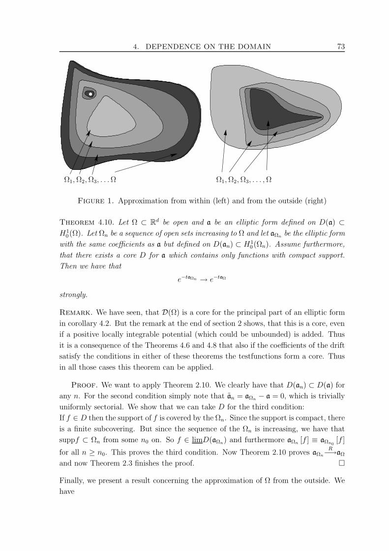
4. DEPENDENCE ON THE DOMAIN 73
Ω1,Ω2,Ω3, . . .Ω Ω1,Ω2,Ω3, . . . ,Ω
Figure 1. Approximation from within (left) and from the outside (right)
Theorem 4.10. Let Ω ⊂ Rd be open and a be an elliptic form defined on D(a) ⊂H1
0 (Ω). Let Ωn be a sequence of open sets increasing to Ω and let aΩn be the elliptic form
with the same coefficients as a but defined on D(an) ⊂ H10 (Ωn). Assume furthermore,
that there exists a core D for a which contains only functions with compact support.
Then we have that
e−taΩn → e−taΩ
strongly.
Remark. We have seen, that D(Ω) is a core for the principal part of an elliptic form
in corollary 4.2. But the remark at the end of section 2 shows, that this is a core, even
if a positive locally integrable potential (which could be unbounded) is added. Thus
it is a consequence of the Theorems 4.6 and 4.8 that also if the coefficients of the drift
satisfy the conditions in either of these theorems the testfunctions form a core. Thus
in all those cases this theorem can be applied.
Proof. We want to apply Theorem 2.10. We clearly have that D(an) ⊂ D(a) for
any n. For the second condition simply note that an = aΩn − a = 0, which is trivially
uniformly sectorial. We show that we can take D for the third condition:
If f ∈ D then the support of f is covered by the Ωn. Since the support is compact, there
is a finite subcovering. But since the sequence of the Ωn is increasing, we have that
suppf ⊂ Ωn from some n0 on. So f ∈ limD(aΩn) and furthermore aΩn [f ] ≡ aΩn0[f ]
for all n ≥ n0. This proves the third condition. Now Theorem 2.10 proves aΩn
R−→aΩ
and now Theorem 2.3 finishes the proof.
Finally, we present a result concerning the approximation of Ω from the outside. We
have
74 CHAPTER 4. APPLICATIONS TO ELLIPTIC FORMS
Theorem 4.11. Let Ω ⊂ Rd be an open set, and (Ωn)n∈N be a sequence of open sets
shrinking to Ω. Assume that H10 (Ω) = H1
0 (Ω). Let aΩ1 be an elliptic form defined on
D(aΩ1) ⊂ H10 (Ω1) and let aΩn and a be the elliptic forms with the same coefficients
defined on D(aΩn) ⊂ H10 (Ωn). Then we have that
e−taΩn → e−taΩ
strongly.
Proof. Here of course, we will apply Theorem 2.11. We clearly have thatD(aΩn+1) ⊂D(aΩn). Also the second condition (even the strong second condition without the mod-
ulus) is obvious, since aΩm −aΩn = 0 for m ≥ n. Also, we have that D(a) =⋂D(aΩn).
Here, the inclusion ⊂ is obvious and the other inclusion uses that H10 (Ω) = H1
0 (Ω). It
follows that aΩn → a. Now the Theorems 2.11 and 2.3 prove the assertion.
Notes and References for Chapter 4: As form methods are the usual means of es-
tablishing differential operators as semigroup generators and as there is a wealth of results
concerning differential operators, we could give plenty of references here. However we men-
tion:
Ouhabaz [14, chapter 4] and Arendt et al [4, chapter 7] for general elliptic forms,
Arendt, Batty [3] and Davies [8, chapter 8] for Schrodinger operators.
Theorem 4.6 was suggested by R. Chill, whereas unbounded drifts were considered by
Arendt, Metafune, Pallara in [5]. However, the technique used there is different and
leads to different results.
Domain approximation as in section 4, was considered by Arendt [2] but there were also
different methods used.
Bibliography
[1] R. Adams Sobolev Spaces Academic Press (1975)
[2] W. Arendt Approximation of Degenerate Semigroups Taiwanese J. Math. Vol. 5 No. 2 (2001)
279-295
[3] W. Arendt, C. Batty Absorption Semigroups and Dirichlet Boundary Conditions Math. Ann.
295 (1993) 427-448
[4] W. Arendt, C. Batty, M. Hieber, F. Neubrander Vector-valued Laplace Transform and
Cauchy Problems Birkhauser, Basel (2001)
[5] W. Arendt, G. Metafune, D. Pallara Schrodinger Operators with Unbounded Drift
Preprint
[6] H. Brezis Operateurs Maximaux Monotones North Holland (1973)
[7] P. Chernoff Product Formulas, Nonlinear Semigroups and Addition of Unbounded Operators
Mem. Amer. Math. Soc. 140 (1974)
[8] E. Davies Spectral Theory and Differential Operators Cambridge University Press (1995)
[9] K. Engel, R. Nagel One-Parameter Semigroups for Linear Evolution Equations Springer
Verlag, Berlin (2000)
[10] T. Kato Perturbation Theorie for Linear Operators Springer Verlag, Berlin (1966)
[11] T. Kato Trotter’s Product Formula for an Abitrary Pair of Selfadjoint Contraction Semigroups
Adv. in Math., supp. Studies Vol. 3 (1978) 185-195
[12] T. Kato, K. Masuda Trotter’s Product Formula for nonlinear semigroups generated by the
subdifferentials of convex functionals J. Math. Soc. Japan Vol. 30 No. 1 (1978) 169-178
[13] Mate Matolcsi On the Relation of Closed Forms and Trotter’s Product Formula J. Funct.
Anal. 205 (2003) 401-413
[14] E. M. Ouhabaz Analysis of Heat Equations on Domains Priceton University Press (2004)
[15] E. M. Ouhabaz Second Order Elliptic Operators with Essential Spectrum [0,∞) on Lp Comm.
in PDE 20 (5&6) (1995) 763-773
[16] M. Reed, B. Simon Methods of Modern Mathematical Physics, Vol. 1 Academical Press, New
York (1980)
[17] B. Simon A Canonical Decomposition for Quadratic Forms with Applications to Monotone
Convergence Theorems J. Funct. Anal. 28 (1978) 377-385
[18] D. Werner Funktionalanalysis Springer Verlag, Berlin (2000)
75

Index
Chernoff product formula, 52
Convergence
in the strong resolvent sense, 34
in the weak resolvent sense, 35
of degenerate semigroups, 36
Convergence theorems, 39
for a decreasing sequence, 41
for an increasing sequence, 40
from above, 42
from below, 44
Core, 15
Degenerate semigroup, 28, 29
Elliptic form, 63
core, 65
dependence on the domain, 72
with drift, 69
with unbounded coefficients in the pricipal
part, 65
Form, 5
bounded, 9
bounded with respect to, 11
closable, 11, 13, 14
closed, 8
closure, 15
holomorphic family of, 36
inner product associated with, 6, 7
pseudoresolvent of a, 29
Friedrichs extension, 22
M-sectorial operators, 17
Numerical range
of a form, 6
of an operator, 17
Perturbation of forms, 11
Polarization identity, 6
Potential, 63
Pseudoresolvent, 28
Regular part, 15
Representation Theorem, 19
with D(A) = D(a), 23
Schrodinger operator, 67
core, 69
dependence on the potential, 68
Sum of forms, 8, 11
Trotter’s formula, 48
characterisation of M-sectorial operators , 58
for nonlinear semigroups, 56
for projections, 55
77