Forschungsbericht 2017-35

Numerical Simulation Concept for Low-Noise Wind Turbine Rotors

Christof Rautmann

Deutsches Zentrum für Luft- und Raumfahrt Institut für Aerodynamik und Strömungstechnik Braunschweig

169 Seiten 74 Bilder 11 Tabellen 84 Literaturstellen

TU Braunschweig – Niedersächsisches Forschungszentrum für Luftfahrt

Berichte aus der Luft- und Raumfahrttechnik

Forschungsbericht 2017-11

Numerical Simulation Concept for Low-Noise Wind Turbine Rotors

Christof Rautmann

Deutsches Zentrum für Luft- und Raumfahrt Institut für Aerodynamik und Strömungstechnik

Braunschweig

Diese Veröffentlichung wird gleichzeitig in der Berichtsreihe „NFL - Forschungsberichte“ geführt. Diese Arbeit erscheint gleichzeitig als von der Fakultät für Maschinenbau der Technischen Universität Carolo-Wilhel-mina zu Braunschweig zur Erlangung des akademischen Grades eines Doktor-Ingenieurs genehmigte Dissertation.

Numerical Simulation Conceptfor Low-Noise

Wind Turbine Rotors

Von der Fakultät für Maschinenbauder Technischen Universität Carolo-Wilhelmina zu Braunschweig

zur Erlangung der Würdeeines Doktor-Ingenieurs (Dr.-Ing.)

genehmigte Dissertation

vonChristof Rautmann, M.Sc.

geboren in Greifswald

eingereicht am: 08.12.2016

mündliche Prüfung am: 07.07.2017

Vorsitz: Prof. Dr.-Ing. R. Radespiel

Gutachter: Prof. Dr.-Ing. J. W. Delfs

Prof. Dr.-Ing. F.-H. Wurm

2017

Summary

Wind power is the major technology in the transition from conventional energy towardsgreener, renewable energy. Especially for its public acceptance, the noise emission of theturbines plays an important role. Against this background, this thesis deals with theacoustic simulation of wind turbine noise. The work focuses on the main noise source ofthe rotor blades, the turbulent boundary layer trailing-edge interaction noise.Numerous simulations of two-dimensional aerodynamic profiles were performed within theframework of the investigations. Therefore, several consecutive steps are necessary. Aninitial numeric flow simulation (CFD) yields the aerodynamic coefficients of the airfoilsfor the defined set of flow conditions. The turbulence model used in the CFD simulationsprovides time-averaged turbulence statistics which are subsequently used as input valuesfor a stochastic turbulence reconstruction utilizing the fast random particle mesh method(FRPM). This enables the stationary average turbulence to be resolved in time and spaceand thus to generate the transient turbulent sound sources in the subsequent computa-tional aeroacoustic simulation (CAA) with the acoustic solver PIANO. Sound pressure levelsand spectra can be evaluated at arbitrary positions from the calculated spatio-temporalsound pressure field. Compared to other methods for the calculation of trailing-edgenoise, the described hybrid approach (CFD/CAA) offers the advantage of high qualityresults with comparatively little computational effort (less than 20 h on 6 CPUs).The validation of the results was based on published data of the BANC-II workshop. Forall airfoils, the simulated spectra were within the uncertainty range of the measurementdata. The accuracy was higher than with the classical semi-empirical calculation modelsusually used for this purpose. Physical effects, such as the apart drifting of the pressureand suction side spectrum with increasing angle of attack were correctly reproduced.A best practice setup was created using parameter studies. Furthermore, the CFD-FRPM-CAA simulation toolchain was largely automized. Thus, arbitrary airfoil geome-tries could be examined for their aerodynamic as well as acoustic characteristics. System-atic variation of the DU-96-W180 airfoil geometry showed a noise mitigation potentialof approx. 4 dB with the same aerodynamic performance (same L-over-D ratio cL/cD).Applying a forced transition of the wall boundary layer from laminar to turbulent flowresults in a noise increase of approx. 3-4 dB.On the basis of the simulation toolchain’s results, characteristics of a low-noise airfoil wereformulated, e.g. low turbulence kinetic energy values and a low positive pressure gradientat the suction side in the vicinity of the trailing-edge. A low-noise airfoil was developedand its effect on the turbine level was investigated using the NREL 5MW reference ro-tor. Since three-dimensional CAA simulations showed a too high computational effort,an alternative procedure based on 2D airfoil sections and a blade element momentummethod (BEM) for the rotor blade aerodynamics was developed. A 2 dB noise reductionwithout sacrificing the turbine’s energy generation or loads could be achieved by usingthe low-noise airfoil. Furthermore, by varying the observer position around the turbine,it was possible to show that the lowest sound pressure levels occur directly in the rotorplane (crosswind direction from the turbine), but at this location they exhibit the high-est temporal fluctuations. A phenomenon which is also known as amplitude modulationwithin the wind turbine acoustic community.The developed calculation methods as well as their results provide a great potential forfinding the next generation designs of wind turbine power plants. The future will showwhether the noise reduction potentials will be used to increase public acceptance of windturbines or to further optimize their costs.

Zusammenfassung

Windkraft spielt eine entscheidende Rolle beim Übergang von konventioneller Energieer-zeugung zu regenerativen Energien. Besonders wichtig für die Akzeptanz von Winden-ergieanlagen (WEAs) ist deren Lärmemission. Vor diesem Hintergrund beschäftigt sichdie vorliegende Arbeit mit der akustischen Simulation des Windturbinengeräusches. DerFokus liegt dabei auf der Hauptlärmquelle der Rotorblätter, dem Hinterkantenschalldurch Interaktion der turbulenten Grenzschicht mit der Hinterkante.Im Rahmen der Untersuchungen wurden umfangreiche numerische Simulationen an zwei-dimensionalen aerodynamischen Profilen durchgeführt. Hierfür sind mehrere aufeinanderaufbauende Schritte notwendig. Aus einer initialen Strömungssimulation (CFD) könnendie aerodynamischen Beiwerte des Profils bestimmt werden. Das Turbulenzmodell derCFD Simulation liefert zeitlich gemittelte Turbulenzstatistiken, die im weiteren Verlaufals Eingangswerte für eine stochastische Turbulenzrekonstruktion mit dem FRPM Ver-fahren genutzt werden. Hierin wird die stationäre Turbulenz wieder zeitlich und räumlichaufgelöst und dient anschließend als instationäre Turbulenzschallquelle in der aeroakustis-chen Simulation (CAA) mit dem Akustiklöser PIANO. Aus dem berechneten Schalldruck-feld können an beliebigen Positionen Schalldruckpegel und Spektren ausgewertet werden.Im Vergleich zu anderen Verfahren zur Berechnung von Hinterkantenschall bietet dasbeschriebene hybride Vorgehen (CFD/CAA) den Vorteil einer hohen Genauigkeit desErgebnisses bei vergleichsweise geringem Rechenaufwand (weniger als 20 h auf 6 CPUs).Eine Validierung der Ergebnisse erfolgte anhand veröffentlichter Daten aus den BANC-IIWorkshop. Für alle Profile lagen die simulierten Spektren innerhalb des Unsicherheits-bereichs der Messdaten. Die Genauigkeit war höher als mit alternativen klassischen semi-empirischen Berechnungsmodellen. Physikalische Effekte, wie z. B. das Auseinander-driften des Druck- und Saugseitenspektrums bei Anstellwinkelerhöhung, wurden korrektwiedergegeben. Anhand von Parameterstudien wurde ein Best-Practice-Setup erstellt.Weiterhin wurde die CFD-FRPM-CAA Rechenkette weitestgehend automatisiert. Somitkonnten beliebige Profilgeometrien sowohl auf ihre aerodynamischen als auch akustischenKennwerte untersucht werden. Eine systematische Variation des DU-96-W180 Profilszeigte ein Lärmminderungspotential von ca. 4 dB bei gleicher aerodynamischer Güte(gleicher Gleitzahl cL/cD). Erzwungene Transition der Wandgrenzschicht von laminarzu turbulent hat eine Lärmerhöhung von ca. 3-4 dB zur Folge.Mit den Ergebnissen wurden Eigenschaften eines lärmarmen Profils identifiziert, z.B.geringe Werte turbulenter kinetischer Energie und ein niedriger positiver Druckgradientauf der Saugseite nahe der Hinterkante. Ein lärmarmes Profil wurde entwickelt und seinEinfluss auf die Gesamtanlage am NREL 5 MW Referenzrotor untersucht. Da sich dreidi-mensionale CAA-Simulationen als zu rechenintensiv herausstellten, wurde ein alternativesVerfahren beruhend auf Simulationsdaten von 2D Schnitten und einer Blatt-Elementen-Methode (BEM) für die Rotorblattaerodynamik entwickelt. Mit dem neuen Profil konnteder Schalleistungspegel der Referenzanlage bei gleicher Leistung und identischen Lastenum bis zu 2 dB reduziert werden. Weiterhin ließ sich durch Variation der Beobachterpo-sition relativ zur WEA zeigen, dass die Schalldruckpegel in der Rotorebene (querab derWEA) zwar am geringsten sind, sie jedoch die größten zeitlichen Schwankungen aufweisen.Ein Phänomen, dass in der Windkraftakustik als Amplitudenmodulation bekannt ist.Die entwickelten Rechenverfahren sowie deren Ergebnisse bieten großes Potential Einzugin den Entwurf von Windenergieanlagen der nächsten Generation zu finden. Ob die Lär-mminderungspotentiale dabei zur Akzeptanzsteigerung oder zur Kostenoptimierung derTurbinen verwendet werden, wird die Zukunft zeigen.

Contents

Summary vii

Zusammenfassung ix

List of Figures xv

List of Tables xvii

Nomenclature xix

1 Introduction 11.1 Motivation . . . . . . . . . . . . . . . . . . . . . . . . . . . . . . . . . . . 11.2 Previous Work . . . . . . . . . . . . . . . . . . . . . . . . . . . . . . . . . 41.3 Objectives . . . . . . . . . . . . . . . . . . . . . . . . . . . . . . . . . . . . 51.4 Structure . . . . . . . . . . . . . . . . . . . . . . . . . . . . . . . . . . . . 6

2 Theory 72.1 Making Torque from Wind . . . . . . . . . . . . . . . . . . . . . . . . . . 7

2.1.1 1D Momentum Theory . . . . . . . . . . . . . . . . . . . . . . . . . 82.1.2 Blade Element Momentum Method (BEM) . . . . . . . . . . . . . 102.1.3 Turbine Operation . . . . . . . . . . . . . . . . . . . . . . . . . . . 12

2.2 Aerodynamics - CFD . . . . . . . . . . . . . . . . . . . . . . . . . . . . . . 132.2.1 Governing Equations . . . . . . . . . . . . . . . . . . . . . . . . . . 142.2.2 Numerical Simulation Technique . . . . . . . . . . . . . . . . . . . 142.2.3 Turbulence Modeling . . . . . . . . . . . . . . . . . . . . . . . . . . 15

2.3 Aeroacoustics - CAA . . . . . . . . . . . . . . . . . . . . . . . . . . . . . . 172.3.1 General . . . . . . . . . . . . . . . . . . . . . . . . . . . . . . . . . 172.3.2 Acoustic Analogy . . . . . . . . . . . . . . . . . . . . . . . . . . . . 182.3.3 Scattering Half Plane . . . . . . . . . . . . . . . . . . . . . . . . . 192.3.4 Governing Equations . . . . . . . . . . . . . . . . . . . . . . . . . . 202.3.5 Numerical Simulation Technique . . . . . . . . . . . . . . . . . . . 222.3.6 FRPM . . . . . . . . . . . . . . . . . . . . . . . . . . . . . . . . . . 232.3.7 Wind Turbine Noise Sources . . . . . . . . . . . . . . . . . . . . . 26

3 Simulation Methods 313.1 Toolchain Overview . . . . . . . . . . . . . . . . . . . . . . . . . . . . . . 313.2 CFD . . . . . . . . . . . . . . . . . . . . . . . . . . . . . . . . . . . . . . . 33

3.2.1 Mesh . . . . . . . . . . . . . . . . . . . . . . . . . . . . . . . . . . . 343.2.2 Boundary Conditions and Models . . . . . . . . . . . . . . . . . . . 373.2.3 Grid Refinement Study . . . . . . . . . . . . . . . . . . . . . . . . 393.2.4 Validation . . . . . . . . . . . . . . . . . . . . . . . . . . . . . . . . 42

xii Contents

3.3 CAA with FRPM . . . . . . . . . . . . . . . . . . . . . . . . . . . . . . . . 433.3.1 Mesh . . . . . . . . . . . . . . . . . . . . . . . . . . . . . . . . . . . 443.3.2 Boundary Conditions and Models . . . . . . . . . . . . . . . . . . . 483.3.3 FRPM . . . . . . . . . . . . . . . . . . . . . . . . . . . . . . . . . . 493.3.4 Grid Refinement Study . . . . . . . . . . . . . . . . . . . . . . . . 563.3.5 Best Practice Aspects . . . . . . . . . . . . . . . . . . . . . . . . . 58

3.4 Data Processing and Scripting . . . . . . . . . . . . . . . . . . . . . . . . 60

4 Results and Discussion 634.1 Validation Test Cases from BANC-II . . . . . . . . . . . . . . . . . . . . . 63

4.1.1 Test case #1 NACA0012 . . . . . . . . . . . . . . . . . . . . . . . 644.1.2 Test case #2 NACA0012 . . . . . . . . . . . . . . . . . . . . . . . 664.1.3 Test case #3 NACA0012 . . . . . . . . . . . . . . . . . . . . . . . 674.1.4 Test case #4 NACA0012 . . . . . . . . . . . . . . . . . . . . . . . 684.1.5 Test case #5 DU96-W-180 . . . . . . . . . . . . . . . . . . . . . . 69

4.2 Geometry Variation Strategy . . . . . . . . . . . . . . . . . . . . . . . . . 714.2.1 Geometry . . . . . . . . . . . . . . . . . . . . . . . . . . . . . . . . 714.2.2 Flow Parameters . . . . . . . . . . . . . . . . . . . . . . . . . . . . 72

4.3 Geometry Variation Results . . . . . . . . . . . . . . . . . . . . . . . . . . 734.3.1 Aerodynamics . . . . . . . . . . . . . . . . . . . . . . . . . . . . . . 744.3.2 Aerodynamics and Acoustics . . . . . . . . . . . . . . . . . . . . . 76

4.4 Relationship between Boundary Layer Values and Noise . . . . . . . . . . 814.4.1 Cases with same L-over-D Ratio and different OASPL . . . . . . . 814.4.2 Cases with different L-over-D Ratio and same OASPL . . . . . . . 834.4.3 Further Data Analysis . . . . . . . . . . . . . . . . . . . . . . . . . 85

4.5 Strategy for Low Noise Airfoils . . . . . . . . . . . . . . . . . . . . . . . . 90

5 Turbine Evaluation 935.1 Method . . . . . . . . . . . . . . . . . . . . . . . . . . . . . . . . . . . . . 93

5.1.1 3D CAA Simulation . . . . . . . . . . . . . . . . . . . . . . . . . . 935.1.2 Alternative Method using 2D CAA Results . . . . . . . . . . . . . 95

5.2 Results and Discussion . . . . . . . . . . . . . . . . . . . . . . . . . . . . . 975.2.1 Analysis of the NREL 5MW Reference Turbine . . . . . . . . . . . 975.2.2 Improvement of NREL 5MW Turbine with Low-Noise Airfoils . . . 1055.2.3 Influence of Airfoil Performance on the overall Turbine Performance 114

5.3 Benefit of Noise Reduction . . . . . . . . . . . . . . . . . . . . . . . . . . . 116

6 Conclusions and Future Work 1196.1 Impact of Results on Next-Generation Turbines . . . . . . . . . . . . . . . 1236.2 Outlook . . . . . . . . . . . . . . . . . . . . . . . . . . . . . . . . . . . . . 124

A Appendix 127A.1 Derivation of the BEM Method . . . . . . . . . . . . . . . . . . . . . . . . 127A.2 Governing Equations . . . . . . . . . . . . . . . . . . . . . . . . . . . . . . 131A.3 From Governing Equations to Wave Equation . . . . . . . . . . . . . . . . 132A.4 Realizing a Liepmann Turbulence Spectrum with FRPM . . . . . . . . . . 133A.5 PIANO Input File for CAA Airfoil Simulations . . . . . . . . . . . . . . . 136A.6 Modified Trailing-Edge Noise Directivity . . . . . . . . . . . . . . . . . . . 138A.7 Additional Airfoil Geometries . . . . . . . . . . . . . . . . . . . . . . . . . 141

Contents xiii

Bibliography 143

List of Figures

1.1 Global Wind Capacity . . . . . . . . . . . . . . . . . . . . . . . . . . . . . 21.2 EU Power Installation and Power Mix . . . . . . . . . . . . . . . . . . . . 31.3 Turbulence Related Noise Prediction . . . . . . . . . . . . . . . . . . . . . 3

2.1 1D Momentum Theory . . . . . . . . . . . . . . . . . . . . . . . . . . . . . 82.2 Efficiency of an optimum Turbine . . . . . . . . . . . . . . . . . . . . . . . 92.3 Velocities and Forces in the Rotor Plane . . . . . . . . . . . . . . . . . . . 102.4 Operational Parameters of a generic HAWT . . . . . . . . . . . . . . . . . 132.5 Flow over semi-infinite Half Plane . . . . . . . . . . . . . . . . . . . . . . 192.6 Resolution of Finite Differencing Schemes . . . . . . . . . . . . . . . . . . 222.7 Airfoil Self Noise Mechanisms . . . . . . . . . . . . . . . . . . . . . . . . . 272.8 Visualized Noise at Wind Turbine . . . . . . . . . . . . . . . . . . . . . . 28

3.1 Simulation Toolchain . . . . . . . . . . . . . . . . . . . . . . . . . . . . . . 323.2 CFD Toolchain . . . . . . . . . . . . . . . . . . . . . . . . . . . . . . . . . 333.3 CFD Mesh Example . . . . . . . . . . . . . . . . . . . . . . . . . . . . . . 363.4 Sketch of CFD Domain . . . . . . . . . . . . . . . . . . . . . . . . . . . . 373.5 Distribution of local Reynolds Number along Blade . . . . . . . . . . . . . 383.6 Grid Convergence Study CFD . . . . . . . . . . . . . . . . . . . . . . . . . 403.7 y+ Values for NACA0012 and NACA64618 . . . . . . . . . . . . . . . . . 413.8 CFD and Measurement Data of NACA0012 and NACA64618 . . . . . . . 423.9 CAA Toolchain . . . . . . . . . . . . . . . . . . . . . . . . . . . . . . . . . 433.10 CAA Domain . . . . . . . . . . . . . . . . . . . . . . . . . . . . . . . . . . 453.11 CAA Mesh Example . . . . . . . . . . . . . . . . . . . . . . . . . . . . . . 473.12 FRPM Patch Examples . . . . . . . . . . . . . . . . . . . . . . . . . . . . 503.13 FRPM TKE Reconstruction . . . . . . . . . . . . . . . . . . . . . . . . . . 513.14 FRPM Influence of Weighting Function . . . . . . . . . . . . . . . . . . . 523.15 FRPM Influence of Length Scale Factor . . . . . . . . . . . . . . . . . . . 533.16 FRPM Turbulence Spectra and Improvement . . . . . . . . . . . . . . . . 553.17 Grid Refinement Study for CAA . . . . . . . . . . . . . . . . . . . . . . . 563.18 Grid Refinement Study for FRPM . . . . . . . . . . . . . . . . . . . . . . 583.19 Overview of automized Toolchain . . . . . . . . . . . . . . . . . . . . . . . 60

4.1 Validation: Boundary Layer Properties . . . . . . . . . . . . . . . . . . . . 654.2 BANC Case #1 Sound Pressure Field and Directivity . . . . . . . . . . . 664.3 BANC Case #1 and #2 Spectrum . . . . . . . . . . . . . . . . . . . . . . 674.4 BANC Case #3 Spectrum . . . . . . . . . . . . . . . . . . . . . . . . . . . 684.5 BANC Case #4 Spectrum . . . . . . . . . . . . . . . . . . . . . . . . . . . 694.6 BANC Case #5 Spectrum and Directivity . . . . . . . . . . . . . . . . . . 704.7 DU96 Airfoil Geometry . . . . . . . . . . . . . . . . . . . . . . . . . . . . 72

xvi List of Figures

4.8 Airfoil Geometry Variation . . . . . . . . . . . . . . . . . . . . . . . . . . 734.9 DU Variation Aerodynamics for fixed Transition . . . . . . . . . . . . . . 754.10 DU Variation Aerodynamics for natural Transition . . . . . . . . . . . . . 764.11 DU Variation Sound Pressure Field and Spectra . . . . . . . . . . . . . . 774.12 DU Variation Acoustics vs. Aerodynamics . . . . . . . . . . . . . . . . . . 794.13 DU Variation Acoustics vs. Aerodynamics including natural Transition . . 804.14 DU Variation same L/D Spectrum and Pressure Distribution . . . . . . . 824.15 DU Variation same L/D Boundary Layer Values . . . . . . . . . . . . . . 844.16 DU Variation same OASPL Spectrum and Pressure Distribution . . . . . 854.17 DU Variation same OASPL Boundary Layer Values . . . . . . . . . . . . 864.18 Several Airfoils OASPL vs. Aerodynamics . . . . . . . . . . . . . . . . . . 874.19 Correlation of BL Parameters and Sound Pressure . . . . . . . . . . . . . 884.20 Correlation of TKE and Sound Pressure . . . . . . . . . . . . . . . . . . . 89

5.1 3D CAA Simulation . . . . . . . . . . . . . . . . . . . . . . . . . . . . . . 945.2 Method for Turbine Simulation . . . . . . . . . . . . . . . . . . . . . . . . 955.3 Overview of Turbine Location and relevant Directions . . . . . . . . . . . 965.4 NREL 5MW Turbine: Geometry and Performance . . . . . . . . . . . . . 985.5 NREL 5MW Turbine outer Blade Aerodynamics . . . . . . . . . . . . . . 995.6 NREL 5MW Turbine Acoustics . . . . . . . . . . . . . . . . . . . . . . . . 1015.7 NREL 5MW Noise Sound Map natural Transition . . . . . . . . . . . . . 1025.8 NREL 5MW Noise Sound Map fixed Transition . . . . . . . . . . . . . . . 1035.9 NREL 5MW OASPL at Distance 163m . . . . . . . . . . . . . . . . . . . 1035.10 NREL 5MW OASPL at two Locations for different Rotor Positions . . . . 1045.11 Geometry and Aerodynamics of NREL Airfoils . . . . . . . . . . . . . . . 1065.12 Acoustic Performance of NACA and LNCR Airfoil . . . . . . . . . . . . . 1075.13 Performance for modified NREL Turbine . . . . . . . . . . . . . . . . . . . 1095.14 NREL 5MW Turbine Acoustics with Modification . . . . . . . . . . . . . 1115.15 Comparison of Noise Maps for NREL Turbine . . . . . . . . . . . . . . . . 1125.16 NREL 5MW: OASPL around the Turbine and for different Rotor Positions 1135.17 Power Coefficient vs. L-over-D Ratio . . . . . . . . . . . . . . . . . . . . . 1155.18 Benefit of Noise Reduction . . . . . . . . . . . . . . . . . . . . . . . . . . . 117

A.1 Rayleigh distribution of wind speed . . . . . . . . . . . . . . . . . . . . . . 130A.2 FRPM Energy Spectra . . . . . . . . . . . . . . . . . . . . . . . . . . . . . 136A.3 Modified Flat Plate Directivity . . . . . . . . . . . . . . . . . . . . . . . . 139A.4 NREL 5MW Noise Comparison for modified Directivity I . . . . . . . . . 140A.5 NREL 5MW Noise Comparison for modified Directivity II . . . . . . . . . 141A.6 Airfoil Geometries . . . . . . . . . . . . . . . . . . . . . . . . . . . . . . . 142

List of Tables

3.1 Results of Grid Convergence Study NACA0012 . . . . . . . . . . . . . . . 393.2 Results of Grid Convergence Study NACA64618 . . . . . . . . . . . . . . 403.3 NACA0012 and NACAC64618 GCI Values . . . . . . . . . . . . . . . . . . 41

4.1 Flow Parameters for DU based Airfoil Variation . . . . . . . . . . . . . . . 744.2 Test Cases with matching L-over-D Ratio . . . . . . . . . . . . . . . . . . 814.3 Test Cases with matching OASPL . . . . . . . . . . . . . . . . . . . . . . 84

5.1 BEM Data of the NREL Turbine . . . . . . . . . . . . . . . . . . . . . . . 1005.2 Data modified NREL Turbine natural Transition . . . . . . . . . . . . . . 1095.3 Data modified NREL Turbine fixed Transition . . . . . . . . . . . . . . . 1105.4 AEP of NREL Turbine . . . . . . . . . . . . . . . . . . . . . . . . . . . . . 110

A.1 IEC Wind Classes . . . . . . . . . . . . . . . . . . . . . . . . . . . . . . . 130

Nomenclature

Latin SymbolsA rotor areaa axial induction factorA amplitude functiona′ tangential induction factorB number of bladescD drag coefficientcf skin friction coefficientcL lift coefficientcn normal load coefficientCP turbine power coefficientcp pressure coefficientCT turbine thrust coefficientct tangential load coefficientc∞ ambient speed of soundcM25 pitching moment coefficient around lc/4cM pitching moment coefficientD directivityE internal energye specific internal energyet specific total energyF correction factorf frequencyF flux density tensor~f external forces vectorFn load normal to rotor planeFt load tangential to rotor planeG0 Gaussian filter kernelhr Rayleigh wind speed distributionhr Weibull wind speed distributionk wave number

xx Nomenclature

kt turbulence kinetic energy (TKE)l length scale~L′ Lamb vectorlc chord lengthLp sound pressure levelLW sound power levellref reference lengthM Mach numberm camber as fraction of chordm mass flowP powerp chordwise position of maximum camberp pressurep′ fluctuating sound pressurep0 mean flow pressurep∞ ambient pressure~QF vector of fluxes over control volume~q heat flux vectorr radius positionr tip radiusR correlationRe Reynolds numberSij mean strain tensorSt Strouhal numberT temperatureT thrustt airfoil thicknesst timeu axial velocity component in the rotor planeU spatiotemporal white-noise fieldu1 velocity in wakeV0 mean wind speed~v velocity vectorV0 wind speed~v0 mean flow velocity vector~W vector of conserved quantitiesx coordinatey coordinate

Nomenclature xxi

z coordinate

Greek Symbolsα angle of attackβ twist angleδ boundary layer thicknessδ∗ boundary layer displacement thicknessε error estimatorκ ratio of specific heats (isentropic exponent)κ von Kármán constantλ tip speed ratioµ dynamic viscosityν = µ/ρ kinematic viscosityω angular velocityω specific dissipationΦ flow angleΦ local angle from source to observerϕ rotor blade positionψ stream functionρ densityρ0 mean flow densityρ∞ ambient densityσ solidityτ stress tensorτw wall shear stressΘ local angle from source to observerΘ local pitch angleθ external heatΘp blade pitch angle

Indicesavg averagec convectiveff far-fieldi direction ij direction jk direction kmax maximum value

xxii Nomenclature

min minimum valueOA over all (sound pressure level)obs observer locationopt optimum valueref reference or standard valuet indicates fluctuating turbulent value0 steady mean flow quantity

AbbreviationsAEP Annual Energy ProductionAM Amplitude ModulationAoA Angle of AttackASD Artificial Selective DampingAWB Acoustic Wind Tunnel BraunschweigBANC Benchmark for Airframe Noise ComputationsBC Boundary ConditionBEM Blade Element Momentum MethodBL Boundary LayerBPM Brooks, Pope and Marcolini (semi-empirical method)CAA Computational AeroacousticsCFD Computational Fluid DynamicsCFL Courant–Friedrichs–Lewy (condition)COE Cost of EnergyDLR Deutsches Zentrum für Luft- und Raumfahrt (German Aerospace Center)DNS Direct Numerical SimulationDRP Dispersion Relation Preserving (scheme)EWEA European Wind Energy AssociationFFT fast Fourier transformationFRPM Fast Random Particle Mesh (method)FWH Ffowcs-Williams and Hawkings (method)GCI Grid Convergence IndexGWEC Global Wind Energy CouncilHAWT Horizontal Axis Wind TurbineIAG Institute of Aerodynamics and Gasdynamics (University of Stuttgart)IEC International Electrotechnical CommissionLDDRK Low-Dissipation, Low-Dispersion Runge-Kutta (algorithm)LEE Linearized Euler EquationsLES Large Eddy Simulation

Nomenclature xxiii

NREL National Renewable Energy LaboratoryNS Navier Stokes (equations)OASPL Overall Sound Pressure LevelPIANO Perturbation Investigation of Aeroacoustic Noise (CAA code)PV PhotovoltaicRANS Reynolds Averaged Navier Stokes (equations)RPM Revolutions per MinuteSPL Sound Pressure LevelTBL-TEN Turbulent Boundary Layer Trailing-Edge NoiseTEN Trailing-Edge NoiseTKE Turbulence Kinetic EnergyTNO The Netherlands Organization of Applied Scientific ResearchTSR Tip Speed Ratio

1 Introduction

Harvesting the wind has been a challenge to mankind ever since. The energy containedin the flowing mass of air was used over centuries by windmills to grind grain, pumpwater or propel other machinery. It drove sailing boats across the oceans long before thesteam engine was invented and is used today by many wind and kite surfers to powertheir sporting goods.

With an energy resource that is quasi infinite, carbon emission free, decentralized usableand reasonable in its efficiency the focus nowadays shifts more towards wind turbinesas energy producers. They are the cornerstone technology for most countries in theirrenewable energy politics. Ongoing improvements and the maturation of the technologyled to turbine dimensions way beyond those of modern commercial airliners1. Due tothe limited areas suitable to build wind farms turbines are moving closer to inhabitedareas. Here, beside aesthetic aspects noise coming from the turbines is one of the majorissues for the nearby living people. This thesis aims on the understanding of the noisegeneration process and the development of tools for low noise turbines.

The following chapter outlines the thesis by explaining the background of the wind turbinenoise issue. A classification with view towards political and technical fields is given. Theidea behind the chosen noise prediction approach is presented and compared to otherstate-of-the-art methods.

1.1 Motivation

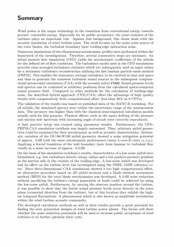
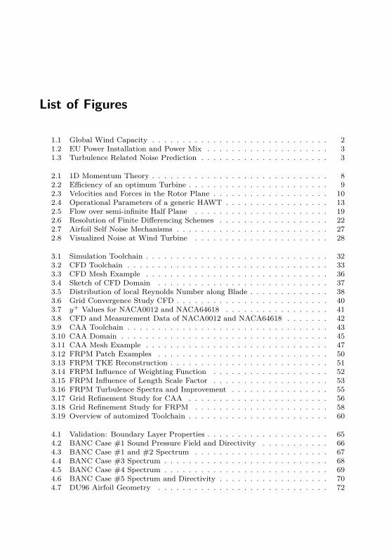
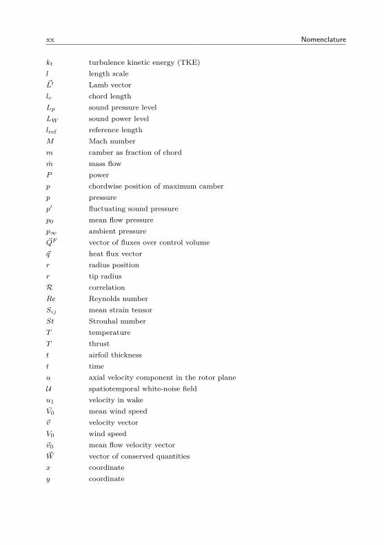
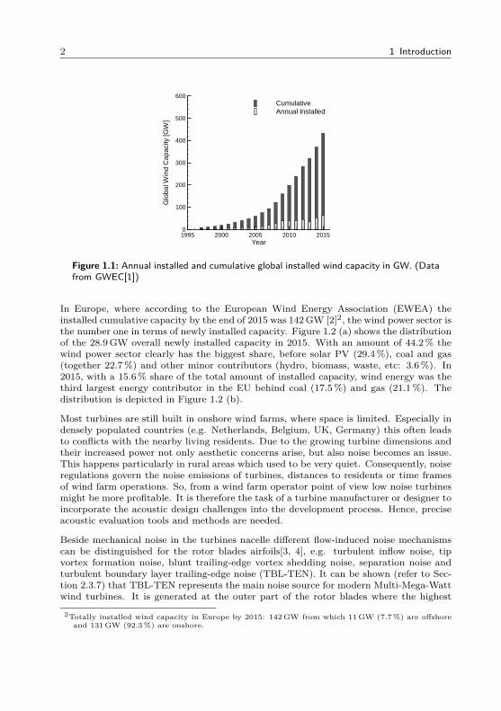
Over the last decade energy politics around the world have changed progressively towardsgreener and renewable energy sources. In the aftermath of the Fukushima nuclear disasterin 2011 many governments decided to reduce their nuclear power production or even shutdown all nuclear power plants as introduced within the German Energiewende (Energytransition). The transition from nuclear power and classical fuels (e.g. coal, oil and gas)to renewable energy (e.g. wind and solar photovoltaics (PV)) led to an increasing numberof wind turbines which are apparent in today’s environment. According to the GlobalWind Energy Council (GWEC) a total amount of 432GW of wind capacity was installedby the end of 2015 [1]. The worldwide development is depicted in Figure 1.1. In 2015alone the volume of 63GW of new capacity was added, representing an annual growthrate of 17% (which is still below the average annual growth rate of 25% over the last 18years).

1For example the rotor blade of a Nordex N131 turbine with a length of 65.5m is about 25.6m longerthan the wing of an Airbus A380-800 with a span of 79.8m.

2 1 Introduction

Year

Glo

bal W

ind

Cap

acity

[GW

]

1995 2000 2005 2010 20150

100

200

300

400

500

600CumulativeAnnual Installed

Figure 1.1: Annual installed and cumulative global installed wind capacity in GW. (Datafrom GWEC[1])

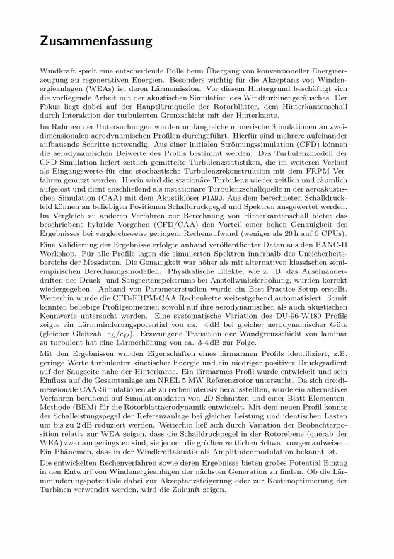
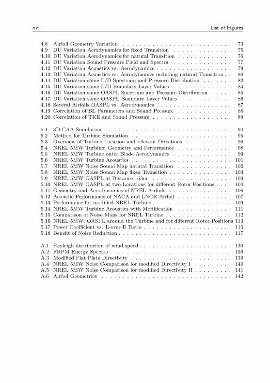
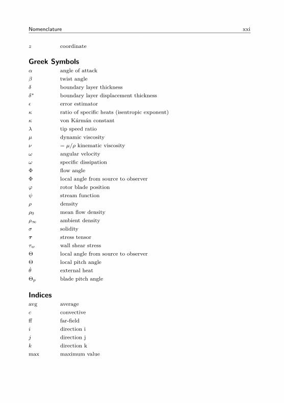
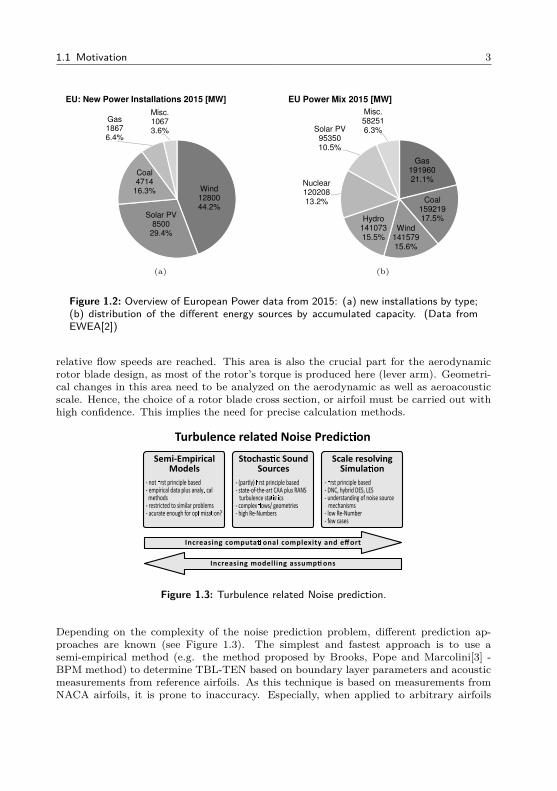
In Europe, where according to the European Wind Energy Association (EWEA) theinstalled cumulative capacity by the end of 2015 was 142GW [2]2, the wind power sector isthe number one in terms of newly installed capacity. Figure 1.2 (a) shows the distributionof the 28.9GW overall newly installed capacity in 2015. With an amount of 44.2% thewind power sector clearly has the biggest share, before solar PV (29.4%), coal and gas(together 22.7%) and other minor contributors (hydro, biomass, waste, etc: 3.6%). In2015, with a 15.6% share of the total amount of installed capacity, wind energy was thethird largest energy contributor in the EU behind coal (17.5%) and gas (21.1%). Thedistribution is depicted in Figure 1.2 (b).

Most turbines are still built in onshore wind farms, where space is limited. Especially indensely populated countries (e.g. Netherlands, Belgium, UK, Germany) this often leadsto conflicts with the nearby living residents. Due to the growing turbine dimensions andtheir increased power not only aesthetic concerns arise, but also noise becomes an issue.This happens particularly in rural areas which used to be very quiet. Consequently, noiseregulations govern the noise emissions of turbines, distances to residents or time framesof wind farm operations. So, from a wind farm operator point of view low noise turbinesmight be more profitable. It is therefore the task of a turbine manufacturer or designer toincorporate the acoustic design challenges into the development process. Hence, preciseacoustic evaluation tools and methods are needed.

Beside mechanical noise in the turbines nacelle different flow-induced noise mechanismscan be distinguished for the rotor blades airfoils[3, 4], e.g. turbulent inflow noise, tipvortex formation noise, blunt trailing-edge vortex shedding noise, separation noise andturbulent boundary layer trailing-edge noise (TBL-TEN). It can be shown (refer to Sec-tion 2.3.7) that TBL-TEN represents the main noise source for modern Multi-Mega-Wattwind turbines. It is generated at the outer part of the rotor blades where the highest

2Totally installed wind capacity in Europe by 2015: 142GW from which 11GW (7.7%) are offshoreand 131GW (92.3%) are onshore.

1.1 Motivation 3

Wind

12800

44.2%

Solar PV

8500

29.4%

Coal

4714

16.3%

Gas

1867

6.4%

Misc.

1067

3.6%

EU: New Power Installations 2015 [MW]

(a)

Gas 191960 21.1%

Coal 159219 17.5%

Wind 141579 15.6%

Hydro 141073 15.5%

Nuclear 120208 13.2%

Solar PV 95350 10.5%

Misc. 58251 6.3%

EU Power Mix 2015 [MW]

(b)

Figure 1.2: Overview of European Power data from 2015: (a) new installations by type;(b) distribution of the different energy sources by accumulated capacity. (Data fromEWEA[2])

relative flow speeds are reached. This area is also the crucial part for the aerodynamicrotor blade design, as most of the rotor’s torque is produced here (lever arm). Geometri-cal changes in this area need to be analyzed on the aerodynamic as well as aeroacousticscale. Hence, the choice of a rotor blade cross section, or airfoil must be carried out withhigh confidence. This implies the need for precise calculation methods.

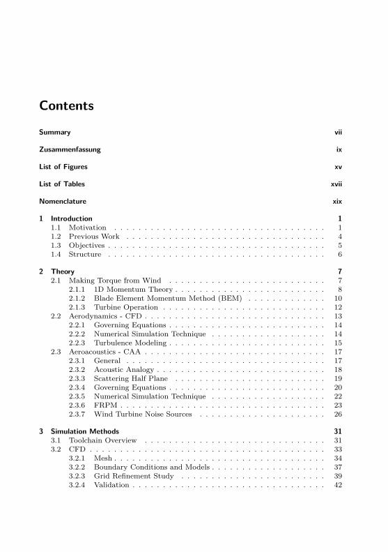
Turbulence related Noise Predic on

Semi-EmpiricalModels

Stochas c SoundSources

Scale resolvingSimula on

- not rst principle based- empirical data plus analy cal methods

- restricted to similar problems- acurate enough for op miza on?

- (partly) rst principle based- state-of-the-art CAA plus RANS turbulence sta s cs- complex ows/ geometries- high Re-Numbers

- rst principle based- DNC, hybrid DES, LES- understanding of noise source mechanisms- low Re-Number- few cases

Increasing computa onal complexity and effort

Increasing modelling assumpons

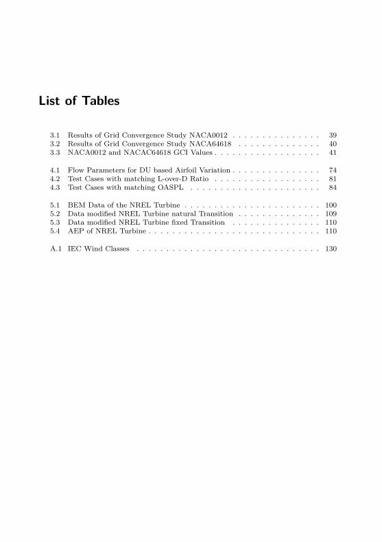
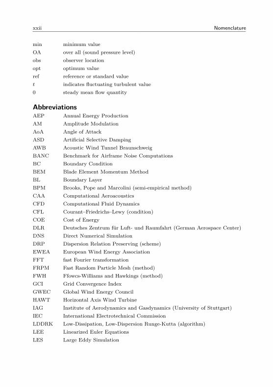
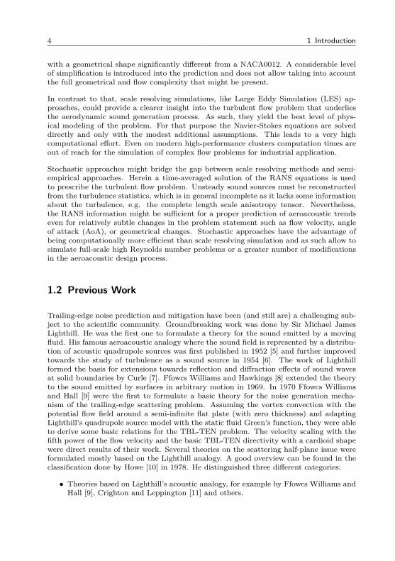
Figure 1.3: Turbulence related Noise prediction.

Depending on the complexity of the noise prediction problem, different prediction ap-proaches are known (see Figure 1.3). The simplest and fastest approach is to use asemi-empirical method (e.g. the method proposed by Brooks, Pope and Marcolini[3] -BPM method) to determine TBL-TEN based on boundary layer parameters and acousticmeasurements from reference airfoils. As this technique is based on measurements fromNACA airfoils, it is prone to inaccuracy. Especially, when applied to arbitrary airfoils

4 1 Introduction

with a geometrical shape significantly different from a NACA0012. A considerable levelof simplification is introduced into the prediction and does not allow taking into accountthe full geometrical and flow complexity that might be present.

In contrast to that, scale resolving simulations, like Large Eddy Simulation (LES) ap-proaches, could provide a clearer insight into the turbulent flow problem that underliesthe aerodynamic sound generation process. As such, they yield the best level of phys-ical modeling of the problem. For that purpose the Navier-Stokes equations are solveddirectly and only with the modest additional assumptions. This leads to a very highcomputational effort. Even on modern high-performance clusters computation times areout of reach for the simulation of complex flow problems for industrial application.

Stochastic approaches might bridge the gap between scale resolving methods and semi-empirical approaches. Herein a time-averaged solution of the RANS equations is usedto prescribe the turbulent flow problem. Unsteady sound sources must be reconstructedfrom the turbulence statistics, which is in general incomplete as it lacks some informationabout the turbulence, e.g. the complete length scale anisotropy tensor. Nevertheless,the RANS information might be sufficient for a proper prediction of aeroacoustic trendseven for relatively subtle changes in the problem statement such as flow velocity, angleof attack (AoA), or geometrical changes. Stochastic approaches have the advantage ofbeing computationally more efficient than scale resolving simulation and as such allow tosimulate full-scale high Reynolds number problems or a greater number of modificationsin the aeroacoustic design process.

1.2 Previous Work

Trailing-edge noise prediction and mitigation have been (and still are) a challenging sub-ject to the scientific community. Groundbreaking work was done by Sir Michael JamesLighthill. He was the first one to formulate a theory for the sound emitted by a movingfluid. His famous aeroacoustic analogy where the sound field is represented by a distribu-tion of acoustic quadrupole sources was first published in 1952 [5] and further improvedtowards the study of turbulence as a sound source in 1954 [6]. The work of Lighthillformed the basis for extensions towards reflection and diffraction effects of sound wavesat solid boundaries by Curle [7]. Ffowcs Williams and Hawkings [8] extended the theoryto the sound emitted by surfaces in arbitrary motion in 1969. In 1970 Ffowcs Williamsand Hall [9] were the first to formulate a basic theory for the noise generation mecha-nism of the trailing-edge scattering problem. Assuming the vortex convection with thepotential flow field around a semi-infinite flat plate (with zero thickness) and adaptingLighthill’s quadrupole source model with the static fluid Green’s function, they were ableto derive some basic relations for the TBL-TEN problem. The velocity scaling with thefifth power of the flow velocity and the basic TBL-TEN directivity with a cardioid shapewere direct results of their work. Several theories on the scattering half-plane issue wereformulated mostly based on the Lighthill analogy. A good overview can be found in theclassification done by Howe [10] in 1978. He distinguished three different categories:

• Theories based on Lighthill’s acoustic analogy, for example by Ffowcs Williams andHall [9], Crighton and Leppington [11] and others.

1.3 Objectives 5

• Theories based on linearized hydroacoustic methods, e.g. Crighton [12] or theevanescent wave theory by Chase [13, 14] or Amiet’s approach where the trailing-edge noise is generated by a scattering hydrodynamic pressure wave [15, 16].

• Ad hoc models which are not purely theoretical but involve source distributions andstrengths which are determined empirically.

The prediction of trailing-edge noise was further promoted by the use of semi-empiricalprediction models. In 1989 Brooks, Pope, and Marcolini [3] published their BPM (ab-breviation of the initials of the three authors) model. It is based on extensive noisemeasurements of a NACA0012 airfoil at various Reynolds and Mach numbers, as wellas several angles of attack. By appropriate scaling of peak levels, spectral shape andStrouhal numbers the model can be used for the noise prediction of arbitrary airfoils. Italso includes other airfoil self-noise mechanisms e.g. stall or separation noise. However,as only symmetric NACA airfoils were used for the generation of the underlying datasets, the question remains of how accurate the BPM model performs for dissimilar airfoilgeometries.

Other prediction approaches were done using diffraction theories for example by Brooksand Hodgson [17] or by Parchen [18]. A result of Parchen’s work is the Blake-TNOmodel [18] where major turbulent boundary layer characteristics, e.g. the main velocityprofile, turbulence kinetic energy and turbulence length scale, are linked to the trailing-edge noise generation. The BPM and the TNO model are incorporated into the freelyavailable airfoil noise prediction software NAFNoise (NREL Airfoil Noise[19, 20]) devel-oped by NREL for the design of wind turbine airfoils.

A good summary of the wind turbine noise issue can be found in the book by Wagner,Bareiss and Guidati [4]. Relevant theoretical background as well as prediction and miti-gation approaches can be found here. Recent work in the wind turbine sector was donein the European project SIROCCO [21], where a noise reduction by the optimizationof wind turbine airfoils was investigated. Moreover several contributions in the field ofwind turbine noise mitigation of reduction by airfoil design can be found, for examplethe work of Lutz [22], Oerlemanns [23–26] and Hutcheson [27, 28] to only name a few ofthe most relevant publications. Moreover, simulation approaches were used to calculatethe trailing-edge noise generation. Among others the hybrid RANS based approach pre-sented by Ewert [29–31] showed the most promising results concerning result quality andcomputational efficiency and is thus used as a basis for the further development presentedin this thesis.

1.3 Objectives

Within in the described background, trailing-edge noise is identified to be the main driverof the overall wind turbine noise. The scope should therefore be, to reduce this mainnoise contributor by a better understanding of the relevant relations between rotor bladegeometry as well as aerodynamic and acoustic influence parameters. As discussed, theavailable semi-empirical or high fidelity tools are not suitable for this task under industrialaspects, because they either lack accuracy or they raise the computational effort to anunreachable amount.

6 1 Introduction

Therefore, a combined modeling approach which connects flow and acoustic simulationswith a high degree of accuracy but which is requiring a reasonable amount of computa-tional resources will be chosen and validated for its use in the rotor blade design process.Starting from two-dimensional CFD and CAA simulations the generated results will beused in a toolchain to simulate the overall power and noise levels of a wind turbine. Withthis approach it should be possible to build a low noise rotor blade from the simulatedand evaluated airfoils and prove the overall ability of the procedure. Condensed, the mainobjectives of this thesis are:

• Improve and validate the hybrid numerical approach for two-dimensional airfoilsimulations.

• Identify the main noise drivers for wind turbine airfoil design.

• Improve the noise emission by geometric changes to a reference airfoil geometrywithout compromising its aerodynamic performance.

• Incorporate the aerodynamic and acoustic results into a toolchain for the predictionof a whole wind turbine’s performance.

• Show the noise reduction effects in the rotor blade design.

1.4 Structure

The thesis is divided into five main parts. The theoretical background of wind turbineaerodynamics together with the relevant basics of the used numerical flow and acousticsimulations are presented in Chapter 2. Thereafter, the hybrid aerodynamic/aeroacousticsimulation toolchain for the precise and efficient simulation of trailing-edge noise is de-scribed in detail in Chapter 3. Validation results are presented in Chapter 4. Moreover,the influence of geometric airfoil variations is investigated by using a systematic approach,based on a wind turbine reference airfoil. A closer look into the noise driving parametersis conducted together with guidelines for a low noise airfoil design. The results on theairfoil level are used in Chapter 5 to calculated the noise and power of the NREL 5MWreference turbine. The influence of a newly developed low noise airfoil is investigated andadvantages on aerodynamic and acoustic performance are shown. The last part of thethesis (Chapter 6) summarizes the main insights and gives advices for future work.

2 Theory

As wind turbine noise is a multidisciplinary subject, a short theoretical review of the majorissues is presented in this chapter. An introduction to specific wind turbine aerodynam-ics and the standard calculation models is given. The different operational modes aredescribed to understand the necessity for noise reduction in certain wind speed ranges. Aclassification of typical wind turbine noise sources is discussed, from which the main sourcecan be identified. For the noise calculation approach presented in this thesis aerodynamic(CFD) and aeroacoustic (CAA) simulations are used. The underlying fundamentals willbe presented. To keep the overall extend of this chapter as short as possible, only themajor aspects are discussed. For further insights the reader is directed to the publishedsupplementing literature (e.g. see References [4, 32–37]).

2.1 Making Torque from Wind

The transformation of kinetic energy contained in the wind into mechanical energy andfinally into electrical energy is the main purpose of a wind turbine. If it would be possibleto extract all the energy contained in the wind by reducing its speed to zero, the maximumextractable energy would be:

Pmax = 1/2mV 20 = 1/2ρAV 3

0 . (2.1)

Equation 2.1 shows, that the extractable energy depends cubically on the wind speed V0,linearly on the fluid density ρ and also linearly on the (rotor) area A over which it isextracted. Two major trends in the wind turbine industry can directly be derived fromthis insights:

• Increasing Turbine Dimensions: With new manufacturing techniques and lightermaterials longer rotor blades can be built to enlarge the area A over which thewind is harvested. Due to A = πR2 the energy output scales quadratically withthe rotor radius R or the rotor blade length. In addition, the fact that the windspeed V0 increases with the height above the ground (atmospheric boundary layer)is utilized with higher towers.

• Ideal Turbine Site: Due to the cubical influence of the wind speed, sites with highconstant wind speeds (e.g. coastal regions or flat table lands) are preferred for windturbine projects. As space is limited, turbines are also build in places with lowerwind speeds. The loss of energy output is often compensated by the turbine dimen-sions. Consequently, turbines are getting bigger and moving closer to populatedareas.

8 2 Theory

The most common wind turbine design nowadays is the three bladed horizontal axis windturbine (HAWT). The rotor is mounted in a upwind position in relation to the tower.The generator is placed in the nacelle. Depending on the turbine type, a gearbox is usedto convert the rotational speed of the rotor. The turbine is controlled via its rotationalspeed and the incidence angle (pitch angle) of the rotor blades. This design has provenits technical and economic feasibility throughout all kinds of fields (manufacturing, costof energy, transportation, erection, loads, etc.).

2.1.1 1D Momentum Theory

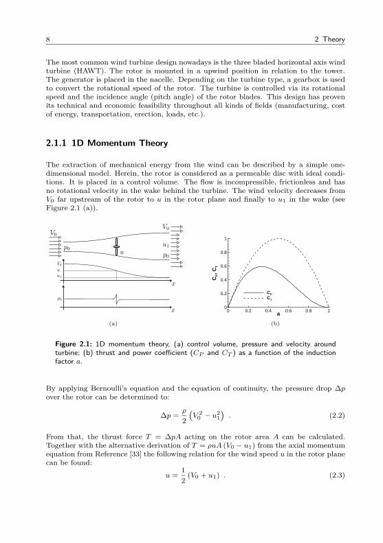
The extraction of mechanical energy from the wind can be described by a simple one-dimensional model. Herein, the rotor is considered as a permeable disc with ideal condi-tions. It is placed in a control volume. The flow is incompressible, frictionless and hasno rotational velocity in the wake behind the turbine. The wind velocity decreases fromV0 far upstream of the rotor to u in the rotor plane and finally to u1 in the wake (seeFigure 2.1 (a)).

(a)

a

CP, C

T

0 0.2 0.4 0.6 0.8 10

0.2

0.4

0.6

0.8

1

CP

CT

(b)

Figure 2.1: 1D momentum theory, (a) control volume, pressure and velocity aroundturbine; (b) thrust and power coefficient (CP and CT ) as a function of the inductionfactor a.

By applying Bernoulli’s equation and the equation of continuity, the pressure drop ∆pover the rotor can be determined to:

∆p =ρ

2(V 2

0 − u21). (2.2)

From that, the thrust force T = ∆pA acting on the rotor area A can be calculated.Together with the alternative derivation of T = ρuA (V0 − u1) from the axial momentumequation from Reference [33] the following relation for the wind speed u in the rotor planecan be found:

u =12

(V0 + u1) . (2.3)

2.1 Making Torque from Wind 9

After defining the axial induction factor a (with u = (1− a)V0) and non-dimensionalizingpower and thrust with respect to Pmax and Tmax, the power and thrust coefficients (CPand CT ) can be derived:

CP =P

12ρV

30 A

= 4a (1− a)2 , (2.4)

CT =T

12ρV

20 A

= 4a (1− a) . (2.5)

By differentiating CP with respect to a the maximum power coefficient CP,max = 16/27for a = 1/3 can be found. This theoretical maximum for an ideal wind turbine is alsoknown as the Betz limit. It describes, that a maximum of approximately 59.3% of theenergy contained in the wind can be extracted if the wind speed is reduced to u = 2/3V0in the rotor area or u1 = 1/3V0 behind the turbine. Graphs for CP and CT are plottedagainst the axial induction in Figure 2.1 (b). The desired maximum CP at a = 1/3 canclearly be seen.

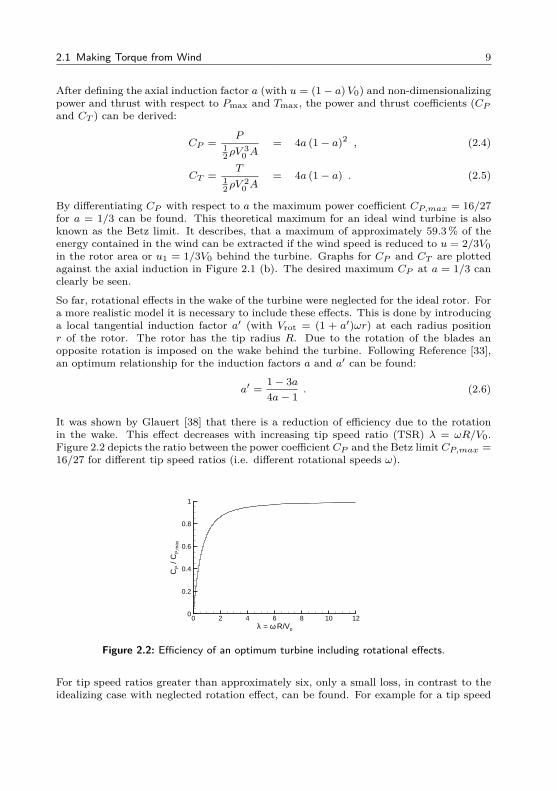
So far, rotational effects in the wake of the turbine were neglected for the ideal rotor. Fora more realistic model it is necessary to include these effects. This is done by introducinga local tangential induction factor a′ (with Vrot = (1 + a′)ωr) at each radius positionr of the rotor. The rotor has the tip radius R. Due to the rotation of the blades anopposite rotation is imposed on the wake behind the turbine. Following Reference [33],an optimum relationship for the induction factors a and a′ can be found:

a′ =1− 3a4a− 1

. (2.6)

It was shown by Glauert [38] that there is a reduction of efficiency due to the rotationin the wake. This effect decreases with increasing tip speed ratio (TSR) λ = ωR/V0.Figure 2.2 depicts the ratio between the power coefficient CP and the Betz limit CP,max =16/27 for different tip speed ratios (i.e. different rotational speeds ω).

λ = ω R/V0

CP /

CP

,max

0 2 4 6 8 10 120

0.2

0.4

0.6

0.8

1

Figure 2.2: Efficiency of an optimum turbine including rotational effects.

For tip speed ratios greater than approximately six, only a small loss, in contrast to theidealizing case with neglected rotation effect, can be found. For example for a tip speed

10 2 Theory

ratio of λ = 7.5 a power coefficient of CP = 0.983 · CP,max = 0.5825 could be reachedfor an ideal turbine. For a real turbine losses due to aerodynamic friction as well asthree-dimensional flow phenomena at the blade root and tip lead to an even lower value,usually around CP ≈ 0.5.

Figure 2.2 also explains the trend to go for high tip speed ratios on modern turbines. Ifthis is done via the increase of the rotational speed ω, also the rotor torque M = P/ωcould be reduced. This offers benefits for all mechanical parts (e.g. rotor shaft, bearings,gearbox, etc.). Unfortunately, this also results in a high tip speed (Vtip = ωR), which isunfavorable due to acoustic reasons (see Section 2.3.2).

2.1.2 Blade Element Momentum Method (BEM)

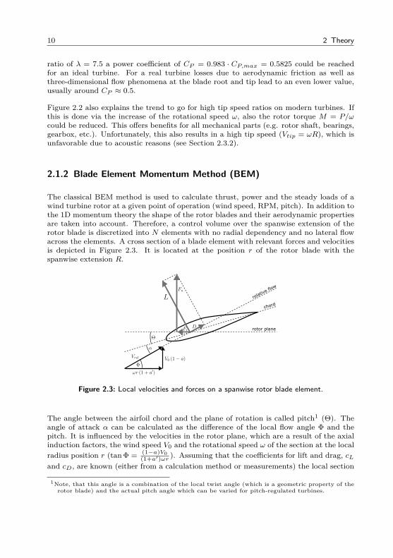
The classical BEM method is used to calculate thrust, power and the steady loads of awind turbine rotor at a given point of operation (wind speed, RPM, pitch). In addition tothe 1D momentum theory the shape of the rotor blades and their aerodynamic propertiesare taken into account. Therefore, a control volume over the spanwise extension of therotor blade is discretized into N elements with no radial dependency and no lateral flowacross the elements. A cross section of a blade element with relevant forces and velocitiesis depicted in Figure 2.3. It is located at the position r of the rotor blade with thespanwise extension R.

rotor plane

chord

relative flo

w

Figure 2.3: Local velocities and forces on a spanwise rotor blade element.

The angle between the airfoil chord and the plane of rotation is called pitch1 (Θ). Theangle of attack α can be calculated as the difference of the local flow angle Φ and thepitch. It is influenced by the velocities in the rotor plane, which are a result of the axialinduction factors, the wind speed V0 and the rotational speed ω of the section at the localradius position r (tan Φ = (1−a)V0

(1+a′)ωr ). Assuming that the coefficients for lift and drag, cLand cD, are known (either from a calculation method or measurements) the local section

1Note, that this angle is a combination of the local twist angle (which is a geometric property of therotor blade) and the actual pitch angle which can be varied for pitch-regulated turbines.

2.1 Making Torque from Wind 11

forces, tangential and normal to the rotor plane Ft and Fn respectively their coefficientsct and cn, can be determined:

cn =Fn

12ρV

2rellc

= cL cos Φ + cD sin Φ , (2.7)

ct =Ft

12ρV

2rellc

= cL sin Φ− cD cos Φ . (2.8)

These results can be related with the 1D momentum theory. After introducing the solidityσ(r) = lc(r)B

2πr , which is the ratio of the blade surface and surface of the annular area ofthe element (for B blades), the equations for the induction factors:

a =1

4 sin2 Φσcn

+ 1, (2.9)

a′ =1

4 sin Φ cos Φσct

− 1(2.10)

can be found. Now, the induction factors can be calculated iteratively by solving theequation for the flow angle Φ and the corresponding aerodynamic forces at the chosenpoint of operation (see Appendix A.1 for a detailed description). As each annular controlvolume is - per definition - independent from the others, each radial position can be solvedon its own. Finally Prandtl’s tip loss factor (correction for a finite number of rotor blades)and the Glauert correction (correction for induction factors a > 0.4) need to be consideredto yield the full picture (see also Appendix A.1 for more details).

One of the major wind turbine attributes - the power curve - can be computed using theBEM method. If this function of shaft power against wind speed is combined with a prob-ability density function f (Vi < V0 < Vi+1) for the occurrence of certain wind speeds ata specific location, the annual energy production (AEP) can be calculated. The functionf (Vi < V0 < Vi+1) is typically obtained from a Weibull or Rayleigh distribution for themean wind speed (V0). It includes correction factors for the local meteorological and sit-ing effects (landscape, vegetation, obstacles). They can be taken from the literature, e.g.Refernce [39]. By the AEP the turbine efficiency can be evaluated in an economical kindof sense. Basically, the only input data needed therefore is the rotor blade design (geom-etry, aerodynamic coefficients) and the operational conditions at the proposed location.The low computational resources to conduct the BEM method and the precise results incomparison with measurements made it the industry standard for quick estimations ofnew turbine designs. Note, that it is important to provide the method with precise inputdata, e.g. aerodynamic coefficients or meteorological conditions in order to provide highquality results. Aerodynamic phenomena (e.g. stall effects) can only be evaluated by alimited accuracy due to the two-dimensional modeling approach. High fidelity calculationmethods (e.g. CFD simulations) are thus needed in the design phase of a rotor blade.

12 2 Theory

2.1.3 Turbine Operation

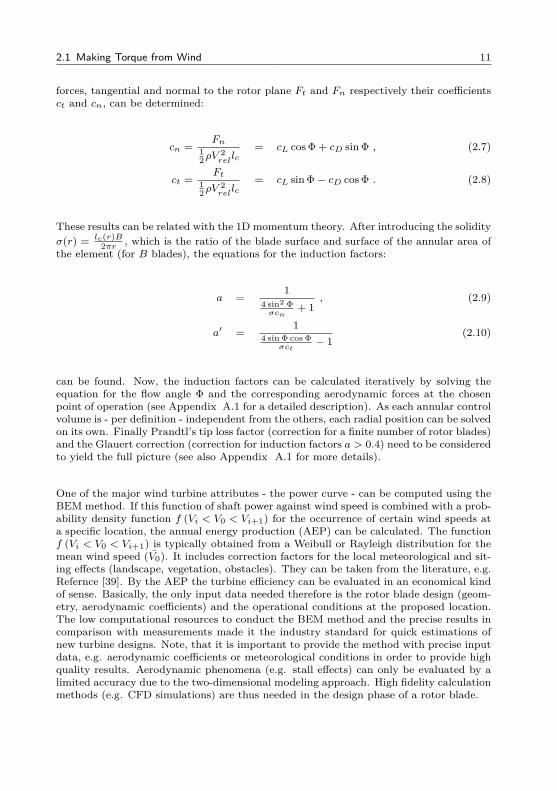
The efficiency of a wind turbine depends on its control algorithm. Some basic aspectsfor pitch regulated HAWTs with variable speed2 are discussed in the following. Theinterplay of specific turbine parameters like tip speed ratio (λ = ωR/V0), rotational speed(ω), power coefficient (CP ) and pitch angle (Θ) with the wind speed (V0) is depicted inFigure 2.4 for a generic HAWT. It can be seen, that the turbine exhibits four distinctstates of operation throughout the increasing wind speed V0.

• State I: For very low wind speeds the energy contained in the wind is not enoughto turn the rotor. The turbine is idling and waiting for V0 to increase. Once the so-called cut-in wind speed is reached, the rotor begins turning and mechanical energyis converted into electrical energy. The rotational speed is constant and determinedby the minimum speed allowed by the partial converter. This leads to a relativehigh λ above the optimal tip speed ratio λopt and thus to a reduced CP belowCP,max. The pitch is zero.

• State II: Further increase of the wind speed brings the power coefficient to itsmaximum value of CP,max3. The rotational speed of the rotor is increased relatedto the wind speed in order to keep the tip speed ratio constant at the optimumλopt. As a result of that, local angles of attack at each section of the blade stayconstant (see Figure 2.3). Energy output increases with the third power of V0 butis still below rated power. The pitch is zero.

• State III: The maximum rotational speed of the partial converter is reached andthus limits further increase of ω. While the rotational speed is held constant fromthe beginning of state III the tip speed ratio decreases with increasing V0. Thepower coefficient moves slightly away from its maximum. The energy output is stillgrowing with approximately the third power of the wind speed and the pitch is stillzero.

• State IV: The turbine reaches rated power (Prated) and the energy output is nowheld constant over the increasing wind speed. This is done by the increase of thepitch angle Θ. The intended loss of CP is compensated by the higher amountof kinetic energy contained in the incoming flow. The local angles of attack aredecreased. Finally the turbine will stop its operation (not shown in Figure 2.3) atthe cut-off wind speed of around 2.5 ∼ 3 · V0 to avoid critical loads outside thedesired design conditions.

For the acoustic evaluation of a wind turbine the states II and III are of primary interest.For state II the local sections angle of attack stays constant (λopt = const.), while theflow speed (Reynolds and Mach number) increases because of the increasing ω. For astandard turbine design, this range of maximum CP corresponds with the maximum

2The predominant amount of currently installed turbines utilizes this control strategy, where theblades can be rotated around the pitch axis in order to adjust the local incidence angles andthereby determine the aerodynamic forces. In contrast to that, smaller turbines from the earlyyears of wind power had fixed rotor blades and were only be controlled by variable rotor speeds.Increasing wind speeds in combination with a fixed maximum rotational speed led to high angles ofattack at the rotor blades and finally to stalled flow conditions with reduced forces. This, so-calledstall regulation, is only applicable for small turbines as loads and vibrations can become very high.

3Modern wind turbines can reach CP,max values around 0.5 which is still below the Betz-limit of16/27 ≈ 0.593 for an ideal wind turbine (ref. Section 2.1.1).

2.2 Aerodynamics - CFD 13

P/P

rated

0

0.5

1

CP/C

P,max

0

0.5

1

ω/ω

max

0

0.5

1

λ/λopt

hr

0.5

1

1.5

0

0.05

0.1

V0/V

0,rated

Θ/Θ

max

0 0.5 1 1.50

0.5

1

I II III IV

Figure 2.4: Operational parameters of a generic HAWT (dashed graph indicates typicalprobability of wind speed occurrence hr )

probability hr of the occurrence of the mean wind velocity V 0. Consequently, most ofthe turbine operation hours are within this wind speed range. In state III the magnitudeof the incoming flow velocity for each blade segment is constant, while the angle of attackis increasing with the wind speed up to the point where the rotor blades are pitched.Close to rated power (just before the blades are pitched) the local angles of attack reachtheir maximum values. Amongst others, the influence of these two parameters (incomingflow vector and angle of attack) on the emitted noise of the turbine will be investigated.For state IV the wind turbine noise issue vanishes, as the turbine noise levels stay nearlyconstant (constant tip speed due to limited ω) At the same time, the background noiselevels (eg. wind whistling through the trees) steadily increase. The turbine noise ismasked by the background noise.

2.2 Aerodynamics - CFD

A short theoretical review of the relevant aspects for the numerical flow simulation is givenin this section. Individual settings and chosen models are further described in Section 3.2in Chapter 3.

14 2 Theory

2.2.1 Governing Equations

The behavior of a compressible fluid is described by the conservation equations for mass,momentum and energy. These equations are an extension of the Euler equations andinclude the effects of viscosity on the flow. They were derived independently by ClaudeLouis Marie Henri Navier and Sir George Gabriel Stokes in the first half of the nineteenthcentury. In the conservative differential form the Navier-Stokes (NS) equation systemreads:

∂ρ

∂t+∇ · (ρ~v) = m (2.11)

∂ρ~v

∂t+∇ · (ρ~v~v) +∇p = ∇τ + ~f + m~v (2.12)

∂ρet

∂t+∇ · (ρet~v) +∇ (ρ~v) = −∇~q +∇ · (τ~v) + θ + ~f~v + met (2.13)

In the above equations ρ represents the fluid density, ~v the velocity vector, p the pressureand et = e + 1

2~v2 the specific total energy. On the right hand side of the equations the

source terms for mass m , external forces ~f and external heat θ can be found. The viscousstresses in the fluid are represented by the stress tensor τ and the heat flux is denoted as ~q.The stress tensor can be calculated by the Stokes hypothesis τ =

(∇~v + t∇~v − 2

3I∇ · ~v),

where µ represents the dynamic viscosity of the fluid. For the heat flux Fourier’s law ofheat conduct ~q = −k∇T , with the heat conductivity k and the temperature T can beused. Together with the thermal and caloric equation of state, p = ρRT and e = cvT(with the gas constant R and the specific heat at constant volume cv) the equation systemcan be solved for the seven unknowns (ρ, ~v, p, et, T ).

2.2.2 Numerical Simulation Technique

Apart from some special cases, where an analytical solution is possible, the equationsystem (2.11-2.13) is solved numerically by means of computational fluid dynamics (CFD).Each CFD simulation thereby consists of the same basic steps:

• Pre-Processing: Definition of the problem geometry, discretization of the volumeunder investigation (mesh) and setting of the boundary conditions and flow param-eters.

• Solving: Choice of physical models and equations (viscosity, compressibility, tur-bulence treatment, boundary treatment, etc.), iteratively solving of the equationsuntil a defined convergence criteria is reached.

• Post-Processing: Evaluation of flow parameters or integral results for the problem,visualization and analysis of the results.

To iteratively solve the equations a discretization of the governing equations (2.11-2.13)is needed. In the majority of the CFD codes finite volume methods are used for this. Themain advantage of a finite volume method is that the mesh can be of an unstructuredtype. An acceleration of the mesh generation process, especially for complex geometries is

2.2 Aerodynamics - CFD 15

possible. The conservation equations are normally used in their conservative integral for-mulation for the control volume V with the vector of conserved quantities ~W (containingρ, ~v, e) and the flux density tensor F (containing the fluxes):

∂

∂t

∫∫∫V

~W = −∫∫∂V

F · ~ndS . (2.14)

See Appendix A.2 for more details. Basically, the change of the flow parameters in a fixed(time and space) control volume can be determined from the fluxes over its boundaries( ~QF ):

d

dt~W = −

1V· ~QF . (2.15)

For the integration of the fluxes over the control volume boundary different discretizationschemes can be used4. They distinguish in their numerical stability, order of accuracyand computational effort. Moreover, artificially added numerical dissipation has to beconsidered. For most engineering CFD applications in a subsonic flow regime centralschemes show good results with reasonable stability.

The spatial discretization of the computational domain around the geometry is donewith a mesh (or grid). Different commercial and non-commercial grid generators can beused for the mesh generation. Areas with large gradients (for example boundary layers)need to be resolved with a high mesh density. Moreover, certain quality criteria (gridlines parallel and perpendicular to the flow direction, limited skewness and aspect ratios,moderate size increase of neighboring cells) need to be observed. The mesh generationis a crucial process of each CFD simulation. Poor mesh quality can easily lead to wrongresults.

In a CFD simulation, the flow problem can be computed either for a time-averaged (steadystate) or a time-accurate (unsteady) solution. Time-accurate solutions require more diskspace and computational time. For attached flow conditions (for example a wind turbineairfoil under normal operation conditions) steady-state solutions are the best tradeoff ofcomputational resources and accuracy. Moreover, the commonly used turbulence modelsalso average out the temporal fluctuations even in an unsteady simulation so that onlylarge scale effects (like flow separation) can be resolved.

CFD simulations offer a lot of insights into specific flow characteristics and phenomena.However, all subsequent steps and sub-models in the working process need to be carefullyscrutinized by the user in order to avoid incorrect final results. Profound verification andvalidation steps are thus crucial for high quality solutions.

2.2.3 Turbulence Modeling

By nature, most of the flows considered for technical applications (such as the flow arounda wind turbine airfoil) are turbulent. Turbulent flows are unsteady, highly diffusive,

4Depending on the used discretization method and the flow problem under investigation a whole lotof different discretization schemes and variations of them can be used (e.g. upwind, downwind,central). The complete description of the discretization and solving procedure can fill books and isskipped here as it is not the main matter of this thesis (for further reading see References [36, 40])

16 2 Theory

highly dissipative, rotational and three-dimensional. The flow regime is characterized byirregular and seemingly random (chaotic) rapid variations of pressure and flow velocity intime and space on many different length scales, which all interact with each other. Thecomplete simulation of all turbulent features, down to the smallest length scale with aDNS (Direct Numerical Simulation) or LES (Large Eddy Simulation), is a very challengingtask. Even with modern high performance computing equipment the calculation timesare very high - especially for high Reynolds number flows - and not applicable in anindustrial environment.

For engineering applications the modeling of turbulence is the state of the art method.Therefore Reynolds Averaged Navier Stokes equations (RANS) are used. Herein, the flowquantities are decomposed into a mean part and a fluctuating part (e.g u = u+u′). As aconsequence additional terms result from all non-linear terms in the NS equations. Theseadditional terms are of the form −ρu′iu

′j and are called Reynolds stresses. They built the

Reynolds stress tensor. The calculation of the Reynolds stress tensor is needed in order toclose the equation system (closure problem). In analogy to the viscous stresses (where thestresses are proportional to the viscosity and the velocity gradient) the Reynolds stressesare often determined from a (turbulent) eddy viscosity µt and the gradient of the meanvelocity (Boussinesq Approximation).

−ρu′iu′j = 2µtSij −

23ρktδij (2.16)

With the mean strain tensor Sij and the mean turbulence kinetic energy kt as:

Sij =12

(∂ui

∂xj+∂uj

∂xi−

23∂uk

∂xkδij

)(2.17)

andkt =

12(u′1u′1 + u′2u

′2 + u′3u

′3)

(2.18)

and the Dirac delta function as:

δij =

1 for i = j0 for i 6= j

. (2.19)

Different turbulence models based on empirical constants can be used for the modeling ofthe eddy viscosity and the turbulence kinetic energy kt. In this thesis, the two-equationSST-k-ω turbulence model as proposed by Menter[41] is used. It is a combination of thek-ε-model with:

µt = Cµρk2/ε (2.20)

and the k-ω-model with:µt = ρk/ω (2.21)

from Wilcox[42]. Note, that in this context ω is a turbulence dissipation quantity ratherthan an angular frequency. Two more differential equations are solved in the iterationprocess for k and ω = ε/k. They contain several model constants which were determinedfrom a comparison with experimental data (see Reference [42]).The SST-k-ω turbulencemodel overcomes the disadvantages of using the k-ε-model in near wall regions with strongadverse pressure gradients by switching to the more accurate k-ω-model. Precise resultsthroughout a wide range of applications made this model very popular. It became theindustry standard for most flow simulation problems.

2.3 Aeroacoustics - CAA 17

2.3 Aeroacoustics - CAA

A review of the relevant theoretical background for the aeroacoustic phenomena and theirnumerical simulation is given in this section. The main focus is put on the simulation oftrailing-edge noise. The actual settings and modeling decisions made for the individualsimulations can be found in Section 3.3.

2.3.1 General

Sound is characterized by small fluctuations of a quantity Φ′ around its steady meanvalue Φ0. For example, the pressure p(t) can be divided into:

p (t) = p0 + p′ . (2.22)

With the steady part p0:

p0 = limT→∞

1T

∫ T2

−T2

p(t+ t′

)dt (2.23)

and the fluctuating sound pressure p′(t). Introducing this principle into the governingequations for fluid dynamics (2.11 - 2.13), together with standard perturbation tech-niques for linearization, leads to the wave equation for the pressure fluctuation p′ (seeAppendix A.3 for further details):

1c20

∂2p′

∂t2−∆p′ = Qp . (2.24)

And similar for the velocity perturbation (or particle velocity) ~v′:

1c20

∂2 (∇ · ~v′)∂t2

−∆(∇ · ~v′

)= Qv . (2.25)

Note, that in the above equations the medium is supposed to be stagnant (~v0 = 0) andthe mean density and mean pressure are assumed constant (ρ0 = const., p0 = const.).∆ denotes the Laplacian, where ∆ = ∇ · ∇. If the compression and expansion of themedium is supposed to be isentropic (s = const.) , the relationship

p′ = c20ρ′ (2.26)

holds. Where, for a perfect gas the propagation speed of the disturbances (speed of sound)c0 can be calculated as:

c20 =(∂ρ

∂p

)−1 ∣∣∣s=const.

= κRT (2.27)

Herein κ is the ratio of specific heats (or isentropic exponent), R the specific gas constantand T the absolute temperature. The Equations 2.24 and 2.25 are called wave equations.Their left hand side describes the wave dynamics of a perturbation wave (p′ or ~v′) in

18 2 Theory

time and space. The right hand side stands for the source terms Qp and Qv which areconsidered given and can be calculated for a perfect gas (e.g. air) as:

Qp =1κ

∂m

∂t+κ− 1c20

∂ϑ

∂t−∇ · ~f ′ (2.28)

and

Qv =1ρ0

(−∆θ′ +

1c20

∂∇ · ~f ′

∂t

). (2.29)

It can be seen, that sound can be generated by either a mass source m, external forces ~f ′or a heat sources θ (respectively their time derivatives). Especially sources from unsteadylocal fluid forces and their interaction with inhomogeneities are the most important onesfor the wind turbine trailing-edge noise problem.

2.3.2 Acoustic Analogy

A further look into the nature of aeroacoustic sources is given by Lighthill’s famousacoustic analogy[5]. It can be derived by subtracting the divergence of the momentumequation (Eq. 2.12) from the time-derivative of the continuity equation (Eq. 2.11) andneglecting mass flow sources and external forces.

∂2ρ

∂t2= ∇ · ∇ · (ρ~v~v + pI − τ ) (2.30)

The term c20∆ρ needs to be subtracted from both sides of Equation 2.30 to achievethe form of the wave equation. Additionally, the fluctuating quantities for the acousticpressure p′ (Equation 2.22) and similar fluctuating density ρ′ are introduced. The meanvalues are supposed to be constant (p0 = const., ρ0 = const.).

∂2ρ′

∂t2− c20∆ρ′ = ∇ · ∇ ·

(ρ~v~v +

(p′ − c20ρ

′)I − τ

)(2.31)

Equation 2.31 is the basis of the acoustic analogy as formulated by Lighthill. The lefthand side represents a wave equation (see Equation 2.24) while the right hand side is thedouble divergence of the so-called Lighhill stress tensor. It is now possible to directlyconnect the wave equation with the aeroacoustic sources calculated from the governingequations. The Lighthill stress tensor T =

(ρ~v~v +

(p′ − c20ρ

′)I − τ

)consists of three

parts which can be identified as distinct source mechanisms.

• ρ~v~v: changes in flow velocity (e.g. turbulence)

• s′ = p′ − c20ρ′: changes in entropy s (e.g. temperature changes due to combustion)

• τ : changes in viscous friction (usually unimportant)

If in Equation 2.28 one would identify m = 0, ϑ = 1/(κ−1)∂s′/∂t and ~f ′ = ∇·(τ − ρ~v~v),these source quantities are equivalently related to the Lighthill sources.

2.3 Aeroacoustics - CAA 19

Introducing source quantities in in Equation 2.28 directly leads to the pressure from ofthe Lighthill analogy:

1c20

∂2p′

∂t2−∆p′ = ∇ · ∇ · (ρ~v~v − τ ) +

1c20

∂2

∂t2

(p′ − c20ρ

′). (2.32)

If no entropy changes are present the source mechanisms can be reduced to the turbulenceintroduced velocity changes as the main noise source for aeroacoustic problems. With hisconcept for the sound radiation caused by fluctuating Reynolds stresses, Lighthill foundthe following dependence of the sound intensity I of the main parameters:

I ∝ ρ0c30M

8(l

r

)2α2 . (2.33)

Herein l denotes the dimension of the turbulent region, α is the normalized turbulenceintensity and M = v∞/c∞ the Mach number. Note, that the intensity scales withthe eighth power of the Mach number for free turbulence (e.g. as present in a jet orhomogeneous boundary layers). This dependence is also known as the eighth powerlaw. It shows, that especially at low Mach numbers (M < 1), free turbulence is a veryinefficient sound source.

2.3.3 Scattering Half Plane

When the turbulent structures interact with an edge in the flow their inefficient quadrupoleradiation is superimposed by an additional, much more efficient dipole type radiation.Ffowcs Williams and Hall [9] investigated the sound field due to a turbulent eddy in thevicinity of a scattering half plane. They could show, that the intensity I now scales withthe following relation with respect to the main parameters:

I ∝ ρ0c30 cos3

(Θ)M5 sl

r2 α2 · sin (φ) sin2

(Θ2

). (2.34)

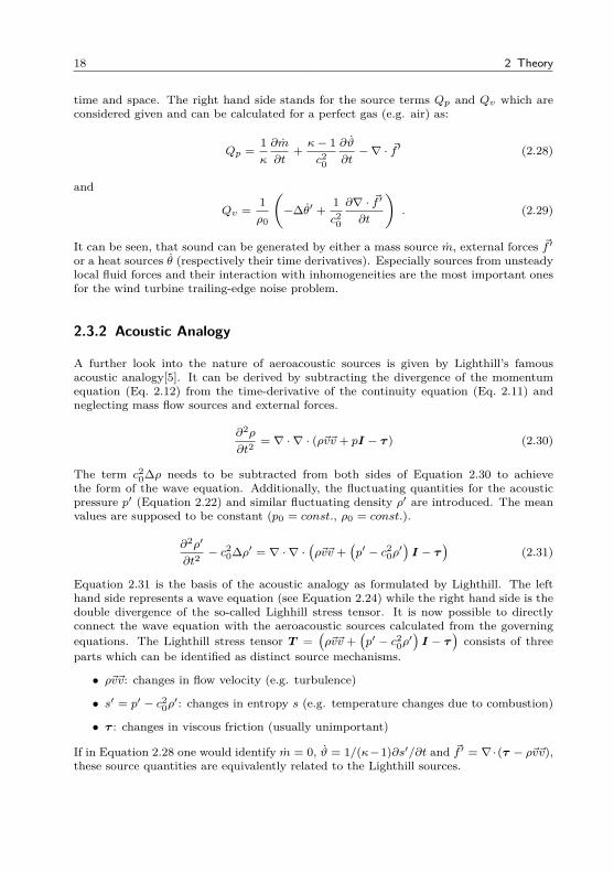
In the above equation, a convecting turbulent stream of the height l and the width s isassumed. The definition of the respective angles relative to the flow (φ and Θ) can beseen in Figure 2.5.

trailing-edge

x

y

z

plate

observer

Figure 2.5: Flow over the semi-infinite half plane with the respective angles.

20 2 Theory

The flow vector is aligned parallel to the surface. Usually, it passes the trailing-edge withan angle of 90 (Θ = 0 ).

Comparing Equation 2.33 with Equation 2.34 it can be seen, that the radiation efficiencychanges from M8 to M5 for turbulent eddies in the vicinity of an edge. As the flowMach number for typical wind turbine issues is M = 0.3 or less, this indicates a clearlymore efficient radiation for the presence of an edge by a factor of M−3. Remember, thatthis not only holds for incoming turbulence which hits the rotor blades but also for selfproduce turbulence in the boundary layer of the airfoils.

2.3.4 Governing Equations

The simulation of noise generation and propagation is the main objective of a CAA code.With the PIANO code, the inviscid dynamics of the perturbations are simulated over asteady, time-averaged mean-flow field. Interactions of vorticity with solid structures orgradients in the flow field can be covered. In the code non-dimensionalized quantities areused for the calculations. The reference values for the nondimensionalization are the ref-erence length lref (usually the chord length lref = lc), the pre-multiplied ambient pressureκp∞ = ρc2∞ (with the isentropic exponent κ), the ambient density ρ∞ and the ambientspeed of sound c∞. The mean flow and FRPM quantities are non-dimensionalized asfollows (values with dimension are indicated by ∗):

xi =x∗ilref

, ~v =~v∗

c∞, ρ =

ρ∗

ρ∞, p =

p∗

ρ∞c2∞, k =

k∗

c2∞, ω =

ω∗lrefc∞

. (2.35)

At standard conditions where Tref = 288.15 K and p∞ = 101325 Pa the reference den-sity is ρ∞ = 1.225 kg/m3 and the reference speed of sound is c∞ = 340.3 m/s. Thenondimensionalization has to be considered for all steps throughout the acoustic simula-tion process. For the interpretation of absolute results, a reverse conversion needs to bedone. An equation system for the small perturbations about the (viscous) mean flow maybe derived from the Navier-Stokes Equations (refer to Section 2.2.1). For this purposethey are put into the primitive formulation for the quantities of interest (ρ,~v,p) to yield(non-dimensional):

∂ρ

∂t+ ~v · ∇ρ+ ρ∇ · ~v = 0 , (2.36)

∂~v

∂t+ ~v · ∇~v +

1ρ∇p =

M

Re

1ρ∇ · τ , (2.37)

∂p

∂t+ ~v · ∇p+ p∇ · ~v =

M

Re

[(κ− 1) τ : ∇~v −

1Pr∇ · ~q

]. (2.38)

In the equations above, the Reynolds number for the reference length L and the referencedynamic viscosity µ∞ is expressed by Re = ρ∞v∞L/µ∞ and the Prandtl number byPr = µ∞cp/k∞ (with the reference thermal conductivity k∞). The non-dimensionalheat flux density is represented by ~q (referenced to k∞c20/ (cp (1− κ)L)).

To account for the amplitude fluctuations about a steady mean-flow a further splitting ofthe variables, to a steady mean flow quantity and a small fluctuating part, is done (e.g.(ρ,~v, p, τ , ~q) = (ρ0, ~v0, p, τ0, ~q0) + ε (ρ′, ~v′, p′, τ ′, ~q′)). Following the linearization strategy

2.3 Aeroacoustics - CAA 21

described in Refernce [43] and assuming that direct viscosity and heat conduction effectson the perturbation field may be neglected (i.e. τ ′ and ~q′), the linearized Euler equationsor LEE can be derived:

∂ρ′

∂t+ ~v′ · ∇ρ0 + ~v0 · ∇ρ′ +∇ · ~v0ρ

′ +∇~v′ρ0 = 0 , (2.39)

∂~v′

∂t+ ~v′ · ∇~v0 + ~v0 · ∇~v′ +

1ρ0

(∇p′ + ρ′~v0 · ∇~v0

)= 0 , (2.40)

∂p′

∂t+ ~v′ · ∇p0 + ~v0 · ∇p′ + κ

(∇ · ~v0p

′ +∇ · ~v′p0)

= 0 . (2.41)

The equation system can be solved for the acoustic field with the variables ρ′, ~v′ and p′.The (turbulent) mean-flow field is represented by the variables ρ0, ~v0 and p0.

The acoustic perturbation equations (APE[44]) are a modification of the LEE so, thatvorticity or entropy convection is entirely prescribed by the source term (which addsstability to the equation system by removing the vorticity convection mode from thegoverning equations), whereas acoustic generation and radiation is simulated dynamically.The APE realize a solution to the wave operator of irrotational flow. Together withproper right-hand side volume sources this becomes an acoustic analogy based on thewave operator. The source term mainly acts as a vorticity source term. Sound due to theinteraction of vorticity with the trailing-edge is generated as part of the CAA simulationstep. The vortex dynamic is dominated by linear contributions to the source terms. Non-linear contributions mainly deemed responsible for sound generation of free turbulentflow are neglected. It was observed that for edge noise problems the incorporation ofturbulence decay into the source model had no effect on the spectra compared withsimulations based on frozen turbulence.

Neglecting entropy fluctuations and density fluctuations, due to turbulent velocities in(cold) low Mach number flows, the APE-4 equation system (with corresponding right-hand sides) reads:

∂p′

∂t+ c20∇

(ρ0 ~v′ + ~v0

p′

c20

)= 0 , (2.42)

∂v′

∂t+∇

(~v0 · ~v′

)+∇

(p′

ρ0

)= ~L′ . (2.43)

The turbulent sources are represented by the fluctuating Lamb vector ~L′. Quantitieswith subscript 0 denote mean-flow variables. The prime indicates fluctuating quantities.The perturbation velocity is represented by ~v′. The fluctuating acoustic pressure p′ andfluctuating density ρ′ are linked via

p′ = c20ρ′ , (2.44)

where the squared speed of sound c20 is defined by the mean-flow variables (with theisentropic exponent of air κ = 1.4):

c20 = κp0

ρ0. (2.45)

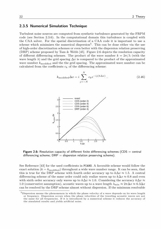
22 2 Theory

2.3.5 Numerical Simulation Technique

Turbulent noise sources are computed from synthetic turbulence generated by the FRPMcode (see Section 2.3.6). In the computational domain this turbulence is coupled withthe CAA solver. For the spatial discretization of a CAA code it is important to use ascheme which minimizes the numerical dispersion5. This can be done either via the useof high-order discretization schemes or even better with the dispersion relation preserving(DRP) scheme proposed by Tam & Webb [45]. Figure 2.6 depicts the resolution capacityof different differencing schemes. The product of the wave number k = 2π/λ (with thewave length λ) and the grid spacing ∆x is compared to the product of the approximatedwave number kmodified and the the grid spacing. The approximated wave number can becalculated from the coefficients ck of the differencing scheme:

kmodified∆x = i

N∑j=−N

cke−ij(k∆x) . (2.46)

k ∆x

k mod

ified

∆x

0 0.5 1 1.5 2 2.5 30

0.5

1

1.5

2

2.5

3exactCDS (order 2)CDS (order 4)CDS (order 6)DRP (order 4)

Figure 2.6: Resolution capacity of different finite differencing schemes (CDS = centraldifferencing scheme; DRP = dispersion relation preserving scheme).

See Reference [43] for the used coefficients in PIANO. A favorable scheme would follow theexact solution (k = kmodified) throughout a wide wave number range. It can be seen, thatthis is true for the DRP scheme with fourth order accuracy up to k∆x ≈ 1.5. A centraldifferencing scheme of the same order could only realize waves up to k∆x ≈ 0.8 and evenwith sixth order accuracy only waves up to k∆x ≈ 1.0. Considering the accuracy k∆x ≈1.0 (conservative assumption), acoustic waves up to a wave length λmin ≈ 2π∆x ≈ 6.3∆xcan be resolved by the DRP scheme almost without dispersion. If the minimum resolvable

5Dispersion means the phenomenon in which the phase velocity of a wave depends on its wave lengthor frequency. Dispersion occurs when the phase velocities of the traveling acoustic waves are notthe same for all frequencies. If it is introduced by a numerical scheme it reduces the accuracy ofthe simulated results and yields artificial noise.

2.3 Aeroacoustics - CAA 23

wave lengths is thus resolved by at least seven points, the maximum frequency can becalculated to:

fmax =c0

λmin=

c0

7 ·∆x. (2.47)

In the numerical code PIANO, seven point stencils are used for the numerical approxima-tion of the derivatives with the DRP scheme. Special formulations for non-uniform gridspacings as well as modified stencils for unsymmetrical stencils (e.g. at mesh boundaries)are applied. Further details can be found in Reference [43].

For very short wave lengths (f > fmax), which cannot be represented correctly due tothe finite grid spacing, the artificial selective damping (ASD) approach of Tam, Webband Dong [46] is used. The damping can be applied to the whole computational domainor to distinct physical areas (for example around the airfoil’s leading-edge).

The temporal discretization is done using a two-step low-dissipation, low-dispersion Runge-Kutta (LDDRK) algorithm from Hu et al. [47]. The coefficients in this approach arechosen to minimize dissipation and dispersion errors without compromising the stabilityof the procedure. It also has the advantage of low storage requirements. The coefficientsas well as further details can also be found in [43].

2.3.6 FRPM

For the preparation of unsteady vortex sound sources a synthetic turbulence methoddeveloped at DLR is adopted to force the linearized applied acoustic perturbation equa-tions. The stochastic approach is especially well suited for aeroacoustics purposes, e.g.realizing a four-dimensional time and space based prediction of fluctuating sources in arestricted volume. This volume is called the source patch (or short: patch). The RandomParticle-Mesh Method (RPM) was first published in 2005 by Roland Ewert [48]. It allowsto synthetically realize the time-dependent, turbulent fluctuations from averaged turbu-lence statistics. It is discretized by equidistantly distributed mean flow stream lines thatcover the resolved source domain. To avoid this elaborate patch generation procedure,the method was extended to the fast Random Particle-Mesh Method (FRPM) in 2007[29]so, that a single block Cartesian background mesh could be used for its spatial discretiza-tion. Fluctuating sound sources are computed in the cell vertices of the background mesh(patch) and further interpolated onto the CAA mesh. Despite the discretization proce-dure RPM and FRPM rely on the same theoretical background. In the following, theterm FRPM will be used for the descriptions.

FRPM generates synthetic turbulence by means of spatially and temporally fluctuatingquantities. These fluctuations accurately reproduce provided autocorrelations and inte-gral length scales, for example from a time-averaged RANS simulation. According to[49] the two-point spatiotemporal correlation R = ψt (~x, t)ψt (~x+ ~r, t+ τ) of a turbulentquantity ψt can be written as:

R (~x, ~r, τ) = R · exp(−|τ |τs−π (~r − ~vcτ)2

4l2

). (2.48)

The relevant parameters are the time and length scales τs and l, the mean square valueof the correlated quantity R and the convection velocity ~vc.

24 2 Theory

The turbulence is generated by spatially filtering of a convective white-noise field with aGaussian filter of the respective length scale. A scaling with the local variance (e.g. theturbulence kinetic energy kt or TKE) yields the final fluctuating quantities. Due to thefilter kernel an energy spectrum of Gaussian shape is realized.

For the turbulence reconstruction FRPM realizes a fluctuating stream function ψt of thefollowing form for the n-dimensional problem:

ψt (~x, t) =∫V

(n)S

A(n)G0(~x− ~x′, l

)U(~x′, t)dn~x′ . (2.49)

Fluctuating turbulent values are represented by the superscript t. The term A(n) isresponsible for the local amplitude scaling (as a result of the local turbulence statisticskt and ω from RANS). The Gaussian filter kernel is represented by G0 (~x− ~x′, l) andU (~x′, t) is the used spatiotemporal white noise field which contains the random values.The integration is done over the volume V (n)

S , where the unsteady sources are realized.The filter kernel is normalized, so that the autocorrelation ψt (~x, t)ψt (~x, t) = 1 for A = 1.The filter kernel depends on the distance ~x− ~x′ and the kernel width l which representsthe local length scale.

For the simulation of frozen turbulence the white-noise field U (~x′, t) is uniquely definedby the properties:

U (~x, t) = 0 , (2.50)

U (~x, t)U (~x+ ~r, t) = δ (~r) , (2.51)D0

DtU (~x, t) = 0 . (2.52)

Here, δ (~r) denotes the multi-dimensional Dirac δ-function. The term D0Dt

in Equation 2.52denotes the material derivative, e.g. D0

Dtϕ = ∂

∂xϕ+ ~v0 · ∇ϕ. It is responsible for the con-

vective property of the fluctuation model. So, the white noise field is passively convectedwith the mean-flow velocity (~v = ~v0). It is discussed in Reference [29], that for largerlength scales l the convection velocity will be an average over the surrounding mean-flow field. For example in turbulent boundary layers, where the convection velocity ~vc isslower than the velocity outside the boundary layer (~vc ≈ 0.6...0.7~v∞), this length scaledependent averaging yields the correct physical behavior of the turbulent noise sourcesand the proper Mach scaling. The Gaussian filter kernel reads:

G0 = exp(−π

2|~x− ~x′|2

l2

). (2.53)

It is shown in Reference [48] that the spatial normalized correlation

R0 (~r, τ) =ψ (~x+ r, t+ τ)ψ (~x, t)

ψ (~x, t)ψ (~x, t)(2.54)

2.3 Aeroacoustics - CAA 25

satisfies R0 (0, 0) = 1 and

R0 (~r, 0) = exp(−π

4|~x− ~x′|2

l2

). (2.55)

For the realization of turbulent vortex sound sources, the turbulent velocity ~vt is calcu-lated from the curl of the stream function:

~vt = ∇× ~ψ . (2.56)

Taking again the curl of the turbulent velocity ~vt yields the fluctuating vorticity vector:

~ωt = ∇× ~vt . (2.57)

With the results of Equation 2.56 and 2.57 the linearized fluctuating Lamb vector thatoccurs as the major vortex-force source term on the right-hand side of the momentumequation (Equation 2.43) can be calculated to:

~L′ = w(~x)(−~ω0 × ~vt − ~ωt × ~v0

). (2.58)

In the above given source term ~v0 and ~vt are the mean and fluctuating velocity thatdefine the unsteady flow velocity via ~v = ~v0 + ~vt. The local source term weighting isrepresented by w(~x). Furthermore, ~ω0 = ∇× ~v0 and ~ωt = ∇× ~vt denote the mean andfluctuating vorticity, respectively. While ~ω0 and ~v0 are results of the RANS simulation,~vt and ~ωt are results of the FRPM turbulence reconstruction.

It was shown by Ewert [29], that for the two-dimensional case the amplitude R in Equa-tion 2.48 must be set to

R =4l2kt3π

(2.59)

to reconstruct convecting isotropic frozen turbulence with the appropriate statistics givenby RANS (according to the desired correlation given in Equation 2.48). The resulting

longitudinal correlation function is a Gaussian (f (r) = exp(−π4

~r2

l2

)) with an integral

length scale l. The length scale can be directly determined from the RANS solution. Fora k-ω turbulence model the corresponding relation reads:

l =cl

Cµ

√k

ω. (2.60)

According to Reference [50] the constant cl ≈ 0.54 can be approximated for a modifiedvan Kármán turbulence spectrum. Together witch the constant Cµ = 0.09 from theturbulence model, the length scale factor lfac = cl

Cµ≈ 6.0 can be determined.

The simulations are carried out by generating one turbulent two-dimensional slice out ofthe three-dimensional turbulent field (see Reference [30]) and conducting a CAA simula-tion on a two-dimensional mesh. The result is a severe benefit in terms of computationaltimes, compared to other scale resolving turbulence simulations (e.g. LES or DNS). It

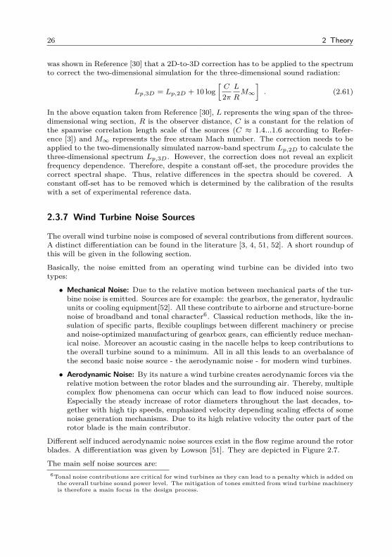
26 2 Theory

was shown in Reference [30] that a 2D-to-3D correction has to be applied to the spectrumto correct the two-dimensional simulation for the three-dimensional sound radiation:

Lp,3D = Lp,2D + 10 log[C

2πL

RM∞

]. (2.61)

In the above equation taken from Reference [30], L represents the wing span of the three-dimensional wing section, R is the observer distance, C is a constant for the relation ofthe spanwise correlation length scale of the sources (C ≈ 1.4...1.6 according to Refer-ence [3]) and M∞ represents the free stream Mach number. The correction needs to beapplied to the two-dimensionally simulated narrow-band spectrum Lp,2D to calculate thethree-dimensional spectrum Lp,3D. However, the correction does not reveal an explicitfrequency dependence. Therefore, despite a constant off-set, the procedure provides thecorrect spectral shape. Thus, relative differences in the spectra should be covered. Aconstant off-set has to be removed which is determined by the calibration of the resultswith a set of experimental reference data.

2.3.7 Wind Turbine Noise Sources

The overall wind turbine noise is composed of several contributions from different sources.A distinct differentiation can be found in the literature [3, 4, 51, 52]. A short roundup ofthis will be given in the following section.

Basically, the noise emitted from an operating wind turbine can be divided into twotypes:

• Mechanical Noise: Due to the relative motion between mechanical parts of the tur-bine noise is emitted. Sources are for example: the gearbox, the generator, hydraulicunits or cooling equipment[52]. All these contribute to airborne and structure-bornenoise of broadband and tonal character6. Classical reduction methods, like the in-sulation of specific parts, flexible couplings between different machinery or preciseand noise-optimized manufacturing of gearbox gears, can efficiently reduce mechan-ical noise. Moreover an acoustic casing in the nacelle helps to keep contributions tothe overall turbine sound to a minimum. All in all this leads to an overbalance ofthe second basic noise source - the aerodynamic noise - for modern wind turbines.

• Aerodynamic Noise: By its nature a wind turbine creates aerodynamic forces via therelative motion between the rotor blades and the surrounding air. Thereby, multiplecomplex flow phenomena can occur which can lead to flow induced noise sources.Especially the steady increase of rotor diameters throughout the last decades, to-gether with high tip speeds, emphasized velocity depending scaling effects of somenoise generation mechanisms. Due to its high relative velocity the outer part of therotor blade is the main contributor.

Different self induced aerodynamic noise sources exist in the flow regime around the rotorblades. A differentiation was given by Lowson [51]. They are depicted in Figure 2.7.

The main self noise sources are:6Tonal noise contributions are critical for wind turbines as they can lead to a penalty which is added on

the overall turbine sound power level. The mitigation of tones emitted from wind turbine machineryis therefore a main focus in the design process.

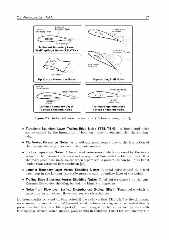
2.3 Aeroacoustics - CAA 27

airfoil

bladetip

blunttrailing-edge

laminar boundary layer

turbulent boundary layer

trailing-edge

Trubulent Boundary Layer

Trailing-Edge Noise (TBL-TEN)

airfoil

boundary layerseparation

airfoil

large-scaleseparation (stall)

Separation/Stall Noise

tip vortex

airfoil

instabilitywaves

laminar boundary layer

vortex shedding

Tip Vortex Formation Noise

Laminar Boundary Layer

Vortex Shedding Noise

high angleof attack

airfoil

vortex shedding

Trailing-Edge Bluntness

Vortex Shedding Noise

Figure 2.7: Airfoil self noise mechanisms. (Picture reffering to [51])

• Turbulent Boundary Layer Trailing-Edge Noise (TBL-TEN): A broadband noisesource caused by the interaction of boundary layer turbulence with the trailing-edge.

• Tip Vortex Formation Noise: A broadband noise source due to the interaction ofthe tip turbulence (vortex) with the blade surface.

• Stall or Separation Noise: A broadband noise source which is caused by the inter-action of the massive turbulence in the separated flow with the blade surface. It isthe most prominent noise source when separation is present. It can be up to 10 dBlouder than attached flow condition [53].

• Laminar Boundary Layer Vortex Shedding Noise: A tonal noise caused by a feedback loop in the laminar (normally pressure side) boundary layer of the airfoil.

• Trailing-Edge Bluntness Vortex Shedding Noise: Tonal noise triggered by the von-Kármán like vortex shedding behind the blunt trailing-edge.

• Noise from Flow over Surface Disturbances (Holes, Slits): Tonal noise which iscaused by instable shear flows over surface disturbances.

Different studies on wind turbine noise[23] have shown that TBL-TEN is the dominantnoise source for modern multi-Megawatt wind turbines as long as no separated flow ispresent in the outer rotor blade parts[4]. This finding is further underlined by tests withtrailing-edge devices which showed good results in reducing TBL-TEN and thereby the

28 2 Theory

overall levels [21, 22, 54]. As TBL-TEN scales with the fifth power of the relative flowvelocity[9], the outer parts of the rotor (with high relative velocities) are of most interest.

Figure 2.8: Visualization of aerodynamic noise on downward moving rotor blade. (Pic-ture from [23])

Figure 2.8 shows the aerodynamic noise of the downward moving blade of a G58 windturbine taken by Oerlemans[23] in the framework of the European SIROCCO project[21].The noise signature is visualized with an acoustic array of 148 microphones situatedin front of the turbine. Two main noise sources can be distinguished: the nacelle andthe outer part of the rotor blade. Note, that it is clearly visible that the main noisesource (indicated by the red color) is the rotor blade. The strength of the aerodynamicnoise is first increasing from the blade root towards the tip, due to the increased relativevelocity(velocity scaling) with increasing rotor radius, but then decreases again at thetip part of the blade. This circumstance can be observed at almost every modern windturbine. The reason is the reduction in the airfoil incidence angle and chord length inthe blade tip region to reduce lift production and tip vortex formation. Thereby, twonoise mechanisms (tip vortex formation noise and TBL-TEN) are reduced in this region.Consequently, the most interesting part of the rotor blade for noise reduction is theutmost third fraction of the blade and not necessarily the blade tip7. Aside from noise,

7This statement relies on the assumption, that a conservative low noise tip design is used (reductionof chord and twist). Low noise airfoils or the reduction of the tip vortex strength might also helpto increase the blade’s twist angles and thereby the lift production in the tip area. Thus, a higherenergy production of the turbine might be possible.

2.3 Aeroacoustics - CAA 29

aerodynamic design constraints need to be considered in this region, as most of the rotor’storque is produced here. A high influence on the turbine’s energy production as well asloads is implied. Therefore, changes in airfoil geometry must always be analyzed againstthe backdrop of aerodynamic as well as acoustic performance.

3 Simulation Methods

The choice of a wind turbine airfoil has been a challenging task in rotor blade design eversince. Competing functions have to be weighed against each other in order to find the"perfect" airfoil. Most times, it is even hard to define what is understood as "perfect" andwhat is not. In this thesis, the main focus is put on aerodynamic as well as aeroacousticaspects1. They are analyzed in a combined, first principle based numeric procedure whichconsists of multiple consecutive steps.

An overview of the toolchain is given in Section 3.1. Sections 3.2 and 3.3 comprise allinformation necessary to set up the aerodynamic and aeroacoustic simulation steps whichare implied into the method. Due to the rather large amount of airfoils to investigate,automation scripts were generated for several steps of the procedure. The automationis described in Section 3.4. The methods shown in this chapter build the foundationfor the analysis presented and discussed in Chapter 4. The validation of the describedapproach is shown in Section 4.1 by a comparison with available measurement data. WhileChapter 3 and Chapter 4 deal mainly with the investigation of two-dimensional airfoilgeometries, Chapter 5 is dedicated to the performance of the whole wind turbine. Therelated methods for this full turbine investigation are presented in Chapter 5 as well.

3.1 Toolchain Overview

A combination of different simulation tools is used to determine the broadband trailing-edge noise signal of the airfoils under investigation and finally of a rotor blade comprisingthese airfoils. Besides that, several aerodynamic characteristics are analyzed. A ratherlarge amount of data is recorded during the process which has the advantage that nearlyall interesting parameters (acoustic as well as aerodynamic) can be evaluated from theavailable simulation data. The major steps of the toolchain which is depicted in Figure 3.1are:

• CFD Flow Simulation: With the airfoil geometry (given as x and y coordinates) asimulation of the time-averaged turbulent flow field around the airfoil is conducted.In the rotor blade design process this data might already exist and a dual use ispossible if the boundary layer is resolved correctly. From the CFD results the mean-flow variables (velocity vector ~v0, density ρ0 and pressure p0) are extracted for theCAA step. Moreover, the turbulence statistics are used as an input for the FRPMturbulence reconstruction. For more details on the CFD simulation see Section 3.2.

• CAA Acoustics Simulation: The time and space resolved fluctuating sound pressurefield (p′ = f(~x, t)) around the airfoil is simulated in the CAA step. For this purpose

1Nevertheless, structural requirements are considered in terms of geometrical boundary conditions inorder to guarantee the structural strength and integrity of the airfoil geometry.

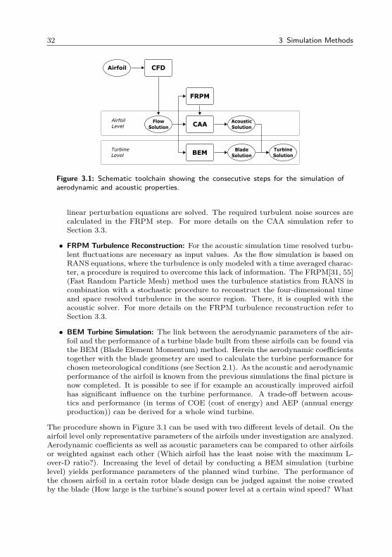
32 3 Simulation Methods

Airfoil CFD

CAAFlow

Solution

FRPM

Acoustic

Solution

BEMBlade

Solution

Turbine

Solution

Airfoil

Level

Turbine

Level

Figure 3.1: Schematic toolchain showing the consecutive steps for the simulation ofaerodynamic and acoustic properties.

linear perturbation equations are solved. The required turbulent noise sources arecalculated in the FRPM step. For more details on the CAA simulation refer toSection 3.3.

• FRPM Turbulence Reconstruction: For the acoustic simulation time resolved turbu-lent fluctuations are necessary as input values. As the flow simulation is based onRANS equations, where the turbulence is only modeled with a time averaged charac-ter, a procedure is required to overcome this lack of information. The FRPM[31, 55](Fast Random Particle Mesh) method uses the turbulence statistics from RANS incombination with a stochastic procedure to reconstruct the four-dimensional timeand space resolved turbulence in the source region. There, it is coupled with theacoustic solver. For more details on the FRPM turbulence reconstruction refer toSection 3.3.

• BEM Turbine Simulation: The link between the aerodynamic parameters of the air-foil and the performance of a turbine blade built from these airfoils can be found viathe BEM (Blade Element Momentum) method. Herein the aerodynamic coefficientstogether with the blade geometry are used to calculate the turbine performance forchosen meteorological conditions (see Section 2.1). As the acoustic and aerodynamicperformance of the airfoil is known from the previous simulations the final picture isnow completed. It is possible to see if for example an acoustically improved airfoilhas significant influence on the turbine performance. A trade-off between acous-tics and performance (in terms of COE (cost of energy) and AEP (annual energyproduction)) can be derived for a whole wind turbine.

The procedure shown in Figure 3.1 can be used with two different levels of detail. On theairfoil level only representative parameters of the airfoils under investigation are analyzed.Aerodynamic coefficients as well as acoustic parameters can be compared to other airfoilsor weighted against each other (Which airfoil has the least noise with the maximum L-over-D ratio?). Increasing the level of detail by conducting a BEM simulation (turbinelevel) yields performance parameters of the planned wind turbine. The performance ofthe chosen airfoil in a certain rotor blade design can be judged against the noise createdby the blade (How large is the turbine’s sound power level at a certain wind speed? What

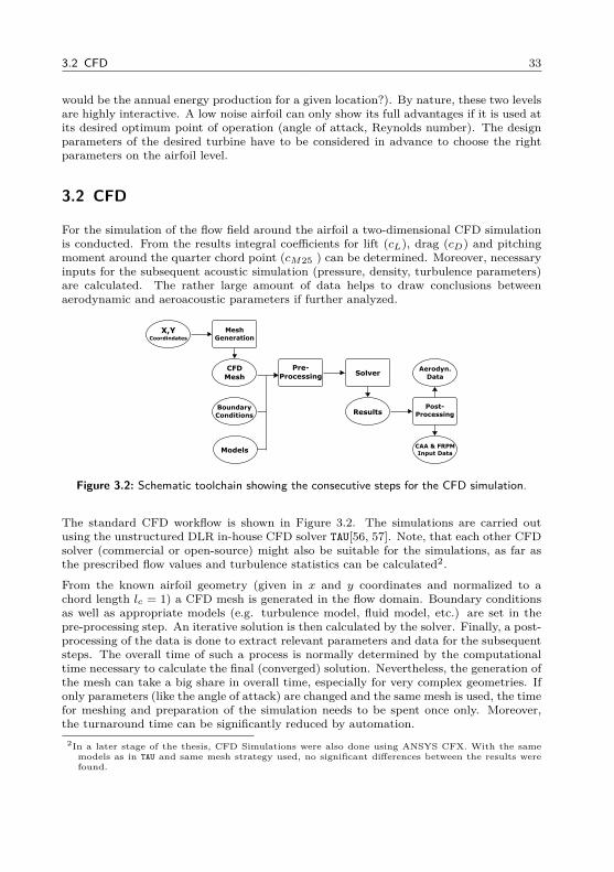
3.2 CFD 33

would be the annual energy production for a given location?). By nature, these two levelsare highly interactive. A low noise airfoil can only show its full advantages if it is used atits desired optimum point of operation (angle of attack, Reynolds number). The designparameters of the desired turbine have to be considered in advance to choose the rightparameters on the airfoil level.

3.2 CFD

For the simulation of the flow field around the airfoil a two-dimensional CFD simulationis conducted. From the results integral coefficients for lift (cL), drag (cD) and pitchingmoment around the quarter chord point (cM25 ) can be determined. Moreover, necessaryinputs for the subsequent acoustic simulation (pressure, density, turbulence parameters)are calculated. The rather large amount of data helps to draw conclusions betweenaerodynamic and aeroacoustic parameters if further analyzed.

X,YCoordindates

Mesh

Generation

CFD

Mesh

Boundary

Conditions

Models

Pre-

Processing

Post-

Processing

Solver

Results

CAA & FRPM

Input Data

Aerodyn.

Data

Figure 3.2: Schematic toolchain showing the consecutive steps for the CFD simulation.

The standard CFD workflow is shown in Figure 3.2. The simulations are carried outusing the unstructured DLR in-house CFD solver TAU[56, 57]. Note, that each other CFDsolver (commercial or open-source) might also be suitable for the simulations, as far asthe prescribed flow values and turbulence statistics can be calculated2.

From the known airfoil geometry (given in x and y coordinates and normalized to achord length lc = 1) a CFD mesh is generated in the flow domain. Boundary conditionsas well as appropriate models (e.g. turbulence model, fluid model, etc.) are set in thepre-processing step. An iterative solution is then calculated by the solver. Finally, a post-processing of the data is done to extract relevant parameters and data for the subsequentsteps. The overall time of such a process is normally determined by the computationaltime necessary to calculate the final (converged) solution. Nevertheless, the generation ofthe mesh can take a big share in overall time, especially for very complex geometries. Ifonly parameters (like the angle of attack) are changed and the same mesh is used, the timefor meshing and preparation of the simulation needs to be spent once only. Moreover,the turnaround time can be significantly reduced by automation.

2In a later stage of the thesis, CFD Simulations were also done using ANSYS CFX. With the samemodels as in TAU and same mesh strategy used, no significant differences between the results werefound.

34 3 Simulation Methods

On standard hardware (6 CPU machine) it takes less than 20 minutes to conduct a CFDsimulation for one set of input parameters. Thus, a whole angle of attack polar can besimulated in just a few hours.

3.2.1 Mesh

For each airfoil a two-dimensional computational domain is generated using the commer-cial grid generator ICEM CFD. With the use of replay-scripts it was possible to automateall steps of the mesh creation. In this way a consistent meshing approach with almostunvarying quality could be ensured for all geometries.

The domain’s outer boundaries extend about 100 chord lengths around the airfoil toprevent unphysical interferences of the boundary conditions with the near airfoil flow.A hybrid meshing strategy is chosen where the viscous sub-layer and the near airfoilregion are resolved by a structured grid and areas far away from the airfoil are resolvedby a coarser, quad-dominated unstructured grid. This meshing strategy reduces cells inless interesting areas (far away from the airfoil) and thereby saves computational effort(time and storage space). The total number of grid cells is approximately 100k. A gridrefinement study is shown in Section 3.2.3.

The near airfoil mesh is built in a C-type topology for airfoils with a sharp (one point)trailing-edge3. Throughout the airfoil surface 225 nodes are distributed along the upperside and the same number is also used for the lower side. Both sides are treated individ-ually and are divided at the airfoil nose in order to set individual boundary conditionsin the pre-processing (e.g. transition locations). Moreover, a separate post-processing ofthe results from both sides is possible. A smooth transition between different cell sizesalong the surface is enforced with an exponential growth ratio for neighboring cells notbigger then the factor 1.2. For the correct simulation of near-wall viscous flow effects(boundary layer development, laminar turbulent transition etc.) a correct resolution ofthe airfoil boundary layer is mandatory. Otherwise, wall-functions would be used (in-stead of the desired turbulence model) whose accuracy is not sufficient for the designatedaerodynamic and aeroacoustic investigation. An indicator for the correct mesh resolutionin the boundary layer and the height of the first cell at the wall is the dimensionless walldistance y+. It can be calculated from the wall shear stress τw, the fluid density ρ andthe kinematic viscosity ν = µ/ρ for a specific distance y.

y+ =

√τwρy

ν(3.1)

3An alternative strategy using a O-type grid topology, to account for finite TE thickness, was alsodeveloped. The basic concepts and dimension are the same, so that only the C-type meshingstrategy is explained in this section. In the outer part of a wind turbine rotor blade it is alwaysthe aspiration to keep the trailing-edge thickness as thin as possible to avoid tonal blunt trailing-edge vortex shedding noise. The exact thickness value depends on the manufacturing and finishingprocess of the blade and is usually around 2-3mm. As the main objective of this thesis is thesimulation of broadband TBL-TE noise, the simulations are conducted with zero TE thickness.This hypothesis is valid, as long as no blunt TE noise according to Reference [4] occurs. Thevalidity of neglecting a small trailing edge thickness on the radiated broadband spectrum of anairfoil slat was shown by Marcus Bauer[58]. Note, that the nature of the used hybrid CFD-CAAapproach would (also with the O-grid topology and the consideration of finite TE thickness) notallow the simulation of blunt trailing-edge vortex shedding noise, as it relies on the time averaged(RANS) flow simulation where the vortex shedding would be suppressed.

3.2 CFD 35

An estimation of the height of the first cell at the wall y = ∆s1 can be done using theestimation for the smooth flat plate with turbulent boundary layer (see Schlichting[59]).It relates the skin friction coefficient (cf ) with the local Reynolds number Rex based onempirical data:

cf = 2(

κ

lnRexG (lnRex)

)2. (3.2)

With a von Kármán constant of κ = 0.41 and the function G (lnRex) ≈ 1.5 (accordingto [59]) cf and from it τw = 1/2cfρv2

∞ can be determined. Equation 3.1 can now besolved for y = ∆s1 with a desired dimensionless wall distance y+ = 1 or below. Forstandard conditions (ρ = 1.225 kg/m3 and µ = 1.79 · 10−5 kg/ms) and a typical windturbine airfoil Reynolds number between 3 · 106 and 6 · 106, the height ∆s1 lies between6.6 · 10−6 m and 3.45 · 10−6 m (with a corresponding airfoil chord length of lc = 1 m).A value of ∆s1 = 3.0 · 10−6 m is chosen for all generated CFD meshes. This low valueensures y+ values less than one for all typical Reynolds numbers and accounts for theuncertainties in the estimation procedure. Nevertheless, y+ values need to be checked inthe final simulation results.

The structured near-airfoil grid extends about 110 layers from the wall with an exponentialgrowth factor of 1.1. Hence, a good resolution of the viscous sub-layer is realized and thenumerical error is reduced. Moreover, the near airfoil blocks are distributed such, thatalmost perpendicular cells are generated at the airfoil wall. Therefore, the block cornersare positioned with respect to the airfoil geometry by the ICEM replay script to accountfor changes of the geometry.

As an example, the CFD mesh for a 18% thick DU-96-W-180[60] airfoil, normalized bythe chord lengths lc is depicted in Figure 3.3 (a). The structured region in the vicinityof the airfoil can be seen in detail (b) of Figure 3.3 and the high mesh resolution towardsthe wall (to resolve the boundary layer) can be seen in detail (c). The same blockingstrategy and meshing procedure was used for all airfoils in this thesis.

To quantify the mesh quality the following indicators where extracted for the exampleDU-96 mesh using ICEM CFD:

• Maximum Aspect Ratio = 2250 (highest ratio for thin cells directly at the wall; lowvalues are desired but not possible within the very thin boundary layer cells)

• Minimum Angle = 52.5 (minimum angle of cell internal faces; values should be atleast greater than 20 for reasonable result quality)

• Maximum Angle = 126 (maximum angle of cell internal faces; values should be atleast lower than 160 for reasonable result quality)

• Minimum Eriksson Skewness = 0.806 (empirical criterion in ICEM CFD to judge the el-ement shear for a hexahedral element4; acceptable elements should have a skewnessgreater than 0.5)

• Maximum Volume Change = 1.15 (in the structured near airfoil region and 1.4 inthe outer mesh region; ensures smooth increase in volume of neighboring cells; lowvalues are desired)

4calculated by dividing the volume of its closest parallelepiped by the product of its edges (rangingbetween 1=perfect and 0=unacceptable)

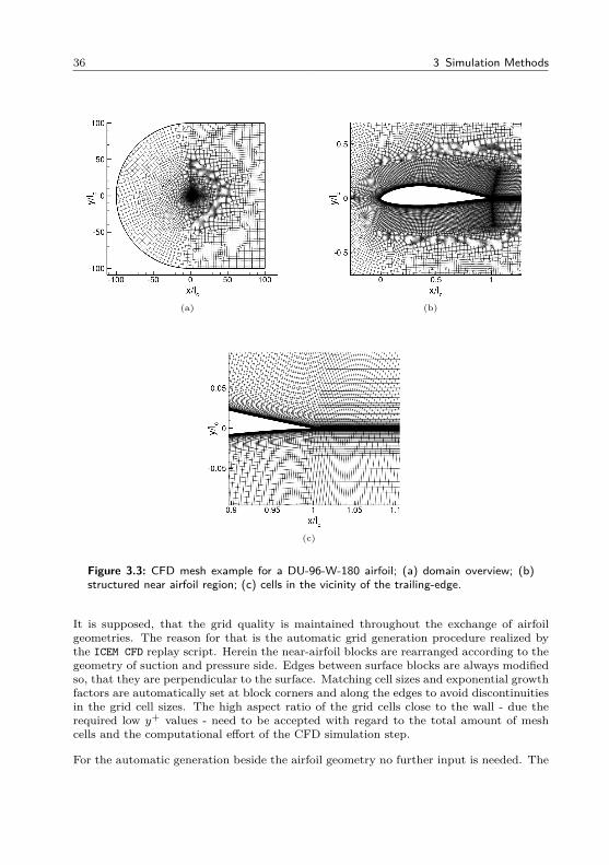
36 3 Simulation Methods

(a) (b)

(c)

Figure 3.3: CFD mesh example for a DU-96-W-180 airfoil; (a) domain overview; (b)structured near airfoil region; (c) cells in the vicinity of the trailing-edge.

It is supposed, that the grid quality is maintained throughout the exchange of airfoilgeometries. The reason for that is the automatic grid generation procedure realized bythe ICEM CFD replay script. Herein the near-airfoil blocks are rearranged according to thegeometry of suction and pressure side. Edges between surface blocks are always modifiedso, that they are perpendicular to the surface. Matching cell sizes and exponential growthfactors are automatically set at block corners and along the edges to avoid discontinuitiesin the grid cell sizes. The high aspect ratio of the grid cells close to the wall - due therequired low y+ values - need to be accepted with regard to the total amount of meshcells and the computational effort of the CFD simulation step.

For the automatic generation beside the airfoil geometry no further input is needed. The

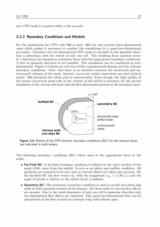
3.2 CFD 37

new CFD mesh is created within a few seconds.

3.2.2 Boundary Conditions and Models

For the simulations the CFD code TAU is used. TAU can only process three-dimensionalcases which makes it necessary to conduct the simulations in a quasi-two-dimensionalprocedure. Therefore the two-dimensional CFD mesh is extruded in the spanwise direc-tion (z-direction) with the extent of only one cell. The resulting faces (normal vectorin z-direction) are deemed as symmetry faces with the appropriate boundary conditions.A flow in spanwise direction is not possible. The simulation can be considered as two-dimensional. Figure 3.4 shows an overview of the computational domain and the relevantboundary conditions. Note, that there is no interface between the structured and un-structured volumes of the mesh. Instead, one-to-one nodal connections are used (hybridmesh). TAU interprets the whole grid as unstructured. Even though, the high quality ofthe former structured mesh cells in the vicinity of the airfoil is necessary for the precisesimulation of the viscous sub-layer and the flow phenomena present in the boundary layer.

structured near-

airfoil mesh

unstructured

mesh

1 cell

symmetry BCfarfield BC

viscous wall

(no-slip) BC

100 lc

Figure 3.4: Sketch of the CFD domain; boundary conditions (BC) for the relevant facesare indicated in bold letters.

The following boundary conditions (BC) where used at the appropriate faces in themesh:

• Far-Field BC: A far-field boundary condition is defined at the outer borders of themesh (100lc away from the airfoil). It acts as an inflow and outflow condition. Allgradients are assumed to be zero and no viscous effects are taken into account. Onthe far-field BC the flow vector ~v0, with the magnitude v∞ = f (Re, lc) and theangle of attack α relative to the airfoil chord, is defined.

• Symmetry BC: The symmetry boundary condition is used to model zero-shear slipwalls at both spanwise borders of the domain. On these walls no viscous flow effectsare present. Due to the mesh dimension of only one cell in spanwise direction onlytwo-dimensional flow effects are captured. This quasi-two-dimensional flow can beinterpreted as the flow around an unswept wing with infinite span.

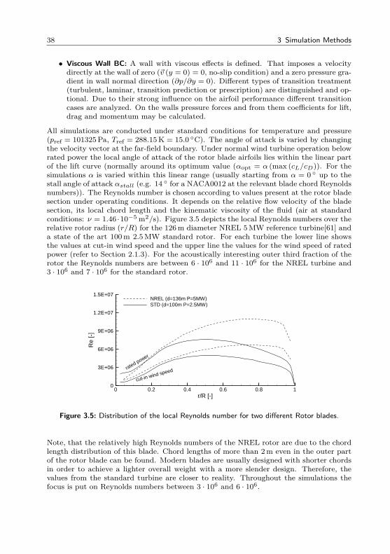
38 3 Simulation Methods

• Viscous Wall BC: A wall with viscous effects is defined. That imposes a velocitydirectly at the wall of zero (~v (y = 0) = 0, no-slip condition) and a zero pressure gra-dient in wall normal direction (∂p/∂y = 0). Different types of transition treatment(turbulent, laminar, transition prediction or prescription) are distinguished and op-tional. Due to their strong influence on the airfoil performance different transitioncases are analyzed. On the walls pressure forces and from them coefficients for lift,drag and momentum may be calculated.

All simulations are conducted under standard conditions for temperature and pressure(pref = 101325 Pa, Tref = 288.15 K = 15.0 C). The angle of attack is varied by changingthe velocity vector at the far-field boundary. Under normal wind turbine operation belowrated power the local angle of attack of the rotor blade airfoils lies within the linear partof the lift curve (normally around its optimum value (αopt = α (max (cL/cD)). For thesimulations α is varied within this linear range (usually starting from α = 0 up to thestall angle of attack αstall (e.g. 14 for a NACA0012 at the relevant blade chord Reynoldsnumbers)). The Reynolds number is chosen according to values present at the rotor bladesection under operating conditions. It depends on the relative flow velocity of the bladesection, its local chord length and the kinematic viscosity of the fluid (air at standardconditions: ν = 1.46 ·10−5 m2/s). Figure 3.5 depicts the local Reynolds numbers over therelative rotor radius (r/R) for the 126m diameter NREL 5MW reference turbine[61] anda state of the art 100m 2.5MW standard rotor. For each turbine the lower line showsthe values at cut-in wind speed and the upper line the values for the wind speed of ratedpower (refer to Section 2.1.3). For the acoustically interesting outer third fraction of therotor the Reynolds numbers are between 6 · 106 and 11 · 106 for the NREL turbine and3 · 106 and 7 · 106 for the standard rotor.

r/R [-]

Re

[-]

0 0.2 0.4 0.6 0.8 10

3E+06

6E+06

9E+06

1.2E+07

1.5E+07NREL (d=136m P=5MW)STD (d=100m P=2.5MW)

cut-in wind speedrated power

Figure 3.5: Distribution of the local Reynolds number for two different Rotor blades.

Note, that the relatively high Reynolds numbers of the NREL rotor are due to the chordlength distribution of this blade. Chord lengths of more than 2m even in the outer partof the rotor blade can be found. Modern blades are usually designed with shorter chordsin order to achieve a lighter overall weight with a more slender design. Therefore, thevalues from the standard turbine are closer to reality. Throughout the simulations thefocus is put on Reynolds numbers between 3 · 106 and 6 · 106.

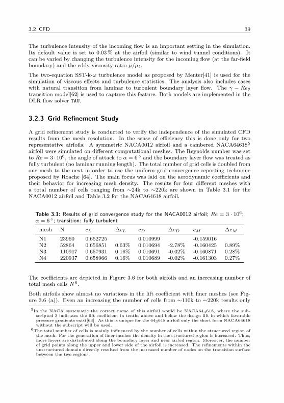
3.2 CFD 39

The turbulence intensity of the incoming flow is an important setting in the simulation.Its default value is set to 0.03% at the airfoil (similar to wind tunnel conditions). Itcan be varied by changing the turbulence intensity for the incoming flow (at the far-fieldboundary) and the eddy viscosity ratio µ/µt.

The two-equation SST-k-ω turbulence model as proposed by Menter[41] is used for thesimulation of viscous effects and turbulence statistics. The analysis also includes caseswith natural transition from laminar to turbulent boundary layer flow. The γ − Reθtransition model[62] is used to capture this feature. Both models are implemented in theDLR flow solver TAU.

3.2.3 Grid Refinement Study

A grid refinement study is conducted to verify the independence of the simulated CFDresults from the mesh resolution. In the sense of efficiency this is done only for tworepresentative airfoils. A symmetric NACA0012 airfoil and a cambered NACA646185airfoil were simulated on different computational meshes. The Reynolds number was setto Re = 3 · 106, the angle of attack to α = 6 and the boundary layer flow was treated asfully turbulent (no laminar running length). The total number of grid cells is doubled fromone mesh to the next in order to use the uniform grid convergence reporting techniqueproposed by Roache [64]. The main focus was laid on the aerodynamic coefficients andtheir behavior for increasing mesh density. The results for four different meshes witha total number of cells ranging from ∼24k to ∼220k are shown in Table 3.1 for theNACA0012 airfoil and Table 3.2 for the NACA64618 airfoil.

Table 3.1: Results of grid convergence study for the NACA0012 airfoil; Re = 3 · 106;α = 6 ; transition: fully turbulentmesh N cL ∆cL cD ∆cD cM ∆cMN1 23960 0.652725 0.010999 -0.159016N2 52864 0.656851 0.63% 0.010694 -2.78% -0.160425 0.89%N3 110917 0.657931 0.16% 0.010691 -0.02% -0.160871 0.28%N4 220937 0.658966 0.16% 0.010689 -0.02% -0.161303 0.27%

The coefficients are depicted in Figure 3.6 for both airfoils and an increasing number oftotal mesh cells N6.

Both airfoils show almost no variations in the lift coefficient with finer meshes (see Fig-ure 3.6 (a)). Even an increasing the number of cells from ∼110k to ∼220k results only

5In the NACA systematic the correct name of this airfoil would be NACA643618, where the sub-scripted 3 indicates the lift coefficient in tenths above and below the design lift in which favorablepressure gradients exist[63]. As this is unique for the 643618 airfoil only the short form NACA64618without the subscript will be used.

6The total number of cells is mainly influenced by the number of cells within the structured region ofthe mesh. For the generation of finer meshes the density in the structured region is increased. Thus,more layers are distributed along the boundary layer and near airfoil region. Moreover, the numberof grid points along the upper and lower side of the airfoil is increased. The refinements within theunstructured domain directly resulted from the increased number of nodes on the transition surfacebetween the two regions.

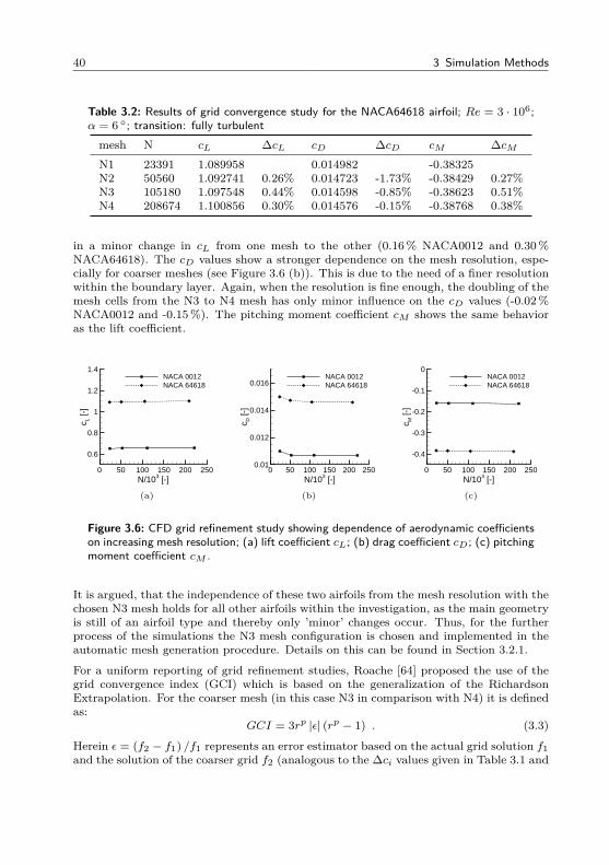
40 3 Simulation Methods

Table 3.2: Results of grid convergence study for the NACA64618 airfoil; Re = 3 · 106;α = 6 ; transition: fully turbulentmesh N cL ∆cL cD ∆cD cM ∆cMN1 23391 1.089958 0.014982 -0.38325N2 50560 1.092741 0.26% 0.014723 -1.73% -0.38429 0.27%N3 105180 1.097548 0.44% 0.014598 -0.85% -0.38623 0.51%N4 208674 1.100856 0.30% 0.014576 -0.15% -0.38768 0.38%

in a minor change in cL from one mesh to the other (0.16% NACA0012 and 0.30%NACA64618). The cD values show a stronger dependence on the mesh resolution, espe-cially for coarser meshes (see Figure 3.6 (b)). This is due to the need of a finer resolutionwithin the boundary layer. Again, when the resolution is fine enough, the doubling of themesh cells from the N3 to N4 mesh has only minor influence on the cD values (-0.02%NACA0012 and -0.15%). The pitching moment coefficient cM shows the same behavioras the lift coefficient.

N/103 [-]

c L [-

]

0 50 100 150 200 250

0.6

0.8

1

1.2

1.4NACA 0012NACA 64618

(a)

N/103 [-]

c D [-

]

0 50 100 150 200 2500.01

0.012

0.014

0.016NACA 0012NACA 64618

(b)

N/103 [-]

c M [-

]

0 50 100 150 200 250

-0.4

-0.3

-0.2

-0.1

0NACA 0012NACA 64618

(c)

Figure 3.6: CFD grid refinement study showing dependence of aerodynamic coefficientson increasing mesh resolution; (a) lift coefficient cL; (b) drag coefficient cD; (c) pitchingmoment coefficient cM .

It is argued, that the independence of these two airfoils from the mesh resolution with thechosen N3 mesh holds for all other airfoils within the investigation, as the main geometryis still of an airfoil type and thereby only ’minor’ changes occur. Thus, for the furtherprocess of the simulations the N3 mesh configuration is chosen and implemented in theautomatic mesh generation procedure. Details on this can be found in Section 3.2.1.

For a uniform reporting of grid refinement studies, Roache [64] proposed the use of thegrid convergence index (GCI) which is based on the generalization of the RichardsonExtrapolation. For the coarser mesh (in this case N3 in comparison with N4) it is definedas:

GCI = 3rp |ε| (rp − 1) . (3.3)

Herein ε = (f2 − f1) /f1 represents an error estimator based on the actual grid solution f1and the solution of the coarser grid f2 (analogous to the ∆ci values given in Table 3.1 and

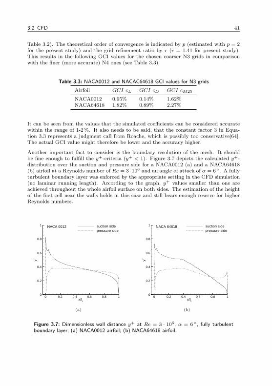
3.2 CFD 41

Table 3.2). The theoretical order of convergence is indicated by p (estimated with p = 2for the present study) and the grid refinement ratio by r (r = 1.41 for present study).This results in the following GCI values for the chosen coarser N3 grids in comparisonwith the finer (more accurate) N4 ones (see Table 3.3).

Table 3.3: NACA0012 and NACAC64618 GCI values for N3 gridsAirfoil GCI cL GCI cD GCI cM25

NACA0012 0.95% 0.14% 1.62%NACA64618 1.82% 0.89% 2.27%

It can be seen from the values that the simulated coefficients can be considered accuratewithin the range of 1-2%. It also needs to be said, that the constant factor 3 in Equa-tion 3.3 represents a judgment call from Roache, which is possibly too conservative[64].The actual GCI value might therefore be lower and the accuracy higher.

Another important fact to consider is the boundary resolution of the mesh. It shouldbe fine enough to fulfill the y+-criteria (y+ < 1). Figure 3.7 depicts the calculated y+-distribution over the suction and pressure side for a NACA0012 (a) and a NACA64618(b) airfoil at a Reynolds number of Re = 3 ·106 and an angle of attack of α = 6 . A fullyturbulent boundary layer was enforced by the appropriate setting in the CFD simulation(no laminar running length). According to the graph, y+ values smaller than one areachieved throughout the whole airfoil surface on both sides. The estimation of the heightof the first cell near the walls holds in this case and still bears enough reserve for higherReynolds numbers.

x/lc

y+

0 0.2 0.4 0.6 0.8 10

0.2

0.4

0.6

0.8

1 suction sidepressure side

NACA 0012

(a)

x/lc

y+

0 0.2 0.4 0.6 0.8 10

0.2

0.4

0.6

0.8

1 suction sidepressure side

NACA 64618

(b)

Figure 3.7: Dimensionless wall distance y+ at Re = 3 · 106, α = 6 , fully turbulentboundary layer; (a) NACA0012 airfoil; (b) NACA64618 airfoil.

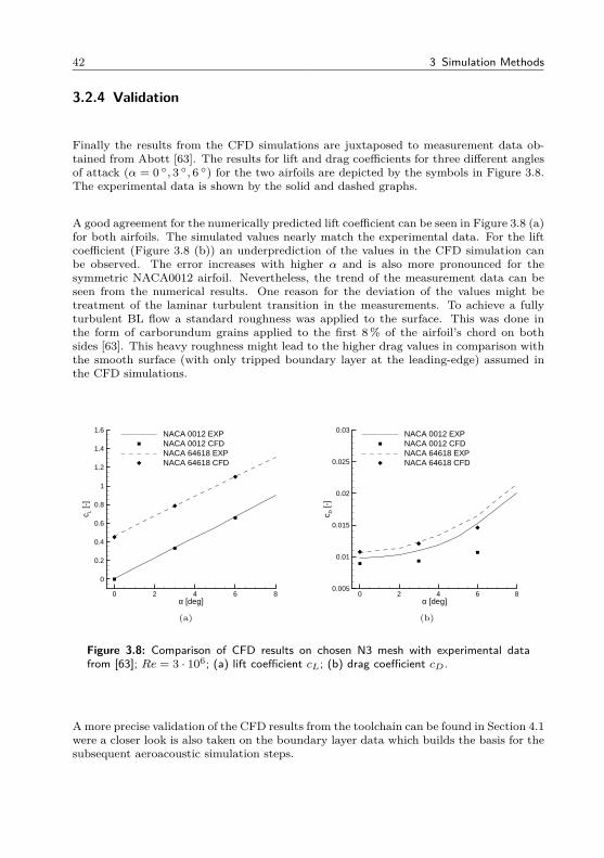
42 3 Simulation Methods

3.2.4 Validation

Finally the results from the CFD simulations are juxtaposed to measurement data ob-tained from Abott [63]. The results for lift and drag coefficients for three different anglesof attack (α = 0 , 3 , 6 ) for the two airfoils are depicted by the symbols in Figure 3.8.The experimental data is shown by the solid and dashed graphs.

A good agreement for the numerically predicted lift coefficient can be seen in Figure 3.8 (a)for both airfoils. The simulated values nearly match the experimental data. For the liftcoefficient (Figure 3.8 (b)) an underprediction of the values in the CFD simulation canbe observed. The error increases with higher α and is also more pronounced for thesymmetric NACA0012 airfoil. Nevertheless, the trend of the measurement data can beseen from the numerical results. One reason for the deviation of the values might betreatment of the laminar turbulent transition in the measurements. To achieve a fullyturbulent BL flow a standard roughness was applied to the surface. This was done inthe form of carborundum grains applied to the first 8% of the airfoil’s chord on bothsides [63]. This heavy roughness might lead to the higher drag values in comparison withthe smooth surface (with only tripped boundary layer at the leading-edge) assumed inthe CFD simulations.

α [deg]

c L [-

]

0 2 4 6 8

0

0.2

0.4

0.6

0.8

1

1.2

1.4

1.6 NACA 0012 EXPNACA 0012 CFDNACA 64618 EXPNACA 64618 CFD

(a)

α [deg]

c D [-

]

0 2 4 6 80.005

0.01

0.015

0.02

0.025

0.03 NACA 0012 EXPNACA 0012 CFDNACA 64618 EXPNACA 64618 CFD

(b)

Figure 3.8: Comparison of CFD results on chosen N3 mesh with experimental datafrom [63]; Re = 3 · 106; (a) lift coefficient cL; (b) drag coefficient cD.

Amore precise validation of the CFD results from the toolchain can be found in Section 4.1were a closer look is also taken on the boundary layer data which builds the basis for thesubsequent aeroacoustic simulation steps.

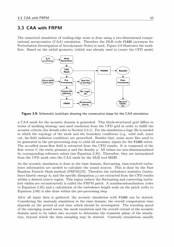
3.3 CAA with FRPM 43

3.3 CAA with FRPM

The numerical simulation of trailing-edge noise is done using a two-dimensional compu-tational aeroacoustics (CAA) simulation. Therefore the DLR code PIANO (acronym forPerturbation Investigation of Aerodynamic Noise) is used. Figure 3.9 illustrates the work-flow. Based on the airfoil geometry (which was already used to create the CFD mesh)

X,YCoordindates

Mesh

Generation

CAA

Mesh

Spectra,

OASPL,

etc.

Post-

ProcessingCAA & FRPM

Input Data

FRPM

PIANO

Pre-

Processing

Turbulence Data

(FRPM Patch)

Mean Flow

on CAA Mesh

4D Stochastic

Sources

BC, Logic,

etc.

Results

Figure 3.9: Schematic toolchain showing the consecutive steps for the CAA simulation.

a CAA mesh for the acoustic domain is generated. This block-structured grid differs interms of meshing strategy and used resolution from the CFD grid in order to fulfill theacoustic criteria (for details refer to Section 3.3.1). For the simulation a logic file is neededin which the topology of the mesh and the boundary conditions (e.g. solid wall, innercut, far-field radiation condition) are prescribed. Besides that, some more files need tobe generated in the pre-processing step to yield all necessary inputs for the PIANO solver.The so-called mean-flow field is extracted from the CFD results. It is composed of theflow vector ~v, the static pressure p and the density ρ. All values are non-dimensionalizedby corresponding reference values (see Equation 2.35). Thereafter, they are interpolatedfrom the CFD mesh onto the CAA mesh by the DLR tool UGINT.

As the acoustic simulation is done in the time domain, fluctuating, time-resolved turbu-lence information are needed to calculate the sound sources. This is done by the FastRandom Particle Mesh method (FRPM)[55]. Therefore the turbulence statistics (turbu-lence kinetic energy kt and the specific dissipation ω) are extracted from the CFD resultswithin a desired source region. This region (where the fluctuating and convecting turbu-lent eddies are reconstructed) is called the FRPM patch. A nondimensionalization (referto Equation 2.35) and a calculation of the turbulence length scale on the patch (refer toEquation 2.60) is also done within the pre-processing step.

After all input data is gathered, the acoustic simulation with PIANO can be started.Considering the unsteady simulation in the time domain, the overall computation timedepends on the period of real time which should be investigated. The traveling speedof the emerging sound waves, the mesh resolution and the overall extend of the acousticdomain need to be taken into account to determine the transient phase of the simula-tion, beyond which the data sampling may be started. Unsteady simulations usually

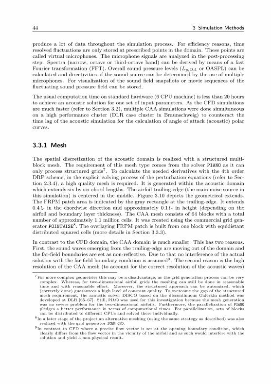
44 3 Simulation Methods

produce a lot of data throughout the simulation process. For efficiency reasons, timeresolved fluctuations are only stored at prescribed points in the domain. These points arecalled virtual microphones. The microphone signals are analyzed in the post-processingstep. Spectra (narrow, octave or third-octave band) can be derived by means of a fastFourier transformation (FFT). Overall sound pressure levels (Lp,OA or OASPL) can becalculated and directivities of the sound source can be determined by the use of multiplemicrophones. For visualization of the sound field snapshots or movie sequences of thefluctuating sound pressure field can be stored.

The usual computation time on standard hardware (6 CPU machine) is less than 20 hoursto achieve an acoustic solution for one set of input parameters. As the CFD simulationsare much faster (refer to Section 3.2), multiple CAA simulations were done simultaneouson a high performance cluster (DLR case cluster in Braunschweig) to counteract thetime lag of the acoustic simulation for the calculation of angle of attack (acoustic) polarcurves.

3.3.1 Mesh

The spatial discretization of the acoustic domain is realized with a structured multi-block mesh. The requirement of this mesh type comes from the solver PIANO as it canonly process structured grids7. To calculate the needed derivatives with the 4th orderDRP scheme, in the explicit solving process of the perturbation equations (refer to Sec-tion 2.3.4), a high quality mesh is required. It is generated within the acoustic domainwhich extends six by six chord lengths. The airfoil trailing-edge (the main noise source inthis simulation) is centered in the middle. Figure 3.10 depicts the geometrical extends.The FRPM patch area is indicated by the gray rectangle at the trailing-edge. It extends0.4 lc in the chordwise direction and approximately 0.1 lc in height (depending on theairfoil and boundary layer thickness). The CAA mesh consists of 64 blocks with a totalnumber of approximately 1.1 million cells. It was created using the commercial grid gen-erator POINTWISE8. The overlaying FRPM patch is built from one block with equidistantdistributed squared cells (more details in Section 3.3.3).

In contrast to the CFD domain, the CAA domain is much smaller. This has two reasons.First, the sound waves emerging from the trailing-edge are moving out of the domain andthe far-field boundaries are set as non-reflective. Due to that no interference of the actualsolution with the far-field boundary condition is assumed9. The second reason is the highresolution of the CAA mesh (to account for the correct resolution of the acoustic waves)

7For more complex geometries this may be a disadvantage, as the grid generation process can be verycomplex. Whereas, for two-dimensional airfoil grids the meshing can still be done in reasonabletime and with reasonable effort. Moreover, the structured approach can be automized, which(correctly done) guarantees a high level of constant quality. To overcome the gap of the structuredmesh requirement, the acoustic solver DISCO based on the discontinuous Galerkin method wasdeveloped at DLR [65–67]. Still, PIANO was used for this investigation because the mesh generationwas no severe problem for the two-dimensional airfoils. Furthermore, the parallelization of PIANOpledges a better performance in terms of computational times. For parallelization, sets of blockscan be distributed to different CPUs and solved there individually.

8In a later stage of the project an alternative meshing (using the same strategy as described) was alsorealized with the grid generator ICEM CFD.

9In contrast to CFD where a precise flow vector is set at the opening boundary condition, whichclearly differs from the flow vector in the vicinity of the airfoil and as such would interfere with thesolution and yield a non-physical result.

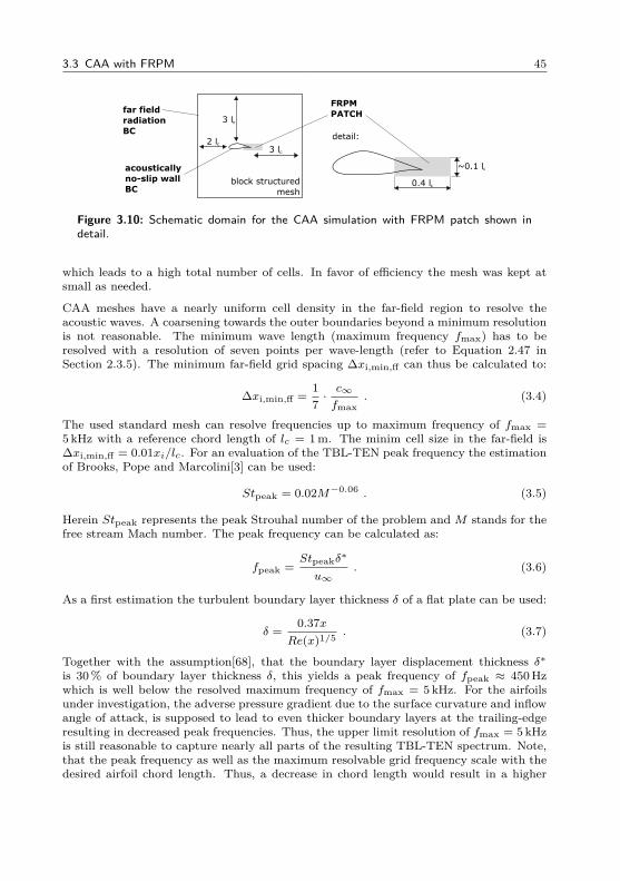
3.3 CAA with FRPM 45

2 lc3 lc

3 lc

acoustically

no-slip wall

BC

far field

radiation

BC

FRPM

PATCH

block structured

mesh

detail:

0.4 lc

~0.1 lc

Figure 3.10: Schematic domain for the CAA simulation with FRPM patch shown indetail.

which leads to a high total number of cells. In favor of efficiency the mesh was kept atsmall as needed.

CAA meshes have a nearly uniform cell density in the far-field region to resolve theacoustic waves. A coarsening towards the outer boundaries beyond a minimum resolutionis not reasonable. The minimum wave length (maximum frequency fmax) has to beresolved with a resolution of seven points per wave-length (refer to Equation 2.47 inSection 2.3.5). The minimum far-field grid spacing ∆xi,min,ff can thus be calculated to:

∆xi,min,ff =17·c∞

fmax. (3.4)

The used standard mesh can resolve frequencies up to maximum frequency of fmax =5 kHz with a reference chord length of lc = 1 m. The minim cell size in the far-field is∆xi,min,ff = 0.01xi/lc. For an evaluation of the TBL-TEN peak frequency the estimationof Brooks, Pope and Marcolini[3] can be used:

Stpeak = 0.02M−0.06 . (3.5)

Herein Stpeak represents the peak Strouhal number of the problem and M stands for thefree stream Mach number. The peak frequency can be calculated as:

fpeak =Stpeakδ

∗

u∞. (3.6)

As a first estimation the turbulent boundary layer thickness δ of a flat plate can be used:

δ =0.37x

Re(x)1/5 . (3.7)

Together with the assumption[68], that the boundary layer displacement thickness δ∗is 30% of boundary layer thickness δ, this yields a peak frequency of fpeak ≈ 450 Hzwhich is well below the resolved maximum frequency of fmax = 5 kHz. For the airfoilsunder investigation, the adverse pressure gradient due to the surface curvature and inflowangle of attack, is supposed to lead to even thicker boundary layers at the trailing-edgeresulting in decreased peak frequencies. Thus, the upper limit resolution of fmax = 5 kHzis still reasonable to capture nearly all parts of the resulting TBL-TEN spectrum. Note,that the peak frequency as well as the maximum resolvable grid frequency scale with thedesired airfoil chord length. Thus, a decrease in chord length would result in a higher

46 3 Simulation Methods

peak frequency and also in a higher resolvable frequency. Consequently no mesh adaptionis required if the absolute chord length is changed.

For the simulations with the FRPMmethod, the CAAmesh must have the same resolutionas the FRPM source patch within the patch region. The resolution of the patch isdetermined by the smallest turbulent eddy size which should be reconstructed (for detailssee Section 3.3.3). For the trailing-edge noise problem, this resolution is usually waybelow the far-field resolution(e.g. ∆xi,min,patch = 0.0005xi/lc which represents a sizereduction by the factor 20). This leads to the difficulty that a much finer resolutionoccurs within the trailing-edge region (FRPM patch region) of the CAA mesh. If allthe mesh would be resolved with this fine resolution, the total number of cells wouldget unacceptably high. This would either lead to a higher number of CPUs for theparallelization or simply to longer computational times. To counteract this, a meshingstrategy is used, where the increase of cell numbers (and thereby the decrease of cell sizes)within a certain region around the trailing-edge is possible without interfering too strongwith other parts of the block-structured mesh. Therefore, a so-called clamping grid willbe used, where an O-type mesh runs around the trailing-edge. This strategy makes itpossible to stretch the dense cells directly at the trailing-edge source region towards theouter parts of the mesh. Moreover the number of cells within the O-grid can directly becontrolled without influence on other parts of the CAA mesh. The O-grid disemboguesin a C-type grid around the airfoil nose which is further embedded in a H-grid topologytowards the outer boundaries. Figure 3.11 shows an exemplary CAA mesh for a DU-96-W-180 airfoil created with the prescribed strategy. An overview of the acoustic domain isshown in Figure 3.11 (a). The trailing-edge region, the clamping meshing approach andthe overlying FRPM patch (indicated in red) are shown in (b). A detailed view of theTE region can be seen in (c). Note, that due to visualization issues only every tenth gridline is shown in these plots.

The clamping CAA grid strategy allows it to keep the overall amount of cells withinreasonable and feasible limits. Due to the rather large ratio of the different cell sizesa denser mesh region above and below the trailing-edge remains. A smooth transitionbetween different cell sizes with an exponential growth factor of 1.1 is enforced. Furtherdistortion of the cells towards the outside region is avoided to keep the internal cellangles as close to 90 as possible. Still, a very high grid quality is achieved whichis mandatory for good aeroacoustic results. Finally, a smoothing algorithm is used toimprove the blending between different cell sizes and angles, especially at the internalblock intersections.

To quantify the mesh quality the following indicators are extracted from the exampleDU-96 mesh using ICEM CFD:

• Maximum Aspect Ratio = 21.9 (highest ratio for thin cells in the dense area aboveand below the TE towards the far-field)

• Minimum Angle = 39.5 (minimum angle of cell internal faces)

• Maximum Angle = 144.9 (maximum angle of cell internal faces)

• Minimum Eriksson Skewness = 0.638 (empirical criterion in ICEM CFD to judge theelement shear for a hexahedral element (see Footnote 4))

• Maximum Volume Change = 1.15 in the structured near airfoil region and 1.4 in theouter mesh region (ensures smooth increase in volume of neighboring cells)

3.3 CAA with FRPM 47

(a) (b)

(c)

Figure 3.11: CAA mesh example for a DU-96-W-180 with FRPM source patch mesh(shown in red) - for better visualization only every tenth grid line is shown; (a) do-main overview; (b) blocks in TE vicinity (clamping) with FRPM patch; (c) matchingresolutions of CAA mesh and FRPM patch.

Similar to the preparation of the CFD grid an automation strategy relying on replayscripts was developed for the CAA meshes. Beside the fast generation of acoustic gridsfor new airfoil geometries it ensures a consistent mesh quality throughout arbitrary airfoilgeometries.

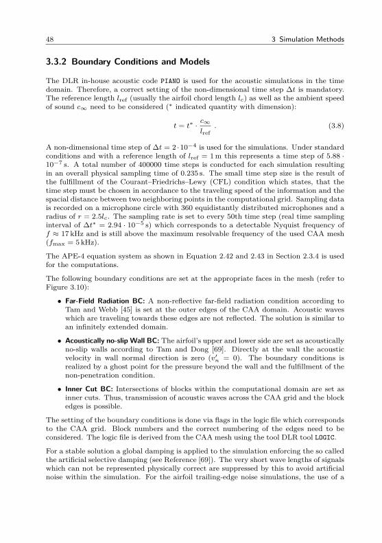
48 3 Simulation Methods

3.3.2 Boundary Conditions and Models

The DLR in-house acoustic code PIANO is used for the acoustic simulations in the timedomain. Therefore, a correct setting of the non-dimensional time step ∆t is mandatory.The reference length lref (usually the airfoil chord length lc) as well as the ambient speedof sound c∞ need to be considered (∗ indicated quantity with dimension):

t = t∗ ·c∞

lref. (3.8)

A non-dimensional time step of ∆t = 2 ·10−4 is used for the simulations. Under standardconditions and with a reference length of lref = 1 m this represents a time step of 5.88 ·10−7 s. A total number of 400000 time steps is conducted for each simulation resultingin an overall physical sampling time of 0.235 s. The small time step size is the result ofthe fulfillment of the Courant–Friedrichs–Lewy (CFL) condition which states, that thetime step must be chosen in accordance to the traveling speed of the information and thespacial distance between two neighboring points in the computational grid. Sampling datais recorded on a microphone circle with 360 equidistantly distributed microphones and aradius of r = 2.5lc. The sampling rate is set to every 50th time step (real time samplinginterval of ∆t∗ = 2.94 · 10−5 s) which corresponds to a detectable Nyquist frequency off ≈ 17 kHz and is still above the maximum resolvable frequency of the used CAA mesh(fmax = 5 kHz).

The APE-4 equation system as shown in Equation 2.42 and 2.43 in Section 2.3.4 is usedfor the computations.

The following boundary conditions are set at the appropriate faces in the mesh (refer toFigure 3.10):

• Far-Field Radiation BC: A non-reflective far-field radiation condition according toTam and Webb [45] is set at the outer edges of the CAA domain. Acoustic waveswhich are traveling towards these edges are not reflected. The solution is similar toan infinitely extended domain.

• Acoustically no-slip Wall BC: The airfoil’s upper and lower side are set as acousticallyno-slip walls according to Tam and Dong [69]. Directly at the wall the acousticvelocity in wall normal direction is zero (v′n = 0). The boundary conditions isrealized by a ghost point for the pressure beyond the wall and the fulfillment of thenon-penetration condition.

• Inner Cut BC: Intersections of blocks within the computational domain are set asinner cuts. Thus, transmission of acoustic waves across the CAA grid and the blockedges is possible.

The setting of the boundary conditions is done via flags in the logic file which correspondsto the CAA grid. Block numbers and the correct numbering of the edges need to beconsidered. The logic file is derived from the CAA mesh using the tool DLR tool LOGIC.

For a stable solution a global damping is applied to the simulation enforcing the so calledthe artificial selective damping (see Reference [69]). The very short wave lengths of signalswhich can not be represented physically correct are suppressed by this to avoid artificialnoise within the simulation. For the airfoil trailing-edge noise simulations, the use of a

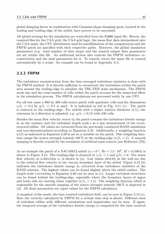
3.3 CAA with FRPM 49

global damping factor in combination with Gaussian-shape damping spots, located at theleading and trailing-edge of the airfoil, have proven to be successful.

All global settings for the simulation are controlled from the PIANO input file. Herein, therequired files for the CAA grid, the CAA grid logic, the mean flow data interpolated ontothe CAA mesh, the CPU distribution used for parallelization of the computations and theFRPM patch are specified with their respective paths. Moreover, the global simulationparameters (e.g. total number of time steps) and the wanted output data parametersare set within this file. An additional section also controls the FRPM turbulence re-construction and the used parameters for it. To remedy errors the input file is createdautomatically by a script. An example can be found in Appendix A.5.

3.3.3 FRPM

The turbulence reconstruction from the time averaged turbulence statistics is done withthe FRPM method. It is thereby sufficient to reconstruct the turbulence within the patcharea around the trailing-edge to simulate the TBL-TEN noise mechanism. The FRPMmesh size and the total number of cells within the patch account for the numerical effortin the simulation process. The FRPM calculations are processed solely by one CPU.

For all test cases a 800 by 200 cells source patch with quadratic cells and the dimensionsx/lc = 0.4 by y/lc = 0.1 is used. It is indicated in red in Fig. 3.11 (c). The patchis centered at the trailing-edge. For airfoils with a higher relative thickness (t/lc) theextension in y-direction is adjusted, e.g. y/lc = 0.12 with 240 cells.

Besides the mean flow velocity vector ~v0 the patch contains the turbulence kinetic energykt as the variance and the turbulent length scale l as a size measurement of the recon-structed eddies. All values are extracted from the previously conducted RANS simulationand non-dimensionalized according to Equation 2.35. Additionally, a weighting functionw(~x) as indicated in Equation 2.58 is set as a variable on the patch. This weighting func-tion ramps the source strength towards 100 % at the trailing-edge (x/lc = 1). A smoothramping is thereby crucial for the avoidance of artificial noise sources (see Reference [70])

As an example the patch of a NACA0012 airfoil (α = 0 , Re = 1.5 · 106, M = 0.1664) isshown in Figure 3.12. The trailing-edge is situated at x/lc = 1 and y/lc = 0. The meanflow velocity in x-direction vx is shown in (a). Low values directly at the wall are dueto the reduced flow velocity in the viscous boundary layer of the airfoil. Figure 3.12 (b)indicates the turbulence kinetic energy kt extracted from turbulence statistics of theRANS solution. The highest values can be found slightly above the airfoil surface. Thelength scale l according to Equation 2.60 can be seen in (c). Larger turbulent structurescan be found behind the trailing-edge, especially where the boundary layers of upperand lower side are moving closer together (x/lc > 1.1). The weighting function which isresponsible for the smooth ramping of the source strength towards 100 % is depicted in(d). All these parameters are input values for the FRPM calculation.

A snapshot of the result, the time resolved turbulence field, can be seen in Figure 3.12 (e).Here the vorticity calculated by FRPM for a certain time step is shown. Different sizesof turbulent eddies with different orientations and magnitudes can be seen. If again,the temporal average of the turbulence kinetic energy is computed for the time resolved

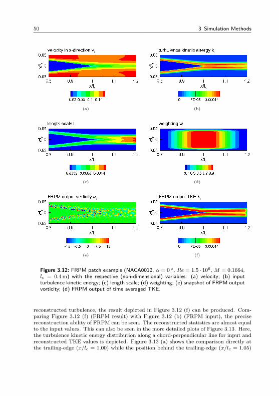
50 3 Simulation Methods

(a) (b)

(c) (d)

(e) (f)

Figure 3.12: FRPM patch example (NACA0012, α = 0 , Re = 1.5 · 106, M = 0.1664,lc = 0.4 m) with the respective (non-dimensional) variables: (a) velocity; (b) inputturbulence kinetic energy; (c) length scale; (d) weighting; (e) snapshot of FRPM outputvorticity; (d) FRPM output of time averaged TKE.

reconstructed turbulence, the result depicted in Figure 3.12 (f) can be produced. Com-paring Figure 3.12 (f) (FRPM result) with Figure 3.12 (b) (FRPM input), the precisereconstruction ability of FRPM can be seen. The reconstructed statistics are almost equalto the input values. This can also be seen in the more detailed plots of Figure 3.13. Here,the turbulence kinetic energy distribution along a chord-perpendicular line for input andreconstructed TKE values is depicted. Figure 3.13 (a) shows the comparison directly atthe trailing-edge (x/lc = 1.00) while the position behind the trailing-edge (x/lc = 1.05)

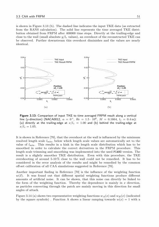
3.3 CAA with FRPM 51

is shown in Figure 3.13 (b). The dashed line indicates the input TKE data (as extractedfrom the RANS calculation). The solid line represents the time averaged TKE distri-bution obtained from FRPM after 400000 time steps. Directly at the trailing-edge andclose to the wall (small absolute y/lc values), an overshoot of the reconstructed TKE canbe observed. Further downstream this overshoot diminishes and the values are nearlyidentical.

kt

y/l c

0 0.0001 0.0002 0.0003-0.04

-0.02

0

0.02

0.04TKE InputTKE Result FRPM

FRPM patch

NACA0012

Position:x/lc = 1.00

(a)

kt

y/l c

0 0.0001 0.0002 0.0003-0.04

-0.02

0

0.02

0.04TKE InputTKE Result FRPM

FRPM patch

NACA0012

Position:x/lc = 1.05

(b)

Figure 3.13: Comparison of input TKE to time averaged FRPM result along a verticalline (y-direction) (NACA0012, α = 0 , Re = 1.5 · 106, M = 0.1664, lc = 0.4 m):(a) directly at the trailing-edge at x/lc = 1.00 and (b) behind the trailing-edge atx/lc = 1.05.

It is shown in Reference [70], that the overshoot at the wall is influenced by the minimumresolved length scale lmin, below which length scale values are automatically set to thevalue of lmin. This results in a kink in the length scale distribution which has to besmoothed in order to calculate the correct derivatives in the FRPM procedure. Thislength scale trimming and smoothing was implemented into the used PIANO version. Theresult is a slightly smoother TKE distribution. Even with this procedure, the TKEovershooting of around 5-10% close to the wall could not be remedied. It has to beconsidered in the error analysis of the results and might be remedied by the commonoff-set calibration of all CAA simulations suggested in Reference [70].

Another important finding in Reference [70] is the influence of the weighting functionw(~x). It was found out that different spatial weighting functions produce differentamounts of artificial noise. It can be shown, that this noise can directly be linked tothe form of the weighting function. Thereby the dependence is mainly in x direction,as particles convecting through the patch are mainly moving in this direction for smallangles of attack.

Figure 3.14 (a) shows two representative weighting functions wA(x) and wB(x) (indicatedby the square symbols) . Function A shows a linear ramping towards w(x) = 1 with a

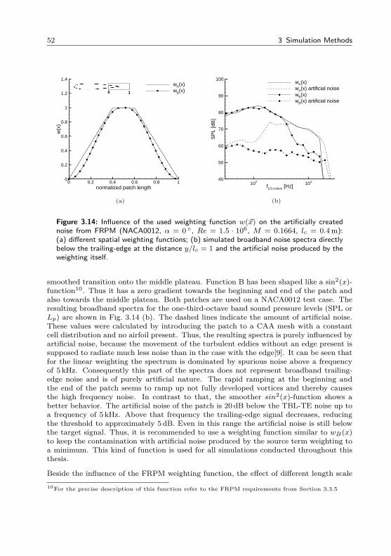
52 3 Simulation Methods

normalized patch length

w(x

)

0 0.2 0.4 0.6 0.8 10

0.2

0.4

0.6

0.8

1

1.2

1.4wA(x)wB(x)0 1

(a)

f1/3 octave [Hz]

SP

L [d

B]

103 10440

50

60

70

80

90

100wA(x)wA(x) artificial noisewB(x)wB(x) artificial noise

(b)

Figure 3.14: Influence of the used weighting function w(~x) on the artificially creatednoise from FRPM (NACA0012, α = 0 , Re = 1.5 · 106, M = 0.1664, lc = 0.4 m):(a) different spatial weighting functions; (b) simulated broadband noise spectra directlybelow the trailing-edge at the distance y/lc = 1 and the artificial noise produced by theweighting itself.

smoothed transition onto the middle plateau. Function B has been shaped like a sin2(x)-function10. Thus it has a zero gradient towards the beginning and end of the patch andalso towards the middle plateau. Both patches are used on a NACA0012 test case. Theresulting broadband spectra for the one-third-octave band sound pressure levels (SPL orLp) are shown in Fig. 3.14 (b). The dashed lines indicate the amount of artificial noise.These values were calculated by introducing the patch to a CAA mesh with a constantcell distribution and no airfoil present. Thus, the resulting spectra is purely influenced byartificial noise, because the movement of the turbulent eddies without an edge present issupposed to radiate much less noise than in the case with the edge[9]. It can be seen thatfor the linear weighting the spectrum is dominated by spurious noise above a frequencyof 5 kHz. Consequently this part of the spectra does not represent broadband trailing-edge noise and is of purely artificial nature. The rapid ramping at the beginning andthe end of the patch seems to ramp up not fully developed vortices and thereby causesthe high frequency noise. In contrast to that, the smoother sin2(x)-function shows abetter behavior. The artificial noise of the patch is 20 dB below the TBL-TE noise up toa frequency of 5 kHz. Above that frequency the trailing-edge signal decreases, reducingthe threshold to approximately 5 dB. Even in this range the artificial noise is still belowthe target signal. Thus, it is recommended to use a weighting function similar to wB(x)to keep the contamination with artificial noise produced by the source term weighting toa minimum. This kind of function is used for all simulations conducted throughout thisthesis.

Beside the influence of the FRPM weighting function, the effect of different length scale10For the precise description of this function refer to the FRPM requirements from Section 3.3.5

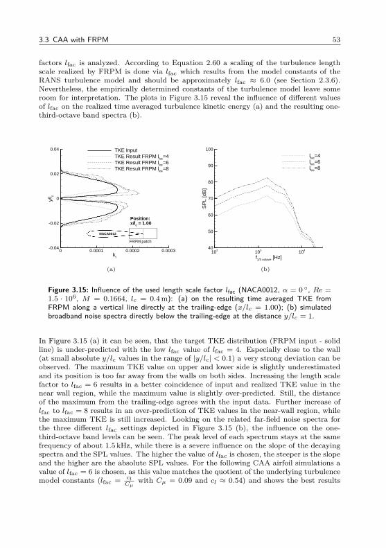
3.3 CAA with FRPM 53

factors lfac is analyzed. According to Equation 2.60 a scaling of the turbulence lengthscale realized by FRPM is done via lfac which results from the model constants of theRANS turbulence model and should be approximately lfac ≈ 6.0 (see Section 2.3.6).Nevertheless, the empirically determined constants of the turbulence model leave someroom for interpretation. The plots in Figure 3.15 reveal the influence of different valuesof lfac on the realized time averaged turbulence kinetic energy (a) and the resulting one-third-octave band spectra (b).

kt

y/l c

0 0.0001 0.0002 0.0003-0.04

-0.02

0

0.02

0.04 TKE InputTKE Result FRPM lfac=4TKE Result FRPM lfac=6TKE Result FRPM lfac=8

FRPM patch

NACA0012

Position:x/lc = 1.00

(a)

f1/3 octave [Hz]

SP

L [d

B]

102 103 10440

50

60

70

80

90

100

lfac=4lfac=6lfac=8

(b)

Figure 3.15: Influence of the used length scale factor lfac (NACA0012, α = 0 , Re =1.5 · 106, M = 0.1664, lc = 0.4 m): (a) on the resulting time averaged TKE fromFRPM along a vertical line directly at the trailing-edge (x/lc = 1.00); (b) simulatedbroadband noise spectra directly below the trailing-edge at the distance y/lc = 1.

In Figure 3.15 (a) it can be seen, that the target TKE distribution (FRPM input - solidline) is under-predicted with the low lfac value of lfac = 4. Especially close to the wall(at small absolute y/lc values in the range of |y/lc| < 0.1) a very strong deviation can beobserved. The maximum TKE value on upper and lower side is slightly underestimatedand its position is too far away from the walls on both sides. Increasing the length scalefactor to lfac = 6 results in a better coincidence of input and realized TKE value in thenear wall region, while the maximum value is slightly over-predicted. Still, the distanceof the maximum from the trailing-edge agrees with the input data. Further increase oflfac to lfac = 8 results in an over-prediction of TKE values in the near-wall region, whilethe maximum TKE is still increased. Looking on the related far-field noise spectra forthe three different lfac settings depicted in Figure 3.15 (b), the influence on the one-third-octave band levels can be seen. The peak level of each spectrum stays at the samefrequency of about 1.5 kHz, while there is a severe influence on the slope of the decayingspectra and the SPL values. The higher the value of lfac is chosen, the steeper is the slopeand the higher are the absolute SPL values. For the following CAA airfoil simulations avalue of lfac = 6 is chosen, as this value matches the quotient of the underlying turbulencemodel constants (lfac = cl

Cµwith Cµ = 0.09 and cl ≈ 0.54) and shows the best results

54 3 Simulation Methods

in turbulence statistics reconstruction. Also, a good agreement of the resulting far-fieldspectrum with experimental data could be achieved with this value (for details refer toSection 4.1).

In Reference [70] the problem of a too steep decrease of the far-field noise spectra in thehigh frequency region was discussed. The theory which links this decrease with the real-ized turbulent energy spectrum E(k) (where k is the wave number k = 2π/λ) providedby FRPM was formulated. By its implementation FRPM realizes a Gaussian energyspectrum EG(k). Contrary to that, Liepmann[71] proposed a different form of the energyspectrum EL(k) with a much shallower decay of turbulence energy towards higher wavenumbers. This can be seen in Figure A.2 (a) in Appendix A.4. In Reference [70] a methodwas shown to realize this Liepmann energy spectrum with a superposition of differentlyscaled mutually uncorrelated individual FRPM realizations with a Gaussian spectrum.Details on this can be found in Appendix A.4. Practically, multiple simulations withdifferently scaled TKE distributions on the FRPM patch according to Equation A.57need to be conducted and later on superposed. The computational effort is thus mul-tiplied by the number of scaled Gaussian FRPM realizations to achieve the Liepmannenergy spectrum. First test cases showed that a number of ten individual simulationswas needed to achieve a precise form of the spectrum. With a logarithmic distribution ofthe scaling factors a reduction to five individual simulations might be feasible. Still, thecomputational effort is increased by the factor of five with this method11.

Throughout progressive research and testing it was found, that a smaller minimum lengthscale factor together with an adapted (finer) patch and CAA resolution, brought thesame effect as the Liepmann realization. Especially in the high frequency region, thesimulated sound pressure levels are better matching the available experimental results.As this solution is considered computationally more efficient than the Liepmann method,it is thus better suitable for the proposed best-practice CAA airfoil simulation. For theplaned simulations of multiple airfoils it is chosen as the best tradeoff of result qualityand computational efficiency. A non-dimensional grid spacing of ∆x/lc = 0.0005 must beused for the FRPM patch as well as the CAA grid in the source region to obtain reliableresults for the desired frequency range. The minimum length scale resolved by FRPMlmin must be at least lmin = 0.002. With this settings lmin is resolved with a resolutionof four patch cells.

Figure 3.16 depicts the differences of the simulated CAA results in contrast to measure-ment data from Reference [72]. Together with the measurement values (black squares)error bars indicate the uncertainty range of the acoustic wind tunnel data which is given by3 dB. For the symmetric NACA0012 airfoil under an angle of attack of zero degrees it canbe seen, that the reference CAA simulation (solid line; ∆x/lc = 0.0008 and lmin = 0.005)is able to reproduce the peak frequency of the experimental data around f = 1.5 kHz.Up to a frequency of f = 3 kHz the sound pressure level decay lies within the uncertaintyrange of the measurements. For higher frequencies the simulated values are too low. Incontrast to that, the Liepmann FRPM method (dashed line), which was condensed fromten individual simulations, shows a better matching in the high frequency range. Up tof = 20 kHz the CAA data lies well within the error bars. Note, that the used CAA mesh

11The parallel processing of the different FRPM source patches as multiple uncorrelated sources withinone CAA simulation could help to reduce this effort. Thus, only additional CPUs are necessary toprocess the additional FRPM patches. In a limited resource environment this also might become aproblem.

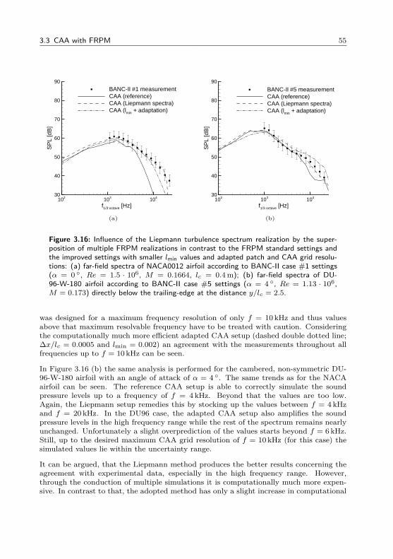
3.3 CAA with FRPM 55

f1/3 octave [Hz]

SP

L [d

B]

102 103 10430

40

50

60

70

80

90

BANC-II #1 measurementCAA (reference)CAA (Liepmann spectra)CAA (lmin + adaptation)

(a)

f1/3 octave [Hz]S

PL

[dB

]102 103 104

30

40

50

60

70

80

90

BANC-II #5 measurementCAA (reference)CAA (Liepmann spectra)CAA (lmin + adaptation)

(b)

Figure 3.16: Influence of the Liepmann turbulence spectrum realization by the super-position of multiple FRPM realizations in contrast to the FRPM standard settings andthe improved settings with smaller lmin values and adapted patch and CAA grid resolu-tions: (a) far-field spectra of NACA0012 airfoil according to BANC-II case #1 settings(α = 0 , Re = 1.5 · 106, M = 0.1664, lc = 0.4 m); (b) far-field spectra of DU-96-W-180 airfoil according to BANC-II case #5 settings (α = 4 , Re = 1.13 · 106,M = 0.173) directly below the trailing-edge at the distance y/lc = 2.5.

was designed for a maximum frequency resolution of only f = 10 kHz and thus valuesabove that maximum resolvable frequency have to be treated with caution. Consideringthe computationally much more efficient adapted CAA setup (dashed double dotted line;∆x/lc = 0.0005 and lmin = 0.002) an agreement with the measurements throughout allfrequencies up to f = 10 kHz can be seen.

In Figure 3.16 (b) the same analysis is performed for the cambered, non-symmetric DU-96-W-180 airfoil with an angle of attack of α = 4 . The same trends as for the NACAairfoil can be seen. The reference CAA setup is able to correctly simulate the soundpressure levels up to a frequency of f = 4 kHz. Beyond that the values are too low.Again, the Liepmann setup remedies this by stocking up the values between f = 4 kHzand f = 20 kHz. In the DU96 case, the adapted CAA setup also amplifies the soundpressure levels in the high frequency range while the rest of the spectrum remains nearlyunchanged. Unfortunately a slight overprediction of the values starts beyond f = 6 kHz.Still, up to the desired maximum CAA grid resolution of f = 10 kHz (for this case) thesimulated values lie within the uncertainty range.

It can be argued, that the Liepmann method produces the better results concerning theagreement with experimental data, especially in the high frequency range. However,through the conduction of multiple simulations it is computationally much more expen-sive. In contrast to that, the adopted method has only a slight increase in computational

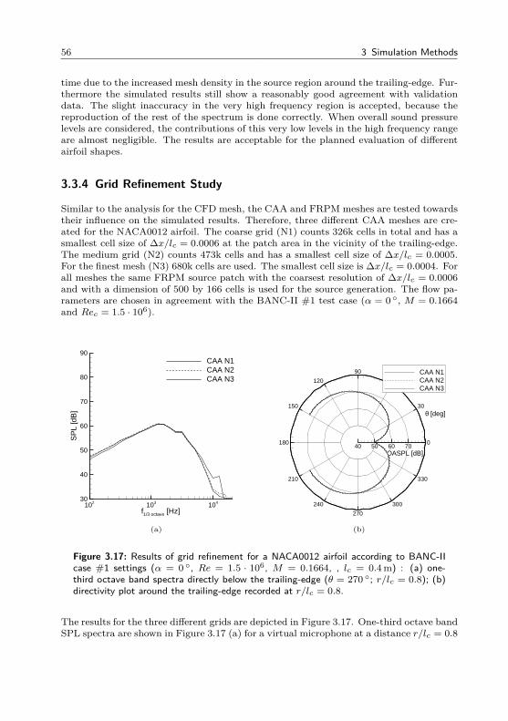
56 3 Simulation Methods

time due to the increased mesh density in the source region around the trailing-edge. Fur-thermore the simulated results still show a reasonably good agreement with validationdata. The slight inaccuracy in the very high frequency region is accepted, because thereproduction of the rest of the spectrum is done correctly. When overall sound pressurelevels are considered, the contributions of this very low levels in the high frequency rangeare almost negligible. The results are acceptable for the planned evaluation of differentairfoil shapes.

3.3.4 Grid Refinement Study

Similar to the analysis for the CFD mesh, the CAA and FRPM meshes are tested towardstheir influence on the simulated results. Therefore, three different CAA meshes are cre-ated for the NACA0012 airfoil. The coarse grid (N1) counts 326k cells in total and has asmallest cell size of ∆x/lc = 0.0006 at the patch area in the vicinity of the trailing-edge.The medium grid (N2) counts 473k cells and has a smallest cell size of ∆x/lc = 0.0005.For the finest mesh (N3) 680k cells are used. The smallest cell size is ∆x/lc = 0.0004. Forall meshes the same FRPM source patch with the coarsest resolution of ∆x/lc = 0.0006and with a dimension of 500 by 166 cells is used for the source generation. The flow pa-rameters are chosen in agreement with the BANC-II #1 test case (α = 0 , M = 0.1664and Rec = 1.5 · 106).

f1/3 octave [Hz]

SP

L [d

B]

102 103 10430

40

50

60

70

80

90CAA N1CAA N2CAA N3

(a)

θ [deg]

OASPL [dB]

0

30

60

90

120

150

180

210

240

270

300

330

40 50 60 70

CAA N1CAA N2CAA N3

(b)

Figure 3.17: Results of grid refinement for a NACA0012 airfoil according to BANC-IIcase #1 settings (α = 0 , Re = 1.5 · 106, M = 0.1664, , lc = 0.4 m) : (a) one-third octave band spectra directly below the trailing-edge (θ = 270 ; r/lc = 0.8); (b)directivity plot around the trailing-edge recorded at r/lc = 0.8.

The results for the three different grids are depicted in Figure 3.17. One-third octave bandSPL spectra are shown in Figure 3.17 (a) for a virtual microphone at a distance r/lc = 0.8

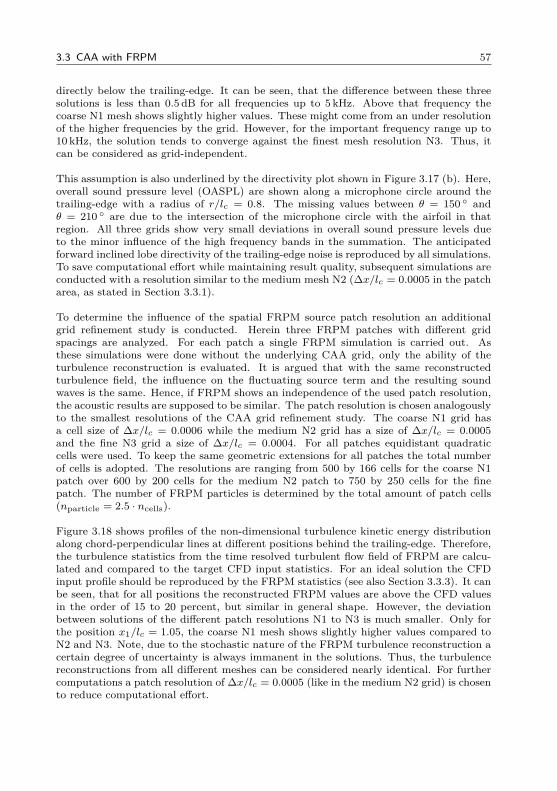
3.3 CAA with FRPM 57

directly below the trailing-edge. It can be seen, that the difference between these threesolutions is less than 0.5 dB for all frequencies up to 5 kHz. Above that frequency thecoarse N1 mesh shows slightly higher values. These might come from an under resolutionof the higher frequencies by the grid. However, for the important frequency range up to10 kHz, the solution tends to converge against the finest mesh resolution N3. Thus, itcan be considered as grid-independent.

This assumption is also underlined by the directivity plot shown in Figure 3.17 (b). Here,overall sound pressure level (OASPL) are shown along a microphone circle around thetrailing-edge with a radius of r/lc = 0.8. The missing values between θ = 150 andθ = 210 are due to the intersection of the microphone circle with the airfoil in thatregion. All three grids show very small deviations in overall sound pressure levels dueto the minor influence of the high frequency bands in the summation. The anticipatedforward inclined lobe directivity of the trailing-edge noise is reproduced by all simulations.To save computational effort while maintaining result quality, subsequent simulations areconducted with a resolution similar to the medium mesh N2 (∆x/lc = 0.0005 in the patcharea, as stated in Section 3.3.1).

To determine the influence of the spatial FRPM source patch resolution an additionalgrid refinement study is conducted. Herein three FRPM patches with different gridspacings are analyzed. For each patch a single FRPM simulation is carried out. Asthese simulations were done without the underlying CAA grid, only the ability of theturbulence reconstruction is evaluated. It is argued that with the same reconstructedturbulence field, the influence on the fluctuating source term and the resulting soundwaves is the same. Hence, if FRPM shows an independence of the used patch resolution,the acoustic results are supposed to be similar. The patch resolution is chosen analogouslyto the smallest resolutions of the CAA grid refinement study. The coarse N1 grid hasa cell size of ∆x/lc = 0.0006 while the medium N2 grid has a size of ∆x/lc = 0.0005and the fine N3 grid a size of ∆x/lc = 0.0004. For all patches equidistant quadraticcells were used. To keep the same geometric extensions for all patches the total numberof cells is adopted. The resolutions are ranging from 500 by 166 cells for the coarse N1patch over 600 by 200 cells for the medium N2 patch to 750 by 250 cells for the finepatch. The number of FRPM particles is determined by the total amount of patch cells(nparticle = 2.5 · ncells).

Figure 3.18 shows profiles of the non-dimensional turbulence kinetic energy distributionalong chord-perpendicular lines at different positions behind the trailing-edge. Therefore,the turbulence statistics from the time resolved turbulent flow field of FRPM are calcu-lated and compared to the target CFD input statistics. For an ideal solution the CFDinput profile should be reproduced by the FRPM statistics (see also Section 3.3.3). It canbe seen, that for all positions the reconstructed FRPM values are above the CFD valuesin the order of 15 to 20 percent, but similar in general shape. However, the deviationbetween solutions of the different patch resolutions N1 to N3 is much smaller. Only forthe position x1/lc = 1.05, the coarse N1 mesh shows slightly higher values compared toN2 and N3. Note, due to the stochastic nature of the FRPM turbulence reconstruction acertain degree of uncertainty is always immanent in the solutions. Thus, the turbulencereconstructions from all different meshes can be considered nearly identical. For furthercomputations a patch resolution of ∆x/lc = 0.0005 (like in the medium N2 grid) is chosento reduce computational effort.

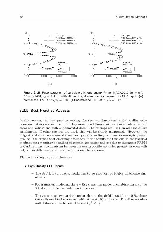
58 3 Simulation Methods

kt

y/l c

0 0.0001 0.0002 0.0003-0.04

-0.02

0

0.02

0.04TKE InputTKE Result FRPM N1TKE Result FRPM N2TKE Result FRPM N3

FRPM patch

NACA0012

Position:x/lc = 1.00

(a)

kt

y/l c

0 0.0001 0.0002 0.0003-0.04

-0.02

0

0.02

0.04TKE InputTKE Result FRPM N1TKE Result FRPM N2TKE Result FRPM N3

FRPM patch

NACA0012

Position:x/lc = 1.05

(b)

Figure 3.18: Reconstruction of turbulence kinetic energy kt for NACA0012 (α = 0 ,M = 0.1664, lc = 0.4 m) with different grid resolutions compared to CFD input; (a)normalized TKE at x1/lc = 1.00; (b) normalized TKE at x1/lc = 1.05.

3.3.5 Best Practice Aspects

In this section, the best practice settings for the two-dimensional airfoil trailing-edgenoise simulations are summed up. They were found throughout various simulations, testcases and validations with experimental data. The settings are used on all subsequentsimulations. If other settings are used, this will be clearly mentioned. However, thediligent and continuous use of these best practice settings will ensure unvarying resultquality. It is argued that emerging differences in the results are thus due to the physicalmechanisms governing the trailing-edge noise generation and not due to changes in FRPMor CAA settings. Comparisons between the results of different airfoil geometries even withonly minor differences can be done in reasonable accuracy.

The main an important settings are:

• High Quality CFD Inputs

– The SST-k-ω turbulence model has to be used for the RANS turbulence sim-ulation.

– For transition modeling, the γ−Reθ transition model in combination with theSST-k-ω turbulence model has to be used.

– The viscous sublayer and the region close to the airfoil’s wall (up to 0.3lc abovethe wall) need to be resolved with at least 100 grid cells. The dimensionlesswall distance must be less than one (y+ < 1).

3.3 CAA with FRPM 59

• CAA Mesh Requirements

– The CAA mesh should extend at least six by six chord lengths with the trailing-edge in the center (consequently, the microphone circle for the evaluation canbe set up at a distance of 2.5lc around the trailing-edge).

– The dimensionless far-field resolution should be ∆x/lc = 0.01. Thus, theTBL-TEN spectrum lies always within the resolved frequency range. Changesof the absolute reference length (absolute chord length) are covered by Strouhalscaling effects.

– In the source patch area, the resolution of the CAA mesh and the FRPMpatch must be identical. This requires a much finer resolution of the meshin the vicinity of the trailing-edge. The transition from the fine mesh to themuch coarser outer mesh should be done with an O-grid blocking strategy(clamping). The total number of grid cells should be around one million toresolve an area of six by six chord lengths with a reasonable refinement in thesource region.

– Damping spots at trailing and leading-edge of the airfoil must be added forstability enhancement.

• FRPM Requirements

– The patch must be created as one block with squared cells extending fromx/lc = 0.8 to x/lc = 1.2 and y/lc = −0.05 to y/lc = 0.05 with a cell size of∆x/lc = ∆y/lc = 0.0005. For thicker airfoils or thicker boundary layers they-extension must be adapted so, that the full boundary layer profile lies withinthe patch area.

– The number of FRPM particles must be 2.5 times the number of patch cells

– To ramp the source strength up and down, a weighting function of the formw(x) = f

(sin2

(x

0.18lcπ2

))scaled to a length of 0.18lc must be used in x-

direction on both sides. In the y-direction a weighting function of the formw = f

(sin2

(y

0.01lcπ2

))with a length of 0.01lc must be used.

– The minimum resolved length scale must be lmin = 0.002. It is resolved byfour patch cells.

• PIANO Requirements

– A total number of 400000 time steps must be simulated with a non-dimensionaltime step of ∆t = 2 · 10−4.

– A microphone circle with 360 equidistantly positioned microphones should beset up with a radius of 2.5lc around the trailing-edge. It is sufficient to samplethe microphone data (p′(t)) at every 50th non-dimensional time step.

– Using 14 CPUs, where the CAA simulation is done parallel on 13 CPUs andthe FRPM turbulence reconstruction is done on one single CPU, results in anoverall wall clock time of less than 16 hours for a complete simulation12.

12Simulations were conducted in 2014 and 2015 using the DLR case cluster which is equipped withIntel Xeon X5670 processors with a base frequency of 2.93GHz.

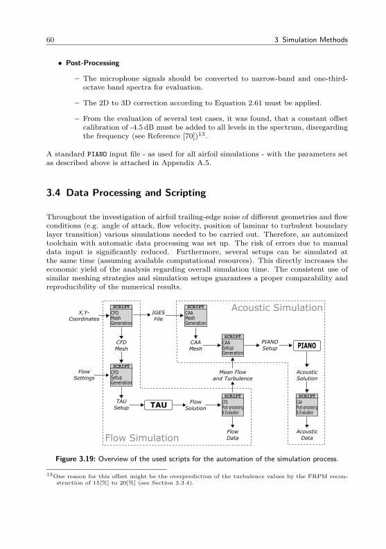
60 3 Simulation Methods

• Post-Processing

– The microphone signals should be converted to narrow-band and one-third-octave band spectra for evaluation.

– The 2D to 3D correction according to Equation 2.61 must be applied.

– From the evaluation of several test cases, it was found, that a constant offsetcalibration of -4.5 dB must be added to all levels in the spectrum, disregardingthe frequency (see Reference [70])13.

A standard PIANO input file - as used for all airfoil simulations - with the parameters setas described above is attached in Appendix A.5.

3.4 Data Processing and Scripting

Throughout the investigation of airfoil trailing-edge noise of different geometries and flowconditions (e.g. angle of attack, flow velocity, position of laminar to turbulent boundarylayer transition) various simulations needed to be carried out. Therefore, an automizedtoolchain with automatic data processing was set up. The risk of errors due to manualdata input is significantly reduced. Furthermore, several setups can be simulated atthe same time (assuming available computational resources). This directly increases theeconomic yield of the analysis regarding overall simulation time. The consistent use ofsimilar meshing strategies and simulation setups guarantees a proper comparability andreproducibility of the numerical results.

X,Y-

Coordinates

IGES

File

CAA

Mesh

PIANO

Setup PIANOCFD

Mesh

Flow

Settings

TAU

Setup TAUFlow

Solution

Flow

Data

Acoustic

Data

Acoustic

Solution

Mean Flow

and Turbulence

Flow Simulation

Acoustic SimulationCFDMeshGeneration

SCRIPT SCRIPT

CAAMeshGeneration

SCRIPT

CFDSetupGeneration

SCRIPT

CFDPost-processing& Evaluation

SCRIPT

CAAPost-processing& Evaluation

SCRIPT

CAASetupGeneration

Figure 3.19: Overview of the used scripts for the automation of the simulation process.

13One reason for this offset might be the overprediction of the turbulence values by the FRPM recon-struction of 15[%] to 20[%] (see Section 3.3.4).

3.4 Data Processing and Scripting 61

Figure 3.19 depicts the subsequent automation scripts used for the processing of the sim-ulation. The scripts are highlighted as gray boxes. Each script is written in bash. Systemcommands are used throughout the scripts to run specific software like grid generators orpost-processing tools (e.g. TECPLOT). Each script can be used on its own, as long as therequired input data is available. Thus, it is also possible to run the flow simulation partof the analysis without the acoustic calculations if the main focus lies on the integral flowparameters.

In the following, a short description of each automation script is given:

• CFD Mesh Generation

– The grid generator ICEM CFD is automized via an ICEM replay script (successivesequence of program commands).

– The standard replay script is modified to the new x and y coordinates (givenas ASCII file).

– ICEM automatically adjusts all structured near airfoil blocks so, that the wallnormal edges are as perpendicular as possible to the airfoil surface.

– The unstructured outside mesh is generated, the airfoil geometry is saved asIGES file and the final mesh in the TAU readable format (popform) is written.

• CFD Setup Generation

– A standard TAU setup file is copied and the used CFD mesh is adjusted to thenew airfoil.

– The flow parameters (angle of attack, Reynolds number, transition) are readfrom a user provided table. Individual folders, containing the mesh and thespecific TAU input files, are created for each parameter set.

– The folders are copied to the high performance cluster and the simulations arestarted.

• CFD Post-Processing and Evaluation

– The CFD folders are gathered and copied back to the local machine.

– From the data, the integral coefficients (lift, drag, torque) are extracted. More-over, specific distributions, e.g. the pressure coefficient along the airfoil’s sur-face or the TKE and velocity distribution in the trailing-edge region, are ex-tracted using TECPLOT.

– The flow data is prepared for the CAA simulation step. TECPLOT is used to non-dimensionalize the mean-flow variables and extract the turbulence statistics inthe FRPM patch area.

• CAA Mesh Generation

– The grid generator POINTWISE is used. Like with the CFD mesh, the procedureis automized using a replay script.

– The IGES geometry file is read and the default CAA mesh is modified so, thatthe near airfoil CAA mesh is adapted to the new geometry.

62 3 Simulation Methods

– A mesh smoothing is performed in POINTWISE and the resulting mesh is writtenin PLOT 3D format and thereafter converted in the PIANO readable popformformat using TECPLOT.

• CAA Setup Generation

– The provided mean-flow is interpolated onto the CAA mesh.

– A default PIANO input file is copied for each set of input parameters and therespective mean-flow, patch and CAA mesh files are set in the PIANO inputfile. For each parameter set, one PIANO input folder, with all files needed toconduct the simulation, is created.

– The folders are copied to the high performance cluster, where the acousticsimulations can be done in parallel on the available resources.

• CAA Post-Processing and Evaluation

– The acoustic solution folders are gathered and copied back to the local machine.

– From the recorded acoustic pressure over time signals (microphone circle) spec-tral data is calculated using an FFT analysis.

– From the spectral data over all sound pressure levels (OASPL) and directivitydistributions of the emitted trailing-edge noise signals are calculated.

The vast amount of produced data throughout the conducted simulations builds thebasis for the trailing-edge noise investigation. Multiple airfoil shapes under different op-erational conditions can be studied using the automized procedure. Within an industrialenvironment, the flow simulation data can be considered given as this analysis is crucialfor the particular choice of an airfoil for a new rotor blade design. The only additionalexpense results from the acoustic simulations, as well as the preparation of the CFD dataso, that it can be used as input data for the CAA simulation. After completing bothsimulation tasks it is possible to compare the airfoil performance on an aerodynamic aswell as acoustic scale.

4 Results and Discussion

This chapter contains the results of the two-dimensional airfoil analysis. Relevant as-pects for the trailing-edge noise generation as well as the aerodynamic relations will bediscussed. For the simulations the models and approaches described in Chapter 3 areinherently used. Variations of this settings (if used) are explicitly mentioned. The resultsare gathered with the overall focus to highlight the design driving aspects for low noiseairfoils. The influences of geometry and flow variations are systematically analyzed. Allis done with regard to the aerodynamic performance and under structural constraints.

First, the validation of the hybrid CAA/CFD approach is shown in Section 4.1. Thereforemeasurement data and test cases from the BANC-II workshop are used to validate thesimulated results. Thereafter, the systematic geometry and flow parameter variationstrategy is described in Section 4.2. Starting from a reference airfoil different geometryparameters and their influence on the emitted trailing-edge noise signal are analyzed.Moreover, the influence of laminar turbulent boundary layer transition is studied. Theresults are grouped in Section 4.3. Starting from these general trends, a more preciseinvestigation with aerodynamic data from the boundary layer is conducted in Section 4.4.From these discoveries a strategy for the development of new low noise airfoils is derivedin Section 4.5 and purposes for future airfoil design trends are presented.

4.1 Validation Test Cases from BANC-II

The validation of the outlined hybrid CFD/CAA method is shown according to avail-able TBL-TEN measurement data from the BANC-II (Benchmark for Airframe NoiseComputations) workshop[73].

The best practice settings according to Section 3.3.5 are used for the numerical simula-tions. All shown sound pressure level spectra are corrected according to Equation 2.61.Thus, the sound radiation is corrected to account for the 3D case, as measured in theBANC test cases. Untapered, unswept airfoil sections with a wetted span of 1m are con-sidered. A common off-set calibration of -4.5 dB is used on all simulated CAA spectra.

A microphone position orthogonal to the chord 2.5 chord lengths below the trailing-edgeis chosen to compare simulated and measured acoustic data1. According to the BANC-IIproblem statement, the provided measurements have an uncertainty of roughly 3 dB. Thisis indicated by error bars in the graphs. Furthermore, spectra calculated by the semi-empirical Brooks, Pope and Marcolini BPM tool NAFnoise[19] are additionally plottedin the following graphs (dashed lines). In general, a good match between simulated and

1In the BANC test cases airfoils with a chord lengths of lc = 0.4 m were measured. The microphoneposition was chosen in the far-field at a distance of r = 2.5lc = 1 m. The same far-field observationposition was chosen for the CAA simulations. The simulation data was then scaled to account foran airfoil with a span of 1m and an observer distance of 1m.

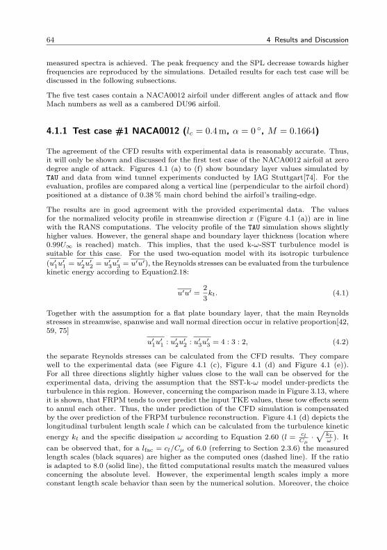
64 4 Results and Discussion

measured spectra is achieved. The peak frequency and the SPL decrease towards higherfrequencies are reproduced by the simulations. Detailed results for each test case will bediscussed in the following subsections.

The five test cases contain a NACA0012 airfoil under different angles of attack and flowMach numbers as well as a cambered DU96 airfoil.

4.1.1 Test case #1 NACA0012 (lc = 0.4 m, α = 0 , M = 0.1664)

The agreement of the CFD results with experimental data is reasonably accurate. Thus,it will only be shown and discussed for the first test case of the NACA0012 airfoil at zerodegree angle of attack. Figures 4.1 (a) to (f) show boundary layer values simulated byTAU and data from wind tunnel experiments conducted by IAG Stuttgart[74]. For theevaluation, profiles are compared along a vertical line (perpendicular to the airfoil chord)positioned at a distance of 0.38% main chord behind the airfoil’s trailing-edge.

The results are in good agreement with the provided experimental data. The valuesfor the normalized velocity profile in streamwise direction x (Figure 4.1 (a)) are in linewith the RANS computations. The velocity profile of the TAU simulation shows slightlyhigher values. However, the general shape and boundary layer thickness (location where0.99U∞ is reached) match. This implies, that the used k-ω-SST turbulence model issuitable for this case. For the used two-equation model with its isotropic turbulence(u′1u′1 = u′2u

′2 = u′3u

′3 = u′u′), the Reynolds stresses can be evaluated from the turbulence

kinetic energy according to Equation2.18:

u′u′ =23kt. (4.1)

Together with the assumption for a flat plate boundary layer, that the main Reynoldsstresses in streamwise, spanwise and wall normal direction occur in relative proportion[42,59, 75]

u′1u′1 : u′2u′2 : u′3u′3 = 4 : 3 : 2, (4.2)

the separate Reynolds stresses can be calculated from the CFD results. They comparewell to the experimental data (see Figure 4.1 (c), Figure 4.1 (d) and Figure 4.1 (e)).For all three directions slightly higher values close to the wall can be observed for theexperimental data, driving the assumption that the SST-k-ω model under-predicts theturbulence in this region. However, concerning the comparison made in Figure 3.13, whereit is shown, that FRPM tends to over predict the input TKE values, these tow effects seemto annul each other. Thus, the under prediction of the CFD simulation is compensatedby the over prediction of the FRPM turbulence reconstruction. Figure 4.1 (d) depicts thelongitudinal turbulent length scale l which can be calculated from the turbulence kineticenergy kt and the specific dissipation ω according to Equation 2.60 (l = cl

Cµ·√

ktω). It

can be observed that, for a lfac = cl/Cµ of 6.0 (referring to Section 2.3.6) the measuredlength scales (black squares) are higher as the computed ones (dashed line). If the ratiois adapted to 8.0 (solid line), the fitted computational results match the measured valuesconcerning the absolute level. However, the experimental length scales imply a moreconstant length scale behavior than seen by the numerical solution. Moreover, the choice

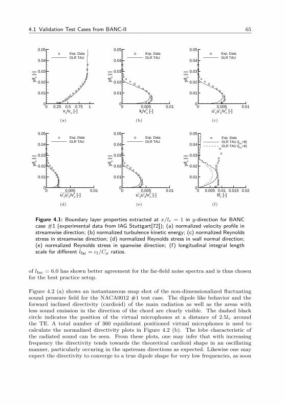
4.1 Validation Test Cases from BANC-II 65

vx/v∞ [-]

y/l c [

-]

0 0.25 0.5 0.75 10

0.01

0.02

0.03

0.04

0.05Exp. DataDLR TAU

(a)

kt/v2∞ [-]

y/l c [

-]0 0.005 0.01

0

0.01

0.02

0.03

0.04

0.05Exp. DataDLR TAU

(b)

u’1u’1/v2∞ [-]

y/l c [

-]

0 0.005 0.010

0.01

0.02

0.03

0.04

0.05Exp. DataDLR TAU

__________

(c)

u’2u’2/v2∞ [-]

y/l c [

-]

0 0.005 0.010

0.01

0.02

0.03

0.04

0.05Exp. DataDLR TAU

__________

(d)

u’3u’3/v2∞ [-]

y/l c [

-]

0 0.005 0.010

0.01

0.02

0.03

0.04

0.05Exp. DataDLR TAU

__________

(e)

l/lc [-]

y/l c [

-]0 0.005 0.01 0.015 0.02

0

0.01

0.02

0.03

0.04

0.05Exp. DataDLR TAU (lfac=8)DLR TAU (lfac=6)

(f)

Figure 4.1: Boundary layer properties extracted at x/lc = 1 in y-direction for BANCcase #1 (experimental data from IAG Stuttgart[72]); (a) normalized velocity profile instreamwise direction; (b) normalized turbulence kinetic energy; (c) normalized Reynoldsstress in streamwise direction; (d) normalized Reynolds stress in wall normal direction;(e) normalized Reynolds stress in spanwise direction; (f) longitudinal integral lengthscale for different lfac = cl/Cµ ratios.

of lfac = 6.0 has shown better agreement for the far-field noise spectra and is thus chosenfor the best practice setup.

Figure 4.2 (a) shows an instantaneous snap shot of the non-dimensionalized fluctuatingsound pressure field for the NACA0012 #1 test case. The dipole like behavior and theforward inclined directivity (cardioid) of the main radiation as well as the areas withless sound emission in the direction of the chord are clearly visible. The dashed blackcircle indicates the position of the virtual microphones at a distance of 2.5lc aroundthe TE. A total number of 360 equidistant positioned virtual microphones is used tocalculate the normalized directivity plots in Figure 4.2 (b). The lobe characteristic ofthe radiated sound can be seen. From these plots, one may infer that with increasingfrequency the directivity tends towards the theoretical cardioid shape in an oscillatingmanner, particularly occuring in the upstream directions as expected. Likewise one mayexpect the directivity to converge to a true dipole shape for very low frequencies, as soon

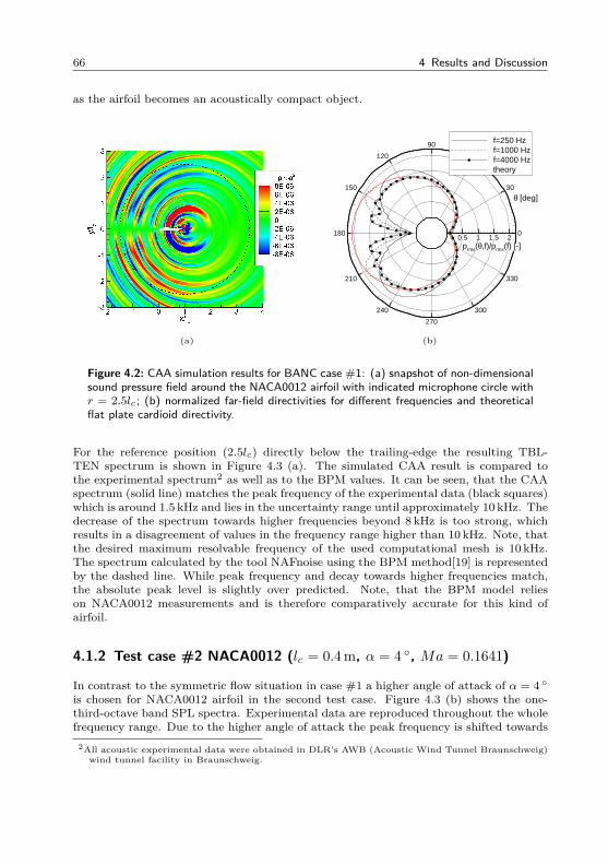
66 4 Results and Discussion

as the airfoil becomes an acoustically compact object.

(a)

θ [deg]

prms(θ,f)/prms(f) [-]

0

30

60

90

120

150

180

210

240

270

300

330

0.5 1 1.5 2

f=250 Hzf=1000 Hzf=4000 Hztheory

(b)

Figure 4.2: CAA simulation results for BANC case #1: (a) snapshot of non-dimensionalsound pressure field around the NACA0012 airfoil with indicated microphone circle withr = 2.5lc; (b) normalized far-field directivities for different frequencies and theoreticalflat plate cardioid directivity.

For the reference position (2.5lc) directly below the trailing-edge the resulting TBL-TEN spectrum is shown in Figure 4.3 (a). The simulated CAA result is compared tothe experimental spectrum2 as well as to the BPM values. It can be seen, that the CAAspectrum (solid line) matches the peak frequency of the experimental data (black squares)which is around 1.5 kHz and lies in the uncertainty range until approximately 10 kHz. Thedecrease of the spectrum towards higher frequencies beyond 8 kHz is too strong, whichresults in a disagreement of values in the frequency range higher than 10 kHz. Note, thatthe desired maximum resolvable frequency of the used computational mesh is 10 kHz.The spectrum calculated by the tool NAFnoise using the BPM method[19] is representedby the dashed line. While peak frequency and decay towards higher frequencies match,the absolute peak level is slightly over predicted. Note, that the BPM model relieson NACA0012 measurements and is therefore comparatively accurate for this kind ofairfoil.

4.1.2 Test case #2 NACA0012 (lc = 0.4 m, α = 4 , Ma = 0.1641)

In contrast to the symmetric flow situation in case #1 a higher angle of attack of α = 4 is chosen for NACA0012 airfoil in the second test case. Figure 4.3 (b) shows the one-third-octave band SPL spectra. Experimental data are reproduced throughout the wholefrequency range. Due to the higher angle of attack the peak frequency is shifted towards

2All acoustic experimental data were obtained in DLR’s AWB (Acoustic Wind Tunnel Braunschweig)wind tunnel facility in Braunschweig.

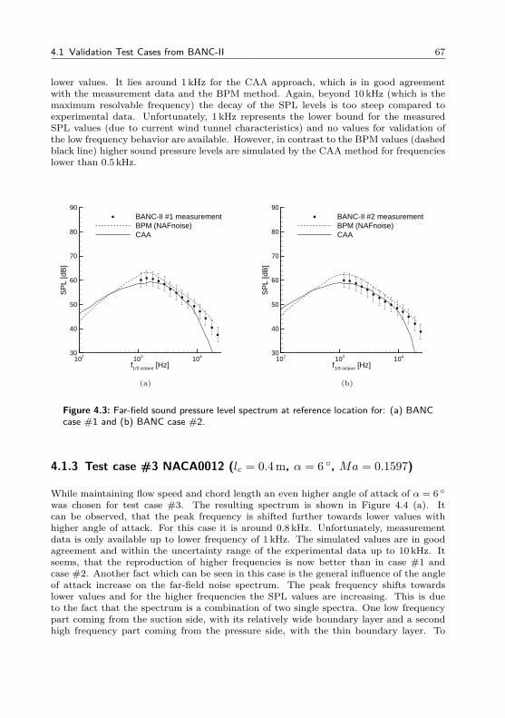
4.1 Validation Test Cases from BANC-II 67

lower values. It lies around 1 kHz for the CAA approach, which is in good agreementwith the measurement data and the BPM method. Again, beyond 10 kHz (which is themaximum resolvable frequency) the decay of the SPL levels is too steep compared toexperimental data. Unfortunately, 1 kHz represents the lower bound for the measuredSPL values (due to current wind tunnel characteristics) and no values for validation ofthe low frequency behavior are available. However, in contrast to the BPM values (dashedblack line) higher sound pressure levels are simulated by the CAA method for frequencieslower than 0.5 kHz.

f1/3 octave [Hz]

SP

L [d

B]

102 103 10430

40

50

60

70

80

90BANC-II #1 measurementBPM (NAFnoise)CAA

(a)

f1/3 octave [Hz]

SP

L [d

B]

102 103 10430

40

50

60

70

80

90BANC-II #2 measurementBPM (NAFnoise)CAA

(b)

Figure 4.3: Far-field sound pressure level spectrum at reference location for: (a) BANCcase #1 and (b) BANC case #2.

4.1.3 Test case #3 NACA0012 (lc = 0.4 m, α = 6 , Ma = 0.1597)

While maintaining flow speed and chord length an even higher angle of attack of α = 6 was chosen for test case #3. The resulting spectrum is shown in Figure 4.4 (a). Itcan be observed, that the peak frequency is shifted further towards lower values withhigher angle of attack. For this case it is around 0.8 kHz. Unfortunately, measurementdata is only available up to lower frequency of 1 kHz. The simulated values are in goodagreement and within the uncertainty range of the experimental data up to 10 kHz. Itseems, that the reproduction of higher frequencies is now better than in case #1 andcase #2. Another fact which can be seen in this case is the general influence of the angleof attack increase on the far-field noise spectrum. The peak frequency shifts towardslower values and for the higher frequencies the SPL values are increasing. This is dueto the fact that the spectrum is a combination of two single spectra. One low frequencypart coming from the suction side, with its relatively wide boundary layer and a secondhigh frequency part coming from the pressure side, with the thin boundary layer. To

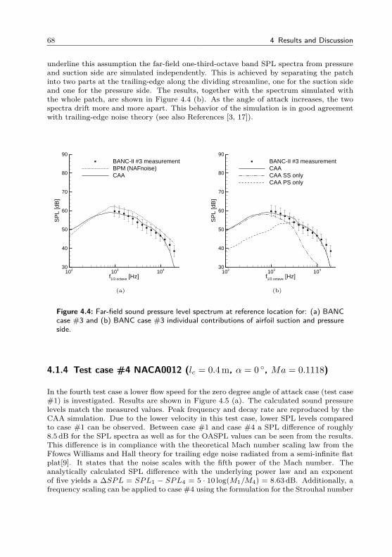
68 4 Results and Discussion

underline this assumption the far-field one-third-octave band SPL spectra from pressureand suction side are simulated independently. This is achieved by separating the patchinto two parts at the trailing-edge along the dividing streamline, one for the suction sideand one for the pressure side. The results, together with the spectrum simulated withthe whole patch, are shown in Figure 4.4 (b). As the angle of attack increases, the twospectra drift more and more apart. This behavior of the simulation is in good agreementwith trailing-edge noise theory (see also References [3, 17]).

f1/3 octave [Hz]

SP

L [d

B]

102 103 10430

40

50

60

70

80

90BANC-II #3 measurementBPM (NAFnoise)CAA

(a)

f1/3 octave [Hz]

SP

L [d

B]

102 103 10430

40

50

60

70

80

90BANC-II #3 measurementCAACAA SS onlyCAA PS only

(b)

Figure 4.4: Far-field sound pressure level spectrum at reference location for: (a) BANCcase #3 and (b) BANC case #3 individual contributions of airfoil suction and pressureside.

4.1.4 Test case #4 NACA0012 (lc = 0.4 m, α = 0 , Ma = 0.1118)

In the fourth test case a lower flow speed for the zero degree angle of attack case (test case#1) is investigated. Results are shown in Figure 4.5 (a). The calculated sound pressurelevels match the measured values. Peak frequency and decay rate are reproduced by theCAA simulation. Due to the lower velocity in this test case, lower SPL levels comparedto case #1 can be observed. Between case #1 and case #4 a SPL difference of roughly8.5 dB for the SPL spectra as well as for the OASPL values can be seen from the results.This difference is in compliance with the theoretical Mach number scaling law from theFfowcs Williams and Hall theory for trailing edge noise radiated from a semi-infinite flatplat[9]. It states that the noise scales with the fifth power of the Mach number. Theanalytically calculated SPL difference with the underlying power law and an exponentof five yields a ∆SPL = SPL1 − SPL4 = 5 · 10 log(M1/M4) = 8.63 dB. Additionally, afrequency scaling can be applied to case #4 using the formulation for the Strouhal number

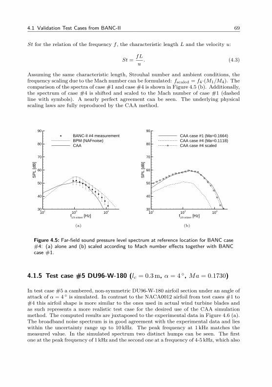
4.1 Validation Test Cases from BANC-II 69

St for the relation of the frequency f , the characteristic length L and the velocity u:

St =fL

u. (4.3)

Assuming the same characteristic length, Strouhal number and ambient conditions, thefrequency scaling due to the Mach number can be formulated: fscaled = f4·(M1/M4). Thecomparison of the spectra of case #1 and case #4 is shown in Figure 4.5 (b). Additionally,the spectrum of case #4 is shifted and scaled to the Mach number of case #1 (dashedline with symbols). A nearly perfect agreement can be seen. The underlying physicalscaling laws are fully reproduced by the CAA method.

f1/3 octave [Hz]

SP

L [d

B]

102 103 10430

40

50

60

70

80

90BANC-II #4 measurementBPM (NAFnoise)CAA

(a)

f1/3 octave [Hz]

SP

L [d

B]

102 103 10430

40

50

60

70

80

90CAA case #1 (Ma=0.1664)CAA case #4 (Ma=0.1118)CAA case #4 scaled

(b)

Figure 4.5: Far-field sound pressure level spectrum at reference location for BANC case#4: (a) alone and (b) scaled according to Mach number effects together with BANCcase #1.

4.1.5 Test case #5 DU96-W-180 (lc = 0.3 m, α = 4 , Ma = 0.1730)

In test case #5 a cambered, non-symmetric DU96-W-180 airfoil section under an angle ofattack of α = 4 is simulated. In contrast to the NACA0012 airfoil from test cases #1 to#4 this airfoil shape is more similar to the ones used in actual wind turbine blades andas such represents a more realistic test case for the desired use of the CAA simulationmethod. The computed results are juxtaposed to the experimental data in Figure 4.6 (a).The broadband noise spectrum is in good agreement with the experimental data and lieswithin the uncertainty range up to 10 kHz. The peak frequency at 1 kHz matches themeasured value. In the simulated spectrum two distinct humps can be seen. The firstone at the peak frequency of 1 kHz and the second one at a frequency of 4-5 kHz, which also

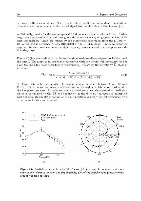
70 4 Results and Discussion

agrees with the measured data. They can be related to the two individual contributionsof suction and pressure side to the overall signal (see detailed description in case #3).

Additionally, results for the semi-empirical BPM code are depicted (dashed line). Ratherlarge inaccuracy can be observed throughout the whole frequency range greater than 2 kHzwith this method. These are caused by the geometrical differences from the DU-96-W-180 airfoil to the reference NACA0012 airfoil of the BPM method. The semi-empiricalapproach tends to over estimate the high frequency levels emitted from the pressure sideboundary layer.

Figure 4.6 (b) shows a directivity plot for the simulated overall sound pressure level aroundthe airfoil. The graph is in reasonable agreement with the theoretical directivity for flatplate trailing-edge noise according to Reference [3, 76], where the directivity D (Θ, φ) isgiven as:

D (Θ,Φ) ≈2 sin (Θ/2) sin2 φ

(1 +M cos Θ) [1 + (M −Mc) cos Θ]2. (4.4)

See Figure 2.5 for further details. The smaller simulation values between Θ = 150 andΘ = 210 are due to the presence of the airfoil in this region, which is not considered inthe flat plate test case. In order to compare absolute values, the theoretical predictionwhich is normalized to the TE noise radiation in the Θ = 90 direction is multipliedwith the absolute simulated values for the 90 position. A nearly perfect agreement withexperimental data can be found.

f1/3 octave [Hz]

SP

L [d

B]

102 103 10430

40

50

60

70

80

90BANC-II #5 measurementBPM (NAFnoise)CAA

(a)

θ [deg]

OASPL [dB]

0

30

60

90

120

150

180

210

240

270

300

330

40 50 60 70 80

CAATheory

(b)

Figure 4.6: Far-field acoustic data for BANC case #5: (a) one-third octave band spec-trum at the reference location and (b) directivity plot of the overall sound pressure levelsaround the trailing-edge.

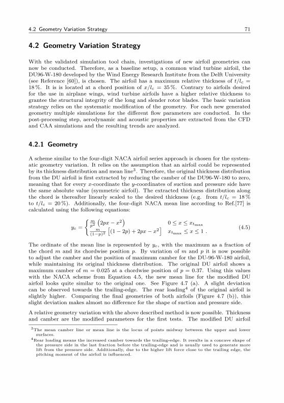
4.2 Geometry Variation Strategy 71

4.2 Geometry Variation Strategy

With the validated simulation tool chain, investigations of new airfoil geometries cannow be conducted. Therefore, as a baseline setup, a common wind turbine airfoil, theDU96-W-180 developed by the Wind Energy Research Institute from the Delft University(see Reference [60]), is chosen. The airfoil has a maximum relative thickness of t/lc =18 %. It is is located at a chord position of x/lc = 35 %. Contrary to airfoils desiredfor the use in airplane wings, wind turbine airfoils have a higher relative thickness tograntee the structural integrity of the long and slender rotor blades. The basic variationstrategy relies on the systematic modification of the geometry. For each new generatedgeometry multiple simulations for the different flow parameters are conducted. In thepost-processing step, aerodynamic and acoustic properties are extracted from the CFDand CAA simulations and the resulting trends are analyzed.

4.2.1 Geometry

A scheme similar to the four-digit NACA airfoil series approach is chosen for the system-atic geometry variation. It relies on the assumption that an airfoil could be representedby its thickness distribution and mean line3. Therefore, the original thickness distributionfrom the DU airfoil is first extracted by reducing the camber of the DU96-W-180 to zero,meaning that for every x-coordinate the y-coordinates of suction and pressure side havethe same absolute value (symmetric airfoil). The extracted thickness distribution alongthe chord is thereafter linearly scaled to the desired thickness (e.g. from t/lc = 18 %to t/lc = 20 %). Additionally, the four-digit NACA mean line according to Ref.[77] iscalculated using the following equations:

yc =mp2

(2px− x2

)0 ≤ x ≤ xtmax

m(1−p)2

[(1− 2p) + 2px− x2

]xtmax ≤ x ≤ 1 .

(4.5)

The ordinate of the mean line is represented by yc, with the maximum as a fraction ofthe chord m and its chordwise position p. By variation of m and p it is now possibleto adjust the camber and the position of maximum camber for the DU-96-W-180 airfoil,while maintaining its original thickness distribution. The original DU airfoil shows amaximum camber of m = 0.025 at a chordwise position of p = 0.37. Using this valueswith the NACA scheme from Equation 4.5, the new mean line for the modified DUairfoil looks quite similar to the original one. See Figure 4.7 (a). A slight deviationcan be observed towards the trailing-edge. The rear loading4 of the original airfoil isslightly higher. Comparing the final geometries of both airfoils (Figure 4.7 (b)), thisslight deviation makes almost no difference for the shape of suction and pressure side.

A relative geometry variation with the above described method is now possible. Thicknessand camber are the modified parameters for the first tests. The modified DU airfoil

3The mean camber line or mean line is the locus of points midway between the upper and lowersurfaces.

4Rear loading means the increased camber towards the trailing-edge. It results in a concave shape ofthe pressure side in the last fraction before the trailing-edge and is usually used to generate morelift from the pressure side. Additionally, due to the higher lift force close to the trailing edge, thepitching moment of the airfoil is influenced.

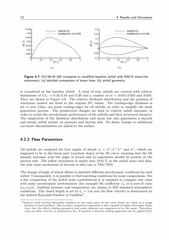
72 4 Results and Discussion

x/lc [-]

y/l c [

-]

0 0.2 0.4 0.6 0.8 10

0.005

0.01

0.015

0.02

0.025

0.03

0.035original DUmodified DU m=0.025

(a)

x/lc [-]

y/l c [

-]

0 0.2 0.4 0.6 0.8 1-0.1

-0.05

0

0.05

0.1

0.15

0.2original DUmodified DU m=0.025

(b)

Figure 4.7: DU-96-W-180 compared to modified baseline airfoil with NACA mean-linesystematic; (a) detailed comparison of mean lines; (b) airfoil geometry.

is considered as the baseline airfoil. A total of nine airfoils are created with relativethicknesses of t/lc = 0.16, 0.18 and 0.20 and a camber of m = 0.015, 0.025 and 0.035.They are shown in Figure 4.8. The relative thickness distribution and the position ofmaximum camber are fixed to the original DU values. The trailing-edge thickness isset to zero (thin, one point trailing-edge) for all airfoils, in order to simplify the meshgeneration process. The geometrical changes are kept to relative subtle amounts, inorder to retain the aerodynamic performance of the airfoils and their structural integrity.The adaptation of the thickness distribution and mean line also guarantees a smoothand steady airfoil surface on pressure and suction side. No dents, bumps or additionalcurvature discontinuities are added to the surface.

4.2.2 Flow Parameters

All airfoils are analyzed for four angles of attack α = 3 , 4 , 5 and 6 , which aresupposed to lie in the linear part (constant slope) of the lift curve, meaning that the liftlinearly increases with the angle of attack and no separation should be present at thesuction side. The inflow turbulence is nearly zero (0.01% at the airfoil nose) and thus,the only noise mechanism of interest in this case is TBL-TEN.

The change of angle of attack allows to simulate different aerodynamic conditions for eachairfoil. Consequently, it is possible to find matching conditions for noise comparisons. Fora fair comparison of the airfoil noise contributions it is essential to compare test caseswith same aerodynamic performances (for example lift coefficient cL or L-over-D ratio(cL/cD)). Ambient pressure and temperature are chosen to ISO standard atmosphericconditions. The chord length is set to lc = 1 m and the flow velocity is determined bythe desired Reynolds-Number of 3million5.

5Typical wind turbine Reynolds numbers in the outer part of the rotor blade are often in a rangebetween 3 and 6million. The acoustic simulation approach is also capable of higher Reynolds Num-bers, but the effects linking geometry and noise emission are supposed to be the same. Therefore,only one flow velocity is analyzed so far. If needed, a desired scaling approach can be applied.[54]

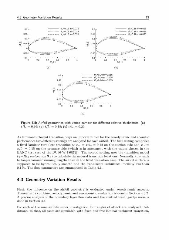
4.3 Geometry Variation Results 73

x/lc [-]

y/l c [

-]

0 0.2 0.4 0.6 0.8 1-0.1

-0.05

0

0.05

0.1

0.15

0.2 t/lc=0.16 m=0.015t/lc=0.16 m=0.025t/lc=0.16 m=0.035

(a)

x/lc [-]

y/l c [

-]

0 0.2 0.4 0.6 0.8 1-0.1

-0.05

0

0.05

0.1

0.15

0.2 t/lc=0.18 m=0.015t/lc=0.18 m=0.025t/lc=0.18 m=0.035

(b)

x/lc [-]

y/l c [

-]

0 0.2 0.4 0.6 0.8 1-0.1

-0.05

0

0.05

0.1

0.15

0.2 t/lc=0.20 m=0.015t/lc=0.20 m=0.025t/lc=0.20 m=0.035

(c)

Figure 4.8: Airfoil geometries with varied camber for different relative thicknesses; (a)t/lc = 0.16; (b) t/lc = 0.18; (c) t/lc = 0.20.

As laminar-turbulent transition plays an important role for the aerodynamic and acousticperformance two different settings are analyzed for each airfoil. The first setting comprisesa fixed laminar turbulent transition at xtr = x/lc = 0.12 on the suction side and xtr =x/lc = 0.15 on the pressure side (which is in agreement with the values chosen in theBANC test case of the DU96-W-180[72]). The second setting uses the transition model(γ−Reθ see Section 3.2) to calculate the natural transition locations. Normally, this leadsto longer laminar running lengths than in the fixed transition case. The airfoil surface issupposed to be hydraulically smooth and the free-stream turbulence intensity less than0.1%. The flow parameters are summarized in Table 4.1.

4.3 Geometry Variation Results

First, the influence on the airfoil geometry is evaluated under aerodynamic aspects.Thereafter, a combined aerodynamic and aeroacoustic evaluation is done in Section 4.3.2.A precise analysis of the boundary layer flow data and the emitted trailing-edge noise isdone in Section 4.4.

For each of the nine airfoils under investigation four angles of attack are analyzed. Ad-ditional to that, all cases are simulated with fixed and free laminar turbulent transition,

74 4 Results and Discussion

Table 4.1: Flow parameters for DU based airfoil variation.parameter symbol value unitpressure p∞ 101325 Patemperature T∞ 288.15 Kdensity ρ∞ 1.225 kg/m3

velocity u∞ 43.82 m/schord length lc 1.0 mRe number Re 3 · 106 −Ma number M 0.129 −angle of attack α 3; 4; 5; 6

resulting in total number of 72 combined CFD/CAA simulations. This rather largeamount of computations requires the automated data processing strategy explained inSection 3.4. The computationally most expensive step is clearly the CAA simulation. Ittakes about 16 hours on a high performance cluster node (refer to Section 3.3.5). All othersteps, including the TAU CFD simulation can be done in less than four hours, bringingthe computational time to around 20 hours per case. For the simulations multiple nodeson the DLR CASE-cluster could be used for parallel simulations of the individual runs.This keeps the overall computational time within reasonable limits.

4.3.1 Aerodynamics

Figure 4.9 shows lift curves for the airfoils in the desired angle of attack range. Laminarturbulent transition is fixed according to the values given in Section 4.2.2. The linearincrease of the lift coefficient cL with increasing angle of attack underlines the statement,that no suction side separation is present in the chosen angle of attack range. It is clearlyvisible, that the airfoil camber m indicated by the symbols in Figure 4.9 (a) is the maininfluence parameter for the lift. An increase in camber of one percent leads to a lift gainof roughly ∆cL = 0.1. The slope of the nine curves is almost identical and independentof the geometry. Considering the relative thickness - indicated by the line style - onlya minor influence on the lift coefficient can be observed. The 20% thick airfoil alwayshas the smallest lift compared to thinner airfoils with the same camber. The effectof lift mitigation by thickness increase is most prominent for strong cambered airfoils(m = 0.035; ∆cL = 0.03). It diminishes for only slightly cambered airfoils (m = 0.015;∆cL = 0.01).

Taking a look at the cL versus cD plots depicted in Figure 4.9 (b) the picture changes alittle bit. While the main driver for the lift coefficient cL is the airfoils camber, the dragcoefficient cD is primary influenced by the relative airfoil thickness t/lc. It is obvious, thatthicker airfoils tend to produce more drag than thinner ones because of their bigger cross-section perpendicular to the flow yields more pressure drag (or form drag). Generallyspeaking, two effects govern the aerodynamic efficiency of the airfoils determined by theL-over-D ratio (ratio cL/cD, or sometimes glide ratio). The efficiency is thereby increasedby either increasing camber or decreasing thickness. This kind of trivial finding willbecome more interesting when interpreting the aeroacoustic performance of the airfoils.

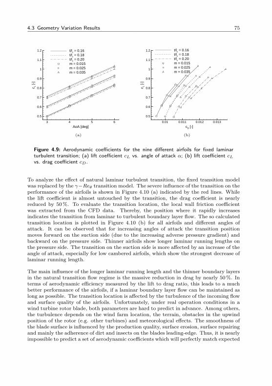
4.3 Geometry Variation Results 75

AoA [deg]

c L [-

]

3 4 5 6

0.5

0.6

0.7

0.8

0.9

1

1.1

1.2 t/lc = 0.16t/lc = 0.18t/lc = 0.20m = 0.015m = 0.025m = 0.035

(a)

cD [-]

c L [-

]

0.01 0.011 0.012 0.013

0.5

0.6

0.7

0.8

0.9

1

1.1

1.2 t/lc = 0.16t/lc = 0.18t/lc = 0.20m = 0.015m = 0.025m = 0.035

(b)

Figure 4.9: Aerodynamic coefficients for the nine different airfoils for fixed laminarturbulent transition; (a) lift coefficient cL vs. angle of attack α; (b) lift coefficient cLvs. drag coefficient cD.

To analyze the effect of natural laminar turbulent transition, the fixed transition modelwas replaced by the γ−Reθ transition model. The severe influence of the transition on theperformance of the airfoils is shown in Figure 4.10 (a) indicated by the red lines. Whilethe lift coefficient is almost untouched by the transition, the drag coefficient is nearlyreduced by 50%. To evaluate the transition location, the local wall friction coefficientwas extracted from the CFD data. Thereby, the position where it rapidly increasesindicates the transition from laminar to turbulent boundary layer flow. The so calculatedtransition location is plotted in Figure 4.10 (b) for all airfoils and different angles ofattack. It can be observed that for increasing angles of attack the transition positionmoves forward on the suction side (due to the increasing adverse pressure gradient) andbackward on the pressure side. Thinner airfoils show longer laminar running lengths onthe pressure side. The transition on the suction side is more affected by an increase of theangle of attack, especially for low cambered airfoils, which show the strongest decrease oflaminar running length.

The main influence of the longer laminar running length and the thinner boundary layersin the natural transition flow regime is the massive reduction in drag by nearly 50%. Interms of aerodynamic efficiency measured by the lift to drag ratio, this leads to a muchbetter performance of the airfoils, if a laminar boundary layer flow can be maintained aslong as possible. The transition location is affected by the turbulence of the incoming flowand surface quality of the airfoils. Unfortunately, under real operation conditions in awind turbine rotor blade, both parameters are hard to predict in advance. Among others,the turbulence depends on the wind farm location, the terrain, obstacles in the upwindposition of the rotor (e.g. other turbines) and meteorological effects. The smoothness ofthe blade surface is influenced by the production quality, surface erosion, surface repairingand mainly the adherence of dirt and insects on the blades leading-edge. Thus, it is nearlyimpossible to predict a set of aerodynamic coefficients which will perfectly match expected

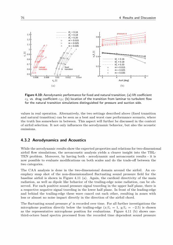
76 4 Results and Discussion

cD [-]

c L [-

]

0.006 0.008 0.01 0.012 0.014

0.5

0.6

0.7

0.8

0.9

1

1.1

1.2

1.3t/lc = 0.16t/lc = 0.18t/lc = 0.20m = 0.015m = 0.025m = 0.035

fixedtransition

naturaltransition

(a)

AoA [deg]

x tr/l c [

-]

3 4 5 60

0.2

0.4

0.6

0.8

t/lc = 0.16t/lc = 0.18t/lc = 0.20m = 0.015m = 0.025m = 0.035

pressure si

(b)

Figure 4.10: Aerodynamic performance for fixed and natural transition; (a) lift coefficientcL vs. drag coefficient cD; (b) location of the transition from laminar to turbulent flowfor the natural transition simulations distinguished for pressure and suction side.

values in real operation. Alternatively, the two settings described above (fixed transitionand natural transition) can be seen as a best and worst case performance scenario, wherethe truth lies somewhere in between. This aspect will further be discussed in the contextof airfoil selection. It not only influences the aerodynamic behavior, but also the acousticemissions.

4.3.2 Aerodynamics and Acoustics

While the aerodynamic results show the expected properties and relations for two-dimensionalairfoil flow simulations, the aeroacoustic analysis yields a clearer insight into the TBL-TEN problem. Moreover, by having both - aerodynamic and aeroacoustic results - it isnow possible to evaluate modifications on both scales and do the trade-off between thetwo categories.

The CAA analysis is done in the two-dimensional domain around the airfoil. An ex-emplary snap shot of the non-dimensionalized fluctuating sound pressure field for thebaseline airfoil is shown in Figure 4.11 (a). Again, the cardioid directivity of the mainradiation, as well as dipole like behavior of the trailing-edge noise radiation, can be ob-served. For each positive sound pressure signal traveling in the upper half plane, there isa respective negative signal traveling in the lower half plane. In front of the leading-edgeand behind the trailing-edge these wave cancel out each other, resulting in zones withless or almost no noise impact directly in the direction of the airfoil chord.

The fluctuating sound pressure p′ is recorded over time. For all further investigations themicrophone position directly below the trailing-edge (x/lc = 1, y/lc = −2.5) is chosenas the representative microphone position for evaluations. Figure 4.11 (b) shows one-third-octave band spectra processed from the recorded time dependent sound pressure

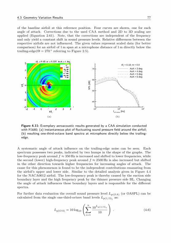
4.3 Geometry Variation Results 77

of the baseline airfoil at this reference position. Four curves are shown, one for eachangle of attack. Corrections due to the used CAA method and 2D to 3D scaling areapplied (Equation 2.61). Note, that the corrections are independent of the frequencyand only yield a constant shift in sound pressure levels. Relative differences between therespective airfoils are not influenced. The given values represent scaled data (for bettercomparison) for an airfoil of 1m span at a microphone distance of 1m directly below thetrailing-edge(Θ = 270 referring to Figure 2.5).

(a)

f1/3 octave [Hz]

SP

L [d

B]

102 103 104

40

50

60

70 AoA = 3 degAoA = 4 degAoA = 5 degAoA = 6 deg

t/lc = 0.18; m = 0.0

(b)

Figure 4.11: Exemplary aeroacoustic results generated by a CAA simulation conductedwith PIANO; (a) instantaneous plot of fluctuating sound pressure field around the airfoil;(b) resulting one-third-octave band spectra at microphone directly below the trailing-edge.

A systematic angle of attack influence on the trailing-edge noise can be seen. Eachspectrum possesses two peaks, indicated by two humps in the shape of the graphs. Thelow-frequency peak around f ≈ 350 Hz is increased and shifted to lower frequencies, whilethe second (lower) high-frequency peak around f ≈ 2500 Hz is also increased but shiftedin the other direction towards higher frequencies for increasing angles of attack. Thecause for this phenomenon is found to be the independent contributions emanating fromthe airfoil’s upper and lower side. Similar to the detailed analysis given in Figure 4.4for the NACA0012 airfoil. The low-frequency peak is thereby caused by the suction sideboundary layer and the high frequency peak by the thinner pressure side BL. Changingthe angle of attack influences these boundary layers and is responsible for the differentspectra.

For further data evaluation the overall sound pressure level Lp(OA) (or OASPL) can becalculated from the single one-third-octave band levels Lp(1/3)i as:

Lp(OA) = 10 log10

(n∑i=1

10Lp(1/3)i

10

). (4.6)

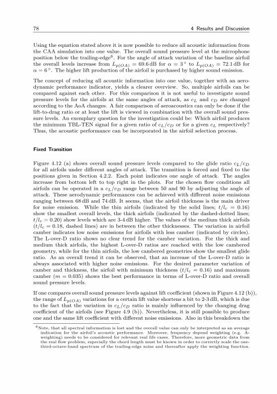
78 4 Results and Discussion

Using the equation stated above it is now possible to reduce all acoustic information fromthe CAA simulation into one value. The overall sound pressure level at the microphoneposition below the trailing-edge6. For the angle of attack variation of the baseline airfoilthe overall levels increase from Lp(OA) = 69.6 dB for α = 3 to Lp(OA) = 72.1 dB forα = 6 . The higher lift production of the airfoil is purchased by higher sound emission.

The concept of reducing all acoustic information into one value, together with an aero-dynamic performance indicator, yields a clearer overview. So, multiple airfoils can becompared against each other. For this comparison it is not useful to investigate soundpressure levels for the airfoils at the same angles of attack, as cL and cD are changedaccording to the AoA changes. A fair comparison of aeroacoustics can only be done if thelift-to-drag ratio or at least the lift is viewed in combination with the overall sound pres-sure levels. An exemplary question for the investigation could be: Which airfoil producesthe minimum TBL-TEN signal for a given ratio of cL/cD or for a given cL respectively?Thus, the acoustic performance can be incorporated in the airfoil selection process.

Fixed Transition

Figure 4.12 (a) shows overall sound pressure levels compared to the glide ratio cL/cDfor all airfoils under different angles of attack. The transition is forced and fixed to thepositions given in Section 4.2.2. Each point indicates one angle of attack. The anglesincrease from bottom left to top right in the plots. For the chosen flow conditions allairfoils can be operated in a cL/cD range between 50 and 90 by adjusting the angle ofattack. These aerodynamic performances can be achieved with different noise emissionsranging between 68 dB and 74 dB. It seems, that the airfoil thickness is the main driverfor noise emission. While the thin airfoils (indicated by the solid lines; t/lc = 0.16)show the smallest overall levels, the thick airfoils (indicated by the dashed-dotted lines;t/lc = 0.20) show levels which are 3-4 dB higher. The values of the medium thick airfoils(t/lc = 0.18, dashed lines) are in between the other thicknesses. The variation in airfoilcamber indicates low noise emissions for airfoils with less camber (indicated by circles).The L-over-D ratio shows no clear trend for the camber variation. For the thick andmedium thick airfoils, the highest L-over-D ratios are reached with the low camberedgeometry, while for the thin airfoils, the low cambered geometries show the smallest glideratio. As an overall trend it can be observed, that an increase of the L-over-D ratio isalways associated with higher noise emissions. For the desired parameter variation ofcamber and thickness, the airfoil with minimum thickness (t/lc = 0.16) and maximumcamber (m = 0.035) shows the best performance in terms of L-over-D ratio and overallsound pressure levels.

If one compares overall sound pressure levels against lift coefficient (shown in Figure 4.12 (b)),the range of Lp(OA) variations for a certain lift value shortens a bit to 2-3 dB, which is dueto the fact that the variation in cL/cD ratio is mainly influenced by the changing dragcoefficient of the airfoils (see Figure 4.9 (b)). Nevertheless, it is still possible to produceone and the same lift coefficient with different noise emissions. Also in this breakdown the

6Note, that all spectral information is lost and the overall value can only be interpreted as an averageindication for the airfoil’s acoustic performance. Moreover, frequency depend weighting (e.g. A-weighting) needs to be considered for relevant real life cases. Therefore, more geometric data fromthe real flow problem, especially the chord length must be known in order to correctly scale the one-third-octave-band spectrum of the trailing-edge noise and thereafter apply the weighting function.

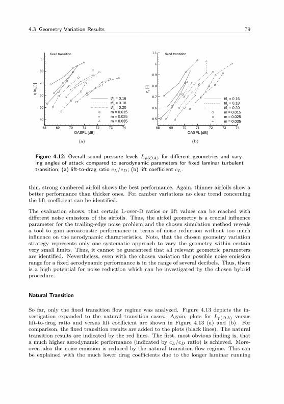
4.3 Geometry Variation Results 79

OASPL [dB]

c L/c D

[-]

68 69 70 71 72 73 74

40

50

60

70

80

90

t/lc = 0.16t/lc = 0.18t/lc = 0.20m = 0.015m = 0.025m = 0.035

fixed transition

(a)

OASPL [dB]

c L [-

]

68 69 70 71 72 73 74

0.5

0.6

0.7

0.8

0.9

1

1.1

t/lc = 0.16t/lc = 0.18t/lc = 0.20m = 0.015m = 0.025m = 0.035

fixed transition

(b)

Figure 4.12: Overall sound pressure levels Lp(OA) for different geometries and vary-ing angles of attack compared to aerodynamic parameters for fixed laminar turbulenttransition; (a) lift-to-drag ratio cL/cD; (b) lift coefficient cL.

thin, strong cambered airfoil shows the best performance. Again, thinner airfoils show abetter performance than thicker ones. For camber variations no clear trend concerningthe lift coefficient can be identified.

The evaluation shows, that certain L-over-D ratios or lift values can be reached withdifferent noise emissions of the airfoils. Thus, the airfoil geometry is a crucial influenceparameter for the trailing-edge noise problem and the chosen simulation method revealsa tool to gain aeroacoustic performance in terms of noise reduction without too muchinfluence on the aerodynamic characteristics. Note, that the chosen geometry variationstrategy represents only one systematic approach to vary the geometry within certainvery small limits. Thus, it cannot be guaranteed that all relevant geometric parametersare identified. Nevertheless, even with the chosen variation the possible noise emissionrange for a fixed aerodynamic performance is in the range of several decibels. Thus, thereis a high potential for noise reduction which can be investigated by the chosen hybridprocedure.

Natural Transition

So far, only the fixed transition flow regime was analyzed. Figure 4.13 depicts the in-vestigation expanded to the natural transition cases. Again, plots for Lp(OA) versuslift-to-drag ratio and versus lift coefficient are shown in Figure 4.13 (a) and (b). Forcomparison, the fixed transition results are added to the plots (black lines). The naturaltransition results are indicated by the red lines. The first, most obvious finding is, thata much higher aerodynamic performance (indicated by cL/cD ratio) is achieved. More-over, also the noise emission is reduced by the natural transition flow regime. This canbe explained with the much lower drag coefficients due to the longer laminar running

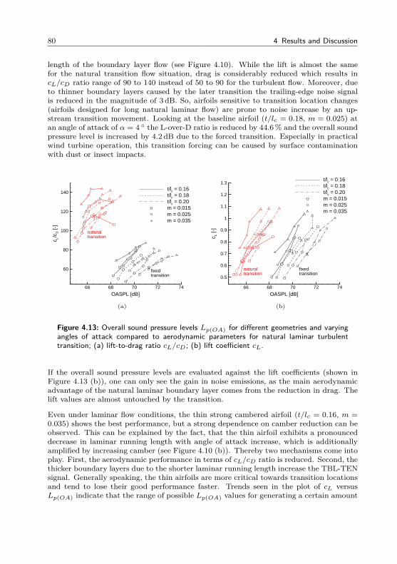
80 4 Results and Discussion

length of the boundary layer flow (see Figure 4.10). While the lift is almost the samefor the natural transition flow situation, drag is considerably reduced which results incL/cD ratio range of 90 to 140 instead of 50 to 90 for the turbulent flow. Moreover, dueto thinner boundary layers caused by the later transition the trailing-edge noise signalis reduced in the magnitude of 3 dB. So, airfoils sensitive to transition location changes(airfoils designed for long natural laminar flow) are prone to noise increase by an up-stream transition movement. Looking at the baseline airfoil (t/lc = 0.18, m = 0.025) atan angle of attack of α = 4 the L-over-D ratio is reduced by 44.6% and the overall soundpressure level is increased by 4.2 dB due to the forced transition. Especially in practicalwind turbine operation, this transition forcing can be caused by surface contaminationwith dust or insect impacts.

OASPL [dB]

c L/c D

[-]

66 68 70 72 74

60

80

100

120

140t/lc = 0.16t/lc = 0.18t/lc = 0.20m = 0.015m = 0.025m = 0.035

naturaltransition

fixedtransition

(a)

OASPL [dB]

c L [-

]

66 68 70 72 74

0.5

0.6

0.7

0.8

0.9

1

1.1

1.2

1.3t/lc = 0.16t/lc = 0.18t/lc = 0.20m = 0.015m = 0.025m = 0.035

naturaltransition

fixedtransition

(b)

Figure 4.13: Overall sound pressure levels Lp(OA) for different geometries and varyingangles of attack compared to aerodynamic parameters for natural laminar turbulenttransition; (a) lift-to-drag ratio cL/cD; (b) lift coefficient cL.

If the overall sound pressure levels are evaluated against the lift coefficients (shown inFigure 4.13 (b)), one can only see the gain in noise emissions, as the main aerodynamicadvantage of the natural laminar boundary layer comes from the reduction in drag. Thelift values are almost untouched by the transition.

Even under laminar flow conditions, the thin strong cambered airfoil (t/lc = 0.16, m =0.035) shows the best performance, but a strong dependence on camber reduction can beobserved. This can be explained by the fact, that the thin airfoil exhibits a pronounceddecrease in laminar running length with angle of attack increase, which is additionallyamplified by increasing camber (see Figure 4.10 (b)). Thereby two mechanisms come intoplay. First, the aerodynamic performance in terms of cL/cD ratio is reduced. Second, thethicker boundary layers due to the shorter laminar running length increase the TBL-TENsignal. Generally speaking, the thin airfoils are more critical towards transition locationsand tend to lose their good performance faster. Trends seen in the plot of cL versusLp(OA) indicate that the range of possible Lp(OA) values for generating a certain amount

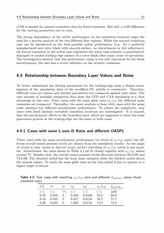
4.4 Relationship between Boundary Layer Values and Noise 81

of lift is smaller for natural transition than for fixed transition. But still, a 2 dB differencefor the varying geometries can be seen.

The strong dependency of the airfoil performance on the transition locations urges theneed for a precise analysis of the two different flow regimes. While the natural transitioncase can be interpreted as the best possible airfoil performance (e.g. for a perfectlymanufactured new rotor blade with smooth surface, no disturbances or dirt adherence),the forced transition at the airfoil nose represents the worst case scenario (contaminated,damaged or eroded leading-edge surface of a rotor blade after many years of operation).The investigation showed, that this performance range is not only important for the bladeaerodynamics, but also has a severe influence on the acoustic emissions.

4.4 Relationship between Boundary Layer Values and Noise

To better understand the driving parameters for the trailing-edge issue a deeper inves-tigation of the simulation data of the modified DU airfoils is conducted. Therefore,different cases are chosen and distinct parameters are compared against each other. Thevast amount of available simulation data from the CFD and CAA simulation is a clearadvantage in this case. First, cases with the same glide ratio cL/cD but different noiseemissions are compared. Thereafter, the same analysis is done with cases with the samenoise emission but different aerodynamic performance. To reduce the complexity, onlycases with fixed laminar turbulent transition locations are investigated. It is argued,that the aerodynamic effects in the boundary layer which are supposed to drive the noisegeneration process at the trailing-edge are the same in both cases.

4.4.1 Cases with same L-over-D Ratio and different OASPL

Three cases with the same aerodynamic performance (in terms of cL/cD ratio) but dif-ferent overall sound pressure levels are chosen from the simulation results. As the angleof attack is only varied in discrete steps, perfect matching of cL/cD ratios is not possi-ble. Nevertheless, the cases shown in Table 4.2 all lie closely together with cL/cD valuesaround 75. Besides that, the overall sound pressure levels alternate between 69.6 dB and73.6 dB. The thinnest airfoil has the least noise emission while the thickest airfoil showsthe utmost values. To reach the same glide ratio as the thin airfoil it has to operate at ahigher angle of attack.

Table 4.2: Test cases with matching cL/cD ratio and different Lp(OA) values (fixedtransition only).

t/lc m α cL cD cL/cD Lp(OA)

[−] [−] [] [−] [−] [−] [dB]0.16 0.035 4 0.820 0.0108 76.2 69.60.18 0.035 5 0.917 0.0120 76.7 71.70.20 0.035 6 1.002 0.0135 74.3 73.6

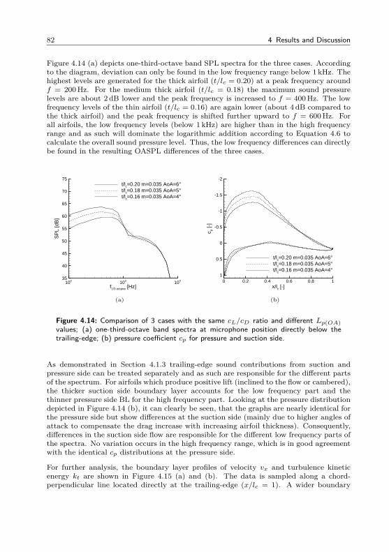
82 4 Results and Discussion

Figure 4.14 (a) depicts one-third-octave band SPL spectra for the three cases. Accordingto the diagram, deviation can only be found in the low frequency range below 1 kHz. Thehighest levels are generated for the thick airfoil (t/lc = 0.20) at a peak frequency aroundf = 200 Hz. For the medium thick airfoil (t/lc = 0.18) the maximum sound pressurelevels are about 2 dB lower and the peak frequency is increased to f = 400 Hz. The lowfrequency levels of the thin airfoil (t/lc = 0.16) are again lower (about 4 dB compared tothe thick airfoil) and the peak frequency is shifted further upward to f = 600 Hz. Forall airfoils, the low frequency levels (below 1 kHz) are higher than in the high frequencyrange and as such will dominate the logarithmic addition according to Equation 4.6 tocalculate the overall sound pressure level. Thus, the low frequency differences can directlybe found in the resulting OASPL differences of the three cases.

f1/3 octave [Hz]

SP

L [d

B]

102 103 10435

40

45

50

55

60

65

70

75t/lc=0.20 m=0.035 AoA=6°t/lc=0.18 m=0.035 AoA=5°t/lc=0.16 m=0.035 AoA=4°

(a)

x/lc [-]

c p [-

]

0 0.2 0.4 0.6 0.8 1

-2

-1.5

-1

-0.5

0

0.5

1

t/lc=0.20 m=0.035 AoA=6°t/lc=0.18 m=0.035 AoA=5°t/lc=0.16 m=0.035 AoA=4°

(b)

Figure 4.14: Comparison of 3 cases with the same cL/cD ratio and different Lp(OA)values; (a) one-third-octave band spectra at microphone position directly below thetrailing-edge; (b) pressure coefficient cp for pressure and suction side.

As demonstrated in Section 4.1.3 trailing-edge sound contributions from suction andpressure side can be treated separately and as such are responsible for the different partsof the spectrum. For airfoils which produce positive lift (inclined to the flow or cambered),the thicker suction side boundary layer accounts for the low frequency part and thethinner pressure side BL for the high frequency part. Looking at the pressure distributiondepicted in Figure 4.14 (b), it can clearly be seen, that the graphs are nearly identical forthe pressure side but show differences at the suction side (mainly due to higher angles ofattack to compensate the drag increase with increasing airfoil thickness). Consequently,differences in the suction side flow are responsible for the different low frequency parts ofthe spectra. No variation occurs in the high frequency range, which is in good agreementwith the identical cp distributions at the pressure side.

For further analysis, the boundary layer profiles of velocity vx and turbulence kineticenergy kt are shown in Figure 4.15 (a) and (b). The data is sampled along a chord-perpendicular line located directly at the trailing-edge (x/lc = 1). A wider boundary

4.4 Relationship between Boundary Layer Values and Noise 83

layer with higher kt values can be observed for the thicker airfoil at the suction side.The boundary layer thickness δ can be estimated from the velocity profile as the pointwhere the gradient reduces to zero7. Compared to the thick airfoil, the boundary layer ofthe thin airfoil is reduced by 30% from y/lc = 0.065 to y/lc = 0.045. Correspondingly,the thick airfoil shows a higher peak in the TKE values at the suction side. The peakis also located further away from the trailing-edge. The shapes of the TKE profiles onthe suction side look identical. Their actual size scales with the boundary layer thicknessand corresponds to the order of the maximum SPL values in the one-third-octave bandspectra. High turbulence and wide boundary layers cause the higher noise emissionsin the low frequency range, which is the dominant part of the TBL-TEN spectrum.From a merely acoustic point of view, it does make sense to find airfoils which showthin boundary layers at their desired point of operation. Comparing Figure 4.14 (b)and Figure 4.15 this can be achieved by a low adverse pressure gradient for the suctionside pressure regain. As the main function of the airfoils is lift production, this fact issomehow intrinsic in the problem statement. Lift cannot be produced without trailing-edge noise, but with elaborate choice of geometry and point of operation a reduction ispossible. One major finding is, that by evaluating the TKE profile at the trailing-edge (aninformation that can be generated by a rather simple CFD simulation) it is possible tomake an assessment for the acoustic performance of the airfoil. This bears the possibilityto compare airfoils against each other based on their turbulence production at the suctionside to make a relative benchmark in terms of TBL-TEN. Clearly, all considerations needto be evaluated also against concurring branches in the rotor blade design process (e.g.structural mechanics or production aspects).

4.4.2 Cases with different L-over-D Ratio and same OASPL

In contrast to the previous subsection, three different cases with equal noise emissions butdifferent aerodynamic performances are juxtaposed. Representative values can be foundin Table 4.3. Again, three airfoils varying in thickness and operating under differentangles are investigated. Thereby, the thinnest airfoil has the highest angle of attack,while the thickest airfoil has the lowest. The overall sound pressure levels nearly matchwith values slightly below 70.5 dB. The higher lift coefficient together with the higherangle of attack results in a better cL/cD ratio of 83.9 for the thin airfoil compared to54.3 for the thick airfoil.

Figure 4.16 (a) shows the one-third-octave band SPL spectra for the three different cases.It can be observed that all three spectra show the same levels in the low frequency rangebelow 1 kHz. Slight differences can only be seen in the high frequency range. As theOASPL is dominated by the highest values in the spectrum, all OASPL values for thethree cases match. The difference in the high frequencies has such a minor contributionthat it is not important here. Again, cp distributions for the three cases are analyzedand depicted in Figure 4.16 (b). For the suction side the graphs of the distributions arenearly identical in the pressure regain region downstream of x/lc = 0.4. Only upstream of

7Note, that the determination of boundary layer thicknesses with the definition as the position where99% of the free stream velocity v∞ is reached is not applicable for boundary layers with pressuregradients and accelerating and decelerating flow velocities. One suggested definition for the BLthickness in this cases can be found in Reference [73]. Here, the inflection point of the velocityprofile is chosen for determination of the boundary layer thickness. The same procedure is used forthe calculation of the δ values, stated in this work.

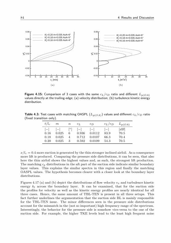
84 4 Results and Discussion

vx [m/s]

y/l c

0 5 10 15 20 25 30 35 40 45-0.04

-0.02

0

0.02

0.04

0.06

0.08

t/lc=0.20 m=0.035 AoA=6°t/lc=0.18 m=0.035 AoA=5°t/lc=0.16 m=0.035 AoA=4°

(a)

kt [m2/s2]

y/l c

0 5 10 15 20 25 30 35-0.04

-0.02

0

0.02

0.04

0.06

0.08

t/lc=0.20 m=0.035 AoA=6°t/lc=0.18 m=0.035 AoA=5°t/lc=0.16 m=0.035 AoA=4°

(b)

Figure 4.15: Comparison of 3 cases with the same cL/cD ratio and different Lp(OA)values directly at the trailing-edge; (a) velocity distribution; (b) turbulence kinetic energydistribution.

Table 4.3: Test cases with matching OASPL (Lp(OA)) values and different cL/cD ratio(fixed transition only).

t/lc m α cL cD cL/cD Lp(OA)

[−] [−] [] [−] [−] [−] [dB]0.16 0.025 6 0.936 0.0112 83.9 70.50.18 0.025 4 0.712 0.0107 66.3 70.40.20 0.025 3 0.592 0.0109 54.3 70.5

x/lc = 0.4 more suction is generated by the thin stronger inclined airfoil. As a consequencemore lift is produced. Comparing the pressure side distributions, it can be seen, that alsohere the thin airfoil shows the highest values and, as such, the strongest lift production.The matching cp distributions in the aft part of the suction side indicate similar boundarylayer values. This explains the similar spectra in this region and finally the matchingOASPL values. The hypothesis becomes clearer with a closer look at the boundary layerdistributions.

Figures 4.17 (a) and (b) depict the distributions of flow velocity vx and turbulence kineticenergy kt across the boundary layer. It can be examined, that for the suction sidethe profiles for velocity as well as the kinetic energy profiles are nearly identical for allthree cases. Hence, the same amount of TBL-TEN is present in all three setups. Thisfact further underlines the argumentation that the suction side BL is mainly responsiblefor the TBL-TEN issue. The minor differences seen in the pressure side distributionsaccount for the mismatch in the (not so important) high frequency range of the spectrum.Interestingly, the behavior for the pressure side is somehow vice-versa to the one of thesuction side. For example, the higher TKE levels lead to the least high frequent noise

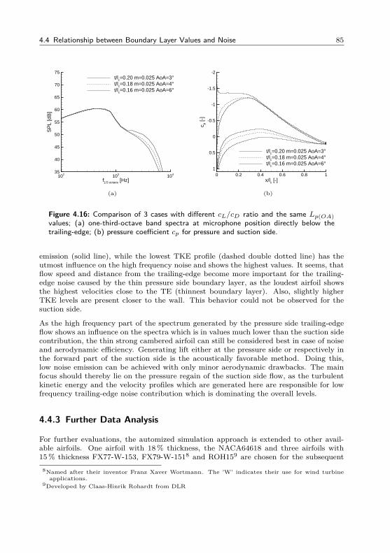
4.4 Relationship between Boundary Layer Values and Noise 85

f1/3 octave [Hz]

SP

L [d

B]

102 103 10435

40

45

50

55

60

65

70

75t/lc=0.20 m=0.025 AoA=3°t/lc=0.18 m=0.025 AoA=4°t/lc=0.16 m=0.025 AoA=6°

(a)

x/lc [-]

c p [-

]

0 0.2 0.4 0.6 0.8 1

-2

-1.5

-1

-0.5

0

0.5

1

t/lc=0.20 m=0.025 AoA=3°t/lc=0.18 m=0.025 AoA=4°t/lc=0.16 m=0.025 AoA=6°

(b)

Figure 4.16: Comparison of 3 cases with different cL/cD ratio and the same Lp(OA)values; (a) one-third-octave band spectra at microphone position directly below thetrailing-edge; (b) pressure coefficient cp for pressure and suction side.

emission (solid line), while the lowest TKE profile (dashed double dotted line) has theutmost influence on the high frequency noise and shows the highest values. It seems, thatflow speed and distance from the trailing-edge become more important for the trailing-edge noise caused by the thin pressure side boundary layer, as the loudest airfoil showsthe highest velocities close to the TE (thinnest boundary layer). Also, slightly higherTKE levels are present closer to the wall. This behavior could not be observed for thesuction side.

As the high frequency part of the spectrum generated by the pressure side trailing-edgeflow shows an influence on the spectra which is in values much lower than the suction sidecontribution, the thin strong cambered airfoil can still be considered best in case of noiseand aerodynamic efficiency. Generating lift either at the pressure side or respectively inthe forward part of the suction side is the acoustically favorable method. Doing this,low noise emission can be achieved with only minor aerodynamic drawbacks. The mainfocus should thereby lie on the pressure regain of the suction side flow, as the turbulentkinetic energy and the velocity profiles which are generated here are responsible for lowfrequency trailing-edge noise contribution which is dominating the overall levels.

4.4.3 Further Data Analysis

For further evaluations, the automized simulation approach is extended to other avail-able airfoils. One airfoil with 18% thickness, the NACA64618 and three airfoils with15% thickness FX77-W-153, FX79-W-1518 and ROH159 are chosen for the subsequent

8Named after their inventor Franz Xaver Wortmann. The ’W’ indicates their use for wind turbineapplications.

9Developed by Claas-Hinrik Rohardt from DLR

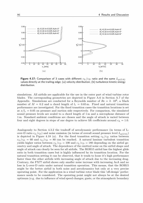
86 4 Results and Discussion

vx [m/s]

y/l c

0 5 10 15 20 25 30 35 40 45-0.04

-0.02

0

0.02

0.04

0.06

0.08t/lc=0.20 m=0.025 AoA=3°t/lc=0.18 m=0.025 AoA=4°t/lc=0.16 m=0.025 AoA=6°

(a)

kt [m2/s2]

y/l c

0 5 10 15 20 25 30 35-0.04

-0.02

0

0.02

0.04

0.06

0.08

t/lc=0.20 m=0.025 AoA=3°t/lc=0.18 m=0.025 AoA=4°t/lc=0.16 m=0.025 AoA=6°

(b)

Figure 4.17: Comparison of 3 cases with different cL/cD ratio and the same Lp(OA)values directly at the trailing-edge; (a) velocity distribution; (b) turbulence kinetic energydistribution.

simulations. All airfoils are applicable for the use in the outer part of wind turbine rotorblades. The corresponding geometries are depicted in Figure A.6 in Section A.7 of theAppendix. Simulations are conducted for a Reynolds number of Re = 3 · 106, a Machnumber of M = 0.2 and a chord length of lc = 0.65 m. Fixed and natural transitionperformance are investigated. For the fixed transition cases the transition locations is setat x/lc = 0.05 on pressure and suction side respectively. For comparison, the simulatedsound pressure levels are scaled to a chord length of 1m and a microphone distance of1m. Standard ambient conditions are chosen and the angle of attack is varied betweenfour and eight degrees in steps of one degree to achieve lift coefficients around cL = 1.0.

Analogously to Section 4.3.2 the tradeoff of aerodynamic performance (in terms of L-over-D ratio cL/cD) and noise emission (in terms of overall sound pressure level Lp(OA))is depicted in Figure 4.18 (a). For the fixed transition setting cL/cD ratios betweencL/cD = 60 and cL/cD = 80 can be reached. A natural laminar turbulent transitionyields higher ratios between cL/cD = 100 and cL/cD = 180 depending on the airfoil ge-ometry and angle of attack. The dependence of the emitted noise on the airfoil shape andangle of attack can clearly be seen for all airfoils. The ROH15 airfoil has the highest glideratio in both transition cases but is highly influenced by its transition location. For thenatural transition setting it can be observed, that it tends to loose it’s high performancefaster than the other airfoils with increasing angle of attack due to the increasing drag.Contrary, the FX77 airfoil shows only smaller noise increase with increasing AoA and noloss in L-over-D ratio under natural transition operation. This means, that the ROH15might be the better airfoil in both noise and aerodynamics but only at a very preciseoperating point. For the application in a wind turbine rotor blade this ’off-design’ perfor-mance needs to be considered. The operating point might not always be at the desiredoptimum (e.g. due to influence of wind speed changes, gusts, or the atmospheric boundary

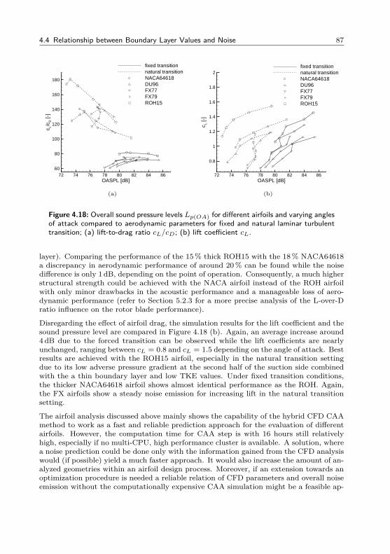
4.4 Relationship between Boundary Layer Values and Noise 87

OASPL [dB]

c L/c D

[-]

72 74 76 78 80 82 84 8660

80

100

120

140

160

180

fixed transitionnatural transitionNACA64618DU96FX77FX79ROH15

(a)

OASPL [dB]

c L [-

]

72 74 76 78 80 82 84 86

0.8

1

1.2

1.4

1.6

1.8

2fixed transitionnatural transitionNACA64618DU96FX77FX79ROH15

(b)

Figure 4.18: Overall sound pressure levels Lp(OA) for different airfoils and varying anglesof attack compared to aerodynamic parameters for fixed and natural laminar turbulenttransition; (a) lift-to-drag ratio cL/cD; (b) lift coefficient cL.

layer). Comparing the performance of the 15% thick ROH15 with the 18% NACA64618a discrepancy in aerodynamic performance of around 20% can be found while the noisedifference is only 1 dB, depending on the point of operation. Consequently, a much higherstructural strength could be achieved with the NACA airfoil instead of the ROH airfoilwith only minor drawbacks in the acoustic performance and a manageable loss of aero-dynamic performance (refer to Section 5.2.3 for a more precise analysis of the L-over-Dratio influence on the rotor blade performance).

Disregarding the effect of airfoil drag, the simulation results for the lift coefficient and thesound pressure level are compared in Figure 4.18 (b). Again, an average increase around4 dB due to the forced transition can be observed while the lift coefficients are nearlyunchanged, ranging between cL = 0.8 and cL = 1.5 depending on the angle of attack. Bestresults are achieved with the ROH15 airfoil, especially in the natural transition settingdue to its low adverse pressure gradient at the second half of the suction side combinedwith the a thin boundary layer and low TKE values. Under fixed transition conditions,the thicker NACA64618 airfoil shows almost identical performance as the ROH. Again,the FX airfoils show a steady noise emission for increasing lift in the natural transitionsetting.

The airfoil analysis discussed above mainly shows the capability of the hybrid CFD CAAmethod to work as a fast and reliable prediction approach for the evaluation of differentairfoils. However, the computation time for CAA step is with 16 hours still relativelyhigh, especially if no multi-CPU, high performance cluster is available. A solution, wherea noise prediction could be done only with the information gained from the CFD analysiswould (if possible) yield a much faster approach. It would also increase the amount of an-alyzed geometries within an airfoil design process. Moreover, if an extension towards anoptimization procedure is needed a reliable relation of CFD parameters and overall noiseemission without the computationally expensive CAA simulation might be a feasible ap-

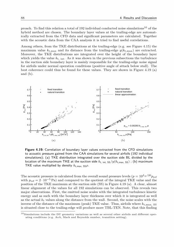
88 4 Results and Discussion

proach. To find this relation a total of 192 individual conducted noise simulations10 of thehybrid method are chosen. The boundary layer values at the trailing-edge are automat-ically extracted from the CFD data and significant parameters are calculated. Togetherwith the acoustic data from the CAA analysis it is tried to find useful correlations.

Among others, from the TKE distributions at the trailing-edge (e.g. see Figure 4.15) themaximum value kt,max and its distance from the trailing-edge y(kt,max) are extracted.Moreover, the TKE distributions are integrated over the height of the boundary layerwhich yields the value kt, int. As it was shown in the previous subsections the turbulencein the suction side boundary layer is mainly responsible for the trailing-edge noise signalfor airfoils under normal operation conditions (positive angle of attack below stall). Thebest coherence could thus be found for these values. They are shown in Figure 4.19 (a)and (b).

kt, int, SS / y(kt, max, SS) [m2/s2]

p rms [

Pa]

0 20 40 60 80 100 120 1400

0.1

0.2

0.3

0.4

0.5

0.6

0.7 fixed transitionnatural transition

(a)

kt, max, SS ρ [Pa]

p rms [

Pa]

0 50 100 1500

0.1

0.2

0.3

0.4

0.5

0.6

0.7 fixed transitionnatural transitionlinear approximation

prms = 0.00293 kt, max, SS ρ

(b)

Figure 4.19: Correlation of boundary layer values extracted from the CFD simulationsto acoustic pressure gained from the CAA simulations for several airfoils (192 individualsimulations); (a) TKE distribution integrated over the suction side BL divided by thelocation of the maximum TKE at the suction side kt, int, SS/y(kt,max, SS) ; (b) maximumTKE value multiplied by density kt,max, SSρ.

The acoustic pressure is calculated from the overall sound pressure levels (p = 10Lp/20prefwith pref = 2 · 10−5 Pa) and compared to the quotient of the integral TKE value and theposition of the TKE maximum at the suction side (SS) in Figure 4.19 (a). A clear, almostlinear alignment of the values for all 192 simulations can be observed. This reveals twomajor observations. First, the emitted noise scales with the integrated turbulence kineticenergy and as such with the boundary layer thickness over which it is integrated as wellas the actual kt values along the distance from the wall. Second, the noise scales with theinverse of the distance of the maximum (peak) TKE value. Thus, airfoils where kt,max, SSis situated close to the trailing-edge will produce more TBL-TEN. Note, that this finding10Simulations include the DU geometry variations as well as several other airfoils and different oper-

ating conditions (e.g. AoA, Mach and Reynolds number, transition setting).

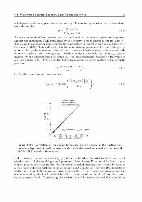
4.4 Relationship between Boundary Layer Values and Noise 89

is independent of the applied transition setting. The following relation can be formulatedfrom the results:

p ∼kt, int, SS

y(kt,max, SS). (4.7)

An even more significant correlation can be found if the acoustic pressure is plottedagainst the maximum TKE multiplied by the density. This is shown in Figure 4.19 (b).The clear, linear relationship between the parameters is indicated by the solid line withthe slope 0.00293. This indicates, that the main driving parameter for the trailing-edgenoise is clearly the maximum value of the turbulence kinetic energy in the suction sideboundary layer at the trailing-edge. Further analysis revealed, that if kt,max, SSρ isdivided by the ambient speed of sound c∞ the proportionality changes to the value ofone (see Figure 4.20). This yields the following relation for an estimation of the acousticpressure:

p 'kt,max, SS · ρ

c∞

[m

s

]. (4.8)

Or for the overall sound pressure level:

Lp(OA) = 20 log

(kt,max, SS·ρ

c∞

[ms

]pref

). (4.9)

kt, max, SS ρ [Pa]/c∝ [Pa s/m]

p rms [

Pa]

0 0.1 0.2 0.3 0.4 0.5 0.6 0.70

0.1

0.2

0.3

0.4

0.5

0.6

fixed transitionnatural transitionlinear approximation

prms = 0.9994 kt, max, SS ρ / c∝ [m/s]

Figure 4.20: Correlation of maximum turbulence kinetic energy in the suction sideboundary layer and acoustic pressure scaled with the speed of sound c∞ for severalairfoils (192 individual simulations).

Unfortunately, the unit of a velocity (m/s) had to be added in order to yield the correctphysical units of the resulting sound pressure. Nevertheless, Equation 4.9 allows to pre-viously predict the CAA results. For an acoustic airfoil optimization it could be used asa first noise indicator without conducting any CAA simulation. For the 192 simulationsplotted in Figure 4.20 the average error between the predicted acoustic pressure and theone simulated by the CAA method is 10% or in terms of decibel 0.8 dB for the overallsound pressure level. Considering the variety of airfoil geometries and flow conditions

90 4 Results and Discussion

which are analyzed, this is a fairly accurate estimation. It can be used as a guideline forthe design of new, low-noise airfoils to filter the available CFD data and thereafter decidewhich settings should be further investigated by the means of CAA simulations.

4.5 Strategy for Low Noise Airfoils

As a result of the aeroacoustic analysis conclusions for the desired features of low noiseairfoils may be drawn. These guidelines can later be used to achieve a noise mitigation inthe airfoil design phase. Nevertheless, competing requirements from aerodynamics andstructural design still need to be considered. An improvement of one feature will oftenresult in a drawback for another. The tradeoff of the requirements is thus crucial toobtain a good overall design. The subsequent list highlights the major points for a lownoise airfoil design.

• Region of Lift Generation: More lift should be generated at the pressure side. Therelatively thin boundary layer here shows only minor influence on the overall soundemission of the airfoil (see Figure 4.16). This could be done by moving the airfoil’smaximum thickness forward which creates a higher flow acceleration beyond thenose. Additionally a more concave shape (rear loading) could be introduced at theback part of the pressure side. Also, the lift generation at the suction side shouldbe concentrated more on the forward part of the airfoil to enhance the moderatepressure regain (see next point).

• Pressure Regain at the Suction Side: In Figures 4.14 and 4.15 it is shown thatthe pressure regain at the aft part of the suction side is mainly responsible forthe boundary layer thickness and the turbulence kinetic energy levels. A shallowerpressure regain with a lower absolute minimum cp value is thus favorable. Of course,this also decreases the generated lift force (tradeoff).

• Reduction of Turbulence Kinetic Energy in the Boundary Layer: A distinct scaling ofthe OASPL values of the tested airfoils with the TKE distribution and its maximumlevels is shown in Figures 4.19 and 4.20. A reduction of TKE will thus directly leadto a noise reduction. Geometry changes of the aft part of the suction side (e.g.an inverse suction side rear loading) should be considered to achieve a TKE reduc-tion. Possible negative side effects (flow separation, high negative lift productionat negative AoAs) need to be closely monitored.

• Thin Airfoil Design: For a better aerodynamic performance (mainly due to thereduced form (shape) drag) in combination with low TKE levels in the boundarylayer, thinner airfoils should be preferred. Clearly, this decision is often governedby structural issues and it is not always possible to reduce the relative thickness. Itcould be argued, that with the achievable noise benefit the higher price for stiffermaterials (e.g. carbon fiber) is justified which might compensate the structuraldrawback of the thinner geometry.

• Long laminar Flow: Airfoils designed for laminar flow have two main advantages.While the L-over-D ratio is almost doubled, the overall noise is reduced by around3 dB compared to their fully turbulent performance (e.g. see Figure 4.13). The useof this advantages seems obvious, but is controversial for an actual wind turbineairfoil. Due to surface contamination and aging, an essential smooth surface cannot

4.5 Strategy for Low Noise Airfoils 91

be guaranteed throughout the lifetime of a rotor blade. Thus, the performanceis highly decreased, especially for laminar designed airfoils. The uncertainty gapbetween turbulent and laminar performance should be as small as possible if thelaminar operation cannot be precisely foreseen. Incorporating a laminar airfoil,which is always operated at its maximum performance, is a challenging task witha high risk of uncertainty but also with a big chance of aerodynamic and acousticadvantages.

The above stated design guidelines will be used to modify the outer rotor blade airfoilNACA64618 of the NREL 5MW turbine. The results on airfoil and turbine level interms of aeroacoustic and aerodynamic behavior are presented in Section 5.2.2 in thenext chapter.

5 Turbine Evaluation

For the full view of the acoustic wind turbine performance it is necessary to link the resultsgained in the previous section with the final three-dimensional design of the turbine.This task can be fulfilled in two basic ways. The first is to extend the two-dimensionalCAA approach to the third dimension and conduct a three-dimensional CAA simulationfor the (acoustically relevant) outer rotor blade region. The second option would beto find a strategy to link the two-dimensional results from the airfoil analysis with theoperational parameters of the turbine, the rotor blade geometry and the observer position.This approach is mainly shown in this Chapter. Its advantages against the 3D CAAsimulation are discussed and results for the observed trailing-edge noise in the vicinityof a wind turbine are shown. This Chapter unites almost all of the aforementionedmethods, beginning with the blade element momentum method (BEM) to determine thewind turbine performance and using the aerodynamic and aeroacoustic results of theairfoil simulation toolchain as high fidelity input data.

5.1 Method

First, the three-dimensional CAA performance is shortly discussed to point out the veryhigh computational effort and to underline the need for a more efficient method whichincorporates the previously gained 2D results.

5.1.1 3D CAA Simulation

A three-dimensional simulation is conducted for the NACA0012 airfoil similar to theBANC-II #1 test case settings (lc = 0.4 m, α = 0 , M = 0.1664). The 2D CAA meshis used as the basis for the 3D mesh. In order to reduce the overall amount of cells,the final three-dimensional mesh is cropped to an extend of 2.35lc in x-direction and2.2lc in y-direction. Moreover, the initial blocks are split into smaller blocks for a betterparallelization of the computations. This results in a 2D mesh with 162 blocks and finally,with 4 blocks into the z-direction, in 648 blocks for the 3D mesh1. The final 3D meshcontains around 40 million cells. Its extend in spanwise direction is 0.05lc. Due to thefine FRPM patch and the adopted resolution in the patch area the mesh shows a highercell density in the middle and coarsens towards the outer parts. This adaptation is alsomade in z-direction. The FRPM patch is extended by 50 layers in the spanwise direction,extending 0.025lc (50% of the CAA mesh). This results in a total number of 6 millionpatch cells. One FRPM particle per cell is set. The flow data of the 2D simulation is

1The parallelization approach of PIANO relies on the distribution of blocks from the computationalmesh to individual CPUs. Thus a certain amount of blocks as well as a nearly equal distribution ofmesh cells within the individual blocks is necessary for an efficient simulation in a multi-CPU highperformance environment.

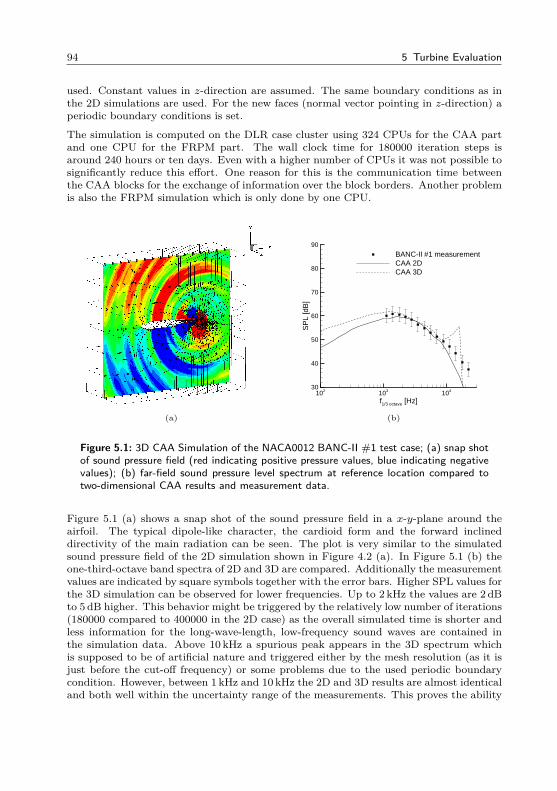
94 5 Turbine Evaluation

used. Constant values in z-direction are assumed. The same boundary conditions as inthe 2D simulations are used. For the new faces (normal vector pointing in z-direction) aperiodic boundary conditions is set.

The simulation is computed on the DLR case cluster using 324 CPUs for the CAA partand one CPU for the FRPM part. The wall clock time for 180000 iteration steps isaround 240 hours or ten days. Even with a higher number of CPUs it was not possible tosignificantly reduce this effort. One reason for this is the communication time betweenthe CAA blocks for the exchange of information over the block borders. Another problemis also the FRPM simulation which is only done by one CPU.

(a)

f1/3 octave [Hz]

SP

L [d

B]

102 103 10430

40

50

60

70

80

90

BANC-II #1 measurementCAA 2DCAA 3D

(b)

Figure 5.1: 3D CAA Simulation of the NACA0012 BANC-II #1 test case; (a) snap shotof sound pressure field (red indicating positive pressure values, blue indicating negativevalues); (b) far-field sound pressure level spectrum at reference location compared totwo-dimensional CAA results and measurement data.

Figure 5.1 (a) shows a snap shot of the sound pressure field in a x-y-plane around theairfoil. The typical dipole-like character, the cardioid form and the forward inclineddirectivity of the main radiation can be seen. The plot is very similar to the simulatedsound pressure field of the 2D simulation shown in Figure 4.2 (a). In Figure 5.1 (b) theone-third-octave band spectra of 2D and 3D are compared. Additionally the measurementvalues are indicated by square symbols together with the error bars. Higher SPL values forthe 3D simulation can be observed for lower frequencies. Up to 2 kHz the values are 2 dBto 5 dB higher. This behavior might be triggered by the relatively low number of iterations(180000 compared to 400000 in the 2D case) as the overall simulated time is shorter andless information for the long-wave-length, low-frequency sound waves are contained inthe simulation data. Above 10 kHz a spurious peak appears in the 3D spectrum whichis supposed to be of artificial nature and triggered either by the mesh resolution (as it isjust before the cut-off frequency) or some problems due to the used periodic boundarycondition. However, between 1 kHz and 10 kHz the 2D and 3D results are almost identicaland both well within the uncertainty range of the measurements. This proves the ability

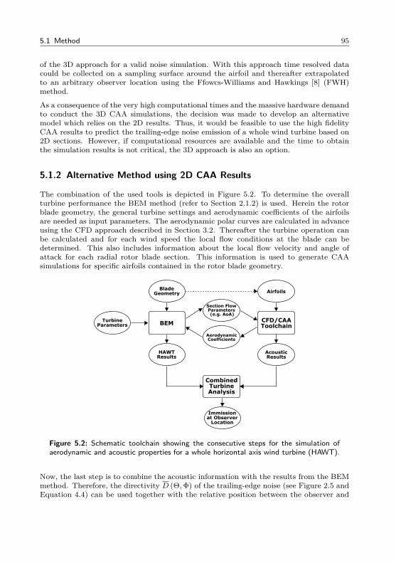
5.1 Method 95

of the 3D approach for a valid noise simulation. With this approach time resolved datacould be collected on a sampling surface around the airfoil and thereafter extrapolatedto an arbitrary observer location using the Ffowcs-Williams and Hawkings [8] (FWH)method.

As a consequence of the very high computational times and the massive hardware demandto conduct the 3D CAA simulations, the decision was made to develop an alternativemodel which relies on the 2D results. Thus, it would be feasible to use the high fidelityCAA results to predict the trailing-edge noise emission of a whole wind turbine based on2D sections. However, if computational resources are available and the time to obtainthe simulation results is not critical, the 3D approach is also an option.

5.1.2 Alternative Method using 2D CAA Results

The combination of the used tools is depicted in Figure 5.2. To determine the overallturbine performance the BEM method (refer to Section 2.1.2) is used. Herein the rotorblade geometry, the general turbine settings and aerodynamic coefficients of the airfoilsare needed as input parameters. The aerodynamic polar curves are calculated in advanceusing the CFD approach described in Section 3.2. Thereafter the turbine operation canbe calculated and for each wind speed the local flow conditions at the blade can bedetermined. This also includes information about the local flow velocity and angle ofattack for each radial rotor blade section. This information is used to generate CAAsimulations for specific airfoils contained in the rotor blade geometry.

TurbineParameters BEM

HAWTResults

AcousticResults

Immissionat Observer

Location

BladeGeometry Airfoils

CFD/CAAToolchain

Section FlowParameters (e.g. AoA)

CombinedTurbineAnalysis

AerodynamicCoefficients

Figure 5.2: Schematic toolchain showing the consecutive steps for the simulation ofaerodynamic and acoustic properties for a whole horizontal axis wind turbine (HAWT).

Now, the last step is to combine the acoustic information with the results from the BEMmethod. Therefore, the directivity D (Θ,Φ) of the trailing-edge noise (see Figure 2.5 andEquation 4.4) can be used together with the relative position between the observer and

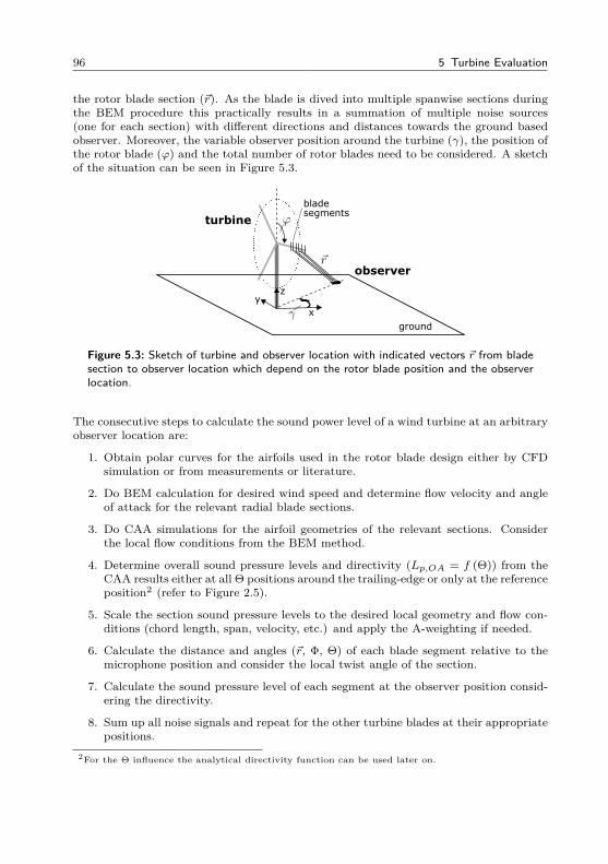
96 5 Turbine Evaluation

the rotor blade section (~r). As the blade is dived into multiple spanwise sections duringthe BEM procedure this practically results in a summation of multiple noise sources(one for each section) with different directions and distances towards the ground basedobserver. Moreover, the variable observer position around the turbine (γ), the position ofthe rotor blade (ϕ) and the total number of rotor blades need to be considered. A sketchof the situation can be seen in Figure 5.3.

xy

observer

z

bladesegments

ground

turbine

Figure 5.3: Sketch of turbine and observer location with indicated vectors ~r from bladesection to observer location which depend on the rotor blade position and the observerlocation.

The consecutive steps to calculate the sound power level of a wind turbine at an arbitraryobserver location are:

1. Obtain polar curves for the airfoils used in the rotor blade design either by CFDsimulation or from measurements or literature.

2. Do BEM calculation for desired wind speed and determine flow velocity and angleof attack for the relevant radial blade sections.

3. Do CAA simulations for the airfoil geometries of the relevant sections. Considerthe local flow conditions from the BEM method.

4. Determine overall sound pressure levels and directivity (Lp,OA = f (Θ)) from theCAA results either at all Θ positions around the trailing-edge or only at the referenceposition2 (refer to Figure 2.5).

5. Scale the section sound pressure levels to the desired local geometry and flow con-ditions (chord length, span, velocity, etc.) and apply the A-weighting if needed.

6. Calculate the distance and angles (~r, Φ, Θ) of each blade segment relative to themicrophone position and consider the local twist angle of the section.

7. Calculate the sound pressure level of each segment at the observer position consid-ering the directivity.

8. Sum up all noise signals and repeat for the other turbine blades at their appropriatepositions.

2For the Θ influence the analytical directivity function can be used later on.

5.2 Results and Discussion 97

9. Repeat the above stated procedure for other rotor positions and average the results.

The scaling of step 5 and 6 is done via the following equation:

Lp,obs = Lp,OA,ref + 10 log(D)︸ ︷︷ ︸

I

+ 10 log(

d

dref

)︸ ︷︷ ︸

II

+ 50 log(vrelvref

)︸ ︷︷ ︸

III

+ 20 log( 1|~r|

)︸ ︷︷ ︸

IV

. (5.1)

The scaling equation (Equation 5.1) consists of four distinct parts. In term I, the two-dimensional CAA sound pressure level at the reference position3 Lp,CAA,ref is combinedwith the directivity function D = f (Θ) to include the influence of the relative observerposition. Note, that contrary to the semi-infinite half plane for which the directivity func-tion is derived, some adaptions need to be made to account for airfoil geometries withlimited x-dimension and an extend in the y-direction (thickness). The modification of Din the two-dimensional airfoil plane (x-y-plane) is shown in Appendix A.6. The approachof the reference location sound pressure level plus the modified directivity function can beused if acoustic information are only available at this position (i.e. also for measurementswith only one microphone). If acoustic results are available for the whole microphonecircle around the TE, as it is the case with all CAA simulations, this directivity infor-mation (which is a direct result of the simulation) can be used for the procedure. Thus,only the out of plane directivity due to Φ needs to be considered. Term II accounts forthe spanwise extend of the section d in comparison to the span of the reference section ofdref = 1 m. The velocity scaling is done in term III. Herein, the relative velocity vrel of therotor blade section due to the radial position the turbine RPM and the wind speed andthe reference velocity of the CAA simulation vref are considered. The last term accountsfor the distance of the section to the observer position |~r|.

The presented approach for the evaluation of the sound immission at a certain observerposition relies on several assumptions. First, the atmospheric damping of sound wavestraveling from source to observer is neglected. Moreover refraction effects due to the windspeed and the atmospheric boundary layer profile are ignored. Also, frequency shifts dueto the relative movement of source and observer (Doppler effect) are not taken intoaccount. An assumption which is valid, at least for positions upstream and downstreamof the turbine where the relative movement is reasonable small. Also, for A-weightedsound pressure levels the narrow-band spectra need to be considered and appropriatelyscaled and thereafter weighted for the correct final values. All these drawbacks need to beconsidered when the approach is used for a full turbine analysis. Nevertheless, the shownprocedure in combination with the BEM turbine prediction can be used for a holisticevaluation approach of wind turbine performance and acoustics.

5.2 Results and Discussion

5.2.1 Analysis of the NREL 5MW Reference Turbine

For the predictions the NREL 5MW reference off-shore turbine from Reference [61] isused. The advantage of this turbine clearly lies in the available data. Ranging from

3The reference position directly below the trailing-edge (Θ = 90 ) at a distance of 1m.

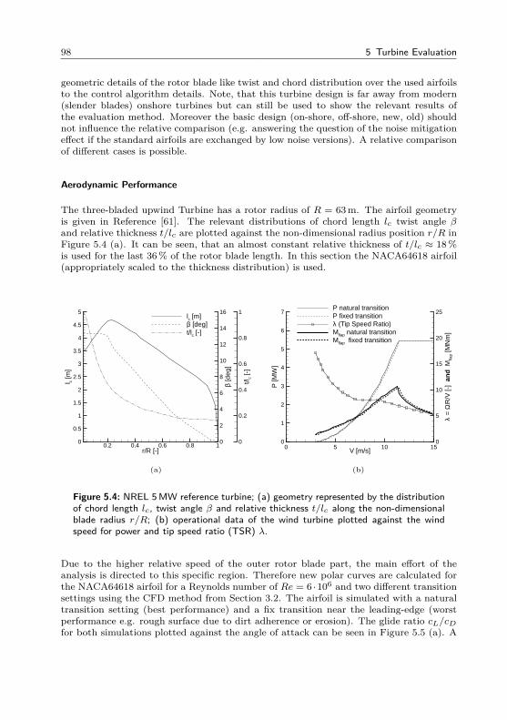
98 5 Turbine Evaluation

geometric details of the rotor blade like twist and chord distribution over the used airfoilsto the control algorithm details. Note, that this turbine design is far away from modern(slender blades) onshore turbines but can still be used to show the relevant results ofthe evaluation method. Moreover the basic design (on-shore, off-shore, new, old) shouldnot influence the relative comparison (e.g. answering the question of the noise mitigationeffect if the standard airfoils are exchanged by low noise versions). A relative comparisonof different cases is possible.

Aerodynamic Performance

The three-bladed upwind Turbine has a rotor radius of R = 63 m. The airfoil geometryis given in Reference [61]. The relevant distributions of chord length lc twist angle βand relative thickness t/lc are plotted against the non-dimensional radius position r/R inFigure 5.4 (a). It can be seen, that an almost constant relative thickness of t/lc ≈ 18 %is used for the last 36% of the rotor blade length. In this section the NACA64618 airfoil(appropriately scaled to the thickness distribution) is used.

r/R [-]

l c [m

]

β [d

eg]

t/lc [

-]

0.2 0.4 0.6 0.8 10

0.5

1

1.5

2

2.5

3

3.5

4

4.5

5

0

2

4

6

8

10

12

14

16

0

0.2

0.4

0.6

0.8

1lc [m]β [deg]t/lc [-]

(a)

V [m/s]

P [M

W]

λ =

ΩR

/V [-

] an

d M

flap

[MN

m]

0 5 10 150

1

2

3

4

5

6

7

0

5

10

15

20

25P natural transitionP fixed transitionλ (Tip Speed Ratio)Mflap natural transitionMflap fixed transition

(b)

Figure 5.4: NREL 5MW reference turbine; (a) geometry represented by the distributionof chord length lc, twist angle β and relative thickness t/lc along the non-dimensionalblade radius r/R; (b) operational data of the wind turbine plotted against the windspeed for power and tip speed ratio (TSR) λ.

Due to the higher relative speed of the outer rotor blade part, the main effort of theanalysis is directed to this specific region. Therefore new polar curves are calculated forthe NACA64618 airfoil for a Reynolds number of Re = 6 ·106 and two different transitionsettings using the CFD method from Section 3.2. The airfoil is simulated with a naturaltransition setting (best performance) and a fix transition near the leading-edge (worstperformance e.g. rough surface due to dirt adherence or erosion). The glide ratio cL/cDfor both simulations plotted against the angle of attack can be seen in Figure 5.5 (a). A

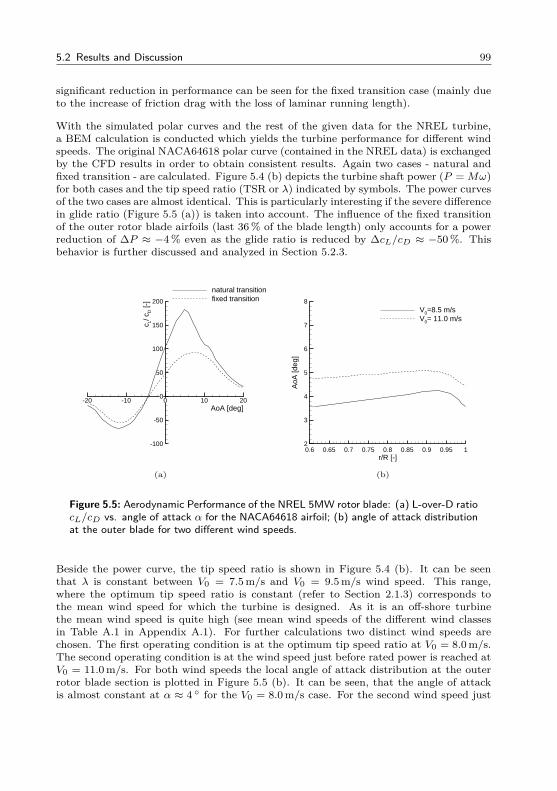
5.2 Results and Discussion 99

significant reduction in performance can be seen for the fixed transition case (mainly dueto the increase of friction drag with the loss of laminar running length).

With the simulated polar curves and the rest of the given data for the NREL turbine,a BEM calculation is conducted which yields the turbine performance for different windspeeds. The original NACA64618 polar curve (contained in the NREL data) is exchangedby the CFD results in order to obtain consistent results. Again two cases - natural andfixed transition - are calculated. Figure 5.4 (b) depicts the turbine shaft power (P = Mω)for both cases and the tip speed ratio (TSR or λ) indicated by symbols. The power curvesof the two cases are almost identical. This is particularly interesting if the severe differencein glide ratio (Figure 5.5 (a)) is taken into account. The influence of the fixed transitionof the outer rotor blade airfoils (last 36% of the blade length) only accounts for a powerreduction of ∆P ≈ −4 % even as the glide ratio is reduced by ∆cL/cD ≈ −50 %. Thisbehavior is further discussed and analyzed in Section 5.2.3.

AoA [deg]

c L/ c

D [-

]

-20 -10 0 10 20

-100

-50

0

50

100

150

200

natural transitionfixed transition

(a)

r/R [-]

AoA

[deg

]

0.6 0.65 0.7 0.75 0.8 0.85 0.9 0.95 12

3

4

5

6

7

8V0=8.5 m/sV0= 11.0 m/s

(b)

Figure 5.5: Aerodynamic Performance of the NREL 5MW rotor blade: (a) L-over-D ratiocL/cD vs. angle of attack α for the NACA64618 airfoil; (b) angle of attack distributionat the outer blade for two different wind speeds.

Beside the power curve, the tip speed ratio is shown in Figure 5.4 (b). It can be seenthat λ is constant between V0 = 7.5 m/s and V0 = 9.5 m/s wind speed. This range,where the optimum tip speed ratio is constant (refer to Section 2.1.3) corresponds tothe mean wind speed for which the turbine is designed. As it is an off-shore turbinethe mean wind speed is quite high (see mean wind speeds of the different wind classesin Table A.1 in Appendix A.1). For further calculations two distinct wind speeds arechosen. The first operating condition is at the optimum tip speed ratio at V0 = 8.0 m/s.The second operating condition is at the wind speed just before rated power is reached atV0 = 11.0 m/s. For both wind speeds the local angle of attack distribution at the outerrotor blade section is plotted in Figure 5.5 (b). It can be seen, that the angle of attackis almost constant at α ≈ 4 for the V0 = 8.0 m/s case. For the second wind speed just

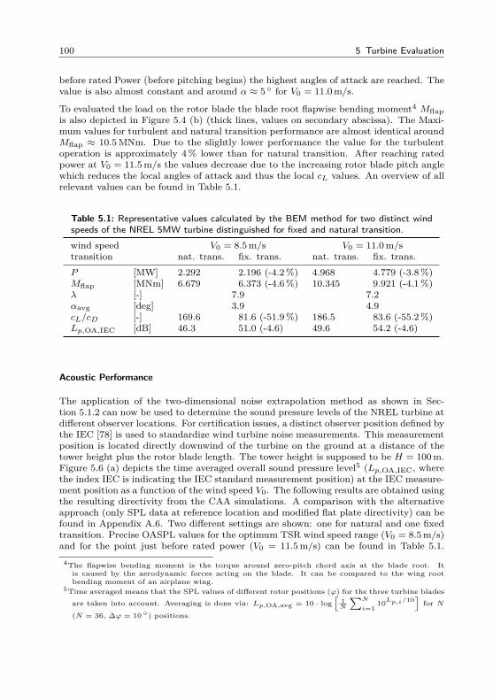
100 5 Turbine Evaluation

before rated Power (before pitching begins) the highest angles of attack are reached. Thevalue is also almost constant and around α ≈ 5 for V0 = 11.0 m/s.

To evaluated the load on the rotor blade the blade root flapwise bending moment4 Mflapis also depicted in Figure 5.4 (b) (thick lines, values on secondary abscissa). The Maxi-mum values for turbulent and natural transition performance are almost identical aroundMflap ≈ 10.5 MNm. Due to the slightly lower performance the value for the turbulentoperation is approximately 4% lower than for natural transition. After reaching ratedpower at V0 = 11.5 m/s the values decrease due to the increasing rotor blade pitch anglewhich reduces the local angles of attack and thus the local cL values. An overview of allrelevant values can be found in Table 5.1.

Table 5.1: Representative values calculated by the BEM method for two distinct windspeeds of the NREL 5MW turbine distinguished for fixed and natural transition.wind speed V0 = 8.5 m/s V0 = 11.0 m/stransition nat. trans. fix. trans. nat. trans. fix. trans.P [MW] 2.292 2.196 (-4.2%) 4.968 4.779 (-3.8%)Mflap [MNm] 6.679 6.373 (-4.6%) 10.345 9.921 (-4.1%)λ [-] 7.9 7.2αavg [deg] 3.9 4.9cL/cD [-] 169.6 81.6 (-51.9%) 186.5 83.6 (-55.2%)Lp,OA,IEC [dB] 46.3 51.0 (-4.6) 49.6 54.2 (-4.6)

Acoustic Performance

The application of the two-dimensional noise extrapolation method as shown in Sec-tion 5.1.2 can now be used to determine the sound pressure levels of the NREL turbine atdifferent observer locations. For certification issues, a distinct observer position defined bythe IEC [78] is used to standardize wind turbine noise measurements. This measurementposition is located directly downwind of the turbine on the ground at a distance of thetower height plus the rotor blade length. The tower height is supposed to be H = 100 m.Figure 5.6 (a) depicts the time averaged overall sound pressure level5 (Lp,OA,IEC, wherethe index IEC is indicating the IEC standard measurement position) at the IEC measure-ment position as a function of the wind speed V0. The following results are obtained usingthe resulting directivity from the CAA simulations. A comparison with the alternativeapproach (only SPL data at reference location and modified flat plate directivity) can befound in Appendix A.6. Two different settings are shown: one for natural and one fixedtransition. Precise OASPL values for the optimum TSR wind speed range (V0 = 8.5 m/s)and for the point just before rated power (V0 = 11.5 m/s) can be found in Table 5.1.

4The flapwise bending moment is the torque around zero-pitch chord axis at the blade root. Itis caused by the aerodynamic forces acting on the blade. It can be compared to the wing rootbending moment of an airplane wing.

5Time averaged means that the SPL values of different rotor positions (ϕ) for the three turbine bladesare taken into account. Averaging is done via: Lp,OA,avg = 10 · log

[1N

∑N

i=110Lp,i/10

]for N

(N = 36, ∆ϕ = 10 ) positions.

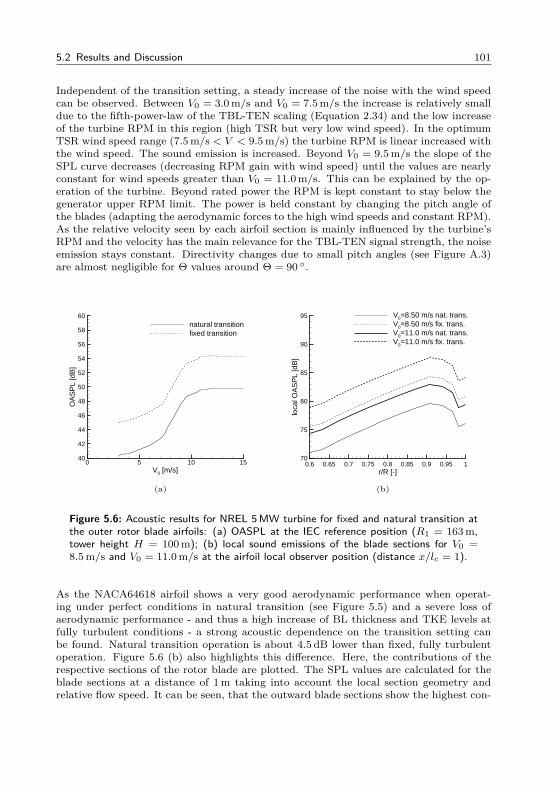
5.2 Results and Discussion 101

Independent of the transition setting, a steady increase of the noise with the wind speedcan be observed. Between V0 = 3.0 m/s and V0 = 7.5 m/s the increase is relatively smalldue to the fifth-power-law of the TBL-TEN scaling (Equation 2.34) and the low increaseof the turbine RPM in this region (high TSR but very low wind speed). In the optimumTSR wind speed range (7.5 m/s < V < 9.5 m/s) the turbine RPM is linear increased withthe wind speed. The sound emission is increased. Beyond V0 = 9.5 m/s the slope of theSPL curve decreases (decreasing RPM gain with wind speed) until the values are nearlyconstant for wind speeds greater than V0 = 11.0 m/s. This can be explained by the op-eration of the turbine. Beyond rated power the RPM is kept constant to stay below thegenerator upper RPM limit. The power is held constant by changing the pitch angle ofthe blades (adapting the aerodynamic forces to the high wind speeds and constant RPM).As the relative velocity seen by each airfoil section is mainly influenced by the turbine’sRPM and the velocity has the main relevance for the TBL-TEN signal strength, the noiseemission stays constant. Directivity changes due to small pitch angles (see Figure A.3)are almost negligible for Θ values around Θ = 90 .

V0 [m/s]

OA

SP

L [d

B]

0 5 10 1540

42

44

46

48

50

52

54

56

58

60natural transitionfixed transition

(a)

r/R [-]

loca

l OA

SP

L [d

B]

0.6 0.65 0.7 0.75 0.8 0.85 0.9 0.95 170

75

80

85

90

95 V0=8.50 m/s nat. trans.V0=8.50 m/s fix. trans.V0=11.0 m/s nat. trans.V0=11.0 m/s fix. trans.

(b)

Figure 5.6: Acoustic results for NREL 5MW turbine for fixed and natural transition atthe outer rotor blade airfoils: (a) OASPL at the IEC reference position (R1 = 163 m,tower height H = 100 m); (b) local sound emissions of the blade sections for V0 =8.5 m/s and V0 = 11.0 m/s at the airfoil local observer position (distance x/lc = 1).

As the NACA64618 airfoil shows a very good aerodynamic performance when operat-ing under perfect conditions in natural transition (see Figure 5.5) and a severe loss ofaerodynamic performance - and thus a high increase of BL thickness and TKE levels atfully turbulent conditions - a strong acoustic dependence on the transition setting canbe found. Natural transition operation is about 4.5 dB lower than fixed, fully turbulentoperation. Figure 5.6 (b) also highlights this difference. Here, the contributions of therespective sections of the rotor blade are plotted. The SPL values are calculated for theblade sections at a distance of 1m taking into account the local section geometry andrelative flow speed. It can be seen, that the outward blade sections show the highest con-

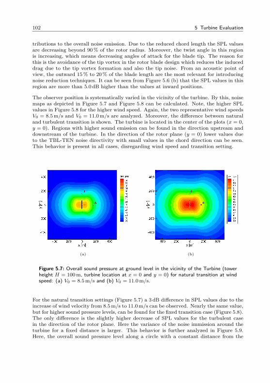
102 5 Turbine Evaluation

tributions to the overall noise emission. Due to the reduced chord length the SPL valuesare decreasing beyond 90% of the rotor radius. Moreover, the twist angle in this regionis increasing, which means decreasing angles of attack for the blade tip. The reason forthis is the avoidance of the tip vortex in the rotor blade design which reduces the induceddrag due to the tip vortex formation and also the tip noise. From an acoustic point ofview, the outward 15% to 20% of the blade length are the most relevant for introducingnoise reduction techniques. It can be seen from Figure 5.6 (b) that the SPL values in thisregion are more than 5.0 dB higher than the values at inward positions.

The observer position is systematically varied in the vicinity of the turbine. By this, noisemaps as depicted in Figure 5.7 and Figure 5.8 can be calculated. Note, the higher SPLvalues in Figure 5.8 for the higher wind speed. Again, the two representative wind speedsV0 = 8.5 m/s and V0 = 11.0 m/s are analyzed. Moreover, the difference between naturaland turbulent transition is shown. The turbine is located in the center of the plots (x = 0,y = 0). Regions with higher sound emission can be found in the direction upstream anddownstream of the turbine. In the direction of the rotor plane (y = 0) lower values dueto the TBL-TEN noise directivity with small values in the chord direction can be seen.This behavior is present in all cases, disregarding wind speed and transition setting.

(a) (b)

Figure 5.7: Overall sound pressure at ground level in the vicinity of the Turbine (towerheight H = 100 m, turbine location at x = 0 and y = 0) for natural transition at windspeed: (a) V0 = 8.5 m/s and (b) V0 = 11.0 m/s.

For the natural transition settings (Figure 5.7) a 3 dB difference in SPL values due to theincrease of wind velocity from 8.5m/s to 11.0m/s can be observed. Nearly the same value,but for higher sound pressure levels, can be found for the fixed transition case (Figure 5.8).The only difference is the slightly higher decrease of SPL values for the turbulent casein the direction of the rotor plane. Here the variance of the noise immission around theturbine for a fixed distance is larger. This behavior is further analyzed in Figure 5.9.Here, the overall sound pressure level along a circle with a constant distance from the

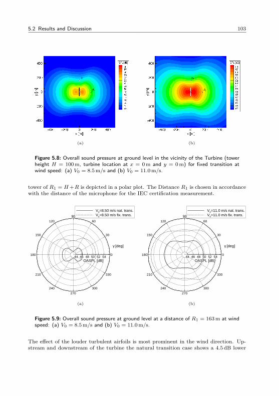
5.2 Results and Discussion 103

(a) (b)

Figure 5.8: Overall sound pressure at ground level in the vicinity of the Turbine (towerheight H = 100 m, turbine location at x = 0 m and y = 0 m) for fixed transition atwind speed: (a) V0 = 8.5 m/s and (b) V0 = 11.0 m/s.

tower of R1 = H+R is depicted in a polar plot. The Distance R1 is chosen in accordancewith the distance of the microphone for the IEC certification measurement.

γ [deg]

OASPL [dB]

0

30

60

90

120

150

180

210

240

270

300

330

44 46 48 50 52 54

V0=8.50 m/s nat. trans.V0=8.50 m/s fix. trans.

(a)

γ [deg]

OASPL [dB]

0

30

60

90

120

150

180

210

240

270

300

330

44 46 48 50 52 54

V0=11.0 m/s nat. trans.V0=11.0 m/s fix. trans.

(b)

Figure 5.9: Overall sound pressure at ground level at a distance of R1 = 163 m at windspeed: (a) V0 = 8.5 m/s and (b) V0 = 11.0 m/s.

The effect of the louder turbulent airfoils is most prominent in the wind direction. Up-stream and downstream of the turbine the natural transition case shows a 4.5 dB lower

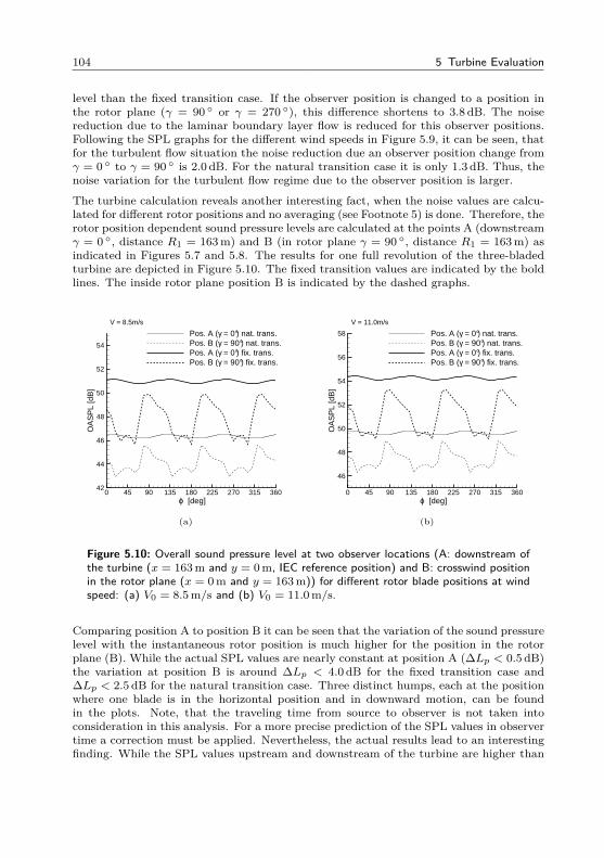
104 5 Turbine Evaluation

level than the fixed transition case. If the observer position is changed to a position inthe rotor plane (γ = 90 or γ = 270 ), this difference shortens to 3.8 dB. The noisereduction due to the laminar boundary layer flow is reduced for this observer positions.Following the SPL graphs for the different wind speeds in Figure 5.9, it can be seen, thatfor the turbulent flow situation the noise reduction due an observer position change fromγ = 0 to γ = 90 is 2.0 dB. For the natural transition case it is only 1.3 dB. Thus, thenoise variation for the turbulent flow regime due to the observer position is larger.

The turbine calculation reveals another interesting fact, when the noise values are calcu-lated for different rotor positions and no averaging (see Footnote 5) is done. Therefore, therotor position dependent sound pressure levels are calculated at the points A (downstreamγ = 0 , distance R1 = 163 m) and B (in rotor plane γ = 90 , distance R1 = 163 m) asindicated in Figures 5.7 and 5.8. The results for one full revolution of the three-bladedturbine are depicted in Figure 5.10. The fixed transition values are indicated by the boldlines. The inside rotor plane position B is indicated by the dashed graphs.

ϕ [deg]

OA

SP

L [d

B]

0 45 90 135 180 225 270 315 36042

44

46

48

50

52

54

Pos. A (γ = 0°) nat. trans.Pos. B (γ = 90°) nat. trans.Pos. A (γ = 0°) fix. trans.Pos. B (γ = 90°) fix. trans.

V = 8.5m/s

(a)

ϕ [deg]

OA

SP

L [d

B]

0 45 90 135 180 225 270 315 360

46

48

50

52

54

56

58 Pos. A (γ = 0°) nat. trans.Pos. B (γ = 90°) nat. trans.Pos. A (γ = 0°) fix. trans.Pos. B (γ = 90°) fix. trans.

V = 11.0m/s

(b)

Figure 5.10: Overall sound pressure level at two observer locations (A: downstream ofthe turbine (x = 163 m and y = 0 m, IEC reference position) and B: crosswind positionin the rotor plane (x = 0 m and y = 163 m)) for different rotor blade positions at windspeed: (a) V0 = 8.5 m/s and (b) V0 = 11.0 m/s.

Comparing position A to position B it can be seen that the variation of the sound pressurelevel with the instantaneous rotor position is much higher for the position in the rotorplane (B). While the actual SPL values are nearly constant at position A (∆Lp < 0.5 dB)the variation at position B is around ∆Lp < 4.0 dB for the fixed transition case and∆Lp < 2.5 dB for the natural transition case. Three distinct humps, each at the positionwhere one blade is in the horizontal position and in downward motion, can be foundin the plots. Note, that the traveling time from source to observer is not taken intoconsideration in this analysis. For a more precise prediction of the SPL values in observertime a correction must be applied. Nevertheless, the actual results lead to an interestingfinding. While the SPL values upstream and downstream of the turbine are higher than

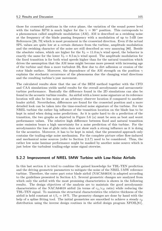
5.2 Results and Discussion 105

those for crosswind positions in the rotor plane, the variation of the sound power levelwith the turbine RPM is much higher for the γ = 90 position. This corresponds toa phenomenon called amplitude modulation (AM). AM is described as a swishing noiseat the frequency of the blade passing frequency with a modulation of up to 5 dB (seeReferences [26, 79] which is most prominent in the crosswind direction. Even if the actualSPL values are quite low at a certain distance from the turbine, amplitude modulationand the swishing character of the noise are still described as very annoying [80]. Besidethe absolute values, which are higher for the V0 = 11.0 m/s wind speed, the behavior isexactly the same for the lower V0 = 8.5 m/s wind speed. The amplitude modulation forthe fixed transition is for both wind speeds higher than for the natural transition whichdrives the assumption that the AM issue might become more present with increasing ageof the turbine and thus a more turbulent BL flow due to dirt adhesion or erosion of therotor blade surface. Moreover, the dependence of the AM strength on the position γexplains the stochastic occurrence of the phenomena due the changing wind directionsand the resulting turbine’s yaw movement.

The calculated results show that the use of the BEM method together with the CFDand CAA simulations yields useful results for the overall aerodynamic and aeroacousticturbine performance. Basically the difference found in the 2D simulations can also befound in the acoustic turbine results. An airfoil with a lower noise signature at its referencelocation will also be less noisy at an arbitrary observer location if compared to anotherlouder airfoil. Nevertheless, differences are found for the crosswind position and a moredetailed look can be taken into the time-resolved noise signature of the turbine. For theNREL turbine the rather big influence of the transition location on the blade has to bekept in mind when doing noise predictions. As it is quite hard to do a prediction of thetransition, the two graphs as depicted in Figure 5.6 (a) must be seen as best and worstperformance values. The relative high difference between fixed and natural transitionnoise emission bears a high uncertainty for a noise prediction of this turbine. For theaerodynamics the loss of glide ratio does not show such a strong influence as it is doingfor the acoustics. Moreover, it has to be kept in mind, that the presented approach onlycontains the trailing-edge noise mechanism. For the complete picture other flow-inducedand mechanical noise sources (refer to Section 2.3.7) need to be considered. Thus, therather low noise laminar performance might be masked by another noise source which isjust below the turbulent trailing-edge noise signal oterwise.

5.2.2 Improvement of NREL 5MW Turbine with Low-Noise Airfoils

In this last section it is tried to combine the gained knowledge for TBL-TEN predictionand the driving geometric parameters to mitigate the noise of the NREL 5MW referenceturbine. Therefore, the outer part rotor blade airfoil (NACA64618) is adapted accordingto the guidelines presented in Section 4.5. Several geometric changes are analyzed fromwhich only the airfoil with the most promising characteristics is shown in the followingresults. The design objectives of the analysis are to maintain the good aerodynamiccharacteristics of the NACA64618 airfoil (in terms of cL/cD ratio) while reducing theTBL-TEN signal. To maintain the structural characteristics the relative thickness of theairfoil is held constant at t/lc = 18 %. The geometry changes are done by hand with thehelp of a spline fitting tool. The initial geometries are smoothed to achieve a steady cpdistribution using the inverse design routines in the airfoil design program XFOIL[81].

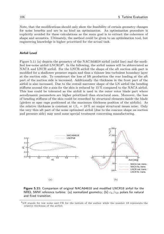
106 5 Turbine Evaluation

Note, that the modifications should only show the feasibility of certain geometry changesfor noise benefits and are in no kind an optimization. An optimization procedure isexplicitly avoided for these calculations as the main goal is to extract the coherence ofshape and acoustics. Ultimately, the method could be given to an optimization tool, butengineering knowledge is higher prioritized for the actual task.

Airfoil Level

Figure 5.11 (a) depicts the geometry of the NACA64618 airfoil (solid line) and the modi-fied low-noise airfoil LNCR186. In the following, the airfoil names will be abbreviated asNACA and LNCR airfoil. For the LNCR airfoil the shape of the aft suction side part ismodified for a shallower pressure regain and thus a thinner less turbulent boundary layerat the suction side. To counteract the loss of lift production the rear loading at the aftpart of the suction side is increased. Additionally the thickness in the front part of theairfoil is also increased. Due to the overall narrower shape of the LN airfoil the bendingstiffness around the x-axis for the skin is reduced by 15% compared to the NACA airfoil.This loss could be tolerated as the airfoil is used in the outer rotor blade part whereaerodynamic parameters are higher prioritized than structural ones. Moreover, the lossof bending stiffness of the skin could be remedied by structural elements inside the blade(girders or spar caps positioned at the maximum thickness position of the airfoils). Asthe relative thickness is constant at t/lc = 18 % no major structural issues arise. Onlythe very thin aft part of the noise optimized airfoil (due to the concave shape on suctionand pressure side) may need some special treatment concerning manufacturing.

x/lc

y/l c

0 0.2 0.4 0.6 0.8 1-0.2

-0.1

0

0.1

0.2NACA64618LNCR18

(a)

AoA [deg]

c L/ c

D [-

]

-20 -10 0 10 20

-100

-50

0

50

100

150

200

NACA nat. trans.NACA fix. trans.LNCR nat. trans.LNCR fix. trans.

(b)

Figure 5.11: Comparison of original NACA64618 and modified LNCR18 airfoil for theNREL 5MW reference turbine: (a) normalized geometry; (b) cL/cD polars for naturaland fixed transition.

6LN stands for low noise and CR for the initials of the author while the number 18 represents therelative thickness of the airfoil.

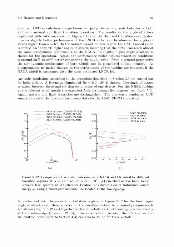
5.2 Results and Discussion 107

Standard CFD calculations are performed to judge the aerodynamic behavior of bothairfoils in natural and fixed transition operation. The results for the angle of attackdependent glide ratio are shown in Figure 5.11 (b). For the fixed transition case (dashedlines) a slightly better performance of the LNCR airfoil can be observed for angles ofattack higher than α = 6 . In the natural transition flow regime the LNCR airfoil curveis shifted 1.5 towards higher angles of attack, meaning that the airfoil can reach almostthe same aerodynamic performance as the NACA if a slightly higher angle of attack ischosen for the operation. Again, the performance under natural transition conditionsis around 50% to 80% better considering the cL/cD ratio. From a general perspectivethe aerodynamic performance of both airfoils can be considered almost identical. Asa consequence no major changes in the performance of the turbine are expected if theNACA airfoil is exchanged with the noise optimized LNCR foil.

Acoustic simulations according to the procedure described in Section 3.3 are carried outfor both airfoils. A Reynolds Number of Re = 6.0 · 106 is chosen. The angle of attackis varied between three and six degrees in steps of one degree. For the NREL turbineat the relevant wind speeds the expected AoA lies around five degrees (see Table 5.1).Again, natural and fixed transition are distinguished. The previously conducted CFDsimulations yield the flow and turbulence data for the PIANO FRPM simulation.

f1/3 octave [Hz]

SP

L [d

B]

102 103 10450

55

60

65

70

75

80NACA nat. trans. (OASPL=77.6dB)NACA fix. trans. (OASPL=82.6dB)LNCR nat. trans. (OASPL=77.7dB)LNCR fix. trans. (OASPL=80.4dB)

(a)

kt [m2/s2]

y/l c [

-]

0 10 20 30 40 50 60 70-0.04

-0.02

0

0.02

0.04

0.06

0.08 NACA nat. trans.NACA fix. trans.LNCR nat. trans.LNCR fix. trans

(b)

Figure 5.12: Comparison of acoustic performance of NACA and LN airfoil for differenttransition regimes at α = 4.0 an Re = 6.0 · 106: (a) one-third octave band soundpressure level spectra at 2D reference location; (b) distribution of turbulence kineticenergy kt along a chord-perpendicular line located at the trailing-edge.

A precise look into the acoustic airfoil data is given in Figure 5.12 for the four degreeangle of attack case. Here, spectra for the one-third-octave band sound pressure levelsare shown (Figure 5.12 (a)) together with the turbulence kinetic energy profiles directlyat the trailing-edge (Figure 5.12 (b)). The close relation between the TKE values andthe emitted noise (refer to Section 4.4) can also be found for these airfoils.

108 5 Turbine Evaluation

For the NACA airfoil (black lines) a strong increase of TKE levels especially at the suctionside can be observed when the transition is fixed at the leading edge. Higher TKE levelsand a thicker suction side boundary layer result in higher SPL values at lower frequencies.Consequently, the overall sound pressure level is increased by 5 dB. The same behaviorcan be observed for the low-noise airfoil. The only difference is the spectral shape forthe natural transition case of the LNCR foil. Here, the peak frequency is shifted towardshigher values (around f = 3 kHz). One explanation for this could be the pronouncedpeak at the pressure side TKE profile directly at the wall which seems to trigger higherfrequencies. Even though the suction side TKE profile shows lower values in the naturaltransition case for the LNCR airfoil than for the NACA airfoil the overall sound pressurelevels are almost identical for the two airfoils(77.7 dB for the NACA and 77.6 dB for theLNCR airfoil). Considering the fixed transition case the picture changes. Now, the LNairfoil has lower TKE values on both sides resulting in lower SPL values throughout thespectrum and thus in an overall sound pressure 2.2 dB below the NACA value. This noisereduction is achieved without aerodynamic drawbacks (refer to Figure 5.11 (b)).

Turbine Level

A combined view of aerodynamic and acoustic airfoil performance is given in Figure 5.13 (a).Overall sound pressure levels and glide ratios are plotted for angles of attack from threeto six degrees in steps of one degree. It can be seen, that for the natural transition case(solid lines) both airfoils can reach glide ratios between 140 and 190 while the overallsound pressure level lies between 77.5 dB and 79.5 dB. The performance on both scales inthis case seems almost identical. The main difference between the two airfoils can be ob-served for the fixed transition simulations. Here, both airfoils reach glide ratios between75 and 95 in the desired AoA range while clearly reduced overall sound pressure levels canbe found for the LNCR airfoil. The NACA airfoil shows OASPL values between 82 dBand 83 dB, the LN airfoil operates at values which are between 1 dB to 2 dB lower. Whilethe same aerodynamic performance is achieved a significant noise reduction is possiblewith the LNCR airfoil.

In a final step the newly designed low noise airfoil is incorporated into the NREL designby exchanging the outer rotor blade NACA airfoil with the new LNCR airfoil. From CFDsimulations all relevant aerodynamic coefficients are known to feed the BEM calculationsand determine the overall turbine characteristics. The results for different wind speedsare depicted in Figure 5.13 (b). Precise values for two distinct wind speeds of 8.5m/sand 11.0m/s (refer to Section 5.2.1) are grouped together in Table 5.2 for the naturaltransition case and Table 5.3 for the fixed transition case.

For the natural transition case the new noise optimized airfoils result in a negligibleincrease of power of 0.3% at 8.5m/s which diminishes towards the rated-power windspeed of 11m/s where no influence can be observed. This behavior was almost expected,as the aerodynamic performance of both airfoils is nearly identical. An interesting facthere is the reduction of the flapwise bending momentMflap of roughly three percent due tothe new airfoils throughout both wind speed cases (see Table 5.2). Thus, a load reductionwithout power influence is achieved with the new airfoils. For the fixed transition casethe new LNCR airfoil yields a power increase of roughly one percent, while the flapwisebending moment remains almost unchanged (reduction between 0.3% and 0.1%). Thepower increase is achieved without any load increase which can be seen as a positive

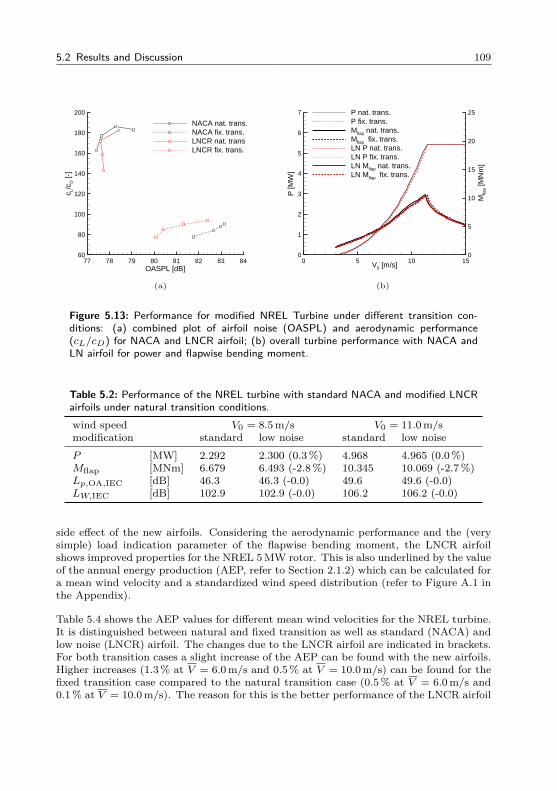
5.2 Results and Discussion 109

OASPL [dB]

c L/c D

[-]

77 78 79 80 81 82 83 8460

80

100

120

140

160

180

200

NACA nat. trans.NACA fix. trans.LNCR nat. transLNCR fix. trans.

(a)

V0 [m/s]

P [M

W]

Mfla

p [M

Nm

]

0 5 10 150

1

2

3

4

5

6

7

0

5

10

15

20

25P nat. trans.P fix. trans.Mflap nat. trans.Mflap fix. trans.LN P nat. trans.LN P fix. trans.LN Mflap nat. trans.LN Mflap fix. trans.

(b)

Figure 5.13: Performance for modified NREL Turbine under different transition con-ditions: (a) combined plot of airfoil noise (OASPL) and aerodynamic performance(cL/cD) for NACA and LNCR airfoil; (b) overall turbine performance with NACA andLN airfoil for power and flapwise bending moment.

Table 5.2: Performance of the NREL turbine with standard NACA and modified LNCRairfoils under natural transition conditions.wind speed V0 = 8.5 m/s V0 = 11.0 m/smodification standard low noise standard low noiseP [MW] 2.292 2.300 (0.3%) 4.968 4.965 (0.0%)Mflap [MNm] 6.679 6.493 (-2.8%) 10.345 10.069 (-2.7%)Lp,OA,IEC [dB] 46.3 46.3 (-0.0) 49.6 49.6 (-0.0)LW,IEC [dB] 102.9 102.9 (-0.0) 106.2 106.2 (-0.0)

side effect of the new airfoils. Considering the aerodynamic performance and the (verysimple) load indication parameter of the flapwise bending moment, the LNCR airfoilshows improved properties for the NREL 5MW rotor. This is also underlined by the valueof the annual energy production (AEP, refer to Section 2.1.2) which can be calculated fora mean wind velocity and a standardized wind speed distribution (refer to Figure A.1 inthe Appendix).

Table 5.4 shows the AEP values for different mean wind velocities for the NREL turbine.It is distinguished between natural and fixed transition as well as standard (NACA) andlow noise (LNCR) airfoil. The changes due to the LNCR airfoil are indicated in brackets.For both transition cases a slight increase of the AEP can be found with the new airfoils.Higher increases (1.3% at V = 6.0 m/s and 0.5% at V = 10.0 m/s) can be found for thefixed transition case compared to the natural transition case (0.5% at V = 6.0 m/s and0.1% at V = 10.0 m/s). The reason for this is the better performance of the LNCR airfoil

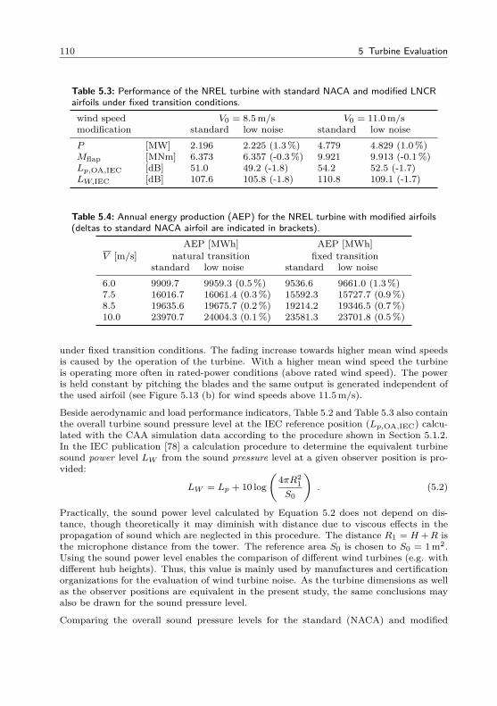
110 5 Turbine Evaluation

Table 5.3: Performance of the NREL turbine with standard NACA and modified LNCRairfoils under fixed transition conditions.wind speed V0 = 8.5 m/s V0 = 11.0 m/smodification standard low noise standard low noiseP [MW] 2.196 2.225 (1.3%) 4.779 4.829 (1.0%)Mflap [MNm] 6.373 6.357 (-0.3%) 9.921 9.913 (-0.1%)Lp,OA,IEC [dB] 51.0 49.2 (-1.8) 54.2 52.5 (-1.7)LW,IEC [dB] 107.6 105.8 (-1.8) 110.8 109.1 (-1.7)

Table 5.4: Annual energy production (AEP) for the NREL turbine with modified airfoils(deltas to standard NACA airfoil are indicated in brackets).

AEP [MWh] AEP [MWh]V [m/s] natural transition fixed transition

standard low noise standard low noise6.0 9909.7 9959.3 (0.5%) 9536.6 9661.0 (1.3%)7.5 16016.7 16061.4 (0.3%) 15592.3 15727.7 (0.9%)8.5 19635.6 19675.7 (0.2%) 19214.2 19346.5 (0.7%)10.0 23970.7 24004.3 (0.1%) 23581.3 23701.8 (0.5%)

under fixed transition conditions. The fading increase towards higher mean wind speedsis caused by the operation of the turbine. With a higher mean wind speed the turbineis operating more often in rated-power conditions (above rated wind speed). The poweris held constant by pitching the blades and the same output is generated independent ofthe used airfoil (see Figure 5.13 (b) for wind speeds above 11.5m/s).

Beside aerodynamic and load performance indicators, Table 5.2 and Table 5.3 also containthe overall turbine sound pressure level at the IEC reference position (Lp,OA,IEC) calcu-lated with the CAA simulation data according to the procedure shown in Section 5.1.2.In the IEC publication [78] a calculation procedure to determine the equivalent turbinesound power level LW from the sound pressure level at a given observer position is pro-vided:

LW = Lp + 10 log(

4πR21

S0

). (5.2)

Practically, the sound power level calculated by Equation 5.2 does not depend on dis-tance, though theoretically it may diminish with distance due to viscous effects in thepropagation of sound which are neglected in this procedure. The distance R1 = H +R isthe microphone distance from the tower. The reference area S0 is chosen to S0 = 1 m2.Using the sound power level enables the comparison of different wind turbines (e.g. withdifferent hub heights). Thus, this value is mainly used by manufactures and certificationorganizations for the evaluation of wind turbine noise. As the turbine dimensions as wellas the observer positions are equivalent in the present study, the same conclusions mayalso be drawn for the sound pressure level.

Comparing the overall sound pressure levels for the standard (NACA) and modified

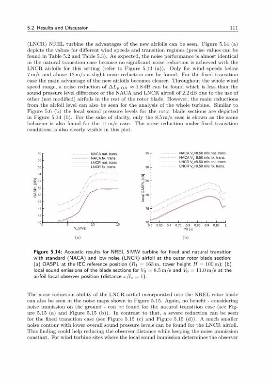
5.2 Results and Discussion 111

(LNCR) NREL turbine the advantages of the new airfoils can be seen. Figure 5.14 (a)depicts the values for different wind speeds and transition regimes (precise values can befound in Table 5.2 and Table 5.3). As expected, the noise performance is almost identicalin the natural transition case because no significant noise reduction is achieved with theLNCR airfoils for this setting (refer to Figure 5.13 (a)). Only for wind speeds below7m/s and above 12m/s a slight noise reduction can be found. For the fixed transitioncase the main advantage of the new airfoils becomes clearer. Throughout the whole windspeed range, a noise reduction of ∆Lp,OA ≈ 1.8 dB can be found which is less than thesound pressure level difference of the NACA and LNCR airfoil of 2.2 dB due to the use ofother (not modified) airfoils in the rest of the rotor blade. However, the main reductionsfrom the airfoil level can also be seen for the analysis of the whole turbine. Similar toFigure 5.6 (b) the local sound pressure levels for the rotor blade sections are depictedin Figure 5.14 (b). For the sake of clarity, only the 8.5m/s case is shown as the samebehavior is also found for the 11m/s case. The noise reduction under fixed transitionconditions is also clearly visible in this plot.

V0 [m/s]

OA

SP

L [d

B]

0 5 10 1540

42

44

46

48

50

52

54

56

58

60 NACA nat. trans.NACA fix. trans.LNCR nat. trans.LNCR fix. trans.

(a)

r/R [-]

loca

l OA

SP

L [d

B]

0.6 0.65 0.7 0.75 0.8 0.85 0.9 0.95 170

75

80

85

90

95 NACA V0=8.50 m/s nat. trans.NACA V0=8.50 m/s fix. trans.LNCR V0=8.50 m/s nat. trans.LNCR V0=8.50 m/s fix. trans.

(b)

Figure 5.14: Acoustic results for NREL 5MW turbine for fixed and natural transitionwith standard (NACA) and low noise (LNCR) airfoil at the outer rotor blade section:(a) OASPL at the IEC reference position (R1 = 163 m, tower height H = 100 m); (b)local sound emissions of the blade sections for V0 = 8.5 m/s and V0 = 11.0 m/s at theairfoil local observer position (distance x/lc = 1).

The noise reduction ability of the LNCR airfoil incorporated into the NREL rotor bladecan also be seen in the noise maps shown in Figure 5.15. Again, no benefit - consideringnoise immission on the ground - can be found for the natural transition case (see Fig-ure 5.15 (a) and Figure 5.15 (b)). In contrast to that, a severe reduction can be seenfor the fixed transition case (see Figure 5.15 (c) and Figure 5.15 (d)). A much smallernoise contour with lower overall sound pressure levels can be found for the LNCR airfoil.This finding could help reducing the observer distance while keeping the noise immissionconstant. For wind turbine sites where the local sound immission determines the observer

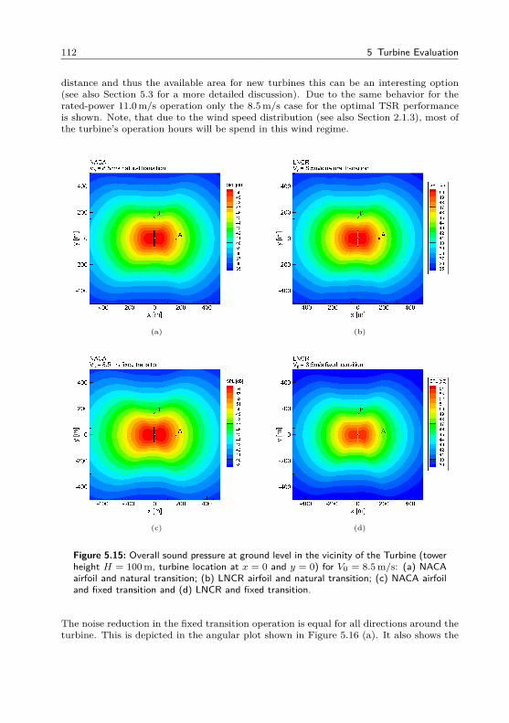
112 5 Turbine Evaluation

distance and thus the available area for new turbines this can be an interesting option(see also Section 5.3 for a more detailed discussion). Due to the same behavior for therated-power 11.0m/s operation only the 8.5m/s case for the optimal TSR performanceis shown. Note, that due to the wind speed distribution (see also Section 2.1.3), most ofthe turbine’s operation hours will be spend in this wind regime.

(a) (b)

(c) (d)

Figure 5.15: Overall sound pressure at ground level in the vicinity of the Turbine (towerheight H = 100 m, turbine location at x = 0 and y = 0) for V0 = 8.5 m/s: (a) NACAairfoil and natural transition; (b) LNCR airfoil and natural transition; (c) NACA airfoiland fixed transition and (d) LNCR and fixed transition.

The noise reduction in the fixed transition operation is equal for all directions around theturbine. This is depicted in the angular plot shown in Figure 5.16 (a). It also shows the

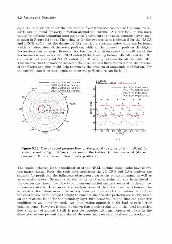
5.2 Results and Discussion 113

equal sound distribution for the natural and fixed transition case where the same overalllevels can be found for every direction around the turbine. A closer look on the noisevalues for different azimuthal rotor positions (equivalent to the noise immission over time)is taken in Figure 5.16 (b). The behavior for the two positions is identical for the NACAand LNCR airfoil. At the downwind (A) position a constant noise value can be foundwhich is independent of the rotor position, while at the crosswind position (B) higherfluctuations can be seen. However, for the fixed transition case the amplitude of thefluctuations is smaller for the LNCR airfoil (3.0 dB ranging between 45.5 dB and 48.5 dB)compared to the original NACA airfoil (4.5 dB ranging between 45.5 dB and 50.0 dB).This means, that the noise optimized airfoil also reduces fluctuations due to the rotationof the blades and thus might help to remedy the problem of amplitude modulation. Forthe natural transition case, again an identical performance can be found.

γ [deg]

OASPL [dB]

0

30

60

90

120

150

180

210

240

270

300

330

44 46 48 50 52 54

NACA V0=8.50 m/s nat. trans.NACA V0=8.50 m/s fix. trans.LNCR V0=8.50 m/s nat. trans.LNCR V0=8.50 m/s fix. trans.

(a)

ϕ [deg]

OA

SP

L [d

B]

0 45 90 135 180 225 270 315 36042

44

46

48

50

52

54Pos. A (γ = 0°) nat. trans.Pos. B (γ = 90°) nat. trans.Pos. A (γ = 0°) fix. trans.Pos. B (γ = 90°) fix. trans.

V = 8.5m/sNACA values in black LNCR values in red

(b)

Figure 5.16: Overall sound pressure level at the ground (distance of R1 = 163 m) fora wind speed of V0 = 8.5 m/s: (a) around the turbine; (b) for downwind (A) andcrosswind (B) position and different rotor positions ϕ.

The results achieved for the modification of the NREL turbine rotor blades have showntwo major things. First, the tools developed from the 2D CFD and CAA analysis aresuitable for predicting the influences of geometry variations on aerodynamic as well asaeroacoustic scales. Second, a benefit in terms of noise reduction can be achieved ifthe conclusions drawn from the two-dimensional airfoil analysis are used to design new(low-noise) airfoils. Even more, the analysis revealed that this noise reduction can beachieved without drawbacks of the aerodynamic performance of wind turbine. Note, thatthe chosen new airfoil design thought to enhance the acoustic performance is only basedon the relations found for the boundary layer turbulence values and that the geometrymodification was done by hand. An optimization approach might lead to even betterenhancements. However, it could be shown that a noise reduction in the fixed transitionflow situation of around 1.8 dB is possible together with an increase of power in thedimension of one percent (and almost the same increase of annual energy production)

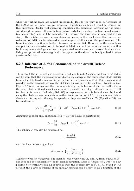
114 5 Turbine Evaluation

while the turbine loads are almost unchanged. Due to the very good performance ofthe NACA airfoil under natural transition conditions no benefit could be gained forthis operation. Under real operating conditions the transition locations on the bladewill depend on many different factors (inflow turbulence, surface quality, manufacturingtolerances, etc.) and will be somewhere in between the two extrema analyzed in thisstudy. One might average the two states and come to the conclusion, that an averagereduction of 1 dB can be achieved without negative influence on the performance. Thebenefit of this reduction is further discussed in Section 5.3. However, as the main focuswas put on the demonstration of the used toolchain and not on the actual noise reductionby finding new airfoil geometries, the generated results are in a reasonable dimension.Using an optimization strategy which incorporates the shown tools might lead to evengreater reductions.

5.2.3 Influence of Airfoil Performance on the overall TurbinePerformance

Throughout the investigations a certain trend was found. Considering Figure 5.4 (b) itcan be seen, that the the loss of power due to the change of the outer rotor blade airfoilsfrom natural to fixed transition is only a few percent (less than 5%). This seems kind ofparadox, as the L-over-D ratio of the airfoils is almost halved by the forced transition (seeFigure 5.5 (a)). So, against the common thinking the influence of the L-over-D ratio inthe outer blade section does not seem to have the anticipated high influence on the overallturbine performance. Following Bak [82] an explanation for this behavior can be foundusing the blade element momentum method (refer to Section 2.1.1). For an annular bladeelement - rotating with the angular speed ω - the power coefficient Cp (Equation 2.4) canbe rewritten to:

Cp =dFtrω

12ρV

30 dA

=[

(1− a)2 + λloc2(1 + a′

)2]λlocctσ . (5.3)

Assuming an ideal axial induction of a = 1/3 the equation shortens to:

Cp =[4

9+ λloc2

(1 + a′

)2]λlocctσ . (5.4)

The solidity σ can also be expressed as:

σ =2 sin2 Φcn

(5.5)

and the local inflow angle Φ as:

Φ = arctan( 1− aλloc (1 + a′)

). (5.6)

Together with the tangential and normal force coefficients (ct and cn from Equation 2.7and 2.8) and the equation for the rotational induction factor a′ (Equation 2.10) it is nowpossible to iteratively solve all equations with the dependency of a′, ct, cn, σ and Φ. Asa result the power coefficient of an annular element can be plotted as a function of the

5.2 Results and Discussion 115

TSR λ loc [-]

CP =

P/P

avai

l [-]

1 2 3 4 5 6 7 8 90.4

0.45

0.5

0.55

0.6

inviscid flowcL/cD = 200cL/cD = 150cL/cD = 100cL/cD = 50

Betz Limit CP = 16/27

Figure 5.17: Local power coefficient for an annular element at different local tip speedλloc ratios for varying L-over-D ratio cL/cD.

local tip speed ratio λloc and the L-over-D ratio cL/cD of the section. This relation isdepicted in Figure 5.17. Note, that ideal axial induction (a = 1/3) and zero tip loss areassumed.

In Figure 5.17 the power coefficient is plotted against the local tip speed ratio for differentL-over-D ratios. It can be seen, that the highest glide ratio yields the highest powercoefficient. For the inviscid flow situation (cD = 0) the Betz limit (CP = 16/27) can bereached. The local tip speed ratio can be interpreted as the radial position of the airfoilsection. The higher relative speed (ωr) due to the radius position of the outer rotor bladesections results in higher values for λloc.

A reduction of the L-over-D ratio leads to a decrease of the maximum power coefficientof the section. This trend becomes stronger as the absolute values for cL/cD becomelower. For example for an outer rotor blade section (assuming λloc = 7) the changeof L-over-D ratio from cL/cD = 200 to cL/cD = 150 results in a 2% decrease of Cpwhile the change from cL/cD = 100 to cL/cD = 50 yields a Cp reduction of 12%. Thisexplains why the rather large difference in glide ratio for the different transition settingsonly shows a reduced influence on the overall turbine performance. From a practicalpoint of view the highest increases of the power coefficient can be reached if airfoils withsmall L-over-D ratios (e.g. cL/cD < 100) are improved. For high L-over-D ratio airfoils(e.g. cL/cD > 100) a further increase of the aerodynamic performance only yields minorimprovements on the overall turbine scale. Considering the very high effort for designingairfoils with ultra high glide ratios (laminar boundary layer flow, low thickness etc.) thisinsight has to be kept in mind. Other structural parameters, like a high bending stiffnessfor airfoils with increased thickness, might justify the choice of an airfoil with a glide ratioaround cL/cD = 100 as the gain with a higher glide ratio is rather small.

116 5 Turbine Evaluation

5.3 Benefit of Noise Reduction

Reducing wind turbine noise is also interesting from a more commercial point of view.The assumption is, that the actual noise reduction is not directly used to design a quieterturbine or wind farm, but instead is spend in other disciplines to yield a reduction of costsor an increase of energy production. Doing this, the question of the effective value of anoise reduction, of for example one decibel, can be answered. Using simple relationshipssome main aspects can be derived (see also Figure 5.18):

• Amount of Turbines in a Wind Farm: Considering a sound pressure level at a certainsite generated by N incoherent and mutually uncorrelated sources (wind turbinesset up in a wind farm), the summation of the single sound pressure levels Lp yieldsthe total sound pressure level Lp,total = 10 log

(N · 10Lp/10

). A reduction of Lp

for each turbine could thus be used to increase the amount of turbines if the totalsound pressure level Lp,total is held constant: ∆Lp = 10 log

(N1N2

). A reduction of

1 dB for each turbine theoretically yields an increase of 25% of the total numberof turbines in the wind farm. The profit of the wind farm directly scales with thisfigure, as more energy can be produced with the increased number of turbines.

• Power Increase: As stated in Equation 2.34 TBL-TEN scales with the fifth powerof the flow velocity. A noise reduction could be traded against an increase of the

turbine tip speed vtip with the relation: ∆Lp = 10 log(vtip1vtip2

)5. If the rotational

speed of the turbine is held constant (ω = const.), a longer rotor blade could bebuilt (vtip = Rω). As the turbine power scales linear with the rotor area (P ∼ A)a noise reduction of 1 dB could be used for a power increase of roughly 10% whenlonger rotor blades are used and the same sound power level as before should bereached. Again, this figure can directly be added to the turbine’s revenue, buthigher loads and more material need to be considered.

• Load Reduction: Contrary to the point above, the tip speed influence of the noisereduction could also be used for a reduction of loads if the turbine power and theblade length are held constant. Due to P = Mω a noise reduction can be used toincrease the tip speed by increasing the angular rotor speed ω. A reduction of 5%of the rotor torque M can be utilized if the turbine noise can be reduced by 1 dB.The rotor torque is the main driver for the dimensioning loads of the main shaft,the gearbox and all connected parts e.g. bearings. Thus, a load reduction woulddirectly reduce the dimensions of these parts and finally their cost.

• Observer Distance to the Turbine: Another benefit of noise reduction can be seenfrom Equation 5.1. Disregarding damping effects in the medium, the sound pres-sure level decreases quadratically with the distance from the turbine: ∆Lp =10 log

( |r2||r1|

)2. Consequently, if a wind turbine site is influenced by a certain noise

level at a distinct location, a noise reduction of the turbine could be used to reducethe distance between the turbine and the location by maintaining a constant noiseimmission. A distance reduction of 10% is possible with a noise reduction of 1 dB.New wind farm areas especially in noise sensitive surroundings can be conqueredthis way.

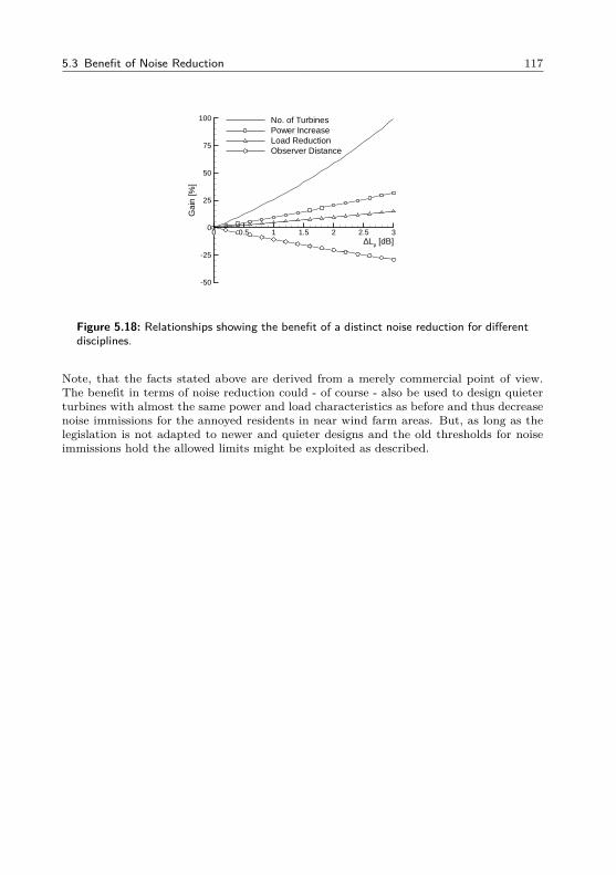
5.3 Benefit of Noise Reduction 117

∆Lp [dB]

Gai

n [%

]

0 0.5 1 1.5 2 2.5 3

-50

-25

0

25

50

75

100 No. of TurbinesPower IncreaseLoad ReductionObserver Distance

Figure 5.18: Relationships showing the benefit of a distinct noise reduction for differentdisciplines.

Note, that the facts stated above are derived from a merely commercial point of view.The benefit in terms of noise reduction could - of course - also be used to design quieterturbines with almost the same power and load characteristics as before and thus decreasenoise immissions for the annoyed residents in near wind farm areas. But, as long as thelegislation is not adapted to newer and quieter designs and the old thresholds for noiseimmissions hold the allowed limits might be exploited as described.

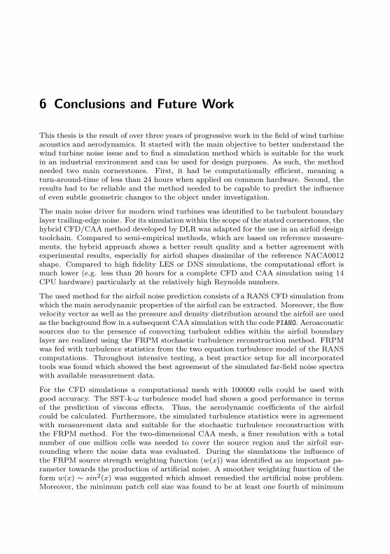
6 Conclusions and Future Work

This thesis is the result of over three years of progressive work in the field of wind turbineacoustics and aerodynamics. It started with the main objective to better understand thewind turbine noise issue and to find a simulation method which is suitable for the workin an industrial environment and can be used for design purposes. As such, the methodneeded two main cornerstones. First, it had be computationally efficient, meaning aturn-around-time of less than 24 hours when applied on common hardware. Second, theresults had to be reliable and the method needed to be capable to predict the influenceof even subtle geometric changes to the object under investigation.

The main noise driver for modern wind turbines was identified to be turbulent boundarylayer trailing-edge noise. For its simulation within the scope of the stated cornerstones, thehybrid CFD/CAA method developed by DLR was adapted for the use in an airfoil designtoolchain. Compared to semi-empirical methods, which are based on reference measure-ments, the hybrid approach shows a better result quality and a better agreement withexperimental results, especially for airfoil shapes dissimilar of the reference NACA0012shape. Compared to high fidelity LES or DNS simulations, the computational effort ismuch lower (e.g. less than 20 hours for a complete CFD and CAA simulation using 14CPU hardware) particularly at the relatively high Reynolds numbers.

The used method for the airfoil noise prediction consists of a RANS CFD simulation fromwhich the main aerodynamic properties of the airfoil can be extracted. Moreover, the flowvelocity vector as well as the pressure and density distribution around the airfoil are usedas the background flow in a subsequent CAA simulation with the code PIANO. Aeroacousticsources due to the presence of convecting turbulent eddies within the airfoil boundarylayer are realized using the FRPM stochastic turbulence reconstruction method. FRPMwas fed with turbulence statistics from the two equation turbulence model of the RANScomputations. Throughout intensive testing, a best practice setup for all incorporatedtools was found which showed the best agreement of the simulated far-field noise spectrawith available measurement data.

For the CFD simulations a computational mesh with 100000 cells could be used withgood accuracy. The SST-k-ω turbulence model had shown a good performance in termsof the prediction of viscous effects. Thus, the aerodynamic coefficients of the airfoilcould be calculated. Furthermore, the simulated turbulence statistics were in agreementwith measurement data and suitable for the stochastic turbulence reconstruction withthe FRPM method. For the two-dimensional CAA mesh, a finer resolution with a totalnumber of one million cells was needed to cover the source region and the airfoil sur-rounding where the noise data was evaluated. During the simulations the influence ofthe FRPM source strength weighting function (w(x)) was identified as an important pa-rameter towards the production of artificial noise. A smoother weighting function of theform w(x) ∼ sin2(x) was suggested which almost remedied the artificial noise problem.Moreover, the minimum patch cell size was found to be at least one fourth of minimum

120 6 Conclusions and Future Work

resolved turbulent length scale (lmin), to correctly reproduce the high frequency part ofthe noise spectrum.

After finding the best possible settings for each step in the airfoil acoustic simulationtoolchain, a lot of effort was spend on the automation and scripting of the procedure.Several Linux shell scripts and Python routines were developed which govern the automa-tion of the mesh generation, the setup and data gathering of the CFD simulation, thepost processing of the CFD results in terms of aerodynamic coefficient determination aswell as in preparing the flow data for the subsequent CAA step and other major partsin the analysis. Moreover, the CAA mesh is created from an automatic script using thesame input geometry as for the CFD mesh. All files needed for the PIANO and FRPMCAA run are gathered and prepared by a script. After the simulations are completed,another script is used for the post processing and the extraction of the relevant acousticresults. The use of automated scripts did not only accelerate the work and generate agreater amount of output, it also resulted in a quality enhancement, as it avoided user in-put errors e.g. by always generating computational meshes with the same input data, cellsizes and blocking strategy for the different cases. Errors due to the use of wrong inputdata, especially for the CAA simulations where a lot of different files are needed, couldbe completely reduced. Thanks to the semi-automized two-dimensional airfoil simulationchain it was possible to evaluate a lot of geometries at several different flow conditions.

Comparing the simulated results to available measurement data from the BANC-II work-shop emphasized the validity of the used approach. It was shown, that throughout allfrequencies covered by the measurements the simulations were able to reproduce the ex-perimental data within the given uncertainty range. Basic physical relations, e.g. betweenthe angle of attack and the form of the far-field noise spectrum were correctly simulated.For the NACA0012 simulation under six degrees angle of attack the two separate spectrafrom suction side (thick boundary layer - low frequencies) and pressure side (thin bound-ary layer - high frequencies) could be solely simulated in individual simulations and lateron superimposed to indeed yield the same result as for the simulation of the completecase and also the same result as in the measurements. The mentioned increase in re-sult quality could clearly be shown for the wind turbine designed DU-96 airfoil, wherethe hybrid CFD/CAA approach showed a good alignment with the measured spectra incontrast to the NACA-calibrated semi-empirical BPM method.

After showing the validity of the chosen approach the toolchain was used to evaluate thedesign driving parameters for airfoil trailing-edge noise. For this purpose the geometryof the DU-96 airfoil was systematically varied. The four-digit NACA series approach wasadapted for this task. In a first step the geometry was bent back to its symmetricalshape. Thereafter, the NACA mean-line function was calculated for a specific amountof camber and a desired camber position. This mean-line was then used to modify thethickness-scaled symmetric DU airfoil to a new shape with the appropriate values. Fora holistic comparison of the data it was important to not only judge an airfoil by itsoverall noise emission at a certain reference position. Even as import as the acousticperformance was the look on the aerodynamic performance. The objective was to findan airfoil shape which shows a low noise emission but also a high aerodynamic gradein terms of L-over-D ratio (cL/cD) and lift coefficient (cL). Closest to this objectivecame a strongly cambered thickness-reduced version of the DU-96 airfoil. For a chosenL-over-D ratio, the noise levels of all analyzed airfoils varied in the range of three to fivedecibels. This clearly underlined the fact, that the same aerodynamic performance could

121

be generated under different noise emissions and that an acoustic enhancement is thuspossible. Moreover, the influence of the very important laminar to turbulent boundarylayer transition was investigated. For cases where the transition was fixed close to theairfoil nose (e.g. representing the operation under with an uneven surface due to dirtadhesive or erosion), higher noise levels were emitted and the overall noise was increasedby as much as four decibels while the aerodynamic performance in terms of L-over-D ratiodropped by almost 50% due to the increased airfoil drag. As this is a severe influenceand it is further hard to set a transition location in accordance with real wind turbineoperations, all subsequent results were calculated for a nose-region fixed transition (worstcase scenario) as well as the natural transition case (best case scenario).

The availability of a whole lot of simulation data from CFD and CAA calculations for dif-ferent airfoils under several flow conditions, made it possible to draw conclusions betweenthe relevant flow parameters and their influence on the aeroacoustics. Relevant boundarylayer parameters were extracted and compared to the far-field noise immissions. It wasfound, that the maximum value of the turbulence kinetic energy in the usually thicker(positive angle of attack implied) suction side boundary layer at the trailing-edge almostdirectly predicts the overall far-field sound pressure level. A relationship between thisvalue and the acoustic pressure in the far-field was shown which can be used for predic-tions within the accuracy of 0.8 dB. Moreover, beside the value also the distance of themaximum TKE from the trailing-edge needs to be considered. The closer this maximummoves to the TE, the more efficient becomes the TBL-TEN source. Identifying the mainnoise driving aspects it was possible to formulate some major recommendations for alow-noise airfoil design:

• The turbulence levels within the suction side boundary layer should be as low aspossible (soft pressure regain, concave surface shape in the back of the suction side).

• Other areas than the aft part of the suction side should be used to compensatethe loss of lift production (e.g. shift more load to the pressure side by using arear-loading).

• More lift should be generated in the forward part of the airfoil and the minimum cpvalues should be kept low (absolute) to avoid a to steep slope of the pressure regainat the suction side.

• The position of the laminar turbulent transitions needs to be considered as it has asevere influence on the TKE levels within the boundary layer and thus the aerody-namic as well as aeroacoustic performance of the airfoil.

Beside the two-dimensional analysis it was planned to continue the study with a three-dimensional modeling approach, to evaluate the acoustic performance, not only of rotorblade airfoils, but for a whole three-dimensional section of the blade and finally the wholeturbine. First tests showed, that this was only possible by using massive computationalresources, even for a relative small 3D extrapolation of a NACA0012 test case. As thisdemand for resources was outside the scope of the preferred industrial fast and reliablemantra, an alternative strategy was developed to generate results for a complete windturbine. Therefore, the classic blade element momentum theory, which is a standardfor aerodynamic examinations of whole wind turbines, was coupled with the developedtwo-dimensional toolchain. Simulations were conducted for the relevant 2D rotor bladesections. The aerodynamic data (lift and drag coefficients) was used to feed the BEM fromwhich local angles of attack as well as other relevant operating parameters to determine

122 6 Conclusions and Future Work

the relevant acoustic data (from previously conducted CAA simulations) were calculated.Using the acoustic information plus the geometric information of the relative positionfrom the rotor blade sections towards a ground based observer at an arbitrary position,it was possible to calculate the directivity influence. Moreover, an appropriate scalingfor each section’s geometric extensions (local chord lengths) and flow speed was doneand the emission of all seperate sections from the three blades were superposed in theobserver position. This combined procedure yielded the acoustic immission at the observerposition plus a lot of turbine performance data from the BEM e.g. the power curve orthe development of the blade root bending moment over different wind speeds. With themethod, noise maps for the trailing-edge noise emission in the vicinity of the wind turbinecould be calculated.

The described turbine simulation procedure was tested with available data from the NREL5MW reference turbine. Setting up the BEM and acoustic calculations, the baselinevalues for this turbine could be calculated. In a second step the main outer rotor airfoil(NACA64618) was exchanged by a self-modified low noise airfoil, the LNCR-18 airfoil.The geometry of the LNCR airfoil was made by hand using the mentioned key factsfor a low noise airfoil design. As the NACA airfoil showed a quite good performanceunder natural transition conditions no improvement could be gained here. But alsono deterioration was present and the performance (acoustically and aerodynamically)remained almost unchanged by the new airfoil. In fact, the flapwise bending momentcould even be reduced on the order of three percent. The main advantages of the lownoise airfoil design came into play in the fixed transition case. Here, a noise reductionon the order of two decibels over the complete frequency range of interest was achievedwithout influencing the aerodynamic performance of the blade. The turbine power waseven increased by one percent and the flapwise bending moment remained untouched(-0.3%). Under real turbine operating conditions, this case is also closer to reality due todirt and disturbances which are always present on the blade surface and lead to earliertransition. Generally speaking, a noise reduction in the range of one decibel with amanually shaped airfoil represents a truly significant advantage. Note, that so far nooptimization techniques were used, which are thought to generate an even higher noisereduction. Nevertheless, a noise reduction of even only one decibel is quite valuable in awind turbine design case. The noise reduction could help winning noise sensitive projectswith the turbine where often every single dB counts. For immission based regulations itcould help to either put more (quieter) wind turbines in a certain wind farm or even reducethe distance to the immission point but still keep the threshold levels set by legislation.

The main outcomes of this thesis are the used tool-chains and tools which allow the windturbine designer to previously evaluate the noise emission of a planned new turbine. Inan early stage of the design, these tools help to choose the correct airfoils for which everconstraints (aerodynamic or acoustically) are present. For short notice the main resultsare grouped in the following list:

• Development of a combined aerodynamic and acoustic toolchain on airfoil and tur-bine level with an appropriate best practice setup and validated results.

• Extraction of the main noise driving parameters in the airfoil design.

• Identification of useful aerodynamic parameters which can be generated throughouta simple CFD simulation and their influence towards TBL-TEN.

• Design of an example low-noise airfoil.

6.1 Impact of Results on Next-Generation Turbines 123

• Improvement of the baseline wind turbine in terms of acoustics without any aero-dynamic drawbacks.

6.1 Impact of Results on Next-Generation Turbines

Throughout the wind turbine industry a clear trend can be found. Each new turbinegeneration is not only bigger than the one before (concerning overall dimensions, ratedpower, etc.), it also comprises newly developed technologies as well as new insights gainedby progressive research and testing. Especially in the field of acoustics the results of thisthesis can help to incorporate the evaluation of the turbine’s noise emissions in an earlystage of the rotor blade design. So far, the acoustic predictions in the design phase ofa rotor blade were often limited to basic estimations mainly based on the tip speed andthe fifth-power law. Noise measurements of actual turbines helped to tune these simpleestimations, but only to a limited extend. Using semi-empirical prediction codes eased thesituation a little bit, but due to the inaccuracy for non-NACA-similar airfoils they werenot able to correctly predict geometric changes in the airfoil design with a credibilitydemanded. Often, the reliable statements on the acoustic performance could only bemade after the first prototype was built. Errors, for example a too noisy design couldthus primarily be seen at this very advanced project stage. This led to the situation,that in order to avoid a costly reworking a more conservative design approach was used.Thus, safety margins were often quite high and the resulting output of the turbine (interms of actual power output or even load reduction) was lower than possible. A reliableprediction tool can tackle this issue and help judging design decisions in the early stagesof a new rotor blade design process. The shown toolchain can be used on an airfoil aswell as turbine level to support the work in this field. Moreover, the shown relationshipsof boundary layer turbulence data can be used in simpler models to quickly judge theperformance on a noise emission scale. Using the turbine noise prediction technique,specific noise maps can be calculated for every single point of operation. This allowsa better coordination of the turbine control as well as the turbine positioning for theagreement with local regulations. As discussed, the acoustic benefits can be spend indifferent ways.

Condensed, the basic advantages of the presented work on new turbine generations mightbe:

• Incorporating the acoustic predictions into the design of new rotor blades on ahighly validated level.

• Reducing security margins due to the better understanding and prediction of thedesign and thus gaining more yield.

• Selective acoustic enhancement of rotor blades (optimization).

• Judging of the effects of noise reduction or increase on the aerodynamic performanceof the rotor blade.

124 6 Conclusions and Future Work

6.2 Outlook

For progression in the field of wind turbine aeroacoustics it would make sense to spendmore effort on the extension of the presented hybrid approach towards a three-dimensionalcases. As shown, this is actually possible but only with a high demand of computationalresources. A better parallelization strategy might help here. The three-dimensionalsimulations are of major interest so far, as 3D flow effects, e.g. in the region of the blade tipand the related tip vortex were not covered by the presented two-dimensional toolchain.Also, it would be possible to judge other interesting noise effects if a reliable three-dimensional method would be available. This would for example include the simulationsof vortex generators which are often used on the rotor blade airfoils to avoid a too earlyflow separation by introducing higher momentum air flow into the boundary layer througha vortex. Moreover, noise mitigation devices, for example trailing-edge serrations could beanalyzed to better understand their noise mitigation effect and to quantify their impactin the overall blade noise emissions. Geometric design studies would be possible.

Another interesting field to use the shown methods of this thesis would be the field ofoptimization. Due to the massive use of automation procedures, the method is either onairfoil as well as on full turbine scale prone to be used within an optimization process, toe.g. find the airfoil design with the least noise but best aerodynamic performance. A lotmore parameters than presented within this work could be tested towards their influenceon trailing-edge noise as well as other competing disciplines. Considering the actualwork, engineering knowledge, as well as the setup of robust and reliable toolchains werehigher prioritized than a geometry study driven by an optimization with a few hundredor thousand designs. In the mind of the author, this is the more trustful way to go whichalso has the higher impact considering the understanding of relevant features and theoverall context. Nevertheless, a fully automized optimization procedure might help tofind the last bit of noise reduction and add the last few percent on the power generation,which from a purely cost driven industrial view are still worth to be found.

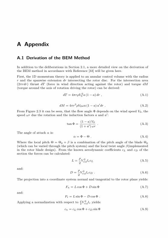
A Appendix

A.1 Derivation of the BEM Method

In addition to the deliberations in Section 2.1, a more detailed view on the derivation ofthe BEM method in accordance with Reference [33] will be given here.

First, the 1D momentum theory is applied to an annular control volume with the radiusr and the spanwise extension dr intersecting the rotor disc. For the intersection area(2πrdr) thrust dT (force in wind direction acting against the rotor) and torque dM(torque around the axis of rotation driving the rotor) can be derived:

dT = 4πrρV 20 a (1− a) dr , (A.1)

dM = 4πr3ρV0ωa (1− a) a′dr . (A.2)

From Figure 2.3 it can be seen, that the flow angle Φ depends on the wind speed V0, thespeed ωr due the rotation and the induction factors a and a′:

tan Φ =(1− a)V0

(1 + a′)ωr. (A.3)

The angle of attack α is:α = Φ−Θ . (A.4)

Where the local pitch Θ = Θp + β is a combination of the pitch angle of the blade Θp(which can be varied through the pitch system) and the local twist angle β(implementedin the rotor blade design). From the known aerodynamic coefficients cL and cD of thesection the forces can be calculated:

L =ρ

2V 2rellccL (A.5)

and:D =

ρ

2V 2rellccD . (A.6)

The projection into a coordinate system normal and tangential to the rotor plane yields:

Fn = L cos Φ +D sin Φ (A.7)

and:Ft = L sin Φ−D cos Φ . (A.8)

Applying a normalization with respect to ρ2V

2rellc yields:

cn = cL cos Φ + cD sin Φ (A.9)

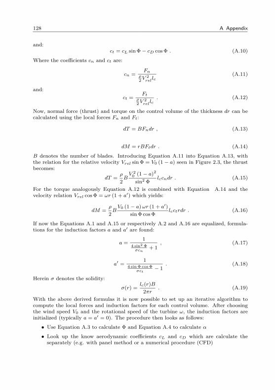
128 A Appendix

and:ct = cL sin Φ− cD cos Φ . (A.10)

Where the coefficients cn and ct are:

cn =Fn

ρ2V

2rellc

(A.11)

and:ct =

Ftρ2V

2rellc. (A.12)

Now, normal force (thrust) and torque on the control volume of the thickness dr can becalculated using the local forces Fn and Ft:

dT = BFndr , (A.13)

dM = rBFtdr . (A.14)

B denotes the number of blades. Introducing Equation A.11 into Equation A.13, withthe relation for the relative velocity Vrel sin Φ = V0 (1− a) seen in Figure 2.3, the thrustbecomes:

dT =ρ

2BV 2

0 (1− a)2

sin2 Φlccndr . (A.15)

For the torque analogously Equation A.12 is combined with Equation A.14 and thevelocity relation Vrel cos Φ = ωr (1 + a′) which yields:

dM =ρ

2BV0 (1− a)ωr (1 + a′)

sin Φ cos Φlcctrdr . (A.16)

If now the Equations A.1 and A.15 or respectively A.2 and A.16 are equalized, formula-tions for the induction factors a and a′ are found:

a =1

4 sin2 Φσcn

+ 1, (A.17)

a′ =1

4 sin Φ cos Φσct

− 1. (A.18)

Herein σ denotes the solidity:

σ(r) =lc(r)B

2πr. (A.19)

With the above derived formulas it is now possible to set up an iterative algorithm tocompute the local forces and induction factors for each control volume. After choosingthe wind speed V0 and the rotational speed of the turbine ω, the induction factors areinitialized (typically a = a′ = 0). The procedure then looks as follows:

• Use Equation A.3 to calculate Φ and Equation A.4 to calculate α

• Look up the know aerodynamic coefficients cL and cD which are calculate theseparately (e.g. with panel method or a numerical procedure (CFD)

A.1 Derivation of the BEM Method 129

• Compute cn and ct from Equation A.9 and A.10

• Use Equation A.17 and A.18 to calculate a and a′

The above described steps are repeated until the change of the induction factors is withinthe desired limit. By then, the local loads and forces of the blade segment can be com-puted. The integration of the segments over the blade radius R yields the global pa-rameters such as the mechanical power, thrust or the bending moment of the blade inedge-wise or flap-wise direction.

Prandtl’s Tip Loss Factor

Prandtl found, that a correction for a finite number of blades needs to be applied in orderto account for the vortex system in the wake behind the turbine. Therefore he derivedthe correction factor:

F =2π

cos−1(e−

B(R−r)2r sin Φ

). (A.20)

It is introduced into Equations A.17 and A.18 which yields:

a =1

4F sin2 Φσcn

+ 1, (A.21)

a′ =1

4F sin Φ cos Φσct

− 1. (A.22)

Glauert Correction

For axial induction factors larger than approximately 0.4, the mometum theory breaksdown [33] and a correction needs to be applied. An empirical approach was shown bySpera [83] where the formulation for the tangential load coefficient is modified:

ct =

4a (1− a)F for a ≤ ac4(a2c + (1− 2ac) a

)F for a > ac

(A.23)

By that, Equations A.17 changes to:

a =

1

4F sin2 Φσcn

+1for a ≤ ac

12

[2 +K (1− 2ac)−

√(K (1− 2ac) + 2)2 + 4 (Ka2

c − 1)]

for a > ac(A.24)

with:

K =4F sin2 Φσcn

. (A.25)

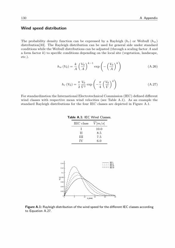
130 A Appendix

Wind speed distribution

The probability density function can be expressed by a Rayleigh (hr) or Weibull (hw)distribution[33]. The Rayleigh distribution can be used for general side under standardconditions while the Weibull distributions can be adjusted (through a scaling factor A anda form factor k) to specific conditions depending on the local site (vegetation, landscape,etc.).

hw (V0) =k

A

(V0

A

)k−1exp(−(V0

A

)k)(A.26)

hr (V0) =π

2V0

V 2 exp(−π

4

(V0

V

)2)

(A.27)

For standardization the International Electrotechnical Commission (IEC) defined differentwind classes with respective mean wind velocities (see Table A.1). As an example thestandard Rayleigh distributions for the four IEC classes are depicted in Figure A.1.

Table A.1: IEC Wind Classes.

IEC class V [m/s]I 10.0II 8.5III 7.5IV 6.0

V0 [m/s]

hr [

-]

0 5 10 15 20 250

0.02

0.04

0.06

0.08

0.1

0.12

0.14IEC IIEC IIIEC IIIIEC IV

Figure A.1: Rayleigh distribution of the wind speed for the different IEC classes accordingto Equation A.27.

A.2 Governing Equations 131

A.2 Governing Equations

Navier-Stokes equations in conservative integral form (non-moving control volume) asimplemented in the DLR Tau code[40]:

∂

∂t

∫∫∫V

~W = −∫∫∂V

F · ~ndS (A.28)

With the vector of conserved quantities ~W :

~W =

ρρuρvρwρE

(A.29)

The flux density tensor F with inviscid (index i) and viscid (index v) flux vectors ~F , ~Gand ~H (superscript c indicates the convective nature of the terms):

F =(~F ci + ~F cv

)· ~ex +

(~Gci + ~Gcv

)· ~ey +

(~Hci + ~Hc

v

)· ~ez (A.30)

The viscous and invicid fluxes:

~F ci =

ρu

ρu2 + pρuvρuwρHu

, ~F cv =

0τxxτxyτxz

uτxx + vτxy + wτxz + k ∂T∂x

(A.31)

~Gci =

ρvρuv

ρv2 + pρvwρHv

, ~Gcv =

0τxyτyyτyz

uτxy + vτyy + wτyz + k ∂T∂y

(A.32)

~Hci =

ρwρuwρvw

ρw2 + pρHw

, ~Hcv =

0τxzτyzτzz

uτxz + vτyz + wτzz + k ∂T∂z

(A.33)

The equation of state for the pressure p:

p = (κ− 1) ρ(E −

u2 + v2 + w2

2

)(A.34)

132 A Appendix

The temporal change of the conservative variables ~W can be derived from Equation A.28as:

∂

∂t~W =

∫∫∂V

F · ~ndS∫∫∫V

dV. (A.35)

It can be seen, that the the change of the flow conditions is related to the fluxes overthe volume boundary ∂V and its size V . For a control volume fixed in time and spaceEquation A.35 changes to:

d

dt~W = −

1V· ~QF . (A.36)

The vector ~QF represents the fluxes over the control volume boundaries. Dividing theboundary into n faces leads to:

~QF =n∑i=1

~QFi =n∑i=1

(~QF,ci − ~Di

). (A.37)

Inviscid fluxes over the representative face are denoted by ~QF,ci , additional dissipativeterms with ~Di. With the determination of the convective fluxes over the control volumeboundaries the temporal change of the flow quantities inside the volume can be deter-mined. For upwind solving schemes the ~Di terms are zero, for central schemes additionaldissipation has to be computed.

A.3 From Governing Equations to Wave Equation

Starting from the continuity and the momentum equation (2.11 and 2.12) in Section 2.2,the homogenous wave equation (without right hand side source terms) can be derived.After the neglection of the mass flow m the time-derivative of Equation 2.11 yields:

∂2ρ

∂t2+

∂

∂t∇ · (ρ~v) = 0 . (A.38)

From the momentum equation (2.12) the divergence is taken (mass flow, external forcesand viscous friction neglected).

∂

∂t∇ · (ρ~v) +∇ · ∇ · (ρ~v~v) +∇ · ∇p = 0 (A.39)

Equation A.39 is subtracted from Equation A.38 which yields:

∂2ρ

∂t2−∇ · ∇ · (ρ~v~v)−∇ · ∇p = 0 . (A.40)

The variables are split into a steady mean flow part (subscript 0) and a small fluctuatingpart (superscript ′).

p = p0 + p′, ρ = ρ0 + ρ′, ~v = ~v0 + ~v′ (A.41)

A.4 Realizing a Liepmann Turbulence Spectrum with FRPM 133

With these terms Equation A.40 then becomes:

∂2 (ρ0 + ρ′)∂t2

−∇ · ∇ ·((ρ0 + ρ′

) (~v0 + ~v′

) (~v0 + ~v′

))−∇ · ∇

(p0 + p′

)= 0 . (A.42)

It can now be linearized by neglecting products of small quantities (indicated by supersript′). Additionally, the mean pressure and density p0 and ρ0 are supposed to be constantand the medium is at rest (~v0 = 0). Equation A.42 therefore becomes:

∂2ρ′

∂t2−∇ · ∇p′ = 0 . (A.43)

Now, the relationship of the fluctuating acoustic density ρ′ and the acoustic pressure p′as given in Equation 2.26 can be used which yields the homogeneous wave equations forthe acoustic pressure:

∂2p′

∂t21c20−∆p′ = 0 . (A.44)

The Laplacian operator ∆ = ∇ · ∇ is used to shorten the equation.

A.4 Realizing a Liepmann Turbulence Spectrum with FRPM

The following section describes the realization of of Liepmann turbulence spectrum by thesuperposition of different scaled FRPM realizations according to the procedure describedin Reference [70].

It is supposed that the decrease of the far-field sound pressure level spectrum is linkedto the form of the realized turbulent energy spectrum E(k) provided by FRPM. A differ-ent form of the energy spectrum can be achieved by a superposition of different FRPMstochastic fields, each generated from independent random particle representations anddifferent length scales per field. Therefore, each realization is scaled with a length scaledependent weighting function. Since the different FRPM realizations are mutually un-correlated, it means that the realized turbulent spectra for each length scale can simplybe superposed.

Each FRPM realization of a specific length scale realizes a turbulent Gaussian spectrumEG of the form:

EG(k, l) =8ktk4l5

3π3 exp(−k2l2

π

). (A.45)

Here kt denotes the turbulence kinetic energy, k is the wave number, and l the integrallength scale of the Gaussian spectrum. The Gaussian spectrum is normalized such thatits integral over all wave-numbers is one for kt = 1, i.e.∫ ∞

0EG(k)|kt=1 dk = 1. (A.46)

The aim is to find a weighting function (variance for each length scale) f(l) to realize:

E(k) =∫ ∞

0f(l) EG(k, l)|kt=1 dl =

8k4

3π3

∫ ∞0

f(l)l5 exp(−k2l2

π

)dl . (A.47)

134 A Appendix

With the substitution l2/π = 1/2σ2 and dl = −√π/8/σ3 dσ2 the integral is written in

a form suitable for Gaussian transformation as introduced by Alecu et al.[84],

p(k) =E(k)k4 =

∫ ∞0

√2π

6σ7 f

(√π/2σ

)︸ ︷︷ ︸

G(σ2)

1√

2πσexp(−k2

2σ2

)︸ ︷︷ ︸

N(x|σ2)

dσ2. (A.48)

Hence, from the Gaussian transform G(σ2) the weighting function derives as

f (l) =6σ7√

2πG(σ2), with σ =

√π/2l

. (A.49)

The weighting function f(l) is the variance realized by the FRPM field with length scalel. Hence, that amplitude used in FRPM must be ∝

√f(l) (and therefore f(l) must be

positive).

Besides the Gaussian spectrum Liepmann[71] proposed a different form of the energyspectrum EL, with a much shallower decay of turbulence energy towards higher wavenum-bers. This drives the assumption, that with a realized Liepmann spectrum a benefit inthe simulation of sound pressure levels in the higher frequencies could be achieved. Thus,a solution was searched to implement this feasibility into the FRPM approach with itsGaussian realization with the above stated method. From the Liepmann spectrum

EL(k) =16ktk4Λ5

3π (1 + Λ2k2)3 (A.50)

the left-hand side expression of Eq. (A.48) to be inverted by Gaussian transform becomes

p(k) =E(k)k4 =

16kt3πΛ

b2ν

(b2 + k2)ν+2.5 . (A.51)

This is of the form of the generalized Cauchy distribution shown in the appendix of theAlecu paper[84] with ν = 2.5 and b = 1/Λ. As shown there, the Gaussian transform isderived from the inverse Laplacian transform of L−1(b2 + s)−3, with b = 1/Λ and

L−1 (f(s)) =1

2πi

∫ ε+i∞

ε−i∞f(u)eutdu. (A.52)

The Laplacian transform yields t2/2 exp(−t/Λ2), i.e. it is positive everywhere. Further-more, the Gaussian transformation demands for replacing t by t = 1/(2σ)2. This gives

G(σ2) =2kt

3√

2πΛσ7exp(−

12σ2Λ2

)(A.53)

Finally, this yields with the help of Eq. (A.49)

f(l) =2ktπΛ

exp(−

l2

πΛ2

). (A.54)

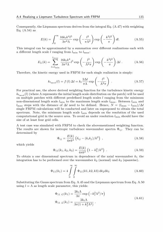
A.4 Realizing a Liepmann Turbulence Spectrum with FRPM 135

Consequently, the Liepmann spectrum derives from the integral Eq. (A.47) with weightingEq. (A.54) as

E(k) =∫ ∞

0

16ktk4l5

3π4Λexp(−

l2

πΛ2

)exp(−k2l2

π

)dl. (A.55)

This integral can be approximated by a summation over different realizations each witha different length scale l ranging from lmin to lmax:

EL(k) =lmax∑l=lmin

16ktk4

3π4Λl5 exp

(−

l2

Λ2π

)exp(−k2l2

π

)∆l . (A.56)

Therefore, the kinetic energy used in FRPM for each single realization is simply:

ktmod (l) = f (l) ∆l = kt2∆lπΛ

exp(−

l2

Λ2π

). (A.57)

For practical use, the above derived weighting function for the turbulence kinetic energyktmod (l) (where Λ represents the initial length scale distribution on the patch) will be usedon multiple patches with different predefined length scales l ranging from the minimumnon-dimensional length scale lmin to the maximum length scale lmax. Between lmin andlmax steps with the distance of ∆l need to be defined. Hence, N = (lmax − lmin)/∆lsingle FRPM calculations will be conducted and later on superposed to obtain the totalspectrum. Note, the minimum length scale lmin depends on the resolution of the usedcomputational grid in the source area. To avoid an under resolution lmin should have thesize of at least four grid cells.

A test case was simulated with FRPM to check the abovementioned weighting function.The results are shown for isotropic turbulence wavenumber spectra Φij . They can bedetermined by

Φij =E(k)4πk2

(δij − (kikj)/k2

), (A.58)

which yields

Φ11(k1, k2, k3) =E(k)4πk2

(1− k2

1/k2). (A.59)

To obtain a one dimensional spectrum in dependence of the axial wavenumber k1 theintegration has to be performed over the wavenumber k2 (normal) und k3 (spanwise).

Φ11(k1) = 4

∞∫0

∞∫0

Φ11(k1, k2, k3)dk2dk3 (A.60)

Substituting the Gauss spectrum from Eq. A.45 and the Liepmann spectrum from Eq. A.50using l = Λ as length scale parameter, this yields:

Φ11 G(k1) =2ktΛ3π

exp(−k2

1Λ2/π)

Φ11 L(k1) =2ktΛ

3π(1 + k21Λ2)

.(A.61)

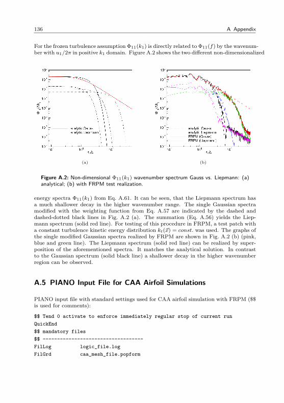
136 A Appendix

For the frozen turbulence assumption Φ11(k1) is directly related to Φ11(f) by the wavenum-ber with u1/2π in positive k1 domain. Figure A.2 shows the two different non-dimensionalized

(a) (b)

Figure A.2: Non-dimensional Φ11(k1) wavenumber spectrum Gauss vs. Liepmann: (a)analytical; (b) with FRPM test realization.

energy spectra Φ11(k1) from Eq. A.61. It can be seen, that the Liepmann spectrum hasa much shallower decay in the higher wavenumber range. The single Gaussian spectramodified with the weighting function from Eq. A.57 are indicated by the dashed anddashed-dotted black lines in Fig. A.2 (a). The summation (Eq. A.56) yields the Liep-mann spectrum (solid red line). For testing of this procedure in FRPM, a test patch witha constant turbulence kinetic energy distribution kt(~x) = const. was used. The graphs ofthe single modified Gaussian spectra realized by FRPM are shown in Fig. A.2 (b) (pink,blue and green line). The Liepmann spectrum (solid red line) can be realized by super-position of the aforementioned spectra. It matches the analytical solution. In contrastto the Gaussian spectrum (solid black line) a shallower decay in the higher wavenumberregion can be observed.

A.5 PIANO Input File for CAA Airfoil Simulations

PIANO input file with standard settings used for CAA airfoil simulation with FRPM ($$is used for comments):

$$ Tend 0 activate to enforce immediately regular stop of current runQuickEnd$$ mandatory files$$ ––––––––––––––––––––––––––––––––––-FilLog logic_file.logFilGrd caa_mesh_file.popform

A.5 PIANO Input File for CAA Airfoil Simulations 137

FilMean mean_flow_file.popformFilProc cpu_distribution_file$$ FRPM files$$ ––––––––––––––––––––––––––––––––––-FilFRPM FRPM_patch_file.datFilFRPMRec FRPM_record_fileFRPM_FILOUT FRPM$$ Restartfile$$ ––––––––––––––––––––––––––––––––––-FilRec PIANO_record_fileTsave 100000$$ output:$$ ––––––––––––––––––––––––––––––––––-DirOut ./output$$ Contour OutputFilNois Contour (’.bin’,’.plt’/’.dat’ depending on sign of Tout)AreaVar0 u first rec. var. out of rho, u, v, [w,] p, [uqRPM,omega]AreaVar1 p last rec. var. out of rho, u, v, [w,] p, [uqRPM,omega]$$ MicrophonesFilHis Time (’.bin’,’.plt’/’.dat’ depending on sign of HistoryOut)HistoryOut -50 store time history in FilHis after HistoryOut stepsMicsVar0 p first rec. var. out of rho, u, v, [w,] p, [uqRPM,omega]MicsVar1 p last rec. var. out of rho, u, v, [w,] p, [uqRPM,omega]$$ Circle OutputFilCirc Circle (’.bin’,’.plt’/’.dat’ depending on sign of CircOut)CircOut -50 store circle values after CircOut steps in FilCircCircNoMic 360 number of microphones refering whole circumferenceCircNormVec 0.D0 0.D0 1.D0 normal vector of directivity circleCircStartVec 1.D0 0.D0 0.D0 start vector of directivity circleCircCentre 1.0D0 0.0D0 0.D0 centre of directivity circleCircRadius 2.5D0 radius of directivity circle$$ Solver$$ ––––––––––––––––––––––––––––––––––-dt 2.0E-4Tend 400000Tout 100000Tupdate 50000APE4stabilimit 1.D3newXref 1.0D0 0.0D0 0.D0 reference point (as normal as possible to boundary)

138 A Appendix

$$ specification of FRPM (fast Random Particle Mesh) parameters:$$ ––––––––––––––––––––––––––––––––––-FRPMlmin 0.002D0FRPMlfac 6.0D0 scaling factor for patch-data length scaleFRPM_norm filtered_fieldFRPM_lambsourceFRPM_RESTRICTIVE_VELFRPM_nparticle 450000FRPM_NFILTER 4FRPM_LTECOUT$$ Damping$$ ––––––––––––––––––––––––––––––––––-damping 5.D-2 general damping coefficient$$ LEXDamp 0.0D0 0.0D0 0.D0MagDamp 0.2D0RadDamp 0.4D0$$ TEXDamp 1.0D0 0.0D0 0.D0MagDamp 0.2D0RadDamp 0.4D0End

A.6 Modified Trailing-Edge Noise Directivity

For the use of the directivity function D = f (Θ) according to Equation 4.4 in the turbineevaluation of Chapter 5, a modification is made to account for the geometrical differenceof airfoils and the flat plate from which the theory was originally developed.

Contrary to the semi-infinite flat plate, the forward directivity of airfoils looks different.Due to their limited extend the opposite phasing sound waves can cancel out each otherjust in front of the airfoils. Moreover, the geometric extend of the airfoils in the thicknessdirection yields some shadow zone in front of the airfoil, as the trailing-edge source is hid-den behind the airfoil, when looking downstream from an upstream position in extensionof the chord.

Figure A.3 (a) depicts the theoretical in-plane two-dimensional directivity (Φ = 90 ) forthe flat plate (dashed line). It is calculated by using Equation 4.4 from Reference [3]. Thedifference to the NACA0012 directivity extracted from the CAA results of the BANC-IIcase #1 simulation (solid line) is clearly visible. The theoretical results thus need to becorrect for Θ values between Θbegin = 110 to Θend = 260 . To obtain the correcteddirectivity function, indicated by the black circles in Figure A.3 (a), Equation A.62 can

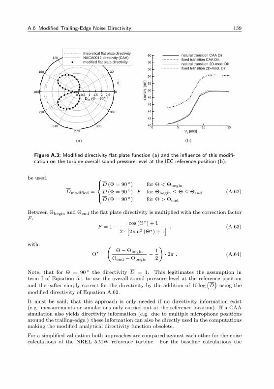
A.6 Modified Trailing-Edge Noise Directivity 139

θ

D2D (Φ = 90°)

0

30

60

90

120

150

180

210

240

270

300

330

0 0.5 1 1.5 2 2.5

theoretical flat plate directivityNACA0012 directivity (CAA)modified flat plate directivity

(a)

V0 [m/s]

OA

SP

L [d

B]

0 5 10 1540

42

44

46

48

50

52

54

56

58

60 natural transition CAA Dir.fixed transition CAA Dir.natural transition 2D-mod. Dirfixed transition 2D-mod. Dir

(b)

Figure A.3: Modified directivity flat plate function (a) and the influence of this modifi-cation on the turbine overall sound pressure level at the IEC reference position (b).

be used.

Dmodified =

D (Φ = 90 ) for Θ < ΘbeginD (Φ = 90 ) · F for Θbegin ≤ Θ ≤ ΘendD (Φ = 90 ) for Θ > Θend

(A.62)

Between Θbegin and Θend the flat plate directivity is multiplied with the correction factorF :

F = 1−cos (Θ∗) + 1

2 ·[2 sin2 (Θ∗) + 1

] , (A.63)

with:

Θ∗ =(

Θ−Θbegin

Θend −Θbegin−

12

)· 2π . (A.64)

Note, that for Θ = 90 the directivity D = 1. This legitimates the assumption interm I of Equation 5.1 to use the overall sound pressure level at the reference positionand thereafter simply correct for the directivity by the addition of 10 log

(D)using the

modified directivity of Equation A.62.

It must be said, that this approach is only needed if no directivity information exist(e.g. measurements or simulations only carried out at the reference location). If a CAAsimulation also yields directivity information (e.g. due to multiple microphone positionsaround the trailing-edge.) these information can also be directly used in the computationsmaking the modified analytical directivity function obsolete.

For a simplified validation both approaches are compared against each other for the noisecalculations of the NREL 5MW reference turbine. For the baseline calculations the

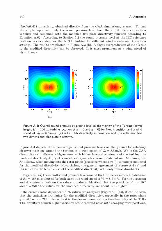
140 A Appendix

NACA64618 directivity, obtained directly from the CAA simulations, is used. To testthe simpler approach, only the sound pressure level from the airfoil reference positionis taken and combined with the modified flat plate directivity function according toEquation A.62. According to Section 5.2 the sound pressure level at the IEC referenceposition is calculated for the NREL turbine for different wind speeds and transitionsettings. The results are plotted in Figure A.3 (b). A slight overprediction of 0.5 dB dueto the modified directivity can be observed. It is most prominent at a wind speed ofV0 = 11 m/s.

(a) (b)

Figure A.4: Overall sound pressure at ground level in the vicinity of the Turbine (towerheight H = 100 m, turbine location at x = 0 and y = 0) for fixed transition and a windspeed of V0 = 8.5 m/s: (a) with CAA directivity information and (b) with modifiedtwo-dimensional flat plate directivity.

Figure A.4 depicts the time-averaged sound pressure levels on the ground for arbitraryobserver positions around the turbine at a wind speed of V0 = 8.5 m/s. While the CAAdirectivity (a) indicates a bigger area with higher levels downstream of the turbine, themodified directivity (b) yields an almost symmetric sound distribution. Moreover, theSPL decay, when moving into the rotor plane (positions where x ≈ 0), is more pronouncedfor the modified directivity. Nevertheless, the general agreement of Figure A.4 (a) and(b) indicates the feasible use of the modified directivity with only minor drawbacks.

In FigureA.5 (a) the overall sound pressure level around the turbine for a constant distanceof R1 = 163 m is plotted for both cases at a wind speed of V0 = 8.5 m/s. For the upstreamand downstream position the values are almost identical. For the positions of γ = 90 and γ = 270 the values for the modified directivity are about 1 dB higher.

If the current rotor dependend SPL values are analyzed (FigureA.5 (b)), it can be seen,that the variations are higher for the modified directivity, especially in the rotor planeγ = 90 or γ = 270 . In contrast to the downstream position the directivity of the TBL-TEN results in a much higher variation of the received noise with changing rotor positions.

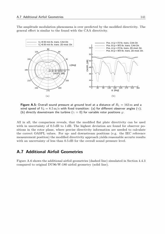
A.7 Additional Airfoil Geometries 141

The amplitude modulation phenomena is over predicted by the modified directivity. Thegeneral effect is similar to the found with the CAA directivity.

γ [deg]

OASPL [dB]

0

30

6090

120

150

180

210

240270

300

330

44 46 48 50 52 54

V0=8.50 m/s fix. trans. CAA Dir.V0=8.50 m/s fix. trans. 2D-mod. Dir.

(a)

ϕ [deg]

OA

SP

L [d

B]

0 45 90 135 180 225 270 315 36042

44

46

48

50

52

54

Pos. A (γ = 0°) fix. trans. CAA Dir.Pos. B (γ = 90°) fix. trans. CAA Dir.Pos. A (γ = 0°) fix. trans. 2D-mod. Dir.Pos. B (γ = 90°) fix. trans. 2D-mod. Dir.

(b)

Figure A.5: Overall sound pressure at ground level at a distance of R1 = 163 m and awind speed of V0 = 8.5 m/s with fixed transition: (a) for different observer angles (γ);(b) directly downstream the turbine (γ = 0) for variable rotor positions ϕ.

All in all, the comparison reveals, that the modified flat plate directivity can be usedwith in uncertainty of 0.5 dB to 1 dB. The highest deviation are found for observer po-sitions in the rotor plane, where precise directivity information are needed to calculatethe correct OASPL values. For up- and downstream positions (e.g. the IEC referencemeasurement position) the modified directivity approach yields reasonable accurte resultswith an uncertainty of less than 0.5 dB for the overall sound pressure level.

A.7 Additional Airfoil Geometries

Figure A.6 shows the additional airfoil geometries (dashed line) simulated in Section 4.4.3compared to original DU96-W-180 airfoil geometry (solid line).

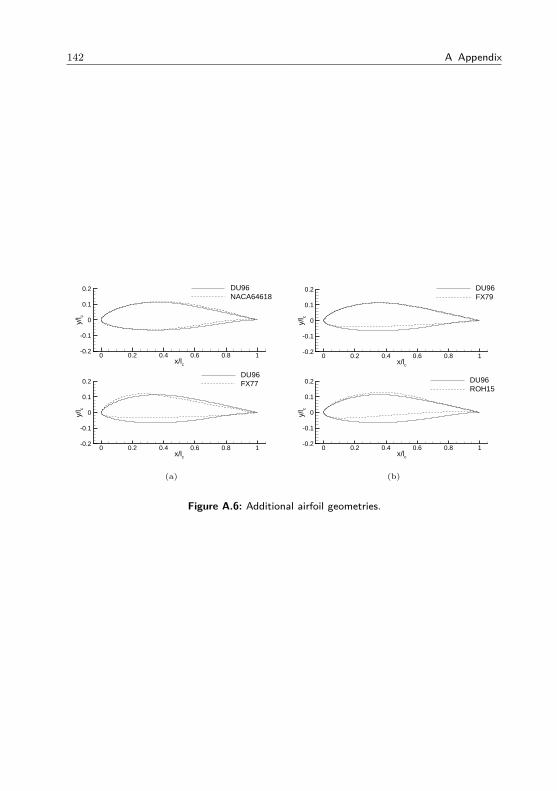
142 A Appendix

x/lc

y/l c

0 0.2 0.4 0.6 0.8 1-0.2

-0.1

0

0.1

0.2 DU96NACA64618

x/lc

y/l c

0 0.2 0.4 0.6 0.8 1-0.2

-0.1

0

0.1

0.2DU96FX77

(a)

x/lc

y/l c

0 0.2 0.4 0.6 0.8 1-0.2

-0.1

0

0.1

0.2 DU96FX79

x/lc

y/l c

0 0.2 0.4 0.6 0.8 1-0.2

-0.1

0

0.1

0.2 DU96ROH15

(b)

Figure A.6: Additional airfoil geometries.

Bibliography

[1] GWEC: Global Wind Report 2014: Annual market update. Brussels, 2014

[2] EWEA: Wind in Power: 2015 European statistics. 2015

[3] Brooks, Thomas F. ; Pope, Stuart D. ; Marcolini, Michael A.: Airfoil self-noiseand prediction. In: NASA Refrence Publication (1989), Nr. 1218, S. 1–137

[4] Wagner, S. ; Bareiss, R. ; Guidati, G.: Wind Turbine Noise. Berlin and , NewYork : Springer, 1996. – ISBN 3–540–60592–4

[5] Lighthill, M. J.: On Sound Generated Aerodynamically. I. General Theory. In: Pro-ceedings of the Royal Society A: Mathematical, Physical and Engineering Sciences211 (1952), Nr. 1107, S. 564–587. http://dx.doi.org/10.1098/rspa.1952.0060. –DOI 10.1098/rspa.1952.0060. – ISSN 1364–5021

[6] Lighthill, M. J.: On Sound Generated Aerodynamically. II. Turbulence as a Sourceof Sound. In: Proceedings of the Royal Society A: Mathematical, Physical andEngineering Sciences 222 (1954), Nr. 1148, S. 1–32. http://dx.doi.org/10.1098/rspa.1954.0049. – DOI 10.1098/rspa.1954.0049. – ISSN 1364–5021

[7] Curle, N.: The Influence of Solid Boundaries upon Aerodynamic Sound. In: Pro-ceedings of the Royal Society A: Mathematical, Physical and Engineering Sciences231 (1955), Nr. 1187, S. 505–514. http://dx.doi.org/10.1098/rspa.1955.0191. –DOI 10.1098/rspa.1955.0191. – ISSN 1364–5021

[8] Ffowcs Williams, J. E. ; Hawkings, D. L.: Sound Generation by Turbulence andSurfaces in Arbitrary Motion. In: Philosophical Transactions of the Royal SocietyA: Mathematical, Physical and Engineering Sciences 264 (1969), Nr. 1151, S. 321–342. http://dx.doi.org/10.1098/rsta.1969.0031. – DOI 10.1098/rsta.1969.0031.– ISSN 1364–503X

[9] Ffowcs Williams, J. E. ; Hall, L. H.: Aerodynamic sound generation by turbulentflow in the vicinity of a scattering half plane. In: Journal of Fluid Mechanics 40(1970), Nr. 04, S. 657–670

[10] Howe, M.S: A review of the theory of trailing edge noise. In: Journal of Sound andVibration 61 (1978), Nr. 3, S. 437–465. http://dx.doi.org/10.1016/0022-460X(78)90391-7. – DOI 10.1016/0022–460X(78)90391–7. – ISSN 0022460X

[11] Crighton, D. G. ; Leppington, F. G.: Scattering of aerodynamic noise bya semi-infinite compliant plate. In: Journal of Fluid Mechanics 43 (1970),Nr. 04, S. 721. http://dx.doi.org/10.1017/S0022112070002690. – DOI10.1017/S0022112070002690

144 Bibliography

[12] Crighton, D. G.: Radiation Properties of the Semi-Infinite Vortex Sheet. In: Pro-ceedings of the Royal Society A: Mathematical, Physical and Engineering Sciences330 (1972), Nr. 1581, S. 185–198. http://dx.doi.org/10.1098/rspa.1972.0139. –DOI 10.1098/rspa.1972.0139. – ISSN 1364–5021

[13] Chase, David M.: Sound Radiated by Turbulent Flow off a Rigid Half-Plane asObtained from a Wavevector Spectrum of Hydrodynamic Pressure. In: The Journalof the Acoustical Society of America 52 (1972), Nr. 3B, S. 1011. http://dx.doi.org/10.1121/1.1913170. – DOI 10.1121/1.1913170. – ISSN 00014966

[14] Chase, David M.: Noise Radiated from an Edge in Turbulent Flow. In: AIAAJournal 13 (1975), Nr. 8, S. 1041–1047. http://dx.doi.org/10.2514/3.60502. –DOI 10.2514/3.60502. – ISSN 0001–1452

[15] Amiet, R.K: Acoustic radiation from an airfoil in a turbulent stream. In: Journalof Sound and Vibration 41 (1975), Nr. 4, S. 407–420. http://dx.doi.org/10.1016/S0022-460X(75)80105-2. – DOI 10.1016/S0022–460X(75)80105–2. – ISSN 0022460X

[16] Amiet, R.K: Noise due to turbulent flow past a trailing edge. In: Journal ofSound and Vibration 47 (1976), Nr. 3, S. 387–393. http://dx.doi.org/10.1016/0022-460X(76)90948-2. – DOI 10.1016/0022–460X(76)90948–2. – ISSN 0022460X

[17] Brooks, T.F ; Hodgson, T.H: Trailing edge noise prediction from measured sur-face pressures. In: Journal of Sound and Vibration 78 (1981), Nr. 1, S. 69–117. http://dx.doi.org/10.1016/S0022-460X(81)80158-7. – DOI 10.1016/S0022–460X(81)80158–7. – ISSN 0022460X

[18] Parchen, Rene ; TNO Institute of Applied (Hrsg.): Progress Report DRAW:A Prediction Scheme for Trailing-Edge Noise Based on Detailed Boundary-LayerCharacteristics: TNO Rept. HAG-RPT-980023. Netherlands, 1998

[19] Moriarty, P. ; Migliore, P.: Semi-Empirical Aeroacoustic Noise Prediction Codefor Wind Turbines: NREL/TP-500-34478. 2003

[20] Moriarty, Patrick ; Guidati, Gianfranco ; Migliore, Paul: Recent Improvementof a Semi-Empirical Aeroacoustic Prediction Code for Wind Turbines. In: 10thAIAA/CEAS Aeroacoustics Conference, 2004, S. 1–25

[21] Schepers, J. G. ; Curvers, A. P. W. M. ; Oerlemans, S. ; Braun, K. ; Lutz, T. ;Herrig, A. ; Wuerz, W. ; Mantesanz, A. ; Garcillán, L. ; Fisher, M. ; Koegler,K. ; Maeder, T. ; ECN Wind Energy (Hrsg.): SIROCCO: Silent rotors by acousticoptimisation: ECN-M–07-064. 2007

[22] Lutz, Thorsten ; Herrig, Andreas ; Würz, Werner ; Kamruzzaman, Mohammad; Krämer, Ewald: Design and Wind-Tunnel Verification of Low-Noise Airfoils forWind Turbines. In: AIAA Journal 45 (2007), Nr. 4, S. 779–785. http://dx.doi.org/10.2514/1.27658. – DOI 10.2514/1.27658. – ISSN 0001–1452

[23] Oerlemans, S. ; Sijtsma, P. ; Méndez López, B.: Location and quantifica-tion of noise sources on a wind turbine. In: Journal of Sound and Vibration 299(2007), Nr. 4-5, S. 869–883. http://dx.doi.org/10.1016/j.jsv.2006.07.032. – DOI10.1016/j.jsv.2006.07.032. – ISSN 0022460X

[24] Oerlemans, S. ; Schepers, J. G.: Prediction of wind turbine noise and validationagainst experiment. 2009

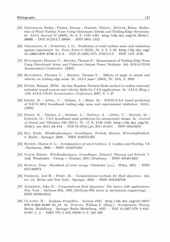
Bibliography 145

[25] Oerlemans, Stefan ; Fisher, Murray ; Maeder, Thierry ; Kögler, Klaus: Reduc-tion of Wind Turbine Noise Using Optimized Airfoils and Trailing-Edge Serrations.In: AIAA Journal 47 (2009), Nr. 6, S. 1470–1481. http://dx.doi.org/10.2514/1.38888. – DOI 10.2514/1.38888. – ISSN 0001–1452

[26] Oerlemans, S. ; Schepers, J. G.: Prediction of wind turbine noise and validationagainst experiment. In: Noise Notes 9 (2010), Nr. 2, S. 3–28. http://dx.doi.org/10.1260/1475-4738.9.2.3. – DOI 10.1260/1475–4738.9.2.3. – ISSN 1475–4738

[27] Hutcheson, Florence V. ; Brooks, Thomas F.: Measurement of Trailing Edge NoiseUsing Directional Array and Coherent Output Power Methods: 8th AIAA/CEASAeroacoustics Conference. (2002)

[28] Hutcheson, Florence V. ; Brooks, Thomas F.: Effects of angle of attack andvelocity on trailing edge noise. In: AIAA paper (2004), Nr. 1031, S. 2004

[29] Ewert, Roland: RPM - the fast Random Particle-Mesh method to realize unsteadyturbulent sound sources and velocity fields for CAA applications. In: AIAA (Hrsg.):13th AIAA/CEAS Aeroacoustics Conference, 2007, S. 1–27

[30] Ewert, R. ; Appel, C. ; Dierke, J. ; Herr, M.: RANS/CAA based predictionof NACA 0012 broadband trailing edge noise and experimental validation: AIAA.(2009)

[31] Ewert, R. ; Dierke, J. ; Siebert, J. ; Neifeld, A. ; Appel, C. ; Siefert, M. ;Kornow, O.: CAA broadband noise prediction for aeroacoustic design. In: Journalof Sound and Vibration 330 (2011), Nr. 17, S. 4139–4160. http://dx.doi.org/10.1016/j.jsv.2011.04.014. – DOI 10.1016/j.jsv.2011.04.014. – ISSN 0022460X

[32] Hau, Erich: Windkraftanlagen: Grundlagen, Technik, Einsatz, Wirtschaftlichkeit.4. Berlin : Springer, 2008. – ISBN 3540721509

[33] Hansen, Martin O. L.: Aerodynamics of wind turbines. 2. London and Sterling, VA: Earthscan, 2008. – ISBN 1844074382

[34] Gasch, Robert: Windkraftanlagen: Grundlagen, Entwurf, Planung und Betrieb. 7.Aufl. Wiesbaden : Vieweg + Teubner, 2011 (Studium). – ISBN 3834814601

[35] Burton, Tony: Handbook of wind energy. Chichester [u.a.] : Wiley, 2001. – ISBN0471489972

[36] Ferziger, Joel H. ; Perić, M.: Computational methods for fluid dynamics. 3rd,rev. ed. Berlin and New York : Springer, 2002. – ISBN 3540420746

[37] Anderson, John D.: Computational fluid dynamics: The basics with applications.New York : McGraw-Hill, 1995 (McGraw-Hill series in mechanical engineering). –ISBN 0070016852

[38] Glauert, H.: Airplane Propellers. Version: 1935. http://dx.doi.org/10.1007/978-3-642-91487-4_3. In: Durand, William F. (Hrsg.): Aerodynamic Theory.Berlin, Heidelberg : Springer Berlin Heidelberg, 1935. – DOI 10.1007/978–3–642–91487–4_3. – ISBN 978–3–642–89630–9, S. 169–360

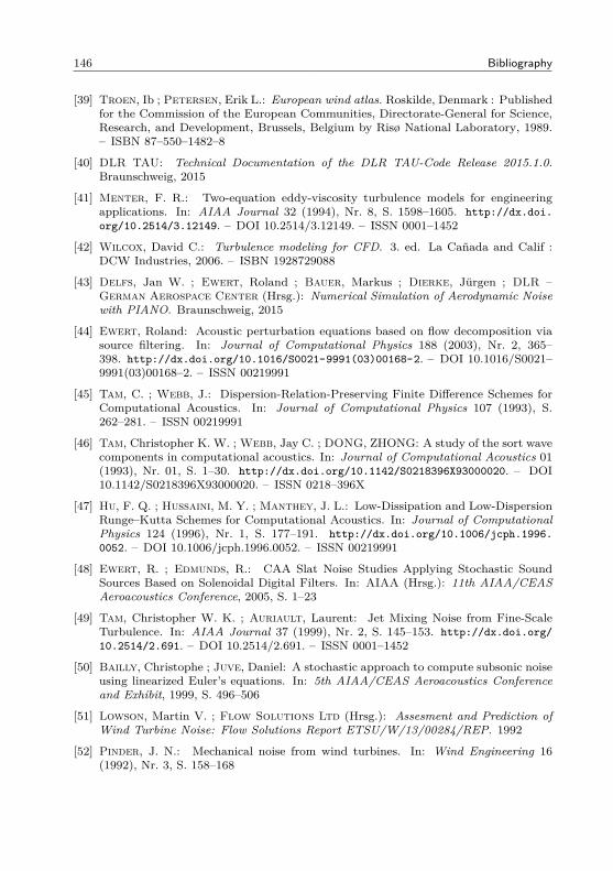
146 Bibliography

[39] Troen, Ib ; Petersen, Erik L.: European wind atlas. Roskilde, Denmark : Publishedfor the Commission of the European Communities, Directorate-General for Science,Research, and Development, Brussels, Belgium by Risø National Laboratory, 1989.– ISBN 87–550–1482–8

[40] DLR TAU: Technical Documentation of the DLR TAU-Code Release 2015.1.0.Braunschweig, 2015

[41] Menter, F. R.: Two-equation eddy-viscosity turbulence models for engineeringapplications. In: AIAA Journal 32 (1994), Nr. 8, S. 1598–1605. http://dx.doi.org/10.2514/3.12149. – DOI 10.2514/3.12149. – ISSN 0001–1452

[42] Wilcox, David C.: Turbulence modeling for CFD. 3. ed. La Cañada and Calif :DCW Industries, 2006. – ISBN 1928729088

[43] Delfs, Jan W. ; Ewert, Roland ; Bauer, Markus ; Dierke, Jürgen ; DLR –German Aerospace Center (Hrsg.): Numerical Simulation of Aerodynamic Noisewith PIANO. Braunschweig, 2015

[44] Ewert, Roland: Acoustic perturbation equations based on flow decomposition viasource filtering. In: Journal of Computational Physics 188 (2003), Nr. 2, 365–398. http://dx.doi.org/10.1016/S0021-9991(03)00168-2. – DOI 10.1016/S0021–9991(03)00168–2. – ISSN 00219991

[45] Tam, C. ; Webb, J.: Dispersion-Relation-Preserving Finite Difference Schemes forComputational Acoustics. In: Journal of Computational Physics 107 (1993), S.262–281. – ISSN 00219991

[46] Tam, Christopher K. W. ; Webb, Jay C. ; DONG, ZHONG: A study of the sort wavecomponents in computational acoustics. In: Journal of Computational Acoustics 01(1993), Nr. 01, S. 1–30. http://dx.doi.org/10.1142/S0218396X93000020. – DOI10.1142/S0218396X93000020. – ISSN 0218–396X

[47] Hu, F. Q. ; Hussaini, M. Y. ; Manthey, J. L.: Low-Dissipation and Low-DispersionRunge–Kutta Schemes for Computational Acoustics. In: Journal of ComputationalPhysics 124 (1996), Nr. 1, S. 177–191. http://dx.doi.org/10.1006/jcph.1996.0052. – DOI 10.1006/jcph.1996.0052. – ISSN 00219991

[48] Ewert, R. ; Edmunds, R.: CAA Slat Noise Studies Applying Stochastic SoundSources Based on Solenoidal Digital Filters. In: AIAA (Hrsg.): 11th AIAA/CEASAeroacoustics Conference, 2005, S. 1–23

[49] Tam, Christopher W. K. ; Auriault, Laurent: Jet Mixing Noise from Fine-ScaleTurbulence. In: AIAA Journal 37 (1999), Nr. 2, S. 145–153. http://dx.doi.org/10.2514/2.691. – DOI 10.2514/2.691. – ISSN 0001–1452

[50] Bailly, Christophe ; Juve, Daniel: A stochastic approach to compute subsonic noiseusing linearized Euler’s equations. In: 5th AIAA/CEAS Aeroacoustics Conferenceand Exhibit, 1999, S. 496–506

[51] Lowson, Martin V. ; Flow Solutions Ltd (Hrsg.): Assesment and Prediction ofWind Turbine Noise: Flow Solutions Report ETSU/W/13/00284/REP. 1992

[52] Pinder, J. N.: Mechanical noise from wind turbines. In: Wind Engineering 16(1992), Nr. 3, S. 158–168

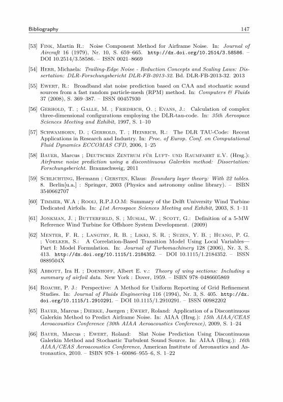
Bibliography 147

[53] Fink, Martin R.: Noise Component Method for Airframe Noise. In: Journal ofAircraft 16 (1979), Nr. 10, S. 659–665. http://dx.doi.org/10.2514/3.58586. –DOI 10.2514/3.58586. – ISSN 0021–8669

[54] Herr, Michaela: Trailing-Edge Noise - Reduction Concepts and Scaling Laws: Dis-sertation: DLR-Forschungsbericht DLR-FB-2013-32. Bd. DLR-FB-2013-32. 2013

[55] Ewert, R.: Broadband slat noise prediction based on CAA and stochastic soundsources from a fast random particle-mesh (RPM) method. In: Computers & Fluids37 (2008), S. 369–387. – ISSN 00457930

[56] Gerhold, T. ; Galle, M. ; Friedrich, O. ; Evans, J.: Calculation of complexthree-dimensional configurations employing the DLR-tau-code. In: 35th AerospaceSciences Meeting and Exhibit, 1997, S. 1–10

[57] Schwamborn, D. ; Gerhold, T. ; Heinrich, R.: The DLR TAU-Code: RecentApplications in Research and Industry. In: Proc. of Europ. Conf. on ComputationalFluid Dynamics ECCOMAS CFD, 2006, 1–25

[58] Bauer, Marcus ; Deutsches Zentrum für Luft- und Raumfahrt e.V. (Hrsg.):Airframe noise prediction using a discontinuous Galerkin method: Dissertation:Forschungsbericht. Braunschweig, 2011

[59] Schlichting, Hermann ; Gersten, Klaus: Boundary layer theory: With 22 tables.8. Berlin[u.a.] : Springer, 2003 (Physics and astronomy online library). – ISBN3540662707

[60] Timmer, W.A ; Rooij, R.P.J.O.M: Summary of the Delft University Wind TurbineDedicated Airfoils. In: 41st Aerospace Sciences Meeting and Exhibit, 2003, S. 1–11

[61] Jonkman, J. ; Butterfield, S. ; Musial, W. ; Scott, G.: Definition of a 5-MWReference Wind Turbine for Offshore System Development. (2009)

[62] Menter, F. R. ; Langtry, R. B. ; Likki, S. R. ; Suzen, Y. B. ; Huang, P. G.; Voelker, S.: A Correlation-Based Transition Model Using Local Variables—Part I: Model Formulation. In: Journal of Turbomachinery 128 (2006), Nr. 3, S.413. http://dx.doi.org/10.1115/1.2184352. – DOI 10.1115/1.2184352. – ISSN0889504X

[63] Abbott, Ira H. ; Doenhoff, Albert E. v.: Theory of wing sections: Including asummary of airfoil data. New York : Dover, 1959. – ISBN 978–0486605869

[64] Roache, P. J.: Perspective: A Method for Uniform Reporting of Grid RefinementStudies. In: Journal of Fluids Engineering 116 (1994), Nr. 3, S. 405. http://dx.doi.org/10.1115/1.2910291. – DOI 10.1115/1.2910291. – ISSN 00982202

[65] Bauer, Marcus ; Dierke, Juergen ; Ewert, Roland: Application of a DiscontinuousGalerkin Method to Predict Airframe Noise. In: AIAA (Hrsg.): 15th AIAA/CEASAeroacoustics Conference (30th AIAA Aeroacoustics Conference), 2009, S. 1–24

[66] Bauer, Marcus ; Ewert, Roland: Slat Noise Prediction Using DiscontinuousGalerkin Method and Stochastic Turbulent Sound Source. In: AIAA (Hrsg.): 16thAIAA/CEAS Aeroacoustics Conference, American Institute of Aeronautics and As-tronautics, 2010. – ISBN 978–1–60086–955–6, S. 1–22

148 Bibliography

[67] Bauer, Marcus ; Dierke, Jürgen ; Ewert, Roland: Application of a DiscontinuousGalerkin Method to Discretize Acoustic Perturbation Equations. In: AIAA Jour-nal 49 (2011), Nr. 5, S. 898–908. http://dx.doi.org/10.2514/1.J050333. – DOI10.2514/1.J050333. – ISSN 0001–1452

[68] Anderson, John D.: Fundamentals of aerodynamics. 4. Boston : McGraw-HillHigher Education, 2007 (McGraw-Hill series in aeronautical and aerospace engineer-ing). – ISBN 0071254080

[69] Tam, Christopher ; DONG, ZHONG: Wall boundary conditions for high-order finitedifference schemes in computational aeroacoustics. In: 32nd Aerospace SciencesMeeting and Exhibit, 1994, S. 1788–1796

[70] Rautmann, Christof ; Dierke, Juergen ; Ewert, Roland ; Hu, Nan ; Delfs, Jan:Generic Airfoil Trailing-Edge Noise Prediction using Stochastic Sound Sources fromSynthetic Turbulence. In: AIAA (Hrsg.): 20th AIAA/CEAS Aeroacoustics Confer-ence, 2014, S. 1–21

[71] Liepmann, H. W. ; Laufer, J. ; Liepmann, Kate ; National Advisory Commit-tee for Aeronautics (Hrsg.): On the spectrum of isotropic turbulence: NACATechnical Notes. 1951 (NACA-TN-2473)

[72] Herr, M. ; Kamruzzaman, M.: Benchmarking of Trailing-Edge Noise Computa-tions|Outcome of the BANC-II Workshop: AIAA. (2013)

[73] Herr, M. ; Bahr, C. ; Kamruzzaman, M.: Workshop Category 1: Trailing-EdgeNoise. Problem Statement for the AIAA/CEAS Second Workshop on BenchmarkProblems for Airframe Noise Computations (BANC-II): June 7-8 2012, ColoradoSprings, Colorado, USA. https://info.aiaa.org/tac/ASG/FDTC/DG/BECAN_files_/BANCII_category1. Version: 2012

[74] Herrig, Andreas: Validation and application of a hot-wire based method for trailing-edge noise measurements on airfoils: Doctoral thesis. Stuttgart : IAG, 2011

[75] Townsend, A. A.: The structure of turbulent shear flow. 2. Cambridge [Eng.], NewYork : Cambridge University Press, 1980 (Cambridge monographs on mechanics andapplied mathematics). – ISBN 0521298199

[76] SCHLINKER, R. ; AMIET, R.: Helicopter rotor trailing edge noise. In: 7th Aeroa-coustics Conference, 1981, S. 1–25

[77] Eastman ; Jacobs, N. ; Kenneth, E. ; Ward, E. ; Pinkerton, Robert M.: TheCharacteristics of 78 Related Airfoil Sections from Tests in the Variable-densityWind Tunnel: NACA Rept. No. 460. 1933

[78] IEC: IEC 64100-11 second edition. 2. 2002

[79] Bowdler, Dick: Amplitude modulation of wind turbine noise: a review of theevidence. In: Institute of Acoustics Bulletin 33.4 33 (2008), Nr. 4, S. 31–41

[80] Lee, Seunghoon ; Kim, Kyutae ; Choi, Wooyoung ; Lee, Soogab: Annoyance causedby amplitude modulation of wind turbine noise. In: Noise Control EngineeringJournal 59 (2011), Nr. 1, S. 38. http://dx.doi.org/10.3397/1.3531797. – DOI10.3397/1.3531797. – ISSN 07362501

Bibliography 149

[81] Drela, Mark: XFOIL: An Analysis and Design System for Low Reynolds NumberAirfoils. Version: 1989. http://dx.doi.org/10.1007/978-3-642-84010-4_1. In:Brebbia, C. A. (Hrsg.) ; Orszag, S. A. (Hrsg.) ; Seinfeld, J. H. (Hrsg.) ; Spanos,P. (Hrsg.) ; Cakmak, A. S. (Hrsg.) ; Silvester, P. (Hrsg.) ; Desai, C. S. (Hrsg.) ;Pinder, G. (Hrsg.) ; McCrory, R. (Hrsg.) ; Yip, S. (Hrsg.) ; Leckie, F. A. (Hrsg.); Ponter, A. R. S. (Hrsg.) ; Holz, K.-P (Hrsg.) ; Bathe, K.-J (Hrsg.) ; Connor,J. (Hrsg.) ; Wunderlich, W. (Hrsg.) ; Argyris, J. (Hrsg.) ; Mueller, Thomas J.(Hrsg.): Low Reynolds Number Aerodynamics Bd. 54. Berlin, Heidelberg : SpringerBerlin Heidelberg, 1989. – DOI 10.1007/978–3–642–84010–4_1. – ISBN 978–3–540–51884–6, S. 1–12

[82] Bak, Christian: Risø R, Report. Bd. 1611: Research in aeroelasticity EFP-2006 .Roskilde : Risø National Laboratory, 2007. – ISBN 978–87–550–3610–9

[83] Spera, David A.: Wind turbine technology: Fundamental concepts of wind turbineengineering. New York : ASME Press, 1994. – ISBN 0791812057

[84] Alecu, Teodor I. ; Voloshynovskiy, Sviatoslav ; Pun, Thierry: The gaussiantransform. In: EUSIPCO2005, 13th European Signal Processing Conference Bd.2005, 2005, S. 4–8