TECHNISCHE UNIVERSITÄT MÜNCHENLehrstuhl für Echtzeitsysteme und Robotik

Framework for Modelica Based FunctionDevelopment

Bernhard Amadeus Thiele

Vollständiger Abdruck der von der Fakultät der Informatik der Technischen Universität Münchenzur Erlangung des akademischen Grades eines

Doktors der Naturwissenschaften (Dr. rer. nat.)

genehmigten Dissertation.

Vorsitzender: Univ.-Prof. Dr. rer. nat. Alexander PretschnerPrüfer der Dissertation: 1. Univ.-Prof. Dr.-Ing. Alois Knoll

2. Hon.-Prof. Dr.-Ing. Martin Otter3. Prof. Marc Pouzet, Université Pierre et Marie Curie in the Computer

Science Department (DIENS) of École normale supérieure (ENS),Paris/Frankreich

Die Dissertation wurde am 15.04.2015 bei der Technischen Universität München eingereichtund durch die Fakultät für Informatik am 03.08.2015 angenommen.

Zusammenfassung

Rasante Fortschritte in der Leistungsfähigkeit von elektronischen Steuerungsgerä-ten führen zu immer umfangreicheren Softwarefunktionen, die innerhalb des Ent-wicklungsprozesses beherrscht werden müssen. Eine besondere Herausforderungsind hierbei auf vernetzte Recheneinheiten verteilte Softwarefunktionen, welche inRückkopplung mit physikalischen Prozessen stehen.

Für die Entwicklung und Validierung derartiger Funktionen ist es nicht länger aus-reichend, weitgehend autarke Einzelkomponenten zu betrachten, ohne die wech-selseitige Beeinflussung innerhalb des Gesamtsystems (einschließlich der physi-kalischen Prozesse) zu berücksichtigen. Aufgrund von unterschiedlichen wissen-schaftlichen Gemeinschaften hat sich jedoch der Stand der Technik für Modellie-rungssprachen im Bereich physikalischer Systeme sehr unterschiedlich zum Standder Technik im Bereich der Modellierung von Software entwickelt. Dies erschwertganzheitliche Entwicklungsansätze.

Diese Arbeit befasst sich mit der Entwicklung einer Methodik, welche eine ver-besserte Integration der zwei Welten auf den jeweils aktuellen Stand der Tech-nik ermöglicht: Die Modellierung von (sicherheitsrelevanten) digitalen steuerungs-und regelungstechnischen Funktionen und die Modellierung von physikalischenMultidomänen-Systemen. Als Basis dient die primär für physikalische Systeme ent-wickelte Modellierungssprache Modelica, welche auf folgende Aspekte der Funkti-onsentwicklung hin untersucht wird: a) Die Voraussetzungen, die erfüllt sein müs-sen, um Funktionsmodelle innerhalb eines Entwicklungsprozesses für sicherheits-relevante Systeme implementieren zu können, und b) ihre Nutzung für eine durch-gängige Entwicklungsmethodik, angefangen von der logischen Systemarchitekturbis herunter auf die technische Systemarchitektur.

In einem ersten Schritt werden allgemeine Anforderungen an eine domänenori-entierte Modellierungssprache für die sicherheitsrelevante modellbasierte Funkti-onsentwicklung formuliert. Im zweiten Schritt wird Modelica im Hinblick auf dieformulierten Anforderungen analysiert und bestehende Defizite werden identifi-ziert. Auf diese Analyse aufbauend, werden auf die Modellierung von digitalensteuerungs- und regelungstechnischen Funktionen zugeschnittene Spracheinschrän-kungen und -erweiterungen vorgeschlagen. Die dadurch spezifizierte Sprache wirdals ACG-Modelica bezeichnet und als geeignete Basis für die Implementierunghochwertiger Seriencode-Generatoren angesehen. Im dritten Schritt wird dies durcheine Realisierbarkeitsstudie belegt, in deren Mittelpunkt die Angabe einer translato-rischen Semantik steht, welche eine repräsentative Teilmenge von ACG-Modelicain eine ausgewählte Zielsprache transformiert.

Abstract

Electronic control technology is evolving leading to more complex software func-tions that need to be managed efficiently within a development process. To managethe complexity of the various stages of development, model-based function devel-opment has become a standard approach. A particular challenge are software func-tions running on distributed, networked computing devices which are in feedbackloops with physical processes.

For the development and validation of these functions it is no longer sufficient tosolely consider a single, self-contained component without taking the interactionof this part within the whole system (including the physics!) into account. How-ever, due to different communities, state-of-the-art modeling languages for softwarefunctions have evolved very differently from modeling languages targeted for phys-ical systems. This impedes integrated holistic modeling approaches.

This thesis concerns the problem of a development methodology that is capableof integrating the two worlds: State-of-the-art modeling for (safety-related) digitalcontrol functions and state-of-the-art modeling for multi-domain physical systems.Based on the physical modeling language Modelica the thesis addresses two aspectsof function development: a) the conditions that need to be fulfilled to allow the us-age of Modelica for implementing function models in a safety-related developmentprocess with automatic code generation, and b) the use of Modelica as a basis fora seamless development methodology starting from the logical virtual model downto the technical system architecture.

In a first step requirements to a high-level, domain-oriented language targeted forsafety-related, model-based function development are established. Second, Model-ica is analyzed with respect to the established requirements and present shortcom-ings are identified. Based on this, language restrictions and extensions are proposed,effectively leading to a language sub- and superset for discrete-time controller func-tion modeling, which is deemed suitable as basis for a high-integrity automatic codegenerator (ACG). Third, the feasibility of implementing such an ACG is demon-strated.

Acknowledgements

This work would not have been possible without the support of many people towhom I am deeply indebted. First I would like to thank my supervisor Prof. AloisKnoll for accepting me as an external PhD student and for giving me the opportunityto write this thesis. I highly appreciate his valuable feedback, ideas, and guidancethat supported my work. I would also like to thank Prof. Marc Pouzet for acceptingto be my external reviewer.

Most of this work originates from my time as research scientist at the GermanAerospace Center (German: Deutsches Zentrum für Luft- und Raumfahrt e.V., ab-breviated DLR) at the Institute of System Dynamics and Control and I am indebtedto the director of the institute, Dr. Johann Bals for the opportunity to work on thisthesis. I am particularly indebted to Prof. Martin Otter and Dr. Dirk Zimmer whosupervised my thesis work at DLR and provided indispensable and comprehensivefeedback, support and encouragement that kept me going on. Additionally I wouldlike to thank my colleagues at DLR for the many inspiring discussions and the goodlaughs that we had together, particularly my long-time office colleague Dr. TobiasBellmann with whom I shared a passion for Modelica, nifty programming solutionsand LATEX.

I would also like to warmly thank Prof. Peter Fritzson who is leading the group thatdevelops the OpenModelica compiler at the Programming Environment Laboratory(PELAB) at Linköping University. He gave me the opportunity to join his groupafter my affiliation to DLR ended and supported my pursuit to finalize this thesis.

As a researcher I was part of the Modelica Community and I would like to thank themembers of this community for the friendly atmosphere and the good discussionsand inspiring ideas during conferences and during the Modelica design meetingsthat I attended.

Last but not least, I would like to thank my friends and my family for supportingme and cheering me up at appropriate times. Thanks to Thomas van Marwick forgiving me insight into the use of the Ada programming language for safety-relevantsystems. Thanks to my mother, Anna Thiele, for proofreading my thesis in orderto spot English language mistakes. And finally, my warmest thanks go to Mihaelawho stood by my side at good and bad days and who gave me all support and lovethat makes life so much more worth living.

Contents

Contents iii

1. Introduction 11.1. Motivation . . . . . . . . . . . . . . . . . . . . . . . . . . . . . . . . . . . . . 11.2. Main Contributions . . . . . . . . . . . . . . . . . . . . . . . . . . . . . . . . 21.3. Thesis Outline . . . . . . . . . . . . . . . . . . . . . . . . . . . . . . . . . . . 41.4. Related Publications . . . . . . . . . . . . . . . . . . . . . . . . . . . . . . . 5

2. Background 72.1. The Complexity Challenge at the Example of the Automotive Sector . . . . . . 72.2. Modeling in (Control) Engineering and Computer Science Communities . . . . 82.3. Model-Based Development . . . . . . . . . . . . . . . . . . . . . . . . . . . . 82.4. Modeling Tools and Languages for Embedded Systems Design . . . . . . . . . 112.5. Safety Relevant Software Functions . . . . . . . . . . . . . . . . . . . . . . . 14

2.5.1. Terminology . . . . . . . . . . . . . . . . . . . . . . . . . . . . . . . 142.5.2. Functional Safety Standards . . . . . . . . . . . . . . . . . . . . . . . 152.5.3. Consequences . . . . . . . . . . . . . . . . . . . . . . . . . . . . . . . 15

2.6. Software Architectures . . . . . . . . . . . . . . . . . . . . . . . . . . . . . . 16

3. Requirements for Model-Based Function Development 173.1. Development Roles . . . . . . . . . . . . . . . . . . . . . . . . . . . . . . . . 183.2. Modeling Language Requirements . . . . . . . . . . . . . . . . . . . . . . . . 183.3. Graphical Representation Requirements . . . . . . . . . . . . . . . . . . . . . 22

4. Modelica’s Synchronous Language Elements Extension 254.1. Activation of Discrete-Time Equations . . . . . . . . . . . . . . . . . . . . . . 254.2. Pre-Modelica 3.3 Support for Sampled-Data Systems . . . . . . . . . . . . . . 264.3. Sampled-Data Systems with Synchronous Language Elements . . . . . . . . . 274.4. Notes to the Development of the Synchronous Extension . . . . . . . . . . . . 33

5. Enabling Modelica for Function Development — ACG-Modelica 355.1. Motivation . . . . . . . . . . . . . . . . . . . . . . . . . . . . . . . . . . . . . 35

5.1.1. Language Complexity . . . . . . . . . . . . . . . . . . . . . . . . . . 355.1.2. Terminology . . . . . . . . . . . . . . . . . . . . . . . . . . . . . . . 36

5.2. System Compilation: From Function Model to Target Binary . . . . . . . . . . 375.2.1. Tool Qualification . . . . . . . . . . . . . . . . . . . . . . . . . . . . 375.2.2. Typical Modelica Code Generation . . . . . . . . . . . . . . . . . . . 39

iii

CONTENTS

5.3. Utilization of Suitable Model of Computation . . . . . . . . . . . . . . . . . . 415.3.1. Relevance of Formal Model Specifications . . . . . . . . . . . . . . . 415.3.2. Models of Computation . . . . . . . . . . . . . . . . . . . . . . . . . 415.3.3. Modelica’s Synchronous Model of Computation . . . . . . . . . . . . 42

5.4. Language Restrictions . . . . . . . . . . . . . . . . . . . . . . . . . . . . . . 435.4.1. Modeling Language Rules . . . . . . . . . . . . . . . . . . . . . . . . 445.4.2. Graphical Representation Rules . . . . . . . . . . . . . . . . . . . . . 47

5.5. Support of Target Data Types and Operations . . . . . . . . . . . . . . . . . . 515.5.1. Limitations of Current Language Standard . . . . . . . . . . . . . . . . 515.5.2. Proposal for Data Type Extension . . . . . . . . . . . . . . . . . . . . 555.5.3. Proposal for Operation Extensions . . . . . . . . . . . . . . . . . . . . 575.5.4. Alternative Solutions . . . . . . . . . . . . . . . . . . . . . . . . . . . 59

5.6. Modularization of Dynamic Execution Aspects . . . . . . . . . . . . . . . . . 625.6.1. Limitations of Current Language Standard . . . . . . . . . . . . . . . . 625.6.2. Proposal for Atomic Blocks . . . . . . . . . . . . . . . . . . . . . . . 65

5.7. Manual Block Scheduling . . . . . . . . . . . . . . . . . . . . . . . . . . . . . 685.7.1. Limitations of Current Language Standard . . . . . . . . . . . . . . . . 685.7.2. Proposal for Clock Priorities . . . . . . . . . . . . . . . . . . . . . . . 685.7.3. Example . . . . . . . . . . . . . . . . . . . . . . . . . . . . . . . . . 695.7.4. Interaction with the (Physical) Environment . . . . . . . . . . . . . . . 705.7.5. Alternative Solution . . . . . . . . . . . . . . . . . . . . . . . . . . . 72

5.8. Causal Data-Flow Semantics . . . . . . . . . . . . . . . . . . . . . . . . . . . 745.8.1. Limitations of Current Language Standard . . . . . . . . . . . . . . . . 755.8.2. Proposal for safer, causal data-flow semantics . . . . . . . . . . . . . . 775.8.3. Alternative Solutions . . . . . . . . . . . . . . . . . . . . . . . . . . . 78

5.9. Translation to a Synchronous Data-Flow Kernel . . . . . . . . . . . . . . . . . 805.9.1. Intuitive Normalization . . . . . . . . . . . . . . . . . . . . . . . . . . 815.9.2. Intuitive Translation . . . . . . . . . . . . . . . . . . . . . . . . . . . 835.9.3. Applicability to the Complete ACG-Modelica Language . . . . . . . . 835.9.4. Normalized mACG-Modelica with clock operators . . . . . . . . . . . 855.9.5. Translator Implementation . . . . . . . . . . . . . . . . . . . . . . . . 89

5.10. Further Extensions to ACG-Modelica . . . . . . . . . . . . . . . . . . . . . . 915.10.1. Inheritance . . . . . . . . . . . . . . . . . . . . . . . . . . . . . . . . 915.10.2. State Machines . . . . . . . . . . . . . . . . . . . . . . . . . . . . . . 91

6. Servo System Example 936.1. Model of a Simple Electric Drive System . . . . . . . . . . . . . . . . . . . . 936.2. Control Design with Reduced-Order Model . . . . . . . . . . . . . . . . . . . 956.3. Digital Controller Implementation . . . . . . . . . . . . . . . . . . . . . . . . 97

6.3.1. “Textbook” Implementation . . . . . . . . . . . . . . . . . . . . . . . 976.3.2. Practical PID Controller Implementation . . . . . . . . . . . . . . . . 986.3.3. Graphical Representation . . . . . . . . . . . . . . . . . . . . . . . . . 100

6.4. Code Generation and SIL Validation . . . . . . . . . . . . . . . . . . . . . . . 101

iv

CONTENTS

7. Discussion and Conclusions 1037.1. Discussion . . . . . . . . . . . . . . . . . . . . . . . . . . . . . . . . . . . . . 1037.2. Future Work . . . . . . . . . . . . . . . . . . . . . . . . . . . . . . . . . . . . 1057.3. Conclusion . . . . . . . . . . . . . . . . . . . . . . . . . . . . . . . . . . . . 106

A. Introduction to Modelica 107A.1. Object-orientation . . . . . . . . . . . . . . . . . . . . . . . . . . . . . . . . . 107A.2. Equation-based Behavior Modeling . . . . . . . . . . . . . . . . . . . . . . . 107

A.2.1. Equation Level . . . . . . . . . . . . . . . . . . . . . . . . . . . . . . 109A.2.2. Component Connection Level . . . . . . . . . . . . . . . . . . . . . . 112

A.3. Inheritance and Redeclaration . . . . . . . . . . . . . . . . . . . . . . . . . . 119A.4. Control Systems . . . . . . . . . . . . . . . . . . . . . . . . . . . . . . . . . . 121A.5. Summary . . . . . . . . . . . . . . . . . . . . . . . . . . . . . . . . . . . . . 121

B. Formal Translation Semantics 123B.1. The Synchronous Data-Flow Kernel (SDFK) . . . . . . . . . . . . . . . . . . . 123B.2. mACG-Modelica . . . . . . . . . . . . . . . . . . . . . . . . . . . . . . . . . 125B.3. A Multilevel Translation Approach . . . . . . . . . . . . . . . . . . . . . . . . 127B.4. Normalization . . . . . . . . . . . . . . . . . . . . . . . . . . . . . . . . . . . 128

B.4.1. Notation . . . . . . . . . . . . . . . . . . . . . . . . . . . . . . . . . 128B.4.2. Generation of Connection Equations . . . . . . . . . . . . . . . . . . . 128B.4.3. Modification and Dot Access Normalization . . . . . . . . . . . . . . . 131B.4.4. Top-Level Block Instantiation . . . . . . . . . . . . . . . . . . . . . . 138

B.5. Normalized mACG-Modelica . . . . . . . . . . . . . . . . . . . . . . . . . . . 138B.6. Translation . . . . . . . . . . . . . . . . . . . . . . . . . . . . . . . . . . . . 139

Bibliography 145

Curriculum Vitae 155

v

1. Introduction

1.1. Motivation

Electronic control technology is evolving leading to more complex software functions that needto be managed efficiently within a development process. For example, within the automotiveindustry the following trends are visible:

• More functions are integrated into a single Electronic Control Unit (ECU) to reduce theoverall number of ECUs per vehicle.

• Complex functions are distributed on several networked ECUs.

• Software functions provide safety-related functionality.

For the development and validation of these functions, it is no longer sufficient to solely considera single, self-contained component without taking the interaction of this part within the wholevehicle system into account. A more global approach is needed for efficient development andvalidation of such functions.

Various tools and methodologies exist for supporting the development of embedded systems(freely available or as commercial product). However, they usually focus on improving thecoding and debugging process for single, self-contained entities (i.e., a single ECU). The inter-action of the ECU within a complex environment consisting of physical components with highlynonlinear behavior and other networked control systems is not within the scope of these tools.

On the other hand, the modeling and simulation (M&S) community has improved their method-ology and tools to efficiently handle complex multi-domain problems by supporting a modelingstyle that allows to plug models of system components together in the same way, as the real com-ponents are being assembled in manufacturing plants. The paradigm that drove this developmentis termed object-oriented physical system modeling.

Of great significance within that M&S community was the forming of an international stan-dard committee (the Modelica Association) in the late 1990s. This group designed a new physi-cal modeling language (called Modelica) that had the goal to unify concepts and notations usedby diverse (research) groups to define object-oriented languages for physical modeling.

Since that time, the Modelica language has evolved and proved to be a powerful tool to modellarge-scale, multi-physics systems in industrial real-world use cases. The language also supportsthe modeling of sampled data systems. Because of that, it provides a particularly good basis tomodel the dynamic behavior of complex systems composed of physical subsystems together withcomputing and networking (e.g., by modeling a complete virtual vehicle including the logicalcontroller functions). These kind of systems are in the following denoted as cyber-physical

1

1. Introduction

systems 1 (CPS). Given that qualities, Modelica seems to be particularly well-suited to enablethe global approach to model-based development stipulated at the beginning of this section.

However, up to now, the use of Modelica for embedded systems development has actuallybeen very limited. This can partly be attributed to a somewhat too limited expressiveness inmodeling discrete-time controller functions, and partly to the lack of a seamless developmentapproach from the controller model comprising the logical functions to the technical systemarchitecture (i.e., code running on the target platform).

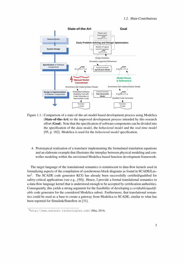
The goal of this thesis is to enable a Modelica based development process that removes theselimitations. Figure 1.1 contrasts a model-based development process using the current state-of-the-art technology with an improved process that takes advantage of results from the researchefforts of this thesis. Note the gap in the transition from Modelica control function specificationmodels to models used during the design and implementation phase. Modelica is currently notwell-suited to be used in that phase. This makes it necessary to manually rebuild the modelswithin a more dedicated embedded software modeling tool (with suitable automatic code gen-erator) or to convert the models manually to C code. In either way, the manual conversion istime-consuming and error-prone, especially if several design iterations are required.

Closing this gap in order to enable a more integrated approach to the development of cyber-physical systems is the main motivation for this thesis.

1.2. Main Contributions

The main result of this thesis is a Modelica based framework for model-based control functiondevelopment, which integrates state-of-the-art modeling for digital control functions with state-of-the-art modeling for physical systems.

The essential approach to achieve this is by transferring concepts from synchronous languagesfor safety-related real-time applications into the Modelica language. This enables to close thegap in the transition from Modelica control function specification models to models used duringthe design and implementation phase (see Figure 1.1). My main contributions in this contextare:

1. Identification of the current shortcomings of Modelica with respect to established require-ments in safety-related, model-based function development.

2. A proposal for language restrictions and extensions dedicated to modeling discrete-timecontroller functions, that is deemed suitable as basis for a high-integrity automatic codegenerator (ACG), resulting in a language denoted as ACG-Modelica.

3. Formulation of a translational semantics that maps a representative subset of ACG-Modelicato a synchronous data-flow kernel language.

1The term “cyber-physical system” (CPS) is rather new and attributed to Helen Gil who coined the term around2006 at the National Science Foundation in the United States [65, p. 5]. There is no complete consensus aboutthe precise meaning of CPS within the academic world yet. My use of the term CPS coincides with the definitionof Lee [63]: “A cyber-physical system (CPS) is an integration of computation with physical processes. Embeddedcomputers and networks monitor and control the physical processes, usually with feedback loops where physicalprocesses affect computations and vice versa.”.

2

1.2. Main Contributions

Qualified Code Generator

Specification of Software

Components

Requirements

System Design Models of Logical Control Functions

Physics and Environment

Design & Implementation

of Software Components

Control Function Code Generation

Model

FunctionC-Code

Model Reuse

& Refinement

Simulation supported Refinement

Control Function Specification Model

Design Iterations

Embedded Software

Modeling Tool with

Code Generator or

Hand-written Code

Manual Model

Conversion

Enrichment with Implementation Details Enrichment with Implementation Details

FunctionC-Code

State-of-the-Art Goal

Early Problem Solving and Design Optimization

Figure 1.1.: Comparison of a state-of-the-art model-based development process using Modelica(State-of-the-Art) to the improved development process intended by this researcheffort (Goal). Note that the specification of software components can be divided intothe specification of the data model, the behavioral model and the real-time model[95, p. 182]. Modelica is used for the behavioral model specification.

4. Prototypical realization of a translator implementing the formulated translation equationsand an elaborate example that illustrates the interplay between physical modeling and con-troller modeling within the envisioned Modelica based function development framework.

The target language of the translational semantics is reminiscent to data-flow kernels used informalizing aspects of the compilation of synchronous block diagrams as found in SCADE/Lus-tre2. The SCADE code generator KCG has already been successfully certified/qualified forsafety-critical applications (see e.g., [50]). Hence, I provide a formal translational semantics toa data-flow language kernel that is understood enough to be accepted by certification authorities.Consequently, this yields a strong argument for the feasibility of developing a certifiable/qualifi-able code generator for the considered Modelica subset. Furthermore, that translational seman-tics could be used as a base to create a gateway from Modelica to SCADE, similar to what hasbeen reported for Simulink/Stateflow in [31].

2http://www.esterel-technologies.com/ (May, 2014).

3

1. Introduction

1.3. Thesis Outline

The thesis addresses two aspects of function development with Modelica: first the conditionsthat need to be fulfilled to allow the usage of Modelica for implementing function models ina safety-related development process with automatic code generation, and second the use ofModelica as a basis for a seamless development methodology starting from the logical virtualmodel down to the technical system architecture.

Chapter 2: Background The chapter describes the state-of-the-art and defines relevantterms.

Chapter 3: Requirements for Model-Based Function Development This chapteridentifies (to some degree arguably subjective) requirements to a high-level, domain-orientedlanguage that need to be fulfilled in order that the language is suitable to be used in a safety-related, model-based function development process. This includes in particular:

• The identification of several key stake-holders within the development process includingtheir specific requirements that impact the requirements imposed on a suitable domain-oriented language.

• The identification of general requirements to a domain-oriented language for model-based(control) function development

• Additional considerations regarding the effectiveness and efficiency of model reviews forlanguages that are (formally) specified at the textual level but also have a graphical repre-sentation (as is the case for Modelica).

The so established requirements guide the language design decisions in the following chap-ters.

Chapter 4: Modelica’s Synchronous Language Elements Extension The synchronouslanguage elements extension was introduced in Modelica 3.3, May 2012 in order to improve thelanguage support for modeling sampled data systems. This chapter describes this extension,compares it with the previous approach of modeling sampled-data systems in Modelica andconcludes with a brief note about the historical development that led to that recent extensionincluding contributions that can be attributed to the author of this thesis.

Chapter 5: Enabling Modelica for Function Development The Modelica language isanalyzed with respect to the identified requirements for a domain-oriented language for model-based control function development. Based on this analysis current shortcomings are identifiedand practical proposals to mitigate the shortcomings are worked out. In particular:

• Established technologies and procedures for safety-related function development with au-tomatic code-generation are briefly presented and contrasted to current Modelica technol-ogy. Based on this, I propose an adaption of current Modelica technology.

4

1.4. Related Publications

• I propose specific language restrictions to ease the challenge of tool qualification.

• Also, I work out proposals for language extensions in order to increase the suitability ofModelica to model discrete-time controller functions. These include proposals for:

– Supporting most relevant target data types and operations.

– Modularization of dynamic execution aspects.

– Manual block scheduling.

– Causal data-flow semantics

The result of this effort is a restricted and extended Modelica language set for safety-relateddigital control applications that I denote as ACG-Modelica.

Finally, I present a translational semantics from a representative subset of the ACG-Modelicalanguage to a synchronous data-flow kernel language. This kernel language allows to resort toestablished automatic code generation techniques for data-flow languages that are, in particular,understood enough to be accepted by certification authorities.

Chapter 6: Servo System Example The chapter presents a typical control engineeringtask: the design of a digital controller for an electric drive system (servo control system). Theexample illustrates the usage of Modelica and ACG-Modelica in a framework for model-basedfunction development.

Chapter 7: Discussion and Conclusions A final discussion of the essential contents ofthe individual chapters and a brief conclusion regarding the main results of this thesis.

1.4. Related Publications

The research results presented in this thesis are partly based on the following peer reviewedconference and journal papers:

• Bernhard Thiele, Alois Knoll, and Peter Fritzson. Towards Qualifiable Code Generation from aClocked Synchronous Subset of Modelica. Modeling, Identification and Control, 36(1):23–52,2015. http://dx.doi.org/10.4173/mic.2015.1.3

• Bernhard Thiele, Stefan-Alexander Schneider, and Pierre R. Mai. A Modelica Sub-and Supersetfor Safety-Relevant Control Applications. In 9th Int. Modelica Conference, Munich, Germany,September 2012. http://dx.doi.org/10.3384/ecp12076455

• Martin Otter, Bernhard Thiele, and Hilding Elmqvist. A Library for Synchronous Control Systemsin Modelica. In 9th Int. Modelica Conference, Munich, Germany, September 2012.http://dx.doi.org/10.3384/ecp1207627

• Bernhard Thiele and Dan Henriksson. Using the Functional Mockup Interface as an Intermedi-ate Format in AUTOSAR Software Component Development. In 8th Int. Modelica Conference,Dresden, Germany, March 2011. http://dx.doi.org/10.3384/ecp11063484

• Hilding Elmqvist, Martin Otter, Dan Henriksson, Bernhard Thiele, and Sven Erik Mattsson. Mod-elica for Embedded Systems. In 7th Int. Modelica Conference, pages 354–363, Como, Italy,September 2009. http://dx.doi.org/10.3384/ecp09430096

5

2. Background

2.1. The Complexity Challenge at the Example of theAutomotive Sector

The rapid advances in electronic control technology lead to more complex software functionsthat pose a challenge to the development process. This development is not restricted to specificindustrial sectors. However, some sectors observed a significant higher growth rate of softwarecomplexity within the recent years than others. Among them is the automotive industry wherethe complexity1 of embedded software code increased about fiftyfold within the last 15 years[37].

Modern automotive vehicles can have over 60 ECUs (Electronic Control Units) which areinterconnected by a heterogeneous network of automotive buses, like CAN, FlexRay, LIN, andMOST for communication purposes [37]. Handling such complex systems is a big challengewhich is intensified by tightly scheduled development phases due to product market competition.Currently the development phase for vehicles is estimated to be about three years [95]. Theincreased use of virtual engineering methods has the potential to further reduce the requireddevelopment time span.

An additional important requirement for embedded automotive systems is safety. Today,ECUs increasingly provide safety-related functionality. Provided functions range from situationanalysis (e.g., speedometer display) and giving situation assessment (e.g., black-ice warning) toactive intervention in braking or steering actions (e.g., in a vehicle equipped with active frontsteering (AFS) [61]). Future vehicle designs might even go a step further and dispense me-chanical back-up linkages to the braking and steering system (Break-by-Wire, Steer-by-Wire)[38, 28, 9]. At the same time, safety requirements requested by authorities are raising, which isreflected in safety regulations like IEC 61508 (“Functional safety of electrical/electronic/pro-grammable electronic safety-related Systems”) and its application specific derivations, most no-tably the recent ISO 26262 (“Road vehicles – Functional safety”) for automotive applications.As a consequence, virtual prototyping methods need to be amenable to support activities thatimprove confidence in the functional safety of the system.

In order to develop and validate functions for cyber-physical systems, it is no longer sufficientto solely consider single, self-contained components without taking the interaction of the func-tion within the whole system into account. Technology that is capable of seamless integrationof physical system models and safety-related software functions within a virtual prototyping en-vironment is mandatory to cope with the inherent complexity of CPS, enable short developmentcycles, and at the same time, ensure safe products.

1Taking the size in object instruction as a measure of code complexity.

7

2. Background

2.2. Modeling in (Control) Engineering and ComputerScience Communities

When working in the interdisciplinary field of cyber-physical systems care has to be taken aboutthe meaning of similar terms in different communities. As Henzinger and Sifakis note about the“education challenge” in the discipline of embedded systems design [55]:

“The lack of a common cultural background also results in fragmented research.Different communities use different terminologies.”

An important example is the term “model” which is omnipresent throughout this text.Control engineers with mechanical or electrical engineering background typically expect

models to abstract from reality by providing a mathematical description (equations!) of thebehavior of the modeled object2. Computer programs that provide support for building such an-alytical models are also expected to be able to execute/simulate them. Typical modeling abstrac-tion in control engineering are block diagrams (transfer functions composed by port connectionswith a data flow semantics) or declarative (acausal) equations3.

Software engineers, tend to have a more abstract view of the term “model”. A model may beany form of (formal) notation that is capable of describing certain aspects of a matter of interest.They are also accustomed to the concept of meta-models (a term absent in more traditionalengineering education), denoting a (formal) notation that is capable of describing another model.Consequently, software engineers also do not tend to implicitly expect that a model in a machineconsumable format will be executable. A well known example for modeling within the disciplineof software engineering is the UML language with its four-layers meta-modeling architecture[81].

This text embraces the more abstract view of the term “model”. Nevertheless, the consideredmodels are mainly of analytic nature and therefore match well with what might be expected byreaders with a control engineering background.

2.3. Model-Based Development

Model-Based Development (MBD) makes systematic use of (formal) models as primary arti-facts throughout the overall development process. In classical software development (e.g., ITand business applications), this traditionally refers to the application of advanced software mod-eling technology to capture requirements, and software structure [18]. However, in the embed-ded (control) systems community the term is usually more narrowly understood as (analytical)executable system models (consisting of control algorithm models as well as the correspond-ing physical plant models) that are the primary artifacts for the control function design process.Starting with capturing the requirements, the system model is continuously elaborated and con-stitutes the heart of design, implementation and testing activities. This view, the model as centerof all development and design activities, is also often referred to as model-based design [97].

2 Of course there exist model abstractions used in engineering where equations are not in the foreground. Notablygeometry models, as used in engineering drawings, as well as wiring or hydraulic diagrams etc. However, acontrol engineer usually doesn’t associate that kind of models when using the term modeling.

3Acausal means that the causality of how to solve the equations is not decided at modeling time

8

2.3. Model-Based Development

Nowadays, model-based development has become a well established development approachin the domain of embedded (control) systems and the original promise of model-based devel-opment, to provide a more rapid and economic development process, seems to be confirmed inindustrial practice [24].

In automotive software engineering the term Model-based Function Development is com-monly used to indicate that the traditional function development process is replaced by a model-based approach – using analytical (graphical) models for developing the behavioral part of theembedded software.

Using this more precise term allows to distinguish between Model-based Function Devel-opment and Model-based System Development, where the later term encompasses the use ofmodels to describe system and software architecture models [78].

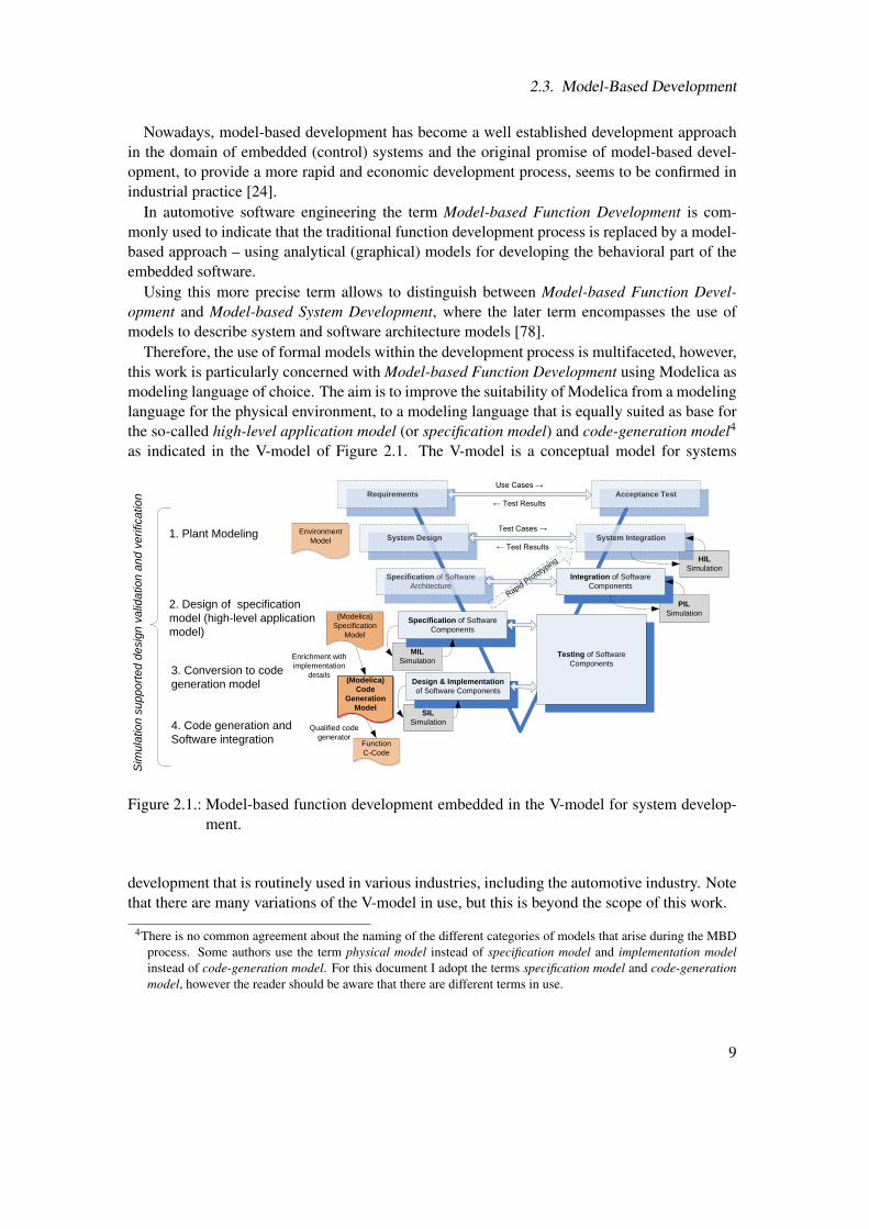
Therefore, the use of formal models within the development process is multifaceted, however,this work is particularly concerned with Model-based Function Development using Modelica asmodeling language of choice. The aim is to improve the suitability of Modelica from a modelinglanguage for the physical environment, to a modeling language that is equally suited as base forthe so-called high-level application model (or specification model) and code-generation model4

as indicated in the V-model of Figure 2.1. The V-model is a conceptual model for systems

HIL

Simulation

PIL

Simulation

SIL

Simulation

Integration of Software

Components

System Integration

Acceptance Test

Testing of Software

Components

MIL

Simulation

Specification of Software

Components

Design & Implementation

of Software Components

Requirements

System Design

Specification of Software

Architecture

Test Cases →

← Test Results

Use Cases →

← Test Results

Rapid Pro

totyp

ing

Function

C-Code

(Modelica)

Specification

Model

(Modelica)

Code

Generation

Model

Environment

Model

Enrichment with

implementation

details

Qualified code

generator

1. Plant Modeling

2. Design of specification

model (high-level application

model)

3. Conversion to code

generation model

4. Code generation and

Software integration

Sim

ula

tio

n s

up

po

rte

d d

esig

n v

alid

atio

n a

nd

ve

rifica

tio

n

Figure 2.1.: Model-based function development embedded in the V-model for system develop-ment.

development that is routinely used in various industries, including the automotive industry. Notethat there are many variations of the V-model in use, but this is beyond the scope of this work.

4There is no common agreement about the naming of the different categories of models that arise during the MBDprocess. Some authors use the term physical model instead of specification model and implementation modelinstead of code-generation model. For this document I adopt the terms specification model and code-generationmodel, however the reader should be aware that there are different terms in use.

9

2. Background

In order to optimize the benefits gained by a model-based development process as illustratedin Figure 2.1, it is crucial that formally specified high-level applications can be automaticallytransformed (usually by using generated embedded C-code) into executable binary code forrespective embedded platforms, thus eliminating error prone and expensive manual recodingof the application into a general-purpose programming language. Note that for accentuatingthat formal models are transformed into executable code (as opposed to “just” being used forspecification/illustration purposes) the term Model-Driven Software Development5 (MDSD) isalso commonly used in the literature [98].

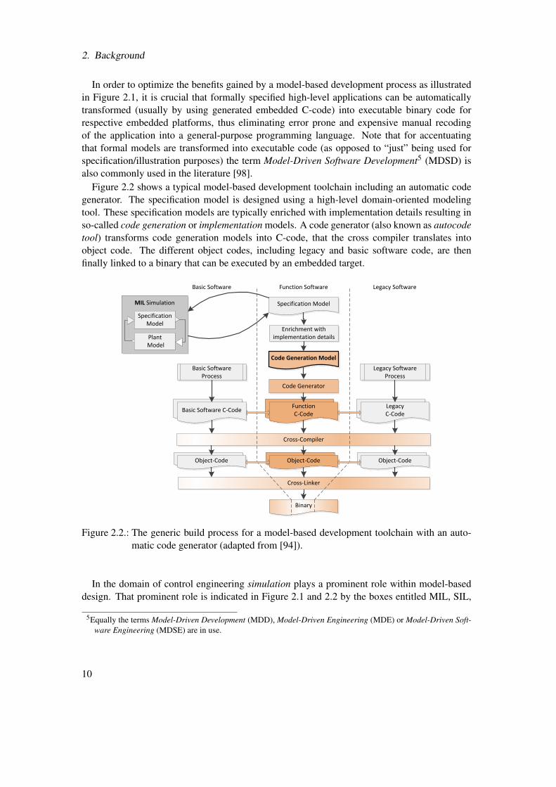
Figure 2.2 shows a typical model-based development toolchain including an automatic codegenerator. The specification model is designed using a high-level domain-oriented modelingtool. These specification models are typically enriched with implementation details resulting inso-called code generation or implementation models. A code generator (also known as autocodetool) transforms code generation models into C-code, that the cross compiler translates intoobject code. The different object codes, including legacy and basic software code, are thenfinally linked to a binary that can be executed by an embedded target.

Code Generation Model

FunctionC-Code

Object-Code

Binary

Code Generator

Cross-Compiler

Cross-Linker

Specification Model

Enrichment with implementation details

LegacyC-Code

Basic Software C-Code

Legacy Software Process

Basic Software Process

Function SoftwareBasic Software Legacy Software

Object-Code Object-Code

MIL Simulation

Specification Model

Plant Model

Figure 2.2.: The generic build process for a model-based development toolchain with an auto-matic code generator (adapted from [94]).

In the domain of control engineering simulation plays a prominent role within model-baseddesign. That prominent role is indicated in Figure 2.1 and 2.2 by the boxes entitled MIL, SIL,

5Equally the terms Model-Driven Development (MDD), Model-Driven Engineering (MDE) or Model-Driven Soft-ware Engineering (MDSE) are in use.

10

2.4. Modeling Tools and Languages for Embedded Systems Design

PIL, and HIL simulation (meaning Model-in-the-Loop, Software-in-the-Loop, Processor-in-the-Loop and Hardware-in-the-Loop simulation).

Especially as systems become more complex (as typical for cyber-physical systems) MIL sim-ulation becomes an indispensable tool for early design validation and verification. In particular,given an executable model of physical aspects (plant model) and software aspects (high-levelapplication model) of the complete system, it becomes feasible to

• obtain very fast feedback about the effect of system design decision in an early develop-ment phase;

• evaluate and incrementally improve designs, even without available prototypical hard-ware;

• apply (multi-criteria) computational optimization methods in order to find a better balancebetween possible design variations;

• test and evaluate system behavior under extreme conditions that otherwise would be toocostly, dangerous or (physically) unfeasible with real prototypes;

• synthesize and analyze high-performance (model-based) controllers.

2.4. Modeling Tools and Languages for Embedded SystemsDesign

The most prevalent domain-specific software for model-based design of embedded software(including code generation) on the market is Matlab/Simulink [10, 103] from MathWorks. Mat-lab is a numerical computing environment, suitable for algorithm prototyping, data analysis,and advanced data visualization capabilities. Simulink is primarily a graphical block diagramlanguage that is tightly coupled with Matlab. Block diagrams are a popular domain specific lan-guage (DSL) used within control systems and digital signal processing (DSP) development. It ispossible to generate C code from Simulink models for various (embedded) target platforms us-ing code generators offered by MathWorks or third party companies (most notably the dSPACETargetLink tool [52]).

However, the modeling capabilities of Simulink for physical systems are rather primitive. InSimulink physical systems need to be modeled using the same graphical block diagrams thatare common in control engineering and DSP design. Yet, block diagrams are not up to thestate of the art in physical modeling. MathWorks finally reacted to this deficiency by offeringa Simulink toolbox named SimScape to enable object-oriented physical modeling (SimScapemade its debut in the R2007A release of Matlab/Simulink). Unfortunately, instead of using theopen Modelica language standard, MathWorks decided to create its own, proprietary, physicalmodeling language. In effect, the huge pool of high-quality (free and commercial) physicalmodeling libraries already available for Modelica cannot be reused in SimScape.

In contrast to Simulink that has its roots in control systems and DSP engineering and was laterextended to offer decent support for physical modeling, the development of the Modelica lan-guage started from the beginning with the aim of creating a language that excels in multi-domain

11

2. Background

physical modeling. Modelica was conceived in the late 1990s by the Modelica association6. Itsinitial design was heavily influenced by the pioneering work of Elmqvist [40]. From the begin-ning Modelica embraced a truly object-oriented physical modeling style and was actively main-tained and developed as open standard by the non-profit Modelica Association. Today, severalimplementations (commercial and free) of Modelica are available7. The best known commercialimplementations include Dymola8 and SimulationX9, a decent open-source implementation isavailable with OpenModelica10.

Modelica proved to be a powerful tool to model large-scale, multi-physics systems in indus-trial real-world use cases. Thus, it is well suited to model the dynamic behavior of complexcyber-physical systems (CPS) (e.g., by modeling a complete virtual vehicle including the log-ical controller functions [11, 36, 32]), which is a key requirement for a model-based, globaldevelopment approach.

However, up to now the use of Modelica for the design of control algorithms has been verylimited. Available records of using Modelica for control algorithm development are restrictedto high-level prototypical work for advanced (model-based) controller designs [68, 5, 111, 112,102]. After prototyping the control algorithms in Modelica, the Simulink toolchain or manuallywritten code is used for deploying the control logic to an embedded system target.

A notably exception is the direct use of executable code generated from Modelica within amodel predictive control (MPC) framework for optimized start-up of power plants reported byFranke [46]. However, control on the process management level (with time horizons betweenminutes to hours) is very different to the embedded control systems that are considered in thisthesis (with time horizons of the magnitude of (sub-)milliseconds).

Published reports of using Modelica as source format for direct generation of code for em-bedded system targets have been, so far, of purely academic nature [42, 2, 20]. This can bepartly attributed to a somewhat too limited expressiveness in modeling discrete-time con-troller functions, and partly to the lack of a flexible, seamless development methodologyfrom the controller model comprising the logical functions to the technical system architecture(i.e., code running on the target platform).

Although there exist a lot of concepts, technology and software targeting embedded systems(both industrial and academic), the available technology usually either focuses on modeling theembedded software, or focuses on modeling the environment.

It is important to mention that there exist quite a lot of industry relevant languages that tar-get embedded systems development. However, they either focus on modeling the embeddedsoftware, or focus on modeling the physical environment.

• OMG SysML [80] is a language specifically designed to support system engineering.Although it provides a holistic system view, the abstraction level and expressiveness is notwell suited for physical modeling and simulation11.

6Modelica Association (2012), https://www.modelica.org/.7A good overview is provided by the Modelica Association (2012), https://www.modelica.org/tools/.8Dymola, Dassault Systèmes AB (2012), http://www.dymola.com/.9SimulationX, ITI Gesellschaft für ingenieurtechnische Informationsverarbeitung mbH (2012),

http://www.simulationx.com/.10OpenModelica, Open Source Modelica Consortium (OSMC) (2012), http://www.openmodelica.org/.11Note that ongoing research tries to integrate the descriptive power of SysML with the analytic and computational

12

2.4. Modeling Tools and Languages for Embedded Systems Design

• Synchronous languages [16] are an established technology for modeling, specifying, val-idating, and implementing real-time embedded applications. Prominent members of thesynchronous family include the Lustre [30], Esterel [21] and Signal [62] language. Thegreatest industry relevancy can be attributed to the Lustre-based commercial SCADE tool[91] that is especially used for the development of safety critical software functions. Syn-chronous languages have no notion of continuous time and are therefore not suited forphysical modeling.

• VHDL-AMS [7] is an extension to the VHDL electronic systems hardware descriptionlanguage. It is capable of multi-domain (physical) modeling. Its root in electronic de-sign circuits is still noticeable, consequently its main focus is currently the verification ofanalog, mixed-signal integrated circuits. It is not intended for generating code.

Note the lack of decent combined support of both, physical and functional modeling, conse-quently these languages are not suitable for the envisioned integrated approach to CPS develop-ment.

There is also a considerable amount of academic research activities relevant within the re-search subject. Naturally that includes work conducted in the field of hybrid modeling andsimulation as well as in the field of languages for (formal) control algorithm specification. Ofparticular interest in this work is the interplay between control system modeling and physicalmodeling.

• The Ptolemy project [39] studies different aspects of the design of embedded systems. Akey concern is the interaction between well-defined models of computation (MoC). It ispossible to model hybrid systems by combining a continuous MoC with one or severalof the provided discrete-time MoC [66]. The continuous modeling is similar to the blockdiagrams used in Simulink and thus, physical modeling capabilities are rather constrained.

• Scicos [75] is a graphical system modeler and simulator for hybrid dynamical systems[76]. Its model of execution is based on the synchronous language Signal extended tocontinuous-time systems. Interestingly, it allows to integrate a subset of the Modelicalanguage to enrich its continuous-time dynamics modeling capabilities. However, the par-tial support of Modelica severely limits potential reuse of available Modelica libraries.Furthermore, a really seamless integration of Modelica into Scicos is missing (a prepro-cessing step is required in which C code conforming to an ordinary external Scicos blockneeds to be generated from a Modelica model which then needs to be compiled and linkedagainst Scicos before simulation).

• A lot of research in hybrid systems targets the formal verification of system properties thatdepend on the interaction of discrete control algorithms and the physical environment (i.e.,plant to be controlled) see e.g., [4, 3, 54]. It should be noted that applying these verificationmethods to large scale models is still an unsolved problem due to state explosion issues.

power of Modelica models [92].

13

2. Background

• Within the synchronous language community recent studies attempt to establish alterna-tive semantic foundations for hybrid systems modeling [12, 14]. Benveniste et al. [14]proposes to use non standard analysis [90] as mathematical base for establishing the se-mantics of a hybrid simulator. Bauer and Schneider [12] consider a semantically welldefined hybrid extension of the synchronous language Quartz [93] to enable simulationand formal verification. The emphasis of this work is rather in mathematical rigor andfundamentals than in providing a practical methodology for the virtual prototyping ofreal-world systems.

• All of the aforementioned work primarily target functional aspects of embedded systemsdevelopment. In practice, non-functional aspects like process management, communica-tion or fault-tolerance mechanisms are an integral part of the complete system. Integrationof that aspects within a model-based development process is considered in [26, 27, 25]. Ishare the spirit of this contributions in the sense that these aspects need to be consideredwithin a virtual prototyping methodology for cyber-physical systems.

2.5. Safety Relevant Software Functions

Naturally, customers and users of a technical product (be it a household appliance or a civil air-craft) may expect that the product is “safe”. In order to ensure the absence of non reasonablerisks related with the use of a product, legislative authorities have established rules and regula-tions that are mandatory for producers, distributors, and others who make the products availableto the public. This regulations can include approval requirements by official authorities as aprerequisite for making the product available or product liability laws that held producers liablefor harm caused because of defects within their products.

2.5.1. Terminology

Product liability (in regard to person injury or death) is the area of law in which producers areheld liable for harm caused because of defects within their products.

A product has a defect if it does not provide the safety a person is entitled to expect.A product is considered safe if the risks caused by faults/failures of the product and interac-

tions with the product are within reasonable limits.Risk is the combination of the occurrence probability of a failure and the severity of the harm

that may be expected by the failure (e.g., injury or death of persons).Functional safety is the absence of not reasonable risk caused by malfunctioning behavior of

E/E safety-related systems and interaction of these systems12.Functional safety standards give guidelines about the limits of what the majority of experts

consider a reasonable risk, as well as actions that can be taken to reduce risk to a level that isconsidered reasonable.

12Functional safety as defined by ISO 26262 does not address hazards related to electric shock, fire, smoke, heat,radiation, toxicity, flammability, reactivity, corrosion, release of energy, and similar hazards unless directly causedby malfunctioning behavior of E/E safety-related systems [58, ISO 26262-3:2011, p. 1].

14

2.5. Safety Relevant Software Functions

Safety-relevant software functions are software functions that are part of an E/E safety-related system. They are required to fulfill certain safety integrity levels in order to reduce therisk stemming from the software and its interaction with the environment to a reasonable level.

2.5.2. Functional Safety Standards

The international standard IEC 61508 Functional safety of electrical/electronic/programmableelectronic safety-related systems is intended to be a base norm for functional safety with generalapplicability in industry. However, the mapping of the generic base standard to specific applica-tion can be difficult. For that reason, application specific standards exist that interpret IEC 61508in the context of a specific domain.

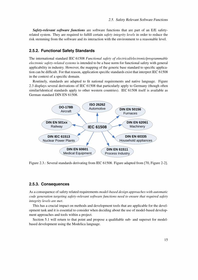
Routinely, standards are adapted to fit national requirements and native language. Figure2.3 displays several derivations of IEC 61508 that particularly apply to Germany (though oftensimilar/identical standards apply to other western countries). IEC 61508 itself is available asGerman standard DIN EN 61508.

IEC 61508

ISO 26262

Automotive DIN EN 50156

Furnaces

DIN EN 62061

Machinery

DIN EN 60335

Household appliances

DIN EN 61511

Process Industry

DIN EN 60601

Medical Equipment

DIN IEC 61513

Nuclear Power Plants

DIN EN 501xx

Railway

DO-178B

Aircraft

Figure 2.3.: Several standards derivating from IEC 61508. Figure adapted from [70, Figure 2-2].

2.5.3. Consequences

As a consequence of safety related requirements model-based design approaches with automaticcode generation targeting safety-relevant software functions need to ensure that required safetyintegrity levels are met.

This has a crucial impact on methods and development tools that are applicable for the devel-opment task and it is essential to consider when deciding about the use of model-based develop-ment approaches and tools within a project.

Section 5.1 will return to that point and propose a qualifiable sub- and superset for model-based development using the Modelica language.

15

2. Background

2.6. Software Architectures

Different definitions exist in literature for what is meant by the term “Software Architecture”. InClements et al. [33] following definition is provided:

“The software architecture of a computing system is the set of structures needed toreason about the system, which comprise software elements, relations among them,and properties of both.”

Software architectures are typically tailored to the requirements of their respective applica-tion domain and address aspects that are sometimes termed as non-functional requirements (e.g.,communication, scheduling, reliability, maintainability, scalability, efficiency, testability, exten-sibility, portability).

A well known examples of a reference software architectures for embedded systems in theautomotive domain is AUTOSAR (AUTomotive Open System ARchitecture13).

But how do software architectures affect the high-level application models considered in thistext? Functions developed for complex systems (i.e., systems similar to the systems discussed inSection 2.1) will need to integrate into an (already existing) software architecture. That naturallyhas consequences for the tooling, e.g., the code generator has to produce code that conforms tothe interface expected by the software architecture. In addition, it also has consequences forthe environment model required during virtual prototyping of the function. “Non-functional”aspects like performance (time) models of (distributed) functions, scheduling policies, and buscommunication characteristics have essential impact whether a design works as expected.

The term Architecture-Driven Development (ADD) has emerged to emphasise the central roleof software architecture during such a development process. Niggemann et al. provide a notablediscussion about the effects of ADD on established model-based function development practicesand tools [77], stating

“Most behaviour modeling and code generation tools, e.g., TargetLink, have sofar mixed at least three different concerns: algorithmic models, function networks,and ECU configuration. Since such tools now focus on the "algorithmic model"concern in an architecture-driven development process, some modification becomenecessary.”.

Since the use of architecture has become the state-of-the-art to enable improved reuse andintegration of (embedded) software components I have in mind that my proposed framework forModelica based function development integrates well in ADD processes.

13 AUTOSAR development cooperation (2015), http://www.autosar.org/.

16

3. Requirements for Model-BasedFunction Development

This chapter is an extensively revised and extended version of Section 2 and 3 of the publication

Bernhard Thiele, Stefan-Alexander Schneider, and Pierre R. Mai. A Modelica Sub-and Superset for Safety-Relevant Control Applications. In 9th Int. Modelica Confer-ence, Munich, Germany, September 2012. http://dx.doi.org/10.3384/ecp12076455.

An increasing number of embedded software components is specified in models representingthe so-called high-level application which is then automatically transformed into embedded tar-get code (Figure 2.2). The specification model is designed using a high-level, domain-orientedlanguage which is in the following succinctly referred to as the modeling language. In this chap-ter, I try to identify requirements imposed on such a language with a special attention to safetyrequirements, which are indispensable for many real-world applications.

The modeling language (and the software development process) has to provide a balancebetween rigidness and flexibility: on the one hand, the user may not be restricted too much andmust still have room for creativity and principal control over all development activities sincetoo many restrictions reduce the acceptance, the productivity and quality of the work. On theother hand, too few restrictions lead to error-prone development practices and ultimately topreventable faults in the software.

In order to understand the different requirements imposed in this chapter, it is beneficial toconsider the various stake-holders which participate in the development in different roles withdifferent requirements and expectations. Consequently, this chapter starts with introducing themost relevant roles within the intended development process.

In the following sections, the requirements resulting from the introduced roles are developed.An essential implication of these requirements is that they only can be met by specific restrictionsand extensions of the domain language Modelica considered in this work. This will be elaboratedupon in following chapters.

Another important aspect is the intention to allow for code reviews being done entirely onmodel level (as opposed to embedded C source code level). Code reviews are a well establishedactivity in development processes targeting safety relevant software (see, e.g., [100, 101, 104,59]). A model-based development process may require that automatically generated code istreated with the same scrutiny as handcrafted code, in particular performing code reviews onautomatically generated code may be necessary [100, 13]. However, in order to fully benefitfrom a model-driven approach (and thereby reducing costs) it is desirable to make C code levelreviews redundant and perform solely model reviews. This becomes feasible as soon as a suitablyqualified/certified toolchain is available [94, 13].

17

3. Requirements for Model-Based Function Development

For some modeling languages, the language semantics is entirely defined on the graphicallevel (e.g., Simulink). However, for Modelica, the modeling language considered in this work,the language specification defines the semantics on the textual level and defines annotations forstoring extra information like the graphical representation of the model. As a consequence, therequirements at the modeling language have been split into two parts: Section 3.2 defines gen-eral requirements for a modeling language deemed suitable for model-based (control) functiondevelopment. In addition, Section 3.3 introduces requirements that are targeted specifically tothe graphical representation of modeling languages whose semantics is originally defined at thetextual level.

3.1. Development Roles

Various stake-holders participate in the development having different roles with different re-quirements and expectations. A suitable domain-oriented language will have to support at leastthe following roles in the development process [109, Section 2]:

Role 1 - Developer. Developer of the embedded control system. This role requires a sufficientlyexpressive modeling language based on sound language elements with clear semantics to designand test the intended functionality.

Role 2 - Tool Developer. This role requires the precise definition of the input modeling lan-guage: there should be no unclear corner cases in the semantics. The language should be effi-ciently compilable to target code.

Role 3 - Reviewer. Reviewer for functional safety. This role requires a clear and unambiguousdescription of the functionality, including all semantically relevant modeling details in compactform for efficient reviews. It should be possible to determine coverage at the model level andallow for tracing of requirements to the relevant model parts.

Role 4 - Tool Qualifier. This role requires a sufficiently small number of modeling elementswith clear semantics as well as clear, ideally highly localized composition rules, in order toestablish a validation suite for the development tool. The boundaries of the development tools,i.e., input and output notations, have to be clearly defined. Automated processes should ideallybe separately testable to minimize complexity. For more details see Section 5.2.1.

These different roles have partly coincident (semantic aspects) and partly contradictory (ex-pressiveness of the language) requirements to the modeling language and its associated devel-opment tools.

3.2. Modeling Language Requirements

This section establishes general requirements for modeling languages that shall be used as basefor a high-level application model. The requirements are to some extent subjective, however aclear rationale is provided for any stated requirement.

It is assumed that the modeling language shall be used for high-level applications that have anopen- or closed-loop control nature and provide potentially safety-relevant functionality. Due tothis safety aspect, it is important that the language supports high assurance designs. Therefore,

18

3.2. Modeling Language Requirements

the feasibility of tool qualification is of high importance and similarly the suitability for efficientand effective model reviews.

For modeling languages whose semantics are specified on the textual level, it is, at first glance,natural to do the functional reviews on the textual level. Even if a graphical representation isalso available in some form, (as is the case for Modelica) the graphical level may hide importantimplementation details. However, of course the graphical level provides an abstraction that easescomprehension of the intended model semantics and is hence an extremely valuable supplemen-tary to the textual review. Beyond this, it is as well desirable to allow reviews to be done entirelyon the graphical level. For this purpose Section 3.3 provides additional requirements with theaim to ensure that the graphical representation is clear without ambiguity. It is then left to thereviewer and his or her preferences to either perform a textual or a graphical review.

As has been explained in Section 2.3, it is of paramount importance in the model-based de-velopment of complex (cyber-physical) systems that also the physical system parts can be ad-equately modeled. However, the requirements for modeling the physical system parts are notconsidered in this section. This section solely targets the language requirements in respect to thehigh-level application model. Nevertheless, the modeling language for the high-level applica-tion should integrate seamlessly into system models that contain physical system parts. This isreflected in the “zeroth requirement”:

Requirement 0 - Support for System Design and Early Problem Solving. The languageshould integrate seamlessly into a model-based system design approach in order tosupport early problem solving and validation and verification activities.

The following requirements are specifically targeted to properties that need to be met by amodeling language for the high-level application model. Due to its importance to all roles, thefirst requirement is of particular importance:

Requirement 1 - Formally Sound Language Set. The language must be formally sound.Rationale: Ambiguity and impreciseness in the language must be eliminated in order to avoiddifferent interpretation possibilities. The language should be well suited to support (formal)validation and verification activities.Mainly demanded by: All roles.

Requirement 2 - High-Level Domain Oriented Notation. The language must have enoughexpressiveness to allow the clear and concise specification of discrete open- and closed-loopcontrol algorithms and their related support logic.Rationale: Embedded control developers need a language that provides good support for imple-menting relevant control algorithms.Mainly demanded by: Developer.

Requirement 3 - Suitable Model of Computation (MoC). The utilized MoC behind the lan-guage should be clearly defined, intuitive to the control system developer, and well-understoodand accepted by (certification) authorities.Rationale: MoCs provide mental models to express, understand, discuss and analyze computa-tional execution (cf. [64, 39]). Depending on the problem at hand, a particular MoC might resultin a superior abstraction than another. On the one hand the utilized MoC should be intuitive

19

3. Requirements for Model-Based Function Development

to control system developers, on the other hand it should be well-understood and accepted by(certification) authorities to facilitate tool qualification activities.Mainly demanded by: Developer and Tool Qualifier.

Requirement 4 - Target Data Types and Operations. The language should provide a mecha-nism that allows to extend its data types and operations to support fundamental data types andoperations available on the embedded target platform.Rationale: Low-level hardware-aspects play an important role for dedicated code generatorsand high-level languages targeting microcontrollers or digital signal processors, which strive toproduce optimized, target-aware code [52, 56, 44]. The major motivation is to lower costs ofrequired hardware by optimizing the memory and runtime efficiency of the software. Despite ofoptimizing code generators developers may still need full manual control over data types, datastorage, memory alignment and the implementation of interfaces in the generated code in orderto optimize the code generated for a particular target [89, p. 78].Mainly demanded by: Developer and Tool Developer.

Requirement 5 - Compile Time Analysis. The language should allow compile time analysisof important properties in order to reject problematic models.Rationale: Compile time checks are means to increase the degree of confidence that one mayhave in the correctness of a model/program. Possible properties that can be checked by compiletime analysis include: missing/incompatible initial values, type checking, clock analysis, cyclicdefinitions that result in algebraic loops, and equality of the number of equations with the numberof unknown variables.Mainly demanded by: Developer and Reviewer.

Requirement 6 - Modularity. The language must support constructs that allow modular mod-eling.Rationale: Modularisation is a key technique to cope with the complexity of software. It im-proves understandability and thus reviewability of complex models. It also facilitates its imple-mentation and maintenance.Mainly demanded by: Developer, Reviewer and Tool Qualifier.

The following requirement is mainly motivated by the role of a tool qualifier and typicallyholds the most potential for discussion with the other roles, especially with the role Developer:

Requirement 7 - Restricted Language Scope. The language should be as simple and clearas possible. This shall be achieved by restricting the scope of the language to a (preferablysmall) core relevant for the addressed problem domain. Particularly, simplicity and clarity of thelanguage is to be preferred over feature richness.Rationale: Facilitate tool qualification activities.Mainly demanded by: Tool Qualifier.

The next requirements concern the interplay between automatic code generation and the mod-eling language. It could be argued that requirements on the code generation is orthogonal to themodeling language. However, this is not entirely true since semantics of the modeling languageneeds to be faithfully reproduced by the generated code. Thus the modeling input language willnaturally affect the target code structure that can be automatically generated from it. Therefore,the formulated requirements do have impacts on the modeling language.

20

3.2. Modeling Language Requirements

Requirement 8 - Automatic Code Generation (ACG). The language should permit automaticgeneration of target platform C-code that is: a) efficient, b) adheres to good software engineeringpractice, c) is traceable, and d) integrates smoothly into embedded systems software architec-tures.Rationale: Automatic target code generation is crucial to optimize the benefits gained from amodel-based development process (see Section 2.3). Automatic C-code generation is stipulated,since C-code is the most popular language for targeting embedded systems and (certifiable) com-pilers are available. However, this should not be understood as if the use of other target languagesor the direct generation of binaries was inferior. Efficiency is a natural requirement for code thatis meant to run on a cost-efficient embedded system. For safety-related applications it is oftenrequired that also generated code “adheres to good software engineering practice and followsthe standard styles for the target language” [115]. For generated C-code in the automotive areathat typically means that conformance to some coding standards, e.g., MISRA AC AGC [107] isrequired. Traceability refers to the property that given a fragment of the automatically generatedC-code, it must be possible to trace it back to the model elements that caused its generation.Traceable code facilitates validation activities, e.g., manual inspections, automated analysis ofthe generated code1, and testing [115]. Finally, the generated code typically needs to be inte-grated into a given software architecture (see Section 2.6).Mainly demanded by: Developer, Tool Developer and Tool Qualifier.

Requirement 9 - Tangible Fixation of Automatically Deduced Properties. It must be pos-sible to fixate all properties of a model that influence code generation in a tangible, reviewableform.Rationale: In order to ensure reproducibility of code generation and reviewability2, it must bepossible to fixate all properties of a model that influence code generation in a tangible, review-able form. In particular, it must be possible to fixate initial values that are automatically deducedby a tool, so that code generation will always use the fixated values instead of recalculating thosevalues on the fly at the time of code generation.Mainly demanded by: Reviewer and Tool Qualifier.

Requirement 10 - Modular Code Generation. The language should support modular codegeneration. Modular code generation in this context is understood as: (1) code for a modu-lar structure in the modeling language should be generated independently from the context inwhich that structure is used, and (2) if a modular structure is composed of several other modularstructures, only minimal knowledge about that structures (their respective interface informa-tion) should be needed. E.g., presume the language has a structuring construct similar to theblocks typically encountered in the block diagrams used by control engineers (i.e., hierarchi-cal synchronous data-flow block diagrams). Further on, presume such a block is composed byconnecting several “building” blocks. For modular code generation it should then be possible togenerate a minimal set of transition functions (preferably one) for each of the respective buildingblock definitions and produce the overall transition function(s) by their composition.

1One example is to perform code coverage analysis on the target level but mirror back the results onto the modellevel.

2Note that this requirement also enables separate validation of code generator and property-deduction code, sincethe fully fixated model provides the checkable interface between both processes.

21

3. Requirements for Model-Based Function Development

Rationale: Imperative languages (like C) use functional decomposition as a means for modular-ization, abstraction and structuring. Modular code generation allows to map modular structuresat the model level to modular structures at the target code level. Although modular code genera-tion should not be considered as an axiomatic requirement to a code generator for safety-relevantsoftware it offers several advantages (see also Section 5.6):

1. Modular code generation preserves structure. Given that generated code is well-structuredand obeys similar guidelines as handcrafted code, generated code may be treated just likehandcrafted code artifacts in the further development process. In particular, that allows todirectly reuse the validation and verification methods and criteria that are already acceptedfor handcrafted code. Note that this can be an attractive approach, especially if the codegenerator itself is not (yet) sufficiently qualified for the intended purpose at hand andqualification would be too costly.

2. Modular code generation helps to establish a good traceability between model and gener-ated code (supports Requirement 8, traceability).

3. Modular code generation may decrease the size of the generated code, since generatedtransition functions can be potentially reused at different parts of the model (supportsRequirement 8, efficiency).

4. Modular code generation allows for separate compilation of the generated code artifactswhich has two advantages: First, it allows to distribute that modules without giving awaythe source code (in order to protect intellectual property) and second, it avoids processingall source code every time the binary is built which in turn saves development time.

Mainly demanded by: Developer, Tool Developer and Tool Qualifier.

3.3. Graphical Representation Requirements

For a modeling language which is specified at the textual level (like Modelica) a suitable graph-ical representation often provides an abstraction that significantly eases the comprehension ofthe intended model semantics. Therefore, a model review done on the graphical level can bepotentially more efficient than one done at the textual level (since the relevant details can beunderstood faster).

However, if the semantics of a modeling language is described on a textual level, but therealso exists a graphical representation the following question arises:

How can it be avoided that details that are not obvious or even hidden in the graph-ical representation prevent the reviewers from performing an efficient and effectivegraphical review?

For establishing an effective graphical code review it has to be ensured that the full semanticsof the textual representation is also available in the graphical representation. This motivates thefollowing additional requirement for the graphical representation that should allow developersand reviewers to mostly work at a graphical level:

22

3.3. Graphical Representation Requirements

Requirement 11 - Encoding of Full Semantics in the Graphical Representation. Any se-mantics associated with the graphical representation of language elements and their composi-tions should be completely evident by inspecting the graphical diagram layer, i.e., apart fromclearly marked exceptional cases there should be no cases where the semantics of a model is notentirely and uniquely understandable from inspection of the graphical diagram.Rationale: Code reviews of models should be feasible as far as possible at the graphical level.Consequently, the semantics of a model should be completely evident by inspecting the graphi-cal diagram layer.Mainly demanded by: Reviewer.

Note, that for Modelica it is typical that a library developer uses the textual Modelica lan-guage to code basic functionality in components that are annotated with a graphical illustration,while an application/model developer (library user) works on a graphical level by just dragging,dropping and connecting the library components in order to compose the intended functionality.Therefore, there is no direct correspondence between basic textual language elements and thegraphical representation. For such languages, requirements to the language design translate intorequirements to the library design.

The first of the additional requirements for the design of such libraries assures that the graphi-cal representation of library components is close to notations typically used by control engineers.It is therefore analog to Requirement 2.

Requirement 12 - Intuitive Graphical Representation. Library components and their (graph-ical) compositions should not exhibit any behavior which would be deemed surprising or non-obvious by embedded control systems experts.Rationale: In order to minimize the risk of misunderstanding it is important that the graphicalrepresentation is intuitive for domain experts.Mainly demanded by: Developer and Reviewer.

The restriction on allowed basic library components reflects the textual requirement 7:

Requirement 13 - Restricted Set of Allowed Basic Library Components. A high-level ap-plication model is only allowed to be composed from a set of approved (thoroughly tested andvalidated) basic library components whose semantics have been completely specified.Rationale: In order to allow a review on the graphical level the full semantics of all the usedlibrary components must be unambiguously specified. Hence, the set of allowed basic com-ponents needs to be restricted and it needs to be ensured that their behavior conforms to theirspecified semantics. Note that this does not automatically rule out that developers design addi-tional components using the underlying textual language — this just has the consequence thatthe review for such components must be done on the textual level.Mainly demanded by: Reviewer and Tool Qualifier.

The last requirement is not restricted to graphical modeling but applies equally to modelingon the textual level. It can be seen as a strategy to meet some of the requirements formulatedabove (and therefore as already being a part of the solution space rather than belonging into therequirement section), but at the same time it can be seen as a requirement on its own. It is pre-sented here as distinct requirement, because, in contrast to the already presented requirements,it calls for the establishment of rules on how an “approved” language is to be used by devel-

23

3. Requirements for Model-Based Function Development

opers, rather than “solely” guiding the design of the language or the design of the “approvedbasic library components”. This is an important aspect, particularly for allowing effective modelreviews.

Requirement 14 - Adaption of Modeling Guidelines. Suitable modeling guidelines should bedevised and adhered to.Rationale: The adoption of modeling guidelines or coding guidelines is highly recommendedin safety-related development projects (e.g., [59]). Stürmer et al. [101] list the following advan-tages of modeling guidelines: (1) increase of comprehensibility (readability), (2) maintainability,(3) reusability and extensibility, and (4) ease of testing.Mainly demanded by: Developer and Reviewer.

24

4. Modelica’s Synchronous LanguageElements Extension

The synchronous language elements extension was introduced in Modelica 3.3, May 2012 [73]in order to improve the language support for modeling sampled data systems. This chapterdescribes this extension and compares it with the previous approach of sampled-data modeling.It concludes with a brief note about the historical development that led to that recent extension,accounting for the contributions that can be attributed to the author of this thesis.

The chapter assumes that the reader already has basic knowledge about the Modelica lan-guage and equation-based object-oriented (EOO) modeling. In case that this prerequisite is notfulfilled, please refer to the Modelica introduction available in Appendix A.

4.1. Activation of Discrete-Time Equations

The following discussion about activation of discrete-time equations was presented by me in[109, Section 4.2.3, Activation of Discrete-time Equations in Modelica]. It is reproduced (al-most) literally in this section since it provides valuable context information to the developmentof the synchronous language elements extension.

Before the recently released Modelica 3.3 language standard the activation of discrete-timeequations was either due to time events or state events.

Time events are scheduled by the solver along a global simulation time line. Time is a (phys-ical) real number (as opposed to the principle of multi-form time1 adapted by synchronous lan-guages) that steadily increases during execution (simulation) of a Modelica model. The globalsimulation time can be accessed anywhere in a Modelica model by the built-in variable time2.

State events are detected by the solver if a variable (controlled by the solver) experiences azero-crossing.

This event handling approach works well for simulating a plethora of hybrid system models,but it has shortcomings if embedded systems code shall be generated from a Modelica model.The prerequisite that an “omniscient” solver “running in the background” detects and schedulesevents in order to activate the evaluation of a set of equations impedes straightforward integrationinto external environments.

In order to allow smooth integration of code generated from Modelica into embedded systemssoftware projects, Modelica needs to allow external code to simply cause the evaluation of aset of (discrete-time) Modelica equations (without the internal participation of a hybrid systems

1The multi-form time principle states that any sequence of events can be considered as a time scale for the reactivesystem that perceives these events.

2Note that in the proposed language restrictions in Section 5.4.1, Rule 10, the use of the built-in variable time isforbidden.

25

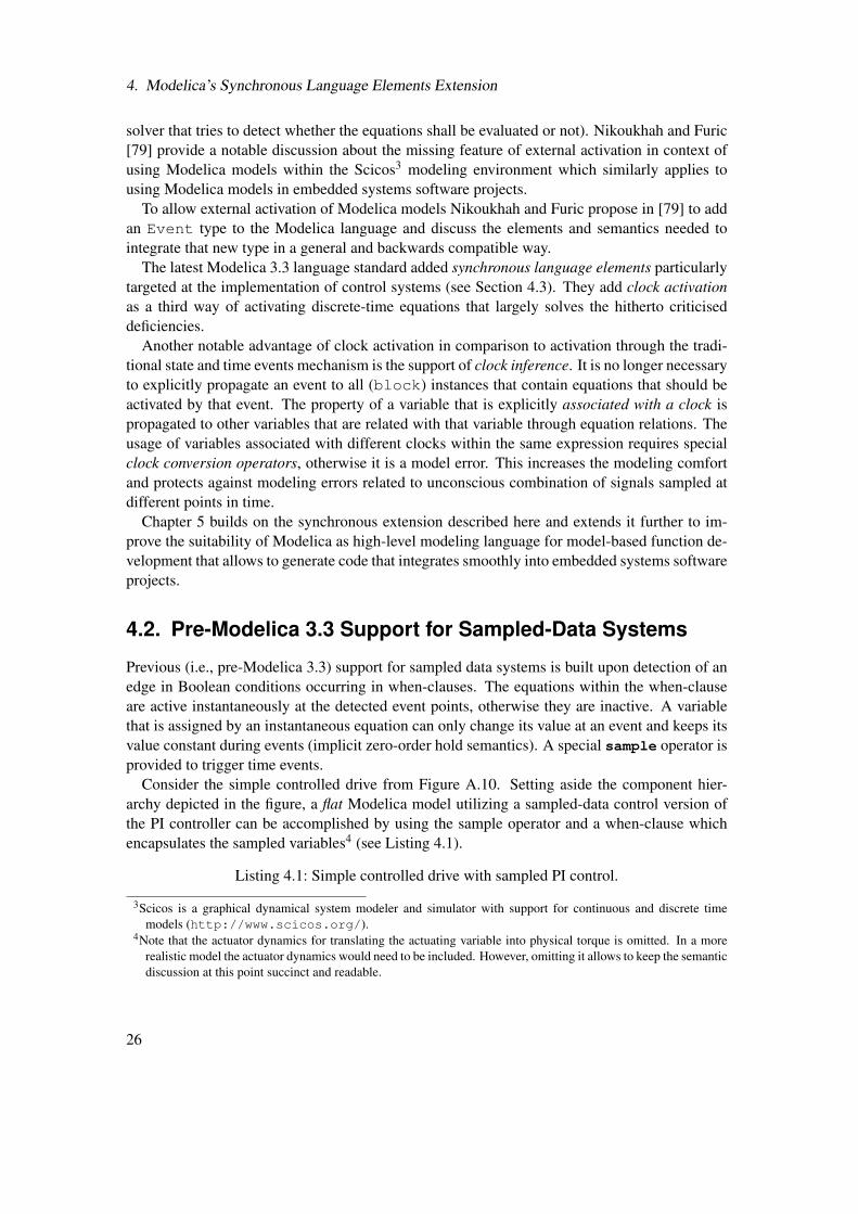
4. Modelica’s Synchronous Language Elements Extension

solver that tries to detect whether the equations shall be evaluated or not). Nikoukhah and Furic[79] provide a notable discussion about the missing feature of external activation in context ofusing Modelica models within the Scicos3 modeling environment which similarly applies tousing Modelica models in embedded systems software projects.

To allow external activation of Modelica models Nikoukhah and Furic propose in [79] to addan Event type to the Modelica language and discuss the elements and semantics needed tointegrate that new type in a general and backwards compatible way.

The latest Modelica 3.3 language standard added synchronous language elements particularlytargeted at the implementation of control systems (see Section 4.3). They add clock activationas a third way of activating discrete-time equations that largely solves the hitherto criticiseddeficiencies.

Another notable advantage of clock activation in comparison to activation through the tradi-tional state and time events mechanism is the support of clock inference. It is no longer necessaryto explicitly propagate an event to all (block) instances that contain equations that should beactivated by that event. The property of a variable that is explicitly associated with a clock ispropagated to other variables that are related with that variable through equation relations. Theusage of variables associated with different clocks within the same expression requires specialclock conversion operators, otherwise it is a model error. This increases the modeling comfortand protects against modeling errors related to unconscious combination of signals sampled atdifferent points in time.

Chapter 5 builds on the synchronous extension described here and extends it further to im-prove the suitability of Modelica as high-level modeling language for model-based function de-velopment that allows to generate code that integrates smoothly into embedded systems softwareprojects.

4.2. Pre-Modelica 3.3 Support for Sampled-Data Systems

Previous (i.e., pre-Modelica 3.3) support for sampled data systems is built upon detection of anedge in Boolean conditions occurring in when-clauses. The equations within the when-clauseare active instantaneously at the detected event points, otherwise they are inactive. A variablethat is assigned by an instantaneous equation can only change its value at an event and keeps itsvalue constant during events (implicit zero-order hold semantics). A special sample operator isprovided to trigger time events.

Consider the simple controlled drive from Figure A.10. Setting aside the component hier-archy depicted in the figure, a flat Modelica model utilizing a sampled-data control version ofthe PI controller can be accomplished by using the sample operator and a when-clause whichencapsulates the sampled variables4 (see Listing 4.1).

Listing 4.1: Simple controlled drive with sampled PI control.

3Scicos is a graphical dynamical system modeler and simulator with support for continuous and discrete timemodels (http://www.scicos.org/).

4Note that the actuator dynamics for translating the actuating variable into physical torque is omitted. In a morerealistic model the actuator dynamics would need to be included. However, omitting it allows to keep the semanticdiscussion at this point succinct and readable.

26

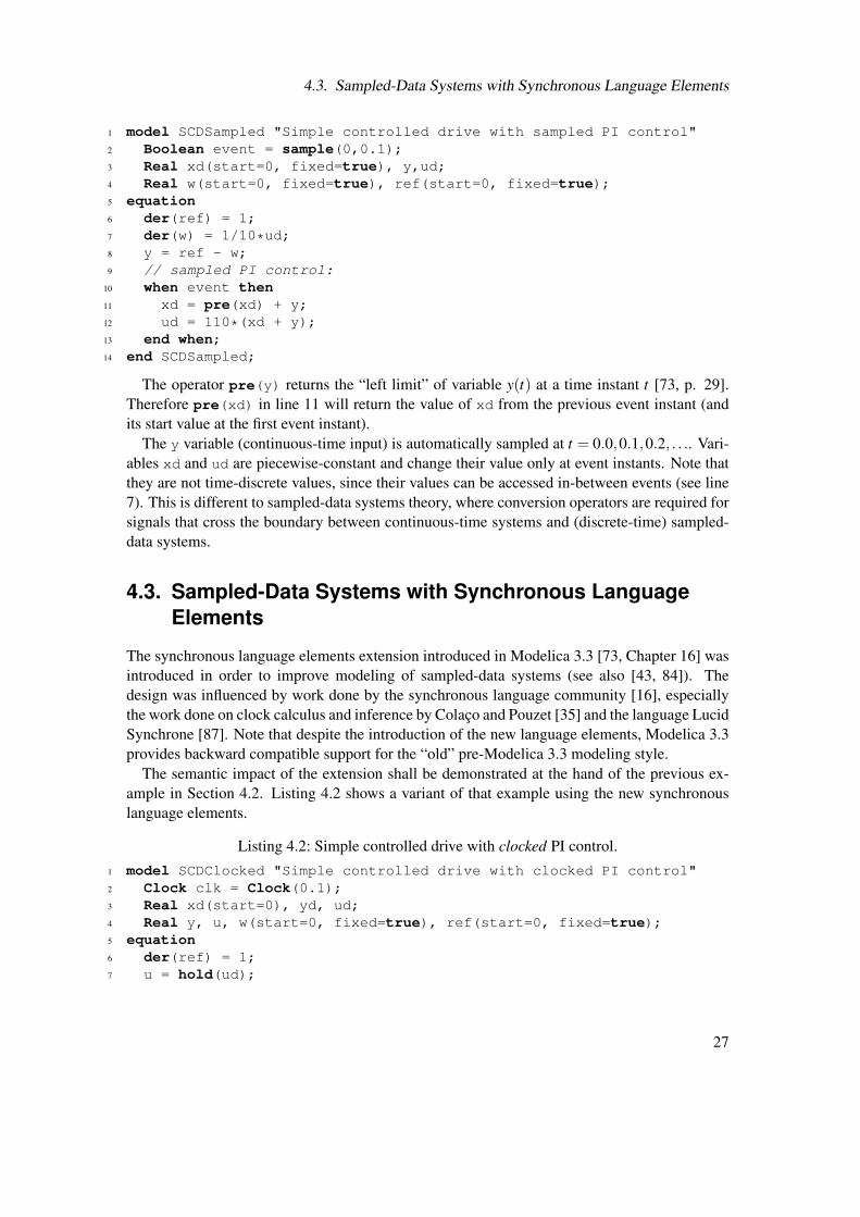
4.3. Sampled-Data Systems with Synchronous Language Elements

1 model SCDSampled "Simple controlled drive with sampled PI control"2 Boolean event = sample(0,0.1);3 Real xd(start=0, fixed=true), y,ud;4 Real w(start=0, fixed=true), ref(start=0, fixed=true);5 equation6 der(ref) = 1;7 der(w) = 1/10*ud;8 y = ref - w;9 // sampled PI control:

10 when event then11 xd = pre(xd) + y;12 ud = 110*(xd + y);13 end when;14 end SCDSampled;

The operator pre(y) returns the “left limit” of variable y(t) at a time instant t [73, p. 29].Therefore pre(xd) in line 11 will return the value of xd from the previous event instant (andits start value at the first event instant).

The y variable (continuous-time input) is automatically sampled at t = 0.0,0.1,0.2, . . .. Vari-ables xd and ud are piecewise-constant and change their value only at event instants. Note thatthey are not time-discrete values, since their values can be accessed in-between events (see line7). This is different to sampled-data systems theory, where conversion operators are required forsignals that cross the boundary between continuous-time systems and (discrete-time) sampled-data systems.

4.3. Sampled-Data Systems with Synchronous LanguageElements

The synchronous language elements extension introduced in Modelica 3.3 [73, Chapter 16] wasintroduced in order to improve modeling of sampled-data systems (see also [43, 84]). Thedesign was influenced by work done by the synchronous language community [16], especiallythe work done on clock calculus and inference by Colaço and Pouzet [35] and the language LucidSynchrone [87]. Note that despite the introduction of the new language elements, Modelica 3.3provides backward compatible support for the “old” pre-Modelica 3.3 modeling style.

The semantic impact of the extension shall be demonstrated at the hand of the previous ex-ample in Section 4.2. Listing 4.2 shows a variant of that example using the new synchronouslanguage elements.

Listing 4.2: Simple controlled drive with clocked PI control.1 model SCDClocked "Simple controlled drive with clocked PI control"2 Clock clk = Clock(0.1);3 Real xd(start=0), yd, ud;4 Real y, u, w(start=0, fixed=true), ref(start=0, fixed=true);5 equation6 der(ref) = 1;7 u = hold(ud);

27

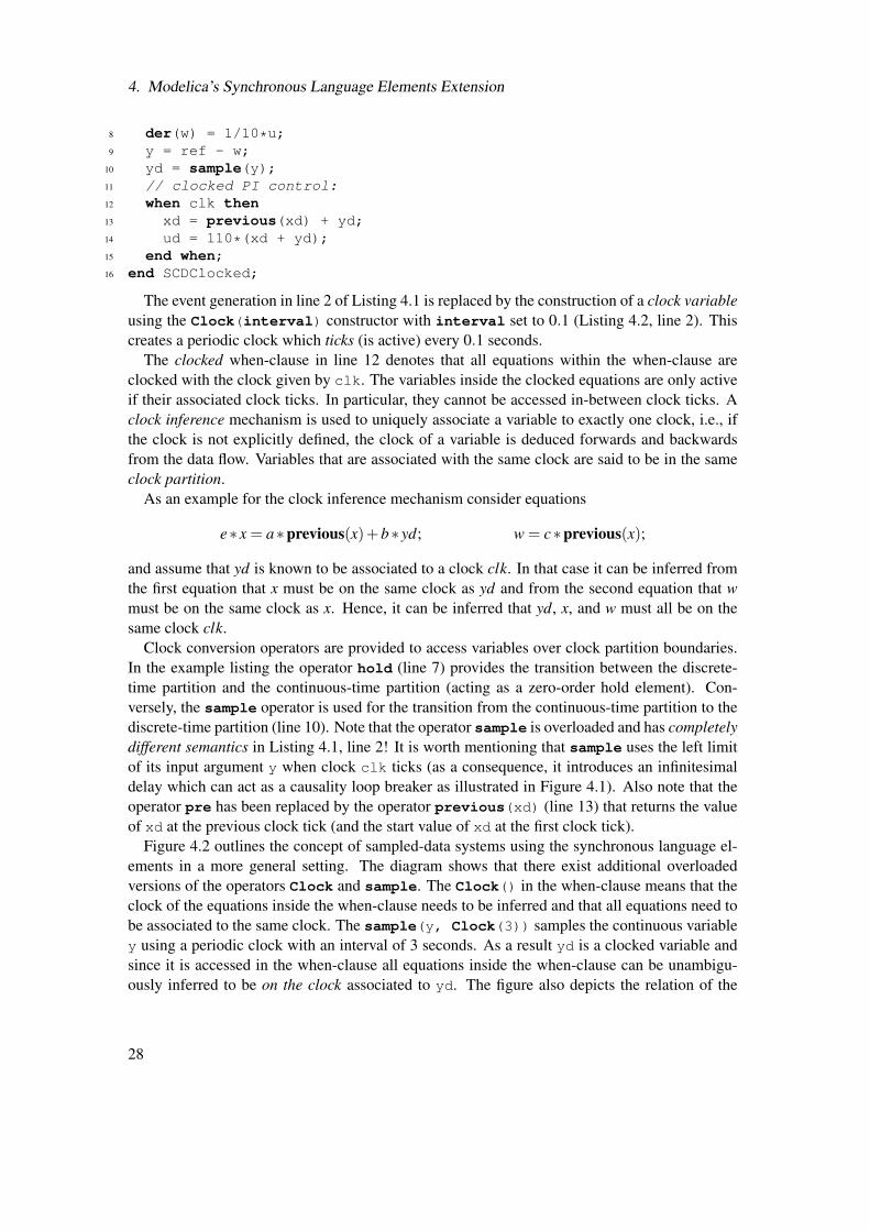
4. Modelica’s Synchronous Language Elements Extension

8 der(w) = 1/10*u;9 y = ref - w;

10 yd = sample(y);11 // clocked PI control:12 when clk then13 xd = previous(xd) + yd;14 ud = 110*(xd + yd);15 end when;16 end SCDClocked;

The event generation in line 2 of Listing 4.1 is replaced by the construction of a clock variableusing the Clock(interval) constructor with interval set to 0.1 (Listing 4.2, line 2). Thiscreates a periodic clock which ticks (is active) every 0.1 seconds.

The clocked when-clause in line 12 denotes that all equations within the when-clause areclocked with the clock given by clk. The variables inside the clocked equations are only activeif their associated clock ticks. In particular, they cannot be accessed in-between clock ticks. Aclock inference mechanism is used to uniquely associate a variable to exactly one clock, i.e., ifthe clock is not explicitly defined, the clock of a variable is deduced forwards and backwardsfrom the data flow. Variables that are associated with the same clock are said to be in the sameclock partition.

As an example for the clock inference mechanism consider equations

e∗ x = a∗previous(x)+b∗ yd; w = c∗previous(x);

and assume that yd is known to be associated to a clock clk. In that case it can be inferred fromthe first equation that x must be on the same clock as yd and from the second equation that wmust be on the same clock as x. Hence, it can be inferred that yd, x, and w must all be on thesame clock clk.

Clock conversion operators are provided to access variables over clock partition boundaries.In the example listing the operator hold (line 7) provides the transition between the discrete-time partition and the continuous-time partition (acting as a zero-order hold element). Con-versely, the sample operator is used for the transition from the continuous-time partition to thediscrete-time partition (line 10). Note that the operator sample is overloaded and has completelydifferent semantics in Listing 4.1, line 2! It is worth mentioning that sample uses the left limitof its input argument y when clock clk ticks (as a consequence, it introduces an infinitesimaldelay which can act as a causality loop breaker as illustrated in Figure 4.1). Also note that theoperator pre has been replaced by the operator previous(xd) (line 13) that returns the valueof xd at the previous clock tick (and the start value of xd at the first clock tick).

Figure 4.2 outlines the concept of sampled-data systems using the synchronous language el-ements in a more general setting. The diagram shows that there exist additional overloadedversions of the operators Clock and sample. The Clock() in the when-clause means that theclock of the equations inside the when-clause needs to be inferred and that all equations need tobe associated to the same clock. The sample(y, Clock(3)) samples the continuous variabley using a periodic clock with an interval of 3 seconds. As a result yd is a clocked variable andsince it is accessed in the when-clause all equations inside the when-clause can be unambigu-ously inferred to be on the clock associated to yd. The figure also depicts the relation of the

28

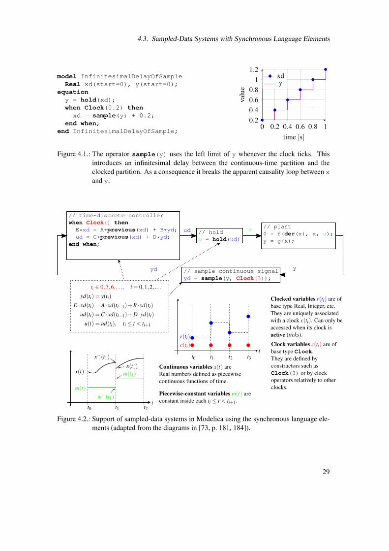
4.3. Sampled-Data Systems with Synchronous Language Elements

model InfinitesimalDelayOfSampleReal xd(start=0), y(start=0);

equationy = hold(xd);when Clock(0.2) then

xd = sample(y) + 0.2;end when;

end InfinitesimalDelayOfSample;0 0.2 0.4 0.6 0.8 1

0.20.40.60.8

11.2

time [s]

valu

e

xdy

Figure 4.1.: The operator sample(y) uses the left limit of y whenever the clock ticks. Thisintroduces an infinitesimal delay between the continuous-time partition and theclocked partition. As a consequence it breaks the apparent causality loop between xand y.

// time-discrete controllerwhen Clock() thenE*xd = A*previous(xd) + B*yd;ud = C*previous(xd) + D*yd;

end when;

// holdu = hold(ud)

ud u

t0t

r(ti)c(ti)

t1 t2 t3

Continuous variables x(t) areReal numbers defined as piecewisecontinuous functions of time.

Piecewise-constant variables m(t) areconstant inside each ti ≤ t < ti+1.t

t0 t1 t2

x(t)

x−(t1)

m(t)

x(t1)

m−(t1)

m(t1)

// plant0 = f(der(x), x, u);y = g(x);

// sample continuous signalyd = sample(y, Clock(3));

ti ∈ 0,3,6, . . ., i = 0,1,2, . . .

yd(ti) = y(ti)

E ·xd(ti) = A ·xd(ti−1)+B ·yd(ti)

ud(ti) =C ·xd(ti−1)+D ·yd(ti)

u(t) = ud(ti), ti ≤ t < ti+1

yyd

Clock variables c(ti) are ofbase type Clock.They are defined byconstructors such asClock(3) or by clockoperators relatively to otherclocks.

Clocked variables r(ti) are ofbase type Real, Integer, etc.They are uniquely associatedwith a clock c(ti). Can only beaccessed when its clock isactive (ticks).

Figure 4.2.: Support of sampled-data systems in Modelica using the synchronous language ele-ments (adapted from the diagrams in [73, p. 181, 184]).

29

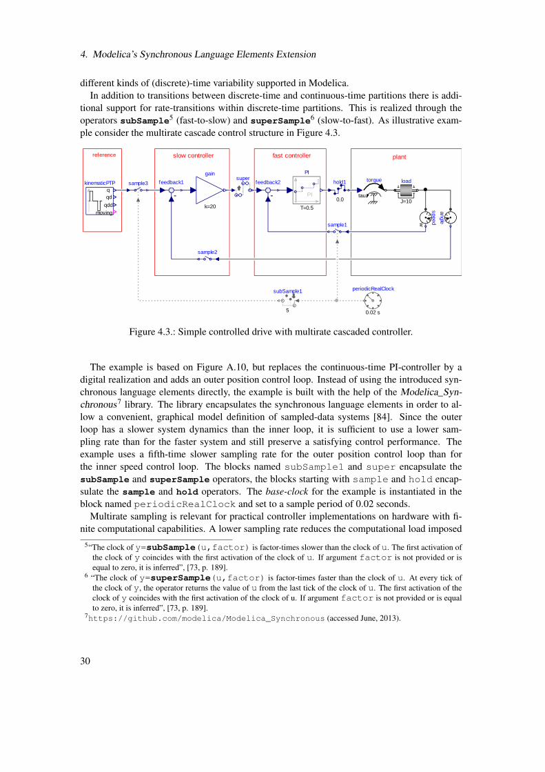
4. Modelica’s Synchronous Language Elements Extension

different kinds of (discrete)-time variability supported in Modelica.In addition to transitions between discrete-time and continuous-time partitions there is addi-

tional support for rate-transitions within discrete-time partitions. This is realized through theoperators subSample5 (fast-to-slow) and superSample6 (slow-to-fast). As illustrative exam-ple consider the multirate cascade control structure in Figure 4.3.

fast controller plantreference slow controller

load

J=10

speedw

PI

PI

T=0.5

-

feedback2 torque

tau

angle

kinematicPTPqqd

qdd

moving

-

feedback1

k=20

gain

sample1

sample2

0.0

hold1sample3super

subSample1

5

periodicRealClock

0.02 s

Figure 4.3.: Simple controlled drive with multirate cascaded controller.

The example is based on Figure A.10, but replaces the continuous-time PI-controller by adigital realization and adds an outer position control loop. Instead of using the introduced syn-chronous language elements directly, the example is built with the help of the Modelica_Syn-chronous7 library. The library encapsulates the synchronous language elements in order to al-low a convenient, graphical model definition of sampled-data systems [84]. Since the outerloop has a slower system dynamics than the inner loop, it is sufficient to use a lower sam-pling rate than for the faster system and still preserve a satisfying control performance. Theexample uses a fifth-time slower sampling rate for the outer position control loop than forthe inner speed control loop. The blocks named subSample1 and super encapsulate thesubSample and superSample operators, the blocks starting with sample and hold encap-sulate the sample and hold operators. The base-clock for the example is instantiated in theblock named periodicRealClock and set to a sample period of 0.02 seconds.

Multirate sampling is relevant for practical controller implementations on hardware with fi-nite computational capabilities. A lower sampling rate reduces the computational load imposed

5“The clock of y=subSample(u,factor) is factor-times slower than the clock of u. The first activation ofthe clock of y coincides with the first activation of the clock of u. If argument factor is not provided or isequal to zero, it is inferred”, [73, p. 189].

6 “The clock of y=superSample(u,factor) is factor-times faster than the clock of u. At every tick ofthe clock of y, the operator returns the value of u from the last tick of the clock of u. The first activation of theclock of y coincides with the first activation of the clock of u. If argument factor is not provided or is equalto zero, it is inferred”, [73, p. 189].

7https://github.com/modelica/Modelica_Synchronous (accessed June, 2013).

30

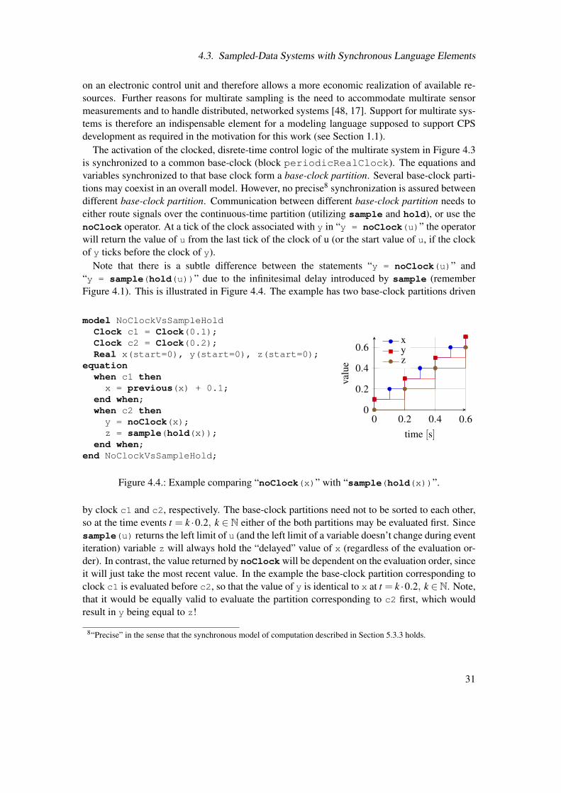
4.3. Sampled-Data Systems with Synchronous Language Elements

on an electronic control unit and therefore allows a more economic realization of available re-sources. Further reasons for multirate sampling is the need to accommodate multirate sensormeasurements and to handle distributed, networked systems [48, 17]. Support for multirate sys-tems is therefore an indispensable element for a modeling language supposed to support CPSdevelopment as required in the motivation for this work (see Section 1.1).

The activation of the clocked, disrete-time control logic of the multirate system in Figure 4.3is synchronized to a common base-clock (block periodicRealClock). The equations andvariables synchronized to that base clock form a base-clock partition. Several base-clock parti-tions may coexist in an overall model. However, no precise8 synchronization is assured betweendifferent base-clock partition. Communication between different base-clock partition needs toeither route signals over the continuous-time partition (utilizing sample and hold), or use thenoClock operator. At a tick of the clock associated with y in “y = noClock(u)” the operatorwill return the value of u from the last tick of the clock of u (or the start value of u, if the clockof y ticks before the clock of y).

Note that there is a subtle difference between the statements “y = noClock(u)” and“y = sample(hold(u))” due to the infinitesimal delay introduced by sample (rememberFigure 4.1). This is illustrated in Figure 4.4. The example has two base-clock partitions driven

model NoClockVsSampleHoldClock c1 = Clock(0.1);Clock c2 = Clock(0.2);Real x(start=0), y(start=0), z(start=0);

equationwhen c1 then

x = previous(x) + 0.1;end when;when c2 then

y = noClock(x);z = sample(hold(x));

end when;end NoClockVsSampleHold;

0 0.2 0.4 0.60

0.2

0.4

0.6

time [s]

valu

exyz

Figure 4.4.: Example comparing “noClock(x)” with “sample(hold(x))”.

by clock c1 and c2, respectively. The base-clock partitions need not to be sorted to each other,so at the time events t = k ·0.2, k ∈ N either of the both partitions may be evaluated first. Sincesample(u) returns the left limit of u (and the left limit of a variable doesn’t change during eventiteration) variable z will always hold the “delayed” value of x (regardless of the evaluation or-der). In contrast, the value returned by noClock will be dependent on the evaluation order, sinceit will just take the most recent value. In the example the base-clock partition corresponding toclock c1 is evaluated before c2, so that the value of y is identical to x at t = k ·0.2, k ∈N. Note,that it would be equally valid to evaluate the partition corresponding to c2 first, which wouldresult in y being equal to z!

8“Precise” in the sense that the synchronous model of computation described in Section 5.3.3 holds.

31

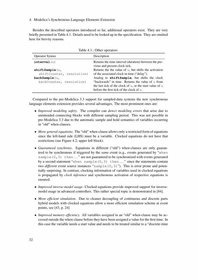
4. Modelica’s Synchronous Language Elements Extension

Besides the described operators introduced so far, additional operators exist. They are verybriefly presented in Table 4.1. Details need to be looked up in the specification. They are omittedhere for brevity reasons.

Table 4.1.: Other operators

Operator Syntax Description

interval(u) Returns the time interval (duration) between the pre-vious and present clock tick.

shiftSample(u,shiftCounter, resolution)

Returns the the value of u, but shifts the activationof the associated clock in time (“delay”).

backSample(u,backCounter, resolution)

Analog to shiftSample, but shifts the clock“backwards” in time. Returns the value of u fromthe last tick of the clock of u, or the start value of ubefore the first tick of the clock of u.

Compared to the pre-Modelica 3.3 support for sampled-data systems the new synchronouslanguage elements extension provides several advantages. The most prominent ones are:

• Improved modeling safety. The compiler can detect modeling errors that arise due tounintended connecting blocks with different sampling period. This was not possible inpre-Modelica 3.3 due to the automatic sample and hold semantics of variables occurringin “old” when-clauses.

• More general equations. The “old” when-clause allows only a restricted form of equationssince the left-hand side (LHS) must be a variable. Clocked equations do not have thatrestrictions (see Figure 4.2, upper left block).

• Guaranteed synchrony. Equations in different (“old”) when-clauses are only guaran-teed to be synchronous if triggered by the same event (e.g., events generated by “whensample(0,3) then . . . ” are not guaranteed to be synchronized with events generatedby a second statement “when sample(0,3) then . . . ” since the statements containtwo different event source instances “sample(0,3)”). This is error prone and poten-tially surprising. In contrast, clocking information of variables used in clocked equationsis propagated by clock inference and synchronous activation of respective equations isensured.

• Improved inverse-model usage. Clocked equations provide improved support for inverse-model usage in advanced controllers. This rather special topic is demonstrated in [84].

• More efficient simulation. Due to cleaner decoupling of continuous and discrete partshybrid models with clocked equations allow a more efficient simulation scheme at eventpoints, see [43, p. 24]

• Improved memory efficiency. All variables assigned in an “old” when-clause may be ac-cessed outside the when-clause before they have been assigned a value for the first time. Inthis case the variable needs a start value and needs to be treated similar to a “discrete-time

32

4.4. Notes to the Development of the Synchronous Extension

state” variable. It is difficult for a compiler to deduce whether this situation applies, sothat in practice usually all such variables are treated similar to “discrete-time state” vari-ables, although in reality only a subset of them actually needs an initial state [43, p. 24].This isn’t the case for clocked variables, so that clocked variables can be handled morememory efficient.

• Simplified initialization. The initialization of a (hybrid) Modelica model is usually aglobal system-level issue involving many intricacies which require considerable expertknowledge to fully understand9. For improved comprehensibility, the initialization rulesfor clocked partitions follows a simplified scheme that is independent from global systemlevel aspects (see [73, p. 197]).

4.4. Notes to the Development of the Synchronous Extension

The development of the synchronous language elements extension to Modelica started at theend of 2010 and was initiated and decisively driven by Hilding Elmqvist (see fundamental paper[43]), though a larger group of people contributed to the discussion, development and testing.

During the discussion phase the author of this thesis emphasized that the synchronous exten-sion should not only consider periodic activation of sampled data systems, but also providemeans to allow aperiodic activation of sampled data systems during hybrid simulation (i.e.,combined simulation of synchronous (discrete-time) and physical (continuous-time) model). Awell-known practical example for aperiodic activation of (control) data-systems is a moderncombustion engine management system in which fuel injection and spark ignition is synchro-nized with the engine crankshaft position. This significantly contributed to the introduction ofthe boolean clock constructor which allows to drive clock activation by events generated by acontinuous-time expression of type Boolean. Its definition is

clock(condition, startInterval)

where condition is the event condition and startInterval is the value returned by theoperator interval() at the first clock tick. A simple usage example is given below.

Clock clk = Clock(angle > 0.2, 0.1);

Also, using the synchronous language elements for modeling at the textual level seems tohave a rather steep learning curve and easily leads to models that can hardly be understood.This triggered the development of the MODELICA_SYNCHRONOUS library that had the aim toprovide a more usable interface to the new synchronous language extension [84]. For an examplesee Figure 4.3. This library in which I did essential conceptual and development work is now acandidate to become an official part of the Modelica Standard Library.

9Beside the relevant parts in the Modelica specification, e.g., [73, p. 90ff], Lennart and Bachmann [82] provide acomprehensive description of the initialization process.

33

5. Enabling Modelica for FunctionDevelopment — ACG-Modelica

This chapter is an extensively revised and extended version of Section 4 of the publication

Bernhard Thiele, Stefan-Alexander Schneider, and Pierre R. Mai. A Modelica Sub-and Superset for Safety-Relevant Control Applications. In 9th Int. Modelica Confer-ence, Munich, Germany, September 2012. http://dx.doi.org/10.3384/ecp12076455.

5.1. Motivation

The aim of this chapter is to propose extensions and restrictions to the Modelica language thatimprove the suitability of Modelica as high-level modeling language for safety-related, model-based function development.

To achieve this, the impact of a safety-relevant development process (relying on validatedtools) to high-level, domain-oriented modeling languages will be investigated. Based on thisanalysis I introduce a sub- and superset of Modelica that is simple in order to facilitate high as-surance designs, yet expressive enough to allow modeling of many control strategies of practicalrelevance. This sub- and superset is in the following referred to as ACG-Modelica.

A practical control example illustrates the use of the proposed language elements in a servosystem model presented in Chapter 6.

5.1.1. Language Complexity

For both the validation of the input language and the transformation process, one has to copewith the curse of complexity. It is therefore of crucial importance to keep the language of thecode generator models as simple and well-defined as possible, especially with regards to thenumber and complexity of basic constructs in the language, while also minimizing the numberand complexity of performed transformation rules in the code generation process. This is es-pecially true of transformation rules stemming from optimization rules. On the other hand thelanguage so defined still has to be suitable for human consumption, so that the complexities ofthe code generation process are not just offloaded to the programmer.

When discussing the use of Modelica in the context of control application, advanced controlconcepts based on inverted plant dynamics are often described [111], [112], [29]. Some Model-ica tools are capable of automatically synthesising such controllers and generate code for them.This usually requires fairly sophisticated symbolic manipulation capabilities by the tool. For

35

5. Enabling Modelica for Function Development — ACG-Modelica

example, it may require to differentiate a subset of the equations, select appropriate states andsolve the resulting system of differential and algebraic equations numerically.

However, the intrinsic complexity in the resulting control algorithms imposes an additionalburden if the topmost design goal is in providing high assurance control systems. Therefore theconsiderations that guide the design of ACG-Modelica are:

• Design trade-off is biased to prefer high assurance control over high performance controlsystems.

• Use of language restriction as primary means to keep the complexity of the language aslow as possible.

• Careful language extensions where deemed necessary to satisfy typical requirements ex-pressed by developers of embedded control systems.

• Modifications to established Modelica simulation tools in order to support simulation ofACG-Modelica models should be kept as small as possible (note that production code-generation from models may differ significantly from simulation of models as describedin Section 5.2.2).

• The requirements specified in Chapter 3 need to be covered.

5.1.2. Terminology

The following list defines some key terms used subsequently.

Basic Blocks Blocks that have no inner instance of other blocks are subsequently referred toas basic blocks. These blocks may only contain parameters, connectors, auxiliary vari-ables, and (textual) equations.

Composite Blocks Blocks that are (graphically) composed from other blocks are subse-quently referred to as composite blocks. These blocks may only be composed from otherblocks connected by connect(..,..) equations. Therefore they do not contain anyother textual equations.

Clocks Clocks provide an activation signal or clock signal used for synchronous schedulingof a set of equations activated by that clock signal. They recently entered the Modelicalanguage standard (see Section 4).

Clock Blocks Special basic blocks containing clocks that provide a clock signal are subse-quently referred to as clock blocks.

Atomic Blocks Blocks which are executed as a single unit (akin to a function call with inputand output arguments) are referred to as atomic blocks.

36

5.2. System Compilation: From Function Model to Target Binary

5.2. System Compilation: From Function Model to TargetBinary

Section 2.3 briefly reviewed a typical model-based development process and outlined the struc-ture of a corresponding toolchain in Figure 2.2.

Starting from the code generation model the generation of the executable binary from themodel is mainly based on two development tools: the code generator and the cross compiler(including the cross linker). From an abstract point of view, the concatenation of these twocompilers is again a (system) compiler, and can be treated by the same theory as a compiler thatwould translate directly from the code generation model to the executable code. In the following,all such translation tools will be denoted abstractly as development tools.

In order to be usable in (safety-relevant) industry applications a development process and itsassociated development tools need to satisfy the requirements formulated in Chapter 3. Typ-ically, this places constraints on the characteristics of suitable code generation model and thecorresponding development tool. Figure 5.1 illustrates the system compilation process. Notethat the input to the system compiler, the code generation model, has been constrained to a sub-and superset of the Modelica language (i.e., ACG-Modelica). This is in order to allow satisfyingrequirements from Chapter 3 and will be explained in more detail later.

The generated C-code can be seen as intermediate representation of the model, because itis both output of the code generator as well as input to the cross compiler for the target. Thisperspective of the development tool is of central significance, because there is no need to performany qualification activities on such internal representations as long as the C-code is only usedas input to the cross compiler and is not further manipulated or used in any other activities thatneed to rely on the readability of the C-code. As a consequence, no C-code reviews are neededin this case. This approach opens up the possibility to perform reviews on the model level. Amain topic of this thesis is addressing the conditions that need to be established to allow suchmodel level reviews.

Development tools may inject systematic faults into the executable program. Increasing thefunctional safety in this context means to minimize erroneous outputs of the development toolsdue to malfunctions and/or reliably detecting those erroneous outputs when they occur. This willbe discussed in the next section.

5.2.1. Tool Qualification

As noted in Section 2.5, the development of safety-relevant software needs to typically complyto rules described in functional safety standards (Section 2.5.2). This also affects the used devel-opment tools. A development tool may need to fulfil a certain level of qualification dependingon the severity of the impact a malfunctioning in the development tool is expected to have ona safety-related item. For example, in the automotive domain the ISO 26262 [60, Section 11Qualification of software tools]) establishes a set of recommendations concerning the neededqualifications of such software tools.

In order to increase the confidence in the toolchain depicted in Figure 5.1 it is, in principle,possible to apply a number of techniques that have been proposed for ensuring safety of compil-ers. The survey of Frank et al. [45] gives an overview of existing techniques and also comments

37

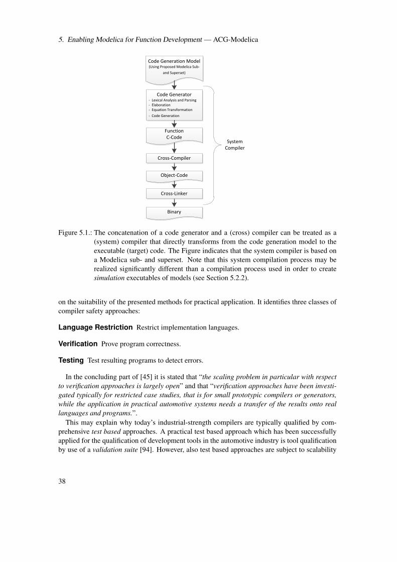
5. Enabling Modelica for Function Development — ACG-Modelica

Code Generation Model (Using Proposed Modelica Sub-

and Superset)

FunctionC-Code

Object-Code

Binary

Code Generator- Lexical Analysis and Parsing- Elaboration- Equation Transformation

- Code Generation

Cross-Compiler

Cross-Linker

System Compiler

Figure 5.1.: The concatenation of a code generator and a (cross) compiler can be treated as a(system) compiler that directly transforms from the code generation model to theexecutable (target) code. The Figure indicates that the system compiler is based ona Modelica sub- and superset. Note that this system compilation process may berealized significantly different than a compilation process used in order to createsimulation executables of models (see Section 5.2.2).

on the suitability of the presented methods for practical application. It identifies three classes ofcompiler safety approaches:

Language Restriction Restrict implementation languages.

Verification Prove program correctness.

Testing Test resulting programs to detect errors.

In the concluding part of [45] it is stated that “the scaling problem in particular with respectto verification approaches is largely open” and that “verification approaches have been investi-gated typically for restricted case studies, that is for small prototypic compilers or generators,while the application in practical automotive systems needs a transfer of the results onto reallanguages and programs.”.

This may explain why today’s industrial-strength compilers are typically qualified by com-prehensive test based approaches. A practical test based approach which has been successfullyapplied for the qualification of development tools in the automotive industry is tool qualificationby use of a validation suite [94]. However, also test based approaches are subject to scalability

38

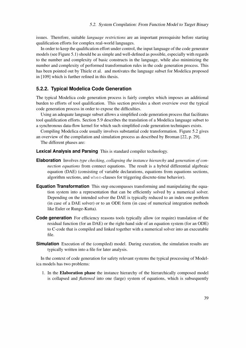
5.2. System Compilation: From Function Model to Target Binary

issues. Therefore, suitable language restrictions are an important prerequisite before startingqualification efforts for complex real-world languages.

In order to keep the qualification effort under control, the input language of the code generatormodels (see Figure 5.1) should be as simple and well-defined as possible, especially with regardsto the number and complexity of basic constructs in the language, while also minimizing thenumber and complexity of performed transformation rules in the code generation process. Thishas been pointed out by Thiele et al. and motivates the language subset for Modelica proposedin [109] which is further refined in this thesis.

5.2.2. Typical Modelica Code Generation

The typical Modelica code generation process is fairly complex which imposes an additionalburden to efforts of tool qualification. This section provides a short overview over the typicalcode generation process in order to expose the difficulties.

Using an adequate language subset allows a simplified code generation process that facilitatestool qualification efforts. Section 5.9 describes the translation of a Modelica language subset toa synchronous data-flow kernel for which such simplified code generation techniques exists.

Compiling Modelica code usually involves substantial code transformation. Figure 5.2 givesan overview of the compilation and simulation process as described by Broman [22, p. 29].

The different phases are:

Lexical Analysis and Parsing This is standard compiler technology.

Elaboration Involves type checking, collapsing the instance hierarchy and generation of con-nection equations from connect equations. The result is a hybrid differential algebraicequation (DAE) (consisting of variable declarations, equations from equations sections,algorithm sections, and when-clauses for triggering discrete-time behavior).

Equation Transformation This step encompasses transforming and manipulating the equa-tion system into a representation that can be efficiently solved by a numerical solver.Depending on the intended solver the DAE is typically reduced to an index one problem(in case of a DAE solver) or to an ODE form (in case of numerical integration methodslike Euler or Runge-Kutta).

Code generation For efficiency reasons tools typically allow (or require) translation of theresidual function (for an DAE) or the right-hand side of an equation system (for an ODE)to C-code that is compiled and linked together with a numerical solver into an executablefile.

Simulation Execution of the (compiled) model. During execution, the simulation results aretypically written into a file for later analysis.

In the context of code generation for safety relevant systems the typical processing of Model-ica models has two problems:

1. In the Elaboration phase the instance hierarchy of the hierarchically composed modelis collapsed and flattened into one (large) system of equations, which is subsequently

39

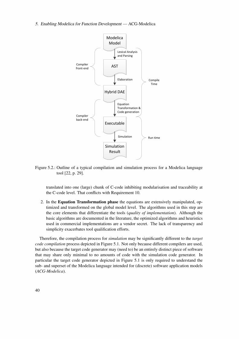
5. Enabling Modelica for Function Development — ACG-Modelica

Modelica Model

AST

Lexical Analysis and Parsing

Hybrid DAE

Elaboration

Executable

Simulation Result

Equation Transformation & Code generation

Simulation

Compile Time

Run time

Compiler front-end

Compiler back-end

Figure 5.2.: Outline of a typical compilation and simulation process for a Modelica languagetool [22, p. 29].

translated into one (large) chunk of C-code inhibiting modularisation and traceability atthe C-code level. That conflicts with Requirement 10.

2. In the Equation Transformation phase the equations are extensively manipulated, op-timized and transformed on the global model level. The algorithms used in this step arethe core elements that differentiate the tools (quality of implementation). Although thebasic algorithms are documented in the literature, the optimized algorithms and heuristicsused in commercial implementations are a vendor secret. The lack of transparency andsimplicity exacerbates tool qualification efforts.

Therefore, the compilation process for simulation may be significantly different to the targetcode compilation process depicted in Figure 5.1. Not only because different compilers are used,but also because the target code generator may (need to) be an entirely distinct piece of softwarethat may share only minimal to no amounts of code with the simulation code generator. Inparticular the target code generator depicted in Figure 5.1 is only required to understand thesub- and superset of the Modelica language intended for (discrete) software application models(ACG-Modelica).

40

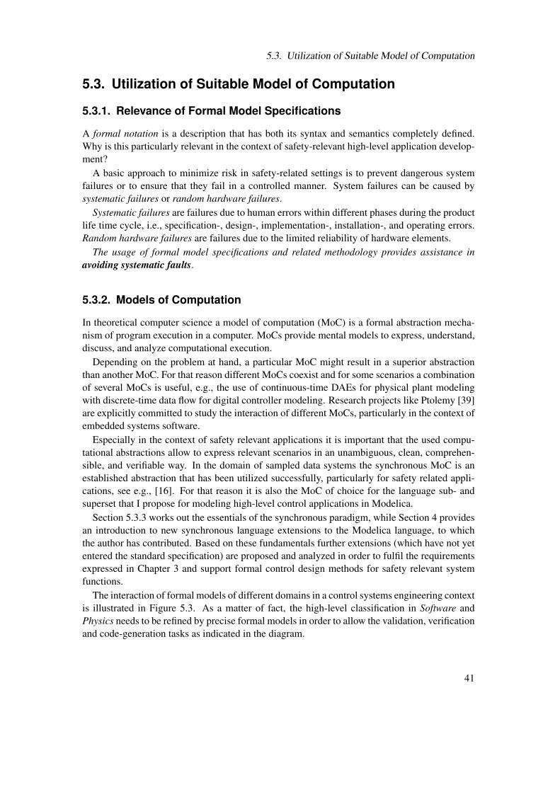
5.3. Utilization of Suitable Model of Computation

5.3. Utilization of Suitable Model of Computation

5.3.1. Relevance of Formal Model Specifications

A formal notation is a description that has both its syntax and semantics completely defined.Why is this particularly relevant in the context of safety-relevant high-level application develop-ment?

A basic approach to minimize risk in safety-related settings is to prevent dangerous systemfailures or to ensure that they fail in a controlled manner. System failures can be caused bysystematic failures or random hardware failures.

Systematic failures are failures due to human errors within different phases during the productlife time cycle, i.e., specification-, design-, implementation-, installation-, and operating errors.Random hardware failures are failures due to the limited reliability of hardware elements.

The usage of formal model specifications and related methodology provides assistance inavoiding systematic faults.

5.3.2. Models of Computation

In theoretical computer science a model of computation (MoC) is a formal abstraction mecha-nism of program execution in a computer. MoCs provide mental models to express, understand,discuss, and analyze computational execution.

Depending on the problem at hand, a particular MoC might result in a superior abstractionthan another MoC. For that reason different MoCs coexist and for some scenarios a combinationof several MoCs is useful, e.g., the use of continuous-time DAEs for physical plant modelingwith discrete-time data flow for digital controller modeling. Research projects like Ptolemy [39]are explicitly committed to study the interaction of different MoCs, particularly in the context ofembedded systems software.

Especially in the context of safety relevant applications it is important that the used compu-tational abstractions allow to express relevant scenarios in an unambiguous, clean, comprehen-sible, and verifiable way. In the domain of sampled data systems the synchronous MoC is anestablished abstraction that has been utilized successfully, particularly for safety related appli-cations, see e.g., [16]. For that reason it is also the MoC of choice for the language sub- andsuperset that I propose for modeling high-level control applications in Modelica.

Section 5.3.3 works out the essentials of the synchronous paradigm, while Section 4 providesan introduction to new synchronous language extensions to the Modelica language, to whichthe author has contributed. Based on these fundamentals further extensions (which have not yetentered the standard specification) are proposed and analyzed in order to fulfil the requirementsexpressed in Chapter 3 and support formal control design methods for safety relevant systemfunctions.

The interaction of formal models of different domains in a control systems engineering contextis illustrated in Figure 5.3. As a matter of fact, the high-level classification in Software andPhysics needs to be refined by precise formal models in order to allow the validation, verificationand code-generation tasks as indicated in the diagram.

41

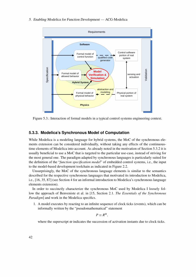
5. Enabling Modelica for Function Development — ACG-Modelica

Physical portion of

real system

Control software

portion of real

system

abstraction and

modeling

qualified code

generator

sensing and

actuation

Requirements

Va

lida

tio

n

Formal model of

physical behavior

Formal model of

allowed behavior

Formal model of

control function

Sp

ecific

atio

n

Model

Verification &

Simulation

Hybrid System

Physics

Software

Figure 5.3.: Interaction of formal models in a typical control systems engineering context.

5.3.3. Modelica’s Synchronous Model of Computation

While Modelica is a modeling language for hybrid systems, the MoC of the synchronous ele-ments extension can be considered individually, without taking any effects of the continuous-time elements of Modelica into account. As already noted in the motivation of Section 5.3.2 it isusually beneficial to use a MoC that is targeted to the particular use-case, instead of striving forthe most general one. The paradigm adapted by synchronous languages is particularly suited forthe definition of the “function specification model” of embedded control systems, i.e., the inputto the model-based development toolchain as indicated in Figure 2.2.

Unsurprisingly, the MoC of the synchronous language elements is similar to the semanticsdescribed for the respective synchronous languages that motivated its introduction to Modelica,i.e., [16, 35, 87] (see Section 4 for an informal introduction to Modelica’s synchronous languageelements extension).

In order to succinctly characterize the synchronous MoC used by Modelica I loosely fol-low the approach of Benveniste et al. in [15, Section 2.1. The Essentials of the SynchronousParadigm] and work in the Modelica specifics.

1. A model executes by reacting to an infinite sequence of clock ticks (events), which can beinformally written by the “pseudomathematical” statement

P≡ Rω ,

where the superscript ω indicates the succession of activation instants due to clock ticks.

42

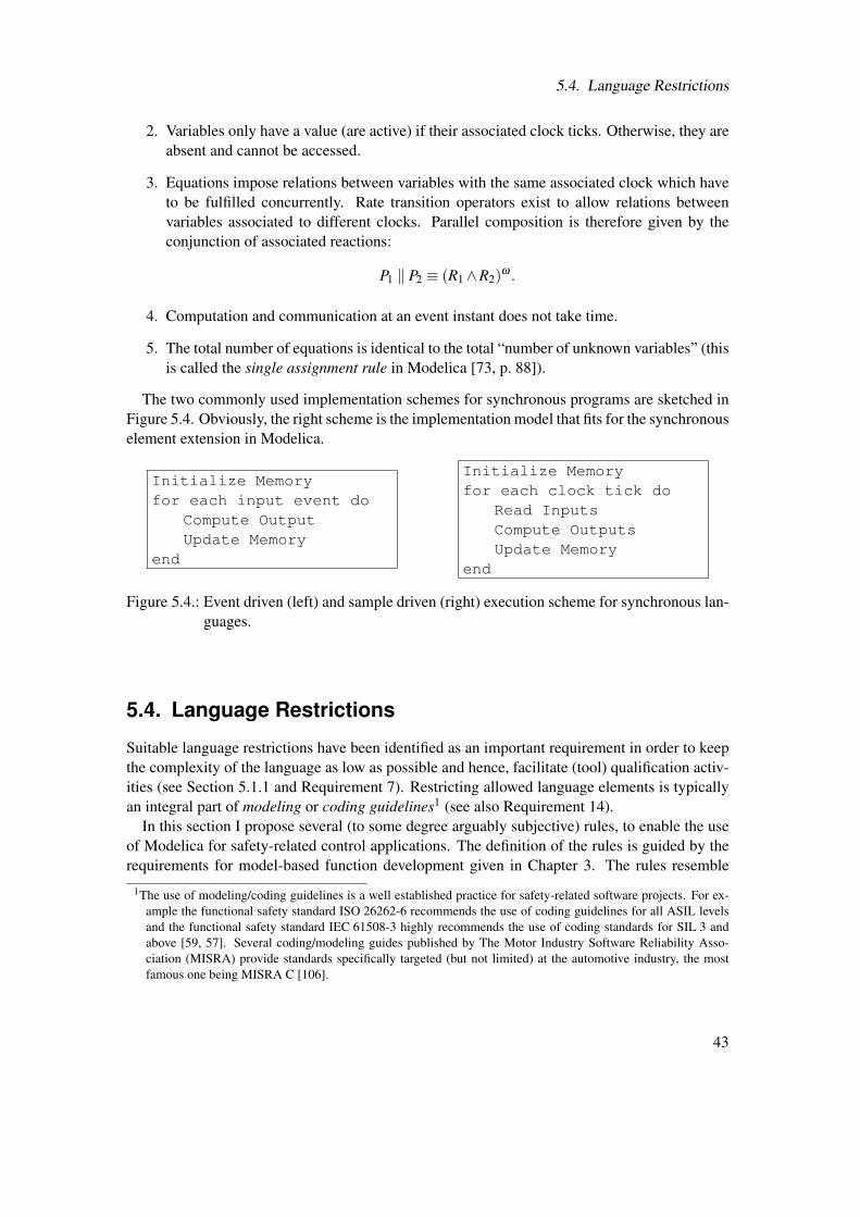
5.4. Language Restrictions

2. Variables only have a value (are active) if their associated clock ticks. Otherwise, they areabsent and cannot be accessed.

3. Equations impose relations between variables with the same associated clock which haveto be fulfilled concurrently. Rate transition operators exist to allow relations betweenvariables associated to different clocks. Parallel composition is therefore given by theconjunction of associated reactions:

P1 ‖ P2 ≡ (R1∧R2)ω .

4. Computation and communication at an event instant does not take time.

5. The total number of equations is identical to the total “number of unknown variables” (thisis called the single assignment rule in Modelica [73, p. 88]).

The two commonly used implementation schemes for synchronous programs are sketched inFigure 5.4. Obviously, the right scheme is the implementation model that fits for the synchronouselement extension in Modelica.

Initialize Memoryfor each input event do

Compute OutputUpdate Memory

end

Initialize Memoryfor each clock tick do

Read InputsCompute OutputsUpdate Memory

end

Figure 5.4.: Event driven (left) and sample driven (right) execution scheme for synchronous lan-guages.

5.4. Language Restrictions

Suitable language restrictions have been identified as an important requirement in order to keepthe complexity of the language as low as possible and hence, facilitate (tool) qualification activ-ities (see Section 5.1.1 and Requirement 7). Restricting allowed language elements is typicallyan integral part of modeling or coding guidelines1 (see also Requirement 14).

In this section I propose several (to some degree arguably subjective) rules, to enable the useof Modelica for safety-related control applications. The definition of the rules is guided by therequirements for model-based function development given in Chapter 3. The rules resemble

1The use of modeling/coding guidelines is a well established practice for safety-related software projects. For ex-ample the functional safety standard ISO 26262-6 recommends the use of coding guidelines for all ASIL levelsand the functional safety standard IEC 61508-3 highly recommends the use of coding standards for SIL 3 andabove [59, 57]. Several coding/modeling guides published by The Motor Industry Software Reliability Asso-ciation (MISRA) provide standards specifically targeted (but not limited) at the automotive industry, the mostfamous one being MISRA C [106].

43

5. Enabling Modelica for Function Development — ACG-Modelica

modeling guidelines, however for the following reasons they are not equivalent to the modelingguidelines referred to in Requirement 14:

• Section 5.4.1 is primarily focused on defining a language subset of Modelica that isdeemed suitable to be used for safety-related function development and is not particularlyconcerned with how such an “approved” language is then used by developers!

• Section 5.4.2 provides additional rules for the graphical representation that are intendedto enable a potentially more efficient development and review process by allowing de-velopers and reviewers to work (mostly) at the graphical level. For that reason, it doesalso contain some “core” rules for graphical level modeling that are targeted at develop-ers. However, these core rules would need to be extended (amongst others, consideringproject and toolchain specific characteristics) in order to produce sufficiently detailed andcomplete modeling guidelines in the sense of Requirement 14.

Note that to meet the requirements defined in Chapter 3 it is not sufficient to solely restrictthe language elements to a subset of the current Modelica 3.3 standard specification. In additionit is necessary to introduce a few language extensions. Proposals for respective extensions arepresented in Sections 5.5, 5.6, 5.7, and 5.8. The following rule definitions assume that theselanguage extensions are available.

The rules restrict the allowed language elements, and hence define a language subset. Theyare presented in conjunction with a clear Rationale for the rule and a Trace information thatreferences the particular requirements that motivated the definition of the rule.

5.4.1. Modeling Language Rules

This section is the counterpart to the modeling language requirements presented in Section 3.2.It has the aim to propose a set of rules that impose restrictions on the (textual) language level inorder to ensure that Modelica meets the previously formulated requirements.

Rule 1 - Clocked Variables Exclusivity. Occurring variables and equations must be part of(discrete-time) clocked partitions. Note that this restriction implies that all allowed high-levelapplications have a purely time-discrete nature.Rationale: Clocked variables and equations were introduced in Modelica 3.3 to provide im-proved support for implementation of (discrete-time) control systems. See Section 4.3 for de-tails.Trace: Requirement 2, 3, 5, 7, 8 and 9.

Rule 2 - Causal Data-Flow Exclusivity. (1) Equations shall be restricted to a form where asingle variable (the unknown of that equation) is at the left-hand side and a flow expression isat the right-hand side, e.g., assume a is the unknown, then a = b ·c is valid while a+ b = 0 ora2 = b is invalid. (2) The data-flow between input and output connectors must be directed fromthe input connector to the output connector.Rationale: (1) The potentially substantial symbolic transformations performed by a Modelicatool to generate sequential code from equations interferes with the ability of a developer to tightlycontrol the evaluation of expressions. The imposed restriction avoids that hazard. (2) The data-flow direction between causal connectors can be inverted in Modelica under certain conditions.

44

5.4. Language Restrictions

This is potentially counterintuitive to embedded control system experts and is therefore ruledout. See Section 5.8 for a detailed discussion.Trace: Requirement 3 and 7.

Rule 3 - No Algebraic Loops. There must be no algebraic loops (i.e., causality cycles) withinthe equations. Algebraic loops occur if a static scheduling of the equations according to datadependencies is not possible due to causality loops, e.g.,

x = 1− y

y = x.

The compiler needs to detect (and reject) algebraic loops during causality analysis.Rationale: In general, solving algebraic loops needs (potentially unbounded) numerical itera-tion. This is usually not acceptable for real-time control application. Note that symbolic ma-nipulation would allow to solve the specific example from above (x = 1/2) and hence avoid theproblematic numerical iteration. However, this would come to the price of a more complex codegeneration step.Trace: Requirement 5 and 8.

Rule 4 - Simplified Modifications. At a component declaration a modification2 can be appliedto the subcomponents of that component, but not to deeper nested components, e.g., b(c=2) isallowed (one nesting level), while a(b(c=2)) (two nesting levels) is not allowed. Additionally,modifications are restricted to parameter components, e.g., in b(c=2) subcomponent c must bedeclared in the class of b with the type prefix parameter.Rationale: The correct handling of modifications is a difficult challenge during Modelica com-pilation (see [116] for a good exposition of the difficulties). A more restricted form of modifica-tions simplifies the code generation process, hence reducing tool development and qualificationefforts. Also, an unrestricted form of modifications impedes modular code generation, since theenclosing component needs to expose all modifiable elements of its subcomponents (and thesubcomponents of its subcomponent and so forth). This would lead to potentially less readableand less (memory) efficient code.Trace: Requirement 7, 8 and 10.

Rule 5 - Atomic Blocks for Highly-Cohesive Components. Blocks representing high-levelcomponents with strong cohesion should be preferably modeled as atomic blocks (see Sec-tion 5.6.2).Rationale: The use of atomic blocks requires a conscious decision by the developer. The trade-offs that need to be considered for that decision are described in Section 5.6. Apart from designtrade-offs there might also exist hard reasons that require the use of atomic blocks: (1) The gener-ated code shall be executed as an atomic entity (e.g., because its behavior shall be encapsulatedin a single C-function in order to allow smooth integration into a given software architectureframework like AUTOSAR), (2) the block should allow to be separately compiled in order toprotect intellectual property.Trace: Requirement 6 and 10.

2Modelica modifications may change the value of primitive variables of a subcomponent. See Figure A.4 for ashortened intuitive description, or refer to [116] and [73] for details.

45

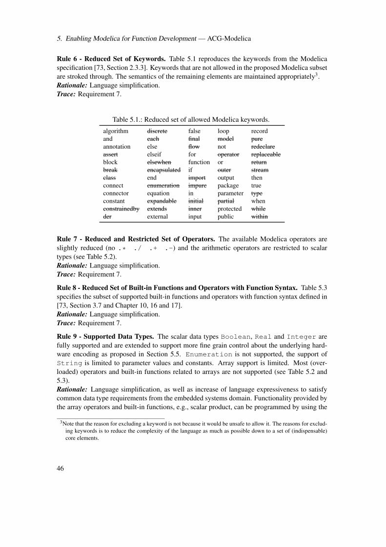
5. Enabling Modelica for Function Development — ACG-Modelica

Rule 6 - Reduced Set of Keywords. Table 5.1 reproduces the keywords from the Modelicaspecification [73, Section 2.3.3]. Keywords that are not allowed in the proposed Modelica subsetare stroked through. The semantics of the remaining elements are maintained appropriately3.Rationale: Language simplification.Trace: Requirement 7.

Table 5.1.: Reduced set of allowed Modelica keywords.

algorithm discrete false loop recordand each final model pureannotation else flow not redeclareassert elseif for operator replaceableblock elsewhen function or returnbreak encapsulated if outer streamclass end import output thenconnect enumeration impure package trueconnector equation in parameter typeconstant expandable initial partial whenconstrainedby extends inner protected whileder external input public within

Rule 7 - Reduced and Restricted Set of Operators. The available Modelica operators areslightly reduced (no .* ./ .+ .-) and the arithmetic operators are restricted to scalartypes (see Table 5.2).Rationale: Language simplification.Trace: Requirement 7.

Rule 8 - Reduced Set of Built-in Functions and Operators with Function Syntax. Table 5.3specifies the subset of supported built-in functions and operators with function syntax defined in[73, Section 3.7 and Chapter 10, 16 and 17].Rationale: Language simplification.Trace: Requirement 7.

Rule 9 - Supported Data Types. The scalar data types Boolean, Real and Integer arefully supported and are extended to support more fine grain control about the underlying hard-ware encoding as proposed in Section 5.5. Enumeration is not supported, the support ofString is limited to parameter values and constants. Array support is limited. Most (over-loaded) operators and built-in functions related to arrays are not supported (see Table 5.2 and5.3).Rationale: Language simplification, as well as increase of language expressiveness to satisfycommon data type requirements from the embedded systems domain. Functionality provided bythe array operators and built-in functions, e.g., scalar product, can be programmed by using the

3Note that the reason for excluding a keyword is not because it would be unsafe to allow it. The reasons for exclud-ing keywords is to reduce the complexity of the language as much as possible down to a set of (indispensable)core elements.

46

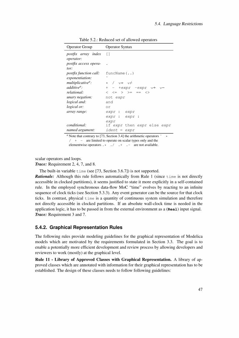
5.4. Language Restrictions

Table 5.2.: Reduced set of allowed operators

Operator Group Operator Syntax

postfix array indexoperator:

[]

postfix access opera-tor:

.

postfix function call: funcName(..)exponentiation: ˆmultiplicativea: * / .* ./additivea: + - +expr -expr .+ .-relational: < <= > >= == <>unary negation: not exprlogical and: andlogical or: orarray range: expr : expr

expr : expr :expr

conditional: if expr then expr else exprnamed argument: ident = expra Note that contrary to [73, Section 3.4] the arithmetic operators ˆ */ + - are limited to operate on scalar types only and theelementwise operators .* ./ .+ .- are not available.

scalar operators and loops.Trace: Requirement 2, 4, 7, and 8.

The built-in variable time (see [73, Section 3.6.7]) is not supported.Rationale: Although this rule follows automatically from Rule 1 (since time is not directlyaccessible in clocked partitions), it seems justified to state it more explicitly in a self-containedrule. In the employed synchronous data-flow MoC “time” evolves by reacting to an infinitesequence of clock ticks (see Section 5.3.3). Any event generator can be the source for that clockticks. In contrast, physical time is a quantity of continuous system simulation and thereforenot directly accessible in clocked partitions. If an absolute wall-clock time is needed in theapplication logic, it has to be passed in from the external environment as a (Real) input signal.Trace: Requirement 3 and 7.

5.4.2. Graphical Representation Rules

The following rules provide modeling guidelines for the graphical representation of Modelicamodels which are motivated by the requirements formulated in Section 3.3. The goal is toenable a potentially more efficient development and review process by allowing developers andreviewers to work (mostly) at the graphical level.

Rule 11 - Library of Approved Classes with Graphical Representation. A library of ap-proved classes which are annotated with information for their graphical representation has to beestablished. The design of these classes needs to follow following guidelines:

47

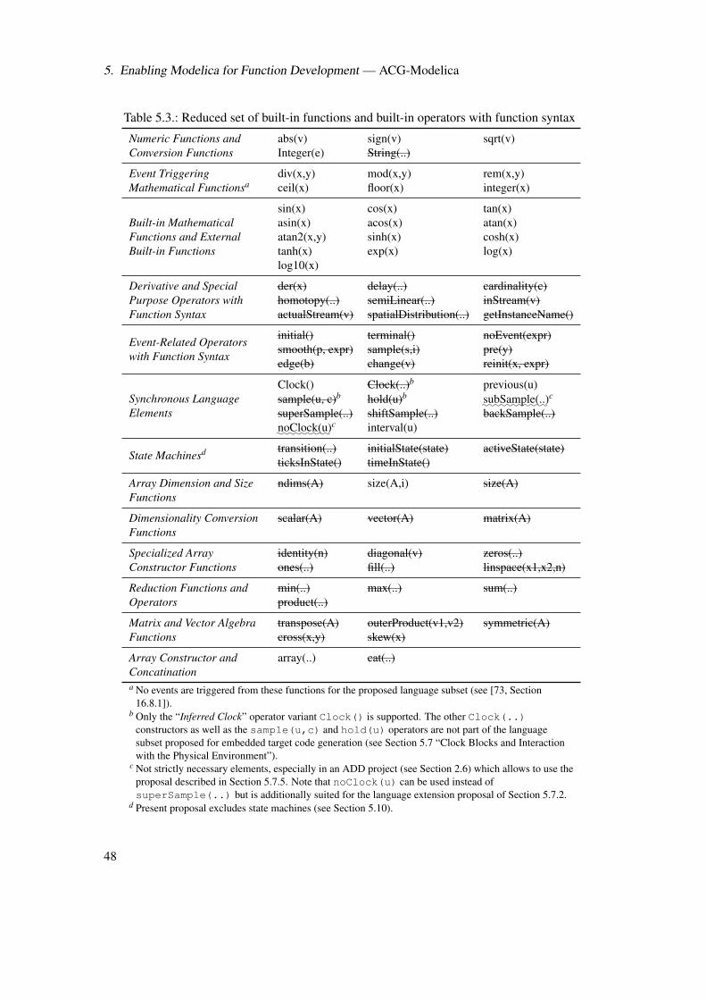
5. Enabling Modelica for Function Development — ACG-Modelica

Table 5.3.: Reduced set of built-in functions and built-in operators with function syntax

Numeric Functions andConversion Functions

abs(v) sign(v) sqrt(v)Integer(e) String(..)

Event TriggeringMathematical Functionsa

div(x,y) mod(x,y) rem(x,y)ceil(x) floor(x) integer(x)

Built-in MathematicalFunctions and ExternalBuilt-in Functions

sin(x) cos(x) tan(x)asin(x) acos(x) atan(x)atan2(x,y) sinh(x) cosh(x)tanh(x) exp(x) log(x)log10(x)

Derivative and SpecialPurpose Operators withFunction Syntax

der(x) delay(..) cardinality(c)homotopy(..) semiLinear(..) inStream(v)actualStream(v) spatialDistribution(..) getInstanceName()

Event-Related Operatorswith Function Syntax

initial() terminal() noEvent(expr)smooth(p, expr) sample(s,i) pre(y)edge(b) change(v) reinit(x, expr)

Synchronous LanguageElements

Clock() Clock(..)b previous(u)sample(u, c)b hold(u)b

:::::::::::subSample(..)c

superSample(..) shiftSample(..) backSample(..)

:::::::::noClock(u)c interval(u)

State Machinesd transition(..) initialState(state) activeState(state)ticksInState() timeInState()

Array Dimension and SizeFunctions

ndims(A) size(A,i) size(A)

Dimensionality ConversionFunctions

scalar(A) vector(A) matrix(A)

Specialized ArrayConstructor Functions

identity(n) diagonal(v) zeros(..)ones(..) fill(..) linspace(x1,x2,n)

Reduction Functions andOperators

min(..) max(..) sum(..)product(..)

Matrix and Vector AlgebraFunctions

transpose(A) outerProduct(v1,v2) symmetric(A)cross(x,y) skew(x)

Array Constructor andConcatination

array(..) cat(..)

a No events are triggered from these functions for the proposed language subset (see [73, Section16.8.1]).

b Only the “Inferred Clock” operator variant Clock() is supported. The other Clock(..)constructors as well as the sample(u,c) and hold(u) operators are not part of the languagesubset proposed for embedded target code generation (see Section 5.7 “Clock Blocks and Interactionwith the Physical Environment”).

c Not strictly necessary elements, especially in an ADD project (see Section 2.6) which allows to use theproposal described in Section 5.7.5. Note that noClock(u) can be used instead ofsuperSample(..) but is additionally suited for the language extension proposal of Section 5.7.2.

d Present proposal excludes state machines (see Section 5.10).

48

5.4. Language Restrictions

• Lean and straight-forward encapsulation of language operators in synchronous data-flowblocks.

• Graphical representations for basic data structures (e.g., interface ports/connectors) andgraphical representations for modeling the flow of execution (e.g., conditional constructs,signal routing).

• Additional “convenience” blocks encapsulating typical algorithms/operations used in dis-crete open- and closed-loop control.

• Blocks should be designed so that extensive testing of the blocks is easily possible, i.e.,simple, lean designs are preferred over sophisticated, complex designs.

• Intuitive and unambiguous graphical representation (icon) for every approved class/block.

• Every class/block must have an identifying feature that allows to recognize that it is anelement of the approved library.

• Semantics of every basic class/block needs to be completely and unambiguously docu-mented/specified.

• Every basic class/block needs to pass through an adequate approval process which in-cludes thoroughly testing and validation activities.

Rationale: Modelica’s language elements have no inherent graphical representation. However,some elements (e.g., classes/blocks) can be annotated with graphical representation information.These elements can be collected in libraries and (given sufficient development tool support) canthen be used by developers in a drag and drop style (see Section A.2.2). In order to work (en-tirely) on the graphical level, it is therefore necessary to provide a library with a sufficiently richset of (annotated) classes/blocks which offer enough expressiveness to allow the clear and con-cise specification of discrete open- and closed-loop control algorithms and their related supportlogic.

The semantics of these blocks must be clearly defined and the graphical representation needsto be unambiguous in order to enable graphical reviews. Furthermore, there must be a visualclue that allows to identify a class/block as being part of the approved library in order to discernsuch block from classes/blocks which are defined by the developer of the embedded system.

Extensive tests increase the confidence that can be placed in the correct functioning of theblocks. Simplicity facilitates testing and ensures that the semantics can be unambiguously un-derstood. Therefore, simple and lean blocks are preferred over feature loaded blocks.Trace: Requirement 11, 12, and 13.

Rule 12 - Block Diagrams with Synchronous Data-Flow Semantics. Block diagrams withsynchronous data-flow semantics must be used at the graphical model level.Rationale: Essentially, the synchronous data-flow semantics on the graphical level follows natu-rally since the synchronous data-flow semantics of the underlying textual level is just “lifted” tothe graphical level. Nevertheless, it seems appropriate to emphasis that consequence by statingit as a self-contained rule for the graphical representation.

49

5. Enabling Modelica for Function Development — ACG-Modelica

Block diagrams with synchronous data-flow semantics are an established notation in thedomain of control engineering. Also, the existing compilation/translation techniques for syn-chronous data-flow programs are understood enough to be accepted by certification authorities.Therefore, adopting that model of computation is an appropriate choice for safety-related open-and closed-loop applications.Trace: Requirement 11 and 12.

Rule 13 - Causal Connectors Exclusivity. Only connectors with directed (causal) data-floware allowed.Rationale: Although this essentially follows from Rule 12, it seems justified to state it explicitlyin a self-contained rule. In general, Modelica connectors don’t denote the direction of the data-flow (see Section A.2.2 and 5.8). However, requiring block diagrams to have a synchronousdata-flow semantics implies that data-flow between connected blocks is restricted to directed(causal) data-flow.Trace: Requirement 11.

Rule 14 - Exclusive Use of Approved Library. Developers may only use elements from anapproved library4 (according to Rule 11). Deviations from this rule are possible — however, inthat case the reviews for corresponding elements are required to be done on the textual level.Rationale: It is only possible to put legitimate trust in the semantics of a composition of ele-ments, if legitimate trust can be put into the correctness of any of the involved elements. Thismeans that it needs to be ensured that any of the involved elements behaves as expected/spec-ified. Hence, developers must exclusively use the elements provided by an approved library.Note that this rule must be part of the modeling guidelines requested in Requirement 14.Trace: Requirement 11.

Rule 15 - Textual/Composite Block Exclusivity. Textual equation must not be mixed withgraphical block instances. In exceptional cases it is allowed to deviate from this rule, however,such deviations must be clearly documented and the corresponding block(s) need clearly notice-able visual marks.Rationale: Mixing textual equations with graphical block instances in one block can be veryconfusing and dangerous since the semantics of that block cannot be anymore deduced entirelyfrom the graphical level. This clearly would violate Requirement 11. This rule must be part ofthe modeling guidelines requested in Requirement 14. Note, that it also seems highly advisablethat a tool provides automatized checks that ensure conformance to this rule.Trace: Requirement 11.

Rule 16 - Use of Intermediate “(De)mux” Blocks. Direct connections of a scalar connector toand from array connectors are not allowed. Intermediate “(De)mux” blocks must be used whenscalar connectors shall be connected with array connectors. In exceptional cases it is allowedto deviate from this rule, however, such deviations must be clearly documented and the corre-sponding block(s) need clearly noticeable visual marks.Rationale: Modelica allows to directly connect scalar connectors with array connectors by usingarray indices, e.g., connect(a,b[2]). This is no problem at the textual level, since the seman-tics is obvious. However, it is usually not possible to recognize the array index at the graphical

4Note, that it is of course also possible that a project uses several approved libraries

50

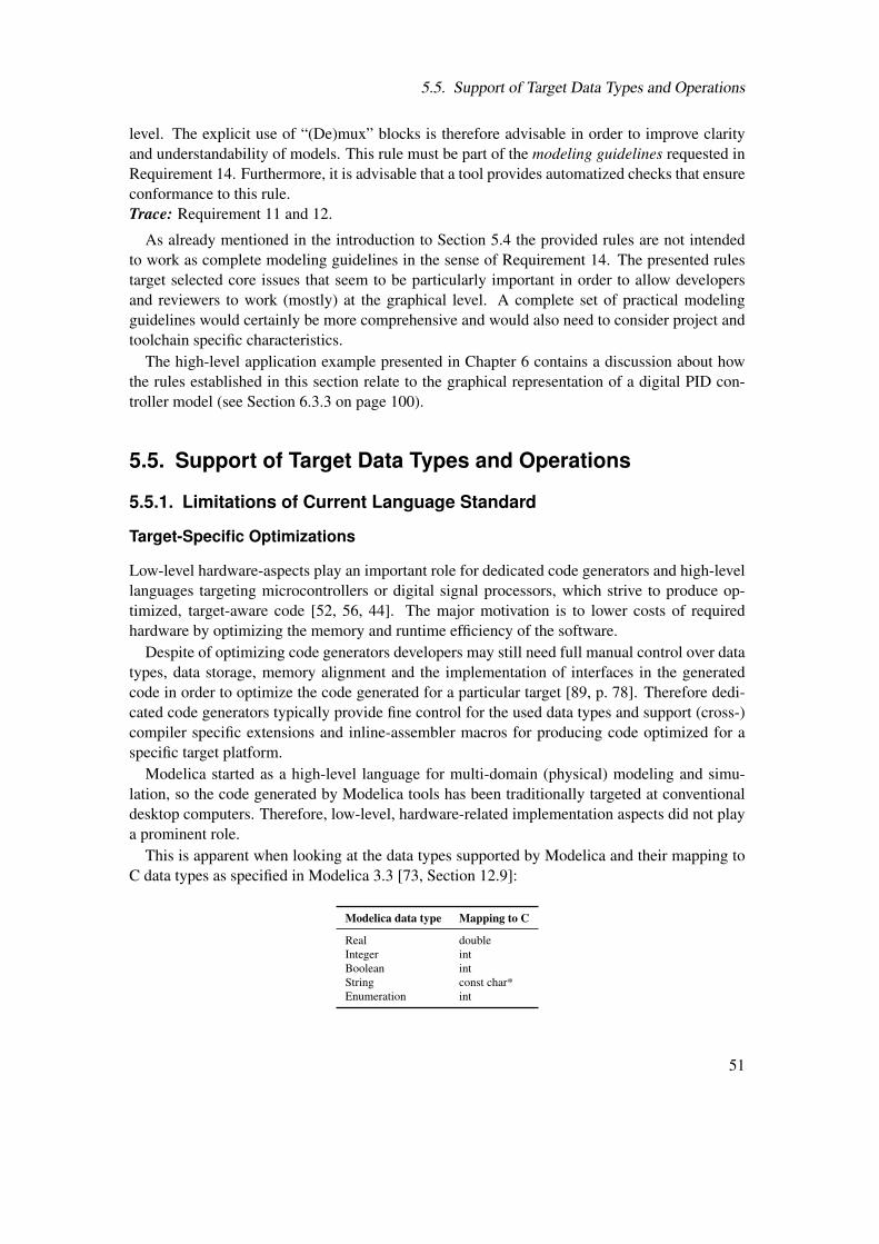
5.5. Support of Target Data Types and Operations

level. The explicit use of “(De)mux” blocks is therefore advisable in order to improve clarityand understandability of models. This rule must be part of the modeling guidelines requested inRequirement 14. Furthermore, it is advisable that a tool provides automatized checks that ensureconformance to this rule.Trace: Requirement 11 and 12.

As already mentioned in the introduction to Section 5.4 the provided rules are not intendedto work as complete modeling guidelines in the sense of Requirement 14. The presented rulestarget selected core issues that seem to be particularly important in order to allow developersand reviewers to work (mostly) at the graphical level. A complete set of practical modelingguidelines would certainly be more comprehensive and would also need to consider project andtoolchain specific characteristics.

The high-level application example presented in Chapter 6 contains a discussion about howthe rules established in this section relate to the graphical representation of a digital PID con-troller model (see Section 6.3.3 on page 100).

5.5. Support of Target Data Types and Operations

5.5.1. Limitations of Current Language Standard

Target-Specific Optimizations

Low-level hardware-aspects play an important role for dedicated code generators and high-levellanguages targeting microcontrollers or digital signal processors, which strive to produce op-timized, target-aware code [52, 56, 44]. The major motivation is to lower costs of requiredhardware by optimizing the memory and runtime efficiency of the software.

Despite of optimizing code generators developers may still need full manual control over datatypes, data storage, memory alignment and the implementation of interfaces in the generatedcode in order to optimize the code generated for a particular target [89, p. 78]. Therefore dedi-cated code generators typically provide fine control for the used data types and support (cross-)compiler specific extensions and inline-assembler macros for producing code optimized for aspecific target platform.

Modelica started as a high-level language for multi-domain (physical) modeling and simu-lation, so the code generated by Modelica tools has been traditionally targeted at conventionaldesktop computers. Therefore, low-level, hardware-related implementation aspects did not playa prominent role.

This is apparent when looking at the data types supported by Modelica and their mapping toC data types as specified in Modelica 3.3 [73, Section 12.9]:

Modelica data type Mapping to C

Real doubleInteger intBoolean intString const char*Enumeration int

51

5. Enabling Modelica for Function Development — ACG-Modelica

This is not sufficient when targeting embedded systems. Developers will therefore need finercontrol over the used data types5. An additional difficulty is that low-level properties of the datatypes are not precisely specified. The specification recommends the range of Real numbers tohave at least the range provided by IEEE double precision floating-point numbers and Integernumbers are recommended to have at least the range of a two’s-complement 32-bit integer [73,p. 13]. In addition, there is a non-normative comment in [73, p. 52] that states:

“For external functions in C89, RealType by default maps to double and IntegerTypeby default maps to int. In the mapping proposed in Annex F of the C99 standard, Re-alType/double matches the IEC 60559:1989 (ANSI/IEEE 754-1985) double format.Typically IntegerType represents a 32-bit 2-complement signed integer.”

However, note that Modelica provides no access to some prominent features of IEEE 754floating-points, like testing for special values such as Infinity or NaN. The specification [73,p. 16] states: “If a numeric operation overflows the result is undefined. For literals it is rec-ommended to automatically convert the number to another type with greater precision.”. So,there is no precisely specified behaviour for dealing with exceptional cases (e.g., undefined orunsupported mathematical operation, overflow, underflow, denormalization).

Target-Specific Functionality

Another, more functional motivation to include low-level hardware-aspects into the modelinglanguage is to support accessing hardware devices like analog-digital converters (ADCs), Pulse-width modulation (PWM) units, timers, etc. as well as services due to a (possibly) available“middleware” (i.e., operating system and additional services, like communication services anddata management) from within the model. Within certain limits the external function interfaceof Modelica [73, Section 12.9] allows to integrate such low-level hardware functionality as longas the functionality can be wrapped into a C function that is called from the model during modelexecution. However, note that direct calls to I/O drivers or other basic software layers is usuallyunwanted if following an architecture-driven development process. In that case it is necessaryto support standardized middleware functions or macros that are “connected” in a subsequentsoftware integration process with the required services provided by the basic software layer.

Also note, that the desired source of the control flow does not always stem from the modelexecution that causes the execution of code to access the peripherals (e.g., by reading or writingto an ADC), but may also stem from external events (e.g., hardware interrupts) that shall causethe execution of specific control algorithms6 modeled in the high-level language. Modelica’s

5E.g., for increased memory efficiency or because the embedded system simply doesn’t provide efficient supportfor that data type, e.g., an embedded system with a FPU (Floating Point Unit) that supports only single precisionfloating point arithmetic.

6A well known example is the execution of a control algorithm for precisely timing the fuel injection and sparkignition in a modern internal combustion engine. In this case the algorithm execution needs to be synchronizedwith the position of each piston and its working phase. Since the position of the crankshaft is related to eachpiston position, synchronization can be achieved by sensor technology which measures the engine’s crankshaftangular position and triggers a hardware interrupt at specific reference positions. The interrupt causes controllogic to be executed, e.g., setting timers that in turn cause precisely timed fuel injection and spark ignition at an“optimal” position.

52

5.5. Support of Target Data Types and Operations

synchronous language elements provide clocks to model activation conditions for a partitionof model equations, but it is not possible to explicitly connect a clock to external events likehardware interrupts. Although it should be possible to extend the language to support that usecase, this is not proposed for ACG-Modelica.

Instead, it is proposed to delegate the connection of clocks with external activation eventsinto the subsequent software component integration step (see Figure 2.1 at the right-hand side).Therefore, software components, or parts of them, are mapped onto tasks using tools or notationsthat are specialized for that concern, e.g., AUTOSAR authoring tools when using an AUTOSARsoftware architecture. This separation of concern is characteristic for an architecture-drivendevelopment process as advocated in Section 2.6 (for a good exposition of behavior modelingtools within an architecture-driven development process see Niggemann et al. [77]).

Operators

Bitwise operators. Modelica provides adequate support for arithmetic, relational and log-ical operators, however, it has no bitwise operators. While bitwise operators are not neededfor physical simulation, they are important for efficient bit manipulation in embedded systemssoftware.

Conversion operators. Conversion between data types is automatic in Modelica if no lossof precision is expected, e.g., when converting from Integer (signed 32 bits integer) to Real(double precision floating-point, 53 bits of precision7). The inverse conversion needs an conver-sion operator, e.g,

Integer x = integer(1.2);

Although Boolean and Enumeration values are mapped to int values in the external C in-terface, explicit conversion between these values is required at the Modelica language level. Insummery, Modelica’s rules for data type conversion are comprehensible and intuitive.

However, there are subtle difficulties with the automatic conversion. Consider the model inListing 5.1.

Listing 5.1: Difficulty of automatic conversion in equations.1 model AutomaticConversion2 Real a, b;3 Integer c;4 equation5 c = a + b; // Does automatic conversion to Real apply?6 a = 1;7 b = 2;8 end AutomaticConversion;

7The significand of IEEE double precisions floating-points is actually 52 bits, but the leading one bit of a normalizedsignificand is not actually stored. The Modelica specification defines the minimal recommended range of floating-point numbers to that specified for the IEEE double precision floating-points [73, 2.4.1 Floating Point Numbers].

53

5. Enabling Modelica for Function Development — ACG-Modelica

Line 5 declares an equation involving Real variables and one Integer variable. As describedin Section 5.2.2, type checking is typically done before the equation causalization process. Con-sequently, it is not known during the type checking phase which variable a, b, or c, will beassigned to after causalization. However, this information is needed to decide whether auto-matic conversion of c to a Real value is reasonable!

Translating this model with the Dymola tool results in a rather confusing error message8. Notyping error is detected, but the following error is reported:

...The Real part has 2 unknowns and 3 equations.The Integer part has 1 unknowns and 0 equations....

This suggests that the Integer variable in line 5.1 has been tentatively converted to Real,which makes it an equation for the “Real part”. So, although an error is finally detected, it is notdetected as type error as one might expect!

The core of the problem is that it is not known during type analysis, which unknown variableof an equation is determined by that equation. After transforming the model to a computablesequential code, this determined variable will be at the left-hand side of an assignment statementand its declared type consequently defines the type required at the right-hand side. While the ex-pression at the right-hand side can be automatically converted to another type during evaluation,the type of the left-hand side is fixed by the variable declaration!

Extending the available basic data types as proposed in Section 5.5.2 leads to further com-plications. For example, consider an automatic conversion from a 32 bit Integer to a singleprecision Real (24 bits of precision9). This will loose precision for values greater than 224.Therefore, additional conversion operators need to be introduced to enable compile checks toprevent unconscious loss of precision and motivate the developer to think about possibly harm-ful conversion effects.

Safety-Related considerations

Although target-aware code optimization of code-generators and compilers is highly desirablefor optimizing utilization of embedded system resources, it also introduces additional difficultiesin respect to tool qualification. As Stürmer states in [99, p. 5] “authorities generally regard thequalification of an optimizing compiler or code generator for safety-relevant software as prob-lematic, as it is, on the one hand, an extremely complex tool and, on the other hand, its behaviourwhen applied to optimizations cannot be clearly comprehended”. To increase the confidence inC code “safe” subsets of the C language have been defined for use in safety-related projects.The most popular one in the automotive industry is MISRA C. Thomsen discusses the conse-quences of requiring a code generator to adhere to the (now superseded) MISRA C:1998 versionof the standard, which essentially prohibits many target-specific optimizations introduced bycode generators [105, 110]. More recent standards published by the “Motor Industry Software

8Tested with Dymola 2014.9The significand of IEEE single precisions floating-points is actually 23 bits, but the leading one bit of a normalized

significant is not actually stored.

54

5.5. Support of Target Data Types and Operations

Reliability Association" are more lenient with respect to deviations from the MISRA C rules ofautomatically generated code, since it has been recognized that code generators are not in thesame way susceptible to common coding errors as human programmers are [107]. Neverthe-less, a conflict remains between providing a maximal amount of (automatic) optimization anda maximal amount of reliability. As a consequence a trade-off needs to be made between fea-ture completeness and validation costs. For example, it needs to be checked whether the savinggained by supporting a particular data type (e.g., because a cheaper ECU can be used) outweighsthe additional costs in (tool) validation.

5.5.2. Proposal for Data Type Extension

A severe limitation of Modelica with respect to embedded system development is the absence offine control over the used data type. This section will therefore propose a mechanism to extendthe standard Modelica data types with more low-level hardware encoding information. In theautomotive industry the use of fixed-point micro controllers units has a high significance, dueto achievable cost savings in a high-volume mass-production setting. However, the engineer-ing effort for realizing fixed-point designs is significantly higher than for floating-point designs(Vitkin et al. report a reduction of development time of 80% when using floating-point insteadof fixed-point implementations and expects a significant shift toward floating-point targets evenfor high-volume products [113]). A notable alternative to dedicated fixed-point code is the useof floating-point code in conjunction with optimized compiler libraries for doing floating-pointarithmetic on fixed-point processors. Anoop and Betta report that execution times achievable byusing floating-point code with floating-point libraries can even outperform fixed-point code [6].With respect to qualifying a code-generator it needs to be considered that the validation effortwill raise for every supported data type and associated operations. Therefore, it needs to becarefully calculated whether a dedicated fixed-point implementation is profitable for a particularproject.

Since the primary concern of the thesis is to establish the conditions that need to be met inorder to enable safety-related function development using Modelica, it is necessary to make atrade-off between feature completeness and associated validation costs. Given that the addi-tional effort introduced by fixed-point support for development and development tool validationmay possibly not offset achievable cost savings due to cheaper hardware, a fixed-point extensionis not included in the Modelica sub- and superset proposed for automatic code generation10.

The relevant part of the Modelica specification defining the basic data types is [73, Section4.8]. The notation in the specification is adapted to extend the definition of the Real, Integerand Boolean data types. The predefined types

ModelicaServices.Types.ImplementationType and

ModelicaServices.Types.ImplementationRealType

define the data types supported by the respective tool. The choices annotation is used to desig-nate the possible string values (see [73, p. 78]). Since a string is used instead of an enumeration,10Note that if fixed-point arithmetic is required, it is still possible (though not convenient) to use the proposed Mod-

elica language extensions to implement and validate custom basic blocks that provide the required functionalityor compile using software floating-point support as described above.

55

5. Enabling Modelica for Function Development — ACG-Modelica

it is easy for different tools to extend the supported data types if needed. The following namesof data types are proposed to be standardized.

type ImplementationType = String annotation(choices(choice="UInt8" "8-bit unsigned integer",choice="SInt8" "8-bit signed integer",choice="UInt16" "16-bit unsigned integer",choice="SInt16" "16-bit signed integer",choice="UInt32" "32-bit unsigned integer",choice="SInt32" "32-bit signed integer"

));

type ImplementationRealType = String annotation(choices(Single "IEEE 754 single precision floating type",Double "IEEE 754 double precision floating type",

));

Since every supported data type increases development and validation costs for a developmenttool it needs to be carefully considered whether only supporting a subset of the standardized datatypes is already sufficient.

Using the definitions, above the predefined types of Modelica are extended with the additionalattribute implementationType. Some attributes specified in [73] are not supported and arecrossed out. The rationale for not supporting an attribute is given in the corresponding footnote.Note that the types are defined with Modelica syntax although they are predefined data types inModelica.

type RealRealType value; /* Accessed without dot-notation */parameter StringType quantity;11

parameter StringType unit;parameter StringType displayUnit;11

parameter RealType min=-Inf, max=+Inf;parameter RealType start;12

parameter BooleanType fixed;13

parameter RealType nominal;14

parameter StateSelect stateSelect;15

parameter ImplementationRealType implementationType = "Double";end Real;

11Omitted for the sake of language simplification (Requirement 7).12Missing required start values are detected during compile time analysis (Requirement 5). In case that a tool deduces

some start values automatically, the resulting start values need to be fixated for code generation (in compliancewith Requirement 9).

13The Attribute "fixed" cannot be applied on clocked discrete-time variables. It is true for variables to which theprevious() operator is applied, otherwise false [73, Section 16.9].

14Nominal values are only useful in the context of numerical solvers. They have no relevance for the targeted discreteapplications.

15Only useful for solving (continuous) differential equation systems.

56

5.5. Support of Target Data Types and Operations

type IntegerIntegerType value; /* Accessed without dot-notation */parameter StringType quantity;11

parameter IntegerType min=-Inf, max=+Inf;parameter IntegerType start;12

parameter BooleanType fixed;13

parameter ImplementationType implementationType = "Sint32";end Integer;

type BooleanBooleanType value; /* Accessed without dot-notation */parameter StringType quantity;11

parameter BooleanType start;12

parameter BooleanType fixed;13

parameter ImplementationType implementationType = "Sint32";end Boolean;

Note that the attribute values of the variables may not be directly manipulated in memory andconsequently there are no access routines.

Extending available data types also requires to extend the semantics of operators in respect tothe new data types. From a high-level viewpoint, the semantics of available Modelica operatorscarry over naturally to the extension, since I “just” allow to approximate integer and real numberswith a different implementation type. The developer is responsible to ensure that no exceptionalcases, e.g., arithmetic overflow or division through zero, can occur within the specified operationconditions.

However, there are some semantic subtleties when evaluating terms that involve integer orreal expression of different ranges or precision. This will be discussed in the following section,in which necessary extensions to the available conversion operators are discussed.

5.5.3. Proposal for Operation Extensions

Conversion Operators

Despite the subtle difficulties of Modelica’s automatic conversion rules pointed out in Section5.5.1 it is possible to maintain those rules under appropriate conditions in ACG-Modelica. Dueto the proposed restriction of the language sub- and superset to causal data-flow semantics (seeSection 5.8.2), it is already known during type analysis which unknown variable is supposed tobe determined by a particular equation. Consequently, type analysis can detect a type error inequations similar to the equation in line 5 of the Listing 5.1 on page 53.

Therefore, in line with the conversion philosophy of current Modelica, it is proposed to pro-vide automatic conversion between data types if no loss of precision is expected. Otherwise,the use of explicit conversion operators is required. The already available conversion operatorinteger(x) is extended to take a second element that designates the data type that x shall beconverted into (defaulting to "SInt32" if the argument is omitted which provides backwardscompatibility). Additionally, the operator is overloaded, so that it can take any of the sup-ported Integer or Real types. It returns the largest integer not greater than x of the specifiedimplementationType.

57

5. Enabling Modelica for Function Development — ACG-Modelica

integer(x, implementationType = "SInt32")

Similarly, a new conversion operator for conversion into Real values is introduced. Alsothis operator is overloaded, so that it can take any of the supported Real or Integer types,though the only conversion from an integer expression to a real expression that requires explicitconversion is that of converting from a 32-bit integer to a single precision floating-point (seeSection 5.5.1). Rounding is performed according to the floating-point rounding mode of thetarget language17.

real(x, implementationType = "Double")

Note that there is no need for a conversion operator for Boolean values, e.g., a Booleanvalue stored in an underlying SInt32 implementation type can be assigned to a Boolean withunderlying implementation type UInt8 without the danger of overflow.

A remaining point is whether numbers may be automatically converted to another type withgreater precision/range in order to perform an operation, e.g., what is the expected outcome ofthe following expression:

Integer u16a(implementationType=UInt16) = 32768; // = 2^15Integer u16b(implementationType=UInt16) = 32768;Integer u32a(implementationType=UInt32) = u16a + u16b;

The outcome depends on whether the addition is performed with 32-bit values (in which casethe result will be 216), or whether the addition is performed with 16-bit values (in which case anoverflow occurs and the result is not defined in Modelica).

If this code was translated to C in a straightforward way, e.g.:

uint16_t u16a = 32768, u16b = 32768;uint32_t u32a = u16a + u16b;

the result of the addition would depend on the implemented size of int. If it was 32-bit, Cwould automatically convert the values to 32-bit before performing the addition (due to a Cconcept called integral promotion). However, if the implemented size of int was 16-bit, anoverflow would occur and the result would be 0.

The proposal refrains from guaranteeing automatic widening of types before performing op-erations. If widening of types is required, it should be encoded explicitly, e.g.:

Integer u32b(implementationType=UInt32) =integer(u16a,"UInt32") + integer(u16b, "UInt32");

Bitwise Operations

Introducing bitwise operations is a bit delicate. Bit manipulation is a low-level task and it may belegitimately disputed whether they should be made available in a high-level modeling language.In order to keep the language as simple as possible I am inclined to do without them!

17I refrain from prescribing a specific rounding mode, since the available rounding modes may depend on the targethardware and the cross-compiler. However, the most common rounding mode is the “round to even” mode whichis the default rounding mode of the IEEE 754 standard [49].

58

5.5. Support of Target Data Types and Operations

However, efficiency considerations will render them desirable for many developers. There-fore, the following tentative proposal is presented. Table 5.4 lists the proposed bitwise operators.Instead of the familiar operator symbols known from C or Java (~ & | ^ << >>), the oper-ators from Table 5.4 have function syntax.

Table 5.4.: Proposed bitwise operators

Operator Syntax Description

bitNot(x) Bitwise complement of xbitAnd(x,y) Bitwise AND between x and ybitOr(x,y) Bitwise OR between x and ybitXor(x,y) Bitwise Exclusive OR (XOR) between x and ybitLeft(x,n) Left shift bits of x by n positionsbitRight(x,n) Right shift bits of x by n positions

The operators from Table 5.4 are only defined for the unsigned Uint8, Uint16 and Uint32

types, and the return type equals the type in which the operation was performed.

5.5.4. Alternative Solutions

A rather suggestive alternative to the data type extension proposal of Section 5.5 is to extendthe data types using Modelica’s short class definitions to specialize the Integer type (similardefinitions can be introduced for Real and Boolean data types), e.g.:type UInt8 = Integer(min=0, max=255);type SInt8 = Integer(min=-128, max=127);

...type SInt32 = Integer(min=-2147483648, max=2147483647);

While a code-generator could use this information to generate respective target platform code(e.g., mapping UInt8 to unsigned char when targeting C) a simulation tool could justcheck that no range violation occurs.

However, developing a (graphical) library would require to duplicate blocks that perform basicoperation (e.g., addition or multiplication) for any of the supported data types (connector decla-rations need a commitment to a specific data type, see Section A.4). In contrast, the solution pro-posed in Section 5.5.2 allows to implement library blocks for which the “implementationType”of all the respective variables and interface declaration within a block can be adjusted by justchanging one parameter which is passed down to all variable declarations.

The proposed solution is an admittedly ad hoc mechanism for a limited form of parametricpolymorphism. A more ambitious solution would be to introduce full-fledged support for para-metric polymorphism, and possibly a type inference mechanism into the language. However,these are fundamental changes to the language. They do not only impose a huge challenge inrespect to language design implications, they also impose high implementation efforts whenintroducing that features into existing tools.

Another option is to use an already existing, more limited form of parametric polymorphismbased on “redeclaration” (see Section A.3). Listing 5.2 illustrates the basic idea.

59

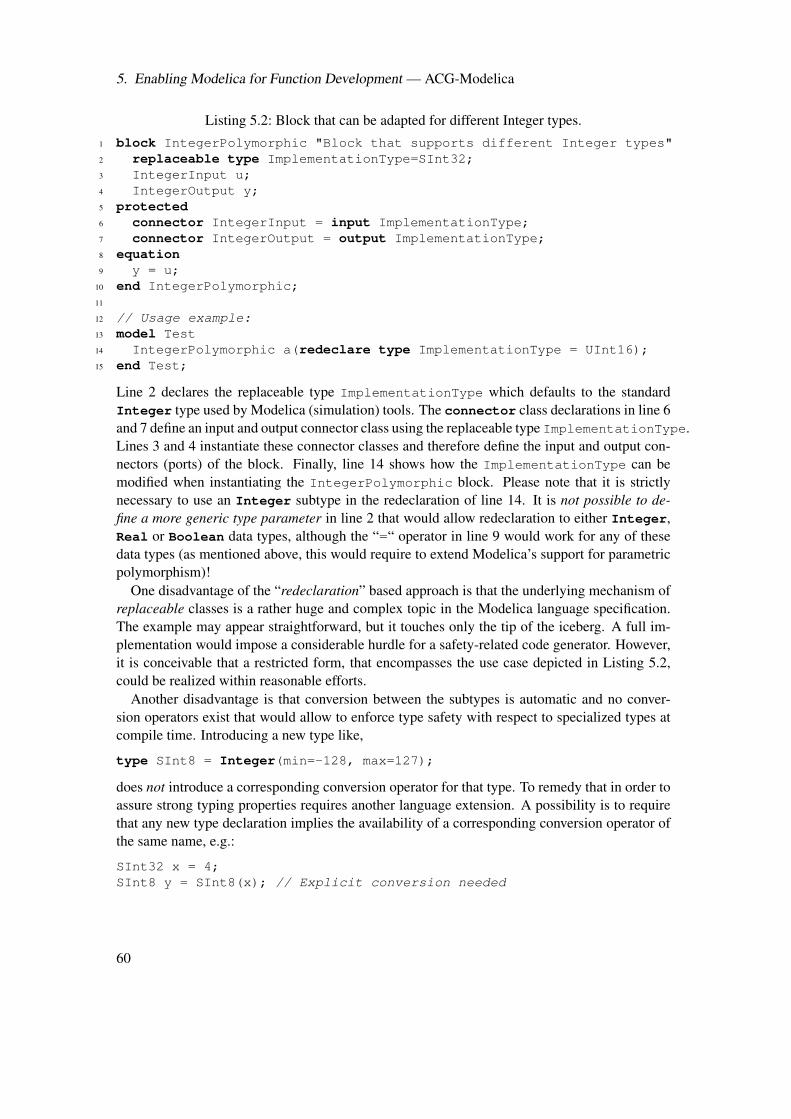
5. Enabling Modelica for Function Development — ACG-Modelica

Listing 5.2: Block that can be adapted for different Integer types.1 block IntegerPolymorphic "Block that supports different Integer types"2 replaceable type ImplementationType=SInt32;3 IntegerInput u;4 IntegerOutput y;5 protected6 connector IntegerInput = input ImplementationType;7 connector IntegerOutput = output ImplementationType;8 equation9 y = u;

10 end IntegerPolymorphic;11

12 // Usage example:13 model Test14 IntegerPolymorphic a(redeclare type ImplementationType = UInt16);15 end Test;

Line 2 declares the replaceable type ImplementationType which defaults to the standardInteger type used by Modelica (simulation) tools. The connector class declarations in line 6and 7 define an input and output connector class using the replaceable type ImplementationType.Lines 3 and 4 instantiate these connector classes and therefore define the input and output con-nectors (ports) of the block. Finally, line 14 shows how the ImplementationType can bemodified when instantiating the IntegerPolymorphic block. Please note that it is strictlynecessary to use an Integer subtype in the redeclaration of line 14. It is not possible to de-fine a more generic type parameter in line 2 that would allow redeclaration to either Integer,Real or Boolean data types, although the “=“ operator in line 9 would work for any of thesedata types (as mentioned above, this would require to extend Modelica’s support for parametricpolymorphism)!

One disadvantage of the “redeclaration” based approach is that the underlying mechanism ofreplaceable classes is a rather huge and complex topic in the Modelica language specification.The example may appear straightforward, but it touches only the tip of the iceberg. A full im-plementation would impose a considerable hurdle for a safety-related code generator. However,it is conceivable that a restricted form, that encompasses the use case depicted in Listing 5.2,could be realized within reasonable efforts.

Another disadvantage is that conversion between the subtypes is automatic and no conver-sion operators exist that would allow to enforce type safety with respect to specialized types atcompile time. Introducing a new type like,

type SInt8 = Integer(min=-128, max=127);

does not introduce a corresponding conversion operator for that type. To remedy that in order toassure strong typing properties requires another language extension. A possibility is to requirethat any new type declaration implies the availability of a corresponding conversion operator ofthe same name, e.g.:

SInt32 x = 4;SInt8 y = SInt8(x); // Explicit conversion needed

60

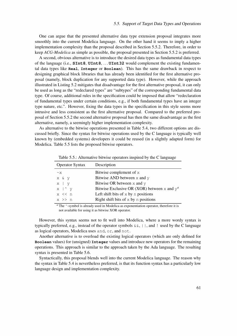
5.5. Support of Target Data Types and Operations

One can argue that the presented alternative data type extension proposal integrates moresmoothly into the current Modelica language. On the other hand it seems to imply a higherimplementation complexity than the proposal described in Section 5.5.2. Therefore, in order tokeep ACG-Modelica as simple as possible, the proposal presented in Section 5.5.2 is preferred.

A second, obvious alternative is to introduce the desired data types as fundamental data typesof the language (i.e., SInt8, UInt8, . . .UInt32 would complement the existing fundamen-tal data types like Real, Integer or Boolean). This has the same drawback in respect todesigning graphical block libraries that has already been identified for the first alternative pro-posal (namely, block duplication for any supported data type). However, while the approachillustrated in Listing 5.2 mitigates that disadvantage for the first alternative proposal, it can onlybe used as long as the “redeclared types” are “subtypes” of the corresponding fundamental datatype. Of course, additional rules in the specification could be imposed that allow “redeclarationof fundamental types under certain conditions, e.g., if both fundamental types have an integertype nature, etc.”. However, fixing the data types in the specification in this style seems moreintrusive and less consistent as the first alternative proposal. Compared to the preferred pro-posal of Section 5.5.2 the second alternative proposal has then the same disadvantage as the firstalternative, namely, a seemingly higher implementation complexity.

As alternative to the bitwise operations presented in Table 5.4, two different options are dis-cussed briefly. Since the syntax for bitwise operations used by the C language is typically wellknown by (embedded systems) developers it could be reused (in a slightly adapted form) forModelica. Table 5.5 lists the proposed bitwise operators.

Table 5.5.: Alternative bitwise operators inspired by the C language

Operator Syntax Description

~x Bitwise complement of xx & y Bitwise AND between x and yx | y Bitwise OR between x and yx |^ y Bitwise Exclusive OR (XOR) between x and ya

x << n Left shift bits of x by n positionsx >> n Right shift bits of x by n positionsa The ^-symbol is already used in Modelica as exponentiation operator, therefore it is

not available for using it as bitwise XOR operator.

However, this syntax seems not to fit well into Modelica, where a more wordy syntax istypically preferred, e.g., instead of the operator symbols &&, ||, and ! used by the C languageas logical operators, Modelica uses and, or, and not.

Another alternative is to overload the existing logical operators (which are only defined forBoolean values) for (unsigned) Integer values and introduce new operators for the remainingoperations. This approach is similar to the approach taken by the Ada language. The resultingsyntax is presented in Table 5.6.

Syntactically, this proposal blends well into the current Modelica language. The reason whythe syntax in Table 5.4 is nevertheless preferred, is that its function syntax has a particularly lowlanguage design and implementation complexity.

61

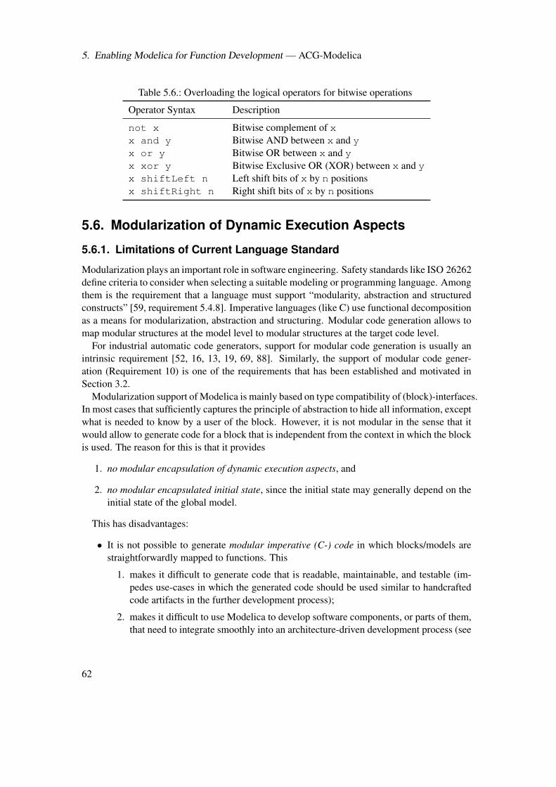
5. Enabling Modelica for Function Development — ACG-Modelica

Table 5.6.: Overloading the logical operators for bitwise operations

Operator Syntax Description

not x Bitwise complement of xx and y Bitwise AND between x and yx or y Bitwise OR between x and yx xor y Bitwise Exclusive OR (XOR) between x and yx shiftLeft n Left shift bits of x by n positionsx shiftRight n Right shift bits of x by n positions

5.6. Modularization of Dynamic Execution Aspects

5.6.1. Limitations of Current Language Standard

Modularization plays an important role in software engineering. Safety standards like ISO 26262define criteria to consider when selecting a suitable modeling or programming language. Amongthem is the requirement that a language must support “modularity, abstraction and structuredconstructs” [59, requirement 5.4.8]. Imperative languages (like C) use functional decompositionas a means for modularization, abstraction and structuring. Modular code generation allows tomap modular structures at the model level to modular structures at the target code level.

For industrial automatic code generators, support for modular code generation is usually anintrinsic requirement [52, 16, 13, 19, 69, 88]. Similarly, the support of modular code gener-ation (Requirement 10) is one of the requirements that has been established and motivated inSection 3.2.

Modularization support of Modelica is mainly based on type compatibility of (block)-interfaces.In most cases that sufficiently captures the principle of abstraction to hide all information, exceptwhat is needed to know by a user of the block. However, it is not modular in the sense that itwould allow to generate code for a block that is independent from the context in which the blockis used. The reason for this is that it provides

1. no modular encapsulation of dynamic execution aspects, and

2. no modular encapsulated initial state, since the initial state may generally depend on theinitial state of the global model.

This has disadvantages:

• It is not possible to generate modular imperative (C-) code in which blocks/models arestraightforwardly mapped to functions. This

1. makes it difficult to generate code that is readable, maintainable, and testable (im-pedes use-cases in which the generated code should be used similar to handcraftedcode artifacts in the further development process);

2. makes it difficult to use Modelica to develop software components, or parts of them,that need to integrate smoothly into an architecture-driven development process (see

62

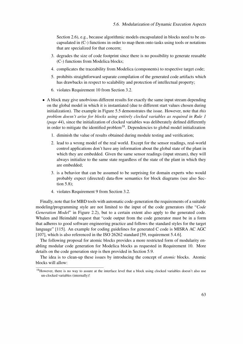
5.6. Modularization of Dynamic Execution Aspects

Section 2.6), e.g., because algorithmic models encapsulated in blocks need to be en-capsulated in (C-) functions in order to map them onto tasks using tools or notationsthat are specialized for that concern;

3. degrades the size of code footprint since there is no possibility to generate reusable(C-) functions from Modelica blocks;

4. complicates the traceability from Modelica (components) to respective target code;

5. prohibits straightforward separate compilation of the generated code artifacts whichhas drawbacks in respect to scalability and protection of intellectual property;

6. violates Requirement 10 from Section 3.2.

• A block may give unobvious different results for exactly the same input stream dependingon the global model in which it is instantiated (due to different start values chosen duringinitialization). The example in Figure 5.5 demonstrates the issue. However, note that thisproblem doesn’t arise for blocks using entirely clocked variables as required in Rule 1(page 44), since the initialization of clocked variables was deliberately defined differentlyin order to mitigate the identified problem18. Dependencies to global model initialization

1. diminish the value of results obtained during module testing and verification;

2. lead to a wrong model of the real world. Except for the sensor readings, real-worldcontrol applications don’t have any information about the global state of the plant inwhich they are embedded. Given the same sensor readings (input stream), they willalways initialize to the same state regardless of the state of the plant in which theyare embedded;

3. is a behavior that can be assumed to be surprising for domain experts who wouldprobably expect (directed) data-flow semantics for block diagrams (see also Sec-tion 5.8);

4. violates Requirement 9 from Section 3.2.

Finally, note that for MBD tools with automatic code-generation the requirements of a suitablemodeling/programming style are not limited to the input of the code generators (the “CodeGeneration Model” in Figure 2.2), but to a certain extent also apply to the generated code.Whalen and Heimdahl request that “code output from the code generator must be in a formthat adheres to good software engineering practice and follows the standard styles for the targetlanguage” [115]. An example for coding guidelines for generated C code is MISRA AC AGC[107], which is also referenced in the ISO 26262 standard [59, requirement 5.4.6].

The following proposal for atomic blocks provides a more restricted form of modularity en-abling modular code generation for Modelica blocks as requested in Requirement 10. Moredetails on the code generation step is then provided in Section 5.9.

The idea is to clean-up these issues by introducing the concept of atomic blocks. Atomicblocks will allow:18However, there is no way to assure at the interface level that a block using clocked variables doesn’t also use

un-clocked variables (internally)!

63

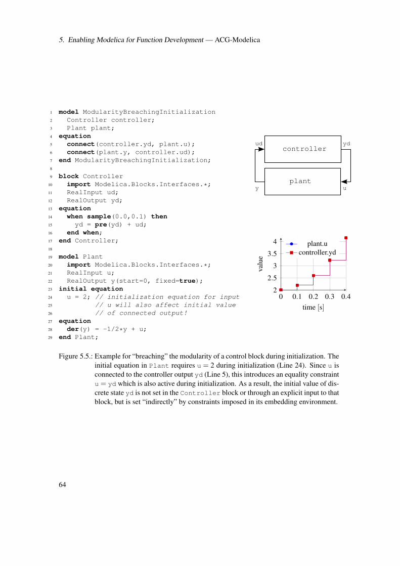
5. Enabling Modelica for Function Development — ACG-Modelica

1 model ModularityBreachingInitialization2 Controller controller;3 Plant plant;4 equation5 connect(controller.yd, plant.u);6 connect(plant.y, controller.ud);7 end ModularityBreachingInitialization;8

9 block Controller10 import Modelica.Blocks.Interfaces.*;11 RealInput ud;12 RealOutput yd;13 equation14 when sample(0.0,0.1) then15 yd = pre(yd) + ud;16 end when;17 end Controller;18

19 model Plant20 import Modelica.Blocks.Interfaces.*;21 RealInput u;22 RealOutput y(start=0, fixed=true);23 initial equation24 u = 2; // initialization equation for input25 // u will also affect initial value26 // of connected output!27 equation28 der(y) = -1/2*y + u;29 end Plant;

controlleryd

plantu

ud

y

0 0.1 0.2 0.3 0.42

2.5

3

3.5

4

time [s]

valu

e

plant.ucontroller.yd

Figure 5.5.: Example for “breaching” the modularity of a control block during initialization. Theinitial equation in Plant requires u = 2 during initialization (Line 24). Since u isconnected to the controller output yd (Line 5), this introduces an equality constraintu = yd which is also active during initialization. As a result, the initial value of dis-crete state yd is not set in the Controller block or through an explicit input to thatblock, but is set “indirectly” by constraints imposed in its embedding environment.

64

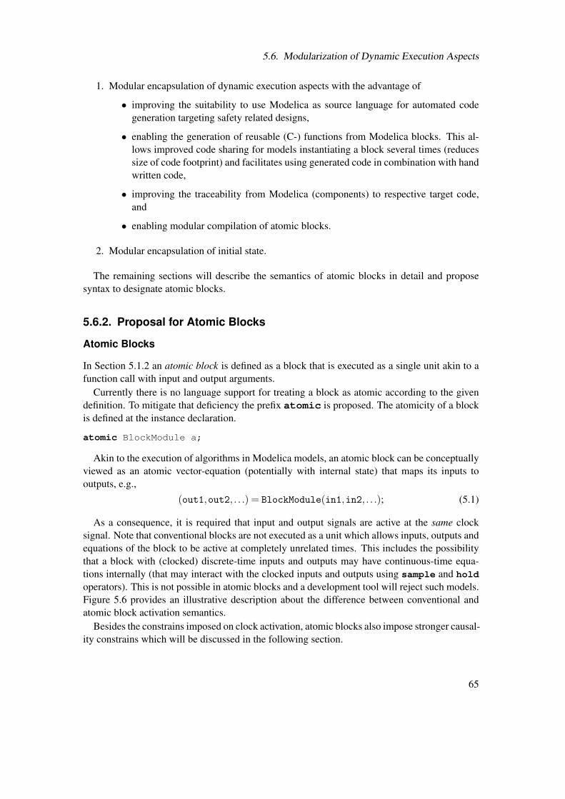
5.6. Modularization of Dynamic Execution Aspects

1. Modular encapsulation of dynamic execution aspects with the advantage of

• improving the suitability to use Modelica as source language for automated codegeneration targeting safety related designs,

• enabling the generation of reusable (C-) functions from Modelica blocks. This al-lows improved code sharing for models instantiating a block several times (reducessize of code footprint) and facilitates using generated code in combination with handwritten code,

• improving the traceability from Modelica (components) to respective target code,and

• enabling modular compilation of atomic blocks.

2. Modular encapsulation of initial state.

The remaining sections will describe the semantics of atomic blocks in detail and proposesyntax to designate atomic blocks.

5.6.2. Proposal for Atomic Blocks

Atomic Blocks

In Section 5.1.2 an atomic block is defined as a block that is executed as a single unit akin to afunction call with input and output arguments.

Currently there is no language support for treating a block as atomic according to the givendefinition. To mitigate that deficiency the prefix atomic is proposed. The atomicity of a blockis defined at the instance declaration.

atomic BlockModule a;

Akin to the execution of algorithms in Modelica models, an atomic block can be conceptuallyviewed as an atomic vector-equation (potentially with internal state) that maps its inputs tooutputs, e.g.,

(out1,out2, . . .) = BlockModule(in1,in2, . . .); (5.1)

As a consequence, it is required that input and output signals are active at the same clocksignal. Note that conventional blocks are not executed as a unit which allows inputs, outputs andequations of the block to be active at completely unrelated times. This includes the possibilitythat a block with (clocked) discrete-time inputs and outputs may have continuous-time equa-tions internally (that may interact with the clocked inputs and outputs using sample and holdoperators). This is not possible in atomic blocks and a development tool will reject such models.Figure 5.6 provides an illustrative description about the difference between conventional andatomic block activation semantics.

Besides the constrains imposed on clock activation, atomic blocks also impose stronger causal-ity constrains which will be discussed in the following section.

65

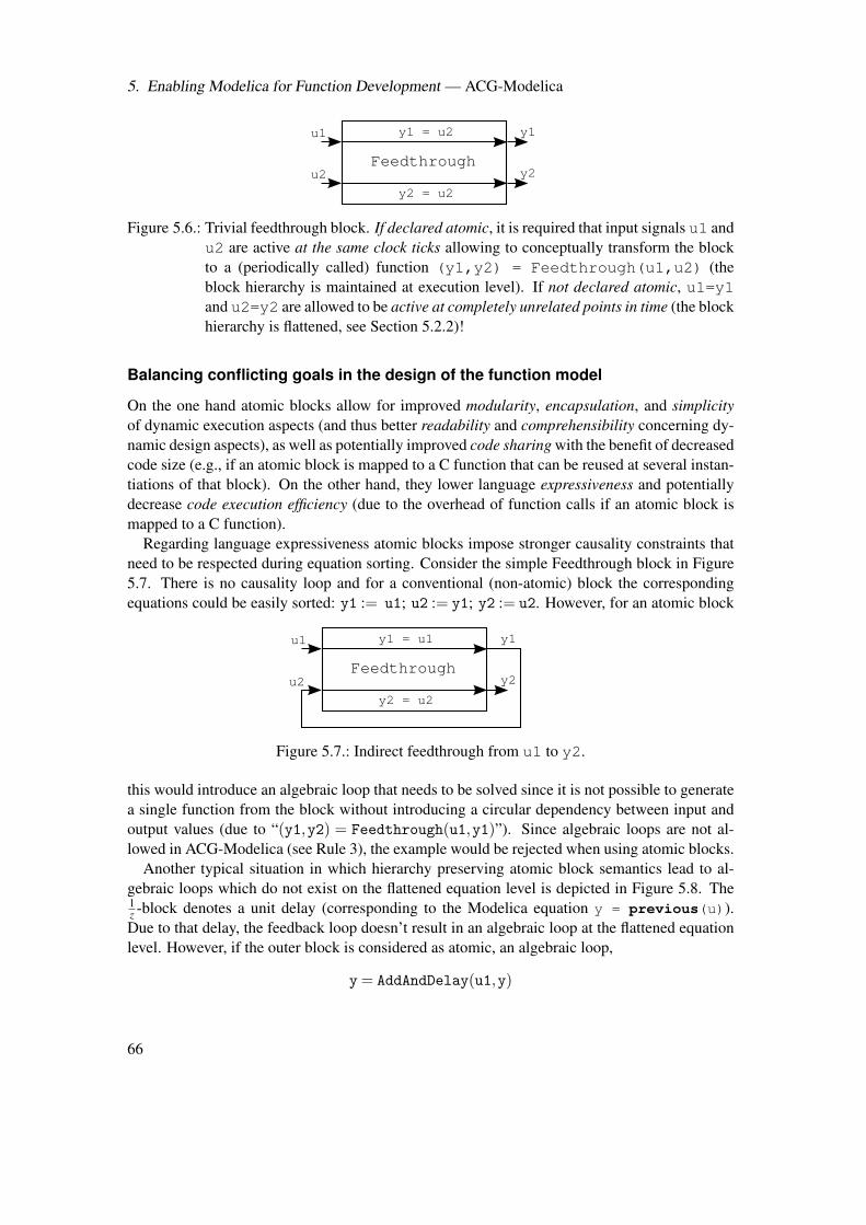
5. Enabling Modelica for Function Development — ACG-Modelica

Feedthrough

y1 = u2

y2 = u2

u1

u2 y2

y1

Figure 5.6.: Trivial feedthrough block. If declared atomic, it is required that input signals u1 andu2 are active at the same clock ticks allowing to conceptually transform the blockto a (periodically called) function (y1,y2) = Feedthrough(u1,u2) (theblock hierarchy is maintained at execution level). If not declared atomic, u1=y1and u2=y2 are allowed to be active at completely unrelated points in time (the blockhierarchy is flattened, see Section 5.2.2)!

Balancing conflicting goals in the design of the function model

On the one hand atomic blocks allow for improved modularity, encapsulation, and simplicityof dynamic execution aspects (and thus better readability and comprehensibility concerning dy-namic design aspects), as well as potentially improved code sharing with the benefit of decreasedcode size (e.g., if an atomic block is mapped to a C function that can be reused at several instan-tiations of that block). On the other hand, they lower language expressiveness and potentiallydecrease code execution efficiency (due to the overhead of function calls if an atomic block ismapped to a C function).

Regarding language expressiveness atomic blocks impose stronger causality constraints thatneed to be respected during equation sorting. Consider the simple Feedthrough block in Figure5.7. There is no causality loop and for a conventional (non-atomic) block the correspondingequations could be easily sorted: y1 := u1; u2 := y1; y2 := u2. However, for an atomic block

Feedthrough

y1 = u1

y2 = u2

u1

y2u2

y1

Figure 5.7.: Indirect feedthrough from u1 to y2.

this would introduce an algebraic loop that needs to be solved since it is not possible to generatea single function from the block without introducing a circular dependency between input andoutput values (due to “(y1,y2) = Feedthrough(u1,y1)”). Since algebraic loops are not al-lowed in ACG-Modelica (see Rule 3), the example would be rejected when using atomic blocks.

Another typical situation in which hierarchy preserving atomic block semantics lead to al-gebraic loops which do not exist on the flattened equation level is depicted in Figure 5.8. The1z -block denotes a unit delay (corresponding to the Modelica equation y = previous(u)).Due to that delay, the feedback loop doesn’t result in an algebraic loop at the flattened equationlevel. However, if the outer block is considered as atomic, an algebraic loop,

y= AddAndDelay(u1,y)

66

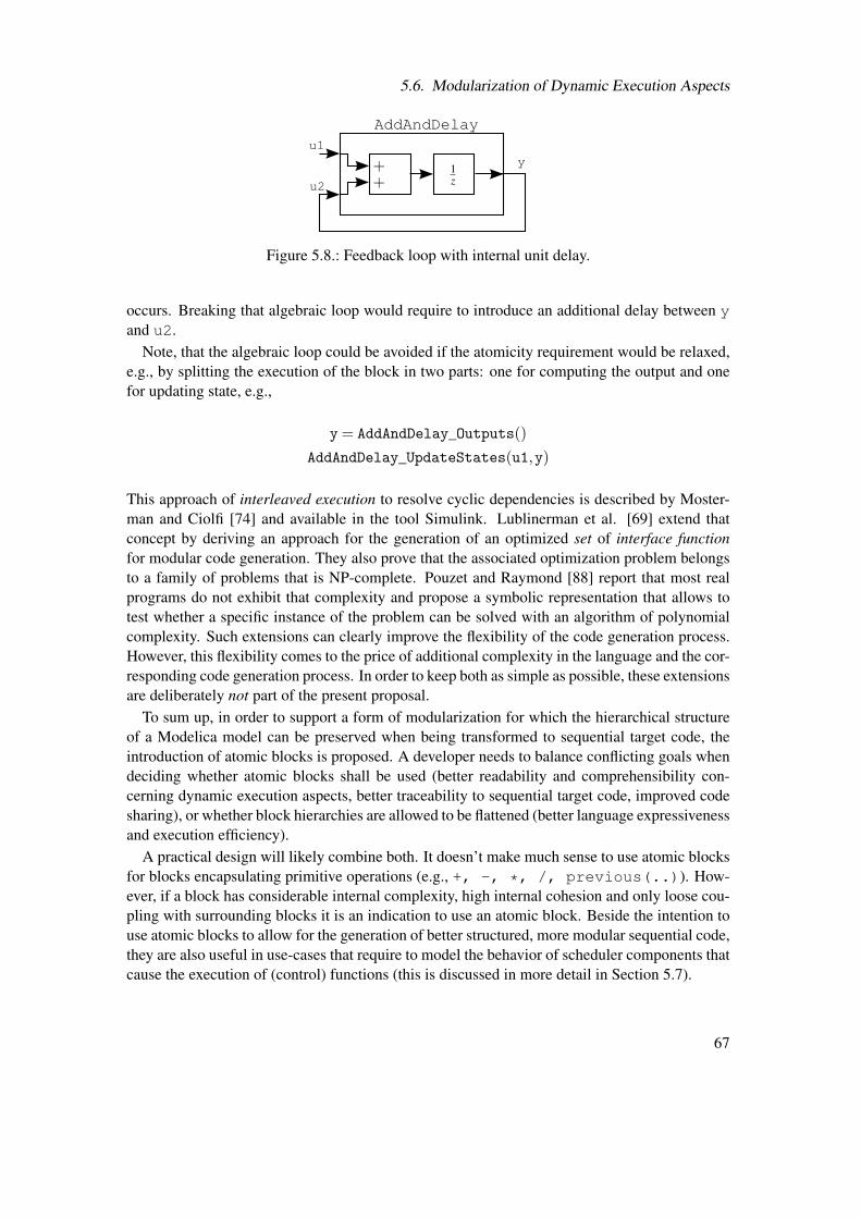
5.6. Modularization of Dynamic Execution Aspects

1z

++

AddAndDelayu1

u2

y

Figure 5.8.: Feedback loop with internal unit delay.

occurs. Breaking that algebraic loop would require to introduce an additional delay between yand u2.

Note, that the algebraic loop could be avoided if the atomicity requirement would be relaxed,e.g., by splitting the execution of the block in two parts: one for computing the output and onefor updating state, e.g.,

y= AddAndDelay_Outputs()

AddAndDelay_UpdateStates(u1,y)

This approach of interleaved execution to resolve cyclic dependencies is described by Moster-man and Ciolfi [74] and available in the tool Simulink. Lublinerman et al. [69] extend thatconcept by deriving an approach for the generation of an optimized set of interface functionfor modular code generation. They also prove that the associated optimization problem belongsto a family of problems that is NP-complete. Pouzet and Raymond [88] report that most realprograms do not exhibit that complexity and propose a symbolic representation that allows totest whether a specific instance of the problem can be solved with an algorithm of polynomialcomplexity. Such extensions can clearly improve the flexibility of the code generation process.However, this flexibility comes to the price of additional complexity in the language and the cor-responding code generation process. In order to keep both as simple as possible, these extensionsare deliberately not part of the present proposal.

To sum up, in order to support a form of modularization for which the hierarchical structureof a Modelica model can be preserved when being transformed to sequential target code, theintroduction of atomic blocks is proposed. A developer needs to balance conflicting goals whendeciding whether atomic blocks shall be used (better readability and comprehensibility con-cerning dynamic execution aspects, better traceability to sequential target code, improved codesharing), or whether block hierarchies are allowed to be flattened (better language expressivenessand execution efficiency).

A practical design will likely combine both. It doesn’t make much sense to use atomic blocksfor blocks encapsulating primitive operations (e.g., +, -, *, /, previous(..)). How-ever, if a block has considerable internal complexity, high internal cohesion and only loose cou-pling with surrounding blocks it is an indication to use an atomic block. Beside the intention touse atomic blocks to allow for the generation of better structured, more modular sequential code,they are also useful in use-cases that require to model the behavior of scheduler components thatcause the execution of (control) functions (this is discussed in more detail in Section 5.7).

67

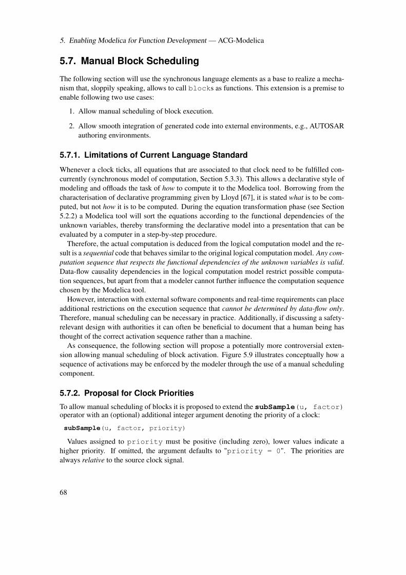
5. Enabling Modelica for Function Development — ACG-Modelica

5.7. Manual Block Scheduling

The following section will use the synchronous language elements as a base to realize a mecha-nism that, sloppily speaking, allows to call blocks as functions. This extension is a premise toenable following two use cases:

1. Allow manual scheduling of block execution.

2. Allow smooth integration of generated code into external environments, e.g., AUTOSARauthoring environments.

5.7.1. Limitations of Current Language Standard

Whenever a clock ticks, all equations that are associated to that clock need to be fulfilled con-currently (synchronous model of computation, Section 5.3.3). This allows a declarative style ofmodeling and offloads the task of how to compute it to the Modelica tool. Borrowing from thecharacterisation of declarative programming given by Lloyd [67], it is stated what is to be com-puted, but not how it is to be computed. During the equation transformation phase (see Section5.2.2) a Modelica tool will sort the equations according to the functional dependencies of theunknown variables, thereby transforming the declarative model into a presentation that can beevaluated by a computer in a step-by-step procedure.

Therefore, the actual computation is deduced from the logical computation model and the re-sult is a sequential code that behaves similar to the original logical computation model. Any com-putation sequence that respects the functional dependencies of the unknown variables is valid.Data-flow causality dependencies in the logical computation model restrict possible computa-tion sequences, but apart from that a modeler cannot further influence the computation sequencechosen by the Modelica tool.

However, interaction with external software components and real-time requirements can placeadditional restrictions on the execution sequence that cannot be determined by data-flow only.Therefore, manual scheduling can be necessary in practice. Additionally, if discussing a safety-relevant design with authorities it can often be beneficial to document that a human being hasthought of the correct activation sequence rather than a machine.

As consequence, the following section will propose a potentially more controversial exten-sion allowing manual scheduling of block activation. Figure 5.9 illustrates conceptually how asequence of activations may be enforced by the modeler through the use of a manual schedulingcomponent.

5.7.2. Proposal for Clock Priorities

To allow manual scheduling of blocks it is proposed to extend the subSample(u, factor)operator with an (optional) additional integer argument denoting the priority of a clock:

subSample(u, factor, priority)

Values assigned to priority must be positive (including zero), lower values indicate ahigher priority. If omitted, the argument defaults to "priority = 0". The priorities arealways relative to the source clock signal.

68

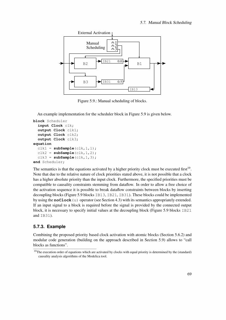
5.7. Manual Block Scheduling

B2IB21

123

IB31B3

B1

External Activation

ManualScheduling

IB13

0.0

0.5

Figure 5.9.: Manual scheduling of blocks.

An example implementation for the scheduler block in Figure 5.9 is given below.

block Schedulerinput Clock clk;output Clock clk1;output Clock clk2;output Clock clk3;

equationclk1 = subSample(clk,1,1);clk2 = subSample(clk,1,2);clk3 = subSample(clk,1,3);

end Scheduler;

The semantics is that the equations activated by a higher priority clock must be executed first19.Note that due to the relative nature of clock priorities stated above, it is not possible that a clockhas a higher absolute priority than the input clock. Furthermore, the specified priorities must becompatible to causality constraints stemming from dataflow. In order to allow a free choice ofthe activation sequence it is possible to break dataflow constraints between blocks by insertingdecoupling blocks (Figure 5.9 blocks IB13, IB21, IB31). These blocks could be implementedby using the noClock(u) operator (see Section 4.3) with its semantics appropriately extended.If an input signal to a block is required before the signal is provided by the connected outputblock, it is necessary to specify initial values at the decoupling block (Figure 5.9 blocks IB21and IB31).

5.7.3. Example

Combining the proposed priority based clock activation with atomic blocks (Section 5.6.2) andmodular code generation (building on the approach described in Section 5.9) allows to “callblocks as functions”.19The execution order of equations which are activated by clocks with equal priority is determined by the (standard)

causality analysis algorithms of the Modelica tool.

69

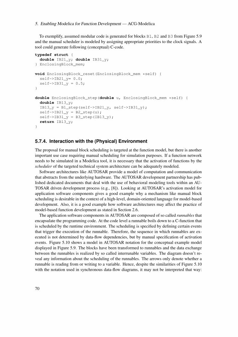
5. Enabling Modelica for Function Development — ACG-Modelica

To exemplify, assumed modular code is generated for blocks B1, B2 and B3 from Figure 5.9and the manual scheduler is modeled by assigning appropriate priorities to the clock signals. Atool could generate following (conceptual) C-code.

typedef struct double IB21_y; double IB31_y;

EnclosingBlock_mem;

void EnclosingBlock_reset(EnclosingBlock_mem *self) self->IB21_y= 0.0;self->IB31_y = 0.5;

double EnclosingBlock_step(double u, EnclosingBlock_mem *self) double IB13_y;IB13_y = B1_step(self->IB21_y, self->IB31_y);self->IB21_y = B2_step(u);self->IB31_y = B3_step(IB13_y);return IB13_y;

5.7.4. Interaction with the (Physical) Environment

The proposal for manual block scheduling is targeted at the function model, but there is anotherimportant use case requiring manual scheduling for simulation purposes. If a function networkneeds to be simulated in a Modelica tool, it is necessary that the activation of functions by thescheduler of the targeted technical system architecture can be adequately modeled.

Software architectures like AUTOSAR provide a model of computation and communicationthat abstracts from the underlying hardware. The AUTOSAR development partnership has pub-lished dedicated documents that deal with the use of behavioral modeling tools within an AU-TOSAR driven development process (e.g., [8]). Looking at AUTOSAR’s activation model forapplication software components gives a good example why a mechanism like manual blockscheduling is desirable in the context of a high-level, domain-oriented language for model-baseddevelopment. Also, it is a good example how software architectures may affect the practice ofmodel-based function development as stated in Section 2.6.

The application software components in AUTOSAR are composed of so called runnables thatencapsulate the programming code. At the code level a runnable boils down to a C-function thatis scheduled by the runtime environment. The scheduling is specified by defining certain eventsthat trigger the execution of the runnable. Therefore, the sequence in which runnables are ex-ecuted is not determined by data-flow dependencies, but by manual specification of activationevents. Figure 5.10 shows a model in AUTOSAR notation for the conceptual example modeldisplayed in Figure 5.9. The blocks have been transformed to runnables and the data exchangebetween the runnables is realized by so called interrunable variables. The diagram doesn’t re-veal any information about the scheduling of the runnables. The arrows only denote whether arunnable is reading from or writing to a variable. Hence, despite the similarities of Figure 5.10with the notation used in synchronous data-flow diagrams, it may not be interpreted that way:

70

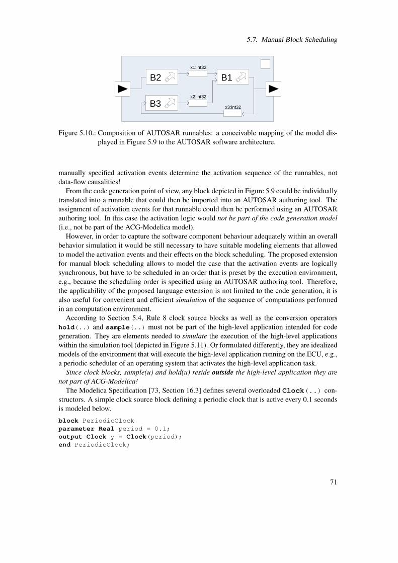
5.7. Manual Block Scheduling

B1

B3

x1:int32

B2

x2:int32

x3:int32

Figure 5.10.: Composition of AUTOSAR runnables: a conceivable mapping of the model dis-played in Figure 5.9 to the AUTOSAR software architecture.

manually specified activation events determine the activation sequence of the runnables, notdata-flow causalities!

From the code generation point of view, any block depicted in Figure 5.9 could be individuallytranslated into a runnable that could then be imported into an AUTOSAR authoring tool. Theassignment of activation events for that runnable could then be performed using an AUTOSARauthoring tool. In this case the activation logic would not be part of the code generation model(i.e., not be part of the ACG-Modelica model).

However, in order to capture the software component behaviour adequately within an overallbehavior simulation it would be still necessary to have suitable modeling elements that allowedto model the activation events and their effects on the block scheduling. The proposed extensionfor manual block scheduling allows to model the case that the activation events are logicallysynchronous, but have to be scheduled in an order that is preset by the execution environment,e.g., because the scheduling order is specified using an AUTOSAR authoring tool. Therefore,the applicability of the proposed language extension is not limited to the code generation, it isalso useful for convenient and efficient simulation of the sequence of computations performedin an computation environment.

According to Section 5.4, Rule 8 clock source blocks as well as the conversion operatorshold(..) and sample(..) must not be part of the high-level application intended for codegeneration. They are elements needed to simulate the execution of the high-level applicationswithin the simulation tool (depicted in Figure 5.11). Or formulated differently, they are idealizedmodels of the environment that will execute the high-level application running on the ECU, e.g.,a periodic scheduler of an operating system that activates the high-level application task.

Since clock blocks, sample(u) and hold(u) reside outside the high-level application they arenot part of ACG-Modelica!

The Modelica Specification [73, Section 16.3] defines several overloaded Clock(..) con-structors. A simple clock source block defining a periodic clock that is active every 0.1 secondsis modeled below.

block PeriodicClockparameter Real period = 0.1;output Clock y = Clock(period);end PeriodicClock;

71

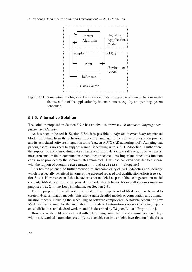
5. Enabling Modelica for Function Development — ACG-Modelica

ControlAlgorithm

Plant

High-LevelAppplicationModel

Reference

Clock Source

sample(..)

EnvironmentModel

hold(..)

Figure 5.11.: Simulation of a high-level application model using a clock source block to modelthe execution of the application by its environment, e.g., by an operating systemscheduler.

5.7.5. Alternative Solution

The solution proposed in Section 5.7.2 has an obvious drawback: It increases language com-plexity considerably.

As has been indicated in Section 5.7.4, it is possible to shift the responsibility for manualblock scheduling from the behavioral modeling language to the software integration processand its associated software integration tools (e.g., an AUTOSAR authoring tool). Adopting thatpattern, there is no need to support manual scheduling within ACG-Modelica. Furthermore,the support of accommodating data streams with multiple sample rates (e.g., due to sensorsmeasurements or finite computation capabilities) becomes less important, since this functioncan also be provided by the software integration tool. Thus, one can even consider to dispensewith the support of operators subSample(..) and noClock(..) altogether!

This has the potential to further reduce size and complexity of ACG-Modelica considerably,which is especially beneficial in terms of the expected reduced tool qualification efforts (see Sec-tion 5.1.1). However, even if that behavior is not modeled as part of the code generation model(i.e., ACG-Modelica) it must be possible to model that behavior for overall system simulationpurposes (i.e., X-in-the-Loop simulation, see Section 2.3).

For the purpose of overall system simulation the complete set of Modelica may be used tocreate hybrid simulation models. This allows quite detailed models of computation and commu-nication aspects, including the scheduling of software components. A notable account of howModelica can be used for the simulation of distributed automation systems (including experi-enced difficulties and devised workarounds) is described by Wagner, Lui and Frey in [114].

However, while [114] is concerned with determining computation and communication delayswithin a networked automation system (e.g., to enable runtime or delay investigations), the focus

72

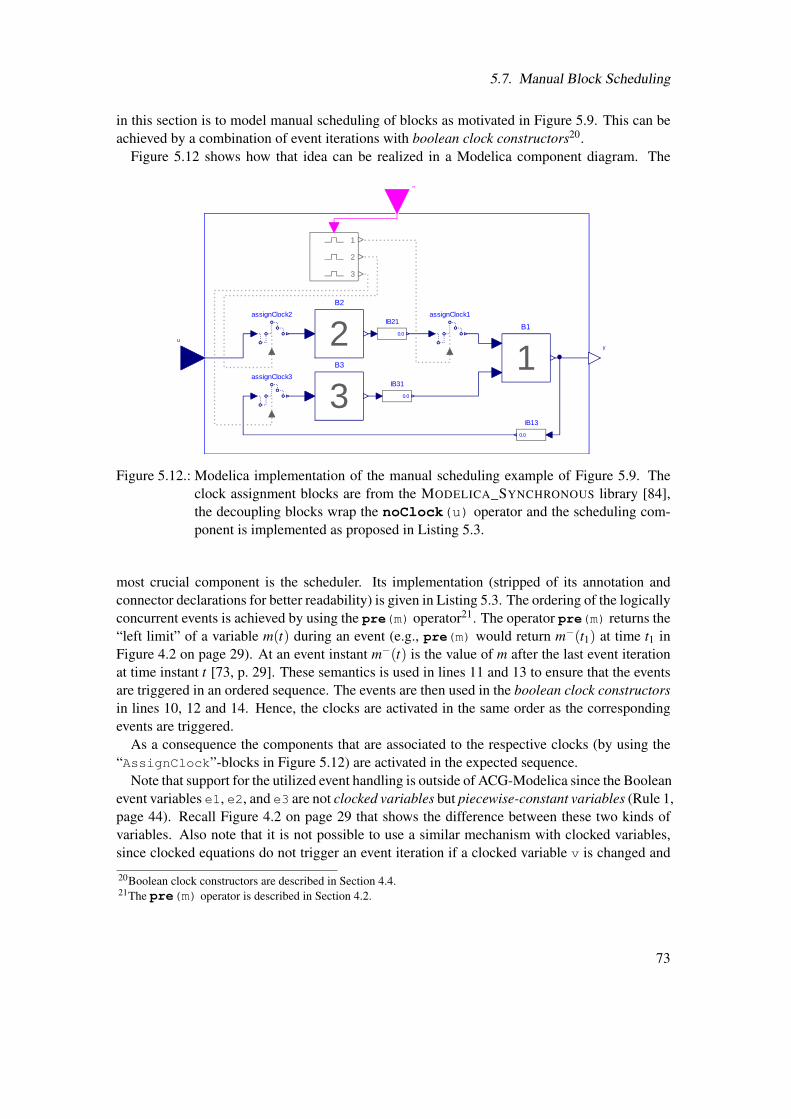
5.7. Manual Block Scheduling

in this section is to model manual scheduling of blocks as motivated in Figure 5.9. This can beachieved by a combination of event iterations with boolean clock constructors20.

Figure 5.12 shows how that idea can be realized in a Modelica component diagram. The

B2

2assignClock1assignClock2

1

2

3

B3

3assignClock3

IB21

0.0

IB31

0.0

B1

1

IB13

0.0

u

y

c

Figure 5.12.: Modelica implementation of the manual scheduling example of Figure 5.9. Theclock assignment blocks are from the MODELICA_SYNCHRONOUS library [84],the decoupling blocks wrap the noClock(u) operator and the scheduling com-ponent is implemented as proposed in Listing 5.3.

most crucial component is the scheduler. Its implementation (stripped of its annotation andconnector declarations for better readability) is given in Listing 5.3. The ordering of the logicallyconcurrent events is achieved by using the pre(m) operator21. The operator pre(m) returns the“left limit” of a variable m(t) during an event (e.g., pre(m) would return m−(t1) at time t1 inFigure 4.2 on page 29). At an event instant m−(t) is the value of m after the last event iterationat time instant t [73, p. 29]. These semantics is used in lines 11 and 13 to ensure that the eventsare triggered in an ordered sequence. The events are then used in the boolean clock constructorsin lines 10, 12 and 14. Hence, the clocks are activated in the same order as the correspondingevents are triggered.

As a consequence the components that are associated to the respective clocks (by using the“AssignClock”-blocks in Figure 5.12) are activated in the expected sequence.

Note that support for the utilized event handling is outside of ACG-Modelica since the Booleanevent variables e1, e2, and e3 are not clocked variables but piecewise-constant variables (Rule 1,page 44). Recall Figure 4.2 on page 29 that shows the difference between these two kinds ofvariables. Also note that it is not possible to use a similar mechanism with clocked variables,since clocked equations do not trigger an event iteration if a clocked variable v is changed and

20Boolean clock constructors are described in Section 4.4.21The pre(m) operator is described in Section 4.2.

73

5. Enabling Modelica for Function Development — ACG-Modelica

Listing 5.3: Scheduler that triggers event clocks by using an ordered event iteration.1 model Scheduler2 input Boolean e1;3 output Clock c1;4 output Clock c2;5 output Clock c3;6 protected7 Boolean e2(start=false,fixed=true);8 Boolean e3(start=false,fixed=true);9 equation

10 c1 = Clock(e1);11 e2 = pre(e1);12 c2 = Clock(e2);13 e3 = pre(e2);14 c3 = Clock(e3);15 end Scheduler;

previous(v) appears in the equations.

5.8. Causal Data-Flow Semantics

Modelica can be called an equation-based object-oriented (EOO) language (see Appendix A).Equations are of acausal (or non-causal) nature in the sense that the causality of how the equa-tions have to be solved need not be specified at modeling time (see Section A.2 for details). Thisis in contrast to the block diagrams used in control systems and DSP engineering applications.In block diagrams the response characteristics of individual components are depicted by blockswith input and output ports. Connections between blocks denote directed (causal) data-flow.

Although typical data-flow languages like Lustre also refer to equations on flow expressionswhich define the behaviour of a program, these equations are more constrained than the equa-tions referred to in EOO terminology. The equations definitions in data-flow languages consistof one variable on the left-hand side and a flow expression on the right-hand side. These equa-tions only prescribe causal data-flow (the right-hand side expression is assigned to the left-handside variable), e.g., in a data-flow assignment equation a := b ·c the variable a is assumed tobe unknown, while b and c are assumed to be known. Note that in contrast to assignmentsin imperative languages the order in which the data-flow equations appear in the program hasno relevance. A single assignment rule ensures that a variable has no more than one definingequation at a time instant and the set of data-flow equations defining the program behavior issorted during compilation in order to satisfy data-flow causality constraints between individualequations.

Now, although the foundation of Modelica is rooted in modeling using acausal equations thereis also support for a causal block diagram style of modeling (see Section A.4).

However, in the context of a language considered for safety-related model-based functiondevelopment, there are subtle problems with the approach taken by Modelica:

74

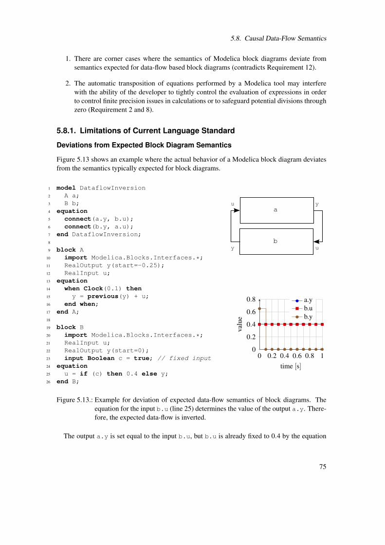
5.8. Causal Data-Flow Semantics

1. There are corner cases where the semantics of Modelica block diagrams deviate fromsemantics expected for data-flow based block diagrams (contradicts Requirement 12).

2. The automatic transposition of equations performed by a Modelica tool may interferewith the ability of the developer to tightly control the evaluation of expressions in orderto control finite precision issues in calculations or to safeguard potential divisions throughzero (Requirement 2 and 8).

5.8.1. Limitations of Current Language Standard

Deviations from Expected Block Diagram Semantics

Figure 5.13 shows an example where the actual behavior of a Modelica block diagram deviatesfrom the semantics typically expected for block diagrams.

1 model DataflowInversion2 A a;3 B b;4 equation5 connect(a.y, b.u);6 connect(b.y, a.u);7 end DataflowInversion;8

9 block A10 import Modelica.Blocks.Interfaces.*;11 RealOutput y(start=-0.25);12 RealInput u;13 equation14 when Clock(0.1) then15 y = previous(y) + u;16 end when;17 end A;18

19 block B20 import Modelica.Blocks.Interfaces.*;21 RealInput u;22 RealOutput y(start=0);23 input Boolean c = true; // fixed input24 equation25 u = if (c) then 0.4 else y;26 end B;

ay

bu

u

y

0 0.2 0.4 0.6 0.8 10

0.2

0.4

0.6

0.8

time [s]

valu

e

a.yb.ub.y

Figure 5.13.: Example for deviation of expected data-flow semantics of block diagrams. Theequation for the input b.u (line 25) determines the value of the output a.y. There-fore, the expected data-flow is inverted.

The output a.y is set equal to the input b.u, but b.u is already fixed to 0.4 by the equation

75

5. Enabling Modelica for Function Development — ACG-Modelica

declared in line 2522. The resulting system of equations is:

a.y = previous(a.y)+a.u;b.u = if (true) then 0.4 else y;b.y = a.u;b.u = a.y;

This system of equations can be easily transformed into a computable sequence of assignments(note that the start values of a.y and b.y are −0.25 and 0, respectively):

// Initial sectiona.y_previous := -0.25;b.y_previous := 0;

// Output at clock ticksb.u := 0.4;a.y := b.u;a.u := a.y - a.y_previous;b.y := a.u;a.y_previous := a.y;

However, this inversion of input and output causality is not expected for block diagrams thatindicate a directed data-flow from a.y to b.u. Therefore, the observed behavior contradictsRequirement 3 and 7. Note that the example is somewhat artificially constructed (due to line25), but less obvious situations that lead to unexpected data-flow inversion cannot be completelyruled out by current Modelica semantics. It is worth mentioning that the possibility to invertthe data-flow is not a disadvantage per se: it is the prerequisite to allow automatic generation ofinverse models for advanced controllers [111, 84].

Effects of Symbolic Transformations of Acausal Equations

A consequence of the declarative equation based modeling style is that a Modelica tool mayperform substantial symbolic transformations in order to generate sequential code (see Section5.2.2 and A.2). The symbolic equation transformations performed may interfere with the abilityof the developer to tightly control the evaluation of expressions in order to control finite preci-sion issues. It is well known that numerical precision affects the results of computations andthe order in which computations are performed matters. For example, for addition and multipli-cation of floating-point numbers neither associative nor distributive properties hold in general.An illustrative example where the associative law of algebra does not hold for floating-pointnumbers (of double precision) is given by David Goldberg [49, p. 30]: “(x+ y)+ z has a totallydifferent answer than x+(y+ z) when x = 1030, y =−1030, and z = 1 (it is 1 in the former case,0 in the latter)”.

Please note that numerical precision issues are not a problem specific to EOO languagesor Modelica. They are generally encountered in language design and compiler implementa-

22In order to have locally balanced models the Modelica specification requires that a class/block has the samenumber of unknowns and equations [73, Section 4.7]. Since inputs are considered known “block B” requiresone equation for its output y. Therefore y needs to appear formally in the equation in line 25 in order to makethe model valid.

76

5.8. Causal Data-Flow Semantics

tion (Goldberg provides a notable discussion about the interaction of languages, compilers andfloating-point arithmetic in [49]). However, due to the extend of symbolic transformation inModelica the abilities of a developer to exert manual control over the way computations areperformed in the final program is more limited than in more low-level languages like C.

An EOO language specific issue is that the use of equations instead of assignments may renderpotential divisions through zero less visible. As a consequence, necessary precautions might beoverlooked. An equation like

a = b ·c

may appear safe at first glance, but of course this depends on the unknown variable which isdefined by the context in which the equation is declared. E.g., if the unknown is c a tool willtransform the equation to the assignment

c := a/b

which is unsafe if b = 0 cannot be excluded.

Improvement Goals

The aim of the following proposal is:

• Ensure that the semantics indicated by block diagrams do not exhibit any behavior deemedsurprising or non-obvious by a domain expert (Requirement 12).

• Restrict equations semantics to the semantics known from typical data-flow languages inorder to reduce potential detrimental effects due to automatic transposition of equations(Requirement 2).

5.8.2. Proposal for safer, causal data-flow semantics

Mitigation for the aforementioned limitations can be achieved by diverse means. The preferredone is by extension of the language restrictions imposed in Section 5.4. Alternative solutions arebriefly outlined and compared to the preferred solution.

Restrictions on Equations and Causal Connectors

In addition to Modelica’s synchronous model of computation described in Section 5.3.3, follow-ing restriction applies:

Equations shall be restricted to a form where a single variable (the unknown) is atthe left-hand side and a flow expression is at the right-hand side, e.g., a = b ·c isvalid while a+b = 0 or a2 = b is invalid.

This restriction does not only prevent potentially undesirable symbolic transformations (asdescribed in Section 5.8.1), but also affects the connections between causal connectors. Togetherwith the balanced model principle formulated in the Modelica specification [73, Section 4.7],inversion of data-flow is excluded. The balanced model principle requires that the local number

77

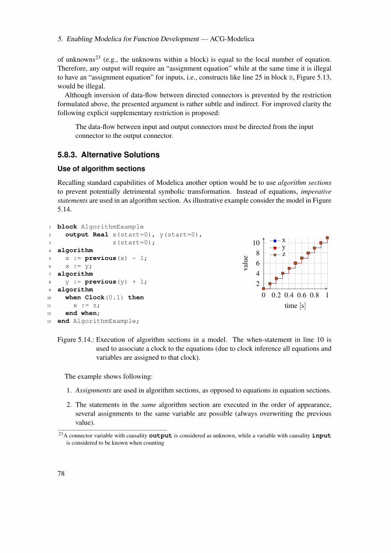
5. Enabling Modelica for Function Development — ACG-Modelica

of unknowns23 (e.g., the unknowns within a block) is equal to the local number of equation.Therefore, any output will require an “assignment equation” while at the same time it is illegalto have an “assignment equation” for inputs, i.e., constructs like line 25 in block B, Figure 5.13,would be illegal.

Although inversion of data-flow between directed connectors is prevented by the restrictionformulated above, the presented argument is rather subtle and indirect. For improved clarity thefollowing explicit supplementary restriction is proposed:

The data-flow between input and output connectors must be directed from the inputconnector to the output connector.

5.8.3. Alternative Solutions

Use of algorithm sections

Recalling standard capabilities of Modelica another option would be to use algorithm sectionsto prevent potentially detrimental symbolic transformation. Instead of equations, imperativestatements are used in an algorithm section. As illustrative example consider the model in Figure5.14.

1 block AlgorithmExample2 output Real x(start=0), y(start=0),3 z(start=0);4 algorithm5 x := previous(x) - 1;6 x := y;7 algorithm8 y := previous(y) + 1;9 algorithm

10 when Clock(0.1) then11 x := z;12 end when;13 end AlgorithmExample;

0 0.2 0.4 0.6 0.8 1

2468

10

time [s]

valu

exyz

Figure 5.14.: Execution of algorithm sections in a model. The when-statement in line 10 isused to associate a clock to the equations (due to clock inference all equations andvariables are assigned to that clock).

The example shows following:

1. Assignments are used in algorithm sections, as opposed to equations in equation sections.

2. The statements in the same algorithm section are executed in the order of appearance,several assignments to the same variable are possible (always overwriting the previousvalue).

23A connector variable with causality output is considered as unknown, while a variable with causality inputis considered to be known when counting

78

5.8. Causal Data-Flow Semantics

3. Statements appearing in different algorithm sections are not executed together. Instead,any algorithm section is conceptually viewed as an atomic vector equation (y1,y2, . . .) =f (u1,u2, . . .) where yi are variables appearing on the left-hand side of assignments, whileui are right-hand side variables. These equations are then sorted according to data-flowdependencies.

While the use of algorithm sections instead of equations also effectively prevents potentiallydetrimental symbolic transformation, I see following disadvantages compared to the preferredsolution:

• If one prescribes the use of algorithm sections like shown in line 4–6 of the examplefavorable properties inherent to the single-assignment rule are lost. In this respect I agreewith the rating by Ackerman [1, p. 20]: “However, the advantages of single assignmentlanguages, namely, clarity and ease of verification, generally outweigh the “convenience”of reusing the same name”.

• To eliminate the disadvantage expressed above, one could require that any assignmentstatement needs to have its own algorithm section as it is the case for the statements inline 8 and 11 of the example. This would give the desired semantics, but to the price of anawkward, unpleasant syntax.

Dedicated language elements for causal data-flow semantics

Instead of imposing additional restrictions on existing elements, another alternative is to definenew language elements to achieve the specified goals. Conceivable is to specify a new prefixcausal which can be applied to block declarations in order to restrict the form of the allowedequations within the block similarly to the rule formulated in the preferred proposal, e.g.:

causal block A...end A;

In order to explicitly ensure directed data-flow semantics between input and output connectorsthe prefixes causalInput and causalOutput can be introduced as an alternative to theexisting input and output prefixes. The definition of adequate connectors is then similar tothe definition presented in Section A.4 for the RealInput and RealOutput connectors, butinstead uses the causalInput and causalOutput prefixes, e.g.,

connector RealCausalInput = causalInput Real;

connector RealCausalOutput = causalOutput Real;

These dedicated language elements have the advantage that they give the developer the free-dom to decide on a situation aware basis about the appropriate modeling style. However, thedisadvantage is a bloating of the language that hampers comprehensibility, increases languageimplementation efforts and renders the language less appealing in terms of conceptual clarityand consistency.

79

5. Enabling Modelica for Function Development — ACG-Modelica

This is particular evident in the proposal for directed connectors, where the semantics of thecausal variants are almost identical to the existing language elements, except for some very spe-cial cases. Therefore, enforcing moderate restrictions on the valid semantics for safety-relevantapplications (in order to guarantee the absence of certain kinds of faults), as specified in thefavored proposal, seems to be the better solution.

5.9. Translation to a Synchronous Data-Flow Kernel

The language sub- and superset ACG-Modelica was presented as a possible solution to allow theusage of Modelica for safety-related model-based function development. The proposed languagerestrictions and extensions have been substantiated by providing detailed rationales, includingreferences to open literature where possible. However, despite all these efforts the evidencethat it is practically feasible to develop an automatic code generator for ACG-Modelica that isqualifiable for safety related developments remains vague.

To mitigate that deficiency a formal translational semantics from a subset of ACG-Modelica(further denoted as mACG-Modelica) to a synchronous data-flow kernel language (further de-noted as SDFK) was developed as part of these thesis efforts (Thiele et al. [108]). The syn-chronous data-flow kernel language is borrowed from Biernacki et al. [19], where Biernacki etal. describe code generation from the synchronous data-flow kernel language into imperativecode and note that “The principles presented in this article are implemented in the RELUC com-piler of SCADE/LUSTRE and experimented on industrial real-size examples”. Furthermore,that synchronous data-flow kernel is considered as a “basic calculus that is powerful enough toexpress any Lustre program”.

The commercial Lustre-based SCADE tool provides a code generator, KCG, that has alreadybeen successfully qualified for safety-critical applications (see e.g., [50]). Hence, I provide atranslational semantics to a data-flow language kernel that is understood enough to be acceptedby certification authorities. Consequently, this yields a strong argument for the feasibility ofdeveloping a qualifiable code generator for the considered Modelica subset. Furthermore, thattranslational semantics could be used as a base to create a gateway from Modelica to SCADE,similar to what has been reported for Simulink/Stateflow in [31].

The SDFK language semantics as well as the formal translation from mACG-Modelica toSDFK (as described in [108]) is reproduced in Appendix B. The following sections explain thattranslation informally by using an illustrative example. The formal translation in [108] doesnot include support for Modelica rate transition operators. Section 5.9.4 presents how supportfor Modelica rate transition operators can be added to the formal translation, i.e., the mACG-Modelica language subset is further extended in order to allow modeling of multirate digitalcontrol systems.

The translation to the SDFK language is rather complex. To keep the translation manageableit is subdivided into several steps (see Section B.3) with the two major steps normalisation andtranslation. The normalisation is a source-to-source transformation in which mACG-Modelica(see Section B.2 for the language definition) is transformed into a representation that allows amore straight-forward mapping to SDFK. The output of the normalization step is again Modelicacode denoted as normalized mACG-Modelica. In comparison to ACG-Modelica it has a simpli-

80

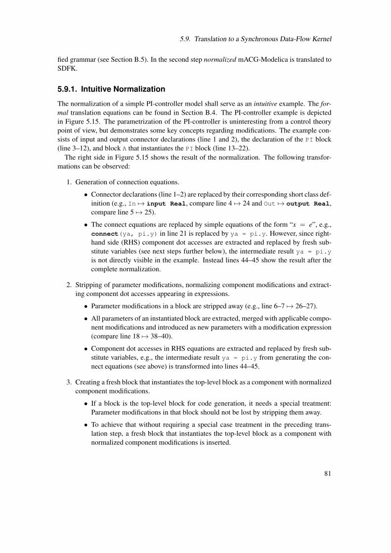
5.9. Translation to a Synchronous Data-Flow Kernel

fied grammar (see Section B.5). In the second step normalized mACG-Modelica is translated toSDFK.

5.9.1. Intuitive Normalization

The normalization of a simple PI-controller model shall serve as an intuitive example. The for-mal translation equations can be found in Section B.4. The PI-controller example is depictedin Figure 5.15. The parametrization of the PI-controller is uninteresting from a control theorypoint of view, but demonstrates some key concepts regarding modifications. The example con-sists of input and output connector declarations (line 1 and 2), the declaration of the PI block(line 3–12), and block A that instantiates the PI block (line 13–22).

The right side in Figure 5.15 shows the result of the normalization. The following transfor-mations can be observed:

1. Generation of connection equations.

• Connector declarations (line 1–2) are replaced by their corresponding short class def-inition (e.g., In 7→ input Real, compare line 4 7→ 24 and Out 7→ output Real,compare line 5 7→ 25).

• The connect equations are replaced by simple equations of the form “x = e”, e.g.,connect(ya, pi.y) in line 21 is replaced by ya = pi.y. However, since right-hand side (RHS) component dot accesses are extracted and replaced by fresh sub-stitute variables (see next steps further below), the intermediate result ya = pi.y

is not directly visible in the example. Instead lines 44–45 show the result after thecomplete normalization.

2. Stripping of parameter modifications, normalizing component modifications and extract-ing component dot accesses appearing in expressions.

• Parameter modifications in a block are stripped away (e.g., line 6–7 7→ 26–27).

• All parameters of an instantiated block are extracted, merged with applicable compo-nent modifications and introduced as new parameters with a modification expression(compare line 18 7→ 38–40).

• Component dot accesses in RHS equations are extracted and replaced by fresh sub-stitute variables, e.g., the intermediate result ya = pi.y from generating the con-nect equations (see above) is transformed into lines 44–45.

3. Creating a fresh block that instantiates the top-level block as a component with normalizedcomponent modifications.

• If a block is the top-level block for code generation, it needs a special treatment:Parameter modifications in that block should not be lost by stripping them away.

• To achieve that without requiring a special case treatment in the preceding trans-lation step, a fresh block that instantiates the top-level block as a component withnormalized component modifications is inserted.

81

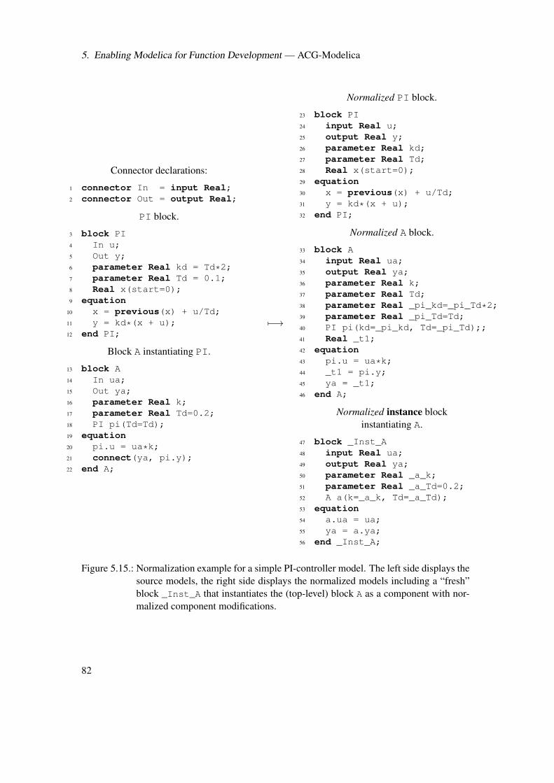
5. Enabling Modelica for Function Development — ACG-Modelica

Connector declarations:

1 connector In = input Real;2 connector Out = output Real;

PI block.

3 block PI4 In u;5 Out y;6 parameter Real kd = Td*2;7 parameter Real Td = 0.1;8 Real x(start=0);9 equation

10 x = previous(x) + u/Td;11 y = kd*(x + u);12 end PI;

Block A instantiating PI.

13 block A14 In ua;15 Out ya;16 parameter Real k;17 parameter Real Td=0.2;18 PI pi(Td=Td);19 equation20 pi.u = ua*k;21 connect(ya, pi.y);22 end A;

7−→

Normalized PI block.

23 block PI24 input Real u;25 output Real y;26 parameter Real kd;27 parameter Real Td;28 Real x(start=0);29 equation30 x = previous(x) + u/Td;31 y = kd*(x + u);32 end PI;

Normalized A block.

33 block A34 input Real ua;35 output Real ya;36 parameter Real k;37 parameter Real Td;38 parameter Real _pi_kd=_pi_Td*2;39 parameter Real _pi_Td=Td;40 PI pi(kd=_pi_kd, Td=_pi_Td);;41 Real _t1;42 equation43 pi.u = ua*k;44 _t1 = pi.y;45 ya = _t1;46 end A;

Normalized instance blockinstantiating A.

47 block _Inst_A48 input Real ua;49 output Real ya;50 parameter Real _a_k;51 parameter Real _a_Td=0.2;52 A a(k=_a_k, Td=_a_Td);53 equation54 a.ua = ua;55 ya = a.ya;56 end _Inst_A;

Figure 5.15.: Normalization example for a simple PI-controller model. The left side displays thesource models, the right side displays the normalized models including a “fresh”block _Inst_A that instantiates the (top-level) block A as a component with nor-malized component modifications.

82

5.9. Translation to a Synchronous Data-Flow Kernel

• Lines 47–56 show the block that is inserted if block A is considered as top-levelblock.

• Block _Inst_A instantiates A as component a in line 52.

• The inputs and outputs of A are replicated in _Inst_A (lines 48–49) and delegated tothe corresponding input and output ports of component a by introducing appropriateequations (lines 54–55).

5.9.2. Intuitive Translation

After normalization, the model is available in the normalized mACG-Modelica language (seeSection B.5 for the normalized mACG-Modelica language definition). This form allows a morestraightforward translation to the SDFK language (see Section B.1 for the SDFK language defi-nition).

Again, the simple PI-controller model introduced in Section 5.9.1 shall serve as an intuitiveexample for the translation to the SDFK language. The formal translation equations can befound in Section B.6. The left-hand side of Figure 5.16 shows the PI-controller model afternormalization, hence it is the right-hand side of Figure 5.15). The right-hand side of Figure 5.16shows the resulting model after the transformation to the SDFK.

Following transformations can be observed:

• Blocks are mapped to nodes.

• Inputs and parameters without modification binding are mapped to node input arguments,e.g., lines 2,4,5 7→ 35–37.

• Outputs are mapped to node return values, e.g., line 3 7→ 38.

• There is a lexicographic order relation imposed on node input and output arguments.

• Delays and the start values of their arguments are mapped to initialized delays (e.g.,“previous(x)” 7→ “0 fby x”, if “x(start=0)”, compare lines 6,8 7→ 40).

• Parameters with modification bindings are mapped to local variables and equations, e.g.,line 16 7→ 46,49.

• Component modifications and component dot accesses are mapped to function applicationlike node instance calls, e.g., lines 18,21,22 7→ 52,53.

• Note that instance wrapper blocks such as _Inst_A in lines 25–34 are not treated in aspecial way—they are transformed by exactly the same rules as the other blocks.

5.9.3. Applicability to the Complete ACG-Modelica Language

The foregoing discussion is based on a subset of the ACG-Modelica language. This allows tokeep the scope of the translation within manageable bounds and allows to focus on showingthe close correspondence of ACG-Modelica’s distinctive synchronous characteristics to wellestablished and understood synchronous data-flow languages.

83

5. Enabling Modelica for Function Development — ACG-Modelica

Normalized PI block.

1 block PI2 input Real u;3 output Real y;4 parameter Real kd;5 parameter Real Td;6 Real x(start=0);7 equation8 x = previous(x) + u/Td;9 y = kd*(x + u);

10 end PI;

Normalized A block.

11 block A12 input Real ua;13 output Real ya;14 parameter Real k;15 parameter Real Td;16 parameter Real _pi_kd=_pi_Td*2;17 parameter Real _pi_Td=Td;18 PI pi(kd=_pi_kd, Td=_pi_Td);19 Real _t1;20 equation21 pi.u = ua*k;22 _t1 = pi.y;23 ya = _t1;24 end A;

Normalized instance blockinstantiating A.

25 block _Inst_A26 input Real ua;27 output Real ya;28 parameter Real _a_k;29 parameter Real _a_Td=0.2;30 A a(k=_a_k, Td=_a_Td);31 equation32 a.ua = ua;33 ya = a.ya;34 end _Inst_A;

7−→

SDFK PI node.

35node PI (Td:float,36kd:float,37u:float) =38y:float with39var x: float in40x = 0 fby x + u/Td41and y = kd*(x + u)

SDFK A node.

42node A (Td:float,43k:float,44ua:float) =45(ya:float) with46var _pi_kd:float,47_pi_Td:float,48_t1:float in49_pi_kd = _pi_Td*250and _pi_Td = Td51and ya = _t152and _t1 = PI(_pi_Td,53_pi_kd, ua*k)

SDFK _Inst_A node.

54node _Inst_A (_a_k:float,55ua:float) =56ya:float with57var _a_Td:float in58ya = A(_a_k, _a_Td, ua)59and _a_Td = 0.2

Figure 5.16.: Translation example for a simple PI-controller model. The left side displays thesource model (the result of the normalization shown in Figure 5.15), the right sidedisplays the model after translation to the SDFK language.

The multilevel translation approach presented in Section B.3 allows to add new languageelements in a way that keeps the lower level untouched. This is thus an attractive way to further

84

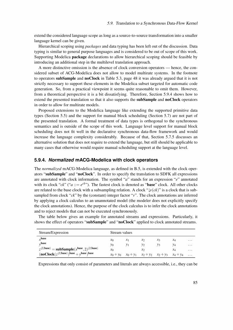
5.9. Translation to a Synchronous Data-Flow Kernel

extend the considered language scope as long as a source-to-source transformation into a smallerlanguage kernel can be given.

Hierarchical scoping using packages and data typing has been left out of the discussion. Datatyping is similar to general purpose languages and is considered to be out of scope of this work.Supporting Modelica package declarations to allow hierarchical scoping should be feasible byintroducing an additional step in the multilevel translation approach.

A more distinctive omission is the absence of clock conversion operators — hence, the con-sidered subset of ACG-Modelica does not allow to model multirate systems. In the footnoteto operators subSample and noClock in Table 5.3, page 48 it was already argued that it is notstrictly necessary to support these elements in the Modelica subset targeted for automatic codegeneration. So, from a practical viewpoint it seems quite reasonable to omit them. However,from a theoretical perspective it is a bit dissatisfying. Therefore, Section 5.9.4 shows how toextend the presented translation so that it also supports the subSample and noClock operatorsin order to allow for multirate models.

Proposed extensions to the Modelica language like extending the supported primitive datatypes (Section 5.5) and the support for manual block scheduling (Section 5.7) are not part ofthe presented translation. A formal treatment of data types is orthogonal to the synchronoussemantics and is outside of the scope of this work. Language level support for manual blockscheduling does not fit well in the declarative synchronous data-flow framework and wouldincrease the language complexity considerably. Because of that, Section 5.7.5 discusses analternative solution that does not require to extend the language, but still should be applicable tomany cases that otherwise would require manual scheduling support at the language level.

5.9.4. Normalized mACG-Modelica with clock operators

The normalized mACG-Modelica language, as defined in B.5, is extended with the clock oper-ators “subSample” and “noClock”. In order to specify the translation to SDFK all expressionsare annotated with clock information. The symbol “a” stands for an expression “e” annotatedwith its clock “ck” (“a ::= eck”). The fastest clock is denoted as “base” clock. All other clocksare related to the base clock with a subsampling relation. A clock “↓v(ck)” is a clock that is sub-sampled from clock “ck” by the (constant) integer factor “v”. The clock annotations are inferredby applying a clock calculus to an unannotated model (the modeler does not explicitly specifythe clock annotations). Hence, the purpose of the clock calculus is to infer the clock annotationsand to reject models that can not be executed synchronously.

The table below gives an example for annotated streams and expressions. Particularly, itshows the effect of operators “subSample” and “noClock” applied to clock annotated streams.

Stream/Expression Stream values

xbase x0 x1 x2 x3 x4 . . .ybase y0 y1 y2 y3 y4 . . .z↓2(base) = subSample(xbase,2)↓2(base) x0 x2 x4 . . .(noClock(z↓2(base))base + ybase)base x0 + y0 x0 + y1 x2 + y2 x2 + y3 x4 + y4 . . .

Expressions that only consist of parameters and literals are always accessible, i.e., they can be

85

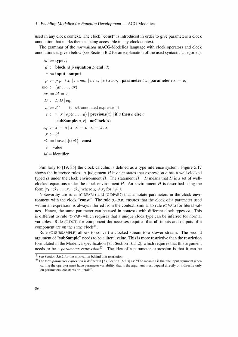
5. Enabling Modelica for Function Development — ACG-Modelica

used in any clock context. The clock “const” is introduced in order to give parameters a clockannotation that marks them as being accessible in any clock context.

The grammar of the normalized mACG-Modelica language with clock operators and clockannotations is given below (see Section B.2 for an explanation of the used syntactic categories).

td ::= type t;

d ::= block id p equation D end id;

c ::= input | outputp ::= p p | t x; | t x mo; | c t x; | c t x mo; | parameter t x | parameter t x = e;

mo ::= (ar , . . . , ar)

ar ::= id = e

D ::= D D | eq;

a ::= eck (clock annotated expression)

e ::= v | x | op(a, . . . ,a) | previous(x) | if a then a else a

| subSample(a,v) | noClock(a)eq ::= x = a | x . x = a | x = x . x

x ::= id

ck ::= base | ↓v(ck) | constv = value

id = identifier

Similarly to [19, 35] the clock calculus is defined as a type inference system. Figure 5.17shows the inference rules. A judgement H ` e : ct states that expression e has a well-clockedtyped ct under the clock environment H. The statement H ` D means that D is a set of well-clocked equations under the clock environment H. An environment H is described using theform [x1 : ck1, . . . ,xn : ckn] where xi 6= x j for i 6= j.

Noteworthy are rules (C-DPAR1) and (C-DPAR2) that annotate parameters in the clock envi-ronment with the clock “const”. The rule (C-PAR) ensures that the clock of a parameter usedwithin an expression is always inferred from the context, similar to rule (C-VAL) for literal val-ues. Hence, the same parameter can be used in contexts with different clock types ck. Thisis different to rule (C-VAR) which requires that a unique clock type can be inferred for normalvariables. Rule (C-DOT) for component dot accesses requires that all inputs and outputs of acomponent are on the same clock24.

Rule (C-SUBSAMPLE) allows to convert a clocked stream to a slower stream. The secondargument of “subSample” needs to be a literal value. This is more restrictive than the restrictionformulated in the Modelica specification [73, Section 16.5.2], which requires that this argumentneeds to be a parameter expression25. The idea of a parameter expression is that it can be24See Section 5.6.2 for the motivation behind that restriction.25The term parameter expression is defined in [73, Section 16.2.3] as: “The meaning is that the input argument when

calling the operator must have parameter variability, that is the argument must depend directly or indirectly onlyon parameters, constants or literals”.

86

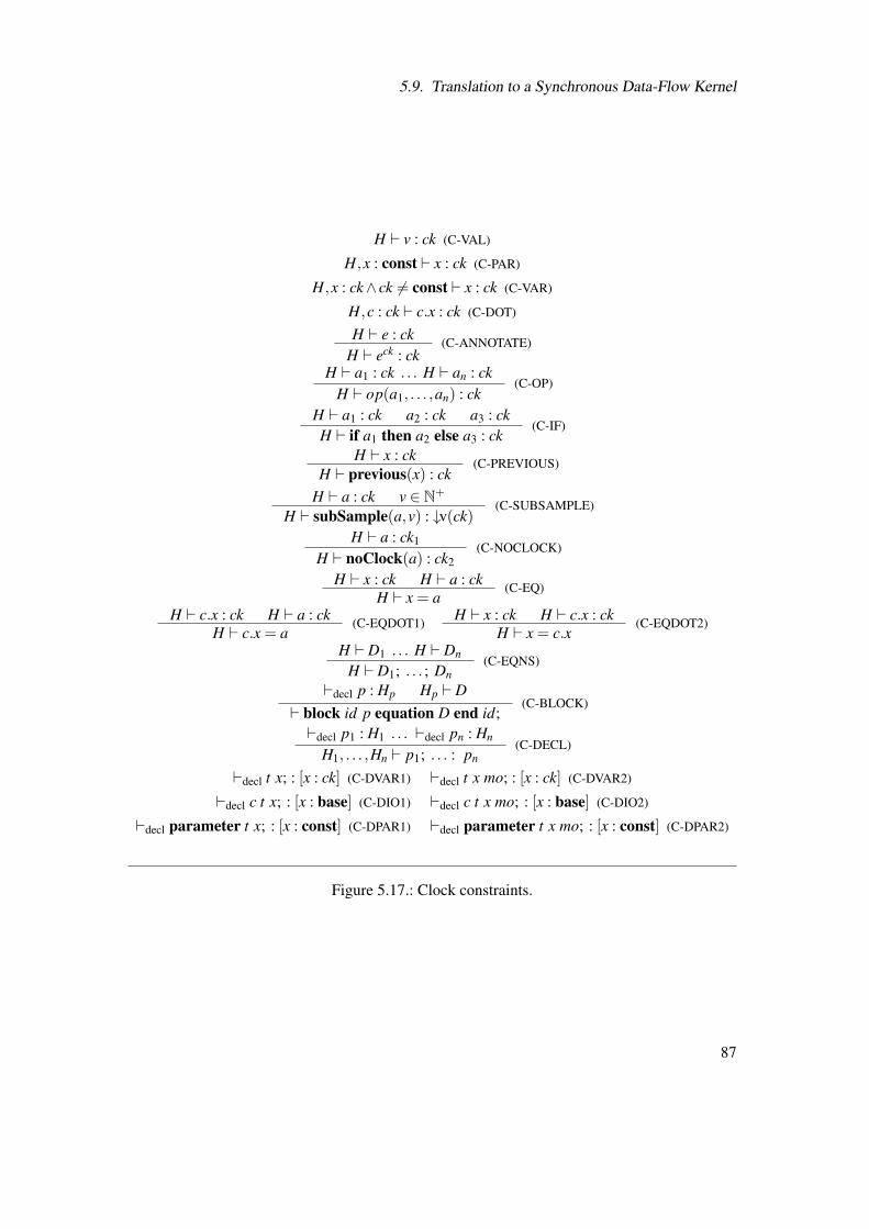
5.9. Translation to a Synchronous Data-Flow Kernel

H ` v : ck (C-VAL)

H,x : const ` x : ck (C-PAR)

H,x : ck∧ ck 6= const ` x : ck (C-VAR)

H,c : ck ` c.x : ck (C-DOT)

H ` e : ckH ` eck : ck

(C-ANNOTATE)

H ` a1 : ck . . . H ` an : ckH ` op(a1, . . . ,an) : ck

(C-OP)

H ` a1 : ck a2 : ck a3 : ckH ` if a1 then a2 else a3 : ck

(C-IF)

H ` x : ckH ` previous(x) : ck

(C-PREVIOUS)

H ` a : ck v ∈ N+

H ` subSample(a,v) : ↓v(ck)(C-SUBSAMPLE)

H ` a : ck1

H ` noClock(a) : ck2(C-NOCLOCK)

H ` x : ck H ` a : ckH ` x = a

(C-EQ)

H ` c.x : ck H ` a : ckH ` c.x = a

(C-EQDOT1) H ` x : ck H ` c.x : ckH ` x = c.x

(C-EQDOT2)

H ` D1 . . . H ` Dn

H ` D1; . . . ; Dn(C-EQNS)

`decl p : Hp Hp ` D` block id p equation D end id;

(C-BLOCK)

`decl p1 : H1 . . . `decl pn : Hn

H1, . . . ,Hn ` p1; . . . : pn(C-DECL)

`decl t x; : [x : ck] (C-DVAR1) `decl t x mo; : [x : ck] (C-DVAR2)

`decl c t x; : [x : base] (C-DIO1) `decl c t x mo; : [x : base] (C-DIO2)

`decl parameter t x; : [x : const] (C-DPAR1) `decl parameter t x mo; : [x : const] (C-DPAR2)

Figure 5.17.: Clock constraints.

87

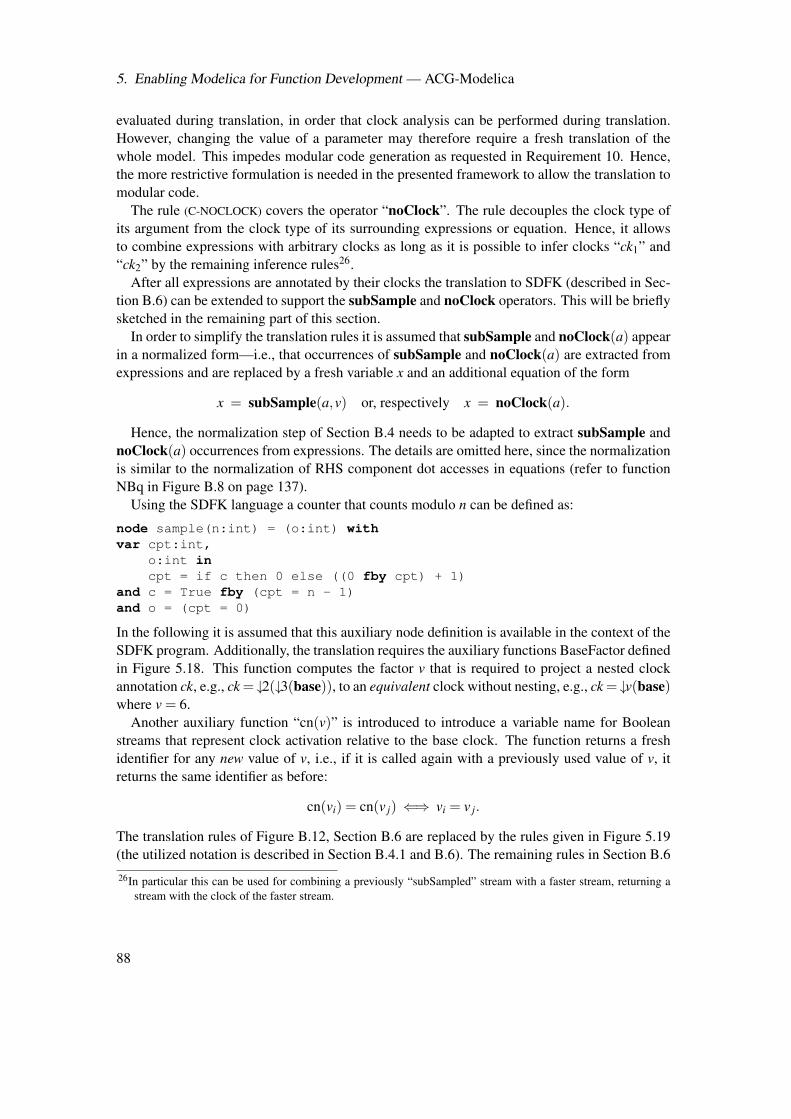
5. Enabling Modelica for Function Development — ACG-Modelica

evaluated during translation, in order that clock analysis can be performed during translation.However, changing the value of a parameter may therefore require a fresh translation of thewhole model. This impedes modular code generation as requested in Requirement 10. Hence,the more restrictive formulation is needed in the presented framework to allow the translation tomodular code.

The rule (C-NOCLOCK) covers the operator “noClock”. The rule decouples the clock type ofits argument from the clock type of its surrounding expressions or equation. Hence, it allowsto combine expressions with arbitrary clocks as long as it is possible to infer clocks “ck1” and“ck2” by the remaining inference rules26.

After all expressions are annotated by their clocks the translation to SDFK (described in Sec-tion B.6) can be extended to support the subSample and noClock operators. This will be brieflysketched in the remaining part of this section.

In order to simplify the translation rules it is assumed that subSample and noClock(a) appearin a normalized form—i.e., that occurrences of subSample and noClock(a) are extracted fromexpressions and are replaced by a fresh variable x and an additional equation of the form

x = subSample(a,v) or, respectively x = noClock(a).

Hence, the normalization step of Section B.4 needs to be adapted to extract subSample andnoClock(a) occurrences from expressions. The details are omitted here, since the normalizationis similar to the normalization of RHS component dot accesses in equations (refer to functionNBq in Figure B.8 on page 137).

Using the SDFK language a counter that counts modulo n can be defined as:

node sample(n:int) = (o:int) withvar cpt:int,

o:int incpt = if c then 0 else ((0 fby cpt) + 1)

and c = True fby (cpt = n - 1)and o = (cpt = 0)

In the following it is assumed that this auxiliary node definition is available in the context of theSDFK program. Additionally, the translation requires the auxiliary functions BaseFactor definedin Figure 5.18. This function computes the factor v that is required to project a nested clockannotation ck, e.g., ck = ↓2(↓3(base)), to an equivalent clock without nesting, e.g., ck = ↓v(base)where v = 6.

Another auxiliary function “cn(v)” is introduced to introduce a variable name for Booleanstreams that represent clock activation relative to the base clock. The function returns a freshidentifier for any new value of v, i.e., if it is called again with a previously used value of v, itreturns the same identifier as before:

cn(vi) = cn(v j) ⇐⇒ vi = v j.

The translation rules of Figure B.12, Section B.6 are replaced by the rules given in Figure 5.19(the utilized notation is described in Section B.4.1 and B.6). The remaining rules in Section B.626In particular this can be used for combining a previously “subSampled” stream with a faster stream, returning a

stream with the clock of the faster stream.

88

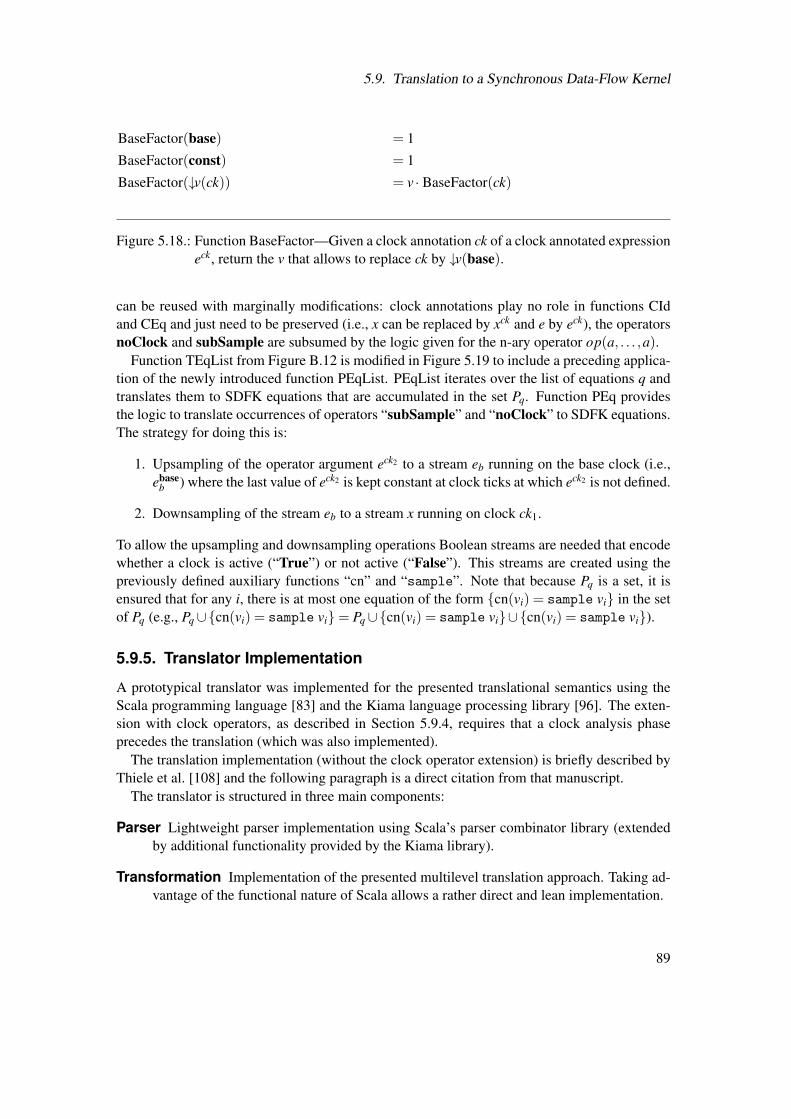
5.9. Translation to a Synchronous Data-Flow Kernel

BaseFactor(base) = 1

BaseFactor(const) = 1

BaseFactor(↓v(ck)) = v · BaseFactor(ck)

Figure 5.18.: Function BaseFactor—Given a clock annotation ck of a clock annotated expressioneck, return the v that allows to replace ck by ↓v(base).

can be reused with marginally modifications: clock annotations play no role in functions CIdand CEq and just need to be preserved (i.e., x can be replaced by xck and e by eck), the operatorsnoClock and subSample are subsumed by the logic given for the n-ary operator op(a, . . . ,a).

Function TEqList from Figure B.12 is modified in Figure 5.19 to include a preceding applica-tion of the newly introduced function PEqList. PEqList iterates over the list of equations q andtranslates them to SDFK equations that are accumulated in the set Pq. Function PEq providesthe logic to translate occurrences of operators “subSample” and “noClock” to SDFK equations.The strategy for doing this is:

1. Upsampling of the operator argument eck2 to a stream eb running on the base clock (i.e.,ebase

b ) where the last value of eck2 is kept constant at clock ticks at which eck2 is not defined.

2. Downsampling of the stream eb to a stream x running on clock ck1.

To allow the upsampling and downsampling operations Boolean streams are needed that encodewhether a clock is active (“True”) or not active (“False”). This streams are created using thepreviously defined auxiliary functions “cn” and “sample”. Note that because Pq is a set, it isensured that for any i, there is at most one equation of the form cn(vi) = sample vi in the setof Pq (e.g., Pq∪cn(vi) = sample vi= Pq∪cn(vi) = sample vi∪cn(vi) = sample vi).

5.9.5. Translator Implementation

A prototypical translator was implemented for the presented translational semantics using theScala programming language [83] and the Kiama language processing library [96]. The exten-sion with clock operators, as described in Section 5.9.4, requires that a clock analysis phaseprecedes the translation (which was also implemented).

The translation implementation (without the clock operator extension) is briefly described byThiele et al. [108] and the following paragraph is a direct citation from that manuscript.

The translator is structured in three main components:

Parser Lightweight parser implementation using Scala’s parser combinator library (extendedby additional functionality provided by the Kiama library).

Transformation Implementation of the presented multilevel translation approach. Taking ad-vantage of the functional nature of Scala allows a rather direct and lean implementation.

89

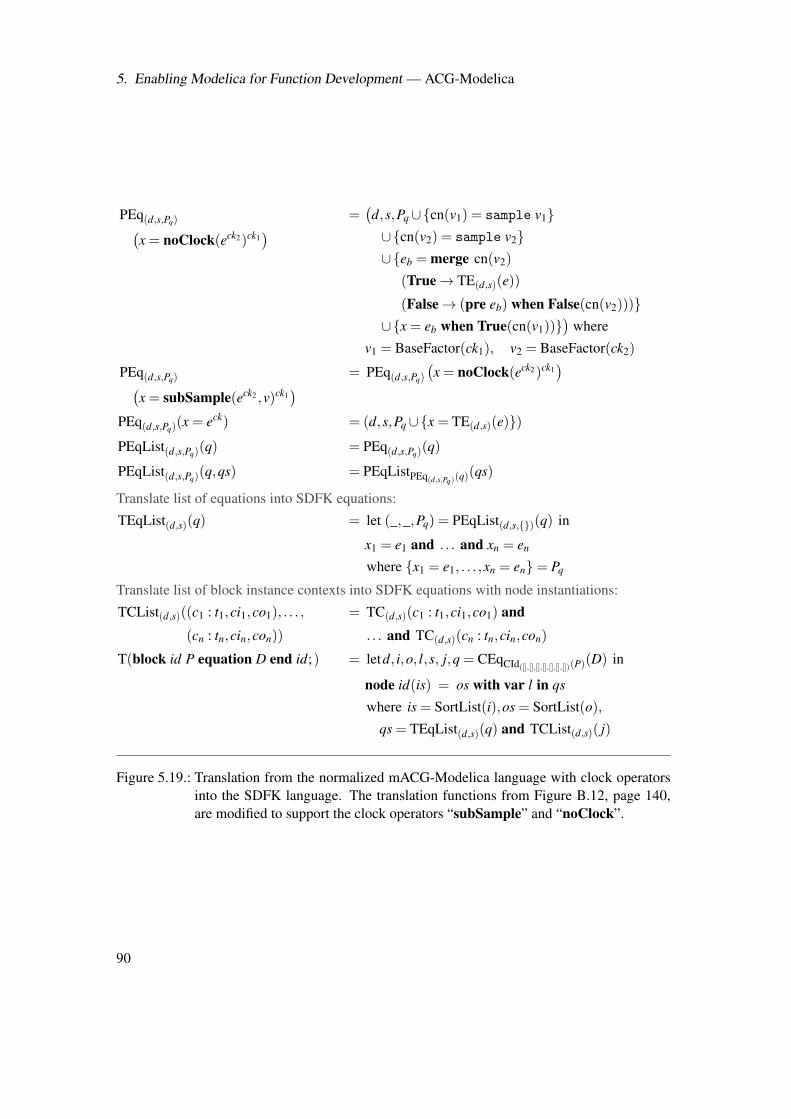
5. Enabling Modelica for Function Development — ACG-Modelica

PEq(d,s,Pq)(x = noClock(eck2)ck1

) =(d,s,Pq∪cn(v1) = sample v1∪cn(v2) = sample v2∪eb = merge cn(v2)

(True→ TE(d,s)(e))

(False→ (pre eb) when False(cn(v2)))∪x = eb when True(cn(v1))

)where

v1 = BaseFactor(ck1), v2 = BaseFactor(ck2)

PEq(d,s,Pq)(x = subSample(eck2 ,v)ck1

) = PEq(d,s,Pq)

(x = noClock(eck2)ck1

)PEq(d,s,Pq)(x = eck) = (d,s,Pq∪x = TE(d,s)(e))

PEqList(d,s,Pq)(q) = PEq(d,s,Pq)(q)

PEqList(d,s,Pq)(q,qs) = PEqListPEq(d,s,Pq)(q)(qs)

Translate list of equations into SDFK equations:

TEqList(d,s)(q) = let (_,_,Pq) = PEqList(d,s,)(q) in

x1 = e1 and . . . and xn = en

where x1 = e1, . . . ,xn = en= Pq

Translate list of block instance contexts into SDFK equations with node instantiations:

TCList(d,s)((c1 : t1,ci1,co1), . . . ,

(cn : tn,cin,con))

= TC(d,s)(c1 : t1,ci1,co1) and. . . and TC(d,s)(cn : tn,cin,con)

T(block id P equation D end id;) = letd, i,o, l,s, j,q = CEqCId([],[],[],[],[],[],[])(P)(D) in

node id(is) = os with var l in qs

where is = SortList(i),os = SortList(o),

qs = TEqList(d,s)(q) and TCList(d,s)( j)

Figure 5.19.: Translation from the normalized mACG-Modelica language with clock operatorsinto the SDFK language. The translation functions from Figure B.12, page 140,are modified to support the clock operators “subSample” and “noClock”.

90

5.10. Further Extensions to ACG-Modelica

Emitter Emitters to the SDFK language defined in Section B.1 and to Lustre code. The emit-ter component utilizes the functional pretty printing combinators provided by the Kiamalibrary.

The SDFK output is not executable and needs to be checked statically (currently by manualinspection). The Lustre output allows taking advantage of the software infrastructure that isavailable around Lustre. Particularly, using Lustre as intermediate presentation allows to gen-erate executable C-code utilizing Verimag’s Lustre V4 Toolbox27. This C-code can be used fordynamic testing. The translator supports that by allowing to generate appropriate Modelica codeadapters (“C code wrapper blocks”) that provide an interface from Modelica to the generated Ccode (using Modelica’s external function interface). These wrappers can be directly loaded intoModelica simulation environments, enabling convenient back-to-back testing.

Section 6.4 demonstrates the use of the wrapper block feature for SIL validation in the contextof a servo system example.

5.10. Further Extensions to ACG-Modelica

This section comments briefly on further extensions to ACG-Modelica that are likely to be ofinterest to developers.

5.10.1. Inheritance

Inheritance is a powerful concept in object-oriented programming and it is supported in Mod-elica, but excluded in ACG-Modelica. The Modelica language provides rather intricate waysto combine (multiple) inheritance with structural modifications that highly increase languagecomplexity. Keeping language complexity to a minimum is the reason why inheritance is notsupported in the presented ACG-Modelica language. However, extending ACG-Modelica tosupport a suitably restricted form of inheritance seems quite feasible.

5.10.2. State Machines

While data-flow parts in control applications are naturally described with block diagrams, sys-tem logic parts are often described naturally using state machine formalisms. Modelica 3.3added built-in language elements to support state machines [73, Chapter 17] with a compara-ble modeling power as Statecharts [53]. Extending synchronous data-flow with state machineshas been described in pioneering work of Maraninchi and Rémond on Mode-Automata [71, 72]and also by Colaço et al. [34]. Colaço et al. describe a synchronous data-flow kernel languagewhich is extended with language elements for Mode-Automata and provide a translational se-mantics from that extended language set to the basic synchronous data-flow kernel language.Extending ACG-Modelica with support for state machines in a similar way is desirable, but it isa substantial challenge on its own.

27The Lustre V4 Toolbox is available from the VERIMAG research center (2014), http://www-verimag.imag.fr/.

91

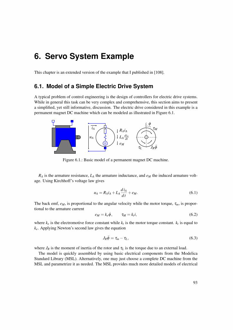
6. Servo System Example

This chapter is an extended version of the example that I published in [108].

6.1. Model of a Simple Electric Drive System

A typical problem of control engineering is the design of controllers for electric drive systems.While in general this task can be very complex and comprehensive, this section aims to presenta simplified, yet still informative, discussion. The electric drive considered in this example is apermanent magnet DC machine which can be modeled as illustrated in Figure 6.1.

uA

iA τM

JRφ

φ

τL

RAiA

eM

LAdiAdt

Figure 6.1.: Basic model of a permanent magnet DC machine.

RA is the armature resistance, LA the armature inductance, and eM the induced armature volt-age. Using Kirchhoff’s voltage law gives

uA = RAiA +LAd iAd t

+ eM. (6.1)

The back emf, eM, is proportional to the angular velocity while the motor torque, τm, is propor-tional to the armature current

eM = keφ , τM = kt i, (6.2)

where ke is the electromotive force constant while kt is the motor torque constant. kt is equal toke. Applying Newton’s second law gives the equation

JRφ = τm− τL, (6.3)

where JR is the moment of inertia of the rotor and τL is the torque due to an external load.The model is quickly assembled by using basic electrical components from the Modelica

Standard Library (MSL). Alternatively, one may just choose a complete DC machine from theMSL and parametrize it as needed. The MSL provides much more detailed models of electrical

93

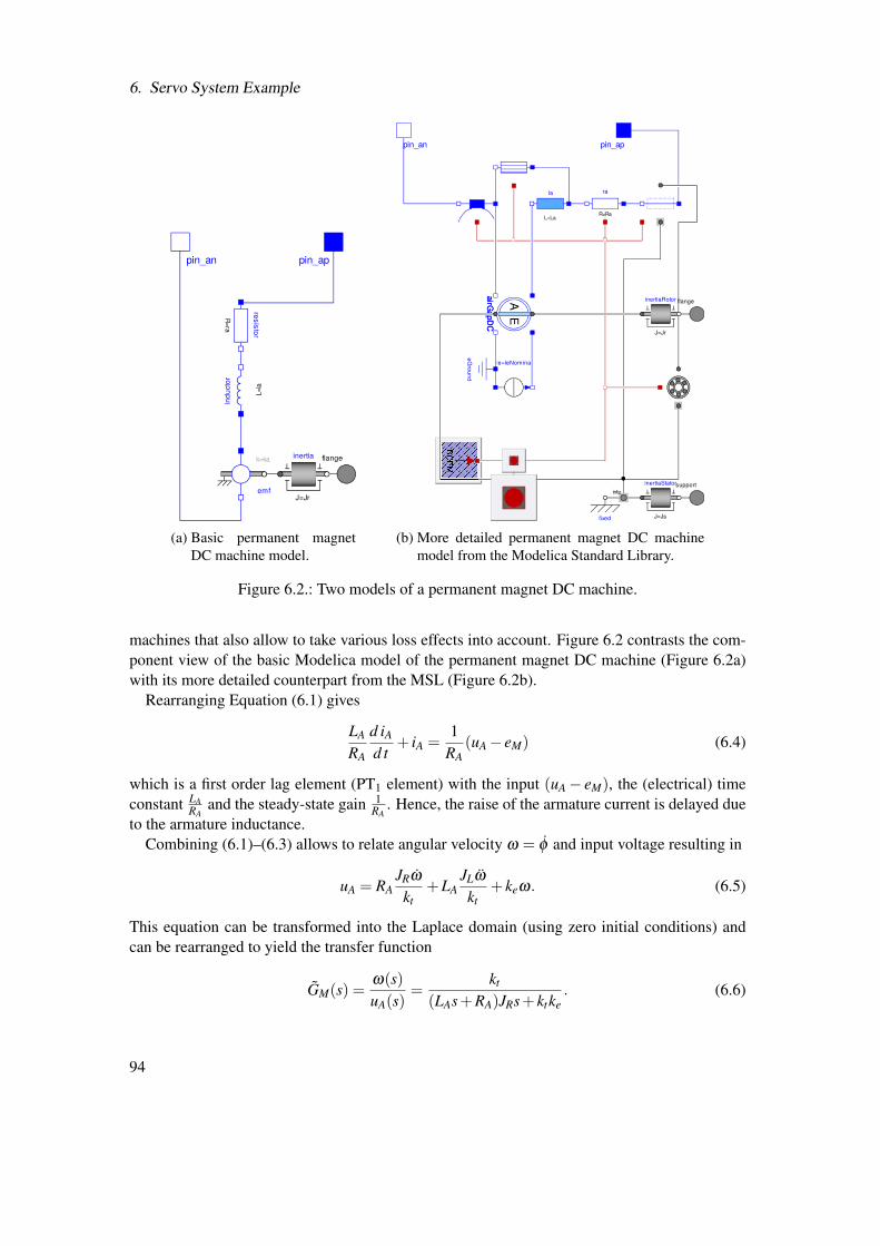
6. Servo System Example

emf

k=ka

R=ra

resistor

inertia

J=Jr

L=la

indu

ctor

flange

pin_appin_an

(a) Basic permanent magnetDC machine model.

inertiaRotor

J=Jr

inertiaStator

J=Jsfixed

R=Ra

ra

L=La

la

E

airGapDC

AairGapDC

eGround

ie=IeNominal

flange

supportinte

pin_appin_an

(b) More detailed permanent magnet DC machinemodel from the Modelica Standard Library.

Figure 6.2.: Two models of a permanent magnet DC machine.

machines that also allow to take various loss effects into account. Figure 6.2 contrasts the com-ponent view of the basic Modelica model of the permanent magnet DC machine (Figure 6.2a)with its more detailed counterpart from the MSL (Figure 6.2b).

Rearranging Equation (6.1) gives

LA

RA

d iAd t

+ iA =1

RA(uA− eM) (6.4)

which is a first order lag element (PT1 element) with the input (uA− eM), the (electrical) timeconstant LA

RAand the steady-state gain 1

RA. Hence, the raise of the armature current is delayed due

to the armature inductance.Combining (6.1)–(6.3) allows to relate angular velocity ω = φ and input voltage resulting in

uA = RAJRω

kt+LA

JLω

kt+ keω. (6.5)

This equation can be transformed into the Laplace domain (using zero initial conditions) andcan be rearranged to yield the transfer function

GM(s) =ω(s)uA(s)

=kt

(LAs+RA)JRs+ ktke. (6.6)

94

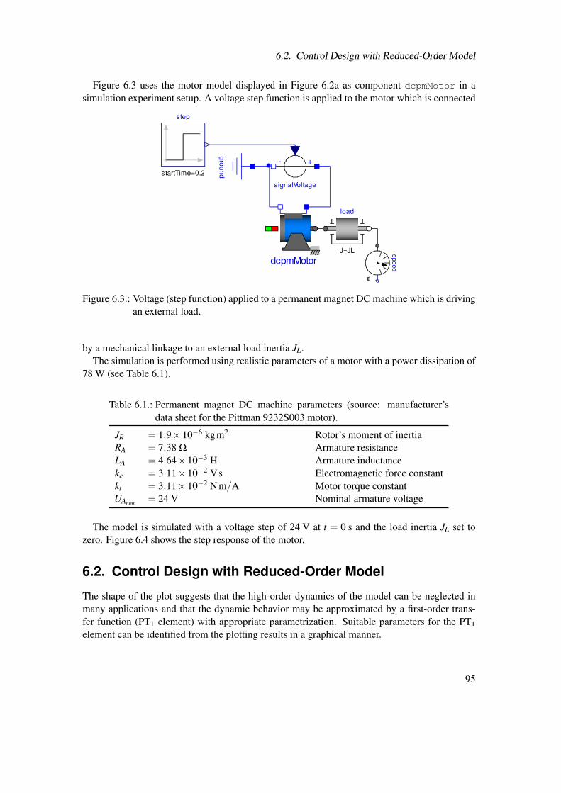
6.2. Control Design with Reduced-Order Model

Figure 6.3 uses the motor model displayed in Figure 6.2a as component dcpmMotor in asimulation experiment setup. A voltage step function is applied to the motor which is connected

speed

ws ignalVoltage

+-

ground

load

J=JLdcpmMotor

step

startTime=0.2

Figure 6.3.: Voltage (step function) applied to a permanent magnet DC machine which is drivingan external load.

by a mechanical linkage to an external load inertia JL.The simulation is performed using realistic parameters of a motor with a power dissipation of

78 W (see Table 6.1).

Table 6.1.: Permanent magnet DC machine parameters (source: manufacturer’sdata sheet for the Pittman 9232S003 motor).

JR = 1.9×10−6 kgm2 Rotor’s moment of inertiaRA = 7.38 Ω Armature resistanceLA = 4.64×10−3 H Armature inductanceke = 3.11×10−2 Vs Electromagnetic force constantkt = 3.11×10−2 Nm/A Motor torque constantUAnom = 24 V Nominal armature voltage

The model is simulated with a voltage step of 24 V at t = 0 s and the load inertia JL set tozero. Figure 6.4 shows the step response of the motor.

6.2. Control Design with Reduced-Order Model

The shape of the plot suggests that the high-order dynamics of the model can be neglected inmany applications and that the dynamic behavior may be approximated by a first-order trans-fer function (PT1 element) with appropriate parametrization. Suitable parameters for the PT1element can be identified from the plotting results in a graphical manner.

95

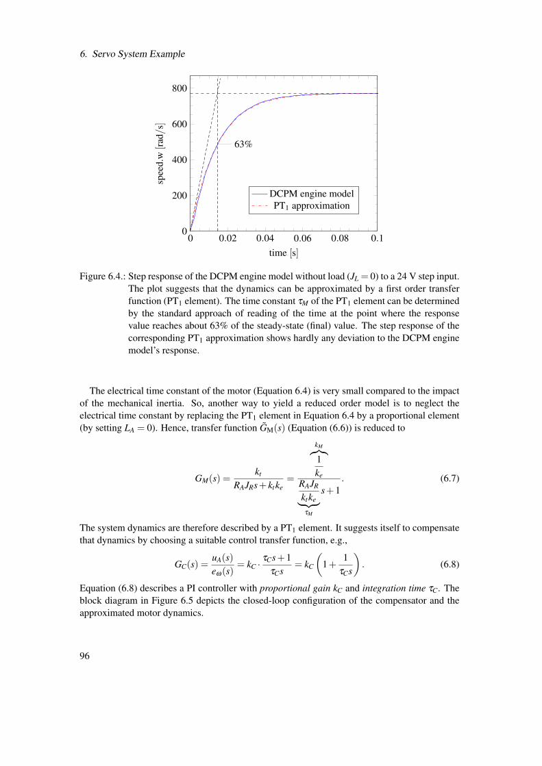
6. Servo System Example

0 0.02 0.04 0.06 0.08 0.10

200

400

600

800

63%

time [s]

spee

d.w[r

ad/

s]

DCPM engine modelPT1 approximation

Figure 6.4.: Step response of the DCPM engine model without load (JL = 0) to a 24 V step input.The plot suggests that the dynamics can be approximated by a first order transferfunction (PT1 element). The time constant τM of the PT1 element can be determinedby the standard approach of reading of the time at the point where the responsevalue reaches about 63% of the steady-state (final) value. The step response of thecorresponding PT1 approximation shows hardly any deviation to the DCPM enginemodel’s response.

The electrical time constant of the motor (Equation 6.4) is very small compared to the impactof the mechanical inertia. So, another way to yield a reduced order model is to neglect theelectrical time constant by replacing the PT1 element in Equation 6.4 by a proportional element(by setting LA = 0). Hence, transfer function GM(s) (Equation (6.6)) is reduced to

GM(s) =kt

RAJRs+ ktke=

kM︷︸︸︷1ke

RAJR

ktke︸ ︷︷ ︸τM

s+1. (6.7)

The system dynamics are therefore described by a PT1 element. It suggests itself to compensatethat dynamics by choosing a suitable control transfer function, e.g.,

GC(s) =uA(s)eω(s)

= kC ·τCs+1

τCs= kC

(1+

1τCs

). (6.8)

Equation (6.8) describes a PI controller with proportional gain kC and integration time τC. Theblock diagram in Figure 6.5 depicts the closed-loop configuration of the compensator and theapproximated motor dynamics.

96

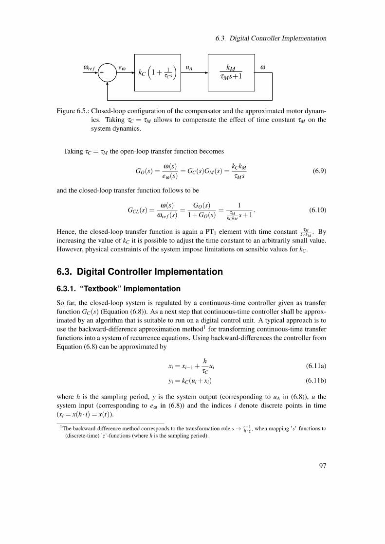
6.3. Digital Controller Implementation

uAeωωre f ωkMτMs+1kC

(1+ 1

τCs

)

Figure 6.5.: Closed-loop configuration of the compensator and the approximated motor dynam-ics. Taking τC = τM allows to compensate the effect of time constant τM on thesystem dynamics.

Taking τC = τM the open-loop transfer function becomes

GO(s) =ω(s)eω(s)

= GC(s)GM(s) =kCkM

τMs(6.9)

and the closed-loop transfer function follows to be

GCL(s) =ω(s)

ωre f (s)=

GO(s)1+GO(s)

=1

τMkCkM

s+1. (6.10)

Hence, the closed-loop transfer function is again a PT1 element with time constant τMkCkM

. Byincreasing the value of kC it is possible to adjust the time constant to an arbitrarily small value.However, physical constraints of the system impose limitations on sensible values for kC.

6.3. Digital Controller Implementation

6.3.1. “Textbook” Implementation

So far, the closed-loop system is regulated by a continuous-time controller given as transferfunction GC(s) (Equation (6.8)). As a next step that continuous-time controller shall be approx-imated by an algorithm that is suitable to run on a digital control unit. A typical approach is touse the backward-difference approximation method1 for transforming continuous-time transferfunctions into a system of recurrence equations. Using backward-differences the controller fromEquation (6.8) can be approximated by

xi = xi−1 +hτC

ui (6.11a)

yi = kC(ui + xi) (6.11b)

where h is the sampling period, y is the system output (corresponding to uA in (6.8)), u thesystem input (corresponding to eω in (6.8)) and the indices i denote discrete points in time(xi = x(h · i) = x(t)).

1The backward-difference method corresponds to the transformation rule s→ z−1h ·z , when mapping ’s’-functions to

(discrete-time) ’z’-functions (where h is the sampling period).

97

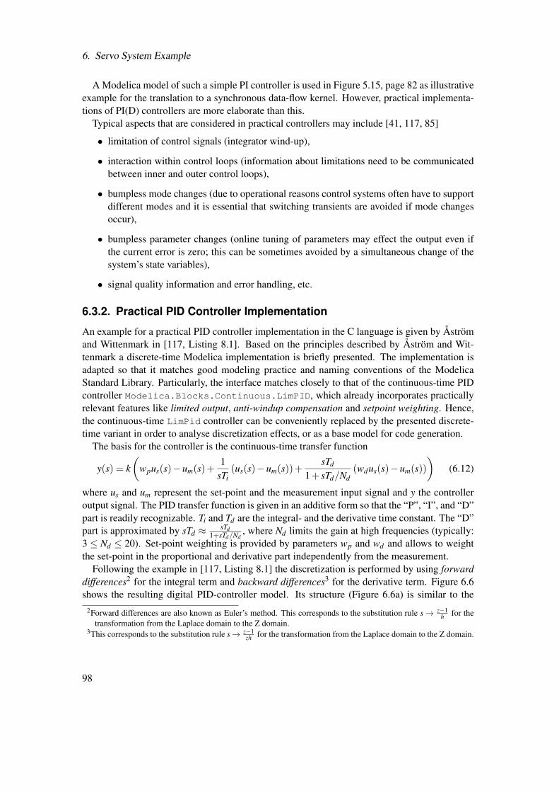
6. Servo System Example

A Modelica model of such a simple PI controller is used in Figure 5.15, page 82 as illustrativeexample for the translation to a synchronous data-flow kernel. However, practical implementa-tions of PI(D) controllers are more elaborate than this.

Typical aspects that are considered in practical controllers may include [41, 117, 85]

• limitation of control signals (integrator wind-up),

• interaction within control loops (information about limitations need to be communicatedbetween inner and outer control loops),

• bumpless mode changes (due to operational reasons control systems often have to supportdifferent modes and it is essential that switching transients are avoided if mode changesoccur),

• bumpless parameter changes (online tuning of parameters may effect the output even ifthe current error is zero; this can be sometimes avoided by a simultaneous change of thesystem’s state variables),

• signal quality information and error handling, etc.

6.3.2. Practical PID Controller Implementation

An example for a practical PID controller implementation in the C language is given by Åströmand Wittenmark in [117, Listing 8.1]. Based on the principles described by Åström and Wit-tenmark a discrete-time Modelica implementation is briefly presented. The implementation isadapted so that it matches good modeling practice and naming conventions of the ModelicaStandard Library. Particularly, the interface matches closely to that of the continuous-time PIDcontroller Modelica.Blocks.Continuous.LimPID, which already incorporates practicallyrelevant features like limited output, anti-windup compensation and setpoint weighting. Hence,the continuous-time LimPid controller can be conveniently replaced by the presented discrete-time variant in order to analyse discretization effects, or as a base model for code generation.

The basis for the controller is the continuous-time transfer function

y(s) = k(

wpus(s)−um(s)+1

sTi(us(s)−um(s))+

sTd

1+ sTd/Nd(wdus(s)−um(s))

)(6.12)

where us and um represent the set-point and the measurement input signal and y the controlleroutput signal. The PID transfer function is given in an additive form so that the “P”, “I”, and “D”part is readily recognizable. Ti and Td are the integral- and the derivative time constant. The “D”part is approximated by sTd ≈ sTd

1+sTd/Nd, where Nd limits the gain at high frequencies (typically:

3 ≤ Nd ≤ 20). Set-point weighting is provided by parameters wp and wd and allows to weightthe set-point in the proportional and derivative part independently from the measurement.

Following the example in [117, Listing 8.1] the discretization is performed by using forwarddifferences2 for the integral term and backward differences3 for the derivative term. Figure 6.6shows the resulting digital PID-controller model. Its structure (Figure 6.6a) is similar to the

2Forward differences are also known as Euler’s method. This corresponds to the substitution rule s→ z−1h for the

transformation from the Laplace domain to the Z domain.3This corresponds to the substitution rule s→ z−1

zh for the transformation from the Laplace domain to the Z domain.

98

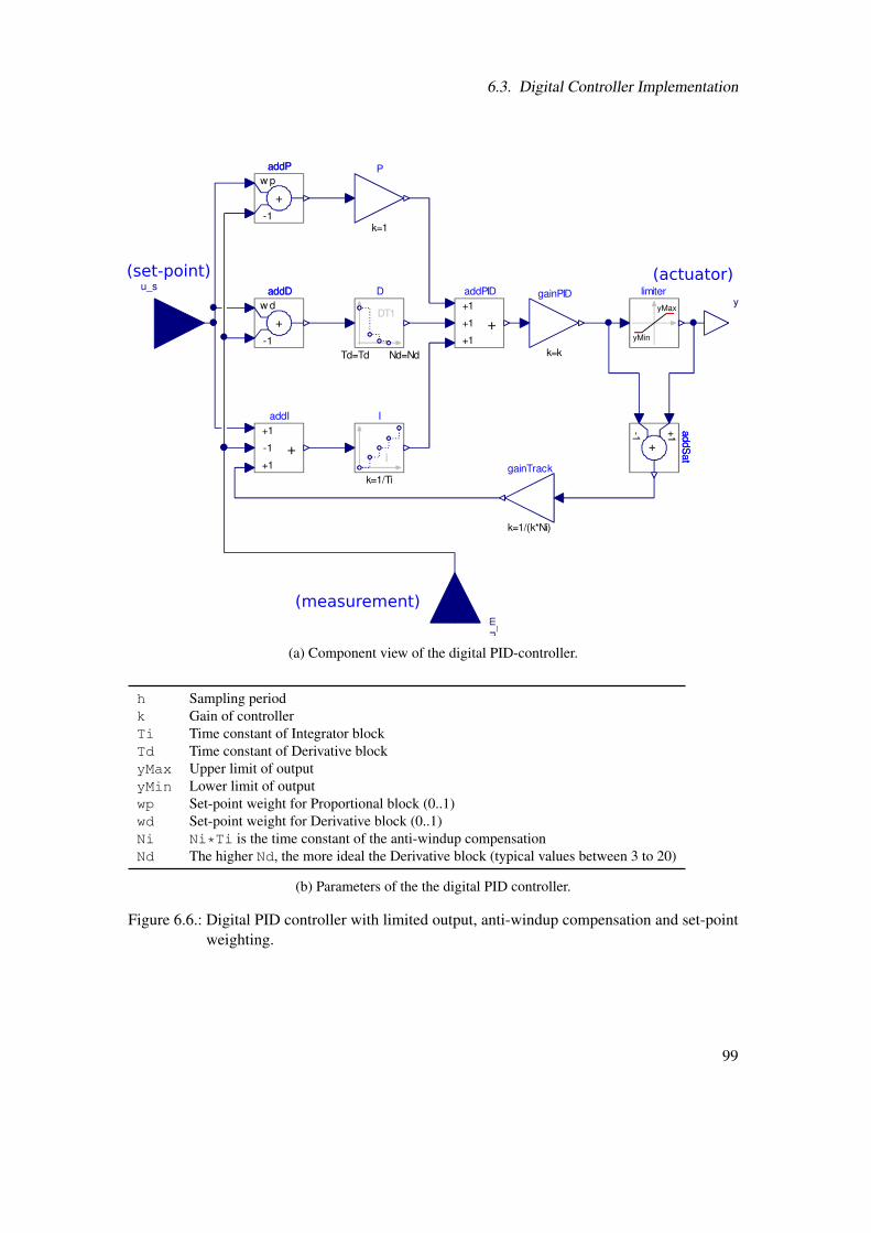
6.3. Digital Controller Implementation

addP

+wp

-1

addP

addD

+wd

-1

addD

k=1

P

I

I

k=1/Ti

D

DT1

Td=Td Nd=Nd k=k

gainPIDaddPID+1

+1

+1+

addI+1

-1

+1+

addSat

++1-1 addS

at

k=1/(k*Ni)

gainTrack

limiter

yMax

yMin

u_s

u_m

y

(set-point) (actuator)

(measurement)

(a) Component view of the digital PID-controller.

h Sampling periodk Gain of controllerTi Time constant of Integrator blockTd Time constant of Derivative blockyMax Upper limit of outputyMin Lower limit of outputwp Set-point weight for Proportional block (0..1)wd Set-point weight for Derivative block (0..1)Ni Ni*Ti is the time constant of the anti-windup compensationNd The higher Nd, the more ideal the Derivative block (typical values between 3 to 20)

(b) Parameters of the the digital PID controller.

Figure 6.6.: Digital PID controller with limited output, anti-windup compensation and set-pointweighting.

99

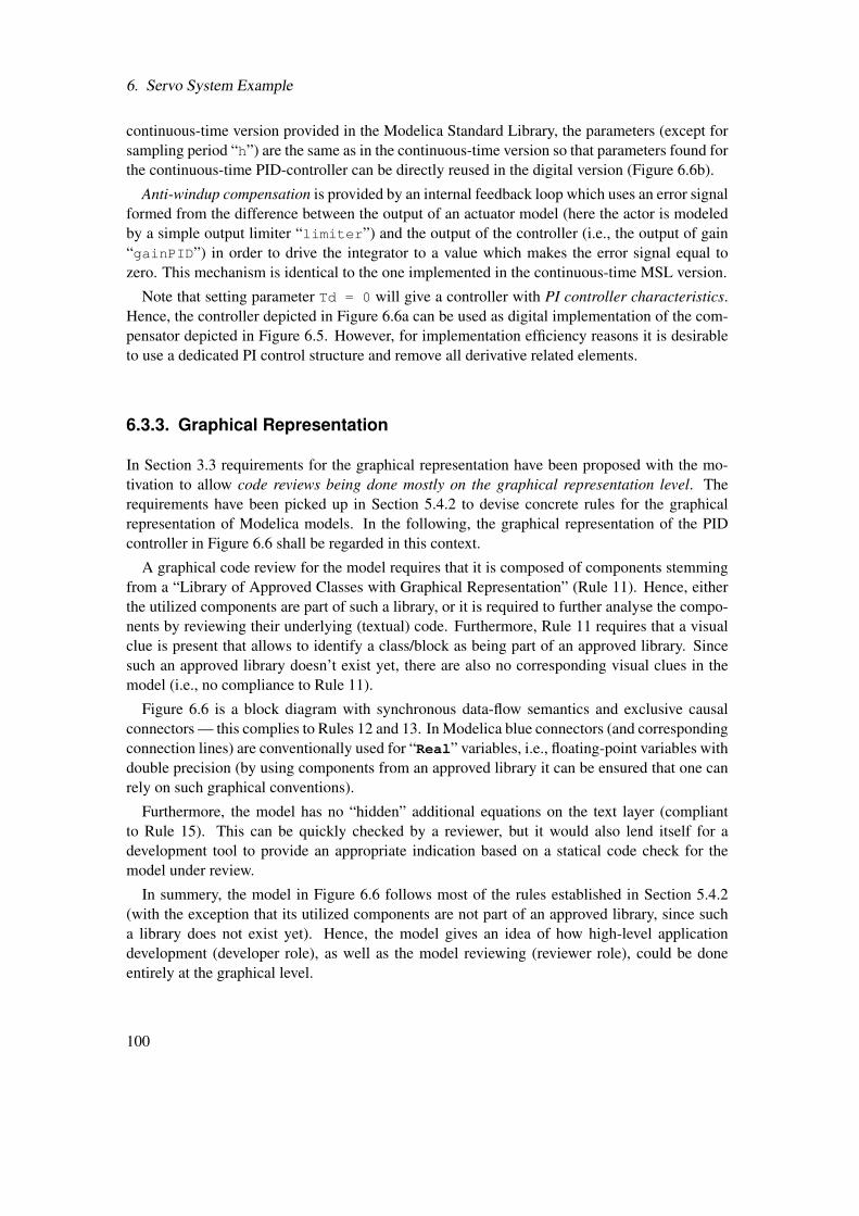
6. Servo System Example

continuous-time version provided in the Modelica Standard Library, the parameters (except forsampling period “h”) are the same as in the continuous-time version so that parameters found forthe continuous-time PID-controller can be directly reused in the digital version (Figure 6.6b).

Anti-windup compensation is provided by an internal feedback loop which uses an error signalformed from the difference between the output of an actuator model (here the actor is modeledby a simple output limiter “limiter”) and the output of the controller (i.e., the output of gain“gainPID”) in order to drive the integrator to a value which makes the error signal equal tozero. This mechanism is identical to the one implemented in the continuous-time MSL version.

Note that setting parameter Td = 0 will give a controller with PI controller characteristics.Hence, the controller depicted in Figure 6.6a can be used as digital implementation of the com-pensator depicted in Figure 6.5. However, for implementation efficiency reasons it is desirableto use a dedicated PI control structure and remove all derivative related elements.

6.3.3. Graphical Representation

In Section 3.3 requirements for the graphical representation have been proposed with the mo-tivation to allow code reviews being done mostly on the graphical representation level. Therequirements have been picked up in Section 5.4.2 to devise concrete rules for the graphicalrepresentation of Modelica models. In the following, the graphical representation of the PIDcontroller in Figure 6.6 shall be regarded in this context.

A graphical code review for the model requires that it is composed of components stemmingfrom a “Library of Approved Classes with Graphical Representation” (Rule 11). Hence, eitherthe utilized components are part of such a library, or it is required to further analyse the compo-nents by reviewing their underlying (textual) code. Furthermore, Rule 11 requires that a visualclue is present that allows to identify a class/block as being part of an approved library. Sincesuch an approved library doesn’t exist yet, there are also no corresponding visual clues in themodel (i.e., no compliance to Rule 11).

Figure 6.6 is a block diagram with synchronous data-flow semantics and exclusive causalconnectors — this complies to Rules 12 and 13. In Modelica blue connectors (and correspondingconnection lines) are conventionally used for “Real” variables, i.e., floating-point variables withdouble precision (by using components from an approved library it can be ensured that one canrely on such graphical conventions).

Furthermore, the model has no “hidden” additional equations on the text layer (compliantto Rule 15). This can be quickly checked by a reviewer, but it would also lend itself for adevelopment tool to provide an appropriate indication based on a statical code check for themodel under review.

In summery, the model in Figure 6.6 follows most of the rules established in Section 5.4.2(with the exception that its utilized components are not part of an approved library, since sucha library does not exist yet). Hence, the model gives an idea of how high-level applicationdevelopment (developer role), as well as the model reviewing (reviewer role), could be doneentirely at the graphical level.

100

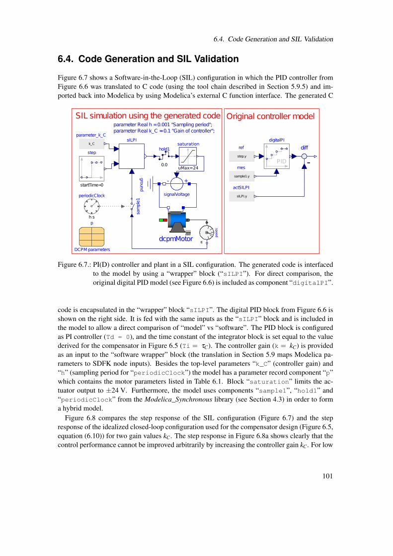
6.4. Code Generation and SIL Validation

6.4. Code Generation and SIL Validation

Figure 6.7 shows a Software-in-the-Loop (SIL) configuration in which the PID controller fromFigure 6.6 was translated to C code (using the tool chain described in Section 5.9.5) and im-ported back into Modelica by using Modelica’s external C function interface. The generated C

SIL simulation using the generated code Original controller modelparameter Real h =0.001 "Sampling period";parameter Real k_C =0.1 "Gain of controller";

p

DCPM parameters

speed

wsignalVoltage

+-

ground

dcpmMotor

digitalPI

PID

sam

ple1

periodicClock

h s

0.0

hold1step

startTime=0

sILPI

step.y

refk_C

parameter_k_C

sample1.y

mes-

diff

sILPI.y

actSILPI

uMax=24

saturation

Figure 6.7.: PI(D) controller and plant in a SIL configuration. The generated code is interfacedto the model by using a “wrapper” block (“sILPI”). For direct comparison, theoriginal digital PID model (see Figure 6.6) is included as component “digitalPI”.

code is encapsulated in the “wrapper” block “sILPI”. The digital PID block from Figure 6.6 isshown on the right side. It is fed with the same inputs as the “sILPI” block and is included inthe model to allow a direct comparison of “model” vs “software”. The PID block is configuredas PI controller (Td = 0), and the time constant of the integrator block is set equal to the valuederived for the compensator in Figure 6.5 (Ti = τC). The controller gain (k = kC) is providedas an input to the “software wrapper” block (the translation in Section 5.9 maps Modelica pa-rameters to SDFK node inputs). Besides the top-level parameters “k_C” (controller gain) and“h” (sampling period for “periodicClock”) the model has a parameter record component “p”which contains the motor parameters listed in Table 6.1. Block “saturation” limits the ac-tuator output to ±24 V. Furthermore, the model uses components “sample1”, “hold1” and“periodicClock” from the Modelica_Synchronous library (see Section 4.3) in order to forma hybrid model.

Figure 6.8 compares the step response of the SIL configuration (Figure 6.7) and the stepresponse of the idealized closed-loop configuration used for the compensator design (Figure 6.5,equation (6.10)) for two gain values kC. The step response in Figure 6.8a shows clearly that thecontrol performance cannot be improved arbitrarily by increasing the controller gain kC. For low

101

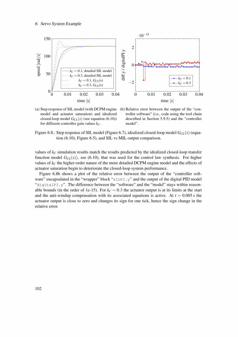
6. Servo System Example

0 0.01 0.02 0.03 0.040

50

100

150

time [s]

spee

d[r

ad/

s]

kC = 0.1, detailed SIL modelkC = 0.3, detailed SIL model

kC = 0.1, GCL(s)kC = 0.3, GCL(s)

(a) Step response of SIL model (with DCPM enginemodel and actuator saturation) and idealizedclosed-loop model GCL(s) (see equation (6.10))for different controller gain values kC.

0 0.01 0.02 0.03 0.04

−2

0

2

·10−15

time [s]

diff

.y/d

igita

lPI.y

kC = 0.1kC = 0.3

(b) Relative error between the output of the “con-troller software” (i.e., code using the tool chaindescribed in Section 5.9.5) and the “controllermodel”.

Figure 6.8.: Step response of SIL model (Figure 6.7), idealized closed-loop model GCL(s) (equa-tion (6.10), Figure 6.5), and SIL vs MIL output comparison.

values of kC simulation results match the results predicted by the idealized closed-loop transferfunction model GCL(s)), see (6.10), that was used for the control law synthesis. For highervalues of kC the higher-order nature of the more detailed DCPM engine model and the effects ofactuator saturation begin to deteriorate the closed-loop system performance.

Figure 6.8b shows a plot of the relative error between the output of the “controller soft-ware” encapsulated in the “wrapper” block “sILPI.y” and the output of the digital PID model“digitalPI.y”. The difference between the “software” and the “model” stays within reason-able bounds (in the order of 1e-15). For kC = 0.3 the actuator output is at its limits at the startand the anti-windup compensation with its associated equations is active. At t = 0.005 s theactuator output is close to zero and changes its sign for one tick, hence the sign change in therelative error.

102

7. Discussion and Conclusions

7.1. Discussion

This thesis had the goal to devise a development methodology that is capable of integrating twoworlds: State-of-the-art modeling for (safety-related) digital control functions and state-of-the-art modeling for multi-domain physical systems.

Due to different communities state-of-the-art modeling languages for software functions haveevolved very differently from modeling languages targeted for physical systems. However, mod-ern products rely increasingly on the tight integration of computation and physical processes,where computation in networked embedded computers affects physical processes and vice versa.These kinds of systems have been termed cyber-physical systems. The development of such sys-tems requires more integrated development approaches that reconcile state-of-the-art modelingmethodology for software functions and multi-domain physical systems.

This thesis used the modeling language Modelica as a base to address the challenge of in-tegrated software and physical modeling. Modelica’s modeling capabilities for multi-domainphysical models can be considered as the state-of-the-art in this field and therefore satisfy therequirements in this respect. However, despite some efforts, it is so far not practicable to useModelica for safety-related digital control functions. Hence, the main effort of this thesis wasto extend the state-of-the-art by establishing foundations that allow to use Modelica for safety-related digital control functions.

Chapter 1 and 2 motivate the research effort and recapitulate the most relevant backgroundinformation.

Chapter 3 establishes a set of requirements (including their rationale) for model-based func-tion development from the authors perspective. These requirements form the base for identifyingcurrent deficiencies in the Modelica language and to propose respective remedies.

Chapter 4 describes the synchronous language elements extension, which is a recent extensionto the Modelica language that particularly addresses improved modeling of discrete-time controlsystems. The synchronous language elements, to which the author contributed, is the base forlanguage extensions, restrictions and associated methods that are elaborated on in the remainingchapters. The extensions add the notion of clock activation of discrete-time equations. Themodel of computation within such partitions of discrete-time equations (clocked partitions) isbased on the same synchronous paradigm as synchronous data-flow languages like Lustre orSCADE. The chapter contrasts this new approach to previous Modelica support for sampled-data systems and explains why the new approach is superior.

Despite that recent improvements, important requirements for model-based function devel-opment have still not been met. Identifying this deficiencies and developing remedies is thepurpose of Chapter 5.

103

7. Discussion and Conclusions

The chapter proposes language restrictions and extensions deemed suitable to enable Model-ica to be used for safety-related (control) function development. The resulting language sub- andsuperset of Modelica is termed as ACG-Modelica. It is a central goal of the thesis to facilitatethe development of a qualifiable automatic code generator (ACG) for this language set. It isimportant to understand that such an ACG may share little or no code with a typical Modelicacompiler used for compiling simulation binaries (see Section 5.2).

The feasibility of qualifying a code generator is directly related to the complexity of the inputlanguage. Modelica is a very complex language, impeding attempts to implement a qualifiablecode generator. However, it is possible to reduce language complexity significantly for codegeneration models (i.e., the discrete-time “software” part of the model for which many languageelements for physical modeling are not needed). The proposed restrictions therefore representa compromise that carefully strives to balance language expressivity (to suit the developers)and simplicity (to suit tool qualifiers). This compromise is inevitably subjective, however mucheffort has been spent not to make it arbitrarily. Proposed restrictions are justified and traced backto the requirements established in Chapter 3 (see Sections 5.4 and 5.8). As a result, the languagecomplexity of ACG-Modelica is significantly reduced.

Besides language restrictions, Chapter 5 also proposes several language extensions. Theseextensions are motivated by perceived limitations of the current language standard. These limi-tations are addressed and a remediation proposal is worked out.

Section 5.5 proposes an extension to allow more fine-grained control over the data types usedon an (embedded) target platform. For efficiency reasons, it is also proposed to introduce bitwiseoperations as a built-in language feature.

Section 5.6 adds the notion of “atomic” blocks in order to enable modular code generationtechniques. Several advantages are identified for modular code generation: (i) it enables sep-arate compilation, which has advantages in respect to scalability and protection of intellectualproperty, (ii) it improves the traceability from the model to the generated code, which is ben-eficial for high-integrity code generation, (iii) it allows improved code sharing, which reducesthe size of code footprint, (iv) it facilitates the combination of generated code with handwrittencode, and last but not least (v) it facilitates to generate code which is well-structured and adheresto good software engineering practice. The last point allows to pass a generated code artifactinto a standard assurance process for handwritten code. This property is not strictly needed ifthe tool chain (including the ACG) has been qualified up to a suitable level within the intendedapplication domain — however, this may not always be the case. In such cases at least someeffort can be saved if code can be generated (instead of writing it by hand), even if the code mustsubsequently go through a standard assurance process (e.g., by performing code inspections onthe generated code).

Section 5.7 explains why more manual control over the scheduling of blocks is desirable forsome use cases. Besides a language extension proposal to enable manual block scheduling thesection also proposes an alternative solution based on a modeling pattern. The modeling patternbased solution is not as powerful, but should be adequate for many use cases. Its important ad-vantage is that it can be realized using existing language capabilities which make it the preferredsolution for ACG-Modelica.

Section 5.8 discusses trade-offs between acausal and causal data-flow semantics. It demon-strates that Modelica’s acausal data-flow can be problematic in safety-related applications. While

104

7.2. Future Work

adequate safeguarding mechanisms should be able to mitigate perceived problems the simple so-lution proposed for ACG-Modelica is to use causal data-flow semantics exclusively. Note thatany valid ACG-Modelica program based on causal data-flow is also a valid (acausal data-flow)Modelica program. The inverse is not true. Besides, causal data-flow is the standard seman-tics used in control engineering so that this restriction should be well acceptable for a controloriented subset of the Modelica language.

In the context of this thesis, Section 5.9 is of particular importance: it provides a formalizedargument that it is possible to develop a qualifiable automatic code generator for an appropriatecontrol-oriented subset of Modelica. This argument is obtained by (i) introducing a synchronousdata-flow kernel language (SDFK) considered suitable to allow the proposition that a qualifiableautomatic code generation can be implemented for it, (ii) definition of a representative Mod-elica language kernel (mACG-Modelica), and (iii) definition of a set of translation equationsfrom mACG-Modelica to SDFK (i.e., translational semantics of mACG-Modelica in terms ofSDFK). In addition to the formal translation equations the section briefly reports on a concreteprototypical translator that was implemented as part of the research efforts.

The translation provides two novelties: (i) a theoretical justification for the feasibility of de-veloping a qualifiable automatic code-generator for Modelica and (ii) a base that can be usedto develop a gateway from Modelica to existing qualifiable code generators based on the syn-chronous data-flow paradigm, e.g., SCADE/KCG.

Chapter 6 provides an elaborated example of using Modelica as a framework for model-basedfunction development. The example targets a typical control engineering task: design of a dig-ital controller for an electric drive system (servo control system). It illustrates that a typicaldevelopment process requires models of varying fidelity that suffice for different purposes, e.g.,reduced-order continuous-time plant models in order to apply established control law synthe-sis methods, discrete-time controller models that approximate continuous-time control design toenable digital controller implementations, high-fidelity hybrid models in order to evaluate andfine-tune system performance.

Section 6.3 seizes aspects of practical controller implementations that are often omitted inmore theoretical oriented control design “textbooks” and presents a practical-oriented PID con-troller model for automatic code generation. The controller is modeled using the ACG-Modelicalanguage subset and the prototypical translator for that subset is used to generate code. The gen-erated code is interfaced to the simulation tool for software-in-the-loop simulation. Results ofsoftware- and model-in-the-loop simulation are compared against each other. In summary, theservo control system example illustrates how important aspects of model-based developmentcan be handled in a compelling integrated and seamless fashion using the proposed Modelicaframework.

7.2. Future Work

This thesis proposes a path to a qualifiable automatic code generator for Modelica and providestheoretical as well as practical evidence for the feasibility of such an undertaking. An obviouspoint for the future is to use these results as a base and develop and qualify an industry-strengthcode generator — an undertaking that is expected to require a (semi-) commercial effort, since

105

7. Discussion and Conclusions

it can hardly be achieved in a purely academic setting.Naturally, there are many options and directions for extending the language subset and sup-

porting additional features. Any such extensions will need to renegotiate the balance betweentool qualification efforts and language expressiveness. Particularly, the support of inheritanceand built-in language support for state machines modeling as discussed in Section 5.10 are can-didates for future extensions.

In the context of modern Modelica compiler technology, further more visionary extensionssuggest themselves. Section 2.4 reported about high-level prototypical work using Modelicatechnology for advanced model-based controller designs. These works leverage the powerfulsymbolic equation manipulation capabilities available in some Modelica tools to synthesize non-linear inverse models for control or enable nonlinear model predictive control approaches. Itis an interesting research question how such capabilities can be reconciled with safety-relateddevelopment objectives. A promising approach could be to present critical symbolic transforma-tions by the development tool in a human-checkable form that allows to validate them manually.Novel methods for debugging equation-based languages already keep track of symbolic trans-formations during the translation process [86]. Whether this methods could also be leveragedto validate critical transformations occurring during code generation for advanced model-basedcontrollers is a topic for future research.

7.3. Conclusion

The motivation for this thesis effort was the lack of a development methodology that is capa-ble of integrating two worlds: state-of-the-art modeling for multi-domain physical systems andstate-of-the-art modeling for (safety-related) digital control functions. The thesis addressed thegap that so far prevented using Modelica for the later, i.e., adequate language expressivenessfor discrete-time controller functions and production quality automatic code generation. Bothaspects have been addressed by restricting and extending Modelica to a language set termedACG-Modelica and investigating a formal translation of this language to an established syn-chronous data-flow kernel language for which production quality code-generation techniquesare known and implemented in industrial code generators for safety-relevant embedded soft-ware. The semantic distance between ACG-Modelica and the synchronous data-flow kernel hasshown to be wider than initially expected which is reflected in the complexity of the translationequations that have been deduced. The concluding servo system example illustrates the inter-play between physical modeling and controller modeling within the envisioned Modelica basedfunction development framework.

106

A. Introduction to Modelica

Modelica can be called an equation-based object-oriented (EOO) language. That term, coinedby Broman [22], nicely subsumes the central, distinguishing language characteristics.

Equation-based: behavior is described declaratively using mathematical equations.

Object-oriented: Objects encapsulate behavior and constitute building blocks that are used tobuild more complex objects.

A.1. Object-orientation

The term object-oriented is not to be understood in exactly the same way like in common object-oriented programming (OOP) languages like Smalltalk, C++ or Java. In OOP languages objectsare instances of classes that comprise data + methods. Objects behave by methods that arecalled from other objects or by sending or receiving messages.

In contrast to method calls or message passing, behavior in EOO languages is described byequations. Therefore EOO language objects are instances of classes that basically comprisedata + equations.

Similar to common OOP languages Modelica also supports mechanisms like inheritance andsubtyping-polymorphism. Note that in Modelica objects are termed components, while classesare often referred to as models.

Modelica provides annotations that can be used to define a graphical component representa-tion. Professional Modelica development environments typically provide a graphical diagramview in which models can be composed from such annotated components in a drag-and-dropstyle. Figure A.1 shows diagram views of a complete vehicle system model assembled fromModelica components spanning several domains such as powertrain, thermo, and multi-bodydynamics.

A.2. Equation-based Behavior Modeling

Equations have been used as adequate notation for capturing system dynamic behavior overmany centuries. The key characteristic of EOO languages is to directly use declarative mathe-matical equations for describing system dynamic behavior.

Modelica currently provides support for models described by

• ordinary differential equations (ODE),

• algebraic equations,

107

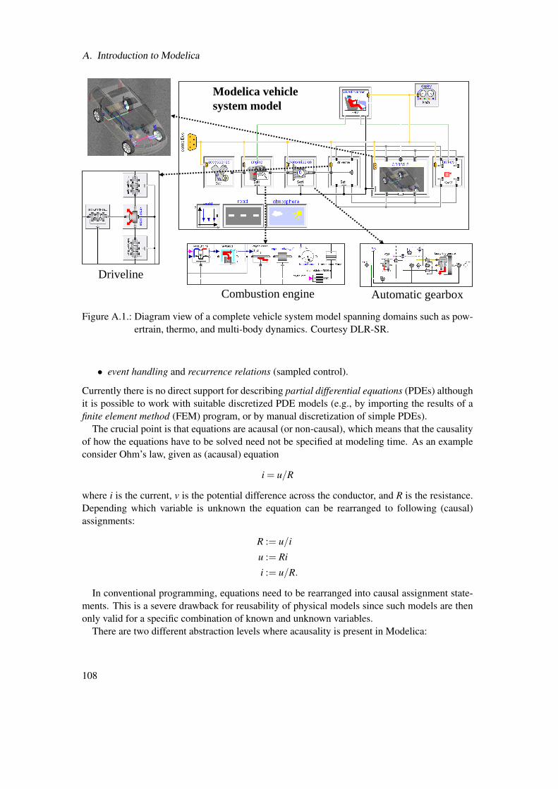
A. Introduction to Modelica

Modelica vehicle

system model

Automatic gearbox Combustion engine

Driveline

Figure A.1.: Diagram view of a complete vehicle system model spanning domains such as pow-ertrain, thermo, and multi-body dynamics. Courtesy DLR-SR.

• event handling and recurrence relations (sampled control).

Currently there is no direct support for describing partial differential equations (PDEs) althoughit is possible to work with suitable discretized PDE models (e.g., by importing the results of afinite element method (FEM) program, or by manual discretization of simple PDEs).

The crucial point is that equations are acausal (or non-causal), which means that the causalityof how the equations have to be solved need not be specified at modeling time. As an exampleconsider Ohm’s law, given as (acausal) equation

i = u/R

where i is the current, v is the potential difference across the conductor, and R is the resistance.Depending which variable is unknown the equation can be rearranged to following (causal)assignments:

R := u/i

u := Ri

i := u/R.

In conventional programming, equations need to be rearranged into causal assignment state-ments. This is a severe drawback for reusability of physical models since such models are thenonly valid for a specific combination of known and unknown variables.

There are two different abstraction levels where acausality is present in Modelica:

108

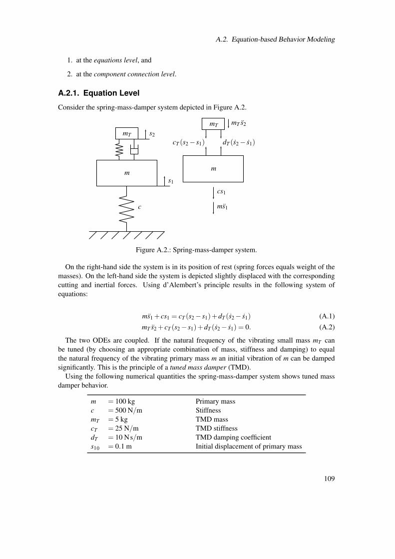
A.2. Equation-based Behavior Modeling

1. at the equations level, and

2. at the component connection level.

A.2.1. Equation Level

Consider the spring-mass-damper system depicted in Figure A.2.

m

c

s1

m

cs1

ms1

mT s2

mT mT s2

cT (s2− s1) dT (s2− s1)

Figure A.2.: Spring-mass-damper system.

On the right-hand side the system is in its position of rest (spring forces equals weight of themasses). On the left-hand side the system is depicted slightly displaced with the correspondingcutting and inertial forces. Using d’Alembert’s principle results in the following system ofequations:

ms1 + cs1 = cT (s2− s1)+dT (s2− s1) (A.1)

mT s2 + cT (s2− s1)+dT (s2− s1) = 0. (A.2)

The two ODEs are coupled. If the natural frequency of the vibrating small mass mT canbe tuned (by choosing an appropriate combination of mass, stiffness and damping) to equalthe natural frequency of the vibrating primary mass m an initial vibration of m can be dampedsignificantly. This is the principle of a tuned mass damper (TMD).

Using the following numerical quantities the spring-mass-damper system shows tuned massdamper behavior.

m = 100 kg Primary massc = 500 N/m StiffnessmT = 5 kg TMD masscT = 25 N/m TMD stiffnessdT = 10 Ns/m TMD damping coefficients10 = 0.1 m Initial displacement of primary mass

109

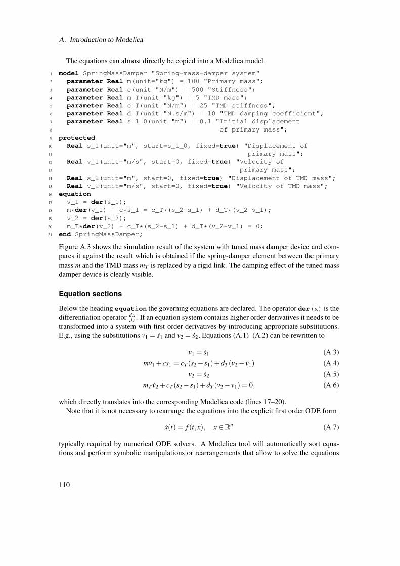
A. Introduction to Modelica

The equations can almost directly be copied into a Modelica model.

1 model SpringMassDamper "Spring-mass-damper system"2 parameter Real m(unit="kg") = 100 "Primary mass";3 parameter Real c(unit="N/m") = 500 "Stiffness";4 parameter Real m_T(unit="kg") = 5 "TMD mass";5 parameter Real c_T(unit="N/m") = 25 "TMD stiffness";6 parameter Real d_T(unit="N.s/m") = 10 "TMD damping coefficient";7 parameter Real s_1_0(unit="m") = 0.1 "Initial displacement8 of primary mass";9 protected

10 Real s_1(unit="m", start=s_1_0, fixed=true) "Displacement of11 primary mass";12 Real v_1(unit="m/s", start=0, fixed=true) "Velocity of13 primary mass";14 Real s_2(unit="m", start=0, fixed=true) "Displacement of TMD mass";15 Real v_2(unit="m/s", start=0, fixed=true) "Velocity of TMD mass";16 equation17 v_1 = der(s_1);18 m*der(v_1) + c*s_1 = c_T*(s_2-s_1) + d_T*(v_2-v_1);19 v_2 = der(s_2);20 m_T*der(v_2) + c_T*(s_2-s_1) + d_T*(v_2-v_1) = 0;21 end SpringMassDamper;

Figure A.3 shows the simulation result of the system with tuned mass damper device and com-pares it against the result which is obtained if the spring-damper element between the primarymass m and the TMD mass mT is replaced by a rigid link. The damping effect of the tuned massdamper device is clearly visible.

Equation sections

Below the heading equation the governing equations are declared. The operator der(x) is thedifferentiation operator d x

d t . If an equation system contains higher order derivatives it needs to betransformed into a system with first-order derivatives by introducing appropriate substitutions.E.g., using the substitutions v1 = s1 and v2 = s2, Equations (A.1)–(A.2) can be rewritten to

v1 = s1 (A.3)

mv1 + cs1 = cT (s2− s1)+dT (v2− v1) (A.4)

v2 = s2 (A.5)

mT v2 + cT (s2− s1)+dT (v2− v1) = 0, (A.6)

which directly translates into the corresponding Modelica code (lines 17–20).Note that it is not necessary to rearrange the equations into the explicit first order ODE form

x(t) = f (t,x), x ∈ Rn (A.7)

typically required by numerical ODE solvers. A Modelica tool will automatically sort equa-tions and perform symbolic manipulations or rearrangements that allow to solve the equations

110

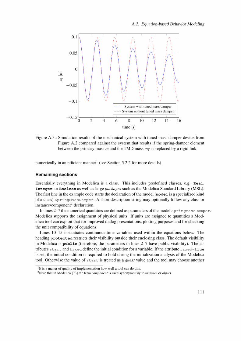
A.2. Equation-based Behavior Modeling

0 2 4 6 8 10 12 14 16−0.15

−0.1

−0.05

0

0.05

0.1

time [s]

s 1[m

]

System with tuned mass damperSystem without tuned mass damper

Figure A.3.: Simulation results of the mechanical system with tuned mass damper device fromFigure A.2 compared against the system that results if the spring-damper elementbetween the primary mass m and the TMD mass mT is replaced by a rigid link.

numerically in an efficient manner1 (see Section 5.2.2 for more details).

Remaining sections

Essentially everything in Modelica is a class. This includes predefined classes, e.g., Real,Integer, or Boolean as well as large packages such as the Modelica Standard Library (MSL).The first line in the example code starts the declaration of the model (model is a specialized kindof a class) SpringMassDamper. A short description string may optionally follow any class orinstance/component2 declaration.

In lines 2–7 the numerical quantities are defined as parameters of the model SpringMassDamper.Modelica supports the assignment of physical units. If units are assigned to quantities a Mod-elica tool can exploit that for improved dialog presentations, plotting purposes and for checkingthe unit compatibility of equations.

Lines 10–15 instantiates continuous-time variables used within the equations below. Theheading protected restricts their visibility outside their enclosing class. The default visibilityin Modelica is public (therefore, the parameters in lines 2–7 have public visibility). The at-tributes start and fixed define the initial condition for a variable. If the attribute fixed=trueis set, the initial condition is required to hold during the initialization analysis of the Modelicatool. Otherwise the value of start is treated as a guess value and the tool may choose another

1It is a matter of quality of implementation how well a tool can do this.2Note that in Modelica [73] the term component is used synonymously to instance or object.

111

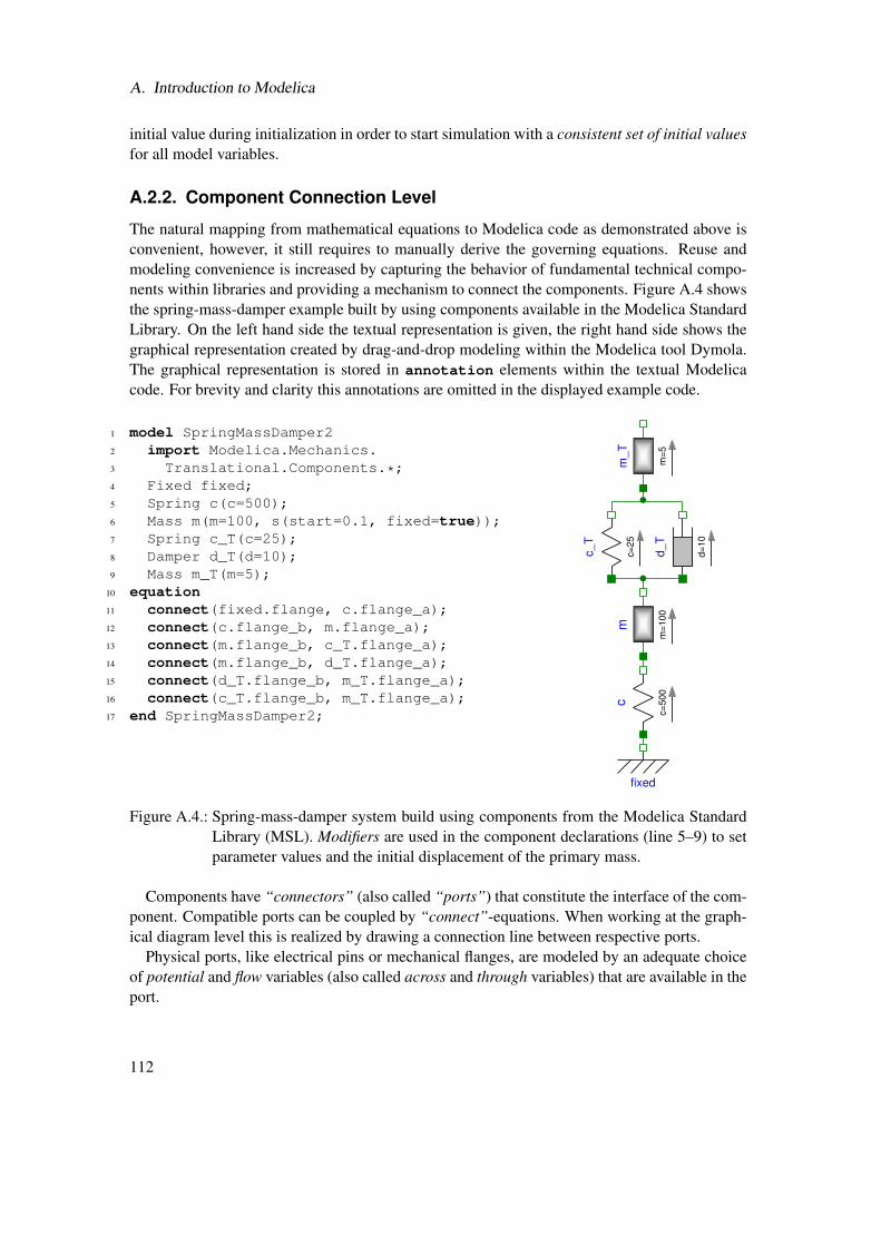
A. Introduction to Modelica

initial value during initialization in order to start simulation with a consistent set of initial valuesfor all model variables.

A.2.2. Component Connection Level

The natural mapping from mathematical equations to Modelica code as demonstrated above isconvenient, however, it still requires to manually derive the governing equations. Reuse andmodeling convenience is increased by capturing the behavior of fundamental technical compo-nents within libraries and providing a mechanism to connect the components. Figure A.4 showsthe spring-mass-damper example built by using components available in the Modelica StandardLibrary. On the left hand side the textual representation is given, the right hand side shows thegraphical representation created by drag-and-drop modeling within the Modelica tool Dymola.The graphical representation is stored in annotation elements within the textual Modelicacode. For brevity and clarity this annotations are omitted in the displayed example code.

1 model SpringMassDamper22 import Modelica.Mechanics.3 Translational.Components.*;4 Fixed fixed;5 Spring c(c=500);6 Mass m(m=100, s(start=0.1, fixed=true));7 Spring c_T(c=25);8 Damper d_T(d=10);9 Mass m_T(m=5);

10 equation11 connect(fixed.flange, c.flange_a);12 connect(c.flange_b, m.flange_a);13 connect(m.flange_b, c_T.flange_a);14 connect(m.flange_b, d_T.flange_a);15 connect(d_T.flange_b, m_T.flange_a);16 connect(c_T.flange_b, m_T.flange_a);17 end SpringMassDamper2;

fixed

c

c=50

0

m

m=1

00

c_T

c=25

d_T

d=10

m_T

m=5

Figure A.4.: Spring-mass-damper system build using components from the Modelica StandardLibrary (MSL). Modifiers are used in the component declarations (line 5–9) to setparameter values and the initial displacement of the primary mass.

Components have “connectors” (also called “ports”) that constitute the interface of the com-ponent. Compatible ports can be coupled by “connect”-equations. When working at the graph-ical diagram level this is realized by drawing a connection line between respective ports.

Physical ports, like electrical pins or mechanical flanges, are modeled by an adequate choiceof potential and flow variables (also called across and through variables) that are available in theport.

112

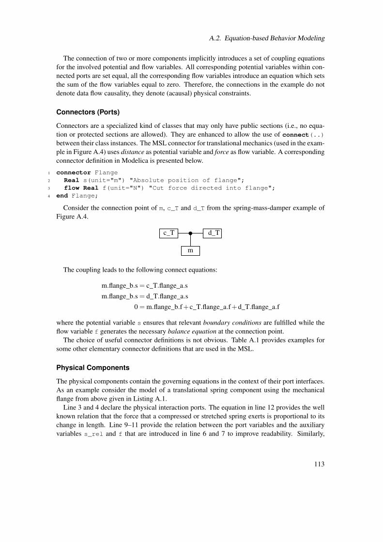
A.2. Equation-based Behavior Modeling

The connection of two or more components implicitly introduces a set of coupling equationsfor the involved potential and flow variables. All corresponding potential variables within con-nected ports are set equal, all the corresponding flow variables introduce an equation which setsthe sum of the flow variables equal to zero. Therefore, the connections in the example do notdenote data flow causality, they denote (acausal) physical constraints.

Connectors (Ports)

Connectors are a specialized kind of classes that may only have public sections (i.e., no equa-tion or protected sections are allowed). They are enhanced to allow the use of connect(..)between their class instances. The MSL connector for translational mechanics (used in the exam-ple in Figure A.4) uses distance as potential variable and force as flow variable. A correspondingconnector definition in Modelica is presented below.

1 connector Flange2 Real s(unit="m") "Absolute position of flange";3 flow Real f(unit="N") "Cut force directed into flange";4 end Flange;

Consider the connection point of m, c_T and d_T from the spring-mass-damper example ofFigure A.4.

m

c_T d_T

The coupling leads to the following connect equations:

m.flange_b.s = c_T.flange_a.s

m.flange_b.s = d_T.flange_a.s

0 = m.flange_b.f+ c_T.flange_a.f+d_T.flange_a.f

where the potential variable s ensures that relevant boundary conditions are fulfilled while theflow variable f generates the necessary balance equation at the connection point.

The choice of useful connector definitions is not obvious. Table A.1 provides examples forsome other elementary connector definitions that are used in the MSL.

Physical Components

The physical components contain the governing equations in the context of their port interfaces.As an example consider the model of a translational spring component using the mechanicalflange from above given in Listing A.1.

Line 3 and 4 declare the physical interaction ports. The equation in line 12 provides the wellknown relation that the force that a compressed or stretched spring exerts is proportional to itschange in length. Line 9–11 provide the relation between the port variables and the auxiliaryvariables s_rel and f that are introduced in line 6 and 7 to improve readability. Similarly,

113

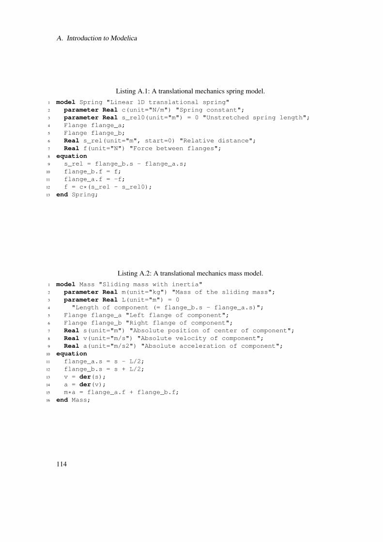
A. Introduction to Modelica

Listing A.1: A translational mechanics spring model.1 model Spring "Linear 1D translational spring"2 parameter Real c(unit="N/m") "Spring constant";3 parameter Real s_rel0(unit="m") = 0 "Unstretched spring length";4 Flange flange_a;5 Flange flange_b;6 Real s_rel(unit="m", start=0) "Relative distance";7 Real f(unit="N") "Force between flanges";8 equation9 s_rel = flange_b.s - flange_a.s;

10 flange_b.f = f;11 flange_a.f = -f;12 f = c*(s_rel - s_rel0);13 end Spring;

Listing A.2: A translational mechanics mass model.1 model Mass "Sliding mass with inertia"2 parameter Real m(unit="kg") "Mass of the sliding mass";3 parameter Real L(unit="m") = 04 "Length of component (= flange_b.s - flange_a.s)";5 Flange flange_a "Left flange of component";6 Flange flange_b "Right flange of component";7 Real s(unit="m") "Absolute position of center of component";8 Real v(unit="m/s") "Absolute velocity of component";9 Real a(unit="m/s2") "Absolute acceleration of component";

10 equation11 flange_a.s = s - L/2;12 flange_b.s = s + L/2;13 v = der(s);14 a = der(v);15 m*a = flange_a.f + flange_b.f;16 end Mass;

114

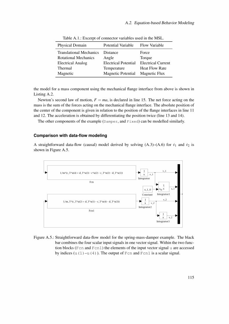
A.2. Equation-based Behavior Modeling

Table A.1.: Excerpt of connector variables used in the MSL.

Physical Domain Potential Variable Flow Variable

Translational Mechanics Distance ForceRotational Mechanics Angle TorqueElectrical Analog Electrical Potential Electrical CurrentThermal Temperature Heat Flow RateMagnetic Magnetic Potential Magnetic Flux

the model for a mass component using the mechanical flange interface from above is shown inListing A.2.

Newton’s second law of motion, F = ma, is declared in line 15. The net force acting on themass is the sum of the forces acting on the mechanical flange interface. The absolute position ofthe center of the component is given in relation to the position of the flange interfaces in line 11and 12. The acceleration is obtained by differentiating the position twice (line 13 and 14).

The other components of the example (Damper, and Fixed) can be modelled similarly.

Comparison with data-flow modeling

A straightforward data-flow (causal) model derived by solving (A.3)–(A.6) for v1 and v2 isshown in Figure A.5.

Integrator3

1s

Integrator2

1s

Integrator1

1sxo

Integrator

1s

Fcn1

1/m_T*(c_T*u(2) + d_T*u(1) - c_T*u(4) - d_T*u(3))

Fcn

1/m*(c_T*u(4) + d_T*u(3) - c*u(2) - c_T*u(2) - d_T*u(1))

Constant

s_1_0

v_1

v_1

s_1

v_2

v_2

s_2

Figure A.5.: Straightforward data-flow model for the spring-mass-damper example. The blackbar combines the four scalar input signals in one vector signal. Within the two func-tion blocks (Fcn and Fcn1) the elements of the input vector signal u are accessedby indices (u(1)–u(4)). The output of Fcn and Fcn1 is a scalar signal.

115

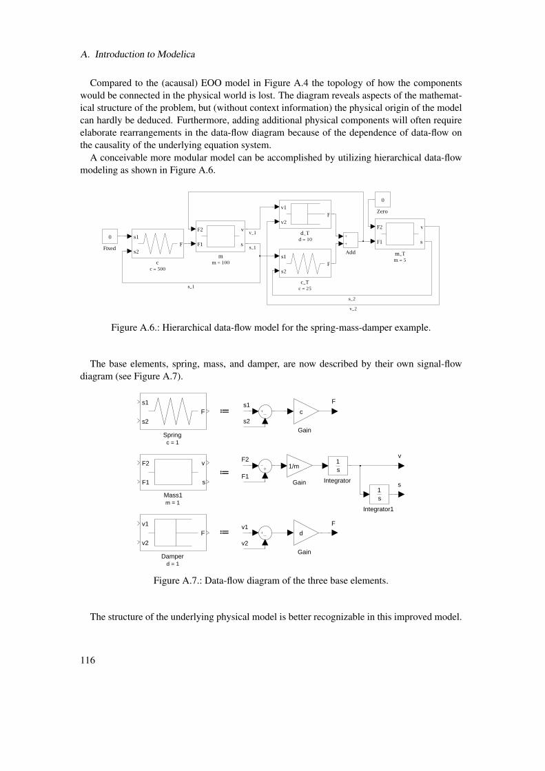
A. Introduction to Modelica

Compared to the (acausal) EOO model in Figure A.4 the topology of how the componentswould be connected in the physical world is lost. The diagram reveals aspects of the mathemat-ical structure of the problem, but (without context information) the physical origin of the modelcan hardly be deduced. Furthermore, adding additional physical components will often requireelaborate rearrangements in the data-flow diagram because of the dependence of data-flow onthe causality of the underlying equation system.

A conceivable more modular model can be accomplished by utilizing hierarchical data-flowmodeling as shown in Figure A.6.

m_Tm = 5

F2

F1

v

s

mm = 100

F2

F1

v

s

d_Td = 10

v1

v2

F

c_Tc = 25

s1

s2

Fcc = 500

s1

s2

F

Zero

0

Fixed

0

Add

v_2

s_2

v_1

s_1

s_1

Figure A.6.: Hierarchical data-flow model for the spring-mass-damper example.

The base elements, spring, mass, and damper, are now described by their own signal-flowdiagram (see Figure A.7).

F

s

v

F

Springc = 1

s1

s2

F

Mass1m = 1

F2

F1

v

s

Integrator1

1s

Integrator

1s

d

c

Gain

1/m

Damperd = 1

v1

v2

F

v2

v1

F2

s2

s1

F1

≔

≔

≔

Gain

Gain

Figure A.7.: Data-flow diagram of the three base elements.

The structure of the underlying physical model is better recognizable in this improved model.

116

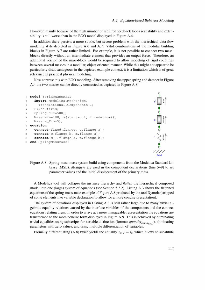
A.2. Equation-based Behavior Modeling

However, mainly because of the high number of required feedback loops readability and exten-sibility is still worse than in the EOO model displayed in Figure A.4.

In addition there persists a more subtle, but severe problem with the hierarchical data-flowmodeling style depicted in Figure A.6 and A.7. Valid combinations of the modular buildingblocks in Figure A.7 are rather limited. For example, it is not possible to connect two mass-blocks directly without an intermediate element that provides an output force. Therefore, anadditional version of the mass-block would be required to allow modeling of rigid couplingsbetween several masses in a modular, object oriented manner. While this might not appear to beparticularly disadvantageous in the depicted example context, it is a limitation which is of greatrelevance in practical physical modeling.

Now contrast this with EOO modeling. After removing the upper spring and damper in FigureA.4 the two masses can be directly connected as depicted in Figure A.8.

1 model SpringMassMass2 import Modelica.Mechanics.3 Translational.Components.*;4 Fixed fixed;5 Spring c(c=500);6 Mass m(m=100, s(start=0.1, fixed=true));7 Mass m_T(m=5);8 equation9 connect(fixed.flange, c.flange_a);

10 connect(c.flange_b, m.flange_a);11 connect(m_T.flange_a, m.flange_b);12 end SpringMassMass;

fixedc

c=50

0

m

m=1

00

m_

T

m=5

Figure A.8.: Spring-mass-mass system build using components from the Modelica Standard Li-brary (MSL). Modifiers are used in the component declarations (line 5–9) to setparameter values and the initial displacement of the primary mass.

A Modelica tool will collapse the instance hierarchy and flatten the hierarchical composedmodel into one (large) system of equations (see Section 5.2.2). Listing A.3 shows the flattenedequations of the spring-mass-mass example of Figure A.8 produced by the tool Dymola (strippedof some elements like variable declaration to allow for a more concise presentation).

The system of equations displayed in Listing A.3 is still rather large due to many trivial al-gebraic equality relations caused by the interface variables of the components and the connectequations relating them. In order to arrive at a more manageable representation the equations aretransformed to the more concise form displayed in Figure A.9. This is achieved by eliminatingtrivial equalities using subscripts for variable distinction (format: quantityobjectflange

), eliminatingparameters with zero values, and using multiple differentiation of variables.

Formally differentiating (A.8) twice yields the equality sm_T = sm which allows to substitute

117

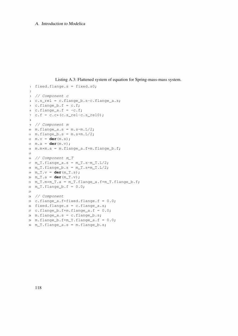
A. Introduction to Modelica

Listing A.3: Flattened system of equation for Spring-mass-mass system.1 fixed.flange.s = fixed.s0;2

3 // Component c4 c.s_rel = c.flange_b.s-c.flange_a.s;5 c.flange_b.f = c.f;6 c.flange_a.f = -c.f;7 c.f = c.c*(c.s_rel-c.s_rel0);8

9 // Component m10 m.flange_a.s = m.s-m.L/2;11 m.flange_b.s = m.s+m.L/2;12 m.v = der(m.s);13 m.a = der(m.v);14 m.m*m.a = m.flange_a.f+m.flange_b.f;15

16 // Component m_T17 m_T.flange_a.s = m_T.s-m_T.L/2;18 m_T.flange_b.s = m_T.s+m_T.L/2;19 m_T.v = der(m_T.s);20 m_T.a = der(m_T.v);21 m_T.m*m_T.a = m_T.flange_a.f+m_T.flange_b.f;22 m_T.flange_b.f = 0.0;23

24 // Component25 c.flange_a.f+fixed.flange.f = 0.0;26 fixed.flange.s = c.flange_a.s;27 c.flange_b.f+m.flange_a.f = 0.0;28 m.flange_a.s = c.flange_b.s;29 m.flange_b.f+m_T.flange_a.f = 0.0;30 m_T.flange_a.s = m.flange_b.s;

118

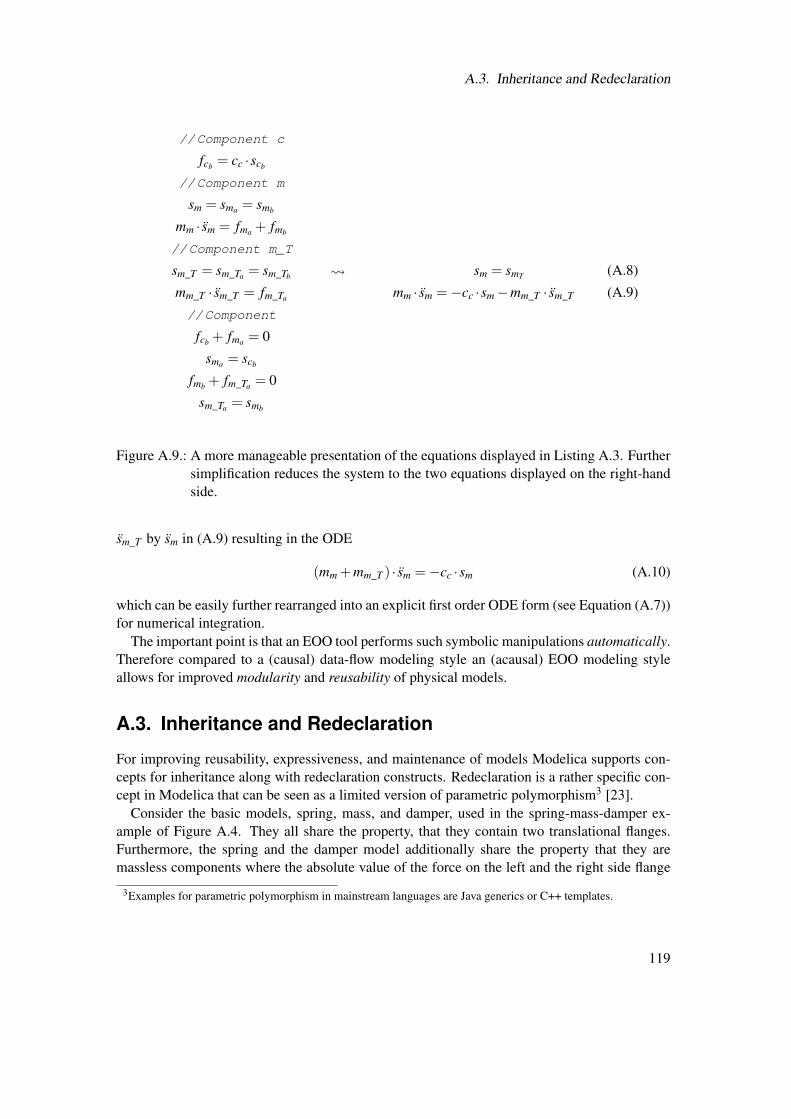
A.3. Inheritance and Redeclaration

//Component c

fcb = cc ·scb

//Component m

sm = sma = smb

mm · sm = fma + fmb

//Component m_T

sm_T = sm_Ta = sm_Tb

mm_T · sm_T = fm_Ta

//Component

fcb + fma = 0

sma = scb

fmb + fm_Ta = 0

sm_Ta = smb

sm = smT (A.8)

mm · sm =−cc ·sm−mm_T · sm_T (A.9)

Figure A.9.: A more manageable presentation of the equations displayed in Listing A.3. Furthersimplification reduces the system to the two equations displayed on the right-handside.

sm_T by sm in (A.9) resulting in the ODE

(mm +mm_T ) · sm =−cc ·sm (A.10)

which can be easily further rearranged into an explicit first order ODE form (see Equation (A.7))for numerical integration.

The important point is that an EOO tool performs such symbolic manipulations automatically.Therefore compared to a (causal) data-flow modeling style an (acausal) EOO modeling styleallows for improved modularity and reusability of physical models.

A.3. Inheritance and Redeclaration

For improving reusability, expressiveness, and maintenance of models Modelica supports con-cepts for inheritance along with redeclaration constructs. Redeclaration is a rather specific con-cept in Modelica that can be seen as a limited version of parametric polymorphism3 [23].

Consider the basic models, spring, mass, and damper, used in the spring-mass-damper ex-ample of Figure A.4. They all share the property, that they contain two translational flanges.Furthermore, the spring and the damper model additionally share the property that they aremassless components where the absolute value of the force on the left and the right side flange

3Examples for parametric polymorphism in mainstream languages are Java generics or C++ templates.

119

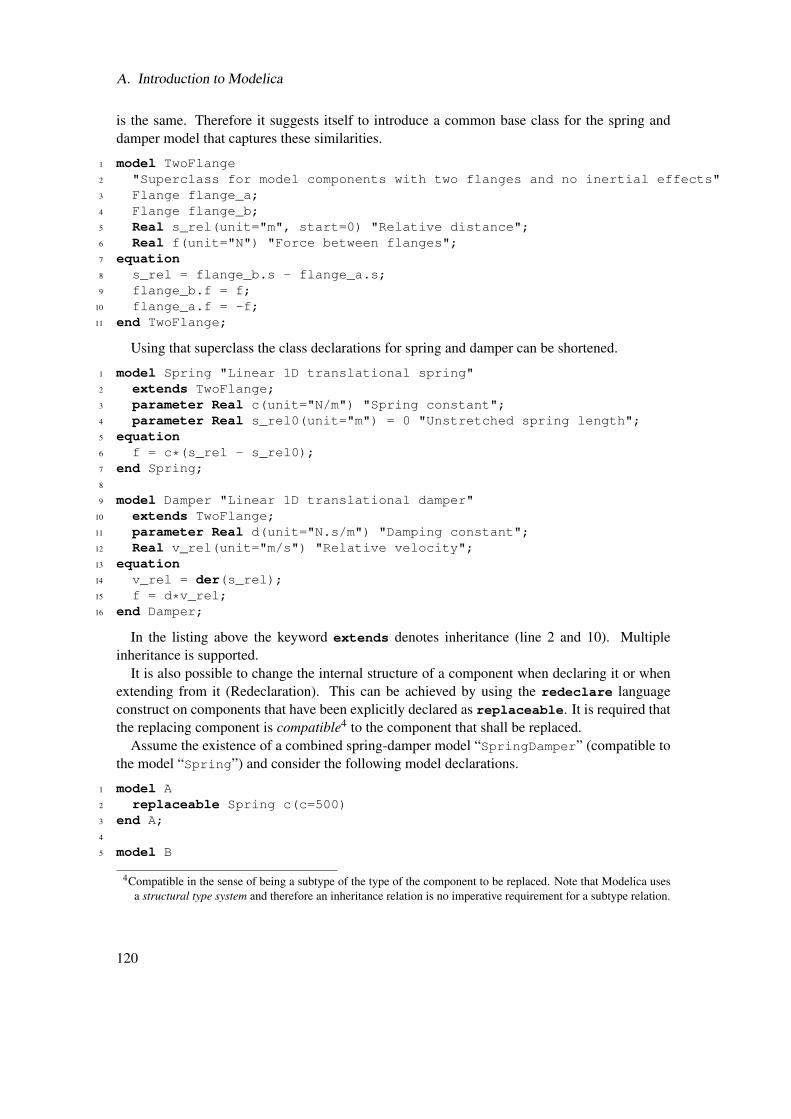
A. Introduction to Modelica

is the same. Therefore it suggests itself to introduce a common base class for the spring anddamper model that captures these similarities.

1 model TwoFlange2 "Superclass for model components with two flanges and no inertial effects"3 Flange flange_a;4 Flange flange_b;5 Real s_rel(unit="m", start=0) "Relative distance";6 Real f(unit="N") "Force between flanges";7 equation8 s_rel = flange_b.s - flange_a.s;9 flange_b.f = f;

10 flange_a.f = -f;11 end TwoFlange;

Using that superclass the class declarations for spring and damper can be shortened.

1 model Spring "Linear 1D translational spring"2 extends TwoFlange;3 parameter Real c(unit="N/m") "Spring constant";4 parameter Real s_rel0(unit="m") = 0 "Unstretched spring length";5 equation6 f = c*(s_rel - s_rel0);7 end Spring;8

9 model Damper "Linear 1D translational damper"10 extends TwoFlange;11 parameter Real d(unit="N.s/m") "Damping constant";12 Real v_rel(unit="m/s") "Relative velocity";13 equation14 v_rel = der(s_rel);15 f = d*v_rel;16 end Damper;

In the listing above the keyword extends denotes inheritance (line 2 and 10). Multipleinheritance is supported.

It is also possible to change the internal structure of a component when declaring it or whenextending from it (Redeclaration). This can be achieved by using the redeclare languageconstruct on components that have been explicitly declared as replaceable. It is required thatthe replacing component is compatible4 to the component that shall be replaced.

Assume the existence of a combined spring-damper model “SpringDamper” (compatible tothe model “Spring”) and consider the following model declarations.

1 model A2 replaceable Spring c(c=500)3 end A;4

5 model B

4Compatible in the sense of being a subtype of the type of the component to be replaced. Note that Modelica usesa structural type system and therefore an inheritance relation is no imperative requirement for a subtype relation.

120

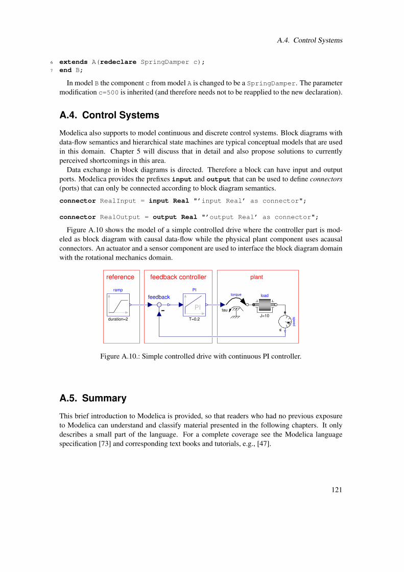
A.4. Control Systems

6 extends A(redeclare SpringDamper c);7 end B;

In model B the component c from model A is changed to be a SpringDamper. The parametermodification c=500 is inherited (and therefore needs not to be reapplied to the new declaration).

A.4. Control Systems

Modelica also supports to model continuous and discrete control systems. Block diagrams withdata-flow semantics and hierarchical state machines are typical conceptual models that are usedin this domain. Chapter 5 will discuss that in detail and also propose solutions to currentlyperceived shortcomings in this area.

Data exchange in block diagrams is directed. Therefore a block can have input and outputports. Modelica provides the prefixes input and output that can be used to define connectors(ports) that can only be connected according to block diagram semantics.

connector RealInput = input Real "’input Real’ as connector";

connector RealOutput = output Real "’output Real’ as connector";

Figure A.10 shows the model of a simple controlled drive where the controller part is mod-eled as block diagram with causal data-flow while the physical plant component uses acausalconnectors. An actuator and a sensor component are used to interface the block diagram domainwith the rotational mechanics domain.

feedback controller plantreference

load

J=10 speed

w

ramp

duration=2

PI

PI

T=0.2-

feedback torque

tau

Figure A.10.: Simple controlled drive with continuous PI controller.

A.5. Summary

This brief introduction to Modelica is provided, so that readers who had no previous exposureto Modelica can understand and classify material presented in the following chapters. It onlydescribes a small part of the language. For a complete coverage see the Modelica languagespecification [73] and corresponding text books and tutorials, e.g., [47].

121

B. Formal Translation Semantics

The content of this chapter has been published in

Bernhard Thiele, Alois Knoll, and Peter Fritzson. Towards Qualifiable Code Gen-eration from a Clocked Synchronous Subset of Modelica. Modeling, Identifica-tion and Control, 36(1):23–52, 2015. http://dx.doi.org/10.4173/mic.2015.1.3.

The following text is a citation from the above mentioned manuscript.

B.1. The Synchronous Data-Flow Kernel (SDFK)

The utilized synchronous data-flow kernel (SDFK) is described in [19], i.e.,

Dariusz Biernacki, Jean-Louis Colaço, Gregoire Hamon, and Marc Pouzet. Clock-directed modular code generation for synchronous data-flow languages. SIGPLANNot., 43(7):121–130, June 2008. http://doi.acm.org/10.1145/1379023.1375674.

In order to keep the following discussion more self-contained, the syntax and intuitive seman-tics1 described in [19, Section 2] are briefly reproduced in the current section.

A program is made of a list of global type (“td”) and node (“d”) declarations. In order toallow a clear and brief presentation, only abstract types and enumerated types are considered inthe discussion. A global node declaration “d” has the form “node f (p) = p with var p in D”.Within this node declaration “p” denotes a list of variables while “D” denotes a list of parallelequations. In an equation “pat = a” the pattern “pat” is either a variable or a tuple of patterns“(pat, . . . , pat)” and “a” denotes an annotated expression “e” with its clock “ct”. Table B.1briefly describes various elements that can be part of an expression. The expressionscan be extended by the conditional “if/then/else” which relates to the original kernel by theequivalence relation:

if x then e2 else e3 = merge x

(True→ e2 when True(x))(False→ e3 when False(x))

(B.1)

1 The semantics of the synchronous data-flow kernel is given informally in [19]. The paper refers to [34] for theformal semantics of the clock calculus. Actually, the extended language presented in [34] is similar to the oneused in [19]. In [34] this extended language is formally translated into a more “basic” data-flow kernel by asource-to-source transformation. For this “basic” data-flow kernel [34, Section 3.1] refers to [35] for a (formal)denotational Kahn semantics (except for the semantics of the modular reset operator “every” which is formallydefined in [51]).

123

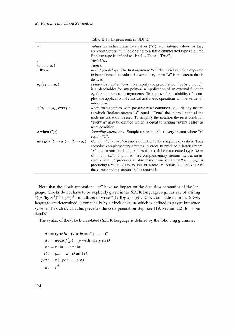
B. Formal Translation Semantics

Table B.1.: Expressions in SDFK

v Values are either immediate values (“i”), e.g., integer values, or theyare constructors (“C”) belonging to a finite enumerated type (e.g., theBoolean type is defined as “bool = False+True”).

x Variables.(a1, . . . ,an) Tuples.v fby a Initialized delays. The first argument “v” (the initial value) is expected

to be an immediate value, the second argument “a” is the stream that isdelayed.

op(a1, . . . ,an) Point-wise applications. To simplify the presentation, “op(a1, . . . ,an)”is a placeholder for any point-wise application of an external functionop (e.g., +, not) to its arguments. To improve the readability of exam-ples, the application of classical arithmetic operations will be written ininfix form.

f (a1, . . . ,an) every a Node instantiations with possible reset condition “a”. At any instantat which Boolean stream “a” equals “True” the internal state of thenode instantiation is reset. To simplify the notation the reset condition“every a” may be omitted which is equal to writing “every False” asreset condition.

a when C(x) Sampling operations. Sample a stream “a” at every instant where “x”equals “C”.

merge x (C→ a1) . . .(C→ an) Combination operations are symmetric to the sampling operation: Theycombine complementary streams in order to produce a faster stream.“x” is a stream producing values from a finite enumerated type “bt =C1 + . . .+Cn”. “a1, . . . ,an” are complementary streams, i.e., at an in-stant where “x” produces a value at most one stream of “a1, . . . ,an” isproducing a value. At every instant where “x” equals “Ci” the value ofthe corresponding stream “ai” is returned.

Note that the clock annotations “ct” have no impact on the data-flow semantics of the lan-guage. Clocks do not have to be explicitly given in the SDFK language, e.g., instead of writing“((v fby xck)ck + yck)ck” it suffices to write “((v fby x)+ y)”. Clock annotations in the SDFKlanguage are determined automatically by a clock calculus which is defined as a type inferencesystem. This clock calculus precedes the code generation step (see [19, Section 2.2] for moredetails).

The syntax of the (clock-annotated) SDFK language is defined by the following grammar:

td ::= type bt | type bt =C+ . . .+C

d ::= node f (p) = p with var p in D

p ::= x : bt; . . . ;x : bt

D ::= pat = a | D and D

pat ::= x | (pat, . . . , pat)

a ::= eck

124

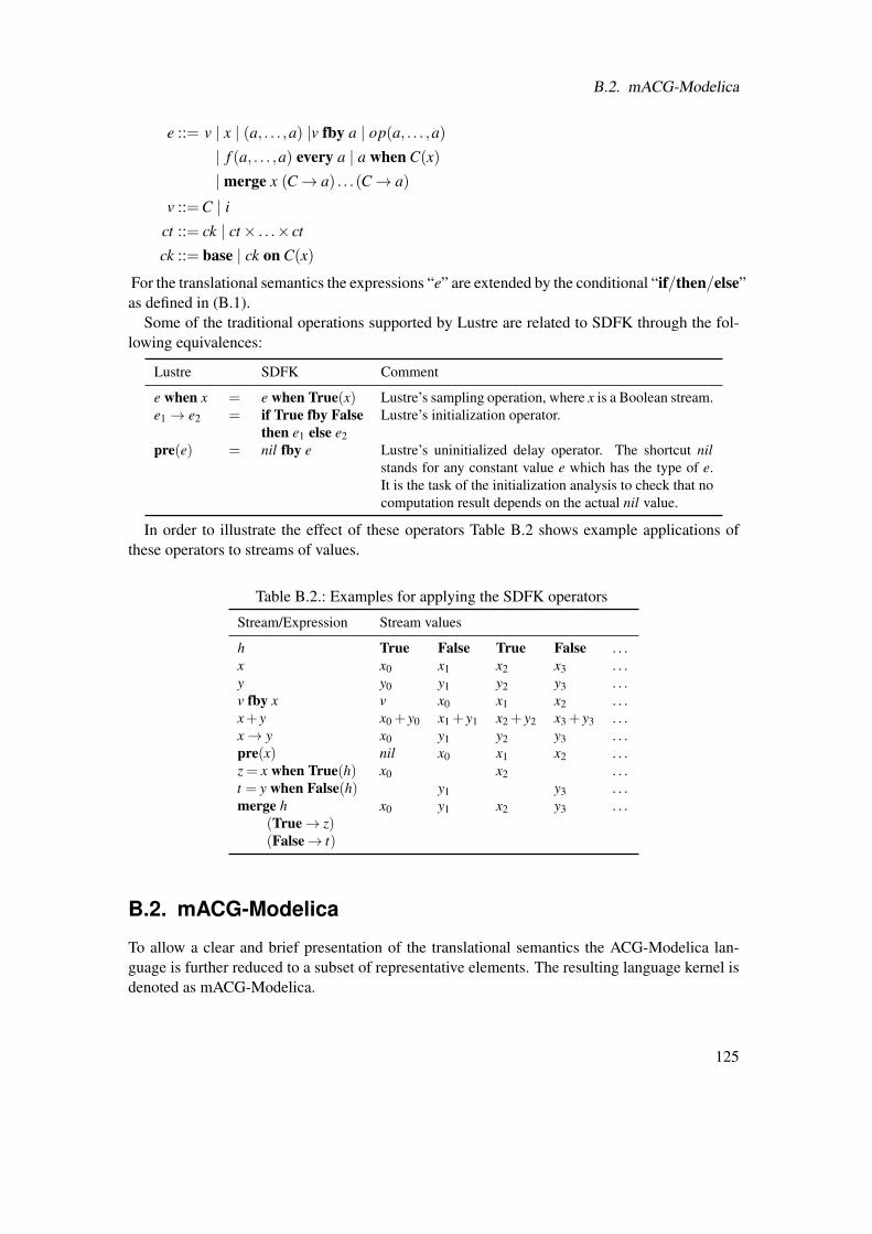
B.2. mACG-Modelica

e ::= v | x | (a, . . . ,a) |v fby a | op(a, . . . ,a)

| f (a, . . . ,a) every a | a when C(x)

|merge x (C→ a) . . .(C→ a)

v ::=C | ict ::= ck | ct× . . .× ct

ck ::= base | ck on C(x)

For the translational semantics the expressions “e” are extended by the conditional “if/then/else”as defined in (B.1).

Some of the traditional operations supported by Lustre are related to SDFK through the fol-lowing equivalences:

Lustre SDFK Comment

e when x = e when True(x) Lustre’s sampling operation, where x is a Boolean stream.e1 → e2 = if True fby False Lustre’s initialization operator.

then e1 else e2pre(e) = nil fby e Lustre’s uninitialized delay operator. The shortcut nil

stands for any constant value e which has the type of e.It is the task of the initialization analysis to check that nocomputation result depends on the actual nil value.

In order to illustrate the effect of these operators Table B.2 shows example applications ofthese operators to streams of values.

Table B.2.: Examples for applying the SDFK operators

Stream/Expression Stream values

h True False True False . . .x x0 x1 x2 x3 . . .y y0 y1 y2 y3 . . .v fby x v x0 x1 x2 . . .x+ y x0 + y0 x1 + y1 x2 + y2 x3 + y3 . . .x→ y x0 y1 y2 y3 . . .pre(x) nil x0 x1 x2 . . .z = x when True(h) x0 x2 . . .t = y when False(h) y1 y3 . . .merge h

(True→ z)(False→ t)

x0 y1 x2 y3 . . .

B.2. mACG-Modelica

To allow a clear and brief presentation of the translational semantics the ACG-Modelica lan-guage is further reduced to a subset of representative elements. The resulting language kernel isdenoted as mACG-Modelica.

125

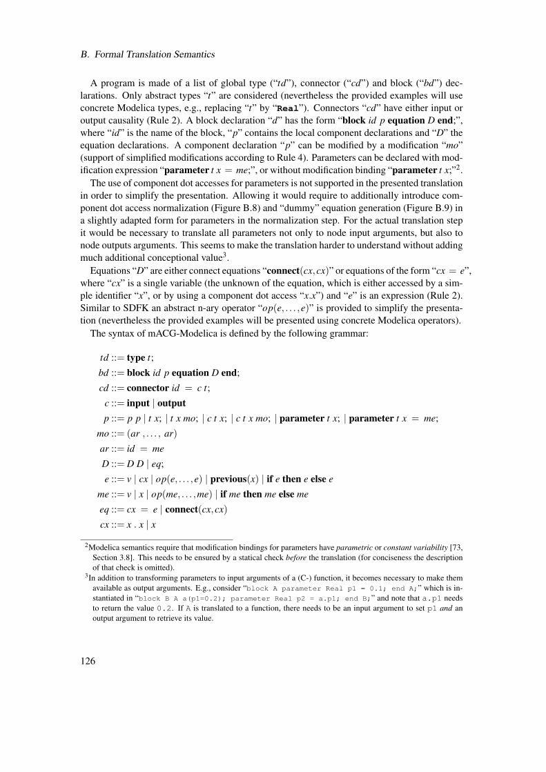
B. Formal Translation Semantics

A program is made of a list of global type (“td”), connector (“cd”) and block (“bd”) dec-larations. Only abstract types “t” are considered (nevertheless the provided examples will useconcrete Modelica types, e.g., replacing “t” by “Real”). Connectors “cd” have either input oroutput causality (Rule 2). A block declaration “d” has the form “block id p equation D end;”,where “id” is the name of the block, “p” contains the local component declarations and “D” theequation declarations. A component declaration “p” can be modified by a modification “mo”(support of simplified modifications according to Rule 4). Parameters can be declared with mod-ification expression “parameter t x = me;”, or without modification binding “parameter t x;”2.

The use of component dot accesses for parameters is not supported in the presented translationin order to simplify the presentation. Allowing it would require to additionally introduce com-ponent dot access normalization (Figure B.8) and “dummy” equation generation (Figure B.9) ina slightly adapted form for parameters in the normalization step. For the actual translation stepit would be necessary to translate all parameters not only to node input arguments, but also tonode outputs arguments. This seems to make the translation harder to understand without addingmuch additional conceptional value3.

Equations “D” are either connect equations “connect(cx,cx)” or equations of the form “cx = e”,where “cx” is a single variable (the unknown of the equation, which is either accessed by a sim-ple identifier “x”, or by using a component dot access “x.x”) and “e” is an expression (Rule 2).Similar to SDFK an abstract n-ary operator “op(e, . . . ,e)” is provided to simplify the presenta-tion (nevertheless the provided examples will be presented using concrete Modelica operators).

The syntax of mACG-Modelica is defined by the following grammar:

td ::= type t;

bd ::= block id p equation D end;

cd ::= connector id = c t;

c ::= input | outputp ::= p p | t x; | t x mo; | c t x; | c t x mo; | parameter t x; | parameter t x = me;

mo ::= (ar , . . . , ar)

ar ::= id = me

D ::= D D | eq;

e ::= v | cx | op(e, . . . ,e) | previous(x) | if e then e else e

me ::= v | x | op(me, . . . ,me) | if me then me else me

eq ::= cx = e | connect(cx,cx)

cx ::= x . x | x

2Modelica semantics require that modification bindings for parameters have parametric or constant variability [73,Section 3.8]. This needs to be ensured by a statical check before the translation (for conciseness the descriptionof that check is omitted).

3In addition to transforming parameters to input arguments of a (C-) function, it becomes necessary to make themavailable as output arguments. E.g., consider “block A parameter Real p1 = 0.1; end A;” which is in-stantiated in “block B A a(p1=0.2); parameter Real p2 = a.p1; end B;” and note that a.p1 needsto return the value 0.2. If A is translated to a function, there needs to be an input argument to set p1 and anoutput argument to retrieve its value.

126

B.3. A Multilevel Translation Approach

x ::= id

v = value

id = identifier

Abstract types “t” encompass predefined primitive types and user-defined structured types(blocks and connectors). The set “B” is introduced to denote the set of all predefined primitivetypes, particularly Modelica’s Boolean, Integer, and Real types.

From all the synchronous language elements that are listed in Table 5.3 on page 48 only“previous” appears in the grammar above. The clock conversion operators “subSample” and“noClock” are omitted — as described in Section 5.7.5 they are not necessarily indispensableelements in the Modelica subset targeted for automatic code generation. Nevertheless, Sec-tion 5.9.4 shows how the translational semantics can be extended to support these operators.

Also the operator “interval(u)” is missing in the grammar. This operator is considered to beavailable as external function call or macro — the time span between a previous and a presenttick is typically only known by the environment that triggers the execution of the synchronousdata-flow program. Consequently, this value needs to be provided by the runtime environment.In the case of single-rate programs (i.e., if no clock conversion operators are supported) theinterval duration is simply the duration between two ticks of the base clock, in case of multi-rate programs it becomes more complicated and the value depends on the specific clock that isassociated to the operators argument ”u”.

B.3. A Multilevel Translation Approach

The translation to SDFK is rather complex. In order to keep the translation manageable andunderstandable the translation is subdivided into several steps. The two major steps are:

1. Normalization of mACG-Modelica (formulated as source-to-source transformation). Thisstep is again subdivided in:

a) Generation of connection equations.

b) Stripping of parameter modifications, normalizing component modifications and ex-tracting component dot accesses appearing in expressions.

c) Creating a fresh block that instantiates the top-level block as a component with nor-malized component modifications.

2. Translation to SDFK.

Normalization and translation are defined as a system of mutually recursive functions. Thenormalization is needed in order to transform mACG-Modelica into a (simplified) normalizedform which is the basis for the translation to SDFK. The syntax for the normalized mACG-Modelica language can be found in Section B.5.

Using a multilevel translation approach facilitates to include further language elements, aslong as a source-to-source transformation into a smaller language kernel can be given. The

127

B. Formal Translation Semantics

generation of connection equations is a good example for this: it eliminates the connector dec-larations and connect equations by replacing them with simple variable declarations (using theproper input/output causalities) and simple equations of the form “x = e”. Hence, the multileveltranslation approach provides a path to incrementally extend the mACG-Modelica subset untilthe complete ACG-Modelica language is supported (see also the discussion in Section 5.9.3).

B.4. Normalization

B.4.1. Notation

The following notation shall be used. A sequence of elements (e1, . . . ,en) is frequently writtenas a list [e1; . . . ; en] for which an operator “+” is defined so that if p1 = [e1; . . . ; en] andp2 = [e′1; . . . ; e′k] then p1 + p2 = [e1; . . . ; en; e′1; . . . ;e′k] provided ei 6= e′j for all i, j such that1≤ i≤ n, 1≤ j ≤ k. [] denotes an empty list. Furthermore, e1 ∈ p1 shall denote that e1 appearsas an element in p1.

Frequently, elements ei are tuples (e.g., ei = (xi, ti)). Especially if tuples encode variablenames and their associated types an alternative notation is preferred in which “,” is replaced by“:” and the parentheses are dropped (e.g., ei = xi : ti). The underscore “_” is used as a placeholderfor entries which are irrelevant in the specific context.

Mutually recursive functions “Function(context)(element)” are used for defining a transforma-tion of an element within a context. To keep the notation concise the definition of a function isoften overloaded — its actual interpretation should be clear from the context.

B.4.2. Generation of Connection Equations

The generation of connection equations is defined as a source-to-source transformation througha set of mutually recursive functions. G(D) at the bottom of Figure B.1 defines the translation ofModelica code that includes connect-equations into a Modelica code in which these connect-equations are replaced by simple connection equations of the form “x = e”.

G(D) relies on GCenv(..) to create an environment (I,O,Bs) which is utilized in the transla-tion function GTcd(I,O,Bs)(D).

GTcd traverses the class declarations. It removes the connector declarations and utilizesfunction GTd (see Figure B.2) to replace connect-equations by simple equations of the form“x = e”.

The environment (I,O,Bs) is a tuple of (globally) declared input connectors I, output connec-tors O and block declarations Bs. I = [i1 : t1; . . . ; in : tn] is a list of input connector short classdefinitions where i denotes the class name and t denotes the respective (primitive) data type as-sociated to that input connector. O = [o1 : t1; . . . ; on : tn] is a list of output connector short classdefinitions where o denotes the class name and t denotes the respective (primitive) data typeassociated to that output connector. Bs = [Bd1; . . . ; Bdn] is the list of block declarations

Each element Bd = (b,d) is a tuple there b denotes the block class name and d stands for alist of component declarations in b. d = [x1 : t1; . . . ; xn : tn] is composed from the componentnames x and their respective type t.

128

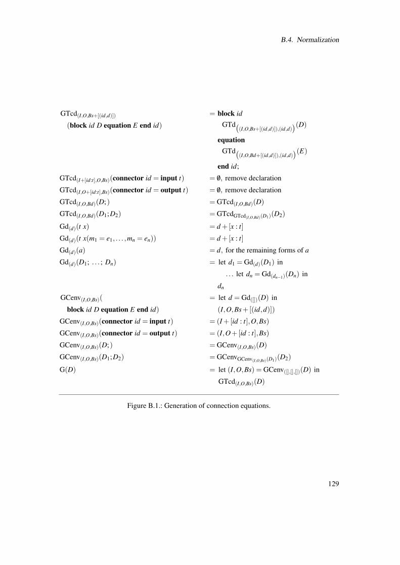
B.4. Normalization

GTcd(I,O,Bs+[(id,d)])

(block id D equation E end id)

= block id

GTd((I,O,Bs+[(id,d)]),(id,d)

)(D)

equationGTd(

(I,O,Bd+[(id,d)]),(id,d))(E)

end id;

GTcd(I+[id:t],O,Bs)(connector id = input t) = /0, remove declaration

GTcd(I,O+[id:t],Bs)(connector id = output t) = /0, remove declaration

GTcd(I,O,Bd)(D;) = GTcd(I,O,Bd)(D)

GTcd(I,O,Bd)(D1;D2) = GTcdGTcd(I,O,Bd)(D1)(D2)

Gd(d)(t x) = d +[x : t]

Gd(d)(t x(m1 = e1, . . . ,mn = en)) = d +[x : t]

Gd(d)(a) = d, for the remaining forms of a

Gd(d)(D1; . . . ; Dn) = let d1 = Gd(d)(D1) in

. . . let dn = Gd(dn−1)(Dn) in

dn

GCenv(I,O,Bs)(

block id D equation E end id)

= let d = Gd([])(D) in

(I,O,Bs+[(id,d)])

GCenv(I,O,Bs)(connector id = input t) = (I +[id : t],O,Bs)

GCenv(I,O,Bs)(connector id = output t) = (I,O+[id : t],Bs)

GCenv(I,O,Bs)(D;) = GCenv(I,O,Bs)(D)

GCenv(I,O,Bs)(D1;D2) = GCenvGCenv(I,O,Bs)(D1)(D2)

G(D) = let (I,O,Bs) = GCenv([],[],[])(D) in

GTcd(I,O,Bs)(D)

Figure B.1.: Generation of connection equations.

129

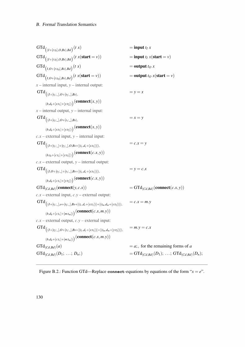
B. Formal Translation Semantics

GTd((I+[t:tI ],O,Bs),Bd

)(t x) = input tI x

GTd((I+[t:tI ],O,Bs),Bd

)(t x(start = v)) = input tI x(start = v)

GTd(I,O+[t:tO],Bs),Bd

)(t x) = output tO x

GTd(I,O+[t:tO],Bs),Bd

)(t x(start = v)) = output tO x(start = v)

x – internal input, y – internal output:

GTd((I+[t1:_],O+[t2:_],Bs),

(b,db+[x:t1]+[y:t2]))(connect(x,y))

= y = x

x – internal output, y – internal input:

GTd((I+[t2:_],O+[t1:_],Bs),

(b,db+[x:t1]+[y:t2]))(connect(x,y))

= x = y

c.x – external input, y – internal input:

GTd((I+[t1:_]+[t2:_],O,Bs+[(tc,dc+[x:t1])]),

(b,tb+[c:tc]+[y:t2]]))(connect(c.x,y))

= c.x = y

c.x – external output, y – internal output:

GTd((I,O+[t2:_]+[t1:_],Bs+[(tc,dc+[x:t1])]),

(b,db+[c:tc]+[y:t2]))(connect(c.x,y))

= y = c.x

GTd(Cd,Bd)(connect(y,c.x)) = GTd(Cd,Bd)(connect(c.x,y))c.x – external input, c.y – external output:

GTd((I+[t1:_],o+[t2:_],Bs+[(tc,dc+[x:t1])]+[(tm,dm+[y:t2])]),

(b,db+[c:tc]+[m:tm]))(connect(c.x,m.y))

= c.x = m.y

c.x – external output, c.y – external input:

GTd((I+[t2:_],O+[t1:_],Bs+[(tc,dc+[x:t1])]+[(tm,dm+[y:t2])]),

(b,db+[c:tc]+[m:tm]))(connect(c.x,m.y))

= m.y = c.x

GTd(Cd,Bd)(a) = a; , for the remaining forms of a

GTd(Cd,Bd)(D1; . . . ; Dn;) = GTd(Cd,Bd)(D1); . . . ; GTd(Cd,Bd)(Dn);

Figure B.2.: Function GTd—Replace connect-equations by equations of the form “x = e”.

130

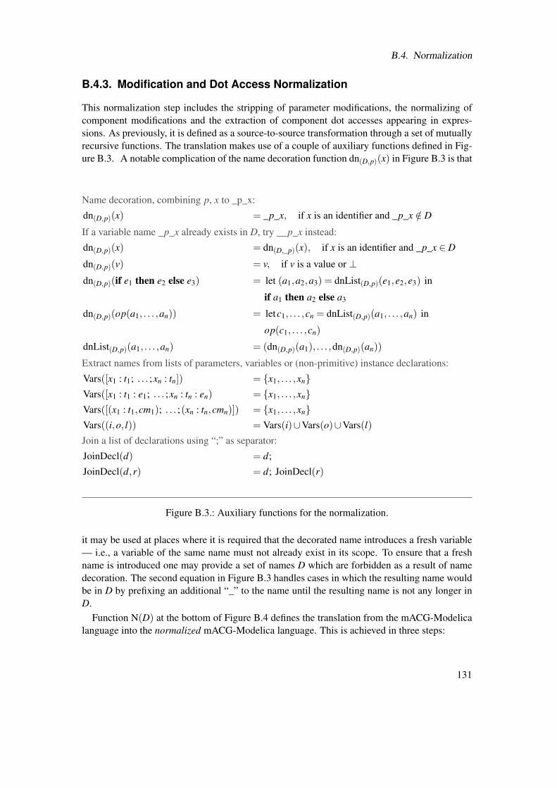
B.4. Normalization

B.4.3. Modification and Dot Access Normalization

This normalization step includes the stripping of parameter modifications, the normalizing ofcomponent modifications and the extraction of component dot accesses appearing in expres-sions. As previously, it is defined as a source-to-source transformation through a set of mutuallyrecursive functions. The translation makes use of a couple of auxiliary functions defined in Fig-ure B.3. A notable complication of the name decoration function dn(D,p)(x) in Figure B.3 is that

Name decoration, combining p, x to _p_x:

dn(D,p)(x) = _p_x, if x is an identifier and _p_x /∈ D

If a variable name _p_x already exists in D, try __p_x instead:

dn(D,p)(x) = dn(D,_p)(x), if x is an identifier and _p_x ∈ D

dn(D,p)(v) = v, if v is a value or ⊥dn(D,p)(if e1 then e2 else e3) = let (a1,a2,a3) = dnList(D,p)(e1,e2,e3) in

if a1 then a2 else a3

dn(D,p)(op(a1, . . . ,an)) = letc1, . . . ,cn = dnList(D,p)(a1, . . . ,an) in

op(c1, . . . ,cn)

dnList(D,p)(a1, . . . ,an) = (dn(D,p)(a1), . . . ,dn(D,p)(an))

Extract names from lists of parameters, variables or (non-primitive) instance declarations:

Vars([x1 : t1; . . . ;xn : tn]) = x1, . . . ,xnVars([x1 : t1 : e1; . . . ;xn : tn : en) = x1, . . . ,xnVars([(x1 : t1,cm1); . . . ;(xn : tn,cmn)]) = x1, . . . ,xnVars((i,o, l)) = Vars(i)∪Vars(o)∪Vars(l)

Join a list of declarations using “;” as separator:

JoinDecl(d) = d;

JoinDecl(d,r) = d; JoinDecl(r)

Figure B.3.: Auxiliary functions for the normalization.

it may be used at places where it is required that the decorated name introduces a fresh variable— i.e., a variable of the same name must not already exist in its scope. To ensure that a freshname is introduced one may provide a set of names D which are forbidden as a result of namedecoration. The second equation in Figure B.3 handles cases in which the resulting name wouldbe in D by prefixing an additional “_” to the name until the resulting name is not any longer inD.

Function N(D) at the bottom of Figure B.4 defines the translation from the mACG-Modelicalanguage into the normalized mACG-Modelica language. This is achieved in three steps:

131

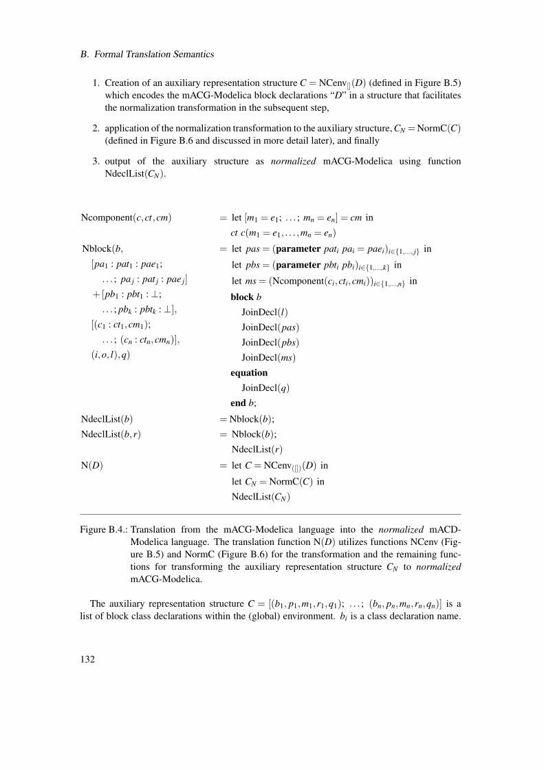
B. Formal Translation Semantics

1. Creation of an auxiliary representation structure C = NCenv[](D) (defined in Figure B.5)which encodes the mACG-Modelica block declarations “D” in a structure that facilitatesthe normalization transformation in the subsequent step,

2. application of the normalization transformation to the auxiliary structure, CN =NormC(C)(defined in Figure B.6 and discussed in more detail later), and finally

3. output of the auxiliary structure as normalized mACG-Modelica using functionNdeclList(CN).

Ncomponent(c,ct,cm) = let [m1 = e1; . . . ; mn = en] = cm in

ct c(m1 = e1, . . . ,mn = en)

Nblock(b,

[pa1 : pat1 : pae1;

. . . ; pa j : pat j : pae j]

+ [pb1 : pbt1 :⊥;

. . . ; pbk : pbtk :⊥],[(c1 : ct1,cm1);

. . . ; (cn : ctn,cmn)],

(i,o, l),q)

= let pas = (parameter pati pai = paei)i∈1,..., j in

let pbs = (parameter pbti pbi)i∈1,...,k in

let ms = (Ncomponent(ci,cti,cmi))i∈1,...,n in

block b

JoinDecl(l)

JoinDecl(pas)

JoinDecl(pbs)

JoinDecl(ms)

equationJoinDecl(q)

end b;

NdeclList(b) = Nblock(b);

NdeclList(b,r) = Nblock(b);

NdeclList(r)

N(D) = let C = NCenv([])(D) in

let CN = NormC(C) in

NdeclList(CN)

Figure B.4.: Translation from the mACG-Modelica language into the normalized mACD-Modelica language. The translation function N(D) utilizes functions NCenv (Fig-ure B.5) and NormC (Figure B.6) for the transformation and the remaining func-tions for transforming the auxiliary representation structure CN to normalizedmACG-Modelica.

The auxiliary representation structure C = [(b1, p1,m1,r1,q1); . . . ; (bn, pn,mn,rn,qn)] is alist of block class declarations within the (global) environment. bi is a class declaration name.

132

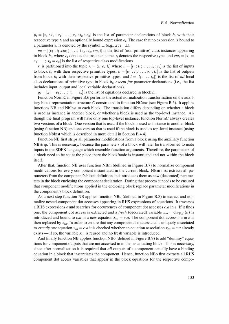
B.4. Normalization

pi = [x1 : t1 : e1; . . . ; xn : tn : en] is the list of parameter declarations of block bi with theirrespective type ti and an optionally bound expression ei. The case that no expression is bound toa parameter ei is denoted by the symbol ⊥ (e.g., x : t :⊥).

mi = [(c1 : t1,cm1); . . . ; (cn : tn,cmn)] is the list of (non-primitive) class instances appearingin block bi, where ci denotes the instance name, ti denotes the respective type, and cmi = [x1 =e1; . . . ; xn = en] is the list of respective class modifications.

ri is partitioned into the tuple ri = (ii,oi, li) where ii = [i1 : t1; . . . ; in : tn] is the list of inputsto block bi with their respective primitive types, o = [o1 : t1; . . . ;on : tn] is the list of outputsfrom block bi with their respective primitive types, and l = [l1; . . . ; ln]) is the list of all localclass declarations of primitive type in block bi, except for parameter declarations (i.e., the listincludes input, output and local variable declarations).

qi = [x1 = e1; . . . ; xn = en] is the list of equations declared in block bi.Function NormC in Figure B.6 performs the actual normalization transformation on the auxil-

iary block representation structure C constructed in function NCenv (see Figure B.5). It appliesfunctions NB and NbInst to each block. The translation differs depending on whether a blockis used as instance in another block, or whether a block is used as the top-level instance. Al-though the final program will have only one top-level instance, function NormC always createstwo versions of a block: One version that is used if the block is used as instance in another block(using function NB) and one version that is used if the block is used as top-level instance (usingfunction NbInst which is described in more detail in Section B.4.4).

Function NB first strips all parameter modifications from a block using the auxiliary functionNBstrip. This is necessary, because the parameters of a block will later be transformed to nodeinputs in the SDFK language which resemble function arguments. Therefore, the parameters ofa block need to be set at the place there the block/node is instantiated and not within the blockitself.

After that, function NB uses function NBm (defined in Figure B.7) to normalize componentmodifications for every component instantiated in the current block. NBm first extracts all pa-rameters from the component’s block definition and introduces them as new (decorated) parame-ters in the block enclosing the component declaration. During that process it needs to be ensuredthat component modifications applied in the enclosing block replace parameter modifications inthe component’s block definition.

As a next step function NB applies function NBq (defined in Figure B.8) to extract and nor-malize nested component dot accesses appearing in RHS expressions of equations. It traversesa RHS expressions e and searches for occurrences of component dot accesses c.a in e. If it findsone, the component dot access is extracted and a fresh (decorated) variable xca = dn(D,c)(a) isintroduced and bound to c.a in a new equation xca = c.a. The component dot access c.a in e isthen replaced by xca. In order to ensure that any component dot access c.a is uniquely associatedto exactly one equation xca = c.a it is checked whether an equation association xca = c.a alreadyexists — if so, the variable xca is reused and no fresh variable is introduced.

And finally function NB applies function NBo (defined in Figure B.9) to add “dummy” equa-tions for component outputs that are not accessed in in the instantiating block. This is necessary,since after normalization it is required that all outputs of a component actually have a bindingequation in a block that instantiates the component. Hence, function NBo first extracts all RHScomponent dot access variables that appear in the block equations for the respective compo-

133

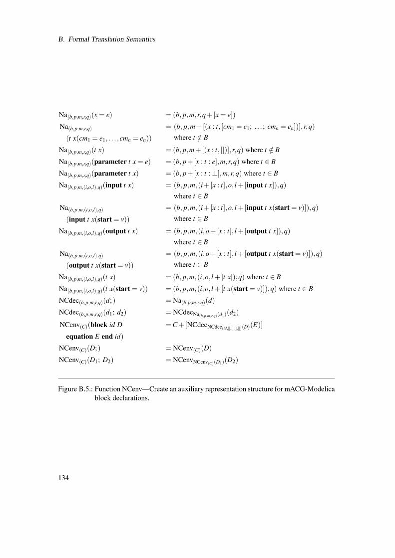
B. Formal Translation Semantics

Na(b,p,m,r,q)(x = e) = (b, p,m,r,q+[x = e])

Na(b,p,m,r,q)

(t x(cm1 = e1, . . . ,cmn = en))

= (b, p,m+[(x : t, [cm1 = e1; . . . ; cmn = en])],r,q)

where t /∈ B

Na(b,p,m,r,q)(t x) = (b, p,m+[(x : t, [])],r,q) where t /∈ B

Na(b,p,m,r,q)(parameter t x = e) = (b, p+[x : t : e],m,r,q) where t ∈ B

Na(b,p,m,r,q)(parameter t x) = (b, p+[x : t :⊥],m,r,q) where t ∈ B

Na(b,p,m,(i,o,l),q)(input t x) = (b, p,m,(i+[x : t],o, l +[input t x]),q)

where t ∈ B

Na(b,p,m,(i,o,l),q)

(input t x(start = v))

= (b, p,m,(i+[x : t],o, l +[input t x(start = v)]),q)

where t ∈ B

Na(b,p,m,(i,o,l),q)(output t x) = (b, p,m,(i,o+[x : t], l +[output t x]),q)

where t ∈ B

Na(b,p,m,(i,o,l),q)

(output t x(start = v))

= (b, p,m,(i,o+[x : t], l +[output t x(start = v)]),q)

where t ∈ B

Na(b,p,m,(i,o,l),q)(t x) = (b, p,m,(i,o, l +[t x]),q) where t ∈ B

Na(b,p,m,(i,o,l),q)(t x(start = v)) = (b, p,m,(i,o, l +[t x(start = v)]),q) where t ∈ B

NCdec(b,p,m,r,q)(d;) = Na(b,p,m,r,q)(d)

NCdec(b,p,m,r,q)(d1; d2) = NCdecNa(b,p,m,r,q)(d1)(d2)

NCenv(C)(block id D

equation E end id)

=C+[NCdecNCdec(id,[],[],[],[])(D)(E)]

NCenv(C)(D;) = NCenv(C)(D)

NCenv(C)(D1; D2) = NCenvNCenv(C)(D1)(D2)

Figure B.5.: Function NCenv—Create an auxiliary representation structure for mACG-Modelicablock declarations.

134

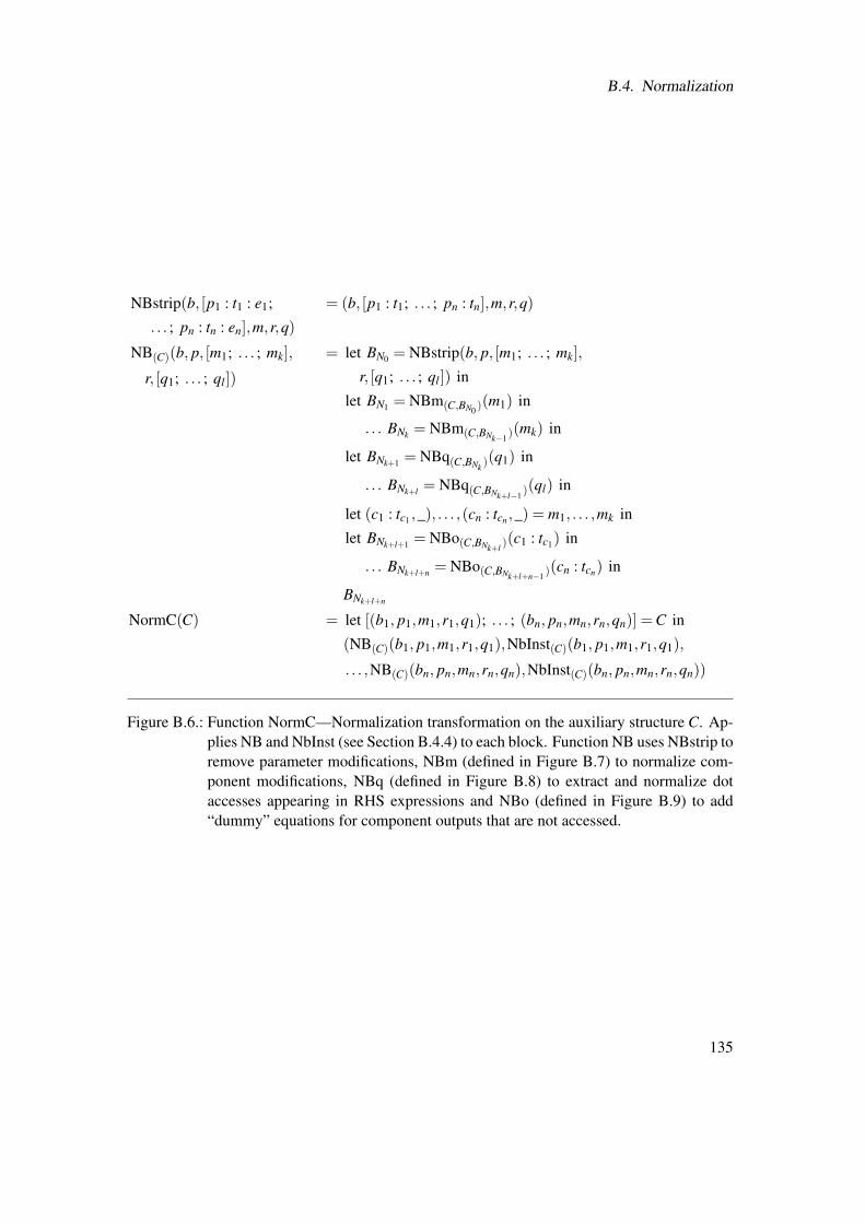
B.4. Normalization

NBstrip(b, [p1 : t1 : e1;

. . . ; pn : tn : en],m,r,q)

= (b, [p1 : t1; . . . ; pn : tn],m,r,q)

NB(C)(b, p, [m1; . . . ; mk],

r, [q1; . . . ; ql])

= let BN0 = NBstrip(b, p, [m1; . . . ; mk],

r, [q1; . . . ; ql]) in

let BN1 = NBm(C,BN0 )(m1) in

. . . BNk = NBm(C,BNk−1 )(mk) in

let BNk+1 = NBq(C,BNk )(q1) in

. . . BNk+l = NBq(C,BNk+l−1 )(ql) in

let (c1 : tc1 ,_), . . . ,(cn : tcn ,_) = m1, . . . ,mk in

let BNk+l+1 = NBo(C,BNk+l )(c1 : tc1) in

. . . BNk+l+n = NBo(C,BNk+l+n−1 )(cn : tcn) in

BNk+l+n

NormC(C) = let [(b1, p1,m1,r1,q1); . . . ; (bn, pn,mn,rn,qn)] =C in

(NB(C)(b1, p1,m1,r1,q1),NbInst(C)(b1, p1,m1,r1,q1),

. . . ,NB(C)(bn, pn,mn,rn,qn),NbInst(C)(bn, pn,mn,rn,qn))

Figure B.6.: Function NormC—Normalization transformation on the auxiliary structure C. Ap-plies NB and NbInst (see Section B.4.4) to each block. Function NB uses NBstrip toremove parameter modifications, NBm (defined in Figure B.7) to normalize com-ponent modifications, NBq (defined in Figure B.8) to extract and normalize dotaccesses appearing in RHS expressions and NBo (defined in Figure B.9) to add“dummy” equations for component outputs that are not accessed.

135

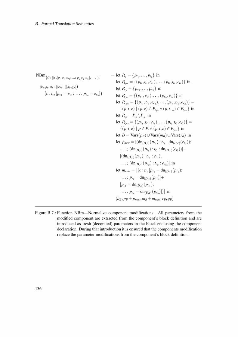
B. Formal Translation Semantics

NBm(C+[(tc,[pt1 :tt1 :et1 ; ...; ptk :ttk :etk ],_,_,_)],

(bB,pB,mB+[(c:tc,_)],rB,qB))(

c : tc, [pc1 = ec1 ; . . . ; pcn = ecn ])

= let Ptp = pt1 , . . . , ptk in

let Ptpte = (pt1 , tt1 ,et1), . . . ,(ptk , ttk ,etk) in

let Pcp = pc1 , . . . , pc j in

let Pcpe = (pc1 ,ec1), . . . ,(pcn ,ecn) in

let Pcpte = (pc1 , tc1 ,ec1), . . . ,(pcn , tcn ,ecn)=(p, t,e) | (p,e) ∈ Pcpe ∧ (p, t,_) ∈ Ptpte in

let Prp = Ptp \Pcp in

let Prpte = (pr1 , tr1 ,er1), . . . ,(prl , trl ,erl )=(p, t,e) | p ∈ Pr ∧ (p, t,e) ∈ Ptpte in

let D = Vars(pB)∪Vars(mB)∪Vars(rB) in

let pnew = [(dn(D,c)(pr1) : tr1 : dn(D,c)(er1));

. . . ; (dn(D,c)(prl ) : trl : dn(D,c)(erl ))]+

[(dn(D,c)(pc1) : tc1 : ec1);

. . . ; (dn(D,c)(pcn) : tcn : ecn)] in

let mnew =[(c : tc, [pr1 = dn(D,c)(pr1);

. . . ; prl = dn(D,c)(prl )]+

[pc1 = dn(D,c)(pc1);

. . . ; pcn = dn(D,c)(pcn)])]

in

(bB, pB + pnew,mB +mnew,rB,qB)

Figure B.7.: Function NBm—Normalize component modifications. All parameters from themodified component are extracted from the component’s block definition and areintroduced as fresh (decorated) parameters in the block enclosing the componentdeclaration. During that introduction it is ensured that the components modificationreplace the parameter modifications from the component’s block definition.

136

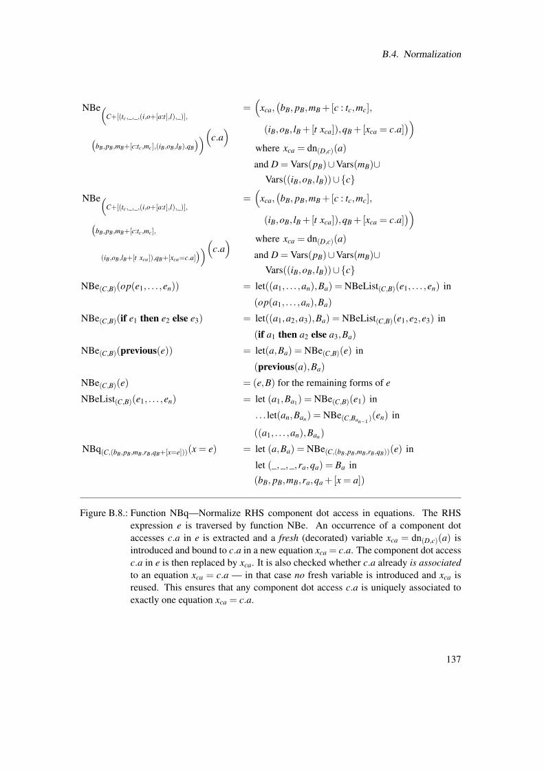
B.4. Normalization

NBe(C+[(tc,_,_,(i,o+[a:t],l),_)],

(bB,pB,mB+[c:tc,mc],(iB,oB,lB),qB

))(c.a) =

(xca,(bB, pB,mB +[c : tc,mc],

(iB,oB, lB +[t xca]),qB +[xca = c.a]))

where xca = dn(D,c)(a)

and D = Vars(pB)∪Vars(mB)∪Vars((iB,oB, lB))∪c

NBe(C+[(tc,_,_,(i,o+[a:t],l),_)],(

bB,pB,mB+[c:tc,mc],

(iB,oB,lB+[t xca]),qB+[xca=c.a]))(c.a

)=(

xca,(bB, pB,mB +[c : tc,mc],

(iB,oB, lB +[t xca]),qB +[xca = c.a]))

where xca = dn(D,c)(a)

and D = Vars(pB)∪Vars(mB)∪Vars((iB,oB, lB))∪c

NBe(C,B)(op(e1, . . . ,en)) = let((a1, . . . ,an),Ba) = NBeList(C,B)(e1, . . . ,en) in

(op(a1, . . . ,an),Ba)

NBe(C,B)(if e1 then e2 else e3) = let((a1,a2,a3),Ba) = NBeList(C,B)(e1,e2,e3) in

(if a1 then a2 else a3,Ba)

NBe(C,B)(previous(e)) = let(a,Ba) = NBe(C,B)(e) in

(previous(a),Ba)

NBe(C,B)(e) = (e,B) for the remaining forms of e

NBeList(C,B)(e1, . . . ,en) = let (a1,Ba1) = NBe(C,B)(e1) in

. . . let(an,Ban) = NBe(C,Ban−1 )(en) in

((a1, . . . ,an),Ban)

NBq(C,(bB,pB,mB,rB,qB+[x=e]))(x = e) = let (a,Ba) = NBe(C,(bB,pB,mB,rB,qB))(e) in

let (_,_,_,ra,qa) = Ba in

(bB, pB,mB,ra,qa +[x = a])

Figure B.8.: Function NBq—Normalize RHS component dot access in equations. The RHSexpression e is traversed by function NBe. An occurrence of a component dotaccesses c.a in e is extracted and a fresh (decorated) variable xca = dn(D,c)(a) isintroduced and bound to c.a in a new equation xca = c.a. The component dot accessc.a in e is then replaced by xca. It is also checked whether c.a already is associatedto an equation xca = c.a — in that case no fresh variable is introduced and xca isreused. This ensures that any component dot access c.a is uniquely associated toexactly one equation xca = c.a.

137

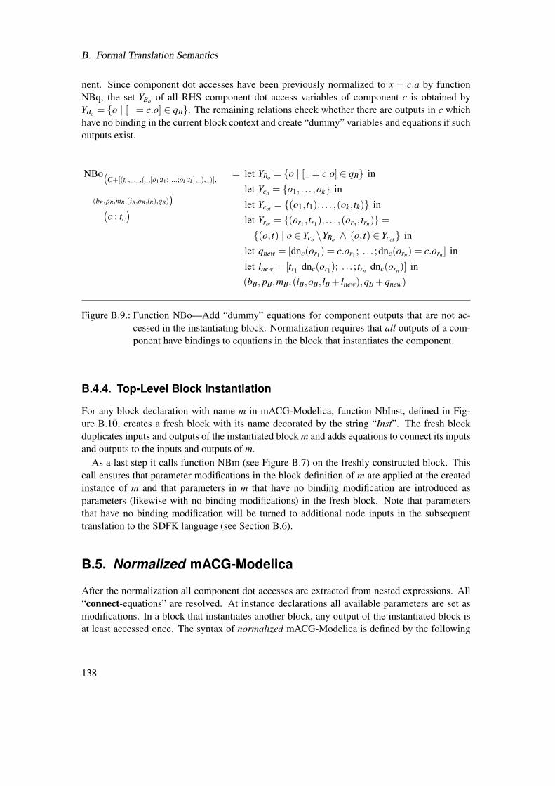
B. Formal Translation Semantics

nent. Since component dot accesses have been previously normalized to x = c.a by functionNBq, the set YBo of all RHS component dot access variables of component c is obtained byYBo = o | [_ = c.o] ∈ qB. The remaining relations check whether there are outputs in c whichhave no binding in the current block context and create “dummy” variables and equations if suchoutputs exist.

NBo(C+[(tc,_,_,(_,[o1:t1; ...;ok:tk],_),_)],

(bB,pB,mB,(iB,oB,lB),qB))(

c : tc)

= let YBo = o | [_ = c.o] ∈ qB in

let Yco = o1, . . . ,ok in

let Ycot = (o1, t1), . . . ,(ok, tk) in

let Yrot = (or1 , tr1), . . . ,(orn , trn)=(o, t) | o ∈ Yco \YBo ∧ (o, t) ∈ Ycot in

let qnew = [dnc(or1) = c.or1 ; . . . ;dnc(orn) = c.orn ] in

let lnew = [tr1 dnc(or1); . . . ; trn dnc(orn)] in

(bB, pB,mB,(iB,oB, lB + lnew),qB +qnew)

Figure B.9.: Function NBo—Add “dummy” equations for component outputs that are not ac-cessed in the instantiating block. Normalization requires that all outputs of a com-ponent have bindings to equations in the block that instantiates the component.

B.4.4. Top-Level Block Instantiation

For any block declaration with name m in mACG-Modelica, function NbInst, defined in Fig-ure B.10, creates a fresh block with its name decorated by the string “Inst”. The fresh blockduplicates inputs and outputs of the instantiated block m and adds equations to connect its inputsand outputs to the inputs and outputs of m.

As a last step it calls function NBm (see Figure B.7) on the freshly constructed block. Thiscall ensures that parameter modifications in the block definition of m are applied at the createdinstance of m and that parameters in m that have no binding modification are introduced asparameters (likewise with no binding modifications) in the fresh block. Note that parametersthat have no binding modification will be turned to additional node inputs in the subsequenttranslation to the SDFK language (see Section B.6).

B.5. Normalized mACG-Modelica

After the normalization all component dot accesses are extracted from nested expressions. All“connect-equations” are resolved. At instance declarations all available parameters are set asmodifications. In a block that instantiates another block, any output of the instantiated block isat least accessed once. The syntax of normalized mACG-Modelica is defined by the following

138

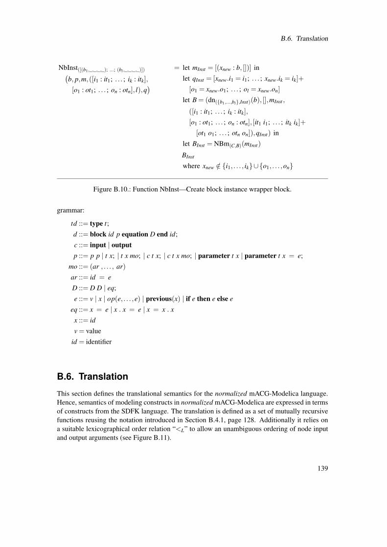
B.6. Translation

NbInst([(b1,_,_,_,_); ...; (bl ,_,_,_,_)])(b, p,m,([i1 : it1; . . . ; ik : itk],

[o1 : ot1; . . . ; on : otn], l),q)

= let mInst = [(xnew : b, [])] in

let qInst = [xnew.i1 = i1; . . . ; xnew.ik = ik]+

[o1 = xnew.o1; . . . ; ol = xnew.on]

let B = (dn(b1,...,bl,Inst)(b), [],mInst ,

([i1 : it1; . . . ; ik : itk],

[o1 : ot1; . . . ; on : otn], [it1 i1; . . . ; itk ik]+

[ot1 o1; . . . ; otn on]),qInst) in

let BInst = NBm(C,B)(mInst)

BInst

where xnew /∈ i1, . . . , ik∪o1, . . . ,on

Figure B.10.: Function NbInst—Create block instance wrapper block.

grammar:

td ::= type t;

d ::= block id p equation D end id;

c ::= input | outputp ::= p p | t x; | t x mo; | c t x; | c t x mo; | parameter t x | parameter t x = e;

mo ::= (ar , . . . , ar)

ar ::= id = e

D ::= D D | eq;

e ::= v | x | op(e, . . . ,e) | previous(x) | if e then e else e

eq ::= x = e | x . x = e | x = x . x

x ::= id

v = value

id = identifier

B.6. Translation

This section defines the translational semantics for the normalized mACG-Modelica language.Hence, semantics of modeling constructs in normalized mACG-Modelica are expressed in termsof constructs from the SDFK language. The translation is defined as a set of mutually recursivefunctions reusing the notation introduced in Section B.4.1, page 128. Additionally it relies ona suitable lexicographical order relation “<L” to allow an unambiguous ordering of node inputand output arguments (see Figure B.11).

139

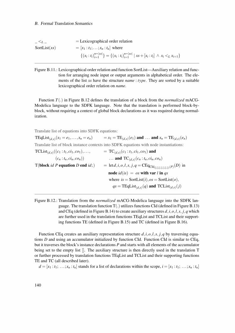
B. Formal Translation Semantics

_ <L _ = Lexicographical order relation

SortList(xs) = [x1 : t1; . . . ;xn : tn] where

(xi : ti)n=|xs|i=1 = (xi : ti)

n=|xs|i=1 | xs+[xi : ti] ∧ xi <L xi+1

Figure B.11.: Lexicographical order relation and function SortList—Auxiliary relation and func-tion for arranging node input or output arguments in alphabetical order. The ele-ments of the list xs have the structure name : type. They are sorted by a suitablelexicographical order relation on name.

Function T (.) in Figure B.12 defines the translation of a block from the normalized mACG-Modelica language to the SDFK language. Note that the translation is performed block-by-block, without requiring a context of global block declarations as it was required during normal-ization.

Translate list of equations into SDFK equations:

TEqList(d,s)(x1 = e1, . . . ,xn = en) = x1 = TE(d,s)(e1) and . . . and xn = TE(d,s)(en)

Translate list of block instance contexts into SDFK equations with node instantiations:

TCList(d,s)((c1 : t1,ci1,co1), . . . ,

(cn : tn,cin,con))

= TC(d,s)(c1 : t1,ci1,co1) and. . . and TC(d,s)(cn : tn,cin,con)

T(block id P equation D end id;) = letd, i,o, l,s, j,q = CEqCId([],[],[],[],[],[],[])(P)(D) in

node id(is) = os with var l in qs

where is = SortList(i),os = SortList(o),

qs = TEqList(d,s)(q) and TCList(d,s)( j)

Figure B.12.: Translation from the normalized mACG-Modelica language into the SDFK lan-guage. The translation function T(.) utilizes functions CId (defined in Figure B.13)and CEq (defined in Figure B.14) to create auxiliary structures d, i,o, l,s, j,q whichare further used in the translation functions TEqList and TCList and their support-ing functions TE (defined in Figure B.15) and TC (defined in Figure B.16).

Function CEq creates an auxiliary representation structure d, i,o, l,s, j,q by traversing equa-tions D and using an accumulator initialized by function CId. Function CId is similar to CEq,but it traverses the block’s instance declarations P and starts with all elements of the accumulatorbeing set to the empty list []. The auxiliary structure is then directly used in the translation Tor further processed by translation functions TEqList and TCList and their supporting functionsTE and TC (all described later).

d = [x1 : t1; . . . ;xn : tn] stands for a list of declarations within the scope, i = [x1 : t1; . . . ;xn : tn]

140

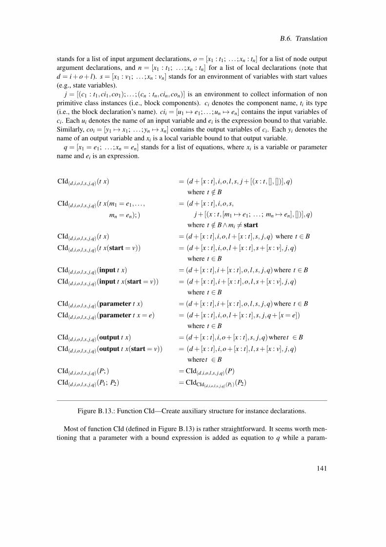
B.6. Translation

stands for a list of input argument declarations, o = [x1 : t1; . . . ;xn : tn] for a list of node outputargument declarations, and n = [x1 : t1; . . . ;xn : tn] for a list of local declarations (note thatd = i+ o+ l). s = [x1 : v1; . . . ;xn : vn] stands for an environment of variables with start values(e.g., state variables).

j = [(c1 : t1,ci1,co1); . . . ;(cn : tn,cin,con)] is an environment to collect information of nonprimitive class instances (i.e., block components). ci denotes the component name, ti its type(i.e., the block declaration’s name). cii = [u1 7→ e1; . . . ;un 7→ en] contains the input variables ofci. Each ui denotes the name of an input variable and ei is the expression bound to that variable.Similarly, coi = [y1 7→ x1; . . . ;yn 7→ xn] contains the output variables of ci. Each yi denotes thename of an output variable and xi is a local variable bound to that output variable.

q = [x1 = e1; . . . ;xn = en] stands for a list of equations, where xi is a variable or parametername and ei is an expression.

CId(d,i,o,l,s, j,q)(t x) = (d +[x : t], i,o, l,s, j+[(x : t, [], [])],q)

where t /∈ B

CId(d,i,o,l,s, j,q)(t x(m1 = e1, . . . ,

mn = en);)

= (d +[x : t], i,o,s,

j+[(x : t, [m1 7→ e1; . . . ; mn 7→ en], [])],q)

where t /∈ B∧mi 6= startCId(d,i,o,l,s, j,q)(t x) = (d +[x : t], i,o, l +[x : t],s, j,q) where t ∈ B

CId(d,i,o,l,s, j,q)(t x(start = v)) = (d +[x : t], i,o, l +[x : t],s+[x : v], j,q)

where t ∈ B

CId(d,i,o,l,s, j,q)(input t x) = (d +[x : t], i+[x : t],o, l,s, j,q)where t ∈ B

CId(d,i,o,l,s, j,q)(input t x(start = v)) = (d +[x : t], i+[x : t],o, l,s+[x : v], j,q)

where t ∈ B

CId(d,i,o,l,s, j,q)(parameter t x) = (d +[x : t], i+[x : t],o, l,s, j,q)where t ∈ B

CId(d,i,o,l,s, j,q)(parameter t x = e) = (d +[x : t], i,o, l +[x : t],s, j,q+[x = e])

where t ∈ B

CId(d,i,o,l,s, j,q)(output t x) = (d +[x : t], i,o+[x : t],s, j,q)where t ∈ B

CId(d,i,o,l,s, j,q)(output t x(start = v)) = (d +[x : t], i,o+[x : t], l,s+[x : v], j,q)

where t ∈ B

CId(d,i,o,l,s, j,q)(P;) = CId(d,i,o,l,s, j,q)(P)

CId(d,i,o,l,s, j,q)(P1; P2) = CIdCId(d,i,o,l,s, j,q)(P1)(P2)

Figure B.13.: Function CId—Create auxiliary structure for instance declarations.

Most of function CId (defined in Figure B.13) is rather straightforward. It seems worth men-tioning that a parameter with a bound expression is added as equation to q while a param-

141

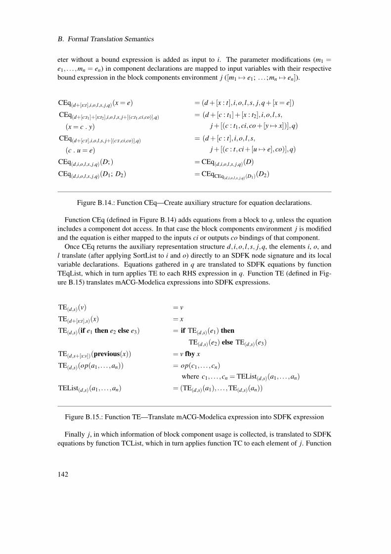
B. Formal Translation Semantics

eter without a bound expression is added as input to i. The parameter modifications (m1 =e1, . . . ,mn = en) in component declarations are mapped to input variables with their respectivebound expression in the block components environment j ([m1 7→ e1; . . . ;mn 7→ en]).

CEq(d+[x:t],i,o,l,s, j,q)(x = e) = (d +[x : t], i,o, l,s, j,q+[x = e])

CEq(d+[c:t1]+[x:t2],i,o,l,s, j+[(c:t1,ci,co)],q)

(x = c . y)

= (d +[c : t1]+ [x : t2], i,o, l,s,

j+[(c : t1,ci,co+[y 7→ x])],q)

CEq(d+[c:t],i,o,l,s, j+[(c:t,ci,co)],q)

(c . u = e)

= (d +[c : t], i,o, l,s,

j+[(c : t,ci+[u 7→ e],co)],q)

CEq(d,i,o,l,s, j,q)(D;) = CEq(d,i,o,l,s, j,q)(D)

CEq(d,i,o,l,s, j,q)(D1; D2) = CEqCEq(d,i,o,l,s, j,q)(D1)(D2)

Figure B.14.: Function CEq—Create auxiliary structure for equation declarations.

Function CEq (defined in Figure B.14) adds equations from a block to q, unless the equationincludes a component dot access. In that case the block components environment j is modifiedand the equation is either mapped to the inputs ci or outputs co bindings of that component.

Once CEq returns the auxiliary representation structure d, i,o, l,s, j,q, the elements i, o, andl translate (after applying SortList to i and o) directly to an SDFK node signature and its localvariable declarations. Equations gathered in q are translated to SDFK equations by functionTEqList, which in turn applies TE to each RHS expression in q. Function TE (defined in Fig-ure B.15) translates mACG-Modelica expressions into SDFK expressions.

TE(d,s)(v) = v

TE(d+[x:t],s)(x) = x

TE(d,s)(if e1 then e2 else e3) = if TE(d,s)(e1) thenTE(d,s)(e2) else TE(d,s)(e3)

TE(d,s+[x:v])(previous(x)) = v fby x

TE(d,s)(op(a1, . . . ,an)) = op(c1, . . . ,cn)

where c1, . . . ,cn = TEList(d,s)(a1, . . . ,an)

TEList(d,s)(a1, . . . ,an) = (TE(d,s)(a1), . . . ,TE(d,s)(an))

Figure B.15.: Function TE—Translate mACG-Modelica expression into SDFK expression

Finally j, in which information of block component usage is collected, is translated to SDFKequations by function TCList, which in turn applies function TC to each element of j. Function

142

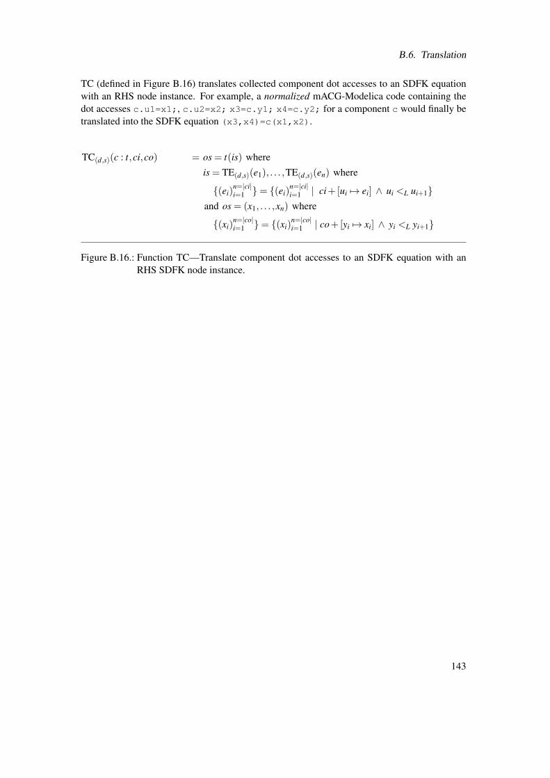
B.6. Translation

TC (defined in Figure B.16) translates collected component dot accesses to an SDFK equationwith an RHS node instance. For example, a normalized mACG-Modelica code containing thedot accesses c.u1=x1;, c.u2=x2; x3=c.y1; x4=c.y2; for a component c would finally betranslated into the SDFK equation (x3,x4)=c(x1,x2).

TC(d,s)(c : t,ci,co) = os = t(is) where

is = TE(d,s)(e1), . . . ,TE(d,s)(en) where

(ei)n=|ci|i=1 = (ei)

n=|ci|i=1 | ci+[ui 7→ ei] ∧ ui <L ui+1

and os = (x1, . . . ,xn) where

(xi)n=|co|i=1 = (xi)

n=|co|i=1 | co+[yi 7→ xi] ∧ yi <L yi+1

Figure B.16.: Function TC—Translate component dot accesses to an SDFK equation with anRHS SDFK node instance.

143

Bibliography

[1] W. B. Ackerman. Data flow languages. Computer, 15(2):15–25, 1982.

[2] J. Åkesson, U. Nordström, and H. Elmqvist. Dymola and Modelica_EmbeddedSystemsin Teaching–Experiences from a Project Course. In 7th Int. Modelica Conference, pages603–611, 2009.

[3] R. Alur, C. Courcoubetis, N. Halbwachs, T. Henzinger, P. Ho, X. Nicollin, A. Olivero,J. Sifakis, and S. Yovine. The algorithmic analysis of hybrid systems. Theoretical Com-puter Science, 138(1):3–34, February 1995.

[4] R. Alur, C. Courcoubetis, T. Henzinger, and P.-H. Ho. Hybrid automata: An algorith-mic approach to the specification and verification of hybrid systems. Hybrid systems,736:209–229, 1993.

[5] J. Andreasson and T. Bünte. Global chassis control based on inverse vehicle dynamicsmodels. Vehicle System Dynamics, 44:321–328, 2006.

[6] C. V. Anoop and C. Betta. Comparative Study of Fixed-Point and Floating-Point Codefor a Fixed-Point Micro. In dSPACE User Conference, Bangalore, India, Sept 2012.

[7] P. J. Ashenden, G. D. Peterson, and D. A. Teegarden. The System Designer’s Guide toVHDL-AMS. Morgan Kaufmann Publishers, San Francisco, September 2002.

[8] AUTOSAR. Specification of Interaction with Behavioral Models. Part of Release 4.1,Jan., 18 2013. http://www.autosar.org/.

[9] N. Bajçinca, R. Cortesão, and M. Hauschild. Robust control for steer-by-wire vehicles.Autonomous Robots, 19:193 – 214, 08 2005.

[10] P. Barnard. Software development principles applied to graphical model development.In AIAA Modeling and Simulation Technologies Conference and Exhibit, San Francisco,2005.

[11] J. Batteh and M. Tiller. A modular model architecture in Modelica for rapid virtual proto-typing of conventional and hybrid ground vehicles. In Ground Vehicle Systems Engineer-ing and Technology Symposium (GVSETS), pages 493–502, Bielefeld, Germany, March2009.

[12] K. Bauer and K. Schneider. From synchronous programs to symbolic representationsof hybrid systems. In Proceedings of the 13th ACM international conference on Hybridsystems: computation and control, HSCC ’10, pages 41–50, New York, NY, USA, 2010.ACM.

145

BIBLIOGRAPHY

[13] M. Beine, R. Otterbach, and M. Jungmann. Development of Safety-Critical SoftwareUsing Automatic Code Generation. In SAE World Congress, 2004.

[14] A. Benveniste, B. Caillaud, and M. Pouzet. The fundamentals of hybrid systems modelers.In 49th IEEE International Conference on Decision and Control (CDC’10), pages 4180–4185, Atlanta, Georgia, USA, December 15-17 2010.

[15] A. Benveniste, B. Caillaud, and P. Le Guernic. Compositionality in dataflow synchronouslanguages: specification and distributed code generation. Information and Computation,163:125–171, 2000.

[16] A. Benveniste, S. A. Edwards, N. Halbwachs, P. Le Guernic, and R. de Simone. Thesynchronous languages 12 years later. In Proceedings of the IEEE, volume 91 (1), pages64–83, 2003.

[17] M. C. Berg, N. Amit, and J. D. Powell. Multirate digital control system design. AutomaticControl, IEEE Transactions on, 33(12):1139–1150, 1988.

[18] D. Bhatt, B. Hall, S. Dajani-Brown, S. Hickman, and M. Paulitsch. Model-based devel-opment and the implications to design assurance and certification. In Digital AvionicsSystems Conference, 2005. DASC 2005. The 24th, volume 2, 2005.

[19] D. Biernacki, J.-L. Colaço, G. Hamon, and M. Pouzet. Clock-directed modular codegeneration for synchronous data-flow languages. SIGPLAN Not., 43(7):121–130, June2008.

[20] M. Bonvini, F. Donida, and A. Leva. Modelica as a design tool for hardware-in-the-loopsimulation. In 7th Int. Modelica Conference, pages 378–385, Como, Italy, Sep. 2009.

[21] F. Boussinot and R. De Simone. The ESTEREL language. Proceedings of the IEEE,79(9):1293–1304, 1991.

[22] D. Broman. Meta-Languages and Semantics for Equation-Based Modeling and Simula-tion. PhD thesis, Linköping University, PELAB - Programming Environment Laboratory,The Institute of Technology, 2010.

[23] D. Broman, P. Fritzson, and S. Furic. Types in the Modelica Language. In 5th Int. Mod-elica Conference, pages 303–315, Vienna, Austria, September 2006.

[24] M. Broy, H. Krcmar, J. Zimmermann, and S. Kirstan. Einfluss des Software-Designsauf die Wirtschaftlichkeit von Software-Entwicklungen. ATZelektronik, 02:34–37, April2011.

[25] C. Buckl. Model-Based Development of Fault-Tolerant Real-Time Systems. PhD thesis,Lehrstuhl für Echtzeitsysteme und Robotik, Technische Universität München, 2008.

[26] C. Buckl, A. Knoll, and G. Schrott. Model-based development of fault-tolerant embeddedsoftware. In Proceedings of Second International Symposium on Leveraging Applicationsof Fomal Methods, Verification and Validation (IEEE-ISoLA), 2006.

146

BIBLIOGRAPHY

[27] C. Buckl, M. Regensburger, A. Knoll, and G. Schrott. Models for automatic generationof safety-critical real-time systems. In Second International Conference on Availability,Reliability and Security (ARES), 2007.

[28] T. Bünte, J. Brembeck, and L. M. Ho. Human machine interface concept for interactivemotion control of a highly maneuverable robotic vehicle. In The Intelligent VehiclesSymposium, Baden-Baden, Germany, June 2011.

[29] T. Bünte, A. Sahin, and N. Bajcinca. Inversion of Vehicle Steering Dynamics with Mod-elica/Dymola. In G. Schmitz, editor, 4th Int. Modelica Conference, pages 319–328, Ham-burg, Germany, March 2005.

[30] P. Caspi, D. Pilaud, N. Halbwachs, and J. A. Plaice. Lustre: a declarative language forreal-time programming. In Proceedings of the 14th ACM SIGACT-SIGPLAN symposiumon Principles of programming languages, POPL ’87, pages 178–188, New York, NY,USA, 1987. ACM.

[31] P. Caspi, A. Curic, A. Maignan, C. Sofronis, S. Tripakis, and P. Niebert. From Simulinkto SCADE/Lustre to TTA: a layered approach for distributed embedded applications. InProceedings of the 2003 ACM SIGPLAN conference on Language, compiler, and tool forembedded systems, LCTES ’03, pages 153–162, New York, NY, USA, 2003. ACM.

[32] E. Chrisofakis, A. Junghanns, C. Kehrer, and A. Rink. Simulation-based development ofautomotive control software with Modelica. In 8th Int. Modelica Conference, pages 1–7,Dresden, Germany, March 2011.

[33] P. Clements, F. Bachmann, L. Bass, D. Garlan, J. Ivers, R. Little, P. Merson, R. Nord, andJ. Stafford. Documenting Software Architectures: Views and Beyond. Addison-Wesley,2010.

[34] J.-L. Colaço, B. Pagano, and M. Pouzet. A conservative extension of synchronous data-flow with state machines. In Proceedings of the 5th ACM International Conference onEmbedded Software, EMSOFT ’05, pages 173–182, New York, NY, USA, 2005. ACM.

[35] J.-L. Colaço and M. Pouzet. Clocks as First Class Abstract Types. In Third InternationalConference on Embedded Software (EMSOFT’03), Philadelphia, Pennsylvania, USA, Oc-tober 2003.

[36] A. Deuring, J. Gerl, and H. Wilhelm. Multi-Domain Vehicle Dynamics Simulation inDymola. In 8th Int. Modelica Conference, pages 13–17, Dresden, Germany, March 2011.

[37] C. Ebert and C. Jones. Embedded software: Facts, figures, and future. Computer, 42:42–52, April 2009.

[38] M. Eder and A. Knoll. Design of an Experimental Platform for an X-by-wire Car withFour-wheel Steering. In Proc. IEEE Conf. Automation Science and Engineering (CASE),pages 656–661, 2010.

147

BIBLIOGRAPHY

[39] J. Eker, J. W. Janneck, E. A. Lee, J. Liu, J. Liu, J. Ludvig, S. Neuendorffer, S. Sachs,and Y. Xiong. Taming heterogeneity - the Ptolemy approach. Proceedings of the IEEE,91(1):127 – 144, jan. 2003.

[40] H. Elmqvist. A Structured Model Language for Large Continuous Systems. PhD thesis,Lund Institute of Technology, Lund, Sweden, 1978.

[41] H. Elmqvist. An Object and Data-Flow Based Visual Language for Process Control. InISA/92-Canada Conference & Exhibition, pages 181–192, Toronto, Canada, April 1992.Instrument Society of America.

[42] H. Elmqvist, M. Otter, D. Henriksson, B. Thiele, and S. E. Mattsson. Modelica for Em-bedded Systems. In 7th Int. Modelica Conference, pages 354–363, Como, Italy, Septem-ber 2009.

[43] H. Elmqvist, M. Otter, and S. E. Mattsson. Fundamentals of Synchronous Control inModelica. In M. Otter and D. Zimmer, editors, 9th Int. Modelica Conference, pages 15–26, Munich, Germany, September 2012.

[44] T. Erkinnen. Fixed-Point ECU Code Optimization and Verification with Model-BasedDesign. In SAE 2009 World Congress & Exhibition, Detroit, Michigan, United States,April 2009. SAE Technical Paper 2009-01-0269.

[45] S. Frank, M. Grabmüller, P. Hofstedt, D. Kleeblatt, P. Pepper, P. R. Mai, and S.-A. Schnei-der. Safety of Compilers and Translation Techniques – Status quo of Technology andScience. In Automotive – Safety & Security, 2008.

[46] R. Franke, B. Babji, M. Antoine, and A. Isaksson. Model-based online applications inthe ABB Dynamic Optimization framework. In B. Bachmann, editor, 6th Int. ModelicaConference, pages 279–285, Bielefeld, 2008.

[47] P. Fritzson. Principles of Object-Oriented Modeling and Simulation with Modelica 2.1.Wiley-IEEE Press, 2003.

[48] D. Glasson. Development and applications of multirate digital control. Control SystemsMagazine, IEEE, 3(4):2–8, 1983.

[49] D. Goldberg. What Every Computer Scientist Should Know About Floating-Point Arith-metic. ACM Computing Surveys, 23(1):5–48, March 1991.

[50] N. Halbwachs. A Synchronous Language at Work: the Story of Lustre. In Third ACM andIEEE International Conference on Formal Methods and Models for Co-Design. MEM-OCODE ’05., pages 3–11, July 2005.

[51] G. Hamon and M. Pouzet. Modular Resetting of Synchronous Data-flow Programs. InACM International conference on Principles of Declarative Programming (PPDP’00),Montreal, Canada, September 2000.

148

BIBLIOGRAPHY

[52] H. Hanselmann, U. Kiffmeier, L. Koster, M. Meyer, and A. Rukgauer. Production qualitycode generation from simulink block diagrams. In Proceedings of the 1999 IEEE Inter-national Symposium on Computer Aided Control System Design, pages 213–218, KohalaCoast-Island of Hawai’i, Hawai’i, USA, August 1999. IEEE.

[53] D. Harel. Statecharts: a visual formalism for complex systems. Science of ComputerProgramming, 8(3):231–274, 1987.

[54] T. Henzinger. The theory of hybrid automata. In 11th Annual IEEE Symposium on Logicin Computer Science (LICS), pages 278–292. IEEE, 1996.

[55] T. Henzinger and J. Sifakis. The discipline of embedded systems design. Computer,40(10):32 –40, oct. 2007.

[56] U. Honekamp, J. Reidel, K. Werther, T. Zurawka, and T. Beck. Component-node-network: three levels of optimized code generation with ASCET-SD. In Computer AidedControl System Design, 1999. Proceedings of the 1999 IEEE International Symposiumon, pages 243–248, 1999.

[57] IEC 61508, Functional safety of electrical/electronic/programmable electronic safety-related systems, Parts 1 through 7, Edition 1.0, 1998–2000.

[58] ISO 26262: Road vehicles – Functional safety, Parts 1 through 10, 2011-2012.

[59] ISO 26262-6:2011, Road vehicles – Functional safety – Part 6: Product development atthe software level, November 2011.

[60] ISO 26262-8:2011, Road vehicles – Functional safety – Part 8: Supporting processes,November 2011.

[61] M. Krenn and T. Richter. Active steering-BMW’s approach to modern steering technol-ogy. In Braking 2004: Vehicle Braking and Chassis Control, page 3. Wiley, 2004.

[62] P. Le Guernic, T. Gautier, M. Le Borgne, and C. Le Maire. Programming real-time appli-cations with SIGNAL. Proceedings of the IEEE, 79(9):1321–1336, 1991.

[63] E. A. Lee. Cyber-physical systems - are computing foundations adequate? In NSFWorkshop on Cyber-Physical Systems, October 2006.

[64] E. A. Lee and A. Sangiovanni-Vincentelli. A framework for comparing models of com-putation. IEEE Transactions on CAD, 17(12):1217–1229, December 1998.

[65] E. A. Lee and S. A. Seshia. Introduction to Embedded Systems, A Cyber-Physical SystemsApproach. http://LeeSeshia.org, ISBN 978-0-557-70857-4, 2011.

[66] E. A. Lee and H. Zheng. Operational semantics of hybrid systems. In M. Morari andL. Thiele, editors, Hybrid Systems: Computation and Control, volume 3414 of LectureNotes in Computer Science, pages 25–53. Springer Berlin / Heidelberg, 2005.

149

BIBLIOGRAPHY

[67] J. W. Lloyd. Practical Advantages of Declarative Programming. In M. Alpuente, R. Bar-buti, and I. Ramos, editors, Joint Conference on Declarative Programming, GULP-PRODE’94, volume 1, pages 18–33, Peñiscola, Spain, September 19–22 1994.

[68] G. Looye. Design of Robust Autopilot Control Laws with Nonlinear Dynamic Inversion.at - Automatisierungstechnik, 49(12):523–531, December 2001.

[69] R. Lublinerman, C. Szegedy, and S. Tripakis. Modular code generation from synchronousblock diagrams: Modularity vs. code size. In ACM SIGPLAN Notices, volume 44, pages78–89. ACM, 2009.

[70] P. Löw, R. Pabst, and E. Petry. Funktionale Sicherheit in der Praxis. dpunkt.verlag, 2010.

[71] F. Maraninchi and Y. Rémond. Mode-Automata: About Modes and States for ReactiveSystems. In European Symposium On Programming, Lisbon, Portugal, March 1998.Springer-Verlag.

[72] F. Maraninchi and Y. Rémond. Mode-Automata: a new domain-specific construct for thedevelopment of safe critical systems. Science of Computer Programming, 46:219–254,2003.

[73] Modelica Association. Modelica—A Unified Object-Oriented Language for Sys-tems Modeling v3.3. Standard Specification, May 2012. Available athttp://www.modelica.org/.

[74] P. Mosterman and J. Ciolfi. Using interleaved execution to resolve cyclic dependencies intime-based block diagrams. In Decision and Control, 2004. CDC. 43rd IEEE Conferenceon, volume 4, pages 4057–4062 Vol.4, Dec 2004.

[75] M. Najafi, S. Furic, and R. Nikoukhah. Scicos: a general purpose modeling and simula-tion environment. In 4th Int. Modelica Conference, pages 367–374, Hamburg-Harburg,Germany, March 2005.

[76] M. Najafi and R. Nikoukhah. Implementation of Hybrid Automata in Scicos. In Con-trol Applications, 2007. CCA 2007. IEEE International Conference on, pages 819–824,Singapore, October 2007. IEEE.

[77] O. Niggemann, U. Eisemann, M. Beine, and U. Kiffmeier. Behavior Modeling Tools inan Architecture-Driven Development Process - From Function Models to AUTOSAR. InSAE 2007 World Congress & Exhibition, Detroit, Michigan, United States, April 2007.SAE Technical Paper 2007-01-0507.

[78] O. Niggemann and J. Stroop. Models for model’s sake: why explicit system modelsare also an end to themselves. In Proceedings of the 30th international conference onSoftware engineering, ICSE ’08, pages 561–570, New York, NY, USA, 2008. ACM.

[79] R. Nikoukhah and S. Furic. Towards a full integration of Modelica models in the scicosenvironment. In 7th Modelica Conference, pages 641–645, Como, Italy, September 2009.

150

BIBLIOGRAPHY

[80] Object Management Group. OMG Systems Modeling Language (OMG SysML) v1.2.Standard Specification, November 2010. OMG document number: formal/2010-06-01,available at http://www.omgsysml.org.

[81] Object Management Group. OMG Unified Modelling Language Specification (OMGUML) v2.4.1. Standard Specification, August 2011.

[82] L. A. Ochel and B. Bachmann. Initialization of Equation-Based Hybrid Models withinOpenModelica. In 5th International Workshop on Equation-Based Object-Oriented Mod-eling Languages and Tools, pages 97–103, Nottingham, UK, April 2013.

[83] M. Odersky, L. Spoon, and B. Venners. Programming in Scala. Artima Press, secondedition, 2010.

[84] M. Otter, B. Thiele, and H. Elmqvist. A Library for Synchronous Control Systems inModelica. In M. Otter and D. Zimmer, editors, 9th Int. Modelica Conference, pages 27–36, Munich, Germany, September 2012.

[85] L. Parnebo and B. Hansson. Plug and play in control loop design. In Preprints Regler-möte, Linköping, Sweden, May 2002.

[86] A. Pop, M. Sjölund, A. Ashgar, P. Fritzson, and F. Casella. Integrated Debugging ofModelica Models. Modeling, Identification and Control, 35(2):93–107, 2014.

[87] M. Pouzet. Lucid Synchrone Tutorial and Reference Manual, 2006.

[88] M. Pouzet and P. Raymond. Modular Static Scheduling of Synchronous Data-flow Net-works: An efficient symbolic representation. Journal of Design Automation for EmbeddedSystems, 3(14):165–192, 2010.

[89] A. Rau. Modellbasierte Entwicklung von eingebetteten Regelungssystemen in der Auto-mobilindustrie. PhD thesis, Fakultät für Informatik, Eberhard-Karls-Universität Tübin-gen, 2002.

[90] A. Robinson. Non Standard Analysis. Princeton Landmarks in Mathematics, 1996.

[91] S. Sauvage and A. Bouali. Development Approaches in Software Development. In Em-bedded Real Time Software (ERTS), Toulouse, France, January 2006.

[92] W. Schamai, P. Frizson, C. Paredis, and A. Pop. Towards Unified System Modelingand Simulation with ModelicaML: Modeling of Executable Behavior Using GraphicalNotations. In 7th Int. Modelica Conference, pages 612–621, Como, Italy, September2009.

[93] K. Schneider. The synchronous programming language Quartz. Internal Report 375,Department of Computer Science, University of Kaiserslautern, Kaiserslautern, Germany,December 2009.

151

BIBLIOGRAPHY

[94] S.-A. Schneider, T. Lovric, and P. R. Mai. The Validation Suite Approach to SafetyQualification of Tools. In SAE World Congress, Detroit, MI, USA, April 2009. SAEInternational.

[95] J. Schäuffele and T. Zurawka. Automotive Software Engineering – Principles, Processes,Methods and Tools. SAE International, 2005.

[96] A. M. Sloane. Lightweight Language Processing in Kiama. In J. Fernandes, R. Lämmel,J. Visser, and J. Saraiva, editors, Generative and Transformational Techniques in SoftwareEngineering III, volume 6491 of Lecture Notes in Computer Science, pages 408–425.Springer Berlin Heidelberg, 2011.

[97] P. Smith, S. Prabhu, and J. Friedman. Best Practices for Establishing a Model-BasedDesign Culture. In SAE 2007 World Congress & Exhibition, Detroit, Michigan, UnitedStates, April 2007. SAE Technical Paper 2007-01-0777.

[98] T. Stahl and M. Völter. Model-Driven Software Development: Technology, Engineering,Management. Wiley, 2006.

[99] I. Stürmer. Systematic Testing of Code Generation Tools. PhD thesis, Technische Univer-sität Berlin, 2006.

[100] I. Stürmer, M. Conrad, I. Fey, and H. Dörr. Experiences with Model and Autocode Re-views in Model-based Software Development. In Proceedings of the 2006 internationalworkshop on Software engineering for automotive systems, SEAS ’06, pages 45–52, NewYork, NY, USA, 2006. ACM.

[101] I. Stürmer, D. Weinberg, and M. Conrad. Overview of existing safeguarding techniquesfor automatically generated code. In Proceedings of the Second International Workshopon Software Engineering for Automotive Systems, SEAS ’05, pages 1–6, New York, NY,USA, 2005. ACM.

[102] E. D. Tate, M. Sasena, J. Gohl, and M. Tiller. Model embedded control: A method torapidly synthesize controllers in a modeling environment. In 6th Int. Modelica Confer-ence, 2008.

[103] A. Tewari. Modern Control Design with Matlab and Simulink. John Wiley & Sons, Ltd.,2002.

[104] The Motor Industry Software Reliability Association. Development Guidelines for Vehi-cle Based Software, 1994. http://www.misra.org.uk.

[105] The Motor Industry Software Reliability Association. MISRA-C:1998 - Guidelines forthe use of the C language in vehicle based systems, 1998. (superseeded by MISRAC:2012) http://www.misra.org.uk.

[106] The Motor Industry Software Reliability Association. MISRA-C:2004 - Guidelines forthe use of the C language in critical systems, 2004. http://www.misra.org.uk.

152

BIBLIOGRAPHY

[107] The Motor Industry Software Reliability Association. MISRA AC AGC - Guidelinesfor the application of MISRA-C:2004 in the context of automatic code generation, 2007.http://www.misra.org.uk.

[108] B. Thiele, A. Knoll, and P. Fritzson. Towards Qualifiable Code Generation from a ClockedSynchronous Subset of Modelica. Modeling, Identification and Control, 36(1):23–52,2015.

[109] B. Thiele, S.-A. Schneider, and P. R. Mai. A Modelica Sub-and Superset for Safety-Relevant Control Applications. In M. Otter and D. Zimmer, editors, 9th Int. ModelicaConference, pages 455–476, Munich, Germany, September 2012.

[110] T. Thomsen. MISRA C und seine Anwendbarkeit auf Seriencodegeneratoren. Technicalreport, dSPACE GmbH, 2003.

[111] M. Thümmel, M. Kurze, M. Otter, and J. Bals. Nonlinear inverse models for control. In4th Int. Modelica Conference, pages 267–279, 2005.

[112] M. Thümmel, M. Otter, and J. Bals. Vibration control of elastic joint robots by inverse dy-namics models. In H. Ulbrich and W. Günthner, editors, IUTAM Symposium on VibrationControl of Nonlinear Mechanisms and Structures, pages 343–353, München, 2005.

[113] L. Vitkin, S. Dong, and M. Chandrashekar. Selection of Fixed-Point or Floating-Point forProduction Applications. In dSPACE User Conference, 2006.

[114] F. Wagner, L. Lui, and G. Frey. Simulation of Distributed Automation Systems in Mod-elica. In 6th International Modelica Conference, pages 113–122, Bielefeld, Germany,2008.

[115] M. Whalen and M. Heimdahl. On the requirements of high-integrity code generation. InHigh-Assurance Systems Engineering, 1999. Proceedings. 4th IEEE International Sym-posium on, pages 217–224, 1999.

[116] J. Åkesson, T. Ekman, and G. Hedin. Implementation of a Modelica compiler usingJastAdd attribute grammars. Science of Computer Programming, 75(1–2):21–38, 2010.Special Issue on ETAPS 2006 and 2007 Workshops on Language Descriptions, Tools, andApplications (LDTA ’06 and ’07).

[117] K. J. Åström and B. Wittenmark. Computer-Controlled Systems: Theory and Design.Prentice-Hall, Inc., 1997.

153

Curriculum Vitae

Persönliche DatenName: Bernhard Amadeus ThieleGeburtsdatum und -ort: 27.09.1980 in Garmisch-PartenkirchenFamilienstand: ledigAdresse: Rydsvägen 84A lgh 1001

58431 Linköping, SchwedenE-Mail: bernhard-thiele@web.de

Schul- und Berufsausbildung2012 – heute externer Doktorand

Technische Universität MünchenLehrstuhl für Echtzeitsysteme und RobotikTitel: Framework for Modelica Based Function DevelopmentBetreuer: Univ.-Prof. Dr. Alois Knoll

2001 – 2007 Diplom-Ingenieur Maschinenwesen (Dipl.-Ing. Univ.)Technische Universität MünchenTitel: Einsatz adaptiver Regelstrategien für aktive Komponentenin Werkzeug-Maschinen

2004 – 2005 AuslandssemesterUniversity of Birmingham, UKMechanical Engineering Department and School of Mathematics

2000 – 2001 Wehrdienst

1991 – 2000 AbiturWerdenfels-Gymnasium Garmisch-Partenkirchen

Berufspraxis2014 – heute wissenschaftlicher Mitarbeiter

Linköping UniversityDepartment of Computer and Information Science581 83 Linköping, Sweden

2007 – 2014 wissenschaftlicher MitarbeiterDeutsches Zentrum für Luft- und Raumfahrt e.V. (DLR)Institut für Systemdynamik und RegelungstechnikMünchner Straße 20, 82234 Weßling

155