Embed Size (px)
Citation preview
Technische Universität MünchenInstitut für Energietechnik
Lehrstuhl für Thermodynamik
Hollow ConeSpray Characterizationand Integral Modeling
Peter Bollweg
Vollständiger Abdruck der von der Fakultät für Maschinenwesen derTechnischen Universität München zur Erlangung des akademischenGrades eines
DOKTOR-INGENIEURS
genehmigten Dissertation.
Vorsitzender: Univ.-Prof. Dr.-Ing. Hans-Jakob Kaltenbach
Prüfer der Dissertation: 1. Univ.-Prof. Wolfgang Polifke, Ph.D. (CCNY)2. Univ.-Prof. Dr.-Ing. Georg Wachtmeister
Die Dissertation wurde am 01.12.2011 bei der TechnischenUniversität München eingereicht und durch die Fakultät fürMaschinenwesen am 22.06.2012 angenommen.

Abstract
Gasoline direct injection (GDI) has been widely introduced in todaysinternal combustion engines for automotive applications. One wayto increase the engines efficiency is to reduce throttling losses. Thisengine operation mode requires the stratification of the fuel air mixturewithin the combustion cylinder. Hollow cone injectors enable suchmixture stratification.
The present work investigates the spray formation resulting from theinjection of liquid fuel into air by a hollow cone injector. A method-ological overview establishes the need of a fast spray model to simu-late the engine operation at a system level. A detailed insight into thefluid mechanics of a hollow cone two-phase jet is obtained by meansof a computational fluid dynamics (CFD) investigation. The model isvalidated experimentally both by the global penetration behavior andby the velocity field outside of the dense spray. Based on the character-ization of the hollow cone two-phase flow, a one-dimensional modelis derived. It describes the temporal evolution of the two-phase jetinduced by the hollow cone injection process. Diffusive transport ofmass, momentum, and energy between the dense spray zone and itsenvironment is modeled by means of a boundary layer description.


Was wirklich zählt ist Intuition. (Albert Einstein)


Preface
The research work presented in this thesis was accomplished in theGasoline Systems Advanced Development Team at Continental AG(formerly Siemens VDO Automotive AG) in Regensburg, Germany.
I express my special thanks to my thesis supervisor Prof. WolfgangPolifke, Ph.D. Both his thorough insight into the topic and the fruitfuldiscussions with him supported my progress to a great extend.
I also thank Prof. Dr.-Ing. Georg Wachtmeister for participating inthe defense committee and Prof. Dr.-Ing. Hans-Jakob Kaltenbach forchairing the examination.
I am very grateful to Prof. Dr. André Kaufmann who introduced me tothe interesting but complex subject of dispersed two-phase flows andinitiated this thesis work. Him sharing his experience and ideas withme gave me a great ahead start in understanding two-phase flows anddeveloping my own modeling ideas.
This research work was funded by Continental AG which I gratefullyacknowledge. Special thanks are directed to Dr. Harald Bäcker inwho’s Combustion Team this research was conducted. I would alsolike to thank my colleagues within the combustions team for the goodtimes and professional exchange. I am especially grateful to Dr. Chris-tian Lohfink with whom I shared the researcher’s fate.
Many thanks go to the two-phase flow group at the Lehrstuhl fürThermodynamik at Technische Universität München – namely VolkerKaufmann, Joao Carpintero, and Roland Kaess – for their open discus-sions at the chair and the pleasant times we spent during conferencesand researching at CERFACS (Toulouse, France).

Eventually, I owe special thanks to my family, my wife and two sons,who spared some of my attention while I finished this work, and myparents, who lay the foundation to my personal and professional de-velopment years ago.
Stuttgart, July 2012
Peter Bollweg
viii
Contents
Nomenclature xi
1 Introduction 1
2 Modeling methodology 72.1 Injection induced two-phase flow characterization . . . 72.2 Model classification overview . . . . . . . . . . . . . 132.3 Motivation and modeling strategy . . . . . . . . . . . 192.4 Hollow cone injection . . . . . . . . . . . . . . . . . . 25
2.4.1 Conservation equations in conical coordinates . 262.4.2 Two-phase jet dynamics . . . . . . . . . . . . 30
2.5 Summary . . . . . . . . . . . . . . . . . . . . . . . . 38
3 Dispersed two-phase flow analysis 393.1 Two-phase flow description . . . . . . . . . . . . . . . 40
3.1.1 Continuous phase transport . . . . . . . . . . . 423.1.2 Dispersed phase transport . . . . . . . . . . . 433.1.3 Source terms . . . . . . . . . . . . . . . . . . 463.1.4 CFD setup . . . . . . . . . . . . . . . . . . . 51
3.2 Hollow cone injection induced two-phase flow . . . . . 583.2.1 Experimental data . . . . . . . . . . . . . . . 583.2.2 CFD model validation . . . . . . . . . . . . . 623.2.3 Inter-phase momentum exchange . . . . . . . 703.2.4 Carrier phase transport . . . . . . . . . . . . . 813.2.5 Temporal evolution . . . . . . . . . . . . . . . 89
3.3 Summary . . . . . . . . . . . . . . . . . . . . . . . . 93
Contents
4 Integral modeling 954.1 Spray model motivation and outline . . . . . . . . . . 954.2 Cross-stream length scales . . . . . . . . . . . . . . . 984.3 Momentum conservation . . . . . . . . . . . . . . . . 103
4.3.1 Dispersed phase and dense spray zone . . . . . 1044.3.2 Carrier phase integral boundary layer descrip-
tion . . . . . . . . . . . . . . . . . . . . . . . 1084.3.3 Cross-stream length scale dynamics . . . . . . 1134.3.4 ttBL model assessment . . . . . . . . . . . . . 1244.3.5 Numerical scheme and boundary conditions . . 1294.3.6 Results . . . . . . . . . . . . . . . . . . . . . 130
4.3.6.1 Transient single phase boundary layer(tBL) . . . . . . . . . . . . . . . . . 130
4.3.6.2 Transient two-phase boundary layer(ttBL) . . . . . . . . . . . . . . . . 135
4.3.6.3 Chamber pressure dependence . . . 1394.4 Evaporation . . . . . . . . . . . . . . . . . . . . . . . 1414.5 Turbulence . . . . . . . . . . . . . . . . . . . . . . . 1584.6 Summary . . . . . . . . . . . . . . . . . . . . . . . . 163
5 Conclusion 165
Bibliography 169
Appendix 183
A Navier-Stokes equations in conical coordinates 183
B Boundary layer fluxes 187
x
Nomenclature
Roman lettersD diffusion coefficientF , F force NL length scale mP production rateT time scale sU velocity scale m/sC, c constant, coefficientCD drag coefficientD diameter mk turbulent kinetic energy m2 s−2
l length mm, M mass kgMF volume specific fuel vapor mass kg/mr radial coordinates mx, y, z cartesian coordinates mY species mass fraction
Greek lettersα volume fractionδ boundary layer length scale mη cross-stream cone coordinate mΓ evaporating mass density source term kg/m/sλ cross-stream cone coordinate mλ thermal diffusion coefficient Wm−1 K−1
φ circumferential coordinate rad
Contents
Π energy density source term J/m/sσ surface density 1/mτ shear stress N/mτp particle relaxation time sθ cone half-opening angleξ streamwise cone coordinate m
Non-dimensional numbersPe Peclet numberPr Prandtl numberRe Reynolds numberSt Stokes numberWe Weber number
Sub- and superscriptsτ shear stress(0) initial(c) characteristicc fluid / carrier phaseF fueli, j, k indicesm mixing / mixturep Particle or dispersed phaseT turbulent
Abbreviations and acronymsAV artificial viscosityBL boundary layerCFD computational fluid dynamicsconv convectivediff diffusive
xii
Contents
DPS discrete particle simulationDSZ dense spray zoneEE Euler-Eulereff effectiveEL Euler-Lagrangeentr entrainedGDI gasoline direct injectionICE internal combustion engineLES large eddy simulationLIF laser induced fluorescenceNS Navier-StokesODE ordinary differential equationPDE partial differential equationSGS sub-grid scaleTPF two-phase flow
xiii

1 Introduction
The development of internal combustion engines for automotive appli-cations has been driven primarily by the international emission legisla-tion and fuel efficiency. Until today, the focus of the legislation lay onthe restriction of pollutant emissions, i.e. the unwanted side productsresulting from combustion of the fuel-air mixture. In future, carbon-dioxide emission targets will additionally require the introduction oftechnologies to increase fuel efficiency.
In the context of gasoline internal combustion engines, the direct in-jection of the fuel into the combustion chamber is supposed to providea substantial potential to reduce fuel consumption [106]. One advan-tage of injecting the fuel directly into the cylinder is the possibility ofmixture stratification: Fuel may be injected so that an ignitable air-fuel mixture is positioned near the spark plug at the time of ignitionwhile the total cylinder charge exhibits a lean quality. This engine op-eration enables to take the air into the cylinder at ambient pressure andthereby to reduce throttling losses.
The so-called first generation of gasoline direct injection (GDI) ap-plied pressure swirl or multi-hole injectors to achieve mixture strat-ification [91]. The charge motion was used to redirect the ignitableair/fuel mixture towards the spark plug. The so called “wall guided”setup depends on a special piston bowl design to initiate a tumble mo-tion of the cylinder charge [58]. Mixture stratification by a tumblingcharge motion was also realized by appropriate intake port designs(“air guided”). The first generation GDI approach suffers from com-paratively large cycle-to-cycle variations [26] and above all results inonly limited fuel savings.
1 Introduction
Second generation direct injection
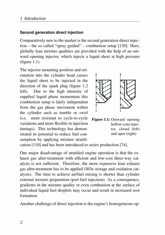
Comparatively new to the market is the second generation direct injec-tion – the so called “spray guided” – combustion setup [130]: Here,globally lean mixture qualities are provided with the help of an out-ward opening injector, which injects a liquid sheet at high pressure(figure 1.1).
Figure 1.1: Outward openinghollow cone injec-tor, closed (left)and open (right)
The injector mounting position and ori-entation into the cylinder head causesthe liquid sheet to be injected in thedirection of the spark plug (figure 1.2left). Due to the high intensity ofsupplied liquid phase momentum thiscombustion setup is fairly independentfrom the gas phase movement withinthe cylinder such as tumble or swirl(i.e. more resistant to cycle-to-cyclevariations and more flexible in injectiontimings). This technology has demon-strated its potential to reduce fuel con-sumption by applying mixture stratifi-cation [110] and has been introduced to series production [74].
One major disadvantage of stratified engine operation is that the ex-haust gas after-treatment with efficient and low-cost three-way cat-alysts is not sufficient. Therefore, the more expensive lean exhaustgas after-treatment has to be applied (NOx storage and oxidation cat-alysts). The time to achieve air/fuel mixing is shorter than cylinderexternal mixture preparation (port fuel injection). As a consequence,gradients in the mixture quality or even combustion at the surface ofindividual liquid fuel droplets may occur and result in increased sootformation.
Another challenge of direct injection is the engine’s homogeneous op-
2
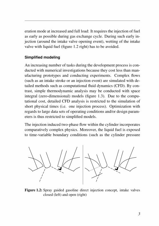
eration mode at increased and full load: It requires the injection of fuelas early as possible during gas exchange cycle. During such early in-jection (around the intake valve opening event), wetting of the intakevalve with liquid fuel (figure 1.2 right) has to be avoided.
Simplified modeling
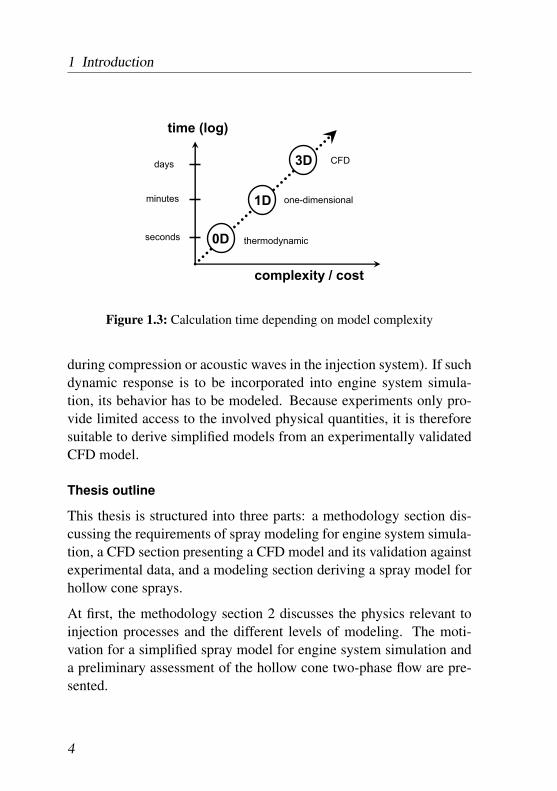
An increasing number of tasks during the development process is con-ducted with numerical investigations because they cost less than man-ufacturing prototypes and conducting experiments. Complex flows(such as an intake stroke or an injection event) are simulated with de-tailed methods such as computational fluid dynamics (CFD). By con-trast, simple thermodynamic analysis may be conducted with spaceintegral (zero-dimensional) models (figure 1.3). Due to the compu-tational cost, detailed CFD analysis is restricted to the simulation ofshort physical times (i.e. one injection process). Optimization withregards to large data sets of operating conditions and/or design param-eters is thus restricted to simplified models.
The injection induced two-phase flow within the cylinder incorporatescomparatively complex physics. Moreover, the liquid fuel is exposedto time-variable boundary conditions (such as the cylinder pressure
Figure 1.2: Spray guided gasoline direct injection concept, intake valvesclosed (left) and open (right)
3
1 Introduction
time (log)
complexity / cost
1D
3D
thermodynamicseconds
minutes
days
0D
one-dimensional
CFD
Figure 1.3: Calculation time depending on model complexity
during compression or acoustic waves in the injection system). If suchdynamic response is to be incorporated into engine system simula-tion, its behavior has to be modeled. Because experiments only pro-vide limited access to the involved physical quantities, it is thereforesuitable to derive simplified models from an experimentally validatedCFD model.
Thesis outline
This thesis is structured into three parts: a methodology section dis-cussing the requirements of spray modeling for engine system simula-tion, a CFD section presenting a CFD model and its validation againstexperimental data, and a modeling section deriving a spray model forhollow cone sprays.
At first, the methodology section 2 discusses the physics relevant toinjection processes and the different levels of modeling. The moti-vation for a simplified spray model for engine system simulation anda preliminary assessment of the hollow cone two-phase flow are pre-sented.
4

The hollow cone injection process is investigated by means of three-dimensional CFD in section 3. The basic physical description is sum-marized in section 3.1. The transient evolution of spray characteristicsis modeled by both Lagrangian and Eulerian two-phase flow descrip-tions. The CFD model’s validation is based on carrier phase velocitymeasurements outside the dense hollow cone sheet. The sensitivity ofboth physical and numerical quantities is investigated. The CFD anal-ysis (section 3.2) focuses on the mechanisms occurring due to inter-phase momentum exchange and the global flow structure due to thehollow cone geometry.
Based on the presented flow details, an integral model for the hollowcone injection process is proposed in section 4. It describes the tran-sient evolution of the two-phase jet induced by the hollow cone injec-tion process. Mass, momentum and energy equations are resolved inone spatial coordinate. Sources due to momentum exchange, dropletheat-up, and fuel evaporation are accounted for.The model is explicitly suited for dense sprays. Diffusive transportof momentum, energy, and fuel species mass between the dense sprayzone and its environment is modeled by means of a boundary layerdescription. The dense spray characteristics predicted by the modelare assessed both qualitatively and in comparison to CFD data.
5

2 Modeling methodology
In order to deduce a simplified model for a hollow cone spray, thephysical phenomena relevant to describe the two-phase jet need to beidentified. For this reason, injection specific physics are shortly dis-cussed in section 2.1 and the dominant effects for the injection into acold gas environment are outlined. In section 2.2, an overview of thedifferent levels of physical modeling is given. The detailed motivationfor a simplified description for hollow cone sprays is presented in sec-tion 2.3. The preliminary assessment of an injection induced hollowcone flow (section 2.4) provides the basis for both the CFD investiga-tion and the modeling approach presented in the later chapters.
2.1 Injection induced two-phase flow characterization
The spatial distribution of a liquid dispersed phase injected into agaseous carrier phase environment is the result of several (interacting)basic physical phenomena. They are shortly reviewed in the followingin order to emphasize their contribution to the overall evolution of thetwo-phase flow. Special attention is directed towards the process ofinter-phase momentum exchange.
Basic physical phenomena
An injection induced two-phase flow is influenced by the injector in-ternal flow (ejection direction, mean mass flow rate, etc.). The charac-teristics of the dispersed phase closed to the injector exit are the resultof primary breakup, the formation of ligaments and droplets from a
2 Modeling methodology
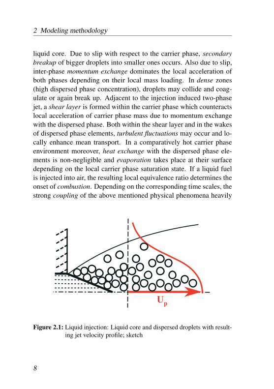
liquid core. Due to slip with respect to the carrier phase, secondarybreakup of bigger droplets into smaller ones occurs. Also due to slip,inter-phase momentum exchange dominates the local acceleration ofboth phases depending on their local mass loading. In dense zones(high dispersed phase concentration), droplets may collide and coag-ulate or again break up. Adjacent to the injection induced two-phasejet, a shear layer is formed within the carrier phase which counteractslocal acceleration of carrier phase mass due to momentum exchangewith the dispersed phase. Both within the shear layer and in the wakesof dispersed phase elements, turbulent fluctuations may occur and lo-cally enhance mean transport. In a comparatively hot carrier phaseenvironment moreover, heat exchange with the dispersed phase ele-ments is non-negligible and evaporation takes place at their surfacedepending on the local carrier phase saturation state. If a liquid fuelis injected into air, the resulting local equivalence ratio determines theonset of combustion. Depending on the corresponding time scales, thestrong coupling of the above mentioned physical phenomena heavily
Figure 2.1: Liquid injection: Liquid core and dispersed droplets with result-ing jet velocity profile; sketch
8
2.1 Injection induced two-phase flow characterization
influences the dynamics of the individual effects.
Physical time scales
The application of an internal combustion engine incorporates a largerange of physical time and corresponding length scales: For exam-ple, the transient engine-warmup process after a cold-start may takeminutes until a cycle-stationary mean temperature is approximatelyreached. Transients in engine operating conditions such as enginespeed and load are completed within seconds. One engine workingcycle takes several milliseconds and the injection of small quantitieslasts for times of the order of fractions of milliseconds.On the other hand, cumulated small time scale effects dominate thelarge time scale behavior: The dynamics of e.g. mixture formationand combustion are influenced by turbulent fluctuations, which deter-mine the local mixing rate of evaporated fuel and air. The inclusion oflocal turbulent fluctuations necessitates the spatial and temporal reso-lution of the smallest scales – namely the Kolmogorov scale at whichturbulent eddies are consumed by viscous dissipation. Even whencycle-stationary conditions in the environment (e.g. for the cylinderhead temperature) are reached based on the resolution of the smallestscales, the chaotic nature of turbulent fluctuations brings about cycle-to-cycle fluctuations [3]. In order to accurately describe the cycle-average transport due to turbulent fluctuations, several realizations ofindividual cycles have to be accounted for.
Momentum exchange
The momentum exchange of injected dispersed phase with the carrierphase is dominated by the local values of slip velocity and mass con-centrations of both phases:Momentum is locally exchanged if a particle’s velocity differs fromthe carrier phase velocity (source term magnitude, drag force). Theacceleration due to the resulting drag force acting on both phases de-
9
2 Modeling methodology
pends on the local mass concentrations. If no further momentum issupplied to the two-phase flow system, slip velocities decrease untilboth phases move with approximately the same velocity (unforced orfree system): The injection process after injection has ended is charac-terized by a relaxation process.By contrast during the injection process, momentum is continuallysupplied at the injection outlet so that velocity differences within thedense spray zone between both phases are maintained (forced system).After the injection has begun, the external forcing leads to increasedpenetration of dispersed phase into the carrier phase environment andto local acceleration of the carrier phase (spatially distributed forc-ing). The local pressure drop due to the accelerated carrier phase massforces convective transport of carrier phase towards the dense sprayzone in the direction normal to the main injection direction (entrain-ment). Also, the local carrier phase acceleration causes steep gradientsin the carrier phase velocity profile so that tangential shear stressesdue to the carrier phase’s molecular viscosity are evoked. They causethe adjacent carrier phase mass to be accelerated (and the carrier phasemass exposed to momentum exchange with the dispersed phase to de-celerate). The above mentioned transport of carrier phase mass normalto the main injection direction additionally enforces the formation ofsteep cross-stream gradients of the carrier phase streamwise velocitycomponent.
The cumulative effect of local displacement (acceleration) of carrierphase mass due to momentum exchange as well as the shearing motionwithin the carrier phase and the consequential growth of the width ofcross-stream velocity profiles is called entrainment. In a single phasejet, the cross-stream integral of streamwise momentum is conservedalong the injection direction while the contained volume increases.The flow field resulting from injection induced spatially distributedforcing of the carrier phase flow may be termed a two-phase jet. In atwo-phase jet, the local acceleration of carrier phase mass causes an
10
2.1 Injection induced two-phase flow characterization
additional excess entrainment of carrier phase mass into the two-phasejet.Since the amount of carrier phase mass available for (excess) entrain-ment may be restricted both due to the chamber geometry (confinedjet) and due to the rate of momentum diffusion, vortex structures areformed (vortex formation). Depending on their position and intensity,local entrainment of carrier phase mass is enhanced or reduced.
Breakup & poly-dispersion
The existence of dispersed phase elements like droplets within thedomain results from liquid disintegration in the vicinity of the injec-tor outlet due to instabilities within and at the boundary of the ini-tially cohesive liquid (primary breakup) [25]. The instability of aliquid core surrounded by gas is a three dimensional and non-lineareffect [69, 87]. Many works investigate the disintegration of liquidround jets injected in air (e.g. [85]) and the shear induced instability atthe surface of liquid sheets [37, 66, 76, 78] and the resulting formationof droplets [103].The processes involved with primary breakup result in a spatial andtemporal distribution of droplet diameters and velocities which givethe boundary condition for momentum exchange and secondary breakup.Models have been proposed to account for breakup mechanisms basedon injector internal flow properties and geometrical boundary condi-tions both for round Diesel like jets [13] as well as for conical sheets(resulting from low pressure [32] or high pressure injection [111]).Such models have been implemented in CFD codes (e.g. [29]) andapplied to gasoline direct injection applications [28, 123].
Dense dispersed phase coupling
If dispersed phase elements are influenced by the carrier phase flowbut not vice versa, the two-phase flow is termed one-way coupled.With increasing local dispersed phase volume loading, the dispersed
11
2 Modeling methodology
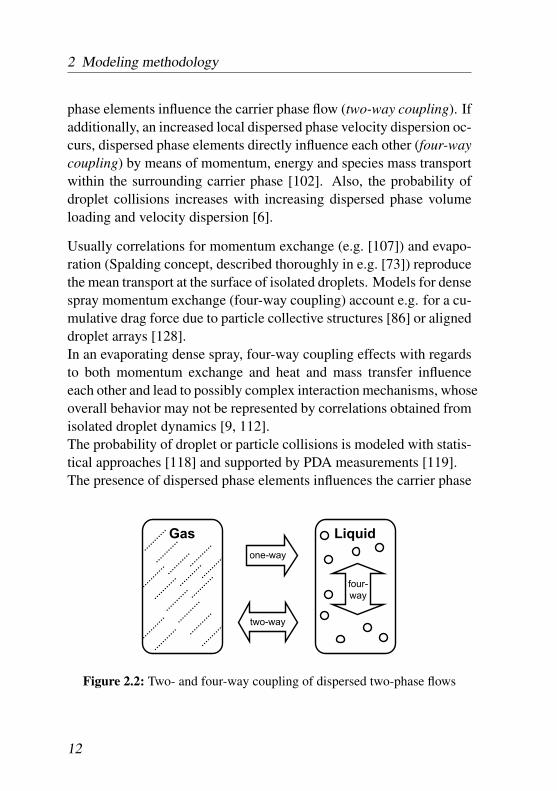
phase elements influence the carrier phase flow (two-way coupling). Ifadditionally, an increased local dispersed phase velocity dispersion oc-curs, dispersed phase elements directly influence each other (four-waycoupling) by means of momentum, energy and species mass transportwithin the surrounding carrier phase [102]. Also, the probability ofdroplet collisions increases with increasing dispersed phase volumeloading and velocity dispersion [6].
Usually correlations for momentum exchange (e.g. [107]) and evapo-ration (Spalding concept, described thoroughly in e.g. [73]) reproducethe mean transport at the surface of isolated droplets. Models for densespray momentum exchange (four-way coupling) account e.g. for a cu-mulative drag force due to particle collective structures [86] or aligneddroplet arrays [128].In an evaporating dense spray, four-way coupling effects with regardsto both momentum exchange and heat and mass transfer influenceeach other and lead to possibly complex interaction mechanisms, whoseoverall behavior may not be represented by correlations obtained fromisolated droplet dynamics [9, 112].The probability of droplet or particle collisions is modeled with statis-tical approaches [118] and supported by PDA measurements [119].The presence of dispersed phase elements influences the carrier phase
Gas
one-way
two-way
Liquid
four-
way
Figure 2.2: Two- and four-way coupling of dispersed two-phase flows
12
2.2 Model classification overview
turbulence statistics [33]. The turbulence modulation within in-ho-mogenous turbulent carrier phase flows at non-uniform particle massloading is e.g. investigated by means of very sophisticated simulationapproaches such as point-particle DNS [19, 120, 121]. Contributionsto statistical modeling of two-phase turbulence effects also includekinetic models for joint probability density functions [53, 113, 115,127]. More simple models accounting for turbulent transport in thecontext of the two-fluid model include two-equation two-phase turbu-lence models [46, 47] or simple gradient diffusion models [18, 79, 80].
2.2 Model classification overview
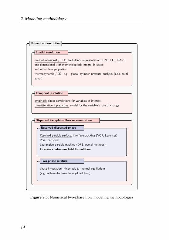
The underlying mean dynamics of both laminar and turbulent single-phase fluid flows are described in detail by numerous authors, e.g. [4,11, 94, 108]. Dispersed two-phase flows are characterized both experi-mentally and numerically [22, 65]. Numerical methods providing highquality temporal integration solutions are proposed both with respectto single [52] and two-phase flows [96]. In order to later choose anappropriate model concept, a classification of numerical descriptionsavailable for two-phase flows is presented in figure 2.3.
Any numerical simulation technique may be characterized by the de-gree of spatial homogeneity it assumes: Computational fluid dynamicmodels usually incorporate a spatial resolution in three dimensions.Turbulent fluctuations are resolved depending on their energy level:In a “direct numerical simulation” (DNS) approach, all scales down tothe smallest ones being dissipated by molecular viscosity are resolvedand no turbulence related modeling is required. In “large eddy simula-tion” (LES), a filter function is applied and the effect of scales smallerthan the filter size on the resolved scales is modeled as a sub-gridviscosity. In the “Reynolds averaged Navier-Stokes” (RANS) descrip-tion, the total of the Reynolds stress tensor is modeled and only the
13
2 Modeling methodology
multi-dimensional / CFD: turbulence representation: DNS, LES, RANS
one-dimensional / phenomenological: integral in space
and other flow properties
thermodynamic / 0D: e.g. global cylinder pressure analysis (also multi-
zonal)
empirical: direct correlations for variables of interest
time-itterative / predictive: model for the variable’s rate of change
Resolved particle surface: interface tracking (VOF, Level-set)
Point particles:
Lagrangian particle tracking (DPS, parcel methods);
Eulerian continuum field formulation
phase integration: kinematic & thermal equilibrium
(e.g. self-similar two-phase jet solution)
Numerical description
Spatial resolution
Temporal resolution
Dispersed two-phase flow representation
Resolved dispersed phase
Two-phase mixture
Figure 2.3: Numerical two-phase flow modeling methodologies
14
2.2 Model classification overview
isotropic part is transported, e.g. in one- and two-equation turbulencemodels such as the k-ε , the k-ω-model or a combination of both likethe “shear stress transport” (SST) model [88].One-dimensional models describe integral properties in space such aspipe flow where only the dynamics along the pipe axis are spatiallyresolved and phenomena like friction forces within the flow and at thewall boundary are accounted for by loss coefficients. The modelingassumption of self-similarity also produces the projection of multi-dimensional effects onto only one (non-dimensional) similarity vari-able such as in single phase boundary layer flows∗.Purely thermodynamic models assume complete spatial homogeneity(zero-dimensional). For example, steady states within turbo-engines(stationary open system) are analyzed or transient work cycles as inreciprocating engines (transient closed system) may be characterizedin this way.
The modeling approaches accounting for the temporal evolution in-corporate mainly two types: Either the temporal development of thequantity of interest is provided in the form of an explicit function intime (such as the penetration depth of an injected jet), or the modeldescribing the temporal rate-of-change of the quantity of interest isobtained from temporal integration (e.g. of the current particle veloc-ity in order to obtain the particle’s path). The latter kind of modelrepresents the dynamics inherent to the described physical system andis therefore termed “predictive”.
The appropriate numerical description of dispersed two-phase flowsdepends among other factors on the material densities of the phasesinvolved. Here the focus lies on the flow induced in a gaseous car-rier phase by a liquid dispersed phase. Hence, the dispersed to carrierphase material density ratio and consequentially also the momentum
∗ Furthermore assuming locally stationary conditions most often allows thederivation of an analytic solution from the remaining ODE so that the integral quan-tity is known a-priori and is not subject to numerical integration.
15
2 Modeling methodology
ratio in the vicinity of a dispersed phase element (particle) are of theorder ρp/ρc ≈ 103 � 1.In advanced two-phase descriptions, the interface separating the twophases may be resolved, such as in interface tracking methods [125].The volume of fluid method applies a discrete marker function indi-cating the phase jump-condition as a diffuse inter-phase. The level-setmethod incorporates a continuous marker function which enables amore precise reconstruction of the interface.Less detail and thereby more computational efficiency provides theassumption that with regards to the global carrier phase flow pattern,the dispersed phase elements (droplets) occupy only a small volumeand may therefore be characterized as point-particles, whose individ-ual equation of motion defines their path (Lagrangian particle track-ing) [57, 89, 95]. The detailed interaction with the carrier phase atthe particle surface (drag, heat and mass transfer) is described by in-tegral correlations obtained experimentally (such as drag correlations)or analytically (such as the Spalding droplet evaporation model). Ac-cording to the level of detail in single phase turbulence modeling, therepresentation of the total amount of dispersed phase mass by individ-ually tracked particles is termed “discrete” particle simulation (DPS).Because spatially neighboring particles of similar initial properties(e.g. diameter, velocity, temperature etc.) interact with approximatelythe same carrier phase mass elements, they tend to keep on carryingsimilar properties after the interaction. This physical effect suggeststo model numbers of particles of similar properties to be grouped incomputational parcels. The strongest advantage of the Lagrangianmethod is that it intrinsically incorporates a statistical representationof the dispersed phase property dispersion: The spatial and temporaldevelopment of distributions in e.g. diameter, velocity, temperatureetc. due to some initial conditions is produced by the application ofthis method. If large amounts of particles (parcels) have to be tracked,the computational cost increases.The two-fluid method applies volume or ensemble averaging to the
16
2.2 Model classification overview
dispersed phase and thereby locally assigns continuum properties tothe dispersed phase. The averaging process introduces a “one-pointone-value” relation to the dispersed phase: If particles are to exhibite.g. two different velocities at one location, two such continua haveto be transported. A dispersed phase property dispersion may only beaccounted for by a “spectral solution”, where several continua repre-sent the local distribution function. If the accuracy loss due to volumeaveraging is increased by such a spectral approach, the computationalcost increases with the power of the covered dispersion relations (e.g.for diameter, velocity, and temperature with the power of three) so thatthe Lagrangian representation again becomes more attractive.The least detailed method to treat dispersed two-phase flows is themixture model which assumes both phases to be in kinematic and ther-mal equlilibrium by applying a local integration over both phases.
Eulerian multi-fluid
In the context of dispersed two-phase flow, a contradiction occurswhen the Lagrangian statistical approach is used and turbulence ef-fects are to be partly resolved as in LES. The increase in spatial reso-lution required for LES reduces the statistical quality of the dispersedphase representation. Also, spatial resolutions of the order of the localparticle diameter contradict the point-particle assumption, introduce(possibly non-physically) high local gradients to the carrier phase andthereby necessitate the modeling of spatially distributed inter-phasecoupling.The field of high spatial resolution is thus a domain of the Euleriancontinuum representation of the dispersed phase. The Eulerian tur-bulence modeling of the dispersed phase (which becomes importantwhere St = τp/τ f ≈ 1) was introduced by [115] and further developedand implemented by [68, 75, 100]. An extension to poly-dispersionhas been proposed by [90].
17
2 Modeling methodology
Eulerian moment transport & poly-celerity
The representation of dispersed phase property dispersion (e.g. re-garding the local diameter or velocity distribution) was introducedwith the Lagrangian statistical approach. The exact statistical proba-bility of finding a particle with properties within a certain range of thetotal spectrum is described by the Williams spray equation [131]. Withregards to the Eulerian dispersed phase transport, several approachesattempt to transport integrals of the distribution function, i.e. theirmoments.
Most interest lies in the representation of poly-dispersion, i.e. a dis-tribution of particle diameters. The proposed methods contain the“method of moments” (MOM), where moments of the local parti-cle diameter distribution are transported [14, 15, 16, 17] and whichwas further developed for impinging sprays [7] and applied to massand heat transfer [23]. An alternative approach is the “direct quadra-ture method of moments” (DQMOM) [43, 48, 81, 84] which modelsthe temporal change of a (possibly complex) diameter distribution bytransporting convenient abscissas and weights representing the distri-bution function.An important property of poly-dispersed systems is their non-linear re-sponse to momentum exchange with the carrier phase. Some modelsdirectly focus on the effect of the local dispersion in velocity (poly-celerity) [75]. Others relate the velocities at which diameter distri-bution moments are transported to some representative velocity for arepresentative diameter and introduce moment specific slip velocitiesto account for changes in the diameter distribution [14]. Yet anotherapproach is to directly model moment velocities [56].An alternative to modeling moments of the diameter distribution func-tion is to reduce the computational cost of the full spectral solution.This is performed by relating the acceleration of particles correspond-ing to some class by the acceleration of a neighboring size class andthereby avoiding to solve momentum equations for some size classes.
18
2.3 Motivation and modeling strategy
For inertial particles of limited Stokes number this was introducedwith the “equilibrium Eulerian approach” [50, 51] in the context ofturbulent dispersion modeling. An extension of this approach enablingthe transport of inertial particles of increased Stokes numbers has beensuggested by the author and co-workers [21].
2.3 Motivation and modeling strategy
The improvement of the performance of a product like e.g. an injectoror an engine necessitates a thorough understanding of the various rele-vant physical functionalities. In order to enhance the understanding ofcomplex physical systems like an injection process, experimental andnumerical investigations work in a complimentary manner. Depend-ing on the required degree of detail and the available computationalpower, numerical models produce the response of dynamics of physi-cal systems to certain initial and boundary conditions at different timescales: Some models feature real-time capabilities (such as “hardwarein the loop” models for engine CPUs), while complex models incorpo-rating a vast range of time and length scales (like e.g. climatic models)may require months of computational time on thousands of processorsto produce results.
In an industrial context, even complex models (such as high resolutionCFD models of an injection process) are supposed to produce resultsat the most within days so that then, changes in the model or the de-sign may be applied. Processes like one single injection happen atcharacteristic time scales of milliseconds. By contrast, a transient en-gine system operation may take seconds or minutes. Depending on theengine speed, a significant number of working cycles with several in-jections per working cycle may need to be characterized (e.g. at 6000rpm, 50 working cycles per second in a four-stroke engine).The main physical effects present within an engine system – except
19
2 Modeling methodology
the injection and combustion cycle within the cylinder – may be de-scribed with sufficient accuracy by comparatively simple models (e.g.gas exchange dynamics or transient engine warm-up). Engine sys-tem simulation thus requires less computational power than a com-plex CFD analysis. On a desktop computer, several working cyclesmay be simulated within minutes. The injection of liquid fuel and theconsequential combustion are most efficiently accounted for by exper-imentally obtained cylinder pressure traces. For this approach, enginehardware has to exist prior to any simulation work and engine systemsimulation is therefore applied as a post-processing tool to an experi-mental investigation.By contrast during an early stage in the development cycle, enginesystem simulation is used to investigate major changes in engine ge-ometry or operating conditions. Even though burn rates from previ-ous engine applications may be adopted, such explicit functions lackthe ability to respond dynamically to changes in boundary conditions(such as e.g. an altered thermodynamic state of the charge initiallycontained within the cylinder after the intake valve has closed). Anapproach to introduce dynamics to integral heat release characteristicshas been presented by the author and co-workers [20]. The assessmentscrutinizes the need to incorporate mixture formation effects resultingfrom the injection process into the engine system simulation, espe-cially for gasoline engines.
Modeling limits
If numerical models of certain applications are first built, their accu-racy is assessed applying comparisons to experimental data (modelvalidation). Measurements include detailed investigations of isolatedeffects such as individual droplet kinematics or heat and mass transferat isolated droplet surfaces. When models are to incorporate the cu-mulative effects of e.g. the propagation of a droplet cloud in initiallyquiescent air or the evaporation of a droplet cloud, often only integral
20
2.3 Motivation and modeling strategy
qualities such as the spray penetration depth into a pressure chamberor a spray life time may be obtained experimentally.Especially for dense dispersed systems, to which optical measurementtechniques provide only limited access, the link between the detaileddynamics on the level of individual droplets and the cumulative (inte-gral) effects is very hard to establish: A breakup model may reproducethe temporal and spatial development obtained from a PDA investiga-tion, but the question whether the congruence stems from correct mod-eling of the underlying individual droplet dynamics within the cloud(wind induced breakup, collision and coalescence, etc.) remains ques-tionable. Likewise heat and mass transfer correlations obtained fromexperiments with isolated or a limited number of interacting dropletsmay produce an experimentally obtained spray life time. But the val-idation of individual droplet evaporation dynamics within a cloud ofseveral hundreds of thousands of droplets is practically impossible.When high-detail models such as breakup models are applied withsuccess, the (numerical) “path” at which the solution is obtained re-mains unclear and the congruence of results may well be the result ofan interference of model errors, which cancel each other out. Theseeffects introduce limits of applicability of computational dispersedphase transport descriptions like the Lagrangian particle tracking indense spray zones [1, 38, 60] and demonstrate the need to locally in-troduce models accounting for integral effects in dense sprays.
Simplified modeling
Thorough documentation of basic physical dynamics and modeling isavailable with regards to the overall engine system [59], the gas dy-namics within the intake and exhaust system [77], and spray injectionand mixture formation [12, 122].Among the simplified models for the overall engine system, the modelpart representing the processes happening within the cylinder after “in-take valve closes” and before “exhaust valve opens” (cylinder model)
21
2 Modeling methodology
has to reproduce the most complicated dynamics. The need to intro-duce models more sophisticated than simple thermodynamical ones– accounting for the injection and mixture formation process at com-paratively low computational cost – has been accentuated [20, 122].Integral spray quantities like spray tip penetration depth or the globalspray life time may be characterized by purely empirical correlations.Dynamic response to altered boundary conditions by contrast has toresult from a dynamic, time-iterative (predictive) model.
Dispersed two-phase jet models
Several attempts have been made to dynamically describe injection in-duced propagation of a dispersed two-phase jet. The so called “packetmodel” of Hiroyasu [62] is aimed at the description of round jet Dieselspray and combustion modeling. With a somewhat reduced CFD phi-losophy, a limited region around the injector is resolved and explicitcorrelations for e.g. the spray tip velocity are given (two-phase mix-ture model). This approach has been adopted by several authors, e.g.[71].Inspired by the space integral description of turbulent jet diffusionflames of Peters [92], Wan [129] presented a spray model for a roundDiesel jet. The penetration behavior of the two-phase jet results fromassumed cross-stream top hat profiles which represent the mean prop-erties of both phases within the jet. It utilizes a parameter which ac-counts for the jet opening angle. Depending on this spreading rate, thelocal increase of carrier phase mass due to entrainment available forinter-phase momentum exchange is modeled. Breakup and evapora-tion are accounted for. Based on Hiroyasu’s classification of a com-plete spray (locally homogeneous two-phase flow) [61], velocity dif-ferences between phases are completely neglected in a second step.From this assumption of a two-phase mixture, relations for spray tippenetration (which are explicit in time) are derived. After a first imple-mentation in the context of [129], the model was validated for Diesel
22
2.3 Motivation and modeling strategy
injection applications [72].With the assumption of a steady state condition within the main partof the round jet (except for regions very close to the injector and atthe spray front), a square root dependency of the spray front pene-tration with time is found from the cross-stream integrated momen-tum equation. The accuracy of this description for Diesel jets is con-firmed by e.g. [101] for various experimental data sets. For the de-scription of the initially transient penetration behavior of a round fueljet, Sazhin et al. [105] employed the individual droplet’s kinematicsas characteristic to the front propagation. In combination with modelsfor evaporation and breakup, good agreement with experimental datawas obtained.
Hollow cone sprays are much less commonly applied in industry thanround fuel jets as typically found in Diesel engines. As a consequence,also less theoretical and characterization work has been performed.The major difference of a hollow cone spray is that its global struc-ture is less stable than the spray structure resulting from a round jet(see section 2.4). It causes an injection induced global recirculationzone. This behavior was observed in experiments with pressure swirlinjectors [29] as well as piezo-electrically driven, outward-openinginjectors [97] and is again supported by the CFD investigation in sec-tion 3.2.Cossali [31] studied the gas entrainment into a hollow cone spraybased on a spatial self-similarity assumption and for steady state con-ditions (i.e. for constant boundary conditions and flow states longafter the injector has opened). He confirms that the hollow cone jetdynamics resulting from an injection induced two-phase flow differconsiderably from those of both single phase jets and round Dieseljets.
23
2 Modeling methodology
Model outline
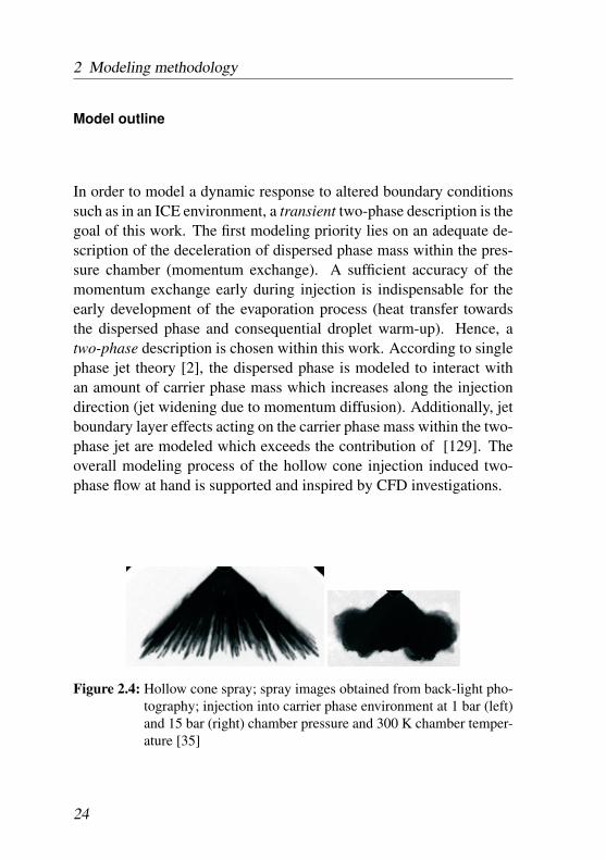
In order to model a dynamic response to altered boundary conditionssuch as in an ICE environment, a transient two-phase description is thegoal of this work. The first modeling priority lies on an adequate de-scription of the deceleration of dispersed phase mass within the pres-sure chamber (momentum exchange). A sufficient accuracy of themomentum exchange early during injection is indispensable for theearly development of the evaporation process (heat transfer towardsthe dispersed phase and consequential droplet warm-up). Hence, atwo-phase description is chosen within this work. According to singlephase jet theory [2], the dispersed phase is modeled to interact withan amount of carrier phase mass which increases along the injectiondirection (jet widening due to momentum diffusion). Additionally, jetboundary layer effects acting on the carrier phase mass within the two-phase jet are modeled which exceeds the contribution of [129]. Theoverall modeling process of the hollow cone injection induced two-phase flow at hand is supported and inspired by CFD investigations.
Figure 2.4: Hollow cone spray; spray images obtained from back-light pho-tography; injection into carrier phase environment at 1 bar (left)and 15 bar (right) chamber pressure and 300 K chamber temper-ature [35]
24
2.4 Hollow cone injection
2.4 Hollow cone injection
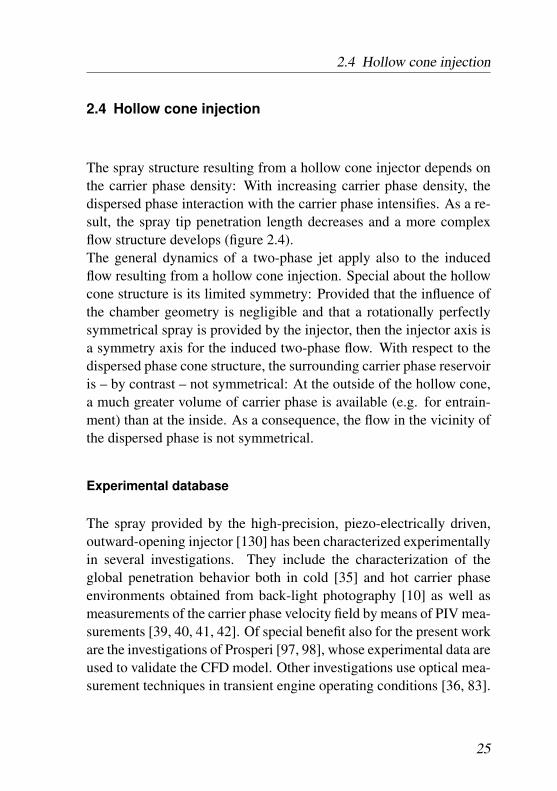
The spray structure resulting from a hollow cone injector depends onthe carrier phase density: With increasing carrier phase density, thedispersed phase interaction with the carrier phase intensifies. As a re-sult, the spray tip penetration length decreases and a more complexflow structure develops (figure 2.4).The general dynamics of a two-phase jet apply also to the inducedflow resulting from a hollow cone injection. Special about the hollowcone structure is its limited symmetry: Provided that the influence ofthe chamber geometry is negligible and that a rotationally perfectlysymmetrical spray is provided by the injector, then the injector axis isa symmetry axis for the induced two-phase flow. With respect to thedispersed phase cone structure, the surrounding carrier phase reservoiris – by contrast – not symmetrical: At the outside of the hollow cone,a much greater volume of carrier phase is available (e.g. for entrain-ment) than at the inside. As a consequence, the flow in the vicinity ofthe dispersed phase is not symmetrical.
Experimental database
The spray provided by the high-precision, piezo-electrically driven,outward-opening injector [130] has been characterized experimentallyin several investigations. They include the characterization of theglobal penetration behavior both in cold [35] and hot carrier phaseenvironments obtained from back-light photography [10] as well asmeasurements of the carrier phase velocity field by means of PIV mea-surements [39, 40, 41, 42]. Of special benefit also for the present workare the investigations of Prosperi [97, 98], whose experimental data areused to validate the CFD model. Other investigations use optical mea-surement techniques in transient engine operating conditions [36, 83].
25
2 Modeling methodology
2.4.1 Conservation equations in conical coordinates
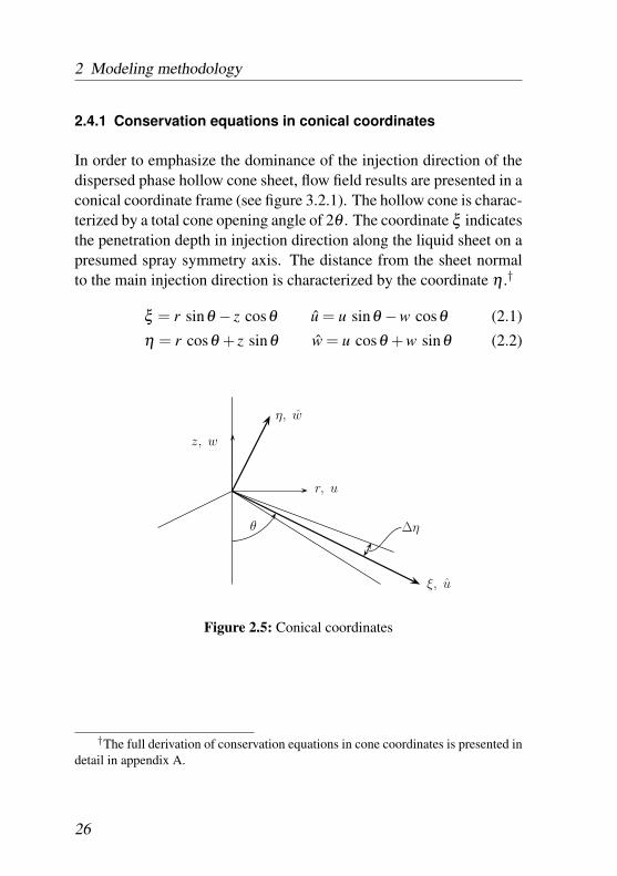
In order to emphasize the dominance of the injection direction of thedispersed phase hollow cone sheet, flow field results are presented in aconical coordinate frame (see figure 3.2.1). The hollow cone is charac-terized by a total cone opening angle of 2θ . The coordinate ξ indicatesthe penetration depth in injection direction along the liquid sheet on apresumed spray symmetry axis. The distance from the sheet normalto the main injection direction is characterized by the coordinate η .†
ξ = r sinθ − z cosθ u = u sinθ −w cosθ (2.1)
η = r cosθ + z sinθ w = u cosθ +w sinθ (2.2)
r, u
z, w
η, w
ξ, u
∆ηθ
Figure 2.5: Conical coordinates
†The full derivation of conservation equations in cone coordinates is presented indetail in appendix A.
26
2.4 Hollow cone injection
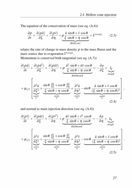
The equation of the conservation of mass (see eq. (A.6))
∂ρ∂ t
+∂ (ρ u)
∂ξ+
∂ (ρ v)∂η
+ρu sinθ + v cosθξ sinθ +η cosθ︸ ︷︷ ︸
RADconti
= Γ(evap) (2.3)
relates the rate of change in mass density ρ to the mass fluxes and themass source due to evaporation Γ(evap).Momentum is conserved both tangential (see eq. (A.7))
∂ (ρ u)∂ t
+∂ (ρ u2)
∂ξ+
∂ (ρ uv)∂η
+ρu2 sinθ + uv cosθξ sinθ +η cosθ︸ ︷︷ ︸
RADmomX
= −∂ p∂ξ
+ Iξ︸︷︷︸dragX
+ µe f f
⎡⎢⎢⎢⎢⎣
∂ 2u∂ξ 2︸︷︷︸viscX1
µ
+sinθ ∂ u
∂ξ + cosθ ∂ u∂η
ξ sinθ +η cosθ︸ ︷︷ ︸viscX2
µ
+∂ 2u∂η2︸︷︷︸viscX3
µ
−sinθu sinθ + v cosθ
(ξ sinθ +η cosθ)2︸ ︷︷ ︸viscX4
µ
⎤⎥⎥⎥⎥⎦ ,
(2.4)
and normal to main injection direction (see eq. (A.8))
∂ (ρ v)∂ t
+∂ (ρ uv)
∂ξ+
∂ (ρ v2)∂η
+ρuv sinθ + v2 cosθξ sinθ +η cosθ︸ ︷︷ ︸
RADmomY
= − ∂ p∂η
+ Iη︸︷︷︸dragY
+ µe f f
⎡⎢⎢⎢⎢⎣
∂ 2v∂ξ 2︸︷︷︸viscY 1
µ
+sinθ ∂ v
∂ξ + cosθ ∂ v∂η
ξ sinθ +η cosθ︸ ︷︷ ︸viscY 2
µ
+∂ 2v∂η2︸︷︷︸viscY 3
µ
−cosθu sinθ + v cosθ
(ξ sinθ +η cosθ)2︸ ︷︷ ︸viscY 4
µ
⎤⎥⎥⎥⎥⎦ .
(2.5)
27
2 Modeling methodology
From the conservation equations, the cylindrical character is clearlyvisible. The cone specific terms appearing on the left hand side (LHS)of the set of equations (2.3) through (2.5) reflect the dependency onboth the spatial coordinates and the velocity vector components. Thefourth viscous term on the right hand side (RHS) of equations (2.4)and (2.5) directly corresponds to the cylindrical description. Specialabout the momentum conservation equations expressed in cone coor-dinates are the second viscous terms viscX2 and viscY 2, which ac-count for the spatial velocity gradients of the conserved momentumcomponent.
Hollow cone boundary layer
The formulation of the momentum conservation equations in coni-cal coordinates introduces viscous terms accounting for radial widen-ing. In order to estimate the contribution of the individual terms inthe streamwise momentum equation (2.4), the conservation equations(2.3) through (2.5) are assessed in terms of dimensionless variables fora boundary layer of characteristic thickness δ according to the proce-dure presented by Schlichting [108].
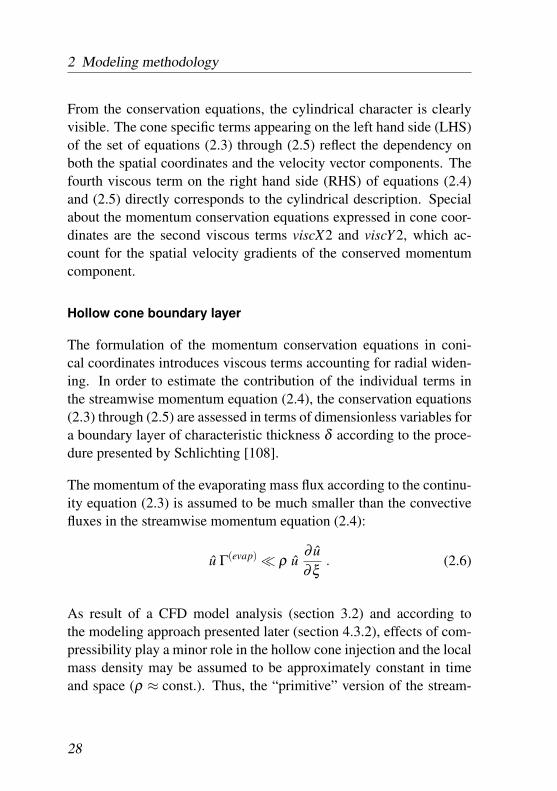
The momentum of the evaporating mass flux according to the continu-ity equation (2.3) is assumed to be much smaller than the convectivefluxes in the streamwise momentum equation (2.4):
u Γ(evap) � ρ u∂ u∂ξ
. (2.6)
As result of a CFD model analysis (section 3.2) and according tothe modeling approach presented later (section 4.3.2), effects of com-pressibility play a minor role in the hollow cone injection and the localmass density may be assumed to be approximately constant in timeand space (ρ ≈ const.). Thus, the “primitive” version of the stream-
28
2.4 Hollow cone injection
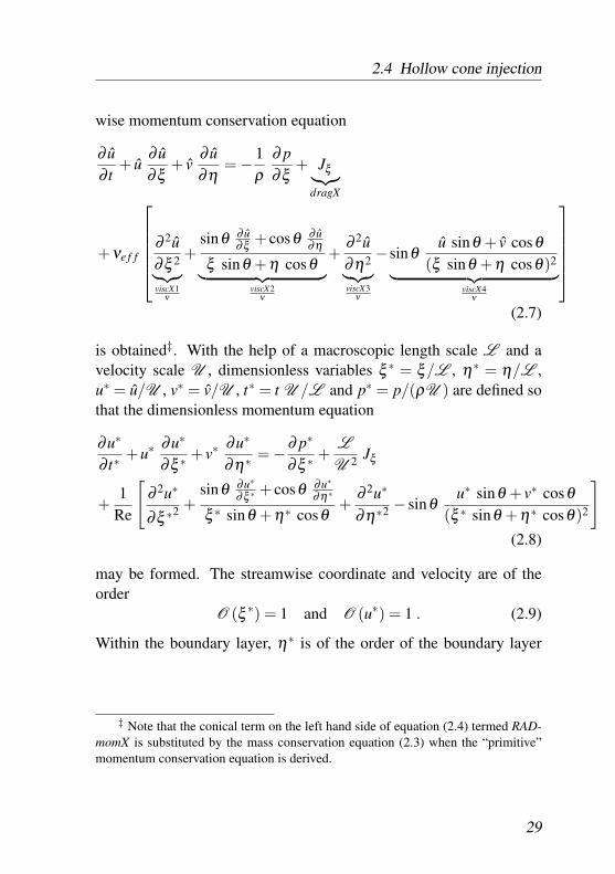
wise momentum conservation equation
∂ u∂ t
+ u∂ u∂ξ
+ v∂ u∂η
= − 1ρ
∂ p∂ξ
+ Jξ︸︷︷︸dragX
+νe f f
⎡⎢⎢⎢⎢⎣
∂ 2u∂ξ 2︸︷︷︸viscX1
ν
+sinθ ∂ u
∂ξ + cosθ ∂ u∂η
ξ sinθ +η cosθ︸ ︷︷ ︸viscX2
ν
+∂ 2u∂η2︸︷︷︸viscX3
ν
−sinθu sinθ + v cosθ
(ξ sinθ +η cosθ)2︸ ︷︷ ︸viscX4
ν
⎤⎥⎥⎥⎥⎦
(2.7)
is obtained‡. With the help of a macroscopic length scale L and avelocity scale U , dimensionless variables ξ ∗ = ξ/L , η∗ = η/L ,u∗ = u/U , v∗ = v/U , t∗ = t U /L and p∗ = p/(ρU ) are defined sothat the dimensionless momentum equation
∂u∗
∂ t∗+u∗
∂u∗
∂ξ ∗ + v∗∂u∗
∂η∗ = −∂ p∗
∂ξ ∗ +L
U 2 Jξ
+1
Re
[∂ 2u∗
∂ξ ∗2 +sinθ ∂u∗
∂ξ ∗ + cosθ ∂u∗∂η∗
ξ ∗ sinθ +η∗ cosθ+
∂ 2u∗
∂η∗2 − sinθu∗ sinθ + v∗ cosθ
(ξ ∗ sinθ +η∗ cosθ)2
](2.8)
may be formed. The streamwise coordinate and velocity are of theorder
O (ξ ∗) = 1 and O (u∗) = 1 . (2.9)
Within the boundary layer, η∗ is of the order of the boundary layer
‡ Note that the conical term on the left hand side of equation (2.4) termed RAD-momX is substituted by the mass conservation equation (2.3) when the “primitive”momentum conservation equation is derived.
29
2 Modeling methodology
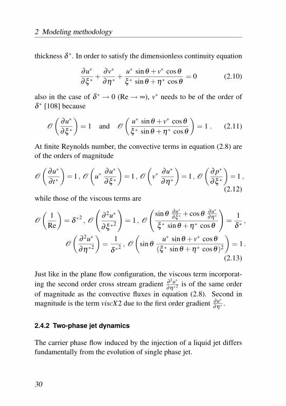
thickness δ ∗. In order to satisfy the dimensionless continuity equation
∂u∗
∂ξ ∗ +∂v∗
∂η∗ +u∗ sinθ + v∗ cosθξ ∗ sinθ +η∗ cosθ
= 0 (2.10)
also in the case of δ ∗ → 0 (Re → ∞), v∗ needs to be of the order ofδ ∗ [108] because
O
(∂u∗
∂ξ ∗
)= 1 and O
(u∗ sinθ + v∗ cosθξ ∗ sinθ +η∗ cosθ
)= 1 . (2.11)
At finite Reynolds number, the convective terms in equation (2.8) areof the orders of magnitude
O
(∂u∗
∂ t∗
)= 1 , O
(u∗
∂u∗
∂ξ ∗
)= 1 , O
(v∗
∂u∗
∂η∗
)= 1 , O
(∂ p∗
∂ξ ∗
)= 1 ,
(2.12)while those of the viscous terms are
O
(1
Re
)= δ ∗2 , O
(∂ 2u∗
∂ξ ∗2
)= 1 , O
(sinθ ∂u∗
∂ξ ∗ + cosθ ∂u∗∂η∗
ξ ∗ sinθ +η∗ cosθ
)=
1δ ∗ ,
O
(∂ 2u∗
∂η∗2
)=
1
δ ∗2 , O
(sinθ
u∗ sinθ + v∗ cosθ(ξ ∗ sinθ +η∗ cosθ)2
)= 1 .
(2.13)
Just like in the plane flow configuration, the viscous term incorporat-ing the second order cross stream gradient ∂ 2u∗
∂η∗2 is of the same orderof magnitude as the convective fluxes in equation (2.8). Second inmagnitude is the term viscX2 due to the first order gradient ∂u∗
∂η∗ .
2.4.2 Two-phase jet dynamics
The carrier phase flow induced by the injection of a liquid jet differsfundamentally from the evolution of single phase jet.
30
2.4 Hollow cone injection
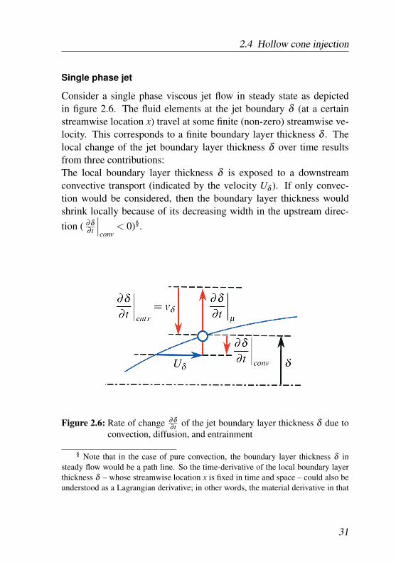
Single phase jet
Consider a single phase viscous jet flow in steady state as depictedin figure 2.6. The fluid elements at the jet boundary δ (at a certainstreamwise location x) travel at some finite (non-zero) streamwise ve-locity. This corresponds to a finite boundary layer thickness δ . Thelocal change of the jet boundary layer thickness δ over time resultsfrom three contributions:The local boundary layer thickness δ is exposed to a downstreamconvective transport (indicated by the velocity Uδ ). If only convec-tion would be considered, then the boundary layer thickness wouldshrink locally because of its decreasing width in the upstream direc-tion ( ∂δ
∂ t
∣∣∣conv
< 0)§.
Figure 2.6: Rate of change ∂δ∂ t of the jet boundary layer thickness δ due to
convection, diffusion, and entrainment
§ Note that in the case of pure convection, the boundary layer thickness δ insteady flow would be a path line. So the time-derivative of the local boundary layerthickness δ – whose streamwise location x is fixed in time and space – could also beunderstood as a Lagrangian derivative; in other words, the material derivative in that
31
2 Modeling methodology
At the same time, cross-stream diffusion of streamwise momentumcauses the fluid outside of the boundary layer region to accelerate,thereby contributing to the local growth of the boundary layer thick-ness ( ∂δ
∂ t
∣∣∣µ
> 0).
At the boundary layer boundary δ , mass is entering the jet region witha non-zero velocity component normal to the injection direction. Thisentrainment causes a contraction of the jet width δ (at the speed of theentrainment velocity vδ (y = δ ) = ∂δ
∂ t
∣∣∣entr
< 0).
After the initial boundary layer growth (also referred to as a “startupprocess”), the three contributions named above approach an equilib-rium state. The superposition of the three contributions is here referred
to as the net diffusive boundary layer growth(
∂δ∂ t
)(net)
µ, where
(∂δ∂ t
)(net)
µ=
∂δ∂ t
∣∣∣∣(t�T
(c)shear)
=∂δ∂ t
∣∣∣∣conv
+∂δ∂ t
∣∣∣∣µ
+∂δ∂ t
∣∣∣∣entr
= 0 .
(2.14)
In a single phase jet (resulting from a single point of momentum sup-ply) and for a comparatively large boundary layer measure of choice(e.g. the displacement thickness δ1), the velocity magnitudes at the jetboundary are comparatively small so that the entrainment velocity atthe boundary layer border is small.
In a conventional single phase jet of incompressible media resultingfrom a single location of momentum supply, the total volume fluxalong the main injection direction remains constant, i.e. the stream-
case equals the convective derivative since no change in δ occurs along the stream-wise coordinate x. In viscous flow however, the jet boundary layer thickness δ (andthe mass contained within the jet) changes along the streamwise direction, so that – ingeneral – the jet boundary does not lie on a path line. For this reason, the boundarylayer evolution with respect to a steady (resting) coordinate frame is investigated hereand the Eulerian derivative is used.
32
2.4 Hollow cone injection
wise momentum contained within the jet cross section is conservedalong the streamwise coordinate [108]. Along the injection direction,the cross-stream distribution of the streamwise momentum is rear-ranged to broader and flatter profiles due to momentum diffusion sothat additional mass is “entrained” into the jet. As the jet spreads andan increasing volume normal to the injection direction is affected, thecross-stream peak of the streamwise velocity (the center line velocity)decreases.
Two-phase jet and “excess entrainment”
By contrast in the two-phase jet (here liquid droplets dispersed in air),additional streamwise momentum is introduced to the carrier phase asit travels downstream: Due to the injection process, the liquid dropletstravel at a higher velocity than the carrier phase. The drag forces be-tween both phases cause the carrier phase to be accelerated. Velocitydifferences and consequential drag do not occur at the point of injec-tion only but are spatially distributed along the main injection direc-tion ξ (“spatially distributed forcing”).The excess carrier phase mass flux caused by the drag with the dis-persed phase has to be accomplished for by additional entrainment(“excess entrainment”) of carrier phase mass into the jet volume. Asa consequence from the entraining carrier phase mass, the boundarylayer is locally contracted.Both effects named above lead to a local increase of velocity gradi-ents which again cause the shear stress within the carrier phase of thetwo-phase flow to increases.
Exemplary CFD results
As a more detailed insight into the dynamics of the injection inducedtwo-phase flow field, an exemplary result from the CFD investigationprovided later in this work (see sec. 3.2) is presented in figure 2.7. Thehorizontal line at η = 0mm is the presumed spray center line and the
33
2 Modeling methodology
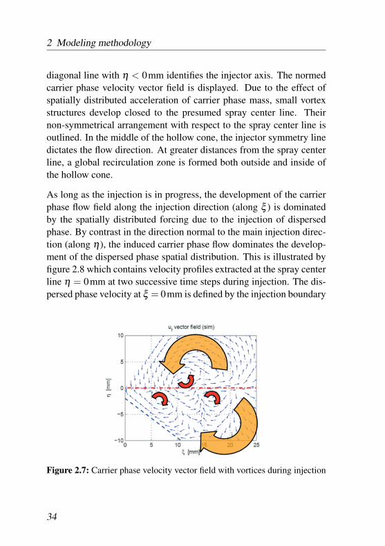
diagonal line with η < 0mm identifies the injector axis. The normedcarrier phase velocity vector field is displayed. Due to the effect ofspatially distributed acceleration of carrier phase mass, small vortexstructures develop closed to the presumed spray center line. Theirnon-symmetrical arrangement with respect to the spray center line isoutlined. In the middle of the hollow cone, the injector symmetry linedictates the flow direction. At greater distances from the spray centerline, a global recirculation zone is formed both outside and inside ofthe hollow cone.
As long as the injection is in progress, the development of the carrierphase flow field along the injection direction (along ξ ) is dominatedby the spatially distributed forcing due to the injection of dispersedphase. By contrast in the direction normal to the main injection direc-tion (along η), the induced carrier phase flow dominates the develop-ment of the dispersed phase spatial distribution. This is illustrated byfigure 2.8 which contains velocity profiles extracted at the spray centerline η = 0mm at two successive time steps during injection. The dis-persed phase velocity at ξ = 0mm is defined by the injection boundary
Figure 2.7: Carrier phase velocity vector field with vortices during injection
34
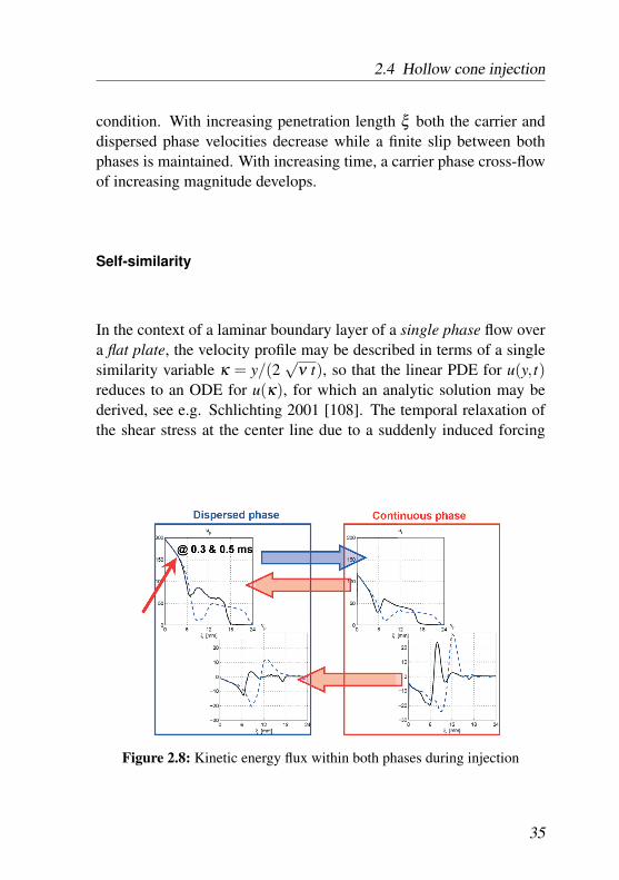
2.4 Hollow cone injection
condition. With increasing penetration length ξ both the carrier anddispersed phase velocities decrease while a finite slip between bothphases is maintained. With increasing time, a carrier phase cross-flowof increasing magnitude develops.
Self-similarity
In the context of a laminar boundary layer of a single phase flow overa flat plate, the velocity profile may be described in terms of a singlesimilarity variable κ = y/(2
√ν t), so that the linear PDE for u(y, t)
reduces to an ODE for u(κ), for which an analytic solution may bederived, see e.g. Schlichting 2001 [108]. The temporal relaxation ofthe shear stress at the center line due to a suddenly induced forcing
Figure 2.8: Kinetic energy flux within both phases during injection
35

2 Modeling methodology
(“moving wall”) velocity Uc = u(κ → 0) is then described by¶
τc(Uc, t) = µ∂u∂y
∣∣∣∣c= −ρ Uc
√ν
π t(2.15)
while the boundary layer thickness evolves over time according to
δ = 3.6 · √ν t . (2.16)
Turbulence
Turbulence effects are only accounted for with respect to the gaseouscarrier phase. The level of turbulent fluctuations within the liquidphase resulting from the injector internal flow is neglected here.
Within the flow domain, maximum magnitudes of the carrier phasevelocity are of the order of O (uc) = 100m/s. The kinematic viscosityof the gas phase is assumed to νc =1.5×10⁻⁵ m2/s. When the injectoris fully open, the half width associated with the effective cross-sectionof the exiting liquid flow is of the order of O (h/2) =10µm. TheReynolds number
Reh =uc h/2
νc= 67 � 2×10⁵ (2.17)
corresponding to the half-width h/2 indicates that no noteworthy tur-bulent intensity may be expected directly at the injector outlet.On the level of individual particles, the slip velocity does not exceed200m/s (which corresponds to the limiting case of particles injected
¶ For locally constant carrier phase center line velocity Uc, eq. (2.15) delivers thetime rate of change of shear stress at the center line position
∂τc
∂ t
∣∣∣∣Uc
=ρ Uc
2
√ν
π t3 .
36
2.4 Hollow cone injection
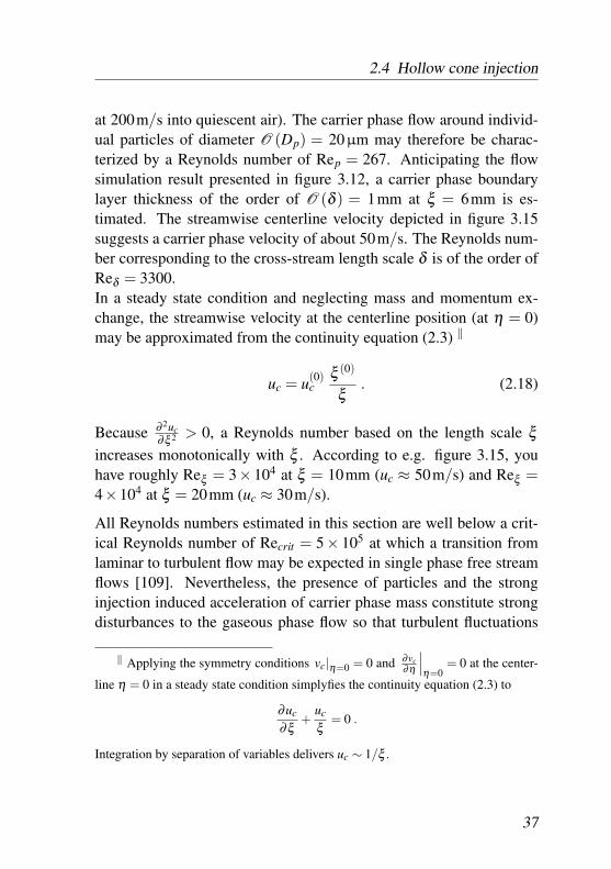
at 200m/s into quiescent air). The carrier phase flow around individ-ual particles of diameter O (Dp) = 20µm may therefore be charac-terized by a Reynolds number of Rep = 267. Anticipating the flowsimulation result presented in figure 3.12, a carrier phase boundarylayer thickness of the order of O (δ ) = 1mm at ξ = 6mm is es-timated. The streamwise centerline velocity depicted in figure 3.15suggests a carrier phase velocity of about 50m/s. The Reynolds num-ber corresponding to the cross-stream length scale δ is of the order ofReδ = 3300.In a steady state condition and neglecting mass and momentum ex-change, the streamwise velocity at the centerline position (at η = 0)may be approximated from the continuity equation (2.3) ‖
uc = u(0)c
ξ (0)
ξ. (2.18)
Because ∂ 2uc∂ξ 2 > 0, a Reynolds number based on the length scale ξ
increases monotonically with ξ . According to e.g. figure 3.15, youhave roughly Reξ = 3× 10⁴ at ξ = 10mm (uc ≈ 50m/s) and Reξ =4×10⁴ at ξ = 20mm (uc ≈ 30m/s).
All Reynolds numbers estimated in this section are well below a crit-ical Reynolds number of Recrit = 5× 10⁵ at which a transition fromlaminar to turbulent flow may be expected in single phase free streamflows [109]. Nevertheless, the presence of particles and the stronginjection induced acceleration of carrier phase mass constitute strongdisturbances to the gaseous phase flow so that turbulent fluctuations
‖ Applying the symmetry conditions vc|η=0 = 0 and ∂vc∂η
∣∣∣η=0
= 0 at the center-
line η = 0 in a steady state condition simplyfies the continuity equation (2.3) to
∂uc
∂ξ+
uc
ξ= 0 .
Integration by separation of variables delivers uc ∼ 1/ξ .
37
2 Modeling methodology
may well occur below the critical Reynolds number known from sin-gle phase flow.
2.5 Summary
Computational models support today’s product engineering. The sim-ulation of an internal combustion engine system incorporates a largerange of time scales. In an industrial development environment, suit-able models need to produce results at the most within days in orderto suggest design changes.
In the context of direct injecting gasoline engines, priority lies on themodeling of heat release and thus mixture formation. They result froman appropriate model of the injection process.
The analysis of the non-dimensional conservation equations for massand momentum in a problem specific cone coordinate system reveal adominance of the second order cross-steam gradients among the vis-cous fluxes in the streamwise momentum equation. In comparison toa single phase jet, additional (“excess”) entrainment of gas is causedby the two-phase jet. The ability of the gas phase to transport momen-tum away from regions of dense spray determines the global sprayfront propagation. Although gas phase Reynolds numbers based ondifferent length scales are below the critical Reynolds number for freestream flows, turbulent fluctuations are expected close to the densespray zones due to the locally high velocity gradients induced in thetwo-phase flow by the injection of liquid fuel.
38
3 Dispersed two-phase flow analysis
The preliminary assessment of the two-phase flow induced by the in-jection of a dispersed phase presented in section 2.4 revealed the prin-cipal physical effects leading to the experimentally observed flow be-havior (cf. figure 2.4):The penetration behavior of the two-phase jet results from the mo-mentum exchange between both phases in regions of high dispersedphase loading. The available experimental data characterizing the car-rier phase flow field (cp. section 3.2.1 in this chapter) only provideaccess to flow regions comparatively far away from the dense sprayzones and as a result do not allow to examine the carrier phase flow inregions of high dispersed phase loadings. For this reason, the hollowcone injection is investigated by means of a computational fluid dy-namics (CFD) model, which provides access to flow properties withinthe whole flow domain.
As a basis for both the CFD investigation (and the chapter 4 on simpli-fied modeling presented later), the mathematical description applied totwo-phase flows is recapitulated in section 3.1. The CFD model set-tings are presented in section 3.1.4.
In section 3.2, the flow results from the CFD model are presented. Thefirst part contains the validation of the CFD model on the basis of mea-sured carrier phase velocity fields. Then, the inter-phase momentumexchange and the induced carrier phase flow are discussed in detail.
3 Dispersed two-phase flow analysis
3.1 Two-phase flow description
Conservation laws are usually derived from a volume integral over amaterial element: The accumulation of quantity ψ within the volumeelement Vm is composed by the influx ψin over the volume element sur-face Am and the rate of production ψsource of ψ within volume elementVm.
∂∂ t
∫Vm
ψ dV = −∮
Am
ψin dV +∫
Vm
ψsource dV (3.1)
If the spatial distribution of ψ is sufficiently smooth for spatial deriva-tives to exist (continuity assumption), the general conservation law forthe quantity ψ in differential form
DψDt︸︷︷︸
Lagrangian time derivative
=∂ψ∂ t︸︷︷︸
rate of change
+∂ (ψu j)
∂x j︸ ︷︷ ︸convection
= −∂Φ j
∂x j︸ ︷︷ ︸surface flux
+ ψsource︸ ︷︷ ︸volume source
(3.2)with the diffusion flux Φ may be obtained.In accordance with Newton’s second law, the acceleration of mass perunit volume depends on the net force it is exposed to (with the stresstensor σi j and force vector Fi).
D(ρ ui)Dt
=∂σi j
∂x j+Fi (3.3)
For Newtonian fluids with constant material properties, a linear de-pendence of the stresses on the time rate of strain, respectively veloc-ity gradients, is assumed (e.g. to describe one-dimensional wall shearstress according to τw = µ ∂u
∂y |w).The stress tensor σi j may be expressed in terms of an isotropic (sym-metric) part representing the normal (hydrostatic) stress (p = σkk/3)and a deviatoric (anti-symmetric) part containing the tangential stresses
40
3.1 Two-phase flow description
acting on a fluid element [93]
σi j = −p δi j + τi j . (3.4)
The deviatoric (viscous) stress tensor τi j depends on the rate of straintensor Si j
∗
τi j = 2µ Si j with Si j =12
(∂ui
∂x j+
∂u j
∂xi
). (3.5)
Insertion of the above produces the well known Navier-Stokes equa-tions. They describe the time-dependent movement of a continuouscompressible fluid in space based on the rate of change in velocity
∗ The effect of a non-linear relation emerges for flows with fast varying den-sity (such as acoustic wave propagation or shock). Then the fluid is subject to anadditional viscocity contribution called volume viscosity or bulk viscosity which re-sists to sudden volume expansion or contraction. In this case, the stress tensor is notsoleniodal so that ∂ui
∂xi�= 0 and with the Stokes hypothesis (µ(2) = −2/3µ), eq. (3.4)
becomes [70]
τi j = 2µ(
si j − 13
siiδi j
)= µ
(∂ui
∂x j+
∂u j
∂xi− 2
3∂ui
∂xi
).
41
3 Dispersed two-phase flow analysis
depending on the pressure field and viscous stress forces†
∂ρ∂ t
+∂ (ρu j)
∂x j= S , (3.6)
∂ (ρui)∂ t
+∂ (ρuiu j)
∂x j= − ∂ p
∂xi+
∂τi j
∂x j+Fi . (3.7)
3.1.1 Continuous phase transport
In the description of dispersed two-phase flows, the conservation ofthe (bulk) carrier phase mass per unit volume ρc = (αcρc) is describedapplying the Navier-Stokes equations.
∂ρc
∂ t+
∂ (ρcuc, j)∂x j
= Γ(evap) , (3.8)
∂ (ρcuc,i)∂ t
+∂ (ρcuc,iuc, j)
∂x j= −∂ pc
∂xi+
∂∂x j
(µc
∂uc, j
∂x j
)+FD,i .
(3.9)
The source terms account for mass transfer due to evaporation (Γ(evap))and momentum exchange with the dispersed phase (FD).
† The Navier-Stokes equation (or more specifically the momentum conservationequation) is a non-linear, second order PDE which is broadly applied when solvingfluid dynamic problems. In spite of its universal acceptance (which is based on thehigh accuracy solutions it produces when integrated numerically) it is noteworthy thatthe unrestricted existence of solutions is not proven to the present day, just like thegeneral smoothness of such solutions (the universal exclusion of discontinuities andsingularities). Both problems belong to the top ten unsolved mathematical problemstoday [49].
42
3.1 Two-phase flow description
3.1.2 Dispersed phase transport
One important aspect in two-phase flow CFD is the representation ofthe dispersed phase. Two major approaches exist.
Lagrangian
In the Lagragian description, the path of the dispersed phase elements(here also termed “particles” and therefore indexed “p”) is obtainedfrom solving an equation of motion for individual particles (“Lagrangianparticle tracking”)
mpDup,i
Dt= FD,i . (3.10)
This equation accurately describes the path of particles when the dis-persed phase is dilute, i.e. if the time τp characterizing the relaxationof fluid forces acting on the particle (see eq. (3.28)) is much smallerthan the characteristic time between inter-particle collisions T
(c)coll .
The diluteness of dispersed two-phase flow may also be characterizedwhen the mean distance between particles Lp is than their diameterDp: For a ratio Lp/Dp > 10 it may well be assumed that collisions donot dominate the dispersed phase movement. This corresponds to adispersed phase volume fraction of αp < 10−3.When the diluteness assumption is applied in CFD analysis of injec-tion processes, the effect of volume displacement due to the presenceof dispersed phase is generally neglected with regard to the carrierphase transport: In equation (3.8), the carrier phase volume fraction isset to αc = 1 and consequently ρc = ρc.
The obvious advantage of the Lagrangian dispersed phase representa-tion – that each dispersed phase element is assigned its unique char-acteristics – also bears limitations to its applicability: The number ofparticles summing up to a constant dispersed phase mass increaseswhen smaller particles are transported (np ∼ D−3
p , see eq. (3.11)), sothat the demand for both computation power and storage requirements
43
3 Dispersed two-phase flow analysis
rises accordingly.Another problem resulting from the Lagrangian description arises whenthe spatial resolution of the computational mesh is increased to orabove the order of the mean particle diameter such as in the context ofDNS or LES of turbulent reactive two-phase flows, e.g. [30, 44]. If thespatial resolution is of the order of the dispersed phase diameter, thedispersed phase concentration may locally no longer be assumed to bedilute. The resulting increased dispersed phase volume fractions thenalso introduce discontinuities to the carrier phase mass conservationequation.
Eulerian
An alternative to the tracking of the individual particle paths is a con-tinuum formulation for the dispersed phase. It is obtained from anaveraging procedure [45].With regards to turbulence effects in a dilute two-phase flow withsolid particles, Simonin et al. [115] derive a continuum formulationby means of ensemble averaging based on the kinetic theory of gases.Similar to the LES approach, a continuum formulation for the dis-persed phase may also be derived by volume filtering [114]. Here, theexistence of the Navier-Stokes equations for both phases is assumed.A sub-grid energy is identified which accounts for the uncorrelatedmotion at length scales below the filter size (which in numerical sim-ulation is identical to the mesh size). Among other contributions, itresults from gradients in the dispersed phase velocity and contributesas a diffusion term to the dispersed phase momentum transport. Bothderivations are compared in [68].The solver used in this investigation [5] applies a simplified conserva-tion equation based on volume filtering for the dispersed phase volumefraction
αp = npπ6
D3p . (3.11)
44
3.1 Two-phase flow description
No pressure (and therefore no pressure gradient) is assigned to thedispersed phase liquid. No sub-grid energy conservation is solved. Amean viscosity µp is assigned to the dispersed phase and the diffu-sion of dispersed phase momentum is modeled by a simple gradientdiffusion hypothesis.
∂ (ρpαp)∂ t
+∂ (ρpαpup, j)
∂x j= −Γ(evap) , (3.12)
∂ (ρpαpup,i)∂ t
+∂ (ρpαpup,iup, j)
∂x j=
∂∂x j
(µp
∂up, j
∂x j
)︸ ︷︷ ︸
σp
−FD,i . (3.13)
Formally, both equations are similar to the description of the carrierphase (eqs. (3.8) and (3.9)). Note that in order to conserve volume,the carrier phase volume fraction is generally αc ≤ 1.The key issue with the Eulerian description of dispersed two-phaseflow is the modeling of the stress tensor σp (or the apparent particleviscosity µp). It may e.g. incorporate mean stresses resulting frominter-particle collisions (resulting in diagonal contributions or pres-sure terms assigned to the dispsersed phase) or turbulent fluctuationsof the dispersed phase velocity [68, 100].The major shortcoming emerging with the Eulerian representation ofthe dispersed phase results from the averaging process: For each dis-persed phase characteristic (e.g. temperature, particle diameter, or ve-locity), only one (average) may be transported. Especially the rep-resentation of poly-dispersion (multiple particle diameters) or poly-celerity (multiple velocities, e.g. in the case of two dilute and possiblyinter-penetrating jets resulting from two different injection directions)may not be described with the conventional (two-fluid) model. Severalcontributions have been proposed accounting for poly-dispersion [90]and poly-celeridity [43, 75] by transporting additional integrals ofthe particle size distribution and introducing additional source terms(see sec. 2.2).
45
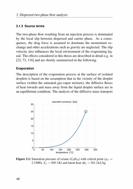
3 Dispersed two-phase flow analysis
3.1.3 Source terms
The two-phase flow resulting from an injection process is dominatedby the local slip between dispersed and carrier phase. As a conse-quence, the drag force is assumed to dominate the momentum ex-change and other accelerations such as gravity are neglected. The slipvelocity also influences the local environment of the evaporating liq-uid. The effects considered in this thesis are described in detail e.g. in[22, 73, 116] and are shortly summarized in the following.
Evaporation
The description of the evaporation process at the surface of isolateddroplets is based on the assumption that in the vicinity of the dropletsurface (within the saturated gas-vapor mixture), the diffusive fluxesof heat towards and mass away from the liquid droplet surface are inan equilibrium condition. The analysis of the diffusive mass transport
0 50 100 150 200 250 300 3500
5
10
15
20
25
30
temperature [°C]
saturation pressure [bar]
Figure 3.1: Saturation pressure of octane (C8H18) with critical point (pcr =2.5MPa, Tcr = 569.3K) and latent heat ∆hv = 301.2kJ/kg
46
3.1 Two-phase flow description
in the vicinity of an isolated droplet’s surface leads to the well knownD2-law. It describes the decrease of the square of the droplet diameterto be linearly dependent on time
D2p = (Dp,0)2 −βSpald t . (3.14)
The Spalding coefficient
βSpald = 8ρFs DFs
ρpln(1+BM) (3.15)
incorporates the mass diffusion potential
BM =YFs −YF∞
1−YFs(3.16)
between the mass concentrations of fuel vapor in the saturated film(with fuel species mass fraction YFs) and in the undisturbed surround-ing (YF∞). Ds quantifies the material diffusion coefficient within thesaturated mixture at the droplet surface.The saturated fuel vapor concentration YFs is calculated from the molec-ular masses of the pure carrier phase gas mc and the saturated gas vapormixture ms where pc is the carrier phase pressure and ps is the satu-ration pressure according to the Clausius-Clapeyron equation (latentheat ∆hv, gas constant of saturated mixture Rs).
YFs =psms
psms +(pc − ps)mcand ps = pre f · exp
{∆hv
Rs
(1
Tre f− 1
Tl
)}(3.17)
The evaporating fuel mass flow rate at the surface of an isolated dropletis
Γ(evap)iso = −ρp
∂ (π6 D3
p)∂ t
=π4
ρp Dp βSpald (3.18)
47
3 Dispersed two-phase flow analysis
so that the total evaporating mass flow rate of np particles per unitvolume is simply
Γ(evap) = npπ4
ρp Dp βSpald . (3.19)
The characteristic time for the evaporation process is the droplet lifetime
T(c)
evap =D2
p,0
βSpald=
ρp D2p,0
8 ρs,c Ds ln(1+BM). (3.20)
Note that the characteristic time needed for a droplet to reach the equi-librium temperature is of the order T
(c)heatup = O(ρlClD2
p/λl). Gener-ally it may be estimated [116] that
T(c)
heatup
T(c)
evap
= 2λc
λp
Cv,c
Cpln(1+BM) � 1 (3.21)
so that from the energy flux equilibrium at the saturated droplet surface( ∂Ts
∂ t = 0), the so called adiabatic “wet bulb” temperature T (wb) may bequantified
T (wb) = T∞ − ∆hv
Cv,cBM . (3.22)
Drag
If the particle surface velocity differs from the carrier phase velocityin the vicinity of the droplet, a boundary layer is formed at the particlesurface, which results in shear forces tangential to the particle surfaceand momentum is exchanged between both phases. Additionally if thecarrier phase is considered compressible, a local pressure maximumahead of the particle and a local pressure minimum in the rear of theparticle is formed. The surface integral of the carrier phase fluid forcesacting on the particle surface may be represented by a net drag force
48
3.1 Two-phase flow description
FD. If the particle surface is not spatially resolved (which is typicallythe case when applying the above mentioned point particle descriptionof the dispersed phase), the net drag force
FD =12
ρc CD Ap |up −uc| (up −uc) (3.23)
is estimated from experimental correlations incorporating e.g. a dragcoefficient
CD =FD
12 ρc u2
slip Ap(3.24)
which relates the effective drag force FD acting on the particle tothe dynamic pressure pdyn = 1
2 ρc uslip Ap with the projected particlesurface Ap = π D2
p/4.Stokes found that for creeping flow (Rep < 1), CD = Rep/24. Schillerand Naumann [107] introduced the correlation correction factor fSN
CD =Rep
24fSN with fSN = 1+0.15 Rep
0.687 . (3.25)
From the net drag on an isolated (spherical) particle
F(iso)D = 3πµc Dp fSN (up −uc) (3.26)
the total drag force per unit volume may be calculated (with the parti-cle number density np and the particle mass per unit volume mp)
FD = np F(iso)D = mp
18 µ f fSN
ρp D2p
(up −uc) . (3.27)
The fraction in equation (3.27) characterizes a relaxation time
τp =ρp D2
p
18 µc fSN(3.28)
49
3 Dispersed two-phase flow analysis
for the relaxation of the velocity of an isolated particle in an undis-turbed carrier phase environment
∂up
∂ t=
1τp
(uc −up) . (3.29)
Turbulent dispersion
Turbulent fluctuations within the carrier phase cause small perturba-tions to the individual particle paths. As a consequence, sharp gradi-ents in the dispersed phase concentration profile relax due to a mean(turbulent) diffusion flux.In the present CFD model, this effect is modeled based on the Favreaveraged inter-phase drag force [24] and depends on the momentumtransfer (drag) coefficient CD and the turbulent carrier phase Schmidtnumber Scc
F(T D)D = CD
νc
Scc
(∇αp
αp− ∇αc
αc
). (3.30)
Viscosity
Based on kinetic theory for ideal gases it may be derived [8] that thedynamic viscosity of an ideal gas
µ =13
λ c m n (3.31)
is dependent on the molecule mass m, the molecular number densityn, the mean free path between molecules λ and the velocity c char-acterizing the kinetic energy of the molecules‡. With increasing gaspressure, the mean free path λ decreases while the molecular number
‡ Likewise, the thermal conductivity
κth =13
λ c Cv [A] (3.32)
50
3.1 Two-phase flow description
density n increases
λ ∼ 1p
and n ∼ p . (3.34)
As a consequence, the dynamic viscosity is independent of density tofirst order of accuracy [27]. By contrast, the mean kinetic energy andthus the dynamic viscosity is proportional to the gas temperature
µ ∼ T 1/2 (3.35)
which may also be obtained from the Sutherland formula
µµ0
=T0 +CT +C
(TT0
) 32
(3.36)
with the gas specific Sutherland constant C (which for air approxi-mately is C = 120K).
3.1.4 CFD setup
The CFD model is validated based on measurements of the cold flowonly so that the effect of evaporation is not included in the presentCFD model.Spatial velocity gradients in the vicinity of the dense spray are to beresolved so that consequentially a comparatively fine grid resolution ischosen. Because of the effects related to the statistical description ofthe Lagrangian dispersed phase description discussed in section 2.3,results from the Eulerian (two-fluid) method are predominantly pre-
depends on the heat capacity Cv and the molecular concentration [A]. In a similarfashion, the mass diffusivity
D =13
λ c (3.33)
is obtained.
51
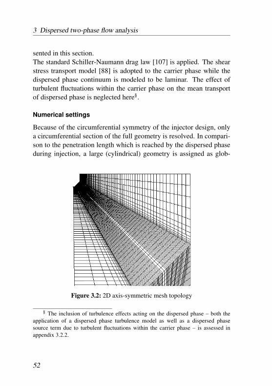
3 Dispersed two-phase flow analysis
sented in this section.The standard Schiller-Naumann drag law [107] is applied. The shearstress transport model [88] is adopted to the carrier phase while thedispersed phase continuum is modeled to be laminar. The effect ofturbulent fluctuations within the carrier phase on the mean transportof dispersed phase is neglected here§.
Numerical settings
Because of the circumferential symmetry of the injector design, onlya circumferential section of the full geometry is resolved. In compari-son to the penetration length which is reached by the dispersed phaseduring injection, a large (cylindrical) geometry is assigned as glob-
Figure 3.2: 2D axis-symmetric mesh topology
§ The inclusion of turbulence effects acting on the dispersed phase – both theapplication of a dispersed phase turbulence model as well as a dispersed phasesource term due to turbulent fluctuations within the carrier phase – is assessed inappendix 3.2.2.
52
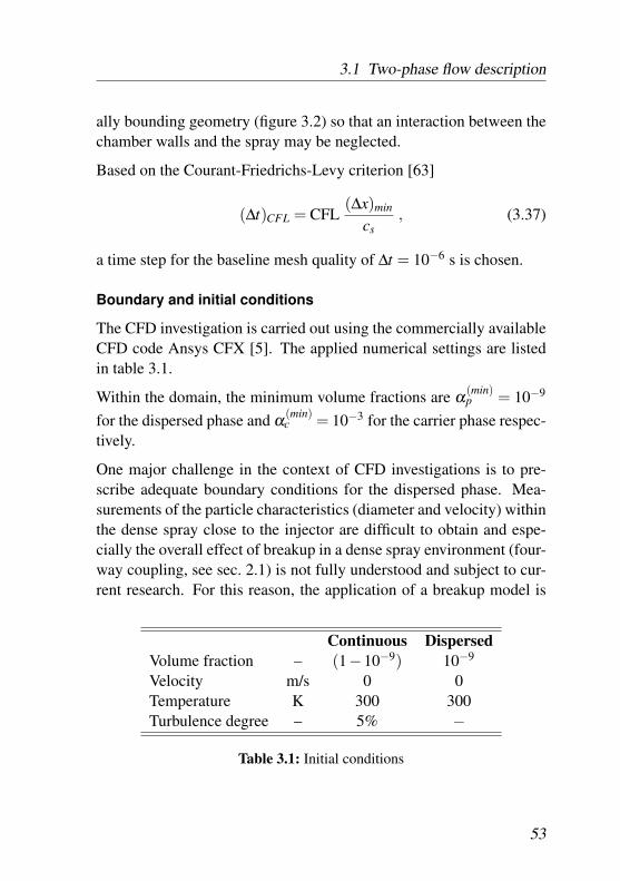
3.1 Two-phase flow description
ally bounding geometry (figure 3.2) so that an interaction between thechamber walls and the spray may be neglected.
Based on the Courant-Friedrichs-Levy criterion [63]
(∆t)CFL = CFL(∆x)min
cs, (3.37)
a time step for the baseline mesh quality of ∆t = 10−6 s is chosen.
Boundary and initial conditions
The CFD investigation is carried out using the commercially availableCFD code Ansys CFX [5]. The applied numerical settings are listedin table 3.1.
Within the domain, the minimum volume fractions are α(min)p = 10−9
for the dispersed phase and α(min)c = 10−3 for the carrier phase respec-
tively.
One major challenge in the context of CFD investigations is to pre-scribe adequate boundary conditions for the dispersed phase. Mea-surements of the particle characteristics (diameter and velocity) withinthe dense spray close to the injector are difficult to obtain and espe-cially the overall effect of breakup in a dense spray environment (four-way coupling, see sec. 2.1) is not fully understood and subject to cur-rent research. For this reason, the application of a breakup model is
Continuous DispersedVolume fraction – (1−10−9) 10−9
Velocity m/s 0 0Temperature K 300 300Turbulence degree – 5% −
Table 3.1: Initial conditions
53
3 Dispersed two-phase flow analysis
discarded here and a representative mean droplet diameter is applied.For an approximate estimation of the droplet size distribution, theMalvern technique [82] yields reliable results up to certain maximumdroplet number concentrations (maximum liquid volume fractions).For this reason, the droplet size spectrum close to the injector exit ingeneral may not be measured. Only the size distribution at a locationfurther downstream is accessible.For a steady state operating condition (injection pressure pin j =180barand maximum injector opening), the particle size distribution of themodeled injector was measured at a distance 75 mm along injectoraxis [35]. Figure 3.3 shows the resulting discrete normalized dis-tribution representing the normalized volume fraction of the corre-sponding size class (from here onwards referred to as the volume fre-quency [34]).Particles of diameters between 10 and 20µm represent approximately60% of the liquid volume. About 15% of the liquid volume consistsof particles larger than 20µm and consequently about 20% of the liq-uid volume is composed of particles of diameter smaller than 10µm.
The second major input parameter to the CFD model is the velocity atwhich the liquid phase exits the injector outlet. Experimentally, thisvelocity may be evaluated from photographic images taken at the verybeginning of the injection process (shortly after the injector opens). Bycontrast, it may not be measured when the injector is fully opened: Atthis flow condition, only the apparent spray front velocity is accessiblefrom data obtained through photography.The injector exit velocity may be approximated from the static massflow rate min j which is supplied to the injector. Conservation of massthen yields (liquid density ρl , injector exit velocity vin j)
min j = ρp Ain j vin j. (3.38)
In general, the effective cross section Ain j is smaller than the geomet-
54
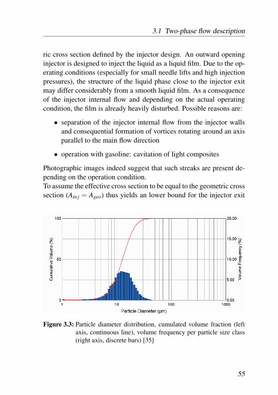
3.1 Two-phase flow description
ric cross section defined by the injector design. An outward openinginjector is designed to inject the liquid as a liquid film. Due to the op-erating conditions (especially for small needle lifts and high injectionpressures), the structure of the liquid phase close to the injector exitmay differ considerably from a smooth liquid film. As a consequenceof the injector internal flow and depending on the actual operatingcondition, the film is already heavily disturbed. Possible reasons are:
• separation of the injector internal flow from the injector wallsand consequential formation of vortices rotating around an axisparallel to the main flow direction
• operation with gasoline: cavitation of light composites
Photographic images indeed suggest that such streaks are present de-pending on the operation condition.To assume the effective cross section to be equal to the geometric crosssection (Ain j = Ageo) thus yields an lower bound for the injector exit
Figure 3.3: Particle diameter distribution, cumulated volume fraction (leftaxis, continuous line), volume frequency per particle size class(right axis, discrete bars) [35]
55
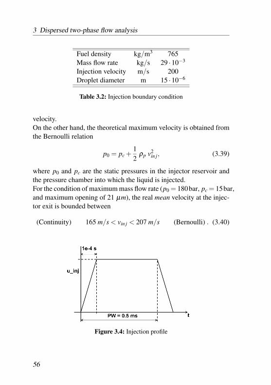
3 Dispersed two-phase flow analysis
Fuel density kg/m3 765Mass flow rate kg/s 29 ·10−3
Injection velocity m/s 200Droplet diameter m 15 ·10−6
Table 3.2: Injection boundary condition
velocity.On the other hand, the theoretical maximum velocity is obtained fromthe Bernoulli relation
p0 = pc +12
ρp v2in j, (3.39)
where p0 and pc are the static pressures in the injector reservoir andthe pressure chamber into which the liquid is injected.For the condition of maximum mass flow rate (p0 = 180bar, pc = 15bar,and maximum opening of 21 µm), the real mean velocity at the injec-tor exit is bounded between
(Continuity) 165 m/s < vin j < 207 m/s (Bernoulli) . (3.40)
Figure 3.4: Injection profile
56
3.1 Two-phase flow description
Based on the preceding assessment, the representative droplet diame-ter and injection velocity assigned to the dispersed phase are Dp = 15µmand vin j = 200m/s unless indicated otherwise.
The mean mass flow rate through the injector is measured at steadystate operating conditions. After “start of injection” (SOI), the injec-tion profiles of both mass flow rate as well as injection velocity aremodeled to increase linearly until the corresponding maximum valuesare reached within 0.1ms. The injector driver signal (“pulse width”PW) causing the opening of the injector is 0.5ms long. After thistime, the injection is assumed to close in a similar fashion to the open-ing event, i.e. linearly within 0.1ms.
57
3 Dispersed two-phase flow analysis
3.2 Hollow cone injection induced two-phase flow
A CFD model of the hollow cone spray is employed in order to char-acterize the injection induced two-phase flow. On the basis of carrierphase velocity fields measured by means of PIV (section 3.2.1), exem-plary results from the CFD model validation are given in section 3.2.2.The results from CFD investigation (subsequent sections) then focuson the characterization of the inter-phase momentum exchange andthe injection induced carrier phase flow.
3.2.1 Experimental data
The most reliable way of validation of CFD models is to compare thesolution to experimental data. The range of methods to generate datafrom experiments is discussed in the methodology section (section 2).For the present investigation, the carrier phase velocity field is com-pared to measurements applying particle image velocimetry (PIV).
Experimental data overview
This investigation utilizes data obtained from PIV measurements per-formed by Prosperi [97] on a constant pressure chamber. Differentcarrier phase pressures are investigated while the carrier phase tem-perature was set constant (Tg = 300K) ¶. The focus of the CFD inves-tigation lies on comparatively short injection times to that only dataresulting from injection pulse widths of 0.5ms is considered. For the
¶ For the mentioned measurement campaign, the focus lay on the interaction ofthe dispersed phase with “pure” air. Evaporation of liquid phase and the formationof air-fuel vapour mixture was deliberately suppressed. For this as well as for safetyreasons, the experiments presented in the subsequent sections were carried out witha gas called CF4 which yields a larger density. The pressures referred to in thissection (e.g. in table 3.3) indicate pressures air exhibits if charged to the density (andtemperature) level at which the experiments with CF4 are carried out.
58
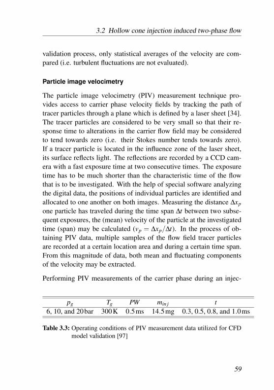
3.2 Hollow cone injection induced two-phase flow
validation process, only statistical averages of the velocity are com-pared (i.e. turbulent fluctuations are not evaluated).
Particle image velocimetry
The particle image velocimetry (PIV) measurement technique pro-vides access to carrier phase velocity fields by tracking the path oftracer particles through a plane which is defined by a laser sheet [34].The tracer particles are considered to be very small so that their re-sponse time to alterations in the carrier flow field may be consideredto tend towards zero (i.e. their Stokes number tends towards zero).If a tracer particle is located in the influence zone of the laser sheet,its surface reflects light. The reflections are recorded by a CCD cam-era with a fast exposure time at two consecutive times. The exposuretime has to be much shorter than the characteristic time of the flowthat is to be investigated. With the help of special software analyzingthe digital data, the positions of individual particles are identified andallocated to one another on both images. Measuring the distance ∆xp
one particle has traveled during the time span ∆t between two subse-quent exposures, the (mean) velocity of the particle at the investigatedtime (span) may be calculated (vp = ∆xp/∆t). In the process of ob-taining PIV data, multiple samples of the flow field tracer particlesare recorded at a certain location area and during a certain time span.From this magnitude of data, both mean and fluctuating componentsof the velocity may be extracted.
Performing PIV measurements of the carrier phase during an injec-
pg Tg PW min j t6, 10, and 20bar 300K 0.5ms 14.5mg 0.3, 0.5, 0.8, and 1.0ms
Table 3.3: Operating conditions of PIV measurement data utilized for CFDmodel validation [97]
59
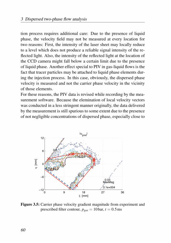
3 Dispersed two-phase flow analysis
tion process requires additional care: Due to the presence of liquidphase, the velocity field may not be measured at every location fortwo reasons: First, the intensity of the laser sheet may locally reduceto a level which does not produce a reliable signal intensity of the re-flected light. Also, the intensity of the reflected light at the location ofthe CCD camera might fall below a certain limit due to the presenceof liquid phase. Another effect special to PIV in gas-liquid flows is thefact that tracer particles may be attached to liquid phase elements dur-ing the injection process. In this case, obviously, the dispersed phasevelocity is measured and not the carrier phase velocity in the vicinityof those elements.For these reasons, the PIV data is revised while recording by the mea-surement software. Because the elemination of local velocity vectorswas conducted in a less stringent manner originally, the data deliveredby the measurement is still spurious to some extent due to the presenceof not negligible concentrations of dispersed phase, especially close to
0 9 18 27 36−12
−6
0
6
12
|ugrad
|
ξ [mm]
η [
mm
]
0.2
0.20.2 0.20.2
0.20.03
0.030.03
MaxMag
3.1e+004
Figure 3.5: Carrier phase velocity gradient magnitude from experiment andprescribed filter contour, pgas = 10bar, t = 0.5ms
60
3.2 Hollow cone injection induced two-phase flow
the spray front region, where unphysical structures of the velocity pro-files (high velocity gradients) were recorded. So for the present com-parison, an additional revision of the PIV data was carried out basedon the gray level of a corresponding Mie scattering image. From theMie intensity isoline (figure 3.5), a convex structure is identified as thefront of the dense spray zone.
Representation in conical coordinates
The usage of cone specific coordinates ξ and η (see section 2.4.1 andfigure on page 61) is introduced in detail in appendix A. In order toshortly revise the data representation in conical coordinates, figure 3.6displays normalized velocity vector fields from both experiment (onthe left) and simulation (on the right). In the top row figures, the y-axis coincides with the injector axis where y = 0-line cuts the injectoroutlet at x ≈ 2.1mm. The diagonal dash-dotted line indicates the (pre-sumed) dispersed phase cone jet center line.In cone coordinates (bottom row figures), the ξ -axis corresponds tothe spray cone center line and η is the coordinate normal to ξ . Pos-itive values of η indicate the region outside and negative values theinside of the hollow cone. The diagonal dashed line now indicates theinjector axis. In the following, conical coordinates are used, exceptindicated otherwise.
From figure 3.6 it becomes evident that the PIV measurement of theinjection process only allows to access the carrier phase velocity fieldat locations comparatively far away from the dense spray zones (lefthand side figures). Moreover, the velocity information in the regionclose to the injector outlet at (ξ = 0, η = 0) is considered to be notreliable for η ≤ 0 since at the displayed instant in time, liquid is stillinjected at full flow rate so that a good quality of the laser signal is notto be expected in this region (which is also supported by the fact thatthe experimental data does not yield a predominant flow direction inthis region).
61
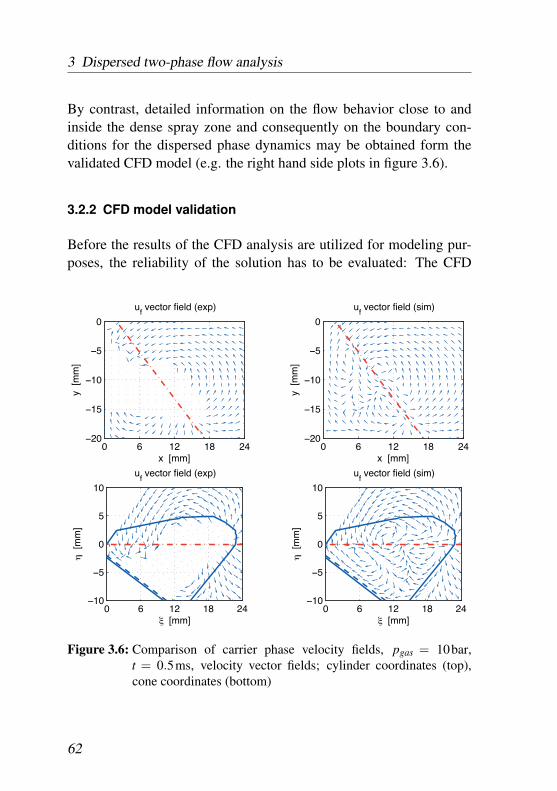
3 Dispersed two-phase flow analysis
By contrast, detailed information on the flow behavior close to andinside the dense spray zone and consequently on the boundary con-ditions for the dispersed phase dynamics may be obtained form thevalidated CFD model (e.g. the right hand side plots in figure 3.6).
3.2.2 CFD model validation
Before the results of the CFD analysis are utilized for modeling pur-poses, the reliability of the solution has to be evaluated: The CFD
0 6 12 18 24−20
−15
−10
−5
0
x [mm]
y [m
m]
uf vector field (exp)
0 6 12 18 24−20
−15
−10
−5
0
x [mm]
y [m
m]
uf vector field (sim)
0 6 12 18 24−10
−5
0
5
10
ξ [mm]
η [
mm
]
uf vector field (exp)
0 6 12 18 24−10
−5
0
5
10
ξ [mm]
η [
mm
]
uf vector field (sim)
Figure 3.6: Comparison of carrier phase velocity fields, pgas = 10bar,t = 0.5ms, velocity vector fields; cylinder coordinates (top),cone coordinates (bottom)
62
3.2 Hollow cone injection induced two-phase flow
model has to be validated. The validation procedure has two mainobjectives: First, elements of the results obtained from CFD have tocompare to data obtained in an alternate way – e.g. by means of anexperiment (level of accuracy of the solution). Secondly, the responseof the model to alterations in the input parameters has to be evaluated(robustness of the solution). For both validation criteria, levels of thedesired solution quality have to be defined.
The experimental (PIV) data listed in table 3.3 is used for validationin two ways:Because the spacial distribution of carrier phase momentum (or veloc-ity) and its development over time characterizes the volume of carrierphase which is affected by the injection process, the comparison ofthe gas phase velocity field is applied as the primary indicator for thequality of the CFD model.Since preceding the comparison, a spray front is identified from thePIV measurements (see figure 3.5), a penetration length of the dis-persed phase into the pressure chamber may be compared.
As discussed in the methodology section, the focus of the CFD investi-gation lies on the usage of the Eulerian representation of the dispersedphase. Therefore, only results from this setup are presented here inorder to quantitatively verify the injection induced carrier phase ve-locity field (accuracy validation). The sensitivity of the CFD solutionto an altered dispersed phase representation (namely the Lagrangianformulation) and to changes in numerical parameters is examined inthe subsequent sections (robustness validation).
Carrier phase velocity fields
In general, the comparison of experimental and simulated velocitydata reveals a satisfactory quality of the CFD model. This impressionis amplified by identical locations of the displayed vectors in both plotsand their normalized representation. Because of this and the complex-ity of the vector data representation mentioned above, the two velocity
63
3 Dispersed two-phase flow analysis
components are compared individually from here onwards.
The grid resolution of the simulation is orders of magnitude higherthan the spatial resolution of the PIV measurement. Therefore the ve-locity resulting from CFD is examined at the locations where experi-mental data are available. (The high grid resolution of the CFD modelmakes an interpolation superfluous – the data is simply copied fromthe nearest neighbor location.) Isolines of velocity component mag-nitudes are depicted in figure 3.7. In order to emphasize the distancefrom the injector outlet into the pressure chamber along the main flowdirection ξ at which carrier phase is set into motion due to the injec-tion, the corresponding figures obtained from experiment and simula-tion are placed above each other.The contours of the streamwise velocity component u (positive alongthe main flow direction ξ ) as well as the cross-stream velocity compo-nent v (positive along the coordinate η normal to the main flow direc-tion) both exhibit a comparatively good agreement. The four explicitlylabeled contours u = −3m/s, u = 1m/s, v = −5m/s, and v = 1m/sindicate that approximately the same volume of carrier phase mass isset into motion due to the injection process – both measured along andnormal to the main injection direction. (Note that the straight diagonallines in the figures resulting from the experiment do not indicate a flowpattern but stem from the choice of the measurement plane boundary.)
In summary, the temporal development both during (at 0.3 and 0.5ms)and after injection (at 0.8 and 1.0ms) match well over the whole cham-ber pressure range investigated here. Recall that two-phase flow sen-sitive input parameters to the CFD model such as particle diameterand maximum injection velocity are kept constant for varying timeand chamber pressure. This result supports the reasoning presentedin the context of the methodology section: To first order of accuracy,the superimposing effects of poly-dispersion, particle breakup and co-alescence in volumes with high particle loading, and segregation ofdifferent size particles due to interaction with the (locally constant)
64
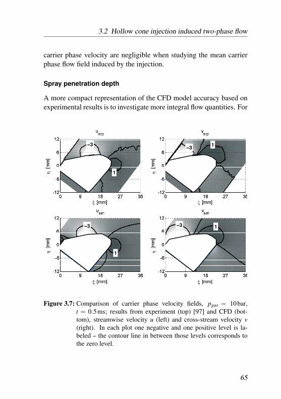
3.2 Hollow cone injection induced two-phase flow
carrier phase velocity are negligible when studying the mean carrierphase flow field induced by the injection.
Spray penetration depth
A more compact representation of the CFD model accuracy based onexperimental results is to investigate more integral flow quantities. For
−3
1
−3
1
1−3
1−3
Figure 3.7: Comparison of carrier phase velocity fields, pgas = 10bar,t = 0.5ms; results from experiment (top) [97] and CFD (bot-tom), streamwise velocity u (left) and cross-stream velocity v(right). In each plot one negative and one positive level is la-beled – the contour line in between those levels corresponds tothe zero level.
65
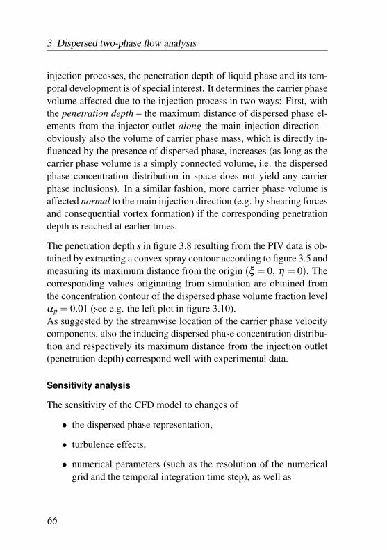
3 Dispersed two-phase flow analysis
injection processes, the penetration depth of liquid phase and its tem-poral development is of special interest. It determines the carrier phasevolume affected due to the injection process in two ways: First, withthe penetration depth – the maximum distance of dispersed phase el-ements from the injector outlet along the main injection direction –obviously also the volume of carrier phase mass, which is directly in-fluenced by the presence of dispersed phase, increases (as long as thecarrier phase volume is a simply connected volume, i.e. the dispersedphase concentration distribution in space does not yield any carrierphase inclusions). In a similar fashion, more carrier phase volume isaffected normal to the main injection direction (e.g. by shearing forcesand consequential vortex formation) if the corresponding penetrationdepth is reached at earlier times.
The penetration depth s in figure 3.8 resulting from the PIV data is ob-tained by extracting a convex spray contour according to figure 3.5 andmeasuring its maximum distance from the origin (ξ = 0, η = 0). Thecorresponding values originating from simulation are obtained fromthe concentration contour of the dispersed phase volume fraction levelαp = 0.01 (see e.g. the left plot in figure 3.10).As suggested by the streamwise location of the carrier phase velocitycomponents, also the inducing dispersed phase concentration distribu-tion and respectively its maximum distance from the injection outlet(penetration depth) correspond well with experimental data.
Sensitivity analysis
The sensitivity of the CFD model to changes of
• the dispersed phase representation,
• turbulence effects,
• numerical parameters (such as the resolution of the numericalgrid and the temporal integration time step), as well as
66
3.2 Hollow cone injection induced two-phase flow
0 200 400 600 800 10000
10
20
30
40
time [µs]
s [m
m]
expsim
0 200 400 600 800 10000
10
20
30
40
time [µs]s
[mm
]
expsim
0 200 400 600 800 10000
10
20
30
40
time [µs]
s [m
m]
expsim
Figure 3.8: Comparison of spray front penetration depth ξ at 6 (left), 10(middle), and 20bar chamber pressure (right)
• physical parameter (such as the mean droplet diameter and themean injection velocity)
was assessed.
Because of their principal differences, the CFD solution of the two-phase flow induced by the hollow cone injection yields differenceswhen the mathematical description of the dispersed phase is altered:The cross-stream width of the dispersed phase volume fraction field ismore slender when the Lagrangian description is applied. The diffu-sive term in the Eulerian momentum equation (3.13) causes the dis-persed phase volume fraction field to take on broader shapes thanthe Lagrangian results. The consequentially broader boundary layerthickness of the carrier phase jet causes smaller magnitudes of shearstresses, so that larger magnitudes of streamwise carrier phase veloc-ity are obtained.Because the total momentum (which is supplied to the flow domainby the injection boundary condition) needs to be conserved within theflow domain, increased carrier phase velocities correspond to smallerpenetration depths of the dispersed phase mass: The total momentumcarried by the carrier phase increases, while the total dispersed phasemomentum within the flow domain decreases. Consequentially, thesmaller velocity magnitudes resulting from the Lagrangian dispersed
67
3 Dispersed two-phase flow analysis
phase representation correspond to a larger penetration depth of theliquid jet and vice versa.
The standard model coefficients of the carrier phase turbulence modelwere not changed in this investigation.The application of a turbulent dispersion force generally leads to broadercross-stream profiles of the dispersed phase mass. As a consequence,the dispersed phase interacts with a larger volume (i.e. a larger amountof mass) of carrier phase and the penetration depth of the liquid jetdecreases. The strong influence of this model indicates that the cali-bration of this sub-model is critical to the overall performance of thetwo-phase flow CFD model. Because the data available for the cal-ibration of a mean turbulent dispersion force (both experimental andnumerical) is limited in the case of a transient hollow cone flow re-sulting from high pressure injection as investigated here, the turbulentdispersion force model is omitted in the quantitative description pre-sented in the remainder of section 3.2.The presence of particles of finite Stokes number introduces additionaldisturbances to the carrier phase flow and thereby enhances the inten-sity of its turbulent fluctuations. The influence of a turbulence en-hancement model [104] was found to be of minor influence in the con-text of the hollow cone injection. The production of turbulent kineticenergy, which is proportial to the square of the cross-stream velocitygradients within the carrier phase, exhibits much larger magnitudesthan the turbulence enhancement source term which is proportional tothe slip velocity.
Both the spatial and temporal resolution sensitivity was investigated.With increasing mesh quality, additional small scale vortex structuresbecome visible as expected.At the highest investigated spatial resolution, especially the Eulerianrepresentation of the dispersed phase causes small scale artifacts in thedispersed phase volume fraction field, which are not physically plau-sible.
68

3.2 Hollow cone injection induced two-phase flow
An important result from the sensitivity analysis of the mesh quality isthat – for the set of investigated mesh qualities – the penetration depthof the dispersed phase jet is approximately independent from the reso-lution of the numerical grid: In the context of the Lagrangian descrip-tion, increased dispersed phase volume fractions occur when the meshquality is increased. But the cumulative effect of increased dispersedphase volume fractions on the local drag force does not change theglobal penetration depth. The cross-stream profiles of the dispersedphase volume fraction field resulting from the Eulerian description aremore slender in shape when the mesh quality is increased while likein the Lagrangian case, the global penetration depth does not changewith varying mesh quality. This result indicates that cross-stream gra-dients are sufficiently resolved even when the nominal mesh quality isdecreased.
The CFD model result responds in a robust manner to variations intime step size which suggests that the chosen time step based on theCFL criterion at the injection boundary condition sufficiently resolvesthe flow dynamics.
The number of computational parcels employed for the Lagrangiandescription does not influence the global penetration behavior. Whenmore computational parcels are tracked, slight differences in the frontregion of the two-phase jet may be observed.
Because of the square dependence of the drag force on the particlediameter, the flow solution responds rather sensitive to variations inparticle diameter. The sensitivity of the flow to variations in the mo-mentum which is supplied by the injection boundary condition (injec-tion velocity) is found to have less influence than the particle diameter.
69
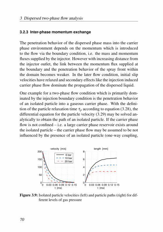
3 Dispersed two-phase flow analysis
3.2.3 Inter-phase momentum exchange
The penetration behavior of the dispersed phase mass into the carrierphase environment depends on the momentum which is introducedto the flow via the boundary condition, i.e. the mass and momentumfluxes supplied by the injector. However with increasing distance fromthe injector outlet, the link between the momentum flux supplied atthe boundary and the penetration behavior of the spray front withinthe domain becomes weaker. In the later flow condition, initial slipvelocities have relaxed and secondary effects like the injection inducedcarrier phase flow dominate the propagation of the dispersed liquid.
One example for a two-phase flow condition which is primarily dom-inated by the injection boundary condition is the penetration behaviorof an isolated particle into a gaseous carrier phase. With the defini-tion of the particle relaxation time τp according to equation (3.28), thedifferential equation for the particle velocity (3.29) may be solved an-alytically to obtain the path of an isolated particle. If the carrier phaseflow is not confined – i.e. a large carrier phase reservoir exists aroundthe isolated particle – the carrier phase flow may be assumed to be notinfluenced by the presence of an isolated particle (one-way coupling,
0 0.03 0.06 0.09 0.12 0.150
50
100
150
200velocity [m/s]
t [ms]
6 bar10 bar20 bar
0 0.03 0.06 0.09 0.12 0.150
2
4
6
8length [mm]
t [ms]
Figure 3.9: Isolated particle velocities (left) and particle paths (right) for dif-ferent levels of gas pressure
70
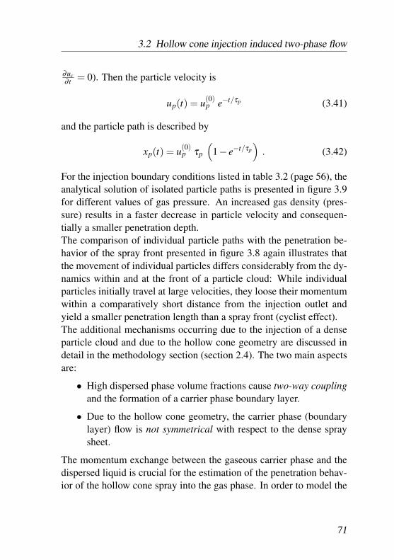
3.2 Hollow cone injection induced two-phase flow
∂uc∂ t = 0). Then the particle velocity is
up(t) = u(0)p e−t/τp (3.41)
and the particle path is described by
xp(t) = u(0)p τp
(1− e−t/τp
). (3.42)
For the injection boundary conditions listed in table 3.2 (page 56), theanalytical solution of isolated particle paths is presented in figure 3.9for different values of gas pressure. An increased gas density (pres-sure) results in a faster decrease in particle velocity and consequen-tially a smaller penetration depth.The comparison of individual particle paths with the penetration be-havior of the spray front presented in figure 3.8 again illustrates thatthe movement of individual particles differs considerably from the dy-namics within and at the front of a particle cloud: While individualparticles initially travel at large velocities, they loose their momentumwithin a comparatively short distance from the injection outlet andyield a smaller penetration length than a spray front (cyclist effect).The additional mechanisms occurring due to the injection of a denseparticle cloud and due to the hollow cone geometry are discussed indetail in the methodology section (section 2.4). The two main aspectsare:
• High dispersed phase volume fractions cause two-way couplingand the formation of a carrier phase boundary layer.
• Due to the hollow cone geometry, the carrier phase (boundarylayer) flow is not symmetrical with respect to the dense spraysheet.
The momentum exchange between the gaseous carrier phase and thedispersed liquid is crucial for the estimation of the penetration behav-ior of the hollow cone spray into the gas phase. In order to model the
71
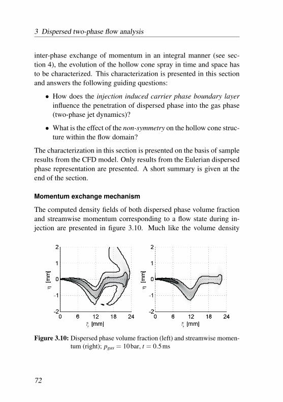
3 Dispersed two-phase flow analysis
inter-phase exchange of momentum in an integral manner (see sec-tion 4), the evolution of the hollow cone spray in time and space hasto be characterized. This characterization is presented in this sectionand answers the following guiding questions:
• How does the injection induced carrier phase boundary layerinfluence the penetration of dispersed phase into the gas phase(two-phase jet dynamics)?
• What is the effect of the non-symmetry on the hollow cone struc-ture within the flow domain?
The characterization in this section is presented on the basis of sampleresults from the CFD model. Only results from the Eulerian dispersedphase representation are presented. A short summary is given at theend of the section.
Momentum exchange mechanism
The computed density fields of both dispersed phase volume fractionand streamwise momentum corresponding to a flow state during in-jection are presented in figure 3.10. Much like the volume density
αp (αp ρp up)
Figure 3.10: Dispersed phase volume fraction (left) and streamwise momen-tum (right); pgas = 10bar, t = 0.5ms
72
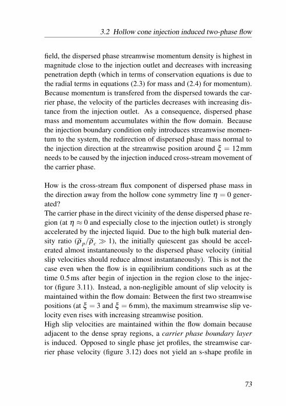
3.2 Hollow cone injection induced two-phase flow
field, the dispersed phase streamwise momentum density is highest inmagnitude close to the injection outlet and decreases with increasingpenetration depth (which in terms of conservation equations is due tothe radial terms in equations (2.3) for mass and (2.4) for momentum).Because momentum is transfered from the dispersed towards the car-rier phase, the velocity of the particles decreases with increasing dis-tance from the injection outlet. As a consequence, dispersed phasemass and momentum accumulates within the flow domain. Becausethe injection boundary condition only introduces streamwise momen-tum to the system, the redirection of dispersed phase mass normal tothe injection direction at the streamwise position around ξ = 12mmneeds to be caused by the injection induced cross-stream movement ofthe carrier phase.
How is the cross-stream flux component of dispersed phase mass inthe direction away from the hollow cone symmetry line η = 0 gener-ated?The carrier phase in the direct vicinity of the dense dispersed phase re-gion (at η ≈ 0 and especially close to the injection outlet) is stronglyaccelerated by the injected liquid. Due to the high bulk material den-sity ratio (ρ p/ρc � 1), the initially quiescent gas should be accel-erated almost instantaneously to the dispersed phase velocity (initialslip velocities should reduce almost instantaneously). This is not thecase even when the flow is in equilibrium conditions such as at thetime 0.5ms after begin of injection in the region close to the injec-tor (figure 3.11). Instead, a non-negligible amount of slip velocity ismaintained within the flow domain: Between the first two streamwisepositions (at ξ = 3 and ξ = 6mm), the maximum streamwise slip ve-locity even rises with increasing streamwise position.High slip velocities are maintained within the flow domain becauseadjacent to the dense spray regions, a carrier phase boundary layeris induced. Opposed to single phase jet profiles, the streamwise car-rier phase velocity (figure 3.12) does not yield an s-shape profile in
73
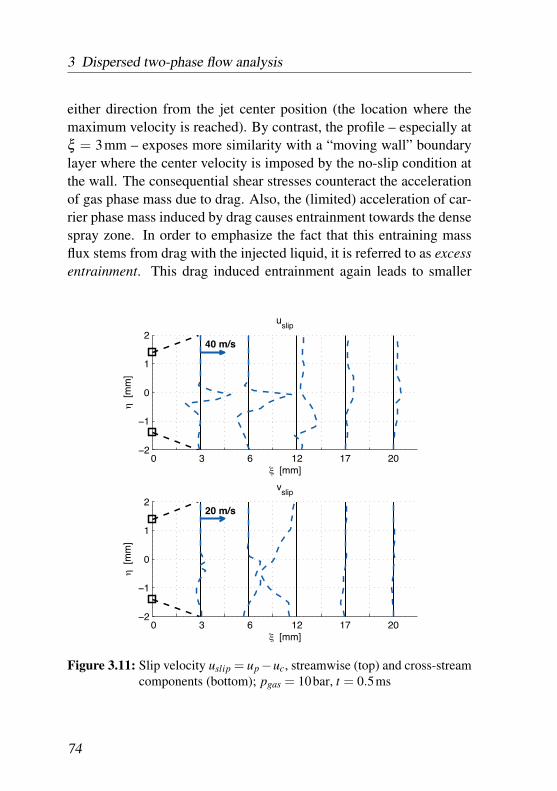
3 Dispersed two-phase flow analysis
either direction from the jet center position (the location where themaximum velocity is reached). By contrast, the profile – especially atξ = 3mm – exposes more similarity with a “moving wall” boundarylayer where the center velocity is imposed by the no-slip condition atthe wall. The consequential shear stresses counteract the accelerationof gas phase mass due to drag. Also, the (limited) acceleration of car-rier phase mass induced by drag causes entrainment towards the densespray zone. In order to emphasize the fact that this entraining massflux stems from drag with the injected liquid, it is referred to as excessentrainment. This drag induced entrainment again leads to smaller
0 3 6 12 17 20−2
−1
0
1
2
uslip
40 m/s
ξ [mm]
η [
mm
]
0 3 6 12 17 20−2
−1
0
1
2
vslip
20 m/s
ξ [mm]
η [
mm
]
Figure 3.11: Slip velocity uslip = up−uc, streamwise (top) and cross-streamcomponents (bottom); pgas = 10bar, t = 0.5ms
74
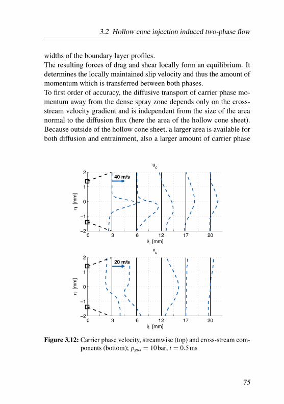
3.2 Hollow cone injection induced two-phase flow
widths of the boundary layer profiles.The resulting forces of drag and shear locally form an equilibrium. Itdetermines the locally maintained slip velocity and thus the amount ofmomentum which is transferred between both phases.To first order of accuracy, the diffusive transport of carrier phase mo-mentum away from the dense spray zone depends only on the cross-stream velocity gradient and is independent from the size of the areanormal to the diffusion flux (here the area of the hollow cone sheet).Because outside of the hollow cone sheet, a larger area is available forboth diffusion and entrainment, also a larger amount of carrier phase
0 3 6 12 17 20−2
−1
0
1
2
uc
40 m/s
ξ [mm]
η [
mm
]
0 3 6 12 17 20−2
−1
0
1
2
vc
20 m/s
ξ [mm]
η [
mm
]
Figure 3.12: Carrier phase velocity, streamwise (top) and cross-stream com-ponents (bottom); pgas = 10bar, t = 0.5ms
75
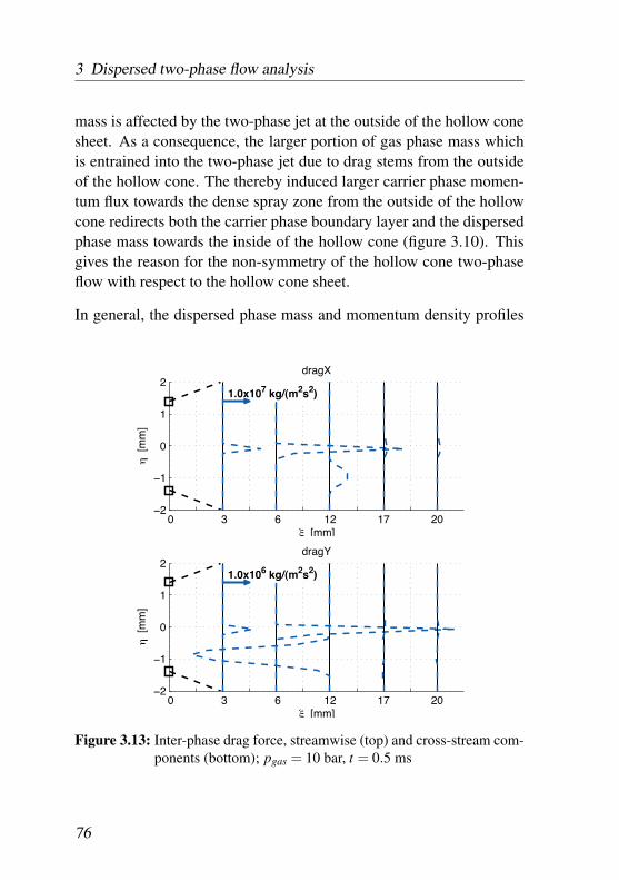
3 Dispersed two-phase flow analysis
mass is affected by the two-phase jet at the outside of the hollow conesheet. As a consequence, the larger portion of gas phase mass whichis entrained into the two-phase jet due to drag stems from the outsideof the hollow cone. The thereby induced larger carrier phase momen-tum flux towards the dense spray zone from the outside of the hollowcone redirects both the carrier phase boundary layer and the dispersedphase mass towards the inside of the hollow cone (figure 3.10). Thisgives the reason for the non-symmetry of the hollow cone two-phaseflow with respect to the hollow cone sheet.
In general, the dispersed phase mass and momentum density profiles
0 3 6 12 17 20−2
−1
0
1
2dragX
1.0x10⁷ kg/(m2s2)
ξ [mm]
η [
mm
]
0 3 6 12 17 20−2
−1
0
1
2dragY
1.0x10⁶ kg/(m2s2)
ξ [mm]
η [
mm
]
Figure 3.13: Inter-phase drag force, streamwise (top) and cross-stream com-ponents (bottom); pgas = 10 bar, t = 0.5 ms
76
3.2 Hollow cone injection induced two-phase flow
are more slender than the ones of the carrier phase. Nevertheless,also the dispersed phase cross-stream profiles become broader with in-creasing penetration due to momentum diffusion (figure 3.10). Conse-quentially, the cross-stream width which is occupied by high dispersedphase momentum densities and which is available for inter-phase mo-mentum exchange increases with increasing penetration depth. Withinbroader dense spray zones, also higher maximum streamwise slip ve-locities occur (figure 3.11) and as a consequence, drag forces of highermagnitude are exchanged (3.13 at ξ = 6 versus ξ = 3mm).From figure 3.13, the dominance of the injection direction is clearlyvisible at the first two streamwise positions: The streamwise dragforce component is one order of magnitude higher than its cross-streamcomponent. At ξ = 12mm by contrast, both components are of thesame order of magnitude. This indicates that from this position on-wards in the downstream direction, the two-phase jet may be char-acterized as a homogeneous mixture with regards to the momentumequation. The kinematic mixture property of the downstream flow isalso supported by the face that the streamwise carrier phase velocityprofile displays a typical jet shape, which is not deformed by injectioninduced drag.
Temporal evolution
In order to characterize the temporal evolution of the inter-phase mo-mentum exchange in more detail, profiles extracted from the presumedspray center line (η = 0) at two instances in time t = 0.3 and t = 0.5msare investigated.The almost identical profiles indicate that the flow is in a steady statecondition while the injection is in progress (figure 3.14). The dis-persed phase momentum maintained within the domain decreases withincreasing distance from the momentum supply position (the injectorexit). The intermediate drop of the dispersed phase velocity (e.g. for8 < ξ < 11mm at t = 0.5ms) and the subsequent rise of the carrier
77
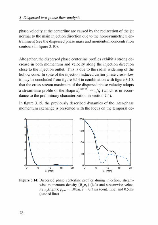
3 Dispersed two-phase flow analysis
phase velocity at the centerline are caused by the redirection of the jetnormal to the main injection direction due to the non-symmetrical en-trainment (see the dispersed phase mass and momentum concentrationcontours in figure 3.10).
Altogether, the dispersed phase centerline profiles exhibit a strong de-crease in both momentum and velocity along the injection directionclose to the injection outlet. This is due to the radial widening of thehollow cone. In spite of the injection induced carrier phase cross-flowit may be concluded from figure 3.14 in combination with figure 3.10,that the cross-stream maximum of the dispersed phase velocity adoptsa streamwise profile of the shape u(center)
p ∼ 1/ξ (which is in accor-dance to the preliminary characterization in section 2.4).
In figure 3.15, the previously described dynamics of the inter-phasemomentum exchange is presented with the focus on the temporal de-
0 6 12 18 240
1
2
3
4
5
60
ξ [mm]0 6 12 18 24
0
50
100
150
200
ξ [mm]
Figure 3.14: Dispersed phase centerline profiles during injection; stream-wise momentum density (ρ pup) (left) and streamwise veloc-ity up(right); pgas = 10bar, t = 0.3ms (cont. line) and 0.5ms(dashed line)
78
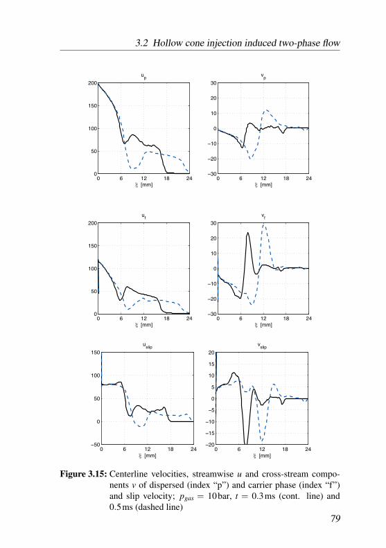
3.2 Hollow cone injection induced two-phase flow
0 6 12 18 240
50
100
150
200
up
ξ [mm]
0 6 12 18 240
50
100
150
200
uf
ξ [mm]
0 6 12 18 24−30
−20
−10
0
10
20
30
vp
ξ [mm]
0 6 12 18 24−30
−20
−10
0
10
20
30
vf
ξ [mm]
0 6 12 18 24−50
0
50
100
150
uslip
ξ [mm]0 6 12 18 24
−20
−15
−10
−5
0
5
10
15
20
vslip
ξ [mm]
Figure 3.15: Centerline velocities, streamwise u and cross-stream compo-nents v of dispersed (index “p”) and carrier phase (index “f”)and slip velocity; pgas = 10bar, t = 0.3ms (cont. line) and0.5ms (dashed line)
79
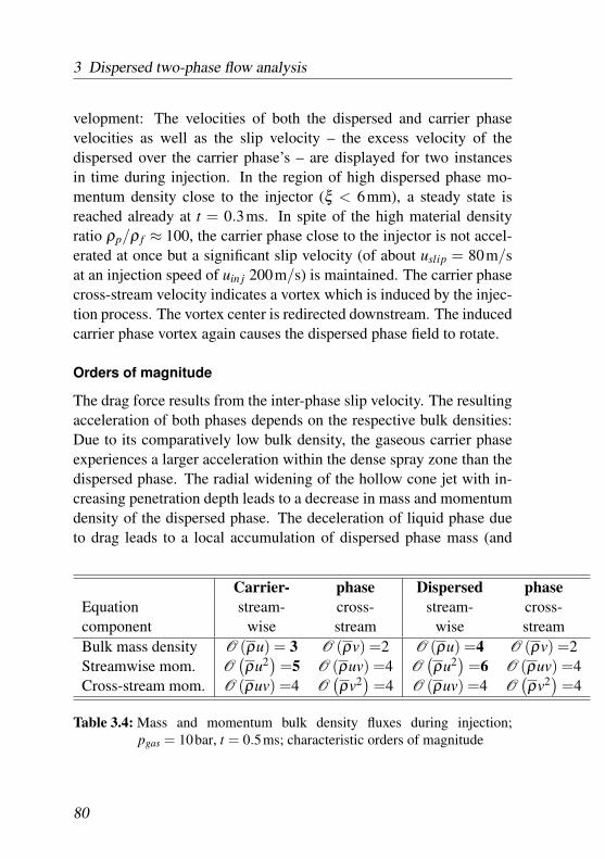
3 Dispersed two-phase flow analysis
velopment: The velocities of both the dispersed and carrier phasevelocities as well as the slip velocity – the excess velocity of thedispersed over the carrier phase’s – are displayed for two instancesin time during injection. In the region of high dispersed phase mo-mentum density close to the injector (ξ < 6mm), a steady state isreached already at t = 0.3ms. In spite of the high material densityratio ρp/ρ f ≈ 100, the carrier phase close to the injector is not accel-erated at once but a significant slip velocity (of about uslip = 80m/sat an injection speed of uin j 200m/s) is maintained. The carrier phasecross-stream velocity indicates a vortex which is induced by the injec-tion process. The vortex center is redirected downstream. The inducedcarrier phase vortex again causes the dispersed phase field to rotate.
Orders of magnitude
The drag force results from the inter-phase slip velocity. The resultingacceleration of both phases depends on the respective bulk densities:Due to its comparatively low bulk density, the gaseous carrier phaseexperiences a larger acceleration within the dense spray zone than thedispersed phase. The radial widening of the hollow cone jet with in-creasing penetration depth leads to a decrease in mass and momentumdensity of the dispersed phase. The deceleration of liquid phase dueto drag leads to a local accumulation of dispersed phase mass (and
Carrier- phase Dispersed phaseEquation stream- cross- stream- cross-component wise stream wise streamBulk mass density O (ρu) = 3 O (ρv) =2 O (ρu) =4 O (ρv) =2Streamwise mom. O
(ρu2)
=5 O (ρuv) =4 O(ρu2)
=6 O (ρuv) =4Cross-stream mom. O (ρuv) =4 O
(ρv2)
=4 O (ρuv) =4 O(ρv2)
=4
Table 3.4: Mass and momentum bulk density fluxes during injection;pgas = 10bar, t = 0.5ms; characteristic orders of magnitude
80
3.2 Hollow cone injection induced two-phase flow
thus momentum) and thereby compensates the rarefaction due to theradial widening: Even though spatially dispersed, the bulk momentumdensity of the liquid droplets within the dense spray zone is one orderof magnitude higher than the carrier phase (bulk) density during theforcing period (i.e. while injection proceeds, see table 3.4).Also in preparation of the derivation of a simplified model for the hol-low cone penetration behavior it is helpful to compare fluxes occuringin the individual conservation equations of mass and momentum withrespect to their orders of magnitude. The overview over the fluxes ofmass and momentum equations is given in table 3.4. The comparisonreflects the dominance of the streamwise over the cross-stream com-ponents and among them the dispersed phase over the carrier phasefluxes: For example in the carrier phase streamwise momentum equa-tion, the streamwise component (O
(ρu2)
= 5) dominates the cross-stream component (O (ρuv) = 4).By contrast, the fluxes of cross-stream momentum (last row in ta-ble 3.4) are of the same order of magnitude for both phases and bothcomponents.The contributions of the gradients of the fluxes within the individualconservation equations are contrasted in section 3.2.5.
3.2.4 Carrier phase transport
The injection of dispersed liquid into a gas pressure chamber consti-tutes a spatially distributed source of momentum to the carrier phasegas. Comparing the carrier phase velocity (figure 3.12) with its cor-responding momentum distribution (figure 3.16) reveals that with re-gards to the carrier phase, compressibility effects – both due to com-pression of the carrier phase itself as well as due to bulk effects (carrierphase mass rarefaction resulting from increased dispersed phase massconcentration) – play a minor role in the present flow configuration.
81
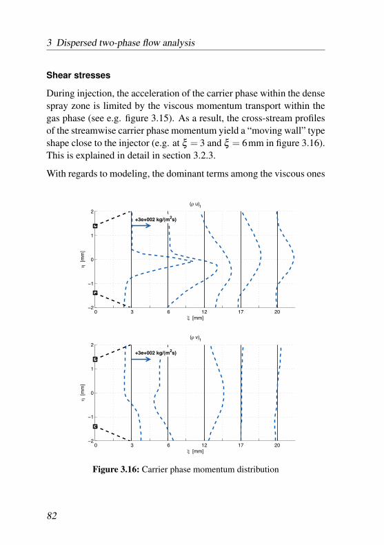
3 Dispersed two-phase flow analysis
Shear stresses
During injection, the acceleration of the carrier phase within the densespray zone is limited by the viscous momentum transport within thegas phase (see e.g. figure 3.15). As a result, the cross-stream profilesof the streamwise carrier phase momentum yield a “moving wall” typeshape close to the injector (e.g. at ξ = 3 and ξ = 6mm in figure 3.16).This is explained in detail in section 3.2.3.
With regards to modeling, the dominant terms among the viscous ones
0 3 6 12 17 20−2
−1
0
1
2
(ρ u)f
+3e+002 kg/(m2s)
ξ [mm]
η [
mm
]
0 3 6 12 17 20−2
−1
0
1
2
(ρ v)f
+3e+002 kg/(m2s)
ξ [mm]
η [
mm
]
Figure 3.16: Carrier phase momentum distribution
82
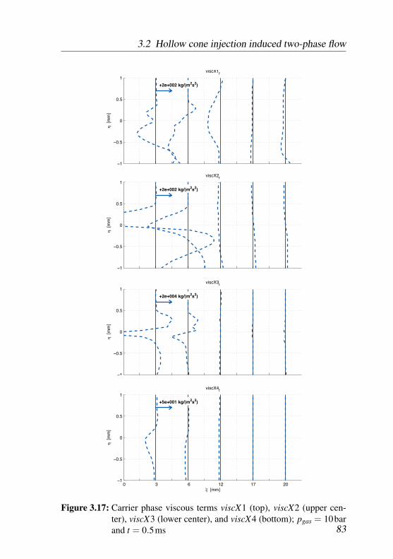
3.2 Hollow cone injection induced two-phase flow
−1
−0.5
0
0.5
1
viscX1f
+2e+002 kg/(m2s2)
η [
mm
]
−1
−0.5
0
0.5
1
viscX2f
+2e+002 kg/(m2s2)
η [
mm
]
−1
−0.5
0
0.5
1
viscX3f
+2e+004 kg/(m2s2)
η [
mm
]
0 3 6 12 17 20−1
−0.5
0
0.5
1
viscX4f
+5e+001 kg/(m2s2)
ξ [mm]
η [
mm
]
Figure 3.17: Carrier phase viscous terms viscX1 (top), viscX2 (upper cen-ter), viscX3 (lower center), and viscX4 (bottom); pgas = 10barand t = 0.5ms 83
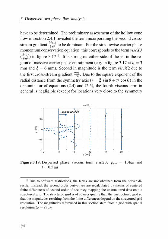
3 Dispersed two-phase flow analysis
have to be determined. The preliminary assessment of the hollow coneflow in section 2.4.1 revealed the term incorporating the second cross-stream gradient ∂ 2(∗)
∂η2 to be dominant. For the streamwise carrier phasemomentum conservation equation, this corresponds to the term viscX3( ∂ 2u f
∂η2 ) in figure 3.17 ‖. It is strong on either side of the jet in the re-gion of massive carrier phase entrainment (e.g. in figure 3.17 at ξ = 3mm and ξ = 6 mm). Second in magnitude is the term viscX2 due tothe first cross-stream gradient ∂u f
∂η . Due to the square exponent of theradial distance from the symmetry axis (r = ξ sinθ +η cosθ ) in thedenominator of equations (2.4) and (2.5), the fourth viscous term ingeneral is negligible (except for locations very close to the symmetry
0 3 6 12 17 20−1
−0.5
0
0.5
1
viscX3p
+5e+006 kg/(m2s2)
ξ [mm]
η [
mm
]
Figure 3.18: Dispersed phase viscous term viscX3; pgas = 10bar andt = 0.5ms
‖ Due to software restrictions, the terms are not obtained from the solver di-rectly. Instead, the second order derivatives are recalculated by means of centeredfinite differences of second order of accuracy mapping the unstructured data onto astructured grid. The structured grid is of coarser quality than the unstructured grid sothat the magnitudes resulting from the finite differences depend on the structured gridresolution. The magnitudes referenced in this section stem from a grid with spatialresolution ∆x = 83µm.
84
3.2 Hollow cone injection induced two-phase flow
axis).In the context of the Eulerian continuum representation, a viscous mo-mentum diffusion is assigned also to the dispersed phase. For the car-rier phase state referred to in figure 3.17 (p = 10 bar, t = 0.5 ms), pro-files of the the third viscous term of the dispersed phase are presentedin figure 3.18 in order to illustrate the volume affected by the dispersedphase shear force during the injection process. The viscous terms ofthe dispersed phase are larger in magnitude than those of the carrierphase, but their profiles exhibit a more narrow cross-stream width.
85
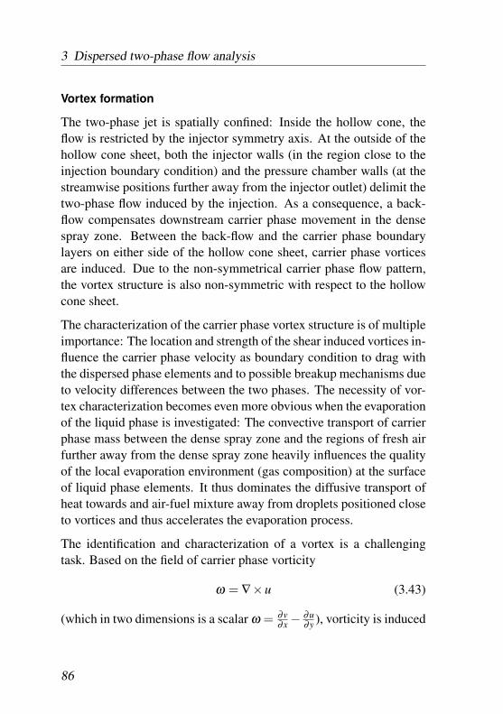
3 Dispersed two-phase flow analysis
Vortex formation
The two-phase jet is spatially confined: Inside the hollow cone, theflow is restricted by the injector symmetry axis. At the outside of thehollow cone sheet, both the injector walls (in the region close to theinjection boundary condition) and the pressure chamber walls (at thestreamwise positions further away from the injector outlet) delimit thetwo-phase flow induced by the injection. As a consequence, a back-flow compensates downstream carrier phase movement in the densespray zone. Between the back-flow and the carrier phase boundarylayers on either side of the hollow cone sheet, carrier phase vorticesare induced. Due to the non-symmetrical carrier phase flow pattern,the vortex structure is also non-symmetric with respect to the hollowcone sheet.
The characterization of the carrier phase vortex structure is of multipleimportance: The location and strength of the shear induced vortices in-fluence the carrier phase velocity as boundary condition to drag withthe dispersed phase elements and to possible breakup mechanisms dueto velocity differences between the two phases. The necessity of vor-tex characterization becomes even more obvious when the evaporationof the liquid phase is investigated: The convective transport of carrierphase mass between the dense spray zone and the regions of fresh airfurther away from the dense spray zone heavily influences the qualityof the local evaporation environment (gas composition) at the surfaceof liquid phase elements. It thus dominates the diffusive transport ofheat towards and air-fuel mixture away from droplets positioned closeto vortices and thus accelerates the evaporation process.
The identification and characterization of a vortex is a challengingtask. Based on the field of carrier phase vorticity
ω = ∇×u (3.43)
(which in two dimensions is a scalar ω = ∂v∂x − ∂u
∂y ), vorticity is induced
86
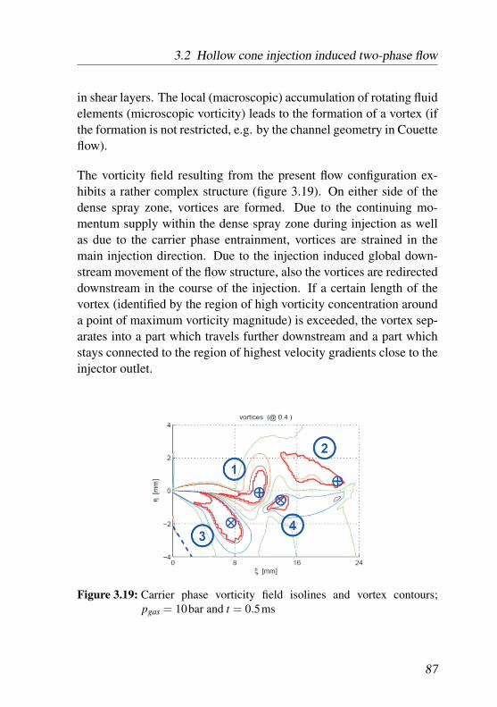
3.2 Hollow cone injection induced two-phase flow
in shear layers. The local (macroscopic) accumulation of rotating fluidelements (microscopic vorticity) leads to the formation of a vortex (ifthe formation is not restricted, e.g. by the channel geometry in Couetteflow).
The vorticity field resulting from the present flow configuration ex-hibits a rather complex structure (figure 3.19). On either side of thedense spray zone, vortices are formed. Due to the continuing mo-mentum supply within the dense spray zone during injection as wellas due to the carrier phase entrainment, vortices are strained in themain injection direction. Due to the injection induced global down-stream movement of the flow structure, also the vortices are redirecteddownstream in the course of the injection. If a certain length of thevortex (identified by the region of high vorticity concentration arounda point of maximum vorticity magnitude) is exceeded, the vortex sep-arates into a part which travels further downstream and a part whichstays connected to the region of highest velocity gradients close to theinjector outlet.
Figure 3.19: Carrier phase vorticity field isolines and vortex contours;pgas = 10bar and t = 0.5ms
87
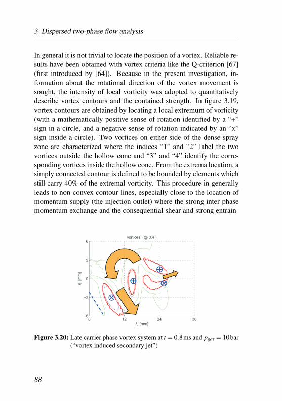
3 Dispersed two-phase flow analysis
In general it is not trivial to locate the position of a vortex. Reliable re-sults have been obtained with vortex criteria like the Q-criterion [67](first introduced by [64]). Because in the present investigation, in-formation about the rotational direction of the vortex movement issought, the intensity of local vorticity was adopted to quantitativelydescribe vortex contours and the contained strength. In figure 3.19,vortex contours are obtained by locating a local extremum of vorticity(with a mathematically positive sense of rotation identified by a “+”sign in a circle, and a negative sense of rotation indicated by an “x”sign inside a circle). Two vortices on either side of the dense sprayzone are characterized where the indices “1” and “2” label the twovortices outside the hollow cone and “3” and “4” identify the corre-sponding vortices inside the hollow cone. From the extrema location, asimply connected contour is defined to be bounded by elements whichstill carry 40% of the extremal vorticity. This procedure in generallyleads to non-convex contour lines, especially close to the location ofmomentum supply (the injection outlet) where the strong inter-phasemomentum exchange and the consequential shear and strong entrain-
Figure 3.20: Late carrier phase vortex system at t = 0.8ms and pgas = 10bar(“vortex induced secondary jet”)
88
3.2 Hollow cone injection induced two-phase flow
ing mass flux prevent the vortex fluid elements from rearranging in themost compact form, namely a circular cross-section, corresponding toa torus shape.
An elaborate characterization of the vortex system induced by the hol-low cone injection has been conducted. The investigation reveals thatthe vortex at the outside of the hollow cone at the downstream position(number “2” in figure 3.19) exhibits the greatest cross-section. It ac-quires a greater amount of rotational energy from the injection carrierphase flow in the streamwise direction during injection than the othervortices.
After end of injection, the total flow is dominated by the energy con-tained in this vortex: Its (in figure 3.19 counter-clockwise) sense ofrotation causes vortex “1” to move in between the vortex pair originat-ing from the inside of the hollow cone (figure 3.20). Each of the twoinduced vortex pairs causes an ejection of material present betweeneach pair: A smaller ejection flow is caused in the original injectiondirection while a stronger ejection flow is induced in the direction par-allel to the injector axis. The later explains why in comparatively coldconditions (limited evaporation), a cloud of liquid droplets is ejectedfrom the inside of the hollow cone along the injector axis shortly afterend of injection.
3.2.5 Temporal evolution
In the previous two sections, the mechanism of momentum transferfrom the injected to the carrier phase as well as the induced carrierphase boundary layer and resulting vortex system was discussed. Ina simplified but fast model, as it is aimed for in this work (section 4),details of the three-dimensional formulation need to be dropped sothat dominant effects (manifesting in dominant conservation equationterms) may be identified.
89
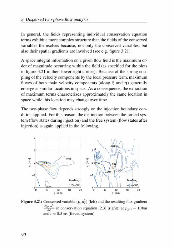
3 Dispersed two-phase flow analysis
In general, the fields representing individual conservation equationterms exhibit a more complex structure than the fields of the conservedvariables themselves because, not only the conserved variables, butalso their spatial gradients are involved (see e.g. figure 3.21).
A space integral information on a given flow field is the maximum or-der of magnitude occurring within the field (as specified for the plotsin figure 3.21 in their lower right corner). Because of the strong cou-pling of the velocity components by the local pressure term, maximumfluxes of both main velocity components (along ξ and η) generallyemerge at similar locations in space. As a consequence, the extractionof maximum terms characterizes approximately the same location inspace while this location may change over time.
The two-phase flow depends strongly on the injection boundary con-dition applied. For this reason, the distinction between the forced sys-tem (flow states during injection) and the free system (flow states afterinjection) is again applied in the following.
0 6 12 18 24−4
−2
0
2
4
ξ [mm]
η [
mm
]
0.4
0.05
0.05
MaxMag
1.2e+005
0 6 12 18 24−4
−2
0
2
ξ [mm]
η [
mm
]
5
0.05
04
−0.004 −0.004
004
−0.004
MaxMag
4.1e+008
Figure 3.21: Conserved variable (ρcu2c) (left) and the resulting flux gradient
∂ (ρcu2c)
∂ξ in conservation equation (2.3) (right); at pgas = 10barand t = 0.5ms (forced system)
90
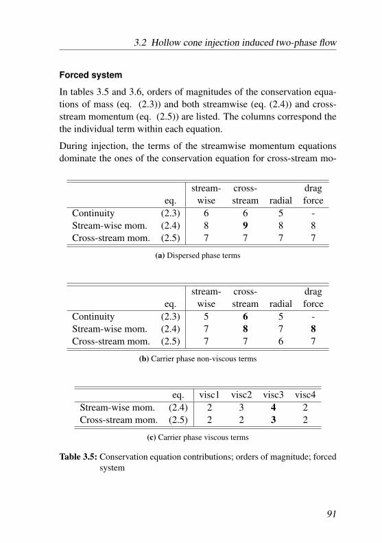
3.2 Hollow cone injection induced two-phase flow
Forced system
In tables 3.5 and 3.6, orders of magnitudes of the conservation equa-tions of mass (eq. (2.3)) and both streamwise (eq. (2.4)) and cross-stream momentum (eq. (2.5)) are listed. The columns correspond thethe individual term within each equation.
During injection, the terms of the streamwise momentum equationsdominate the ones of the conservation equation for cross-stream mo-
stream- cross- drageq. wise stream radial force
Continuity (2.3) 6 6 5 -Stream-wise mom. (2.4) 8 9 8 8Cross-stream mom. (2.5) 7 7 7 7
(a) Dispersed phase terms
stream- cross- drageq. wise stream radial force
Continuity (2.3) 5 6 5 -Stream-wise mom. (2.4) 7 8 7 8Cross-stream mom. (2.5) 7 7 6 7
(b) Carrier phase non-viscous terms
eq. visc1 visc2 visc3 visc4Stream-wise mom. (2.4) 2 3 4 2Cross-stream mom. (2.5) 2 2 3 2
(c) Carrier phase viscous terms
Table 3.5: Conservation equation contributions; orders of magnitude; forcedsystem
91
3 Dispersed two-phase flow analysis
mentum. This applies to both phases and corresponds to the momen-tum fluxes listed earlier (see table 3.4).
The terms contributing to the streamwise momentum conservation ofdispersed phase are of comparable orders of magnitude. Only thecross-stream flux is slightly increased because within the term
∂ (ρ p up vp)∂η ,
the dispersed phase volume fraction cross-stream gradient ∂αp∂η is large.
For the carrier phase streamwise momentum equation, the cross-streamterm (i.e. the term containing the cross-stream gradient) dominateswhich supports the preliminary investigation in section 2.4.1.The dominance of the cross-stream gradients in carrier phase conser-vation equations of both streamwise momentum and continuity re-flects the effect of excess entrainment which is induced by drag withthe dispersed phase: The drag force and the cross-stream gradient inthe streamwise carrier phase momentum equation are of the same or-der.
During the total of the injection period, the terms accounting for theradial widening of the two-phase jet are non-negligible but about oneorder of magnitude smaller than the streamwise and cross-stream con-tributions.
Due to the large cross-stream gradients appearing in the streamwisemomentum equation, a strong shear force is induced. Unfortunately,the solver does not provide direct access to the second order spa-tial gradient of each velocity component in the result files, so thatit is calculated in a post-processing step. For this reason, the veloc-ity components are first projected onto a equidistant mesh which iscoarser than the computational mesh on which CFD results are avail-able (∆x = 83µm). In a second step, the second spatial gradient (offirst order of accuracy) is calculated and the viscous terms are com-posed. Note that because of the projection procedure, the orders ofmagnitude obtained for the viscous terms (table 3.22c) are only com-parable among themselves but not to the fluxes presented above.
92
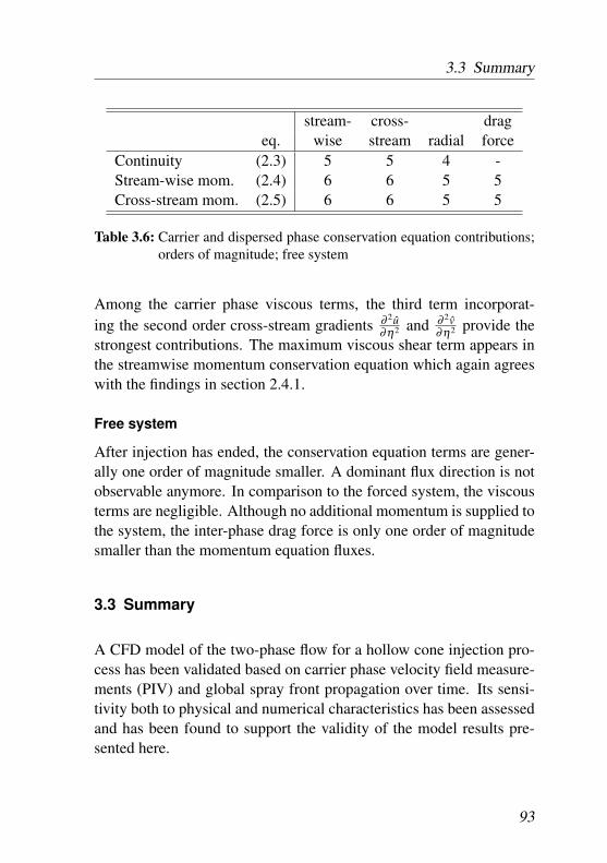
3.3 Summary
stream- cross- drageq. wise stream radial force
Continuity (2.3) 5 5 4 -Stream-wise mom. (2.4) 6 6 5 5Cross-stream mom. (2.5) 6 6 5 5
Table 3.6: Carrier and dispersed phase conservation equation contributions;orders of magnitude; free system
Among the carrier phase viscous terms, the third term incorporat-ing the second order cross-stream gradients ∂ 2u
∂η2 and ∂ 2v∂η2 provide the
strongest contributions. The maximum viscous shear term appears inthe streamwise momentum conservation equation which again agreeswith the findings in section 2.4.1.
Free system
After injection has ended, the conservation equation terms are gener-ally one order of magnitude smaller. A dominant flux direction is notobservable anymore. In comparison to the forced system, the viscousterms are negligible. Although no additional momentum is supplied tothe system, the inter-phase drag force is only one order of magnitudesmaller than the momentum equation fluxes.
3.3 Summary
A CFD model of the two-phase flow for a hollow cone injection pro-cess has been validated based on carrier phase velocity field measure-ments (PIV) and global spray front propagation over time. Its sensi-tivity both to physical and numerical characteristics has been assessedand has been found to support the validity of the model results pre-sented here.
93
3 Dispersed two-phase flow analysis
The effect of spatially distributed acceleration of gas phase due to theinjection of liquid fuel has been studied. The inter-phase momentumexchange due to the injection of a dispersed liquid phase into a gaseouscarrier phase exhibits fundamentally different dynamics than a singlephase jet in the region close to the injection boundary condition. Inthe dense spray zones, the injected liquid causes a strong accelera-tion of carrier phase mass. The streamwise acceleration of gas locallycauses additional (“excess”) entrainment in regions of high momen-tum fluxes within the dispersed phase, i.e. close to the injection outlet.The later causes the width of the local boundary layer thickness to de-crease thereby increasing momentum diffusion normal to the injectiondirection. The induced boundary layer in the carrier phase counteractsthe acceleration due to drag so that considerable magnitudes of slipvelocity are maintained within the flow domain.
A secondary carrier phase flow pattern is induced by the injection.Due to the hollow cone geometry, it is not symmetric with respectto the hollow cone sheet. It causes a redirection of the dispersedphase normal to the main injection direction and thereby induces anon-symmetric vortex system around the liquid sheet.
During injection, two main region are observed within the dispersedphase: Near the injection outlet, the flow is in steady state conditions.The spray front, by contrast, is influenced by the secondary flow pat-tern within the carrier phase.
In order to support the modeling steps taken in the following sec-tion, the maximum occurring orders of magnitude corresponding tothe field of the conservation equation terms were analyzed. The termsof the streamwise momentum equation dominate those of the cross-stream momentum equation. Among the convective and the viscousfluxes within the streamwise momentum equations, the cross-streamcomponents are larger in magnitude than the streamwise terms forboth phases.
94
4 Integral modeling
In this section, major features of the hollow cone two-phase jet elu-cidated in the previous sections are exploited for modeling purposes.The main targets and essential properties of the proposed model areshortly outlined in section 4.1. The main results are presented in twosections: Section 4.2 introduces the concept of a cross-stream lengthscale, which characterizes the boundary layer of the dense two-phaseflow. Section 4.3 contains the modeling of the inter-phase momen-tum exchange and defines proper boundary conditions (section 4.3.5).The boundary layer concept is applied to evaporation in section 4.4.A simple turbulence model is applied in section 4.5. The model issummarized in section 4.6.
4.1 Spray model motivation and outline
Target definition
The main intention of the simplified spray model developed in thefollowing is to provide an estimate of the local dispersed phase massconcentration and the gas phase air fuel mixture quality resulting fromevaporation. Based on the validated CFD model results (section 3.2)and especially inspired by the characteristics obtained from cross-stream averaging (section 4.2), the model is designed to meet threemajor characteristics:
• Spatial changes are resolved along the main injection direction.For this reason, a one-dimensional description is sought.
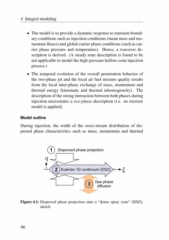
4 Integral modeling
• The model is to provide a dynamic response to transient bound-ary conditions such as injection conditions (mean mass and mo-mentum fluxes) and global carrier phase conditions (such as car-rier phase pressure and temperature). Hence, a transient de-scription is derived. (A steady state description is found to benot applicable to model the high-pressure hollow-cone injectionprocess.)
• The temporal evolution of the overall penetration behavior ofthe two-phase jet and the local air fuel mixture quality resultsfrom the local inter-phase exchange of mass, momentum andthermal energy (kinematic and thermal inhomogeneity). Thedescription of the strong interaction between both phases duringinjection necessitates a two-phase description (i.e. no mixturemodel is applied).
Model outline
During injection, the width of the cross-stream distribution of dis-persed phase characteristics such as mass, momentum and thermal
� ������������������� ����
�������������������� ���������������
�������
���������
Figure 4.1: Dispersed phase projection onto a “dense spray zone” (DSZ);sketch
96
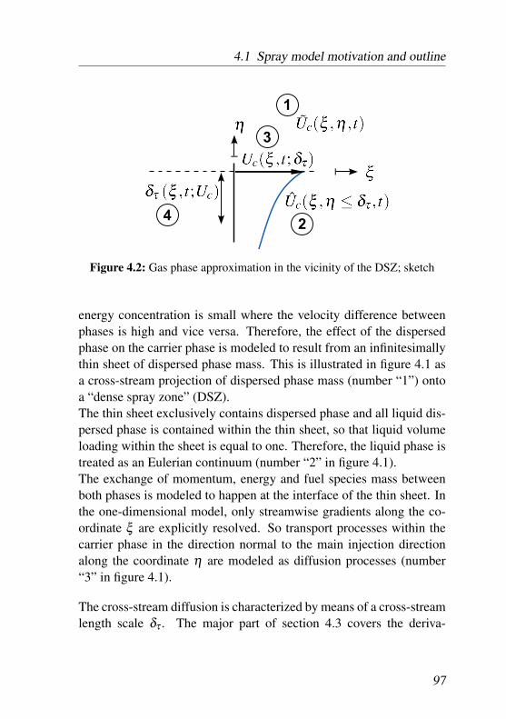
4.1 Spray model motivation and outline
�
��
�
Figure 4.2: Gas phase approximation in the vicinity of the DSZ; sketch
energy concentration is small where the velocity difference betweenphases is high and vice versa. Therefore, the effect of the dispersedphase on the carrier phase is modeled to result from an infinitesimallythin sheet of dispersed phase mass. This is illustrated in figure 4.1 asa cross-stream projection of dispersed phase mass (number “1”) ontoa “dense spray zone” (DSZ).The thin sheet exclusively contains dispersed phase and all liquid dis-persed phase is contained within the thin sheet, so that liquid volumeloading within the sheet is equal to one. Therefore, the liquid phase istreated as an Eulerian continuum (number “2” in figure 4.1).The exchange of momentum, energy and fuel species mass betweenboth phases is modeled to happen at the interface of the thin sheet. Inthe one-dimensional model, only streamwise gradients along the co-ordinate ξ are explicitly resolved. So transport processes within thecarrier phase in the direction normal to the main injection directionalong the coordinate η are modeled as diffusion processes (number“3” in figure 4.1).
The cross-stream diffusion is characterized by means of a cross-streamlength scale δτ . The major part of section 4.3 covers the deriva-
97
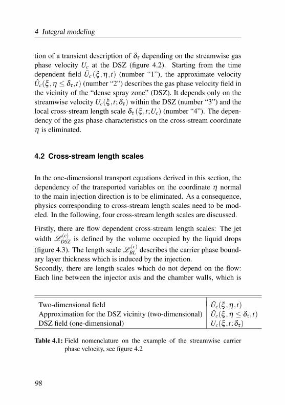
4 Integral modeling
tion of a transient description of δτ depending on the streamwise gasphase velocity Uc at the DSZ (figure 4.2). Starting from the timedependent field Uc (ξ ,η , t) (number “1”), the approximate velocityUc(ξ ,η ≤ δτ , t) (number “2”) describes the gas phase velocity field inthe vicinity of the “dense spray zone” (DSZ). It depends only on thestreamwise velocity Uc(ξ , t;δτ) within the DSZ (number “3”) and thelocal cross-stream length scale δτ (ξ , t;Uc) (number “4”). The depen-dency of the gas phase characteristics on the cross-stream coordinateη is eliminated.
4.2 Cross-stream length scales
In the one-dimensional transport equations derived in this section, thedependency of the transported variables on the coordinate η normalto the main injection direction is to be eliminated. As a consequence,physics corresponding to cross-stream length scales need to be mod-eled. In the following, four cross-stream length scales are discussed.
Firstly, there are flow dependent cross-stream length scales: The jetwidth L
(c)DSZ is defined by the volume occupied by the liquid drops
(figure 4.3). The length scale L(c)
BL describes the carrier phase bound-ary layer thickness which is induced by the injection.Secondly, there are length scales which do not depend on the flow:Each line between the injector axis and the chamber walls, which is
Two-dimensional field Uc(ξ ,η , t)Approximation for the DSZ vicinity (two-dimensional) Uc(ξ ,η ≤ δτ , t)DSZ field (one-dimensional) Uc(ξ , t;δτ)
Table 4.1: Field nomenclature on the example of the streamwise carrierphase velocity, see figure 4.2
98
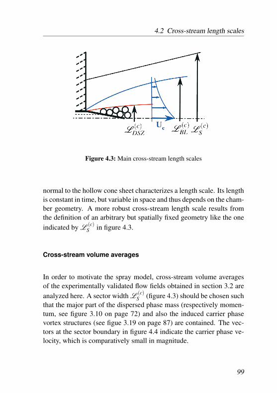
4.2 Cross-stream length scales
Figure 4.3: Main cross-stream length scales
normal to the hollow cone sheet characterizes a length scale. Its lengthis constant in time, but variable in space and thus depends on the cham-ber geometry. A more robust cross-stream length scale results fromthe definition of an arbitrary but spatially fixed geometry like the oneindicated by L
(c)S in figure 4.3.
Cross-stream volume averages
In order to motivate the spray model, cross-stream volume averagesof the experimentally validated flow fields obtained in section 3.2 areanalyzed here. A sector width L
(c)S (figure 4.3) should be chosen such
that the major part of the dispersed phase mass (respectively momen-tum, see figure 3.10 on page 72) and also the induced carrier phasevortex structures (see figue 3.19 on page 87) are contained. The vec-tors at the sector boundary in figure 4.4 indicate the carrier phase ve-locity, which is comparatively small in magnitude.
99
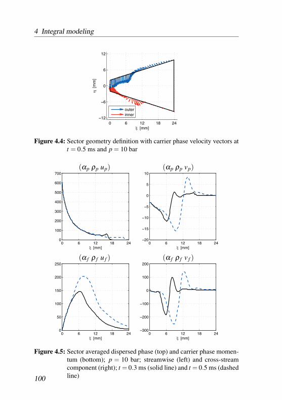
4 Integral modeling
0 6 12 18 24−12
−6
0
6
12
ξ [mm]
η [
mm
]
outerinner
Figure 4.4: Sector geometry definition with carrier phase velocity vectors att = 0.5 ms and p = 10 bar
(αp ρp up) (αp ρp vp)
0 6 12 18 240
100
200
300
400
500
600
700
ξ [mm]0 6 12 18 24
−20
−15
−10
−5
0
5
10
ξ [mm]
(α f ρ f u f ) (α f ρ f v f )
0 6 12 18 240
50
100
150
200
250
ξ [mm]0 6 12 18 24
−300
−200
−100
0
100
200
ξ [mm]
Figure 4.5: Sector averaged dispersed phase (top) and carrier phase momen-tum (bottom); p = 10 bar; streamwise (left) and cross-streamcomponent (right); t = 0.3 ms (solid line) and t = 0.5 ms (dashedline)100
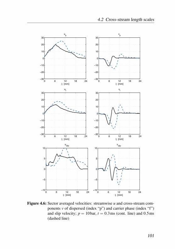
4.2 Cross-stream length scales
0 6 12 18 24−30
−20
−10
0
10
20
30
up
ξ [mm]0 6 12 18 24
−30
−20
−10
0
10
20
30
vp
ξ [mm]
0 6 12 18 24−30
−20
−10
0
10
20
30
uf
ξ [mm]0 6 12 18 24
−30
−20
−10
0
10
20
30
vf
ξ [mm]
0 6 12 18 24−10
−5
0
5
10
uslip
ξ [mm]0 6 12 18 24
−10
−5
0
5
10
vslip
ξ [mm]
Figure 4.6: Sector averaged velocities: streamwise u and cross-stream com-ponents v of dispersed (index “p”) and carrier phase (index “f”)and slip velocity; p = 10bar, t = 0.3ms (cont. line) and 0.5ms(dashed line)
101
4 Integral modeling
The volume average
Φ =∫
Φ dV/ ∫
dV (4.1)
of quantity Φ is calculated based on cross-stream volume averagingover the sector geometry.
The mean dispersed phase streamwise momentum (Φ = αpρpup) islarge close to the injection outlet and almost constant in time duringinjection (figure 4.5). The cross-stream component (Φ = αpρpvp) isorders of magnitude smaller. This evaluation supports the assumptionof the dominance of the injection direction introduced earlier.Despite of the density ratio ρp/ρ f ≈ 100 � 1, the mean streamwisemomentum of the gas phase within the sector acquires larger valuesthan the liquid droplets. This reflects the observation of L
(c)DSZ �L
(c)BL .
The mean velocities of both phases as well as the slip velocity vslip =vp − v f are displayed in figure 4.6. Maximum mean streamwise ve-locities are of the order of 20 m/s with corresponding slip velocitiesof about 5 m/s.
Between the two time steps considered in figure 4.6, a steady statefor the sector volume averaged quantities is reached by the dispersedphase for ξ < 6mm and by the carrier phase for ξ < 4mm at t = 0.3ms.Since at this instant in time, the dispersed phase penetration depth isapproximately ξ = 17mm (figure 4.5), the major streamwise portionof the flow is in transient conditions.
Although L(c)
S represents a larger length scale than the liquid sheetscale L
(c)DSZ and even the gas phase boundary layer width L
(c)BL , no in-
variants may be deduced from the volume averaged momentum fluxesor velocities. Thus it is not feasible to base the one-dimensional modelon averaging over a large sector.
102
4.3 Momentum conservation
4.3 Momentum conservation
The primary physical effect controlling the injection process is themomentum exchange; it determines the propagation of the spray front.Momentum is supplied to the system by the injection of liquid massthrough the injector outlet. Within the flow domain, the liquid phaseexhibits a slip velocity with regards to the carrier phase. Therefore,momentum is exchanged between both phases.A locally high slip velocity (and the corresponding inter-phase mo-mentum exchange) experiences changes with respect to:
• time (especially during injection) and
• space (especially close to the injection outlet).
The appropriate modeling of these flow conditions is the basis for theflow evolution in regions further away from the injection outlet and attimes after injection.
A presumed spray center line is identified as the primary direction ofmomentum exchange ∗: Due to the injector mounting position andgeometry – namely the angle θ between injector axis and the pre-sumed spray symmetry line (see figure 3.2.1 on page 61) – , the direc-tion of the dispersed phase mass and momentum flux dominates theflow structure in the region close to the injector exit (dominance ofthe cone geometry). The injector is assumed to provide a rotationallyperfectly symmetrical spray, so that circumferential gradients may beneglected. In order to account for changes along the dominant flowdirection while neglecting gradients both normal to the main injectiondirection and along the circumferential direction, a one-dimensionaldescription is sought.
∗This is also supported by the dominance of the streamwise drag force magnitudeacting along the main injection direction, see figure 3.13 on page 76
103
4 Integral modeling
4.3.1 Dispersed phase and dense spray zone
This section covers the modeling of the dispersed phase. The shapeof its cross-stream distribution as well as the region where momentumis exchanged with the carrier phase are specified. Space-integral con-servation equations for the dispersed phase mass and momentum arepresented.
Thin dense spray zone (DSZ)
The dispersed phase is modeled to occupy a smaller volume than thecarrier phase. At any streamwise location ξ , the cross-stream charac-teristic length scale L
(c)DSZ of the volume occupied by the major part
of the dispersed phase is smaller than the characteristic length scale ofthe carrier phase shear boundary layer L
(c)BL (figures 4.3 and 4.7).
Therefore with regards to the carrier phase, the DSZ is modeled toyield a zero cross-stream width (L (c)
DSZ = 0), i.e. the DSZ carries nocarrier phase mass (α(DSZ)
p = 1).
Due to streamwise velocity gradients within the DSZ, dispersed phasemass may locally accumulate. Streamwise accumulation of dispersedphase mass is accounted for by the dispersed phase continuity equation(see eq. (2.3)). In a finite volume approach, the transport of dispersedphase bulk density ρ p is described by
∂ρ p
∂ t+
∂ (ρ p up)∂ξ
+ρ pup sinθ + vp cosθξ sinθ +η cosθ
= Γp . (4.2)
The dependency on the cross-stream coordinate η in equation (4.2)has been eliminated by means of a modeling step: With regards to thecarrier phase, dispersed phase mass is projected onto the presumedhollow cone sheet (see the assumption of a “thin dense spray zone”above). Mathematically, the projection corresponds to a spatial inte-gration with respect to the cross-stream coordinate η . Within the DSZ,
104
4.3 Momentum conservation
the (projected) dispersed phase mass
Mp(ξ ) ≡∞∫
η=−ξ/tanθ
ρ p(ξ , η) dη
/L (4.3)
is transported. The lower bound of the integral results from the in-jector symmetry axis so that in the case of θ → π/2 (a hollow-coneopening angle of 180◦), η → −∞. Additionally, both the upper andlower bounds may be restricted by the chamber geometry. The lengthscale L in the denominator of equation (4.3) ensures that formally,a volume specific formulation may be maintained when covering forthe carrier phase† so that the projected dispersed phase mass concen-tration Mp still yields units kg/m3. The length scale L is assumed tobe constant in time and space.Due to the dominance of the streamwise dispersed phase flow dur-ing injection, the maximum streamwise velocity of the cross-streamprofiles Up(η) occurs at the presumed spray center line. As a con-sequence from the strong streamwise velocity component, the cross-stream velocity Vp = 0 at the presumed spray center line η = 0.The cross-stream integrated conservation equation of the dispersedphase mass Mp (units kg/m3) therefore reads
∂Mp
∂ t+
∂ (Mp Up)∂ξ
+Mp Up
ξ= Γp . (4.4)
Inter-phase momentum exchange
Inter-phase momentum exchange is modelled to occur at the interfaceof the DSZ.
† Note that in equation (4.3), division by the length integral∫
dη instead ofthe length scale L produces a cross-stream average of the dispersed phase massdistribution. This is not aimed for in the modeling of the dense hollow cone sheetspray.
105
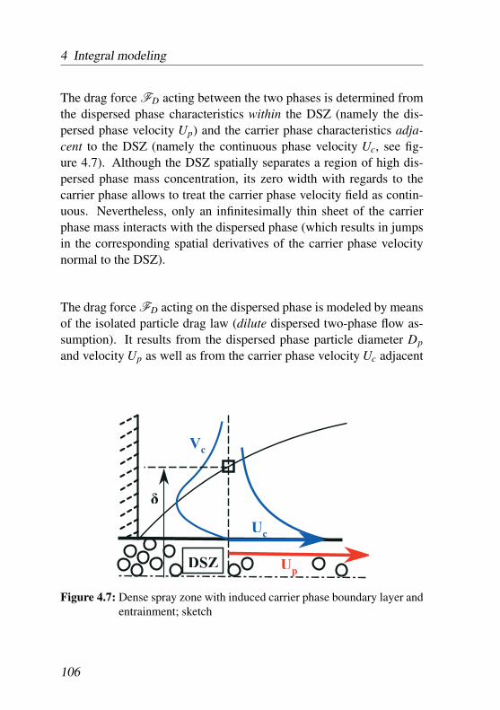
4 Integral modeling
The drag force FD acting between the two phases is determined fromthe dispersed phase characteristics within the DSZ (namely the dis-persed phase velocity Up) and the carrier phase characteristics adja-cent to the DSZ (namely the continuous phase velocity Uc, see fig-ure 4.7). Although the DSZ spatially separates a region of high dis-persed phase mass concentration, its zero width with regards to thecarrier phase allows to treat the carrier phase velocity field as contin-uous. Nevertheless, only an infinitesimally thin sheet of the carrierphase mass interacts with the dispersed phase (which results in jumpsin the corresponding spatial derivatives of the carrier phase velocitynormal to the DSZ).
The drag force FD acting on the dispersed phase is modeled by meansof the isolated particle drag law (dilute dispersed two-phase flow as-sumption). It results from the dispersed phase particle diameter Dp
and velocity Up as well as from the carrier phase velocity Uc adjacent
Figure 4.7: Dense spray zone with induced carrier phase boundary layer andentrainment; sketch
106
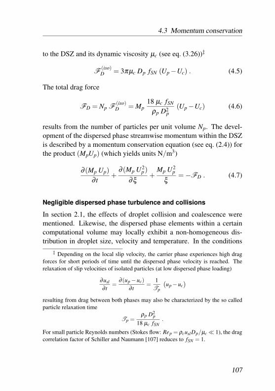
4.3 Momentum conservation
to the DSZ and its dynamic viscosity µc (see eq. (3.26))‡
F(iso)D = 3πµc Dp fSN (Up −Uc) . (4.5)
The total drag force
FD = Np F(iso)D = Mp
18 µc fSN
ρp D2p
(Up −Uc) (4.6)
results from the number of particles per unit volume Np. The devel-opment of the dispersed phase streamwise momentum within the DSZis described by a momentum conservation equation (see eq. (2.4)) forthe product (MpUp) (which yields units N/m3)
∂ (Mp Up)∂ t
+∂ (Mp U2
p)∂ξ
+Mp U2
p
ξ= −FD . (4.7)
Negligible dispersed phase turbulence and collisions
In section 2.1, the effects of droplet collision and coalescence werementioned. Likewise, the dispersed phase elements within a certaincomputational volume may locally exhibit a non-homogeneous dis-tribution in droplet size, velocity and temperature. In the conditions
‡ Depending on the local slip velocity, the carrier phase experiences high dragforces for short periods of time until the dispersed phase velocity is reached. Therelaxation of slip velocities of isolated particles (at low dispersed phase loading)
∂usl
∂ t=
∂ (up −uc)∂ t
=1
Tp
(up −uc
)resulting from drag between both phases may also be characterized by the so calledparticle relaxation time
Tp =ρp D2
p
18 µc fSN.
For small particle Reynolds numbers (Stokes flow: Rep = ρcuslDp/µc � 1), the dragcorrelation factor of Schiller and Naumann [107] reduces to fSN = 1.
107
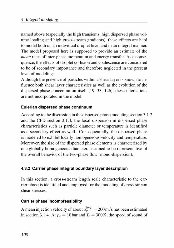
4 Integral modeling
named above (especially the high transients, high dispersed phase vol-ume loading and high cross-stream gradients), these effects are hardto model both on an individual droplet level and in an integral manner.The model proposed here is supposed to provide an estimate of themean rates of inter-phase momentum and energy transfer. As a conse-quence, the effects of droplet collision and coalescence are consideredto be of secondary importance and therefore neglected in the presentlevel of modeling.Although the presence of particles within a shear layer is known to in-fluence both shear layer characteristics as well as the evolution of thedispersed phase concentration itself [19, 33, 126], these interactionsare not incorporated in the model.
Eulerian dispersed phase continuum
According to the discussion in the dispersed phase modeling section 3.1.2and the CFD section 3.1.4, the local dispersion in dispersed phasecharacteristics such as particle diameter or temperature is identifiedas a secondary effect as well. Consequentially, the dispersed phaseis modeled to exhibit locally homogeneous velocity and temperature.Moreover, the size of the dispersed phase elements is characterized byone globally homogeneous diameter, assumed to be representative ofthe overall behavior of the two-phase flow (mono-dispersion).
4.3.2 Carrier phase integral boundary layer description
In this section, a cross-stream length scale characteristic to the car-rier phase is identified and employed for the modeling of cross-streamshear stresses.
Carrier phase incompressibility
A mean injection velocity of about u(in j)p = 200m/s has been estimated
in section 3.1.4. At pc = 10bar and Tc = 300K, the speed of sound of
108
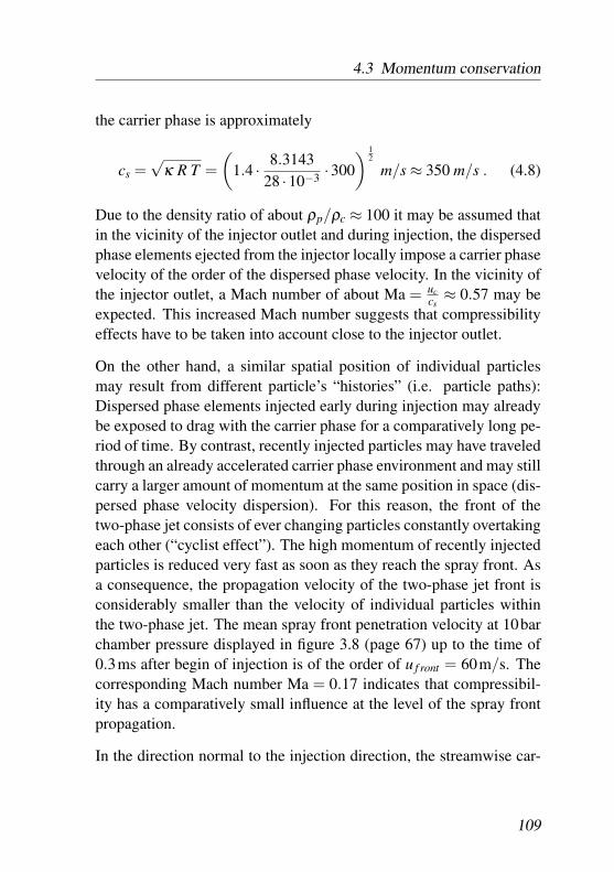
4.3 Momentum conservation
the carrier phase is approximately
cs =√
κ R T =(
1.4 · 8.314328 ·10−3 ·300
) 12
m/s ≈ 350 m/s . (4.8)
Due to the density ratio of about ρp/ρc ≈ 100 it may be assumed thatin the vicinity of the injector outlet and during injection, the dispersedphase elements ejected from the injector locally impose a carrier phasevelocity of the order of the dispersed phase velocity. In the vicinity ofthe injector outlet, a Mach number of about Ma = uc
cs≈ 0.57 may be
expected. This increased Mach number suggests that compressibilityeffects have to be taken into account close to the injector outlet.
On the other hand, a similar spatial position of individual particlesmay result from different particle’s “histories” (i.e. particle paths):Dispersed phase elements injected early during injection may alreadybe exposed to drag with the carrier phase for a comparatively long pe-riod of time. By contrast, recently injected particles may have traveledthrough an already accelerated carrier phase environment and may stillcarry a larger amount of momentum at the same position in space (dis-persed phase velocity dispersion). For this reason, the front of thetwo-phase jet consists of ever changing particles constantly overtakingeach other (“cyclist effect”). The high momentum of recently injectedparticles is reduced very fast as soon as they reach the spray front. Asa consequence, the propagation velocity of the two-phase jet front isconsiderably smaller than the velocity of individual particles withinthe two-phase jet. The mean spray front penetration velocity at 10barchamber pressure displayed in figure 3.8 (page 67) up to the time of0.3ms after begin of injection is of the order of u f ront = 60m/s. Thecorresponding Mach number Ma = 0.17 indicates that compressibil-ity has a comparatively small influence at the level of the spray frontpropagation.
In the direction normal to the injection direction, the streamwise car-
109
4 Integral modeling
rier phase velocity reduces within a smaller length than the spray pen-etration length so that local Mach numbers decrease. On the otherhand, a locally occurring carrier phase velocity of e.g. uc = 200m/sat pc = 10bar (ρc ≈ 10 kg/m3) corresponds to a dynamic pressure ofpdyn = ρc/2 ·u2
c ≈ 2 bar. As a result, the carrier phase density at the po-sition of such high convective velocity is about 20% smaller than thepressure condition far away from the dense two-phase jet, and con-sequentially, a non-negligible pressure gradient ∂ pc
∂η contributes to thecross-stream momentum conservation equation.
Since both phases are modeled to be spatially separated, bulk effectsdue to gradients in volume fractions do not occur.
In summary, pressure fluctuations within the carrier phase are assumedto propagate faster than the local convective velocities (Ma � 1) andthe carrier phase is modeled to be not compressible.
Limited DSZ carrier phase capacity
The zone of strong dispersed phase volume loading (dense spray zoneDSZ, see figure 4.7) is assumed to be much thinner than the carrierphase boundary layer thickness. Consequently, the dispersed phase ismodeled to directly interact with only a very small amount of carrierphase mass. Due to the high density ratio ρp/ρc � 1 (e.g. at 10bar gaspressure and 300K gas temperature, ρp/ρc = O
(102)), the drag force
resulting from local slip between both phases leads to an accelerationof the carrier phase: If the carrier phase mass exchanges momentumdirectly with dispersed phase, it would almost instantaneously be ac-celerated to the dispersed phase velocity §.
§ Because of the locally high bulk density ratio between dispersed and carrierphase ρ p/ρc = (αpρp)/(α f ρ f ), the drag force (eq. (4.6)) primarily acts on the carrierphase. The time scale
T(c)
drag =Up −Uc∂ (Up−Uc)
∂ t
(4.9)
110
4.3 Momentum conservation
As a consequence, the amount of carrier phase mass directly exposedto exchange of mass, momentum, and thermal energy with the dis-persed phase (which is supposed to happen at the boundary of theDSZ) is negligible. In other words: In comparison to the carrier phasefluxes occurring outside the DSZ, the ability of the carrier phase tostore mass, momentum and thermal energy within the DSZ is negligi-ble. Consequentially, the ability of the carrier phase to exchange e.g.momentum with the dispersed phase depends on momentum diffusionnormal to the main injection direction.
Diffusion normal to the main injection direction is defined by thecross-stream velocity profile.
Carrier phase velocity profile
As a consequence from the dominant dispersed phase momentum fluxduring injection, the carrier phase is strongly accelerated near thespray center line, which in turn causes strong entrainment: The widthof the carrier phase boundary layer thickness is limited and an “accel-erated wall” type profile develops (see section 3.2.3, e.g. figure 3.12on page 75).Further downstream, a single phase jet like S-profile develops. Never-theless, streamwise slip velocities are of the same order of magnitudeas in the region of the upstream “accelerated wall” boundary layer(see figure 3.11). Also, the cross-stream width occupied by the dis-
at which carrier phase is exposed to acceleration resulting from drag at high dispersedphase concentrations (as it is the case within/close to the DSZ) relates the current slipvelocity Usl = Up −Uc to its rate of change.
With the help of Newtons law FD = ρc∂ (Up−Uc)
∂ t , the continuous phase accelerationtime scale
T(c)
drag, c =ρc (Up −Uc)
FD(4.10)
is obtained. In the limit of the DSZ assumption (αc → 0 ⇔ ρ p/ρc → ∞), the carrier
phase acceleration time scale tends towards T(c)
drag, c → 0.
111
4 Integral modeling
persed phase mass is still smaller than the boundary layer thickness ofthe carrier phase (figure 3.11 left).
From the identification of the dominance of the dispersed phase mo-mentum flux direction and the induced “accelerated wall” type bound-ary layer, two major properties of the carrier phase flow during injec-tion may be deduced:
• The cross-stream maximum of the streamwise velocity occursat the presumed spray center line (the “accelerated wall”).
• The drag induced acceleration of carrier phase at the presumedspray center line causes the entrainment of additional gas phasetowards the spray center line (“excess entrainment”) so that thecross-stream component of the carrier phase velocity tends to-wards zero at the spray center line.
Cross-stream length scale
The carrier phase momentum is diffusively transported away from theDSZ due to cross-stream gradients of the carrier phase streamwise ve-locity: A carrier phase boundary layer is formed close to the DSZ (fig-ure 4.7). Because the velocity normal to the main injection directionis not spatially resolved, a cross-stream gradient cannot be estimatedand a length scale characterizing the shearing motion close to the DSZδτ has to be modeled.
The carrier phase velocity within the shear layer is large (especiallyclose to the DSZ), thus the carrier phase far away from the DSZ maybe modeled as quiescent. The length scale δτ characterizing the max-imum shear stress (occurring in the vicinity of the DSZ) is modeledas the length scale of the maximum cross-stream velocity gradient ∂Uc
∂ηadjacent to the DSZ (see figure 4.8):
∂Uc
∂η= −Uc
δτ. (4.11)
112
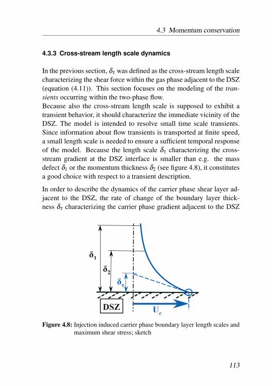
4.3 Momentum conservation
4.3.3 Cross-stream length scale dynamics
In the previous section, δτ was defined as the cross-stream length scalecharacterizing the shear force within the gas phase adjacent to the DSZ(equation (4.11)). This section focuses on the modeling of the tran-sients occurring within the two-phase flow.Because also the cross-stream length scale is supposed to exhibit atransient behavior, it should characterize the immediate vicinity of theDSZ. The model is intended to resolve small time scale transients.Since information about flow transients is transported at finite speed,a small length scale is needed to ensure a sufficient temporal responseof the model. Because the length scale δτ characterizing the cross-stream gradient at the DSZ interface is smaller than e.g. the massdefect δ1 or the momentum thickness δ2 (see figure 4.8), it constitutesa good choice with respect to a transient description.
In order to describe the dynamics of the carrier phase shear layer ad-jacent to the DSZ, the rate of change of the boundary layer thick-ness δτ characterizing the carrier phase gradient adjacent to the DSZ
Figure 4.8: Injection induced carrier phase boundary layer length scales andmaximum shear stress; sketch
113
4 Integral modeling
(see eq. (4.11)) needs to be quantified. In total, the time rate of changeof the local two-phase jet boundary layer thickness length scale(
∂δτ
∂ t
)(T PF)
=(
∂δτ
∂ t
)(conv)
+(
∂δτ
∂ t
)(µ)
(4.12)
is composed of contributions due to changes due to convective fluxesand due to gradient diffusion of momentum.The convective term(
∂δτ
∂ t
)(conv)
=(
∂δτ
∂ t
)( ∂Uc∂ξ )
+(
∂δτ
∂ t
)(cone)
+(
∂δτ
∂ t
)(exen)
(4.13)
is composed of a contribution resulting from streamwise velocity gra-dients within the carrier phase and of the additional effect of localcarrier phase acceleration due to drag with the dispersed phase andconsequential excess entrainment (superscript “exen”) ¶. The convec-
tive part accounting for the carrier phase flux(
∂δτ∂ t
)( ∂Uc∂ξ )
may be un-derstood as the “usual” entrainment phenomenon occurring in singlephase jets, where momentum is only supplied at the injection outletand no additional momentum is introduced to the (carrier phase) jetwithin the flow domain.
Due to the cone geometry, a contribution(
∂δτ∂ t
)(cone)accounting for
the radial widening is expected.
¶ The speed of local excess entrainment due to local drag with the carrier phaseand consequential contraction of the boundary layer may be characterized by meansof an entrainment time scale T
(c)entr.
T(c)
entr =δτVc
114
4.3 Momentum conservation
Cross-stream length scale transport
In the following, a transport equation for the cross-stream length scaleδτ is developed. The derivation starts from the two-dimensional stream-wise momentum conservation equation of the carrier phase (super-script “tilde”). Its terms are approximated in the vicinity of the DSZby means of a Taylor series expansion (super-script “hat”). Deriva-tives of the cross-stream velocity component are substituted by meansof the incompressible continuity equation. In order to drop the ex-plicit dependence on the cross-stream coordinate η , the approximatedstreamwise momentum equation is integrated over the (comparativelysmall) cross-stream length scale δτ . With this choice, only the portionof the boundary layer in the direct vicinity of the DSZ is taken intoaccount of the integration and a transient boundary layer descriptionis obtained.
For the derivation of a transient description of the cross-stream lengthscale δτ , the streamwise momentum conservation equation for the car-rier phase velocity field Uc(ξ ,η , t) in conical coordinates (see eq. (A.9)in the appendix)
∂Uc
∂ t+Uc
∂Uc
∂ξ+Vc
∂Uc
∂η
= ν
⎛⎝∂ 2Uc
∂ξ 2 +sinθ ∂Uc
∂ξ + cosθ ∂Uc∂η
ξ sinθ +η cosθ+
∂ 2Uc
∂η2 − sinθUc sinθ +Vc cosθ(ξ sinθ +η cosθ)2
⎞⎠
(4.14)
is employed for the carrier phase. In section 3.2.4, the second ordercross-stream derivatives ∂ 2(∗)
∂η2 (figure 3.18) were verified to be domi-nant among the viscous terms. So if the conventional boundary layerassumption
∂ 2(∗)∂ξ 2 � ∂ 2(∗)
∂η2 (4.15)
115
4 Integral modeling
is applied, then the streamwise momentum conservation equation reads
∂Uc
∂ t+Uc
∂Uc
∂ξ+Vc
∂Uc
∂η= ν
∂ 2Uc
∂η2 . (4.16)
Due to negligible compressibility effects within the carrier phase, theaverage density is ρ(DSZ)
c = const. and the continuity equation
∂ρc
∂ t+
∂ (ρcUc)∂ξ
+∂ (ρcVc)
∂η+ρc
Uc sinθ +Vc cosθξ sinθ +η cosθ
= 0 (4.17)
simplifies to
∂Uc
∂ξ+
∂Vc
∂η+
Uc sinθ +Vc cosθξ sinθ +η cosθ
= 0 . (4.18)
The assumption of an incompressible carrier phase is used to approx-imate the first
∂Vc
∂η= −∂Uc
∂ξ− Uc sinθ +Vc cosθ
ξ sinθ +η cosθ(4.19)
and second order derivatives based on the continuity equation (4.18)
∂ 2Vc
∂η2 =− ∂∂ξ
(∂Uc
∂η
)−
∂Uc∂η sinθ + ∂Vc
∂η cosθξ sinθ +η cosθ
+cosθUc sinθ +Vc cosθ(ξ sinθ +η cosθ)2 .
(4.20)
Presumed center line
The cross-stream maximum of the streamwise velocity is defined asUc(ξ ) = Uc(ξ ,η)
∣∣η=0 and analogously Vc(ξ ) = Vc(ξ ,η)
∣∣η=0. At the
presumed center position η = 0, Vc ≈ 0 due to a presumed flow sym-metry. In two-phase flow, the carrier phase exchanges momentum withthe dispersed phase so that a drag source term ΦD is introduced to the
116
4.3 Momentum conservation
streamwise momentum equation (4.16)
∂Uc
∂ t+Uc
∂Uc
∂ξ= 2 ν
∂ 2Uc
∂η2 +ΦD . (4.21)
The factor 2 in front of the diffusive part of equation (4.21) accountsfor the fact that the hollow cone sheet is surrounded by two adjacentboundary layers.With the approximation of the cross-stream gradient (equation (4.31)presented later in this section), the carrier phase momentum equationis
∂Uc
∂ t+Uc
∂Uc
∂ξ= ΦD −2 ν
Uc
δ 2τ
. (4.22)
Due to the primitive representation of the carrier phase momentum inequation (4.22), the momentum source term reads
ΦD =FD
ρc. (4.23)
The sum of the RHS terms in equation (4.22) represents an effectivespecific drag force
Φ(e f f )D =
FD
ρc−2 ν
Uc
δ 2τ
, (4.24)
which is experienced by the carrier phase at the presumed center lineposition. The final version of the carrier phase momentum conserva-tion equation is
∂Uc
∂ t+Uc
∂Uc
∂ξ=
FD
ρc−2 ν
Uc
δ 2τ
= Φ(e f f )D . (4.25)
117
4 Integral modeling
The derivatives of equations (4.19) and (4.20) are
∂Vc
∂η= −∂Uc
∂ξ− Uc
ξ. (4.26)
and ‖
∂ 2Vc
∂η2 = − ∂∂ξ
(∂Uc
∂η
)− 1
ξ
(∂Uc
∂η+
1tanθ
∂Vc
∂η
)+
1ξ 2 tanθ
Uc .
(4.27)Employing the continuity equation (4.19), the gradient ∂Vc
∂η and thusthe dependency on the cross-stream velocity is eliminated
∂ 2Vc
∂η2 = − ∂∂ξ
(∂Uc
∂η
)− 1
ξ∂Uc
∂η+
1ξ tanθ
∂Uc
∂ξ+
2ξ 2 tanθ
Uc .
(4.28)
Boundary layer approximation
The boundary layer thickness scale δτ as it is characterized in fig-ure 4.8 is a flow property which characterizes gas phase flow condi-tions at the presumed center line (at η = 0). The temporal evolutionof the local boundary layer length scale depends on the carrier phasemomentum transport at the position at which it characterizes the crossstream gradient, namely at the presumed spray center line η = 0. Arelation between the temporal and spatial gradients of Uc is given byequation (4.21) which covers also for the diffusive loss of streamwisemomentum normal to the main flow direction. Note that an assump-tion on the cross-stream profile Uc(η) is not needed for the descriptionof the streamwise momentum transport at the presumed spray center
‖ Note that if the second derivative at the center line position directly derivedfrom (4.26)
∂ 2Vc
∂η2 = − ∂∂ξ
(∂Uc
∂η
)− 1
ξ∂Uc
∂η,
a dependency on the cone opening angle θ may not be maintained.
118
4.3 Momentum conservation
line.By contrast, the temporal development of δτ due to (see eq. (4.13))
• local acceleration of carrier phase mass due to drag with the dis-persed phase and consequential excess entrainment (local con-traction of the boundary layer cross-stream width) and
• streamwise gradients in δτ and Uc
remains to be modeled. Because convection of carrier phase masstowards the presumed center line needs to be modeled, an assumptionon the velocity profile in the vicinity of the DSZ becomes inevitable.
Not the whole of the cross-stream profile needs to be modeled sincethe major influence of the flow at the presumed center line stems fromthe evolution of the flow in the vicinity of η = 0. Therefore, the cross-stream profile in the vicinity of the DSZ is approximated by meansof the cross-stream length scale δτ in terms of the gradients at theDSZ, i.e. by means of a Taylor series expansion. In that fashion, e.g.the streamwise carrier phase velocity Uc(η) resulting from a Taylorexpansion approximates the “exact” velocity field Uc(η).
The procedure of deriving a relation for the local rate of change ofthe cross-stream length scale δτ is presented in the following. It de-pends on streamwise gradients of both that very length scale δτ andthe streamwise carrier phase velocity at the DSZ Uc = Uc(η = 0).The velocity profile Uc is approximated by a second order polynomialfunction.The Taylor expansions of the streamwise and cross-stream velocityprofiles read
Uc(η) = Uc|η=0 +η∂Uc
∂η
∣∣∣∣η=0
+η2
2∂ 2Uc
∂η2
∣∣∣∣η=0
(4.29)
119
4 Integral modeling
and
Vc(η) = Vc|η=0 +η∂Vc
∂η
∣∣∣∣η=0
+η2
2∂ 2Vc
∂η2
∣∣∣∣η=0
. (4.30)
When a cross-stream profile is defined by means of a second order ap-proximating function (three fitting coefficients), three boundary condi-tions need to be applied in order to uniquely define the velocity profile.The cross-stream gradients are approximated by means of the cross-stream length scale δτ
Uc∣∣η=0 =Uc ,
∂Uc
∂η
∣∣∣∣η=0
=∂Uc
∂η=−Uc
δτand
∂ 2Uc
∂η2
∣∣∣∣η=0
=∂ 2Uc
∂η2 =Uc
δ 2τ
(4.31)so that the Taylor approximation of the cross-stream profile of thestreamwise carrier phase velocity may be described by
Uc(η) = Uc
(1− η
δτ+
η2
2 δ 2τ
). (4.32)
With the continuity assumption utilized in equations (4.26) and (4.28),the approximated cross-stream velocity close to the DSZ (|η | ≤ δτ )
Vc(η) = 0−η(
∂Uc
∂ξ+
Uc
ξ
)
− η2
2
[∂ (Uc
δτ)
∂ξ+
1ξ
∂Uc
∂η− 1
ξ tanθ
(∂Uc
∂ξ+
2 Uc
ξ tanθ
)] (4.33)
120
4.3 Momentum conservation
may be expressed by means of the center line streamwise velocity
Vc(η) = −η∂Uc
∂ξ
[1− η
2
(1δτ
+1
ξ tanθ
)]
− ηξ
Uc
[1−η
(1
2δτ+
1ξ tanθ
)]− η2
2 δ 2τ
Uc∂δτ
∂ξ.
(4.34)
Integrated momentum equation
The Taylor approximation Uc (eq.(4.32)) is now inserted into the indi-vidual terms of eq. (4.16)
∂Uc
∂ t=
∂Uc
∂ t
(1− η
δτ+
η2
2 δ 2τ
)+Uc
ηδ 2
τ
(1− η
δτ
)∂δτ
∂ t(4.35)
∂Uc
∂ξ=
∂Uc
∂ξ
(1− η
δτ+
η2
2 δ 2τ
)+Uc
ηδ 2
τ
(1− η
δτ
)∂δτ
∂ξ(4.36)
∂Uc
∂η= −Uc
δτ
(1− η
δτ
)(4.37)
∂ 2Uc
∂η2 =Uc
δ 2τ
(4.38)
and the corresponding products of eq. (4.16) are formed.
Uc∂Uc
∂ξ= Uc
{∂Uc
∂ξ
[1−2
ηδτ
+2(
ηδτ
)2
−(
ηδτ
)3
+14
(ηδτ
)4]
+Uc
δτ
ηδτ
∂δτ
∂ξ
[1−2
ηδτ
+32
(ηδτ
)2
− 12
(ηδτ
)3]}
(4.39)
121
4 Integral modeling
Vc∂Uc
∂η= Uc
ηδτ
(∂Uc
∂ξ+
Uc
ξ
) [1− 3
2ηδτ
+12
(ηδτ
)2
− ηξ tanθ
(1− η
δτ
)]
− η2
2ξ δτ tanθUc
∂Uc
∂ξ
(1− η
δτ
)+
η2
2δ 3τ
U2c
∂δτ
∂ξ
(1− η
δτ
)(4.40)
As a result of the Taylor approximation, the gradients at the DSZboundary ∂Uc
∂ t , ∂Uc∂ξ and Uc are expressed independent from the η coor-
dinate in the vicinity of the DSZ.The dependence of the terms contributing to the streamwise momen-tum equation (4.16) on the cross-stream coordinate η is eliminated byintegration over the cross-stream direction.
δτ∫0
∂Uc
∂ tdη =
23
δτ∂Uc
∂ t+
16
Uc∂δτ
∂ t(4.41)
δτ∫0
(Uc
∂Uc
∂ξ
)dη =
715
δτ Uc∂Uc
∂ξ+
13120
U2c
∂δτ
∂ξ(4.42)
δτ∫0
(Vc
∂Uc
∂η
)dη = δτ Uc
(∂Uc
∂ξ+
Uc
ξ
) (18− 1
12δτ
ξ tanθ
)
− 124
δ 2τ
ξ tanθUc
∂Uc
∂ξ+
124
U2c
∂δτ
∂ξ(4.43)
δτ∫0
(ν
∂ 2Uc
∂η2
)dη =
Uc νδτ
(4.44)
122
4.3 Momentum conservation
Transient two-phase boundary layer (ttBL)
Insertion of the above terms into the integrated form of the streamwisemomentum equation (4.16) leads to
δτ∂Uc
∂ t+
14
Uc∂δτ
∂ t+δτ Uc
∂Uc
∂ξ
(7180
− 316
δτ
ξ tanθ
)
+δτU2
c
ξ
(316
− 18
δτ
ξ tanθ
)+
940
U2c
∂δτ
∂ξ=
32
Uc νδτ
(4.45)
or (solved for ∂δτ∂ t )
∂δτ
∂ t+
4 δτ
Uc
∂Uc
∂ t+δτ
∂Uc
∂ξ
(7120
− 34
δτ
ξ tanθ
)
+δτUc
ξ
(34− 1
2δτ
ξ tanθ
)+
910
Uc∂δτ
∂ξ=
6 νδτ
.
(4.46)
This is an equation quantifying the local rate of change ∂δτ (ξ , t)∂ t and
therefore constitutes a transient, one-dimensional transport equationfor the cross-stream length scale. The individual contributions intro-duced in equations (4.12) and (4.13) may now be identified. By meansof the opening angle θ , it accounts for the geometry of a hollow cone.It covers for streamwise gradients in both the length scale measure δτand the velocity Uc as well as for the acceleration due to drag with thedispersed phase.
The contributions of the overall rate of change of local length scaleinitially described in equations (4.12) and (4.13) may now be identi-
123
4 Integral modeling
fied:(∂δτ
∂ t
)(exen)
=− 4 δτ
Uc
∂Uc
∂ t, (4.47)
(∂δτ
∂ t
)( ∂Uc∂ξ )
=− 7120
δτ∂Uc
∂ξ− 9
10Uc
∂δτ
∂ξ, (4.48)(
∂δτ
∂ t
)(cone)
=−δτUc
ξ
(34− 1
2δτ
ξ tanθ
)+
34
∂Uc
∂ξδ 2
τξ tanθ
,
(4.49)(∂δτ
∂ t
)(µ)
=6 νδτ
. (4.50)
4.3.4 ttBL model assessment
The proposed boundary layer model is designed to describe the tran-sient response of the two-phase jet resulting from the injection of liq-uid fuel into air. The physical validity of the derived model equationsis assessed in this section.
Analogies
At first sight, the proposed model shows similarities to classical bound-ary layer models as summarized in [108]: It is derived by cross-streamintegration and it contains a boundary layer thickness in the resultingtransport equation.On the other hand, it shows clear differences to the classical integralmethods: First of all, it does not exploit self-similarity, neither in spacenor time. It describes the transient response of the local length scale δτto boundary condition changes. Also, no boundary layer integral mo-mentum or mass flux is transported by means of a conservation equa-tion. Only the transport equation for the evolution of the local length
124
4.3 Momentum conservation
scale is described. The integral over the approximated streamwise mo-mentum equation is only utilized in the course of its derivation.In order to compare the proposed model to the classical boundary layermethod, the integrals of mass and momentum based on the assumedvelocity profile are derived in appendix B: For the plane 2D case, in-tegral equations of mass and momentum contained within a boundarylayer of thickness δ and with a presumed cross-stream velocity pro-file according to equation B.12 are assessed. The form and discussionof both the steady state integrals (equations B.14 and B.15) as wellas their transient contributions (equations B.20 and B.21) support thevalidity of the proposed transport equation of the cross-stream lengthscale δτ (equation 4.46).
Variable local length scale
An other challenge of the model is to accept the concept of transport-ing a non-sensible and non-conserved quantity such as a local lengthscale as opposed to conserved variables like mass or energy. Neverthe-less, the transport of non-conserved quantities is well accepted in otherfields of fluid mechanics, e.g. the transport of a rate of dissipation ofturbulent kinetic energy in the k-ε turbulence model.
The feasibility of the proposed transport equation (4.46) is discussedin the following section.
Presumed cross-stream velocity profile
The carrier phase velocity in the vicinity of the dense spray zone(DSZ) is modeled as a function of the flow characteristics inside thedense spray zone: The carrier phase velocity Uc(η) in the vicinity ofthe DSZ is approximated in terms of the DSZ carrier phase velocityUc.
Uc(η) = Uc
(1− η
δτ+
η2
2 δ 2τ
)(4.32)
125
4 Integral modeling
For the approximation of the cross-stream velocity profile U(η), threeboundary conditions at the presumed center line position are applied,see eq. (4.31).
At the position η = δτ , the approximated (modeled) cross-stream ve-locity profile U(η) according to eq. (4.32) produces the velocity Uc(η =δτ) = Uc/2 and the velocity gradient ∂Uc(η=δτ )
∂η = 0. The same veloc-ity profile is obtained if in eq. (4.31), the third boundary condition∂ 2Uc∂η2
∣∣∣η=0
= ∂ 2Uc∂η2 = Uc
δ 2τ
is substituted by ∂Uc∂η
∣∣∣η=δτ
= 0.
So in terms of the 2D streamwise momentum equation
∂Uc
∂ t+Uc
∂Uc
∂ξ+Vc
∂Uc
∂η= ν
∂ 2Uc
∂η2 , (4.16)
the approximated velocity profile U(η) (eq. (4.32)) has two majorcharacteristics:
• Because ∂Uc∂η
∣∣∣η=δτ
= 0, the streamwise momentum transport at
the boundary η = δτ is independent from the magnitude of theapproximated cross-stream velocity V (η = δτ): (V ∂U
∂η )∣∣∣η=δτ
=
0
• As a consequence from the choice of a second order approxima-tion, the cross-stream diffusion rate of the approximated stream-wise momentum is modeled to be constant throughout the bound-ary layer: ∂Uc
∂η = Uc/δτ . Its magnitude is solely determined bythe local boundary layer thickness δτ and the DSZ velocity Uc.
The two major properties mentioned above indicate that the choice ofthe presumed cross-stream velocity profile according to eq. (4.32) iswell suited for cross-stream integration as presented in section 4.3.3.
126
4.3 Momentum conservation
Hollow cone geometry
Due to the hollow cone geometry, tanθ may only take on values withinthe bounds 0 < tanθ ≤ π/2. Because θ appears in the denominator,θ → 0 has to be excluded from the scope of validity of equation (4.46).In the context of the flow induced by the hollow cone injection, gen-erally θ ≈ 40o.
The cone opening angle θ only influences the cross-stream lengthscale transport when the boundary layer length scale δτ is of the or-der of the streamwise coordinate ξ . This condition is fulfilled only forcomparatively small values of ξ , i.e. the influence of the cone openingangle θ is restricted to regions very close to the injector symmetry line.Far away from the injector symmetry line (ξ � δτ ), the terms contain-ing the cone opening angle θ may be neglected and equation (4.46)simplifies to
∂δτ
∂ t+4
δτ
Uc
∂Uc
∂ t+
7120
δτ∂Uc
∂ξ+
34
δτ Uc
ξ+
910
Uc∂δτ
∂ξ= 6
νδτ
.
(4.51)In regions very far away from the injector symmetry line (ξ → ∞,where consequentially also ξ � δτ ), the flux due to the cone term(δτ Uc)/ξ may be neglected too and equation (4.51) reduces to
∂δτ
∂ t+4
δτ
Uc
∂Uc
∂ t+
7120
δτ∂Uc
∂ξ+
910
Uc∂δτ
∂ξ= 6
νδτ
(4.52)
which corresponds to the plane 2D case.
If in equation (4.52), the center line velocity Uc is in a steady state con-dition ( ∂Uc
∂ t = 0) and streamwise gradients of both streamwise velocityUc and boundary layer thickness δτ are negligible ( ∂ (∗)
∂ξ = 0), then thelocal boundary layer length scale grows only due to diffusion effectscharacterized by the momentum diffusion coefficient ν .The terms in equation (4.52) containing streamwise gradients ∂ (∗)
∂ξ lead
127
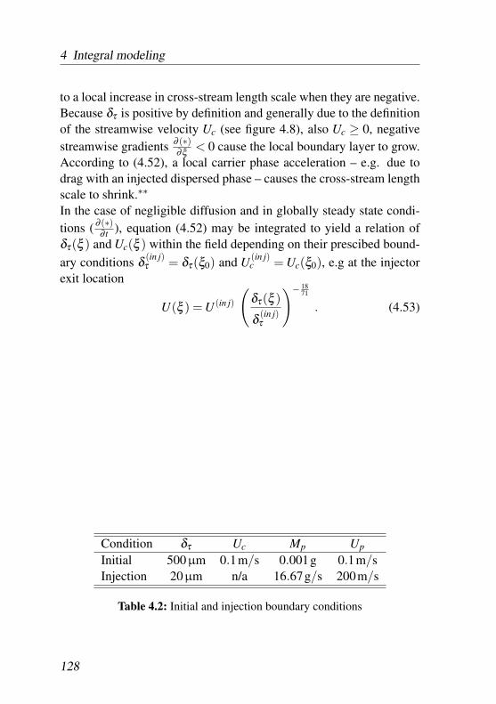
4 Integral modeling
to a local increase in cross-stream length scale when they are negative.Because δτ is positive by definition and generally due to the definitionof the streamwise velocity Uc (see figure 4.8), also Uc ≥ 0, negativestreamwise gradients ∂ (∗)
∂ξ < 0 cause the local boundary layer to grow.According to (4.52), a local carrier phase acceleration – e.g. due todrag with an injected dispersed phase – causes the cross-stream lengthscale to shrink.∗∗
In the case of negligible diffusion and in globally steady state condi-tions ( ∂ (∗)
∂ t ), equation (4.52) may be integrated to yield a relation ofδτ(ξ ) and Uc(ξ ) within the field depending on their prescibed bound-ary conditions δ (in j)
τ = δτ(ξ0) and U (in j)c = Uc(ξ0), e.g at the injector
exit location
U(ξ ) = U (in j)
(δτ(ξ )
δ (in j)τ
)− 1871
. (4.53)
Condition δτ Uc Mp Up
Initial 500µm 0.1m/s 0.001g 0.1m/sInjection 20µm n/a 16.67g/s 200m/s
Table 4.2: Initial and injection boundary conditions
128
4.3 Momentum conservation
4.3.5 Numerical scheme and boundary conditions
For the implementation of the proposed model, a finite-difference de-scription is applied. The one-dimensional space is resolved by a com-putational grid with a non-equidistant distribution of points. Spatialgradients are calculated as centered differences of second order of ac-curacy with the help of Fornberg’s formulas [54, 55]. Temporal inte-gration is conducted with an simple Euler forward method.
The injection velocity U (in j) as well as temperature T (in j) are specifieddirectly. The dispersed phase mass density M(in j)
p present at the in-jection node is calculated from the injected fuel mass flow rate m(in j).During a time increment δ t, a mass increment δm(in j)
p = m(in j) δ t is in-jected. At the prescribed injection velocity U (in j)
p , it will be transportedover a length increment δξ = U (in j)
p δ t. The resulting dispersed phasemass concentration present at the injection inlet is thereby defined as
Mp =δm(in j)
p
δξ=
m(in j)p
U (in j)p
. (4.54)
Initial and boundary conditions are listed in table 4.2. If not statedotherwise, the “injection” boundary conditions for the carrier phaseare equal to the initialization state. At the downstream boundary, azero gradient boundary condition is applied.
For the characteristic cross-steam length scale δτ , the condition at the
∗∗ If ∂Uc∂ t from equation (4.21) is inserted into (4.46), an alternative conservation
equation for the cross-stream length scale δτ is obtained.
∂δτ∂ t
+9
10Uc
∂δτ∂ξ
= δτ∂Uc
∂ξ
(9
20+
34
δτξ tanθ
)
+δτUc
ξ
(134
+12
δτξ tanθ
)+
2νδτ
129
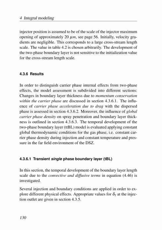
4 Integral modeling
injector position is assumed to be of the scale of the injector maximumopening of approximately 20 µm, see page 56. Initially, velocity gra-dients are negligible. This corresponds to a large cross-stream lengthscale. The value in table 4.2 is chosen arbitrarily. The development ofthe two-phase boundary layer is not sensitive to the initialization valuefor the cross-stream length scale.
4.3.6 Results
In order to distinguish carrier phase internal effects from two-phaseeffects, the model assessment is subdivided into different sections:Changes in boundary layer thickness due to momentum conservationwithin the carrier phase are discussed in section 4.3.6.1. The influ-ence of carrier phase acceleration due to drag with the dispersedphase is assessed in section 4.3.6.2. Moreover, the influence of globalcarrier phase density on spray penetration and boundary layer thick-ness is outlined in section 4.3.6.3. The temporal development of thetwo-phase boundary layer (ttBL) model is evaluated applying constantglobal thermodynamic conditions for the gas phase, i.e. constant car-rier phase density during injection and constant temperature and pres-sure in the far field environment of the DSZ.
4.3.6.1 Transient single phase boundary layer (tBL)
In this section, the temporal development of the boundary layer lengthscale due to the convective and diffusive terms in equation (4.46) isinvestigated.
Several injection and boundary conditions are applied in order to ex-plore different physical effects. Appropriate values for δτ at the injec-tion outlet are given in section 4.3.5.
130
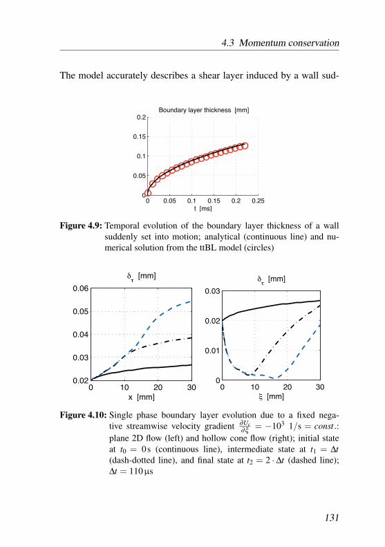
4.3 Momentum conservation
The model accurately describes a shear layer induced by a wall sud-
0 0.05 0.1 0.15 0.2 0.250
0.05
0.1
0.15
0.2Boundary layer thickness [mm]
t [ms]
Figure 4.9: Temporal evolution of the boundary layer thickness of a wallsuddenly set into motion; analytical (continuous line) and nu-merical solution from the ttBL model (circles)
0 10 20 300.02
0.03
0.04
0.05
0.06
δτ [mm]
x [mm]0 10 20 30
0
0.01
0.02
0.03
δτ [mm]
ξ [mm]
Figure 4.10: Single phase boundary layer evolution due to a fixed nega-tive streamwise velocity gradient ∂Uc
∂ξ = −103 1/s = const.:plane 2D flow (left) and hollow cone flow (right); initial stateat t0 = 0s (continuous line), intermediate state at t1 = ∆t(dash-dotted line), and final state at t2 = 2 ·∆t (dashed line);∆t = 110µs
131
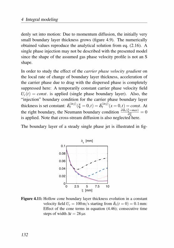
4 Integral modeling
denly set into motion: Due to momentum diffusion, the initially verysmall boundary layer thickness grows (figure 4.9). The numericallyobtained values reproduce the analytical solution from eq. (2.16). Asingle phase injection may not be described with the presented modelsince the shape of the assumed gas phase velocity profile is not an Sshape.
In order to study the effect of the carrier phase velocity gradient onthe local rate of change of boundary layer thickness, acceleration ofthe carrier phase due to drag with the dispersed phase is completelysuppressed here: A temporarily constant carrier phase velocity fieldUc(t) = const. is applied (single phase boundary layer). Also, the“injection” boundary condition for the carrier phase boundary layerthickness is set constant: δ (in j)
τ (ξ = 0, t) = δ (in j)τ (x = 0, t) = const. At
the right boundary, the Neumann boundary condition ∂δτ (ξ=max)∂ξ = 0
is applied. Note that cross-stream diffusion is also neglected here.
The boundary layer of a steady single phase jet is illustrated in fig-
0 2.5 5 7.5 100
0.02
0.04
0.06
0.08
0.1
δτ [mm]
ξ [mm]
Figure 4.11: Hollow cone boundary layer thickness evolution in a constantvelocity field Uc = 100m/s starting from δτ(t = 0) = 0.1mm:Effect of the cone terms in equation (4.46); consecutive timesteps of width ∆t = 28µs
132
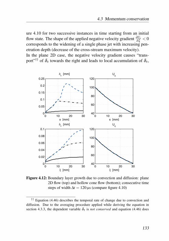
4.3 Momentum conservation
ure 4.10 for two successive instances in time starting from an initialflow state. The shape of the applied negative velocity gradient ∂Uc
∂ξ < 0corresponds to the widening of a single phase jet with increasing pen-etration depth (decrease of the cross-stream maximum velocity).In the plane 2D case, the negative velocity gradient causes “trans-port”†† of δτ towards the right and leads to local accumulation of δτ ,
0 10 20 300
0.05
0.1
0.15
0.2
0.25
δτ [mm]
x [mm]0 10 20 30
40
60
80
100
120
Uc
x [mm]
0 10 20 300
0.02
0.04
0.06
0.08
0.1
δτ [mm]
ξ [mm]0 10 20 30
40
60
80
100
120
Uc
ξ [mm]
Figure 4.12: Boundary layer growth due to convection and diffusion: plane2D flow (top) and hollow cone flow (bottom); consecutive timesteps of width ∆t = 120µs (compare figure 4.10)
†† Equation (4.46) describes the temporal rate of change due to convection anddiffusion. Due to the averaging procedure applied while deriving the equation insection 4.3.3, the dependent variable δτ is not conserved and equation (4.46) does
133
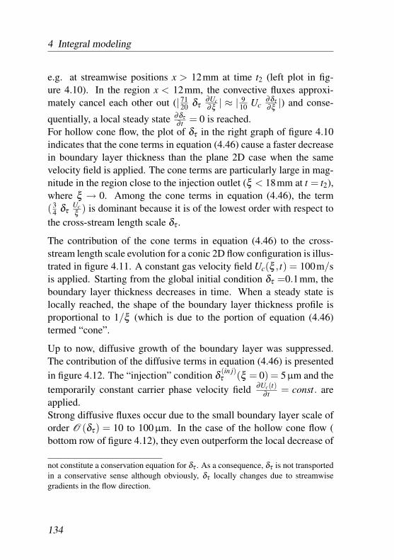
4 Integral modeling
e.g. at streamwise positions x > 12mm at time t2 (left plot in fig-ure 4.10). In the region x < 12mm, the convective fluxes approxi-mately cancel each other out (|71
20 δτ∂Uc∂ξ | ≈ | 9
10 Uc∂δτ∂ξ |) and conse-
quentially, a local steady state ∂δτ∂ t = 0 is reached.
For hollow cone flow, the plot of δτ in the right graph of figure 4.10indicates that the cone terms in equation (4.46) cause a faster decreasein boundary layer thickness than the plane 2D case when the samevelocity field is applied. The cone terms are particularly large in mag-nitude in the region close to the injection outlet (ξ < 18mm at t = t2),where ξ → 0. Among the cone terms in equation (4.46), the term(3
4 δτUcξ ) is dominant because it is of the lowest order with respect to
the cross-stream length scale δτ .
The contribution of the cone terms in equation (4.46) to the cross-stream length scale evolution for a conic 2D flow configuration is illus-trated in figure 4.11. A constant gas velocity field Uc(ξ , t) = 100m/sis applied. Starting from the global initial condition δτ =0.1mm, theboundary layer thickness decreases in time. When a steady state islocally reached, the shape of the boundary layer thickness profile isproportional to 1/ξ (which is due to the portion of equation (4.46)termed “cone”.
Up to now, diffusive growth of the boundary layer was suppressed.The contribution of the diffusive terms in equation (4.46) is presentedin figure 4.12. The “injection” condition δ (in j)
τ (ξ = 0) = 5µm and thetemporarily constant carrier phase velocity field ∂Uc(t)
∂ t = const. areapplied.Strong diffusive fluxes occur due to the small boundary layer scale oforder O (δτ) = 10 to 100µm. In the case of the hollow cone flow (bottom row of figure 4.12), they even outperform the local decrease of
not constitute a conservation equation for δτ . As a consequence, δτ is not transportedin a conservative sense although obviously, δτ locally changes due to streamwisegradients in the flow direction.
134
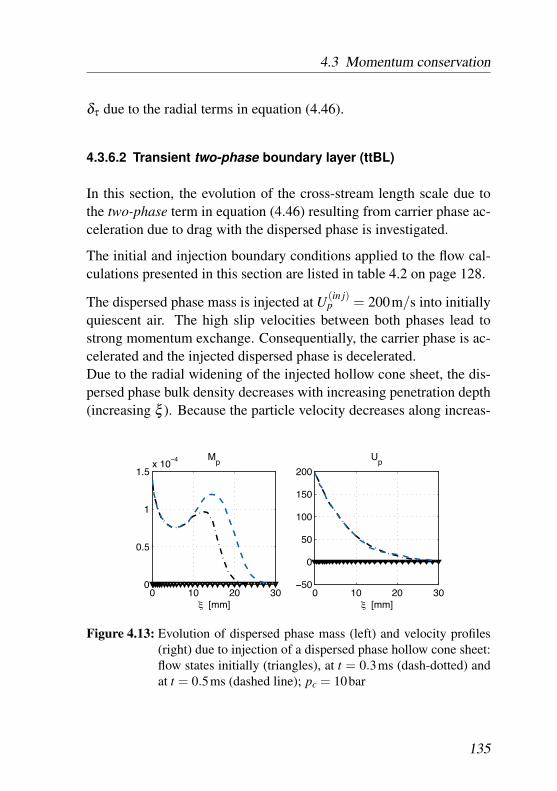
4.3 Momentum conservation
δτ due to the radial terms in equation (4.46).
4.3.6.2 Transient two-phase boundary layer (ttBL)
In this section, the evolution of the cross-stream length scale due tothe two-phase term in equation (4.46) resulting from carrier phase ac-celeration due to drag with the dispersed phase is investigated.
The initial and injection boundary conditions applied to the flow cal-culations presented in this section are listed in table 4.2 on page 128.
The dispersed phase mass is injected at U (in j)p = 200m/s into initially
quiescent air. The high slip velocities between both phases lead tostrong momentum exchange. Consequentially, the carrier phase is ac-celerated and the injected dispersed phase is decelerated.Due to the radial widening of the injected hollow cone sheet, the dis-persed phase bulk density decreases with increasing penetration depth(increasing ξ ). Because the particle velocity decreases along increas-
0 10 20 300
0.5
1
1.5x 10
−4 Mp
ξ [mm]0 10 20 30
−50
0
50
100
150
200
Up
ξ [mm]
Figure 4.13: Evolution of dispersed phase mass (left) and velocity profiles(right) due to injection of a dispersed phase hollow cone sheet:flow states initially (triangles), at t = 0.3ms (dash-dotted) andat t = 0.5ms (dashed line); pc = 10bar
135
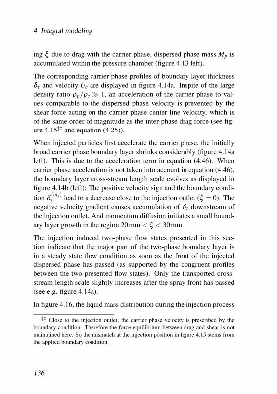
4 Integral modeling
ing ξ due to drag with the carrier phase, dispersed phase mass Mp isaccumulated within the pressure chamber (figure 4.13 left).
The corresponding carrier phase profiles of boundary layer thicknessδτ and velocity Uc are displayed in figure 4.14a. Inspite of the largedensity ratio ρp/ρc � 1, an acceleration of the carrier phase to val-ues comparable to the dispersed phase velocity is prevented by theshear force acting on the carrier phase center line velocity, which isof the same order of magnitude as the inter-phase drag force (see fig-ure 4.15‡‡ and equation (4.25)).
When injected particles first accelerate the carrier phase, the initiallybroad carrier phase boundary layer shrinks considerably (figure 4.14aleft). This is due to the acceleration term in equation (4.46). Whencarrier phase acceleration is not taken into account in equation (4.46),the boundary layer cross-stream length scale evolves as displayed infigure 4.14b (left): The positive velocity sign and the boundary condi-tion δ (in j)
τ lead to a decrease close to the injection outlet (ξ = 0). Thenegative velocity gradient causes accumulation of δτ downstream ofthe injection outlet. And momentum diffusion initiates a small bound-ary layer growth in the region 20mm < ξ < 30mm.
The injection induced two-phase flow states presented in this sec-tion indicate that the major part of the two-phase boundary layer isin a steady state flow condition as soon as the front of the injecteddispersed phase has passed (as supported by the congruent profilesbetween the two presented flow states). Only the transported cross-stream length scale slightly increases after the spray front has passed(see e.g. figure 4.14a).
In figure 4.16, the liquid mass distribution during the injection process
‡‡ Close to the injection outlet, the carrier phase velocity is prescribed by theboundary condition. Therefore the force equilibrium between drag and shear is notmaintained here. So the mismatch at the injection position in figure 4.15 stems fromthe applied boundary condition.
136
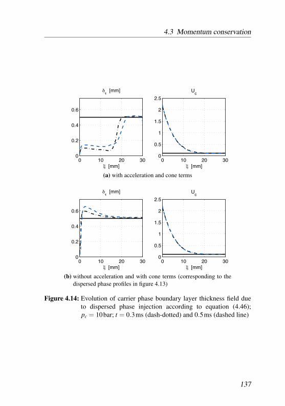
4.3 Momentum conservation
0 10 20 300
0.2
0.4
0.6
δτ [mm]
ξ [mm]0 10 20 30
0
0.5
1
1.5
2
2.5
Uc
ξ [mm]
(a) with acceleration and cone terms
0 10 20 300
0.2
0.4
0.6
δτ [mm]
ξ [mm]0 10 20 30
0
0.5
1
1.5
2
2.5
Uc
ξ [mm]
(b) without acceleration and with cone terms (corresponding to thedispersed phase profiles in figure 4.13)
Figure 4.14: Evolution of carrier phase boundary layer thickness field dueto dispersed phase injection according to equation (4.46);pc = 10bar; t = 0.3ms (dash-dotted) and 0.5ms (dashed line)
137
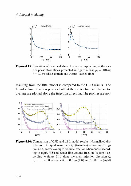
4 Integral modeling
0 10 20 30−2
0
2
4
6
8x 10
4 drag force
ξ [mm]0 10 20 30
−1
0
1
2
3x 10
4 shear force
ξ [mm]
Figure 4.15: Evolution of drag and shear forces corresponding to the car-rier phase flow states presented in figure 4.14a; pc = 10bar;t = 0.3ms (dash-dotted) and 0.5ms (dashed line)
resulting from the ttBL model is compared to the CFD results. Theliquid volume fraction profiles both at the center line and the sectoraverage are plotted along the injection direction. The profiles are nor-
0
0.2
0.4
0.6
0.8
1
0 5 10 15 20
ξξξξ [mm]
Liquid mass density (ttBL)
Center line volume fraction (CFD)
Sector averaged volume fraction (CFD)
0
0.2
0.4
0.6
0.8
1
0 5 10 15 20 25 30
ξξξξ [mm]
Figure 4.16: Comparison of CFD and ttBL model results: Normalized dis-tribution of liquid mass density (triangles) according to fig-ure 4.13, sector averaged volume fraction (diamonds) accord-ing to figure 4.5 and center line volume fraction (squares) ac-cording to figure 3.10 along the main injection direction ξ ;pc = 10bar; flow states at t = 0.3ms (left) and t = 0.5ms (right)
138
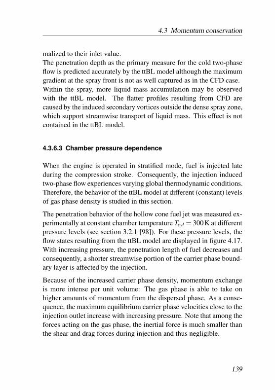
4.3 Momentum conservation
malized to their inlet value.The penetration depth as the primary measure for the cold two-phaseflow is predicted accurately by the ttBL model although the maximumgradient at the spray front is not as well captured as in the CFD case.Within the spray, more liquid mass accumulation may be observedwith the ttBL model. The flatter profiles resulting from CFD arecaused by the induced secondary vortices outside the dense spray zone,which support streamwise transport of liquid mass. This effect is notcontained in the ttBL model.
4.3.6.3 Chamber pressure dependence
When the engine is operated in stratified mode, fuel is injected lateduring the compression stroke. Consequently, the injection inducedtwo-phase flow experiences varying global thermodynamic conditions.Therefore, the behavior of the ttBL model at different (constant) levelsof gas phase density is studied in this section.
The penetration behavior of the hollow cone fuel jet was measured ex-perimentally at constant chamber temperature Tcyl = 300K at differentpressure levels (see section 3.2.1 [98]). For these pressure levels, theflow states resulting from the ttBL model are displayed in figure 4.17.With increasing pressure, the penetration length of fuel decreases andconsequently, a shorter streamwise portion of the carrier phase bound-ary layer is affected by the injection.
Because of the increased carrier phase density, momentum exchangeis more intense per unit volume: The gas phase is able to take onhigher amounts of momentum from the dispersed phase. As a conse-quence, the maximum equilibrium carrier phase velocities close to theinjection outlet increase with increasing pressure. Note that among theforces acting on the gas phase, the inertial force is much smaller thanthe shear and drag forces during injection and thus negligible.
139
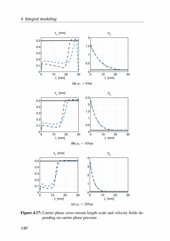
4 Integral modeling
0 10 20 300
0.1
0.2
0.3
0.4
0.5
δτ [mm]
ξ [mm]0 10 20 30
0
0.5
1
1.5
2
Uc
ξ [mm]
(a) pc = 6bar
0 10 20 300
0.1
0.2
0.3
0.4
0.5
δτ [mm]
ξ [mm]0 10 20 30
0
0.5
1
1.5
2
2.5
Uc
ξ [mm]
(b) pc = 10bar
0 10 20 300
0.1
0.2
0.3
0.4
0.5
δτ [mm]
ξ [mm]0 10 20 30
0
1
2
3
4
Uc
ξ [mm]
(c) pc = 20bar
Figure 4.17: Carrier phase cross-stream length scale and velocity fields de-pending on carrier phase pressure
140
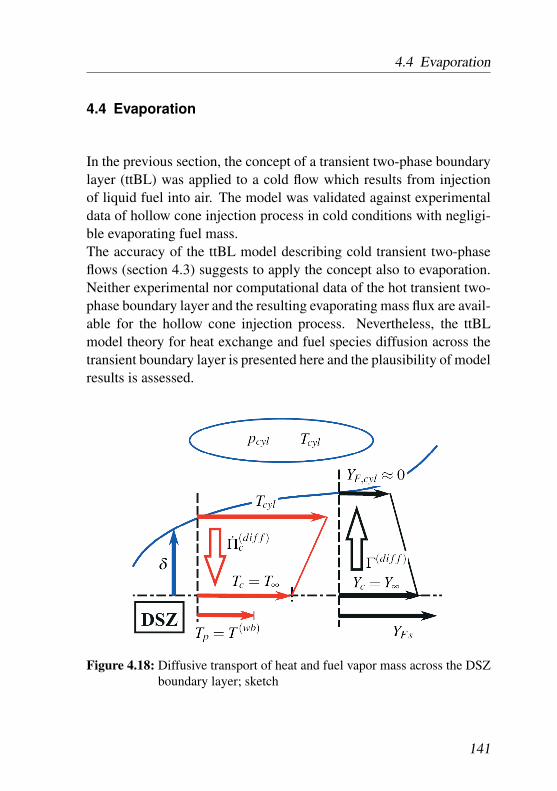
4.4 Evaporation
4.4 Evaporation
In the previous section, the concept of a transient two-phase boundarylayer (ttBL) was applied to a cold flow which results from injectionof liquid fuel into air. The model was validated against experimentaldata of hollow cone injection process in cold conditions with negligi-ble evaporating fuel mass.The accuracy of the ttBL model describing cold transient two-phaseflows (section 4.3) suggests to apply the concept also to evaporation.Neither experimental nor computational data of the hot transient two-phase boundary layer and the resulting evaporating mass flux are avail-able for the hollow cone injection process. Nevertheless, the ttBLmodel theory for heat exchange and fuel species diffusion across thetransient boundary layer is presented here and the plausibility of modelresults is assessed.
Figure 4.18: Diffusive transport of heat and fuel vapor mass across the DSZboundary layer; sketch
141
4 Integral modeling
Consider a boundary layer of thickness δ resulting from injection ofliquid fuel into a combustion chamber according to figure 4.18:The evaporation of the injected liquid fuel is determined by the aver-age thermodynamic state of the gas within the cylinder (pcyl and Tcyl).Across the DSZ boundary layer, both heat and fuel vapor mass aretransported diffusively normal to the main injection direction. Forthe diffusive heat flux Π(di f f )
c , the driving potential is defined by thetemperature difference between the mean gas temperature within thecylinder Tcyl and the gas phase temperature at the DSZ Tc. This tem-perature Tc is modeled to be identical to the far field temperature T∞,which defines the diffusive transport of fuel species mass away fromthe saturated liquid droplet surface in Spalding’s evaporation model.The liquid droplet temperature Tp equals the wet bulb temperatureT (wb).In the same manner, the diffusive mass flux Γ(di f f ) of fuel speciesmass across the boundary layer is approximated. The species concen-tration Yc at the DSZ is again modeled to equal the far field speciesconcentration Y∞ at the droplet level. Fuel species diffusion across theDSZ boundary layer is defined by the difference between the averagefuel vapor species concentration YF,cyl within the cylinder and the fuelspecies mass fraction Yc within the DSZ. YFs is the saturated film massfraction at the droplet surface. In this section, the cylinder thermody-namic state is kept constant and the average fuel species concentrationwithin the cylinder YF,cyl is assumed to be zero (i.e. the mass of aircontained in the cylinder reservoir is assumed to be much larger thanthe injected fuel mass).
Fuel mass fraction transport & saturation state
Since the specific carrier phase mass within the DSZ is equal to thespecific gas phase mass at the DSZ interface ρ(DSZ)
c , the volume spe-cific fuel vapor mass MF within the DSZ carrier phase mass is defined
142
4.4 Evaporation
by the fuel species mass fraction
YF =MF
ρ(DSZ)c
. (4.55)
The conservation of fuel vapor mass MF is accounted for by a transportequation for the average fuel mass fraction YF adjacent to DSZ:
∂YF
∂ t+
∂ (YF Uc)∂ξ
+YF Uc
ξ=
1
ρ(DSZ)c
(Γ(evap)−2 ·Γ(di f f )
)︸ ︷︷ ︸
Γ(net)
. (4.56)
Note that the gas phase density within the dense spray zone ρ(DSZ)c
was assumed to be constant (see section 4.3.3). The factor in the RHSdenominator accounts for the fact that the DSZ is surrounded by twoadjacent carrier phase boundary layers.
According to the physics of evaporating isolated droplets and dropletclouds discussed in detail section 3.1.3, the source term Γ(evap) ineq. (4.56) accounting for evaporating of fuel mass is derived from theflow rate of evaporating fuel mass at the surface of an isolated droplet
Γ(evap)iso = −ρp
∂ (π6 D3
p)∂ t
=π4
ρp Dp βSpald . (3.18)
According to eq. (3.19), the mass flow rate Γ(evap) of Np evaporatingdispersed particles per unit volume is
Γ(evap) = −ρp∂αp
∂ t=
32
βSpald
D2p
Mp (4.57)
where βSpald = 8 ρFsρp
DFs ln(1 + BM) and BM = (YFs −YF)/(1−YFs).The saturation fuel vapor mass fraction is calculated from the partialpressure ps of saturated fuel vapor mixture, which is obtained from
143
4 Integral modeling
the Clausius-Clapeyron relation
YFs =psMs
psMs +(pc − ps)ρ(DSZ)c
and ps = pre f ·exp{
∆hv
Rs
(1
Tre f− 1
Tp
)}.
(3.17)
The source term Γ(di f f ) in eq. (4.56) accounts for the gross diffusivefuel vapor mass flux MFη normal to the main injection direction. Forits approximation it is assumed that outside of the DSZ region, the fuelmass concentration is close to zero (YF∞ = 0) and that the density
Γ(di f f )F = −ρ(DSZ)
c DF∂YF
∂η≈ ρ(DSZ)
c DFYF −YF,cyl
δ (spec)τ
. (4.58)
The length scale δ (spec)τ characterizing the cross-stream species gradi-
ent is assumed to be proportional to the momentum diffusion lengthscale δτ . The proportionality is approximated by means of the Schmidtnumber
Sc =νc
DF≈ δτ
δ (spec)τ
, (4.59)
so that the species diffusion source term is
Γ(di f f )F ≈ ρ(DSZ)
c Sc DFYF −YF,cyl
δτ. (4.60)
The evaporating mass flow rate is limited by both the saturation stateand the fuel species diffusion across the boundary layer. Therefore, themaximum source term for the effective fuel vapor mass flux is definedas
Γ(e f f ) = min{
Γ(evap) ; 2 Γ(di f f )F
}. (4.61)
The factor “2” stems from the fact that the hollow cone sheet is ex-posed to two adjacent boundary layers.
144
4.4 Evaporation
Energy conservation
The temperatures of both phases have to be estimated by the conser-vation of the volume specific internal energy (e = ρ cv T )
∂e∂ t
+∂ (e u)
∂ξ+
e uξ
= − ∂∂ξ
(λc
∂T∂ξ
)+Πe , (4.62)
with the source term Πe accounting for energy consumption duringevaporation. Because of the dominant convective effects occurringwithin the DSZ during the injection process, the streamwise diffusionof thermal energy is neglected. Also the thermal energy productiondue to viscous dissipation is assumed to be small and neglected in thefollowing. Thus, if the heat capacities are assumed to be constant,the dispersed phase energy conservation equation reduces to a simpleconvection-diffusion equation for the temperature
∂ (Mp Tp)∂ t
+∂ (Mp Tp Up)
∂ξ+
Mp Tp Up
ξ=
Πp
Cp, (4.63)
The carrier phase energy conservation equation incorporates the tem-perature diffusive energy flux due to the difference between the DSZ(Tc) and the undisturbed cylinder environment (Tcyl)
∂Tc
∂ t+
∂ (Tc Uc)∂ξ
+Tc Uc
ξ=
1
ρ(DSZ)c Cv,c
(2 ·Π(di f f )
c −Πp
). (4.64)
The heat instantaneously consumed from the evaporating mass fluxΓ(evap) is
Πp = Γ(evap) ∆hv . (4.65)
The cross-stream diffusion flux of carrier phase energy close to theDSZ is approximated from the difference in carrier phase temperature
145
4 Integral modeling
between the DSZ Tc and the reservoir outside of the DSZ Tcyl:
Π(di f f )c = λ (e f f )
c∂Tc
∂η≈ λ (e f f )
cTcyl −Tc
δ (th)τ
. (4.66)
The temperature gradient at the DSZ boundary is approximated by thethermal length scale δ (th)
τ
∂Tc
∂η≈ Tcyl −Tc
δ (th)τ
. (4.67)
The thermal length scale δ (th)τ characterizes the cross-stream temper-
ature gradient. It is modeled to be proportional to the velocity gradi-ent length scale δτ . As proportionality factor between the two lengthscales δτ and δ (th)
τ , the proportionality between the diffusion coeffi-cients of momentum νc and thermal energy λc may be expressed bymeans of the Prandtl number
Pr =ρc Cp νc
λc≈ δτ
δ (th)τ
, (4.68)
so that the diffusion source term reads
Π(di f f )c ≈ Pr λ (e f f )
cTcyl −Tc
δτ. (4.69)
Flux analysis and physical simplifications
In the following, the orders of magnitude of the source terms account-ing for the conservation of species (Γ(evap) and Γ(di f f )
F ) and energy(Π(di f f )
c and Πp) are assessed.Starting from the fully transient description of the droplet heat-up andevaporation process, the dilute spray assumption is shortly discussed,and a third way accounting for the dense spray modeling approach is
146
4.4 Evaporation
presented.
If the complete transient behavior of the two-phase system is to bedescribed, the energy exchange at the droplet surface has to be re-solved [116]. Then, the heat transfer rate towards an isolated droplet
Q(iso)HE =
Nu λDp
πD2p︸︷︷︸
Ap
(Tc −Tp)
leads to the total volume specific heat transfer rate (utilizing Mp =Np
π6 D3
p)§§
QHE = Q(iso)HE Np =
6 Mp Nu λρpD2
p(Tc −Tp) .
Because the specific enthalpy of liquid fuel is much smaller than itsspecific latent heat, the droplet heat-up process occurs much fasterthan the total evaporation process [73]. So for the total evaporationprocess, a thermal equilibrium within the DSZ may be assumed andtransients in the heat transfer at the droplet surface are therefore ne-glected. If the two-phase mixture is locally in thermal equilibrium, thesimilarity assumption between heat and mass diffusion at the dropletsurface is valid so that the temperature difference between both phasesis given by the fuel vapor mass diffusion potential at the droplet sur-
§§ For the non-dimensional heat transfer coefficient (Nusselt number) at thedroplet surface, experimental correlations of spheres exposed to forced convectiveflow have been derived. For the present approximation, a simplified heat transfer lawis adopted [99]:
Nu = 2+(
0.4 Re12p +0.06 Re
23p
)Pr
25c . (4.70)
The carrier phase Prandtl number is set to Prc = 0.7.
147
4 Integral modeling
face (see section 3.1.3)
T (wb) = Tp = Tc − ∆hv
CvBM . (3.22)
The amount at which the temperature of one phase is affected by evap-oration process depends on the ratio of enthalpy densities (ρ pCp/(ρc Cv)between dispersed and carrier phase. Since generally Cp/Cv � ρ p/ρc,the mass density ratio ρ p/ρc is more relevant than the ratio of specificheats.
If e.g. the evaporation at the surface of an isolated droplet is in-vestigated (ρ p/ρc � 1, “dilute spray assumption”), the temperaturechange in the carrier phase environment may be assumed to be smallerthan the temperature change of the droplet (corresponding to a com-paratively big carrier phase internal energy capacity ρc Cv around thedroplet). In that case, the carrier phase temperature far away from thedroplet surface is assumed to be constant (Tc = T∞ = const., ∂Tc
∂ t =0) and the mass diffusion potential (eq. (3.22)) defines the dispersedphase temperature Tp.
By contrast, a local mass loading ρ p/ρc � 1 is observed within theDSZ (“dense spray assumption”). So the dispersed phase experiencesa negligible temperature change (Tp = T (wb) = const., ∂Tp
∂ t = 0) andthe mass diffusion potential (eq. (3.22)) defines the resulting carrierphase temperature Tc within the DSZ. This approach is adopted in thecoarse of this work.
Peclet model
The temporal development of the carrier phase temperature adjacentto the DSZ depends on the ratio of the convective energy flux withinthe DSZ E(conv) along the main injection direction ξ and the diffu-sive energy flux Π(di f f )
c normal to the main injection direction. The
148
4.4 Evaporation
streamwise convective energy flux adjacent to the DSZ
E(conv) = Ic Cv,c Tc = ρc Uc Cv,c Tc (4.71)
corresponds to the carrier phase momentum flux Ic = ρc Uc. The ratioof the area specific energy fluxes resulting from diffusion Π(di f f )
c andconvection E(conv) is identified as a Peclet number for the carrier phasemass adjacent to the DSZ
PeΠ =E(conv)
Π(di f f )c
=δτ ρc Uc Cv,c
λ (e f f )c
Tc
Tcyl −Tc. (4.72)
Consider the limiting cases for a given temperature difference (Tcyl −Tc) > 0 and finite material properties (Cv,c). At finite flow properties(λ (e f f )
c ), PeΠ → 0 for Uc → ∞ (dominance of convective heat trans-fer). On the other hand at limited Uc and effective thermal diffusivityλ (e f f )
c → ∞, PeΠ → ∞ (dominance of diffusive heat transfer). The ef-fective thermal diffusion coefficient subsumes the effects of thermaldiffusivity and mean convective transport due to turbulent fluctuationswithin the carrier phase adjacent to the DSZ.
λ (e f f )c = λc +ρc Cv,c νT (4.73)
When the temporal development of dispersed phase temperature ischaracterized by small time scales, which are not intended to be re-solved by the numerical integration scheme, the carrier phase temper-ature msy be modeled to result from the local ratio between convectiveand diffusive energy fluxes within the carrier phase as quantified by the
149
4 Integral modeling
local carrier phase Peclet number (eq. (4.72)) ¶¶
Tc −T (0)c
Tcyl −T (0)c
=1
1+PeΠwith T (0)
c = T (wb) +∆hv
Cv,cBM (4.74)
The original carrier phase temperature T (0)c is the (apparent) carrier
phase environment temperature corresponding to the current local sat-uration state within the DSZ in the case of zero convection (with thewet bulb temperature T (wb) = Tp). Depending on the carrier phasePeclet number, Tc varies between T (0)
c (dominance of the heat andmass transfer equilibrium around the dispersed phase droplets, Pec →∞) and Tcyl (dominance of carrier phase energy convection adjacent tothe DSZ, Pec → 0).
The energy source term accounts for the gain due to the dispersedphase temperature change and the loss due to evaporating mass.
Πp = Mp Cp
(∂Tp
∂ t
)(HE)
−Γ(evap) Cp Tp (4.75)
The carrier phase has to compensate both the dispersed phase tem-perature change and the latent heat of the evaporating dispersed phase
¶¶ The utilization of a Peclet number to approximate the contribution of convectiveand diffusive fluxes can also be applied to the fuel species transport:
PeΓ =m(conv)
Γ(di f f ) ≈ Uc
DF
δτYF −YF,cyl
withYF −Y (0)
F
YF,cyl −Y (0)F
=1
1+PeΓ.
150
4.4 Evaporation
mass flux Γ(evap).
Πc = ρ(DSZ)c Cv,c
(∂Tc
∂ t
)(HE)
−Mp Cp
(∂Tp
∂ t
)(HE)
−Γ(evap) ∆hv
(4.76)
This approach provides an alternative to the estimation of the carrierphase temperature Tc within the DSZ. Nevertheless, the dense sprayassumption presented above is utilized in the following results section.
Results
In the following, the treatment of evaporation within the transient two-phase boundary layer (ttBL) model proposed above is assessed.
In a two-phase boundary layer, the diffusive rate of heat transfer to-wards and of evaporating fuel vapor species away from the jet centeris dominated by the characteristic cross-stream length scale. Duringinjection, the cross-stream length scale is predominantly the result ofmomentum exchange between both phases and consequential (excess)entrainment of carrier phase from the far field towards the jet center.By contrast, the influence of the magnitude of the energy and massfluxes across the boundary layer on the development of the bound-ary layer thickness is smaller than the influence of the boundary layerthickness on the cross-stream diffusion fluxes. As a result, the interac-tion of streamwise momentum transport with mass and energy cross-stream transfer may be characterized as a one-way coupled system:Momentum exchange does influence the evaporation process, and theinfluence of evaporation on the local rates of momentum exchange isnegligible. For this reason, transient droplet cloud heat-up and evapo-ration within the injection induced boundary layer is the focus of thissection, while the reverse mechanism is neglected.
The transient response of liquid phase temperature and fuel vapormass fraction (equations (4.56) and (4.63)) to the cross-stream dif-fusion fluxes is studied in the following. In order to separate the
151
4 Integral modeling
diffusion contribution from fluxes due to temporal variations in thecross-stream length scale (which are primarily caused by injectioninduced momentum exchange), a constant streamwise profile of thecross-stream length scale
δτ(x, t) = 0.1mm+0.002 · x and Uc(x, t) = 100m/s (4.77)
is assumed. The initial conditions for the temperatures of both phasesand the fuel species mass fraction are
t = 0 : Tp(t = 0) = 20 ◦C , Tc = T ∞c (x, t) = 300 ◦C , and YF = 0 .
(4.78)Figure 4.19 shows streamwise temperature profiles during evapora-
tion due to thermal diffusion from the comparatively warm “cylinderinfinity” environment towards the dense spray zone (DSZ). The satu-ration state at the liquid surface is defined by the dispersed phase tem-perature (infinite liquid conductivity model). Because of the zero gasphase capacity within the DSZ, the temperature Tc instantaneously de-creases to the corresponding gas phase equilibrium temperature. Be-cause of the large temperature difference between liquid phase and theenvironment (and the small cross-stream length scale which charac-terizes the temperature gradient), thermal energy is transfered towardsthe DSZ and the liquid phase starts warming up (figure 4.19a). Thestreamwise gradient in the cross-stream length scale profile causes theenergy flux to be comparatively large in areas of small cross-streamlength scale, i.e. for x → 0.
As the liquid phase warms up, an equilibrium between thermal en-ergy diffusion across the boundary layer and the evaporation processis approached (figure 4.19b): At this thermodynamic state, the energyflux diffusively transported towards the DSZ is equal to the latent heatflux consumed by the evaporating mass flux (which is again definedby the liquid phase temperature). Note that this state is dominatedby the “cylinder infinity” temperature T ∞
c and the influence of stream-
152
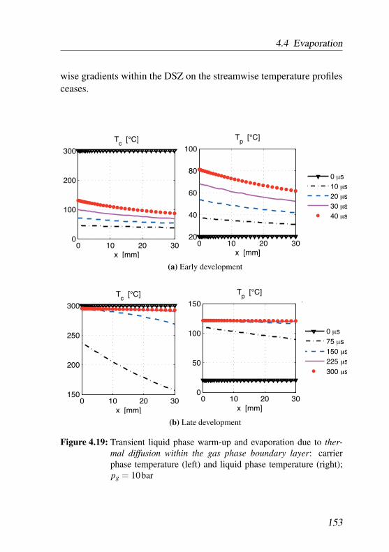
4.4 Evaporation
wise gradients within the DSZ on the streamwise temperature profilesceases.
0 10 20 300
100
200
300
Tc [°C]
x [mm]
0 10 20 3020
40
60
80
100
Tp [°C]
x [mm]
= 0;0) = 0;1
0 µs10 µs20 µs30 µs40 µs
(a) Early development
0 10 20 30150
200
250
300
Tc [°C]
x [mm]
0 10 20 300
50
100
150
Tp [°C]
x [mm]
1
= 0;0) = 0;1
0 µs75 µs150 µs225 µs300 µs
(b) Late development
Figure 4.19: Transient liquid phase warm-up and evaporation due to ther-mal diffusion within the gas phase boundary layer: carrierphase temperature (left) and liquid phase temperature (right);pg = 10bar
153
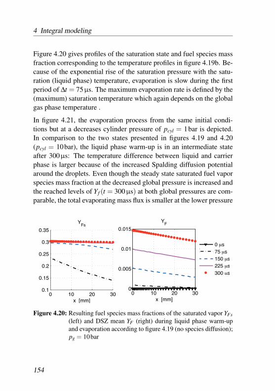
4 Integral modeling
Figure 4.20 gives profiles of the saturation state and fuel species massfraction corresponding to the temperature profiles in figure 4.19b. Be-cause of the exponential rise of the saturation pressure with the satu-ration (liquid phase) temperature, evaporation is slow during the firstperiod of ∆t = 75µs. The maximum evaporation rate is defined by the(maximum) saturation temperature which again depends on the globalgas phase temperature .
In figure 4.21, the evaporation process from the same initial condi-tions but at a decreases cylinder pressure of pcyl = 1bar is depicted.In comparison to the two states presented in figures 4.19 and 4.20(pcyl = 10bar), the liquid phase warm-up is in an intermediate stateafter 300µs: The temperature difference between liquid and carrierphase is larger because of the increased Spalding diffusion potentialaround the droplets. Even though the steady state saturated fuel vaporspecies mass fraction at the decreased global pressure is increased andthe reached levels of Yf (t = 300µs) at both global pressures are com-parable, the total evaporating mass flux is smaller at the lower pressure
0 10 20 300.1
0.15
0.2
0.25
0.3
0.35
YFs
x [mm]0 10 20 30
0
0.005
0.01
0.015
YF
x [mm]
= 0;0) = 0;1
0 µs75 µs150 µs225 µs300 µs
Figure 4.20: Resulting fuel species mass fractions of the saturated vapor YFs(left) and DSZ mean YF (right) during liquid phase warm-upand evaporation according to figure 4.19 (no species diffusion);pg = 10bar
154
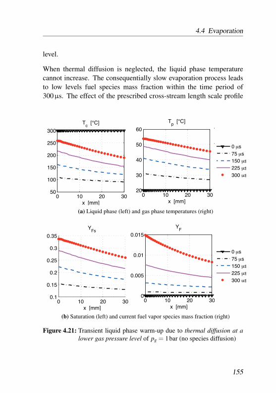
4.4 Evaporation
level.
When thermal diffusion is neglected, the liquid phase temperaturecannot increase. The consequentially slow evaporation process leadsto low levels fuel species mass fraction within the time period of300µs. The effect of the prescribed cross-stream length scale profile
0 10 20 3050
100
150
200
250
300
Tc [°C]
x [mm]
0 10 20 3020
30
40
50
60
Tp [°C]
x [mm]
1
1
= 0;0) = 0;1
0 µs75 µs150 µs225 µs300 µs
(a) Liquid phase (left) and gas phase temperatures (right)
0 10 20 300.1
0.15
0.2
0.25
0.3
0.35
YFs
x [mm]0 10 20 30
0
0.005
0.01
0.015
YF
x [mm]
= 0;0) = 0;1
0 µs75 µs150 µs225 µs300 µs
(b) Saturation (left) and current fuel vapor species mass fraction (right)
Figure 4.21: Transient liquid phase warm-up due to thermal diffusion at alower gas pressure level of pg = 1bar (no species diffusion)
155
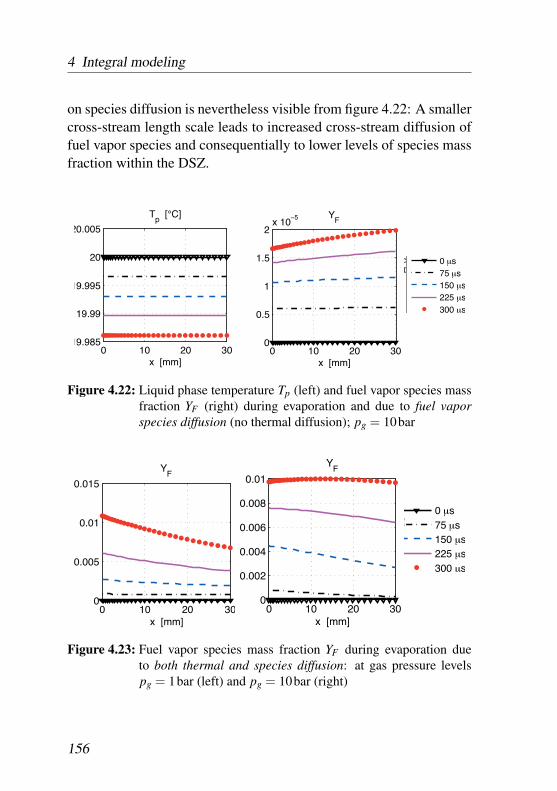
4 Integral modeling
on species diffusion is nevertheless visible from figure 4.22: A smallercross-stream length scale leads to increased cross-stream diffusion offuel vapor species and consequentially to lower levels of species massfraction within the DSZ.
0 10 20 3019.985
19.99
19.995
20
20.005
Tp [°C]
x [mm]0 10 20 30
0
0.5
1
1.5
2x 10
−5 YF
x [mm]
c) = 0;0Tc) = 1;0
0 µs75 µs150 µs225 µs300 µs
Figure 4.22: Liquid phase temperature Tp (left) and fuel vapor species massfraction YF (right) during evaporation and due to fuel vaporspecies diffusion (no thermal diffusion); pg = 10bar
0 10 20 300
0.005
0.01
0.015
YF
x [mm]0 10 20 30
0
0.002
0.004
0.006
0.008
0.01
YF
x [mm]
= 0;0) = 1;1
0 µs75 µs150 µs225 µs300 µs
Figure 4.23: Fuel vapor species mass fraction YF during evaporation dueto both thermal and species diffusion: at gas pressure levelspg = 1bar (left) and pg = 10bar (right)
156
4.4 Evaporation
Allowing both thermal and species cross-stream diffusion results inthe fuel species streamwise profiles presented in figure 4.23: For bothglobal pressure levels, the additional effect of fuel species diffusionreduces the values of YF at t = 300µs and x ≈ 0 from YF ≈ 0.015 byabout 30%.
157
4 Integral modeling
4.5 Turbulence
Because the local cross-stream gradient of the carrier phase velocityis considered to have a major influence on the overall penetration be-havior of the hollow cone spray (section 4.3.2), also cross-stream dif-fusion of streamwise momentum due to turbulent fluctuations has tobe expected to increase cross-stream transport.Close to the injector, the local boundary layer thickness should be ofthe order of the injector exit cross-section length scale. Due to theinitially small boundary layer thickness, the boundary layer flow islikely to be laminar at the injection outlet.∗∗∗ On the other hand, thepresence of small liquid droplets introduces disturbances to the carrierphase flow and may promote the onset of turbulence.If turbulent fluctuations do first occur, their intensity is heavily pro-moted by the strong cross-stream gradients within the mean carrierphase velocity profile. Because the mean diffusive effect of turbulenceis orders of magnitude larger than the molecular viscosity and cross-stream diffusion of streamwise momentum is considered in the presentmodel (see section 4.3), a simple turbulence model is incorporated.
Recall that according to the turbulent gradient diffusion hypothesis,the diffusive flux ⟨
u jΦ⟩
= −DT∂ 〈Φ〉∂x j
(4.79)
due to fluctuations of the scalar quantity Φ is approximated [93]. In
∗∗∗For example at a maximum injector exit speed of 200m/s and a maximum in-jector opening half width of about 15µm, only a Reynolds number of the order of1.5 ·105 is reached.
158
4.5 Turbulence
the Reynolds averaged momentum equation
D 〈Ui〉Dt
=∂
∂x j
[− 1
ρ〈p〉 δi j +
µρ
Si j −⟨uiu j⟩]
with Si j =12
(∂ 〈Ui〉∂x j
+∂⟨Uj⟩
∂xi
) (4.80)
an additional term resulting from the fluctuating velocity component– the Reynolds stress tensor
⟨uiu j⟩
– occurs. The turbulent viscos-ity hypothesis states that the deviatoric stress due to turbulent fluc-tuations (the anisotropic part of the Reynolds stress tensor
⟨uiu j⟩) is
determined by the local mean rate of strain in terms of a linear rela-tion [124]:
−⟨uiu j⟩+
23
k δi j = 2 νT Si j . (4.81)
The turbulent viscosity (or turbulent exchange coefficient for momen-tum) is determined by a combination of a characteristic length LT andvelocity UT :
νT = LT UT . (4.82)
In the context of large eddy simulation, Smagorinski [117] models thetransport of turbulent eddies which are not spatially resolved by meansof a sub-grid turbulent viscosity
ν(SG)T = l2
m
√2 S2
i j . (4.83)
The maximum length scale which may locally occur and not be spa-tially resolved is defined by the local filter width ∆ characterizing thegrid cell size
lm = CSmag ∆ . (4.84)
This is identical to the application of a mixing length model (zero
159
4 Integral modeling
equation turbulence model).
νT = l2m
∣∣∣∣∂U∂y
∣∣∣∣ (4.85)
In the context of the presented boundary layer model, the local gradi-ent could be approximated by the length scale LT = lm = δτ and thevelocity scale UT = Uc, so that the turbulent viscosity would be
νT = δτ Uc (4.86)
and the rate of change of local boundary layer thickness due to turbu-lent viscosity (
∂δτ
∂ t
)T
=νT
δτ(4.87)
would simply come out to be(
∂δτ∂ t
)T
= Uc: Due to turbulent fluctu-
ations, the temporal change of the boundary layer thickness δτ wouldbe of the order of the streamwise convective velocity. This is a simplebut too simplifying description of turbulent diffusivity effect since theturbulent diffusion would be over-estimated.
More detail is introduced by applying a one-equation turbulence modeland solving a transport equation for the turbulent kinetic energy k [93].
k =12〈uiui〉 (4.88)
∂k∂ t
+∂ (k u j)
∂x j=
∂∂x j
(νT
PrT
∂k∂x j
)+Pk − εk (4.89)
In only one spatial dimension (ξ ) and cone coordinates, the conserva-
160
4.5 Turbulence
tion equation at the presumed spray center line reads
∂k∂ t
+∂ (k Uc)
∂ξ+
k Uc
ξ=
∂∂ξ
(νT
PrT
∂k∂ξ
)︸ ︷︷ ︸
ΠνT
+Pk − εk . (4.90)
The turbulent viscosity νT , the shear induced rates of production Pkand dissipation εk are quantified with appropriate model constantsstemming from experiments [93] (see table 4.3).
νT = Cµk2
ε= ct lm k1/2 (4.91)
Pk = νT
(∂U∂η
)2
(4.92)
εk =Cµ k3/2
ct lm(4.93)
The length scale lm (which is intrinsic to the one-equation model de-scribed above and fixes the ratio of the level of turbulent kinetic energyand its dissipation rate)
lm =Cµ
ct
k3/2
εk(4.94)
has to be specified a priori. Here it is assumed that the local lengthscale lm corresponds to the cross-stream length scale δτ . The localcross-stream gradient in the production is again approximated with
161
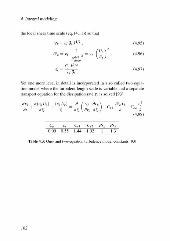
4 Integral modeling
the local shear time scale (eq. (4.11)) so that
νT = ct δτ k1/2 , (4.95)
Pk = νT1
T(c)
shear
2 = νT
(Uc
δτ
)2
, (4.96)
εk =Cµ k3/2
ct δτ. (4.97)
Yet one more level in detail is incorporated in a so called two equa-tion model where the turbulent length scale is variable and a separatetransport equation for the dissipation rate εk is solved [93].
∂εk
∂ t+
∂ (εk Uc)∂ξ
+(εk Uc)
ξ=
∂∂ξ
(νT
Prε
∂εk
∂ξ
)+Cε1
Pk εk
k−Cε2
ε2kk
(4.98)
Cµ ct Cε1 Cε2 Prk Prε0.09 0.55 1.44 1.92 1 1.3
Table 4.3: One- and two-equation turbulence model constants [93]
162
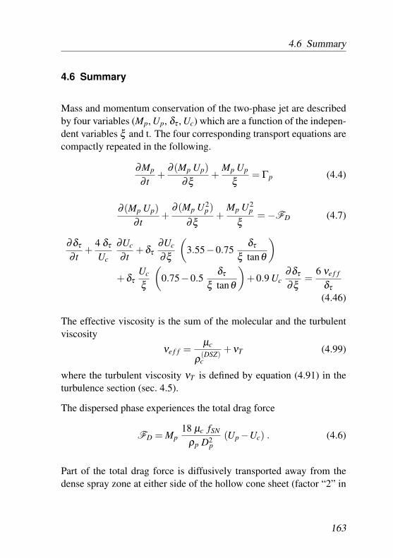
4.6 Summary
4.6 Summary
Mass and momentum conservation of the two-phase jet are describedby four variables (Mp, Up, δτ , Uc) which are a function of the indepen-dent variables ξ and t. The four corresponding transport equations arecompactly repeated in the following.
∂Mp
∂ t+
∂ (Mp Up)∂ξ
+Mp Up
ξ= Γp (4.4)
∂ (Mp Up)∂ t
+∂ (Mp U2
p)∂ξ
+Mp U2
p
ξ= −FD (4.7)
∂δτ
∂ t+
4 δτ
Uc
∂Uc
∂ t+δτ
∂Uc
∂ξ
(3.55−0.75
δτ
ξ tanθ
)
+δτUc
ξ
(0.75−0.5
δτ
ξ tanθ
)+0.9 Uc
∂δτ
∂ξ=
6 νe f f
δτ(4.46)
The effective viscosity is the sum of the molecular and the turbulentviscosity
νe f f =µc
ρ(DSZ)c
+νT (4.99)
where the turbulent viscosity νT is defined by equation (4.91) in theturbulence section (sec. 4.5).
The dispersed phase experiences the total drag force
FD = Mp18 µc fSN
ρp D2p
(Up −Uc) . (4.6)
Part of the total drag force is diffusively transported away from thedense spray zone at either side of the hollow cone sheet (factor “2” in
163
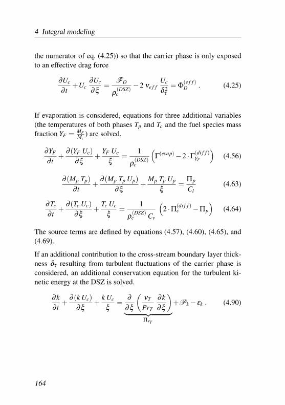
4 Integral modeling
the numerator of eq. (4.25)) so that the carrier phase is only exposedto an effective drag force
∂Uc
∂ t+Uc
∂Uc
∂ξ=
FD
ρ(DSZ)c
−2 νe f fUc
δ 2τ
= Φ(e f f )D . (4.25)
If evaporation is considered, equations for three additional variables(the temperatures of both phases Tp and Tc and the fuel species massfraction YF = MF
Mc) are solved.
∂YF
∂ t+
∂ (YF Uc)∂ξ
+YF Uc
ξ=
1
ρ(DSZ)c
(Γ(evap)−2 ·Γ(di f f )
YF
)(4.56)
∂ (Mp Tp)∂ t
+∂ (Mp Tp Up)
∂ξ+
Mp Tp Up
ξ=
Πp
Cl(4.63)
∂Tc
∂ t+
∂ (Tc Uc)∂ξ
+Tc Uc
ξ=
1
ρ(DSZ)c Cv
(2 ·Π(di f f )
c −Πp
)(4.64)
The source terms are defined by equations (4.57), (4.60), (4.65), and(4.69).
If an additional contribution to the cross-stream boundary layer thick-ness δτ resulting from turbulent fluctuations of the carrier phase isconsidered, an additional conservation equation for the turbulent ki-netic energy at the DSZ is solved.
∂k∂ t
+∂ (k Uc)
∂ξ+
k Uc
ξ=
∂∂ξ
(νT
PrT
∂k∂ξ
)︸ ︷︷ ︸
ΠνT
+Pk − εk . (4.90)
164
5 Conclusion
In this thesis hollow cone sprays are investigated. A thorough discus-sion of both two-phase flow physics as well as available models and aboundary layer assessment of the hollow cone flow is carried out (sec-tion 2). Based on an experimentally validated CFD model, the two-phase flow induced by the injection is characterized (section 3) beforethe main findings are utilized to derive a simplified spray model. Fi-nally, its behavior (namely momentum exchange and evaporation) atconstant global thermodynamic conditions is studied (section 4).
The vast range of physical length and time scales incorporated in in-ternal combustion engines for automotive applications necessitates thedevelopment of simplified models for injection processes. For directinjecting gasoline engines applying multiple injections per workingcycle, the need of a transient and one-dimensional spray model is es-tablished (section 2.3). The assessment of the hollow cone boundarylayer shows that the second order cross-stream term dominates theviscous terms (section 2.4.1).
The analysis of the experimentally validated CFD model reveals thatcomparatively simple physical models (Eulerian dispersed phase treat-ment with only one particle size class) sufficiently describe flow char-acteristics such as the global penetration of the dispersed phase andthe induced carrier phase velocity field outside the dense hollow conespray very well (section 3.2.2 ).The strong acceleration of the carrier phase due to injected liquid fuelinduces cross-stream velocity profiles similar to those resulting froman accelerated wall (section 3.2.3). Even when turbulent effects suchas a turbulent dispersion force on the liquid phase lead to broader
5 Conclusion
cross-stream profiles, this flow pattern is maintained, especially closeto the injection outlet. The resulting shear forces limit the accelera-tion of the carrier phase, which is directly exposed to the dispersedphase. As a result, the injection induced carrier phase boundary layeris crucial for the evolution of the momentum exchange along the maininjection direction and the global penetration depth.Due to the non-symmetric environment of the dense spray elements,a flow pattern develops which is non-symmetric with respect to thehollow cone geometry. Nevertheless, the injection direction – whichis prescribed by the injector design – is found to be the dominant flowdirection, also at positions further away from the injection outlet (sec-tion 3.2.4).
A simplified spray model for hollow cone sprays is presented. It isbased on the main two-phase characteristics first introduced in sec-tion 2 and supported by the CFD analysis (section 3.2). According tothe discussed requirements of engine system simulation, the descrip-tion is
• two-phase, i.e. no mixture model assumption is applied, butmomentum as well as energy conservation are covered for eachphase by separate transport equations;
• transient, i.e. the response to time-invariant boundary condi-tions is implicitly described (the conservation equations containtemporal rates of change of the conserved variables);
• one-dimensional, i.e. fluxes along the main injection directionare accounted for (the description contains the steamwise gradi-ents of the conserved variables).
As the first major modeling step, the model employs the property ofthe “accelerated wall” type cross-stream velocity profile: With respectto the carrier phase, the dispersed phase mass is modeled to occupya cross-stream width approaching zero (the “dense spray zone” DSZ,section 4.3.1). The second most distinctive modeling part is the deriva-
166
tion of a transport equation for the cross-stream length scale, which ischaracteristic to the mean diffusion rate of mass, momentum, and en-ergy in the cross-stream direction (section 4.3.3).
The proposed transient two-phase boundary layer (ttBL) model is firstassessed with respect to momentum conservation transport. The modelproduces the well known square root shape of the streamwise bound-ary layer profile for a single phase jet (section 4.3.6.1).For the injection induced two-phase flow (section 4.3.6.2), the contrac-tion term in the transport equation for the cross-stream length scale(accounting for “excess entrainment” of carrier phase mass into thedense spray region) limits the cross-stream growth of the boundarylayer. The temporal development of the spray front position depend-ing on the global thermodynamic state of the carrier phase correspondsto the experimental data (section 4.3.6.3).The modeling assumption of a characteristic cross-stream length scaleis also applied to both thermal energy diffusion towards and fuel vaporspecies diffusion away from the dense spray region (section 4.4). Theresults provide a qualitative insight into the (due to the saturation statewithin the DSZ) highly non-linear evolution of liquid phase warm-upand fuel species concentration.
The proposed ttBL model constitutes a new approach to two-phaseflow modeling of dense sprays: It extends the commonly applied Schiller-Naumann drag law and the Spalding evaporation model. The carrierphase fluxes of momentum, thermal energy, and fuel species are pri-marily controlled by diffusion through the boundary layer adjacent tothe dense spray. While the model is applied to a one-dimensional de-scription here, it may well serve as a sub-grid model to multi-dimensionalflow simulation models.
While in general, the predictions of the ttBL model are in good agree-ment with experimental data, some discrepancies may be observed:The velocity magnitude of convective transport within the carrier phaseduring injection obtained by the ttBL model is comparatively low. Al-
167
5 Conclusion
though measurements of the “true” carrier phase velocity in regionsof highest dispersed phase volume loading are not available, increasedmagnitudes of carrier phase velocity (such as observed from the CFDresults in section 3.2.4) should be expected.The low carrier phase velocity magnitudes result from the small cross-stream length scales characterizing the shear force. They again area result of the “excess entrainment” term in the cross-stream lengthscale transport equation; and the weights of the terms in the transportequation result from the presumed cross-stream profile shape and theupper integration limit applied in section 4.3.3. During the derivationof the model both have been intuitively chosen (i.e. a Taylor seriesexpansion of second order as the most general profile shape featuringa non-zero curvature and a spatial integration over just the length scalewhich is modeled).
Further attention may focus on both the CFD modeling and the one-dimensional model: When further analyzing evaporation by means ofCFD, more detail will have to be incorporated, especially the con-sideration of poly-dispersion. Since smaller particles are also moreaffected by turbulent fluctuations, turbulence effects will need to beinvestigated in more detail. The proposed ttBL model requires fur-ther development. As next steps, the model’s sensitivity to turbulenceeffects, the choice of the cross-steam length scale measure characteriz-ing the cross-stream diffusion, and its ability to appropriately describethe diffusion of energy and species mass require future attention.
168
Bibliography
[1] Abraham, J.: What is adequate resolution in the numerical com-putations of transient jets? SAE Paper 970051, 1997.
[2] Abramovich, G.: The theory of turbulent jets. M.I.T. Press,1963.
[3] Adomeit, Ph. and S. Pischinger and: Analysis of cyclic fluctua-tions of charge motion and mixture formation in a DISI enginein stratified operation. SAE Paper 2007-01-1412, 2007.
[4] Anderson, J.: Computational Fluid Dynamics. Mcgraw-Hill,1995.
[5] Ansys, Inc.: Ansys cfx solver, release 10.
[6] Apte, S., K. Maheshy, and T. Lundgren: A Eulerian-Lagrangianmodel to simulate two-phase/particulate fows. In Center forTurbulence Research, 2003.
[7] Aramburo, E.: A new methodology for modelling impingingsprays based on drop size moments. PhD thesis, Univ. Manch-ester, 2004.
[8] Atkins, P. and J de Paula: Physical chemistry. Oxford Univ.Press, 2006.
[9] Atthasit, A.: Etude experimentale des phenomenesd’interaction dans les jet diphasiques denses au moyende jets rectilihnes momodisperses. PhD thesis, L’ecolenationale superieure de l’aeronautique et de l’espace, 2003.
Bibliography
[10] Automotive, Continental: Spray characterization of two piezo-injectors for different fuels using multiple optical measurementtechniques. Internal communication, 2007.
[11] Batchelor, G.: An introduction to fluid dynamics. CambridgeMath. Library, 2000.
[12] Baumgarten, C.: Mixture Formation in Internal CombustionEngines. Springer, 2006.
[13] Baumgarten, C., J. Stegemann, and G. Merker: A new modelfor cavitation induced primary breakup of Diesel sprays. Proc.18th ILASS Europe, pages 15 – 20, 2002.
[14] Beck, J.: Computational modelling of polydisperse sprays with-out segregation into droplet size classes. PhD thesis, Univ.Manchester, 2000.
[15] Beck, J. and A. Watkins: On the development of spray submod-els based on droplet size moments. J. Comp. Phys., 182:586 –621, 2002.
[16] Beck, J. and A. Watkins: The droplet number moments ap-proach to spray modelling: The development of heat and masstransfer sub-models. Int. J. Heat Fluid Flow, 24:242 – 259,2003.
[17] Beck, J. and A. Watkins: On the development of a spraymodel based on drop-size moments. Proc. Roy. Soc. London,459:1365 – 1394, 2003.
[18] Bocksell, T. and E. Loth: Random walk models for particle dif-fusion in free-shear flows. AIAA Journal, 39:1086 – 1096,2001.
[19] Boivin, M., O. Simonin, and K. Squires: Direct numerical sim-ulation of turbulence modulation by particles in isotropic tur-bulence. J. Fluid Mech., 375:235 – 263, 1998.
170
Bibliography
[20] Bollweg, P. and A. Kaufmann: Dynamic burn rate modeling forthe 1D simulation of a gdi engine in homogeneous and stratifiedoperation mode. SAE Int. J. Engines, 1(1):1045 – 1056, 2008.
[21] Bollweg, P., A. Kaufmann, and W. Polifke: Derivation and ap-plication of a poly-celerid method for poly-dispersed two-phaseflows. In 6th International Conference Multiphase Flow, 2007.
[22] Brennen: Fundamentals of Multiphase Flow. Cambridge Univ.Pr., 2005.
[23] Brown, D. and E. Kauppinen: A method of moments based cfdmodel for polydisperse aerosol flows with strong interphasemass and heat transfer. Comp. Fluids, 35:762 – 780, 2006.
[24] Burns, A., T. Frank, . Hamill, and J. Shi: The Favre averageddrag model for turbulent dispersion in Eulerian multi-phaseflows. In Int. Conf. on Multiphase Flow, 2004.
[25] Carvalho, I., M. Heitoyr, and D. Santos: Liquid film disintegra-tion. Int. J. Multiphase Flow, 28:773 – 789, 2002.
[26] Castagné, M., E. Chevé, J. Dumas, and S. Henriot: Advancedtools for analysis of gasoline direct injection engines. SAEPaper 2000-01-1903, 2000.
[27] Chapman, S. and T. Cowling: The mathematical theory of non-uniform gases. Cambridge Univ. Press, 1970.
[28] Chryssakis, C., K. Driscoll, and V. Sick ad D. Assanis: Vali-dation of an enhanced liquid sheet atomozation model againstquantitative laser diagnostic measurements. In ILASS Europe,2002.
[29] Chryssakis, Ch., D. Assanis, J. Lee, and K. Nishida: Fuel spraysimulation of high-pressure swirl-injector for disi engines andcomparison with laser diagnostic measurements. SAE Paper2003-01-0007, 2003.
171
Bibliography
[30] Colin, O., F. Ducros, and D. Veynante: A thickened flame modelfor large eddy simulations of turbulent premixed combustion.Phys. Fluids, 12, 2000.
[31] Cossali, G.: An integrated model for gas entrainment into fullcone sprays. J. Fluid Mech., 439:353 – 366, 2001.
[32] Cousin, J. and H. Nuglisch: Modeling of internal flow in highpressure swirl injectors. SAE Paper 2001-01-0963, 2001.
[33] Crowe, C.: On models for turbulence modulation in fluid-particle flows. Int. J. Multiphase Flow, 26:719 – 727, 2000.
[34] Crowe, C., M. Sommerfeld, and Y. Tsuji: Multiphase Flowswith Droplets and Particles. CRC Press, 1998.
[35] da Pinna, A. and G. Corbinelli: Measurement of the penetraiondepth of a hollow cone spray in a constant pressure chamber.Internal Communication, Siemens AG, 2004.
[36] de Francqueville, L., B. Thirouard, V. Ricordeau, J. Cherel, andL. Hermant: Experimental investigation of the air entrainmentcharacteristics within the periphery of a gasoline direct injec-tion (GDI) spray by PIV. In ILASS Americas, 2005.
[37] de Luca, L. and M. Costa: Instability of a spatially developingsheet. J. Fluid Mech., 337:127 – 144, 1997.
[38] Deen, N. and J. Kuipers: Numerical simulation of dense gas-particle flows using the Euler-Lagrange approach. Prog. Comp.Fluid Dynamics, 7, 2007.
[39] Delay, G.: Analyse des ecoulements transitoires dans les sys-temes d’injection directe essence effets sor l’entainement d’airinstationnaire du spray. PhD thesis, INP Toulouse, 2005.
[40] Delay, G., A. Arbeau, R. Bazile, and G. Charnay: Experimen-tal analysis of density effects on air entrainment in Diesel andgasoline dense sprays by PIV on fluorescent dyes. In 6th World
172
Bibliography
Conference on Experimental Heat Transfer, Fluid Mechanics,and Thermodynamics, 2005.
[41] Delay, G., R. Bazile, G. Charnay, and H. Nuglisch: Couplingbetween instantaneous liquid flow rate and transient air en-trainment for GDI sprays. In 3rd International symposium ontwo-phase flow modeling and experimentation, 2004.
[42] Delay, G., R. Bazile, G. Charnay, and H. Nuglisch: Temporaldependency of air entrainement to liquid flow rate variationsfor gasoline direct injection sprays. In 12th International Sym-posium on Applications of Laser Techniques to Fluid Mechan-ics, 2004.
[43] Desjardins, O., R. Fox, and P. Villedieu: A quadrature-basedmoment closure for the Williams spray equation. In Center forTurbulence Research, 2006.
[44] Domingo, P., L. Vervisch, and J. Réveillon: Dns analysis ofpartially premixed combustion in spray and gaseous turbulentflame-bases stabilized in hot air. Combust. Flame, 140 (3):172– 195, 2005.
[45] Drew, D. and S. Passman: Theory of Multicomponent Fluids.Springer, New York, 1999.
[46] Elghobashi, S. and T. Abou-Arab: A two-equation turbulencemodel for two-phase flows. Phys. Fluids, 26:931 – 938, 1983.
[47] Elghobashi, S. and G. Truesdell: On the two-way interactionbetween homogeneous turbulence and dispersed solid particles.i: Turbulence modification. Phys. Fluids, 7:1790 – 1801, 1993.
[48] Fan, R., D. Marchisio, and R. Fox: Application of the directquadrature method of moments to polydisperse gas-solid flu-idized beds. Powder Technology, 139:7 – 20, 2004.
[49] Fefferman, C.: Existence and smoothness of theNavier-Stokes equations (official problem descrip-
173
Bibliography
tion). In http://www.claymath.org/millennium/Navier-Stokes_Equations/navierstokes.pdf (Clay Mathematics Insti-tute), 2008.
[50] Ferry, J. and S. Balachandar: A fast Eulerian method for dis-perse two-phase flow. Int. J. Multiphase Flow, 27:1199 – 1226,2001.
[51] Ferry, J. and S. Balachandar: Equilibrium expansion for the Eu-lerian velocity of small particles. Powder Technol., 125:131 –139, 2002.
[52] Ferziger, J. and M. Peric: Computational Methods for Fluid Dy-namics. Springer, 2002.
[53] Fevrier, P. and O. Simonin: Constitutive relations for fluid-particle velocity correlations in gas-solid turbulent flows. InInt. conf. on multiphase flows, 1998.
[54] Fornberg, B.: Generation of finite difference formulas onarbitrarily spaced grids. Mathematics of Computation,51(184):699 – 706, 1988.
[55] Fornberg, B.: Calculation of weights in finite difference formu-las. Society of industrial and Applied Mathematics Review,40(3):685 – 691, 1998.
[56] Gharaibah, E., M. Brandt, and W. Polifke: Numerical modelof dispersed two phase flow in aerated stirred vessels basedon presumed shape number density functions. In Proc. of theGerman-Japanese Workshop on Multi-Phase Flow, 2002.
[57] Han, Z., L. Fan, and R.D. Reitz: Multidimensional modelingof spray atomization and air-fuel mixing in a direct-injectionspark-ignition engine. SAE Paper, (970884), 1997.
[58] Hentschel, W., A. Homburg, G. Ohmstede, T. Müller, andG. Grünefeld: Investigation of spray formation of DI gasoline
174
Bibliography
hollow-cone injectors inside a pressure chamber and a glassring engine by multiple optical techniques. SAE Paper 1999-01-3660, 1999.
[59] Heywood, J.: Internal combustion engine fundamentals.McGraw-Hill, 1988.
[60] Hieber, D.: An investigation of the mesh dependence of thestochastic discrete droplet model applied to dense liquid sprays.Master’s thesis, Michigan Techn. University, 2001.
[61] Hiroyasu, H.: Break-up length of a liquid jet and internal flowin a nozzle. In ICLASS-91, 1991.
[62] Hiroyasu, H., T. Kadota, and M. Arai: Development and use ofa spray combustion model to predict Diesel engine efficiencyand pollutant emissions. JSME, 26:569 – 583, 1983.
[63] Hirsch, C.: Numerical Computation of Internal and ExternalFlows, volume 2: Computational Methods for Inviscid and Vis-cous Flows. John Wiley & Sons, New York, 1990.
[64] Hunt, J., A. Wray, and P. Moin: Eddies, stream and conver-gende zones in turbulent flows. In CTR summer program, 1988.
[65] Ishii, M. and T. Hibiki: Thermo-fluid Dynamics of Two-PhaseFlow. Springer, 2005.
[66] Jazayeri, S. and X. Li: Nonlinear instability of plane liquidsheet. J. Fluid Mech., 406:281 – 308, 2000.
[67] Jeong, J. and F. Hussain: On the identification of a vortex. J.Fluid Mech., 285:69 – 94, 1995.
[68] Kaufmann, A.: Towards Eulerian-Eulerian Large Eddy Simu-lation of Reactive Two-Phase Flows. PhD thesis, CERFACS,2004.
175
Bibliography
[69] Kim, I. and W. Sirignano: Three-dimensional wavedistortionand disintegration of thin planar liquid sheets. J. Fluid Mech.,410:147 – 183, 2000.
[70] Kolev, N.: Multiphase Flow Dynamics 1 – Fundamentals.Springer, 2004.
[71] Kouremenos, D., C. Rakopoulos, and D. Hountalas: Multi-zonemodeling for the prediction of pollutant emissions and perfor-mance of DI Diesel engines. SAE Paper 970635, 1997.
[72] Krueger, Chr.: Validierung eines 1D-Spraymodells zur Simu-lation der Gemischbildung in direkteinspritzenden Dieselmo-toren. PhD thesis, RWTH Aachen, 2001.
[73] Kuo, K.: Principles of Combustion. John Wiley & Sons, Inc.,Hoboken, New Jersey, USA, 2005.
[74] Langen, P., T. Melcher, S. Missy, and C. Schwarz: New BMWSix- and Four-Cylinder Petrol Engines with High Precision In-jection and Stratified Combustion. In 28th Int. Vienna EngineSymp., 2007.
[75] Laurent, F., M. Massot, and P. Villedieu: Eulerian multi-fuidmodeling for the numerical simulation of polydisperse denseliquid sprays. J. Comp. Phys., 194:505 – 543, 2004.
[76] Li, X. and R. Tankin: On the temporal instability of a two-dimensional viscous liquid sheet. J. Fluid Mech., 220:425 –443, 1991.
[77] Liepmann, H. and A. Roshko: Elements of gasdynamics. Doverpublications, 1957.
[78] Lin, S., Z. Lian, and B. Creighton: Absolute and convective in-stability of a liquid sheet. J. Fluid Mech., 220:673 – 689, 1990.
[79] Lopez de Bertodano, M.: Two fluid model for two-phase turbu-lent jets. Nuclear engineering and design, 179:65 – 74, 1998.
176
Bibliography
[80] Loth, E.: An Eulerian turbulent diffusion model for particlesand bubbles. Int. J. Multiphase Flow, 27:1051 – 1063, 2001.
[81] Madsen, J.: Computational and experimental study of spraysfrom the breakup of water sheets. PhD thesis, 2006.
[82] Malvern, Inc.: Spray particle analyzer. pagehttp://www.malvern.de/LabGer/products/spraytec/spraytec.htm,2008.
[83] Marchi, A., J. Nourl, Y. Yan, and C. Arcoumanis: Internalflow and spray characteristics of pintle-type outwards openingpiezo injectors for gasoline direct-injection engines. SAE Paper2007-01-1406, 2007.
[84] Marchisio, D. and R. Fox: Solution of population balanceequations using the direct quadrature method of moments. J.Aerosol. Sci., 36:43 – 73, 2005.
[85] Marmottant, P. and E. Villermaux: On spray formation. J. FluidMech., 421:73 – 111, 2004.
[86] Massol, A.: Simulations numeriques d’ecoulements a traversdes reseaux fixes de spheres monodisperses et bidisperses, pourdes nombres de Reynolds moderes. PhD thesis, INP Toulouse,2004.
[87] Mehring, C. and W. Sirignano: Nonlinear capillary wave dis-tortion and disintegration of thin planar liquid sheets. J. FluidMech., 388:69 – 113, 1999.
[88] Menter, F.: Two-equation eddy-viscosity turbulence models forengineering applications. AIAA journal, 32:1598 – 1605,1994.
[89] Moon, S., Ch. Bae, J. Choi, and E. Abo-Serie: The influence ofairflow on fuel spray characteristics from a slit injector. Fuel,86:400 – 409, 2007.
177
Bibliography
[90] Mossa, J.: Extension polydisperse pour la description Euler-Euler des ecoulements diphasiques reactives. PhD thesis, INPToulouse, 2005.
[91] Ortmann, R., S. Arndt, J. Raimann, R. Grzeszik, and G. Würfel:Methods and analysis of fuel injection, mixture preparation andcharge stratification in different direct injected si engines. SAEPaper 2001-01-0970, 2001.
[92] Peters, N. and J. Göttgens: Scaling of buoyant turbulent jet dif-fusion flames. Comb. Flame, 85:206 – 214, 1991.
[93] Pope, S.: Turbulent Flows. Cambridge Univ. Press, 2000.
[94] Prandtl, L. and O. Tietjens: Fundamentals of hydrodynamicsand aeromechanics. Dover publications, 1934.
[95] Preussner, C., C. Döring, S. Fehler, and S. Kampmann: GDI:Interaction between mixture preparation, combustion systemand injector performance. SAE Paper 980498, 1998.
[96] Prosperetti, A.: Computational Methods for Multiphase Flow.Cambridge Univ Pr, 2006.
[97] Prosperi, B.: Analyse de l’entrainement d’air induit par le de-veloppement instationnaire d’un spray conique creux. Applica-tion a l’injection directe essence. PhD thesis, IMF Toulouse,2008.
[98] Prosperi, B., J. Helie, and R. Bazile: PIV measurements of in-jection pressure influence on gas entrainment in GDI engines.In ILASS Europe, 2007.
[99] Renz, U.: Heat and mass transfer (lecture script). Lehrstuhlfuer Waermebertragung und Klimatechnik, RWTH Aachen,Aachen, 2002.
[100] Riber, E.: Developpement de la methode de simulation auxgrandes echelles pour les ecoulements diphasiques turbulents.PhD thesis, INP Toulouse, 2007.
178
Bibliography
[101] Roisman, I., L. Araneo, and C. Tropea: Effect of ambient pres-sure on penetration of a diesel spray. Int. J. Multiphase Flow,33:904 – 920, 2007.
[102] Rusche, H.: Computational Fluid Dynamcis of Dispersed Two-Phase Flows at High Phase Fractions. PhD thesis, ImperialCollege London, 2002.
[103] Saber, H. and M. El-Genk: On the breakup of a thin liquid filmsubject to interfacial shear. J. Fluid Mech., 421:113 – 133,2004.
[104] Sato, Y. and K. Sekoguchi: Liquid velocity distribution in two-phase bubbly flow. Int. J. Multiphase Flow, 2:79, 1975.
[105] Sazhin, S., C. Crua, D. Kennaird, and M. Heikal: The initialstage of fuel spray penetration. Fuel, 82:875 – 885, 2003.
[106] Scheele, M.: Potentialabschaetzung zur Verbesserung des in-dizierten Wirkungsgrades kleinvolumiger Ottomotoren. PhDthesis, Hannover Univ., 1999.
[107] Schiller, L. and A. Naumann: A drag coefficient correlation.VDI Zeitung, 77:318 – 320, 1935.
[108] Schlichting, H. and K. Gersten: Boundary Layer Theory.Springer, 2001.
[109] Schroeder, W.: Fluidmechanik. Wissenschaftsverlag Mainz inAachen, 2000.
[110] Schwarz, C., E. Schuenemann, and B. Durst: Potentials of thespray-guided BMW DI combustion system. SAE Paper 2006-01-1265, 2006.
[111] Senecal, P., D. Schmidt, I. Nouar, C. Rutland, R. Reitz, and M.Corradini: Modeling high-speed viscous liquid sheet atomiza-tion. Int. J. Multiphase Flow, 25:1073 – 1097, 1999.
179
Bibliography
[112] Silverman, I. and W. Sirignano: Multi-droplet interaction ef-fects in dense sprays. Int. J. Multiphase Flow, 20:99 – 116,1994.
[113] Simonin, O.: Prediction of the dispersed phase turbulence inpartcle-laden jets. In Proc. 4th int. symp. on gas solid flows.ASME FED, 1991.
[114] Simonin, O.: Combustion and turbulence in two-phase flows.Lecture series, von Karman institute for fluid dynamics, 1996.
[115] Simonin, O., P. Fevrier, and J. Lavieville: On the spacial distri-bution of heavy-particle velocities in turbulent flow: from con-tinuous field to particulate chaos. J. of Turbulence, 3, 2002.
[116] Sirignano, W.: Fluid Dynamics and Transport of Droplets andSprays. Cambridge University Press, Cambridge, 1999.
[117] Smagorinski, J.: General circulation experiments with the prim-itive equations. i. the basic experiment. Monthly Weather Re-view, 91:99 – 164, 1963.
[118] Sommerfeld, M.: Review of numerical modeling of dispersedtwo-phase flows: A stochastic Lagrangian model. In Fifth Int.Symp. on Refined Flow Modeling and Turbulence Measure-ment, 1993.
[119] Sommerfeld, M.: Inter-particle collisions in turbulent flows: ALagrangian model. In First int. symp. on turbulence and shearflow phenomena, 1999.
[120] Squire, K. and J. Eaton: Particle response and turbulence modi-fication in isotropic turbulence. Phys. Fluids A, 2:1191 – 1203,1990.
[121] Squire, K. and Eaton J: Effect of selective modification of tur-bulence on two-equation models for particle-laden turbulentflows. J. Fluid Engng, 116:778 – 784, 1994.
180
Bibliography
[122] Stiesch, G.: Modeling Engine Spray and Combustion Pro-cesses. Heat and Mass Transfer. Springer, 2003.
[123] Suh, E. and C. Rutland: Numerical study of fuel/air mixturepreparation in a GDI engine. SAE Paper 1999-01-3657, 1999.
[124] Tennekes, M. and J. Lumley: A First Course in Turbulence.MIT Press, 1972.
[125] Tryggvason, G., Bunner B. Esmaeeli A. Juric D. Al Rawahi N.Tauber W. Han J. Nas S. & Jan Y. J: A front-tracking method forthe com- putations of multiphase flow. J. Comp. Phys., 169:708– 759, 2001.
[126] Vermorel, O., B. Bedat, O. Simonin, and T. Poinsot: Numeri-cal study and modelling of turbulence modulation in a particleladen slab flow. JoT, 4, 2003.
[127] Villedieu, Ph. and O. Simonin: Modeling of coalescence in tur-bulent gas-droplet flows. Comm. Math. Sci., 1:13 – 33, 2004.
[128] Virepinte, J.: Edude du comportement dynamique et thermiquede thermique de gouttes en regime d’interaction dans le casde jets rectilignes. PhD thesis, L’ecole nationale superieure del’aeronautique et de l’espace, 1999.
[129] Wan, Y.: Numerical Study of Transient Fuel Sprays with Au-toignition and Combustion Under Diesel-Engine Relevant Con-ditions. PhD thesis, RWTH Aachen, 1997.
[130] Warnecke, V., E. Achleitner, and H. Baecker: Development sta-tus of the Siemens VDO piezo injection system for spray-guidedcombustion. In 27th Int. Vienna Engine Symp., 2006.
[131] Williams, F.: Spray combustion and atomization. Phys. Fluids,1:541 – 545, 1958.
181

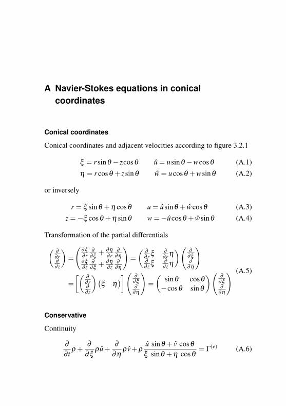
A Navier-Stokes equations in conicalcoordinates
Conical coordinates
Conical coordinates and adjacent velocities according to figure 3.2.1
ξ = r sinθ − zcosθ u = usinθ −wcosθ (A.1)
η = r cosθ + zsinθ w = ucosθ +wsinθ (A.2)
or inversely
r = ξ sinθ +η cosθ u = usinθ + wcosθ (A.3)
z = −ξ cosθ +η sinθ w = −ucosθ + wsinθ (A.4)
Transformation of the partial differentials
( ∂∂ r∂∂ z
)=
( ∂ξ∂ r
∂∂ξ + ∂η
∂ r∂
∂η∂ξ∂ z
∂∂ξ + ∂η
∂ z∂
∂η
)=( ∂
∂ r ξ ∂∂ r η
∂∂ z ξ ∂
∂ z η
)( ∂∂ξ∂
∂η
)
=[( ∂
∂ r∂∂ z
)(ξ η
)]( ∂∂ξ∂
∂η
)=(
sinθ cosθ−cosθ sinθ
)( ∂∂ξ∂
∂η
) (A.5)
Conservative
Continuity
∂∂ t
ρ +∂
∂ξρ u+
∂∂η
ρ v+ρu sinθ + v cosθξ sinθ +η cosθ
= Γ(e) (A.6)
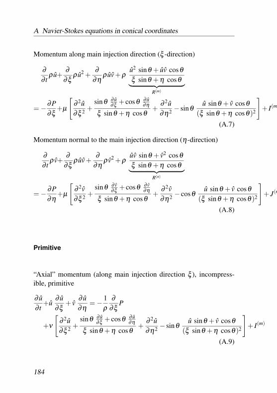
A Navier-Stokes equations in conical coordinates
Momentum along main injection direction (ξ -direction)
∂∂ t
ρ u+∂
∂ξρ u2 +
∂∂η
ρ uv+ρu2 sinθ + uv cosθξ sinθ +η cosθ︸ ︷︷ ︸
R(m)
= −∂P∂ξ
+µ
[∂ 2u∂ξ 2 +
sinθ ∂ u∂ξ + cosθ ∂ u
∂η
ξ sinθ +η cosθ+
∂ 2u∂η2 − sinθ
u sinθ + v cosθ(ξ sinθ +η cosθ)2
]+ I(m)
(A.7)
Momentum normal to the main injection direction (η-direction)
∂∂ t
ρ v+∂
∂ξρ uv+
∂∂η
ρ v2 +ρuv sinθ + v2 cosθξ sinθ +η cosθ︸ ︷︷ ︸
R(n)
= −∂P∂η
+µ
[∂ 2v∂ξ 2 +
sinθ ∂ v∂ξ + cosθ ∂ v
∂η
ξ sinθ +η cosθ+
∂ 2v∂η2 − cosθ
u sinθ + v cosθ(ξ sinθ +η cosθ)2
]+ J(m
(A.8)
Primitive
“Axial” momentum (along main injection direction ξ ), incompress-ible, primitive
∂ u∂ t
+u∂ u∂ξ
+ v∂ u∂η
= − 1ρ
∂∂ξ
P
+ν
[∂ 2u∂ξ 2 +
sinθ ∂ u∂ξ + cosθ ∂ u
∂η
ξ sinθ +η cosθ+
∂ 2u∂η2 − sinθ
u sinθ + v cosθ(ξ sinθ +η cosθ)2
]+ I(m)
(A.9)
184
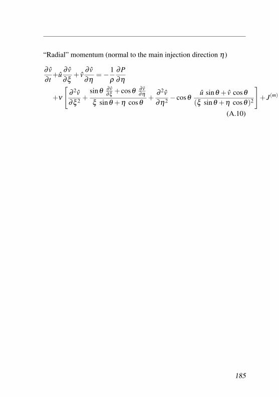
“Radial” momentum (normal to the main injection direction η)
∂ v∂ t
+u∂ v∂ξ
+ v∂ v∂η
= − 1ρ
∂P∂η
+ν
[∂ 2v∂ξ 2 +
sinθ ∂ v∂ξ + cosθ ∂ v
∂η
ξ sinθ +η cosθ+
∂ 2v∂η2 − cosθ
u sinθ + v cosθ(ξ sinθ +η cosθ)2
]+ J(m)
(A.10)
185

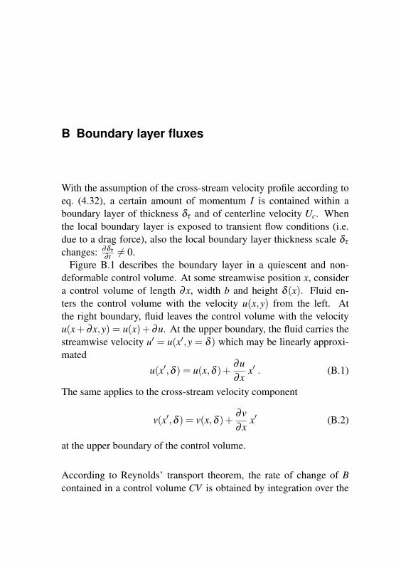
B Boundary layer fluxes
With the assumption of the cross-stream velocity profile according toeq. (4.32), a certain amount of momentum I is contained within aboundary layer of thickness δτ and of centerline velocity Uc. Whenthe local boundary layer is exposed to transient flow conditions (i.e.due to a drag force), also the local boundary layer thickness scale δτchanges: ∂δτ
∂ t �= 0.Figure B.1 describes the boundary layer in a quiescent and non-
deformable control volume. At some streamwise position x, considera control volume of length ∂x, width b and height δ (x). Fluid en-ters the control volume with the velocity u(x,y) from the left. Atthe right boundary, fluid leaves the control volume with the velocityu(x + ∂x,y) = u(x)+ ∂u. At the upper boundary, the fluid carries thestreamwise velocity u′ = u(x′,y = δ ) which may be linearly approxi-mated
u(x′,δ ) = u(x,δ )+∂u∂x
x′ . (B.1)
The same applies to the cross-stream velocity component
v(x′,δ ) = v(x,δ )+∂v∂x
x′ (B.2)
at the upper boundary of the control volume.
According to Reynolds’ transport theorem, the rate of change of Bcontained in a control volume CV is obtained by integration over the
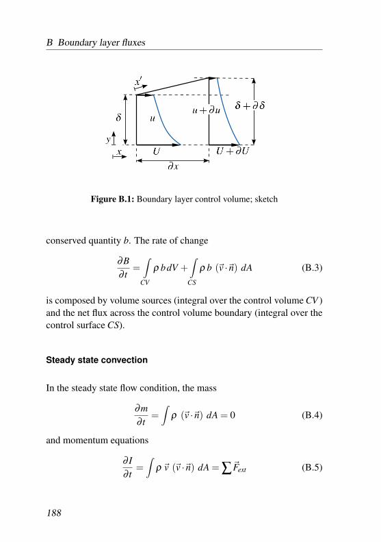
B Boundary layer fluxes
Figure B.1: Boundary layer control volume; sketch
conserved quantity b. The rate of change
∂B∂ t
=∫
CV
ρ bdV +∫
CS
ρ b (�v ·�n) dA (B.3)
is composed by volume sources (integral over the control volume CV )and the net flux across the control volume boundary (integral over thecontrol surface CS).
Steady state convection
In the steady state flow condition, the mass
∂m∂ t
=∫
ρ (�v ·�n) dA = 0 (B.4)
and momentum equations
∂ I∂ t
=∫
ρ �v (�v ·�n) dA = ∑�Fext (B.5)
188
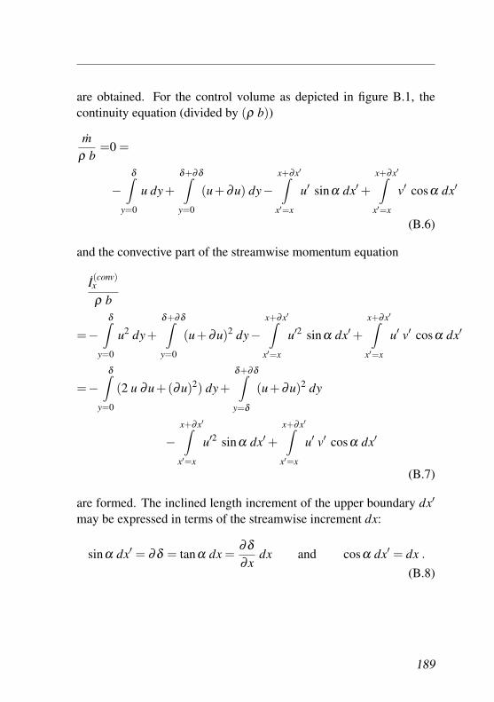
are obtained. For the control volume as depicted in figure B.1, thecontinuity equation (divided by (ρ b))
mρ b
=0 =
−δ∫
y=0
u dy+δ+∂δ∫y=0
(u+∂u) dy−x+∂x′∫x′=x
u′ sinα dx′ +x+∂x′∫x′=x
v′ cosα dx′
(B.6)
and the convective part of the streamwise momentum equation
I(conv)x
ρ b
=−δ∫
y=0
u2 dy+δ+∂δ∫y=0
(u+∂u)2 dy−x+∂x′∫x′=x
u′2 sinα dx′ +x+∂x′∫x′=x
u′ v′ cosα dx′
=−δ∫
y=0
(2 u ∂u+(∂u)2) dy+δ+∂δ∫y=δ
(u+∂u)2 dy
−x+∂x′∫x′=x
u′2 sinα dx′ +x+∂x′∫x′=x
u′ v′ cosα dx′
(B.7)
are formed. The inclined length increment of the upper boundary dx′
may be expressed in terms of the streamwise increment dx:
sinα dx′ = ∂δ = tanα dx =∂δ∂x
dx and cosα dx′ = dx .
(B.8)
189
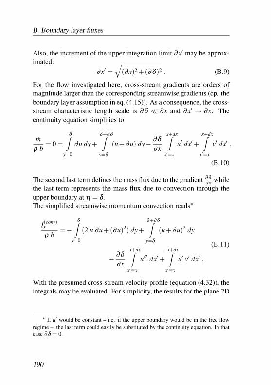
B Boundary layer fluxes
Also, the increment of the upper integration limit ∂x′ may be approx-imated:
∂x′ =√
(∂x)2 +(∂δ )2 . (B.9)
For the flow investigated here, cross-stream gradients are orders ofmagnitude larger than the corresponding streamwise gradients (cp. theboundary layer assumption in eq. (4.15)). As a consequence, the cross-stream characteristic length scale is ∂δ � ∂x and ∂x′ → ∂x. Thecontinuity equation simplifies to
mρ b
= 0 =δ∫
y=0
∂u dy+δ+∂δ∫y=δ
(u+∂u) dy− ∂δ∂x
x+dx∫x′=x
u′ dx′ +x+dx∫
x′=x
v′ dx′ .
(B.10)
The second last term defines the mass flux due to the gradient ∂δ∂x while
the last term represents the mass flux due to convection through theupper boundary at η = δ .The simplified streamwise momentum convection reads∗
I(conv)x
ρ b=−
δ∫y=0
(2 u ∂u+(∂u)2) dy+δ+∂δ∫y=δ
(u+∂u)2 dy
− ∂δ∂x
x+dx∫x′=x
u′2 dx′ +x+dx∫
x′=x
u′ v′ dx′ .
(B.11)
With the presumed cross-stream velocity profile (equation (4.32)), theintegrals may be evaluated. For simplicity, the results for the plane 2D
∗ If u′ would be constant – i.e. if the upper boundary would be in the free flowregime –, the last term could easily be substituted by the continuity equation. In thatcase ∂δ = 0.
190
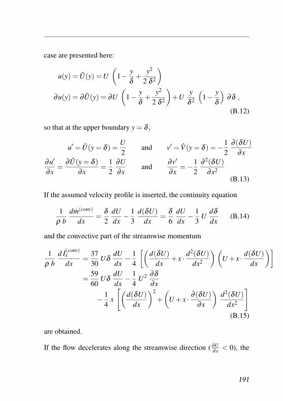
case are presented here:
u(y) = U(y) = U(
1− yδ
+y2
2 δ 2
)
∂u(y) = ∂U(y) = ∂U(
1− yδ
+y2
2 δ 2
)+U
yδ 2
(1− y
δ
)∂δ ,
(B.12)
so that at the upper boundary y = δ ,
u′ = U(y = δ ) =U2
and v′ = V (y = δ ) = −12
∂ (δU)∂x
∂u′
∂x=
∂U(y = δ )∂x
=12
∂U∂x
and∂v′
∂x= −1
2∂ 2(δU)
∂x2
(B.13)
If the assumed velocity profile is inserted, the continuity equation
1ρ b
dm(conv)
dx=
δ2
dUdx
− 13
d(δU)dx
=δ6
dUdx
− 13
Udδdx
(B.14)
and the convective part of the streamwise momentum
1ρ b
d I(conv)x
dx=
3730
UδdUdx
− 14
[(d(δU)
dx+ x · d2(δU)
dx2
) (U + x · d(δU)
dx
)]
=5960
UδdUdx
− 14
U2 ∂δ∂x
− 14
x
[(d(δU)
dx
)2
+(
U + x · ∂ (δU)∂x
)d2(δU)
dx2
](B.15)
are obtained.
If the flow decelerates along the streamwise direction ( ∂U∂x < 0), the
191
B Boundary layer fluxes
contained mass flux increases along the streamwise direction ( ∂ m∂x > 0).
Because at constant speed ( ∂u∂x = 0) and at increasing boundary layer
thickness ( ∂δ∂x > 0) more mass leaves the control volume at the right
side in figure B.1, the net contained mass flux decreases along thesteamwise direction: ∂ m
∂x < 0.
For the assessment of the integral momentum equation (B.15), firstconsider streamwise profiles of δ (x) and U(x) so that ∂ (δ U)
∂x = 0. Inthat case, the streamwise momentum flux due to convection changesproportionally to the contained momentum δ U and proportional to thesteamwise velocity gradient ∂U
∂x . In a steady jet flow, usually ∂δ∂x > 0
and ∂U∂x < 0 so that for ∂ (δ U)
∂x = 0, the momentum flux contained inthe control volume (fig. B.1) decreases along the streamwise direc-
tion: d I(conv)xdx < 0. This corresponds to the observation on the continu-
ity equation above: The assumed changes in the cross-stream velocityprofile cause the amount of momentum leaving the control volume onthe right to exceed the momentum entering from the left. †
† The Reynolds stress tensor
σ ji = τ ji −−p δ ji = µ(
∂u j
∂xi+
∂ui
∂x j
)− p δ ji (B.16)
For the evaluation of the shear stresses τ ji, the Gauss theorem∫
δV
∂ui
∂x jdAi =
∫V
∂∂xi
∂ui
∂x jdV =
∫V
∂∂x j
∂ui
∂xidV = 0 (B.17)
in combination with the incompressibility assumption ( ∂ui∂xi
= 0) indicate that the
terms due to the surface integrals∫
δV∂ui∂x j
dAi = 0.
192
Steady state momentum diffusion
In the streamwise direction, the contribution of the boundary integrals
δ∫y=0
τ1i dAi +δ+∂δ∫y=0
τ1i dAi = −bδ∫
y=0
µ∂u∂x
∣∣∣∣x
dy+bδ+∂δ∫y=0
µ∂u∂x
∣∣∣∣x+dx
dy
(B.18)to the streamwise momentum integral are negligible for flow condi-tions outside the viscous dominated regime with Reynolds numbersRe � 1.The assumed cross-stream velocity profile (eq. (4.32)) results in a con-stant diffusion rate across the boundary layer of thickness ∂δ so thatthe momentum flux within the control volume does not change dueto cross-stream viscous diffusion. Because ∂u
∂y
∣∣∣y=0
= −Uδ , the shear
stress introduced to the control volume at the lower boundary is
∫τ1i dAi = −b
x+∂x′∫x′=x
µ∂u∂y
∣∣∣∣y=0
dx′ = b µUδ
dx . (B.19)
Because pressure fluctuations are assumed to propagate fast comparedto convective fluxes (Ma < 0.3), the contribution of pressure gradientsto the streamwise momentum equation is neglected here.
Transient flow
The analysis of the momentum fluxes within the boundary layer andtheir changes due to the proposed model is based on a quiescent andnon-deformable control volume. A temporarily changing control vol-ume (boundary layer thickness) is excluded from the analysis.But if the changes of mass and momentum fluxes due to ∂δ
∂ t �= 0 areconceived as volume source terms, the contribution of the variable
193
B Boundary layer fluxes
boundary layer thickness may be characterized:
(∂m∂ t
)(trans)
=∂∂ t
∫∂V
ρ dV =∂∂ t
⎛⎝ρ bdx
δ∫y=0
dy
⎞⎠= ρ bdx
∂δ∂ t
,
(B.20)(∂ Ix
∂ t
)(trans)
=∂∂ t
∫∂V
ρ u dV =∂∂ t
⎛⎝ρ bdx
δ∫y=0
udy
⎞⎠= ρ bdx
23
∂ (δ U)∂ t
.
(B.21)In combination with the convective parts (equaitons (B.14) and (B.15))and the diffusive term (equation (B.19)), you obtain
1ρ b
∂ m∂x
=∂δ∂ t
=δ6
dUdx
− 13
Udδdx
(B.22)
and
1ρ b
∂ Ix
∂x=
23
∂ (δ U)∂ t
=5960
UδdUdx
− 14
U2 ∂δ∂x
− 14
x
[(d(δU)
dx
)2
+(
U + x · ∂ (δU)∂x
)d2(δU)
dx2
]
−νUδ
.
(B.23)
194


![REGENERIERUNG FESTER KATALYSATOREN FÜR … · US ultrastabilisiert U.S. United States ... gasoline blending components. ... [4,5]. Several classes of](https://img.pdfslide.org/doc/110x75/5b14e61d7f8b9a4e2c8c8155/regenerierung-fester-katalysatoren-fuer-us-ultrastabilisiert-us-united-states.jpg)