Embed Size (px)
Citation preview
Hydrographical and
biogeochemical characterization of
the Beibu Gulf, South China Sea
Dissertation
zur
Erlangung des akademischen Grades
doctor rerum naturalium (Dr. rer. nat.)
der Mathematisch-Naturwissenschaftlichen Fakultät
der Universität Rostock
vorgelegt von
Andrea Bauer
geb. am 08.03.1985 in Jena
Rostock, den 30. August 2012
Gutachter
PD Dr. habil. Joanna J. Waniek
Leibniz-Institut für Ostseeforschung Warnemünde
Prof. Dr. Detlef E. Schulz-Bull
Leibniz-Institut für Ostseeforschung Warnemünde
Prof. Dr. Venugopalan Ittekkot
Zentrum für Marine Tropenökologie
Datum der öffentlichen Verteidigung: 21.01.2013
Contents
Contents
Abstract IV
Zusammenfassung VI
1 Introduction 1
1.1 Global importance of shelf seas . . . . . . . . . . . . . . . . . . . . . . 1
1.2 The Beibu Gulf . . . . . . . . . . . . . . . . . . . . . . . . . . . . . . 8
1.3 Thesis outline . . . . . . . . . . . . . . . . . . . . . . . . . . . . . . . 11
2 Material and Methods 13
2.1 Sampling and in-situ data processing . . . . . . . . . . . . . . . . . . . 13
2.2 Current measurements . . . . . . . . . . . . . . . . . . . . . . . . . . 13
2.3 Coupled physical-biological model . . . . . . . . . . . . . . . . . . . . 16
2.4 Additional data sets . . . . . . . . . . . . . . . . . . . . . . . . . . . . 19
3 Regional differences of hydrographical and sedimentological prop-
erties in the Beibu Gulf, South China Sea 20
3.1 Introduction . . . . . . . . . . . . . . . . . . . . . . . . . . . . . . . . 21
3.2 Material and Methods . . . . . . . . . . . . . . . . . . . . . . . . . . . 24
3.2.1 Study area . . . . . . . . . . . . . . . . . . . . . . . . . . . . . 24
3.2.2 Water samples . . . . . . . . . . . . . . . . . . . . . . . . . . 25
3.2.3 Geological samples . . . . . . . . . . . . . . . . . . . . . . . . 26
3.2.4 Geochemical samples . . . . . . . . . . . . . . . . . . . . . . . 27
3.2.5 Additional data sets . . . . . . . . . . . . . . . . . . . . . . . . 28
3.3 Results . . . . . . . . . . . . . . . . . . . . . . . . . . . . . . . . . . . 29
3.3.1 Beibu Gulf Coastal Zone . . . . . . . . . . . . . . . . . . . . . 32
3.3.2 Qiongzhou Strait Zone . . . . . . . . . . . . . . . . . . . . . . 38
I
Contents
3.3.3 Beibu Gulf Central Zone . . . . . . . . . . . . . . . . . . . . . 40
3.3.4 Southern Beibu Gulf Zone . . . . . . . . . . . . . . . . . . . . 42
3.4 Discussion . . . . . . . . . . . . . . . . . . . . . . . . . . . . . . . . . 44
3.4.1 Hydrographical and biogeochemical differences between
the zones . . . . . . . . . . . . . . . . . . . . . . . . . . . . . 44
3.4.2 Differences of sediment characteristics and geochemical prop-
erties between the zones . . . . . . . . . . . . . . . . . . . . . 51
3.5 Conclusions . . . . . . . . . . . . . . . . . . . . . . . . . . . . . . . . 58
4 Factors affecting the chlorophyll a concentration in the central Beibu
Gulf, South China Sea 59
4.1 Introduction . . . . . . . . . . . . . . . . . . . . . . . . . . . . . . . . 60
4.2 Material and Methods . . . . . . . . . . . . . . . . . . . . . . . . . . . 63
4.2.1 Study area . . . . . . . . . . . . . . . . . . . . . . . . . . . . . 63
4.2.2 In situ data for model validation . . . . . . . . . . . . . . . . . 64
4.2.3 Simple 1D coupled physical-biological model . . . . . . . . . . 65
4.2.4 Meteorological and comparative satellite data . . . . . . . . . . 69
4.3 Results . . . . . . . . . . . . . . . . . . . . . . . . . . . . . . . . . . . 69
4.3.1 Mean annual cycle . . . . . . . . . . . . . . . . . . . . . . . . 71
4.3.2 Annual cycle 2009 . . . . . . . . . . . . . . . . . . . . . . . . 75
4.3.3 Effects of strong wind events . . . . . . . . . . . . . . . . . . . 77
4.3.4 Effects of tides . . . . . . . . . . . . . . . . . . . . . . . . . . 78
4.3.5 Interannual variability . . . . . . . . . . . . . . . . . . . . . . 81
4.4 Discussion . . . . . . . . . . . . . . . . . . . . . . . . . . . . . . . . . 86
4.5 Conclusions . . . . . . . . . . . . . . . . . . . . . . . . . . . . . . . . 92
5 Sediment resuspension patterns and the diffusive boundary layer
in the Beibu Gulf, South China Sea 97
5.1 Introduction . . . . . . . . . . . . . . . . . . . . . . . . . . . . . . . . 97
5.2 Material and methods . . . . . . . . . . . . . . . . . . . . . . . . . . . 100
5.2.1 Current records and their analysis . . . . . . . . . . . . . . . . 100
5.2.2 Water and sediment sampling . . . . . . . . . . . . . . . . . . 102
5.2.3 Tidal model . . . . . . . . . . . . . . . . . . . . . . . . . . . . 102
II
Contents
5.3 Results and discussion . . . . . . . . . . . . . . . . . . . . . . . . . . 105
5.3.1 Tidal cycle . . . . . . . . . . . . . . . . . . . . . . . . . . . . 105
5.3.2 Sedimentation patterns . . . . . . . . . . . . . . . . . . . . . . 108
5.3.3 Diffusive Boundary Layer . . . . . . . . . . . . . . . . . . . . 113
5.4 Conclusions . . . . . . . . . . . . . . . . . . . . . . . . . . . . . . . . 118
Conclusions 120
References 124
List of Figures 137
List of Tables 139
List of Abbreviations 140
Specific contributions to the manuscripts 142
Danksagung 144
Eidesstattliche Erklärung 146
III
Abstract
Abstract
As a transition zone between the highly populated Chinese and Vietnamese land masses,
providing a great river discharge, and the South China Sea, the Beibu Gulf plays an im-
portant role for near-costal input of terrestrial, naturally and anthropogenically induced,
matter and material as well as energy fluxes into the South China Sea northwestern
areas. Therefore, the Beibu Gulf is a significant region for biogeochemical cycling,
degradation of organic matter and hence induced element fluxes as well as sediment
accumulation.
Influenced by the Asian monsoon system, strong tidal currents and occasionally ty-
phoon crossings, affecting circulation patterns and the water mass exchange with the
South China Sea, hydrographical conditions, water column biogeochemistry and sedi-
mentation processes are highly variable in this shallow shelf sea. On this account, the
Beibu Gulf is an interesting region for deepening the understanding of meteorological
and tidal forcing on hydrography, biogeochemical properties as well as sedimentation
patterns and processes regulating the benthic-pelagic material and energy fluxes.
To characterize the Beibu Gulf hydrographically and biogeochemically, this thesis
combines investigations on physical and biogeochemical conditions of the water col-
umn, current and sedimentation patterns as well as geochemical properties of the sedi-
ments. The analyses are based on in-situ measurements (temperature, salinity, σt, cur-
rents, chlorophyll, nutrients, suspended particulate matter, grain size, sediment pore
water properties, foraminifera and plant pigment contents in surface sediments) carried
out during two German-Chinese cruises with the RV FENDOU 5 in September/October
2009 and RV SONNE in December 2011, model work and satellite derived sea surface
temperature and surface chlorophyll concentrations.
For the understanding of the system "Beibu Gulf", its hydrodynamics, sedimentolog-
ical and geochemical variability, different zones are distinguished in the study area for
the sampling period in September/October 2009, extending from the coastal areas in the
north and east across the central region to the southern part of the gulf. These zones are
IV
Abstract
mainly influenced by tidal mixing and riverine input in the coastal regions, water mass
transport from the South China coastal regions through the Qiongzhou Strait in the east
and South China Sea waters in the south, due to circulation patterns driven by monsoon
winds and tides. The regional hydrographic peculiarities are mirrored in the biogeo-
chemical properties of the water column and sediment characteristics like grain size,
plant pigment contents and foraminifera in the surface sediments as well as geochemi-
cal properties, which follow the hydrodynamically controlled sedimentation conditions
and reflect distinctions in primary production within the water column.
The physical structure of the water column mainly driven by monsoonal forcing is
reflected in the seasonal cycle of primary production, with a low-productive period in
summer due to water column stratification and a phytoplankton bloom in winter initiated
by vertical mixing and related nutrient supply. Along with the semi-annual wind system
change, occasionally strong wind events (typhoons) play an important role in primary
production and the associated biogeochemical cycling in the Beibu Gulf.
While wind forcing influences the water column from top-down the tidal forcing is
the main mechanism driving sedimentation patterns and influencing geochemical pro-
cesses within the sediments. For all zones and tidal phases (ebb, flood, slack water)
current velocities contribute to sediment deposition, transport and resuspension during
the sampling period in September/October 2009. The, in general, strong currents dur-
ing most of the tidal cycle prevent the establishment of a diffusive boundary layer and
hence allow an exchange of compounds, nutrients and gases across the sediment-water
interface, which indicates an existing benthic-pelagic coupling in the Beibu Gulf.
V
Zusammenfassung
Zusammenfassung
Der Beibu Golf bildet eine Übergangszone zwischen dem stark bevölkerten chinesi-
schen/vietnamesischen Festland und dem Südchinesischen Meer. Aus diesem Grund
spielt er eine bedeutende Rolle für den küstennahen, natürlichen und anthropogenen,
Stoffeintrag sowie für Material- und Energieflüsse in die nordwestlichen Regionen des
Südchinesischen Meeres. Diese Region ist wichtig für biogeochemische Kreisläufe, den
Abbau von organischem Material und damit einhergehenden Elementflüssen sowie für
sedimentäre Ablagerungsprozesse.
Die physikalischen und biogeochemischen Eigenschaften der Wassersäule sowie Sedi-
mentationsprozesse im Golf unterliegen starken Schwankungen, da Zirkulationsmuster
und der Wassermassenaustausch mit dem Südchinesischen Meer stark durch wechseln-
de Monsunwinde, Gezeitenströmungen und gelegentlich vorüber ziehende Taifune be-
einflusst werden. Daher ist der Beibu Golf eine interessante Region um das Verständnis
für den Einfluss von meteorologischen und Gezeitenkräften auf die Wassersäuleneigen-
schaften sowie auf Sedimentationsmuster zu vertiefen.
Um den Beibu Golf hydrographisch und biogeochemisch zu charakterisieren, werden
in dieser Arbeit Untersuchungen der physikalischen und biogeochemischen Bedingung-
en der Wassersäule mit Strömungs- und Sedimentationsmustern sowie geochemischen
Parametern der Sedimente kombiniert. Hierzu wurden in-situ Messungen (Temperatur,
Salzgehalt, σt, Strömungen, Chlorophyll, Nährstoffe, suspendiertes partikuläres Ma-
terial, Korngröße, Porenwassereigenschaften der Sedimente und Foraminiferen sowie
Pflanzenpigmentkonzentrationen in den Oberflächensedimenten) zweier deutsch-chine-
sischer Expeditionen, mit den Forschungsschiffen FENDOU 5 im September/Oktober
2009 und SONNE im Dezember 2011, ausgewertet sowie Modellierungsarbeiten in
Verbindung mit von Satellitendaten abgeleiteten Meeresoberflächentemperaturen und
-chlorophyllkonzentrationen durchgeführt.
Um die hydrodynamische, sedimentologische und geochemische Variabilität des Sys-
tems "Beibu Golf" zu verstehen, wurden, in einem ersten Schritt, verschiedene Zonen
VI
Zusammenfassung
für das Untersuchungsgebiet und den Untersuchungszeitraum September/Oktober 2009
definiert. Diese Zonen erstrecken sich von den Küstenregionen im Norden und Osten
über den zentralen bis hin zum südlichen Teil des Golfes. Sie sind hauptsächlich beein-
flusst durch gezeitengetriebene Durchmischung und Flusseinträge in den küstennahen
Regionen, Transport von Wassermassen der Südchinesischen Küstenregionen durch die
Qiongzhou Straße im Osten und Wassermassen des Südchinesischen Meeres im Süden
des Golfes. Dabei wird der jeweilige Einfluss der Wassermassen auf die Zonen durch die
golfweite Zirkulation, angetrieben durch Monsunwinde und Gezeiten, bestimmt. Die
regionalen Besonderheiten der Hydrographie spiegeln sich in den biogeochemischen
Eigenschaften der Wassersäule und in denen der Sedimente, wie Korngröße, Pflanzen-
pigmentkonzentrationen und Foraminiferen in den Oberflächensedimenten sowie geo-
chemischen Parametern, wider. Die Sedimenteigenschaften folgen dabei den hydrody-
namisch kontrollierten Sedimentationsbedingungen und reflektieren gleichzeitig Unter-
schiede in der Primärproduktionsrate der Wassersäule.
Die physikalische Struktur der Wassersäule, beeinflusst durch die Monsunwinde,
wird von der Primärproduktion reflektiert, mit einer Phase geringer Produktion im Som-
mer durch Schichtung der Wassersäule und einer Phytoplankton Blüte im Winter, aus-
gelöst durch vertikale Durchmischung und damit zusammenhängender Verfügbarkeit
von Nährstoffen. Zusammen mit dem halbjährlichen Wechsel des Windsystems, tragen
auch zeitweise auftretende starke Stürme (Taifune) erheblich zur Primärproduktion und
den damit in Zusammenhang stehenden biogeochemischen Kreisläufen bei.
Während der Wind die Wassersäule an der Oberfläche beeinflusst, sind Gezeiten
die treibenden Kräfte für Ablagerungsbedingungen und bestimmen gleichzeitig auch
geochemische Eigenschaften der Sedimente. Für den Beprobungszeitraum im Septem-
ber/Oktober 2009 tragen Strömungsgeschwindigkeiten in allen Zonen und zu allen Ge-
zeitenphasen (Ebbe, Flut, Stillwasser) zu Ablagerung, Transport und Resuspension der
Sedimente bei. Die im Allgemeinen während eines Gezeitenzyklus sehr starken Strö-
mungen verhindern die Entstehung einer diffusiven, bodennahen Grenzschicht und er-
lauben dadurch einen Austausch von Verbindungen, Nährstoffen und Gasen zwischen
Sediment und Wassersäule. Das weist auf eine benthisch-pelagische Kopplung im Beibu
Golf hin.
VII
Chapter 1: Introduction
1 Introduction
1.1 Global importance of shelf seas
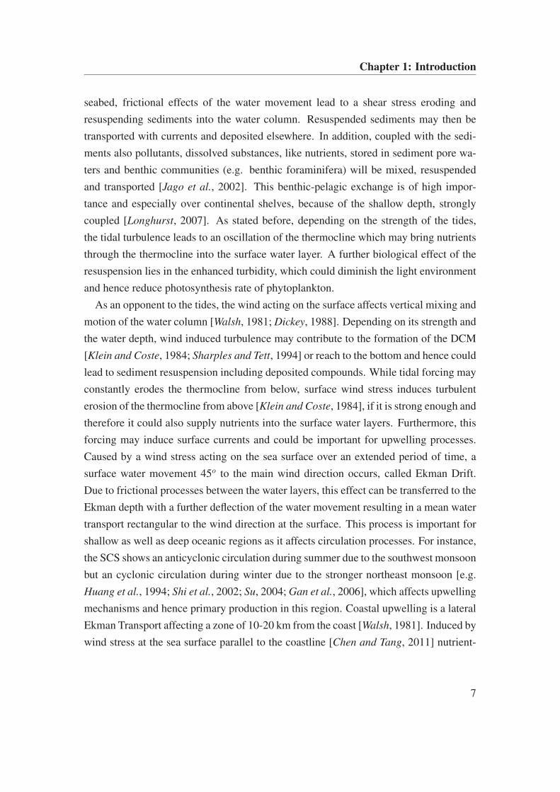
Continental shelves reach in their spatial extent from the coastline to the continental
slope and form a margin around continents variant in width. With a depth up to 200 m,
shelves provide only a mere of 7% of the oceans surface and less than 0.5% of the
oceans volume [Chen et al., 2003] compared to the around 4000 m mean depth of the
open ocean (Fig. 1.1a). A clear definition of strict boundaries between the open ocean
and shelf seas is difficult as water masses of oceanic and neritic provinces blend into
each other in most cases. However, in general, the continental slope is the area where
hydrographic conditions change between both provinces [Postma and Zijlstra, 1988].
The global importance of shelf areas is primarily caused by the immediate prox-
imity to the land masses. As regions connecting the mainland with the open oceans,
shelf seas are important regions for transferring energy and material, controlling an-
thropogenic and terrestrial fluxes and fates of chemicals, pollutants and primary pro-
duction to and from the open ocean [Mantoura et al., 1991]. In shelf and deltaic regions
over 90% of the riverine particulates and associated carbon, trace metals and pollutants
are trapped [Mantoura et al., 1991]. Anthropogenic perturbations are mainly caused by
land use, land reclamation and sand mining, industry and aquaculture/mariculture which
affect mobilization, input and deposition of metals, anthropogenic organic compounds,
toxic substances and nutrients leading to eutrophication, which may influence marine
ecosystems and the composition of biological communities, especially in coastal regions
[O’Kane et al., 1991; Doney et al., 2003]. Further direct and indirect human impacts
are, for example, due to waste disposal, tourism, coastal engineering, freshwater man-
agement and changes in river flows, habitat destruction like cutting of mangrove forests,
draining of marshes with associated effects on sediment dynamics as well as diminish-
ing fishery resources which may lead to a shift in species dominance [Sharp, 1988;
1
Chapter 1: Introduction
O’Kane et al., 1991]. Shelf regions respond very quickly to environmental changes and
are important regions for biogeochemical fluxes, with a carbon turnover time from days
to weeks [Ross, 2004], for instance.
180°W 150°W 120°W 90°W 60°W 30°W 0° 30°E 60°E 90°E 120°E 150°E 180°E90°S
60°S
30°S
0°
30°N
60°N
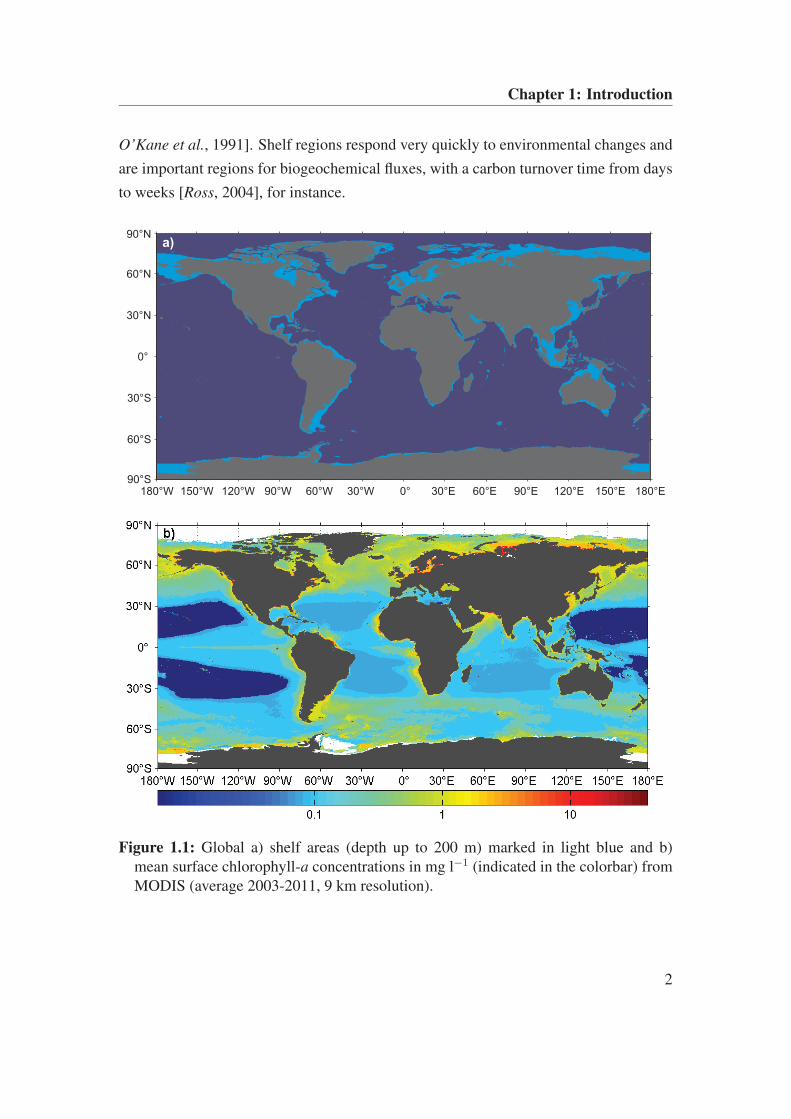
90°Na)
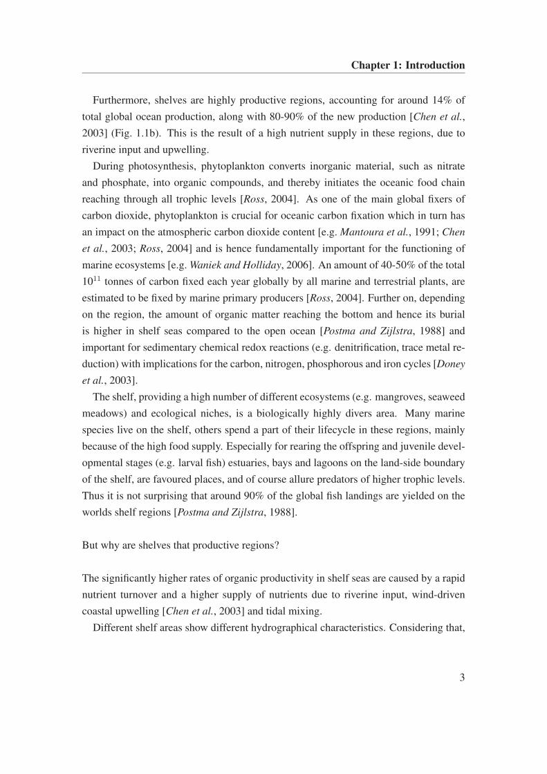
Figure 1.1: Global a) shelf areas (depth up to 200 m) marked in light blue and b)mean surface chlorophyll-a concentrations in mg l−1 (indicated in the colorbar) fromMODIS (average 2003-2011, 9 km resolution).
2
Chapter 1: Introduction
Furthermore, shelves are highly productive regions, accounting for around 14% of
total global ocean production, along with 80-90% of the new production [Chen et al.,
2003] (Fig. 1.1b). This is the result of a high nutrient supply in these regions, due to
riverine input and upwelling.
During photosynthesis, phytoplankton converts inorganic material, such as nitrate
and phosphate, into organic compounds, and thereby initiates the oceanic food chain
reaching through all trophic levels [Ross, 2004]. As one of the main global fixers of
carbon dioxide, phytoplankton is crucial for oceanic carbon fixation which in turn has
an impact on the atmospheric carbon dioxide content [e.g. Mantoura et al., 1991; Chen
et al., 2003; Ross, 2004] and is hence fundamentally important for the functioning of
marine ecosystems [e.g. Waniek and Holliday, 2006]. An amount of 40-50% of the total
1011 tonnes of carbon fixed each year globally by all marine and terrestrial plants, are
estimated to be fixed by marine primary producers [Ross, 2004]. Further on, depending
on the region, the amount of organic matter reaching the bottom and hence its burial
is higher in shelf seas compared to the open ocean [Postma and Zijlstra, 1988] and
important for sedimentary chemical redox reactions (e.g. denitrification, trace metal re-
duction) with implications for the carbon, nitrogen, phosphorous and iron cycles [Doney
et al., 2003].
The shelf, providing a high number of different ecosystems (e.g. mangroves, seaweed
meadows) and ecological niches, is a biologically highly divers area. Many marine
species live on the shelf, others spend a part of their lifecycle in these regions, mainly
because of the high food supply. Especially for rearing the offspring and juvenile devel-
opmental stages (e.g. larval fish) estuaries, bays and lagoons on the land-side boundary
of the shelf, are favoured places, and of course allure predators of higher trophic levels.
Thus it is not surprising that around 90% of the global fish landings are yielded on the
worlds shelf regions [Postma and Zijlstra, 1988].
But why are shelves that productive regions?
The significantly higher rates of organic productivity in shelf seas are caused by a rapid
nutrient turnover and a higher supply of nutrients due to riverine input, wind-driven
coastal upwelling [Chen et al., 2003] and tidal mixing.
Different shelf areas show different hydrographical characteristics. Considering that,
3
Chapter 1: Introduction
the shaping of the shelf region is of consequence, which means width, bathymetry, na-
ture of the coastline itself [Longhurst, 2007] and the shape of the connection to the
adjacent ocean, its latitudinal position, which determines the solar irradiance and hence
the seasonal temperature cycle [Walsh, 1981], and the wind regime. Especially the
width, which is very variable between 0 and 1500 km [Postma, 1988], the bathymetry,
the connection to the open ocean and the strength of the tidal forcing are responsible for
the residence time of the shelf water bodies which is important for material deposition
in the shelf sea itself or rapid transport via currents into the open ocean, biogeochemical
cycles and hence the water quality. The faster water exchanges, phytoplankton cells
may be transported away from the shelf and hence away from optimal living conditions
related to nutrients, light availability and stratification. In general, planktonic algae tend
to be larger in shelves because of the reduced vertical stability in these regions and the
occasional presence of upwelling [Postma and Zijlstra, 1988]. In addition, organic mat-
ter can only be deposited to a minor degree which influences especially biogeochemical
cycles within the sediments, burial of organic matter and benthic communities.
The residence times for shelf seas can mostly be measured rather in months than
in years [Postma and Zijlstra, 1988]. An exception is, for example, the Baltic Sea,
having only a narrow connection to the Atlantic through Skagerrak/Kattegat, which
leads to an only sporadically water exchange and a residence time of about 30 years.
The wind regime contributes to the water residence time as well, as it introduces specific
circulation patterns, best documented for the changing monsoon winds in Asian regions,
for instance, the Arabian Sea and the South China Sea (SCS).
As a land-ocean interface shelf seas are influenced by riverine freshwater discharge,
which may bring nutrients into the system and lead to coastal near water masses deter-
mined by lower salinities and higher buoyancy, on the one hand and high saline waters
from the open ocean which intrudes into the shelf regions on the other hand. These
different water masses may lead to the formation of shelf break fronts, which occur al-
most everywhere due to the density gradient between the shelf and the oceanic water
[Longhurst, 2007], and can be taken as boundaries for the shelf region. Associated with
the fronts nutrient upwelling from deeper nutrient-rich waters can occur and enhance
primary production within the frontal region.
The most important characteristic of shelf seas, responsible for most of the distinct
differences to the open ocean, is their shallowness. This feature leads to a faster warm-
4
Chapter 1: Introduction
ing and cooling of water bodies compared to the open ocean and causes a seasonal
stratification. During periods of highest solar irradiance, in the northern hemisphere in
spring and summer, its influence overcomes the capacity of tidal mixing to maintain a
vertically well-mixed water column and the water column stratifies thermally [Sharples,
2008]. The seasonal thermocline is an physical barrier separating the wind-mixed sur-
face layer from the tidally-mixed deeper water layer [Ross and Sharples, 2007]. It
further inhibits properties transfer, such as oxygen, nutrients and algal cells [e.g. Klein
and Coste, 1984; Sharples et al., 2001]. Above, the light environment promotes photo-
synthesis but the water layer is impoverished of nutrients in most cases, due to their only
limited availability, fast consumption and prevented replenishment from deeper waters.
Below the thermocline, enough nutrients are available but the poor light conditions pre-
vent primary production. A net production through photosynthesis, compensating de-
struction processes by respiration, can only occur, when algal cells are trapped near the
surface and nutrients as well as light are sufficiently available [Sverdrup, 1953; Ward
and Waniek, 2007].
Many stratified regions show oligotrophic conditions during the period of vertical
stratification [Varela et al., 1992]. A result of the poor nutrient supply in these re-
gions, is a low primary production which is common for the outer shelf regions. In
those regions a deep chlorophyll maximum (DCM) is commonly observed within the
thermocline. This feature is promoted by pulses in the strength of mixing processes,
such as tidally-induced motion, wind events and surface breaking waves [Lauria et al.,
1999] bringing nutrients into the thermocline [Klein and Coste, 1984; Sharples and Tett,
1994]. The oscillation of the thermocline induced by these pulses supports also a nutri-
ent flux into the surface layer. For the western North Pacific Ocean almost 55% of the
total chlorophyll in the entire water column has been found within 50 m depth around
the DCM layer [Takahashi and Hori, 1984].
In autumn the stratification breaks down due to sea surface cooling and eroding of
the thermocline by wind and tides and leads to a deep mixing. The nutrient supply in
the euphotic zone increases, which triggers a winter phytoplankton bloom especially
in subtropical waters where the solar irradiance during winter still supports primary
production [Yoder et al., 1993]. By contrast, in temperate to polar/subpolar latitudes the
phytoplankton biomass cycle is dominated by a spring bloom, which occurs in response
to the stratification and increasing solar irradiance during spring and summer [Yoder
5
Chapter 1: Introduction
et al., 1993]. Depending on the depth of the oceanic region, phytoplankton may be
vertically transported below the euphotic depth during periods of deep mixing and can
not conduct photosynthesis anymore [Lauria et al., 1999] although enough nutrients are
provided. In shallow coastal areas, without stratification periods, nutrients are almost
permanently available resulting in eutrophic conditions with high primary production
rates.
Due to the high nutrient uptake during a phytoplankton bloom, different input of nu-
trients through atmospheric wet (rainfall) and dry (dust) deposition, river discharge and
vertical fluxes [Longhurst, 2007] mainly during periods of stratification, lead to a change
in the availability of dissolved nutrients. As a consequence of either nitrate or phosphate
limitation in the surface waters, the shifts in nutrient supply induce changes in the stoi-
chiometry of nutrient uptake (Redfield ratio) and consequently may limit phytoplankton
growth [Boyd and Doney, 2003]. Further, such changes may affect the species compo-
sition and species succession as well. For example, the essential uptake of silicate by
diatoms may lead to a silicate limitation. If no silicate will further be induced into the
system, hence, the diatom bloom terminates.
Tidal forces, inducing currents and undulation everywhere in the marine environment,
are only fully effective in shallow regions [e.g. Li et al., 2004]. Tides on shelves are
co-oscillating tides because they are mainly generated by incoming tidal waves from
the adjacent ocean [Postma, 1988]. While in the deep oceans tidal waves only lead to
a slight forward and backward movement of the water, in the shelf regions they can
trigger strong mixing processes. As a result of the decreasing depth, the tidal energy,
which could spread vertically over the entire depth of several 1000 m in the deep ocean
basins, is forced to spread over a depth of only 200 m and less when it comes upon
the shelf break. Consequently, the tidal wave is modified in height and direction by
morphology, bottom friction, Coriolis force and reflection against the coast which may
increase or decrease the tidal amplitude, depending on the relative importance of the
influencing factors, and leads to high tidal currents which increase, in general, from
the shelf edge towards the shore [Postma, 1988]. Tidal effects do not show the same
intensity in all shelf regions. At an open, wide shelf region with a gradual bathymetric
slope, tidal forcing is of little importance compared to semi-closed shelf regions, with a
sharply rising bathymetry.
The with tides associated turbulence causes vertical and horizontal mixing. At the
6
Chapter 1: Introduction
seabed, frictional effects of the water movement lead to a shear stress eroding and
resuspending sediments into the water column. Resuspended sediments may then be
transported with currents and deposited elsewhere. In addition, coupled with the sedi-
ments also pollutants, dissolved substances, like nutrients, stored in sediment pore wa-
ters and benthic communities (e.g. benthic foraminifera) will be mixed, resuspended
and transported [Jago et al., 2002]. This benthic-pelagic exchange is of high impor-
tance and especially over continental shelves, because of the shallow depth, strongly
coupled [Longhurst, 2007]. As stated before, depending on the strength of the tides,
the tidal turbulence leads to an oscillation of the thermocline which may bring nutrients
through the thermocline into the surface water layer. A further biological effect of the
resuspension lies in the enhanced turbidity, which could diminish the light environment
and hence reduce photosynthesis rate of phytoplankton.
As an opponent to the tides, the wind acting on the surface affects vertical mixing and
motion of the water column [Walsh, 1981; Dickey, 1988]. Depending on its strength and
the water depth, wind induced turbulence may contribute to the formation of the DCM
[Klein and Coste, 1984; Sharples and Tett, 1994] or reach to the bottom and hence could
lead to sediment resuspension including deposited compounds. While tidal forcing may
constantly erodes the thermocline from below, surface wind stress induces turbulent
erosion of the thermocline from above [Klein and Coste, 1984], if it is strong enough and
therefore it could also supply nutrients into the surface water layers. Furthermore, this
forcing may induce surface currents and could be important for upwelling processes.
Caused by a wind stress acting on the sea surface over an extended period of time, a
surface water movement 45o to the main wind direction occurs, called Ekman Drift.
Due to frictional processes between the water layers, this effect can be transferred to the
Ekman depth with a further deflection of the water movement resulting in a mean water
transport rectangular to the wind direction at the surface. This process is important for
shallow as well as deep oceanic regions as it affects circulation processes. For instance,
the SCS shows an anticyclonic circulation during summer due to the southwest monsoon
but an cyclonic circulation during winter due to the stronger northeast monsoon [e.g.
Huang et al., 1994; Shi et al., 2002; Su, 2004; Gan et al., 2006], which affects upwelling
mechanisms and hence primary production in this region. Coastal upwelling is a lateral
Ekman Transport affecting a zone of 10-20 km from the coast [Walsh, 1981]. Induced by
wind stress at the sea surface parallel to the coastline [Chen and Tang, 2011] nutrient-
7
Chapter 1: Introduction
rich deeper waters originating from offshore are brought to the surface and probably
enhance primary production.
Another feature, especially important for subtropical/tropical regions, are hurricanes
or typhoons. These short but strong wind events are able to break down the seasonal
stratification and mix the water column completely, particularly important in shelf re-
gions, which leads to a nutrient supply in the surface water layer and may induce a
phytoplankton bloom [e.g. Zheng and Tang, 2007]. Hence, the cyclone events made the
shelf more active in producing particulate and dissolved organic matter [Shiah et al.,
2000]. The effect of such an event depends on the wind’s intensity, the transit time and
the ocean’s precondition, which means the depth of the nutrient-rich water body [Lin,
2012]. Typhoon Kai-Tak, for instance, passed the SCS in July 2000 and accounted for
2-4% of the annual new production in the oligotrophic SCS [Lin et al., 2003].
The combination of all processes acting on shelf regions provide a highly turbulent
environment for primary producers which always have to cope with the limitation of
nutrients in a stratified and the vertical attenuation of light in a well-mixed regime.
Although shelf sea areas represent only a comparatively small part of the world oceans
surface they are highly productive regions representing a major carbon sink affecting
intensely the global carbon mass balance [Walsh, 1981; Mantoura et al., 1991; de Haas
et al., 2002; Chen et al., 2003], and hence the global climate.
1.2 The Beibu Gulf
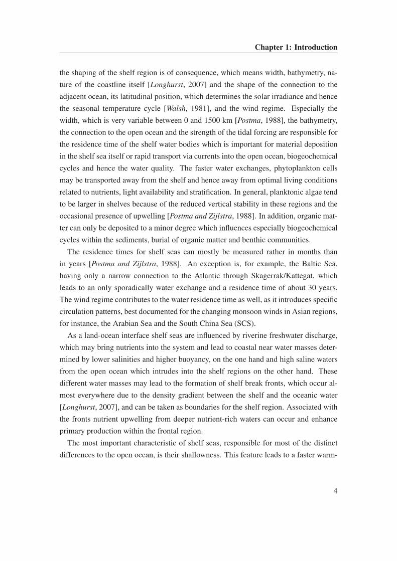
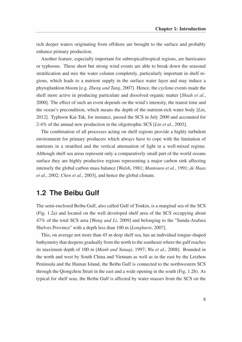
The semi-enclosed Beibu Gulf, also called Gulf of Tonkin, is a marginal sea of the SCS
(Fig. 1.2a) and located on the well developed shelf area of the SCS occupying about
47% of the total SCS area [Wang and Li, 2009] and belonging to the "Sunda-Arafura
Shelves Province" with a depth less than 100 m [Longhurst, 2007].
This, on average not more than 45 m deep shelf sea, has an individual tongue-shaped
bathymetry that deepens gradually from the north to the southeast where the gulf reaches
its maximum depth of 100 m [Manh and Yanagi, 1997; Wu et al., 2008]. Bounded in
the north and west by South China and Vietnam as well as in the east by the Leizhou
Peninsula and the Hainan Island, the Beibu Gulf is connected to the northwestern SCS
through the Qiongzhou Strait in the east and a wide opening in the south (Fig. 1.2b). As
typical for shelf seas, the Beibu Gulf is affected by water masses from the SCS on the
8
Chapter 1: Introduction
100 105 110 115 120 125
0
5
10
15
20
25
Longitude / °E
Latitu
de /
°N
China
Vietnam
South
China
Sea
Gulf
of
Thailand
Beibu
Gulf
Kalimantan Island
Taiw
an
Luzo
n
Pacific
Thailand
Malaysia
a)
105.5 106 106.5 107 107.5 108 108.5 109 109.5 110 110.5 111
17
17.5
18
18.5
19
19.5
20
20.5
21
21.5
22
0
0
0
25
25
2525
25
25
25
2525
25
25
25
25
25
25
25
25
25
25
25
25
25
25
2525
50
50
5050
50
50
50
50
50
50
50
50
50
50
50
5050
50
50
50
75
75
75
75
75
75
75
75
75
75
75 75
75
75
75
75
7575
75
75
75
75
75
7575 75
75
100
100
100100
100
100
100
100
100
100
100
100100
100100
100
Longitude / °E
Latitu
de /
°N
China
Vietnam
Hainan Island
Leiz
ho
u P
en
insu
la
Qiongzhou Strait
South
China
Sea
b)
Figure 1.2: a) The South China Sea and b) the Beibu Gulf. Bathymetry is based onETOPO1 (http://www.ngdc.noaa.gov).
one hand and river discharge along the shore on the other hand. Especially the Red River
water discharge of about 123 km3 yr−1 [Milliman and Meade, 1983; Wong et al., 2007]
along with rivers at the northern coast influence Beibu Gulf waters, generating a low
salinity zone in the northwestern part [Chen et al., 2009] particularly during the rainy
season in summer [Dai et al., 2011]. In addition to the water transport, the Red River,
for instance, also transports on average 160x106 t yr−1 suspended load which may reach
the SCS [Milliman, 1991]. The connections to the SCS lead to a water mass exchange
from the SCS to the Beibu Gulf and vice versa, transporting, for example, chlorophyll
and suspended sediments. Water masses transported through Qiongzhou Strait originate
mainly from the South China coastal areas, probably including discharge from the Pearl
River [e.g. Su and Weng, 1994; Tang et al., 2003]. Hence, the Beibu Gulf plays an
important role for the understanding of material and energy fluxes in the north-western
coastal regions of the SCS.
The Beibu Gulf is influenced by tidal waves entering the gulf through the connections
to the SCS and, due to the gulfs shape, induce a diurnal tidal regime [Manh and Yanagi,
1997; Shi et al., 2002; Wu et al., 2008] with strongest currents of about 60 m s−1 [Manh
9
Chapter 1: Introduction
and Yanagi, 1997]. The propagation of tidal waves into the gulf from the south drives
mainly the southern marine influence and currents important for the gulf’s circulation
[Cai et al., 2003]. The circulation pattern in the Beibu Gulf, driven by monsoon winds,
tidal currents and currents outside the gulf [Chen et al., 2009], is hardly discussed. For-
mer studies demonstrated that the surface circulation reverses monsoonal driven from
a cyclonic pattern in winter to an anticyclonic one in summer [e.g. Manh and Yanagi,
1997, 2000]. Such a changing circulation pattern is already known from the SCS main
basin generated by the winter northeast monsoon and the southwest monsoon occur-
ring during summer [e.g. Huang et al., 1994; Shi et al., 2002; Su, 2004; Gan et al.,
2006]. In contrast, most recent results show that the circulation in the Beibu Gulf is
cyclonic throughout the entire year [Shi et al., 2002; Wu et al., 2008] mainly driven by a
tide-induced westward transport through the Qiongzhou Strait in all seasons [Shi et al.,
2002] a surface southward flow along the Vietnamese coast and a compensating north-
ern directed return flow in the interior and along Hainan Island’s west coast [Wu et al.,
2008].
The surface water temperatures in the Beibu Gulf are relatively uniform, between
27.5 and 29.5°C in summer and 20 to 24°C during winter [Manh and Yanagi, 2000]. The
annual cycle of phytoplankton biomass is typical for subtropical/tropical regions with a
main productive season in winter with higher chlorophyll concentrations in the northeast
and lower in the southwest part [Hu et al., 2003; Tang et al., 2003]. During summer
surface chlorophyll concentrations are relatively low [Hu et al., 2003] and uniform in
the entire gulf, due to stratification, but with a narrow zone of high concentrations along
the coasts [Tang et al., 2003] caused by riverine nutrient input. The reversal monsoon
winds and concomitant changes of the water conditions cause the seasonality of primary
production [Tang et al., 2003].
On average, 24 typhoons occur at the northwestern Pacific and the SCS every year
[Shiah et al., 2000] and an annual average of 5 typhoons passes Hainan Island [Chen
and Tang, 2011]. Hence, for the Beibu Gulf typhoons are a common feature affecting
this area intensely and may initiate or intensify phytoplankton blooms in the entire gulf
during their passing.
10
Chapter 1: Introduction
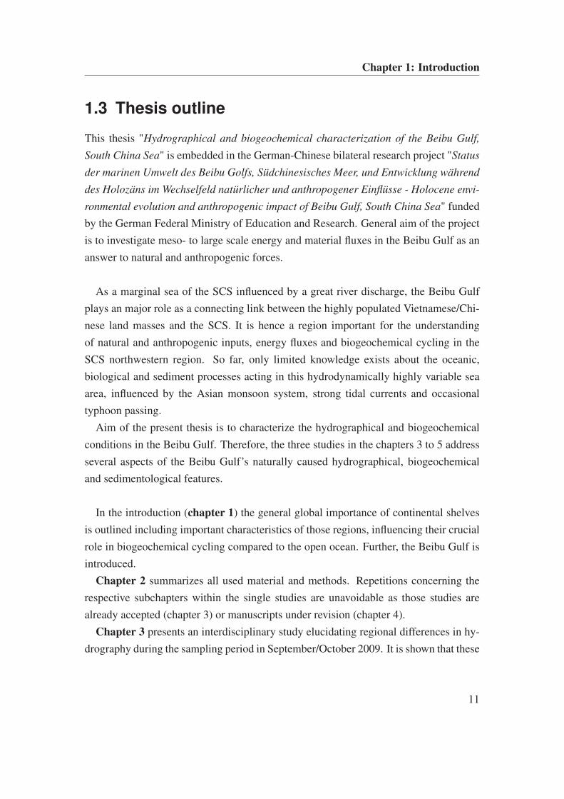
1.3 Thesis outline
This thesis "Hydrographical and biogeochemical characterization of the Beibu Gulf,
South China Sea" is embedded in the German-Chinese bilateral research project "Status
der marinen Umwelt des Beibu Golfs, Südchinesisches Meer, und Entwicklung während
des Holozäns im Wechselfeld natürlicher und anthropogener Einflüsse - Holocene envi-
ronmental evolution and anthropogenic impact of Beibu Gulf, South China Sea" funded
by the German Federal Ministry of Education and Research. General aim of the project
is to investigate meso- to large scale energy and material fluxes in the Beibu Gulf as an
answer to natural and anthropogenic forces.
As a marginal sea of the SCS influenced by a great river discharge, the Beibu Gulf
plays an major role as a connecting link between the highly populated Vietnamese/Chi-
nese land masses and the SCS. It is hence a region important for the understanding
of natural and anthropogenic inputs, energy fluxes and biogeochemical cycling in the
SCS northwestern region. So far, only limited knowledge exists about the oceanic,
biological and sediment processes acting in this hydrodynamically highly variable sea
area, influenced by the Asian monsoon system, strong tidal currents and occasional
typhoon passing.
Aim of the present thesis is to characterize the hydrographical and biogeochemical
conditions in the Beibu Gulf. Therefore, the three studies in the chapters 3 to 5 address
several aspects of the Beibu Gulf’s naturally caused hydrographical, biogeochemical
and sedimentological features.
In the introduction (chapter 1) the general global importance of continental shelves
is outlined including important characteristics of those regions, influencing their crucial
role in biogeochemical cycling compared to the open ocean. Further, the Beibu Gulf is
introduced.
Chapter 2 summarizes all used material and methods. Repetitions concerning the
respective subchapters within the single studies are unavoidable as those studies are
already accepted (chapter 3) or manuscripts under revision (chapter 4).
Chapter 3 presents an interdisciplinary study elucidating regional differences in hy-
drography during the sampling period in September/October 2009. It is shown that these
11
Chapter 1: Introduction
differences affect biological properties in the water column and are further mirrored in
sediment deposition patterns and its geochemical and biological characteristics [Bauer
et al., in press].
In chapter 4 a 1D coupled physical-biological model is used to simulate the seasonal
cycle of primary production in the central Beibu Gulf. For an 11 year period, important
factors generating interannual variability in the timing of stratification and the phyto-
plankton bloom are demonstrated. Furthermore, effects of the spring-neap tidal cycle
and strong wind events on the primary production are shown [Bauer and Waniek, 2013].
In chapter 5 the bottom currents and associated sediment resuspension patterns as
well as the establishment of a diffusive boundary layer in relation to the different tidal
stages, during the sampling period in September/October 2009, and regions defined in
chapter 3 are investigated. It is demonstrated that within the Beibu Gulf, the different
current patterns influence sedimentological and geochemical processes substantially.
Finally, in chapter 6 the main outcomes of the thesis are summarized and some fur-
ther, yet unanswered questions as well as future perspectives are outlined.
All references are listed in the "References" section at the end of this thesis.
12
Chapter 2: Material & Methods
2 Material and Methods
In this section all materials and methods used in this work are only summarized. A
detailed description of the methods (including all calculations) used for the respective
studies is given in each of the following chapters.
2.1 Sampling and in-situ data processing
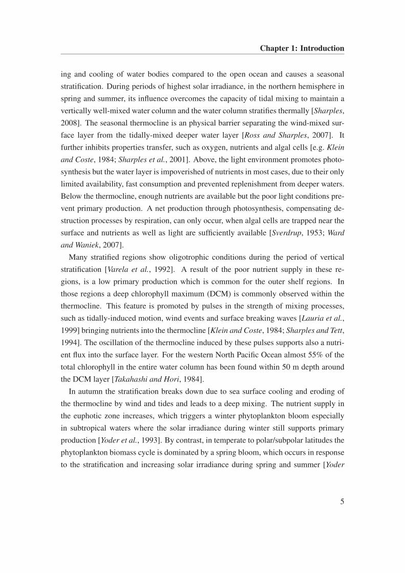
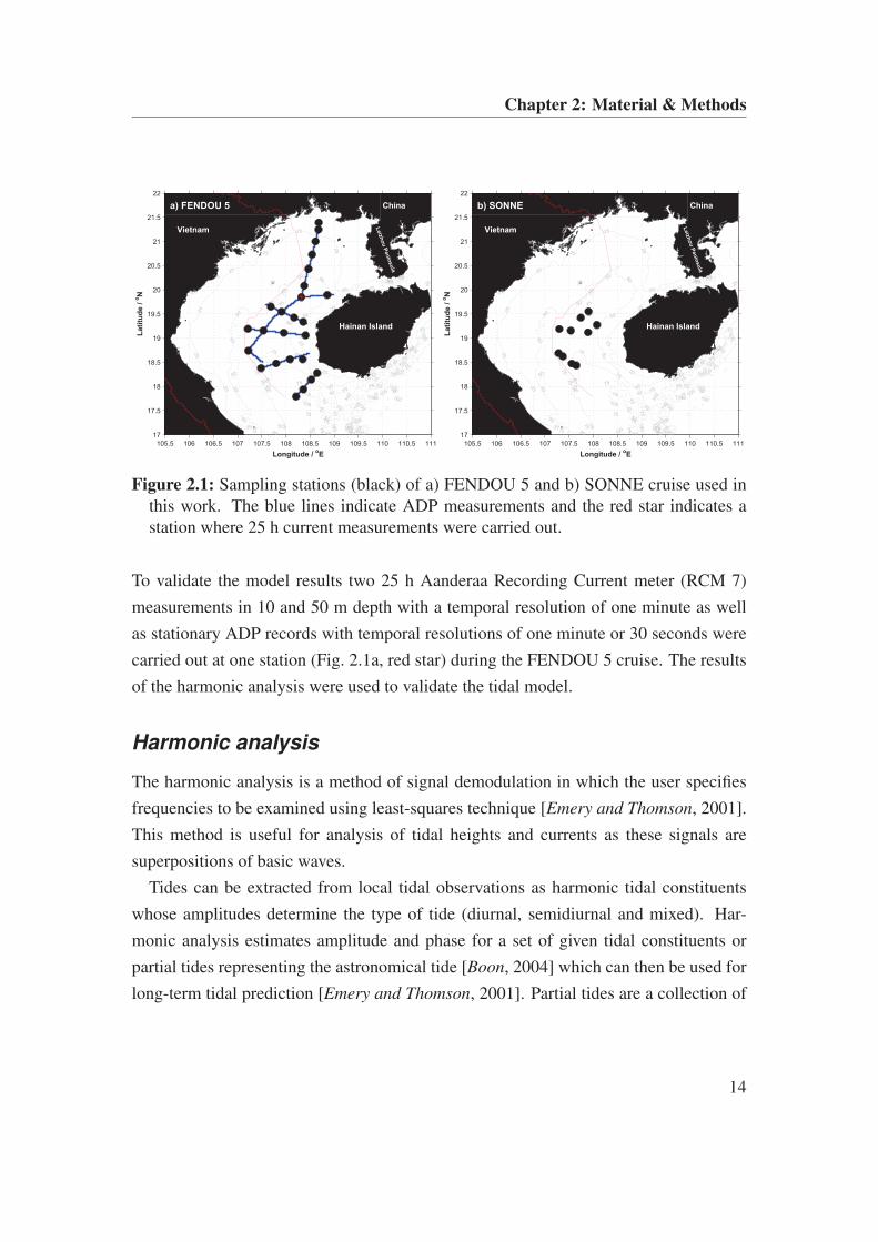
In-situ data were collected during two German-Chinese expeditions with the Chinese
RV FENDOU 5 in September/October 2009 and the German RV SONNE in December
2011 (Fig. 2.1). During the FENDOU 5 cruise depth profiles (temperature, conductivity,
oxygen, chlorophyll-fluorescence) were recorded and water samples were taken at 25
stations (Fig. 2.1a) using a IOW mini PUMP CTD system based on Strady et al. [2008]
including a YSI probe (6600 V2-4). For a detailed description please read section 3.2.
A Seabird CTD with a Niskin bottle rosette sampler system was used during SONNE
cruise for hydrographical profiling and water sampling at 14 stations analyzed in this
work (Fig. 2.1b). For analysis of chlorophyll, nutrients (NO2, NO3, PO4 and SiO4)
and suspended particulate matter (SPM) concentrations water samples were taken at all
stations from different depths during the upcast. Treatments of water samples according
to the respective parameters are described in detail in sections 3.2, 4.2 and 5.2.
2.2 Current measurements
U- and v-component (zonal and meridional) of currents were recorded during transects
using an Acoustic Doppler Profiler (ADP) (Fig. 2.1a) and used for analyzing the bottom
current field during the FENDOU 5 cruise after pre-processing (chapter 5). A simple
tidal model has been developed to identify the tidal stages of all stations and ADP lines
by using tidal heights predicted by the WXTide32 software (explained in section 5.2).
13
Chapter 2: Material & Methods
105.5 106 106.5 107 107.5 108 108.5 109 109.5 110 110.5 111
17
17.5
18
18.5
19
19.5
20
20.5
21
21.5
22
0 0
0
0
0
2525
25
25
25
25
25
25
25
25
25
25
25
25
25
25
25
25
25
25
25
25
25
25
25
252550
50
50
50
50
50
50 50
50
50
50
50
50
50
50
50
5050
50
50
50
50
50
75
75
75
75
75
75
7575
75
75
75
75 75
75
75
75
75
75
75
75
75
75
75
75
75
75
757575
75
75
100
100
100
100100
100
100
100
100
100
100
100
100
100
100100
100
100100
100
100
Longitude / oE
Lati
tud
e /
oN
China
Vietnam
Hainan Island
Leiz
ho
u P
en
insu
la
a) FENDOU 5
105.5 106 106.5 107 107.5 108 108.5 109 109.5 110 110.5 111
17
17.5
18
18.5
19
19.5
20
20.5
21
21.5
22
0 0
0
0
0
2525
25
25
25
25
25
2525
25
25
25
25
25
25
25
25
25
25
25
25
25
25
25
25
252550
50
50
50
50
50
50 50
50
50
50
50
50
50
50
50
5050
50
50
50
50
50
75
75
75
75
75
75
7575
75
75
75
75 75
75
75
75
75
75
75
75
75
75
75
75
75
75
757575
75
75
100
100
100
100
100
100
100
100
100
100
100
100
100
100
100100
100
100100
100
100
Longitude / oE
Lati
tud
e /
oN
China
Vietnam
Hainan Island
Leiz
ho
u P
en
insu
la
b) SONNE
Figure 2.1: Sampling stations (black) of a) FENDOU 5 and b) SONNE cruise used inthis work. The blue lines indicate ADP measurements and the red star indicates astation where 25 h current measurements were carried out.
To validate the model results two 25 h Aanderaa Recording Current meter (RCM 7)
measurements in 10 and 50 m depth with a temporal resolution of one minute as well
as stationary ADP records with temporal resolutions of one minute or 30 seconds were
carried out at one station (Fig. 2.1a, red star) during the FENDOU 5 cruise. The results
of the harmonic analysis were used to validate the tidal model.
Harmonic analysis
The harmonic analysis is a method of signal demodulation in which the user specifies
frequencies to be examined using least-squares technique [Emery and Thomson, 2001].
This method is useful for analysis of tidal heights and currents as these signals are
superpositions of basic waves.
Tides can be extracted from local tidal observations as harmonic tidal constituents
whose amplitudes determine the type of tide (diurnal, semidiurnal and mixed). Har-
monic analysis estimates amplitude and phase for a set of given tidal constituents or
partial tides representing the astronomical tide [Boon, 2004] which can then be used for
long-term tidal prediction [Emery and Thomson, 2001]. Partial tides are a collection of
14
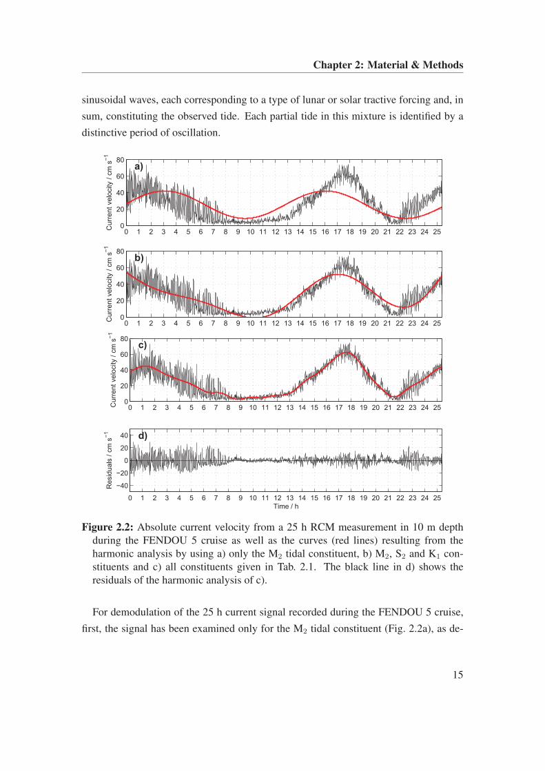
Chapter 2: Material & Methods
sinusoidal waves, each corresponding to a type of lunar or solar tractive forcing and, in
sum, constituting the observed tide. Each partial tide in this mixture is identified by a
distinctive period of oscillation.
0 1 2 3 4 5 6 7 8 9 10 11 12 13 14 15 16 17 18 19 20 21 22 23 24 250
20
40
60
80
Curr
ent
velo
city /
cm
s−
1
a)
0 1 2 3 4 5 6 7 8 9 10 11 12 13 14 15 16 17 18 19 20 21 22 23 24 250
20
40
60
80
Curr
ent
velo
city /
cm
s−
1
b)
0 1 2 3 4 5 6 7 8 9 10 11 12 13 14 15 16 17 18 19 20 21 22 23 24 250
20
40
60
80
Curr
ent
velo
city /
cm
s−
1
c)
0 1 2 3 4 5 6 7 8 9 10 11 12 13 14 15 16 17 18 19 20 21 22 23 24 25
−40
−20
0
20
40
Resid
uals
/ c
m s
−1
Time / h
d)
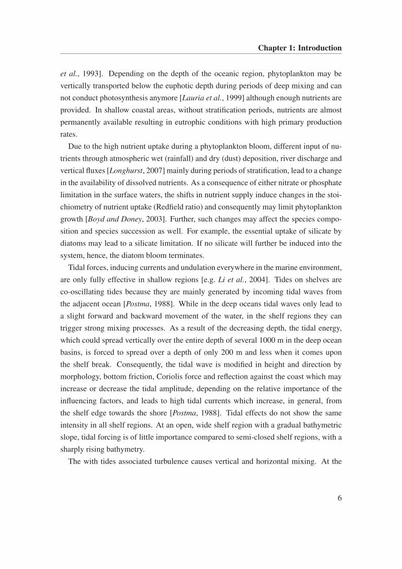
Figure 2.2: Absolute current velocity from a 25 h RCM measurement in 10 m depthduring the FENDOU 5 cruise as well as the curves (red lines) resulting from theharmonic analysis by using a) only the M2 tidal constituent, b) M2, S2 and K1 con-stituents and c) all constituents given in Tab. 2.1. The black line in d) shows theresiduals of the harmonic analysis of c).
For demodulation of the 25 h current signal recorded during the FENDOU 5 cruise,
first, the signal has been examined only for the M2 tidal constituent (Fig. 2.2a), as de-
15
Chapter 2: Material & Methods
scribed by Emery and Thomson [2001]. The resulting curve does not fit with the mea-
sured current signal (Fig. 2.2a). In the next step, the M2, K1 and S2 tidal constituents has
been applied simultaneously, which resulting curve corresponds better with the raw sig-
nal (Fig. 2.2b). The original time series can be reconstructed once the tidal constituents
defining the current signal have been determined (Tab. 2.1, Fig. 2.2c).
In the Beibu Gulf, besides the astronomically dominated main constituents for mar-
ginal seas, additional periods occur (Tab. 2.1) generated by friction processes [van
Maren et al., 2004]. These are tides with periods shorter than semidiurnal tides, arising
in shallow water areas, also called shallow water tides or overtides which are multiples
of fundamental frequencies. The differences between observed and predicted tide, the
so-called residual components (Fig. 2.2d), are tidal and non-tidal variations (e.g. meteo-
rological causes) not captured by harmonic analysis [Emery and Thomson, 2001; Boon,
2004].
In this work results of the harmonically analyzed current measurements has been used
to calculate the S2 tidal amplitude as a fraction of M2 needed for the modeling study in
chapter 4 and for the already mentioned validation of a tidal model essential for current
analysis in chapter 5.
2.3 Coupled physical-biological model
As in-situ data are rare for biogeochemical investigations within longer time scales
(>1 year) a 1-dimensional physical-biological coupled model was used established by
Sharples [1999]. The model has been particularly developed for shelf seas and simulates
daily vertical profiles of currents, temperature, turbulent mixing, photosynthetic active
radiation (PAR), chlorophyll and dissolved inorganic nitrogen (DIN). Using this model
the linkage between meteorological forcing (daily mean wind u- and v-components,
daily mean dewpoint temperature and daily mean solar irradiance), physical properties
of the water column (temperature distribution), especially stratification and mixing, and
primary production (chlorophyll distribution) in the central Beibu Gulf has been studied.
The vertical model grid is split into a series of grid cells [Sharples, 1999] which are
coupled among each other through vertical turbulent mixing (Fig. 2.3) controlled by a
2.2b turbulence closure scheme [Simpson et al., 1996] in the physical module. Quadratic
stress boundary conditions are applied at the surface by wind to transmit wind-driven
16
Chapter 2: Material & Methods
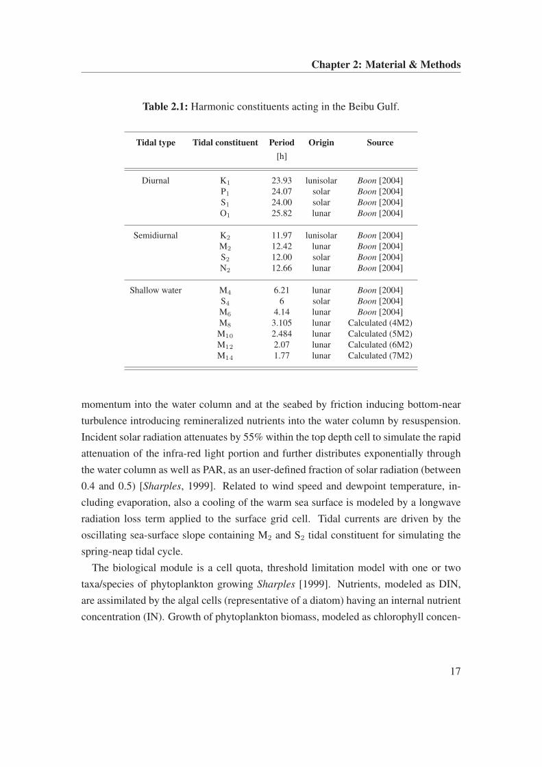
Table 2.1: Harmonic constituents acting in the Beibu Gulf.
Tidal type Tidal constituent Period Origin Source
[h]
Diurnal K1 23.93 lunisolar Boon [2004]P1 24.07 solar Boon [2004]S1 24.00 solar Boon [2004]O1 25.82 lunar Boon [2004]
Semidiurnal K2 11.97 lunisolar Boon [2004]M2 12.42 lunar Boon [2004]S2 12.00 solar Boon [2004]N2 12.66 lunar Boon [2004]
Shallow water M4 6.21 lunar Boon [2004]S4 6 solar Boon [2004]M6 4.14 lunar Boon [2004]M8 3.105 lunar Calculated (4M2)M10 2.484 lunar Calculated (5M2)M12 2.07 lunar Calculated (6M2)M14 1.77 lunar Calculated (7M2)
momentum into the water column and at the seabed by friction inducing bottom-near
turbulence introducing remineralized nutrients into the water column by resuspension.
Incident solar radiation attenuates by 55% within the top depth cell to simulate the rapid
attenuation of the infra-red light portion and further distributes exponentially through
the water column as well as PAR, as an user-defined fraction of solar radiation (between
0.4 and 0.5) [Sharples, 1999]. Related to wind speed and dewpoint temperature, in-
cluding evaporation, also a cooling of the warm sea surface is modeled by a longwave
radiation loss term applied to the surface grid cell. Tidal currents are driven by the
oscillating sea-surface slope containing M2 and S2 tidal constituent for simulating the
spring-neap tidal cycle.
The biological module is a cell quota, threshold limitation model with one or two
taxa/species of phytoplankton growing Sharples [1999]. Nutrients, modeled as DIN,
are assimilated by the algal cells (representative of a diatom) having an internal nutrient
concentration (IN). Growth of phytoplankton biomass, modeled as chlorophyll concen-
17
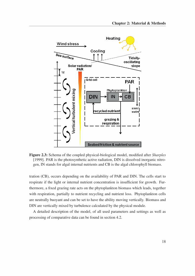
Chapter 2: Material & Methods
Figure 2.3: Schema of the coupled physical-biological model, modified after Sharples
[1999]. PAR is the photosynthetic active radiation, DIN is dissolved inorganic nitro-gen, IN stands for algal internal nutrients and CB is the algal chlorophyll biomass.
tration (CB), occurs depending on the availability of PAR and DIN. The cells start to
respirate if the light or internal nutrient concentration is insufficient for growth. Fur-
thermore, a fixed grazing rate acts on the phytoplankton biomass which leads, together
with respiration, partially to nutrient recycling and nutrient loss. Phytoplankton cells
are neutrally buoyant and can be set to have the ability moving vertically. Biomass and
DIN are vertically mixed by turbulence calculated by the physical module.
A detailed description of the model, of all used parameters and settings as well as
processing of comparative data can be found in section 4.2.
18
Chapter 2: Material & Methods
2.4 Additional data sets
To identify the monsoonal phase during the FENDOU 5 expedition, daily surface wind
fields for the Beibu Gulf region were obtained from the National Centers for Environ-
mental Prediction (NCEP/NCAR, http://www.esrl.noaa.gov; Kalnay et al. [1996]). To
calculate the Ekman depth (chapter 3) during the passing of typhoon KETSANA (23.-
30.09.2009) regional daily wind speeds were obtained from weather stations in Haikou,
Dongfang and Sanya (www.cmabbs.com). Daily wind speeds from the NCEP/NCAR
Reanalysis database were used to calculate Ekman depth in chapter 5. For the model-
ing necessary meteorological parameters (wind components, downward longwave ra-
diation flux as well as air temperature and relative humidity for calculating dewpoint
temperature) were taken as well from the NCEP/NCAR Reanalysis database for 11
years (2000-2010). For model validation, satellite data for daily sea surface tempera-
ture (SST) were taken from http://www.remss.com (Tropical Rainfall Measuring Mis-
sion Microwave Imager (TMI), resolution 0.25◦ x 0.25◦) and monthly SeaWiFS (2000-
2010) as well as MODIS (07/2002-2010) surface chlorophyll concentrations from http:
//gdata1.sci.gsfc.nasa.gov were used. All remotely measured data for the modeling
study, used in a meteorological data file as well as comparative satellite data, were
averaged for the central Beibu Gulf (explained in section 4.2.4).
For sediment sampling, box corer, multi corer and gravity corer were used during
FENDOU 5 cruise. Sediment cores were described macroscopically and sliced for fur-
ther investigations. Samples were taken for grain size, geochemical (water contents,
particulate major and trace elements, organic and inorganic carbon, total nitrogen) as
well as surface sediment foraminifera and plant pigment analysis. Furthermore, pore
water samples were taken with rhizons [e.g. Seeberg-Elverfeldt et al., 2005] on board
of FENDOU 5. The sampling of geological and geochemical parameters is described in
detail in sections 3.2.3, 3.2.4 and 5.2.2.
19
Chapter 3: Regional differences
3 Regional differences of hydrographical
and sedimentological properties in the
Beibu Gulf, South China Sea
Bauer et al. (in press), Journal of Coastal Research: Special Issue 66
Abstract
Analyzing the Beibu Gulf’s hydrography and sediment properties is crucial for the un-
derstanding of naturally and anthropogenically induced matter and energy fluxes in the
SCS’s northwestern coastal regions. For this reason, the present study combines hydro-
graphical (T, S, σt), chlorophyll, nutrients, SPM) and sedimentological (grain size, pore
water properties, phosphate speciation, foraminifera, plant pigment contents) investiga-
tions.
On the basis of hydrographical profiles (temperature, salinity and σt) taken at 25
stations, four ecological zones are identified in the study area for the sampling period in
September/October 2009. These zones are mainly influenced by riverine input and tidal
mixing, water mass transport through the Qiongzhou Strait which also affects the gulf’s
circulation, and SCS waters in the southern Beibu Gulf. The zonation extends from the
coastal areas in the northern Beibu Gulf and west of Hainan Island across the central
regions to the southern part of the gulf.
The study demonstrates that the hydrographical peculiarities of the different zones in-
fluence not only the biogeochemical features (chlorophyll, nutrients, SPM) of the water
column but also the deposition of sediments and their biological (plant pigment contents
and foraminifera) and geochemical (pore water properties) characteristics. Both, the
near-shore area and the zone in the vicinity of the Qiongzhou Strait show relatively high
chlorophyll concentrations and therefore give evidence of enhanced primary production
20
Chapter 3: Regional differences
in the entire water column. Whereas the grain size and the foraminifera in the surface
sediments follow the hydrodynamically controlled sedimentation conditions, plant pig-
ment contents in the surface sediments additionally follow the productivity pattern in
the water column. Depending on the depositional environments with their respective
sedimentology and organic matter contents, the geochemical sediment properties reflect
the primary production within the water column as well.
3.1 Introduction
The SCS is one of the largest and for the regional climate most important sea of the
Southeast Asian Waters [Liu et al., 2002]. Bathymetrically, about 47% of the total area
of the SCS consist of a well developed shelf area [Wang and Li, 2009]. This broad
shelf with a depth less than 100 m belongs to the so-called "Sunda-Arafura Shelves
Province", a large continental shelf area extending from Burma and South China down
to the northern coast of Australia [Longhurst, 2007].
The Beibu Gulf, also known as the Gulf of Tonkin, is one of the SCS major embay-
ments. It is located in the northwestern part of the SCS, bounded by South China and
Vietnam in the north and west and by Leizhou Peninsula and Hainan Island in the east,
connected to the northwestern shelf of the SCS through the Qiongzhou Strait, and has
a broad opening to the western SCS in the south. As a shallow shelf sea area the Beibu
Gulf has an average depth of about 45 m and a bathymetry that deepens gradually to
the south where the gulf reaches its maximum depth of about 100 m [Manh and Yanagi,
1997; Wu et al., 2008].
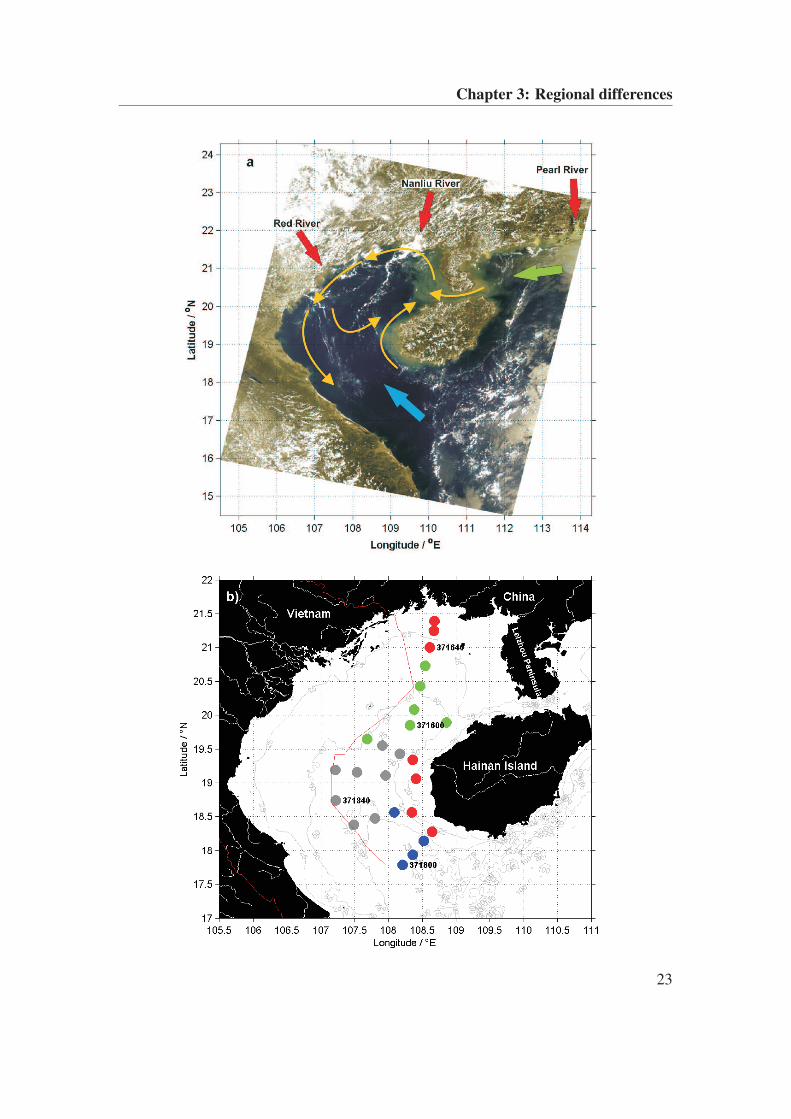
The circulation in the Beibu Gulf is mainly governed by wind, tidal currents and cur-
rents outside the gulf [Chen et al., 2009]. In the traditional view the surface circulation
in the Beibu Gulf reverses from a winter cyclonic to a summer anticyclonic circulation
due to the change from northeast to southwest monsoon [e.g. Manh and Yanagi, 1997,
2000], equally to the circulation in the SCS main basin [e.g. Huang et al., 1994]. How-
ever, most recent modeling results and observational data reveal that the circulation is
cyclonic throughout the entire year [Shi et al., 2002; Wu et al., 2008]. A broad south-
ward flow in the upper layer along the Vietnamese coast is compensated by a northward
return flow in the interior and along the west coast of Hainan Island which results in
a gulf-wide cyclonic gyre [Wu et al., 2008] (Fig. 3.1a). The tide-induced westward
21
Chapter 3: Regional differences
mean transport of about 0.1-0.2 Sv through Qiongzhou Strait into the Gulf of Beibu in
all seasons [Shi et al., 2002] (Fig. 3.1a) is the key factor for the cyclonic circulation,
especially in summer when the southwestern monsoonal forcing tends to drive an an-
ticyclonic one [Wu et al., 2008]. Many rivers with a mean annual discharge of about
14 x 1010 m3 influence the Beibu Gulf [Chen et al., 2009]. Rivers play a major role
in the transport of material from land to the sea and thereby significantly influence the
biogeochemical processes in coastal waters [Gago et al., 2005]. River loads from the
Red River and some smaller rivers in the northern coastal area [Tang et al., 2003] are
transported southward through the Beibu Gulf into the SCS (Fig. 3.1a). Furthermore,
the semi-enclosed Beibu Gulf interacts with the surrounding SCS through water mass
exchanges [Wu et al., 2008]. Different water masses originating from the coastal areas
off South China in the northern SCS can be transported through Qiongzhou Strait and
therefore influence the region [e.g. Su and Weng, 1994]. Also discharge from the Pearl
River located 400 km away to the northeast may reach the gulf through the Qiongzhou
Strait [Tang et al., 2003] (Fig. 3.1a).
The marine influence from the south is mainly driven by tidal waves propagating into
the Beibu Gulf through the wide opening with a current velocity of about 40 cm s−1
at the surface [Manh and Yanagi, 1997] (Fig. 3.1a). Model experiments by Cai et al.
[2003] showed that tidally driven currents play a significant role in the formation of a
cyclonic circulation in the Beibu Gulf, especially in summer.
This study presents first results of the German/Chinese bilateral research project
BEIBU which focusses on the Beibu Gulf. Shelf areas like the Beibu Gulf are hot spots
for biogeochemical fluxes and respond very quickly to environmental changes, e.g. the
carbon turnover time is in order of days to weeks [Ross, 2004]. Therefore, they are im-
Figure 3.1 (following page): a) Satellite image of the Beibu Gulf region from ESAENVISAT MERIS (18. September 2009) showing the general cyclonic circulationpattern (yellow arrows, after Shi et al. [2002] and Wu et al. [2008], riverine (red ar-row), coastal parallel (green arrow) and marine input (blue arrow). b) FENDOU 5cruise track in September/October 2009. The different zones as defined in this studyare color-coded (red dots: BGCoZ, Beibu Gulf Coastal Zone, green dots: QiongzhouStrait Zone, QSZ, grey dots: Beibu Gulf Central Zone, BGCeZ and blue dots: South-ern Beibu Gulf Zone, SBGZ). The stations representing the zones are labelled.
22
Chapter 3: Regional differences
23
Chapter 3: Regional differences
portant for the understanding of changes in the balance of river input and coastal erosion,
near-surface degradation of organic material and hence induced element fluxes as well
as changes in the conditions of recent sediment accumulation. As a large marginal sea
of the SCS the Beibu Gulf plays an important role for the understanding of naturally and
anthropogenically induced matter and energy fluxes in the SCS northwestern coastal re-
gions. So far, less is known about the biogeochemical element cycles in the Beibu Gulf,
which is nowadays an important region for the industrial production of P-bearing fertil-
izers [Yan, 2006]. Element and material transport via benthic-pelagic coupling towards
surface waters, for example, may be an important factor driving primary production in
this region.
The aim of this study is to elucidate regional differences in hydrography influenc-
ing not only biological properties in the water column but also deposition and coupled
geochemical and biological characteristics of the sediments. Until now, no interdisci-
plinary study on the Beibu Gulf which combines water column and sediment properties
has been presented or published.
3.2 Material and Methods
3.2.1 Study area
The study area is situated in the northern and eastern part of the Beibu Gulf in the
territorial waters of P. R. China (Fig. 3.1b).
During summer, the surface water temperature is high, ranging from 27.5°C in the
north of the gulf to 29.5°C in the south [Manh and Yanagi, 2000]. Because of the high
fresh water discharge in summer in the northwestern area, a low salinity zone and a
cold water mass exists in the center of the gulf [Chen et al., 2009]. In winter, the water
column is vertically well mixed and surface water temperatures increase from 20°C in
the north to 24°C in the south [Manh and Yanagi, 2000].
The Beibu Gulf contains tropical mesotrophic waters [Tang et al., 2003]. A verti-
cal stratification develops in summer with rapidly decreasing water temperatures from
about 29.5°C at the surface, to 19°C at depth [Manh and Yanagi, 2000] and a relative
uniform SST in the entire gulf. This stratification, caused by sea surface heating, limits
entrainment of nutrients and phytoplankton growth [Tang et al., 2003]. Therefore, in
24
Chapter 3: Regional differences
summer the chlorophyll a content is relatively low and uniform in the entire gulf [Tang
et al., 2003]. In a narrow band along the coasts, tidal mixing induces upwelling of nu-
trients to the euphotic zone which leads to a higher chlorophyll a concentration and a
higher primary production [Tang et al., 2003]. In contrast, during winter the chlorophyll
a concentrations increase in the entire gulf, with higher chlorophyll a concentrations in
the northeastern and lower in the southwestern part [Tang et al., 2003].
Geologically, the depositional center of the gulf and local depressions are filled with
fine-grained sediments, substituted by sandy deposits closer to the coasts [Su and Wang,
1994]. The near-surface sediment layers are complex and include siliciclastic deposits
with variable carbonate-organogenic components [Su and Wang, 1994]. The accumula-
tion rate varies between 1.2 mm yr−1 for the deltas [Liu et al., 1992] and 0.25 mm yr−1
in local lagoons [Li et al., 1996]. It has to be mentioned that in earlier stages during the
Holocene the accumulation rates reached in delta areas more that 3 mm yr−1 [Tanabe
et al., 2003a,b].
3.2.2 Water samples
During a cruise with the Chinese RV FENDOU 5 in September/October 2009 depth
profiles (temperature, conductivity, oxygen, chlorophyll-fluorescence) were recorded as
well as water, pore water and sediment samples were taken at 25 stations (Fig. 3.1b).
Hydrographic profiling and water sampling was done by using an IOW mini PUMP
CTD system based on Strady et al. [2008]. The instrument consists of a YSI probe (6600
V2-4) including sensors for pressure, temperature, conductivity, oxygen, fluorescence
and turbidity in a frame additionally equipped with an extra underwater high pressure
pump. This pump produces a water flow from the CTD through a 150 m long tube with
a rate of about 2 l min−1 to the ship-board laboratory. The YSI is directly connected
to a notebook on deck for continuous recording of the hydrographical parameters and
calculating the depth during downcast.
Water samples were taken from different depths during upcast and stored in 5 l can-
isters. For chlorophyll and SPM analyses, 0.5 to 1 l water were low vacuum filtered
through 0.7 µm Whatman GF/F glass fibre filters. In addition, water samples for anal-
ysis of dissolved nutrients (NO2, NO3, PO4, SiO4) were taken. All filters were washed
with deionized water before storage and frozen at around -20°C until laboratory analy-
25
Chapter 3: Regional differences
sis at Leibniz-Institute for Baltic Sea Research (IOW). The extracted chlorophyll sam-
ples were analyzed through a fluorometer (TURNER 10-AU) after JGOFS [1994] with-
out correction for phaeopigments. Nutrient samples were processed using an autoana-
lyzer (EVOLUTION III, Aliance Instruments, (detection limits: NO2: 0.02 µM, NO3:
0.05 µM, PO4: 0.02 µM, SiO4: 0.1 µM)) according to standard procedures [Hansen
and Koroleff , 1999].
3.2.3 Geological samples
For sediment sampling box corer (BC), multi corer (MUC), and gravity corer (GC) were
used. The MUC was equipped with 4 liners (60 cm long, inner diameter 10 cm), the GC
was loaded with 4 m long plastic liners (diameter of 120 mm). After recovery, the GC
cores were cut into sections of 1 m. At each station the first gravity core was used for
macroscopic sediment description according to standard protocols, e.g. sediment color
was determined using the rock-color chart [Rock Color Chart, 1991].
The MUC cores were sliced into 1 cm sections for the upper 20 cm and 2 cm sections
for depths >20 cm. Cores taken by GC were cut into 2 cm slices. Every sample from
the upper 50 cm and every second sample from the lower 50 cm of the GC core was an-
alyzed in the laboratory later. Preparation, treatment and measurement of all sediment
samples were carried out in the laboratory of Marine Geology Section, IOW and in the
laboratory of the Guangzhou Marine Geological Survey (GMGS). The grain size was
determined using a laser particle sizer analyzer (Cilas 1180L) with an ultrasonic pre-
treatment for 10 min to disperse the aggregates (T. Leipe, personal comment) at IOW
(cores at stations 371800 and 371840) and a diffraction particle size analyzer (Master-
sizer 2000) at GMGS (cores at stations 371600 and 371640). For further geological
analysis sediment samples were freeze-dried and homogenized by mixing and grinding.
The sediment samples for plant pigment analyses were taken from the topmost 1 cm
of cores recovered by BC and MUC. After thawing in the dark, four sediment por-
tions per sample were placed in a fluorometric cuvette containing 7 ml 90% acetone in
magnesium carbonate solution and left for extraction for 24 h in the dark at 4°C in the
laboratory of the University of Szczecin, Poland. Pigment contents in the extracts were
measured fluorometrically in a calibrated TURNER 10-AU fluorometer (Turner De-
signs, USA) before (chlorophyll a) and after (phaeopigments) acidification with 0.1 N
26
Chapter 3: Regional differences
HCl. The extracted sediment was dried at 105°C and weighted. The fluorescence read-
outs were converted to pigment content per 1 g dry sediment and the results of the 4
portions per sample were averaged.
For foraminiferal analysis, BC sediment samples, about 20 g each, were processed us-
ing standard techniques according to Wei et al. [2006]. First, the samples were washed
in distilled water to remove adhering particles and then soaked in 10% NaOCl solution
for 24 h to remove organic materials. The samples were pre-sieved on a 0.063 mm
mesh size sieve and the residues >0.063 mm were separated into two fractions using a
0.15 mm mesh size copper sieve. Foraminifera from the >0.15 mm fraction were iden-
tified and counted without discrimination between living and dead individuals. Finally,
the abundances of various species were standardized to 10 g sediment because of the
low total abundance.
3.2.4 Geochemical samples
Particulate major and trace elements were analysed by ICP-OES (Thermo iCAP 6300-
Duo). Precision (1σ) and accuracy of all measurements were checked by parallel anal-
ysis of international and in-house reference materials (precision and accuracy were
≤ 7.4% and ≤ 4.3% for major elements and ≤ 6.8% and ≤ 10.7% for trace metals)
according to Dellwig et al. [2010]. Samples for pore water analysis were taken with
rhizons [e.g. Seeberg-Elverfeldt et al., 2005] connected to syringes through holes in the
core liners on board of the ship. Samples for dissolved elements were filtered through
0.45 µm SFCA syringe filters and acidified to 1 vol% HNO3 in precleaned PE-bottles.
All acids used were of suprapure quality.
Sediments were taken from sliced sections of sedimentary short (MUC) and long
cores (GC) and analyzed for water contents (gravimetry), organic and inorganic carbon,
and total nitrogen as described by Leipe et al. [2010]. For the depth correction of all
gravity cores, an estimated top core loss of about 20 cm was assumed. Sedimentary
phosphorous (P) fractions were extracted sequentially according to the scheme of van
Beusekom (after De Jonge and Engelkes [1993]). Reactive iron was extracted from
wet sediments using 0.5 M HCl for 1 h at room temperature [Kostka and I.G.W., 1994;
Thamdrup et al., 1994]. A one hour extraction with HCl is selective for the amorphous
or poorly crystallized Fe-ox(yhydrox)ide and carbonate phases, with minor contribu-
27
Chapter 3: Regional differences
tion of silicates [e.g. Haese et al., 1997]. The extracted P fractions (iron-bound (P-Fe),
iron-aluminum-bound (P-FeAl) and Ca-apatite (P-Ap)) and extractable iron (Fe*) were
measured by spectrophotometry (Specord 40 spectrophotometer, Analytik Jena) accord-
ing to Koroleff and Kremling [1999] and Stookey [1970], respectively.
3.2.5 Additional data sets
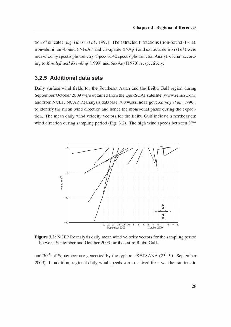
Daily surface wind fields for the Southeast Asian and the Beibu Gulf region during
September/October 2009 were obtained from the QuikSCAT satellite (www.remss.com)
and from NCEP/ NCAR Reanalysis database (www.esrl.noaa.gov; Kalnay et al. [1996])
to identify the mean wind direction and hence the monsoonal phase during the expedi-
tion. The mean daily wind velocity vectors for the Beibu Gulf indicate a northeastern
wind direction during sampling period (Fig. 3.2). The high wind speeds between 27th
25 26 27 28 29 30 1 2 3 4 5 6 7 8 9 10−15
−10
−5
0
N
O
S
W
Win
d /
m s
−1
September 2009 October 2009
Figure 3.2: NCEP Reanalysis daily mean wind velocity vectors for the sampling periodbetween September and October 2009 for the entire Beibu Gulf.
and 30th of September are generated by the typhoon KETSANA (23.-30. September
2009). In addition, regional daily wind speeds were received from weather stations in
28
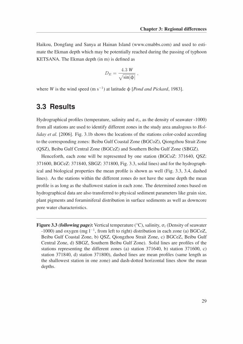
Chapter 3: Regional differences
Haikou, Dongfang and Sanya at Hainan Island (www.cmabbs.com) and used to esti-
mate the Ekman depth which may be potentially reached during the passing of typhoon
KETSANA. The Ekman depth (in m) is defined as
DE =4.3 W
√
sin|φ|,
where W is the wind speed (m s−1) at latitude φ [Pond and Pickard, 1983].
3.3 Results
Hydrographical profiles (temperature, salinity and σt, as the density of seawater -1000)
from all stations are used to identify different zones in the study area analogous to Hol-
liday et al. [2006]. Fig. 3.1b shows the locations of the stations color-coded according
to the corresponding zones: Beibu Gulf Coastal Zone (BGCoZ), Qiongzhou Strait Zone
(QSZ), Beibu Gulf Central Zone (BGCeZ) and Southern Beibu Gulf Zone (SBGZ).
Henceforth, each zone will be represented by one station (BGCoZ: 371640, QSZ:
371600, BGCeZ: 371840, SBGZ: 371800, Fig. 3.3, solid lines) and for the hydrograph-
ical and biological properties the mean profile is shown as well (Fig. 3.3, 3.4, dashed
lines). As the stations within the different zones do not have the same depth the mean
profile is as long as the shallowest station in each zone. The determined zones based on
hydrographical data are also transferred to physical sediment parameters like grain size,
plant pigments and foraminiferal distribution in surface sediments as well as downcore
pore water characteristics.
Figure 3.3 (following page): Vertical temperature (°C), salinity, σt (Density of seawater-1000) and oxygen (mg l−1, from left to right) distribution in each zone (a) BGCoZ,Beibu Gulf Coastal Zone, b) QSZ, Qiongzhou Strait Zone, c) BGCeZ, Beibu GulfCentral Zone, d) SBGZ, Southern Beibu Gulf Zone). Solid lines are profiles of thestations representing the different zones (a) station 371640, b) station 371600, c)station 371840, d) station 371800), dashed lines are mean profiles (same length asthe shallowest station in one zone) and dash-dotted horizontal lines show the meandepths.
29
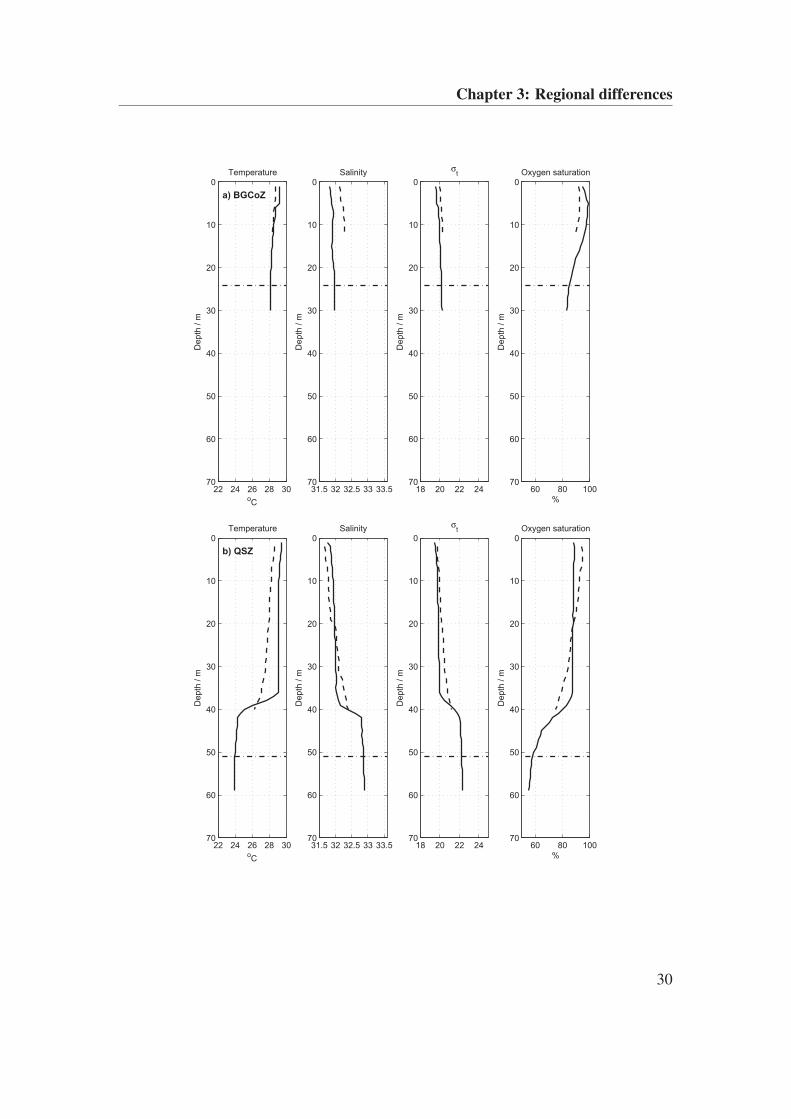
Chapter 3: Regional differences
22 24 26 28 30
0
10
20
30
40
50
60
70
Temperature
oC
Depth
/ m
a) BGCoZ
31.5 32 32.5 33 33.5
0
10
20
30
40
50
60
70
Salinity
Depth
/ m
18 20 22 24
0
10
20
30
40
50
60
70
σt
Depth
/ m
60 80 100
0
10
20
30
40
50
60
70
Oxygen saturation
%D
epth
/ m
22 24 26 28 30
0
10
20
30
40
50
60
70
Temperature
oC
Depth
/ m
b) QSZ
31.5 32 32.5 33 33.5
0
10
20
30
40
50
60
70
Salinity
Depth
/ m
18 20 22 24
0
10
20
30
40
50
60
70
σt
Depth
/ m
60 80 100
0
10
20
30
40
50
60
70
Oxygen saturation
%
Depth
/ m
30
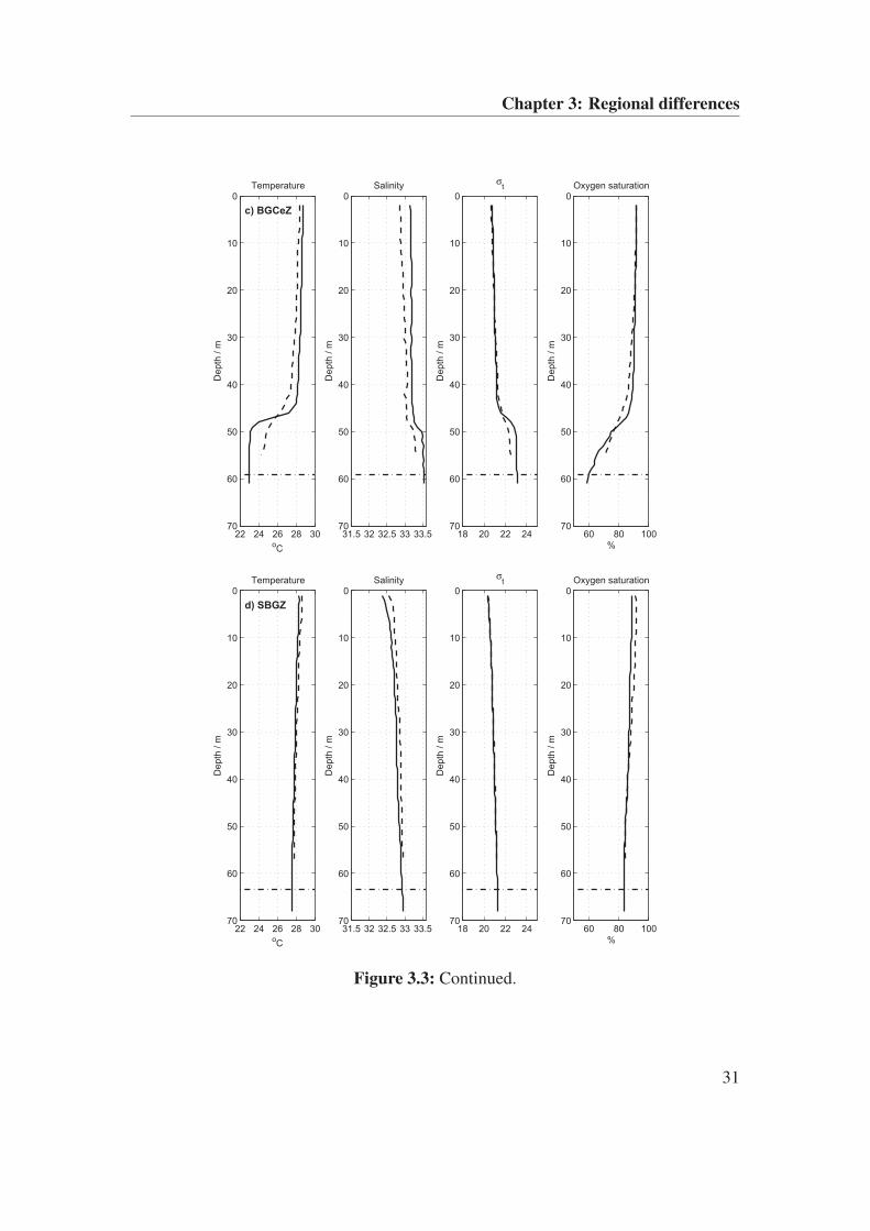
Chapter 3: Regional differences
22 24 26 28 30
0
10
20
30
40
50
60
70
Temperature
oC
Depth
/ m
c) BGCeZ
31.5 32 32.5 33 33.5
0
10
20
30
40
50
60
70
Salinity
Depth
/ m
18 20 22 24
0
10
20
30
40
50
60
70
σt
Depth
/ m
60 80 100
0
10
20
30
40
50
60
70
Oxygen saturation
%D
epth
/ m
22 24 26 28 30
0
10
20
30
40
50
60
70
Temperature
oC
Depth
/ m
d) SBGZ
31.5 32 32.5 33 33.5
0
10
20
30
40
50
60
70
Salinity
Depth
/ m
18 20 22 24
0
10
20
30
40
50
60
70
σt
Depth
/ m
60 80 100
0
10
20
30
40
50
60
70
Oxygen saturation
%
Depth
/ m
Figure 3.3: Continued.
31
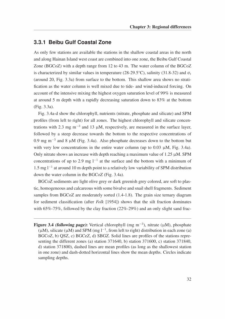
Chapter 3: Regional differences
3.3.1 Beibu Gulf Coastal Zone
As only few stations are available the stations in the shallow coastal areas in the north
and along Hainan Island west coast are combined into one zone, the Beibu Gulf Coastal
Zone (BGCoZ) with a depth range from 12 to 43 m. The water column of the BGCoZ
is characterized by similar values in temperature (28-29.5°C), salinity (31.8-32) and σt
(around 20, Fig. 3.3a) from surface to the bottom. This shallow area shows no strati-
fication as the water column is well mixed due to tide- and wind-induced forcing. On
account of the intensive mixing the highest oxygen saturation level of 99% is measured
at around 5 m depth with a rapidly decreasing saturation down to 83% at the bottom
(Fig. 3.3a).
Fig. 3.4a-d show the chlorophyll, nutrients (nitrate, phosphate and silicate) and SPM
profiles (from left to right) for all zones. The highest chlorophyll and silicate concen-
trations with 2.3 mg m−3 and 13 µM, respectively, are measured in the surface layer,
followed by a steep decrease towards the bottom to the respective concentrations of
0.9 mg m−3 and 8 µM (Fig. 3.4a). Also phosphate decreases down to the bottom but
with very low concentrations in the entire water column (up to 0.03 µM, Fig. 3.4a).
Only nitrate shows an increase with depth reaching a maximum value of 1.25 µM. SPM
concentrations of up to 2.9 mg l−1 at the surface and the bottom with a minimum of
1.5 mg l−1 at around 10 m depth point to a relatively low variability of SPM distribution
down the water column in the BGCoZ (Fig. 3.4a).
BGCoZ sediments are light olive grey or dark greenish grey colored, are soft to plas-
tic, homogeneous and calcareous with some bivalve and snail shell fragments. Sediment
samples from BGCoZ are moderately sorted (1.4-1.8). The grain size ternary diagram
for sediment classification (after Folk [1954]) shows that the silt fraction dominates
with 65%-75%, followed by the clay fraction (22%-29%) and an only slight sand frac-
Figure 3.4 (following page): Vertical chlorophyll (mg m−3), nitrate (µM), phosphate(µM), silicate (µM) and SPM (mg l−1, from left to right) distribution in each zone (a)BGCoZ, b) QSZ, c) BGCeZ, d) SBGZ. Solid lines are profiles of the stations repre-senting the different zones (a) station 371640, b) station 371600, c) station 371840,d) station 371800), dashed lines are mean profiles (as long as the shallowest stationin one zone) and dash-dotted horizontal lines show the mean depths. Circles indicatesampling depths.
32
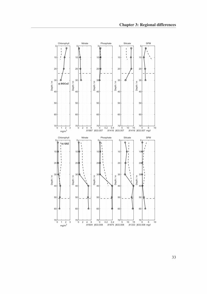
Chapter 3: Regional differences
0 1 2 3
0
10
20
30
40
50
60
70
Chlorophyll
mg/m3
Depth
/ m
b) QSZ
0 2 4 6
0
10
20
30
40
50
60
70
Nitrate
M
Depth
/ m
0 0.2 0.4
0
10
20
30
40
50
60
70
Phosphate
M
Depth
/ m
5 10 15
0
10
20
30
40
50
60
70
Silicate
M
Depth
/ m
0 5 10
0
10
20
30
40
50
60
70
SPM
mg/l
Depth
/ m
0 1 2 3
0
10
20
30
40
50
60
70
Chlorophyll
mg/m3
Depth
/ m a) BGCoZ
0 2 4 6
0
10
20
30
40
50
60
70
Nitrate
M
Depth
/ m
0 0.2 0.4
0
10
20
30
40
50
60
70
Phosphate
M
Depth
/ m
5 10 15
0
10
20
30
40
50
60
70
Silicate
M
Depth
/ m
0 5 10
0
10
20
30
40
50
60
70
SPM
mg/l
Depth
/ m
33
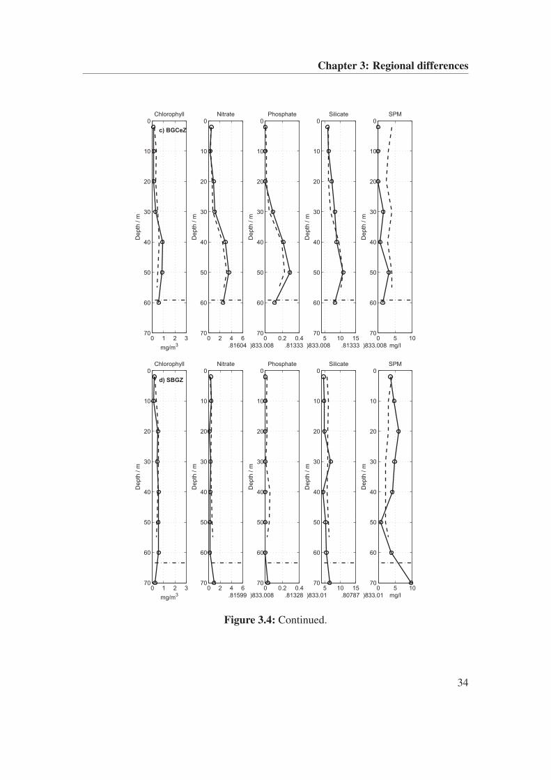
Chapter 3: Regional differences
0 1 2 3
0
10
20
30
40
50
60
70
Chlorophyll
mg/m3
Depth
/ m
d) SBGZ
0 2 4 6
0
10
20
30
40
50
60
70
Nitrate
M
Depth
/ m
0 0.2 0.4
0
10
20
30
40
50
60
70
Phosphate
M
Depth
/ m
5 10 15
0
10
20
30
40
50
60
70
Silicate
M
Depth
/ m
0 5 10
0
10
20
30
40
50
60
70
SPM
mg/l
Depth
/ m
0 1 2 3
0
10
20
30
40
50
60
70
Chlorophyll
mg/m3
Depth
/ m
c) BGCeZ
0 2 4 6
0
10
20
30
40
50
60
70
Nitrate
M
Depth
/ m
0 0.2 0.4
0
10
20
30
40
50
60
70
Phosphate
M
Depth
/ m
5 10 15
0
10
20
30
40
50
60
70
Silicate
M
Depth
/ m
0 5 10
0
10
20
30
40
50
60
70
SPM
mg/l
Depth
/ m
Figure 3.4: Continued.
34
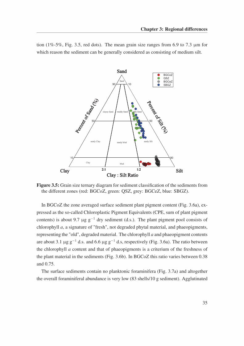
Chapter 3: Regional differences
tion (1%-5%, Fig. 3.5, red dots). The mean grain size ranges from 6.9 to 7.3 µm for
which reason the sediment can be generally considered as consisting of medium silt.
50 50
10
90 10
90
Per
cent
of San
d (%
) Percent of S
ilt (%)
Clay : Silt Ratio
2:1 1:2Clay Silt
Sand
Sand
clayey Sand muddy Sand silty Sand
sandy Clay sandy Siltsandy Mud
ClayMud
Silt
Per
cent
of San
d (%
) Percent of S
ilt (%)
Clay : Silt Ratio
2:1 1:2Clay Silt
Sand
Sand
clayey Sand muddy Sand silty Sand
sandy Clay sandy Siltsandy Mud
ClayMud
Silt
Per
cent
of San
d (%
) Percent of S
ilt (%)
Clay : Silt Ratio
2:1 1:2Clay Silt
Sand
Sand
clayey Sand muddy Sand silty Sand
sandy Clay sandy Siltsandy Mud
ClayMud
Silt
Per
cent
of San
d (%
) Percent of S
ilt (%)
Clay : Silt Ratio
2:1 1:2Clay Silt
Sand
Sand
clayey Sand muddy Sand silty Sand
sandy Clay sandy Siltsandy Mud
ClayMud
Silt
BGCoZ
QSZ
BGCeZ
SBGZ
Figure 3.5: Grain size ternary diagram for sediment classification of the sediments fromthe different zones (red: BGCoZ, green: QSZ, grey: BGCeZ, blue: SBGZ).
In BGCoZ the zone averaged surface sediment plant pigment content (Fig. 3.6a), ex-
pressed as the so-called Chloroplastic Pigment Equivalents (CPE, sum of plant pigment
contents) is about 9.7 µg g−1 dry sediment (d.s.). The plant pigment pool consists of
chlorophyll a, a signature of "fresh", not degraded phytal material, and phaeopigments,
representing the "old", degraded material. The chlorophyll a and phaeopigment contents
are about 3.1 µg g−1 d.s. and 6.6 µg g−1 d.s, respectively (Fig. 3.6a). The ratio between
the chlorophyll a content and that of phaeopigments is a criterium of the freshness of
the plant material in the sediments (Fig. 3.6b). In BGCoZ this ratio varies between 0.38
and 0.75.
The surface sediments contain no planktonic foraminifera (Fig. 3.7a) and altogether
the overall foraminiferal abundance is very low (83 shells/10 g sediment). Agglutinated
35
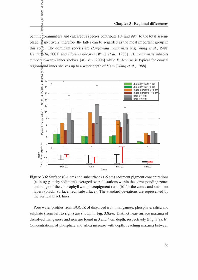
Chapter 3: Regional differences
benthic foraminifera and calcareous species contribute 1% and 99% to the total assem-
blage, respectively, therefore the latter can be regarded as the most important group in
this zone. The dominant species are Hanzawaia mantaensis [e.g. Wang et al., 1988;
He and Hu, 2001] and Florilus decorus [Wang et al., 1988]. H. mantaensis inhabits
temperate-warm inner shelves [Murray, 2006] while F. decorus is typical for coastal
regions and inner shelves up to a water depth of 50 m [Wang et al., 1988].
0
2
4
6
8
10
12
14
16
18
20
a
Pig
ment
concentr
ation /
g/g
dry
sedim
ent
BGCoZ QSZ BGCeZ SBGZ0
0.5
1
b
Zones
Ratio
Chl a :
Phaeopig
ments
Chlorophyll a 0−1 cm
Chlorophyll a 1−5 cm
Phaeopigments 0−1 cm
Phaeopigments 1−5 cm
Total 0−1 cm
Total 1−5 cm
Figure 3.6: Surface (0-1 cm) and subsurface (1-5 cm) sediment pigment concentrations(a, in µg g−1 dry sediment) averaged over all stations within the corresponding zonesand range of the chlorophyll a to phaeopigment ratio (b) for the zones and sedimentlayers (black: surface, red: subsurface). The standard deviations are represented bythe vertical black lines.
Pore water profiles from BGCoZ of dissolved iron, manganese, phosphate, silica and
sulphate (from left to right) are shown in Fig. 3.8a-e. Distinct near-surface maxima of
dissolved manganese and iron are found in 3 and 4 cm depth, respectively (Fig. 3.8a, b).
Concentrations of phosphate and silica increase with depth, reaching maxima between
36
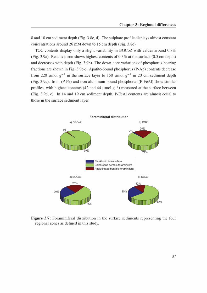
Chapter 3: Regional differences
8 and 10 cm sediment depth (Fig. 3.8c, d). The sulphate profile displays almost constant
concentrations around 26 mM down to 15 cm depth (Fig. 3.8e).
TOC contents display only a slight variability in BGCoZ with values around 0.8%
(Fig. 3.9a). Reactive iron shows highest contents of 0.3% at the surface (0.5 cm depth)
and decreases with depth (Fig. 3.9b). The down-core variations of phosphorus-bearing
fractions are shown in Fig. 3.9c-e. Apatite-bound phosphorus (P-Ap) contents decrease
from 220 µmol g−1 in the surface layer to 150 µmol g−1 in 20 cm sediment depth
(Fig. 3.9c). Iron- (P-Fe) and iron-aluminum-bound phosphorus (P-FeAl) show similar
profiles, with highest contents (42 and 44 µmol g−1) measured at the surface between
(Fig. 3.9d, e). In 14 and 19 cm sediment depth, P-FeAl contents are almost equal to
those in the surface sediment layer.
99%
a) BGCoZ
1%
79%
b) QSZ
20%2%
55%
c) BGCeZ
20%
25%
63%
d) SBGZ
12%
25%
Planktonic foraminifera
Calcareous benthic foraminifera
Agglutinated benthic foraminifera
Foraminiferal distribution
Figure 3.7: Foraminiferal distribution in the surface sediments representing the fourregional zones as defined in this study.
37
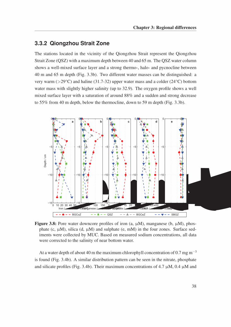
Chapter 3: Regional differences
3.3.2 Qiongzhou Strait Zone
The stations located in the vicinity of the Qiongzhou Strait represent the Qiongzhou
Strait Zone (QSZ) with a maximum depth between 40 and 65 m. The QSZ water column
shows a well-mixed surface layer and a strong thermo-, halo- and pycnocline between
40 m and 65 m depth (Fig. 3.3b). Two different water masses can be distinguished: a
very warm (>29°C) and haline (31.7-32) upper water mass and a colder (24°C) bottom
water mass with slightly higher salinity (up to 32.9). The oxygen profile shows a well
mixed surface layer with a saturation of around 88% and a sudden and strong decrease
to 55% from 40 m depth, below the thermocline, down to 59 m depth (Fig. 3.3b).
0 10 20 30 40 50
0
−5
−10
−15
Iron / M
Depth
/ c
m
a
0 50 100 150
0
−5
−10
−15
Manganese / M
b
0 5 10 15 20
0
−5
−10
−15
Phosphate / M
c
0 100200300400
0
−5
−10
−15
Silica / M
d
0 10 20 30
0
−5
−10
−15
Sulphate / mM
e
BGCoZ QSZ BGCeZ SBGZ
Figure 3.8: Pore water downcore profiles of iron (a, µM), manganese (b, µM), phos-phate (c, µM), silica (d, µM) and sulphate (e, mM) in the four zones. Surface sed-iments were collected by MUC. Based on measured sodium concentrations, all datawere corrected to the salinity of near bottom water.
At a water depth of about 40 m the maximum chlorophyll concentration of 0.7 mg m−3
is found (Fig. 3.4b). A similar distribution pattern can be seen in the nitrate, phosphate
and silicate profiles (Fig. 3.4b). Their maximum concentrations of 4.7 µM, 0.4 µM and
38
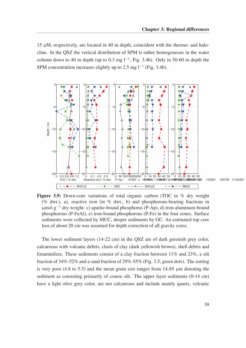
Chapter 3: Regional differences
15 µM, respectively, are located in 40 m depth, coincident with the thermo- and halo-
cline. In the QSZ the vertical distribution of SPM is rather homogeneous in the water
column down to 40 m depth (up to 0.3 mg l−1, Fig. 3.4b). Only in 50-60 m depth the
SPM concentration increases slightly up to 2.5 mg l−1 (Fig. 3.4b).
0 0.3 0.6 0.9 1.2
0
−5
−10
−15
−20
TOC / % dwt.
Depth
/ c
m
a
0 0.1 0.2 0.3
0
−5
−10
−15
−20
Reactive Iron / % dwt.
b
0 50 100150200250
0
−5
−10
−15
−20
P−Ap / mol/g dwt.
c
0 10 20 30 40 50
0
−5
−10
−15
−20
P−FeAl / mol/g dwt.
d
0 10 20 30 40 50
0
−5
−10
−15
−20
P−Fe / mol/g dwt.
e
BGCoZ QSZ BGCeZ SBGZ
Figure 3.9: Down-core variations of total organic carbon (TOC in % dry weight(% dwt.), a), reactive iron (in % dwt., b) and phosphorous-bearing fractions inµmol g−1 dry weight: c) apatite-bound phosphorus (P-Ap), d) iron-aluminum-boundphosphorous (P-FeAl), e) iron-bound phosphorous (P-Fe) in the four zones. Surfacesediments were collected by MUC, deeper sediments by GC. An estimated top coreloss of about 20 cm was assumed for depth correction of all gravity cores.
The lower sediment layers (14-22 cm) in the QSZ are of dark greenish grey color,
calcareous with volcanic debris, clasts of clay (dark yellowish brown), shell debris and
foraminifera. These sediments consist of a clay fraction between 11% and 23%, a silt
fraction of 34%-52% and a sand fraction of 29%-55% (Fig. 3.5, green dots). The sorting
is very poor (4.8 to 5.5) and the mean grain size ranges from 14-85 µm denoting the
sediment as consisting primarily of coarse silt. The upper layer sediments (0-14 cm)
have a light olive grey color, are not calcareous and include mainly quartz, volcanic
39
Chapter 3: Regional differences
debris and clasts of shells. Sand provides the highest fraction (42%-66%), followed by
silt (27%-66%) and clay (6%-15%, Fig. 3.5, green dots). With values between 3.4 and
6.1 the sorting in the upper sediments is very poor as well. The mean grain diameter
is between 21 and 118 µm denoting the sediment as fine sand. For the entire sediment
core in the QSZ the averaged mean grain size is about 61 µm showing the sediments to
be dominated by coarse silt or fine sand.
In QSZ, the CPE amounts to 12.5 µg g−1 d.s. with chlorophyll a and phaeopigment
contents of 2.5 µg g−1 d.s. and 10 µg g−1 d.s., respectively (Fig. 3.6a). Here the ratio
of chlorophyll a to phaeopigments ranges between 0.1 and 0.75 (Fig. 3.6b).
The foraminiferal abundance in the QSZ surface sediments is about 2760 shells/10 g
sediment of which a proportion of 79% is provided by calcareous benthic foraminifera,
the most abundant group in the surface sediment sample (Fig. 3.7b). The proportion
of agglutinated foraminifera accounts for 20% of the total assemblage. The dominant
species are Pseudorotalia indopacifica [Wang et al., 1988], a marine species living
in shallow waters from temperate to tropical conditions [Gallagher et al., 2009], and
Eponides spp. [He and Hu, 2001], an epifaunal species occurring from shelf to abyssal
depths [Murray, 1991]. Planktonic foraminifera are sparsely represented with only 2%.
The pore waters of QSZ depict near-surface maxima of dissolved manganese and
iron in around 4 and 8 cm sediment depth, respectively (Fig. 3.8a, b). Additionally,
slight phosphate and silica maxima are visible in 8-10 cm depth (Fig. 3.8c, d), and
sulphate shows almost constant values around 27 mM (Fig. 3.8e). The TOC profile dis-
plays strong variations with a minimum (0.2%) in around 12 cm depth and a maximum
(1.3%) in 16 cm depth (Fig. 3.9a). In the surface sediments very low contents of reactive
iron are measured (Fig. 3.9b). Apatite-bound phosphorus shows a strong near-surface
decrease and remains constant at higher depths (Fig. 3.9c). The profiles of P-FeAl and
P-Fe contents show nearly no vertical variability and are low, ranging between 3 and
5 µmol g−1 and 7-9 µmol g−1, respectively (Fig. 3.9d, e).
3.3.3 Beibu Gulf Central Zone
The Beibu Gulf Central Zone (BGCeZ) is identified by parameters determined at the
stations located in the central part of the Beibu Gulf (maximum depth between 54 and
78 m). This zone is characterized by a strong thermo-, halo- and pycnocline in around
40
Chapter 3: Regional differences
45-50 m water depth. With a salinity of about 33.2 at surface and 33.5 at the bottom
the BGCeZ is the most haline zone in the Beibu Gulf (Fig. 3.3c). The oxygen satura-
tion remains relatively constant down to 45 m depth with 85-92% followed by a strong
decrease to 59% in around 60 m depth. With a concentration of 0.9 mg m−3, the chloro-
phyll maximum is located slightly above the thermo- and halocline (Fig. 3.4c). Below,
the chlorophyll concentration decreases to 0.5 mg m−3 in 60 m depth. The profiles of ni-
trate, phosphate and silicate show a similar pattern (Fig. 3.4c). Their maxima of 4.7 µM,
0.4 µM and 15 µM, respectively, are measured at 50 m depth concurrent with the chloro-
phyll maximum. Beneath the maximum the nutrient concentrations decrease to 3 µM,
0.1 µM and 8 µM, respectively, at a depth of 60 m. From the surface down to a depth of
20 m SPM concentrations below the detection limit are found (Fig. 3.4c). Furthermore,
the SPM distribution shows concentrations ranging between 0.6 and 3.1 mg l−1 from
20 m depth down to the bottom (Fig. 3.4c).
The BGCeZ sediment properties were determined from the 386 cm long GC sediment
core 371840. The sediments are of light olive grey or greyish green color, plastic, cal-
careous and homogeneous, and contain mainly fine to medium sand embeddings, quartz
and shell debris. Foraminifera as well as bivalve and snail shells are found between 10
and 169 cm depth. The sediments show a high silt content (77%-84%), less clay (12%-
15%) and a slight sand admixture of up to 11% (Fig. 3.5, grey dots). With sorting values
of 2-3.2 sediment in the entire core is very poorly sorted. The medium grain size varies
between 6.7 and 11 µm thus showing the sediment to consist, generally, of medium silt.
The CPE content in the BGCeZ surface sediments is about 9.7 µg g−1 d.s. (Fig. 3.6a).
The chlorophyll a and phaeopigment contents are 2.3 µg g−1 d.s. and 7.3 µg g−1 d.s,
respectively, and the chlorophyll a to phaeopigment ratio varies between 0.09 and 0.79
(Fig. 3.6a, b).
The foraminiferal abundance in the surface sediments of BGCeZ amounts to about
1852 shells/10 g sediment. Planktonic foraminifera account for 25% of the assemblage
(Fig. 3.7c). As typical for subtropical/tropical regions most of the identified species
are thermophilous: Globigerinella aequilateralis, Globigerinoides quadrilobatus, Glo-
bigerinoides ruber, Globigerinoides sacculifer and Pulleniatina obliquiloculata. Fur-
thermore, the fraction of calcareous benthic foraminifera and the fraction of agglutinated
foraminifera is about 55% and 20%, respectively. The benthic foraminiferal assemblage
is dominated by Pseudorotalia schroeteriana [He and Hu, 2001], a neritic, euryhaline
41
Chapter 3: Regional differences
species living in tropical and subtropical regions [Gallagher et al., 2009].
The down-core pore water profile of dissolved iron from BGCeZ reveals a maximum
in 7 cm sediment depth (Fig. 3.8a). Dissolved manganese shows highest concentration
in 3 cm depth and constant concentrations below (Fig. 3.8b). The phosphate and silica
profiles display down core increasing concentrations (Fig. 3.8c, d). Sulphate concentra-
tions are relatively uniform (29 mM, Fig. 3.8e). The sediment TOC profile of BGCeZ
evince relatively stable organic carbon contents of around 0.8% (Fig. 3.9a). A very low
(about 0.03%) and relatively constant content of reactive iron is found throughout the
entire core (Fig. 3.9b). The apatite-bound phosphorus shows a decrease in the upper
5 cm depth and remains uniform down to 20 cm depth (Fig. 3.9c). In case of P-FeAl
the measured concentrations are relatively uniform in the entire core (Fig. 3.9d). The
profile of P-Fe shows a maximum in 2.5 cm depth and also constant contents further
down the core (Fig. 3.9e).
3.3.4 Southern Beibu Gulf Zone
The Southern Beibu Gulf Zone (SBGZ) includes the stations located southwest of the
Hainan Island in the transition zone between the Beibu Gulf and the SCS with a maxi-
mum depth ranging from 57 to 94 m. The water column in the SBGZ shows no thermo-
cline but a gradually decreasing temperature profile with a difference of around 0.8°C
from the surface (28.3°C) to the bottom (27.5°C). Temperature, salinity, σt and oxygen
profiles are shown in Fig. 3.3d. The salinity distribution shows a gradual increase with
depth from 32.4 at the surface to around 33 at the bottom. In case of oxygen saturation
the water column is well mixed with a total difference in saturation between surface
(89%) and bottom (83%) of only about 6%. In this zone the chlorophyll maximum
is found between 40 and 60 m water depth with a concentration of about 0.6 mg m−3
(Fig. 3.4d). Slightly lower concentrations are found above (0.1-0.5 mg m−3) and below
(0.2 mg m−3) the chlorophyll maximum. Nitrate is sparsely available with values below
0.5 µM up to 70 m depth, then the concentration increases to 1.5 µM in 90 m depth.
No phosphate is found down to 70 m depth (Fig. 3.4d). Below that water depth the con-
centration increases slightly to 0.03 µM. Silicate exhibits a maximum of around 7 µM
in 30 m depth, 10 m below the first small chlorophyll peak of 0.5 mg m−3. In general,
chlorophyll and silicate profiles show opposite patterns (Fig. 3.4d). In SBGZ the verti-
42
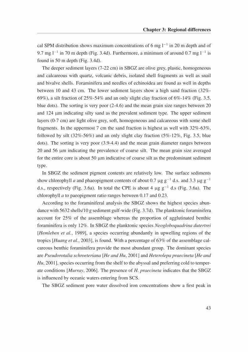
Chapter 3: Regional differences
cal SPM distribution shows maximum concentrations of 6 mg l−1 in 20 m depth and of
9.7 mg l−1 in 70 m depth (Fig. 3.4d). Furthermore, a minimum of around 0.7 mg l−1 is
found in 50 m depth (Fig. 3.4d).
The deeper sediment layers (7-22 cm) in SBGZ are olive grey, plastic, homogeneous
and calcareous with quartz, volcanic debris, isolated shell fragments as well as snail
and bivalve shells. Foraminifera and needles of echinoidea are found as well in depths
between 10 and 43 cm. The lower sediment layers show a high sand fraction (32%-
69%), a silt fraction of 25%-54% and an only slight clay fraction of 6%-14% (Fig. 3.5,
blue dots). The sorting is very poor (2-4.6) and the mean grain size ranges between 20
and 124 µm indicating silty sand as the prevalent sediment type. The upper sediment
layers (0-7 cm) are light olive grey, soft, homogeneous and calcareous with some shell
fragments. In the uppermost 7 cm the sand fraction is highest as well with 32%-63%,
followed by silt (32%-56%) and an only slight clay fraction (5%-12%, Fig. 3.5, blue
dots). The sorting is very poor (3.9-4.4) and the mean grain diameter ranges between
20 and 56 µm indicating the prevalence of coarse silt. The mean grain size averaged
for the entire core is about 50 µm indicative of coarse silt as the predominant sediment
type.
In SBGZ the sediment pigment contents are relatively low. The surface sediments
show chlorophyll a and phaeopigment contents of about 0.7 µg g−1 d.s. and 3.3 µg g−1
d.s., respectively (Fig. 3.6a). In total the CPE is about 4 µg g−1 d.s (Fig. 3.6a). The
chlorophyll a to paeopigment ratio ranges between 0.17 and 0.23.
According to the foraminiferal analysis the SBGZ shows the highest species abun-
dance with 5632 shells/10 g sediment gulf-wide (Fig. 3.7d). The planktonic foraminifera
account for 25% of the assemblage whereas the proportion of agglutinated benthic
foraminifera is only 12%. In SBGZ the planktonic species Neogloboquadrina dutertrei
[Hemleben et al., 1989], a species occurring abundantly in upwelling regions of the
tropics [Huang et al., 2003], is found. With a percentage of 63% of the assemblage cal-
careous benthic foraminifera provide the most abundant group. The dominant species
are Pseudorotalia schroeteriana [He and Hu, 2001] and Heterolepa praecineta [He and
Hu, 2001], species occurring from the shelf to the abyssal and preferring cold to temper-
ate conditions [Murray, 2006]. The presence of H. praecineta indicates that the SBGZ
is influenced by oceanic waters entering from SCS.
The SBGZ sediment pore water dissolved iron concentrations show a first peak in
43
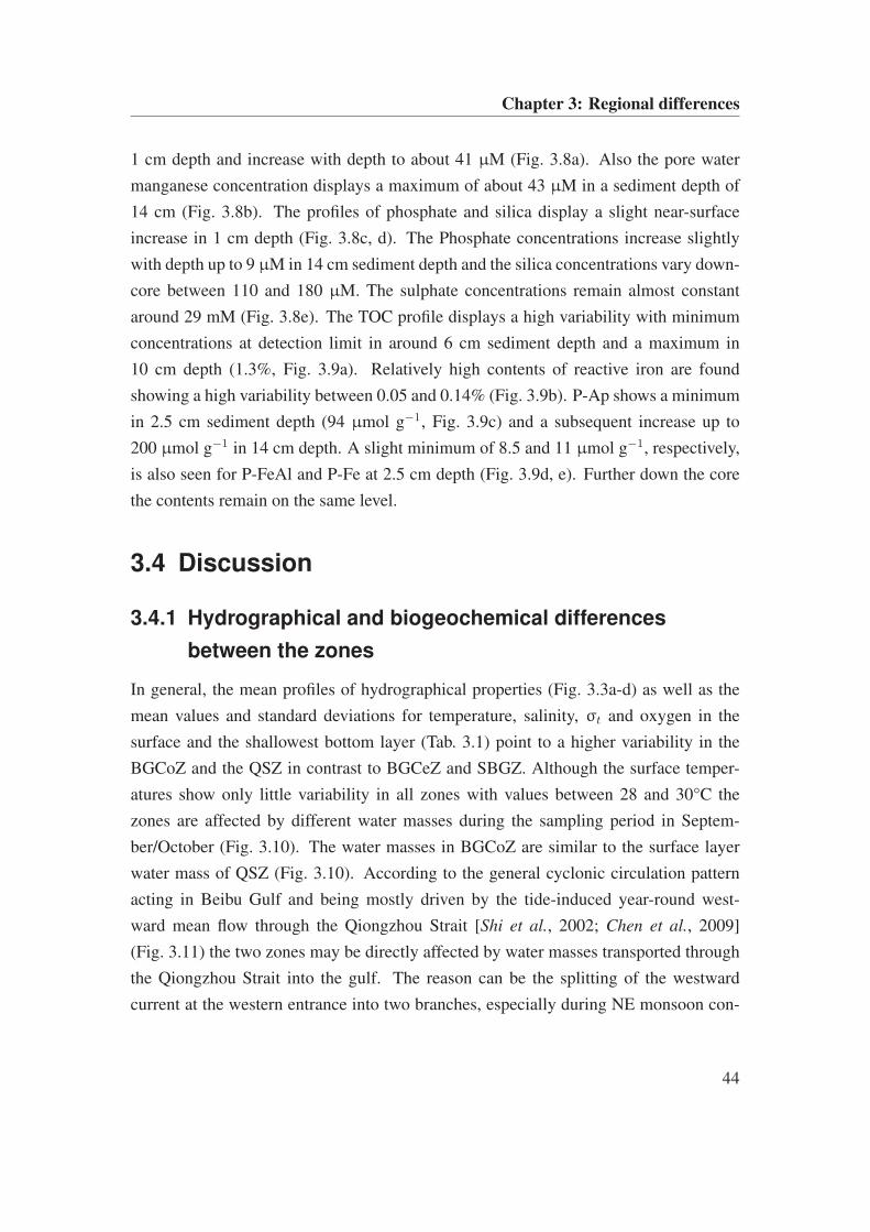
Chapter 3: Regional differences
1 cm depth and increase with depth to about 41 µM (Fig. 3.8a). Also the pore water
manganese concentration displays a maximum of about 43 µM in a sediment depth of
14 cm (Fig. 3.8b). The profiles of phosphate and silica display a slight near-surface
increase in 1 cm depth (Fig. 3.8c, d). The Phosphate concentrations increase slightly
with depth up to 9 µM in 14 cm sediment depth and the silica concentrations vary down-
core between 110 and 180 µM. The sulphate concentrations remain almost constant
around 29 mM (Fig. 3.8e). The TOC profile displays a high variability with minimum
concentrations at detection limit in around 6 cm sediment depth and a maximum in
10 cm depth (1.3%, Fig. 3.9a). Relatively high contents of reactive iron are found
showing a high variability between 0.05 and 0.14% (Fig. 3.9b). P-Ap shows a minimum
in 2.5 cm sediment depth (94 µmol g−1, Fig. 3.9c) and a subsequent increase up to
200 µmol g−1 in 14 cm depth. A slight minimum of 8.5 and 11 µmol g−1, respectively,
is also seen for P-FeAl and P-Fe at 2.5 cm depth (Fig. 3.9d, e). Further down the core
the contents remain on the same level.
3.4 Discussion
3.4.1 Hydrographical and biogeochemical differences
between the zones
In general, the mean profiles of hydrographical properties (Fig. 3.3a-d) as well as the
mean values and standard deviations for temperature, salinity, σt and oxygen in the
surface and the shallowest bottom layer (Tab. 3.1) point to a higher variability in the
BGCoZ and the QSZ in contrast to BGCeZ and SBGZ. Although the surface temper-
atures show only little variability in all zones with values between 28 and 30°C the
zones are affected by different water masses during the sampling period in Septem-
ber/October (Fig. 3.10). The water masses in BGCoZ are similar to the surface layer
water mass of QSZ (Fig. 3.10). According to the general cyclonic circulation pattern
acting in Beibu Gulf and being mostly driven by the tide-induced year-round west-
ward mean flow through the Qiongzhou Strait [Shi et al., 2002; Chen et al., 2009]
(Fig. 3.11) the two zones may be directly affected by water masses transported through
the Qiongzhou Strait into the gulf. The reason can be the splitting of the westward
current at the western entrance into two branches, especially during NE monsoon con-
44
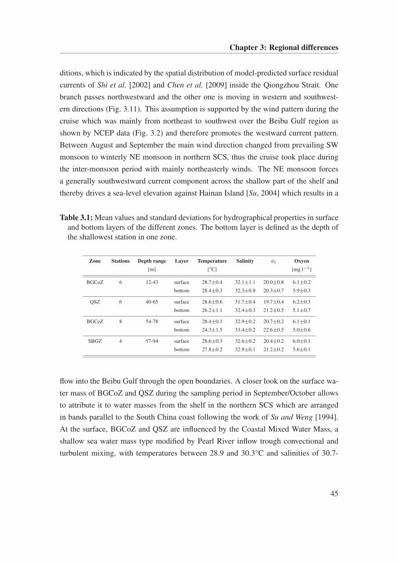
Chapter 3: Regional differences
ditions, which is indicated by the spatial distribution of model-predicted surface residual
currents of Shi et al. [2002] and Chen et al. [2009] inside the Qiongzhou Strait. One
branch passes northwestward and the other one is moving in western and southwest-
ern directions (Fig. 3.11). This assumption is supported by the wind pattern during the
cruise which was mainly from northeast to southwest over the Beibu Gulf region as
shown by NCEP data (Fig. 3.2) and therefore promotes the westward current pattern.
Between August and September the main wind direction changed from prevailing SW
monsoon to winterly NE monsoon in northern SCS, thus the cruise took place during
the inter-monsoon period with mainly northeasterly winds. The NE monsoon forces
a generally southwestward current component across the shallow part of the shelf and
thereby drives a sea-level elevation against Hainan Island [Su, 2004] which results in a
Table 3.1: Mean values and standard deviations for hydrographical properties in surfaceand bottom layers of the different zones. The bottom layer is defined as the depth ofthe shallowest station in one zone.
Zone Stations Depth range Layer Temperature Salinity σt Oxyen
[m] [°C] [mg l−1]
BGCoZ 6 12-43 surface 28.7±0.4 32.1±1.1 20.0±0.8 6.1±0.2
bottom 28.4±0.3 32.3±0.9 20.3±0.7 5.9±0.3
QSZ 6 40-65 surface 28.6±0.6 31.7±0.4 19.7±0.4 6.2±0.3
bottom 26.2±1.1 32.4±0.3 21.2±0.5 5.1±0.7
BGCeZ 8 54-78 surface 28.4±0.3 32.9±0.2 20.7±0.2 6.1±0.1
bottom 24.3±1.5 33.4±0.2 22.6±0.5 5.0±0.6
SBGZ 4 57-94 surface 28.6±0.3 32.6±0.2 20.4±0.2 6.0±0.1
bottom 27.8±0.2 32.9±0.1 21.2±0.2 5.6±0.1
flow into the Beibu Gulf through the open boundaries. A closer look on the surface wa-
ter mass of BGCoZ and QSZ during the sampling period in September/October allows
to attribute it to water masses from the shelf in the northern SCS which are arranged
in bands parallel to the South China coast following the work of Su and Weng [1994].
At the surface, BGCoZ and QSZ are influenced by the Coastal Mixed Water Mass, a
shallow sea water mass type modified by Pearl River inflow trough convectional and
turbulent mixing, with temperatures between 28.9 and 30.3°C and salinities of 30.7-
45
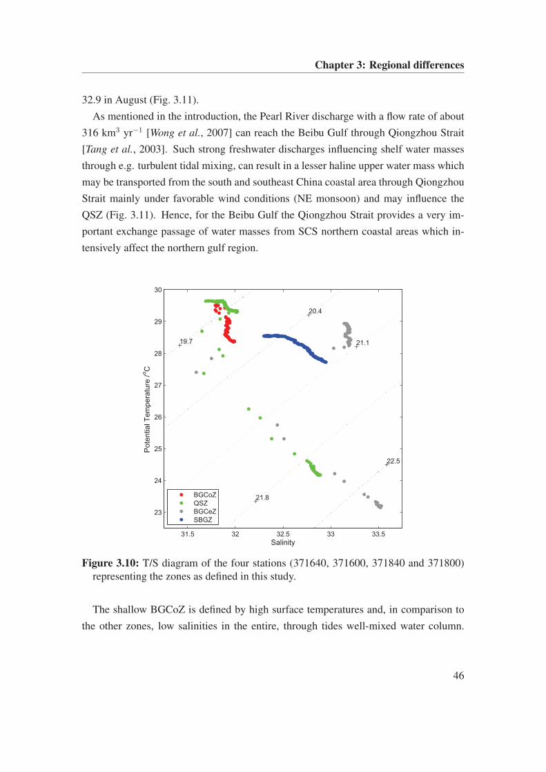
Chapter 3: Regional differences
32.9 in August (Fig. 3.11).
As mentioned in the introduction, the Pearl River discharge with a flow rate of about
316 km3 yr−1 [Wong et al., 2007] can reach the Beibu Gulf through Qiongzhou Strait
[Tang et al., 2003]. Such strong freshwater discharges influencing shelf water masses
through e.g. turbulent tidal mixing, can result in a lesser haline upper water mass which
may be transported from the south and southeast China coastal area through Qiongzhou
Strait mainly under favorable wind conditions (NE monsoon) and may influence the
QSZ (Fig. 3.11). Hence, for the Beibu Gulf the Qiongzhou Strait provides a very im-
portant exchange passage of water masses from SCS northern coastal areas which in-
tensively affect the northern gulf region.
Salinity
Pote
ntial T
em
pera
ture
/ oC
19.7
20.4
21.1
21.8
22.5
31.5 32 32.5 33 33.5
23
24
25
26
27
28
29
30
BGCoZ
QSZ
BGCeZ
SBGZ
Figure 3.10: T/S diagram of the four stations (371640, 371600, 371840 and 371800)representing the zones as defined in this study.
The shallow BGCoZ is defined by high surface temperatures and, in comparison to
the other zones, low salinities in the entire, through tides well-mixed water column.
46
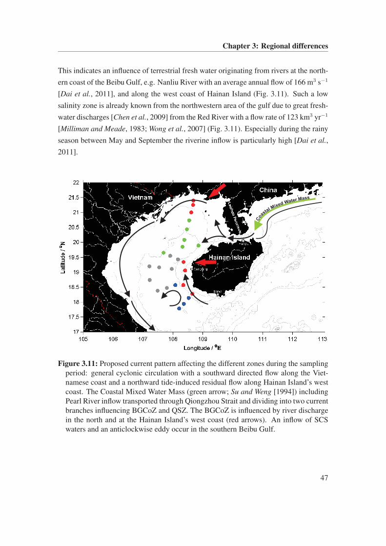
Chapter 3: Regional differences
This indicates an influence of terrestrial fresh water originating from rivers at the north-
ern coast of the Beibu Gulf, e.g. Nanliu River with an average annual flow of 166 m3 s−1
[Dai et al., 2011], and along the west coast of Hainan Island (Fig. 3.11). Such a low
salinity zone is already known from the northwestern area of the gulf due to great fresh-
water discharges [Chen et al., 2009] from the Red River with a flow rate of 123 km3 yr−1
[Milliman and Meade, 1983; Wong et al., 2007] (Fig. 3.11). Especially during the rainy
season between May and September the riverine inflow is particularly high [Dai et al.,
2011].
Co
asta
l Mixed Water Mass
Figure 3.11: Proposed current pattern affecting the different zones during the samplingperiod: general cyclonic circulation with a southward directed flow along the Viet-namese coast and a northward tide-induced residual flow along Hainan Island’s westcoast. The Coastal Mixed Water Mass (green arrow; Su and Weng [1994]) includingPearl River inflow transported through Qiongzhou Strait and dividing into two currentbranches influencing BGCoZ and QSZ. The BGCoZ is influenced by river dischargein the north and at the Hainan Island’s west coast (red arrows). An inflow of SCSwaters and an anticlockwise eddy occur in the southern Beibu Gulf.
47
Chapter 3: Regional differences
The stratified QSZ and BGCeZ are influenced by the same water mass in the deeper
layer but different water masses in the upper layers above the thermo- and halocline
(Fig. 3.10). In the Beibu Gulf a stratification develops during summer due to sea surface
heating whereas the water column is well mixed in winter [Manh and Yanagi, 2000;
Tang et al., 2003].
The bottom layer water mass with lower temperature and higher salinity may be
tidally transported into the Beibu Gulf from the SCS main basin through the broad
opening in the south. Diurnal tidal waves and associated strong tidal currents of up
to 50 cm s−1 propagate northward from the main SCS basin and enter the gulf from
the south of Hainan Island [Shi et al., 2002; Hu et al., 2003] (Fig. 3.11). Furthermore,
a tide-induced residual flow over the entire water column is stationary in this region
and reaches maximum current velocities at the surface of up to 30 cm s−1 in winter
and 22 cm s−1 in summer [Manh and Yanagi, 2000]. A calculated seasonal variability
of residual flow shows that it the bottom layers the currents pass northward along the
Hainan Island’s west coast into the Beibu Gulf in summer [Manh and Yanagi, 2000]
(Fig. 3.11). Consequently, this current re-direction produces a continuous flow of SCS
waters into the Beibu Gulf and thereby results in a higher salinity below 30 m water
depth in the QSZ and the BGCeZ. The bathymetry, gradually shallowing from the south
to the north, may be one reason why the BGCoZ is not affected by this denser bottom
water mass.
In comparison to the other zones only the well mixed SBGZ is defined by a com-
pletely different water mass. The SBGZ southernmost station (371800) may be under
direct influence of SCS waters during sampling period. When the main wind direction
changes from SW to NE monsoon in autumn the whole circulation in the Beibu Gulf is
affected. As a result the residual flow intensifies in winter, compared to that in summer,
and an cyclonic eddy occurs in the lower level (50 m depth) of the southern part of the
gulf [Manh and Yanagi, 2000] (Fig. 3.11). This eddy could have developed during the
sampling period and, in combination with the stronger residual flow, may result in a
turbulent mixing of the water masses and hence a stratification breakdown which ap-
parently already happened in the SBGZ. This situation leads also to the assumption that
waters in both QSZ and BGCeZ become mixed when the NE monsoon has been fully
developed.
In the Beibu Gulf, winter is the main productive season [Tang et al., 2003] and there-
48
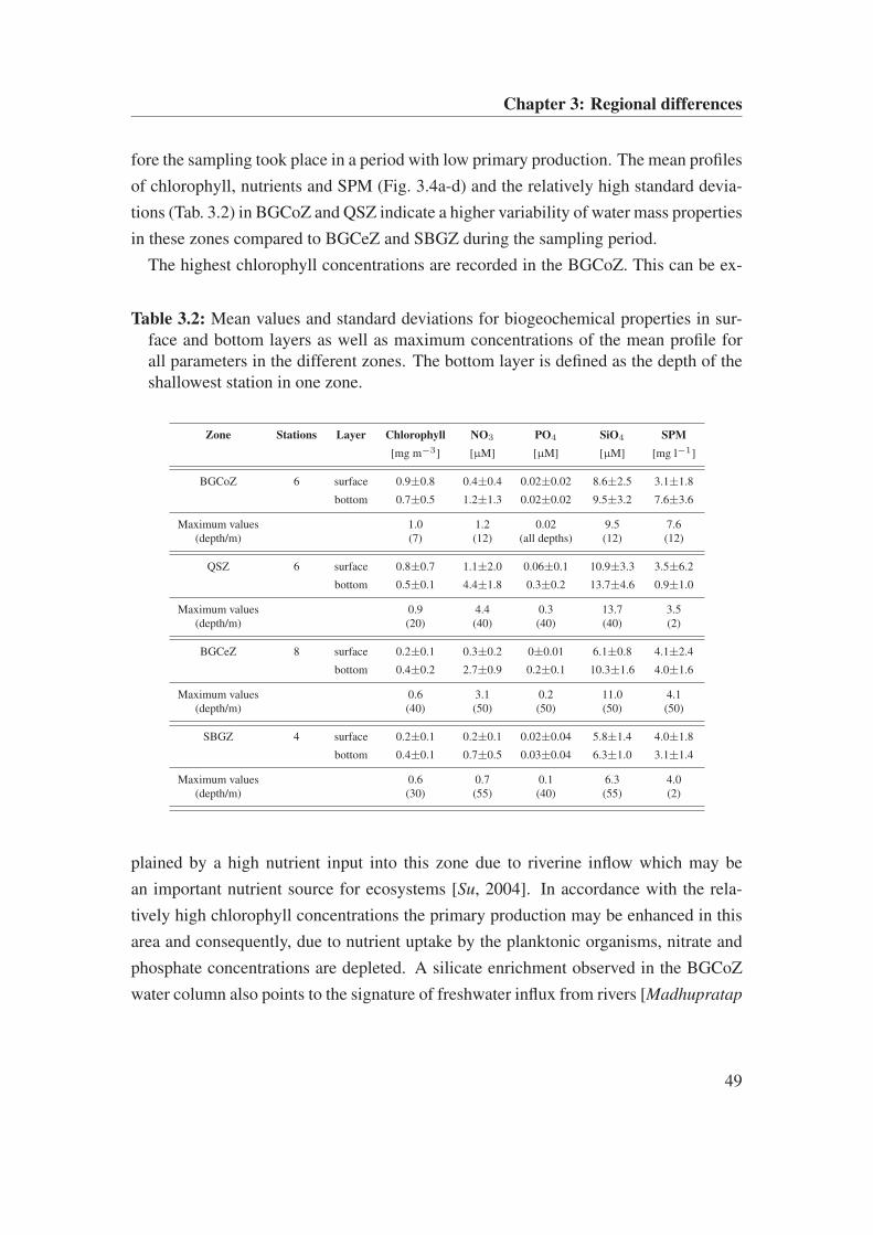
Chapter 3: Regional differences
fore the sampling took place in a period with low primary production. The mean profiles
of chlorophyll, nutrients and SPM (Fig. 3.4a-d) and the relatively high standard devia-
tions (Tab. 3.2) in BGCoZ and QSZ indicate a higher variability of water mass properties
in these zones compared to BGCeZ and SBGZ during the sampling period.
The highest chlorophyll concentrations are recorded in the BGCoZ. This can be ex-
Table 3.2: Mean values and standard deviations for biogeochemical properties in sur-face and bottom layers as well as maximum concentrations of the mean profile forall parameters in the different zones. The bottom layer is defined as the depth of theshallowest station in one zone.
Zone Stations Layer Chlorophyll NO3 PO4 SiO4 SPM
[mg m−3] [µM] [µM] [µM] [mg l−1]
BGCoZ 6 surface 0.9±0.8 0.4±0.4 0.02±0.02 8.6±2.5 3.1±1.8
bottom 0.7±0.5 1.2±1.3 0.02±0.02 9.5±3.2 7.6±3.6
Maximum values 1.0 1.2 0.02 9.5 7.6(depth/m) (7) (12) (all depths) (12) (12)
QSZ 6 surface 0.8±0.7 1.1±2.0 0.06±0.1 10.9±3.3 3.5±6.2
bottom 0.5±0.1 4.4±1.8 0.3±0.2 13.7±4.6 0.9±1.0
Maximum values 0.9 4.4 0.3 13.7 3.5(depth/m) (20) (40) (40) (40) (2)
BGCeZ 8 surface 0.2±0.1 0.3±0.2 0±0.01 6.1±0.8 4.1±2.4
bottom 0.4±0.2 2.7±0.9 0.2±0.1 10.3±1.6 4.0±1.6
Maximum values 0.6 3.1 0.2 11.0 4.1(depth/m) (40) (50) (50) (50) (50)
SBGZ 4 surface 0.2±0.1 0.2±0.1 0.02±0.04 5.8±1.4 4.0±1.8
bottom 0.4±0.1 0.7±0.5 0.03±0.04 6.3±1.0 3.1±1.4
Maximum values 0.6 0.7 0.1 6.3 4.0(depth/m) (30) (55) (40) (55) (2)
plained by a high nutrient input into this zone due to riverine inflow which may be
an important nutrient source for ecosystems [Su, 2004]. In accordance with the rela-
tively high chlorophyll concentrations the primary production may be enhanced in this
area and consequently, due to nutrient uptake by the planktonic organisms, nitrate and
phosphate concentrations are depleted. A silicate enrichment observed in the BGCoZ
water column also points to the signature of freshwater influx from rivers [Madhupratap
49
Chapter 3: Regional differences
et al., 2003]. Silicates in rivers derive mainly from weathering of silicate minerals along
the river course [Gago et al., 2005]. The high silicate concentrations exclude a diatom
bloom during the time of the cruise thus indicating other organisms (e.g. dinoflagel-
lates or coccolithophores) being responsible for the high chlorophyll concentrations in
the vicinity of the rivers along the coasts of the gulf. The phytoplankton in the area is
dominated by freshwater and brackish plankton species, tropical neritic forms are abun-
dant as well [Guo, 1994]. It is also possible that nutrient-rich water masses as well as
phytoplankton have been transported from the South China coast east of the Leizhou
Peninsula through Qiongzhou Strait in accordance with the previously described circu-
lation patterns. This assumption is corroborated as the QSZ is as well characterized by
relatively high chlorophyll and nutrient concentrations in the upper layer. In the QSZ
and especially in the BGCeZ the stratification increases chlorophyll concentrations in
the vicinity of the thermocline due to increased nutrient concentrations in the deeper
layers. The nutricline, the depth in which nitrate reaches concentrations of more than
1 µM for the first time [Fasham et al., 1985], is located in 30-40 m water depth in the
BGCeZ, more or less coincident with the thermocline. Due to the stratification the up-
welling of nutrients is limited [Tang et al., 2003], therefore, chlorophyll and nutrient
concentrations are only enhanced in the vicinity of the thermocline and below. Such
a deep chlorophyll maximum is a characteristic feature of seasonally stratified shelf
seas and is caused by nutrient pulses into the thermocline through vertical tidally driven
mixing processes. The generally low concentrations (<1 µM) of dissolved nitrate and
phosphate found in the upper layer of BGCeZ and in the entire water column of SBGZ
are typical for oligotrophic regions. In all zones dissolved phosphate concentrations
are low, therefore phosphorus seems to be the limiting factor for primary production in
the surface layer. A calculated N/P molar ratio of 19 in the entire eastern Beibu Gulf,
higher than the Redfield ratio of 16, supports the assumption that the Beibu Gulf is
phosphorus-limited [Gago et al., 2005].
Enhanced SPM concentrations in the BGCoZ water column point to a strong influ-
ence of resuspended sediments. In the Qiongzhou Strait as well as off the west coast of
Leizhou Peninsula and Hainan Island, strong tidal currents and thus strong tidal mixing
[Tang et al., 2003] lead to sediment resuspension (Fig. 3.1a). Furthermore, sediment re-
suspension off the southeastern China coast can be transported through Qiongzhou Strait
into the gulf, in accordance with the general circulation pattern, and affect the BGCoZ
50
Chapter 3: Regional differences
(Fig. 3.1a). Seasonal differences in water transparency through, e.g. elevated SPM con-
centrations can limit phytoplankton growth through light limitation [Longhurst, 2007].
Low SPM concentrations in the surface layer and highest concentrations in the bottom
layer of QSZ and BGCeZ indicate a tidally driven sediment resuspension at the bottom
but exclude an intense sediment transport with currents into these zones from other re-
gions. The tide-driven sediment resuspension can be also responsible for the relatively
high chlorophyll concentrations in the bottom layers of QSZ and BGCeZ (the sediment
pigment contents will be discussed later). Typhoon KETSANA which passed the study
area a few days before the sampling period may have caused the enhanced SPM con-
centrations in the entire water column of all zones shown in the mean SPM profiles
(Fig. 3.4a-d). This strong wind event may induce a strong resuspension of coastal sed-
iments along the coasts of Hainan Island and Leizhou Peninsula as well as the South
China east coast which may be transported through Qiongzhou Strait or through the
southern boundary into the Beibu Gulf. Moreover, the strong winds may enhance the
water mass transport through Qiongzhou Strait and the cyclonic circulation in the gulf.
Ekman depth calculations, using the highest wind speeds measured at weather stations
on the Hainan Island (10.8 m s−1 in Haikou, 11.8 m s−1 in Dongfang and 18.5 m s−1 in
Sanya), indicate penetration depths for the wind-induced mixing between 79 m in the
north and 142 m in the south. This leads to a mixing of the entire water column down
to the bottom and thus has the potential to enhance sediment resuspension in all zones.
As the Beibu Gulf sediments are fine grained the deposition after the storm takes some
time and is therefore substantially slower than the re-stratification of the water column.
3.4.2 Differences of sediment characteristics and
geochemical properties between the zones
Mainly two different sediment types are found in the different zones: BGCoZ and
BGCeZ are characterized by fine-grained material whereas in QSZ and SBGZ coarser
material is deposited. The low variability of the mean grain diameter and clay concen-
tration in the cores collected in the BGCoZ and the BGCeZ indicate a relatively stable
depositional environment which allows also fine material to be deposited. The BGCoZ
may receive material mainly from rivers entering the Beibu Gulf at the north coast or
along Hainan Island’s west coasts. In comparison to the Red River, these smaller rivers,
51
Chapter 3: Regional differences
e.g. Nanliu River, provide only a low runoff and thereby the suspended sediments may
not be transported far away. Coarse-grained material deposits close to the coast whereas
finer sediment fractions are transported into the gulf over longer distances to regions
with weaker hydrodynamics and deposit gradually in a 40-50 km wide band along the
northern coast of Beibu Gulf and the Hainan Island west coast [Su and Wang, 1994]. For
a full tidal cycle (25 h) measured with Aanderaa current meters at station 371600 during
the FENDOU 5 cruise a southeasterly directed mean water movement at the surface of
22.8 km d−1 and at 50 m depth of 26.8 km d−1 has been calculated. Furthermore, in
accordance with the general circulation pattern in the Beibu Gulf and the water masses
influencing the BGCoZ as well as the QSZ, the two zones may accumulate fine sed-
iments transported, due to strong tide-induced currents, through the Qiongzhou Strait
from the SCS northeastern coastal areas, including sediment load discharged by the
Pearl River (69 x 106t yr−1 [Halim, 1991]) as well as material from the Leizhou Penin-
sula coast. The intensity of river discharges and the transport through Qiongzhou Strait
depend on the monsoon season [Tanabe et al., 2003a; Xu et al., 2008]. The large fluctu-
ations of sand proportion in the QSZ sediments indicate a highly dynamic and hence a
depositionally unstable environment. Besides material transported through Qiongzhou
Strait the QSZ also receives sediments from the Hainan Island north and west coast.
The BGCeZ sediments originate mainly from Hainan Island [Xu et al., 2008]. Also here
the hydrographical dynamics seem to be weak compared to those in QSZ and SBGZ.
The variability in the mean grain size as well as the relatively high proportion of sand
in the SBGZ sediment indicates an unstable and dynamic environment present in this
zone. As the dynamics are tide-dominated, the sediments may originate mainly from
the south and southwest of Hainan Island [Xu et al., 2008]. Otherwise, the changing
monsoonal wind system and the resultant changes in circulation patterns may induce
material transport from the Vietnamese coast northward into Beibu Gulf [see Manh and
Yanagi, 2000], and hence affect the sediments deposited there as well. As sorting is
a good indicator for the hydrodynamic forcing these values indicate that the BGCoZ
with its moderately sorted sediment is hydrodynamically the calmest zone among all
those distinguished. The very poorly sorted sediments in the remaining zones are in-
dicative of depositionally more unstable environments. In addition to tidal currents and
river input, strong storms (typhoons), mainly during summer, are also responsible for
the sedimentation regime, resuspension and subsequent re-sedimentation, in the Beibu
52
Chapter 3: Regional differences
Gulf.
The sediment pigment contents in the Beibu Gulf remain within the range reported
from other Chinese seas (Liu et al. [2005], personal communication E. Hua, Ocean
University of China, Qingdao). In the QSZ and the SBGZ the surface chlorophyll a
contents are slightly higher than the contents of the subsurface levels, whereas they are
equal in the BGCoZ. Only in BGCeZ the chlorophyll a contents in the subsurface are
somewhat higher than in the surface layer, which may be taken as evidence of intensive
burial of freshly settled plant organic material. The presence of chlorophyll a and its
contribution to the total plant pigment pool reflects the actual input of fresh plant mate-
rial, as chlorophyll a is very labile and degrades rapidly under aerobic conditions [e.g.
Bianchi et al., 2000]. Furthermore, its presence in the subsurface sediments provides
evidence of processes, such as bioturbation, leading to organic matter burial in the sed-
iments. In addition, to being buried in the sediment by physical forces or bioturbation,
the fresh phytodetritus can be ingested by the benthic fauna [e.g. Enge et al., 2011] and
excreted on the sediment surface and beneath it [Braeckman et al., 2011]. The faeces,
which can themselves be buried in the sediment, contain degraded plant-derived mate-
rial the presence of which augments the sedimentary phaeopigment pool [Shields and
Hughes, 2009]. Also the nature of seafloor sediment itself and its accumulation po-
tential, which in turn is affected by resuspension due to the hydrodynamic regime, are
of importance for the distribution of pigments [e.g. Lund-Hansen et al., 1993]. In all
zones the phaeopigment contents in the surface sediments are higher than below, which
indicates an efficient utilisation of fresh material that has been buried in the subsurface
layer. The phytal pigment content in the subsurface sediment is also related to the rate
of diagenesis [Repeta and Gagosian, 1987; Sun et al., 1993; Sun and Wakeham, 1999].
It may be said that the major proportion of the sediment-bound organic material of plant
origin is in the degraded form. This is further substantiated by the chlorophyll a to
phaeopigments ratio in the sediments as a proxy for the "freshness" of the plant mate-
rial. In all zones, the ratio is below 1 in the surface layer and also in the subsurface
layer in BGCoZ, QSZ and SBGZ. Only in BGCeZ the ratio is 1.4. The ratio >1 signi-
fies the prevalence of fresh plant material input over its degradation, and the degree of
fresh plant material preservation, whereas the ratio <1 evidences preponderance of in-
situ degradation of plant material and sedimentation of phytodetritus already degraded
in the water column. The sedimentation of plant material is an important means for
53
Chapter 3: Regional differences
transfer organic matter from the water column to the sediments, especially in the BG-
CoZ, QSZ and BGCeZ. The distribution of phytal pigments in the Beibu Gulf sediments
follows, to some extent, the pattern of water surface productivity. Lowest pigment con-
tents are found in SBGZ, the deepest zone and the one with limited primary production,
whereas all other zones differ widely in their pigment contents with high variabilities,
especially within the BGCoZ and QSZ, indicated by the high standard deviations. The
sediment plant pigment distribution pattern is similar to that emerging from SeaWIFS
August 2000 and modelling data for the SCS water surface chlorophyll a, presented by
Liu et al. [2002]. BGCoZ, the region with highest chlorophyll concentrations in the
water column, shows the highest signal of "fresh" material supply. In this region, also
the material discharge by riverine runoff [e.g. Bianchi et al., 1993] could be a source of
plant pigments. The highest accumulation of degraded plant material is found in QSZ
probably induced by water masses originating from southern China coastal areas east
of Hainan Island, which brought degraded material from a near-shore phytoplankton
bloom into the Beibu Gulf. The deposition center in BGCeZ could be affected by tidal
currents and therefore a near-bottom transport of pigments from other regions.
The distribution of buried foraminifera shells is influenced by several factors such
as water depth, water mass properties (temperature, salinity), nutrient availability, sed-
iment type and currents as transport mechanisms. In general, increased absolute abun-
dance of foraminiferal tests is observed with increasing distance from shore [Zheng
and Fu, 1994]. Accordingly, the highest abundance of foraminiferal tests is found
in the surface sediments of SBGZ (5632 shells/10 g sediment), the lowest in BGCoZ
(83 shells/10 g sediment). The low abundance in the BGCoZ is presumably caused by
rapid deposition of sediments in the coastal zone diminishing foraminiferal test con-
centration per amount sediment. In all zones calcareous benthic foraminifera are dom-
inating. The distribution of benthic foraminifera is related to, among others, sediment
grain size, bottom water temperature, salinity, organic matter deposition and the current
velocity [Mackensen et al., 1990; Jorissen et al., 2007] and is affected by the strong
variability of these parameters, especially in shallow waters. The interaction of all these
factors is responsible for the distribution of calcareous and agglutinated forms. At that
point further investigations are needed. With increasing water depth the ratio of plank-
tonic foraminifera increases from BGCoZ to BGCeZ and SBGZ to up to 25%. One rea-
son is that planktonic foraminifera avoid neritic waters over continental shelves because
54
Chapter 3: Regional differences
they need deep oceanic waters to complete their life cycle [Schmuker, 2000; Kucera,
2007] so that the greatest abundance occurs at the continental slope [Zheng and Fu,
1994]. Additionally, the low abundances of planktonic foraminifera in the BGCoZ can
be caused by high turbidity due to the relatively high concentration of SPM in the water
column [Schmuker, 2000]. Suspended loads may promote benthic foraminifera which in
turn may have a diluting effect on planktonic foraminifera. Distribution and abundance
of planktonic foraminfera are strongly linked to current systems and surface-water prop-
erties but within the range of normal marine conditions (salinity of 33-36), salinity does
not appear to exert any significant influence on them [Hemleben et al., 1989; Zheng
and Fu, 1994; Kucera, 2007]. These conditions are only found in the surface waters of
BGCeZ, all other zones show lower salinity. Zheng and Fu [1994] described an absence
of living planktonic foraminifera in the western Guangdong coastal areas because of
coastal currents mixed with river waters and a salinity <34. Despite that the proportion
of planktonic foraminifera reaches 25% also in SBGZ, a zone strongly influenced by
the continental shelf water mass and a tide-induced water transport from northwestern
SCS to the Beibu Gulf. Therefore, Neogloboquadrina dutertrei, a species occurring
abundantly in upwelling regions of the tropics and is commonly used to indicate high
productivity [Huang et al., 2003] as well as Globigerina bulloides, an indicator for high-
productivity regimes [Kucera, 2007], are found there. As living organisms as well as
their tests can be transported via currents or during storm events away from their eco-
logical optimum [Kucera, 2007] they have probably been transported from SCS into
the Beibu Gulf. Particularly in the SCS, the abundance of Neogloboquadrina dutertrei
generally exceeds 10%.
In general, the investigated surface sediments in the Beibu Gulf are characterized by
TOC contents below 1.5%. Besides riverine input, productivity and redox conditions
the TOC contents in the top layers depend on the amount of available clay/silt minerals
[Keil et al., 1994; Mayer, 1994; Böttcher et al., 2000]. Therefore, TOC contents increase
from sandy via silty to clayish sediments.
The down-core compositional changes of the electron acceptors, metabolites as well
as the solid phase phosphorus speciation reflect microbial activity in the surface sedi-
ments. In typical continental margin sediments, sulphate reduction is the most important
final electron acceptor upon anaerobic organic matter decomposition [Jørgensen, 1982;
Skyring, 1987; Jørgensen and Kasten, 2006]. Although known from other coastal envi-
55
Chapter 3: Regional differences
ronments (e.g. tidal flats; Al-Raei et al. [2009]), dissolved sulphate in the pore waters
of the investigated sediments of the Beibu Gulf reflect no significant net sulphate re-
duction in all zones (Fig. 3.8e). This observation does not exclude near-surface gross
sulphate reduction, but may be a further indication for the interaction of dissolved sul-
phide with ("reactive") metal oxides in the sediments [e.g. Jørgensen and Kasten, 2006].
In agreement with this assumption, reactive iron is found in the upper centimeters of the
sediments (Fig. 3.9b). Higher contents of reactive iron are found in BGCoZ and SBGZ.
Furthermore, the pore water profiles show distinct near-surface maxima of dissolved
iron in all zones, and of dissolved manganese in BGCoZ as well as in BGCeZ. These
are liberated upon reduction either by heterotrophic bacterial activity or chemically,
by the interaction between pore water sulphide and metal oxihydroxides. In QSZ and
SBGZ, only slight manganese concentration maxima are found which indicates minor
contributions from the reduction of manganese oxides. It has to be remembered that
the non-steady state sediment deposition due to re-suspension through tidal forcing or
during heavy storms may have lead to the burial of layers enriched in reducible metals.
In agreement, changing metal concentrations in the pore waters are partly associated
with lithological changes. An elevated accumulation of iron, manganese and metabolits
in BGCoZ and BGCeZ occurs due to the presence of medium silty sediments, in com-
parison to the coarser material in QSZ and SBGZ.
Pore water profiles of phosphate and silica show pronounced near-surface increases
in all zones. The accumulation of both, silica and phosphate is caused by the decom-
position of diatoms in the surface sediments of the Beibu Gulf. When compared to
the expected stoichiometric Si:P ratio of 15:1 for diatom biomass [Brzezinski, 1985],
the ratio of the liberated concentrations, however, is clearly shifted towards higher sil-
ica concentrations (Fig. 3.12). This trend can be explained by further interactions of
liberated phosphate with sedimentary iron-oxides or the formation of apatite.
Burial in organic matter, sorption to the surface of iron(III) and aluminum(III) oxyhy-
droxides, and formation of authigenic minerals are the main routes for P removal from
the pelagic part of the ecosystem. The dominant phosphorus sink in the sediments of all
zones is apatite-bound phosphorus (Fig. 3.9c), which is a very stable and consequently
a long term reservoir. In BGCoZ, QSZ and SBGZ a similar P-Ap concentration level is
found while BGCeZ is distinguished by lowest concentrations in depths >4 cm. High-
est contents occur in the uppermost sediment layers indicating that most of the apatite
56
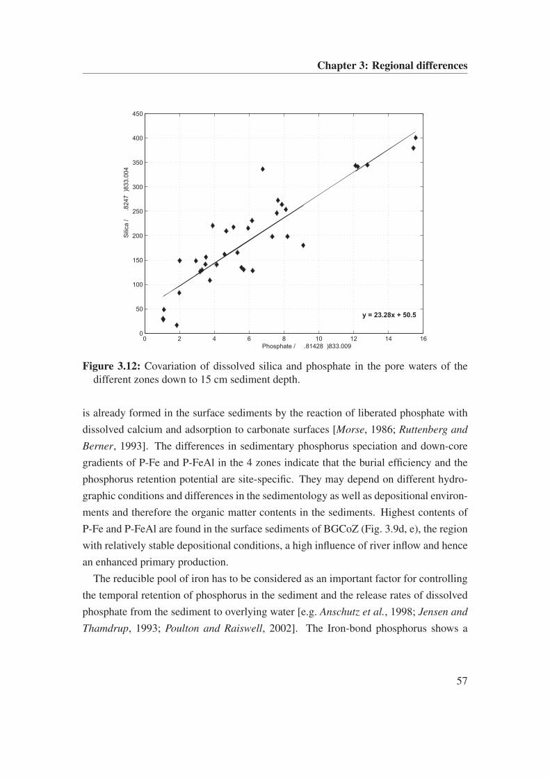
Chapter 3: Regional differences
0 2 4 6 8 10 12 14 160
50
100
150
200
250
300
350
400
450
Phosphate / M
Sili
ca /
M
y = 23.28x + 50.5
Figure 3.12: Covariation of dissolved silica and phosphate in the pore waters of thedifferent zones down to 15 cm sediment depth.
is already formed in the surface sediments by the reaction of liberated phosphate with
dissolved calcium and adsorption to carbonate surfaces [Morse, 1986; Ruttenberg and
Berner, 1993]. The differences in sedimentary phosphorus speciation and down-core
gradients of P-Fe and P-FeAl in the 4 zones indicate that the burial efficiency and the
phosphorus retention potential are site-specific. They may depend on different hydro-
graphic conditions and differences in the sedimentology as well as depositional environ-
ments and therefore the organic matter contents in the sediments. Highest contents of
P-Fe and P-FeAl are found in the surface sediments of BGCoZ (Fig. 3.9d, e), the region
with relatively stable depositional conditions, a high influence of river inflow and hence
an enhanced primary production.
The reducible pool of iron has to be considered as an important factor for controlling
the temporal retention of phosphorus in the sediment and the release rates of dissolved
phosphate from the sediment to overlying water [e.g. Anschutz et al., 1998; Jensen and
Thamdrup, 1993; Poulton and Raiswell, 2002]. The Iron-bond phosphorus shows a
57
Chapter 3: Regional differences
close correlation with reactive iron trends, which is in agreement with the known close
biogeochemical association of phosphorus and iron in near-surface sediments, due to
the effective sorption of phosphate by iron(III) oxides [e.g. Einsele, 1938; Hyacinthe
and Van Cappellen, 2004].
3.5 Conclusions
Based on hydrographical properties different zones were distinguished in the Beibu Gulf
during the sampling period in September/October 2009. The identified zones are mainly
influenced by riverine input and tidal mixing in the coastal areas (BGCoZ), water mass
transport through Qiongzhou Strait from the southern Chinese coast east of Leizhou
Peninsula (BGCoZ and QSZ surface waters) and the influence of SCS waters (bottom
water mass of QSZ and BGCeZ as well as SBGZ). Furthermore, the gulf’s circulation
driven by monsoon winds, tidal currents entering the Beibu Gulf from the south and
through Qiongzhou Strait as well as residual water transport through Qiongzhou Strait
and the resuspension effect of a typhoon crossing the region during the sampling period
influence substantially the biogeochemical properties (chlorophyll, nutrients and SPM)
of the water column within the different zones. The shallow BGCoZ and the QSZ show
relatively high chlorophyll concentrations and therefore give evidence for enhanced pri-
mary production in the entire water column although the sampling took place during
low productive season. The grain size, distribution of plant pigments (chlorophyll a
and phaeopigments) and foraminifera in the surface sediments also reflect the regional
hydrodynamic differences and different water masses affecting the zones and, in case of
the plant pigments, follow also the pattern of surface water productivity. Additionally,
geochemical properties of the sediments depend on the sedimentology, the depositional
environment and the organic matter content, and reflect primary production in the water
column as well. In the Beibu Gulf, the dominant route of phosphorus removal from the
pelagic to the benthic part of the ecosystem is apatite-bound phosphorus.
The first step towards identification of different zones is the understanding of the
hydrodynamic variability, deposition patterns associated with it and geochemical pro-
cesses in the sediments of the Beibu Gulf. Further and more detailed studies are neces-
sary to understand the dynamics in Beibu Gulf and its importance for the SCS.
58
Chapter 4: Factors affecting chlorophyll a concentration
4 Factors affecting the chlorophyll a
concentration in the central Beibu Gulf,
South China Sea
Bauer & Waniek (2013), Marine Ecology Progress Series: 474, 67-88
Abstract
Since in-situ data are sparse a 1D-coupled physical-biological model was used to inves-
tigate the complex connection between atmospheric forcing, associated physical water
column structure and primary production within the entire seasonal cycle in the cen-
tral Beibu Gulf for an 11 year period (2000-2010). The results were corroborated by
remotely measured SST and surface chlorophyll concentrations in combination with in-
situ measurements (temperature and chlorophyll) carried out among others during two
German-Chinese cruises FENDOU 5 in September/October 2009 and SONNE in De-
cember 2011. Over the 11 year period, 87% of the observed variance in daily SST was
captured by the model. The model indicates that the central Beibu Gulf is generally
unaffected by water masses from the SCS and the Beibu Gulf coastal regions. Thereby
most of the primary production is locally generated. A strong stratification and a DCM
develop during summer, vanishing in autumn when the stratification breaks down due
to the change from the weak southwest to the stronger northeast monsoon. Deep mixing
brings a higher nutrient supply to the surface waters leading to a phytoplankton bloom
which lasts on average for about 6 months. Along with the semi-annual wind system
change, temporally short, strong wind events affect the primary productivity in the re-
gion. Typhoon crossings can enhance the primary production by up to 275% relative
to the summer background chlorophyll concentration at the surface according to our
modeling results. These events play an important role in primary production and the
59
Chapter 4: Factors affecting chlorophyll a concentration
corresponding biogeochemical cycling in this oligotrophic region during the summer
and the autumn low-productive periods.
4.1 Introduction
Primary production and the associated energy transfer into higher trophic levels due
to grazing [Ross, 2004], as well as nutrient recycling through biomass sinking and de-
composition play a major role in the biogeochemical cycling of oceanic regions [Chen
et al., 2003]. For this, phytoplankton is fundamentally important for the functioning
of marine ecosystems [e.g. Waniek and Holliday, 2006] and crucial for oceanic carbon
fixation which in turn has an impact on the atmospheric carbon dioxide content [Chen
et al., 2003].
The growth of phytoplankton depends on the availability of nutrients, incident solar
irradiance and grazing pressure and varies regionally through different oceanic condi-
tions [Yoder et al., 1993]. Compared to land-based primary producers phytoplankton
are subject to the strong variability of the turbulent marine environment. This means
their occurrence, regional distributions and seasonal cycles are determined by physi-
cal processes [Ward and Waniek, 2007] such as currents, vertical mixing, particularly
through tides generating a near-bottom turbulence and wind-stress creating additional
turbulence near the sea surface [Tett et al., 1986], and stratification. As a result phy-
toplankton always has to cope with rapid vertical attenuation of light [Sharples, 1999]
and the limitation of nutrient supply from the deeper waters in stratified regimes.
Tides, wind, solar radiation and their interactions affect motion and mixing of the
water column [Dickey, 1988] and lead to the characteristic seasonal cycles in the mixed
layer thickness [Williams and Follows, 2003]. From autumn to spring (in the northern
hemisphere), a low surface heating and a steady influence of wind and tides lead to the
eroding of the seasonal thermocline and hence to a deep mixing. Depending on the water
depth, this mixing can even reach the bottom which is common in shallow shelf regions.
The deep mixing leads indeed to a high nutrient supply in the euphotic zone which could
immediately trigger a phytoplankton bloom. This has been identified as the determinant
of the primary production in, for instance, the western part of the Mediterranean Sea
[Klein and Coste, 1984]. It is the availability of light which makes the difference in the
timing of the phytoplankton bloom between regions in high and those in low latitudes.
60
Chapter 4: Factors affecting chlorophyll a concentration
Seasonal cycles in subtropical waters show highest surface chlorophyll concentrations
during winter, e.g. in the SCS [e.g. Liu et al., 2002], and lowest in summer contrary to
polar and subpolar waters [Howard and Yoder, 1997] which are dominated by a spring
bloom [Yoder et al., 1993], e.g. Northeast Atlantic [Waniek, 2003]. Furthermore, de-
pending on the depth of the oceanic region, due to the deep mixing and tidally driven
turbulence, phytoplankton may be vertically transported below the euphotic depth and
can not conduct photosynthesis anymore [Lauria et al., 1999] (e.g. North Atlantic [cf.
Ward and Waniek, 2007]). If the influence of solar irradiance overcomes the capacity
for tidal mixing in deep regions or regions with low tidal currents, the vertically ho-
mogeneous water column can not be maintained anymore and thermally stratifies in
spring and summer [Sharples, 2008]. Then the algal cells and nutrients are trapped in
the surface layer and may induce a spring phytoplankton bloom.
As an important physical barrier, the seasonal thermocline separates the wind-mixed
surface layer from the, particularly, tidally-mixed deeper waters [Ross and Sharples,
2007] and inhibits the transfer of properties, like nutrients, algal cells and oxygen [e.g.
Klein and Coste, 1984; Sharples et al., 2001]. Many regions show oligotrophic con-
ditions during the period of vertical stratification [Varela et al., 1992] due to the fast
consumption of the only limited available nutrients and the prevented replenishment
of those. In those regions, a DCM, which in most studies represents a real maximum
in phytoplankton biomass [Sharples et al., 2001], is commonly observed within the
thermocline. The DCM is caused by not steady pulses in the strength of the mixing pro-
cesses bringing nutrients into the thermocline [Klein and Coste, 1984; Sharples and Tett,
1994] such as periodical tidally-induced motion, surface breaking waves, wind events
and internal wave instabilities [Lauria et al., 1999]. These pulses lead to an oscillation
of the thermocline supporting a nutrient flux into the surface layer. Due to episodic
weakening of the thermocline and consequent nutrient input to the surface waters, the
variability in the surface wind stress, especially during storm events like typhoons, also
contributes to the formation of the subsurface chlorophyll maximum [Klein and Coste,
1984; Sharples and Tett, 1994] and are important especially in the subtropical/tropical
regions.
To understand the temporal and spatial variability of primary production in marine
environments, the connection between primary production and the seasonal variability
of the vertical water column stability [Sharples, 1999; Ross, 2006] needs to be investi-
61
Chapter 4: Factors affecting chlorophyll a concentration
gated. The timing, strength and duration of the phytoplankton bloom is known to play
a fundamental role for growth and survival of organisms of higher trophic levels and
hence the functioning of biological communities [e.g. Ridderinkhof , 1992; Waniek and
Holliday, 2006; Sharples, 2008]. For the northeast Atlantic meteorological factors (so-
lar heating, wind mixing) have been shown to be responsible for timing and strength of
the spring bloom [Waniek, 2003].
To investigate the complex connection between atmospheric forcing, associated phys-
ical water column structure and the primary production, a continuous and extensive
sampling within the respective study area is necessary. In most regions this is impossi-
ble, we can, however, use numerical models as tools to explain intermittently observed
distributions.
The first aim of this study is therefore to examine the timing of stratification and
phytoplankton growth in the Beibu Gulf throughout an annual cycle using a simple
1-dimensional model. Due to a lack of empirical in-situ data little is known about
the oceanic and biological processes, including spatial and seasonal variation of phy-
toplankton concentration in this region [Tang et al., 2003], which plays an important
role in biogeochemical cycling in the northwestern region of the SCS [Song, 2010]. The
modeling results are compared to satellite as well as in-situ measurements and literature
values from all seasons in different years. Since the Beibu Gulf is affected by tidal cur-
rents with velocities up to 0.6 m s−1 [Manh and Yanagi, 1997] and occasional typhoon
crossings, another two questions arise: 1) What effect does the spring-neap tidal cycle
have on the primary production in the Beibu Gulf, especially within the thermocline in
relation to the DCM, and 2) to what extent do strong wind events (>10 m s−1) affect
phytoplankton growth? It is known that both forces can contribute to the enhancement
of nutrient flux from the deeper into the surface water layers which in turn can cause the
development of a phytoplankton bloom [Williams and Follows, 2003]. Finally, impor-
tant factors in generating inter-annual variability in the timing of stratification and the
phytoplankton bloom will be discussed.
62
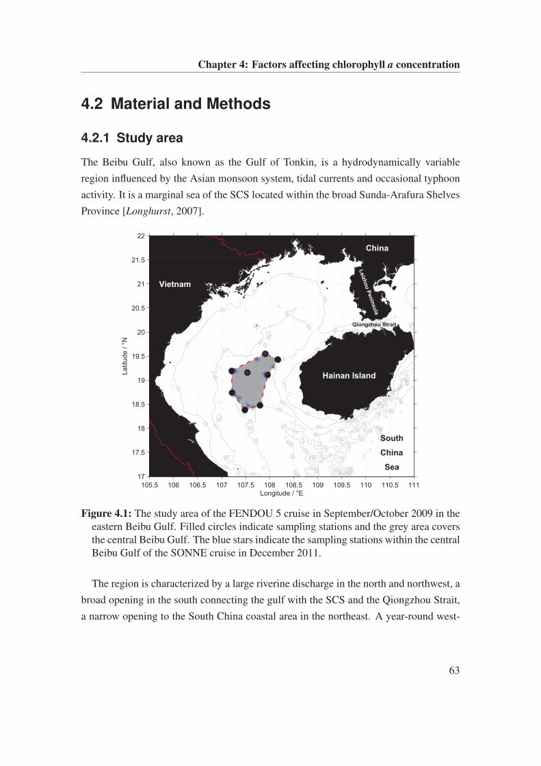
Chapter 4: Factors affecting chlorophyll a concentration
4.2 Material and Methods
4.2.1 Study area
The Beibu Gulf, also known as the Gulf of Tonkin, is a hydrodynamically variable
region influenced by the Asian monsoon system, tidal currents and occasional typhoon
activity. It is a marginal sea of the SCS located within the broad Sunda-Arafura Shelves
Province [Longhurst, 2007].
105.5 106 106.5 107 107.5 108 108.5 109 109.5 110 110.5 111
17
17.5
18
18.5
19
19.5
20
20.5
21
21.5
2225
25
25
25
25
25
25
25
25
25
25
25
25
25
25
25
25
25
25
25
25
25
25
25
25
25
50
50
50
50
50
5050
50
50
50
50
50
50
50
50
5050
50
50
50
50
75
75
75
75
75 7
5
75
75
75
75
75 75
75
75
75
75
7575
75
75
75
75
75
7575 75
75
100
100
100
100
100
100
100
100
100
100
100100
100
100
100
Longitude / °E
Latitu
de /
°N
China
Vietnam
Hainan Island
Leiz
ho
u P
en
insu
la
Qiongzhou Strait
South
China
Sea
Figure 4.1: The study area of the FENDOU 5 cruise in September/October 2009 in theeastern Beibu Gulf. Filled circles indicate sampling stations and the grey area coversthe central Beibu Gulf. The blue stars indicate the sampling stations within the centralBeibu Gulf of the SONNE cruise in December 2011.
The region is characterized by a large riverine discharge in the north and northwest, a
broad opening in the south connecting the gulf with the SCS and the Qiongzhou Strait,
a narrow opening to the South China coastal area in the northeast. A year-round west-
63
Chapter 4: Factors affecting chlorophyll a concentration
ward mean water transport through the Qiongzhou Strait forces a gulf-wide cyclonic
circulation pattern in all seasons [Shi et al., 2002; Wu et al., 2008].
In this study we concentrate on the central Beibu Gulf (Fig. 4.1) a region which
may only be affected by external water masses to a small degree in comparison to other
regions within the gulf [Bauer et al., in press]. Therefore most of the primary production
should be locally generated with a small amount being transported through Qiongzhou
Strait or from the SCS during strong wind events.
The central Beibu Gulf is an area with a depth between 54 and 78 m and a sum-
mer stratification with a strong thermocline between 20 and 50 m depth [Huang et al.,
2008; Bauer et al., in press]. Surface chlorophyll-a concentrations are low in summer
(<0.5 mg m−3) and show a seasonal peak in winter due to the strong northeast mon-
soonal winds [Hu et al., 2003; Tang et al., 2003]. Typically for oligotrophic regions only
low surface nitrate (up to 0.5 µM) and phosphate (at detection limit) concentrations were
found in the central Beibu Gulf with an N:P ratio >16 indicating phosphate limitation
[Bauer et al., in press]. Due to the strong stratification in summer, nutrient supply from
the deeper nutrient-rich water is limited and enhanced chlorophyll concentrations are
located in the vicinity of the thermocline, where sufficient nutrient concentrations and
light are available. This DCM lies typically in around 30-50 m depth with a maximum
chlorophyll-a concentration of about 0.6-1 mg m−3 [Huang et al., 2008; Wu et al., 2008;
Bauer et al., in press].
4.2.2 In situ data for model validation
Observational data were collected during the German-Chinese FENDOU 5 cruise in
September/October 2009 and the SONNE cruise in December 2011. Using an IOW mini
PUMP CTD system [Strady et al., 2008] depth profiles of hydrographical parameters
(temperature, conductivity and oxygen) were recorded at 8 stations within the central
Beibu Gulf during FENDOU 5 cruise. For hydrographic profiling and water sampling
a Seabird CTD was used during the SONNE 219 cruise. Water samples were taken
at different depths during the upcast for chlorophyll and nutrient analysis (NO2, NO3,
PO4 and SiO4). The samples were low vacuum filtered through 0.7 µm Whatman GF/F
glass fibre filters, which were pre-combusted for preparing water samples for nutrient
analysis, and frozen at around -20°C. Extracted chlorophyll samples [JGOFS, 1994]
64
Chapter 4: Factors affecting chlorophyll a concentration
were analyzed fluorometrically (Turner 10-AU) without correction for phaeopigments.
According to standard methods [Hansen and Koroleff , 1999] an autoanalyzer (Evolution
III, Aliance Instruments) was used to process nutrient samples (detection limits: NO2:
0.02 µM, NO3: 0.05 µM, PO4: 0.02 µM, SiO4: 0.1 µM).
Furthermore, in-situ CTD data (temperature) and surface chlorophyll concentrations
from August 2009, August 2010 and September 2011 provided by the SCS Branch of
the State Oceanic Administration (SOA) and from the WOCE Upper Ocean Thermal
(WOCE UOT, 2006, http://doi.pangaea.de/10.1594/PANGAEA.361180?format=html)
from January 1992 were used for model validation.
4.2.3 Simple 1D coupled physical-biological model
To investigate the link between the physical environment, especially stratification and
mixing of the water column, and the phytoplankton growth in the central Beibu Gulf a
simple 1-D coupled physical-biological model established by Sharples [1999] was used.
This model is limited to depths less than 200 m and can be applied to regions from
estuaries to the shelf edge [Sharples, 1999]. The physical module of the model simu-
lates daily mean vertical profiles of temperature (°C), u-component of currents (zonal,
m s−1) and turbulent mixing (m2 s−1) with 1 m depth resolution. An oscillating sea
surface slope, with two tidal constituents, drives the tidal currents. Only the M2 and
S2 tidal constituents are used because those are mainly responsible for the Spring-Neap
tidal cycle [Sharples, 2008]. This allows investigation into the effect of varying kinetic
energy levels in the bottom layer caused by the strongest and weakest tidal currents for
a semimonthly time period. Meteorological data, daily mean wind u- and v-components
(zonal and meridional, m s−1), daily mean dewpoint temperature (°C) and daily mean
solar irradiance (W m−2), are used by the physical module to calculate heat fluxes across
the air-sea boundary and wind-driven momentum flux transmitted into the water column
by using a quadratic stress boundary condition at the sea surface [Sharples, 1999]. The
daily mean vertical profiles of the PAR (W m−2) are calculated by the model deter-
mining the surface PAR as a fraction of the incident solar radiation (Tab. 4.1). PAR
is then distributed through the water column by using a vertical absorption coefficient
[Sharples, 1999] (Tab. 4.1). As the attenuation coefficient for PAR changes seasonally
within each region it has been calculated after Kirk [2011] by using the mean Secchi
65
Chapter 4: Factors affecting chlorophyll a concentration
depth of 9.2 m determined from all, only sparsely available Secchi depths measured
from the FENDOU 5 and SONNE cruises.
The biological component of the model is a simple cell quota, threshold-limitation
scheme after Tett et al. [1986] simulating vertical profiles of phytoplankton biomass (in
mg chlorophyll m−3) and DIN (in mmol m−3). This module has the same vertical (1 m)
and temporal (daily) resolution as the physical component. Phytoplankton growth de-
pends on the availability of light, driven by the mean PAR within a model grid depth
element [Sharples, 1999], and DIN. Both potentially limiting resources lead to respi-
ration if there is insufficient growth due to the light environment or nutrient limitation
[Sharples et al., 2006]. A fixed grazing rate that recycles nutrients acts on phytoplank-
ton biomass throughout the year and in addition, remineralized nitrogen diffuses from
the seabed. To simulate the behavior of zooplankton feeding when it is energetically
favorable, the assumed linear grazing (Tab. 4.1, grazing exponent) is only allowed to
take place if the biomass is greater than a threshold value [Sharples and Tett, 1994].
This threshold value is set to 0.16 mg Chl m−3 the lowest remotely measured surface
chlorophyll concentration for the central Beibu Gulf in 2009. Phytoplankton biomass
and DIN are vertically mixed by turbulence calculated by the physical module. Initial-
ization parameters used for both modules (physical and biological) are summarized in
Tab. 4.1.
The maximum depth of the central Beibu Gulf averages 63 m, this was chosen as
well as the mean latitude of 19◦N. Current data was only obtained during the spring tide
leading to a calculated mean M2 amplitude of 0.6 m s−1. For the neap tide a lowering of
this amplitude is expected which would lead to a lower mean M2 amplitude. Therefore,
for all model runs the M2 amplitude was set to the mean value of 0.15 m s−1, containing
several tidal cycles, estimated from Manh and Yanagi [1997] as well as Zu et al. [2008]
for the central Beibu Gulf. Published tidal ellipse polarisations for the Beibu Gulf are
conflicting [e.g. Manh and Yanagi, 1997; Zu et al., 2008]. For this reason, the tidal
cycles recorded during the FENDOU 5 cruise at different depths were used to define
the tidal ellipse polarisation as a degenerated one. The mean S2 tidal amplitude (0.98)
which is expressed as a fraction of M2 is calculated from the predictions provided by
harmonic analysis for the current records [Emery and Thomson, 2001]. Changing the
mean S2 tidal amplitude did not show any significant effect in the model output. As a
result of the S2 tidal amplitude activation from 0 to 1, a cooling of about 0.2% in the
66
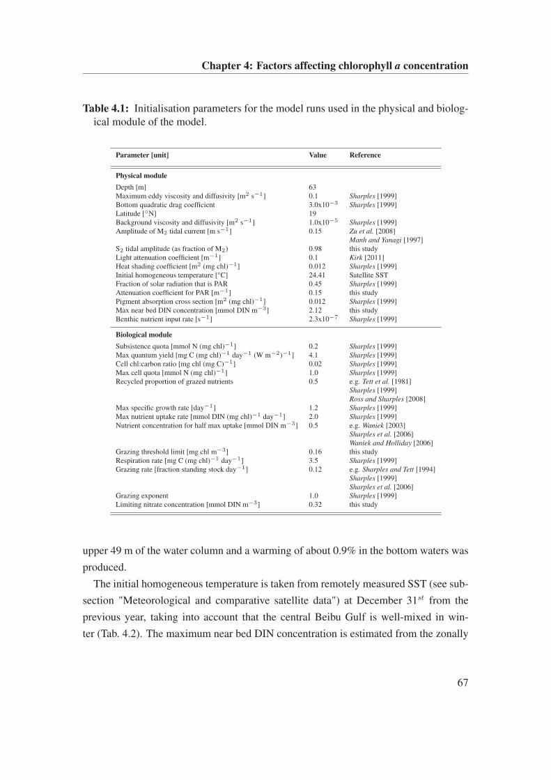
Chapter 4: Factors affecting chlorophyll a concentration
Table 4.1: Initialisation parameters for the model runs used in the physical and biolog-ical module of the model.
Parameter [unit] Value Reference
Physical module
Depth [m] 63Maximum eddy viscosity and diffusivity [m2 s−1] 0.1 Sharples [1999]Bottom quadratic drag coefficient 3.0x10⁻³ Sharples [1999]Latitude [◦N] 19Background viscosity and diffusivity [m2 s−1] 1.0x10⁻⁵ Sharples [1999]Amplitude of M2 tidal current [m s−1] 0.15 Zu et al. [2008]
Manh and Yanagi [1997]S2 tidal amplitude (as fraction of M2) 0.98 this studyLight attenuation coefficient [m−1] 0.1 Kirk [2011]Heat shading coefficient [m2 (mg chl)−1] 0.012 Sharples [1999]Initial homogeneous temperature [°C] 24.41 Satellite SSTFraction of solar radiation that is PAR 0.45 Sharples [1999]Attenuation coefficient for PAR [m−1] 0.15 this studyPigment absorption cross section [m2 (mg chl)−1] 0.012 Sharples [1999]Max near bed DIN concentration [mmol DIN m−3] 2.12 this studyBenthic nutrient input rate [s−1] 2.3x10⁻⁷ Sharples [1999]
Biological module
Subsistence quota [mmol N (mg chl)−1] 0.2 Sharples [1999]Max quantum yield [mg C (mg chl)−1 day−1 (W m−2)−1] 4.1 Sharples [1999]Cell chl:carbon ratio [mg chl (mg C)−1] 0.02 Sharples [1999]Max cell quota [mmol N (mg chl)−1] 1.0 Sharples [1999]Recycled proportion of grazed nutrients 0.5 e.g. Tett et al. [1981]
Sharples [1999]Ross and Sharples [2008]
Max specific growth rate [day−1] 1.2 Sharples [1999]Max nutrient uptake rate [mmol DIN (mg chl)−1 day−1] 2.0 Sharples [1999]Nutrient concentration for half max uptake [mmol DIN m−3] 0.5 e.g. Waniek [2003]
Sharples et al. [2006]Waniek and Holliday [2006]
Grazing threshold limit [mg chl m−3] 0.16 this studyRespiration rate [mg C (mg chl)−1 day−1] 3.5 Sharples [1999]Grazing rate [fraction standing stock day−1] 0.12 e.g. Sharples and Tett [1994]
Sharples [1999]Sharples et al. [2006]
Grazing exponent 1.0 Sharples [1999]Limiting nitrate concentration [mmol DIN m−3] 0.32 this study
upper 49 m of the water column and a warming of about 0.9% in the bottom waters was
produced.
The initial homogeneous temperature is taken from remotely measured SST (see sub-
section "Meteorological and comparative satellite data") at December 31st from the
previous year, taking into account that the central Beibu Gulf is well-mixed in win-
ter (Tab. 4.2). The maximum near bed DIN concentration is estimated from the zonally
67
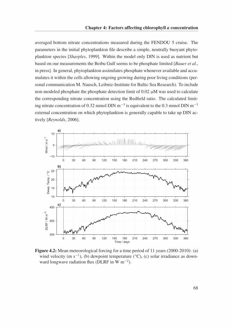
Chapter 4: Factors affecting chlorophyll a concentration
averaged bottom nitrate concentrations measured during the FENDOU 5 cruise. The
parameters in the initial phytoplankton file describe a simple, neutrally buoyant phyto-
plankton species [Sharples, 1999]. Within the model only DIN is used as nutrient but
based on our measurements the Beibu Gulf seems to be phosphate limited [Bauer et al.,
in press]. In general, phytoplankton assimilates phosphate whenever available and accu-
mulates it within the cells allowing ongoing growing during poor living conditions (per-
sonal communication M. Nausch, Leibniz-Institute for Baltic Sea Research). To include
non-modeled phosphate the phosphate detection limit of 0.02 µM was used to calculate
the corresponding nitrate concentration using the Redfield ratio. The calculated limit-
ing nitrate concentration of 0.32 mmol DIN m−3 is equivalent to the 0.3 mmol DIN m−3
external concentration on which phytoplankton is generally capable to take up DIN ac-
tively [Reynolds, 2006].
0 30 60 90 120 150 180 210 240 270 300 330 360
−10
0
10
Win
d /
m s
−1
a)
0 30 60 90 120 150 180 210 240 270 300 330 360
10
15
20
25
Dew
p.
Tem
p.
/ °C
b)
0 30 60 90 120 150 180 210 240 270 300 330 360
350
400
450
DLR
F /
W m
−2
c)
Time / days
Figure 4.2: Mean meteorological forcing for a time period of 11 years (2000-2010): (a)wind velocity (m s−1), (b) dewpoint temperature (°C), (c) solar irradiance as down-ward longwave radiation flux (DLRF in W m−2).
68
Chapter 4: Factors affecting chlorophyll a concentration
4.2.4 Meteorological and comparative satellite data
The model is forced with daily surface u- and v-components of wind, dewpoint tem-
perature, calculated after Wanielista et al. [1997] using air temperature and relative
humidity, and downward longwave radiation flux all taken from NCEP obtained at
http://www.esrl.noaa.gov for 11 years (2000-2010, Fig. 4.2, Fig. S1a-c in the supple-
ment). As the spatial resolution of the NCEP Reanalysis data set is 2.5◦ x 2.5◦ [Kalnay
et al., 1996], the Beibu Gulf area has been cubically interpolated to a resolution of 0.1◦
x 0.1◦. The interpolated meteorological data were averaged for the entire area in the
central Beibu Gulf to force the model (18.3-19.6◦N 107.2-108.2◦E, Fig. 4.1).
Comparative satellite data for daily SST were taken from http://www.remss.com (TMI
SST), resolution 0.25◦ x 0.25◦) and used for the comparison with the predicted SST. To
compare the modeled primary production monthly SeaWiFS (2000-2010) and MODIS
(07/2002-2010) surface chlorophyll concentrations from http://gdata1.sci.gsfc.nasa.gov
were used and averaged between 07/2002 and 2010 because of gaps in both data sets.
The satellite data were averaged for the entire central Beibu Gulf region as well.
4.3 Results
All model simulations for the years 2000 to 2010 started at the same initial conditions
for the physical and biological module (Tab. 4.1). The only differences were in the me-
teorological forcing and in the initial homogeneous temperature which was taken from
satellite SST for the previous year on December 31st (Tab. 4.2). A comparison of a
three years run using meteorological data from 2009 shows a similar vertical tempera-
ture distribution for each year, indicating stability of the numerical scheme. Despite that,
an initial leg of one year was introduced to allow a better adaptation of the biological
components.
69
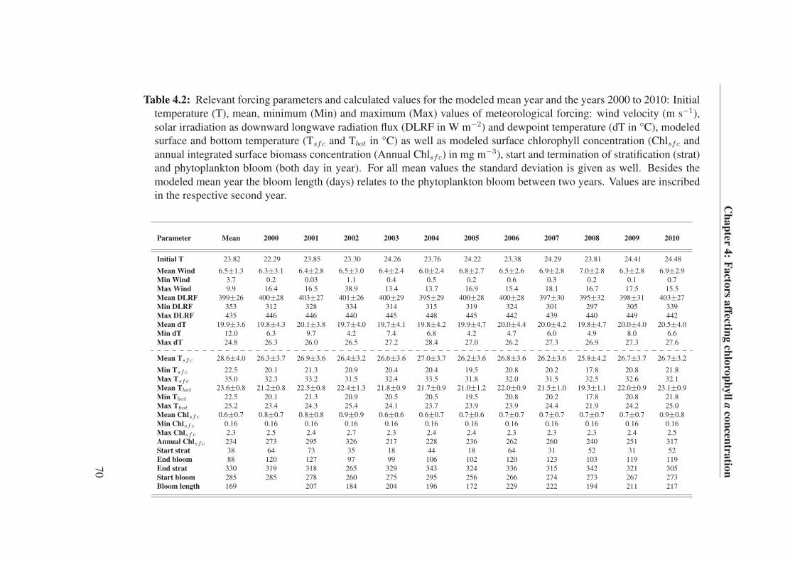
Ch
ap
ter4
:F
acto
rsa
ffecting
chlo
rop
hy
lla
con
centra
tion
Table 4.2: Relevant forcing parameters and calculated values for the modeled mean year and the years 2000 to 2010: Initialtemperature (T), mean, minimum (Min) and maximum (Max) values of meteorological forcing: wind velocity (m s−1),solar irradiation as downward longwave radiation flux (DLRF in W m−2) and dewpoint temperature (dT in °C), modeledsurface and bottom temperature (Tsfc and Tbot in °C) as well as modeled surface chlorophyll concentration (Chlsfc andannual integrated surface biomass concentration (Annual Chlsfc) in mg m−3), start and termination of stratification (strat)and phytoplankton bloom (both day in year). For all mean values the standard deviation is given as well. Besides themodeled mean year the bloom length (days) relates to the phytoplankton bloom between two years. Values are inscribedin the respective second year.
Parameter Mean 2000 2001 2002 2003 2004 2005 2006 2007 2008 2009 2010
Initial T 23.82 22.29 23.85 23.30 24.26 23.76 24.22 23.38 24.29 23.81 24.41 24.48
Mean Wind 6.5±1.3 6.3±3.1 6.4±2.8 6.5±3.0 6.4±2.4 6.0±2.4 6.8±2.7 6.5±2.6 6.9±2.8 7.0±2.8 6.3±2.8 6.9±2.9Min Wind 3.7 0.2 0.03 1.1 0.4 0.5 0.2 0.6 0.3 0.2 0.1 0.7Max Wind 9.9 16.4 16.5 38.9 13.4 13.7 16.9 15.4 18.1 16.7 17.5 15.5Mean DLRF 399±26 400±28 403±27 401±26 400±29 395±29 400±28 400±28 397±30 395±32 398±31 403±27Min DLRF 353 312 328 334 314 315 319 324 301 297 305 339Max DLRF 435 446 446 440 445 448 445 442 439 440 449 442Mean dT 19.9±3.6 19.8±4.3 20.1±3.8 19.7±4.0 19.7±4.1 19.8±4.2 19.9±4.7 20.0±4.4 20.0±4.2 19.8±4.7 20.0±4.0 20.5±4.0Min dT 12.0 6.3 9.7 4.2 7.4 6.8 4.2 4.7 6.0 4.9 8.0 6.6Max dT 24.8 26.3 26.0 26.5 27.2 28.4 27.0 26.2 27.3 26.9 27.3 27.6
Mean Tsfc 28.6±4.0 26.3±3.7 26.9±3.6 26.4±3.2 26.6±3.6 27.0±3.7 26.2±3.6 26.8±3.6 26.2±3.6 25.8±4.2 26.7±3.7 26.7±3.2
Min Tsfc 22.5 20.1 21.3 20.9 20.4 20.4 19.5 20.8 20.2 17.8 20.8 21.8Max Tsfc 35.0 32.3 33.2 31.5 32.4 33.5 31.8 32.0 31.5 32.5 32.6 32.1Mean Tbot 23.6±0.8 21.2±0.8 22.5±0.8 22.4±1.3 21.8±0.9 21.7±0.9 21.0±1.2 22.0±0.9 21.5±1.0 19.3±1.1 22.0±0.9 23.1±0.9Min Tbot 22.5 20.1 21.3 20.9 20.5 20.5 19.5 20.8 20.2 17.8 20.8 21.8Max Tbot 25.2 23.4 24.3 25.4 24.1 23.7 23.9 23.9 24.4 21.9 24.2 25.0Mean Chlsfc 0.6±0.7 0.8±0.7 0.8±0.8 0.9±0.9 0.6±0.6 0.6±0.7 0.7±0.6 0.7±0.7 0.7±0.7 0.7±0.7 0.7±0.7 0.9±0.8Min Chlsfc 0.16 0.16 0.16 0.16 0.16 0.16 0.16 0.16 0.16 0.16 0.16 0.16Max Chlsfc 2.3 2.5 2.4 2.7 2.3 2.4 2.4 2.3 2.3 2.3 2.4 2.5Annual Chlsfc 234 273 295 326 217 228 236 262 260 240 251 317Start strat 38 64 73 35 18 44 18 64 31 52 31 52End bloom 88 120 127 97 99 106 102 120 123 103 119 119End strat 330 319 318 265 329 343 324 336 315 342 321 305Start bloom 285 285 278 260 275 295 256 266 274 273 267 273Bloom length 169 207 184 204 196 172 229 222 194 211 217
70
Chapter 4: Factors affecting chlorophyll a concentration
4.3.1 Mean annual cycle
In order to investigate the effect of the meteorological forcing a mean annual cycle
was modeled using the mean meteorological forcing calculated as the average over the
years 2000-2010 (Fig. 4.2 and Fig. 4.3). The analysis of the model results focuses on
the annual cycle of physical factors, e.g. vertical temperature distribution, mixed layer
depth (MLD, depth where the difference of 0.5°C between SST and temperature at the
depth is reached), euphotic depth (1% of the surface PAR) and biological properties,
e.g. chlorophyll distribution representing primary production. The mean modeled tem-
perature distribution for 2000-2010 for the entire water column down to the mean depth
of 63 m for the central Beibu Gulf shows a surface heating in summer with an associated
stratification and a winter deep mixing (Fig. 4.3a). The stratification establishes on av-
erage in spring around day 38 and exists until end of November (day 330, Fig. 4.3a, b).
The beginning of stratification is defined as the first day in spring when surface and bot-
tom temperatures are not equal anymore whereas the end of stratification is defined as
the first day in autumn when both temperatures are equal again (Fig. 4.3b). During sum-
mer the MLD persists on average in about 18 m depth and shows a deepening during
winter (January and December) due to strong vertical mixing (Fig. 4.3a).
To validate the model predictions simulated mean daily SST is compared to satel-
lite derived SST which is averaged over the 11 years period (2000-2010) and in-situ
Figure 4.3 (following page): Simulated mean annual cycle using mean meteorolog-ical forcing for a time period of 11 years (2000-2010) in the central Beibu Gulf:(a) Temperature (°C) distribution over the entire water column. The white dashedline indicates the calculated MLD. (b) Simulated daily mean SST (°C, red line) incomparison to remotely measured SST (°C, black line) averaged over the 11 yearsand in-situ observations (symbols). The blue line represents the modeled daily meanbottom temperature (°C) and the respective observations (symbols). (c) Chlorophyll(mg m−3) distribution over the entire water column. The white dashed line indicatesthe calculated MLD, the white dotted line indicates the euphotic depth (1% of surfacePAR). (d) Simulated monthly mean sea surface chlorophyll concentrations (mg m−3,green line) in comparison to satellite derived monthly mean surface chlorophyll con-centrations (mg m−3, black line). The sources for the values indicated by the blacksymbols are given in the legend. The black bars indicate the standard deviations ofthe remotely measured chlorophyll concentrations.
71
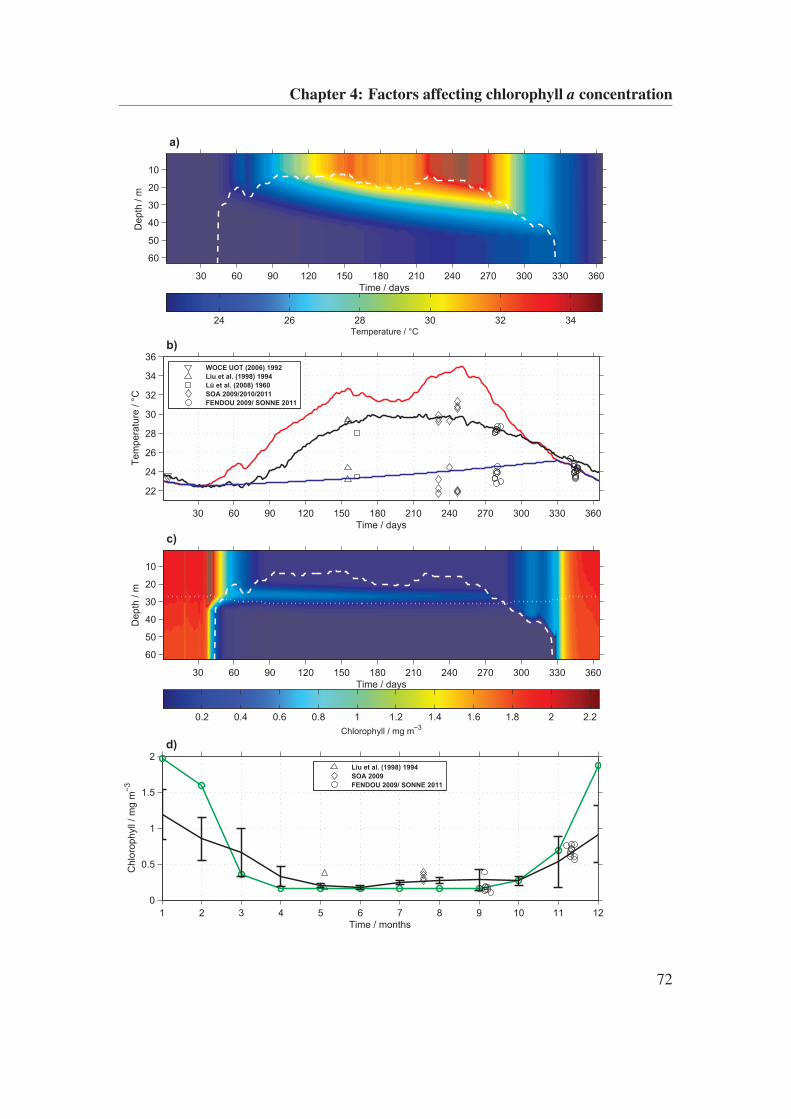
Chapter 4: Factors affecting chlorophyll a concentration
1 2 3 4 5 6 7 8 9 10 11 12
0
0.5
1
1.5
2
Time / months
Chlo
rophyll
/ m
g m
−3
d)
Liu et al. (1998) 1994
SOA 2009
FENDOU 2009/ SONNE 2011
Time / days
Depth
/ m
c)
30 60 90 120 150 180 210 240 270 300 330 360
10
20
30
40
50
60
Chlorophyll / mg m−3
0.2 0.4 0.6 0.8 1 1.2 1.4 1.6 1.8 2 2.2
30 60 90 120 150 180 210 240 270 300 330 360
22
24
26
28
30
32
34
36
Time / days
Tem
pera
ture
/ °
C
b)
WOCE UOT (2006) 1992
Liu et al. (1998) 1994
Lü et al. (2008) 1960
SOA 2009/2010/2011
FENDOU 2009/ SONNE 2011
Time / days
Depth
/ m
l
a)
30 60 90 120 150 180 210 240 270 300 330 360
10
20
30
40
50
60
Temperature / °C
24 26 28 30 32 34
72
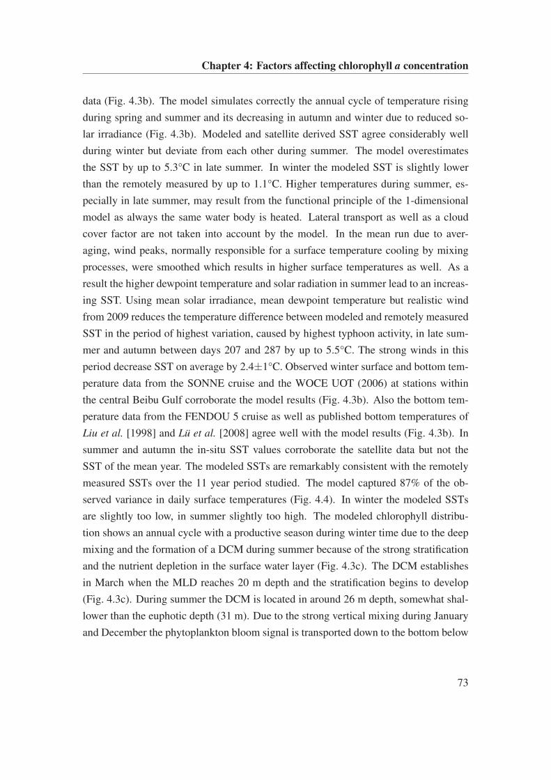
Chapter 4: Factors affecting chlorophyll a concentration
data (Fig. 4.3b). The model simulates correctly the annual cycle of temperature rising
during spring and summer and its decreasing in autumn and winter due to reduced so-
lar irradiance (Fig. 4.3b). Modeled and satellite derived SST agree considerably well
during winter but deviate from each other during summer. The model overestimates
the SST by up to 5.3°C in late summer. In winter the modeled SST is slightly lower
than the remotely measured by up to 1.1°C. Higher temperatures during summer, es-
pecially in late summer, may result from the functional principle of the 1-dimensional
model as always the same water body is heated. Lateral transport as well as a cloud
cover factor are not taken into account by the model. In the mean run due to aver-
aging, wind peaks, normally responsible for a surface temperature cooling by mixing
processes, were smoothed which results in higher surface temperatures as well. As a
result the higher dewpoint temperature and solar radiation in summer lead to an increas-
ing SST. Using mean solar irradiance, mean dewpoint temperature but realistic wind
from 2009 reduces the temperature difference between modeled and remotely measured
SST in the period of highest variation, caused by highest typhoon activity, in late sum-
mer and autumn between days 207 and 287 by up to 5.5°C. The strong winds in this
period decrease SST on average by 2.4±1°C. Observed winter surface and bottom tem-
perature data from the SONNE cruise and the WOCE UOT (2006) at stations within
the central Beibu Gulf corroborate the model results (Fig. 4.3b). Also the bottom tem-
perature data from the FENDOU 5 cruise as well as published bottom temperatures of
Liu et al. [1998] and Lü et al. [2008] agree well with the model results (Fig. 4.3b). In
summer and autumn the in-situ SST values corroborate the satellite data but not the
SST of the mean year. The modeled SSTs are remarkably consistent with the remotely
measured SSTs over the 11 year period studied. The model captured 87% of the ob-
served variance in daily surface temperatures (Fig. 4.4). In winter the modeled SSTs
are slightly too low, in summer slightly too high. The modeled chlorophyll distribu-
tion shows an annual cycle with a productive season during winter time due to the deep
mixing and the formation of a DCM during summer because of the strong stratification
and the nutrient depletion in the surface water layer (Fig. 4.3c). The DCM establishes
in March when the MLD reaches 20 m depth and the stratification begins to develop
(Fig. 4.3c). During summer the DCM is located in around 26 m depth, somewhat shal-
lower than the euphotic depth (31 m). Due to the strong vertical mixing during January
and December the phytoplankton bloom signal is transported down to the bottom below
73
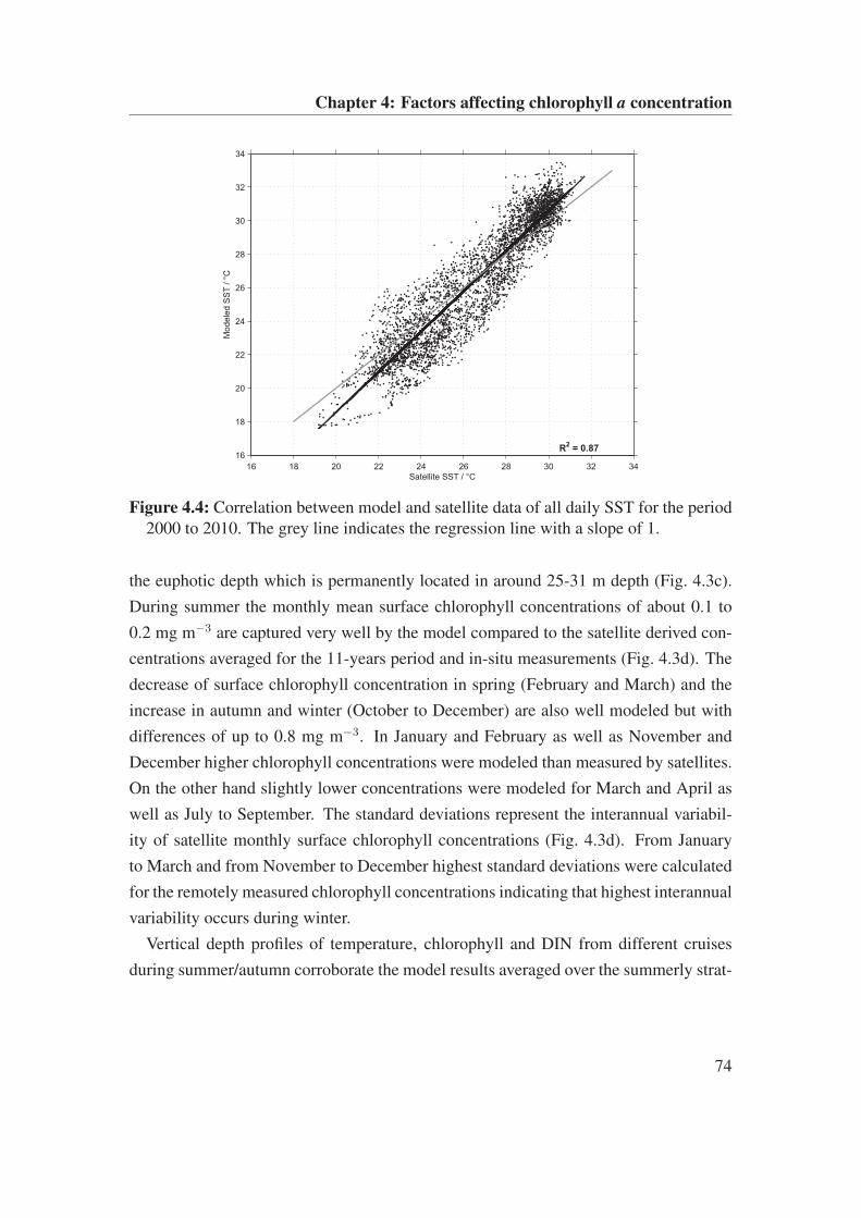
Chapter 4: Factors affecting chlorophyll a concentration
16 18 20 22 24 26 28 30 32 34
16
18
20
22
24
26
28
30
32
34
Satellite SST / °C
Modele
d S
ST
/ °
C
R2 = 0.87
Figure 4.4: Correlation between model and satellite data of all daily SST for the period2000 to 2010. The grey line indicates the regression line with a slope of 1.
the euphotic depth which is permanently located in around 25-31 m depth (Fig. 4.3c).
During summer the monthly mean surface chlorophyll concentrations of about 0.1 to
0.2 mg m−3 are captured very well by the model compared to the satellite derived con-
centrations averaged for the 11-years period and in-situ measurements (Fig. 4.3d). The
decrease of surface chlorophyll concentration in spring (February and March) and the
increase in autumn and winter (October to December) are also well modeled but with
differences of up to 0.8 mg m−3. In January and February as well as November and
December higher chlorophyll concentrations were modeled than measured by satellites.
On the other hand slightly lower concentrations were modeled for March and April as
well as July to September. The standard deviations represent the interannual variabil-
ity of satellite monthly surface chlorophyll concentrations (Fig. 4.3d). From January
to March and from November to December highest standard deviations were calculated
for the remotely measured chlorophyll concentrations indicating that highest interannual
variability occurs during winter.
Vertical depth profiles of temperature, chlorophyll and DIN from different cruises
during summer/autumn corroborate the model results averaged over the summerly strat-
74
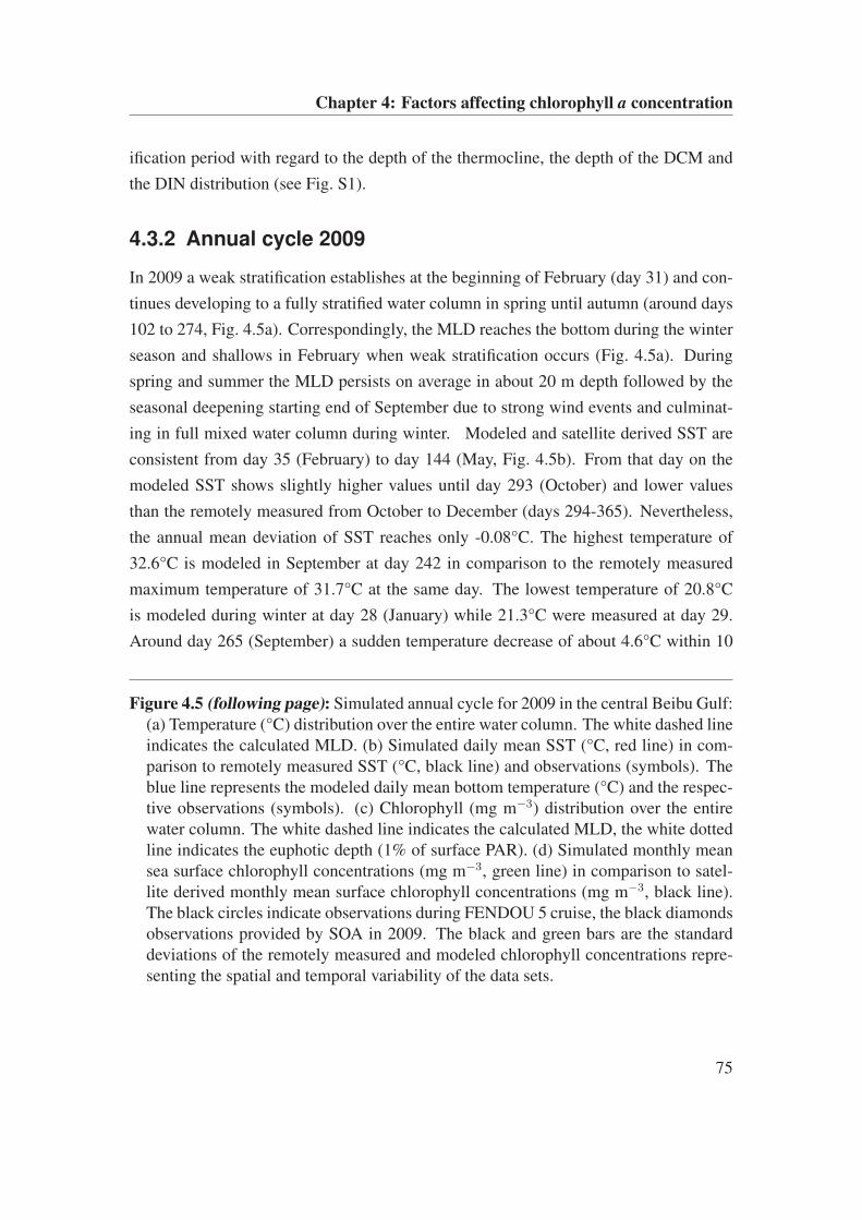
Chapter 4: Factors affecting chlorophyll a concentration
ification period with regard to the depth of the thermocline, the depth of the DCM and
the DIN distribution (see Fig. S1).
4.3.2 Annual cycle 2009
In 2009 a weak stratification establishes at the beginning of February (day 31) and con-
tinues developing to a fully stratified water column in spring until autumn (around days
102 to 274, Fig. 4.5a). Correspondingly, the MLD reaches the bottom during the winter
season and shallows in February when weak stratification occurs (Fig. 4.5a). During
spring and summer the MLD persists on average in about 20 m depth followed by the
seasonal deepening starting end of September due to strong wind events and culminat-
ing in full mixed water column during winter. Modeled and satellite derived SST are
consistent from day 35 (February) to day 144 (May, Fig. 4.5b). From that day on the
modeled SST shows slightly higher values until day 293 (October) and lower values
than the remotely measured from October to December (days 294-365). Nevertheless,
the annual mean deviation of SST reaches only -0.08°C. The highest temperature of
32.6°C is modeled in September at day 242 in comparison to the remotely measured
maximum temperature of 31.7°C at the same day. The lowest temperature of 20.8°C
is modeled during winter at day 28 (January) while 21.3°C were measured at day 29.
Around day 265 (September) a sudden temperature decrease of about 4.6°C within 10
Figure 4.5 (following page): Simulated annual cycle for 2009 in the central Beibu Gulf:(a) Temperature (°C) distribution over the entire water column. The white dashed lineindicates the calculated MLD. (b) Simulated daily mean SST (°C, red line) in com-parison to remotely measured SST (°C, black line) and observations (symbols). Theblue line represents the modeled daily mean bottom temperature (°C) and the respec-tive observations (symbols). (c) Chlorophyll (mg m−3) distribution over the entirewater column. The white dashed line indicates the calculated MLD, the white dottedline indicates the euphotic depth (1% of surface PAR). (d) Simulated monthly meansea surface chlorophyll concentrations (mg m−3, green line) in comparison to satel-lite derived monthly mean surface chlorophyll concentrations (mg m−3, black line).The black circles indicate observations during FENDOU 5 cruise, the black diamondsobservations provided by SOA in 2009. The black and green bars are the standarddeviations of the remotely measured and modeled chlorophyll concentrations repre-senting the spatial and temporal variability of the data sets.
75
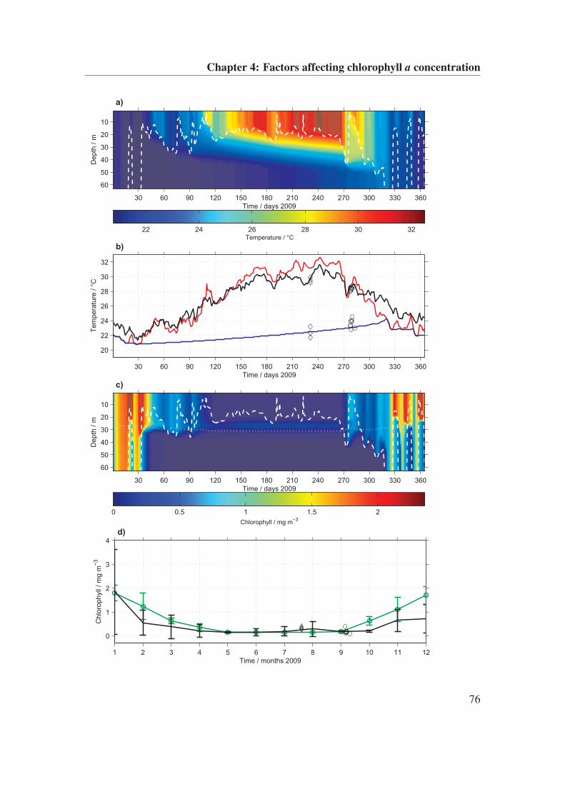
Chapter 4: Factors affecting chlorophyll a concentration
1 2 3 4 5 6 7 8 9 10 11 12
0
1
2
3
4
Time / months 2009
Chlo
rophyll
/ m
g m
−3
d)
Time / days 2009
Depth
/ m
c)
30 60 90 120 150 180 210 240 270 300 330 360
10
20
30
40
50
60
Chlorophyll / mg m−3
0 0.5 1 1.5 2
30 60 90 120 150 180 210 240 270 300 330 360
20
22
24
26
28
30
32
Time / days 2009
Tem
pera
ture
/ °
C
b)
Time / days 2009
Depth
/ m
a)
30 60 90 120 150 180 210 240 270 300 330 360
10
20
30
40
50
60
Temperature / °C
22 24 26 28 30 32
76
Chapter 4: Factors affecting chlorophyll a concentration
days took place induced by a typhoon which passed the study area. After that the water
column was well mixed down to 44 m depth for around 7 days (271-277, Fig. 4.5a).
Then the water column stratified again for a short period of around two weeks (days
276-291) and transits slowly to the winterly conditions. The bottom temperature shows
a persistent warming from day 26 (January) with 20.9°C to day 321 (November) with
24.2°C (Fig. 4.5b). From the end of November the bottom water temperature decreases
again due to the winter mixing of the entire water column and reduced solar radiation
as well as decreased dewpoint temperature during this time of the year. The observed
surface and bottom temperature data from the FENDOU 5 (2009) cruise and received
from SOA at the stations within the central Beibu Gulf corroborate the model results
(Fig. 4.5b).
After the MLD reached its shallowest depth (around 3 m) and the stratification is fully
developed in April the DCM establishes (Fig. 4.5c). The summerly DCM is located at
around 27 m depth, again shallower than the euphotic depth (30 m). The phytoplankton
bloom in January with 1.9 mg m−3 chlorophyll and the low concentrations of about 0.1
to 0.2 mg m−3 chlorophyll during summer are modeled quite well (Fig. 4.5d). In gen-
eral, the surface chlorophyll decrease in spring (February and March) and increase in
autumn and winter (October to December) are well captured with differences of up to
0.9 mg m−3. During winter the model results show higher concentrations than remotely
measured (Fig. 4.5d). The standard deviations indicated by the green and black bars
(Fig. 4.5d) indicate the temporal and in case of the satellite data also spatial variability
of monthly mean surface chlorophyll concentrations (Tab. S1 in the supplement). High-
est variability occurs during winter and spring (between January and April as well as
November and December). The measurements and the overlapping standard deviations
point to a good agreement between the modeled and the remotely measured monthly
mean surface chlorophyll concentrations.
4.3.3 Effects of strong wind events
The wind forcing at the surface is demonstrated in fig. 4.6a for a time period of 40 days
including the passing of typhoon KETSANA (25.-30.09.2009, days 268-273) with max-
imum wind speeds of up to 17.5 m s−1 in the central Beibu Gulf around day 272.
The stratification is very strong during summer prior to the typhoon crossing and the
77
Chapter 4: Factors affecting chlorophyll a concentration
MLD only reaches down to 20 m depth (Fig. 4.6b). During the typhoon (day 272) the
temperature of the surface layer decreases rapidly from around 32 to 27°C, the ther-
mocline deepens and destabilizes and the mixed layer reaches 44 m depth (Fig. 4.6b).
As a consequence, between days 271 and 274 the nutrient concentration in the sur-
face waters exceeds 0.32 mmol DIN m−3, the defined limiting nitrate concentration
or nutricline (Fig. 4.6c). This in turn leads to an enhanced primary production in the
surface layer above the euphotic depth which is visible with a lag of about 2 days
(Fig. 4.6d). The chlorophyll concentration increases from values of around 0.16 mg m−3
to 1 mg m−3 at day 278 at the surface. The nutrient concentration reached the maximum
(0.35 mmol m−3) at the same day (272) the wind reached its maximum velocity whereas
the maximum in chlorophyll concentration within the upper 20 m depth is reached five
days (277-278) later.
4.3.4 Effects of tides
Fig. 4.7a-c show the effect of tidal forcing on the DCM within a 50 day period from July
to September 2009. The resulting DCM from a model run with tides (Fig. 4.7b) is more
developed than the DCM of a model run without tides (M2 and S2 tidal amplitudes set
to 0, Fig. 4.7a). Maximum chlorophyll concentrations for the model run without tidal
forcing reach 0.31 mg m−3 in around 26.5 m depth in comparison to 0.42 mg m−3 for
the model run with tides at similar depth. This is an increase of around 36%. Be-
sides the higher concentrations the tidally forced DCM is also slightly broader with a
thickness (determined as the part of the chlorophyll depth profiles showing higher val-
ues than surface background chlorophyll concentration of 0.16 mg m−3, Fig. 4.7c) of
around 12 m compared to 9 m for the run without tides (Fig. 4.7c) which is an increase
of around 33%. Due to the maximum tidal forcing during spring tide the modeled DCM
Figure 4.6 (following page): A 40 days section (September/October) of the year 2009(days 250-290) showing the effect of a typhoon passing throughout the region basedon (a) absolute wind velocity (m s−1), (b) vertical temperature distribution (°C), (c)vertical distribution of DIN (mmol m−3) and (d) vertical chlorophyll distribution(mg m−3). The white dashed line is the MLD (b-d), the white dotted lines indicatethe limiting nitrate concentration of 0.32 mmol m−3 (c-d) and the white solid line in(d) is the euphotic depth.
78
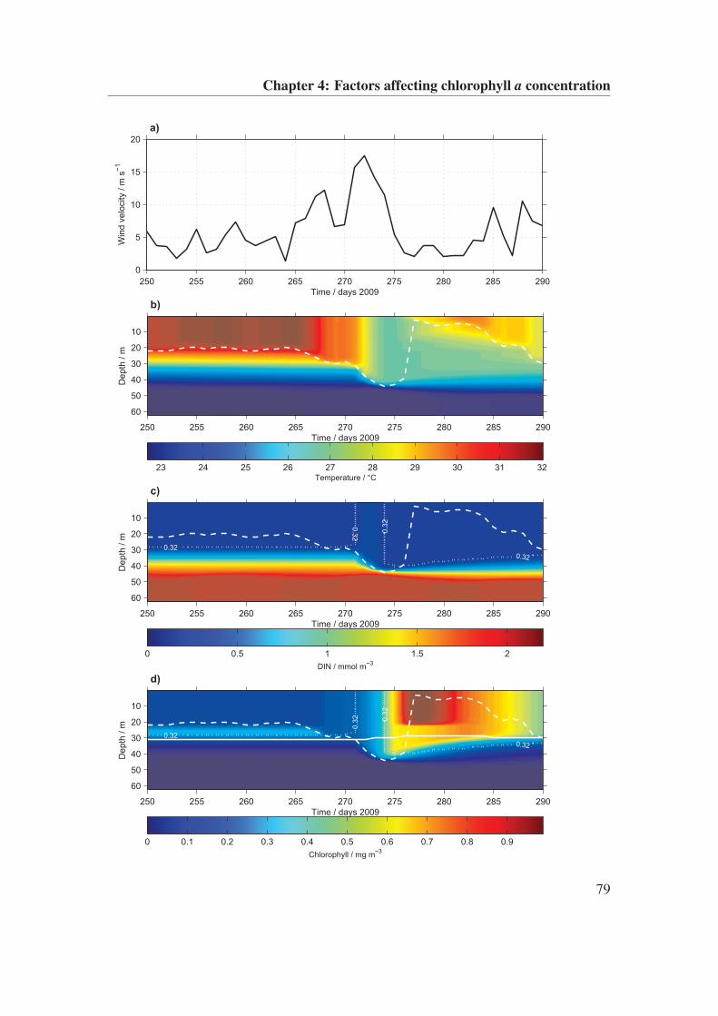
Chapter 4: Factors affecting chlorophyll a concentration
0.3
2
0.32
0.3
2
0.32
Time / days 2009
Depth
/ m
d)
250 255 260 265 270 275 280 285 290
10
20
30
40
50
60
Chlorophyll / mg m−3
0 0.1 0.2 0.3 0.4 0.5 0.6 0.7 0.8 0.9
0.3
2
0.32
0.3
2
0.32
Time / days 2009
Depth
/ m
c)
250 255 260 265 270 275 280 285 290
10
20
30
40
50
60
DIN / mmol m−3
0 0.5 1 1.5 2
Time / days 2009
Depth
/ m
b)
250 255 260 265 270 275 280 285 290
10
20
30
40
50
60
Temperature / °C
23 24 25 26 27 28 29 30 31 32
250 255 260 265 270 275 280 285 290
0
5
10
15
20
Win
d v
elo
city /
m s
−1
Time / days 2009
a)
79
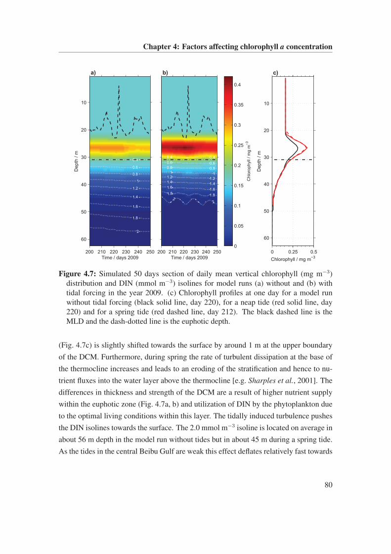
Chapter 4: Factors affecting chlorophyll a concentration
0.4
0.6
0.8
1
1.2
1.4
1.6
1.8
2
Depth
/ m
Time / days 2009
a)
200 210 220 230 240 250
10
20
30
40
50
60
0.4 0.4
0.6 0.60.8 0.8
1 11.2 1.21.4 1.41.6
1.6
1.8 1.82
2
Time / days 2009
b)
200 210 220 230 240 250C
hlo
rophyll
/ m
g m
−3
0
0.05
0.1
0.15
0.2
0.25
0.3
0.35
0.4
0 0.25 0.5
10
20
30
40
50
60
Depth
/ m
Chlorophyll / mg m−3
c)
Figure 4.7: Simulated 50 days section of daily mean vertical chlorophyll (mg m−3)distribution and DIN (mmol m−3) isolines for model runs (a) without and (b) withtidal forcing in the year 2009. (c) Chlorophyll profiles at one day for a model runwithout tidal forcing (black solid line, day 220), for a neap tide (red solid line, day220) and for a spring tide (red dashed line, day 212). The black dashed line is theMLD and the dash-dotted line is the euphotic depth.
(Fig. 4.7c) is slightly shifted towards the surface by around 1 m at the upper boundary
of the DCM. Furthermore, during spring the rate of turbulent dissipation at the base of
the thermocline increases and leads to an eroding of the stratification and hence to nu-
trient fluxes into the water layer above the thermocline [e.g. Sharples et al., 2001]. The
differences in thickness and strength of the DCM are a result of higher nutrient supply
within the euphotic zone (Fig. 4.7a, b) and utilization of DIN by the phytoplankton due
to the optimal living conditions within this layer. The tidally induced turbulence pushes
the DIN isolines towards the surface. The 2.0 mmol m−3 isoline is located on average in
about 56 m depth in the model run without tides but in about 45 m during a spring tide.
As the tides in the central Beibu Gulf are weak this effect deflates relatively fast towards
80
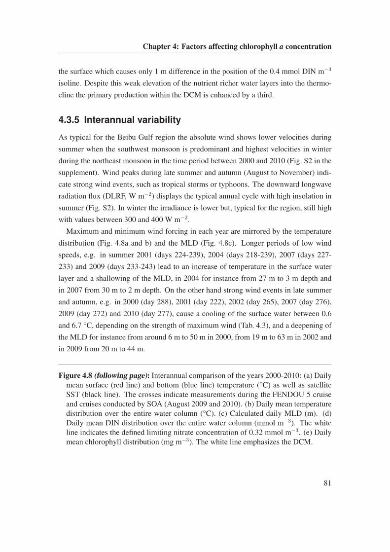
Chapter 4: Factors affecting chlorophyll a concentration
the surface which causes only 1 m difference in the position of the 0.4 mmol DIN m−3
isoline. Despite this weak elevation of the nutrient richer water layers into the thermo-
cline the primary production within the DCM is enhanced by a third.
4.3.5 Interannual variability
As typical for the Beibu Gulf region the absolute wind shows lower velocities during
summer when the southwest monsoon is predominant and highest velocities in winter
during the northeast monsoon in the time period between 2000 and 2010 (Fig. S2 in the
supplement). Wind peaks during late summer and autumn (August to November) indi-
cate strong wind events, such as tropical storms or typhoons. The downward longwave
radiation flux (DLRF, W m−2) displays the typical annual cycle with high insolation in
summer (Fig. S2). In winter the irradiance is lower but, typical for the region, still high
with values between 300 and 400 W m−2.
Maximum and minimum wind forcing in each year are mirrored by the temperature
distribution (Fig. 4.8a and b) and the MLD (Fig. 4.8c). Longer periods of low wind
speeds, e.g. in summer 2001 (days 224-239), 2004 (days 218-239), 2007 (days 227-
233) and 2009 (days 233-243) lead to an increase of temperature in the surface water
layer and a shallowing of the MLD, in 2004 for instance from 27 m to 3 m depth and
in 2007 from 30 m to 2 m depth. On the other hand strong wind events in late summer
and autumn, e.g. in 2000 (day 288), 2001 (day 222), 2002 (day 265), 2007 (day 276),
2009 (day 272) and 2010 (day 277), cause a cooling of the surface water between 0.6
and 6.7 °C, depending on the strength of maximum wind (Tab. 4.3), and a deepening of
the MLD for instance from around 6 m to 50 m in 2000, from 19 m to 63 m in 2002 and
in 2009 from 20 m to 44 m.
Figure 4.8 (following page): Interannual comparison of the years 2000-2010: (a) Dailymean surface (red line) and bottom (blue line) temperature (°C) as well as satelliteSST (black line). The crosses indicate measurements during the FENDOU 5 cruiseand cruises conducted by SOA (August 2009 and 2010). (b) Daily mean temperaturedistribution over the entire water column (°C). (c) Calculated daily MLD (m). (d)Daily mean DIN distribution over the entire water column (mmol m−3). The whiteline indicates the defined limiting nitrate concentration of 0.32 mmol m−3. (e) Dailymean chlorophyll distribution (mg m−3). The white line emphasizes the DCM.
81
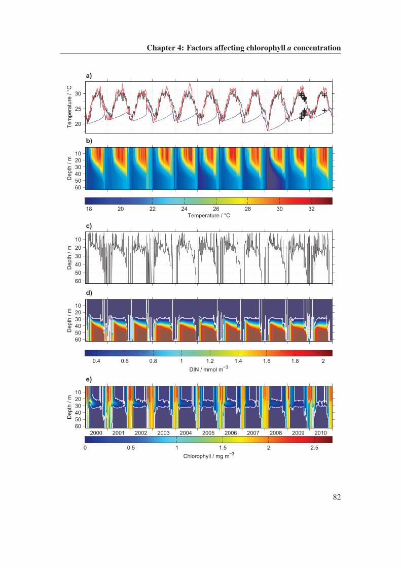
Chapter 4: Factors affecting chlorophyll a concentration
20
25
30
Tem
pera
ture
/ °
C
a)D
epth
/ m
b)
10
20
30
40
50
60
Temperature / °C
18 20 22 24 26 28 30 32
10
20
30
40
50
60
Depth
/ m
c)
Depth
/ m
d)
10
20
30
40
50
60
DIN / mmol m−3
0.4 0.6 0.8 1 1.2 1.4 1.6 1.8 2
Depth
/ m
2000 2001 2002 2003 2004 2005 2006 2007 2008 2009 2010
e)
10
20
30
40
50
60
Chlorophyll / mg m−3
0 0.5 1 1.5 2 2.5
82
Chapter 4: Factors affecting chlorophyll a concentration
The start of sustained stratification and vertical mixing is indicated by the surface
and bottom temperature trends when SST and bottom temperature begin to diverge in
spring and converge again in autumn, respectively (Fig. 4.8a). Periods of mixing and/or
weak stratification occur between the middle of September and the middle of March of
the following year. The beginning of the main period of stratification is defined as the
first day after last day of entire vertical mixing, the end as the first day of total verti-
cal mixing in one year (Fig. 4.8a, Tab. 4.2). In the Beibu Gulf the winter period is the
main productive season [Hu et al., 2003; Tang et al., 2003]. The termination of the ther-
mal stratification in autumn/winter is the most important factor for the timing of nutrient
supply from the bottom waters (Fig. 4.8d) and hence the initiation and timing of the phy-
toplankton bloom. On average the termination of stratification takes place in November
with a strong nutrient input into the surface layer in most of the years directly after
the stratification breakdown indicated by shallowing of the nutricline (Fig. 4.8d, white
line). In all years the limiting nitrate concentration of about 0.32 mmol m−3 (which is
equivalent to a phosphate concentration of 0.02 mmol m−3 necessary for phytoplankton
growth) lies on average in 29 m depth during summer, with higher values below and a
nutrient depleted surface water body (Fig. 4.8d). In autumn and winter when the mixed
layer deepens nutrient inputs from the bottom water layer into the surface layer enhance
nutrient concentrations within the euphotic zone (Fig. 4.8d).
In some years (e.g. 2001, 2004 and 2010) this nutrient input is not visible because
it is directly ingested by phytoplankton in the model. In autumn 2002 a strong wind
event at day 265 (Fig. S1) terminated the stratification by September which led to a
strong nutrient input into the surface layer and hence an early phytoplankton bloom
(Fig. 4.8d, e). In all years a phytoplankton bloom developed between autumn and winter
and persisted until spring (Fig. 4.8e). At the turn of the year 2000/2001, 2002/2003,
2005/2006 and 2007/2008 the phytoplankton bloom is well developed. By contrast the
bloom is less pronounced between 2001/2002, 2004/2005, 2006/2007 and 2008/2009
(Fig. 4.8e). Due to the maximum MLD (63 m) during winter the signal of the bloom
reaches the bottom in every year. The stratification vanishes in autumn between day 265
and 343 but the already established phytoplankton bloom starts between day 256 and
295 (Tab. 4.2). Strong wind events as well as the change from the weaker southwest
to the stronger northeast monsoon lead to a weakening of the thermocline in autumn,
to episodical nutrient supply into the surface waters and hence a phytoplankton bloom
83
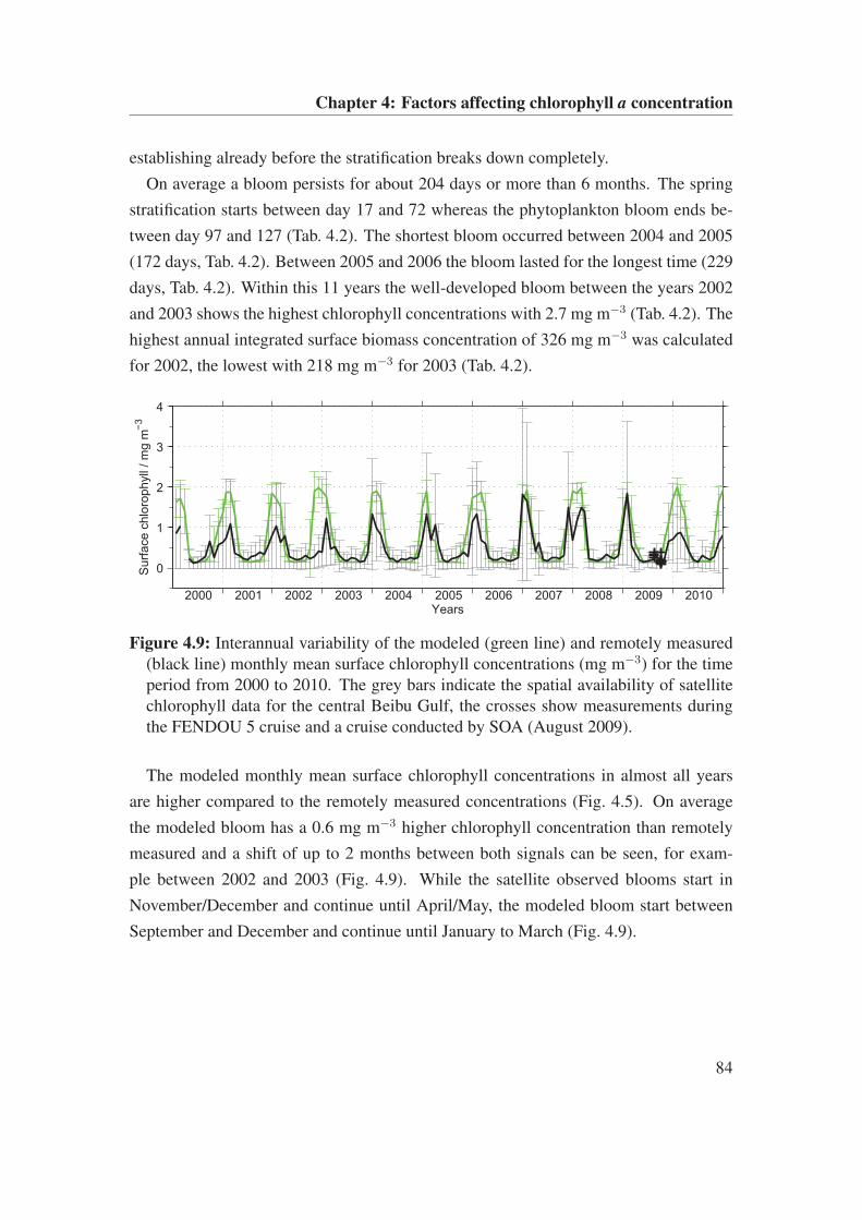
Chapter 4: Factors affecting chlorophyll a concentration
establishing already before the stratification breaks down completely.
On average a bloom persists for about 204 days or more than 6 months. The spring
stratification starts between day 17 and 72 whereas the phytoplankton bloom ends be-
tween day 97 and 127 (Tab. 4.2). The shortest bloom occurred between 2004 and 2005
(172 days, Tab. 4.2). Between 2005 and 2006 the bloom lasted for the longest time (229
days, Tab. 4.2). Within this 11 years the well-developed bloom between the years 2002
and 2003 shows the highest chlorophyll concentrations with 2.7 mg m−3 (Tab. 4.2). The
highest annual integrated surface biomass concentration of 326 mg m−3 was calculated
for 2002, the lowest with 218 mg m−3 for 2003 (Tab. 4.2).
0
1
2
3
4
Years
Surf
ace c
hlo
rophyll
/ m
g m
−3
2000 2001 2002 2003 2004 2005 2006 2007 2008 2009 2010
Figure 4.9: Interannual variability of the modeled (green line) and remotely measured(black line) monthly mean surface chlorophyll concentrations (mg m−3) for the timeperiod from 2000 to 2010. The grey bars indicate the spatial availability of satellitechlorophyll data for the central Beibu Gulf, the crosses show measurements duringthe FENDOU 5 cruise and a cruise conducted by SOA (August 2009).
The modeled monthly mean surface chlorophyll concentrations in almost all years
are higher compared to the remotely measured concentrations (Fig. 4.5). On average
the modeled bloom has a 0.6 mg m−3 higher chlorophyll concentration than remotely
measured and a shift of up to 2 months between both signals can be seen, for exam-
ple between 2002 and 2003 (Fig. 4.9). While the satellite observed blooms start in
November/December and continue until April/May, the modeled bloom start between
September and December and continue until January to March (Fig. 4.9).
84
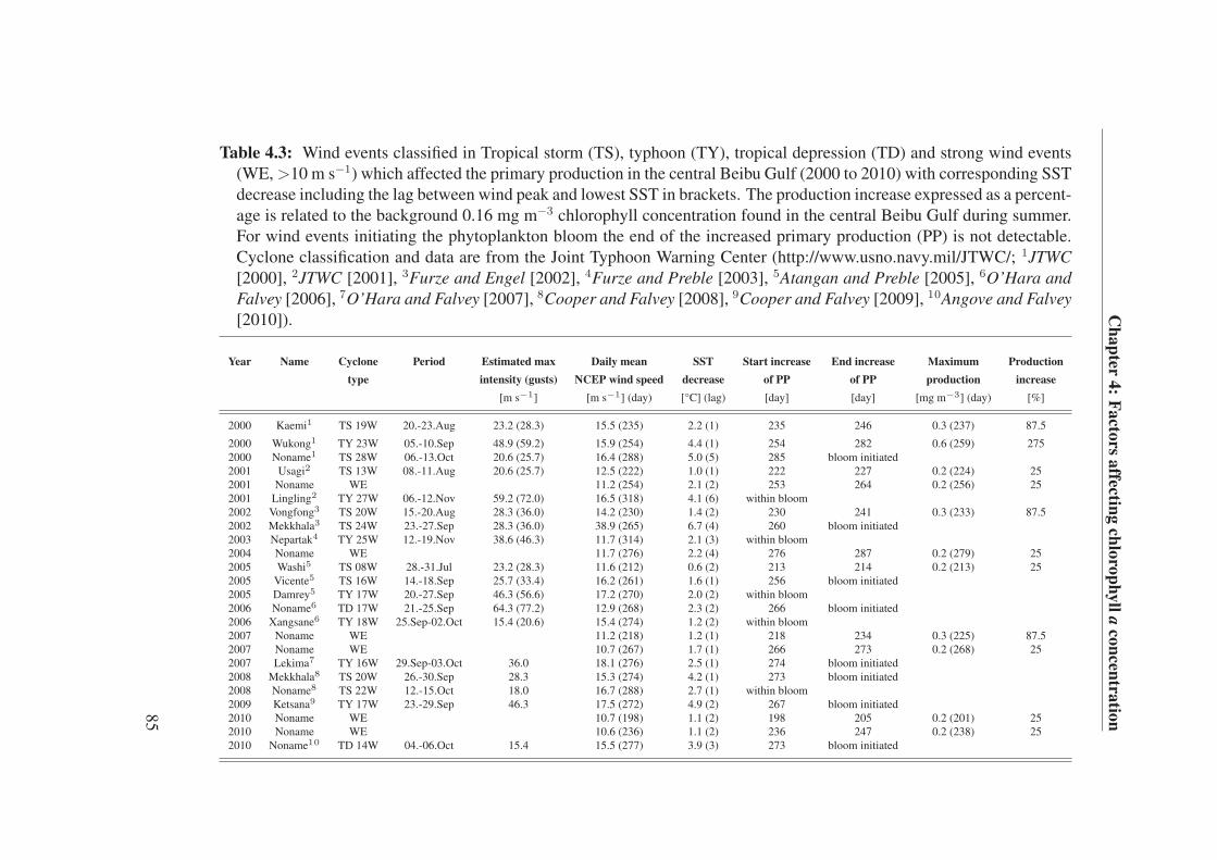
Ch
ap
ter4
:F
acto
rsa
ffecting
chlo
rop
hy
lla
con
centra
tion
Table 4.3: Wind events classified in Tropical storm (TS), typhoon (TY), tropical depression (TD) and strong wind events(WE, >10 m s−1) which affected the primary production in the central Beibu Gulf (2000 to 2010) with corresponding SSTdecrease including the lag between wind peak and lowest SST in brackets. The production increase expressed as a percent-age is related to the background 0.16 mg m−3 chlorophyll concentration found in the central Beibu Gulf during summer.For wind events initiating the phytoplankton bloom the end of the increased primary production (PP) is not detectable.Cyclone classification and data are from the Joint Typhoon Warning Center (http://www.usno.navy.mil/JTWC/; 1JTWC
[2000], 2JTWC [2001], 3Furze and Engel [2002], 4Furze and Preble [2003], 5Atangan and Preble [2005], 6O’Hara and
Falvey [2006], 7O’Hara and Falvey [2007], 8Cooper and Falvey [2008], 9Cooper and Falvey [2009], 10Angove and Falvey
[2010]).
Year Name Cyclone Period Estimated max Daily mean SST Start increase End increase Maximum Production
type intensity (gusts) NCEP wind speed decrease of PP of PP production increase
[m s−1] [m s−1] (day) [°C] (lag) [day] [day] [mg m−3] (day) [%]
2000 Kaemi1 TS 19W 20.-23.Aug 23.2 (28.3) 15.5 (235) 2.2 (1) 235 246 0.3 (237) 87.5
2000 Wukong1 TY 23W 05.-10.Sep 48.9 (59.2) 15.9 (254) 4.4 (1) 254 282 0.6 (259) 2752000 Noname1 TS 28W 06.-13.Oct 20.6 (25.7) 16.4 (288) 5.0 (5) 285 bloom initiated2001 Usagi2 TS 13W 08.-11.Aug 20.6 (25.7) 12.5 (222) 1.0 (1) 222 227 0.2 (224) 252001 Noname WE 11.2 (254) 2.1 (2) 253 264 0.2 (256) 252001 Lingling2 TY 27W 06.-12.Nov 59.2 (72.0) 16.5 (318) 4.1 (6) within bloom2002 Vongfong3 TS 20W 15.-20.Aug 28.3 (36.0) 14.2 (230) 1.4 (2) 230 241 0.3 (233) 87.52002 Mekkhala3 TS 24W 23.-27.Sep 28.3 (36.0) 38.9 (265) 6.7 (4) 260 bloom initiated2003 Nepartak4 TY 25W 12.-19.Nov 38.6 (46.3) 11.7 (314) 2.1 (3) within bloom2004 Noname WE 11.7 (276) 2.2 (4) 276 287 0.2 (279) 252005 Washi5 TS 08W 28.-31.Jul 23.2 (28.3) 11.6 (212) 0.6 (2) 213 214 0.2 (213) 252005 Vicente5 TS 16W 14.-18.Sep 25.7 (33.4) 16.2 (261) 1.6 (1) 256 bloom initiated2005 Damrey5 TY 17W 20.-27.Sep 46.3 (56.6) 17.2 (270) 2.0 (2) within bloom2006 Noname6 TD 17W 21.-25.Sep 64.3 (77.2) 12.9 (268) 2.3 (2) 266 bloom initiated2006 Xangsane6 TY 18W 25.Sep-02.Oct 15.4 (20.6) 15.4 (274) 1.2 (2) within bloom2007 Noname WE 11.2 (218) 1.2 (1) 218 234 0.3 (225) 87.52007 Noname WE 10.7 (267) 1.7 (1) 266 273 0.2 (268) 252007 Lekima7 TY 16W 29.Sep-03.Oct 36.0 18.1 (276) 2.5 (1) 274 bloom initiated2008 Mekkhala8 TS 20W 26.-30.Sep 28.3 15.3 (274) 4.2 (1) 273 bloom initiated2008 Noname8 TS 22W 12.-15.Oct 18.0 16.7 (288) 2.7 (1) within bloom2009 Ketsana9 TY 17W 23.-29.Sep 46.3 17.5 (272) 4.9 (2) 267 bloom initiated2010 Noname WE 10.7 (198) 1.1 (2) 198 205 0.2 (201) 252010 Noname WE 10.6 (236) 1.1 (2) 236 247 0.2 (238) 252010 Noname10 TD 14W 04.-06.Oct 15.4 15.5 (277) 3.9 (3) 273 bloom initiated
85
Chapter 4: Factors affecting chlorophyll a concentration
In all years a DCM was detected more or less developed with a thickness between
19 m (e.g. in 2001) and 33 m (e.g. in 2004, Fig. 4.8e, emphasized by the white line
which indicates the 0.2 mg chl m−3 isoline). In some years short-lived blooms prior
to the main phytoplankton bloom were modeled. These blooms are associated with
strong wind events in late summer and autumn (Fig. S1) for example in 2000, 2005-
2010 (Fig. 4.8e).
4.4 Discussion
Considering that the model works simply with vertical exchange and does not include
advective flows the models success to capture 87% of the observed variance in daily
surface temperatures indicates that surface water masses from the SCS or the Beibu
Gulf coastal regions do not strongly affect the central Beibu Gulf. This agrees with the
general cyclonic circulation pattern in the Beibu Gulf [Wu et al., 2008]. Therefore the
local meteorological forcing seems to be the most important factor for the formation of
the vertical water column temperature distribution. The approximately 14% over- and
underestimation for summer and winter temperatures, respectively, can be explained by
the structure of the 1-D model itself, as it always warms up and cools down the same
body of water, because lateral transports of water masses are not taken into account by
the model. Another reason is the missing cloud cover correction within the model. The
surface dewpoint temperature (minimum of 4.2°C in winter and maximum of 28.4°C
in summer, Tab. 4.2) and the high solar irradiance (typically ranging between 297 and
449 W m−2, Tab. 4.2) result in a strong stratification during summer with SSTs of up
to 33.5°C. It is the wind and its effects on water column stability that seem to play
the most important role for the phytoplankton growth in the central Beibu Gulf. The
assumption was tested using the model with only one changed meteorological forc-
ing parameter (dewpoint temperature, solar irradiance and wind velocities) for 2009
in each run. The minimum and maximum values of the respective forcing parameter
were used to act throughout the year. The differences in the resulting annual mean
of surface chlorophyll concentrations between the model runs forced with the mini-
mum and maximum value of every meteorological input are 4% for the solar irradiance
(min = 305 W m−2, max = 449 W m−2), 63% for the surface dewpoint temperature
(min = 8.0°C, max = 27.3°C) and 90% for the wind velocities (minu = -0.0017 m s−1,
86
Chapter 4: Factors affecting chlorophyll a concentration
minv = -0.041 m s−1, maxu = -11.99 m s−1, maxv = -14.95 m s−1). This supports our
conclusion that wind is the most important parameter for phytoplankton growth in the
central Beibu Gulf. This is already known from the Arabian Sea, an also monsoon-
influenced region [e.g. Bauer et al., 1991]. Based on observations, Bauer et al. [1991]
identified the wind forcing as the primary factor influencing the MLD and hence pig-
ment biomass in the monsoon season.
As the light regime is relatively constant throughout the year the phytoplankton growth
depends mainly on the availability of nutrients, which in turn is affected by the water
column structure and physical forces acting upon it. Due to the strong water column
stratification (see Fig. S2a) most pronounced between February and November, the cen-
tral Beibu Gulf is nutrient depleted in the upper water layer during this period (Fig. S2c).
As a result only minimum phytoplankton growth takes place in the surface waters and a
DCM develops in around 20-30 m depth where the nutricline and euphotic zone overlap
(see Fig. 4.6d). The depth of the DCM seems to depend on the depth of the nutricline
rather than on the euphotic depth (Fig. 4.6d), which has been described by Cullen and
Eppley [1981] for the Southern California Bight. They found the depth of the DCM in
about 20-50 m more correlating with the depth of the nutricline (15-45 m, 15-6% of
the surface irradiance available) than with the euphotic depth (33-66 m). For the mean
modeled year the calculated PAR in the mean depth of the DCM (26 m) is about 4%
of the surface PAR. The link between the nutricline and the DCM results in a gradual
deepening of the nutricline and the DCM within the thermocline, which has been shown
for the western English Channel by Sharples et al. [2001].
The mean modeled DCM is located somewhat shallower than the depth range for the
DCM in the central Beibu Gulf of about 30-50 m published by Huang et al. [2008],
Wu [2008] and Bauer et al. [in press]. Own measurements and literature values [Liu
et al., 1998] indicate a relatively high variability in the depth of the DCM as well as
in its strength. The mean modeled DCM shows maximum chlorophyll concentrations
of around 0.5 mg m−3 (Fig. 4.3c) whereas the maximum chlorophyll concentrations
within the DCM vary between 0.2 and 1.1 mg m−3 (Fig. 4.8e) for the different years
and, particularly for different periods within the years which agrees well with the range
of 0.6-1 mg m−3 reported by Wu [2008] and Bauer et al. [in press]. If enough nutrients
and light, to compensate loss processes through photosynthesis, are available a net phy-
toplankton blooming occurs when cells are trapped near the surface [Sverdrup, 1953;
87
Chapter 4: Factors affecting chlorophyll a concentration
Ward and Waniek, 2007]. Despite the strong stratification during summer, the existence
of a DCM implies that a complete decoupling of the surface and bottom waters does
not occur [Sharples and Tett, 1994]. The continuous presence of the DCM throughout
the summer is caused by the variability in surface wind stress driving occasional events
introducing DIN into the system [Sharples and Tett, 1994], rather than by tidally-driven
turbulence as discussed later. Depending on the strength and quantity of these events
the DCM is more or less strongly developed within the different years. The DCM can
disappear for periods when the time between the entrainment events is longer than the
utilization time scale of DIN [Sharples and Tett, 1994], this is clearly happening in
autumn 2004 and summer 2010 (Fig. 4.8d).
Due to the strong northeast monsoon beginning in autumn the stratification breaks
down between October and December and allows the development of a phytoplankton
bloom. The onset of the phytoplankton bloom around day 273±22 (Tab. 4.2), some 47
days before the disappearance of stratification on day 320±55, leads to the assumption
that the stratification is already weakened in autumn due to tides, storms and the change
of the wind system to the stronger northeast monsoon, before it finally disappears. The
stronger wind-driven turbulence induced at the surface deepens the MLD [Bauer et al.,
1991] and leads to a nutrient input into the surface water layer through the thermocline.
In turn this allows a phytoplankton bloom to start before the stratification breaks down.
Differences in the strength and quantity of nutrient inputs lead to a different timing and
development of the phytoplankton bloom [cf. Waniek, 2003]. Ongoing strong winds
and the further decrease in solar irradiance then enable a mixing down to the seabed and
full development of the bloom. The spring stratification starts on average around day
44±19 whereas the phytoplankton bloom ends around day 112±15 (Tab. 4.2). It takes
about 69 days until the stratification is fully developed and nutrients within the surface
water layer are depleted. About 2 months after stratification occurs the phytoplankton
growth is terminated indicating a very slow onset of full stratification, probably with pe-
riodic nutrient inputs in the surface layer due to tidal forcing, a low nutrient uptake rate,
slow remineralisation or a low grazing pressure acting on the phytoplankton. According
to Chung et al. [2012] phytoplankton blooms are terminated due to herbivore grazing
rather than nutrient depletion or sedimentation: a model test with deactivated grazing
showed that a strong phytoplankton bloom would persist over the entire year. Despite
nutrient depletion during summer zooplankton grazing seems to be the most important
88
Chapter 4: Factors affecting chlorophyll a concentration
factor for the termination of the phytoplankton bloom in the central Beibu Gulf. The
variability in the beginning and ending of stratification and phytoplankton bloom, indi-
cate that the timing of the bloom is less variable than the timing of the stratification [e.g.
Sharples et al., 2006]. This also supports the conclusion that wind forcing is the most
important factor driving primary production in the central Beibu Gulf.
Differences between both developments of modeled and remotely measured monthly
mean surface chlorophyll concentration could be caused by lateral transport which is
not contained in the model (Fig. 4.9). Through currents and tide-induced lateral trans-
port nutrients for phytoplankton growing or phytoplankton itself as well as grazers may
be transported to/from the central Beibu Gulf from/to other regions. This would have
an effect on the surface chlorophyll concentration within the central Beibu Gulf. The
standard deviations for the satellite data (Fig. 4.9) display the spatial variability of the
remotely measured surface chlorophyll concentrations. Between 0 and 121 pixel per
month were recorded by SeaWiFS within the central Beibu Gulf (Tab. S1). During win-
ter, satellite data for the central Beibu Gulf is sparse probably due to a higher cloud cover
caused by activity of tropical storms. The differences between the surface chlorophyll
concentrations and the beginning of the phytoplankton bloom can therefore be attributed
to the lack of available satellite data. The small standard deviations on the output data
indicate that the model successfully simulated the surface chlorophyll concentrations
for the region.
The low variability in meteorological forcing is mirrored in the model results (Tab.
4.2). Surface and bottom water temperatures as well as surface chlorophyll concentra-
tions do not show great differences between the years, variations are the result of strong
wind events. In correspondence with the strong wind events the SST declines due to
entrainment of colder, subsurface water masses into surface waters [Price, 1981] by
0.6-6.7°C (Tab. 4.3), depending on the winds strength, comparable to measured SST
responses between -2.5 and -9°C Chang et al. [1996]; Lin et al. [2003]; Walker et al.
[2005]; Shi and Wang [2007]; Zheng and Tang [2007]. The lag between the wind peak
and the lowest SST is about 1-6 days [cf. Shi and Wang, 2007], depending as well on
the winds intensity and the duration of strong winds influence or the transit time of the
respective typhoon. Despite the pronounced summer stratification, strong wind events
like tropical storms lead to a deepening of the MLD [Price, 1981; Jiang et al., 2009] and
hence to a higher nutrient supply in the surface water layer resulting in a short-lived en-
89
Chapter 4: Factors affecting chlorophyll a concentration
hancement of the primary productivity or a phytoplankton bloom [e.g. Zheng and Tang,
2007]. These results are supported by several studies based on satellite data or in-situ
measurements describing such blooms for different typhoon- or hurricane-influenced
regions [e.g. Chang et al., 1996; Fogel et al., 1999; Shiah et al., 2000; Lin et al., 2003;
Babin et al., 2004; Zheng and Tang, 2007; Chung et al., 2012; Lin, 2012]. Wind veloci-
ties (Fig. S1) show that typically more than one strong wind event influenced the central
Beibu Gulf region during almost every year from 2000 to 2010 in late summer and au-
tumn. In the 11 year period 11 events were detected which initiated a small bloom prior
to the highly developed bloom, statistically one event per year (Tab. 4.3). On average
the estimated temporary increase in primary production induced by these strong wind
events accounts for 65% with an averaged duration of 11±7 days. This result corre-
sponds well to the 11 days bloom duration after the crossing of Hurricane Katrina in the
Gulf of Mexico in August 2005 [Shi and Wang, 2007]. About 1-7 days lagged between
the wind-stress peak and the modeled chlorophyll peak at the surface (Tab. 4.3) which
is comparable to the 3-4 days lag postulated by Walker et al. [2005] for the Hurricane
Ivan, the 4 days lag described by Shi and Wang [2007] for the Hurricane Katrina, both
in the Gulf of Mexico, and the 3-6 days lag described by Zheng and Tang [2007] for the
Typhoon Damrey in the SCS. The modeled lag between the lowest SST and the chloro-
phyll peak of up to 6 days agrees well with the 4 days lag described by Zheng and Tang
[2007].
However, to what extent a typhoon will affect an oceanic region depends on the wind’s
intensity, the transit time as well as the ocean’s precondition, which means how deep
or shallow the nutrient-rich water body lies [Lin, 2012]. Is any condition unfavorable
the oceans response will be weakened [Lin, 2012]. For example, the modeled typhoon
Washi enhanced the surface chlorophyll concentration in the central Beibu Gulf to up
to 0.2 mg m−3 at a maximum wind speed of 11.6 m s−1 but enhanced the maximum
surface chlorophyll concentration by up to 0.9 mg m−3 (around 3.8 times before the
typhoon) in the SCS at wind speeds of around 18 m s−1 [Chen and Tang, 2011]. The
greatest effect on the chlorophyll increase was seen from the passage of the typhoon
WUKONG through the region in 2000 (Tab. 4.3). This storm initiated a bloom lasting
for 28 days with a maximum surface chlorophyll concentration of 0.6 mg m−3, an in-
crease of 275% compared to the summer background surface chlorophyll concentration
of 0.16 mg m−3. Along with these temporary bloom events, tropical storms can also ini-
90
Chapter 4: Factors affecting chlorophyll a concentration
tiate a phytoplankton proliferation, for example in 2000, 2002, 2005-2010, resulting in
a bloom as early as mid-September such as those in 2002 or 2005. The effect of strong
wind events on surface chlorophyll concentration during the fully developed bloom is
difficult to estimate.
Contrary to our expectations the effect of the tides on the primary production within
the central Beibu Gulf is only moderate. This may be a result of the relatively great
depth (63 m), the distance from shore, the associated small tidal forcing in this region
and the lateral transport initiated by tides, which is not included in the model, or a com-
bination of those. The strong stratification can reduce the already weak tidal forcing
which therefore only has a minor effect on mixing in the surface water column during
summer. In spite of the weak tides (0.15 m s−1 for amplitude of M2 tidal currents) in this
region the tidally generated turbulence increases the strength of the DCM by up to 36%
and its thickness by up to 33% as well. According to the results of Sharples et al. [2006]
a tidal current amplitude of 0.4 m s−1 can offset the influence of the heating in strati-
fying the water column. The result of this would be a weakly stratified water column
and a breakdown of stratification that occurs earlier in the year. Ultimately, due to the
intense nutrient input from the deep water to the surface layer it would strongly enhance
the primary production within the surface water layer throughout the year. The rising
bathymetry from south to north in the region means the shallow northern or coastal
regions may be considerably more affected by tidal currents than the relatively deep
central part of the gulf. In a system which is strongly influenced by tides a constant
competition between tidal turbulence in the bottom layer and wind-driven turbulence
in the surface layer determine the position of the thermocline and its associated DCM
[Sharples, 1999]. During spring tides, when the maximum currents occur, the tidal tur-
bulence pushes the thermocline towards the sea surface while during neap tides, with
only weak currents, the wind-driven turbulence pushes the thermocline deeper in the
water column [e.g. Sharples, 1999]. These forces cause periodic pulses of nutrients to
the euphotic zone and hence higher chlorophyll concentrations within the DCM. In the
central Beibu Gulf the influence of the spring-neap tidal cycle on the elevation of the
DIN isolines is only visible to a depth of 40 m (Fig. 4.7b). Hence the expected periodic
pulses of higher chlorophyll concentrations within the DCM do not occur.
91
Chapter 4: Factors affecting chlorophyll a concentration
4.5 Conclusions
As typical for subtropical/tropical shelf seas the central Beibu Gulf shows an annual
cycle with a strong stratification during summer and a deep mixing down to the seabed
in winter. The physical structure of the water column is reflected in the seasonal cycle of
primary production. A phytoplankton bloom develops when the wind system changes in
autumn into the stronger northeast monsoon, the solar irradiance decreases, deep mixing
occurs and nutrients from bottom waters are supplied to the surface waters and therefore
are available for phytoplankton. During summer, due to the strong stratification, the
surface waters are nutrient depleted and therefore only low phytoplankton growth is
possible. At a depth of around 20-30 m, where euphotic depth and nutricline co-exist a
DCM developed in all modeled years.
The model simulated successfully the observed stratification, SST and bottom tem-
perature as well as the chlorophyll distribution. Differences in the SST and the monthly
mean surface chlorophyll concentrations are a consequence of the absent horizontal ad-
vection and the missing cloud cover in the model as well as attributable to the lack of
satellite data.
The water depth of 63 m, the distance from shore and associated weak tidal forcing
explain the weak tidal influence in the central Beibu Gulf. However, tides lead to an
enhanced nutrient supply within the euphotic zone and hence to a considerable increase
in strength and thickness of the DCM.
Although the interannual variability is generally low, the timing of the stratification
breakdown and the establishment of a phytoplankton bloom are variable within a time-
frame of about 2.5 months and around 1 month in autumn/winter. Besides these fea-
tures, strong wind events play an important role in the primary production within the
central Beibu Gulf. Single events strongly enhance primary production during the usu-
ally low productive summer season and are able to initiate a prior phytoplankton bloom.
In summary, the monsoon winds and the occasionally strong wind events are the most
important forces driving the primary production in the central Beibu Gulf.
Our study helps to compensate the lack of remotely measured and in-situ data for
the central Beibu Gulf and hence contributes to a more comprehensive understanding of
processes influencing the primary production in that region.
92
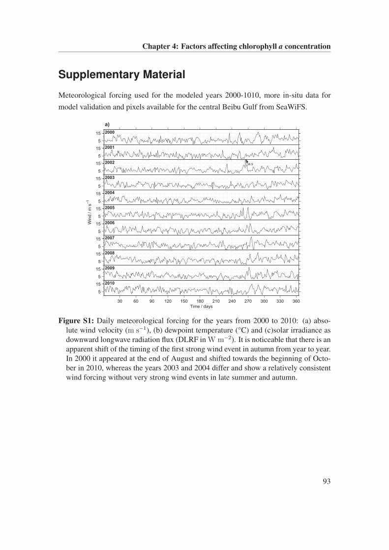
Chapter 4: Factors affecting chlorophyll a concentration
Supplementary Material
Meteorological forcing used for the modeled years 2000-1010, more in-situ data for
model validation and pixels available for the central Beibu Gulf from SeaWiFS.
5
15
a)
2000
5
15 2001
5
15 2002 38.9
5
15 2003
5
15 2004
5
15 2005
5
15Win
d /
m s
−1
2006
5
15 2007
5
15 2008
30 60 90 120 150 180 210 240 270 300 330 360
5
15
Time / days
2010
5
15 2009
Figure S1: Daily meteorological forcing for the years from 2000 to 2010: (a) abso-lute wind velocity (m s
−1), (b) dewpoint temperature (°C) and (c)solar irradiance asdownward longwave radiation flux (DLRF in W m
−2). It is noticeable that there is anapparent shift of the timing of the first strong wind event in autumn from year to year.In 2000 it appeared at the end of August and shifted towards the beginning of Octo-ber in 2010, whereas the years 2003 and 2004 differ and show a relatively consistentwind forcing without very strong wind events in late summer and autumn.
93
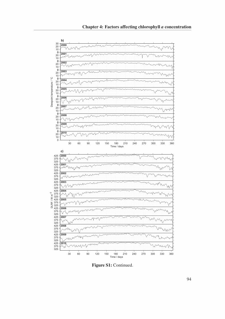
Chapter 4: Factors affecting chlorophyll a concentration
0102030
b)
2000
01020
02001
01020
02002
01020
02003
01020
02004
01020
02005
01020
0
Dew
poin
t te
mpera
ture
/ °
C
2006
01020
02007
01020
02008
30 60 90 120 150 180 210 240 270 300 330 360
01020
0
Time / days
20100
1020
02009
325375425
c)
2000
325375425 2001
325375425 2002
325375425 2003
325375425 2004
325375425 2005
325375425D
LR
F /
W m
−2
2006
325375425 2007
325375425 2008
30 60 90 120 150 180 210 240 270 300 330 360
325375425
Time / days
2010325375425 2009
Figure S1: Continued.
94
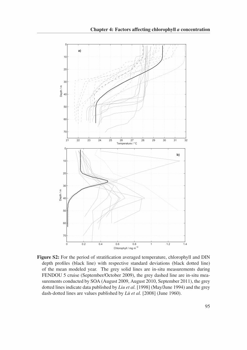
Chapter 4: Factors affecting chlorophyll a concentration
21 22 23 24 25 26 27 28 29 30 31 32
0
10
20
30
40
50
60
70
Temperature / °C
Depth
/ m
a)
0 0.2 0.4 0.6 0.8 1 1.2 1.4
0
10
20
30
40
50
60
70
Chlorophyll / mg m−3
Depth
/ m
b)
Figure S2: For the period of stratification averaged temperature, chlorophyll and DINdepth profiles (black line) with respective standard deviations (black dotted line)of the mean modeled year. The grey solid lines are in-situ measurements duringFENDOU 5 cruise (September/October 2009), the grey dashed line are in-situ mea-surements conducted by SOA (August 2009, August 2010, September 2011), the greydotted lines indicate data published by Liu et al. [1998] (May/June 1994) and the greydash-dotted lines are values published by Lü et al. [2008] (June 1960).
95
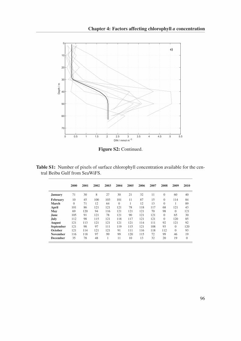
Chapter 4: Factors affecting chlorophyll a concentration
0 0.5 1 1.5 2 2.5 3 3.5 4 4.5 5 5.5
0
10
20
30
40
50
60
70
DIN / mmol m−3
Depth
/ m
c)
Figure S2: Continued.
Table S1: Number of pixels of surface chlorophyll concentration available for the cen-tral Beibu Gulf from SeaWiFS.
2000 2001 2002 2003 2004 2005 2006 2007 2008 2009 2010
January 71 30 8 27 30 21 32 11 0 60 40
February 10 45 100 103 101 11 87 15 0 114 84March 0 71 12 64 0 1 12 13 0 1 89April 101 86 121 121 121 78 118 117 68 121 43May 69 120 94 116 121 121 121 70 98 0 121June 105 91 121 78 121 90 121 121 0 65 30July 112 98 115 121 118 117 121 121 0 120 85August 121 113 121 121 121 121 114 111 92 121 92September 121 98 97 111 119 115 121 108 93 0 120October 121 114 121 121 91 111 116 118 112 0 93November 116 118 97 99 99 120 115 72 99 46 19December 35 78 48 1 11 10 13 32 20 19 0
96
Chapter 5: Sediment resuspension
5 Sediment resuspension patterns and
the diffusive boundary layer in the
Beibu Gulf, South China Sea
Bauer et al.: Manuscript
5.1 Introduction
Sediment resuspension is known from all kinds of marine environments [Tengberg et al.,
2003] and, in addition to river discharge is, one of the important processes determining
sediment concentration in the water column and hence the magnitude of suspended
sediment transport [Guillén et al., 2002]. Sediment stirring is naturally caused by water
motion due to density differences, strong winds and tidal currents. Especially in shelf
sea areas, the combination of shallow waters, strong tidal currents, wind and waves
creates a complex pattern of sediment resuspension, transport and deposition dynamics
[Guinder et al., 2009], that are of environmental significance. Frictional effects of the
water against the sea floor lead to a shear stress which erodes and resuspends sediments
into the water column after exceeding a critical value [Yuan et al., 2009].
The interaction of tidal and wind-induced flow with the bottom roughness is responsi-
ble for the turbulence at the seabed which results in a tidally driven boundary layer, pro-
viding a significant interface between the seabed and the water column for the exchange
of particles, nutrients and organisms [Grant and Madsen, 1986; Werner et al., 2003].
This layer is also important for the longshore near-coast transport of pollutants, for ex-
ample, oil spill originating from accidental leakages [Holmedal and Myrhaug, 2008].
Furthermore, this flow may determine conditions for phytoplankton growth and trans-
port in the ocean [Holmedal and Myrhaug, 2008]. The thickness of the bottom bound-
ary layer depends on the current strength, bottom roughness and vertical stratification
97
Chapter 5: Sediment resuspension
[Werner et al., 2003]. As a result, particles, depending on their grain size, weight, sort-
ing, degree of compactness and the acting current strength, are transported along the sea
floor by currents [Tengberg et al., 2003] over varying distances. Fine sediments like clay
and silt will be already eroded under weak flow conditions whereby coarse sediments
keep undisturbed. Other mechanisms resuspending sediments are bioresuspension and
bioturbation, induced by animals actively moving particles [Graf and Rosenberg, 1997]
and anthropogenic perturbations like trawling, dredging [Tengberg et al., 2003], sand
mining and land reclamation.
Concentrations of SPM in the water column vary on different time scales, as a result
of fluctuations in river discharge, the prevailing hydrodynamics or throughout a tidal
cycle [Velegrakis et al., 1997]. The specific role of tidal flows causing sediment resus-
pension arise from the flow structure as it is determined by periodical acceleration and
deceleration [Grant and Madsen, 1986]. Velegrakis et al. [1997] showed that the SPM
concentrations in the water column are significantly varying throughout the tidal cycle
caused by horizontal advection and vertical material exchange (resuspension and depo-
sition). In general, the tide-induced shear stress near the bottom increases shoreward;
the sediment grain size usually becomes coarser in the same direction [Guillén et al.,
2002]. Resuspension of fine-grained sediments takes place during the energetic parts of
the tidal cycle but deposition occurs only during slack water [Jago et al., 1993], whereas
coarse-grained sediments may be also deposited during less energetic stages of the tides
[Velegrakis et al., 1997]. Tengberg et al. [2003] reported a necessary bottom current
strength of 40 cm s−1 to induce resuspension of fine-grained, soft and muddy sediments
on the West Coast of Sweden.
The importance of the sediment resuspension lies, first of all, in the sediment trans-
port itself which is crucial for the understanding of geological records [Grant and
Madsen, 1986]. Coupled with the sediments, also deposited pollutants, benthic fluff,
which is organic-rich SPM of biological origin, and benthic communities (e.g. benthic
foraminifera) will be mixed, resuspended, transported by currents [Grant and Madsen,
1986; Jago et al., 2002] and deposited in calmer regions. A study by Tengberg et al.
[2003] showed that resuspension also affects the fluxes of total carbonate, oxygen and
nutrients from the bottom sediments into the water column due to mixing of sediment
pore waters which is very important for the benthic-pelagic exchange [Jago et al., 2002].
Resuspension and deposition of organic-rich SPM further moderates the redox-climate
98
Chapter 5: Sediment resuspension
at the seabed, controls organic matter remineralization and nutrient supply to the sub-
strate [Jago et al., 2002]. Despite an induced nutrient supply by resuspension which
would enhance primary production, suspended matter concentrations may also lead to
enhanced turbidity causing poor light conditions and consequently reduced photosyn-
thesis rates.
Important for the exchange rate between the seabed and the water column is the de-
velopment of a diffusive boundary layer (DBL). This sediment-water interface, with a
thickness of a few millimeters to centimeters, is formed due to friction retard of the water
movement at the seabed, depending on sediment surface roughness, resulting in dom-
inating viscous forces and a velocity approaching to zero [Jørgensen and Des Marais,
1990]. Hence, the DBL can influence biogeochemical cycles by allowing fluxes of
dissolved reactive compounds, nutrients and gases across the sediment-water interface
through molecular diffusion [Jørgensen and Des Marais, 1990; Santschi et al., 1991;
Kelly-Gerreyn et al., 2005]. By altering the diffusion time through the DBL, changes in
thickness, due to different current speeds, influence reaction rates in the sediment, such
as oxidation of organic matter, denitrification and sulphate reduction [Kelly-Gerreyn
et al., 2005], which may have consequences for nutrient and carbon budgets.
Aim of this study is to characterize bottom currents and associated sediment resus-
pension as well as to determine different thicknesses of the DBL during tidal stages at
various stations in the eastern Beibu Gulf in September/October 2009.
As a semi-enclosed shallow shelf sea, the Beibu Gulf is mainly governed by strong
monsoon winds and tides, both responsible for strong currents and the cyclonic circula-
tion pattern [e.g. Wu et al., 2008], affecting resuspension, transport and deposition pro-
cesses. Although many geological surveys have been done in this region in the past, until
now, only limited knowledge exist about tide- and wind-induced resuspension dynam-
ics, which is important to understand recent sedimentation patterns and geochemical
processes near and in the seabed. This work is particularly important as a fundamental
research of the relationship between currents and sediment dynamics in the Beibu Gulf
and hence crucial for further geochemical investigations on element and energy fluxes
within the small-scale DBL.
Bauer et al. [in press] demonstrated that the eastern Beibu Gulf can be partitioned into
four zones for the study period, related to hydrography, water column biogeochemistry,
sediment properties and deposition. A coastal zone exists in the north and along Hainan
99
Chapter 5: Sediment resuspension
Island west coast. One zone lies in the vicinity of the Qiongzhou Strait, an important
passage for water exchange with the south-east China coast. The central Beibu Gulf
represents the third and the transition area between Beibu Gulf and SCS waters in the
southern part of the Gulf the fourth zone. These zones will be used to provide a more
comprehensive picture of resuspension processes during the study period.
5.2 Material and methods
5.2.1 Current records and their analysis
Current velocity profiles were recorded using a ship-mounted ADP (SonTek, 500 kHz)
during the FENDOU 5 cruise in September/October 2009 (Fig. 5.1). The ADP uses the
so-called Doppler shift to measure current velocity. The system is equipped with three
transducers having different orientations and generating a narrow beam of sound that is
projected through the water column and reflected or "scattered" from particles (SPM,
organic matter, air bubbles, [SonTek/YSI, 2005]). The measured current velocities for
each of the transducer are transformed into "East-North-Up" coordinates by the ADP
system. Current velocity and direction profiles were recorded every 10 or 30 s with a
vertical resolution of 1 m. As the measurements took place on a moving vessel the ADP
was set to the bottom-track mode to remove vessel motion and to obtain the absolute
water current speed and direction. An echo intensity (beam 1-3) exceeding a value of
100 indicates the bottom. All profiles has been cut at this value.
To obtain mean, minimum and maximum velocities influencing the water column
and sediment sampling the bottom current records from the ADP measurements were
averaged for a 10 km radius around the position of each station (Fig. 5.1).
To calculate the geostrophic currents between adjacent stations first the geopotential
anomaly of each station has been computed by integrating the specific volume anomaly
upward from the bottom after Pond and Pickard [1983] using depth profiles of temper-
ature, salinity and pressure. The geostrophic velocity was then computed after Mas-
carenhas Jr. et al. [2004] depending on pressure, the distance between two stations, the
Coriolis parameter and the latitude.
To investigate the penetration depth of the wind forcing and its effect on the measured
currents the Ekman depth and velocity has been calculated. For this, daily surface u- and
100
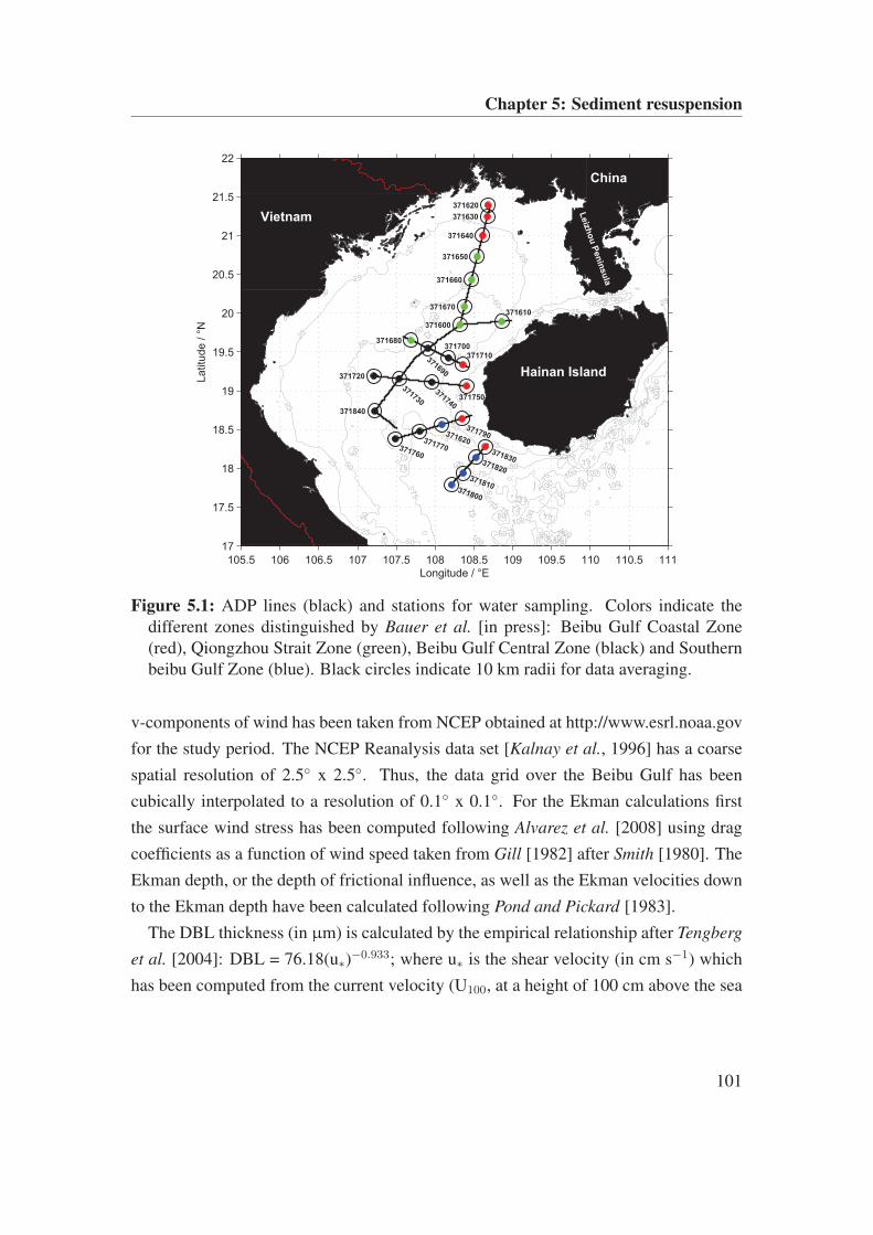
Chapter 5: Sediment resuspension
105.5 106 106.5 107 107.5 108 108.5 109 109.5 110 110.5 111
17
17.5
18
18.5
19
19.5
20
20.5
21
21.5
22
0
0
0
25
25
25
25
25
25
25
25
25
25
25
25
25
25
25
25
25
25
25
25
25
25
25
2525
50
50
5050
50
50
50
50
50
50
50
50
50
50
50
5050
50
50
50
75
75
75
75
75
75
75
75
75
75
75 75
75
75
75
75
7575
75
75
75
75
75
7575 75
75
100
100
100100
100
100
100
100
100
100
100
100100
100100
100
371620
371630
371640
371710
371750
371840
371720
371600
371650
371660
371670
371680
371610
371690
371700
371790371620
371730
371740
371760
371770371830
371800
371810
371820
Longitude / °E
Latitu
de /
°N
China
Vietnam
Hainan Island
Leiz
ho
u P
en
insu
la
Figure 5.1: ADP lines (black) and stations for water sampling. Colors indicate thedifferent zones distinguished by Bauer et al. [in press]: Beibu Gulf Coastal Zone(red), Qiongzhou Strait Zone (green), Beibu Gulf Central Zone (black) and Southernbeibu Gulf Zone (blue). Black circles indicate 10 km radii for data averaging.
v-components of wind has been taken from NCEP obtained at http://www.esrl.noaa.gov
for the study period. The NCEP Reanalysis data set [Kalnay et al., 1996] has a coarse
spatial resolution of 2.5◦ x 2.5◦. Thus, the data grid over the Beibu Gulf has been
cubically interpolated to a resolution of 0.1◦ x 0.1◦. For the Ekman calculations first
the surface wind stress has been computed following Alvarez et al. [2008] using drag
coefficients as a function of wind speed taken from Gill [1982] after Smith [1980]. The
Ekman depth, or the depth of frictional influence, as well as the Ekman velocities down
to the Ekman depth have been calculated following Pond and Pickard [1983].
The DBL thickness (in µm) is calculated by the empirical relationship after Tengberg
et al. [2004]: DBL = 76.18(u∗)−0.933; where u∗ is the shear velocity (in cm s−1) which
has been computed from the current velocity (U100, at a height of 100 cm above the sea
101
Chapter 5: Sediment resuspension
bottom) using the quadratic stress law
u∗ = U100
√
Cd,
with the drag coefficient Cd = 2.5x10⁻³ [Santschi et al., 1991].
5.2.2 Water and sediment sampling
Hydrographic profiling (temperature, conductivity) and water sampling were done by
using an IOW mini PUMP CTD system based on Strady et al. [2008] at 25 stations.
For the sampling of SPM 0.5-1 l sea water was low vacuum filtered through 0.7 µm
pre-weighted Whatman GF/F glass fibre filters. The filters were washed with deionized
water and weighted again after drying in a compartment dryer at 60◦C for 24 h. The
SPM concentration is calculated from the weight difference between the empty and the
loaded filter and the amount of filtered water.
Surface sediment samples at all stations were taken by a box corer. Grain size was de-
termined using a diffraction particle size analyzer (Mastersizer 2000) at the Guangzhou
Marine Geological Survey in China for a particle range from 0.01 to 2000 µm. The
sediment classification followed Shepard [1954] and the grain size parameters were
calculated according to McManus [1988].
5.2.3 Tidal model
To estimate the tidal stages at which the ADP lines were recorded and the stations sam-
pled a tidal model has been set up using MATLAB. For 32 stations along the Chinese
and Vietnamese coasts in the Beibu Gulf tidal levels were predicted by WXTide32 soft-
ware (http://www.wxtide32.com/) for September/October 2009 with an interval of five
minutes. The tidal levels along the coasts has been cubically interpolated over the Beibu
Gulf area (16-22◦N, 105-111◦E) to a resolution of 0.1◦ x 0.1◦ for every time step. This
allows the output of the tidal cycle at almost every location within the Beibu Gulf. To
validate the predicted tides by the tidal model, a 25 h current record obtained on fixed
position during the FENDOU 5 cruise for a spring-tide using the ADP (recording in-
terval 30 or 60 s) and in parallel an Aanderaa RCM (recording interval one minute) in
50 m depth has been used.
102
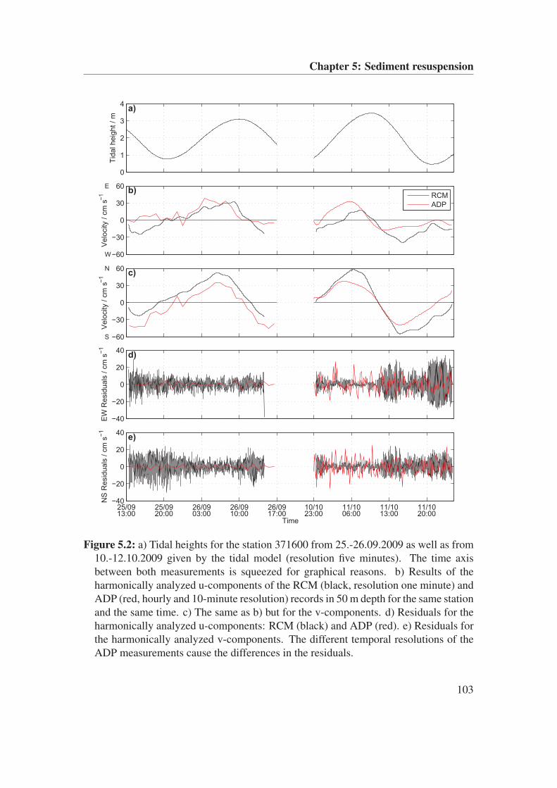
Chapter 5: Sediment resuspension
−60
−30
0
30
60b)
E
W
Velo
city /
cm
s−
1 RCM
ADP
−60
−30
0
30
60c)
N
S
Velo
city /
cm
s−
1
0
1
2
3
4a)
Tid
al heig
ht
/ m
−40
−20
0
20
40d)
EW
Resid
uals
/ c
m s
−1
25/09 25/09 26/09 26/09 26/09 10/10 11/10 11/10 11/10−40
−20
0
20
40e)
NS
Resid
uals
/ c
m s
−1
Time13:00 20:00 03:00 10:00 17:00 23:00 06:00 13:00 20:00
Figure 5.2: a) Tidal heights for the station 371600 from 25.-26.09.2009 as well as from10.-12.10.2009 given by the tidal model (resolution five minutes). The time axisbetween both measurements is squeezed for graphical reasons. b) Results of theharmonically analyzed u-components of the RCM (black, resolution one minute) andADP (red, hourly and 10-minute resolution) records in 50 m depth for the same stationand the same time. c) The same as b) but for the v-components. d) Residuals for theharmonically analyzed u-components: RCM (black) and ADP (red). e) Residuals forthe harmonically analyzed v-components. The different temporal resolutions of theADP measurements cause the differences in the residuals.
103
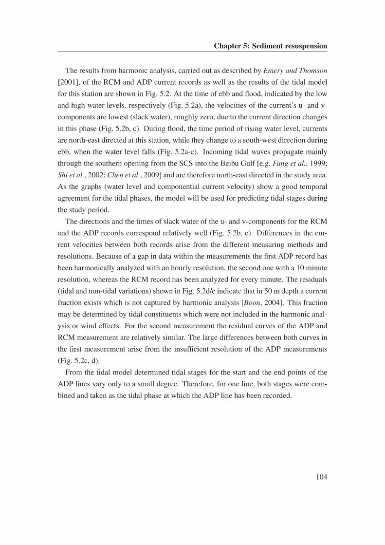
Chapter 5: Sediment resuspension
The results from harmonic analysis, carried out as described by Emery and Thomson
[2001], of the RCM and ADP current records as well as the results of the tidal model
for this station are shown in Fig. 5.2. At the time of ebb and flood, indicated by the low
and high water levels, respectively (Fig. 5.2a), the velocities of the current’s u- and v-
components are lowest (slack water), roughly zero, due to the current direction changes
in this phase (Fig. 5.2b, c). During flood, the time period of rising water level, currents
are north-east directed at this station, while they change to a south-west direction during
ebb, when the water level falls (Fig. 5.2a-c). Incoming tidal waves propagate mainly
through the southern opening from the SCS into the Beibu Gulf [e.g. Fang et al., 1999;
Shi et al., 2002; Chen et al., 2009] and are therefore north-east directed in the study area.
As the graphs (water level and componential current velocity) show a good temporal
agreement for the tidal phases, the model will be used for predicting tidal stages during
the study period.
The directions and the times of slack water of the u- and v-components for the RCM
and the ADP records correspond relatively well (Fig. 5.2b, c). Differences in the cur-
rent velocities between both records arise from the different measuring methods and
resolutions. Because of a gap in data within the measurements the first ADP record has
been harmonically analyzed with an hourly resolution, the second one with a 10 minute
resolution, whereas the RCM record has been analyzed for every minute. The residuals
(tidal and non-tidal variations) shown in Fig. 5.2d/e indicate that in 50 m depth a current
fraction exists which is not captured by harmonic analysis [Boon, 2004]. This fraction
may be determined by tidal constituents which were not included in the harmonic anal-
ysis or wind effects. For the second measurement the residual curves of the ADP and
RCM measurement are relatively similar. The large differences between both curves in
the first measurement arise from the insufficient resolution of the ADP measurements
(Fig. 5.2c, d).
From the tidal model determined tidal stages for the start and the end points of the
ADP lines vary only to a small degree. Therefore, for one line, both stages were com-
bined and taken as the tidal phase at which the ADP line has been recorded.
104
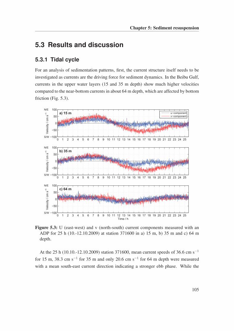
Chapter 5: Sediment resuspension
5.3 Results and discussion
5.3.1 Tidal cycle
For an analysis of sedimentation patterns, first, the current structure itself needs to be
investigated as currents are the driving force for sediment dynamics. In the Beibu Gulf,
currents in the upper water layers (15 and 35 m depth) show much higher velocities
compared to the near-bottom currents in about 64 m depth, which are affected by bottom
friction (Fig. 5.3).
0 1 2 3 4 5 6 7 8 9 10 11 12 13 14 15 16 17 18 19 20 21 22 23 24 25−100
−50
0
50
100
Velo
city /
cm
s−
1 a) 15 mN/E
S/W
u−component
v−component
0 1 2 3 4 5 6 7 8 9 10 11 12 13 14 15 16 17 18 19 20 21 22 23 24 25−100
−50
0
50
100
Velo
city /
cm
s−
1 b) 35 mN/E
S/W
0 1 2 3 4 5 6 7 8 9 10 11 12 13 14 15 16 17 18 19 20 21 22 23 24 25−100
−50
0
50
100
Time / h
Velo
city /
cm
s−
1 c) 64 mN/E
S/W
Figure 5.3: U (east-west) and v (north-south) current components measured with anADP for 25 h (10.-12.10.2009) at station 371600 in a) 15 m, b) 35 m and c) 64 mdepth.
At the 25 h (10.10.-12.10.2009) station 371600, mean current speeds of 36.6 cm s−1
for 15 m, 38.3 cm s−1 for 35 m and only 20.6 cm s−1 for 64 m depth were measured
with a mean south-east current direction indicating a stronger ebb phase. While the
105
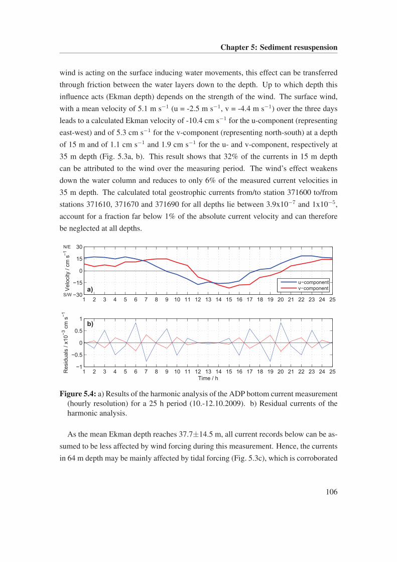
Chapter 5: Sediment resuspension
wind is acting on the surface inducing water movements, this effect can be transferred
through friction between the water layers down to the depth. Up to which depth this
influence acts (Ekman depth) depends on the strength of the wind. The surface wind,
with a mean velocity of 5.1 m s−1 (u = -2.5 m s−1, v = -4.4 m s−1) over the three days
leads to a calculated Ekman velocity of -10.4 cm s−1 for the u-component (representing
east-west) and of 5.3 cm s−1 for the v-component (representing north-south) at a depth
of 15 m and of 1.1 cm s−1 and 1.9 cm s−1 for the u- and v-component, respectively at
35 m depth (Fig. 5.3a, b). This result shows that 32% of the currents in 15 m depth
can be attributed to the wind over the measuring period. The wind’s effect weakens
down the water column and reduces to only 6% of the measured current velocities in
35 m depth. The calculated total geostrophic currents from/to station 371600 to/from
stations 371610, 371670 and 371690 for all depths lie between 3.9x10⁻⁷ and 1x10⁻⁵,
account for a fraction far below 1% of the absolute current velocity and can therefore
be neglected at all depths.
1 2 3 4 5 6 7 8 9 10 11 12 13 14 15 16 17 18 19 20 21 22 23 24 25−30
−15
0
15
30
Velo
city /
cm
s−
1
a)
N/E
S/W
u−component
v−component
1 2 3 4 5 6 7 8 9 10 11 12 13 14 15 16 17 18 19 20 21 22 23 24 25−1
−0.5
0
0.5
1
Time / h
Resid
uals
/ x
10
−3 c
m s
−1
b)
Figure 5.4: a) Results of the harmonic analysis of the ADP bottom current measurement(hourly resolution) for a 25 h period (10.-12.10.2009). b) Residual currents of theharmonic analysis.
As the mean Ekman depth reaches 37.7±14.5 m, all current records below can be as-
sumed to be less affected by wind forcing during this measurement. Hence, the currents
in 64 m depth may be mainly affected by tidal forcing (Fig. 5.3c), which is corroborated
106
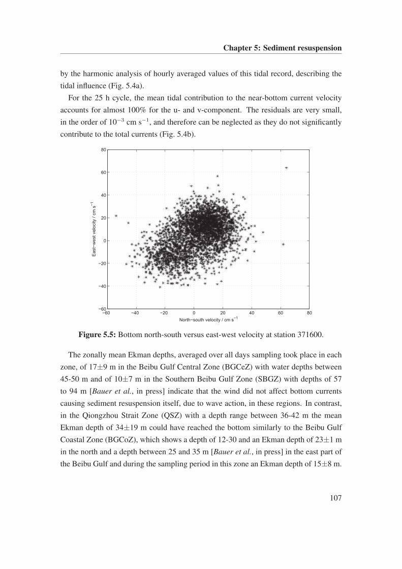
Chapter 5: Sediment resuspension
by the harmonic analysis of hourly averaged values of this tidal record, describing the
tidal influence (Fig. 5.4a).
For the 25 h cycle, the mean tidal contribution to the near-bottom current velocity
accounts for almost 100% for the u- and v-component. The residuals are very small,
in the order of 10−3 cm s−1, and therefore can be neglected as they do not significantly
contribute to the total currents (Fig. 5.4b).
−60 −40 −20 0 20 40 60 80−60
−40
−20
0
20
40
60
80
North−south velocity / cm s−1
East−
west
velo
city /
cm
s−
1
Figure 5.5: Bottom north-south versus east-west velocity at station 371600.
The zonally mean Ekman depths, averaged over all days sampling took place in each
zone, of 17±9 m in the Beibu Gulf Central Zone (BGCeZ) with water depths between
45-50 m and of 10±7 m in the Southern Beibu Gulf Zone (SBGZ) with depths of 57
to 94 m [Bauer et al., in press] indicate that the wind did not affect bottom currents
causing sediment resuspension itself, due to wave action, in these regions. In contrast,
in the Qiongzhou Strait Zone (QSZ) with a depth range between 36-42 m the mean
Ekman depth of 34±19 m could have reached the bottom similarly to the Beibu Gulf
Coastal Zone (BGCoZ), which shows a depth of 12-30 and an Ekman depth of 23±1 m
in the north and a depth between 25 and 35 m [Bauer et al., in press] in the east part of
the Beibu Gulf and during the sampling period in this zone an Ekman depth of 15±8 m.
107
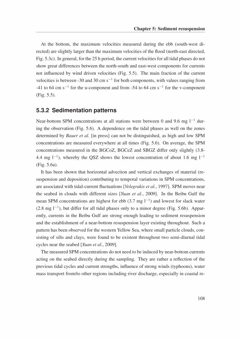
Chapter 5: Sediment resuspension
At the bottom, the maximum velocities measured during the ebb (south-west di-
rected) are slightly larger than the maximum velocities of the flood (north-east directed,
Fig. 5.3c). In general, for the 25 h period, the current velocities for all tidal phases do not
show great differences between the north-south and east-west components for currents
not influenced by wind driven velocities (Fig. 5.5). The main fraction of the current
velocities is between -30 and 30 cm s−1 for both components, with values ranging from
-41 to 64 cm s−1 for the u-component and from -54 to 64 cm s−1 for the v-component
(Fig. 5.5).
5.3.2 Sedimentation patterns
Near-bottom SPM concentrations at all stations were between 0 and 9.6 mg l−1 dur-
ing the observation (Fig. 5.6). A dependence on the tidal phases as well on the zones
determined by Bauer et al. [in press] can not be distinguished, as high and low SPM
concentrations are measured everywhere at all times (Fig. 5.6). On average, the SPM
concentrations measured in the BGCoZ, BGCeZ and SBGZ differ only slightly (3.8-
4.4 mg l−1), whereby the QSZ shows the lowest concentration of about 1.6 mg l−1
(Fig. 5.6a).
It has been shown that horizontal advection and vertical exchanges of material (re-
suspension and deposition) contributing to temporal variations in SPM concentrations,
are associated with tidal-current fluctuations [Velegrakis et al., 1997]. SPM moves near
the seabed in clouds with different sizes [Yuan et al., 2009]. In the Beibu Gulf the
mean SPM concentrations are highest for ebb (3.7 mg l−1) and lowest for slack water
(2.8 mg l−1), but differ for all tidal phases only to a minor degree (Fig. 5.6b). Appar-
ently, currents in the Beibu Gulf are strong enough leading to sediment resuspension
and the establishment of a near-bottom resuspension layer existing throughout. Such a
pattern has been observed for the western Yellow Sea, where small particle clouds, con-
sisting of silts and clays, were found to be existent throughout two semi-diurnal tidal
cycles near the seabed [Yuan et al., 2009].
The measured SPM concentrations do not need to be induced by near-bottom currents
acting on the seabed directly during the sampling. They are rather a reflection of the
previous tidal cycles and current strengths, influence of strong winds (typhoons), water
mass transport from/to other regions including river discharge, especially in coastal re-
108
Chapter 5: Sediment resuspension
0
2
4
6
8
10
371620
371640
371710
371750
371830
371600
371610
371650
371660
371670
371680
371690
371700
371720
371730
371740
371760
371770
371840
371780
371800
371810
371820
SP
M /
mg l
−1
BGCoZ
QSZ BGCeZ SBGZa)
0
2
4
6
8
10
371610
371620
371650
371660
371670
371700
371730
371740
371760
371770
371800
371600
371640
371680
371750
371780
371810
371820
371830
371840
371690
371710
371720
SP
M /
mg l
−1
Ebb Flood Slackwaterb)
Station
Figure 5.6: Near-bottom SPM concentrations (mg l−1) measured at stations a) in theBeibu Gulf Coastal Zone (BGCoZ), Qiongzhou Strait Zone (QSZ), Beibu Gulf Cen-tral Zone (BGCeZ) and Southern Beibu Gulf Zone (SBGZ) and b) during differenttidal phases (ebb, flood, slack water). The horizontal lines indicate mean values forthe respective groups.
gions, and the sediment grain size. The total amount of flow transported suspended load
is larger if the sediment grain size available for resuspension is smaller [Hoitink and
Hoekstra, 2005]. According to the resuspended particle size, the material needs some
time to deposit again. But not only sediments contribute to SPM, also, for example,
phytoplankton blooms, enhancing particle agglutination and hence the settling veloc-
ity, as well as zooplankton, egesting faecal pellets [Krivtsov et al., 2009]. Especially
the fine-grained deposition of biological origin, the benthic fluff, may be resuspended
more easily also during weaker currents [Velegrakis et al., 1997]. For the Beibu Gulf,
relatively high plant pigment contents in the surface sediments and an increased water
column chlorophyll concentrations near the bottom were found, indicating that these
109
Chapter 5: Sediment resuspension
biogenic deposits has been resuspended [Bauer et al., in press].
Fine-grained material can be comparatively easily resuspended by tidal flows [Hoitink
and Hoekstra, 2005]. In general, sediments in the Beibu Gulf are relatively fine, with a
grain size between 7 and 500 µm, mainly consisting of silt and clay.
Depending on the grain size and the currents acting on the sea bed, sediments are
deposited, transported or eroded. The relationship between the current strength and
the sediment grain size, allowing to decide if sediment deposition, transport or ero-
sion occurs, is described by the Hjulström diagram (Fig. 5.7). According to this dia-
gram, deposition takes place during lowest current velocities (<18 cm s−1), which were
recorded during all current measurements around the stations and during all tidal phases
(Fig. 5.7a, b).
For most stations in all zones the mean current velocity leads to a sediment transport
and shows similar values. The relatively similar mean currents for all stations indicate
low variability of the near-bottom current velocities within the study area in respect to
the different zones. For three stations, belonging to the BGCoZ and QSZ, relatively
large grain sizes (50-480 µm, silty sand to sand) in combination with relatively high
mean velocities (60-95 cm s−1) result in sediment resuspension (Fig. 5.7a). Although
at one station in the BGCoZ (371750) the highest mean velocity of about 149 cm s−1
is recorded, due to the small grain size of 8 µm (clayey silt), at this station only sedi-
ment transport may occur. For this station, located at Hainan Island’s west coast where
maximum tidal currents (on average 40-50 cm s−1) has been reported [Hu et al., 2003],
a current velocity of about 180 cm s−1 would be necessary for sediment resuspension
which is not reached during the sampling period. The finer the sediments, stronger cur-
rents are needed for erosion, due to stronger cohesiveness between the particles [Seibold
Figure 5.7 (following page): Hjulström diagram [Hjulström, 1935] showing the relationbetween near-bottom currents and the sediment grain size deposition, transport (greyarea) and erosion (after Sundborg [1956] and Seibold and Berger [1996]). a) Allstations sampled during the FENDOU 5 cruise in September/October 2009 are colorcoded according to the zones defined by Bauer et al. [in press]: Beibu Gulf CoastalZone (BGCoZ), Qiongzhou Strait Zone (QSZ), Beibu Gulf Central Zone (BGCeZ)and Southern Beibu Gulf Zone (SBGZ). b) Colors indicate the tidal phase of theADP records around every station. Symbols indicate minimum, maximum and meancurrent velocities around the respective station.
110
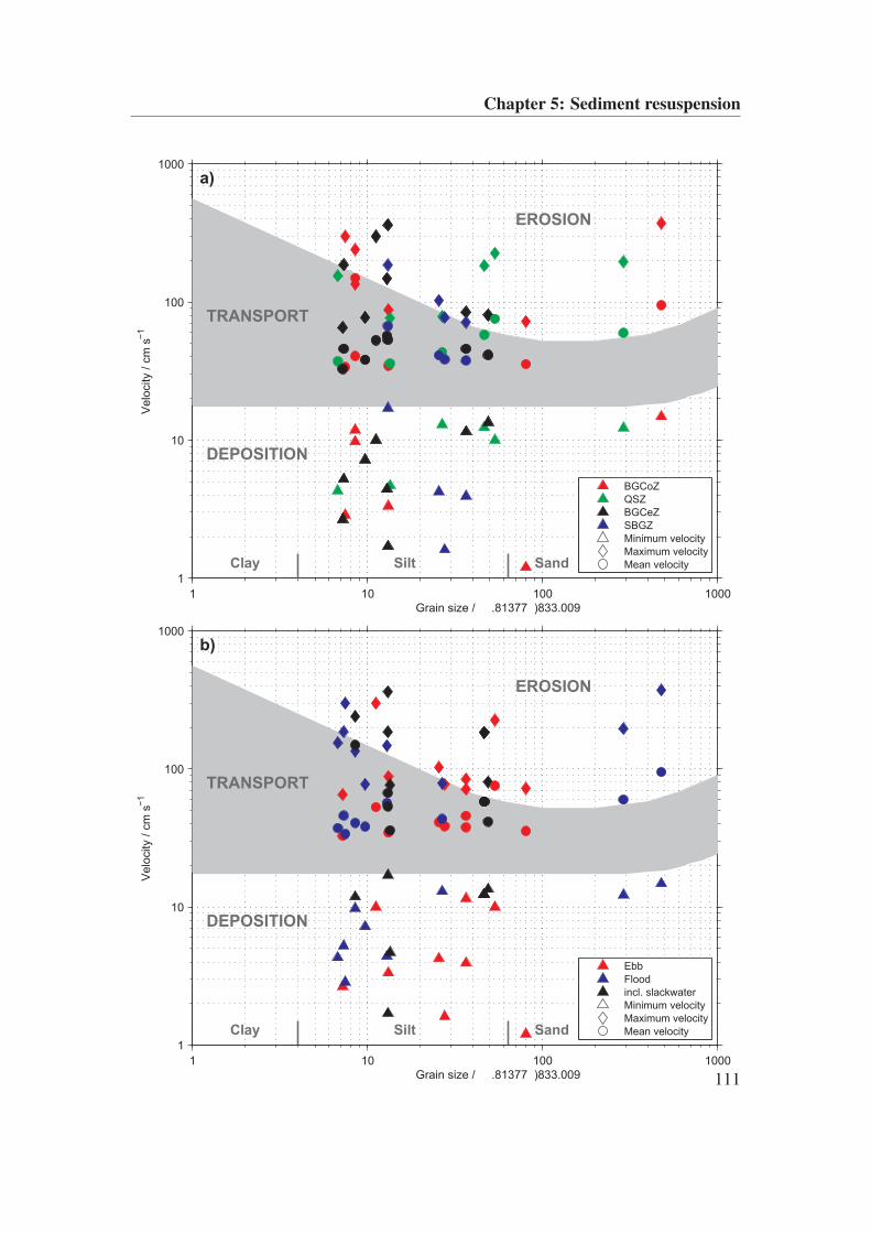
Chapter 5: Sediment resuspension
1 10 100 1000
1
10
100
1000
Clay Silt Sand
Grain size / m
Velo
city /
cm
s−
1
EROSION
TRANSPORT
DEPOSITION
a)
BGCoZ
QSZ
BGCeZ
SBGZ
Minimum velocity
Maximum velocity
Mean velocity
1 10 100 1000
1
10
100
1000
Clay Silt Sand
Grain size / m
Velo
city /
cm
s−
1
EROSION
TRANSPORT
DEPOSITION
b)
Ebb
Flood
incl. slackwater
Minimum velocity
Maximum velocity
Mean velocity
111
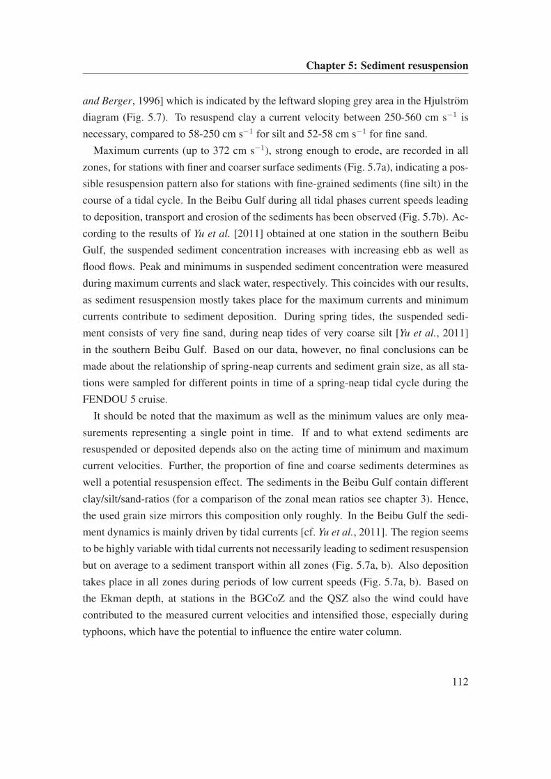
Chapter 5: Sediment resuspension
and Berger, 1996] which is indicated by the leftward sloping grey area in the Hjulström
diagram (Fig. 5.7). To resuspend clay a current velocity between 250-560 cm s−1 is
necessary, compared to 58-250 cm s−1 for silt and 52-58 cm s−1 for fine sand.
Maximum currents (up to 372 cm s−1), strong enough to erode, are recorded in all
zones, for stations with finer and coarser surface sediments (Fig. 5.7a), indicating a pos-
sible resuspension pattern also for stations with fine-grained sediments (fine silt) in the
course of a tidal cycle. In the Beibu Gulf during all tidal phases current speeds leading
to deposition, transport and erosion of the sediments has been observed (Fig. 5.7b). Ac-
cording to the results of Yu et al. [2011] obtained at one station in the southern Beibu
Gulf, the suspended sediment concentration increases with increasing ebb as well as
flood flows. Peak and minimums in suspended sediment concentration were measured
during maximum currents and slack water, respectively. This coincides with our results,
as sediment resuspension mostly takes place for the maximum currents and minimum
currents contribute to sediment deposition. During spring tides, the suspended sedi-
ment consists of very fine sand, during neap tides of very coarse silt [Yu et al., 2011]
in the southern Beibu Gulf. Based on our data, however, no final conclusions can be
made about the relationship of spring-neap currents and sediment grain size, as all sta-
tions were sampled for different points in time of a spring-neap tidal cycle during the
FENDOU 5 cruise.
It should be noted that the maximum as well as the minimum values are only mea-
surements representing a single point in time. If and to what extend sediments are
resuspended or deposited depends also on the acting time of minimum and maximum
current velocities. Further, the proportion of fine and coarse sediments determines as
well a potential resuspension effect. The sediments in the Beibu Gulf contain different
clay/silt/sand-ratios (for a comparison of the zonal mean ratios see chapter 3). Hence,
the used grain size mirrors this composition only roughly. In the Beibu Gulf the sedi-
ment dynamics is mainly driven by tidal currents [cf. Yu et al., 2011]. The region seems
to be highly variable with tidal currents not necessarily leading to sediment resuspension
but on average to a sediment transport within all zones (Fig. 5.7a, b). Also deposition
takes place in all zones during periods of low current speeds (Fig. 5.7a, b). Based on
the Ekman depth, at stations in the BGCoZ and the QSZ also the wind could have
contributed to the measured current velocities and intensified those, especially during
typhoons, which have the potential to influence the entire water column.
112
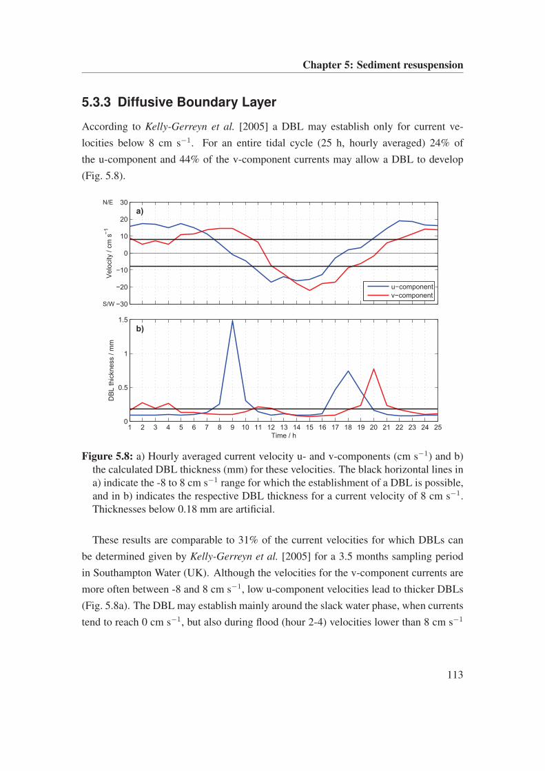
Chapter 5: Sediment resuspension
5.3.3 Diffusive Boundary Layer
According to Kelly-Gerreyn et al. [2005] a DBL may establish only for current ve-
locities below 8 cm s−1. For an entire tidal cycle (25 h, hourly averaged) 24% of
the u-component and 44% of the v-component currents may allow a DBL to develop
(Fig. 5.8).
−30
−20
−10
0
10
20
30
Velo
city /
cm
s−
1
a)N/E
S/W
u−component
v−component
1 2 3 4 5 6 7 8 9 10 11 12 13 14 15 16 17 18 19 20 21 22 23 24 250
0.5
1
1.5
DB
L t
hic
kness /
mm
Time / h
b)
Figure 5.8: a) Hourly averaged current velocity u- and v-components (cm s−1) and b)the calculated DBL thickness (mm) for these velocities. The black horizontal lines ina) indicate the -8 to 8 cm s−1 range for which the establishment of a DBL is possible,and in b) indicates the respective DBL thickness for a current velocity of 8 cm s−1.Thicknesses below 0.18 mm are artificial.
These results are comparable to 31% of the current velocities for which DBLs can
be determined given by Kelly-Gerreyn et al. [2005] for a 3.5 months sampling period
in Southampton Water (UK). Although the velocities for the v-component currents are
more often between -8 and 8 cm s−1, low u-component velocities lead to thicker DBLs
(Fig. 5.8a). The DBL may establish mainly around the slack water phase, when currents
tend to reach 0 cm s−1, but also during flood (hour 2-4) velocities lower than 8 cm s−1
113
Chapter 5: Sediment resuspension
were detected and may lead to DBL establishment (Fig. 5.8b).
At all stations, the mean and maximum velocities show values greater than 8 cm s−1
during the sampling period, indicating that in the Beibu Gulf the mean currents and
the currents for high energetic tidal phases are too strong for establishment of a DBL
(Fig. 5.9a). The required low velocities were measured for the minimum currents at
only 13 stations (Fig. 5.9b).
0
100
200
300
400
Velo
city /
cm
s−
1
a) Maximum velocity
Mean velocity
Minimum velocity
0
5
10
15
20
371600
371610
371620
371640
371650
371660
371670
371680
371690
371700
371710
371720
371730
371740
371750
371760
371770
371780
371790
371800
371810
371820
371830
371840
Velo
city /
cm
s−
1
b)
Station
Figure 5.9: a) Maximum, mean and minimum near-bottom velocities for all stations. b)Minimum near-bottom velocities for all stations. The black horizontal line indicatesthe 8 cm s−1 velocities below which DBLs can become established.
The thickness of the DBL depends directly on the near-bottom current velocity: the
stronger the currents the thinner is the DBL due to a higher bottom stress [Jørgensen and
Des Marais, 1990; Tengberg et al., 2004]. The calculated thicknesses of the DBLs lie
between 0.19 and 1.05 mm for current velocities between 7.2 and 1.2 cm s−1 (Fig. 5.10).
These thicknesses are consistent with those determined by Santschi et al. [e.g. 1983,
1991]; Jørgensen and Des Marais [e.g. 1990] and Kelly-Gerreyn et al. [2005] ranging
between 0.1 to 1.2 mm. It should be noted that the calculation of the DBL by using
114
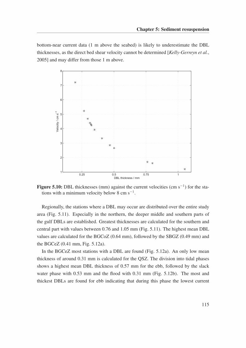
Chapter 5: Sediment resuspension
bottom-near current data (1 m above the seabed) is likely to underestimate the DBL
thicknesses, as the direct bed shear velocity cannot be determined [Kelly-Gerreyn et al.,
2005] and may differ from those 1 m above.
0.25 0.5 0.75 11
2
3
4
5
6
7
8
DBL thickness / mm
Velo
city /
cm
s−
1
Figure 5.10: DBL thicknesses (mm) against the current velocities (cm s−1) for the sta-tions with a minimum velocity below 8 cm s−1.
Regionally, the stations where a DBL may occur are distributed over the entire study
area (Fig. 5.11). Especially in the northern, the deeper middle and southern parts of
the gulf DBLs are established. Greatest thicknesses are calculated for the southern and
central part with values between 0.76 and 1.05 mm (Fig. 5.11). The highest mean DBL
values are calculated for the BGCoZ (0.64 mm), followed by the SBGZ (0.49 mm) and
the BGCeZ (0.41 mm, Fig. 5.12a).
In the BGCeZ most stations with a DBL are found (Fig. 5.12a). An only low mean
thickness of around 0.31 mm is calculated for the QSZ. The division into tidal phases
shows a highest mean DBL thickness of 0.57 mm for the ebb, followed by the slack
water phase with 0.53 mm and the flood with 0.31 mm (Fig. 5.12b). The most and
thickest DBLs are found for ebb indicating that during this phase the lowest current
115
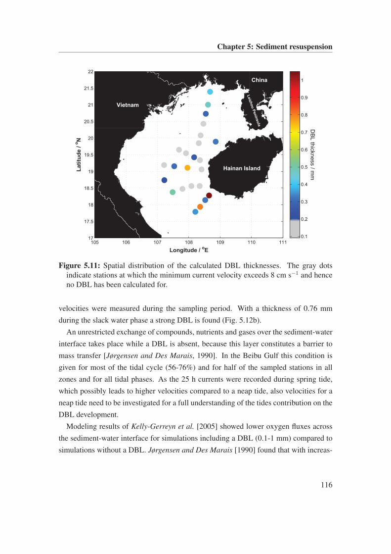
Chapter 5: Sediment resuspension
105 106 107 108 109 110 11117
17.5
18
18.5
19
19.5
20
20.5
21
21.5
22
Longitude / oE
Lati
tud
e /
oN
China
Vietnam
Hainan Island
Leiz
ho
u P
en
insu
la
DB
L th
ickness / m
m
0.1
0.2
0.3
0.4
0.5
0.6
0.7
0.8
0.9
1
Figure 5.11: Spatial distribution of the calculated DBL thicknesses. The gray dotsindicate stations at which the minimum current velocity exceeds 8 cm s−1 and henceno DBL has been calculated for.
velocities were measured during the sampling period. With a thickness of 0.76 mm
during the slack water phase a strong DBL is found (Fig. 5.12b).
An unrestricted exchange of compounds, nutrients and gases over the sediment-water
interface takes place while a DBL is absent, because this layer constitutes a barrier to
mass transfer [Jørgensen and Des Marais, 1990]. In the Beibu Gulf this condition is
given for most of the tidal cycle (56-76%) and for half of the sampled stations in all
zones and for all tidal phases. As the 25 h currents were recorded during spring tide,
which possibly leads to higher velocities compared to a neap tide, also velocities for a
neap tide need to be investigated for a full understanding of the tides contribution on the
DBL development.
Modeling results of Kelly-Gerreyn et al. [2005] showed lower oxygen fluxes across
the sediment-water interface for simulations including a DBL (0.1-1 mm) compared to
simulations without a DBL. Jørgensen and Des Marais [1990] found that with increas-
116
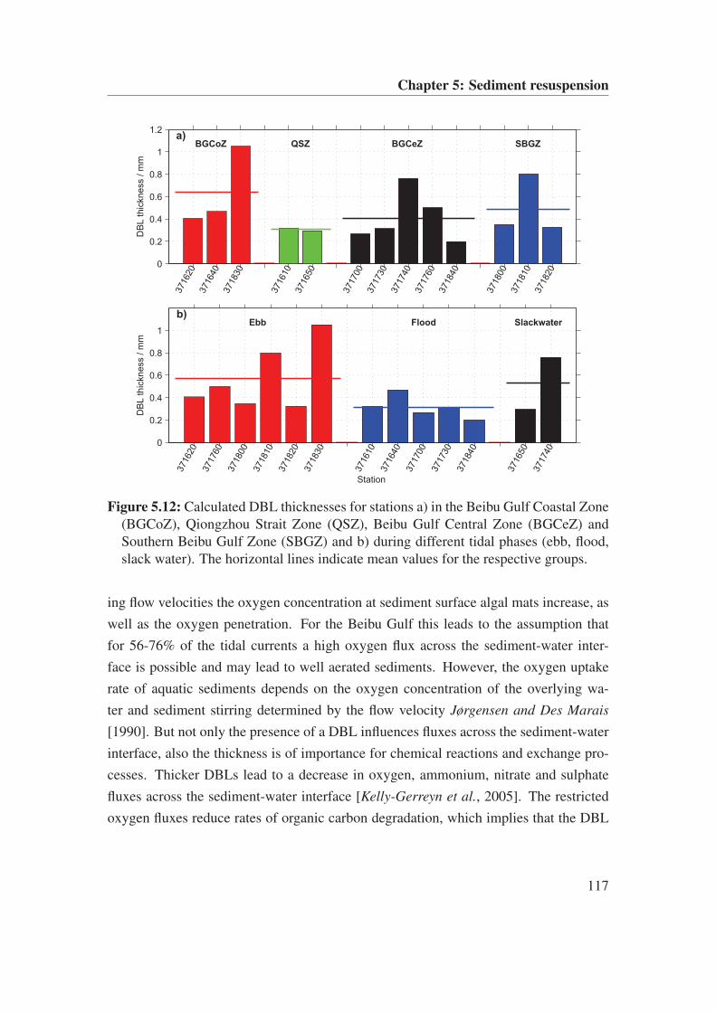
Chapter 5: Sediment resuspension
0
0.2
0.4
0.6
0.8
1
1.2
371620
371640
371830
371610
371650
371700
371730
371740
371760
371840
371800
371810
371820
DB
L t
hic
kness /
mm
BGCoZ QSZ BGCeZ SBGZa)
0
0.2
0.4
0.6
0.8
1
371620
371760
371800
371810
371820
371830
371610
371640
371700
371730
371840
371650
371740
DB
L t
hic
kness /
mm
Ebb Flood Slackwaterb)
Station
Figure 5.12: Calculated DBL thicknesses for stations a) in the Beibu Gulf Coastal Zone(BGCoZ), Qiongzhou Strait Zone (QSZ), Beibu Gulf Central Zone (BGCeZ) andSouthern Beibu Gulf Zone (SBGZ) and b) during different tidal phases (ebb, flood,slack water). The horizontal lines indicate mean values for the respective groups.
ing flow velocities the oxygen concentration at sediment surface algal mats increase, as
well as the oxygen penetration. For the Beibu Gulf this leads to the assumption that
for 56-76% of the tidal currents a high oxygen flux across the sediment-water inter-
face is possible and may lead to well aerated sediments. However, the oxygen uptake
rate of aquatic sediments depends on the oxygen concentration of the overlying wa-
ter and sediment stirring determined by the flow velocity Jørgensen and Des Marais
[1990]. But not only the presence of a DBL influences fluxes across the sediment-water
interface, also the thickness is of importance for chemical reactions and exchange pro-
cesses. Thicker DBLs lead to a decrease in oxygen, ammonium, nitrate and sulphate
fluxes across the sediment-water interface [Kelly-Gerreyn et al., 2005]. The restricted
oxygen fluxes reduce rates of organic carbon degradation, which implies that the DBL
117
Chapter 5: Sediment resuspension
contributes to the organic carbon preservation especially when the organic reactivity is
high [Kelly-Gerreyn et al., 2005]. High surface sediment pigment contents, indicating
a high organic matter input, are found in the BGCoZ, the QSZ and the BGCeZ [Bauer
et al., in press]. Although the organic matter content is high in the BGCoZ, due to the
high thickness of the mean DBL the oxygen fluxes are reduced and lead to a lower rate
of organic carbon degradation in contrast to the QSZ, showing highest sediment pig-
ment contents and thinnest DBLs. This coincides with the results by Xia et al. [in press]
showing slightly lower TOC contents (zonally averaged) in the surface sediments of the
BGCoZ, compared to the QSZ. Temporally, a thin mean DBL is found for the flood
(Fig. 5.12), a thick one for the ebb, indicating that oxygen fluxes and hence organic
carbon degradation are higher during flood compared to the ebb phase. It is still to be
clarified whether the period a DBL establishes is sufficient for those processes. At this
point, a combination of the obtained results with geochemical data for the Beibu Gulf is
necessary for the understanding of organic matter degradation and induced element and
material fluxes.
5.4 Conclusions
Sedimentological and geochemical processes are substantially influenced by the dif-
ferent current patterns within the Beibu Gulf. Tidal forcing is the main mechanism
controlling sediment deposition, transport and erosion, as wind driven and geostrophic
currents contribute less to the current velocities. Apparently, in the Beibu Gulf a near-
bottom resuspension layer exists permanently, caused by currents strong enough leading
to resuspension, small particles with a slow settling velocity and biogenic fluff.
For the mean and minimum currents, sediment transport and deposition, respectively,
take place at most stations and is possible for all tidal phases, whereas, maximum current
velocities leading to sediment resuspension occurring at stations within all zone and
also for all tidal phases. On average the near-bottom currents of all zones are relatively
similar during our observations.
In the Beibu Gulf the exchange across the sediment-water interface is possible for
most of the tidal cycle as the currents are relatively strong and DBLs, restricting ex-
change processes, may establish only for 24 to 44% of the tidal currents and are overall
suppressed. Hence, for a time span of 56-76% of a tidal cycle a direct benthic-pelagic
118
Chapter 5: Sediment resuspension
coupling may exist. Within the BGCoZ lowest organic carbon degradation took place
within the sampling period compared to the other zones, as the mean DBL is thickest
and thereby oxygen fluxes are reduced. In the QSZ, with the thinnest mean DBL, the
most degradation of organic matter took place. Although in both zones the organic mat-
ter input is high, the degree of degradation within the sediment may differ. Also the
different tidal phases may lead to a varying amount of organic carbon degradation.
For a better understanding of the geochemical processes within the Beibu Gulf the ob-
tained results need to be compared to geochemical parameters of the surface sediments.
Further, long-time measurements of tidal currents at different regions in the Beibu Gulf
are necessary to obtain a more detailed picture of the tidal influence on sediment depo-
sition, transport and resuspension as well as of the currents effect on the benthic-pelagic
coupling.
119
Conclusions
Conclusions and future perspectives
The present thesis investigated the hydrographical and biogeochemical conditions in the
Beibu Gulf, SCS, a shelf region playing an important role for the near-coastal terrestrial
material input and thus, as a transition zone between highly populated land masses and
the SCS, fluxes of material and energy into the SCS northwestern areas. So far, only
limited knowledge exists about the functioning of the ecosystem "Beibu Gulf". Hence,
this work contributes to our understanding of the interaction between hydrography, wa-
ter column biogeochemistry and sedimentology in the Beibu Gulf.
As a first step for the understanding of the hydrodynamical and sedimentological vari-
ability of the Beibu Gulf, hydrographical profiles, water and sediment samples has been
taken during a cruise in September/October 2009 and analyzed in the interdisciplinary
study in the third chapter of this thesis [Bauer et al., in press]:
• For the sampling period in September/October 2009 regional differences in hy-
drographical properties has been distinguished. Hydrographically, different zones
were defined which are influenced by riverine input and tidal mixing in the coastal
areas (Beibu Gulf Coastal Zone), water mass transport from the South China
coastal regions through Qiongzhou Strait (Qiongzhou Strait Zone and Beibu Gulf
Central Zone) as well as SCS water influence in the south (Southern Beibu Gulf
Zone).
• The influence of the different water masses due to the gulf’s circulation pattern,
driven by monsoon winds, tidal and residual currents and the effect of a typhoon
is mirrored in the biogeochemical properties of the water column (Chlorophyll,
nutrients and suspended particulate matter), grain size, distribution of plant pig-
ments (chlorophyll a and phaeopigments) and foraminifera in the surface sedi-
ments within the different zones.
• The surface sediment plant pigment contents as well as the geochemical sediment
120
Conclusions
properties, depend on the depositional environment and follow the pattern of sur-
face water productivity which is highest in the Beibu Gulf Coastal Zone and the
Qiongzhou Strait Zone.
• Apatite-bound phosphorous is the dominant route of phosphorus removal from
the pelagic to the benthic part of the ecosystem.
Marine primary production plays an important role in biogeochemical cycling within
the water column as well as in the sediments and is crucial for the oceanic carbon fixa-
tion but only little is known about the oceanic and biological processes, including varia-
tions in spatial and temporal phytoplankton distribution for the Beibu Gulf [Tang et al.,
2003]. An established 1D physical-biological model along with in-situ measurements
and satellite derived surface data has been used to investigate the connection between at-
mospheric forcing, water column structure and primary production in the central Beibu
Gulf for an 11 year period in the fourth chapter [Bauer and Waniek, 2013]:
• During summer the central Beibu Gulf is thermally stratified due to high solar
radiation and relatively weak winds during southwest monsoon which leads to a
nutrient depletion and hence a low primary production in the surface layer and
the development of a deep chlorophyll maximum in about 20-30 m depth, where
euphotic depth and nutricline co-exist. A phytoplankton bloom establishes during
winter when the strong northeast monsoon acts and the water column is deeply
mixed, resulting in a nutrient supply from deeper waters which are then available
for phytoplankton growth. The modeled phytoplankton bloom lasts on average
for 6 months.
• The interannual variability in the meteorological forcing is generally low but nev-
ertheless lead to a variability of about 2.5 months and around 1 month in au-
tumn/winter for the timing of stratification breakdown and the establishment of a
phytoplankton bloom, respectively.
• Strong wind events like typhoons are shown to enhance the primary production
temporally short by up to 275% relative to the summer background chlorophyll
concentration at the surface and play therefore an important role for the primary
production in the central Beibu Gulf in summer and autumn during periods of low
production. Further, these events are able to initiate a phytoplankton proliferation.
121
Conclusions
• In the central Beibu Gulf the tidal forcing is relatively weak, but despite that, con-
tributes to nutrient supply into the thermocline and leads to a significant enhance-
ment in strength (36%) and thickness (33%) of the deep chlorophyll maximum
compared to a system without tidal forcing.
Currents influence not only sediment resuspension, transport and deposition but also
the exchange between the seabed and the water column through the sediment-water
interface. Current records, especially bottom near, has been analyzed to investigate the
current patterns during the sampling period in September/October 2009 and their effects
on sediment resuspension as well as the establishment of a diffusive boundary layer in
the fifth chapter.
• Tidal forcing is the main mechanism controlling sedimentation patterns as well as
material and energy exchange between the sediment and the water column.
• Current velocities contributing to sediment deposition, transport and resuspension
are acting in all zones and during all tidal phases (ebb, flood, slack water) for the
sampling period in September/October 2009.
• In general, the strength of the currents during most of the tidal cycle (56-76%)
prevents the development of a diffusive boundary layer. Therefore, an exchange
of compounds, nutrients and gases across the sediment-water interface is possible.
Diffusive boundary layers may establish during all tidal phases and in all zones
with varying thicknesses.
The obtained results give a first insight in the functioning of the system "Beibu Gulf"
but show simultaneously that there is still need for further investigations to improve the
understanding of processes acting in that region. As one of the next steps in the near
future, the results obtained from the current records (chapter 5) should be combined
with near-bottom water column properties and geochemical parameters also gathered
during the FENDOU 5 cruise. Thereby, spatial and temporal (tidal phases) differences
of the physical and chemical conditions contributing to element fluxes between the water
column and the sediments could be investigated for the time of observation.
In this thesis mainly in-situ data of the FENDOU 5 cruise (September/October 2009)
were analyzed, representing the conditions during the inter-monsoon phase. For an eval-
uation of the role the changing wind system plays for processes in the water column and
122
Conclusions
possibly at the seabed as well as the water mass exchange with the surrounding SCS
waters, it is further necessary to analyze measured properties during other monsoon
phases, for example data obtained during the SONNE cruise (December 2011) charac-
terizing the winter northeast monsoon, and for the entire gulf including the Qiongzhou
Strait.
Especially for an elucidation of the gulf’s circulation pattern and the importance of
tides in the different zones, stationary long-time measurements at selected stations are
inevitable (e.g. moorings with current meters and turbidity sensors), which are unfortu-
nately not available at present. Such data would also contribute to the understanding of
sedimentation processes and the benthic-pelagic coupling. By the help of remote sens-
ing time series conclusions may be drawn for transport processes, circulation patterns,
surface near primary production and typhoon effects, but unfortunately the measure-
ments of bio-optical properties depend on a clear sky. Especially during southwest
monsoon the immense cloud cover prevents such measurements of necessary quality
for the Beibu Gulf. Hence, an intense in-situ sampling is essential for investigating the
Beibu Gulf.
123
References
References
Al-Raei, A., K. Bosselmann, M. Böttcher, B. Hespenheide, and F. Tauber (2009), Seasonal dynamicsof microbial sulfate reduction in temperate intertidal surface sediments: Controls by temperature andorganic matter, Ocean Dynamics, 59(2), 351–370.
Alvarez, I., M. Gomez-Gesteira, M. deCastro, and E. M. Novoa (2008), Ekman transport along the Gali-cian Coast (NW, Spain) calculated from QuikSCAT winds, Journal of Marine Systems, 72(1-4), 101–115.
Angove, M., and R. Falvey (2010), 2010 Annual Tropical Cyclone Report, Tech. rep., U.S. Naval PacificMeteorology and Oceanography Center / Joint Typhoon Warning Center, pp. 93.
Anschutz, P., S. Zhong, B. Sundby, A. Mucci, and C. Gobeil (1998), Burial efficiency of phosphorusand the geochemistry of iron in continental margin sediments, Limnology and Oceanography, 43(1),53–64.
Atangan, J., and A. Preble (2005), 2005 Annual Tropical Cyclone Report, Tech. rep., U.S. Naval PacificMeteorology and Oceanography Center / Joint Typhoon Warning Center, pp. 109.
Babin, S., J. Carton, T. Dickey, and J. Wiggert (2004), Satellite evidence of hurricane-induced phyto-plankton blooms in an oceanic desert, Journal of Geophysical Research, 109(C3), C03043.
Bauer, A., and J. Waniek (2013), Factors affecting chlorophyll a concentration in the central Beibu Gulf,South China Sea, Marine Ecology Progress Series, 474, 67–88.
Bauer, A., et al. (in press), Regional differences of hydrographical and sedimentological properties inBeibu Gulf, South China Sea, Journal of Coastal Research, Special Issue 66, doi:10.2112/SI_66_5.
Bauer, S., G. Hitchcock, and D. Olson (1991), Influence of monsoonally-forced Ekman dynamics uponsurface layer depth and plankton biomass distribution in the Arabian Sea, Deep Sea Research Part I,38(5), 531–553.
Bianchi, T., S. Findlay, and R. Dawson (1993), Organic matter sources in the water column and sedimentsof the Hudson River Estuary: The use of plant pigments as tracers, Estuarine, Coastal and Shelf
Science, 36(4), 359–376.
Bianchi, T., B. Johansson, and R. Elmgren (2000), Breakdown of phytoplankton pigments in Baltic sed-iments: Effects of anoxia and loss of deposit-feeding macrofauna, Journal of Experimental Marine
Biology and Ecology, 251(2), 161–183.
Boon, J. (2004), Secrets of the Tide, Horwood Publishing, Chichester, UK, pp. 212.
Böttcher, M., et al. (2000), The biogeochemistry, stable isotope geochemistry, and microbial communitystructure of a temperate intertidal mudflat: An integrated study, Continental Shelf Research, 20(12),1749–1769.
124
References
Boyd, P., and S. Doney (2003), The impact of climate change and feedback processes on the ocean carboncycle, in Ocean Biogeochemistry, edited by M. Fasham, pp. 157–193, Springer, Berlin, Germany.
Braeckman, U., C. Van Colen, K. Soetaert, M. Vincx, and J. Vanaverbeke (2011), Contrasting mac-robenthic activities differentially affect nematode density and diversity in a shallow subtidal marinesediment, Marine Ecology Progress Series, 422, 179–191.
Brzezinski, M. (1985), The Si:C:N ratio of marine diatoms: Interspecific variability and the effect ofsome environmental variables, Journal of Phycology, 21(3), 347–357.
Cai, S., Q. Huang, and X. Long (2003), Three-dimensional numerical model study of the residual currentin the South China Sea, Oceanologica Acta, 26(5-6), 597–607.
Chang, J., C. Chung, and G. Gong (1996), Influences of cyclones on chlorophyll a concentration and Syne-
chococcus abundance in a subtropical western Pacific coastal ecosystem, Marine Ecology Progress
Series, 140, 199–205.
Chen, C., P. Li, M. Shi, J. Zuo, M. Chen, and H. Sun (2009), Numerical study of the tides and residualcurrents in the Qiongzhou Strait, Chinese Journal of Oceanology and Limnology, 27(4), 931–942.
Chen, C.-T., K.-K. Liu, and R. MacDonald (2003), Continental margin exchanges, in Ocean Biogeochem-
istry, edited by M. Fasham, pp. 53–97, Springer, Berlin, Germany.
Chen, Y., and D. Tang (2011), Remote sensing analysis of impact of typhoon on environment in the seaarea south of Hainan Island, Procedia Environmental Sciences, 10, 1621–1629.
Chung, C., G. Gong, and C. Hung (2012), Effect of Typhoon Morakot on microphytoplankton populationdynamics in the subtropical Northwest Pacific, Marine Ecology Progress Series, 448, 39–49.
Cooper, G., and R. Falvey (2008), 2008 Annual Tropical Cyclone Report, Tech. rep., U.S. Naval PacificMeteorology and Oceanography Center / Joint Typhoon Warning Center, pp. 116.
Cooper, G., and R. Falvey (2009), 2009 Annual Tropical Cyclone Report, Tech. rep., U.S. Naval PacificMeteorology and Oceanography Center / Joint Typhoon Warning Center, pp. 109.
Cullen, J., and R. Eppley (1981), Chlorophyll maximum layers of the Southern California Bight andpossible mechanisms of their formation and maintenance, Oceanologica Acta, 4(1), 23–32.
Dai, J., X. Zhang, D. Wang, C. Guo, R. Fang, and X. Wang (2011), Water quality change of Nanliu Riverin Guangxi Beibu Gulf Economic Zone, International Conference on Remote Sensing, Environment
and Transportation Engineering (RSETE), Nanjing, pp. 5629–5632.
de Haas, H., T. van Weering, and H. de Stigter (2002), Organic carbon in shelf seas: Sinks or sources,processes and products, Continental Shelf Research, 22(5), 691–717.
De Jonge, V., and M. Engelkes (1993), The role of mineral compounds and chemical conditions in thebinding of phosphate in the Ems estuary, Aquatic Ecology, 27(2), 227–236.
Dellwig, O., T. Leipe, C. März, M. Glockzin, F. Pollehne, B. Schnetger, E. Yakushev, M. Böttcher,and H.-J. Brumsack (2010), A new particulate Mn-Fe-P-shuttle at the redoxcline of anoxic basins,Geochimica et Cosmochimica Acta, 74(24), 7100–7115.
125
References
Dickey, T. (1988), Recent advances and future directions in multi-disciplinary in situ oceanographic mea-surement systems, in Toward a theory on biological-physical interactions in the world ocean, editedby B. Rothschild, pp. 555–598, Kluwer Academic Publishers, Dordrecht, Netherlands.
Doney, S., K. Lindsay, and J. Moore (2003), Global ocean carbon cycle modeling, in Ocean Biogeochem-
istry, edited by M. Fasham, pp. 217–238, Springer, Berlin, Germany.
Einsele, W. (1938), Über chemische und kolloidchemische Vorgänge in Eisen-Phosphat-Systemen unterlimnochemischen und limnogeologischen Gesichtspunkten, Archiv für Hydrobiologie, 33, 361–387.
Emery, W., and R. Thomson (2001), Data analysis methods in physical oceanography, 2nd revised ed.,Elsevier Science, Amsterdam, Netherlands, pp. 638.
Enge, A., et al. (2011), Response of the benthic foraminiferal community to a simulated short-term phy-todetritus pulse in the abyssal North Pacific, Marine Ecology Progress Series, 438, 129–142.
Fang, G., Y.-K. Kwok, K. Yu, and Y. Zhu (1999), Numerical simulation of principal tidal constituentsin the South China Sea, Gulf of Tonkin and Gulf of Thailand, Continental Shelf Research, 19(7),845–869.
Fasham, M., T. Platt, B. Irwin, and K. Jones (1985), Factors affecting the spatial pattern of the deepchlorophyll maximum in the region of the Azores Front, Progress In Oceanography, 14, 129–165.
Fogel, M., C. Aguilar, R. Cuhel, D. Hollander, J. Willey, and H. Paerl (1999), Biological and isotopicchanges in coastal waters induced by Hurricane Gordon, Limnology and Oceanography, 44(6), 1359–1369.
Folk, R. (1954), The distinction between grain size and mineral composition in sedimentary-rock nomen-clature, Journal of Geology, 62(4), 344–359.
Furze, P., and G. Engel (2002), 2002 Annual Tropical Cyclone Report, Tech. rep., U.S. Naval PacificMeteorology and Oceanography Center / Joint Typhoon Warning Center, pp. 393.
Furze, P., and A. Preble (2003), 2003 Annual Tropical Cyclone Report, Tech. rep., U.S. Naval PacificMeteorology and Oceanography Center / Joint Typhoon Warning Center, pp. 827.
Gago, J., X. Álvarez Salgado, M. Nieto-Cid, S. Brea, and S. Piedracoba (2005), Continental inputs of C,N, P and Si species to the Ria de Vigo (NW Spain), Estuarine, Coastal and Shelf Science, 65(1-2),74–82.
Gallagher, S., M. Wallace, C. Li, B. Kinna, J. Bye, K. Akimoto, and M. Torii (2009), Neogene history ofthe West Pacific Warm Pool, Kuroshio and Leeuwin currents, Paleoceanography, 24(1), PA1206.
Gan, J., H. Li, E. Curchitser, and D. Haidvogel (2006), Modeling South China Sea circulation: Responseto seasonal forcing regimes, Journal of Geophysical Research, 111, C06034.
Gill, A. (1982), Atmosphere-Ocean Dynamics, International Geophysics Series, vol. 30, Academic Press,London, UK, pp. 662.
Graf, G., and R. Rosenberg (1997), Bioresuspension and biodeposition: A review, Journal of Marine
Systems, 11(3-4), 269–278.
126
References
Grant, W., and O. Madsen (1986), The continental-shelf bottom boundary layer, Annual Review of Fluid
Mechanics, 18, 265–305.
Guillén, J., J. Jiménez, A. Palanques, V. Gracia, P. Puig, and A. Sánchez-Arcilla (2002), Sediment resus-pension across a microtidal, low-energy inner shelf, Continental Shelf Research, 22(2), 305–325.
Guinder, V., C. Popovich, and G. Perillo (2009), Particulate suspended matter concentrations in the BahíaBlanca Estuary, Argentina: Implication for the development of phytoplankton blooms, Estuarine,
Coastal and Shelf Science, 85(1), 157–165.
Guo, Y. (1994), Primary productivity and phytoplankton in China seas, in Oceanology of China Seas,vol. 1, edited by D. Zhou, Y.-B. Liang, and C.-K. Zeng, pp. 227–242, Kluwer Academic Publishers,Dordrecht, Germany.
Haese, R., K. Wallmann, A. Dahmke, U. Kretzmann, P. Müller, and H. Schulz (1997), Iron species deter-mination to investigate early diagenetic reactivity in marine sediments, Geochimica et Cosmochimica
Acta, 61(1), 63–72.
Halim, Y. (1991), The impact of human alterations of the hydrological cycle on ocean margins, in Ocean
Margin Processes in Global Change, edited by R. Mantoura, J.-M. Martin, and R. Wollast, pp. 301–327, John Wiley & Sons, New York, USA.
Hansen, H., and F. Koroleff (1999), Determination of nutrients, in Methods of Seawater Analysis, vol. 2,edited by K. Grasshoff, K. Kremling, and M. Ehrhardt, pp. 159–228, Wiley-VCH, Weinheim, Ger-many.
He, Y., and L.-Y. Hu (2001), Pliocene foraminifers from the Leizhou Peninsula of Guangdong, China,Press of University of Science and Technology of China, Hefei, China, pp. 189 (in Chinese).
Hemleben, C., M. Spindler, and O. Anderson (1989), Modern planktonic foraminifera, Springer, NewYork, USA, pp. 363.
Hjulström, F. (1935), Studies of the morphological activity of rivers as illustrated by the River Fyris,Bulletin of the Geological Institute of Uppsala, 25, 221–527.
Hoitink, A., and P. Hoekstra (2005), Observations of suspended sediment from ADCP and OBS measure-ments in a mud-dominated environment, Coastal Engineering, 52, 103–118.
Holliday, N., J. Waniek, R. Davidson, D. Wilson, L. Brown, R. Sanders, R. Pollard, and J. Allen (2006),Large-scale physical controls on phytoplankton growth in the Irminger Sea Part I: Hydrographic zones,mixing and stratification, Journal of Marine Systems, 59(3-4), 201–218.
Holmedal, L., and D. Myrhaug (2008), Tidal Boundary Layers, in Proceedings of the ASME 27th Inter-
national Conference on Offshore Mechanics and Arctic Engineering, pp. 565–570, Estoril, Portugal.
Howard, K., and J. Yoder (1997), Contribution of the subtropical oceans to global primary production, inSpace Remote Sensing of Subtropical Oceans, Proceedings of COSPAR Colloquium on Space Remote
Sensing of Subtropical Oceans (SRSSO), COSPAR Colloquia Series, vol. 8, edited by C.-T. Liu, pp.157–167, Pergamon.
Hu, J., H. Kawamura, and D. Tang (2003), Tidal front around the Hainan Island, northwest of the SouthChina Sea, Journal of Geophysical Research, 108(C11), 1–9.
127
References
Huang, B., Z. Jian, X. Cheng, and P. Wang (2003), Foraminiferal responses to upwelling variations in theSouth China Sea over the last 220 000 years, Marine Micropaleontology, 47(12), 1–15.
Huang, Q.-Z., W.-Z. Wang, Y. Li, and C. Li (1994), Current characteristics of the South China Sea, inOceanology of China Seas, vol. 1, edited by D. Zhou, Y.-B. Liang, and C.-K. Zeng, pp. 39–47, KluwerAcademic Publishers, Dordrecht, Netherlands.
Huang, Y., Y. Li, H. Shao, and Y.-H. Li (2008), Seasonal variations of sea surface temperature, chlorophylla and turbidity in Beibu Gulf, MODIS imagery study, Journal of Xiamen University (Natural Science),47(6), 856–863 (in Chinese).
Hyacinthe, C., and P. Van Cappellen (2004), An authigenic iron phosphate phase in estuarine sediments:Composition, formation and chemical reactivity, Marine Chemistry, 91(1-4), 227–251.
Jago, C., A. Bale, M. Green, M. Howarth, I. McCave, G. Millward, A. Morris, A. Rowden, and J. Williams(1993), Resuspension processes and seston dynamics, Southern North Sea, Philosophical Transactions
of the Royal Society of London A, 343, 475–491.
Jago, C., S. Jones, R. Latter, R. McCandliss, M. Hearn, and M. Howarth (2002), Resuspension of benthicfluff by tidal currents in deep stratified waters, northern North Sea, Journal of Sea Research, 48(4),259–269.
Jensen, H., and B. Thamdrup (1993), Iron-bound phosphorus in marine sediments as measured bybicarbonate-dithionite extraction, Hydrobiologia, 253, 47–59.
JGOFS, P. (1994), JGOFS Protocols, Protocols for the Joint Global Ocean Flux Study (JGOFS) CoreMeasurement, 97-100.
Jiang, X., Z. Zhong, and J. Jiang (2009), Upper ocean response of the South China Sea to TyphoonKrovanh (2003), Dynamics of Atmospheres and Oceans, 47(1-3), 165–175.
Jørgensen, B. (1982), Mineralization of organic matter in the sea bed - the role of sulfate reduction,Nature, 296, 643–645.
Jørgensen, B., and D. Des Marais (1990), The diffusive boundary layer of sediments - oxygen microgra-dients over a microbial mat, Limnology and Oceanography, 35, 1343–1355.
Jørgensen, B., and S. Kasten (2006), Sulfur cycling and methane oxidation, in Marine Geochemistry,edited by H. Schulz and M. Zabel, pp. 271–309, Springer, Berlin, Germany.
Jorissen, F., C. Fontanier, and E. Thomas (2007), Paleoceanographical proxies based on deep-sea benthicforaminiferal assemblage characteristics, in Proxies in late cenozoic paleoceanography, Developments
in Marine Geology, vol. 1, edited by C. Hillaire-Marcel and A. De Vernal, pp. 263–325, Elsevier,Amsterdam, Netherlands.
JTWC, J. T. W. C. (2000), 2000 Annual Tropical Cyclone Report, Tech. rep., U.S. Naval Pacific Meteo-rology and Oceanography Center / Joint Typhoon Warning Center, pp. 399.
JTWC, J. T. W. C. (2001), 2001 Annual Tropical Cyclone Report, Tech. rep., U.S. Naval Pacific Meteo-rology and Oceanography Center / Joint Typhoon Warning Center, pp. 323.
128
References
Kalnay, E., et al. (1996), The NCEP/NCAR 40-Year Reanalysis Project, Bulletin of the American Mete-
orological Society, 77(3), 437–471.
Keil, R., D. Martlucan, F. Prahl, and J. Hedges (1994), Sorptive preservation of labile organic matter inmarine sediments, Nature, 370, 549–552.
Kelly-Gerreyn, B., D. Hydes, and J. Waniek (2005), Control of the diffusive boundary layer on benthicfluxes: A model study, Marine Ecology Progress Series, 292, 61–74.
Kirk, J. (2011), Light and photosynthesis in aquatic ecosystems, 3rd ed., Cambridge University Press,Cambridge, pp. 649.
Klein, P., and B. Coste (1984), Effects of wind-stress variability on nutrient transport into the mixed layer,Deep Sea Research Part I, 31(1), 21–37.
Koroleff, F., and K. Kremling (1999), Determination of trace elements, in Methods of Seawater Anal-
ysis, edited by K. Grasshoff, K. Kremling, and M. Ehrhardt, pp. 340–342, Wiley-VHC, Weinheim,Germany.
Kostka, J., and L. I.G.W. (1994), Partitioning and speciation of solid phase iron in saltmarsh sediments,Geochimica et Cosmochimica Acta, 58(7), 1701–1710.
Krivtsov, V., M. Howard, and S. Jones (2009), Characterising observed patterns of suspended particulatematter and relationships with oceanographic and meteorological variables: Studies in Liverpool Bay,Environmetal Modelling & Software, 24, 677–685.
Kucera, M. (2007), Planktonic foraminifera as tracers of past oceanic environments, in Proxies in late
cenozoic paleoceanography, Developments in Marine Geology, vol. 1, edited by C. Hillaire-Marceland A. De Vernal, pp. 213–262, Elsevier, Amsterdam, Netherlands.
Lauria, M., D. Purdie, and J. Sharples (1999), Contrasting phytoplankton distributions controlled by tidalturbulence in an estuary, Journal of Marine Systems, 21(1-4), 189–197.
Leipe, T., F. Tauber, H. Vallius, J. Virtasalo, S. Uscinowicz, N. Kowalski, S. Hille, S. Lindgren, andT. Myllyvirta (2010), Particulate organic carbon (POC) in surface sediments of the Baltic Sea, Geo-
Marine Letters, 31(3), 175–188.
Li, C., J. Blanton, and C. Chen (2004), Mapping of tide and tidal flow fields along a tidal channel withvessel-based observations, Journal of Geophysical Research, 109(C4), C04002.
Li, G., W. Liang, S. Liao, and G. Fang (1996), Climatic changes since Holocene along Guangxi coast,Marine Geology & Quaternary Geology, 16(3), 49–60.
Lin, I. (2012), Typhoon-induced phytoplankton blooms and primary productivity increase in the westernNorth Pacific subtropical ocean, Journal of Geophysical Research, 117(C3), C03039.
Lin, I., W. Liu, C.-C. Wu, G. Wong, C. Hu, Z. Chen, W.-D. Liang, Y. Yang, and K.-K. Liu (2003), Newevidence for enhanced ocean primary production triggered by tropical cyclone, Geophysical Research
Letters, 30(13), 1718–1721.
Liu, J., G. Li, M. Chen, and H. Hong (1992), The geomorphological and sedimentary characteristics inoffshore of Guangxi Province, Tropic Oceanology, 11(1), 52–57.
129
References
Liu, K., S. Chao, P. Shaw, G. Gong, C. Chen, and T. Tang (2002), Monsoon-forced chlorophyll distribu-tion and primary production in the South China Sea: Observations and a numerical study, Deep Sea
Research Part I, 49(8), 1387–1412.
Liu, X., Z. Zhang, Y. Wu, Y. Huang, and Y. Zhang (2005), Distribution of sediment chloroplastic pigmentsin the Southern Yellow Sea, Journal of Ocean University of China, 4(2), 163–172.
Liu, Z., X. Ning, and Y. Cai (1998), Distribution characteristics of size-fractionated chlorophyll a andproductivity of phytoplankton in the Beibu Gulf, Acta oceanologica sinica, 20(1), 50–57 (in Chinese).
Longhurst, A. (2007), Ecological Geography of the Sea, 2nd ed., Academic Press, San Diego, California,USA, pp. 542.
Lü, X., F. Qiao, G. Wang, C. Xia, and Y. Yuan (2008), Upwelling off the west coast of Hainan Island insummer: Its detection and mechanisms, Geophysical Research Letters, 35(2), L02604.
Lund-Hansen, L., M. Pejrul, J. Valeur, and A. Jensen (1993), Gross sedimentation rates in the North Sea-Baltic Sea transition: Effects of stratification, wind energy transfer, and resuspension, Oceanologica
Acta, 16(3), 205–212.
Mackensen, A., H. Grobe, G. Kuhn, and D. Fütterer (1990), Benthic foraminiferal assemblages from theeastern Weddell Sea between 68 and 73oS: Distribution, ecology and fossilization potential, Marine
Micropaleontology, 16(3-4), 241–283.
Madhupratap, M., M. Gauns, N. Ramaiah, S. Prasanna Kumar, P. Muraleedharan, S. de Sousa, S. Sardes-sai, and U. Muraleedharan (2003), Biogeochemistry of the Bay of Bengal: Physical, chemical andprimary productivity characteristics of the central and western Bay of Bengal during summer mon-soon 2001, Deep Sea Research Part II, 50(5), 881–896.
Manh, D.-V., and T. Yanagi (1997), A three-dimensional numerical model of tide and tidal current in theGulf of Tongking, La Mer, 35, 15–22.
Manh, D.-V., and T. Yanagi (2000), A study on residual flow in the Gulf of Tongking, Journal of Oceanog-
raphy, 56(1), 59–68.
Mantoura, R., J.-M. Martin, and R. Wollast (1991), Ocean Margin Processes in Global Change, Reportof the Dahlem Workshop on Ocean Margin Processes in Global Change, John Wiley & Sons, NewYork, USA, pp. 469.
Mascarenhas Jr., A., R. Castro, C. Collins, and R. Durazo (2004), Seasonal variation of geostrophic ve-locity and heat flux at the entrance to the Gulf of California, Mexico, Journal of Geophysical Research,109(C7), C07008.
Mayer, L. (1994), Relationships between mineral surfaces and organic carbon concentrations in soils andsediments, Chemical Geology, 11, 347–363.
McManus, I. (1988), Grain-size determination and interpretation, in Techniques in Sedimentology, editedby M. Tucker, pp. 63–85, Blackwell, Oxford, UK.
Milliman, J. (1991), Flux and fate of fluvial sediment and water in coastal seas, in Ocean Margin Pro-
cesses in Global Change, edited by R. Mantoura, J.-M. Martin, and R. Wollast, pp. 69–89, John Wiley& Sons, New York, USA.
130
References
Milliman, J., and R. Meade (1983), Worldwide delivery of river sediment to the oceans, Journal of
Geology, 91, 1–21.
Morse, J. (1986), The surface chemistry of calcium carbonate minerals in natural waters: An overview,Marine Chemistry, 20(1), 91–112.
Murray, J. (1991), Ecology and palaeoecology of benthic foraminifera, Wiley, New York, USA, pp. 397.
Murray, J. (2006), Ecology and applications of benthic foraminifera, Cambridge University Press, Cam-bridge, UK, pp. 426.
O’Hara, J., and R. Falvey (2006), 2006 Annual Tropical Cyclone Report, Tech. rep., U.S. Naval PacificMeteorology and Oceanography Center / Joint Typhoon Warning Center, pp. 98.
O’Hara, J., and R. Falvey (2007), 2007 Annual Tropical Cyclone Report, Tech. rep., U.S. Naval PacificMeteorology and Oceanography Center / Joint Typhoon Warning Center, pp. 124.
O’Kane, J., et al. (1991), What is the response of ocean margin systems to natural and anthropogenicperturbations?, in Ocean Margin Processes in Global Change, edited by R. Mantoura, J.-M. Martin,and R. Wollast, pp. 349–363, John Wiley & Sons, New York, USA.
Pond, S., and G. Pickard (1983), Introductory Dynamical Oceanography, 2 ed., Pergamon Press, Oxford,England, pp. 329.
Postma, H. (1988), Physical and chemical oceanographic aspects of continental shelves, in Continental
Shelves, vol. 27, edited by H. Postma and J. Zijlstra, pp. 5–37, Elsevier, Amsterdam, Netherlands.
Postma, H., and J. Zijlstra (1988), Continental Shelves, Ecosystems of the World, vol. 27, Elsevier, Ams-terdam, Netherlands, pp. 421.
Poulton, S., and R. Raiswell (2002), The low-temperature geochemical cycle of iron: From continentalfluxes to marine sediment deposition, American Journal of Science, 302(9), 774–805.
Price, J. (1981), Upper ocean response to a hurricane, Journal of Physical Oceanography, 11(2), 153–175.
Repeta, D., and R. Gagosian (1987), Carotenoid diagenesis in recent marine sediments - I. The Perucontinental shelf (15oS, 75oW), Geochimica et Cosmochimica Acta, 51(4), 1001–1009.
Reynolds, C. (2006), Ecology of phytoplankton, Ecology, biodiversity and conservation, Cambridge Uni-versity Press, New York, USA, pp. 535.
Ridderinkhof, H. (1992), On the effects of variability in meteorological forcing on the vertical structureof a stratified watercolumn, Continental Shelf Research, 12(1), 25–36.
Rock Color Chart, C. (1991), Rock Color Charts, Geological Society of America, Boulder, Colorado,USA, pp. 1-12.
Ross, O. (2004), Algal motility in variable turbulence, PhD Thesis, University of Southampton,Southampton, UK.
Ross, O. (2006), Particles in motion: How turbulence affects plankton sedimentation from an oceanicmixed layer, Geophysical Research Letters, 33(10), L10609.
131
References
Ross, O., and J. Sharples (2007), Phytoplankton motility and the competition for nutrients in the thermo-cline, Marine Ecology Progress Series, 347, 21–38.
Ross, O., and J. Sharples (2008), Swimming for survival: A role of phytoplankton motility in a stratifiedturbulent environment, Journal of Marine Systems, 70(3-4), 248–262.
Ruttenberg, K., and R. Berner (1993), Authigenic apatite formation and burial in sediments from non-upwelling, continental margin environments, Geochimica et Cosmochimica Acta, 57(5), 991–1007.
Santschi, P., P. Bower, U. Nyffeler, A. Azevedo, and W. Broecker (1983), Estimates of the resistanceto chemical-transport posed by the deep-sea boundary-layer, Limnology and Oceanography, 28, 899–912.
Santschi, P., R. Anderson, M. Fleisher, and W. Bowles (1991), Measurements of diffusive sublayer thick-nesses in the ocean by alabaster dissolution, and their implications for the measurements of benthicfluxes, Journal of Geophysical Research, 96(C6), 10641–10657.
Schmuker, B. (2000), The influence of shelf vicinity on the distribution of planktic foraminifera south ofPuerto Rico, Marine Geology, 166(1-4), 125–143.
Seeberg-Elverfeldt, J., M. Schlüter, T. Feseker, and M. Kölling (2005), Rhizon sampling of porewatersnear the sediment-water interface of aquatic systems, Limnology and Oceanography: Methods, 3,361–371.
Seibold, E., and W. Berger (1996), The Sea Floor, 3rd ed., Springer, Berlin, Germany, pp. 358.
Sharp, G. (1988), Fish populations and fisheries: Their perturbations, natural and man-induced, in Con-
tinental Shelves, vol. 27, edited by H. Postma and J. Zijlstra, pp. 155–202, Elsevier, Amsterdam,Netherlands.
Sharples, J. (1999), Investigating the seasonal vertical structure of phytoplankton in shelf seas, Marine
Models, 1(1-4), 3–38.
Sharples, J. (2008), Potential impacts of the spring-neap tidal cycle on shelf sea primary production,Journal of Plankton Research, 30(2), 183–197.
Sharples, J., and P. Tett (1994), Modelling the effect of physical variability on the midwater chlorophyllmaximum, Journal of Marine Research, 52(2), 219–238.
Sharples, J., M. Moore, T. Rippeth, P. Holligan, D. Hydes, N. Fisher, and J. Simpson (2001), Phytoplank-ton distribution and survival in the thermocline, Limnology and Oceanography, 46(3), 486–496.
Sharples, J., O. Ross, B. Scott, S. Greenstreet, and H. Fraser (2006), Inter-annual variability in the timingof stratification and the spring bloom in the North-western North Sea, Continental Shelf Research,26(6), 733–751.
Shepard, F. (1954), Nomenclature based on sand-silt-clay rations, Journal of Sedimentary Petrology, 24,151–158.
Shi, M., C. Chen, Q. Xu, H. Lin, G. Liu, H. Wang, F. Wang, and J. Yan (2002), The role of QiongzhouStrait in the seasonal variation of the South China Sea circulation, Journal of Physical Oceanography,32(1), 103–121.
132
References
Shi, W., and M. Wang (2007), Observations of a Hurricane Katrina-induced phytoplankton bloom in theGulf of Mexico, Geophysical Research Letters, 34(11), L11607.
Shiah, F.-K., S.-W. Chung, S.-J. Kao, G.-C. Gong, and K.-K. Liu (2000), Biological and hydrographicalresponses to tropical cyclones (typhoons) in the continental shelf of the Taiwan Strait, Continental
Shelf Research, 20(15), 2029–2044.
Shields, M., and D. Hughes (2009), Large-scale variation in macrofaunal communities along the easternNordic Seas continental margin: A comparison of four stations with contrasting food supply, Progress
in Oceanography, 82, 125–136.
Simpson, J., W. Crawford, T. Rippeth, A. R. Campbell, and J. Cheok (1996), The vertical structure ofturbulent dissipation in shelf seas, Journal of Physical Oceanography, 26(8), 1579–1590.
Skyring, G. (1987), Sulfate reduction in coastal ecosystems, Geomicrobiology Journal, 5, 295–374.
Smith, S. (1980), Wind stress and heat flux over the ocean in gale force winds, Journal of Physical
Oceanography, 10(5), 709–726.
Song, J. (2010), Biogeochemical processes of biogenic elements in China marginal seas, Advanced topicsin science and technology in China, Springer / Zhejiang University Press, Hangzhou, China, pp. 662.
SonTek/YSI, I. (2005), RiverSurveyor System Manual, pp. 176.
Stookey, L. (1970), Two new spectrophotometric reagents for copper, Talanta, 17(7), 644–647.
Strady, E., C. Pohl, E. Yakushev, S. Krüger, and U. Hennings (2008), PUMP-CTD-System for trace metalsampling with a high vertical resolution. A test in the Gotland Basin, Baltic Sea, Chemosphere, 70(7),1309–1319.
Su, G.-Q., and T.-X. Wang (1994), Basic characteristics of modern sedimentation in the South ChinaSea, in Oceanology of China Seas, vol. 1, edited by Z. D., Y.-B. Liang, and C.-K. Zeng, pp. 407–418,Kluwer Academic Publishers, Dordrecht, Netherlands.
Su, J. (2004), Overview of the South China Sea circulation and its influence on the coastal physicaloceanography outside the Pearl River Estuary, Continental Shelf Research, 24(16), 1745–1760.
Su, Y.-S., and X.-C. Weng (1994), Water masses in China Seas, in Oceanology of China Seas, vol. 1,edited by D. Zhou, Y.-B. Liang, and C.-K. Zeng, pp. 3–16, Kluwer Academic Publishers, Dordrecht,Netherlands.
Sun, M.-Y., and S. Wakeham (1999), Diagenesis of planktonic fatty acids and sterols in Long IslandSound sediments: Influences of a phytoplankton bloom and bottom water oxygen content, Journal of
Marine Research, 57(2), 357–385.
Sun, M.-Y., C. Lee, and R. Aller (1993), Anoxic and oxic degradation of 14C-labeled chloropigmentsand a 14C-labeled diatom in Long Island Sound sediments, Limnology and Oceanography, 38(7),1438–1451.
Sundborg, Å. (1956), The river Klarälven: A study of fluvial processes, Geografiska Annaler, 38(2),125–237.
133
References
Sverdrup, H. (1953), On conditions for the vernal blooming of phytoplankton, ICES Journal of Marine
Science, 18(3), 287–295.
Takahashi, M., and T. Hori (1984), Abundance of picophytoplankton in the subsurface chlorophyll max-imum layer in subtropical and tropical waters, Marine Biology, 79(2), 177–186.
Tanabe, S., K. Hori, Y. Saito, S. Haruyama, L. Doanh, Y. Sato, and S. Hiraide (2003a), Sedimentaryfacies and radiocarbon dates of the Nam Dinh-1 core from the Song Hong (Red River) delta, Vietnam,Journal of Asian Earth Sciences, 21(5), 503–513.
Tanabe, S., K. Hori, Y. Saito, S. Haruyama, V. Vu, and A. Kitamura (2003b), Song Hong (Red River)delta evolution related to millennium-scale Holocene sea-level changes, Quaternary Science Reviews,22, 2345–2361.
Tang, D., H. Kawamura, M.-A. Lee, and T. Van Dien (2003), Seasonal and spatial distribution ofchlorophyll-a concentrations and water conditions in the Gulf of Tonkin, South China Sea, Remote
Sensing of Environment, 85(4), 475–483.
Tengberg, A., E. Almroth, and P. Hall (2003), Resuspension and its effects on organic carbon recyclingand nutrient exchange in coastal sediments: In situ measurements using new experimental technology,Journal of Experimental Marine Biology and Ecology, 285-286, 119–142.
Tengberg, A., H. Stahl, G. Gust, V. Müller, U. Arning, H. Andersson, and P. O. J. Hall (2004), In-tercalibration of benthic flux chambers I. Accuracy of flux measurements and influence of chamberhydrodynamics, Progress In Oceanography, 60(1), 1–28.
Tett, P., D. Crisp, and G. Fogg (1981), Modelling phytoplankton production at shelf-sea fronts, Philo-
sophical Transactions of the Royal Society of London A, 302(1472), 605–615.
Tett, P., A. Edwards, and K. Jones (1986), A model for the growth of shelf-sea phytoplankton in summer,Estuarine, Coastal and Shelf Science, 23(5), 641–672.
Thamdrup, B., H. Fossing, and B. Jørgensen (1994), Manganese, iron, and sulfur cycling in a coastalmarine sediment, Aarhus Bay, Denmark, Geochimica et Cosmochimica Acta, 58, 5115–5129.
van Maren, D., P. Hoekstra, and A. Hoitink (2004), Tidal flow asymmetry in the diurnal regime: Bed-loadtransport and morphologic changes around the Red River Delta, Ocean Dynamics, 54(3), 424–434.
Varela, R., A. Cruzado, J. Tintore, and E. Garcia Ladona (1992), Modelling the deep-chlorophyll maxi-mum: A coupled physical-biological approach, Journal of Marine Research, 50, 441–463.
Velegrakis, A., S. Gao, R. Lafite, J. Dupont, M. Huault, L. Nash, and M. Collins (1997), Resuspensionand advection processes affecting suspended particulate matter concentrations in the central EnglishChannel, Journal of Sea Research, 38(1-2), 17–34.
Walker, N., R. Leben, and S. Balasubramanian (2005), Hurricane-forced upwelling and chlorophyll aenhancement within cold-core cyclones in the Gulf of Mexico, Geophysical Research Letters, 32(18),L18610.
Walsh, J. (1981), Shelf-sea ecosystems, in Analysis of Marine Ecosystems, edited by A. Longhurst, pp.159–196, Academic Press, London, UK.
134
References
Wang, P., and Q. Li (2009), The South China Sea: Paleoceanography and sedimentology, Developments
in Paleoenvironmental Research, vol. 13, Springer, pp. 516.
Wang, P., L. Zhang, Q. Zhao, Q. Min, Y. Bian, L. Zheng, X. Cheng, and R. Chen (1988), Foraminifera
and ostracoda in bottom sediments of the East China Sea, Ocean Press, Beijing, China, pp. 438 (inChinese).
Waniek, J. (2003), The role of physical forcing in initiation of spring blooms in the northeast Atlantic,Journal of Marine Systems, 39(1-2), 57–82.
Waniek, J., and N. Holliday (2006), Large-scale physical controls on phytoplankton growth in theIrminger Sea, Part II: Model study of the physical and meteorological preconditioning, Journal of
Marine Systems, 59(3-4), 219–237.
Wanielista, M., R. Kersten, and R. Eaglin (1997), Precipitation, in Hydrology: Water quantity and quality
control, 2nd ed., p. 588, John Wiley and Sons, Inc., Toronto, Canada, pp. 588.
Ward, B., and J. Waniek (2007), Phytoplankton growth conditions during autumn and winter in theIrminger Sea, North Atlantic, Marine Ecology Progress Series, 334, 47–61.
Wei, G.-J., C.-Y. Huang, C.-C. Wang, M.-Y. Lee, and K.-Y. Wei (2006), High-resolution benthicforaminifer δ13C records in the South China Sea during the last 150 ka, Marine Geology, 232(3-4),227–235.
Werner, S., R. Beardsley, S. Lentz, D. Hebert, and N. Oakey (2003), Observations and modeling of thetidal bottom boundary layer on the southern flank of Georges Bank, Journal of Geophysical Research,108(C11), 8005–8026.
Williams, R., and M. Follows (2003), Physical transport of nutrients and the maintenance of biologi-cal production, in Ocean Biogeochemistry, edited by M. Fasham, Global Change - The IGBP Series(closed), pp. 19–51, Springer, Berlin, Germany.
Wong, G., T.-L. Ku, M. Mulholland, C.-M. Tseng, and D.-P. Wang (2007), The Southeast Asian Time-series Study (SEATS) and the biogeochemistry of the South China Sea - An overview, Deep Sea
Research Part II, 54(14-15), 1434–1447.
Wu, D., Y. Wang, X. Lin, and J. Yang (2008), On the mechanism of the cyclonic circulation in the Gulfof Tonkin in the summer, Journal of Geophysical Research, 113, C09029.
Wu, Y. (2008), The temporal and spatial patterns and size-fractioned structure of primary productivitiy inBeibu Gulf, M.Sc. Thesis, Xiamen University, Xiamen, China.
Xia, Z., J. Waniek, and T. Leipe (in press), Anthropogenic fingerprint in Beibu Gulf (South China Sea)sediments, Journal of Coastal Research, Special Issue 66, doi:10.2112/SI_66_6.
Xu, D., J. Long, J. Qian, and P. Xi (2008), The modern sedimentation rate and the distribution characterof 7 cores in Hainan Island off shore, Journal of Marine Sciences, 26(13), 9–17.
Yan, D. (2006), Fertilizer products, Beibu Gulf Shipping, 1, 1–13.
Yoder, J., C. McClain, G. Feldman, and W. Esaias (1993), Annual cycles of phytoplankton chlorophyllconcentrations in the global ocean: A satellite view, Global Biogeochem. Cycles, 7(1), 181–193.
135
References
Yu, J., J. Jiang, D. Gong, S. Li, and Y. Xu (2011), Determining suspended sediment concentration and set-tling velocity from PC-ADP measurements in the Beibu Gulf, China, Chinese Journal of Oceanology
and Limnology, 29(3), 691–701.
Yuan, Y., H. Wei, L. Zhao, and Y. Cao (2009), Implications of intermittent turbulent bursts for sedimentresuspension in a coastal bottom boundary layer: A field study in the western Yellow Sea, China,Marine Geology, 263(1-4), 87–96.
Zheng, G., and D. Tang (2007), Offshore and nearshore chlorophyll increases induced by typhoon windsand subsequent terrestrial rainwater runoff, Marine Ecology Progress Series, 333, 61–74.
Zheng, S.-Y., and Z.-X. Fu (1994), Foraminiferal faunal trends in China Seas, in Oceanology of China
Seas, vol. 1, edited by D. Zhou, Y.-B. Liang, and C.-K. Zeng, pp. 255–274, Kluwer Academic Pub-lishers, Dordrecht, Netherlands.
Zu, T., J. Gan, and S. Erofeeva (2008), Numerical study of the tide and tidal dynamics in the South ChinaSea, Deep Sea Research Part I, 55(2), 137–154.
136
List of Figures
List of Figures
1.1 Global shelf areas and mean surface chlorophyll-a concentrations. . . . 21.2 South China Sea and Beibu Gulf. . . . . . . . . . . . . . . . . . . . . . 9
2.1 Sampling stations of FENDOU 5 and SONNE cruise. . . . . . . . . . . 142.2 Harmonic analysis of current data. . . . . . . . . . . . . . . . . . . . . 152.3 Model schema. . . . . . . . . . . . . . . . . . . . . . . . . . . . . . . 18
3.1 Beibu Gulf circulation pattern and cruise track. . . . . . . . . . . . . . 223.2 Wind velocity vectors for the sampling period. . . . . . . . . . . . . . . 283.3 Vertical distribution of hydrographical parameters in the water column. . 293.4 Vertical distribution of biogeochemical parameters in the water column. 323.5 Grain size diagram. . . . . . . . . . . . . . . . . . . . . . . . . . . . . 353.6 Sediment pigment concentrations. . . . . . . . . . . . . . . . . . . . . 363.7 Foraminiferal distribution. . . . . . . . . . . . . . . . . . . . . . . . . 373.8 Pore water profiles. . . . . . . . . . . . . . . . . . . . . . . . . . . . . 383.9 Down-core variations of total organic carbon, reactive iron and phosphorous-
bearing fractions. . . . . . . . . . . . . . . . . . . . . . . . . . . . . . 393.10 T/S diagram of the four stations. . . . . . . . . . . . . . . . . . . . . . 463.11 Proposed current pattern affecting the different zones during the sam-
pling period. . . . . . . . . . . . . . . . . . . . . . . . . . . . . . . . . 473.12 Covariation of dissolved silica and phosphate in the pore waters. . . . . 57
4.1 Study area and sampling stations. . . . . . . . . . . . . . . . . . . . . . 634.2 Mean meteorological forcing. . . . . . . . . . . . . . . . . . . . . . . . 684.3 Simulated mean annual cycle. . . . . . . . . . . . . . . . . . . . . . . 714.4 Correlation between model and satellite SST data. . . . . . . . . . . . . 744.5 Simulated annual cycle for 2009. . . . . . . . . . . . . . . . . . . . . . 754.6 Effect of typhoon KETSANA. . . . . . . . . . . . . . . . . . . . . . . 784.7 Tidal effect on the DCM. . . . . . . . . . . . . . . . . . . . . . . . . . 804.8 Interannual comparison of the years 2000-2010. . . . . . . . . . . . . . 814.9 Interannual variability of the modeled and remotely measured monthly
mean surface chlorophyll concentrations. . . . . . . . . . . . . . . . . 84S1 Meteorological forcing for the years 2000 to 2010 . . . . . . . . . . . . 93S2 Modeled and in-situ measured temperature, chlorophyll and DIN depth
profiles . . . . . . . . . . . . . . . . . . . . . . . . . . . . . . . . . . 95
137
List of Figures
5.1 ADP lines and stations for water sampling. . . . . . . . . . . . . . . . . 1015.2 Validation of the tidal model. . . . . . . . . . . . . . . . . . . . . . . . 1035.3 Current u- and v-components measured in 15, 35 and 64 m depth. . . . 1055.4 Harmonic analysis results of bottom currents. . . . . . . . . . . . . . . 1065.5 Bottom north-south versus east-west velocity. . . . . . . . . . . . . . . 1075.6 Near-bottom SPM concentrations. . . . . . . . . . . . . . . . . . . . . 1095.7 Hjulström diagram. . . . . . . . . . . . . . . . . . . . . . . . . . . . . 1105.8 Tidal cycle current velocities and calculated DBL thicknesses. . . . . . 1135.9 Maximum, mean and minimum near-bottom velocities for all stations. . 1145.10 DBL thicknesses against the current velocities. . . . . . . . . . . . . . 1155.11 Spatial distribution of the calculated DBL thicknesses. . . . . . . . . . 1165.12 Calculated DBL thicknesses for the different zones and tidal phases. . . 117
138
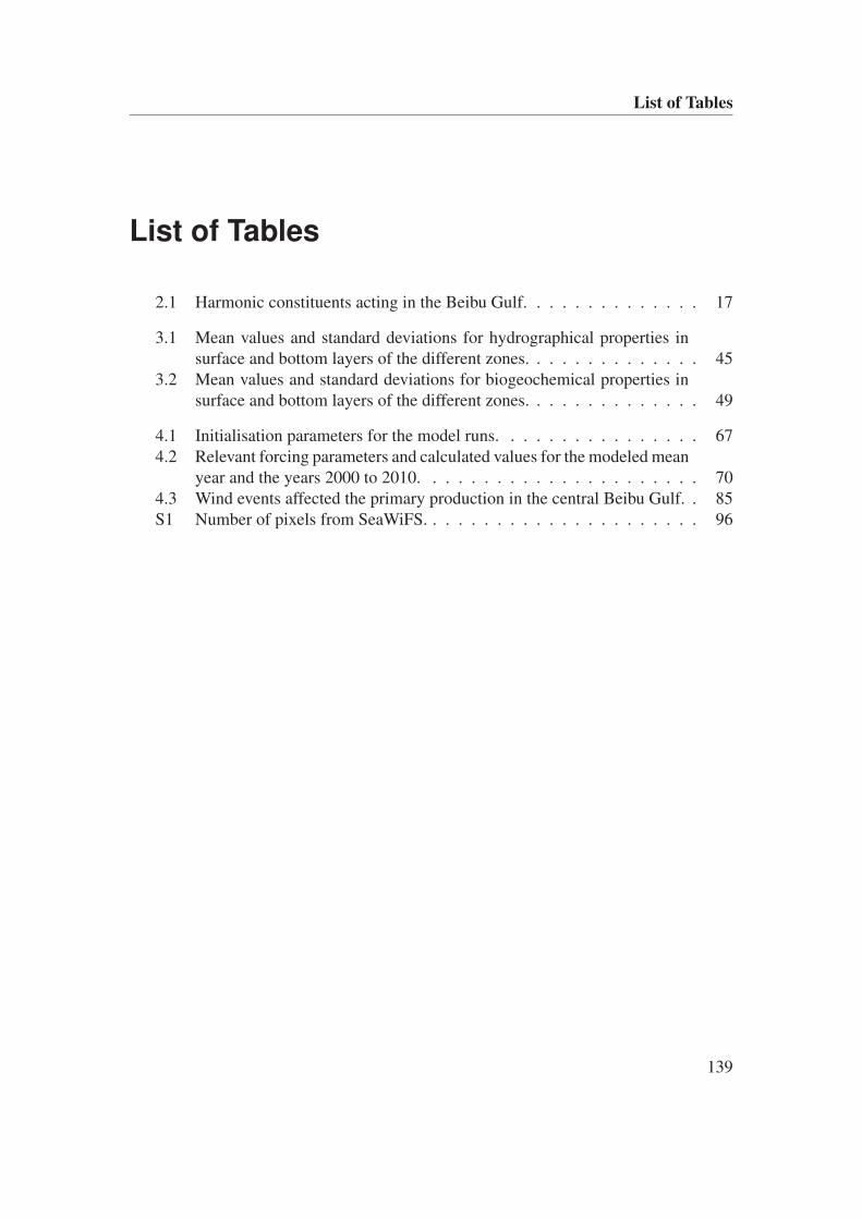
List of Tables
List of Tables
2.1 Harmonic constituents acting in the Beibu Gulf. . . . . . . . . . . . . . 17
3.1 Mean values and standard deviations for hydrographical properties insurface and bottom layers of the different zones. . . . . . . . . . . . . . 45
3.2 Mean values and standard deviations for biogeochemical properties insurface and bottom layers of the different zones. . . . . . . . . . . . . . 49
4.1 Initialisation parameters for the model runs. . . . . . . . . . . . . . . . 674.2 Relevant forcing parameters and calculated values for the modeled mean
year and the years 2000 to 2010. . . . . . . . . . . . . . . . . . . . . . 704.3 Wind events affected the primary production in the central Beibu Gulf. . 85S1 Number of pixels from SeaWiFS. . . . . . . . . . . . . . . . . . . . . . 96
139
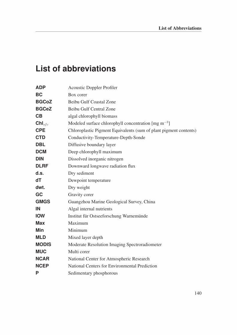
List of Abbreviations
List of abbreviations
ADP Acoustic Doppler Profiler
BC Box corer
BGCoZ Beibu Gulf Coastal Zone
BGCeZ Beibu Gulf Central Zone
CB algal chlorophyll biomass
Chlsfc Modeled surface chlorophyll concentration [mg m−3]
CPE Chloroplastic Pigment Equivalents (sum of plant pigment contents)
CTD Conductivity-Temperature-Depth-Sonde
DBL Diffusive boundary layer
DCM Deep chlorophyll maximum
DIN Dissolved inorganic nitrogen
DLRF Downward longwave radiation flux
d.s. Dry sediment
dT Dewpoint temperature
dwt. Dry weight
GC Gravity corer
GMGS Guangzhou Marine Geological Survey, China
IN Algal internal nutrients
IOW Institut für Ostseeforschung Warnemünde
Max Maximum
Min Minimum
MLD Mixed layer depth
MODIS Moderate Resolution Imaging Spectroradiometer
MUC Multi corer
NCAR National Center for Atmospheric Research
NCEP National Centers for Environmental Prediction
P Sedimentary phosphorous
140
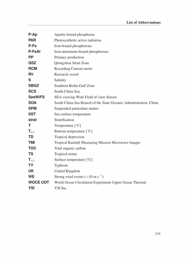
List of Abbreviations
P-Ap Apatite-bound phosphorus
PAR Photosynthetic active radiation
P-Fe Iron-bound phosphorous
P-FeAl Iron-aluminum-bound phosphorous
PP Primary production
QSZ Qiongzhou Strait Zone
RCM Recording Current meter
RV Research vessel
S Salinity
SBGZ Southern Beibu Gulf Zone
SCS South China Sea
SeaWiFS SEA-viewing Wide Field of-view Sensor
SOA South China Sea Branch of the State Oceanic Administration, China
SPM Suspended particulate matter
SST Sea surface temperature
strat Stratification
T Temperature [°C]
Tbot Bottom temperature [°C]
TD Tropical depression
TMI Tropical Rainfall Measuring Mission Microwave Imager
TOC Total organic carbon
TS Tropical storm
Tsfc Surface temperature [°C]
TY Typhoon
UK United Kingdom
WE Strong wind events (>10 m s−1)
WOCE UOT World Ocean Circulation Experiment Upper Ocean Thermal
YSI YSI Inc.
141
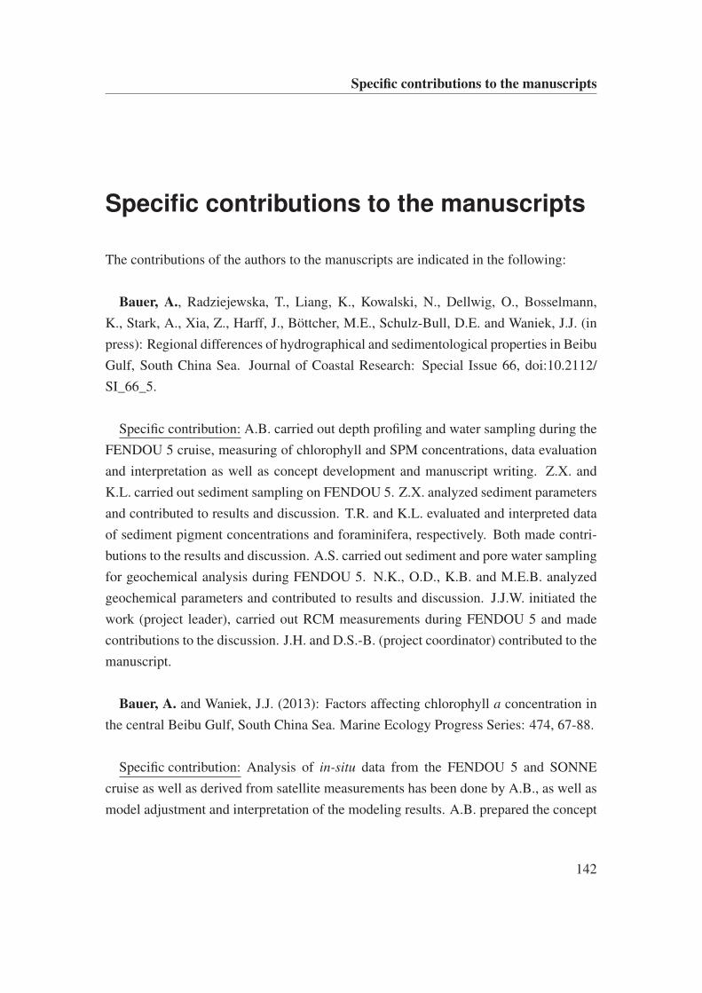
Specific contributions to the manuscripts
Specific contributions to the manuscripts
The contributions of the authors to the manuscripts are indicated in the following:
Bauer, A., Radziejewska, T., Liang, K., Kowalski, N., Dellwig, O., Bosselmann,
K., Stark, A., Xia, Z., Harff, J., Böttcher, M.E., Schulz-Bull, D.E. and Waniek, J.J. (in
press): Regional differences of hydrographical and sedimentological properties in Beibu
Gulf, South China Sea. Journal of Coastal Research: Special Issue 66, doi:10.2112/
SI_66_5.
Specific contribution: A.B. carried out depth profiling and water sampling during the
FENDOU 5 cruise, measuring of chlorophyll and SPM concentrations, data evaluation
and interpretation as well as concept development and manuscript writing. Z.X. and
K.L. carried out sediment sampling on FENDOU 5. Z.X. analyzed sediment parameters
and contributed to results and discussion. T.R. and K.L. evaluated and interpreted data
of sediment pigment concentrations and foraminifera, respectively. Both made contri-
butions to the results and discussion. A.S. carried out sediment and pore water sampling
for geochemical analysis during FENDOU 5. N.K., O.D., K.B. and M.E.B. analyzed
geochemical parameters and contributed to results and discussion. J.J.W. initiated the
work (project leader), carried out RCM measurements during FENDOU 5 and made
contributions to the discussion. J.H. and D.S.-B. (project coordinator) contributed to the
manuscript.
Bauer, A. and Waniek, J.J. (2013): Factors affecting chlorophyll a concentration in
the central Beibu Gulf, South China Sea. Marine Ecology Progress Series: 474, 67-88.
Specific contribution: Analysis of in-situ data from the FENDOU 5 and SONNE
cruise as well as derived from satellite measurements has been done by A.B., as well as
model adjustment and interpretation of the modeling results. A.B. prepared the concept
142
Specific contributions to the manuscripts
of the paper and did the writing. J.J.W. made contributions to the manuscript.
Bauer, A., Fründt, B. and Waniek, J.J. (Manuscript): Sediment resuspension patterns
and the diffusive boundary layer in the Beibu Gulf, South China Sea.
Specific contribution: A.B. analyzed RCM and ADP current data as well as NCEP-
derived wind data, made harmonic analysis and all calculations, gathered data for tidal
heights from WXTide32 and measured SPM concentrations. Surface sediment data
were provided by GMGS. Central idea for the tidal model came from A.B.; B.F. wrote
the calculations routines. Data interpretation as well as concept development and manus-
cript writing has been carried out by A.B. J.J.W. initiated the work and made contribu-
tions to the manuscript.
143
Danksagung
Danksagung
Zu allererst möchte ich mich bei meiner Doktor-Mutter PD Dr. habil. Joanna J. Waniek
bedanken. Sie gab mir die Möglichkeit an diesem interessanten Projekt teilzunehmen
und half mir, als Wissenschaftlerin, vor allem interdisziplinär, zu wachsen. Diese Arbeit
entwickelte sich nicht nur durch meine Anstrengungen, auch ihre Anregungen haben er-
heblich zum Erfolg beigetragen. Danke für deine immerwährende Unterstützung und
Geduld.
Außerdem möchte ich mich für die Möglichkeit zur Teilnahme an der FENDOU 5
Expedition bedanken. Diese Reise war eine unglaublich tolle Erfahrung und ich danke
allen Fahrtteilnehmern, vor allem aber den chinesischen Projektpartnern (Xiong Liu,
Zhangcun Yan, Kai Liang, uvm.) und Besatzungsmitgliedern, für die unvergessliche
Zeit. Insbesondere sei dem Kapitän und seinen Offizieren gedankt, dass sie das Schiff
und uns wohlbehalten durch einen Taifun gesteuert haben.
Ich danke meinem Thesis Komitee: PD Dr. habil. Joanna J. Waniek, Prof. Dr. Detlef
Schulz-Bull, Dr. Herbert Siegel und Dr. Douglas Connelly für die Unterstützung und
schnelle Hilfe, wenn es nötig war: Ihr hattet immer ein offenes Ohr für mich.
Für wissenschaftliche und auch sonstige Unterstützung bedanke ich mich bei: Dr.
Teresa Radziejewska, Dr. Nicole Kowalski, Dr. Olaf Dellwig, Dr. Katja Bosselmann,
Alexander Stark, Prof. Zhen Xia, Prof. Dr. Jan Harff, Prof. Dr. Michael Böttcher,
Birgit Sadkowiak, Ines Hand, Annika Fiskal, Dr. Thomas Leipe, Dr. Kerstin Perner, Iris
Stottmeister und Dr. Ralf Prien.
Ganz besonderer Dank gilt meinen "Büromitbewohnerinnen" Birte Fründt und Dr. Ju-
liane Brust, für die vielen Gespräche, ihre Hilfe bei großen und kleinen Matlab-Sorgen
und die entspannenden Mittagspausen. Die Zeit mit euch war super!
144

Danksagung
Desweiteren sei den Mitarbeitern des IOW, insbesondere der Sektion Meereschemie,
für die schöne Zeit am Institut gedankt.
Mein größter Dank aber gilt meiner Familie, vor allem meinem Mario: Ohne eure
ständige Unterstützung wäre diese Arbeit nicht möglich gewesen! Ihr wart immer für
mich da und habt mich geduldig auch in stressigen Phasen ertragen. Vielen Dank dafür!
145
Eidesstattliche Erklärung
Eidesstattliche Erklärung
Ich versichere hiermit an Eides statt, dass ich die vorliegende Arbeit selbstständig ange-
fertigt und ohne fremde Hilfe verfasst habe, keine außer den von mir angegebenen Hilf-
smitteln und Quellen dazu verwendet habe und die den benutzten Werken inhaltlich und
wörtlich entnommenen Stellen als solche kenntlich gemacht habe.
Andrea Bauer Rostock, den 30. August 2012
146


![Synthesis and Characterization of [n]Cumulenes](https://img.pdfslide.org/doc/110x75/58a181de1a28abb24d8c126c/synthesis-and-characterization-of-ncumulenes-.jpg)