Embed Size (px)
Citation preview
Investigation of a ternary liquid mixture by the light scattering
technique
DISSERTATION
Zur Erlangung des akademischen Grades
doctor rerum naturalium (Dr. rer. nat)
vorgelegt der
Mathematisch-Naturwissenschaftlich-Technischen Fakultät
(mathematisch-naturwissenschaftlicher Bereich)
der Martin-Luther-Universität Halle-Wittenberg
von Herrn Dipl.-Phys. Dimitry A. Ivanov
geb. am 05 April 1977 in Minsk
Gutachterin/Gutachter
1. Prof. Dr. habil. Jochen Winkelmann
2. Prof. Dr. habil. Mikhail A. Anisimov
Halle (Saale), den 18 November 2005
urn:nbn:de:gbv:3-000009293[http://nbn-resolving.de/urn/resolver.pl?urn=nbn%3Ade%3Agbv%3A3-000009293]
2
Contents
Symbols…………………………………………………………………. 41. Introduction………………………………………………………….. 8
2. Theoretical part……………………………………………………… 16
2.1.Light Scattering……………………………………………………………... 162.2.Intensity of scattered light…………………………………………………... 212.3.Critical opalescence………………………………………………………… 242.4.Spectrum of light scattered from hydrodynamic fluctuation……………….. 272.5.Hydrodynamic fluctuations in ternary liquid mixture….…………………... 312.6. Spectrum of light scattered in near-critical ternary fluid mixture…………... 42
3. Experimental part…………………………………………………… 47
3.1.Chemicals and equipment…………………………………………………... 473.2.Preparation of the samples………………………………………………….. 483.3.Determination of related quantities………………………………………… 513.4.Light scattering measurements……………………………………………... 523.5. Check of optical justage of the equipment and performance of the light
scattering measurements……………………………………………………. 54
3.6. Measurements of the autocorrelation function (ACF) and linewidth of the
Rayleigh scattering…………………………………………………………. 57
3.7.Estimation of the chemical potential gradient……………………………… 60
4. Results of the static and dynamic light scattering measurements…… 62
4.1.Determination of the correlation length and the osmotic susceptibility……. 634.2.Data evaluation……………………………………………………………... 694.3.Determination of the diffusion coefficients………………………………… 70
3
5. Discussion…………………………………………………………… 78
5.1.Theoretical analysis of two diffusion modes in the hydrodynamic range….. 785.2. The analysis of two diffusion modes in the critical range and comparison
with experiment…………………………………………………………….. 80
6. Summary…………………………………………………………….. 86
7. Appendix…………………………………………………………….. 89
7.A. Expression for the scattered field………………………………………….. 89
7.B. A time correlation function………………………………………………... 92
7.C. The relation between thermodynamic and transport properties in theternary liquid mixture……………………………………………………… 93
7.D. The solution of the dispersion equation…………………………………… 97
7.E. The linearized hydrodynamic equations in terms of the concentrations,temperature and pressure………………………………………………….. 99
7.F. The expression for the correlation functions of the concentrations andtemperature………………………………………………………………… 100
7.G. The expression for the activity coefficients……………………………….. 102
7.H. Tables……………………………………………………………………… 103
8. References…………………………………………………………… 107
4
Symbols
symbol meaning units
0 dielectric (average) constant -
q scattering vector 1m
0 angular frequency of the incident light rad s
V scattering volume 3m
0I intensity of light beam 2W m
x , z position coordinate, length scale m
,R , position in spherical polar coordinates -
d solid angle sr
,R scattering cross section -
turbidity -
i fk k
wavevector of the incident (scattered) beam 1m
i wavelength in a media m
i angular frequency in a media rad s
t time s
0iE E incident (incoming) electric field V m
in unit vector -
ip dipole moment C m
polarizability 3m
number density of particles in mixture .partn V
n refractive index -
scattering angle rad
fn vector of the polarization -
5
R~ distance between scattering volume and detector m
p pressure Pa
T temperature K
,i ic C concentration of species i 3mol m
SE scattering electric filed V m
R Rayleigh ratio -
S t cS S dynamic, generalized (static) structure factor kg mol
ik thermodynamic coefficients -
molar gas constant 8.314 J mol K
iM molecular weight of species i kg mol
i chemical potential of species i J mol
TC generalized osmotic susceptibility -
correlation length m
( )G t , )(rG time (space) autocorrelation function -
N Avogadro’s constant 23 16.022 10 mol
Bk Boltzmann constant 231.38 10 J K
T isothermal compressibility 1Pa
critical exponent -
sound wave length m
'c c speed (in medium) of sound m s
density 3kg m
S entropy J K
R BMI I intensity of Rayleigh (Brillouin) line 2W m
P vc c heat capacities at constant pressure (volume) J K
6
u mass velocity m s
S V shear (volume) viscosities Pa s
i Onsager kinetic coefficient 3kg s m
i Onsager kinetic coefficient 1Pa s K
Onsager kinetic coefficient J Pa s K mol
im mass of species i kg
thermal conductivity W m K
ik' viscous stress tensor Pa
Q heat current 3J kg mol m
I mass diffusion current J Pa mol
ijD coefficients of the Fick’s diffusion matrix 2m s
Tik thermal diffusion ratio -
Pik thermodynamic quantity -
, , Ta D coefficient of the thermal conductivity -
T thermal expansion coefficient 1K
divergence of u m s
ijP algebraic function - 1 2
12 21
, ,,
M MM M
coupling parameters -
width of Brillouin component rad s
heat capacity ratio -
iA amplitudes of the relaxation modes -
CT , .c visT critical (demixing) temperature K
cix critical mole fraction of species i -
R coefficient of the optical justage -
7
TrI intensities of the transmitted light 2W m
BI intensities of the background scattering 2W m
u depolarization coefficient -
,c d characteristic decay times of ACF s
,c dA characteristic amplitudes of ACF -
ijF thermodynamic correction factor -
i activity coefficient -
ij Kronecker delta -
ijA , ij NTRL parameters K , -
static structure factor exponent -
critical exponents of the osmotic susceptibility -
critical exponents of the correlation length -
heat capacity exponent above the plait point -
critical exponents of the mass diffusion -
1,2D two effective diffusivities 2m s
J Landau-Placzek ratio -
,fast slowD diffusivities of the fast (slow) relaxation modes 2m s
Subscripts
i number of componentj number of component
n last component, number of components in a mixturefast transport properties of a fast mode
slow transport properties of a slow mode
1 Introduction
8
1 Introduction
In the last years an increasing amount of efforts has been devoted to the theoretical andexperimental investigation of mass transfer in liquid mixtures. In the centre of interestwas the mass transfer across liquid-liquid interfaces. The problem of the detailedunderstanding of transport in liquid-liquid interfaces between two (or more) immiscibleliquid phases is of great importance for chemistry and chemical engineering inoperations like liquid extraction, solid extraction, absorption, drying, distillation,chemical reaction processes as well as for biology in operations like fermentation,biological filtration and biological syntheses. In spite of its technological importance,the details of the transfer processes are not very well understood yet. There are severaltopic questions of mass transfer under continuous investigation. One is related to thethermodynamic equilibrium between two phases on their surface area, which bases onthe concept of Nernst who assumed for a non-equilibrium at interfaces, that thedistinction in the chemical potential will cause large forces, which will result in animmediately establishment of the thermodynamic equilibrium. Mass transfer theorygenerally assumes that at the interface a distribution equilibrium exists, but this has notbeen confirmed experimentally till now. A second question is, how to define the phaseboundary. Is it an infinitesimal small geometrical locus with certain concentrationprofile or a small zone with properties differing from those within the bulk phases. Thiscould mean for instance that the mobility of molecules in this region is restricted byadhesive forces and the coefficient of diffusion is noticeably diminished near the liquid-liquid interface. A third one, related to the former two, could be the question of whetherthere exists an interfacial mass transfer resistance. An answer to many of thesequestions could be given, knowing the course of the concentration profile crossing theinterface. The application of optical measurements of mass transfer processes seems tobe a promising step towards this goal. Optical techniques are non-destructive and aconcentration measurement with high spatial and time resolution is possible withoutmajor disturbance of the interesting transport processes. To contribute towards asolution of these questions, the mass transfer of a substance across an interface betweenthree miscible liquids was studied, the used optical measurement technique is describedand results are presented here.
A typical Light Scattering experiment is shown in Figure 1.1. When incoming lightreacts with matter, the electric field component of the radiation induced an oscillatingpolarization of electrons in the molecules. The molecules then serve as secondarysources of light and subsequently they are sources of scattered radiation. The scatteredlight gives us information about molecular structure and motion in the material. Ingeneral, interaction of electromagnetic radiation with a molecule leads either toabsorption, forms the basis of the spectroscopy, or to a scattered radiation. Visible lightis extensively used as a nonperturbative direct probe of the state and the dynamics ofsmall particles in solution. The light traversing through a medium is scattered intodirections other than that of the reflected and refracted beam by the spatial inhomogeneity of the dielectric constant
1 Introduction
9
Transport Behaviour
Molecular Weight
Particle Size
Particle Shape
Mobility
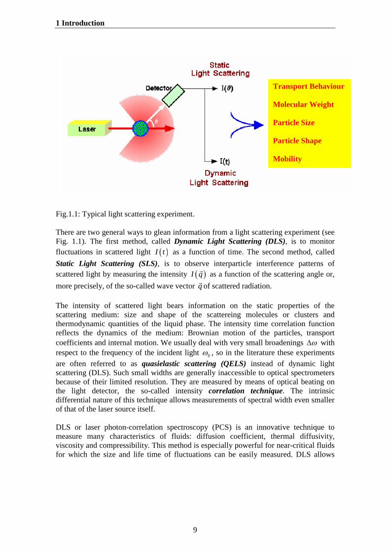
Fig.1.1: Typical light scattering experiment.
There are two general ways to glean information from a light scattering experiment (seeFig. 1.1). The first method, called Dynamic Light Scattering (DLS), is to monitorfluctuations in scattered light I t as a function of time. The second method, calledStatic Light Scattering (SLS), is to observe interparticle interference patterns ofscattered light by measuring the intensity I q
as a function of the scattering angle or,
more precisely, of the so-called wave vector q
of scattered radiation.
The intensity of scattered light bears information on the static properties of thescattering medium: size and shape of the scattereing molecules or clusters andthermodynamic quantities of the liquid phase. The intensity time correlation functionreflects the dynamics of the medium: Brownian motion of the particles, transportcoefficients and internal motion. We usually deal with very small broadenings withrespect to the frequency of the incident light 0 , so in the literature these experimentsare often referred to as quasielastic scattering (QELS) instead of dynamic lightscattering (DLS). Such small widths are generally inaccessible to optical spectrometersbecause of their limited resolution. They are measured by means of optical beating onthe light detector, the so-called intensity correlation technique. The intrinsicdifferential nature of this technique allows measurements of spectral width even smallerof that of the laser source itself.
DLS or laser photon-correlation spectroscopy (PCS) is an innovative technique tomeasure many characteristics of fluids: diffusion coefficient, thermal diffusivity,viscosity and compressibility. This method is especially powerful for near-critical fluidsfor which the size and life time of fluctuations can be easily measured. DLS allows
1 Introduction
10
monitoring the growth of the particles during a particular chemical or physico-chermicalprocess and studying the kinetics of such a process.
In contrast to DLS in static light scattering experiments the time-averaged (or 'total')intensity of the scattered light is observed and measured for a solution. It is related totime-averaged mean-square dielectric constant fluctuations, which in turn are related tothe time-averaged mean-square fluctuations in the thermodynamics quantities. Thecourse of the scattered intensity as a function of the detector angle depends on size andstructure of the particles.
In 1869 Tyndall began experimental studies of light scattering from aerosols and, basedon the initial theoretical work of Rayleigh (1871), light scattering has been used toinvestigate a variety of physical phenomena. Rayleigh explained the blue color of thesky and the red sunset as due to the preferential scattering of short-wave visible light bythe molecules in the atmosphere. The theoretical model of Rayleigh assumes scatteringfrom statistical assemblies of noninteracting particles, which are sufficiently smallcompared to the wavelength of the light to be regarded as point-double oscillators.Debye (1915) made contribution to the theory of large particles and extend thecalculation to the particles of nonspherical shape.
It was soon found that light scattering in multicomponent mixture and in solid gasescould be explained by the Rayleigh theory. In particular, the intensity of scattering by acondensed phase, consisting of N particles, is equal to the sum over N intensities only inthat case where the particles do not interact with each other. However, fromexperimental data one can expect that summation is more complex, dependent on theinteraction of fields of each of scattering particles. To a full interpretation of these data,on the one hand, it is necessary to have the information on intermolecular forces in thesystem, and on the other hand one needs a microscopic theory of an electric fieldinfluence on a molecule. Smoluchowski (1908) and Einstein (1910) elegantlycircumvented this difficulty by considering the liquid to be a continuous medium inwhich thermal fluctuation give rise to local inhomogeneities and thereby to density andconcentration fluctuation. These authors developed a fluctuation theory of lightscattering. According to this theory, the intensity of the light scattering can becalculated from mean-square fluctuations in density for one-component liquid, and / orfluctuation in the concentration in multicomponent liquid mixture, which in turn can bedetermined from macroscopic data such as the isothermal compressibility andconcentration-dependence of the osmotic pressure.
Later Ornstein and Zernike have developed a theory, which takes in account correlationbetween fluctuations in different microscopic elements of the scattering volume. Theypredicted the angular dependence of light intensity that has been scattered in the fluidcritical region. This theory was developed for the explanation of an extreme increase inthe turbidity of a fluid near the critical point (critical opalescence). This marked increasein intensity of scattering light is a consequence of the fact that the pair-correlationfunction in a system near its critical point becomes infinitely long-ranged.
1 Introduction
11
In the foregoing phenomenological theories of Rayleigh and Einstein no attempt wasmade to describe that particles or elements of a scattering volume optically anisotropic.Cabaness (1929) and Gans (1921) have shown that it is necessary to bring in thoseamendments to these theories to take in account optical anisotropy of molecules and itsinfluence on the polarization of scattered light. In these theories, however, it isnecessary to calculate the work of orientation in certain directions of chaotically locatedparticles of a liquid. It is necessary to have experimental information on preferrableorientation in space of the liquid particles, which are rather difficult to receive. Debyemade such calculation for a solution of anisotropic molecules.
Gross conducted a series of light scattering experiments on liquids observing a central(unshifted) Rayleigh peak and the Brillouin doublet, which is shifted in the frequencydistribution of the light scattered from thermal sound waves (phonons) in a liquid.Landau and Placzek (1934) gave a theoretical explanation of these peaks using a quasi-thermodynamic approach.
With the advent of laser, another type of experiments became possible. Analyzing thefrequency distribution of scattered light, Pecora [8,44] (1964) showed that the spectrumwould yield information about values of diffusion coefficient and under certaincondition it might be used to study rotational motion and flexibility of macromolecules.The use of classical interference spectroscopy (Fabry-Perot spectroscopy) to resolve thefrequency distribution of scattered light is not possible, since frequency changes arevery small. To spectrally resolve the light scattering in 1964 Cummins, Knable and Yehused the optical-mixing technique. Since that moment optical-mixing spectroscopy hasbecome a major tool for the measurement of transport properties of gases and liquids.
There exists currently considerable interest in the nature of fluctuations in fluidmixtures driven away from thermal equilibrium by imposing a temperature andconcentration gradient. An interesting feature is that under such nonequilibriumconditions all fluctuations become long-range. These fluctuations can be studyied byobserving the static and dynamic properties of laser light scattered from such fluids outof thermal equilibrium. The behaviour of thermodynamic properties of fluids and fluidmixtures is strongly affected by the presence of critical points, such as the vapour-liquidcritical point in one-component fluids, plait points and consolute points in liquidmixtures, etc. The presence of long-range fluctuations is associated with critical phase-transition phenomena. Based on modern theoretical analysis, we are trying to obtain anaccurate representation of the thermodynamic behaviour of fluids and fluid mixturesclose to and not so close to these critical points. The aim is to obtain fundamentalequations for chemical engineering applications over a wide range in temperature andconcentration that incorporate the crossover from singular critical thermodynamicbehaviour to regular thermodynamic behaviour far away from critical phase transitions.A challenging task of the research is to obtain equations for chemical engineeringapplications that incorporate the universal (affected by fluctuations and cooperativephenomena) critical behaviour of fluids and nonuniversal (affected by specificintermolecular interactions) behaviour far away from the critical point. The presence of
1 Introduction
12
long-range fluctuations in fluids and fluid mixtures near critical-point phase transitionsalso strongly affects the behaviour of transport properties. The effects of long-rangefluctuations on the transport properties can be understood quantitatively with themethods of generalized hydrodynamics.
The first investigations of the static light scattering in a ternary critical mixture ofbrombenzene-acetone-water were carry out in 1969 by Bak and Goldburg [6]. They hadobserved deviations from static scaling law. Indeed larger critical exponents appearedfor the osmotic susceptibility and correlation length than with the three-dimensionalIsing model and the renormalization were to be expected. In 1974, the intensity andRayleigh linewidth of light scattering by concentration fluctuation has been examinedby Chu and Lin [13-15], who studied a liquid-liquid critical point in the ternary ethanol-water-chloroform system. Also in 1982 there have been carried out measurements ofcritical exponents in a ternary mixture benzene-water-ethanol by Rousch, Tartiglia, andChen [48]. In recent time the behaviour of ternary mixtures is also discussed inconnection with "crossover" effects in aequeous electrolyte solutions. In aninvestigation of Sengers et al. [28], a mixture of 3-methylpyridin-water-natriumbromideshowed an enlargement of the critical exponent of the osmotic susceptibility withincreasing concentration in sodium bromide. Müller [39-41] investigated two ternarymixtures: aniline + cyclohexane + p-xylene and N,N-dimetylformamide + n-heptane +toluene. In those systems he studied the correlation length of fluctuations, generalizedosmotic susceptibilities, mutual diffusion coefficients, and viscosities as a function ofthe compositions and temperatures. Moreover, he investigated the shift in criticalexponents, the validity of power lows, and the role of correction to scaling whenchanging from binary critical point to a ternary plaint point. Leipertz et al. [23,24,51-53]specify results of the thermophysical properties for various binary and ternaryrefrigerant liquid mixtures obtained by dynamic light scattering, in both the liquid andthe vapor states, along the saturation line approaching the vapor-liquid critical point.Moreover, they have found data both for the thermal diffusivity and sound speed, andfor the kinematic viscosity in a wide range of temperatures and pressures.
For the first time the theoretical description of the spectrum of the light, scattered by abinary solution, has been given by Mountain and Deutch [38]. To calculate the spectrumof a two-component fluid mixture they are using the approach suggested by Landau andPlaczek in [32]. They used linearized hydrodynamic equations to determine the modesby which the system returns to equilibrium as well as the relative amplitude for eachmode and thermodynamic fluctuation theory to provide initial values. They obtainedexpression for the position and widths of the two-side shifted Brillouin peaks, and thecentral, unshifted Rayleigh peak. Mountain and Deutch had found that the Rayleighpeak consists of a superposition of two Lorentzians that involve the combined dynamiceffect of heat conduction and diffusion. They conclude, that under certain condition it ispossible to simply separate the central peak into two contributions. The first one arisesfrom mass diffusion and the second one from thermal conduction. Hence, havingmeasurements of the light scattering spectrum it should be possible to obtain values ofmulticomponent diffusion.
1 Introduction
13
However, Mountain and Deutch have considered behaviour of the spectrum andtransport properties of binary solution only in the hydrodynamic range, i.e. far awayfrom critical point. Anisimov et al. [1-4,30] have developed aforesaid theory for thecase of a critical mixture. They carried out the correlation analysis of a critical mixtureof methane and ethane. Anisimov’s theory predicts the existence of two-exponentialdecay functions in dynamic light scattering in near-critical fluid mixtures. In this one itis shown that in a binary fluid mixture a coupling can occur between two transportmodes where one is associated with mass diffusion and the other with thermal diffusion.The authors describe the thermodynamic and transport behavior and the criticalbehavior of the dynamic structure factor and they discuss in detail the conditions underwhich weak or strong coupling between the contributions of the effective diffusivitiesD1 and D2 in the dynamic light scattering are to be expected. Moreover, they found thatthe physical meaning of the two diffusivities D1 and D2 changes depending on thepoints on the critical locus that were considered. Contrary to the case of the infinite-dilution limit, where the slow mode diffusivity D1 is associated with the thermaldiffusion and the fast mode D2 with mass diffusion, the authors found that for a liquid-liquid consolute point the physical meaning of D1 and D2 changes as the slow mode D1
is associated with mass diffusion and the fast D2 with thermal diffusion. Leipertz andco-workers [23] experimentally verified the theoretical predictions of Anisimov et al. bysimultaneous determination and separation of the mass diffusion from the thermaldiffusion coefficients.
As an object of the investigations the system glycerol (0) + acetone (1) + water (2) (inthe following with GAW abbreviated) was selected. This system shows strongasymmetry of the critical line. There is one reported measurements of liquid-liquidequilibrium for this system by Krishna et al. [31]. The plaint point from thermodynamicstability consideration of this liquid mixture was determinate. Also for this system werefound the NTRL and UNIQUAC parameter set, which are required for determination ofthe thermodynamic factor (see section 3.7).
Theories advanced in works Mountain, Deutch and Anisimov are applicable only for abinary mixture case. Leaist and Hao [35] give a comparison of their Taylor dispersionand DLS measurements of diffusion coefficient in a ternary system of sodium dodecylsulfate in aqueous sodium chloride solution. Similar comparison of Taylor dispersionand DLS methods has been lead to our study of the GAW system in [26]. Leaist andHao formally extended the theoretical approach for a binary mixture by Mountain andDeutch to ternary solution. But their expression for the spectrum of light scattering byonly the concentration fluctuation case is developed. They have introducing twoeigenvalues for diffusivity. But, they discuss limiting cases of ideal dilute nonelectrolytesolution or diffusion of macroparticle and conclude that only mass transport modesshould result.
1 Introduction
14
Thus we have the following “open questions”:
How is the hydrodynamic theory of Mountain and Deutch to be transformed todescribe a ternary liquid mixture?
Is it possible to describe behaviour of two hydrodynamic relaxation modes(Anisimov’s theory) in near-critical ternary fluid mixture?
How the theory Leaist and Hao will change if to extend with inclusion in itpressure and temperature fluctuations?
It is the main purpose of this thesis to describe the theory of light-scattering experimentand its application to investigate transport properties for ternary liquids mixtures,especially the diffusion behaviour in mixtures with liquid-liquid phase separation. Thiswork deals with the following topics:
Multicomponent models on the basic linearized hydrodynamic equations andtheory of thermodynamic fluctuation to determinate relaxation diffusion modes.
Extending and addition aforesaid theories under various conditions and toternary liquid mixture case.
The physical explanation of two hydrodynamic relaxation modes in the vicinityof different points of binodal curve and far from it.
Determination of the intensities (amplitudes) of one at towards to a plait point ofthe GAW system.
Discuss the condition at which a two-exponentional decay of the autocorrelationfunction (ACF) can be measured by DLS.
Behavior of GAW system at towards to a plait point. The prediction of ternary diffusivities in GAW system in the vicinity form
critical point and far away from it.
This thesis is organized as follows. In Chapter 2 we give the theoretical background onlight scattering from fluctuation of the thermodynamic values in ternary fluids mixture.We first introduce an equation for the generalized structure factor and turbidity of lightscattering, and the concept of the critical opalescence. On the basic theory of thelinearized hydrodynamic equations we derived the new expressions for the spectrum ofthe light scattered of a ternary mixture. Moreover in this Chapter we found expressionsfor the time distribution of the scattered light. Here we developed a theory for thedescription of the critical phenomenon in the multicomponent mixture. By using thisexpression we can predict transport property behaviour in the immediate vicinity to thecritical point and far from it.
Chapter 3 deals with experimental aspects of DLS for ternary mixtures. We describemethods of the light scattering for measurements of both static and dynamic properties.For this purpose we use seventeen different composition of GAW system. Three
1 Introduction
15
samples of our mixtures near plait point were prepared. In this Chapter we discusscheck of optical justage and performance of light scattering measurements. Also weconsider the problem of data evaluations of ACF and estimation data for the chemicalpotential gradient.
Chapter 4 deals with describe experimental data for our ternary mixture. We discuss thebehaviour of static properties, such as the generalized osmotic susceptibility and thecorrelation length, near critical singularity and far from it. Here also we present acollection of ternary diffusion data near critical point. We determine critical exponentsof GAW system of the osmotic susceptibility, the correlation length and mass diffusion,obtained from power-law fitting. Moreover in this Chapter we have shown theprocedure of data evaluation. Finally, we found that, in the vicinity of the criticalsolution point the dynamic light scattering measurements in our system reveal twohydrodynamic relaxation modes with well-separated characteristic relaxation times.
Chapter 5 deals with the analysis of two diffusion modes of ACF in hydrodynamicrange and critical point, and comparison with experiment. The Chapter begins with thedetermination of the condition under which it is possible to separate the Rayleigh peaksimply into two contributions, one arising from mutual diffusion and one from thermalconduction. We discuss in details the behavior of ACF near the critical point. Here weobtained temperature- and concentration-dependences of both diffusivities andamplitudes, and we compared them to the experimental data. The Chapter ends withdiscussion and conclusion.
2 Theoretical part 2.1 Light Scattering
16
2 Theoretical part
In this section, the theoretical background of dynamic light scattering as well as thetheoretical description of the spectral distribution of the scattered light is presented faraway from critical decomposition point and near to it. Moreover, the theoreticalexplanation of the critical opalescence phenomenon is given here. The discussion oflight scattering begins with the scattering theory of electromagnetic waves at isotropicsystems. On the basis of this theory, the equations for static and dynamic lightscattering, necessary of the evaluation for the results of our measurement are deduced.
The dynamic structure factor is calculated from the theory of thermodynamicfluctuations with the help of linearized hydrodynamic equations appropriate to the threecomponents fluid. The knowledge necessary for the evaluation and classification oftransport properties near critical point for ternary mixture is made available. In thevicinity of the critical solution point the calculation of the dynamic structure factor forternary liquid system reveal three hydrodynamic relaxation modes with their owncharacteristic relaxation times.
2.1 Light Scattering
The interaction of light with matter can be used to obtain important information aboutstructure and dynamics of matter. When light interacts with matter it will scatter and thescattered light gives us information about molecular structure and motion in thematerial. In general, interaction of electromagnetic radiation with a molecule leadseither to absorption, which forms the basis of the spectroscopy, or to scattering theradiation. Visible light is extensively used as a nonperturbative direct probe of the stateand the dynamics of small particles in solution. The light traversing a medium isscattered into directions other than that of the reflected and refracted beam by spatialinhomogeneity of the dielectric constant The weaker scattering due to spontaneousthermal fluctuations of in the solvent can usually be neglected or properly subtracted.In this section the theoretical aspects of light scattering will be reviewed briefly.
The physical origin of light scattering can be simply understood by considering theparticle as an elementary dipole, which is forced to oscillate at the frequency of theincident field and, in turn, radiates. Almost all of the scattered light has the samewavelength as the incident radiation and comes from elastic (or Rayleigh) scattering.The radiated or scattered light at a given time is the sum (superposition) of the electricfields radiated from all of the charges in the illuminated scattering volume andconsequently depends on the exact position of the charges. The molecules in theilluminated region are perpetually translating, rotating and vibrating by virtue ofthermal motion (Brownian Motion). Because of this motion the position of the chargesare constantly changing so that the total scattered electric field at the detector will
2 Theoretical part 2.1 Light Scattering
17
fluctuate in time. Implicit in these fluctuations is important structural and dynamicalinformation about the position and orientations of the molecule. This fluctuation giverise to a Doppler effect and so the scattered light possesses a range of frequenciesshifted very slightly from the frequency of the incident light. This phenomenon is calledquasi-elastic light scattering or dynamic light scattering. These frequency shifts yieldinformation relating to the movement (i.e. the dynamics) of the solute molecules.
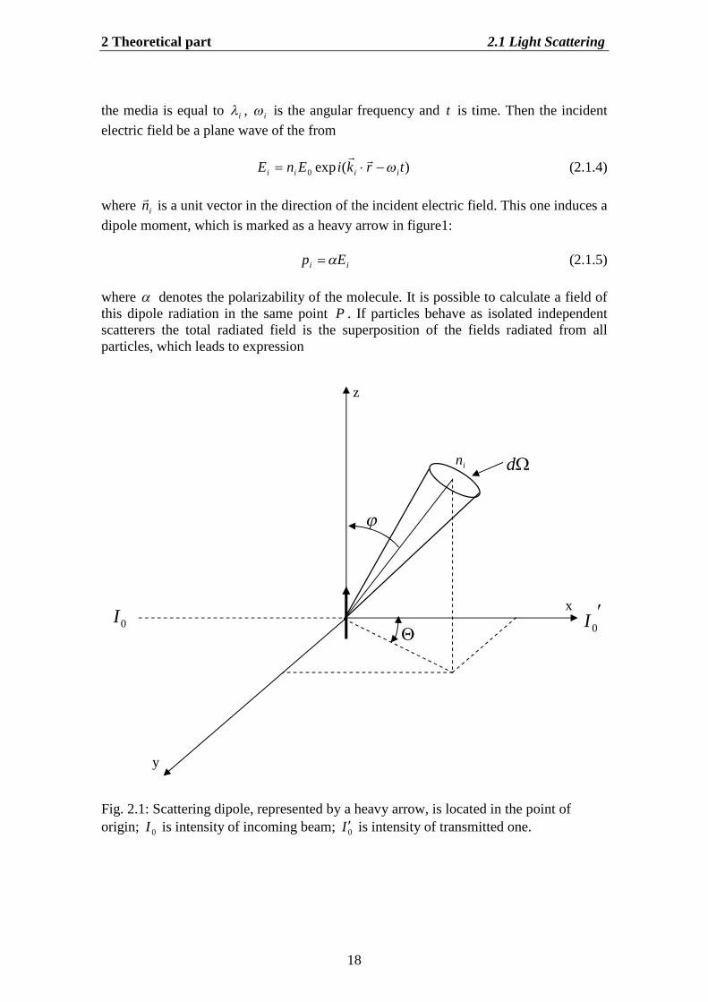
Consider a small scattering volume V , which is located in the point of origin, as shownin Fig.2.1. Let the light beam with intensity 0I , which propagates along an axis x , fallon the given small volume. After passing of a beam through the scattering volume,intensity becomes equal 0I. Measuring the intensity of light beam before and after thescattering volume, it is possible to find an intensity difference I on the distance linside the scattering substance. This signal difference, known as the turbidity of thesample, is defined in differential and integral form the following relations:
,0
lII
leII
0
0 (2.1.1)
Let is place in a point P with spherical polar coordinates ,R and the detectoraccepting stream of light, let out inside of a solid angle d by all point small scatteringvolume which take place in a point of origin. Thus, the ratio of measured intensity ,J
to incident intensity 0I and the scattering volume V , characterize the scattering abilityof a substance. This value is the so-called the total scattering cross section of the givensubstance ,R and it is defined by expression
VI
RI
VI
JR
0
2,
0
,),( (2.1.2)
The turbidity can be directly obtained from the total scattering cross section byintegration on a solid angle
dR , (2.1.3)
Consider the light scattered in molecular scale. Let the plane of a polarized wave beincident upon a small particle that is located in the point of origin. The incident beam isdirected along the positive x axis, polarized in the z direction (see fig. 2.1) andassumed to have negligible width. The particle is assumed small in comparison with awavelength of light, and isotropic enough that incoming light polarized it along an axisz . The wavevector of the incident beam is defined as iik 2 , where wavelength in
2 Theoretical part 2.1 Light Scattering
18
the media is equal to i, i is the angular frequency and t is time. Then the incidentelectric field be a plane wave of the from
)(exp0 trkiEnE iiii
(2.1.4)
where in
is a unit vector in the direction of the incident electric field. This one induces adipole moment, which is marked as a heavy arrow in figure1:
ii Ep (2.1.5)
where denotes the polarizability of the molecule. It is possible to calculate a field ofthis dipole radiation in the same point P . If particles behave as isolated independentscatterers the total radiated field is the superposition of the fields radiated from allparticles, which leads to expression
Fig. 2.1: Scattering dipole, represented by a heavy arrow, is located in the point oforigin; 0I is intensity of incoming beam; 0Iis intensity of transmitted one.
0I0I
z
y
x
din
2 Theoretical part 2.1 Light Scattering
19
,38
),cos1(21
)(
24
224
i
i
n
nR
(2.1.6)
where is number density of particles. It is possible to express this equation bydielectric constant or index of refraction n . Polarizability is connected to the index ofrefraction with Lorentz-Lorentz expression as
2
2
1 42 3
nn
(2.1.7)
By substituting equation (2.1.7) into (2.1.6) Rayleigh expression for independentscatterers is obtained:
).cos1()1(2
)( 24
22
nR (2.1.8)
In the expression of the Rayleigh formula it was assumed, that separate scatterersradiate independently from each other. This condition is not valid in dense medium.Indeed, for absolutely homogeneous media scattering by virtue of interference effectshould be observed only in a direction of incident beam distribution. In real liquidscattering in other direction is not vanishing on account of thermal fluctuations.
It may be shown by the methods, described in Appendix A. that equation (2.1.4) for thecomponent of the scattered electric field in the inhomogeneous (dense) medium at alarge distance R~ between scattering volume and detector is
V
ifffifs rdntrkkntirqiRkiRE
tRE 3
0
0 ,)(exp~
exp~4
),~
(
, (2.1.9)
where fn
is polarization and fk
is the propagation vector of this field. The subscript Vindicated that the integral is over the scattering volume. This formula was first derivedby Einstein (1910). By the difference between the incident wave of the scattering wave
ik
and one that reaches the detector fk
the scattering vectors
fi kkq
(2.1.10)
is defined. Here the values of ik
and fk
are equal in 2 and fn 2 , respectively,
with i is the wavelength in vacuo of incident beam and f that one of scattered wave.
2 Theoretical part 2.1 Light Scattering
20
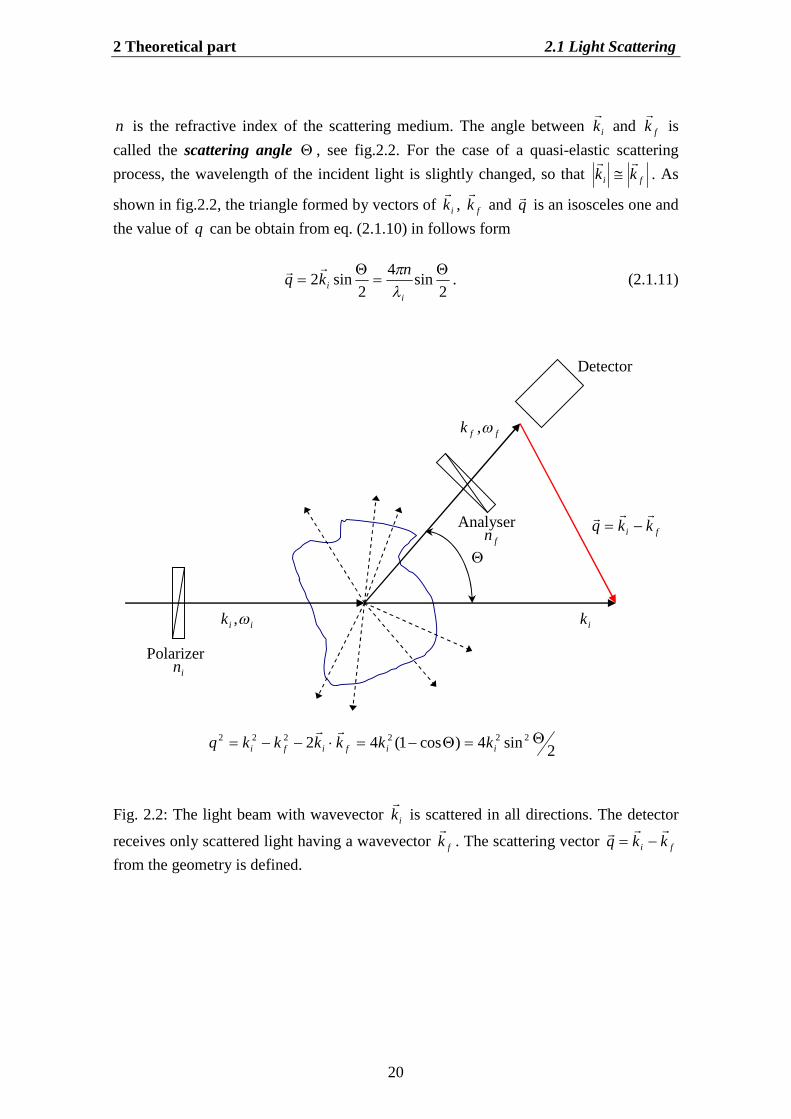
n is the refractive index of the scattering medium. The angle between ik
and fk
iscalled the scattering angle , see fig.2.2. For the case of a quasi-elastic scatteringprocess, the wavelength of the incident light is slightly changed, so that fi kk
. As
shown in fig.2.2, the triangle formed by vectors of ik
, fk
and q
is an isosceles one andthe value of q can be obtain from eq. (2.1.10) in follows form
2sin
42
sin2
i
in
kq
. (2.1.11)
Fig. 2.2: The light beam with wavevector ik
is scattered in all directions. The detector
receives only scattered light having a wavevector fk
. The scattering vector fi kkq
from the geometry is defined.
Detector
fi kkq
ikiik ,
ffk ,
Polarizer
Analyser
in
fn
2sin4)cos1(42 222222 iififi kkkkkkq
2 Theoretical part 2.2 Intensity of scattered light
21
2.2 Intensity of scattered light
In SLS experiments the time-averaged (or 'total') intensity of the scattered light ismeasured, and for one-component liquid or solutions it is related to the time-averagedmean-square dielectric constant fluctuations, which in turn is related to the time-averaged mean-square concentration fluctuation. These concentration fluctuations makea contribution to the scattering that may far exceed the contribution from densityfluctuation. However, in a general case for a multi-component liquid mixture thefluctuations in the local dielectric constant are related to fluctuations in the localthermodynamic quantities as the pressure, concentration and temperature (n-componentmixture case):
1
1
, ,...,
1, ,..., , , ,..., ,
( , ) ( , )
( , ) ( , )
n
n i n
T c c
n
iiP c c i P T c c i n
r t p r tp
T r t C r tT C
(2.2.1)
In terms of the spatial Fourier transform of the dielectric constant fluctuations equationfor the component of the scattering electric field (2.1.9) can be expressed
),()~
(exp~4
),~
(0
02
tqtRkiR
EktRE ifif
fS
(2.2.2)
where
iV
fif nrdtrrqintq
3),(exp),( .
As shown in Appendix B, the time correlation function of the scattering electric fieldcan be evaluated from (2.2.2) and taking into account that the spectral density ofscattered light is fffiii knkn ,,,,
),(),()(exp~16
),~
()0,~
(20
22
20
4
tqoqtiR
EktRERE ififif
fSS
(2.2.3)
In actual photon-correlation experiments, the detectors are photomultiplier tubes whichrespond to the intensity of the scattered light (see Chapter 3 for further details). Thetotal scattering cross section (also called Rayleigt ratio) can be found by substitution ofEq. (2.2.3) into Eq. (2.1.2)
2 Theoretical part 2.2 Intensity of scattered light
22
dttqoqek
qR ififtif
),(),(2
),( 20
4
(2.2.4)
where fi . The angular brackets ... indicate an ensemble average over initialstates of the system. Note that some essential consequences follow from the formula(2.2.4):
It is easy to see, that the intensity of the scattered light is inversely proportionalto wavelength 4 in fourth order. As a consequence at visible light, the bluelight is scattered more than red one. This results in the blue colors of the skyand oceans.
It is much easier to do scattering experiments with a shorter wavelength thanwith a longer one, that is a larger scattering intensities at first case. Forexample, visible light is more preferable in experiment than infrared.
The frequency change occurs only if the fluctuations in the local dielectricconstant ),( tq
vary with time, that is, scattering could occur from “frozen”
fluctuations but the frequency of scattering light would be identical to that ofthe incident one.
Let us rewrite the expression for Rayleigt ratio (2.2.4) in another form:
),(2
),( 20
4
qSk
qR f
In this equation ),( qS
is the generalized structure factor, which containesinformation about the fluctuation in the local dielectric constant. It is defined byMounain [38] to be
trkirtrrrdrddtqS
exp)0,'(),'('Re2),(0
. (2.2.5)
In terms of Fourier-Laplace transforms ),( qS
could be expressed in form
,)(),(̂Re2),( qiqqS (2.2.6)
where
2 Theoretical part 2.2 Intensity of scattered light
23
.exp)0,()(
exp),(),(̂0
rkirrdq
ztrkitrrddtzq
(2.2.7)
The caret is used to indicate a Laplace-time transform.
Using the grand canonical Gibbs ensemble, Kirkwood and Goldberg [29] foundexpressions for the Rayleigh ratio of scattering due to concentration fluctuation inmulti-component mixtures. Their expression for the light scattering contribution ofcomposition fluctuation is
jj cPTkcPTi
n
ki
ikkiC cc
ccq
qR,,,,1,
2
4
16),(
(2.2.8)
where is the determinant of the thermodynamic coefficients ik andik
is the
appropriate co-factor of the determinant , kic , the concentration of a component in
the mixture. The coefficients ik may be written in the following form:
n
kik
cPTi
k
k
ki
cPTk
i
i
kiik
jjcTM
cccTM
cc
0
,,,,
0
,
(2.2.9)
here, is molar gas constant, iM and i the molecular weight, and chemicalpotential of species i , respectively.
In the case of a binary liquid mixture near a critical point, the Rayleigh ratio due toconcentration fluctuations is obtained from Eqs. (2.2.8)
PT
PTbinC cq
TMc
Nq
qR,
221
2,
02
4
))(1(
)(
16),(
(2.2.10)
1,)( PTc denotes the generalized osmotic susceptibility TC , the correlation
length of concentration fluctuation, N is Avogadro’s constant and 0 is the mass ofsolvent in unit volume of a mixture. For a three-component system Eq. (2.2.8) becomes
2 Theoretical part 2.3 Critical opalescence
24
binC
terC
qR
MM
c
TAMqR
),(
)(1
21),(
,0
212
1
21
21
2
2
2
(2.2.11)
where
24
2 2 20 2
1
2
64 (1 )
( )( )
qA
N q c
cc
)(
)(
)()(
22
212
11
211
cc
cc
2.3 Critical opalescence
In the vicinity of a critical point the intensity of light scattering from a liquid systemincreases enormously. At the approach to the critical solution point a liquid systemtakes on a cloudy or opalescent appearance. This phenomenon is called criticalopalescence. The physical mechanism of this phenomenon consists in the existance oflong-range spatial correlations between molecules in the vicinity of critical point. If weconsider the state of our system near a critical point, where local density fluctuationsreach almost macroscopic dimensions, it is necessary to take these correlations intoaccount. We introduce the space autocorrelation function )(rG , which describes theprobability of finding any molecule at a distance 'r from another one. This functionmeasured the correlations of the fluctuation in the thermodynamic quantities at twodifferent points of the fluid mixture 1r and 2r separated by the distance 21' rrr . As
21 rr , the concentration fluctuation (for the multicomponent mixture case)should be uncorrelated so that
1 2
1 2lim ( , ) 0r r
G r r
.
In a spatially uniform system the spatial ACF ),( 21 rrG should be invariant to anarbitrary translation a so that ),(),( 2121 rrGararG . Thus the correlation functiondepends only on a distance between two different points 21' rrr of the fluid. Thestructure factor for density fluctuation (one-component fluid case) has the form:
2 Theoretical part 2.3 Critical opalescence
25
')'()( 3'2 rdrGeVqS rqi
. (2.3.1)
If the system is not correlated, i.e. there exists no correlation between the positions ofthe different particles, then the structure factor is equal NqS )(0
where N is
average number of particles in the scattering volume V . The deviation )()( 0 qSqS
from unity reflects the spatial correlations between different particles in a fluid.
According to the Ornstein–Zernike theory [42, 43], a function )(rG in the limit of verylarge 'r has the form
,'
)'exp()(
rr
rG
at )'( r , (2.3.2)
derived to describe the q
dependence of the Rayleigh ratio near a critical singularity.Here is the correlation length between two molecules. Thus the expression fordynamic structure factor becomes
)1()( 22 qTkqS TB
, (2.3.3)
where Bk and T is the Boltzmann constant, and the isothermal compressibility,respectively. By substitution of Eqs. (2.2.5) and (2.3.1) in Eq (2.3.3), the excessRayleigh ratio for density fluctuations near the critical point becomes
)1(),( 22
,0
q
RqR D
D . (2.3.4)
For a multicomponent liquid mixture the contribution to the Rayleigh ratio due toconcentration fluctuations is given by the value 2qci
. It describes the
concentration fluctuations in space corresponding to the static structure factor cS . It isrelated to the space autocorrelation function of the concentration fluctuations. Acomparison to the structure factor, resulting from the fluctuation theory of Einstein andSmoluchowski [17], leads to the expression
2222
1)()(
q
TckqcqS TiBiC
, (2.3.5)
where T is the osmotic susceptibility and denotes the correlation length ofconcentration fluctuations. Then, the Rayleigh ratio becomes
2 Theoretical part 2.3 Critical opalescence
26
)1(),( 22
qTC
qR TC
(2.3.6)
From the various experiments it is known that in fluid mixtures the magnitude of T asfunction of the thermodynamic state, near the critical point, becomes divergent(arbitrary large). As a consequence the intensity of scattering light increases verystrongly as the critical point is approached. In fact there is so much scattering that thecritical fluid appears cloudy or opalescent. This phenomenon, as mention above, iscalled critical opalescence.
The three interrelated phenomena that are observed near the critical solution point inliquid mixture are:
Increase in the fluctuation of the thermodynamic quantities in themulticomponent mixture.
Increase in the osmotic susceptibility. Increase in the correlation length.
Eqs. (2.3.4) and (2.3.6) are correct only for large 'r . Because of the divergence of thestatic structure factor in the very immediate neighborhood of the critical point Fisher[18-21] introduced a positive and very small critical exponent describing a criticalsingularity of the correlation function (2.3.2). Eqs. (2.3.6) could be expressed:
2122 )1(),(
q
TCqR T
C
(2.3.7)
This equation represents one of several modifications for the correlation function andpredicts a small downward curvature in the reciprocal scattering intensity versus 2q nearthe critical point. One must expect =0.0560.008 according to numerical calculationbased on the 3D Ising model [22]. Müller [39-41] has applied the Ornstein–Zerniketheory to ternary liquid mixture near the critical solution point to the obtain data ofdiffusivities and other mixtures properties.
2 Theoretical part 2.4 Spectrum of light scattered from hydrodynamic fluctuation
27
2.4 Spectrum of light scattered from hydrodynamic fluctuation
Since the fluctuation in liquid, which are responsible for scattered light, change in time,the spectral structure of scattered light will be different from that of the incident beam.The investigation of this spectrum allows studying time behaviour of thermodynamicfluctuations in the liquid medium.
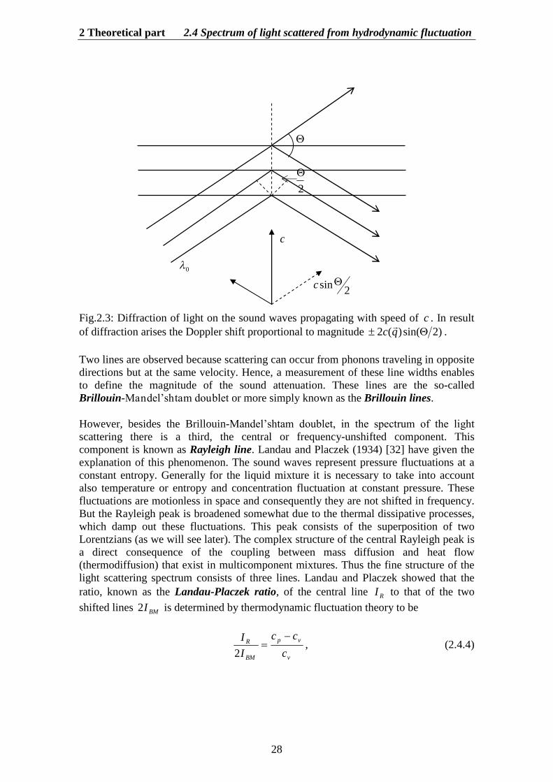
To analyze the spectral structure of light, which is scattered in the liquid, we willconsider in more detail the character of thermal fluctuations. As is known, in a liquidalways there are sound waves. These waves, which are analogous to Debye waves (orphonons) in a crystal, are raised from thermal movement of molecules. Incoming lightwith a wavelength 0 is scattering on those sound waves which length , that satisfiesthe Bragg condition 0)2sin(2 or in wave numbers (see eq. 2.1.11). These wavesare propagating in opposite directions at the adiabatic speed of sound )(qc
, with
projections along the light beam direction that are equal to )2sin()( qc
(see fig. 3).The adiabatic speed of sound in a multicomponent mixture is defined as
icS
pqc
,
)(
(2.4.1)
where p , , S , and ic are the pressure, density, entropy, and concentration of thi component in mixture, respectively. As a result light will be test to Doppler shift, whichreduced to the shift of the angular frequency, is equal
')2sin()(2
0 cqc
, (2.4.2)
where 'c - speed of sound in medium, '0 cki - is angular frequency of incominglight. Therefore at the spectrum there are two shifted lines located symmetrically withrespect to the frequency of the incoming beam 0 , and shifted by an amountproportional to speed of sound:
)(qcq
. (2.4.3)
2 Theoretical part 2.4 Spectrum of light scattered from hydrodynamic fluctuation
28
Fig.2.3: Diffraction of light on the sound waves propagating with speed of c . In resultof diffraction arises the Doppler shift proportional to magnitude )2sin()(2 qc
.
Two lines are observed because scattering can occur from phonons traveling in oppositedirections but at the same velocity. Hence, a measurement of these line widths enablesto define the magnitude of the sound attenuation. These lines are the so-calledBrillouin-Mandel’shtam doublet or more simply known as the Brillouin lines.
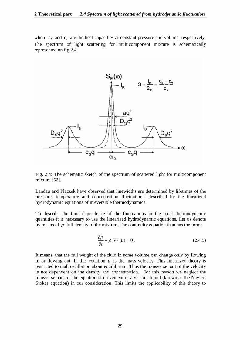
However, besides the Brillouin-Mandel’shtam doublet, in the spectrum of the light scattering there is a third, the central or frequency-unshifted component. Thiscomponent is known as Rayleigh line. Landau and Placzek (1934) [32] have given theexplanation of this phenomenon. The sound waves represent pressure fluctuations at aconstant entropy. Generally for the liquid mixture it is necessary to take into accountalso temperature or entropy and concentration fluctuation at constant pressure. Thesefluctuations are motionless in space and consequently they are not shifted in frequency.But the Rayleigh peak is broadened somewhat due to the thermal dissipative processes,which damp out these fluctuations. This peak consists of the superposition of twoLorentzians (as we will see later). The complex structure of the central Rayleigh peak isa direct consequence of the coupling between mass diffusion and heat flow(thermodiffusion) that exist in multicomponent mixtures. Thus the fine structure of thelight scattering spectrum consists of three lines. Landau and Placzek showed that theratio, known as the Landau-Placzek ratio, of the central line RI to that of the twoshifted lines BMI2 is determined by thermodynamic fluctuation theory to be
v
vp
BM
R
c
cc
II
2
, (2.4.4)
2
0
2sinc
c
2 Theoretical part 2.4 Spectrum of light scattered from hydrodynamic fluctuation
29
where Pc and vc are the heat capacities at constant pressure and volume, respectively.The spectrum of light scattering for multicomponent mixture is schematicallyrepresented on fig.2.4.
Fig. 2.4: The schematic sketch of the spectrum of scattered light for multicomponentmixture [52].
Landau and Placzek have observed that linewidths are determined by lifetimes of thepressure, temperature and concentration fluctuations, described by the linearizedhydrodynamic equations of irreversible thermodynamics.
To describe the time dependence of the fluctuations in the local thermodynamicquantities it is necessary to use the linearized hydrodynamic equations. Let us denoteby means of full density of the mixture. The continuity equation than has the form:
0)(0
ut
, (2.4.5)
It means, that the full weight of the fluid in some volume can change only by flowingin or flowing out. In this equation u is the mass velocity. This linearized theory isrestricted to mall oscillation about equilibrium. Thus the transverse part of the velocityis not dependent on the density and concentration. For this reason we neglect thetransverse part for the equation of movement of a viscous liquid (known as the Navier-Stokes equation) in our consideration. This limits the applicability of this theory to
2 Theoretical part 2.4 Spectrum of light scattered from hydrodynamic fluctuation
30
liquid mixtures in which angular correlations between the molecules are not important[9,33]. The longitudinal part of the Navier-Stokes equation is
uuptu
SVS
31
0 , (2.4.6)
where S and V are the shear and volume viscosities, respectively. Equilibriumvalues in these equations are denoted by a subscript zero.
In a liquid mixture mass transfer can occur by convection and/or diffusion. Masstransfer due to diffusion is found even if a movement of the liquid as a whole is absent.Let I be density of this diffusion flux. Then the continuity equations for ternary liquidmixture case has a form:
2
1
2
1 ii
ii
i divIcutc
. (2.4.7)
In the ternary liquid mixture there are two independent variables for concentration.Since 1222211 mcmcmc , then )1(1 111133 mcmcmc , where ic and im arethe concentration and mass of each component in the mixture, respectively (see also theAppendix C).
In addition to the mass diffusion current I in the liquid there is present also the heatcurrent, which is connected to the thermal conductivity :
TQ (2.4.8)
Following Landau’s method of solution [33] we will obtain the energy transport equation for a ternary liquid mixture
22112211'
IIIIQdivx
SuTS
Tk
iik , (2.4.9)
where ik' is the viscous stress tensor, ki x - derivative of liquid velocity withrespect to coordinates, and S is the entropy. Here we are using the reduced quantities
1 and 2 , which are connected to chemicals potentials of i -th component of the
mixture, where3
3
1
11
''mm
and2
22
'm
, im - the molar masses of the
pure component. The detailed of this formula derivation is given in Appendix C.
2 Theoretical part 2.5 Hydrodynamic fluctuations in ternary liquid mixture
31
2.5 Hydrodynamic fluctuations in ternary liquid mixture
In this section the theory will be applied to the case of ternary liquid mixtures. Thenew model is based on conclusions of the linearized hydrodynamic equations and ofthe methods suggested by Landau [33], and later by Mountain and Deutch [38] for abinary mixture. In addition, Anisimov presented a theory on the coupling of differenttransport modes near the critical point in a binary mixture [1]. Leaist and Hao [35]already formally extended the theoretical approach for binary solution, given byMountain and Deutch, to a ternary solution, but for the special case of a ternary systemin which the temperature and pressure is uniform. They have considered the specialcase, in which the concentration fluctuations are much more essential then the others.So far they did not verify this theoretical concept experimentally.
The main focus of this thesis is a theoretical investigation of transport properties in thehydrodynamic range and in the critical singularity field. In this section a newtheoretical extension of theory to ternary systems is developed. Here we will presentnew expressions for the general case, where the fluctuations in the dielectric constantare in turn caused by the full set of the local thermodynamic quantities such as thepressure, temperature and concentration.
The mass diffusion current and the heat current result from concentration andtemperature gradients, respectively, which are present in the mixture. However, Idepends not only on the concentration gradient, and Q - not only on the temperaturegradient. Generally, each of these currents depends on both gradients. If the gradientsof the concentration and temperature are insignificant, for I and Q it is possible towrite linear functions of i and T :
1 1 1 1
2 2 2 2
1 1 2 2 1 1 2 2
I T
I TQ T T T I I
, (2.5.1)
where ii , and are the Onsager kinetic coefficients. As shown in Appendix C, thefinal expressions for currents have the form
2 Theoretical part 2.5 Hydrodynamic fluctuations in ternary liquid mixture
32
TIT
Tc
k
IT
Tc
kQ
PP
kT
Tk
ccDD
DI
PP
kT
Tk
cDD
cDI
CCPTPC
T
CCPTPC
T
PT
PT
22,,
2
,,2
22
11,,
1
,,1
11
2221
22
21222
112
11
121111
211
212
(2.5.2)
where ijD are the coefficients of the Fick’s diffusion matrix, Tik is the thermal
diffusion ratio, and Pik the thermodynamic quantity
ijCTPi
i
iPi
jc
cp
k
,,
20
0
,
which is called the barodiffusion ratio. Let us consider a liquid without anymacroscopic movement. After substitution of I and Q from Eq.(2.5.2) into Eqs.(2.4.7) and (2.4.9), by the way of simple transformations (see Appendix C), we willobtain the diffusion equations
Pp
kT
Tk
ccDD
Dt
c
Ppk
TTk
cDD
cDtc
PT
PT
0
2
0
221
22
2122
2
0
1
0
12
11
12111
1
, (2.5.3)
and energy transport equation
Ttp
pS
CT
tc
cCk
tc
cCk
tT
CCTPTPCP
T
TPCP
T
2112 ,,
2
,,2
221
,,1
11 . (2.5.4)
In these equations PC is the heat capacity at constant pressure, and PC is thecoefficient of the thermal conductivity. The system of the linearized hydrodynamicequations (2.4.5), (2.4.5), (2.5.3) and (2.5.4) is the system, which described the time
2 Theoretical part 2.5 Hydrodynamic fluctuations in ternary liquid mixture
33
dependence of the concentration, temperature and pressure fluctuations in the ternaryliquid mixture.
These equations have been already solved for binary mixture by Mountain and Deutchin [38]. Here we will adhere to their method of solution and transform it to the ternarymixture case. For beginnings consider the interesting special case of the system inwhich the pressure is uniform, and consequently only the concentration andtemperature fluctuate. In this special case there are no sound modes, and consequentlyno Brillouin-Mandel’shtam doublet. Aforementioned system for the concentration and temperature fluctuations are described by the following system of equations:
Tt
ccC
ktc
cCk
tT
TTk
ccDD
Dt
c
TTk
cDD
cDtc
TPCP
T
TPCP
T
T
T
2
,,2
221
,,1
11
0
221
22
2122
2
0
12
11
12111
1
12
(2.5.5)
For the beginning the system of the linearized hydrodynamic equations should beexpressed in terms of the variables that have been chosen to characterize the local stateof the mixture. Generally, for a ternary system, four such state variable are needed. Thecriterion we will use to select the four states variables is that the probability of afluctuation is statistically independent. In the Gaussian approximation 01 cpT ,
021 ccs and 021 T and either of the obvious candidate choices of the
four thermodynamic variables 21 ,,, ccpT , 21 ,,, ccpS , or 21 ,,, T do notsatisfy the criterion of the statistical independence. Following Mountain’s consideration [16,38], we introduce a set of variables 21 ,,, ccp , where is defined as
pC
TT
P
T
. (2.5.6)
In this expression 21 ,,
1ccpT T , is the thermal expansion coefficient.
Anisimov showed that [1]
2,
21
,
1
12
cT
cT
SCT
cpcpP
. (2.5.7)
The set 21 ,,, ccp is statistically independent with
2 Theoretical part 2.5 Hydrodynamic fluctuations in ternary liquid mixture
34
,
,
,
,,
2
22
,,
2
21
ijcTpi
iBi
P
B
ccS
B
j
cV
Tkc
CVTk
PVTk
p
(2.5.8)
where Bk is Boltzmann’s constant. In thermodynamics the derivative ijcTpii jc ,,
and pC and, therefore,2 and
2ic are defined and can be derived from
experiment. This is why the introduction of the variable is advantageous.
The next task is to rewrite the linearized hydrodynamic equations (2.4.5), (2.4.6),(2.5.3) and (2.5.4) in terms of the variables 21 ,,, ccp and udiv , and the system(2.5.5) in term of the variables Tcc ,, 21 .
Using Fourier transformation on spatial coordinates
),(),(
),(),(
),(),(
),(),(
,),(),(
3
3
3
3
3
truerdtr
trerdtr
trperdtrp
trTerdtrT
trcerdtrc
rqik
rqik
rqik
rqik
irqi
ki
(2.5.9)
we will present the system (2.5.5) in following form:
.0),(
,0),(),(),(
,0),(),(),(
22
,,2
221
,,1
11
0
221
22
21222
2
0
12
11
121
211
1
12
trTqt
ccC
kt
ccC
kt
T
trTTk
trctrcDD
qDt
c
trTTk
trcDD
trcqDt
c
kk
TPCP
Tk
TPCP
Tk
kT
kkk
kT
kkk
(2.5.10)
These differential equations are most easily solved using Laplace transform.Introducing the Laplace transforms
2 Theoretical part 2.5 Hydrodynamic fluctuations in ternary liquid mixture
35
.),(ˆ
,),(ˆ
0
0
dttrTeT
dttrcec
kzt
k
kizt
ki
(2.5.11)
The expressions of the Laplace transform for variables ,p and will be similar toone for variables ic and, T . We will obtain
).0()0()0(
ˆˆˆ
),0(ˆˆˆˆ
),0(ˆˆˆˆ
2
,,2
221
,,1
11
22
,,2
221
,,1
11
20
222
222
22121
2
10
111
2212
211
21
12
12
kk
TPCP
Tk
TPCP
T
kk
TPCP
Tk
TPCP
T
kkT
kk
kkT
kk
TccC
kc
cCk
TqzccC
kzc
cCk
z
cTTk
DqDqzccDq
cTTk
DqcDqDqzc
(2.5.12)
This system, in matrix form is,
)(),(̂ qNTzqNM
, (2.5.13)
where ),(̂ zqN
is column vector with elements ),(),,(),,( 21 zqTzqczqc
. The 33matrix M
2
,,1
11
,,1
11
0
222
222
221
2
0
111
212
211
2
22
qzcC
kz
cCk
z
Tk
DqDqzDq
Tk
DqDqDqz
M
TPCP
T
TPCP
T
T
T
, (2.5.14a)
and T has the form
2 Theoretical part 2.5 Hydrodynamic fluctuations in ternary liquid mixture
36
1
010001
,,1
11
,,1
11
22 TPCP
T
TPCP
T
cCk
cCk
T
. (2.5.14b)
The general structure of the solution of Eq. (2.5.13) is
,),(det
)(),(),(̂
zqM
qNzqPzqN j
Jij
i
(2.5.15)
where ijP is the algebraic function from “i” and “j” variables. The determination of the dynamic structure factor, as we will see further, includes different correlationsbetween these variables. An expression for the correlation function is obtained bytaking inverse Laplace transform of Eq. (2.5.15):
dwiwqM
iwqPe
qN
qNtqN ijiwt
j
ji
),(det
),(
21
)(
)(),(2
. (2.5.16)
This inversion requires that we find the roots of denominator of the right hand side ofEq. (2.5.16). Shift and width of the spectral component by roots of the dispersionequation are defined (obtained from calculated )det(M ). The solution of this cubicequation (see Appendix D), is not particularly useful in this case because of itsalgebraic complexity. It is more convenient to develop a convergent scheme forapproximating the solution to the dispersion equation, in power series of coefficients.The solution can be expressed as )2()1()0( zzzz where )(nz is a term of ordern in any of the small dimensionless parameters cq 2 , cq 2' and cqDij
2 . Here
c is the adiabatic speed of sound (see Eq. 2.4.1), VS 34' is the generalized
kinematic viscosity. The value cq 2' is used just in case when pressure fluctuationsare taken into account. In a typical light scattering experiment 1510 cmq
,
sec105 cmc , so that these quantities are on the order of 210 , 210 , and 410 ,respectively. In the approximation when linear terms in the small quantities are retainedone obtains for determinant (2.5.14a):
221 ))((),(det zzzzzqM
, (2.5.17)
where the roots are
2 Theoretical part 2.5 Hydrodynamic fluctuations in ternary liquid mixture
37
,22
1 12211
23,2
12221112211
21
DDqz
MDMDDDqz(2.5.18)
with
,31
22
222111
212111121222212211211222111
MDMD
MDDMDDMMDDDDDD
(2.5.19)
and
,1
,1
,,2
2
0
22
2
,,1
1
0
21
1
1
2
TPCP
T
TPCP
T
cTCk
M
cTCk
M
2
1
1 2 112
0 1 , ,
1 2 221
0 2 , ,
,
.
T T
P C P T
T T
P C P T
k kM
C T c
k kM
C T c
(2.5.20)
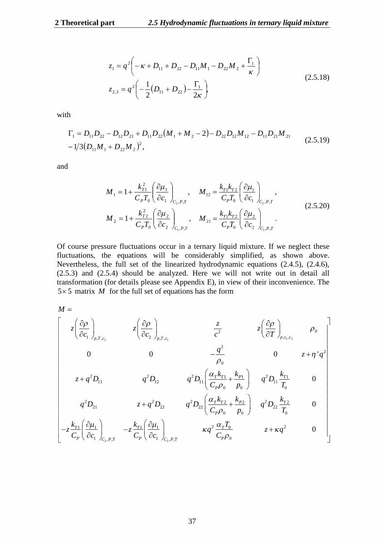
Of course pressure fluctuations occur in a ternary liquid mixture. If we neglect thesefluctuations, the equations will be considerably simplified, as shown above.Nevertheless, the full set of the linearized hydrodynamic equations (2.4.5), (2.4.6),(2.5.3) and (2.5.4) should be analyzed. Here we will not write out in detail alltransformation (for details please see Appendix E), in view of their inconvenience. The
55 matrix M for the full set of equations has the form
1 22 1
2
02, ,1 2, , , ,
22
0
2 2 2 21 1 111 12 11 11
0 0 0
2 2 2 22 2 221 22 22 22
0 0 0
1 1
1 , ,
0 0 0 '
0
0
p c cp T c p T c
T T P T
P
T T P T
P
T
P C P T
M
zz z z
c c c T
qz q
k k kz q D q D q D q D
C p T
k k kq D z q D q D q D
C p T
kz z
C c
2
2 201 1
1 0, ,
0TT
P PC P T
Tkq z q
C c C
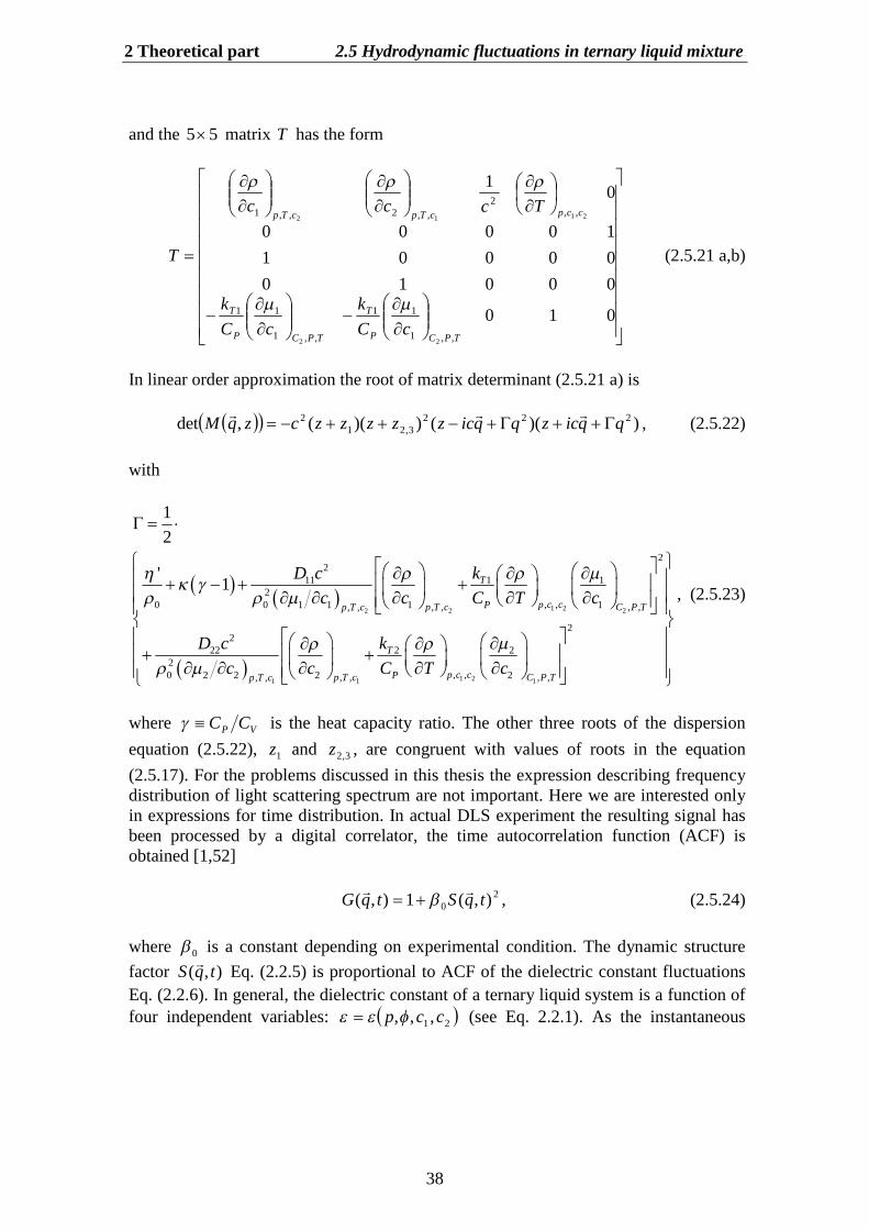
2 Theoretical part 2.5 Hydrodynamic fluctuations in ternary liquid mixture
38
and the 55 matrix T has the form
010
000100000110000
01
,,1
11
,,1
11
,,2
,,2,,1
22
2112
TPCP
T
TPCP
T
ccpcTpcTp
cCk
cCk
Tccc
T
(2.5.21 a,b)
In linear order approximation the root of matrix determinant (2.5.21 a) is
))(())((,det 2223,21
2 qqiczqqiczzzzzczqM
, (2.5.22)
with
1 22 22
1 21 11
22
11 1 12
, ,0 0 1 1 1 1, , , ,, ,
22
22 2 22
, ,0 2 2 2 2, , , ,, ,
12
'1 T
p c cPp T c C P Tp T c
T
p c cPp T c C P Tp T c
D c kc c C T c
D c kc c C T c
, (2.5.23)
where VP CC is the heat capacity ratio. The other three roots of the dispersionequation (2.5.22), 1z and 3,2z , are congruent with values of roots in the equation(2.5.17). For the problems discussed in this thesis the expression describing frequencydistribution of light scattering spectrum are not important. Here we are interested onlyin expressions for time distribution. In actual DLS experiment the resulting signal hasbeen processed by a digital correlator, the time autocorrelation function (ACF) isobtained [1,52]
20 ),(1),( tqStqG
, (2.5.24)
where 0 is a constant depending on experimental condition. The dynamic structurefactor ),( tqS
Eq. (2.2.5) is proportional to ACF of the dielectric constant fluctuations
Eq. (2.2.6). In general, the dielectric constant of a ternary liquid system is a function offour independent variables: 21 ,,, ccp (see Eq. 2.2.1). As the instantaneous
2 Theoretical part 2.5 Hydrodynamic fluctuations in ternary liquid mixture
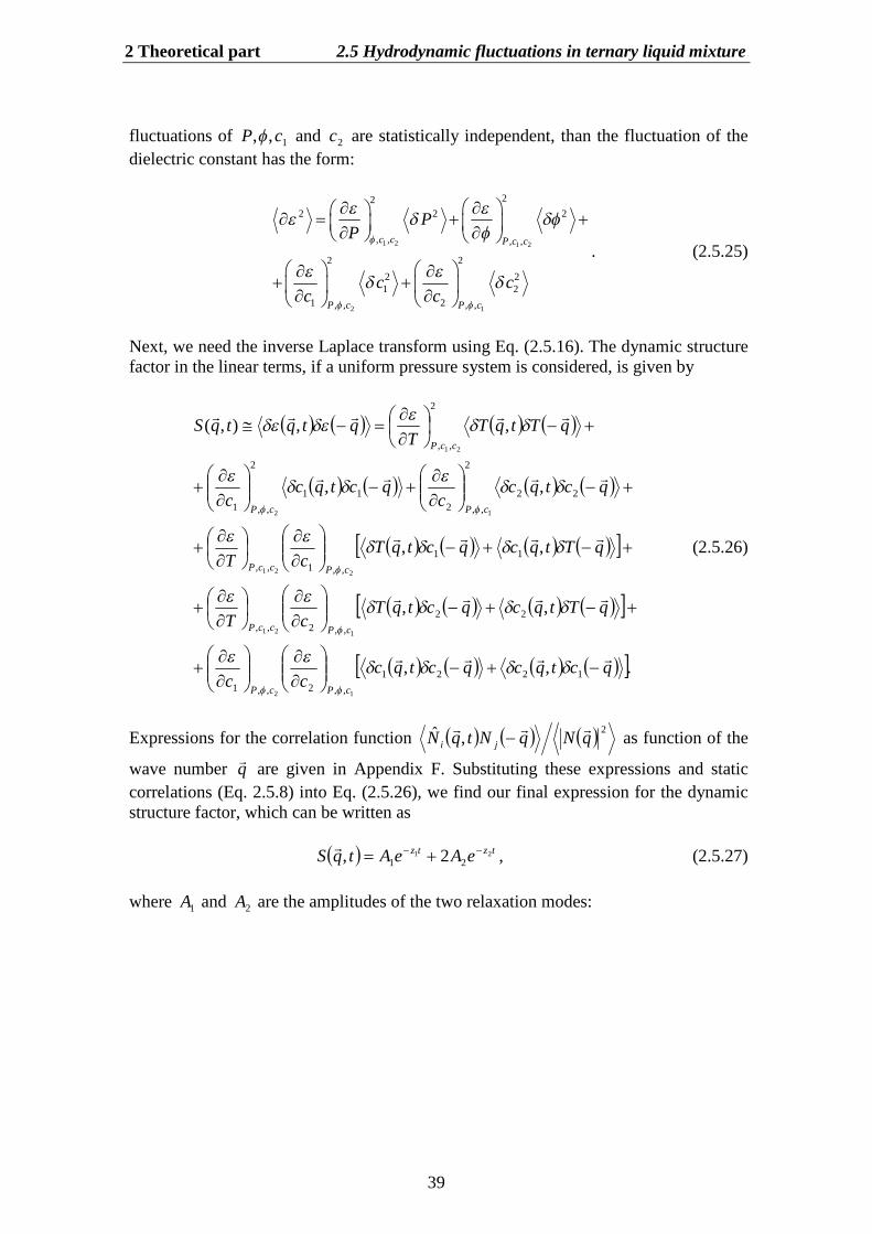
39
fluctuations of 1,, cP and 2c are statistically independent, than the fluctuation of thedielectric constant has the form:
1 2 1 2
2 1
222 2 2
, , , ,
2 2
2 21 2
1 2, , , ,
c c P c c
P c P c
PP
c cc c
. (2.5.25)
Next, we need the inverse Laplace transform using Eq. (2.5.16). The dynamic structurefactor in the linear terms, if a uniform pressure system is considered, is given by
.,,
,,
,,
,,
,,),(
1221
,,2,,1
22
,,2,,
11
,,1,,
22
2
,,211
2
,,1
2
,,
12
121
221
12
21
qctqcqctqccc
qTtqcqctqTcT
qTtqcqctqTcT
qctqcc
qctqcc
qTtqTT
qtqtqS
cPcP
cPccP
cPccP
cPcP
ccP
(2.5.26)
Expressions for the correlation function 2,ˆ qNqNtqN ji
as function of the
wave number q
are given in Appendix F. Substituting these expressions and staticcorrelations (Eq. 2.5.8) into Eq. (2.5.26), we find our final expression for the dynamicstructure factor, which can be written as
tztz eAeAtqS 2121 2,
, (2.5.27)
where 1A and 2A are the amplitudes of the two relaxation modes:
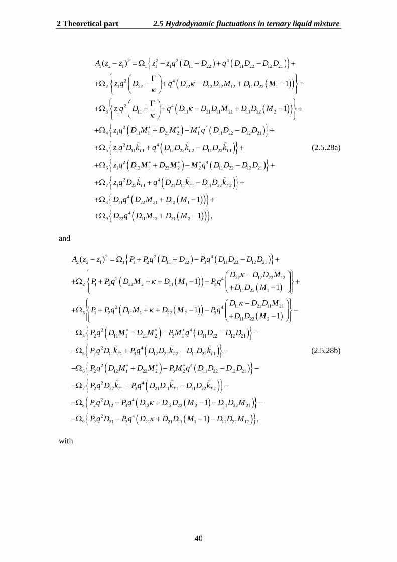
2 Theoretical part 2.5 Hydrodynamic fluctuations in ternary liquid mixture
40
2 2 2 41 2 1 1 1 1 11 22 11 22 12 21
2 42 1 22 22 12 22 12 11 22 1
2 43 1 11 11 21 11 21 11 22 2
2 44 1 11 1 21 2 1 11 22 12 21
25 1
( )
1
1
A z z z z q D D q D D D D
z q D q D D D M D D M
z q D q D D D M D D M
z q D M D M M q D D D D
z q
411 1 12 22 2 11 22 1
2 46 1 12 1 22 2 2 11 22 12 21
2 47 1 22 1 21 11 1 11 22 2
48 11 22 21 12 1
49 22 11 12 21 2
1
1 ,
T T T
T T T
D k q D D k D D k
z q D M D M M q D D D D
z q D k q D D k D D k
D q D M D M
D q D M D M
(2.5.28a)
and
2 2 42 2 1 1 1 2 11 22 3 11 22 12 21
22 12 22 122 42 1 2 22 2 11 1 3
11 22 1
11 21 11 212 43 1 2 11 1 22 2 3
11 22 2
4 2
( )
11
11
A z z P P q D D P q D D D D
D D D MP P q D M D M P q
D D M
D D D MP P q D M D M P q
D D M
P q
2 411 1 21 2 3 1 11 22 12 21
2 45 2 11 1 3 12 22 2 11 22 1
2 46 2 12 1 22 2 3 2 11 22 12 21
2 47 2 22 1 3 21 11 1 11 22 2
2 48 2 12 3 12 12 22 2 11 22 211
T T T
T T T
D M D M P M q D D D D
P q D k P q D D k D D k
P q D M D M P M q D D D D
P q D k P q D D k D D k
P q D P q D D D M D D M
2 49 2 21 3 21 21 11 1 11 22 121 ,P q D P q D D D M D D M
(2.5.28b)
with
2 Theoretical part 2.5 Hydrodynamic fluctuations in ternary liquid mixture
41
1 2
2 2
1 1
1 22 2
2
220
1, ,
2
12 0
1 1, , , ,
2
23 0
2 2, , , ,
14 0
, ,1 1, , , ,
20
51 , ,
,
,
,
,
P c cV
P T c P T c
P T c P T c
P c cP T c P T c
V P T c
RTC T
cRT
c
cRT
c
cRT
c T
RTC c
1 2
1 21 1
1 21
2 1 1
, ,
26 0
, ,2 2, , , ,
20
7, ,2 , ,
28 0
1 2 2, , , , , ,
8 01 , ,
,
,
,
,
P c c
P c cP T c P T c
P c cV P T c
P T c P T c P T c
P T
T
cRT
c T
RTC c T
cRT
c c
RTc
2 2 1
1
1 2, , , ,
.c P T c P T c
cc
.~
,~
,
,
,1,
,2
0
22
0
11
,,2
212
,,1
111
122
12212
21221221
1
2
Tk
k
Tk
k
cCk
M
cCk
M
zztPzztzzP
tzztzzzzP
TT
TT
TpcP
T
TpcP
T
(2.5.29)
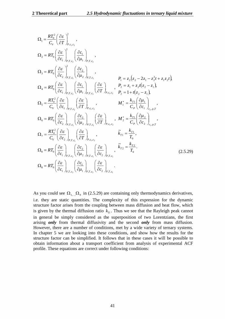
As you could see 9,,1 in (2.5.29) are containing only thermodynamics derivatives,i.e. they are static quantities. The complexity of this expression for the dynamicstructure factor arises from the coupling between mass diffusion and heat flow, whichis given by the thermal diffusion ratio Tik . Thus we see that the Rayleigh peak cannotin general be simply considered as the superposition of two Lorentzians, the firstarising only from thermal diffusivity and the second only from mass diffusion.However, there are a number of conditions, met by a wide variety of ternary systems.In chapter 5 we are looking into these conditions, and show how the results for thestructure factor can be simplified. It follows that in these cases it will be possible toobtain information about a transport coefficient from analysis of experimental ACFprofile. These equations are correct under following conditions:
2 Theoretical… 2.6 Spectrum of light scattered in near-critical ternary fluid mixture
42
The fluctuations can be described by the usual linearized hydrodynamicequations (2.4.5), (2.4.5), (2.5.3) and (2.5.4). In the linearized theory thedeviations of thermodynamic variables about equilibrium are small.
The dimensionless parameters cq 2 , cq 2' and cqDij2 are required
to be small. It means, that the width of the components is small incomparison with the shift of the Brillouin line.
2.6 Spectrum of light scattered in near-critical ternary fluid mixture
In the previous chapter we considered the light scattering spectrum arising from aternary solution, away form its critical point. Far away form critical singularity 1q ismuch greater than the range of molecular correlations. Near the critical point thiscondition breaks down, as the range of molecular correlations is comparable to 1q . Asthe critical point is approached, the q
dependence of fluctuations of thermodynamic
values develops reflecting the long-range of the correlation between two particles. Thisresults in an expression for the Rayleigh ratio (2.3.4) where the Ornstein–Zernikecorrection term is included. Similar corrections should be taking into account atinvestigating of the light scattering spectrum near the critical consolute point of theliquid mixture.
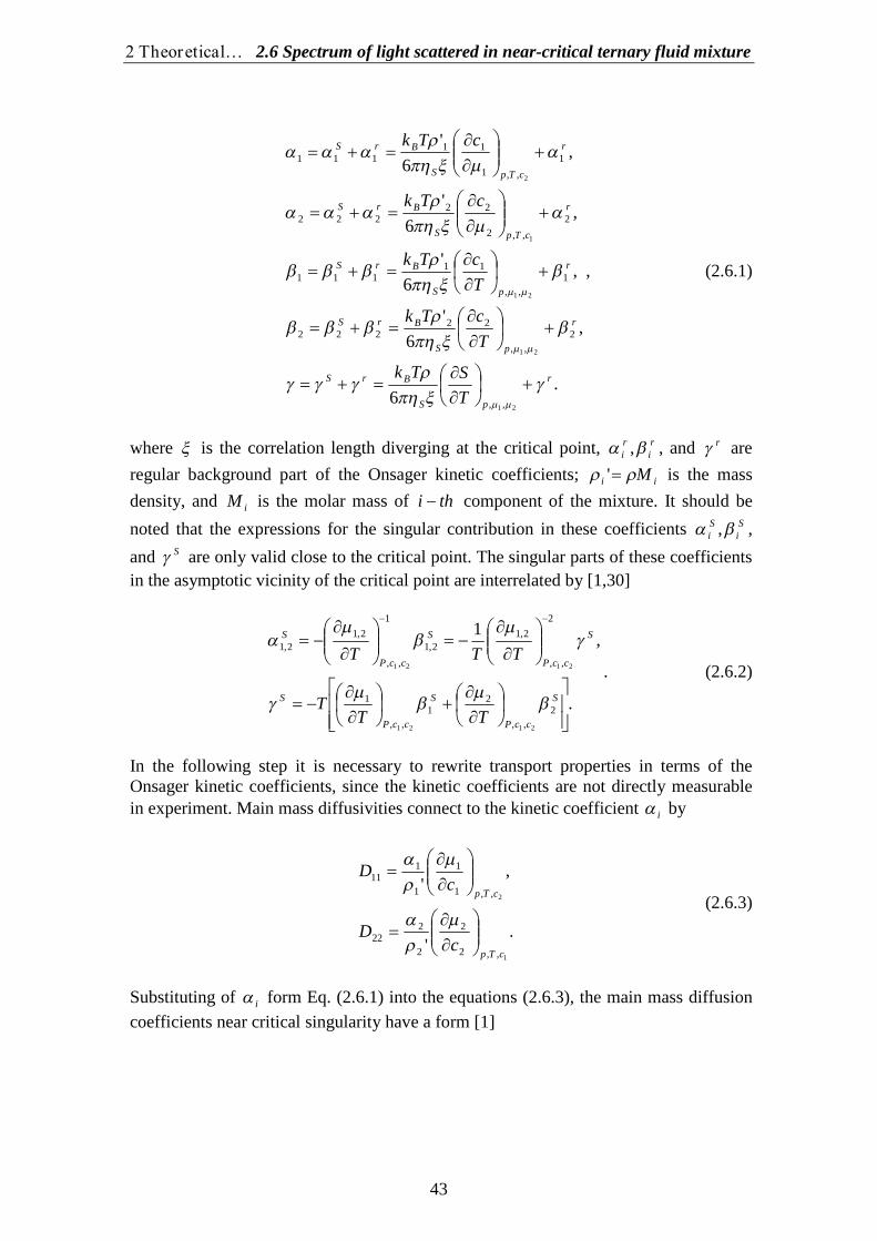
At the beginning we will obtain expressions of transport properties near critical pointadhering to Anisimov’s method [1]. The Onsager kinetic coefficients ii , and ,included in expression (2.5.1), near the critical point can be written as the sum of thesingular and regular parts. These coefficients for ternary liquid mixture satisfy thefollowing equations:
2 Theoretical… 2.6 Spectrum of light scattered in near-critical ternary fluid mixture
43
.6
,6
'
,6
'
,6
'
,6
'
21
21
21
1
2
,,
2,,
22222
1,,
11111
2
,,2
22222
1
,,1
11111
r
pS
BrS
r
pS
BrS
r
pS
BrS
r
cTpS
BrS
r
cTpS
BrS
TSTk
TcTk
TcTk
cTk
cTk
, (2.6.1)
where is the correlation length diverging at the critical point, ri
ri , , and r are
regular background part of the Onsager kinetic coefficients; ii M' is the massdensity, and iM is the molar mass of thi component of the mixture. It should be
noted that the expressions for the singular contribution in these coefficients Si
Si , ,
and S are only valid close to the critical point. The singular parts of these coefficientsin the asymptotic vicinity of the critical point are interrelated by [1,30]
.
,1
2,,
21
,,
1
2
,,
2,12,1
1
,,
2,12,1
2121
2121
S
ccP
S
ccP
S
S
ccP
S
ccP
S
TTT
TTT
. (2.6.2)
In the following step it is necessary to rewrite transport properties in terms of theOnsager kinetic coefficients, since the kinetic coefficients are not directly measurablein experiment. Main mass diffusivities connect to the kinetic coefficient i by
.'
,'
1
2
,,2
2
2
222
,,1
1
1
111
cTp
cTp
cD
cD
(2.6.3)
Substituting of i form Eq. (2.6.1) into the equations (2.6.3), the main mass diffusioncoefficients near critical singularity have a form [1]
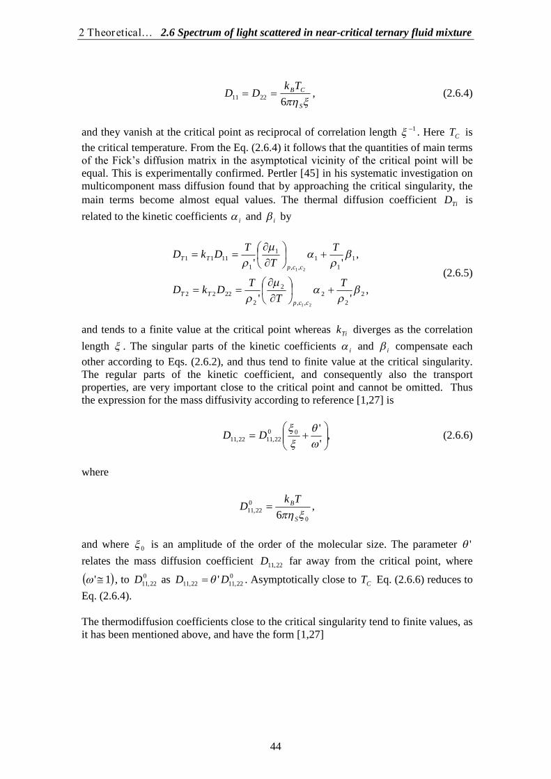
2 Theoretical… 2.6 Spectrum of light scattered in near-critical ternary fluid mixture
44
S
CBTkDD
62211 , (2.6.4)
and they vanish at the critical point as reciprocal of correlation length 1 . Here CT isthe critical temperature. From the Eq. (2.6.4) it follows that the quantities of main termsof the Fick’s diffusion matrix in the asymptotical vicinity of the critical point will be equal. This is experimentally confirmed. Pertler [45] in his systematic investigation onmulticomponent mass diffusion found that by approaching the critical singularity, themain terms become almost equal values. The thermal diffusion coefficient TiD isrelated to the kinetic coefficients i and i by
,''
,''
22
2,,
2
22222
11
1,,
1
11111
21
21
TT
TDkD
TT
TDkD
ccpTT
ccpTT
(2.6.5)
and tends to a finite value at the critical point whereas Tik diverges as the correlationlength . The singular parts of the kinetic coefficients i and i compensate eachother according to Eqs. (2.6.2), and thus tend to finite value at the critical singularity.The regular parts of the kinetic coefficient, and consequently also the transportproperties, are very important close to the critical point and cannot be omitted. Thusthe expression for the mass diffusivity according to reference [1,27] is
,''00
22,1122,11
DD (2.6.6)
where
,6 0
022,11 S
BTkD
and where 0 is an amplitude of the order of the molecular size. The parameter 'relates the mass diffusion coefficient 22,11D far away from the critical point, where
1' , to 022,11D as 0
22,1122,11 ' DD . Asymptotically close to CT Eq. (2.6.6) reduces toEq. (2.6.4).
The thermodiffusion coefficients close to the critical singularity tend to finite values, asit has been mentioned above, and have the form [1,27]
2 Theoretical… 2.6 Spectrum of light scattered in near-critical ternary fluid mixture
45
02,12121
022,112,1 1' TccccT kxxxxDD , (2.6.7)
where cix is the critical mole fraction of species i near the critical point, 02,1Tk is the
thermodiffusion ratio far away from the critical point. Near the consolute point thethermodiffusion ratio becomes
0
02,121212,1 1
TccccT kxxxxk , (2.6.8)
and diverges as .
It is possible to see from the formula for the dynamic structure factor (2.5.27), that, in anear critical ternary liquid mixture, there exists, in general, a three-exponential timedecay. We find three different transport modes that are associated with thermaldiffusion (first time decay) and mass diffusion (other two decays). These three timeexponential modes are defined by coefficients 1z and 3,2z (2.5.18). The diffusivity 3,2z
of the slow mode is associated with mutual diffusion coefficients and diffusivity 1z ofthe fast mode is associated with thermal diffusivity,
S
B
PiTi
TkDz
CDz
622,113,2
1
, (2.6.9)
with 3,21 zz where is the thermal conductivity. According to ref. [1] the secondamplitude from Eqs. (2.5.27) and (2.5.28a,b) near the critical point tends to zero
02 A . Therefore, in the close vicinity of the critical point, the light scattered frommulticomponent liquid system is determined by the fast mass diffusion mode with
TiDz 1 and amplitude 1A .
In the beginning of this section it was stated that in the vicinity of the criticalsingularity the correlation length is comparable with and subsequently even largerthan 1q and the wave numbers q of the static and dynamic properties must be takeninto account. In the case of ternary liquid system, which is characterized by two-exponent decay, the three decay rates 2
11 )(' qqz
and 222 )(' qqz
, observed inlight scattering, depend on the wave numbers as
2 Theoretical… 2.6 Spectrum of light scattered in near-critical ternary fluid mixture
46
.)('
,1,
1,)('
22
3
2
1
qqq
z
(2.6.10)
where 0.06z [11].
Thus, near the critical point, the linewidth of the Rayleigh line is not proportional to asquare of wave number, as in case of the hydrodynamic range, and it contains highervalues of exponents that should appear in expressions of angular dependence of lightscattered.
The present theory allows to calculate thermodynamic and transport properties formulticomponent mixture and to compare the computed data with experiment. Thetheory predicts the existence of the three-exponential decay function in dynamic lightscattering in near-critical ternary fluid mixture. It could be shown that in the ternaryfluid mixture a coupling can occur between three transports modes where one isassociated with thermal diffusions and the others with mass diffusion. Moreover, thetheory allows calculating the relative amplitudes of three relaxations modes for amulticomponent liquid system if enough information about static and dynamicproperties is available.
3 Experimental part 3.1 Chemicals and equipment
47
3 Experimental part
In this chapter we have deals with experimental aspects of DLS for ternary mixture. Thepreparation of the samples and equipment described here. To determination of thedemixing temperatures and critical concentration of the critical samples we used thevolume equivalence criterion. Moreover procedure of light scattering experiment ispresent in this chapter. We discuss methods of the light scattering for measurements ofboth static and dynamic properties. For this aim we used seventeen differentcomposition of GAW system. Three samples of our mixtures near plait point weremade. Here we discuss about check of optical justage and performance of lightscattering measurements. Also we consider problem of measurements of ACF andestimate data of chemical potential gradient.
3.1 Chemicals and equipment
For all described measurements the system glycerol (0) –acetone (1) –water (2)(GAW) has been applied, where we used certified ACS acetone (99,9 mole %) fromAcros Organics Company without further purification. The acetone was ECD tested forpesticide analysis and contained a maximum amount of 0.2% of water. CertificatedC.A.S. spectranalyzed glycerol from Acros Organics Company with a content of 99,5mole % was used. The specifications by the manufacturer are presented in Table 1 (seeAppendix H).
During the sample preparation three components were weighed in flasks in the sequenceglycerol, water and acetone in order to minimize evaporation losses because ofincreasing volatility. After that the samples were closed and sealed quickly with teflontape, so that the loss of sample evaporation, especially of acetone, have been minimized.Since glycerol is very hygroscopic, traces of water have to be removed, because of itslarge heat capacity the water content will significantly raise the phase separationtemperature of the system. Therefore the substance was boiled under reflux withcalcium hydride followed by a distillation under reduced pressure and dried nitrogen asprotective gas.
In order to guarantee the purity of the mixtures, which is necessary for thereproducibility of the measurements, the adsorption of the water on the surface of theglass must be absolutely avoided. Therefore it is necessary to carry out the followingprocedure for the successful treatment of the glass equipment during the work:
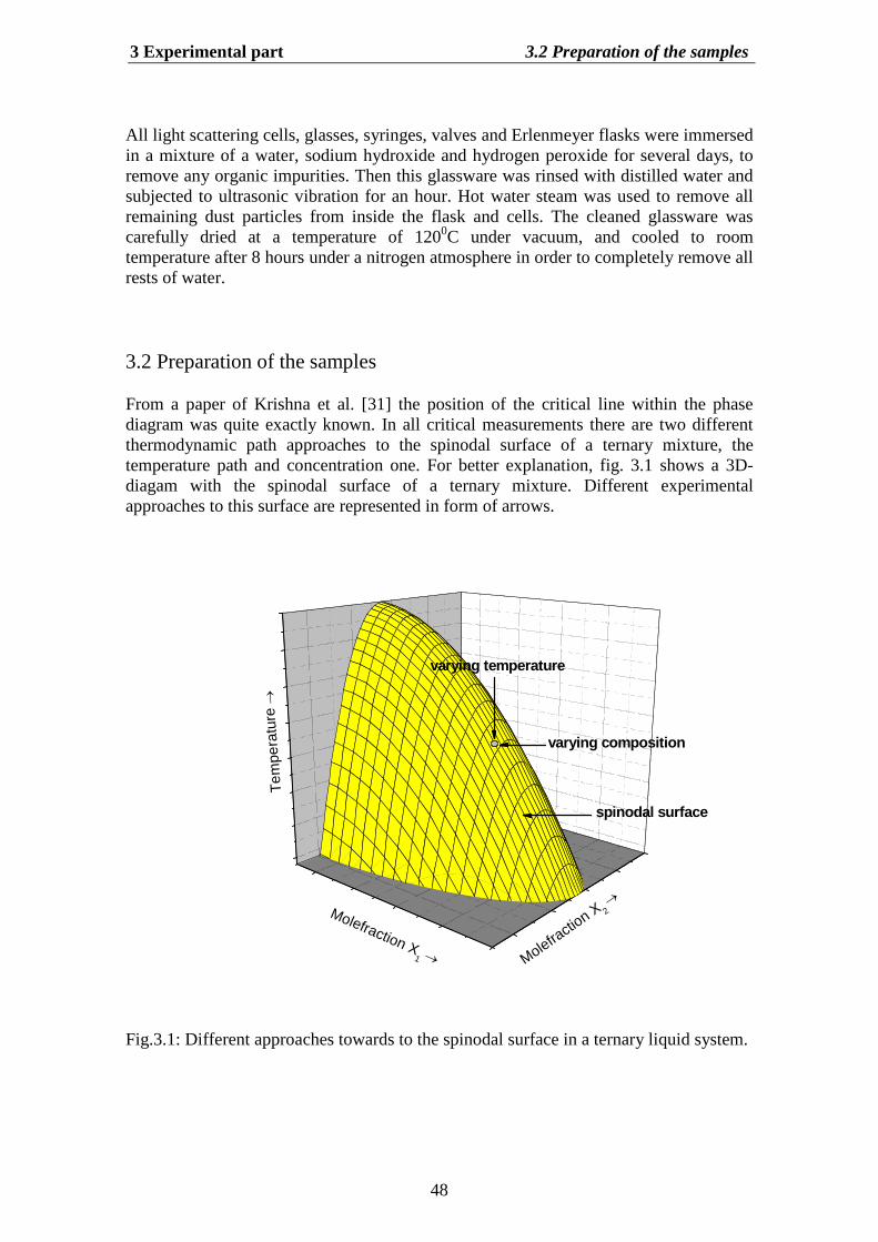
3 Experimental part 3.2 Preparation of the samples
48
All light scattering cells, glasses, syringes, valves and Erlenmeyer flasks were immersedin a mixture of a water, sodium hydroxide and hydrogen peroxide for several days, toremove any organic impurities. Then this glassware was rinsed with distilled water andsubjected to ultrasonic vibration for an hour. Hot water steam was used to remove allremaining dust particles from inside the flask and cells. The cleaned glassware wascarefully dried at a temperature of 1200C under vacuum, and cooled to roomtemperature after 8 hours under a nitrogen atmosphere in order to completely remove allrests of water.
3.2 Preparation of the samples
From a paper of Krishna et al. [31] the position of the critical line within the phasediagram was quite exactly known. In all critical measurements there are two differentthermodynamic path approaches to the spinodal surface of a ternary mixture, thetemperature path and concentration one. For better explanation, fig. 3.1 shows a 3D-diagam with the spinodal surface of a ternary mixture. Different experimentalapproaches to this surface are represented in form of arrows.
spinodal surface
varying composition
varying temperature
Tem
pera
ture
Molefractio
n X 2
Molefraction X1
Fig.3.1: Different approaches towards to the spinodal surface in a ternary liquid system.
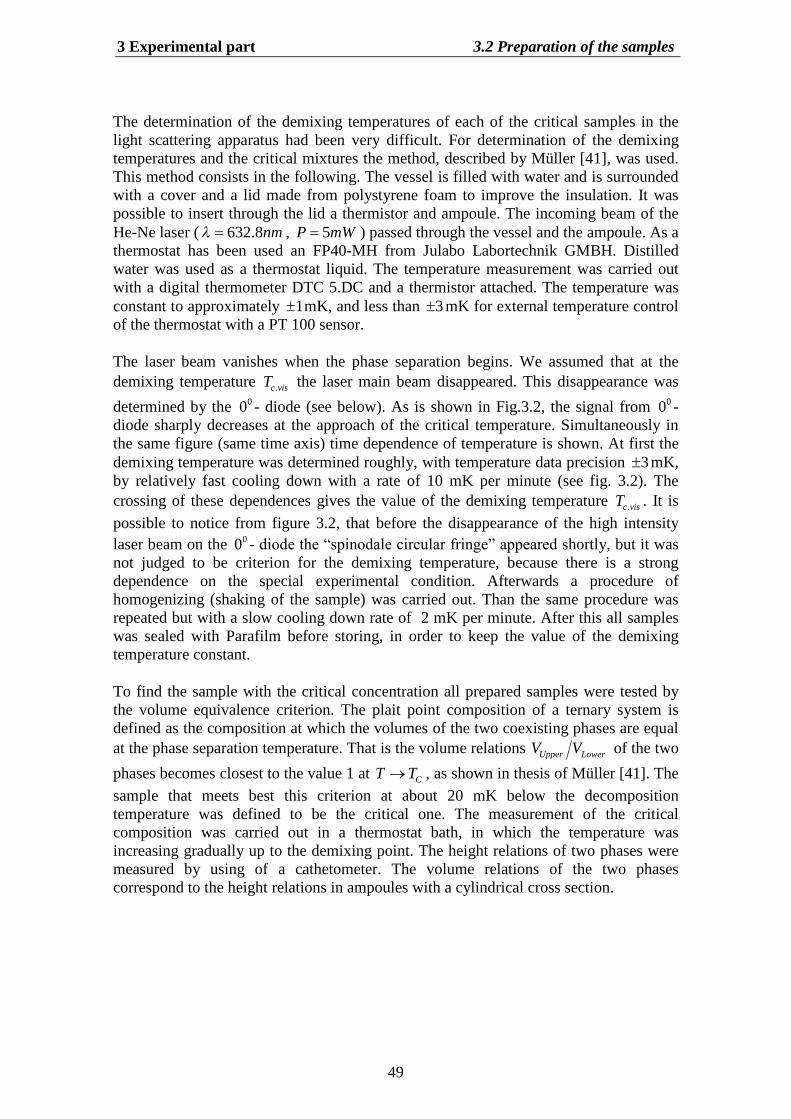
3 Experimental part 3.2 Preparation of the samples
49
The determination of the demixing temperatures of each of the critical samples in thelight scattering apparatus had been very difficult. For determination of the demixingtemperatures and the critical mixtures the method, described by Müller [41], was used.This method consists in the following. The vessel is filled with water and is surroundedwith a cover and a lid made from polystyrene foam to improve the insulation. It waspossible to insert through the lid a thermistor and ampoule. The incoming beam of theHe-Ne laser ( 632.8nm , 5P mW ) passed through the vessel and the ampoule. As athermostat has been used an FP40-MH from Julabo Labortechnik GMBH. Distilledwater was used as a thermostat liquid. The temperature measurement was carried outwith a digital thermometer DTC 5.DC and a thermistor attached. The temperature wasconstant to approximately 1mK, and less than 3mK for external temperature controlof the thermostat with a PT 100 sensor.
The laser beam vanishes when the phase separation begins. We assumed that at thedemixing temperature .c visT the laser main beam disappeared. This disappearance was
determined by the 00 - diode (see below). As is shown in Fig.3.2, the signal from 00 -diode sharply decreases at the approach of the critical temperature. Simultaneously inthe same figure (same time axis) time dependence of temperature is shown. At first thedemixing temperature was determined roughly, with temperature data precision 3mK,by relatively fast cooling down with a rate of 10 mK per minute (see fig. 3.2). Thecrossing of these dependences gives the value of the demixing temperature .c visT . It ispossible to notice from figure 3.2, that before the disappearance of the high intensitylaser beam on the 00 - diode the “spinodale circular fringe” appeared shortly, but it wasnot judged to be criterion for the demixing temperature, because there is a strongdependence on the special experimental condition. Afterwards a procedure ofhomogenizing (shaking of the sample) was carried out. Than the same procedure wasrepeated but with a slow cooling down rate of 2 mK per minute. After this all sampleswas sealed with Parafilm before storing, in order to keep the value of the demixingtemperature constant.
To find the sample with the critical concentration all prepared samples were tested bythe volume equivalence criterion. The plait point composition of a ternary system isdefined as the composition at which the volumes of the two coexisting phases are equalat the phase separation temperature. That is the volume relations Upper LowerV V of the two
phases becomes closest to the value 1 at CT T , as shown in thesis of Müller [41]. Thesample that meets best this criterion at about 20 mK below the decompositiontemperature was defined to be the critical one. The measurement of the criticalcomposition was carried out in a thermostat bath, in which the temperature wasincreasing gradually up to the demixing point. The height relations of two phases weremeasured by using of a cathetometer. The volume relations of the two phasescorrespond to the height relations in ampoules with a cylindrical cross section.
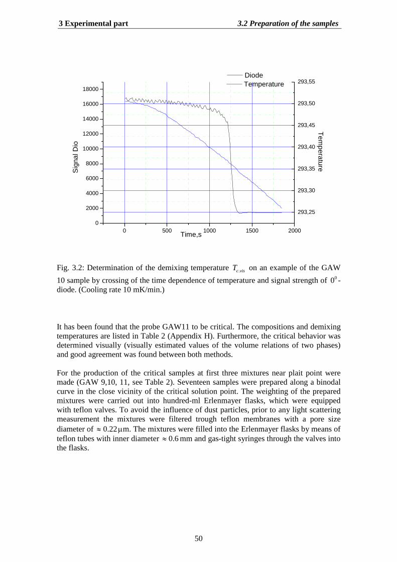
3 Experimental part 3.2 Preparation of the samples
50
0 500 1000 1500 20000
2000
4000
6000
8000
10000
12000
14000
16000
18000
Tem
peratureS
igna
lDio
Time,s
Diode
293,25
293,30
293,35
293,40
293,45
293,50
293,55Temperature
Fig. 3.2: Determination of the demixing temperature .c visT on an example of the GAW
10 sample by crossing of the time dependence of temperature and signal strength of 00 -diode. (Cooling rate 10 mK/min.)
It has been found that the probe GAW11 to be critical. The compositions and demixingtemperatures are listed in Table 2 (Appendix H). Furthermore, the critical behavior wasdetermined visually (visually estimated values of the volume relations of two phases)and good agreement was found between both methods.
For the production of the critical samples at first three mixtures near plait point weremade (GAW 9,10, 11, see Table 2). Seventeen samples were prepared along a binodalcurve in the close vicinity of the critical solution point. The weighting of the preparedmixtures were carried out into hundred-ml Erlenmayer flasks, which were equippedwith teflon valves. To avoid the influence of dust particles, prior to any light scatteringmeasurement the mixtures were filtered trough teflon membranes with a pore sizediameter of 22.0 m. The mixtures were filled into the Erlenmayer flasks by means ofteflon tubes with inner diameter 0.6 mm and gas-tight syringes through the valves intothe flasks.
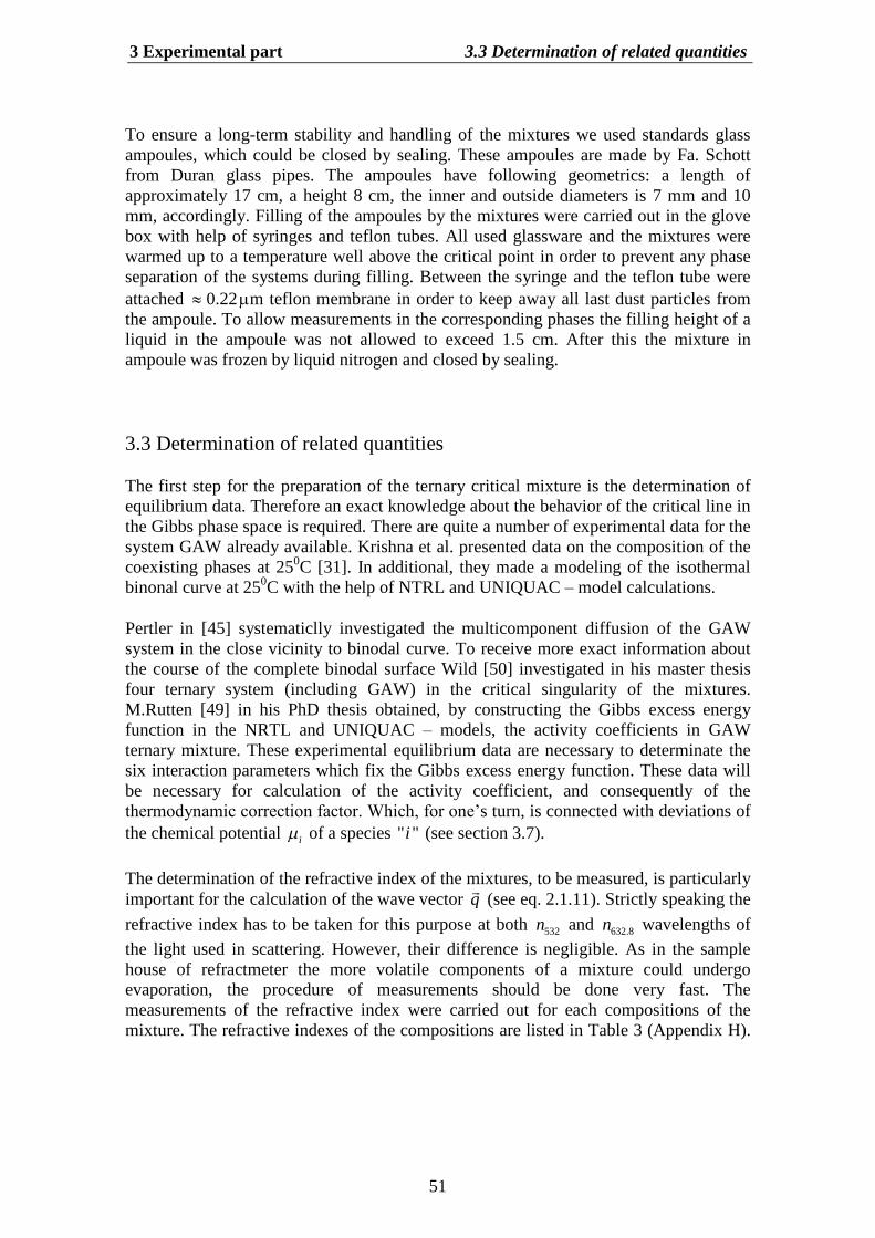
3 Experimental part 3.3 Determination of related quantities
51
To ensure a long-term stability and handling of the mixtures we used standards glassampoules, which could be closed by sealing. These ampoules are made by Fa. Schottfrom Duran glass pipes. The ampoules have following geometrics: a length ofapproximately 17 cm, a height 8 cm, the inner and outside diameters is 7 mm and 10mm, accordingly. Filling of the ampoules by the mixtures were carried out in the glovebox with help of syringes and teflon tubes. All used glassware and the mixtures werewarmed up to a temperature well above the critical point in order to prevent any phaseseparation of the systems during filling. Between the syringe and the teflon tube wereattached 22.0 m teflon membrane in order to keep away all last dust particles fromthe ampoule. To allow measurements in the corresponding phases the filling height of aliquid in the ampoule was not allowed to exceed 1.5 cm. After this the mixture inampoule was frozen by liquid nitrogen and closed by sealing.
3.3 Determination of related quantities
The first step for the preparation of the ternary critical mixture is the determination ofequilibrium data. Therefore an exact knowledge about the behavior of the critical line inthe Gibbs phase space is required. There are quite a number of experimental data for thesystem GAW already available. Krishna et al. presented data on the composition of thecoexisting phases at 250C [31]. In additional, they made a modeling of the isothermalbinonal curve at 250C with the help of NTRL and UNIQUAC–model calculations.
Pertler in [45] systematiclly investigated the multicomponent diffusion of the GAWsystem in the close vicinity to binodal curve. To receive more exact information aboutthe course of the complete binodal surface Wild [50] investigated in his master thesisfour ternary system (including GAW) in the critical singularity of the mixtures.M.Rutten [49] in his PhD thesis obtained, by constructing the Gibbs excess energyfunction in the NRTL and UNIQUAC –models, the activity coefficients in GAWternary mixture. These experimental equilibrium data are necessary to determinate thesix interaction parameters which fix the Gibbs excess energy function. These data willbe necessary for calculation of the activity coefficient, and consequently of thethermodynamic correction factor. Which, for one’s turn, is connected with deviations ofthe chemical potential i of a species " "i (see section 3.7).
The determination of the refractive index of the mixtures, to be measured, is particularlyimportant for the calculation of the wave vector q
(see eq. 2.1.11). Strictly speaking the
refractive index has to be taken for this purpose at both 532n and 632.8n wavelengths ofthe light used in scattering. However, their difference is negligible. As in the samplehouse of refractmeter the more volatile components of a mixture could undergoevaporation, the procedure of measurements should be done very fast. Themeasurements of the refractive index were carried out for each compositions of themixture. The refractive indexes of the compositions are listed in Table 3 (Appendix H).
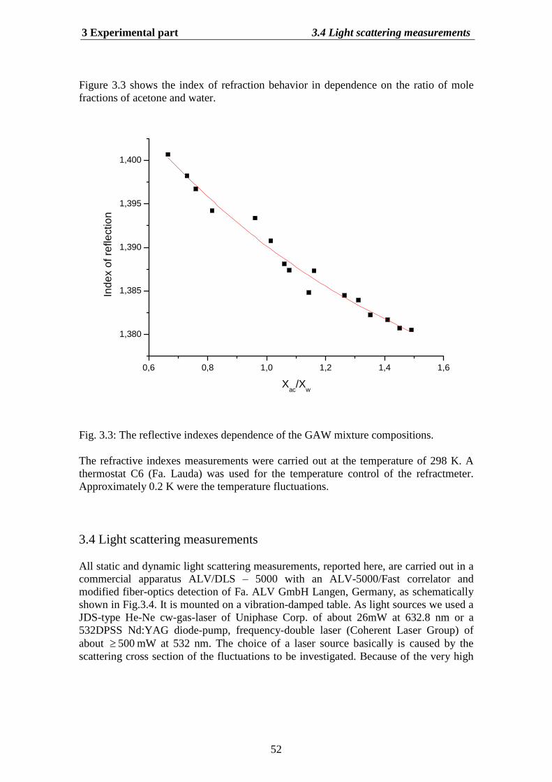
3 Experimental part 3.4 Light scattering measurements
52
Figure 3.3 shows the index of refraction behavior in dependence on the ratio of molefractions of acetone and water.
0,6 0,8 1,0 1,2 1,4 1,6
1,380
1,385
1,390
1,395
1,400
Inde
xof
refle
ctio
n
Xac
/Xw
Fig. 3.3: The reflective indexes dependence of the GAW mixture compositions.
The refractive indexes measurements were carried out at the temperature of 298 K. Athermostat C6 (Fa. Lauda) was used for the temperature control of the refractmeter.Approximately 0.2 K were the temperature fluctuations.
3.4 Light scattering measurements
All static and dynamic light scattering measurements, reported here, are carried out in acommercial apparatus ALV/DLS –5000 with an ALV-5000/Fast correlator andmodified fiber-optics detection of Fa. ALV GmbH Langen, Germany, as schematicallyshown in Fig.3.4. It is mounted on a vibration-damped table. As light sources we used aJDS-type He-Ne cw-gas-laser of Uniphase Corp. of about 26mW at 632.8 nm or a532DPSS Nd:YAG diode-pump, frequency-double laser (Coherent Laser Group) ofabout 500 mW at 532 nm. The choice of a laser source basically is caused by thescattering cross section of the fluctuations to be investigated. Because of the very high
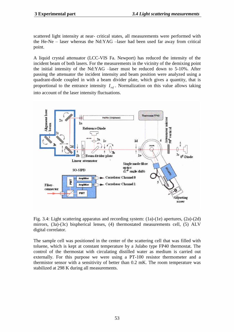
3 Experimental part 3.4 Light scattering measurements
53
scattered light intensity at near- critical states, all measurements were performed withthe He-Ne –laser whereas the Nd:YAG –laser had been used far away from criticalpoint.
A liquid crystal attenuator (LCC-VIS Fa. Newport) has reduced the intensity of theincident beam of both lasers. For the measurements in the vicinity of the demixing pointthe initial intensity of the Nd:YAG –laser must be reduced down to 5-10%. Afterpassing the attenuator the incident intensity and beam position were analyzed using aquadrant-diode coupled in with a beam divider plate, which gives a quantity, that isproportional to the entrance intensity refI . Normalization on this value allows takinginto account of the laser intensity fluctuations.
Fig. 3.4: Light scattering apparatus and recording system: (1a)-(1e) apertures, (2a)-(2d)mirrors, (3a)-(3c) bispherical lenses, (4) thermostated measurements cell, (5) ALVdigital correlator.
The sample cell was positioned in the center of the scattering cell that was filled withtoluene, which is kept at constant temperature by a Julabo type FP40 thermostat. Thecontrol of the thermostat with circulating distilled water as medium is carried outexternally. For this purpose we were using a PT-100 resistor thermometer and athermistor sensor with a sensitivity of better than 0.2 mK. The room temperature wasstabilized at 298 K during all measurements.
3 Experimental part 3.5 Check of optical justage of the equipment…
54
The intensity of the scattered light was measured with photomultipliers. In order toimprove the quality of the signals and to increase the signal-to-noise ratio the intensityof the scattered light was measured with a special single-mode fiber optics inconnection with a cross-correlation detector. The fiber allows to select one single TEM-mode. In the SO-SIPD detector the beam is splitted and fed to two photomultiplier tubes(PMT), which produce a pseudo-cross-correlation function. These two PMT’s have been used in order to avoid distortions in measurements of the correlation function fromafter-pulse and dead-time effects of the PMTs. The PMT-detector is mounted on agoniometer, as shown in Figure 3.4, which allows to scan a range of angle from 300 upto 1520 with an accuracy of better then 0.010. Temperature-, diode-, and angle data aresent through a central control unit LSE 3018 to the PC. The correlation function ismeasured using a special type of a fast photon correlator plate (ALV-5000/FAST) indirect connection with two PMTs in cross-correlation mode. The method ofmeasurements of the ACF will be described in section 3.5. This fast correlator enabledus to obtain delay times down to 12.5 ns for dynamic analysis of scattered light. Allchannels of the digital correlator are calculated in real time, using a strongly parallelarchitecture. The CPU, which is implemented in programmable gate arrays, performs1.8*109 of multiply-and-add operation per second.
The quadrant diode (the 00-diode) was applied for the optical determination of thedemixing temperature .c visT and simultaneously for measuring turbidity data. With helpof the 00-diode it was possible to detect not only the intensity of autocorrelationfunction but also the change in the position of the laser beam. This is useful foradjustment of the position of the cuvette and it is controlled and checked regularly withcalibration scattering measurements.
3.5 Check of optical justage of the equipment and performance of the lightscattering measurements
In order to check the justage of the optical device of the light scattering system and thequality of the toluene bath we carry out calibrating scattering measurements with atoluene –test sample. After light scattering corrections (as discussed later) for dark –counting rates, dead time, scattering volume, laser fluctuations and backgroundcorrection, toluene, as an isotropic scattering medium, should show no angulardependence of its scattering intensity.
The quality of the optical justage is described by the coefficient R . It is determinedfrom measurements of the scattering intensity ( )TolI , which arises from toluene
scattered in the angular range of 0 030 150 at the constant temperature, related tothe intensity at 900:
3 Experimental part 3.5 Check of optical justage of the equipment…
55
0
0
( ) (90 )(90 )
Tol Tol
Tol
I IR
I
(3.5.1)
During the whole measurement period this coefficient should not fluctuate more than3%. These measurements should be repeated several times and performed withextremely pure and dust free toluene. The cuvette must be very carefully cleaned toremove all organic rests and any dust particles from the glasses surface. The toluenemust be filtered with a 0.1m teflon filter and filling in the cuvette in a flow box or aglove box. If there are any light dots in the sample it will not give a good reference.This test should be done in an angle interval of 05 with about 10…20 seconds each.
After centrifugation to remove dust particles from the scattering volume, the sample cellwas positioned into the apparatus. It was allowed to come to thermal equilibrium byobserving the intensity profile over a time range of about 2-3 hours. For the near-criticalsamples it needs especially long time to come to the thermal equilibrium. Theequilibrium process could be observed using the 00-diode. Strong position fluctuationswere often stated here which are apparently caused by conversion currents within thesample. In all samples we measured intensities at 11 angles between 400 and 1400 andabout 60 temperatures with a step of 0.2K in a range KTT C 1206.0 . The samplingtime at each angle and temperature was 40 s. This procedure was repeated five times toget 200 second of total measurement time interrupted by 5 seconds autoscalingprocedure between each sampling time.
The intensity of light scattering measured by the photomultiplier includes a number ofsystematic errors. Therefore it should be necessary to take into account a number ofcorrections for the evaluation of static scattering data, as shown in the PhD thesis ofMüller [41].
Both the photomultiplier and the diodes show a certain counting rate even in absence oflight waves. This dark counting rate is caused by thermal noise. It depends on thetemperature in the laboratory. Therefore the dark counting rate is a linear function of theroom temperature . For this reason the room temperature was permanently monitoredand kept constant during the light scattering measurements:
1 ( )I I a b , (3.5.3)
where the coefficient a and b were determined before the measurements.
Every photomultiplier needs a certain time until the charge, caused by registeredphotons, is reduced again. This leads to a “memory effect”, because of which the intensity contribution, registered at a time t (without dead time), is stored at deadt t .The dead time of our photomultiplier is approximately 20 ns and it will be corrected byan exponential term:
3 Experimental part 3.5 Check of optical justage of the equipment…
56
12 1
deadI tI I e . (3.5.4)
The scattering volume is the cross volume between the scattering cone in the cuvetteand sight cone provided by a pinholes and shutter of the photomultiplier. It has itsminimum at the scattering angle 090 and the correction is carried out by a sinussquare function:
23 2 sinI I . (3.5.5)
Ideally the laser light sources should be very stable in time and space. However, thelaser sources used in practice show temporal and spatial intensity fluctuations, whichare registered by the reference diode (see fig. 3.4). It gives a relative initial intensity
refI . Therefore, for the static light scattering a relative scattering intensity has the form:
34
ref
II
I . (3.5.6)
As it has been noted above near the critical point a liquid mixture shows a more or lessstrong turbidity. This is caused by a multiple scattering. The turbidity correction leadsback to a correction regarding the transmission. This correction can be applied, if theoptical paths lengths for the scattered light and for the transmitted light are the same.Supposed that the center of scattering volume is exactly in the middle of the cylindricalcuvette. For the turbidity correction
5 4,
B
Tr ref B
I IrefI I
I I , (3.5.7)
where TrI and BI are the intensities of the transmitted light and the backgroundscattering, respectively.
In order to extract the effect of criticality from our measurements the followingprocedure was applied for background correction. The same mixture has been used andthe intensity of scattered light was measured at 35 K above the critical temperature. Atthis high temperature no critical effects are expected and thus BI is taken forbackground correction:
5,
B
Bsc
ref B
IT
I II
T
. (3.5.8)
3 Experimental part 3.6 Measurements of the autocorrelation function (ACF)…
57
Furthermore, all previous expressions are valid for isotropic light scattering only. Amore general expression is obtained by taking into account the anisotropic part of thescattered light. If we measure the depolarization u of scattered light we can write thetotal scattering intensity (Eq. 3.5.8) with Cabanne’s factor in the form [12]:
6 6(90)
6 7u
scu
I I
(3.5.9)
The depolarization of the light scattering u was measured with a Glan-Thompsonprism and found that the effect of a depolarized component was negligibly small.Therefore we performed our data analysis without taking into account anydepolarization.
3.6 Measurements of the autocorrelation function (ACF) and linewidth ofthe Rayleigh scattering
With the light scattering apparatus, described in section 3.4, it is possible to measureboth the intensity of the scattered light and simultaneously the relaxation times of thescattered light. In general, the time autocorrelation function gives us information on thedegree to which two dynamic properties are correlated over a considered period in time.The exact form of the ACF depends on the underlying scattering process and on theexperimental conditions that are discussed in detail in works of Leipertz et al [52].Measurements of this intensity time-correlation function provide information abouthydrodynamic transport properties of solute, such as diffusion coefficients andviscosity.
The starting point is the ACF of the electric field
(1) *( ) ( ) ( )G E t E t . (3.6.1)
The ACF of a quantity describes the time scales on which changes in this quantity takeplace and thus conclusions on the underlying transport and thermophysical behaviourcan be drawn. In pure fluids contributions to the ACF may be caused by entropyfluctuations. In this case the first-order correlation function of the electric field gives
(1) ( ) exp( )S dG A , (3.6.2)
where d is the characteristic decay time of the relaxation process caused by thermaldiffusion and SA is the corresponding amplitude. In the case of a liquid mixture there is
3 Experimental part 3.6 Measurements of the autocorrelation function (ACF)…
58
an additional contribution due to concentration fluctuations. Thus the function (1) ( )G becomes a sum of two exponential terms [16,27].
(1) ( ) exp( ) exp( )S d C cG A A . (3.6.3)
The term c denotes the decay time of the mass diffusion process and CA is therespective amplitude. As it has been shown in section 2.5, at the treatment of thedynamic structure factor (Eq. 2.5.27) the connection between the temporal fluctuation ofthe thermodynamic quantities and the ACF of the first order (1) ( )G could be obtained.In actual photon-correlation experiments the photomultiplier are used, which respond tothe intensity of the scattered light. The PMT is a square-law detector, its instantaneouscurrent output is proportional to the square of the incident electric field
2( ) ( )I t E t ,
that is to the intensity of the light or the numbers of photons; it follow that the ACF ofsecond order (2) ( )G is of fourth order in the electric field
(2) ( ) ( ) ( ) ( ) ( )G E t E t E t E t , (3.6.4)
where E is the complex conjugate of E . As long as the scattered light intensity obeysthe Gaussian statistics, it is possible to use the well-know properties of the Gaussianprocess, that higher order moment of the stochastic variable can be factorised with thesecond order moments of the field correlation function [27]. After such a factorisationthe connection between the ACF of the first order and those of the second order can bedescribed with help of the following equation:
(2)
2(1)
( ) ( ) ( ) ( ) ( ) ( ) ( )
( ) ( ) ( ) ( ) ( ) ( ) ( ) ( )
1 ( )
G I t I t E t E t E t E t
E t E t E t E t E t E t E t E t
G
. (3.6.5)
Here, it is assumed that the infinite time average t of the intensity is independent
of its starting value, that is, stationary terms were normalized on unity (1) (0) 1G .Substitution of equation (3.6.4) into (3.6.3) yields for a mixture
(2) 2
2 2
( ) ( )
exp( 2 ) 2 exp( ) exp( 2 )S C
S d S C d c C c
G I I
I I I I
, (3.6.6)
where SI and CI are the intensities due to scattering caused by entropy andconcentration fluctuations, respectively. After normalization of the intensity, Eq. (3.6.6)becomes
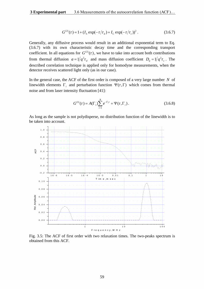
3 Experimental part 3.6 Measurements of the autocorrelation function (ACF)…
59
(2) 2( ) 1 ( exp( ) exp( ))S d C cG I I . (3.6.7)
Generally, any diffusive process would result in an additional exponential term to Eq.(3.6.7) with its own characteristic decay time and the corresponding transportcoefficient. In all equations for (2) ( )G , we have to take into account both contributionsfrom thermal diffusion 21 da q and mass diffusion coefficient 21ij cD q . Thedescribed correlation technique is applied only for homodyne measurements, when thedetector receives scattered light only (as in our case).
In the general case, the ACF of the first order is composed of a very large number N oflinewidth elements i and perturbation function ( , ) which comes from thermalnoise and from laser intensity fluctuation [41]:
(1)
1
( ) ( ) ( , )i
N
i ii
G A e
. (3.6.8)
As long as the sample is not polydisperse, no distribution function of the linewidth is tobe taken into account.
Fig. 3.5: The ACF of first order with two relaxation times. The two-peaks spectrum isobtained from this ACF.
1 1 0 1 0 0
0 , 0 0
0 , 0 2
0 , 0 4
0 , 0 6
0 , 0 8
0 , 1 0
Rel
.Am
plitu
de
F r e q u e n c y , M H z
1 E - 6 1 E - 5 1 E - 4 1 E - 3 0 , 0 1 0 , 1 1 1 0- 0 , 2
0 , 0
0 , 2
0 , 4
0 , 6
0 , 8
1 , 0
AC
F
T i m e , m s e c
3 Experimental part 3.6 Measurements of the autocorrelation function (ACF)…
60
The system used in this work showed two diffusions processes and three diffusioncurrents, which can be associated with temperature and concentration fluctuations.Therefore 3N , but in our system (GAW) two original relaxation times,corresponding to the correlation length of the critical fluctuations, are equal. Thereforein our system only two line widths can be observed, as shown in figure 3.5. Theexpression for the calculation of the linewidths reduced to
1 22(1)1 2( ) 2G A e A e , (3.6.9)
where iA are the amplitudes of the signal with linewidths i. As it is possible to see,we receive an expression for ACF of the first order which is congruent with theequation for the dynamic structure factor (2.5.27). Thus there are two ways, theoreticaland experimental, for a possible separation of the diffusion processes in ternary liquidmixture in the hydrodynamic range and near critical singularity.
3.7 Estimation of the chemical potential gradient
For the full theoretical analysis we need information about the chemical potentialgradient of the GAW system. The chemical potential gradient of a component i in amulticomponent mixture is [49]
1
,1
ni
T p i ij jj
cF c
T
(3.7.1)
with
lnj iij ij
j
cF
c
, (3.7.2)
where ijF is known as the thermodynamic correction factor, i is activity coefficient
and the symbol ij is the Kronecker delta. The thermodynamic factor can be calculatedby common excess free enthalpy models such as NTRL, Uniquac or Wilson. Here theNTRL model was used. From the ternary liquid system from NTRL model it followsthat:
3 Experimental part 3.7 Estimation of the chemical potential gradient
61
1 211 12
1 1
2 121 22
2 2
cT F F
c c
cT F F
c c
, (3.7.3)
where thermodynamic factors for ternary system are determined as
1 111 1
1 0
1 112 1
2 0
ln ln1
ln ln
F cc c
F cc c
;
2 221 2
1 0
2 222 2
2 0
ln ln
ln ln1
F cc c
F cc c
. (3.7.4)
One of the four expressions for the activity coefficients, which were obtained fromNTRL model, has a form:
2 21 21 0 01 0112 21 0 01 2
1 1 2 21 0 01
2 12 0 02 12 02 0 10 2 20 10 202 22 12 0 103 3
2 1 12 0 02 0 1 10 2 20
ln
2 2
c g c gc g c g
c c c g c g
c c g c c gc g c g
c c g c g c c g c g
. (3.7.5)
The rest of the expressions for the activity coefficients (Eq. 3.7.4), in view of theircomplex form, are presented in Appendix G. The NTRL parameters contained inequation (3.7.5) are determined in the following way [49]:
expij ij ij
ijij
g
A
T
. (3.7.6)
The initial parameters ijA and ij for GAW system have been taken from [31], andpresented in Table 4 (see Appendix H). Using both the theoretical model and theexperimental technique we are able to investigate the behaviour of the ternary GAWliquid system.
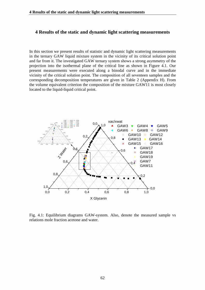
4 Results of the static and dynamic light scattering measurements
62
4 Results of the static and dynamic light scattering measurements
In this section we present results of statistic and dynamic light scattering measurementsin the ternary GAW liquid mixture system in the vicinity of its critical solution pointand far from it. The investigated GAW ternary system shows a strong asymmetry of theprojection into the isothermal plane of the critical line as shown in Figure 4.1. Ourpresent measurements were executed along a binodal curve and in the immediatevicinity of the critical solution point. The composition of all seventeen samples and thecorresponding decomposition temperatures are given in Table 2 (Appendix H). Fromthe volume equivalent criterion the composition of the mixture GAW11 is most closelylocated to the liquid-liquid critical point.
0,0 0,2 0,4 0,6 0,8 1,00,0
0,2
0,4
0,6
0,8
1,00,0
0,2
0,4
0,6
0,8
1,0
0.10 0.15 0.20 0.25 0.30 0.35
0.35
0.40
0.45
0.50
0.55
0.60
0.30
0.35
0.40
0.45
0.50
0.55
0.60
0.907 0.815 0.7600.961 0.666 1.0141.060 1.161 1.1431.264 1.311 1.3521.410 1.451 1.4910.730 1.077
xac/xwatGAW3 GAW4 GAW5GAW6 GAW8 GAW9
GAW10 GAW12GAW13 GAW14GAW15 GAW16
GAW17GAW18GAW19GAW7GAW11
ZW
ater
X Glycerin
Fig. 4.1: Equilibrium diagrams GAW-system. Also, denote the measured sample vsrelations mole fraction acetone and water.
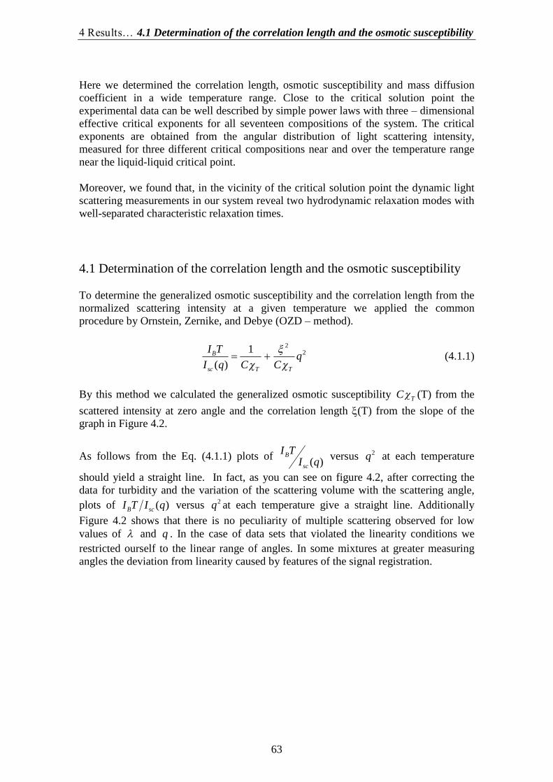
4 Results… 4.1 Determination of the correlation length and the osmotic susceptibility
63
Here we determined the correlation length, osmotic susceptibility and mass diffusioncoefficient in a wide temperature range. Close to the critical solution point theexperimental data can be well described by simple power laws with three–dimensionaleffective critical exponents for all seventeen compositions of the system. The criticalexponents are obtained from the angular distribution of light scattering intensity,measured for three different critical compositions near and over the temperature rangenear the liquid-liquid critical point.
Moreover, we found that, in the vicinity of the critical solution point the dynamic lightscattering measurements in our system reveal two hydrodynamic relaxation modes withwell-separated characteristic relaxation times.
4.1 Determination of the correlation length and the osmotic susceptibility
To determine the generalized osmotic susceptibility and the correlation length from thenormalized scattering intensity at a given temperature we applied the commonprocedure by Ornstein, Zernike, and Debye (OZD–method).
221
( )B
sc T T
I Tq
I q C C
(4.1.1)
By this method we calculated the generalized osmotic susceptibility TC (T) from thescattered intensity at zero angle and the correlation length (T) from the slope of thegraph in Figure 4.2.
As follows from the Eq. (4.1.1) plots of ( )B
sc
I TI q versus 2q at each temperature
should yield a straight line. In fact, as you can see on figure 4.2, after correcting thedata for turbidity and the variation of the scattering volume with the scattering angle,plots of ( )B scI T I q versus 2q at each temperature give a straight line. AdditionallyFigure 4.2 shows that there is no peculiarity of multiple scattering observed for lowvalues of and q . In the case of data sets that violated the linearity conditions werestricted ourself to the linear range of angles. In some mixtures at greater measuringangles the deviation from linearity caused by features of the signal registration.
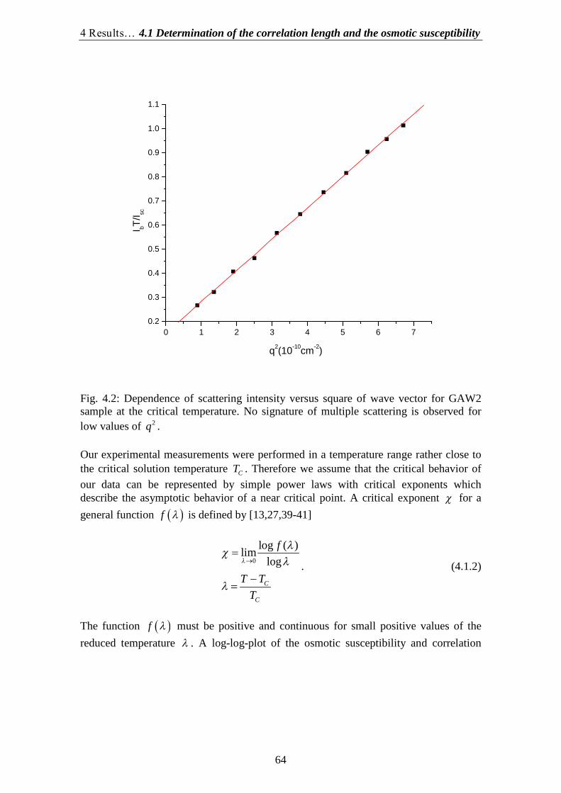
4 Results… 4.1 Determination of the correlation length and the osmotic susceptibility
64
0 1 2 3 4 5 6 70.2
0.3
0.4
0.5
0.6
0.7
0.8
0.9
1.0
1.1
I bT/I sc
q2(10-10cm-2)
Fig. 4.2: Dependence of scattering intensity versus square of wave vector for GAW2sample at the critical temperature. No signature of multiple scattering is observed forlow values of 2q .
Our experimental measurements were performed in a temperature range rather close tothe critical solution temperature CT . Therefore we assume that the critical behavior ofour data can be represented by simple power laws with critical exponents whichdescribe the asymptotic behavior of a near critical point. A critical exponent for ageneral function f is defined by [13,27,39-41]
0
log ( )lim
log
C
C
f
T TT
. (4.1.2)
The function f must be positive and continuous for small positive values of thereduced temperature . A log-log-plot of the osmotic susceptibility and correlation
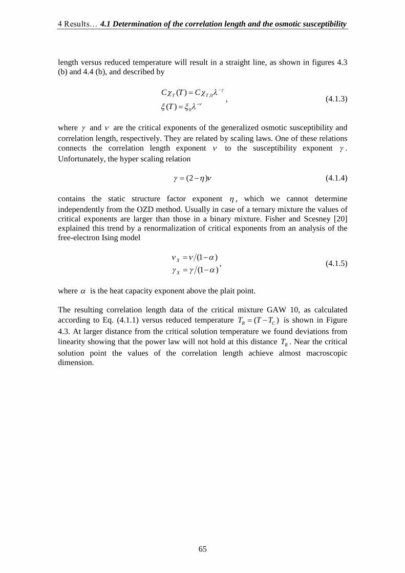
4 Results… 4.1 Determination of the correlation length and the osmotic susceptibility
65
length versus reduced temperature will result in a straight line, as shown in figures 4.3(b) and 4.4 (b), and described by
,0
0
( )
( )T TC T C
T
, (4.1.3)
where and are the critical exponents of the generalized osmotic susceptibility andcorrelation length, respectively. They are related by scaling laws. One of these relationsconnects the correlation length exponent to the susceptibility exponent .Unfortunately, the hyper scaling relation
(2 ) (4.1.4)
contains the static structure factor exponent , which we cannot determineindependently from the OZD method. Usually in case of a ternary mixture the values ofcritical exponents are larger than those in a binary mixture. Fisher and Scesney [20]explained this trend by a renormalization of critical exponents from an analysis of thefree-electron Ising model
(1 )
(1 )X
X
, (4.1.5)
where is the heat capacity exponent above the plait point.
The resulting correlation length data of the critical mixture GAW 10, as calculatedaccording to Eq. (4.1.1) versus reduced temperature ( )R CT T T is shown in Figure4.3. At larger distance from the critical solution temperature we found deviations fromlinearity showing that the power law will not hold at this distance RT . Near the criticalsolution point the values of the correlation length achieve almost macroscopicdimension.
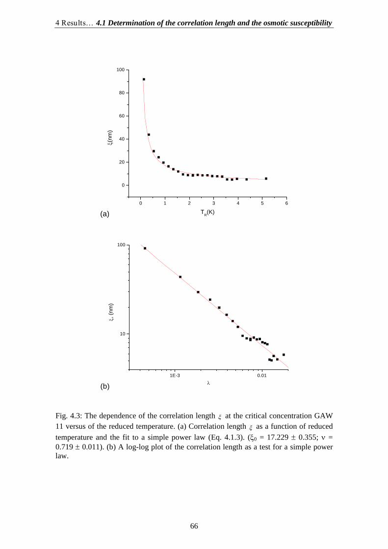
4 Results… 4.1 Determination of the correlation length and the osmotic susceptibility
66
0 1 2 3 4 5 6
0
20
40
60
80
100
(a)
(nm
)
TR(K)
1E-3 0.01
10
100
(b)
,(n
m)
Fig. 4.3: The dependence of the correlation length at the critical concentration GAW11 versus of the reduced temperature. (a) Correlation length as a function of reducedtemperature and the fit to a simple power law (Eq. 4.1.3). (0 = 17.229 0.355; =0.719 0.011). (b) A log-log plot of the correlation length as a test for a simple powerlaw.
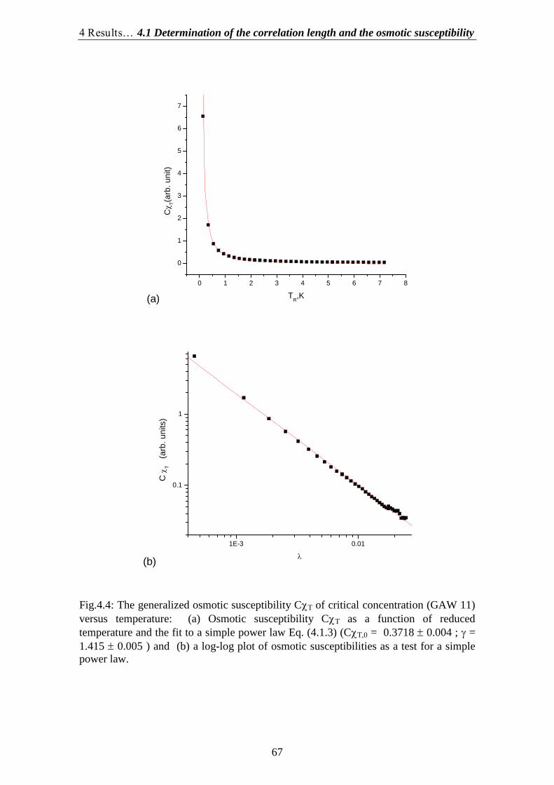
4 Results… 4.1 Determination of the correlation length and the osmotic susceptibility
67
0 1 2 3 4 5 6 7 8
0
1
2
3
4
5
6
7
(a)
C T(
arb.
unit)
TR,K
1E-3 0.01
0.1
1
(b)
C T
(arb
.uni
ts)
Fig.4.4: The generalized osmotic susceptibility CT of critical concentration (GAW 11)versus temperature: (a) Osmotic susceptibility CT as a function of reducedtemperature and the fit to a simple power law Eq. (4.1.3) (CT,0 = 0.3718 0.004 ; =1.415 0.005 ) and (b) a log-log plot of osmotic susceptibilities as a test for a simplepower law.
4 Results… 4.1 Determination of the correlation length and the osmotic susceptibility
68
We were not able to give a single estimate for the uncertainties of over thewhole range of measured temperatures. However, we can specify estimates for thefollowing cases:
In the range 3CT T K , due to the low scattering far from critical opalescencewe found 5nm .
If 3 0.3CT T K the higher scattering intensity leads to 0.1nm . At the immediate vicinity of the critical solution point 0.3CT T K , the system
became very sensitive to fluctuation and the uncertainties grow up to10nm .
Similar ranges are obtained for the generalized osmotic susceptibility. From the zeroangle limit of Eq. (4.1.1) we obtain values for the generalized osmotic susceptibility
TC , the temperature dependence of which is presented in Fig 4.4 a. In Fig. 4.4 b thelinearity of the susceptibility data is shown in a log-log plot. Here the linear range ismuch larger than in the corresponding plot of the correlation length in Fig. 4.3 b. Sinceour data were measured rather close to CT , the divergence of both the correlation length(Fig. 4.3 b) and osmotic susceptibility (Fig. 4.4 b) with reduced temperature can bedescribed by a simple power law (Eq. 4.1.3). To determine the parameters in thisequations we performed nonlinear least-square fits, described in [41,47]. As inputparameters we used weighted ( )TC and data from the OZD method. In the
objective function the critical amplitude was considered a linear parameter, whereas cTand the critical exponents were treated as nonlinear parameters in the fit. Table 5 fromAppendix H gives the results for the correlation length fit of five samples near the plaitpoint of GAW and Table 6 contains those for the osmotic susceptibility. Here we do notpresent data for other compositions of the mixture, since it was not possible to obtainthe desired precision in measurements of the correlation length and the osmoticsusceptibility.
As shown in the first column of Tables 5, 6 we achieved satisfying fits with reasonableresults for both properties. The critical temperatures of both fits agree very well with theexperimental decomposition temperatures, given in Table 2. Within their uncertaintiesthe effective critical exponents and are very close to values of the renormalizedexponents according to Eq. (4.1.5), ( 0,70x and 1, 417x ) respectively.
In our data analysis, we have paid particular attention to possible errors in the least-square fitting procedure due to experimental effects. As in [39,40] we find errorestimates in critical exponents, which are due to such effects as reflection, refraction,dust, temperature uncertainty, optical alignment, extinction coefficient, and linearly ofdetectors, over finite ranges of angles and temperature interval. As shown in Eq.(4.1.1)the OZD method does not consider the singularity of the static structure factor,
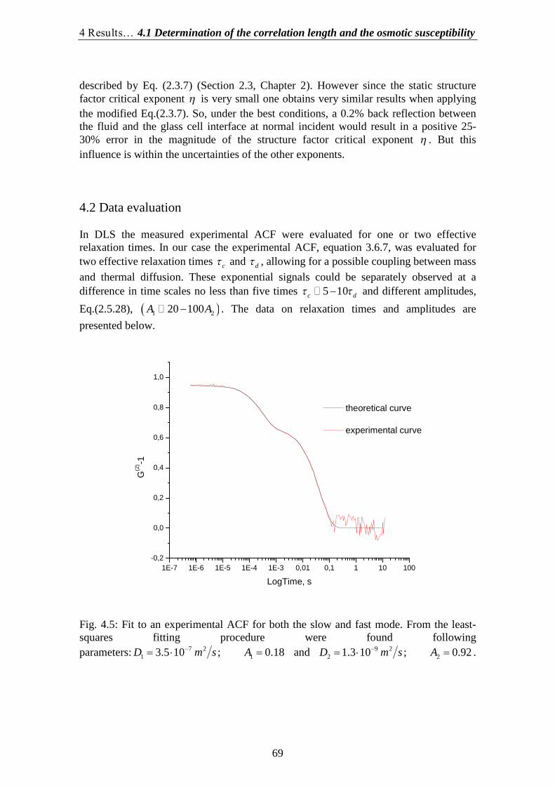
4 Results… 4.1 Determination of the correlation length and the osmotic susceptibility
69
described by Eq. (2.3.7) (Section 2.3, Chapter 2). However since the static structurefactor critical exponent is very small one obtains very similar results when applyingthe modified Eq.(2.3.7). So, under the best conditions, a 0.2% back reflection betweenthe fluid and the glass cell interface at normal incident would result in a positive 25-30% error in the magnitude of the structure factor critical exponent . But thisinfluence is within the uncertainties of the other exponents.
4.2 Data evaluation
In DLS the measured experimental ACF were evaluated for one or two effectiverelaxation times. In our case the experimental ACF, equation 3.6.7, was evaluated fortwo effective relaxation times c and d, allowing for a possible coupling between massand thermal diffusion. These exponential signals could be separately observed at adifference in time scales no less than five times 5 10c d and different amplitudes,
Eq.(2.5.28), 1 220 100A A . The data on relaxation times and amplitudes arepresented below.
1E-7 1E-6 1E-5 1E-4 1E-3 0,01 0,1 1 10 100-0,2
0,0
0,2
0,4
0,6
0,8
1,0
theoretical curve
experimental curve
G(2
) -1
LogTime, s
Fig. 4.5: Fit to an experimental ACF for both the slow and fast mode. From the least-squares fitting procedure were found followingparameters: 7 2
1 13.5 10 ; 0.18D m s A and 9 22 21.3 10 ; 0.92D m s A .
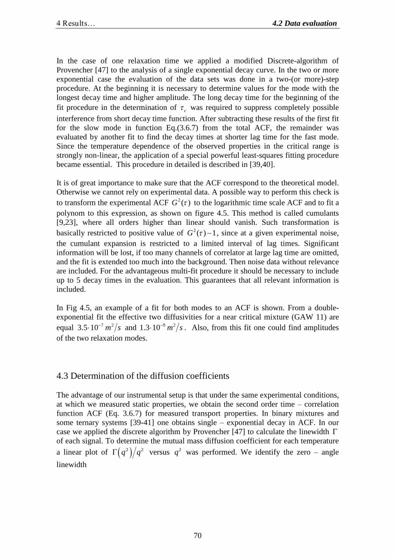
4 Results… 4.2 Data evaluation
70
In the case of one relaxation time we applied a modified Discrete-algorithm ofProvencher [47] to the analysis of a single exponential decay curve. In the two or moreexponential case the evaluation of the data sets was done in a two-(or more)-stepprocedure. At the beginning it is necessary to determine values for the mode with thelongest decay time and higher amplitude. The long decay time for the beginning of thefit procedure in the determination of c was required to suppress completely possibleinterference from short decay time function. After subtracting these results of the first fitfor the slow mode in function Eq.(3.6.7) from the total ACF, the remainder wasevaluated by another fit to find the decay times at shorter lag time for the fast mode.Since the temperature dependence of the observed properties in the critical range isstrongly non-linear, the application of a special powerful least-squares fitting procedurebecame essential. This procedure in detailed is described in [39,40].
It is of great importance to make sure that the ACF correspond to the theoretical model.Otherwise we cannot rely on experimental data. A possible way to perform this check isto transform the experimental ACF 2 ( )G to the logarithmic time scale ACF and to fit apolynom to this expression, as shown on figure 4.5. This method is called cumulants[9,23], where all orders higher than linear should vanish. Such transformation isbasically restricted to positive value of 2 ( ) 1G , since at a given experimental noise,the cumulant expansion is restricted to a limited interval of lag times. Significantinformation will be lost, if too many channels of correlator at large lag time are omitted,and the fit is extended too much into the background. Then noise data without relevanceare included. For the advantageous multi-fit procedure it should be necessary to includeup to 5 decay times in the evaluation. This guarantees that all relevant information isincluded.
In Fig 4.5, an example of a fit for both modes to an ACF is shown. From a double-exponential fit the effective two diffusivities for a near critical mixture (GAW 11) areequal 7 23.5 10 m s and 9 21.3 10 m s . Also, from this fit one could find amplitudesof the two relaxation modes.
4.3 Determination of the diffusion coefficients
The advantage of our instrumental setup is that under the same experimental conditions,at which we measured static properties, we obtain the second order time –correlationfunction ACF (Eq. 3.6.7) for measured transport properties. In binary mixtures andsome ternary systems [39-41] one obtains single –exponential decay in ACF. In ourcase we applied the discrete algorithm by Provencher [47] to calculate the linewidth of each signal. To determine the mutual mass diffusion coefficient for each temperaturea linear plot of 2 2q q versus 2q was performed. We identify the zero –angle
linewidth
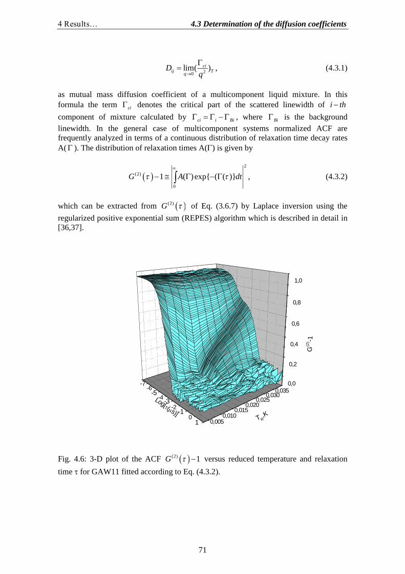
4 Results… 4.3 Determination of the diffusion coefficients
71
20lim( )ci
ij TqD
q
, (4.3.1)
as mutual mass diffusion coefficient of a multicomponent liquid mixture. In thisformula the term ci denotes the critical part of the scattered linewidth of i thcomponent of mixture calculated by ci i Bi , where Bi is the backgroundlinewidth. In the general case of multicomponent systems normalized ACF arefrequently analyzed in terms of a continuous distribution of relaxation time decay ratesA(). The distribution of relaxation times A() is given by
2
(2)
0
1 ( )exp{ ( ( )}G A dt
, (4.3.2)
which can be extracted from (2)G of Eq. (3.6.7) by Laplace inversion using theregularized positive exponential sum (REPES) algorithm which is described in detail in[36,37].
Fig. 4.6: 3-D plot of the ACF (2) 1G versus reduced temperature and relaxation
time for GAW11 fitted according to Eq. (4.3.2).
0,0350,030
0,0250,020
0,0150,010
0,005
0,0
0,2
0,4
0,6
0,8
1,0
-6
-4
-2
-7-5
-3
-10
1
G(2
) - 1
TR,K
Log[(s)]
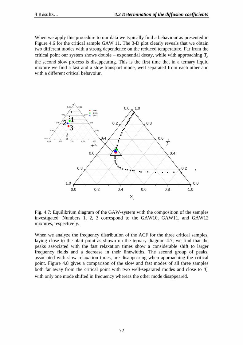
4 Results… 4.3 Determination of the diffusion coefficients
72
When we apply this procedure to our data we typically find a behaviour as presented inFigure 4.6 for the critical sample GAW 11. The 3-D plot clearly reveals that we obtaintwo different modes with a strong dependence on the reduced temperature. Far from thecritical point our system shows double–exponential decay, while with approaching cTthe second slow process is disappearing. This is the first time that in a ternary liquidmixture we find a fast and a slow transport mode, well separated from each other andwith a different critical behavoiur.
Fig. 4.7: Equilibrium diagram of the GAW-system with the composition of the samplesinvestigated. Numbers 1, 2, 3 correspond to the GAW10, GAW11, and GAW12mixtures, respectively.
When we analyze the frequency distribution of the ACF for the three critical samples,laying close to the plait point as shown on the ternary diagram 4.7, we find that thepeaks associated with the fast relaxation times show a considerable shift to largerfrequency fields and a decrease in their linewidths. The second group of peaks,associated with slow relaxation times, are disappearing when approaching the criticalpoint. Figure 4.8 gives a comparison of the slow and fast modes of all three samplesboth far away from the critical point with two well-separated modes and close to cTwith only one mode shifted in frequency whereas the other mode disappeared.
0.0 0.2 0.4 0.6 0.8 1.0
0.0
0.2
0.4
0.6
0.8
1.0 0.0
0.2
0.4
0.6
0.8
1.0
32 1
0.10 0.15 0.20 0.25 0.30
0.35
0.40
0.45
0.50
0.55 0.35
0.40
0.45
0.50
0.55
1.061.1611.077
X 2
X1
X0
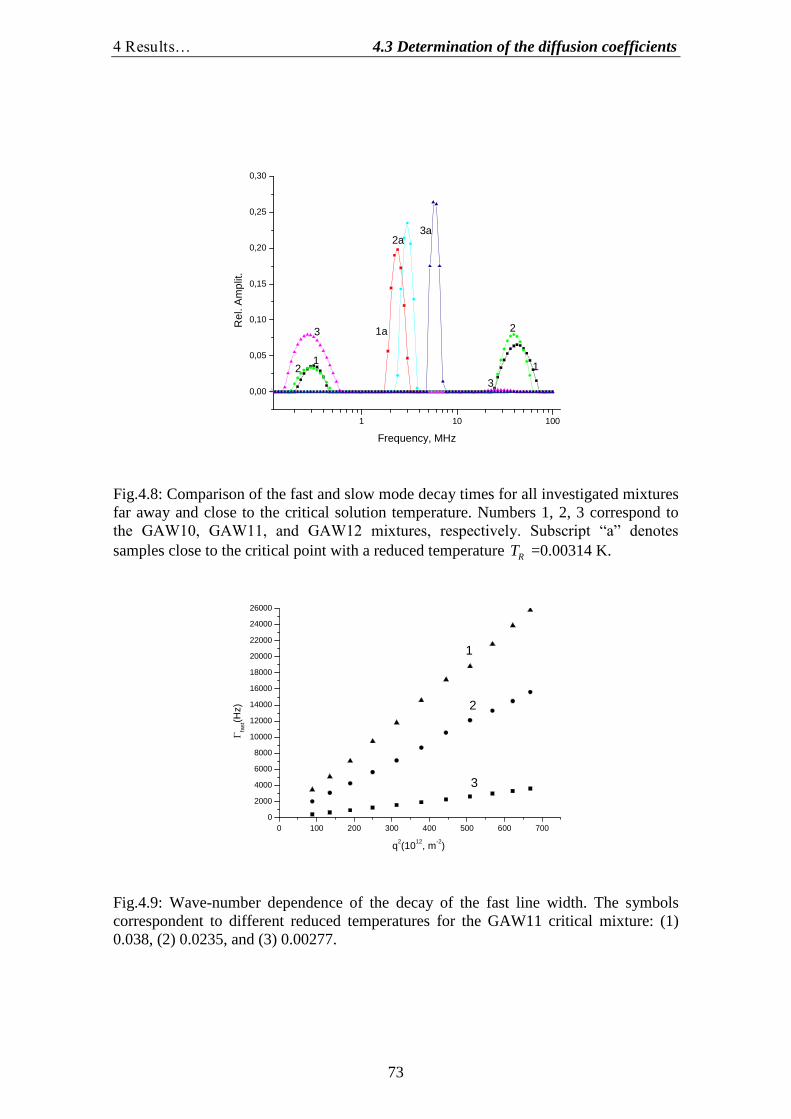
4 Results… 4.3 Determination of the diffusion coefficients
73
1 10 100
0,00
0,05
0,10
0,15
0,20
0,25
0,30
3a2a
1a
3
2
1
3
21
Rel
.Am
plit.
Frequency, MHz
Fig.4.8: Comparison of the fast and slow mode decay times for all investigated mixturesfar away and close to the critical solution temperature. Numbers 1, 2, 3 correspond tothe GAW10, GAW11, and GAW12 mixtures, respectively. Subscript “a” denotes samples close to the critical point with a reduced temperature RT =0.00314 K.
0 100 200 300 400 500 600 7000
2000
4000
6000
8000
10000
12000
14000
16000
18000
20000
22000
24000
26000
3
2
1
fast(H
z)
q2(1012, m-2)
Fig.4.9: Wave-number dependence of the decay of the fast line width. The symbolscorrespondent to different reduced temperatures for the GAW11 critical mixture: (1)0.038, (2) 0.0235, and (3) 0.00277.
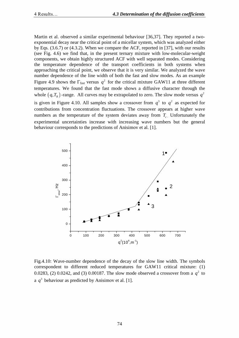
4 Results… 4.3 Determination of the diffusion coefficients
74
Martin et al. observed a similar experimental behaviour [36,37]. They reported a two-exponential decay near the critical point of a micellar system, which was analyzed eitherby Eqs. (3.6.7) or (4.3.2). When we compare the ACF, reported in [37], with our results(see Fig. 4.6) we find that, in the present ternary mixture with low-molecular-weightcomponents, we obtain highly structured ACF with well separated modes. Consideringthe temperature dependence of the transport coefficients in both systems whenapproaching the critical point, we observe that it is very similar. We analyzed the wavenumber dependence of the line width of both the fast and slow modes. As an exampleFigure 4.9 shows the fast versus 2q for the critical mixture GAW11 at three differenttemperatures. We found that the fast mode shows a diffusive character through thewhole , Rq T -range. All curves may be extrapolated to zero. The slow mode versus 2q
is given in Figure 4.10. All samples show a crossover from 3q to 2q as expected forcontributions from concentration fluctuations. The crossover appears at higher wavenumbers as the temperature of the system deviates away from cT . Unfortunately theexperimental uncertainties increase with increasing wave numbers but the generalbehaviour corresponds to the predictions of Anisimov et al. [1].
0 100 200 300 400 500 600 700
0
100
200
300
400
500
3
2
1
slow
,Hz
q2(106,m -1)
Fig.4.10: Wave-number dependence of the decay of the slow line width. The symbolscorrespondent to different reduced temperatures for GAW11 critical mixture: (1)0.0283, (2) 0.0242, and (3) 0.00187. The slow mode observed a crossover from a 2q toa 3q behaviour as predicted by Anisimov et al. [1].
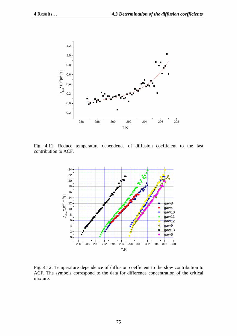
4 Results… 4.3 Determination of the diffusion coefficients
75
286 288 290 292 294 296 298
-0,2
0,0
0,2
0,4
0,6
0,8
1,0
1,2
Dfa
st*1
012[m
2 /s]
T,K
Fig. 4.11: Reduce temperature dependence of diffusion coefficient to the fastcontribution to ACF.
286 288 290 292 294 296 298 300 302 304 306 308
0
2
4
6
8
10
12
14
16
18
20
22
24
gaw3gaw4gaw10gaw11daw12gaw9gaw13gaw6
Dsl
ow*1
012[m
2 /s]
T,K
Fig. 4.12: Temperature dependence of diffusion coefficient to the slow contribution toACF. The symbols correspond to the data for difference concentration of the criticalmixture.
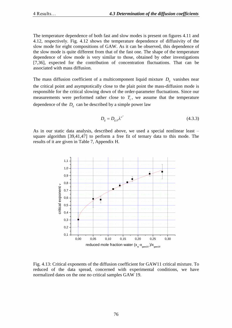
4 Results… 4.3 Determination of the diffusion coefficients
76
The temperature dependence of both fast and slow modes is present on figures 4.11 and4.12, respectively. Fig. 4.12 shows the temperature dependence of diffusivity of theslow mode for eight compositions of GAW. As it can be observed, this dependence ofthe slow mode is quite different from that of the fast one. The shape of the temperaturedependence of slow mode is very similar to those, obtained by other investigations[7,36], expected for the contribution of concentration fluctuations. That can beassociated with mass diffusion.
The mass diffusion coefficient of a multicomponent liquid mixture ijD vanishes nearthe critical point and asymptotically close to the plait point the mass-diffusion mode isresponsible for the critical slowing down of the order-parameter fluctuations. Since ourmeasurements were performed rather close to cT , we assume that the temperaturedependence of the ijD can be described by a simple power law
,0ij ijD D
(4.3.3)
As in our static data analysis, described above, we used a special nonlinear least –square algorithm [39,41,47] to perform a free fit of ternary data to this mode. Theresults of it are given in Table 7, Appendix H.
0,00 0,05 0,10 0,15 0,20 0,25 0,300,1
0,2
0,3
0,4
0,5
0,6
0,7
0,8
0,9
1,0
1,1
criti
cale
xpon
ent
reduced mole fraction water (xw-x
gaw19)/x
gaw19
Fig. 4.13: Critical exponents of the diffusion coefficient for GAW11 critical mixture. Toreduced of the data spread, concerned with experimental conditions, we havenormalized dates on the one no critical samples GAW 19.
4 Results… 4.3 Determination of the diffusion coefficients
77
Finally, Fig. 4.13 shows the results found for the critical exponent of the massdiffusivity in dependence from the reduced mole fraction of the investigated liquidmixture. The critical exponent of the mass diffusion coefficients for the sample GAW11is 0.811 . The effective critical exponents show slightly larger values than thosetheoretically predicted from the exponent renormalization according to Eq. (4.1.5).
5 Discussion 5.1 Theoretical analysis of two diffusion modes in the hydrodynamic…
78
5 Discussion
In the section “Theoretical part” we have obtained expressions for the positions and width of the three peaks of which the spectrum of the light scattering consists. Wefound that the central unshifted Rayleigh peak, for ternary liquid mixture, consists of asuperposition of three Lorentzians (in our approximation two) that involve thecombined dynamical effects of heat and mass diffusion.
In this section we find the condition under which it is possible to separate the centralpeak into two contributions, one arising from mutual diffusion and one from thermalconduction. In detail we investigate the behavior of ACF near the critical point. Weobtained temperature- and concentration-dependences of both diffusivities andamplitudes, and we compared them to the experimental data.
From the autocorrelation functions we can experimentally determine two effectivediffusivities 1D and 2D . In accordance with the theoretical model presented in thechapter 2, there is a possible physical explanation of 1D and 2D . One of these twomodes can be associated with thermal diffusion and the other with mass diffusion. In thespecial case of an incompressible-liquid mixture limit, 1D and 2D are decoupled,becoming mutual mass diffusion coefficient ijD and thermodiffusion coefficient TD .Both the slow and fast mode have been measured as a function of temperature for alldifferent composition investigated in our system.
5.1 Theoretical analysis of two diffusion modes in the hydrodynamic range
The complex structure of the expression describing the central Rayleigh peak is a directconsequence of the coupling between mass diffusion and heat flow that exist inmulticomponent mixture, which is given by the thermal diffusion ratio Tik . The widthof the Lorentzians are 1z and 2,3z , which both depend on ijD , and Tik (see Eqs.2.5.19 - 2.5.21). Thus we see that the central peak cannot be simply considered as thesuperposition of two Lorentzians, the first arising from thermal conduction and thesecond from the mass diffusion.
However, there are a number of conditions, met by a wide variety of ternary systems,that result in a considerably simplified expression for the shape of the Rayleighcomponent of spectrum of the light scattered. It means that in these cases it will bepossible to obtain exact data about a transport coefficient from the width of the centralline.
5 Discussion 5.1 Theoretical analysis of two diffusion modes in the hydrodynamic…
79
In general there are too different limiting cases possible. In the case of a dilute solution
1,2 0c , the thermal diffusion ratio tends to zero value [1], that is ijD and
0lim 0
iTic
k
. (5.1.1)
From Eq. (2.5.20) it then follows that 1,2 1M and 12,21 0M and diffusivity associatedwith the slow mode becomes equal to the thermal diffusivity, while the diffusivityassociated with the fast mode becomes the mass diffusivity
21
22,3 6
ii
B
S
z D q
k Tz q
(5.1.2)
with 1 2,3z z . Since in this case thermal and mass diffusivity are uncoupled the centralline of the LS spectrum consists of the superposition of the two Lorentzians, the widthof one is directly proportional only to the thermal diffusivity and the other only to themutual diffusion coefficient, as can be seen from Eq. 5.1.2. This limiting case gives usthe possibility to very easily resolve the two components of the Rayleigh peak. Thedynamic structure factor can have a simple form
2 2 2
2 2
, ,,
, exp expBB
p T c p Pp T
k TcS q t k T Dq t q t
c T C
. (5.1.3)
Usually, in practice, the dielectric constant is a weak function of the temperature,therefore only the mass diffusion term will be important.
More important is the case of immixable liquids when ijD , since manymulticomponent solutions satisfy this condition. Under these conditions for ternaryliquid systems we have
21 11 22
22,3
12
z D D q
z q
. (5.1.4)
In this case again the central peak is simplified to the superposition of two Lorentzians,one due to the mass and the other to the thermal diffusion. In the limit ijD , thetime distribution of the scattering light (Eq.2.5.27) actually reduces to the more simpleform. Since ijD , the mutual diffusion part of the Rayleigh peak superimposes amuch broader peak arising from heat flow. Consequently, in this case it is possible to
5 Discussion 5.1 Theoretical analysis of two diffusion modes in the hydrodynamic…
80
assign the Rayleigh peak to the mass diffusion. Moreover, as in case of infinite dilution,derivative of dielectric constant with respect to temperature is approximately equal tozero. Than, for this case ijD the dynamic structure factor of the ternary liquidmixture is
2 2 2 2 22 3 8 12 9 21 11 22
1, exp
2S q t q D q D q D D q t
, (5.1.5)
the values i are given in Eq. (2.5.29), Chapter 2. Many multicomponent mixturessatisfy the condition ijD . Hence an experimental determination of and ijD frommeasurement of the ACF of the light scattered is possible.
It will be useful to obtain activity coefficients from measured value of J , the Landau-Placzek ratio (see Eq. 2.4.4)
2 12 1
22 3 8 12 9 21
2 22 211 22
2 20 0 1 1 1 0 2 2 2, , , ,, , , ,
211 22
2
'1
1exp
2
R
BM
p T c p T cp T c p T c
IJ
I
D D
D c D cc c c c
D D q t
. (5.1.6)
5.2 The analysis of two diffusion modes in the critical range andcomparison with experiment
The detailed theoretical analysis of critical diffusivities has been already carried out insection 2.6. But consequences from this analysis and comparison with experimentaldata will be noted here.
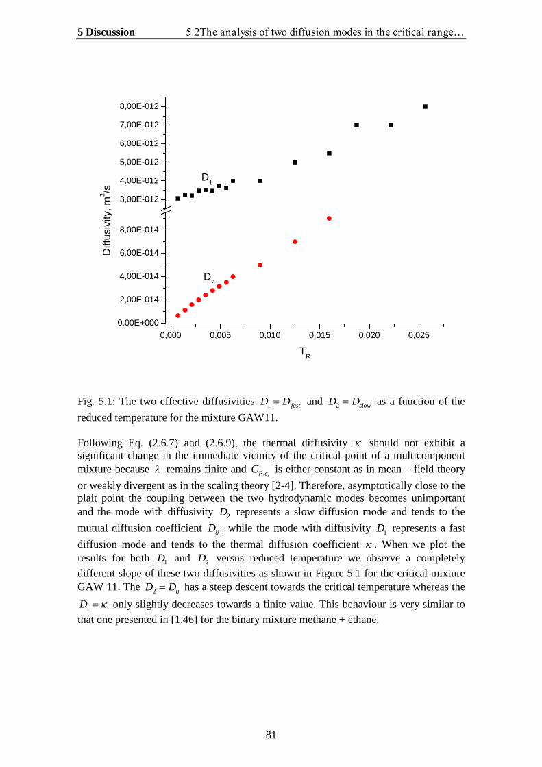
5 Discussion 5.2The analysis of two diffusion modes in the critical range…
81
0,000 0,005 0,010 0,015 0,020 0,0250,00E+000
2,00E-014
4,00E-014
6,00E-014
8,00E-014
3,00E-012
4,00E-012
5,00E-012
6,00E-012
7,00E-012
8,00E-012D
iffus
ivity
,m2 /s
TR
D1
D2
Fig. 5.1: The two effective diffusivities 1 fastD D and 2 slowD D as a function of thereduced temperature for the mixture GAW11.
Following Eq. (2.6.7) and (2.6.9), the thermal diffusivity should not exhibit asignificant change in the immediate vicinity of the critical point of a multicomponentmixture because remains finite and , iP cC is either constant as in mean –field theoryor weakly divergent as in the scaling theory [2-4]. Therefore, asymptotically close to theplait point the coupling between the two hydrodynamic modes becomes unimportantand the mode with diffusivity 2D represents a slow diffusion mode and tends to themutual diffusion coefficient ijD , while the mode with diffusivity 1D represents a fastdiffusion mode and tends to the thermal diffusion coefficient . When we plot theresults for both 1D and 2D versus reduced temperature we observe a completelydifferent slope of these two diffusivities as shown in Figure 5.1 for the critical mixtureGAW 11. The 2 ijD D has a steep descent towards the critical temperature whereas the
1D only slightly decreases towards a finite value. This behaviour is very similar tothat one presented in [1,46] for the binary mixture methane + ethane.
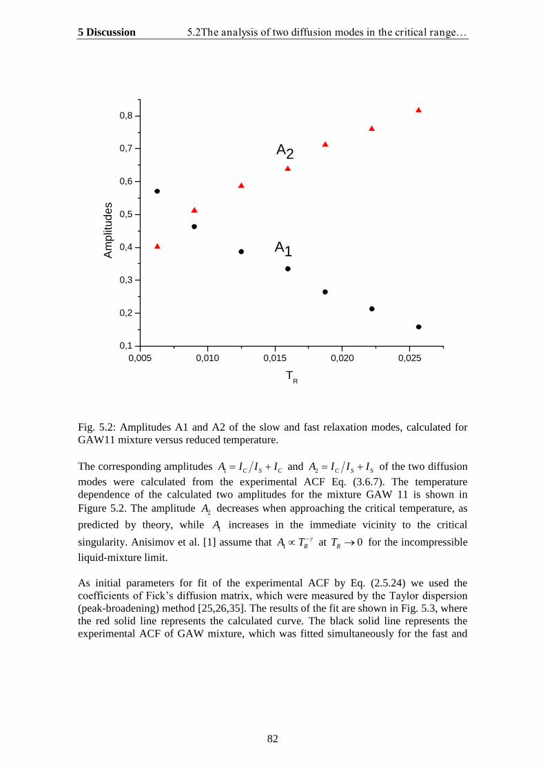
5 Discussion 5.2The analysis of two diffusion modes in the critical range…
82
0,005 0,010 0,015 0,020 0,0250,1
0,2
0,3
0,4
0,5
0,6
0,7
0,8A
mpl
itude
s
TR
A1
A2
Fig. 5.2: Amplitudes A1 and A2 of the slow and fast relaxation modes, calculated forGAW11 mixture versus reduced temperature.
The corresponding amplitudes 1 C S CA I I I and 2 C S SA I I I of the two diffusionmodes were calculated from the experimental ACF Eq. (3.6.7). The temperaturedependence of the calculated two amplitudes for the mixture GAW 11 is shown inFigure 5.2. The amplitude 2A decreases when approaching the critical temperature, aspredicted by theory, while 1A increases in the immediate vicinity to the critical
singularity. Anisimov et al. [1] assume that 1 RA T at 0RT for the incompressibleliquid-mixture limit.
As initial parameters for fit of the experimental ACF by Eq. (2.5.24) we used thecoefficients of Fick’s diffusion matrix, which were measured by the Taylor dispersion (peak-broadening) method [25,26,35]. The results of the fit are shown in Fig. 5.3, wherethe red solid line represents the calculated curve. The black solid line represents theexperimental ACF of GAW mixture, which was fitted simultaneously for the fast and
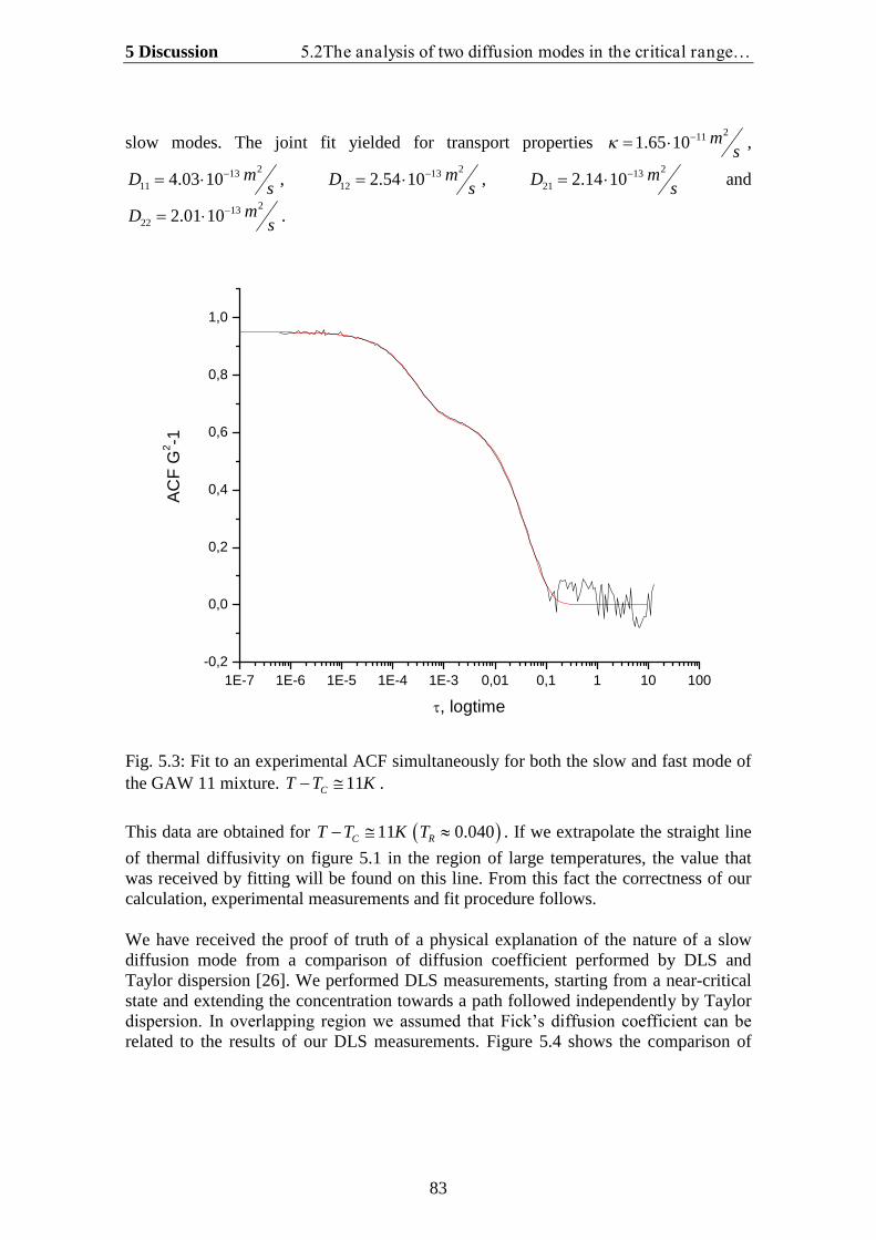
5 Discussion 5.2The analysis of two diffusion modes in the critical range…
83
slow modes. The joint fit yielded for transport properties2111.65 10 m
s ,213
11 4.03 10 mD s ,
21312 2.54 10 mD s
,213
21 2.14 10 mD s and
21322 2.01 10 mD s
.
1E-7 1E-6 1E-5 1E-4 1E-3 0,01 0,1 1 10 100-0,2
0,0
0,2
0,4
0,6
0,8
1,0
AC
FG
2 -1
, logtime
Fig. 5.3: Fit to an experimental ACF simultaneously for both the slow and fast mode ofthe GAW 11 mixture. 11CT T K .
This data are obtained for 11CT T K 0.040RT . If we extrapolate the straight lineof thermal diffusivity on figure 5.1 in the region of large temperatures, the value thatwas received by fitting will be found on this line. From this fact the correctness of ourcalculation, experimental measurements and fit procedure follows.
We have received the proof of truth of a physical explanation of the nature of a slowdiffusion mode from a comparison of diffusion coefficient performed by DLS andTaylor dispersion [26]. We performed DLS measurements, starting from a near-criticalstate and extending the concentration towards a path followed independently by Taylordispersion. In overlapping region we assumed that Fick’s diffusion coefficient can be related to the results of our DLS measurements. Figure 5.4 shows the comparison of
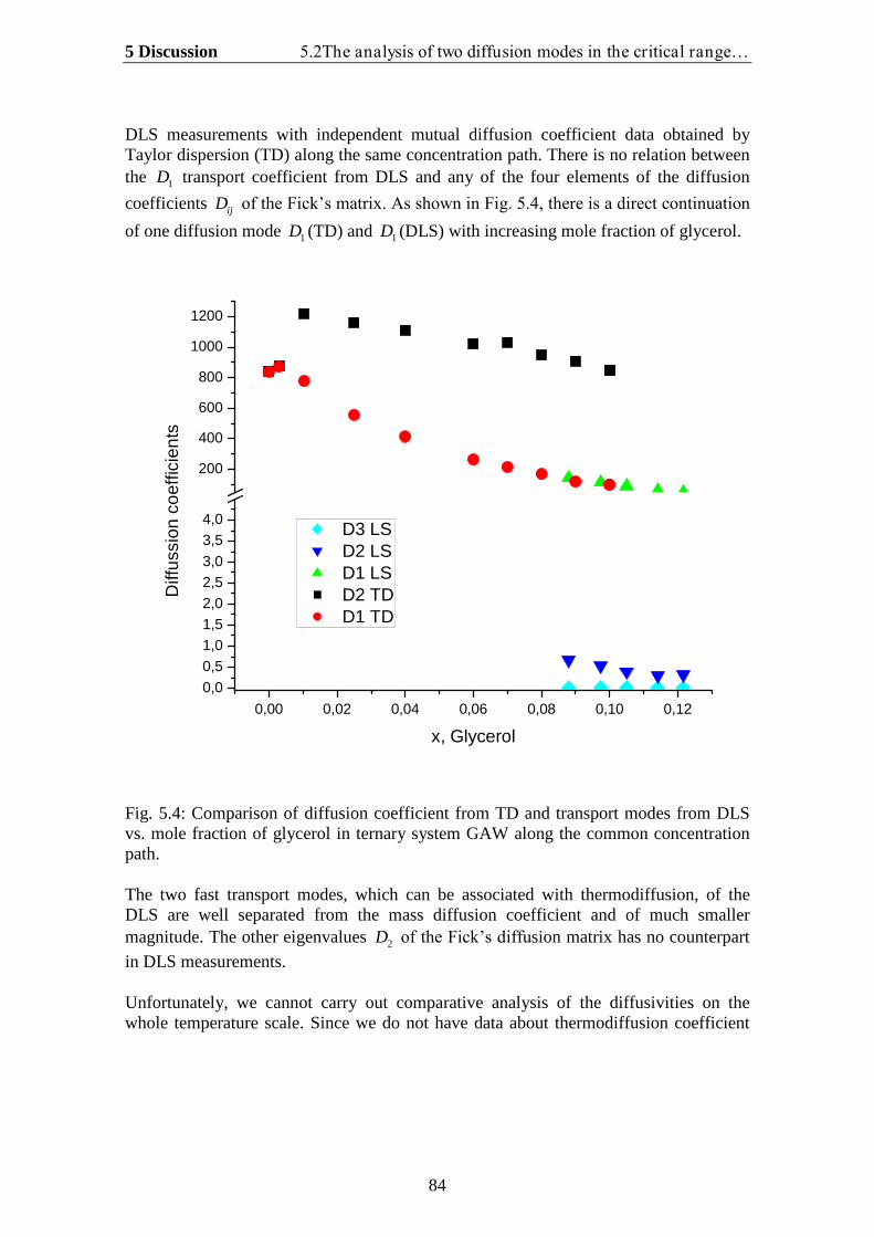
5 Discussion 5.2The analysis of two diffusion modes in the critical range…
84
DLS measurements with independent mutual diffusion coefficient data obtained byTaylor dispersion (TD) along the same concentration path. There is no relation betweenthe 1D transport coefficient from DLS and any of the four elements of the diffusioncoefficients ijD of the Fick’s matrix. As shown in Fig. 5.4, there is a direct continuation
of one diffusion mode 1D (TD) and 1D (DLS) with increasing mole fraction of glycerol.
0,00 0,02 0,04 0,06 0,08 0,10 0,120,00,51,01,52,02,53,03,54,0
200
400
600
800
1000
1200
Diff
ussi
onco
effic
ient
s
x, Glycerol
D3 LSD2 LSD1 LSD2 TDD1 TD
Fig. 5.4: Comparison of diffusion coefficient from TD and transport modes from DLSvs. mole fraction of glycerol in ternary system GAW along the common concentrationpath.
The two fast transport modes, which can be associated with thermodiffusion, of theDLS are well separated from the mass diffusion coefficient and of much smallermagnitude. The other eigenvalues 2D of the Fick’s diffusion matrix has no counterpartin DLS measurements.
Unfortunately, we cannot carry out comparative analysis of the diffusivities on thewhole temperature scale. Since we do not have data about thermodiffusion coefficient
5 Discussion 5.2The analysis of two diffusion modes in the critical range…
85
and Fick’s diffusivities for GAW system at temperatures different from 025 C .However, from our calculations it follows that the coupling parameters ,i ijM M form
(2.5.20) and iM from (2.5.29), which represent the coupling between mass and thermaldiffusion, (especially near critical point) are nonzero values. As we approach the criticalsingularity, the 1,iM ijM and iM always become much larger than unity [1,23].
These modes are strongly coupled, until the condition , ,ij i iM M MDij is achieved.
As shown above (Fig.5.1), at the critical point of a ternary fluid mixture the massdiffusion coefficient vanishes, but the thermal diffusivity does not exhibit a significantchange in the immediate vicinity of the critical point. Hence, based on our andAnisimov’s theory it is possible to approve, that in the near–critical multicomponentmixture a coupling between the two modes results in two characteristic relaxation times,neither of which is associated with pure mass diffusion or pure thermal diffusion.
6 Summary
86
6 Summary
This thesis deals with detailed investigation of the transport properties of a ternaryliquid mixture by light scattering technique. We have extended the theory of the lightscattering experiment and its application to investigate diffusion processes formulticomponent mixture in the immediate vicinity of the liquid-liquid critical point andfar from it. As a model system we have chosen of the strongly non-ideal ternary liquidsystem glycerol + acetone + water. The main focus of this thesis is a theoreticalinvestigation of transport properties of ternary liquid mixture in the hydrodynamic rangeand in the critical singularity field.
Light scattering technique has appeared to become a very useful tool for theinvestigation of diffusive processes and the determination of transport and otherthermophysical properties. Advantages of this method may be summarized as follows:
Measurements in the critical range almost not require high input energy. The light scattering technique allows the determination of both static and
dynamic thermophysical properties of the liquid mixtures. In some instances it is possible to determine transport properties of a mixture
simultaneously. As distinct from other techniques for the investigation of thermodynamic states
of a substance, which disturb the system during measurement, the lightscattering technique is a non-contact one.
Using this technique we determined both the static and the dynamic properties such asthe correlation length, osmotic susceptibility, thermal diffusion and mass diffusion inthe ternary GAW liquid mixture system in the vicinity of its critical solution point andfar from it. Near the critical solution point both the correlation length and thegeneralized osmotic susceptibilities data can be described by simple scaling laws withthree –dimensional Ising critical exponents. For both exponents we obtained valuesclose to the Fisher renormalization exponents. These results agree with previousmeasurements on multicomponent mixtures using photon correlation spectroscopy [39-41]. We obtained good agreement between the calculated critical temperatures and themeasured decomposition temperatures for all measuring compositions of the GAWsystem. Thus, by fitting to simple power laws for both static and dynamic propertieswith effective critical exponents we obtained good agreement with our experimentaldata.
The main scope of this work is the theoretical description of the time distribution of thescattered light and comparison with the experimental data. In this work a newtheoretical extension of the theory to ternary systems is developed. We have presentednew expressions for the general case, where the fluctuations in the dielectric constantare in turn caused by the full set of the local thermodynamic quantities such as the
6 Summary
87
pressure, temperature and concentration. In the introduction we have set some “open question”, which we have tried toanswer during this work.
Firstly we have extended the theoretical description of the spectrum of light, given byMountain and Deutch, to a ternary solution. In contrast to the binary mixture case weobtain more complicated expressions for the dynamic structure factor, which consists ofa superposition of three Lorentzians that involve the combined dynamic effect ofthermal and mass diffusion. For a ternary liquid mixture it is necessary to take intoaccount also the combination effect between mass diffusivities of different componentsof the investigated system. Moreover in a ternary mixture there are combinationsbetween the two (in binary mixture one) mass diffusion currents and the heat current.The expression for two-side Brillouin peaks is the same as in a binary mixture, expectfor widths of the peaks. We have obtained original expressions for the position andwidths of the two-side shifted Brillouin peaks, and the central, unshifted Rayleigh peakfor the ternary liquid system case. We have carried out the analysis of the conditionunder which it is possible to separate the central peak simply in two type diffusivitycontribution, which arise from gradient of the entropy and the concentration.
Secondly Leaist and Hao have derived expressions for the correlation function ofscattered light, taking into account only the concentration fluctuation in the localdielectric constant. They expect a multi-exponential decay in the ACF with (N-1)diffusion modes for a N-component system. For ternary solutions they derive equationsfor two eigenvalues of the diffusion coefficient matrix but than they introduced rathersimplifying approximations so that only one diffusion mode survived. They choseaqueous solutions of macromolecules or micelles where it is evident that DLS willrecord only the diffusion of the macromolecules. Thus, their results do not proof theassumption of a multi-exponential decay of several mass diffusion modes. In ourtheoretical model the local thermodynamic quantities such as the temperature andpressure fluctuation are not ignored. For this reason the expression for ACF and thedynamic structure factor has more complicated form. As mentioned above, the shape ofthe central Rayleigh component of the spectrum endows a thermal diffusion, besides ofa mass one. Moreover in these expressions a term appears, which describes the two-shifted Brillouin components that arise from pressure fluctuations. With DLS we havedetected two diffusivity modes, and determine the decay rate of these modes. From thehydrodynamic theory of fluctuation we derived the expression for them (Eq. 2.5.18).Moreover, our theoretical model allows to calculate the relative amplitudes of threerelaxations modes for a multicomponent liquid system if enough information aboutstatic and dynamic properties is available (Eqs. 2.5.28 a,b).
Thirdly, following the method suggested by Anisimov al. et, we carried out analysis oftransport properties in field of critical singularity for ternary liquid mixtures. Two –exponential decay correlation functions are observed far from the critical solutiontemperatures. This is the first time that in a ternary liquid mixture we find a fast and aslow transport mode, well separated from each other and with a different criticalbehaviour. However, as the critical point is approached, the correlation functions
6 Summary
88
become single –exponential. Two hydrodynamic relaxation modes are associated withthe ACF far from critical singularity. In the immediate vicinity of the critical point, oneis strongly and the other is weakly divergent. According to Anisimov’s theory and to the theoretical model, represented in this work, one of these two modes can be associatedwith thermal diffusion and the other with mass diffusion. In the special cases of anincompressible liquid-mixture limit, 1D and 2D are decoupled, becoming thermaldiffusion coefficient TD and mutual mass diffusion coefficient ijD . The overallbehaviour of our dynamic light scattering data in a ternary liquid mixture agrees verywell with the prediction of Anisimov et al. on binary mixtures. We can generalize thisresult. Both binary and ternary liquid mixtures may have the same set of orderparameters and effective fields of critical fluctuation, which was confirmed byAnisimov [5].
The prediction of transport properties in ternary mixtures is still a problem. As initialparameters for the fit of the experimental ACF we used the coefficients of Fick’s diffusion matrix, which were measured by the Taylor dispersion method [25,26,35].Unfortunately, we cannot carry out comparative analysis of the diffusivities on thewhole temperature scale. Since we do not have data about thermodiffusion coefficientand Fick’s diffusivities, obtained from Taylor dispersion, for our system at temperaturesdifferent from 025 C . Further investigation at concentration areas far from binodalcurves and the comparison with mass diffusion measurements using other methods likeholographic interferometry and Taylor dispersion, will prove the present physicalinterpretation of the two hydrodynamic relaxation mode in a ternary liquid mixture.
7 Appendix 7.A. Expression for the scattered field
89
7 Appendix
7.A. Expression for the scattered field
To obtain the basic equation for the scattered field we have used the Maxwell’s equations system for a nonconducting, nonmagnetic medium. The derivation of thisequation has been suggesting by Landau and Lifshitz [9,34].
For beginning we simplify our consideration by introducing a local dielectric constantin the following form
0I , (7.A.1)
where 0 is average dielectric constant and is the dielectric constant fluctuationtensor. If the incident plane wave fields are , ,i i iE D H and scattering field are
, ,s s sE D H , then the totals of these fields at a point in the scattering medium are
i s
i s
i s
E E E
D D D
H H H
, (7.A.2)
where ,E D and H are vectors of the electric field strength, electric displacement andmagnetic field strength, accordingly. Taking into account Maxwell’s equations, we obtain an equation for the total displacement vector D and vector of the total electricfield strength E which are related through the dielectric constant (Eq. 7.A.1).
0 0i i s sD E E E E (7.A.3)
From Eq. (7.A.2) and neglecting the second order term sE , Eq. (7.A.3) becomes
0s s iD E E (7.A.4)
Solving Eq. (7.A.4) for sE , substituting this equation into one of the Maxwell’s one, we obtain an inhomogeneous wave equation
7 Appendix 7.A. Expression for the scattered field
90
2
2 02 2
ss i
DD E
c t
(7.A.5)
where c is speed of light in a medium. We simplified this equation by introducing anew vector, (the Hertz vector) by
sD (7.A.6)
Substituting Eqs. (7.A.6) into (7.A.5) and solving for the Hertz vector we obtain thefollowing equation:
3, ´1, , ´
4 i
r tR t E r t d r
R r
, (7.A.7)
where Rand r are defined in Chapter 2 and ´t is the retarded time
0´t t R rc
. (7.A.8)
Now we substituted Eq. (2.1.4) for iE into Eq. (7.A.7). Taking into account that
0s sD E , we obtain
30
0
1( , ) exp ( )́ , ´
4s i i i
EE R t i k r t r t n d r
R R r
. (7.A.9)
In actual light scattering experiment the detectors are a large distance from thescattering medium, it is possible to expand R r in a power series
f̂R r R r k , (7.A.10)
where f̂k is a unit vector in the direction R. Substituting Eq. (7.A.10) into Eq. (7.A.8)we obtain expression for the retarded time
0 ˆ´ ft t R r kc
. (7.A.11)
In the next step we performed a Fourier analysis of the dielectric constant fluctuationtensor over time interval
7 Appendix 7.A. Expression for the scattered field
91
, ´ exp ´p pp
r t r i t , (7.A.12)
where2
p p
. From experimental condition follows, that i p [9]. In view of
this condition and substituting Eqs. (7.A.11) and (7.A.12) into Eq. (7.A.9) we have
0
0
3
( , ) exp4
ˆexp ( ) exp
s p i pp
p i p f p p iV
EE R t i k R t k
R
k i k k k r r i t n d r
(7.A.13)
where we have ignored terms of higher order then 1R
and defining
0 ˆp f f
f i p
k kc
As mentioned above i p . In this case a very good approximation is
0 ˆp f f i fk k k k
c
. (7.A.14)
Thus in this approximations Eq. (7.A.13) becomes
30
0
( , ) exp exp ,4s f i f f i
V
EE R t i k R t k k iq r r t n d r
R
(7.A.15)
where the scattering vector q
is defined by Eq.(2.1.10) with the geometry of the Fig.
(2.2), and ik
is defined by Eq. (2.1.11) and same figure. If we consider the componentof scattered electric field sE in the direction fn
, we obtain the expression of Eq (2.1.9).
7 Appendix 7.B. A time correlation function
92
7.B. A time correlation function
The spectral density I of a time correlation function 0A A t is defined as
1exp 0
2I dt i t A A t
(7.B.1)
where A is the complex conjugate of A . As it has been shown in Chapter 3 thisquantity plays an important role in light scattering measurements. The Fourier inversionof Eq. (7.B.1) leads to an expression for the time correlation function in the terms of thespectral density.
0 expA A t dt i t I
(7.B.2)
Hence 0A A t and I are Fourier transforms of one another. We noted that the
equilibrium mean-square value of the property A is found by setting 0t in the Eq.(7.B.2) so that
20A d I
(7.B.3)
The integral kernel can be interpreted as the probability of finding a2
A in the
frequency interval , d . The function A t measured over a time interval canbe expressed in terms of its Fourier components so that
12
ni tn
n
A t A eT
(7.B.4)
In laser experiment we have used coherent, monochromatic radiation. Thus after a seriesof some algebraic transformation we obtain
''
, '
0 exp2
nin nn n
n n
A A dtA A t e i t
T T
(7.B.5)
Using Eq. (7.B.5) we can evaluate expression for the time correlation function of thescattering electric field from Eq. (2.2.2) to Eq. (2.2.3), taking into account conditionsdescribed there.
7 Appendix 7.B. A time correlation function
93
7.C. The relation between thermodynamic and transport properties in theternary liquid mixture
The differential of the Gibbs energy 'G per mole of a ternary mixture is given by
3
1
' ' ' '' i i
i
dPdG S dT dc
(7.C.1)
where ' and 'S the molar density and entropy, accordingly. 'i are the molarchemical potentials and 'ic are mass concentrations of a species " "i . The molar density
' is related to the mass density by
'M
, (7.C.2)
where
3
1i i
i
M nM
n
, (7.C.3)
is molar mass of the ternary mixture, 1 2 3n n n n the total numbers of mole, iM themolar masses and in the numbers of moles of the pure components. Since
2 1 22 3
2 3
1' ; '
c c cc c
m m
, where im are masses of the individual components in the
mixture. Hence, the differential of the Gibbs energy G per unit mass of a ternarymixture gives a following expression:
1 1 2 2
dPdG SdT dc dc
, (7.C.4)
where i are defined in the end of the section 2.4.
We found the linearized hydrodynamic equations by the way suggested by Landau andLifshitz in [33]. The continuity equations for two components in the ternary liquidmixture could be written in a form
7 Appendix 7.C. The relation between thermodynamic and transport…
94
11 1
22 2
cu c divI
t
cu c divI
t
(7.C.5)
For the ternary liquid mixture the thermodynamic equation for the energy and enthalpyis
1 1 2 22
1 1 2 2
1
pdU TdS d dc dc
dH TdS dp dc dc
(7.C.6)
The second equation from (7.C.6) can be expressed in the form
1 1 2 2dp dH TdS dc dc (7.C.7)
Substituting this expression in the energy transport equation [9,33] we obtain:
2
2
1 1 2 2
2
'2
' iik
k
Ut
Sdiv u H u Q T u S
T
divQ I Ix
, (7.C.8)
where , iu I and are also defined in the section 2.4.
The sum of the two last terms from the right side of Eq. (7.C.8) we will write in theform
1 1 2 2 1 1 2 2 1 1 2 2divQ I I div Q I I I I (7.C.9)
The divergence expression in the right side of Eq. (7.C.8), by definition is full energyflux Q in liquid. In the absence of the macroscopic movement the viscosity fluxdisappears and therefore the heat current is simple Q . The equation of the energyconservation is [9,33]:
7 Appendix 7.C. The relation between thermodynamic and transport…
95
2 2
'2 2
U div u w u Qt
(7.C.10)
Term by term subtracting Eq. (7.C.10) from Eq. (7.C.8), and taking into account Eq.(7.C.9), we will obtain the required energy transport equation (2.4.9).
Now we obtain the expression for the heat and mass diffusion current Eqs.(2.5.2).Between Onsager coefficients there is the simple ratio, as a consequence of thesymmetry principle [1]. Hence
2 2 22
21 1 1
2 22
21 1
ii i i
i i i
ii i i
i i
TI T T
T T
TQ I T
T T
(7.C.11)
In view of the symmetry principle T , we can obtain expressions for currents inshape of Eqs. (2.5.1). In expression for the heat current it is convenient to exclude agradient of the chemical potential i , having expressed it through iI and T .
1 21 1 2 2
1 2
T TQ I I T
, (7.C.12)
where
22
1
i
i i
T
.
As shown in [33] the value is the thermal conductivity. In the terms 1, ,p T c and 2cthe gradient of the chemical potential i has a form
1 2 1 22 1
1 2 1 22 1
1 1 1 11 1 2
, ,1 2 , ,, , , ,
2 2 2 22 1 2
, ,1 2 , ,, , , ,
c c p c c Tp T c p T c
c c p c c Tp T c p T c
c c T pc c T p
c c T pc c T p
. (7.C.13)
Substituting i form Eq.(7.C.13) into Eqs. (7.C.12) and (2.5.1), and defining
7 Appendix 7.C. The relation between thermodynamic and transport…
96
,
,
,
, ,
, ,
, ,
, ,
i i j
i j
i i j
j j i
i iij
j p T c
Ti ii ii i
c c p
i p T cpi
i
i p T c
Dc
k DT T
Vc
k P
c
, (7.C.14)
we find equations which are the same as Eqs. (2.5.2). We substitute these equations foriI and Q in Eq. (7.C.5), and Eq.(2.4.9). We omit terms of the second order i iI , Eqs.
(7.C.5), and (2.4.9) becomes
2
1
1 1 2 2
0
0
ii
i
cdivI
tS
T div Q I It
. (7.C.15)
We will transform the derivative St
as follows
1 2 1 2
1 1 2 2
, , , ,
P
p c c p c c
C c cS Tt T t T t T t
. (7.C.16)
In results, after substituting Eqs.(2.5.2) into Eqs. (7.C.15) and taking into accountEq.(7.C.16), we obtain the system of the mass and energy transport equations (2.5.3),and (2.5.4).
7 Appendix 7.D. The solution of the dispersion equation
97
7.D. The solution of the dispersion equation
The linewidth of the Rayleigh peak, and consequently also values of the thermaldiffusivity and mass diffusion coefficients, are determinate by roots of the dispersionequation:
3 211 1 22 2
11 22 11 22 12 21
11 22 1 2 12 22 12 11 21 21
11 22 12 21
2
0
z D M D M z
D D D D D Dz
D D M M D D M D D M
D D D D
(7.D.1)
We will find roots of this dispersion equation in those approximations that aredesignated in section 2.5. We solve Eq. (7.D.1) using a method of auxiliary quantitiesdescribed in [10]. Let us enter new variables:
11 22
11 22 12 21
1 11 1 22 2
2 11 22 1 2 22 12 12 11 21 21
3 1
2
23
D D
D D D D
D M D M
D D M M D D M D D M
. (7.D.2)
The auxiliary quantities for our equation are
2 23 2 1
3 2 23 1 3 2 1 1 2
1 13 3
2 1 1 1 1 227 3 3 3 3 9
p
q
. (7.D.3)
To find the roots it is necessary to know values R and , which are defined as
23 2 1
3 2 22
33 2 2
2
13
3 3 22 127 3arccos arccos 02 1227 3
pR
qR
. (7.D.4)
7 Appendix 7.D. The solution of the dispersion equation
98
Return to the initial variables we will obtain
2 2 1 11 3
22 2 1
2,3
13
31 12 2
z q
z q
. (7.D.5)
Substituting Eq.(7.D.2) into Eqs. (7.D.5) we obtain the roots of the dispersion equationEqs. (2.5.18) and (2.5.19).
7 Appendix 7.E. The linearized hydrodynamic equations in terms…
99
7.E. The linearized hydrodynamic equations in terms of the concentrations,temperature and pressure
To rewrite the linearized hydrodynamic equations in terms of the concentrations,temperature and pressure it is necessary to repeat the procedure done for a case withoutpressure. In terms of Fourier-Laplace transforms
3
3
3
3
3
(̂ , ) ( , ) ,
(̂ , ) ( , )
(̂ , ) ( , )
(̂ , ) ( , )
(̂ , ) ( , )
iq r ztki i
iq r ztk
iq r ztk
iq r ztk
iq r ztk
c r t d r e c r t
T r t d r e T r t
p r t d r e p r t
r t d r e r t
r t d r e u r t
(7.E.1)
we will present the equations (2.4.5), (2.4.6), (2.5.3) and (2.5.4) in following form:
1, 22 1
1, 22 1
1 2 2,1 2, , , ,
1 2 2,1 2, , , ,
22
21 11
ˆ ˆˆ ˆ ˆ
1 ˆˆ ˆ ˆ(0) (0) 0 0 ;
ˆ ˆˆˆ ' 0 ;
ˆ
k k k k kc c pc p T c p T
k k k kc c pc p T c p T
k k k k
k
zz c z c p z
c c c T
c c pc c c T
qz p q
c z q D
2 1
2 2 21 1 112 2 11 11 1
0
2 2 2 22 2 221 1 2 22 22 22 2
0
1 1 2 21 2
1 2, , , ,
ˆˆ ˆ ˆ(0);
ˆˆ ˆ ˆ ˆ(0);
ˆ ˆ
T T P Tk k k k
P
T T P Tk k k k k
P
T Tk k
P PC P T C P T
k k kq D c q D p q D c
C p T
k k kq D c c z q D q D p q D c
C p T
k kz c z c q
C c C c
2 1
2 2
1 1 2 21 2
1 2, , , ,
ˆ
(0) (0) (0).
Tk
P
T Tk k k
P PC P T C P T
Tz q
C
k kc c
C c C c
(7.E.2)
The 5 5 matrix M in the terms of (7.E.1) for the full set equations (7.E.2) has theform (2.5.21 a,b).
7 Appendix 7.F. The expression for the correlation functions…
100
7.F. The expression for the correlation functions of the concentrations andtemperature
The resulting expression for correlation functions contained in Eq. (2.5.26) as functionof the wave number q
, can be written as
1
2
2 21 22 2 11 1 1
422 12 22 12 11 22 11 1
22 22 1 1 22 2 11 1 21
422 12 22 12 11 22 1 3
2
1
1, 1;
1
1
,
z t
z t
z D M D M z qe
D D D M D D M qc q t c q
z z P D M D M P qc qe
D D D M D D M P q
c q
1
2
2 21 11 1 22 2 1
411 21 11 21 11 22 22
22 22 1 1 11 1 22 2 22
411 21 11 21 11 22 2 3
1
11;
1
1
,
z t
z t
z D M D M z qe
D D D M D D M qt c q
z z P D M D M P qc qe
D D D M D D M P q
T q t T q
1
2
1
2 2 41 11 22 1 11 22 12 21
22 2 42 1 1 11 22 2 11 22 12 21 3
12 12 22 22 412 1
11 22 211 222
2 1 2212 2
1;
1
, 1
z t
z t
z t
z D D z q D D D D q e
z z P D D P q D D D D P q eT q
D D D MD z q q e
D D Mc q t c q
z zc qD P q
2
1
2
12 12 22 2 43
11 22 21
2 411 1 1 12 22 2 11 22 11
22 2 42 1 11 1 2 12 22 2 11 22 1 3
;1
, 1
z t
z tT T T
z tT T T
D D D MP q e
D D M
D k z q D D k D D k q ec q t T q
z zT q D k P q D D k D D k P q e
1
2
21 21 11 12 421 1
11 22 122 122
2 1 21 21 11 12 4121 2 3
11 22 12
22 2 1222
2 1
;
1
, 1;
1
, 1
z t
z t
T
D D D MD z q q e
D D Mc q t c q
z z D D D Mc qD P q P q e
D D M
D k zc q t T q
z zT q
1
2
2 421 11 1 11 22 2
2 422 1 2 21 11 1 11 22 2 3
;
z tT T
z tT T T
q D D k D D k q e
D k P q D D k D D k P q e
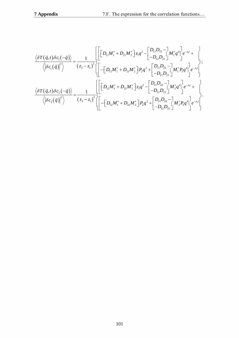
7 Appendix 7.F. The expression for the correlation functions…
101
1
2
11 222 411 1 21 2 1 1
12 21122
2 1 11 222 4111 1 21 2 2 1 3
12 21
12 1 22 22
222 12
, 1;
, 1
z t
z t
D DD M D M z q M q e
D DT q t c q
z z D Dc q D M D M P q M P q eD D
D M D MT q t c q
z zc q
1
2
11 222 41 2
12 21
11 222 412 1 22 2 2 2 3
12 21
.
z t
z t
D Dz q M q e
D D
D DD M D M P q M P q e
D D
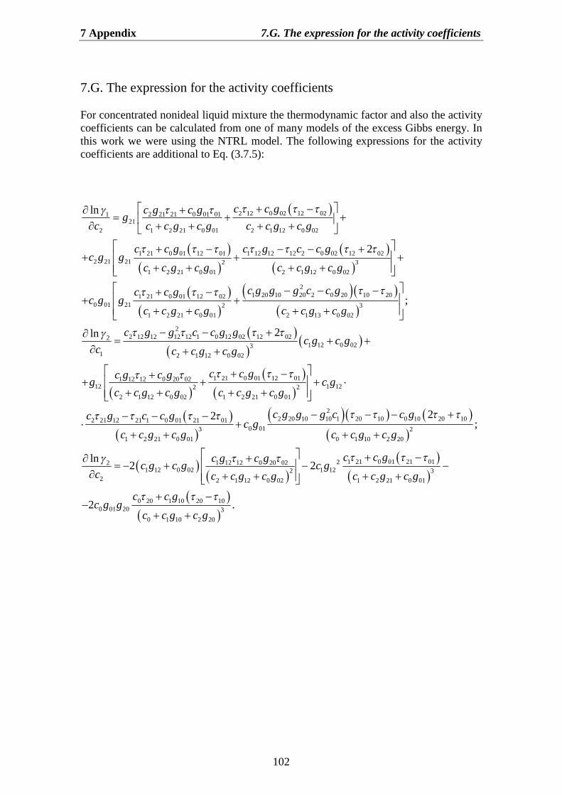
7 Appendix 7.G. The expression for the activity coefficients
102
7.G. The expression for the activity coefficients
For concentrated nonideal liquid mixture the thermodynamic factor and also the activitycoefficients can be calculated from one of many models of the excess Gibbs energy. Inthis work we were using the NTRL model. The following expressions for the activitycoefficients are additional to Eq. (3.7.5):
2 12 0 02 12 022 21 21 0 01 01121
2 1 2 21 0 01 2 1 12 0 02
1 21 0 01 12 01 1 12 12 12 2 0 02 12 022 21 21 2 3
1 2 21 0 01 2 1 12 0 02
1 21 0 01 10 01 21
ln
2
c c gc g c gg
c c c g c g c c g c g
c c g c g c c gc g g
c c g c g c c g c g
c c gc g g
21 20 10 20 2 0 20 10 202 02
2 31 2 21 0 01 2 1 13 0 02
22 12 12 12 12 1 0 12 02 12 022
1 12 0 0231 2 1 12 0 02
1 21 0 01 12 011 12 12 0 20 0212 2
2 1 12 0 02
;
2ln
c g g g c c g
c c g c g c c g c g
c g g c c g gc g c g
c c c g c g
c c gc g c gg
c c g c g c
1 1221 2 21 0 01
22 20 10 10 1 20 10 0 10 20 102 21 12 21 1 0 01 21 01
0 013 21 2 21 0 01 0 1 10 2 20
1 12 12 0 20 0221 12 0 02 1 122
2 2 1 12 0 02
22;
ln2 2
c gc g c g
c g g g c c gc g c c gc g
c c g c g c c g c g
c g c gc g c g c g
c c c g c g
1 21 0 01 21 0123
1 2 21 0 01
0 20 1 10 20 100 01 20 3
0 1 10 2 20
2 .
c c g
c c g c g
c c gc g g
c c g c g
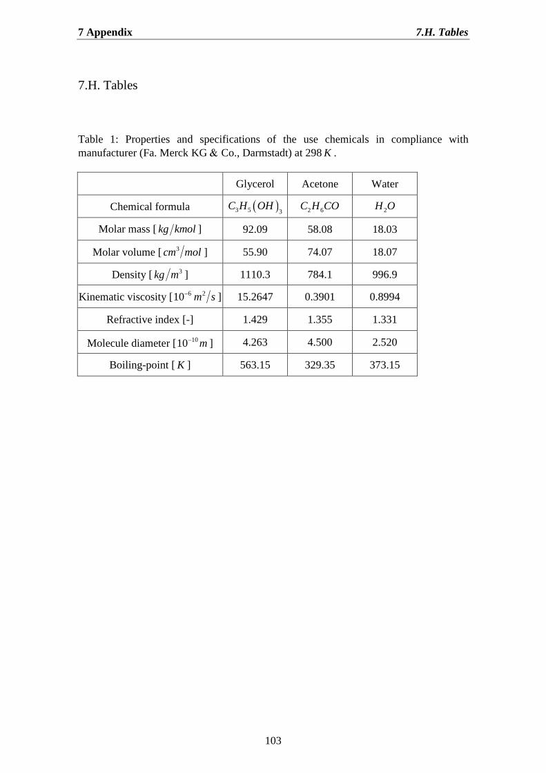
7 Appendix 7.H. Tables
103
7.H. Tables
Table 1: Properties and specifications of the use chemicals in compliance withmanufacturer (Fa. Merck KG Co., Darmstadt) at 298 K .
Glycerol Acetone Water
Chemical formula 3 5 3C H OH 2 6C H CO 2H O
Molar mass [ kg kmol ] 92.09 58.08 18.03
Molar volume [ 3cm mol ] 55.90 74.07 18.07
Density [ 3kg m ] 1110.3 784.1 996.9
Kinematic viscosity [ 6 210 m s ] 15.2647 0.3901 0.8994
Refractive index [-] 1.429 1.355 1.331
Molecule diameter [ 1010 m ] 4.263 4.500 2.520
Boiling-point [ K ] 563.15 329.35 373.15
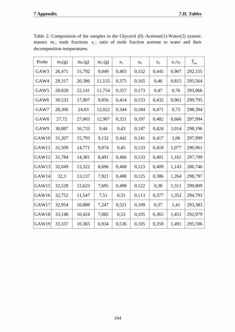
7 Appendix 7.H. Tables
104
Table 2: Composition of the samples in the Glycerol (0)–Acetone(1)-Water(2) system:masses im ; mole fractions ix ; ratio of mole fraction acetone to water and theirdecomposition temperatures.
Probe m1(g) m0 (g) m2 (g) x1 x0 x2 x1/x2 decT
GAW3 26,471 15,792 9,049 0,403 0,152 0,445 0,907 292,155
GAW4 29,317 20,386 11,155 0,375 0,165 0,46 0,815 293,564
GAW5 28,828 22,141 11,754 0,357 0,173 0,47 0,76 293,966
GAW6 30,533 17,907 9,856 0,414 0,153 0,432 0,961 299,795
GAW7 28,306 24,03 12,022 0,344 0,184 0,471 0,73 298,394
GAW8 27,72 27,003 12,907 0,321 0,197 0,482 0,666 297,994
GAW9 30,887 16,733 9,44 0,43 0,147 0,424 1,014 298,196
GAW10 31,207 15,793 9,132 0,442 0,141 0,417 1,06 297,999
GAW11 31,509 14,771 9,074 0,45 0,133 0,418 1,077 290,961
GAW12 31,784 14,381 8,491 0,466 0,133 0,401 1,161 297,799
GAW13 32,049 13,322 8,696 0,468 0,123 0,409 1,143 286,746
GAW14 32,3 13,137 7,921 0,488 0,125 0,386 1,264 298,797
GAW15 32,528 12,623 7,695 0,498 0,122 0,38 1,311 299,809
GAW16 32,752 11,547 7,51 0,51 0,113 0,377 1,352 294,793
GAW17 32,954 10,888 7,247 0,521 0,109 0,37 1,41 293,383
GAW18 33,148 10,424 7,082 0,53 0,105 0,365 1,451 292,979
GAW19 33,337 10,365 6,934 0,536 0,105 0,359 1,491 295,596
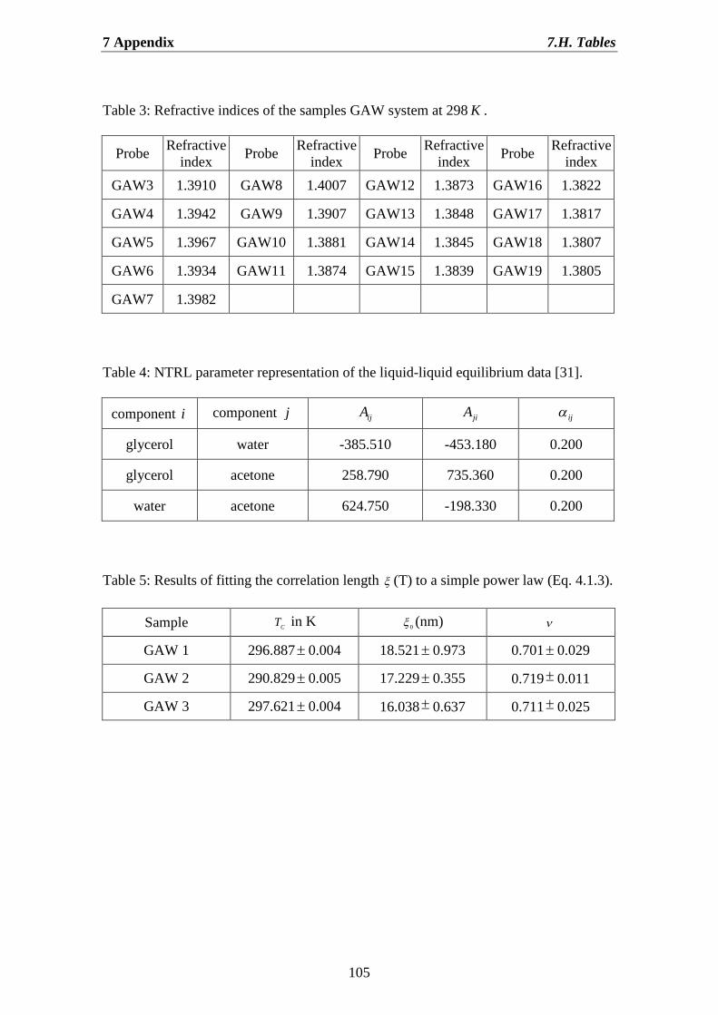
7 Appendix 7.H. Tables
105
Table 3: Refractive indices of the samples GAW system at 298 K .
Probe Refractiveindex Probe Refractive
index Probe Refractiveindex Probe Refractive
index
GAW3 1.3910 GAW8 1.4007 GAW12 1.3873 GAW16 1.3822
GAW4 1.3942 GAW9 1.3907 GAW13 1.3848 GAW17 1.3817
GAW5 1.3967 GAW10 1.3881 GAW14 1.3845 GAW18 1.3807
GAW6 1.3934 GAW11 1.3874 GAW15 1.3839 GAW19 1.3805
GAW7 1.3982
Table 4: NTRL parameter representation of the liquid-liquid equilibrium data [31].
component i component j ijA jiA ij
glycerol water -385.510 -453.180 0.200
glycerol acetone 258.790 735.360 0.200
water acetone 624.750 -198.330 0.200
Table 5: Results of fitting the correlation length (T) to a simple power law (Eq. 4.1.3).
Sample CT in K 0(nm)
GAW 1 296.8870.004 18.5210.973 0.7010.029
GAW 2 290.8290.005 17.2290.355 0.7190.011
GAW 3 297.6210.004 16.0380.637 0.7110.025
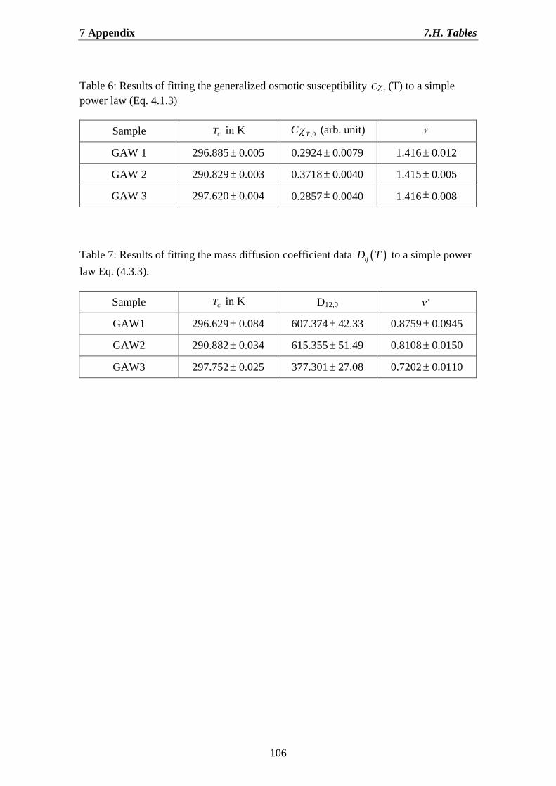
7 Appendix 7.H. Tables
106
Table 6: Results of fitting the generalized osmotic susceptibility TC (T) to a simplepower law (Eq. 4.1.3)
Sample CT in K ,0TC (arb. unit)
GAW 1 296.8850.005 0.29240.0079 1.4160.012
GAW 2 290.8290.003 0.37180.0040 1.4150.005
GAW 3 297.6200.004 0.28570.0040 1.4160.008
Table 7: Results of fitting the mass diffusion coefficient data ijD T to a simple powerlaw Eq. (4.3.3).
Sample CT in K D12,0
GAW1 296.6290.084 607.37442.33 0.87590.0945
GAW2 290.8820.034 615.35551.49 0.81080.0150
GAW3 297.7520.025 377.30127.08 0.72020.0110
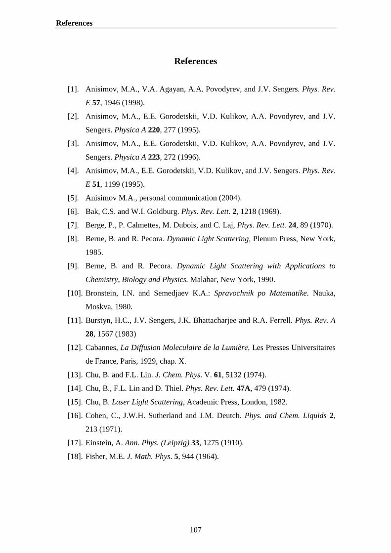
References
107
References
[1]. Anisimov, M.A., V.A. Agayan, A.A. Povodyrev, and J.V. Sengers. Phys. Rev.
E 57, 1946 (1998).
[2]. Anisimov, M.A., E.E. Gorodetskii, V.D. Kulikov, A.A. Povodyrev, and J.V.
Sengers. Physica A 220, 277 (1995).
[3]. Anisimov, M.A., E.E. Gorodetskii, V.D. Kulikov, A.A. Povodyrev, and J.V.
Sengers. Physica A 223, 272 (1996).
[4]. Anisimov, M.A., E.E. Gorodetskii, V.D. Kulikov, and J.V. Sengers. Phys. Rev.
E 51, 1199 (1995).
[5]. Anisimov M.A., personal communication (2004).
[6]. Bak, C.S. and W.I. Goldburg. Phys. Rev. Lett. 2, 1218 (1969).
[7]. Berge, P., P. Calmettes, M. Dubois, and C. Laj, Phys. Rev. Lett. 24, 89 (1970).
[8]. Berne, B. and R. Pecora. Dynamic Light Scattering, Plenum Press, New York,
1985.
[9]. Berne, B. and R. Pecora. Dynamic Light Scattering with Applications to
Chemistry, Biology and Physics. Malabar, New York, 1990.
[10]. Bronstein, I.N. and Semedjaev K.A.: Spravochnik po Matematike. Nauka,
Moskva, 1980.
[11]. Burstyn, H.C., J.V. Sengers, J.K. Bhattacharjee and R.A. Ferrell. Phys. Rev. A
28, 1567 (1983)
[12]. Cabannes, La Diffusion Moleculaire de la Lumière, Les Presses Universitaires
de France, Paris, 1929, chap. X.
[13]. Chu, B. and F.L. Lin. J. Chem. Phys. V. 61, 5132 (1974).
[14]. Chu, B., F.L. Lin and D. Thiel. Phys. Rev. Lett. 47A, 479 (1974).
[15]. Chu, B. Laser Light Scattering, Academic Press, London, 1982.
[16]. Cohen, C., J.W.H. Sutherland and J.M. Deutch. Phys. and Chem. Liquids 2,
213 (1971).
[17]. Einstein, A. Ann. Phys. (Leipzig) 33, 1275 (1910).
[18]. Fisher, M.E. J. Math. Phys. 5, 944 (1964).
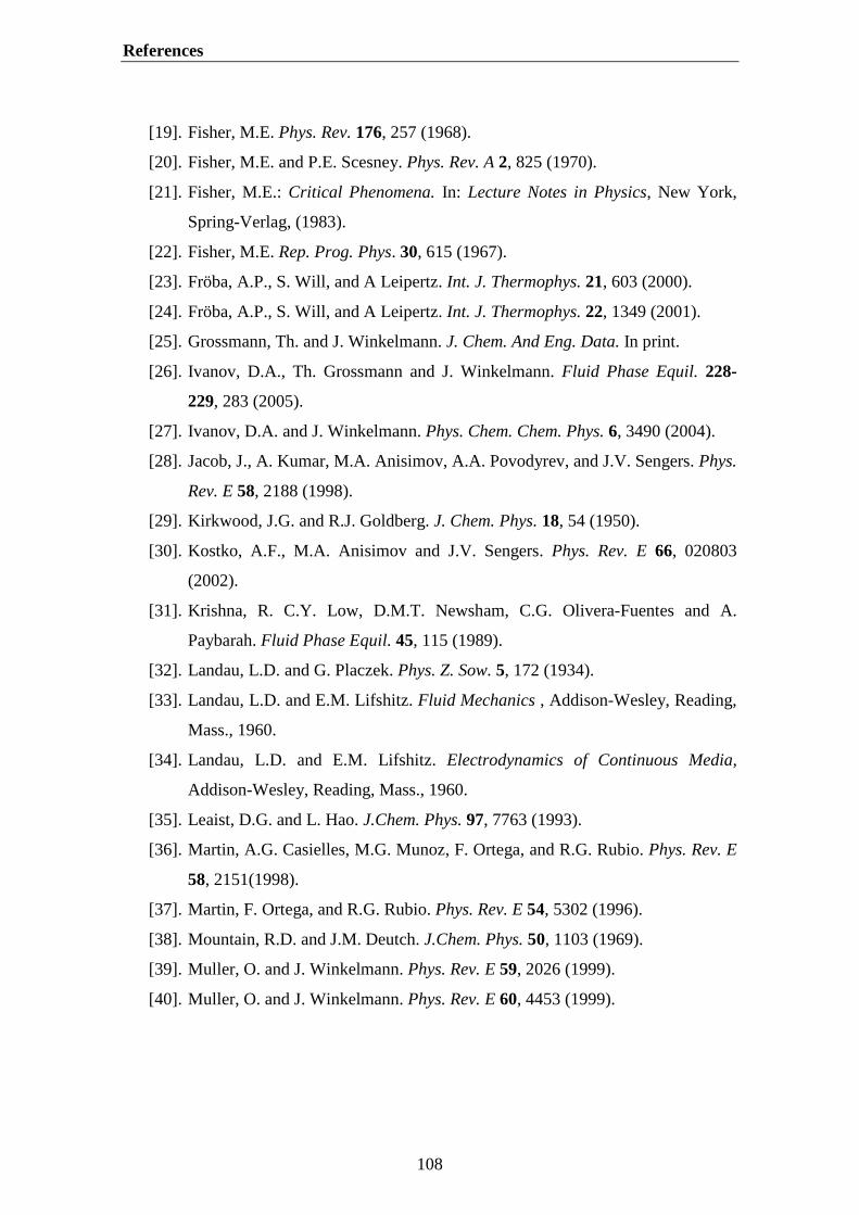
References
108
[19]. Fisher, M.E. Phys. Rev. 176, 257 (1968).
[20]. Fisher, M.E. and P.E. Scesney. Phys. Rev. A 2, 825 (1970).
[21]. Fisher, M.E.: Critical Phenomena. In: Lecture Notes in Physics, New York,
Spring-Verlag, (1983).
[22]. Fisher, M.E. Rep. Prog. Phys. 30, 615 (1967).
[23]. Fröba, A.P., S. Will, and A Leipertz. Int. J. Thermophys. 21, 603 (2000).
[24]. Fröba, A.P., S. Will, and A Leipertz. Int. J. Thermophys. 22, 1349 (2001).
[25]. Grossmann, Th. and J. Winkelmann. J. Chem. And Eng. Data. In print.
[26]. Ivanov, D.A., Th. Grossmann and J. Winkelmann. Fluid Phase Equil. 228-
229, 283 (2005).
[27]. Ivanov, D.A. and J. Winkelmann. Phys. Chem. Chem. Phys. 6, 3490 (2004).
[28]. Jacob, J., A. Kumar, M.A. Anisimov, A.A. Povodyrev, and J.V. Sengers. Phys.
Rev. E 58, 2188 (1998).
[29]. Kirkwood, J.G. and R.J. Goldberg. J. Chem. Phys. 18, 54 (1950).
[30]. Kostko, A.F., M.A. Anisimov and J.V. Sengers. Phys. Rev. E 66, 020803
(2002).
[31]. Krishna, R. C.Y. Low, D.M.T. Newsham, C.G. Olivera-Fuentes and A.
Paybarah. Fluid Phase Equil. 45, 115 (1989).
[32]. Landau, L.D. and G. Placzek. Phys. Z. Sow. 5, 172 (1934).
[33]. Landau, L.D. and E.M. Lifshitz. Fluid Mechanics , Addison-Wesley, Reading,
Mass., 1960.
[34]. Landau, L.D. and E.M. Lifshitz. Electrodynamics of Continuous Media,
Addison-Wesley, Reading, Mass., 1960.
[35]. Leaist, D.G. and L. Hao. J.Chem. Phys. 97, 7763 (1993).
[36]. Martin, A.G. Casielles, M.G. Munoz, F. Ortega, and R.G. Rubio. Phys. Rev. E
58, 2151(1998).
[37]. Martin, F. Ortega, and R.G. Rubio. Phys. Rev. E 54, 5302 (1996).
[38]. Mountain, R.D. and J.M. Deutch. J.Chem. Phys. 50, 1103 (1969).
[39]. Muller, O. and J. Winkelmann. Phys. Rev. E 59, 2026 (1999).
[40]. Muller, O. and J. Winkelmann. Phys. Rev. E 60, 4453 (1999).
References
109
[41]. Muller, O.: Streulichtuntersuchungen zum kritischen Verhalten flüssiger
ternärer Mischungen. Ph.D.-thesis, University Halle-Wittenberg, (2001).
[42]. Ornstein, L.S. and F. Zernike. Proc. Acad. Sci. (Amsterdam) 17, 73 (1914); 18,
1520 (1915); 19, 1312 (1916); 11, 1321 (1916).
[43]. Ornstein, L.S. and F. Zernike. Physik Z. 27, 761 (1926).
[44]. Pecora, R. J. Chem. Phys. 40, 1604 (1964).
[45]. Pertler, M.: Die Mehrkomponenten-Diffusion in nicht vollständing mischbaren
Flüssigkeite. Ph.D.-thesis, TU München, (1996).
[46]. Povodyrev, A.A., G.X. Jin, S.B. Kiselev and J.V. Sengers. Int. J. Thermophys.
17, 909 (1996).
[47]. Provencher, S.W. J. Chem. Phys. 64, 2772 (1976).
[48]. Rouch, J., P.Tartaglia and S.H. Chen. Phys. Rev A 25, 448 (1982).
[49]. Rutten, W.M.: Diffusion in Liquids. Ph.D.-thesis, Delft University Press,
(1992).
[50]. Wild, A.: Multicomponent Diffusion in Liquids. Ph.D.-thesis, TU München,
(2002).
[51]. Will, S. and A Leipertz. Int. J. Thermophys. 20, 791 (1999).
[52]. Will, S. and A Leipertz. Int. J. Thermophys. 22, 317 (2001).
[53]. Wu, G., M. Fiebig, and A. Leipertz. Wärme- und Stoffübertragung 22, 365
(1988).
Erklärung
Hiermit erkläre ich, dass ich die vorliegende Arbeit selbständig und nur unterVerwendung der angegebenen Quellen und Hilfsmittel angefertigt habe. Wörtlichoder inhaltlich übernommene Stellen sind als solche gekennzeichnet.
Diese Arbeit habe ich an keiner anderen Universität oder Hochschule vorgelegt undmich zu keinem frühren Zeitpunkt um den Doktorgrad beworben.
D.A. Ivanov
Halle/Saale, Mai 2005
CURRICULUM VITAE OF DIMITRY A. IVANOV
2001–present PhD research scientific co-worker at Institute of Physical
Chemistry of the Martin –Luther University Halle –Wittenberg,
Germany
DFG-project:„Diffusiver Transport in Mehrkomponentensystemen
mit Flüssig-Flüssig-Grenzphasen“.
Investigation of multicomponent liquid mixture by the light
scattering technique
Supervisors: Prof. Dr. habil. J.Winkelmann
1999–2001 Scientific co-worker at B.I. Stepanov Institute of Physics National
Academy of Sciences of Belarus (Minsk, Belarus)
Research in the Laboratory of Nonlinear Optics;
Development of high-sensitive laser spectroscopy, studies of
interaction of radiation with various media,in the group of
Dr.habil. V.P.Kozich.
1994–1999 Diploma at Physics Department, Belarussian State University,
Minsk, Belarus.
Diploma Thesis: “Changing the statistical properties of noisy laser
radiation in YAG:Nd-laser” performed at B.I. Stepanov Institute of
Physics, in the group of Dr.habil. V.P.Kozich.
1994 School graduation
Scientific interestsNonlinear spectroscopy, photon-correlation spectroscopy, dynamic light scattering inliquid mixtures, phase transition and critical phenomena, behaviour of athermodynamic and transport properties in a multicomponent liquid mixtures nearcritical point and far from it.
Computer skillsProgramming in Microsoft Visual Fortran, Borland Pascal.General practice in MS Office, Corel Draw, Mathematica, Maple, MathCad, Origin.
LanguagesRussian (native), English (intermediate), German (intermediate)
Personal detailsDate and place of birth: 05.04.1977, Minsk/Belarus
D.A. Ivanov
Halle/Saale, Juni 2005
Acknowledgments
I wish to thank all of my colleges who help me to fulfill this work, especially mysupervisor Prof. Dr. Jochen Winkelmann for his patience and constant supportduring the whole study and preparation of work as well as the scientific andorganizational support of the project.
Also special thank devotes to Dr. Thomas Grossmann who introduced me. At thebeginning we carried out light scattering experiments and he assisted me inpreparations of samples.
Many thanks for excellent experimental setup deserve Dr. A.P. Fröba who kindlygave me an opportunity to measure diffusion coefficients of our investigated mixturein a period of my work in Erlangen-Nürnberg University.
My thanks I would like to express to S. Rehfeldt (TU München) who helped mecarrying out holographic interferometry experiment on measurements of a massdiffusion coefficient of the GAW mixture.
Directly I would like to appreciate Prof. Dr. M.A. Anisimov from University ofMaryland, with him I had valuable discussion on the physical interpretation ofdiffusivities in multicomponent mixture and who opened the present problematic ofthe subject.
The author wishes to express his sincere appreciation to the DeutscheForschungsgemeinschaft (DFG) for the financial support.