Embed Size (px)
Citation preview
IVW - Schriftenreihe Band 94 Institut für Verbundwerkstoffe GmbH - Kaiserslautern _________________________________
Muhammad Amir Khan Experimental and Simulative Description of the Thermoplastic Tape Placement Process with Online Consolidation
Bibliografische Information Der Deutschen Bibliothek Die Deutsche Bibliothek verzeichnet diese Publikation in der Deutschen Nationalbibliografie; detaillierte bibliografische Daten sind im Internet über <http://dnb.ddb.de> abrufbar. Bibliographic information published by Die Deutsche Bibliothek Die Deutsche Bibliothek lists this publication in the Deutsche Nationalbibliografie; detailed bibliographic data is available in the Internet at <http://dnb.ddb.de>.
Herausgeber: Institut für Verbundwerkstoffe GmbH Prof. Dr.-Ing. Ulf Breuer Erwin-Schrödinger-Straße TU Kaiserslautern, Gebäude 58 67663 Kaiserslautern http://www.ivw.uni-kl.de Verlag: Institut für Verbundwerkstoffe GmbH Druck: Technische Universität Kaiserslautern ZBT – Abteilung Foto-Repro-Druck D 386 © Institut für Verbundwerkstoffe GmbH, Kaiserslautern 2010 Alle Rechte vorbehalten, auch das des auszugsweisen Nachdrucks, der auszugsweisen oder vollständigen Wiedergabe (Photographie, Mikroskopie), der Speicherung in Datenverarbeitungsanlagen und das der Übersetzung. Als Manuskript gedruckt. Printed in Germany. ISSN 1615-021X ISBN 978-3-934930-90-2
Experimental and Simulative Description of the Thermoplastic Tape Placement Process with Online Consolidation
Beim Fachbereich für Maschinenbau und Verfahrenstechnik
der Technischen Universität Kaiserslautern
genehmigte Dissertation
zur Erlangung des akademischen Grades
Doktor-Ingenieur (Dr.-Ing.)
vorgelegt von
MSc. Muhammad Amir Khan
aus Karachi, Pakistan
Tag der mündlichen Prüfung: 30.08.2010
Prüfungsvorsitzender: Prof. Dr.-Ing. Paul L. Geiß
1. Berichterstatter: Prof. Dr.-Ing. Peter Mitschang
2. Berichterstatter: Prof. Dr.-Ing. Martin Maier
D 386

Preface I
Preface
I would like to express my sincere gratitude to Prof. Dr.-Ing. Peter Mitschang, whose
unparalleled compassion, kindness and generosity allowed me to cruise through the
demands of this research during the period from 2006 to 2010. One thing among
many which I learned from him is how to stay positive in every problem you face.
I would also like to profoundly thank my advisor Dr.-Ing. Ralf Schledjewski. His guid-
ance, continuous encouragement and support right from the start to the end enabled
me to successfully complete this work. He was always there to listen and to give ad-
vice. His constructive comments and remarks during the meetings helped me in un-
derstanding the problem and the relevant concepts. Furthermore I would like to thank
Prof. Dr.-Ing. Paul L. Geiß for chairmanship in the examination board and Prof. Dr.-
Ing. Martin Maier for examining my thesis.
I greatly acknowledge the financial support from Higher Education Commission
(HEC) and Institute of Space Technology, Pakistan for the pursuit of this research
work. Also I want to say thanks to DAAD (German Academic Exchange Service)
whose cooperation with HEC accommodated a number of students in Germany.
Let me also give thank to my colleagues (past and present) with whom I had a won-
derful time and had very helpful discussions. I am obliged to thanks Jens Lichtner
and Angelos Miaris for their very friendly and always ready-to-help attitude. Special
thanks to Rene Holschuh and André Meichsner for proof-reading the manuscript. I
also want to thank Steven Brogdon, for all wonderful conversations we did from tech-
nical issues to horse riding.
There are no words to thank my parents who supported me over the years and
brought me up to what I am today. I am greatly indebted to my wife Maryam Naz, for
her love, support and patience.
Kaiserslautern, September 2010

II
For Ammi Jan and all family members
Contents III
Contents
1 Introduction ....................................................................................................... 1
1.1 Objectives................................................................................................... 2
1.2 Approach .................................................................................................... 3
2 State of the art................................................................................................... 4
2.1 Thermoplastic tape placement setup.......................................................... 4
2.2 Classification of thermoplastic tape placement head.................................. 7
2.3 Tape placement setup at IVW .................................................................. 10
2.4 Process modeling ..................................................................................... 12
2.4.1 Heat transfer model......................................................................... 13
2.4.2 Consolidation under roller ............................................................... 15
2.4.3 Intimate contact and polymer healing.............................................. 19
2.4.4 Thermal degradation ....................................................................... 21
2.4.5 Crystallization.................................................................................. 22
2.4.6 Crystal-melting kinetics ................................................................... 24
2.4.7 Process induced stresses ............................................................... 24
3 Experimental characterization and testing ................................................... 26
3.1 Thermoplastic material ............................................................................. 26
3.2 Thermal mapping under the hot gas torch................................................ 28
3.3 Equivalent heating length ......................................................................... 32
3.4 Convective heat transfer coefficient.......................................................... 34
3.5 Material deformation................................................................................. 37
IV Contents
3.5.1 Thickness build-up .......................................................................... 37
3.5.2 Width change .................................................................................. 40
3.6 Surface roughness ................................................................................... 43
3.7 Rheological properties.............................................................................. 45
3.7.1 Transverse viscosity of unidirectional thermoplastic material.......... 45
3.7.2 Polymer relaxation time (Weld time)................................................ 48
3.7.3 Polymer crosslinking ....................................................................... 50
3.7.4 Thermo-gravimetric properties ........................................................ 51
3.8 Mechanical testing.................................................................................... 54
3.8.1 Peel resistance................................................................................ 54
3.8.2 Interlaminar shear strength (ILSS) .................................................. 57
3.9 Reference plate and experimental bonding degree Db ............................. 59
3.10 Void contents characterization ................................................................. 63
4 Process simulation and parameter study..................................................... 65
4.1 Modeling thermoplastic tape placement process...................................... 65
4.2 Model implementation .............................................................................. 68
4.3 Process simulation ................................................................................... 70
4.4 Thermal simulation ................................................................................... 70
4.4.1 Surface temperature........................................................................ 73
4.5 Simulation for consolidation and strength development ........................... 74
4.5.1 Void consolidation ........................................................................... 75
4.5.2 Geometrical deformation ................................................................. 78
Contents V
4.5.3 Prediction of interlaminar bonding................................................... 80
4.6 Process parameter study.......................................................................... 82
4.6.1 Effect of consolidation force ............................................................ 83
4.6.2 Effect of number of plies (layers) on laminate quality ...................... 85
4.6.3 Effect of tool temperature ................................................................ 87
4.6.4 Overview ......................................................................................... 89
5 Results and discussion.................................................................................. 93
5.1 Weight loss............................................................................................... 93
5.2 Thermal degradation ................................................................................ 95
5.3 Transverse bonding.................................................................................. 97
5.4 Lay-up parameters selection for manufacturing ......................................103
5.5 High quality thermoplastic prepreg material ............................................106
5.5.1 Tape edges ................................................................................... 106
5.5.2 Surface roughness ........................................................................ 106
5.5.3 Tape with less initial void............................................................... 109
5.6 Technological advancement....................................................................110
6 Conclusion and outlook ............................................................................... 114
7 Appendix........................................................................................................ 117
7.1 Code for calculating pressure under rotating roller ..................................117
7.2 Code to calculate heat transfer inside the laminate .................................117
7.3 Code for void calculation .........................................................................118
8 References..................................................................................................... 119
VI Abbreviations
Abbreviations
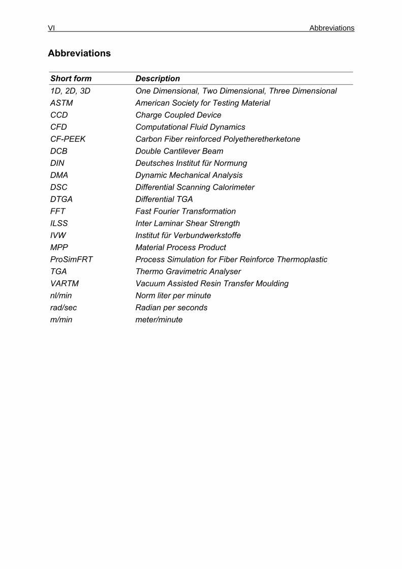
Short form Description 1D, 2D, 3D One Dimensional, Two Dimensional, Three Dimensional ASTM American Society for Testing Material CCD Charge Coupled Device CFD Computational Fluid Dynamics CF-PEEK Carbon Fiber reinforced Polyetheretherketone DCB Double Cantilever Beam DIN Deutsches Institut für Normung DMA Dynamic Mechanical Analysis DSC Differential Scanning Calorimeter DTGA Differential TGA FFT Fast Fourier Transformation ILSS Inter Laminar Shear Strength IVW Institut für Verbundwerkstoffe MPP Material Process Product ProSimFRT Process Simulation for Fiber Reinforce Thermoplastic TGA Thermo Gravimetric Analyser VARTM Vacuum Assisted Resin Transfer Moulding nl/min Norm liter per minute rad/sec Radian per seconds m/min meter/minute
Symbols VII
Symbols
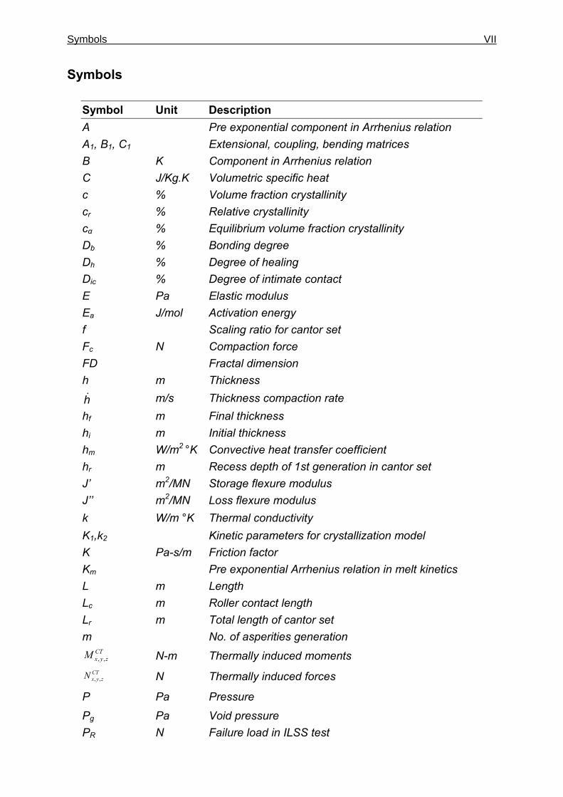
Symbol Unit Description A Pre exponential component in Arrhenius relation A1, B1, C1 Extensional, coupling, bending matrices B K Component in Arrhenius relation C J/Kg.K Volumetric specific heat c % Volume fraction crystallinity cr % Relative crystallinity cα % Equilibrium volume fraction crystallinity Db % Bonding degree Dh % Degree of healing Dic % Degree of intimate contact E Pa Elastic modulus Ea J/mol Activation energy f Scaling ratio for cantor set Fc N Compaction force FD Fractal dimension h m Thickness
h& m/s Thickness compaction rate hf m Final thickness hi m Initial thickness hm W/m2 °K Convective heat transfer coefficient hr m Recess depth of 1st generation in cantor set J’ m2/MN Storage flexure modulus J’’ m2/MN Loss flexure modulus k W/m °K Thermal conductivity K1,k2 Kinetic parameters for crystallization model K Pa-s/m Friction factor Km Pre exponential Arrhenius relation in melt kinetics L m Length Lc m Roller contact length Lr m Total length of cantor set m No. of asperities generation
CTzyxM ,, N-m Thermally induced moments
CTzyxN ,, N Thermally induced forces
P Pa Pressure
Pg Pa Void pressure PR N Failure load in ILSS test
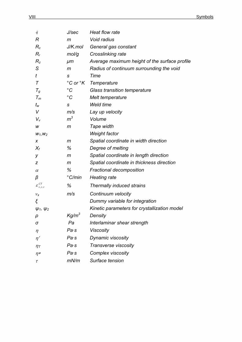
VIII Symbols
q& J/sec Heat flow rate R m Void radius Rc J/K.mol General gas constant Rr mol/g Crosslinking rate Rz µm Average maximum height of the surface profile S m Radius of continuum surrounding the void t s Time T °C or °K Temperature Tg °C Glass transition temperature Tm °C Melt temperature tw s Weld time V m/s Lay up velocity Vv m3 Volume w m Tape width w1,w2 Weight factor x m Spatial coordinate in width direction Xf % Degree of melting y m Spatial coordinate in length direction z m Spatial coordinate in thickness direction α % Fractional decomposition β °C/min Heating rate
CTzyx ,,ε % Thermally induced strains
νx m/s Continuum velocity ξ Dummy variable for integration ψ1, ψ2 Kinetic parameters for crystallization model ρ Kg/m3 Density σ Pa Interlaminar shear strength η Pa·s Viscosity η′ Pa·s Dynamic viscosity ηT Pa·s Transverse viscosity η∗ Pa·s Complex viscosity τ mN/m Surface tension
Kurzfassung IX
Kurzfassung
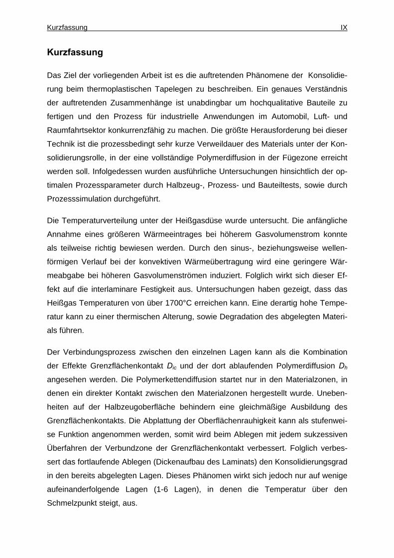
Das Ziel der vorliegenden Arbeit ist es die auftretenden Phänomene der Konsolidie-
rung beim thermoplastischen Tapelegen zu beschreiben. Ein genaues Verständnis
der auftretenden Zusammenhänge ist unabdingbar um hochqualitative Bauteile zu
fertigen und den Prozess für industrielle Anwendungen im Automobil, Luft- und
Raumfahrtsektor konkurrenzfähig zu machen. Die größte Herausforderung bei dieser
Technik ist die prozessbedingt sehr kurze Verweildauer des Materials unter der Kon-
solidierungsrolle, in der eine vollständige Polymerdiffusion in der Fügezone erreicht
werden soll. Infolgedessen wurden ausführliche Untersuchungen hinsichtlich der op-
timalen Prozessparameter durch Halbzeug-, Prozess- und Bauteiltests, sowie durch
Prozesssimulation durchgeführt.
Die Temperaturverteilung unter der Heißgasdüse wurde untersucht. Die anfängliche
Annahme eines größeren Wärmeeintrages bei höherem Gasvolumenstrom konnte
als teilweise richtig bewiesen werden. Durch den sinus-, beziehungsweise wellen-
förmigen Verlauf bei der konvektiven Wärmeübertragung wird eine geringere Wär-
meabgabe bei höheren Gasvolumenströmen induziert. Folglich wirkt sich dieser Ef-
fekt auf die interlaminare Festigkeit aus. Untersuchungen haben gezeigt, dass das
Heißgas Temperaturen von über 1700°C erreichen kann. Eine derartig hohe Tempe-
ratur kann zu einer thermischen Alterung, sowie Degradation des abgelegten Materi-
als führen.
Der Verbindungsprozess zwischen den einzelnen Lagen kann als die Kombination
der Effekte Grenzflächenkontakt Dic und der dort ablaufenden Polymerdiffusion Dh
angesehen werden. Die Polymerkettendiffusion startet nur in den Materialzonen, in
denen ein direkter Kontakt zwischen den Materialzonen hergestellt wurde. Uneben-
heiten auf der Halbzeugoberfläche behindern eine gleichmäßige Ausbildung des
Grenzflächenkontakts. Die Abplattung der Oberflächenrauhigkeit kann als stufenwei-
se Funktion angenommen werden, somit wird beim Ablegen mit jedem sukzessiven
Überfahren der Verbundzone der Grenzflächenkontakt verbessert. Folglich verbes-
sert das fortlaufende Ablegen (Dickenaufbau des Laminats) den Konsolidierungsgrad
in den bereits abgelegten Lagen. Dieses Phänomen wirkt sich jedoch nur auf wenige
aufeinanderfolgende Lagen (1-6 Lagen), in denen die Temperatur über den
Schmelzpunkt steigt, aus.
X Kurzfassung
Auf der Kombination der Prozessgeschwindigkeit und des Heißgasdüsenvolumen-
stroms basierende drei Energieeintragslevel konnten identifiziert werden. Bei Wahl
einer Kombination der beiden Parameter mit insgesamt niedrigem Eintragsniveau ist
der Energieeintrag sowohl in das abzulegende Tape als auch in das bereits abgeleg-
te Substrat begrenzt und ein daraus resultierender unvollständiger Grenzflächenkon-
takt verhindert den Verbund. Obgleich ein hoher Energieeintrag den Grad des Ver-
bundes Db bis hinzu 97% anhebend kann, tritt hierbei das Phänomen der thermi-
schen Degradation auf. Die Polymerdiffusion und die Polymervernetzung folgen der
Arrhenius-Gleichung mit Aktivierungsenergien von 43 KJ/mol und 276 KJ/mol. Die
Polymervernetzung bei hohem Temperatureintrag erschwert die Polymerdiffusion
und resultiert somit in einer verringerten Verbundstärke. Somit ermöglicht die Wahl
optimierter den Energieeintrag betreffenden Prozessparametern eine kontinuierliche
über den gesamten Legeprozess fortschreitende Verbesserung des interlaminaren
Verbundes.
Eine Multi-Parameter-Studie hat gezeigt, dass eine verlängerte Konsolidationsphase,
einerseits erreichbar durch Erhöhungen der Anzahl der Überfahrvorgänge, anderer-
seits durch Verlängerung der Konsolidierungstrecke, oder durch Einsatz von mehre-
ren Konsolidierungsrollen, in einer Aufweitung des Profilverlaufs des Verbundgrades
Db resultiert. Auf diese Weise sind hohe Ablegegeschwindigkeiten (bis zu 7 m/min)
realisierbar und machen den Prozess für industrielle Anwendungen geeignet. Mit der
am IVW vorhandenen Tapelegeeinheit mit einer Kompaktierungsrolle ist eine Lami-
natherstellung möglich, welche autoklav-ähnliche Güte besitzt (bezogen auf ILSS
und Porengehalt), wenn das bändchenförmige vorimprägnierte Halbzeug einen Po-
rengehalt kleiner 1% aufweist.
Als auf die Zugfestigkeit 90° primärer beeinflussender Parameter konnte die Defor-
mationen der Tapekante identifiziert werden. Laminate, welche mit einer leichten
Überlappung der Tapes erstellt wurden, weisen eine ca. 10% Steigerung bezüglich
der Querzugkraft verglichen zu Laminaten mit reiner Stoß-an-Stoß Ablage.
Ein hohes Energieeintragsniveau wirkt sich im Ablegeprozess jedoch negativ auf die
Güte des Querverbundes der Laminate aus, da sich hierbei Lufteinschlüsse bilden.
Nachträgliche Konsolidierungsschritte wie beispielsweise zusätzliche Überfahrvor-
gänge mit geringem Gasvolumenstrom haben sich als positiv erwiesen um die ein-
geschlossenen Poren zu eliminieren und die Gesamtqualität des Laminats zu ver-
Kurzfassung XI
bessern.
Letztlich kann die in dieser Arbeit entwickelte Simulation dazu verwendet werden um
bestehende limitierende Parameterkonstellationen zu identifizieren um somit durch
optimierte Prozessfenster eine vollständige Konsolidation zu erreichen. Die ausge-
führte Parameterstudie hat gezeigt, dass mit der aktuell am Markt angeboten Halb-
zeuggüte (ursprünglicher Porengehalt 3,1%) Laminate mit einem Verbundgrad Db >
97%, bei jedoch gleichzeitig erhöhtem intralaminaren Porengehalt, erstellt werden
können. Obgleich es sich in dieser Arbeit durch experimentelle Untersuchungen ge-
zeigt hat, dass sich das Vorhandensein von intralaminaren Poren nicht negativ auf
ILSS-Werte auswirkt, gibt es Anwendungsfälle (Luft- und Raumfahrt oder Medizin-
technik) in denen ein Porengehalt < 1% gefordert ist. Die Werkzeugtemperatur konn-
te neben der Heißgastemperatur und der Prozessgeschwindigkeit als dritter Parame-
ter mit starken Auswirkungen auf die Laminatgüte identifiziert werden. Ein hochtem-
periertes Werkzeug (260-290 °C) begünstigt einerseits den Verbund innerhalb des
Laminates, andererseits jedoch wird hierdurch eine Porenexpansion gefördert. Simu-
lationsergebnisse zeigen, dass eine Porenexpansion durch eine kalte Werkzeug-
oberfläche verhindert werden kann. Jedoch die zur Ausbildung der Adhäsion zwi-
schen Erstlage und Werkzeug notwendige erhöhte Temperatur steht dem entgegen.
XII Kurzfassung
Abstract
The aim of this study is to describe the consolidation in thermoplastic tape placement
process to obtain high quality structure, making the process viable for automotive
and aerospace industrial applications. The major barrier in this technique is very
short residence time of material under the consolidation roller to accomplished com-
plete polymer diffusion in the bonded region. Hence investigation is performed to find
out the optimize manufacturing parameters by extensive material, process, product
testing and through process simulation.
Temperature distribution and convective heat transfer under the hot gas torch is ex-
perimentally mapped out. Bonding process inside the laminate is the combine effect
of layers (tapes) intimate contact Dic development and resulting polymer diffusion Dh
at these contacted sections. Three energy levels are identified based on the process
velocity and hot gas flow combinations. For the low energy parameter combinations,
the energy input to the incoming tape and substrate material is limited and result in
incomplete intimate contact which restricts the bonding process. On other hand high
energy input although could increase the bonding degree Db even up to the 97%, but
also activate the thermal degradation phenomena. It is found out that the rate of po-
lymer healing (diffusion) and polymer crosslinking follows the Arrhenius laws with the
activation energies of 43 KJ/mol and 276 KJ/mol. The polymer crosslinking at high
temperature exposure hinder the polymer diffusion process and reduces the strength
development. So the parameters combination at intermediate energy level provides
the opportunity of continuous interlaminar strength improvement through out the la-
yup process.
Deformation of tape edges is identified as the dictating factor for the laminate’s trans-
verse strength. Tape placement with slight overlap reinforced the transverse joint by
more 10 % as compared to pure matrix joint. Finally the simulation tool developed in
this research work is used for identifying the existing limitation to achieve full consoli-
dation. A parameter study shows that extended consolidation either by mean of addi-
tional pass or by increasing consolidation length widens the high strength (over 90%)
bonding degree Db contour. Thus high lay-up velocity (up to 7 m/min) is viable for in-
dustrial production rate.
Introduction 1
1 Introduction
The high demand for light weight structure has given a way for the technological pro-
gress in the field of composite material. The fiber reinforced composite materials are
preferably used by the sport, automobile and aerospace industries for their high
strength, cost effectiveness and excellent resistance against thermal / chemical envi-
ronment. On the basis of adhesive matrix system, fiber reinforced composites are
broadly classified as thermoset and thermoplastic material [1]. Processing of the ther-
moset composite involves steps such as impregnation, lamination and curing. Ther-
moplastic materials on other hand are commercially available in fully polymerized
form, and the manufacturing process is based only on lamination and curing.
Thermoplastic materials offer some unique processing opportunities like hot laminate
can be reshaped or formed to produce three dimensional parts. Thermal welding can
be done with similar thermoplastic material as well as with metal to produce assem-
blies. Material can be reconsolidated to eliminate defects and recycled for new appli-
cation. These features lead to various manufacturing processes, such as hand lay-
up, autoclaved molding, fusion bonding, press molding, diaphragm forming, filament
winding and automated tape placement process.
Among them the automated tape placement process has some additional interest
due to high processing rate and potential cost saving in manufacturing because no
secondary processing is needed to complete the consolidation process. Thermoplas-
tic tape placement with online consolidation is a discontinuous process in which a
thermoplastic prepreg material is laid up on the tool or mandrel and consolidated im-
mediately with the application of heat and pressure. Compared to the filament wind-
ing, it provides several additional flexibilities such as the possibility to manufacture
non rotational structures even with concave curves and free fiber orientation.
Online or insitu consolidation is a processing step in which heat and pressure are
applied simultaneously to the thermoplastic material to eliminate spatial gaps and
force out any entrapped air, thereby initiating the interface bonding through polymer
chain diffusion process. Improper consolidation can lead to voids, residual stresses,
warpage and in some cases premature mechanical failure of the composite part [2].
This study explains and addresses the several critical issues of the thermoplastic
2 Introduction
tape placement process with online consolidation that must be overcome to obtain a
composite laminate with optimum properties.
1.1 Objectives
According to the experimental testing conducted on the tape placement setup at IVW
[3-4] the selection of manufacturing conditions highly influences the quality of the fi-
nal parts. Hence the optimized process parameter should be identified to produce a
unidirectional laminate with bonding strength comparable to other established manu-
facturing process like autoclave. The objectives of this research work are three folds
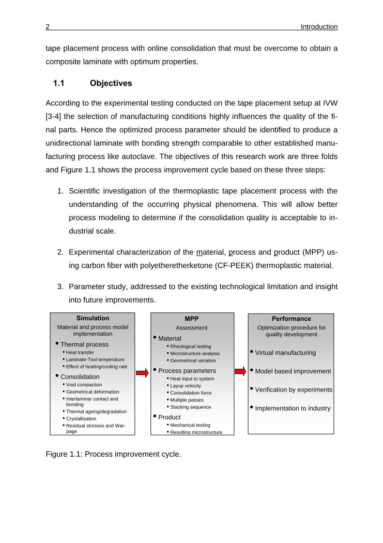
and Figure 1.1 shows the process improvement cycle based on these three steps:
1. Scientific investigation of the thermoplastic tape placement process with the
understanding of the occurring physical phenomena. This will allow better
process modeling to determine if the consolidation quality is acceptable to in-
dustrial scale.
2. Experimental characterization of the material, process and product (MPP) us-
ing carbon fiber with polyetheretherketone (CF-PEEK) thermoplastic material.
3. Parameter study, addressed to the existing technological limitation and insight
into future improvements.
Figure 1.1: Process improvement cycle.
MPP Assessment
• Material • Rheological testing • Microstructure analysis • Geometrical variation
• Process parameters • Heat input to system • Layup velocity • Consolidation force • Multiple passes • Stacking sequence
• Product • Mechanical testing • Resulting microstructure
Performance Optimization procedure for
quality development
• Virtual manufacturing
• Model based improvement
• Verification by experiments
• Implementation to industry
Simulation Material and process model
implementation
• Thermal process • Heat transfer • Laminate-Tool temperature • Effect of heating/cooling rate
• Consolidation • Void compaction • Geometrical deformation • Interlaminar contact and
bonding • Thermal ageing/degradation • Crystallization • Residual stresses and War-
page
Introduction 3
1.2 Approach
The chapter two discusses the basic principal and introduces the basic terminologies
of the thermoplastic tape placement process. The tape placement head involving dif-
ferent mechanism of heating and consolidation conceived within the last few decades
are also discussed. On theoretical side, state of the art models explaining the
thermo-kinetic mechanism for strength development are presented.
Chapter three is focused on the experimental techniques to characterize material,
process and product. The anisotropic nature influences the material response during
the process. Hence the methods are explained for the detail geometrics, rheometric,
mechanical and as well as micro structural examination. The setup parameters are
also monitored using a variety of sensors. The interlaminar bond strength is exam-
ined to develop the quality criteria for the final part. Peel testing and interlaminar
shear strength (ILSS) test are selected for investigating the laminate quality with the
variation of processing parameters. Relative comparison is performed with the refer-
enced autoclaved plate to see the maximum achievable consolidation level.
With sufficient theoretical and experimental explanation of the process parameters,
chapter four drives the research work into the simulation stage. The chapter is di-
vided into two sections. In the first section the results are compared with experimen-
tal measurement to confirm and fine tune the simulation tool. The comparison of void
content, peel strength and ILSS values shows high conformation and accuracy of the
implemented models. In second section results are generated for parameters study
to identify the process window.
Chapter five provide the answers to several design and development related issues.
The thermal degradation, weight loss, details of process parameter selection, effect
of material and technological improvement are all discussed and explained with the
aid of simulation and experimental results.
Chapter six lists the main achievement of this study and present the outlook for the
automatic tape placement process with online consolidation.
4 State of the art
2 State of the art
The thermoplastic tape placement process is developing towards industrial applica-
tion. An overview about the technological and theoretical advancements to exploit the
rapid processing potential of the process in order to achieve the desired cost-
effectiveness, flexibility and quality is presented. Therefore this chapter will first de-
scribe the major setup / components, processing steps, and technical terminologies.
In later section several models will be discussed to explain the incurring phenomenon
in lay-up process.
2.1 Thermoplastic tape placement setup
Manufacturer often come across with complex structure which requires specific
amounts of fibers orientation in particular direction or sections with different thick-
nesses to achieve optimum performance with minimum weights. Also the high cost of
material motivates the manufacturer to reduce the material waste. The idea of auto-
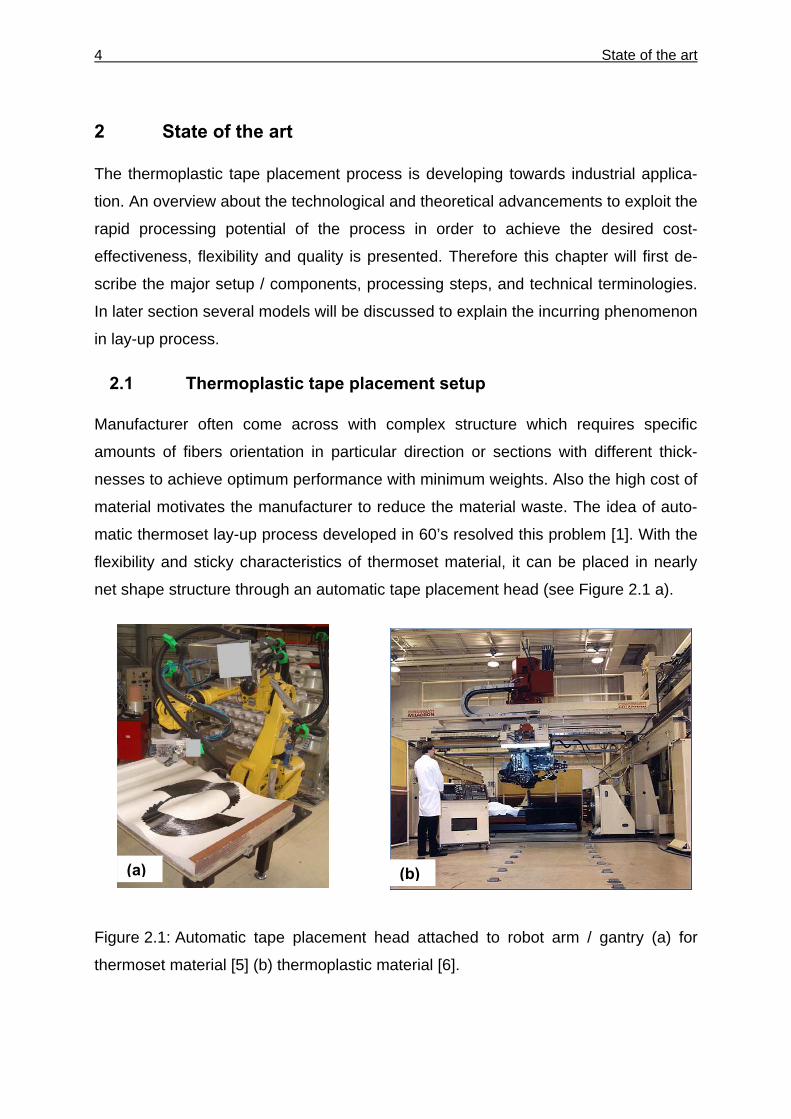
matic thermoset lay-up process developed in 60’s resolved this problem [1]. With the
flexibility and sticky characteristics of thermoset material, it can be placed in nearly
net shape structure through an automatic tape placement head (see Figure 2.1 a).
Figure 2.1: Automatic tape placement head attached to robot arm / gantry (a) for
thermoset material [5] (b) thermoplastic material [6].
(a) (b)
State of the art 5
Since most of the thermoset materials have curing cycle above the room tempera-
ture, a post consolidation step is inevitable for the complete strength development.
Beside this, the tacky state of the material creates several handling and safety haz-
ards in production environment. The introduction of the preimpregnated thermoplastic
material offered new synergy in the lay-up process. The thermoplastic plies offer
ease of handling and can be completely consolidated during the placement without
long time curing.
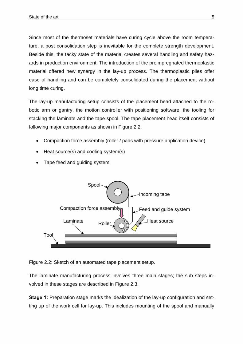
The lay-up manufacturing setup consists of the placement head attached to the ro-
botic arm or gantry, the motion controller with positioning software, the tooling for
stacking the laminate and the tape spool. The tape placement head itself consists of
following major components as shown in Figure 2.2.
• Compaction force assembly (roller / pads with pressure application device)
• Heat source(s) and cooling system(s)
• Tape feed and guiding system
Figure 2.2: Sketch of an automated tape placement setup.
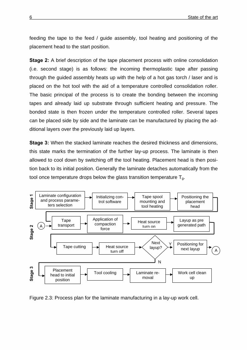
The laminate manufacturing process involves three main stages; the sub steps in-
volved in these stages are described in Figure 2.3.
Stage 1: Preparation stage marks the idealization of the lay-up configuration and set-
ting up of the work cell for lay-up. This includes mounting of the spool and manually
Spool
Compaction force assembly
Roller
Feed and guide system
Tool
Laminate
Incoming tape
Heat source
6 State of the art
feeding the tape to the feed / guide assembly, tool heating and positioning of the
placement head to the start position.
Stage 2: A brief description of the tape placement process with online consolidation
(i.e. second stage) is as follows: the incoming thermoplastic tape after passing
through the guided assembly heats up with the help of a hot gas torch / laser and is
placed on the hot tool with the aid of a temperature controlled consolidation roller.
The basic principal of the process is to create the bonding between the incoming
tapes and already laid up substrate through sufficient heating and pressure. The
bonded state is then frozen under the temperature controlled roller. Several tapes
can be placed side by side and the laminate can be manufactured by placing the ad-
ditional layers over the previously laid up layers.
Stage 3: When the stacked laminate reaches the desired thickness and dimensions,
this state marks the termination of the further lay-up process. The laminate is then
allowed to cool down by switching off the tool heating. Placement head is then posi-
tion back to its initial position. Generally the laminate detaches automatically from the
tool once temperature drops below the glass transition temperature Tg.
Figure 2.3: Process plan for the laminate manufacturing in a lay-up work cell.
Laminate configuration and process parame-
ters selection
Tape spool mounting and tool heating
Initializing con-trol software
Positioning the placement
head
Tape transport
Application of compaction
force
Heat source turn on
Layup as pre generated path
Tape cutting Heat source turn off
Positioning for next layup
Next layup?
A
Y
Placement head to initial
position
Tool cooling Laminate re-moval
Work cell clean up
N
A
Stag
e 1
Stag
e 2
Stag
e 3
State of the art 7
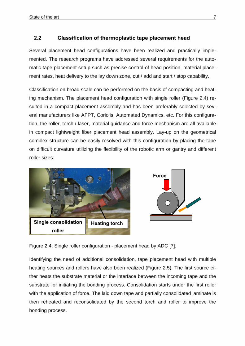
2.2 Classification of thermoplastic tape placement head
Several placement head configurations have been realized and practically imple-
mented. The research programs have addressed several requirements for the auto-
matic tape placement setup such as precise control of head position, material place-
ment rates, heat delivery to the lay down zone, cut / add and start / stop capability.
Classification on broad scale can be performed on the basis of compacting and heat-
ing mechanism. The placement head configuration with single roller (Figure 2.4) re-
sulted in a compact placement assembly and has been preferably selected by sev-
eral manufacturers like AFPT, Coriolis, Automated Dynamics, etc. For this configura-
tion, the roller, torch / laser, material guidance and force mechanism are all available
in compact lightweight fiber placement head assembly. Lay-up on the geometrical
complex structure can be easily resolved with this configuration by placing the tape
on difficult curvature utilizing the flexibility of the robotic arm or gantry and different
roller sizes.
Figure 2.4: Single roller configuration - placement head by ADC [7].
Identifying the need of additional consolidation, tape placement head with multiple
heating sources and rollers have also been realized (Figure 2.5). The first source ei-
ther heats the substrate material or the interface between the incoming tape and the
substrate for initiating the bonding process. Consolidation starts under the first roller
with the application of force. The laid down tape and partially consolidated laminate is
then reheated and reconsolidated by the second torch and roller to improve the
bonding process.
Force
Heating torch Single consolidation roller
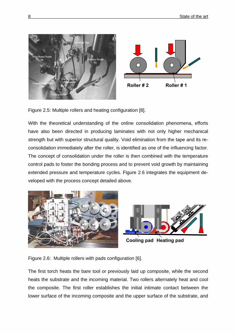
8 State of the art
Figure 2.5: Multiple rollers and heating configuration [8].
With the theoretical understanding of the online consolidation phenomena, efforts
have also been directed in producing laminates with not only higher mechanical
strength but with superior structural quality. Void elimination from the tape and its re-
consolidation immediately after the roller, is identified as one of the influencing factor.
The concept of consolidation under the roller is then combined with the temperature
control pads to foster the bonding process and to prevent void growth by maintaining
extended pressure and temperature cycles. Figure 2.6 integrates the equipment de-
veloped with the process concept detailed above.
Figure 2.6: Multiple rollers with pads configuration [6].
The first torch heats the bare tool or previously laid up composite, while the second
heats the substrate and the incoming material. Two rollers alternately heat and cool
the composite. The first roller establishes the initial intimate contact between the
lower surface of the incoming composite and the upper surface of the substrate, and
Roller # 1 Roller # 2
Cooling pad Heating pad
State of the art 9
initiates healing in those locations where intimate contact has been achieved. A
heated shoe / pad maintains the temperature long enough to foster further intimate
contact and to complete healing of the longest polymer chains in order to develop
interlaminar strength. The second roller consolidates and cools the material, re-
freezing it in place and compressing the voids. A chilled shoe extends the freezing
process by maintaining consolidation pressure to avoid the void deconsolidation [6].
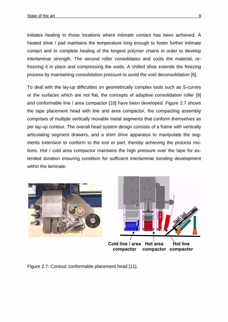
To deal with the lay-up difficulties on geometrically complex tools such as S-curves
or the surfaces which are not flat, the concepts of adaptive consolidation roller [9]
and conformable line / area compactor [10] have been developed. Figure 2.7 shows
the tape placement head with line and area compactor, the compacting assembly
comprises of multiple vertically movable metal segments that conform themselves as
per lay-up contour. The overall head system design consists of a frame with vertically
articulating segment drawers, and a shim drive apparatus to manipulate the seg-
ments extension to conform to the tool or part, thereby achieving the process mo-
tions. Hot / cold area compactor maintains the high pressure over the tape for ex-
tended duration ensuring condition for sufficient interlaminar bonding development
within the laminate.
Figure 2.7: Contour conformable placement head [11].
Hot area compactor
Hot line compactor
Cold line / area compactor
10 State of the art
2.3 Tape placement setup at IVW
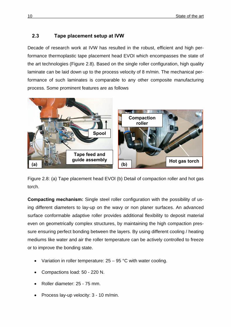
Decade of research work at IVW has resulted in the robust, efficient and high per-
formance thermoplastic tape placement head EVOI which encompasses the state of
the art technologies (Figure 2.8). Based on the single roller configuration, high quality
laminate can be laid down up to the process velocity of 8 m/min. The mechanical per-
formance of such laminates is comparable to any other composite manufacturing
process. Some prominent features are as follows
Figure 2.8: (a) Tape placement head EVOl (b) Detail of compaction roller and hot gas
torch.
Compacting mechanism: Single steel roller configuration with the possibility of us-
ing different diameters to lay-up on the wavy or non planer surfaces. An advanced
surface conformable adaptive roller provides additional flexibility to deposit material
even on geometrically complex structures, by maintaining the high compaction pres-
sure ensuring perfect bonding between the layers. By using different cooling / heating
mediums like water and air the roller temperature can be actively controlled to freeze
or to improve the bonding state.
• Variation in roller temperature: 25 – 95 °C with water cooling.
• Compactions load: 50 - 220 N.
• Roller diameter: 25 - 75 mm.
• Process lay-up velocity: 3 - 10 m/min.
Spool
Tape feed and guide assembly Hot gas torch
Compaction roller
(a) (b)
State of the art 11
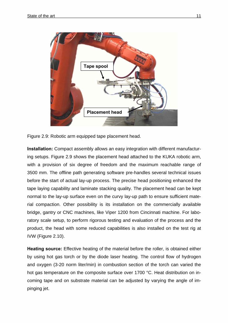
Figure 2.9: Robotic arm equipped tape placement head.
Installation: Compact assembly allows an easy integration with different manufactur-
ing setups. Figure 2.9 shows the placement head attached to the KUKA robotic arm,
with a provision of six degree of freedom and the maximum reachable range of
3500 mm. The offline path generating software pre-handles several technical issues
before the start of actual lay-up process. The precise head positioning enhanced the
tape laying capability and laminate stacking quality. The placement head can be kept
normal to the lay-up surface even on the curvy lay-up path to ensure sufficient mate-
rial compaction. Other possibility is its installation on the commercially available
bridge, gantry or CNC machines, like Viper 1200 from Cincinnati machine. For labo-
ratory scale setup, to perform rigorous testing and evaluation of the process and the
product, the head with some reduced capabilities is also installed on the test rig at
IVW (Figure 2.10).
Heating source: Effective heating of the material before the roller, is obtained either
by using hot gas torch or by the diode laser heating. The control flow of hydrogen
and oxygen (3-20 norm liter/min) in combustion section of the torch can varied the
hot gas temperature on the composite surface over 1700 °C. Heat distribution on in-
coming tape and on substrate material can be adjusted by varying the angle of im-
pinging jet.
Placement head
Tape spool
12 State of the art
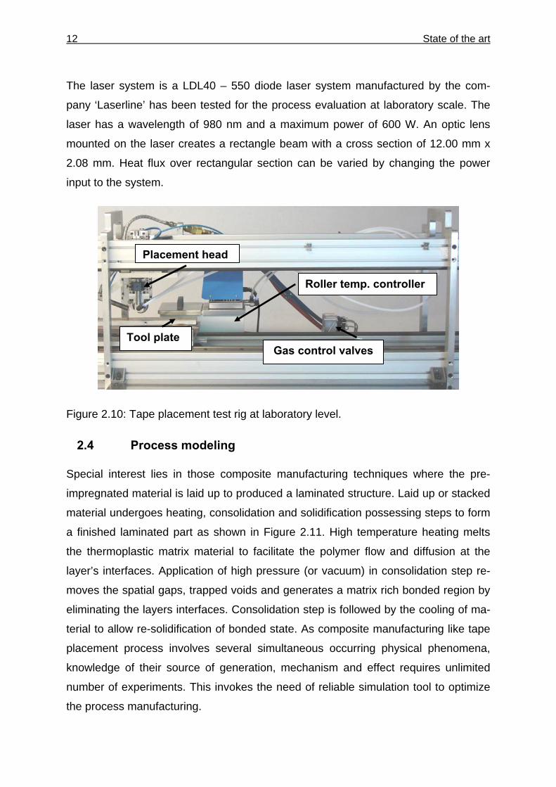
The laser system is a LDL40 – 550 diode laser system manufactured by the com-
pany ‘Laserline’ has been tested for the process evaluation at laboratory scale. The
laser has a wavelength of 980 nm and a maximum power of 600 W. An optic lens
mounted on the laser creates a rectangle beam with a cross section of 12.00 mm x
2.08 mm. Heat flux over rectangular section can be varied by changing the power
input to the system.
Figure 2.10: Tape placement test rig at laboratory level.
2.4 Process modeling
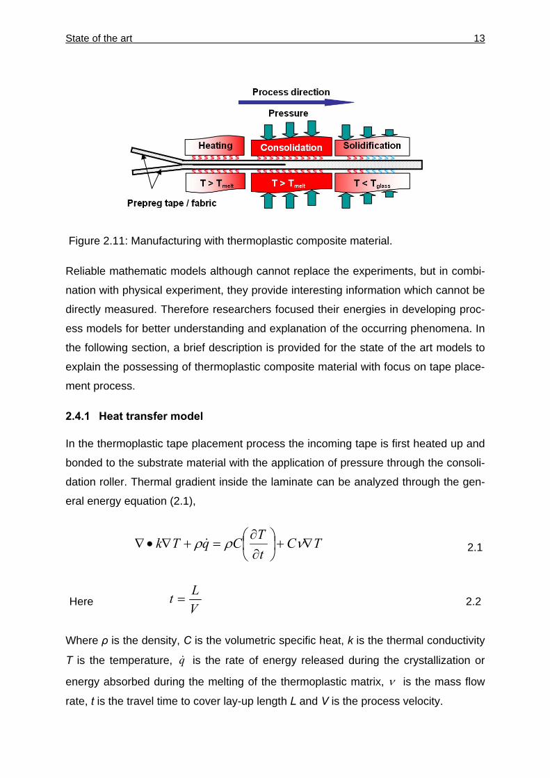
Special interest lies in those composite manufacturing techniques where the pre-
impregnated material is laid up to produced a laminated structure. Laid up or stacked
material undergoes heating, consolidation and solidification possessing steps to form
a finished laminated part as shown in Figure 2.11. High temperature heating melts
the thermoplastic matrix material to facilitate the polymer flow and diffusion at the
layer’s interfaces. Application of high pressure (or vacuum) in consolidation step re-
moves the spatial gaps, trapped voids and generates a matrix rich bonded region by
eliminating the layers interfaces. Consolidation step is followed by the cooling of ma-
terial to allow re-solidification of bonded state. As composite manufacturing like tape
placement process involves several simultaneous occurring physical phenomena,
knowledge of their source of generation, mechanism and effect requires unlimited
number of experiments. This invokes the need of reliable simulation tool to optimize
the process manufacturing.
Tool plate Gas control valves
Placement head
Roller temp. controller
State of the art 13
Figure 2.11: Manufacturing with thermoplastic composite material.
Reliable mathematic models although cannot replace the experiments, but in combi-
nation with physical experiment, they provide interesting information which cannot be
directly measured. Therefore researchers focused their energies in developing proc-
ess models for better understanding and explanation of the occurring phenomena. In
the following section, a brief description is provided for the state of the art models to
explain the possessing of thermoplastic composite material with focus on tape place-
ment process.
2.4.1 Heat transfer model
In the thermoplastic tape placement process the incoming tape is first heated up and
bonded to the substrate material with the application of pressure through the consoli-
dation roller. Thermal gradient inside the laminate can be analyzed through the gen-
eral energy equation (2.1),
TCtTCqTk ∇+⎟
⎠⎞
⎜⎝⎛
∂∂
=+∇•∇ νρρ & 2.1
Here VLt = 2.2
Where ρ is the density, C is the volumetric specific heat, k is the thermal conductivity
T is the temperature, q& is the rate of energy released during the crystallization or
energy absorbed during the melting of the thermoplastic matrix, ν is the mass flow
rate, t is the travel time to cover lay-up length L and V is the process velocity.
14 State of the art
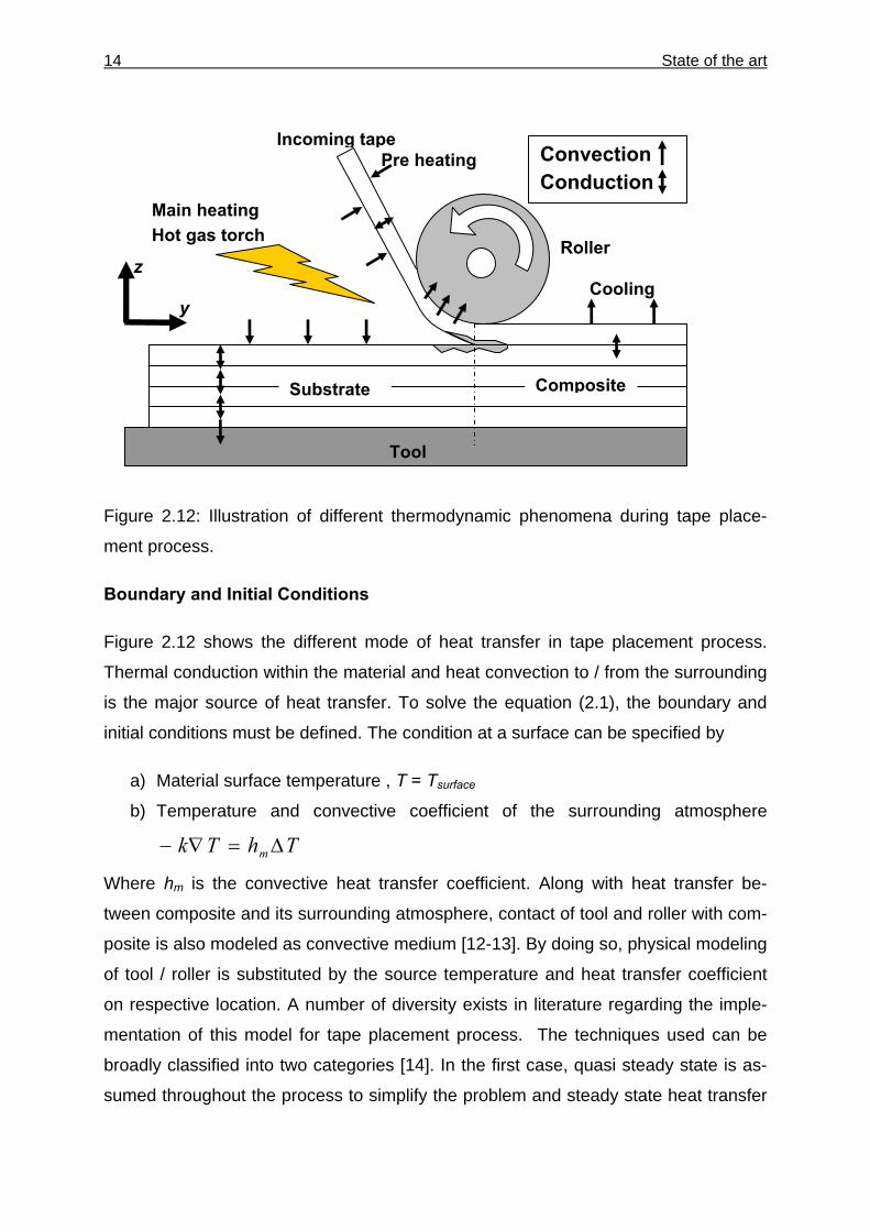
Figure 2.12: Illustration of different thermodynamic phenomena during tape place-
ment process.
Boundary and Initial Conditions
Figure 2.12 shows the different mode of heat transfer in tape placement process.
Thermal conduction within the material and heat convection to / from the surrounding
is the major source of heat transfer. To solve the equation (2.1), the boundary and
initial conditions must be defined. The condition at a surface can be specified by
a) Material surface temperature , T = Tsurface
b) Temperature and convective coefficient of the surrounding atmosphere
ThTk m ∆=∇−
Where hm is the convective heat transfer coefficient. Along with heat transfer be-
tween composite and its surrounding atmosphere, contact of tool and roller with com-
posite is also modeled as convective medium [12-13]. By doing so, physical modeling
of tool / roller is substituted by the source temperature and heat transfer coefficient
on respective location. A number of diversity exists in literature regarding the imple-
mentation of this model for tape placement process. The techniques used can be
broadly classified into two categories [14]. In the first case, quasi steady state is as-
sumed throughout the process to simplify the problem and steady state heat transfer
Main heating Hot gas torch
Tool
Convection Conduction
Roller
Pre heating
Composite
z
y
Substrate
Incoming tape
Cooling
State of the art 15
problem is analyzed by moving the boundary conditions only. While in second case,
the transient heat equation is solved using different numerical techniques by also in-
corporating material movement. Table 2.1 give an insight about the techniques used
for model implementation with their considerations and resulting outputs.
Table 2.1: Overview on the implementation techniques of energy equation (2.1) for
tape placement process.
Consideration for
Model type Dimen-sion
Tech-nique
Tool / Roller
Heat generation / absorption
Output Ref
Transient 3D FE X X T(t,x,y,z) [14]
Transient 3D FE X T(t,x,y,z) [15]
Quasi steady state 2D FE, FD X X T(t,y,z) [16-19]
Quasi steady state 2D FE, FD X T(t,y,z) [12, 20-21]
Quasi steady state 1D FD X T(t,z) [22-25]
2.4.2 Consolidation under roller
Heating of the incoming tape and substrate material starts prior to the application of
consolidating pressure. During this brief interval, the polymer softens and thermally
expands and any crystallinity that it has probably melts [26]. The polymer losses
strength and releases carbon fiber stresses, dissolved volatiles and entrapped air.
This results in an initiation of void growth in the tow. The subsequent application of
compaction pressure serves not only to stop void creation, but to reverse it. Similarly
material leaving the compacting roller is usually above the glass transition tempera-
ture, causing another void growth phenomenon. The level of consolidation is largely
associated with the presence of void contents in thermoplastic material.
Two different strategies have been used in the literature to describe the consolidation
in thermoplastic material during layup process. The first theory relates [22, 27] the
consolidation to bulk matrix and fiber bed compression as a result of matrix flow
along the fiber direction. Therefore the pressure distribution under the roller is ex-
plained on the basis of D’Arcy’s law, which assumes that the matrix flow parallel to
16 State of the art
the fibers and there is no macroscopic transverse flow. The other theory [28] based
on the experimental testing [29] on unidirectional laminate (that showed prominent
transverse squeeze flow but no flow in fiber direction due to high melt viscosity) con-
tradicts this assumption. Experimental testing performs in this study also confirm the
transverse flow mechanism [30]. Therefore later approach is selected preferably by
researcher for modeling consolidation phenomenon during tape placement process.
Table 2.2 summarizes the consolidation model for the tape placement process avail-
able in the literature.
Table 2.2: Consolidation model for tape placement process.
Description Model basis
Ref
Non-iso thermal
condition
Roller contact
pressureDimen-
sion Void
dynamic Geomet-
rical changes
Transverse squeeze flow [28] X X 1D X X
D’Arcy Flow [2] X 1D X
Viscoelastic [31] X X 2D X
Intimate contact [16, 32] X 1D
Model for continuum pressure and velocity
Ranganathan et al. [28] developed a model consisting of an integral differential equa-
tion (2.3) which determines the pressure P under the rotating roller as a function of
change in continuum (laminate) thickness h (see Figure 2.13).
( ) ( ) 010 *
0 01
**
=+⎟⎟⎠
⎞⎜⎜⎝
⎛⎥⎦
⎤⎢⎣
⎡++
∂∂
+∂
∂∫ ∫ ∫ dt
dhdzdxCddxdPv
xth
h z
o
z
TTx ρξ
ηξ
ηξρρ
2.3
Where Tη is the temperature dependent transverse viscosity, ξ is a dummy variable
of integration, *ρ is non-dimensionalized density of the continuum. The values of
( )xC1 and ( )0xv in equation (2.3) may be evaluated from the velocity boundary condi-
tions. The equation for the velocity of viscous material can be written as
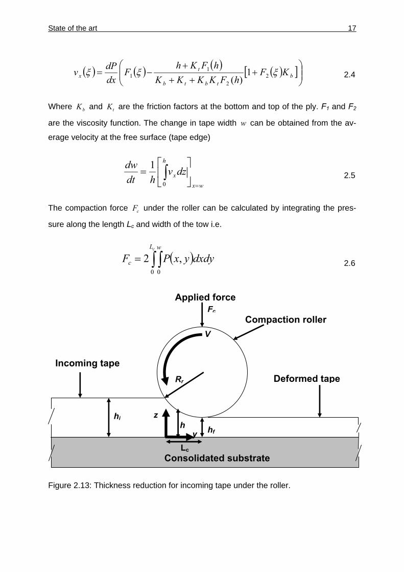
State of the art 17
( ) ( ) ( ) ( )[ ]⎟⎟⎠
⎞⎜⎜⎝
⎛+
+++
−= btbtb
tx KF
hFKKKKhFKh
FdxdPv ξξξ 2
2
11 1
)( 2.4
Where bK and tK are the friction factors at the bottom and top of the ply. F1 and F2
are the viscosity function. The change in tape width w can be obtained from the av-
erage velocity at the free surface (tape edge)
wx
h
xdzvhdt
dw
=
⎥⎦
⎤⎢⎣
⎡= ∫
0
1 2.5
The compaction force cF under the roller can be calculated by integrating the pres-
sure along the length Lc and width of the tow i.e.
( )∫ ∫=cL w
c dxdyyxPF0 0
,2 2.6
Figure 2.13: Thickness reduction for incoming tape under the roller.
Incoming tape
Applied force
Compaction roller
Deformed tape
Fc
V
Rr
hi z h
y hf
Consolidated substrateLc
18 State of the art
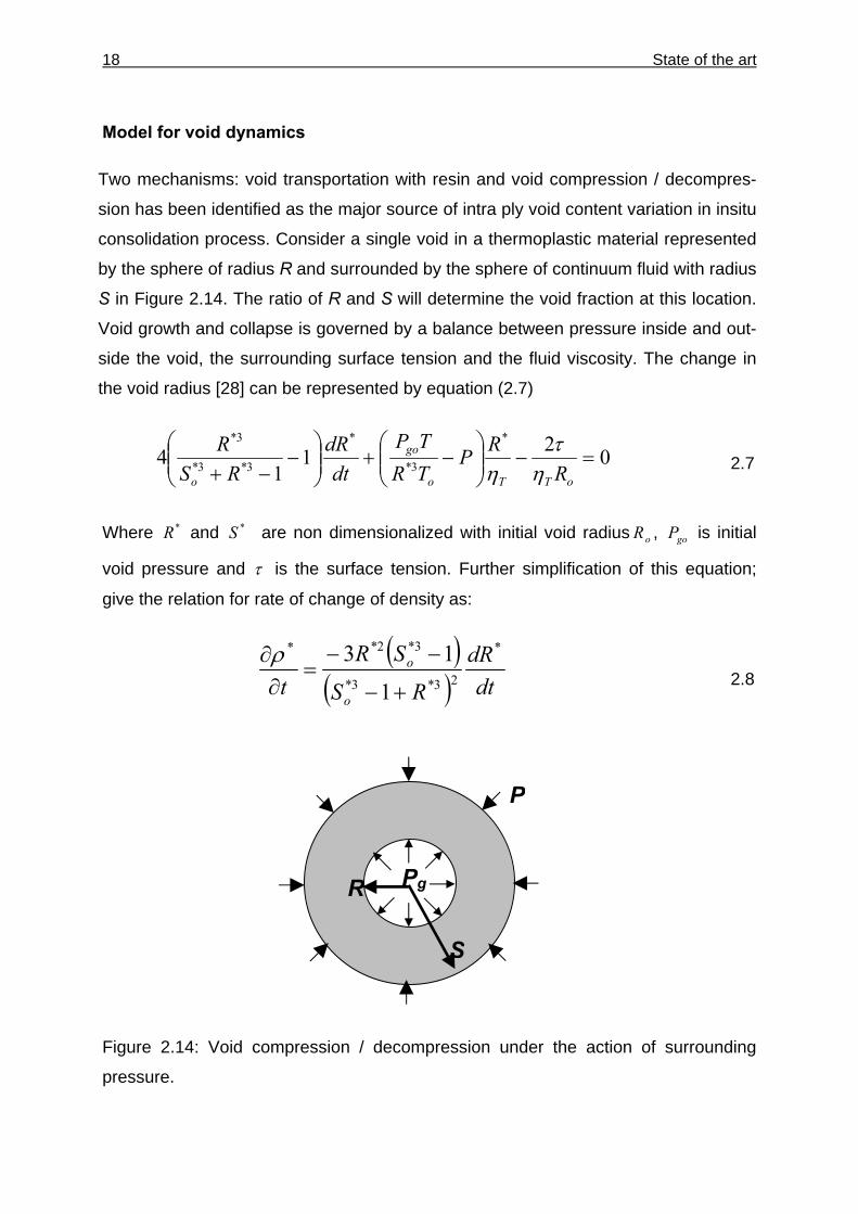
Model for void dynamics
Two mechanisms: void transportation with resin and void compression / decompres-
sion has been identified as the major source of intra ply void content variation in insitu
consolidation process. Consider a single void in a thermoplastic material represented
by the sphere of radius R and surrounded by the sphere of continuum fluid with radius
S in Figure 2.14. The ratio of R and S will determine the void fraction at this location.
Void growth and collapse is governed by a balance between pressure inside and out-
side the void, the surrounding surface tension and the fluid viscosity. The change in
the void radius [28] can be represented by equation (2.7)
0211
4*
3*
*
3*3*
3*
=−⎟⎟⎠
⎞⎜⎜⎝
⎛−+⎟⎟
⎠
⎞⎜⎜⎝
⎛−
−+ oTTo
go
o RRP
TRTP
dtdR
RSR
ητ
η 2.7
Where *R and *S are non dimensionalized with initial void radius oR , goP is initial
void pressure and τ is the surface tension. Further simplification of this equation;
give the relation for rate of change of density as:
( )( ) dt
dRRS
SRt
o
o*
23*3*
3*2**
1
13
+−
−−=
∂∂ρ
2.8
Figure 2.14: Void compression / decompression under the action of surrounding
pressure.
R
S
Pg
P
State of the art 19
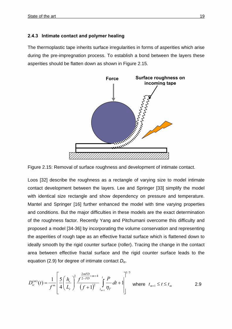
2.4.3 Intimate contact and polymer healing
The thermoplastic tape inherits surface irregularities in forms of asperities which arise
during the pre-impregnation process. To establish a bond between the layers these
asperities should be flatten down as shown in Figure 2.15.
Figure 2.15: Removal of surface roughness and development of intimate contact.
Loos [32] describe the roughness as a rectangle of varying size to model intimate
contact development between the layers. Lee and Springer [33] simplify the model
with identical size rectangle and show dependency on pressure and temperature.
Mantel and Springer [16] further enhanced the model with time varying properties
and conditions. But the major difficulties in these models are the exact determination
of the roughness factor. Recently Yang and Pitchumani overcome this difficulty and
proposed a model [34-36] by incorporating the volume conservation and representing
the asperities of rough tape as an effective fractal surface which is flattened down to
ideally smooth by the rigid counter surface (roller). Tracing the change in the contact
area between effective fractal surface and the rigid counter surface leads to the
equation (2.9) for degree of intimate contact Dic.
( )
5/1
2
422
2)(
1
114
51)(⎥⎥⎥
⎦
⎤
⎢⎢⎢
⎣
⎡+
+⎟⎟⎠
⎞⎜⎜⎝
⎛= ∫
+
++− t
t T
mFD
mFD
r
rm
mic
m
dtP
ff
Lh
ftD
η where mm ttt ≤≤+1 2.9
Force Surface roughness on incoming tape
20 State of the art
Where FD is the fractal dimension, f is the scaling ratio, m is the number of asperity
generations, Lr is the total length of the cantor set, P and t are applied pressure and
duration under roller, and hr is the recess depth of the first generation asperity. Dic=
100% represent the state where two layers have flatten down and achieved perfect
contact.
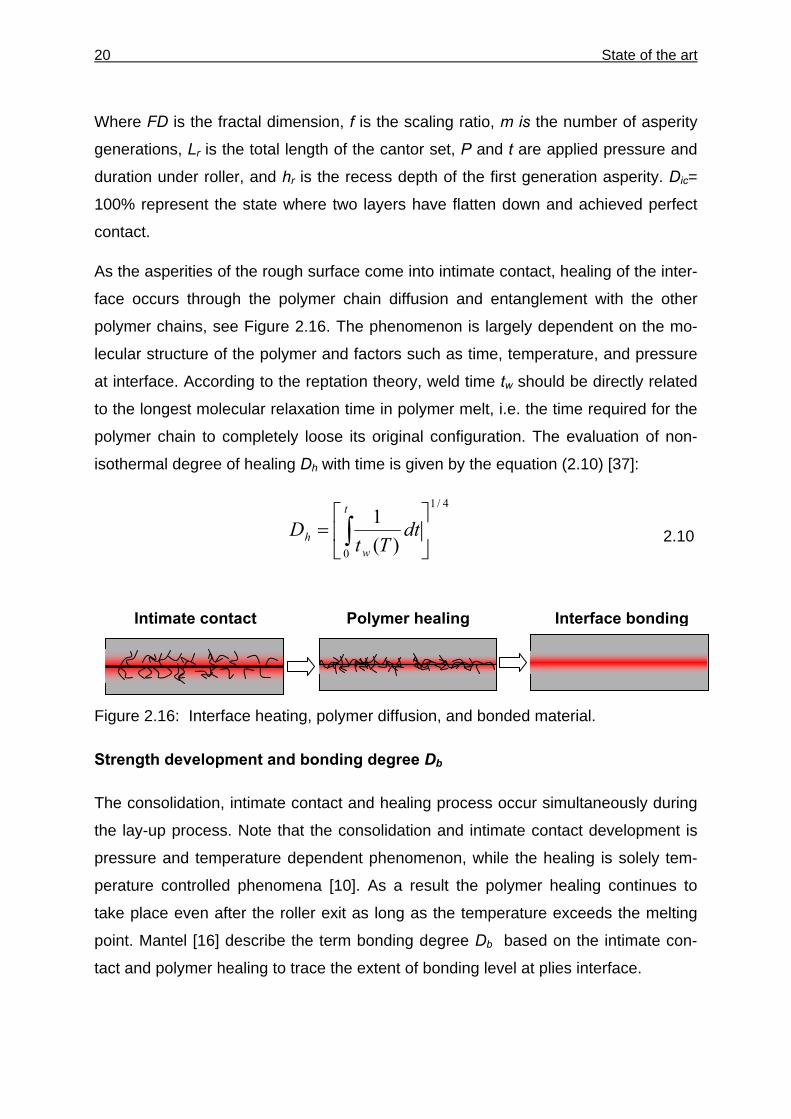
As the asperities of the rough surface come into intimate contact, healing of the inter-
face occurs through the polymer chain diffusion and entanglement with the other
polymer chains, see Figure 2.16. The phenomenon is largely dependent on the mo-
lecular structure of the polymer and factors such as time, temperature, and pressure
at interface. According to the reptation theory, weld time tw should be directly related
to the longest molecular relaxation time in polymer melt, i.e. the time required for the
polymer chain to completely loose its original configuration. The evaluation of non-
isothermal degree of healing Dh with time is given by the equation (2.10) [37]:
4/1
0 )(1
⎥⎦
⎤⎢⎣
⎡= ∫
t
wh dt
TtD 2.10
Figure 2.16: Interface heating, polymer diffusion, and bonded material.
Strength development and bonding degree Db
The consolidation, intimate contact and healing process occur simultaneously during
the lay-up process. Note that the consolidation and intimate contact development is
pressure and temperature dependent phenomenon, while the healing is solely tem-
perature controlled phenomena [10]. As a result the polymer healing continues to
take place even after the roller exit as long as the temperature exceeds the melting
point. Mantel [16] describe the term bonding degree Db based on the intimate con-
tact and polymer healing to trace the extent of bonding level at plies interface.
Intimate contact Interface bondingPolymer healing
State of the art 21
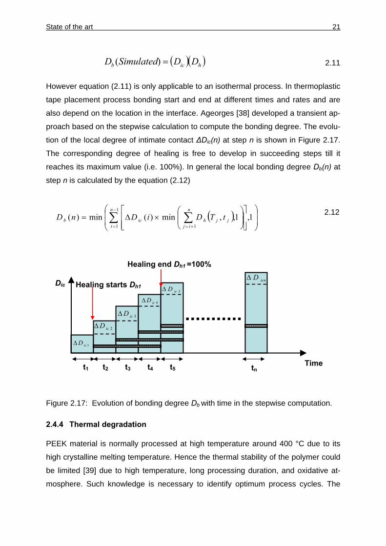
( )( )hicb DDSimulatedD =)( 2.11
However equation (2.11) is only applicable to an isothermal process. In thermoplastic
tape placement process bonding start and end at different times and rates and are
also depend on the location in the interface. Ageorges [38] developed a transient ap-
proach based on the stepwise calculation to compute the bonding degree. The evolu-
tion of the local degree of intimate contact ∆Dic(n) at step n is shown in Figure 2.17.
The corresponding degree of healing is free to develop in succeeding steps till it
reaches its maximum value (i.e. 100%). In general the local bonding degree Db(n) at
step n is calculated by the equation (2.12)
( )⎟⎟⎠
⎞⎜⎜⎝
⎛
⎥⎥⎦
⎤
⎢⎢⎣
⎡⎟⎟⎠
⎞⎜⎜⎝
⎛×∆= ∑ ∑
−
= +=
1
1 11,1,,min)(min)(
n
t
n
ijjjhicb tTDiDnD 2.12
Figure 2.17: Evolution of bonding degree Db with time in the stepwise computation.
2.4.4 Thermal degradation
PEEK material is normally processed at high temperature around 400 °C due to its
high crystalline melting temperature. Hence the thermal stability of the polymer could
be limited [39] due to high temperature, long processing duration, and oxidative at-
mosphere. Such knowledge is necessary to identify optimum process cycles. The
Time
3hD∆
1icD∆
2icD∆3icD∆
4icD∆
icnD∆Dic
5icD∆
t1 t2 t3 t4 t5 tn
Healing starts Dh1
Healing end Dh1 =100%
22 State of the art
thermal degradation in the process is studied by considering the following two influ-
encing trends.
Thermal stability
Cole [40] found through IR spectroscopy that ether and carbonyl groups in PEEK are
less stable in an oxidizing atmosphere. The ether and carbonyl group extract hydro-
gen from an aromatic ring to form phenol and aldehyde groups respectively. The aryl
radicals produced by the loss of hydrogen can then combine to form crosslink be-
tween chains, thus causing the changes in the viscosity and in the crystallization be-
havior. The polymer cross linking rate is experimentally investigated (as in chapter 3)
to develop the non-isothermal Arrhenius relation.
∫ ⎥⎦
⎤⎢⎣
⎡ −=
finalT
iniT c
a
tTRE
ARr340
340 )(.exp 2.13
Where Ea and A are the activation energy and pre-exponential component.
Weight loss
In a high temperature oxidative environment the polymer based composite material
exhibit complex thermogram. Gupta [41] represent through mass spectrograph that
the abundance of oxygen accelerates the weight loss by 50% as compared to non
oxidative environment. The activation energy for the kinetic model [42] can also de-
termined through thermogravimetric analysis.
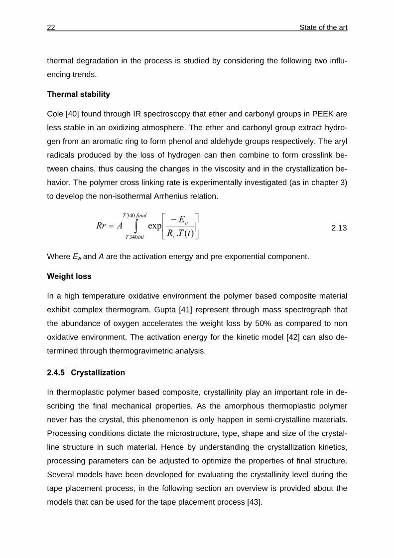
2.4.5 Crystallization
In thermoplastic polymer based composite, crystallinity play an important role in de-
scribing the final mechanical properties. As the amorphous thermoplastic polymer
never has the crystal, this phenomenon is only happen in semi-crystalline materials.
Processing conditions dictate the microstructure, type, shape and size of the crystal-
line structure in such material. Hence by understanding the crystallization kinetics,
processing parameters can be adjusted to optimize the properties of final structure.
Several models have been developed for evaluating the crystallinity level during the
tape placement process, in the following section an overview is provided about the
models that can be used for the tape placement process [43].
State of the art 23
Ozawa’s model
The model [44] is an extended form of Avarmi equation to explain the process of
crystal nucleation and growth for a non-isothermal condition. The relative crystallinity
cr is a function of temperature and cooling rate as:
( )[ ] ( ) ⎟⎠⎞
⎜⎝⎛+=−−
dtdTnTc r loglog1lnlog φ 2.14
Where Φ(T) and n can be obtained from crystallinity measurements at different tem-
perature. Due to the absence of the melt kinetic term, the model is not suitable for the
clearly describing the melt crystallization as opposed to cold crystallization in dual
crystallization mechanism.
Velisaris and Seferis‘s model
A dual mechanism crystallization (nucleation and growth) model [45] based on two
Avarmi expressions show good correlation with experimental data for non-isothermal
heating and cooling in tape placement process [46]. The complete expression to
evaluate volume fraction crystallinity c is:
( )2211 vcvc FwFwcc += α 2.15
Where w1+w2=1; w1 and w2 are the weight factors and cα is the equilibrium volume
fraction of crystallinity of the material. FVC1 and FVC2 represent the normalized volume
fraction crystallinity for each crystal growth mechanism namely spherulitic and epi-
taxial crystal growth.
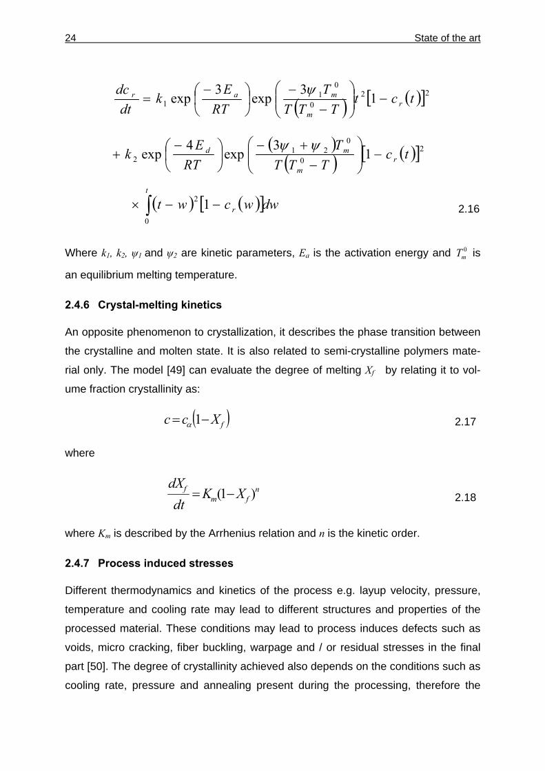
Choe and Lee’s model
Sonmez and Hahn [21] select this model [47] which includes the effect of the tem-
perature of melt from which crystallization is performed. The model is based on the
Tobin phase transformation kinetics [48]. The equation for non isothermal crystalliza-
tion kinetics is given by:
24 State of the art
( ) ( )[ ]220
01
1 13exp3exp tctTTT
TRT
Ekdt
dcr
m
mar −⎟⎟⎠
⎞⎜⎜⎝
⎛−
−⎟⎠⎞
⎜⎝⎛ −
=ψ
( )( ) ( )[ ]2
0
021
2 13exp4exp tcTTT
TRT
Ek rm
md −⎟⎟⎠
⎞⎜⎜⎝
⎛−
+−⎟⎠⎞
⎜⎝⎛ −
+ψψ
( ) ( )[ ]dwwcwtt
r∫ −−×0
2 1 2.16
Where k1, k2, ψ1 and ψ2 are kinetic parameters, Ea is the activation energy and 0mT is
an equilibrium melting temperature.
2.4.6 Crystal-melting kinetics
An opposite phenomenon to crystallization, it describes the phase transition between
the crystalline and molten state. It is also related to semi-crystalline polymers mate-
rial only. The model [49] can evaluate the degree of melting Xf by relating it to vol-
ume fraction crystallinity as:
( )fXcc −= 1α 2.17
where
n
fmf XK
dtdX
)1( −= 2.18
where Km is described by the Arrhenius relation and n is the kinetic order.
2.4.7 Process induced stresses
Different thermodynamics and kinetics of the process e.g. layup velocity, pressure,
temperature and cooling rate may lead to different structures and properties of the
processed material. These conditions may lead to process induces defects such as
voids, micro cracking, fiber buckling, warpage and / or residual stresses in the final
part [50]. The degree of crystallinity achieved also depends on the conditions such as
cooling rate, pressure and annealing present during the processing, therefore the
State of the art 25
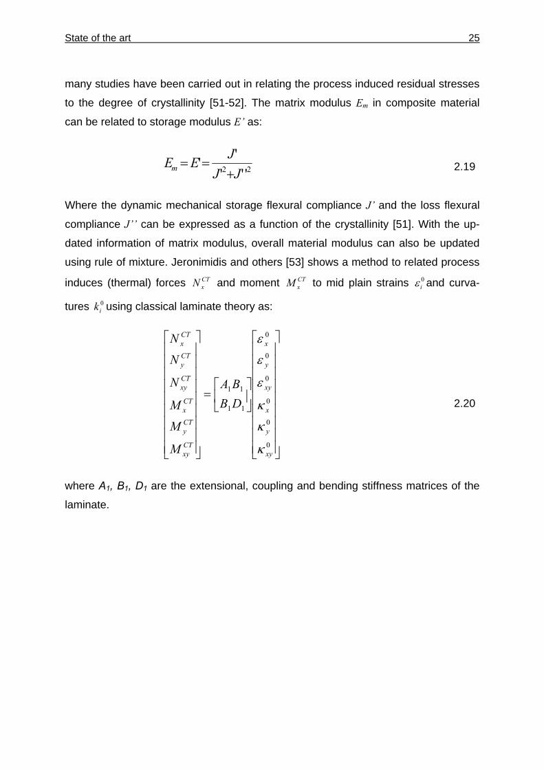
many studies have been carried out in relating the process induced residual stresses
to the degree of crystallinity [51-52]. The matrix modulus Em in composite material
can be related to storage modulus E’ as:
22 '''''JJ
JEEm +== 2.19
Where the dynamic mechanical storage flexural compliance J’ and the loss flexural
compliance J’’ can be expressed as a function of the crystallinity [51]. With the up-
dated information of matrix modulus, overall material modulus can also be updated
using rule of mixture. Jeronimidis and others [53] shows a method to related process
induces (thermal) forces CTxN and moment CT
xM to mid plain strains 0iε and curva-
tures 0ik using classical laminate theory as:
⎥⎥⎥⎥⎥⎥⎥⎥⎥
⎦
⎤
⎢⎢⎢⎢⎢⎢⎢⎢⎢
⎣
⎡
⎥⎦
⎤⎢⎣
⎡=
⎥⎥⎥⎥⎥⎥⎥⎥⎥
⎦
⎤
⎢⎢⎢⎢⎢⎢⎢⎢⎢
⎣
⎡
0
0
0
0
0
0
11
11
xy
y
x
xy
y
x
CTxy
CTy
CTx
CTxy
CTy
CTx
DBBA
M
M
M
N
N
N
κ
κ
κ
ε
ε
ε
2.20
where A1, B1, D1 are the extensional, coupling and bending stiffness matrices of the
laminate.
26 Experimental characterization and testing
3 Experimental characterization and testing
The experimental work provides several information regarding the material, process
and product quality. Methods and techniques which can lead to proper selection of
setup and process parameters are discussed in this section.
3.1 Thermoplastic material
The thermoplastic tape material used in this study is the unidirectional carbon fiber
reinforced polyetheretherketone (i.e. CF-PEEK) by Suprem. The reported and the
experimentally determined general specifications are shown in Table 3.1.
Table 3.1: Specification for the CF-PEEK material.
Specification Reported by supplier Experiment
Thickness 0.13 mm 0.14±0.01 mm Width 12 mm 11.88 ± 0.025 mm
Density 1.6 g/cm3 1.54 g/cm3 Fiber contents (by volume) 60 ± 3% 58 ± 0.7 % Matrix contents (by mass) 33% 33± 0.8 %
Glass transition temperature 143 °C - Melt temperature 340 °C 343 °C
According to supplier data the grade of the thermoplastic polymer is PEEK 150,
therefore following molecular mass values (in Table 3.2) were selected from the lit-
erature [18].
Table 3.2: Molar mass details for the PEEK material.
Specification Number average molecular mass
Mn [g/mol]
Weight average molecular mass
Mw [g/mol] Polydispersity
index Ip
PEEK 151G 28700 75900 2.6
Experimental characterization and testing 27
The thermoplastic material is reinforced with the HEXCEL AS4 high strength carbon
fibers with 94% carbon contents and fiber diameter of 7.1 micron. Table 3.3 shows
the further technical information [54].
Table 3.3: Properties of Hexcel AS4 12K.
Fiber type Tensile strength
[MPa]
Tensile modulus
[GPa]
Elongation at failure
[%]
Weight /length [g/cm]
Density [g/cm3]
AS4 4475 231 1.8 0.858 1.79
The thermal diffusivity and specific heat of thermoplastic material was measured us-
ing a NETZSCH model LFA 447 Nano-Flash diffusivity apparatus [55]. The unit used
in this testing was equipped with a furnace, capable of operation from 25 to 300 °C.
Table 3.4 contains the thermo-physical properties of 2 mm thick CF-PEEK consoli-
dated sample in different directions. The thermal diffusivity decreases and specific
heat increases with increasing temperature. Increasing thermal conductivity values at
increasing temperature are typical for amorphous and semi-crystalline structures.
Significant differences were detected for both directions most probably due to the in-
fluence of fiber orientation. The thermal conductivity in fiber direction is approx. 7-8
times higher.
Table 3.4: Thermal properties of CF-PEEK material.
Temperature [°C]
Measure-ment
direction
Thermal diffusivity [mm2/sec]
Specific heat
[J/g.K]
Thermal conductivity
[W/m.K]
25 0.575 0.886 0.813 300
Transverse to fiber 0.413 1.803 1.188
25 3.922 0.886 5.542 300
Parallel to fiber 3.256 1.803 9.364
28 Experimental characterization and testing
3.2 Thermal mapping under the hot gas torch
Temperature studies in impinging jets reveals its dependency on the Reynolds num-
ber, nozzle to plate distance, nozzle geometry, target shape orientation, cross flow,
etc [56]. As a result, different advance techniques like cooling ring [57], infra red re-
mote sensing [15] and high temperature thermocouple [58] have been implemented
to thermally map the impinging flow around the nip point. Simple and quick setup to
use thermocouple encouraged several [13-14, 18] for the hot gas temperature esti-
mation.
The adiabatic temperature of a stoichiometric hydrogen–air flame is approximately
2807 °C. In high temperature impingement, the combustion products diffuse through
the boundary layer to the colder surface. Baukal [58] described the drop of heat flux
as a function of torch distance from impinging surface. Martin [59] state that for a
torch at an angle of 15° the heat transfer coefficient drops by 43% corresponding to
ones for the normal impingement. Considering these circumstances the thermocou-
ple method was selected for the temperature measurement. An S-type thermocouple
(SAT-24-12 by omega) with wire diameter of 2 mm was used which has the capability
to measured up to 1650 °C. Calibration of thermocouple was performed inside the
autoclaved and under the hot gas torch with K-type thermocouple up to 1000 °C.
Figure 3.1: Hot gas temperature measurement using thermocouple.
Hot gas torch
Thermocouple
Guiding assembly
Tool
Experimental characterization and testing 29
A ceramic tube protected the bare thermocouple wires, exposing only the juncture to
the hot gases. First thermocouple was fixed on the tool plate with the help of PTFE
tape so that the juncture was about 5 mm above the tool surface. The tool plate was
then precisely positioned under the hot gas torch (Figure 3.1) on locations shown in
the mapping diagram in Figure 3.2. Although unlimited points can be selected for
temperature measurement, as the positioning under hot gas torch was carried out by
moving the tool plate, only 18 points were selected over the length of 40 mm as a
first approximation. For incoming guide assembly measurement was performed at
the centre line L-2 only. Efforts were made to take measurement close to the nip
point (roller centre), but the narrow space made it difficult to fix the thermocouple
hence forced the first measurement at least 10 mm from the roller centre.
Figure 3.2: Locations over the tool for thermal mapping under the hot gas torch.
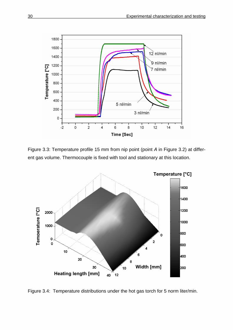
Consider the temperature profile in Figure 3.3 at a point A, which lie on the middle
line L-2 and 15 mm apart from the roller centre (see Figure 3.2). Thermocouple was
positioned at this location and hot gas torch was turned on till the temperature read-
ing became stable and reached the steady state condition. Since the thermocouple
was stationary at the position, the temperature reaches the steady state value with in
few seconds.
Y
Z
A
Heating length [mm]
Wid
th [m
m]
Roller center line
30 Experimental characterization and testing
Figure 3.3: Temperature profile 15 mm from nip point (point A in Figure 3.2) at differ-
ent gas volume. Thermocouple is fixed with tool and stationary at this location.
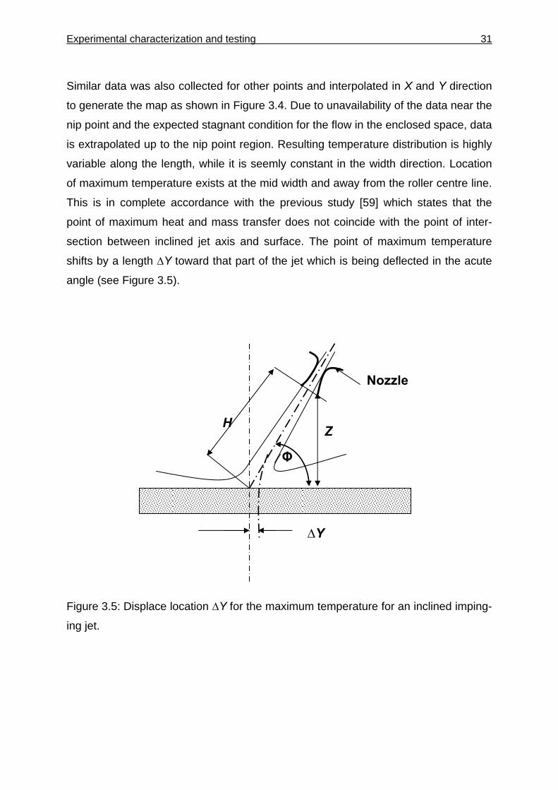
Figure 3.4: Temperature distributions under the hot gas torch for 5 norm liter/min.
Temperature [°C]
Tem
pera
ture
[°C
]
Heating length [mm] Width [mm]
Experimental characterization and testing 31
Similar data was also collected for other points and interpolated in X and Y direction
to generate the map as shown in Figure 3.4. Due to unavailability of the data near the
nip point and the expected stagnant condition for the flow in the enclosed space, data
is extrapolated up to the nip point region. Resulting temperature distribution is highly
variable along the length, while it is seemly constant in the width direction. Location
of maximum temperature exists at the mid width and away from the roller centre line.
This is in complete accordance with the previous study [59] which states that the
point of maximum heat and mass transfer does not coincide with the point of inter-
section between inclined jet axis and surface. The point of maximum temperature
shifts by a length ∆Y toward that part of the jet which is being deflected in the acute
angle (see Figure 3.5).
Figure 3.5: Displace location ∆Y for the maximum temperature for an inclined imping-
ing jet.
H
∆Y
Z
Nozzle
Φ
32 Experimental characterization and testing
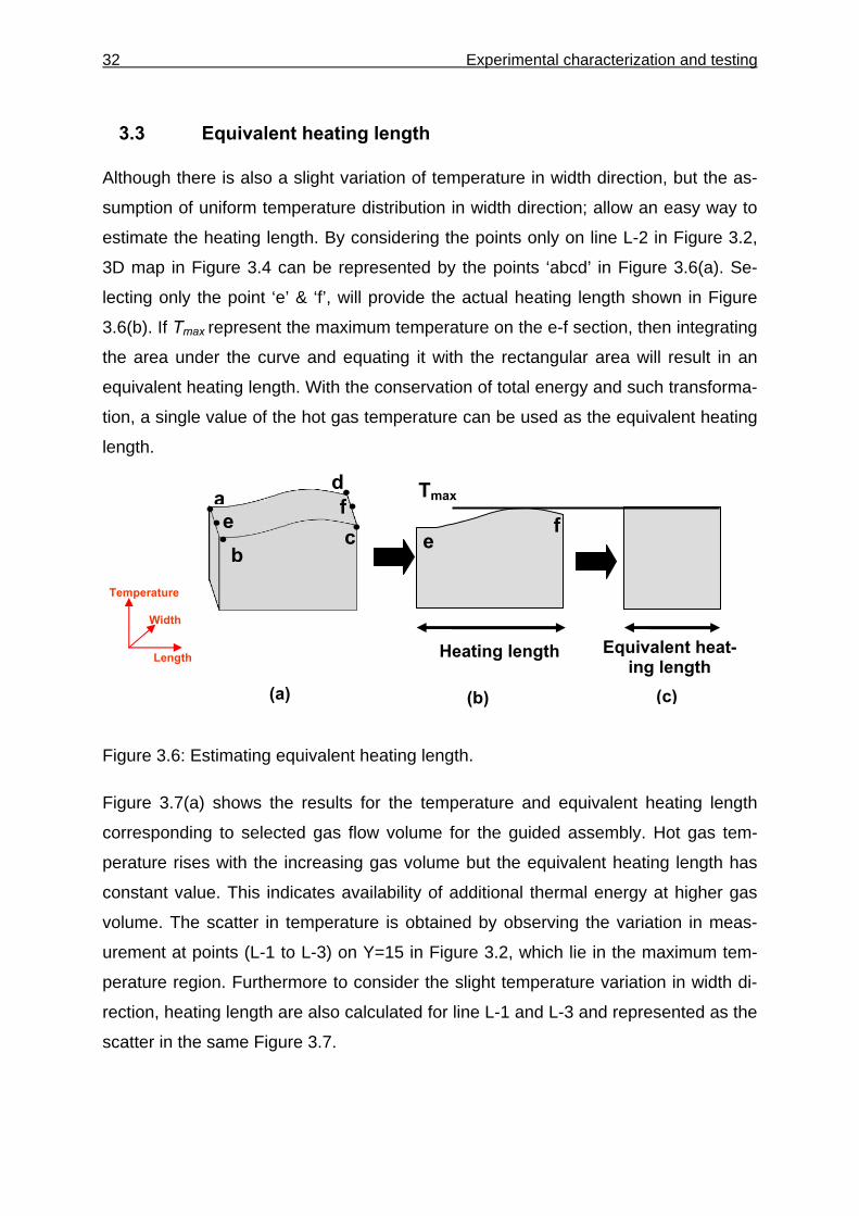
3.3 Equivalent heating length
Although there is also a slight variation of temperature in width direction, but the as-
sumption of uniform temperature distribution in width direction; allow an easy way to
estimate the heating length. By considering the points only on line L-2 in Figure 3.2,
3D map in Figure 3.4 can be represented by the points ‘abcd’ in Figure 3.6(a). Se-
lecting only the point ‘e’ & ‘f’, will provide the actual heating length shown in Figure
3.6(b). If Tmax represent the maximum temperature on the e-f section, then integrating
the area under the curve and equating it with the rectangular area will result in an
equivalent heating length. With the conservation of total energy and such transforma-
tion, a single value of the hot gas temperature can be used as the equivalent heating
length.
Figure 3.6: Estimating equivalent heating length.
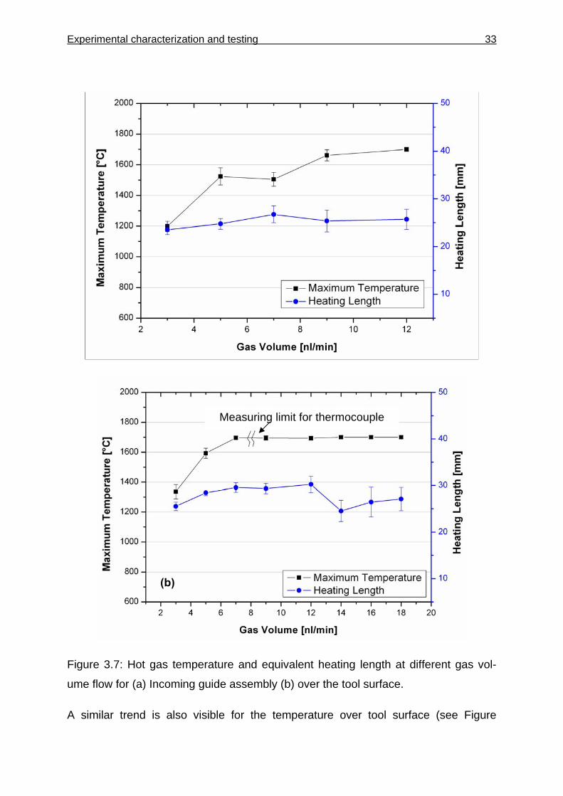
Figure 3.7(a) shows the results for the temperature and equivalent heating length
corresponding to selected gas flow volume for the guided assembly. Hot gas tem-
perature rises with the increasing gas volume but the equivalent heating length has
constant value. This indicates availability of additional thermal energy at higher gas
volume. The scatter in temperature is obtained by observing the variation in meas-
urement at points (L-1 to L-3) on Y=15 in Figure 3.2, which lie in the maximum tem-
perature region. Furthermore to consider the slight temperature variation in width di-
rection, heating length are also calculated for line L-1 and L-3 and represented as the
scatter in the same Figure 3.7.
Heating length Equivalent heat-ing length Length
Width
Temperature
Tmax a
b c
d
e f
e f
(c) (b) (a)
Experimental characterization and testing 33
Figure 3.7: Hot gas temperature and equivalent heating length at different gas vol-
ume flow for (a) Incoming guide assembly (b) over the tool surface.
A similar trend is also visible for the temperature over tool surface (see Figure
(b)
Measuring limit for thermocouple
34 Experimental characterization and testing
3.7(b)). The temperature rises more sharply reaching maximum measurable limit
(1700 °C) for the thermocouple at 9 norm liter/min. Thereafter thermocouple reported
this maximum value for further increase in gas volume. The interesting observation is
a decrease in the equivalent heating length over 12 norm liter/min. Although no fur-
ther information is available about the actual maximum temperature, but the meas-
urement shows sharp drop in temperature from points at Y=15 to Y=40 (in Y direc-
tion) at higher gas volume. This consequently resulted in smaller heating length for
higher gas volume. One possible reason is the concentrated hot gas impingent jet
due to high energetic velocity which consequently results in smaller heating length.
3.4 Convective heat transfer coefficient
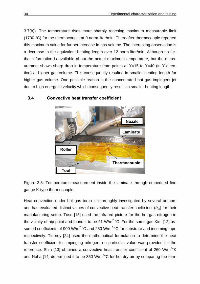
Figure 3.8: Temperature measurement inside the laminate through embedded fine
gauge K-type thermocouple.
Heat convection under hot gas torch is thoroughly investigated by several authors
and has evaluated distinct values of convective heat transfer coefficient (hm) for their
manufacturing setup. Toso [15] used the infrared picture for the hot gas nitrogen in
the vicinity of nip point and found it to be 21 W/m2 °C. For the same gas Kim [12] as-
sumed coefficients of 900 W/m2 °C and 250 W/m2 °C for substrate and incoming tape
respectively. Tierney [24] used the mathematical formulation to determine the heat
transfer coefficient for impinging nitrogen, no particular value was provided for the
reference. Shih [13] obtained a convective heat transfer coefficient of 260 W/m2°K
and Noha [14] determined it to be 350 W/m2°C for hot dry air by comparing the tem-
Roller
Tool
Thermocouple
Laminate
Nozzle
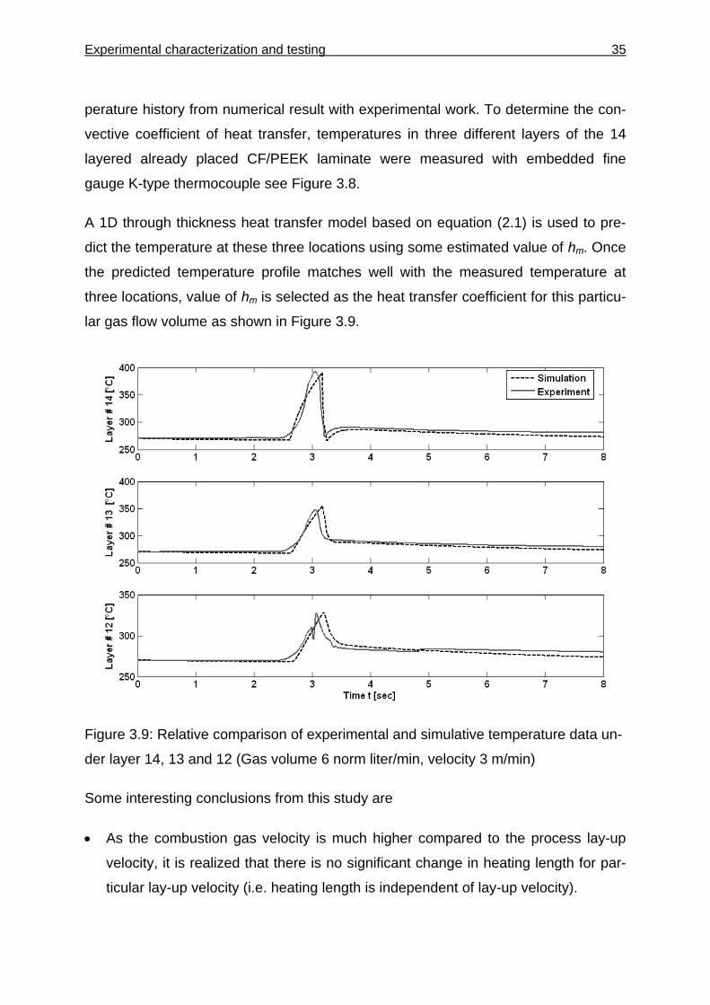
Experimental characterization and testing 35
perature history from numerical result with experimental work. To determine the con-
vective coefficient of heat transfer, temperatures in three different layers of the 14
layered already placed CF/PEEK laminate were measured with embedded fine
gauge K-type thermocouple see Figure 3.8.
A 1D through thickness heat transfer model based on equation (2.1) is used to pre-
dict the temperature at these three locations using some estimated value of hm. Once
the predicted temperature profile matches well with the measured temperature at
three locations, value of hm is selected as the heat transfer coefficient for this particu-
lar gas flow volume as shown in Figure 3.9.
Figure 3.9: Relative comparison of experimental and simulative temperature data un-
der layer 14, 13 and 12 (Gas volume 6 norm liter/min, velocity 3 m/min)
Some interesting conclusions from this study are
• As the combustion gas velocity is much higher compared to the process lay-up
velocity, it is realized that there is no significant change in heating length for par-
ticular lay-up velocity (i.e. heating length is independent of lay-up velocity).
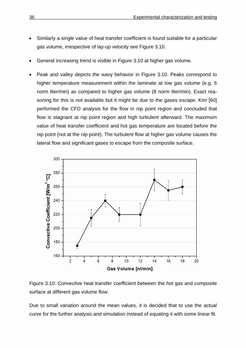
36 Experimental characterization and testing
• Similarly a single value of heat transfer coefficient is found suitable for a particular
gas volume, irrespective of lay-up velocity see Figure 3.10.
• General increasing trend is visible in Figure 3.10 at higher gas volume.
• Peak and valley depicts the wavy behavior in Figure 3.10. Peaks correspond to
higher temperature measurement within the laminate at low gas volume (e.g. 6
norm liter/min) as compared to higher gas volume (8 norm liter/min). Exact rea-
soning for this is not available but it might be due to the gases escape. Kim [60]
performed the CFD analysis for the flow in nip point region and concluded that
flow is stagnant at nip point region and high turbulent afterward. The maximum
value of heat transfer coefficient and hot gas temperature are located before the
nip point (not at the nip point). The turbulent flow at higher gas volume causes the
lateral flow and significant gases to escape from the composite surface.
Figure 3.10: Convective heat transfer coefficient between the hot gas and composite
surface at different gas volume flow.
Due to small variation around the mean values, it is decided that to use the actual
curve for the further analysis and simulation instead of equating it with some linear fit.
Experimental characterization and testing 37
The difficulty in positioning the laminate with embedded thermocouples on guiding
assembly restricts the similar study for the determination of convective heat transfer
coefficient for incoming tape.
The theoretical and experimental study on the variation of roller temperature is also
performed. Noticeable temperature variation is found out during the winding process,
where roller had continuous contact with hot tool or composite for the extended dura-
tion. But the change in roller temperature is negligible for the tape placement proc-
ess, where the continuous contact exists for the short duration during the lay-up. Ex-
perimental testing shows 10 °C rise in roller temperature as it comes in contact with
incoming tape and hot substrate material. But it drop down by 5 °C before roller
makes the second contact. For continues rotation maximum variation of 10 °C was
marked, as the thermal equilibrium established between the roller and the surround-
ing environment through natural convection. Table 3.5 shows the iteratively obtained
values of convective coefficient between roller and composite material by assuming
constant temperature over the roller contact length.
Table 3.5: Estimated convective heat transfer coefficient between roller and compos-ite substrate.
Roller Temperature [°C] Convective heat transfer coefficient [W/m2 °C]
50 65000 60 60000 80 55000 90 55000
3.5 Material deformation
3.5.1 Thickness build-up
Over the glass transition temperature Tg, thermoplastic materials are sensitive to geo-
metrical deformation. Understanding of the thickness build-up and width changes can
help the manufacturer to estimate the number of lay-up and expected material re-
quirements for desired laminate dimensions. A laser distance measuring sensor
(Weltoc) attached to the placement head was used to measure the thickness with
laminate stacking. Exact horizontal location was about 75 mm from the centre of the
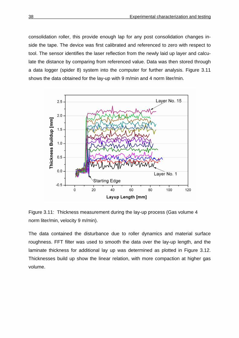
38 Experimental characterization and testing
consolidation roller, this provide enough lap for any post consolidation changes in-
side the tape. The device was first calibrated and referenced to zero with respect to
tool. The sensor identifies the laser reflection from the newly laid up layer and calcu-
late the distance by comparing from referenced value. Data was then stored through
a data logger (spider 8) system into the computer for further analysis. Figure 3.11
shows the data obtained for the lay-up with 9 m/min and 4 norm liter/min.
Figure 3.11: Thickness measurement during the lay-up process (Gas volume 4
norm liter/min, velocity 9 m/min).
The data contained the disturbance due to roller dynamics and material surface
roughness. FFT filter was used to smooth the data over the lay-up length, and the
laminate thickness for additional lay up was determined as plotted in Figure 3.12.
Thicknesses build up show the linear relation, with more compaction at higher gas
volume.
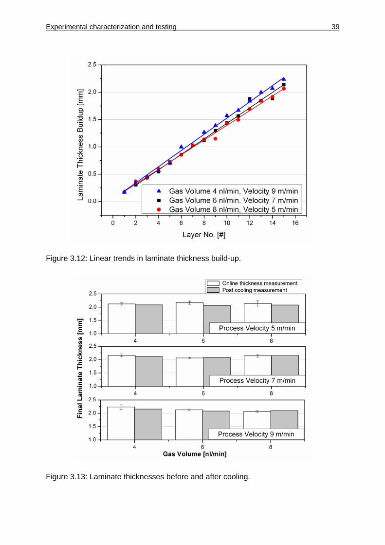
Experimental characterization and testing 39
Figure 3.12: Linear trends in laminate thickness build-up.
Figure 3.13: Laminate thicknesses before and after cooling.
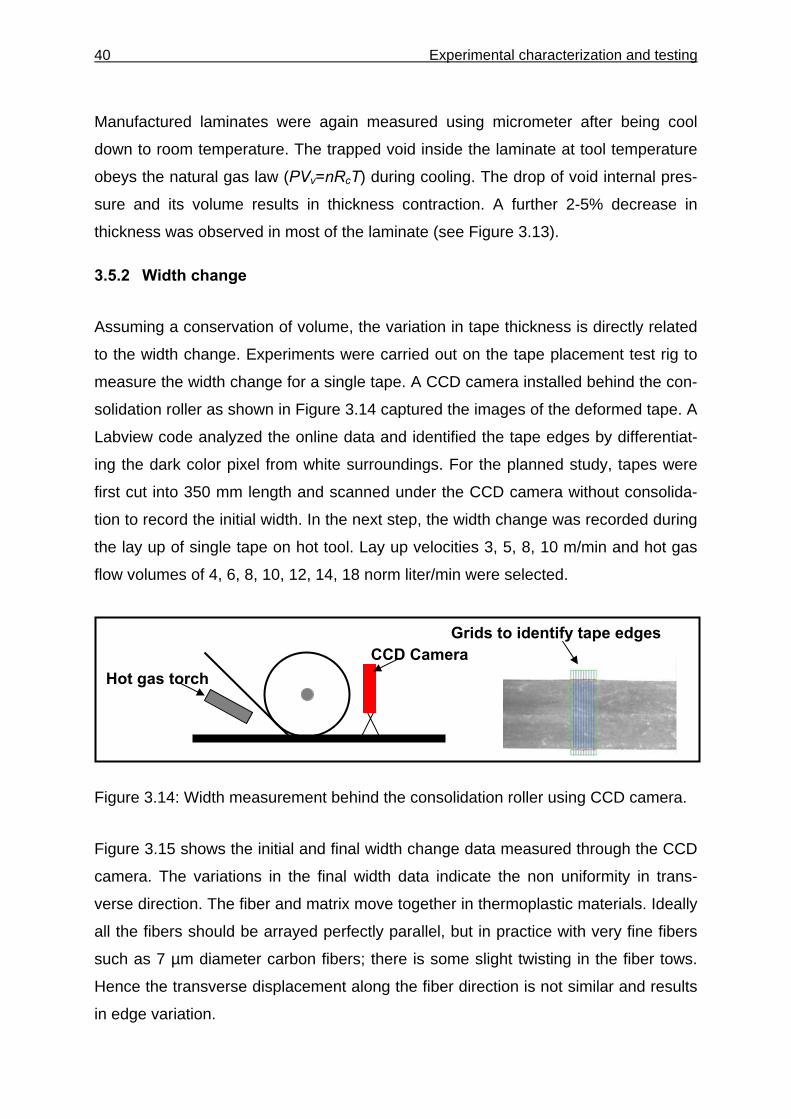
40 Experimental characterization and testing
Manufactured laminates were again measured using micrometer after being cool
down to room temperature. The trapped void inside the laminate at tool temperature
obeys the natural gas law (PVv=nRcT) during cooling. The drop of void internal pres-
sure and its volume results in thickness contraction. A further 2-5% decrease in
thickness was observed in most of the laminate (see Figure 3.13).
3.5.2 Width change
Assuming a conservation of volume, the variation in tape thickness is directly related
to the width change. Experiments were carried out on the tape placement test rig to
measure the width change for a single tape. A CCD camera installed behind the con-
solidation roller as shown in Figure 3.14 captured the images of the deformed tape. A
Labview code analyzed the online data and identified the tape edges by differentiat-
ing the dark color pixel from white surroundings. For the planned study, tapes were
first cut into 350 mm length and scanned under the CCD camera without consolida-
tion to record the initial width. In the next step, the width change was recorded during
the lay up of single tape on hot tool. Lay up velocities 3, 5, 8, 10 m/min and hot gas
flow volumes of 4, 6, 8, 10, 12, 14, 18 norm liter/min were selected.
Figure 3.14: Width measurement behind the consolidation roller using CCD camera.
Figure 3.15 shows the initial and final width change data measured through the CCD
camera. The variations in the final width data indicate the non uniformity in trans-
verse direction. The fiber and matrix move together in thermoplastic materials. Ideally
all the fibers should be arrayed perfectly parallel, but in practice with very fine fibers
such as 7 µm diameter carbon fibers; there is some slight twisting in the fiber tows.
Hence the transverse displacement along the fiber direction is not similar and results
in edge variation.
CCD Camera Hot gas torch
Grids to identify tape edges
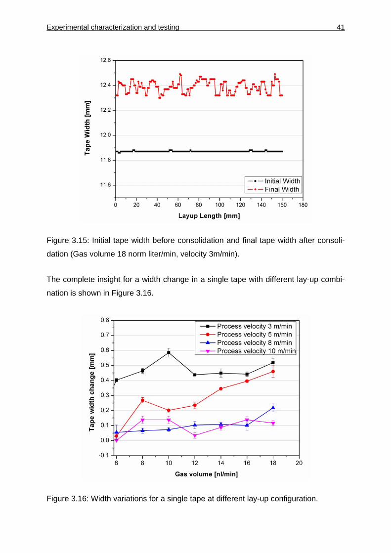
Experimental characterization and testing 41
Figure 3.15: Initial tape width before consolidation and final tape width after consoli-
dation (Gas volume 18 norm liter/min, velocity 3m/min).
The complete insight for a width change in a single tape with different lay-up combi-
nation is shown in Figure 3.16.
Figure 3.16: Width variations for a single tape at different lay-up configuration.
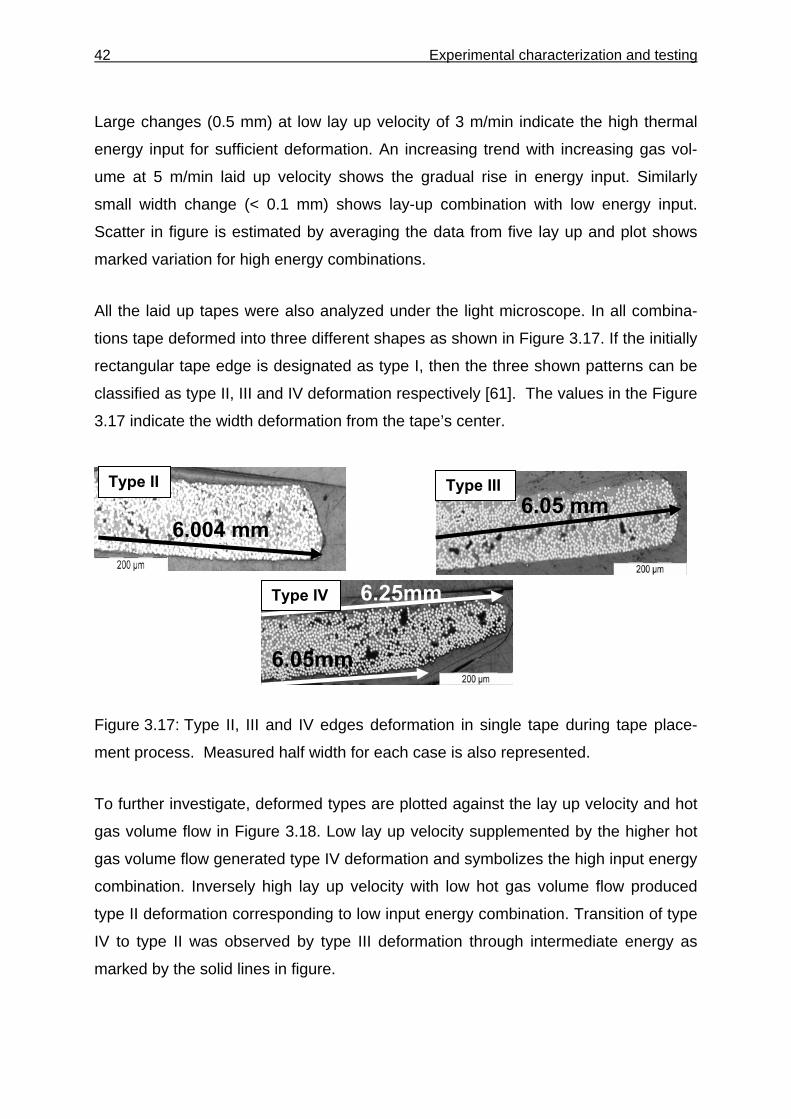
42 Experimental characterization and testing
Large changes (0.5 mm) at low lay up velocity of 3 m/min indicate the high thermal
energy input for sufficient deformation. An increasing trend with increasing gas vol-
ume at 5 m/min laid up velocity shows the gradual rise in energy input. Similarly
small width change (< 0.1 mm) shows lay-up combination with low energy input.
Scatter in figure is estimated by averaging the data from five lay up and plot shows
marked variation for high energy combinations.
All the laid up tapes were also analyzed under the light microscope. In all combina-
tions tape deformed into three different shapes as shown in Figure 3.17. If the initially
rectangular tape edge is designated as type I, then the three shown patterns can be
classified as type II, III and IV deformation respectively [61]. The values in the Figure
3.17 indicate the width deformation from the tape’s center.
Figure 3.17: Type II, III and IV edges deformation in single tape during tape place-
ment process. Measured half width for each case is also represented.
To further investigate, deformed types are plotted against the lay up velocity and hot
gas volume flow in Figure 3.18. Low lay up velocity supplemented by the higher hot
gas volume flow generated type IV deformation and symbolizes the high input energy
combination. Inversely high lay up velocity with low hot gas volume flow produced
type II deformation corresponding to low input energy combination. Transition of type
IV to type II was observed by type III deformation through intermediate energy as
marked by the solid lines in figure.
6.25mm
6.05mm
6.004 mm 6.05 mm
Type II Type III
Type IV
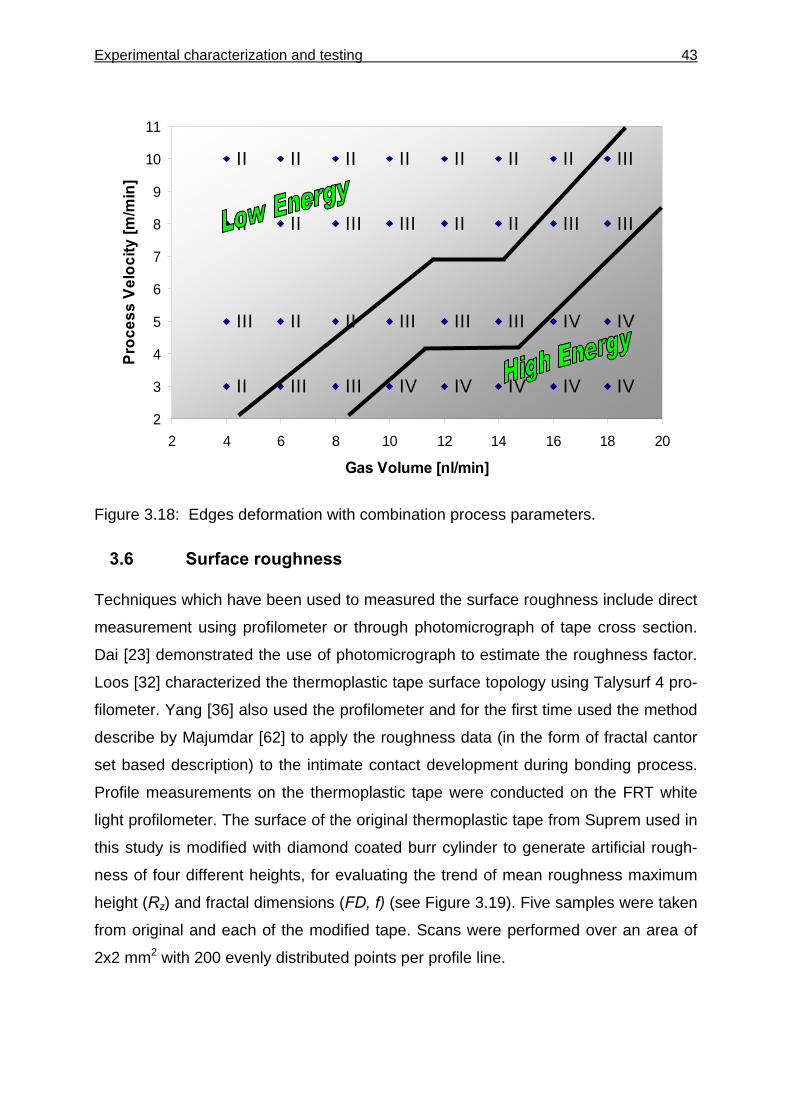
Experimental characterization and testing 43
Figure 3.18: Edges deformation with combination process parameters.
3.6 Surface roughness
Techniques which have been used to measured the surface roughness include direct
measurement using profilometer or through photomicrograph of tape cross section.
Dai [23] demonstrated the use of photomicrograph to estimate the roughness factor.
Loos [32] characterized the thermoplastic tape surface topology using Talysurf 4 pro-
filometer. Yang [36] also used the profilometer and for the first time used the method
describe by Majumdar [62] to apply the roughness data (in the form of fractal cantor
set based description) to the intimate contact development during bonding process.
Profile measurements on the thermoplastic tape were conducted on the FRT white
light profilometer. The surface of the original thermoplastic tape from Suprem used in
this study is modified with diamond coated burr cylinder to generate artificial rough-
ness of four different heights, for evaluating the trend of mean roughness maximum
height (Rz) and fractal dimensions (FD, f) (see Figure 3.19). Five samples were taken
from original and each of the modified tape. Scans were performed over an area of
2x2 mm2 with 200 evenly distributed points per profile line.
II II II II II II II III
II II III III II II III III
III II II III III III IV IV
II III III IV IV IV IV IV
2
3
4
5
6
7
8
9
10
11
2 4 6 8 10 12 14 16 18 20
Gas Volume [nl/min]
Proc
ess
Velo
city
[m/m
in]
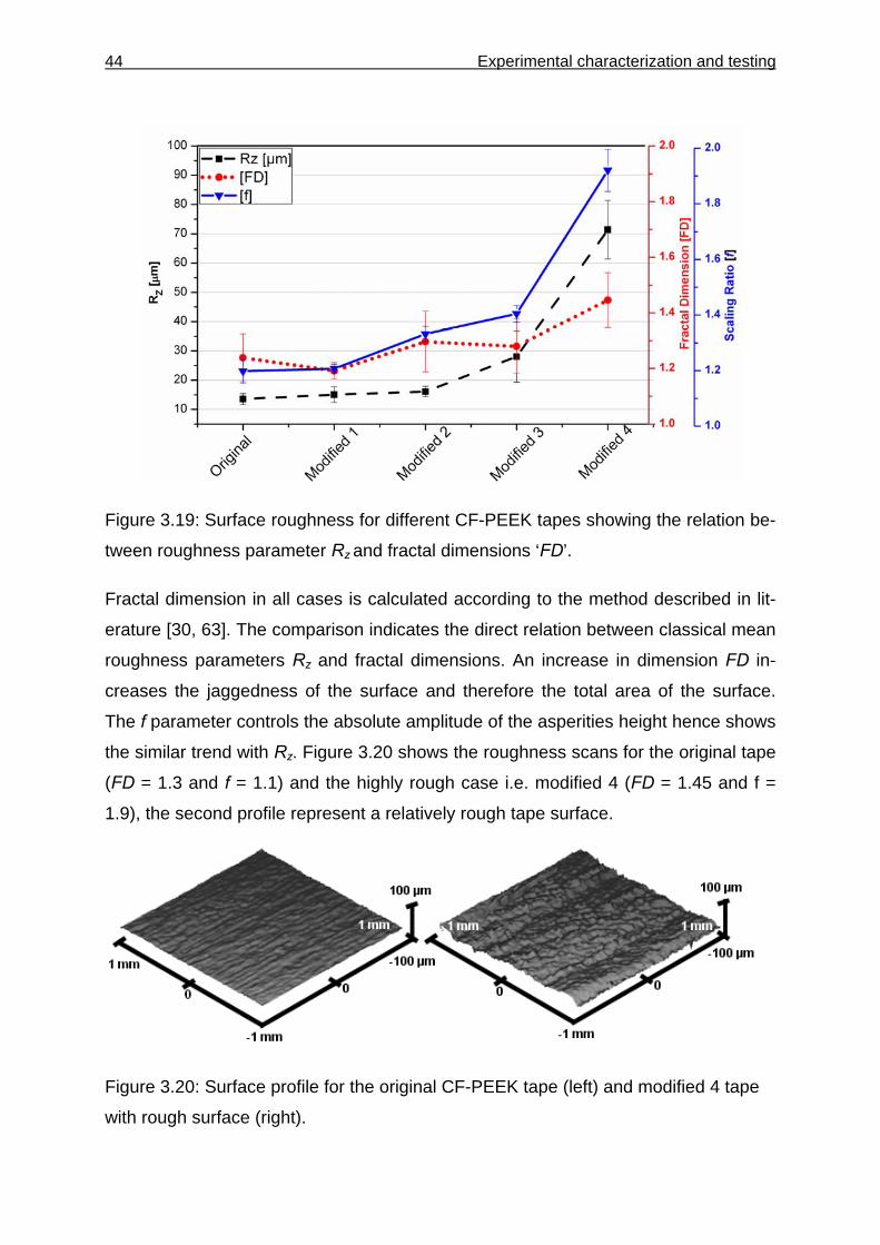
44 Experimental characterization and testing
Figure 3.19: Surface roughness for different CF-PEEK tapes showing the relation be-
tween roughness parameter Rz and fractal dimensions ‘FD’.
Fractal dimension in all cases is calculated according to the method described in lit-
erature [30, 63]. The comparison indicates the direct relation between classical mean
roughness parameters Rz and fractal dimensions. An increase in dimension FD in-
creases the jaggedness of the surface and therefore the total area of the surface.
The f parameter controls the absolute amplitude of the asperities height hence shows
the similar trend with Rz. Figure 3.20 shows the roughness scans for the original tape
(FD = 1.3 and f = 1.1) and the highly rough case i.e. modified 4 (FD = 1.45 and f =
1.9), the second profile represent a relatively rough tape surface.
Figure 3.20: Surface profile for the original CF-PEEK tape (left) and modified 4 tape
with rough surface (right).
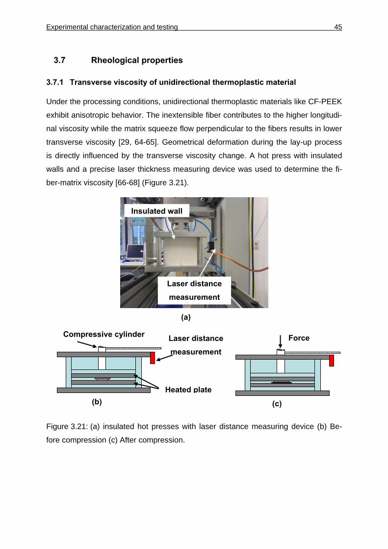
Experimental characterization and testing 45
3.7 Rheological properties
3.7.1 Transverse viscosity of unidirectional thermoplastic material
Under the processing conditions, unidirectional thermoplastic materials like CF-PEEK
exhibit anisotropic behavior. The inextensible fiber contributes to the higher longitudi-
nal viscosity while the matrix squeeze flow perpendicular to the fibers results in lower
transverse viscosity [29, 64-65]. Geometrical deformation during the lay-up process
is directly influenced by the transverse viscosity change. A hot press with insulated
walls and a precise laser thickness measuring device was used to determine the fi-
ber-matrix viscosity [66-68] (Figure 3.21).
Figure 3.21: (a) insulated hot presses with laser distance measuring device (b) Be-
fore compression (c) After compression.
Force
Heated plate
Compressive cylinder Laser distance measurement
(b) (c)
Insulated wall
Laser distance measurement
(a)
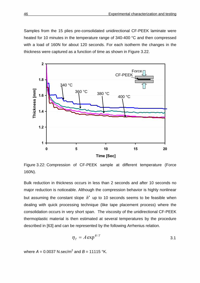
46 Experimental characterization and testing
Samples from the 15 plies pre-consolidated unidirectional CF-PEEK laminate were
heated for 10 minutes in the temperature range of 340-400 °C and then compressed
with a load of 160N for about 120 seconds. For each isotherm the changes in the
thickness were captured as a function of time as shown in Figure 3.22.
1
1.2
1.4
1.6
1.8
2
0 5 10 15 20
Time [Sec]
Thic
knes
s [m
m]
Figure 3.22: Compression of CF-PEEK sample at different temperature (Force
160N).
Bulk reduction in thickness occurs in less than 2 seconds and after 10 seconds no
major reduction is noticeable. Although the compression behavior is highly nonlinear
but assuming the constant slope •h up to 10 seconds seems to be feasible when
dealing with quick processing technique (like tape placement process) where the
consolidation occurs in very short span. The viscosity of the unidirectional CF-PEEK
thermoplastic material is then estimated at several temperatures by the procedure
described in [63] and can be represented by the following Arrhenius relation.
TBT A /exp=η 3.1
where A = 0.0037 N.sec/m2 and B = 11115 °K.
340 °C
400 °C 360 °C 380 °C
Force CF-PEEK
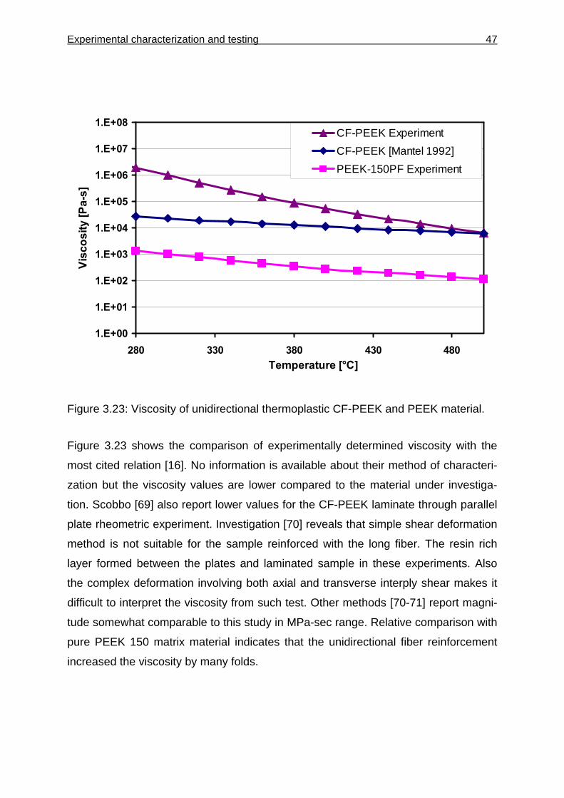
Experimental characterization and testing 47
1.E+00
1.E+01
1.E+02
1.E+03
1.E+04
1.E+05
1.E+06
1.E+07
1.E+08
280 330 380 430 480Temperature [°C]
Visc
osity
[Pa-
s]
CF-PEEK Experiment CF-PEEK [Mantel 1992]PEEK-150PF Experiment
Figure 3.23: Viscosity of unidirectional thermoplastic CF-PEEK and PEEK material.
Figure 3.23 shows the comparison of experimentally determined viscosity with the
most cited relation [16]. No information is available about their method of characteri-
zation but the viscosity values are lower compared to the material under investiga-
tion. Scobbo [69] also report lower values for the CF-PEEK laminate through parallel
plate rheometric experiment. Investigation [70] reveals that simple shear deformation
method is not suitable for the sample reinforced with the long fiber. The resin rich
layer formed between the plates and laminated sample in these experiments. Also
the complex deformation involving both axial and transverse interply shear makes it
difficult to interpret the viscosity from such test. Other methods [70-71] report magni-
tude somewhat comparable to this study in MPa-sec range. Relative comparison with
pure PEEK 150 matrix material indicates that the unidirectional fiber reinforcement
increased the viscosity by many folds.
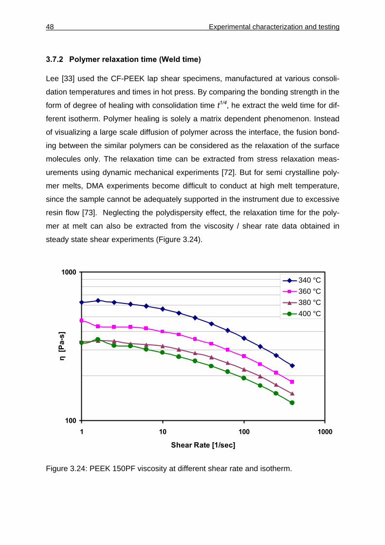
48 Experimental characterization and testing
3.7.2 Polymer relaxation time (Weld time)
Lee [33] used the CF-PEEK lap shear specimens, manufactured at various consoli-
dation temperatures and times in hot press. By comparing the bonding strength in the
form of degree of healing with consolidation time t1/4, he extract the weld time for dif-
ferent isotherm. Polymer healing is solely a matrix dependent phenomenon. Instead
of visualizing a large scale diffusion of polymer across the interface, the fusion bond-
ing between the similar polymers can be considered as the relaxation of the surface
molecules only. The relaxation time can be extracted from stress relaxation meas-
urements using dynamic mechanical experiments [72]. But for semi crystalline poly-
mer melts, DMA experiments become difficult to conduct at high melt temperature,
since the sample cannot be adequately supported in the instrument due to excessive
resin flow [73]. Neglecting the polydispersity effect, the relaxation time for the poly-
mer at melt can also be extracted from the viscosity / shear rate data obtained in
steady state shear experiments (Figure 3.24).
100
1000
1 10 100 1000
Shear Rate [1/sec]
η [P
a-s]
340 °C360 °C380 °C400 °C
Figure 3.24: PEEK 150PF viscosity at different shear rate and isotherm.
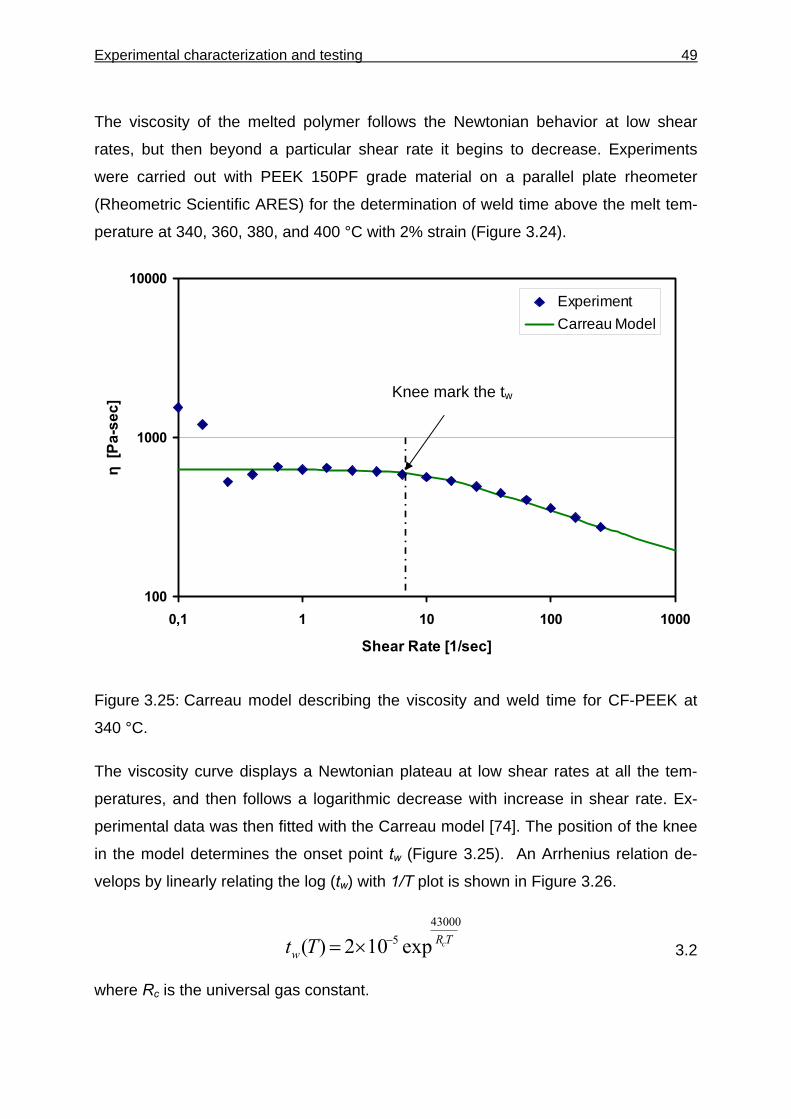
Experimental characterization and testing 49
The viscosity of the melted polymer follows the Newtonian behavior at low shear
rates, but then beyond a particular shear rate it begins to decrease. Experiments
were carried out with PEEK 150PF grade material on a parallel plate rheometer
(Rheometric Scientific ARES) for the determination of weld time above the melt tem-
perature at 340, 360, 380, and 400 °C with 2% strain (Figure 3.24).
100
1000
10000
0,1 1 10 100 1000
Shear Rate [1/sec]
η [P
a-se
c]
ExperimentCarreau Model
Figure 3.25: Carreau model describing the viscosity and weld time for CF-PEEK at
340 °C.
The viscosity curve displays a Newtonian plateau at low shear rates at all the tem-
peratures, and then follows a logarithmic decrease with increase in shear rate. Ex-
perimental data was then fitted with the Carreau model [74]. The position of the knee
in the model determines the onset point tw (Figure 3.25). An Arrhenius relation de-
velops by linearly relating the log (tw) with 1/T plot is shown in Figure 3.26.
TRw
cTt43000
5 exp102)( −×= 3.2
where Rc is the universal gas constant.
Knee mark the tw
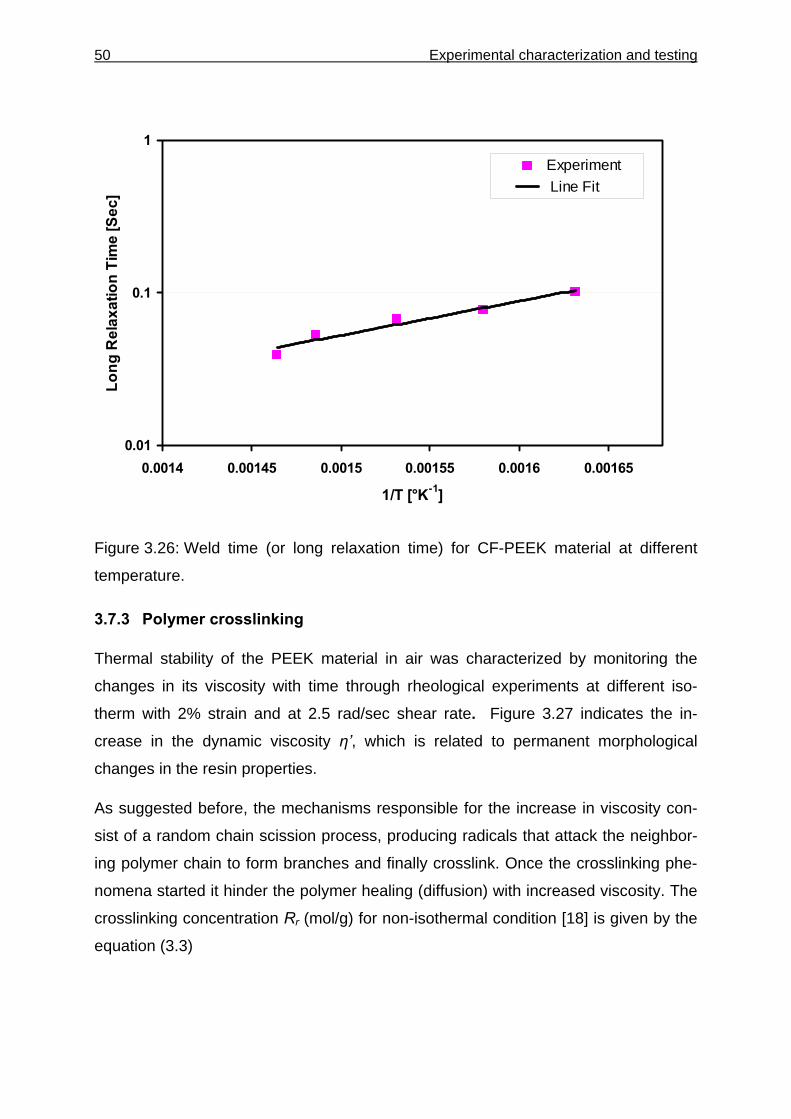
50 Experimental characterization and testing
0.01
0.1
1
0.0014 0.00145 0.0015 0.00155 0.0016 0.00165
1/T [°K-1]
Long
Rel
axat
ion
Tim
e [S
ec]
Experiment Line Fit
Figure 3.26: Weld time (or long relaxation time) for CF-PEEK material at different
temperature.
3.7.3 Polymer crosslinking
Thermal stability of the PEEK material in air was characterized by monitoring the
changes in its viscosity with time through rheological experiments at different iso-
therm with 2% strain and at 2.5 rad/sec shear rate. Figure 3.27 indicates the in-
crease in the dynamic viscosity η’, which is related to permanent morphological
changes in the resin properties.
As suggested before, the mechanisms responsible for the increase in viscosity con-
sist of a random chain scission process, producing radicals that attack the neighbor-
ing polymer chain to form branches and finally crosslink. Once the crosslinking phe-
nomena started it hinder the polymer healing (diffusion) with increased viscosity. The
crosslinking concentration Rr (mol/g) for non-isothermal condition [18] is given by the
equation (3.3)
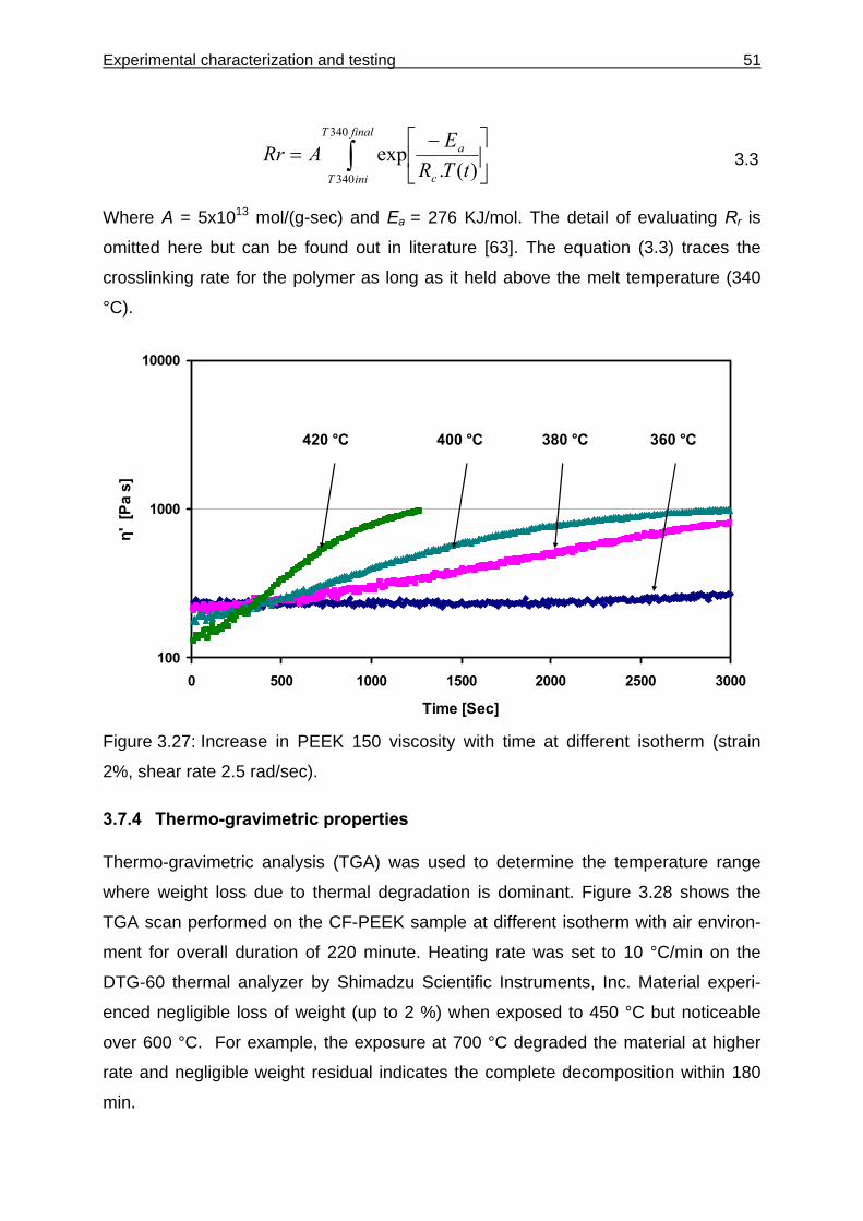
Experimental characterization and testing 51
∫ ⎥⎦
⎤⎢⎣
⎡ −=
finalT
iniT c
a
tTRE
ARr340
340 )(.exp 3.3
Where A = 5x10¹³ mol/(g-sec) and Ea = 276 KJ/mol. The detail of evaluating Rr is
omitted here but can be found out in literature [63]. The equation (3.3) traces the
crosslinking rate for the polymer as long as it held above the melt temperature (340
°C).
100
1000
10000
0 500 1000 1500 2000 2500 3000
Time [Sec]
η' [
Pa s
]
420 °C 400 °C 380 °C 360 °C
Figure 3.27: Increase in PEEK 150 viscosity with time at different isotherm (strain
2%, shear rate 2.5 rad/sec).
3.7.4 Thermo-gravimetric properties
Thermo-gravimetric analysis (TGA) was used to determine the temperature range
where weight loss due to thermal degradation is dominant. Figure 3.28 shows the
TGA scan performed on the CF-PEEK sample at different isotherm with air environ-
ment for overall duration of 220 minute. Heating rate was set to 10 °C/min on the
DTG-60 thermal analyzer by Shimadzu Scientific Instruments, Inc. Material experi-
enced negligible loss of weight (up to 2 %) when exposed to 450 °C but noticeable
over 600 °C. For example, the exposure at 700 °C degraded the material at higher
rate and negligible weight residual indicates the complete decomposition within 180
min.
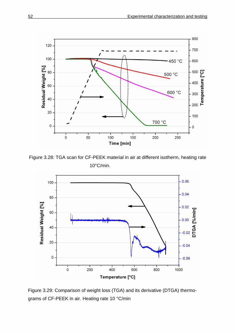
52 Experimental characterization and testing
Figure 3.28: TGA scan for CF-PEEK material in air at different isotherm, heating rate
10°C/min.
Figure 3.29: Comparison of weight loss (TGA) and its derivative (DTGA) thermo-
grams of CF-PEEK in air. Heating rate 10 °C/min
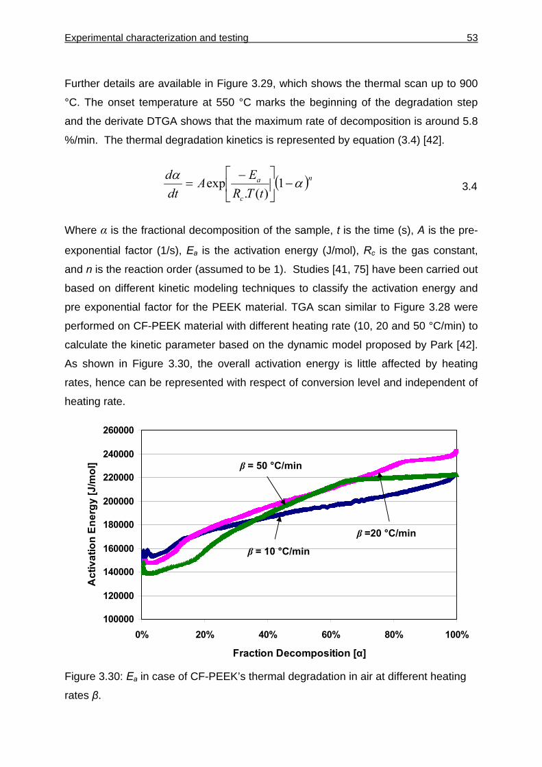
Experimental characterization and testing 53
Further details are available in Figure 3.29, which shows the thermal scan up to 900
°C. The onset temperature at 550 °C marks the beginning of the degradation step
and the derivate DTGA shows that the maximum rate of decomposition is around 5.8
%/min. The thermal degradation kinetics is represented by equation (3.4) [42].
( )n
c
a
tTREA
dtd αα
−⎥⎦
⎤⎢⎣
⎡ −= 1
)(.exp 3.4
Where α is the fractional decomposition of the sample, t is the time (s), A is the pre-
exponential factor (1/s), Ea is the activation energy (J/mol), Rc is the gas constant,
and n is the reaction order (assumed to be 1). Studies [41, 75] have been carried out
based on different kinetic modeling techniques to classify the activation energy and
pre exponential factor for the PEEK material. TGA scan similar to Figure 3.28 were
performed on CF-PEEK material with different heating rate (10, 20 and 50 °C/min) to
calculate the kinetic parameter based on the dynamic model proposed by Park [42].
As shown in Figure 3.30, the overall activation energy is little affected by heating
rates, hence can be represented with respect of conversion level and independent of
heating rate.
100000
120000
140000
160000
180000
200000
220000
240000
260000
0% 20% 40% 60% 80% 100%
Fraction Decomposition [α]
Act
ivat
ion
Ener
gy [J
/mol
]
Figure 3.30: Ea in case of CF-PEEK’s thermal degradation in air at different heating
rates β.
β = 50 °C/min
β =20 °C/min
β = 10 °C/min
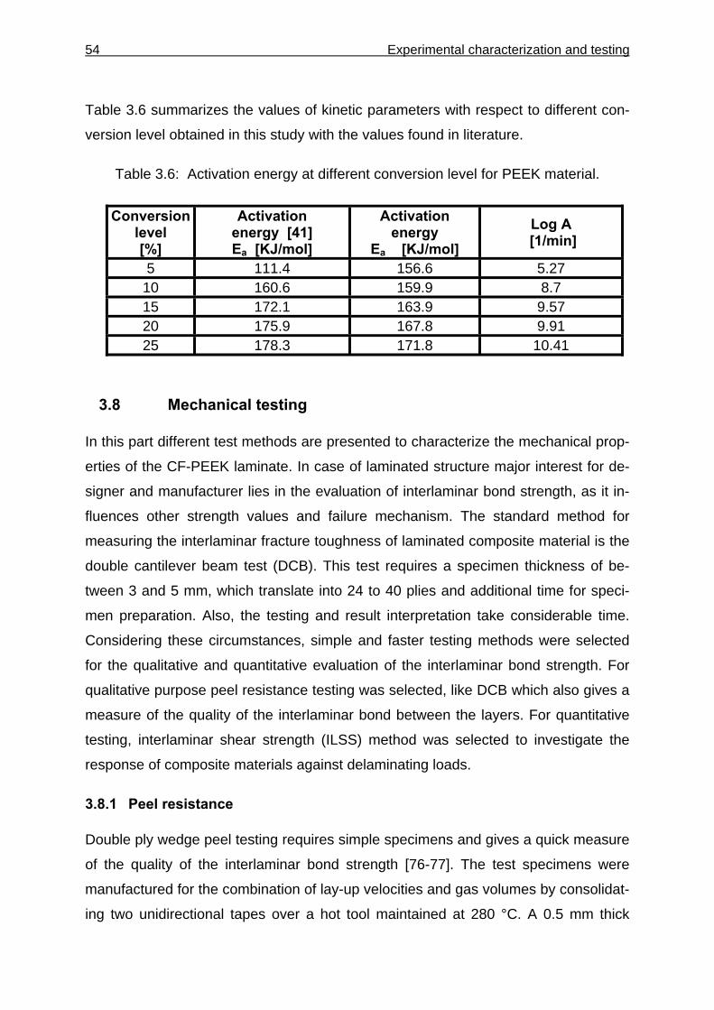
54 Experimental characterization and testing
Table 3.6 summarizes the values of kinetic parameters with respect to different con-
version level obtained in this study with the values found in literature.
Table 3.6: Activation energy at different conversion level for PEEK material.
Conversion level [%]
Activation energy [41] Ea [KJ/mol]
Activation energy
Ea [KJ/mol] Log A
[1/min]
5 111.4 156.6 5.27 10 160.6 159.9 8.7 15 172.1 163.9 9.57 20 175.9 167.8 9.91 25 178.3 171.8 10.41
3.8 Mechanical testing
In this part different test methods are presented to characterize the mechanical prop-
erties of the CF-PEEK laminate. In case of laminated structure major interest for de-
signer and manufacturer lies in the evaluation of interlaminar bond strength, as it in-
fluences other strength values and failure mechanism. The standard method for
measuring the interlaminar fracture toughness of laminated composite material is the
double cantilever beam test (DCB). This test requires a specimen thickness of be-
tween 3 and 5 mm, which translate into 24 to 40 plies and additional time for speci-
men preparation. Also, the testing and result interpretation take considerable time.
Considering these circumstances, simple and faster testing methods were selected
for the qualitative and quantitative evaluation of the interlaminar bond strength. For
qualitative purpose peel resistance testing was selected, like DCB which also gives a
measure of the quality of the interlaminar bond between the layers. For quantitative
testing, interlaminar shear strength (ILSS) method was selected to investigate the
response of composite materials against delaminating loads.
3.8.1 Peel resistance
Double ply wedge peel testing requires simple specimens and gives a quick measure
of the quality of the interlaminar bond strength [76-77]. The test specimens were
manufactured for the combination of lay-up velocities and gas volumes by consolidat-
ing two unidirectional tapes over a hot tool maintained at 280 °C. A 0.5 mm thick
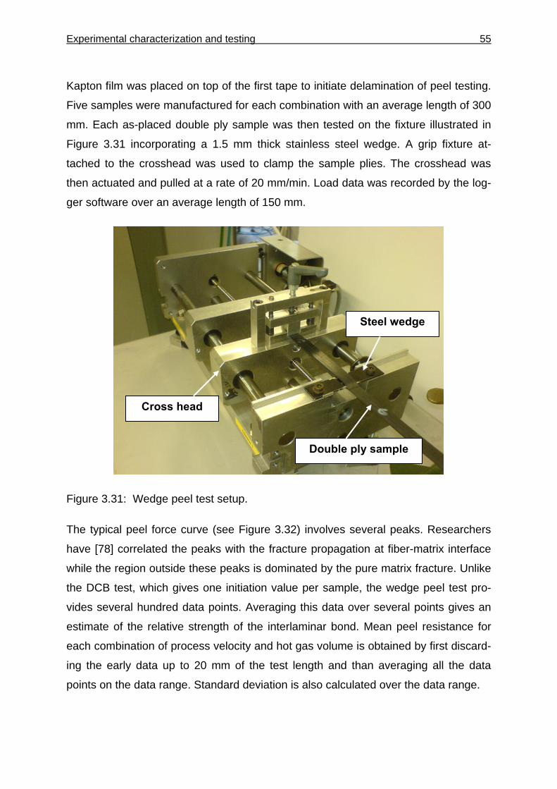
Experimental characterization and testing 55
Kapton film was placed on top of the first tape to initiate delamination of peel testing.
Five samples were manufactured for each combination with an average length of 300
mm. Each as-placed double ply sample was then tested on the fixture illustrated in
Figure 3.31 incorporating a 1.5 mm thick stainless steel wedge. A grip fixture at-
tached to the crosshead was used to clamp the sample plies. The crosshead was
then actuated and pulled at a rate of 20 mm/min. Load data was recorded by the log-
ger software over an average length of 150 mm.
Figure 3.31: Wedge peel test setup.
The typical peel force curve (see Figure 3.32) involves several peaks. Researchers
have [78] correlated the peaks with the fracture propagation at fiber-matrix interface
while the region outside these peaks is dominated by the pure matrix fracture. Unlike
the DCB test, which gives one initiation value per sample, the wedge peel test pro-
vides several hundred data points. Averaging this data over several points gives an
estimate of the relative strength of the interlaminar bond. Mean peel resistance for
each combination of process velocity and hot gas volume is obtained by first discard-
ing the early data up to 20 mm of the test length and than averaging all the data
points on the data range. Standard deviation is also calculated over the data range.
Steel wedge
Double ply sample
Cross head
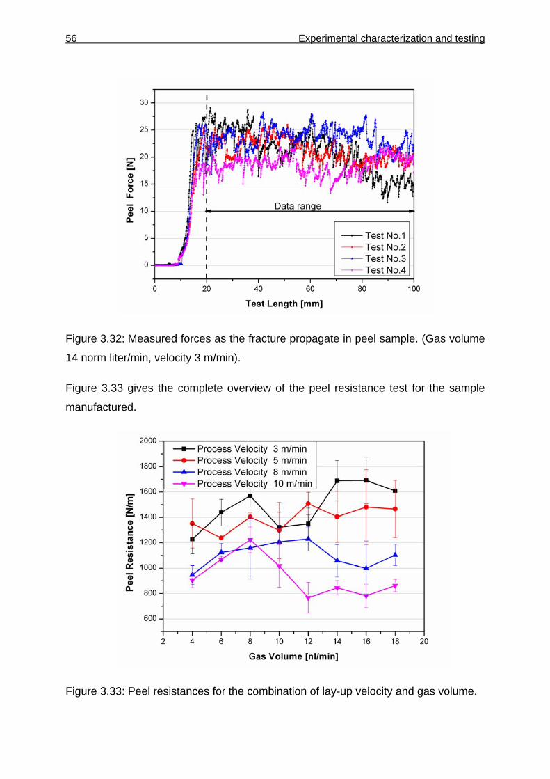
56 Experimental characterization and testing
Figure 3.32: Measured forces as the fracture propagate in peel sample. (Gas volume
14 norm liter/min, velocity 3 m/min).
Figure 3.33 gives the complete overview of the peel resistance test for the sample
manufactured.
Figure 3.33: Peel resistances for the combination of lay-up velocity and gas volume.
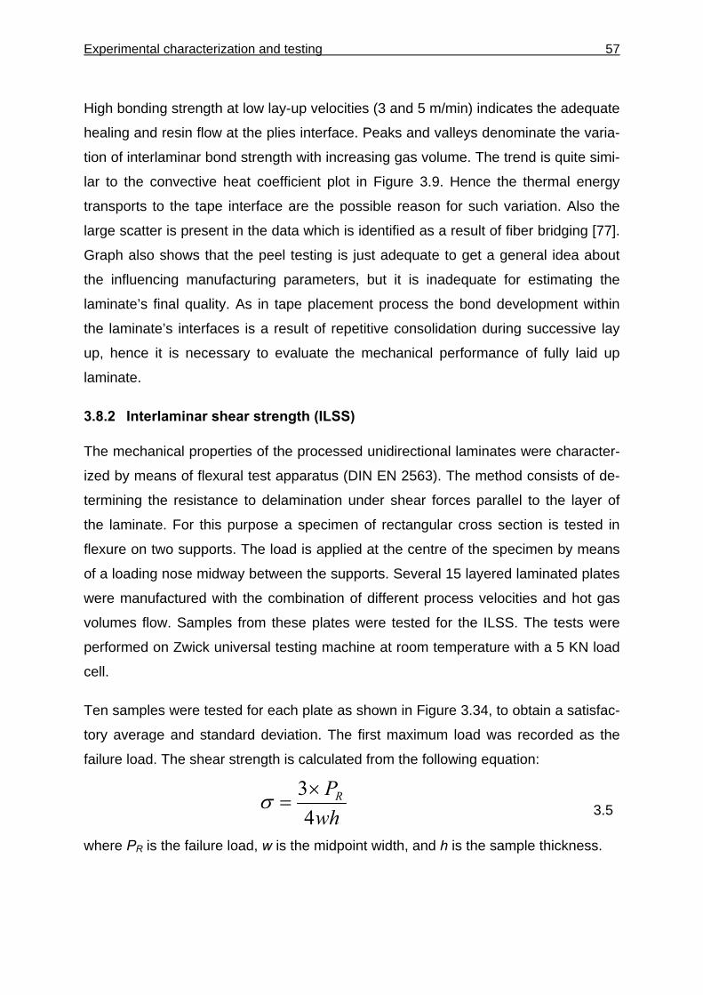
Experimental characterization and testing 57
High bonding strength at low lay-up velocities (3 and 5 m/min) indicates the adequate
healing and resin flow at the plies interface. Peaks and valleys denominate the varia-
tion of interlaminar bond strength with increasing gas volume. The trend is quite simi-
lar to the convective heat coefficient plot in Figure 3.9. Hence the thermal energy
transports to the tape interface are the possible reason for such variation. Also the
large scatter is present in the data which is identified as a result of fiber bridging [77].
Graph also shows that the peel testing is just adequate to get a general idea about
the influencing manufacturing parameters, but it is inadequate for estimating the
laminate’s final quality. As in tape placement process the bond development within
the laminate’s interfaces is a result of repetitive consolidation during successive lay
up, hence it is necessary to evaluate the mechanical performance of fully laid up
laminate.
3.8.2 Interlaminar shear strength (ILSS)
The mechanical properties of the processed unidirectional laminates were character-
ized by means of flexural test apparatus (DIN EN 2563). The method consists of de-
termining the resistance to delamination under shear forces parallel to the layer of
the laminate. For this purpose a specimen of rectangular cross section is tested in
flexure on two supports. The load is applied at the centre of the specimen by means
of a loading nose midway between the supports. Several 15 layered laminated plates
were manufactured with the combination of different process velocities and hot gas
volumes flow. Samples from these plates were tested for the ILSS. The tests were
performed on Zwick universal testing machine at room temperature with a 5 KN load
cell.
Ten samples were tested for each plate as shown in Figure 3.34, to obtain a satisfac-
tory average and standard deviation. The first maximum load was recorded as the
failure load. The shear strength is calculated from the following equation:
whPR
43×
=σ 3.5
where PR is the failure load, w is the midpoint width, and h is the sample thickness.
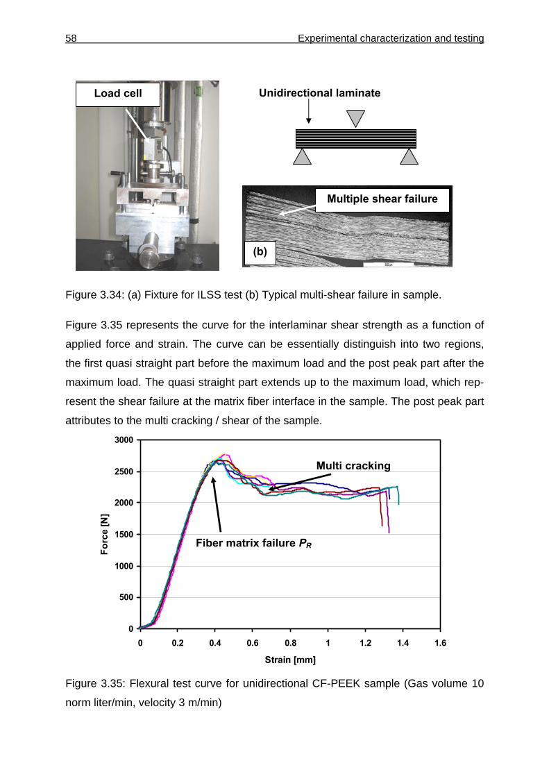
58 Experimental characterization and testing
Figure 3.34: (a) Fixture for ILSS test (b) Typical multi-shear failure in sample.
Figure 3.35 represents the curve for the interlaminar shear strength as a function of
applied force and strain. The curve can be essentially distinguish into two regions,
the first quasi straight part before the maximum load and the post peak part after the
maximum load. The quasi straight part extends up to the maximum load, which rep-
resent the shear failure at the matrix fiber interface in the sample. The post peak part
attributes to the multi cracking / shear of the sample.
0
500
1000
1500
2000
2500
3000
0 0.2 0.4 0.6 0.8 1 1.2 1.4 1.6
Strain [mm]
Forc
e [N
]
Figure 3.35: Flexural test curve for unidirectional CF-PEEK sample (Gas volume 10
norm liter/min, velocity 3 m/min)
Fiber matrix failure PR
Multi cracking
Load cell
(b)
Multiple shear failure
Unidirectional laminate
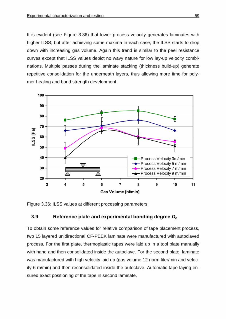
Experimental characterization and testing 59
It is evident (see Figure 3.36) that lower process velocity generates laminates with
higher ILSS, but after achieving some maxima in each case, the ILSS starts to drop
down with increasing gas volume. Again this trend is similar to the peel resistance
curves except that ILSS values depict no wavy nature for low lay-up velocity combi-
nations. Multiple passes during the laminate stacking (thickness build-up) generate
repetitive consolidation for the underneath layers, thus allowing more time for poly-
mer healing and bond strength development.
20
30
40
50
60
70
80
90
100
3 4 5 6 7 8 9 10 11
Gas Volume [nl/min]
ILSS
[Pa]
Process Velocity 3m/minProcess Velocity 5 m/minProcess Velocity 7 m/minProcess Velocity 9 m/min
Figure 3.36: ILSS values at different processing parameters.
3.9 Reference plate and experimental bonding degree Db
To obtain some reference values for relative comparison of tape placement process,
two 15 layered unidirectional CF-PEEK laminate were manufactured with autoclaved
process. For the first plate, thermoplastic tapes were laid up in a tool plate manually
with hand and then consolidated inside the autoclave. For the second plate, laminate
was manufactured with high velocity laid up (gas volume 12 norm liter/min and veloc-
ity 6 m/min) and then reconsolidated inside the autoclave. Automatic tape laying en-
sured exact positioning of the tape in second laminate.
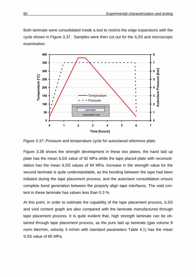
60 Experimental characterization and testing
Both laminate were consolidated inside a tool to restrict the edge expansions with the
cycle shown in Figure 3.37. Samples were then cut out for the ILSS and microscopic
examination.
0
50
100
150
200
250
300
350
400
0 1 2 3 4 5 6 7
Time [hours]
Tem
pera
ture
[°C
]
0
1
2
3
4
5
6
7
8
Aut
ocla
ve P
ress
ure
[bar
]
TemperaturePressure
Laminate
Autoclave tool
Figure 3.37: Pressure and temperature cycle for autoclaved reference plate.
Figure 3.38 shows the strength development in these two plates, the hand laid up
plate has the mean ILSS value of 92 MPa while the tape placed plate with reconsoli-
dation has the mean ILSS values of 94 MPa. Increase in the strength value for the
second laminate is quite understandable, as the bonding between the tape had been
initiated during the tape placement process, and the autoclave consolidation ensure
complete bond generation between the properly align tape interfaces. The void con-
tent in these laminate has values less than 0.3 %.
At this point, in order to estimate the capability of the tape placement process, ILSS
and void content graph are also compared with the laminate manufactured through
tape placement process. It is quite evident that, high strength laminate can be ob-
tained through tape placement process, as the pure laid up laminate (gas volume 8
norm liter/min, velocity 3 m/min with standard parameters Table 4.1) has the mean
ILSS value of 85 MPa.
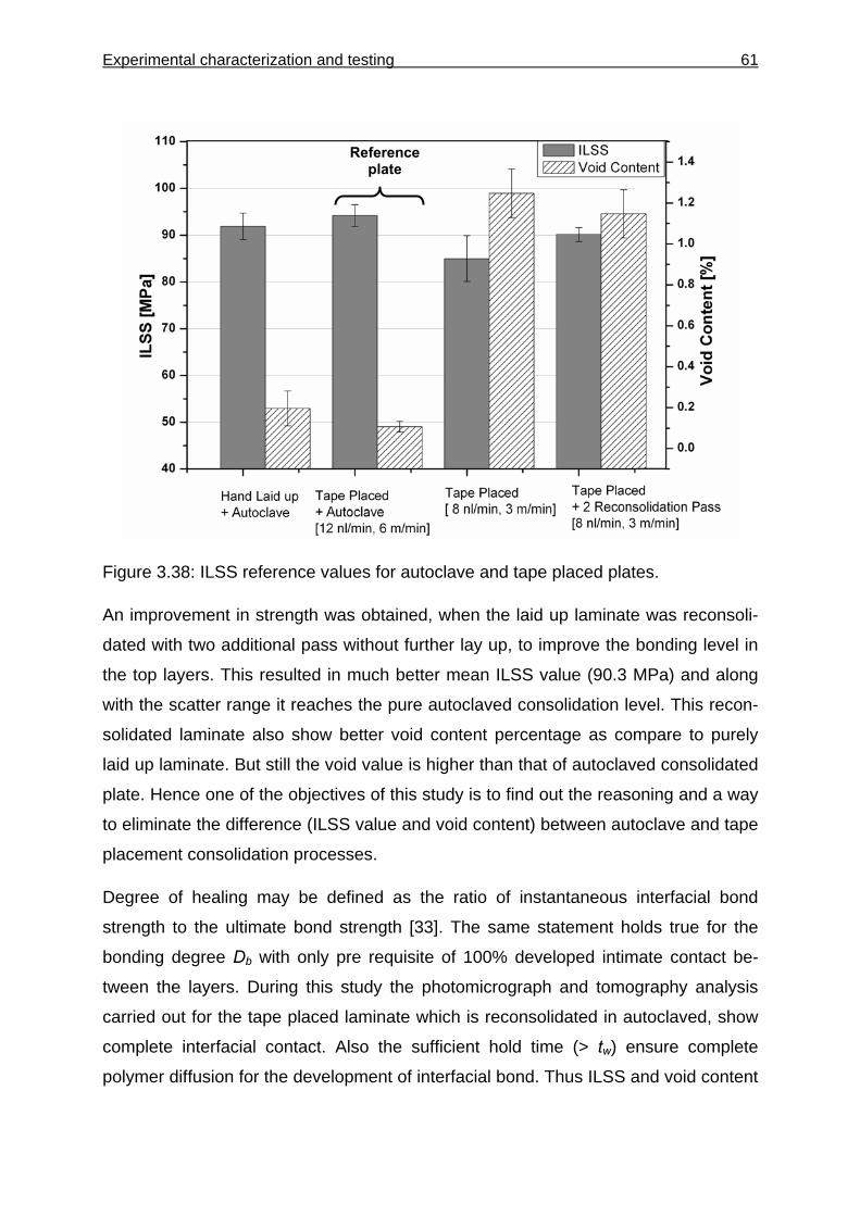
Experimental characterization and testing 61
Figure 3.38: ILSS reference values for autoclave and tape placed plates.
An improvement in strength was obtained, when the laid up laminate was reconsoli-
dated with two additional pass without further lay up, to improve the bonding level in
the top layers. This resulted in much better mean ILSS value (90.3 MPa) and along
with the scatter range it reaches the pure autoclaved consolidation level. This recon-
solidated laminate also show better void content percentage as compare to purely
laid up laminate. But still the void value is higher than that of autoclaved consolidated
plate. Hence one of the objectives of this study is to find out the reasoning and a way
to eliminate the difference (ILSS value and void content) between autoclave and tape
placement consolidation processes.
Degree of healing may be defined as the ratio of instantaneous interfacial bond
strength to the ultimate bond strength [33]. The same statement holds true for the
bonding degree Db with only pre requisite of 100% developed intimate contact be-
tween the layers. During this study the photomicrograph and tomography analysis
carried out for the tape placed laminate which is reconsolidated in autoclaved, show
complete interfacial contact. Also the sufficient hold time (> tw) ensure complete
polymer diffusion for the development of interfacial bond. Thus ILSS and void content
Reference plate
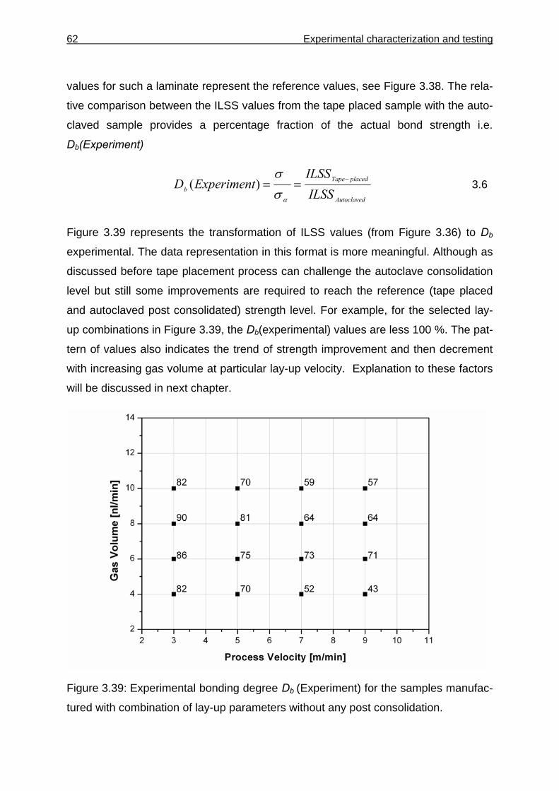
62 Experimental characterization and testing
values for such a laminate represent the reference values, see Figure 3.38. The rela-
tive comparison between the ILSS values from the tape placed sample with the auto-
claved sample provides a percentage fraction of the actual bond strength i.e.
Db(Experiment)
Autoclaved
placedTapeb ILSS
ILSSExperimentD −==
ασσ
)( 3.6
Figure 3.39 represents the transformation of ILSS values (from Figure 3.36) to Db
experimental. The data representation in this format is more meaningful. Although as
discussed before tape placement process can challenge the autoclave consolidation
level but still some improvements are required to reach the reference (tape placed
and autoclaved post consolidated) strength level. For example, for the selected lay-
up combinations in Figure 3.39, the Db(experimental) values are less 100 %. The pat-
tern of values also indicates the trend of strength improvement and then decrement
with increasing gas volume at particular lay-up velocity. Explanation to these factors
will be discussed in next chapter.
Figure 3.39: Experimental bonding degree Db (Experiment) for the samples manufac-
tured with combination of lay-up parameters without any post consolidation.
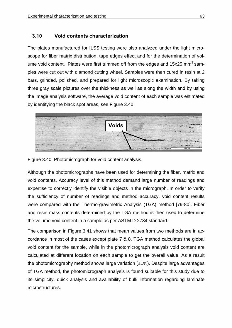
Experimental characterization and testing 63
3.10 Void contents characterization
The plates manufactured for ILSS testing were also analyzed under the light micro-
scope for fiber matrix distribution, tape edges effect and for the determination of vol-
ume void content. Plates were first trimmed off from the edges and 15x25 mm2 sam-
ples were cut out with diamond cutting wheel. Samples were then cured in resin at 2
bars, grinded, polished, and prepared for light microscopic examination. By taking
three gray scale pictures over the thickness as well as along the width and by using
the image analysis software, the average void content of each sample was estimated
by identifying the black spot areas, see Figure 3.40.
Figure 3.40: Photomicrograph for void content analysis.
Although the photomicrographs have been used for determining the fiber, matrix and
void contents. Accuracy level of this method demand large number of readings and
expertise to correctly identify the visible objects in the micrograph. In order to verify
the sufficiency of number of readings and method accuracy, void content results
were compared with the Thermo-gravimetric Analysis (TGA) method [79-80]. Fiber
and resin mass contents determined by the TGA method is then used to determine
the volume void content in a sample as per ASTM D 2734 standard.
The comparison in Figure 3.41 shows that mean values from two methods are in ac-
cordance in most of the cases except plate 7 & 8. TGA method calculates the global
void content for the sample, while in the photomicrograph analysis void content are
calculated at different location on each sample to get the overall value. As a result
the photomicrography method shows large variation (±1%). Despite large advantages
of TGA method, the photomicrograph analysis is found suitable for this study due to
its simplicity, quick analysis and availability of bulk information regarding laminate
microstructures.
Voids
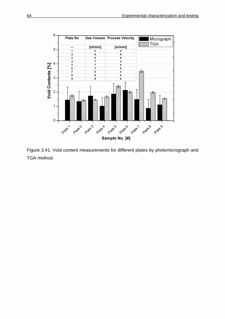
64 Experimental characterization and testing
Figure 3.41: Void content measurements for different plates by photomicrograph and
TGA method.
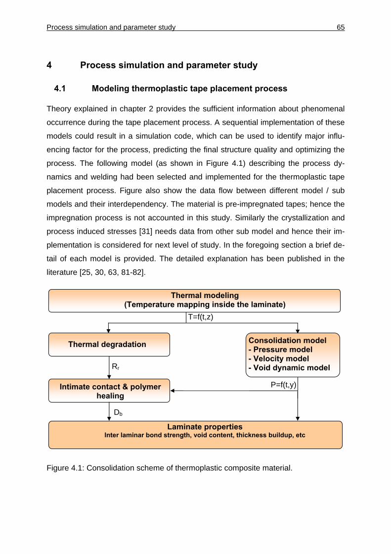
Process simulation and parameter study 65
4 Process simulation and parameter study
4.1 Modeling thermoplastic tape placement process
Theory explained in chapter 2 provides the sufficient information about phenomenal
occurrence during the tape placement process. A sequential implementation of these
models could result in a simulation code, which can be used to identify major influ-
encing factor for the process, predicting the final structure quality and optimizing the
process. The following model (as shown in Figure 4.1) describing the process dy-
namics and welding had been selected and implemented for the thermoplastic tape
placement process. Figure also show the data flow between different model / sub
models and their interdependency. The material is pre-impregnated tapes; hence the
impregnation process is not accounted in this study. Similarly the crystallization and
process induced stresses [31] needs data from other sub model and hence their im-
plementation is considered for next level of study. In the foregoing section a brief de-
tail of each model is provided. The detailed explanation has been published in the
literature [25, 30, 63, 81-82].
Figure 4.1: Consolidation scheme of thermoplastic composite material.
Thermal modeling (Temperature mapping inside the laminate)
Consolidation model - Pressure model - Velocity model - Void dynamic model
Intimate contact & polymer healing
T=f(t,z)
P=f(t,y)
Db
Thermal degradation
Rr
Laminate properties Inter laminar bond strength, void content, thickness buildup, etc
66 Process simulation and parameter study
Thermal model: Although sophisticated modeling techniques are available (as
shown in Table 2.1) but for this study thermal gradient inside the laminate was ana-
lyzed with the 1-D (through thickness) model. Considering small temperature varia-
tion under the hot gas torch in tape’s width direction and assuming heat transfer by
the high velocity hot gas impingent flow through nozzle is much larger than that of
heat conduction through material along the lay up direction due to low thermal con-
ductivity, eliminate the need of complex and time consuming heat transfer calculation
in width and length direction. Also Toso [15] found through DSC measurement that
for high heating rates (over 1000 °C/s) a consideration of heat generated results in
an overestimation of temperature at the nip point by approximately 5 °C. For this rea-
son heat generation/sink effect is not considered in this study. The energy equation
(2.1) is simplified for 1 D heat transfer and implemented as:
2
2
zT
Ck
tT z
∂∂
=∂∂
ρ 4.1
where z is the spatial coordinate in thickness direction. Convection is identified as the
main source of heat transfer in the process by several authors [14, 17, 83].
)( mmz TThzTk −−=
∂∂
4.2
Where hm and Tm in equation (4.3) represents the convective heat transfer coefficient
and temperature surrounding (air, hot gas or tooling) the lay-down laminate. The in-
coming tape enters into the domain with room temperature, while the substrate is ini-
tially assumed at tool temperature. The equation (4.1) is solved for the incoming
tape, substrate and composite section (see Figure 2.12) as describe in the literature
[25].
Consolidation model: Thermoplastic tape placement process is highly non isother-
mal in nature. Moreover, an exact pressure distribution is necessary to determine the
void compression / elimination and geometrical variation within the laminate. Refer-
ring back to Table 2.2, modeling technique based on transverse squeeze flow
method only fulfill all these requirements, hence selected for this study. As input, be-
Process simulation and parameter study 67
sides manufacturing setup detail, model also needs the temperature mapping data
from the thermal model. The output of the model includes the information about pres-
sure distribution, final intraply void content and change in tape’s width / thickness.
Thermal degradation: Experimental testing in section 3.74 shows that PEEK poly-
mer is quite stable up to 360°C, but over this temperature polymer crosslinking re-
sults in an increase in viscosity. Already explained thermal stability model (in section
3.73) is selected for the process simulation along with the experimentally determine
activation energy and pre exponential components. As input model require thermal
exposure history of every layer and output results in the crosslinking rate Rr to show
the extent of polymer crosslinking.
Intimate contact and polymer healing: Surface profilometer scan in section 3.6
shows roughness profile in incoming tape is highly random in fashion. And it cannot
be represented by the single factor, therefore fractal dimensions were determined
and equation (2.9) is used for intimate contact development. Similarly equation (2.10)
is selected for no isothermal healing along with intimate contact development to de-
termine the overall bonding degree using mathematical strategy describe by equation
(2.12).
Figure 4.2: Schematic for the ProSimFRT code.
68 Process simulation and parameter study
4.2 Model implementation
A process simulation code for fiber reinforced thermoplastic (ProSimFRT) is devel-
oped using the Matlab platform for this purpose. Built in numerical functions in the
Matlab software are capable of performing high speed calculation by maintaining the
accuracy. Three implementation levels of ProSimFRT as shown in Figure 4.2 are In-
put, Model Solution and Output section.
Input section (see Figure 4.3) serves as an interface to communicate between the
user and the solver. Different aspects of the problem starting from material details,
lay-up configuration and process setup can be defined in this part. Beside this the
instructions to the solver like the solution time, geometrical descritization of the prob-
lem, selection of appropriate models and control to the output can also be defined
here.
Figure 4.3: Input windows for the simulation code.
Process simulation and parameter study 69
Solver section is the collection of numerically implemented theoretical models; solu-
tion from each model is available to the succeeding model as an input. Simulation
begin with the heat transfer model, and then with simultaneous solution of consolida-
tion and strength development models. Effect of polymer degradation and thermal
stability is also calculated through out the lay-up process. Material characteristic are
updated at every solution stage to represent the actual state.
Figure 4.4: Post-process windows for output section to view the results.
Generated outputs as per predefined format in input section are available at the end
of the solution. Results can be directly viewed through the software see Figure 4.4 or
by using spreadsheet program like Excel or Origin. Extensive information can be ex-
tracted from several data files created during solution. An ‘overview.xls’ data file de-
scribes the overall laminate quality in terms of degree of intimate contact, healing and
bonding. The user can visualize the combine effect of several processes by combin-
ing the available results.
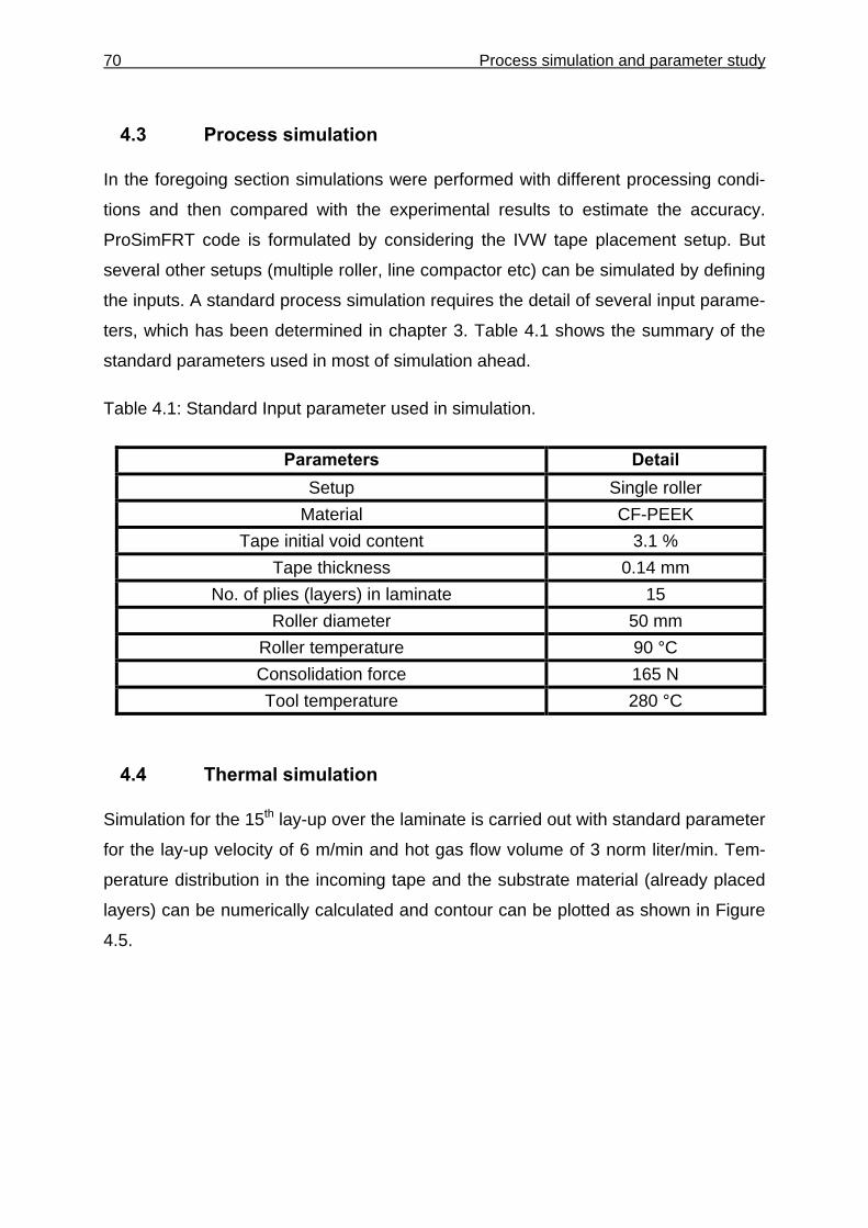
70 Process simulation and parameter study
4.3 Process simulation
In the foregoing section simulations were performed with different processing condi-
tions and then compared with the experimental results to estimate the accuracy.
ProSimFRT code is formulated by considering the IVW tape placement setup. But
several other setups (multiple roller, line compactor etc) can be simulated by defining
the inputs. A standard process simulation requires the detail of several input parame-
ters, which has been determined in chapter 3. Table 4.1 shows the summary of the
standard parameters used in most of simulation ahead.
Table 4.1: Standard Input parameter used in simulation.
Parameters Detail Setup Single roller
Material CF-PEEK Tape initial void content 3.1 %
Tape thickness 0.14 mm No. of plies (layers) in laminate 15
Roller diameter 50 mm Roller temperature 90 °C Consolidation force 165 N Tool temperature 280 °C
4.4 Thermal simulation
Simulation for the 15th lay-up over the laminate is carried out with standard parameter
for the lay-up velocity of 6 m/min and hot gas flow volume of 3 norm liter/min. Tem-
perature distribution in the incoming tape and the substrate material (already placed
layers) can be numerically calculated and contour can be plotted as shown in Figure
4.5.
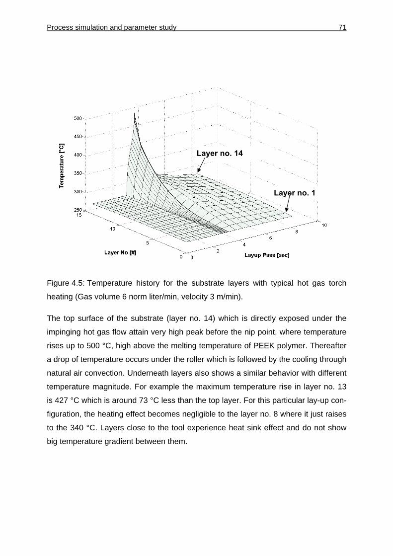
Process simulation and parameter study 71
Figure 4.5: Temperature history for the substrate layers with typical hot gas torch
heating (Gas volume 6 norm liter/min, velocity 3 m/min).
The top surface of the substrate (layer no. 14) which is directly exposed under the
impinging hot gas flow attain very high peak before the nip point, where temperature
rises up to 500 °C, high above the melting temperature of PEEK polymer. Thereafter
a drop of temperature occurs under the roller which is followed by the cooling through
natural air convection. Underneath layers also shows a similar behavior with different
temperature magnitude. For example the maximum temperature rise in layer no. 13
is 427 °C which is around 73 °C less than the top layer. For this particular lay-up con-
figuration, the heating effect becomes negligible to the layer no. 8 where it just raises
to the 340 °C. Layers close to the tool experience heat sink effect and do not show
big temperature gradient between them.
Layer no. 14
Layer no. 1
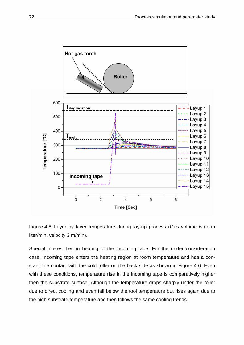
72 Process simulation and parameter study
Figure 4.6: Layer by layer temperature during lay-up process (Gas volume 6 norm
liter/min, velocity 3 m/min).
Special interest lies in heating of the incoming tape. For the under consideration
case, incoming tape enters the heating region at room temperature and has a con-
stant line contact with the cold roller on the back side as shown in Figure 4.6. Even
with these conditions, temperature rise in the incoming tape is comparatively higher
then the substrate surface. Although the temperature drops sharply under the roller
due to direct cooling and even fall below the tool temperature but rises again due to
the high substrate temperature and then follows the same cooling trends.
Hot gas torch
Roller
Tmelt
Tdegradation
Incoming tape
Process simulation and parameter study 73
It is not possible to directly measure the nip point temperature using K-type thermo-
couples, as they could be destroyed under the influence of high gas temperature.
Hence it was decided to measure the temperature one layer beneath the top surface
during the final (15th) lay-up. The thermocouple captured the temperature distribution
under the 14th layer and Figure 4.7 shows the comparison between the measured
and simulated histories.
Figure 4.7: Comparison of simulation and measured results under the 14th (Gas vol-
ume 6 norm liter/min, velocity 3 m/min).
Differences in the measured histories are found sensitive to the exact positioning of
the thermocouple juncture on the tape and variation in tool temperature (±5 °C). Re-
sults showed good correlation with the measured ones by capturing the approximate
peak temperature. Nevertheless the overall prediction captured the transient heating
rather well.
4.4.1 Surface temperature
Thermal histories play an important part in the tape placement process. Large heat
input upstream to the roller, could generate thermal degradation / crosslinking in the
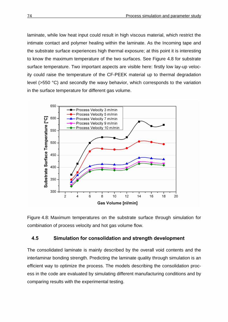
74 Process simulation and parameter study
laminate, while low heat input could result in high viscous material, which restrict the
intimate contact and polymer healing within the laminate. As the Incoming tape and
the substrate surface experiences high thermal exposure; at this point it is interesting
to know the maximum temperature of the two surfaces. See Figure 4.8 for substrate
surface temperature. Two important aspects are visible here: firstly low lay-up veloc-
ity could raise the temperature of the CF-PEEK material up to thermal degradation
level (>550 °C) and secondly the wavy behavior, which corresponds to the variation
in the surface temperature for different gas volume.
Figure 4.8: Maximum temperatures on the substrate surface through simulation for
combination of process velocity and hot gas volume flow.
4.5 Simulation for consolidation and strength development
The consolidated laminate is mainly described by the overall void contents and the
interlaminar bonding strength. Predicting the laminate quality through simulation is an
efficient way to optimize the process. The models describing the consolidation proc-
ess in the code are evaluated by simulating different manufacturing conditions and by
comparing results with the experimental testing.
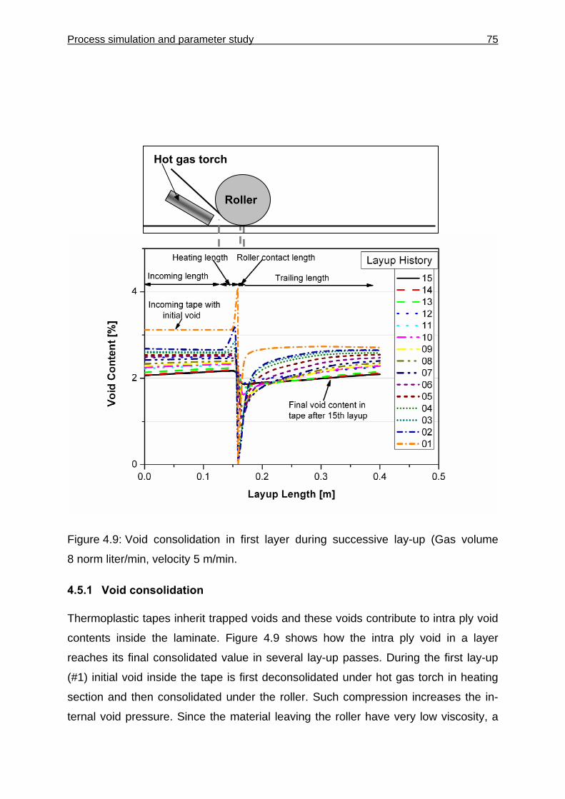
Process simulation and parameter study 75
Figure 4.9: Void consolidation in first layer during successive lay-up (Gas volume
8 norm liter/min, velocity 5 m/min.
4.5.1 Void consolidation
Thermoplastic tapes inherit trapped voids and these voids contribute to intra ply void
contents inside the laminate. Figure 4.9 shows how the intra ply void in a layer
reaches its final consolidated value in several lay-up passes. During the first lay-up
(#1) initial void inside the tape is first deconsolidated under hot gas torch in heating
section and then consolidated under the roller. Such compression increases the in-
ternal void pressure. Since the material leaving the roller have very low viscosity, a
Hot gas torch
Roller
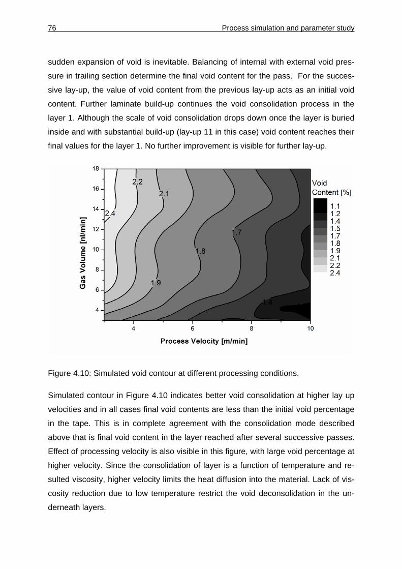
76 Process simulation and parameter study
sudden expansion of void is inevitable. Balancing of internal with external void pres-
sure in trailing section determine the final void content for the pass. For the succes-
sive lay-up, the value of void content from the previous lay-up acts as an initial void
content. Further laminate build-up continues the void consolidation process in the
layer 1. Although the scale of void consolidation drops down once the layer is buried
inside and with substantial build-up (lay-up 11 in this case) void content reaches their
final values for the layer 1. No further improvement is visible for further lay-up.
Figure 4.10: Simulated void contour at different processing conditions.
Simulated contour in Figure 4.10 indicates better void consolidation at higher lay up
velocities and in all cases final void contents are less than the initial void percentage
in the tape. This is in complete agreement with the consolidation mode described
above that is final void content in the layer reached after several successive passes.
Effect of processing velocity is also visible in this figure, with large void percentage at
higher velocity. Since the consolidation of layer is a function of temperature and re-
sulted viscosity, higher velocity limits the heat diffusion into the material. Lack of vis-
cosity reduction due to low temperature restrict the void deconsolidation in the un-
derneath layers.

Process simulation and parameter study 77
Figure 4.11: Comparison between measured and simulated void contents for combi-
nation of process velocity and hot gas volume flow.
Figure 4.11 shows the simulated void content for the 15 layered laminate manufac-
tured with combination of lay-up velocity and hot gas flow. Standard inputs were used
for defining the remaining parameters in code. For low lay-up velocity of 5 m/min void
variations are not noticeable due to sufficient condition for the void deconsolidation at
the roller exit at all gas volumes. But for high lay-up velocity 7 m/min a trend of in-
creasing void contents is visible with higher gas volume. For lay-up velocity of 9
m/min, energy input to the tape in heating section is just sufficient to facilitate the
consolidation under the roller and roller extract the reaming thermal energy by solidi-
fying the material at its exit, preventing the void expansion. In all cases simulated re-
sults are comparable to measured values.
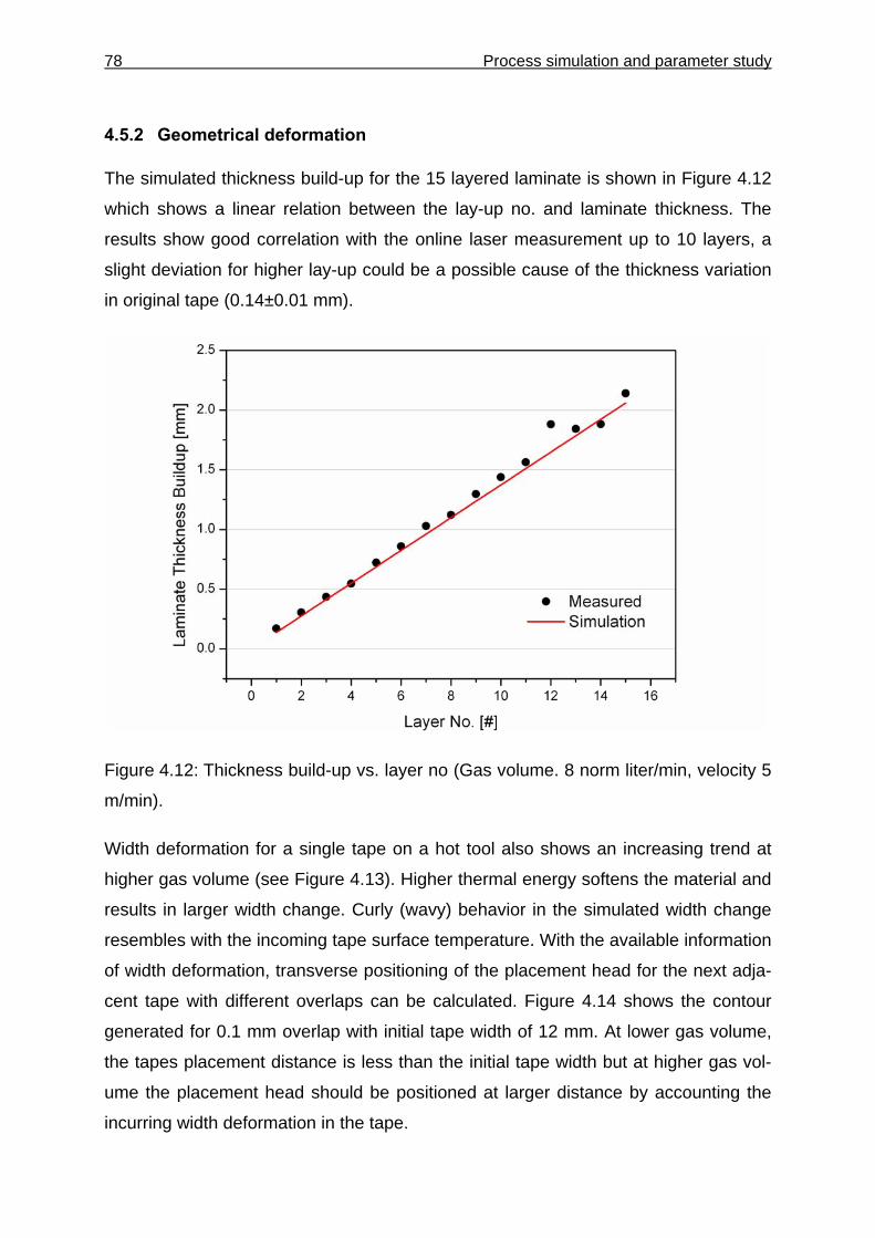
78 Process simulation and parameter study
4.5.2 Geometrical deformation
The simulated thickness build-up for the 15 layered laminate is shown in Figure 4.12
which shows a linear relation between the lay-up no. and laminate thickness. The
results show good correlation with the online laser measurement up to 10 layers, a
slight deviation for higher lay-up could be a possible cause of the thickness variation
in original tape (0.14±0.01 mm).
Figure 4.12: Thickness build-up vs. layer no (Gas volume. 8 norm liter/min, velocity 5
m/min).
Width deformation for a single tape on a hot tool also shows an increasing trend at
higher gas volume (see Figure 4.13). Higher thermal energy softens the material and
results in larger width change. Curly (wavy) behavior in the simulated width change
resembles with the incoming tape surface temperature. With the available information
of width deformation, transverse positioning of the placement head for the next adja-
cent tape with different overlaps can be calculated. Figure 4.14 shows the contour
generated for 0.1 mm overlap with initial tape width of 12 mm. At lower gas volume,
the tapes placement distance is less than the initial tape width but at higher gas vol-
ume the placement head should be positioned at larger distance by accounting the
incurring width deformation in the tape.
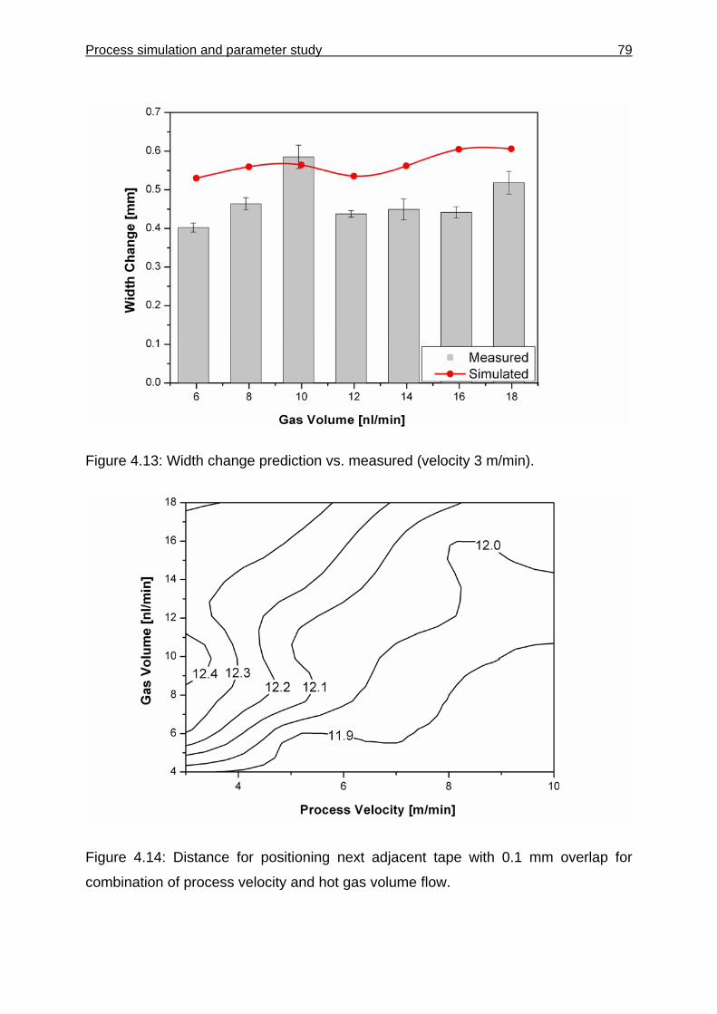
Process simulation and parameter study 79
Figure 4.13: Width change prediction vs. measured (velocity 3 m/min).
Figure 4.14: Distance for positioning next adjacent tape with 0.1 mm overlap for
combination of process velocity and hot gas volume flow.
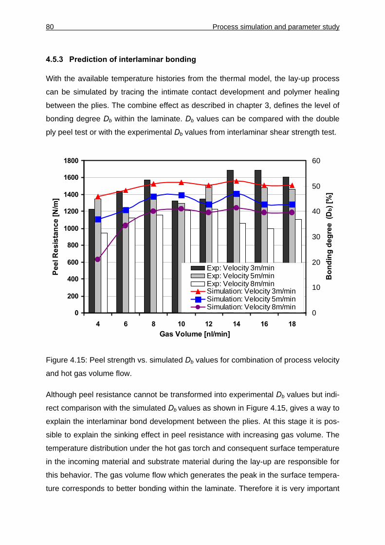
80 Process simulation and parameter study
4.5.3 Prediction of interlaminar bonding
With the available temperature histories from the thermal model, the lay-up process
can be simulated by tracing the intimate contact development and polymer healing
between the plies. The combine effect as described in chapter 3, defines the level of
bonding degree Db within the laminate. Db values can be compared with the double
ply peel test or with the experimental Db values from interlaminar shear strength test.
0
200
400
600
800
1000
1200
1400
1600
1800
4 6 8 10 12 14 16 18Gas Volume [nl/min]
Peel
Res
ista
nce
[N/m
]
0
10
20
30
40
50
60
Bon
ding
deg
ree
(Db)
[%]
Exp: Velocity 3m/minExp: Velocity 5m/minExp: Velocity 8m/minSimulation: Velocity 3m/minSimulation: Velocity 5m/minSimulation: Velocity 8m/min
Figure 4.15: Peel strength vs. simulated Db values for combination of process velocity
and hot gas volume flow.
Although peel resistance cannot be transformed into experimental Db values but indi-
rect comparison with the simulated Db values as shown in Figure 4.15, gives a way to
explain the interlaminar bond development between the plies. At this stage it is pos-
sible to explain the sinking effect in peel resistance with increasing gas volume. The
temperature distribution under the hot gas torch and consequent surface temperature
in the incoming material and substrate material during the lay-up are responsible for
this behavior. The gas volume flow which generates the peak in the surface tempera-
ture corresponds to better bonding within the laminate. Therefore it is very important
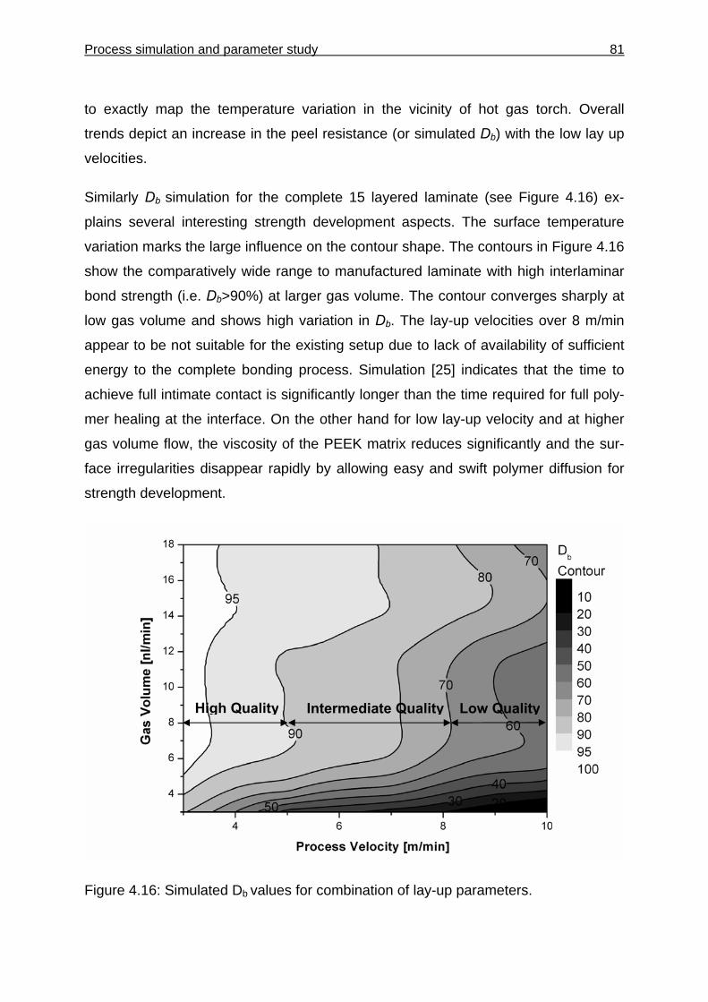
Process simulation and parameter study 81
to exactly map the temperature variation in the vicinity of hot gas torch. Overall
trends depict an increase in the peel resistance (or simulated Db) with the low lay up
velocities.
Similarly Db simulation for the complete 15 layered laminate (see Figure 4.16) ex-
plains several interesting strength development aspects. The surface temperature
variation marks the large influence on the contour shape. The contours in Figure 4.16
show the comparatively wide range to manufactured laminate with high interlaminar
bond strength (i.e. Db>90%) at larger gas volume. The contour converges sharply at
low gas volume and shows high variation in Db. The lay-up velocities over 8 m/min
appear to be not suitable for the existing setup due to lack of availability of sufficient
energy to the complete bonding process. Simulation [25] indicates that the time to
achieve full intimate contact is significantly longer than the time required for full poly-
mer healing at the interface. On the other hand for low lay-up velocity and at higher
gas volume flow, the viscosity of the PEEK matrix reduces significantly and the sur-
face irregularities disappear rapidly by allowing easy and swift polymer diffusion for
strength development.
Figure 4.16: Simulated Db values for combination of lay-up parameters.
High Quality Intermediate Quality Low Quality
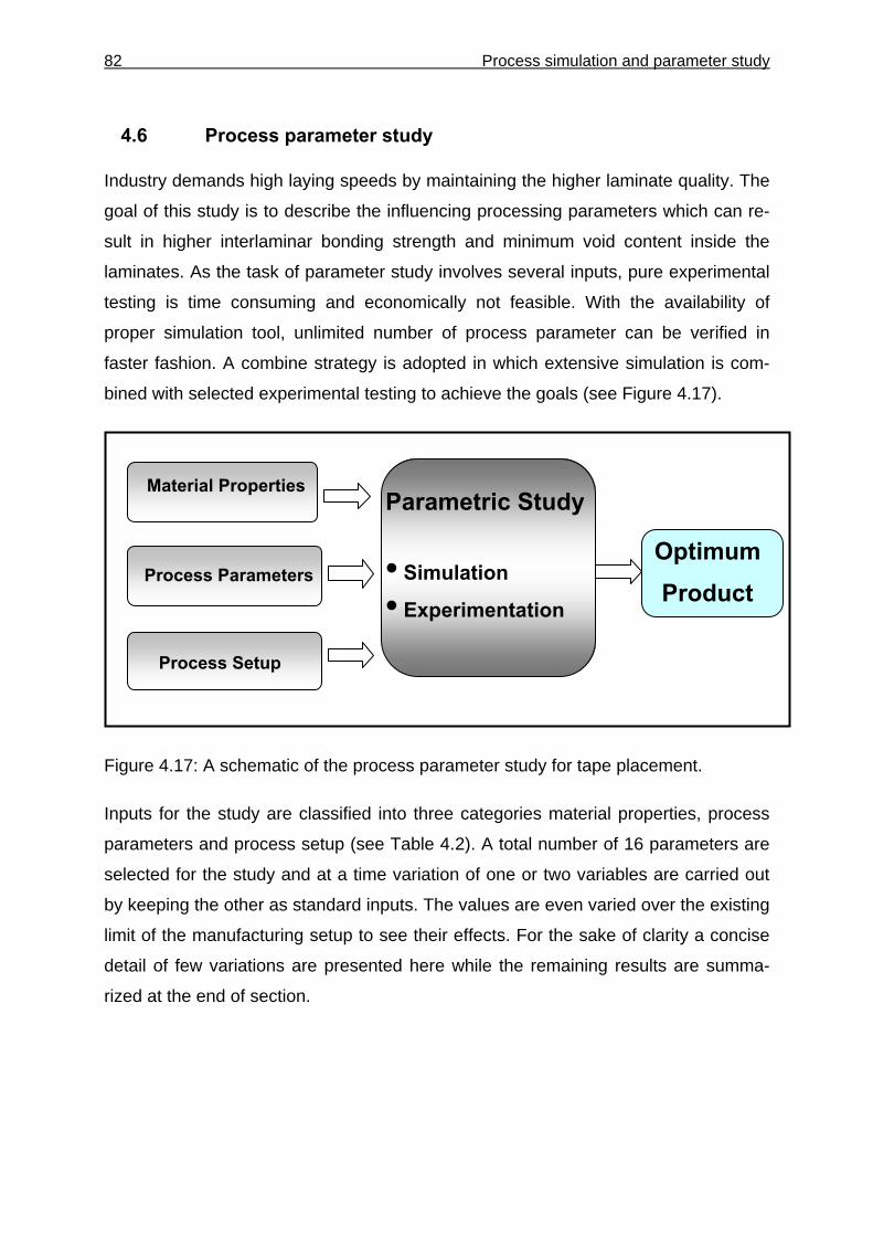
82 Process simulation and parameter study
4.6 Process parameter study
Industry demands high laying speeds by maintaining the higher laminate quality. The
goal of this study is to describe the influencing processing parameters which can re-
sult in higher interlaminar bonding strength and minimum void content inside the
laminates. As the task of parameter study involves several inputs, pure experimental
testing is time consuming and economically not feasible. With the availability of
proper simulation tool, unlimited number of process parameter can be verified in
faster fashion. A combine strategy is adopted in which extensive simulation is com-
bined with selected experimental testing to achieve the goals (see Figure 4.17).
Figure 4.17: A schematic of the process parameter study for tape placement.
Inputs for the study are classified into three categories material properties, process
parameters and process setup (see Table 4.2). A total number of 16 parameters are
selected for the study and at a time variation of one or two variables are carried out
by keeping the other as standard inputs. The values are even varied over the existing
limit of the manufacturing setup to see their effects. For the sake of clarity a concise
detail of few variations are presented here while the remaining results are summa-
rized at the end of section.
Material Properties
Process Setup
Parametric Study
• Simulation
• Experimentation
Optimum Product
Process Parameters
Process simulation and parameter study 83
Table 4.2: Selected process inputs for parameter study, for standard input parame-
ters see Table 4.1.
Process Parameters Process Setup Material PropertiesGas volume Multiple roller Low viscosity
Lay up velocity Additional torch gas volume Initial tape void Roller diameter Force on additional roller Surface roughness Heating length Line compactor with high forces
Consolidation force Tool temperature
Roller temperature Reconsolidation pass Laminate thickness
4.6.1 Effect of consolidation force
Increase in force is considered to result in obtaining better consolidation. Figure 4.18
shows the change in the bonding degree Db and void content with the variation of
force from 50 to 5000 N. For the low lay-up velocity of 3 m/min, even a small force 50
N is capable to produce the bonding degree over 95%, while a slight higher force
165N is well enough to bring it up to 98%, further increase does not seem to be
beneficial. On the other hand at higher lay-up velocities, even the 5000 N of force is
unable to bring the Db to 80%. The reason is incomplete intimate contact and less
residence time under the consolidation roller at higher lay-up velocities which results
in insufficient energy to initiate good bonding.
Void consolidation curves on other hand present the inverse picture. At lower proc-
essing velocity void deconsolidation phenomena upstream to the roller demand very
high consolidation force and must be supplemented by the sudden cooling under and
beyond the roller to freeze this state. But in all cases deconsolidation downstream to
the roller is apparent. Contrary to this fast lay-up velocity causes less void deconsoli-
dation in the heating section hence overall low void contents inside the laminate.
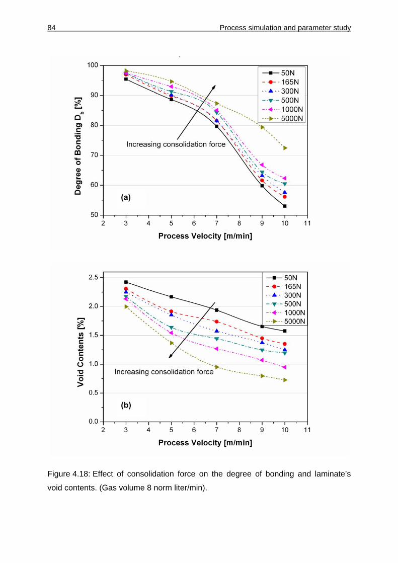
84 Process simulation and parameter study
Figure 4.18: Effect of consolidation force on the degree of bonding and laminate’s
void contents. (Gas volume 8 norm liter/min).
(a)
(b)
Process simulation and parameter study 85
Indeed the consolidation force under the roller is directly related to the interlaminar
contact development but it also increases the internal pressure of the trapped void.
Thus, very high forces are required for the significant improvement making the con-
struction of a tape placement head assembly heavier. Plates were manufactured and
tested to verify the improvement in Db with the increase in consolidation force and
ILSS tests were carried out for the plates manufactured at 100, 160, and 225 N to
examine this effect and it shows (Figure 4.19) good correlation with the simulation.
0
20
40
60
80
100
120
50 100 160 225 300 400Force [N]
Bon
ding
Deg
ree
Db [
%]
ExperimentSimulation
Figure 4.19: Degree of bonding vs. force (Gas volume 6 norm liter/min, velocity 3
m/min).
4.6.2 Effect of number of plies (layers) on laminate quality
Simulations are also performed to investigate the plies (layers) stacking effect i.e.
laminate’s thickness build-up process. The results are shown in Figure 4.20 as a
function of lay-up velocity and as a number of plies in the laminate.
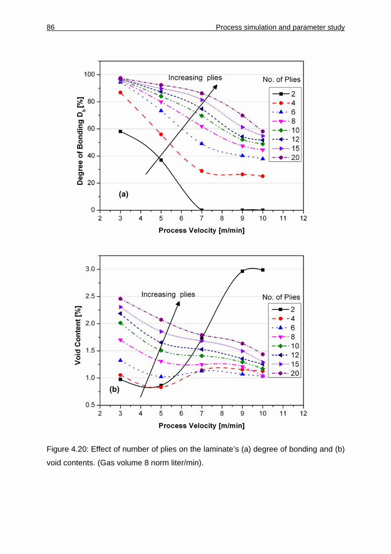
86 Process simulation and parameter study
Figure 4.20: Effect of number of plies on the laminate’s (a) degree of bonding and (b)
void contents. (Gas volume 8 norm liter/min).
(a)
(b)
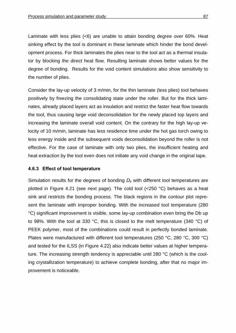
Process simulation and parameter study 87
Laminate with less plies (<6) are unable to attain bonding degree over 60%. Heat
sinking effect by the tool is dominant in these laminate which hinder the bond devel-
opment process. For thick laminates the plies near to the tool act as a thermal insula-
tor by blocking the direct heat flow. Resulting laminate shows better values for the
degree of bonding. Results for the void content simulations also show sensitivity to
the number of plies.
Consider the lay-up velocity of 3 m/min, for the thin laminate (less plies) tool behaves
positively by freezing the consolidating state under the roller. But for the thick lami-
nates, already placed layers act as insulation and restrict the faster heat flow towards
the tool, thus causing large void deconsolidation for the newly placed top layers and
increasing the laminate overall void content. On the contrary for the high lay-up ve-
locity of 10 m/min, laminate has less residence time under the hot gas torch owing to
less energy inside and the subsequent voids deconsolidation beyond the roller is not
effective. For the case of laminate with only two plies, the insufficient heating and
heat extraction by the tool even does not initiate any void change in the original tape.
4.6.3 Effect of tool temperature
Simulation results for the degrees of bonding Db with different tool temperatures are
plotted in Figure 4.21 (see next page). The cold tool (<250 °C) behaves as a heat
sink and restricts the bonding process. The black regions in the contour plot repre-
sent the laminate with improper bonding. With the increased tool temperature (280
°C) significant improvement is visible, some lay-up combination even bring the Db up
to 98%. With the tool at 330 °C, this is closed to the melt temperature (340 °C) of
PEEK polymer, most of the combinations could result in perfectly bonded laminate.
Plates were manufactured with different tool temperatures (250 °C, 280 °C, 300 °C)
and tested for the ILSS (in Figure 4.22) also indicate better values at higher tempera-
ture. The increasing strength tendency is appreciable until 280 °C (which is the cool-
ing crystallization temperature) to achieve complete bonding, after that no major im-
provement is noticeable.
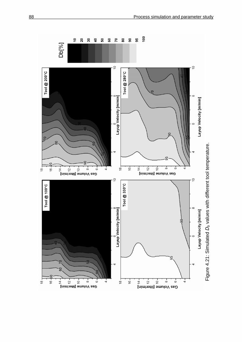
88 Process simulation and parameter study
Figu
re 4
.21:
Sim
ulat
ed D
b val
ues
with
diff
eren
t too
l tem
pera
ture
.
Process simulation and parameter study 89
40
50
60
70
80
90
100
100 200 260 280 300 330
Tool Temperature [°C]
Bon
ding
Deg
ree
Db
[%]
ExperimentSimulation
Figure 4.22: ILSS test results for laminates manufactured at different temperature.
(Gas volume 8 norm liter/min, velocity 3 m/min).
4.6.4 Overview
All other parameters listed in Table 4.2 were analyzed in the similar fashion [82]. Re-
ferring back to Figure 4.16, laminate quality based on the degree of bonding can be
classified into three levels.
• High quality laminate with Db > 90%
• Intermediate quality laminate with 90% > Db > 70%
• Low quality laminate with Db < 60%
For every gas volumes, these three quality levels exist as variable band in combina-
tion of lay up velocities. Also these levels are wide spreads at higher gas volume
compared to the lesser gas volume.
By considering the gas volume of 8 norm liter/min, the bench mark values for the Db
and void contents at these three levels can be obtain at lay up velocities of 3, 5 and 9
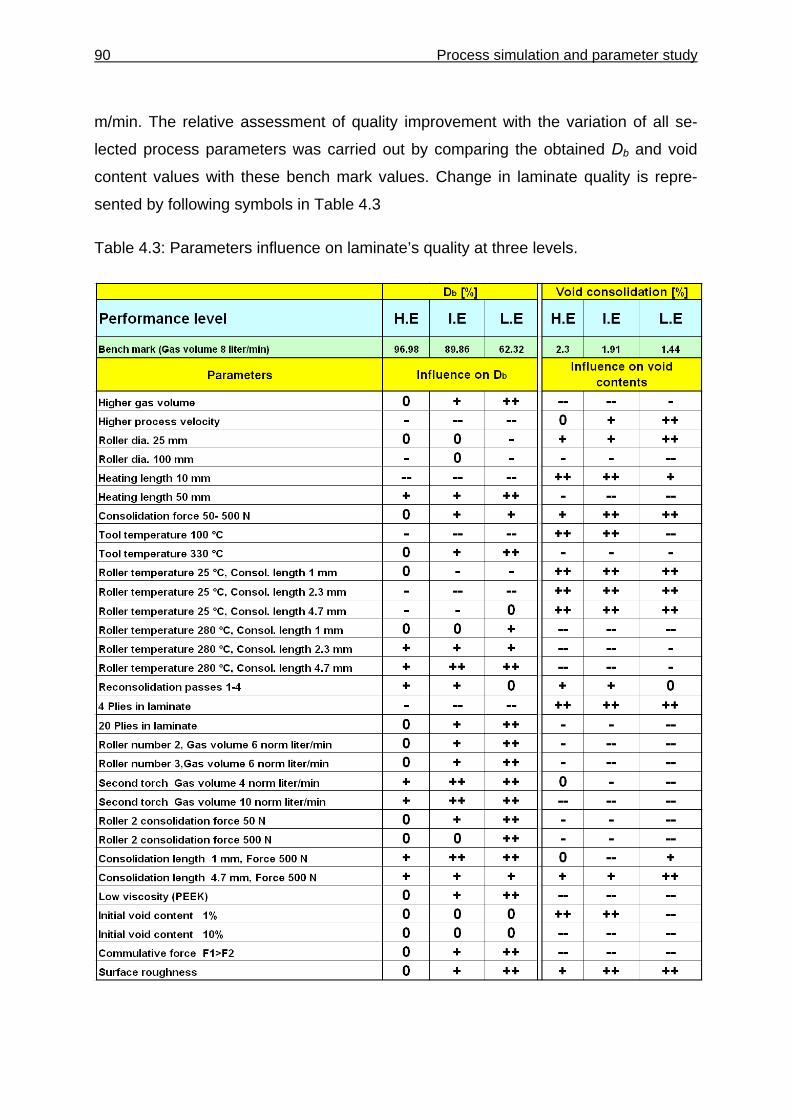
90 Process simulation and parameter study
m/min. The relative assessment of quality improvement with the variation of all se-
lected process parameters was carried out by comparing the obtained Db and void
content values with these bench mark values. Change in laminate quality is repre-
sented by following symbols in Table 4.3
Table 4.3: Parameters influence on laminate’s quality at three levels.
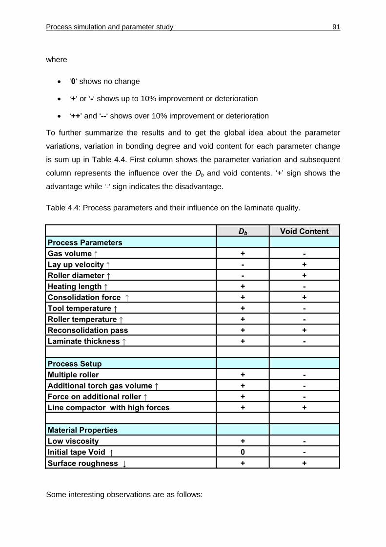
Process simulation and parameter study 91
where
• ‘0’ shows no change
• ‘+’ or ‘-‘ shows up to 10% improvement or deterioration
• ‘++’ and ‘--‘ shows over 10% improvement or deterioration
To further summarize the results and to get the global idea about the parameter
variations, variation in bonding degree and void content for each parameter change
is sum up in Table 4.4. First column shows the parameter variation and subsequent
column represents the influence over the Db and void contents. ‘+’ sign shows the
advantage while ‘-‘ sign indicates the disadvantage.
Table 4.4: Process parameters and their influence on the laminate quality.
Db Void Content Process Parameters Gas volume ↑ + - Lay up velocity ↑ - + Roller diameter ↑ - + Heating length ↑ + - Consolidation force ↑ + + Tool temperature ↑ + - Roller temperature ↑ + - Reconsolidation pass + + Laminate thickness ↑ + - Process Setup Multiple roller + - Additional torch gas volume ↑ + - Force on additional roller ↑ + - Line compactor with high forces + + Material Properties Low viscosity + - Initial tape Void ↑ 0 - Surface roughness ↓ + +
Some interesting observations are as follows:
92 Process simulation and parameter study
• All parameter variations, which supplements the additional heat energy (e.g.
high gas volume, low lay-up velocity) during the lay-up process contributes to
an improvement in the Db value. At the same time such combination increases
the volume void content and reduces the laminate quality.
• Large roller diameter or consolidation length only benefits in combination with
higher force, by extending line pressure to improve both Db and better void
consolidation in the laminate.
• For any particular combination, laminate thickness build-up seems to be posi-
tive, the underneath layer acts as an insulator by hindering the rapid heat flow
from top layer to relatively cold tool. Thus providing more time for polymer dif-
fusion.
• Increase in roller temperature enhanced the bonding process on one side but
accelerates the void expansion (deconsolidation) at the roller exit.
• High tool temperature (up to 300 °C) supports polymer diffusion to improve the
bonding strength.
• Laminate’s top layers always lack the complete consolidation, additional
passes over these layers not only helps in improving the Db values but also in
eliminating trapped void from the laminate.
• Noteworthy improvement in Db value can be obtained through placement head
with multiple rollers. Simulation indicates an additional roller is sufficient to get
this benefit.
• Higher consolidation force on the first roller results in better laminate strength,
as the incoming tape and substrate interface receives high thermal energy by
first torch before entering the consolidation roller.
• Laminate quality is highly influenced by the tape’s initial void content. Tape
with fewer voids is less prone to void deconsolidation.
• Tape with flat surface or with less roughness, results in better intimate contact
generation and enhance the bonding between the layers.
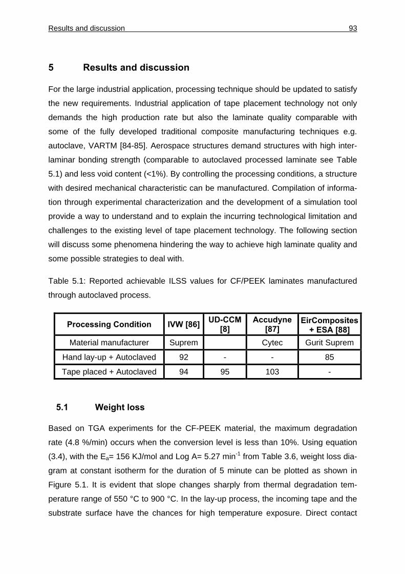
Results and discussion 93
5 Results and discussion
For the large industrial application, processing technique should be updated to satisfy
the new requirements. Industrial application of tape placement technology not only
demands the high production rate but also the laminate quality comparable with
some of the fully developed traditional composite manufacturing techniques e.g.
autoclave, VARTM [84-85]. Aerospace structures demand structures with high inter-
laminar bonding strength (comparable to autoclaved processed laminate see Table
5.1) and less void content (<1%). By controlling the processing conditions, a structure
with desired mechanical characteristic can be manufactured. Compilation of informa-
tion through experimental characterization and the development of a simulation tool
provide a way to understand and to explain the incurring technological limitation and
challenges to the existing level of tape placement technology. The following section
will discuss some phenomena hindering the way to achieve high laminate quality and
some possible strategies to deal with.
Table 5.1: Reported achievable ILSS values for CF/PEEK laminates manufactured
through autoclaved process.
Processing Condition IVW [86] UD-CCM [8]
Accudyne [87]
EirComposites + ESA [88]
Material manufacturer Suprem Cytec Gurit Suprem
Hand lay-up + Autoclaved 92 - - 85
Tape placed + Autoclaved 94 95 103 -
5.1 Weight loss
Based on TGA experiments for the CF-PEEK material, the maximum degradation
rate (4.8 %/min) occurs when the conversion level is less than 10%. Using equation
(3.4), with the Ea= 156 KJ/mol and Log A= 5.27 min-1 from Table 3.6, weight loss dia-
gram at constant isotherm for the duration of 5 minute can be plotted as shown in
Figure 5.1. It is evident that slope changes sharply from thermal degradation tem-
perature range of 550 °C to 900 °C. In the lay-up process, the incoming tape and the
substrate surface have the chances for high temperature exposure. Direct contact
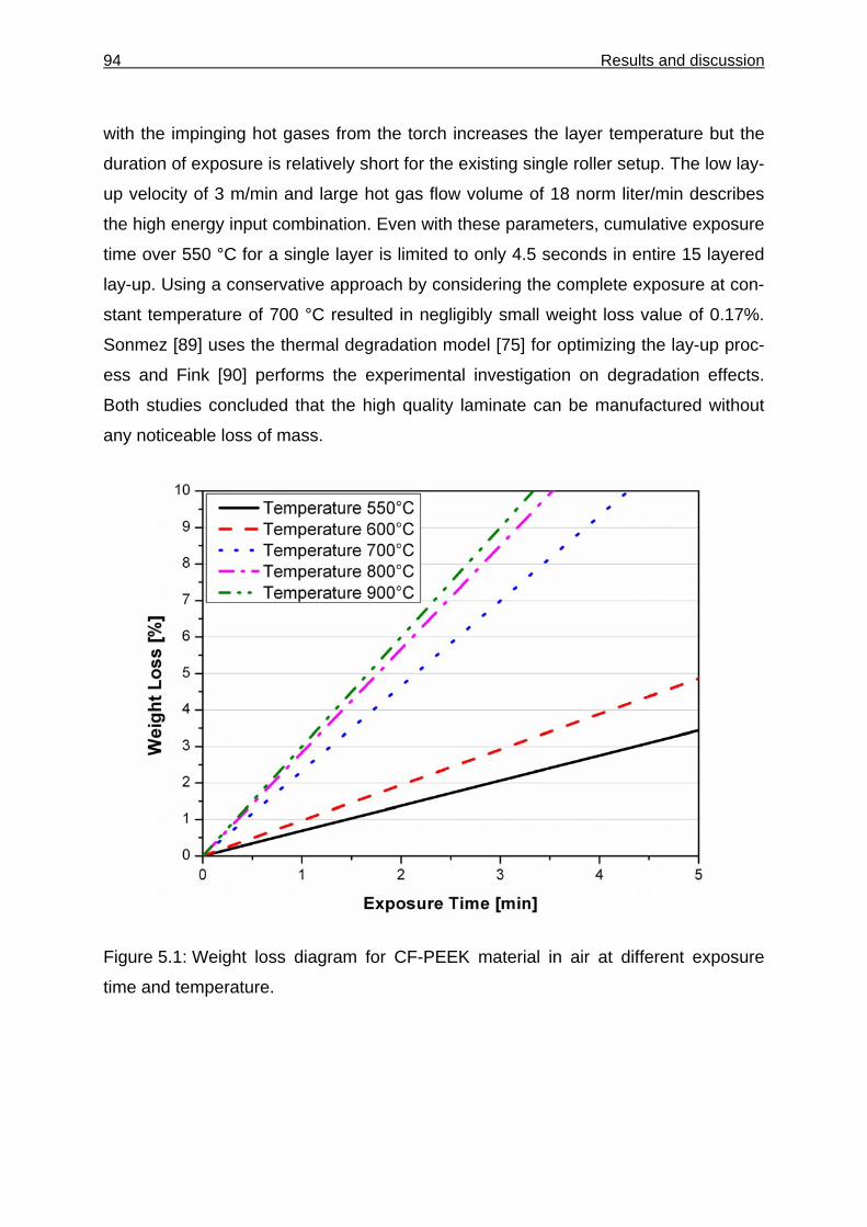
94 Results and discussion
with the impinging hot gases from the torch increases the layer temperature but the
duration of exposure is relatively short for the existing single roller setup. The low lay-
up velocity of 3 m/min and large hot gas flow volume of 18 norm liter/min describes
the high energy input combination. Even with these parameters, cumulative exposure
time over 550 °C for a single layer is limited to only 4.5 seconds in entire 15 layered
lay-up. Using a conservative approach by considering the complete exposure at con-
stant temperature of 700 °C resulted in negligibly small weight loss value of 0.17%.
Sonmez [89] uses the thermal degradation model [75] for optimizing the lay-up proc-
ess and Fink [90] performs the experimental investigation on degradation effects.
Both studies concluded that the high quality laminate can be manufactured without
any noticeable loss of mass.
Figure 5.1: Weight loss diagram for CF-PEEK material in air at different exposure
time and temperature.
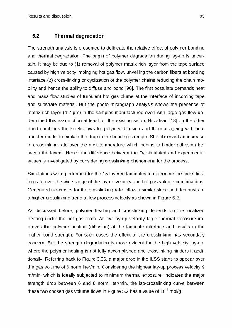
Results and discussion 95
5.2 Thermal degradation
The strength analysis is presented to delineate the relative effect of polymer bonding
and thermal degradation. The origin of polymer degradation during lay-up is uncer-
tain. It may be due to (1) removal of polymer matrix rich layer from the tape surface
caused by high velocity impinging hot gas flow, unveiling the carbon fibers at bonding
interface (2) cross-linking or cyclization of the polymer chains reducing the chain mo-
bility and hence the ability to diffuse and bond [90]. The first postulate demands heat
and mass flow studies of turbulent hot gas plume at the interface of incoming tape
and substrate material. But the photo micrograph analysis shows the presence of
matrix rich layer (4-7 µm) in the samples manufactured even with large gas flow un-
dermined this assumption at least for the existing setup. Nicodeau [18] on the other
hand combines the kinetic laws for polymer diffusion and thermal ageing with heat
transfer model to explain the drop in the bonding strength. She observed an increase
in crosslinking rate over the melt temperature which begins to hinder adhesion be-
tween the layers. Hence the difference between the Db simulated and experimental
values is investigated by considering crosslinking phenomena for the process.
Simulations were performed for the 15 layered laminates to determine the cross link-
ing rate over the wide range of the lay-up velocity and hot gas volume combinations.
Generated iso-curves for the crosslinking rate follow a similar slope and demonstrate
a higher crosslinking trend at low process velocity as shown in Figure 5.2.
As discussed before, polymer healing and crosslinking depends on the localized
heating under the hot gas torch. At low lay-up velocity large thermal exposure im-
proves the polymer healing (diffusion) at the laminate interface and results in the
higher bond strength. For such cases the effect of the crosslinking has secondary
concern. But the strength degradation is more evident for the high velocity lay-up,
where the polymer healing is not fully accomplished and crosslinking hinders it addi-
tionally. Referring back to Figure 3.36, a major drop in the ILSS starts to appear over
the gas volume of 6 norm liter/min. Considering the highest lay-up process velocity 9
m/min, which is ideally subjected to minimum thermal exposure, indicates the major
strength drop between 6 and 8 norm liter/min, the iso-crosslinking curve between
these two chosen gas volume flows in Figure 5.2 has a value of 10-4 mol/g.
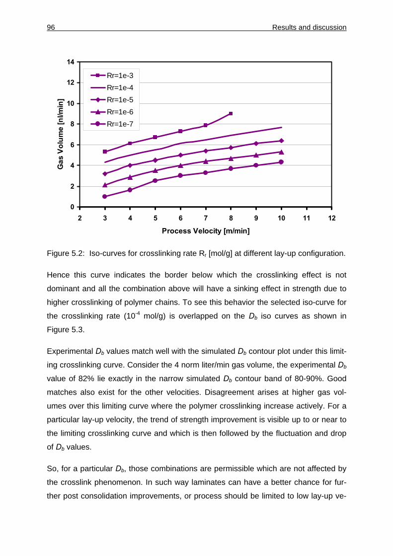
96 Results and discussion
0
2
4
6
8
10
12
14
2 3 4 5 6 7 8 9 10 11 12
Process Velocity [m/min]
Gas
Vol
ume
[nl/m
in]
Rr=1e-3Rr=1e-4Rr=1e-5Rr=1e-6Rr=1e-7
Figure 5.2: Iso-curves for crosslinking rate Rr [mol/g] at different lay-up configuration.
Hence this curve indicates the border below which the crosslinking effect is not
dominant and all the combination above will have a sinking effect in strength due to
higher crosslinking of polymer chains. To see this behavior the selected iso-curve for
the crosslinking rate (10-4 mol/g) is overlapped on the Db iso curves as shown in
Figure 5.3.
Experimental Db values match well with the simulated Db contour plot under this limit-
ing crosslinking curve. Consider the 4 norm liter/min gas volume, the experimental Db
value of 82% lie exactly in the narrow simulated Db contour band of 80-90%. Good
matches also exist for the other velocities. Disagreement arises at higher gas vol-
umes over this limiting curve where the polymer crosslinking increase actively. For a
particular lay-up velocity, the trend of strength improvement is visible up to or near to
the limiting crosslinking curve and which is then followed by the fluctuation and drop
of Db values.
So, for a particular Db, those combinations are permissible which are not affected by
the crosslink phenomenon. In such way laminates can have a better chance for fur-
ther post consolidation improvements, or process should be limited to low lay-up ve-
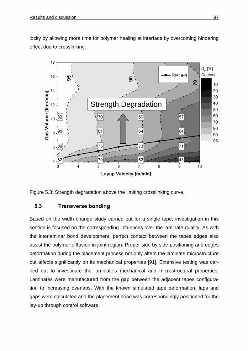
Results and discussion 97
locity by allowing more time for polymer healing at interface by overcoming hindering
effect due to crosslinking.
Figure 5.3: Strength degradation above the limiting crosslinking curve.
5.3 Transverse bonding
Based on the width change study carried out for a single tape, investigation in this
section is focused on the corresponding influences over the laminate quality. As with
the interlaminar bond development, perfect contact between the tapes edges also
assist the polymer diffusion in joint region. Proper side by side positioning and edges
deformation during the placement process not only alters the laminate microstructure
but affects significantly on its mechanical properties [91]. Extensive testing was car-
ried out to investigate the laminate’s mechanical and microstructural properties.
Laminates were manufactured from the gap between the adjacent tapes configura-
tion to increasing overlaps. With the known simulated tape deformation, laps and
gaps were calculated and the placement head was correspondingly positioned for the
lay-up through control software.
Strength Degradation
95
90
70
98 Results and discussion
Figure 5.4: (a) Sample specification for the transverse tensile test (b) Transverse
fracture away from joint (Gas volume 14 norm liter/min, velocity 3 m/min).
Transverse tensile test has been historically used to measure the 90° tensile proper-
ties of unidirectional composite materials. Major draw back of the direct transverse
testing method are the premature failure of the test sample as a result of the exis-
tence internal flaws and failure at the grips. Therefore this test is not recommended
for the joint strength evaluation. For this experimental study more than 60% of the
tested samples experienced these failures making it difficult to interpret the actual
joint strength. Figure 5.4(a) shows the transverse tensile strength test sample along
with transverse fracture, the Figure 5.4(b) clearly shows the fracture propagate away
from the transverse joint.
30 mm
Tape joint
Fracture
(b
(a)
Force
Force
Results and discussion 99
Figure 5.5: Transverse flexural failure at joint section.
Another technique to create transverse failure in tension is by subjecting the laminate
to bending loads. For example under a simple three point flexural loading, the maxi-
mum tensile stress occurs only along a line across the tensile surface at the speci-
men mid span. Accordingly, if the test sample’s joint section is positioned exactly un-
der the loading nose then this specimen should be significantly less flaw sensitive
than a transverse tensile sample. Therefore, the strength results obtained should be
more representative of the actual joint transverse tensile strength [92]. Hence the
transverse flexural samples 20 mm wide and 10 mm long were fabricated. The load-
ing conditions for the test were selected as per DIN EN ISO 178 standards. Figure
5.5 shows the transverse flexural sample after fracture in transverse direction, the
fracture surface passed exactly through the joint section.
The curves in Figure 5.6 shows the two different failure mode experienced in the test-
ing. In both cases forces increased linearly with increasing flexure of the sample, till
the sample failed with the crack initiating from the bottom. The load represents the
maximum transverse load which thereafter falls to zero. However in some sample the
force did not fall immediately, as it recovered midway while the crack continue to
grow. The crack diversion was observed in those samples, as it grew sideways until
the test sample completely broken.
200 µm
100 Results and discussion
0
50
100
150
200
250
0 1 2 3 4 5
Strain [%]
Forc
e [N
]
Figure 5.6: Failure load curve for transverse flexural test (Gas volume 8 norm li-
ter/min, velocity 3 m/min).
Based on the energy levels identified for the single tape deformation in Figure 3.18,
samples from the laminates manufactured with low energy level (Gas Volume. 6
norm liter/min, Velocity 8 m/min) and intermediate energy level (Gas volume 8 norm
liter/min, Velocity 3 m/min) were tested. Photomicrographs from the laminate manu-
factured with low energy level combinations are shown in Figure 5.7 (a & b). Appar-
ent is the fine resin bonded region between the rectangular edges in the first configu-
ration. Edges follow type II & III deformation and produced perfect bond with each
other. The second photomicrograph represents a laminate with 0.15 mm of side over-
laps.
Failure load
Load recovery
Results and discussion 101
Figure 5.7: (a) Transverse joint with no overlap (b) Transverse joint with 0.15 mm
overlap (Gas Volume. 6 norm liter/min, velocity 8 m/min).
Figure 5.8 shows the apparent difference in mean transverse flexure strength for the
two cases. As the failure and crack propagation in pure bonded region took place at
low loading. But in the second laminate where the bonded region is filled with the car-
bon fibers with slight overlapping, the transverse flexural strength increased over
10%.
40
50
60
70
80
90
100
110
Matrix Joint Overlap 0.15 mm
Tran
sver
se F
lexu
ral S
treng
th [
MPa
]
Figure 5.8: Transverse flexural strength comparisons between pure matrix joint and
overlap joint for the LE laminate (Gas volume 6 norm liter/min, velocity 8 m/min).
500 µm
Overlaps
500 µm
Gap filled with matrix
(a) (b)
102 Results and discussion
Tests were then performed on the laminate manufactured with intermediate energy
level. The objectives were two folds, firstly to find out the maximum achievable value
of transverse flexural strength for the laminate manufactured using tape placement
process and secondly the effect of increasing tape overlaps. The laminate produced
with generated gap of 0.1 mm was very fragile to cut and broke away during the flex-
ural sample preparation. Hence no samples were prepared for the transverse testing.
50
60
70
80
90
100
110
Gap 0.1 mm Overlap 0 mm
Overlap 0.1 mm
Overlap0.16 mm
Overlap0.16 mm
AdditionalPass
Autoclaved
Tran
sver
se F
lexu
ral S
treng
th [
MPa
]
Figure 5.9: Effect of overlap and gaps on the laminate’s transverse and interlaminar
shear strength (Gas Volume. 8 norm liter/min, velocity 3 m/min).
Laminates manufactured with perfect edge contact (no gap/overlap) and with in-
creasing overlap show the very slight variation in strength (see Figure 5.9). The
mean value for transverse flexural strength is around 75-80 MPa. Light microscopic
examination revealed that the fibers translated into the matrix region even for the no
overlap configuration. Presence of the fiber reinforced the transverse joint and con-
sequently provides higher values. Increase in overlap distance (0.16 mm) in fact re-
veals a slight decreasing trend. Photomicrograph from these sample showed the
presence of the interlaminar void near to the joint region in top layers see Figure
Samples not
prepared
Results and discussion 103
5.10. Presence of interlaminar void thus reduced the transverse strength as the frac-
ture propagation could shift to the nearby weak regions. An improvement was per-
formed by consolidating the top layers with two additional passes with hot gas torch
turned off. The elimination of the trapped void in top layer improved the strength.
Comparison with autoclave plate shows the relative strength difference of about 10%.
But the tape placed laminates showed less strength variation and the mean values
from these plates lie within the scatter range of autoclaved plate.
Figure 5.10: (a) Void within the top layers (b) Void elimination with additional consoli-
dation passes. (Gas volume 8 norm liter/min, velocity 3 m/min).
5.4 Lay-up parameters selection for manufacturing
The preparation stage in lay-up process involves selection of several setup parame-
ters as shown in Figure 2.3. Using high interlaminar strength as the criteria, a quick
setup scheme for the laminate lay-up is presented here by considering the IVW
setup.
• Higher roller temperatures foster the bonding process. But to avoid the mate-
rial sticking maintain the roller below the glass transition temperature. For the
water controlled tempered roller, 90 °C is the fine compromise.
• Parameter study disclosed that the temperature up to 280 °C is fair enough to
improve the bonding in the early layers and it also provides the proper first ply
sticking mechanism.
• Compaction force less than 50 N generate insufficient consolidating pressure
500 µm 500 µm
Voids
(a) (b)
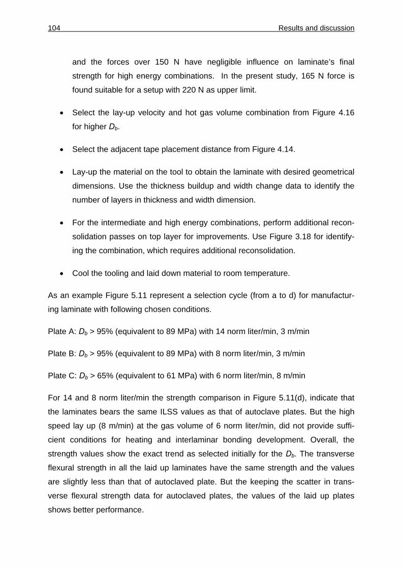
104 Results and discussion
and the forces over 150 N have negligible influence on laminate’s final
strength for high energy combinations. In the present study, 165 N force is
found suitable for a setup with 220 N as upper limit.
• Select the lay-up velocity and hot gas volume combination from Figure 4.16
for higher Db.
• Select the adjacent tape placement distance from Figure 4.14.
• Lay-up the material on the tool to obtain the laminate with desired geometrical
dimensions. Use the thickness buildup and width change data to identify the
number of layers in thickness and width dimension.
• For the intermediate and high energy combinations, perform additional recon-
solidation passes on top layer for improvements. Use Figure 3.18 for identify-
ing the combination, which requires additional reconsolidation.
• Cool the tooling and laid down material to room temperature.
As an example Figure 5.11 represent a selection cycle (from a to d) for manufactur-
ing laminate with following chosen conditions.
Plate A: Db > 95% (equivalent to 89 MPa) with 14 norm liter/min, 3 m/min
Plate B: Db > 95% (equivalent to 89 MPa) with 8 norm liter/min, 3 m/min
Plate C: Db > 65% (equivalent to 61 MPa) with 6 norm liter/min, 8 m/min
For 14 and 8 norm liter/min the strength comparison in Figure 5.11(d), indicate that
the laminates bears the same ILSS values as that of autoclave plates. But the high
speed lay up (8 m/min) at the gas volume of 6 norm liter/min, did not provide suffi-
cient conditions for heating and interlaminar bonding development. Overall, the
strength values show the exact trend as selected initially for the Db. The transverse
flexural strength in all the laid up laminates have the same strength and the values
are slightly less than that of autoclaved plate. But the keeping the scatter in trans-
verse flexural strength data for autoclaved plates, the values of the laid up plates
shows better performance.
Results and discussion 105
Figu
re 5
.11:
Pro
cess
par
amet
ers
sele
ctio
n cy
cle.
A B
A B
C
A
B
C
C
(a)
(b)
(c)
(d)
Det
ail i
n F
igur
e 4.
16
Det
ail i
n Fi
gure
4.1
4
Det
ail i
n Fi
gure
3.1
8

106 Results and discussion
5.5 High quality thermoplastic prepreg material
Although the existing setup can produce the laminate with suggested bonding
strength but the control over the void content values still need some attention. By far
the use of high quality thermoplastic tape seems to be more easy and efficient way to
obtain structure with high mechanical performance. Unfortunately no standard criteria
have been recognized so far but studies have been performed conformable to the
individual placement setup. Some possible criteria for the tape material are dis-
cussed below for technological development.
5.5.1 Tape edges
Beresheim [3] developed a criterion to classify the tape edges into seven different
classes. Tape with rectangular edges was designated best for the transverse bond-
ings while the tape with distorted edges or with cracks was found not feasible for per-
fect bonding. Study on tape edges deformation as discussed before fortified these
facts by indicating the effect on laminates transverse joint. Tapes with rectangle edge
or edge with slight roundness is recommended, as the deformation behaviour for
these geometries can be predicted [81] and lay-up head can be positioned to have
proper overlaps for transverse joint.
5.5.2 Surface roughness
As discussed before the irregularities on tape surface hinder the contact develop-
ment between the layers while the flat tape facilitate in attaining high interlaminar
bonding strength. Simulation for intimate contact development for a 15 layered lami-
nate by assuming a highly rough tape surface (FD = 1.8), moderately rough surface
(FD = 1.4), and relatively smooth surface (FD = 1.2) is shown in Figure 5.12. The
higher intimate contact through out the laminate with smooth tape is evident.
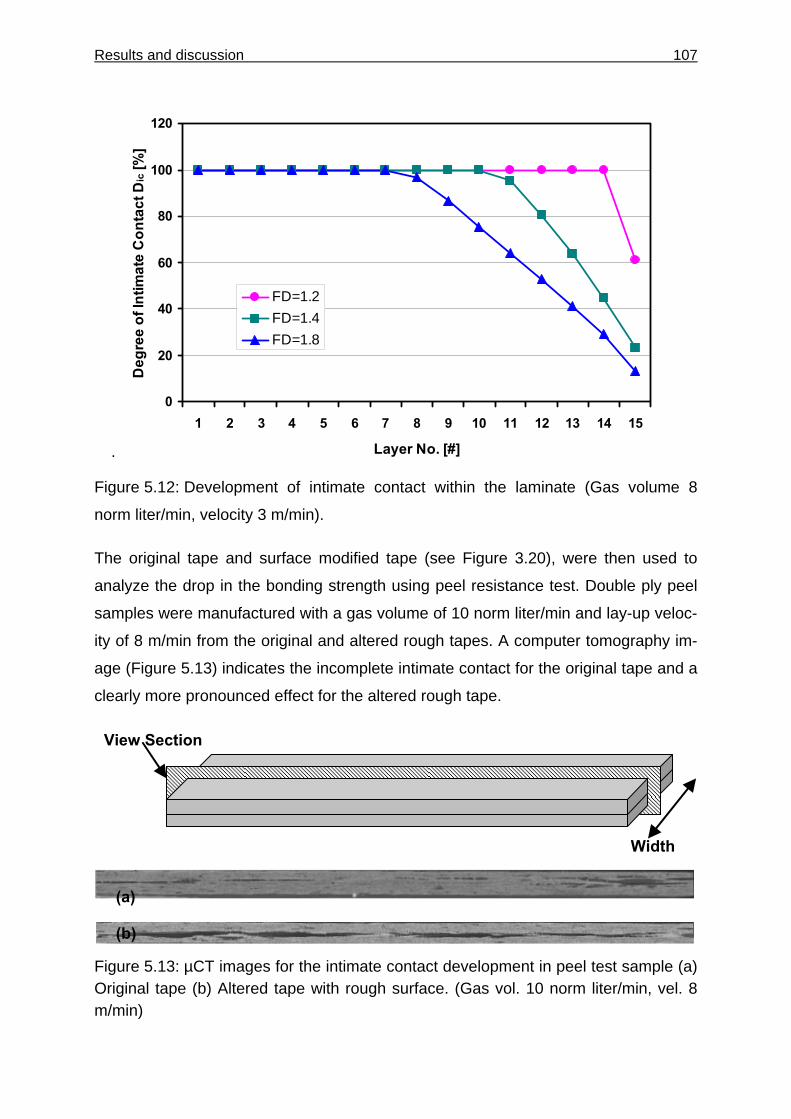
Results and discussion 107
.
0
20
40
60
80
100
120
1 2 3 4 5 6 7 8 9 10 11 12 13 14 15
Layer No. [#]
Deg
ree
of In
timat
e C
onta
ct D
ic [%
]
FD=1.2FD=1.4FD=1.8
Figure 5.12: Development of intimate contact within the laminate (Gas volume 8
norm liter/min, velocity 3 m/min).
The original tape and surface modified tape (see Figure 3.20), were then used to
analyze the drop in the bonding strength using peel resistance test. Double ply peel
samples were manufactured with a gas volume of 10 norm liter/min and lay-up veloc-
ity of 8 m/min from the original and altered rough tapes. A computer tomography im-
age (Figure 5.13) indicates the incomplete intimate contact for the original tape and a
clearly more pronounced effect for the altered rough tape.
Figure 5.13: µCT images for the intimate contact development in peel test sample (a) Original tape (b) Altered tape with rough surface. (Gas vol. 10 norm liter/min, vel. 8 m/min)
View Section
Width
(a)
(b)
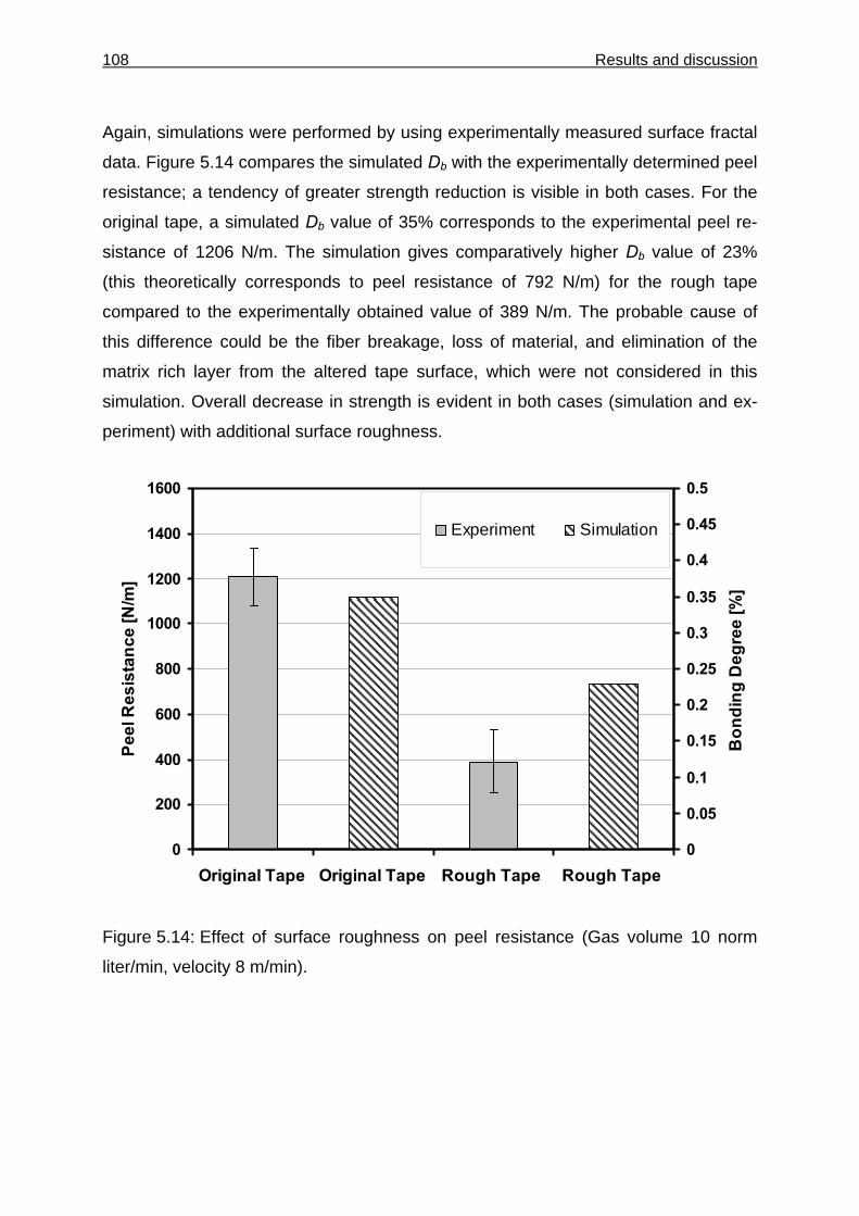
108 Results and discussion
Again, simulations were performed by using experimentally measured surface fractal
data. Figure 5.14 compares the simulated Db with the experimentally determined peel
resistance; a tendency of greater strength reduction is visible in both cases. For the
original tape, a simulated Db value of 35% corresponds to the experimental peel re-
sistance of 1206 N/m. The simulation gives comparatively higher Db value of 23%
(this theoretically corresponds to peel resistance of 792 N/m) for the rough tape
compared to the experimentally obtained value of 389 N/m. The probable cause of
this difference could be the fiber breakage, loss of material, and elimination of the
matrix rich layer from the altered tape surface, which were not considered in this
simulation. Overall decrease in strength is evident in both cases (simulation and ex-
periment) with additional surface roughness.
0
200
400
600
800
1000
1200
1400
1600
Original Tape Original Tape Rough Tape Rough Tape
Peel
Res
ista
nce
[N/m
]
0
0.05
0.1
0.15
0.2
0.25
0.3
0.35
0.4
0.45
0.5
Bon
ding
Deg
ree
[%]
Experiment Simulation
Figure 5.14: Effect of surface roughness on peel resistance (Gas volume 10 norm
liter/min, velocity 8 m/min).
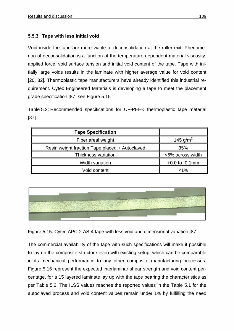
Results and discussion 109
5.5.3 Tape with less initial void
Void inside the tape are more viable to deconsolidation at the roller exit. Phenome-
non of deconsolidation is a function of the temperature dependent material viscosity,
applied force, void surface tension and initial void content of the tape. Tape with ini-
tially large voids results in the laminate with higher average value for void content
[20, 82]. Thermoplastic tape manufacturers have already identified this industrial re-
quirement. Cytec Engineered Materials is developing a tape to meet the placement
grade specification [87] see Figure 5.15
Table 5.2: Recommended specifications for CF-PEEK thermoplastic tape material
[87].
Tape Specification Fiber areal weight 145 g/m2
Resin weight fraction Tape placed + Autoclaved 35% Thickness variation <6% across width
Width variation +0.0 to -0.1mm Void content <1%
Figure 5.15: Cytec APC-2 AS-4 tape with less void and dimensional variation [87].
The commercial availability of the tape with such specifications will make it possible
to lay-up the composite structure even with existing setup, which can be comparable
in its mechanical performance to any other composite manufacturing processes.
Figure 5.16 represent the expected interlaminar shear strength and void content per-
centage, for a 15 layered laminate lay up with the tape bearing the characteristics as
per Table 5.2. The ILSS values reaches the reported values in the Table 5.1 for the
autoclaved process and void content values remain under 1% by fulfilling the need
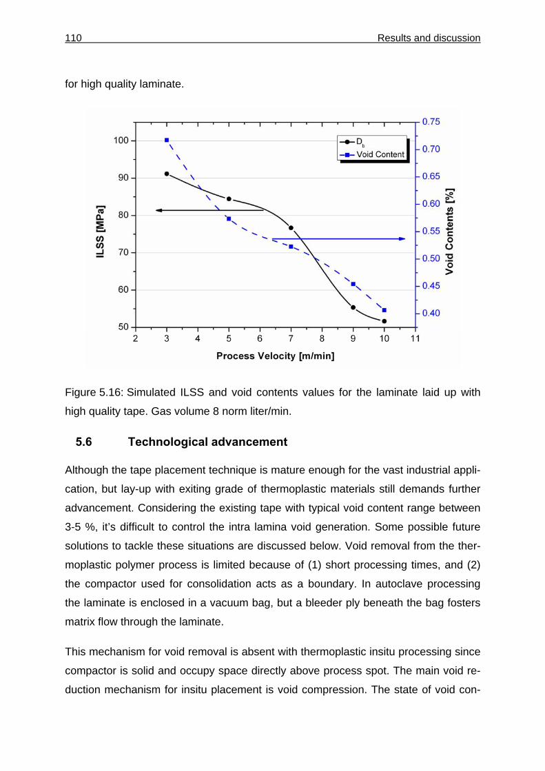
110 Results and discussion
for high quality laminate.
Figure 5.16: Simulated ILSS and void contents values for the laminate laid up with
high quality tape. Gas volume 8 norm liter/min.
5.6 Technological advancement
Although the tape placement technique is mature enough for the vast industrial appli-
cation, but lay-up with exiting grade of thermoplastic materials still demands further
advancement. Considering the existing tape with typical void content range between
3-5 %, it’s difficult to control the intra lamina void generation. Some possible future
solutions to tackle these situations are discussed below. Void removal from the ther-
moplastic polymer process is limited because of (1) short processing times, and (2)
the compactor used for consolidation acts as a boundary. In autoclave processing
the laminate is enclosed in a vacuum bag, but a bleeder ply beneath the bag fosters
matrix flow through the laminate.
This mechanism for void removal is absent with thermoplastic insitu processing since
compactor is solid and occupy space directly above process spot. The main void re-
duction mechanism for insitu placement is void compression. The state of void con-
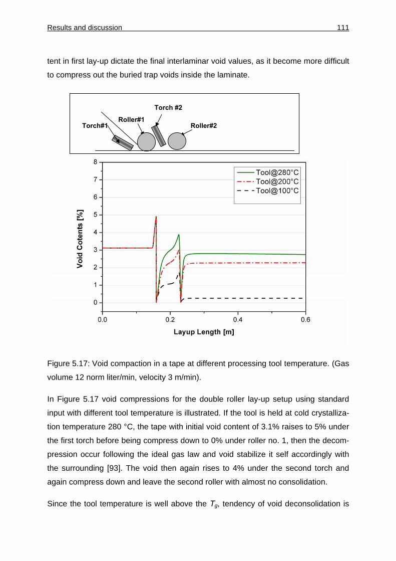
Results and discussion 111
tent in first lay-up dictate the final interlaminar void values, as it become more difficult
to compress out the buried trap voids inside the laminate.
Figure 5.17: Void compaction in a tape at different processing tool temperature. (Gas
volume 12 norm liter/min, velocity 3 m/min).
In Figure 5.17 void compressions for the double roller lay-up setup using standard
input with different tool temperature is illustrated. If the tool is held at cold crystalliza-
tion temperature 280 °C, the tape with initial void content of 3.1% raises to 5% under
the first torch before being compress down to 0% under roller no. 1, then the decom-
pression occur following the ideal gas law and void stabilize it self accordingly with
the surrounding [93]. The void then again rises to 4% under the second torch and
again compress down and leave the second roller with almost no consolidation.
Since the tool temperature is well above the Tg, tendency of void deconsolidation is
Roller#1 Roller#2 Torch#1
Torch #2
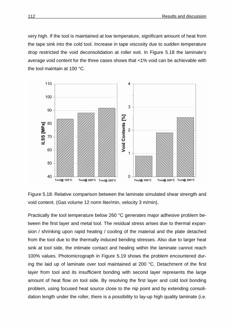
112 Results and discussion
very high. If the tool is maintained at low temperature, significant amount of heat from
the tape sink into the cold tool. Increase in tape viscosity due to sudden temperature
drop restricted the void deconsolidation at roller exit. In Figure 5.18 the laminate’s
average void content for the three cases shows that <1% void can be achievable with
the tool maintain at 100 °C.
Figure 5.18: Relative comparison between the laminate simulated shear strength and
void content. (Gas volume 12 norm liter/min, velocity 3 m/min).
Practically the tool temperature below 260 °C generates major adhesive problem be-
tween the first layer and metal tool. The residual stress arises due to thermal expan-
sion / shrinking upon rapid heating / cooling of the material and the plate detached
from the tool due to the thermally induced bending stresses. Also due to larger heat
sink at tool side, the intimate contact and healing within the laminate cannot reach
100% values. Photomicrograph in Figure 5.19 shows the problem encountered dur-
ing the laid up of laminate over tool maintained at 200 °C. Detachment of the first
layer from tool and its insufficient bonding with second layer represents the large
amount of heat flow on tool side. By resolving the first layer and cold tool bonding
problem, using focused heat source close to the nip point and by extending consoli-
dation length under the roller, there is a possibility to lay-up high quality laminate (i.e.
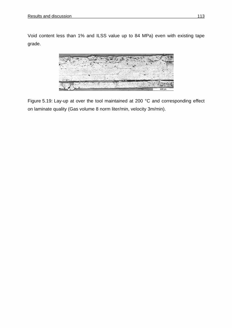
Results and discussion 113
Void content less than 1% and ILSS value up to 84 MPa) even with existing tape
grade.
Figure 5.19: Lay-up at over the tool maintained at 200 °C and corresponding effect
on laminate quality (Gas volume 8 norm liter/min, velocity 3m/min).
114 Conclusion and outlook
6 Conclusion and outlook
The study describes the consolidation in thermoplastic tape placement process to
obtain the high quality structure for industrial application such as aerospace. The ma-
jor barrier in achieving high interlaminar bonding strength is very short residence time
under the roller for consolidation. Hence investigation is performed for the develop-
ment of material; process and product testing procedure, to find out the influencing
process parameters and possible improvement for high strength laminate manufac-
turing.
Temperature distribution under the hot gas torch is mapped out. The initial supposi-
tion of higher heat transfer at higher gas volume is proved to be partially true. The
sinusoidal nature of convective heat transfer coefficient cause the drop of heat trans-
fer even at higher gas volume. Consequently the translation effect of this behavior is
highly noticeable in interlaminar strength development.
The mechanism of surface roughness flattening is a gradual function and degree of
intimate contact Dic at plies interface improves with each successive pass. Similarly,
the polymer diffusion initiates only on the completely contacted tape sections. Hence
the consecutive lay-up (laminate thickness build-up) improve the consolidation level
in the underneath (already placed) layers, but this trend is effective only for the top
few layers (3-6 layers) where the temperature rises above the melting point. For the
low energy parameter combinations, the energy input to the incoming tape and sub-
strate material is limited and incomplete intimate contact restricts the bonding proc-
ess. High energy input although could increase the bonding degree Db even up to the
97%, but activate also the thermal degradation phenomena. The rate of polymer
healing (diffusion) and polymer crosslinking follows the Arrhenius laws with the acti-
vation energies of 43 KJ/mol and 276 KJ/mol. The polymer crosslinking at high tem-
perature exposure hinder the polymer diffusion process and reduce the strength de-
velopment. So the intermediate energy combination can provide laminate with good
mechanical strength.
A multi parameter study shows that extended consolidation either by mean of addi-
tional pass or by increasing consolidation length or by using multiple roller and torch

Conclusion and outlook 115
setup widens the Db 90% contour. Thus high lay-up velocity up to 7 m/min is viable
for high industrial production rate. For the single roller IVW tape placement setup,
laminate manufacturing with autoclaved comparable quality (in terms of ILSS and
void content) is practically realizable, if provided with the flat preimpregnated tape
with less than 1% void content.
Deformation of tape edges is identified as the dictating factor for the laminate’s trans-
verse strength. Tape placement with slight overlap reinforced the transverse joint by
14% as compared to pure matrix joint. Lay-up with high energy process parameters
produces voids pockets at the joint section and reduces the transverse strength. The
post consolidation steps like additional passes with low hot gas volume flow found to
be beneficial in removing these trapped voids and improving the overall laminate
quality.
Finally the simulation tool developed in this research work is used for identifying the
existing limitation to achieve full consolidation. The parametric study identifies the
manufacturing conditions to achieve Db>97% with exiting prepreg thermoplastic ma-
terial, but with the higher intralaminar void contents. Although the presence of intra-
laminar void prove to be ineffective for the ILSS values through experimental testing,
but some application (like aerospace or medicine) demands overall laminate void
content <1%. Tool temperature is identified as one of the highly influencing parame-
ters beside hot gas temperature and lay-up velocity. The tool at high temperature
(260-290 °C) on one side foster the bonding within the laminate but on the other
hand facilitate the void deconsolidation at roller exit. Simulation indicates that the
void can be freeze down to prevent the void deconsolidation inside the laminate, if
laid down on cold tool. But the limitation to maintain the adhesion between the first
layer and tool hinder such advancement.
The methodology outlined in this work may be extended to carry out the remaining
development in the tape placement process. The process improvement should be
supported by the parallel advancement in theoretical technological knowledge or vice
versa. Address to the following points is suggested for the continual improvement to
the tape placement process.
• Material improvement is inevitable in future to foster the large industrial adap-
116 Conclusion and outlook
tation of tape placement process. Thermoplastic pre-peg tapes in future
should inherit smoother face (FD< 1.2), less void contents (<1%) and at least
a fiber diameter thick resin rich layer on top surfaces.
• Compared to the hot gas torch, laser technique has demonstrated [94] the ef-
fective heating over a constant area. Efforts are required to focus the heat flux
as close to the nip point region.
• Laminate manufacturing with less costly polymer thermoplastic material like
PP, PPS, PA12, PEKK and quality testing with other methods like open hole
compression testing (OHC), in plane shear strength (IPSS) should be ex-
ploited.
• The effect on polymer melt viscosity by crosslinking phenomenon has been
discussed. The model may be modified and kinematic constant can be deter-
mined with experimentation for fiber reinforced polymer material.
• Simulation tool can be extended with the non isothermal crystalline and resid-
ual thermal stress model to analyze different heating/cooling rate and envi-
ronment.
• To theoretically explain the transverse bonding phenomenon, a 3D heat trans-
fer model [15] is proposed for simulating thermal distribution over tape width
and length.
• Finally, for larger computational problem, solving capabilities of Matlab soft-
ware are limited. Other scientific programming languages like FORTRAN or
C++ may be exploited for faster solution.
Appendix 117
7 Appendix
7.1 Code for calculating pressure under rotating roller
h=data(tmy,3) ; w=data(tmy-1,6) ; if (tmy>wdivtemp) & (tmy<=wdivtemp+wdiv) hdot=data(tmy-1,4); C=[hdot;h;tmy]; options = []; solinit = bvpinit(linspace(0,w,wdiv),[0 patm]); sol = bvp4c(@twoode,@twobc,solinit,options,C,data2); x = linspace(0,w,wdiv); y = deval(sol,x); if (tmy > wdivtemp+1) if (y(1,1) < 0.9*data2(1,5,tmy-1)) y(1,:) = data2(:,5,tmy-1)'.*0.8; y(2,1)=0; y(2,2:end)= (diff(y(1,:)')./diff(x'))'; end end data2(:,5,tmy)=y(1,:)'; data2(:,7,tmy)=y(2,:)'; else data2(:,5,tmy)=patm; data2(:,7,tmy)=0; end data2(:,6,tmy)=[linspace(0,h,wdiv)]'; data(tmy,8)=(data2(1,5,tmy)) ; data(tmy,12)=mean(data2(:,5,tmy));
7.2 Code to calculate heat transfer inside the laminate
function[utemp,u,t]=tempcal(Lt,Tt,ht,wdivLl,wdivhl,thk,tdiv,N,qin,qsub ) global alpha1 rho cp Ve k utool time=Lt(2)/Ve; time1=Lt(1)/Ve; time2=time1+(Lt(2)-Lt(1))/Ve; time1div=linspace(0,time1-.0001,wdivLl); time2div=linspace(time1,time2,wdivhl); alpha1=k/(rho*cp); m = 0; x = linspace(0,thk,tdiv); t=[time1div time2div]; options = odeset('MaxStep',0.1*time1); if N==0
118 Appendix
u(:,:,1)= pdepe(m,@pdex1pde,@pdex1ic,@(xl,ul,xr,ur,t) pdex2bc(xl,ul,xr,ur,t,Lt,Tt,ht,qin,qsub),x,t); elseif N==1 u(:,:,1)= pdepe(m,@pdex1pde,@pdex1ic2,@(xl,ul,xr,ur,t) pdex1bc(xl,ul,xr,ur,t,Lt,Tt,ht,qin,qsub,N),x,t,options); elseif N==2 u(:,:,1)= pdepe(m,@pdex1pde,@(x) pdex1ic3(x,thk),@(xl,ul,xr,ur,t) pdex1bc(xl,ul,xr,ur,t,Lt,Tt,ht,qin,qsub,N),x,t,options); end utemp=rot90(u) ; x1=linspace(0,1,tdiv) ; utemp=[x1' utemp] ;
7.3 Code for void calculation
So=(Ro^3/Vvo)^(1/3); Sos=So/Ro ; Ros=Ro/Ro; Plyr=2; while Plyr<=NNlyr h2=[INPSTR '\layup' num2str(Plyr)]; load(h2) ; layup2=0; layup2=dat1; dat1=0; h1=[INPSTR '\layup' num2str(Plyr-1)] ; load(h1,'dat1') layup1=0; layup1=dat1; dat1=0; h3=[INPSTR '\tempdata' num2str(Plyr)]; load(h3,'tempdata') tempdata2=0; tempdata2=tempdata; tempdata=[]; for Tylr=1:Plyr-1 curlyup=layup2(:,:,Tylr); prvlyup=layup1(:,:,Tylr) ; tempdata(1,:)=tempdata2(Tylr+1,:); [prvlyup,curlyup]=voidmodel (Ro,Sos,Pgo,To,Vvo,prvlyup,curlyup,tempdata,Tg,Plyr,Tylr,wdiv,wdivtr,Tsigma); layup2(:,:,Tylr) =curlyup; end dat1=layup2; flname=[INPSTR '\layup' num2str(Plyr)]; save(flname,'dat1','wdiv','wdivtr','hsin','NNlyr','hsin','Llin','Lc','Lhin','Ltrin') Plyr=Plyr+1; end
References 119
8 References
1. Gutowski, T.G.P.: Advanced composites manufacturing. 1997, New York, NY: Wiley.
2. Carpenter, C.E.; Colton, J.S.: On-line consolidation mechanisms in thermoplastic filament winding. Polymer Composites, 1994. 15(1): p. 55-63.
3. Beresheim, G.: Thermoplast-Tapelegen –ganzheitliche Prozessanalyse und -entwicklung, in Institut für Verbundwerkstoffe GmbH. 2002: Kaiserslautern, Germany.
4. Latrille, M.: Prozessanalyse und -simulation von Verarbeitungsverfahren für faserverstärkte thermoplastische Bändchenhalbzeuge. 2003, Institut für Verbundwerkstoffe GmbH: Kaiserslautern.
5. Gallet, C.: Innovative and economic fibre placement machines and software. in 3rd Innovative and economic fibre placement machines and software. 2006. NLR Marknesse, The Netherlands.
6. Lamontia, M.A., et al.: Stringer-, honeycomb core-, and tigr -stiffened skins, and ring-stiffened cylinders fabricated from automated thermoplastic fiber placement and filament winding. in SAMPE Europe conference 23. 2002. Paris: p. 213-224.
7. Miscellaneous gallery | Automated Dynamics. Available from: http://www.automateddynamics.com/gallery/affordable_automation/miscellaneous_gallery.
8. Tierney, J.; Gillespie, J.W.: Modeling of In Situ Strength Development for the Thermoplastic Composite Tow Placement Process. Journal of Composite Materials, 2006. 40(16): p. 1487-1506.
9. Steeg, M.; Schledjewski, R.; Schlarb, A.K.: Automation implementation and process development of thermoplastic tape placement for 3-dimensional parts. SAMPE Journal, 2006. 42(5): p. 18-24.
10. Lamontia, M.A., et al.: Developing A Contoured Deposition Head for In-Situ Tape Laying and Fiber Placement, in Sampe International Symposium and Exhibition. 2003: Long Beach, CA.
11. Lamontia, M.A.; Gruber, M.B.: Remaining developments required for commercializing in situ thermoplastic ATP. in SAMPE 2007. Baltimore, MD.
12. Kim, H.J.; Kim, S.K.; Lee, W.I.: A study on heat transfer during thermoplastic composite tape lay-up process: Peter Bradshaw 60th Birthday Issue: Part II. Experimental Thermal and Fluid Science, 1996. 13(4): p. 408-418.
13. Shih, P.J.; Loos, A.C.: Heat Transfer Analysis of the Thermoplastic Filament Winding Process. Journal of Reinforced Plastics and Composites, 1999.
120 References
18(12): p. 1103-1112.
14. Hassan, N., et al.: A Heat Transfer Analysis of the Fiber Placement Composite Manufacturing Process. Journal of Reinforced Plastics and Composites, 2005. 24(8): p. 869-888.
15. Toso, Y.M.P.; Ermanni, P.; Poulikakos, D.: Thermal Phenomena in Fiber-reinforced Thermoplastic Tape Winding Process: Computational Simulations and Experimental Validations. Journal of Composite Materials, 2004. 38(2): p. 107-135.
16. Mantell, S.C.; Springer, G.S.: Manufacturing Process Models for Thermoplastic Composites. Journal of Composite Materials, 1992. 26(16): p. 2348-2377.
17. Latrille, M.; Schledjewski, R.: Processing of unidirectional fiber reinforced tapes--fundamentals on the way to a process simulation tool (ProSimFRT). Composites Science and Technology, 2003. 63(14): p. 2111-2118.
18. Nicodeau, C.: Modelisation du soudage en continu des composites a matrice thermoplastique. 2005, Ecole Nationale Superieure d’Arts et Metiers de Paris: Paris.
19. Agarwal, V., et al.: Thermal Characterization of the Laser-Assisted Consolidation Process. Journal of Thermoplastic Composite Materials, 1992. 5(2): p. 115-135.
20. Pitchumani, R., et al.: Analysis of transport phenomena governing interfacial bonding and void dynamics during thermoplastic tow-placement. International Journal of Heat and Mass Transfer, 1996. 39(9): p. 1883-1897.
21. Sonmez, F.O.; Hahn, H.T.: Modeling of Heat Transfer and Crystallization in Thermoplastic Composite Tape Placement Process. Journal of Thermoplastic Composite Materials, 1997. 10(3): p. 198-240.
22. Colton, J.; Leach, D.: Processing parameters for filament winding thick-section PEEK/carbon fiber composites. Polymer Composites, 1992. 13(6): p. 427-434.
23. Dai, S.-C.; Ye, L.: GF/PP Tape Winding with On-Line Consolidation. Journal of Reinforced Plastics and Composites, 2002. 21(1): p. 71-90.
24. Tierney, J.; Gillespie, J.W.: Modeling of Heat Transfer and Void Dynamics for the Thermoplastic Composite Tow-Placement Process. Journal of Composite Materials, 2003. 37(19): p. 1745-1768.
25. Khan, M.A.; Mitschang, P.; Schledjewski, R.: Tracing the Void Content Development and Identification of its Effecting Parameters During in situ Consolidation of Thermoplastic Tape Material. Polymers and polymer composites, 2010. 18(1): p. 1-15.
References 121
26. Hinkley, J.A.; Marchello, J.M.; Messier, B.C.: Thermoplastic Ribbon-Ply Bonding Model. NASA Technical Memorandum 110203, 1997.
27. Gutowski, T.G.; Morigaki, T.; Zhong Cai: The Consolidation of Laminate Composites. Journal of Composite Materials, 1987. 21(2): p. 172-188.
28. Ranganathan, S.; Advani, S.G.; Lamontia, M.A.: A Non-Isothermal Process Model for Consolidation and Void Reduction during In-Situ Tow Placement of Thermoplastic Composites. Journal of Composite Materials, 1995. 29(8): p. 1040-1062.
29. Rogers, T.G.: Squeezing flow of fibre-reinforced viscous fluids. Journal of Engineering Mathematics, 1989. 23(1): p. 81-89.
30. Khan, M.A.; Schledjewski, R.: Infuencing factors for an online consolidating thermoplastic tape placement process, in 17th International conference on composite materials, ICCM-17. 2009: Edinburgh, UK.
31. Sonmez, F.O.; Hahn, H.T.: Thermoviscoelastic Analysis of the Thermoplastic Composite Tape Placement Process. Journal of Thermoplastic Composite Materials, 1997. 10(4): p. 381-414.
32. Loos, A.C.; Li, M.-C.: Processing of composites: Consolidation during thermoplastic composite processing. 2000, Munich: Hanser.
33. Lee, W.I.; Springer, G.S.: A Model of the Manufacturing Process of Thermoplastic Matrix Composites. Journal of Composite Materials, 1987. 21(11): p. 1017-1055.
34. Yang, F.; Pitchumani, R.: Fractal Description of Interlaminar Contact Development during Thermoplastic Composites Processing. Journal of Reinforced Plastics and Composites, 2001. 20(7): p. 536-546.
35. Yang, F.; Pitchumani, R.: Interlaminar contact development during thermoplastic fusion bonding. Polymer Engineering & Science, 2002. 42(2): p. 424-438.
36. Yang, F.; Pitchumani, R.: A fractal Cantor set based description of interlaminar contact evolution during thermoplastic composites processing. Journal of Materials Science, 2001. 36(19): p. 4661-4671.
37. Yang, F.; Pitchumani, R.: Healing of Thermoplastic Polymers at an Interface under Nonisothermal Conditions. Macromolecules, 2002. 35(8): p. 3213-3224.
38. Ageorges, C., et al.: Characteristics of resistance welding of lap shear coupons. Part I: Heat transfer. Composites Part A: Applied Science and Manufacturing, 1998. 29(8): p. 899-909.
39. Phillips, R.; Glauser, T.; Månson, J.-A.E.: Thermal stability of PEEK/carbon fiber in air and its influence on consolidation. Polymer Composites, 1997. 18(4): p. 500-508.
122 References
40. Cole, K.C.; Casella, I.G.: Fourier transform infrared spectroscopic study of thermal degradation in films of poly(etheretherketone). Thermochimica Acta, 1992. 211: p. 209-228.
41. Gupta, Y.N., et al.: Thermal and thermooxidative degradation of engineering thermoplastics and life estimation. Journal of Applied Polymer Science, 2004. 92(3): p. 1737-1748.
42. Park, J., et al.: Kinetic analysis of thermal decomposition of polymer using a dynamic model. Korean Journal of Chemical Engineering, 2000. 17(5): p. 489-496.
43. Ageorges, C., et al.: Characteristics of resistance welding of lap-shear coupons. Part III. Crystallinity. Composites Part A: Applied Science and Manufacturing, 1998. 29(8): p. 921-932.
44. Ozawa, T.: Kinetics of non-isothermal crystallization. Polymer, 1971. 12(3): p. 150-158.
45. Velisaris, C.N.; Seferis, J.C.: Crystallization kinetics of polyetheretherketone (peek) matrices. Polymer Engineering & Science, 1986. 26(22): p. 1574-1581.
46. Tierney, J.J.; Gillespie Jr, J.W.: Crystallization kinetics behavior of PEEK based composites exposed to high heating and cooling rates. Composites Part A: Applied Science and Manufacturing, 2004. 35(5): p. 547-558.
47. Choe, C.R.; Lee, K.H.: Nonisothermal crystallization kinetics of poly(etheretherketone) (PEEK). Polymer Engineering & Science, 1989. 29(12): p. 801-805.
48. Tobin, M.C.: Theory of phase transition kinetics with growth site impingement. I. Homogeneous nucleation. Journal of Polymer Science: Polymer Physics Edition, 1974. 12(2): p. 399-406.
49. Maffezzoli, A.M.; Kenny, J.M.; Nicolais, L.: Welding of PEEK/Carbon fiber composite laminates. SAMPE Journal, 1989. 25: p. 35-39.
50. Chapman, T.J., et al.: Prediction of Process-Induced Residual Stresses in Thermoplastic Composites. Journal of Composite Materials, 1990. 24(6): p. 616-643.
51. Lawrence, W.: Prediction of residual stresses in continuous fiber semicrystalline thermoplastic composites. in Proceedings of American scociety for composites 5th technical conference. 1990: p. 401-408.
52. Tierney, J.J.; Eduljee, R.F.; Gillespie Jr, J.W.: Material response during robotic tow placement of thermoplastic composites. in Proc. of 11th annual advance composites conf. 1995: p. 315-329.
53. Jeronimidis, G.; Parkyn, A.T.: Residual Stresses in Carbon Fibre-Thermoplastic Matrix Laminates. Journal of Composite Materials, 1988. 22(5):
References 123
p. 401-415.
54. Hexcel: Carbon fiber data sheets. 2010; Available from: http://www.hexcel.com/Products/Downloads/Carbon+Fiber+Data+Sheets.htm?ds=Continuous.
55. Lindemann, A.; Schopper, A.: Thermophysical properties of CF filled PEEK samples.Netzsch Report no. 821.004/09, 2009.
56. Cremers, M.F.G., et al.: Heat transfer mechanisms of laminar flames of hydrogen + oxygen. Combustion and Flame, 2004. 139(1-2): p. 39-51.
57. Baukal, C.E.; Gebhart, B.: Heat transfer from oxygen-enhanced/natural gas flames impinging normal to a plane surface. Experimental thermal and fluid science, 1998. 16(3).
58. Baukal, C.E.; Gebhart, B.: Surface condition effects on flame impingement heat transfer. Experimental thermal and fluid science, 1997. 15(4).
59. Martin, H.: Advances in Heat Transfer. Heat and mass transfer between impinging gs jets and solid surfaces. Vol. 13. 1977: Academic Press.
60. Kim, H.J.; Kim, S.K.; Lee, W.I.: Flow and Heat Transfer Analysis during Tape Layup Process of APC-2 Prepregs. Journal of Thermoplastic Composite Materials, 2004. 17(1): p. 5-12.
61. Lawal, A.; Kalyon, D.M.: Squeezing flow of viscoplastic fluids subject to wall slip. Polymer Engineering & Science, 1998. 38(11): p. 1793-1804.
62. Majumdar, A.; Bhushan, B.: Fractal Model of Elastic-Plastic Contact Between Rough Surfaces. J. Tribol., 1991. 113(1): p. 1-11.
63. Khan, M.A.; Mitschang, P.; Schledjewski, R.: Identification of some optimal parameters to achieve higher laminate quality through tape placement process. Advances in polymer technology, 2010. 29(2): p. 98-111.
64. Barnes, J.A.; Cogswell, F.N.: Transverse flow processes in continuous fibre-reinforced thermoplastic composites: Flow Processes in Composite Materials. Composites, 1989. 20(1): p. 38-42.
65. Cogswell, F.N.: Thermoplastic aromatic polymer composites: A study of the structure, processing and properties of carbon fibre reinforced polyetheretherketone and related materials. 1992, Oxford: Butterworth-Heinemann.
66. Balasubramanyam, R.; Jones, R.S.; Wheeler, A.B.: Modelling transverse flows of reinforced thermoplastic materials: Flow Processes in Composite Materials. Composites, 1989. 20(1): p. 33-37.
67. Deng, Y., et al.: The rheological characterization of fluorinated thermoplastics using squeezing flow viscometry. Polymer Engineering & Science, 1994.
124 References
34(3): p. 213-220.
68. Lin, H.-R.; Advani, S.G.: Processing models and characterization of thermoplastic composite wound parts. Polymer Composites, 1997. 18(3): p. 405-411.
69. Scobbo, J.J.; Nakajima, N.: Dynamic mehcanical analysis of molten thermoplastic / continous graphite fiber composites in simple shear deformation. in 21st Internatinal SAMPE technical conference. 1989. CA.
70. Stanley, W.F.; Mallon, P.J.: Intraply shear characterisation of a fibre reinforced thermoplastic composite. Composites Part A: Applied Science and Manufacturing, 2006. 37(6): p. 939-948.
71. Shuler, S.F.; Advani, S.G.: Transverse squeeze flow of concentrated aligned fibers in viscous fluids. Journal of Non-Newtonian Fluid Mechanics, 1996. 65(1): p. 47-74.
72. Nicodeau, C., et al.: In-situ consolidation process optimization for thermoplastic matrix composites, in SAMPE 2006 Technical Conference Proceedings. 2006, Society for the Advancement of Material and Process Engineering: Long Beach, CA.
73. Agarwal, V.: The role of molecular mobility in the consolidation and bonding of thermplastic composite materials. CCM Report 91-93, 1991.
74. Advani, S.G.; Sozer, E.M.: Process modeling in composites manufacturing. Vol. 59. 2002, New York, NY: Marcel Dekker.
75. Nam, J.-D.; Seferis, J.C.: Generalized composite degradation kinetics for polymeric systems under isothermal and nonisothermal conditions. Journal of Polymer Science Part B: Polymer Physics, 1992. 30(5): p. 455-463.
76. Hulcher, A.B.; Marchello, J.M.; Hinkley, J.A.: Wedge peel testing for Automated fiber placement. Journal of advanced materials, 1999. 31(3).
77. Hulcher, B.; Marchello, J.M.; Hinkley, J.A.: Correlation Between Double Cantilever Beam and Wedge Peel tests for automated tow placement. SAMPE Engineering Series, 1998. 43: p. 1955-1965.
78. Schledjewski, R.: Investigation of testing mechanisms by doping of bonding surfaces with nano particles, in ECCM-13. 2008: Stockholm.
79. Yee, R.Y.; Stephens, T.S.: A TGA technique for determining graphite fiber content in epoxy composites: Advances in International Thermal Sciences: Environment, Polymers, Energy and Techniques. Thermochimica Acta, 1996. 272: p. 191-199.
80. Kim, J.; Moon, T.J.; Howell, J.R.: Cure Kinetic Model, Heat of Reaction, and Glass Transition Temperature of AS4/3501-6 Graphite-Epoxy Prepregs. Journal of Composite Materials, 2002. 36(21): p. 2479-2498.
References 125
81. Khan, M.A.; Lichtner, J.; Schledjewski, R.: An investiagtion on the development of the transverse bonding in automated tape placement process, in ECCM-14. 2010: Budapest, Hungary.
82. Khan, M.A.; Schledjewski, R.: Process simulation and parametric study of an online consolidated composite manufacturing setup. in Solids, Structures and Coupled Problems in Engineering. IV European Congress on Computational Mechanics (ECCM IV) 2010. Paris.
83. Guan, X.; Pitchumani, R.: Modeling of spherulitic crystallization in thermoplastic tow-placement process: spherulitic microstructure evolution. Composites Science and Technology, 2004. 64(9): p. 1363.
84. Ghose, S., et al.: High Temperature VARTM of Phenylethynyl Terminated Imides. High Performance Polymers, 2009. 21(5): p.653-672.
85. Goren, A.; Atas, C.: Manufacturing of polymer matrix composites using vacuum assisted resin infusion molding. Archives of Materials Science and Engineering, 2008. 34(2): p. 117-120.
86. Schledjewski, R.: Thermoplastic Tape Placement-Challenging the Autoclave Process, in 1st European Conference on Materials and Structures in Aerospace (EUCOMAS). 2008: Berlin, Germany. p. 245-251.
87. Lamontia, M.A., et al.: Insitu thermoplastic ATP needs flat tapes and tows with few voids., in SAMPE conference. 2008: Paris.
88. Kilroy, J.P.; Ó Brádaigh, C.M.; Semprimoschnig, C.O.A.: Mechanical and Physical Evaluation of New Carbon Fibre/Peek Composites for Space Applications. SAMPE Journal, 2008. 44(3): p. 22-34.
89. Sonmez, F.O.; Hahn, H.T.: Analysis of the On-Line Consolidation Process in Thermoplastic Composite Tape Placement. Journal of Thermoplastic Composite Materials, 1997. 10(6): p. 543-572.
90. Fink, B.K.; Gillespie, J.W.; Ersoy, N.B.: Thermal Degradation Effects on Consolidation and Bonding in the Thermoplastic Fiber-Placement Process, Army Research Lab Report 1998.
91. Wang, E.L.; Gutowski, T.G.: Laps and gaps in thermoplastic composites processing. Composites Manufacturing, 1991. 2(2): p. 69-78.
92. O’Brien, T.K., et al.: Influence of Specimen Preparation and Specimen Size on Composite Transverse Tensile Strength and Scatter, in NASA/TM-2001-211030. 2001.
93. Ye, L.; Lu, M.; Mai, Y.-W.: Thermal de-consolidation of thermoplastic matrix composites--I. Growth of voids. Composites Science and Technology, 2002. 62(16): p. 2121-2130.
94. Schledjewski, R.; Miaris, A.: Thermoplastic tape placement by means of diode

126 References
laser heating, in SAMPE 2009 Technical Conference Proceedings. 2009: Baltimore, MD.
List of the students supervised
List of the students supervised for practical training
Following students did theoretical and experimental work during this research work.
1. Ricardo Medina Rueda: ‘Quality investigation of tape placed laminate through ex-
perimental testing’, 2008.
2. Carmen Cobo Sánchez: ‘Experimental process parameter study for tape place-ment process’, 2009.
3. Vicente Rouco Sanromán: ‘Influence of hot gas temperature and initial tape width, on the final mechanical strength of fabricated thermoplastic composite structure’, 2009.
4. Jorge Carracedo: ‘Evaluation of thermal degradation phenomenon in carbon rein-forced thermoplastic material’, 2010.