Embed Size (px)
Citation preview

Jan Schulze
Adjoint based jet-noise minimization
Jan Schulze
Adjoint based jet-noise minimization

Bibliografische Information der Deutschen Nationalbibliothek.Die Deutsche Nationalbibliothek verzeichnet diese Publikation in derDeutschen Nationalbibliografie; detaillierte bibliografische Daten sind imInternet über http://dnb.dnb.de/ abrufbar.
Universitätsverlag der TU Berlin 2013http://www.univerlag.tu-berlin.de
Fasanenstr. 88 (im VOLKSWAGEN-Haus), 10623 BerlinTel.: +49 (0)30 314 76131 / Fax: -76133E-Mail: [email protected]
Zugl.: Berlin, Technische Universität, Diss., 20121. Gutachter: Prof. Dr. Jörn Sesterhenn2. Gutachter: Prof. Dr. Christophe BogeyDie Arbeit wurde am 22. Oktober 2012 unter Vorsitzvon Prof. Dr. Michael Möser erfolgreich verteidigt.
Das Manuskript ist urheberrechtlich geschützt.Druck: docupoint GmbH Magdeburg
Cover design: Rosi WahlSatz: Dieses Dokument ist gesetzt mit KOMA-Script und LATEX
ISBN 978-3-7983-2494-7 (Druckversion)ISBN 978-3-7983-2495-4 (Onlineversion)
Zugleich online veröffentlicht auf dem Digitalen Repositoriumder Technischen Universität Berlin:URL http://opus.kobv.de/tuberlin/volltexte/2013/3871/URN urn:nbn:de:kobv:83-opus-38719http://nbn-resolving.de/urn:nbn:de:kobv:83-opus-38719

Zusammenfassung
Freistrahlen (engl. Jets) mit einer komplexen Stoßzellen-Struktur treten invielen technischen Anwendung auf. Die meisten Überschallfreistrahlen inder Luftfahrt sind nicht perfekt angepasst, auch nicht solche aus sorgfältiggestalteten konvergent-divergenten Düsen. Die Anpassung an den Umge-bungsdruck erfolgt in einer Abfolge von schiefen Verdichtungsstößen, die mitden freien Scherschichten interagieren und Lärm erzeugen. Dabei strahlt dieInteraktion von Stoß und Scherschicht einen breitbandigen Lärm ab. Dieskann die dünne Scherschicht am Düsenaustritt anregen und eine Rückkop-plungsschleife bilden, die einen diskreten Ton namens Screech (dt. Kreischen)hervorruft. Beide Komponenten sind aus strukturellen und umgebungsbe-dingten Gesichtspunkten unerwünscht (z. B. Kabinenlärm). Screech-Töneerzeugen Schalldruckpegel von 160 dB und darüber hinaus.
Der Fokus der vorliegenden Arbeit liegt in der Minimierung von ÜberschallJet-Lärm, insbesondere in der Minimierung von Jet-Screech. Da Screech – einPhänomen, das noch nicht in allen Einzelheiten verstanden ist – durch die Ge-ometrie der Jet-Düse beeinflusst wird, soll ein poröses Material an der Düseangebracht werden, um den Rückkopplungsmechanismus zu unterdrücken.Dadurch wird ebenfalls der Screech-Ton unterdrückt. Es ist keineswegs klar,wie die charakteristischen Eigenschaften des porösen Materials beschaffensein sollten, um den Lärm zu minimieren. Zu diesem Zweck wird ein Op-timierungsverfahren, basierend auf adjungierten Methoden, angewandt, umdie Materialeigenschaften in Bezug auf den Lärm zu optimieren.
v

Abstract
Jets with complex shock-cell structures appear in numerous technologicalapplications. Most supersonic jets used in aeronautics will be imperfectlyadapted in flight, even those from carefully designed convergent–divergentnozzles. The adaption to the ambient pressure takes place in a sequence ofoblique shocks which interact with the free shear layers and produce noise.The shock/shear-layer interaction emanates a broadband noise component.This may trigger the thin shear layer at the nozzle exit, forming a feedbackloop which results in a discrete noise component called screech. Both compo-nents are undesirable from structural and environmental (cabin noise) pointsof view. Screech tones produce sound pressure levels of 160 dB and beyond.
The focus of the present thesis lies in the minimization of supersonic jet-noise and in particular in the minimization of jet-screech. Since screech – aphenomenon which is not yet understood in all details – seems to be affectedby the presence of the jet-nozzle, a porous material will be added to the nozzleexit to suppress the feedback mechanism. Thus, to minimize the emanatednoise. It is by no means clear how the shape an characteristic properties ofthe porous material should be. To this end, an optimization technique, basedon adjoint methods, will be applied to optimize the material with respect tothe emanated noise.
vii


Preface
The present work addresses the problem of adjoint based minimization of su-personic jet noise. It started in 2006 with the DFG Sub-Project SP2 (Shock-Induced Noise in Supersonic Jets) at the Technical University in Munich, ini-tiated by Jörn Sesterhenn with the French partners Daniel Juvé, ChristopheBailly and Peter Schmid, and was finished six years later at the TechnicalUniversity in Berlin. Adjoint based optimization is a fairly recent and veryactive research field not only in the academic environment but also in theindustry. Different approaches dealing with the numerical and mathematicaldifficulties were developed within the last years helping to popularize thismethod. Still, many questions are unsolved. This work will provide an in-sight in the method of adjoint based optimization of a supersonic jet. A newand promising approach to optimize a porous medium to suppress jet noiseis applied and validated. The purpose of this research project is to discussthe feasibility of such an approach and to help to improve the understandingof adjoint based methods and the physics of supersonic jet noise generation.
The development of this thesis would not have been possible without theguidance of my two supervisors Jörn Sesterhenn in Munich and Berlin andPeter Schmid in Paris. Their support in any issues concerning the numerical,mathematical or physical part of this work was essential for its outcome.
As part of the Cotutelle I had the opportunity to visit the research groupat the École Polytechnique (LadHyX) in Paris. I was fortunate to meet mycolleagues Shervin Bagheri, François Gallaire and Fulvio Martinelli. Further-more I wish to thank my colleagues in Munich, Alex Barbagallo, ChristophMack and Olivier Marquet for the many suggestions and discussions. Andfinally my colleagues in Berlin, Jens Brouwer, Flavia Cavalcanti Miranda,Mathias Lemke and Julius Reiss for creating the nice and inspiring workingenvironment.
Financial support by the Deutsche Forschungsgemeinschaft (DFG) andthe Deutsch–Französische Hochschule (DFH) and computational time at the
ix

Preface
Leibnitz Rechenzentrum (LRZ) and the Norddeutscher Verbund für Hoch-und Höchstleistungsrechnen (HLRN) is particularly acknowledged. I also liketo thank the DEISA Consortium (co-funded by the EU, FP6 project 508830),for support within the DEISA Extreme Computing Initiative.
Last but not least I want to thank my family, my sister Rosi who alwaysgave me a homelike atmosphere and a place to live both in Paris and Berlin,my parents Sieglinde and Armin for their support and finally Anna for hercare and patience.
Munich, Jan SchulzeMarch, 2013
x
Contents
Zusammenfassung v
Abstract vii
Preface ix
I Computing supersonic jet noise 1
1 Introduction 31.1 Physics of a supersonic jet . . . . . . . . . . . . . . . . . . . . . 41.2 Objective of this thesis . . . . . . . . . . . . . . . . . . . . . . . 30
2 Theory of computing supersonic jet noise 332.1 State of the art . . . . . . . . . . . . . . . . . . . . . . . . . . . . 362.2 Equations of motion . . . . . . . . . . . . . . . . . . . . . . . . . 432.3 Discretization . . . . . . . . . . . . . . . . . . . . . . . . . . . . . 462.4 Including the nozzle . . . . . . . . . . . . . . . . . . . . . . . . . 572.5 Parallelization . . . . . . . . . . . . . . . . . . . . . . . . . . . . . 672.6 Treating shocks . . . . . . . . . . . . . . . . . . . . . . . . . . . . 70
3 Theory of computing flow in porous media 773.1 Porous flow equations . . . . . . . . . . . . . . . . . . . . . . . . 803.2 Validation . . . . . . . . . . . . . . . . . . . . . . . . . . . . . . . 883.3 Examples of porous flow simulations . . . . . . . . . . . . . . . 100
4 Results of supersonic jet noise simulation 1074.1 Planar jet . . . . . . . . . . . . . . . . . . . . . . . . . . . . . . . 1084.2 Round jet . . . . . . . . . . . . . . . . . . . . . . . . . . . . . . . 130
xi
Contents
II Minimizing supersonic jet noise 153
5 Optimization method 1555.1 A simple example . . . . . . . . . . . . . . . . . . . . . . . . . . 1565.2 State of the art . . . . . . . . . . . . . . . . . . . . . . . . . . . . 1605.3 Objective function . . . . . . . . . . . . . . . . . . . . . . . . . . 1645.4 Optimization framework . . . . . . . . . . . . . . . . . . . . . . 1705.5 Examples . . . . . . . . . . . . . . . . . . . . . . . . . . . . . . . 204
6 Results of the minimization of supersonic jet noisewith porous media 2256.1 Adjoint solution . . . . . . . . . . . . . . . . . . . . . . . . . . . 2286.2 Optimized nozzle . . . . . . . . . . . . . . . . . . . . . . . . . . . 2326.3 Noise reduction . . . . . . . . . . . . . . . . . . . . . . . . . . . . 2346.4 Influence on the flow field . . . . . . . . . . . . . . . . . . . . . . 245
7 Conclusion and Outlook 253
A Compressible Navier–Stokes equations 257
B Linearized Navier–Stokes equations 261
C Compressible adjoint Navier–Stokes equations 267
Bibliography 271
xii

List of Tables
1.1 Features of a supersonic jet with different stages of expansion . . . 7
2.1 Overview of the numerical investigation on supersonic jet noise . . 372.2 Coefficients used for the compact schemes . . . . . . . . . . . . . . . 482.3 Standard conditions for dry air . . . . . . . . . . . . . . . . . . . . . 70
3.1 Permeability for different porous media . . . . . . . . . . . . . . . . 79
4.1 Investigated numerical simulations on planar and round supersonicjets . . . . . . . . . . . . . . . . . . . . . . . . . . . . . . . . . . . . . . 108
4.2 Showcase of the flow conditions for a Mj = 1.55 jet at four differentcharacteristic locations . . . . . . . . . . . . . . . . . . . . . . . . . . 109
4.3 Time-step and grid spacing for the investigated resolution of theround nozzle . . . . . . . . . . . . . . . . . . . . . . . . . . . . . . . . 131
5.1 Parameters of the objective function to minimize supersonic jetnoise . . . . . . . . . . . . . . . . . . . . . . . . . . . . . . . . . . . . . 168
5.2 Advantages of the discrete and continuous approach to obtain thediscretized adjoint equations . . . . . . . . . . . . . . . . . . . . . . . 175
6.1 Reduction of the OASPL in different observation directions . . . . 239
xiii


List of Figures
1.1 Overall SPL as a function of the Mach number . . . . . . . . . . . 41.2 Sketch of a supersonic jet for different pressure ratios . . . . . . . 51.3 Schlieren visualization of an under-expanded jet . . . . . . . . . . 61.4 Geometry of a round convergent-divergent Laval nozzle . . . . . . 91.5 Geometry of a planar convergent-divergent Laval nozzle . . . . . 101.6 Flow inside a round convergent-divergent Laval nozzle . . . . . . 111.7 Length of the jet potential core and length of the supersonic area
as a function of the jet Mach number . . . . . . . . . . . . . . . . . 121.8 Noise measurements of an under-expanded supersonic jet with
convergent-divergent nozzle [Norum & Seiner, 1982a] . . . . . . . 131.9 Noise measurements of an under-expanded supersonic jet with
convergent-divergent nozzle [Norum & Seiner, 1982a] . . . . . . . 151.10 Mach wave radiation of a high speed jet with supersonic phase
velocity cp with respect to the ambient speed of sound c∞ . . . . 161.11 Peak Strouhal number SrBB of broadband shock-associated . . . 171.12 Schematic view of the interaction of shock and turbulent mixing
layer in a jet with emanated noise . . . . . . . . . . . . . . . . . . . 181.13 Screech amplitude and frequency of a rectangular jet versus the
fully expanded jet Mach number Mj . . . . . . . . . . . . . . . . . 201.14 Screech amplitude and frequency of a circular jet versus the jet
Mach number Mj for different screech modes . . . . . . . . . . . . 211.15 Instability modes in a jet (acoustic modes) . . . . . . . . . . . . . 221.16 Sketch of the mechanism involved in predicting the screech fre-
quency . . . . . . . . . . . . . . . . . . . . . . . . . . . . . . . . . . . 24
2.1 Total number of grid points of the numerical investigations ofsupersonic jet noise within the last decade and extrapolated . . . 42
xv

List of Figures
2.2 Modified wavenumber for compact fifth order upwind and sixthorder central scheme . . . . . . . . . . . . . . . . . . . . . . . . . . . 47
2.3 Stability area of fourth order Runge–Kutta time integration . . . 492.4 Arnoldi decomposition for a square matrix A with m subspaces
Vm and the reduced Hessenberg matrix Hm . . . . . . . . . . . . . 522.5 Modified wavenumber for two overlapping grids including inter-
polation of different order . . . . . . . . . . . . . . . . . . . . . . . . 602.6 Eigenvalues of the linear convection diffusion operator with in-
terpolation . . . . . . . . . . . . . . . . . . . . . . . . . . . . . . . . . 612.7 Eigenvectors of the linear convection diffusion operator with in-
terpolation . . . . . . . . . . . . . . . . . . . . . . . . . . . . . . . . . 622.8 Sketch of the Cartesian domain including the boundary condi-
tions and the nozzle . . . . . . . . . . . . . . . . . . . . . . . . . . . 632.9 Kolmogorov scale for a jet versus the Reynolds number . . . . . . 642.10 Grid stretching to adapt the grid . . . . . . . . . . . . . . . . . . . 652.11 Nomenclature of the boundaries of the three-dimensional Carte-
sian domain . . . . . . . . . . . . . . . . . . . . . . . . . . . . . . . . 662.12 Example of the sponge function . . . . . . . . . . . . . . . . . . . . 662.13 Decomposed domain in two dimensions . . . . . . . . . . . . . . . . 682.14 Transformation of the decomposed domain in two dimensions . . 692.15 Parallel Speed-Up of the code . . . . . . . . . . . . . . . . . . . . . 702.16 Computation of the shock profiles, based on the one–dimensional
Navier–Stokes equations . . . . . . . . . . . . . . . . . . . . . . . . . 722.17 Comparison of the Navier–Stokes computation with the linear
theory of Taylor [1910] . . . . . . . . . . . . . . . . . . . . . . . . . . 732.18 Computation of the shock profiles, based on the one–dimensional
Navier–Stokes equations with different resolutions and filters . . . 74
3.1 Replacing the density of the fluid ρf in a real porous medium . . 783.2 Eigenvalues of the porous evolution operator extracted with a
Krylov technique . . . . . . . . . . . . . . . . . . . . . . . . . . . . . 853.3 Dependency of the minimal eigenvalue of the evolution operator
on the permeability K . . . . . . . . . . . . . . . . . . . . . . . . . . 873.4 Validation cases for porous properties . . . . . . . . . . . . . . . . 883.5 Shape of a porous medium represented by the technique of vol-
ume penalization . . . . . . . . . . . . . . . . . . . . . . . . . . . . . 893.6 Channel with a porous coating on one side of the channel-walls . 923.7 Acoustic properties of a porous medium . . . . . . . . . . . . . . . 943.8 Reflection coefficient of a porous medium over the permeability
for different wave numbers . . . . . . . . . . . . . . . . . . . . . . . 95
xvi
List of Figures
3.9 Deviation of the reflected wave of a porous medium compared toa wall boundary condition over the permeability and wavenumber 97
3.10 Instantaneous snapshot of the vorticity past a cylinder . . . . . . 983.11 Mean Mach number including the grid . . . . . . . . . . . . . . . . 993.12 Mean absolute velocity profiles along the transverse direction for
six measurement locations . . . . . . . . . . . . . . . . . . . . . . . 1003.13 Comparison of the lift coefficient Cl for the porous and curvilinear
cylinder . . . . . . . . . . . . . . . . . . . . . . . . . . . . . . . . . . . 1013.14 Two-dimensional simulation of a porous Joukowsky wing . . . . . 1023.15 Snapshots of the porous fluidics simulation . . . . . . . . . . . . . 1033.16 Relative mass flux at the upper and lower outlet of the fluidic . . 104
4.1 Snapshot of the planar jet showing the convergent nozzle and theiso-surface of the vorticity magnitude . . . . . . . . . . . . . . . . . 110
4.2 Dimensions of the planar convergent nozzle . . . . . . . . . . . . . 1114.3 Shock cell spacing as a function of the fully expanded jet Mach
number Mj . . . . . . . . . . . . . . . . . . . . . . . . . . . . . . . . 1124.4 Mean velocity profile in the transverse direction of the jet . . . . 1134.5 Screech amplitude and frequency of a rectangular jet versus the
fully expanded jet Mach number Mj . . . . . . . . . . . . . . . . . 1144.6 Maximum height of the expanded jet within the first shock cell . 1164.7 OASPL as a function of observation location . . . . . . . . . . . . 1174.8 RMS pressure fluctuations just outside the jet boundary . . . . . 1184.9 Spectra of the planar jet for different Mach numbers . . . . . . . . 1214.10 History of p′ for different Mach numbers . . . . . . . . . . . . . . . 1234.11 History of the pressure fluctuations captured from the beginning
of the simulation . . . . . . . . . . . . . . . . . . . . . . . . . . . . . 1244.12 Mean pressure along the centerline of the jet for various jet Mach
numbers . . . . . . . . . . . . . . . . . . . . . . . . . . . . . . . . . . 1254.13 Mean absolute velocity along the centerline of the jet for various
jet Mach numbers . . . . . . . . . . . . . . . . . . . . . . . . . . . . 1274.14 Pseudo Schlieren of the planar jet in the x-y-plane . . . . . . . . . 1284.15 RMS pressure fluctuations of the planar jet in the x-y-plane . . . 1304.16 Dimensions of the round convergent nozzle . . . . . . . . . . . . . 1324.17 Instantaneous snapshot of the pseudo Schlieren . . . . . . . . . . . 1344.18 Instantaneous snapshot of pressure fluctuations and the entropy 1364.19 Mean shock cell spacing for the axisymmetric jet as a function of
the fully expanded jet Mach number Mj . . . . . . . . . . . . . . . 1374.20 Screech amplitude and frequency of a round jet versus the jet
Mach number Mj for different screech modes . . . . . . . . . . . . 138
xvii
List of Figures
4.21 OASPL as a function of the observation direction for differentresolutions . . . . . . . . . . . . . . . . . . . . . . . . . . . . . . . . . 140
4.22 Sound pressure level in the acoustic near-field . . . . . . . . . . . . 1424.23 Spectra for three different observation directions for different res-
olutions . . . . . . . . . . . . . . . . . . . . . . . . . . . . . . . . . . . 1434.24 One-third octave band spectra for three different observation di-
rections for different resolutions . . . . . . . . . . . . . . . . . . . . 1454.25 History of the pressure fluctuations for different resolutions . . . 1464.26 Instantaneous slice in the y-z-plane captured at eight equidis-
tantly spaced time-steps . . . . . . . . . . . . . . . . . . . . . . . . . 1474.27 Instantaneous pressure fluctuations in the y − z-plane adapted
from experimental results . . . . . . . . . . . . . . . . . . . . . . . . 1484.28 Mean pressure distribution along a line parallel to the jet axis . . 1494.29 Mean stream-wise velocity distribution along the centerline of the
jet . . . . . . . . . . . . . . . . . . . . . . . . . . . . . . . . . . . . . . 1504.30 RMS stream-wise velocity distribution along the centerline of the
jet . . . . . . . . . . . . . . . . . . . . . . . . . . . . . . . . . . . . . . 1514.31 RMS fluctuation of the entropy along the centerline of the jet . . 151
5.1 Simple example for Lagrange multipliers . . . . . . . . . . . . . . . 1595.2 Sketch of a typical spectrum for a supersonic jet-noise application
with screech . . . . . . . . . . . . . . . . . . . . . . . . . . . . . . . . 1655.3 Sketch of a typical spectrum of an aeroacoustic noise source . . . 1675.4 Iterative optimization loop for a nonlinear equation . . . . . . . . 1735.5 Different ways of the discretization of adjoint equations . . . . . . 1745.6 Two–dimensional test of the sponge boundary conditions for the
direct . . . . . . . . . . . . . . . . . . . . . . . . . . . . . . . . . . . . 1855.7 Kinetic energy as a function of the computational time in the
two-dimensional domain with three different BC . . . . . . . . . . 1875.8 Two–dimensional test of the non–reflecting BC . . . . . . . . . . . 1885.9 Two–dimensional test of the adiabatic wall BC . . . . . . . . . . . 1905.10 Convergence rate of three different optimization directions (SD,
PR, FR) . . . . . . . . . . . . . . . . . . . . . . . . . . . . . . . . . . 1945.11 Optimization history for SD and PR. Test-function: Rosenbrock-
Valley . . . . . . . . . . . . . . . . . . . . . . . . . . . . . . . . . . . . 1965.12 Quadratic objective function (J = (x2 + 2y2)/10) for two opti-
mization parameters (x and y) . . . . . . . . . . . . . . . . . . . . . 1975.13 Instantaneous eigenvalues λ of the direct and adjoint evolution
operator . . . . . . . . . . . . . . . . . . . . . . . . . . . . . . . . . . 1985.14 ǫ-pseudospectra of the direct and adjoint evolution operator . . . 199
xviii
List of Figures
5.15 Validation of the gradient. Comparison of finite difference basedgradient and adjoint based gradient . . . . . . . . . . . . . . . . . . 203
5.16 Error of the adjoint based gradient versus the shift value . . . . . 2045.17 Setup for noise-canceling problem based on the Navier–Stokes
equations . . . . . . . . . . . . . . . . . . . . . . . . . . . . . . . . . . 2055.18 Spectrum and objective function of the model screech noise re-
duction . . . . . . . . . . . . . . . . . . . . . . . . . . . . . . . . . . . 2065.19 Pressure fluctuations and adjoint solution of the model screech
noise reduction . . . . . . . . . . . . . . . . . . . . . . . . . . . . . . 2075.20 Spectrum and objective function of the model screech noise re-
duction . . . . . . . . . . . . . . . . . . . . . . . . . . . . . . . . . . . 2085.21 Pressure fluctuations and adjoint solution of the model supersonic
jet noise reduction . . . . . . . . . . . . . . . . . . . . . . . . . . . . 2095.22 Sketch of the two-dimensional computational domain of the case
with a porous wall . . . . . . . . . . . . . . . . . . . . . . . . . . . . 2105.23 Objective function and time history of the pressure fluctuations
for the porous wall . . . . . . . . . . . . . . . . . . . . . . . . . . . . 2125.24 Optimized porous material in the lower quarter of the computa-
tional domain . . . . . . . . . . . . . . . . . . . . . . . . . . . . . . . 2135.25 Four snapshots of the propagation of the acoustic wave in the
quadratic computational domain . . . . . . . . . . . . . . . . . . . . 2145.26 Objective function and time history of the pressure fluctuations
for the porous wall . . . . . . . . . . . . . . . . . . . . . . . . . . . . 2165.27 Optimal homogeneously distributed permeability in the lower
quarter of the computational domain . . . . . . . . . . . . . . . . . 2175.28 Optimized porous material in the lower quarter of the computa-
tional domain with new initial guess . . . . . . . . . . . . . . . . . 2185.29 Pressure distribution of the controlled and uncontrolled trailing
edge . . . . . . . . . . . . . . . . . . . . . . . . . . . . . . . . . . . . . 2195.30 Trailing edge noise reduction . . . . . . . . . . . . . . . . . . . . . . 2205.31 Sound pressure distribution (SPL) along the control-line . . . . . 2215.32 Optimal distribution of porous media for a trailing edge . . . . . 222
6.1 Screech reduction by porous reflector at the nozzle exit. Experi-mental result by Khan et al. [2008] . . . . . . . . . . . . . . . . . . 226
6.2 Dimensions of the round convergent nozzle with the domain whereporous material can be placed . . . . . . . . . . . . . . . . . . . . . 228
6.3 Location of the objective function to measure the noise of theround supersonic jet . . . . . . . . . . . . . . . . . . . . . . . . . . . 229
xix
List of Figures
6.4 Solution of the absolute adjoint pressure fluctuation ∣p⋆∣ in a two-dimensional x-y-plane . . . . . . . . . . . . . . . . . . . . . . . . . . 230
6.5 Objective function and gradient as a function of the optimizationloops . . . . . . . . . . . . . . . . . . . . . . . . . . . . . . . . . . . . 232
6.6 Nozzle with optimized porous material (3D view) . . . . . . . . . 2336.7 Slice through the optimized porous material in the y-z-plane . . . 2346.8 Slice through the optimized porous material in a x-Φ-plane . . . 2356.9 Spectra of the axisymmetric jet for two different spatial resolu-
tions and three different observation angles . . . . . . . . . . . . . 2366.10 OASPL of the optimized nozzle as a function of the observation
angle . . . . . . . . . . . . . . . . . . . . . . . . . . . . . . . . . . . . 2386.11 Reduction of the OASPL versus the observation angle . . . . . . . 2396.12 OASPL in a two-dimensional x-y plane . . . . . . . . . . . . . . . . 2406.13 OASPL along a measurement line above the shear-layer . . . . . . 2416.14 Colormap of the SPL as a function of the observation angle Θ
with respect to the upstream direction and the Strouhal numberSr . . . . . . . . . . . . . . . . . . . . . . . . . . . . . . . . . . . . . . 242
6.15 History of the pressure fluctuations as a function of time andobservation angle with respect to the upstream direction . . . . . 244
6.16 Mean values of the pressure, the stream-wise velocity u and theentropy along the centerline of the jet . . . . . . . . . . . . . . . . 245
6.17 Characteristics of the shock cells . . . . . . . . . . . . . . . . . . . . 2466.18 RMS values of the pressure fluctuations, the stream-wise velocity
fluctuations u′ and the entropy fluctuations . . . . . . . . . . . . . 2486.19 RMS value of the fluctuations of the Lighthill source term along
the centerline of the jet . . . . . . . . . . . . . . . . . . . . . . . . . 2496.20 Mean velocity profiles of the jet measures at four different loca-
tions in the down-stream direction . . . . . . . . . . . . . . . . . . 2496.21 Pseudo-Schlieren in the x-direction of a two-dimensional slice . . 2506.22 Pressure fluctuation of a two-dimensional slice . . . . . . . . . . . 252
xx
List of Algorithms
2.1 Arnoldi Decomposition . . . . . . . . . . . . . . . . . . . . . . . . . . 532.2 Transpose algorithm for the parallelization . . . . . . . . . . . . . . 71
5.1 Algorithm for a simple optimization loop . . . . . . . . . . . . . . . 1585.2 Algorithm for a simple CG loop . . . . . . . . . . . . . . . . . . . . . 195
xxi


IComputing
supersonic jet noise

1Introduction
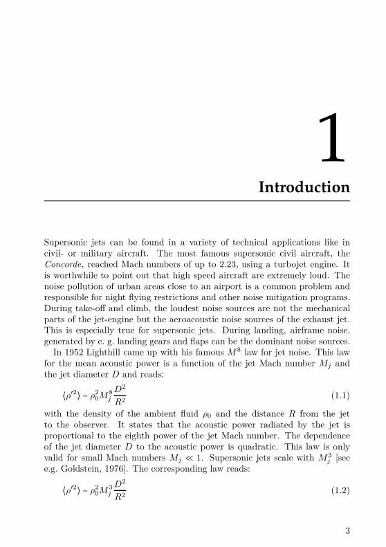
Supersonic jets can be found in a variety of technical applications like incivil- or military aircraft. The most famous supersonic civil aircraft, theConcorde, reached Mach numbers of up to 2.23, using a turbojet engine. Itis worthwhile to point out that high speed aircraft are extremely loud. Thenoise pollution of urban areas close to an airport is a common problem andresponsible for night flying restrictions and other noise mitigation programs.During take-off and climb, the loudest noise sources are not the mechanicalparts of the jet-engine but the aeroacoustic noise sources of the exhaust jet.This is especially true for supersonic jets. During landing, airframe noise,generated by e. g. landing gears and flaps can be the dominant noise sources.
In 1952 Lighthill came up with his famous M8 law for jet noise. This lawfor the mean acoustic power is a function of the jet Mach number Mj andthe jet diameter D and reads:
⟨ρ′2⟩ ∼ ρ20M8
j
D2
R2(1.1)
with the density of the ambient fluid ρ0 and the distance R from the jetto the observer. It states that the acoustic power radiated by the jet isproportional to the eighth power of the jet Mach number. The dependenceof the jet diameter D to the acoustic power is quadratic. This law is onlyvalid for small Mach numbers Mj ≪ 1. Supersonic jets scale with M3
j [seee.g. Goldstein, 1976]. The corresponding law reads:
⟨ρ′2⟩ ∼ ρ20M3
j
D2
R2(1.2)
3
1 Introduction
M3
M8
OASWL[dB]
M
0.1 1 1060
80
100
120
140
160
180
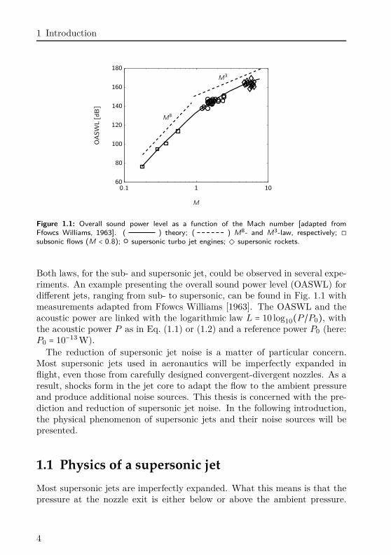
Figure 1.1: Overall sound power level as a function of the Mach number [adapted fromFfowcs Williams, 1963]. ( ) theory; ( ) M8- and M3-law, respectively; ◻subsonic flows (M < 0.8); supersonic turbo jet engines; supersonic rockets.
Both laws, for the sub- and supersonic jet, could be observed in several expe-riments. An example presenting the overall sound power level (OASWL) fordifferent jets, ranging from sub- to supersonic, can be found in Fig. 1.1 withmeasurements adapted from Ffowcs Williams [1963]. The OASWL and theacoustic power are linked with the logarithmic law L = 10 log10(P /P0), withthe acoustic power P as in Eq. (1.1) or (1.2) and a reference power P0 (here:P0 = 10−13 W).
The reduction of supersonic jet noise is a matter of particular concern.Most supersonic jets used in aeronautics will be imperfectly expanded inflight, even those from carefully designed convergent-divergent nozzles. As aresult, shocks form in the jet core to adapt the flow to the ambient pressureand produce additional noise sources. This thesis is concerned with the pre-diction and reduction of supersonic jet noise. In the following introduction,the physical phenomenon of supersonic jets and their noise sources will bepresented.
1.1 Physics of a supersonic jet
Most supersonic jets are imperfectly expanded. What this means is that thepressure at the nozzle exit is either below or above the ambient pressure.
4
1.1 Physics of a supersonic jet
(a) (b)
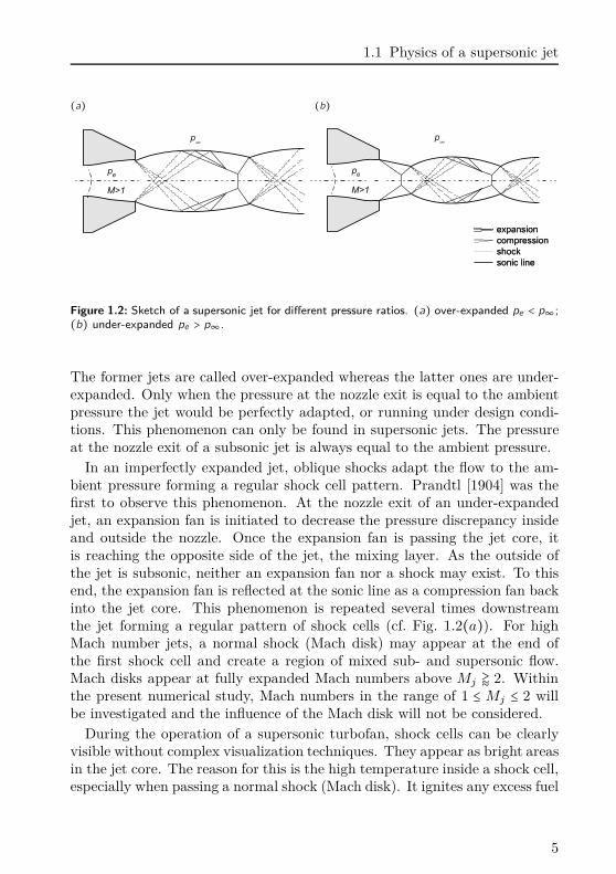
Figure 1.2: Sketch of a supersonic jet for different pressure ratios. (a) over-expanded pe < p∞;(b) under-expanded pe > p∞.
The former jets are called over-expanded whereas the latter ones are under-expanded. Only when the pressure at the nozzle exit is equal to the ambientpressure the jet would be perfectly adapted, or running under design condi-tions. This phenomenon can only be found in supersonic jets. The pressureat the nozzle exit of a subsonic jet is always equal to the ambient pressure.
In an imperfectly expanded jet, oblique shocks adapt the flow to the am-bient pressure forming a regular shock cell pattern. Prandtl [1904] was thefirst to observe this phenomenon. At the nozzle exit of an under-expandedjet, an expansion fan is initiated to decrease the pressure discrepancy insideand outside the nozzle. Once the expansion fan is passing the jet core, itis reaching the opposite side of the jet, the mixing layer. As the outside ofthe jet is subsonic, neither an expansion fan nor a shock may exist. To thisend, the expansion fan is reflected at the sonic line as a compression fan backinto the jet core. This phenomenon is repeated several times downstreamthe jet forming a regular pattern of shock cells (cf. Fig. 1.2(a)). For highMach number jets, a normal shock (Mach disk) may appear at the end ofthe first shock cell and create a region of mixed sub- and supersonic flow.Mach disks appear at fully expanded Mach numbers above Mj ⪆ 2. Withinthe present numerical study, Mach numbers in the range of 1 ≤ Mj ≤ 2 willbe investigated and the influence of the Mach disk will not be considered.
During the operation of a supersonic turbofan, shock cells can be clearlyvisible without complex visualization techniques. They appear as bright areasin the jet core. The reason for this is the high temperature inside a shock cell,especially when passing a normal shock (Mach disk). It ignites any excess fuel
5
1 Introduction
(a)r/D
x/D0 1 2 3 4 5 6 7 8 9 10
−1
0
1
(b)
r/D
x/D0 1 2 3 4 5 6 7 8 9 10
−1
0
1
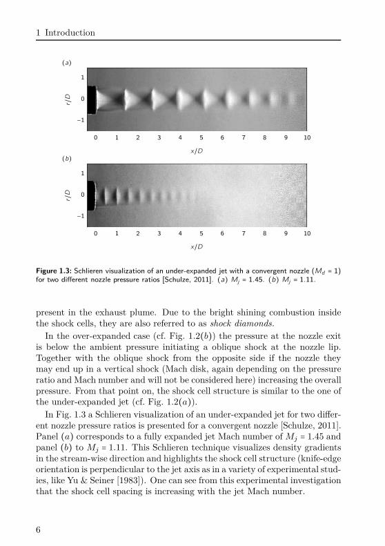
Figure 1.3: Schlieren visualization of an under-expanded jet with a convergent nozzle (Md = 1)for two different nozzle pressure ratios [Schulze, 2011]. (a) Mj = 1.45. (b) Mj = 1.11.
present in the exhaust plume. Due to the bright shining combustion insidethe shock cells, they are also referred to as shock diamonds.
In the over-expanded case (cf. Fig. 1.2(b)) the pressure at the nozzle exitis below the ambient pressure initiating a oblique shock at the nozzle lip.Together with the oblique shock from the opposite side if the nozzle theymay end up in a vertical shock (Mach disk, again depending on the pressureratio and Mach number and will not be considered here) increasing the overallpressure. From that point on, the shock cell structure is similar to the one ofthe under-expanded jet (cf. Fig. 1.2(a)).
In Fig. 1.3 a Schlieren visualization of an under-expanded jet for two differ-ent nozzle pressure ratios is presented for a convergent nozzle [Schulze, 2011].Panel (a) corresponds to a fully expanded jet Mach number of Mj = 1.45 andpanel (b) to Mj = 1.11. This Schlieren technique visualizes density gradientsin the stream-wise direction and highlights the shock cell structure (knife-edgeorientation is perpendicular to the jet axis as in a variety of experimental stud-ies, like Yu & Seiner [1983]). One can see from this experimental investigationthat the shock cell spacing is increasing with the jet Mach number.
6
1.1 Physics of a supersonic jet
over-expanded ideally expanded under-expanded
Mj <Md Mj =Md Mj >Md
Dj <D Dj =D Dj >D
pe > p∞ pe = p∞ pe < p∞
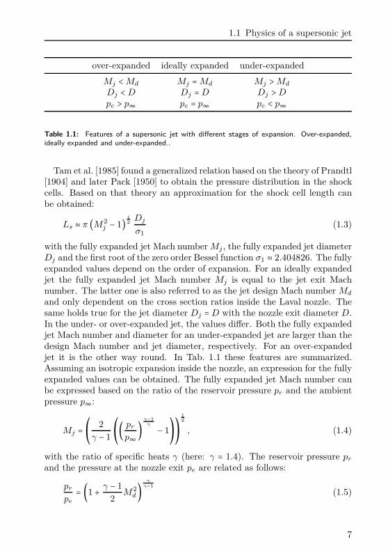
Table 1.1: Features of a supersonic jet with different stages of expansion. Over-expanded,ideally expanded and under-expanded..
Tam et al. [1985] found a generalized relation based on the theory of Prandtl[1904] and later Pack [1950] to obtain the pressure distribution in the shockcells. Based on that theory an approximation for the shock cell length canbe obtained:
Ls ≈ π (M2j − 1) 1
2Dj
σ1
(1.3)
with the fully expanded jet Mach number Mj , the fully expanded jet diameterDj and the first root of the zero order Bessel function σ1 ≈ 2.404826. The fullyexpanded values depend on the order of expansion. For an ideally expandedjet the fully expanded jet Mach number Mj is equal to the jet exit Machnumber. The latter one is also referred to as the jet design Mach number Md
and only dependent on the cross section ratios inside the Laval nozzle. Thesame holds true for the jet diameter Dj =D with the nozzle exit diameter D.In the under- or over-expanded jet, the values differ. Both the fully expandedjet Mach number and diameter for an under-expanded jet are larger than thedesign Mach number and jet diameter, respectively. For an over-expandedjet it is the other way round. In Tab. 1.1 these features are summarized.Assuming an isotropic expansion inside the nozzle, an expression for the fullyexpanded values can be obtained. The fully expanded jet Mach number canbe expressed based on the ratio of the reservoir pressure pr and the ambientpressure p∞:
Mj = ⎛⎝2
γ − 1
⎛⎝(
pr
p∞)
γ−1
γ − 1⎞⎠⎞⎠
1
2
, (1.4)
with the ratio of specific heats γ (here: γ = 1.4). The reservoir pressure pr
and the pressure at the nozzle exit pe are related as follows:
pr
pe
= (1 + γ − 12
M2d)
γ
γ−1
(1.5)
7
1 Introduction
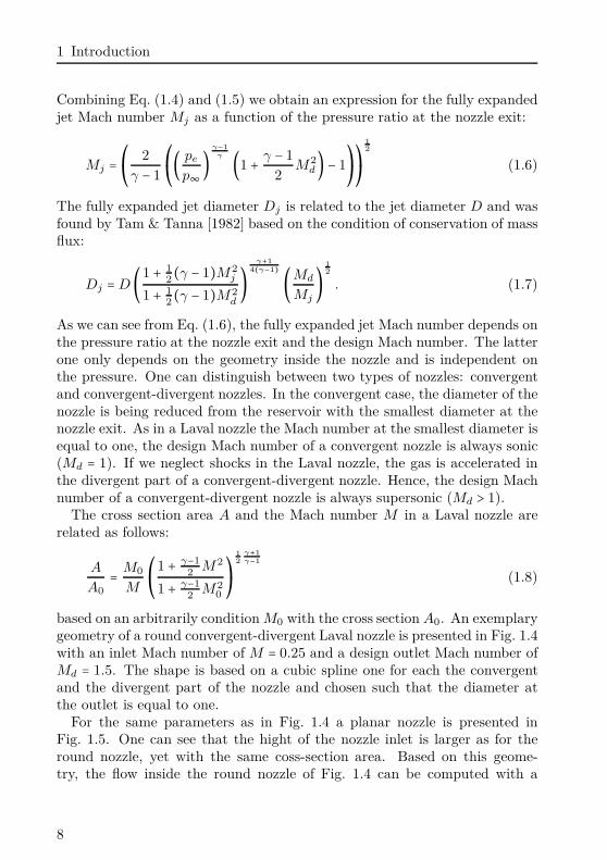
Combining Eq. (1.4) and (1.5) we obtain an expression for the fully expandedjet Mach number Mj as a function of the pressure ratio at the nozzle exit:
Mj = ⎛⎝2
γ − 1
⎛⎝(
pe
p∞)
γ−1
γ (1 + γ − 12
M2d) − 1
⎞⎠⎞⎠
1
2
(1.6)
The fully expanded jet diameter Dj is related to the jet diameter D and wasfound by Tam & Tanna [1982] based on the condition of conservation of massflux:
Dj =D (1 + 12(γ − 1)M2
j
1 + 12(γ − 1)M2
d
)γ+1
4(γ−1) (Md
Mj
)1
2
. (1.7)
As we can see from Eq. (1.6), the fully expanded jet Mach number depends onthe pressure ratio at the nozzle exit and the design Mach number. The latterone only depends on the geometry inside the nozzle and is independent onthe pressure. One can distinguish between two types of nozzles: convergentand convergent-divergent nozzles. In the convergent case, the diameter of thenozzle is being reduced from the reservoir with the smallest diameter at thenozzle exit. As in a Laval nozzle the Mach number at the smallest diameter isequal to one, the design Mach number of a convergent nozzle is always sonic(Md = 1). If we neglect shocks in the Laval nozzle, the gas is accelerated inthe divergent part of a convergent-divergent nozzle. Hence, the design Machnumber of a convergent-divergent nozzle is always supersonic (Md > 1).
The cross section area A and the Mach number M in a Laval nozzle arerelated as follows:
A
A0
= M0
M
⎛⎝
1 + γ−1
2M2
1 + γ−1
2M2
0
⎞⎠
1
2
γ+1
γ−1
(1.8)
based on an arbitrarily condition M0 with the cross section A0. An exemplarygeometry of a round convergent-divergent Laval nozzle is presented in Fig. 1.4with an inlet Mach number of M = 0.25 and a design outlet Mach number ofMd = 1.5. The shape is based on a cubic spline one for each the convergentand the divergent part of the nozzle and chosen such that the diameter atthe outlet is equal to one.
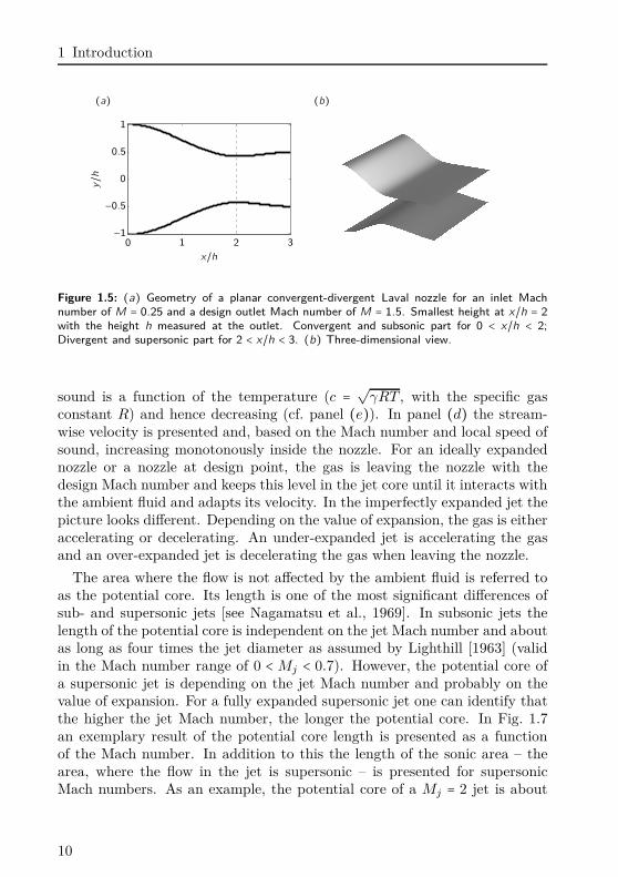
For the same parameters as in Fig. 1.4 a planar nozzle is presented inFig. 1.5. One can see that the hight of the nozzle inlet is larger as for theround nozzle, yet with the same coss-section area. Based on this geome-try, the flow inside the round nozzle of Fig. 1.4 can be computed with a
8
1.1 Physics of a supersonic jet
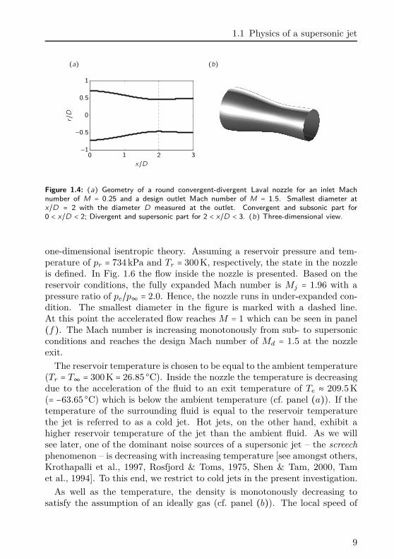
(a) (b)replacements
r/D
x/D0 1 2 3
−1
−0.5
0
0.5
1
Figure 1.4: (a) Geometry of a round convergent-divergent Laval nozzle for an inlet Machnumber of M = 0.25 and a design outlet Mach number of M = 1.5. Smallest diameter atx/D = 2 with the diameter D measured at the outlet. Convergent and subsonic part for0 < x/D < 2; Divergent and supersonic part for 2 < x/D < 3. (b) Three-dimensional view.
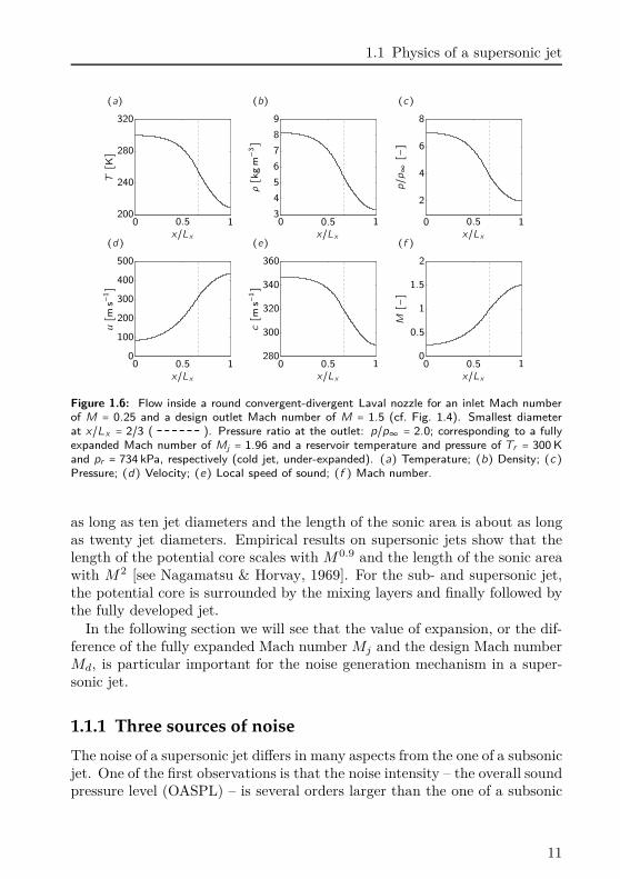
one-dimensional isentropic theory. Assuming a reservoir pressure and tem-perature of pr = 734 kPa and Tr = 300 K, respectively, the state in the nozzleis defined. In Fig. 1.6 the flow inside the nozzle is presented. Based on thereservoir conditions, the fully expanded Mach number is Mj = 1.96 with apressure ratio of pe/p∞ = 2.0. Hence, the nozzle runs in under-expanded con-dition. The smallest diameter in the figure is marked with a dashed line.At this point the accelerated flow reaches M = 1 which can be seen in panel(f). The Mach number is increasing monotonously from sub- to supersonicconditions and reaches the design Mach number of Md = 1.5 at the nozzleexit.
The reservoir temperature is chosen to be equal to the ambient temperature(Tr = T∞ = 300 K = 26.85 C). Inside the nozzle the temperature is decreasingdue to the acceleration of the fluid to an exit temperature of Te ≈ 209.5 K(= −63.65 C) which is below the ambient temperature (cf. panel (a)). If thetemperature of the surrounding fluid is equal to the reservoir temperaturethe jet is referred to as a cold jet. Hot jets, on the other hand, exhibit ahigher reservoir temperature of the jet than the ambient fluid. As we willsee later, one of the dominant noise sources of a supersonic jet – the screechphenomenon – is decreasing with increasing temperature [see amongst others,Krothapalli et al., 1997, Rosfjord & Toms, 1975, Shen & Tam, 2000, Tamet al., 1994]. To this end, we restrict to cold jets in the present investigation.
As well as the temperature, the density is monotonously decreasing tosatisfy the assumption of an ideally gas (cf. panel (b)). The local speed of
9
1 Introduction
(a) (b)ts
y/h
x/h0 1 2 3
−1
−0.5
0
0.5
1
Figure 1.5: (a) Geometry of a planar convergent-divergent Laval nozzle for an inlet Machnumber of M = 0.25 and a design outlet Mach number of M = 1.5. Smallest height at x/h = 2
with the height h measured at the outlet. Convergent and subsonic part for 0 < x/h < 2;Divergent and supersonic part for 2 < x/h < 3. (b) Three-dimensional view.
sound is a function of the temperature (c = √γRT , with the specific gasconstant R) and hence decreasing (cf. panel (e)). In panel (d) the stream-wise velocity is presented and, based on the Mach number and local speed ofsound, increasing monotonously inside the nozzle. For an ideally expandednozzle or a nozzle at design point, the gas is leaving the nozzle with thedesign Mach number and keeps this level in the jet core until it interacts withthe ambient fluid and adapts its velocity. In the imperfectly expanded jet thepicture looks different. Depending on the value of expansion, the gas is eitheraccelerating or decelerating. An under-expanded jet is accelerating the gasand an over-expanded jet is decelerating the gas when leaving the nozzle.
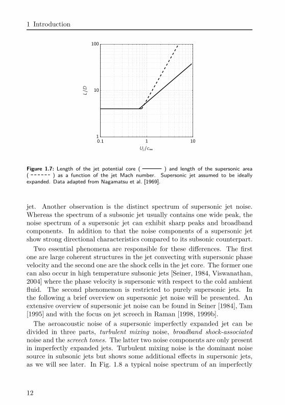
The area where the flow is not affected by the ambient fluid is referred toas the potential core. Its length is one of the most significant differences ofsub- and supersonic jets [see Nagamatsu et al., 1969]. In subsonic jets thelength of the potential core is independent on the jet Mach number and aboutas long as four times the jet diameter as assumed by Lighthill [1963] (validin the Mach number range of 0 < Mj < 0.7). However, the potential core ofa supersonic jet is depending on the jet Mach number and probably on thevalue of expansion. For a fully expanded supersonic jet one can identify thatthe higher the jet Mach number, the longer the potential core. In Fig. 1.7an exemplary result of the potential core length is presented as a functionof the Mach number. In addition to this the length of the sonic area – thearea, where the flow in the jet is supersonic – is presented for supersonicMach numbers. As an example, the potential core of a Mj = 2 jet is about
10
1.1 Physics of a supersonic jet
(a) (b) (c)replacementsT[K]
x/Lx0 0.5 1
200
240
280
320
ρ[kg
m−3]
x/Lx0 0.5 13
4
5
6
7
8
9
p/p∞[−]
x/Lx0 0.5 1
2
4
6
8
(d) (e) (f )
u[m
s−1]
x/Lx0 0.5 10
100
200
300
400
500c[m
s−1]
x/Lx0 0.5 1
280
300
320
340
360
M[−]
x/Lx0 0.5 10
0.5
1
1.5
2
Figure 1.6: Flow inside a round convergent-divergent Laval nozzle for an inlet Mach numberof M = 0.25 and a design outlet Mach number of M = 1.5 (cf. Fig. 1.4). Smallest diameterat x/Lx = 2/3 ( ). Pressure ratio at the outlet: p/p∞ = 2.0; corresponding to a fullyexpanded Mach number of Mj = 1.96 and a reservoir temperature and pressure of Tr = 300 K
and pr = 734 kPa, respectively (cold jet, under-expanded). (a) Temperature; (b) Density; (c)Pressure; (d) Velocity; (e) Local speed of sound; (f ) Mach number.
as long as ten jet diameters and the length of the sonic area is about as longas twenty jet diameters. Empirical results on supersonic jets show that thelength of the potential core scales with M0.9 and the length of the sonic areawith M2 [see Nagamatsu & Horvay, 1969]. For the sub- and supersonic jet,the potential core is surrounded by the mixing layers and finally followed bythe fully developed jet.
In the following section we will see that the value of expansion, or the dif-ference of the fully expanded Mach number Mj and the design Mach numberMd, is particular important for the noise generation mechanism in a super-sonic jet.
1.1.1 Three sources of noise
The noise of a supersonic jet differs in many aspects from the one of a subsonicjet. One of the first observations is that the noise intensity – the overall soundpressure level (OASPL) – is several orders larger than the one of a subsonic
11
1 Introduction
L/D
Uj /c∞0.1 1 101
10
100
Figure 1.7: Length of the jet potential core ( ) and length of the supersonic area( ) as a function of the jet Mach number. Supersonic jet assumed to be ideallyexpanded. Data adapted from Nagamatsu et al. [1969].
jet. Another observation is the distinct spectrum of supersonic jet noise.Whereas the spectrum of a subsonic jet usually contains one wide peak, thenoise spectrum of a supersonic jet can exhibit sharp peaks and broadbandcomponents. In addition to that the noise components of a supersonic jetshow strong directional characteristics compared to its subsonic counterpart.
Two essential phenomena are responsible for these differences. The firstone are large coherent structures in the jet convecting with supersonic phasevelocity and the second one are the shock cells in the jet core. The former onecan also occur in high temperature subsonic jets [Seiner, 1984, Viswanathan,2004] where the phase velocity is supersonic with respect to the cold ambientfluid. The second phenomenon is restricted to purely supersonic jets. Inthe following a brief overview on supersonic jet noise will be presented. Anextensive overview of supersonic jet noise can be found in Seiner [1984], Tam[1995] and with the focus on jet screech in Raman [1998, 1999b].
The aeroacoustic noise of a supersonic imperfectly expanded jet can bedivided in three parts, turbulent mixing noise, broadband shock-associatednoise and the screech tones. The latter two noise components are only presentin imperfectly expanded jets. Turbulent mixing noise is the dominant noisesource in subsonic jets but shows some additional effects in supersonic jets,as we will see later. In Fig. 1.8 a typical noise spectrum of an imperfectly
12
1.1 Physics of a supersonic jet
SPL
f Dj /Uj10−1 100
80
90
100
110
120
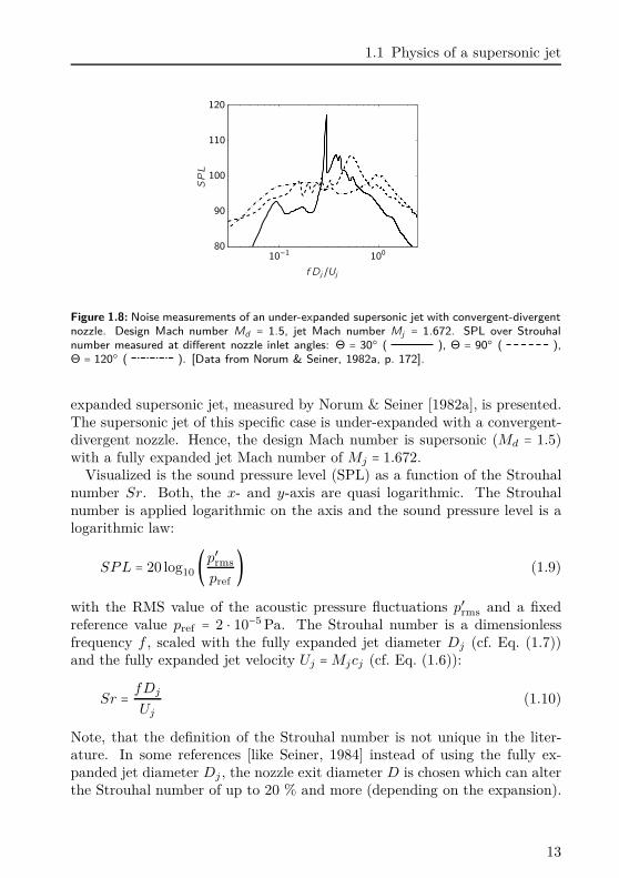
Figure 1.8: Noise measurements of an under-expanded supersonic jet with convergent-divergentnozzle. Design Mach number Md = 1.5, jet Mach number Mj = 1.672. SPL over Strouhalnumber measured at different nozzle inlet angles: Θ = 30 ( ), Θ = 90 ( ),Θ = 120 ( ). [Data from Norum & Seiner, 1982a, p. 172].
expanded supersonic jet, measured by Norum & Seiner [1982a], is presented.The supersonic jet of this specific case is under-expanded with a convergent-divergent nozzle. Hence, the design Mach number is supersonic (Md = 1.5)with a fully expanded jet Mach number of Mj = 1.672.
Visualized is the sound pressure level (SPL) as a function of the Strouhalnumber Sr. Both, the x- and y-axis are quasi logarithmic. The Strouhalnumber is applied logarithmic on the axis and the sound pressure level is alogarithmic law:
SP L = 20 log10 (p′rms
pref
) (1.9)
with the RMS value of the acoustic pressure fluctuations p′rms and a fixedreference value pref = 2 ⋅ 10−5 Pa. The Strouhal number is a dimensionlessfrequency f , scaled with the fully expanded jet diameter Dj (cf. Eq. (1.7))and the fully expanded jet velocity Uj =Mjcj (cf. Eq. (1.6)):
Sr = fDj
Uj
(1.10)
Note, that the definition of the Strouhal number is not unique in the liter-ature. In some references [like Seiner, 1984] instead of using the fully ex-panded jet diameter Dj , the nozzle exit diameter D is chosen which can alterthe Strouhal number of up to 20 % and more (depending on the expansion).
13
1 Introduction
The three curves in Fig. 1.8 correspond to three measurement angles. Onein the upstream direction of the jet (Θ = 30), one in the normal direction(Θ = 90) and one in the downstream direction (Θ = 120) with the angle Θmeasured from the upstream direction. One can observe a strong directivityof the noise with several peaks. Each of the three noise components can beidentified in the spectrum. The most prominent feature is the peak measuredin the upstream direction (Θ = 30) with a frequency of Sr ≈ 0.3 and anamplitude of 117.3 dB. This peak corresponds to the screech tone. It is morethan 10 dB louder than all other peaks in the spectrum.
Listening further in the downstream direction, normal to the jet axis (Θ =90), the peak of the screech tone vanished and an other component, thebroadband shock-associated noise, becomes the dominant noise source. Thepeak of this source is less sharp than the screech tone and of higher frequency(Sr ≈ 0.53). It is also visible in the upstream signal and in the downstreamsignal with increasing frequency when increasing the observation angle (Sr ≈0.4 and Sr ≈ 0.95, respectively). As we will see later, this is due to a Dopplershift of convecting sources. In addition to this, the peak amplitude of thebroadband component in the upstream and normal direction of the jet isabout 5 dB louder than in the downstream direction.
The turbulent mixing noise is of low frequency and low amplitude (20 −30 dB less than the screech tone) and can be detected at all three observationangles. It is characterized by a wide and flat hill with a wide peak in thespectrum. The frequency reaches from the largest wave length up the screechfrequency and beyond. Contrary to the screech tone and the shock-associatednoise the amplitude of the mixing noise is increasing with the observationangle.
1.1.1.1 Turbulent mixing noise
Turbulent mixing noise is caused by the large and small scale turbulent struc-tures in the jet mixing layers. Large scale structures are the dominant sourceswhereas the small scale structures induce the background noise.
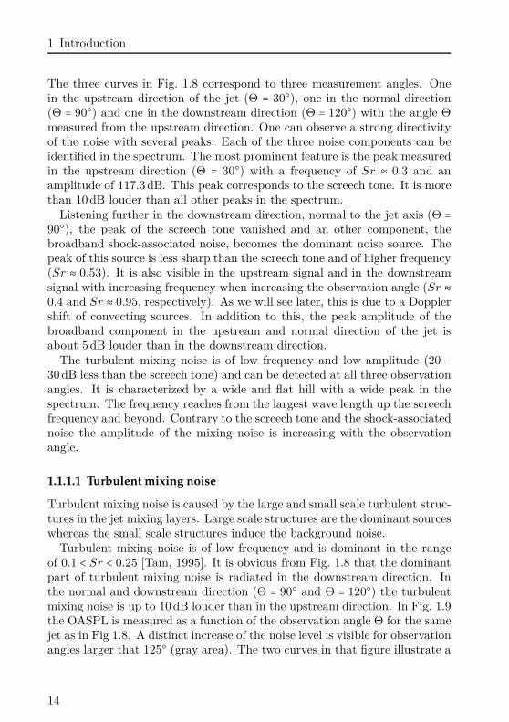
Turbulent mixing noise is of low frequency and is dominant in the rangeof 0.1 < Sr < 0.25 [Tam, 1995]. It is obvious from Fig. 1.8 that the dominantpart of turbulent mixing noise is radiated in the downstream direction. Inthe normal and downstream direction (Θ = 90 and Θ = 120) the turbulentmixing noise is up to 10 dB louder than in the upstream direction. In Fig. 1.9the OASPL is measured as a function of the observation angle Θ for the samejet as in Fig 1.8. A distinct increase of the noise level is visible for observationangles larger that 125 (gray area). The two curves in that figure illustrate a
14
1.1 Physics of a supersonic jet
PSfrag
OASPL
Θ [deg]0 30 60 90 120 150 180
115
120
125
130
135
Figure 1.9: Noise measurements of an under-expanded supersonic jet with convergent-divergentnozzle. Design Mach number Md = 1.5, jet Mach number Mj = 1.672 (same case as in Fig. 1.8).Overall SPL as a function of the observation angle Θ measured from the upstream direction.Gray area (Θ > 125 deg) dominated by turbulent mixing noise. ( ) without screechtone (tab inside the nozzle); ( ) with screech tone (no tab). [Data from Norum &Seiner, 1982a, p. 44f.].
case with screech and one without screech (to suppress the screech, a tab isincluded inside the nozzle [see Norum & Seiner, 1982a, p. 196]). As we willsee later, the screech tone is dominant in the upstream direction and doesnot affect the dominant turbulent mixing noise.
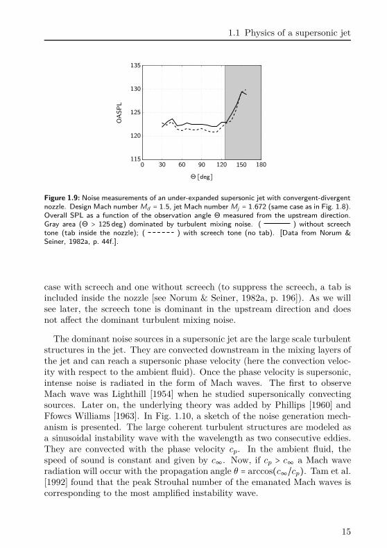
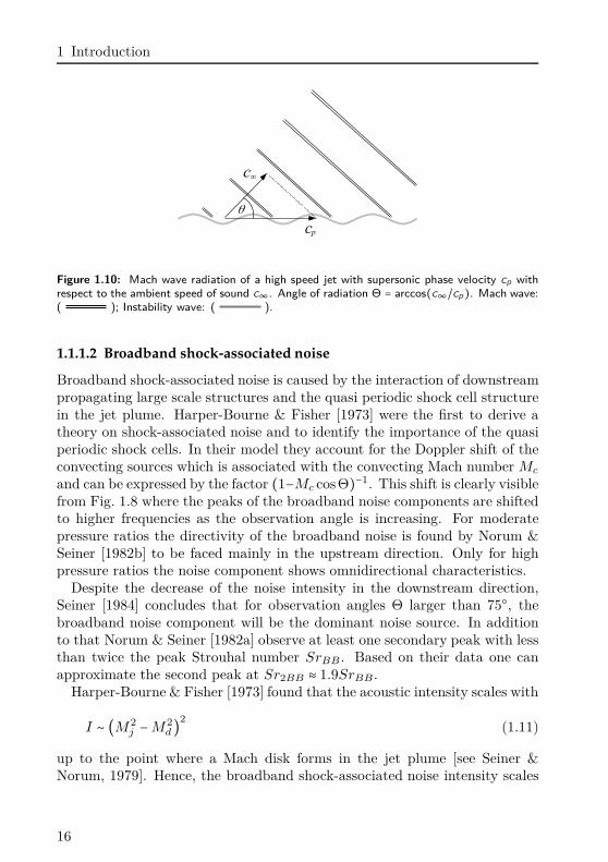
The dominant noise sources in a supersonic jet are the large scale turbulentstructures in the jet. They are convected downstream in the mixing layers ofthe jet and can reach a supersonic phase velocity (here the convection veloc-ity with respect to the ambient fluid). Once the phase velocity is supersonic,intense noise is radiated in the form of Mach waves. The first to observeMach wave was Lighthill [1954] when he studied supersonically convectingsources. Later on, the underlying theory was added by Phillips [1960] andFfowcs Williams [1963]. In Fig. 1.10, a sketch of the noise generation mech-anism is presented. The large coherent turbulent structures are modeled asa sinusoidal instability wave with the wavelength as two consecutive eddies.They are convected with the phase velocity cp. In the ambient fluid, thespeed of sound is constant and given by c∞. Now, if cp > c∞ a Mach waveradiation will occur with the propagation angle θ = arccos(c∞/cp). Tam et al.[1992] found that the peak Strouhal number of the emanated Mach waves iscorresponding to the most amplified instability wave.
15
1 Introduction
Figure 1.10: Mach wave radiation of a high speed jet with supersonic phase velocity cp withrespect to the ambient speed of sound c∞. Angle of radiation Θ = arccos(c∞/cp). Mach wave:( ); Instability wave: ( ).
1.1.1.2 Broadband shock-associated noise
Broadband shock-associated noise is caused by the interaction of downstreampropagating large scale structures and the quasi periodic shock cell structurein the jet plume. Harper-Bourne & Fisher [1973] were the first to derive atheory on shock-associated noise and to identify the importance of the quasiperiodic shock cells. In their model they account for the Doppler shift of theconvecting sources which is associated with the convecting Mach number Mc
and can be expressed by the factor (1−Mc cosΘ)−1. This shift is clearly visiblefrom Fig. 1.8 where the peaks of the broadband noise components are shiftedto higher frequencies as the observation angle is increasing. For moderatepressure ratios the directivity of the broadband noise is found by Norum &Seiner [1982b] to be faced mainly in the upstream direction. Only for highpressure ratios the noise component shows omnidirectional characteristics.
Despite the decrease of the noise intensity in the downstream direction,Seiner [1984] concludes that for observation angles Θ larger than 75, thebroadband noise component will be the dominant noise source. In additionto that Norum & Seiner [1982a] observe at least one secondary peak with lessthan twice the peak Strouhal number SrBB. Based on their data one canapproximate the second peak at Sr2BB ≈ 1.9SrBB.
Harper-Bourne & Fisher [1973] found that the acoustic intensity scales with
I ∼ (M2j −M2
d)2 (1.11)
up to the point where a Mach disk forms in the jet plume [see Seiner &Norum, 1979]. Hence, the broadband shock-associated noise intensity scales
16
1.1 Physics of a supersonic jet
Sr BB
θ [deg] Mj1.2
1.31.4
1.51.6
3060
90120
15010−1
100
101
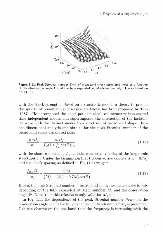
Figure 1.11: Peak Strouhal number SrBB of broadband shock-associated noise as a functionof the observation angle Θ and the fully expanded jet Mach number Mj . Theory based onEq. (1.13).
with the shock strength. Based on a stochastic model, a theory to predictthe spectra of broadband shock-associated noise has been proposed by Tam[1987]. He decomposed the quasi periodic shock cell structure into severaltime independent modes and superimposed the interaction of the instabil-ity wave with the distinct modes to a spectrum of broadband shape. In aone-dimensional analysis one obtains for the peak Strouhal number of thebroadband shock-associated noise:
fBBDj
uj
= ucDj
Ls(1 + uc
c∞cosΘ)uj
(1.12)
with the shock cell spacing Ls and the convective velocity of the large scalestructures uc. Under the assumption that the convective velocity is uc = 0.7uj
and the shock spacing as defined in Eq. (1.3) we get:
fBBDj
uj
= 0.54
(M2j − 1) 1
2 (1 + 0.7Mj cosΘ) . (1.13)
Hence, the peak Strouhal number of broadband shock-associated noise is onlydepending on the fully expanded jet Mach number Mj and the observationangle Θ. Note, that this relation is only valid for Mj > 1.
In Fig. 1.11 the dependence of the peak Strouhal number SrBB on theobservation angle Θ and the fully expanded jet Mach number Mj is presented.One can observe on the one hand that the frequency is increasing with the
17
1 Introduction
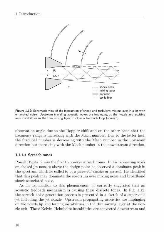
Figure 1.12: Schematic view of the interaction of shock and turbulent mixing layer in a jet withemanated noise. Upstream traveling acoustic waves are impinging at the nozzle and excitingnew instabilities in the thin mixing layer to close a feedback loop (screech).
observation angle due to the Doppler shift and on the other hand that thefrequency range is increasing with the Mach number. Due to the latter fact,the Strouhal number is decreasing with the Mach number in the upstreamdirection but increasing with the Mach number in the downstream direction.
1.1.1.3 Screech tones
Powell [1953a,b] was the first to observe screech tones. In his pioneering workon choked jet nozzles above the design point he observed a dominant peak inthe spectrum which he called to be a powerful whistle or screech. He identifiedthat this peak may dominate the spectrum over mixing noise and broadbandshock associated noise.
As an explanation to this phenomenon, he correctly suggested that anacoustic feedback mechanism is causing these discrete tones. In Fig. 1.12,the screech noise generation process is presented in a sketch of a supersonicjet including the jet nozzle. Upstream propagating acoustics are impingingon the nozzle lip and forcing instabilities in the thin mixing layer at the noz-zle exit. These Kelvin–Helmholtz instabilities are convected downstream and
18
1.1 Physics of a supersonic jet
growing rapidly in the mixing layer of the jet. Subsequently, they are inter-acting with the repeating shock cell structure and emanating noise. As forthe broadband shock-associated noise, these acoustics are emanated mainlyin the upstream direction and transported outside the jet towards the noz-zle. Once they reach the nozzle, new instabilities embryo and the feedbackmechanism is closed.
Experimental investigations on screech tones has been performed by ahost of researchers like Davies & Oldfield [1962a,b], Krothapalli et al. [1986],Mclaughlin et al. [1975], Nagel et al. [1983], Norum [1983], Seiner [1984],Seiner & Norum [1979], Tam & Tanna [1982], Westley & Woolley [1975] andmore recently by Alkislar et al. [2003], Gutmark et al. [1990], Panda [1998,1999], Panda et al. [1997], Ponton & Seiner [1992], Powell et al. [1992], Raman[1997a, 1999a], Yu et al. [1998], Zaman [1999]. A detailed overview over theresearch in jet screech from the beginnings with Powell in 1953 can be foundin Raman [1999b]. In the experiments on screech tones, sound pressure levelsof up to 160 dB could be observed. From Fig. 1.8, one can see that the screechtone is discrete in its frequency. This discrete and intense acoustic of 160 dBcorrespond to a RMS value of the pressure fluctuation of prms = 2000 Pa. Ona surface of one square meter (like e.g. the vertical tail of an airplane) thesepressure fluctuations are responsible for RMS loads of 2000 N. It is reportedin Hay & Rose [1970], Seiner [1994], Seiner et al. [1987] that screech tonesare responsible for structural damage and fatigue failure of airplane.
Powell [1953b] also observed that screech tones are not Doppler shifted.Independent on the observation angle, the screech frequency is constant. Thisleads to the conclusion that the source of screech tones is not convectedand hence linked to the quasi periodic shock cell structure. Despite theindependence on the frequency, the screech amplitude is strongly dependenton the observation angle. Whereas in the upstream direction, the screechtone is the dominant noise source, it is not detectable in the downstreamdirection (cf. Fig. 1.8 for Θ = 30 and Θ = 120).
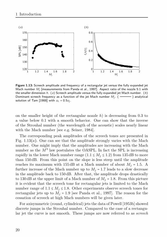
One of the most important observations of Powell [1953b] on his research onaxisymmetric (round) and two-dimensional (rectangular) jets, is the depen-dence of the screech Strouhal number SrS on the fully expanded jet Machnumber Mj . For rectangular jets, he observed a smooth variation of theStrouhal number when modifying the Mach number. More precisely, theStrouhal number decays monotonously with an increasing jet Mach number.A typical behavior of this phenomenon is presented in Fig. 1.13(b) based onmeasurements from Panda et al. [1997]. In his experiments, he used a rect-angular jet with an aspect ratio of the nozzle of 5:1 and varied the Machnumber in the range from 1.1 ≤Mj ≤ 1.85. The Strouhal number (here based
19
1 Introduction
(a) (b)
SPL[dB]
Mj
1 1.2 1.4 1.6 1.8 2120
130
140
150
160
170
f sh/Uj
Mj
1 1.2 1.4 1.6 1.8 20
0.2
0.4
0.6
0.8
Figure 1.13: Screech amplitude and frequency of a rectangular jet versus the fully expanded jetMach number Mj [measurements from Panda et al., 1997]. Aspect ratio of the nozzle 5:1 withthe smaller dimension h. (a) Screech amplitude versus the fully expanded jet Mach number. (b)Dominant screech frequency as a function of the jet Mach number Mj . ( ) analyticalsolution of Tam [1988] with uc = 0.5uj .
on the smaller height of the rectangular nozzle h) is decreasing from 0.3 toa value below 0.1 with a smooth behavior. One can show that the inverseof the Strouhal number (the wavelength of the acoustic) scales nearly linearwith the Mach number [see e.g. Seiner, 1984].
The corresponding peak amplitudes of the screech tones are presented inFig. 1.13(a). One can see that the amplitude strongly varies with the Machnumber. One might imply that the amplitudes are increasing with the Machnumber as the M3 law postulates the OASPL. In fact the SPL is increasingrapidly in the lower Mach number range (1.1 ≤Mj ≤ 1.2) from 135 dB to morethan 150 dB. From this point on the slope is less steep until the amplitudereaches its maximum with 155 dB at a Mach number of about Mj = 1.5. Afurther increase of the Mach number up to Mj = 1.7 leads to a slow decreasein the amplitude back to 150 dB. After that, the amplitude drops drasticallyto 130 dB at the upper limit of a Mach number of Mj = 1.8. From this pictureit is evident that the screech tone for rectangular jets is limited to the Machnumber range of 1.1 ≤Mj ≤ 1.8. Other experiments observe screech tones forrectangular jets up to Mj = 1.9 [see Panda et al., 1997]. The reason for thecessation of screech at high Mach numbers will be given later.
For axisymmetric (round, cylindrical) jets the data of Powell [1953b] showeddiscrete jumps in the Strouhal number. Compared to the case of a rectangu-lar jet the curve is not smooth. These jumps are now referred to as screech
20
1.1 Physics of a supersonic jet
(a) (b)SPL[dB]
Mj
1 1.2 1.4 1.6 1.8 2120
130
140
150
160
170
f sDj/Uj
Mj
1 1.2 1.4 1.6 1.8 20
0.2
0.4
0.6
0.8
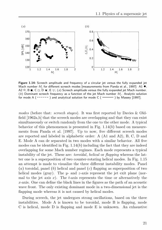
Figure 1.14: Screech amplitude and frequency of a circular jet versus the fully expanded jetMach number Mj for different screech modes [measurements from Panda et al., 1997]: A1 ;A2 ; B ∎; C ◻; D ; E ; (a) Screech amplitude versus the fully expanded jet Mach number.(b) Dominant screech frequency as a function of the jet Mach number Mj . Analytic solutionfor mode A ( ) and analytical solution for mode C ( ) by Massey [1997].
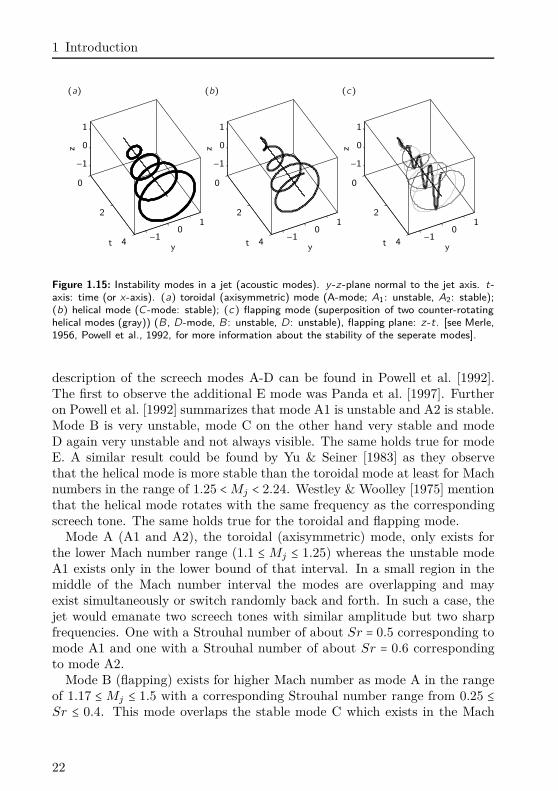
modes (before that: screech stages). It was first reported by Davies & Old-field [1962a,b] that the screech modes are overlapping and that they can existsimultaneously or switch randomly from the one to the other mode. A typicalbehavior of this phenomenon is presented in Fig. 1.14(b) based on measure-ments from Panda et al. [1997]. Up to now, five different screech modesare reported and labeled in alphabetic order: A (A1 and A2), B, C, D andE. Mode A can de separated in two modes with a similar behavior. All fivemodes can be identified in Fig. 1.14(b) including the fact that they are indeedoverlapping for some Mach number regimes. Each mode represents a typicalinstability of the jet. These are: toroidal, helical or flapping whereas the lat-ter one is a superposition of two counter-rotating helical modes. In Fig. 1.15an attempt is made to visualize the three different instability modes. Panel(a) toroidal, panel (b) helical and panel (c) flapping as superposition of twohelical modes (gray). The y- and z-axis represent the jet exit plane (nor-mal to the jet axis x). The t-axis represents the time or alternatively thex-axis. One can define the black lines in the figures as the path of an acousticwave front. The only existing dominant mode in a two-dimensional jet is theflapping mode whereas it is not caused by helical modes.
During screech, the jet undergoes strong oscillations, based on the threeinstabilities. Mode A is known to be toroidal, mode B is flapping, modeC is helical, mode D is flapping and mode E is unknown. An exhaustive
21
1 Introduction
(a) (b) (c)z
yt
0
2
4−1 0
1
−10
1
z
yt
0
2
4−1 0
1
−10
1
z
yt
0
2
4−1 0
1
−10
1
Figure 1.15: Instability modes in a jet (acoustic modes). y -z -plane normal to the jet axis. t-axis: time (or x-axis). (a) toroidal (axisymmetric) mode (A-mode; A1: unstable, A2: stable);(b) helical mode (C-mode: stable); (c) flapping mode (superposition of two counter-rotatinghelical modes (gray)) (B, D-mode, B: unstable, D: unstable), flapping plane: z -t. [see Merle,1956, Powell et al., 1992, for more information about the stability of the seperate modes].
description of the screech modes A-D can be found in Powell et al. [1992].The first to observe the additional E mode was Panda et al. [1997]. Furtheron Powell et al. [1992] summarizes that mode A1 is unstable and A2 is stable.Mode B is very unstable, mode C on the other hand very stable and modeD again very unstable and not always visible. The same holds true for modeE. A similar result could be found by Yu & Seiner [1983] as they observethat the helical mode is more stable than the toroidal mode at least for Machnumbers in the range of 1.25 <Mj < 2.24. Westley & Woolley [1975] mentionthat the helical mode rotates with the same frequency as the correspondingscreech tone. The same holds true for the toroidal and flapping mode.
Mode A (A1 and A2), the toroidal (axisymmetric) mode, only exists forthe lower Mach number range (1.1 ≤ Mj ≤ 1.25) whereas the unstable modeA1 exists only in the lower bound of that interval. In a small region in themiddle of the Mach number interval the modes are overlapping and mayexist simultaneously or switch randomly back and forth. In such a case, thejet would emanate two screech tones with similar amplitude but two sharpfrequencies. One with a Strouhal number of about Sr = 0.5 corresponding tomode A1 and one with a Strouhal number of about Sr = 0.6 correspondingto mode A2.
Mode B (flapping) exists for higher Mach number as mode A in the rangeof 1.17 ≤Mj ≤ 1.5 with a corresponding Strouhal number range from 0.25 ≤Sr ≤ 0.4. This mode overlaps the stable mode C which exists in the Mach
22
1.1 Physics of a supersonic jet
number range from 1.3 ≤Mj ≤ 1.6. Mode C is of higher frequency as mode Band exists without a neighboring mode in the small range from 1.5 ≤Mj ≤ 1.6.What follows is mode D and E up to Mach numbers of Mj = 1.9. They donot overlap each other which might imply that they are of similar structure.
In Fig. 1.14(a) the corresponding amplitudes of the screech tones are pre-sented. One can observe that on the one hand the amplitudes vary withthe jet Mach number, similar as for the rectangular jet, and that each modeexhibits different amplitudes. Modes A1 and A2 are comparable small intheir amplitude. Sound pressure levels of 140 - 150 dB could be measured. Ahigher SPL can be gained for mode B with a peak value of 160 dB. This isfollowed by mode C with the highest amplitude and a peak value of 162 dB.It is interesting to note that in the overlapping area of mode B and C, theamplitude of mode B drops to a value of about 132 dB which is a differenceof 30 dB. Finally, mode D and E exhibit less acoustic energy than the lattertwo ones at which mode D drops rapidly from 155 dB down to 133 dB andthe SPL of mode E is around 145 dB.
Despite the dominant peak values of the screech tone of one individualmode, additional subharmonics of that specific mode can exist. The am-plitude of these modes is usually smaller than the one of the fundamentalfrequency. A detailed description of additional subharmonics can be foundin Powell et al. [1992].
For a numerical experiment, mode instabilities and the so related randomlyback and forth switching of the individual states is extremely expensive. Tocapture the separated modes for a statistically converged result, the exper-iment needs to be simulated for a long time. To this end, we will focus inour axisymmetric jet computations on the helical mode C as it is very sta-ble. Furthermore we avoid an overlapping of other unstable modes. Thus,the remaining Mach number range is 1.5 ≤ Mj ≤ 1.6. The benefit of thisMach number range is also that the corresponding screech amplitude is verypowerful (in the order of 160 dB). Hence, a Mach number in the middle ofMj = 1.55 will be used for axisymmetric (round) jet noise simulations. Fortwo-dimensional (rectangular) jets only one stable mode does exist [Note,that Gutmark et al., 1990, observed a symmetric mode for rectangular jetsfor Mach numbers slightly above chokeing (1 ≤Mj ≤ 1.15) which we will notconsider here]. Hence, the Mach number can be chosen arbitrarily. To vali-date the present numerical method, a Mach number range of 1 ≤Mj ≤ 2 willbe investigated for the planar jet.
As we have seen in Fig. 1.13(b) and 1.14(b) the screech frequency, both forthe axisymmetric and rectangular jet, depends on the fully expanded Machnumber Mj . In fact, the screech frequency is depending on the shock cell
23
1 Introduction
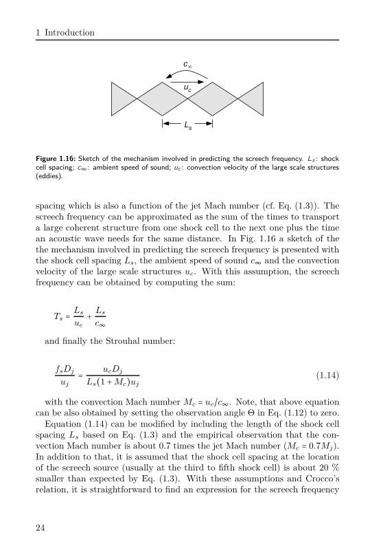
Figure 1.16: Sketch of the mechanism involved in predicting the screech frequency. Ls : shockcell spacing; c∞: ambient speed of sound; uc : convection velocity of the large scale structures(eddies).
spacing which is also a function of the jet Mach number (cf. Eq. (1.3)). Thescreech frequency can be approximated as the sum of the times to transporta large coherent structure from one shock cell to the next one plus the timean acoustic wave needs for the same distance. In Fig. 1.16 a sketch of thethe mechanism involved in predicting the screech frequency is presented withthe shock cell spacing Ls, the ambient speed of sound c∞ and the convectionvelocity of the large scale structures uc. With this assumption, the screechfrequency can be obtained by computing the sum:
Ts = Ls
uc
+Ls
c∞
and finally the Strouhal number:
fsDj
uj
= ucDj
Ls(1 +Mc)uj
(1.14)
with the convection Mach number Mc = uc/c∞. Note, that above equationcan be also obtained by setting the observation angle Θ in Eq. (1.12) to zero.
Equation (1.14) can be modified by including the length of the shock cellspacing Ls based on Eq. (1.3) and the empirical observation that the con-vection Mach number is about 0.7 times the jet Mach number (Mc = 0.7Mj).In addition to that, it is assumed that the shock cell spacing at the locationof the screech source (usually at the third to fifth shock cell) is about 20 %smaller than expected by Eq. (1.3). With these assumptions and Crocco’srelation, it is straightforward to find an expression for the screech frequency
24
1.1 Physics of a supersonic jet
only depending on the jet Mach number and the temperature ratio of the am-bient fluid T∞ and the reservoir temperature Tr, as proposed by Tam et al.[1986]:
fsDj
uj
= 0.67
(M2j − 1) 1
2
⎛⎜⎝1 +0.7Mj
(1 + γ−1
2M2
j ) 1
2
( Tr
T∞)−
1
2⎞⎟⎠−1
(1.15)
Note, that the assumption by Tam et al. [1986] that the convective Machnumber is 0.7 times the jet Mach number is not consistent in the literature.Powell et al. [1992] propose different values for the individual modes: 0.64(mode A), 0.68 (mode B), 0.8 (mode C) and 0.75 (mode D). Similar resultsare proposed by Panda et al. [1997]: 0.67 (mode A), 0.58 (mode B), 0.66(mode C) and 0.69 (mode D). These differences indicate that it is difficult topredict the convection Mach number [see also Gao & Li, 2010]. Furthermore,the convection velocity of the disturbances is not constant in a specific jet asthe disturbances are accelerated right after passing a shock and deceleratedas they approach a shock [see Raman, 1999b]. Improvements in the screechprediction formula, taking into account the individual modes of axisymmet-ric jets can be found e. g. in Gao & Li [2010], Massey [1997], Panda et al.[1997] and Powell et al. [1992]. An estimation of the screech frequency forrectangular jets can be found in Tam [1988].
In most experimental studies, the Reynolds number is in the order of 106.As we will see later, such high Reynolds numbers are unfavorable for directnumerical investigations, based on the state of art high performance comput-ers. In the present numerical investigation on planar and axisymmetric jetscreech, a Reynolds number of Re = 5000 is chosen. The remaining question is,to which extent the Reynolds number influences screech tones. High Reynoldsnumber flows contain more small scale turbulent fluctuations. These fluctua-tions will contribute to the shock-associated noise and will be responsible foradditional broadband components of high frequency. The screech frequencyis obviously depending on the shock cell spacing which is independent onthe Reynolds number. Hu & McLaughlin [1990] show that the small scaleturbulent structures are irrelevant to screech tones. They investigated a lowReynolds number under-expanded jet (ReD = 8000) and compared the re-sults to a high Reynolds number case (Re ≈ 106). It is demonstrated that thelarge scale fluctuations and the shock cell spacing are responsible for screechtones and independent on the Reynolds number. Only the broadband shockassociated noise components are reduced for the low Reynolds number jet.
25
1 Introduction
We have seen that the prediction of the screech frequency is straightforwardand, depending on the screech mode, can be approximated using empiricalresults for the convection Mach number. In contrast to that is the predic-tion of the screech amplitude. Up to now, no theory for the prediction ofthe screech amplitude is available not even an empirical. The difficulty inpredicting the screech amplitude is its strong dependency on the surroundingenvironment. Most sensitive to screech tones is the geometry of the nozzle,since it is responsible for the receptivity process – the coupling of acousticand hydrodynamic instabilities. Raman [1997a] observed that increasing thenozzle lip t of a rectangular jet with t/h = 0.2 to t/h = 2 increases the SPLfrom 130 dB up to 148 dB measured in a distance of 10h normal to the nozzleexit. This is a drastic increase of 18 dB by only changing the nozzle exitlip, a part which does not directly influence the jet flow. Other researcherslike Glass [1968] indicate that screech tones can be enhanced by an acous-tic reflector upstream the nozzle. The reflector can be placed such that thereflected acoustic waves amplify the acoustic fluctuations at the nozzle exitby means of a positive superposition of upstream and downstream propagat-ing waves and therefore enhance the receptivity process. The same reflectorcan be placed upstream the nozzle to suppress screech tones by means ofnoise cancellation at the nozzle exit as reported by Nagel et al. [1983], No-rum [1984]. Hence, the change of the surrounding environment, like reflectingsurfaces or the design of the nozzle have a significant impact on the screechtone amplitude which makes its prediction a challenging task. In additionto that, initial conditions, like a turbulent or laminar boundary layer insidethe nozzle, a swirl in the flow or the velocity distribution in the nozzle exitplane (depending on the contour of the nozzle contraction) may influence theindividual screech modes [Powell et al., 1992]. Especially the position of theneutral plane of the flapping mode may be exited randomly as reported bySeiner et al. [1986b].
One could expect that the screech amplitude is linked to the shock strength,as a certain shock amplitude is necessary to produce screech and strongscreech tones need strong shocks, but indeed the link between shock strengthand screech amplitude is very weak [see amongst others Raman, 1998]. Theshock strength is increasing monotonously [nearly linear; see Raman, 1997a]with the jet Mach number whereas the screech amplitude is first increasingup to a maximum value and then again decreasing (cf. Fig. 1.13(a)). Inthe following section some techniques to influence supersonic jet noise and inparticular jet screech will be addressed.
26
1.1 Physics of a supersonic jet
1.1.2 Mechanism of jet noise reduction
As we have seen, supersonic jet screech can be responsible for a loud anddiscrete noise source. In the early years of jet screech research it was thoughtthat screech tones do not exist in full scale aero-engines due to the non-uniformity of the flow and the complex geometry of the nozzle. However, theexperiments of Jungowski [1979] demonstrate that even a non-uniform flowdoes excite screech tones. It is furthermore reported in Hay & Rose [1970] andSeiner et al. [1987] that screech tones are responsible for structural damageand fatigue failure of airplane. To this end, the understanding and finallythe reduction of screech tones is a matter of particular concern. In the lastdecades several techniques were developed to influence screech tones. Theirmain idea is based on the cancellation of the feedback loop by means of activeand passive devices. In the following some active and passive devices will bepresented, beginning with the passive ones.
Acoustic reflector Glass [1968] was the first to observe that a passive acous-tic reflector can be used to enhance screech tones. He placed the reflector inan upstream position of the nozzle such that impinging acoustic waves (broad-band shock-associated noise) are reflected back in the downstream directionof the jet. These downstream wave are superimposed with the upstreampropagating waves and forming a standing wave with stationary nodes andanti-nodes. Is the reflector located such that the position of an anti-nodematches that of the nozzle exit, the feedback loop will be amplified. Thisphenomenon was also studied recently by Kweon et al. [2006] where theycould show that the jet mixing (here equivalent to screech) can be enhancedby a reflector placed at the nozzle exit. On the other hand, if the reflector islocated such that the position of a node matches that of the nozzle exit, thefeedback loop will be canceled. The latter phenomenon was investigated bya series of researches beginning with Nagel et al. [1983] and Norum [1984]. Itwas also studied recently by Khan et al. [2004]. Based on the theory that theanti-nodes and nodes of a standing wave can influence screech, the locationof the reflector to amplify and to cancel screech can be given. Assuming thescreech wave length to be λs and the fact that at the surface of the reflectoris an anti-node, the position for screech amplification and cancellation is at
x =⎧⎪⎪⎪⎪⎨⎪⎪⎪⎪⎩
−n
2λs amplification
−2n + 1
4λs cancelation
(1.16)
27
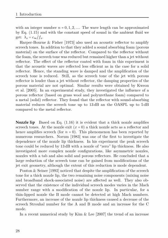
1 Introduction
with an integer number n = 0, 1, 2, .... The wave length can be approximatedby Eq. (1.15) and with the constant speed of sound in the ambient fluid weget: λs = c∞/fs.
Harper-Bourne & Fisher [1973] also used an acoustic reflector to amplifyscreech tones. In addition to that they added a sound absorbing foam (porousmaterial) on the surface of the reflector. Compared to the reflector withoutthe foam, the screech tone was reduced but remained higher than a jet withoutreflector. The effect of the reflector coated with foam in this experiment isthat the acoustic waves are reflected less efficient as in the case for a solidreflector. Hence, the standing wave is damped and the amplification of thescreech tone is reduced. Still, as the screech tone of the jet with porousreflector is louder than a jet without reflector, the damping properties of theporous material are not optimal. Similar results were obtained by Kweonet al. [2005]. In an experimental study, they investigated the influence of aporous reflector (based on grass wool and polyurethane foam) compared toa metal (solid) reflector. They found that the reflector with sound-absorbingmaterial reduces the screech tone up to 13 dB an the OASPL up to 5 dBcompared to the metal reflector.
Nozzle lip Based on Eq. (1.16) it is evident that a thick nozzle amplifiesscreech tones. At the nozzle exit (x = 0) a thick nozzle acts as a reflector andhence amplifies screech (for n = 0). This phenomenon has been reported bynumerous researchers. Norum [1983] was one of the first to investigate thedependence of the nozzle lip thickness. In his experiment the peak screechtone could be reduced by 13 dB with a nozzle of “zero” lip thickness. He alsoinvestigated more complex nozzle configurations, like asymmetric nozzles,nozzles with a tab and also solid and porous reflectors. He concluded that alarge reduction of the screech tone can be gained from modifications of thejet exit geometry, although the extent of this reduction is mode dependent.
Ponton & Seiner [1992] noticed that despite the amplification of the screechtone for a thick nozzle lip, the two remaining noise components (mixing noiseand broadband shock-associated noise) are affected as well. They also ob-served that the existence of the individual screech modes varies in the Machnumber range with a modification of the nozzle lip. In particular, for athin-lipped nozzle the B mode cannot be detected at high Mach numbers.Furthermore, an increase of the nozzle lip thickness caused a decrease of thescreech Strouhal number for the A and B mode and an increase for the Cmode.
In a recent numerical study by Kim & Lee [2007] the trend of an increase
28
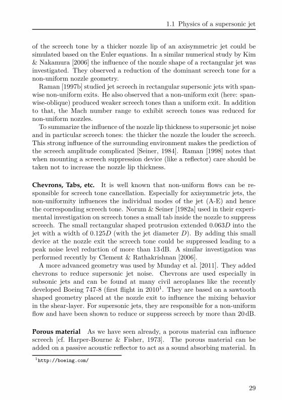
1.1 Physics of a supersonic jet
of the screech tone by a thicker nozzle lip of an axisymmetric jet could besimulated based on the Euler equations. In a similar numerical study by Kim& Nakamura [2006] the influence of the nozzle shape of a rectangular jet wasinvestigated. They observed a reduction of the dominant screech tone for anon-uniform nozzle geometry.
Raman [1997b] studied jet screech in rectangular supersonic jets with span-wise non-uniform exits. He also observed that a non-uniform exit (here: span-wise-oblique) produced weaker screech tones than a uniform exit. In additionto that, the Mach number range to exhibit screech tones was reduced fornon-uniform nozzles.
To summarize the influence of the nozzle lip thickness to supersonic jet noiseand in particular screech tones: the thicker the nozzle the louder the screech.This strong influence of the surrounding environment makes the prediction ofthe screech amplitude complicated [Seiner, 1984]. Raman [1998] notes thatwhen mounting a screech suppression device (like a reflector) care should betaken not to increase the nozzle lip thickness.
Chevrons, Tabs, etc. It is well known that non-uniform flows can be re-sponsible for screech tone cancellation. Especially for axisymmetric jets, thenon-uniformity influences the individual modes of the jet (A-E) and hencethe corresponding screech tone. Norum & Seiner [1982a] used in their experi-mental investigation on screech tones a small tab inside the nozzle to suppressscreech. The small rectangular shaped protrusion extended 0.063D into thejet with a width of 0.125D (with the jet diameter D). By adding this smalldevice at the nozzle exit the screech tone could be suppressed leading to apeak noise level reduction of more than 13 dB. A similar investigation wasperformed recently by Clement & Rathakrishnan [2006].
A more advanced geometry was used by Munday et al. [2011]. They addedchevrons to reduce supersonic jet noise. Chevrons are used especially insubsonic jets and can be found at many civil aeroplanes like the recentlydeveloped Boeing 747-8 (first flight in 20101. They are based on a sawtoothshaped geometry placed at the nozzle exit to influence the mixing behaviorin the shear-layer. For supersonic jets, they are responsible for a non-uniformflow and have been shown to reduce or suppress screech by more than 20 dB.
Porous material As we have seen already, a porous material can influencescreech [cf. Harper-Bourne & Fisher, 1973]. The porous material can beadded on a passive acoustic reflector to act as a sound absorbing material. In
1http://boeing.com/
29
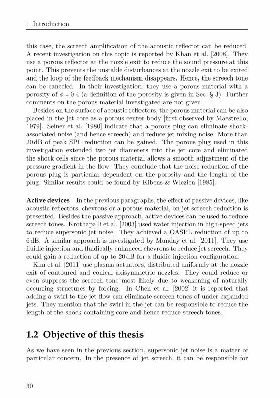
1 Introduction
this case, the screech amplification of the acoustic reflector can be reduced.A recent investigation on this topic is reported by Khan et al. [2008]. Theyuse a porous reflector at the nozzle exit to reduce the sound pressure at thispoint. This prevents the unstable disturbances at the nozzle exit to be exitedand the loop of the feedback mechanism disappears. Hence, the screech tonecan be canceled. In their investigation, they use a porous material with aporosity of φ = 0.4 (a definition of the porosity is given in Sec. § 3). Furthercomments on the porous material investigated are not given.
Besides on the surface of acoustic reflectors, the porous material can be alsoplaced in the jet core as a porous center-body [first observed by Maestrello,1979]. Seiner et al. [1980] indicate that a porous plug can eliminate shock-associated noise (and hence screech) and reduce jet mixing noise. More than20 dB of peak SPL reduction can be gained. The porous plug used in thisinvestigation extended two jet diameters into the jet core and eliminatedthe shock cells since the porous material allows a smooth adjustment of thepressure gradient in the flow. They conclude that the noise reduction of theporous plug is particular dependent on the porosity and the length of theplug. Similar results could be found by Kibens & Wlezien [1985].
Active devices In the previous paragraphs, the effect of passive devices, likeacoustic reflectors, chevrons or a porous material, on jet screech reduction ispresented. Besides the passive approach, active devices can be used to reducescreech tones. Krothapalli et al. [2003] used water injection in high-speed jetsto reduce supersonic jet noise. They achieved a OASPL reduction of up to6 dB. A similar approach is investigated by Munday et al. [2011]. They usefluidic injection and fluidically enhanced chevrons to reduce jet screech. Theycould gain a reduction of up to 20 dB for a fluidic injection configuration.
Kim et al. [2011] use plasma actuators, distributed uniformly at the nozzleexit of contoured and conical axisymmetric nozzles. They could reduce oreven suppress the screech tone most likely due to weakening of naturallyoccurring structures by forcing. In Chen et al. [2002] it is reported thatadding a swirl to the jet flow can eliminate screech tones of under-expandedjets. They mention that the swirl in the jet can be responsible to reduce thelength of the shock containing core and hence reduce screech tones.
1.2 Objective of this thesis
As we have seen in the previous section, supersonic jet noise is a matter ofparticular concern. In the presence of jet screech, it can be responsible for
30
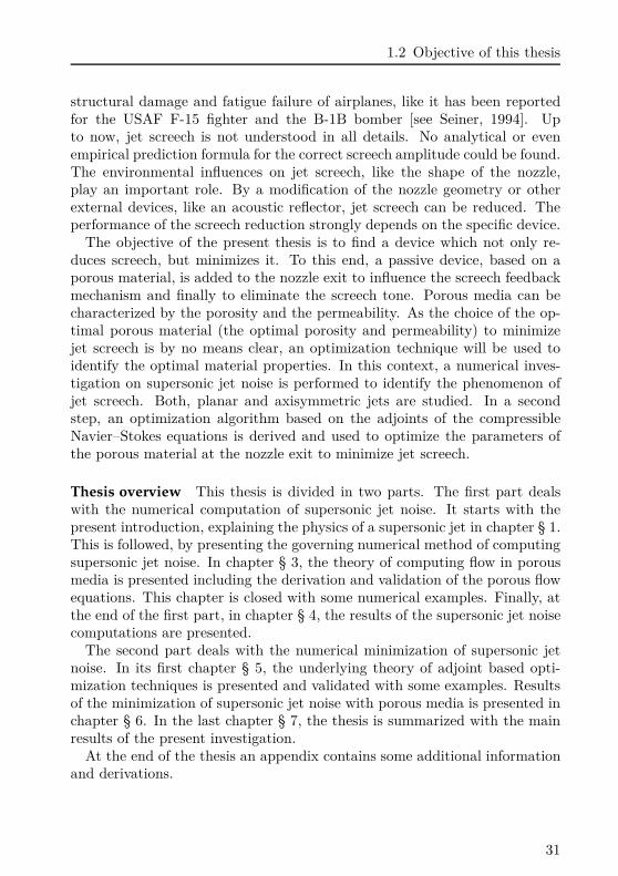
1.2 Objective of this thesis
structural damage and fatigue failure of airplanes, like it has been reportedfor the USAF F-15 fighter and the B-1B bomber [see Seiner, 1994]. Upto now, jet screech is not understood in all details. No analytical or evenempirical prediction formula for the correct screech amplitude could be found.The environmental influences on jet screech, like the shape of the nozzle,play an important role. By a modification of the nozzle geometry or otherexternal devices, like an acoustic reflector, jet screech can be reduced. Theperformance of the screech reduction strongly depends on the specific device.
The objective of the present thesis is to find a device which not only re-duces screech, but minimizes it. To this end, a passive device, based on aporous material, is added to the nozzle exit to influence the screech feedbackmechanism and finally to eliminate the screech tone. Porous media can becharacterized by the porosity and the permeability. As the choice of the op-timal porous material (the optimal porosity and permeability) to minimizejet screech is by no means clear, an optimization technique will be used toidentify the optimal material properties. In this context, a numerical inves-tigation on supersonic jet noise is performed to identify the phenomenon ofjet screech. Both, planar and axisymmetric jets are studied. In a secondstep, an optimization algorithm based on the adjoints of the compressibleNavier–Stokes equations is derived and used to optimize the parameters ofthe porous material at the nozzle exit to minimize jet screech.
Thesis overview This thesis is divided in two parts. The first part dealswith the numerical computation of supersonic jet noise. It starts with thepresent introduction, explaining the physics of a supersonic jet in chapter § 1.This is followed, by presenting the governing numerical method of computingsupersonic jet noise. In chapter § 3, the theory of computing flow in porousmedia is presented including the derivation and validation of the porous flowequations. This chapter is closed with some numerical examples. Finally, atthe end of the first part, in chapter § 4, the results of the supersonic jet noisecomputations are presented.
The second part deals with the numerical minimization of supersonic jetnoise. In its first chapter § 5, the underlying theory of adjoint based opti-mization techniques is presented and validated with some examples. Resultsof the minimization of supersonic jet noise with porous media is presented inchapter § 6. In the last chapter § 7, the thesis is summarized with the mainresults of the present investigation.
At the end of the thesis an appendix contains some additional informationand derivations.
31

2Theory of computing supersonic jet noise
A supersonic jet is a complex flow. The physical process acting on vastly dif-ferent length and time scales are a commonplace observation for this applica-tion. On the one hand, the propagation of long-wave acoustics (O(10−2m) –O(10−1m)) in the far field, like the mixing noise of low frequency or the roll-up of a large vortex (O(10−1m)) in the mixing-layer, are comparatively largescales. In contrast to that are small scale turbulent eddies in the order of theKolmogorov scale (η ≈ O(10−5m), for Re ≈ 106) or oblique or even verticalshocks with a length scale in the order of the mean free path (O(10−7m)).Different temporal scales originate e. g. in areas behind a bluff body, like thenozzle, with a large separation zone (M ≈ 0) compared to the downstreamtransported acoustics in the supersonic jet core (M ≫ 1).
Besides the vastly varying time and length scales, one also has to accountfor different amplitudes in the flow. These arise in particular in the acous-tic pressure fluctuations. The ambient pressure is in the order of O(105Pa).Depending on the noise level, an acoustic wave fluctuates from O(10−4Pa) at20 dB up to O(101Pa) at 120 dB. Propagating the quiet noise with 20 dB
causes a difference of 12 orders of magnitude in the pressure. It is needles tosay that this type of flow configuration causes a great challenge in computa-tional resources as well as numerical methods.
In the last decades different classes of methods developed with increasingcomplexity to compute turbulent flows. Beginning with the three-dimensional(Un)steady Reynolds Averaged Navier–Stokes (URANS) followed by the LargeEddy Simulation (LES) and finally the Direct Numerical Simulation (DNS).
33
2 Theory of computing supersonic jet noise
In addition to that, several subclasses and hybrid approaches combining theindividual methods emerged. A brief overview of the different classes andsubclasses can be found in Spalart [2000].
Reynolds averaged Navier–Stokes simulations do not compute the Navier–Stokes equations but their Reynolds averaged counterpart with the cost ofan additional statistical turbulence model. This method comes with the leastcomputational effort and needs, based on a high Reynolds number compu-tation, like the flow past an aeroplane, about 107 grid points to resolve thecomputational domain. To adjust the statistical turbulence model a lot of em-pirical information of the flow-case needs to be available. The second class,the Large Eddy Simulation, applies a low-pass filter to the Navier–Stokesequations and hence resolves on the large scales (eddies). To close the systemof equations, a sub-grid scale model needs to be included. The computationaleffort of this method is larger than the one of URANS computations and oneneeds for the computation of the high Reynolds number example about 1012
grid points to resolve the large scales. Finally, the Direct Numerical Sim-ulation, comes without any modeling and hence needs to resolve both thelargest and the smallest scales (Kolmogorov length-scale) of the turbulentflow. To resolve the high Reynolds number flow past an aeroplane, a total ofabout 1016 grid points need to be included in the computational domain. It istherefore on the one hand the most expensive method but on the other handthe most accurate one. State of the art high performance computers (HPC),with a peak performance of more than one Petaflop/s and several hundredTerabyte of main memory, are capable to handle about 109 grid points. Evenfor LES, the high Reynolds number flow can not be resolved on the state ofthe art computers. Hence, the numerical computation, especially the DNSis limited to moderate to low Reynolds number flows as the number of gridpoints scales with the Reynolds number, like:
NL ≈ L
η≈ Re
3/4L ; with ReL = UL
ν
in one direction. The smallest length-scale, the Kolmogorov scale η, and thelargest length-scale L determine the number of grid points and can be re-placed with the Reynolds number, based on the characteristic velocity U , thecorresponding length L and the kinematic viscosity ν. In three dimensions,the total number of grid points is:
NL ≈ Re9/4L
Based on the maximum number of grid points of state of the art computations(109) the largest resolvable Reynolds number is Remax = 104 for a DNS [see
34
also Kim et al., 1987]. To give an example on a supersonic jet computationbased on that Reynolds number and the assumption that the fluid is airunder standard conditions, the diameter of the jet would be 0.27mm (basedon Mj = 1.55 and T0 = 20C). In the present application a Reynolds numberof 5000 is chosen which corresponds to a diameter of 0.14mm. This is aboutthe thickness of a human hair. According to that, DNS is still linked to simpleflow geometries and academic cases. It is proposed by Spalart [2000] that ahigh Reynolds number DNS will be available in the year 2080 and a highReynolds number LES in the year 2045.
Above mentioned methods are capable to compute the aeroacoustic noisedirectly, yet with different accuracy. Direct Numerical Simulation (DNS),which resolves all scales, capture the aeroacoustic noise field without anyapproximations and provide the full spectrum of the generated noise withthe drawback of low Reynolds number limitations.
Large Eddy Simulation, model the effect of the small scales and hence failin the prediction of high-frequency noise components. These missing or underpredicted high-frequency spectral components in LES jet noise computationscan be highly annoying to the human ear [2-3 kHz, see Bodony & Lele, 2005]and are the most important components in noise regulation. In addition that,the choice of the sub-grid model in the LES is of particular importance tothe predicted noise. Bogey & Bailly [2005] show that the results obtained bya selective filter as sub-grid model are quantitatively closer to experimentaldata than the ones obtained by the widely used dynamic Smagorinsky modelby Moin et al. [1991]. They explain this behavior with the lowered effectiveReynolds number of the jet computation by means of the eddy viscosity. Areduction of a factor of 50 between the effective Reynolds number of thedynamic Smagorinsky model and the one using a compact/selective filter canbe observed.
Mathew et al. [2006, 2003] show that an explicit filter applied to the flowfield can be used as sub-grid-scale modeling alone. They apply the filterbetween every integration step of any DNS algorithm to obtain a LES andconclude that the solution tends uniformly towards the DNS once the grid isrefined and the filter cut-off is shifted to higher wave numbers.
A direct prediction of aeroacoustic noise by URANS computations presentsthe lowest level of flow details and spatial/temporal accuracy. This methodis only capable to predict the noise of the largest flow scales and fails inthe prediction of broadband components, like shock induced noise [see Wanget al., 2006].
However, the computational domain of any direct approach is limited andusually only contains the hydrodynamic fluctuations and the acoustic near-
35
2 Theory of computing supersonic jet noise
field. To propagate the waves into the acoustic far field or to apply it toURANS computations, hybrid methods can be used. These methods use somekind of source information, either in a volume containing the hydrodynamic(noisy) fluctuations (Lighthill), or on a surface enclosing the fluctuations(Linearized Euler Equations (LEE), Ffowks-Williams-Hawkins (FWH)). Thelatter ones, using the sources, distributed on a surface, can only be applied tomethods capable to compute the noise directly (LES or DNS). An applicationof these hybrid methods to a two-dimensional shear layer can be found inSchulze et al. [2007].
2.1 State of the art
In the following three paragraphs, an overview of the recent achievementsin the numerical simulation of supersonic jet noise, and in particular in su-personic jet screech, is outlined and divided in the three major direct meth-ods, beginning with the DNS, followed by the LES and finally the URANSmethod. The numerical investigations are summarized in Tab. 2.1 and sortedin chronological order.
Direct Numerical Simulation The first direct numerical simulation of su-personic jet noise was reported by Freund et al. [2000]. They computed aReD = 2000 jet based on a fully expanded jet Mach number Mj = 1.92 un-der design condition. Hence, no shocks and no screech was present, onlythe Mach wave radiation in the acoustic near field could be observed. Forthe spatial discretization they used a 6th order compact scheme proposed byLele [1992] and a 4th order Runge–Kutta method for the time integration.Most following research projects on jet noise based on DNS and LES use thiscombination of spatial and temporal discretization. The jet is computed ona cylindrical grid containing about 21 million grid points without includingthe nozzle directly. Instead, they use a inlet velocity profile to model thepresence of the nozzle.
One year later, Freund [2001] applied the DNS on a Mj = 0.9 subsonicjet with a Reynolds number ReD = 3600 and a slightly increased spatialresolution (26 million grid points). In this study, they could compare theirresults to experimental data by Stromberg et al. [1980] and showd a goodagreement in terms of mean flow, noise-spectra and -directivity.
Supersonic jet screech was first reported by Manning [1999], Manning &Lele [1998, 2000]. Instead of computing the whole jet and its acoustic field,they investigated the interaction of a shock wave impinging on a supersonic
36
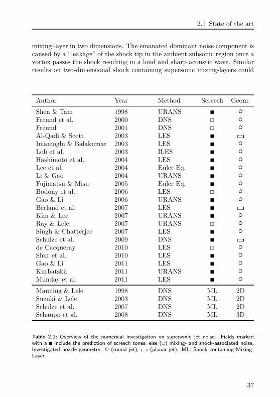
2.1 State of the art
mixing-layer in two dimensions. The emanated dominant noise component iscaused by a “leakage” of the shock tip in the ambient subsonic region once avortex passes the shock resulting in a loud and sharp acoustic wave. Similarresults on two-dimensional shock containing supersonic mixing-layers could
Author Year Method Screech Geom.
Shen & Tam 1998 URANS ∎ Freund et al. 2000 DNS ◻ Freund 2001 DNS ◻ Al-Qadi & Scott 2003 LES ∎ ◻
Imamoglu & Balakumar 2003 LES ∎ Loh et al. 2003 ILES ∎ Hashimoto et al. 2004 LES ∎ Lee et al. 2004 Euler Eq. ∎ Li & Gao 2004 URANS ∎ Fujimatsu & Misu 2005 Euler Eq. ∎ Bodony et al. 2006 LES ◻ Gao & Li 2006 URANS ∎ Berland et al. 2007 LES ∎ ◻
Kim & Lee 2007 URANS ∎ Ray & Lele 2007 URANS ◻ Singh & Chatterjee 2007 LES ∎ Schulze et al. 2009 DNS ∎ ◻
de Cacqueray 2010 LES ◻ Shur et al. 2010 LES ∎ Gao & Li 2011 LES ∎ Kurbatskii 2011 URANS ∎ Munday et al. 2011 LES ∎ Manning & Lele 1998 DNS ML 2DSuzuki & Lele 2003 DNS ML 2DSchulze et al. 2007 DNS ML 2DSchaupp et al. 2008 DNS ML 3D
Table 2.1: Overview of the numerical investigation on supersonic jet noise. Fields markedwith a ∎ include the prediction of screech tones; else (◻) mixing- and shock-associated noise.Investigated nozzle geometry: (round jet); ◻ (planar jet). ML: Shock containing Mixing-Layer.
37
2 Theory of computing supersonic jet noise
be observed by Suzuki & Lele [2003]. Schulze et al. [2007] included severalhybrid approaches (Linearized Euler Equations (LEE), Ffowcs-Williams andHawkins (FWH) and Lighthill) to the two-dimensional mixing-layer to prop-agate the noise in the acoustic far-field. They conclude that FWH besidesLEE are in good agreement to the DNS data and capable to propagate noiseof supersonic flow cases. Later, Schaupp et al. [2008] extended the shockcontaining mixing-layer in three dimensions and conclude that the proposedmethod is suitable for capturing the acoustic field generated in the interactionregion of shock and mixing-layer.
A DNS on a turbulent planar jet including screech could be observed bySchulze et al. [2009a]. They computed an under-expanded planar jet, peri-odic in the transverse direction, with a Reynolds number of ReD = 8000 anda fully expanded jet Mach number Mj = 1.4. The thin computational domaincontains more than 8 million grid points and is based on a Cartesian domainstretched in the stream-wise and transverse direction to refine the grid inthe turbulent region. The nozzle is modeled by a velocity profile as in thework of Freund and does not include the solid nozzle itself. As the sensitiv-ity of the instabilities of the mixing-layer to upstream propagating acousticsseems to be amplified by the presence of the nozzle an artificial forcing ofthe mixing-layer is applied to close the screech feedback loop. To this end,two “microphones” measure the noise in the upstream direction (close to theartificial nozzle exit) and apply this signal, together with a model spectrum,containing the most unstable instability and its subharmonics, to a smallfringe region in the mixing-layer. With this technique, a good agreementwith the theoretically expected screech frequency can be observed whereasthe screech amplitude is under-predicted. The discrepancy in the screechamplitude is probably related to the empirically adjustable gain of the arti-ficial forcing of the mixing-layer. A DNS including nearly 300 million gridpoints without artificial forcing (zero gain) showed no screech component inthe spectrum [see Schulze & Sesterhenn, 2010a, Schulze et al., 2009a].
Large Eddy Simulation LES prediction of supersonic jet noise was firstreported by Al-Qadi & Scott [2003, 2001]. They use a planar jet with aReynolds number based on the fully expanded jet height of Rehj
= 178000and the fully expanded jet Mach number Mj = 1.44 of a convergent nozzle(design Mach number Md = 1). Their Cartesian domain contains more than5 million grid points and is stretched to refine the shear layers. To treat thesub-grid scales, a compact low pass filter is applied together with a secondorder TVD based dissipation to treat shocks.
38
2.1 State of the art
A screech containing LES of a round jet was first reported by Imamoglu &Balakumar [2003] based on a fifth order Weighted Essentially Non Oscillatory(WENO) spatial discretization and a third order total variation diminishing(TVD) Runge–Kutta scheme for the time advancement. The fully expandedjet Mach number is Mj = 1.43 with a sonic design Mach number. Shockcell structure and screech frequency are in agreement to experimental datawithout comparing the screech amplitude.
Loh et al. [2003], Loh & Hultgren [2006] use a second order finite volumemethod to simulate screech of a round nozzle with an unstructured hexahedralgrid with a second order time integration. Based on a fully expanded jet Machnumber Mj = 1.42 they observe the flapping B-mode.
The helical C-mode was investigated by Hashimoto et al. [2004] with a LESof a round jet and a Mach number of Mj = 1.7 with a design Mach numberof Md = 1.33 (under-expanded, convergent-divergent (CD) nozzle). Spatialdiscretization is performed with a fourth order WENO scheme and a thirdorder Runge–Kutta method for the time advancement. Their grid containsmore than six million grid points with a Reynolds number of Re = 580000
In 2006, Bodony et al. simulate the noise radiation of a Mj = 2.2 round jetwith a design Mach number of Md = 1.95 (under-expanded). In this Machnumber regime screech tones are not present and only shock associated andmixing noise can be observed. Based on the fully expanded jet Mach numberand jet diameter a Reynolds number of Re = 394000 is adjusted using acylindrical grid containing one million grid points.
A round over-expanded jet (Mj = 1.49, Md = 2.0) was investigated, as wellas an under-expanded jet (Mj = 1.19, Md = 1.0), by Singh & Chatterjee [2007]using a WENO scheme.
Using an explicit spectral-like filtering of the flow variables, Berland et al.[2006, 2007] aim to minimize the dissipation on the resolved scales by ad-justing the filter close to the grid cutoff wavenumber. Thereby, the effectiveReynolds number of the inlet condition can be maintained [Bogey & Bailly,2005]. In their investigation on planar under-expanded jet screech compu-tation they simulate a Reynolds number of Reh = 60000 based on the jetheight and the fully expanded jet Mach number Mj = 1.55 (convergent noz-zle, Md = 1). A total of 16 million grid points are used on a Cartesian griddiscretized with explicit fourth order schemes in space and time. To avoidnumerical instabilities at discontinuities, like shocks, they apply a selectivefilter [Bogey et al., 2009]. Their results on screech frequency and amplitudeare in good agreement to analytical and experimental data. The observeddiscrepancies are addressed to the computational geometry and initial shearlayer thickness.
39
2 Theory of computing supersonic jet noise
Later, de Cacqueray [2010], de Cacqueray et al. [2011] computed a highsupersonic round jet with a fully expanded jet Mach number Mj = 2.83 atover-expanded conditions with a design Mach number Md = 3.3. This Machnumber regime is outside the range where screech can be observed, henceonly shock associated noise and turbulent mixing noise is considered. TheReynolds number, based on the jet exit conditions, is set to ReD = 94000 andsimulated with the same methods as in the previous mentioned work using27 million grid points. Spectral acoustic properties are in good agreementwith experimental data. Using the acoustic analogy based on the LinearizedEuler Equations (LEE) the acoustic information could be extrapolated intothe acoustic far-field.
Based on the FWH analogy, Shur et al. [2010] used a Mj = 1.36 round andunder-expanded jet, to capture the far-field acoustics including the screechtone. Recently, Gao & Li [2011] computed the axisymmetric mode of a roundMj = 1.19 under-expanded jet with roughly ten million grid points. A widerange of Mach numbers (1.22 ≤Mj ≤ 1.71) is investigated recently by Mundayet al. [2011] for a round over- and under-expanded jet. They use a nozzle in-cluding chevrons to reduce jet screech based on a finite element code including11 million grid points.
Unsteady Reynolds Averaged Navier–Stokes The first investigation to ap-ply a URANS to jet screech computations was performed by Shen & Tam[1998]. They observed both axisymmetric screech modes (A1 and A2) in aMach number range of (1.0 ≤Mj ≤ 1.2) with a convergent nozzle. They alsoinvestigate the influence of the temperature and the nozzle lip thickness onscreech tones in Shen & Tam [2000] and conclude that there is no stronginfluence of the temperature and lip thickness on screech tones for the lowMach number range. Later, Shen & Tam [2001, 2002] extend the Mach num-ber range up to Mj = 1.5 to also capture the flapping B- and helical C-mode.Their results regarding screech amplitude and frequency are in good agree-ment to experimental data and they found that two screech tones can existsimultaneously at one Mach number. They also mention that the presentmethod is not capable to predict broadband shock associated noise and thatempirical constants of the turbulence model need to be adjusted to matchthe analytical results.
A similar setup was studied by Li & Gao [2004, 2005] in a Mach numberrange of 1.05 ≤ Mj ≤ 1.2 where they could observe the A- and B-mode.To observe also the C-Mode, the Mach number range was extended up toMj = 1.6 in Li & Gao [2007] and the helical behavior could be observed.
40
2.1 State of the art
Gao & Li [2006] use a similar method and investigate the influence of thescreech tone to the initial shear layer thickness for the low Mach numberregime (Mj = 1.1). They observe that the a thin shear layer produces a5 dB louder screech tone than a thick shear layer as the thin shear layeris responsible for steeper velocity gradients and hence stronger shocks. Tothis end, they propose to reduce screech tones by enhancing the shear layerthickness.
Kim & Lee [2007], Kim & Nakamura [2006] investigate the influence of thenozzle lip to the screech tone and observe that a larger nozzle lip increasesthe screech frequency. This phenomenon can be explained with an increasedmomentum thickness for a larger nozzle lip due to the stronger reflectionsat the thick nozzle lip. The better the reflection properties, the larger thepressure fluctuations at the nozzle exit an hence the larger the momentumthickness. A thicker shear layer will reduce the effective nozzle diameter andtherefore increase the screech frequency (reduce the sock cell spacing andreduce the screech wavelength) while keeping the jet Mach number constant(only depending on the nozzle pressure ratio).
Over- and under-expanded jets were investigated by Ray & Lele [2007] andthe acoustic field was extrapolated with the LEE method. They found thatthe higher-frequency sound was missing in their computations which mighthave its origin in the intense modeling assumptions.
Recently, Kurbatskii [2011] investigated screech with a general purposesecond order finite volume CFD code in the Mach number range of 1.3 ≤Mj ≤ 1.6 for a convergent nozzle. He could capture the screech frequencyof the B- and C-mode in good agreement to experimental data, while theamplitudes differ with more than 10 dB. In addition to that, he observed anextended Mach number range for the B-mode (up to Mj = 1.6 compared toMj = 1.4 of the experimental data).
Other methods Besides the three above mentioned classes, another smallclass emerged using the Euler equations instead of the Navier–Stokes equa-tions. Hence, friction dependent influences are neglected and a comparison toreal flows is difficult. Lee et al. [2004] investigate screech tones from an under-expanded axisymmetric jet using the two-dimensional Euler equations with agrid containing a total of 160000 points solved with fourth order schemes inspace and time. For the lower Mach number range 1.08 ≤Mj ≤ 1.19 a goodagreement to experimental data can be found whereas the influence on thenozzle lip thickness does not match the experimental data. A similar setupis used by Fujimatsu & Misu [2005].
41
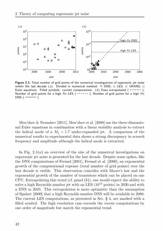
2 Theory of computing supersonic jet noise
(a) (b)
poin
ts
year
2000 2004 2008 2012104
105
106
107
108
109
high Re DNS
high Re LES
poin
ts
year
2000 2020 2040 2060 2080105
1010
1015
1020
Figure 2.1: Total number of grid points of the numerical investigations of supersonic jet noisewithin the last decade (a). Divided in numerical method: DNS; LES; URANS; ◻Euler equations. Filled symbols: current computations. (b) Data extrapolated ( );Number of grid points for a high Re LES ( ); Number of grid points for a high ReDNS ( ).
Men’shov & Nenashev [2011], Men’shov et al. [2008] use the three-dimensio-nal Euler equations in combination with a linear stability analysis to extractthe helical mode of a Mj = 1.7 under-expanded jet. A comparison of thenumerical results to experimental data shows a strong discrepancy in screechfrequency and amplitude although the helical mode is extracted.
In Fig. 2.1(a) an overview of the size of the numerical investigations onsupersonic jet noise is presented for the last decade. Despite some spikes, likethe DNS computations of Freund [2001], Freund et al. [2000], an exponentialgrowth of the computational expense (total number of grid points) over thelast decade is visible. This observation coincides with Moore’s law and theexponential growth of the number of transistors which can be placed on oneCPU. Extrapolating this trend (cf. panel (b)), one would expect the ability tosolve a high Reynolds number jet with an LES (1012 points) in 2030 and witha DNS in 2045. This extrapolation is more optimistic than the assumptionof Spalart [2000] that a high Reynolds number DNS will be available in 2080.The current LES computations, as presented in Sec. § 4, are marked with afilled symbol. The high resolution case exceeds the recent computations byone order of magnitude but match the exponential trend.
42
2.2 Equations of motion
2.2 Equations of motion
As we have seen in the previous introduction, there is a number of methodsavailable in the literature to treat supersonic jet noise computations. In thepresent application, we will use the three-dimensional compressible Navier–Stokes equations in combination with a high order dissipative upwind schemeapplied to the convective terms and a high order central scheme applied to thediffusive terms to solve the flow induced noise directly. As the upwind schemesare dissipative, they behave like a filter applied to the flow variables. To thisend, the present method can be classified as a LES with explicit filtering asproposed by e. g. Bogey & Bailly [2009], Mathew et al. [2006, 2003]. However,as the Reynolds number of the investigated jet noise computations is small(ReD = 5000) and the spatial resolution is high, the large scale computationscan be considered as an under-resolved DNS as the solution tends uniformlytowards the DNS once the grid is refined [see Mathew et al., 2006, 2003].
In the following section the governing equations of motion, as implementedin the present investigation, are presented.
2.2.1 Compressible Navier–Stokes equations
The perturbations of an unsteady fluid flow are described by the Navier–Stokes equations. They are divided in three equations: the mass conservation,the balance of momentum and the balance of energy. All three equations arehighly nonlinear and coupled with each other. Following the derivations inKovasznay [1953], it is possible to decouple the Navier–Stokes equations whenone applies a linearization of small perturbations around a base-flow. Thethree distinctly different modes are: vorticity mode, entropy mode and sound-wave mode. To this end, the three-dimensional compressible Navier–Stokesequations are written in non-conservative pressure p, velocity ui and entropys formulation and read:
∂p
∂t+ ui
∂p
∂xi
= −γ p∂ui
∂xi
+p
Cv
(∂s
∂t+ ui
∂s
∂xi
) (2.1a)
∂ui
∂t+ uj
∂ui
∂xj
= −1ρ
∂p
∂xi
+1ρ
∂τij
∂xj
(2.1b)
∂s
∂t+ ui
∂s
∂xi
= 1ρT(− ∂
∂xi
(−λ∂T
∂xi
) +Φ) (2.1c)
43
2 Theory of computing supersonic jet noise
where
τij ∶= 2µ(sij −13
skkδij) (2.2)
sij ∶= 12( ∂ui
∂xj
+∂uj
∂xi
) (2.3)
Φ ∶= τijsij (2.4)
and the Kronecker delta δij . The effects of the bulk viscosity are neglected.To close the above set of equations the following thermodynamic relationsare used. The fluid is modeled by dry air represented as a perfect gas:
p = ρRT (2.5)
with the gas constant R = 287 [m2K−1s−2] and the density ρ. The viscosityis modeled with Sutherland’s law
µ = µ0
T0 + S
T + S( T
T0
)3/2(2.6)
using the following constants: S = 110.4 [K] (Sutherland’s temperature), andT0 and µ0 the total temperature and corresponding viscosity, respectively.Heat conductivity is, following Fourier’s law, depending on the viscosity:
λ = µCp
P r. (2.7)
with γ = Cp/Cv = 1.4, Cp −Cv = R and P r = 0.71.
2.2.2 Characteristic Formulation
The Navier–Stokes equations are written in a characteristic formulation. Thishas several advantages. First of all, the treatment of the boundary conditionsin aeroacoustic applications is fairly easy since the commonly usual recalcu-lation in characteristic variables is no more necessary. For a non-reflectingboundary condition simply the incoming acoustic wave is set to zero. Otherboundary conditions like solid walls can be treated in a similar way as forcodes written in primitive variables. Secondly, due to the decomposition ofthe flow equations in waves one can use upwind schemes, where the up- anddown-traveling waves are discretized with up- and downwind schemes, respec-tively. Compared to commonly used central schemes, upwind schemes arenumerically dissipative which increases the numerical stability and reduces
44
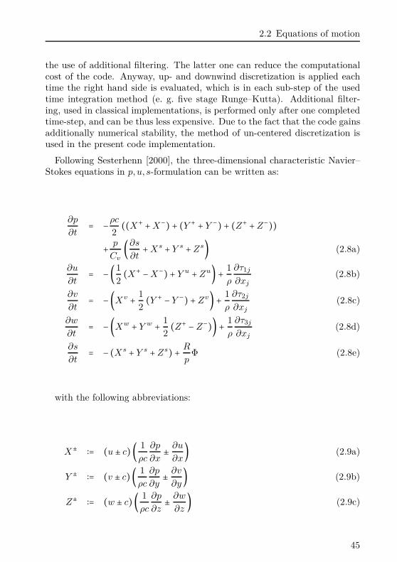
2.2 Equations of motion
the use of additional filtering. The latter one can reduce the computationalcost of the code. Anyway, up- and downwind discretization is applied eachtime the right hand side is evaluated, which is in each sub-step of the usedtime integration method (e. g. five stage Runge–Kutta). Additional filter-ing, used in classical implementations, is performed only after one completedtime-step, and can be thus less expensive. Due to the fact that the code gainsadditionally numerical stability, the method of un-centered discretization isused in the present code implementation.
Following Sesterhenn [2000], the three-dimensional characteristic Navier–Stokes equations in p, u, s-formulation can be written as:
∂p
∂t= −
ρc
2((X+ +X−) + (Y + + Y −) + (Z+ +Z−))
+p
Cv
(∂s
∂t+Xs + Y s +Zs) (2.8a)
∂u
∂t= −(1
2(X+ −X−) + Y u +Zu) + 1
ρ
∂τ1j
∂xj
(2.8b)
∂v
∂t= −(Xv +
12(Y + − Y −) +Zv) + 1
ρ
∂τ2j
∂xj
(2.8c)
∂w
∂t= −(Xw + Y w +
12(Z+ −Z−)) + 1
ρ
∂τ3j
∂xj
(2.8d)
∂s
∂t= − (Xs + Y s +Zs) + R
pΦ (2.8e)
with the following abbreviations:
X± ∶= (u ± c) ( 1ρc
∂p
∂x±
∂u
∂x) (2.9a)
Y ± ∶= (v ± c)( 1ρc
∂p
∂y±
∂v
∂y) (2.9b)
Z± ∶= (w ± c)( 1ρc
∂p
∂z±
∂w
∂z) (2.9c)
45
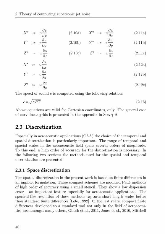
2 Theory of computing supersonic jet noise
Xv ∶= u∂v
∂x(2.10a)
Y u ∶= v∂u
∂y(2.10b)
Zu ∶= w∂u
∂z(2.10c)
Xw ∶= u∂w
∂x(2.11a)
Y w ∶= v∂w
∂y(2.11b)
Zv ∶= w∂v
∂z(2.11c)
Xs ∶= u∂s
∂x(2.12a)
Y s ∶= v∂s
∂y(2.12b)
Zs ∶= w∂s
∂z(2.12c)
The speed of sound c is computed using the following relation:
c =√γRT (2.13)
Above equations are valid for Cartesian coordinates, only. The general caseof curvilinear grids is presented in the appendix in Sec. § A.
2.3 Discretization
Especially in aeroacoustic applications (CAA) the choice of the temporal andspatial discretization is particularly important. The range of temporal andspacial scales in the aeroacoustic field spans several orders of magnitude.To this end, a high order of accuracy for the discretization is necessary. Inthe following two sections the methods used for the spatial and temporaldiscretization are presented.
2.3.1 Space discretization
The spatial discretization in the present work is based on finite differences inan implicit formulation. These compact schemes are modified Padé methodsof high order of accuracy using a small stencil. They show a low dispersionerror – an important feature especially for aeroacoustic applications. Thespectral-like resolution of these methods captures short length scales betterthan standard finite differences [Lele, 1992]. In the last years, compact finitedifferences developed to a standard tool not only in the field of aeroacous-tics [see amongst many others, Ghosh et al., 2011, Jones et al., 2010, Mitchell
46
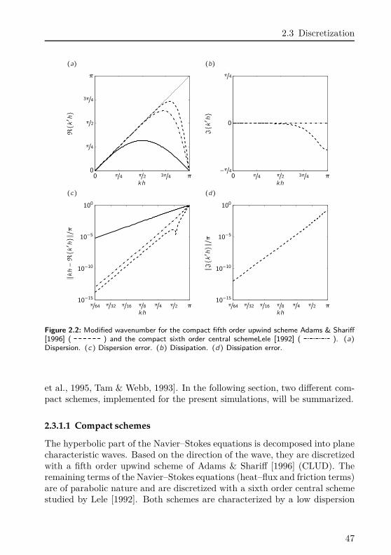
2.3 Discretization
(a) (b)Rk′h
kh0 π/4 π/2 3π/4 π
0
π/4
π/2
3π/4
π
Jk′h
kh0 π/4 π/2 3π/4 π
−π/4
0
π/4
(c) (d)
∥kh−Rk′h∥/π
kh
π/64 π/32 π/16 π/8 π/4 π/2 π10−15
10−10
10−5
100∥Jk′ h∥/π
kh
π/64 π/32 π/16 π/8 π/4 π/2 π10−15
10−10
10−5
100
Figure 2.2: Modified wavenumber for the compact fifth order upwind scheme Adams & Shariff[1996] ( ) and the compact sixth order central schemeLele [1992] ( ). (a)Dispersion. (c) Dispersion error. (b) Dissipation. (d) Dissipation error.
et al., 1995, Tam & Webb, 1993]. In the following section, two different com-pact schemes, implemented for the present simulations, will be summarized.
2.3.1.1 Compact schemes
The hyperbolic part of the Navier–Stokes equations is decomposed into planecharacteristic waves. Based on the direction of the wave, they are discretizedwith a fifth order upwind scheme of Adams & Shariff [1996] (CLUD). Theremaining terms of the Navier–Stokes equations (heat–flux and friction terms)are of parabolic nature and are discretized with a sixth order central schemestudied by Lele [1992]. Both schemes are characterized by a low dispersion
47
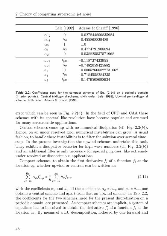
2 Theory of computing supersonic jet noise
Lele [1992] Adams & Shariff [1996]
α−2 0 0.027844800835984α−1
1/3 0.455868829489α0 1 1.0α1
1/3 0.4774791908094α2 0 0.038825537571968
a−21/36 −0.118727423955
a−17/9 −0.7482059425882
a0 0 0.00052666822731662a1
7/9 0.7184558284235a2
1/36 0.1479508698924
Table 2.2: Coefficients used for the compact schemes of Eq. (2.14) on a periodic domain(interior points). Central tridiagonal scheme, sixth order: Lele [1992]; Upwind penta-diagonalscheme, fifth order: Adams & Shariff [1996].
error which can be seen in Fig. 2.2(a). In the field of CFD and CAA theseschemes with its spectral like resolution have become popular and are usedfor many aeroacoustic applications.
Central schemes come up with no numerical dissipation (cf. Fig. 2.2(b)).Hence, on an under resolved grid, numerical instabilities can grow. A usualfashion, to handle these instabilities is to filter the solution aver several time–step. In the present investigation the upwind schemes undertake this task.They exhibit a dissipative behavior for high wave numbers (cf. Fig. 2.2(b))and an additional filter is only necessary for special purposes, like extremelyunder resolved or discontinuous applications.
Compact schemes, to obtain the first derivative f ′i of a function fi at thelocation xi, whether upwind or central, can be written as:
µr∑µ=−µl
αµf ′i+µ = 1h
νr∑ν=−νl
aνfi+ν (2.14)
with the coefficients αµ and aν . If the coefficients αµ = α−µ and aν = a−ν , oneobtains a central scheme and apart from that an upwind scheme. In Tab. 2.2,the coefficients for the two schemes, used for the present discretization on aperiodic domain, are presented. As compact schemes are implicit, a system ofequations has to be solved to obtain the derivative f ′i of a function fi at thelocation xi. By means of a LU decomposition, followed by one forward and
48
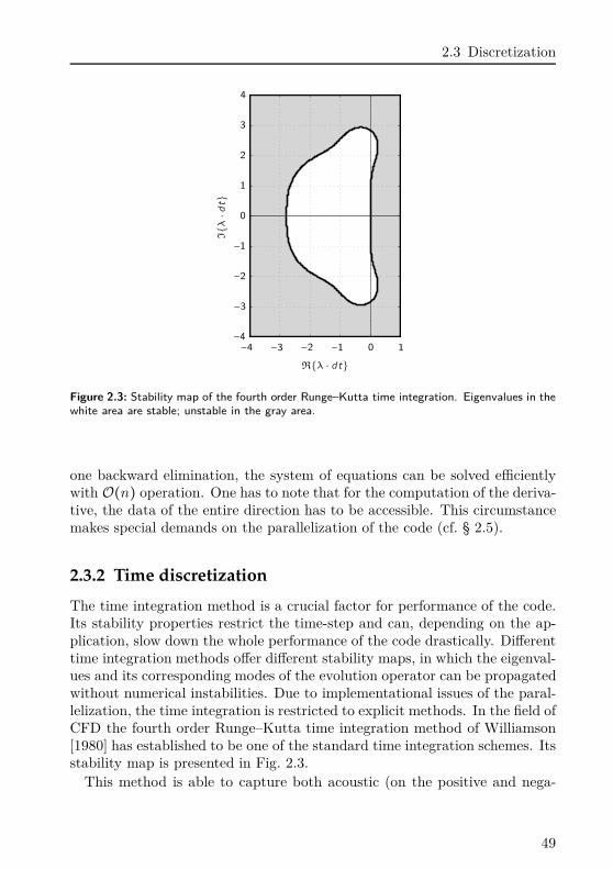
2.3 Discretization
Iλ⋅dt
Rλ ⋅ dt−4 −3 −2 −1 0 1−4
−3
−2
−1
0
1
2
3
4
Figure 2.3: Stability map of the fourth order Runge–Kutta time integration. Eigenvalues in thewhite area are stable; unstable in the gray area.
one backward elimination, the system of equations can be solved efficientlywith O(n) operation. One has to note that for the computation of the deriva-tive, the data of the entire direction has to be accessible. This circumstancemakes special demands on the parallelization of the code (cf. § 2.5).
2.3.2 Time discretization
The time integration method is a crucial factor for performance of the code.Its stability properties restrict the time-step and can, depending on the ap-plication, slow down the whole performance of the code drastically. Differenttime integration methods offer different stability maps, in which the eigenval-ues and its corresponding modes of the evolution operator can be propagatedwithout numerical instabilities. Due to implementational issues of the paral-lelization, the time integration is restricted to explicit methods. In the field ofCFD the fourth order Runge–Kutta time integration method of Williamson[1980] has established to be one of the standard time integration schemes. Itsstability map is presented in Fig. 2.3.
This method is able to capture both acoustic (on the positive and nega-
49
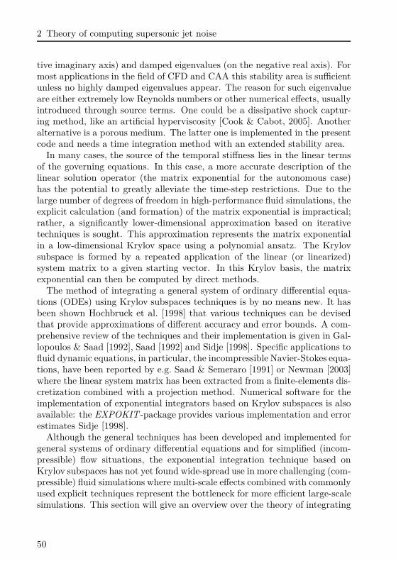
2 Theory of computing supersonic jet noise
tive imaginary axis) and damped eigenvalues (on the negative real axis). Formost applications in the field of CFD and CAA this stability area is sufficientunless no highly damped eigenvalues appear. The reason for such eigenvalueare either extremely low Reynolds numbers or other numerical effects, usuallyintroduced through source terms. One could be a dissipative shock captur-ing method, like an artificial hyperviscosity [Cook & Cabot, 2005]. Anotheralternative is a porous medium. The latter one is implemented in the presentcode and needs a time integration method with an extended stability area.
In many cases, the source of the temporal stiffness lies in the linear termsof the governing equations. In this case, a more accurate description of thelinear solution operator (the matrix exponential for the autonomous case)has the potential to greatly alleviate the time-step restrictions. Due to thelarge number of degrees of freedom in high-performance fluid simulations, theexplicit calculation (and formation) of the matrix exponential is impractical;rather, a significantly lower-dimensional approximation based on iterativetechniques is sought. This approximation represents the matrix exponentialin a low-dimensional Krylov space using a polynomial ansatz. The Krylovsubspace is formed by a repeated application of the linear (or linearized)system matrix to a given starting vector. In this Krylov basis, the matrixexponential can then be computed by direct methods.
The method of integrating a general system of ordinary differential equa-tions (ODEs) using Krylov subspaces techniques is by no means new. It hasbeen shown Hochbruck et al. [1998] that various techniques can be devisedthat provide approximations of different accuracy and error bounds. A com-prehensive review of the techniques and their implementation is given in Gal-lopoulos & Saad [1992], Saad [1992] and Sidje [1998]. Specific applications tofluid dynamic equations, in particular, the incompressible Navier-Stokes equa-tions, have been reported by e.g. Saad & Semeraro [1991] or Newman [2003]where the linear system matrix has been extracted from a finite-elements dis-cretization combined with a projection method. Numerical software for theimplementation of exponential integrators based on Krylov subspaces is alsoavailable: the EXPOKIT -package provides various implementation and errorestimates Sidje [1998].
Although the general techniques has been developed and implemented forgeneral systems of ordinary differential equations and for simplified (incom-pressible) flow situations, the exponential integration technique based onKrylov subspaces has not yet found wide-spread use in more challenging (com-pressible) fluid simulations where multi-scale effects combined with commonlyused explicit techniques represent the bottleneck for more efficient large-scalesimulations. This section will give an overview over the theory of integrating
50
2.3 Discretization
linear and nonlinear ODEs in time with an exponential Krylov scheme. Amore detailed review can be found in Schulze et al. [2009b] which is used asa basis for this section.
2.3.2.1 Theory of Exponential Krylov Time Integration
The exponential time integration with on Krylov subspaces is based on alow-dimensional approximation of the matrix exponential which representsthe exact evolution operator for an autonomous linear system. For inhomo-geneous problems minor modifications have to be implemented, as will beshown later. To start, however, we will consider the simplest case: the linearand autonomous problem. The linear theory will be applied to the adjointcompressible and porous Navier–Sokes equations as they are linear. The non-linear theory of the subsequent paragraph unge be applied to the nonlinearcompressible and porous Navier–Sokes equations.
Linear equations The solution of the linear and autonomous problem
du(t)dt
= Au(t) + q(t), (2.15a)
u(0) = v (2.15b)
with system matrix A, state vector u, initial condition v and external drivingq can formally be written as
u(t) = etAv +∫ t
0e(t−s)Aq(s)ds. (2.16)
The first term involves the matrix exponential and represents the homoge-neous part of the solution, whereas the second term consists of a convolutionintegral, again involving the matrix exponential, and represents the particularpart of the full solution.
We will first consider the homogeneous case, i.e., the case where q = 0, forwhich we need to compute the matrix exponential applied to a vector, etAv. IfA is a bounded operator, which is the case for most fluid dynamic equations,the matrix exponential can be defined by a Taylor power series. For anunbounded operator, like an elliptic operator, the meaning of A comes fromthe mathematical theory of semigroups. A detailed discussion of this topiccan be found in Trefethen [2005]. Since the present research project focuseson fluid dynamic equations, the solution of the matrix exponential will be
51
2 Theory of computing supersonic jet noise
A = Vm Vm+1= HeT1hm+1vm+1Hm +
Hm
= + =
Vm
Vm
Figure 2.4: Arnoldi decomposition for a square matrix A with m subspaces Vm and the reducedHessenberg matrix Hm.
understood as an expansion series for the remainder of this discussion, like
etAv = ∞∑n=0
1n!(tA)n v. (2.17)
A straightforward approach to construct etA is thus a truncated form of(2.17). This is in fact the underlying principle of a Runge–Kutta (or anylinear multi-step) scheme; in general, Runge–Kutta schemes approximate thefirst few terms of the above Taylor series expansion, but are not a recom-mended method – according to Moler & Loan [2003] – to approximate thematrix exponential. Better approximations can be found if we seek a generalpolynomial approximation of the product of the matrix exponential and agiven vector of the form
etAv ≈ pm−1(tA)v (2.18)
with pm−1 denoting a general (m − 1)-degree polynomial.This approximation problem can be recast by introducing a m-dimensional
Krylov subspace based on the starting vector v and the system matrix A
Km = spanv, Av, ..., Am−1v. (2.19)
Our problem thus reduces to finding an element in the Krylov subspace Km
that best approximates the solution to the homogeneous initial-value problem.To efficiently manipulate the elements of the Krylov subspace we generate anorthonormal basis Vm = [v1, v2, ..., vm] of Km. This orthonormal basis isobtained by employing the well-known Arnoldi algorithm starting with theinitial vector v1 = v/β where β = ∥v∥2. Besides the orthonormal basis Vm,
the Arnoldi algorithm also produces an upper m×m Hessenberg-matrix Hm
52
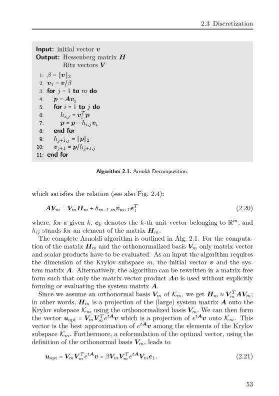
2.3 Discretization
Input: initial vector v
Output: Hessenberg matrix H
Ritz vectors V
1: β = ∥v∥22: v1 = v/β3: for j = 1 to m do4: p =Avj
5: for i = 1 to j do6: hi,j = vT
i p
7: p = p − hi,jvi
8: end for9: hj+1,j = ∥p∥2
10: vj+1 = p/hj+1,j
11: end for
Algorithm 2.1: Arnoldi Decomposition.
which satisfies the relation (see also Fig. 2.4):
AVm = VmHm + hm+1,mvm+1eT1 (2.20)
where, for a given k, ek denotes the k-th unit vector belonging to Rm, and
hij stands for an element of the matrix Hm.The complete Arnoldi algorithm is outlined in Alg. 2.1. For the computa-
tion of the matrix Hm and the orthonormalized basis Vm only matrix-vectorand scalar products have to be evaluated. As an input the algorithm requiresthe dimension of the Krylov subspace m, the initial vector v and the sys-tem matrix A. Alternatively, the algorithm can be rewritten in a matrix-freeform such that only the matrix-vector product Av is used without explicitlyforming or evaluating the system matrix A.
Since we assume an orthonormal basis Vm of Km, we get Hm ≈ V Tm AVm;
in other words, Hm is a projection of the (large) system matrix A onto theKrylov subspace Km using the orthonormalized basis Vm. We can then formthe vector uopt = VmV T
m etAv which is a projection of etAv onto Km. Thisvector is the best approximation of etAv among the elements of the Krylovsubspace Km. Furthermore, a reformulation of the optimal vector, using thedefinition of the orthonormal basis Vm, leads to
uopt = VmV Tm etAv = βVmV T
m etAVme1. (2.21)
53
2 Theory of computing supersonic jet noise
The optimal vector still depends on the matrix exponential etA based on the(large) matrix A, which is in practice unobtainable. However, owing to theorthogonality of the basis Vm, we can introduce the following approximation
V Tm etAVm ≈ etHm (2.22)
and finally rewrite the vector uopt as
uopt ≈ βVmetHm e1, (2.23)
or, with the improved approximation including the residual in Eq. (2.20) withhm+1,m,
uopt ≈ βVm+1etHm+1e1. (2.24)
The original problem — which was to compute etAv with A ∈ Rn×n —has been replaced by evaluating etHm v with Hm ∈ Rm×m and m ≪ n. Forthe reduced problem, the matrix exponential can be computed using highlyaccurate Padé methods [Moler & Loan, 2003].
It should be mentioned that the Arnoldi algorithm merely requires theproduct of A and v to compute Vm and Hm; we thus do not explicitly needto know the system matrix A — which is the case for the present applications.
Contrary to the formulation above, the solution u(t) at a given time t isnot computed directly, but rather advanced from the initial condition v viaa time-stepping algorithm. The problem to be treated by the exponentialtime integration thus reduces to an initial-value problem over one time step[tn, tn + τ]
u(0) = v (2.25a)
u(tn + τ) = e(tn+τ)Av = eτAu(tn). (2.25b)
For various flow configurations the system of governing equations is non-homogeneous, i.e., the source term q in (2.15) is nonzero. Examples includereacting fluids where the combustion terms are modeled as temperature-dependent source terms, or numerical boundary conditions such as an outflowsponge term that applies a highly dissipative force near the boundary whichensures that no (or negligible) energy is scattered back into the computationaldomain. In the present case, the linear adjoint Navier–Stokes equations areintegrated backwards in time with this method. They contain a source term,arising from the objective function, which drives the adjoint peturbationsbackwards in time. The general solution for this problem is given in (2.16)and can be rewritten using the solution of the integral term
u(t) = etAv + tϕ(tA)q (2.26)
54
2.3 Discretization
where ϕ(z) = (ez − 1)/z. The resulting method
un+1 = eτAun + τϕ(τA)q(tn), tn+1 = tn + τ (2.27)
is often called the (explicit) exponential Euler method. Exponential time-integration methods of Runge–Kutta type are studied in Hochbruck & Os-termann [2005].
If we use the following manipulation
u(tn + τ) = eτAu(tn) + τϕ(τA)q(tn),= (τAϕ(τA) + I)u(tn) + τϕ(τA)q(tn),= τϕ(τA)(Au(tn) + q(tn)) +u(tn), (2.28)
the only remaining expensive operation for the inhomogeneous case is toevaluate ϕ(τA)v which can be approximated in a similar manner as eτAv.
We therefore obtain
ϕ(τA)v ≈ βVmϕ(τHm)e1. (2.29)
The Krylov subspace approximation to ϕ(τA)v converges toward the exactsolution as fast as eτAv converges to its exact equivalent, see Hochbruck &Lubich [1997].
Following the formulation in Saad [1992], the function ϕ(Z) of a matrixargument Z — or, more precisely, the product ϕ(Z)e1 — can be computedusing only one matrix exponential
exp( Z e1
0 0 ) = ( exp(Z) ϕ(Z)e1
0 1 ) . (2.30)
This expression can be obtained by explicitly deriving the matrix exponentialby a Taylor series expansion (cf. also Saad [1992]).
Nonlinear equations The exponential time-integration technique is basedon a linear problem given by the system matrix A. However, nonlinear gov-erning equations are well within the reach of this technique. In particular, wewant to apply the Krylov time-integration method to the nonlinear compress-ible porous Navier-Stokes equations, which calls for some small modifications.First, the equations have to be linearized about the current state vector, and,secondly, we need an approximation for the resulting Jacobian matrix A.
55
2 Theory of computing supersonic jet noise
We consider the general nonlinear initial-value problem
du(t)dt
= f(u(t)). (2.31)
A Taylor expansion of the right-hand side about a given state u(tn) yields
f(u(t)) = f(u(tn)) + ∂f
∂u(u(tn))(u(t)−u(tn)) + r(u(t)) (2.32)
with the remainder term r(u(t))and the Jacobian matrix
A ≡ ∂f
∂u(u(tn)) (2.33)
The nonlinear governing equation can then be rewritten in the form
du(t)dt
= f(u(tn)) +A(u(t) −u(tn)) + r(u(t)). (2.34)
Introducing an integrating factor e−tA in Eq. (2.34) and subsequently inte-grating over the interval t ∈ [tn, tn + τ], the solution u(tn + τ) at the newtime-step yields
u(tn+τ) = u(tn)+(eτA−I)A−1f(u(tn))+∫ tn+τ
tn
e(tn+τ−s)Ar(u(s))ds.
(2.35)
Equation (2.35) still depends on A ∈ Rn×n and represents an exact solution toproblem (2.31). The integral term in Eq. (2.35) has to be evaluated numer-ically. Different methods based on quadrature rules like Runge–Kutta andmulti-step methods are presented, e.g., in Tokman [2006] and Hochbruck et al.[1998]. Solving this integral term numerically will enhance the accuracy of thetime-integration method at the expense of an increase in computational time.More precisely, depending on the specific case and the chosen approximationmethod for the integral, the computational time for the solution of the in-tegral roughly matches the computational time for the approximated matrixexponential [see Tokman, 2006]. This raises the question whether the inclu-sion of this integral term is necessary for our specific fluid dynamic equations.It is shown in Schulze et al. [2009b] that omitting the integral is comparableto the error induced by a standard explicit Runge–Kutta method. Methodsof this type are referred to as exponentially fitted Euler methods Hochbruck
56
2.4 Including the nozzle
et al. [1998] or exponential Rosenbrock-Euler methods Caliari & Ostermann[2009]
Using the same ϕ-function from the linear, nonhomogeneous case, ϕ(z) =(ez −1)/z, and setting the integral to zero, we can rewrite Eq. (2.35) and givean approximation for the solution at the new time-step as
u(tn + τ) ≈ u(tn) + τϕ1(τA)f(u(tn)). (2.36)
Employing the approximation of the matrix exponential in the ϕ-function,we obtain
u(tn + τ) ≈ u(tn) + τβVm+1ϕ1(τHm+1)e1 (2.37)
including the improved approximation with Hm+1 = [H 0] .The Jacobian A = ∂f
∂u(u(tn)) of the system can be approximated using
a first Fréchet derivative. However, we choose to implement the Arnoldialgorithm in a matrix-free form; we thus only need the matrix-vector productAv (see Alg. 2.1) which can straightforwardly be approximated by
Av ≈ f(u + εv) − f(u)ε
. (2.38)
The choice of ε in Eq. (2.38) can be influential on the stability of the simu-lation, in particular, for large systems, and has to be adapted judiciously foreach case. For the numerical simulations presented in the next section, wechose the parameter ε according to
ε = ∥u∥2√εmachine (2.39)
which yielded satisfactory results.The present method shows excellent stability properties and is capable to
integrate stiff equations, like the porous Navier–Stokes equations of Sec. 3.1.In Fig. 3.2 of Sec. 3.1.4 these properties are presented in detail. In additionto that, the method is able to treat linear equation in an efficient way. Thisis especially important for the solution of the adjoint equations of Sec. 5.4.1,which are linear.
2.4 Including the nozzle
Supersonic jet screech is very sensitive to the shape of the nozzle geometryand may be even eliminated for certain geometries. Hence, embedding the
57
2 Theory of computing supersonic jet noise
nozzle in the computational domain is of particular importance. Especially incomputational aeroacoustics, where high order schemes combined with finitedifferences are used, the inclusion of solid boundaries is a challenging task.Within the last two decades several methods are developed to simulate thepresence of solid objects with curved boundaries, like immersed-boundarymethods or overlapping (chimera) grids.
In the following, a brief overview of the possible methods to include a nozzlefor jet screech computations will be presented, beginning with a low ordermodeling of the nozzle by a velocity profile, followed by immersed boundarymethods and finally chimera grids.
Velocity profile The presence of the nozzle can be modeled by a velocityprofile without explicitly including the nozzle geometry in the computationaldomain. Instead, the velocity profile of the jet at the nozzle exit is modeledand included in the domain as an inlet boundary condition. However, thescreech feedback mechanism which is amplified due to the reflections at thesolid nozzle lip will not be considered using this approach. It is shown inSchulze et al. [2009a] that a jet with a nozzle modeled by means of a velocityprofile only, does not produce screech tones.
When modeling the nozzle with a velocity profile, there is the option toforce the screech feedback mechanism artificially [see Schulze et al., 2009a].To this end, microphones (sensors) are placed in the upstream direction of thejet (only positions which amplify screech can be considered; see Eq. (1.16)) tocapture the acoustic signal (pressure fluctuations) of the shock-associated jetnoise. This signal is then used to force the instabilities in a small fringe regionin the mixing layers at the nozzle exit. Hence, the feedback loop is closedand screech tones can be detected. Yet, it is not clear how to adjust the gainwhen transforming the measured signal into the forcing in the fringe region.To this end, the screech amplitude, in contrast to the screech frequency, cannot be predicted properly.
Immersed-boundary These methods can be applied by introducing ghostpoints inside the solid domain (which is included in the Cartesian computa-tional grid) which are chosen such that the solid pressure boundary conditionis satisfied [see Kurbatskii & Tam, 1997]. These methods also include thevolume penalization techniques where the velocities inside the solid obstacleare forced to zero for fixed bodies or the velocity of the obstacle if it is movingto satisfy the no-slip condition [Kolomenskiy & Schneider, 2009, Schneider &Farge, 2005]. In the present study, a volume penalization method for the
58
2.4 Including the nozzle
compressible Navier–Stokes equations is implemented and presented in detailin Sec. § 3.
Overlapping grids The most challenging approach to include a nozzle inthe computational domain is based on overlapping grids or also referred toas chimera grids. They use a set of grids, usually containing a curvilineargrid surrounding the solid body which is embedded in a Cartesian grid. Theexchange of information between both grids is based on a three-dimensionalspatial interpolation.
The interpolation is performed in an interpolation zone close to the bound-ary of the curvilinear grids. Depending on the order of interpolation, thewidth of this interpolation zone has to be at lest n + 1 points, where n is theorder of the interpolation. It is proposed by Guenanff et al. [2003] that afourth order Lagrange interpolation is a good compromise between accuracyand computational cost. Based on a Lagrange interpolation in three dimen-sions, the values in the interpolation zone are updated within each iteration ofthe time integration method. Due to the closed feedback loop in the presentapplication (screech) the information of the curvilinear grid and the Cartesiangrid needs to be interpolated in both directions. Thus, a two-way couplinghas to be applied. To increase the numerical stability of the interpolationmethod the Lagrange interpolation can be written in a barycentric formu-lation. For more information on the interpolation procedure in overset gridtechniques see Schulze & Sesterhenn [2010a].
The main advantage of overset grid techniques compared to immersedboundary methods is the ability to obtain a smooth grid at the surface ofthe obstacle and to easily adjust the grid resolution to efficiently resolve theboundary layer. The main disadvantages of overset grid methods is the addi-tional computational time due to the interpolation and the exchange of theinterpolated data between the individual grids using MPI interfaces in highlyparallelized environments [see Schulze & Sesterhenn, 2010b]. Another disad-vantage of overset grid techniques is the creation of spurious waves at theinterface of both grids and the increase of numerical dissipation based on theorder of interpolation. The latter two phenomena will be addressed briefly inthe following.
To this end, the linear convection-diffusion equation is solved on a one-dimensional computational domain with a one-way coupling of two oversetgrids. Spatial discretization is performed with a sixth order compact finitedifferentiation by Lele [1992] as used for the Navier–Stokes equations of thepresent investigation. Due to the interpolation between both overlapping
59
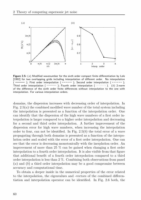
2 Theory of computing supersonic jet noise
(a) (b)Rk′h
kh0 π/4 π/2 3π/4 π
0
π/4
π/2
3π/4
π
∥u−uref∥
interp. order1 2 3 4
0.7
0.8
0.9
1
Figure 2.5: (a) Modified wavenumber for the sixth order compact finite differentiation by Lele[1992] for two overlapping grids including interpolation of different order. No interpolation( ); First order interpolation ( ); Second order interpolation ( );Third order interpolation ( ); Fourth order interpolation ( ). (b) 2-normof the difference of the sixth order finite differences without interpolation to the one withinterpolation. For various interpolation orders.
domains, the dispersion increases with decreasing order of interpolation. InFig. 2.5(a) the combined modified wave number of the total system includingthe interpolation is presented as a function of the interpolation order. Onecan identify that the dispersion of the high wave numbers of a first order in-terpolation is larger compared to a higher order interpolation and decreasingfor a second and third order interpolation. A further improvement of thedispersion error for high wave numbers, when increasing the interpolationorder to four, can not be identified. In Fig. 2.5(b) the total error of a wavepropagating through both domains is presented as a function of the interpo-lation order and scaled with the error of a first order interpolation. One cansee that the error is decreasing monotonically with the inerplation order. Animprovement of more than 25 % can be gained when changing a first orderinterpolation to a fourth order interpolation. It is also visible from that figurethat additional benefit of a fourth order interpolation compared to a thirdorder interpolation is less than 2 %. Combining both observations from panel(a) and (b) a third order interpolation may be a good compromise betweenaccuracy and computational time.
To obtain a deeper inside in the numerical properties of the error relatedto the interpolation, the eigenvalues and -vectors of the combined differen-tiation and interpolation operator can be identified. In Fig. 2.6 both, the
60
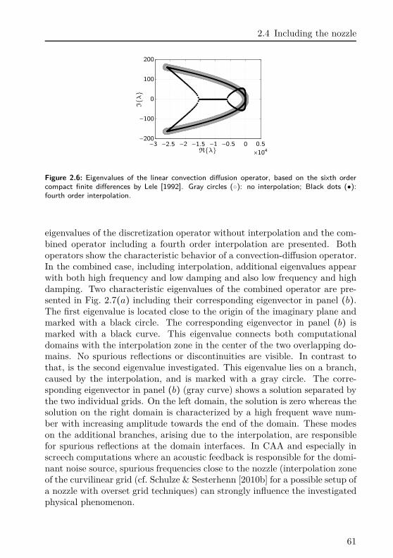
2.4 Including the nozzle
Iλ
Rλ ×104−3 −2.5 −2 −1.5 −1 −0.5 0 0.5
−200
−100
0
100
200
Figure 2.6: Eigenvalues of the linear convection diffusion operator, based on the sixth ordercompact finite differences by Lele [1992]. Gray circles (): no interpolation; Black dots ():fourth order interpolation.
eigenvalues of the discretization operator without interpolation and the com-bined operator including a fourth order interpolation are presented. Bothoperators show the characteristic behavior of a convection-diffusion operator.In the combined case, including interpolation, additional eigenvalues appearwith both high frequency and low damping and also low frequency and highdamping. Two characteristic eigenvalues of the combined operator are pre-sented in Fig. 2.7(a) including their corresponding eigenvector in panel (b).The first eigenvalue is located close to the origin of the imaginary plane andmarked with a black circle. The corresponding eigenvector in panel (b) ismarked with a black curve. This eigenvalue connects both computationaldomains with the interpolation zone in the center of the two overlapping do-mains. No spurious reflections or discontinuities are visible. In contrast tothat, is the second eigenvalue investigated. This eigenvalue lies on a branch,caused by the interpolation, and is marked with a gray circle. The corre-sponding eigenvector in panel (b) (gray curve) shows a solution separated bythe two individual grids. On the left domain, the solution is zero whereas thesolution on the right domain is characterized by a high frequent wave num-ber with increasing amplitude towards the end of the domain. These modeson the additional branches, arising due to the interpolation, are responsiblefor spurious reflections at the domain interfaces. In CAA and especially inscreech computations where an acoustic feedback is responsible for the domi-nant noise source, spurious frequencies close to the nozzle (interpolation zoneof the curvilinear grid (cf. Schulze & Sesterhenn [2010b] for a possible setup ofa nozzle with overset grid techniques) can strongly influence the investigatedphysical phenomenon.
61
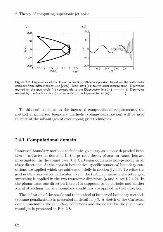
2 Theory of computing supersonic jet noise
(a) (b)Iλ
Rλ ×104−3 −2.5 −2 −1.5 −1 −0.5 0 0.5
−200
−100
0
100
200
EV
x/L0 0.2 0.4 0.6 0.8 1−0.2
−0.1
0
0.1
0.2
Figure 2.7: Eigenvalues of the linear convection diffusion operator, based on the sixth ordercompact finite differences by Lele [1992]. Black dots (): fourth order interpolation. Eigenvaluemarked by the gray circle () corresponds to the Eigenvector in (b) ( ). Eigenvaluemarked by the black circle () corresponds to the Eigenvector in (b) ( ).
To this end, and due to the increased computational requirements, themethod of immersed boundary methods (volume penalization) will be usedin spite of the advantages of overlapping grid techniques.
2.4.1 Computational domain
Immersed boundary methods include the geometry as a space depended func-tion in a Cartesian domain. In the present thesis, planar an round jets areinvestigated. In the round case, the Cartesian domain is non-periodic in allthree directions. At the domain boundaries, specific numerical boundary con-ditions are applied which are addressed briefly in section § 2.4.3. To refine thegrid in the areas with small scales, like in the turbulent areas of the jet, a gridstretching is applied in the two transverse directions (y and z; see § 2.4.2). Inthe planar case, one direction (here z) is supposed to be periodic and neithera grid stretching nor any boundary conditions are applied in that direction.
The definition of the nozzle and the method of immersed boundary methods(volume penalization) is presented in detail in § 3. A sketch of the Cartesiandomain including the boundary conditions and the nozzle for the planar andround jet is presented in Fig. 2.8.
62
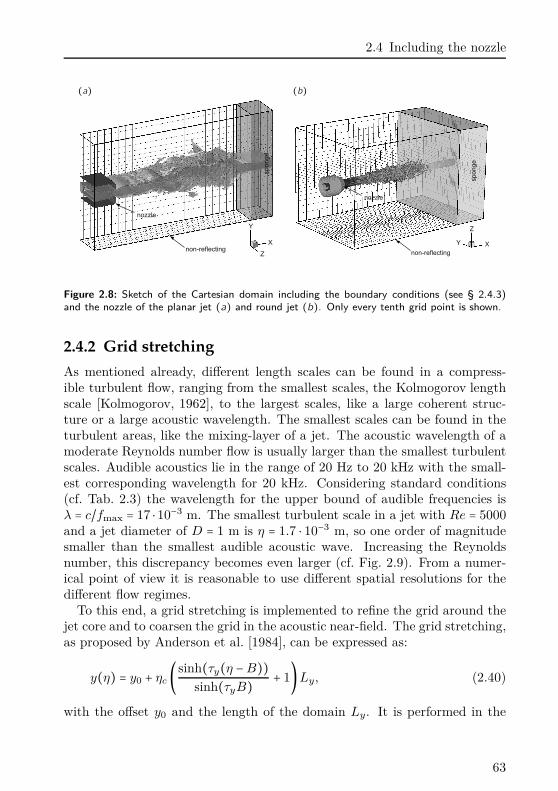
2.4 Including the nozzle
(a) (b)
Figure 2.8: Sketch of the Cartesian domain including the boundary conditions (see § 2.4.3)and the nozzle of the planar jet (a) and round jet (b). Only every tenth grid point is shown.
2.4.2 Grid stretching
As mentioned already, different length scales can be found in a compress-ible turbulent flow, ranging from the smallest scales, the Kolmogorov lengthscale [Kolmogorov, 1962], to the largest scales, like a large coherent struc-ture or a large acoustic wavelength. The smallest scales can be found in theturbulent areas, like the mixing-layer of a jet. The acoustic wavelength of amoderate Reynolds number flow is usually larger than the smallest turbulentscales. Audible acoustics lie in the range of 20 Hz to 20 kHz with the small-est corresponding wavelength for 20 kHz. Considering standard conditions(cf. Tab. 2.3) the wavelength for the upper bound of audible frequencies isλ = c/fmax = 17 ⋅ 10−3 m. The smallest turbulent scale in a jet with Re = 5000and a jet diameter of D = 1 m is η = 1.7 ⋅ 10−3 m, so one order of magnitudesmaller than the smallest audible acoustic wave. Increasing the Reynoldsnumber, this discrepancy becomes even larger (cf. Fig. 2.9). From a numer-ical point of view it is reasonable to use different spatial resolutions for thedifferent flow regimes.
To this end, a grid stretching is implemented to refine the grid around thejet core and to coarsen the grid in the acoustic near-field. The grid stretching,as proposed by Anderson et al. [1984], can be expressed as:
y(η) = y0 + ηc (sinh(τy(η −B))sinh(τyB) + 1)Ly, (2.40)
with the offset y0 and the length of the domain Ly. It is performed in the
63
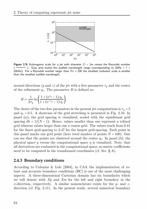
2 Theory of computing supersonic jet noise
wavelengthaudible
λ,η
[m]
Re
100 101 102 103 104 10510−4
10−2
100
102
Figure 2.9: Kolmogorov scale for a jet with diameter D = 1m versus the Reynolds number( ). Gray area marks the audible wavelength range (corresponding to 20Hz < f <20kHz). For a Reynolds number larger than Re ≈ 200 the smallest turbulent scale is smallerthan the smallest audible wavelength.
normal directions (y and z) of the jet with a free parameter τy and the centerof the refinement ηc. The parameter B is defined as:
B ∶= 12τy
ln( 1 + (eτy − 1)ηc
1 + (e−τy − 1)ηc
) .
The choice of the two free parameters in the present jet computations is τy = 5and ηc = 0.5. A showcase of the grid stretching is presented in Fig. 2.10. Inpanel (a), the grid spacing is visualized, scaled with the equidistant gridspacing dh = 1/(N − 1). Hence, values smaller than one represent a refinedgrid whereas values larger than one a coarse grid. The values reach from 0.41for the finest grid-spacing to 2.47 for the largest grid-spacing. Each point inthis panel marks one grid point (here total number of points N = 100). Onecan see that the points are clustered around the center ηc. In panel (b), thephysical space y versus the computational space η is visualized. Note, thatall derivatives are evaluated in the computational space, so metric coefficientsneed to be computed in the transformed coordinates (cf. Sec. § A).
2.4.3 Boundary conditions
According to Colonius & Lele [2004], in CAA the implementation of ro-bust and accurate boundary conditions (BC) is one of the most challengingaspects. A three-dimensional Cartesian domain has six boundaries whichwe will denote with Xp and Xm for the left and right boundary in thex-direction, respectively. A similar nomenclature exists for the y- and z-direction (cf. Fig. 2.11). In the present study, several numerical boundary
64
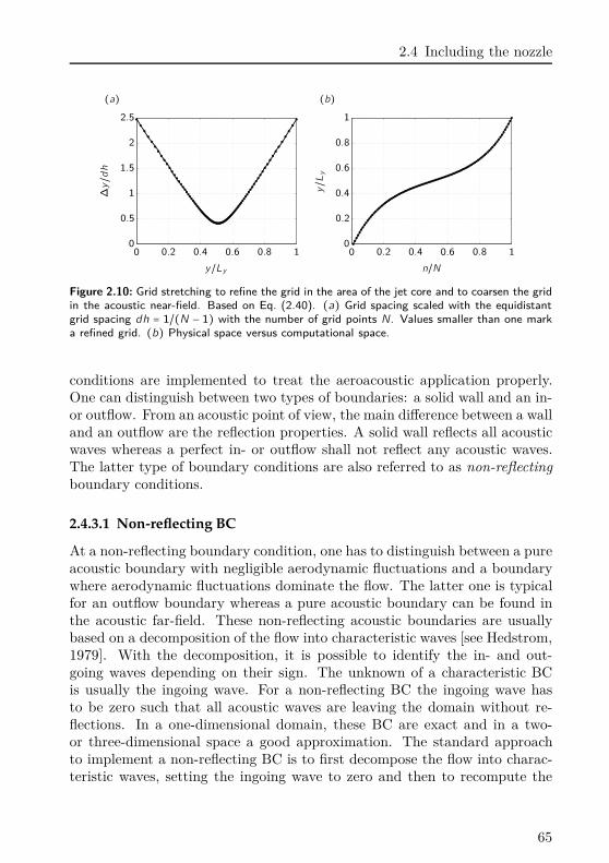
2.4 Including the nozzle
(a) (b)∆y/dh
y/Ly0 0.2 0.4 0.6 0.8 10
0.5
1
1.5
2
2.5
y/Ly
n/N0 0.2 0.4 0.6 0.8 10
0.2
0.4
0.6
0.8
1
Figure 2.10: Grid stretching to refine the grid in the area of the jet core and to coarsen the gridin the acoustic near-field. Based on Eq. (2.40). (a) Grid spacing scaled with the equidistantgrid spacing dh = 1/(N − 1) with the number of grid points N. Values smaller than one marka refined grid. (b) Physical space versus computational space.
conditions are implemented to treat the aeroacoustic application properly.One can distinguish between two types of boundaries: a solid wall and an in-or outflow. From an acoustic point of view, the main difference between a walland an outflow are the reflection properties. A solid wall reflects all acousticwaves whereas a perfect in- or outflow shall not reflect any acoustic waves.The latter type of boundary conditions are also referred to as non-reflectingboundary conditions.
2.4.3.1 Non-reflecting BC
At a non-reflecting boundary condition, one has to distinguish between a pureacoustic boundary with negligible aerodynamic fluctuations and a boundarywhere aerodynamic fluctuations dominate the flow. The latter one is typicalfor an outflow boundary whereas a pure acoustic boundary can be found inthe acoustic far-field. These non-reflecting acoustic boundaries are usuallybased on a decomposition of the flow into characteristic waves [see Hedstrom,1979]. With the decomposition, it is possible to identify the in- and out-going waves depending on their sign. The unknown of a characteristic BCis usually the ingoing wave. For a non-reflecting BC the ingoing wave hasto be zero such that all acoustic waves are leaving the domain without re-flections. In a one-dimensional domain, these BC are exact and in a two-or three-dimensional space a good approximation. The standard approachto implement a non-reflecting BC is to first decompose the flow into charac-teristic waves, setting the ingoing wave to zero and then to recompute the
65
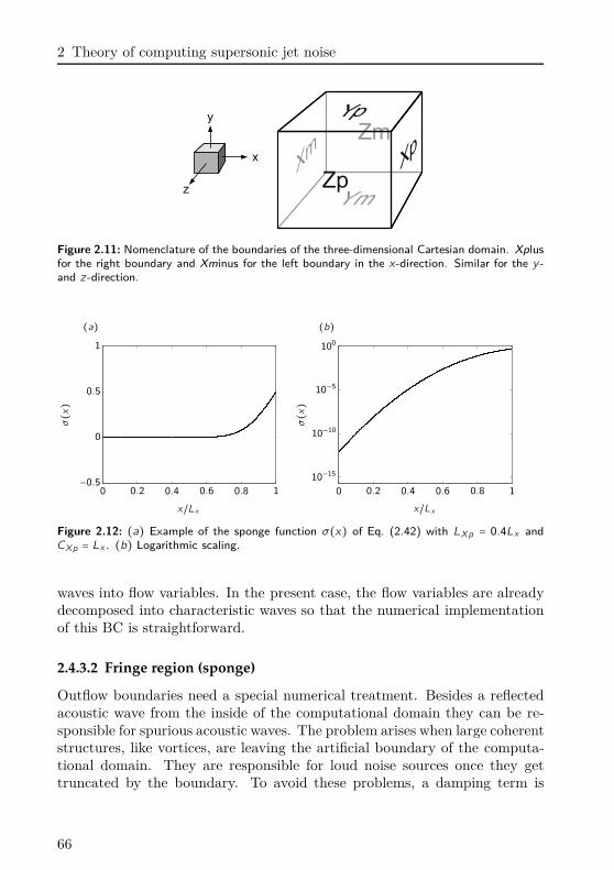
2 Theory of computing supersonic jet noise
Figure 2.11: Nomenclature of the boundaries of the three-dimensional Cartesian domain. Xplusfor the right boundary and Xminus for the left boundary in the x-direction. Similar for the y -and z -direction.
(a) (b)
σ(x)
x/Lx0 0.2 0.4 0.6 0.8 1
−0.5
0
0.5
1
σ(x)
x/Lx0 0.2 0.4 0.6 0.8 1
10−15
10−10
10−5
100
Figure 2.12: (a) Example of the sponge function σ(x) of Eq. (2.42) with LXp = 0.4Lx andCXp = Lx . (b) Logarithmic scaling.
waves into flow variables. In the present case, the flow variables are alreadydecomposed into characteristic waves so that the numerical implementationof this BC is straightforward.
2.4.3.2 Fringe region (sponge)
Outflow boundaries need a special numerical treatment. Besides a reflectedacoustic wave from the inside of the computational domain they can be re-sponsible for spurious acoustic waves. The problem arises when large coherentstructures, like vortices, are leaving the artificial boundary of the computa-tional domain. They are responsible for loud noise sources once they gettruncated by the boundary. To avoid these problems, a damping term is
66
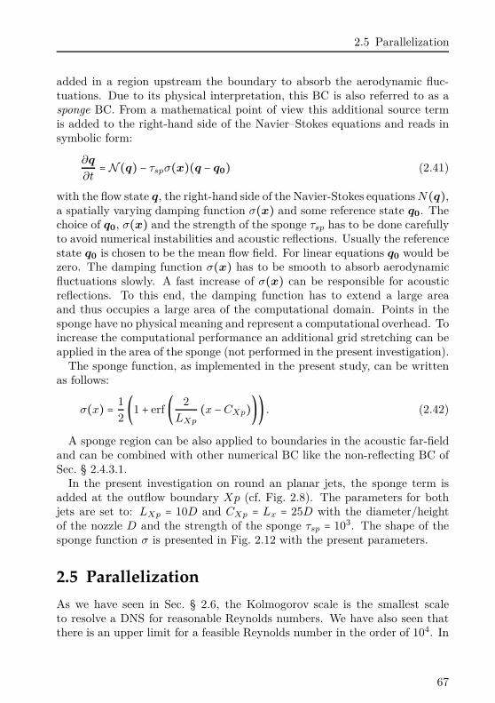
2.5 Parallelization
added in a region upstream the boundary to absorb the aerodynamic fluc-tuations. Due to its physical interpretation, this BC is also referred to as asponge BC. From a mathematical point of view this additional source termis added to the right-hand side of the Navier–Stokes equations and reads insymbolic form:
∂q
∂t= N (q) − τspσ(x)(q − q0) (2.41)
with the flow state q, the right-hand side of the Navier-Stokes equations N(q),a spatially varying damping function σ(x) and some reference state q0. Thechoice of q0, σ(x) and the strength of the sponge τsp has to be done carefullyto avoid numerical instabilities and acoustic reflections. Usually the referencestate q0 is chosen to be the mean flow field. For linear equations q0 would bezero. The damping function σ(x) has to be smooth to absorb aerodynamicfluctuations slowly. A fast increase of σ(x) can be responsible for acousticreflections. To this end, the damping function has to extend a large areaand thus occupies a large area of the computational domain. Points in thesponge have no physical meaning and represent a computational overhead. Toincrease the computational performance an additional grid stretching can beapplied in the area of the sponge (not performed in the present investigation).
The sponge function, as implemented in the present study, can be writtenas follows:
σ(x) = 12(1 + erf ( 2
LXp
(x −CXp))) . (2.42)
A sponge region can be also applied to boundaries in the acoustic far-fieldand can be combined with other numerical BC like the non-reflecting BC ofSec. § 2.4.3.1.
In the present investigation on round an planar jets, the sponge term isadded at the outflow boundary Xp (cf. Fig. 2.8). The parameters for bothjets are set to: LXp = 10D and CXp = Lx = 25D with the diameter/heightof the nozzle D and the strength of the sponge τsp = 103. The shape of thesponge function σ is presented in Fig. 2.12 with the present parameters.
2.5 Parallelization
As we have seen in Sec. § 2.6, the Kolmogorov scale is the smallest scaleto resolve a DNS for reasonable Reynolds numbers. We have also seen thatthere is an upper limit for a feasible Reynolds number in the order of 104. In
67
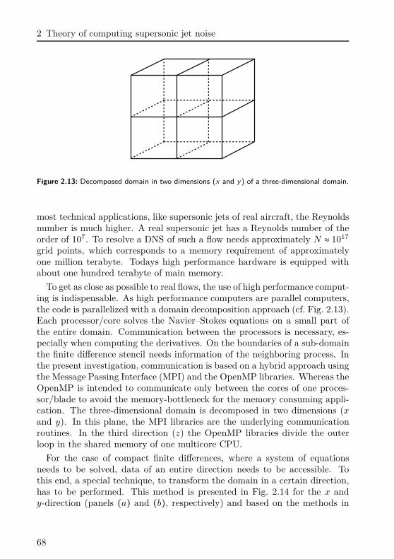
2 Theory of computing supersonic jet noise
Figure 2.13: Decomposed domain in two dimensions (x and y) of a three-dimensional domain.
most technical applications, like supersonic jets of real aircraft, the Reynoldsnumber is much higher. A real supersonic jet has a Reynolds number of theorder of 107. To resolve a DNS of such a flow needs approximately N ≈ 1017
grid points, which corresponds to a memory requirement of approximatelyone million terabyte. Todays high performance hardware is equipped withabout one hundred terabyte of main memory.
To get as close as possible to real flows, the use of high performance comput-ing is indispensable. As high performance computers are parallel computers,the code is parallelized with a domain decomposition approach (cf. Fig. 2.13).Each processor/core solves the Navier–Stokes equations on a small part ofthe entire domain. Communication between the processors is necessary, es-pecially when computing the derivatives. On the boundaries of a sub-domainthe finite difference stencil needs information of the neighboring process. Inthe present investigation, communication is based on a hybrid approach usingthe Message Passing Interface (MPI) and the OpenMP libraries. Whereas theOpenMP is intended to communicate only between the cores of one proces-sor/blade to avoid the memory-bottleneck for the memory consuming appli-cation. The three-dimensional domain is decomposed in two dimensions (xand y). In this plane, the MPI libraries are the underlying communicationroutines. In the third direction (z) the OpenMP libraries divide the outerloop in the shared memory of one multicore CPU.
For the case of compact finite differences, where a system of equationsneeds to be solved, data of an entire direction needs to be accessible. Tothis end, a special technique, to transform the domain in a certain direction,has to be performed. This method is presented in Fig. 2.14 for the x andy-direction (panels (a) and (b), respectively) and based on the methods in
68
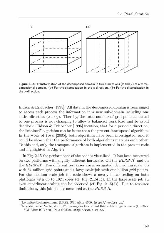
2.5 Parallelization
(a) (b)
Figure 2.14: Transformation of the decomposed domain in two dimensions (x and y) of a three-dimensional domain. (a) For the discretization in the x-direction. (b) For the discretization inthe y -direction.
Eidson & Erlebacher [1995]. All data in the decomposed domain is rearrangedto access each process the information in a new sub-domain including oneentire direction (x or y). Thereby, the total number of grid point allocatedto one process is not changing to allow a balanced work load and to avoiddeadlock. Eidson & Erlebacher [1995] mention, that for a periodic direction,the “chained” algorithm can be faster than the present “transpose” algorithm.In the work of Foysi [2005], both algorithm have been investigated, and itcould be shown that the performance of both algorithms matches each other.To this end, only the transpose algorithm is implemented in the present codeand highlighted in Alg. 2.2.
In Fig. 2.15 the performance of the code is visualized. It has been measuredon two platforms with slightly different hardware. On the HLRB-II1 and onthe HLRN-II2. Two different test cases are investigated. A medium scale jobwith 64 million grid points and a large scale job with one billion grid points.For the medium scale job the code shows a nearly linear scaling on bothplatforms with up to 1024 cores (cf. Fig. 2.15(a)). In the large scale job aneven superlinear scaling can be observed (cf. Fig. 2.15(b)). Due to resourcelimitations, this job is only measured at the HLRB-II.
1Leibnitz–Rechenzentrum (LRZ). SGI Altix 4700. http://www.lrz.de/2Norddeutscher Verbund zur Förderung des Hoch- und Höchstleistungsrechnens (HLRN).
SGI Altix ICE 8200 Plus (ICE2). http://www.hlrn.de/
69
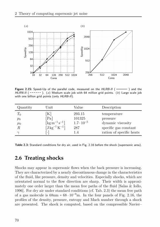
2 Theory of computing supersonic jet noise
(a) (b)tsS
pee
dU
p
Cores16 32 64 128 256 512 1024
16
32
64
128
256
512
1024
Sp
eedU
p
Cores256 512 1024 2048
256
512
1024
2048
Figure 2.15: Speed-Up of the parallel code, measured on the HLRB-II ( ) and theHLRN-II ( ). (a) Medium scale job with 64 million grid points. (b) Large scale jobwith one billion grid points (only HLRB-II).
Quantity Unit Value Description
T0 [K] 293.15 temperaturep0 [Pa] 101325 pressureµ0 [kg m−1 s−1] 1.7 ⋅ 10−5 dynamic viscosityR [J kg−1 K−1] 287 specific gas constantγ [⋅] 1.4 ration of specific heats
Table 2.3: Standard conditions for dry air, used in Fig. 2.16 before the shock (supersonic area).
2.6 Treating shocks
Shocks may appear in supersonic flows when the back pressure is increasing.They are characterized by a nearly discontinuous change in the characteristicsof the fluid, like pressure, density and velocities. Especially shocks, which areorientated normal to the flow direction are sharp. Their width is approxi-mately one order larger than the mean free paths of the fluid [Salas & Iollo,1996]. For dry air under standard conditions (cf. Tab. 2.3) the mean free pathof a gas molecule is 68nm = 68 ⋅ 10−9m. In the four panels of Fig. 2.16, theprofiles of the density, pressure, entropy and Mach number through a shockare presented. The shock is computed, based on the compressible Navier–
70
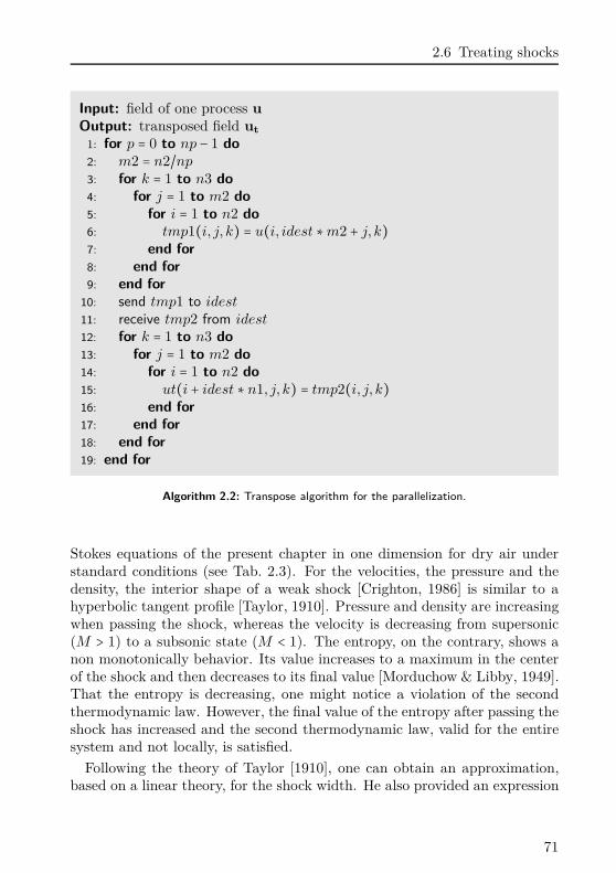
2.6 Treating shocks
Input: field of one process u
Output: transposed field ut
1: for p = 0 to np − 1 do2: m2 = n2/np
3: for k = 1 to n3 do4: for j = 1 to m2 do5: for i = 1 to n2 do6: tmp1(i, j, k) = u(i, idest ∗m2 + j, k)7: end for8: end for9: end for
10: send tmp1 to idest
11: receive tmp2 from idest
12: for k = 1 to n3 do13: for j = 1 to m2 do14: for i = 1 to n2 do15: ut(i + idest ∗ n1, j, k) = tmp2(i, j, k)16: end for17: end for18: end for19: end for
Algorithm 2.2: Transpose algorithm for the parallelization.
Stokes equations of the present chapter in one dimension for dry air understandard conditions (see Tab. 2.3). For the velocities, the pressure and thedensity, the interior shape of a weak shock [Crighton, 1986] is similar to ahyperbolic tangent profile [Taylor, 1910]. Pressure and density are increasingwhen passing the shock, whereas the velocity is decreasing from supersonic(M > 1) to a subsonic state (M < 1). The entropy, on the contrary, shows anon monotonically behavior. Its value increases to a maximum in the centerof the shock and then decreases to its final value [Morduchow & Libby, 1949].That the entropy is decreasing, one might notice a violation of the secondthermodynamic law. However, the final value of the entropy after passing theshock has increased and the second thermodynamic law, valid for the entiresystem and not locally, is satisfied.
Following the theory of Taylor [1910], one can obtain an approximation,based on a linear theory, for the shock width. He also provided an expression
71
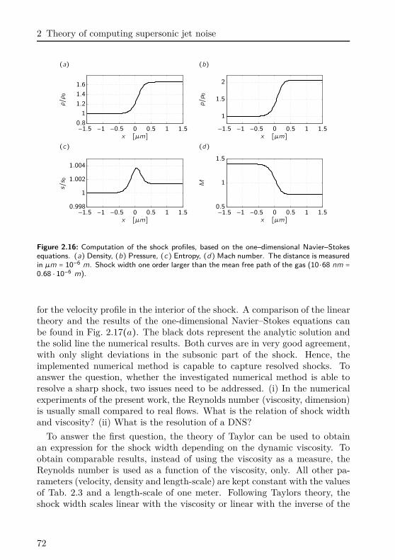
2 Theory of computing supersonic jet noise
(a) (b)ρ/ρ 0
x [µm]−1.5 −1 −0.5 0 0.5 1 1.50.8
1
1.2
1.4
1.6
p/p
0
x [µm]−1.5 −1 −0.5 0 0.5 1 1.5
1
1.5
2
(c) (d)
s/s 0
x [µm]−1.5 −1 −0.5 0 0.5 1 1.5
0.998
1
1.002
1.004
M
x [µm]−1.5 −1 −0.5 0 0.5 1 1.50.5
1
1.5
Figure 2.16: Computation of the shock profiles, based on the one–dimensional Navier–Stokesequations. (a) Density, (b) Pressure, (c) Entropy, (d)Mach number. The distance is measuredin µm = 10−6 m. Shock width one order larger than the mean free path of the gas (10 ⋅68 nm =0.68 ⋅ 10−6 m).
for the velocity profile in the interior of the shock. A comparison of the lineartheory and the results of the one-dimensional Navier–Stokes equations canbe found in Fig. 2.17(a). The black dots represent the analytic solution andthe solid line the numerical results. Both curves are in very good agreement,with only slight deviations in the subsonic part of the shock. Hence, theimplemented numerical method is capable to capture resolved shocks. Toanswer the question, whether the investigated numerical method is able toresolve a sharp shock, two issues need to be addressed. (i) In the numericalexperiments of the present work, the Reynolds number (viscosity, dimension)is usually small compared to real flows. What is the relation of shock widthand viscosity? (ii) What is the resolution of a DNS?
To answer the first question, the theory of Taylor can be used to obtainan expression for the shock width depending on the dynamic viscosity. Toobtain comparable results, instead of using the viscosity as a measure, theReynolds number is used as a function of the viscosity, only. All other pa-rameters (velocity, density and length-scale) are kept constant with the valuesof Tab. 2.3 and a length-scale of one meter. Following Taylors theory, theshock width scales linear with the viscosity or linear with the inverse of the
72
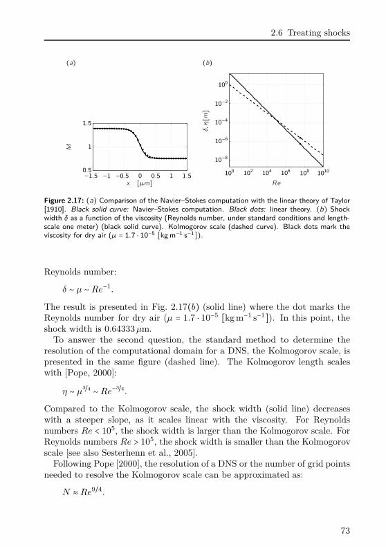
2.6 Treating shocks
(a) (b)M
x [µm]−1.5 −1 −0.5 0 0.5 1 1.50.5
1
1.5
δ,η[m]
Re
100 102 104 106 108 1010
10−8
10−6
10−4
10−2
100
Figure 2.17: (a) Comparison of the Navier–Stokes computation with the linear theory of Taylor[1910]. Black solid curve: Navier–Stokes computation. Black dots: linear theory. (b) Shockwidth δ as a function of the viscosity (Reynolds number, under standard conditions and length-scale one meter) (black solid curve). Kolmogorov scale (dashed curve). Black dots mark theviscosity for dry air (µ = 1.7 ⋅ 10−5 [kg m−1 s−1]).
Reynolds number:
δ ∼ µ ∼ Re−1.
The result is presented in Fig. 2.17(b) (solid line) where the dot marks theReynolds number for dry air (µ = 1.7 ⋅ 10−5 [kg m−1 s−1]). In this point, theshock width is 0.64333 µm.
To answer the second question, the standard method to determine theresolution of the computational domain for a DNS, the Kolmogorov scale, ispresented in the same figure (dashed line). The Kolmogorov length scaleswith [Pope, 2000]:
η ∼ µ3/4 ∼ Re−
3/4.
Compared to the Kolmogorov scale, the shock width (solid line) decreaseswith a steeper slope, as it scales linear with the viscosity. For Reynoldsnumbers Re < 105, the shock width is larger than the Kolmogorov scale. ForReynolds numbers Re > 105, the shock width is smaller than the Kolmogorovscale [see also Sesterhenn et al., 2005].
Following Pope [2000], the resolution of a DNS or the number of grid pointsneeded to resolve the Kolmogorov scale can be approximated as:
N ≈ Re9/4.
73
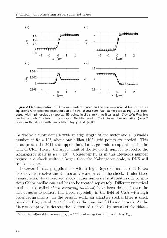
2 Theory of computing supersonic jet noise
(a) (b)ρ/ρ 0
x [µm]−2 −1 0 1 2
0.8
1
1.2
1.4
1.6
p/p
0
x [µm]−2 −1 0 1 2
1
1.5
2
(c) (d)
s/s 0
x [µm]−2 −1 0 1 2
0.998
1
1.002
1.004
M
x [µm]−2 −1 0 1 2
0.5
1
1.5
Figure 2.18: Computation of the shock profiles, based on the one–dimensional Navier–Stokesequations with different resolutions and filters. Black solid line: Same case as Fig. 2.16 com-puted with high resolution (approx. 50 points in the shock); no filter used. Gray solid line: lowresolution (only 7 points in the shock). No filter used. Black circles: low resolution (only 7points in the shock) with shock filter Bogey et al. [2009].
To resolve a cubic domain with an edge length of one meter and a Reynoldsnumber of Re = 104, about one billion (109) grid points are needed. Thisis at present in 2011 the upper limit for large scale computations in thefield of CFD. Hence, the upper limit of the Reynolds number to resolve theKolmogorov scale is Re = 104. Consequently, as in this Reynolds numberregime, the shock width is larger than the Kolmogorov scale, a DNS willresolve a shock.
However, in many applications with a high Reynolds numbers, it is tooexpensive to resolve the Kolmogorov scale or even the shock. Under theseassumptions, the unresolved shock causes numerical instabilities due to spu-rious Gibbs oscillations and has to be treated separately. Different numericalmethods (so called shock–capturing methods) have been designed over thelast decades to address this issue, especially in the field of CAA with highorder requirements. In the present work, an adaptive spatial filter is used,based on Bogey et al. [2009]3, to filter the spurious Gibbs oscillations. As thefilter is adaptive, it detects the location of a shock, by means of the dilata-
3with the adjustable parameter rth = 10−5 and using the optimized filter Fopt
74
2.6 Treating shocks
tion of the velocities as a measure, and applies the filter in this area, only. InFig. 2.18, the same shock as in Fig. 2.16 is computed with a seven times lowerresolution. Only seven points remain in the interior of the shock. Withoutany filter, the numerical result shows strong oscillations around the centerof the shock (gray solid line). To compare the result, the high resolutioncase is presented with the black solid line. Although the under-resolved caseshows strong oscillations, the correct shock jump in all quantities is reached.A small displacement of the center of the shock into the supersonic regionis visible. In contrast to that, the result treated with the shock filter andthe same low resolution, shows a very good agreement with the resolved case(black circles). No oscillations are visible and the correct shock jump andspeed are preserved.
75

3Theory of computing flow
in porous media
In the literature, porous media are not only used to reduce aeroacousticnoise, but can be found in a series of flow control applications. For instance,Bruneau & Mortazavi [2008] controlled the vortex shedding of the flow pasta cylinder with a porous coating. In another numerical study by Sandham &Luedeke [2009], the Mack mode was stabilized in a Mach 6 boundary layerflow by means of a porous surface.
The porous medium investigated in the present study, is modeled by a vol-ume force, similar to Darcy’s law for incompressible flow. For the presentaeroacoustic application the volume force is implemented in the fully com-pressible Navier–Stokes equations leading to a new set of porous flow equa-tions.
A porous medium can be characterized by only two parameters: the poros-ity φ and the permeability K. Whereas φ describes the volume ratio of voidspace Vf to the volume of the whole porous material (φ = Vf /V ). Thus, aporosity equal to one represents void space only, and a porosity of zero a solidbody, where no fluid can penetrate. The latter extreme causes a singularityin the porous flow equations, thus only values of 0 < φ ≤ 1 are feasible.
The second parameter K stands for the permeability of the material and
77
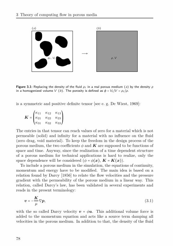
3 Theory of computing flow in porous media
(a) (b)
ρf , Vf
Ð→ρ, V
Figure 3.1: Replacing the density of the fluid ρf in a real porous medium (a) by the density ρin a homogenized volume V (b). The porosity is defined as φ = Vf /V = ρf /ρ.
is a symmetric and positive definite tensor [see e. g. De Wiest, 1969]:
K = ⎛⎜⎝κ11 κ12 κ13
κ21 κ22 κ23
κ31 κ32 κ33
⎞⎟⎠The entries in that tensor can reach values of zero for a material which is notpermeable (solid) and infinity for a material with no influence on the fluid(zero drag, void material). To keep the freedom in the design process of theporous medium, the two coefficients φ and K are supposed to be functions ofspace and time. Anyway, since the realization of a time dependent structureof a porous medium for technical applications is hard to realize, only thespace dependence will be considered (φ = φ(x), K =K(x)).
To include a porous medium in the simulation, the equations of continuity,momentum and energy have to be modified. The main idea is based on arelation found by Darcy [1856] to relate the flow velocities and the pressuregradient with the permeability of the porous medium in a linear way. Thisrelation, called Darcy’s law, has been validated in several experiments andreads in the present terminology:
v = −K
µ∇p, (3.1)
with the so called Darcy velocity v = φu. This additional volume force isadded to the momentum equation and acts like a source term damping allvelocities in the porous medium. In addition to that, the density of the fluid
78
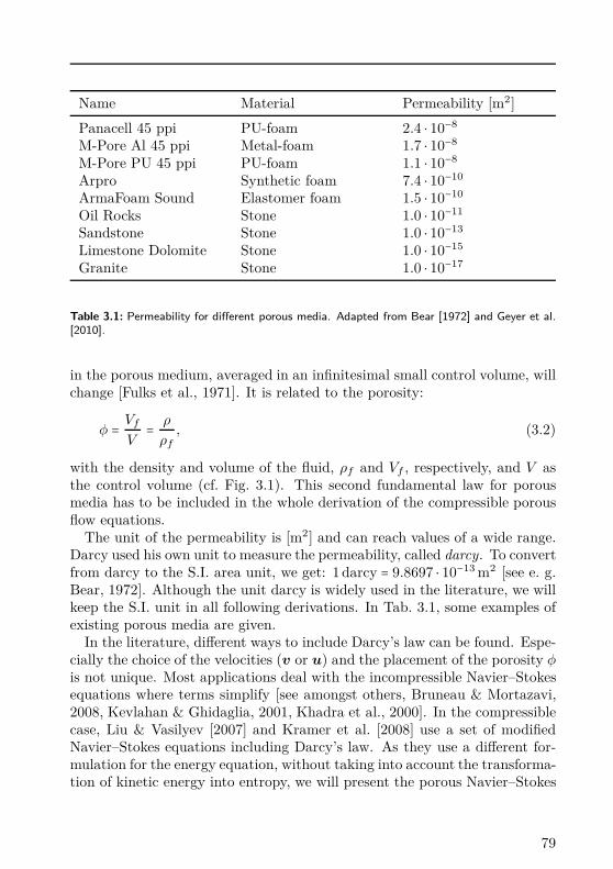
Name Material Permeability [m2]
Panacell 45 ppi PU-foam 2.4 ⋅ 10−8
M-Pore Al 45 ppi Metal-foam 1.7 ⋅ 10−8
M-Pore PU 45 ppi PU-foam 1.1 ⋅ 10−8
Arpro Synthetic foam 7.4 ⋅ 10−10
ArmaFoam Sound Elastomer foam 1.5 ⋅ 10−10
Oil Rocks Stone 1.0 ⋅ 10−11
Sandstone Stone 1.0 ⋅ 10−13
Limestone Dolomite Stone 1.0 ⋅ 10−15
Granite Stone 1.0 ⋅ 10−17
Table 3.1: Permeability for different porous media. Adapted from Bear [1972] and Geyer et al.[2010].
in the porous medium, averaged in an infinitesimal small control volume, willchange [Fulks et al., 1971]. It is related to the porosity:
φ = Vf
V= ρ
ρf
, (3.2)
with the density and volume of the fluid, ρf and Vf , respectively, and V asthe control volume (cf. Fig. 3.1). This second fundamental law for porousmedia has to be included in the whole derivation of the compressible porousflow equations.
The unit of the permeability is [m2] and can reach values of a wide range.Darcy used his own unit to measure the permeability, called darcy. To convertfrom darcy to the S.I. area unit, we get: 1 darcy = 9.8697 ⋅ 10−13 m2 [see e. g.Bear, 1972]. Although the unit darcy is widely used in the literature, we willkeep the S.I. unit in all following derivations. In Tab. 3.1, some examples ofexisting porous media are given.
In the literature, different ways to include Darcy’s law can be found. Espe-cially the choice of the velocities (v or u) and the placement of the porosity φ
is not unique. Most applications deal with the incompressible Navier–Stokesequations where terms simplify [see amongst others, Bruneau & Mortazavi,2008, Kevlahan & Ghidaglia, 2001, Khadra et al., 2000]. In the compressiblecase, Liu & Vasilyev [2007] and Kramer et al. [2008] use a set of modifiedNavier–Stokes equations including Darcy’s law. As they use a different for-mulation for the energy equation, without taking into account the transforma-tion of kinetic energy into entropy, we will present the porous Navier–Stokes
79
3 Theory of computing flow in porous media
equations for compressible flow, including an equation for the entropy in thefollowing section.
3.1 Porous flow equations
The derivation of the compressible porous flow equations is based on thederivation in Fulks et al. [1971], yet with an additional energy equation.Replacing consequently the density ρ by φρf (3.2) and including Darcy’slaw (3.1), one obtains a set of porous flow equations for compressible fluids,based on the Navier–Stokes equations, including an equation for the energy.In what follows, we will omit the subscript (⋅)f and relate all flow variablesto the fluid.
3.1.1 Porous mass equation
The density, averaged over the volume V is simply ρφ and the porosity canbe 0 < φ ≤ 1. To this end, the modified continuity equation reads:
∂φρ
∂t+
∂φρui
∂xi
= 0. (3.3)
Although the time dependence of the porous material will not be consid-ered in the optimization algorithm, the general assumption of a space andtime dependent material will be used to derive the porous flow equations asthey are not restricted to the optimization algorithm (φ = φ(x, t)). In thepresent numerical analysis, the governing equations are based on the pressurep, the velocities ui and the entropy s. To this end, the continuity equation isrewritten using Gibbs fundamental relation which reads:
T ds = de − p d(1ρ) , (3.4)
with the specific entropy s, the specific internal energy e and the specificvolume v = 1/ρ. Again, the density has to be modified for porous media,because only the part of the volume occupied by fluid is considered. Withthe internal energy de = CvdT for an ideal gas, one obtains:
T ds = CvdT − p d( 1φρ) , (3.5)
Note, that φ can be a function of space and time and can not be consideredas constant. To eliminate the explicit dependence of the temperature from
80
3.1 Porous flow equations
Eq. (3.5), the modified relation for an ideal gas is applied which reads:
p = φρRT, (3.6)
or in a variational formulation:
dp = R(ρT dφ + φT dρ + φρdT ), (3.7)
with the specific gas constant R. Now, combining Eq. (3.3), (3.5) and (3.7)we end up with a continuity equation, written in pressure and entropy for-mulation:
∂p
∂t+ ui
∂p
∂xi
= −φρc2 ∂ui
∂xi
+p
Cv
(∂s
∂t+ ui
∂s
∂xi
) (3.8)
Setting φ = 1 (no porous medium), one obtains the original continuity equa-tion for an undisturbed fluid written in pressure and entropy formulation asin Eq. (2.1a). Consequently, this equation can be used for both, the porousdomain and the void domain.
It is interesting to see that this formulation of the continuity equationis no more depending on the variation of the porosity as it is the case forEq. (3.3). Form a numerical point of view, this is of particular importance,since φ can be a discontinuous function in space and time. Its derivative mightbe undefined and can be responsible for numerical instabilities. Especiallyin applications with mixed areas of porous media and void space, as in thepresent application, discontinuities of φ arise at every boundary of the porousmaterial.
3.1.2 Porous momentum equation
To obtain the momentum equation, we follow the same strategy as for thecontinuity equation, by replacing the density with φρ. Furthermore, the abovementioned Darcy term (Eq. (3.1)) is added to the right hand side to accountfor the viscous damping of the velocities in the porous medium, dependingon the permeability of the material [as proposed by Wooding, 1957].
Finally, the momentum equation for a compressible fluid, including porousmedia, can be written as:
∂ui
∂t+ uj
∂ui
∂xj
= − 1φρ
∂p
∂xi
+1
φρ
∂τij
∂xj
−µ
ρ(K−1)ijuj , (3.9)
with τij as defined in Eq. (2.2). As for the continuity equation, this equationis also valid in the void domain with no porous medium, by setting φ = 1 andK →∞ ⋅ I, with the identity matrix I.
81
3 Theory of computing flow in porous media
3.1.3 Porous energy equation
In the present study, the energy is expressed by the entropy. An expression forthe entropy conservation can be obtained by subtracting the kinetic energyfrom the total energy and using Gibbs fundamental relation together withthe conservation of mass. To this end, the equations for continuity (3.8) andmomentum (3.9), multiplied by ui (to obtain the kinetic energy), are com-bined with Gibbs fundamental relation (3.5), to obtain the entropy equationfor porous media.
The total energy equation with modified density can be written as:
Cv
DT
Dt+
D
Dt(1
2uiui) = 1
φρ
∂
∂xj
(−puj + uiτij + (λ ∂T
∂xj
)) (3.10)
Multiplying ui to the momentum equation (3.9) leads to an expression forthe kinetic energy, including Darcy’s law:
D
Dt(1
2uiui) = − 1
φρui
∂p
∂xi
+1
φρui
∂τij
∂xj
− µρ(K−1)ijuiuj (3.11)
Subtracting Eq. (3.11) from Eq. (3.10) reads:
φρCv
DT
Dt− p
∂ui
∂xi
+∂
∂xj
(λ ∂T
∂xj
) +Φ + φµ(K−1)ijuiuj (3.12)
Finally, using Gibbs fundamental relation of Eq. (3.5), which can be rewrittenin the following form:
φρCv
DT
Dt= φρT
γ
Ds
Dt+
1γ
Dp
Dt(3.13)
leads to an expression for the entropy after some standard manipulations andreads:
∂s
∂t+ uj
∂s
∂xj
= 1ρφT
( ∂
∂xj
(λ ∂T
∂xj
) +Φ)+
µ
ρT(K−1)
ijuiuj
´¹¹¹¹¹¹¹¹¹¹¹¹¹¹¹¹¹¹¹¹¹¹¹¹¹¹¹¹¹¹¹¹¹¹¹¹¹¹¹¹¹¹¹¹¹¹¸¹¹¹¹¹¹¹¹¹¹¹¹¹¹¹¹¹¹¹¹¹¹¹¹¹¹¹¹¹¹¹¹¹¹¹¹¹¹¹¹¹¹¹¹¹¶1
−hs
φ(T − Ts)
´¹¹¹¹¹¹¹¹¹¹¹¹¹¹¹¹¹¹¹¹¹¹¹¹¹¸¹¹¹¹¹¹¹¹¹¹¹¹¹¹¹¹¹¹¹¹¹¹¹¹¹¶2
, (3.14)
with the dissipation function Φ as defined in Eq. (2.4) and the thermal con-ductivity λ as defined in Eq. (2.7). In Eq. (3.14), two additional terms,related to the porous medium, can be identified (marked with 1 and 2 ).
82
3.1 Porous flow equations
The first term has its origin in the momentum equation (3.9) multiplied byu, to obtain an expression for the kinetic energy. This term is in fact aK−1-norm (uT K−1u), since K is a positive definite tensor, as is its inverse.Hence, it can be positive only and represents the entropy production due tothe loss of kinetic energy in the porous medium. This entropy production isresponsible for a temperature increase in the porous medium which can leadto particularly high temperatures.
Based on the above equations, the porous medium has the same thermody-namic properties as the fluid. In a technical application the porous mediumis based e. g. on an aluminum foam. This foam will have a different heat con-ductivity and thus a modified temperature. In the present study, we assume aconstant temperature of the porous medium Ts which is a good approximationfor most metal foams, based on aluminum or even copper. To this end, thesecond term is added to the entropy equation with hs = Csτ−1
s T −1s . Whereas
hs is a specific heat transfer coefficient with a characteristic time scale anda characteristic specific heat Cs of the porous material. In the present in-vestigation, the parameters are chosen as follows: Cs = 897 [Jkg−1K−1] as forAluminum and τs = 0.5 [s]. The temperature of the porous medium TS isequal to the ambient temperature of the fluid T0 (here 300 [K]).
If the approximation of a constant temperature is not feasible, it mightbe necessary to solve an additional heat conduction equation for the spaceand time dependent distribution of the temperature in the porous material.This equation would be a part of the system of coupled equations to solveand would consequently produce a corresponding adjoint equation for theadjoint temperature distribution in the adjoint porous medium which is notconsidered here.
Finally, the modified Navier–Stokes equations for porous media are closedwith the thermodynamic relation for an ideal gas (Eq. (3.6)) and Sutherland’slaw to obtain the temperature dependent viscosity as in Eq. (2.6). The specificgas constant is R = Cp−Cv = 287 [J kg−1 K−1] with a constant ratio of specificheats γ = Cp/Cv = 1.4 and a constant Prandtl number P r = 0.71.
The difference between the Navier–Stokes equations of Sec. 2.2.1 and thepresent porous Navier–Stokes equations is restricted to additional sourceterms and the modified density. Hence, the decomposition of the porousNavier–Stokes equations into characteristic waves can be performed in thesame way as described in Sec. 2.2.2. For all following numerical computa-tions, the compressible and porous Navier–Stokes equations of the presentchapter will be used, together with the characteristic formulation. In appli-cations, where no porous material is investigated, φ is set to one and thepermeability is set to infinity with an isotropic behavior.
83
3 Theory of computing flow in porous media
3.1.4 Numerical Implementation
The porous flow equations of section § 3.1.1–§ 3.1.3 can be implemented usingthe same methods as in Sec. § 2.3. Anyway, the time integration technique ofSec. § 2.3.2 plays an important role. Depending on the value of the perme-ability in Eq. (3.9), highly damped eigenvalues may appear in the evolutionoperator. These eigenvalues will be the most damped eigenvalues of theevolution operator when the Darcy term in the porous momentum equationdominates the convection and diffusion terms. One can obtain an analyticalapproximation for the porous dominated eigenvalue by only considering themomentum equation with the Darcy term and neglecting the convection anddissipation terms. The dominant term in the porous Navier–Stokes equations(3.8 - 3.14) will be −µ/ρK−1u. According to that, the corresponding real val-ued eigenvalue is −µ/ρ(K−1)ij which is scaling with the inverse of K. Thiseigenvalue causes stiff equations and constitutes a restriction to the time-stepfor standard explicit time integration methods, like Runge–Kutta. Extremelylow time-steps and a bad performance are the consequence. In contrast tothat, the implemented exponential time integration method based on Krylovsubspaces is able to handle these stiff equations. This method, based on theArnoldi algorithm (cf. Alg. 2.1), captures the largest eigenvalues of the oper-ator including the ones dominated by the porous terms. Hence, these termscan be advanced in time without causing numerical instabilities.
To compare the results of the following sections, a dimensionless value ofthe permeability is introduced. The unit of the permeability is [m2] and inthe momentum equation its inverse scales with µ
ρ:
µ
ρK−1 ∼ 1
ReL
K−1
to this end, the Reynolds number and the length-scale L are used to obtainan expression for the dimensionless permeability:
χ ∶= L2
ReL
K−1. (3.15)
In addition to that, to extract the largest entry of a matrix, the non submul-tiplicative matrix norm ∥A∥max =max∣aij ∣ can be used. Now, a large valueof χ represents a rather solid body, whereas χ = 0 is void space. How tochoose the value of χ to obtain the desired properties is validated in section§ 3.2.
In Fig. 3.2 an example of the spectrum of the evolution operator is pre-sented. The case is based on a periodic chanel flow with 128 grid points in
84
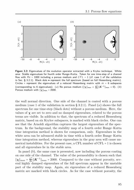
3.1 Porous flow equations
(a) (b)Iλ⋅dt
Rλ ⋅ dt−10 −8 −6 −4 −2 0−4
−2
0
2
4
Iλ⋅dt
Rλ ⋅ dt−10 −8 −6 −4 −2 0−4
−2
0
2
4
Figure 3.2: Eigenvalues of the evolution operator extracted with a Krylov technique. Whitearea: Stable eigenvalues for fourth order Runge–Kutta. Taken for one time-step of a channelflow with Re = 1000 including a porous medium and CFL = 1 (cf. case 1 of the validationin Sec. § 3.2.1). Black dots represent the full spectrum (based on full Hessenberg matrix).Circles represent the eigenvalues of a reduced Hessenberg matrix with m = 6 subspaces
(corresponding to 6 eigenvalues). (a) No porous medium (∥χ∥max =L2
Re∥K−1∥max = 0). (b)
Porous medium with ∥χ∥max = 2000.
the wall normal direction. One side of the channel is coated with a porousmedium (case 1 of the validation in section § 3.2.1). Panel (a) shows the fullspectrum for one time-step (black dots) without a porous medium. Here, thevalues of χ are set to zero and no damped eigenvalues, related to the porousterms are visible. In addition to that, the spectrum of a reduced Hessenbergmatrix, based on six Krylov subspaces, is marked with black circles. One cansee that the Arnoldi algorithm captures the largest eigenvalues of the spec-trum. In the background, the stability map of a fourth order Runge–Kuttatime integration method is shown for comparison, only. Eigenvalues in thewhite area can be advanced stable in time with a fourth order Runge–Kuttatime integration method, whereas eigenvalues in the gray area will cause nu-merical instabilities. For the present case, a CFL number of CFL = 1 is chosenand all eigenvalues lie in the stable area.
In panel (b), the same case is presented, now including the porous coatingon one side of the channel. The value of the permeability is chosen such that∥χ∥max = L2
Re∥K−1∥max = 2000. Compared to the case without porosity, sev-
eral highly damped eigenvalues of the full spectrum appear in the unstablepart of the stability map. Again, six eigenvalues of a reduced Hessenbergmatrix are marked with black circles. As for the case without porosity, the
85
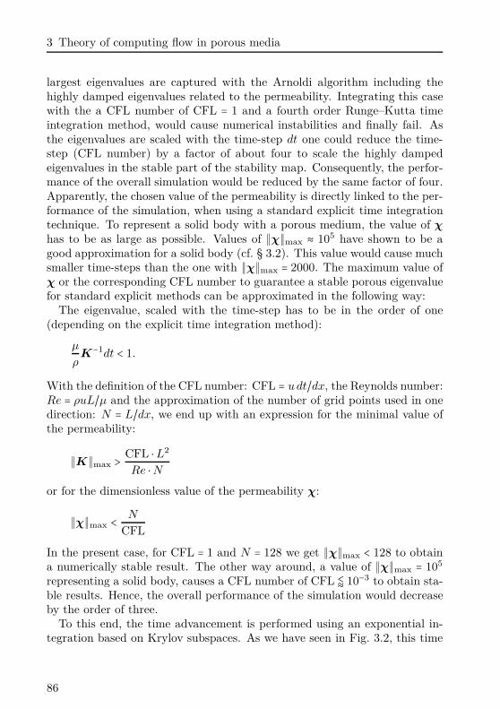
3 Theory of computing flow in porous media
largest eigenvalues are captured with the Arnoldi algorithm including thehighly damped eigenvalues related to the permeability. Integrating this casewith the a CFL number of CFL = 1 and a fourth order Runge–Kutta timeintegration method, would cause numerical instabilities and finally fail. Asthe eigenvalues are scaled with the time-step dt one could reduce the time-step (CFL number) by a factor of about four to scale the highly dampedeigenvalues in the stable part of the stability map. Consequently, the perfor-mance of the overall simulation would be reduced by the same factor of four.Apparently, the chosen value of the permeability is directly linked to the per-formance of the simulation, when using a standard explicit time integrationtechnique. To represent a solid body with a porous medium, the value of χ
has to be as large as possible. Values of ∥χ∥max ≈ 105 have shown to be agood approximation for a solid body (cf. § 3.2). This value would cause muchsmaller time-steps than the one with ∥χ∥max = 2000. The maximum value ofχ or the corresponding CFL number to guarantee a stable porous eigenvaluefor standard explicit methods can be approximated in the following way:
The eigenvalue, scaled with the time-step has to be in the order of one(depending on the explicit time integration method):
µ
ρK−1dt < 1.
With the definition of the CFL number: CFL = u dt/dx, the Reynolds number:Re = ρuL/µ and the approximation of the number of grid points used in onedirection: N = L/dx, we end up with an expression for the minimal value ofthe permeability:
∥K∥max > CFL ⋅L2
Re ⋅N
or for the dimensionless value of the permeability χ:
∥χ∥max < N
CFL
In the present case, for CFL = 1 and N = 128 we get ∥χ∥max < 128 to obtaina numerically stable result. The other way around, a value of ∥χ∥max = 105
representing a solid body, causes a CFL number of CFL ⪅ 10−3 to obtain sta-ble results. Hence, the overall performance of the simulation would decreaseby the order of three.
To this end, the time advancement is performed using an exponential in-tegration based on Krylov subspaces. As we have seen in Fig. 3.2, this time
86
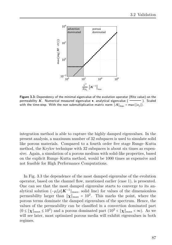
3.2 Validation
PSfragdominatedporous
dominatedadvection
max(∣e
igH⋅dt∣)
L2
ReL∥K−1∥
max
100 102 104 10610−2
100
102
104
Figure 3.3: Dependency of the minimal eigenvalue of the evolution operator (Ritz value) on thepermeability K. Numerical measured eigenvalue , analytical eigenvalue ( ). Scaledwith the time-step. With the non submultiplicative matrix norm ∥A∥max = max∣ai j ∣.
integration method is able to capture the highly damped eigenvalues. In thepresent analysis, a maximum number of 32 subspaces is used to simulate solidlike porous materials. Compared to a fourth order five stage Runge–Kuttamethod, the Krylov technique with 32 subspaces is about six times as expen-sive. Again, a simulation of a porous medium with solid-like properties, basedon the explicit Runge–Kutta method, would be 1000 times as expensive andnot feasible for High Performance Computations.
In Fig. 3.3 the dependence of the most damped eigenvalue of the evolutionoperator, based on the channel flow, mentioned earlier (case 1), is presented.One can see that the most damped eigenvalue starts to converge to its an-alytical solution (−µ/ρ∥K−1∥max, solid line) for values of the dimensionlesspermeability larger than ∥χ∥max = 102. This marks the point, where theporous terms dominate the damped eigenvalues of the spectrum. Hence, thevalues of the permeability can be classified in a convection dominated part(0 ≤ ∥χ∥max ≤ 102) and a porous dominated part (102 < ∥χ∥max <∞). As wewill see later, most optimized porous media will exhibit eigenvalues in bothregimes.
87
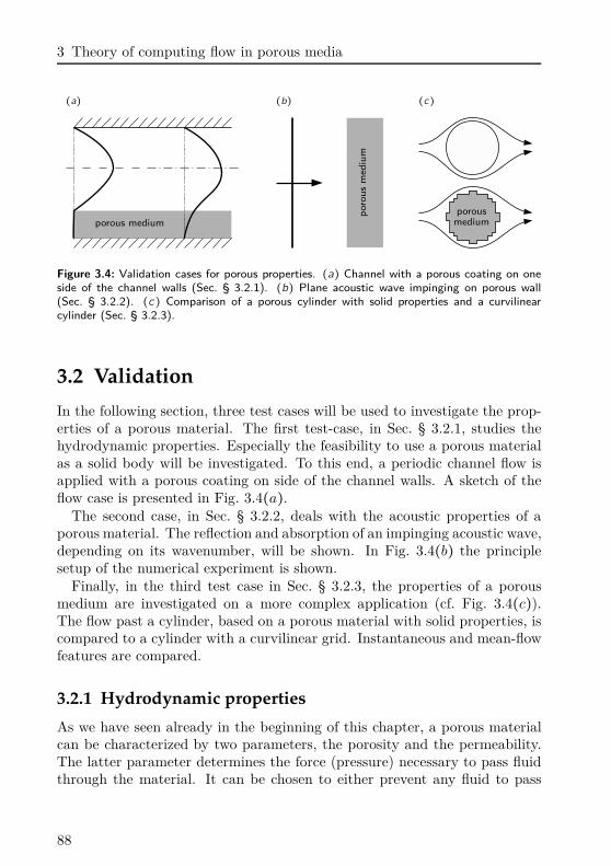
3 Theory of computing flow in porous media
(a) (b) (c)
porous medium
por
ous
med
ium
porousmedium
Figure 3.4: Validation cases for porous properties. (a) Channel with a porous coating on oneside of the channel walls (Sec. § 3.2.1). (b) Plane acoustic wave impinging on porous wall(Sec. § 3.2.2). (c) Comparison of a porous cylinder with solid properties and a curvilinearcylinder (Sec. § 3.2.3).
3.2 Validation
In the following section, three test cases will be used to investigate the prop-erties of a porous material. The first test-case, in Sec. § 3.2.1, studies thehydrodynamic properties. Especially the feasibility to use a porous materialas a solid body will be investigated. To this end, a periodic channel flow isapplied with a porous coating on side of the channel walls. A sketch of theflow case is presented in Fig. 3.4(a).
The second case, in Sec. § 3.2.2, deals with the acoustic properties of aporous material. The reflection and absorption of an impinging acoustic wave,depending on its wavenumber, will be shown. In Fig. 3.4(b) the principlesetup of the numerical experiment is shown.
Finally, in the third test case in Sec. § 3.2.3, the properties of a porousmedium are investigated on a more complex application (cf. Fig. 3.4(c)).The flow past a cylinder, based on a porous material with solid properties, iscompared to a cylinder with a curvilinear grid. Instantaneous and mean-flowfeatures are compared.
3.2.1 Hydrodynamic properties
As we have seen already in the beginning of this chapter, a porous materialcan be characterized by two parameters, the porosity and the permeability.The latter parameter determines the force (pressure) necessary to pass fluidthrough the material. It can be chosen to either prevent any fluid to pass
88
3.2 Validation
(a) (b)
Figure 3.5: (a) Shape of a specific geometry. (b) Shape of (a) represented by the techniqueof volume penalization.
through the material or to let it pass without any resistance, including allintermediate states. In the first case the permeability is set to K = 0 and theporous material represents a solid body. In the second case, the permeabilityis set to K =∞ and simply represents void space.
The first feature is particularly interesting, since one can easily create com-plex geometries by placing a porous body with solid properties in the compu-tational domain without transforming the computational grid. A Cartesiangrid is used in the background to embed the porous material as a function ofthe space and eventually also of the time. The solid body encloses a certainnumber of grid points representing the solid body. Depending on the reso-lution of the underlying Cartesian grid, the surface of the solid body is asrough as the resolution of the grid. In Fig. 3.5, the basic principle to includea solid body in a Cartesian grid, by means of volume penalization, is shown.In any technical application and experiment, a surface of a solid body in afluid flow will always show a certain roughness, depending on the fabricationtechnique. The fabrication tolerance, especially in experimental setups, canbe in the order of one tenth of a millimeter.
Considering e. g. a drilled round laval nozzle with a diameter of 10mmin an experimental setup with a fabrication tolerance of 0.1mm. To obtainthe same surface roughness in the numerical simulation, the resolution ofthe embedding Cartesian grid needs 100 points inside the nozzle. The highresolution numerical experiments of Sec. § 4.2 satisfy this property due toa grid refinement in the jet core. One has to mention, that in the usualfashion with curvilinear grids, the surface roughness of the numerical solution
89
3 Theory of computing flow in porous media
is zero. This influences the turbulence in the boundary layers and specialtechniques are necessary to trip the laminar boundary layers to obtain asimilar turbulence value as measured in the experiment [Bogey & Bailly,2010].
The technique to include a complex geometry in a Cartesian computationaldomain is related to immersed boundary methods and is called in this contextvolume penalization [see amongst others, Angot et al., 1999, Arquis & Calta-girone, 1984, Baur et al., 2009, Carbou, 2008, Keetels et al., 2007, Kevlahan& Ghidaglia, 2001, Kolomenskiy & Schneider, 2010, Liu & Vasilyev, 2007,Schneider & Farge, 2005]). To only use the technique of volume penalizationto include complex geometries as solid bodies in the computational domain,the porous flow equations can be extended with an additional term includinga second derivative of the velocities (Brinkmann penalization [see Brinkman,1949]). This term is similar to the friction terms of the Navier–Stokes equa-tions and adds an artificial viscosity inside the porous material. It reads:
∇p = −µK−1v + µ′∆v, (3.16)
where the first term on the right hand side corresponds to Darcy’s law ofEq. (3.1) and the second term to the Brinkmann extension. The additionalviscosity µ′ in the second term my be different from µ, depending on theconfiguration of the porous material [see Brinkman, 1949, Eq. (19)]. Froma numerical point of view, this additional Brinkmann term can be useful tosatisfy the non-slip condition at the surface of the solid body as the secondderivatives are large in these areas [see Liu & Vasilyev, 2007]. Especially forincompressible, divergence free flows, this can be important [see Kolomen-skiy & Schneider, 2009]. If K is close to zero, the first term will dominateEq. (3.16) even though if the velocity gradients are large. To this end, theBrinkmann extension will only operate for large values of K which corre-sponds to void space in the porous material. Considering a constant µ′ = µ0
and a measurable velocity gradient, a drag on the velocity will be present inthe porous medium even tough if K →∞ (void space).
The focus of the present research project is the optimization of porousmaterial to reduce flow induced noise by means of controlling the permeabilityK. To maintain the freedom in the design process, to create areas of voidspace in regions of porous material, the Brinkmann extension of Eq. (3.16) isnot included in this analysis.
To obtain a solid body with the present equations, one has to choose K → 0.The only problem is that we can not choose a permeability of zero due to therelated stiffness of the flow equations and the corresponding restrictions of
90
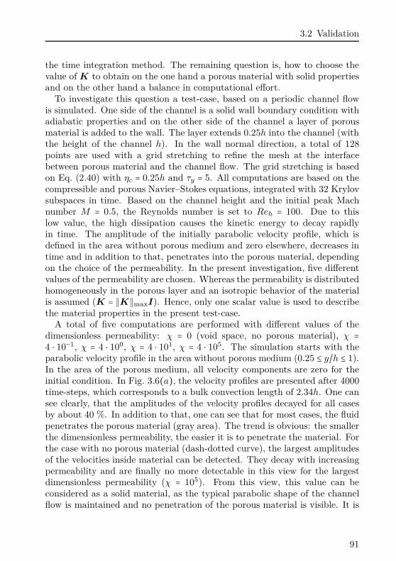
3.2 Validation
the time integration method. The remaining question is, how to choose thevalue of K to obtain on the one hand a porous material with solid propertiesand on the other hand a balance in computational effort.
To investigate this question a test-case, based on a periodic channel flowis simulated. One side of the channel is a solid wall boundary condition withadiabatic properties and on the other side of the channel a layer of porousmaterial is added to the wall. The layer extends 0.25h into the channel (withthe height of the channel h). In the wall normal direction, a total of 128points are used with a grid stretching to refine the mesh at the interfacebetween porous material and the channel flow. The grid stretching is basedon Eq. (2.40) with ηc = 0.25h and τy = 5. All computations are based on thecompressible and porous Navier–Stokes equations, integrated with 32 Krylovsubspaces in time. Based on the channel height and the initial peak Machnumber M = 0.5, the Reynolds number is set to Reh = 100. Due to thislow value, the high dissipation causes the kinetic energy to decay rapidlyin time. The amplitude of the initially parabolic velocity profile, which isdefined in the area without porous medium and zero elsewhere, decreases intime and in addition to that, penetrates into the porous material, dependingon the choice of the permeability. In the present investigation, five differentvalues of the permeability are chosen. Whereas the permeability is distributedhomogeneously in the porous layer and an isotropic behavior of the materialis assumed (K = ∥K∥maxI). Hence, only one scalar value is used to describethe material properties in the present test-case.
A total of five computations are performed with different values of thedimensionless permeability: χ = 0 (void space, no porous material), χ =4 ⋅ 10−1, χ = 4 ⋅ 100, χ = 4 ⋅ 101, χ = 4 ⋅ 105. The simulation starts with theparabolic velocity profile in the area without porous medium (0.25 ≤ y/h ≤ 1).In the area of the porous medium, all velocity components are zero for theinitial condition. In Fig. 3.6(a), the velocity profiles are presented after 4000time-steps, which corresponds to a bulk convection length of 2.34h. One cansee clearly, that the amplitudes of the velocity profiles decayed for all casesby about 40 %. In addition to that, one can see that for most cases, the fluidpenetrates the porous material (gray area). The trend is obvious: the smallerthe dimensionless permeability, the easier it is to penetrate the material. Forthe case with no porous material (dash-dotted curve), the largest amplitudesof the velocities inside material can be detected. They decay with increasingpermeability and are finally no more detectable in this view for the largestdimensionless permeability (χ = 105). From this view, this value can beconsidered as a solid material, as the typical parabolic shape of the channelflow is maintained and no penetration of the porous material is visible. It is
91
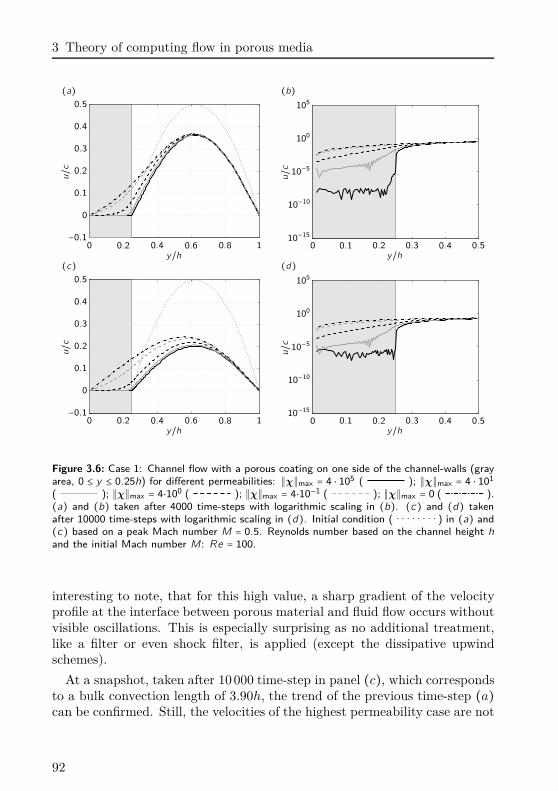
3 Theory of computing flow in porous media
(a) (b)
y/h
u/c
0 0.2 0.4 0.6 0.8 1−0.1
0
0.1
0.2
0.3
0.4
0.5
y/h
u/c
0 0.1 0.2 0.3 0.4 0.510−15
10−10
10−5
100
105
(c) (d)
y/h
u/c
0 0.2 0.4 0.6 0.8 1−0.1
0
0.1
0.2
0.3
0.4
0.5
y/h
u/c
0 0.1 0.2 0.3 0.4 0.510−15
10−10
10−5
100
105
Figure 3.6: Case 1: Channel flow with a porous coating on one side of the channel-walls (grayarea, 0 ≤ y ≤ 0.25h) for different permeabilities: ∥χ∥max = 4 ⋅ 105 ( ); ∥χ∥max = 4 ⋅ 101
( ); ∥χ∥max = 4⋅100 ( ); ∥χ∥max = 4⋅10−1 ( ); ∥χ∥max = 0 ( ).(a) and (b) taken after 4000 time-steps with logarithmic scaling in (b). (c) and (d) takenafter 10000 time-steps with logarithmic scaling in (d). Initial condition ( ) in (a) and(c) based on a peak Mach number M = 0.5. Reynolds number based on the channel height hand the initial Mach number M: Re = 100.
interesting to note, that for this high value, a sharp gradient of the velocityprofile at the interface between porous material and fluid flow occurs withoutvisible oscillations. This is especially surprising as no additional treatment,like a filter or even shock filter, is applied (except the dissipative upwindschemes).
At a snapshot, taken after 10 000 time-step in panel (c), which correspondsto a bulk convection length of 3.90h, the trend of the previous time-step (a)can be confirmed. Still, the velocities of the highest permeability case are not
92
3.2 Validation
detectable in this view. In fact, the velocities do not vanish completely. Inthe corresponding panels (b) and (d), respectively, the velocity profiles arevisualized in a logarithmic scaling. For the high permeability case, the veloc-ity components inside the porous medium are in the order of M = 10−6 whichcan be neglected for the present numerical investigation, where supersonicvelocities with M > 1 dominate the flow.
From this analysis, one can conclude, that from a hydrodynamic point ofview, a dimensionless value of the permeability of χ = 105 can be consideredas a solid body.
3.2.2 Acoustic properties
In the following test case the acoustic properties of a porous medium, basedon the porous Navier–Stokes equations of this chapter are investigated. Thefocus of this investigation lies on the acoustic properties of the interface of aporous medium and void space depending on the permeability of the material.It is well known, that a porous medium can be used as a sound absorber. Forexample, the walls of any anechoic room can be regarded as a porous medium.
This test case is based on a one-dimensional simulation of a plane acousticwave impinging, reflecting and transmitting on a porous wall with a varyingpermeability. In addition to that, the dependence of the wave number of theimpinging and reflecting wave is investigated. To measure the deviation of areflecting wave of a porous wall to a solid wall, a wall boundary condition isimplemented at the location of the interface of void space and porous material.
The one-dimensional plane wave is solved on a domain Ω ∈ [0, L] with128 equidistantly spaced grid points. The interface of void space to porousmaterial is located at x = 3/4L with the porous material ranging from 3/4 ≤x/L ≤ 1. As initial condition, the shape of the plane acoustic wave is ofGaussian type and reads:
p(x) = p0 + exp⎛⎝−(
x − 3/8L
b)2⎞⎠
u(x) = 1ρ0c
exp⎛⎝−(
x − 3/8L
b)2⎞⎠
with the center of the Gaussian distribution at x = 3/8L and the widthb = √2/2 ⋅ 10−1L. The acoustic Reynolds number is set to Rea = 5000 basedon the length of the domain L. In Fig. 3.7 the solution of the acoustic pulseis visualized for four time-steps (t = [1/4, 2/4, 3/4, 4/4]T ) and for different per-meabilities, ranging from ∥χ∥max = 2 ⋅ 100, . . . , 2 ⋅ 104 (with T = L/c and the
93
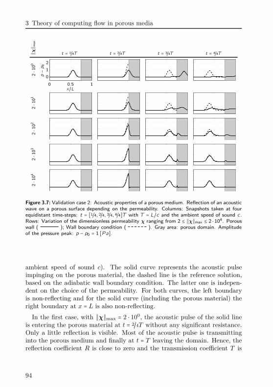
3 Theory of computing flow in porous media∥χ∥ m
ax
t = 1/4T t = 2/4T t = 3/4T t = 4/4T
2⋅100
p−p0
x/L0 0.5 1
0
1
2
2⋅101
2⋅102
2⋅103
2⋅104
Figure 3.7: Validation case 2: Acoustic properties of a porous medium. Reflection of an acousticwave on a porous surface depending on the permeability. Columns: Snapshots taken at fourequidistant time-steps: t = [1/4, 2/4, 3/4, 4/4]T with T = L/c and the ambient speed of sound c .Rows: Variation of the dimensionless permeability χ ranging from 2 ≤ ∥χ∥max ≤ 2 ⋅ 104. Porouswall ( ); Wall boundary condition ( ). Gray area: porous domain. Amplitudeof the pressure peak: p − p0 = 1 [Pa].
ambient speed of sound c). The solid curve represents the acoustic pulseimpinging on the porous material, the dashed line is the reference solution,based on the adiabatic wall boundary condition. The latter one is indepen-dent on the choice of the permeability. For both curves, the left boundaryis non-reflecting and for the solid curve (including the porous material) theright boundary at x = L is also non-reflecting.
In the first case, with ∥χ∥max = 2 ⋅ 100, the acoustic pulse of the solid lineis entering the porous material at t = 2/4T without any significant resistance.Only a little reflection is visible. Most of the acoustic pulse is transmittinginto the porous medium and finally at t = T leaving the domain. Hence, thereflection coefficient R is close to zero and the transmission coefficient T is
94
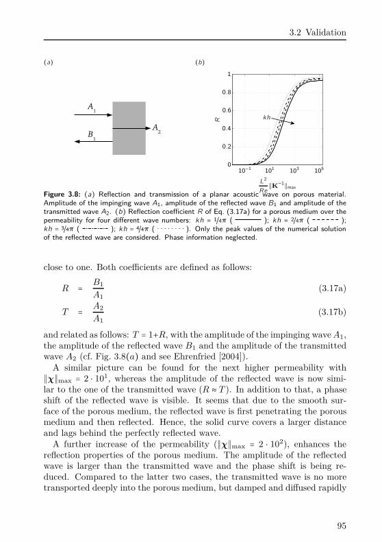
3.2 Validation
(a) (b)
R
L2
Re∥K−1∥max
kh
10−1 101 103 1050
0.2
0.4
0.6
0.8
1
Figure 3.8: (a) Reflection and transmission of a planar acoustic wave on porous material.Amplitude of the impinging wave A1, amplitude of the reflected wave B1 and amplitude of thetransmitted wave A2. (b) Reflection coefficient R of Eq. (3.17a) for a porous medium over thepermeability for four different wave numbers: kh = 1/4π ( ); kh = 2/4π ( );kh = 3/4π ( ); kh = 4/4π ( ). Only the peak values of the numerical solutionof the reflected wave are considered. Phase information neglected.
close to one. Both coefficients are defined as follows:
R = B1
A1
(3.17a)
T = A2
A1
(3.17b)
and related as follows: T = 1+R, with the amplitude of the impinging wave A1,the amplitude of the reflected wave B1 and the amplitude of the transmittedwave A2 (cf. Fig. 3.8(a) and see Ehrenfried [2004]).
A similar picture can be found for the next higher permeability with∥χ∥max = 2 ⋅ 101, whereas the amplitude of the reflected wave is now simi-lar to the one of the transmitted wave (R ≈ T ). In addition to that, a phaseshift of the reflected wave is visible. It seems that due to the smooth sur-face of the porous medium, the reflected wave is first penetrating the porousmedium and then reflected. Hence, the solid curve covers a larger distanceand lags behind the perfectly reflected wave.
A further increase of the permeability (∥χ∥max = 2 ⋅ 102), enhances thereflection properties of the porous medium. The amplitude of the reflectedwave is larger than the transmitted wave and the phase shift is being re-duced. Compared to the latter two cases, the transmitted wave is no moretransported deeply into the porous medium, but damped and diffused rapidly
95
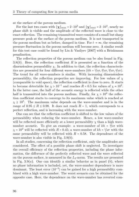
3 Theory of computing flow in porous media
at the surface of the porous medium.For the last two cases with ∥χ∥max = 2 ⋅ 103 and ∥χ∥max = 2 ⋅ 104, nearly no
phase shift is visible and the amplitude of the reflected wave is close to theexact reflection. The remaining transmitted wave consists of a small but sharppressure peak at the surface of the porous medium. It is not transported inthe porous medium but as before, damped in time. For t→∞, the remainingpressure fluctuation in the porous medium will become zero. A similar resultfor this test case could be found by Liu & Vasilyev [2007] with a Brinkmannpenalization.
The reflection properties of the porous medium can be also found in Fig.3.8(b). Here, the reflection coefficient R is presented as a function of thedimensionless permeability χ. In addition to that, the reflection characteris-tics are presented for four different wave-numbers (kh = 1/4π, 2/4π, 3/4π, 4/4π).The trend for all wave-numbers is similar. With increasing dimensionlesspermeability, the reflection properties are improving. For low values of χ
(comparable to void space), the reflection coefficient is close to zero. It startsto become detectable for χ > 10−1 and reaches R = 0.5 for values of χ ≈ 102.In the latter case, the half of the acoustic energy is reflected while the otherhalf is transmitted into the porous medium. Finally, for χ > 104 the reflec-tion coefficient starts to converge to its maximum value which is reached atχ ≥ 105. The maximum value depends on the wave-number and is in therange of 0.95 ≤ R ≤ 0.98. It does not reach R = 1, which corresponds to aperfect reflection, and is increasing with the wave-number.
One can see that the reflection coefficient is shifted to the low values of thepermeability when reducing the wave-number. Hence, a low wave-numberwill be reflected more efficiently at a lower permeability χ than a high wave-number acoustic. To give an example: a wave-number of kh = 3/4π withχ = 102 will be reflected with R = 0.45; a wave-number of kh = 1/4π with thesame permeability will be reflected with R = 0.58. The dependence of thewave-number is also visible in Fig. 3.9(b).
In all studies, concerning the reflection coefficient, only the amplitudes areconsidered. The effect of a possible phase shift is neglected. To investigatethe overall efficiency of the reflection properties, including the phase infor-mation, the difference of the perfectly reflected wave and the wave reflectedon the porous surface, is measured in the L2-norm. The results are presentedin Fig. 3.9(a). One can identify a similar behavior as in panel (b), whereno phase information is included, yet, the wave-number dependence is moredominant. The least error (10−3) can be gained for a high permeability com-bined with a high wave-number. The worst scenario can be obtained for theopposite case. Here, the dependence on the wave-number has reverted com-
96
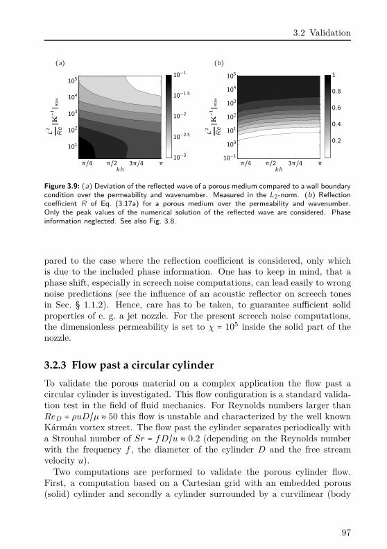
3.2 Validation
(a) (b)
L2
Re∥K
−1∥ m
ax
khπ/4 π/2 3π/4 π
10−3
10−2.5
10−2
10−1.5
10−1
101
102
103
104
105
L2
Re∥K
−1∥ m
ax
khπ/4 π/2 3π/4 π
0.2
0.4
0.6
0.8
1
10−1
100
101
102
103
104
105
Figure 3.9: (a) Deviation of the reflected wave of a porous medium compared to a wall boundarycondition over the permeability and wavenumber. Measured in the L2-norm. (b) Reflectioncoefficient R of Eq. (3.17a) for a porous medium over the permeability and wavenumber.Only the peak values of the numerical solution of the reflected wave are considered. Phaseinformation neglected. See also Fig. 3.8.
pared to the case where the reflection coefficient is considered, only whichis due to the included phase information. One has to keep in mind, that aphase shift, especially in screech noise computations, can lead easily to wrongnoise predictions (see the influence of an acoustic reflector on screech tonesin Sec. § 1.1.2). Hence, care has to be taken, to guarantee sufficient solidproperties of e. g. a jet nozzle. For the present screech noise computations,the dimensionless permeability is set to χ = 105 inside the solid part of thenozzle.
3.2.3 Flow past a circular cylinder
To validate the porous material on a complex application the flow past acircular cylinder is investigated. This flow configuration is a standard valida-tion test in the field of fluid mechanics. For Reynolds numbers larger thanReD = ρuD/µ ≈ 50 this flow is unstable and characterized by the well knownKármán vortex street. The flow past the cylinder separates periodically witha Strouhal number of Sr = fD/u ≈ 0.2 (depending on the Reynolds numberwith the frequency f , the diameter of the cylinder D and the free streamvelocity u).
Two computations are performed to validate the porous cylinder flow.First, a computation based on a Cartesian grid with an embedded porous(solid) cylinder and secondly a cylinder surrounded by a curvilinear (body
97
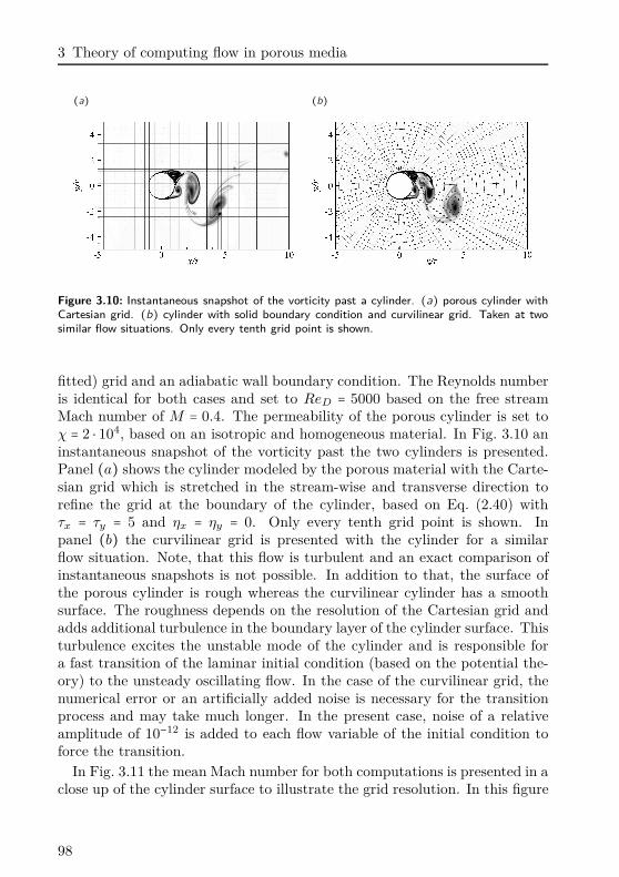
3 Theory of computing flow in porous media
(a) (b)
Figure 3.10: Instantaneous snapshot of the vorticity past a cylinder. (a) porous cylinder withCartesian grid. (b) cylinder with solid boundary condition and curvilinear grid. Taken at twosimilar flow situations. Only every tenth grid point is shown.
fitted) grid and an adiabatic wall boundary condition. The Reynolds numberis identical for both cases and set to ReD = 5000 based on the free streamMach number of M = 0.4. The permeability of the porous cylinder is set toχ = 2 ⋅ 104, based on an isotropic and homogeneous material. In Fig. 3.10 aninstantaneous snapshot of the vorticity past the two cylinders is presented.Panel (a) shows the cylinder modeled by the porous material with the Carte-sian grid which is stretched in the stream-wise and transverse direction torefine the grid at the boundary of the cylinder, based on Eq. (2.40) withτx = τy = 5 and ηx = ηy = 0. Only every tenth grid point is shown. Inpanel (b) the curvilinear grid is presented with the cylinder for a similarflow situation. Note, that this flow is turbulent and an exact comparison ofinstantaneous snapshots is not possible. In addition to that, the surface ofthe porous cylinder is rough whereas the curvilinear cylinder has a smoothsurface. The roughness depends on the resolution of the Cartesian grid andadds additional turbulence in the boundary layer of the cylinder surface. Thisturbulence excites the unstable mode of the cylinder and is responsible fora fast transition of the laminar initial condition (based on the potential the-ory) to the unsteady oscillating flow. In the case of the curvilinear grid, thenumerical error or an artificially added noise is necessary for the transitionprocess and may take much longer. In the present case, noise of a relativeamplitude of 10−12 is added to each flow variable of the initial condition toforce the transition.
In Fig. 3.11 the mean Mach number for both computations is presented in aclose up of the cylinder surface to illustrate the grid resolution. In this figure
98
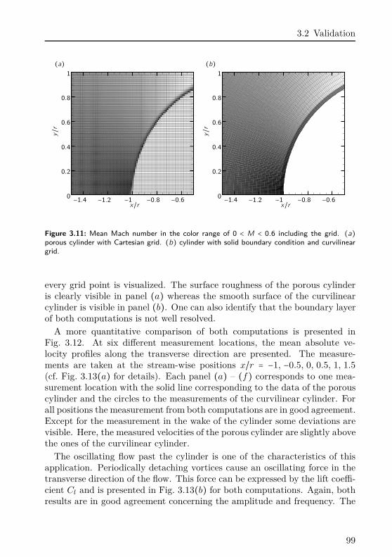
3.2 Validation
(a) (b)y/r
x/r0
0.2
0.4
0.6
0.8
1
−1.4 −1.2 −1 −0.8 −0.6y/r
x/r0
0.2
0.4
0.6
0.8
1
−1.4 −1.2 −1 −0.8 −0.6
Figure 3.11: Mean Mach number in the color range of 0 < M < 0.6 including the grid. (a)porous cylinder with Cartesian grid. (b) cylinder with solid boundary condition and curvilineargrid.
every grid point is visualized. The surface roughness of the porous cylinderis clearly visible in panel (a) whereas the smooth surface of the curvilinearcylinder is visible in panel (b). One can also identify that the boundary layerof both computations is not well resolved.
A more quantitative comparison of both computations is presented inFig. 3.12. At six different measurement locations, the mean absolute ve-locity profiles along the transverse direction are presented. The measure-ments are taken at the stream-wise positions x/r = −1, −0.5, 0, 0.5, 1, 1.5(cf. Fig. 3.13(a) for details). Each panel (a) – (f) corresponds to one mea-surement location with the solid line corresponding to the data of the porouscylinder and the circles to the measurements of the curvilinear cylinder. Forall positions the measurement from both computations are in good agreement.Except for the measurement in the wake of the cylinder some deviations arevisible. Here, the measured velocities of the porous cylinder are slightly abovethe ones of the curvilinear cylinder.
The oscillating flow past the cylinder is one of the characteristics of thisapplication. Periodically detaching vortices cause an oscillating force in thetransverse direction of the flow. This force can be expressed by the lift coeffi-cient Cl and is presented in Fig. 3.13(b) for both computations. Again, bothresults are in good agreement concerning the amplitude and frequency. The
99
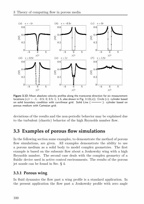
3 Theory of computing flow in porous media
(a) x = −1r (b) x = −0.5r (c) x = 0r
⟨M⟩
y/r−5 0 5
0
0.2
0.4
0.6PSfrag
⟨M⟩
y/r−5 0 5
0
0.2
0.4
0.6
⟨M⟩
y/r−5 0 5
0
0.2
0.4
0.6
(d) x = 0.5r (e) x = 1r (f ) x = 1.5r
⟨M⟩
y/r−5 0 5
0
0.2
0.4
0.6
⟨M⟩
y/r−5 0 5
0
0.2
0.4
0.6
⟨M⟩
y/r−5 0 5
0
0.2
0.4
0.6
Figure 3.12: Mean absolute velocity profiles along the transverse direction for six measurementlocations (x/r = −1; −0.5; 0; 0.5; 1; 1.5; also shown in Fig. 3.13(a)). Circle (): cylinder basedon solid boundary condition with curvilinear grid. Solid Line ( ): cylinder based onporous medium with Cartesian grid.
deviations of the results and the non-periodic behavior may be explained dueto the turbulent (chaotic) behavior of the high Reynolds number flow.
3.3 Examples of porous flow simulations
In the following section some examples, to demonstrate the method of porousflow simulations, are given. All examples demonstrate the ability to usea porous medium as a solid body to model complex geometries. The firstexample is based on the subsonic flow about a Joukowsky wing with a highReynolds number. The second case deals with the complex geometry of afluidic device used in active control environments. The results of the porousjet nozzle can be found in Sec. § 4.
3.3.1 Porous wing
In fluid dynamics the flow past a wing profile is a standard application. Inthe present application the flow past a Joukowsky profile with zero angle
100
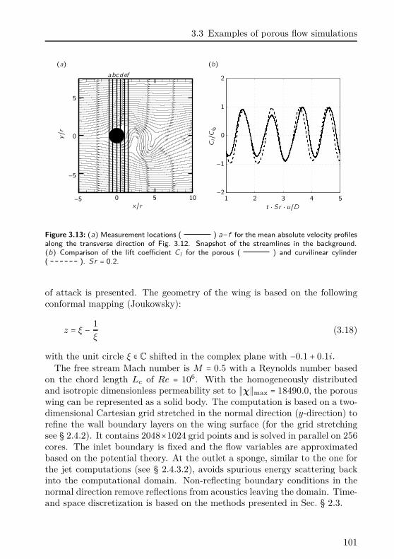
3.3 Examples of porous flow simulations
(a) (b)y/r
x/r10
5
5
−5
−5
0
0
abcdef
Cl/C
l 0
t ⋅ Sr ⋅ u/D1 2 3 4 5
−2
−1
0
1
2
Figure 3.13: (a)Measurement locations ( ) a−f for the mean absolute velocity profilesalong the transverse direction of Fig. 3.12. Snapshot of the streamlines in the background.(b) Comparison of the lift coefficient Cl for the porous ( ) and curvilinear cylinder( ). Sr = 0.2.
of attack is presented. The geometry of the wing is based on the followingconformal mapping (Joukowsky):
z = ξ −1ξ
(3.18)
with the unit circle ξ ∈ C shifted in the complex plane with −0.1 + 0.1i.The free stream Mach number is M = 0.5 with a Reynolds number based
on the chord length Lc of Re = 106. With the homogeneously distributedand isotropic dimensionless permeability set to ∥χ∥max = 18490.0, the porouswing can be represented as a solid body. The computation is based on a two-dimensional Cartesian grid stretched in the normal direction (y-direction) torefine the wall boundary layers on the wing surface (for the grid stretchingsee § 2.4.2). It contains 2048×1024 grid points and is solved in parallel on 256cores. The inlet boundary is fixed and the flow variables are approximatedbased on the potential theory. At the outlet a sponge, similar to the one forthe jet computations (see § 2.4.3.2), avoids spurious energy scattering backinto the computational domain. Non-reflecting boundary conditions in thenormal direction remove reflections from acoustics leaving the domain. Time-and space discretization is based on the methods presented in Sec. § 2.3.
101
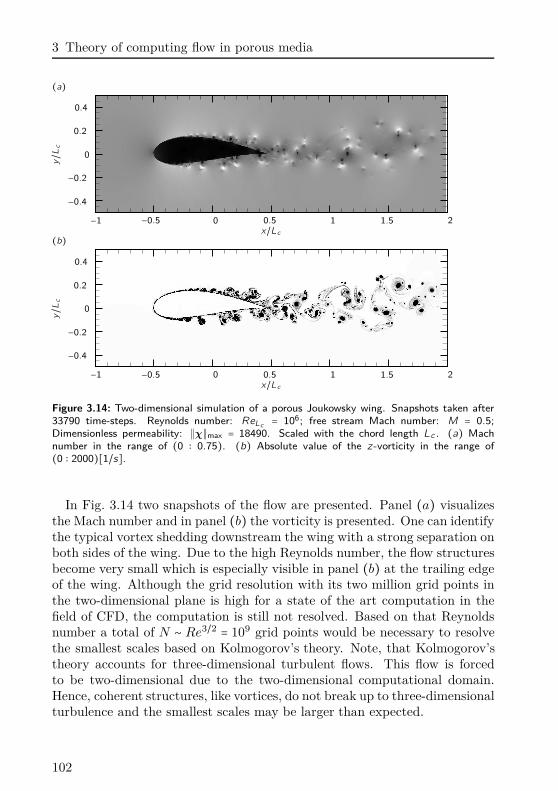
3 Theory of computing flow in porous media
(a)
y/Lc
x/Lc−1 −0.5 0 0.5 1 1.5 2
−0.4
−0.2
0
0.2
0.4
(b)
y/Lc
x/Lc−1 −0.5 0 0.5 1 1.5 2
−0.4
−0.2
0
0.2
0.4
Figure 3.14: Two-dimensional simulation of a porous Joukowsky wing. Snapshots taken after33790 time-steps. Reynolds number: ReLc = 106; free stream Mach number: M = 0.5;Dimensionless permeability: ∥χ∥max = 18490. Scaled with the chord length Lc . (a) Machnumber in the range of (0 ∶ 0.75). (b) Absolute value of the z -vorticity in the range of(0 ∶ 2000)[1/s].
In Fig. 3.14 two snapshots of the flow are presented. Panel (a) visualizesthe Mach number and in panel (b) the vorticity is presented. One can identifythe typical vortex shedding downstream the wing with a strong separation onboth sides of the wing. Due to the high Reynolds number, the flow structuresbecome very small which is especially visible in panel (b) at the trailing edgeof the wing. Although the grid resolution with its two million grid points inthe two-dimensional plane is high for a state of the art computation in thefield of CFD, the computation is still not resolved. Based on that Reynoldsnumber a total of N ∼ Re3/2 = 109 grid points would be necessary to resolvethe smallest scales based on Kolmogorov’s theory. Note, that Kolmogorov’stheory accounts for three-dimensional turbulent flows. This flow is forcedto be two-dimensional due to the two-dimensional computational domain.Hence, coherent structures, like vortices, do not break up to three-dimensionalturbulence and the smallest scales may be larger than expected.
102
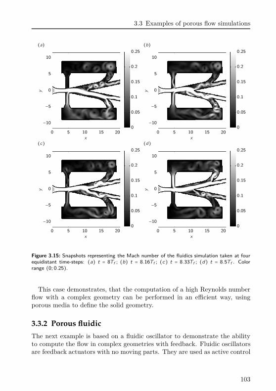
3.3 Examples of porous flow simulations
(a) (b)
y
x
0 5 10 15 200
0.05
0.1
0.15
0.2
0.25
−10
−5
0
5
10
y
x
0 5 10 15 200
0.05
0.1
0.15
0.2
0.25
−10
−5
0
5
10
(c) (d)
y
x
0 5 10 15 200
0.05
0.1
0.15
0.2
0.25
−10
−5
0
5
10
y
x
0 5 10 15 200
0.05
0.1
0.15
0.2
0.25
−10
−5
0
5
10
Figure 3.15: Snapshots representing the Mach number of the fluidics simulation taken at fourequidistant time-steps: (a) t = 8Tf ; (b) t = 8.16Tf ; (c) t = 8.33Tf ; (d) t = 8.5Tf . Colorrange (0; 0.25).
This case demonstrates, that the computation of a high Reynolds numberflow with a complex geometry can be performed in an efficient way, usingporous media to define the solid geometry.
3.3.2 Porous fluidic
The next example is based on a fluidic oscillator to demonstrate the abilityto compute the flow in complex geometries with feedback. Fluidic oscillatorsare feedback actuators with no moving parts. They are used as active control
103
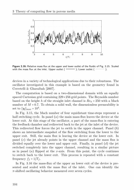
3 Theory of computing flow in porous media
(ρu) ou
t/(ρu) in
t/Tf3 4 5 6 7 8 9 10
0
0.2
0.4
0.6
0.8
1
Figure 3.16: Relative mass flux at the upper and lower outlet of the fluidic of Fig. 3.15. Scaledwith the mass flux at the inlet. Upper outlet ( ); Lower outlet ( ).
devices in a variety of technological applications due to their robustness. Theoscillator investigated in this example is based on the geometry found inCerretelli & Gharaibah [2007].
The computation is based on a two-dimensional domain with an equallyspaced Cartesian grid containing 229×256 grid points. The Reynolds numberbased on the height h of the straight inlet channel is Reh = 250 with a Machnumber of M = 0.7. To obtain a solid wall, the dimensionless permeability isset to ∥χ∥max = 104.
In Fig. 3.15, the Mach number of four equidistant time-steps represent ahalf switching cycle. In panel (a) the main mass-flux leaves the device at thelower exit. At this stage of the oscillator, a part of the mass-flux is enteringthe feedback chamber and redirected back to the jet at the inlet of the device.This redirected flow forces the jet to swith in the upper channel. Panel (b)shows an intermediate snapshot of the flow switching from the lower to theupper exit. Still, the main flux is leaving the device at the lower exit. Inpanel (c) the jet already points in the upper channel and the mass flux isdivided equally over the lower and upper exit. Finally, in panel (d) the jetswitched completely into the upper channel, resulting in a similar pictureas in panel (a) flipped at the x-axis. From this point, the cycle continuesto switch back to the lower exit. This process is repeated with a constantfrequency ff = 1/Tf .
In Fig. 3.16 the mass-flux of the upper an lower exit of the device is pre-sented and scaled with the mass flux of the inlet. One can identify theπ-shifted oscillating behavior measured over seven cycles.
104
3.3 Examples of porous flow simulations
As a conclusion of this chapter, we can see, that the presented porousand compressible Navier–Stokes equations are capable to treat both, acousticand hydrodynamic flow problems with geometries of high complexity. Theseequations will be used in the following section to include a convergent nozzlein the Cartesian computational domain to investigate supersonic jet noise.The focus of the jet noise computation will lie on jet screech, which is ampli-fied due to the reflected acoustic wave at the nozzle lip. Hence, the porousmaterial needs to show its capability to handle both, a proper reflection char-acteristic and sufficient hydrodynamic properties, like an impermeable wall.In addition to this, in Sec. § 6, a porous material will be added to the noz-zle exit to eliminate the feedback mechanism where high demands are madeon the damping properties of the porous material. All these properties areshown to be controllable with the present porous flow equations.
105

4Results of supersonic jet noise simulation
In the following chapter the results on supersonic jet noise computations arepresented. It is divided in two main parts. The first part deals with planarjets whereas axisymmetric jets are investigates in the second part. In bothcases the nozzle is implemented in the computational domain by means ofa porous material with solid properties. No porous material is added tosuppress screech tones. The results of the minimization of supersonic jetnoise are presented in Sec. § 6.
The focus of the computations presented in the present chapter is to in-vestigate screech tones and to validate the numerical method. In the firstpart, dealing with planar jets, a parametric study on the influence of jetMach number to the flow physics, like emanated noise and mean values are,is performed. In the second part dealing with an axisymmetric jet, the Machnumber is kept constant and the spatial resolution is modified.
Tabular 4.1 gives an overview of the main parameters, like Mach numberand grid resolution, of the computations investigated. Both, the planar andthe round jet are based on a Reynolds number of Re = 5000. In the planarcase the Reynolds number is based on the jet height h and in the round caseon the jet diameter D:
ReD = ρ∞Duj
µ∞(4.1a)
Reh = ρ∞huj
µ∞(4.1b)
107
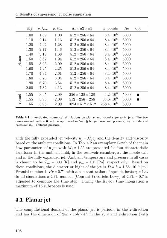
4 Results of supersonic jet noise simulation
Mj pr/p∞ pe/p∞ n1 × n2 × n3 # points Re opt
plan
ar
1.00 1.89 1.00 512 × 256× 64 8.4 ⋅ 106 50001.10 2.14 1.13 512 × 256× 64 8.4 ⋅ 106 50001.20 2.42 1.28 512 × 256× 64 8.4 ⋅ 106 50001.30 2.77 1.46 512 × 256× 64 8.4 ⋅ 106 50001.40 3.18 1.68 512 × 256× 64 8.4 ⋅ 106 50001.50 3.67 1.94 512 × 256× 64 8.4 ⋅ 106 50001.55 3.95 2.09 512 × 256× 64 8.4 ⋅ 106 50001.60 4.25 2.25 512 × 256× 64 8.4 ⋅ 106 50001.70 4.94 2.61 512 × 256× 64 8.4 ⋅ 106 50001.80 5.75 3.04 512 × 256× 64 8.4 ⋅ 106 50001.90 6.70 3.54 512 × 256× 64 8.4 ⋅ 106 50002.00 7.82 4.13 512 × 256× 64 8.4 ⋅ 106 5000
roun
d 1.55 3.95 2.09 256× 128 × 128 4.2 ⋅ 106 5000 ∎
1.55 3.95 2.09 512× 256 × 256 33.6 ⋅ 106 5000 ∎
1.55 3.95 2.09 1024× 512× 512 268.4 ⋅ 106 5000
Table 4.1: Investigated numerical simulations on planar and round supersonic jets. The twocases marked with a ∎ will be optimized in Sec. § 6. pr : reservoir pressure; pe : nozzle exitpressure; p∞: ambient pressure.
with the fully expanded jet velocity uj =Mjcj and the density and viscositybased on the ambient conditions. In Tab. 4.2 an exemplary sketch of the mainflow parameters of a jet with Mj = 1.55 are presented for four characteristiclocations: in the ambient fluid, in the reservoir chamber, at the nozzle exitand in the fully expanded jet. Ambient temperature and pressure in all casesis chosen to be T∞ = 300 [K] and p∞ = 105 [Pa], respectively. Based onthese conditions, the diameter or hight of the jet is D = h = 1.66 ⋅ 10−4 [m].Prandtl number is P r = 0.71 with a constant ration of specific heats γ = 1.4.In all simulations a CFL number (Courant-Friedrichs-Lewy) of CFL = 0.7 isadjusted to compute the time step. During the Krylov time integration amaximum of 15 subspaces is used.
4.1 Planar jet
The computational domain of the planar jet is periodic in the z-directionand has the dimension of 25h × 15h × 4h in the x, y and z-direction (with
108
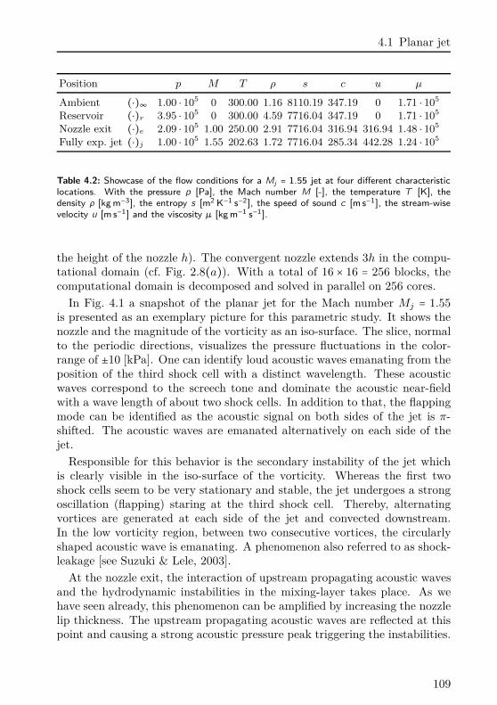
4.1 Planar jet
Position p M T ρ s c u µ
Ambient (⋅)∞ 1.00 ⋅ 105 0 300.00 1.16 8110.19 347.19 0 1.71 ⋅ 105
Reservoir (⋅)r 3.95 ⋅ 105 0 300.00 4.59 7716.04 347.19 0 1.71 ⋅ 105
Nozzle exit (⋅)e 2.09 ⋅ 105 1.00 250.00 2.91 7716.04 316.94 316.94 1.48 ⋅ 105
Fully exp. jet (⋅)j 1.00 ⋅ 105 1.55 202.63 1.72 7716.04 285.34 442.28 1.24 ⋅ 105
Table 4.2: Showcase of the flow conditions for a Mj = 1.55 jet at four different characteristiclocations. With the pressure p [Pa], the Mach number M [-], the temperature T [K], thedensity ρ [kgm−3], the entropy s [m2 K−1 s−2], the speed of sound c [ms−1], the stream-wisevelocity u [ms−1] and the viscosity µ [kgm−1 s−1].
the height of the nozzle h). The convergent nozzle extends 3h in the compu-tational domain (cf. Fig. 2.8(a)). With a total of 16 × 16 = 256 blocks, thecomputational domain is decomposed and solved in parallel on 256 cores.
In Fig. 4.1 a snapshot of the planar jet for the Mach number Mj = 1.55is presented as an exemplary picture for this parametric study. It shows thenozzle and the magnitude of the vorticity as an iso-surface. The slice, normalto the periodic directions, visualizes the pressure fluctuations in the color-range of ±10 [kPa]. One can identify loud acoustic waves emanating from theposition of the third shock cell with a distinct wavelength. These acousticwaves correspond to the screech tone and dominate the acoustic near-fieldwith a wave length of about two shock cells. In addition to that, the flappingmode can be identified as the acoustic signal on both sides of the jet is π-shifted. The acoustic waves are emanated alternatively on each side of thejet.
Responsible for this behavior is the secondary instability of the jet whichis clearly visible in the iso-surface of the vorticity. Whereas the first twoshock cells seem to be very stationary and stable, the jet undergoes a strongoscillation (flapping) staring at the third shock cell. Thereby, alternatingvortices are generated at each side of the jet and convected downstream.In the low vorticity region, between two consecutive vortices, the circularlyshaped acoustic wave is emanating. A phenomenon also referred to as shock-leakage [see Suzuki & Lele, 2003].
At the nozzle exit, the interaction of upstream propagating acoustic wavesand the hydrodynamic instabilities in the mixing-layer takes place. As wehave seen already, this phenomenon can be amplified by increasing the nozzlelip thickness. The upstream propagating acoustic waves are reflected at thispoint and causing a strong acoustic pressure peak triggering the instabilities.
109
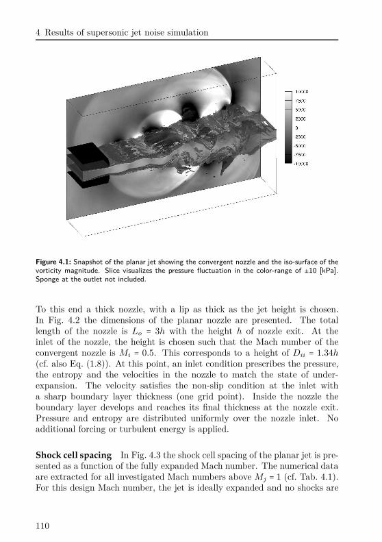
4 Results of supersonic jet noise simulation
Figure 4.1: Snapshot of the planar jet showing the convergent nozzle and the iso-surface of thevorticity magnitude. Slice visualizes the pressure fluctuation in the color-range of ±10 [kPa].Sponge at the outlet not included.
To this end a thick nozzle, with a lip as thick as the jet height is chosen.In Fig. 4.2 the dimensions of the planar nozzle are presented. The totallength of the nozzle is Lo = 3h with the height h of nozzle exit. At theinlet of the nozzle, the height is chosen such that the Mach number of theconvergent nozzle is Mi = 0.5. This corresponds to a height of Dii = 1.34h
(cf. also Eq. (1.8)). At this point, an inlet condition prescribes the pressure,the entropy and the velocities in the nozzle to match the state of under-expansion. The velocity satisfies the non-slip condition at the inlet witha sharp boundary layer thickness (one grid point). Inside the nozzle theboundary layer develops and reaches its final thickness at the nozzle exit.Pressure and entropy are distributed uniformly over the nozzle inlet. Noadditional forcing or turbulent energy is applied.
Shock cell spacing In Fig. 4.3 the shock cell spacing of the planar jet is pre-sented as a function of the fully expanded Mach number. The numerical dataare extracted for all investigated Mach numbers above Mj = 1 (cf. Tab. 4.1).For this design Mach number, the jet is ideally expanded and no shocks are
110
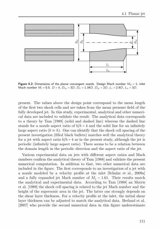
4.1 Planar jet
Figure 4.2: Dimensions of the planar convergent nozzle. Design Mach number Md = 1; inletMach number Mi = 0.5. D = h, Dio = 3D, Di i = 1.34D, Doi = 2D, Li = 2.9D, Lo = 3D.
present. The values above the design point correspond to the mean lengthof the first two shock cells and are taken from the mean pressure field of thefully developed jet. In this study, experimental, analytical and other numeri-cal data are included to validate the result. The analytical data correspondsto a theory by Tam [1988] (solid and dashed line) whereas the dashed linestands for a nozzle aspect ratio of b/h = 4 and the solid line for an infinitelylarge aspect ratio (b≫ h). One can identify that the shock cell spacing of thepresent investigation (filled black bullets) matches well the analytical theoryfor a jet with aspect ratio b/h = 4 as in the present study, although the jet isperiodic (infinitely large aspect ratio). There seems to be a relation betweenthe domain length in the periodic direction and the aspect ratio of the jet.
Various experimental data on jets with different aspect ratios and Machnumbers confirm the analytical theory of Tam [1988] and validate the presentnumerical computation. In addition to that, two other numerical data areincluded in the figure. The first corresponds to an investigation of a jet witha nozzle modeled by a velocity profile at the inlet [Schulze et al., 2009a]and a fully expanded jet Mach number of Mj = 1.61. Their results matchthe analytical and experimental data. According to Tam [1988] an Morriset al. [1989] the shock cell spacing is related to the jet Mach number and theheight of the supersonic area in the jet. The latter one strongly depends onthe shear layer thickness. For a velocity profile at the inlet, the initial shearlayer thickness can be adjusted to match the analytical data. Berland et al.[2007] who provide the second numerical data in this figure underestimate
111
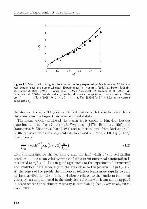
4 Results of supersonic jet noise simulation
Ls/h
Mj
1 1.2 1.4 1.6 1.8 20
1
2
3
4
5
6
Figure 4.3: Shock cell spacing as a function of the fully expanded jet Mach number Mj for var-ious experimental and numerical data. Experimental: +, Hammitt [1961]; ◻, Powell [1953b];, Raman & Rice [1994]; , Panda et al. [1997]; Numerical: , Berland et al. [2007]; ,Schulze et al. [2009a] (nozzle: velocity profile); , current computation (porous nozzle); The-ory: ( ), Tam [1988] for b ≫ h; ( ), Tam [1988] for b/h = 4 (as in the currentcomputation).
the shock cell length. They explain this deviation with the initial shear layerthickness which is larger than in experimental data.
The mean velocity profile of the planar jet is shown in Fig. 4.4. Besidesexperimental data from Gutmark & Wygnanski [1976], Bradbury [1965] andRamaprian & Chandrasekhara [1985] and numerical data from Berland et al.[2006] it also contains an analytical solution based on [Pope, 2000, Eq. (5.187)]which reads:
u
Um
= cosh−2 (log (1 +√2) y
δ0.5
) (4.2)
with the distance to the jet axis y and the half width of the self-similarprofile δ0.5. The mean velocity profile of the current numerical computation ismeasured at x/h = 17. It is in good agreement to the experimental, numericaland analytical data especially in the area close to the jet axis 0 ≤ y/δ0.5 ≤ 2.At the edges of the profile the numerical solution tends more rapidly to zeroas the analytical solution. This deviation is related to the “uniform turbulentviscosity” assumption used in the analytical solution which can not be appliedin areas where the turbulent viscosity is diminishing [see L’vov et al., 2008,Pope, 2000].
112
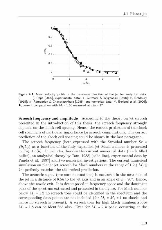
4.1 Planar jet
u/Um
y/δ0.50 1 2 3 4
0
0.2
0.4
0.6
0.8
1
Figure 4.4: Mean velocity profile in the transverse direction of the jet for analytical data:( ), Pope [2000], experimental data: +, Gutmark & Wygnanski [1976]; ◻, Bradbury[1965]; , Ramaprian & Chandrasekhara [1985]; and numerical data: , Berland et al. [2006];, current computation with Mj = 1.55 measured at x/h = 17.
Screech frequency and amplitude According to the theory on jet screechpresented in the introduction of this thesis, the screech frequency stronglydepends on the shock cell spacing. Hence, the correct prediction of the shockcell spacing is of particular importance for screech computations. The correctprediction of the shock cell spacing could be shown in the last paragraph.
The screech frequency (here expressed with the Strouhal number Sr =fh/Uj) as a function of the fully expanded jet Mach number is presentedin Fig. 4.5(b). It includes, besides the current numerical data (black filledbullet), an analytical theory by Tam [1988] (solid line), experimental data byPanda et al. [1997] and two numerical investigations. The current numericalsimulation on planar jet screech for Mach numbers in the range of 1.2 ≤Mj ≤2.0 perfectly matches the theoretical prediction.
The acoustic signal (pressure fluctuations) is measured in the near field ofthe jet in a distance of 6.5h to the jet axis and in an angle of Θ = 90. Hence,above the nozzle exit. It is decomposed in frequency space and the dominantpeak of the spectrum extracted and presented in the figure. For Mach numberbelow Mj = 1.2 no screech tone could be identified in the spectrum and thecorresponding data points are not included (for Mj =Md = 1 no shocks andhence no screech is present). A screech tone for high Mach numbers aboveMj = 1.8 can be identified also. Even for Mj = 2 a peak, occurring at the
113
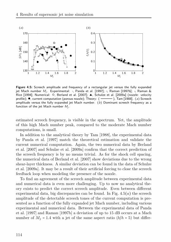
4 Results of supersonic jet noise simulation
(a) (b)
SPL[dB]
Mj
1 1.2 1.4 1.6 1.8 2130
140
150
160
170
f sh/Uj
Mj
1 1.2 1.4 1.6 1.8 20
0.1
0.2
0.3
0.4
Figure 4.5: Screech amplitude and frequency of a rectangular jet versus the fully expandedjet Mach number Mj . Experimental: , Panda et al. [1997]; ◻, Raman [1997b]; , Raman &Rice [1994]; Numerical: , Berland et al. [2007]; , Schulze et al. [2009a] (nozzle: velocityprofile); , current computation (porous nozzle); Theory: ( ), Tam [1988]. (a) Screechamplitude versus the fully expanded jet Mach number. (b) Dominant screech frequency as afunction of the jet Mach number Mj .
estimated screech frequency, is visible in the spectrum. Yet, the amplitudeof this high Mach number peak, compared to the moderate Mach numbercomputations, is small.
In addition to the analytical theory by Tam [1988], the experimental databy Panda et al. [1997] match the theoretical estimation and validate thecurrent numerical computation. Again, the two numerical data by Berlandet al. [2007] and Schulze et al. [2009a] confirm that the correct prediction ofthe screech frequency is by no means trivial. As for the shock cell spacing,the numerical data of Berland et al. [2007] show deviations due to the wrongshear-layer thickness. A similar deviation can be found in the data of Schulzeet al. [2009a]. It may be a result of their artificial forcing to close the screechfeedback loop when modeling the presence of the nozzle.
To find an agreement of the screech amplitude between experimental dataand numerical data is even more challenging. Up to now no analytical the-ory exists to predict the correct screech amplitude. Even between differentexperimental data, big discrepancies can be found. In Fig. 4.5(a) the screechamplitude of the detectable screech tones of the current computation is pre-sented as a function of the fully expanded jet Mach number, including variousexperimental and numerical data. Between the experimental data of Pandaet al. [1997] and Raman [1997b] a deviation of up to 15 dB occurs at a Machnumber of Mj = 1.4 with a jet of the same aspect ratio (b/h = 5) but differ-
114
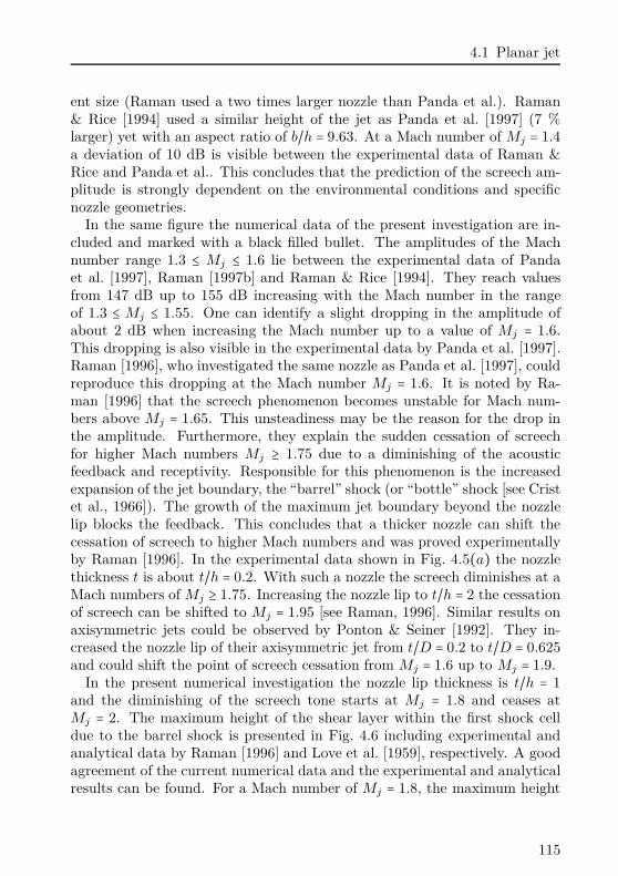
4.1 Planar jet
ent size (Raman used a two times larger nozzle than Panda et al.). Raman& Rice [1994] used a similar height of the jet as Panda et al. [1997] (7 %larger) yet with an aspect ratio of b/h = 9.63. At a Mach number of Mj = 1.4
a deviation of 10 dB is visible between the experimental data of Raman &Rice and Panda et al.. This concludes that the prediction of the screech am-plitude is strongly dependent on the environmental conditions and specificnozzle geometries.
In the same figure the numerical data of the present investigation are in-cluded and marked with a black filled bullet. The amplitudes of the Machnumber range 1.3 ≤ Mj ≤ 1.6 lie between the experimental data of Pandaet al. [1997], Raman [1997b] and Raman & Rice [1994]. They reach valuesfrom 147 dB up to 155 dB increasing with the Mach number in the rangeof 1.3 ≤ Mj ≤ 1.55. One can identify a slight dropping in the amplitude ofabout 2 dB when increasing the Mach number up to a value of Mj = 1.6.This dropping is also visible in the experimental data by Panda et al. [1997].Raman [1996], who investigated the same nozzle as Panda et al. [1997], couldreproduce this dropping at the Mach number Mj = 1.6. It is noted by Ra-man [1996] that the screech phenomenon becomes unstable for Mach num-bers above Mj = 1.65. This unsteadiness may be the reason for the drop inthe amplitude. Furthermore, they explain the sudden cessation of screechfor higher Mach numbers Mj ≥ 1.75 due to a diminishing of the acousticfeedback and receptivity. Responsible for this phenomenon is the increasedexpansion of the jet boundary, the “barrel” shock (or “bottle” shock [see Cristet al., 1966]). The growth of the maximum jet boundary beyond the nozzlelip blocks the feedback. This concludes that a thicker nozzle can shift thecessation of screech to higher Mach numbers and was proved experimentallyby Raman [1996]. In the experimental data shown in Fig. 4.5(a) the nozzlethickness t is about t/h = 0.2. With such a nozzle the screech diminishes at aMach numbers of Mj ≥ 1.75. Increasing the nozzle lip to t/h = 2 the cessationof screech can be shifted to Mj = 1.95 [see Raman, 1996]. Similar results onaxisymmetric jets could be observed by Ponton & Seiner [1992]. They in-creased the nozzle lip of their axisymmetric jet from t/D = 0.2 to t/D = 0.625
and could shift the point of screech cessation from Mj = 1.6 up to Mj = 1.9.In the present numerical investigation the nozzle lip thickness is t/h = 1
and the diminishing of the screech tone starts at Mj = 1.8 and ceases atMj = 2. The maximum height of the shear layer within the first shock celldue to the barrel shock is presented in Fig. 4.6 including experimental andanalytical data by Raman [1996] and Love et al. [1959], respectively. A goodagreement of the current numerical data and the experimental and analyticalresults can be found. For a Mach number of Mj = 1.8, the maximum height
115
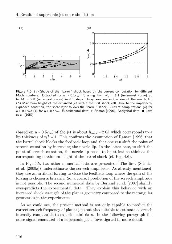
4 Results of supersonic jet noise simulation
(a) (b)
y/h
x/h0 1 2 3 4 5 6
0
1
2
hmax/2h
Mj
1 1.2 1.4 1.6 1.8 20
0.5
1
1.5
2
Figure 4.6: (a) Shape of the “barrel” shock based on the current computation for differentMach numbers. Extracted for u > 0.1c∞. Starting from Mj = 1.1 (innermost curve) upto Mj = 2.0 (outermost curve) in 0.1 steps. Gray area marks the size of the nozzle lip.(b) Maximum height of the expanded jet within the first shock cell. Due to the imperfectlyexpanded condition, the shear-layer follows the “barrel” shock. Current computation: () foru > 0.1c∞; () for u > 0.4c∞. Experimental data: ◻ Raman [1996]. Analytical data: ∎ Loveet al. [1959].
(based on u = 0.5c∞) of the jet is about hmax = 2.0h which corresponds to alip thickness of t/h = 1. This confirms the assumption of Raman [1996] thatthe barrel shock blocks the feedback loop and that one can shift the point ofscreech cessation by increasing the nozzle lip. In the latter case, to shift thepoint of screech cessation, the nozzle lip needs to be at lest as thick as thecorresponding maximum height of the barrel shock (cf. Fig. 4.6).
In Fig. 4.5, two other numerical data are presented. The first (Schulzeet al. [2009a]) underestimate the screech amplitude. As already mentioned,they use an artificial forcing to close the feedback loop where the gain of theforcing is chosen arbitrarily. So, a correct prediction of the screech amplitudeis not possible. The second numerical data by Berland et al. [2007] slightlyover-predicts the experimental data. They explain this behavior with anincreased shock strength of the planar geometry compared to the rectangulargeometries in the experiments.
As we could see, the present method is not only capable to predict thecorrect screech frequency of planar jets but also suitable to estimate a screechintensity comparable to experimental data. In the following paragraph thenoise signal emanated of a supersonic jet is investigated in more detail.
116
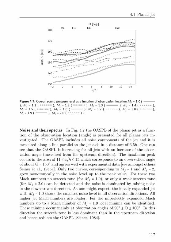
4.1 Planar jet
OA
SP
L[d
B]
Θ [deg.]
x/h
90 110 130 150
−2 0 2 4 6 8 10 12 14130
140
150
160
170
180
Figure 4.7: Overall sound pressure level as a function of observation location.Mj = 1.0 (), Mj = 1.1 ( ), Mj = 1.2 ( ), Mj = 1.3 ( ), Mj = 1.4 ( ),Mj = 1.5 ( ), Mj = 1.6 ( ), Mj = 1.7 ( ), Mj = 1.8 ( ),Mj = 1.9 ( ), Mj = 2.0 ( ) .
Noise and their spectra In Fig. 4.7 the OASPL of the planar jet as a func-tion of the observation location (angle) is presented for all planar jets in-vestigated. The OASPL includes all noise components of the jet and it ismeasured along a line parallel to the jet axis in a distance of 6.5h. One cansee that the OASPL is increasing for all jets with an increase of the obser-vation angle (measured from the upstream direction). The maximum peakoccurs in the area of 11 ≤ x/h ≤ 15 which corresponds to an observation angleof about Θ = 150 and agrees well with experimental data [see amongst othersSeiner et al., 1986a]. Only two curves, corresponding to Mj = 1 and Mj = 2,grow monotonically in the noise level up to the peak value. For these twoMach numbers no screech tone (for Mj = 1.0), or only a weak screech tone(for Mj = 2.0) can be detected and the noise is dominated by mixing noisein the downstream direction. As one might expect, the ideally expanded jetwith Mj = 1.0 shows the smallest noise level in all observation directions. Allhigher jet Mach numbers are louder. For the imperfectly expanded Machnumbers up to a Mach number of Mj = 1.9 local minima can be identified.These minima occur mainly at observation angles of 90 ≤ Θ ≤ 100. In thisdirection the screech tone is less dominant than in the upstream directionand hence reduces the OASPL [Seiner, 1984].
117
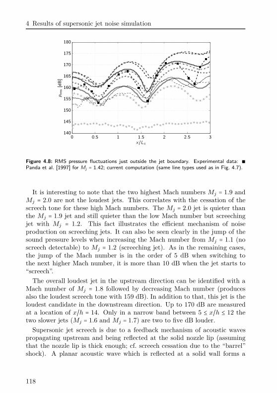
4 Results of supersonic jet noise simulation
replacemen
prm
s[d
B]
x/Ls0 0.5 1 1.5 2 2.5 3
140
145
150
155
160
165
170
175
180
Figure 4.8: RMS pressure fluctuations just outside the jet boundary. Experimental data: ∎Panda et al. [1997] for Mj = 1.42; current computation (same line types used as in Fig. 4.7).
It is interesting to note that the two highest Mach numbers Mj = 1.9 andMj = 2.0 are not the loudest jets. This correlates with the cessation of thescreech tone for these high Mach numbers. The Mj = 2.0 jet is quieter thanthe Mj = 1.9 jet and still quieter than the low Mach number but screechingjet with Mj = 1.2. This fact illustrates the efficient mechanism of noiseproduction on screeching jets. It can also be seen clearly in the jump of thesound pressure levels when increasing the Mach number from Mj = 1.1 (noscreech detectable) to Mj = 1.2 (screeching jet). As in the remaining cases,the jump of the Mach number is in the order of 5 dB when switching tothe next higher Mach number, it is more than 10 dB when the jet starts to“screech”.
The overall loudest jet in the upstream direction can be identified with aMach number of Mj = 1.8 followed by decreasing Mach number (producesalso the loudest screech tone with 159 dB). In addition to that, this jet is theloudest candidate in the downstream direction. Up to 170 dB are measuredat a location of x/h = 14. Only in a narrow band between 5 ≤ x/h ≤ 12 thetwo slower jets (Mj = 1.6 and Mj = 1.7) are two to five dB louder.
Supersonic jet screech is due to a feedback mechanism of acoustic wavespropagating upstream and being reflected at the solid nozzle lip (assumingthat the nozzle lip is thick enough; cf. screech cessation due to the “barrel”shock). A planar acoustic wave which is reflected at a solid wall forms a
118
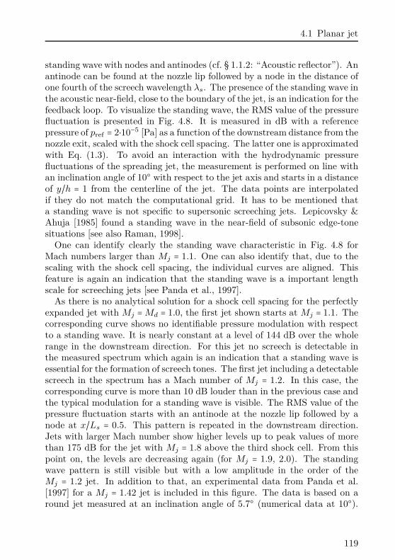
4.1 Planar jet
standing wave with nodes and antinodes (cf. § 1.1.2: “Acoustic reflector”). Anantinode can be found at the nozzle lip followed by a node in the distance ofone fourth of the screech wavelength λs. The presence of the standing wave inthe acoustic near-field, close to the boundary of the jet, is an indication for thefeedback loop. To visualize the standing wave, the RMS value of the pressurefluctuation is presented in Fig. 4.8. It is measured in dB with a referencepressure of pref = 2⋅10−5 [Pa] as a function of the downstream distance from thenozzle exit, scaled with the shock cell spacing. The latter one is approximatedwith Eq. (1.3). To avoid an interaction with the hydrodynamic pressurefluctuations of the spreading jet, the measurement is performed on line withan inclination angle of 10 with respect to the jet axis and starts in a distanceof y/h = 1 from the centerline of the jet. The data points are interpolatedif they do not match the computational grid. It has to be mentioned thata standing wave is not specific to supersonic screeching jets. Lepicovsky &Ahuja [1985] found a standing wave in the near-field of subsonic edge-tonesituations [see also Raman, 1998].
One can identify clearly the standing wave characteristic in Fig. 4.8 forMach numbers larger than Mj = 1.1. One can also identify that, due to thescaling with the shock cell spacing, the individual curves are aligned. Thisfeature is again an indication that the standing wave is a important lengthscale for screeching jets [see Panda et al., 1997].
As there is no analytical solution for a shock cell spacing for the perfectlyexpanded jet with Mj =Md = 1.0, the first jet shown starts at Mj = 1.1. Thecorresponding curve shows no identifiable pressure modulation with respectto a standing wave. It is nearly constant at a level of 144 dB over the wholerange in the downstream direction. For this jet no screech is detectable inthe measured spectrum which again is an indication that a standing wave isessential for the formation of screech tones. The first jet including a detectablescreech in the spectrum has a Mach number of Mj = 1.2. In this case, thecorresponding curve is more than 10 dB louder than in the previous case andthe typical modulation for a standing wave is visible. The RMS value of thepressure fluctuation starts with an antinode at the nozzle lip followed by anode at x/Ls = 0.5. This pattern is repeated in the downstream direction.Jets with larger Mach number show higher levels up to peak values of morethan 175 dB for the jet with Mj = 1.8 above the third shock cell. From thispoint on, the levels are decreasing again (for Mj = 1.9, 2.0). The standingwave pattern is still visible but with a low amplitude in the order of theMj = 1.2 jet. In addition to that, an experimental data from Panda et al.[1997] for a Mj = 1.42 jet is included in this figure. The data is based on around jet measured at an inclination angle of 5.7 (numerical data at 10).
119
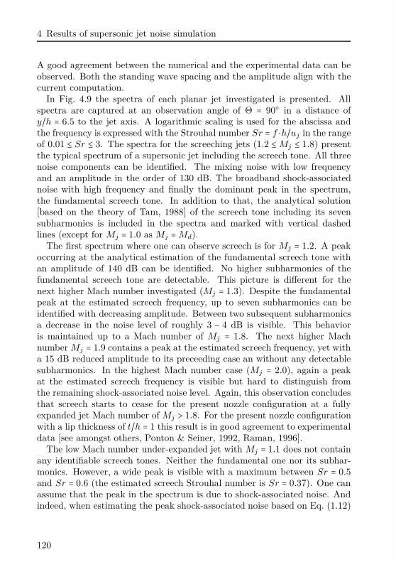
4 Results of supersonic jet noise simulation
A good agreement between the numerical and the experimental data can beobserved. Both the standing wave spacing and the amplitude align with thecurrent computation.
In Fig. 4.9 the spectra of each planar jet investigated is presented. Allspectra are captured at an observation angle of Θ = 90 in a distance ofy/h = 6.5 to the jet axis. A logarithmic scaling is used for the abscissa andthe frequency is expressed with the Strouhal number Sr = f ⋅h/uj in the rangeof 0.01 ≤ Sr ≤ 3. The spectra for the screeching jets (1.2 ≤Mj ≤ 1.8) presentthe typical spectrum of a supersonic jet including the screech tone. All threenoise components can be identified. The mixing noise with low frequencyand an amplitude in the order of 130 dB. The broadband shock-associatednoise with high frequency and finally the dominant peak in the spectrum,the fundamental screech tone. In addition to that, the analytical solution[based on the theory of Tam, 1988] of the screech tone including its sevensubharmonics is included in the spectra and marked with vertical dashedlines (except for Mj = 1.0 as Mj =Md).
The first spectrum where one can observe screech is for Mj = 1.2. A peakoccurring at the analytical estimation of the fundamental screech tone withan amplitude of 140 dB can be identified. No higher subharmonics of thefundamental screech tone are detectable. This picture is different for thenext higher Mach number investigated (Mj = 1.3). Despite the fundamentalpeak at the estimated screech frequency, up to seven subharmonics can beidentified with decreasing amplitude. Between two subsequent subharmonicsa decrease in the noise level of roughly 3 − 4 dB is visible. This behavioris maintained up to a Mach number of Mj = 1.8. The next higher Machnumber Mj = 1.9 contains a peak at the estimated screech frequency, yet witha 15 dB reduced amplitude to its preceeding case an without any detectablesubharmonics. In the highest Mach number case (Mj = 2.0), again a peakat the estimated screech frequency is visible but hard to distinguish fromthe remaining shock-associated noise level. Again, this observation concludesthat screech starts to cease for the present nozzle configuration at a fullyexpanded jet Mach number of Mj > 1.8. For the present nozzle configurationwith a lip thickness of t/h = 1 this result is in good agreement to experimentaldata [see amongst others, Ponton & Seiner, 1992, Raman, 1996].
The low Mach number under-expanded jet with Mj = 1.1 does not containany identifiable screech tones. Neither the fundamental one nor its subhar-monics. However, a wide peak is visible with a maximum between Sr = 0.5and Sr = 0.6 (the estimated screech Strouhal number is Sr = 0.37). One canassume that the peak in the spectrum is due to shock-associated noise. Andindeed, when estimating the peak shock-associated noise based on Eq. (1.12)
120
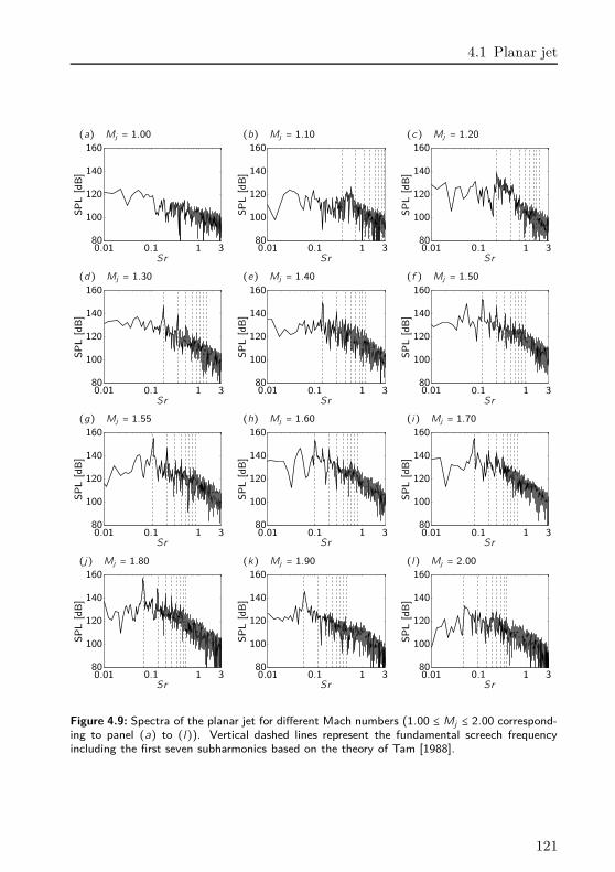
4.1 Planar jet
(a) Mj = 1.00 (b) Mj = 1.10 (c) Mj = 1.20
SP
L[d
B]
Sr0.01 0.1 1 380
100
120
140
160
SP
L[d
B]
Sr0.01 0.1 1 380
100
120
140
160
SP
L[d
B]
Sr0.01 0.1 1 380
100
120
140
160
(d) Mj = 1.30 (e) Mj = 1.40 (f ) Mj = 1.50
SP
L[d
B]
Sr0.01 0.1 1 380
100
120
140
160
SP
L[d
B]
Sr0.01 0.1 1 380
100
120
140
160
SP
L[d
B]
Sr0.01 0.1 1 380
100
120
140
160
(g) Mj = 1.55 (h) Mj = 1.60 (i) Mj = 1.70
SP
L[d
B]
Sr0.01 0.1 1 380
100
120
140
160
SP
L[d
B]
Sr0.01 0.1 1 380
100
120
140
160
SP
L[d
B]
Sr0.01 0.1 1 380
100
120
140
160
(j) Mj = 1.80 (k) Mj = 1.90 (l) Mj = 2.00
SP
L[d
B]
Sr0.01 0.1 1 380
100
120
140
160
SP
L[d
B]
Sr0.01 0.1 1 380
100
120
140
160
SP
L[d
B]
Sr0.01 0.1 1 380
100
120
140
160
Figure 4.9: Spectra of the planar jet for different Mach numbers (1.00 ≤ Mj ≤ 2.00 correspond-ing to panel (a) to (l)). Vertical dashed lines represent the fundamental screech frequencyincluding the first seven subharmonics based on the theory of Tam [1988].
121
4 Results of supersonic jet noise simulation
one obtains a Strouhal number of SrBB = 0.54 which matches the measuredpeak. Another evidence for this peak to be related to shock associated noiseis the fact that it is missing in the Mj = 1.0 jet. In this case, the loudest noisesource is located at the lower end of the displayed spectrum and related tojet mixing noise.
All spectra are based on a FFT of the pressure fluctuations starting fromthe time where the screech tone is developed (cf. also Fig. 4.11). In Fig. 4.10the signal corresponding to the spectra of Fig. 4.9 are presented. Only a smalltime span containing the history of the last ten computed screech cycles isshown. One can identify that the amplitude is increasing with the Machnumber at least up to a value of Mj = 1.8 and then decreasing again. Inaddition to that, one can see that the screech tone is dominating the signalfor the screeching jet Mach numbers. For Mach numbers in the range of1.4 ≤ Mj ≤ 1.8 the signal shows a characteristic sawtooth like shape withsharp wave fronts. This is not as clearly visible in the Mj = 1.2 and Mj = 1.3jet.
All signals are superimposed with a noise component of high frequencycorresponding th the broadband noise sources. Especially in the high Machnumber jet with Mj = 2.0 the noise of high frequency dominates the signal.The signals of the screeching jets are indeed different to each other. Someseem to be very regular, like the one for Mj = 1.4 whereas other seem tobe unstable, like the one for Mj = 1.6. However, most of them exhibit aregular pattern. This is especially visible for the Mj = 1.5 and Mj = 1.8 jet,where the shape of an individual wavefront is repeated every second screechcycle. A high amplitude wave is followed by a low amplitude wave and soon. One can also see that the peaks of the positive pressure fluctuations arelarger, sharper and more noisy than their negative counterparts (see e. g. thesignal for Mj = 1.8). This sharp and loud positive wavefront is likely due tothe shock which “leaks” through the mixing layer and creates this sawtoothlike structure. In Fig. 4.1 this behavior is also apparent where the acousticpressure fluctuations create circularly shaped sharp wavefronts on each sideof the jet. This observation confirms well with the results of e. g. Manning[1999] and Suzuki & Lele [2003] on shock laden mixing layers.
In Fig. 4.11 two characteristic noise signals for a jet with Mj = 1.1 and a jetwith Mj = 1.55 are presented from the beginning of the numerical simulation.In the high Mach number case it is clearly visible that it takes some time todevelop screech tones. The first time, the loud screech tone can be identifiedstarts from roughly t/Ts = 10 (with the time for one screech cycle Ts). Thisinitial time can be approximated using the following assumptions. Duringthe initial condition, the flow in the jet core is based on a velocity distri-
122
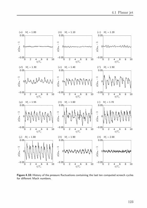
4.1 Planar jet
(a) Mj = 1.00 (b) Mj = 1.10 (c) Mj = 1.20
p/p∞−1
t/Ts0 2 4 6 8 10
−0.05
0
0.05
p/p∞−1
t/Ts0 2 4 6 8 10
−0.05
0
0.05
p/p∞−1
t/Ts0 2 4 6 8 10
−0.05
0
0.05
(d) Mj = 1.30 (e) Mj = 1.40 (f ) Mj = 1.50
p/p∞−1
t/Ts0 2 4 6 8 10
−0.05
0
0.05
p/p∞−1
t/Ts0 2 4 6 8 10
−0.05
0
0.05
p/p∞−1
t/Ts0 2 4 6 8 10
−0.05
0
0.05
(g) Mj = 1.55 (h) Mj = 1.60 (i) Mj = 1.70
p/p∞−1
t/Ts0 2 4 6 8 10
−0.05
0
0.05
p/p∞−1
t/Ts0 2 4 6 8 10
−0.05
0
0.05
p/p∞−1
t/Ts0 2 4 6 8 10
−0.05
0
0.05
(j) Mj = 1.80 (h) Mj = 1.90 (h) Mj = 2.00
p/p∞−1
t/Ts0 2 4 6 8 10
−0.05
0
0.05
p/p∞−1
t/Ts0 2 4 6 8 10
−0.05
0
0.05
p/p∞−1
t/Ts0 2 4 6 8 10
−0.05
0
0.05
Figure 4.10: History of the pressure fluctuations containing the last ten computed screech cyclesfor different Mach numbers.
123
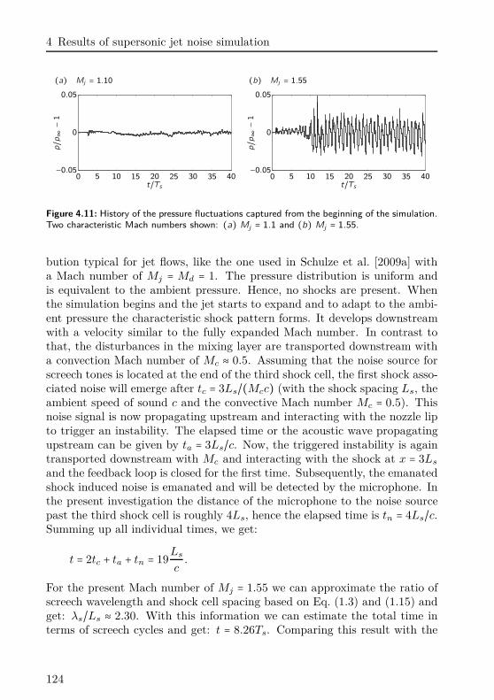
4 Results of supersonic jet noise simulation
(a) Mj = 1.10 (b) Mj = 1.55
p/p∞−1
t/Ts0 5 10 15 20 25 30 35 40
−0.05
0
0.05
p/p∞−1
t/Ts0 5 10 15 20 25 30 35 40
−0.05
0
0.05
Figure 4.11: History of the pressure fluctuations captured from the beginning of the simulation.Two characteristic Mach numbers shown: (a) Mj = 1.1 and (b) Mj = 1.55.
bution typical for jet flows, like the one used in Schulze et al. [2009a] witha Mach number of Mj = Md = 1. The pressure distribution is uniform andis equivalent to the ambient pressure. Hence, no shocks are present. Whenthe simulation begins and the jet starts to expand and to adapt to the ambi-ent pressure the characteristic shock pattern forms. It develops downstreamwith a velocity similar to the fully expanded Mach number. In contrast tothat, the disturbances in the mixing layer are transported downstream witha convection Mach number of Mc ≈ 0.5. Assuming that the noise source forscreech tones is located at the end of the third shock cell, the first shock asso-ciated noise will emerge after tc = 3Ls/(Mcc) (with the shock spacing Ls, theambient speed of sound c and the convective Mach number Mc = 0.5). Thisnoise signal is now propagating upstream and interacting with the nozzle lipto trigger an instability. The elapsed time or the acoustic wave propagatingupstream can be given by ta = 3Ls/c. Now, the triggered instability is againtransported downstream with Mc and interacting with the shock at x = 3Ls
and the feedback loop is closed for the first time. Subsequently, the emanatedshock induced noise is emanated and will be detected by the microphone. Inthe present investigation the distance of the microphone to the noise sourcepast the third shock cell is roughly 4Ls, hence the elapsed time is tn = 4Ls/c.Summing up all individual times, we get:
t = 2tc + ta + tn = 19Ls
c.
For the present Mach number of Mj = 1.55 we can approximate the ratio ofscreech wavelength and shock cell spacing based on Eq. (1.3) and (1.15) andget: λs/Ls ≈ 2.30. With this information we can estimate the total time interms of screech cycles and get: t = 8.26Ts. Comparing this result with the
124
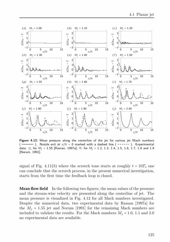
4.1 Planar jet
(a) Mj = 1.00 (b) Mj = 1.10 (c) Mj = 1.20
p/p∞−1
x/h0 5 10 15−1
0
1
2
p/p∞−1
x/h0 5 10 15−1
0
1
2
p/p∞−1
x/h0 5 10 15−1
0
1
2
(d) Mj = 1.30 (e) Mj = 1.40 (f ) Mj = 1.50
p/p∞−1
x/h0 5 10 15−1
0
1
2
p/p∞−1
x/h0 5 10 15−1
0
1
2
p/p∞−1
x/h0 5 10 15−1
0
1
2
(g) Mj = 1.55 (h) Mj = 1.60 (i) Mj = 1.70
p/p∞−1
x/h0 5 10 15−1
0
1
2
p/p∞−1
x/h0 5 10 15−1
0
1
2
p/p∞−1
x/h0 5 10 15−1
0
1
2
(j) Mj = 1.80 (j) Mj = 1.90 (j) Mj = 2.00
p/p∞−1
x/h0 5 10 15−1
0
1
2
p/p∞−1
x/h0 5 10 15−1
0
1
2p/p∞−1
x/h0 5 10 15−1
0
1
2
Figure 4.12: Mean pressure along the centerline of the jet for various jet Mach numbers( ). Nozzle exit at x/h = 0 marked with a dashed line ( ). Experimentaldata: ◻, for Mj = 1.55 [Raman, 1997a]; , for Mj = 1.2, 1.3, 1.4, 1.5, 1.6, 1.7, 1.8 and 1.9
[Norum, 1991].
signal of Fig. 4.11(b) where the screech tone starts at roughly t = 10Ts onecan conclude that the screech process, in the present numerical investigation,starts from the first time the feedback loop is closed.
Mean flow field In the following two figures, the mean values of the pressureand the stream-wise velocity are presented along the centerline of jet. Themean pressure is visualized in Fig. 4.12 for all Mach numbers investigated.Despite the numerical data, two experimental data by Raman [1997a] forthe Mj = 1.55 jet and Norum [1991] for the remaining Mach numbers areincluded to validate the results. For the Mach numbers Mj = 1.0, 1.1 and 2.0no experimental data are available.
125
4 Results of supersonic jet noise simulation
For imperfectly expanded jets one can clearly identify the shock cells inthe jet core with an “U”-like shape. The perfectly expanded jet does notcontain any shocks in the jet core. With increasing Mach number, the nozzleexit pressure is increasing as the value of under-expansion is increasing aswell (cf. Eq. (1.6)). As small part inside the nozzle (for −1 ≤ x/h ≤ 0) showsthe pressure drop in the convergent nozzle as the Mach number is increasinghere up to the design Mach number Md = 1. Note the not the whole nozzleis visualized here. The total length of the nozzle is x/h = 3.
One can identify a significant difference between the screeching jets (1.2 ≤Mj ≤ 1.8) and the non screeching jets (remaining Mach numbers). The dif-ference is clearly visible in the number of detectable shock cells. Whereas onecan count at least eight shock cells for the Mj = 1.1 jet, only two to threeshock cells are remaining for the screeching jets. This trend is also visiblefor the two non screeching high Mach number jets although the presenteddomain is limited and not all shock cells are visible. The reason for the re-duced number of shock cells for a screeching jet has been reported by manyresearchers and is mentioned already in the introduction of this thesis. It isrelated to the enhanced mixing of the screeching jet. The jet undergoes astrong oscillation (flapping or antisymmetric mode) when the screech cycleforms and this destroys the periodic shock cell structure. Hence, the reducedshock cells are an additional evidence for the screeching of a jet. In Sec. § 6we will see that a jet with an optimized porous material (no screech) containsadditional shock cells compared to a jet without porous material (screech).
The experimental data by Raman [1997a] and Norum [1991] indicate thaton the one hand the shock cell spacing (which is increasing with the Machnumber) is captured correctly and on the other hand that the shape of thepressure distribution along the jet axis is predicted correctly. There seemsto be a difference in the amplitude of the shock cells. Whereas the databy Raman [1997a] underestimates the numerical data (Mj = 1.55) the databy Norum [1991] over-predicts slightly the current computation. It is alsointeresting to see that the number of shock cells in the experimental andnumerical data is comparable. Only for the Mach number cases Mj = 1.7 andMj = 1.8 the experimental data show an additional third and fourth shockcell which is not visible in the numerical data. Once again, this is due to theshifted cessation point of screech due to the thick nozzle lip in the presentnumerical investigation. The nozzle lip of the experimental data by Norum[1991] is inclined by 30 and hence less efficient to form a standing wave.
Similar to Fig. 4.12 are the data presented in Fig. 4.13. Here, the absolutevelocity is shown along the centerline of the jet and scaled with the jet exitvelocity ue. One can identify first, that the velocity inside the convergent
126
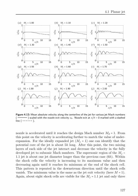
4.1 Planar jet
(a) Mj = 1.00 (b) Mj = 1.10 (c) Mj = 1.20
u/ue
x/h0 5 10 150
1
2
u/ue
x/h0 5 10 150
1
2
u/ue
x/h0 5 10 150
1
2
(d) Mj = 1.30 (e) Mj = 1.40 (f ) Mj = 1.50
u/ue
x/h0 5 10 150
1
2
u/ue
x/h0 5 10 150
1
2
u/ue
x/h0 5 10 150
1
2
(g) Mj = 1.55 (h) Mj = 1.60 (i) Mj = 1.70
u/ue
x/h0 5 10 150
1
2
u/ue
x/h0 5 10 150
1
2
u/ue
x/h0 5 10 150
1
2
(j) Mj = 1.80 (j) Mj = 1.90 (j) Mj = 2.00
u/ue
x/h0 5 10 150
1
2
u/ue
x/h0 5 10 150
1
2u/ue
x/h0 5 10 150
1
2
Figure 4.13: Mean absolute velocity along the centerline of the jet for various jet Mach numbers( ) scaled with the nozzle exit velocity ue . Nozzle exit at x/h = 0 marked with a dashedline ( ).
nozzle is accelerated until it reaches the design Mach number Md = 1. Fromthis point on the velocity is accelerating further to match the value of under-expansion. For the ideally expanded jet (Mj = 1) one can identify that thepotential core of the jet is about 5h long. After this point, the two mixinglayers of each side of the jet interact and decrease the velocity in the fullydeveloped jet to subsonic Mach numbers. The supersonic region of the Mj =1.1 jet is about one jet diameter longer than the previous case (6h). Withinthe shock cells the velocity is increasing to its maximum value and thendecreasing again until it reaches its minimum at the end of the shock cell.This pattern is repeated in the downstream direction until the shock cellsvanish. The minimum value is the same as the jet exit velocity (here M = 1).Again, about eight shock cells are visible for the Mj = 1.1 jet and only three
127
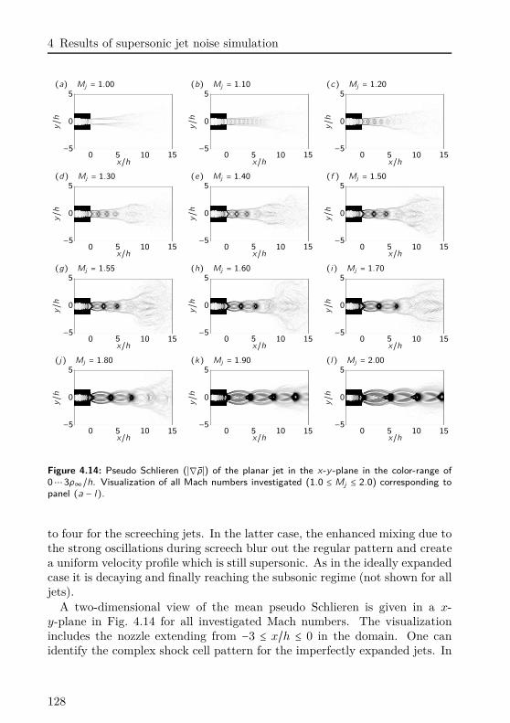
4 Results of supersonic jet noise simulation
(a) Mj = 1.00 (b) Mj = 1.10 (c) Mj = 1.20
y/h
x/h0 5 10 15−5
0
5
y/h
x/h0 5 10 15−5
0
5
y/h
x/h0 5 10 15−5
0
5
(d) Mj = 1.30 (e) Mj = 1.40 (f ) Mj = 1.50
y/h
x/h0 5 10 15−5
0
5y/h
x/h0 5 10 15−5
0
5
y/h
x/h0 5 10 15−5
0
5
(g) Mj = 1.55 (h) Mj = 1.60 (i) Mj = 1.70
y/h
x/h0 5 10 15−5
0
5
y/h
x/h0 5 10 15−5
0
5
y/h
x/h0 5 10 15−5
0
5
(j) Mj = 1.80 (k) Mj = 1.90 (l) Mj = 2.00
y/h
x/h0 5 10 15−5
0
5
y/h
x/h0 5 10 15−5
0
5
y/h
x/h0 5 10 15−5
0
5
Figure 4.14: Pseudo Schlieren (∣∇ρ∣) of the planar jet in the x-y -plane in the color-range of0⋯ 3ρ∞/h. Visualization of all Mach numbers investigated (1.0 ≤ Mj ≤ 2.0) corresponding topanel (a − l).
to four for the screeching jets. In the latter case, the enhanced mixing due tothe strong oscillations during screech blur out the regular pattern and createa uniform velocity profile which is still supersonic. As in the ideally expandedcase it is decaying and finally reaching the subsonic regime (not shown for alljets).
A two-dimensional view of the mean pseudo Schlieren is given in a x-y-plane in Fig. 4.14 for all investigated Mach numbers. The visualizationincludes the nozzle extending from −3 ≤ x/h ≤ 0 in the domain. One canidentify the complex shock cell pattern for the imperfectly expanded jets. In
128
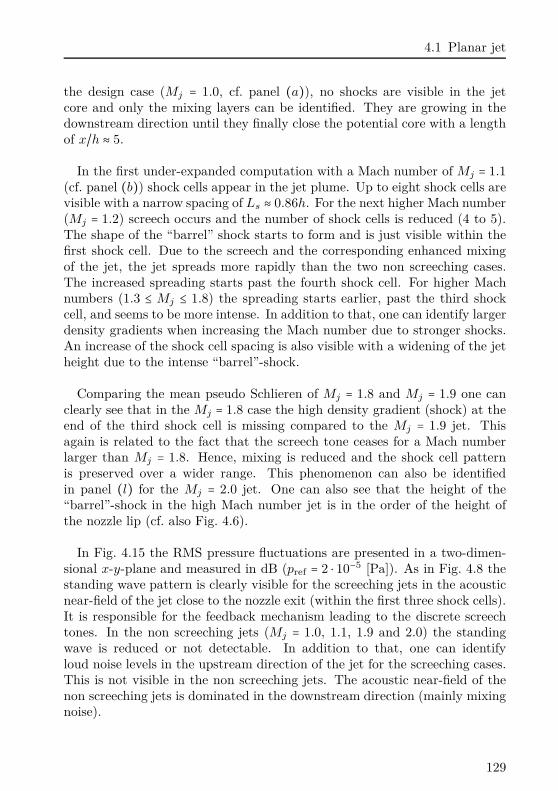
4.1 Planar jet
the design case (Mj = 1.0, cf. panel (a)), no shocks are visible in the jetcore and only the mixing layers can be identified. They are growing in thedownstream direction until they finally close the potential core with a lengthof x/h ≈ 5.
In the first under-expanded computation with a Mach number of Mj = 1.1
(cf. panel (b)) shock cells appear in the jet plume. Up to eight shock cells arevisible with a narrow spacing of Ls ≈ 0.86h. For the next higher Mach number(Mj = 1.2) screech occurs and the number of shock cells is reduced (4 to 5).The shape of the “barrel” shock starts to form and is just visible within thefirst shock cell. Due to the screech and the corresponding enhanced mixingof the jet, the jet spreads more rapidly than the two non screeching cases.The increased spreading starts past the fourth shock cell. For higher Machnumbers (1.3 ≤ Mj ≤ 1.8) the spreading starts earlier, past the third shockcell, and seems to be more intense. In addition to that, one can identify largerdensity gradients when increasing the Mach number due to stronger shocks.An increase of the shock cell spacing is also visible with a widening of the jetheight due to the intense “barrel”-shock.
Comparing the mean pseudo Schlieren of Mj = 1.8 and Mj = 1.9 one canclearly see that in the Mj = 1.8 case the high density gradient (shock) at theend of the third shock cell is missing compared to the Mj = 1.9 jet. Thisagain is related to the fact that the screech tone ceases for a Mach numberlarger than Mj = 1.8. Hence, mixing is reduced and the shock cell patternis preserved over a wider range. This phenomenon can also be identifiedin panel (l) for the Mj = 2.0 jet. One can also see that the height of the“barrel”-shock in the high Mach number jet is in the order of the height ofthe nozzle lip (cf. also Fig. 4.6).
In Fig. 4.15 the RMS pressure fluctuations are presented in a two-dimen-sional x-y-plane and measured in dB (pref = 2 ⋅ 10−5 [Pa]). As in Fig. 4.8 thestanding wave pattern is clearly visible for the screeching jets in the acousticnear-field of the jet close to the nozzle exit (within the first three shock cells).It is responsible for the feedback mechanism leading to the discrete screechtones. In the non screeching jets (Mj = 1.0, 1.1, 1.9 and 2.0) the standingwave is reduced or not detectable. In addition to that, one can identifyloud noise levels in the upstream direction of the jet for the screeching cases.This is not visible in the non screeching jets. The acoustic near-field of thenon screeching jets is dominated in the downstream direction (mainly mixingnoise).
129
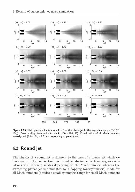
4 Results of supersonic jet noise simulation
(a) Mj = 1.00 (b) Mj = 1.10 (c) Mj = 1.20
y/h
x/h0 5 10 15−5
0
5
y/h
x/h0 5 10 15−5
0
5
y/h
x/h0 5 10 15−5
0
5
(d) Mj = 1.30 (e) Mj = 1.40 (f ) Mj = 1.50
y/h
x/h0 5 10 15−5
0
5y/h
x/h0 5 10 15−5
0
5
y/h
x/h0 5 10 15−5
0
5
(g) Mj = 1.55 (h) Mj = 1.60 (i) Mj = 1.70
y/h
x/h0 5 10 15−5
0
5
y/h
x/h0 5 10 15−5
0
5
y/h
x/h0 5 10 15−5
0
5
(j) Mj = 1.80 (k) Mj = 1.90 (l) Mj = 2.00
y/h
x/h0 5 10 15−5
0
5
y/h
x/h0 5 10 15−5
0
5
y/h
x/h0 5 10 15−5
0
5
150 160 170 180 190
Figure 4.15: RMS pressure fluctuations in dB of the planar jet in the x-y -plane (pref = 2 ⋅ 10−5
[Pa]). Color scaling from white to black (150 - 190 dB). Visualization of all Mach numbersinvestigated (1.0 ≤ Mj ≤ 2.0) corresponding to panel (a − l).
4.2 Round jet
The physics of a round jet is different to the ones of a planar jet which wehave seen in the last section. A round jet during screech undergoes oscil-lations with different modes depending on the Mach number, whereas thescreeching planar jet is dominated by a flapping (antisymmetric) mode forall Mach numbers (besides a small symmetric range for small Mach numbers
130
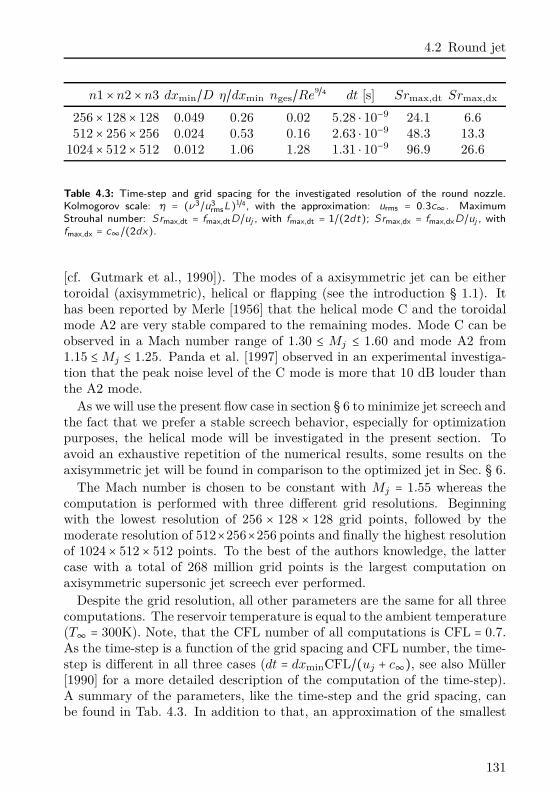
4.2 Round jet
n1 × n2 × n3 dxmin/D η/dxmin nges/Re9/4 dt [s] Srmax,dt Srmax,dx
256 × 128× 128 0.049 0.26 0.02 5.28 ⋅ 10−9 24.1 6.6
512 × 256× 256 0.024 0.53 0.16 2.63 ⋅ 10−9 48.3 13.3
1024× 512× 512 0.012 1.06 1.28 1.31 ⋅ 10−9 96.9 26.6
Table 4.3: Time-step and grid spacing for the investigated resolution of the round nozzle.Kolmogorov scale: η = (ν3/u3rmsL)
1/4, with the approximation: urms = 0.3c∞. MaximumStrouhal number: Srmax,dt = fmax,dtD/uj , with fmax,dt = 1/(2dt); Srmax,dx = fmax,dxD/uj , withfmax,dx = c∞/(2dx).
[cf. Gutmark et al., 1990]). The modes of a axisymmetric jet can be eithertoroidal (axisymmetric), helical or flapping (see the introduction § 1.1). Ithas been reported by Merle [1956] that the helical mode C and the toroidalmode A2 are very stable compared to the remaining modes. Mode C can beobserved in a Mach number range of 1.30 ≤ Mj ≤ 1.60 and mode A2 from1.15 ≤Mj ≤ 1.25. Panda et al. [1997] observed in an experimental investiga-tion that the peak noise level of the C mode is more that 10 dB louder thanthe A2 mode.
As we will use the present flow case in section § 6 to minimize jet screech andthe fact that we prefer a stable screech behavior, especially for optimizationpurposes, the helical mode will be investigated in the present section. Toavoid an exhaustive repetition of the numerical results, some results on theaxisymmetric jet will be found in comparison to the optimized jet in Sec. § 6.
The Mach number is chosen to be constant with Mj = 1.55 whereas thecomputation is performed with three different grid resolutions. Beginningwith the lowest resolution of 256 × 128 × 128 grid points, followed by themoderate resolution of 512×256×256 points and finally the highest resolutionof 1024 × 512 × 512 points. To the best of the authors knowledge, the lattercase with a total of 268 million grid points is the largest computation onaxisymmetric supersonic jet screech ever performed.
Despite the grid resolution, all other parameters are the same for all threecomputations. The reservoir temperature is equal to the ambient temperature(T∞ = 300K). Note, that the CFL number of all computations is CFL = 0.7.As the time-step is a function of the grid spacing and CFL number, the time-step is different in all three cases (dt = dxminCFL/(uj + c∞), see also Müller[1990] for a more detailed description of the computation of the time-step).A summary of the parameters, like the time-step and the grid spacing, canbe found in Tab. 4.3. In addition to that, an approximation of the smallest
131
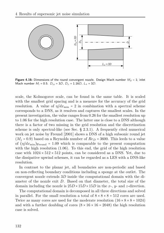
4 Results of supersonic jet noise simulation
Figure 4.16: Dimensions of the round convergent nozzle. Design Mach number Md = 1; inletMach number Mi = 0.5. Dio = 3D, Di i = 1.16D, Lo = 3D.
scale, the Kolmogorov scale, can be found in the same table. It is scaledwith the smallest grid spacing and is a measure for the accuracy of the gridresolution. A value of η/dxmin = 2 in combination with a spectral schemecorresponds to a DNS, as it resolves and captures the smallest scales. In thepresent investigation, the value ranges from 0.26 for the smallest resolution upto 1.06 for the high resolution case. The latter one is close to a DNS althoughthere is a factor of two missing in the grid resolution and the discretizationscheme is only spectral-like (see Sec. § 2.3.1). A frequently cited numericalwork on jet noise by Freund [2001] shows a DNS of a high subsonic round jet(Mj = 0.9) based on a Reynolds number of ReD = 3600. This leeds to a valueof (η/dxmin)Freund = 1.09 which is comparable to the present computationwith the high resolution (1.06). To this end, the grid of the high resolutioncase with 1024 × 512 × 512 points, can be considered as a DNS. Yet, due tothe dissipative upwind schemes, it can be regarded as a LES with a DNS-likeresolution.
In contrast to the planar jet, all boundaries are non-periodic and basedon non-reflecting boundary conditions including a sponge at the outlet. Theconvergent nozzle extends 3D inside the computational domain with the di-ameter of the nozzle exit D. Based on that diameter, the total size of thedomain including the nozzle is 25D×15D×15D in the x-, y- and z-direction.
The computational domain is decomposed in all three directions and solvedin parallel. For the small resolution a total of 8 × 8 × 8 = 512 cores are used.Twice as many cores are used for the moderate resolution (16 × 8 × 8 = 1024)and with a further doubling of cores (8 × 16 × 16 = 2048) the high resolutioncase is solved.
132
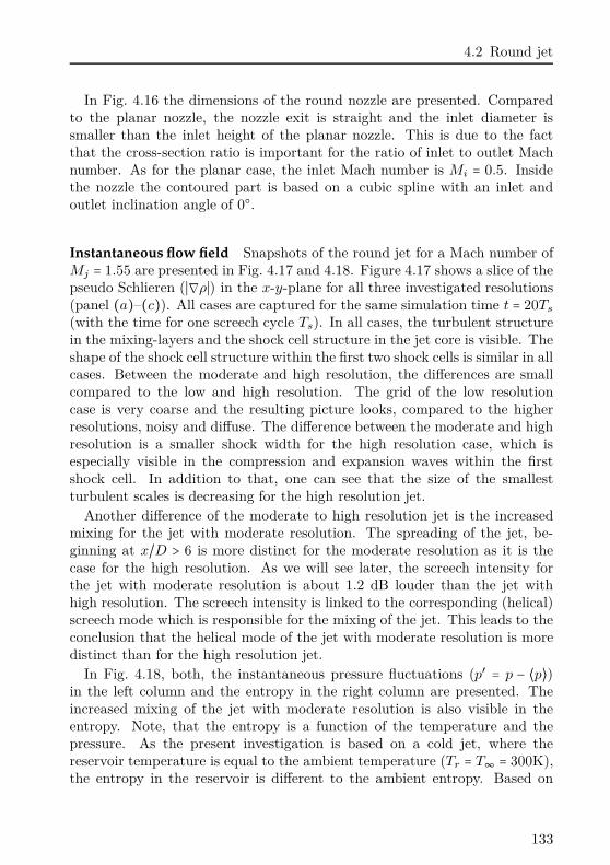
4.2 Round jet
In Fig. 4.16 the dimensions of the round nozzle are presented. Comparedto the planar nozzle, the nozzle exit is straight and the inlet diameter issmaller than the inlet height of the planar nozzle. This is due to the factthat the cross-section ratio is important for the ratio of inlet to outlet Machnumber. As for the planar case, the inlet Mach number is Mi = 0.5. Insidethe nozzle the contoured part is based on a cubic spline with an inlet andoutlet inclination angle of 0.
Instantaneous flow field Snapshots of the round jet for a Mach number ofMj = 1.55 are presented in Fig. 4.17 and 4.18. Figure 4.17 shows a slice of thepseudo Schlieren (∣∇ρ∣) in the x-y-plane for all three investigated resolutions(panel (a)–(c)). All cases are captured for the same simulation time t = 20Ts
(with the time for one screech cycle Ts). In all cases, the turbulent structurein the mixing-layers and the shock cell structure in the jet core is visible. Theshape of the shock cell structure within the first two shock cells is similar in allcases. Between the moderate and high resolution, the differences are smallcompared to the low and high resolution. The grid of the low resolutioncase is very coarse and the resulting picture looks, compared to the higherresolutions, noisy and diffuse. The difference between the moderate and highresolution is a smaller shock width for the high resolution case, which isespecially visible in the compression and expansion waves within the firstshock cell. In addition to that, one can see that the size of the smallestturbulent scales is decreasing for the high resolution jet.
Another difference of the moderate to high resolution jet is the increasedmixing for the jet with moderate resolution. The spreading of the jet, be-ginning at x/D > 6 is more distinct for the moderate resolution as it is thecase for the high resolution. As we will see later, the screech intensity forthe jet with moderate resolution is about 1.2 dB louder than the jet withhigh resolution. The screech intensity is linked to the corresponding (helical)screech mode which is responsible for the mixing of the jet. This leads to theconclusion that the helical mode of the jet with moderate resolution is moredistinct than for the high resolution jet.
In Fig. 4.18, both, the instantaneous pressure fluctuations (p′ = p − ⟨p⟩)in the left column and the entropy in the right column are presented. Theincreased mixing of the jet with moderate resolution is also visible in theentropy. Note, that the entropy is a function of the temperature and thepressure. As the present investigation is based on a cold jet, where thereservoir temperature is equal to the ambient temperature (Tr = T∞ = 300K),the entropy in the reservoir is different to the ambient entropy. Based on
133
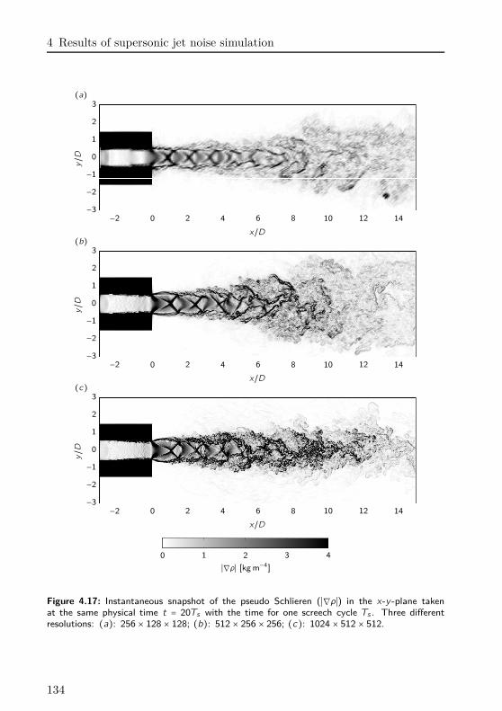
4 Results of supersonic jet noise simulation
(a)y/D
x/D−2 0 2 4 6 8 10 12 14
−3
−2
−1
0
1
2
3
(b)
y/D
x/D−2 0 2 4 6 8 10 12 14
−3
−2
−1
0
1
2
3
(c)
y/D
x/D−2 0 2 4 6 8 10 12 14
−3
−2
−1
0
1
2
3
0 1 2 3 4
∣∇ρ∣ [kg m−4]
Figure 4.17: Instantaneous snapshot of the pseudo Schlieren (∣∇ρ∣) in the x-y -plane takenat the same physical time t = 20Ts with the time for one screech cycle Ts . Three differentresolutions: (a): 256 × 128 × 128; (b): 512 × 256 × 256; (c): 1024 × 512 × 512.
134
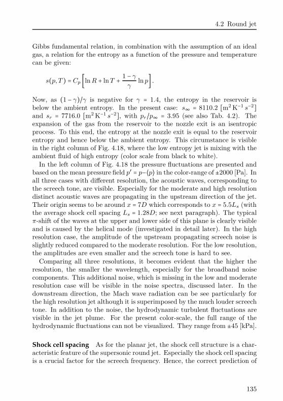
4.2 Round jet
Gibbs fundamental relation, in combination with the assumption of an idealgas, a relation for the entropy as a function of the pressure and temperaturecan be given:
s(p, T ) = Cp [ln R + ln T +1 − γ
γln p] .
Now, as (1 − γ)/γ is negative for γ = 1.4, the entropy in the reservoir isbelow the ambient entropy. In the present case: s∞ = 8110.2 [m2 K−1 s−2]and sr = 7716.0 [m2 K−1 s−2], with pr/p∞ = 3.95 (see also Tab. 4.2). Theexpansion of the gas from the reservoir to the nozzle exit is an isentropicprocess. To this end, the entropy at the nozzle exit is equal to the reservoirentropy and hence below the ambient entropy. This circumstance is visiblein the right column of Fig. 4.18, where the low entropy jet is mixing with theambient fluid of high entropy (color scale from black to white).
In the left column of Fig. 4.18 the pressure fluctuations are presented andbased on the mean pressure field p′ = p−⟨p⟩ in the color-range of ±2000 [Pa]. Inall three cases with different resolution, the acoustic waves, corresponding tothe screech tone, are visible. Especially for the moderate and high resolutiondistinct acoustic waves are propagating in the upstream direction of the jet.Their origin seems to be around x = 7D which corresponds to x = 5.5Ls (withthe average shock cell spacing Ls = 1.28D; see next paragraph). The typicalπ-shift of the waves at the upper and lower side of this plane is clearly visibleand is caused by the helical mode (investigated in detail later). In the highresolution case, the amplitude of the upstream propagating screech noise isslightly reduced compared to the moderate resolution. For the low resolution,the amplitudes are even smaller and the screech tone is hard to see.
Comparing all three resolutions, it becomes evident that the higher theresolution, the smaller the wavelength, especially for the broadband noisecomponents. This additional noise, which is missing in the low and moderateresolution case will be visible in the noise spectra, discussed later. In thedownstream direction, the Mach wave radiation can be see particularly forthe high resolution jet although it is superimposed by the much louder screechtone. In addition to the noise, the hydrodynamic turbulent fluctuations arevisible in the jet plume. For the present color-scale, the full range of thehydrodynamic fluctuations can not be visualized. They range from ±45 [kPa].
Shock cell spacing As for the planar jet, the shock cell structure is a char-acteristic feature of the supersonic round jet. Especially the shock cell spacingis a crucial factor for the screech frequency. Hence, the correct prediction of
135
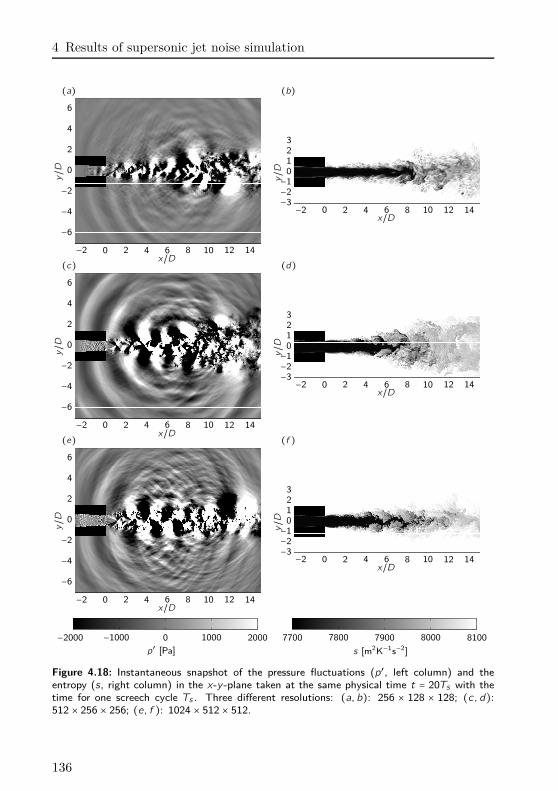
4 Results of supersonic jet noise simulation
(a) (b)
y/D
x/D−2 0 2 4 6 8 10 12 14
−6
−4
−2
0
2
4
6
y/D
x/D−2 0 2 4 6 8 10 12 14−3−2−10123
(c) (d)
y/D
x/D−2 0 2 4 6 8 10 12 14
−6
−4
−2
0
2
4
6y/D
x/D−2 0 2 4 6 8 10 12 14−3−2−10123
(e) (f )
y/D
x/D−2 0 2 4 6 8 10 12 14
−6
−4
−2
0
2
4
6
y/D
x/D−2 0 2 4 6 8 10 12 14−3−2−10123
−2000 −1000 0 1000 2000
7700 7800 7900 8000 8100
p′ [Pa] s [m2K−1s−2]
Figure 4.18: Instantaneous snapshot of the pressure fluctuations (p′, left column) and theentropy (s, right column) in the x-y -plane taken at the same physical time t = 20Ts with thetime for one screech cycle Ts . Three different resolutions: (a, b): 256 × 128 × 128; (c, d):512 × 256 × 256; (e, f ): 1024 × 512 × 512.
136
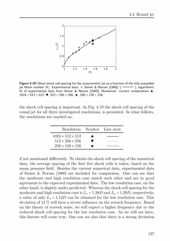
4.2 Round jet
PSfrag
Ls/D
Mj
1 1.2 1.4 1.6 1.8 20
0.5
1
1.5
2
Figure 4.19: Mean shock cell spacing for the axisymmetric jet as a function of the fully expandedjet Mach number Mj . Experimental data: , Seiner & Norum [1980]; ( ), logarithmicfit of experimental data from Seiner & Norum [1980]; Numerical: current computation ,1024 × 512 × 512; , 512 × 256 × 256; , 256 × 128 × 128.
the shock cell spacing is important. In Fig. 4.19 the shock cell spacing of theround jet for all three investigated resolutions, is presented. In what follows,the resolutions are marked as:
Resolution Symbol Line style
1024× 512× 512
512 × 256× 256 256 × 128× 128
if not mentioned differently. To obtain the shock cell spacing of the numericaldata, the average spacing of the first five shock cells is taken, based on themean pressure field. Besides the current numerical data, experimental dataof Seiner & Norum [1980] are included for comparison. One can see thatthe moderate and high resolution case match each other and are in goodagreement to the expected experimental data. The low resolution case, on theother hand, is slightly under predicted. Whereas the shock cell spacing for themoderate and high resolution case is Ls = 1.28D and Ls = 1.29D, respectively,a value of only Ls = 1.12D can be obtained for the low resolution case. Thisdeviation of 12 % will have a severe influence on the screech frequency. Basedon the theory of screech noise, we will expect a higher frequency due to thereduced shock cell spacing for the low resolution case. As we will see later,this feature will come true. One can see also that there is a strong deviation
137
4 Results of supersonic jet noise simulation
(a) (b)
SP
L[d
B]
Mj
1 1.2 1.4 1.6 1.8 2110
120
130
140
150
160
170
f sDj/U
j
Mj
1 1.2 1.4 1.6 1.8 20
0.2
0.4
0.6
0.8
Figure 4.20: Screech amplitude and frequency of a circular jet versus the fully expanded jetMach number Mj for different screech modes Experimental data from Panda et al. [1997]: A1; A2 ; B ◻; C ; D ; E . Experimental data from Seiner [1984]: B ∎; C . currentcomputation: C , 1024 × 512 × 512; , 512 × 256 × 256; , 256 × 128 × 128. (a) Screechamplitude versus the fully expanded jet Mach number. (b) Dominant screech frequency as afunction of the jet Mach number Mj . Analytic solution for mode A ( ) and analyticalsolution for mode C ( ) by Massey [1997].
in the experimental data of Seiner & Norum [1980]. A difference of 10 % tothe logarithmic fit can be identified. The reason for these jumps might beexplained due to the individual screech modes.
Screech frequency and amplitude As we have already seen for the planarjet, the correct prediction of the shock cell spacing is important for the cor-rect prediction of the screech frequency. In the previous paragraph, the shockcell spacing has been presented for all three resolutions. We could see thatthe low resolution jet shows deviations to the experimental data by Seiner &Norum [1980]. In Fig. 4.20(b) the screech frequency of the three numericalinvestigations are presented and compared to experimental data by Pandaet al. [1997] and analytical data by Massey [1997]. The screech frequency isexpressed with the Strouhal number, based on the fully expanded jet values:Sr = fsDj/uj. Note, that for the planar jet, the length-scale in the Strouhalnumber is based on the nozzle exit conditions (h) and not on the fully ex-panded jet conditions (hj) as in the present round case (Dj). All numericaldata of panel (a) and (b) are measured normal to the jet axis (Θ = 90) in adistance of 7.8D to the jet axis.
Both, the moderate and high resolution jet are in very good agreement to
138
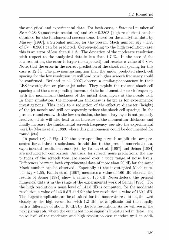
4.2 Round jet
the analytical and experimental data. For both cases, a Strouhal number ofSr = 0.2848 (moderate resolution) and Sr = 0.2803 (high resolution) can beobtained for the fundamental screech tone. Based on the analytical data byMassey [1997], a Strouhal number for the present Mach number Mj = 1.55
of Sr = 0.2801 can be predicted. Corresponding to the high resolution case,this is an error of less than 0.1 %. The deviation of the moderate resolutionwith respect to the analytical data is less than 1.7 %. In the case of thelow resolution, the error is larger (as expected) and reaches a value of 9.8 %.Note, that the error in the correct prediction of the shock cell spacing for thiscase is 12 %. The previous assumption that the under predicted shock cellspacing for the low resolution jet will lead to a higher screech frequency couldbe confirmed. Berland et al. [2007] observe a similar phenomenon in theirLES investigation on planar jet noise. They explain the reduced shock cellspacing and the corresponding increase of the fundamental screech frequencywith the momentum thickness of the initial shear layers at the nozzle exit.In their simulation, the momentum thickness is larger as for experimentalinvestigations. This leads to a reduction of the effective diameter (height)of the jet nozzle and will consequently reduce the shock cell spacing. In thepresent round case with the low resolution, the boundary layer is not properlyresolved. This will also lead to an increase of the momentum thickness andfinally increase the fundamental screech frequency [see also the experimentalwork by Morris et al., 1989, where this phenomenon could be documented forround jets].
In panel (a) of Fig. 4.20 the corresponding screech amplitudes are pre-sented for all three resolutions. In addition to the present numerical data,experimental results on round jets by Panda et al. [1997] and Seiner [1984]are included for comparison. As usual for screech noise predictions, the am-plitudes of the screech tone are spread over a wide range of noise levels.Differences between both experimental data of more than 20 dB for the sameMach number can be observed. Especially at the investigated Mach num-ber Mj = 1.55, Panda et al. [1997] measures a value of 160 dB whereas theresults of Seiner [1984] show a value of 135 dB. Nevertheless, the presentnumerical data is in the range of the experimental work of Seiner [1984]. Forthe high resolution a noise level of 141.8 dB is computed, for the moderateresolution a value of 143.0 dB and for the low resolution a value of 130.1 dB.The largest amplitude can be obtained for the moderate resolution, followedclosely by the high resolution with 1.2 dB less amplitude and then finallywith a difference of about 10 dB, by the low resolution. As we will see in thenext paragraph, where the emanated noise signal is investigated in detail, thenoise level of the moderate and high resolution case matches well an addi-
139
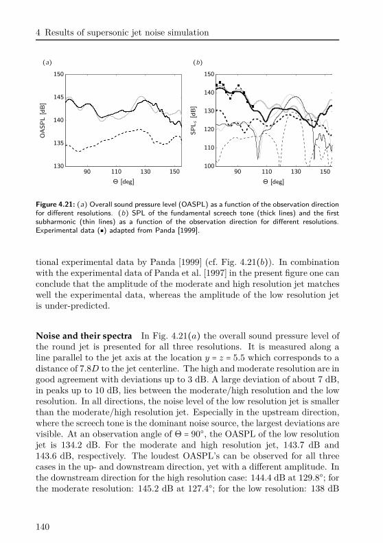
4 Results of supersonic jet noise simulation
(a) (b)
OA
SP
L[d
B]
Θ [deg]
90 110 130 150130
135
140
145
150
SP
Ls
[dB
]
Θ [deg]
90 110 130 150100
110
120
130
140
150
Figure 4.21: (a) Overall sound pressure level (OASPL) as a function of the observation directionfor different resolutions. (b) SPL of the fundamental screech tone (thick lines) and the firstsubharmonic (thin lines) as a function of the observation direction for different resolutions.Experimental data (◾) adapted from Panda [1999].
tional experimental data by Panda [1999] (cf. Fig. 4.21(b)). In combinationwith the experimental data of Panda et al. [1997] in the present figure one canconclude that the amplitude of the moderate and high resolution jet matcheswell the experimental data, whereas the amplitude of the low resolution jetis under-predicted.
Noise and their spectra In Fig. 4.21(a) the overall sound pressure level ofthe round jet is presented for all three resolutions. It is measured along aline parallel to the jet axis at the location y = z = 5.5 which corresponds to adistance of 7.8D to the jet centerline. The high and moderate resolution are ingood agreement with deviations up to 3 dB. A large deviation of about 7 dB,in peaks up to 10 dB, lies between the moderate/high resolution and the lowresolution. In all directions, the noise level of the low resolution jet is smallerthan the moderate/high resolution jet. Especially in the upstream direction,where the screech tone is the dominant noise source, the largest deviations arevisible. At an observation angle of Θ = 90, the OASPL of the low resolutionjet is 134.2 dB. For the moderate and high resolution jet, 143.7 dB and143.6 dB, respectively. The loudest OASPL’s can be observed for all threecases in the up- and downstream direction, yet with a different amplitude. Inthe downstream direction for the high resolution case: 144.4 dB at 129.8; forthe moderate resolution: 145.2 dB at 127.4; for the low resolution: 138 dB
140
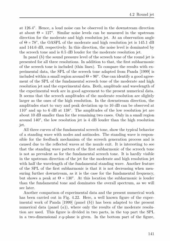
4.2 Round jet
at 126.4. Hence, a loud noise can be observed in the downstream directionat about Θ = 127. Similar noise levels can be measured in the upstreamdirection for the moderate and high resolution jet. At an observation angleof Θ = 78, the OASPL of the moderate and high resolution jet is 145.1 dBand 144.6 dB, respectively. In this direction, the noise level is dominated bythe screech tone and is 0.5 dB louder for the moderate resolution jet.
In panel (b) the sound pressure level of the screech tone of the round jet ispresented for all three resolutions. In addition to that, the first subharmonicof the screech tone is included (thin lines). To compare the results with ex-perimental data, the SPL of the screech tone adapted from Panda [1999] isincluded within a small region around Θ = 90. One can identify a good agree-ment of the SPL of the fundamental screech tone of the moderate and highresolution jet and the experimental data. Both, amplitude and wavelength ofthe experimental work are in good agreement to the present numerical data.It seems that the screech amplitudes of the moderate resolution are slightlylarger as the ones of the high resolution. In the downstream direction, theamplitudes start to vary and peak deviation up to 10 dB can be observed at110 and up to 6 dB at 138. The amplitudes of the low resolution jet areabout 10 dB smaller than for the remaining two cases. Only in a small regionaround 140, the low resolution jet is 4 dB louder than the high resolutionjet.
All three curves of the fundamental screech tone, show the typical behaviorof a standing wave with nodes and antinodes. The standing wave is respon-sible for the feedback mechanism of the screech generation process and iscaused due to the reflected waves at the nozzle exit. It is interesting to seethat the standing wave pattern of the first subharmonic of the screech toneis not as prevalent as for the fundamental screech tone. It is hardly visiblein the upstream direction of the jet for the moderate and high resolution jetwith half the wavelength of the fundamental standing wave. Another featureof the SPL of the first subharmonic is that it is not decreasing when mea-suring further downstream, as it is the case for the fundamental frequency,but shows a peak at Θ = 130. At this location the subharmonic is louderthan the fundamental tone and dominates the overall spectrum, as we willsee later.
Another comparison of experimental data and the present numerical workhas been carried out in Fig. 4.22. Here, a well known figure of the exper-imental work of Panda [1999] (panel (b)) has been adapted to the presentnumerical data (panel (a)), where only the results of the moderate resolu-tion are used. This figure is divided in two parts, in the top part the SPLin a two-dimensional x-y-plane is given. In the bottom part of the figure,
141
4 Results of supersonic jet noise simulation
(a) (b)
y/D
x/D0 2 4 6 8
130
140
150
160
170
−1
0
1
2
3
4
5
6
7
y/D
x/D0 2 4 6 8
130
140
150
160
170
−1
0
1
2
3
4
5
6
7
Figure 4.22: Top part: Sound pressure level in the acoustic near-field measured in dB. Bottompart: (Pseudo)-Schlieren to visualize the shock cells with arbitrary color-scale. (a) OASPL ofthe round jet based on the current numerical computation with Mj = 1.55. (b) SPL of thescreech frequency of a round jet based on experimental data by Panda [1999] with Mj = 1.42
(axis scaled to match the shock cell spacing of a jet at Mj = 1.55).
the (pseudo)-Schlieren of the jet are presented. They visualize the densitygradient in the stream-wise direction of the jet and highlight the shock cellstructure and the turbulence in the mixing-layers. For the experiment, theSchlieren are integrated over the whole jet diameter and in the numericaldata only a two-dimensional slice is shown. This fact is responsible for a dif-ference of both visualizations although the differences are small. In additionto that, the color-scale of the Schlieren pictures are chosen arbitrarily as noinformation of the amplitudes for the experimental data are available.
The noise measured in the top part of both panels is based on the OASPLfor the numerical data and on the screech SPL of the experimental data.This circumstance leads to deviations, especially in the downstream direc-tion, where the screech amplitude is decreasing and the OASPL in increasing(compare also panel (a) and (b) of Fig. 4.21). Nevertheless, the deviations inthe upstream direction are small and a good agreement of the experimentaland the numerical data can be found. Not only the amplitudes of both casesmatch each other but also the spatial distribution of the noise in the acousticnear-field is in good agreement. Again, the standing wave pattern, typicalfor screech noise, can be identified in both cases with the characteristic lobesfacing in the normal direction of the jet.
142
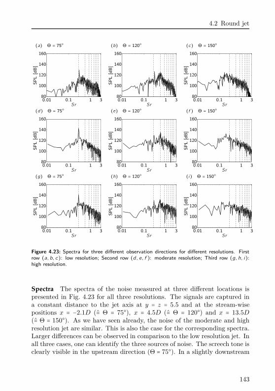
4.2 Round jet
(a) Θ = 75 (b) Θ = 120 (c) Θ = 150
SP
L[d
B]
Sr0.01 0.1 1 380
100
120
140
160
SP
L[d
B]
Sr0.01 0.1 1 380
100
120
140
160
SP
L[d
B]
Sr0.01 0.1 1 380
100
120
140
160
(d) Θ = 75 (e) Θ = 120 (f ) Θ = 150
SP
L[d
B]
Sr0.01 0.1 1 380
100
120
140
160
SP
L[d
B]
Sr0.01 0.1 1 380
100
120
140
160
SP
L[d
B]
Sr0.01 0.1 1 380
100
120
140
160
(g) Θ = 75 (h) Θ = 120 (i) Θ = 150
SP
L[d
B]
Sr0.01 0.1 1 380
100
120
140
160
SP
L[d
B]
Sr0.01 0.1 1 380
100
120
140
160S
PL
[dB
]
Sr0.01 0.1 1 380
100
120
140
160
Figure 4.23: Spectra for three different observation directions for different resolutions. Firstrow (a, b, c): low resolution; Second row (d, e, f ): moderate resolution; Third row (g, h, i):high resolution.
Spectra The spectra of the noise measured at three different locations ispresented in Fig. 4.23 for all three resolutions. The signals are captured ina constant distance to the jet axis at y = z = 5.5 and at the stream-wisepositions x = −2.1D (= Θ = 75), x = 4.5D (= Θ = 120) and x = 13.5D
(= Θ = 150). As we have seen already, the noise of the moderate and highresolution jet are similar. This is also the case for the corresponding spectra.Larger differences can be observed in comparison to the low resolution jet. Inall three cases, one can identify the three sources of noise. The screech tone isclearly visible in the upstream direction (Θ = 75). In a slightly downstream
143
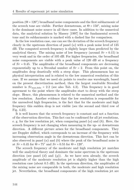
4 Results of supersonic jet noise simulation
position (Θ = 120) broadband noise components and the first subharmonic ofthe screech tone are visible. Further downstream, at Θ = 150, mixing noiseis the dominant noise source in all three cases. In addition to the numericaldata, the analytical solution by Massey [1997] for the fundamental screechtone and its subharmonics is marked with a dashed line for comparison.
In the low resolution case, one can see the deviation of the screech frequencyclearly in the upstream direction of panel (a) with a peak noise level of 135dB. The computed screech frequency is slightly larger than predicted by theanalytical theory. The mixing noise of low frequency (around Sr = 0.15) isvery weak and in the order of 105 dB. For higher frequencies, the broadbandnoise components are visible with a peak value of 120 dB at a frequencyof Sr = 0.45. The amplitudes of the broadband components are decreasingexponentially up to a Strouhal number of Sr = 2. From this point on, theamplitudes drop drastically with a steep slope. This phenomenon has nophysical interpretation and is related to the low numerical resolution of thiscase. If we assume that we need six points to resolve one wavelength, basedon the present discretization method, then the largest resolvable Strouhalnumber is Srmax,6dx = 2.2 (see also Tab. 4.3). This frequency is in goodagreement to the point where the amplitudes start to decay with the steepslope. Hence, this phenomenon is related to the numerical method and thelow resolution. Another evidence that the low resolution is responsible forthe unresolved high frequencies, is the fact that for the moderate and highfrequency this sudden drop is not visible (see the second and third row ofFig. 4.23).
It is well known that the screech frequency is constant and not a functionof the observation direction. This fact can be confirmed for all jet resolutions,e. g. for the low resolution jet, when comparing panel (a) and (b). Here, thescreech frequency is not changing when measuring in the up- or downstreamdirection. A different picture arises for the broadband components. Theyare Doppler shifted, which corresponds to an increase of the frequency withincreasing observation angle in the downstream direction. This fact can bealso observed in panel (a) and (b) where the peak of the broadband noise isat Sr = 0.45 for Θ = 75 and Sr = 0.55 for Θ = 120.
The screech frequency of the moderate and high resolution jet matcheswell the analytical theory and dominate the noise spectrum in the upstreamdirection (see panel (d) and (g)). As we have seen already, the screechamplitude of the moderate resolution jet is slightly higher than the highresolution case (about 0.5 dB). In the upstream direction, the amplitudes ofthe mixing noise are comparable in both, the moderate and high resolutionjet. Nevertheless, the broadband components of the high resolution jet are
144
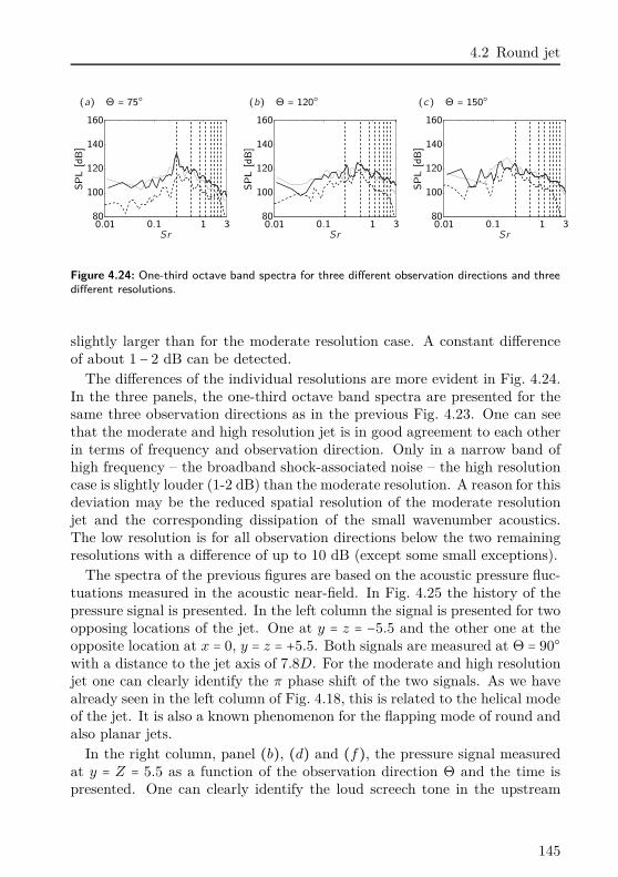
4.2 Round jet
(a) Θ = 75 (b) Θ = 120 (c) Θ = 150
SP
L[d
B]
Sr0.01 0.1 1 380
100
120
140
160
SP
L[d
B]
Sr0.01 0.1 1 380
100
120
140
160
SP
L[d
B]
Sr0.01 0.1 1 380
100
120
140
160
Figure 4.24: One-third octave band spectra for three different observation directions and threedifferent resolutions.
slightly larger than for the moderate resolution case. A constant differenceof about 1 − 2 dB can be detected.
The differences of the individual resolutions are more evident in Fig. 4.24.In the three panels, the one-third octave band spectra are presented for thesame three observation directions as in the previous Fig. 4.23. One can seethat the moderate and high resolution jet is in good agreement to each otherin terms of frequency and observation direction. Only in a narrow band ofhigh frequency – the broadband shock-associated noise – the high resolutioncase is slightly louder (1-2 dB) than the moderate resolution. A reason for thisdeviation may be the reduced spatial resolution of the moderate resolutionjet and the corresponding dissipation of the small wavenumber acoustics.The low resolution is for all observation directions below the two remainingresolutions with a difference of up to 10 dB (except some small exceptions).
The spectra of the previous figures are based on the acoustic pressure fluc-tuations measured in the acoustic near-field. In Fig. 4.25 the history of thepressure signal is presented. In the left column the signal is presented for twoopposing locations of the jet. One at y = z = −5.5 and the other one at theopposite location at x = 0, y = z = +5.5. Both signals are measured at Θ = 90
with a distance to the jet axis of 7.8D. For the moderate and high resolutionjet one can clearly identify the π phase shift of the two signals. As we havealready seen in the left column of Fig. 4.18, this is related to the helical modeof the jet. It is also a known phenomenon for the flapping mode of round andalso planar jets.
In the right column, panel (b), (d) and (f), the pressure signal measuredat y = Z = 5.5 as a function of the observation direction Θ and the time ispresented. One can clearly identify the loud screech tone in the upstream
145
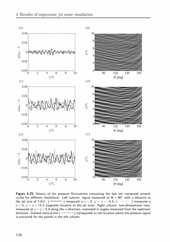
4 Results of supersonic jet noise simulation
(a) (b)
p/p∞−1
t/Ts0 2 4 6 8 10
−0.02
−0.01
0
0.01
0.02
Θ [deg]
t/Ts
90 110 130 1500
2
4
6
8
10
(c) (d)
p/p∞−1
t/Ts0 2 4 6 8 10
−0.02
−0.01
0
0.01
0.02
Θ [deg]
t/Ts
90 110 130 1500
2
4
6
8
10
(e) (f )
p/p∞−1
t/Ts0 2 4 6 8 10
−0.02
−0.01
0
0.01
0.02
Θ [deg]
t/Ts
90 110 130 1500
2
4
6
8
10
Figure 4.25: History of the pressure fluctuations containing the last ten computed screechcycles for different resolutions. Left column: signal measured at Θ = 90 with a distance tothe jet axis of 7.8D. ( ) measured a x = 0, y = z = −5.5; ( ) measured ax = 0, y = z = +5.5 (opposite location to the jet axis). Right column: two-dimensional view,measured at y = z = 5.5 along the x-direction, expressed in angles measured from the upstreamdirection. Dashed vertical line ( ) corresponds to the location where the pressure signalis extracted for the panels in the left column.
146
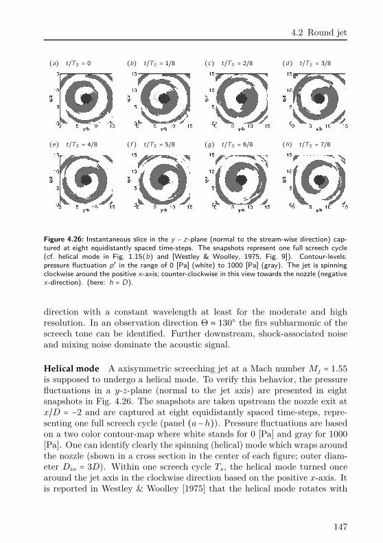
4.2 Round jet
(a) t/TS = 0 (b) t/TS = 1/8 (c) t/TS = 2/8 (d) t/TS = 3/8
(e) t/TS = 4/8 (f ) t/TS = 5/8 (g) t/TS = 6/8 (h) t/TS = 7/8
Figure 4.26: Instantaneous slice in the y − z -plane (normal to the stream-wise direction) cap-tured at eight equidistantly spaced time-steps. The snapshots represent one full screech cycle(cf. helical mode in Fig. 1.15(b) and [Westley & Woolley, 1975, Fig. 9]). Contour-levels:pressure fluctuation p′ in the range of 0 [Pa] (white) to 1000 [Pa] (gray). The jet is spinningclockwise around the positive x-axis; counter-clockwise in this view towards the nozzle (negativex-direction). (here: h = D).
direction with a constant wavelength at least for the moderate and highresolution. In an observation direction Θ ≈ 130 the firs subharmonic of thescreech tone can be identified. Further downstream, shock-associated noiseand mixing noise dominate the acoustic signal.
Helical mode A axisymmetric screeching jet at a Mach number Mj = 1.55is supposed to undergo a helical mode. To verify this behavior, the pressurefluctuations in a y-z-plane (normal to the jet axis) are presented in eightsnapshots in Fig. 4.26. The snapshots are taken upstream the nozzle exit atx/D = −2 and are captured at eight equidistantly spaced time-steps, repre-senting one full screech cycle (panel (a−h)). Pressure fluctuations are basedon a two color contour-map where white stands for 0 [Pa] and gray for 1000
[Pa]. One can identify clearly the spinning (helical) mode which wraps aroundthe nozzle (shown in a cross section in the center of each figure; outer diam-eter Dio = 3D). Within one screech cycle Ts, the helical mode turned oncearound the jet axis in the clockwise direction based on the positive x-axis. Itis reported in Westley & Woolley [1975] that the helical mode rotates with
147
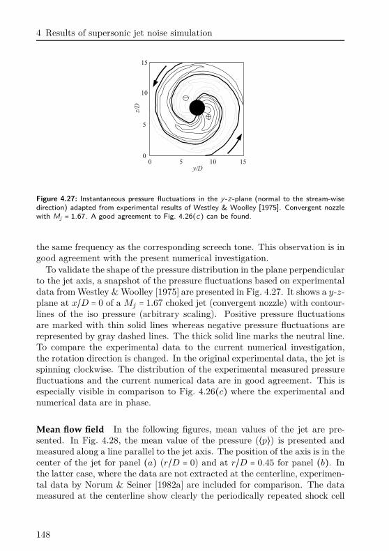
4 Results of supersonic jet noise simulation
Figure 4.27: Instantaneous pressure fluctuations in the y -z -plane (normal to the stream-wisedirection) adapted from experimental results of Westley & Woolley [1975]. Convergent nozzlewith Mj = 1.67. A good agreement to Fig. 4.26(c) can be found.
the same frequency as the corresponding screech tone. This observation is ingood agreement with the present numerical investigation.
To validate the shape of the pressure distribution in the plane perpendicularto the jet axis, a snapshot of the pressure fluctuations based on experimentaldata from Westley & Woolley [1975] are presented in Fig. 4.27. It shows a y-z-plane at x/D = 0 of a Mj = 1.67 choked jet (convergent nozzle) with contour-lines of the iso pressure (arbitrary scaling). Positive pressure fluctuationsare marked with thin solid lines whereas negative pressure fluctuations arerepresented by gray dashed lines. The thick solid line marks the neutral line.To compare the experimental data to the current numerical investigation,the rotation direction is changed. In the original experimental data, the jet isspinning clockwise. The distribution of the experimental measured pressurefluctuations and the current numerical data are in good agreement. This isespecially visible in comparison to Fig. 4.26(c) where the experimental andnumerical data are in phase.
Mean flow field In the following figures, mean values of the jet are pre-sented. In Fig. 4.28, the mean value of the pressure (⟨p⟩) is presented andmeasured along a line parallel to the jet axis. The position of the axis is in thecenter of the jet for panel (a) (r/D = 0) and at r/D = 0.45 for panel (b). Inthe latter case, where the data are not extracted at the centerline, experimen-tal data by Norum & Seiner [1982a] are included for comparison. The datameasured at the centerline show clearly the periodically repeated shock cell
148

4.2 Round jet
(a)replacemen
⟨p⟩/p
∞
x/D0 5 10 150
0.5
1
1.5
2
(b)
⟨p⟩/p
∞
x/D0 5 10 150
0.5
1
1.5
2
Figure 4.28: Mean pressure distribution along a line parallel to the jet axis. (a) at r/D = 0;(b) at r/D = 0.45. , Norum & Seiner [1982a] for Mj = 1.49 at r/D = 0.45; Numerical:current computation: ( ) 256 × 128 × 128; ( ) 512 × 256 × 256; ( )1024 × 512 × 512.
pattern. For the moderate and high resolution jet, the pressure distributionis comparable whereas the shock strength seems to be slightly larger for thehigh resolution jet. In addition to that, the number of detectable shock cellsis larger for the high resolution jet. A total of seven shock cells are visiblewhereas six shock cells can be identified for the moderate resolution jet. Thesame number of seven shock cells can be extracted for the low resolution jet.Nevertheless, as we have seen already, the shock cell spacing and the shockstrength is under-predicted. Comparing these results for the round jet withthe ones of the planar jet of Sec. § 4.1 one can conclude that for the roundjet about twice as many shock cells can be identified in the jet core. Theplanar jet with Mj = 1.55 contains only three detectable shock cells. Thisphenomenon might be related to the strong flapping mode of the planar jetwhich has a stronger impact on the shock cell structure than the helical modeof the round jet.
149
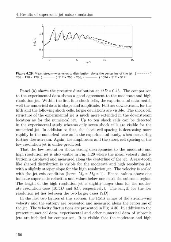
4 Results of supersonic jet noise simulation
⟨u⟩/u
e
x/D0 5 10 150
0.5
1
1.5
2
Figure 4.29: Mean stream-wise velocity distribution along the centerline of the jet. ( )256 × 128 × 128; ( ) 512 × 256 × 256; ( ) 1024 × 512 × 512.
Panel (b) shows the pressure distribution at r/D = 0.45. The comparisonto the experimental data shows a good agreement to the moderate and highresolution jet. Within the first four shock cells, the experimental data matchwell the numerical data in shape and amplitude. Further downstream, for thefifth and the following shock cells, larger deviations are visible. The shock cellstructure of the experimental jet is much more extended in the downstreamlocation as for the numerical jet. Up to ten shock cells can be detectedin the experimental study whereas only seven shock cells are visible for thenumerical jet. In addition to that, the shock cell spacing is decreasing morerapidly in the numerical case as in the experimental study, when measuringfurther downstream. Again, the amplitudes and the shock cell spacing of thelow resolution jet is under-predicted.
That the low resolution shows strong discrepancies to the moderate andhigh resolution jet is also visible in Fig. 4.29 where the mean velocity distri-bution is displayed and measured along the centerline of the jet. A saw-toothlike shaped distribution is visible for the moderate and high resolution jet,with a slightly steeper slope for the high resolution jet. The velocity is scaledwith the jet exit condition (here: Me = Md = 1). Hence, values above oneindicate supersonic velocities and values below one mark the subsonic region.The length of the high resolution jet is slightly larger than for the moder-ate resolution case (10.5D and 8D, respectively). The length for the lowresolution jet lies between the two larger cases (9D).
In the last two figures of this section, the RMS values of the stream-wisevelocity and the entropy are presented and measured along the centerline ofthe jet. The velocity fluctuations are presented in Fig. 4.30. In addition to thepresent numerical data, experimental and other numerical data of subsonicjets are included for comparison. It is visible that the moderate and high
150
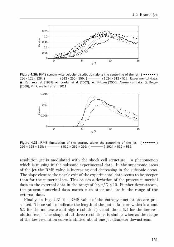
4.2 Round jet
urm
s/ue
x/D0 5 10 150
0.05
0.1
0.15
0.2
0.25
Figure 4.30: RMS stream-wise velocity distribution along the centerline of the jet. ( )256×128×128; ( ) 512×256×256; ( ) 1024×512×512. Experimental data:∎: Raman et al. [1989]; : Jordan et al. [2002]; : Bridges [2006]. Numerical data: ◻; Bogey[2000]; : Cavalieri et al. [2011].
s rms/s e
x/D0 5 10 150
0.005
0.01
0.015
Figure 4.31: RMS fluctuation of the entropy along the centerline of the jet. ( )256 × 128 × 128; ( ) 512 × 256 × 256; ( ) 1024 × 512 × 512.
resolution jet is modulated with the shock cell structure – a phenomenonwhich is missing in the subsonic experimental data. In the supersonic areasof the jet the RMS value is increasing and decreasing in the subsonic areas.The slope close to the nozzle exit of the experimental data seems to be steeperthan for the numerical jet. This causes a deviation of the present numericaldata to the external data in the range of 0 ≤ x/D ≤ 10. Further downstream,the present numerical data match each other and are in the range of theexternal data.
Finally, in Fig. 4.31 the RMS value of the entropy fluctuations are pre-sented. These values indicate the length of the potential core which is about5D for the moderate and high resolution jet and about 6D for the low res-olution case. The shape of all three resolutions is similar whereas the shapeof the low resolution curve is shifted about one jet diameter downstream.
151

IIMinimizing
supersonic jet noise

5Optimization method
In the present application we search for the best porous material to minimizesupersonic jet noise. There will be a series of porous media which will reducejet noise and some of them might perform better than other ones. Numerical[Lai & Luo, 2008] and experimental studies [Geyer et al., 2010] show that itis by no means clear how to choose the porous medium (φ and K) to reduceaeroacoustic noise. In some specific cases they show that a porous mediumcould also amplify noise.
To search for a porous medium to reduce supersonic jet noise by trail anderror, especially for a numerical analysis with high performance computers,is expensive. To find the best choice may be impossible. To this end, anoptimization algorithm is used to find the best porous material to minimizesupersonic jet noise and in particular jet screech.
In a mathematical formulation, the minimization of a function J undernonlinear equality and inequality constraints reads:
minx∈Rn
J(x) subject to ci = 0 i ∈ E
ci ≤ 0 i ∈ I(5.1)
where x is an n-dimensional parameter vector. E and I are a subset ofequality and inequality constraints, respectively. In the present application,x is the characteristic property of the porous material.
In the field of numerical optimization, two main classes of optimizationtechniques can be identified: gradient based and gradient free optimization.The latter class of optimization contains e.g. genetic algorithms. These meth-
155
5 Optimization method
ods use a set of possible solutions (parents) and evaluate their fitness (ob-jective function). Based on that value they choose the best candidates fora recombination and mutation to build the next generation (children). Thechildren are now parents and the process can be repeated to build the nextgeneration and finally to find the “fittest” individual of the population. Suchalgorithm have the ability to find a global minimum of a non convex function.This depends on the distribution of the individuals in the first generation. An-other advantage is that they do not necessarily need to deal with continuousand differentiable functions. They can also handle integer numbers, like theoptimization of the number of rotors on a propeller. For the present appli-cation, where we search for a continuously distributed material property of aporous medium with up to several million degrees of freedom, these methodsare too expensive.
The second class of optimization algorithm use the gradient of the objec-tive function to obtain the direction in which the objective function can beminimized. In a numerical analysis, the gradient can be obtained with finitedifferences, like
∇xiJ ≈ J(xi + δxi) − J(xi)
δxi
(5.2)
These finite differences need to be evaluated for each design variable xi sep-arately. One evaluation of J corresponds in the present study to one compu-tation of the Navier–Stokes equations and is very expensive. Performing thistechnique for several thousand or million design variables x ∈ Rn is impracti-cal.
Within the last years a method based on adjoint equations became moreand more popular in the field of fluid mechanics. With this technique it ispossible to evaluate the gradient of the objective function, independently onthe number of design variable, with only one additional computation of theadjoint equations, where the solution of the adjoint equations is about asexpensive as for the direct equations. This method is particularly suitable tohandle the intended multidimensional problem and will be used to optimizethe porous material. In the following sections the method of adjoint basedoptimization is presented.
5.1 A simple example
Let us start with a very simple example to introduce the method of Lagrangemultipliers (adjoint variables). Consider the following one-dimensional prob-
156
5.1 A simple example
lem:minx∈R
J(x) = x2 (5.3a)
subject to N(x, c) = x − c = 0 (5.3b)
In this example the objective is to minimize the function J(x) subject tothe equality constraint N(x, c) = 0 with the control c. The solution to thisproblem is trivial. Setting c = 0, the objective function J(x) will reach itsminimum. Although the solution to this problem is trivial it will be used inthe following to introduce the concept of Lagrange multipliers.
With a new variable λ, the so called Lagrange multiplier, the correspondingLagrange function can be defined:
L(x, c, λ) = J(x) − λ ⋅N(x, c) (5.4)
whereas it is equivalent whether the latter term with λ is added or subtracted.Now, if x is a stationary point of Eq. (5.3a), then there exists a λ so that(x, λ) is a stationary point of Eq. (5.4). One can reformulate the problem infinding a stationary point of L instead of J including all constraints in oneequation. For a stationary point of a functional, all partial derivatives needto vanish and one obtains a system of equations:
∂L∂x
= 0 = 2x − λ (5.5a)
∂L∂λ
= 0 = x − c (5.5b)
∂L∂c
= 0 = λ (5.5c)
These three equations with the three unknowns x, c and λ form the opti-mization framework which can be solved to obtain the optimal solution. Forthe present system of equations, it directly follows that c = 0 is the optimum.Such an optimization method, where the solution can be gained within onestep, is referred to as an one-shot method. Usually, when Eq. (5.3a) and(5.3b) are nonlinear, this approach is no more possible. To this end, an itera-tive gradient based method is needed. As long as the optimum is not reached,Eq. (5.5c) is the gradient of the objective function with respect to the controlc. We obtain:
∂J
∂c= λ (5.6)
The gradient is depending on the Lagrange multiplier λ and we need to solveEq. (5.5a) to obtain an expression for the Lagrange multiplier:
λ = 2x (5.7)
157
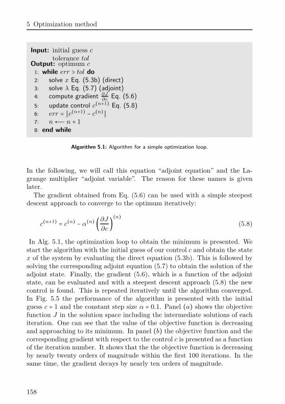
5 Optimization method
Input: initial guess c
tolerance tolOutput: optimum c
1: while err > tol do2: solve x Eq. (5.3b) (direct)3: solve λ Eq. (5.7) (adjoint)4: compute gradient ∂J
∂cEq. (5.6)
5: update control c(n+1) Eq. (5.8)6: err = ∥c(n+1) − c(n)∥7: n←Ð n + 1
8: end while
Algorithm 5.1: Algorithm for a simple optimization loop.
In the following, we will call this equation “adjoint equation” and the La-grange multiplier “adjoint variable”. The reason for these names is givenlater.
The gradient obtained from Eq. (5.6) can be used with a simple steepestdescent approach to converge to the optimum iteratively:
c(n+1) = c(n) − α(n) (∂J
∂c)(n) (5.8)
In Alg. 5.1, the optimization loop to obtain the minimum is presented. Westart the algorithm with the initial guess of our control c and obtain the statex of the system by evaluating the direct equation (5.3b). This is followed bysolving the corresponding adjoint equation (5.7) to obtain the solution of theadjoint state. Finally, the gradient (5.6), which is a function of the adjointstate, can be evaluated and with a steepest descent approach (5.8) the newcontrol is found. This is repeated iteratively until the algorithm converged.In Fig. 5.5 the performance of the algorithm is presented with the initialguess c = 1 and the constant step size α = 0.1. Panel (a) shows the objectivefunction J in the solution space including the intermediate solutions of eachiteration. One can see that the value of the objective function is decreasingand approaching to its minimum. In panel (b) the objective function and thecorresponding gradient with respect to the control c is presented as a functionof the iteration number. It shows that the the objective function is decreasingby nearly twenty orders of magnitude within the first 100 iterations. In thesame time, the gradient decays by nearly ten orders of magnitude.
158
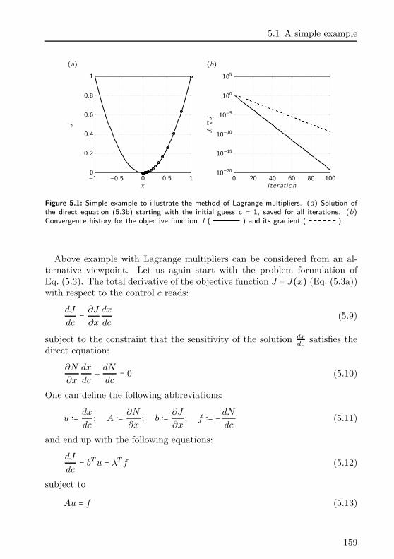
5.1 A simple example
(a) (b)J
x−1 −0.5 0 0.5 10
0.2
0.4
0.6
0.8
1
J,∇J
i teration0 20 40 60 80 100
10−20
10−15
10−10
10−5
100
105
Figure 5.1: Simple example to illustrate the method of Lagrange multipliers. (a) Solution ofthe direct equation (5.3b) starting with the initial guess c = 1, saved for all iterations. (b)Convergence history for the objective function J ( ) and its gradient ( ).
Above example with Lagrange multipliers can be considered from an al-ternative viewpoint. Let us again start with the problem formulation ofEq. (5.3). The total derivative of the objective function J = J(x) (Eq. (5.3a))with respect to the control c reads:
dJ
dc= ∂J
∂x
dx
dc(5.9)
subject to the constraint that the sensitivity of the solution dxdc
satisfies thedirect equation:
∂N
∂x
dx
dc+
dN
dc= 0 (5.10)
One can define the following abbreviations:
u ∶= dx
dc; A ∶= ∂N
∂x; b ∶= ∂J
∂x; f ∶= −dN
dc(5.11)
and end up with the following equations:
dJ
dc= bT u = λT f (5.12)
subject to
Au = f (5.13)
159
5 Optimization method
under the constraint, that λ satisfies the adjoint equation:
AT λ = b. (5.14)
The equivalence of the last two terms in Eq. (5.12) is easily proved:
bT u = (AT λ)T u = λT Au = λT f (5.15)
with the adjoint matrix AT (if A ∈ Rn×n) and the corresponding adjoint
variable λ. From this viewpoint, one can deduce the origin of the nameadjoint optimization, which is not as evident when following the previousapproach with Lagrange multipliers.
One of the main advantages of adjoint based optimization, compared toother gradient based optimization techniques, can be identified. The gradientof the objective function in Eq. (5.12) can be either computed by the termbT u or λT f . As f is a function of the control (f = f(c)), and if the dimensionof the control is large, the evaluation of bT u = bT A−1f , has to be performedfor every single f(c). To this end a system of equations has to be solvedas many times as the dimension of c. In contrast to that, as g ≠ g(c), theevaluation of λT f including the solution of the adjoint equation λ = (AT )−1b
has to be carried out only once. Especially if the dimension of the control islarge and the solution of the direct equations is expensive, adjoint methodsare indispensable.
In the area of fluid mechanics the dimension of the control (e. g. geometryparameters of a wing) is usually in the order of several hundred. In thepresent study, where the optimal spacial distribution of a porous medium isquestioned, the dimension of the control can be easily in the order of severalmillion. In addition to that, the underlying equations, to obtain the state(here u), are based on the Navier–Stokes equations. Their numerical solutionis expensive and requires the use of high performance techniques.
To apply this simple example to the Navier–Stokes equations of the presentinvestigation, the equality constraint in the Lagrange functional N(x, c) hasto be replaced by the Navier–Stokes equations. They constrain the solutionspace of the flow variables.
5.2 State of the art
Adjoint based optimization in the field of fluid mechanics is by no means newbut a field of active research. The first to use adjoint based optimization wasPironneau [1974]. He derived an optimization framework to minimize the
160
5.2 State of the art
drag of a hump on the surface of a body. At this time, he was not able toprovide a numerical solution to this problem and only delivered the theoreticalframework. A wide range of different research topics has followed within thenext years and decades and is still ongoing. The different topics on adjointbased optimization can be classified in three main fields: shape optimization,topology optimization and active optimization. In the following, the state ofthe art will be addressed separately for each topic.
Shape optimization The use of adjoint equations has been pioneered byJameson [1988, 1995]. He used several setups from two- to three-dimensionalconfigurations based on potential equations, the Euler equations and theNavier–Stokes equations. The main focus of shape optimization is to mini-mize the drag of a wing while keeping or even increasing the lift. The earlywork of Jameson was followed by a series of researchers working on that topicup to the present date [see amongst others Asouti et al., 2008, Brezillon &Gauger, 2004, Carpentieri et al., 2007, Fazzolari et al., 2007, Giles & Pierce,2000, 1999, Gunzburger, 2000, Kim et al., 2004, Le Moigne, 2002, Nemec &Zingg, 2001].
Some of the shape optimization applications also deal with transonic orsupersonic wing configurations where shocks are present. They were investi-gated e. g. by Giles [2002], Giles et al. [2003], Nadarajah et al. [2001], Reutheret al. [1996]. It was reported by Giles & Pierce [2001] in an analytic one-dimensional study that the adjoint solution in the presence of shocks is in-correct and needs additional internal boundary conditions in the vicinity ofthe shock. The additional boundary condition arise due to the linearizationof the Navier–Stokes equations when deriving the corresponding adjoints. Inthis step it is assumed that the solution of the equations is smooth and that alinear perturbation theory can be applied. This assumption may be violatedin the presence of a shock. Especially strong shocks may be resolved in a nu-merical investigation by only a view grid points and a linear theory may needadditional boundary conditions to predict the correct jump of the flow vari-ables. If the shock is well resolved by the computational grid or smeared outover several grid points due to a shock capturing method, the linear theorycan be applied and errors in the adjoint solution are not to be expected. Thesame holds true for weak and oblique shocks [see Giles et al., 2003]. In thepresent application on the optimization of a shock containing flow, first, nostrong shocks, like a Mach disk are present, and secondly, a shock capturingscheme smears out strong gradients to obtain a smooth solution. Hence, anadditional boundary condition in the vicinity of shocks is not necessary.
161
5 Optimization method
Shape optimization has not only been applied to lift and drag optimizationbut also to flow induced acoustic, like the minimization of trailing edge noise[Marsden et al., 2001, Rumpfkeil & Zingg, 2009] or the minimization of thenoise of a trailing step [Cao & Stanescu, 2002]. It has also been applied toturbo-machinery noise like the minimization of fan-flow deflector noise [Xionget al., 2010]. In another application, by Feijoo et al. [2004], an inverse acousticscattering problem is presented to find the optimal geometry that satisfies acertain measured acoustic signal. Applications of shape optimization for anacoustic objective in combination with supersonic flows has been reportedby Nadarajah et al. [2003]. They minimized the sonic boom measured at theground surface by changing the geometry of the supersonic aircraft. A similarinvestigation was performed by Mohammadi [2004].
Topology optimization In the latter paragraph, the control to achieve thedesired objective is to change the shape of one or several predefined geome-tries. This approach is limited. The optimization algorithm will neither beable to split a geometry in several geometries nor to “invent” new geometries.As a user of the shape optimization algorithm a lot of empirical informationhas to be provided and the solution space is restricted. In some applications,where it is neither clear how the optimal shape of the geometry should beconfigured nor how many obstacles should be place in the fluid flow, adjointbased topology optimization is the method of choice.
Originally, adjoint based topology optimization was used in solid state me-chanics [Bendsøe, 1995, Eschenauer & Olhoff, 2001]. The first application tofluid mechanics was reported in Borrvall & Petersson [2003] with the topol-ogy optimization of fluids in Stokes flow. The main idea of any adjoint basedtopology optimization algorithm in fluid mechanics is based on a Darcy termin the momentum equation whose sensitivity is obtained via an adjoint com-putation. Hence, the Darcy term is being optimized and represents a passivecontrol. As in topology optimization only solid materials or void space isallowed, one has to distinguish between zero permeability or a high perme-ability (corresponding to a solid body) based on the sensitivity map emergingfrom the adjoint computation. Following the early work of Borrvall & Pe-tersson [2003], many others adapted the method like Olesen et al. [2004] forNavier–Stokes flows in micro-fluidics. Gersborg-Hansen et al. [2005] appliedthe method to the optimization of channel flow problems. A large scale Stokesflow problem was investigated by Aage et al. [2008]. Using a continuous ad-joint formulation for the computation of topological sensitivities, ducted flowsare optimized by Othmer [2008]. Recently Papoutsis-Kiachagias et al. [2011]
162
5.2 State of the art
applied topology optimization to laminar and turbulent flows, including heattransfer.
Topology optimization is also applied to acoustic problems. Dühring et al.[2008] used it to design geometries to reduce the noise level in a certain areaof a room. They applied it to the Helmholtz equations with a fluid in rest.The first to apply topology optimization to an aeroacoustic application wasSchulze & Sesterhenn [2011]. They used the method to optimize the spatialdistribution of a porous medium (with a variable permeability) to reducetrailing edge noise. Some of their main results are presented in Sec. § 5.5.3.
The present application on the minimization on supersonic jet noise bymeans of an optimized porous material can be classified as a topology op-timization. Up to now, it is the first time that topology optimization withporous media is applied to supersonic jet noise. It will be discussed in detailin the remaining part of this thesis.
Active optimization Despite shape and topology optimization, which be-long to the class of passive control as long as the geometry is steady in state,active control can be applied. Examples are blowing and suction, heatingand cooling of a boundary or any other form of volume forcing in the do-main. The first to use blowing and suction in optimal control was Joslin et al.[1995] to suppress the boundary layer instability. A similar investigation wasperformed by Airiau et al. [2003]. Later, Guegan et al. [2006] applied it tothe optimal control in swept Hiemenz flow. Bewley et al. [2001] used blow-ing and suction to reduce the kinetic energy in a plane channel flow. Up tothat time they performed the highest-dimensional control optimization witha total of 107 control variables. Based on the compressible two-dimensionalNavier–Stokes equations Collis et al. [2002b] optimized two counter rotatingvortices impinging on a flat plate.
Active control strategies were frequently used in aeroacoustic applications.It was first reported by Collis et al. [2002a] as they applied it to the blowingand suction of a cylinder vortex interaction and could reduce the aeroacousticnoise by 6 dB. An example based on the Euler equations and an optimaltranspiration control to reduce aeroacoustic noise is reported by Collis et al.[2003].
The first application to free sher flow noise, like the one of mixing-layers orjets, is proposed by Cervino et al. [2002]. They obtained in a two-dimensionalstudy of a Mj = 0.5 jet a sensitivity map to a noise signal measured in theacoustic near field. No optimization was performed in this study. Theymention in Cervino & Bewley [2003] that on the one hand the actuation with
163
5 Optimization method
mass sources is more efficient than with heat sources and on the other handthat high frequency noise can be modified with a low frequency actuation.Wei [2004], Wei & Freund [2002] were the first to control a mixing-layer basedon a thermal volume forcing in a small region in the mixing-layer. They couldreduce the noise by more than 6 dB and showed that the forcing is weak andhas little effect on the structures of the mixing-layer. Later, Wei & Freund[2006] showed that it is not only vortex pairing which is responsible for mixingnoise, as the pairing phenomenon did not vanish for the controlled mixing-layer. Similar studies on mixing-layer noise were performed by a series ofresearchers, like Babucke et al. [2009], Barone [2003], Barone & Lele [2005],Kleinman & Freund [2006], Spagnoli & Airiau [2008].
Recently, Freund [2011] presented an intermediate step of the optimizationof a supersonic axisymmetric jet by means of thermal actuation close to thenozzle exit (similar to the work of Wei & Freund [2006]). The Mach numberof the perfectly expanded jet is Mj = 1.3 with a total of 2.8 ⋅ 106 grid points(LES, nozzle is not included). They presented the first step of the Line Searchalgorithm and gained a reduction of 37 % for the objective function. Theirsimulations are ongoing.
5.3 Objective function
In the present application on supersonic jet screech the noise is character-ized by a specific structure of the frequency spectrum. It contains distinctfrequency peaks with high amplitudes. In Fig. 5.2(a) a sketch of a typicalspectrum of aeroacoustic jet-screech is shown, characterized by a loud anddistinct peak at a specific frequency ωscreech. Other noise sources, such as thelow-frequency mixing noise of the jet or the broadband shock noise are ratherquiet by comparison.
Most recent attempts of noise reduction by iterative optimization use aquadratic objective functional where the acoustic pressure fluctuations p′(x, t)are squared and integrated over space and time. Although this approachmight reduce the objective functional, it is by no means clear which frequen-cies of our noise source will ultimately be reduced. For example, applyingthe above technique could dampen the sound level at some frequencies of thespectrum, but readily amplify others. In a worst-case scenario, the domi-nant noise sources – the peaks in Fig. 5.2(a) – may be amplified while theother (already relatively quiet) parts in the spectrum are further reduced(cf. Fig. 5.2(b)). This may yield an overall reduced objective functional butdoes hardly meet the intentions. One then quickly realizes that, in order to
164
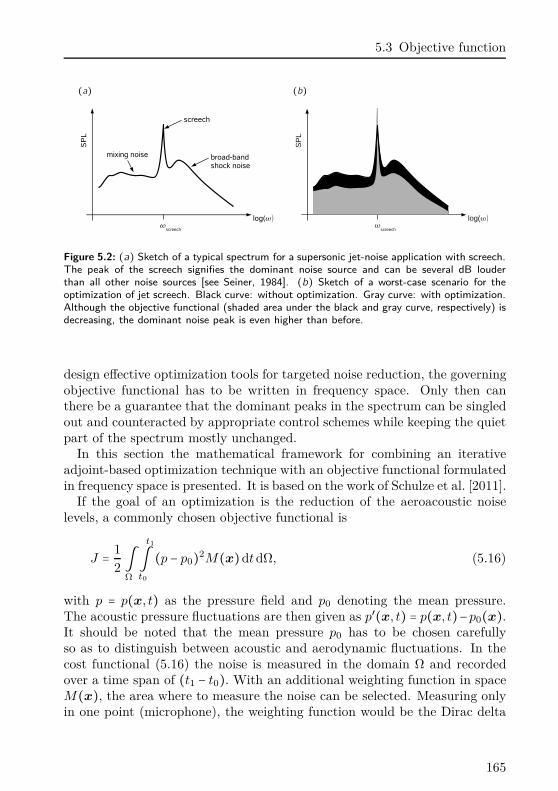
5.3 Objective function
(a) (b)
Figure 5.2: (a) Sketch of a typical spectrum for a supersonic jet-noise application with screech.The peak of the screech signifies the dominant noise source and can be several dB louderthan all other noise sources [see Seiner, 1984]. (b) Sketch of a worst-case scenario for theoptimization of jet screech. Black curve: without optimization. Gray curve: with optimization.Although the objective functional (shaded area under the black and gray curve, respectively) isdecreasing, the dominant noise peak is even higher than before.
design effective optimization tools for targeted noise reduction, the governingobjective functional has to be written in frequency space. Only then canthere be a guarantee that the dominant peaks in the spectrum can be singledout and counteracted by appropriate control schemes while keeping the quietpart of the spectrum mostly unchanged.
In this section the mathematical framework for combining an iterativeadjoint-based optimization technique with an objective functional formulatedin frequency space is presented. It is based on the work of Schulze et al. [2011].
If the goal of an optimization is the reduction of the aeroacoustic noiselevels, a commonly chosen objective functional is
J = 1
2∫Ω
t1
∫t0
(p − p0)2M(x)dt dΩ, (5.16)
with p = p(x, t) as the pressure field and p0 denoting the mean pressure.The acoustic pressure fluctuations are then given as p′(x, t) = p(x, t)−p0(x).It should be noted that the mean pressure p0 has to be chosen carefullyso as to distinguish between acoustic and aerodynamic fluctuations. In thecost functional (5.16) the noise is measured in the domain Ω and recordedover a time span of (t1 − t0). With an additional weighting function in spaceM(x), the area where to measure the noise can be selected. Measuring onlyin one point (microphone), the weighting function would be the Dirac delta
165
5 Optimization method
(M(x) = δ(x−xm), where xm is the location of the microphone). To increasenumerical stability, a Dirac delta can be smoothed out by replacing it with aGaussian distribution.
Following Parseval’s theorem the energy of a signal, in our case the squareof the measured noise, is the integral of the square of all its Fourier coefficients.Applied to the temporal integral in (5.16) we obtain
∫Ω
t1
∫t0
(p′(x, t))2M(x)dt dΩ = 1
2π∫Ω
∞
∫−∞
∣P ′(x, ω)∣2M(x)dω dΩ. (5.17)
A reduction in the objective functional J thus requires an equivalent reduc-tion in the coefficients ∣P ′(x, ω)∣2, which corresponds to a decrease of theamplitudes in the power-spectrum. As previously mentioned, however, byfollowing this approach it remains unclear which frequencies of the noise-spectrum are ultimately reduced. Depending on the underlying physics aswell as on the applied control, it is conceivable that only a certain – maybeuninteresting – frequency-band could be minimized using the above objectivefunctional. In the worst case, the dominant noise source may be amplifiedeven though J is decreasing (cf. Fig. 5.2(b)).5.3.1 Objective functional in frequency space
Given an uncontrolled noise spectrum with peaks at distinct frequencies, onecan introduce an objective functional that allows not only to target certainfrequencies but also to identify sharp peaks. The objective functional in thefrequency domain can be written as
J = λ1
2∫Ω
ωu
∫ωl
⎧⎪⎪⎨⎪⎪⎩∞
∫−∞
e−iωtp′(x, t)dt
⎫⎪⎪⎬⎪⎪⎭2
M(x)dω dΩ
´¹¹¹¹¹¹¹¹¹¹¹¹¹¹¹¹¹¹¹¹¹¹¹¹¹¹¹¹¹¹¹¹¹¹¹¹¹¹¹¹¹¹¹¹¹¹¹¹¹¹¹¹¹¹¹¹¹¹¹¹¹¹¹¹¹¹¹¹¹¹¹¹¹¹¹¹¹¹¹¹¹¹¹¹¹¹¹¹¹¹¹¹¹¹¹¹¹¹¹¹¹¹¹¹¹¹¹¹¹¹¹¹¹¹¹¹¹¹¹¹¹¹¹¹¹¹¹¹¹¹¹¹¹¹¹¹¸¹¹¹¹¹¹¹¹¹¹¹¹¹¹¹¹¹¹¹¹¹¹¹¹¹¹¹¹¹¹¹¹¹¹¹¹¹¹¹¹¹¹¹¹¹¹¹¹¹¹¹¹¹¹¹¹¹¹¹¹¹¹¹¹¹¹¹¹¹¹¹¹¹¹¹¹¹¹¹¹¹¹¹¹¹¹¹¹¹¹¹¹¹¹¹¹¹¹¹¹¹¹¹¹¹¹¹¹¹¹¹¹¹¹¹¹¹¹¹¹¹¹¹¹¹¹¹¹¹¹¹¹¹¹¹¹¶J1
+λ2
2∫Ω
ωu
∫ωl
⎧⎪⎪⎨⎪⎪⎩∂
∂ω
∞
∫−∞
e−iωtp′(x, t)dt
⎫⎪⎪⎬⎪⎪⎭2
M(x)dω dΩ
´¹¹¹¹¹¹¹¹¹¹¹¹¹¹¹¹¹¹¹¹¹¹¹¹¹¹¹¹¹¹¹¹¹¹¹¹¹¹¹¹¹¹¹¹¹¹¹¹¹¹¹¹¹¹¹¹¹¹¹¹¹¹¹¹¹¹¹¹¹¹¹¹¹¹¹¹¹¹¹¹¹¹¹¹¹¹¹¹¹¹¹¹¹¹¹¹¹¹¹¹¹¹¹¹¹¹¹¹¹¹¹¹¹¹¹¹¹¹¹¹¹¹¹¹¹¹¹¹¹¹¹¹¹¹¹¹¹¹¹¹¹¹¹¹¹¹¹¹¹¹¹¸¹¹¹¹¹¹¹¹¹¹¹¹¹¹¹¹¹¹¹¹¹¹¹¹¹¹¹¹¹¹¹¹¹¹¹¹¹¹¹¹¹¹¹¹¹¹¹¹¹¹¹¹¹¹¹¹¹¹¹¹¹¹¹¹¹¹¹¹¹¹¹¹¹¹¹¹¹¹¹¹¹¹¹¹¹¹¹¹¹¹¹¹¹¹¹¹¹¹¹¹¹¹¹¹¹¹¹¹¹¹¹¹¹¹¹¹¹¹¹¹¹¹¹¹¹¹¹¹¹¹¹¹¹¹¹¹¹¹¹¹¹¹¹¹¹¹¹¹¹¹¶J2
(5.18)
with λ1 and λ2 as user-defined weights to give more emphasis to the first orsecond term in the above expression and to influence the convergence of theoptimization algorithm.
166
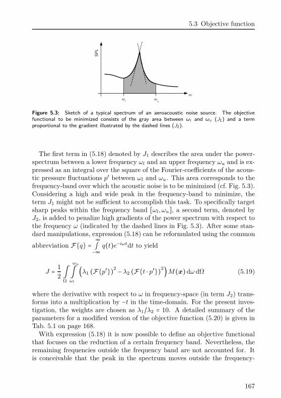
5.3 Objective function
Figure 5.3: Sketch of a typical spectrum of an aeroacoustic noise source. The objectivefunctional to be minimized consists of the gray area between ωl and ωu (J1) and a termproportional to the gradient illustrated by the dashed lines (J2).
The first term in (5.18) denoted by J1 describes the area under the power-spectrum between a lower frequency ωl and an upper frequency ωu and is ex-pressed as an integral over the square of the Fourier-coefficients of the acous-tic pressure fluctuations p′ between ωl and ωu. This area corresponds to thefrequency-band over which the acoustic noise is to be minimized (cf. Fig. 5.3).Considering a high and wide peak in the frequency-band to minimize, theterm J1 might not be sufficient to accomplish this task. To specifically targetsharp peaks within the frequency band [ωl, ωu], a second term, denoted byJ2, is added to penalize high gradients of the power spectrum with respect tothe frequency ω (indicated by the dashed lines in Fig. 5.3). After some stan-dard manipulations, expression (5.18) can be reformulated using the common
abbreviation Fq = ∞∫−∞
q(t)e−iωtdt to yield
J = 1
2∫Ω
ωu
∫ωl
(λ1 (Fp′)2 − λ2 (Ft ⋅ p′)2)M(x)dω dΩ (5.19)
where the derivative with respect to ω in frequency-space (in term J2) trans-forms into a multiplication by −t in the time-domain. For the present inves-tigation, the weights are chosen as λ1/λ2 = 10. A detailed summary of theparameters for a modified version of the objective function (5.20) is given inTab. 5.1 on page 168.
With expression (5.18) it is now possible to define an objective functionalthat focuses on the reduction of a certain frequency band. Nevertheless, theremaining frequencies outside the frequency band are not accounted for. Itis conceivable that the peak in the spectrum moves outside the frequency-
167
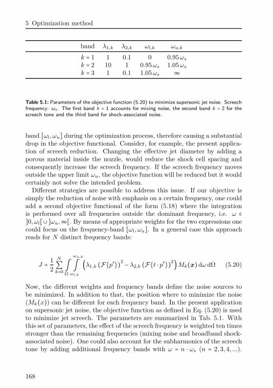
5 Optimization method
band λ1,k λ2,k ωl,k ωu,k
k = 1 1 0.1 0 0.95 ωs
k = 2 10 1 0.95 ωs 1.05 ωs
k = 3 1 0.1 1.05 ωs ∞
Table 5.1: Parameters of the objective function (5.20) to minimize supersonic jet noise. Screechfrequency: ωs . The first band k = 1 accounts for mixing noise, the second band k = 2 for thescreech tone and the third band for shock-associated noise.
band [ωl, ωu] during the optimization process, therefore causing a substantialdrop in the objective functional. Consider, for example, the present applica-tion of screech reduction. Changing the effective jet diameter by adding aporous material inside the nozzle, would reduce the shock cell spacing andconsequently increase the screech frequency. If the screech frequency movesoutside the upper limit ωu, the objective function will be reduced but it wouldcertainly not solve the intended problem.
Different strategies are possible to address this issue. If our objective issimply the reduction of noise with emphasis on a certain frequency, one couldadd a second objective functional of the form (5.18) where the integrationis performed over all frequencies outside the dominant frequency, i.e. ω ∈]0, ωl[∪ ]ωu,∞[. By means of appropriate weights for the two expressions onecould focus on the frequency-band [ωl, ωu]. In a general case this approachreads for N distinct frequency bands:
J = 1
2
N∑k=0∫Ω
ωu,k
∫ωl,k
(λ1,k (Fp′)2 − λ2,k (Ft ⋅ p′)2)Mk(x)dω dΩ (5.20)
Now, the different weights and frequency bands define the noise sources tobe minimized. In addition to that, the position where to minimize the noise(Mk(x)) can be different for each frequency band. In the present applicationon supersonic jet noise, the objective function as defined in Eq. (5.20) is usedto minimize jet screech. The parameters are summarized in Tab. 5.1. Withthis set of parameters, the effect of the screech frequency is weighted ten timesstronger than the remaining frequencies (mixing noise and broadband shock-associated noise). One could also account for the subharmonics of the screechtone by adding additional frequency bands with ω = n ⋅ ωs (n = 2, 3, 4, ...).
168
5.3 Objective function
Nevertheless, the subharmonics are linked to the fundamental screech toneand a reduction of the screech tone will also reduce its subharmonics. To thisend, only the fundamental screech frequency ωs is accounted for.
An alternative strategy is based on keeping the uncontrolled frequenciesunchanged. In the present application this corresponds to a reduction ofscreech noise while keeping the amplitudes of the mixing noise and the shock-associated noise on a constant level. From an environmental point of view,this strategy is not desirable as the optimization may not be as efficient asthe reduction of all frequencies. Nevertheless, this approach can be of par-ticular interest if our goal is not only the minimization of noise in particularfrequency bands but also the discovery and understanding of noise gener-ation mechanisms by specific acoustic sources. In other words, by keepingall uncontrolled frequencies unchanged and simultaneously reducing only thedominant peak within a given frequency band, one can extract the mechanismresponsible for this specific peak in the spectrum. Mathematically, we intro-duce non-negative terms that penalize any changes in the noise spectrumfrom the uncontrolled spectrum for frequencies outside the target interval[ωl, ωu]. For this strategy, the uncontrolled spectrum has to be determinedand stored. We obtain
P = P1 +P2 (5.21a)
P1 = 1
2∫Ω
ωl
∫−∞
(Fp′ −Fp′0)2 M(x)dω dΩ (5.21b)
P2 = 1
2∫Ω
∞
∫ωu
(Fp′ −Fp′0)2 M(x)dω dΩ (5.21c)
with the controlled acoustic pressure fluctuations denoted by p′ and the un-controlled fluctuations by p′0. The term P1 penalizes changes in the spectrumbelow the target frequency-band, i.e, ω ∈ [−∞, ωl[); the term P2 ensuresminimal changes of the spectrum in the frequency-band ω ∈]ωu,∞[.
In the present investigation, the additional penalty term is not includedin the minimization of jet screech, as the focus also lies on the reduction ofthe remaining noise sources. Nevertheless, this term can be used for futureinvestigations, to focus on the individual noise sources.
In addition to the two penalty terms P1 and P2 an additional penalty termis usually added in control theory. This additional penalty term has the
169
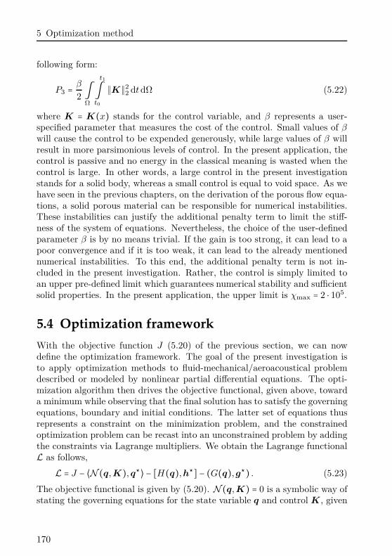
5 Optimization method
following form:
P3 = β
2∫Ω
t1
∫t0
∥K∥22 dt dΩ (5.22)
where K = K(x) stands for the control variable, and β represents a user-specified parameter that measures the cost of the control. Small values of β
will cause the control to be expended generously, while large values of β willresult in more parsimonious levels of control. In the present application, thecontrol is passive and no energy in the classical meaning is wasted when thecontrol is large. In other words, a large control in the present investigationstands for a solid body, whereas a small control is equal to void space. As wehave seen in the previous chapters, on the derivation of the porous flow equa-tions, a solid porous material can be responsible for numerical instabilities.These instabilities can justify the additional penalty term to limit the stiff-ness of the system of equations. Nevertheless, the choice of the user-definedparameter β is by no means trivial. If the gain is too strong, it can lead to apoor convergence and if it is too weak, it can lead to the already mentionednumerical instabilities. To this end, the additional penalty term is not in-cluded in the present investigation. Rather, the control is simply limited toan upper pre-defined limit which guarantees numerical stability and sufficientsolid properties. In the present application, the upper limit is χmax = 2 ⋅ 105.
5.4 Optimization framework
With the objective function J (5.20) of the previous section, we can nowdefine the optimization framework. The goal of the present investigation isto apply optimization methods to fluid-mechanical/aeroacoustical problemdescribed or modeled by nonlinear partial differential equations. The opti-mization algorithm then drives the objective functional, given above, towarda minimum while observing that the final solution has to satisfy the governingequations, boundary and initial conditions. The latter set of equations thusrepresents a constraint on the minimization problem, and the constrainedoptimization problem can be recast into an unconstrained problem by addingthe constraints via Lagrange multipliers. We obtain the Lagrange functionalL as follows,
L = J − ⟨N (q, K), q⋆⟩ − [H(q), h⋆] − (G(q), g⋆) . (5.23)
The objective functional is given by (5.20). N (q, K) = 0 is a symbolic way ofstating the governing equations for the state variable q and control K, given
170
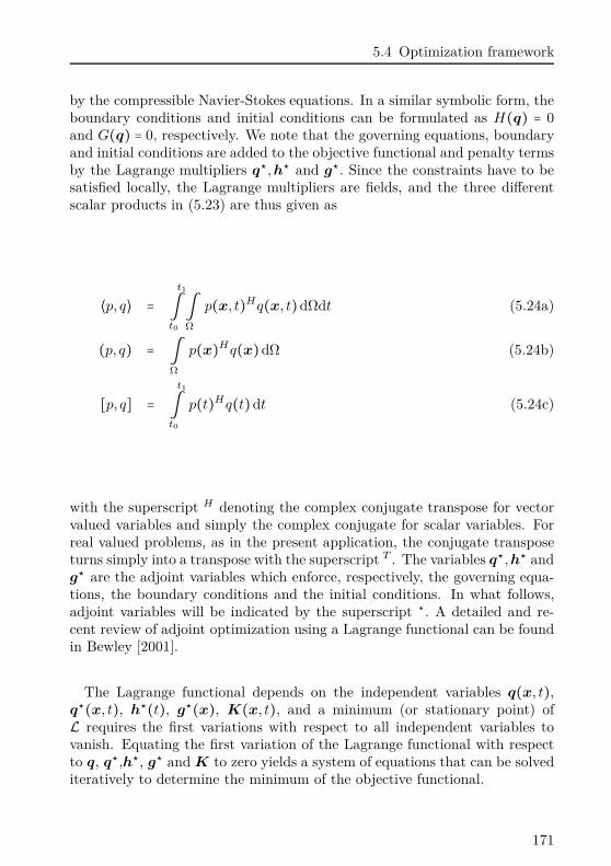
5.4 Optimization framework
by the compressible Navier-Stokes equations. In a similar symbolic form, theboundary conditions and initial conditions can be formulated as H(q) = 0and G(q) = 0, respectively. We note that the governing equations, boundaryand initial conditions are added to the objective functional and penalty termsby the Lagrange multipliers q⋆, h⋆ and g⋆. Since the constraints have to besatisfied locally, the Lagrange multipliers are fields, and the three differentscalar products in (5.23) are thus given as
⟨p, q⟩ =t1
∫t0
∫Ω
p(x, t)Hq(x, t)dΩdt (5.24a)
(p, q) = ∫Ω
p(x)Hq(x)dΩ (5.24b)
[p, q] =t1
∫t0
p(t)Hq(t)dt (5.24c)
with the superscript H denoting the complex conjugate transpose for vectorvalued variables and simply the complex conjugate for scalar variables. Forreal valued problems, as in the present application, the conjugate transposeturns simply into a transpose with the superscript T . The variables q⋆, h⋆ andg⋆ are the adjoint variables which enforce, respectively, the governing equa-tions, the boundary conditions and the initial conditions. In what follows,adjoint variables will be indicated by the superscript ⋆. A detailed and re-cent review of adjoint optimization using a Lagrange functional can be foundin Bewley [2001].
The Lagrange functional depends on the independent variables q(x, t),q⋆(x, t), h⋆(t), g⋆(x), K(x, t), and a minimum (or stationary point) ofL requires the first variations with respect to all independent variables tovanish. Equating the first variation of the Lagrange functional with respectto q, q⋆,h⋆, g⋆ and K to zero yields a system of equations that can be solvediteratively to determine the minimum of the objective functional.
171
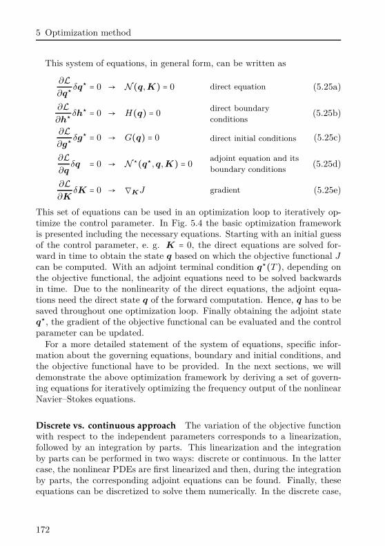
5 Optimization method
This system of equations, in general form, can be written as
∂L∂q⋆
δq⋆ = 0 → N (q, K) = 0 direct equation (5.25a)
∂L∂h⋆
δh⋆ = 0 → H(q) = 0direct boundary
conditions(5.25b)
∂L∂g⋆
δg⋆ = 0 → G(q) = 0 direct initial conditions (5.25c)
∂L∂q
δq = 0 → N ⋆(q⋆, q, K) = 0adjoint equation and its
boundary conditions(5.25d)
∂L∂K
δK = 0 → ∇KJ gradient (5.25e)
This set of equations can be used in an optimization loop to iteratively op-timize the control parameter. In Fig. 5.4 the basic optimization frameworkis presented including the necessary equations. Starting with an initial guessof the control parameter, e. g. K = 0, the direct equations are solved for-ward in time to obtain the state q based on which the objective functional J
can be computed. With an adjoint terminal condition q⋆(T ), depending onthe objective functional, the adjoint equations need to be solved backwardsin time. Due to the nonlinearity of the direct equations, the adjoint equa-tions need the direct state q of the forward computation. Hence, q has to besaved throughout one optimization loop. Finally obtaining the adjoint stateq⋆, the gradient of the objective functional can be evaluated and the controlparameter can be updated.
For a more detailed statement of the system of equations, specific infor-mation about the governing equations, boundary and initial conditions, andthe objective functional have to be provided. In the next sections, we willdemonstrate the above optimization framework by deriving a set of govern-ing equations for iteratively optimizing the frequency output of the nonlinearNavier–Stokes equations.
Discrete vs. continuous approach The variation of the objective functionwith respect to the independent parameters corresponds to a linearization,followed by an integration by parts. This linearization and the integrationby parts can be performed in two ways: discrete or continuous. In the lattercase, the nonlinear PDEs are first linearized and then, during the integrationby parts, the corresponding adjoint equations can be found. Finally, theseequations can be discretized to solve them numerically. In the discrete case,
172
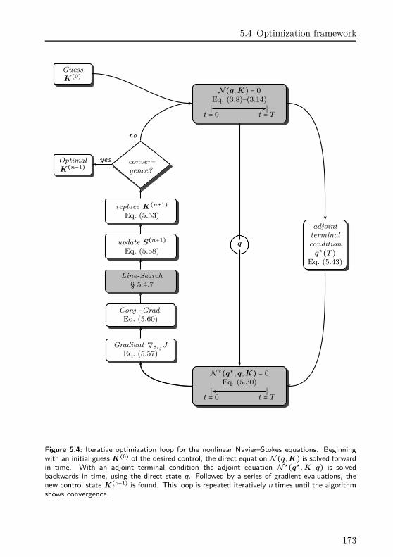
5.4 Optimization framework
Guess
K(0)
no
Optimal
K(n+1)
yes conver–
gence?
replace K(n+1)
Eq. (5.53)
update S(n+1)
Eq. (5.58)
Line-Search
§ 5.4.7
Conj.–Grad.
Eq. (5.60)
Gradient ∇sijJ
Eq. (5.57)
N(q, K) = 0Eq. (3.8)–(3.14)∣ ∣
t = 0 t = T
q
N ⋆(q⋆, q, K) = 0Eq. (5.30)
∣ ∣t = 0 t = T
adjoint
terminal
condition
q⋆(T )Eq. (5.43)
Figure 5.4: Iterative optimization loop for the nonlinear Navier–Stokes equations. Beginningwith an initial guess K(0) of the desired control, the direct equation N(q,K) is solved forwardin time. With an adjoint terminal condition the adjoint equation N ⋆(q⋆,K, q) is solvedbackwards in time, using the direct state q. Followed by a series of gradient evaluations, thenew control state K(n+1) is found. This loop is repeated iteratively n times until the algorithmshows convergence.
173
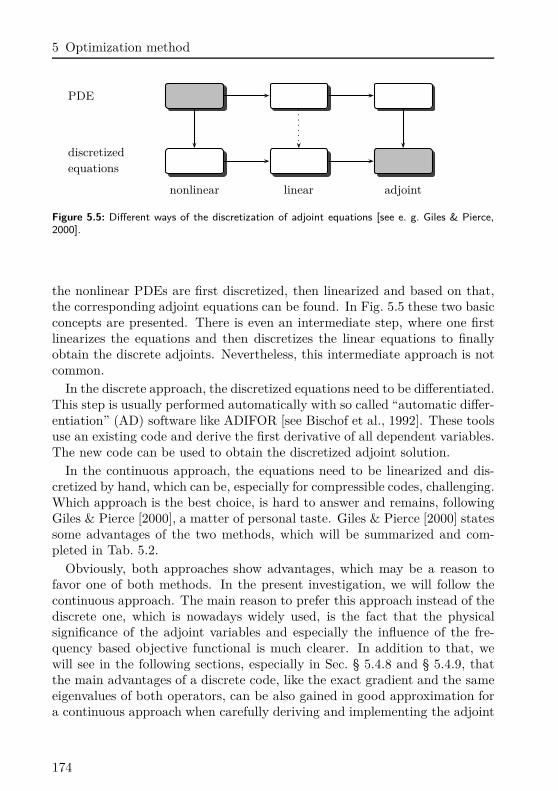
5 Optimization method
PDE
discretized
equations
nonlinear linear adjoint
Figure 5.5: Different ways of the discretization of adjoint equations [see e. g. Giles & Pierce,2000].
the nonlinear PDEs are first discretized, then linearized and based on that,the corresponding adjoint equations can be found. In Fig. 5.5 these two basicconcepts are presented. There is even an intermediate step, where one firstlinearizes the equations and then discretizes the linear equations to finallyobtain the discrete adjoints. Nevertheless, this intermediate approach is notcommon.
In the discrete approach, the discretized equations need to be differentiated.This step is usually performed automatically with so called “automatic differ-entiation” (AD) software like ADIFOR [see Bischof et al., 1992]. These toolsuse an existing code and derive the first derivative of all dependent variables.The new code can be used to obtain the discretized adjoint solution.
In the continuous approach, the equations need to be linearized and dis-cretized by hand, which can be, especially for compressible codes, challenging.Which approach is the best choice, is hard to answer and remains, followingGiles & Pierce [2000], a matter of personal taste. Giles & Pierce [2000] statessome advantages of the two methods, which will be summarized and com-pleted in Tab. 5.2.
Obviously, both approaches show advantages, which may be a reason tofavor one of both methods. In the present investigation, we will follow thecontinuous approach. The main reason to prefer this approach instead of thediscrete one, which is nowadays widely used, is the fact that the physicalsignificance of the adjoint variables and especially the influence of the fre-quency based objective functional is much clearer. In addition to that, wewill see in the following sections, especially in Sec. § 5.4.8 and § 5.4.9, thatthe main advantages of a discrete code, like the exact gradient and the sameeigenvalues of both operators, can be also gained in good approximation fora continuous approach when carefully deriving and implementing the adjoint
174
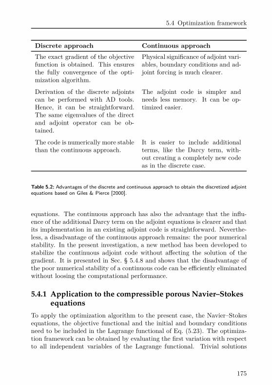
5.4 Optimization framework
Discrete approach Continuous approach
The exact gradient of the objectivefunction is obtained. This ensuresthe fully convergence of the opti-mization algorithm.
Physical significance of adjoint vari-ables, boundary conditions and ad-joint forcing is much clearer.
Derivation of the discrete adjointscan be performed with AD tools.Hence, it can be straightforward.The same eigenvalues of the directand adjoint operator can be ob-tained.
The adjoint code is simpler andneeds less memory. It can be op-timized easier.
The code is numerically more stablethan the continuous approach.
It is easier to include additionalterms, like the Darcy term, with-out creating a completely new codeas in the discrete case.
Table 5.2: Advantages of the discrete and continuous approach to obtain the discretized adjointequations based on Giles & Pierce [2000].
equations. The continuous approach has also the advantage that the influ-ence of the additional Darcy term on the adjoint equations is clearer and thatits implementation in an existing adjoint code is straightforward. Neverthe-less, a disadvantage of the continuous approach remains: the poor numericalstability. In the present investigation, a new method has been developed tostabilize the continuous adjoint code without affecting the solution of thegradient. It is presented in Sec. § 5.4.8 and shows that the disadvantage ofthe poor numerical stability of a continuous code can be efficiently eliminatedwithout loosing the computational performance.
5.4.1 Application to the compressible porous Navier–Stokesequations
To apply the optimization algorithm to the present case, the Navier–Stokesequations, the objective functional and the initial and boundary conditionsneed to be included in the Lagrange functional of Eq. (5.23). The optimiza-tion framework can be obtained by evaluating the first variation with respectto all independent variables of the Lagrange functional. Trivial solutions
175
5 Optimization method
arise for the variation with respect to the adjoint variables, q⋆, h⋆ and g⋆,corresponding to Eq. (5.25a), (5.25b) and (5.25c). As a result, one obtainsthe direct equation and the boundary and initial conditions. These relationsare already present and nothing else has to be done at this step. More efforthas to be exerted to determine the equations stemming from the first varia-tions with respect to the direct state q and the control K, corresponding toEq. (5.25d) and (5.25e). The first variation of the Lagrange functional withrespect to the control yields an expression for the gradient. Its derivation ispresented in Sec. § 5.4.3. The first variation of the Lagrange functional withrespect to the direct state yields an evolution equation for the adjoint stateand the corresponding boundary conditions. It reads:
∂L∂q
δq = ∂J
∂qδq
²1
+(∂G
∂qδq, g⋆)
´¹¹¹¹¹¹¹¹¹¹¹¹¹¹¹¹¹¹¹¹¹¹¹¹¹¹¹¹¸¹¹¹¹¹¹¹¹¹¹¹¹¹¹¹¹¹¹¹¹¹¹¹¹¹¹¹¹¶2
− [∂H
∂qδq, h⋆]
´¹¹¹¹¹¹¹¹¹¹¹¹¹¹¹¹¹¹¹¹¹¹¹¹¹¹¹¹¹¸¹¹¹¹¹¹¹¹¹¹¹¹¹¹¹¹¹¹¹¹¹¹¹¹¹¹¹¹¶3
− ⟨∂N∂q
δq, q⋆⟩´¹¹¹¹¹¹¹¹¹¹¹¹¹¹¹¹¹¹¹¹¹¹¹¹¹¹¹¹¹¸¹¹¹¹¹¹¹¹¹¹¹¹¹¹¹¹¹¹¹¹¹¹¹¹¹¹¹¹¶
4
= 0 (5.26)
Each term of Eq. (5.26) can be treated separately. The first term 1 , thevariation of the objective function, yields a source term for the adjoint equa-tions. It forces the adjoint state, while it is integrated backwards in time.Its derivation is presented in Sec. § 5.4.1.3. The second 2 and the thirdterm 3 will result in the adjoint boundary and terminal condition. Theyare summarized in Sec. § 5.4.2. Finally, the fourth term 4 yields an expres-sion for the unforced adjoint Navier–Stokes equations. The variation of theindividual terms corresponds to a linearization, followed by an integration byparts. Hence, the variation of the fourth term can be accomplished in twosteps. First, by linearizing the direct nonlinear equation and, secondly, by in-tegrating the linearized equation by parts. These two steps are presented forthe nonlinear compressible Navier–Stokes equations in the following section.
5.4.1.1 Adjoint Navier–Stokes equations
In a common notation, the Navier–Stokes equations cover the conservationof mass, momentum and energy. Nevertheless, the basic formulation of thesethree equations is not closed. Additional information on the specific proper-ties of the fluid needs to be included to close the system of equations. Threeadditional algebraic equations for the density, the temperature and the vis-cosity are necessary (see Sec. § 3.1). Hence, a total of eight coupled equationsare necessary to define the closed system. In the present three-dimensionalapplication they can be included in one state vector: q = [p u v w s ρ T µ]T .
When we derive the adjoint equations, we need to transpose the wholeclosed system including the three algebraic equations. To this end, in the
176
5.4 Optimization framework
following linearization and the subsequent integration by parts, the dimensionof the system is always eight.
Without simplifications, like, e.g., a constant viscosity (µ = const.) orsetting Φ = 0 which is a commonplace [see e. g. Cervino et al., 2002, Col-lis et al., 2002b, Spagnoli & Airiau, 2008, Wei & Freund, 2006], the lin-earized compressible and porous Navier–Stokes equations can be writtenin matrix formulation. With the variation of the state vector componentsδq = [δp δu δv δw δs δρ δT δµ]T , we have
B∂δq
∂t+Ak
∂δq
∂xk
+Dij
∂2δq
∂xi∂xj
+Cδq = 0 (5.27)
The matrices can be found in the appendix in Sec. § B on page 261.Based on the linearized matrix formulation, we give an expression for the
term in the tilted brackets. With the scalar product of Eq. (5.24a) we get:
⟨∂N (q, K)∂q
δq, q⋆⟩ =t1
∫t0
∫Ω
∂δqT
∂tBT q⋆ +
∂δqT
∂xk
ATk q⋆ +
∂2δqT
∂xi∂xj
DTijq⋆ + δqT CT q⋆ dΩdt
(5.28)
The dimension of the adjoint state q⋆ is consequently the same as for thedirect state q and it can be given as q⋆ = [p⋆ u⋆ v⋆ w⋆ s⋆ ρ⋆ T ⋆ µ⋆]T withthe adjoint pressure, the adjoint velocities, the adjoint entropy, the adjointdensity, the adjoint temperature and the adjoint viscosity.
After integration by parts and the fact, that the variation δqT is arbitrary,the unforced adjoint equations read:
−∂
∂t(BT q⋆) − ∂
∂xk
(ATk q⋆) + ∂2
∂xi∂xj
(DTijq⋆) +CT q⋆ = 0. (5.29)
Due to the integration by parts, the signs of the first partial derivatives changewhile they keep unchanged for the second derivatives and the source term.The negative sign of the temporal derivative forces us to integrate the adjointequations backwards in time to guarantee a numerically stable solution. Dur-ing the integration by parts, the additional boundary conditions define theadjoint boundary and initial conditions. They will be addressed separatelyin Sec. § 5.4.2. Despite the boundary conditions, the adjoint Navier–Stokes
177
5 Optimization method
equations are not complete, yet. The first variation of the objective func-tion with respect to the direct state will contribute as a forcing/source termto the equations and drive the solution backwards in time. The specificrole of the frequency based objective function will be discussed separately inSec. § 5.4.1.3.
Above matrix formulation can be expanded in separate equations leadingto a set of adjoint PDEs. A total of eight equations will arise as the dimensionof the square matrices in Eq. (5.29) is eight. Five PDEs, one for the adjointpressure, three for each adjoint velocity component and one for the adjointentropy. The additional three algebraic equations, the adjoint density, adjointtemperature and adjoint viscosity close the system of equations. The fivePDEs read:
∂p⋆
∂t= −ui
∂p⋆
∂xi
−1
ρ
∂ui⋆
∂xi
+Θpe +Θ
pf+Θp
p (5.30a)
∂ui⋆
∂t= −uj
∂ui⋆
∂xj
− γp∂p⋆
∂xi
+Θui
e +Θui
f +Θui
p (5.30b)
∂s⋆
∂t= −ui
∂s⋆
∂xi
+p
Cv
(∂p⋆
∂t+ ui
∂p⋆
∂xi
) +Θse +Θs
f +Θsp (5.30c)
The abbreviation for the adjoint sources can be split into three contributions,an Euler part without friction Θα
e , a friction-dependent part Θαf and a part
arising from the porous terms Θαp , where α can be one of p, ui or s. Depend-
ing on the application, some source terms might be omitted, e. g. the termrelated to the porous Navier–Stokes equations (Θα
p ) when no porous materialis concidered.
The explicit form of the adjoint source terms is given as follows:
Friction independent adjoint sources
Θpe ∶= −((1 − γ)∂uj
∂xj
+1
Cv
(∂s
∂t+ uj
∂s
∂xj
))p⋆ + ( 1
ρ2
∂ρ
∂xj
)uj⋆
Θui
e ∶= −((γ − 1) ∂p
∂xi
+p
Cv
∂s
∂xi
)p⋆ −∂uj
∂xj
ui⋆ +
∂uj
∂xi
uj⋆ +
∂s
∂xi
s⋆
Θse ∶= 1
Cv
(∂p
∂t+
∂(puj)∂xj
)p⋆ −∂uj
∂xj
s⋆
178
5.4 Optimization framework
Friction dependent adjoint sources
Θpf∶= −
1
c2ρ⋆ −
1
ρRT ⋆
Θui
f∶= 2
∂
∂xj
(τij⋆
ρ) − ∂2
∂x2j
(µ
ui⋆) − ∂2
∂xi∂xj
(1
3
µ
uj⋆) + 2
∂
∂xj
( τij
ρTs⋆)
Θsf ∶= p
c2Cv
ρ⋆
with the further abbreviations
τij⋆ ∶= 2(sij
⋆ −1
3skk⋆δij)
sij⋆ ∶= 1
2( ∂µ
∂xi
uj⋆ +
∂µ
∂xj
ui⋆) .
Porous dependent adjoint sources
Θpp ∶= 0
Θui
p ∶= µ
ρφ(K−1)
ijuj⋆ − 2
µ
ρφT(K−1)
ijujs⋆
−(R
φ
∂φ
∂xi
+ 2µ
ρφT(K−1)
ijuj) s⋆
Θsp ∶= 0
Three additional algebraic equations, the adjoint density, temperature andviscosity need to be introduced to close the system of adjoint equations (alsoobtained by Eq. (5.28)). For the sake of clearness, the porous terms arediscussed in an extra term (⋅)p. We obtain the following expressions:
Adjoint density
ρ⋆ = −1
ρ2(− ∂p
∂xi
+∂τij
∂xj
)ui⋆
−1
ρ2T( ∂
∂xj
(λ ∂T
∂xj
) +Φ) s⋆ −T
ρT ⋆ + ρp
⋆ (5.31)
ρp⋆ ∶= µ
ρ2φ(K−1)
ijujui
⋆ −µ
ρ2φT(K−1)
ijuiujs⋆
179
5 Optimization method
Adjoint temperature
T ⋆ = ∂
∂xk
(− 1
ρT
∂λ
∂xk
s⋆) − 1
ρT 2( ∂
∂xj
(λ ∂T
∂xj
) +Φ) s⋆
−∂2
∂x2j
(− λ
ρTs⋆) + dµ(T )
dTµ⋆ + Tp
⋆ (5.32)
Tp⋆ ∶= −
µ
ρφT 2(K−1)
ijuiujs⋆
Adjoint viscosity
µ⋆ = ∂
∂xi
(−τij
µρuj⋆) + ∂
∂xi
(− Cp
P rρT
∂T
∂xi
s⋆)+
1
ρ( ∂
∂xj
(τij
µ)ui
⋆)+( Cp
P rρT
∂2T
∂x2j
+Φ
ρT µ)s⋆ + µp
⋆ (5.33)
µp⋆ ∶= −
1
ρφ(K−1)
ijujui
⋆ +1
ρφT(K−1)
ijuiujs⋆
Now, one can see that the adjoint equations are a function of the directstate q. Therefore, the direct state has to be saved throughout the forwardcomputation. Remarks on that topic are given later. Due to the linearizationand the subsequent integration by parts a large number of source terms arisewhich makes the implementation a challenging task. This fact is the reasonwhy it is a commonplace to use simplifications during the linearization, likesetting µ = const. or Φ = 0. Nevertheless, these simplifications will result in awrong gradient. Its impact on the gradient and finally on the solution of theoptimum is not clear and hence will not be used in the present investigation.
Despite the challenging implementation of the large number of source terms,they can lead to a bad condition of the overall system and finally lead tonumerical instabilities. A method to deal with these numerical issues is pre-sented in Sec. § 5.4.8.1.
5.4.1.2 Characteristic formulation
The direct Navier–Stokes equations are written in a characteristic formula-tion of Sesterhenn [2000]. In a continuous adjoint approach it is important to
180
5.4 Optimization framework
use the same numerical method for the direct and for the adjoint computa-tion. To this end, the adjoint Navier–Stokes equations are also decomposedinto characteristic waves. A detailed derivation is given in the appendix inSec. § C.
In three-dimensional space, the adjoint Navier–Stoles equations includingporous media can be written in a characteristic formulation:
∂p⋆
∂t= −
1
2ρc((X+⋆ +X−
⋆) + (Y +⋆ + Y −⋆) + (Z+⋆ +Z−
⋆))+Θp
e +Θpf+Θp
p (5.34a)
∂u⋆
∂t= 1
2(X+⋆ −X−
⋆) + Y u⋆ +Zu⋆ +Θue +Θu
f +Θup (5.34b)
∂v⋆
∂t= Xv⋆ +
1
2(Y +⋆ − Y −
⋆) +Zv⋆ +Θve +Θv
f +Θvp (5.34c)
∂w⋆
∂t= Xw⋆ + Y w⋆ +
1
2(Z+⋆ −Z−
⋆) +Θwe +Θw
f +Θwp (5.34d)
∂s⋆
∂t= Xs⋆ + Y s⋆ +Zs⋆ +
p
Cv
∂p⋆
∂t+Θs
e +Θsf +Θs
p (5.34e)
with the following abbreviation:
Xv⋆ ∶= −u∂v⋆
∂x(5.35a)
Y u⋆ ∶= −v∂u⋆
∂y(5.35b)
Zu⋆ ∶= −w∂u⋆
∂z(5.35c)
Xw⋆ ∶= −u∂w⋆
∂x(5.36a)
Y w⋆ ∶= −u∂w⋆
∂y(5.36b)
Zv⋆ ∶= −u∂v⋆
∂z(5.36c)
X±⋆∶= (−u ± c)(−ρc
∂p⋆
∂x±
∂u⋆
∂x) (5.37a)
Y ±⋆∶= (−v ± c)(−ρc
∂p⋆
∂y±
∂v⋆
∂y) (5.37b)
Z±⋆∶= (−w ± c)(−ρc
∂p⋆
∂z±
∂w⋆
∂z) (5.37c)
181
5 Optimization method
Xs⋆ ∶= u( p
Cv
∂p⋆
∂x−
∂s⋆
∂x) (5.38a)
Y s⋆ ∶= v ( p
Cv
∂p⋆
∂y−
∂s⋆
∂y) (5.38b)
Zs⋆ ∶= w ( p
Cv
∂p⋆
∂z−
∂s⋆
∂z) (5.38c)
In the same way as for the direct Navier–Stokes equations the adjoint Navier–Stokes equations can be derived for curvilinear grids. They are presented inthe appendix in Sec. § C.
5.4.1.3 Adjoint forcing
As mentioned already, the adjoint Navier–Stokes equations are not complete,yet. The forcing term, which accounts for the specific structure of the objec-tive functional is missing. Its origin lies in the first variation of the objectivefunctional with respect to the direct state. It is the first term 1 of Eq. (5.26).Due to the uncommon frequency based structure, its derivation and interpre-tation is discussed in detail in the following. The corresponding term reads:
∂J(q)∂q
δq = ∫Ω
ωu
∫ωl
(λ1Fp′Fδp′ − λ2Ftp′Ftδp′)M(x)dω dΩ
We need to factor the variation of the state out of above equation. To thisend we include the definition of the Fourier transform in a next step and getfor the right hand side:
∫Ω
ωu
∫ωl
⎛⎝λ1Fp′
∞
∫−∞
e−iωtδp′ dt − λ2Ftp′∞
∫−∞
e−iωttδp′ dt⎞⎠M(x)dω dΩ
Now, the order of the integration can be changed and if we assume that thestate and its variation is only existing during the simulation time t ∈ [t0, t1]and zero elsewhere, we can define the following transformation:
∞
∫−∞
p′ dt =t1
∫t0
p′ dt, if p′(t) =⎧⎪⎪⎪⎨⎪⎪⎪⎩
0, t < t0
p′, t0 ≤ t ≤ t1
0, t > t1
.
182
5.4 Optimization framework
Finally, after some rearrangement we get:
∫Ω
t1
∫t0
ωu
∫ωl
(λ1Fp′e−iωtδp′ − λ2Ftp′e−iωttδp′)M(x)dω dt dΩ.
To clarify the meaning of this term, an abbreviation can be defined andincluded in the relation above. We get:
∫Ω
t1
∫t0
(λ1F−1 Fp′∣ωu
ωl
− λ2F−1 Ftp′∣ωu
ωl
t)M(x)δp′ dt dΩ. (5.39)
with the definition of the abbreviation:
F−1 Fp′∣ωu
ωl
=ωu
∫ωl
Fp′e−iωt dω =∞
∫−∞
Fp′ ⋅ T (ω)e−iωt dω (5.40)
Now, this introduced abbreviation is nothing else as a filter with the filterfunction T (ω) and the inverse Fourier transform F−1. The shape of the filterfunction is a top-hat filter with:
T (ω) =⎧⎪⎪⎪⎨⎪⎪⎪⎩
0, ω < ωl
1, ωl ≤ ω ≤ ωu
0, ω > ωu
(5.41)
It can be regarded as a band-pass filter for the quantity p′ (here the pressure).Equation (5.40) and Eq. (5.28) can be added, as both terms appear in thevariation of the Lagrange function with respect to the state and both termsare integrands of the same double integral. To this end, the forcing of theadjoint Navier–Stokes equations can be written as:
N∑k=0
(λ1,kF−1 Fp′∣ωu,k
ωl,k
− λ2,kF−1 Ftp′∣ωu,k
ωl,k
t)M(x) (5.42)
It is a source term, acting on the right hand side of the adjoint pressure equa-tion (5.30a). It is forcing the equation with the band-passed pressure signal.The latter one is measured during the forward computation and applied back-wards in time with the spatial distribution M(x). With the introduction ofthe sum in the forcing of the right hand side, we can account for N distinctbands with different frequency ranges ωl,k ≤ ω ≤ ωu,k and individual weightsλ1,k and λ2,k, corresponding to the objective function (5.20).
183
5 Optimization method
5.4.2 Adjoint boundary- and terminal-condition
The boundary conditions can be derived by carefully evaluating the two partsmarked with a 2 and 3 of the first variation of the Lagrange functional withrespect to the direct state (5.26). In addition to that, additional terms ariseas a result of the integration by parts of the remaining terms. These termscan be combined and form the adjoint boundary conditions in space and theadjoint initial (terminal) condition in time.
5.4.2.1 Adjoint terminal condition
In the adjoint case, the terminal condition at t = T is the initial condition,as the adjoint equations are solved backwards in time. The specific characterof the adjoint terminal condition depends on the definition of the objectivefunction J . It can be either zero or reach any other state, depending on J .If J is, e. g. an integral over the whole simulation time t ∈ [0, T ], then theterminal condition will be zero. If the objective function is defined only atthe terminal condition, like in cases where the objective is the minimizationof the terminal kinetic energy, then the terminal condition will reach somestate unequal to zero. These relations can be easily proven with a simpleexample.
In the present case, the objective function is an integral in time and itsinfluence on the adjoint equation is a source term rather than a terminalcondition. To this end, the terminal condition for the adjoint computation iszero:
q⋆(x, T ) = 0. (5.43)
with the adjoint state q⋆ at the terminal time.Several numerical boundary conditions are implemented to treat the aeroa-
coustic application properly. Each boundary condition for the direct compu-tation needs a corresponding adjoint boundary condition. In the following,three boundary conditions are presented: the adjoint sponge in Sec. § 5.4.2.2,a non-reflecting boundary in Sec. § 5.4.2.3 and an adiabatic wall boundaryin Sec. § 5.4.2.4.
5.4.2.2 Sponge boundary condition
An easy but efficient way of implementing a boundary condition in the directand adjoint case, is a sponge (see Sec. § 2.4.3.2). This boundary conditionis a linear source term and can be implemented in a similar way as for the
184
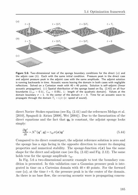
5.4 Optimization framework
(a)t = 0 t = 1/3TL t = 2/3TL t = TL
(b)t = TL t = 2/3TL t = 1/3TL t = 0
(c)
Figure 5.6: Two–dimensional test of the sponge boundary conditions for the direct (a) andthe adjoin case (b). Each with the same initial condition. Pressure peak in the direct caseand adjoint pressure peak in the adjoint case with the same amplitude. The adjoint solutionis running backwards in time. Acoustic waves leaving the domain in both cases with negligiblereflections. Solved on a Cartesian mesh with 40 × 40 points. Solution is self–adjoint (linearacoustic propagation). (c) Spatial distribution of the sponge based on Eq. (2.42) on all fourboundaries (Lsp = 0.1L, Csp = 0.05L, L: length of the quadratic domain). Values at thedomain boundary σ = 1. In the center of the domain σ = 0. Time for an acoustic wave topropagate through the domain TL = L/c (c : speed of sound).
direct Navier–Stokes equations (see Eq. (2.41) and the references Meliga et al.[2010], Spagnoli & Airiau [2008], Wei [2004]). Due to the linearization of thedirect equations and the fact that q0 is constant, the adjoint sponge lookssimply:
∂q⋆
∂t= N ⋆(q⋆, q) + τspσ(x)q⋆ (5.44)
Compared to its direct counterpart, the adjoint reference solution is zero andthe sponge has a sign facing in the opposite direction to ensure its dampingproperties and numerical stability. The sponge-function σ(x) has the sameshape for the direct and adjoint case (see Eq. (2.42) and Fig. 2.12). The sameholds true for the sponge amplitude τsp.
In Fig. 5.6 a two-dimensional acoustic example to test the boundary con-dition is presented. In this validation case a Gaussian pressure peak is inte-grated in time on a Cartesian domain with 40 × 40 points. For the forwardcase (a), at the time t = 0, the pressure peak is in the center of the domain.As there is no base flow, the occurring acoustic wave is propagating concen-
185
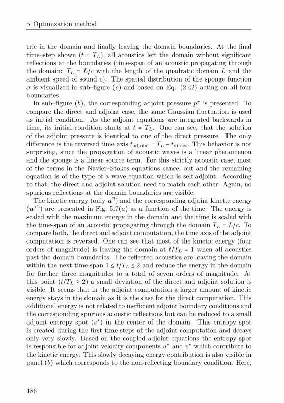
5 Optimization method
tric in the domain and finally leaving the domain boundaries. At the finaltime–step shown (t = TL), all acoustics left the domain without significantreflections at the boundaries (time-span of an acoustic propagating throughthe domain: TL = L/c with the length of the quadratic domain L and theambient speed of sound c). The spatial distribution of the sponge functionσ is visualized in sub–figure (c) and based on Eq. (2.42) acting on all fourboundaries.
In sub–figure (b), the corresponding adjoint pressure p⋆ is presented. Tocompare the direct and adjoint case, the same Gaussian fluctuation is usedas initial condition. As the adjoint equations are integrated backwards intime, its initial condition starts at t = TL. One can see, that the solutionof the adjoint pressure is identical to one of the direct pressure. The onlydifference is the reversed time axis tadjoint = TL − tdirect. This behavior is notsurprising, since the propagation of acoustic waves is a linear phenomenonand the sponge is a linear source term. For this strictly acoustic case, mostof the terms in the Navier–Stokes equations cancel out and the remainingequation is of the type of a wave equation which is self-adjoint. Accordingto that, the direct and adjoint solution need to match each other. Again, nospurious reflections at the domain boundaries are visible.
The kinetic energy (only u2) and the corresponding adjoint kinetic energy(u⋆2) are presented in Fig. 5.7(a) as a function of the time. The energy isscaled with the maximum energy in the domain and the time is scaled withthe time-span of an acoustic propagating through the domain TL = L/c. Tocompare both, the direct and adjoint computation, the time axis of the adjointcomputation is reversed. One can see that most of the kinetic energy (fourorders of magnitude) is leaving the domain at t/TL = 1 when all acousticspast the domain boundaries. The reflected acoustics are leaving the domainwithin the next time-span 1 ≤ t/TL ≤ 2 and reduce the energy in the domainfor further three magnitudes to a total of seven orders of magnitude. Atthis point (t/TL ≥ 2) a small deviation of the direct and adjoint solution isvisible. It seems that in the adjoint computation a larger amount of kineticenergy stays in the domain as it is the case for the direct computation. Thisadditional energy is not related to inefficient adjoint boundary conditions andthe corresponding spurious acoustic reflections but can be reduced to a smalladjoint entropy spot (s⋆) in the center of the domain. This entropy spotis created during the first time-steps of the adjoint computation and decaysonly very slowly. Based on the coupled adjoint equations the entropy spotis responsible for adjoint velocity components u⋆ and v⋆ which contribute tothe kinetic energy. This slowly decaying energy contribution is also visible inpanel (b) which corresponds to the non-reflecting boundary condition. Here,
186
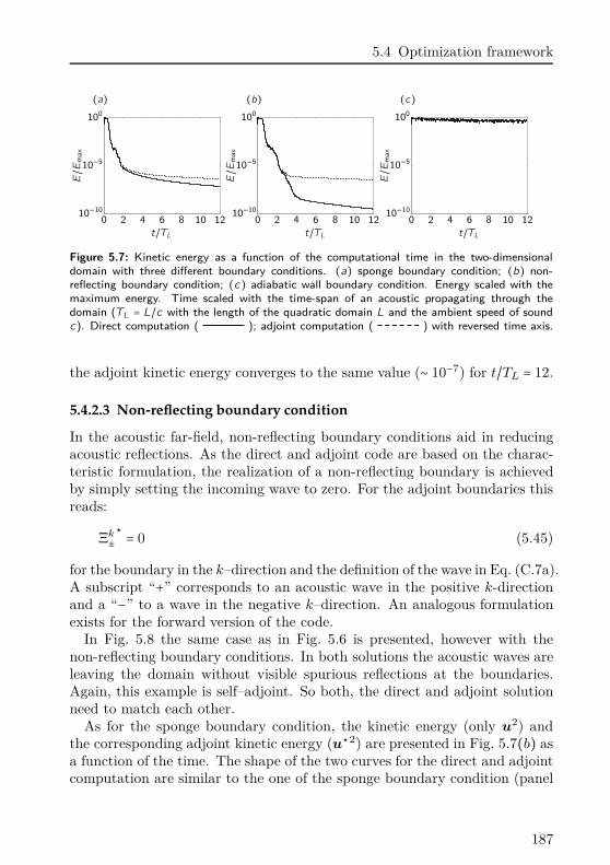
5.4 Optimization framework
(a) (b) (c)E/E
max
t/TL0 2 4 6 8 10 12
10−10
10−5
100
E/E
max
t/TL0 2 4 6 8 10 12
10−10
10−5
100
E/E
max
t/TL0 2 4 6 8 10 12
10−10
10−5
100
Figure 5.7: Kinetic energy as a function of the computational time in the two-dimensionaldomain with three different boundary conditions. (a) sponge boundary condition; (b) non-reflecting boundary condition; (c) adiabatic wall boundary condition. Energy scaled with themaximum energy. Time scaled with the time-span of an acoustic propagating through thedomain (TL = L/c with the length of the quadratic domain L and the ambient speed of soundc). Direct computation ( ); adjoint computation ( ) with reversed time axis.
the adjoint kinetic energy converges to the same value (∼ 10−7) for t/TL = 12.
5.4.2.3 Non-reflecting boundary condition
In the acoustic far-field, non-reflecting boundary conditions aid in reducingacoustic reflections. As the direct and adjoint code are based on the charac-teristic formulation, the realization of a non-reflecting boundary is achievedby simply setting the incoming wave to zero. For the adjoint boundaries thisreads:
Ξk±
⋆ = 0 (5.45)
for the boundary in the k–direction and the definition of the wave in Eq. (C.7a).A subscript “+” corresponds to an acoustic wave in the positive k-directionand a “−” to a wave in the negative k–direction. An analogous formulationexists for the forward version of the code.
In Fig. 5.8 the same case as in Fig. 5.6 is presented, however with thenon-reflecting boundary conditions. In both solutions the acoustic waves areleaving the domain without visible spurious reflections at the boundaries.Again, this example is self–adjoint. So both, the direct and adjoint solutionneed to match each other.
As for the sponge boundary condition, the kinetic energy (only u2) andthe corresponding adjoint kinetic energy (u⋆2) are presented in Fig. 5.7(b) asa function of the time. The shape of the two curves for the direct and adjointcomputation are similar to the one of the sponge boundary condition (panel
187
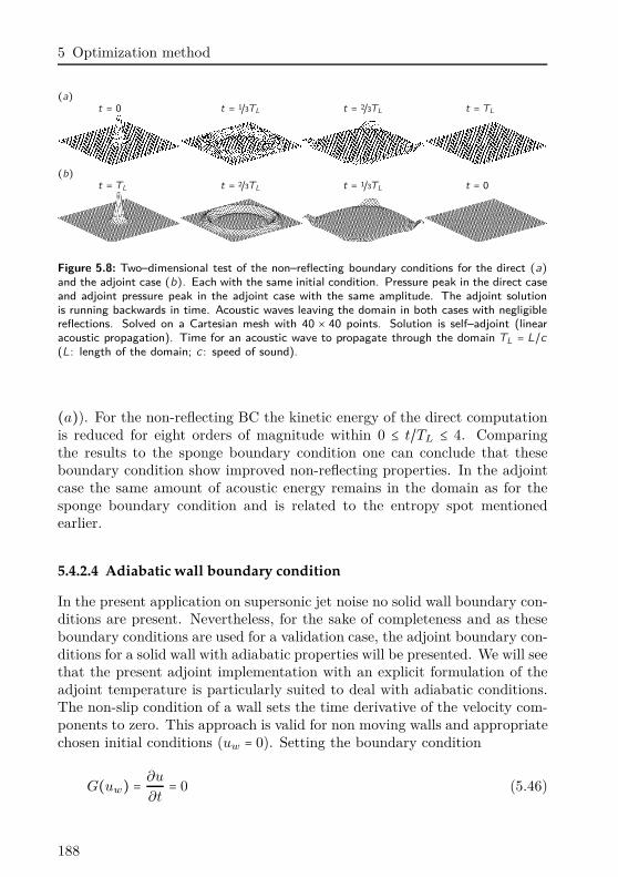
5 Optimization method
(a)t = 0 t = 1/3TL t = 2/3TL t = TL
(b)t = TL t = 2/3TL t = 1/3TL t = 0
Figure 5.8: Two–dimensional test of the non–reflecting boundary conditions for the direct (a)and the adjoint case (b). Each with the same initial condition. Pressure peak in the direct caseand adjoint pressure peak in the adjoint case with the same amplitude. The adjoint solutionis running backwards in time. Acoustic waves leaving the domain in both cases with negligiblereflections. Solved on a Cartesian mesh with 40 × 40 points. Solution is self–adjoint (linearacoustic propagation). Time for an acoustic wave to propagate through the domain TL = L/c(L: length of the domain; c : speed of sound).
(a)). For the non-reflecting BC the kinetic energy of the direct computationis reduced for eight orders of magnitude within 0 ≤ t/TL ≤ 4. Comparingthe results to the sponge boundary condition one can conclude that theseboundary condition show improved non-reflecting properties. In the adjointcase the same amount of acoustic energy remains in the domain as for thesponge boundary condition and is related to the entropy spot mentionedearlier.
5.4.2.4 Adiabatic wall boundary condition
In the present application on supersonic jet noise no solid wall boundary con-ditions are present. Nevertheless, for the sake of completeness and as theseboundary conditions are used for a validation case, the adjoint boundary con-ditions for a solid wall with adiabatic properties will be presented. We will seethat the present adjoint implementation with an explicit formulation of theadjoint temperature is particularly suited to deal with adiabatic conditions.The non-slip condition of a wall sets the time derivative of the velocity com-ponents to zero. This approach is valid for non moving walls and appropriatechosen initial conditions (uw = 0). Setting the boundary condition
G(uw) = ∂u
∂t= 0 (5.46)
188
5.4 Optimization framework
in the Lagrangian one obtains an analogous condition for the correspondingadjoint boundary condition, namely:
∂u⋆
∂t∣w
= 0 (5.47)
for a wall at Xp and Xm, respectively. With this information and after somerearrangement of the adjoint equations one can obtain a formulation for theunknown waves at the boundaries:
• Wall at Xm
X+w⋆ =X−w
⋆− 2Y u
w⋆− 2Zu
w⋆− 2 (Θu
ew +Θufw +Θu
pw)Xv
w⋆ = 1
2(Y +w ⋆ − Y −w
⋆) +Zvw⋆−Θv
ew −Θvfw −Θv
pw
Xww⋆ = 1
2(Z+w⋆ −Z−w
⋆) + Y ww⋆−Θw
ew −Θwfw −Θw
pw
• Wall at Xp
X−w⋆ = −X+w
⋆+ 2Y u
w⋆+ 2Zu
w⋆+ 2 (Θu
ew +Θufw +Θu
pw)Xv
w⋆ = 1
2(Y +w ⋆ − Y −w
⋆) +Zvw⋆−Θv
ew −Θvfw −Θv
pw
Xww⋆ = 1
2(Z+w⋆ −Z−w
⋆) + Y ww⋆−Θw
ew −Θwfw −Θw
pw
Walls at the remaining two dimensions (y and z) can be applied in a similarway.
Adiabatic Wall For an adiabatic wall the temperature fluxes are zero:
∂T
∂n= 0 (5.48)
where n is the wall normal direction. Including this boundary condition inthe Lagrangian formulation one obtains the simple condition for the adjointtemperature:
Tw⋆ = 0 (5.49)
As we can see, the Neumann boundary condition for the direct case switchedto a Dirichlet boundary condition for the adjoint case. This is a typical be-havior for adjoint boundary condition. The implementation of this boundarycondition is, due to the use of the additional adjoint variable T ⋆, straightfor-ward. In Fig. 5.9 the same case as in Fig. 5.6 is presented, however with the
189
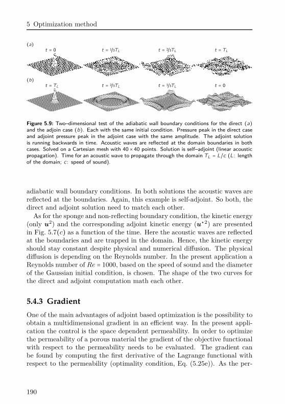
5 Optimization method
(a)t = 0 t = 1/3TL t = 2/3TL t = TL
(b)t = TL t = 2/3TL t = 1/3TL t = 0
Figure 5.9: Two–dimensional test of the adiabatic wall boundary conditions for the direct (a)and the adjoin case (b). Each with the same initial condition. Pressure peak in the direct caseand adjoint pressure peak in the adjoint case with the same amplitude. The adjoint solutionis running backwards in time. Acoustic waves are reflected at the domain boundaries in bothcases. Solved on a Cartesian mesh with 40 × 40 points. Solution is self–adjoint (linear acousticpropagation). Time for an acoustic wave to propagate through the domain TL = L/c (L: lengthof the domain; c : speed of sound).
adiabatic wall boundary conditions. In both solutions the acoustic waves arereflected at the boundaries. Again, this example is self-adjoint. So both, thedirect and adjoint solution need to match each other.
As for the sponge and non-reflecting boundary condition, the kinetic energy(only u2) and the corresponding adjoint kinetic energy (u⋆2) are presentedin Fig. 5.7(c) as a function of the time. Here the acoustic waves are reflectedat the boundaries and are trapped in the domain. Hence, the kinetic energyshould stay constant despite physical and numerical diffusion. The physicaldiffusion is depending on the Reynolds number. In the present application aReynolds number of Re = 1000, based on the speed of sound and the diameterof the Gaussian initial condition, is chosen. The shape of the two curves forthe direct and adjoint computation math each other.
5.4.3 Gradient
One of the main advantages of adjoint based optimization is the possibility toobtain a multidimensional gradient in an efficient way. In the present appli-cation the control is the space dependent permeability. In order to optimizethe permeability of a porous material the gradient of the objective functionalwith respect to the permeability needs to be evaluated. The gradient canbe found by computing the first derivative of the Lagrange functional withrespect to the permeability (optimality condition, Eq. (5.25e)). As the per-
190
5.4 Optimization framework
meability is a symmetric tensor K = κij , the gradient has to be derived foreach element of the tensor κij separately. We get:
∇κijL = − ⟨∇κij
N (q, K), q⋆⟩ . (5.50)
The gradient of the Lagrangian simply reduces to the gradient of the objectivefunctional [see e. g. Guegan et al., 2006], and we get:
∇κijJ = − ⟨∇κij
N (q, K), q⋆⟩ . (5.51)
Finally, after replacing N (q, K) by the porous Navier–Stokes equations ofSec. § 3.1 one obtains the gradient of the objective functional with respect tothe permeability:
∇κijJ = − [µ
ρuj , ui
⋆] + [ µ
ρTuiuj, s⋆] , (5.52)
with the scalar product defined in Eq. (5.24c) to obtain a space dependentgradient. Hence, both terms on the right hand side of Eq. (5.52) are integratedin time which corresponds to a time average. The first term is the scalarproduct of the direct and adjoint velocity components. It arises from theadjoint momentum equations. The second term is a scalar product of thedirect kinetic energy and the adjoint entropy. It has its origin in the adjointenergy equation.
As we will see in the next section, we can not use this gradient directly butneed to transform it to account for an inequality constraint.
5.4.4 Treating inequality constraints
In the present study, the control is the permeability of the porous material.This value can be positive or zero, only. A negative value of K would acceler-ate the fluid in the porous material which has no physical meaning. Besidesthat, positive eigenvalues would arise and cause numerical instabilities forthe time integration method. Thereby, the inequality condition (K ≥ 0) hasto be treated in a special way. One possibility is to use a projected gradi-ent method like for non–negative matrix factorization [see Lin, 2007]. Thistechnique truncates the gradient to satisfy the constraint, which is easy toimplement with the tradeoff of bad convergence. Another common approach,to treat inequality conditions properly, is to apply the optimization problemto the Sequential Quadratic Programming (SQP). This technique interpo-lates the objective function with a quadratic polynomial and linearizes the
191
5 Optimization method
constraints. In addition to that is uses the second derivative of the objec-tive function (Hessenberg matrix; usually approximated) in a Newton likeoptimization method. For a small number of optimization parameters thismethod is very efficient and, due to the variety of available implementations(MatLab1, NLPQLP2, and many others), straightforward to use. Anyway,as the approximation of the Hessenberg matrix is expensive, the method be-comes impractical if the problem is too large as in the present application[see Schittkowski, 2010].
A different approach is to transform the inequality condition into an equal-ity condition by introducing a so called slack variable S = (sij) [see e. g. Boyd& Vandenberghe, 2004], satisfying the following relation:
K = (κij) = (s2ij). (5.53)
Note, that S2 = (sij)2 ≠ (s2ij). The square in Eq. (5.53) is an element-wise
multiplication. In the following we will use the Hadamard product to notatethe element-wise product of two matrices: (s2
ij) = S S. In addition to thatthe permeability is space dependent and each element of the tensor is a vector.
Now, since S S is positive only, the inequality constraint can be rewrittento an equality constraint: K − S S = 0. By introducing an additional La-grange multiplier S⋆, this equality constraint can be added to the Lagrangefunctional of Eq. (5.23), with the following scalar product:
⟨κij − s2ij , sij
⋆⟩The aim of the optimization task has now changed in finding the optimalslack variable S instead of the optimal control K. So, K is replaced byS S and the gradient with respect to S has to be evaluated. Within theoptimization process, the slack variable is updated as in Eq. (5.58) and thenreplaced by Eq. (5.53). The gradient ∇sij
J is obtained by the first variationof the Lagrange functional with respect to the slack variable and reads:
∇sijL = − ⟨2sij , sij
⋆⟩ . (5.54)
In an optimal point, the variation of the Lagrange functional has to vanishand we obtain for the gradient:
∇sijJ = − ⟨2sij , sij
⋆⟩ . (5.55)
1http://www.mathworks.com2http://www.ai7.uni-bayreuth.de/nlpqlp.htm
192
5.4 Optimization framework
Including the variation of the Lagrange functional with respect to the controlK in Eq. (5.55) and the relation that
dJ
dsij
= ∂J
∂κij
dκij
dsij
,
the gradient with respect to the slack variable reads:
∇sijJ = − ⟨2sij∇κij
N (q, K), q⋆⟩ . (5.56)
With the gradient with respect to the permeability as defined in Eq. (5.52),we get:
∇sijJ = −2 [µ
ρsijuj, ui
⋆] + 2 [ µ
ρTsijuiuj , s⋆] . (5.57)
This gradient is used, within the optimization loop (Fig. 5.4), to computethe optimal distribution of porous media to minimize the objective function.Given that K = (κij) and S = (sij) are tensors, the gradient itself is a tensorand has to be evaluated pointwise. Each of the six elements of the symmetrictensor are in addition to that fields in space. Consequently, the number ofparameters to control can be easily in the order of 106.
Note, that the method of slack variables is equivalent to replacing K = SS
in the porous Navier–Stokes equations and then optimizing for S.
5.4.5 Steepest descent
The gradient of the objective function with respect to the control (here theslack variable due to the inequality constraint of the previous section) can beused in a simple steepest descent algorithm to compute a new set of controlvariables in an iterative way. We have
S(n+1) = S(n) −α(n) (∇sijJ)(n) . (5.58)
The gradient is defined in Eq. (5.57) and is itself a tensor. The positiveand scalar valued step-size α(n) has to be chosen carefully to avoid numericalinstabilities and to guarantee an efficient convergence. How to choose a properstep-size is outlined in Sec. § 5.4.7.
However, to improve the convergence properties and the robustness of theoptimization algorithm, a conjugate gradient (CG) algorithm is applied. Inthe following section the implemented CG methods are presented an validatedon a test function.
193
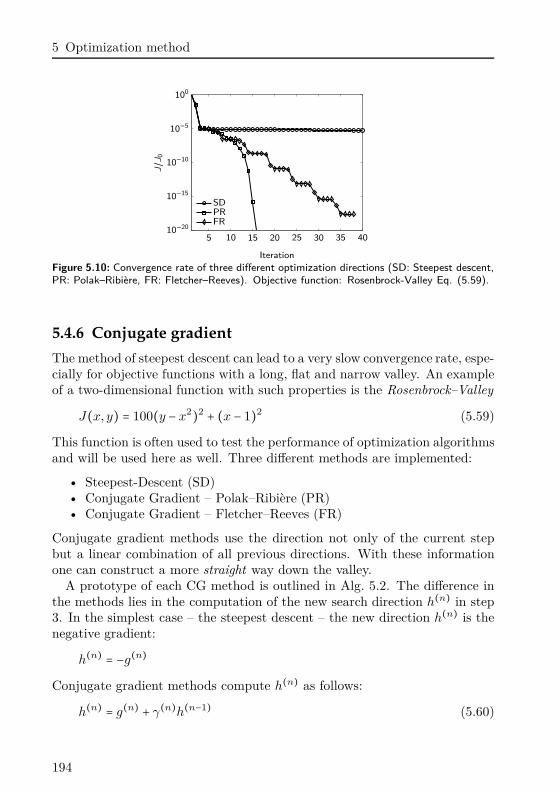
5 Optimization method
FRPRSD
J/J 0
Iteration
5 10 15 20 25 30 35 4010−20
10−15
10−10
10−5
100
Figure 5.10: Convergence rate of three different optimization directions (SD: Steepest descent,PR: Polak–Ribière, FR: Fletcher–Reeves). Objective function: Rosenbrock-Valley Eq. (5.59).
5.4.6 Conjugate gradient
The method of steepest descent can lead to a very slow convergence rate, espe-cially for objective functions with a long, flat and narrow valley. An exampleof a two-dimensional function with such properties is the Rosenbrock–Valley
J(x, y) = 100(y − x2)2 + (x − 1)2 (5.59)
This function is often used to test the performance of optimization algorithmsand will be used here as well. Three different methods are implemented:
• Steepest-Descent (SD)• Conjugate Gradient – Polak–Ribière (PR)• Conjugate Gradient – Fletcher–Reeves (FR)
Conjugate gradient methods use the direction not only of the current stepbut a linear combination of all previous directions. With these informationone can construct a more straight way down the valley.
A prototype of each CG method is outlined in Alg. 5.2. The difference inthe methods lies in the computation of the new search direction h(n) in step3. In the simplest case – the steepest descent – the new direction h(n) is thenegative gradient:
h(n) = −g(n)
Conjugate gradient methods compute h(n) as follows:
h(n) = g(n) + γ(n)h(n−1) (5.60)
194
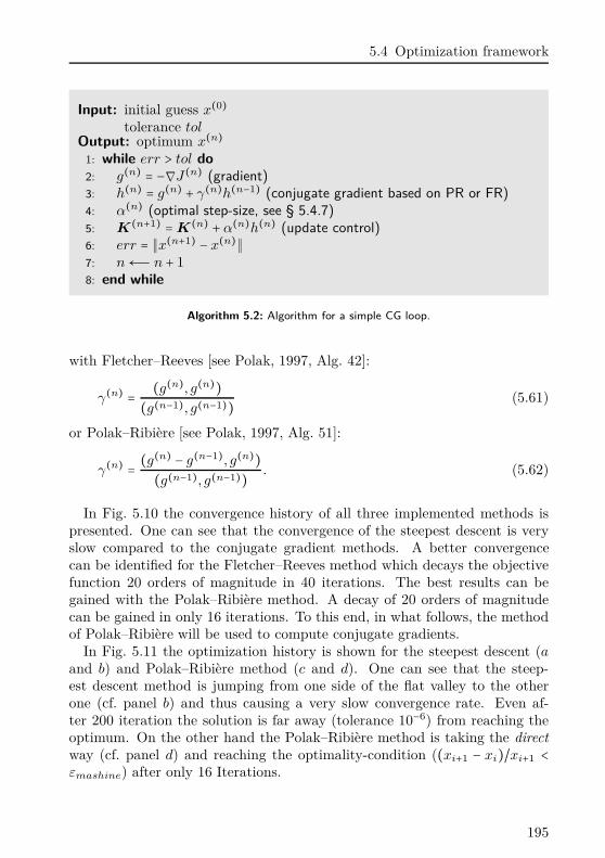
5.4 Optimization framework
Input: initial guess x(0)tolerance tol
Output: optimum x(n)1: while err > tol do2: g(n) = −∇J(n) (gradient)3: h(n) = g(n) + γ(n)h(n−1) (conjugate gradient based on PR or FR)4: α(n) (optimal step-size, see § 5.4.7)5: K(n+1) =K(n) +α(n)h(n) (update control)6: err = ∥x(n+1) − x(n)∥7: n←Ð n + 18: end while
Algorithm 5.2: Algorithm for a simple CG loop.
with Fletcher–Reeves [see Polak, 1997, Alg. 42]:
γ(n) = (g(n), g(n))(g(n−1), g(n−1)) (5.61)
or Polak–Ribière [see Polak, 1997, Alg. 51]:
γ(n) = (g(n) − g(n−1), g(n))(g(n−1), g(n−1)) . (5.62)
In Fig. 5.10 the convergence history of all three implemented methods ispresented. One can see that the convergence of the steepest descent is veryslow compared to the conjugate gradient methods. A better convergencecan be identified for the Fletcher–Reeves method which decays the objectivefunction 20 orders of magnitude in 40 iterations. The best results can begained with the Polak–Ribière method. A decay of 20 orders of magnitudecan be gained in only 16 iterations. To this end, in what follows, the methodof Polak–Ribière will be used to compute conjugate gradients.
In Fig. 5.11 the optimization history is shown for the steepest descent (aand b) and Polak–Ribière method (c and d). One can see that the steep-est descent method is jumping from one side of the flat valley to the otherone (cf. panel b) and thus causing a very slow convergence rate. Even af-ter 200 iteration the solution is far away (tolerance 10−6) from reaching theoptimum. On the other hand the Polak–Ribière method is taking the directway (cf. panel d) and reaching the optimality-condition ((xi+1 − xi)/xi+1 <εmashine) after only 16 Iterations.
195
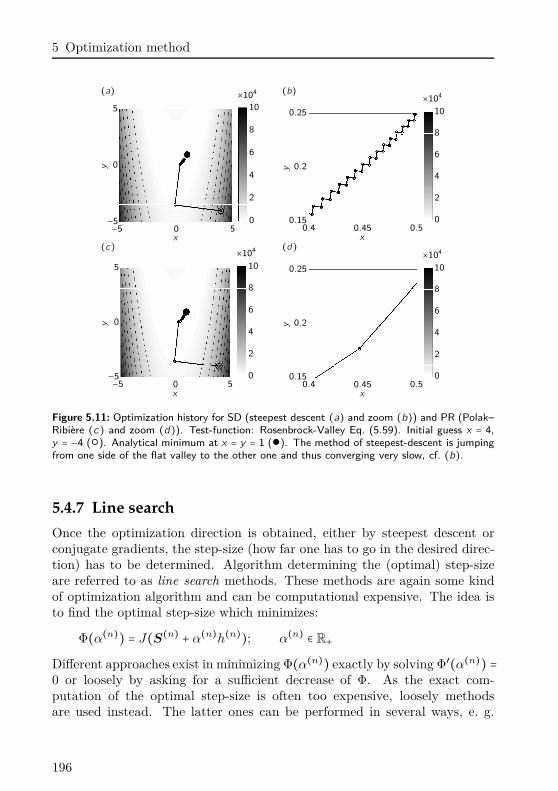
5 Optimization method
(a) (b)
y
x−5 0 5
×104
0
2
4
6
8
10
−5
0
5
y
x0.4 0.45 0.5
×104
0
2
4
6
8
10
0.15
0.2
0.25
(c) (d)
y
x−5 0 5
×104
0
2
4
6
8
10
−5
0
5
y
x0.4 0.45 0.5
×104
0
2
4
6
8
10
0.15
0.2
0.25
Figure 5.11: Optimization history for SD (steepest descent (a) and zoom (b)) and PR (Polak–Ribière (c) and zoom (d)). Test-function: Rosenbrock-Valley Eq. (5.59). Initial guess x = 4,y = −4 (). Analytical minimum at x = y = 1 (). The method of steepest-descent is jumpingfrom one side of the flat valley to the other one and thus converging very slow, cf. (b).
5.4.7 Line search
Once the optimization direction is obtained, either by steepest descent orconjugate gradients, the step-size (how far one has to go in the desired direc-tion) has to be determined. Algorithm determining the (optimal) step-sizeare referred to as line search methods. These methods are again some kindof optimization algorithm and can be computational expensive. The idea isto find the optimal step-size which minimizes:
Φ(α(n)) = J(S(n) + α(n)h(n)); α(n) ∈ R+Different approaches exist in minimizing Φ(α(n)) exactly by solving Φ′(α(n)) =0 or loosely by asking for a sufficient decrease of Φ. As the exact com-putation of the optimal step-size is often too expensive, loosely methodsare used instead. The latter ones can be performed in several ways, e. g.
196
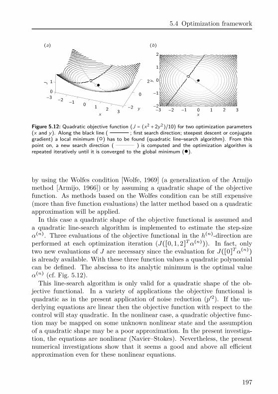
5.4 Optimization framework
(a) (b)J
y
x
−3−2
−10
12
3−2
0
2
0
1 y
x−3 −2 −1 0 1 2 3−2
−1
0
1
2
Figure 5.12: Quadratic objective function (J = (x2 + 2y2)/10) for two optimization parameters(x and y). Along the black line ( ; first search direction; steepest descent or conjugategradient) a local minimum () has to be found (quadratic line–search algorithm). From thispoint on, a new search direction ( ) is computed and the optimization algorithm isrepeated iteratively until it is converged to the global minimum ().
by using the Wolfes condition [Wolfe, 1969] (a generalization of the Armijomethod [Armijo, 1966]) or by assuming a quadratic shape of the objectivefunction. As methods based on the Wolfes condition can be still expensive(more than five function evaluations) the latter method based on a quadraticapproximation will be applied.
In this case a quadratic shape of the objective functional is assumed anda quadratic line-search algorithm is implemented to estimate the step-sizeα(n). Three evaluations of the objective functional in the h(n)-direction areperformed at each optimization iteration (J([0, 1, 2]T α(n))). In fact, onlytwo new evaluations of J are necessary since the evaluation for J([0]T α(n))is already available. With these three function values a quadratic polynomialcan be defined. The abscissa to its analytic minimum is the optimal valueα(n) (cf. Fig. 5.12).
This line-search algorithm is only valid for a quadratic shape of the ob-jective functional. In a variety of applications the objective functional isquadratic as in the present application of noise reduction (p′2). If the un-derlying equations are linear then the objective function with respect to thecontrol will stay quadratic. In the nonlinear case, a quadratic objective func-tion may be mapped on some unknown nonlinear state and the assumptionof a quadratic shape may be a poor approximation. In the present investiga-tion, the equations are nonlinear (Navier–Stokes). Nevertheless, the presentnumerical investigations show that it seems a good and above all efficientapproximation even for these nonlinear equations.
197
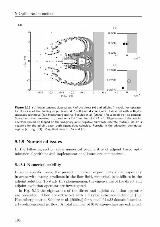
5 Optimization method
(a)Iλ⋅dt
Rλ ⋅ dt−0.5 −0.4 −0.3 −0.2 −0.1 0 0.1
−3
−2
−1
0
1
2
3
(b)
×10−4−1 0 1
0.2297
0.2298
0.2299
(c)
×10−5−1 0 1
0.22979
0.22980
0.22981
Figure 5.13: (a) Instantaneous eigenvalues λ of the direct () and adjoint () evolution operatorfor the case of the trailing edge, taken at t = 0 (initial condition). Extracted with a Krylovsubspace technique (full Hessenberg matrix, Schulze et al. [2009a]) for a small 64× 32 domain.Scaled with the time–step dt, based on a CFL number of CFL = 1. Eigenvalues of the adjointoperator should be flipped on the imaginary axis (negative transpose discrete matrix). As dt isnegative for the adjoint case, both eigenvalues coincide. Porosity in the advection dominatedregime (cf. Fig. 3.3). Magnified view in (b) and (c).
5.4.8 Numerical issues
In the following section some numerical peculiarities of adjoint based opti-mization algorithms and implementational issues are summarized.
5.4.8.1 Numerical stability
In some specific cases, the present numerical experiments show, especiallyin areas with strong gradients in the flow field, numerical instabilities in theadjoint solution. To study this phenomenon, the eigenvalues of the direct andadjoint evolution operator are investigated.
In Fig. 5.13 the eigenvalues of the direct and adjoint evolution operatorare presented. They are extracted with a Krylov subspace technique (fullHessenberg matrix, Schulze et al. [2009a]) for a small 64×32 domain based ona two-dimensional jet flow. A total number of 8192 eigenvalues are extracted.
198
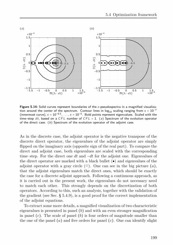
5.4 Optimization framework
(a) (b)
-5-5.5-5.5 -6-6.5-7
Iλ⋅dt
Rλ ⋅ dt ×10−4−1.5 −1 −0.5 0 0.5 1 1.5
×10−4
−1.5
−1
−0.5
0
0.5
1
1.5
-6-6.5-7-7
Iλ⋅dt
Rλ ⋅ dt ×10−4−1.5 −1 −0.5 0 0.5 1 1.5
×10−4
−1.5
−1
−0.5
0
0.5
1
1.5
Figure 5.14: Solid curves represent boundaries of the ǫ-pseudospectra in a magnified visualiza-tion around the center of the spectrum. Contour lines in log10 scaling ranging from ǫ = 10−7
(innermost curve), ǫ = 10−6.5 , . . . , ǫ = 10−5. Bold points represent eigenvalues. Scaled with thetime–step dt, based on a CFL number of CFL = 1. (a) Spectrum of the evolution operatorof the direct case. (b) Spectrum of the evolution operator of the adjoint case.
As in the discrete case, the adjoint operator is the negative transpose of thediscrete direct operator, the eigenvalues of the adjoint operator are simplyflipped on the imaginary axis (opposite sign of the real part). To compare thedirect and adjoint case, both eigenvalues are scaled with the correspondingtime–step. For the direct one dt and −dt for the adjoint one. Eigenvalues ofthe direct operator are marked with a black bullet () and eigenvalues of theadjoint operator with a gray circle (). One can see in the big picture (a),that the adjoint eigenvalues match the direct ones, which should be exactlythe case for a discrete adjoint approach. Following a continuous approach, asit is carried out in the present work, the eigenvalues do not necessary needto match each other. This strongly depends on the discretization of bothoperators. According to this, such an analysis, together with the validation ofthe gradient (see Sec. § 5.4.9), is a good proof for the correct implementationof the adjoint equations.
To extract some more details, a magnified visualization of two characteristiceigenvalues is presented in panel (b) and with an even stronger magnificationin panel (c). The scale of panel (b) is four orders of magnitude smaller thanthe one of the panel (a) and five orders for panel (c). One can identify slight
199
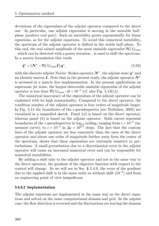
5 Optimization method
deviations of the eigenvalues of the adjoint operator compared to the directone. In particular, one adjoint eigenvalue is moving in the unstable half–plane (positive real part). Such an instability grows exponentially for linearequations, as for the adjoint equations. To avoid this numerical instability,the spectrum of the adjoint operator is shifted in the stable half–plane. Tothis end, the real valued amplitude of the most unstable eigenvalue Rλmax
– which can be detected with a power iteration – is used to shift the spectrum.In a matrix formulation this reads:
q⋆ = (N⋆ −RλmaxI)q⋆, (5.63)
with the discrete adjoint Navier–Stokes operator N⋆, the adjoint state q⋆ andan identity matrix I. Note that in the present study, the adjoint operator N⋆
is accessed in a matrix free implementation. In the present applications onsupersonic jet noise, the largest detectable unstable eigenvalue of the adjointoperator is less than Rλmax ⋅ dt = 10−5 (cf. also Fig. 5.13(c)).
The numerical inaccuracy of the eigenvalues of the adjoint operator can beexplained with its high nonnormality. Compared to the direct operator, thecondition number of the adjoint operator is four orders of magnitude larger.In Fig. 5.14 the boundaries of the ǫ-pseudospectra [see Trefethen, 2005] arevisualized in a magnified sketch. Panel (a) is based on the direct operator,whereas panel (b) is based on the adjoint operator. Solid curves representboundaries of the ǫ-pseudospectra in log10 scaling, ranging from ǫ = 10−7 (in-nermost curve), to ǫ = 10−5 in ∆ǫ = 100.5 steps. The fact that the contourlines of the adjoint operator are less concentric than the ones of the directoperator and about one order of magnitude further away form the center ofthe spectrum, shows that these eigenvalues are extremely sensitive to per-turbations. A small perturbation due to a discretization error in the adjointoperator will cause an increased numerical error and can be responsible fornumerical instabilities.
By adding a shift only to the adjoint operator and not in the same way tothe direct operator, the gradient of the objective function with respect to thecontrol will change. As we will see in Sec. § 5.4.9, the error of the gradientdue to the applied shift is in the same order as without shift (10−5) and froman engineering point of view insignificant.
5.4.8.2 Implementation
The adjoint equations are implemented in the same way as the direct equa-tions and solved on the same computational domain and grid. In the adjointcase, the flow direction is reversed and the fluctuations are leaving the domain
200
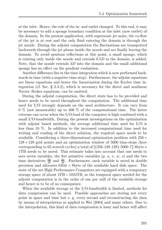
5.4 Optimization framework
at the inlet. Hence, the role of the in- and outlet changed. To this end, it maybe necessary to add a sponge boundary condition at the inlet (now outlet) ofthe domain. In the present application, with supersonic jet noise, the co-flowof the jet is at rest and the only fluid entering the domain is through thejet nozzle. During the adjoint computation the fluctuations are transportedbackwards through the jet plume inside the nozzle and are finally leaving thedomain. To avoid spurious reflections at this point, a small sponge, whichis existing only inside the nozzle and extends 0.5D in the domain, is added.Note, that the nozzle extends 3D into the domain and the small additionalsponge has no effect on the gradient evaluation.
Another difference lies in the time integration which is now performed back-wards in time (with a negative time-step). Furthermore, the adjoint equationsare linear equations and hence the linearization during the Krylov time in-tegration (cf. Sec. § 2.3.2), which is necessary for the direct and nonlinearNavier–Stokes equations, can be omitted.
During the adjoint computation, the direct state has to be provided andhence needs to be saved throughout the computation. The additional timeused for I/O strongly depends on the used architecture. It can vary from0 % (not measurable) up to 400 % of the computational time. The latterextreme can occur when the I/O-load of the computer is high combined with asmall I/O-bandwidth. During the present investigations on the optimizationwith adjoint based methods, the average additional time used for I/O isless than 10 %. In addition to the increased computational time used forwriting and reading of the direct solution, the required space needs to beavailable. Considering a three-dimensional optimization problem with 256 ×
128 × 128 grid points and an optimization window of 5000 time-steps (herecorresponding to 65 screech cycles) a total of [(256 ⋅128 ⋅128) ⋅5000 ⋅7] ⋅8byte ≈1TB needs to be saved. This estimate takes into account that one needs tosave seven variables, the five primitive variables (p, u, v, w, s) and the twotime derivatives ∂p
∂tand ∂s
∂t. Furthermore, each variable is saved in double
precision and allocates 64bit = 8byte of the available hard disk space. Thestate of the art High Performance Computers are equipped with a temporarystorage space of about 1PB = 1024TB, so the temporal space needed for theadjoint computation is in the order of one per mill of the available storageand hence is to be of no consequence.
When the available storage or the I/O-bandwidth is limited, methods fordata compression can be used. Possible approaches are storing not everypoint in space and time but e. g. every second and reconstructing the databy means of interpolation as applied in Wei [2004] and many others. Due tothe interpolation, this kind of data compression is lossy and hence will affect
201
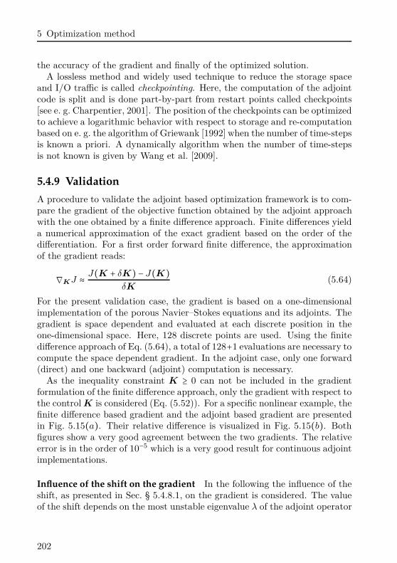
5 Optimization method
the accuracy of the gradient and finally of the optimized solution.A lossless method and widely used technique to reduce the storage space
and I/O traffic is called checkpointing. Here, the computation of the adjointcode is split and is done part-by-part from restart points called checkpoints[see e. g. Charpentier, 2001]. The position of the checkpoints can be optimizedto achieve a logarithmic behavior with respect to storage and re-computationbased on e. g. the algorithm of Griewank [1992] when the number of time-stepsis known a priori. A dynamically algorithm when the number of time-stepsis not known is given by Wang et al. [2009].
5.4.9 Validation
A procedure to validate the adjoint based optimization framework is to com-pare the gradient of the objective function obtained by the adjoint approachwith the one obtained by a finite difference approach. Finite differences yielda numerical approximation of the exact gradient based on the order of thedifferentiation. For a first order forward finite difference, the approximationof the gradient reads:
∇KJ ≈ J(K + δK) − J(K)δK
(5.64)
For the present validation case, the gradient is based on a one-dimensionalimplementation of the porous Navier–Stokes equations and its adjoints. Thegradient is space dependent and evaluated at each discrete position in theone-dimensional space. Here, 128 discrete points are used. Using the finitedifference approach of Eq. (5.64), a total of 128+1 evaluations are necessary tocompute the space dependent gradient. In the adjoint case, only one forward(direct) and one backward (adjoint) computation is necessary.
As the inequality constraint K ≥ 0 can not be included in the gradientformulation of the finite difference approach, only the gradient with respect tothe control K is considered (Eq. (5.52)). For a specific nonlinear example, thefinite difference based gradient and the adjoint based gradient are presentedin Fig. 5.15(a). Their relative difference is visualized in Fig. 5.15(b). Bothfigures show a very good agreement between the two gradients. The relativeerror is in the order of 10−5 which is a very good result for continuous adjointimplementations.
Influence of the shift on the gradient In the following the influence of theshift, as presented in Sec. § 5.4.8.1, on the gradient is considered. The valueof the shift depends on the most unstable eigenvalue λ of the adjoint operator
202
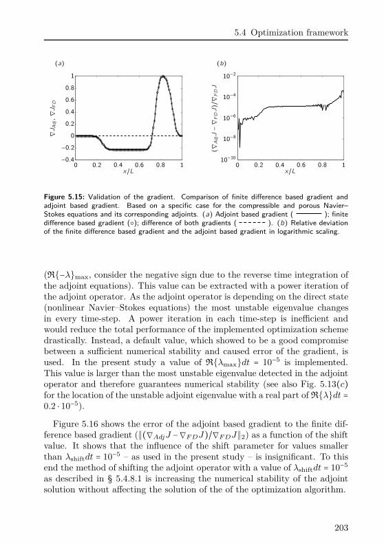
5.4 Optimization framework
(a) (b)∇JAdj,∇JFD
x/L0 0.2 0.4 0.6 0.8 1−0.4
−0.2
0
0.2
0.4
0.6
0.8
1
(∇AdjJ−∇FDJ)/∇
FDJ
x/L0 0.2 0.4 0.6 0.8 110−10
10−8
10−6
10−4
10−2
Figure 5.15: Validation of the gradient. Comparison of finite difference based gradient andadjoint based gradient. Based on a specific case for the compressible and porous Navier–Stokes equations and its corresponding adjoints. (a) Adjoint based gradient ( ); finitedifference based gradient (); difference of both gradients ( ). (b) Relative deviationof the finite difference based gradient and the adjoint based gradient in logarithmic scaling.
(R−λmax, consider the negative sign due to the reverse time integration ofthe adjoint equations). This value can be extracted with a power iteration ofthe adjoint operator. As the adjoint operator is depending on the direct state(nonlinear Navier–Stokes equations) the most unstable eigenvalue changesin every time-step. A power iteration in each time-step is inefficient andwould reduce the total performance of the implemented optimization schemedrastically. Instead, a default value, which showed to be a good compromisebetween a sufficient numerical stability and caused error of the gradient, isused. In the present study a value of Rλmaxdt = 10−5 is implemented.This value is larger than the most unstable eigenvalue detected in the adjointoperator and therefore guarantees numerical stability (see also Fig. 5.13(c)for the location of the unstable adjoint eigenvalue with a real part of Rλdt =0.2 ⋅ 10−5).
Figure 5.16 shows the error of the adjoint based gradient to the finite dif-ference based gradient (∥(∇AdjJ −∇F DJ)/∇F DJ∥2) as a function of the shiftvalue. It shows that the influence of the shift parameter for values smallerthan λshiftdt = 10−5 – as used in the present study – is insignificant. To thisend the method of shifting the adjoint operator with a value of λshiftdt = 10−5
as described in § 5.4.8.1 is increasing the numerical stability of the adjointsolution without affecting the solution of the of the optimization algorithm.
203
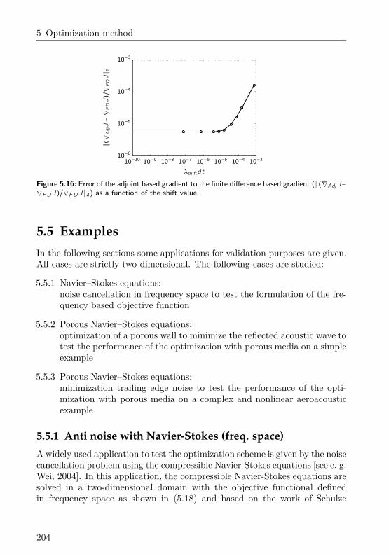
5 Optimization method
∥(∇AdjJ−∇FDJ)/∇
FDJ∥ 2
λshiftdt
10−10 10−9 10−8 10−7 10−6 10−5 10−4 10−310−6
10−5
10−4
10−3
Figure 5.16: Error of the adjoint based gradient to the finite difference based gradient (∥(∇AdjJ−∇FDJ)/∇FDJ∥2) as a function of the shift value.
5.5 Examples
In the following sections some applications for validation purposes are given.All cases are strictly two-dimensional. The following cases are studied:
5.5.1 Navier–Stokes equations:noise cancellation in frequency space to test the formulation of the fre-quency based objective function
5.5.2 Porous Navier–Stokes equations:optimization of a porous wall to minimize the reflected acoustic wave totest the performance of the optimization with porous media on a simpleexample
5.5.3 Porous Navier–Stokes equations:minimization trailing edge noise to test the performance of the opti-mization with porous media on a complex and nonlinear aeroacousticexample
5.5.1 Anti noise with Navier-Stokes (freq. space)
A widely used application to test the optimization scheme is given by the noisecancellation problem using the compressible Navier-Stokes equations [see e. g.Wei, 2004]. In this application, the compressible Navier-Stokes equations aresolved in a two-dimensional domain with the objective functional definedin frequency space as shown in (5.18) and based on the work of Schulze
204
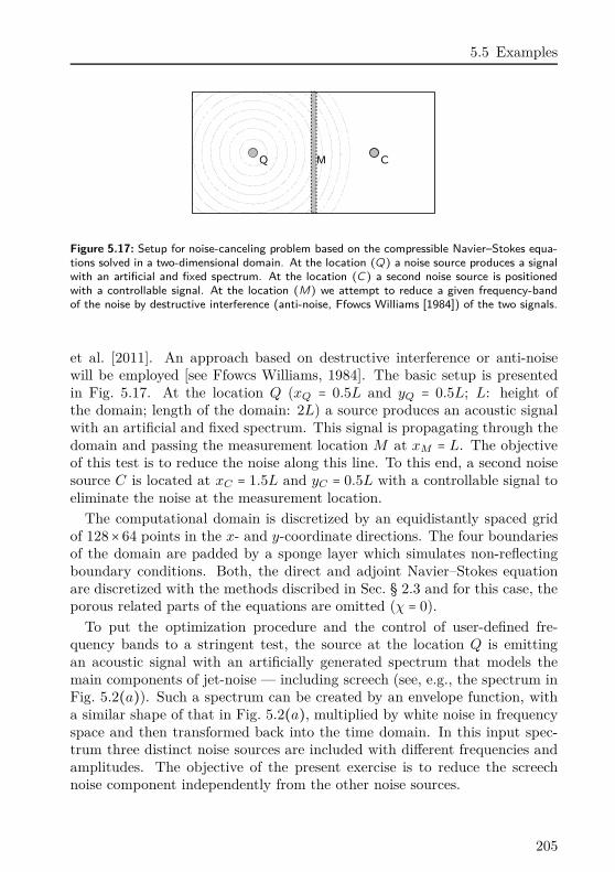
5.5 Examples
Figure 5.17: Setup for noise-canceling problem based on the compressible Navier–Stokes equa-tions solved in a two-dimensional domain. At the location (Q) a noise source produces a signalwith an artificial and fixed spectrum. At the location (C) a second noise source is positionedwith a controllable signal. At the location (M) we attempt to reduce a given frequency-bandof the noise by destructive interference (anti-noise, Ffowcs Williams [1984]) of the two signals.
et al. [2011]. An approach based on destructive interference or anti-noisewill be employed [see Ffowcs Williams, 1984]. The basic setup is presentedin Fig. 5.17. At the location Q (xQ = 0.5L and yQ = 0.5L; L: height ofthe domain; length of the domain: 2L) a source produces an acoustic signalwith an artificial and fixed spectrum. This signal is propagating through thedomain and passing the measurement location M at xM = L. The objectiveof this test is to reduce the noise along this line. To this end, a second noisesource C is located at xC = 1.5L and yC = 0.5L with a controllable signal toeliminate the noise at the measurement location.
The computational domain is discretized by an equidistantly spaced gridof 128× 64 points in the x- and y-coordinate directions. The four boundariesof the domain are padded by a sponge layer which simulates non-reflectingboundary conditions. Both, the direct and adjoint Navier–Stokes equationare discretized with the methods discribed in Sec. § 2.3 and for this case, theporous related parts of the equations are omitted (χ = 0).
To put the optimization procedure and the control of user-defined fre-quency bands to a stringent test, the source at the location Q is emittingan acoustic signal with an artificially generated spectrum that models themain components of jet-noise — including screech (see, e.g., the spectrum inFig. 5.2(a)). Such a spectrum can be created by an envelope function, witha similar shape of that in Fig. 5.2(a), multiplied by white noise in frequencyspace and then transformed back into the time domain. In this input spec-trum three distinct noise sources are included with different frequencies andamplitudes. The objective of the present exercise is to reduce the screechnoise component independently from the other noise sources.
205
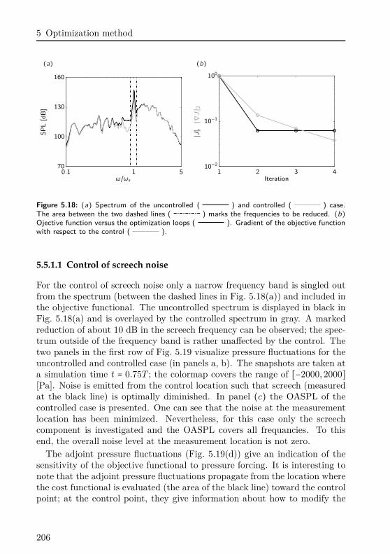
5 Optimization method
(a) (b)
SP
L[d
B]
ω/ωs0.1 1 5
70
100
130
160
∣J∣,∥∇J∥ 2
Iteration1 2 3 4
10−2
10−1
100
Figure 5.18: (a) Spectrum of the uncontrolled ( ) and controlled ( ) case.The area between the two dashed lines ( ) marks the frequencies to be reduced. (b)Ojective function versus the optimization loops ( ). Gradient of the objective functionwith respect to the control ( ).
5.5.1.1 Control of screech noise
For the control of screech noise only a narrow frequency band is singled outfrom the spectrum (between the dashed lines in Fig. 5.18(a)) and included inthe objective functional. The uncontrolled spectrum is displayed in black inFig. 5.18(a) and is overlayed by the controlled spectrum in gray. A markedreduction of about 10 dB in the screech frequency can be observed; the spec-trum outside of the frequency band is rather unaffected by the control. Thetwo panels in the first row of Fig. 5.19 visualize pressure fluctuations for theuncontrolled and controlled case (in panels a, b). The snapshots are taken ata simulation time t = 0.75T ; the colormap covers the range of [−2000, 2000][Pa]. Noise is emitted from the control location such that screech (measuredat the black line) is optimally diminished. In panel (c) the OASPL of thecontrolled case is presented. One can see that the noise at the measurementlocation has been minimized. Nevertheless, for this case only the screechcomponent is investigated and the OASPL covers all frequancies. To thisend, the overall noise level at the measurement location is not zero.
The adjoint pressure fluctuations (Fig. 5.19(d)) give an indication of thesensitivity of the objective functional to pressure forcing. It is interesting tonote that the adjoint pressure fluctuations propagate from the location wherethe cost functional is evaluated (the area of the black line) toward the controlpoint; at the control point, they give information about how to modify the
206
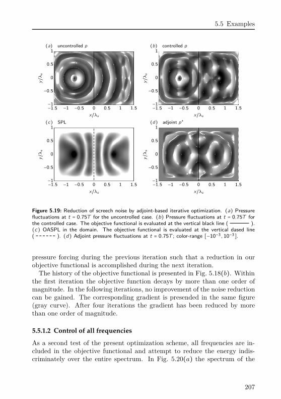
5.5 Examples
(a) uncontrolled p (b) controlled py/λs
x/λs−1.5 −1 −0.5 0 0.5 1 1.5−1
−0.5
0
0.5
1
y/λs
x/λs−1.5 −1 −0.5 0 0.5 1 1.5−1
−0.5
0
0.5
1
(c) SPL (d) adjoint p⋆
y/λs
x/λs−1.5 −1 −0.5 0 0.5 1 1.5−1
−0.5
0
0.5
1
y/λs
x/λs−1.5 −1 −0.5 0 0.5 1 1.5−1
−0.5
0
0.5
1
Figure 5.19: Reduction of screech noise by adjoint-based iterative optimization. (a) Pressurefluctuations at t = 0.75T for the uncontrolled case. (b) Pressure fluctuations at t = 0.75T forthe controlled case. The objective functional is evaluated at the vertical black line ( ).(c) OASPL in the domain. The objective functional is evaluated at the vertical dased line( ). (d) Adjoint pressure fluctuations at t = 0.75T ; color-range [−10−3 , 10−3].
pressure forcing during the previous iteration such that a reduction in ourobjective functional is accomplished during the next iteration.
The history of the objective functional is presented in Fig. 5.18(b). Withinthe first iteration the objective function decays by more than one order ofmagnitude. In the following iterations, no improvement of the noise reductioncan be gained. The corresponding gradient is presended in the same figure(gray curve). After four iterations the gradient has been reduced by morethan one order of magnitude.
5.5.1.2 Control of all frequencies
As a second test of the present optimization scheme, all frequencies are in-cluded in the objective functional and attempt to reduce the energy indis-criminately over the entire spectrum. In Fig. 5.20(a) the spectrum of the
207
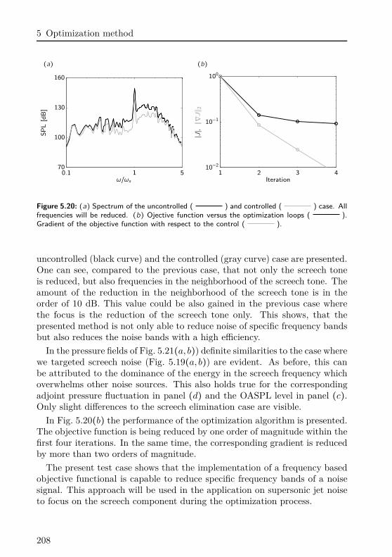
5 Optimization method
(a) (b)
SP
L[d
B]
ω/ωs0.1 1 5
70
100
130
160
∣J∣,∥∇J∥ 2
Iteration1 2 3 4
10−2
10−1
100
Figure 5.20: (a) Spectrum of the uncontrolled ( ) and controlled ( ) case. Allfrequencies will be reduced. (b) Ojective function versus the optimization loops ( ).Gradient of the objective function with respect to the control ( ).
uncontrolled (black curve) and the controlled (gray curve) case are presented.One can see, compared to the previous case, that not only the screech toneis reduced, but also frequencies in the neighborhood of the screech tone. Theamount of the reduction in the neighborhood of the screech tone is in theorder of 10 dB. This value could be also gained in the previous case wherethe focus is the reduction of the screech tone only. This shows, that thepresented method is not only able to reduce noise of specific frequency bandsbut also reduces the noise bands with a high efficiency.
In the pressure fields of Fig. 5.21(a, b)) definite similarities to the case wherewe targeted screech noise (Fig. 5.19(a, b)) are evident. As before, this canbe attributed to the dominance of the energy in the screech frequency whichoverwhelms other noise sources. This also holds true for the correspondingadjoint pressure fluctuation in panel (d) and the OASPL level in panel (c).Only slight differences to the screech elimination case are visible.
In Fig. 5.20(b) the performance of the optimization algorithm is presented.The objective function is being reduced by one order of magnitude within thefirst four iterations. In the same time, the corresponding gradient is reducedby more than two orders of magnitude.
The present test case shows that the implementation of a frequency basedobjective functional is capable to reduce specific frequency bands of a noisesignal. This approach will be used in the application on supersonic jet noiseto focus on the screech component during the optimization process.
208
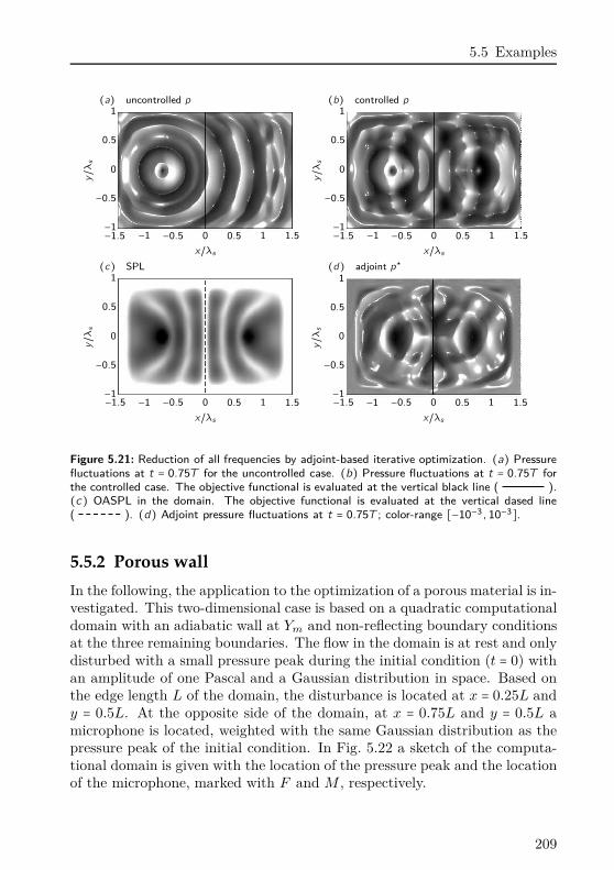
5.5 Examples
(a) uncontrolled p (b) controlled py/λs
x/λs−1.5 −1 −0.5 0 0.5 1 1.5−1
−0.5
0
0.5
1
y/λs
x/λs−1.5 −1 −0.5 0 0.5 1 1.5−1
−0.5
0
0.5
1
(c) SPL (d) adjoint p⋆
y/λs
x/λs−1.5 −1 −0.5 0 0.5 1 1.5−1
−0.5
0
0.5
1
y/λs
x/λs−1.5 −1 −0.5 0 0.5 1 1.5−1
−0.5
0
0.5
1
Figure 5.21: Reduction of all frequencies by adjoint-based iterative optimization. (a) Pressurefluctuations at t = 0.75T for the uncontrolled case. (b) Pressure fluctuations at t = 0.75T forthe controlled case. The objective functional is evaluated at the vertical black line ( ).(c) OASPL in the domain. The objective functional is evaluated at the vertical dased line( ). (d) Adjoint pressure fluctuations at t = 0.75T ; color-range [−10−3 , 10−3].
5.5.2 Porous wall
In the following, the application to the optimization of a porous material is in-vestigated. This two-dimensional case is based on a quadratic computationaldomain with an adiabatic wall at Ym and non-reflecting boundary conditionsat the three remaining boundaries. The flow in the domain is at rest and onlydisturbed with a small pressure peak during the initial condition (t = 0) withan amplitude of one Pascal and a Gaussian distribution in space. Based onthe edge length L of the domain, the disturbance is located at x = 0.25L andy = 0.5L. At the opposite side of the domain, at x = 0.75L and y = 0.5L amicrophone is located, weighted with the same Gaussian distribution as thepressure peak of the initial condition. In Fig. 5.22 a sketch of the computa-tional domain is given with the location of the pressure peak and the locationof the microphone, marked with F and M , respectively.
209
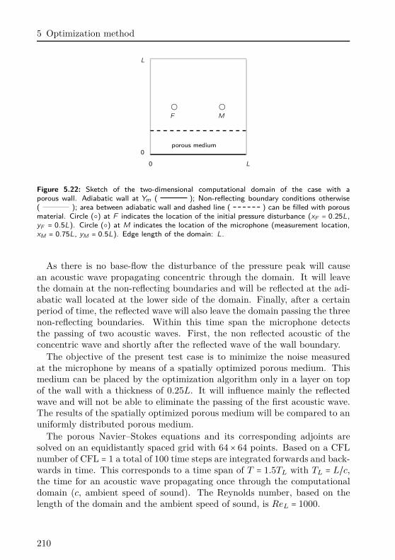
5 Optimization method
e e
0 L
0
L
porous medium
F M
Figure 5.22: Sketch of the two-dimensional computational domain of the case with aporous wall. Adiabatic wall at Ym ( ); Non-reflecting boundary conditions otherwise( ); area between adiabatic wall and dashed line ( ) can be filled with porousmaterial. Circle () at F indicates the location of the initial pressure disturbance (xF = 0.25L,yF = 0.5L). Circle () at M indicates the location of the microphone (measurement location,xM = 0.75L, yM = 0.5L). Edge length of the domain: L.
As there is no base-flow the disturbance of the pressure peak will causean acoustic wave propagating concentric through the domain. It will leavethe domain at the non-reflecting boundaries and will be reflected at the adi-abatic wall located at the lower side of the domain. Finally, after a certainperiod of time, the reflected wave will also leave the domain passing the threenon-reflecting boundaries. Within this time span the microphone detectsthe passing of two acoustic waves. First, the non reflected acoustic of theconcentric wave and shortly after the reflected wave of the wall boundary.
The objective of the present test case is to minimize the noise measuredat the microphone by means of a spatially optimized porous medium. Thismedium can be placed by the optimization algorithm only in a layer on topof the wall with a thickness of 0.25L. It will influence mainly the reflectedwave and will not be able to eliminate the passing of the first acoustic wave.The results of the spatially optimized porous medium will be compared to anuniformly distributed porous medium.
The porous Navier–Stokes equations and its corresponding adjoints aresolved on an equidistantly spaced grid with 64 × 64 points. Based on a CFL
number of CFL = 1 a total of 100 time steps are integrated forwards and back-wards in time. This corresponds to a time span of T = 1.5TL with TL = L/c,the time for an acoustic wave propagating once through the computationaldomain (c, ambient speed of sound). The Reynolds number, based on thelength of the domain and the ambient speed of sound, is ReL = 1000.
210
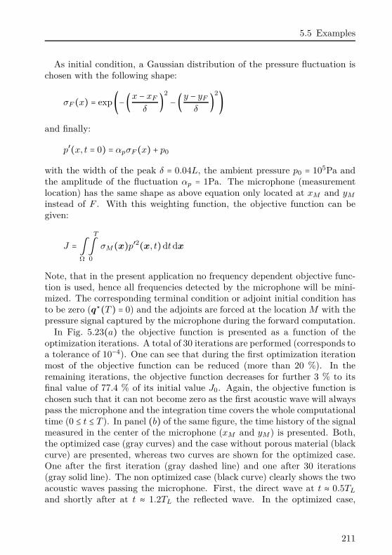
5.5 Examples
As initial condition, a Gaussian distribution of the pressure fluctuation ischosen with the following shape:
σF (x) = exp(−(x − xF
δ)2
− (y − yF
δ)2)
and finally:
p′(x, t = 0) = αpσF (x) + p0
with the width of the peak δ = 0.04L, the ambient pressure p0 = 105Pa andthe amplitude of the fluctuation αp = 1Pa. The microphone (measurementlocation) has the same shape as above equation only located at xM and yM
instead of F . With this weighting function, the objective function can begiven:
J = ∫Ω
T
∫0
σM(x)p′2(x, t)dt dx
Note, that in the present application no frequency dependent objective func-tion is used, hence all frequencies detected by the microphone will be mini-mized. The corresponding terminal condition or adjoint initial condition hasto be zero (q⋆(T ) = 0) and the adjoints are forced at the location M with thepressure signal captured by the microphone during the forward computation.
In Fig. 5.23(a) the objective function is presented as a function of theoptimization iterations. A total of 30 iterations are performed (corresponds toa tolerance of 10−4). One can see that during the first optimization iterationmost of the objective function can be reduced (more than 20 %). In theremaining iterations, the objective function decreases for further 3 % to itsfinal value of 77.4 % of its initial value J0. Again, the objective function ischosen such that it can not become zero as the first acoustic wave will alwayspass the microphone and the integration time covers the whole computationaltime (0 ≤ t ≤ T ). In panel (b) of the same figure, the time history of the signalmeasured in the center of the microphone (xM and yM ) is presented. Both,the optimized case (gray curves) and the case without porous material (blackcurve) are presented, whereas two curves are shown for the optimized case.One after the first iteration (gray dashed line) and one after 30 iterations(gray solid line). The non optimized case (black curve) clearly shows the twoacoustic waves passing the microphone. First, the direct wave at t ≈ 0.5TL
and shortly after at t ≈ 1.2TL the reflected wave. In the optimized case,
211
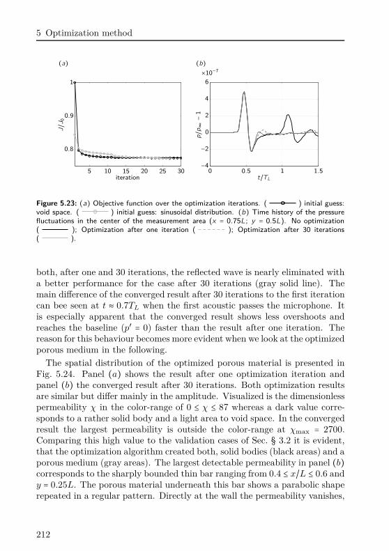
5 Optimization method
(a) (b)J/J 0
iteration5 10 15 20 25 30
0.8
0.9
1
p/p∞−1
t/TL0 0.5 1 1.5
×10−7
−4
−2
0
2
4
6
Figure 5.23: (a) Objective function over the optimization iterations. ( ) initial guess:void space. ( ) initial guess: sinusoidal distribution. (b) Time history of the pressurefluctuations in the center of the measurement area (x = 0.75L; y = 0.5L). No optimization( ); Optimization after one iteration ( ); Optimization after 30 iterations( ).
both, after one and 30 iterations, the reflected wave is nearly eliminated witha better performance for the case after 30 iterations (gray solid line). Themain difference of the converged result after 30 iterations to the first iterationcan bee seen at t ≈ 0.7TL when the first acoustic passes the microphone. Itis especially apparent that the converged result shows less overshoots andreaches the baseline (p′ = 0) faster than the result after one iteration. Thereason for this behaviour becomes more evident when we look at the optimizedporous medium in the following.
The spatial distribution of the optimized porous material is presented inFig. 5.24. Panel (a) shows the result after one optimization iteration andpanel (b) the converged result after 30 iterations. Both optimization resultsare similar but differ mainly in the amplitude. Visualized is the dimensionlesspermeability χ in the color-range of 0 ≤ χ ≤ 87 whereas a dark value corre-sponds to a rather solid body and a light area to void space. In the convergedresult the largest permeability is outside the color-range at χmax = 2700.Comparing this high value to the validation cases of Sec. § 3.2 it is evident,that the optimization algorithm created both, solid bodies (black areas) and aporous medium (gray areas). The largest detectable permeability in panel (b)corresponds to the sharply bounded thin bar ranging from 0.4 ≤ x/L ≤ 0.6 andy = 0.25L. The porous material underneath this bar shows a parabolic shaperepeated in a regular pattern. Directly at the wall the permeability vanishes,
212
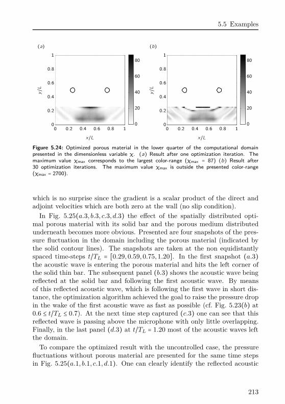
5.5 Examples
(a) (b)
y/L
x/L0 0.2 0.4 0.6 0.8 1
0
20
40
60
80
0
0.2
0.4
0.6
0.8
1
y/L
x/L0 0.2 0.4 0.6 0.8 1
0
20
40
60
80
0
0.2
0.4
0.6
0.8
1
Figure 5.24: Optimized porous material in the lower quarter of the computational domainpresented in the dimensionless variable χ. (a) Result after one optimization iteration. Themaximum value χmax corresponds to the largest color-range (χmax = 87) (b) Result after30 optimization iterations. The maximum value χmax is outside the presented color-range(χmax = 2700).
which is no surprise since the gradient is a scalar product of the direct andadjoint velocities which are both zero at the wall (no slip condition).
In Fig. 5.25(a.3, b.3, c.3, d.3) the effect of the spatially distributed opti-mal porous material with its solid bar and the porous medium distributedunderneath becomes more obvious. Presented are four snapshots of the pres-sure fluctuation in the domain including the porous material (indicated bythe solid contour lines). The snapshots are taken at the non equidistantlyspaced time-steps t/TL = [0.29, 0.59, 0.75, 1.20]. In the first snapshot (a.3)the acoustic wave is entering the porous material and hits the left corner ofthe solid thin bar. The subsequent panel (b.3) shows the acoustic wave beingreflected at the solid bar and following the first acoustic wave. By meansof this reflected acoustic wave, which is following the first wave in short dis-tance, the optimization algorithm achieved the goal to raise the pressure dropin the wake of the first acoustic wave as fast as possible (cf. Fig. 5.23(b) at0.6 ≤ t/TL ≤ 0.7). At the next time step captured (c.3) one can see that thisreflected wave is passing above the microphone with only little overlapping.Finally, in the last panel (d.3) at t/TL = 1.20 most of the acoustic waves leftthe domain.
To compare the optimized result with the uncontrolled case, the pressurefluctuations without porous material are presented for the same time stepsin Fig. 5.25(a.1, b.1, c.1, d.1). One can clearly identify the reflected acoustic
213
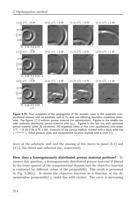
5 Optimization method
(a.1) t/TL = 0.29 (b.1) t/TL = 0.59 (c.1) t/TL = 0.75 (d.1) t/TL = 1.20
y/L
x/L0 0.25 0.5 0.75 10
0.25
0.5
0.75
1
(a.2) t/TL = 0.29 (b.2) t/TL = 0.59 (c.2) t/TL = 0.75 (d.2) t/TL = 1.20
y/L
x/L0 0.25 0.5 0.75 10
0.25
0.5
0.75
1
(a.3) t/TL = 0.29 (b.3) t/TL = 0.59 (c.3) t/TL = 0.75 (d.3) t/TL = 1.20
y/L
x/L0 0.25 0.5 0.75 10
0.25
0.5
0.75
1
Figure 5.25: Four snapshots of the propagation of the acoustic wave in the quadratic com-putational domain with an adiabatic wall at Ym and non-reflecting boundary conditions other-wise. Top figures (?.1) without porous material (no optimization). Figures in the middle rowwith uniformly distributed porous material with χmin. Figures in the last row with optimizedporous material (after 30 iterations). All snapshots taken at four (non equidistant) time-steps:t/TL = [0.29, 0.59, 0.75, 1.20]. Contours of the porous medium marked with a black solid line( ). Initial pressure peak and measurement location marked with a circle ().
wave at the adiabatic wall and the passing of two waves in panel (b.1) and(d.1), the direct and reflected one, respectively.
How does a homogeneously distributed porous material perform? Toanswer this question, a homogeneously distributed porous material is placedin the lower quarter of the computational domain and the objective functionis evaluated for different values of the permeability. The result is presentedin Fig. 5.26(a). It shows the objective function as a function of the di-mensionless permeability χ (solid line with circles). The curve is decreasing
214
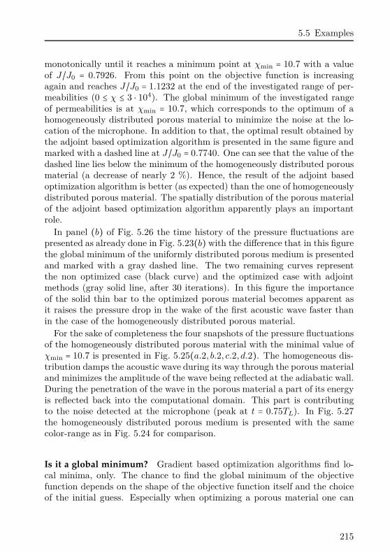
5.5 Examples
monotonically until it reaches a minimum point at χmin = 10.7 with a valueof J/J0 = 0.7926. From this point on the objective function is increasingagain and reaches J/J0 = 1.1232 at the end of the investigated range of per-meabilities (0 ≤ χ ≤ 3 ⋅ 104). The global minimum of the investigated rangeof permeabilities is at χmin = 10.7, which corresponds to the optimum of ahomogeneously distributed porous material to minimize the noise at the lo-cation of the microphone. In addition to that, the optimal result obtained bythe adjoint based optimization algorithm is presented in the same figure andmarked with a dashed line at J/J0 = 0.7740. One can see that the value of thedashed line lies below the minimum of the homogeneously distributed porousmaterial (a decrease of nearly 2 %). Hence, the result of the adjoint basedoptimization algorithm is better (as expected) than the one of homogeneouslydistributed porous material. The spatially distribution of the porous materialof the adjoint based optimization algorithm apparently plays an importantrole.
In panel (b) of Fig. 5.26 the time history of the pressure fluctuations arepresented as already done in Fig. 5.23(b) with the difference that in this figurethe global minimum of the uniformly distributed porous medium is presentedand marked with a gray dashed line. The two remaining curves representthe non optimized case (black curve) and the optimized case with adjointmethods (gray solid line, after 30 iterations). In this figure the importanceof the solid thin bar to the optimized porous material becomes apparent asit raises the pressure drop in the wake of the first acoustic wave faster thanin the case of the homogeneously distributed porous material.
For the sake of completeness the four snapshots of the pressure fluctuationsof the homogeneously distributed porous material with the minimal value ofχmin = 10.7 is presented in Fig. 5.25(a.2, b.2, c.2, d.2). The homogeneous dis-tribution damps the acoustic wave during its way through the porous materialand minimizes the amplitude of the wave being reflected at the adiabatic wall.During the penetration of the wave in the porous material a part of its energyis reflected back into the computational domain. This part is contributingto the noise detected at the microphone (peak at t = 0.75TL). In Fig. 5.27the homogeneously distributed porous medium is presented with the samecolor-range as in Fig. 5.24 for comparison.
Is it a global minimum? Gradient based optimization algorithms find lo-cal minima, only. The chance to find the global minimum of the objectivefunction depends on the shape of the objective function itself and the choiceof the initial guess. Especially when optimizing a porous material one can
215
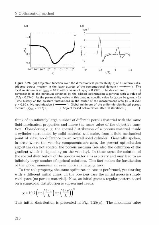
5 Optimization method
(a) (b)tsJ/J 0
χ
10−3 10−2 10−1 100 101 102 103 104
0.8
0.9
1
1.1
p/p∞−1
t/TL0 0.5 1 1.5
×10−7
−4
−2
0
2
4
6
Figure 5.26: (a) Objective function over the dimensionless permeability χ of a uniformly dis-tributed porous medium in the lower quarter of the computational domain ( ). Thelocal minimum is at χmin = 10.7 with a value of J/J0 = 0.7926. The dashed line ( )corresponds to the minimum obtained by the adjoint optimization algorithm with a value ofJ/J0 = 0.7740. As the permeability varies in this case, no specific value for χ can be given. (b)Time history of the pressure fluctuations in the center of the measurement area (x = 0.75L;y = 0.5L). No optimization ( ); Global minimum of the uniformly distributed porousmedium (χmin = 10.7) ( ); Adjoint based optimization after 30 iterations ( ).
think of an infinitely large number of different porous material with the samefluid-mechanical properties and hence the same value of the objective func-tion. Considering e. g. the spatial distribution of a porous material insidea cylinder surrounded by solid material will make, from a fluid-mechanicalpoint of view, no difference to an overall solid cylinder. Generally spoken,in areas where the velocity components are zero, the present optimizationalgorithm can not control the porous medium (see also the definition of thegradient which is depending on the velocity). In these areas the solution ofthe spatial distribution of the porous material is arbitrary and may lead to aninfinitely large number of optimal solutions. This fact makes the localizationof the global minimum an even more challenging task.
To test this property, the same optimization case is performed, yet startingwith a different initial guess. In the previous case the initial guess is simplyvoid space (no porous material). Now, as initial guess a regular pattern basedon a sinusoidal distribution is chosen and reads:
χ = 10.7(sin(4πx
L) sin(4πy
L))2
This initial distribution is presented in Fig. 5.28(a). The maximum value
216
5.5 Examples
y/L
x/L0 0.2 0.4 0.6 0.8 1
0
20
40
60
80
0
0.2
0.4
0.6
0.8
1
Figure 5.27: Optimal homogeneously distributed porous material in the lower quarter of thecomputational domain presented in the dimensionless variable χ. To compare it with the adjointcased optimization, the same color-range as in Fig. 5.24 is chosen. Optimal permeability:χmin = 10.7 (cf. also Fig. 5.26(a)).
(χmax = 10.7) is taken from the previous study with a homogeneously dis-tributed porous medium as it showed to be the optimal value. The convergedoptimal solution can be gained after 27 optimization iterations (with a toler-ance of 10−4) and reaches the same optimal value as in the previous study. Inthe history of the objective function (presented in Fig. 5.23(a), gray curve)one can identify that the initial guess is a better choice as simply void spacesince the value of the first iteration starts at J/J0 = 0.84, with the value ofthe objective function J0 based on the void space initial guess. In addition tothat, the final optimal value after 27 iteration reaches the same value as theone of the void space initial guess. Now, one could postulate that both opti-mizations found the same optimal solution and hence ended up in the samelocal minimum which now could be a global one. In fact, when comparingboth optimal solutions in Fig. 5.24(b) (void initial guess) and Fig. 5.28(b)(sinusoidal initial guess) one can identify differences. Still the main featuresare present, like the thin solid bar and the parabolic shaped porous mediumunderneath it. A main difference is the missing porous medium directly be-low the solid thin bar (gray area at x = 0.5L, y = 0.1L). Nevertheless, thisarea is covered by the thin bar and surrounded by porous medium. To thisend, no fluid (acoustic waves) can penetrate this area from outside and, froma fluid-mechanical point of view, does not play a role for the optimizationobjective.
To conclude the results of this test case we can see that the optimizationwith a spatially distributed porous medium is capable to minimize acous-
217
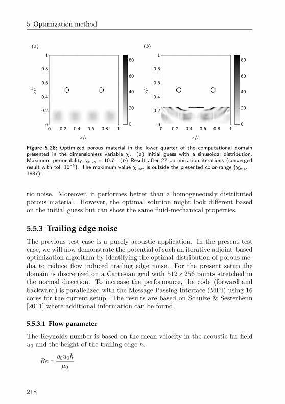
5 Optimization method
(a) (b)
y/L
x/L0 0.2 0.4 0.6 0.8 1
0
20
40
60
80
0
0.2
0.4
0.6
0.8
1
y/L
x/L0 0.2 0.4 0.6 0.8 1
0
20
40
60
80
0
0.2
0.4
0.6
0.8
1
Figure 5.28: Optimized porous material in the lower quarter of the computational domainpresented in the dimensionless variable χ. (a) Initial guess with a sinusoidal distribution.Maximum permeability χmax = 10.7. (b) Result after 27 optimization iterations (convergedresult with tol. 10−4). The maximum value χmax is outside the presented color-range (χmax =1887).
tic noise. Moreover, it performes better than a homogeneously distributedporous material. However, the optimal solution might look different basedon the initial guess but can show the same fluid-mechanical properties.
5.5.3 Trailing edge noise
The previous test case is a purely acoustic application. In the present testcase, we will now demonstrate the potential of such an iterative adjoint–basedoptimization algorithm by identifying the optimal distribution of porous me-dia to reduce flow induced trailing edge noise. For the present setup thedomain is discretized on a Cartesian grid with 512 × 256 points stretched inthe normal direction. To increase the performance, the code (forward andbackward) is parallelized with the Message Passing Interface (MPI) using 16cores for the current setup. The results are based on Schulze & Sesterhenn[2011] where additional information can be found.
5.5.3.1 Flow parameter
The Reynolds number is based on the mean velocity in the acoustic far-fieldu0 and the height of the trailing edge h.
Re = ρ0u0h
µ0
218
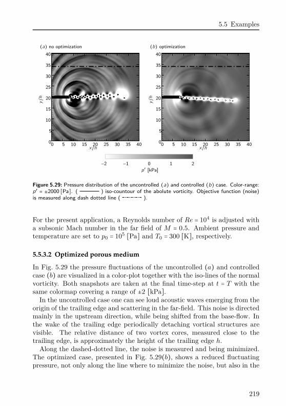
5.5 Examples
(a) no optimization (b) optimization
y/h
x/h00
5
5
10
10
15
15
20
20
25
25
30
30
35
35
40
40
y/h
x/h00
5
5
10
10
15
15
20
20
25
25
30
30
35
35
40
40
−2 −1 −0
p′ [kPa]
+1 +2
Figure 5.29: Pressure distribution of the uncontrolled (a) and controlled (b) case. Color-range:p′ = ±2000 [Pa]. ( ) iso-countour of the abolute vorticity. Objective function (noise)is measured along dash dotted line ( ).
For the present application, a Reynolds number of Re = 104 is adjusted witha subsonic Mach number in the far field of M = 0.5. Ambient pressure andtemperature are set to p0 = 105 [Pa] and T0 = 300 [K], respectively.
5.5.3.2 Optimized porous medium
In Fig. 5.29 the pressure fluctuations of the uncontrolled (a) and controlledcase (b) are visualized in a color-plot together with the iso-lines of the normalvorticity. Both snapshots are taken at the final time-step at t = T with thesame colormap covering a range of ±2 [kPa].
In the uncontrolled case one can see loud acoustic waves emerging from theorigin of the trailing edge and scattering in the far-field. This noise is directedmainly in the upstream direction, while being shifted from the base-flow. Inthe wake of the trailing edge periodically detaching vortical structures arevisible. The relative distance of two vortex cores, measured close to thetrailing edge, is approximately the height of the trailing edge h.
Along the dashed-dotted line, the noise is measured and being minimized.The optimized case, presented in Fig. 5.29(b), shows a reduced fluctuatingpressure, not only along the line where to minimize the noise, but also in the
219
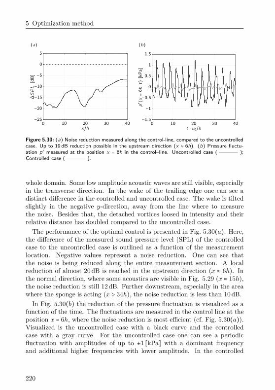
5 Optimization method
(a) (b)
∆SPL
[dB
]
x/h0 10 20 30 40
−25
−20
−15
−10
−5
0
5
p′ (x=6h,t)
[kP
a]
t ⋅ u0/h0 10 20 30 40
−1.5
−1
−0.5
0
0.5
1
1.5
Figure 5.30: (a) Noise reduction measured along the control-line, compared to the uncontrolledcase. Up to 19 dB reduction possible in the upstream direction (x ≈ 6h). (b) Pressure fluctu-ation p′ measured at the position x = 6h in the control–line. Uncontrolled case ( );Controlled case ( ).
whole domain. Some low amplitude acoustic waves are still visible, especiallyin the transverse direction. In the wake of the trailing edge one can see adistinct difference in the controlled and uncontrolled case. The wake is tiltedslightly in the negative y-direction, away from the line where to measurethe noise. Besides that, the detached vortices loosed in intensity and theirrelative distance has doubled compared to the uncontrolled case.
The performance of the optimal control is presented in Fig. 5.30(a). Here,the difference of the measured sound pressure level (SPL) of the controlledcase to the uncontrolled case is outlined as a function of the measurementlocation. Negative values represent a noise reduction. One can see thatthe noise is being reduced along the entire measurement section. A localreduction of almost 20 dB is reached in the upstream direction (x ≈ 6h). Inthe normal direction, where some acoustics are visible in Fig. 5.29 (x ≈ 15h),the noise reduction is still 12 dB. Further downstream, especially in the areawhere the sponge is acting (x > 34h), the noise reduction is less than 10 dB.
In Fig. 5.30(b) the reduction of the pressure fluctuation is visualized as afunction of the time. The fluctuations are measured in the control line at theposition x = 6h, where the noise reduction is most efficient (cf. Fig. 5.30(a)).Visualized is the uncontrolled case with a black curve and the controlledcase with a gray curve. For the uncontrolled case one can see a periodicfluctuation with amplitudes of up to ±1 [kPa] with a dominant frequencyand additional higher frequencies with lower amplitude. In the controlled
220
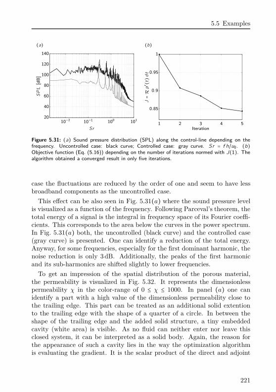
5.5 Examples
(a) (b)SPL
[dB
]
Sr
10−2 10−1 100 10120
40
60
80
100
120
140
J=Rp′ (t)dt
Iteration1 2 3 4 5
0.85
0.9
0.95
1
Figure 5.31: (a) Sound pressure distribution (SPL) along the control-line depending on thefrequency. Uncontrolled case: black curve; Controlled case: gray curve. Sr = f h/u0. (b)Objective function (Eq. (5.16)) depending on the number of iterations normed with J(1). Thealgorithm obtained a converged result in only five iterations.
case the fluctuations are reduced by the order of one and seem to have lessbroadband components as the uncontrolled case.
This effect can be also seen in Fig. 5.31(a) where the sound pressure levelis visualized as a function of the frequency. Following Parceval’s theorem, thetotal energy of a signal is the integral in frequency space of its Fourier coeffi-cients. This corresponds to the area below the curves in the power spectrum.In Fig. 5.31(a) both, the uncontrolled (black curve) and the controlled case(gray curve) is presented. One can identify a reduction of the total energy.Anyway, for some frequencies, especially for the first dominant harmonic, thenoise reduction is only 3 dB. Additionally, the peaks of the first harmonicand its sub-harmonics are shifted slightly to lower frequencies.
To get an impression of the spatial distribution of the porous material,the permeability is visualized in Fig. 5.32. It represents the dimensionlesspermeability χ in the color-range of 0 ≤ χ ≤ 1000. In panel (a) one canidentify a part with a high value of the dimensionless permeability close tothe trailing edge. This part can be treated as an additional solid extentionto the trailing edge with the shape of a quarter of a circle. In between theshape of the trailing edge and the added solid structure, a tiny embeddedcavity (white area) is visible. As no fluid can neither enter nor leave thisclosed system, it can be interpreted as a solid body. Again, the reason forthe appearance of such a cavity lies in the way the optimization algorithmis evaluating the gradient. It is the scalar product of the direct and adjoint
221
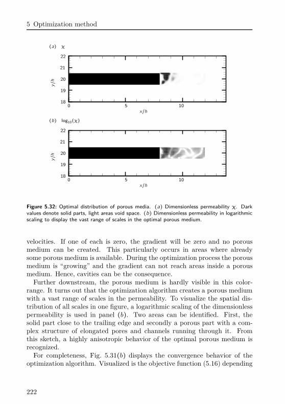
5 Optimization method
(a) χ
y/h
x/h18
19
20
21
22
0 5 10
(b) log10(χ)
y/h
x/h18
19
20
21
22
0 5 10
Figure 5.32: Optimal distribution of porous media. (a) Dimensionless permeability χ. Darkvalues denote solid parts, light areas void space. (b) Dimensionless permeability in logarithmicscaling to display the vast range of scales in the optimal porous medium.
velocities. If one of each is zero, the gradient will be zero and no porousmedium can be created. This particularly occurs in areas where alreadysome porous medium is available. During the optimization process the porousmedium is “growing” and the gradient can not reach areas inside a porousmedium. Hence, cavities can be the consequence.
Further downstream, the porous medium is hardly visible in this color-range. It turns out that the optimization algorithm creates a porous mediumwith a vast range of scales in the permeability. To visualize the spatial dis-tribution of all scales in one figure, a logarithmic scaling of the dimensionlesspermeability is used in panel (b). Two areas can be identified. First, thesolid part close to the trailing edge and secondly a porous part with a com-plex structure of elongated pores and channels running through it. Fromthis sketch, a highly anisotropic behavior of the optimal porous medium isrecognized.
For completeness, Fig. 5.31(b) displays the convergence behavior of theoptimization algorithm. Visualized is the objective function (5.16) depending
222
5.5 Examples
on the number of iterations. The algorithm shows convergence in only fiveiterations. This test case is the first to apply the optimization of a porousmaterial to an aeroacoustic application. It can be showed that the presentoptimization algorithm is capable treat these problems. In the followingchapter. This method is applied to reduce the noise of a supersonic jet withthe focus on jet screech.
223

6Results of the minimization of
supersonic jet noise with porous media
In the following section the potential of adjoint-based optimization to reducesupersonic jet noise will be demonstrated. The control objective is to optimizea porous material at the nozzle exit to minimize the noise of the jet in a pre-described location of the computational domain. From a physical point ofview, the porous material at the nozzle exit is supposed to influence thereceptivity at the nozzle lip to eliminate the feedback loop, responsible forscreech tones. To this end the dominant noise source in a supersonic jet willbe eliminated.
It has been shown by a series of researchers, who investigated supersonicjet noise experimentally that a porous material can reduce the screech tone(already mentioned Sec. § 1.1.2). Harper-Bourne & Fisher [1973] added aporous material at the surface of an acoustic reflector to act as a sound ab-sorbing material and showed that the screech tone could be reduced. A recentinvestigation on this topic is reported by Khan et al. [2008]. They added aporous reflector at the nozzle exit (similar as in the present investigation) andshowed that the screech tone could be reduced by more than 6 dB. However,their data also show that on the one hand the screech tone is not completelyeliminated and on the other hand that the OASPL of the jet is nearly onedB louder with the porous reflector than without. Especially the broadbandshock associated noise and the mixing noise is louder with porous materialthan without (cf. Fig. 6.1). The correct choice of the porous material to
225
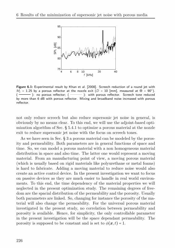
6 Results of the minimization of supersonic jet noise with porous media
PSfrag replacemen
SP
L[d
B]
f [kHz]4 6 8 10 20 40
75
80
85
90
95
Figure 6.1: Experimental result by Khan et al. [2008]. Screech reduction of a round jet withMj = 1.25 by a porous reflector at the nozzle exit (D = 10 [mm], measured at Θ = 90).( ): no porous reflector; ( ): with porous reflector. Screech tone reducedby more than 6 dB with porous reflector. Mixing and broadband noise increased with porousreflector.
not only reduce screech but also reduce supersonic jet noise in general, isobviously by no means clear. To this end, we will use the adjoint-based opti-mization algorithm of Sec. § 5.4.1 to optimize a porous material at the nozzleexit to reduce supersonic jet noise with the focus on screech tones.
As we have seen in Sec. § 3 a porous material can be modeled by the poros-ity and permeability. Both parameters are in general functions of space andtime. So, we can model a porous material with a non homogeneous materialdistribution in space and also time. The latter one would represent a movingmaterial. From an manufacturing point of view, a moving porous material(which is usually based on rigid materials like polyurethane or metal foams)is hard to fabricate. Adding a moving material to reduce noise would alsocreate an active control device. In the present investigation we want to focuson passive devices as they are much easier to handle in real world environ-ments. To this end, the time dependency of the material properties we willneglected in the present optimization study. The remaining degrees of free-dom are the spacial distribution of the permeability and the porosity. Usuallyboth parameters are linked. So, changing for instance the porosity of the ma-terial will also change the permeability. For the universal porous materialinvestigated in the present study, no correlation between permeability andporosity is available. Hence, for simplicity, the only controllable parameterin the present investigation will be the space dependant permeability. Theporosity is supposed to be constant and is set to φ(x, t) = 1.
226
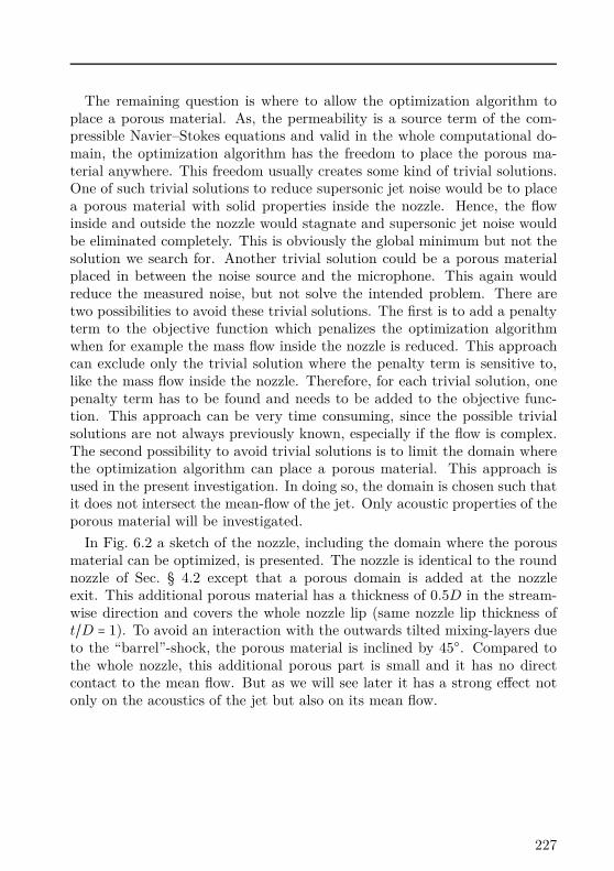
The remaining question is where to allow the optimization algorithm toplace a porous material. As, the permeability is a source term of the com-pressible Navier–Stokes equations and valid in the whole computational do-main, the optimization algorithm has the freedom to place the porous ma-terial anywhere. This freedom usually creates some kind of trivial solutions.One of such trivial solutions to reduce supersonic jet noise would be to placea porous material with solid properties inside the nozzle. Hence, the flowinside and outside the nozzle would stagnate and supersonic jet noise wouldbe eliminated completely. This is obviously the global minimum but not thesolution we search for. Another trivial solution could be a porous materialplaced in between the noise source and the microphone. This again wouldreduce the measured noise, but not solve the intended problem. There aretwo possibilities to avoid these trivial solutions. The first is to add a penaltyterm to the objective function which penalizes the optimization algorithmwhen for example the mass flow inside the nozzle is reduced. This approachcan exclude only the trivial solution where the penalty term is sensitive to,like the mass flow inside the nozzle. Therefore, for each trivial solution, onepenalty term has to be found and needs to be added to the objective func-tion. This approach can be very time consuming, since the possible trivialsolutions are not always previously known, especially if the flow is complex.The second possibility to avoid trivial solutions is to limit the domain wherethe optimization algorithm can place a porous material. This approach isused in the present investigation. In doing so, the domain is chosen such thatit does not intersect the mean-flow of the jet. Only acoustic properties of theporous material will be investigated.
In Fig. 6.2 a sketch of the nozzle, including the domain where the porousmaterial can be optimized, is presented. The nozzle is identical to the roundnozzle of Sec. § 4.2 except that a porous domain is added at the nozzleexit. This additional porous material has a thickness of 0.5D in the stream-wise direction and covers the whole nozzle lip (same nozzle lip thickness oft/D = 1). To avoid an interaction with the outwards tilted mixing-layers dueto the “barrel”-shock, the porous material is inclined by 45. Compared tothe whole nozzle, this additional porous part is small and it has no directcontact to the mean flow. But as we will see later it has a strong effect notonly on the acoustics of the jet but also on its mean flow.
227
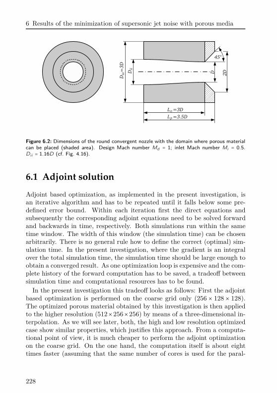
6 Results of the minimization of supersonic jet noise with porous media
Figure 6.2: Dimensions of the round convergent nozzle with the domain where porous materialcan be placed (shaded area). Design Mach number Md = 1; inlet Mach number Mi = 0.5.Di i = 1.16D (cf. Fig. 4.16).
6.1 Adjoint solution
Adjoint based optimization, as implemented in the present investigation, isan iterative algorithm and has to be repeated until it falls below some pre-defined error bound. Within each iteration first the direct equations andsubsequently the corresponding adjoint equations need to be solved forwardand backwards in time, respectively. Both simulations run within the sametime window. The width of this window (the simulation time) can be chosenarbitrarily. There is no general rule how to define the correct (optimal) sim-ulation time. In the present investigation, where the gradient is an integralover the total simulation time, the simulation time should be large enough toobtain a converged result. As one optimization loop is expensive and the com-plete history of the forward computation has to be saved, a tradeoff betweensimulation time and computational resources has to be found.
In the present investigation this tradeoff looks as follows: First the adjointbased optimization is performed on the coarse grid only (256 × 128 × 128).The optimized porous material obtained by this investigation is then appliedto the higher resolution (512×256×256) by means of a three-dimensional in-terpolation. As we will see later, both, the high and low resolution optimizedcase show similar properties, which justifies this approach. From a computa-tional point of view, it is much cheaper to perform the adjoint optimizationon the coarse grid. On the one hand, the computation itself is about eighttimes faster (assuming that the same number of cores is used for the paral-
228
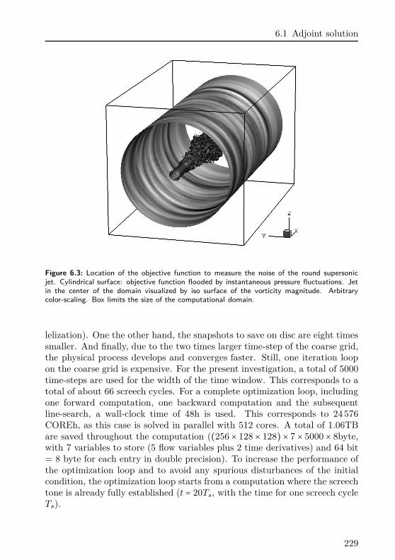
6.1 Adjoint solution
Figure 6.3: Location of the objective function to measure the noise of the round supersonicjet. Cylindrical surface: objective function flooded by instantaneous pressure fluctuations. Jetin the center of the domain visualized by iso surface of the vorticity magnitude. Arbitrarycolor-scaling. Box limits the size of the computational domain.
lelization). One the other hand, the snapshots to save on disc are eight timessmaller. And finally, due to the two times larger time-step of the coarse grid,the physical process develops and converges faster. Still, one iteration loopon the coarse grid is expensive. For the present investigation, a total of 5000
time-steps are used for the width of the time window. This corresponds to atotal of about 66 screech cycles. For a complete optimization loop, includingone forward computation, one backward computation and the subsequentline-search, a wall-clock time of 48h is used. This corresponds to 24 576
COREh, as this case is solved in parallel with 512 cores. A total of 1.06TBare saved throughout the computation ((256 × 128 × 128) × 7 × 5000 × 8byte,with 7 variables to store (5 flow variables plus 2 time derivatives) and 64 bit= 8 byte for each entry in double precision). To increase the performance ofthe optimization loop and to avoid any spurious disturbances of the initialcondition, the optimization loop starts from a computation where the screechtone is already fully established (t = 20Ts, with the time for one screech cycleTs).
229
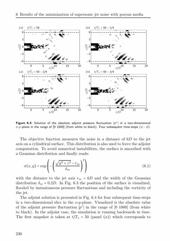
6 Results of the minimization of supersonic jet noise with porous media
(a) t/Ts = 50 (b) t/Ts = 50 − 1/4
y/D
x/D0 5 10 15 20
−6
−3
0
3
6
y/D
x/D0 5 10 15 20
−6
−3
0
3
6
(a) t/Ts = 50 − 2/4 (b) t/Ts = 50 − 3/4
y/D
x/D0 5 10 15 20
−6
−3
0
3
6
y/D
x/D0 5 10 15 20
−6
−3
0
3
6
Figure 6.4: Solution of the absolute adjoint pressure fluctuation ∣p⋆∣ in a two-dimensionalx-y -plane in the range of [0 1000] (from white to black). Four subsequent time-steps (a − d).
The objective function measures the noise in a distance of 6D to the jetaxis on a cylindrical surface. This distribution is also used to force the adjointcomputation. To avoid numerical instabilities, the surface is smoothed witha Gaussian distribution and finally reads:
σ(x, y) = exp⎛⎜⎝−⎛⎝√
y2 + z2 − rm
δm
⎞⎠
2⎞⎟⎠ (6.1)
with the distance to the jet axis rm = 6D and the width of the Gaussiandistribution δm = 0.2D. In Fig. 6.3 the position of the surface is visualized,flooded by instantaneous pressure fluctuations and including the vorticity ofthe jet.
The adjoint solution is presented in Fig. 6.4 for four subsequent time-stepsin a two-dimensional slice in the x-y-plane. Visualized is the absolute valueof the adjoint pressure fluctuation ∣p⋆∣ in the range of [0 1000] (from whiteto black). In the adjoint case, the simulation is running backwards in time.The first snapshot is taken at t/Ts = 50 (panel (a)) which corresponds to
230
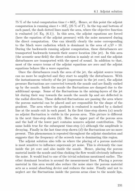
6.1 Adjoint solution
75 % of the total computation time t = 66Ts. Hence, at this point the adjointcomputation is running since t = 16Ts (25 % of T ). In the top and bottom ofeach panel, the dash dotted lines mark the area, where the objective functionis evaluated (cf. Eq. (6.1)). In this area, the adjoint equations are forced(here the equation of the adjoint pressure) with the noise measured duringthe direct computation. One can identify clearly the noise correspondingto the Mach wave radiation which is dominant in the area of x/D = 10.During the backwards running adjoint computation, these disturbances aretransported backwards towards their source location (the jet). In this area(the acoustic near-field) the direct solution is mainly at rest and the adjointdisturbances are transported with the speed of sound. In addition to that,most of the source terms of the adjoint equations are zero and the adjointequations behave like a wave equation.
Once the disturbances reach the area of the jet, the adjoint source termscan no more be neglected and they start to amplify the disturbances. Withthe instantaneous velocity of the jet (supersonic in the jet core), the adjointpressure fluctuations are convected towards the nozzle and are finally suckedup by the nozzle. Inside the nozzle the fluctuations are damped due to theadditional sponge. Some of the fluctuations in the mixing-layers of the jethit during their way towards the nozzle the nozzle lip and are deflected inthe radial direction. These deflected fluctuations are passing the area wherethe porous material can be placed and are responsible for the shape of thegradient. The area where the gradient is evaluated is marked by a dashedline at the nozzle exit in each panel. In the first time-step shown (a) nearlyno adjoint fluctuation is visible in the porous area. This picture is differentin the next time-step shown (b). Here, the upper part of the porous areaand the half of the lower part contains nonzero adjoint contribution. Thesame holds true for the subsequent time-step (c) although the amplitude isdecaying. Finally in the last time-step shown (d) the fluctuations are no morepresent. This phenomenon is repeated throughout the adjoint simulation andsuggests that the frequency of the screech tone is dominating this region.
The adjoint solution also tells us where the placing of a porous materialis most sensitive to influence supersonic jet noise. This is obviously the caseinside the jet core and also inside the nozzle. Hence, placing the porousmaterial inside the nozzle and thus choking the flow would obviously influencethe noise. It would lead to one of the trivial solutions mentioned earlier. Theother dominant location is around the measurement lines. Placing a porousmaterial in this area would also reduce the noise since the porous materialacts as a sound absorbing device and reduces the noise. Finally and not toneglect are the fluctuations inside the porous areas close to the nozzle lips,
231
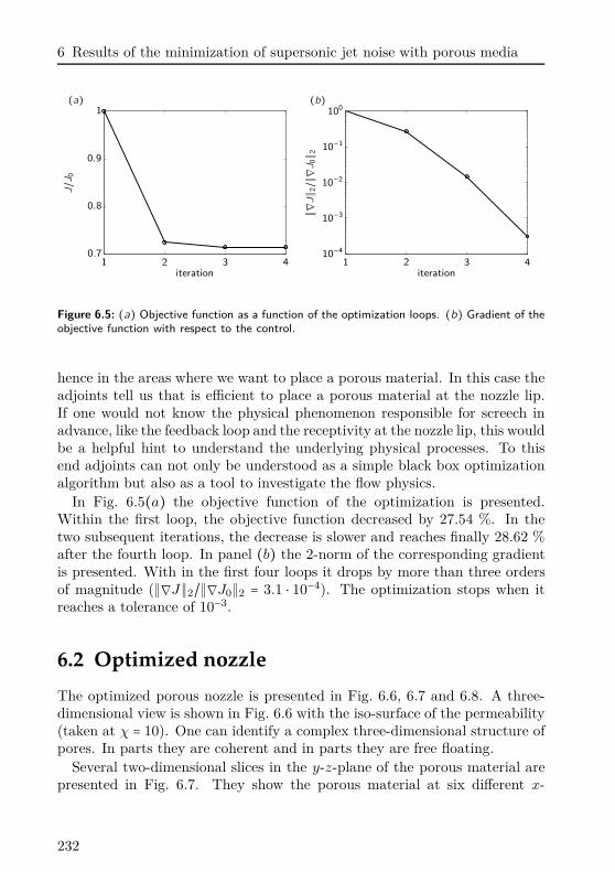
6 Results of the minimization of supersonic jet noise with porous media
(a) (b)
J/J 0
iteration1 2 3 4
0.7
0.8
0.9
1
iteration
∥∇J∥ 2/∥∇J0∥ 2
1 2 3 410−4
10−3
10−2
10−1
100
Figure 6.5: (a) Objective function as a function of the optimization loops. (b) Gradient of theobjective function with respect to the control.
hence in the areas where we want to place a porous material. In this case theadjoints tell us that is efficient to place a porous material at the nozzle lip.If one would not know the physical phenomenon responsible for screech inadvance, like the feedback loop and the receptivity at the nozzle lip, this wouldbe a helpful hint to understand the underlying physical processes. To thisend adjoints can not only be understood as a simple black box optimizationalgorithm but also as a tool to investigate the flow physics.
In Fig. 6.5(a) the objective function of the optimization is presented.Within the first loop, the objective function decreased by 27.54 %. In thetwo subsequent iterations, the decrease is slower and reaches finally 28.62 %after the fourth loop. In panel (b) the 2-norm of the corresponding gradientis presented. With in the first four loops it drops by more than three ordersof magnitude (∥∇J∥2/∥∇J0∥2 = 3.1 ⋅ 10−4). The optimization stops when itreaches a tolerance of 10−3.
6.2 Optimized nozzle
The optimized porous nozzle is presented in Fig. 6.6, 6.7 and 6.8. A three-dimensional view is shown in Fig. 6.6 with the iso-surface of the permeability(taken at χ = 10). One can identify a complex three-dimensional structure ofpores. In parts they are coherent and in parts they are free floating.
Several two-dimensional slices in the y-z-plane of the porous material arepresented in Fig. 6.7. They show the porous material at six different x-
232
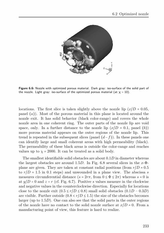
6.2 Optimized nozzle
Figure 6.6: Nozzle with optimized porous material. Dark gray: iso-surface of the solid part ofthe nozzle. Light gray: iso-surface of the optimized porous material (at χ = 10).
locations. The first slice is taken slightly above the nozzle lip (x/D = 0.05,panel (a)). Most of the porous material in this plane is located around thenozzle exit. It has solid behavior (black color-range) and covers the wholenozzle area in one coherent ring. The outer parts of the nozzle lip are voidspace, only. In a further distance to the nozzle lip (x/D = 0.1, panel (b))more porous material appears on the outer regions of the nozzle lip. Thistrend is repeated in the subsequent slices (panel (d−f)). In these panels onecan identify large and small coherent areas with high permeability (black).The permeability of these black areas is outside the color-range and reachesvalues up to χ = 2000. It can be treated as a solid body.
The smallest identifiable solid obstacles are about 0.1D in diameter whereasthe largest obstacles are around 1.5D. In Fig. 6.8 several slices in the x-Φ-plane are given. They are taken at constant radial positions (from r/D = 0.5to r/D = 1.5 in 0.1 steps) and unwounded in a plane view. The abscissa s
measures circumferential distance (s = 2rπ, from 0 ≤ Φ ≤ 2π) whereas s = 0 isat y/D = 0 and z = r (cf. Fig. 6.7). Positive s values measure in the clockwiseand negative values in the counterclockwise direction. Especially for locationsclose to the nozzle exit (0.5 ≤ r/D ≤ 0.8) small solid obstacles (0.1D – 0.3D)are visible. Further outside (0.8 < r/D ≤ 1.5) the size of the obstacles becomeslarger (up to 1.5D). One can also see that the solid parts in the outer regionsof the nozzle have no contact to the solid nozzle surface at x/D = 0. From amanufacturing point of view, this feature is hard to realize.
233
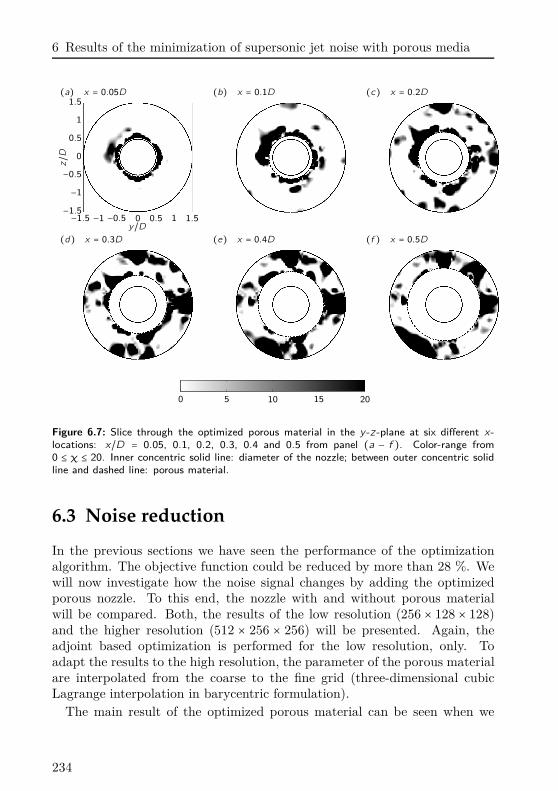
6 Results of the minimization of supersonic jet noise with porous media
(a) x = 0.05D (b) x = 0.1D (c) x = 0.2D
z/D
y/D−1.5 −1 −0.5 0 0.5 1 1.5−1.5
−1
−0.5
0
0.5
1
1.5
(d) x = 0.3D (e) x = 0.4D (f ) x = 0.5D
0 5 10 15 20
Figure 6.7: Slice through the optimized porous material in the y -z -plane at six different x-locations: x/D = 0.05, 0.1, 0.2, 0.3, 0.4 and 0.5 from panel (a − f ). Color-range from0 ≤ χ ≤ 20. Inner concentric solid line: diameter of the nozzle; between outer concentric solidline and dashed line: porous material.
6.3 Noise reduction
In the previous sections we have seen the performance of the optimizationalgorithm. The objective function could be reduced by more than 28 %. Wewill now investigate how the noise signal changes by adding the optimizedporous nozzle. To this end, the nozzle with and without porous materialwill be compared. Both, the results of the low resolution (256 × 128 × 128)and the higher resolution (512 × 256 × 256) will be presented. Again, theadjoint based optimization is performed for the low resolution, only. Toadapt the results to the high resolution, the parameter of the porous materialare interpolated from the coarse to the fine grid (three-dimensional cubicLagrange interpolation in barycentric formulation).
The main result of the optimized porous material can be seen when we
234
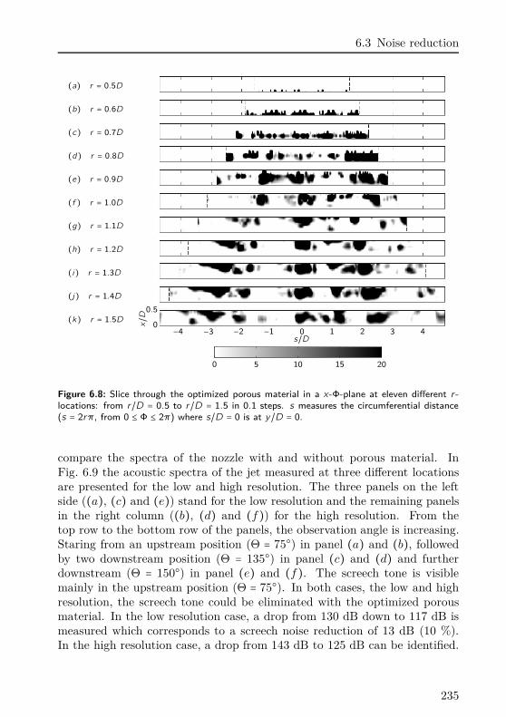
6.3 Noise reduction
(a) r = 0.5D
(b) r = 0.6D
(c) r = 0.7D
(d) r = 0.8D
(e) r = 0.9D
(f ) r = 1.0D
(g) r = 1.1D
(h) r = 1.2D
(i) r = 1.3D
replacemen
(j) r = 1.4D
(k) r = 1.5D
x/D
s/D−4 −3 −2 −1 0 1 2 3 40
0.5
0 5 10 15 20
Figure 6.8: Slice through the optimized porous material in a x-Φ-plane at eleven different r -locations: from r/D = 0.5 to r/D = 1.5 in 0.1 steps. s measures the circumferential distance(s = 2rπ, from 0 ≤ Φ ≤ 2π) where s/D = 0 is at y/D = 0.
compare the spectra of the nozzle with and without porous material. InFig. 6.9 the acoustic spectra of the jet measured at three different locationsare presented for the low and high resolution. The three panels on the leftside ((a), (c) and (e)) stand for the low resolution and the remaining panelsin the right column ((b), (d) and (f)) for the high resolution. From thetop row to the bottom row of the panels, the observation angle is increasing.Staring from an upstream position (Θ = 75) in panel (a) and (b), followedby two downstream position (Θ = 135) in panel (c) and (d) and furtherdownstream (Θ = 150) in panel (e) and (f). The screech tone is visiblemainly in the upstream position (Θ = 75). In both cases, the low and highresolution, the screech tone could be eliminated with the optimized porousmaterial. In the low resolution case, a drop from 130 dB down to 117 dB ismeasured which corresponds to a screech noise reduction of 13 dB (10 %).In the high resolution case, a drop from 143 dB to 125 dB can be identified.
235
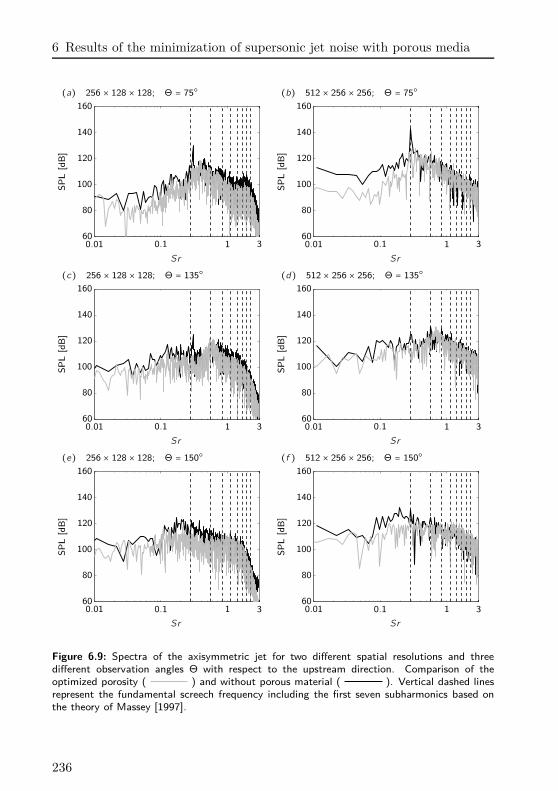
6 Results of the minimization of supersonic jet noise with porous media
(a) 256 × 128 × 128; Θ = 75 (b) 512 × 256 × 256; Θ = 75
SP
L[d
B]
Sr
0.01 0.1 1 360
80
100
120
140
160
SP
L[d
B]
Sr
0.01 0.1 1 360
80
100
120
140
160
(c) 256 × 128 × 128; Θ = 135 (d) 512 × 256 × 256; Θ = 135
SP
L[d
B]
Sr
0.01 0.1 1 360
80
100
120
140
160S
PL
[dB
]
Sr
0.01 0.1 1 360
80
100
120
140
160
(e) 256 × 128 × 128; Θ = 150 (f ) 512 × 256 × 256; Θ = 150
SP
L[d
B]
Sr
0.01 0.1 1 360
80
100
120
140
160
SP
L[d
B]
Sr
0.01 0.1 1 360
80
100
120
140
160
Figure 6.9: Spectra of the axisymmetric jet for two different spatial resolutions and threedifferent observation angles Θ with respect to the upstream direction. Comparison of theoptimized porosity ( ) and without porous material ( ). Vertical dashed linesrepresent the fundamental screech frequency including the first seven subharmonics based onthe theory of Massey [1997].
236
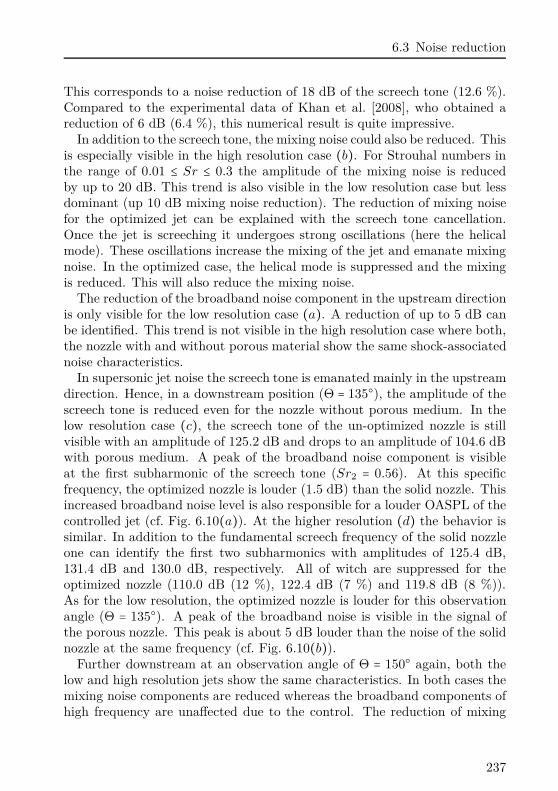
6.3 Noise reduction
This corresponds to a noise reduction of 18 dB of the screech tone (12.6 %).Compared to the experimental data of Khan et al. [2008], who obtained areduction of 6 dB (6.4 %), this numerical result is quite impressive.
In addition to the screech tone, the mixing noise could also be reduced. Thisis especially visible in the high resolution case (b). For Strouhal numbers inthe range of 0.01 ≤ Sr ≤ 0.3 the amplitude of the mixing noise is reducedby up to 20 dB. This trend is also visible in the low resolution case but lessdominant (up 10 dB mixing noise reduction). The reduction of mixing noisefor the optimized jet can be explained with the screech tone cancellation.Once the jet is screeching it undergoes strong oscillations (here the helicalmode). These oscillations increase the mixing of the jet and emanate mixingnoise. In the optimized case, the helical mode is suppressed and the mixingis reduced. This will also reduce the mixing noise.
The reduction of the broadband noise component in the upstream directionis only visible for the low resolution case (a). A reduction of up to 5 dB canbe identified. This trend is not visible in the high resolution case where both,the nozzle with and without porous material show the same shock-associatednoise characteristics.
In supersonic jet noise the screech tone is emanated mainly in the upstreamdirection. Hence, in a downstream position (Θ = 135), the amplitude of thescreech tone is reduced even for the nozzle without porous medium. In thelow resolution case (c), the screech tone of the un-optimized nozzle is stillvisible with an amplitude of 125.2 dB and drops to an amplitude of 104.6 dBwith porous medium. A peak of the broadband noise component is visibleat the first subharmonic of the screech tone (Sr2 = 0.56). At this specificfrequency, the optimized nozzle is louder (1.5 dB) than the solid nozzle. Thisincreased broadband noise level is also responsible for a louder OASPL of thecontrolled jet (cf. Fig. 6.10(a)). At the higher resolution (d) the behavior issimilar. In addition to the fundamental screech frequency of the solid nozzleone can identify the first two subharmonics with amplitudes of 125.4 dB,131.4 dB and 130.0 dB, respectively. All of witch are suppressed for theoptimized nozzle (110.0 dB (12 %), 122.4 dB (7 %) and 119.8 dB (8 %)).As for the low resolution, the optimized nozzle is louder for this observationangle (Θ = 135). A peak of the broadband noise is visible in the signal ofthe porous nozzle. This peak is about 5 dB louder than the noise of the solidnozzle at the same frequency (cf. Fig. 6.10(b)).
Further downstream at an observation angle of Θ = 150 again, both thelow and high resolution jets show the same characteristics. In both cases themixing noise components are reduced whereas the broadband components ofhigh frequency are unaffected due to the control. The reduction of mixing
237
6 Results of the minimization of supersonic jet noise with porous media
(a) 256 × 128 × 128 (b) 512 × 256 × 256
180
150
12090
60
30
0125135145
180
150
12090
60
30
0125135145
Figure 6.10: OASPL as a function of the observation angle with respect to the upstreamdirection. No optimization ( ); optimized porous material ( ). Circles ()mark the positions where the spectra of Fig. 6.9 are captured.
noise at a Strouhal number of Sr ≈ 0.2 is in both cases around 10 dB.In Fig. 6.10 the OASPL as a function of the observation angle is presented.
Although the low and high resolution case predict different OASPL’s thetrend is similar. The largest reduction can be identified in the upstream anddownstream direction. In the low resolution case (a) the OASPL drops from134.39 dB to 132.35 dB in the upstream direction (Θ = 75). This corre-sponds to a reduction of 2.04 dB. A similar reduction can be reached in thedownstream direction (Θ = 150). Here the OASPL drops from 136.42 dB to133.79 dB (a reduction of 2.63 dB). In an observation angle of Θ = 135
the OASPL with optimized nozzle is louder than with solid nozzle (plus1.04 dB). Compared to the corresponding spectrum in Fig. 6.9(c), the broad-band shock-associated noise component is responsible for the increase of theOASPL in this direction. An explanation for this phenomenon may be theincreased number of shock cells in the optimized case due to the suppressedhelical mode (see the comparison of mean flow fields in Sec. § 6.4). Theadditional shocks cells emanate shock associated noise and may increase theSPL of the broadband noise components. This is the tradeoff between screechnoise reduction and the corresponding suppression of the helical mode.
A similar picture of the OASPL can be found for the high resolution case(Fig. 6.10(b)). In the upstream direction, a reduction of 7.06 dB can beobserved, which corresponds to a drop from 144.40 dB to 137.34 dB. Lessefficient is the reduction in the downstream direction. At an observationangle of Θ = 150 the OASPL drops from 141.50 dB to 138.78 dB whichcorresponds to a reduction of 2.72 dB. As for the low resolution case, in anintermediate observation direction (Θ = 135) the OASPL of the optimizednozzle is louder. An increase of 0.15 dB can be measured (from 142.38 dB to
238
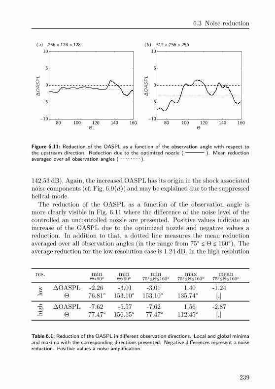
6.3 Noise reduction
(a) 256 × 128 × 128 (b) 512 × 256 × 256
∆OASPL
Θ80 100 120 140 160
−10
−5
0
5
10
∆OASPL
Θ80 100 120 140 160
−10
−5
0
5
10
Figure 6.11: Reduction of the OASPL as a function of the observation angle with respect tothe upstream direction. Reduction due to the optimized nozzle ( ). Mean reductionaveraged over all observation angles ( ).
142.53 dB). Again, the increased OASPL has its origin in the shock associatednoise components (cf. Fig. 6.9(d)) and may be explained due to the suppressedhelical mode.
The reduction of the OASPL as a function of the observation angle ismore clearly visible in Fig. 6.11 where the difference of the noise level of thecontrolled an uncontrolled nozzle are presented. Positive values indicate anincrease of the OASPL due to the optimized nozzle and negative values areduction. In addition to that, a dotted line measures the mean reductionaveraged over all observation angles (in the range from 75 ≤ Θ ≤ 160). Theaverage reduction for the low resolution case is 1.24 dB. In the high resolution
res. minΘ<90
minΘ>90
min75≤Θ≤160
max75≤Θ≤160
mean75≤Θ≤160
low ∆OASPL -2.26 -3.01 -3.01 1.40 -1.24
Θ 76.81 153.10 153.10 135.74 [.]
high ∆OASPL -7.62 -5.57 -7.62 1.56 -2.87
Θ 77.47 156.15 77.47 112.45 [.]
Table 6.1: Reduction of the OASPL in different observation directions. Local and global minimaand maxima with the corresponding directions presented. Negative differences represent a noisereduction. Positive values a noise amplification.
239
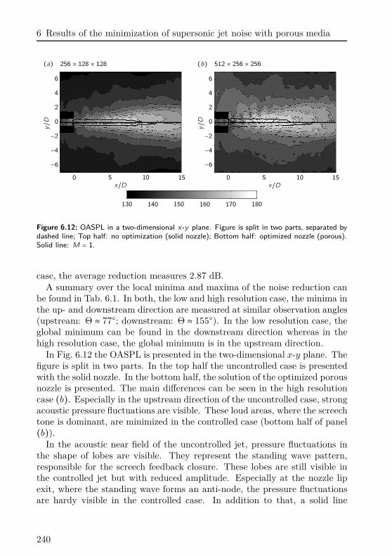
6 Results of the minimization of supersonic jet noise with porous media
(a) 256 × 128 × 128 (b) 512 × 256 × 256
y/D
x/D0 5 10 15
−6
−4
−2
0
2
4
6
y/D
x/D0 5 10 15
−6
−4
−2
0
2
4
6
130 140 150 160 170 180
Figure 6.12: OASPL in a two-dimensional x-y plane. Figure is split in two parts, separated bydashed line; Top half: no optimization (solid nozzle); Bottom half: optimized nozzle (porous).Solid line: M = 1.
case, the average reduction measures 2.87 dB.A summary over the local minima and maxima of the noise reduction can
be found in Tab. 6.1. In both, the low and high resolution case, the minima inthe up- and downstream direction are measured at similar observation angles(upstream: Θ ≈ 77; downstream: Θ ≈ 155). In the low resolution case, theglobal minimum can be found in the downstream direction whereas in thehigh resolution case, the global minimum is in the upstream direction.
In Fig. 6.12 the OASPL is presented in the two-dimensional x-y plane. Thefigure is split in two parts. In the top half the uncontrolled case is presentedwith the solid nozzle. In the bottom half, the solution of the optimized porousnozzle is presented. The main differences can be seen in the high resolutioncase (b). Especially in the upstream direction of the uncontrolled case, strongacoustic pressure fluctuations are visible. These loud areas, where the screechtone is dominant, are minimized in the controlled case (bottom half of panel(b)).
In the acoustic near field of the uncontrolled jet, pressure fluctuations inthe shape of lobes are visible. They represent the standing wave pattern,responsible for the screech feedback closure. These lobes are still visible inthe controlled jet but with reduced amplitude. Especially at the nozzle lipexit, where the standing wave forms an anti-node, the pressure fluctuationsare hardy visible in the controlled case. In addition to that, a solid line
240
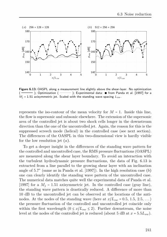
6.3 Noise reduction
(a) 256 × 128 × 128 (b) 512 × 256 × 256
prm
s[d
B]
x/Lsw0 1 2 3 4 5
140
150
160
170
180
prm
s[d
B]
x/Lsw0 1 2 3 4 5
140
150
160
170
180
Figure 6.13: OASPL along a measurement line slightly above the shear-layer. No optimization( ); Optimization ( ); Experimental data: ∎ from Panda et al. [1997] for aMj = 1.51 axisymmetric jet. Scaled with the standing wave spacing Lsw .
represents the iso-contour of the mean velocity for M = 1. Inside this line,the flow is supersonic and subsonic elsewhere. The extension of the supersonicarea of the controlled jet is about two shock cells longer in the downstreamdirection than the one of the uncontrolled jet. Again, the reason for this is thesuppressed screech mode (helical) in the controlled case (see next section).The differences of the OASPL in this two-dimensional view is hardly visiblefor the low resolution jet (a).
To get a deeper insight in the differences of the standing wave pattern forthe controlled and uncontrolled case, the RMS pressure fluctuations (OASPL)are measured along the shear layer boundary. To avoid an interaction withthe turbulent hydrodynamic pressure fluctuations, the data of Fig. 6.13 isextracted from a line parallel to the growing shear layer with an inclinationangle of 5.7 (same as in Panda et al. [1997]). In the high resolution case (b)one can clearly identify the standing wave pattern of the uncontrolled case.The numerical data matches quite well the experimental data of Panda et al.[1997] for a Mj = 1.51 axisymmetric jet. In the controlled case (gray line),the standing wave pattern is drastically reduced. A difference of more than10 dB to the uncontrolled jet can be observed at the locations of the anti-nodes. At the nodes of the standing wave (here at x/Lsw = 0.5, 1.5, 2.5, . . . )the pressure fluctuation of the controlled and uncontrolled jet coincide onlywithin the first wavelength (0 ≤ x/Lsw ≤ 2). Further downstream, the noiselevel at the nodes of the controlled jet is reduced (about 5 dB at x = 5.5Lsw).
241
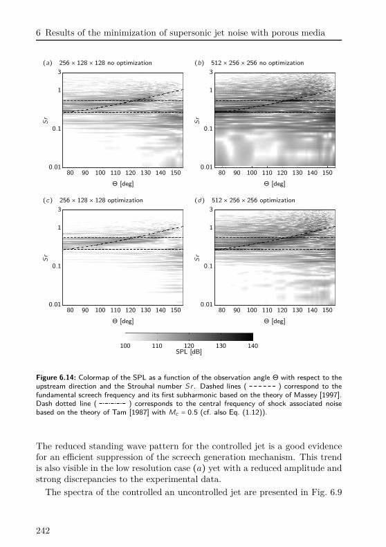
6 Results of the minimization of supersonic jet noise with porous media
(a) 256 × 128 × 128 no optimization (b) 512 × 256 × 256 no optimization
Sr
Θ [deg]
80 90 100 110 120 130 140 1500.01
0.1
1
3
Sr
Θ [deg]
80 90 100 110 120 130 140 1500.01
0.1
1
3
(c) 256 × 128 × 128 optimization (d) 512 × 256 × 256 optimization
Sr
Θ [deg]
80 90 100 110 120 130 140 1500.01
0.1
1
3
Sr
Θ [deg]
80 90 100 110 120 130 140 1500.01
0.1
1
3
100 110 120 130 140SPL [dB]
Figure 6.14: Colormap of the SPL as a function of the observation angle Θ with respect to theupstream direction and the Strouhal number Sr . Dashed lines ( ) correspond to thefundamental screech frequency and its first subharmonic based on the theory of Massey [1997].Dash dotted line ( ) corresponds to the central frequency of shock associated noisebased on the theory of Tam [1987] with Mc = 0.5 (cf. also Eq. (1.12)).
The reduced standing wave pattern for the controlled jet is a good evidencefor an efficient suppression of the screech generation mechanism. This trendis also visible in the low resolution case (a) yet with a reduced amplitude andstrong discrepancies to the experimental data.
The spectra of the controlled an uncontrolled jet are presented in Fig. 6.9
242
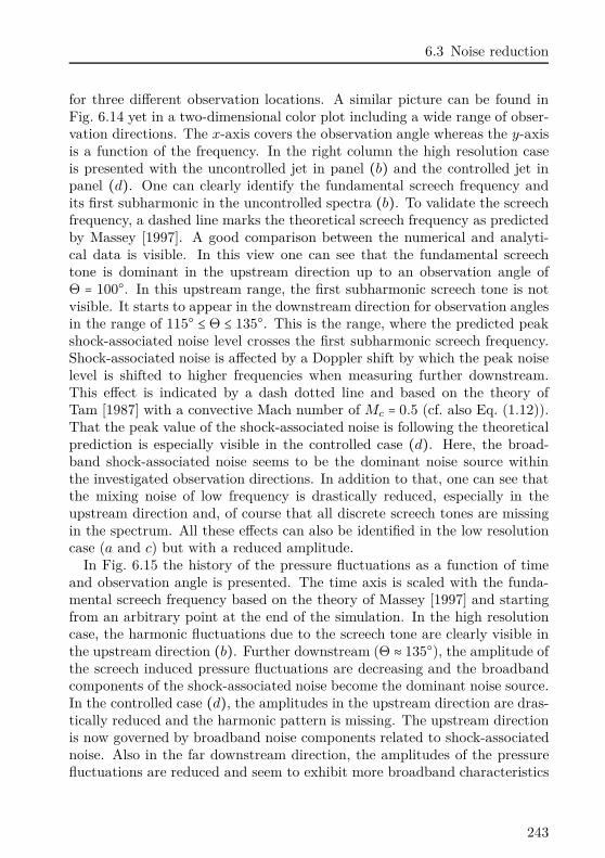
6.3 Noise reduction
for three different observation locations. A similar picture can be found inFig. 6.14 yet in a two-dimensional color plot including a wide range of obser-vation directions. The x-axis covers the observation angle whereas the y-axisis a function of the frequency. In the right column the high resolution caseis presented with the uncontrolled jet in panel (b) and the controlled jet inpanel (d). One can clearly identify the fundamental screech frequency andits first subharmonic in the uncontrolled spectra (b). To validate the screechfrequency, a dashed line marks the theoretical screech frequency as predictedby Massey [1997]. A good comparison between the numerical and analyti-cal data is visible. In this view one can see that the fundamental screechtone is dominant in the upstream direction up to an observation angle ofΘ = 100. In this upstream range, the first subharmonic screech tone is notvisible. It starts to appear in the downstream direction for observation anglesin the range of 115 ≤ Θ ≤ 135. This is the range, where the predicted peakshock-associated noise level crosses the first subharmonic screech frequency.Shock-associated noise is affected by a Doppler shift by which the peak noiselevel is shifted to higher frequencies when measuring further downstream.This effect is indicated by a dash dotted line and based on the theory ofTam [1987] with a convective Mach number of Mc = 0.5 (cf. also Eq. (1.12)).That the peak value of the shock-associated noise is following the theoreticalprediction is especially visible in the controlled case (d). Here, the broad-band shock-associated noise seems to be the dominant noise source withinthe investigated observation directions. In addition to that, one can see thatthe mixing noise of low frequency is drastically reduced, especially in theupstream direction and, of course that all discrete screech tones are missingin the spectrum. All these effects can also be identified in the low resolutioncase (a and c) but with a reduced amplitude.
In Fig. 6.15 the history of the pressure fluctuations as a function of timeand observation angle is presented. The time axis is scaled with the funda-mental screech frequency based on the theory of Massey [1997] and startingfrom an arbitrary point at the end of the simulation. In the high resolutioncase, the harmonic fluctuations due to the screech tone are clearly visible inthe upstream direction (b). Further downstream (Θ ≈ 135), the amplitude ofthe screech induced pressure fluctuations are decreasing and the broadbandcomponents of the shock-associated noise become the dominant noise source.In the controlled case (d), the amplitudes in the upstream direction are dras-tically reduced and the harmonic pattern is missing. The upstream directionis now governed by broadband noise components related to shock-associatednoise. Also in the far downstream direction, the amplitudes of the pressurefluctuations are reduced and seem to exhibit more broadband characteristics
243
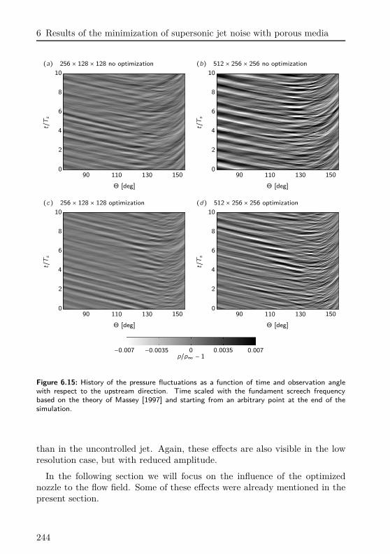
6 Results of the minimization of supersonic jet noise with porous media
(a) 256 × 128 × 128 no optimization (b) 512 × 256 × 256 no optimization
Θ [deg]
t/Ts
90 110 130 1500
2
4
6
8
10
Θ [deg]
t/Ts
90 110 130 1500
2
4
6
8
10
(c) 256 × 128 × 128 optimization (d) 512 × 256 × 256 optimization
Θ [deg]
t/Ts
90 110 130 1500
2
4
6
8
10
Θ [deg]
t/Ts
90 110 130 1500
2
4
6
8
10
−0.007 −0.0035 0 0.0035 0.007p/p∞ − 1
Figure 6.15: History of the pressure fluctuations as a function of time and observation anglewith respect to the upstream direction. Time scaled with the fundament screech frequencybased on the theory of Massey [1997] and starting from an arbitrary point at the end of thesimulation.
than in the uncontrolled jet. Again, these effects are also visible in the lowresolution case, but with reduced amplitude.
In the following section we will focus on the influence of the optimizednozzle to the flow field. Some of these effects were already mentioned in thepresent section.
244
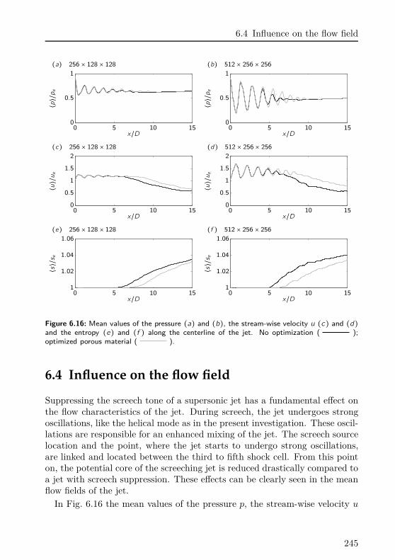
6.4 Influence on the flow field
(a) 256 × 128 × 128 (b) 512 × 256 × 256
⟨p⟩/p
e
x/D0 5 10 150
0.5
1
⟨p⟩/p
e
x/D0 5 10 150
0.5
1
(c) 256 × 128 × 128 (d) 512 × 256 × 256
⟨u⟩/u
e
x/D0 5 10 150
0.5
1
1.5
2
⟨u⟩/u
e
x/D0 5 10 150
0.5
1
1.5
2
(e) 256 × 128 × 128 (f ) 512 × 256 × 256
⟨s⟩/s e
x/D0 5 10 151
1.02
1.04
1.06
⟨s⟩/s e
x/D0 5 10 151
1.02
1.04
1.06
Figure 6.16: Mean values of the pressure (a) and (b), the stream-wise velocity u (c) and (d)and the entropy (e) and (f ) along the centerline of the jet. No optimization ( );optimized porous material ( ).
6.4 Influence on the flow field
Suppressing the screech tone of a supersonic jet has a fundamental effect onthe flow characteristics of the jet. During screech, the jet undergoes strongoscillations, like the helical mode as in the present investigation. These oscil-lations are responsible for an enhanced mixing of the jet. The screech sourcelocation and the point, where the jet starts to undergo strong oscillations,are linked and located between the third to fifth shock cell. From this pointon, the potential core of the screeching jet is reduced drastically compared toa jet with screech suppression. These effects can be clearly seen in the meanflow fields of the jet.
In Fig. 6.16 the mean values of the pressure p, the stream-wise velocity u
245
6 Results of the minimization of supersonic jet noise with porous media
(a) (b) (c)
xs/D
shock number
1 2 3 4 5 6 7 80
2
4
6
8
10
Ls/D
shock number
1 2 3 4 5 6 7 80
0.5
1
1.5
2
p1/p∞−1
shock number
1 2 3 4 5 6 7 80
0.2
0.4
0.6
0.8
1
Figure 6.17: Characteristics of the shock cells for the high resolution case (512 × 256 × 256).No optimization ( ); optimized porous material ( ). (a) Position of the shockcell. (b) Length of the shock cell. (c) Strength of the shock cell (p1 is the pressure upstreamthe shock).
and the entropy s are presented along the centerline of the jet. The valuesof the optimized nozzle with porous media (gray curve) are compared tothe solid nozzle without optimization (black curve). Both, the low and highresolution case are presented whereas the high resolution case is presented inthe right column. Each of the values are scaled with its nozzle exit conditionsand the abscissa is scaled with the nozzle diameter. In panel (b) the meanpressure is visualized. One can clearly see the shock cell pattern in the jetcore for both, the solid and the porous nozzle. Within the first three shockcells (0 ≤ x/D ≤ 4.14), the pressure distribution of the controlled and theuncontrolled jet are matching each other up to slight deviation. Furtherdownstream, beginning with the third shock cell, deviations between bothjets become visible. The shock cell pattern of the screeching jet (no porousmedium) starts to dissappear and can no more be detected past the sixthshock cell (around x = 7.2D). In the optimized case, a lager number of shockcells is preserved. Up to eight shock cells can be detected in the jet plume.In addition to that, the shock cell spacing past the third shock cell is largerfor the optimized case.
This is also visible in Fig. 6.17(a) and (b), where the location of the shockand the shock cell length is presented as a function of the shock cell number.One can see that the position of the shock cell for the optimized jet is shiftedfurther downstream than for the screeching jet. In panel (b) the shock celllength of each shock cell is presented. In both cases the shock cell length isdecreasing with the shock cell number. For the screeching jet, the shock celllength starts to decrease more rapidly beginning with the third shock cell.
246
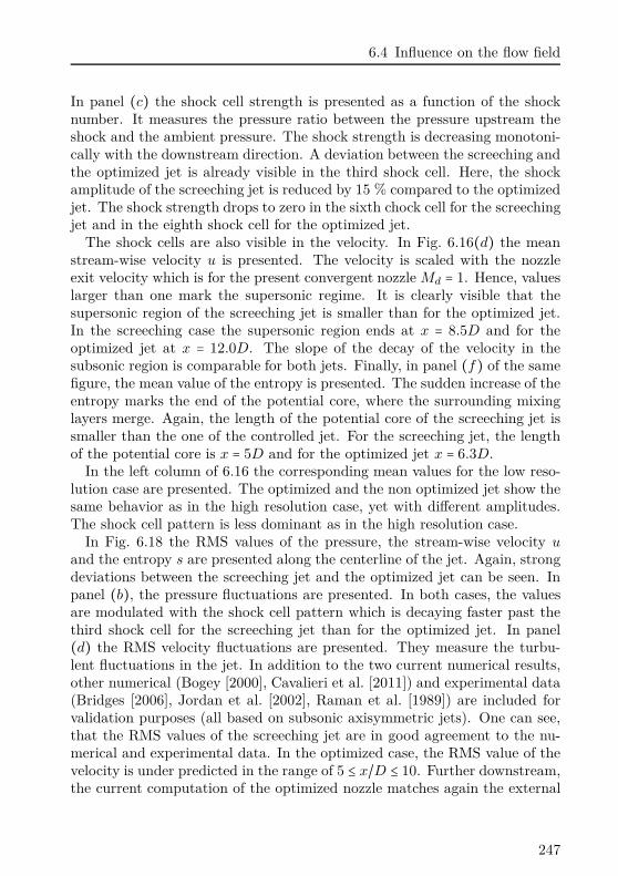
6.4 Influence on the flow field
In panel (c) the shock cell strength is presented as a function of the shocknumber. It measures the pressure ratio between the pressure upstream theshock and the ambient pressure. The shock strength is decreasing monotoni-cally with the downstream direction. A deviation between the screeching andthe optimized jet is already visible in the third shock cell. Here, the shockamplitude of the screeching jet is reduced by 15 % compared to the optimizedjet. The shock strength drops to zero in the sixth chock cell for the screechingjet and in the eighth shock cell for the optimized jet.
The shock cells are also visible in the velocity. In Fig. 6.16(d) the meanstream-wise velocity u is presented. The velocity is scaled with the nozzleexit velocity which is for the present convergent nozzle Md = 1. Hence, valueslarger than one mark the supersonic regime. It is clearly visible that thesupersonic region of the screeching jet is smaller than for the optimized jet.In the screeching case the supersonic region ends at x = 8.5D and for theoptimized jet at x = 12.0D. The slope of the decay of the velocity in thesubsonic region is comparable for both jets. Finally, in panel (f) of the samefigure, the mean value of the entropy is presented. The sudden increase of theentropy marks the end of the potential core, where the surrounding mixinglayers merge. Again, the length of the potential core of the screeching jet issmaller than the one of the controlled jet. For the screeching jet, the lengthof the potential core is x = 5D and for the optimized jet x = 6.3D.
In the left column of 6.16 the corresponding mean values for the low reso-lution case are presented. The optimized and the non optimized jet show thesame behavior as in the high resolution case, yet with different amplitudes.The shock cell pattern is less dominant as in the high resolution case.
In Fig. 6.18 the RMS values of the pressure, the stream-wise velocity u
and the entropy s are presented along the centerline of the jet. Again, strongdeviations between the screeching jet and the optimized jet can be seen. Inpanel (b), the pressure fluctuations are presented. In both cases, the valuesare modulated with the shock cell pattern which is decaying faster past thethird shock cell for the screeching jet than for the optimized jet. In panel(d) the RMS velocity fluctuations are presented. They measure the turbu-lent fluctuations in the jet. In addition to the two current numerical results,other numerical (Bogey [2000], Cavalieri et al. [2011]) and experimental data(Bridges [2006], Jordan et al. [2002], Raman et al. [1989]) are included forvalidation purposes (all based on subsonic axisymmetric jets). One can see,that the RMS values of the screeching jet are in good agreement to the nu-merical and experimental data. In the optimized case, the RMS value of thevelocity is under predicted in the range of 5 ≤ x/D ≤ 10. Further downstream,the current computation of the optimized nozzle matches again the external
247
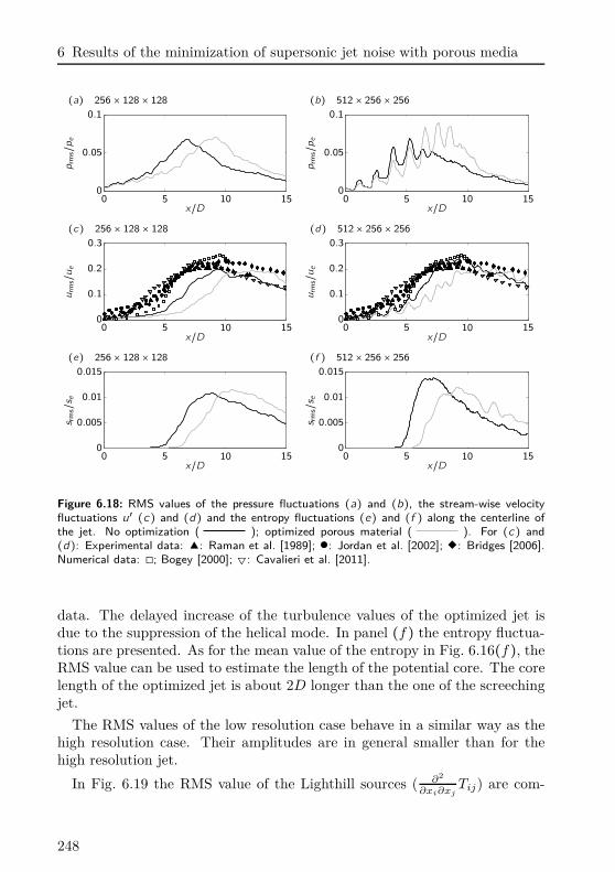
6 Results of the minimization of supersonic jet noise with porous media
(a) 256 × 128 × 128 (b) 512 × 256 × 256
prm
s/pe
x/D0 5 10 150
0.05
0.1
prm
s/pe
x/D0 5 10 150
0.05
0.1
(c) 256 × 128 × 128 (d) 512 × 256 × 256
urm
s/ue
x/D0 5 10 150
0.1
0.2
0.3
urm
s/ue
x/D0 5 10 150
0.1
0.2
0.3
(e) 256 × 128 × 128 (f ) 512 × 256 × 256
s rms/s e
x/D0 5 10 150
0.005
0.01
0.015
s rms/s e
x/D0 5 10 150
0.005
0.01
0.015
Figure 6.18: RMS values of the pressure fluctuations (a) and (b), the stream-wise velocityfluctuations u′ (c) and (d) and the entropy fluctuations (e) and (f ) along the centerline ofthe jet. No optimization ( ); optimized porous material ( ). For (c) and(d): Experimental data: : Raman et al. [1989]; : Jordan et al. [2002]; : Bridges [2006].Numerical data: ◻; Bogey [2000]; : Cavalieri et al. [2011].
data. The delayed increase of the turbulence values of the optimized jet isdue to the suppression of the helical mode. In panel (f) the entropy fluctua-tions are presented. As for the mean value of the entropy in Fig. 6.16(f), theRMS value can be used to estimate the length of the potential core. The corelength of the optimized jet is about 2D longer than the one of the screechingjet.
The RMS values of the low resolution case behave in a similar way as thehigh resolution case. Their amplitudes are in general smaller than for thehigh resolution jet.
In Fig. 6.19 the RMS value of the Lighthill sources ( ∂2
∂xi∂xjTij) are com-
248
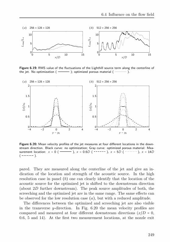
6.4 Influence on the flow field
(a) 256 × 128 × 128 (b) 512 × 256 × 256
Lrm
s/Le
x/D0 5 10 150
5
10
Lrm
s/Le
x/D0 5 10 150
5
10
Figure 6.19: RMS value of the fluctuations of the Lighthill source term along the centerline ofthe jet. No optimization ( ); optimized porous material ( ).
(a) 256 × 128 × 128 (b) 512 × 256 × 256
⟨u⟩/u
e
y − y0
−4 −2 0 2 40
0.5
1
1.5
2
⟨u⟩/u
e
y − y0
−4 −2 0 2 40
0.5
1
1.5
2
Figure 6.20: Mean velocity profiles of the jet measures at four different locations in the down-stream direction. Black curve: no optimization; Gray curve: optimized porous material: Mea-surement location: x = 0 ( ), x = 0.6D ( ), x = 5D ( ), x = 14D
( ).
pared. They are measured along the centerline of the jet and give an in-dication of the location and strength of the acoustic source. In the highresolution case in panel (b) one can clearly identify that the location of theacoustic source for the optimized jet is shifted to the downstream direction(about 2D further downstream). The peak source amplitudes of both, thescreeching and the optimized jet are in the same range. The same effects canbe observed for the low resolution case (a), but with a reduced amplitude.
The differences between the optimized and screeching jet are also visiblein the transverse y-direction. In Fig. 6.20 the mean velocity profiles arecompared and measured at four different downstream directions (x/D = 0,0.6, 5 and 14). At the first two measurement locations, at the nozzle exit
249
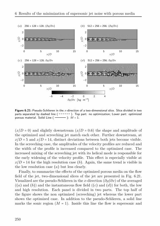
6 Results of the minimization of supersonic jet noise with porous media
(a) 256 × 128 × 128; ⟨∂ρ/∂x⟩ (b) 512 × 256 × 256; ⟨∂ρ/∂x⟩
y/D
x/D0 5 10 15
−2
0
2
y/D
x/D0 5 10 15
−2
0
2
(c) 256 × 128 × 128; ∂ρ/∂x (d) 512 × 256 × 256; ∂ρ/∂x
y/D
x/D0 5 10 15
−2
0
2
y/D
x/D0 5 10 15
−2
0
2
−6 −4 −2 0 2 4
∂ρ/∂x [kg ⋅ m−4]
Figure 6.21: Pseudo-Schlieren in the x-direction of a two-dimensional slice. Slice divided in twoparts separated by dashed line ( ). Top part: no optimization; Lower part: optimizedporous material. Solid Line ( ): M = 1.
(x/D = 0) and slightly downstream (x/D = 0.6) the shape and amplitude ofthe optimized and screeching jet match each other. Further downstream, atx/D = 5 and x/D = 14, distinct deviations between both jets become visible.In the screeching case, the amplitudes of the velocity profiles are reduced andthe width of the profile is increased compared to the optimized case. Theincreased mixing of the screeching jet with its helical mode is responsible forthe early widening of the velocity profile. This effect is especially visible atx/D = 14 for the high resolution case (b). Again, the same trend is visible inthe low resolution case (a) but less clearly.
Finally, to summarize the effects of the optimized porous media on the flowfield of the jet, two-dimensional slices of the jet are presented in Fig. 6.21.Visualized are the pseudo-Schlieren in the x-direction (∂ρ/∂x) of the averaged((a) and (b)) and the instantaneous flow field ((c) and (d)) for both, the lowand high resolution. Each panel is divided in two parts. The top half ofthe figure shows the non optimized (screeching) jet whereas the lower partshows the optimized case. In addition to the pseudo-Schlieren, a solid linemarks the sonic region (M = 1). Inside this line the flow is supersonic and
250
6.4 Influence on the flow field
subsonic elsewhere. Past the nozzle exit, one can see that the sonic linefollows the shape of the barrel shock (visible in the time averaged panels).This pattern is repeated in the downstream direction at least for the firstthree shock cells. In the time averaged panels, the sonic line marks the maindifference in the flow field: the reduced potential core of the screeching jet.As we have already seen in a previous figure, the supersonic region of thescreeching jet ends an x = 8.5D whereas it is extended up to x = 12D forthe optimized jet (suppressed helical mode). One can also identify a largernumber of shock cells in the jet core for the optimized jet (8 instead of 6).In the instantaneous view of the high resolution case (d) it is visible that thescreeching jet is spreading faster than the controlled jet. Due to the increasedmixing, caused by the helical mode, turbulent fluctuations are visible furtherapart from the centerline of the jet as in the controlled case.
In the last figure of this section in Fig. 6.22 the instantaneous pressurefluctuations are presented for the optimized and screeching jet. This figurehighlights the instantaneous acoustic field of the jet. As the previous figure,it is devided in two parts. The top half shows the jet without optimization(screeching jet) and the bottom half with optimized porous material (screechsuppression). One can clearly see that the screech tone is minimized in theoptimized case, especially in the high resolution case of panel (b). In theupstream direction the frequency of the screech tone is reduced and governedby shock-associated noise. The dminant frequency of the shock-associatednoise in the upstream direction is equal to the screech frequency (at lest forΘ = 0). Hence, the wavelength of the screech tone can still be identifiedin the controlled case, yet with a reduced amplitude and superimposed bybroadband components. Again, the effect can be also identified for the lowresolution jet in panel (a) with a reduced amplidtude.
251
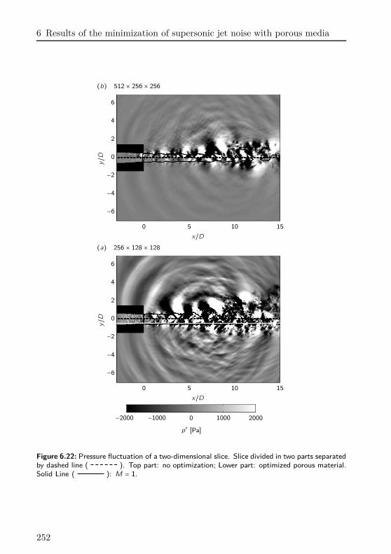
6 Results of the minimization of supersonic jet noise with porous media
(b) 512 × 256 × 256
y/D
x/D0 5 10 15
−6
−4
−2
0
2
4
6
(a) 256 × 128 × 128
y/D
x/D0 5 10 15
−6
−4
−2
0
2
4
6
−2000 −1000 0 1000 2000
p′ [Pa]
Figure 6.22: Pressure fluctuation of a two-dimensional slice. Slice divided in two parts separatedby dashed line ( ). Top part: no optimization; Lower part: optimized porous material.Solid Line ( ): M = 1.
252
7Conclusion and Outlook
Supersonic jet flows and their emanated noise are governed by complex phys-ical phenomena. On the one hand, the periodic shock cell pattern in the jetcore, the shock–diamonds, and on the other hand, the propagation of theaeroacoustic noise including the complex geometry of the jet nozzle, to closethe screech feedback loop, make high demands on the numerical method. Tothis end, a high order scheme, to solve the compressible Navier–Stokes equa-tion is implemented in the present investigation together with a high spatialresolution. Up to now, the present work represents the largest computationon axisymmetric supersonic jet noise ever performed. In addition to this, thecompressible Navier–Stokes equations were extended by a porous medium toinclude both, a solid body of arbitrarily complexity and a porous material tocontrol the fluid flow.
The implemented numerical method shows the ability to solve the intendedproblem with high accuracy. A perfect agreement of the computed aeroacous-tic noise to experimental and analytical data can be shown. Especially thecomputed frequency and amplitude of the screech tone, which is excited bya series of coupled physical phenomena, can be captured with high precision.It could be confirmed that the cessation of screech is a reason of the reducedreceptivity due to the “barrel”-shock as proposed by Raman [1996]. In addi-tion to that, the presence of the helical screech mode, which is the dominantmode of a Mj = 1.55 jet, could be identified.
Not only the acoustic properties matched the theoretical prediction but alsothe noise generating supersonic jet flow. Shock cell spacing and amplitude
253
7 Conclusion and Outlook
and the number of shock cells computed by the numerical method are ingood agreement to experimental observations. Statistical data concerning theturbulent Reynolds stresses and pressure fluctuations found in the literaturecould be reproduced by the present work. The results show that the methodpresented in this thesis is not only capable to compute aeroacoustic noiseincluding complex geometries with high accuracy but also in a efficient way.
In the second part of the thesis a novel method is derived to obtain anoptimized porous material to minimize supersonic jet noise. The method isbased on the adjoints of the porous and compressible Navier–Stokes equationswhich are derived in a continuous manner without any further simplifications.Evaluating the direct and adjoint equations subsequently, one can obtain thegradient information of the objective function with respect to the control.In the present study, the control is the space dependent permeability of theporous medium and the objective is to reduce supersonic jet noise with thefocus on jet screech. Repeating the evaluation of the gradient followed byan update of the control in an iterative loop, the optimal control (porousmedium) can be obtained. Only three optimization loops were necessary toreduce the gradient by three orders of magnitude. As a result, a complexthree-dimensional structure of a porous medium is created and placed at thenozzle exit. It acts as a sound absorbing material to influence the receptiv-ity at the nozzle lip and finally to eliminate the screech sustaining feedbackloop. A reduction of up to 20 dB of the screech tone could be observed whichcorresponds to a complete elimination of this tone from the measured spec-trum. In addition to that, mixing and broadband noise could be reducedas well in the up- and downstream direction. Especially in the downstreamdirection, the mixing noise is drastically reduced. The reason for this liesin the elimination of the screech tone and the corresponding elimination ofthe helical mode. The latter one is responsible for an increased mixing ofthe jet including mixing noise. Hence, its suppression leads to a reductionof the mixing noise which is emanated mainly in the downstream direction.Only in a small area slightly tilted in the downstream direction, broadbandshock associated noise of the controlled jet is louder than of the one withoutporous medium. Again, this phenomenon can be explained with the suppres-sion of the helical mode. As the elimination of the screech mode sustainsthe periodic shock cell pattern in the downstream direction of the jet, ad-ditional sources for shock-associated noise are created. Outside this narrowobservation sector, an overall noise reduction of almost 3 dB can be observed.The present method confirms the theoretical background on supersonic jetscreech, especially the role of the feedback loop.
The work on adjoint based control with porous media, as presented in this
254
thesis, is the first to apply it to an aeroacoustic problem and can be consid-ered as a “proof-of-concept”. An impressive performance of the optimizationalgorithm could be shown, where the intended problem could be solved withcomparable little computational effort.
The remaining question of the present investigation is, how to obtain a“real” porous material from the optimized permeability. There is no directlink between permeability and existing porous material. Even if the relationbetween permeability and the design of the material would be known, it maybe a challenging manufacturing process. Especially if solid obstacles wouldnot be connected to each other and hover in the material matrix. Hence, apost-processing of the optimized permeability, to obtain a real world materialis necessary, and more work has to be carried out to interprete the meaningof the optimized permeability with respect to its producibility.
Once a real porous material is found, its performance to eliminate screechcould be validated by an experimental setup. The supersonic jets investigatedin the present thesis are based on a Reynolds number of ReD = 5000. Assum-ing air under standard conditions for the fluid flow, the diameter of the jetwould be in the order of a human hair (0.1mm). For an experimental investi-gation including a porous material of this size, the diameter of the jet will betoo small. Hence, a computation based on a higher Reynolds number in theorder of Re ≈ 100 000 will be necessary. To resolve the small scales, a totalof about 10 billion grid points will be necessary. This is not a restriction forthe next generation high performance computers with a peak performance ofseveral PetaFlop/s (10.3PetaFlop/s, as of Nov. 2011, “K computer”). Basedon that Reynolds number, a comparison to experimental setups of jets witha diameter of several centimeters will be possible.
The novel method of adjoint based optimization, in combination withporous media, are a promising and efficient method to minimize supersonicjet noise. Beyond the aeroacoustic field, this type of flow optimization mayfind application in a variety of disciplines and configurations where the opti-mization of any objective by means of a modification of the geometry and/ormaterial is desired.
255

ACompressible Navier–Stokes equations
In the following, the compressible Navier–Stokes equations are given in acharacteristic formulation based on non Cartesian coordinates. In the presentinvestigation, all derivatives are computed in the computational domain withrespect to the contravariant basis vectors ξ, η and ζ. If the grid is timedependent, an additional time variable τ will arise. The physical variablesare described in the x, y and z domain with the time t. To compute aderivative in the physical domain, a grid transformation has to be applied.The contravariant basis vectors are dependent on the physical domain:
ξ = ξ(x, y, z, t)η = η(x, y, z, t)ζ = ζ(x, y, z, t)τ = τ(t)
A derivative with respect to the physical space has to follow the chain rule:
∂
∂xi
= ∂ξ
∂xi
∂
∂ξ+
∂η
∂xi
∂
∂η+
∂ζ
∂xi
∂
∂ζ
= ∂ξl
∂xi
∂
∂ξl
= ξl,i
∂
∂ξl
with the shorthand ξl,i ∶= ∂ξl
∂xi.
257
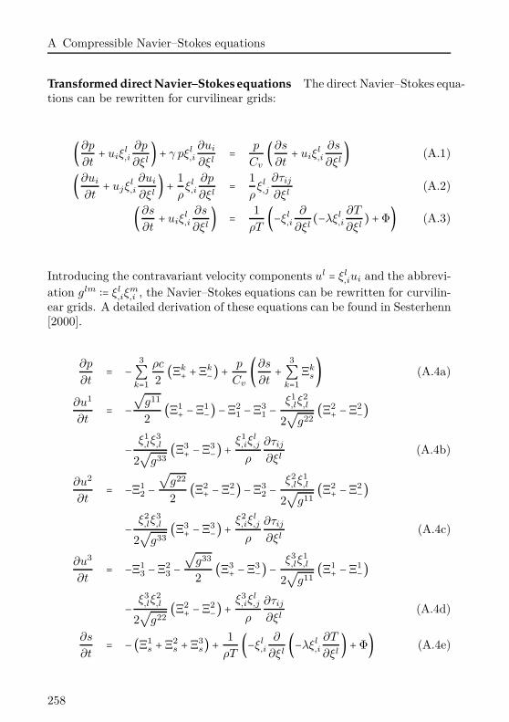
A Compressible Navier–Stokes equations
Transformed direct Navier–Stokes equations The direct Navier–Stokes equa-tions can be rewritten for curvilinear grids:
(∂p
∂t+ uiξ
l,i
∂p
∂ξl) + γ pξl
,i
∂ui
∂ξl= p
Cv
(∂s
∂t+ uiξ
l,i
∂s
∂ξl) (A.1)
(∂ui
∂t+ ujξl
,i
∂ui
∂ξl) + 1
ρξl
,i
∂p
∂ξl= 1
ρξl
,j
∂τij
∂ξl(A.2)
(∂s
∂t+ uiξ
l,i
∂s
∂ξl) = 1
ρT(−ξl
,i
∂
∂ξl(−λξl
,i
∂T
∂ξl) +Φ) (A.3)
Introducing the contravariant velocity components ul = ξl,iui and the abbrevi-
ation glm ∶= ξl,iξ
m,i , the Navier–Stokes equations can be rewritten for curvilin-
ear grids. A detailed derivation of these equations can be found in Sesterhenn[2000].
∂p
∂t= −
3∑k=1
ρc
2(Ξk+ +Ξk
−) + p
Cv
(∂s
∂t+
3∑k=1
Ξks) (A.4a)
∂u1
∂t= −
√g11
2(Ξ1+ −Ξ1
−) −Ξ2
1 −Ξ31 −
ξ1,lξ
2,l
2√
g22(Ξ2+ −Ξ2
−)
−ξ1
,lξ3,l
2√
g33(Ξ3+ −Ξ3
−) + ξ1
,iξl,j
ρ
∂τij
∂ξl(A.4b)
∂u2
∂t= −Ξ1
2 −
√g22
2(Ξ2+ − Ξ2
−) −Ξ32 −
ξ2,lξ
1,l
2√
g11(Ξ2+ −Ξ2
−)−
ξ2,lξ
3,l
2√
g33(Ξ3+ −Ξ3
−) + ξ2
,iξl,j
ρ
∂τij
∂ξl(A.4c)
∂u3
∂t= −Ξ1
3 −Ξ23 −
√g33
2(Ξ3+ −Ξ3
−) − ξ3,lξ
1,l
2√
g11(Ξ1+ −Ξ1
−)−
ξ3,lξ
2,l
2√
g22(Ξ2+ −Ξ2
−) + ξ3,iξ
l,j
ρ
∂τij
∂ξl(A.4d)
∂s
∂t= − (Ξ1
s + Ξ2s +Ξ3
s) + 1
ρT(−ξl
,i
∂
∂ξl(−λξl
,i
∂T
∂ξl) +Φ) (A.4e)
258
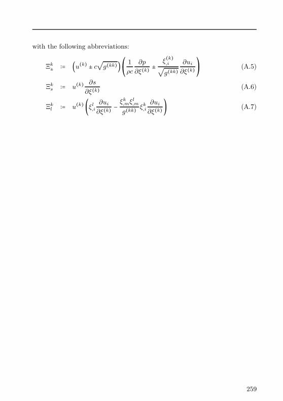
with the following abbreviations:
Ξk± ∶= (u(k) ± c
√g(kk))⎛⎝
1
ρc
∂p
∂ξ(k)±
ξ(k),i√g(kk)
∂ui
∂ξ(k)⎞⎠ (A.5)
Ξks ∶= u(k) ∂s
∂ξ(k)(A.6)
Ξkl ∶= u(k) (ξl
,i
∂ui
∂ξ(k)−
ξk,mξl
,m
g(kk) ξk,i
∂ui
∂ξ(k)) (A.7)
259

BLinearized Navier–Stokes equations
Based on the nonlinear, porous and compressible Navier–Stokes equations ofSec. § 3.1, the linearized Navier–Stokes equations can be written in matrixformulation. To obtain the adjoints of the direct equations, we need to includeall information to close the system of equations. Hence, besides the fivepartial differential equations, three additional algebraic equations to closesystem need to be included. To this end, the dimension of the system is eightwith the following state vector of the fluctuations:
δq = (δp, δu, δv, δw, δs, δρ, δT, δµ)T .
The first five entries correspond to the five PDE’s of the Navier–Stokes equa-tions for the pressure δp, the three velocity components δu, δv, δw and theentropy δs. The latter three entries correspond to the fluctuations of thedensity δρ, the temperature δT and the viscosity δµ. Note, that the viscosityis only a function of the temperature (see Sutherland’s law of Eq. (2.6)) andits variational formulation can be given as:
δµ = dµ(T )dT
δT
Finally, the linearized, porous and compressible Navier–Stokes equations canbe written as:
B∂δq
∂t+Ak
∂δq
∂xk
+Dij
∂2δq
∂xi∂xj
+Cδq = 0 (B.1)
with the matrices:
261
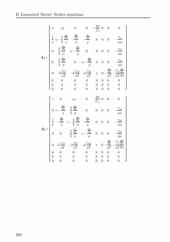
B Linearized Navier–Stokes equations
A1 =
⎡⎢⎢⎢⎢⎢⎢⎢⎢⎢⎢⎢⎢⎢⎢⎢⎢⎢⎢⎢⎢⎢⎢⎢⎢⎢⎢⎢⎢⎢⎢⎢⎢⎢⎣
u γ p 0 0 −pu
Cv
0 0 0
1
ρu −
4
3
∂µ
∂x
ρ−
∂µ
∂y
ρ−
∂µ
∂z
ρ0 0 0 −
τ11
µρ
02
3
∂µ
∂y
ρu −
∂µ
∂x
ρ0 0 0 0 −
τ12
µρ
02
3
∂µ
∂z
ρ0 u −
∂µ
∂x
ρ0 0 0 −
τ13
µρ
0 −2τ11
ρT−2
τ12
ρT−2
τ13
ρTu 0 −
∂λ∂x
ρT−
Cp∂T∂x
ρT Pr
0 0 0 0 0 0 0 0
0 0 0 0 0 0 0 0
0 0 0 0 0 0 0 0
⎤⎥⎥⎥⎥⎥⎥⎥⎥⎥⎥⎥⎥⎥⎥⎥⎥⎥⎥⎥⎥⎥⎥⎥⎥⎥⎥⎥⎥⎥⎥⎥⎥⎥⎦
A2 =
⎡⎢⎢⎢⎢⎢⎢⎢⎢⎢⎢⎢⎢⎢⎢⎢⎢⎢⎢⎢⎢⎢⎢⎢⎢⎢⎢⎢⎢⎢⎢⎢⎢⎢⎢⎣
v 0 γ p 0 −pv
Cv
0 0 0
0 v −
∂µ
∂y
ρ
2
3
∂µ
∂x
ρ0 0 0 0 −
τ12
µρ
1
ρ−
∂µ
∂x
ρv −
4
3
∂µ
∂y
ρ−
∂µ
∂z
ρ0 0 0 −
τ22
µρ
0 02
3
∂µ
∂z
ρv −
∂µ
∂y
ρ0 0 0 −
τ23
µρ
0 −2τ12
ρT−2
τ22
ρT−2
τ23
ρTv 0 −
∂λ∂y
ρT−
Cp∂T∂y
ρT Pr
0 0 0 0 0 0 0 0
0 0 0 0 0 0 0 0
0 0 0 0 0 0 0 0
⎤⎥⎥⎥⎥⎥⎥⎥⎥⎥⎥⎥⎥⎥⎥⎥⎥⎥⎥⎥⎥⎥⎥⎥⎥⎥⎥⎥⎥⎥⎥⎥⎥⎥⎥⎦
262
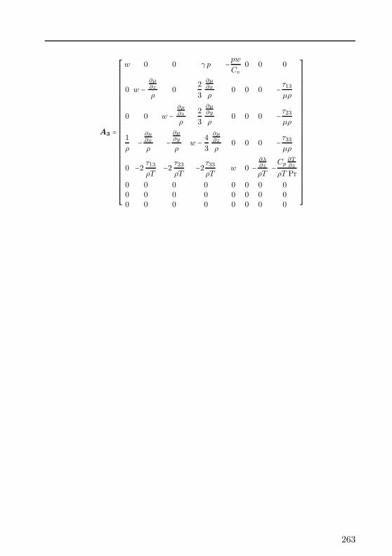
A3 =
⎡⎢⎢⎢⎢⎢⎢⎢⎢⎢⎢⎢⎢⎢⎢⎢⎢⎢⎢⎢⎢⎢⎢⎢⎢⎢⎢⎢⎢⎢⎢⎢⎢⎢⎣
w 0 0 γ p −pw
Cv
0 0 0
0 w −
∂µ
∂z
ρ0
2
3
∂µ
∂x
ρ0 0 0 −
τ13
µρ
0 0 w −
∂µ
∂z
ρ
2
3
∂µ
∂y
ρ0 0 0 −
τ23
µρ
1
ρ−
∂µ
∂x
ρ−
∂µ
∂y
ρw −
4
3
∂µ
∂z
ρ0 0 0 −
τ33
µρ
0 −2τ13
ρT−2
τ23
ρT−2
τ33
ρTw 0 −
∂λ∂z
ρT−
Cp∂T∂z
ρT Pr
0 0 0 0 0 0 0 0
0 0 0 0 0 0 0 0
0 0 0 0 0 0 0 0
⎤⎥⎥⎥⎥⎥⎥⎥⎥⎥⎥⎥⎥⎥⎥⎥⎥⎥⎥⎥⎥⎥⎥⎥⎥⎥⎥⎥⎥⎥⎥⎥⎥⎥⎦
263
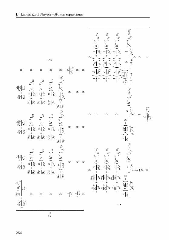
B Linearized Navier–Stokes equations
C=⎡ ⎢ ⎢ ⎢ ⎢ ⎢ ⎢ ⎢ ⎢ ⎢ ⎢ ⎢ ⎢ ⎢ ⎢ ⎢ ⎢ ⎢ ⎢ ⎢ ⎢ ⎢ ⎢ ⎢ ⎢ ⎢ ⎢ ⎢ ⎢ ⎢ ⎢ ⎢ ⎢ ⎢ ⎢ ⎢ ⎢ ⎣γ
∂u
j
∂x
j
−
∂s
∂t+
uj
∂s
∂x
j
Cv
∂p
∂x−
p∂
s∂
x
Cv
∂p
∂y−
p∂
s∂
y
Cv
∂p
∂z−
p∂
s∂
z
Cv
0
0∂
u
∂x+
µ ρφ( K−
1) 11
∂u
∂y+
µ ρφ( K−
1) 12
∂u
∂z+
µ ρφ( K−
1) 13
0
0∂
v
∂x+
µ ρφ( K−
1) 21
∂v
∂y+
µ ρφ( K−
1) 22
∂v
∂z+
µ ρφ( K−
1) 32
0
0∂
w
∂x+
µ ρφ( K−
1) 31
∂w
∂y+
µ ρφ( K−
1) 32
∂w
∂z+
µ ρφ( K−
1) 33
0
0∂
s
∂x−
2µ
ρφ
T( K−
1) 1j
uj
∂s
∂y−
2µ
ρφ
T( K−
1) 2j
uj
∂s
∂z−
2µ
ρφ
T( K−
1) 3j
uj
0
−1 c2
00
0p
c2C
v
−1 ρR
00
00
00
00
0
⤸
⤹
00
0
−
∂ ∂x
p
ρ2+
∂τ
1j
∂x
j
ρ2−
µ
ρ2φ( K−
1) 1j
uj
0−
1 ρ(∂
∂x
j
(τ 1j
µ))+
1 ρφ( K−
1) 1j
uj
−
∂ ∂yp
ρ2+
∂τ
2j
∂x
j
ρ2−
µ
ρ2φ( K−
1) 2j
uj
0−
1 ρ(∂
∂x
j
(τ 2j
µ))+
1 ρφ( K−
1) 2j
uj
−
∂ ∂zp
ρ2+
∂τ
3j
∂x
j
ρ2−
µ
ρ2φ( K−
1) 3j
uj
0−
1 ρ(∂
∂x
j
(τ 3j
µ))+
1 ρφ( K−
1) 3j
uj
∂∂
xj(λ
∂T
∂x
j)+
Φ
(ρ)2
T+
µ
ρ2φ
T( K−
1) ij
uiu
j
∂∂
xj(λ
∂T
∂x
j)+
Φ
ρ(T)
2+
µ
ρφ
T2( K−
1) ij
uiu
j−
Cp(∂2
T∂
x2 j
)P
rρT−
Φ
ρT
µ−
1
ρφ
T( K−
1) ij
uiu
j
10
0T ρ
10
0−
d dT
µ(T)
1
⎤ ⎥ ⎥ ⎥ ⎥ ⎥ ⎥ ⎥ ⎥ ⎥ ⎥ ⎥ ⎥ ⎥ ⎥ ⎥ ⎥ ⎥ ⎥ ⎥ ⎥ ⎥ ⎥ ⎥ ⎥ ⎥ ⎥ ⎥ ⎥ ⎥ ⎥ ⎥ ⎥ ⎦
264
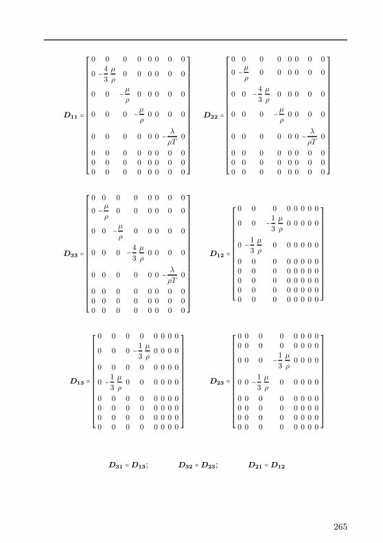
D11 =
⎡⎢⎢⎢⎢⎢⎢⎢⎢⎢⎢⎢⎢⎢⎢⎢⎢⎢⎢⎢⎢⎢⎢⎢⎢⎢⎢⎢⎣
0 0 0 0 0 0 0 0
0 −4
3
µ
ρ0 0 0 0 0 0
0 0 −µ
ρ0 0 0 0 0
0 0 0 −µ
ρ0 0 0 0
0 0 0 0 0 0 −λ
ρT0
0 0 0 0 0 0 0 0
0 0 0 0 0 0 0 0
0 0 0 0 0 0 0 0
⎤⎥⎥⎥⎥⎥⎥⎥⎥⎥⎥⎥⎥⎥⎥⎥⎥⎥⎥⎥⎥⎥⎥⎥⎥⎥⎥⎥⎦
D22 =
⎡⎢⎢⎢⎢⎢⎢⎢⎢⎢⎢⎢⎢⎢⎢⎢⎢⎢⎢⎢⎢⎢⎢⎢⎢⎢⎢⎢⎣
0 0 0 0 0 0 0 0
0 −µ
ρ0 0 0 0 0 0
0 0 −4
3
µ
ρ0 0 0 0 0
0 0 0 −µ
ρ0 0 0 0
0 0 0 0 0 0 −λ
ρT0
0 0 0 0 0 0 0 0
0 0 0 0 0 0 0 0
0 0 0 0 0 0 0 0
⎤⎥⎥⎥⎥⎥⎥⎥⎥⎥⎥⎥⎥⎥⎥⎥⎥⎥⎥⎥⎥⎥⎥⎥⎥⎥⎥⎥⎦
D33 =
⎡⎢⎢⎢⎢⎢⎢⎢⎢⎢⎢⎢⎢⎢⎢⎢⎢⎢⎢⎢⎢⎢⎢⎢⎢⎢⎢⎢⎣
0 0 0 0 0 0 0 0
0 −µ
ρ0 0 0 0 0 0
0 0 −µ
ρ0 0 0 0 0
0 0 0 −4
3
µ
ρ0 0 0 0
0 0 0 0 0 0 −λ
ρT0
0 0 0 0 0 0 0 0
0 0 0 0 0 0 0 0
0 0 0 0 0 0 0 0
⎤⎥⎥⎥⎥⎥⎥⎥⎥⎥⎥⎥⎥⎥⎥⎥⎥⎥⎥⎥⎥⎥⎥⎥⎥⎥⎥⎥⎦
D12 =
⎡⎢⎢⎢⎢⎢⎢⎢⎢⎢⎢⎢⎢⎢⎢⎢⎢⎢⎢⎢⎢⎢⎣
0 0 0 0 0 0 0 0
0 0 −1
3
µ
ρ0 0 0 0 0
0 −1
3
µ
ρ0 0 0 0 0 0
0 0 0 0 0 0 0 0
0 0 0 0 0 0 0 0
0 0 0 0 0 0 0 0
0 0 0 0 0 0 0 0
0 0 0 0 0 0 0 0
⎤⎥⎥⎥⎥⎥⎥⎥⎥⎥⎥⎥⎥⎥⎥⎥⎥⎥⎥⎥⎥⎥⎦
D13 =
⎡⎢⎢⎢⎢⎢⎢⎢⎢⎢⎢⎢⎢⎢⎢⎢⎢⎢⎢⎢⎢⎢⎣
0 0 0 0 0 0 0 0
0 0 0 −1
3
µ
ρ0 0 0 0
0 0 0 0 0 0 0 0
0 −1
3
µ
ρ0 0 0 0 0 0
0 0 0 0 0 0 0 0
0 0 0 0 0 0 0 0
0 0 0 0 0 0 0 0
0 0 0 0 0 0 0 0
⎤⎥⎥⎥⎥⎥⎥⎥⎥⎥⎥⎥⎥⎥⎥⎥⎥⎥⎥⎥⎥⎥⎦
D23 =
⎡⎢⎢⎢⎢⎢⎢⎢⎢⎢⎢⎢⎢⎢⎢⎢⎢⎢⎢⎢⎢⎢⎣
0 0 0 0 0 0 0 0
0 0 0 0 0 0 0 0
0 0 0 −1
3
µ
ρ0 0 0 0
0 0 −1
3
µ
ρ0 0 0 0 0
0 0 0 0 0 0 0 0
0 0 0 0 0 0 0 0
0 0 0 0 0 0 0 0
0 0 0 0 0 0 0 0
⎤⎥⎥⎥⎥⎥⎥⎥⎥⎥⎥⎥⎥⎥⎥⎥⎥⎥⎥⎥⎥⎥⎦
D31 =D13; D32 =D23; D21 =D12
265

CCompressible adjoint Navier–Stokes
equations
The direct Navier–Stokes equations are written in a characteristic formulationof Sesterhenn [2000]. In a continuous adjoint approach it is important to usethe same numerical method for the direct as for the adjoint computation.To this end, the adjoint Navier–Stokes equations are also decomposed intocharacteristic waves. First, the scalar product of
αT (−BT ∂q⋆
∂t−Ak
T ∂q⋆
∂xk
) = 0 (C.1)
is calculated with αT = (α1, α2, α3, α4, α5), where, to simplify matters,only the variations in x are considered and written in the form:
(−α1 +α5
p
Cv
) ∂p⋆
∂t+(−α2γp − α1u +α5
p
Cv
u) ∂p⋆
∂x+
−α2
∂u⋆
∂t+(−α2u −
α1
ρ) ∂u⋆
∂x+
−α3
∂v⋆
∂t+(−α3u) ∂v⋆
∂x+
−α4
∂w⋆
∂t+(−α4u) ∂w⋆
∂x+
−α5
∂s⋆
∂t+(−α5u) ∂s⋆
∂x= 0
267
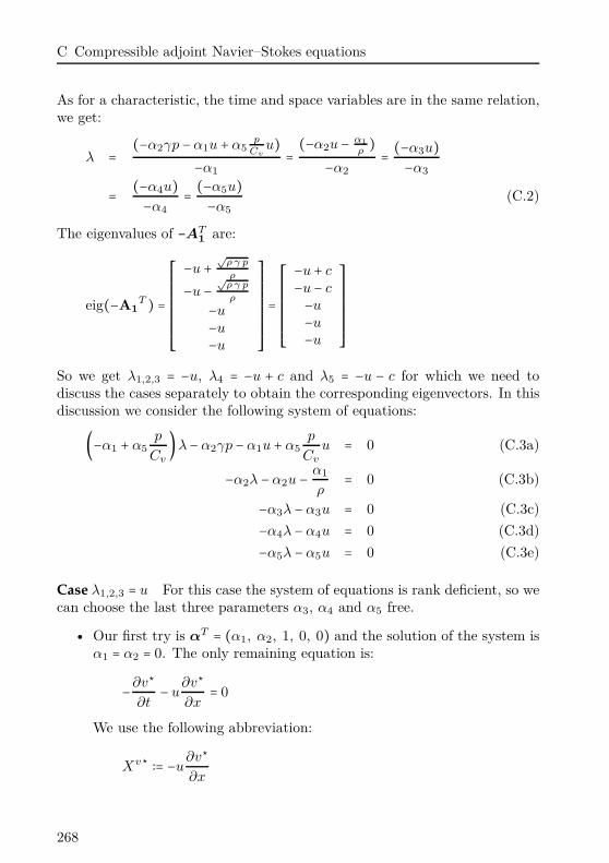
C Compressible adjoint Navier–Stokes equations
As for a characteristic, the time and space variables are in the same relation,we get:
λ = (−α2γp −α1u +α5p
Cvu)
−α1
= (−α2u − α1
ρ)
−α2
= (−α3u)−α3
= (−α4u)−α4
= (−α5u)−α5
(C.2)
The eigenvalues of −AT1
are:
eig(−A1T ) =
⎡⎢⎢⎢⎢⎢⎢⎢⎢⎢⎢⎣
−u +√
ρ γ p
ρ
−u −√
ρ γ p
ρ
−u
−u
−u
⎤⎥⎥⎥⎥⎥⎥⎥⎥⎥⎥⎦=⎡⎢⎢⎢⎢⎢⎢⎢⎢⎢⎣
−u + c
−u − c
−u
−u
−u
⎤⎥⎥⎥⎥⎥⎥⎥⎥⎥⎦So we get λ1,2,3 = −u, λ4 = −u + c and λ5 = −u − c for which we need todiscuss the cases separately to obtain the corresponding eigenvectors. In thisdiscussion we consider the following system of equations:
(−α1 + α5
p
Cv
)λ − α2γp −α1u + α5
p
Cv
u = 0 (C.3a)
−α2λ −α2u −α1
ρ= 0 (C.3b)
−α3λ −α3u = 0 (C.3c)
−α4λ −α4u = 0 (C.3d)
−α5λ −α5u = 0 (C.3e)
Case λ1,2,3 = u For this case the system of equations is rank deficient, so wecan choose the last three parameters α3, α4 and α5 free.
• Our first try is αT = (α1, α2, 1, 0, 0) and the solution of the system isα1 = α2 = 0. The only remaining equation is:
−∂v⋆
∂t− u
∂v⋆
∂x= 0
We use the following abbreviation:
Xv⋆ ∶= −u∂v⋆
∂x
268
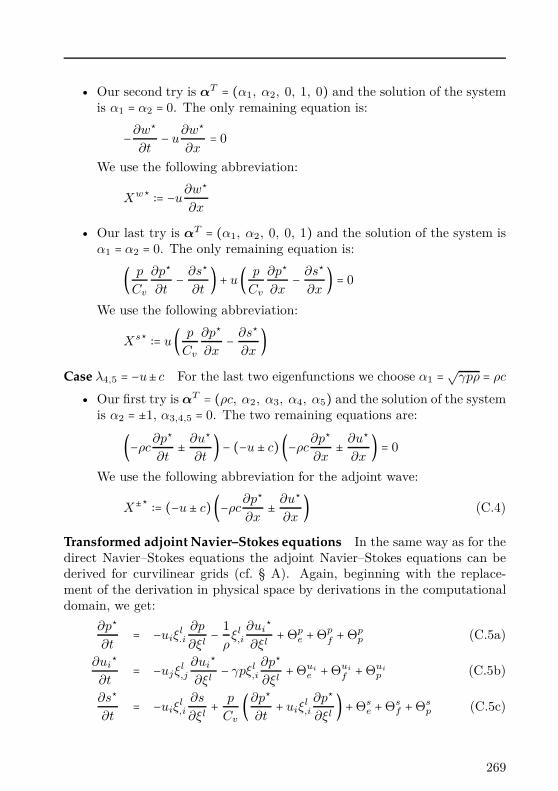
• Our second try is αT = (α1, α2, 0, 1, 0) and the solution of the systemis α1 = α2 = 0. The only remaining equation is:
−∂w⋆
∂t− u
∂w⋆
∂x= 0
We use the following abbreviation:
Xw⋆ ∶= −u∂w⋆
∂x
• Our last try is αT = (α1, α2, 0, 0, 1) and the solution of the system isα1 = α2 = 0. The only remaining equation is:
( p
Cv
∂p⋆
∂t−
∂s⋆
∂t) + u( p
Cv
∂p⋆
∂x−
∂s⋆
∂x) = 0
We use the following abbreviation:
Xs⋆ ∶= u( p
Cv
∂p⋆
∂x−
∂s⋆
∂x)
Case λ4,5 = −u± c For the last two eigenfunctions we choose α1 =√γpρ = ρc
• Our first try is αT = (ρc, α2, α3, α4, α5) and the solution of the systemis α2 = ±1, α3,4,5 = 0. The two remaining equations are:
(−ρc∂p⋆
∂t±
∂u⋆
∂t) − (−u ± c) (−ρc
∂p⋆
∂x±
∂u⋆
∂x) = 0
We use the following abbreviation for the adjoint wave:
X±⋆∶= (−u ± c)(−ρc
∂p⋆
∂x±
∂u⋆
∂x) (C.4)
Transformed adjoint Navier–Stokes equations In the same way as for thedirect Navier–Stokes equations the adjoint Navier–Stokes equations can bederived for curvilinear grids (cf. § A). Again, beginning with the replace-ment of the derivation in physical space by derivations in the computationaldomain, we get:
∂p⋆
∂t= −uiξ
l.i
∂p
∂ξl−
1
ρξl
,i
∂ui⋆
∂ξl+Θp
e +Θpf+Θp
p (C.5a)
∂ui⋆
∂t= −ujξl
,j
∂ui⋆
∂ξl− γpξl
,i
∂p⋆
∂ξl+Θui
e +Θui
f+Θui
p (C.5b)
∂s⋆
∂t= −uiξ
l,i
∂s
∂ξl+
p
Cv
(∂p⋆
∂t+ uiξ
l,i
∂p⋆
∂ξl) +Θs
e +Θsf +Θs
p (C.5c)
269
C Compressible adjoint Navier–Stokes equations
Finally, after some math in the same manner as for the direct Navier–Stokesequations the adjoint Navier–Stokes equations can be written in characteristicwaves for curvilinear grids.
∂p⋆
∂t= −
3∑k=1
1
2ρc(Ξk+
⋆
+Ξk−
⋆) +Θpe +Θ
pf+Θp
p (C.6a)
∂u1⋆
∂t=√
g11
2(Ξ1+
⋆
−Ξ1−
⋆) +Ξ21
⋆
+Ξ31
⋆
+ξ1
,lξ2,l
2√
g22(Ξ2+
⋆
−Ξ2−
⋆)+
ξ1,lξ
3,l
2√
g33(Ξ3+
⋆
− Ξ3−
⋆) + ξ1,i (Θui
e +Θui
f+Θui
p ) (C.6b)
∂u2⋆
∂t= Ξ1
2
⋆
+
√g22
2(Ξ2+
⋆
−Ξ2−
⋆) +Ξ32
⋆
+ξ2
,lξ1,l
2√
g11(Ξ2+
⋆
−Ξ2−
⋆)+
ξ2,lξ
3,l
2√
g33(Ξ3+
⋆
− Ξ3−
⋆) + ξ2,i (Θui
e +Θui
f+Θui
p ) (C.6c)
∂u3⋆
∂t= Ξ1
3
⋆
+ Ξ23
⋆
+
√g33
2(Ξ3+
⋆
−Ξ3−
⋆) + ξ3,lξ
1,l
2√
g11(Ξ1+
⋆
−Ξ1−
⋆)+
ξ3,lξ
2,l
2√
g22(Ξ2+
⋆
− Ξ2−
⋆) + ξ3,i (Θui
e +Θui
f+Θui
p ) (C.6d)
∂s⋆
∂t= (Ξ1
s
⋆
+ Ξ2s
⋆
+Ξ3s
⋆) + p
Cv
∂p⋆
∂t+ (Θs
e +Θsf +Θs
p) (C.6e)
and the abbreviation for the adjoint characteristic waves for curvilinear grids
Ξk±
⋆
∶= (−u(k) ± c√
g(kk))⎛⎝−ρc∂p⋆
∂ξ(k)±
ξ(k),i√g(kk)
∂ui⋆
∂ξ(k)⎞⎠ (C.7a)
Ξks
⋆
∶= u(k) ( p
Cv
∂p⋆
∂ξ(k)−
∂s⋆
∂ξ(k)) (C.7b)
Ξkl
⋆
∶= −u(k) (ξl,i
∂ui⋆
∂ξ(k)−
ξk,mξl
,m
g(kk) ξk,i
∂ui⋆
∂ξ(k)) (C.7c)
270
Bibliography
Aage, N., Poulsen, T., Gersborg-Hansen, A., & Sigmund, O. (2008). Topologyoptimization of large scale stokes flow problems. Structural and Multidis-ciplinary Optimization, 35, 175–180.
Adams, N. A. & Shariff, K. (1996). A high-resolution hybrid compact-eno scheme for shock-turbulence interaction problems. J. Comput. Phys.,127(1), 27–51.
Airiau, C., Bottaro, A., Walther, S., & Legendre, D. (2003). A methodologyfor optimal laminar flow control: Application to the damping of tollmienschlichting waves in a boundary layer. Phys. Fluids, 15(5), 1131–1145.
Al-Qadi, I. & Scott, J. (2003). High-order three-dimensional numerical sim-ulation of a supersonic rectangualr jet. In 9th AIAA/CEAS AeroacousticsConference and Exhibit, number 2003-3238: AIAA.
Al-Qadi, I. M. A. & Scott, J. N. (2001). Simulations of unsteady behavior inunder-expanded supersonic rectangular jets. In AIAA/CEAS AeroacousticsConference and Exhibit, number 2001-2119: AIAA.
Alkislar, M. B., Krothapalli, A., & Lourenco, L. M. (2003). Structure of ascreeching rectangular jet: a stereoscopic particle image velocimetry study.J. Fluid Mech., 489, 121–154.
Anderson, D., Tannehill, J., & Pletcher, R. (1984). Computational fluidmechanics and heat transfer. Hemisphere Publishing, New York, NY.
Angot, P., Bruneau, C.-H., & Fabrie, P. (1999). A penalization method totake into account obstacles in incompressible viscous flows. NumerischeMathematik, 81, 497–520. 10.1007/s002110050401.
271
Bibliography
Armijo, L. (1966). Minimization of functions having lipschitz continuous firstpartial derivatives. Pacific J. Math., 16(1), 1–3.
Arquis, E. & Caltagirone, J. (1984). Sur les conditions hydrodynamiquesau voisinage d’une interface milieu fluide-milieu poreux: application á laconvection naturelle. C.R. Acad. Sci. Paris II, 299, 1–4.
Asouti, V. G., Zymaris, A. S., Papadimitriou, D. I., & Giannakoglou, K. C.(2008). Continuous and discrete adjoint approaches for aerodynamic shapeoptimization with low mach number preconditioning. Int. J. Numer. Meth-ods Fluids, 57(10), 1485–1504.
Babucke, A., Spagnoli, B., Airiau, C., Kloker, M., & Rist, U. (2009). Mech-anisms and active control of jet-induced noise. In C. Brun, D. Juve, M.Manhart, & C.-D. Munz (Eds.), Numerical Simulation of Turbulent Flowsand Noise Generation, volume 104 of Notes on Numerical Fluid Mechanicsand Multidisciplinary Design (pp. 75–98). Springer Berlin / Heidelberg.
Barone, M. F. (2003). Receptivity of compressible mixing layers. PhD thesis,Stanford University.
Barone, M. F. & Lele, S. (2005). Receptivity of the compressible mixing layer.J. Fluid Mech., 540, 301–335.
Baur, C., Bontoux, P., Kornhaas, M., Minguez, M., Pasquetti, R., Schäfer,M., Serre, E., & Séverac, E. (2009). High-order methods for large-eddy sim-ulation in complex geometries. In C. Brun, D. Juvé, M. Manhart, & C.-D.Munz (Eds.), Numerical Simulation of Turbulent Flows and Noise Gener-ation, volume 104 of Notes on Numerical Fluid Mechanics and Multidisci-plinary Design (pp. 309–334). Springer Berlin / Heidelberg. 10.1007/978-3-540-89956-3.
Bear, J. (1972). Dynamics of fluids in porous media. Environmental scienceseries. New York: American Elsevier. 0-444-00114-X.
Bendsøe, M. (1995). Optimization of structural topology, shape, and material,volume 414. Springer Berlin.
Berland, J., Bogey, C., & Bailly, C. (2006). Large eddy simulation of screechtone generation in a planar underexpanded jet. In 12th AIAA/CEASAeroacoustics Conference (27th AIAA Aeroacoustics Conference), number2006-2496: AIAA.
272
Bibliography
Berland, J., Bogey, C., & Bailly, C. (2007). Numerical study of screechgeneration in a planar supersonic jet. Phys. Fluids, 19(7), 075105.
Bewley, T. R. (2001). Flow Control: New Challenges for a New Renaissance.Pro. Aerospace Sci., 37(1), 21–58.
Bewley, T. R., Moin, P., & Temam, R. (2001). Dns-based predictive controlof turbulence: an optimal benchmark for feedback algorithms. J. FluidMech., 447, 179–225.
Bischof, C., Carle, A., Corliss, G., Griewank, A., & Hovland, P. (1992).Adifor-generating derivative codes from fortran programs. Sci. Program.,1, 11–29.
Bodony, D., Ryu, J., Ray, P., & Lele, S. (2006). Investigating broadbandshock-associated noise of axisymmetric jets using large-eddy simulation.In 12th AIAA/CEAS Aeroacoustics Conference (27th AIAA AeroacousticsConference), number 2006-2495: AIAA.
Bodony, D. J. & Lele, S. K. (2005). On using large-eddy simulation for theprediction of noise from cold and heated turbulent jets. Phys. Fluids, 17(8),085103–1–20.
Bogey, C. (2000). Calcul direct du bruit aérodynamique et validation de mod-éles acoustiques hybrides. PhD thesis, Ecole Central de Lyon.
Bogey, C. & Bailly, C. (2005). Decrease of the effective reynolds number witheddy-viscosity subgrid modeling. AIAA J., 43(2), 437–439.
Bogey, C. & Bailly, C. (2009). Turbulence and energy budget in a self-preserving round jet: direct evaluation using large eddy simulation. J.Fluid Mech., 627, 129–160.
Bogey, C. & Bailly, C. (2010). Influence of nozzle-exit boundary-layer con-ditions on the flow and acoustic fields of initially laminar jets. J. FluidMech., 663, 507–538.
Bogey, C., de Cacqueray, N., & Bailly, C. (2009). A shock-capturing method-ology based on adaptative spatial filtering for high-order non-linear com-putations. J. Comput. Phys., 228(5), 1447–1465.
Borrvall, T. & Petersson, J. (2003). Topology optimization of fluids in stokesflow. Int. J. Numer. Methods Fluids, 41(1), 77–107.
273
Bibliography
Boyd, S. & Vandenberghe, L. (2004). Convex optimization. Cambridge UnivPr.
Bradbury, L. J. S. (1965). The structure of a self-preserving turbulent planejet. J. Fluid Mech., 23(1), 31–64.
Brezillon, J. & Gauger, N. (2004). 2d and 3d aerodynamic shape optimisationusing the adjoint approach. Aerosp. Sci. Technol., 8(8), 715–727.
Bridges, J. (2006). Effect of heat on space-time correlations in jets. In 12thAIAA/CEAS Aeroacoustics Conference, number 2006-2534: AIAA.
Brinkman, H. (1949). A calculation of the viscous force exerted by aflowing fluid on a dense swarm of particles. Appl. Sci. Res., 1, 27–34.10.1007/BF02120313.
Bruneau, C.-H. & Mortazavi, I. (2008). Numerical modelling and passive flowcontrol using porous media. Comput. Fluids, 37(5), 488–498. Special IssueDedicated to Professor M.M. Hafez on the Occasion of his 60th Birthday- Special Issue Dedicated to Professor M.M. Hafez on the Occasion of his60th Birthday.
Caliari, M. & Ostermann, A. (2009). Implementation of exponentialrosenbrock-type integrators. Appl. Numer. Math., 59, 568–581.
Cao, Y. & Stanescu, D. (2002). Shape optimization for noise radiation prob-lems. Computers and Mathematics with Applications, 44(12), 1527–1537.
Carbou, G. (2008). Brinkmann model and double penalization method forthe flow around a porous thin layer. J. Math. Fluid Mech., 10, 126–158.10.1007/s00021-006-0221-y.
Carpentieri, G., Koren, B., & van Tooren, M. (2007). Adjoint-based aero-dynamic shape optimization on unstructured meshes. J. Comput. Phys.,224(1), 267–287.
Cavalieri, A. V., Daviller, G., Comte, P., Jordan, P., Tadmor, G., & Gervais,Y. (2011). Using large eddy simulation to explore sound-source mechanismsin jets. J. Sound Vib., 330(17), 4098–4113.
Cerretelli, C. & Gharaibah, E. (2007). An experimental and numerical inves-tigation on fluidic oscillators for flow control. In 37th AIAA Fluid DynamicsConference and Exhibit, number 2007-3854 (pp. 1–9).
274
Bibliography
Cervino, L. I. & Bewley, T. R. (2003). Adjoint analysis and control opportu-nities in a 2d jet. In Proceedings of the 42nd IEEE Conference on Decisionand Control.
Cervino, L. I., Bewley, T. R., Freund, J. B., & Lele, S. K. (2002). Perturbationand adjoint analyses of flow-acoustic interactions in an unsteady 2d jet. InCTR, Proc. Summer Program (pp. 27–40).
Charpentier, I. (2001). Checkpointing schemes for adjoint codes: Applicationto the meteorological model meso-nh. SIAM J. Sci. Comput., 22(6), 2135–2151.
Chen, R. H., Saadani, S. B., & Chew, L. P. (2002). Effect of nozzle size onscreech noise elimination from swirling underexpanded jets. J. Sound Vib.,252(1), 178–186.
Clement, S. & Rathakrishnan, E. (2006). Characteristics of sonic jets withtabs. Shock Waves, 15, 219–227. 10.1007/s00193-006-0017-2.
Collis, S. S., Ghayour, K., & Heinkenschloss, M. (2002a). Optimal control ofaeroacoustic noise generated by cylinder vortex interaction. Int. J. Aeroa-coustics, 1(2), 97–114.
Collis, S. S., Ghayour, K., & Heinkenschloss, M. (2003). Optimal transpira-tion boundary control for aeroacoustics. AIAA J., 41(7), 1257–1270.
Collis, S. S., Ghayour, K., Heinkenschloss, M., Ulbrich, M., & Ulbrich, S.(2002b). Optimal control of unsteady compressible viscous flows. Int. J.Numer. Methods Fluids, 40(11), 1401–1429.
Colonius, T. & Lele, S. K. (2004). Computational aeroacoustics: progress onnonlinear problems of sound generation. Pro. Aerosp. Sci., 40(6), 345–416.
Cook, A. W. & Cabot, W. H. (2005). Hyperviscosity for shock-turbulenceinteractions. J. Comput. Phys., 203(2), 379–385.
Crighton, D. G. (1986). The taylor internal structure of weak shock waves.J. Fluid Mech., 173, 625–642.
Crist, S., Shermann, P. M., & Glass, D. R. (1966). Study of the highlyunderexpanded sonic jet. AIAA J., 4(1), 68–71.
Darcy, H. (1856). Les fontaines publiques de la ville de Dijon. Paris: VictorDalmont.
275
Bibliography
Davies, M. G. & Oldfield, D. E. S. (1962a). Tones from a choked axisymmetricjet. I. Cell structure, eddy velocity and source locations. Acustica, 12(4),257–266.
Davies, M. G. & Oldfield, D. E. S. (1962b). Tones from a choked axisymmetricjet. II. The self exited loop and mode of oscillation. Acustica, 12(4), 267–277.
de Cacqueray, N. (2010). Méthodes numériques pour les écoulements super-soniques avec application au calcul du bruit rayonné par un jet sur-détendu.PhD thesis, Ecole Central de Lyon.
de Cacqueray, N., Bogey, C., & Bailly, C. (2011). Investigation of a high-mach-number overexpanded jet using large-eddy simulation. AIAA J.,49(10), 2171–2182.
De Wiest, R. J. (1969). Flow through porous media. Acad. Pr.
Dühring, M. B., Jensen, J. S., & Sigmund, O. (2008). Acoustic design bytopology optimization. J. Sound Vib., 317(3-5), 557–575.
Ehrenfried, K. (2004). Strömungsakustik, Skript zur Vorlesung. Mensch &Buch Verlag, Berlin.
Eidson, T. M. & Erlebacher, G. (1995). Implementation of a fully balancedperiodic tridiagonal solver on a parallel distributed memory architecture.Concurrency: Practice and Experience, 7(4), 273–302.
Eschenauer, H. A. & Olhoff, N. (2001). Topology optimization of continuumstructures: A review. Applied Mechanics Reviews, 54(4), 331–390.
Fazzolari, A., Gauger, N. R., & Brezillon, J. (2007). Efficient aerodynamicshape optimization in mdo context. J. Comput. Appl. Math., 203(2), 548–560.
Feijoo, G. R., Oberai, A. A., & Pinsky, P. M. (2004). An application ofshape optimization in the solution of inverse acoustic scattering problems.Inverse Problems, 20(1), 199.
Ffowcs Williams, J. E. (1963). The noise from turbulence convected at highspeed. Philos. Trans. R. Soc. London, Ser. A, Math. Phys. Sci., 255(1061),469–503.
276
Bibliography
Ffowcs Williams, J. E. (1984). Anti–Sound. Proc. R. Soc. London, Ser. A,Math. Phys. Sci., 395, 63–88.
Foysi, H. (2005). Transport passiver Skalare in wandgebundener und isotroperkompressibler Turbulenz. PhD thesis, Technical university Munich.
Freund, J. B. (2001). Noise sources in a low-reynolds-number turbulent jetat mach 0.9. J. Fluid Mech., 438, 277–305.
Freund, J. B. (2011). Adjoint-based optimization for understanding and sup-pressing jet noise. J. Sound Vib., 330(17), 4114–4122.
Freund, J. B., Lele, S. K., & Moin, P. (2000). Direct simulation of a mach1.92 jet and its sound field. AIAA Journal, 38(11), 2023–2031.
Fujimatsu, N. & Misu, I. (2005). Numerical investigation of sound generationin supersonic jet screech. In 43rd AIAA Aerospace Sciences Meeting andExhibit, number 2005-796: AIAA.
Fulks, W. B., Guenther, R. B., & Roetman, E. L. (1971). Equation of motionand continuity of fluid flow in a porous medium. Acta Mechanica, 12,121–129.
Gallopoulos, E. & Saad, Y. (1992). Efficient solution of parabolic equationsby krylov approximation methods. SIAM J. Sci. Stat. Comput., 13, 1236–1264.
Gao, J. & Li, X. (2006). A numerical study of nozzle boundary layer thick-ness on axisymmetric supersonic jet screech tones. In 12th AIAA/CEASAeroacoustics Conference (27th AIAA Aeroacoustics Conference), number2006-2675: AIAA.
Gao, J. H. & Li, X. D. (2010). A multi-mode screech frequency predictionformula for circular supersonic jets. J. Acoust. Soc. Am., 127(3), 1251–1257.
Gao, J. H. & Li, X. D. (2011). Large eddy simulation of supersonic jet noisefrom a circular nozzle. Int. J. Aeroacoustics, 10(4), 465–474.
Gersborg-Hansen, A., Sigmund, O., & Haber, R. (2005). Topology optimiza-tion of channel flow problems. Structural and Multidisciplinary Optimiza-tion, 30, 181–192.
277
Bibliography
Geyer, T., Sarradj, E., & Fritzsche, C. (2010). Measurement of the noisegeneration at the trailing edge of porous airfoils. Exp. Fluids, 48, 291–308.10.1007/s00348-009-0739-x.
Ghosh, S., Friedrich, R., Pfitzner, M., Stemmer, C., Cuenot, B., & El Hafi,M. (2011). Effects of radiative heat transfer on the structure of turbulentsupersonic channel flow. J. Fluid Mech., 677, 417–444.
Giles, M. & Pierce, N. (2000). An introduction to the adjoint approach todesign. Flow, Turb. Combust., 65, 393–415. 10.1023/A:1011430410075.
Giles, M. & Pierce, N. (2001). Analytic adjoint solutions for the quasi-one-dimensional euler equations. J. Fluid Mech., 426, 327–345.
Giles, M. B. (2002). Discrete adjoint approximations with shocks. In T. Hou& E. Tadmo (Eds.), Conference on Hyperbolic Problems: Springer-Verlag.
Giles, M. B., Duta, M. C., Bijan Mohammadi, M. W., & Pierce, N. A. (2003).Algorithm developments for discrete adjoint methods. AIAA J., 41(2),198–205.
Giles, M. B. & Pierce, N. A. (1999). Improved lift and drag estimates usingadjoint euler equations. In 14th Computational Fluid Dynamics Confer-ence, number 1999-3293: AIAA.
Glass, D. R. (1968). Effects of acoustic feedback on the spread and decay ofsupersonic jets. AIAA J., 6(10), 1890–1897.
Goldstein, M. E. (1976). Aeroacoustics. McGraw-Hill International BookCompany.
Griewank, A. (1992). Achieving logarithmic growth of temporal and spatialcomplexity in reverse automatic differentiation. Optim. Methods Software,1(1), 35–54.
Guegan, A., Schmid, P., & Huerre, P. (2006). Optimal energy growth andoptimal control in swept hiemenz flow. J. Fluid Mech., 566, 11–45.
Guenanff, R., Sagaut, P., Manoha, E., Terracol, M., & Lewandowski, R.(2003). Theoretical aspects of a multi-domain high-order method for caa.AIAA Paper, 2003-3117.
Gunzburger, M. (2000). Adjoint equation-based methods for control prob-lems in incompressible, viscous flows. Flow, Turb. Combust., 65, 249–272.10.1023/A:1011455900396.
278
Bibliography
Gutmark, E., Schadow, K. C., & Bicker, C. J. (1990). Near acoustic field andshock structure of rectangular supersonic jets. AIAA J., 28(7), 1163–1170.
Gutmark, E. & Wygnanski, I. (1976). The planar turbulent jet. J. FluidMech., 73(3), 465–495.
Hammitt, A. G. (1961). The oscillation and noise of an overpressure sonicjet. J. Aerosp. Sci., 28, 673–680.
Harper-Bourne, M. & Fisher, M. (1973). The noise from shock waves insupersonic jets. In AGARD Conference Proceedings CP-131 (pp. 1111–1113).
Hashimoto, A., Men’shov, I., & Nakamura, Y. (2004). Sound emission fromthe helical mode of supersonic jet. In 34th AIAA Fluid Dynamics Confer-ence and Exhibit, number 2004-2656: AIAA.
Hay, J. & Rose, E. (1970). In flight shock cell noise. J. Sound Vib., 11,411–420.
Hedstrom, G. (1979). Nonreflecting boundary conditions for nonlinear hy-perbolic systems. J. Comput. Phys., 30(2), 222–237.
Hochbruck, M. & Lubich, C. (1997). On krylov subspace approximationsto the matrix exponential operator. SIAM J. on Numer. Anal., 34(5),1911–1925.
Hochbruck, M., Lubich, C., & Selhofer, H. (1998). Exponential integratorsfor large systems of differential equations. SIAM J. Sci. Comput., 19, 1552–1574.
Hochbruck, M. & Ostermann, A. (2005). Explicit exponential runge-kuttamethods for semilinear parabolic problems. SIAM J. Numer. Anal., 43,1069–1090.
Hu, T.-F. & McLaughlin, D. (1990). Flow and acoustic properties of lowreynolds number underexpanded supersonic jets. J. Sound Vib., 141(3),485–505.
Imamoglu, B. & Balakumar, P. (2003). Three dimensional computationof shock induced noise in imperfectly expanded supersonic jets. In 9thAIAA/CEAS Aeroacoustics Conference and Exhibit, number 2003-3249:AIAA.
279
Bibliography
Jameson, A. (1988). Aerodynamic design via control theory. J. Sci. Comput.,3, 233–260. 10.1007/BF01061285.
Jameson, A. (1995). Optimum aerodynamic design using cfd and controltheory. In 12t AIAA Computational Fluid Dynamics Conference, number1995-1729: AIAA.
Jones, L. E., Sandberg, R. D., & Sandham, N. D. (2010). Stability andreceptivity characteristics of a laminar separation bubble on an aerofoil. J.Fluid Mech., 648, 257–296.
Jordan, P., Gervais, Y., Valiére, J.-C., & Foulon, H. (2002). Final resultfrom single point measurement. Technical Report G4RD-CT2000-00313,Laboratoire d′ Études Aérodynamiques.
Joslin, R. D., Gunzburger, M. D., Nicolaides, R. A., Erlebacher, G., & Hus-saini, M. Y. (1995). Self-Contained Automated Methodology for OptimalFlow Control. Technical report, Institute for Computer Applications inScience and Engineering (ICASE).
Jungowski, W. M. (1979). Influence of closely located solid surfaces on thesound spectra radiated by gas jets. In E.-A. Mueller (Ed.), Mechanics ofSound Generation in Flows (pp. 116–122).
Keetels, G., D’Ortona, U., Kramer, W., Clercx, H., Schneider, K., & vanHeijst, G. (2007). Fourier spectral and wavelet solvers for the incompress-ible navier-stokes equations with volume-penalization: Convergence of adipole-wall collision. J. Comput. Phys., 227(2), 919–945.
Kevlahan, N. K. R. & Ghidaglia, J.-M. (2001). Computation of turbulentflow past an array of cylinders using a spectral method with brinkmanpenalization. Eur. J. Mech. B. Fluids, 20(3), 333–350.
Khadra, K., Angot, P., Parneix, S., & Caltagirone, J.-P. (2000). Fictitiousdomain approach for numerical modelling of navier–stokes equations. Int.J. Numer. Methods Fluids, 34(8), 651–684.
Khan, M., Teramoto, K., Matsuo, S., & Setoguchi, T. (2008). Jet screechreduction with perforated flat reflector. J. Therm. Sci., 17, 224–227.10.1007/s11630-008-0224-5.
Khan, M. T. I., Seto, K., Xu, Z., & Ohta, H. (2004). An approach to noise re-duction of a supersonic jet with a spherical reflector. Acoust. Sci. Technol.,25(2), 136–143.
280
Bibliography
Kibens, V. & Wlezien, R. W. (1985). Noise reduction mechanisms in super-sonic jets with porous centerbodies. AIAA J., 23(5), 678–684.
Kim, J., Moin, P., & Moser, R. (1987). Turbulence statistics in fully developedchannel flow at low reynolds number. J. Fluid Mech., 177, 133–166.
Kim, J.-H., Kearney-Fischer, M., Samimy, M., & Gogineni, S. (2011). Far-field noise control in supersonic jets from conical and contoured nozzles. J.Eng. Gas Turbines Power, 133(8), 1–9.
Kim, S., Alonso, J. J., & Jameson, A. (2004). Multi-element high-lift config-uration design optimization using viscous continuous adjoint method. J.Aircraft, 41(5), 1082–1097.
Kim, Y. & Lee, D. (2007). Acoustic properties associated with nozzlelip thickness in screeching jets. J. Mech. Sci. Technol., 21, 764–771.10.1007/BF02916354.
Kim, Y. & Nakamura, Y. (2006). Effect of nozzle lip shape on screech tonein supersonic jet. In AIAA 2006-3706 (pp. 1–9).
Kleinman, R. & Freund, J. (2006). Adjoint-based control of the noise from aturbulent mixing layer. In 12th AIAA/CEAS Aeroacoustics Conference.
Kolmogorov, A. N. (1962). A refinement of previous hypotheses concerningthe local structure of turbulence in a viscous incompressible fluid at highreynolds number. J. Fluid Mech., 13(01), 82–85.
Kolomenskiy, D. & Schneider, K. (2009). A fourier spectral method for thenavier-stokes equations with volume penalization for moving solid obsta-cles. J. Comput. Phys., 228(16), 5687–5709.
Kolomenskiy, D. & Schneider, K. (2010). Numerical simulations of fallingleaves using a pseudo-spectral method with volume penalization. Theor.Comput. Fluid Dyn., 24, 169–173. 10.1007/s00162-009-0171-0.
Kovasznay, L. (1953). Turbulence in supersonic flow. J. Aero. Sci., 20(10),657–682.
Kramer, J., Jecl, R., & Skerget, L. (2008). Heat and mass transfer porousmedium saturated with compressible fluid with boundary domain integralmethod. Defect Diffusion Forum, 273-276, 808–813.
281
Bibliography
Krothapalli, A., Hsia, Y., Baganoff, D., & Karamcheti, K. (1986). The roleof screech tones in mixing of an underexpanded rectangular jet. J. SoundVib., 106(1), 119–143.
Krothapalli, A., Soderman, P. T., Allen, C. S., Hayes, J. A., & Jaeger, S. M.(1997). Flight effects on the far-field noise of a heated supersonic jet. AIAAJ., 35(6), 952–957.
Krothapalli, A., Venkatakrishnan, L., Lourenco, L., Greska, B., &Elavarasan, R. (2003). Turbulence and noise suppression of a high-speedjet by water injection. J. Fluid Mech., 491, 131–159.
Kurbatskii, K. (2011). Numerical simulation of three-dimensional jetscreech tones using a general purpose finite-volume cfd code. In 49thAIAA Aerospace Sciences Meeting including the New Horizons Forum andAerospace, number 2011-1085 (pp. 1–9).: AIAA.
Kurbatskii, K. A. & Tam, C. K. W. (1997). Cartesian boundary treatmentof curved walls for high-order computational aeroacoustics schemes. AIAAJ., 35(1), 133–140.
Kweon, Y., Tsuchida, M., Miyazato, Y., Aoki, T., Kim, H., & Setoguchi, T.(2005). The effect of reflector with sound-absorbing material on supersonicjet noise. J. Therm. Sci., 14, 22–27. 10.1007/s11630-005-0035-x.
Kweon, Y.-H., Miyazato, Y., Aoki, T., Kim, H.-D., & Setoguchi, T. (2006).Experimental investigation of nozzle exit reflector effect on supersonic jet.Shock Waves, 15, 229–239. 10.1007/s00193-006-0021-6.
Lai, H. & Luo, K. (2008). A conceptual study of cavity aeroacousticscontrol using porous media inserts. Flow, Turb. Combust., 80, 375–391.10.1007/s10494-007-9129-8.
Le Moigne, A. (2002). A discrete Navier-Stokes adjoint method for aero-dynamic optimisation of BlendedWing-Body configurations. PhD thesis,Cranfield University.
Lee, I. C., Kim, W., & Lee, D.-J. (2004). An analysis of screech tone noiseand its mode change of an axisymmetric supersonic jet using an optimizedcompact scheme. In 10th AIAA/CEAS Aeroacoustics Conference, number2004-2952: AIAA.
Lele, S. K. (1992). Compact finite difference schemes with spectral-like reso-lution. J. Comput. Phys., 103(1), 16–42.
282
Bibliography
Lepicovsky, J. & Ahuja, K. K. (1985). Experimental results on edge-toneoscillations in high-speed subsonic jets. AIAA J., 23(10), 1463–1468.
Li, X. & Gao, J. (2004). Numerical simulation of axisymmetric supersonicscreech tones. In 10th AIAA/CEAS Aeroacoustics Conference, number2004-2951: AIAA.
Li, X. & Gao, J. (2007). Prediction and understanding of three-dimensionalscreech phenomenon from a circular nozzle. In 13th AIAA/CEAS Aeroa-coustics Conference (28th AIAA Aeroacoustics Conference), number 2007-3637: AIAA.
Li, X. D. & Gao, J. H. (2005). Numerical simulation of the generation mech-anism of axisymmetric supersonic jet screech tones. Phys. Fluids, 17(8),085105.
Lighthill, M. J. (1952). On sound generated aerodynamically. I. Generaltheory. Proc. R. Soc. London, Ser. A, Math. Phys. Sci., 211(1107), 564–587.
Lighthill, M. J. (1954). On sound generated aerodynamically. II. Turbulenceas a source of sound. Proc. R. Soc. London, Ser. A, Math. Phys. Sci.,222(1148), 1–32.
Lighthill, M. J. (1963). Jet noise. AIAA J., 1(7), 1507–1517.
Lin, C.-J. (2007). Projected gradient methods for non-negative matrix factor-ization. Technical report, Neural Comp.
Liu, Q. & Vasilyev, O. V. (2007). A brinkman penalization method for com-pressible flows in complex geometries. J. Comput. Phys., 227, 946–966.
Loh, C., Himansu, A., & Hultgren, L. S. (2003). A 3-d ce/se navier-stokessolver with unstructured hexahedral grid for computation of nearfield jetscreech noise. In 9th AIAA/CEAS Aeroacoustics Conference and Exhibit,number 2003-3207: AIAA.
Loh, C. & Hultgren, L. (2006). Jet screech noise computation. AIAA J.,44(5), 992–998.
Love, E. S., Grigsby, C. E., Lee, L. P., & Woodling, M. J. (1959). Experimen-tal and Theoretical Studies of Axisymmetric Free Jets. Technical ReportNASA-TR-R-6, NASA Langley Research Center.
283
Bibliography
L’vov, V. S., Pomyalov, A., Procaccia, I., & Govindarajan, R. (2008). Ran-dom vortex-street model for a self-similar plane turbulent jet. Phys. Rev.Lett., 101(9), 094503–1–4.
Maestrello, L. (1979). An experimental study on porous plug jet noise sup-pressor. In 5th Aeroacoustics Conference, number AIAA 1979-0673 (pp.1–10).: AIAA.
Manning, T. (1999). A numerical investigation of sound generation in super-sonic jet screech. PhD thesis, Department of aeronautics and astronautics,Stanford University.
Manning, T. A. & Lele, S. K. (1998). Numerical simulations of shock-vortexinteractions in supersonic jet screech. In 36th Aerospace Sciences Meetingand Exhibit, number 1998-282: AIAA.
Manning, T. A. & Lele, S. K. (2000). A numerical investigation of soundgeneration in supersonic jet screech. In 6th AIAA/CEAS, AeroacousticsConference and Exhibit, number 2000-2081: AIAA.
Marsden, A. L., Wang, M., & Mohammadi, B. (2001). Shape optimizationfor aerodynamic noise control. In Annual Research Briefs. Center for Tur-bulence Research.
Massey, K. C. (1997). Flow/acoustic coupling in heated and unheated free andducted jets. PhD thesis, Georgia Institute of Technology.
Mathew, J., Foysi, H., & Friedrich, R. (2006). A new approach to les basedon explicit filtering. Int. J. Heat Fluid Flow, 27(4), 594–602.
Mathew, J., Lechner, R., Foysi, H., Sesterhenn, J., & Friedrich, R. (2003).An explicit filtering method for large eddy simulation of compressible flows.Phys. Fluids, 15(8), 2279–2289.
Mclaughlin, D. K., Morrison, G. L., & Troutt, T. R. (1975). Experimentson the instability waves in a supersonic jet and their acoustic radiation. J.Fluid Mech., 69(01), 73–95.
Meliga, P., Sipp, D., & Chomaz, J.-M. (2010). Open-loop control of compress-ible afterbody flows using adjoint methods. Phys. Fluids, 22(5), 054109.
Men’shov, I. & Nenashev, A. (2011). Spiral-mode instability and thescreech-tone effect in supersonic jet flows. Doklady Physics, 56, 288–293.10.1134/S1028335811050077.
284
Bibliography
Men’shov, I., Semenov, I., & Akhmedyanov, I. (2008). Mechanism of discretetone generation in supersonic jet flows. Doklady Physics, 53, 278–282.10.1134/S1028335808050108.
Merle, M. (1956). Sur les fréquencies des sondes émises par un jet d’air ágrande vitesse. Acad. Sci., Paris, C. R., 243, 490–493.
Mitchell, B. E., Lele, S. K., & Moin, P. (1995). Direct computation of thesound from a compressible co-rotating vortex pair. J. Fluid Mech., 285,181–202.
Mohammadi, B. (2004). Optimization of aerodynamic and acoustic perfor-mances of supersonic civil transports. Int. J. Num. Methods Heat FluidFlow, 14(7), 893–909.
Moin, P., Squires, K., Cabot, W., & Lee, S. (1991). A dynamic subgrid scalemodel for compressible turbulence and scalar transport. Phys. Fluids A,3(11), 2746–2757.
Moler, C. & Loan, C. V. (2003). Nineteen dubious ways to compute theexponential of a matrix, twenty-five years later. SIAM Rev., 45(1), 3–49.
Morduchow, M. & Libby, P. (1949). On a complete solution of the one-dimensional flow equations of a viscous, heat conducting, compressible gas.J. Aeronaut. Sci., (pp. 674–684).
Morris, P., Bhat, T., & Chen, G. (1989). A linear shock cell model for jetsof arbitrary exit geometry. J. Sound Vib., 132(2), 199–211.
Müller, B. (1990). Linear stability condition for explicit runge-kutta methodsto solve the compressible navier-stokes equations. Math. Methods Appl.Sci., 12(2), 139–151.
Munday, D., Heeb, N., Gutmark, E., Liu, J., & Kailasanath, K. (2011).Supersonic jet noise reduction technologies for gas turbine engines. J. Eng.Gas Turbines Power, 133(10), 101201/1–10.
Nadarajah, S. K., Jameson, A., & Alonso, J. J. (2001). An adjoint methodfor the calculation of non-collocated sensitivities in supersonic flow. In 1stMIT Conference on Computational Fluid and Solid Mechanics (pp. 11–14).
Nadarajah, S. K., Kim, S., Jameson, A., & Alonso, J. J. (2003). Sonic boomreduction using an adjoint method for supersonic transport aircraft con-figurations. In H. Sobieczky (Ed.), IUTAM Symposium Transsonicum IV,
285
Bibliography
volume 73 of Fluid Mechanics and Its Applications (pp. 355–362). SpringerNetherlands. 10.1007/978-94-010-0017-8_53.
Nagamatsu, H. T. & Horvay, G. (1969). Supersonic Jet Noise. TechnicalReport 69-C-161, GE Research and Development Center.
Nagamatsu, H. T., Sheer, R. E., J., & Horvay, G. (1969). Supersonic jet noisetheory and experiments. In I. R. Schwartz (Ed.), Basic Aerodynamic NoiseResearch, number NASA SP-207 (pp. 17–51).: NASA.
Nagel, R. T., Denham, J. W., & Papathanasiou, A. G. (1983). Supersonicjet screech tone cancellation. AIAA J., 21(5), 1541–1545.
Nemec, M. & Zingg, D. W. (2001). Towards efficient aerodynamic shapeoptimization based on the navier-stokes equations. In 15th AIAA Compu-tational Fluid Dynamics Conference, number 2001-2532: AIAA.
Newman, C. K. (2003). Exponential Integrators for the Incompressible Navier-Stokes Equations. PhD thesis, Virginia Polytechnic Institute and StateUniversity.
Norum, T. D. (1983). Screech suppression in supersonic jets. AIAA J., 21(2),235–240.
Norum, T. D. (1984). Control of jet shock associated noise by a reflector. In9th Aeroacoustics Conference, number AIAA-1984-2279 (pp. 1–9).
Norum, T. D. (1991). Supersonic rectangular jet impingement noise experi-ments. AIAA J., 29(7), 1051–1057.
Norum, T. D. & Seiner, J. (1982a). Measurements of mean static pressureand far field acoustics of shock containing supersonic jets. Technical ReportNASA-TM-84521, NASA Langley Research Center.
Norum, T. D. & Seiner, J. M. (1982b). Broadband shock noise from super-sonic jets. AIAA J., 20(1), 68–73.
Olesen, L. H., Okkels, F., & Bruus, H. (2004). Topology optimization ofnavier-stokes flow in microfluidics. In ECCOMAS 2004.
Othmer, C. (2008). A continuous adjoint formulation for the computation oftopological and surface sensitivities of ducted flows. Int. J. Numer. MethodsFluids, 58(8), 861–877.
286
Bibliography
Pack, D. C. (1950). A note on prandtl’s formula for the wavelength of asupersonic gas jet. Q. J. Mech. Appl. Math, 3, 173–181.
Panda, J. (1998). Shock oscillation in underexpanded screeching jets. J. FluidMech., 363, 173–198.
Panda, J. (1999). An experimental investigation of sreech noise generation.J. Fluid Mech., 378, 71–96.
Panda, J., Raman, G., & Zaman, K. B. M. Q. (1997). Underexpanded screech-ing jets from circular, rectangular, and elliptic nozzles. In Third Aeroacous-tics Conference cosponsored by the American Institute of Aeronautics andAstronautics and the Confederation of European Aerospace Societies.
Papoutsis-Kiachagias, E., Kontoleontos, E., Zymaris, A., Papadimitriou, D.,& Giannakoglou, K. (2011). Constrained topology optimization for laminarand turbulent flows, including heat transfer. In C. Poloni, D. Quagliarella,J. Periaux, N. Gauger, & K. Giannakoglou (Eds.), Evolutionary and De-terministic Methods for Design, Optimization and Control.
Phillips, O. M. (1960). On the generation of sound by supersonic turbulentshear layers. J. Fluid Mech., 9(1), 1–28.
Pironneau, O. (1974). On optimum design in fluid mechanics. J. Fluid Mech.,64(1), 97–110.
Polak, E. (1997). Optimization: Algorithms and Consistent Approximations.New York: Springer.
Ponton, M. K. & Seiner, J. M. (1992). The effects of nozzle exit lip thicknesson plume resonance. J. Sound Vib., 154(3), 531–549.
Pope, S. B. (2000). Turbulent Flows. Cambridge University Press.
Powell, A. (1953a). On the mechanism of choked jet noise. Proc. Phys. Soc.B, 66(12), 1039–1056.
Powell, A. (1953b). On the noise emanating from a two-dimensional jet abovethe critical pressure. Aeronautical Quaterly, 4, 103–122AGARD ConferenceProceedings.
Powell, A., Umeda, Y., & Ishii, R. (1992). Observations of the oscillationmodes of choked circular jets. J. Acoust. Soc. Am., 92(5), 2823–2836.
287
Bibliography
Prandtl, L. (1904). Stationary waves in a gaseous jet. Phys. Z., 5, 599–601.
Raman, G. (1996). Cessation of screech in underexpanded jets. In 2nd AIAAand CEAS Aeroacoustics Conference, number 1996-1719: AIAA.
Raman, G. (1997a). Cessation of screech in underexpanded jets. J. FluidMech., 336, 69–90.
Raman, G. (1997b). Screech tones from rectangular jets with spanwise obliqueshock-cell structures. J. Fluid Mech., 330, 141–168.
Raman, G. (1998). Advances in understanding supersonic jet screech: Reviewand perspective. Pro. Aerosp. Sci., 34(1-2), 45–106.
Raman, G. (1999a). Shock-induced flow resonance in supersonic jets of com-plex geometry. Phys. Fluids, 11(3), 692–709.
Raman, G. (1999b). Supersonic jet screech: Half-century from powell to thepresent. J. Sound Vib., 225(3), 543–571.
Raman, G. & Rice, E. J. (1994). Instability modes excited by natural screechtones in a supersonic rectangular jet. Phys. Fluids, 6(12), 3999–4008.
Raman, G., Zaman, K. B. M. Q., & Rice, E. J. (1989). Initial turbulenceeffect on jet evolution with and without tonal excitation. Phys. Fluids A:Fluid Dyn., 1(7), 1240–1248.
Ramaprian, B. R. & Chandrasekhara, M. S. (1985). Lda measurements inplane turbulent jets. J. Fluids Eng., 107(2), 264–271.
Ray, P. K. & Lele, S. K. (2007). Sound generated by instability wave/shock-cell interaction in supersonic jets. J. Fluid Mech., 587, 173–215.
Reuther, J., AIonso, J. J., Rimlinger, M. J., & Jameson, A. (1996). Aero-dynamic Shape Optimization of Supersonic Aircraft Configurations via anAdjoint Formulation on Parallel Computers. Technical report, NASA AmesResearch Center (RIACS).
Rosfjord, T. J. & Toms, H. L. (1975). Recent observations including tempera-ture dependence of axisymmetric jet screech. AIAA J., 13(10), 1384–1386.
Rumpfkeil, M. P. & Zingg, D. W. (2009). Far-field noise minimization usingan adjoint approach. In H. Choi, H. G. Choi, & J. Y. Yoo (Eds.), Com-putational Fluid Dynamics 2008 (pp. 69–75). Springer Berlin Heidelberg.10.1007/978-3-642-01273-0_6.
288
Bibliography
Saad, Y. (1992). Analysis of some krylov subspace approximations to thematrix exponential operator. SIAM J. Numer. Anal., 29, 209–228.
Saad, Y. & Semeraro, D. (1991). Application of krylov exponential propaga-tion to fluid dynamics equations. RIACS Tech. Report 91.06.
Salas, M. D. & Iollo, A. (1996). Entropy jump across an inviscid shock wave.Theor. Comput. Fluid Dyn., 8, 365–375. 10.1007/BF00456376.
Sandham, N. & Luedeke, H. (2009). A numerical study of mach 6 boundarylayer stabilization by means of a porous surface. AIAA-2009-1288.
Schaupp, C., Sesterhenn, J., & Friedrich, R. (2008). On a method for di-rect numerical simulation of shear layer/compression wave interaction foraeroacoustic investigations. Comput. Fluids, 37(4), 463–474. TurbulentFlow and Noise Generation.
Schittkowski, K. (2010). NLPQLP: A Fortran Implementation of a Sequen-tial Quadratic Programming Algorithm with Distributed and Non-MonotoneLine Search - User’s Guide, Version 3.1. Technical report, Department ofComputer Science University of Bayreuth.
Schneider, K. & Farge, M. (2005). Numerical simulation of the transient flowbehaviour in tube bundles using a volume penalization method. J. FluidsStruct., 20(4), 555–566. Bluff-Body/Flow Interactions.
Schulze, J. (2011). Experimental investigation of under-expanded axisym-metric jets. Unpublished.
Schulze, J., Schaupp, C., Sesterhenn, J., Friedrich, R., Berland, J., Bogey, C.,& Juvé, D. (2007). Shock-induced noise in 2d sub- and supersonic mixinglayers. ESAIM: Proc., 16, 51–65.
Schulze, J., Schmid, P., & Sesterhenn, J. (2011). Iterative optimization basedon an objective functional in frequency-space with application to jet-noisecancellation. J. Comput. Phys., 230(15), 6075–6098.
Schulze, J. & Sesterhenn, J. (2010a). Numerical simulation of supersonic jetnoise with overset grid techniques. In M. Deville, T.-H. Le, & P. Sagaut(Eds.), Turbulence and Interactions, volume 110 of Notes on Numeri-cal Fluid Mechanics and Multidisciplinary Design (pp. 327–336). SpringerBerlin / Heidelberg. 10.1007/978-3-642-14139-3_40.
289

Bibliography
Schulze, J. & Sesterhenn, J. (2010b). Numerical simulation of supersonic jetnoise with overset grid techniques for highly parallelized computing. In HighPerformance Computing in Science and Engineering, Garching/Munich2009 (pp. 99–108). Springer Berlin Heidelberg. 10.1007/978-3-642-13872-0_9.
Schulze, J., Sesterhenn, J., Schmid, P., Bogey, C., de Cacqueray, N., Berland,J., & Bailly, C. (2009a). Numerical simulation of supersonic jet noise. In C.Brun, D. Juvé, M. Manhart, & C.-D. Munz (Eds.), Numerical Simulationof Turbulent Flows and Noise Generation, volume 104 of Notes on Numer-ical Fluid Mechanics and Multidisciplinary Design (pp. 29–46). SpringerBerlin/Heidelberg. 10.1007/978-3-540-89956-3_2.
Schulze, J. C., Schmid, P. J., & Sesterhenn, J. L. (2009b). Exponential timeintegration using krylov subspaces. Int. J. Numer. Methods Fluids, 60(6),591–609.
Schulze, J. C. & Sesterhenn, J. L. (2011). Optimal distribution of porousmedia to reduce trailing edge noise. Computers & Fluids. In Press.
Seiner, J. (1994). Impact of dynamic loads on propulsion integration. InAGARD, Impact of Acoustic Loads on Aircraft Structures, number CP-549.
Seiner, J., Manning, J., & Ponton, M. (1987). Model and full scale study oftwin supersonic plume resonance. AIAA Paper, 244, 1–10.
Seiner, J. & Norum, T. D. (1980). Aerodynamic aspects of shock containingjet plumes. In 6th Aeroacoustics Conference, number 1980-965: AIAA.
Seiner, J. M. (1984). Advances in High Speed Jet Aeroacoustics. AIAAPaper, 84-2275, 1–40.
Seiner, J. M., Manning, J., & Ponton, M. (1986a). Acoustic properties asso-ciated with rectangular geometry supersonic nozzles. In 10th AeroacousticsConference, number 1986-1867: AIAA.
Seiner, J. M., Manning, J. C., & Ponton, M. (1986b). The preferred spatialmode of instability for a mach 2 jet. In 10th Aeroacoustics Conference,number AIAA-1986-1942 (pp. 1–13).
Seiner, J. M. & Norum, T. D. (1979). Experiments of shock associated noiseof supersonic jets. In 12th Fluid and Plasma Dynamics Conference, numberAIAA-1979-1526 (pp. 1–16).
290

Bibliography
Seiner, J. M., Norum, T. D., & Maestrello, L. (1980). Effects of nozzle designon the noise from supersonic jets. In Supersonic Cruise Res. 1979, Pt. 1(pp. 479–491). NASA Langley Research Center.
Sesterhenn, J. (2000). A Characteristic-Type Formulation of the Navier-Stokes Equations for High Order Upwind Schemes. Comput. Fluids, 30(1),37–67.
Sesterhenn, J., Dohogne, J.-F., & Friedrich, R. (2005). Direct numericalsimulation of the interaction of isotropic turbulence with a shock waveusing shock-fitting. Comptes Rendus Mécanique, 333(1), 87–94.
Shen, H. & Tam, C. K. W. (1998). Numerical simulation of the generationof axisymmetric mode jet screech tones. AIAA J., 36(10), 1801–1807.
Shen, H. & Tam, C. K. W. (2000). Effects of jet temperature and nozzle-lipthickness on screech tones. AIAA J., 38(5), 762–767.
Shen, H. & Tam, C. K. W. (2001). Three-dimensional numerical simulationof the jet screech phenomenon. In 39th Aerospace Sciences Meeting andExhibit, number 2001-820: AIAA.
Shen, H. & Tam, C. K. W. (2002). Three-dimensional numerical simulationof the jet screech phenomenon. AIAA J., 40(1), 33–41.
Shur, M., Spalart, P., & Strelets, M. (2010). Les-based noise prediction forshocked jets in static and flight conditions. In 16th AIAA/CEAS Aeroa-coustics Conference, number 2010-3840: AIAA.
Sidje, R. B. (1998). Expokit: a software package for computing matrix ex-ponentials. ACM Trans. Math. Softw., 24, 130–156.
Singh, A. & Chatterjee, A. (2007). Numerical prediction of supersonic jetscreech frequency. Shock Waves, 17, 263–272. 10.1007/s00193-007-0110-1.
Spagnoli, B. & Airiau, C. (2008). Adjoint analysis for noise control in a two-dimensional compressible mixing layer. Comput. Fluids, 37(4), 475–486.
Spalart, P. R. (2000). Strategies for turbulence modelling and simulations.Int. J. Heat Fluid Flow, 21(3), 252–263.
Stromberg, J., McLaughlin, D., & Troutt, T. (1980). Flow field and acousticproperties of a mach number 0.9 jet at a low reynolds number. J. SoundVib., 72(2), 159–176.
291

Bibliography
Suzuki, T. & Lele, S. K. (2003). Shock leakage through an unsteady vortex-laden mixing layer: application to jet screech. J. Fluid Mech., 490, 139–167.
Tam, C. (1987). Stochastic model theory of broadband shock associated noisefrom supersonic jets. J. Sound Vib., 116(2), 265–302.
Tam, C. (1988). The shock-cell structures and screech tone frequencies ofrectangular and non-axisymmetric supersonic jets. J. Sound Vib., 121(1),135–147.
Tam, C. (1995). Supersonic jet noise. Annu. Rev. Fluid Mech., 27, 17–43.
Tam, C., Seiner, J., & Yu, J. (1986). Proposed relationship between broad-band shock associated noise and screech tones. J. Sound Vib., 110(2),309–321.
Tam, C. & Tanna, H. (1982). Shock associated noise of supersonic jets fromconvergent-divergent nozzles. J. Sound Vib., 81(3), 337–358.
Tam, C. K. W., Ahuja, K. K., & Jones, R. R. (1994). Screech tones from freeand ducted supersonic jets. AIAA J., 32(5), 917–922.
Tam, C. K. W., Chen, P., & Seiner, J. M. (1992). Relationship between theinstability waves and noise of high-speed jets. AIAA J., 30(7), 1747–1752.
Tam, C. K. W., Jackson, J. A., & Seiner, J. M. (1985). A multiple-scalesmodel of the shock-cell structure of imperfectly expanded supersonic jets.J. Fluid Mech., 153, 123–149.
Tam, C. K. W. & Webb, J. C. (1993). Dispersion-relation-preserving finitedifference schemes for computational acoustics. J. Comput. Phys., 107(2),262–281.
Taylor, G. I. (1910). The conditions necessary for discontinuous motion ingases. Proc. R. Soc. London, Ser. A, 84(571), 371–377.
Tokman, M. (2006). Efficient integration of large stiff systems of odes withexponential propagation iterative (epi) methods. J. Comput. Phys., 213,748–776.
Trefethen, L. N. (2005). Spectra and Pseudospectra: The Behavior of Non-normal Matrices and Operators. Princeton University Press.
Viswanathan, K. (2004). Aeroacoustics of hot jets. J. Fluid Mech., 516,39–82.
292
Bibliography
Wang, M., Freund, J. B., & Lele, S. K. (2006). Computational prediction offlow-generated sound. Annu. Rev. Fluid Mech., 38, 483–512.
Wang, Q., Moin, P., & Iaccarino, G. (2009). Minimal repetition dynamiccheckpointing algorithm for unsteady adjoint calculation. SIAM J. Sci.Comput., 31(4), 2549–2567.
Wei, M. (2004). Jet noise control by adjoint-based optimization. PhD thesis,University of Illinois at Urbana-Champaign.
Wei, M. & Freund, J. B. (2002). Optimal control of free shear flow noise.In 40th AIAA Aerospace Sciences Meeting and Exhibit, number 2002-0665(pp. 1–7).: AIAA.
Wei, M. & Freund, J. B. (2006). A Noise–Controlled Free Shear Flow. J.Fluid Mech., 546(-1), 123–152.
Westley, R. & Woolley, J. H. (1975). The near field sound pressures of achoked jet when oscillating in the spinning mode. In 2nd AeroacousticConference, number AIAA-1975-479 (pp. 1–9).
Williamson, J. H. (1980). Low-storage runge-kutta schemes. J. Comput.Phys., 35(1), 48–56.
Wolfe, P. (1969). Convergence conditions for ascent methods. SIAM Rev.,11(2), 226–235.
Wooding, R. A. (1957). Steady state free thermal convection of liquid in asaturated permeable medium. J. Fluid Mech., 2(3), 273–285.
Xiong, J., Liu, F., & Papamoschou, D. (2010). Aerodynamic shape optimiza-tion of fan-flow deflectors for noise reduction using adjoint method. In 28thAIAA Applied Aerodynamics Conference, number 2010-4675: AIAA.
Yu, J. C. & Seiner, J. M. (1983). Nearfield observations of tones generatedfrom supersonic jet flows. In AIAA Aeroacoustics Conference, 8th, Atlanta,GA, number 1983-706: AIAA.
Yu, Y.-K., Chen, R.-H., & Chew, L. (1998). Screech tone noise and modeswitching in supersonic swirling jets. AIAA J., 36(11), 1968–1974.
Zaman, K. B. M. Q. (1999). Spreading characteristics of compressible jetsfrom nozzles of various geometries. J. Fluid Mech., 383, 197–228.
293