Lambacher Schweizer, Ausgabe Bayern, VI ...schule.martin-meier.org/mathematik/klasse11/kap6.pdf · VI Natürliche Exponential-Lambacher Schweizer, Ausgabe Bayern, und Logarithmusfunktion

125© Ernst Klett Verlag GmbH, Stuttgart 2010 | www.klett.deAlle Rechte vorbehalten.

Lambacher Schweizer, Ausgabe Bayern, Lösungen und Materialien – Klasse 11 ISBN 978-3-12-732763-2

VI Natürliche Exponential- und Logarithmusfunktion

Schülerbuchseite 152 – 154 Lösungen vorläufig

� VI Natürliche�Exponential-�und�Logarithmusfunktion

1� Die�natürliche�Exponentialfunktion�und�ihre�Ableitung

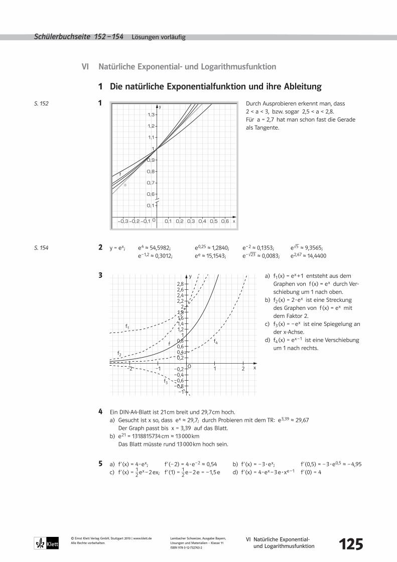
1 Durch Ausprobieren erkennt man, dass 2 < a < 3, bzw. sogar 2,5 < a < 2,8.

Für a = 2,7 hat man schon fast die Gerade als Tangente.

2 y = e x; e 4 ≈ 54,5982; e 0,25 ≈ 1,2840; e – 2 ≈ 0,1353; e 90000 5 ≈ 9,3565; e – 1,2 ≈ 0,3012; e e ≈ 15,1543; e – 90000000 23 ≈ 0,0083; e 2,67 ≈ 14,4400

3 a) f1 (x) = e x + 1 entsteht aus dem Graphen von f (x) = e x durch Ver-schiebung um 1 nach oben.

b) f2 (x) = 2·e x ist eine Streckung des Graphen von f (x) = e x mit dem Faktor 2.

c) f3 (x) = – e x ist eine Spiegelung an der x-Achse.

d) f4 (x) = e x – 1 ist eine Verschiebung um 1 nach rechts.

4 Ein DIN-A4-Blatt ist 21 cm breit und 29,7 cm hoch. a) Gesucht ist x so, dass e x ≈ 29,7; durch Probieren mit dem TR: e 3,39 ≈ 29,67 Der Graph passt bis x = 3,39 auf das Blatt. b) e 21 = 1318815734 cm ≈ 13 000 km Das Blatt müsste rund 13 000 km hoch sein.

5 a) f ’ (x) = 4·e x; f ’ (– 2) = 4·e – 2 ≈ 0,54 b) f ’ (x) = – 3·e x; f ’ (0,5) = – 3·e 0,5 ≈ – 4,95 c) f ’ (x) = 1 _ 2 e x – 2 ex; f ’ (1) = 1 _ 2 e – 2 e = – 1,5 e d) f ’ (x) = 4·e x – 3 e·x e – 1 f ’ (0) = 4

S. 152

x

y

0,2 0,30,1−0,1−0,2−0,3 0,4 0,5 0,6O

0,1

0,6

0,7

0,8

0,9

1

1,1

1,2

1,3

a

f

S. 154

xO

–0,4–0,2

–0,6–0,8

–1

0,20,40,60,8

1,21,41,61,8

22,22,42,62,8

1

1–1–2

y

f1

2

f

f2

f4

f3

VI Natürliche Exponential- und Logarithmusfunktion 126

© Ernst Klett Verlag GmbH, Stuttgart 2010 | www.klett.deAlle Rechte vorbehalten.


Schülerbuchseite 154 Lösungen vorläufig

6 a) f ’ (x) = e x; Ansatz für g: y = m x + t, wobei mA = f ’ (1) und mB = f ’ (– 1) f ’ (1) = e; e = e·1 + t ⇒ t = 0; tA: y = e x

f ’ (– 1) = 1 _ e ; 1 _ e = – 1 _ e + t ⇒ t = 2 _ e ; tB: y = 1 _ e x + 2 _ e

b) mN = – 1 _ mA bzw. mN = – 1

_ mB

Steigung der Normalen in A: mN = – 1 _ e ; Steigung der Normalen in B: mN = – e

7 Parallele Tangenten haben dieselbe Steigung, also f ’ (x) = g’ (x) a) f ’ (x) = e x; g’ (x) = 1 ⇒ e x = 1 P (0 | 1); Q (0 | 0) b) f ’ (x) = 2 e x; g’ (x) = – 4 ⇒ 2 e x = – 4 keine Lösung möglich

c) f ’ (x) = 90000 e ; g’ (x) = e x ⇒ 90000 e = e x P ( 1 _ 2 | 1 _ 2 90000 e ) ; Q ( 1 _ 2 | e 1 _ 2 – 2 )

8 fc (x) = c·e x; Schnittpunkt mit der y-Achse: c·e0 = c ¥ (0 | c) f ’c (x) = c·e x; f ’c (0) = c = 0,4 f0,4 (x) = 0,4·e x

9 a) Gleichung der Tangente im Punkt P (a | e a) mP = f ’ (a) = e a; e a = e a·a + t ⇒ t = e a·(1 – a) ⇒ t: y = e a·x + (1 – a)·e a

Q: e a·x + (1 – a)·e a = 0 ⇒ x = a – 1 b) Die x-Koordinate des Punktes Q ist um 1 kleiner als die x-Koordinate des Punktes P. c) tan α = e a

tan α = ea _ xP – xQ

d) Zu jedem Punkt P (a | f (a)) findet man immer einen 2. Punkt Q (a – 1 | 0), der auch auf der Tangente liegt.

Die Verbindungsgerade PQ stellt die Tangente dar.

10 Vgl. Aufgabe 9. Wenn die Tangente durch (0 | 0) geht, hat der Berührpunkt die Koordinaten (1 | e). Die Tangente hat

die Gleichung y = e x.

11 a) Der Graph von f (x) wird an der y-Achse gespiegelt und um 1 nach oben verschoben. b) Der Graph von f (x) verschiebt sich um 1 nach links. c) Der Graph von f (x) wird an der x- und der y-Achse gespiegelt. d) Der Graph von f (x) verschiebt sich um 1 nach links und wird an der y-Achse gespiegelt.

12 f1 (x) gehört zu dem lilafarbigen Graphen; f1 (0) = 0 f2 (x) gehört zu dem blauen Graphen; f2 (0) = 1 f3 (x) gehört zu dem orangefarbigen Graphen; Spiegelung von y = e x an der y-Achse und Verschie-

bung um 1 nach oben. f4 (x) gehört zu dem roten Graphen; f4 (2) = 0; es handelt sich um eine um 2 nach rechts verscho-

bene und mit dem Faktor 0,5 gestauchte Normalparabel.

13 a) f (2) = 1 ⇒ c e 2 + a = 1, a = 1 – c e 2

f (x) = c·e x + 1 – c e 2; also keine eindeutige Lösung möglich. Bsp.: c = 1 ⇒ a = 1 – e 2 ⇒ f (x) = e x + 1 – e 2

b) f (0) = 1 ⇒ c·e 0 + a = 1, a = 1 – c f ’ (0) = 2 ⇒ c·e 0 = 2 ⇒ c = 2 f (x) = 2 e x – 1

14 a) 18° b) 57,3° c) – 36° d) 225° e) 143,2° f) – 286,5° g) 480° h) 47° i) – 257,8° k) – 510°

ea = ea _ xP – xQ

⇒ xP – xQ = 1 oder xQ = xP – 1

a = – 1





2� Die�natürliche�Logarithmusfunktion�und�ihre�Ableitung

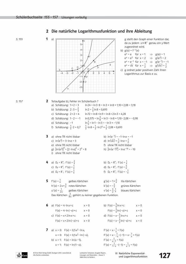
1 a) g stellt den Graph einer Funktion dar, da zu jedem x * R+ genau ein y-Wert zugeordnet wird.

b) g (x) = f – 1 (x) e x = e für x = 1 ⇒ g (e) = 1 e x = e 2 für x = 2 ⇒ g (e 2) = 2 e x = e – 1 für x = – 1 ⇒ g (e – 1) = – 1 e x = 90000 e für x = 1 _ 2 ⇒ g ( 90000 e ) = 1 _ 2

c) g ordnet jeder positiven Zahl ihren Logarithmus zur Basis e zu.

2 Teilaufgabe b), Fehler im Schülerbuch ? a) Schätzung: 1 + 2 = 3 ln 24 = ln 3·8 = ln 3 + ln 8 ≈ 1,10 + 2,08 = 3,18

b) Schätzung: 2 : 3 = 2 _ 3 ln 2 = 1 _ 3 ln 8 = 0,693

c) Schätzung: 2 + 2 = 4 ln 72 = ln 8 + ln 9 = ln 8 + 2 ln 3 = 4,28

d) Schätzung: 1 – 2 = – 1 ln 0,375 = ln 3 _ 8 = ln 3 – ln 8 ≈ 1,10 – 2,08 = – 0,98

e) Schätzung: – 1 ln 1 _ 3 = ln 1 – ln 3 = – ln 3 ≈ – 1,10

f) Schätzung: 1 _ 3 ·2 = 0,7 1 _ 3 ·ln 8 = 1 _ 3 ·ln 23 ≈ 1 _ 3 ·2,08 = 0,693

3 a) ohne TR nicht lösbar b) ln (e – 1) = – 1·ln e = – 1

c) ln (e 3) = 3·ln e = 3 d) ln ( 90000 e ) = 1 _ 2 ·ln e = 1 _ 2

e) ohne TR nicht lösbar f) ohne TR nicht lösbar

g) [ln (e 2)]3 = [2·ln e]3 = 23 = 8 h) [ln (e – 2)5] = ln e – 10 = – 10 i) ohne TR nicht lösbar

4 a) Df = R+; f ’ (x) = 2 _ x b) Df = R+; f ’ (x) = 1 _ x

c) Df = R+; f ’ (x) = 1 _ x d) Df = R+; f ’ (x) = 3 _ x

e) Df = R–; f ’ (x) = 1 _ x f) Df = R+; f ’ (x) = – 1 _ x

5 f ’ (x) = 1 _ x gelbes Kärtchen g’ (x) = 1 + 2 _ x lila Kärtchen

h’ (x) = 2 x + 3 _ x rotes Kärtchen k’ (x) = – 2 _ x grünes Kärtchen

u’ (x) = 1 _ 2 x gelbes Kärtchen v’ (x) = 3 _ 2 · 1 _ x blaues Kärtchen

Das Kärtchen 3 _ 8 x gehört zu keiner gegebenen Funktion.

6 a) F (x) = 4·ln x + c x > 0 b) F (x) = 3 _ 4 ln x + c x > 0

F (x) = 4·ln (– x) + c x < 0 F (x) = 3 _ 4 ln (– x) + c x < 0

c) F (x) = x + 2 ln x + c x > 0 d) F (x) = x – 5 _ 2 ln x + c x > 0

F (x) = x + 2 ln (– x) + c x < 0 F (x) = x – 5 _ 2 ln (– x) + c x < 0

7 a) x > 0: F (x) = 0,5 x2 – ln x; F’ (x) = x – 1 _ x = f (x)

x < 0: F (x) = 0,5 x2 – ln (– x); F’ (x) = x – 1 _ – x ·(– 1) = x – 1 _

x = f (x)

b) x > 1: F (x) = ln (x – 1); F’ (x) = 1 _ x – 1 = f (x)

x < 1: F (x) = ln (1 – x); F’ (x) = 1 _ 1 – x ·(– 1) = 1

_ x – 1 = f (x)

S. 155

x

y

2 31−1−2−3−4 4 5O

2

3

1

–1

–2

–3

g

4

5

A

C

C'

D

D'

E

E'

F

F'

B

a

b

S. 157





8 a) f ’ (0,5) = 2; f ’ (1) = 1; f ’ (2) = 0,5; f ’ (4) = 0,25 b) abgelesen: f ’ (1,75) ≈ f (1,75) mit TR: f ’ (1,76) ≈ 0,568; f (1,76) ≈ 0,565

9 Ansatz: y = m x + t

a) m = f ’ (e2) = 1 _ e2

f (e 2) = 2 b) Tangentengleichung an einem beliebigen Punkt P (xP | ln xP) * Gf : Steigung: f ’ (xP) = 1 _ xP

⇒ ln xP = 1 _ xP ·xP + t ⇒ t = ln xP – 1

tP: y = 1 _ xP ·x + ln xP – 1

A * t: 2 = 1 _ xP ·0 + ln xP – 1 ⇒ 3 = ln xP ⇒ xP = e 3

tA: y = e – 3·x + 2 c) Tangentengleichung siehe b): t: y = 1 _ xP

·x + ln xP – 1 B (0 | n) * t: n = 1 _ xP

·0 + ln xP – 1 ⇒ n + 1 = ln xP ⇒ xP = e n + 1

tB: y = e – (n + 1)·x + n

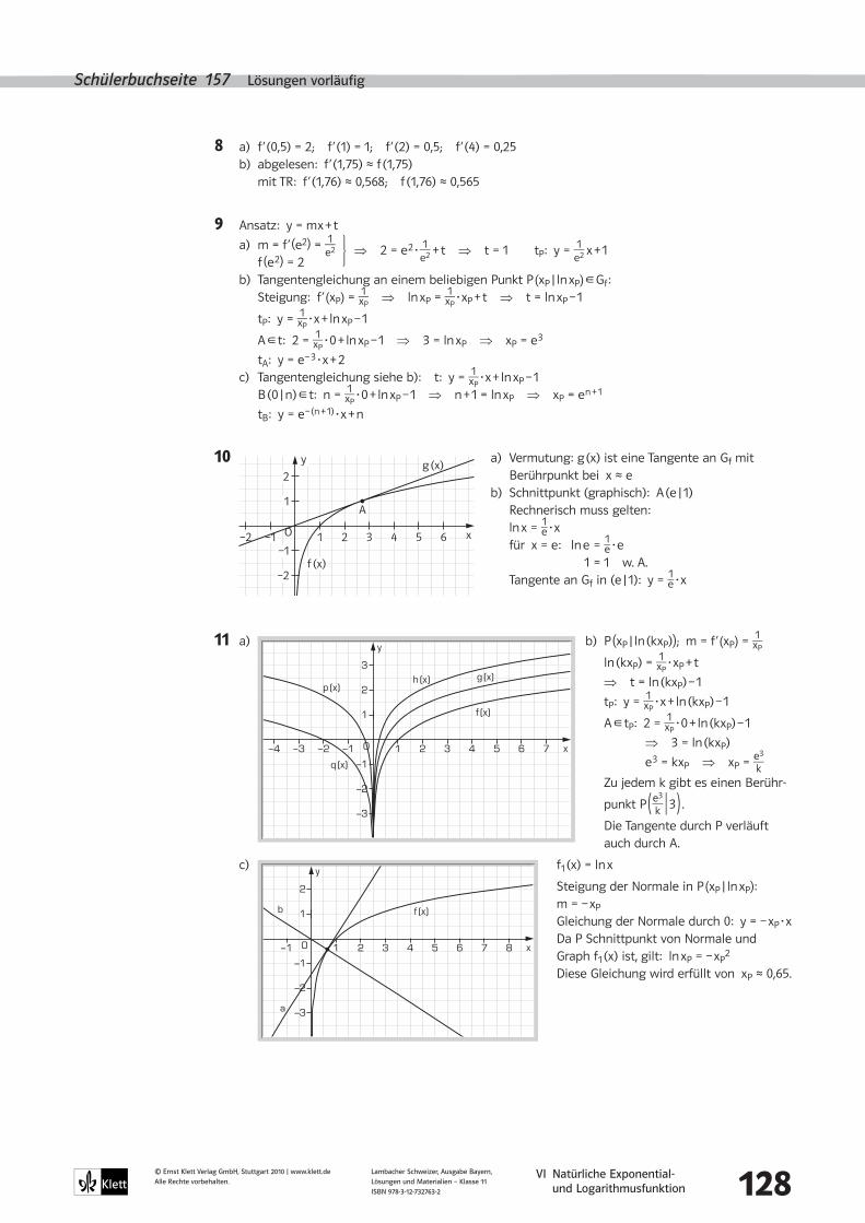
10 a) Vermutung: g (x) ist eine Tangente an Gf mit Berührpunkt bei x ≈ e

b) Schnittpunkt (graphisch): A (e | 1) Rechnerisch muss gelten: ln x = 1 _ e ·x für x = e: ln e = 1 _ e ·e 1 = 1 w. A. Tangente an Gf in (e | 1): y = 1 _ e ·x

11 a) b) P (xP | ln (k xP)); m = f ’ (xP) = 1 _ xP

ln (k xP) = 1 _ xP ·xP + t

⇒ t = ln (k xP) – 1

tP: y = 1 _ xP ·x + ln (k xP) – 1

A * tP: 2 = 1 _ xP ·0 + ln (k xP) – 1

⇒ 3 = ln (k xP)

e 3 = k xP ⇒ xP = e3 _ k

Zu jedem k gibt es einen Berühr-

punkt P ( e3 _ k | 3 ) .

Die Tangente durch P verläuft auch durch A.

c) f1 (x) = ln x

Steigung der Normale in P (xP | ln xP): m = – xP

Gleichung der Normale durch 0: y = – xP·x Da P Schnittpunkt von Normale und

Graph f1 (x) ist, gilt: ln xP = – xP2

Diese Gleichung wird erfüllt von xP ≈ 0,65.

⇒ 2 = e 2· 1 _ e2 + t ⇒ t = 1 tP: y = 1 _

e2 x + 1

xO

–2

–1

1

2

1 2 4 53 6–1

y

f (x)

–2

g (x)

A

x

y

2 31−1−2−3−4 4 5 6 7O

2

3

1

–1

–2

–3

f (x)

g (x)h (x)

q (x)

p (x)

x

y

2 31−1 4 5 6 7 8O

2

1

–1

–2

–3

f (x)b

a





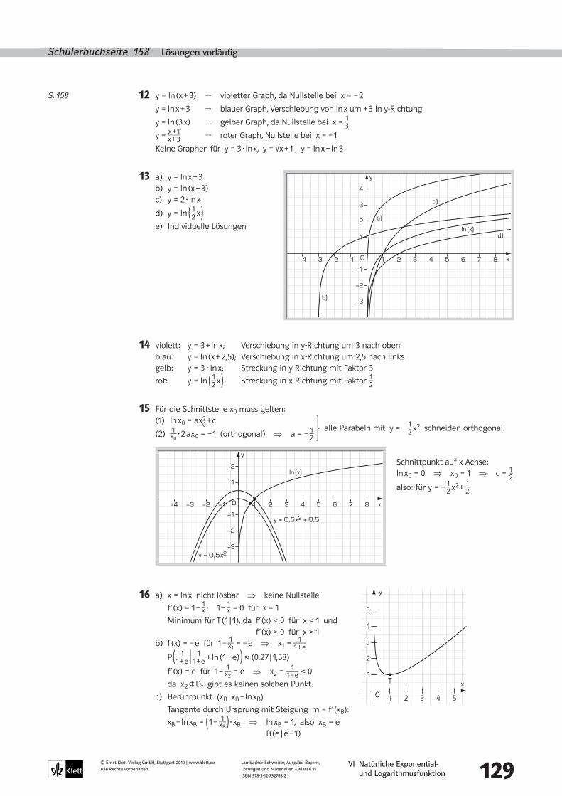
12 y = ln (x + 3) ¥ violetter Graph, da Nullstelle bei x = – 2

y = ln x + 3 ¥ blauer Graph, Verschiebung von ln x um + 3 in y-Richtung

y = ln (3 x) ¥ gelber Graph, da Nullstelle bei x = 1 _ 3

y = x + 1 _ x + 3 ¥ roter Graph, Nullstelle bei x = – 1

Keine Graphen für y = 3·ln x, y = 900000000000 x + 1 , y = ln x + ln 3

13 a) y = ln x + 3 b) y = ln (x + 3) c) y = 2·ln x

d) y = ln ( 1 _ 2 x ) e) Individuelle Lösungen

14 violett: y = 3 + ln x; Verschiebung in y-Richtung um 3 nach oben blau: y = ln (x + 2,5); Verschiebung in x-Richtung um 2,5 nach links gelb: y = 3 ·ln x; Streckung in y-Richtung mit Faktor 3

rot: y = ln ( 1 _ 2 x ) ; Streckung in x-Richtung mit Faktor 1 _ 2

15 Für die Schnittstelle x0 muss gelten: (1) ln x0 = a x 0 2 + c

(2) 1 _ x0 ·2 a x 0 = – 1 (orthogonal) ⇒ a = – 1 _ 2

Schnittpunkt auf x-Achse: ln x 0 = 0 ⇒ x 0 = 1 ⇒ c = 1 _ 2

also: für y = – 1 _ 2 x2 + 1 _ 2

16 a) x = ln x nicht lösbar ⇒ keine Nullstelle

f ’ (x) = 1 – 1 _ x ; 1 – 1 _ x = 0 für x = 1

Minimum für T (1 | 1), da f ’ (x) < 0 für x < 1 und f ’ (x) > 0 für x > 1

b) f (x) = – e für 1 – 1 _ x1 = – e ⇒ x1 = 1

_ 1 + e

P ( 1 _ 1 + e | 1

_ 1 + e + ln (1 + e) ) ≈ (0,27 | 1,58)

f ’ (x) = e für 1 – 1 _ x2 = e ⇒ x2 = 1

_ 1 – e < 0

da x2 + Df gibt es keinen solchen Punkt.

c) Berührpunkt: (xB | xB – ln xB) Tangente durch Ursprung mit Steigung m = f ’ (xB): xB – ln xB = ( 1 – 1 _ xB

) ·xB ⇒ ln xB = 1, also xB = e B (e | e – 1)

S. 158

x

y

2 31−1−2−3−4 4 5 6 7 8O

2

1

–1

–2

–3

3

4

ln (x)

b)

d)

c)

a)

alle Parabeln mit y = – 1 _ 2 x2 schneiden orthogonal.

x

y

2 31−1−2−3−4 4 5 6 7 8O

2

1

–1

–2

–3

ln (x)

y = 0,5x2

y = 0,5x2 + 0,5

x

1 2 3 4 5

1

2

3

4

5

y

O

T





17 a) Df = R+

b) f ’ (x) = x· 4 _ x – 4 ln x

__ x2 =

4·(1 – ln x) __

x2

Extremwert für 4·(1 – ln x) = 0 ⇒ ln x = 1, also x = e;

da f ’ (x) > 0 für x < e und f ’ (x) < 0 für x > 0 ⇒ H ( e | 4 _ e ) c) f (x) → – • für x → 0, da f ’ (x) > 0 für x < e und einzige Nullstelle bei x = 1

18 Sei J = Junge; D = Note 3

a) P (D) = 13 _ 30 ≈ 43,3 % b) P ( J ° D) = 9 _ 30 = 30 %

c) PJ (D) = 1 _ 2 = 50 % d) PD ( J) = 9 _ 13 ≈ 69,2 %

3� Ableiten�zusammengesetzter�Funktionen

1 a) h1 (x) = x2 + 1 – e x = u (x) – f (x); h2 (x) = (x2 + 1)·ln x = u (x)·g (x)

h3 (x) = e x2 + 1 = f (u (x)); h4 (x) = x2 + 1

_ ln x = u (x)

_ g (x)

h5 (x) = (e x)2 + 1 = u (f (x)); h6 (x) = g (u (x))

b) h5’ (x) = 2·e 2 x ; h6’ (x) = 2 x _

x2 + 1 (Anwendung der Kettenregel)

2 a) f ’ (x) = 1 – e x b) f ’ (x) = 2·e 2 x c) f ’ (x) = 3 _

1 _ 3 ·x · 1 _ 3 = 3 _

x

d) f ’ (x) = 3·e 3 x + 4 e) f ’ (x) = 1 __

1 _ 2 x2 + 1 ·2· 1 _ 2 x = x

__ 1 _ 2 x2 + 1

f) f ’ (x) = – 2 e – 2 x

g) f ’ (x) = 1 _ 2 · e x2 + 2 ·2 x = x· e x2 + 2 h) f ’ (x) = 1 _ 1 _ x ·

(– 1) _

x2 = – 1 _ x oder f (x) = ln 1 – ln x; f ’ (x) = – 1 _ x

3 a) f ist Stammfunktion von g (x) = f ’ (x) = 1 _ x2 ·2 x = 2 _

x

b) g ist Stammfunktion von f (x) = g’ (x) = 2·ln x· 1 _ x = 2 ln x _ x

4 a) Df = R; f ’ (x) = 2·e x + 2 x·e x = 2 e x (1 + x)

b) Df = R+; f ’ (x) = ln x + x· 1 _ x = ln x + 1

c) Df = R; f ’ (x) = 2 x·e – x + x2·e – x·(– 1) = x·e – x (2 – x)

d) Df = R+; f ’ (x) = 1 _ 90000 x

· 1 _

2 90000 x = 1

_ 2 x oder f (x) = 1 _ 2 ln x ⇒ f ’ (x) = 1 _ 2 · 1 _ x

e) Df = R+; f ’ (x) = 1 _

2 90000 x ·ln x + 90000 x · 1 _ x = ln x

_ 2 90000 x

+ 1 _ 90000 x

= 1 _ 90000 x

( 1 _ 2 ln x + 1 ) f) Df = R; f (x) = 2 x·e 4 x ; f ’ (x) = 2·e 4 x + 2 x·e 4 x·4 = 2 e 4 x·(1 + 4 x)

g) Df = R \ [0 ; 1]; f ’ (x) = 1 _

x _ x – 1

· ( x – 1 – x _

(x – 1)2 ) = (x – 1)·(– 1)

__ x (x – 1)2 = – 1

__ x (x – 1)

h) Df = R \ {– 1}; f’ (x) = (x + 1)·2·e 2 x – e 2 x

___ (x + 1)2 =

e 2 x·(2 (x + 1) – 1) ___

(x + 1)2 = e 2 x·(2 x + 1)

__ (x + 1)2

5 a) richtig: f ’ (x) = – e – x·cos x + e – x·(– sin x) = e – x·(– cos x – sin x) Vorzeichenfehler bei der Ableitung von cos x!

b) richtig: f ’ (x) = – e – x·ln x + e – x· 1 _ x = e – x ( – ln x + 1 _ x ) Fehler bei der Ableitung von e – x : Richtig ist (e – x) = – e – x

J _ J

D 9 4 13

_ D 9 8 17

18 12 30

S. 159

S. 160





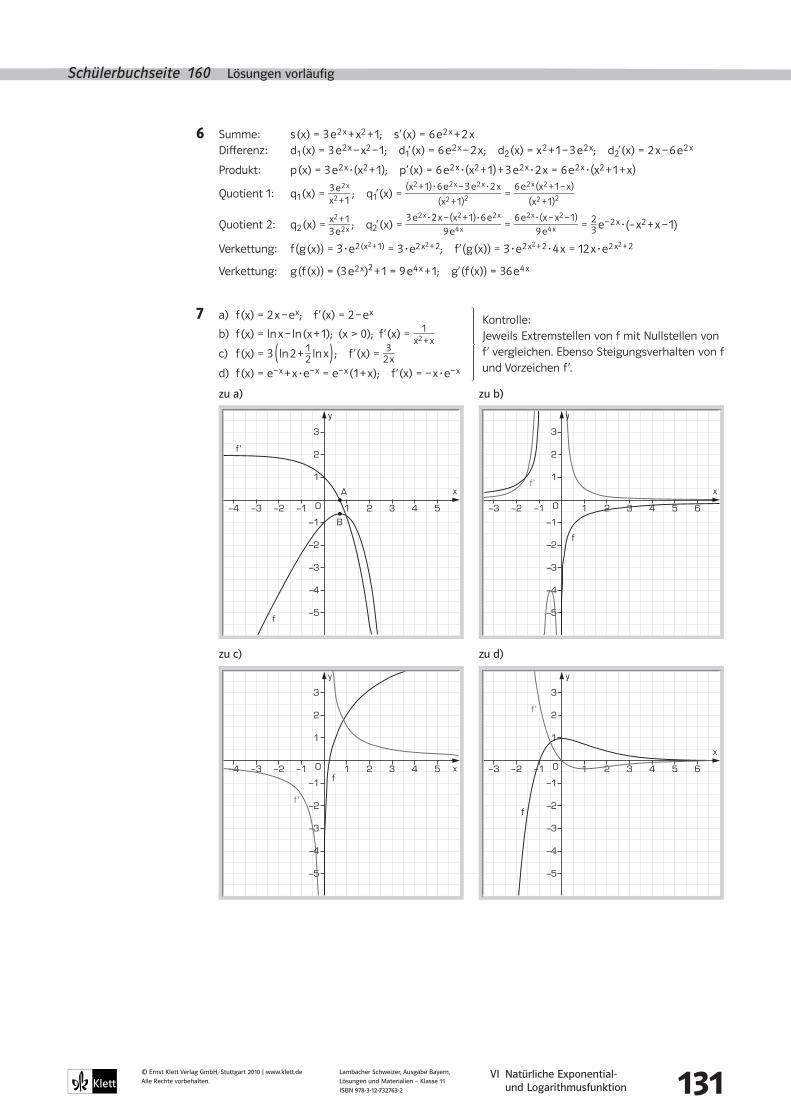
6 Summe: s (x) = 3 e 2 x + x2 + 1; s’ (x) = 6 e 2 x + 2 x Differenz: d1 (x) = 3 e 2 x – x2 – 1; d1’ (x) = 6 e 2 x – 2 x; d2 (x) = x 2 + 1 – 3 e 2 x; d2’ (x) = 2 x – 6 e 2 x

Produkt: p (x) = 3 e 2 x·(x2 + 1); p’ (x) = 6 e 2 x·(x2 + 1) + 3 e 2 x·2 x = 6 e 2 x·(x2 + 1 + x)

Quotient 1: q1 (x) = 3 e 2 x _

x2 + 1 ; q1’ (x) =

(x2 + 1)·6 e 2 x – 3 e 2 x·2 x ____

(x2 + 1)2 =

6 e 2 x (x2 + 1 – x) ___

(x2 + 1)2

Quotient 2: q2 (x) = x2 + 1

_ 3 e 2 x ; q2’ (x) =

3 e 2 x·2 x – (x2 + 1)·6 e 2 x

____ 9 e 4 x =

6 e 2 x·(x – x2 – 1) ___

9 e 4 x = 2 _ 3 e – 2 x·(– x2 + x – 1)

Verkettung: f (g (x)) = 3· e 2 (x2 + 1) = 3· e 2 x2 + 2 ; f ’ (g (x)) = 3· e 2 x2 + 2 ·4 x = 12 x· e 2 x2 + 2

Verkettung: g (f (x)) = (3 e 2 x)2 + 1 = 9 e 4 x + 1; g’ (f (x)) = 36 e 4 x

7 a) f (x) = 2 x – e x; f ’ (x) = 2 – e x

b) f (x) = ln x – ln (x + 1); (x > 0); f ’ (x) = 1 _

x2 + x

c) f (x) = 3 ( ln 2 + 1 _ 2 ln x ) ; f ’ (x) = 3 _ 2 x

d) f (x) = e – x + x·e – x = e – x (1 + x); f ’ (x) = – x·e – x

Kontrolle: Jeweils Extremstellen von f mit Nullstellen von f ’ vergleichen. Ebenso Steigungsverhalten von f und Vorzeichen f ’.

2 31−1−2−3−4 4 5O

2

3

1

–1

–2

A

y

x

B

f

f '

zu a) zu b)

2 31−1−2−3 4 5 6O

2

3

1

–1

–2

–3

–4

–5

–3

–4

–5–5

y

x

x

x

f

f '

2 31−1−2−3−4 4 5O

2

3

1

–1

–2

y

f

f '

2 31−1−2−3 4 5 6O

2

3

1

–1

–2

–3

–4

–5

–3

–4

y

f

f '

zu c) zu d)





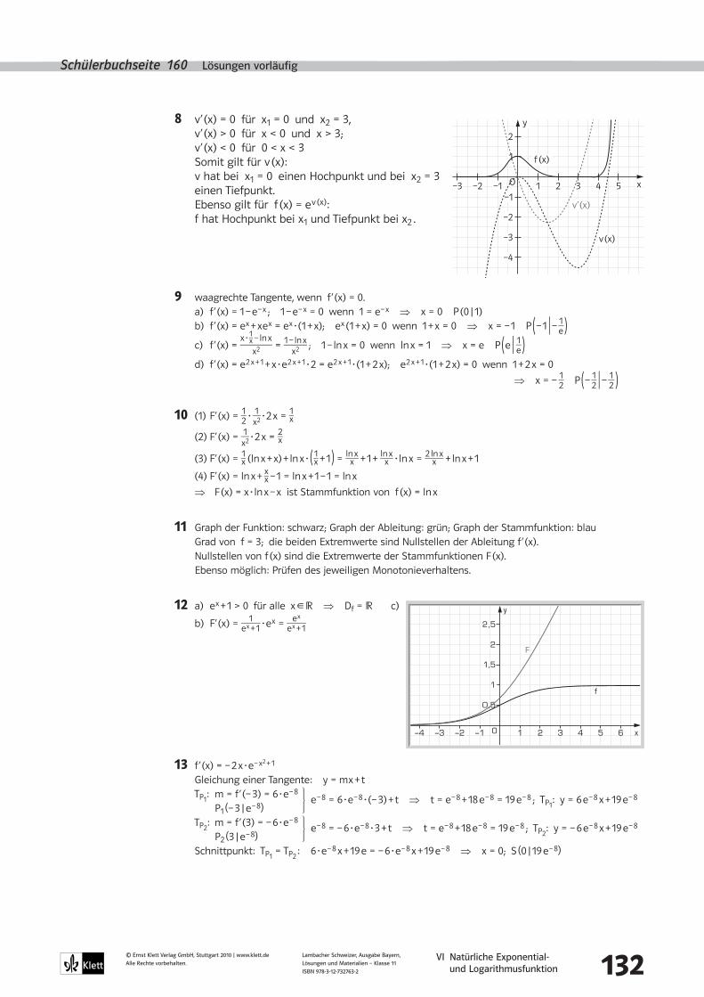
8 v’ (x) = 0 für x1 = 0 und x2 = 3, v’ (x) > 0 für x < 0 und x > 3; v’ (x) < 0 für 0 < x < 3 Somit gilt für v (x): v hat bei x1 = 0 einen Hochpunkt und bei x2 = 3

einen Tiefpunkt. Ebenso gilt für f (x) = e v (x): f hat Hochpunkt bei x1 und Tiefpunkt bei x2 .

9 waagrechte Tangente, wenn f ’ (x) = 0. a) f ’ (x) = 1 – e – x ; 1 – e – x = 0 wenn 1 = e – x ⇒ x = 0 P (0 | 1) b) f ’ (x) = e x + x e x = e x·(1 + x); e x (1 + x) = 0 wenn 1 + x = 0 ⇒ x = – 1 P ( – 1 | – 1 _

e ) c) f ’ (x) =

x· 1 _ x – ln x __

x2 = 1 – ln x _

x2 ; 1 – ln x = 0 wenn ln x = 1 ⇒ x = e P ( e | 1 _ e )

d) f ’ (x) = e 2 x + 1 + x·e 2 x + 1·2 = e 2 x + 1·(1 + 2 x); e 2 x + 1·(1 + 2 x) = 0 wenn 1 + 2 x = 0

⇒ x = – 1 _ 2 P ( – 1 _ 2 | – 1 _ 2 )

10 (1) F’ (x) = 1 _ 2 · 1 _ x2 ·2 x = 1 _ x

(2) F’ (x) = 1 _ x2 ·2 x = 2 _ x

(3) F’ (x) = 1 _ x (ln x + x) + ln x· ( 1 _ x + 1 ) = ln x _ x + 1 + ln x

_ x ·ln x = 2 ln x _ x + ln x + 1

(4) F’ (x) = ln x + x _ x – 1 = ln x + 1 – 1 = ln x

⇒ F (x) = x·ln x – x ist Stammfunktion von f (x) = ln x

11 Graph der Funktion: schwarz; Graph der Ableitung: grün; Graph der Stammfunktion: blau Grad von f = 3; die beiden Extremwerte sind Nullstellen der Ableitung f ’ (x). Nullstellen von f (x) sind die Extremwerte der Stammfunktionen F (x). Ebenso möglich: Prüfen des jeweiligen Monotonieverhaltens.

12 a) e x + 1 > 0 für alle x * R ⇒ Df = R c)

b) F’ (x) = 1 _ e x + 1 ·e x = e x

_ e x + 1

13 f ’ (x) = – 2 x· e – x2 + 1 Gleichung einer Tangente: y = m x + t TP1

: m = f ’ (– 3) = 6·e – 8

P1 (– 3 | e – 8) TP2

: m = f ’ (3) = – 6·e – 8

P2 (3 | e – 8) Schnittpunkt: TP1

= TP2 : 6·e – 8 x + 19 e = – 6·e – 8 x + 19 e – 8 ⇒ x = 0; S (0 | 19 e – 8)

xO

–2

–3

–4

–1

1

2

1 2 4 53–1

y

–2–3

v(x)

v’ (x)

f (x)

2 31−1−2−3−4 4 5 6O

1

1,5

0,5

2

2,5

y

x

f

F

e – 8 = 6·e – 8·(– 3) + t ⇒ t = e – 8 + 18 e – 8 = 19 e – 8 ; TP1: y = 6 e – 8 x + 19 e – 8

e – 8 = – 6·e – 8·3 + t ⇒ t = e – 8 + 18 e – 8 = 19 e – 8 ; TP2: y = – 6 e – 8 x + 19 e – 8





14 f (x) = g (x); 4 _ x = m x + 2 ⇒ m x2 + 2 x – 4 = 0

m ≠ 0: x1/2 = – 2 ± 900000000000000000000 4 + 16 m __ 2 m

Es gibt genau eine Lösung, wenn 4 + 16 m = 0,

also für m = – 1 _ 4 .

Dann gilt für S: x1 = x2 = – 2 ± 0 __

2· ( – 1 _ 4 ) = 4 ⇒ S1 (4 | 1)

m = 0 ⇒ 4 _ x = 2 ⇒ S2 (2 | 2)

4� Exponentialfunktionen�und�Exponentialgleichungen

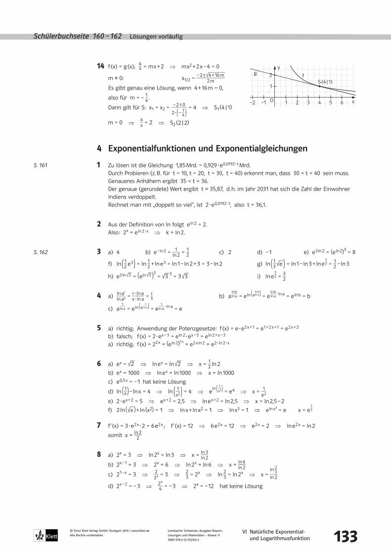
1 Zu lösen ist die Gleichung 1,85 Mrd. = 0,929·e 0,0192·t Mrd. Durch Probieren (z. B. für t = 10, t = 20, t = 30, t = 40) erkennt man, dass 30 < t < 40 sein muss. Genaueres Anhähern ergibt 35 < t < 36. Der genaue (gerundete) Wert ergibt t ≈ 35,87, d. h. im Jahr 2031 hat sich die Zahl der Einwohner

Indiens verdoppelt. Rechnet man mit „doppelt so viel“, ist 2·e 0,0192·t, also t = 36,1.

2 Aus der Definition von ln folgt e ln 2 = 2. Also: 2 x = e ln 2·x ⇒ k = ln 2.

3 a) 4 b) e – ln 2 = 1 _ ln 2 = 1 _ 2 c) 2 d) – 1 e) e 3 ln 2 = (e ln 2)3 = 8

f) ln ( 1 _ 2 e 3 ) = ln 1 _ 2 + ln e 3 = ln 1 – ln 2 + 3 = 3 – ln 2 g) ln ( 1 _ 3 90000 e ) = ln 1 – ln 3 + ln e 1 _ 2 = 1 _ 2 – ln 3

h) e 3 ln 90000 3 = ( e ln 90000 3 ) 3 = 90000 3 3 = 3 90000 3 i) ln e 3 _ 2 = 3 _ 2

4 a) ln ar _ ln as = r·ln a

_ s·ln a = r _ s b) a ln b

_ ln a = e ln ( a ln b

_ ln a ) = e ln b

_ ln a ·ln a = e ln b = b

c) a 1 _ ln a = e ln ( a

1 _ ln a ) = e

1 _ ln a ·ln a = e

5 a) richtig; Anwendung der Potenzgesetze: f (x) = e·e 2 x + 1 = e 1 + 2 x + 1 = e 2 x + 2

b) falsch; f (x) = 2·e x – 3 = e ln 2·e x – 3 = e ln 2 + x – 3

a) richtig; f (x) = 22 x = (e ln 2)2 x = e 2 x ln 2 = e 2·ln 2·x

6 a) e x = 90000 2 ⇒ ln e x = ln 90000 2 ⇒ x = 1 _ 2 ln 2

b) e x = 1000 ⇒ ln e x = ln 1000 ⇒ x = ln 1000

c) e 0,5 x = – 1 hat keine Lösung

d) ln ( 1 _ x ) – ln x = 4 ⇒ ln ( 1 _ x2 ) = 4 ⇒ e

ln ( 1 _ x2 ) = e 4 ⇒ x = 1 _

e 2

e) 2·e x + 2 = 5 ⇒ e x + 2 = 2,5 ⇒ ln e x + 2 = ln 2,5 ⇒ x = ln 2,5 – 2

f) 2 ln ( 90000 x ) + ln (x2) = 1 ⇒ ln x + ln x2 = 1 ⇒ ln x3 = 1 ⇒ e ln x3 = e x = e 1 _ 3

7 f ’ (x) = 3·e 2 x·2 = 6 e 2 x ; f ’ (x) = 12 ⇒ 6 e 2 x = 12 ⇒ e 2 x = 2 ⇒ ln e 2 x = ln 2

somit x = ln 2 _ 2

8 a) 2 x = 3 ⇒ ln 2 x = ln 3 ⇒ x = ln 3 _ ln 2

b) 2 x – 1 = 3 ⇒ 2 x = 6 ⇒ ln 2 x = ln 6 ⇒ x = ln 6 _ ln 2

c) 2 1 – x = 3 ⇒ 2 _ 2 x

= 3 ⇒ 2 _ 3 = 2 x ⇒ ln 2 _ 3 = ln 2 x ⇒ x = ln 2 _ 3

_ ln 2

d) 2 x – 2 = – 3 ⇒ 2 x _ 4 = – 3 ⇒ 2 x = – 12 hat keine Lösung

xO

1

2

1 2 4 53 6–1

y

f

–2

g

S(4|1)

S. 161

S. 162

8 v’ (x) = 0 für x1 = 0 und x2 = 3, v’ (x) > 0 für x < 0 und x > 3; v’ (x) < 0 für 0 < x < 3 Somit gilt für v (x): v hat bei x1 = 0 einen Hochpunkt und bei x2 = 3

einen Tiefpunkt. Ebenso gilt für f (x) = e v (x): f hat Hochpunkt bei x1 und Tiefpunkt bei x2 .

9 waagrechte Tangente, wenn f ’ (x) = 0. a) f ’ (x) = 1 – e – x ; 1 – e – x = 0 wenn 1 = e – x ⇒ x = 0 P (0 | 1) b) f ’ (x) = e x + x e x = e x·(1 + x); e x (1 + x) = 0 wenn 1 + x = 0 ⇒ x = – 1 P ( – 1 | – 1 _

e ) c) f ’ (x) =

x· 1 _ x – ln x __

x2 = 1 – ln x _

x2 ; 1 – ln x = 0 wenn ln x = 1 ⇒ x = e P ( e | 1 _ e )

d) f ’ (x) = e 2 x + 1 + x·e 2 x + 1·2 = e 2 x + 1·(1 + 2 x); e 2 x + 1·(1 + 2 x) = 0 wenn 1 + 2 x = 0

⇒ x = – 1 _ 2 P ( – 1 _ 2 | – 1 _ 2 )

10 (1) F’ (x) = 1 _ 2 · 1 _ x2 ·2 x = 1 _ x

(2) F’ (x) = 1 _ x2 ·2 x = 2 _ x

(3) F’ (x) = 1 _ x (ln x + x) + ln x· ( 1 _ x + 1 ) = ln x _ x + 1 + ln x

_ x ·ln x = 2 ln x _ x + ln x + 1

(4) F’ (x) = ln x + x _ x – 1 = ln x + 1 – 1 = ln x

⇒ F (x) = x·ln x – x ist Stammfunktion von f (x) = ln x

11 Graph der Funktion: schwarz; Graph der Ableitung: grün; Graph der Stammfunktion: blau Grad von f = 3; die beiden Extremwerte sind Nullstellen der Ableitung f ’ (x). Nullstellen von f (x) sind die Extremwerte der Stammfunktionen F (x). Ebenso möglich: Prüfen des jeweiligen Monotonieverhaltens.

12 a) e x + 1 > 0 für alle x * R ⇒ Df = R c)

b) F’ (x) = 1 _ e x + 1 ·e x = e x

_ e x + 1

13 f ’ (x) = – 2 x· e – x2 + 1 Gleichung einer Tangente: y = m x + t TP1

: m = f ’ (– 3) = 6·e – 8

P1 (– 3 | e – 8) TP2

: m = f ’ (3) = – 6·e – 8

P2 (3 | e – 8) Schnittpunkt: TP1

= TP2 : 6·e – 8 x + 19 e = – 6·e – 8 x + 19 e – 8 ⇒ x = 0; S (0 | 19 e – 8)

e – 8 = 6·e – 8·(– 3) + t ⇒ t = e – 8 + 18 e – 8 = 19 e – 8 ; TP1: y = 6 e – 8 x + 19 e – 8

e – 8 = – 6·e – 8·3 + t ⇒ t = e – 8 + 18 e – 8 = 19 e – 8 ; TP2: y = – 6 e – 8 x + 19 e – 8





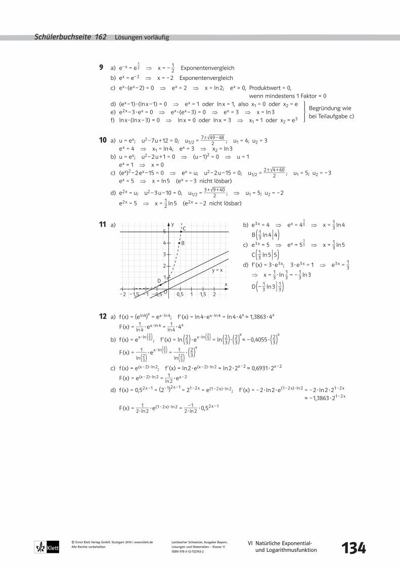
9 a) e – x = e 1 _ 2 ⇒ x = – 1 _ 2 Exponentenvergleich

b) e x = e – 2 ⇒ x = – 2 Exponentenvergleich

c) e x·(e x – 2) = 0 ⇒ e x = 2 ⇒ x = ln 2; e x > 0, Produktwert = 0, wenn mindestens 1 Faktor = 0

d) (e x – 1)·(ln x – 1) = 0 ⇒ e x = 1 oder ln x = 1, also x1 = 0 oder x2 = e e) e 2 x – 3·e x = 0 ⇒ e x·(e x – 3) = 0 ⇒ e x = 3 ⇒ x = ln 3 f) ln x·(ln x – 3) = 0 ⇒ ln x = 0 oder ln x = 3 ⇒ x1 = 1 oder x2 = e 3

10 a) u = e x; u2 – 7 u + 12 = 0; u1/2 = 7 ± 9000000000000000000 49 – 48 __ 2 ; u1 = 4; u2 = 3

e x = 4 ⇒ x1 = ln 4; e x = 3 ⇒ x2 = ln 3 b) u = e x; u2 – 2 u + 1 = 0 ⇒ (u – 1)2 = 0 ⇒ u = 1 e x = 1 ⇒ x = 0 c) (e x)2 – 2 e x – 15 = 0 ⇒ e x = u; u2 – 2 u – 15 = 0; u1/2 = 2 ± 9000000000000000 4 + 60

__ 2 ; u1 = 5; u2 = – 3 e x = 5 ⇒ x = ln 5 (e x = – 3 nicht lösbar)

d) e 2 x = u; u2 – 3 u – 10 = 0; u1/2 = 3 + 9000000000000000 9 + 40 __ 2 ; ⇒ u1 = 5; u2 = – 2

e 2 x = 5 ⇒ x = 1 _ 2 ln 5 (e 2 x = – 2 nicht lösbar)

11 a) b) e 3 x = 4 ⇒ e x = 4 1 _ 3 ⇒ x = 1 _ 3 ln 4

B ( 1 _ 3 ln 4 | 4 ) c) e 3 x = 5 ⇒ e x = 5

1 _ 3 ⇒ x = 1 _ 3 ln 5

C ( 1 _ 3 ln 5 | 5 ) d) f’ (x) = 3·e 3 x; 3·e 3 x = 1 ⇒ e 3 x = 1 _ 3

⇒ x = 1 _ 3 ·ln 1 _ 3 = – 1 _ 3 ln 3

D ( – 1 _ 3 ln 3 | 1 _ 3 )

12 a) f (x) = (e ln4)x = e x·ln 4; f ’ (x) = ln 4·e x·ln 4 = ln 4·4 x ≈ 1,3863·4 x

F (x) = 1 _ ln 4 ·e x·ln 4 = 1

_ ln 4 ·4 x

b) f (x) = e x·ln ( 2 _ 3 ) ; f ’ (x) = ln ( 2 _ 3 ) · e x·ln ( 2 _ 3 ) = ln ( 2 _ 3 ) · ( 2 _ 3 ) x ≈ – 0,4055· ( 2 _ 3 )

x

F (x) = 1 _

ln ( 2 _ 3 ) · e x·ln ( 2 _ 3 ) = 1

_ ln ( 2 _ 3 )

· ( 2 _ 3 ) x

c) f (x) = e (x – 2)·ln 2; f ’ (x) = ln 2·e (x – 2)·ln 2 = ln 2·2 x – 2 ≈ 0,6931·2 x – 2

F (x) = e (x – 2)·ln 2 = 1 _ ln 2 ·e x – 2

d) f (x) = 0,5 2 x – 1 = (2 – 1)2 x – 1 = 21 – 2 x = e (1 – 2 x)·ln 2 ; f ’ (x) = – 2·ln 2·e (1 – 2 x)·ln 2 = – 2·ln 2·2 1 – 2 x

≈ – 1,3863·2 1 – 2 x

F (x) = 1 _ 2·ln 2 ·e (1 – 2 x)·ln 2 = – 1

_ 2·ln 2 ·0,5 2 x – 1

Begründung wie bei Teilaufgabe c)

1

2

3

4

5

x

O

y

0,5–0,5–1–1,5–2 1 1,5 2

C

B

y = x

D





13 a) b)

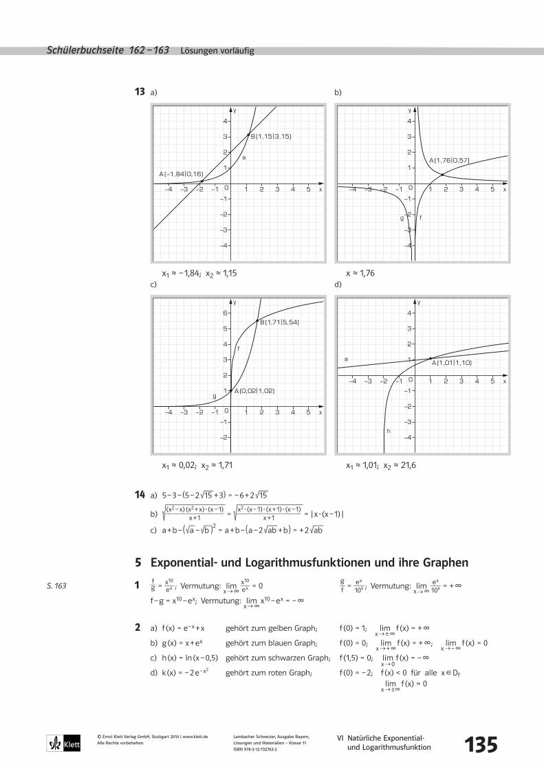
x1 ≈ – 1,84; x2 ≈ 1,15 x ≈ 1,76 c) d)

x1 ≈ 0,02; x2 ≈ 1,71 x1 ≈ 1,01; x2 ≈ 21,6

14 a) 5 – 3 – (5 – 2 90000000 15 + 3) = – 6 + 2 90000000 15

b) 90000000000000000000000000000000000000000000 (x2 – x) (x2 + x)·(x – 1)

___ x + 1 = 9000000000000000000000000000000000000000000000000 x2·(x – 1)·(x + 1)·(x – 1)

____ x + 1 = | x·(x – 1) |

c) a + b – ( 90000 a – 900000 b ) 2 = a + b – ( a – 2 90000000 ab + b ) = + 2 90000000 ab

5� Exponential-�und�Logarithmusfunktionen�und�ihre�Graphen

1 f _ g = x

10 _ e x ; Vermutung: lim

x → • x

10 _ e x = 0

g _ f = e x

_ 10x ; Vermutung: lim

x → • e x

_ 10x = + •

f – g = x10 – e x; Vermutung: lim x → •

x10 – e x = – •

2 a) f (x) = e – x + x gehört zum gelben Graph; f (0) = 1; lim x → ± •

f (x) = + •

b) g (x) = x + e x gehört zum blauen Graph; f (0) = 0; lim x → + •

f (x) = + •; lim x → – •

f (x) = 0

c) h (x) = ln (x – 0,5) gehört zum schwarzen Graph; f (1,5) = 0; lim x → 0

f (x) = – •

d) k (x) = – 2 e – x2 gehört zum roten Graph; f (0) = – 2; f (x) < 0 für alle x * Df lim x → ±•

f (x) = 0

2 31−1−2−3−4 4 5O

2

3

1

–1

–2

–3

–4

4

y

x

fg

A (1,76|0,57)

2 31−1−2−3−4 4 5O

2

3

1

–1

–2

–3

–4

4

y

x

a

A (−1,84|0,16)

B (1,15|3,15)

2 31−1−2−3−4 4 5O

2

3

1

–1

–2

–3

–4

4

y

x

h

aA (1,01|1,10)

2 31−1−2−3−4 4 5O

2

3

1

–1

–2

4

5

6

y

x

A (0,02|1,02)

B (1,71|5,54)

f

g2 31−1−2−3−4 4 5O

2

3

1

–1

–2

–3

–4

4

y

x

h

aA (1,01|1,10)

2 31−1−2−3−4 4 5O

2

3

1

–1

–2

4

5

6

y

x

A (0,02|1,02)

B (1,71|5,54)

f

g

S. 163





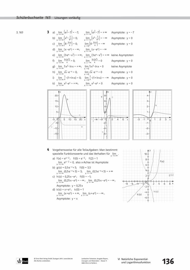
3 a) lim x → + •

( e 3 _ x – 7 ) = – 7; lim

x → – • ( e

3 _ x – 7 ) = + • Asymptote: y = – 7

b) lim x → + •

( x5· 1 _ e x ) = 0; lim x → – •

( x5· 1 _ e x ) = – • Asymptote: y = 0

c) lim x → + •

( 8· ln x _ x ) = 0; lim

x → 0 ( 8· ln x

_ x ) = – • Asymptote: y = 0

d) lim x → + •

( x – e x ) = – •; lim x → – •

( x – e x ) = – •

e) lim x → + •

(3 e x – x7 ) = + •; lim x → – •

(3 e x – x7 ) = + • keine Asymptoten

f) lim x → + •

ln (x2) _ x = 0; lim

x → – • ln (x2)

_ x = 0 Asymptote: y = 0

g) lim x → + •

5 x3·ln x = + •; lim x → 0

5 x3·ln x = 0 keine Asymptote

h) lim x → + •

90000 x ·e – x = 0; lim x → 0

90000 x ·e – x = 0 Asymptote: y = 0

i) lim x → + •

1 _ x ·(1 + ln x) = 0; lim

x → 0 1 _

x ·(1 + ln x) = – • Asymptote: y = 0

k) lim x → + •

x2·e x = + •; lim x → – •

x2·e x = 0 Asymptote: y = 0

4 Vorgehensweise für alle Teilaufgaben: Man bestimmt spezielle Funktionswerte und das Verhalten für lim

x → ± • .

a) f (x) = e x – 2 ; f (0) = e – 2 ; f (2) = 1 lim

x → + • e x – 2 = 0, also x-Achse ist Asymptote

b) g (x) = 0,5 e – x + 3; f (0) = 3,5 lim

x → + • (0,5 e – x + 3) = 3; lim

x → – • (0,5 e – x + 3) = + •

c) h (x) = 0,25 x – e x ; f (0) = – 1; lim

x → + • (0,25 x – e x) = – • ; lim

x → – • (0,25 x – e x) = – • ;

Asymptote: y = 0,25 x d) k (x) = x + e x ; k (0) = 1 lim

x → + • (x + e x) = + •, lim

x → – • (x + e x) = – • ;

Asymptote: y = x

S. 165

y

4 62−2−4 O

4

6

2

–2

–4

–6

8

f

h

ge

y

2 31−1−2 O

2

3

1

–1

–2

–3

4

k

g

i

x

y

10 155−5 20O

10

15

5

–5

–10

–15

20

d a

c

x

b

x

xO

–4

–6

–2

2

4

6

8

10

2 4 86–2

y

f (x)

–4–6–8

g (x)

h (x)k (x)





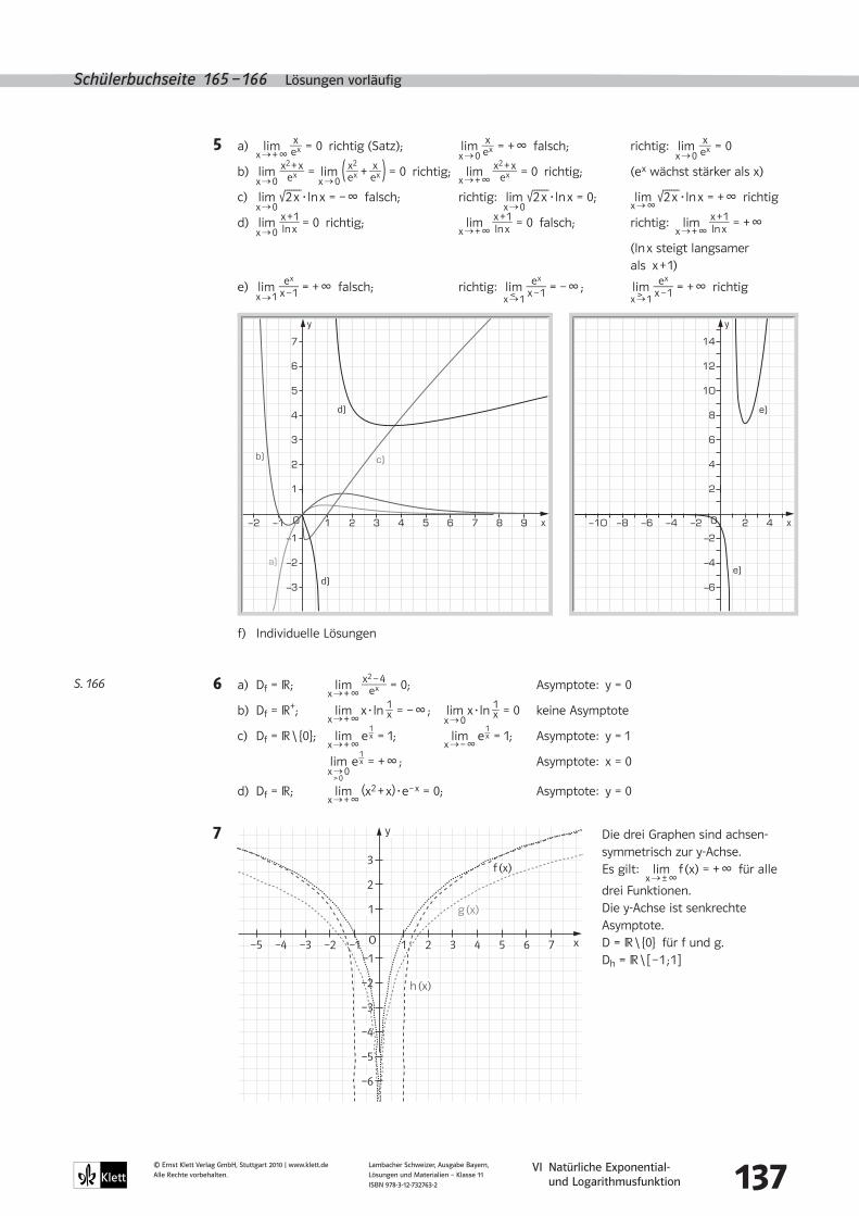
5 a) lim x → + •

x _ e x = 0 richtig (Satz); lim x → 0

x _ e x = + • falsch; richtig: lim x → 0

x _ e x = 0

b) lim x → 0

x2 + x

_ e x = lim x → 0

( x2 _ e x + x _ e x ) = 0 richtig; lim

x → + • x

2 + x _ e x = 0 richtig; (e x wächst stärker als x)

c) lim x → 0

900000000 2 x ·ln x = – • falsch; richtig: lim x → 0

900000000 2 x ·ln x = 0; lim x → •

900000000 2 x ·ln x = + • richtig

d) lim x → 0

x + 1 _ ln x = 0 richtig; lim

x → + • x + 1

_ ln x = 0 falsch; richtig: lim x → + •

x + 1 _ ln x = + •

(ln x steigt langsamer als x + 1)

e) lim x → 1

e x _ x – 1 = + • falsch; richtig: lim

< x → 1 e x

_ x – 1 = – • ; lim > x → 1

e x _ x – 1 = + • richtig

f) Individuelle Lösungen

6 a) Df = R; lim x → + •

x2 – 4

_ e x = 0; Asymptote: y = 0

b) Df = R+; lim x → + •

x·ln 1 _ x = – • ; lim x → 0

x·ln 1 _ x = 0 keine Asymptote

c) Df = R \ {0}; lim x → + •

e 1 _ x = 1; lim

x → – • e

1 _ x = 1; Asymptote: y = 1

lim x →

> 0 0 e

1 _ x = + • ; Asymptote: x = 0

d) Df = R; lim x → + •

(x2 + x)·e – x = 0; Asymptote: y = 0

7 Die drei Graphen sind achsen-symmetrisch zur y-Achse.

Es gilt: lim x → ± •

f (x) = + • für alle

drei Funktionen. Die y-Achse ist senkrechte Asymptote. D = R \ {0} für f und g. Dh = R \ [ – 1 ; 1 ]

x

y

2 31−1−2 4 5 6 7 8 9O

2

3

1

–1

–2

–3

4

5

6

7

x

y

42−2−4−6−8−10 O

4

6

2

–2

–4

–6

8

10

12

14

a)

b) c)

d)

d)

e)

e)

S. 166

xO

–2

–3

–4

–5

–6

–1

1

2

3

1 2 4 5 6 73–1

y

f (x)

–2–3–4–5

g (x)

h (x)





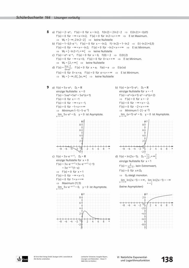
8 a) f ’ (x) = 2 – e x ; f ’ (x) = 0 für x = ln 2; f (ln 2) = 2 ln 2 – 2 ⇒ E (ln 2 | ≈ – 0,61) f ’ (x) > 0 für – • < x < ln 2; f ’ (x) < 0 für ln 2 < x < + • ⇒ E ist Maximum. ⇒ Wf = ] – • ; 2 ln 2 – 2 ] ⇒ keine Nullstelle b) f ’ (x) = 1 – 0,5·e – x ; f ’ (x) = 0 für x = – ln 2; f (– ln 2) = 1 – ln 2 ⇒ E (– ln 2 | ≈ 0,3) f ’ (x) < 0 für – • < x < – ln 2; f ’ (x) > 0 für – ln 2 < x < + • ⇒ E ist Minimum. ⇒ Wf = [ – ln 2 + 1 ; + • [ ⇒ keine Nullstelle c) f ’ (x) = e x – e – x ; f ’ (x) = 0 für x = 0; f (0) = 2 ⇒ E (0 | 2) f ’ (x) < 0 für – • < x < 0; f ’ (x) > 0 für 0 < x < + • ⇒ E ist Minimum. ⇒ Wf = [ 2 ; + • [ ⇒ keine Nullstelle

d) f ’ (x) = ln x – 1 _

(ln x)2 ; f ’ (x) = 0 für x = e; f (e) = e ⇒ E (e | e)

f ’ (x) < 0 für 0 < x < e; f ’ (x) > 0 für e < x < + • ⇒ E ist Minimum. ⇒ Wf = ] – • ; 0 [ , [ e ; • [ ⇒ keine Nullstelle

9 a) f (x) = 5 x·e x ; Df = R einzige Nullstelle: x = 0 f ’ (x) = 5 x e x + 5 e x = 5 e x (x + 1) f ’ (x) = 0 für x = – 1 f ’ (x) < 0 für – • < x < – 1; f ’ (x) > 0 für – 1 < x < + • ⇒ Minimum (– 1 | – 5·e – 1) lim

x → – • 5 x·e x = 0; y = 0 ist Asymptote.

c) f (x) = 3 x·e – x + 1 ; Df = R einzige Nullstelle für x = 0 f ’ (x) = 3 x·e – x + 1 + 3 x·e – x + 1·(– 1)

= 3 e – x + 1 (1 – x) ⇒ f ’ (x) = 0 für x = 1 f ’ (x) > 0 für – • < x < 1; f ’ (x) < 0 für 1 < x < + • ⇒ Maximum (1 | 3) lim

x → + • 3 x·e – x + 1 = 0; y = 0 ist Asymptote.

b) f (x) = (x + 1)·e x ; Df = R einzige Nullstelle für x = – 1 f ’ (x) = e x + (x + 1)·e x = e x (x + 2) ⇒ f ’ (x) = 0 für x = – 2 f ’ (x) < 0 für – • < x < – 2; f ’ (x) > 0 für – 2 < x < + • ⇒ Minimum (– 2 | – e – 2) lim

x → – • (x + 1)·e x = 0; y = 0 ist Asymptote.

xO

–2

2

4

6

8

2 4 86–2

y

–4–6–8xO

–2

2

4

6

8

2 4 86–2

y

–4–6–8

d) f (x) = ln (2 x – 1); Df = ] 1 _ 2 ; + • [ einzige Nullstelle für x = 1

f ’ (x) = 2 _ 2 x – 1 ; kein Extremwert;

f ’ (x) > 0 für x * Df

⇒ Gf steigt monoton.

lim x → + •

ln (2 x – 1) = + • ; lim x → 1 _ 2

ln (2 x – 1) = – •

(keine Asymptoten)

xO

–4

–6

–8

–2

2

2 4 86–2

y

–4–6–8

xO

–2

2

4

6

8

2 4 86–2

y

–4–6–8





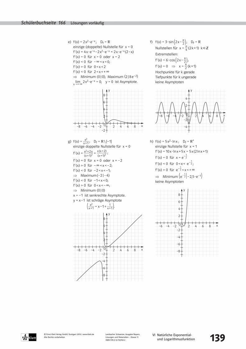
e) f (x) = 2 x2·e – x ; Df = R einzige (doppelte) Nullstelle für x = 0 f ’ (x) = 4 x·e – x – 2 x2·e – x = 2 x·e – x (2 – x) f ’ (x) = 0 für x = 0 oder x = 2 f ’ (x) < 0 für – • < x < 0; f ’ (x) > 0 für 0 < x < 2 f ’ (x) < 0 für 2 < x < + • ⇒ Minimum (0 | 0); Maximum (2 | 8 e – 2) lim

x → + • 2 x2·e – x = 0; y = 0 ist Asymptote.

g) f (x) = x2 _ x + 1 ; Df = R \ {– 1}

einzige doppelte Nullstelle für x = 0

f ’ (x) = x2 + 2 x

__ (x + 1)2 =

x (x + 2) __

(x + 1)2 ;

f ’ (x) = 0 für x = 0 oder x = – 2 f ’ (x) > 0 für – • < x < – 2; f ’ (x) < 0 für – 2 < x < – 1; ⇒ Maximum (– 2 | – 4) f ’ (x) < 0 für – 1 < x < 0; f ’ (x) > 0 für 0 < x < – •; ⇒ Minimum (0 | 0) x = – 1 ist senkrechte Asymptote. y = x – 1 ist schräge Asymptote

( x2 _ x + 1 = x – 1 + 1

_ x + 1 ) .

f) f (x) = 3·sin ( 2 x – π _ 2 ) ; Df = R

Nullstellen für x = π _ 4 (2 k + 1) k * Z

Extremstellen:

f ’ (x) = 6·cos ( 2 x – π _ 2 ) ; f ’ (x) = 0 ⇒ x = π _ 2 (k + 1)

Hochpunkte für k gerade Tiefpunkte für k ungerade keine Asymptoten

xO

–4

–2

2

4

2 4 86–2

y

–4–6–8

xO

–2

2

4

6

8

2 4 86–2

y

–4–6–8

h) f (x) = 5 x2·ln x ; Df = R+

einzige Nullstelle für x = 1 f ’ (x) = 10 x·ln x + 5 x = 5 x (2 ln x + 1)

f ’ (x) = 0 für x = e – 1 _ 2

f ’ (x) < 0 für 0 < x < e – 1 _ 2 ;

f ’ (x) > 0 für e – 1 _ 2 < x < + •

⇒ Minimum ( e – 1 _ 2 | – 2,5·e – 1 ) keine Asymptoten

xO

–4

–6

–8

–2

2

4

6

8

2 4 86–2

y

–4–6

xO

–4

–6

–8

–2

2

4

6

8

2 4 86–2

y

–4–6–8





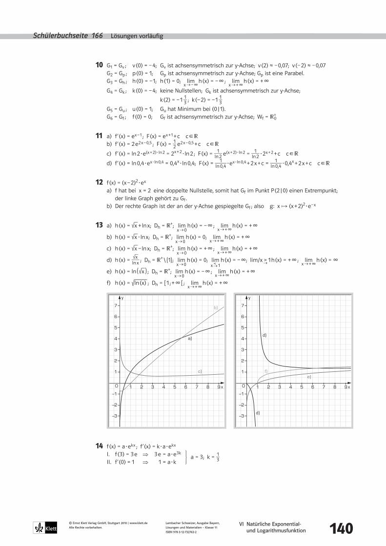
10 G1 = Gv ; v (0) = – 4; Gv ist achsensymmetrisch zur y-Achse; v (2) ≈ – 0,07; v (– 2) ≈ – 0,07 G2 = Gp ; p (0) = 1; Gp ist achsensymmetrisch zur y-Achse; Gp ist eine Parabel. G3 = Gh ; h (0) = – 1; h (1) = 0; lim

x → – • h (x) = – • ; lim

x → + • h (x) = + •

G4 = Gk ; k (0) = – 4; keine Nullstellen; Gk ist achsensymmetrisch zur y-Achse;

k (2) = – 1 1 _ 3 ; k (– 2) = – 1 1 _ 3

G5 = Gu ; u (0) = 1; Gu hat Minimum bei (0 | 1). G6 = Gf ; f (0) = 0; Gf ist achsensymmetrisch zur y-Achse; Wf = R 0

+

11 a) f ’ (x) = e x – 1 ; F (x) = e x + 1 + c c * R b) f ’ (x) = 2 e 2 x – 0,5 ; F (x) = 1 _ 2 e 2 x – 0,5 + c c * R

c) f ’ (x) = ln 2·e (x + 2)·ln 2 = 2 x + 2·ln 2 ; F (x) = 1 _ ln 2 e (x + 2)·ln 2 = 1

_ ln 2 ·2 x + 2 + c c * R

d) f ’ (x) = ln 0,4·e x·ln 0,4 = 0,4 x·ln 0,4; F (x) = 1 _ ln 0,4 ·e x·ln 0,4 + 2 x + c = 1

_ ln 0,4 ·0,4 x + 2 x + c c * R

12 f (x) = (x – 2)2·e x

a) f hat bei x = 2 eine doppelte Nullstelle, somit hat Gf im Punkt P (2 | 0) einen Extrempunkt; der linke Graph gehört zu Gf . b) Der rechte Graph ist der an der y-Achse gespiegelte Gf ; also g: x ° (x + 2)2·e – x

13 a) h (x) = 90000 x + ln x; Dh = R+; lim x → 0

h (x) = – • ; lim x → + •

h (x) = + •

b) h (x) = 90000 x ·ln x; Dh = R+; lim x → 0

h (x) = 0; lim x → + •

h (x) = + •

c) h (x) = 90000 x – ln x; Dh = R+; lim x → 0

h (x) = + • ; lim x → + •

h (x) = + •

d) h (x) = 90000 x

_ ln x ; Dh = R+ \ {1}; lim x → 0

h (x) = 0; lim < x → 1

h (x) = – •; lim/x > → 1 h (x) = + • ; lim x → + •

h (x) = •

e) h (x) = ln ( 90000 x ) ; Dh = R+; lim x → 0

h (x) = – • ; lim x → + •

h (x) = + •

f) h (x) = 90000000000000 ln (x) ; Dh = [ 1 ; + • [ ; lim x → + •

h (x) = + •

14 f (x) = a·e k x ; f ’ (x) = k·a·e k x

I. f (3) = 3 e ⇒ 3 e = a·e 3 k

II. f ’ (0) = 1 ⇒ 1 = a·k

x

y

2 31 4 5 6 7 8 9O

2

3

1

–1

–2

–3

4

5

6

7

a)

b)

c)

x

y

2 31 4 5 6 7 8 9O

2

3

1

–1

–2

–3

4

5

6

7

f)e)

d)

d)

a = 3; k = 1 _ 3





15 f (x) = (ln x)2; doppelte Nullstelle für x = 1

a) f ’ (x) = 2 _ x ·ln x; f ’ (x) = 0 für x = 1; f ’ (x) < 0 für 0 < x < 1; f ’ (x) > 0 für 1 < x < + • ;

⇒ P (1 | 0) ist Minimum.

b) Gleichung der Ursprungsgeraden: y = m·x; m = f ’ (x) = 2 _ x ·ln x

Für Berührpunkt B (xB | (ln xB)2) * Ursprungsgeraden ⇒ (ln xB)2 = 2 _ xB ·ln xB·xB

(ln xB)2 = 2·ln xB ⇒ ln xB = 0 oder ln xB = 2 ⇒ xB = 1 oder xB = e 2

⇒ Tangenten: y = 0 oder y = 4 _ e 2

·x

c) F’ (x) = (ln x)2 + x·2·ln x· 1 _ x – 2·ln x – 2 x· 1 _ x + 2 = (ln x)2 + 2 ln x – 2 ln x – 2 + 2 = (ln x)2

16 a) z. B. f (x) = ln (x – 2) [f (x) = ln (x + 4)] b) z. B. f (x) = e – x + 2 [f (x) = e – x – 3]

c) z. B. f (x) = e x _ x + 2 [f (x) = ln x

_ x – 3 ] d) z. B. f (x) = e x + e – x

17 a) f (x) = 0 für x = 2, also Schnittpunkt mit der x-Achse (2 | 0). f (0) = – 2, also Schnittpunkt mit der y-Achse (0 | – 2). (Lage der y-Achse und Einheiten siehe Graphik) b) f ’ (x) = e x + (x – 2)·e x = e x·(x – 1); f ’ (x) = 0 für x = 1 f ’ (x) < 0 für – • < x < 1 f ’ (x) > 0 für 1 < x < + •

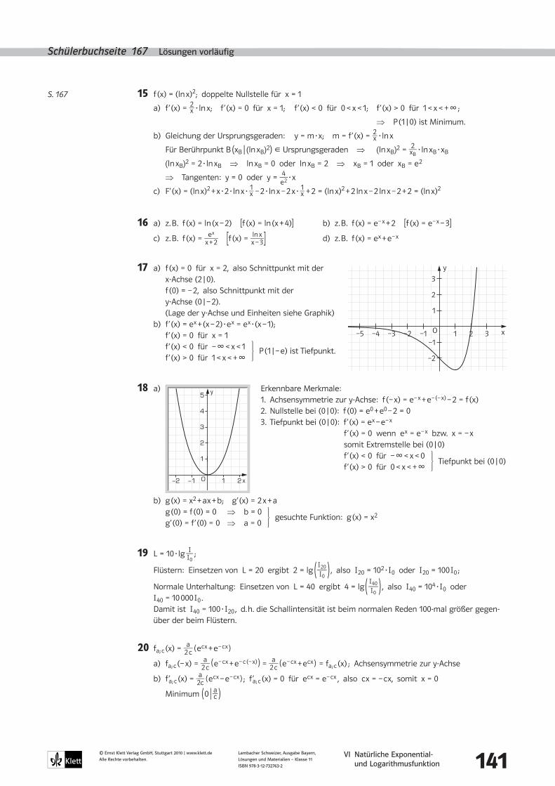
18 a) Erkennbare Merkmale: 1. Achsensymmetrie zur y-Achse: f (– x) = e – x + e – (– x) – 2 = f (x) 2. Nullstelle bei (0 | 0): f (0) = e0 + e0 – 2 = 0 3. Tiefpunkt bei (0 | 0): f ’ (x) = e x – e – x

f ’ (x) = 0 wenn e x = e – x bzw. x = – x somit Extremstelle bei (0 | 0) f ’ (x) < 0 für – • < x < 0 f ’ (x) > 0 für 0 < x < + •

b) g (x) = x2 + a x + b; g’ (x) = 2 x + a g (0) = f (0) = 0 ⇒ b = 0 g’ (0) = f ’ (0) = 0 ⇒ a = 0

19 L = 10·lg Ø _ Ø0 ;

Flüstern: Einsetzen von L = 20 ergibt 2 = lg ( Ø20 _ Ø0 ) , also Ø20 = 102·Ø0 oder Ø20 = 100 Ø0 ;

Normale Unterhaltung: Einsetzen von L = 40 ergibt 4 = lg ( Ø40 _ Ø0 ) , also Ø40 = 104·Ø0 oder

Ø40 = 10 000 Ø0 . Damit ist Ø40 = 100·Ø20 , d. h. die Schallintensität ist beim normalen Reden 100-mal größer gegen-

über der beim Flüstern.

20 fa; c (x) = a _ 2 c ( e c x + e – c x )

a) fa; c (– x) = a _ 2 c ( e – c x + e – c (– x) ) = a _ 2 c ( e – c x + e c x ) = fa; c (x) ; Achsensymmetrie zur y-Achse

b) f ’a; c (x) = a _ 2c ( e c x – e – c x ) ; f ’a; c (x) = 0 für e c x = e – c x , also c x = – c x, somit x = 0

Minimum ( 0 | a _ c )

S. 167

xO

–2

–1

1

2

3

1 2 3–1

y

–2–3–4–5

P (1 | – e) ist Tiefpunkt.

y

21−1−2 O

2

3

1

4

5

x

Tiefpunkt bei (0 | 0)

gesuchte Funktion: g (x) = x2





c) Es muss gelten: I. fc (0) = a _ c = 5

II. fc (100) = a _ 2 c ( e 100 c + e – 100 c ) = 30

aus I: a = 5 c eingesetzt in II:

5 _ 2 ( e 100 c + e – 100 c ) = 30 ⇔ e 100 c + e – 100 c – 12 = 0

Substitution u = e 100 c :

u + 1 _ u – 12 = 0 ⇒ u2 – 12 u + 1 = 0; u1 = 6 + 90000000 35 ≈ 11,9161; u2 = 6 – 90000000 35 ≈ 0,0839

u = e 100 c folgt c ≈ 0,0247789 oder c ≈ – 0,0247789 Damit erhält man in beiden Fällen dieselbe Funktion: f (x) = 2,5· ( e0,024779 x + e – 0,024779 x ) d) f ’ (x) = 0,061947· ( e0,024779 x + e – 0,024779 x ) f ’ (100) = 0,73298; tan φ = 0,73298 ergibt ein Gefälle von ca. 73 %. φ ≈ 36,2°

e) Bedingung: f (x) = 15, also 2,5· ( e0,024779 x + e – 0,024779 x ) = 15

Substitution: u = e0,024779 x: u + u – 1 – 6 = 0 ⇒ u2 – 6 u + 1 = 0; u1 = 3 + 2 90000 2 ≈ 5,8284

u2 = 3 – 2 90000 2 ≈ 0,17157

u = e – 0,024779 x folgt: x ≈ 71,14

Die Seilhöhe beträgt im Abstand von ca. 71 m, gemessen von der tiefsten Stelle, 15 m.

f) Bedingung: f ’ (x) = 0,2, also 0,061947· ( e0,024779 x – e – 0,024779 x ) = 0,2

Daraus erhält man x ≈ 50,7

Ein Stuntman könnte das Seil auf einer Strecke von gut 100 m befahren.

21 a) Jeder Repräsentant von _

› g liegt parallel zur Geraden g.

Somit gibt _

› g die Richtung der Geraden g an.

Ein Steigungsdreieck von g hat die Katheten 4 und 3, also gibt

der Vektor ( 4 3 ) die Richtung von g an.

Wegen ( 1

– 4 _ 3 ) = 1 _ 4 · ( 4 3 ) gilt dies auch für

_ › g .

b) n: x2 = – 4 _ 3 ·x1 + t; _

› n = ( 1

– 4 _ 3

) ; _

› n °

_ › g = ( 1

– 4 _ 3

) ° ( 1 4 _ 3

) = 1·1 + ( – 4 _ 3 ) · 3 _ 4 = 1 – 1 = 0

Die Vektoren _

› n und

_ › g stehen senkrecht aufeinander, somit ist auch die Gerade n senkrecht zur

Geraden g.

DieEuler’scheZahle

1 a) K20 = K0 ( 1 + p _ 100 ) 20

= 2 K0 ⇒ 20 000 € = 10 000 · ( 1 + p _ 100 ) 20

2 = ( 1 + p _ 100 ) 20

⇒ p = 100 · ( 20 90000 2 – 1 ) ≈ 3,5

Der Jahreszinssatz beträgt etwa 3,5 %. b) K20 = K0 · 1,0520 = 10 000 € · 1,0520 ≈ 26 532,98 €

c) K20 = K0 · ( 1 + 1 _ 7200 ) 7200

= 10 000 € · ( 1 + 1 _ 7200 ) 7200

≈ 27 180,93 €

2 a) t0 = 0 ⇒ n (t 0 + 0) = n (t); n (t 0) = n (0) = 1000 n (t) = n (0) + 1,75 t · n (0) = 1000 + 1750 t = 1000 (1 + 1,75 t) b) n (15) = 1000 (1 + 1,75 t · 15) = 27 250

3 Es muss gelten: sn + 1 – sn = 1 _ (n + 1)! < 10 – 6. Dies ist ab n = 9 der Fall.

t _ › g = ( 1

3 _ 4 )

x1

x2

g: x2 = 4 _ 3 ·x1 + t

43

S. 169

Documents

Lambacher Schweizer, Ausgabe Bayern, VI ...schule.martin-meier.org/mathematik/klasse11/kap6.pdf · VI Natürliche Exponential-Lambacher Schweizer, Ausgabe Bayern, und Logarithmusfunktion