Embed Size (px)
Citation preview
Long-Range Interactions, weakmagnetic fields amplification,and End states for Quantum
Computing
INAUGURALDISSERTATION
zur
Erlangung der Wurde eines Doktors derPhilosophie
vorgelegt der
Philosophisch-Naturwissenschaftlichen Fakultat
der Universitat Basel
von
Luka Trifunovic
aus Belgrad, Serbien
Basel, 2015

Namensnennung-Keine kommerzielle Nutzung-Keine Bearbeitung 2.5 Schweiz
Sie dürfen:
das Werk vervielfältigen, verbreiten und öffentlich zugänglich machen
Zu den folgenden Bedingungen:
Namensnennung. Sie müssen den Namen des Autors/Rechteinhabers in der von ihm festgelegten Weise nennen (wodurch aber nicht der Eindruck entstehen darf, Sie oder die Nutzung des Werkes durch Sie würden entlohnt).
Keine kommerzielle Nutzung. Dieses Werk darf nicht für kommerzielle Zwecke verwendet werden.
Keine Bearbeitung. Dieses Werk darf nicht bearbeitet oder in anderer Weise verändert werden.
• Im Falle einer Verbreitung müssen Sie anderen die Lizenzbedingungen, unter welche dieses Werk fällt, mitteilen. Am Einfachsten ist es, einen Link auf diese Seite einzubinden.
• Jede der vorgenannten Bedingungen kann aufgehoben werden, sofern Sie die Einwilligung des Rechteinhabers dazu erhalten.
• Diese Lizenz lässt die Urheberpersönlichkeitsrechte unberührt.
Quelle: http://creativecommons.org/licenses/by-nc-nd/2.5/ch/ Datum: 3.4.2009
Die gesetzlichen Schranken des Urheberrechts bleiben hiervon unberührt.
Die Commons Deed ist eine Zusammenfassung des Lizenzvertrags in allgemeinverständlicher Sprache: http://creativecommons.org/licenses/by-nc-nd/2.5/ch/legalcode.de
Haftungsausschluss:Die Commons Deed ist kein Lizenzvertrag. Sie ist lediglich ein Referenztext, der den zugrundeliegenden Lizenzvertrag übersichtlich und in allgemeinverständlicher Sprache wiedergibt. Die Deed selbst entfaltet keine juristische Wirkung und erscheint im eigentlichen Lizenzvertrag nicht. Creative Commons ist keine Rechtsanwaltsgesellschaft und leistet keine Rechtsberatung. Die Weitergabe und Verlinkung des Commons Deeds führt zu keinem Mandatsverhältnis.
Genehmigt von der Philosophisch-NaturwissenschaftlichenFakultat auf Antrag von
Prof. Dr. Daniel Loss
Prof. Dr. Guido Burkard
Basel, den 14. Oktober 2014
Prof. Dr. Jorg SchiblerDekan

Acknowledgments
See print version.
iv
Summary
It was Richard Feynman who first proposed, in 1982, the far-reachingconcept of a ”quantum computer”—a device more powerful than clas-sical computers. The idea of a quantum computer is to employ the fas-cinating and often counterintuitive laws of quantum mechanics to pro-cess information. It is far from obvious that the proposed concept ofa quantum computer is more powerful than its classical counterpart, itwas only in 1994 when Peter Shor theoretically demonstrated the exis-tence of a quantum algorithm for factorizing integers into prime factorsthat runs in polynomial time unlike its classical counterpart which worksin sub-exponential time. The factorization of integers into prime factorsis the basis of asymmetric cryptography. These early theoretical resultslunched an immense interest of the scientific community. Already dur-ing ’90s, the first proposals for the physical implementation of quantumcomputation emerged. Ever since, many experimental groups aroundthe world pursued different physical implementations of quantum bits(qubits). The first decade of the new century saw a steady improvementin the control and decoherence time (the time over which the informa-tion carried by the qubit is lost) for various qubits by many orders ofmagnitude. The natural next step in this context is to answer the ques-tion of how to scale the system up to include many qubits and thus builda quantum computer? One of the main parts of this thesis addresses ex-actly this question, namely the question of architecture and scalability offuture quantum computer.
Among various different physical realizations of qubits, the idea ofusing electron spins trapped in electrostatic semiconductor quantum dotsas the building blocks of a quantum computer (the so-called spin qubits),put forward by Daniel Loss and David DiVincenzo in 1997, triggeredtremendous interest in scientific community. Nevertheless, the imple-mentation of the original Loss-DiVincenzo proposal posed a considerabletechnical challenge. It used quantum tunneling between qubits to enabletheir communication with each other, and thus required that the qubits to
v
vi
be placed very close to each other. This requirement not only leaves littlespace for the placement of the vast amount of gates and wirings neededto define the electrostatic quantum dots, but also makes it challenging tocontrol the local magnetic field needed for single-qubit operations. Forthese reasons, no system with more than a couple of spin qubits has beensuccessfully implemented thus far. In the first part of this thesis, we leapover this long-standing problem with an entirely different strategy of us-ing metallic floating gates or ferromagnets to couple together qubits thatare separated over a long distance. Our scheme works for any type ofspin qubits, including the qubits based on nitrogen-vacancy center (NV-center) in diamond and technologically very important silicon qubits.
The main topic of this thesis is related to quantum computer. Still,quite unexpectedly, some of the ideas we employed in order to tacklethe problem of quantum computer scalability can be utilized in a com-pletely different field of research, namely, in the field of magnetic fieldsensing. Qubit are not only a necessary ingredient of quantum computerbut they also provide a way to measure very accurately magnetic fields.The magnetometer build upon the qubit based on NV-center, so-calledNV-magnetometer, emerged in recent years as most sensitive magneticmoment sensor. These magnetometers are able to detect about hundrednuclear spins within a minute of acquisition time. In the second part ofthis thesis, we propose an entirely novel experimental realization of NV-magnetometers which increases present NV-center sensitivities by fourorders of magnitude at room temperature. This unprecedented amplifi-cation of sensitivity will render magnetometers capable of detecting in-dividual nuclear spins. This amplification is achieved by introducing aferromagnetic particle between the nuclear spin that needs to be detectedand the NV-magnetometer. Our setup, in contrast to existing schemes,is particularly advantageous because, due to the large amplification ofsensitivity, the nuclear spin need not lie within a few nanometers of thesurface but rather can be detectable at a distance of 30 nm. With thesenovelties, our scheme provides chemically sensitive spin detection un-der ambient conditions allowing nanoscale resolution of nuclear mag-netic moments in biological systems—the holy grail of nuclear magneticresonance.
In the last part of the thesis we focus our attention to a new directionin quantum computer implementation that deals with topological quan-tum computer introduced by Alexei Kitaev in 1997; in this approach theidea is to use quasiparticles with ”fractional” statistics and to performthe single- and two-qubit gates by merely exchanging these quasiparti-cles. Additionally, information in this system is stored non-locally thus
vii
it mitigates the problem of decoherence caused by local noise from theenvironment. Majorana fermions are one of the most well known ex-amples of such excitations. We analyze transport signatures of differenttopological states in one-dimensional systems, like Majorana fermionsand fractionally charged states. We envision an Aharonov-Bohm setupwherein conductance measurement provides a clear signature of pres-ence of fractionally charged fermionic states, since oscillations with dou-ble period emerge in this case. Additionally, we propose a very sim-ple setup that enables existence of degenerate mid-gap states, so-calledTamm-Shockley states that are characterized by fractional charge anddiscuss possible ways of detecting these states experimentally.
Contents
Contents vii
1 Introduction 11.1 The “Loss-DiVincenzo” proposal . . . . . . . . . . . . . . . 11.2 Qubits based on nitrogen-vacancy centers . . . . . . . . . . 51.3 Topological quantum computation by anyons . . . . . . . . 9
I Long-Range Indirect Interaction of Spins Qubits
2 Introduction 14
3 Long-Distance Spin-Spin Coupling via Floating Gates 173.1 Electrostatics of the floating gate . . . . . . . . . . . . . . . 183.2 Qubit-qubit coupling . . . . . . . . . . . . . . . . . . . . . . 203.3 Scalable Architecture . . . . . . . . . . . . . . . . . . . . . . 253.4 Implementation of two-qubit gates . . . . . . . . . . . . . . 313.5 Numeric Modeling of Realistic Devices . . . . . . . . . . . . 323.6 Conclusions . . . . . . . . . . . . . . . . . . . . . . . . . . . 353.7 Acknolwedgment . . . . . . . . . . . . . . . . . . . . . . . . 363.A SPIN-SPIN COUPLING - singly occupied double-dots . . . 363.B SPIN-SPIN COUPLING - the hybrid system . . . . . . . . . 393.C Implementation of two-qubit gates . . . . . . . . . . . . . . 41
4 Long-Distance Entanglement of Spin-Qubits via Ferromagnet 444.1 Model . . . . . . . . . . . . . . . . . . . . . . . . . . . . . . . 444.2 Decoherence . . . . . . . . . . . . . . . . . . . . . . . . . . . 504.3 Estimates . . . . . . . . . . . . . . . . . . . . . . . . . . . . . 554.4 Conclusions . . . . . . . . . . . . . . . . . . . . . . . . . . . 564.5 Acknowledgements . . . . . . . . . . . . . . . . . . . . . . . 564.A Holstein-Primakoff transformation . . . . . . . . . . . . . . 56
viii
CONTENTS ix
4.B Transverse correlators 〈S+q (t)S−−q(0)〉 . . . . . . . . . . . . . 57
4.C Longitudinal correlators 〈Szq(t)Sz−q(0)〉 . . . . . . . . . . . . 614.D Exchange coupling to the ferromagnet . . . . . . . . . . . . 644.E Fourth order contributions to decoherence . . . . . . . . . . 68
5 Long-Range Interaction of Spin-Qubits via Ferromagnets 725.1 Ferromagnet . . . . . . . . . . . . . . . . . . . . . . . . . . . 735.2 Coupling between ST-qubits . . . . . . . . . . . . . . . . . . 735.3 Coupling between spin-1/2 qubits . . . . . . . . . . . . . . 795.4 Coupling between spin-1/2 and ST-qubits . . . . . . . . . . 855.5 Validity of the effective Hamiltonian . . . . . . . . . . . . . 875.6 Switching mechanisms . . . . . . . . . . . . . . . . . . . . . 885.7 Coupling strengths and operation times . . . . . . . . . . . 885.8 Conclusions . . . . . . . . . . . . . . . . . . . . . . . . . . . 905.9 Acknowledgment . . . . . . . . . . . . . . . . . . . . . . . . 915.A Rotated Hamiltonian for CNOT gate . . . . . . . . . . . . . 91
II Weak magnetic field amplification for room-temperaturemagnetometry
6 Introduction 94
7 High-efficiency resonant amplification of weak magnetic fieldsfor single spin magnetometry 967.1 Setup . . . . . . . . . . . . . . . . . . . . . . . . . . . . . . . 977.2 Proposed magnetometer sensitivity . . . . . . . . . . . . . . 1007.3 Conclusions . . . . . . . . . . . . . . . . . . . . . . . . . . . 1077.4 Acknowledgments . . . . . . . . . . . . . . . . . . . . . . . 1087.5 Methods . . . . . . . . . . . . . . . . . . . . . . . . . . . . . 1087.A Cramer-Rao Bound . . . . . . . . . . . . . . . . . . . . . . . 1117.B Sensitivity of an NV-center . . . . . . . . . . . . . . . . . . . 1127.C AC sensitivity for θ = 0 . . . . . . . . . . . . . . . . . . . . . 1147.D Calculation of ϕNV (ti) and β(ti, τ) . . . . . . . . . . . . . . . 1157.E Stray field from a uniformly magnetized cuboid . . . . . . 119
IIIEnd states in one-dimensional systems
8 Introduction 124
9 Localized end states in density modulated quantum wires andrings 1289.1 Lattice model . . . . . . . . . . . . . . . . . . . . . . . . . . 1299.2 Disorder effects . . . . . . . . . . . . . . . . . . . . . . . . . 1309.3 Continuum model . . . . . . . . . . . . . . . . . . . . . . . . 132
CONTENTS x
9.4 Interaction effects . . . . . . . . . . . . . . . . . . . . . . . . 1339.5 Detection . . . . . . . . . . . . . . . . . . . . . . . . . . . . . 1359.6 Effective quantum dot . . . . . . . . . . . . . . . . . . . . . 1389.7 Conclusions . . . . . . . . . . . . . . . . . . . . . . . . . . . 1399.8 Acknowledgements . . . . . . . . . . . . . . . . . . . . . . . 139
10 Realistic transport modeling for a superconducting nanowirewith Majorana fermions 14010.1 Model . . . . . . . . . . . . . . . . . . . . . . . . . . . . . . . 14110.2 Discussion . . . . . . . . . . . . . . . . . . . . . . . . . . . . 14410.3 Conclusions . . . . . . . . . . . . . . . . . . . . . . . . . . . 15210.4 Acknowledgments . . . . . . . . . . . . . . . . . . . . . . . 152
11 Transport signatures of fractional Fermions in Rashba nanowires15311.1 Model . . . . . . . . . . . . . . . . . . . . . . . . . . . . . . . 15411.2 Method . . . . . . . . . . . . . . . . . . . . . . . . . . . . . . 15511.3 Results . . . . . . . . . . . . . . . . . . . . . . . . . . . . . . 15711.4 Experimental feasibility . . . . . . . . . . . . . . . . . . . . 16011.5 Conclusions . . . . . . . . . . . . . . . . . . . . . . . . . . . 16111.6 Acknowledgements . . . . . . . . . . . . . . . . . . . . . . . 162
Bibliography 163
CHAPTER 1Introduction
In this section we introduce several concepts that are used as a startingpoint for the work presented in this thesis. Since the main part of thethesis deals with physical implementations of quantum computer andquantum bits (qubits) we start by reviewing Loss-DiVincenzo proposaland DiVincenzo criteria, see Sec. 1.1. We then describe another imple-mentation of qubits using defects in diamond. Even tough the term qubitis mainly used in context of quantum computing, it can also be a power-ful tool to for magnetic field sensing as described in Sec. 1.2. Finally inSec. 1.3, we turn our attention to a new paradigm of quantum computa-tion by introducing the basic concepts needed to understand advantagesof topological quantum computation.
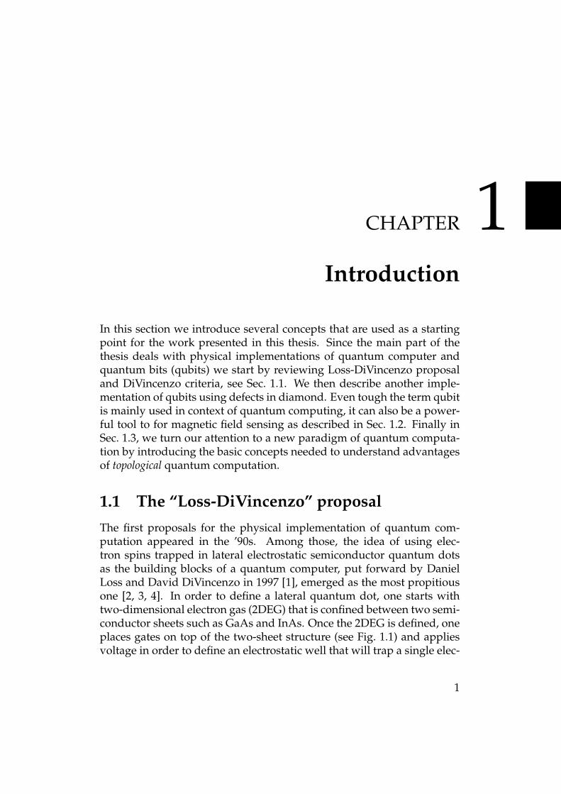
1.1 The “Loss-DiVincenzo” proposalThe first proposals for the physical implementation of quantum com-putation appeared in the ’90s. Among those, the idea of using elec-tron spins trapped in lateral electrostatic semiconductor quantum dotsas the building blocks of a quantum computer, put forward by DanielLoss and David DiVincenzo in 1997 [1], emerged as the most propitiousone [2, 3, 4]. In order to define a lateral quantum dot, one starts withtwo-dimensional electron gas (2DEG) that is confined between two semi-conductor sheets such as GaAs and InAs. Once the 2DEG is defined, oneplaces gates on top of the two-sheet structure (see Fig. 1.1) and appliesvoltage in order to define an electrostatic well that will trap a single elec-
1
CHAPTER 1. INTRODUCTION 2
Figure 1.1: Scheme of the Loss-DiVincenzo proposal. The yellow gateson the top that give rise to an electrostatic potential that defines wells(quantum dots) as well as control the tunneling between the wells. Theblack arrows denote electron’s spin degree of freedom.
tron. Since a single electron is spatially separated from the rest of the2DEG, its spin can be used to define a two-level system, i.e., a qubit.
In order for a qubit to be used as a building block of a quantum com-puter, it has to satisfy the stringent requirements know as DiVincenzocriteria [5], that can be summarized as follows:
• Reliable initialization in a predefined state of the qubit
• Coherent quantum control of a single qubit (single-qubit gates) andcontrolled entangling interaction between the pairs of adjacent qubits(two-qubit gates)
• The coherent superposition of the two states of the qubit has to belonger lived than the single- and two-qubit operation times
• Possibility to readout the qubit state within the time shorter thanthe qubit relaxation time
• Scalability, i.e., the possibility to scale up the number of qubits
Figure 1.1 illustrates the Loss-DiVincenzo proposal. Each qubit is en-coded in the spin (arrow) of an electron that is trapped in a lateral quan-
CHAPTER 1. INTRODUCTION 3
tum dot. Formally, the two basis states of the qubit are defined as
|0〉 = | ↑〉 and |1〉 = | ↓〉 , (1.1)
with | ↑〉 and | ↓〉 being the two states of the electron spin with oppositespin projection along the certain axis defined by an externally appliedmagnetic field. A general qubit state is then an arbitrary superpositionof the basis states
|ψ〉 = α|0〉+ β|1〉 , (1.2)
with |α|2 + |β|2 = 1.We now clarify why Loss-DiVincenzo proposal satisfies most of Di-
Vincenzo criteria. The qubit initialization can be achieved by externallyapplying magnetic field Bz along z-axis (the choice of axis is arbitrary),which causes the | ↑〉 and | ↓〉 states of the qubit to split up with energydifference EZ = ~µBgBz, with Lande factor g = −0.44 for GaAs andµB being the Bohr magneton. Assuming that the applied magnetic fieldis big enough |EZ | kBT (kB is Boltzmann constant), the initializationis achieved by waiting for electron spins to reach their thermodynamicequilibrium.1
Next, the single-qubit gates can be performed by applying AC mag-netic field in xy-plane. When the frequency of the applied AC magneticfield matches the qubit Zeeman splitting, it will cause the transitions thatare periodic in time between the two qubit states—so-called Rabi oscilla-tions. By varying the duration of applied AC magnetic field any single-qubit gate can be achieved. This scheme is know as electron spin reso-nance (ESR). It is worth noting at this point that one needs in principleto apply AC magnetic field locally on the qubit which is experimentallyvery challenging task. An alternative approach is to use spatially vary-ing g-factor—the qubit we want to address is pulled into a layer withhigher g-factor thus only this qubit satisfies the resonant condition withthe applied AC field. Additionally, making use of spin-orbit interac-tion allows an all-electrical implementation of single-qubit gates. Fur-thermore, the two-qubit gates can be performed by using the exchangecoupling between the neighbouring spins, where the strength of this in-teraction can be tuned electrically by adjusting the gate voltage that con-trols the barrier height between two neighbouring potential wells. Thetime-dependent interaction Hamiltonian is of Heisenberg type
1In this scheme, the initialization time is given by the qubit relaxation time andtherefore it is slow. We note that there exist fast initialization schemes.
CHAPTER 1. INTRODUCTION 4
H12 = J(t)S1 · S2 , (1.3)
and it was demonstrated [1] that this type of interaction is enough toproduce entanglement between the interacting qubits.
Finally, it is possible to readout spin state of the qubit by convertingspin state into charge state and using quantum point contact to detectcharge [6].
The scalability of Loss-DiVincenzo proposal is experimentally verychallenging, since—with present day technology—there is hardly enoughspace to place the large amount of metallic gates and wires needed to de-fine and to address the spin qubits. A promising strategy to meet thischallenge is to implement long-range interactions between the qubitswhich allows the quantum dots to be moved apart and to create spacefor the wirings.
In this thesis we extend Loss-DiVincenzo proposal such that the scal-ability requirement is satisfied. We achieve this by proposing a long-range electrostatic interaction between the qubits mediated via a dog-bone shaped floating metallic gate. In order for the scheme to work, thespin degree of freedom has to be coupled to charge which is achievedthrough the spin orbit interaction (SOI). Furthermore, we argue that in-clusion of a floating gate does not induce detrimental source of decoher-ence since the system already contains the gates that define the quan-tum dots. We construct explicitly a controlled-NOT (CNOT) two-qubitgate and obtain the operation time of a few tens of nanoseconds forGaAs quantum dots—significantly below the typical coherence time ofthe quantum dot defined qubit. Thus the extended Loss-DiVincenzo pro-posal satisfies all DiVincenzo criteria. The details of our proposal can befound in Chapter 3.
Certain semiconductors have very weak or practically no SOI (fore.g. silicon, a technologically very important material). In such mate-rials the previously described electrostatic coupler would yield too smallcoupling. In order to provide a scheme that would mediate a long-rangeinteraction also in this kind of material, we propose a setup that consistof a dog-bone shaped ferromagnet (FM). Herein, no SOI is needed sincethe qubit spin degree of freedom is directly coupled to the FM spins viadipolar interaction. This scheme applied to semiconductor lateral quan-tum dots is described in Chapter 5.
CHAPTER 1. INTRODUCTION 5
1A
orbital excitedstates (3E)
orbital groundstates (3A)ESR
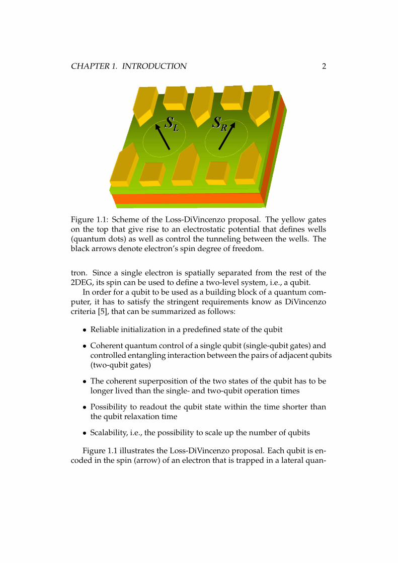
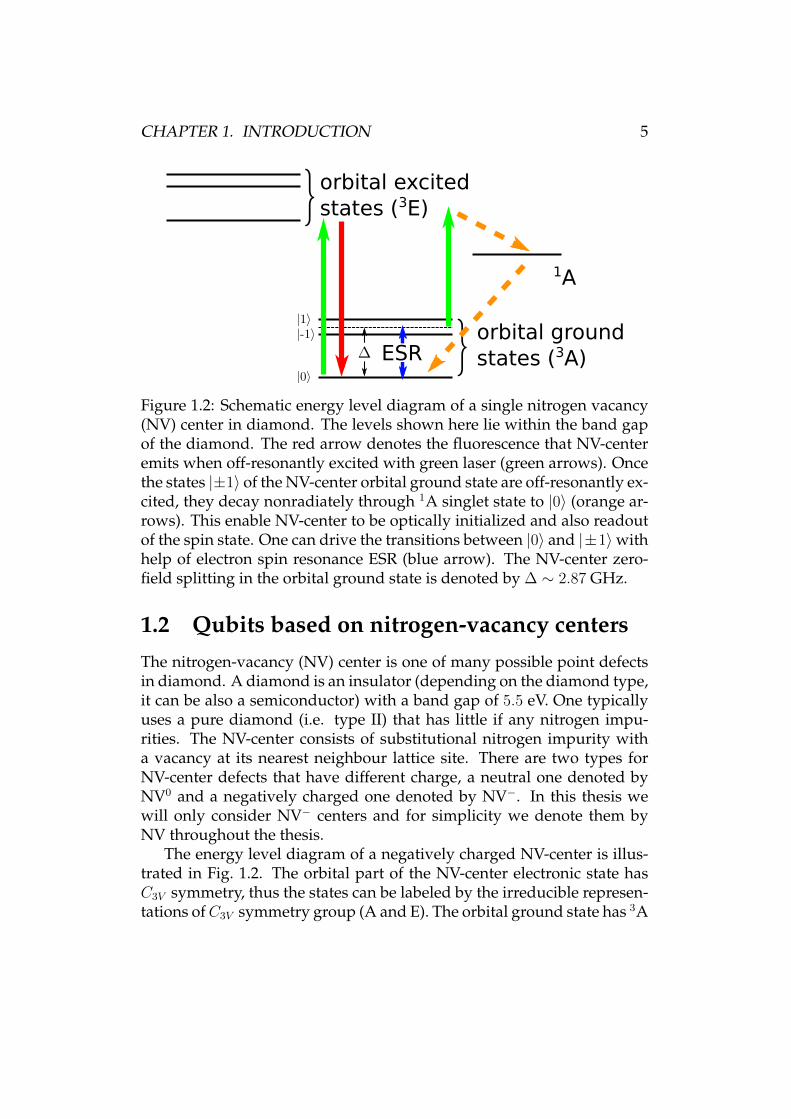
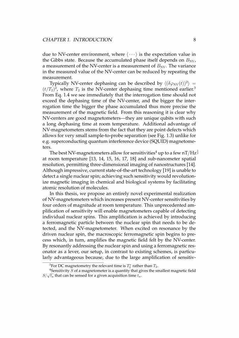
Figure 1.2: Schematic energy level diagram of a single nitrogen vacancy(NV) center in diamond. The levels shown here lie within the band gapof the diamond. The red arrow denotes the fluorescence that NV-centeremits when off-resonantly excited with green laser (green arrows). Oncethe states |±1〉 of the NV-center orbital ground state are off-resonantly ex-cited, they decay nonradiately through 1A singlet state to |0〉 (orange ar-rows). This enable NV-center to be optically initialized and also readoutof the spin state. One can drive the transitions between |0〉 and |±1〉withhelp of electron spin resonance ESR (blue arrow). The NV-center zero-field splitting in the orbital ground state is denoted by ∆ ∼ 2.87 GHz.
1.2 Qubits based on nitrogen-vacancy centersThe nitrogen-vacancy (NV) center is one of many possible point defectsin diamond. A diamond is an insulator (depending on the diamond type,it can be also a semiconductor) with a band gap of 5.5 eV. One typicallyuses a pure diamond (i.e. type II) that has little if any nitrogen impu-rities. The NV-center consists of substitutional nitrogen impurity witha vacancy at its nearest neighbour lattice site. There are two types forNV-center defects that have different charge, a neutral one denoted byNV0 and a negatively charged one denoted by NV−. In this thesis wewill only consider NV− centers and for simplicity we denote them byNV throughout the thesis.
The energy level diagram of a negatively charged NV-center is illus-trated in Fig. 1.2. The orbital part of the NV-center electronic state hasC3V symmetry, thus the states can be labeled by the irreducible represen-tations ofC3V symmetry group (A and E). The orbital ground state has 3A

CHAPTER 1. INTRODUCTION 6
symmetry, which means that the orbital part has A symmetry (i.e. it is in-variant under C3V group operations) and there are 3 states with differentspin projections. Even in the absence of an externally applied magneticfield, the ground state |0〉 and the excited states | ± 1〉 are split by energy∆—so-called zero-field splitting, while the states | ± 1〉 are degenerate.This crystal field splitting quantized the spin projection along the N-Vsymmetry axis. Since the energy difference between |0〉 and | ± 1〉 stateslies in microwave region, one can drive transition between these states(i.e. Rabi oscillations) with microwave radiation.
There are several optical properties of the NV-centers that make themvery attractive for various applications in the field of quantum informa-tion processing; here we mention the most important ones. Firstly, theorbital ground states of the NV-center can be off-resonantly excited witha green laser. If the NV-center was initially in |0〉 state, then due to selec-tion rules, it decays back to |0〉 state with emission of an photon (photo-luminescence). On the other hand, if the initial state of the NV-center is| ± 1〉, then the predominant channel for the relaxation is through nonra-diant decay via metastable singlet state (1A, see Fig. 1.2) into the |0〉 state.Thus we see that the NV-center can be initialized into |0〉 state by simplyshining the green laser onto it. Furthermore, by detecting the photonsfrom spin-dependent photoluminescence, we can determine the state ofthe NV-center, i.e., perform the readout of the NV-center state; if the NV-center was initially in |0〉 photon is detected, otherwise no photon is de-tected. This readout scheme is limited by photon detection efficiencyand photon shot noise. We stress that quite remarkably both initializa-tion and the readout2 can be performed at room temperature. We noteherein that the described spin-dependent fluorescence readout schemeis spoiled when there is a component of an externally applied magneticfield that is perpendicular to the N-V axis. Namely, such a magnetic fieldcomponent mixes |0〉 and | ± 1〉 states which in turn affects the abovementioned selection rules. In practice, perpendicular magnetic field upto 10 mT can be tolerated [9].
When an external magnetic field is applied along the N-V symmetryaxis, the | ± 1〉 states split and one can use |0〉 and | − 1〉 states to de-fine a qubit. We already mentioned that such a qubit can be readout andinitialized optically at room temperature. Additionally, one can also per-
2At low temperature it is also possible to perform a resonant single-shot readout [7].At room temperature a single-shot readout is still possible with help of a nuclear spinin vicinity of the NV-center [8].
CHAPTER 1. INTRODUCTION 7
form single-qubit gates by using microwave drive (ESR) [10]. Probablyone of the most remarkable features of the NV-centers is their long co-herence time even at room temperature, T ∗2 ≈ 20µs and T2 ≈ 1.8ms [11].We see that the qubit defined by two states of a NV-center satisfies al-most all of DiVincenzo criteria. The only ingredient missing in order touse NV-center as a building block of a quantum computer is the possi-bility to perform two-qubit gates, i.e., possibility of having a controlledinteraction between the NV-centers. We note that two-qubit gates on NV-centers have been experimentally demonstrated [12], but unfortunatelythis scheme is not scalable. In this thesis we tackle this important prob-lem by proposing a way to mediate a controlled long-range couplingbetween two NV-centers. The proposed coupling is mediated by vir-tual magnons, a virtual excitations that propagate through a dog-boneshaped ferromagnet that is placed between the two NV-centers that needto be coupled. The details of our scheme are presented in Chapter 4.
Scanning magnetometry with a single NV-center
In this section we explain why qubits are useful not only in the contextof quantum computation and quantum information processing, but alsoprovide possibility of very accurate magnetic field sensing by makinguse of Ramsey type measurements. We focus here on NV-centers, butany long-lived qubit can be used instead.
We start by initializing the NV-center in the state |0〉. Then, a π/2pulse is applied to the NV-center which leaves it in a superposition state(|0〉 + |1〉)/
√2, then we wait for the NV-center to accumulate the phase
during the interrogation time t, this phase is proportional the magneticfield component along the N-V axis BNV. After the interrogation timet has passed, the NV-center is in the state (|0〉 + eiϕNV |1〉)/
√2, where
ϕNV = γBNVt. Finally, another π/2 pulse is applied to the NV-centerwhich transfers the phase difference between the |0〉 and |1〉 states intothe occupation of these two states, which is given by following probabil-ity distribution
p(n|ϕNV(t)) =1
2
(1 + n cos(ϕNV(t))e−〈(δϕNV(t))2〉
). (1.4)
Here, n = ±1 are the two possible outcomes when the state of the NV-center is measured. We also included dephasing in the NV-center viaterm 〈(δϕNV(t))2〉 that describes the fluctuations of the accumulated phase
CHAPTER 1. INTRODUCTION 8
due to NV-center environment, where 〈 · · · 〉 is the expectation value inthe Gibbs state. Because the accumulated phase itself depends on BNV,a measurement of the NV-center is a measurement of BNV. The variancein the measured value of the NV-center can be reduced by repeating themeasurement.
Typically NV-center dephasing can be described by 〈(δϕNV(t))2〉 =(t/T2)2, where T2 is the NV-center dephasing time mentioned earlier.3
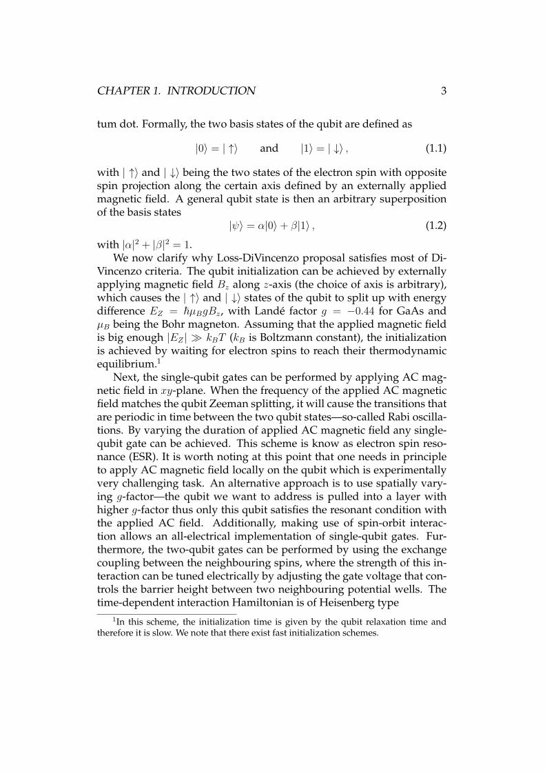
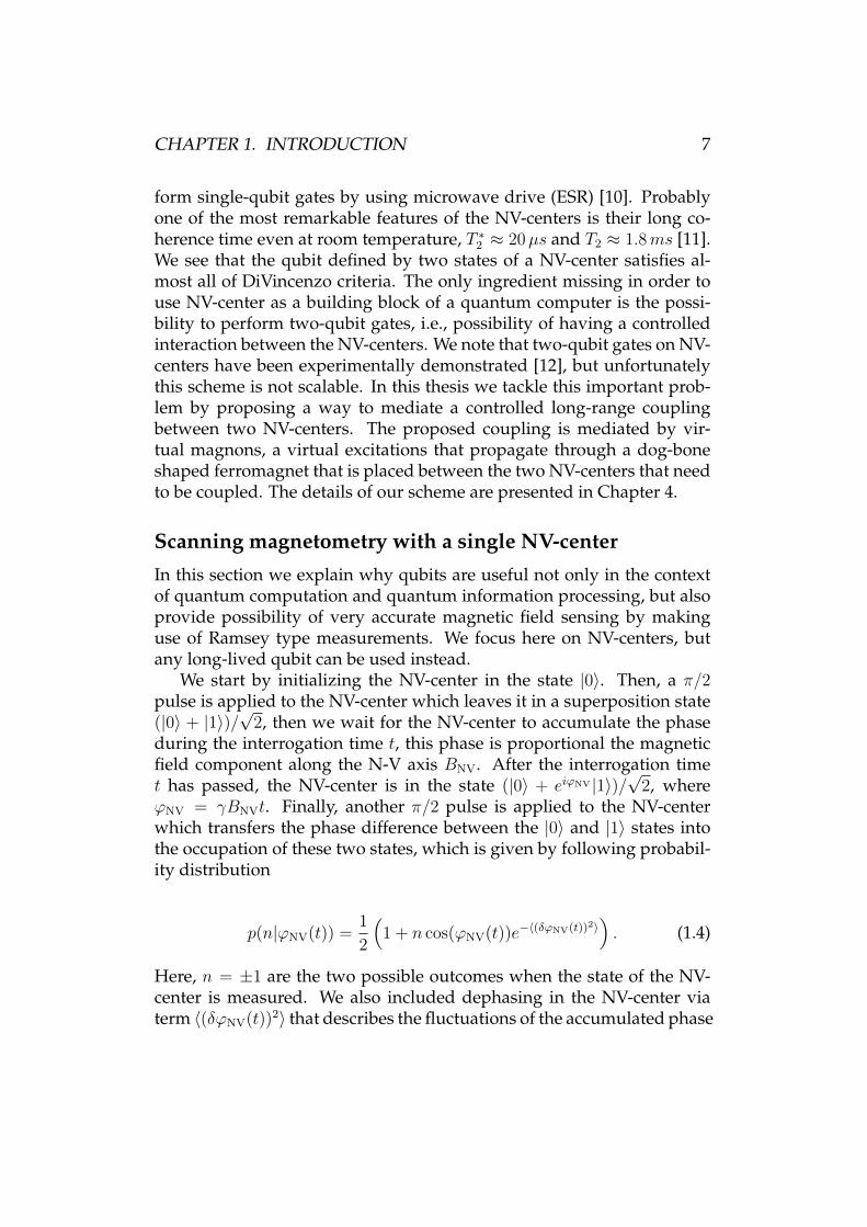
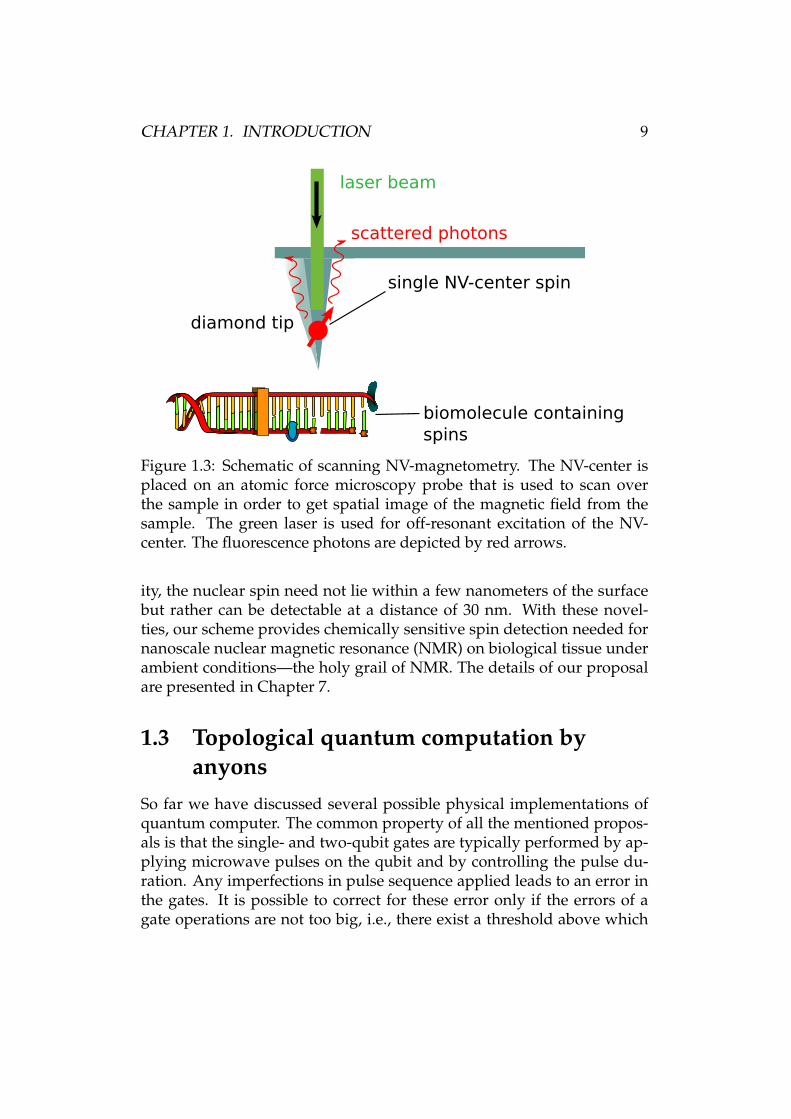
From Eq. 1.4 we see immediately that the interrogation time should notexceed the dephasing time of the NV-center, and the bigger the inter-rogation time the bigger the phase accumulated thus more precise themeasurement of the magnetic field. From this reasoning it is clear whyNV-centers are good magnetometers—they are unique qubits with sucha long dephasing time at room temperature. Additional advantage ofNV-magnetometers stems from the fact that they are point defects whichallows for very small sample-to-probe separation (see Fig. 1.3) unlike fore.g. superconducting quantum interference device (SQUID) magnetome-ters.
The best NV-magnetometers allow for sensitivities4 up to a few nT/Hz12
at room temperature [13, 14, 15, 16, 17, 18] and sub-nanometer spatialresolution, permitting three-dimensional imaging of nanostructures [14].Although impressive, current state-of-the-art technology [19] is unable todetect a single nuclear spin; achieving such sensitivity would revolution-ize magnetic imaging in chemical and biological systems by facilitatingatomic resolution of molecules.
In this thesis, we propose an entirely novel experimental realizationof NV-magnetometers which increases present NV-center sensitivities byfour orders of magnitude at room temperature. This unprecedented am-plification of sensitivity will enable magnetometers capable of detectingindividual nuclear spins. This amplification is achieved by introducinga ferromagnetic particle between the nuclear spin that needs to be de-tected, and the NV-magnetometer. When excited on resonance by thedriven nuclear spin, the macroscopic ferromagnetic spin begins to pre-cess which, in turn, amplifies the magnetic field felt by the NV-center.By resonantly addressing the nuclear spin and using a ferromagnetic res-onator as a lever, our setup, in contrast to existing schemes, is particu-larly advantageous because, due to the large amplification of sensitiv-
3For DC magnetometry the relevant time is T ∗2 rather than T2.4Sensitivity S of a magnetometer is a quantity that gives the smallest magnetic field
S/√ta that can be sensed for a given acquisition time ta.
CHAPTER 1. INTRODUCTION 9
diamond tip
laser beam
single NV-center spin
scattered photons
biomolecule containingspins
Figure 1.3: Schematic of scanning NV-magnetometry. The NV-center isplaced on an atomic force microscopy probe that is used to scan overthe sample in order to get spatial image of the magnetic field from thesample. The green laser is used for off-resonant excitation of the NV-center. The fluorescence photons are depicted by red arrows.
ity, the nuclear spin need not lie within a few nanometers of the surfacebut rather can be detectable at a distance of 30 nm. With these novel-ties, our scheme provides chemically sensitive spin detection needed fornanoscale nuclear magnetic resonance (NMR) on biological tissue underambient conditions—the holy grail of NMR. The details of our proposalare presented in Chapter 7.
1.3 Topological quantum computation byanyons
So far we have discussed several possible physical implementations ofquantum computer. The common property of all the mentioned propos-als is that the single- and two-qubit gates are typically performed by ap-plying microwave pulses on the qubit and by controlling the pulse du-ration. Any imperfections in pulse sequence applied leads to an error inthe gates. It is possible to correct for these error only if the errors of agate operations are not too big, i.e., there exist a threshold above which
CHAPTER 1. INTRODUCTION 10
AB1 2
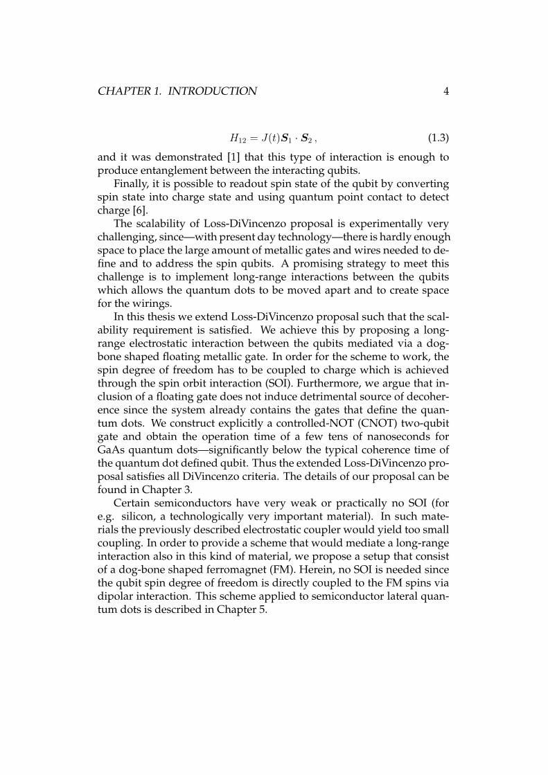
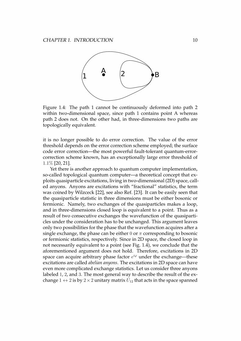
Figure 1.4: The path 1 cannot be continuously deformed into path 2within two-dimensional space, since path 1 contains point A whereaspath 2 does not. On the other had, in three-dimensions two paths aretopologically equivalent.
it is no longer possible to do error correction. The value of the errorthreshold depends on the error correction scheme employed; the surfacecode error correction—the most powerful fault-tolerant quantum-error-correction scheme known, has an exceptionally large error threshold of1.1% [20, 21].
Yet there is another approach to quantum computer implementation,so-called topological quantum computer—a theoretical concept that ex-ploits quasiparticle excitations, living in two-dimensional (2D) space, call-ed anyons. Anyons are excitations with “fractional” statistics, the termwas coined by Wilzceck [22], see also Ref. [23]. It can be easily seen thatthe quasiparticle statistic in three dimensions must be either bosonic orfermionic. Namely, two exchanges of the quasiparticles makes a loop,and in three-dimensions closed loop is equivalent to a point. Thus as aresult of two consecutive exchanges the wavefunction of the quasiparti-cles under the consideration has to be unchanged. This argument leavesonly two possibilities for the phase that the wavefunction acquires after asingle exchange, the phase can be either 0 or π corresponding to bosonicor fermionic statistics, respectively. Since in 2D space, the closed loop innot necessarily equivalent to a point (see Fig. 1.4), we conclude that theaforementioned argument does not hold. Therefore, excitations in 2Dspace can acquire arbitrary phase factor eiϕ under the exchange—theseexcitations are called abelian anyons. The excitations in 2D space can haveeven more complicated exchange statistics. Let us consider three anyonslabeled 1, 2, and 3. The most general way to describe the result of the ex-change 1↔ 2 is by 2×2 unitary matrix U12 that acts in the space spanned
CHAPTER 1. INTRODUCTION 11
by the particles 1 and 2. Similarly, the exchange 2 ↔ 3 corresponds tothe unitary matrix U23. These matrices generally do not mutually com-mute, i.e. [U12, U23] 6= 0, which explains the adjective non-abelian used todescribe these anyons. It is important to note that the form of unitarymatrices Uij does not depend on the exact shape of the path used for theexchange but only on the topology of the path, hence the name topologi-cal quantum computation. Thus local errors induced by the environmentduring the exchange process do not cause errors in the resulting state.Additionally, the space used for the computation has to be degeneratesince the braiding of the particles cannot change the energy of the initialstate. From here we immediately see the potential use of these anyonicexcitations, the quantum gates can be performed by merely performingbraiding of certain anyons. Unfortunately, it is not always possible to ob-tain the universal set of quantum gates5 in topologically protected man-ner described above. An example of anyon is Majorana fermion (MFs)described below that allows for error-free implementation only of cer-tain gates from universal set of quantum gates.
When it comes to physical implementation of a topological quantumcomputer, the study of MFs that emerge as end-states in various solid-state systems has recently attracted a lot of attention [24, 25, 26, 27, 28,29, 30]. These theoretical efforts motivated the experimental quest forMFs, since they required quite simple ingredients—superconductivity,spin-orbit interaction and magnetic fields. This quest in turn gave riseto lot of controversy over whether MFs are actually observed in the re-cent experiments [31, 32, 33] or not. In the Chapter 10 of this thesis wecontribute to clarification of some of these controversies by analyzing thetransport signatures of MFs in a realistic model that corresponds well tothe setup used in Ref. [31].
In Chapter 9 we introduce a simple model that allows for mid-gapend-states that are characterised by fractional charge. Further researchshowed that this model can be extended in order to support phases withMFs and a complementary phase characterized by fractionally chargedfermions (FF) [34]. These FF can exhibit non-Abelian braiding statis-tics [35], but they exist both with and without superconductivity. InChapter 11 we analyze the transport signatures of FF and discuss the
5One example of the universal set of quantum gates is the set consisting ofHadamard gate, a phase rotation gate and the controlled-NOT gate. By repeated ap-plication of these gates, where the number of steps scales at most polynomially withthe desired accuracy, one can reach any desired state within the Hilbert space of thequantum computer memory within desired accuracy.
CHAPTER 1. INTRODUCTION 12
possible detection schemes that bare relevance for designing future ex-periments.
Part I
Long-Range Indirect Interactionof Spins Qubits
13
CHAPTER 2Introduction
Quantum coherence and entanglement lie at the heart of quantum in-formation processing. One of the basic requirements for implementingquantum computing is to generate, control, and measure entanglementin a given quantum system. This is a rather challenging task, as it re-quires to overcome several obstacles, the most important one being de-coherence processes. These negative effects have their origin in the un-avoidable coupling of the quantum systems to the environment they areresiding in.
A guiding principle in the search for a good system to encode qubits isthe smaller the system the more coherence, or, more precisely, the fewerdegrees of freedom the weaker the coupling to the environment. Simul-taneously, one needs to be able to coherently manipulate the individualquantum objects, which is more efficient for larger systems. This imme-diately forces us to compromise between manipulation and decoherencerequirements.
Following this principle, among the most promising candidates forencoding a qubit we find atomistic two-level systems, such as NV-centersand silicon-based spin qubits [36, 37, 38, 39, 40, 41, 42, 43, 44, 45, 46, 47].The latter are composed of nuclear (electron) spins of phosphorus atomsin a silicon nanostructure. They have very long T2 times of 60ms [48]for nuclei and of 200µs for electrons [49]. Recently, high fidelity singlequbit gates and readout have been demonstrated experimentally [49].Nitrogen-vacancy centers [50] in diamond have also been demonstratedexperimentally to be very stable with long decoherence times of T ∗2 ≈20µs and T2 ≈ 1.8ms [11]. Both types of spin qubits have the additional
14
CHAPTER 2. INTRODUCTION 15
advantage that noise due to surrounding nuclear spins can be avoidedby isotopically purifying the material.
Unfortunately, it is hardly possible to make these spin qubits inter-act with each other in a controlled and scalable fashion. They are verylocalized and their position in the host material is given and cannot beadjusted easily. Therefore, if during their production two qubits turnout to lie close to each other they will always be coupled, while if theyare well-isolated from each other they will never interact. It is thus ofhigh interest to propose a scheme to couple such atomistic qubits in away that allows a high degree of control. While there have been variousproposals over the last years in order to couple spin qubits over large dis-tances [51, 52, 53, 54, 55, 56, 57, 58, 59, 60, 61, 62], none of these methodsapply straightforwardly to atomisitc qubits such as silicon-based qubitsand N-V centers.
Alternative successful candidates for encoding a qubit are an elec-tron spin localized in a semiconductor quantum dot, gate-defined or self-assembled, or a singlet-triplet qubit with two electrons in a double quan-tum well [4, 63]. These natural two-level systems are very long-lived (re-laxation time T1 ∼ 1s [64], and decoherence time T2 > 200µs [65]), theycan be controlled efficiently by both electric and magnetic fields [66, 67,68], and, eventually, may be scaled into a large network. It has been ex-perimentally demonstrated that qubit-qubit couplings can be generatedand controlled efficiently for these systems [61].
A large-scale quantum computer must be capable of reaching a sys-tem size of thousands of qubits, in particular to accommodate the over-head for quantum error correction [69]. This poses serious architecturalchallenges for the exchange-based quantum dot scheme [1], since—withpresent day technology—there is hardly enough space to place the largeamount of metallic gates and wires needed to define and to address thespin qubits. A promising strategy to meet this challenge is to implementlong-range interactions between the qubits which allows the quantumdots to be moved apart and to create space for the wirings. Based onsuch a design we propose a quantum computer architecture that con-sists of a two-dimensional lattice of spin-qubits, with nearest neighbor(and beyond) qubit-qubit interaction. Such an architecture provides theplatform to implement the surface code–the most powerful fault-tolerantquantum error correction scheme known with an exceptionally large er-ror threshold of 1.1% [70, 20].
To achieve such long-range interactions we propose a mechanism forentangling spin qubits in quantum dots (QDs) based on floating gates
CHAPTER 2. INTRODUCTION 16
and spin-orbit interaction. The actual system we analyze is composed oftwo double-QDs which are not tunnel coupled. The number of electronsin each double-QD can be controlled efficiently by tuning the potentialon the nearby gates. Moreover, the electrons can be moved from theleft to the right dot within each double-QD by applying strong bias volt-age. Thus, full control over the double-QD is possible by only electricalmeans. The double-QDs are separated by a large distance compared totheir own size so that they can interact only capacitively. An electromag-netic cavity [52, 53] can be used to create a long-range qubit-qubit cou-pling [58, 71]. Here we consider the classical limit thereof, i.e., a metallicfloating gate [72, 73, 74, 75, 59] suspended over the two double-QDs, ora shared 2DEG lead between the qubits. The strength of the couplingmediated by this gate depends on its geometry, as well as on the positionand orientation of the double-QDs underneath the gate. Finally, we showthat spin-qubits based on spins-1/2 [1] and on singlet-triplet states [63]can be coupled, and thus hybrid systems can be formed that combine theadvantages of both spin-qubit types.
We propose additional mechanism of long-range coherent interactionalso in the absence of any spin-orbit interaction, thus enabling the cou-pling between any kind of spin qubits. The idea is to use the dipolar cou-pling of spin qubits to the spins of a dogbone-shaped ferromagnet. Weshow that coupling strengths of about 10−8eV are achievable betweenspin qubits separated by a distance of about 1µm. Our scheme is demon-strated to be applicable to singlet-triplet qubits as well. Furthermore, weexplicitly construct the required sequences to implement a CNOT gateand estimate the corresponding operation times. The additional deco-herence induced by the coupling to the ferromagnet is studied and wefind a regime where fluctuations are under control and no significant ad-ditional decoherence is introduced. A particularly promising applicationof our proposal is to atomistic spin-qubits such as silicon-based qubitsand NV-centers in diamond to which previous coupling schemes do notapply.
CHAPTER 3Long-Distance Spin-Spin
Coupling via Floating Gates
Adapted from:Luka Trifunovic, Oliver Dial, Mircea Trif, James R. Wootton, Rediet Abebe,
Amir Yacoby, and Daniel Loss“Long-Distance Spin-Spin Coupling via Floating Gates”,
Phys. Rev. X 2, 011006 (2012)
The electron spin is a natural two level system that allows a qubit to beencoded. When localized in a gate defined quantum dot, the electron spinprovides a promising platform for a future functional quantum computer.The essential ingredient of any quantum computer is entanglement—for thecase of electron spin qubits considered here—commonly achieved via theexchange interaction. Nevertheless, there is an immense challenge as to howto scale the system up to include many qubits. Here we propose a novelarchitecture of a large scale quantum computer based on a realization oflong-distance quantum gates between electron spins localized in quantumdots. The crucial ingredients of such a long-distance coupling are floatingmetallic gates that mediate electrostatic coupling over large distances. Weshow, both analytically and numerically, that distant electron spins in anarray of quantum dots can be coupled selectively, with coupling strengthsthat are larger than the electron spin decay and with switching times on theorder of nanoseconds.
17
CHAPTER 3. LONG-DISTANCE SPIN-SPIN COUPLING VIAFLOATING GATES 18
3.1 Electrostatics of the floating gateThe Coulomb interaction and spin-orbit interaction (SOI) enable cou-pling between spin-qubits of different QD systems in the complete ab-sence of tunneling [56, 57, 76, 77]. However, the Coulomb interactionis screened at large distances by electrons of the 2DEG and of the metalgates. Thus, the long-distance coupling between two spin-qubits is notfeasible via direct Coulomb interaction. However, by exploiting long-range electrostatic forces, it was demonstrated experimentally [72, 74]that QDs can be coupled and controlled capacitively via floating metallicgates over long distances. The optimal geometric design of such float-ing gates should be such that the induced charge stays as close as pos-sible to the nearest QDs, and does not spread out uniformly over theentire gate surface. In other words, the dominant contributions to thetotal gate-capacitance should come from the gate-regions that are nearthe QDs. To achieve a strong qubit-qubit coupling there is one more re-quirement: the electric field induced on one QD needs to be sensitive tothe changes of the charge distribution of the other QD. Thus, the chargegradient, (∂qind/∂r)r=0, needs to be large, where r is the position-vectorof the point charge with the respect to the center of the respective QD.To fulfill these requirements we assume the floating gates consist of twometallic discs of radius R joined by a thin wire of length L.
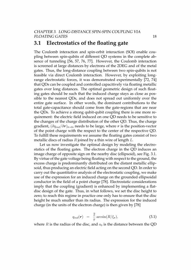
Let us now investigate the optimal design by modeling the electro-statics of the floating gates. The electron charge in the QD induces animage charge of opposite sign on the nearby disc (ellipsoid), see Fig. 3.1.By virtue of the gate voltage being floating with respect to the ground, theexcess charge is predominantly distributed on the distant metallic ellip-soid, thus producing an electric field acting on the second QD. In order tocarry out the quantitative analysis of the electrostatic coupling, we makeuse of the expression for an induced charge on the grounded ellipsoidalconductor in the field of a point charge [78]. Electrostatic considerationsimply that the coupling (gradient) is enhanced by implementing a flat-disc design of the gate. Thus, in what follows, we set the disc height tozero; to reach this regime in practice one only has to ensure that the discheight be much smaller than its radius. The expression for the inducedcharge (in the units of the electron charge) is then given by [78]
qind(r) =2
πarcsin(R/ξr), (3.1)
where R is the radius of the disc, and a0 is the distance between the QD
CHAPTER 3. LONG-DISTANCE SPIN-SPIN COUPLING VIAFLOATING GATES 19
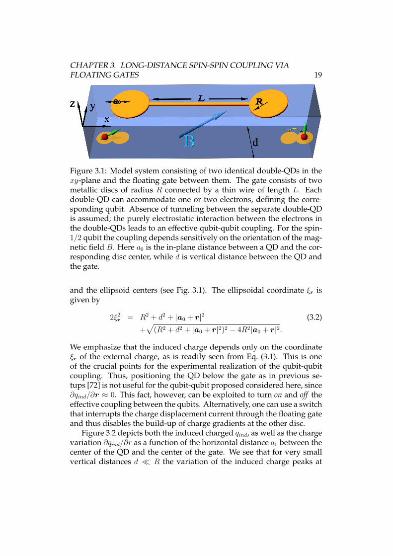
Figure 3.1: Model system consisting of two identical double-QDs in thexy-plane and the floating gate between them. The gate consists of twometallic discs of radius R connected by a thin wire of length L. Eachdouble-QD can accommodate one or two electrons, defining the corre-sponding qubit. Absence of tunneling between the separate double-QDis assumed; the purely electrostatic interaction between the electrons inthe double-QDs leads to an effective qubit-qubit coupling. For the spin-1/2 qubit the coupling depends sensitively on the orientation of the mag-netic field B. Here a0 is the in-plane distance between a QD and the cor-responding disc center, while d is vertical distance between the QD andthe gate.
and the ellipsoid centers (see Fig. 3.1). The ellipsoidal coordinate ξr isgiven by
2ξ2r = R2 + d2 + |a0 + r|2 (3.2)
+√
(R2 + d2 + |a0 + r|2)2 − 4R2|a0 + r|2.
We emphasize that the induced charge depends only on the coordinateξr of the external charge, as is readily seen from Eq. (3.1). This is oneof the crucial points for the experimental realization of the qubit-qubitcoupling. Thus, positioning the QD below the gate as in previous se-tups [72] is not useful for the qubit-qubit proposed considered here, since∂qind/∂r ≈ 0. This fact, however, can be exploited to turn on and off theeffective coupling between the qubits. Alternatively, one can use a switchthat interrupts the charge displacement current through the floating gateand thus disables the build-up of charge gradients at the other disc.
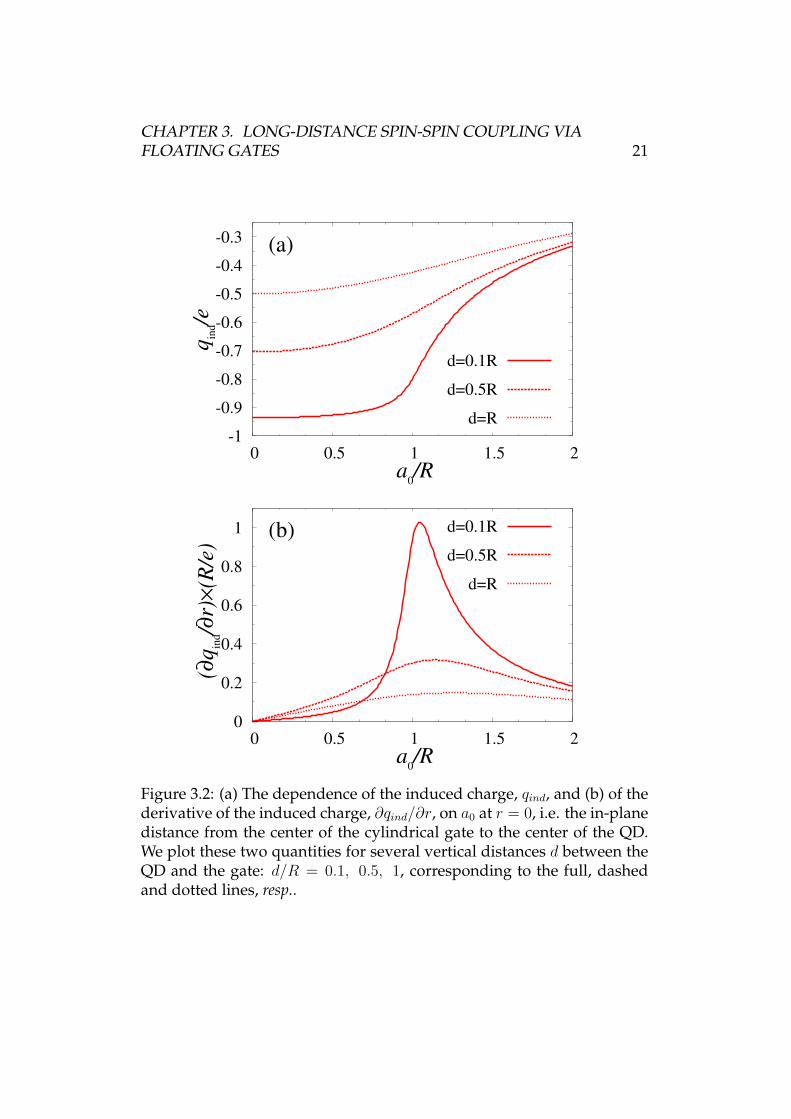
Figure 3.2 depicts both the induced charged qind, as well as the chargevariation ∂qind/∂r as a function of the horizontal distance a0 between thecenter of the QD and the center of the gate. We see that for very smallvertical distances d R the variation of the induced charge peaks at
CHAPTER 3. LONG-DISTANCE SPIN-SPIN COUPLING VIAFLOATING GATES 20
a0 ≈ R, reaching values as high as unity for d = 0.1R, and falls downquickly for a0 larger or smaller than R. As mentioned above, this couldbe used as an efficient switching mechanism. However, as d increasesto higher values, comparable to the disc radius R, the charge variation∂qind/∂r flattens out over a wide range of in-plane distances a0. Thismeans that for larger depths d & λ of the quantum dot the switchingmechanism turns out to be rather inefficient, even though the magnitudeof the coupling is only weakly reduced (∂qind/∂r ≈ 0.3 for r ≈ R andd = 0.5R). Nevertheless, the gates confining the QDs, as well as the2DEG itself could lead to screening of the interaction between the QDand the floating gate, allowing for an improved switching even in thiscase.
Finally, by utilizing the expression for the electrostatic potential ofa charged thin disc [78] we arrive at the expression for the electrostaticcoupling
V (r1, r2) =παqκ
e2qind(r1)qind(r2)
R, (3.3)
where κ is the dielectric constant, αq = CdCw+2Cd
is the charge distributionfactor of the gate, and Cd and Cw are the capacitances of the discs andwire, respectively (see Appendix 3.A). We mention that Eq. (3.3) is de-rived in the limit when the floating gate is immersed in the dielectric,and it provides a lower bound for V (r1, r2) in the realistic case when thefloating gate sits on top of the dielectric.
3.2 Qubit-qubit couplingNext, we consider the coupling between qubits. These can be for eithersingle- or double-QDs. The two-qubit system with the floating gate iswell described by the Hamiltonian
H = V +∑
i=1,2
H iqubit , (3.4)
where V describes the electrostatic coupling between the distant chargesin the qubits and is given by Eq. (3.3), and H i
qubit stands for either thesingle-QD or double-QD Hamiltonian [79, 57]
HQD =H0 +HZ +HSO, (3.5)HDQD =J S1 · S2 +H1
Z +H2Z . (3.6)
CHAPTER 3. LONG-DISTANCE SPIN-SPIN COUPLING VIAFLOATING GATES 21
-1
-0.9
-0.8
-0.7
-0.6
-0.5
-0.4
-0.3
0 0.5 1 1.5 2
a0/R
qin
d/e
(a)
d=0.1R
d=0.5R
d=R
0
0.2
0.4
0.6
0.8
1
0 0.5 1 1.5 2
a0/R
(∂q
ind/∂r)
×(R/e)
(b) d=0.1R
d=0.5R
d=R
Figure 3.2: (a) The dependence of the induced charge, qind, and (b) of thederivative of the induced charge, ∂qind/∂r, on a0 at r = 0, i.e. the in-planedistance from the center of the cylindrical gate to the center of the QD.We plot these two quantities for several vertical distances d between theQD and the gate: d/R = 0.1, 0.5, 1, corresponding to the full, dashedand dotted lines, resp..
CHAPTER 3. LONG-DISTANCE SPIN-SPIN COUPLING VIAFLOATING GATES 22
Here, H0 = p2i /2m
∗+m∗(ω2xx
2i +ω2
yy2i )/2 is the energy of an electron in dot
i described by a harmonic confinement potential, m∗ being the effectivemass and ~ωx,y the corresponding single-particle level spacings. For asingle-QD HZ = gµBB ·σ/2, stands for the Zeeman coupling, with σ thePauli matrix for the spin-1/2, and both Rashba and Dresselhaus spin-orbit interactions
HSO = α(pxσy − pyσx) + β(−pxσx + pyσy), (3.7)
where α (β) is the Rashba (Dresselhauss) spin-orbit interaction strength.The double-QD is described by an effective Heisenberg model [79], seeEq. (3.6), with Si being the spin in the double-QD. In what follows weassume the floating gate to be aligned along the x-axis, see Fig. 3.1.
Singly occupied double-QDs
We start by considering two single-QD qubits. Let us first give a physicaldescription of the qubit-qubit coupling. The purely electrostatic couplingbetween the QDs involves only the charge degrees of freedom of the elec-trons. Within each QD the spin degree of freedom is then coupled to theone of the charge via spin-orbit interaction. Hence, we expect the effec-tive spin-spin coupling to be second order in the SOI and first order inthe electrostatic interaction. In fact, one has also to assume Zeeman split-ting to be present on at least one QD in order to remove the van Vleckcancellation [80, 81]. Such a cancellation occurs due to linearity in themomentum of the SOI—for the SOI cubic in momentum (as for e.g. theself-assembled QDs), one obtains a spin-spin coupling even in the ab-sence of magnetic fields1.
Proceeding to a quantitative description, we assume the spin-orbitstrength to be small compared to the QD confinement energies ~ωx,y. Fol-lowing Refs. [81, 57], we apply a unitary Schrieffer-Wolff transformationto remove the first order SOI terms. The resulting Hamiltonian has de-coupled spin and orbital degrees of freedom (to second order in SOI),with the effective qubit-qubit coupling (see Appendix 3.A), with
HS−S = J12(σ1 · γ)(σ2 · γ) (3.8)
J12 =m∗ω2
x,12E2Z
2(ω2x − E2
Z)2, (3.9)
1We have checked that for the SOI given by σxp3x, the spin-spin coupling of the
form Jxx = −(5π3/2)m3α2α3qα
3c(∂qind/∂x)6ω6
x is obtained in the absence of the mag-netic field.
CHAPTER 3. LONG-DISTANCE SPIN-SPIN COUPLING VIAFLOATING GATES 23
where γ = (β cos 2γ,−α−β sin 2γ, 0); γ being the angle between the crys-tallographic axes of the 2DEG and the xyz-coordinate system defined inFig. 3.1. Here we assumed for simplicity that the magnetic field is per-pendicular to the 2DEG substrate, with EZ = gµBB the correspondingZeeman energy (assumed also the same for both dots). However, neitherthe orientation nor the possible difference in the Zeeman splittings in thetwo dots affect the functionality of our scheme (see Appendix 3.A for themost general coupling case). We mention that the spin-spin interactionin Eq. (3.8) is of Ising type, which, together with single qubit gates formsa set of universal gates (see below).
All information about the floating gate coupling is embodied in thequantity
ω2x,12 = παqαC
(∂qind∂x
)2
r=0
ω2x, (3.10)
where αC = e2/(κR~ωx), and x = x/λ (λ is the QD size).2 Remarkably,the coupling has only a weak dependence on the wire length L—throughthe capacitance ratio αq.
Next, we give estimates for the qubit-qubit coupling for GaAs andInAs QDs. Taking the spin-orbit strength for GaAs semiconductors λ '0.1λSO (λSO = ~/(m∗α)), and assuming EZ1 ' EZ2 ≡ EZ ' 0.5~ωx (B =2T and ~ωx ' 1meV ), we obtain Hs−s ' αqαC(∂qind/∂x)2
r=0 × 10−7eV .The electrostatic coupling strongly depends (like d−2) on the vertical dis-tance between the gate and the QDs. Typically, d ' λ, and one obtainsusing Eq. (3.1) maximal coupling Hs−s ' 10−11 − 10−10eV (for R = 1.6λ,L = 10µm, and Rw = 30nm leading to αq = 0.02; a0 = 1.9λ). Although,it is experimentally challenging to decrease d to a value of about 10nm,the gain would be a significantly stronger coupling 10−9 − 10−8eV (forR = 0.17λ and a0 = 0.2λ). Moreover, if a semiconductor with largerspin-orbit coupling is used—such as InAs (λ/λSO ' 1)—the coupling isincreased by two orders of magnitude compared to GaAs, reaching theµeV -regime. Quite remarkably, these values almost reach within the ex-change strengths range, Jexc ∼ 10−100µeV (10−100ps), occurring in typ-ical GaAs double quantum dots [1, 82]. Actually, for realistic devices—aspresented in the Sec. 3.5—the coupling is almost two orders of magni-tude larger then the estimates presented herein, and thus operation timesare well below the decoherence times for QD. This discrepancy is not
2It is interesting to note that the derived coupling, Eq. (3.8), is independent of theorbital states of the QDs, and thus, insensitive to the fluctuations of a QD electron chargedistribution.
CHAPTER 3. LONG-DISTANCE SPIN-SPIN COUPLING VIAFLOATING GATES 24
very surprising and it is mainly due to our conservative treatment of thedielectric, and the sensitivity of the electric field gradient to geometry ofthe surrounding gates.
Hybrid spin-qubits
A number of different spin-based qubits in quantum dots have been in-vestigated over the years [83], each with its own advantages and chal-lenges. The most prominent ones are spin-1/2 and singlet-triplet spinqubits. Here, we show that these qubits can be cross-coupled to eachother and thus hybrid spin-qubits can be formed which open up the pos-sibility to take advantage of the ’best of both worlds’.
We model the hybrid system by a single- and a double-QD qubit, de-scribed by Eqs. (3.5) and (3.6), respectively. The single-QD and the float-ing gate act as an electric field, leading to the change in the splitting be-tween the logical states of the double-QD spin-qubit, J → J + xeδJ [79],with xe = xeλ being the x-coordinate of the electron in the single-QD and
δJ =3
sinh(2l)
ω2x,12
lω2D
ε . (3.11)
Here, ωD is the confinement energy in the DQD, l is the distance betweenthe double-QD minima measured in units of a QD size λ. The previousformula is valid for the regime ε & ωD.
In order to decouple spin and orbital degrees of freedom, we againemploy a Schrieffer-Wolff transformation and obtain the hybrid couplingin lowest order (see Appendix 3.B)
Hhybrid =3µg δJ(γ ×B) · σ
4(ω2x − E2
Z1)λτz . (3.12)
Here, τz is a Pauli matrix acting in the pseudo-spin space spanned bythe logical states of the singlet-triplet qubit. It should be noted that thesign of this coupling can be manipulated by changing the sign of the de-
tuning voltage ε. As an estimate, we can write Hhybrid '(ωx,12
ωx
)2EZωD
aBλSO
ε.Assuming the parameters cited in the previous section for the GaAs-QDswe obtain the estimate HS−s ' 10−10 − 10−9eV . Reducing the distance dor using InAs-QDs we can gain one order of magnitude more in the cou-pling.
CHAPTER 3. LONG-DISTANCE SPIN-SPIN COUPLING VIAFLOATING GATES 25
Doubly occupied double-QDs
To complete our discussion about the qubit-qubit couplings, we now con-sider two double-QDs coupled via the floating gate. As already noted,owing to the different charge distributions of the logical states in thedouble-QD, the SOI term is not needed for the qubit-qubit coupling [76].Certainly, the SOI exists in double-QDs but its effect on the ST splittingcan be neglected [84]. Below only a rough estimate of the coupling isprovided, while the detailed analysis can be found in Ref. [76].
We assume both double-QDs to be strongly detuned, thereupon thesinglet logic state is almost entirely localized on the lower potential wellof the double-QD. The electrostatic energy difference between the singlet-singlet and triplet-triplet system configurations gives the rough estimateof the qubit-qubit coupling, HS−S ' V (R,R)−V (R+ l, R+ l). Taking thedistance between the double-QD minima l ' R and the same GaAs pa-rameters as before, we finally obtain the estimate HS−S ' 10−5− 10−6eV .As can be seen from Fig. 3.2, reducing d to 10nm increases the couplingfive times.
3.3 Scalable ArchitectureOne central issue in quantum computing is scalability, meaning that thebasic operations such as initialization, readout, single- and two-qubitgates should not depend on the total number of qubits. In particular,this enables the implementation of fault-tolerant quantum error correc-tion [69], such as surface codes where error thresholds are as large as1.1% [70, 20].
To this end, the architecture of the qubit system becomes of centralimportance [85]. Making use of the electrostatic long-distance gates pre-sented above, we now discuss two illustrative examples for such scalablearchitectures.
Design with floating metal gates
In the first design we propose here, the metallic gates above the 2DEGare utilized for qubit-qubit coupling, while the switching of the couplingis achieved by moving the QDs (see Fig. 3.3). Only the coupling be-tween adjacent QDs is possible in this design. Without this constraint,the induced charge due to nearby QDs would be spread over the wholesystem, resulting in an insufficient qubit-qubit coupling.
CHAPTER 3. LONG-DISTANCE SPIN-SPIN COUPLING VIAFLOATING GATES 26
The actual virtue of the setup is its experimental feasibility, as sug-gested by recent experiments [72, 74]. However, as explained in Sec. II,a minor but crucial difference here is that the qubit-qubit coupling de-pends not on the charge itself but rather on its gradient, in contrast toearlier designs [72, 74]. This requires the dots to be positioned off thedisc-center.
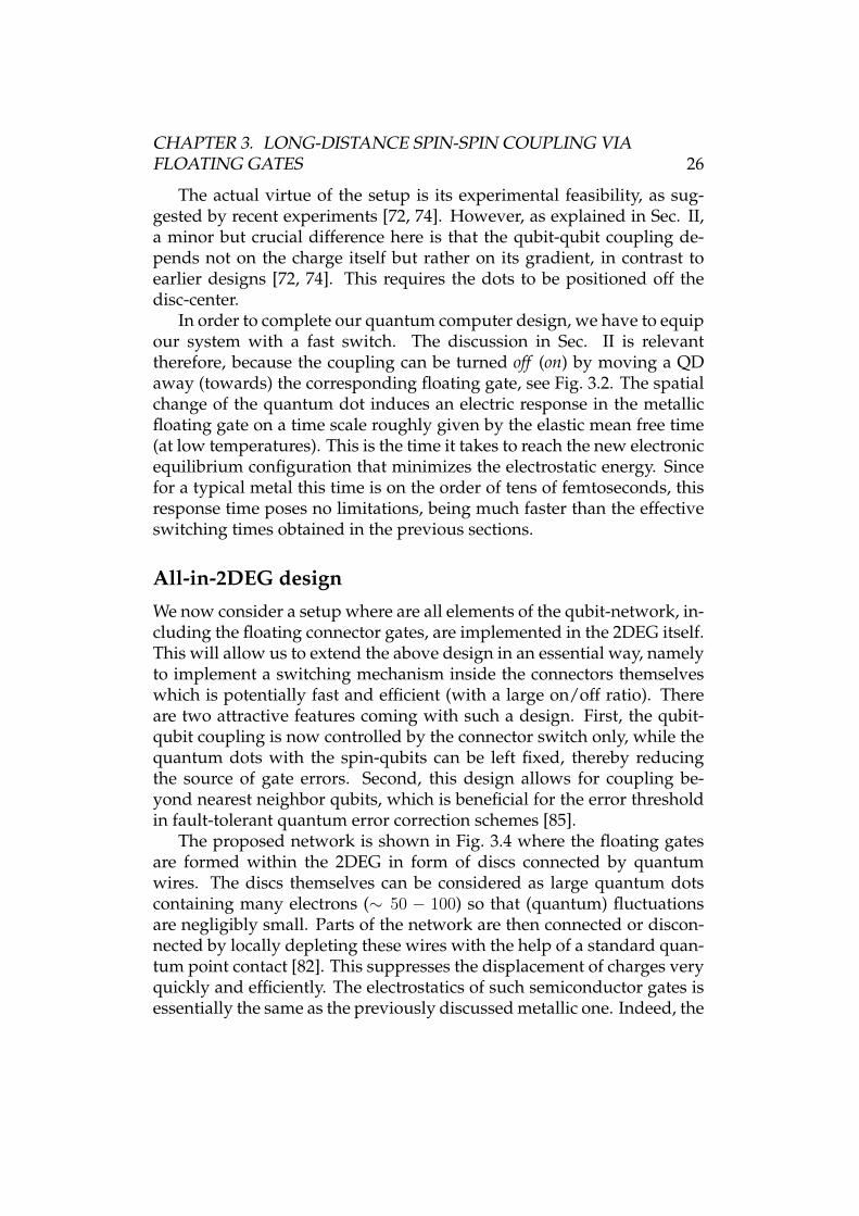
In order to complete our quantum computer design, we have to equipour system with a fast switch. The discussion in Sec. II is relevanttherefore, because the coupling can be turned off (on) by moving a QDaway (towards) the corresponding floating gate, see Fig. 3.2. The spatialchange of the quantum dot induces an electric response in the metallicfloating gate on a time scale roughly given by the elastic mean free time(at low temperatures). This is the time it takes to reach the new electronicequilibrium configuration that minimizes the electrostatic energy. Sincefor a typical metal this time is on the order of tens of femtoseconds, thisresponse time poses no limitations, being much faster than the effectiveswitching times obtained in the previous sections.
All-in-2DEG design
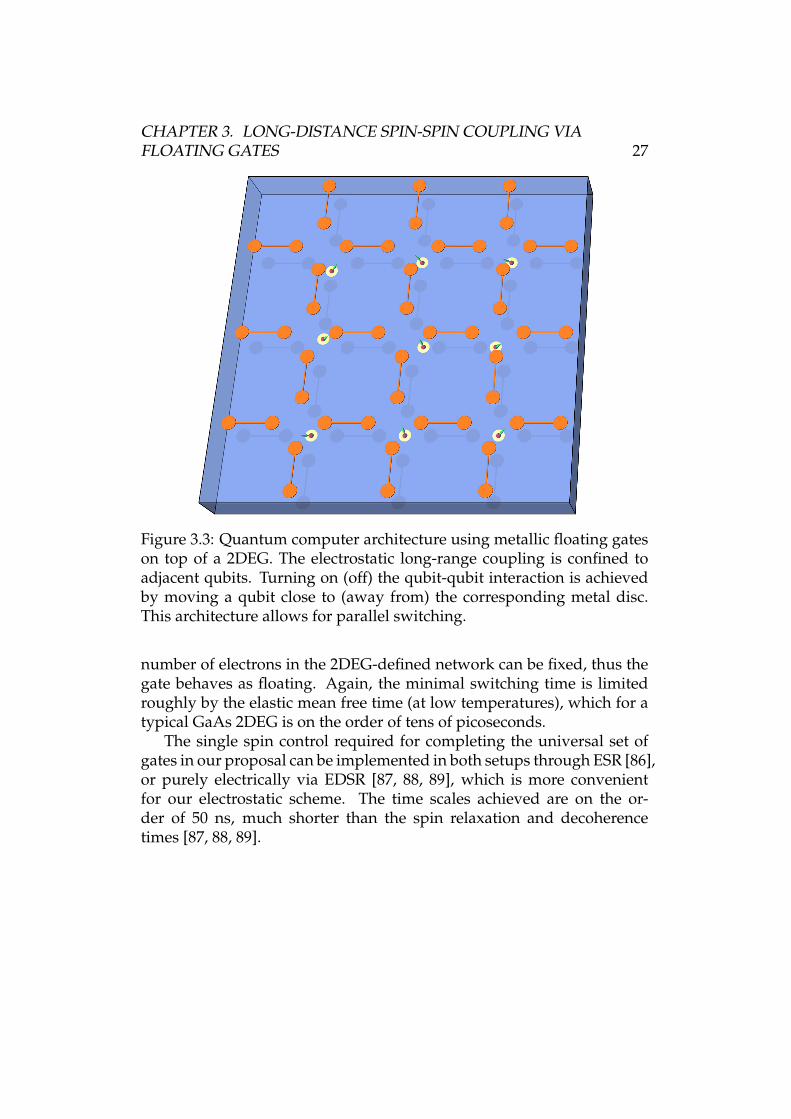
We now consider a setup where are all elements of the qubit-network, in-cluding the floating connector gates, are implemented in the 2DEG itself.This will allow us to extend the above design in an essential way, namelyto implement a switching mechanism inside the connectors themselveswhich is potentially fast and efficient (with a large on/off ratio). Thereare two attractive features coming with such a design. First, the qubit-qubit coupling is now controlled by the connector switch only, while thequantum dots with the spin-qubits can be left fixed, thereby reducingthe source of gate errors. Second, this design allows for coupling be-yond nearest neighbor qubits, which is beneficial for the error thresholdin fault-tolerant quantum error correction schemes [85].
The proposed network is shown in Fig. 3.4 where the floating gatesare formed within the 2DEG in form of discs connected by quantumwires. The discs themselves can be considered as large quantum dotscontaining many electrons (∼ 50 − 100) so that (quantum) fluctuationsare negligibly small. Parts of the network are then connected or discon-nected by locally depleting these wires with the help of a standard quan-tum point contact [82]. This suppresses the displacement of charges veryquickly and efficiently. The electrostatics of such semiconductor gates isessentially the same as the previously discussed metallic one. Indeed, the
CHAPTER 3. LONG-DISTANCE SPIN-SPIN COUPLING VIAFLOATING GATES 27
Figure 3.3: Quantum computer architecture using metallic floating gateson top of a 2DEG. The electrostatic long-range coupling is confined toadjacent qubits. Turning on (off) the qubit-qubit interaction is achievedby moving a qubit close to (away from) the corresponding metal disc.This architecture allows for parallel switching.
number of electrons in the 2DEG-defined network can be fixed, thus thegate behaves as floating. Again, the minimal switching time is limitedroughly by the elastic mean free time (at low temperatures), which for atypical GaAs 2DEG is on the order of tens of picoseconds.
The single spin control required for completing the universal set ofgates in our proposal can be implemented in both setups through ESR [86],or purely electrically via EDSR [87, 88, 89], which is more convenientfor our electrostatic scheme. The time scales achieved are on the or-der of 50 ns, much shorter than the spin relaxation and decoherencetimes [87, 88, 89].
CHAPTER 3. LONG-DISTANCE SPIN-SPIN COUPLING VIAFLOATING GATES 28
Figure 3.4: All-in-2DEG design: the qubits and the floating connectorgates are all implemented within the same 2DEG. The spin-qubits (greenarrow) are confined to double quantum dots (small yellow double circles)and are at a fixed position with maximum coupling strength to the float-ing gate (big disc) (see Fig. 3.2). The network consists of quantum chan-nels (lines) that enable the electrostatic coupling between discs (large cir-cles) so that two individual qubits at or beyond nearest neighbor sites canbe selectively coupled to each other. In the figure shown are four pairsof particular discs that are connected by quantum channels (full lines),while the remaining discs (red) are disconnected from the network (in-terrupted red lines) The discs can be considered as large quantum dotscontaining many electrons. The quantum wires can be efficiently discon-nected (interrupted lines) by depleting the single-channel with a metallictop gate (not shown). This architecture allows for parallel switching.
CHAPTER 3. LONG-DISTANCE SPIN-SPIN COUPLING VIAFLOATING GATES 29
Design based on 1D nanowire quantum dots
The floating gate architecture efficiency is strongly dependent on thestrength of the SOI experienced by the electrons in the QDs, which haveto be large enough to overcome the spin decoherence rates. InAs nano-wires are such strong SOI materials, with strengths larger by an orderof magnitude than in GaAs 2DEG [90]. Moreover, the electron spins inQDs created in these nanowires show long coherence times [89] and canbe controlled (electrically) on times scales comparable to those found forthe electron spin manipulation in GaAs gate defined QDs [89].
In Fig. 3.5 we show a sketch of an architecture based on nanowirescontaining single or double QDs. Typical examples for such wires areInAs [90, 89] or Ge/Si [75, 91] nanowires, Carbon nanotubes [74, 92, 93,94], etc. The default position of a QD is chosen so that the coupling toany of the surrounding gates is minimal. Neighboring QDs in the samenanowire are coupled by a vertical metal gate, while QDs in adjacentnanowires by a horizontal metal gate. The electron in a given QD canbe selectively coupled to only two of the surrounding gates by movingit (via the gates that confine the electrons) in regions where the electricfield gradient for the induced charge is maximum on these two ’active’gates, while negligible for the others two ’passive’ gates. The other QDpartner in the coupling is moved towards one of the ’active’ gates thusresulting in a qubit-qubit coupling. Note that there are in total three ’ac-tive’ gates, but only one of them is shared by both QDs, thus allowingselective coupling of any nearest neighbor pair in the network.
The spin coupling mechanism as well as the 2D geometry are similarto the previous 2DEG GaAs QDs designs, showing the great flexibility ofthe floating gate architecture. As before, the spin-qubits can be manipu-lated purely electrically, via the same gates that confine the QDs [89]. Wemention also that the gate geometry (dog-bone like) shown in Fig. 3.5 isnot optimized to achieve the best switching ratio, more asymmetric gategeometries possibly leading to better results.
Spin qubit decoherence and relaxation
Decoherence and relaxation are ones of the main obstacles to overcome inbuilding a quantum computer. The main source of qubit decay in typicalGaAs quantum dots comes from nuclear spins and phonons (via spinorbit interaction), and has been studied in great detail theoretically andexperimentally, see e.g. Ref. [95]. The longest relaxation and decoherence
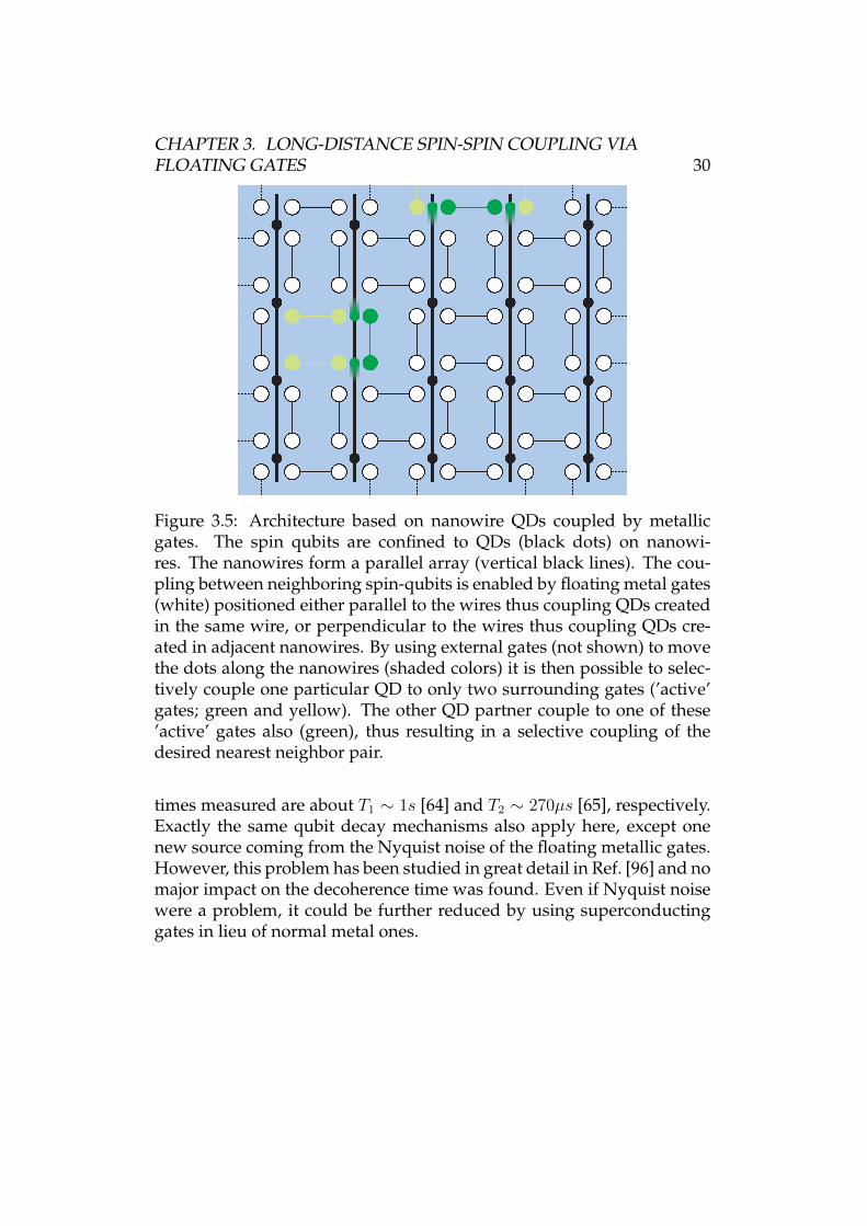
CHAPTER 3. LONG-DISTANCE SPIN-SPIN COUPLING VIAFLOATING GATES 30
Figure 3.5: Architecture based on nanowire QDs coupled by metallicgates. The spin qubits are confined to QDs (black dots) on nanowi-res. The nanowires form a parallel array (vertical black lines). The cou-pling between neighboring spin-qubits is enabled by floating metal gates(white) positioned either parallel to the wires thus coupling QDs createdin the same wire, or perpendicular to the wires thus coupling QDs cre-ated in adjacent nanowires. By using external gates (not shown) to movethe dots along the nanowires (shaded colors) it is then possible to selec-tively couple one particular QD to only two surrounding gates (’active’gates; green and yellow). The other QD partner couple to one of these’active’ gates also (green), thus resulting in a selective coupling of thedesired nearest neighbor pair.
times measured are about T1 ∼ 1s [64] and T2 ∼ 270µs [65], respectively.Exactly the same qubit decay mechanisms also apply here, except onenew source coming from the Nyquist noise of the floating metallic gates.However, this problem has been studied in great detail in Ref. [96] and nomajor impact on the decoherence time was found. Even if Nyquist noisewere a problem, it could be further reduced by using superconductinggates in lieu of normal metal ones.
CHAPTER 3. LONG-DISTANCE SPIN-SPIN COUPLING VIAFLOATING GATES 31
3.4 Implementation of two-qubit gatesSince the Hamiltonian of Eq. (3.8) is entangling, it can be used to imple-ment two-qubit gates. Here we consider the CNOT gate, widely usedin schemes for quantum computation [70, 20]. The Hamiltonian for twosingle-QD qubits interacting via the floating gate is the sum of HS−S andthe Zeeman terms. The strength of the latter in comparison to the for-mer allows us to approximate the Hamiltonian by H ′ = J12|γ|2(σ1
xσ2x +
σ1yσ
2y)/2 + Ez(σ
1z + σ2
z)/2, for which qubit-qubit interaction and Zeemanterms commute. The CNOT gate, C, may then be realized with the fol-lowing sequences,
C =√σ1z
√σ2xH1ei(σ
1z+σ2
z)Ezte−iH′t
σ1x e
i(σ1z+σ2
z)Ezte−iH′t σ1
xH1, (3.13)
C =√σ1z
√σ2xH1 σ2
x e−iH′t/2 σ1
xσ2x e−iH′t/2
σ2x e−iH′t/2 σ1
xσ2x e−iH′t/2H1 (3.14)
where t = π/(4J12|γx|2) and H denotes the single qubit Hadamard rota-tion. These sequences require two and four applications of the floatinggate, respectively. More details on their construction can be found in Ap-pendix 3.C. The time t is the bottleneck process in the sequence, and sothe time taken to implement the gates will be on the order of this value.For a realistic value of J12|γ|2 = 10µeV , this gives a time of around ananosecond.
Since H ′ is only an approximation of the total Hamiltonian, these se-quences will yield approximate CNOTs. Their success can be character-ized by the fidelity which depends only on the relative strengths of theparameters. For a realistic device we can expect the Zeeman terms tobe an order of magnitude stronger than the qubit-qubit coupling. Theabove sequences then yield fidelities of 99.33% and 99.91% respectively.For realistic parameters, with the Zeeman terms an order of magnitudestronger than the qubit-qubit coupling, the above sequences yield fideli-ties of 99.33% and 99.91% respectively. For two orders of magnitude be-tween the Zeeman terms and qubit-qubit coupling the approximationimproves, giving fidelities of 99.993% and 99.998%, respectively. Theseare all well above the fidelity of 99.17%, corresponding to the thresholdfor noisy CNOTs in the surface code [20]. Hence, despite the differencein error models, we can be confident that the gates of our scheme areequally useful for quantum computation.
CHAPTER 3. LONG-DISTANCE SPIN-SPIN COUPLING VIAFLOATING GATES 32
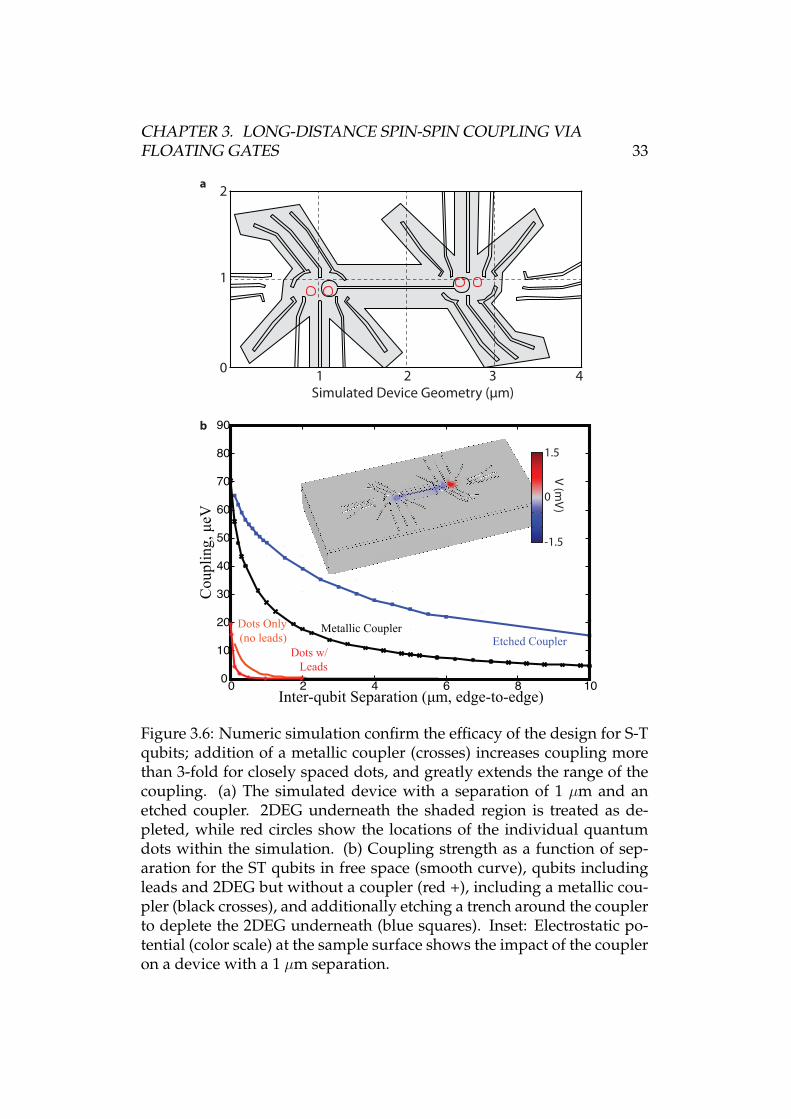
3.5 Numeric Modeling of Realistic DevicesIn the previous sections, a number of practical concerns related to theconstruction of working devices were neglected; most notably, the exis-tence of the metallic gates used to define the quantum dots themselvesand the presence of undepleted 2DEG outside of the quantum dots. Thesehave finite capacitances to the coupler, shunting away some of the chargethat would otherwise contribute to the inter-qubit interaction. To con-firm that substantial couplings can still be attained at large distanceswith these limitations, we have performed numeric simulations of de-vices with realistic geometries similar to currently in-use ST spin qubits.A typical simulated geometry is included in Fig. 3.6. The gate and het-erostructure design is identical to a functional device currently beingcharacterized, and the boundaries of the 2DEG and placement of the elec-trons within the dot are estimates guided by experimentally measuredparameters. Each quantum dot is modeled as a fixed charge metallic disc50 nm in diameter within the 2DEG. While unsophisticated, this sufficesto estimate the practicality of this scheme.
We define the coupling between two ST qubits as the change in de-tuning in one ST qubit induced by the transfer of a full electron from onedot to the other dot in a second ST qubit. For our reference ST qubit de-sign with the two qubits physically adjacent to each other and no coupler(680 nm center-to-center), we calculate a coupling of 20µeV. As the qubitsare separated, the coupling vanishes rapidly as the 2DEG in between thequbits screens the electric field; it is reduced by an order of magnitude ifthe dots are separated by an additional 250 nm. This rapid falloff makesthe gate density needed for large scale integration of these qubits prob-lematic.
Addition of a floating metallic coupler of the type described hereinincreases the coupling at zero separation to 70µeV and allows the qubitsto be separated by more than 6µm before the coupling drops to the levelseen for two directly adjacent qubits. We can further improve upon thiscoupling by etching the device in the vicinity of the coupler, reducingthe shunt capacitance of the coupler to the grounded 2DEG between thedevices.
For the case of single spins this metallic coupler is modified to placethe quantum dots at the edges of the coupler rather than under the discs.We define the coupling in this case as the electric field in V/m inducedon one qubit in response to 1nm of motion of the electron on the otherqubit. We continue to find substantial couplings even at large separa-
CHAPTER 3. LONG-DISTANCE SPIN-SPIN COUPLING VIAFLOATING GATES 33
0 2 41 3
1
2
Simulated Device Geometry (μm)
Etched CouplerMetallic Coupler
0
10
20
30
40
50
60
70
80
90
0 2 4 6 8 10
Cou
plin
g, μ
eV
Inter-qubit Separation (μm, edge-to-edge)
Dots Only(no leads)
Dots w/Leads
b
a
1.5
0
-1.5
V (mV
)
Figure 3.6: Numeric simulation confirm the efficacy of the design for S-Tqubits; addition of a metallic coupler (crosses) increases coupling morethan 3-fold for closely spaced dots, and greatly extends the range of thecoupling. (a) The simulated device with a separation of 1 µm and anetched coupler. 2DEG underneath the shaded region is treated as de-pleted, while red circles show the locations of the individual quantumdots within the simulation. (b) Coupling strength as a function of sep-aration for the ST qubits in free space (smooth curve), qubits includingleads and 2DEG but without a coupler (red +), including a metallic cou-pler (black crosses), and additionally etching a trench around the couplerto deplete the 2DEG underneath (blue squares). Inset: Electrostatic po-tential (color scale) at the sample surface shows the impact of the coupleron a device with a 1 µm separation.
CHAPTER 3. LONG-DISTANCE SPIN-SPIN COUPLING VIAFLOATING GATES 34
Top Gate1
0
0.5
0 0.5 1.51
Coupler
aa
b
1.5
0
V (mV
)
E (V
/m/n
m)
10
8
6
4
2
0Inter-qubit Separation (μm, edge-to-edge)1 2 3 4 5
Lead Coupler (on)
Metallic Coupler (modified)Lead Coupler (off)
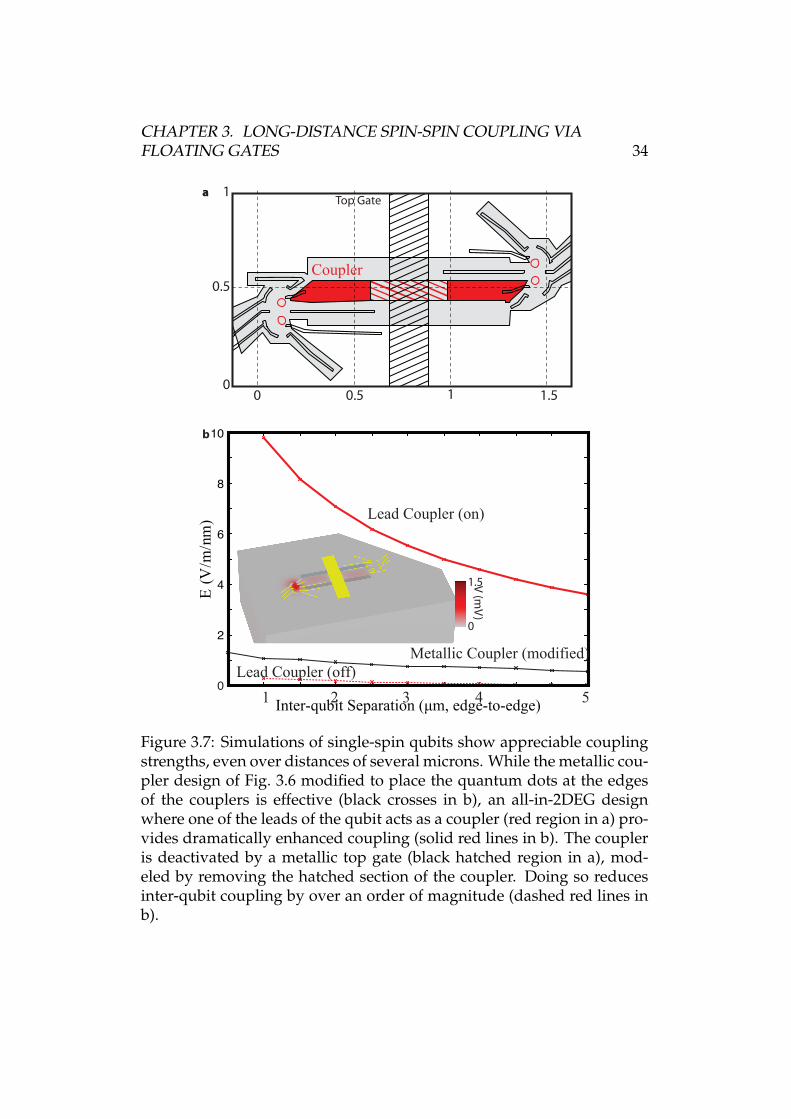
Figure 3.7: Simulations of single-spin qubits show appreciable couplingstrengths, even over distances of several microns. While the metallic cou-pler design of Fig. 3.6 modified to place the quantum dots at the edgesof the couplers is effective (black crosses in b), an all-in-2DEG designwhere one of the leads of the qubit acts as a coupler (red region in a) pro-vides dramatically enhanced coupling (solid red lines in b). The coupleris deactivated by a metallic top gate (black hatched region in a), mod-eled by removing the hatched section of the coupler. Doing so reducesinter-qubit coupling by over an order of magnitude (dashed red lines inb).
CHAPTER 3. LONG-DISTANCE SPIN-SPIN COUPLING VIAFLOATING GATES 35
tions (Fig. 3.7). However, in this case we find we can further improvecouplings by moving to the all-in-2DEG design where one of the leadsof the quantum dot is used as the coupler (Fig. 3.7 a). Using the lead inthis fashion should be harmless; no current is driven into the lead duringqubit manipulations. The lead (colored region) is modeled as a metallicstrip at the level of the 2DEG. Due to the close proximity of the lead tothe qubit as well as the sharp electric field gradients near the point ofthe lead, we find strongly enhanced coupling for this lead coupler overthe floating metallic coupler for single spin qubits. By depleting part ofthe lead coupler using a metallic top gate (yellow region), it is possibleto selectively turn this coupling on and off. The reduction in couplingin the off state is more than an order of magnitude, and can be furtherimproved by increasing the size of the depleted region.
3.6 ConclusionsWe proposed and analyzed an experimentally feasible setup for imple-menting quantum gates in an array of spin qubits localized in gate-definedquantum dots based on the interplay of the Coulomb repulsion betweenthe electrons, SOI and externally applied magnetic fields. As opposed tothe current schemes based on direct exchange, here there is no need forelectron tunneling between the quantum dots, thus bringing the schemewithin experimental reach based only on current spin-qubit technology.
We showed, both analytically and numerically, that using either metal-lic floating gates in the shape of a dog-bone, or the 2DEG itself acting asa metallic gate, long-range spin-spin coupling is achieved, with couplingstrengths exceeding the spin decay rates. Moreover, the coupling can beselectively switched on and off between any pairs of qubits by only lo-cal qubit manipulation, allowing entangling quantum gates such as theCNOT to be performed accurately and efficiently. The two-dimensionalarchitecture based on the design provides a platform for implementingthe powerful surface code.
The electrostatic scheme proposed here is a step forward towardsan efficient implementation of gates also between hybrid qubits, like STqubit, hole-spin qubits, or even superconducting qubits. This opens upnew avenues for a future working hybrid quantum computer based noton one, but several types of qubits.
CHAPTER 3. LONG-DISTANCE SPIN-SPIN COUPLING VIAFLOATING GATES 36
3.7 AcknolwedgmentWe thank C. Marcus and D. Stepanenko for helpful discussions and ac-knowledge support from the Swiss NF, NCCRs Nanoscience and QSIT,and DARPA. This research was partially supported by IARPA/MQCOprogram and the U. S. Army Research Office under Contract No. W911NF-11-1-0068. MT acknowledges financial support from NSF under GrantNo. DMR-0840965.
3.A SPIN-SPIN COUPLING - singly occupieddouble-dots
In this section we derive explicitly the effective spin-spin coupling. Thespin-orbit interaction (SOI) HamiltonianHSO is assumed to be small com-pared to both the orbital Hamiltonian H0 + V and the Zeeman couplingHZ , so that we can treat it in perturbation theory. The method of choicefor the perturbation theory is based on the Schrieffer-Wolff (SW) transfor-mation, following Refs. [81, 57]. This method is very suitable for derivingeffective Hamiltonians, as we aim at herein. We first perform a unitarytransformation on the full Hamiltonian, i.e. H → eSHe−S ≡ HSW , with San anti-unitary operator so that we get
HSW = Hd +HSO + [S,Hd +HSO] (3.15)
+1
2[S, [S,Hd +HSO]] + . . . ,
where Hd = H0 + V + HZ . We look for the transformation S so thatthis diagonalizes the full Hamiltonian H in the basis of Hd. In leadingorder in HSO, we choose S so that [S,H0 + V + HZ ] = −(1 − P)HSO,with the projector operator P satisfying PA =
∑En=Em
Anm|m〉〈n|, ∀A,i.e. it projects onto the diagonal part of the Hamiltonian Hd. Keepingthe lowest order terms in α and β in the SW transformation, we are leftwith the effective interaction Hamiltonian HSW that contains the desiredspin-spin coupling in the basis of Hd
HSW = Hd −1
2P [S,HSO], (3.16)
where S = (1 − P)L−1d HSO, with Ld being the Liouvillian superoperator
(LdA = [Hd, A],∀A).
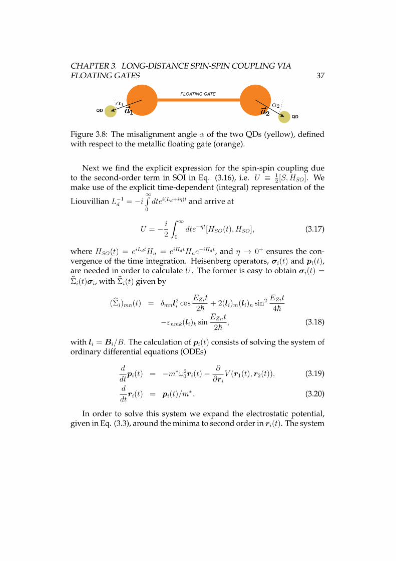
CHAPTER 3. LONG-DISTANCE SPIN-SPIN COUPLING VIAFLOATING GATES 37
FLOATING GATE
QD
QD
Figure 3.8: The misalignment angle α of the two QDs (yellow), definedwith respect to the metallic floating gate (orange).
Next we find the explicit expression for the spin-spin coupling dueto the second-order term in SOI in Eq. (3.16), i.e. U ≡ 1
2[S,HSO]. We
make use of the explicit time-dependent (integral) representation of the
Liouvillian L−1d = −i
∞∫0
dtei(Ld+iη)t and arrive at
U = − i2
∫ ∞
0
dte−ηt[HSO(t), HSO], (3.17)
where HSO(t) = eiLdtHn = eiHdtHne−iHdt, and η → 0+ ensures the con-
vergence of the time integration. Heisenberg operators, σi(t) and pi(t),are needed in order to calculate U . The former is easy to obtain σi(t) =
Σi(t)σi, with Σi(t) given by
(Σi)mn(t) = δmnl2i cos
EZit
2~+ 2(li)m(li)n sin2 EZit
4~
−εnmk(li)k sinEZnt
2~, (3.18)
with li = Bi/B. The calculation of pi(t) consists of solving the system ofordinary differential equations (ODEs)
d
dtpi(t) = −m∗ω2
0ri(t)−∂
∂riV (r1(t), r2(t)), (3.19)
d
dtri(t) = pi(t)/m
∗. (3.20)
In order to solve this system we expand the electrostatic potential,given in Eq. (3.3), around the minima to second order in ri(t). The system
CHAPTER 3. LONG-DISTANCE SPIN-SPIN COUPLING VIAFLOATING GATES 38
of ODEs now reads
d2
dt2
(p1(t)p2(t)
)= −Ω
(p1(t)p2(t)
), (3.21)
Ω =
ω2x 0
0 ω2y
Ω12
Ω†12
ω2x 0
0 ω2y
. (3.22)
In this approximation only termsO(r2i ) are retained—this is valid for low
lying levels. We ignore the renormalization of the frequencies (ωx andωy) because it gives higher order (in the Coulomb energy) contributionto the effective spin-spin coupling. The coupling between the QDs (Ω12)is given by
(Ω12)ij =παqαC
(∂qind∂ri
)(∂qind∂rj
)ωiωj, (3.23)
(∂qind/∂ri)r=0 =2R√ξ2
0 −R2aiπξ2
0(2ξ20 − a2
0 −R2 − d2), (3.24)
where αq = Cd/(Cd + Cw), αC = e2/(κR~ωx), and ri = ri/λi (λi is the QDsize along the i-th direction). ai are the vectors that define the position ofthe QDs with respect to the nearby disc center, see Fig. 3.8. Note that theexpressions for the disc (Cd) and wire (Cw) capacitances, resp. are givenby
Cd = 2R/π, (3.25)
Cw =L
2 ln (L/Rw), (3.26)
where R is the radius of the disk, Rw is the radius of the wire and L is thelength of the wire.
In order to obtain the solution of Eq. (3.22), we note that even a slightellipticity (|ω2
x − ω2y| max[(Ω12)2
xy, (Ω12)2yx]) of the QDs causes the mo-
tion in the x- and y-direction to be decoupled. Having in mind that(Ω12)2
yx,xy/ω2x,y ∼ 10−3 − 10−4, we conclude that such a ellipticity is un-
avoidable in realistic experimental devices. Thus, we put off-diagonalelements of the Ω12 matrix to zero and obtain the solutions
pi1,2(t) = ±pia cos(ωi+t) + pis cos(ωi−t)∓ (3.27)
∓m∗riaωi+ sin(ωi+t)−m∗risωi− sin(ωi−t),
CHAPTER 3. LONG-DISTANCE SPIN-SPIN COUPLING VIAFLOATING GATES 39
herein the notation rs,a = (r1 ± r2)/2, ps,a = (p1 ± p2)/2 and ω± =(√ω2x ± (Ω12)2
xx,√ω2y ± (Ω12)2
yy
)has been introduced. In the previous
formula, a superscript of a vector denotes the corresponding componentof the vector.
Next, the obtained solutions are inserted into Eq. (3.17). Finally, afterperforming the integration over time one obtains the effective spin-spincoupling for arbitrary orientation of the magnetic field
Hs−s =∑
i=x,y
m∗ω2i,12E
2Z1(l1 × (l1 × γi)) · σ1(σ2 · γi)
4(ω2x − E2
Z1)(ω2x − E2
Z2)
+1↔ 2, (3.28)
where γx = (β cos 2γ,−α − β cos 2γ, 0), γy = (α − β sin 2γ,−β cos 2γ, 0),and li = Bi/B. For simplicity of notation, γx is referred to as γ in themain text.
Few remarks should be made herein for the result in Eq. (3.28). Firstof all, from Eq. (3.24) we see that Ω12 ∝ a1⊗a2, accordingly, the two termsin the sum of Eq. (3.28) are proportional to cosα1 cosα2 and sinα1 sinα2—the angles αi are being depicted in Fig. 3.8. When only Rashba SOI ispresent in the material, the coefficients in front of the two terms are equaland the coupling is proportional to a1 ·a2. This gives yet another efficientswitching mechanism thereby, when the QDs are rotated in such a waythat the two vectors are orthogonal (a1 · a2 = 0).3
3.B SPIN-SPIN COUPLING - the hybridsystem
We start from the Hamiltonian of the system and then apply the Schrieffer-Wolff transformation to remove the first order SOI term (present only inthe single QD). The electrostatic potential V is again expanded aroundthe minimum
V (re, r1, r2) = V (re, r1) + V (re, r2) (3.29)
≈ m∗∑
i=e,1,2
(δω2xx
2i + δω2
yy2i )
+m∗ω2x,12xe(x1 + x2),
3coupling is zero up to the small terms O(
(Ω12)2xy,yx/|ω2x − ω2
y|)
CHAPTER 3. LONG-DISTANCE SPIN-SPIN COUPLING VIAFLOATING GATES 40
where re, r1, and r2 are the coordinates with respect to the local minimafor the electron in the single QD, and the two electrons in the DQD, re-spectively. The terms under the sum only renormalize the frequencies,we do not take them into account, they give only higher order (in theCoulomb energy) contributions to the final results. The last term acts asan electric field on the DQD; as has been shown in the Ref. [79], this leadsto a change in the exchange splitting between the singlet and triplet statesin the DQD.
H = H0 +HZ +HSO + δJxeS1 · S2, (3.30)
where δJ is given by
δJ =3
sinh(2l2)
ω2x,12
lω2D
ε. (3.31)
ωD is the confinement energy in the DQD, l is the distance between theDQD minima measured in units of a QD size. We assumed that the de-tuning ε is applied to the DQD in order to get the coupling linear in elec-trostatic coupling.
The Schrieffer-Wolff transformation S is given by the following ex-pression S = (L0 + LZ + LH)−1HSO. Similarly to the previous section, inorder to find the inverse Liouvillian we have to solve the system of ODEs
d
dtpe,x(t) = −m∗ω2
xxe(t)−m∗JS1 · S2, (3.32)
d
dtpe,y(t) = −m∗ω2
yye(t), (3.33)
d
dtre(t) = pe(t)/m
∗. (3.34)
The solution is easily obtained
pxe(t) = pxe cos(ωxt) (3.35)
−m∗(xeωx +
J
m∗ωxλS1 · S2
)sin(ωxt),
pye(t) = pye cos(ωyt)−m∗yeωy sin(ωyt). (3.36)
CHAPTER 3. LONG-DISTANCE SPIN-SPIN COUPLING VIAFLOATING GATES 41
After integration over time, the S transformation is obtained
−iS =∑
i=x,y
m∗re,i (µ2g2(B · γi)(B · σ)− 4ω2
i γi · σ)
8(ω2i − E2
Z)
+µg(B × σ) · γipe,i
4(ω2i − E2
Z)(3.37)
+µ2g2(B · γx)(B · σ)− 4ω2
xγx · σ8ω2
x(ω2x − E2
Z)λδJS1 · S2,
The coupling is contained in the [S,HZ + δJxeS1 · S2] term
HS−s =3µg δJ(γx ×B) · σ
4(ω2x − E2
Z)λ(S1 · S2). (3.38)
By rewriting the last equation in the pseudo-spin space the generaliza-tion for Eq. (3.12) for arbitrary magnetic field orientation is obtained.
3.C Implementation of two-qubit gatesTwo qubits interacting via the floating gate evolve according to the Hamil-tonian H = HS−S +EZ(σ1
z + σ2z), the sum of the qubit-qubit coupling and
Zeeman term. In general these contributions do not commute, makingit difficult to use the evolution to implement standard entangling gates.However, when the field is perpendicular to the 2DEG substrate, HS−Stakes the form of Eq. (3.8) which can be decomposed into two terms asfollows,
HS−S = J12(Γ1 − iΓ2σ1z)(σ
1xσ
2x − σ1
yσ2y)/2
+ J12|γx|2(σ1xσ
2x + σ1
yσ2y)/2. (3.39)
Here Γ1 = ((γx)2x−(γx)
2y) and Γ2 = (γx)x(γx)y. The first of these two terms
anticommutes with the Zeeman term, whereas the second commutes. Assuch, when EZ J12|γx|2, HS−S can be approximated by the secondterm alone,
HS−S ≈ H ′S−S =J12|γx|2
2(σ1
xσ2x + σ1
yσ2y), (3.40)
H ≈ H ′ = H ′S−S + Ez(σ1z + σ2
z)/2. (3.41)
With this approximation, the coupling and Zeeman terms in H ′ nowcommute.
CHAPTER 3. LONG-DISTANCE SPIN-SPIN COUPLING VIAFLOATING GATES 42
We consider the implementation of the gate√σxσx = exp(−iσ1
xσ2xπ/4),
which is locally equivalent to a CNOT. The Hamiltonian H ′ already con-tains a σ1
xσ2x term, so implementation of the
√σxσx gate requires only that
the effects of the other terms be removed by appropriate local rotations.Two possible sequences that can be used to achieve this are,
√σxσx = ei(σ
1z+σ2
z)Ezte−iH′t
σ1xei(σ1
z+σ2z)Ezte−iH
′tσ1x, (3.42)√
σxσx = σ2x e−iH′t/2 σ1
xσ2x e−iH′t/2
σ2x e−iH′t/2 σ1
xσ2x e−iH′t/2, (3.43)
where t = π/(4J12|γ|2). The first sequence requires two applications ofthe qubit-qubit coupling, whereas the second requires four. The main dif-ference is that the former removes the effects of the field through the ap-plication of corresponding z-rotations after each application ofH ′, wherethe latter uses x-rotations to negate the sign of the field terms and addi-tional applications of H ′ to cancel them out. The former is therefore sim-pler to implement, however the latter method will also cancel terms nottaken into account in the approximation.
Once the√σxσx has been implemented using either of the above se-
quences, the CNOT gate, C, may be applied using the appropriate localrotations,
C =√σ1z
√σ2xH1 √σxσx H1. (3.44)
HereH denotes the single qubit Hadamard rotation.Since H ′ is an approximation of H , the above sequences will yield
approximate CNOTs, C ′, when used with the full Hamiltonian. Thesuccess of the sequences therefore depends on the fidelity of the gates,F (C ′). Ideally this would be defined using a minimization over all pos-sible states of two qubits. However, to characterize the fidelity of an im-perfect CNOT it is sufficient to consider the following four logical statesof two qubits: |+, 0〉, |+, 1〉, |−, 0〉, and |−, 1〉. These are product stateswhich, when acted upon by a perfect CNOT, become the four maximallyentangled Bell states |Φ+〉, |Ψ+〉, |Φ−〉, and |Ψ−〉, respectively. As such, thefidelity of an imperfect CNOT may be defined,
F (C ′) = mini∈+,−,j∈0,1
|〈i, j|C†C ′|i, j〉|2. (3.45)
The choice of basis used here ensures that F (C ′) gives a good characteri-zation of the properties ofC ′ in comparison to a perfect CNOT, especiallyfor the required task of generating entanglement.
CHAPTER 3. LONG-DISTANCE SPIN-SPIN COUPLING VIAFLOATING GATES 43
In a realistic parameter regime it can be expected that (γx)x and (γx)ywill be of the same order, and the qubit-qubit coupling will be a feworders of magnitude less than the Zeeman terms. To get a rough idea ofwhat fidelities can be achieved in such cases using the schemes proposed,we average over 104 samples for which (γx)y is randomly assigned valuesbetween (γx)x/2 and 3(γx)x/2 according to the uniform distribution, andJ12(γx)x/EZ = 0.1. This yields values of 99.33% and 99.91% for the se-quences of Eq. (3.42) and Eq. (3.43), respectively. For J12(γx)x/EZ = 0.01these improve, becoming 99.993% and 99.998%, respectively.
To compare these values to the thresholds found in schemes for quan-tum computation, we must first note that imperfect CNOTs in these casesare usually modelled by the perfect implementation of the gate followedby depolarizing noise at a certain probability. It is known that such noisyCNOTs can be used for quantum computation in the surface code if thedepolarizing probability is less than 1.1% [20]. This corresponds to a fi-delity, according to the definition above, of 99.17%. The fidelities thatmay be achieved in the schemes proposed here are well above this valueand hence, though they do not correspond to the same noise model, wecan expect these gates to be equally suitable for fault-tolerant quantumcomputation.
CHAPTER 4Long-Distance Entanglement of
Spin-Qubits via Ferromagnet
Adapted from:Luka Trifunovic, Fabio L. Pedrocchi, and Daniel Loss,
“Long-Distance Entanglement of Spin-Qubits via Ferromagnet”,Phys. Rev. X 3, 041023 (2013)
We propose a mechanism of coherent coupling between distant spin qubitsinteracting dipolarly with a ferromagnet. We derive an effective two-spininteraction Hamiltonian and find a regime where dynamics is coherent.Finally, we present a sequence for the implementation of the entanglingCNOT gate and estimate the corresponding operation time to be a few tensof nanoseconds. A particularly promising application of our proposal is toatomistic spin-qubits such as silicon-based qubits and NV-centers in dia-mond to which existing coupling schemes do not apply.
4.1 ModelThe system we consider consists of two spin-1
2qubits coupled dipolarly
to the ferromagnetH = Hσ +HF +HI, (4.1)
where HF is for the moment unspecified Hamiltonian of the dog-boneshaped ferromagnet that is assumed to be polarized along the x-axis. We
44
CHAPTER 4. LONG-DISTANCE ENTANGLEMENT OF SPIN-QUBITSVIA FERROMAGNET 45
first assume that the qubits are also polarized along the x-axis, Hσ =∑i=1,2
∆i
2σxi , while the ferromagnet disc axes are along z, see Fig. 4.1. The
magnetic dipole coupling between the ferromagnet and the spin-qubitscan be written as
HI =µ0µbµ
4πa3
∑
i=1,2
∫drSxr
[(3iA′i,r
2+
3C ′′i,r4
)σ+i + h.c.
+1
2
(Bi,r − 3C ′i,r
)σxi
]
+S+r
[(3
8C ′i,r −
3i
2A′′i,r +
3
8Bi,r
)σ+i
−1
8
(Bi,r − 3C ′i,r
)σ−i +
(3C ′′i,r
4+
3iA′i,r2
)σxi
]
+h.c, (4.2)
where Ar, Br, Cr are given by
Ar =1
a3
rzr+
r5, (4.3)
Cr =1
a3
(r+)2
r5, (4.4)
Br =1
a3
1
r3
(2− 3r+r−
r2
), (4.5)
with S±r = Syr± iSzr , σ± = σy± iσz, and lattice constant a. Here we denotethe real part of a complex number with prime and the imaginary partwith double prime. The operatorSr describes the spin of the ferromagnetat the position r.
Next, we release the assumptions about the mutual orientation of thedisc axes, the axes of polarization of the ferromagnet, and the direction ofthe qubits splitting and assume that these can take arbitrary directions.Now the interaction Hamiltonian reads
HI =µ0µbµ
4πa3
∑
i=1,2
∫drS zr
[ai,rσ
zi + bi,rσ
+i + h.c.
]+
S+r
[ci,rσ
zi + di,rσ
+i + ei,rσ
−i
]+ h.c, (4.6)
where Sr has quantization axis along z and σr along z. The coordinatesystems (x, y, z) for the qubit σ and (x, y, z) for the ferromagnet can bedifferent. The expressions of the coefficients in Eq. (4.6) are now more
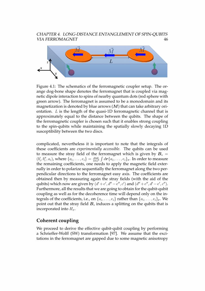
CHAPTER 4. LONG-DISTANCE ENTANGLEMENT OF SPIN-QUBITSVIA FERROMAGNET 46
Lx
y
z
Figure 4.1: The schematics of the ferromagnetic coupler setup. The or-ange dog-bone shape denotes the ferromagnet that is coupled via mag-netic dipole interaction to spins of nearby quantum dots (red sphere withgreen arrow). The ferromagnet is assumed to be a monodomain and itsmagnetization is denoted by blue arrows (M ) that can take arbitrary ori-entation. L is the length of the quasi-1D ferromagnetic channel that isapproximately equal to the distance between the qubits. The shape ofthe ferromagnetic coupler is chosen such that it enables strong couplingto the spin-qubits while maintaining the spatially slowly decaying 1Dsusceptibility between the two discs.
complicated, nevertheless it is important to note that the integrals ofthese coefficients are experimentally accessible. The qubits can be usedto measure the stray field of the ferromagnet which is given by Bs =(b′i, b
′′i , ai), where ai, . . . , ei = µ0µ
4πa3
∫drai, . . . , eir. In order to measure
the remaining coefficients, one needs to apply the magnetic field exter-nally in order to polarize sequentially the ferromagnet along the two per-pendicular directions to the ferromagnet easy axis. The coefficients areobtained then by measuring again the stray fields (with the aid of thequbits) which now are given by (d′+e′, d′′−e′′, c′) and (d′′+e′′, d′−e′, c′′).Furthermore, all the results that we are going to obtain for the qubit-qubitcoupling as well as for the decoherence time will depend only on the in-tegrals of the coefficients, i.e., on ai, . . . , ei rather than ai, . . . , eir. Wepoint out that the stray field Bs induces a splitting on the qubits that isincorporated into Hσ.
Coherent coupling
We proceed to derive the effective qubit-qubit coupling by performinga Schrieffer-Wolff (SW) transformation [97]. We assume that the exci-tations in the ferromagnet are gapped due to some magnetic anisotropy
CHAPTER 4. LONG-DISTANCE ENTANGLEMENT OF SPIN-QUBITSVIA FERROMAGNET 47
(e.g. shape-anisotropy) or externally applied magnetic field, with the gapbeing denoted by ∆F (for FMR dependence on externally applied mag-netic field see Kittel [98]). This is important because when the qubitsplitting ∆ is below FMR frequency, flipping the qubit spin cannot ex-cite magnons in the ferromagnet, thus there are only virtual magnons ex-cited via coupling to the qubits—otherwise such a coupling would leadto strong decoherence in the qubits. Due to presence of the gap in theferromagnet, its transversal susceptibility χ⊥(ω, r) decays exponentiallybelow FMR (ω < ∆F ) with the characteristic length lF ∝ 1/
√∆F − ω,
thus we take into account only terms with ω ∼ ∆F , see Eqs. (4.72) and(4.74) in Appendix 4.B. Straightforward application of lowest order SWtransformation accompanied by tracing out the degrees of freedom of theferromagnet yields the effective qubit-qubit coupling Hamiltonian
Heff = Hσ + χ1D⊥ (∆1, L)e1σ
−1 (c2σ
z2 + d2σ
+2 + e2σ
−2 )†+
1↔ 2 + h.c., (4.7)
where χ1D⊥ is the transverse susceptibility (i.e. transverse to the z direc-
tion) of a quasi-1D ferromagnet, since we assumed a dog-bone shapedferromagnet. We have neglected the longitudinal susceptibility χ‖ sinceit is suppressed by temperature. It can be seen from the above expres-sion that in order to obtain a sizable coupling between the qubits wehave to tune both the qubits close to resonance, ∆i ∼ ∆F (see Sec. 4.1).This can be achieved by applying an external magnetic field. Since theg-factor of the ferromagnet is generally not the same as the g-factor ofthe qubit, it is possible to tune the system on resonance with an exter-nal homogeneous magnetic field. The fine tuning can then be achievedby applying locally a small external magnetic field from a coil. The on-resonance requirement offers an elegant way to switch on/off the cou-pling between the qubits. The idea is to tune the qubit splitting closeto resonance for switching on the mediated interaction and to tune it offresonance to switch off the mediated interaction.
The expression for the transverse susceptibility of a ferromagnet isgiven in Eq. (4.74) of Appendix 4.B assuming HF to be of Heisenbergtype. The derivation given therein relays on the fact that dispersion oflow-laying ferromagnetic excitations (i.e. spin waves) is quadratic [99].Note that for very long wave lengths (bigger than a micron) the excita-tions are so-called dipolar spin waves with dispersion very different fromquadratic one and dependent on concrete boundary conditions [100].Since we are considering ferromagnets with dimensions not exceeding
CHAPTER 4. LONG-DISTANCE ENTANGLEMENT OF SPIN-QUBITSVIA FERROMAGNET 48
micron, the relevant excitations are exchange spin waves with quadraticdispersion which is practically independent of specific boundary condi-tions [100]. We note here that the FMR can increase toward the edges ofthe sample [101], in this case one should use ferromagnetic coupler withlateral dimensions bigger than the one quoted in Sec. 4.3 in order to havea middle region with nearly spatially independent FMR.
Special care has to be taken for the validity of the perturbation theoryemployed herein, since we are working close to FMR, i.e., ∆ − ∆F hasto be small but still much larger than the coupling of a qubit to an indi-vidual spin of the ferromagnet. For the perturbation theory to be validwe require the tilt of each ferromagnet spin to be sufficiently small (i.e.〈S±r 〉 1). The tilt of the central spin of the ferromagnetic disk can beestimated by the integral over the dogbone disk D
〈S±r 〉 =
∫
D
χ⊥(r)B⊥(r)dr , (4.8)
where B⊥(r) is the perpendicular (to the magnetization direction) com-ponent of the field produced at position r by the qubit. Using cylindricalcoordinates we then obtain
〈S±r 〉 ∼µ0µ
2B
2a
∫ R
0
ρdρ1
(ρ2 + h2)3/2
S
Dρ, (4.9)
where SDρ
is the spatial decay of the transversal susceptibility and 1(ρ2+h2)3/2
is the decay of the dipolar field causing the perturbation of the ferromag-net. For our choice of parameters, we obtain a tilt 〈S±r 〉 < 10−7 1. Eventhough each spin is just slightly tilted, we obtain a sizable coupling dueto big number of spins involved in mediating the coupling.
For the sake of completeness, in Appendix 4.D we present a detaileddiscussion of the effective coupling mediated by the dog-bone when thequbits are exchange coupled to the ferromagnet which requires a tunnelcoupling between spin qubit and ferromagnet.
Implementation of two-qubit gates
Two qubits interacting via the ferromagnet evolve according to the Hamil-tonian Heff , see Eq. (4.7). The Hamiltonian is therefore the sum of Zee-man terms and qubit-qubit interaction. These terms, by and large, do notcommute, making it difficult to use the evolution to implement standardentangling gates. In order to obtain sizable coupling we need to assume
CHAPTER 4. LONG-DISTANCE ENTANGLEMENT OF SPIN-QUBITSVIA FERROMAGNET 49
that the two qubits are on-resonance with each other, ∆1 ' ∆2. NowHσ acts only in the subspace spanned by | ↑, ↑〉, | ↓, ↓〉 and the Zee-man splitting of the qubits is much larger than the effective qubit-qubitcoupling, we can neglect the effect of Heff in this part of the subspaceand approximate it by its projection in the space spanned by the vectors| ↑, ↓〉, | ↓, ↑〉
H ′eff = Hσ + α(σx1σx2 − σy1σy2) + β(σx1σ
y2 + σy1σ
x2 ), (4.10)
where α = −8Re(e1e∗2) and β = −4Re(d1e
∗2 + d2e
∗1). Within this approxi-
mation, the coupling in H ′eff and the Zeeman terms now commute. Fromhere we readily see that the stray field components, ai, bi, as well as thecoefficient ci do not determine the operation time of the two qubit gates—the operation time depends only on di and ei. To proceed we perform arotation on the second qubit around the z-axis by an angle tan θ = β/αand arrive at the Hamiltonian
H ′eff = Hσ +√α2 + β2(σx1 σ
x2 − σy1 σy2). (4.11)
We consider the implementation of the iSWAP gate
UiSWAP = ei(σx1 σ
x2 +σy1 σ
y2 )π/4, (4.12)
which can be used to implement the CNOT gate [102]. The HamiltonianH ′ can be transformed to the desired form by changing the sign of σx1 σx2term. This is achieved with the following sequence [103]
UiSWAP = σy1eiHσte−iH
′eff tσy1 , (4.13)
where t = π/(4√α2 + β2). When iSWAP is available, the CNOT gate can
be constructed in the standard way [104]
UCNOT = e−iπ4σz1ei
π4σx2 ei
π4σz2UiSWAP e
−iπ4σx1UiSWAP e
iπ4σz2 . (4.14)
Since H ′eff is an approximation of Heff , the above sequence will yieldapproximate CNOT, U ′CNOT , when used with the full the Hamiltonian.The success of the sequences therefore depends on the fidelity of thegates, F (U ′CNOT ). Ideally this would be defined using a minimizationover all possible states of two qubits. However, to characterize the fi-delity of an imperfect CNOT it is sufficient to consider the following fourlogical states of two qubits [60]: |+, ↑〉, |+, ↓〉, |−, ↑〉, and |−, ↓〉. These areproduct states which, when acted upon by a perfect CNOT, become the
CHAPTER 4. LONG-DISTANCE ENTANGLEMENT OF SPIN-QUBITSVIA FERROMAGNET 50
four maximally entangled Bell states |Φ+〉, |Ψ+〉, |Φ−〉, and |Ψ−〉, respec-tively. As such, the fidelity of an imperfect CNOT may be defined,
F (U ′CNOT ) = mini∈+,−,j∈0,1
|〈i, j|U †CNOTU ′CNOT |i, j〉|2. (4.15)
The choice of basis used here ensures that F (U ′CNOT ) gives a good char-acterization of the properties of U ′CNOT in comparison to a perfect CNOT,especially for the required task of generating entanglement. For realis-tic parameters, with the Zeeman terms two order of magnitude strongerthan the qubit-qubit coupling, the above sequence yields fidelity for theCNOT gate of 99.976%.
To compare these values to the thresholds found in schemes for quan-tum computation, we must first note that imperfect CNOTs in these casesare usually modeled by the perfect implementation of the gate followedby depolarizing noise at a certain probability. It is known that such noisyCNOTs can be used for quantum computation in the surface code if thedepolarizing probability is less than 1.1% [20]. This corresponds to a fi-delity, according to the definition above, of 99.17%. The fidelities thatmay be achieved in the schemes proposed here are well above this valueand hence, though they do not correspond to the same noise model, wecan expect these gates to be equally suitable for fault-tolerant quantumcomputation.
4.2 DecoherenceIn this section we study the dynamics of a single qubit coupled to the fer-romagnet. In particular we want to answer the question whether the two-qubit dynamics studied in the previous section is coherent, i.e., whetherthe decoherence time solely due to the dipolar coupling to the ferromag-net is larger than the qubit operation time.
A ferromagnet has two types of fluctuations—longitudinal and trans-verse ones. The longitudinal noise stems from fluctuations of the longitu-dinal S z component (we recall that the ferromagnet is polarized along z),while the transverse one is related to fluctuations of S±. In what followswe study these two noise sources separately. The general noise modelthat describes both types of noise is then given by
H = HF +∆
2σz + σz ⊗X + σ+ ⊗ Y + h.c., (4.16)
CHAPTER 4. LONG-DISTANCE ENTANGLEMENT OF SPIN-QUBITSVIA FERROMAGNET 51
where the ferromagnet operators X (Y ) with zero expectation value cou-ple longitudinally (transversally) to the qubit. The noise model given inEq. (4.16) leads to the following relaxation and decoherence times withinBorn-Markov approximation [105]
T−11 = SY (ω = ∆), (4.17)
T−12 =
1
2T−1
1 + SX(ω = 0), (4.18)
where we defined the fluctuation power spectrum of an operator A inthe following way, SA(ω) =
∫dte−iωtA†(t), A(0). In order to obtain
expression for the decoherence times we need a specific model for theferromagnet Hamiltonian, herein taken to be a gapped Heisenberg modelHF = −J∑〈r,r′〉 Sr ·Sr′ + ∆F
∑r S
zr , J being the exchange coupling and
∆F the excitation gap.
Longitudinal noise
The power spectrum of longitudinal fluctuations is given by the follow-ing expression for ω T (see Appendix 4.C and in particular Eq. (4.85))
S3D‖ (ω) =
α√βω
2β2D3e−β∆F coth(βω/2), (4.19)
while for ω T (see Appendix 4.C, Eq. (4.87))
S3D‖ (ω) =
ln(1 + nk=0)
16πβD3ω coth(βω/2), (4.20)
where D = 2JS. We study transverse (Y ) and longitudinal (X) couplingseparately. In the case of longitudinal coupling we solve the problemexactly while we treat the transverse coupling within the framework ofperturbation theory.
Transverse coupling to longitudinal noise
The part of the Hamiltonian that describes transverse coupling to thelongitudinal noise reads
H = HF + σ+ ⊗∫drb1,rS
zr + h.c. (4.21)
CHAPTER 4. LONG-DISTANCE ENTANGLEMENT OF SPIN-QUBITSVIA FERROMAGNET 52
Using Eq. (4.18) and the inequality
S3D‖ (ω, r) ≤ S3D
‖ (ω, r = 0),
we obtain the relaxation time
T−11 =
∫drdr′b1,rb1,r′S
3D‖ (∆, r − r′)
≤∫drdr′b1,rb1,r′S
3D‖ (∆, r = 0)
= b21S
3D‖ (∆), (4.22)
where expression for S3D‖ (∆) is given in Eq. (4.19) since ∆ T . The
above expression readily shows that relaxation time can be tailored arbi-trarily small by choosing the ratio T/∆F sufficiently small.
Longitudinal coupling to longitudinal noise
Here we consider only longitudinal coupling to longitudinal noise thusthe Hamiltonian reads
H = HF + σz ⊗ V + ε σz , (4.23)
with ε the qubit splitting and V =∫dra1,rS
zr . To simplify the problem
further [106], we substitute S zr → Sxr since the latter is linear in magnonoperators while the former is quadratic. When the final formula for thedecoherence time is obtained we substitute back the power spectrum ofS zr instead of Sxr .
In order to study decoherence we have to calculate the followingquantity [106]
〈σ−(t)〉 = eiεt/~〈σ−(0)〉× (4.24)
×⟨T exp
(i
∫ t
0
V dt′)T exp
(i
∫ t
0
V dt′)⟩
,
with (T ) T the (anti-) time ordering operator. The average in the aboveexpression can be evaluated using a cluster expansion [107] and since theperturbation V is linear in the bosonic operators, only the second ordercluster contributes. Therefore, the final exact result for the time-evolutionof σ−(t) reads
〈σ−(t)〉 = eiεt/~〈σ−(0)〉e− 12
∫ t0
∫ t0 S(t2−t1)dt1dt2 , (4.25)
CHAPTER 4. LONG-DISTANCE ENTANGLEMENT OF SPIN-QUBITSVIA FERROMAGNET 53
where S(t) = 〈[V (t), V (0)]+〉. After performing the Fourier transforma-tion we obtain
〈σ−(t)〉 = eiεt/~〈σ−(0)〉× (4.26)
× exp
(−1
2
∫dω
2πS(ω)
sin2(ωt/2)
(ω/2)2
).
Note that this expression is of exactly the same form as the one for aclassical Gaussian noise [108]. Now we substitute back Sxr → S zr
〈σ−(t)〉 = eiεt/~〈σ−(0)〉 ×
× exp
(−1
2
∫dω
2π
∫drdr′a1,ra1,r′S
3D‖ (ω, r − r′)sin2(ωt/2)
(ω/2)2
).
(4.27)
For long times t ~/T the dynamics is of the form
〈σ−(t)〉 ∼ e−a21T
2 ln(1+nk=0)t/(8πD3)+i∆t, (4.28)
where we have used the inequality S3D‖ (ω, r) ≤ S3D
‖ (ω, r = 0). Thus,this type of decoherence can be suppressed by choosing the ratio T/∆F
sufficiently small.
Transverse noise
The power spectrum of transverse fluctuations of the ferromagnet van-ishes for ω < ∆F (see Eqs. (4.75) and (4.73) in Appendix 4.B),
S3D⊥ (ω) = 0 , ω < ∆F , (4.29)
S3D⊥ (ω) =
S√ω −∆F
D3/2coth(βω/2), ω > ∆F . (4.30)
Since the transverse fluctuations are gapped and the precession frequencyof the qubits is below the gap, this noise source does not contribute in thesecond order (Born approximation) because only virtual magnons can beexcited. In this section we choose the quantization axes such that qubitsplitting is along the z-axis, while the ferromagnet is polarized along thex-axis (see Fig. 4.1), this is done solely for simplicity and all the conclu-sions are also valid for the most general case. The Hamiltonian of the
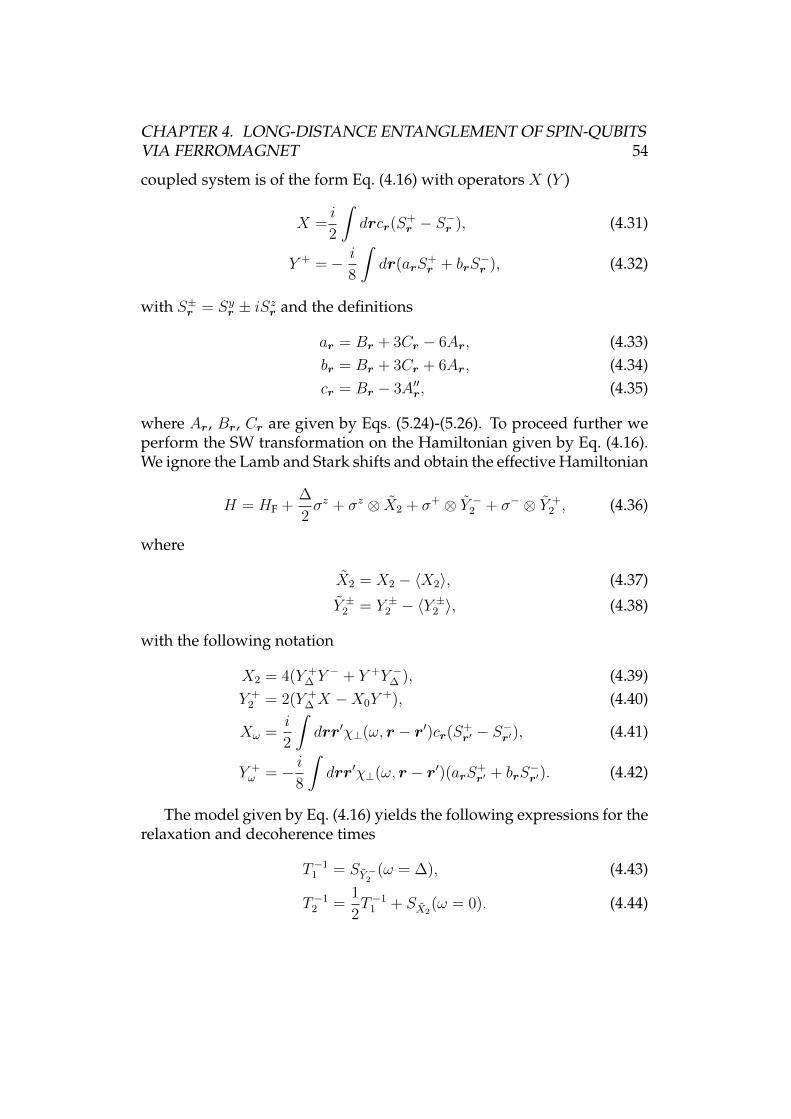
CHAPTER 4. LONG-DISTANCE ENTANGLEMENT OF SPIN-QUBITSVIA FERROMAGNET 54
coupled system is of the form Eq. (4.16) with operators X (Y )
X =i
2
∫drcr(S+
r − S−r ), (4.31)
Y + =− i
8
∫dr(arS
+r + brS
−r ), (4.32)
with S±r = Syr ± iSzr and the definitions
ar = Br + 3Cr − 6Ar, (4.33)br = Br + 3Cr + 6Ar, (4.34)cr = Br − 3A′′r, (4.35)
where Ar, Br, Cr are given by Eqs. (5.24)-(5.26). To proceed further weperform the SW transformation on the Hamiltonian given by Eq. (4.16).We ignore the Lamb and Stark shifts and obtain the effective Hamiltonian
H = HF +∆
2σz + σz ⊗ X2 + σ+ ⊗ Y −2 + σ− ⊗ Y +
2 , (4.36)
where
X2 = X2 − 〈X2〉, (4.37)
Y ±2 = Y ±2 − 〈Y ±2 〉, (4.38)
with the following notation
X2 = 4(Y +∆ Y
− + Y +Y −∆ ), (4.39)Y +
2 = 2(Y +∆ X −X0Y
+), (4.40)
Xω =i
2
∫drr′χ⊥(ω, r − r′)cr(S+
r′ − S−r′), (4.41)
Y +ω = − i
8
∫drr′χ⊥(ω, r − r′)(arS+
r′ + brS−r′). (4.42)
The model given by Eq. (4.16) yields the following expressions for therelaxation and decoherence times
T−11 = SY −2 (ω = ∆), (4.43)
T−12 =
1
2T−1
1 + SX2(ω = 0). (4.44)
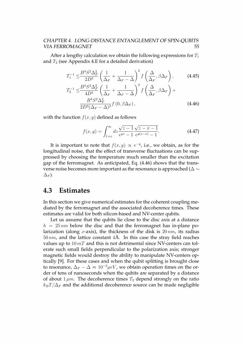
CHAPTER 4. LONG-DISTANCE ENTANGLEMENT OF SPIN-QUBITSVIA FERROMAGNET 55
After a lengthy calculation we obtain the following expressions for T1
and T2 (see Appendix 4.E for a detailed derivation)
T−11 ≤B
4S2∆2F
2D3
(1
∆F
+1
∆F −∆
)2
f
(∆
∆F
, β∆F
), (4.45)
T−12 ≤B
4S2∆2F
4D3
(1
∆F
+1
∆F −∆
)2
f
(∆
∆F
, β∆F
)+
B4S2∆2F
2D3(∆F −∆)2f (0, β∆F ) , (4.46)
with the function f(x, y) defined as follows
f(x, y) =
∫ ∞
1+x
dz
√z − 1
eyz − 1
√z − x− 1
ey(z−x) − 1. (4.47)
It is important to note that f(x, y) ∝ e−y, i.e., we obtain, as for thelongitudinal noise, that the effect of transverse fluctuations can be sup-pressed by choosing the temperature much smaller than the excitationgap of the ferromagnet. As anticipated, Eq. (4.46) shows that the trans-verse noise becomes more important as the resonance is approached (∆ ∼∆F ).
4.3 EstimatesIn this section we give numerical estimates for the coherent coupling me-diated by the ferromagnet and the associated decoherence times. Theseestimates are valid for both silicon-based and NV-center qubits.
Let us assume that the qubits lie close to the disc axis at a distanceh = 25nm below the disc and that the ferromagnet has in-plane po-larization (along x-axis), the thickness of the disk is 20nm, its radius50nm, and the lattice constant 4A. In this case the stray field reachesvalues up to 10mT and this is not detrimental since NV-centers can tol-erate such small fields perpendicular to the polarization axis; strongermagnetic fields would destroy the ability to manipulate NV-centers op-tically [9]. For these cases and when the qubit splitting is brought closeto resonance, ∆F − ∆ ≈ 10−2µeV , we obtain operation times on the or-der of tens of nanoseconds when the qubits are separated by a distanceof about 1µm. The decoherence times T2 depend strongly on the ratiokBT/∆F and the additional decoherence source can be made negligible
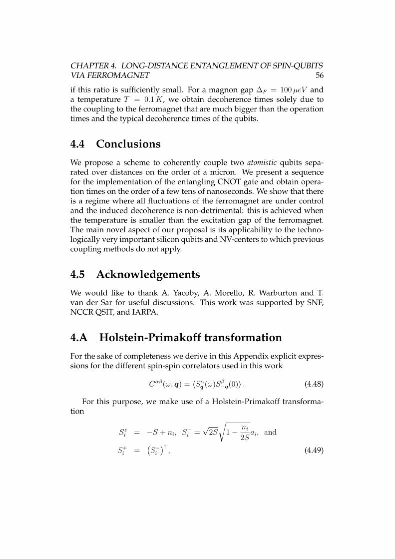
CHAPTER 4. LONG-DISTANCE ENTANGLEMENT OF SPIN-QUBITSVIA FERROMAGNET 56
if this ratio is sufficiently small. For a magnon gap ∆F = 100µeV anda temperature T = 0.1K, we obtain decoherence times solely due tothe coupling to the ferromagnet that are much bigger than the operationtimes and the typical decoherence times of the qubits.
4.4 ConclusionsWe propose a scheme to coherently couple two atomistic qubits sepa-rated over distances on the order of a micron. We present a sequencefor the implementation of the entangling CNOT gate and obtain opera-tion times on the order of a few tens of nanoseconds. We show that thereis a regime where all fluctuations of the ferromagnet are under controland the induced decoherence is non-detrimental: this is achieved whenthe temperature is smaller than the excitation gap of the ferromagnet.The main novel aspect of our proposal is its applicability to the techno-logically very important silicon qubits and NV-centers to which previouscoupling methods do not apply.
4.5 AcknowledgementsWe would like to thank A. Yacoby, A. Morello, R. Warburton and T.van der Sar for useful discussions. This work was supported by SNF,NCCR QSIT, and IARPA.
4.A Holstein-Primakoff transformationFor the sake of completeness we derive in this Appendix explicit expres-sions for the different spin-spin correlators used in this work
Cαβ(ω, q) = 〈Sαq (ω)Sβ−q(0)〉 . (4.48)
For this purpose, we make use of a Holstein-Primakoff transforma-tion
Szi = −S + ni, S−i =√
2S
√1− ni
2Sai, and
S+i =
(S−i)†, (4.49)
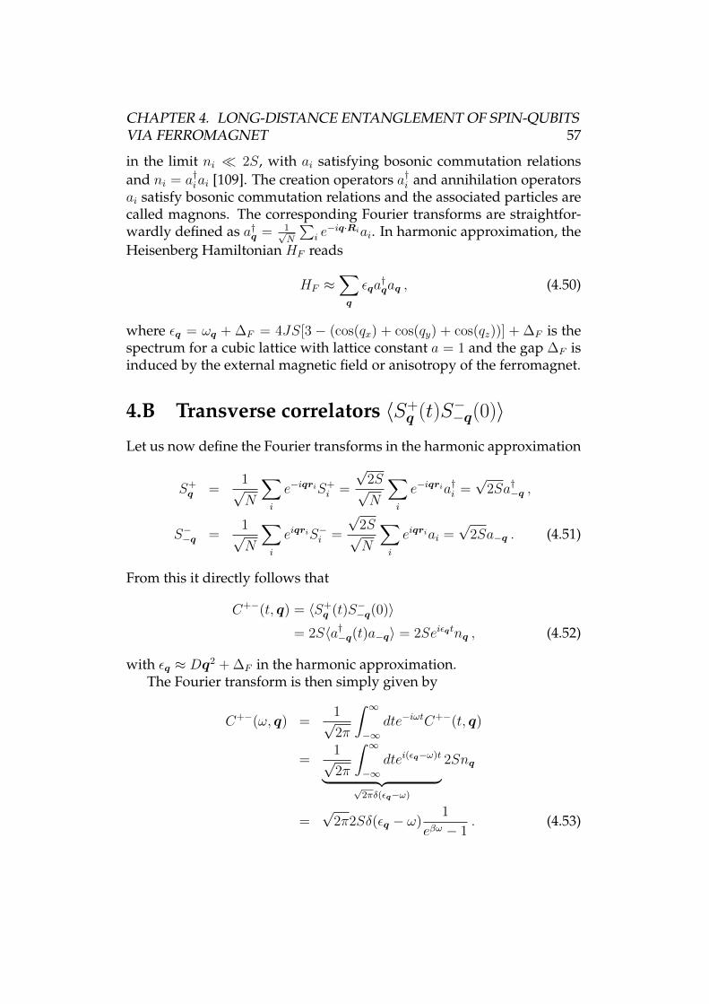
CHAPTER 4. LONG-DISTANCE ENTANGLEMENT OF SPIN-QUBITSVIA FERROMAGNET 57
in the limit ni 2S, with ai satisfying bosonic commutation relationsand ni = a†iai [109]. The creation operators a†i and annihilation operatorsai satisfy bosonic commutation relations and the associated particles arecalled magnons. The corresponding Fourier transforms are straightfor-wardly defined as a†q = 1√
N
∑i e−iq·Riai. In harmonic approximation, the
Heisenberg Hamiltonian HF reads
HF ≈∑
q
εqa†qaq , (4.50)
where εq = ωq + ∆F = 4JS[3 − (cos(qx) + cos(qy) + cos(qz))] + ∆F is thespectrum for a cubic lattice with lattice constant a = 1 and the gap ∆F isinduced by the external magnetic field or anisotropy of the ferromagnet.
4.B Transverse correlators 〈S+q (t)S
−−q(0)〉
Let us now define the Fourier transforms in the harmonic approximation
S+q =
1√N
∑
i
e−iqriS+i =
√2S√N
∑
i
e−iqria†i =√
2Sa†−q ,
S−−q =1√N
∑
i
eiqriS−i =
√2S√N
∑
i
eiqriai =√
2Sa−q . (4.51)
From this it directly follows that
C+−(t, q) = 〈S+q (t)S−−q(0)〉
= 2S〈a†−q(t)a−q〉 = 2Seiεqtnq , (4.52)
with εq ≈ Dq2 + ∆F in the harmonic approximation.The Fourier transform is then simply given by
C+−(ω, q) =1√2π
∫ ∞
−∞dte−iωtC+−(t, q)
=1√2π
∫ ∞
−∞dtei(εq−ω)t
︸ ︷︷ ︸√2πδ(εq−ω)
2Snq
=√
2π2Sδ(εq − ω)1
eβω − 1. (4.53)
CHAPTER 4. LONG-DISTANCE ENTANGLEMENT OF SPIN-QUBITSVIA FERROMAGNET 58
The corresponding correlator in real space is then simply given by (q :=|q|)
C+−(ω, r) =1
(2π)3/2
∫dqeiqrC+−(ω, q) (4.54)
=
√2π
(2π)3/22S
1
eβω − 1
∫dqδ(Dq2 + ∆F − ω)eiqr
=2S
eβω − 1
∫ 1
−1
∫ ∞
0
dqdxq2δ(Dq2 + ∆F − ω)eiqrx
=4S
r
1
eβω − 1
∫ ∞
0
dqqδ(Dq2 + ∆F − ω) sin(qr) .
Let us now perform the following substitution
y = Dq2, (4.55)
which gives for ω > ∆F
C+−(ω, r) =4S/r
2D(eβω − 1)
∫ ∞
0
dyδ(y + ∆F − ω)×
× sin
(√y
Dr
)(4.56)
=2S
D
1
eβω − 1
sin(√
(ω −∆F )/Dr)
r.
We remark thatC+−(ω, r) = 0, ω < ∆F . (4.57)
We note the diverging behavior of the above correlation function for∆F = 0 and ω → 0, namely
1
eβω − 1
sin(√
ωDr)
r→ 1√
Dβ
1√ω. (4.58)
Similarly, it is now easy to calculate the corresponding commutators andanticommutators. Let us define
S⊥(t, q) :=1
2S+
q (t), S−−q(0) . (4.59)
It is then straightforward to show that
S⊥(t, q) = Seiεqt(1 + 2nq) , (4.60)
CHAPTER 4. LONG-DISTANCE ENTANGLEMENT OF SPIN-QUBITSVIA FERROMAGNET 59
and therefore
S⊥(ω, q) =S√2π
∫ ∞
−∞ei(εq−ω)t(1 + 2nq)
= S√
2πδ(εq − ω)
(1 + 2
1
eβω − 1
). (4.61)
Following essentially the same steps as the one performed above, weobtain the 3D real space anticommutator for ω > ∆F
S3D⊥ (ω, q) = S coth(βω/2)× (4.62)
×∫ 1
−1
∫ ∞
0
dxdqq2eiqrxδ(εq − ω)
=S
Dcoth(βω/2)
sin(√
(ω −∆F )/Dr)
r.
(4.63)
Let us now finally calculate the transverse susceptibility defined as
χ⊥(t, q) = −iθ(t)[S+q (t), S−−q(0)] . (4.64)
As before, in the harmonic approximation, one finds
χ⊥(t, q) = iθ(t)2Seiεqt . (4.65)
In the frequency domain, we then have
χ⊥(ω, q) =2iS√
2π
∫ ∞
0
dtei(εq−ω)t−ηt (4.66)
= − 2S√2π
1
εq − ω + iη,
and thus in the small q expansion
χ⊥(ω, q) = − 2S√2π
1
Dq2 + ∆F − ω + iη. (4.67)
In real space, for the three-dimensional case, we obtain
χ3D⊥ (ω, r) = − 2S√
2π
2π
(2π)3/2
∫ ∞
0
∫ 1
−1
dxdqq2 1
Dq2 + ∆F − ω + iηeiqrx
= − 4S√2π
2π
(2π)3/2
1
r
∫ ∞
0
dqq1
Dq2 + ∆F − ω + iηsin(qr) .(4.68)
CHAPTER 4. LONG-DISTANCE ENTANGLEMENT OF SPIN-QUBITSVIA FERROMAGNET 60
Making use of the Plemelj formula we obtain for ω > ∆F
χ3D⊥ (ω, r) = − 2S√
2π
2π
(2π)3/2
1
r
∫ ∞
−∞dqq
1
Dq2 + ∆F − ω + iηsin(qr)
= − 2S√2π
2π
(2π)3/2
1
rP
∫ ∞
−∞dq
q
Dq2 + ∆F − ωsin(qr)
+i2S√2π
2π2
(2π)3/2
1
r
∫ ∞
−∞dqqδ(Dq2 + ∆F − ω) sin(qr)
= − SD
cos(r√
(ω −∆F )/D)
r+ i
S
2D
sin(√
(ω −∆F )/Dr)
r.
(4.69)
It is worth pointing out that the imaginary part of the susceptibility van-ishes,
χ3D⊥ (ω, r)′′ = 0, ω < ∆F , (4.70)
and therefore the susceptibility is purely real and takes the form of aYukawa potential
χ3D⊥ (ω, r) = − S
D
e−r/lF
r, ω < ∆F , (4.71)
where
lF =
√D
∆F − ω. (4.72)
Note also that the imaginary part of the transverse susceptibility satisfiesthe well-know fluctuation-dissipation theorem
S3D⊥ (ω, r) = coth(βω/2)χ3D
⊥ (ω, r)′′ . (4.73)
In three dimensions the susceptibility decay as 1/r, where r is mea-sured in lattice constants. For distances of order of 1µm this leads to fourorders of magnitude reduction.
For quasi one-dimensional ferromagnets such a reduction is absentand the transverse susceptibility reads
χ1D⊥ (ω, r) = − S
DlF e−r/lF , ω < ∆F , (4.74)
where lF is defined as above and the imaginary part vanishes as above,i.e.,
χ1D⊥ (ω, r)′′ = 0, ω < ∆F . (4.75)
CHAPTER 4. LONG-DISTANCE ENTANGLEMENT OF SPIN-QUBITSVIA FERROMAGNET 61
Similarly for ω > ∆F we have
χ1D⊥ (ω, r) = S
sin(√
(ω −∆F )/Dr)
√D(ω −∆F )
, (4.76)
and
χ1D⊥ (ω, r)′′ =
S
2D
√D
ω −∆F
cos(√
(ω −∆F )/Dr). (4.77)
4.C Longitudinal correlators 〈Szq(t)Sz−q(0)〉The longitudinal susceptibility reads
χ‖(t, q) = −iθ(t)[Szq(t), Sz−q(0)] (4.78)
= −θ(t) 1
N
∑
q′,q′′
eit(εq′−εq′+q)〈[a†q′aq′+q, a†q′′aq′′−q]〉 .
Applying Wick’s theorem and performing a Fourier transform, we obtainthe susceptibility in frequency domain
χ‖(ω, q) = − 1
N
∑
k
nk − nk+q
ω − εk+q + εk + iη, (4.79)
where nk is the magnon occupation number given by the Bose-Einsteindistribution
nk =1
eβεk − 1, (4.80)
where εk is again the magnon spectrum (εk = ωk + ∆F ≈ Dk2 + ∆F forsmall k). Note that the longitudinal susceptibility is proportional to 1/S,due to the fact that εk − εk+q = ωk − ωk+q ∝ S.
Since we are interested in the decoherence processes caused by thelongitudinal fluctuations, we calculate the imaginary part of χ‖(ω, q) thatis related to the fluctuations via the fluctuation-dissipation theorem. Per-forming a small q expansion and assuming without loss of generality
CHAPTER 4. LONG-DISTANCE ENTANGLEMENT OF SPIN-QUBITSVIA FERROMAGNET 62
ω > 0, we obtain for the imaginary part
χ3D‖ (ω, q)′′ =
π
(2π)3
∫dk(nk − nk+q)δ(ωk − ωk+q + ω)
=1
4π
∫ ∞
0
dkk2
∫ 1
−1
dx
(1
eβ(∆F+Dk2) − 1− 1
eβ(ω+∆F+Dk2) − 1
)×
×δ(ω −Dq2 − 2Dkqx)
=1
4π
∫ ∞
0
dkk2
∫ 1
−1
dx
(1
eβ(∆F+Dk2) − 1− 1
eβ(ω+∆F+Dk2) − 1
)×
×δ(k − ω −Dq2
2Dqx
) ∣∣∣∣1
2Dqx
∣∣∣∣
=1
4π
∫ 1
−1
dx
∣∣∣∣1
2Dqx
∣∣∣∣(ω −Dq2
2Dqx
)2
θ
(ω −Dq2
2Dqx
)×
×
1
eβ
(∆F+D
(ω−Dq22Dqx
)2)− 1
− 1
eβ
(ω+∆F+D
(ω−Dq22Dqx
)2)− 1
=1
4π
∫ 1
0
dx1
2Dqx
(ω −Dq2
2Dqx
)2
× 1
eβ
(∆F+D
(ω−Dq22Dqx
)2)− 1
− 1
eβ
(ω+∆F+D
(ω−Dq22Dqx
)2)− 1
. (4.81)
Next, since we are interested in the regime where ω T (and thus βω 1), we have nk nk+q. Furthermore, we approximate the distributionfunction nk = e−β(∆F+ωk)
1−e−β∆F +βωk(this is valid when βωk 1) and arrive at the
following expression
χ3D‖ (ω, q)′′ =
1
4π
∫ 1
0
dx1
2Dqx
(ω −Dq2
2Dqx
)2e−β(
∆F+D
(ω−Dq22Dqx
)2)
1− e−β∆F + βD(ω−Dq2
2Dqx
)2
= −e1−e−β∆F−β∆F
4βD2qEi
(e−β∆F +
1
4
(−4− βDq2 + 2βω − βω2
Dq2
)),
(4.82)
where Ei(z) is the exponential integral function. We also need the the real
CHAPTER 4. LONG-DISTANCE ENTANGLEMENT OF SPIN-QUBITSVIA FERROMAGNET 63
space representation obtained after inverse Fourier transformation,
χ3D‖ (ω, r)′′ =
√2
π
1
r
∫ ∞
0
dqqχ3D‖ (ω, q)′′ sin(qr) . (4.83)
In order to perform the above integral we note that the imaginary partof the longitudinal susceptibility, given by Eq. (4.82), is peaked aroundq =
√ω/D with the width of the peak (1/
√βD) much smaller than its
position in the regime we are working in (ω T ). For r = 0, the integra-tion over q can be then performed approximately and yields the follow-ing expression
χ3D‖ (ω, r = 0)′′ =
√πe−e
−β∆F−3β∆F /2
2β2D3
(ee−β∆F +β∆F /2
− e√π√eβ∆F − 1 (4.84)
× Erfc(e−β∆F /2√eβ∆F − 1)
)√βω ,
where Erfc(z) denotes the complementary error function. It is readilyobserved from the above expression that the longitudinal fluctuationsare exponentially suppressed by the gap. Assuming that ∆F T , weobtain the following simplified expression
χ3D‖ (ω, r = 0)′′ =
√π − eπErfc(1)
2β2D3e−β∆F
√βω . (4.85)
We observe that, since J(ω) = χ‖(ω, r)′′, the longitudinal noise of theferromagnet is—as the transverse one—sub-ohmic [105].
It is interesting to obtain the behavior of the longitudinal susceptibil-ity in the opposite limit, when βω 1. In this limit, the difference of thetwo Boltzmann factors in Eq. (4.81) can be expanded to the lowest orderin the small quantity βω,
χ3D‖ (ω, q)′′ =
∫ 1
0
dx1
8πDqx
(ω −Dq2
2Dqx
)2
×
βω
ch
(β∆F + βD
(ω−Dq2
2Dqx
)2)− 1
=ω
16πD2q
(eβ∆F+
β(ω−Dq2)2
4Dq2 − 1
) . (4.86)
CHAPTER 4. LONG-DISTANCE ENTANGLEMENT OF SPIN-QUBITSVIA FERROMAGNET 64
In order to calculate the Fourier transform to real space, we note that forω ∆F the denominator of the above expression depends only weaklyon ω, thus we ignore this dependence and obtain the Fourier transformfor r = 0
χ3D‖ (ω)′′ =
ln(1 + nk=0)
16πβD3ω. (4.87)
The above formula shows that the longitudinal noise of a ferromagnetat high temperatures (βω 1) behaves as ohmic rather than sub-ohmicbath.
Next we calculate the longitudinal fluctuations for the case of a quasi-one-dimensional ferromagnet (∆F T ) and obtain
χ1D‖ (ω, r = 0)′′ =
1
4π
∫ ∞
−∞dk
∫ ∞
−∞dq
(1
eβ(∆F+Dk2) − 1
− 1
eβ(ω+∆F+Dk2) − 1
)δ(ω −Dq2 − 2Dkq)
=
∫ ∞
−∞dk
e−βDk2
1− e−β∆F + βDk2
1
D√k2 + ω/D
=γ
D√βω
e−β∆F , (4.88)
where γ is a numerical factor of order unity.Note that S‖(ω, r) is defined through the fluctuation dissipation theo-
rem asS‖(ω, r) = coth(βω/2)χ‖(ω, r)′′ . (4.89)
4.D Exchange coupling to the ferromagnetExchange coupling
The Hamiltonian we consider is of the following form
H = HF +Hσ + A∑
i
σi · Sri , (4.90)
where A is the exchange coupling constant between the qubit spins andthe ferromagnet. The ferromagnet is assumed to be below the Curie
CHAPTER 4. LONG-DISTANCE ENTANGLEMENT OF SPIN-QUBITSVIA FERROMAGNET 65
temperature with the magnetization pointing along the out-of-plane z-direction. The qubit Hamiltonian is assumed to be without splitting ini-tially, that is H(0)
σ = 0. Nevertheless, since the ferromagnet is in the or-dered phase, there exists a first order effect due to coupling to the fer-romagnet which gives rise to the term of the form A
∑i σ
zi 〈Szri〉. Such
a splitting is undesirable if one is interested in coherent interaction—weremedy this by coupling the spins to another ferromagnet, albeit withanti-parallel magnetization. Since we allow for some misalignment be-tween orientation of the magnetization of the two ferromagnets, the finalHamiltonian for the qubits in the spin space after taking into account thefirst order corrections due to coupling to the ferromagnet reads
Hσ =1
2∆∑
i
σxi . (4.91)
The splitting in the x-direction of the qubit (or equivalently along the y-direction) is beneficial since it reduces decoherence due to longitudinalnoise of the ferromagnet: the effect of such noise spectrum can signifi-cantly influence decoherence times for the case of no splitting of the qubitbecause the longitudinal noise is gapless.
Coherent coupling
We proceed with the derivation of an effective two-spin interaction Hamil-tonian for A J by employing a perturbative Schrieffer-Wolff transfor-mation [97] up to the second order
Heff = Hσ +A2
8χ⊥(∆)(2σy1σ
y2 + σz1σ
x2 + σx1σ
z2) , (4.92)
where we introduced the notation χ⊥(ω) = χ⊥(ω, L) (L = |r2 − r1|) andχ⊥(ω, r) is the transverse real space spin susceptibility of the ferromag-net. Note that we have neglected χ3D
⊥ (−∆) and χ3D⊥ (0) in comparison to
χ1D⊥ (∆), as well as the longitudinal susceptibility χ‖ since it is smaller by
factor of 1/S compared to the transverse one and it is suppressed by tem-perature. The real space transverse susceptibility of the 3D ferromagnetis given by
χ3D⊥ (ω, r) = − S
D
e−r/lF
r, ω < ∆F , (4.93)
where ∆F is the gap induced via applied external magnetic field or due
to internal anisotropy of the ferromagnet, lF =√
D∆F−ω
and D = 2JS.
CHAPTER 4. LONG-DISTANCE ENTANGLEMENT OF SPIN-QUBITSVIA FERROMAGNET 66
In what follows, we assume that the external gap is always larger thanthe qubit splitting, ∆ < ∆F , as this ensures that the transverse noise isnot contributing to decoherence in second order since transverse noise isrelated to the vanishing imaginary part of the transverse susceptibility,χ⊥(ω)′′ = 0 (ω < ∆F ). The spatial dependence of the effective two spincoupling given by Eq. (4.93) is of Yukawa type due to presence of theexternal gap. If we assume a realistic tunnel coupling to the ferromag-net of 100µeV [110, 111], the Curie temperature of 550K [as for examplefor yttrium iron garnet (YIG)] and a gap of ∆F = 100µeV, and the qubitsplitting close to the resonance ∆F −∆ = 3× 10⁻³µeV (corresponding toa magnetic field of about B = 60µT) we obtain for the qubit-qubit cou-pling strength a value on the order of 4 × 10⁻¹¹ eV for a lattice constantof about 4A. This coupling strength gives rise to the operation times of50µs—significantly below the relaxation and decoherence times of thespin qubit, T1 = 1s [64] and T2 > 200µs [65] respectively. Furthermore,the error threshold—defined as the ratio between the two-qubit gate op-eration time to the decoherence time—we obtain with such an operationtime is about 10−2, which is good enough for implementing the surfacecode error correction [21]. Here we used T2 instead of T ∗2 since spin-echocan be performed together with two-qubit gates [112]. Alternatively, thedecoherence time of GaAs qubits can be increased without spin-echo bynarrowing the state of the nuclear spins [113, 114].
The dimensionality of the ferromagnet plays an important role—ifwe assume 10nm width of the trench where the ferromagnet is placed,then, for energies below 0.1meV, the ferromagnet behaves as quasi one-dimensional (1D). In this case we obtain
χ1D⊥ (ω, r) = − S
DlF e−r/lF , ω < ∆F , (4.94)
wherefrom it is evident that at distances r . lF the susceptibility of aquasi-1D ferromagnet is practically constant in contrast to the 3D case,where a 1/r decay is obtained, see Eq. (4.93). Additionally, we requirelF . D/(AS) = 2J/A for the perturbation theory to be valid. Thus, forthe same parameters as above, but without the need to tune very close tothe resonance (we set herein ∆F − ∆ = 0.5µeV, corresponding to aboutB = 10mT) a coupling strength of 10−8eV is obtained.
For 1D case there is yet another rather promising possibility—to usemagnetic semiconductors [115]. These materials are characterized by aparticularly low Curie temperature of 30K or below [115], and the dis-tance between the ions that are magnetically ordered via RKKY interac-
CHAPTER 4. LONG-DISTANCE ENTANGLEMENT OF SPIN-QUBITSVIA FERROMAGNET 67
tion is about 10 − 100nm. Such a large lattice constant is very beneficialfor the long range coupling—if we take the lattice constant to be 10nm,the coupling to the ferromagnet A = 15µeV and the qubit splitting closeto resonance (∆F − ∆ = 0.5µeV, corresponding to about B = 10mT),the qubit-qubit coupling becomes of the order of 1µeV. Such a couplingstrength in turn leads to an error threshold on the order of 10−8. There-fore, even the standard error correction protocol can be used in this case.
Derivation of the effective Hamiltonian (exchange coupling)
Here we give a detailed derivation of the qubit-qubit effective Hamilto-nian. As stated above, the total Hamiltonian of the system reads
H = HF +Hσ + A∑
i
(1
2(σ+
i S−ri
+ σ−i S+ri
) + σzi Szri
), (4.95)
where we identify the main part as H0 = HF + Hσ and the small pertur-bation as the exchange coupling V = A
∑i σi · Sri . The Hamiltonian of
the ferromagnet reads HF = −J∑〈r,r′〉 Sr · Sr′ , while the Hamiltonianfor the two distant qubits is Hσ = ∆
2
∑i=1,2 σ
xi .
The second order effective Hamiltonian [97] is given byH(2)eff = H0+U ,
whereU = − i
2limη→0+
∫ ∞
0
dte−ηt[V (t), V ] , (4.96)
where V (t) = eiH0tV e−iH0t.We have
σ+i (t) =
1 + cos(∆t)
2σ+i +
1− cos(∆t)
2σ−i − i sin(∆t)σzi , (4.97)
and σ−i (t) = σ+i (t)†.
Recalling that the zz susceptibility can be neglected and that only thetransverse susceptibility contributes, we obtain the following result fromEq. (4.96), U = lim
η→0+
∫∞0dte−ηt
∑ij Uij
Uij =− iA2
8
([σ−i (t)S+
ri(t), σ+
j S−rj
] + h.c.)
=− iA2
8
(σ−i (t)σ+
j [S+ri
(t), S−rj ] + h.c.)
(4.98)
CHAPTER 4. LONG-DISTANCE ENTANGLEMENT OF SPIN-QUBITSVIA FERROMAGNET 68
Finally, by rewriting cos(∆t) = ei∆t+e−i∆t
2, sin(∆t) = ei∆t−e−i∆t
2i, and using
the definition of the real space transverse spin susceptibility
χ⊥(ω, ri − rj) = −i limη→0+
∫ ∞
0
dte−(iω+η)t[S+ri
(t), S−rj ] , (4.99)
we obtain by inserting Eq. (4.97) into Eq. (4.98)
U =A2
8
∑
ij
(χ⊥(0)
2+χ⊥(∆) + χ⊥(−∆)
4
)σ−i σ
+j
+A2
8
∑
ij
(χ⊥(0)
2− χ⊥(∆) + χ⊥(−∆)
4
)σ+i σ
+j
−A2
8
∑
ij
χ⊥(∆)− χ⊥(−∆)
2σzi σ
+j + h.c. (4.100)
Since the decay length of the susceptibility χ(ω, r) is large only close tothe resonance, ∆F ∼ ∆, we can simplify the above equation by neglectingχ(−∆, r) and χ(0, r) in comparison to χ(∆, r) which is assumed to beclose to the resonance. Within this approximation we arrive at Eq. (4.92)of the main text.
4.E Fourth order contributions to decoherenceIn this section we determine the effect of the transverse noise in the low-est non-vanishing order due to coupling dipolarly to the ferromagnet.Here we choose quantizations axes such that the qubit splitting is alongthe z-axis, while the ferromagnet is polarized along x-axis. The Hamilto-nian of the coupled system reads
H = HF +∆
2σz + σz ⊗X + σ+ ⊗ Y − + σ− ⊗ Y +, (4.101)
where the operator X (Y ) that couples longitudinally (transversally) tothe qubit is linear in the transverse operators of the ferromagnet
X =i
2
∫drcr(S+
r − S−r ), (4.102)
Y + =− i
8
∫dr(arS
+r + brS
−r ), (4.103)
CHAPTER 4. LONG-DISTANCE ENTANGLEMENT OF SPIN-QUBITSVIA FERROMAGNET 69
with S±r = Syr ± iSzr and the definitions of the coefficients
ar = Br + 3Cr − 6Ar, (4.104)br = Br + 3Cr + 6Ar, (4.105)cr = Br − 3A′′r, (4.106)
Ar =1
a3
rzr+
r5, (4.107)
Cr =1
a3
(r+)2
r5, (4.108)
Br =1
a3
1
r3
(2− 3r+r−
r2
). (4.109)
To proceed further we perform the SW transformation on the Hamilto-nian given by Eq. (4.101). We ignore the Lamb and Stark shifts and obtainthe effective Hamiltonian
H = HF +∆
2σz + σz ⊗ X2 + σ+ ⊗ Y −2 + σ− ⊗ Y +
2 , (4.110)
where
X2 = X2 − 〈X2〉, (4.111)
Y ±2 = Y ±2 − 〈Y ±2 〉, (4.112)
with the following notation
X2 = 4(Y +∆ Y
− + Y +Y −∆ ), (4.113)Y +
2 = 2(Y +∆ X −X0Y
+), (4.114)
Xω =i
2
∫drr′χ⊥(ω, r − r′)cr(S+
r′ − S−r′), (4.115)
Y +ω = − i
8
∫drr′χ⊥(ω, r − r′)(arS+
r′ + brS−r′), (4.116)
The model given by Eq. (4.110) yields the following expressions forthe relaxation and decoherence times
T−11 = SY −2 (ω = ∆), (4.117)
T−12 =
1
2T−1
1 + SX2(ω = 0), (4.118)
where, again, SA(ω) =∫dte−iωtA†(t), A(0).
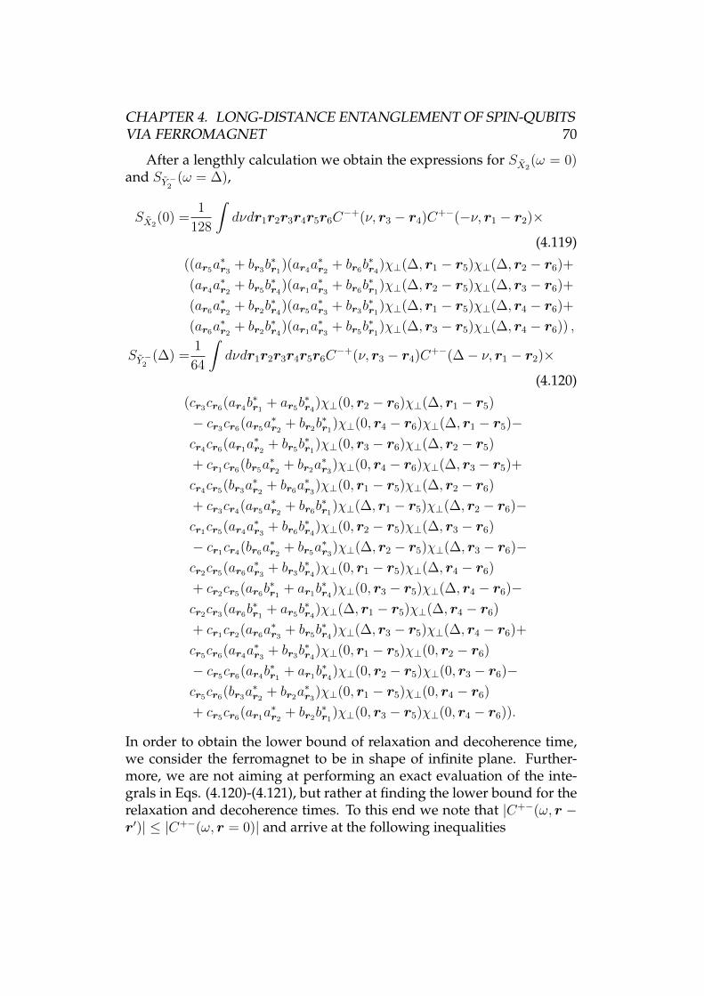
CHAPTER 4. LONG-DISTANCE ENTANGLEMENT OF SPIN-QUBITSVIA FERROMAGNET 70
After a lengthly calculation we obtain the expressions for SX2(ω = 0)
and SY −2 (ω = ∆),
SX2(0) =
1
128
∫dνdr1r2r3r4r5r6C
−+(ν, r3 − r4)C+−(−ν, r1 − r2)×(4.119)
((ar5a∗r3
+ br3b∗r1
)(ar4a∗r2
+ br6b∗r4
)χ⊥(∆, r1 − r5)χ⊥(∆, r2 − r6)+
(ar4a∗r2
+ br5b∗r4
)(ar1a∗r3
+ br6b∗r1
)χ⊥(∆, r2 − r5)χ⊥(∆, r3 − r6)+
(ar6a∗r2
+ br2b∗r4
)(ar5a∗r3
+ br3b∗r1
)χ⊥(∆, r1 − r5)χ⊥(∆, r4 − r6)+
(ar6a∗r2
+ br2b∗r4
)(ar1a∗r3
+ br5b∗r1
)χ⊥(∆, r3 − r5)χ⊥(∆, r4 − r6)) ,
SY −2 (∆) =1
64
∫dνdr1r2r3r4r5r6C
−+(ν, r3 − r4)C+−(∆− ν, r1 − r2)×(4.120)
(cr3cr6(ar4b∗r1
+ ar5b∗r4
)χ⊥(0, r2 − r6)χ⊥(∆, r1 − r5)
− cr3cr6(ar5a∗r2
+ br2b∗r1
)χ⊥(0, r4 − r6)χ⊥(∆, r1 − r5)−cr4cr6(ar1a
∗r2
+ br5b∗r1
)χ⊥(0, r3 − r6)χ⊥(∆, r2 − r5)
+ cr1cr6(br5a∗r2
+ br2a∗r3
)χ⊥(0, r4 − r6)χ⊥(∆, r3 − r5)+
cr4cr5(br3a∗r2
+ br6a∗r3
)χ⊥(0, r1 − r5)χ⊥(∆, r2 − r6)
+ cr3cr4(ar5a∗r2
+ br6b∗r1
)χ⊥(∆, r1 − r5)χ⊥(∆, r2 − r6)−cr1cr5(ar4a
∗r3
+ br6b∗r4
)χ⊥(0, r2 − r5)χ⊥(∆, r3 − r6)
− cr1cr4(br6a∗r2
+ br5a∗r3
)χ⊥(∆, r2 − r5)χ⊥(∆, r3 − r6)−cr2cr5(ar6a
∗r3
+ br3b∗r4
)χ⊥(0, r1 − r5)χ⊥(∆, r4 − r6)
+ cr2cr5(ar6b∗r1
+ ar1b∗r4
)χ⊥(0, r3 − r5)χ⊥(∆, r4 − r6)−cr2cr3(ar6b
∗r1
+ ar5b∗r4
)χ⊥(∆, r1 − r5)χ⊥(∆, r4 − r6)
+ cr1cr2(ar6a∗r3
+ br5b∗r4
)χ⊥(∆, r3 − r5)χ⊥(∆, r4 − r6)+
cr5cr6(ar4a∗r3
+ br3b∗r4
)χ⊥(0, r1 − r5)χ⊥(0, r2 − r6)
− cr5cr6(ar4b∗r1
+ ar1b∗r4
)χ⊥(0, r2 − r5)χ⊥(0, r3 − r6)−cr5cr6(br3a
∗r2
+ br2a∗r3
)χ⊥(0, r1 − r5)χ⊥(0, r4 − r6)
+ cr5cr6(ar1a∗r2
+ br2b∗r1
)χ⊥(0, r3 − r5)χ⊥(0, r4 − r6)).
In order to obtain the lower bound of relaxation and decoherence time,we consider the ferromagnet to be in shape of infinite plane. Further-more, we are not aiming at performing an exact evaluation of the inte-grals in Eqs. (4.120)-(4.121), but rather at finding the lower bound for therelaxation and decoherence times. To this end we note that |C+−(ω, r −r′)| ≤ |C+−(ω, r = 0)| and arrive at the following inequalities
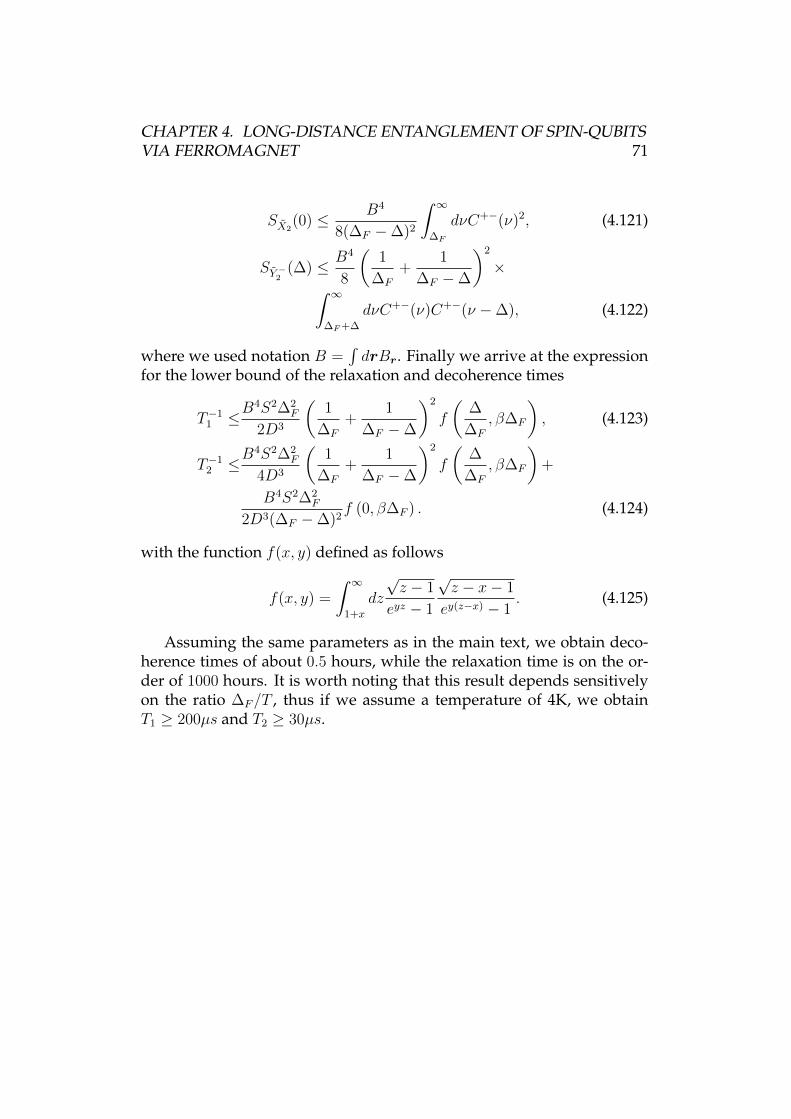
CHAPTER 4. LONG-DISTANCE ENTANGLEMENT OF SPIN-QUBITSVIA FERROMAGNET 71
SX2(0) ≤ B4
8(∆F −∆)2
∫ ∞
∆F
dνC+−(ν)2, (4.121)
SY −2 (∆) ≤ B4
8
(1
∆F
+1
∆F −∆
)2
×∫ ∞
∆F+∆
dνC+−(ν)C+−(ν −∆), (4.122)
where we used notation B =∫drBr. Finally we arrive at the expression
for the lower bound of the relaxation and decoherence times
T−11 ≤B
4S2∆2F
2D3
(1
∆F
+1
∆F −∆
)2
f
(∆
∆F
, β∆F
), (4.123)
T−12 ≤B
4S2∆2F
4D3
(1
∆F
+1
∆F −∆
)2
f
(∆
∆F
, β∆F
)+
B4S2∆2F
2D3(∆F −∆)2f (0, β∆F ) . (4.124)
with the function f(x, y) defined as follows
f(x, y) =
∫ ∞
1+x
dz
√z − 1
eyz − 1
√z − x− 1
ey(z−x) − 1. (4.125)
Assuming the same parameters as in the main text, we obtain deco-herence times of about 0.5 hours, while the relaxation time is on the or-der of 1000 hours. It is worth noting that this result depends sensitivelyon the ratio ∆F/T , thus if we assume a temperature of 4K, we obtainT1 ≥ 200µs and T2 ≥ 30µs.
CHAPTER 5Long-Range Interaction of
Spin-Qubits via Ferromagnets
Adapted from:Luka Trifunovic, Fabio L. Pedrocchi, and Daniel Loss,
“Long-Range Interaction of Singlet-Triplet Qubits via Ferromagnets”,ArXiv: 1305.2451 (2013).
We propose a mechanism of a long-range coherent interaction between twosinglet-triplet qubits dipolarly coupled to a dogbone-shaped ferromagnet.An effective qubit-qubit interaction Hamiltonian is derived and the cou-pling strength is estimated. Furthermore we derive the effective couplingbetween two spin-1/2 qubits that are coupled via dipolar interaction to theferromagnet and that lie at arbitrary positions and deduce the optimal po-sitioning. We consider hybrid systems consisting of spin-1/2 and ST qubitsand derive the effective Hamiltonian for this case. We then show that op-eration times vary between 1MHz and 100MHz and give explicit estimatesfor GaAs, Silicon, and NV-center based spin qubits. Finally, we explicitlyconstruct the required sequences to implement a CNOT gate. The result-ing quantum computing architecture retains all the single qubit gates andmeasurement aspects of earlier approaches, but allows qubit spacing at dis-tances of order 1µm for two-qubit gates, achievable with current semicon-ductor technology.
72
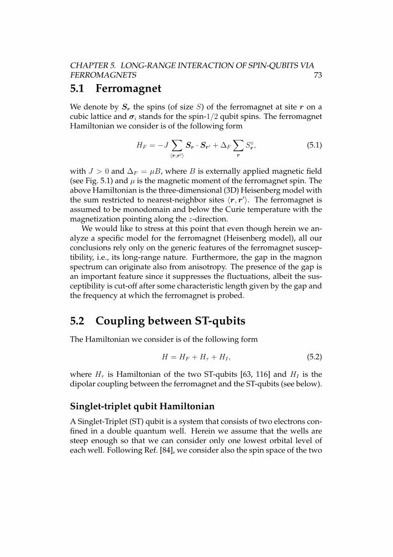
CHAPTER 5. LONG-RANGE INTERACTION OF SPIN-QUBITS VIAFERROMAGNETS 73
5.1 FerromagnetWe denote by Sr the spins (of size S) of the ferromagnet at site r on acubic lattice and σi stands for the spin-1/2 qubit spins. The ferromagnetHamiltonian we consider is of the following form
HF = −J∑
〈r,r′〉
Sr · Sr′ + ∆F
∑
r
Szr, (5.1)
with J > 0 and ∆F = µB, where B is externally applied magnetic field(see Fig. 5.1) and µ is the magnetic moment of the ferromagnet spin. Theabove Hamiltonian is the three-dimensional (3D) Heisenberg model withthe sum restricted to nearest-neighbor sites 〈r, r′〉. The ferromagnet isassumed to be monodomain and below the Curie temperature with themagnetization pointing along the z-direction.
We would like to stress at this point that even though herein we an-alyze a specific model for the ferromagnet (Heisenberg model), all ourconclusions rely only on the generic features of the ferromagnet suscep-tibility, i.e., its long-range nature. Furthermore, the gap in the magnonspectrum can originate also from anisotropy. The presence of the gap isan important feature since it suppresses the fluctuations, albeit the sus-ceptibility is cut-off after some characteristic length given by the gap andthe frequency at which the ferromagnet is probed.
5.2 Coupling between ST-qubitsThe Hamiltonian we consider is of the following form
H = HF +Hτ +HI , (5.2)
where Hτ is Hamiltonian of the two ST-qubits [63, 116] and HI is thedipolar coupling between the ferromagnet and the ST-qubits (see below).
Singlet-triplet qubit Hamiltonian
A Singlet-Triplet (ST) qubit is a system that consists of two electrons con-fined in a double quantum well. Herein we assume that the wells aresteep enough so that we can consider only one lowest orbital level ofeach well. Following Ref. [84], we consider also the spin space of the two
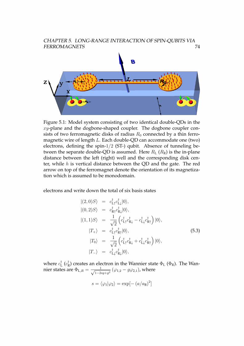
CHAPTER 5. LONG-RANGE INTERACTION OF SPIN-QUBITS VIAFERROMAGNETS 74
Figure 5.1: Model system consisting of two identical double-QDs in thexy-plane and the dogbone-shaped coupler. The dogbone coupler con-sists of two ferromagnetic disks of radius R0 connected by a thin ferro-magnetic wire of length L. Each double-QD can accommodate one (two)electrons, defining the spin-1/2 (ST-) qubit. Absence of tunneling be-tween the separate double-QD is assumed. Here RL (RR) is the in-planedistance between the left (right) well and the corresponding disk cen-ter, while h is vertical distance between the QD and the gate. The redarrow on top of the ferromagnet denote the orientation of its magnetiza-tion which is assumed to be monodomain.
electrons and write down the total of six basis states
|(2, 0)S〉 = c†L↑c†L↓|0〉,
|(0, 2)S〉 = c†R↑c†R↓|0〉,
|(1, 1)S〉 =1√2
(c†L↑c
†R↓ − c†L↓c†R↑
)|0〉,
|T+〉 = c†L↑c†R↑|0〉, (5.3)
|T0〉 =1√2
(c†L↑c
†R↓ + c†L↓c
†R↑
)|0〉,
|T−〉 = c†L↓c†R↓|0〉,
where c†L (c†R) creates an electron in the Wannier state ΦL (ΦR). The Wan-nier states are ΦL,R = 1√
1−2sg+g2(ϕ1,2 − gϕ2,1), where
s = 〈ϕ1|ϕ2〉 = exp[− (a/aB)2]
CHAPTER 5. LONG-RANGE INTERACTION OF SPIN-QUBITS VIAFERROMAGNETS 75
is the overlap of the harmonic oscillator ground state wave functions ofthe two wells, aB =
√~/mω0 is the Bohr radius of a single quantum dot,
~ω0 is the single-particle level spacing, and 2a = l is the interdot distance.The mixing factor of the Wannier states is g = (1−
√1− s2)/s. Using
these six basis states we can represent the Hamiltonian of the ST-qubits
H0 =
(HSS 0
0 HTT,0
). (5.4)
In writing the above equation we have neglected the spin-orbit interac-tion (SOI), thus there are no matrix elements coupling the singlet andtriplet blocks. The effect of SOI in ST-qubit was studied in Ref. [84] andno major influence on the qubit spectra was found.
The two qubit states are |T0〉 and, in the absence of SOI, the linearcombination of the singlet states |S〉 = α|(2, 0)S〉+ β|(1, 1)S〉+ γ|(0, 2)S〉,where the coefficients α, β, γ depend on the detuning ε between the twoquantum wells. In particular, when ε = 0 we have |S〉 = |(1, 1)S〉. Inwhat follows, we always consider Hamiltonians only in the qubit sub-space, thus the Hamiltonian of two ST-qubits reads
Hτ = −∆
2
∑
i=1,2
τ zi , (5.5)
where τx,y,z are the Pauli matrices acting in the space spanned by vectors|S〉, |T0〉 and ∆ is the ST-qubit splitting.
Dipolar coupling to ST-qubit
In this section we derive the dipolar coupling between the ferromagnetand the ST-qubit. To this end we first project the Zeeman coupling to theST-qubit system on the two-dimensional qubit subspace
HZ = g∗µB (BL · SL +BR · SR) , (5.6)
where BL (BR) is the magnetic field in the left (right) quantum well,SiL,R = (σi)ss′c
†L,R,scL,R,s′ and g∗ is the effective Lande factor. After pro-
jecting on the qubit space we obtain
HZ = g∗µB(BzL −Bz
R)τx. (5.7)
With this result we are ready to write down the ferromagnet/ST-qubitinteraction Hamiltonian
HI =∑
i=1,2
g∗µ0µB
(Bz
L(i)− BzR(i))τxi , (5.8)
CHAPTER 5. LONG-RANGE INTERACTION OF SPIN-QUBITS VIAFERROMAGNETS 76
where index i enumerates ST-qubits, and the magnetic field from the fer-romagnet can be express through the integral over the ferromagnet
BzL,R(i) =
µ0µ
4πa3
∫dr(i)L,R
1
r(i)3L,R× (5.9)
(Szr(i)L,R
−3(Sr(i)L,R · r(i)L,R)r(i)zL,R
r(i)2L,R
),
where the coordinate system for r(i)L (r(i)R) is positioned in left (right)quantum well of the i-th qubit.
Effective coupling between two ST-qubits
Given the total Hamitonian, Eq. (5.2), we can easily derive the effectivequbit-qubit coupling with help of Schrieffer-Wolff transformation
Heff = Hτ − limν→0+
i
2
∫ ∞
0
dte−νt [HI(t), HI ] , (5.10)
with HI(t) = eiHτ tHIe−iHτ t.
We assume that the radius of the two disks is much smaller than thedistance between their centers (R0 L). Within this assumption we cantake for the susceptibility between two points at opposite disks the sameas the 1D susceptibility. Next we take only on-resonance susceptibilityand make use of the expression τx(∆) = 1
2(τx + iτ y), where τx(ω) is the
Fourier transform of τx(t) = eiHτ tτxe−iHτ t. We define the transverse sus-ceptibility in the standard way
χ⊥(ω, ri − rj) = −i limη→0+
∫ ∞
0
dte(−iω−η)t[S+ri
(t), S−rj ]. (5.11)
The longitudinal susceptibility, defined via
χ‖(ω, ri − rj) = −i limη→0+
∫ ∞
0
dte(−iω−η)t[Szri(t), Szrj
], (5.12)
can be neglected compared to the transverse one because the former issmaller by a factor 1/S and is proportional to the magnon occupationnumber. Therefore the longitudinal susceptibility vanishes at zero tem-perature, while the is not the case for the transverse susceptibility. Wearrive finally at the following expression
Heff = Hτ +9
4Bχ1D⊥ (∆, L)τx1 τ
x2 , (5.13)
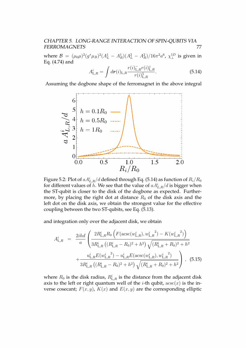
CHAPTER 5. LONG-RANGE INTERACTION OF SPIN-QUBITS VIAFERROMAGNETS 77
where B = (µ0µ)2(g∗µB)2(A1L − A1
R)(A2L − A2
R)/16π2a6, χ1D⊥ is given in
Eq. (4.74) and
AiL,R =
∫dr(i)L,R
r(i)−L,Rr(i)zL,R
r(i)5L,R
. (5.14)
Assuming the dogbone shape of the ferromagnet in the above integral
Figure 5.2: Plot of aAiL,R/d defined through Eq. (5.14) as function ofRi/R0
for different values of h. We see that the value of aAiL,R/d is bigger whenthe ST-qubit is closer to the disk of the dogbone as expected. Further-more, by placing the right dot at distance R0 of the disk axis and theleft dot on the disk axis, we obtain the strongest value for the effectivecoupling between the two ST-qubits, see Eq. (5.13).
and integration only over the adjacent disk, we obtain
AiL,R =2ihd
a
2RiL,RR0
(F (acsc(wiL,R), wiL,R
2)−K(wiL,R
2))
3RiL,R
((Ri
L,R −R0)2 + h2)√
(RiL,R +R0)2 + h2
+uiL,RE(wiL,R
2)− uiL,RE(acsc(wiL,R), wiL,R
2)
3RiL,R
((Ri
L,R −R0)2 + h2)√
(RiL,R +R0)2 + h2
, (5.15)
where R0 is the disk radius, RiL,R is the distance from the adjacent disk
axis to the left or right quantum well of the i-th qubit, acsc(x) is the in-verse cosecant; F (x, y), K(x) and E(x, y) are the corresponding elliptic
CHAPTER 5. LONG-RANGE INTERACTION OF SPIN-QUBITS VIAFERROMAGNETS 78
integrals. Furthermore, we introduced the notation uiL,R = RiL,R
2+R2
0 +h2
and wiL,R =
√1− 4RiL,RR0
(RiL,R+R0)2+h2 , where h is the distance in the z-direction
between the ST-qubit plane and the adjacent disk bottom and d is thedisk thickness, see Fig. 5.1.
Figure 5.2 illustrates the dependence of the AiL,R integrals on the po-sition of the quantum wells. Since the coupling constant is given by thedifference of this integrals for left and right quantum well, we concludethat the strongest coupling is obtained if one quantum well of the ST-qubit is positioned below the disk center and the other exactly below theedge. Furthermore, when h R0 the value of the integral is stronglypeaked around R ∼ R0 and this can be exploited as yet another switch-ing mechanism—moving one quantum well away from the edge of thedisk.
Sequence for CNOT gate
Two qubits interacting via the ferromagnet evolve according to the Hamil-tonian Heff , see Eq. (5.13). The Hamiltonian is therefore the sum of Zee-man terms and qubit-qubit interaction. These terms do not commute,making it difficult to use the evolution to implement standard entan-gling gates. Nevertheless, since Hτ acts only in the subspace spannedby | ↑↑〉, | ↓↓〉 and ∆ J12 = 9Bχ⊥(∆)/4, we can neglect the effect ofHeff in this part of the space and approximate it by its projection in thespace spanned by vectors | ↑↓〉, | ↓↑〉
H ′eff = Hτ + J12(τx1 τx2 + τ y1 τ
y2 ). (5.16)
Within this approximation, the coupling in H ′eff and Zeeman terms nowcommute.
We consider the implementation of the iSWAP gate [103]
UiSWAP = e−i(τx1 τ
x2 +τy1 τ
y2 )3π/4,
which can be used to implement the CNOT gate:
UiSWAP = eiHτ te−iH′eff t, (5.17)
where t = 3π/(4J12). When iSWAP is available, the CNOT gate can beconstructed in the standard way [104]
UCNOT = e−iπ4τz1 ei
π4τx2 ei
π4τz2UiSWAP e
−iπ4τx1 UiSWAP e
iπ4τz2 . (5.18)
CHAPTER 5. LONG-RANGE INTERACTION OF SPIN-QUBITS VIAFERROMAGNETS 79
Since H ′eff is an approximation of Heff , the above sequence will yieldapproximate CNOT, U ′CNOT , when used with the full Hamiltonian. Thesuccess of the sequences therefore depends on the fidelity of the gates,F (U ′CNOT ). Ideally this would be defined using a minimization over allpossible states of two qubits. However, to characterize the fidelity ofan imperfect CNOT it is sufficient to consider the following four logicalstates of two qubits [60]: |+, 0〉, |+, 1〉, |−, 0〉, and |−, 1〉. These are prod-uct states which, when acted upon by a perfect CNOT, become the fourmaximally entangled Bell states |Φ+〉, |Ψ+〉, |Φ−〉, and |Ψ−〉, respectively.As such, the fidelity of an imperfect CNOT may be defined,
F (U ′CNOT ) = mini∈+,−,j∈0,1
|〈i, j|U †CNOTU ′CNOT |i, j〉|2. (5.19)
The choice of basis used here ensures that F (U ′CNOT ) gives a good char-acterization of the properties of U ′CNOT in comparison to a perfect CNOT,especially for the required task of generating entanglement. For realis-tic parameters, with the Zeeman terms two order of magnitude strongerthan the qubit-qubit coupling, the above sequence yields fidelity for theCNOT gate of 99.976%.
To compare these values to the thresholds found in schemes for quan-tum computation, we must first note that imperfect CNOT’s in thesecases are usually modelled by the perfect implementation of the gate fol-lowed by depolarizing noise at a certain probability. It is known that suchnoisy CNOT’s can be used for quantum computation in the surface codeif the depolarizing probability is less than 1.1% [20]. This corresponds toa fidelity, according to the definition above, of 99.17%. The fidelities thatmay be achieved in the schemes proposed here are well above this valueand hence, though they do not correspond to the same noise model, wecan expect these gates to be equally suitable for fault-tolerant quantumcomputation.
5.3 Coupling between spin-1/2 qubitsIn this section we study the coupling of two spin-1/2 quantum dots viainteraction with a dog-bone shaped ferromagnet. The Hamiltonian hasagain the form as in Eq. (5.2) and we allow for splittings of the spin-1/2qubits both along x and z direction,
Hσ =∆x
2
∑
i=1,2
σxi +∆z
2
∑
i=1,2
σzi , (5.20)
CHAPTER 5. LONG-RANGE INTERACTION OF SPIN-QUBITS VIAFERROMAGNETS 80
where σi are the Pauli operators of the ith spin-1/2 quantum dot. Hamil-tonian (5.20) is a generalized version of the Hamiltonian [60], where weconsidered splitting along x only. We present here a detailed derivationof the effective coupling between two quantum dots located at an arbi-trary position with respect to the dogbone shaped ferromagnet, i.e., con-trary to Ref. [60] we do not assume that the quantum dots are positionedat a highly symmetric point but consider the most general case. Thisallows us to determine the optimal positioning of the qubit in order toachieve the strongest coupling between the qubits.
The dipolar coupling between the ferromagnet and the spin-1/2 qubitsis given by
HI =∑
i,r
g∗µ0µBµ
4πr3
(σi · Sr −
3(σi · r)(Sr · r)
r2
), (5.21)
where µD is the magnetic moment of the spin-1/2 qubit. The explicitexpressions for the time evolution of the Pauli operators in Heisenbergpicture is
σ+i (t) = − 1
∆2(i∆ cos(∆t/2)−∆z sin(∆t/2))2σ+
i
− ∆2x
2∆2(cos(t∆)− 1)σ−i
+∆x
∆2(∆z −∆z cos(t∆)− i∆ sin(t∆))σzi ,
σzi (t) =∆x
2∆2(∆z −∆z cos(t∆)− i∆ sin(t∆))σ+
i
+∆x
2∆2(∆z −∆z cos(t∆) + i∆ sin(t∆))σ−i
+∆2z + ∆2
x cos(t∆)
∆2σzi , (5.22)
where we introduced the notation ∆ =√
∆2x + ∆2
z. We also assumethat ∆ < ∆F such that the susceptibility χ⊥(∆, r) is purely real—thusthe transverse noise is gapped. By replacing the above expressions in
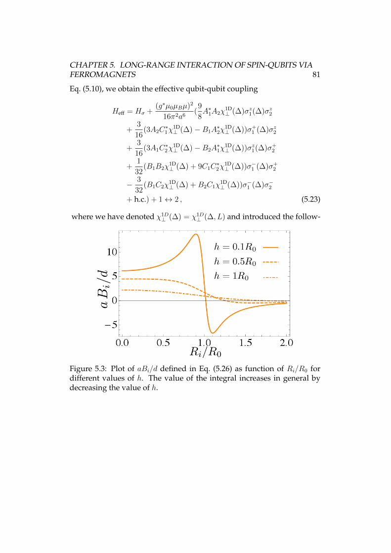
CHAPTER 5. LONG-RANGE INTERACTION OF SPIN-QUBITS VIAFERROMAGNETS 81
Eq. (5.10), we obtain the effective qubit-qubit coupling
Heff = Hσ +(g∗µ0µBµ)2
16π2a6(9
8A∗1A2χ
1D⊥ (∆)σz1(∆)σz2
+3
16(3A2C
∗1χ
1D⊥ (∆)−B1A
∗2χ
1D⊥ (∆))σ+
1 (∆)σz2
+3
16(3A1C
∗2χ
1D⊥ (∆)−B2A
∗1χ
1D⊥ (∆))σz1(∆)σ+
2
+1
32(B1B2χ
1D⊥ (∆) + 9C1C
∗2χ
1D⊥ (∆))σ−1 (∆)σ+
2
− 3
32(B1C2χ
1D⊥ (∆) +B2C1χ
1D⊥ (∆))σ−1 (∆)σ−2
+ h.c.) + 1↔ 2 , (5.23)
where we have denoted χ1D⊥ (∆) = χ1D
⊥ (∆, L) and introduced the follow-
Figure 5.3: Plot of aBi/d defined in Eq. (5.26) as function of Ri/R0 fordifferent values of h. The value of the integral increases in general bydecreasing the value of h.
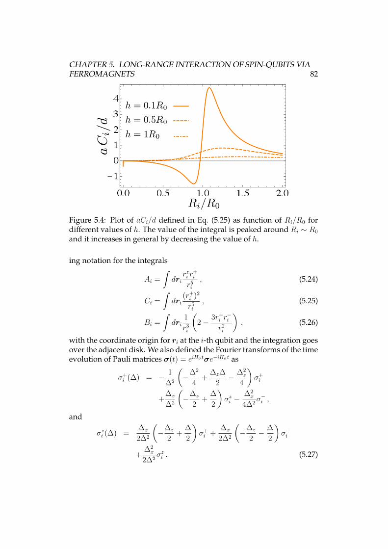
CHAPTER 5. LONG-RANGE INTERACTION OF SPIN-QUBITS VIAFERROMAGNETS 82
Figure 5.4: Plot of aCi/d defined in Eq. (5.25) as function of Ri/R0 fordifferent values of h. The value of the integral is peaked around Ri ∼ R0
and it increases in general by decreasing the value of h.
ing notation for the integrals
Ai =
∫dri
rzi r+i
r5i
, (5.24)
Ci =
∫dri
(r+i )2
r5i
, (5.25)
Bi =
∫dri
1
r3i
(2− 3r+
i r−i
r2i
), (5.26)
with the coordinate origin for ri at the i-th qubit and the integration goesover the adjacent disk. We also defined the Fourier transforms of the timeevolution of Pauli matrices σ(t) = eiHσtσe−iHσt as
σ+i (∆) = − 1
∆2
(−∆2
4+
∆z∆
2− ∆2
z
4
)σ+i
+∆x
∆2
(−∆z
2+
∆
2
)σzi −
∆2x
4∆2σ−i ,
and
σzi (∆) =∆x
2∆2
(−∆z
2+
∆
2
)σ+i +
∆x
2∆2
(−∆z
2− ∆
2
)σ−i
+∆2x
2∆2σzi . (5.27)
CHAPTER 5. LONG-RANGE INTERACTION OF SPIN-QUBITS VIAFERROMAGNETS 83
By assuming a dogbone-shaped ferromagnet and integrating only overthe adjacent disk as above, we obtain Ai given in Eq. (5.15) with Ri
L,R
replaced by Ri since there is now only one spin-1/2 qubit below eachdisk of the dogbone. The remaining integrals yield the following results
Bi = −2d
3a
(R4i + 3R2
i (h2 −R20) + (R2
0 + h2)2)E (1− w2
i )
R2i ((Ri −R0)2 + h2)
√(Ri +R0)2 + h2
,
−((Ri −R0)2 + h2) (R2i + 2 (R2
0 + h2))K (1− w2i )
R2i ((Ri −R0)2 + h2)
√(Ri +R0)2 + h2
)
Ci =2d
a
((Ri −R0)2 + h2)K (1− w2i )− 2 (R2
i −R20 + h2)E (1− w2
i )
((Ri −R0)2 + h2)√
(Ri +R0)2 + h2,
(5.28)
where wi =√
1− 4RiR0
(Ri+R0)2+h2 , R0 is the radius of each disk, Ri is the dis-tance of the i-th qubit to the adjacent dog bone axis, and R0 and h aredefined as in Sec. 5.2. In deriving Eq. (5.23) we took again only ‘on-resonance’ terms into account (i.e. we neglected χ1D
⊥ (0) and χ1D⊥ (−∆)).
Furthermore we assumed, as above, that the susceptibility between twopoints on different disks of the dogbone is well approximated by the 1Dtransverse susceptibility. In the limit where each quantum dot lies on thevertical axis going through the center of each cylinder of the dogbone,the axial symmetry leads to A1 = A2 = C1 = C2 = 0, B1 = B2 = B, andwith ∆z = 0 we recover the result
Heff = Hσ +(g∗µ0µBµ)2
16 π2a6
B2
32χ1D⊥ (∆)(2σy1σ
y2 + σz1σ
x2 + σx1σ
z2) (5.29)
derived in Ref. [60]. The analysis carried out herein assumes arbitrary po-sitioning of the qubit and allow us to determine the optimal positioningfor the strongest coupling. To this end, we analyze integrals Ai, Bi, Ci,see Figs. 5.2-5.4. It is readily observed that the coupling strength in-creases as the vertical distance between the qubit and coupler plane, h,decreases. Additionally, we observe that the strongest coupling strengthis obtained when the qubit is positioned below the edge of the adjacentdisk.
The derived coupling is valid for any dogbone-like shape of the fer-romagnet, i.e., it is not crucial to assume disk shape.
CHAPTER 5. LONG-RANGE INTERACTION OF SPIN-QUBITS VIAFERROMAGNETS 84
Sequence for CNOT gate
The effective Hamiltonian derived in previous section, Eq. (5.23), can bere-expressed in the following form
Heff =(g∗µ0µBµ)2
16π2a6χ1D⊥ (∆, L)σT1 · H · σ2 +
1
2∆ · (σ1 + σ2), (5.30)
with ∆ = (∆x, 0,∆z)T and H being the symmetric matrix with all entries
being non-zero. The question now arises how to construct the CNOTgate sequence for such a general Hamiltonian. We tackle this problem bytaking first the quantization axis to be along the total magnetic field act-ing on the two qubits and denote by σi Pauli matrix vector with respectto this new quantization axis. The Hamiltonian now reads
Heff =(g∗µ0µBµ)2
16π2a6χ1D⊥ (∆, L) σT1 · ˆH · σ2 +
1
2∆(σz1 + σz2), (5.31)
where the components of the matrix ˆH are given in Appendix 5.A.We proceed further along the lines presented in Sec. 5.2, i.e., we project
the rotated Hamiltonian, Eq. (5.31), on the subspace spanned by vectors|↑↓〉, |↓↑〉. This procedure yields the following result
H ′eff = J12(σx1 σx2 + σy1 σ
y2) + ∆(σz1 + σz2), (5.32)
J12 = (µ0g∗µBµ)2
(4π)2a6
χ1D⊥ (∆,L)
32A12. The dimensionless constant A12 is defined
through the following expression
A12 =∆x
2 (36A1A2 + (B1 + 3C1) (B2 + 3C2))
16∆2
+6∆x∆z (A2 (B1 − 3C1) + A1 (B2 − 3C2))
16∆2
+2∆z (B1B2 + 9C1C2) (∆ + ∆z)
16∆2. (5.33)
The projected Hamiltonian in Eq. (5.32) is identical to the one alreadyconsidered in Sec. 5.2, Eq. (5.16). Thus the CNOT gate sequence can beobtained in exactly same way, namely via Eqs. (5.17) and (5.18).
Similar to the previously studied case of ST-qubits, the CNOT gatesequence described in this section is only approximate one. For realis-tic parameters, with the Zeeman terms two order of magnitude stronger
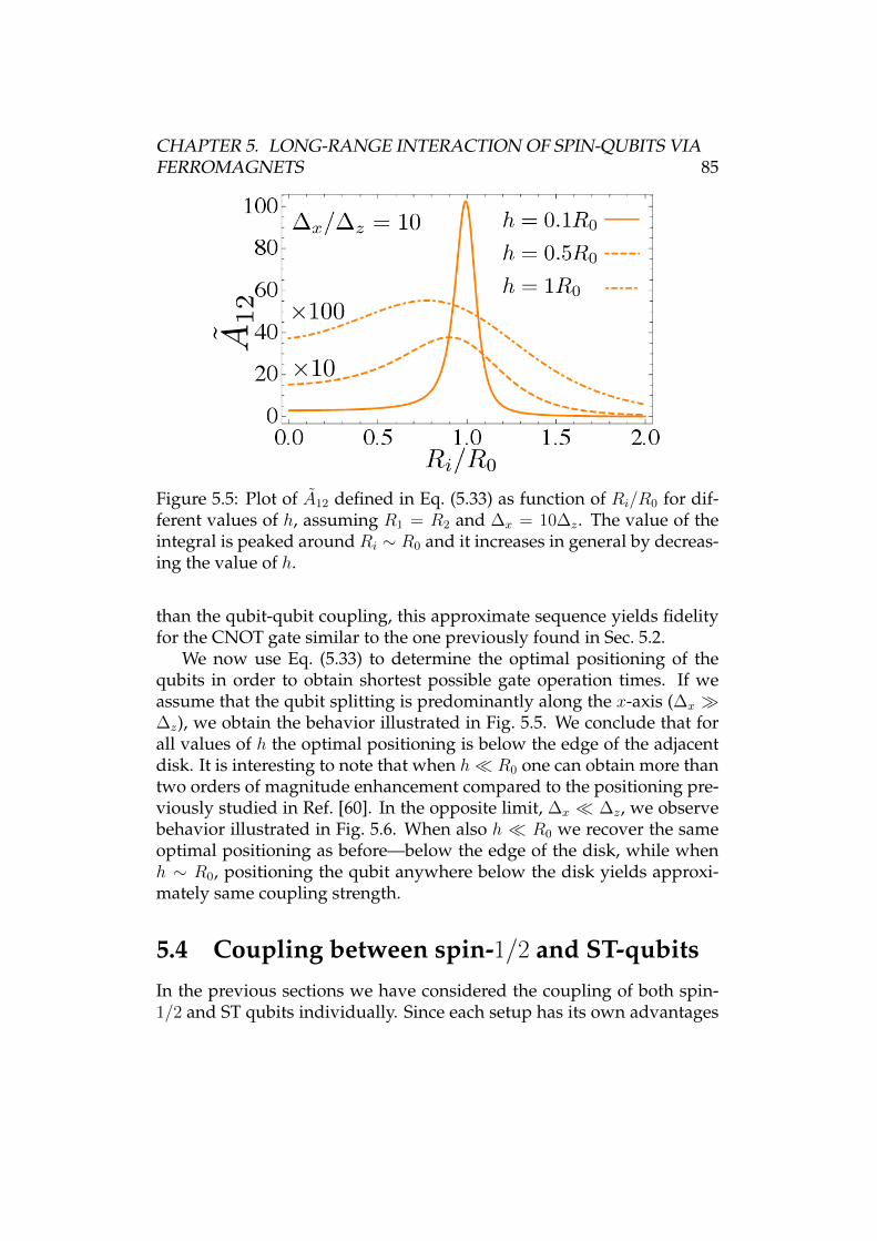
CHAPTER 5. LONG-RANGE INTERACTION OF SPIN-QUBITS VIAFERROMAGNETS 85
Figure 5.5: Plot of A12 defined in Eq. (5.33) as function of Ri/R0 for dif-ferent values of h, assuming R1 = R2 and ∆x = 10∆z. The value of theintegral is peaked around Ri ∼ R0 and it increases in general by decreas-ing the value of h.
than the qubit-qubit coupling, this approximate sequence yields fidelityfor the CNOT gate similar to the one previously found in Sec. 5.2.
We now use Eq. (5.33) to determine the optimal positioning of thequbits in order to obtain shortest possible gate operation times. If weassume that the qubit splitting is predominantly along the x-axis (∆x ∆z), we obtain the behavior illustrated in Fig. 5.5. We conclude that forall values of h the optimal positioning is below the edge of the adjacentdisk. It is interesting to note that when h R0 one can obtain more thantwo orders of magnitude enhancement compared to the positioning pre-viously studied in Ref. [60]. In the opposite limit, ∆x ∆z, we observebehavior illustrated in Fig. 5.6. When also h R0 we recover the sameoptimal positioning as before—below the edge of the disk, while whenh ∼ R0, positioning the qubit anywhere below the disk yields approxi-mately same coupling strength.
5.4 Coupling between spin-1/2 and ST-qubitsIn the previous sections we have considered the coupling of both spin-1/2 and ST qubits individually. Since each setup has its own advantages
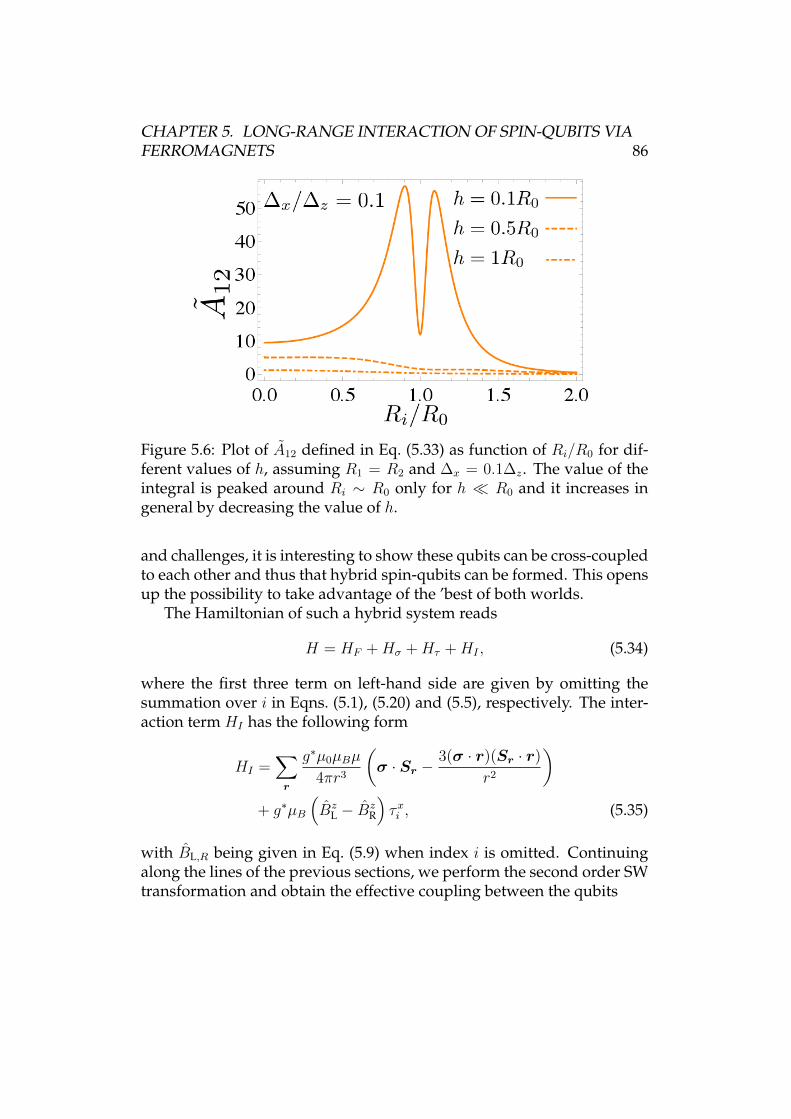
CHAPTER 5. LONG-RANGE INTERACTION OF SPIN-QUBITS VIAFERROMAGNETS 86
Figure 5.6: Plot of A12 defined in Eq. (5.33) as function of Ri/R0 for dif-ferent values of h, assuming R1 = R2 and ∆x = 0.1∆z. The value of theintegral is peaked around Ri ∼ R0 only for h R0 and it increases ingeneral by decreasing the value of h.
and challenges, it is interesting to show these qubits can be cross-coupledto each other and thus that hybrid spin-qubits can be formed. This opensup the possibility to take advantage of the ’best of both worlds.
The Hamiltonian of such a hybrid system reads
H = HF +Hσ +Hτ +HI , (5.34)
where the first three term on left-hand side are given by omitting thesummation over i in Eqns. (5.1), (5.20) and (5.5), respectively. The inter-action term HI has the following form
HI =∑
r
g∗µ0µBµ
4πr3
(σ · Sr −
3(σ · r)(Sr · r)
r2
)
+ g∗µB
(Bz
L − BzR
)τxi , (5.35)
with BL,R being given in Eq. (5.9) when index i is omitted. Continuingalong the lines of the previous sections, we perform the second order SWtransformation and obtain the effective coupling between the qubits
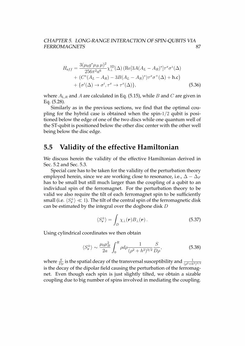
CHAPTER 5. LONG-RANGE INTERACTION OF SPIN-QUBITS VIAFERROMAGNETS 87
Heff =3(µ0g
∗µB µ)2
256π2a6χ1D⊥ (∆) (Re[3A(AL − AR)∗]τxσz(∆)
+ (C∗(AL − AR)− 3B(AL − AR)∗)τxσ+(∆) + h.c)
+ σi(∆)→ σi, τx → τx(∆), (5.36)
where AL,R and A are calculated in Eq. (5.15), while B and C are given inEq. (5.28).
Similarly as in the previous sections, we find that the optimal cou-pling for the hybrid case is obtained when the spin-1/2 qubit is posi-tioned below the edge of one of the two discs while one quantum well ofthe ST-qubit is positioned below the other disc center with the other wellbeing below the disc edge.
5.5 Validity of the effective HamiltonianWe discuss herein the validity of the effective Hamiltonian derived inSec. 5.2 and Sec. 5.3.
Special care has to be taken for the validity of the perturbation theoryemployed herein, since we are working close to resonance, i.e., ∆ − ∆F
has to be small but still much larger than the coupling of a qubit to anindividual spin of the ferromagnet. For the perturbation theory to bevalid we also require the tilt of each ferromagnet spin to be sufficientlysmall (i.e. 〈S±r 〉 1). The tilt of the central spin of the ferromagnetic diskcan be estimated by the integral over the dogbone disk D
〈S±r 〉 =
∫
D
χ⊥(r)B⊥(r) . (5.37)
Using cylindrical coordinates we then obtain
〈S±r 〉 ∼µ0µ
2B
2a
∫ R
0
ρdρ1
(ρ2 + h2)3/2
S
Dρ, (5.38)
where SDρ
is the spatial decay of the transversal susceptibility and 1(ρ2+h2)3/2
is the decay of the dipolar field causing the perturbation of the ferromag-net. Even though each spin is just slightly tilted, we obtain a sizablecoupling due to big number of spins involved in mediating the coupling.
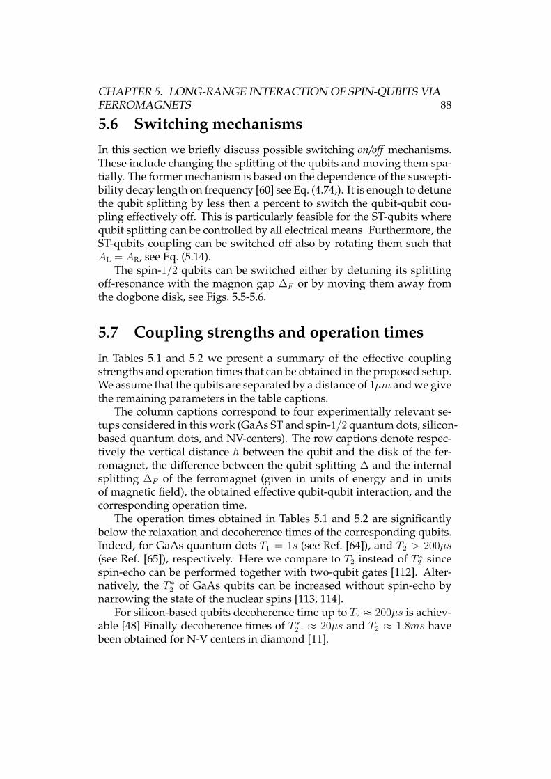
CHAPTER 5. LONG-RANGE INTERACTION OF SPIN-QUBITS VIAFERROMAGNETS 88
5.6 Switching mechanismsIn this section we briefly discuss possible switching on/off mechanisms.These include changing the splitting of the qubits and moving them spa-tially. The former mechanism is based on the dependence of the suscepti-bility decay length on frequency [60] see Eq. (4.74,). It is enough to detunethe qubit splitting by less then a percent to switch the qubit-qubit cou-pling effectively off. This is particularly feasible for the ST-qubits wherequbit splitting can be controlled by all electrical means. Furthermore, theST-qubits coupling can be switched off also by rotating them such thatAL = AR, see Eq. (5.14).
The spin-1/2 qubits can be switched either by detuning its splittingoff-resonance with the magnon gap ∆F or by moving them away fromthe dogbone disk, see Figs. 5.5-5.6.
5.7 Coupling strengths and operation timesIn Tables 5.1 and 5.2 we present a summary of the effective couplingstrengths and operation times that can be obtained in the proposed setup.We assume that the qubits are separated by a distance of 1µm and we givethe remaining parameters in the table captions.
The column captions correspond to four experimentally relevant se-tups considered in this work (GaAs ST and spin-1/2 quantum dots, silicon-based quantum dots, and NV-centers). The row captions denote respec-tively the vertical distance h between the qubit and the disk of the fer-romagnet, the difference between the qubit splitting ∆ and the internalsplitting ∆F of the ferromagnet (given in units of energy and in unitsof magnetic field), the obtained effective qubit-qubit interaction, and thecorresponding operation time.
The operation times obtained in Tables 5.1 and 5.2 are significantlybelow the relaxation and decoherence times of the corresponding qubits.Indeed, for GaAs quantum dots T1 = 1s (see Ref. [64]), and T2 > 200µs(see Ref. [65]), respectively. Here we compare to T2 instead of T ∗2 sincespin-echo can be performed together with two-qubit gates [112]. Alter-natively, the T ∗2 of GaAs qubits can be increased without spin-echo bynarrowing the state of the nuclear spins [113, 114].
For silicon-based qubits decoherence time up to T2 ≈ 200µs is achiev-able [48] Finally decoherence times of T ∗2 . ≈ 20µs and T2 ≈ 1.8ms havebeen obtained for N-V centers in diamond [11].
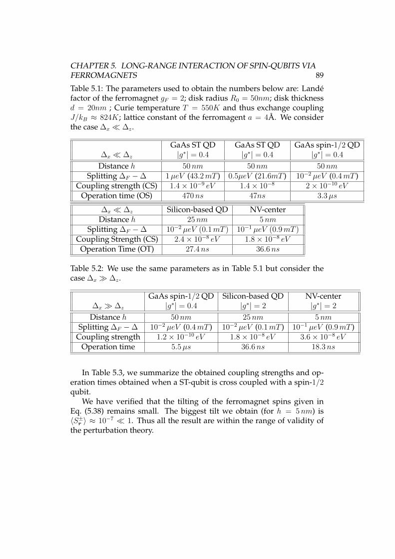
CHAPTER 5. LONG-RANGE INTERACTION OF SPIN-QUBITS VIAFERROMAGNETS 89
Table 5.1: The parameters used to obtain the numbers below are: Landefactor of the ferromagnet gF = 2; disk radius R0 = 50nm; disk thicknessd = 20nm ; Curie temperature T = 550K and thus exchange couplingJ/kB ≈ 824K; lattice constant of the ferromagent a = 4A. We considerthe case ∆x ∆z.
GaAs ST QD GaAs ST QD GaAs spin-1/2 QD∆x ∆z |g∗| = 0.4 |g∗| = 0.4 |g∗| = 0.4
Distance h 50nm 50nm 50nmSplitting ∆F −∆ 1µeV (43.2mT ) 0.5µeV (21.6mT ) 10−2 µeV (0.4mT )
Coupling strength (CS) 1.4× 10⁻⁹ eV 1.4× 10⁻⁸ 2× 10⁻¹⁰ eVOperation time (OS) 470ns 47ns 3.3µs
∆x ∆z Silicon-based QD NV-centerDistance h 25nm 5nm
Splitting ∆F −∆ 10−2 µeV (0.1mT ) 10−1 µeV (0.9mT )Coupling Strength (CS) 2.4× 10⁻⁸ eV 1.8× 10⁻⁸ eV
Operation Time (OT) 27.4ns 36.6ns
Table 5.2: We use the same parameters as in Table 5.1 but consider thecase ∆x ∆z.
GaAs spin-1/2 QD Silicon-based QD NV-center∆x ∆z |g∗| = 0.4 |g∗| = 2 |g∗| = 2
Distance h 50nm 25nm 5nmSplitting ∆F −∆ 10−2 µeV (0.4mT ) 10−2 µeV (0.1mT ) 10−1 µeV (0.9mT )
Coupling strength 1.2× 10⁻¹⁰ eV 1.8× 10⁻⁸ eV 3.6× 10⁻⁸ eVOperation time 5.5µs 36.6ns 18.3ns
In Table 5.3, we summarize the obtained coupling strengths and op-eration times obtained when a ST-qubit is cross coupled with a spin-1/2qubit.
We have verified that the tilting of the ferromagnet spins given inEq. (5.38) remains small. The biggest tilt we obtain (for h = 5nm) is〈S±r 〉 ≈ 10−7 1. Thus all the result are within the range of validity ofthe perturbation theory.
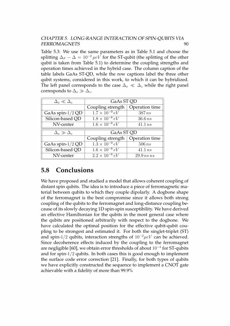
CHAPTER 5. LONG-RANGE INTERACTION OF SPIN-QUBITS VIAFERROMAGNETS 90
Table 5.3: We use the same parameters as in Table 5.1 and choose thesplitting ∆F − ∆ = 10−2 µeV for the ST-qubit (the splitting of the otherqubit is taken from Table 5.1) to determine the coupling strengths andoperation times achieved in the hybrid case. The column caption of thetable labels GaAs ST-QD, while the row captions label the three otherqubit systems, considered in this work, to which it can be hybridized.The left panel corresponds to the case ∆x ∆z while the right panelcorresponds to ∆x ∆z.
∆x ∆z GaAs ST QDCoupling strength Operation time
GaAs spin-1/2 QD 1.7× 10⁻⁹ eV 387nsSilicon-based QD 1.8× 10⁻⁸ eV 36.6ns
NV-center 1.6× 10⁻⁸ eV 41.1ns
∆x ∆z GaAs ST QDCoupling strength Operation time
GaAs spin-1/2 QD 1.3× 10⁻⁹ eV 506nsSilicon-based QD 1.6× 10⁻⁸ eV 41.1ns
NV-center 2.2× 10⁻⁸ eV 29.9ns ns
5.8 ConclusionsWe have proposed and studied a model that allows coherent coupling ofdistant spin qubits. The idea is to introduce a piece of ferromagnetic ma-terial between qubits to which they couple dipolarly. A dogbone shapeof the ferromagnet is the best compromise since it allows both strongcoupling of the qubits to the ferromagnet and long-distance coupling be-cause of its slowly decaying 1D spin-spin susceptibility. We have derivedan effective Hamiltonian for the qubits in the most general case wherethe qubits are positioned arbitrarily with respect to the dogbone. Wehave calculated the optimal position for the effective qubit-qubit cou-pling to be strongest and estimated it. For both the singlet-triplet (ST)and spin-1/2 qubits, interaction strengths of 10−2µeV can be achieved.Since decoherence effects induced by the coupling to the ferromagnetare negligible [60], we obtain error thresholds of about 10−4 for ST-qubitsand for spin-1/2 qubits. In both cases this is good enough to implementthe surface code error correction [21]. Finally, for both types of qubitswe have explicitly constructed the sequence to implement a CNOT gateachievable with a fidelity of more than 99.9%
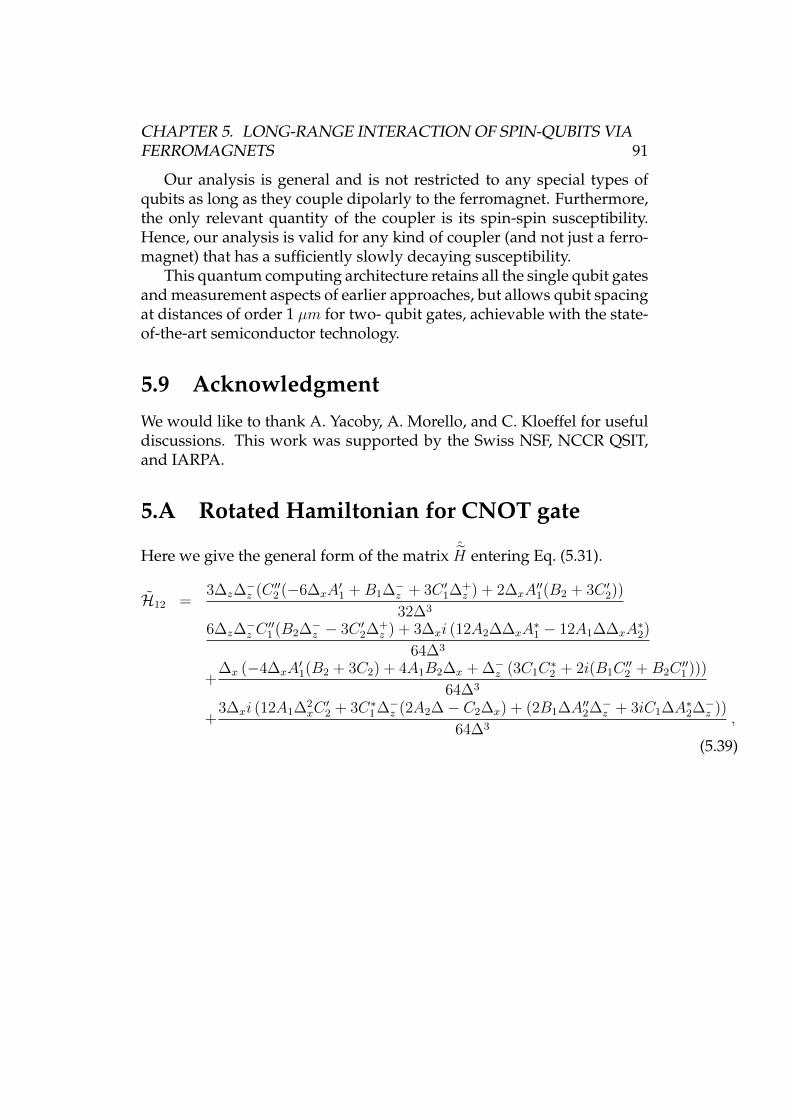
CHAPTER 5. LONG-RANGE INTERACTION OF SPIN-QUBITS VIAFERROMAGNETS 91
Our analysis is general and is not restricted to any special types ofqubits as long as they couple dipolarly to the ferromagnet. Furthermore,the only relevant quantity of the coupler is its spin-spin susceptibility.Hence, our analysis is valid for any kind of coupler (and not just a ferro-magnet) that has a sufficiently slowly decaying susceptibility.
This quantum computing architecture retains all the single qubit gatesand measurement aspects of earlier approaches, but allows qubit spacingat distances of order 1 µm for two- qubit gates, achievable with the state-of-the-art semiconductor technology.
5.9 AcknowledgmentWe would like to thank A. Yacoby, A. Morello, and C. Kloeffel for usefuldiscussions. This work was supported by the Swiss NSF, NCCR QSIT,and IARPA.
5.A Rotated Hamiltonian for CNOT gate
Here we give the general form of the matrix ˆH entering Eq. (5.31).
H12 =3∆z∆
−z (C ′′2 (−6∆xA
′1 +B1∆−z + 3C ′1∆+
z ) + 2∆xA′′1(B2 + 3C ′2))
32∆3
6∆z∆−z C′′1 (B2∆−z − 3C ′2∆+
z ) + 3∆xi (12A2∆∆xA∗1 − 12A1∆∆xA
∗2)
64∆3
+∆x (−4∆xA
′1(B2 + 3C2) + 4A1B2∆x + ∆−z (3C1C
∗2 + 2i(B1C
′′2 +B2C
′′1 )))
64∆3
+3∆xi (12A1∆2
xC′2 + 3C∗1∆−z (2A2∆− C2∆x) + (2B1∆A′′2∆−z + 3iC1∆A∗2∆−z ))
64∆3,
(5.39)
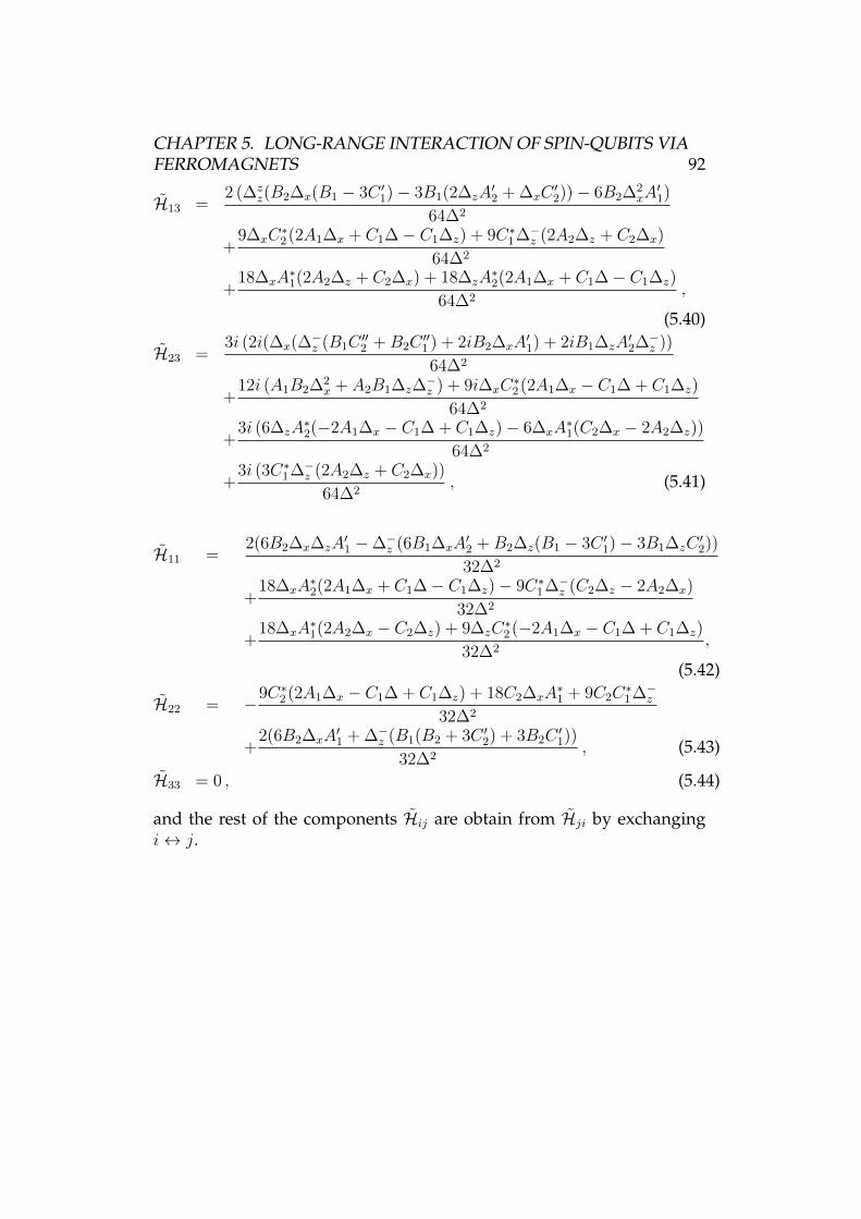
CHAPTER 5. LONG-RANGE INTERACTION OF SPIN-QUBITS VIAFERROMAGNETS 92
H13 =2 (∆z
z(B2∆x(B1 − 3C ′1)− 3B1(2∆zA′2 + ∆xC
′2))− 6B2∆2
xA′1)
64∆2
+9∆xC
∗2(2A1∆x + C1∆− C1∆z) + 9C∗1∆−z (2A2∆z + C2∆x)
64∆2
+18∆xA
∗1(2A2∆z + C2∆x) + 18∆zA
∗2(2A1∆x + C1∆− C1∆z)
64∆2,
(5.40)
H23 =3i (2i(∆x(∆
−z (B1C
′′2 +B2C
′′1 ) + 2iB2∆xA
′1) + 2iB1∆zA
′2∆−z ))
64∆2
+12i (A1B2∆2
x + A2B1∆z∆−z ) + 9i∆xC
∗2(2A1∆x − C1∆ + C1∆z)
64∆2
+3i (6∆zA
∗2(−2A1∆x − C1∆ + C1∆z)− 6∆xA
∗1(C2∆x − 2A2∆z))
64∆2
+3i (3C∗1∆−z (2A2∆z + C2∆x))
64∆2, (5.41)
H11 =2(6B2∆x∆zA
′1 −∆−z (6B1∆xA
′2 +B2∆z(B1 − 3C ′1)− 3B1∆zC
′2))
32∆2
+18∆xA
∗2(2A1∆x + C1∆− C1∆z)− 9C∗1∆−z (C2∆z − 2A2∆x)
32∆2
+18∆xA
∗1(2A2∆x − C2∆z) + 9∆zC
∗2(−2A1∆x − C1∆ + C1∆z)
32∆2,
(5.42)
H22 = −9C∗2(2A1∆x − C1∆ + C1∆z) + 18C2∆xA∗1 + 9C2C
∗1∆−z
32∆2
+2(6B2∆xA
′1 + ∆−z (B1(B2 + 3C ′2) + 3B2C
′1))
32∆2, (5.43)
H33 = 0 , (5.44)
and the rest of the components Hij are obtain from Hji by exchangingi↔ j.
Part II
Weak magnetic fieldamplification for
room-temperature magnetometry
93

CHAPTER 6Introduction
Magnetic resonance techniques not only provide powerful imaging toolsthat have revolutionized medicine, but they have a wide spectrum of ap-plications in other fields of science like biology, chemistry, neuroscience,and physics [117, 118]. In order to resolve structures on the nanome-ter scale and thus image individual molecules, however, one needs togo beyond conventional magnetometric techniques. In particular, stan-dard nuclear magnetic resonance (NMR) and magnetic resonance imag-ing (MRI) experiments detect magnetic fields through the current in-duced inside a coil according to Faraday’s law; unfortunately induction-based detection is not sensitive enough to allow resolution in the sub-micrometer regime [119].
Over the last years, a lot of experimental effort has been put intoimproving magnetic detection schemes. At present, Hall-sensors andSQUID sensors are among the most sensitive magnetic field detectors [120,121]. Furthermore, a great deal of success has been achieved with mag-netic resonance force microscopy, where the force between a magnetictip and the magnetic moment under investigation is exploited to de-tect single electron-spins, achieving a resolution of a few cubic nanome-ters [122, 123, 124]. On the other hand, the very low temperatures that arerequired in such schemes represent a considerable drawback to imagingsystems in many biological environments.
NV-center spins also provide very good candidates for magnetome-try, boosting sensitivities up to a few nT/
√Hz at room temperature [13,
14, 15, 16, 17, 18] and sub-nanometer spatial resolution, permitting three-dimensional imaging of nanostructures [14]. These results are realizable
94
CHAPTER 6. INTRODUCTION 95
due to the amazingly long decoherence times of NV-centers at room tem-perature and the ability to noninvasively engineer an NV-magnetometervery close to the magnetic sample. Although impressive, current state-of-the-art technology [19] is unable to detect a single nuclear spin; achievingsuch sensitivity would revolutionize magnetic imaging in chemical andbiological systems by facilitating atomic resolution of molecules.
In this work, we propose an experimental realization of NV-magne-tometers which could increase present NV-center sensitivities by four or-ders magnitude at room temperature; this unprecedented amplificationof sensitivity forecasts magnetometers capable of detecting individualnuclear spins. This can be achieved by introducing a ferromagnetic par-ticle between the spin that needs to be detected, which henceforth wecall a qubit,1 and the NV-magnetometer. When excited on resonanceby the driven qubit, the macroscopic ferromagnetic spin begins to pre-cess which, in turn, amplifies the magnetic field felt by the NV-center.By resonantly addressing the qubit and using a ferromagnetic resonatoras a lever, our setup, in contrast to existing schemes, is particularly ad-vantageous because, due to the large amplification of sensitivity, the nu-clear spin need not lie within a few nanometers of the surface [125] butrather can be detectable at a distance of 30 nm, and, while related exist-ing schemes rely on the quantum nature of a mediator spin [126], our pro-posal is fully classical. With these novelties, our scheme provides chemi-cally sensitive spin detection.
1We emphasize that we denote the target magnetic moment by ’qubit’ solely forthe purpose of convenience in nomenclature and that our scheme does not rely on thequantum nature of the magnetic moment we aim to measure.
CHAPTER 7High-efficiency resonant
amplification of weak magneticfields for single spin
magnetometry
Adapted from:Luka Trifunovic, Fabio L. Pedrocchi, Silas Hoffman, Patrick Maletinsky, Amir
Yacoby, and Daniel Loss“High-efficiency resonant amplification of weak magnetic fields for single spin
magnetometry”,Nature Nanotechnology 10, 541 (2015)
96
CHAPTER 7. HIGH-EFFICIENCY RESONANT AMPLIFICATION OFWEAK MAGNETIC FIELDS FOR SINGLE SPIN MAGNETOMETRY 97
Magnetic resonance techniques not only provide powerful imaging toolsthat have revolutionized medicine, but they have a wide spectrum of ap-plications in other fields of science like biology, chemistry, neuroscience,and physics. However, current state-of-the-art magnetometers are unableto detect a single nuclear spin unless the tip-to-sample separation is madesufficiently small. Here, we demonstrate theoretically that by placing a fer-romagnetic particle between a nitrogen-vacancy (NV) magnetometer and atarget spin, the magnetometer sensitivity is improved dramatically. Usingmaterials and techniques already experimentally available, our proposedsetup is sensitive enough to detect a single nuclear spin within ten millisec-onds of data acquisition at room temperature. The sensitivity is practicallyunchanged when the ferromagnet surface to the target spin separation issmaller than the ferromagnet lateral dimensions; typically about a tenth ofa micron. This scheme further benefits when used for NV ensemble mea-surements, enhancing sensitivity by an additional three orders of magni-tude. Our proposal opens the door for nanoscale nuclear magnetic reso-nance (NMR) on biological material under ambient conditions.
7.1 SetupThe standard experimental setup, yielding the most accurate NV-magne-tometers [14]), consists of an NV-center near the target qubit and two dis-tinct microwave sources that independently control the NV-center andqubit so that double electron-electron (electron-nuclear) resonance, DEER(DENR), can be performed. We extend this setup by including a macro-spin ferromagnetic particle (FM) between the NV-magnetometer and thequbit we want to measure, see Fig. 7.1. A recent experiment [127, 128]demonstrates that there is no significant quenching of the NV-center pho-toluminescence in the presence of the FM. On the other hand, due to thestray field of the FM, the qubit energy-splitting, and therefore the fre-quency (ωs) at which the qubit responds resonantly, is strongly modified;one needs first to characterize the FM stray field in order to be able to con-trol the qubit by, in our case, applying π-pulses.1 Treating the ferromag-net as a single classical spin, the Hamiltonian of this system is [130, 131]
H =KV (1−m2z) +MFV bmz − µsns(t) · BFm, (7.1)
1Instead of performing the qubit control resonantly, one can make use of ‘adiabaticpassage’ [129] wherein triangular pulses are applied in lieu of square pulses. In sucha setup, knowledge of the exact value of the qubit Zeeman splitting, and therefore theFM stray field, is not needed.
CHAPTER 7. HIGH-EFFICIENCY RESONANT AMPLIFICATION OFWEAK MAGNETIC FIELDS FOR SINGLE SPIN MAGNETOMETRY 98
where m is the normalized magnetization of the FM, MF the satura-tion magnetization of the FM, and V its volume. We assume uniaxialanisotropy in the FM with the anisotropy constant, K > 0, composed ofboth shape and crystalline anisotropy, with an easy axis along z. An ex-ternal magnetic field b is applied along the z axis. The magnetic momentof the qubit is µs andns(t) is its polarization at time t. The 3×3-matrix BFis defined as (BF )ij = Bj
F (rs)·ei, whereBjF (rs) is the stray field produced
by the FM at the position of the qubit, rs, when the FM is polarized alongthe j-axis for j = x, y, or z. The Hamiltonian of the qubit is not explic-itly written as its polarization is completely determined by the externallyapplied static and time-dependent microwave field and the stray field ofthe FM. For example, in equilibrium the ground state of the qubit is po-larized along the total static field acting on it ns = (b ± Bz
F )/|b ± BzF |
when mz = ±1. Although in the following we take V small enough toapproximate the FM as a monodomain, our analysis and therefore ourresults are amenable to including the effects of magnetic texture.
Using two independent microwave sources we apply a train of π-pulses first to the qubit and subsequently a Carr-Purcell-Meiboom-Gill(CPMG) pulse sequence [132, 133] to the NV-center, see Fig. 7.2. Asthe qubit is pulsed it will drive the FM at the frequency of the pulsesequence π/τ , τ being the time between the application of two subse-quent π-pulses. When π/τ is close to the ferromagnetic resonance (FMR)frequency, ωF , the response of the FM becomes large and one obtains alarge amplification of the magnetic field felt by the NV-center. The pulsesare applied to the qubit only until the FM reaches steady state preces-sion. We also allow for a possible time offset, ξ, between the pulse se-quences applied to the qubit and the NV-center, see Fig. 7.2. Here, ξ maybe chosen to compensate for the phase difference between the drivingof the qubit and the response of the FM, thus maximizing the sensitivityof our magnetometry scheme. Since the microwave field applied to thequbit is a sequence of π-pulses, the polarization is simplyns(t) = nsfτ (t),where fτ (t) may take the values ±1 according to the pulse sequence. Itis worth noting that even though we excite the FMR with the inhomo-geneous dipolar field of the qubit, only the lowest Kittel mode is excitedsince for a small FM higher modes are separated by an energy gap thatexceeds the perturbation amplitude. Therefore the macrospin approxi-mation used in Eq. (7.1) is justified.
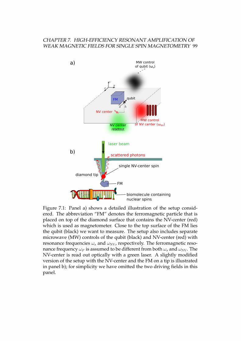
CHAPTER 7. HIGH-EFFICIENCY RESONANT AMPLIFICATION OFWEAK MAGNETIC FIELDS FOR SINGLE SPIN MAGNETOMETRY 99
NV center
qubitFM
NV centerreadout
MW controlof qubit (ωs)
MW controlof NV center (ωNV)
diamond tip
laser beam
single NV-center spin
scattered photons
FM
biomolecule containingnuclear spins
a)
b)
Figure 7.1: Panel a) shows a detailed illustration of the setup consid-ered. The abbreviation “FM” denotes the ferromagnetic particle that isplaced on top of the diamond surface that contains the NV-center (red)which is used as magnetometer. Close to the top surface of the FM liesthe qubit (black) we want to measure. The setup also includes separatemicrowave (MW) controls of the qubit (black) and NV-center (red) withresonance frequencies ωs and ωNV, respectively. The ferromagnetic reso-nance frequency ωF is assumed to be different from both ωs and ωNV. TheNV-center is read out optically with a green laser. A slightly modifiedversion of the setup with the NV-center and the FM on a tip is illustratedin panel b); for simplicity we have omitted the two driving fields in thispanel.
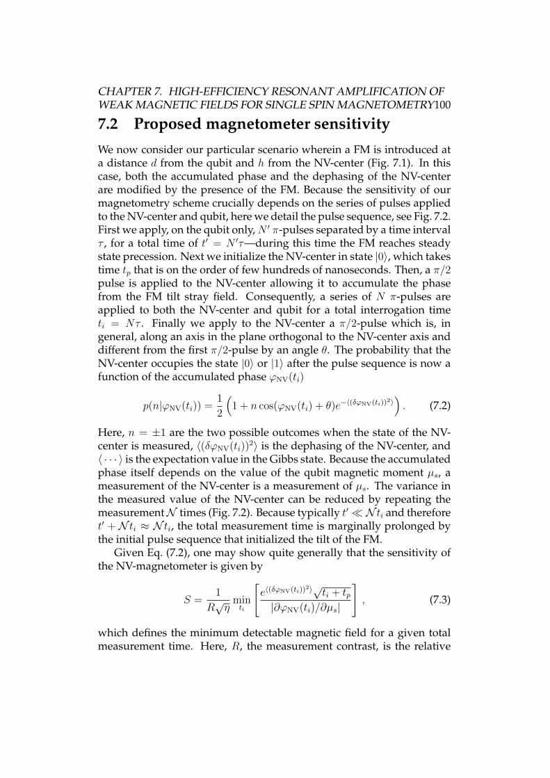
CHAPTER 7. HIGH-EFFICIENCY RESONANT AMPLIFICATION OFWEAK MAGNETIC FIELDS FOR SINGLE SPIN MAGNETOMETRY100
7.2 Proposed magnetometer sensitivityWe now consider our particular scenario wherein a FM is introduced ata distance d from the qubit and h from the NV-center (Fig. 7.1). In thiscase, both the accumulated phase and the dephasing of the NV-centerare modified by the presence of the FM. Because the sensitivity of ourmagnetometry scheme crucially depends on the series of pulses appliedto the NV-center and qubit, here we detail the pulse sequence, see Fig. 7.2.First we apply, on the qubit only,N ′ π-pulses separated by a time intervalτ , for a total time of t′ = N ′τ—during this time the FM reaches steadystate precession. Next we initialize the NV-center in state |0〉, which takestime tp that is on the order of few hundreds of nanoseconds. Then, a π/2pulse is applied to the NV-center allowing it to accumulate the phasefrom the FM tilt stray field. Consequently, a series of N π-pulses areapplied to both the NV-center and qubit for a total interrogation timeti = Nτ . Finally we apply to the NV-center a π/2-pulse which is, ingeneral, along an axis in the plane orthogonal to the NV-center axis anddifferent from the first π/2-pulse by an angle θ. The probability that theNV-center occupies the state |0〉 or |1〉 after the pulse sequence is now afunction of the accumulated phase ϕNV(ti)
p(n|ϕNV(ti)) =1
2
(1 + n cos(ϕNV(ti) + θ)e−〈(δϕNV(ti))
2〉). (7.2)
Here, n = ±1 are the two possible outcomes when the state of the NV-center is measured, 〈(δϕNV(ti))
2〉 is the dephasing of the NV-center, and〈 · · · 〉 is the expectation value in the Gibbs state. Because the accumulatedphase itself depends on the value of the qubit magnetic moment µs, ameasurement of the NV-center is a measurement of µs. The variance inthe measured value of the NV-center can be reduced by repeating themeasurementN times (Fig. 7.2). Because typically t′ N ti and thereforet′ + N ti ≈ N ti, the total measurement time is marginally prolonged bythe initial pulse sequence that initialized the tilt of the FM.
Given Eq. (7.2), one may show quite generally that the sensitivity ofthe NV-magnetometer is given by
S =1
R√η
minti
[e〈(δϕNV(ti))
2〉√ti + tp|∂ϕNV(ti)/∂µs|
], (7.3)
which defines the minimum detectable magnetic field for a given totalmeasurement time. Here, R, the measurement contrast, is the relative
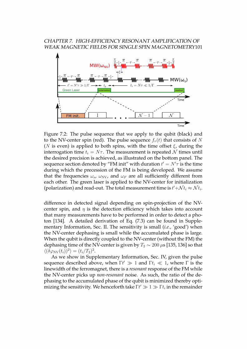
CHAPTER 7. HIGH-EFFICIENCY RESONANT AMPLIFICATION OFWEAK MAGNETIC FIELDS FOR SINGLE SPIN MAGNETOMETRY101
Green Laser readout
MW( NV)
MW( s)
Time
polarization
Time
Figure 7.2: The pulse sequence that we apply to the qubit (black) andto the NV-center spin (red). The pulse sequence fτ (t) that consists of N(N is even) is applied to both spins, with the time offset ξ, during theinterrogation time ti = Nτ . The measurement is repeated N times untilthe desired precision is achieved, as illustrated on the bottom panel. Thesequence section denoted by “FM init” with duration t′ = N ′τ is the timeduring which the precession of the FM is being developed. We assumethat the frequencies ωs, ωNV, and ωF are all sufficiently different fromeach other. The green laser is applied to the NV-center for initialization(polarization) and read-out. The total measurement time is t′+N ti ≈ N ti.
difference in detected signal depending on spin-projection of the NV-center spin, and η is the detection efficiency which takes into accountthat many measurements have to be performed in order to detect a pho-ton [134]. A detailed derivation of Eq. (7.3) can be found in Supple-mentary Information, Sec. II. The sensitivity is small (i.e., ‘good’) whenthe NV-center dephasing is small while the accumulated phase is large.When the qubit is directly coupled to the NV-center (without the FM) thedephasing time of the NV-center is given by T2 ∼ 200 µs [135, 136] so that〈(δϕNV(ti))
2〉 = (ti/T2)2.As we show in Supplementary Information, Sec. IV, given the pulse
sequence described above, when Γt′ 1 and Γti 1, where Γ is thelinewidth of the ferromagnet, there is a resonant response of the FM whilethe NV-center picks up non-resonant noise. As such, the ratio of the de-phasing to the accumulated phase of the qubit is minimized thereby opti-mizing the sensitivity. We henceforth take Γt′ 1 Γti in the remainder
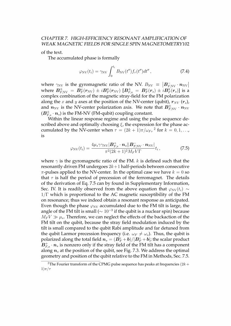
CHAPTER 7. HIGH-EFFICIENCY RESONANT AMPLIFICATION OFWEAK MAGNETIC FIELDS FOR SINGLE SPIN MAGNETOMETRY102
of the text.The accumulated phase is formally
ϕNV(ti) = γNV
∫ ti
0
BNV(t′′)fτ (t′′)dt′′ , (7.4)
where γNV is the gyromagnetic ratio of the NV. BNV ≡∣∣B−F,NV · nNV
∣∣where B±F,NV = Bx
F (rNV) ± iByF (rNV) [B±F,s = Bx
F (rs) ± iByF (rs)] is a
complex combination of the magnetic stray-field for the FM polarizationalong the x and y axes at the position of the NV-center (qubit), rNV (rs),and nNV is the NV-center polarization axis. We note that B±F,NV · nNV
(B±F,s · ns) is the FM-NV (FM-qubit) coupling constant.Within the linear response regime and using the pulse sequence de-
scribed above and optimally choosing ξ, the expression for the phase ac-cumulated by the NV-center when τ = (2k + 1)π/ωF , 2 for k = 0, 1, . . .,is
ϕNV(ti) =4µsγγNV|B+
F,s · ns||B−F,NV · nNV|π2(2k + 1)2MFV Γ
ti , (7.5)
where γ is the gyromagnetic ratio of the FM. k is defined such that theresonantly driven FM undergoes 2k+1 half-periods between consecutiveπ-pulses applied to the NV-center. In the optimal case we have k = 0 sothat τ is half the period of precession of the ferromagnet. The detailsof the derivation of Eq. 7.5 can by found in Supplementary Information,Sec. IV. It is readily observed from the above equation that ϕNV(ti) ∼1/Γ which is proportional to the AC magnetic susceptibility of the FMon resonance; thus we indeed obtain a resonant response as anticipated.Even though the phase ϕNV accumulated due to the FM tilt is large, theangle of the FM tilt is small (∼ 10−3 if the qubit is a nuclear spin) becauseMFV µs. Therefore, we can neglect the effects of the backaction of theFM tilt on the qubit, because the stray field modulation induced by thetilt is small compared to the qubit Rabi amplitude and far detuned fromthe qubit Larmor precession frequency (i.e. ωF 6= ωs). Thus, the qubit ispolarized along the total field ns = (Bz
F +b)/|BzF +b|; the scalar product
B+F,s · ns is nonzero only if the stray field of the FM tilt has a component
along ns at the position of the qubit, see Fig. 7.3. We address the optimalgeometry and position of the qubit relative to the FM in Methods, Sec. 7.5.
2The Fourier transform of the CPMG pulse sequence has peaks at frequencies (2k+1)π/τ
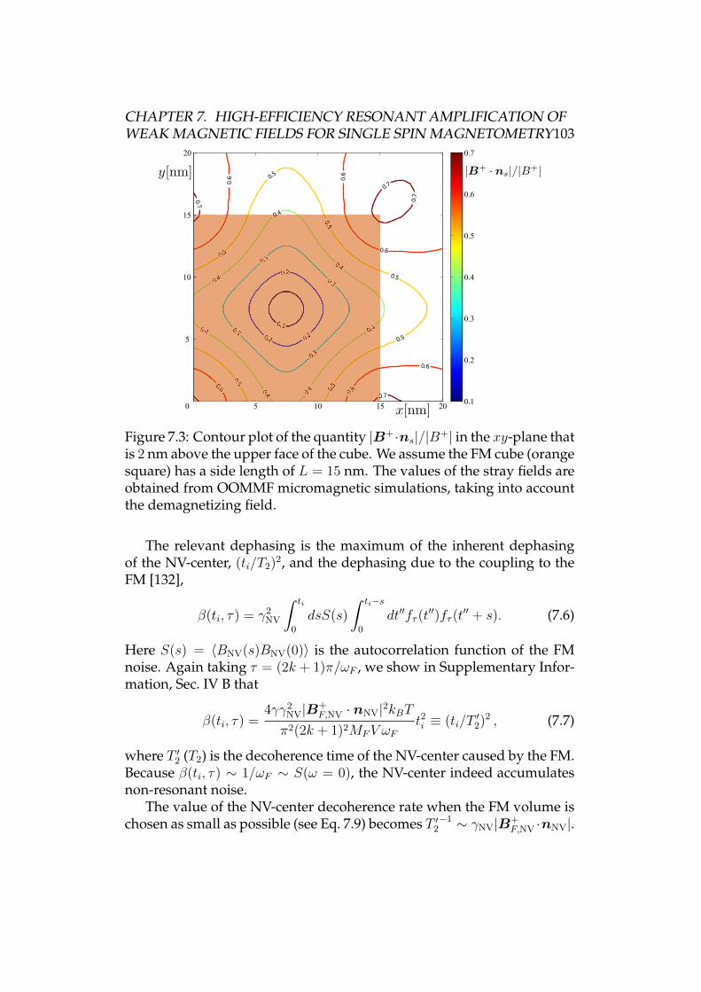
CHAPTER 7. HIGH-EFFICIENCY RESONANT AMPLIFICATION OFWEAK MAGNETIC FIELDS FOR SINGLE SPIN MAGNETOMETRY103
0.1
0.2
0.2
0.2
0.3
0.3
0.3
0.3
0.4
0.4
0.4
0.4
0.4
0.4
0.4
0.5
0.5
0.5
0.5
0.5
0.5
0.5
0.6
0.6
0.6
0.6
0.6
0.6
0.7
0.7
0.7
0.7
0
5
10
15
20
0.1
0.2
0.3
0.4
0.5
0.6
0.7
5 10 15 20
Figure 7.3: Contour plot of the quantity |B+·ns|/|B+| in the xy-plane thatis 2 nm above the upper face of the cube. We assume the FM cube (orangesquare) has a side length of L = 15 nm. The values of the stray fields areobtained from OOMMF micromagnetic simulations, taking into accountthe demagnetizing field.
The relevant dephasing is the maximum of the inherent dephasingof the NV-center, (ti/T2)2, and the dephasing due to the coupling to theFM [132],
β(ti, τ) = γ2NV
∫ ti
0
dsS(s)
∫ ti−s
0
dt′′fτ (t′′)fτ (t
′′ + s). (7.6)
Here S(s) = 〈BNV(s)BNV(0)〉 is the autocorrelation function of the FMnoise. Again taking τ = (2k + 1)π/ωF , we show in Supplementary Infor-mation, Sec. IV B that
β(ti, τ) =4γγ2
NV|B+F,NV · nNV|2kBT
π2(2k + 1)2MFV ωFt2i ≡ (ti/T
′2)2 , (7.7)
where T ′2 (T2) is the decoherence time of the NV-center caused by the FM.Because β(ti, τ) ∼ 1/ωF ∼ S(ω = 0), the NV-center indeed accumulatesnon-resonant noise.
The value of the NV-center decoherence rate when the FM volume ischosen as small as possible (see Eq. 7.9) becomes T ′2
−1 ∼ γNV|B+F,NV ·nNV|.
CHAPTER 7. HIGH-EFFICIENCY RESONANT AMPLIFICATION OFWEAK MAGNETIC FIELDS FOR SINGLE SPIN MAGNETOMETRY104
Furthermore, since the optimal interrogation time is ti ∼ T ′2, we obtainthat for typical values of the FM stray field we are in the limit ti tp.After substituting 〈(δϕNV(ti))
2〉 = β(ti, τ) and ϕNV(ti) from Eq. (7.5) andEq. (7.7) into Eq. (7.3) and performing the minimization over the interro-gation time in Eq. (7.3), we find the sensitivity SA of our magnetometryscheme
SA =1
R√η
πe12 (2k + 1)MFV Γ√
2γ|B+F,s · ns|
√γkBTtpMFV ωF
. (7.8)
The best sensitivity is obtained when one half-period of the FM oscilla-tion occurs over the timescale τ , i.e., k = 0. In practice, experimentallimitations, such as limitations to the qubit Rabi frequency, bound τ andtherefore k from below. Thus, in order to achieve the resonance, one hasto use k 0 (at the expense of sensitivity) or to tune the FMR frequencyas described in the following subsection. We note that since the sensitiv-ity in Eq. 7.8 scales as SA ∼ Γ, using low loss FM materials like YttriumIron Garnet (YIG) is crucial for achieving high sensitivities.
A few comments are in order regarding the obtained expression forthe sensitivity in Eq. 7.8. First, we note that SA is completely indepen-dent of the FM-NV coupling constant |B±F,NV ·nNV|—this behavior holdsas long as the stray field at position of the NV is not too weak, since other-wise a weak FM-NV coupling leads to long T ′2 and thus we are no longerin the limit ti tp and thus Eq. 7.8 is no longer valid. Therefore, SA de-pends only on d but not on h (see Fig. 7.1). Having a magnetometer withthe sensitivity that is independent of the NV positioning 3 is particularlyadvantageous for NV ensemble measurements since we can place manyNV-centers that would all have the same sensitivity (though different op-timal interrogation times) and thus obtain significant improvement of thetotal sensitivity. Finally, SA depends on the FM-qubit coupling constantand therefore depends on d. But herein, rather than having a sensitivitythat has cubic dependence on the tip-to-sample separation, we have onlyweak dependence on d since the FM stray field is not changed much aslong as d L ≡ V 1/3 (see Methods, Sec. 7.5). The spatial resolution ofour scheme does not differ from the standard NV-magnetometry resolu-tion [14]. In practice the spatial resolution for detection of an isolated spinis determined by the ratio between the magnetic field gradient and thetarget qubit linewidth. In the case of interacting spins there is a broaden-ing caused by homonuclear dipolar interaction, thus the techniques such
3We stress that this statement is true only in region of space near the FM whereT ′2 tp, i.e., where the FM stray field is bigger that the threshold value Bth ∼ 1 Gauss.
CHAPTER 7. HIGH-EFFICIENCY RESONANT AMPLIFICATION OFWEAK MAGNETIC FIELDS FOR SINGLE SPIN MAGNETOMETRY105
as magic angle spinning (MAS) should be used [137]. Since MAS is usu-ally performed by spinning the sample in a static magnetic field whichis impractical for our scheme, one can use rotating magnetic fields [138]instead, with the frequency different from ωNV , ωF and ωs for performingMAS.
While the electron spin in a NV-center can be driven at GHz frequen-cies [139, 140], the same driving field for a proton spin would yield Rabifrequency in the MHz range. Thus, the FMR frequency needs to be tunedto meet the resonance critieria. The method to achieve such a tuning isdescribed in Methods, Sec. 7.5. The idea is to use the metastable stateof the FM which has frequency that can be lowered by applying an ex-ternal magnetic field, see Fig. 7.4. In order for the FM to remain in themetastable state during the measurement time, the FM volume must sat-isfy
V &γkBT
MFω+F
| lnα|, (7.9)
In case of minimal volume, the sensitivity reads
SA =1
R√η
π(2k + 1)α√e| lnα|tpkBT√
2|B+F,s · ns|
. (7.10)
As noted earlier, the sensitivity of our scheme does not depend onthe FM-NV coupling constant. Thus, we can take advantage of this factto obtain an improvement of sensitivity by a factor of
√NNV, when NNV
NV-centers are used for the detection. We present a detailed discussionin Sec. 7.5 of the Methods.
Estimates
In this section we give estimates for the sensitivity SA for two cases: withand without tuning of the FMR frequency (to MHz range). We also pro-vide the estimates for the case when an NV ensemble is used for the mea-surement. For all the estimates provided in the following, we assumeroom temperature and that the FM material is YIG, so that α ∼ 10−5,µ0MF = 0.185 T, and K/MF = 60 mT [141]. For simplicity but withoutloss of generality, we assume that the FM has the shape of a cube for theestimates given below. For a cube and in the macrospin approximationthere is no contribution from shape anisotropy.
If we tune the FMR frequency to MHz range the minimum FM vol-ume V according to Eq. (7.9) corresponds to a cube with side L = 210 nm.
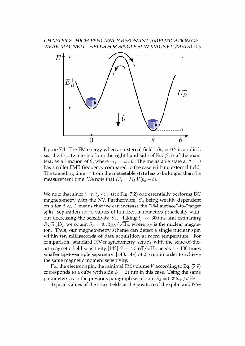
CHAPTER 7. HIGH-EFFICIENCY RESONANT AMPLIFICATION OFWEAK MAGNETIC FIELDS FOR SINGLE SPIN MAGNETOMETRY106
Figure 7.4: The FM energy when an external field b/ba = 0.2 is applied,i.e., the first two terms from the right-hand side of Eq. (7.1) of the maintext, as a function of θ, where mz = cos θ. The metastable state at θ = 0has smaller FMR frequency compared to the case with no external field.The tunneling time τ+ from the metastable state has to be longer than themeasurement time. We note that E+
B = MFV (ba − b).
We note that since ti tp τ (see Fig. 7.2) one essentially performs DCmagnetometry with the NV. Furthermore, SA being weakly dependenton d for d L means that we can increase the “FM surface”-to-“targetspin” separation up to values of hundred nanometers practically with-out decreasing the sensitivity SA. Taking tp ∼ 300 ns and estimatingR√η [13], we obtain SA = 0.13µN/
√Hz, where µN is the nuclear magne-
ton. Thus, our magnetometry scheme can detect a single nuclear spinwithin ten milliseconds of data acquisition at room temperature. Forcomparison, standard NV-magnetometry setups with the state-of-the-art magnetic field sensitivity [142] S = 4.3 nT/
√Hz needs a ∼100 times
smaller tip-to-sample separation [143, 144] of 2.5 nm in order to achievethe same magnetic moment sensitivity.
For the electron spin, the minimal FM volume V according to Eq. (7.9)corresponds to a cube with side L = 21 nm in this case. Using the sameparameters as in the previous paragraph we obtain SA = 0.32µN/
√Hz.
Typical values of the stray fields at the position of the qubit and NV-
CHAPTER 7. HIGH-EFFICIENCY RESONANT AMPLIFICATION OFWEAK MAGNETIC FIELDS FOR SINGLE SPIN MAGNETOMETRY107
center in the limit d, h L for YIG are on the order of a few hundreds ofGauss. The presence of a magnetic field perpendicular to the NV-centeraxis can significantly limit the read-out fidelity of the NV-center, it wasfound that fields up to 100 Gauss can be tolerated [9]. Since the sensitivitySA does not depend on the FM-NV coupling constant, the NV should beplaced in the region where the stray fieldBF,NV is less than 100 Gauss butbigger than the threshold value Bth, i.e., 1 Gauss < BF,NV < 100 Gauss.For |B±F,NV · nNV| ∼ 10 Gauss, the decoherence time of the NV is T ′2 ∼100 ns [see Eq. (7.7)], which is also the value of the optimal interroga-tion time. Thus, because the signal amplification in our scheme far ex-ceeds the effect of the additional decoherence it induces, even shallowNV-centers [136, 135] or dense ensembles of NV-centers [134] with rela-tively short decoherence time can be used and significantly outperformlong-lived NV-centers (without the FM).
Finally, we give the estimates for the case of the FMR tuned to theMHz range and for measurements with ensembles of NV-centers. Asexperimentally demonstrated [145], NV ensembles with a separation ofabout 10 nm between neighboring NV-centers can be achieved. SuchNV ensembles have T ∗2 ∼ 100 ns, but this property, as noted in the pre-vious paragraph, does not affect the sensitivity of our scheme. We candistribute the NV-centers in the volume where the stray field satisfiesBF,NV > Bth and such a volume can be estimated to be a cube with sidelength of 1 µm. Therefore, NNV ∼ 106 which yields an unprecedentedsensitivity of SA = 0.13× 10⁻³µN/
√Hz.
7.3 ConclusionsWe have proposed and analyzed, both analytically and numerically, amodification of a standard NV-magnetometry setup that yields a signifi-cant improvement of NV-magnetometer sensitivity—the obtained sensi-tivity is practically unchanged as long as the ferromagnet surface to thetarget spin separation is smaller than the ferromagnet lateral dimensionswhich is typically about a tenth of a micron. Our scheme is based on aferromagnetic particle, placed in close proximity to a sensing NV-centerspin. The qubit spin to be detected is then used to resonantly drive thelarge macrospin of the FM giving rise to a strong, amplified stray fieldacting on the NV-magnetometer. Compared to the existing schemes thatuse the quantum nature of an intermediate spin for improving sensitiv-ity [126], we stress that our scheme is fully classical and thus should be
CHAPTER 7. HIGH-EFFICIENCY RESONANT AMPLIFICATION OFWEAK MAGNETIC FIELDS FOR SINGLE SPIN MAGNETOMETRY108
easily realizable at room temperature—all the ingredients of our schemeare already demonstrated in separate experiments [139, 140, 14, 146, 128,127, 147].
The magnetometric scheme including a ferromagnetic particle pro-posed here is a step forward to a more accurate magnetic field measure-ment. In particular, it enables the detection of a single nuclear spin at dis-tances that are noninvasive to the system under study. Therefore, the pro-posed room temperature magnetometry scheme opens up new venuesfor future analyses of previously inaccessible biological and chemicalsystems.
7.4 AcknowledgmentsWe would like to thank H. Fanghor for sharing his expertise about mi-cromagnetic simulations. This work was supported by the SNF, NCCRQSIT, IARPA, DARPA QuASAR programs and the MURI QuISM. F. L. P.is grateful for support from the Alexander von Humboldt foundation.
7.5 Methods
Tuning the FMR frequency
It has been demonstrated experimentally [139, 140] that the electron spinof NV-centers can be coherently driven at GHz frequency. For a protonspin, however, the same drive would yield Rabi oscillations in the MHzrange. Because typical FMR frequencies are in GHz range, ωF needs to bereduced in order for the proton Rabi frequency to be on resonance withthe FMR.
One way to decrease ωF is to apply an external magnetic field antipar-allel to m [148], whereby there is a metastable state when b < ba, withba = K/MF the FM (crystalline and shape) anisotropy field. In Fig. 7.4,we plot the energy of the FM as a function of angle θ of the magnetizationwith respect to the easy axis, according to Eq. (7.1) of the main text. It isstraightforward to show that the FMR frequency in the metastable state isω+F = γ(ba− b). On the other hand, the ferromagnet will relax to the ther-
mal state on a timescale τ+ given by the Arrhenius law τ+ = τ0eE+B/kBT ,
where τ0 ∼ 1/ω+F is the attempt time. We can insure that the FM is ini-
tialized in the metastable state by first measuring the direction of themagnetization, applying an external magnetic field b antiparallel to m
CHAPTER 7. HIGH-EFFICIENCY RESONANT AMPLIFICATION OFWEAK MAGNETIC FIELDS FOR SINGLE SPIN MAGNETOMETRY109
and checking subsequently that the FM magnetization direction is un-changed, which can be done under hundred picoseconds [149, 150, 151].
In order for the ferromagnet to remain in the metastable state whilethe measurement is being performed, we require τ+ 1/Γ. Indeed, thetotal measurement time T should be larger than the FMR initializationtime t′ 1/Γ, and smaller than Arrhenius’ timescale τ+ & T , see Fig. 7.2in the main text. Thus, if we want to tune ω+
F to a certain value and workat room temperature, the Arrhenius law suggests that the FM volumemust satisfy
V &γkBT
MFω+F
| lnα|, (7.11)
in order for the metastable state lifetime to be bigger than the measure-ment time. Here α = Γ/ω+
F is the Gilbert damping of the FM. SubstitutingEq. (7.9) for the minimal volume into Eq. (7.8) of the main text we obtain
SA =1
R√η
π(2k + 1)α√e| lnα|tpkBT√
2|B+F,s · ns|
(7.12)
Compared to the sensitivity in Eq. (7.8) of the main text, the above ex-pression is independent of the FMR frequency ωF and the FM volume V .Thus, irrespective of the choice of the frequency we work at, the samevalue for the sensitivity SA is obtained. Furthermore, the only depen-dence on the volume is incorporated in the stray fields but, as shownin Sec. 7.5, this dependence is weak in the limit d L. The volumein Eq. (7.9) is implicitly bounded from above in order to remain in theregime where the macrospin approximation is valid.
An alternative setup to achieve resonance between the qubit and FMis to place the NV-center and the FM on a cantilever [152] with reso-nance frequency in the GHz range. By driving the cantilever, we alleviatethe necessity of driving the qubit at FMR frequency as the qubit field ismodulated by the oscillations of the cantilever. Since the dipolar field ofthe qubit decays rapidly with distance, the modulation of the qubit fieldachieved in this scheme is almost as big as when the qubit is driven viaa microwave field (the previously described scheme for which the sensi-tivity estimates are given). Therefore, we conclude that the estimates forthe sensitivity SA given in Sec. 7.2 still hold in that case.
CHAPTER 7. HIGH-EFFICIENCY RESONANT AMPLIFICATION OFWEAK MAGNETIC FIELDS FOR SINGLE SPIN MAGNETOMETRY110
FM geometry and demagnetizing fields
In the absence of an external magnetic field, the qubit aligns along thestray field direction of the FM, while the FM spins are aligned along theeasy axis. Because MFV µs, the FM tilt induced by the qubit is negli-gible. Therefore, the qubit will align along the direction of the stray fieldproduced by the FM. However, for most geometries of the FM and po-sitions of the qubit, the FM-qubit coupling constant is almost zero, i.e.|B+
F,s · ns| ∼ Bx,yF,s ·Bz
F,s ∼ 0, and therefore the sensitivity is bad S−1A ∼ 0.
In the following discussion, we consider our ferromagnet to be a cubeof side L, but our conclusions can be straightforwardly generalized toother geometries. To gain insight into the direction and strength of thestray field, we use the well-known analogy between the stray field of ahomogeneously magnetized body and an electric field produced by sur-face charges. Specifically, we may consider the surfaces of the cube tohave charge density ∼MF m · s, where s is the vector normal to the sur-face of the cube. Therefore, when the position of the qubit is very closeto the center of the FM surface which is perpendicular to the polariza-tion direction (here assumed along z-axis), Bz
F,s points along the z-axis.Similarly, Bx
F,s and ByF,s are almost aligned with the x and y axes close
to the surface, respectively. Therefore, in these positions, Bx,yF,s ·Bz
F,s ∼ 0.However, this is not true near the edges of the ferromagnet. Therefore, inorder to obtain a sensitive magnetometer, one needs, first, a ferromagnetwith edges and, second, to position the qubit close to the edges. One mayshow analytically and numerically (see Fig. 7.3) that |B+ · ns|/|B+| closeto the edges is about an order of magnitude bigger than close to the facecenter and that it has local maxima close to the cube’s corners.
In evaluating Bx,y,zF,s , we assume that the FM is homogeneously mag-
netized as, in cubic geometry, one can find an analytical formula for thestray field in this case (see Supplementary Information, Sec. V). How-ever, it is important to note that due to demagnetizing fields (arisingfrom dipole-dipole interactions in the FM), the FM ground-state is nothomogeneous but rather “flowerlike” [153]. Specifically, the canting ofthe spins close to the edges is more pronounced [154], which modifiesthe FM stray field close to the edges. To account for the effects of the de-magnetizing fields, we perform micromagnetic simulations in OOMMF. 4
In Fig. 7.3 we plot |B+ · ns|/|B+| in the xy-plane that is 2 nm above theupper face of the cube. We find that the inclusion of demagnetizing fieldschanges our value of Bx,y,z
F,s by only ∼ 1% as compared to the uniformly4The code is available at http://math.nist.gov/oommf
CHAPTER 7. HIGH-EFFICIENCY RESONANT AMPLIFICATION OFWEAK MAGNETIC FIELDS FOR SINGLE SPIN MAGNETOMETRY111
magnetized cube. Therefore, we expect the analytical expression for thestray field to be valid for our choice of parameters.
Because the sensitivity SA depends on d only through the stray field atthe position of the qubit, herein we detail this dependence and show thatthe sensitivity of our magnetometry scheme is practically unchanged asd is varied. The stray field close to the cube edge (in comparison to L) isequivalent to the electric field of a set of infinite line charges. Therefore,there is a logarithmic dependence of the stray field on the distance to theedge, d, of the cube in units of L so that the sensitivity SA is only weaklydependent on d.
NV ensemble measurements
As noted earlier, the sensitivity of our scheme SA does not depend onthe FM-NV coupling constant. Such behavior of the sensitivity is in starkcontrast to the cubic dependence on the tip-to-sample separation of typ-ical NV-magnetometer sensitivity. This property of SA is very useful ifwe want to perform the measurements with an ensemble of NV-centerssince all of them would have the same sensitivity irrespective of the ac-tual value of the FM-NV coupling constant. Thus, we obtain an improve-ment of sensitivity by a factor of
√NNV, where NNV is the number of NV-
centers in the ensemble. In our scheme NNV is the maximum number ofNV-centers that we can place in the region of space around the FM wherethe stray field value is above the threshold Bth.
As the FM volume is increased, the sensitivity is decreased as SA ∼√V see Eq. 7.8. Nevertheless, in case of an NV ensemble measurement,
increasing V leads to an increase of NNV V . Thus, for ensemble mea-surements our scheme does not loose sensitivity when the FM volume isincreased, but rather the sensitivity is logarithmically improved due toincreasing the FM-qubit coupling constant. The possibility of having alarge FM without loss of sensitivity is important since it can be experi-mentally more feasible to work with micron-sized FMs.
7.A Cramer-Rao BoundFor the sake of completeness, we review here the proof of the Cramer-Rao bound,
〈(δµs)2〉 ≥ 1/F (µs), (7.13)
CHAPTER 7. HIGH-EFFICIENCY RESONANT AMPLIFICATION OFWEAK MAGNETIC FIELDS FOR SINGLE SPIN MAGNETOMETRY112
that we use to derive the sensitivity expression in Eq. (7.3) of the maintext.
The Fisher information of the parameter estimator µs is given by
F (µs) = −∑
n=±1
p(n|µs)∂2 ln(p(n|µs))
∂µ2s
. (7.14)
The Cramer-Rao bound follows from the trivial identity
0 =∑
n1
· · ·∑
nN
p(n1|µs) . . . p(nN |µs)∆µs, (7.15)
where ∆µs = µs(n1, . . . , nN ) − 〈µs〉. Taking the derivative of this iden-tity with respect to µs and using the fact that the estimator µs does notdepend explicitly on µs, we obtain
∑
n1
· · ·∑
nN
p(n1|µs) . . . p(nN |µs)(N∑
k=1
∂ ln p(nk|µs)∂µs
)∆µs =
d〈µs〉dµs
. (7.16)
Furthermore, for the unbiased estimator, 〈µs〉 = µs and thus the right-hand side of Eq. (7.16) is equal to 1. Finally, applying the Schwarz in-equality, cov(X, Y )2 ≥ var(X)var(Y ), to the above equation yields theCramer-Rao bound, Eq. (7.13).
7.B Sensitivity of an NV-centerThe variance of any estimator µs of the unknown parameter µs satisfiesthe Cramer-Rao inequality Eq. (7.13). Using the probability distributionfrom Eq. (7.2) of the main text, we obtain
F (µs) =(∂ϕNV(ti)/∂µs)
2 sin2(ϕNV(ti) + θ)
e2〈(δϕNV(ti))2〉 − cos2(ϕNV(ti) + θ). (7.17)
Thus, a bigger Fisher information F (µs) leads to a more accurate valueof the estimator µs.
For DC magnetometry we typically have ϕNV(ti) = γNV(B0 + B)ti ≡ti/T
′ and 〈(δϕNV(ti))2〉 = ti/T
∗2 , where γNVB0 = 2.87GHz is the zero-field
splitting of the NV-center and T ∗2 is typically on the order of a few mi-croseconds. The field we want to measure is B = µ0µs/(4πd
3), with dthe distance between the qubit and the NV-center. Consider the scenario
CHAPTER 7. HIGH-EFFICIENCY RESONANT AMPLIFICATION OFWEAK MAGNETIC FIELDS FOR SINGLE SPIN MAGNETOMETRY113
T ′ T2 which is valid for DC magnetometry. In such a situation, onemay choose an interrogation time maximizing sin2[ϕNV(ti) + θ] and min-imizing cos2[ϕNV(ti) + θ] in Eq. (7.17). This is independent of the angleθ which we set to zero without loss of generality. Thus instead of maxi-mizing the Fisher information from Eq. (7.17), we need only to maximizeits envelope function,
F (µs) = (∂ϕNV(ti)/∂µs)2e−2〈(δϕNV(ti))
2〉 . (7.18)
Repeating the measurement N = T/(tp + ti) times (tp is the initializa-tion time) reduces the variance by a factor 1/N . The Cramer-Rao bound(7.13) then leads to 〈(δµs)2〉 ≥ 1
NF (µs). The minimal value of the magnetic
moment µs(ti, T ) (that can be resolved within measurement time T andinterrogation time ti) is determined by the one for which the mean valueis equal to its standard deviation,
µs(ti, T ) =1√NF (µs)
. (7.19)
We finally obtain the sensitivity
S =1
R√η
minti
[e〈(δϕNV(ti))
2〉√ti + tp|∂ϕNV(ti)/∂µs|
]. (7.20)
As mentioned in the main text, R is the measurement contrast and η isthe detection efficiency; [134] these quantities take into account that themeasurement has to be performed many times in order to detect a pho-ton.
The situation for AC magnetometry is different, here
ϕNV(ti) = λγNVBti ≡ ti/T′, (7.21)
while we still have 〈(δϕNV(ti))2〉 = ti/T2. (Note that the constant of pro-
portionality λ depends on the specific pulse sequence applied.) In typicalsituations, the AC magnetic field is small and T ′ T2. In such sce-nario, and for vanishing angle θ, the accumulated phase will never reacha value of π/2 and one needs to maximize the Fisher information (7.17),not only its envelope. In this limit, we obtain a very different expres-sion for the sensitivity, and, in particular, the expression is in units of“magnetic moment”/Hz
14 (see Sec. 7.C). Fortunately, such result can be
improved: one may take a nonzero value of the angle θ such that the ex-pression ϕNV(ti) + θ = π/2 within the interrogation time. In this case, thesensitivity takes the form (7.20), improving the sensitivity.
CHAPTER 7. HIGH-EFFICIENCY RESONANT AMPLIFICATION OFWEAK MAGNETIC FIELDS FOR SINGLE SPIN MAGNETOMETRY114
7.C AC sensitivity for θ = 0
The goal of this appendix is to derive the expression for the AC sensitiv-ity when the angle θ between the two π/2-pulses, applied at the begin-ning and at the end of the sequence, is zero. This calculation is presentedfor the sake of completeness, however, this is not the expression we useto derive sensitivity of our magnetometry scheme. As mentioned in themain text, for AC magnetometry we have
ϕNV(ti) ∝ γNVBti ≡ ti/T′, (7.22)
〈(δϕNV(ti))2〉 = ti/T2, (7.23)
where the constant of proportionality depends on the specific pulse se-quence applied. It is important to note that here only the AC field com-ponent that matches the frequency of the pulse sequence contributes (i.e.,there is no contribution from B0). When the magnitude of the AC driv-ing field is small, we are in the limit of T ′ T2. As noted above, in thisregime the accumulated phase ϕNV(ti) will not reach the value of π/2and thus the full Fisher information needs to be maximized. Namely, wemaximize
F (µs) =(∂ϕNV(ti)/∂µs)
2 sin2(ϕNV(ti) + θ)
e2〈(δϕNV(ti))2〉 − cos2(ϕNV(ti) + θ). (7.24)
Therefore,
√〈(δµs)2〉 ≥
√e2〈(δϕNV(ti))2〉 − cos2(ϕNV(ti))
√tp + ti√
T | sin(ϕNV(ti))∂ϕNV(ti)/∂µs|. (7.25)
In contrast to the result obtained [126] [which is similar to the one ob-tained in Eq. (7.18)], the Fisher information in Eq. (7.25) depends on theestimation parameter µs. The minimal value of the magnetic momentµs(ti, T ) (that can be resolved within measurement time T and interro-gation time ti) is again determined as the one for which the mean valueis equal to its standard deviation, Eq. (7.19). Therefore, using the factthat ϕNV(ti) depends linearly on µs and that for typical interrogation timeϕNV(ti) 1 and assuming tp ti, we find an approximate solution toEq. (7.19). Minimizing over the interrogation time, we obtain
µs(T ) ≡ minti
[µs(ti, T )] (7.26)
= minti
[(e2〈(δϕNV(ti))
2〉 − 1)14
|∂ϕNV(ti)/∂µs|
(tiT
) 14
].
CHAPTER 7. HIGH-EFFICIENCY RESONANT AMPLIFICATION OFWEAK MAGNETIC FIELDS FOR SINGLE SPIN MAGNETOMETRY115
Now, if we remove the dependence on the total measurement time fromthe above expression, we obtain the quantity that describes the magneticmoment sensitivity in units of “magnetic moment”/Hz
14 , i.e.,
S =1
R√η
minti
[(e2〈(δϕNV(ti))
2〉 − 1)14 t
14i
|∂ϕNV(ti)/∂µs|
]. (7.27)
7.D Calculation of ϕNV (ti) and β(ti, τ )
The goal of this appendix is to give a detailed derivation of Eqs. (7.5)and (7.7) of the main text that are central to our work. The former de-scribes the phase accumulated by the NV-magnetometer, while the latterthe variance of this accumulated phase.
Within linear response, the accumulated phase is
ϕNV(ti) =µsγγNV
MFVRe[iXξ(ti, t
′)(B+F,s · ns
) (B−F,NV · nNV
)], (7.28)
where ξ (|ξ| ≤ τ ) is the time offset between the CPMG pulse sequence ap-plied to the qubit and the NV-center. We have introduced the followingnotation,
Xξ(ti, t′) =
∫ t′
0
dse−Ωs
∫ ti
0
dt′′fτ (t′′)fτ (t
′′ − s− ξ) + e−Ωt′∫ ti
0
dse−Ωspτ (s, t; ξ)
≡Xξ(ti, t′) + e−Ωt′Yξ(ti), (7.29)
with Ω = iωF + Γ and pτ (s, ti; ξ) =∫ ti−s
0dt′′fτ (t
′′ − ξ)fτ (t′′ + s). After
performing the integral in Eq. (7.29) and using ti = Nτ , t′ = N ′τ , weobtain
CHAPTER 7. HIGH-EFFICIENCY RESONANT AMPLIFICATION OFWEAK MAGNETIC FIELDS FOR SINGLE SPIN MAGNETOMETRY116
Xξ(Nτ,N′τ) = e−Ωξ
[Xξ=0(Nτ,N ′τ)
− (1− e−Ωt′)Ωτ − 2 + e−Ωξ(2 + 2Ωξ − Ωτ)
Ω2N
], (7.30)
Xξ=0(Nτ,N ′τ) =(1− e−N ′Ωτ )N(2 + eΩτ (Ωτ − 2) + Ωτ)
Ω2(1 + eΩτ ),
(7.31)
Yξ=0(Nτ) = − 4sh4(Ωτ/4)
Ω2ch2(Ωτ/2)+
2 + Ωτ + (Ωτ − 2)eΩτ
Ω2(1 + eΩτ )N
+(eΩτ/2 − 1)4
Ω2(1 + eΩτ )2e−NΩτ . (7.32)
Since we want the qubit to perturb the ferromagnet within a narrow fre-quency window around the FMR (i.e., narrower than the FMR linewidthΓ), we require that Γt′ 1. In this limit, the expression for Xξ(ti, t
′) issignificantly simplified
Xξ(Nτ,N′τ) = e−Ωξ
[Xξ=0(Nτ,N ′τ)− Ωτ − 2 + e−Ωξ(2 + 2Ωξ − Ωτ)
Ω2N
],
Xξ=0(Nτ,N ′τ) ≈ Xξ=0(Nτ) ≡ N(2 + eΩτ (Ωτ − 2) + Ωτ)
Ω2(1 + eΩτ ). (7.33)
The expression for dephasing can be obtained from [132]
β(ti, τ) = γ2NV
∫ ti
0
ds〈BNV(s)BNV(0)〉pτ (s, ti; ξ = 0). (7.34)
Furthermore,
〈BNV(t)BNV(0)〉 = |B+F,NV · nNV|2Re[〈m+(t)m−(0)〉]. (7.35)
In the limit MFV (ba ± b) kBT (ba = K/MF is the anisotropy field) oneobtains the following expression for the fluctuations of the ferromagnet,
〈m+(t)m−(0)〉 =2kBT
MFV (ba ± b)e−iωF t−Γ|t|. (7.36)
Combining equations (7.34-7.36) we finally obtain
β(Nτ, τ) =2γ2
NV|B+F,NV · nNV|2kBT
MFV (ba ± b)Y ′ξ=0(Nτ). (7.37)
CHAPTER 7. HIGH-EFFICIENCY RESONANT AMPLIFICATION OFWEAK MAGNETIC FIELDS FOR SINGLE SPIN MAGNETOMETRY117
On-resonance case τ = (2k + 1)π/ωF
The Fourier transform of the CPMG sequence depicted in Fig. 7.2 haspeaks at frequencies (2k + 1)π/τ . Thus we have a resonant behaviorwhenever this frequency matches ωF . Assuming Γt′ 1 and ωF (2k + 1)Γ leads to the following expression for Xξ(ti), namely
Xξ(N) =
[− 4N
(2k + 1)πΓωF+ i
((2k + 1)2π2 − 8)N
(2k + 1)πω2F
]e−iψ, (7.38)
where ψ = ωF ξ. Assuming ωF (2k+ 1)2π2Γ, we can neglect the secondterm in the bracket in Eq. (7.38) and obtain the expression for the phaseaccumulated by the NV-center during the interrogation time ti,
ϕNV(ti) =4µsγγNVIm
[e−iψ(B+
F,s · ns)(B−F,NV · nNV)]
π2(2k + 1)2MFV Γti . (7.39)
Next, we choose the time offset ξ (i.e., ψ) such that ϕNV(ti) in the aboveequation is maximized
ψ = arg[(B+
F,s · ns)(B−F,NV · nNV)]
(7.40)
we obtain
ϕNV(ti) =4µsγγNV|B+
F,s · ns||B−F,NV · nNV|π2(2k + 1)2MFV Γ
ti . (7.41)
Assuming that the optimal interrogation time satisfies Γti 1, we arriveat the following expression for Y ′ξ=0(ti), namely
Y ′ξ=0(N) =2N
ω3F
[((2k + 1)π − 4(−1)k
)Γ +NωF
]
∼ 2N2
ω2F
. (7.42)
The above expression yields the following variance of the phase accumu-lated by the NV-center
β(ti, τ) =4γγ2
NV|B+F,NV · nNV|2kBT
π2(2k + 1)2MFV ωFt2i . (7.43)
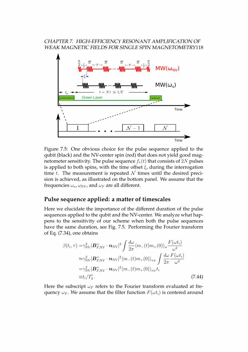
CHAPTER 7. HIGH-EFFICIENCY RESONANT AMPLIFICATION OFWEAK MAGNETIC FIELDS FOR SINGLE SPIN MAGNETOMETRY118
Green Laser readout
MW( NV)
MW( s)
Time
polarization
Time
Figure 7.5: One obvious choice for the pulse sequence applied to thequbit (black) and the NV-center spin (red) that does not yield good mag-netometer sensitivity. The pulse sequence fτ (t) that consists of 2N pulsesis applied to both spins, with the time offset ξ, during the interrogationtime t. The measurement is repeated N times until the desired preci-sion is achieved, as illustrated on the bottom panel. We assume that thefrequencies ωs, ωNV, and ωF are all different.
Pulse sequence applied: a matter of timescales
Here we elucidate the importance of the different duration of the pulsesequences applied to the qubit and the NV-center. We analyze what hap-pens to the sensitivity of our scheme when both the pulse sequenceshave the same duration, see Fig. 7.5. Performing the Fourier transformof Eq. (7.34), one obtains
β(ti, τ) =γ2NV|B+
F,NV · nNV|2∫dω
2π〈m−(t)m+(0)〉ω
F (ωti)
ω2
≈γ2NV|B+
F,NV · nNV|2〈m−(t)m+(0)〉ωF∫dω
2π
F (ωti)
ω2
=γ2NV|B+
F,NV · nNV|2〈m−(t)m+(0)〉ωF ti≡ti/T ′2 . (7.44)
Here the subscript ωF refers to the Fourier transform evaluated at fre-quency ωF . We assume that the filter function F (ωti) is centered around
CHAPTER 7. HIGH-EFFICIENCY RESONANT AMPLIFICATION OFWEAK MAGNETIC FIELDS FOR SINGLE SPIN MAGNETOMETRY119
the frequency ωF (on-resonance case) and that it is much narrower thanthe FMR linewidth, i.e., Γti 1—this is exactly the opposite limit fromthe one assumed to arrive at Eq. (7.7). The accumulated phase is given inEq. (7.5), and thus the magnetic moment sensitivity in this case reads
SA =1
R√η
π2
4i |B+F,s · ns|
√〈m−(t)m+(0)〉ωF
χ⊥(ωF ), (7.45)
where χ⊥(ω) = γ/ [MFV (ωF − ω + iΓ)]. The above expression does notyields good sensitivity, since we do not only excite the FM resonantlybut also the NV-center picks up the resonant noise. If we rewrite Eq. (7.7)in the form β(ti, τ) ≡ (ti/T
′′2 )2, we can understand that the decoherence
times in the two considered limits differ from each other by many ordersof magnitude, namely
T ′′2T ′2
=Γ
πγNV|B+F,NV · nNV|
√MFV ωFγkBT
1. (7.46)
7.E Stray field from a uniformly magnetizedcuboid
In this section we review the analytical formulas giving the stray fieldof a uniformly magnetized cuboid of side lengths Lx, Ly, and Lz, seeFig. 7.7. As mentioned in the main text, the magnetic field B(r) at a pointr = (x, y, z) outside of the cuboid can be calculated from the expressionfor the electric field originating from charges uniformly distributed onthe surfaces of the cuboid perpendicular to the magnetization [155, 156],see Fig. 7.7. For the sake of simplicity, we assume that the magnetizationdirection points either along x, y, or z. The expression for the stray fieldis then
Bδ(r) =µ0MF
4π
∫ Lα
0
dα
∫ Lβ
0
dβ
r− rαβδ|r− rαβδ |3
− r− rαβδ
|r− rαβδ|3
(7.47)
for δ = x, y, z. Here, α and β are the directions perpendicular to δ, i.e.,rαβx = (Lx, α, β), rαβy = (α,Ly, β), and rαβz = (α, β, Lz), and rαβ
δ= rαβδ |Lδ=0.
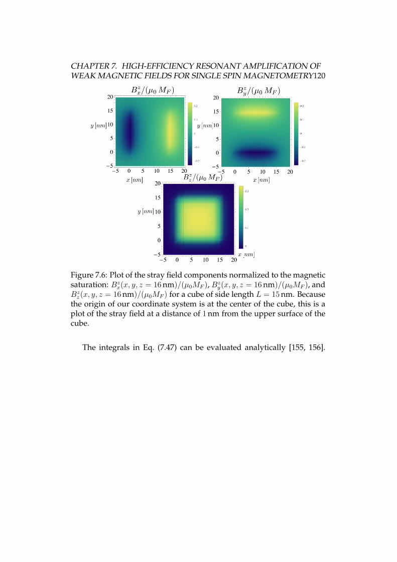
CHAPTER 7. HIGH-EFFICIENCY RESONANT AMPLIFICATION OFWEAK MAGNETIC FIELDS FOR SINGLE SPIN MAGNETOMETRY120
Figure 7.6: Plot of the stray field components normalized to the magneticsaturation: Bz
x(x, y, z = 16 nm)/(µ0MF ), Bzy(x, y, z = 16 nm)/(µ0MF ), and
Bzz (x, y, z = 16 nm)/(µ0MF ) for a cube of side length L = 15 nm. Because
the origin of our coordinate system is at the center of the cube, this is aplot of the stray field at a distance of 1 nm from the upper surface of thecube.
The integrals in Eq. (7.47) can be evaluated analytically [155, 156].
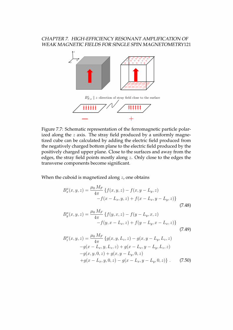
CHAPTER 7. HIGH-EFFICIENCY RESONANT AMPLIFICATION OFWEAK MAGNETIC FIELDS FOR SINGLE SPIN MAGNETOMETRY121
+ + + + + ++ + + + + ++ + + + + ++ + + + + +
+
BzF,s k z :direction of stray field close to the surface
z
xy
Figure 7.7: Schematic representation of the ferromagnetic particle polar-ized along the z axis. The stray field produced by a uniformly magne-tized cube can be calculated by adding the electric field produced fromthe negatively charged bottom plane to the electric field produced by thepositively charged upper plane. Close to the surfaces and away from theedges, the stray field points mostly along z. Only close to the edges thetransverse components become significant.
When the cuboid is magnetized along z, one obtains
Bxx(x, y, z) =
µ0MF
4πf(x, y, z)− f(x, y − Ly, z)
−f(x− Lx, y, z) + f(x− Lx, y − Ly, z)(7.48)
Bxy (x, y, z) =
µ0MF
4πf(y, x, z)− f(y − Ly, x, z)
−f(y, x− Lx, z) + f(y − Ly, x− Lx, z)(7.49)
Bxz (x, y, z) =
µ0MF
4πg(x, y, Lz, z)− g(x, y − Ly, Lz, z)
−g(x− Lx, y, Lz, z) + g(x− Lx, y − Ly, Lz, z)−g(x, y, 0, z) + g(x, y − Ly, 0, z)+g(x− Lx, y, 0, z)− g(x− Lx, y − Ly, 0, z) . (7.50)
CHAPTER 7. HIGH-EFFICIENCY RESONANT AMPLIFICATION OFWEAK MAGNETIC FIELDS FOR SINGLE SPIN MAGNETOMETRY122
Here
f(a, b, z) = log
(√a2 + (z − Lz)2(b+
√a2 + b2 + z2)√
a2 + z2(b+√a2 + b2 + (z − Lz)2)
),
(7.51)
g(a, b, c, z) = arctan
(a b
(z − c)√a2 + b2 + (z − c)2
). (7.52)
The analytical expressions for By,z(r) are found similarly.For the sake of illustration, we plot in Fig. 7.6 the three components
of Bz as function of x and y for a cube of size L = Lx = Ly = Lz = 15 nmat a distance of 1 nm above the upper face.
Part III
End states in one-dimensionalsystems
123
CHAPTER 8Introduction
Over the last decades a number of proposals have been made for solid-state implementations of a quantum computer. Among these, electronspins in GaAs quantum dots [1, 82] are most promising candidates withunusually long coherence times [157]. Such dots contain typically manylevels which are filled according to Hund’s rule. Thus, the condition fora spin-qubit, which requires the presence of only a single unpaired elec-tron, becomes challenging [82], and the scalability of such an approach isstill an open problem. Herein we propose a simple setup, involving pe-riodically modulated gates on top of a quantum wire, which eventuallyresults in an effective double dot system. Due to the spatial modulationof the gate voltage the energy spectrum of the quantum wire acquiresa charge density wave (CDW) gap. Recently, similarly modulated se-tups have been discussed with focus on metal-insulator transitions [158]and transport properties in an infinite-wire superlattice [159]. Here, weshow that the modulated quantum wire supports localized, fractionallycharged states at each end of the wire, known as Tamm-Shockley boundstates [160, 161], with their energies lying inside the gap. These endwave-functions are well protected from the continuum and can host sta-ble spin-qubits.
The previously described fractionally charged end-states are relatedto the field of topological quantum computing that has emerged in re-cent years as a promising alternative to standard quantum computingschemes (such as previously described spin-qubit based quantum com-puting). The main difference in this approach to quantum computingas compared to other schemes is that some of the universal quantum
124
CHAPTER 8. INTRODUCTION 125
gates are performed by braiding topological excitations in the solid statesystems, thus this approach provides, in principle, an error-free imple-mentation of some of the universal quantum gates. Within this fieldof research, the study of Majorana fermions (MFs) that emerge as end-states in various solid-state systems has recently attracted a lot of at-tention [24, 25, 26, 27, 28, 29, 30]. In particular, the possibility of real-izing them as zero-energy states localized at the end of one-dimensionalsystems—so-called Majorana end states (MES).
It was shown that the scheme to induce the fractional Tamm-Shockleybound states can be modified by assuming the simultaneous presenceof Rashba spin-orbit interaction (SOI) and uniform and spatially peri-odic magnetic field which produce gapped phases with a rich phase di-agram, including a reentrance behavior of MFs and a complementaryphase characterized by fractionally charged fermions (FF) [34]. Similarlyto MFs, these fractional fermion states can exhibit non-Abelian braidingstatistics [35], but they exist both with and without superconductivity.
We first consider one-dimensional discrete and continuum modelsand find a number of remarkable features for the end states resultingfrom the CDW modulation. In particular, using exact numerical diag-onalization of the discrete open chain we analyze the stability of thesestates in the presence of a random potential and find that for weak disor-der the end states remain stable. For the continuum model we consider aperiodically modulated potential of the form ∆0 cos(kCDWx + ϑ), where∆0 is the strength of the potential, kCDW the CDW vector, and ϑ a con-stant phase. For ϑ = π/2, the CDW phase supports zero energy boundstates which are remarkably robust to position dependent fluctuations in∆0. We also show that for ϑ = π/2 the model maps to the Jackiw-Rebbimodel for massive Dirac fermions with midgap bound states [162]. Wetreat interactions via fermionic and bosonic techniques and find that theyprimarily renormalize the gap and decrease the localization length. Weconsider end states in a ring-geometry by connecting them directly viatunnel junction. The Aharanov-Bohm oscillation in such rings exhibitsan unusual 4π periodicity, providing a striking signature of the existenceof end states. Finally, we show that the two opposite end states serve aseffective double quantum dot which can be used to implement quantumcomputing gates for spin-qubits.
Next, we analyze the experimental signature of MFs in transport se-tups. The experimental search [31, 32, 33] of MFs predicted to occur incondensed matter systems is challenging due to the fact that MFs arecharacterized by zero coupling to electromagnetic fields. Only an indi-
CHAPTER 8. INTRODUCTION 126
rect identification is possible, in particular via a zero-bias conductancepeak (ZBP) [163, 164]. However, such features are not an unambiguousdemonstration of MFs. The same ZBPs can be induced by different mech-anisms, including the Kondo effect [165], Andreev bound states [166],weak antilocalization and reflectionless tunneling [167].
A typical experimental setup [31, 32, 33] consists of a semiconduct-ing nanowire with Rashba spin-orbit interaction (SOI) deposited on orcoated with a bulk s-wave superconductor (S) on one end and contactedthrough a tunnel barrier by a normal lead, on the other end. Part of thenanowire is in a superconducting state induced by proximity effect.
The transition to the topological phase controlled by a magnetic fieldB is accompanied by a closing and reopening of the excitation gap [25,26, 27, 28, 29, 30]. The topological phase persists for all B-fields above acritical Bc in a one-band model, while it could have a finite upper crit-ical field in a multiband model, where bands cross at large fields andhybridization of MFs takes place. However, in experiments one typicallyexplores regimes where only one band undergoes a transition [31, 32, 33].For a topological section of finite length L?, the MFs at each end with lo-calization length ξM depending on B can overlap, leading to splitting ofthe ZBP at strong B-fields.
The experiments [31, 32, 33] show features which are partially consis-tent with the existence of MFs. However, quantitative agreement with thetheory is still missing. To fill in this gap, we perform numerical calcula-tions of the two-terminal conductance G in a hybrid structure, referredto as NSS′ setup which closely models the experiment. Here, G is cal-culated within the standard scattering theory [168], with the help of therecursive Green’s function techniques [169]. This allows us to model acomplex structure close to experiment that is not amenable to analyticalapproaches.1
To be specific, we focus on InSb nanowires [31, 32] and we use as aprimary reference the experiment [31]. Nonidealities such as multipleoccupied subbands, disorder, finite width of electrostatic barriers, finitecoherence lengths, and nonzero temperature are taken into account.
Our study reveals important features not emphasized so far. For this,the presence of the bulk superconductor turns out to be decisive. Wesummarize here our main findings. In our NSS′ setup, the gap-edge con-
1Note that the SW region is not grounded in typical experiments while the mean-field formalism adopted here implies this assumption. Such difference can be accountedfor through a modified formula for the conductance, and leads to small corrections [168,170].
CHAPTER 8. INTRODUCTION 127
ductance peak decreases in intensity for increasing B, a feature that isalso not captured by simpler models. Further, in some regimes the clos-ing of the gap becomes visible in the conductance, while it does not in anNS setup. We find oscillations of the ZBP as a function of B and explaintheir origin. We argue that disorder is unlikely to be the explanation ofthe observed ZBPs. Further, we show that the tunnel barrier plays animportant role for the visibility of peaks. Finally, according to our resultsthe experimental dI/dV behavior seems to point to a SOI strength largerthan the one reported.
Finally, we study the transport and noise characteristics of FFs thathave not been investigated so far, i.e., we address the question of findingtransport signatures related to FFs in non-superconducting Rashba NWs,which we regard as one of the most promising setups for the observationof FFs.
To carry out our analysis, we consider the NW contacted by two nor-mal (N) leads at its two ends. We find that the FF phase is identified in adistinctive way by a series of features in the conductance behavior of thejunction. The fractional charge of the bound states, however, cannot bedirectly demonstrated by standard two-terminal measurements.
CHAPTER 9Localized end states in densitymodulated quantum wires and
rings
Adapted from:Suhas Gangadharaiah, Luka Trifunovic, and Daniel Loss
“Localized end states in density modulated quantum wires and rings”,Phys. Rev. Lett. 108, 136803 (2012)
We study finite quantum wires and rings in the presence of a charge densitywave gap induced by a periodic modulation of the chemical potential. Weshow that the Tamm-Shockley bound states emerging at the ends of the wireare stable against weak disorder and interactions, for discrete open chainsand for continuum systems. The low-energy physics can be mapped ontothe Jackiw-Rebbi equations describing massive Dirac fermions and boundend states. We treat interactions via the continuum model and show thatthey increase the charge gap and further localize the end states. In anAharonov-Bohm ring with weak link, the bound states give rise to an un-usual 4π-peridodicity in the spectrum and persistent current as function ofan external flux. The electrons placed in the two localized states on the op-posite ends of the wire can interact via exchange interactions and this setupcan be used as a double quantum dot hosting spin-qubits.
128
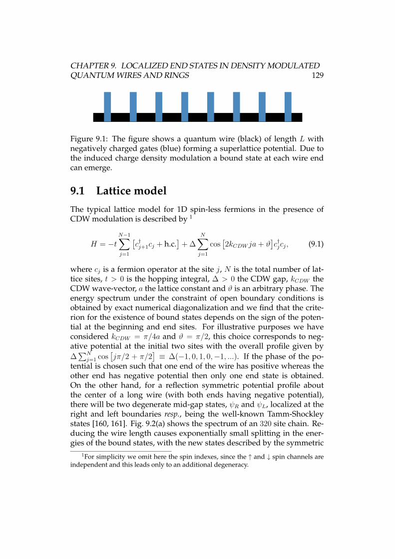
CHAPTER 9. LOCALIZED END STATES IN DENSITY MODULATEDQUANTUM WIRES AND RINGS 129
Figure 9.1: The figure shows a quantum wire (black) of length L withnegatively charged gates (blue) forming a superlattice potential. Due tothe induced charge density modulation a bound state at each wire endcan emerge.
9.1 Lattice modelThe typical lattice model for 1D spin-less fermions in the presence ofCDW modulation is described by 1
H = −tN−1∑
j=1
[c†j+1cj + h.c.
]+ ∆
N∑
j=1
cos[2kCDW ja+ ϑ
]c†jcj, (9.1)
where cj is a fermion operator at the site j, N is the total number of lat-tice sites, t > 0 is the hopping integral, ∆ > 0 the CDW gap, kCDW theCDW wave-vector, a the lattice constant and ϑ is an arbitrary phase. Theenergy spectrum under the constraint of open boundary conditions isobtained by exact numerical diagonalization and we find that the crite-rion for the existence of bound states depends on the sign of the poten-tial at the beginning and end sites. For illustrative purposes we haveconsidered kCDW = π/4a and ϑ = π/2, this choice corresponds to neg-ative potential at the initial two sites with the overall profile given by∆∑N
j=1 cos[jπ/2 + π/2
]≡ ∆(−1, 0, 1, 0,−1, ...). If the phase of the po-
tential is chosen such that one end of the wire has positive whereas theother end has negative potential then only one end state is obtained.On the other hand, for a reflection symmetric potential profile aboutthe center of a long wire (with both ends having negative potential),there will be two degenerate mid-gap states, ψR and ψL, localized at theright and left boundaries resp., being the well-known Tamm-Shockleystates [160, 161]. Fig. 9.2(a) shows the spectrum of an 320 site chain. Re-ducing the wire length causes exponentially small splitting in the ener-gies of the bound states, with the new states described by the symmetric
1For simplicity we omit here the spin indexes, since the ↑ and ↓ spin channels areindependent and this leads only to an additional degeneracy.
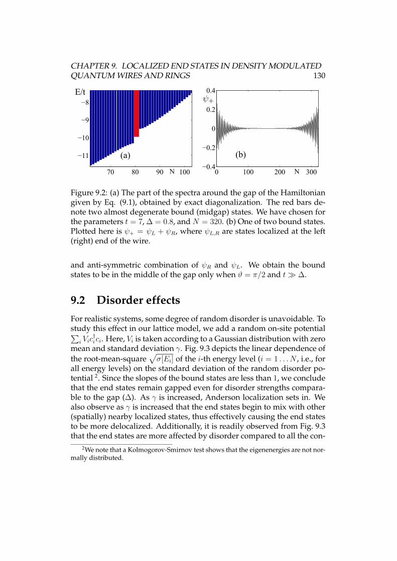
CHAPTER 9. LOCALIZED END STATES IN DENSITY MODULATEDQUANTUM WIRES AND RINGS 130
70 80 90 100
−11
−10
−9
−8
E/t
(a)
0 100 200 300−0.4
−0.2
0
0.2
0.4
N
(b)
N
Figure 9.2: (a) The part of the spectra around the gap of the Hamiltoniangiven by Eq. (9.1), obtained by exact diagonalization. The red bars de-note two almost degenerate bound (midgap) states. We have chosen forthe parameters t = 7, ∆ = 0.8, and N = 320. (b) One of two bound states.Plotted here is ψ+ = ψL + ψR, where ψL,R are states localized at the left(right) end of the wire.
and anti-symmetric combination of ψR and ψL. We obtain the boundstates to be in the middle of the gap only when ϑ = π/2 and t ∆.
9.2 Disorder effectsFor realistic systems, some degree of random disorder is unavoidable. Tostudy this effect in our lattice model, we add a random on-site potential∑
i Vic†ici. Here, Vi is taken according to a Gaussian distribution with zero
mean and standard deviation γ. Fig. 9.3 depicts the linear dependence ofthe root-mean-square
√σ[Ei] of the i-th energy level (i = 1 . . . N , i.e., for
all energy levels) on the standard deviation of the random disorder po-tential 2. Since the slopes of the bound states are less than 1, we concludethat the end states remain gapped even for disorder strengths compara-ble to the gap (∆). As γ is increased, Anderson localization sets in. Wealso observe as γ is increased that the end states begin to mix with other(spatially) nearby localized states, thus effectively causing the end statesto be more delocalized. Additionally, it is readily observed from Fig. 9.3that the end states are more affected by disorder compared to all the con-
2We note that a Kolmogorov-Smirnov test shows that the eigenenergies are not nor-mally distributed.
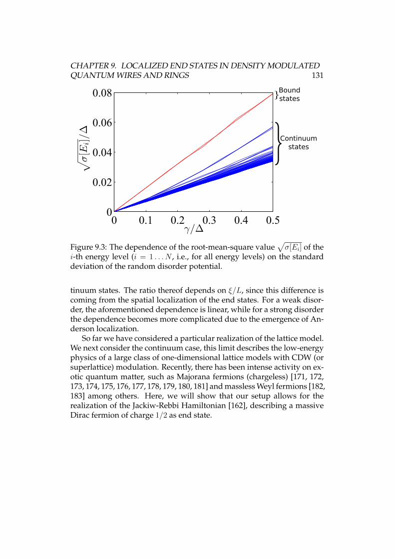
CHAPTER 9. LOCALIZED END STATES IN DENSITY MODULATEDQUANTUM WIRES AND RINGS 131
0 0.1 0.2 0.3 0.4 0.50
0.02
0.04
0.06
0.08
Continuumstates
Boundstates
Figure 9.3: The dependence of the root-mean-square value√σ[Ei] of the
i-th energy level (i = 1 . . . N , i.e., for all energy levels) on the standarddeviation of the random disorder potential.
tinuum states. The ratio thereof depends on ξ/L, since this difference iscoming from the spatial localization of the end states. For a weak disor-der, the aforementioned dependence is linear, while for a strong disorderthe dependence becomes more complicated due to the emergence of An-derson localization.
So far we have considered a particular realization of the lattice model.We next consider the continuum case, this limit describes the low-energyphysics of a large class of one-dimensional lattice models with CDW (orsuperlattice) modulation. Recently, there has been intense activity on ex-otic quantum matter, such as Majorana fermions (chargeless) [171, 172,173, 174, 175, 176, 177, 178, 179, 180, 181] and massless Weyl fermions [182,183] among others. Here, we will show that our setup allows for therealization of the Jackiw-Rebbi Hamiltonian [162], describing a massiveDirac fermion of charge 1/2 as end state.
CHAPTER 9. LOCALIZED END STATES IN DENSITY MODULATEDQUANTUM WIRES AND RINGS 132
9.3 Continuum modelWe consider a quantum wire in the presence of a gate-induced potentialwith periodicity λCDW = 2π/kCDW . For carrier densities smaller than theintraband energy gap only the lowest subband is occupied. The physicsof the fermion mode Ψσ (σ =↑, ↓ is the spin index) in the lowest sub-band is described in terms of the slowly varying right Rσ(x) and leftLσ(x) parts and is expressed as Ψσ(x) = Rσ(x)eikF x + Lσ(x)e−ikF x. Foran open wire, the boundary condition Ψσ(x = 0) = 0 imposes the con-straint [184, 185], Rσ(x) = −Lσ(−x). Thus, the Hamiltonian can be ex-pressed in terms of right movers only.
The non-interacting Hamiltonian can be written as a sum of two parts,H0 = H
(1)0 +H
(2)0 , where the kinetic part can be expressed in terms of only
the right moving fermions (the original range [0, L] now becomes [−L,L])and is given by (summation on the spin indices is assumed)
H(1)0 = −ivF
∫ L
−LdxR†σ(x)∂xRσ(x) (9.2)
and the CDW term by
H(2)0 = ∆0
∫ L
0
dx cos(2kCDWx+ ϑ)Ψ†σ(x)Ψσ(x), (9.3)
with ϑ being a constant phase factor. Thus
H0 = (1/2)
∫ L
−LdxR†σH0Rσ, (9.4)
where Rσ(x) = [Rσ(x),Rσ(−x)]T and the Hamiltonian density H0 foreach spin is the same and given by
H0 = −ivF τz∂x +m1(x)τx +m2(x)τy, (9.5)
where
m1(x) = − cos[2δkx+ ϑsgn(x)]∆0/2,
m2(x) = sin[2δkx+ ϑsgn(x)]∆0/2, (9.6)
and δk = kCDW − kF . If δk = 0 and the charge-density wave vanishesat the boundary, i.e., ϑ = π/2, then it is easy to verify that H0 satisfiesthe ‘chiral symmetry’ [186] PH0 = −H0P (P is a complex conjugation
CHAPTER 9. LOCALIZED END STATES IN DENSITY MODULATEDQUANTUM WIRES AND RINGS 133
operator). Moreover, the eigenvalue equation (H0ψσ = εψσ) of the chiralsymmetricH0 is related to the Jackiw-Rebbi equation describing massivefermions, 3
HJRψJR = [τz∂x +msgn(x)]ψJR = ετxψJR, (9.7)
via the transformation, ψJR = U−1τyψ and HJR = U−1H0τyU , whereU = exp(iτ · n2π/3) and n = (i + j + k)/
√3. Here, τx,y,z denote Pauli
matrices acting on the spinor Rσ(x). Solving the eigenvalue equationfor L vF/∆0 one obtains exponentially decaying bound states ψσ ∼exp[−(∆0/2vF )x] and ψσ ∼ exp[−(∆0/2vF )(L − x)] at x = 0 and x = L.Away from the chiral symmetry point (ϑ 6= π/2) bound states still existas long as sinϑ > 0, with the eigenstates given by
ψσ ∼ exp[−i(∆0 exp[−iϑ]/2vF )x] (9.8)ψσ ∼ exp[−i(∆0 exp[−iϑ]/2vF )(L− x)]. (9.9)
For infinite wires the eigenvalues are degenerate and given by
ε = −∆0 cos(ϑ)/2. (9.10)
However, finite length introduces overlap between the end states leadingto an exponentially small splitting in the energy (see below and Fig. 9.4).
In a realistic quantum wire the gap ∆(x) and the phase ϑ(x) will in-variably be position dependent. Assuming this dependence to be weak,the correction in lowest order in δ(x)/∆0 1 is given by,
δε = − ∆0
4vF
∫ ∞
0
dxδ(x) sin 2ϑ(x)e−∆0 sin[ϑ0]x/vF , (9.11)
where 〈δ(x)〉 = 0 and 〈ϑ(x)〉 = 〈ϑ0 + δϑ(x)〉 = ϑ0, and they both varyslowly on the Fermi wavelength λF = 2π/kF . Thus, δε ∆0, and thebound states remain stable to weak perturbations.
9.4 Interaction effectsIn the following, we consider the effect of repulsive interactions on theend states. For simplicity, we consider spinless fermions with kF = kCDW
3The fractional charge 1/2 of the end states are seen only in the continuummodel [162] but not in the lattice model. This difference is coming from subtractingan infinite Fermi sea when passing to the continuum model.
CHAPTER 9. LOCALIZED END STATES IN DENSITY MODULATEDQUANTUM WIRES AND RINGS 134
and ϑ = π/2. As usual in 1D, the interactions can be split into forwardand back scattering parts. The former
HF = πvFg4
∫ L
0
dx(:JRJR: + :JLJL:), (9.12)
where JR = R†(x)R(x) and JL = L†(x)L(x), is responsible for the veloc-ity renormalization [187], v = vF (1+g4). On the other hand, the backscat-tering part given by
HB = πvFg2
∫ L
0
dx:JLJR:, (9.13)
renormalizes the gap at the lowest order in interaction. The mean-fieldgap ∆(x) ∝ g2vF 〈R(x)R†(−x)〉 adds to the externally induced gap
m2(x) = sgn(x)∆0/2. (9.14)
We note that similar to m2(x), ∆(0+) = −∆(0−). This can be seen byinvoking the boundary condition, R(x) = −L(−x), and by expressingR(x) = exp(i
√4πφR) and L(x) = exp(−i
√4πφL) in terms of the bosonic
fields φR(x) and φL(x) which themselves satisfy [185]√
4πφR(0) = −√
4πφL(0) + π. (9.15)
Thus, for weak interactions the bound states retain the same form as forthe non-interacting case but with renormalized velocity and gap. To esti-mate the gap size we evaluate the self-energy, Σ, using the unperturbedGreen’s function for an infinite wire, G0(iω, k) = (iω−vFkτz−∆0τy/2)−1.In leading order, the gap renormalizes to
(∆0/2)[1 + (g2/4) ln[min(Λ, vFL−1)/∆0]], (9.16)
where Λ is the band width. Thus, the localization length, given by ξ =(2vF/∆0)1 + g4 − (g2/4) ln[vF/L∆0], reduces with interaction. In otherwords, due to the repulsive interaction between the continuum and theend states, the latter states get squeezed.
The renormalization of the gap can be more rigorously analyzed viabosonization. Using standard procedures [188], we obtain the followingform for the bosonic Lagrangian
L(x, t) =∑
ν=c,s
[ 1
2vνKν
(∂tφν)2 − vν
2Kν
(∂xφν)2]
(9.17)
+vF
2πa2
∑
η=↑,↓
yη sin[√
4πφη − 2δkx− ϑ],
CHAPTER 9. LOCALIZED END STATES IN DENSITY MODULATEDQUANTUM WIRES AND RINGS 135
where the subscripts c, s refer to charge and spin, resp. The ∂xφc/s fielddescribes the charge/spin density fluctuations and θc/s is the conjugatedfield, and φ↑,↓ = (φc ± φs)/
√2. The Luttinger liquid parameters Kc/s
and velocities vc/s encode interactions, and y↑,↓ = a∆0/vF . The sine termdenotes the coupling of up and down spin fermions with the external po-tential. As before, we assume δk = 0. In general, there are two additionalterms: one of them arises due to backscattering between opposite spinelectrons and is given by cos(
√8πφs), and the other, cos(4
√πφc − 4kFx),
describes the Umklapp scattering. However, both can be neglected asthe two operators flow to zero under a renormalization group (RG) treat-ment.
The scaling dimensions of sin(√
4πφ↑,↓), d↑,↓ = (Kc + Ks)/2 ≈ 1, in-dicate that near commensurability (δkvF/∆0 1) the sine terms arestrongly relevant. The parameters y↑,↓ have an identical flow [so as topreserve the SU(2) symmetry, this also implies Ks = 1] towards thestrong coupling regime and yields an effective localization length ξ ∼a(a∆0/vF )2/(Kc−3) for the bound state. Thus as before the role of the in-teractions is to reinforce the externally induced gap. We note that underRG additional terms of the type ∂iφc∂iφs (where i = x, τ ) are generated,however, they are marginal and leave the essential physics unaltered.
9.5 DetectionA viable approach for detecting the energy splitting between the boundstates is through persistent current measurements. For this the wire shouldbe in a ring geometry so that the end states are connected together viaa tunnel junction and also large enough such that the energy splittingbetween the bound states is small yet the overlap of the localized wave-functions remain non-zero. Such a set-up can enclose magnetic flux Φ in-ducing Aharonov-Bohm (AB) oscillations in a mesoscopic (phase-coherent)regime. Next consider a single electron placed in one of the bound states.The effective Hamiltonian for the spinless fermion in terms of the orthog-onal symmetric, |+〉, and anti-symmetric, |−〉, states can thus be written
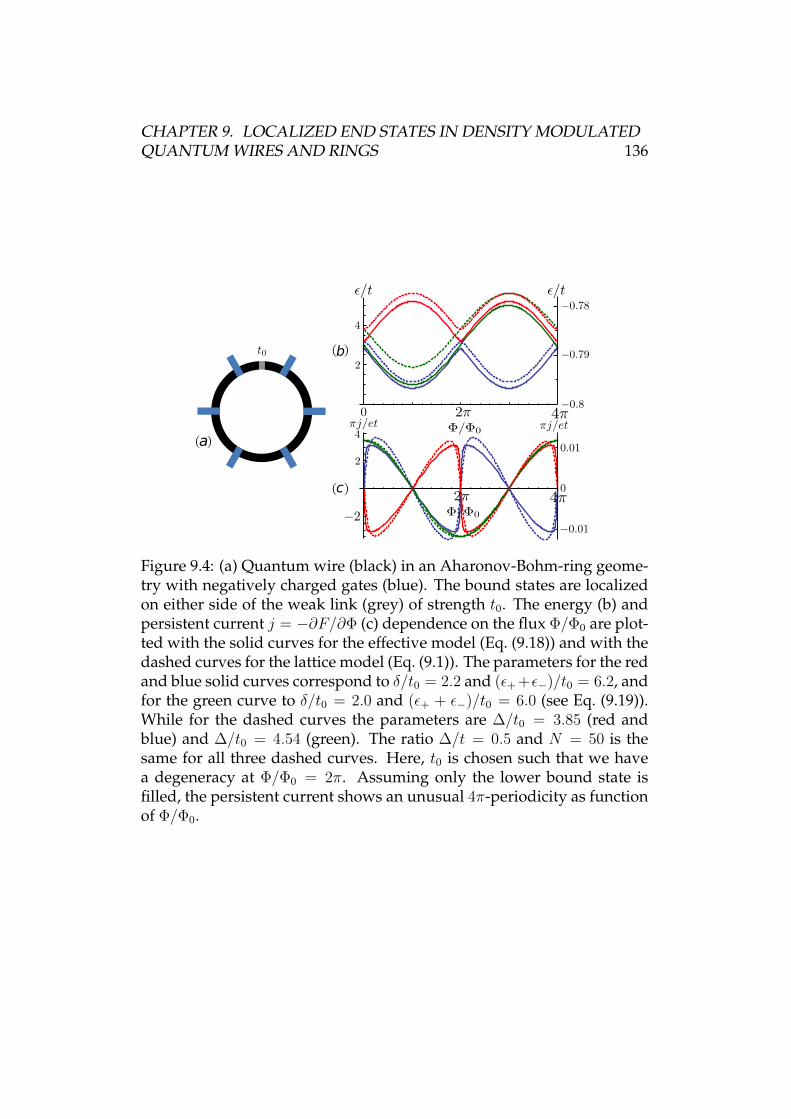
CHAPTER 9. LOCALIZED END STATES IN DENSITY MODULATEDQUANTUM WIRES AND RINGS 136
a
b
c
Figure 9.4: (a) Quantum wire (black) in an Aharonov-Bohm-ring geome-try with negatively charged gates (blue). The bound states are localizedon either side of the weak link (grey) of strength t0. The energy (b) andpersistent current j = −∂F/∂Φ (c) dependence on the flux Φ/Φ0 are plot-ted with the solid curves for the effective model (Eq. (9.18)) and with thedashed curves for the lattice model (Eq. (9.1)). The parameters for the redand blue solid curves correspond to δ/t0 = 2.2 and (ε+ +ε−)/t0 = 6.2, andfor the green curve to δ/t0 = 2.0 and (ε+ + ε−)/t0 = 6.0 (see Eq. (9.19)).While for the dashed curves the parameters are ∆/t0 = 3.85 (red andblue) and ∆/t0 = 4.54 (green). The ratio ∆/t = 0.5 and N = 50 is thesame for all three dashed curves. Here, t0 is chosen such that we havea degeneracy at Φ/Φ0 = 2π. Assuming only the lower bound state isfilled, the persistent current shows an unusual 4π-periodicity as functionof Φ/Φ0.
CHAPTER 9. LOCALIZED END STATES IN DENSITY MODULATEDQUANTUM WIRES AND RINGS 137
as 4
H =∑
η=±
[εη + ηt0 cos
( Φ
Φ0
)]|η〉〈η|+ it0 sin
( Φ
Φ0
)
×[|−〉〈+| − |+〉〈−|
], (9.18)
where Φ0 = h/e is the flux quantum, ε+ (ε−) the energy of the symmetric(anti-symmetric) mode, and the tunneling across the weak link is associ-ated with a factor νt0 exp(iµΦ/Φ0), where ν, µ = ±1 and t0 the tunnelingamplitude. For (anti-) clockwise tunneling we have µ = +(−), while thesign of ν depends on the relative sign between the wave-functions acrossthe weak link. The energy eigenvalues are
ε1/2 =1
2
(ε− + ε+ ±
√4t20 + δ2 − 4t0δ cos[Φ/Φ0]
), (9.19)
where δ = |ε+− ε−|. At Φ/Φ0 = 2π the separation between the two eigen-values is minimal and given by |2t0 − δ|. For large separations, the en-ergy levels exhibit the usual 2π dependence on the flux Φ/Φ0. In contrast,for a flux sweep-rate ω larger than |2t0 − δ| a scenario emerges whereinan electron placed in one of the levels can jump to the second level andcome back to the original one after a second 2π phase, thus exhibitingan unusual 4π-periodicity in the persistent current, j = −∂F/∂Φ, whereF is the free energy [189]. By independently varying t0 and ω the split-ting δ can be estimated. For typical values t0 ∼ δ ∼ 10µeV we estimatej ∼ 0.1nA, which is of measurable size [190, 191]. For the observation,the phase-coherence length Lφ of the ring needs to exceed L. For GaAsrings, we note that Lφ & µm for sub-Kelvin temperatures [190, 191].
The effective model, Eq. (9.18), does not take into account the contri-bution arising from the filled Fermi sea of continuum states. However,when the number of continuum states below the gap is even—the statescome in pairs with mutually canceling contributions to the current. Onthe other hand, when this number is odd, the topmost filled continuumstate contributes to the current. Nevertheless, the amplitude of the per-sistent current, due to the end and continuum states, scale differentlywith the lattice length N—the latter behaves like 1/N , while the formerlike δ ∼ e−ξ/Na. Thus, for chains with N 1 and ∆ ∼ ~vF/Na, thepersistent current will be dominated by the end states and our effective
4For simplicity we omit here the spin indexes, since the ↑ and ↓ spin channels areindependent and this leads only to an additional degeneracy
CHAPTER 9. LOCALIZED END STATES IN DENSITY MODULATEDQUANTUM WIRES AND RINGS 138
description fully applies. The dashed curves in Fig. 9.4 include contri-butions from the bound states as well as the filled Fermi sea. Indeed wehave confirmed that the contributions from the continuum states are twoorders of magnitude less compared to those from the bound states. Fi-nally, for the spinfull case, the amplitude of j simply doubles, whereasthe periodicity remains unchanged.
9.6 Effective quantum dotSimilar to the discrete quantum dot states, the presence of spinful, CDW-induced, localized states in the quantum wire opens up an intriguingpossibility for the realization of a quantum computer device. These statesare well separated from the continuum and can be filled by tuning thechemical potential to the end state level. We note that these ‘quantumdots’ contain automatically only one orbital level, and no individual gatesare needed to tune them into a single electron regime. Due to incompletescreening there will be half-filling, i.e., only one state on either end willbe filled. This is simply because once one of the energy levels on eitherend is filled, to fill the remaining two levels requires additional energy toovercome the Coulomb repulsion. The physics of the half-filled state isdescribed by the usual Hubbard model, H = −t∑σ=↑,↓(c
†σ,Rcσ,L + h.c.) +
U∑
i=L,R n↑,in↓,i, where t is the tunneling amplitude and U is the onsiterepulsion. For the energy hierarchy ∆ U t the effective Hamilto-nian acquires the Heisenberg form, H = JSR · SL, where J = 4t2/U .The effective exchange coupling J can be controlled by changing thegate potential which determines the overlap between the left and rightend modes and hence the tunneling amplitude t. We note that for weakoverlap, t is small and U large making the J to be small, whereas forstrong overlap the opposite is true. 5 By switching on and off the ex-change constant in an appropriate sequence, the essential operations ofthe quantum dot, both the ‘swap’ and ‘square-root-of-swap’ operationscan be performed, which, together with two single spin-qubit operations,enables the fundamental XOR gate [1].
Finite overlap between the right and the left end states can be ensuredif their localization length ξ is on the order of the wire length L. Thisrestriction yields an estimate for the strength of the periodically modu-lated external voltage, ∆0 ∼ Λ(a/L)(3−Kc)/2, where Λ ∼ vF/a is the band
5We note that because of the gap between the bound state and the continuum,Kondo physics does not play a role.
CHAPTER 9. LOCALIZED END STATES IN DENSITY MODULATEDQUANTUM WIRES AND RINGS 139
width. A GaAs quantum wire with length L ∼ 1µm with approximately10 − 20 gates requires a Fermi wave-length λF ∼ 50nm. And with theparameters [192], Λ ∼ 0.2eV, Kc = 0.8, and lattice spacing a ≈ 5A, weobtain ∆0 ∼ 0.04meV. Thus, the upper bound for temperatures are in theachievable range of a few hundred milli-Kelvin.
9.7 ConclusionsWe have shown that a CDW gap in a quantum wire can lead to boundstates at the ends of the wire which are stable against weak disorderand interactions. They map to massive Dirac fermions desrcibed by theJackiw-Rebbi model. In an AB-ring, the bound states lead to an unusual4π-periodicity in the persistent current. Finally, the two opposite endstates serve as effective double quantum dot which can be used to imple-ment quantum computing gates for spin-qubits.
9.8 AcknowledgementsWe acknowledge discussions with K. Damle, C. Kloffel, D. Rainis, B.Rothlisberger, D. Stepanenko, and V. Tripathi. This work is supportedby the Swiss NSF, NCCR Nanoscience and NCCR QSIT, DARPA, andIARPA.
CHAPTER 10Realistic transport modeling for a
superconducting nanowire withMajorana fermions
Adapted from:Diego Rainis, Luka Trifunovic, Jelena Klinovaja, and Daniel Loss
“Realistic transport modeling for a superconducting nanowire with Majoranafermions”,
Phys. Rev. B 87, 024515 (2013)
Motivated by recent experiments searching for Majorana fermions (MFs) inhybrid semiconducting-superconducting nanostructures, we consider a re-alistic tight-binding model and analyze its transport behavior numerically.In particular, we take into account the presence of a superconducting con-tact, used in real experiments to extract the current, which is usually not in-cluded in theoretical calculations. We show that important features emergethat are absent in simpler models, such as the shift in energy of the prox-imity gap signal, and the enhanced visibility of the topological gap for in-creased spin-orbit interaction. We find oscillations of the zero bias peak asa function of the magnetic field and study them analytically. We argue thatmany of the experimentally observed features hint at an actual spin-orbit in-teraction larger than the one typically assumed. However, even taking intoaccount all the known ingredients of the experiments and exploring manyparameter regimes for MFs, we are not able to reach full agreement with thereported data. Thus, a different physical origin for the observed zero-biaspeak cannot be excluded.
140
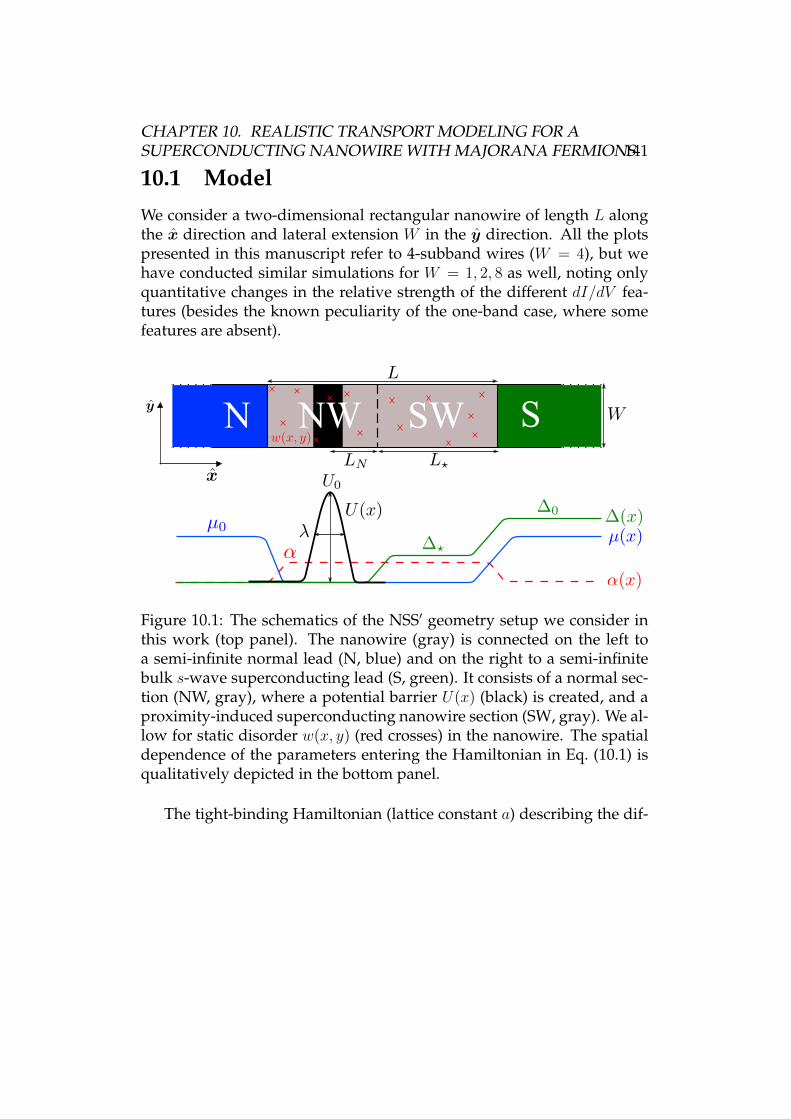
CHAPTER 10. REALISTIC TRANSPORT MODELING FOR ASUPERCONDUCTING NANOWIRE WITH MAJORANA FERMIONS141
10.1 ModelWe consider a two-dimensional rectangular nanowire of length L alongthe x direction and lateral extension W in the y direction. All the plotspresented in this manuscript refer to 4-subband wires (W = 4), but wehave conducted similar simulations for W = 1, 2, 8 as well, noting onlyquantitative changes in the relative strength of the different dI/dV fea-tures (besides the known peculiarity of the one-band case, where somefeatures are absent).
N SW SNW
Figure 10.1: The schematics of the NSS′ geometry setup we consider inthis work (top panel). The nanowire (gray) is connected on the left toa semi-infinite normal lead (N, blue) and on the right to a semi-infinitebulk s-wave superconducting lead (S, green). It consists of a normal sec-tion (NW, gray), where a potential barrier U(x) (black) is created, and aproximity-induced superconducting nanowire section (SW, gray). We al-low for static disorder w(x, y) (red crosses) in the nanowire. The spatialdependence of the parameters entering the Hamiltonian in Eq. (10.1) isqualitatively depicted in the bottom panel.
The tight-binding Hamiltonian (lattice constant a) describing the dif-
CHAPTER 10. REALISTIC TRANSPORT MODELING FOR ASUPERCONDUCTING NANOWIRE WITH MAJORANA FERMIONS142
ferent sections of the setup has the form
H =∑
m,d
c†m+d,α
[−tδαβ − iαm(x · d)σyαβ
]cm,β
+∑
m
c†m,α
[(εm − µ0)δαβ −
gm2µBBxσ
xαβ
]cm,β
+∑
m
∆m
(c†m,↑c
†m,↓ + H.c.
), (10.1)
where t = ~2/(2ma2) is the hopping amplitude (set to 1 and taken asan energy unit) and α is the spin-flip hopping amplitude, related to thephysical SOI parameter by α = α/2a and to the SOI energy byEso = α2/t.Here and in the remainder of the paper we are neglecting transverse spin-orbit coupling, but we have checked that the introduction of a small fi-nite transverse SOI is not affecting qualitatively our results. We made theassignment t = 10 meV, which corresponds to taking a ' 15 nm, and re-alistic sizes (∼ µm) are then amenable to reasonable computations. Thesums run over all lattice sites m and nearest neighbors (m + d). Im-plicit summation over repeated spin indices is assumed. The constantµ0 is chosen to set the common chemical potential to the zero-field bot-tom of the topmost band and depends on the number of subbands (i.e.on W ). Further, εm = −µm + Um + wm accounts for local variations ofthe chemical potential, for the tunnel-barrier potential Um, and includesan on-site random potential wm which models Anderson disorder. Thetunnel barrier has a Gaussian profile with height U0 and width λ. The ex-ternal magnetic fieldB points along the nanowire axis (x) and induces aZeeman splitting 2VZ = gmµBB. Finally, ∆ is the pairing amplitude andcan either account for the native superconductivity in the bulk s-wavesuperconducting lead (∆0) or for the proximity-induced pairing in thenanowire (∆?), as exemplified in Fig. 10.1. All the above quantities aretaken to be site-dependent along the x direction (except wm, which istaken to be completely random), so that we can model different parts ofthe setup. The normal lead is characterized by
α = 0, µ ' −µ0 (i.e. metallic regime),
g = 2, wm = 0, ∆m = 0. (10.2)
The nanowire is characterized by finite α = αR, chemical potential µ ' 0close to the bottom of the topmost band, g = 50 appropriate for InSbnanowires, and ∆m varying from 0 in the normal section to ∆? in the
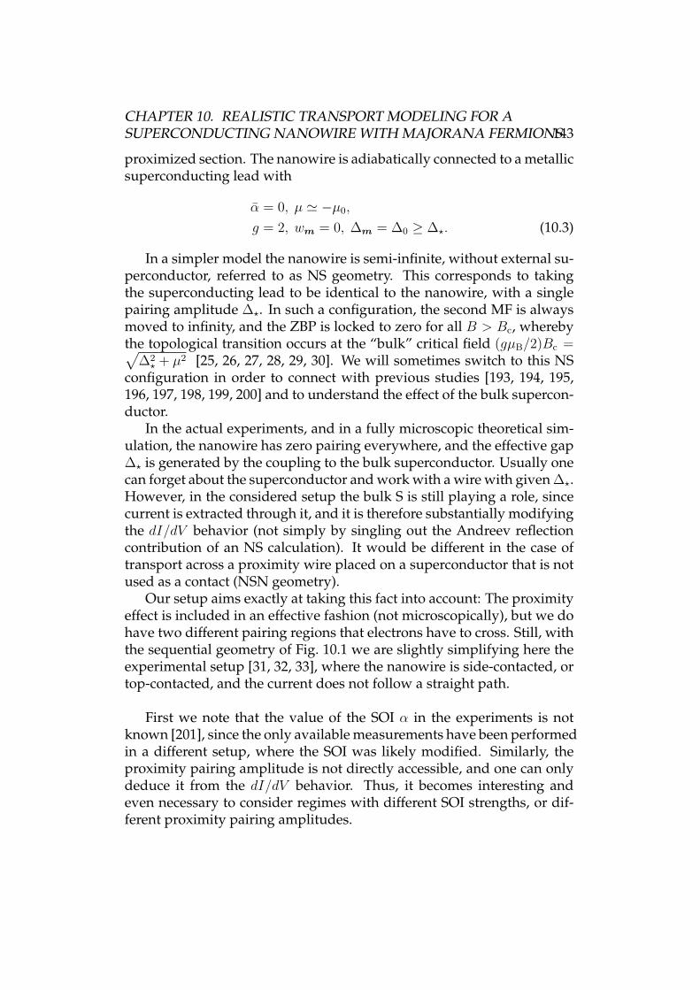
CHAPTER 10. REALISTIC TRANSPORT MODELING FOR ASUPERCONDUCTING NANOWIRE WITH MAJORANA FERMIONS143
proximized section. The nanowire is adiabatically connected to a metallicsuperconducting lead with
α = 0, µ ' −µ0,
g = 2, wm = 0, ∆m = ∆0 ≥ ∆?. (10.3)
In a simpler model the nanowire is semi-infinite, without external su-perconductor, referred to as NS geometry. This corresponds to takingthe superconducting lead to be identical to the nanowire, with a singlepairing amplitude ∆?. In such a configuration, the second MF is alwaysmoved to infinity, and the ZBP is locked to zero for all B > Bc, wherebythe topological transition occurs at the “bulk” critical field (gµB/2)Bc =√
∆2? + µ2 [25, 26, 27, 28, 29, 30]. We will sometimes switch to this NS
configuration in order to connect with previous studies [193, 194, 195,196, 197, 198, 199, 200] and to understand the effect of the bulk supercon-ductor.
In the actual experiments, and in a fully microscopic theoretical sim-ulation, the nanowire has zero pairing everywhere, and the effective gap∆? is generated by the coupling to the bulk superconductor. Usually onecan forget about the superconductor and work with a wire with given ∆?.However, in the considered setup the bulk S is still playing a role, sincecurrent is extracted through it, and it is therefore substantially modifyingthe dI/dV behavior (not simply by singling out the Andreev reflectioncontribution of an NS calculation). It would be different in the case oftransport across a proximity wire placed on a superconductor that is notused as a contact (NSN geometry).
Our setup aims exactly at taking this fact into account: The proximityeffect is included in an effective fashion (not microscopically), but we dohave two different pairing regions that electrons have to cross. Still, withthe sequential geometry of Fig. 10.1 we are slightly simplifying here theexperimental setup [31, 32, 33], where the nanowire is side-contacted, ortop-contacted, and the current does not follow a straight path.
First we note that the value of the SOI α in the experiments is notknown [201], since the only available measurements have been performedin a different setup, where the SOI was likely modified. Similarly, theproximity pairing amplitude is not directly accessible, and one can onlydeduce it from the dI/dV behavior. Thus, it becomes interesting andeven necessary to consider regimes with different SOI strengths, or dif-ferent proximity pairing amplitudes.
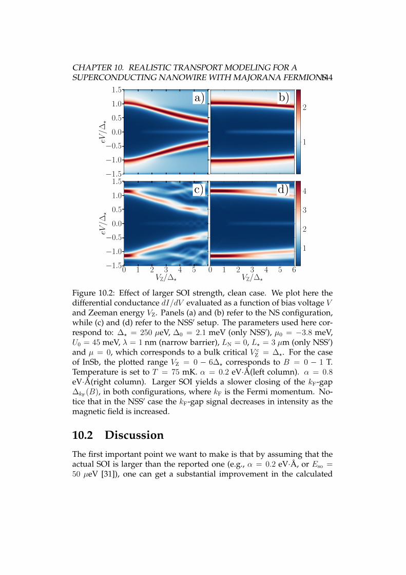
CHAPTER 10. REALISTIC TRANSPORT MODELING FOR ASUPERCONDUCTING NANOWIRE WITH MAJORANA FERMIONS144
0 1 2 3 4 5 6VZ/∆
−1.5
−1.0
−0.5
0.0
0.5
1.0
1.5
eV/∆
1
2
0 1 2 3 4 5 6VZ/∆
−1.5
−1.0
−0.5
0.0
0.5
1.0
1.5
eV/∆
1
2
3
40 1 2 3 4 5 6VZ/∆
−1.5
−1.0
−0.5
0.0
0.5
1.0
1.5
eV/∆
1
2
0 1 2 3 4 5 6VZ/∆
−1.5
−1.0
−0.5
0.0
0.5
1.0
1.5eV
/∆
1
2
3
4
Figure 10.2: Effect of larger SOI strength, clean case. We plot here thedifferential conductance dI/dV evaluated as a function of bias voltage Vand Zeeman energy VZ. Panels (a) and (b) refer to the NS configuration,while (c) and (d) refer to the NSS′ setup. The parameters used here cor-respond to: ∆? = 250 µeV, ∆0 = 2.1 meV (only NSS′), µ0 = −3.8 meV,U0 = 45 meV, λ = 1 nm (narrow barrier), LN = 0, L? = 3 µm (only NSS′)and µ = 0, which corresponds to a bulk critical V c
Z = ∆?. For the caseof InSb, the plotted range VZ = 0 − 6∆? corresponds to B = 0 − 1 T.Temperature is set to T = 75 mK. α = 0.2 eV·A(left column). α = 0.8eV·A(right column). Larger SOI yields a slower closing of the kF-gap∆kF
(B), in both configurations, where kF is the Fermi momentum. No-tice that in the NSS′ case the kF-gap signal decreases in intensity as themagnetic field is increased.
10.2 DiscussionThe first important point we want to make is that by assuming that theactual SOI is larger than the reported one (e.g., α = 0.2 eV·A, or Eso =50 µeV [31]), one can get a substantial improvement in the calculated
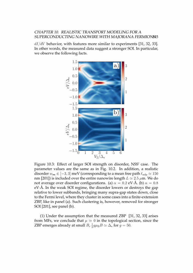
CHAPTER 10. REALISTIC TRANSPORT MODELING FOR ASUPERCONDUCTING NANOWIRE WITH MAJORANA FERMIONS145
dI/dV behavior, with features more similar to experiments [31, 32, 33].In other words, the measured data suggest a stronger SOI. In particular,we observe the following facts.
0 1 2 3 4 5 6VZ/∆
−1.5
−1.0
−0.5
0.0
0.5
1.0
1.5
eV/∆
1
2
3
0 1 2 3 4 5 6VZ/∆
−1.5
−1.0
−0.5
0.0
0.5
1.0
1.5
eV/∆
1
2
3
Figure 10.3: Effect of larger SOI strength on disorder, NSS′ case. Theparameter values are the same as in Fig. 10.2. In addition, a realisticdisorder wm ∈ [−3, 3] meV (corresponding to a mean free path `mfp ' 150nm [201]) is included over the entire nanowire length L ' 2.5 µm. We donot average over disorder configurations. (a) α = 0.2 eV·A. (b) α = 0.8eV·A. In the weak SOI regime, the disorder lowers or destroys the gaprelative to lower subbands, bringing many supra-gap states down, closeto the Fermi level, where they cluster in some cases into a finite-extensionZBP, like in panel (a). Such clustering is, however, removed for strongerSOI [201], see panel (b).
(1) Under the assumption that the measured ZBP [31, 32, 33] arisesfrom MFs, we conclude that µ ' 0 in the topological section, since theZBP emerges already at small B, 1
2gµBB ' ∆? for g = 50.
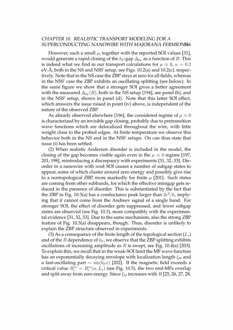
CHAPTER 10. REALISTIC TRANSPORT MODELING FOR ASUPERCONDUCTING NANOWIRE WITH MAJORANA FERMIONS146
However, such a small µ, together with the reported SOI values [31],would generate a rapid closing of the kF-gap ∆kF
as a function of B. Thisis indeed what we find in our transport calculations for µ ' 0, α = 0.2eV·A, both in the NS and NSS′ setup, see Figs. 10.2(a) and 10.2(c), respec-tively. Note that in the NS case the ZBP stays at zero for all fields, whereasin the NSS′ case the ZBP exhibits an oscillating splitting (see below). Inthe same figure we show that a stronger SOI gives a better agreementwith the measured ∆kF
(B), both in the NS setup [194], see panel (b), andin the NSS′ setup, shown in panel (d). Note that this latter SOI effect,which answers the issue raised in point (iv) above, is independent of thenature of the observed ZBP.
As already observed elsewhere [196], the considered regime of µ ' 0is characterized by an invisible gap closing, probably due to pretransitionwave functions which are delocalized throughout the wire, with littleweight close to the probed edges. At finite temperature we observe thisbehavior both in the NS and in the NSS′ setups. On can thus state thatissue (i) has been settled.
(2) When realistic Anderson disorder is included in the model, theclosing of the gap becomes visible again even in the µ ' 0 regime [197,201, 198], reintroducing a discrepancy with experiments [31, 32, 33]. Dis-order in a nanowire with weak SOI causes a number of subgap states toappear, some of which cluster around zero energy and possibly give riseto a nontopological ZBP, more markedly for finite µ [201]. Such statesare coming from other subbands, for which the effective minigap gets re-duced in the presence of disorder. This is substantiated by the fact thatthe ZBP in Fig. 10.3(a) has a conductance peak larger than 2e2/h, imply-ing that it cannot come from the Andreev signal of a single band. Forstronger SOI, the effect of disorder gets suppressed, and fewer subgapstates are observed (see Fig. 10.3), more compatibly with the experimen-tal evidence [31, 32, 33]. Due to the same mechanism, also the strong ZBPfeature of Fig. 10.3(a) disappears, though. Thus, disorder is unlikely toexplain the ZBP structure observed in experiments.
(3) As a consequence of the finite length of the topological section (L?)and of theB dependence of kF, we observe that the ZBP splitting exhibitsoscillations of increasing amplitude as B is swept, see Fig. 10.4(a) [203].To explain this, we recall that in the weak-SOI limit the MF wave functionhas an exponentially decaying envelope with localization length ξM anda fast-oscillating part ∼ sin(kFx) [202]. If the magnetic field exceeds acritical value B∗∗c = B∗∗c (α,L?) (see Fig. 10.5), the two end-MFs overlapand split away from zero energy. Since ξM increases withB [25, 26, 27, 28,
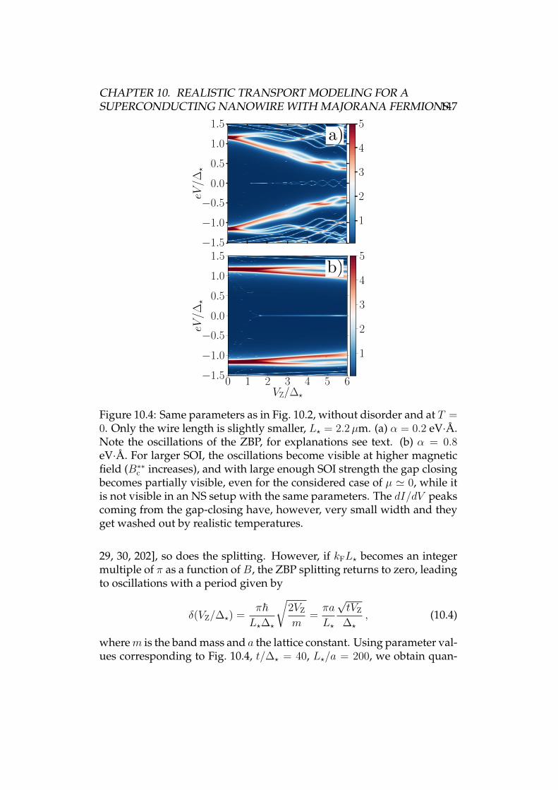
CHAPTER 10. REALISTIC TRANSPORT MODELING FOR ASUPERCONDUCTING NANOWIRE WITH MAJORANA FERMIONS147
0 1 2 3 4 5 6VZ/?
1.5
1.0
0.5
0.0
0.5
1.0
1.5
eV/
?
1
2
3
4
5
0 1 2 3 4 5 6VZ/?
1.5
1.0
0.5
0.0
0.5
1.0
1.5
eV/
?
1
2
3
4
5
Figure 10.4: Same parameters as in Fig. 10.2, without disorder and at T =0. Only the wire length is slightly smaller, L? = 2.2µm. (a) α = 0.2 eV·A.Note the oscillations of the ZBP, for explanations see text. (b) α = 0.8eV·A. For larger SOI, the oscillations become visible at higher magneticfield (B∗∗c increases), and with large enough SOI strength the gap closingbecomes partially visible, even for the considered case of µ ' 0, while itis not visible in an NS setup with the same parameters. The dI/dV peakscoming from the gap-closing have, however, very small width and theyget washed out by realistic temperatures.
29, 30, 202], so does the splitting. However, if kFL? becomes an integermultiple of π as a function of B, the ZBP splitting returns to zero, leadingto oscillations with a period given by
δ(VZ/∆?) =π~L?∆?
√2VZ
m=πa
L?
√tVZ
∆?
, (10.4)
wherem is the band mass and a the lattice constant. Using parameter val-ues corresponding to Fig. 10.4, t/∆? = 40, L?/a = 200, we obtain quan-
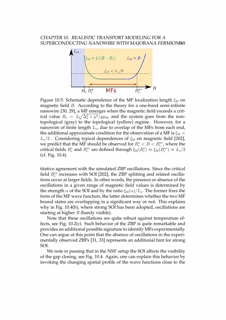
CHAPTER 10. REALISTIC TRANSPORT MODELING FOR ASUPERCONDUCTING NANOWIRE WITH MAJORANA FERMIONS148
Figure 10.5: Schematic dependence of the MF localization length ξM onmagnetic field B. According to the theory for a one-band semi-infinitenanowire [30, 29], a MF emerges when the magnetic field exceeds a crit-ical value Bc = 2
√∆2? + µ2/gµB, and the system goes from the non-
topological (gray) to the topological (yellow) regime. However, for ananowire of finite length L?, due to overlap of the MFs from each end,the additional approximate condition for the observation of a MF is ξM <L?/2 . Considering typical dependences of ξM on magnetic field [202],we predict that the MF should be observed for B∗c < B < B∗∗c , where thecritical fields B∗c and B∗∗c are defined through ξM(B∗c ) ≈ ξM(B∗∗c ) ≈ L?/2(cf. Fig. 10.4).
titative agreement with the simulated ZBP oscillations. Since the criticalfield B∗∗c increases with SOI [202], the ZBP splitting and related oscilla-tions occur at larger fields. In other words, the presence or absence of theoscillations in a given range of magnetic field values is determined bythe strength α of the SOI and by the ratio ξM(α)/L?. The former fixes theform of the MF wave function, the latter determines whether the two MFbound states are overlapping in a significant way or not. This explainswhy in Fig. 10.4(b), where strong SOI has been adopted, oscillations arestarting at higher B (barely visible).
Note that these oscillations are quite robust against temperature ef-fects, see Fig. 10.2(c). Such behavior of the ZBP is quite remarkable andprovides an additional possible signature to identify MFs experimentally.One can argue at this point that the absence of oscillations in the experi-mentally observed ZBPs [31, 33] represents an additional hint for strongSOI.
We note in passing that in the NSS′ setup the SOI affects the visibilityof the gap closing, see Fig. 10.4. Again, one can explain this behavior byinvoking the changing spatial profile of the wave functions close to the
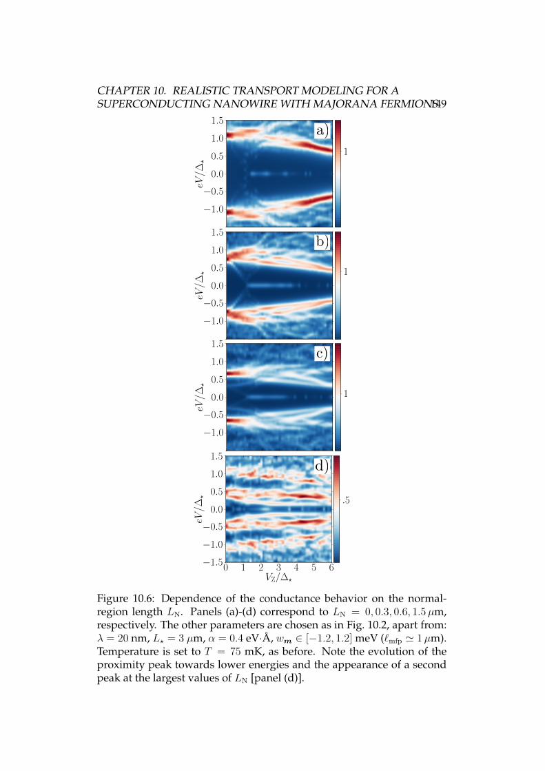
CHAPTER 10. REALISTIC TRANSPORT MODELING FOR ASUPERCONDUCTING NANOWIRE WITH MAJORANA FERMIONS149
0 1 2 3 4 5 6VZ/∆
−1.5
−1.0
−0.5
0.0
0.5
1.0
1.5
eV/∆
.5
0 1 2 3 4 5 6VZ/∆
−1.5
−1.0
−0.5
0.0
0.5
1.0
1.5
eV/∆
1
0 1 2 3 4 5 6VZ/∆
−1.5
−1.0
−0.5
0.0
0.5
1.0
1.5
eV/∆
1
0 1 2 3 4 5 6VZ/∆
−1.5
−1.0
−0.5
0.0
0.5
1.0
1.5
eV/∆
1
Figure 10.6: Dependence of the conductance behavior on the normal-region length LN. Panels (a)-(d) correspond to LN = 0, 0.3, 0.6, 1.5µm,respectively. The other parameters are chosen as in Fig. 10.2, apart from:λ = 20 nm, L? = 3 µm, α = 0.4 eV·A, wm ∈ [−1.2, 1.2] meV (`mfp ' 1µm).Temperature is set to T = 75 mK, as before. Note the evolution of theproximity peak towards lower energies and the appearance of a secondpeak at the largest values of LN [panel (d)].
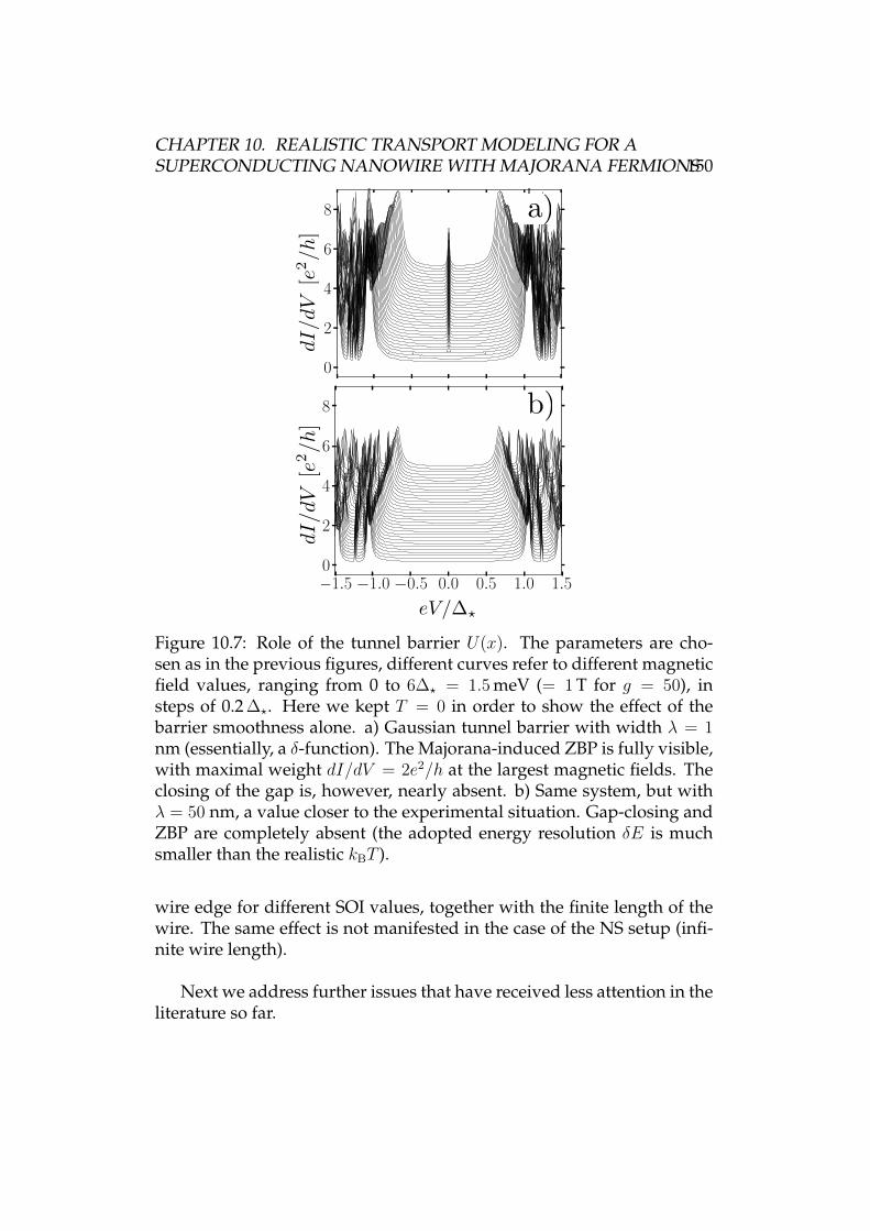
CHAPTER 10. REALISTIC TRANSPORT MODELING FOR ASUPERCONDUCTING NANOWIRE WITH MAJORANA FERMIONS150
1.5 1.0 0.5 0.0 0.5 1.0 1.5eV/pr
0
2
4
6
8
dI/d
V e2 /
h
1.5 1.0 0.5 0.0 0.5 1.0 1.5eV/pr
0
2
4
6
8
dI/d
V e2 /
h
Figure 10.7: Role of the tunnel barrier U(x). The parameters are cho-sen as in the previous figures, different curves refer to different magneticfield values, ranging from 0 to 6∆? = 1.5 meV (= 1 T for g = 50), insteps of 0.2 ∆?. Here we kept T = 0 in order to show the effect of thebarrier smoothness alone. a) Gaussian tunnel barrier with width λ = 1nm (essentially, a δ-function). The Majorana-induced ZBP is fully visible,with maximal weight dI/dV = 2e2/h at the largest magnetic fields. Theclosing of the gap is, however, nearly absent. b) Same system, but withλ = 50 nm, a value closer to the experimental situation. Gap-closing andZBP are completely absent (the adopted energy resolution δE is muchsmaller than the realistic kBT ).
wire edge for different SOI values, together with the finite length of thewire. The same effect is not manifested in the case of the NS setup (infi-nite wire length).
Next we address further issues that have received less attention in theliterature so far.
CHAPTER 10. REALISTIC TRANSPORT MODELING FOR ASUPERCONDUCTING NANOWIRE WITH MAJORANA FERMIONS151
(4) The position of the proximity gap ∆kF(B = 0) as observed in the
dI/dV curves is in general different from ∆? inserted in the Hamilto-nian, Eq. (10.1). This observation is important, since it means that de-ducing the proximity gap from the conductance curves is not a correctprocedure [31, 33]. Such an energy shift can be due to the presence ofa normal section of finite length LN between tunnel barrier and NS in-terface. More precisely, the observed peak moves to lower bias voltagesfor larger LN. By increasing LN, one can move the conductance peakdeeper inside the gap and eventually even introduce additional peakswhen LN & ξ = ~vF/(π∆?), similarly to the case of McMillan-Rowellresonances [204]. This behavior is summarized in Fig. 10.6. Alterna-tively, in the NSS′ configuration the peak corresponding to ∆? itself canbe viewed as a subgap resonance of the larger gap ∆0, and its positioncan be changed by varying the distance L? of the N-S interface from theS-S′ interface. In this case, the peak moves to larger energies for decreas-ing L?, see, e.g., Fig. 10.2(c) and 10.2(d), and Fig. 10.4, where the dI/dVpeak is above ∆? due to the finite wire length [compare with Figs. 10.2(a)and 10.2(b)].
(5) In both NS and NSS′ configurations, the tunnel barrier plays animportant role — it determines the transmission of each transport chan-nel, which in turn sets the width of the subgap resonances [204] (with-out changing their height). Introduction of temperature smears the res-onances while preserving their weight, which implies a reduction of theheight in correspondence to the barrier-induced reduction of the width.This explains the very small value of the ZBP in experiments, and an-swers to issue (iii). If the resonance width becomes smaller than thetemperature, the resonance is essentially invisible [201]. Consequently, ifthe barrier is wide enough, no subgap features are present in the dI/dVcurve. If the tunnel barrier is chosen to be sharp (like in many analyticaland numerical calculations), all the states present in the nanowire couldbecome visible. However, that is not a realistic choice, since a typical bar-rier in experiments has a characteristic width of∼ 50 nm. For such valueswe already observe a momentum filtering [194], leading in some cases toa complete disappearance of MF signatures, see Fig. 10.7. Again, intro-ducing disorder can make the aforementioned subgap features reappear.Therefore, it is the combined effect of barrier shape, SOI, and disorderstrength that determines the final visibility of MFs.
CHAPTER 10. REALISTIC TRANSPORT MODELING FOR ASUPERCONDUCTING NANOWIRE WITH MAJORANA FERMIONS152
10.3 ConclusionsIn summary, by numerically simulating a more realistic setup than be-fore, we have obtained new features in the transport that are similar tothe ones observed in experiments. However, even after considerable ef-fort, we do not reproduce all such features in a single configuration, andwe still lack a satisfactory agreement with experiments. In particular, theexact shape of the measured ZBP is not very compatible with the pictureof MFs that form and then split as a function of magnetic field. Thus,either the theoretical model is still incomplete, or a different physical ori-gin for the observed ZBP [31, 32, 33] is to be considered. More precisely,from our findings it seems possible that in the experiments the MF fea-tures are essentially invisible and the observed ZBP is coming from somedifferent coexisting phenomenon, like Kondo effect, which seems indeedto yield a similar behavior in some situations [205].
10.4 AcknowledgmentsWe thank Fabio Pedrocchi for useful discussions and Fabio Taddei forsupport with the numerics. This work has been supported by the SwissNSF, NCCR Nanoscience, NCCR QSIT, and the EU project SOLID.
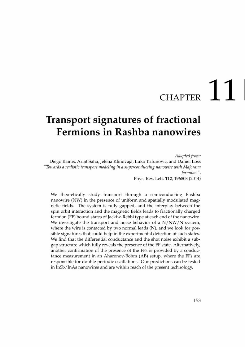
CHAPTER 11Transport signatures of fractional
Fermions in Rashba nanowires
Adapted from:Diego Rainis, Arijit Saha, Jelena Klinovaja, Luka Trifunovic, and Daniel Loss
“Towards a realistic transport modeling in a superconducting nanowire with Majoranafermions”,
Phys. Rev. Lett. 112, 196803 (2014)
We theoretically study transport through a semiconducting Rashbananowire (NW) in the presence of uniform and spatially modulated mag-netic fields. The system is fully gapped, and the interplay between thespin orbit interaction and the magnetic fields leads to fractionally chargedfermion (FF) bound states of Jackiw-Rebbi type at each end of the nanowire.We investigate the transport and noise behavior of a N/NW/N system,where the wire is contacted by two normal leads (N), and we look for pos-sible signatures that could help in the experimental detection of such states.We find that the differential conductance and the shot noise exhibit a sub-gap structure which fully reveals the presence of the FF state. Alternatively,another confirmation of the presence of the FFs is provided by a conduc-tance measurement in an Aharonov-Bohm (AB) setup, where the FFs areresponsible for double-periodic oscillations. Our predictions can be testedin InSb/InAs nanowires and are within reach of the present technology.
153
CHAPTER 11. TRANSPORT SIGNATURES OF FRACTIONALFERMIONS IN RASHBA NANOWIRES 154
11.1 ModelWe consider a semiconducting NW of length L along the x direction,in the presence of long the z direction and a magnetic field that in-cludes a uniform (B) and a spatially periodic component (Bn). The NWcontinuum Hamiltonian is given by H0 = 1
2
∫dxΨ†(x)H0Ψ(x), where
Ψ = (Ψ↑,Ψ↓)T, Ψσ(x) is the annihilation operator for a spin-σ electron
at position x. The Hamiltonian density is of the form
H0 = −~2∂2x/2m− µ− iασz∂x , (11.1)
with m the electron band mass, α the oefficient, and µ the chemical po-tential. The spectrum ofH0 consists of two parabolas centered at the SOImomenta ±kso = ±mα/~2. The magnetic field leads to the Zeeman term
Hz = gµB[B +Bn(x)] · σ /2 , (11.2)
where g is the Lande g-factor and µB the Bohr magneton. Chosen alongthe x direction,B opens a gap ∆z = gµBB/2 at k = 0. The oscillating fieldBn(x) is oriented along y, Bn = yBn sin(4ksox + θ) (but other equivalentconfigurations are possible [34]). It couples the two exterior branches ofthe spectrum, and opens up a gap ∆n = gµBBn/4. Such a field can begenerated externally, by an array of nanomagnets placed in proximityto the wire [206, 207, 208], or internally, e.g., by the hyperfine field ofordered nuclear spins inside the nanowire [209].
In our analysis, we are assuming that the nergy εso = mα2/2~2 isthe largest energy scale in the NW. In this strong-egime, we follow theprocedure described in Refs. [210, 202], which allows us to linearize H0
around k = 0 (“interior branch”) and k = ±2kso (“exterior branches”).For µ = 0, one obtains the spectrum around k = 0 and k = ±2kso asE2m = (αk)2 + ∆2
m , with ∆m = ∆z,∆n for m = i, e. In such situation thesystem is fully gapped, with no propagating modes at subgap energies,|E| < min∆z,∆n. However, there can be localized edge states, FFs, inthe gap [34]. For example, in a semi-infinite geometry there is one boundstate, localized at the nanowire end, with energy
EFF =∆z∆n sin θ√
∆2z + ∆2
n − 2∆z∆n cos θ. (11.3)
The angle θ encodes the boundary condition for the oscillating field atthe nanowire edge. The FF state exists only if the following relation issatisfied: cos θ < min∆z,∆n/max∆z,∆n ≤ 1, see Fig. 11.1.
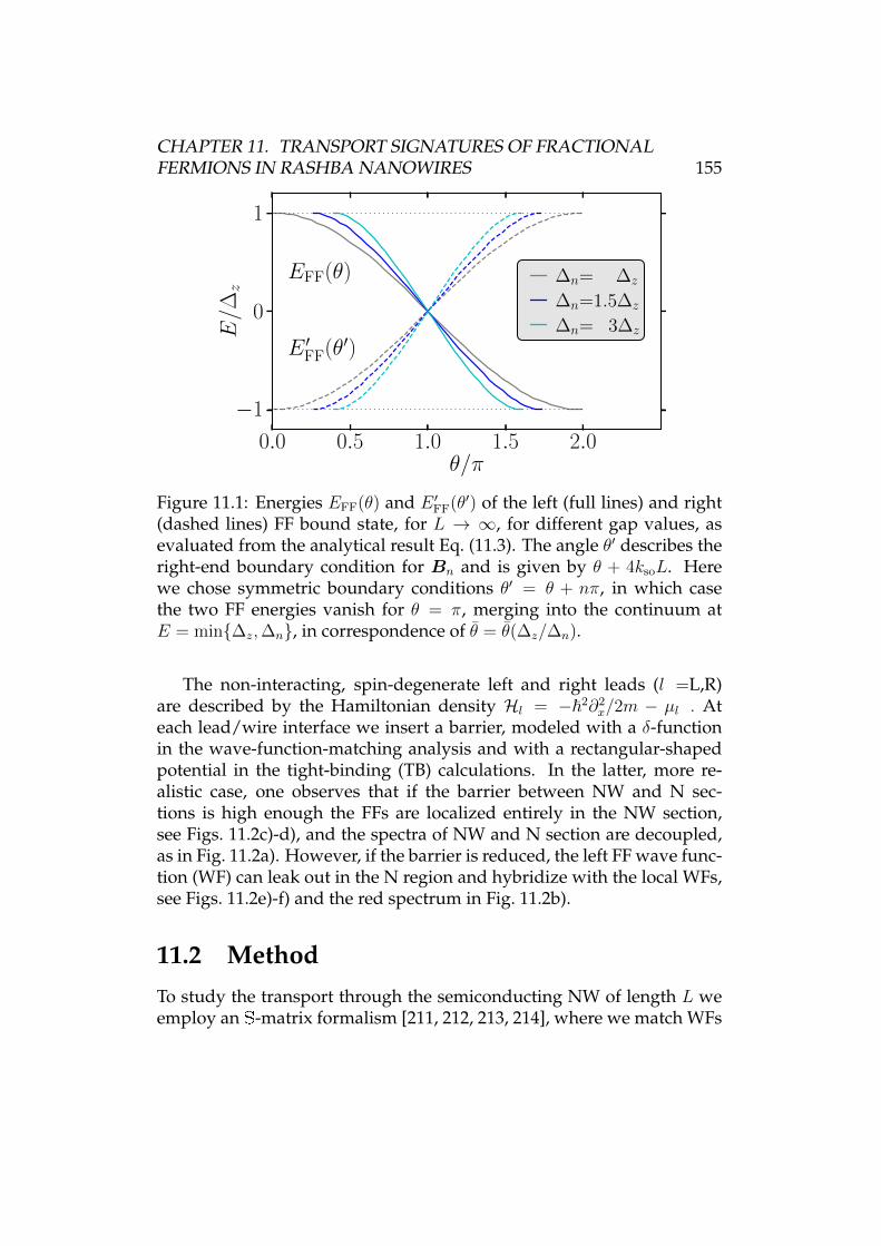
CHAPTER 11. TRANSPORT SIGNATURES OF FRACTIONALFERMIONS IN RASHBA NANOWIRES 155
0.0 0.5 1.0 1.5 2.0/
1
0
1E
/z
EFF()
E 0FF(0)
n= z
n=1.5z
n= 3z
Figure 11.1: Energies EFF(θ) and E ′FF(θ′) of the left (full lines) and right(dashed lines) FF bound state, for L → ∞, for different gap values, asevaluated from the analytical result Eq. (11.3). The angle θ′ describes theright-end boundary condition for Bn and is given by θ + 4ksoL. Herewe chose symmetric boundary conditions θ′ = θ + nπ, in which casethe two FF energies vanish for θ = π, merging into the continuum atE = min∆z,∆n, in correspondence of θ = θ(∆z/∆n).
The non-interacting, spin-degenerate left and right leads (l =L,R)are described by the Hamiltonian density Hl = −~2∂2
x/2m − µl . Ateach lead/wire interface we insert a barrier, modeled with a δ-functionin the wave-function-matching analysis and with a rectangular-shapedpotential in the tight-binding (TB) calculations. In the latter, more re-alistic case, one observes that if the barrier between NW and N sec-tions is high enough the FFs are localized entirely in the NW section,see Figs. 11.2c)-d), and the spectra of NW and N section are decoupled,as in Fig. 11.2a). However, if the barrier is reduced, the left FF wave func-tion (WF) can leak out in the N region and hybridize with the local WFs,see Figs. 11.2e)-f) and the red spectrum in Fig. 11.2b).
11.2 MethodTo study the transport through the semiconducting NW of length L weemploy an S-matrix formalism [211, 212, 213, 214], where we match WFs
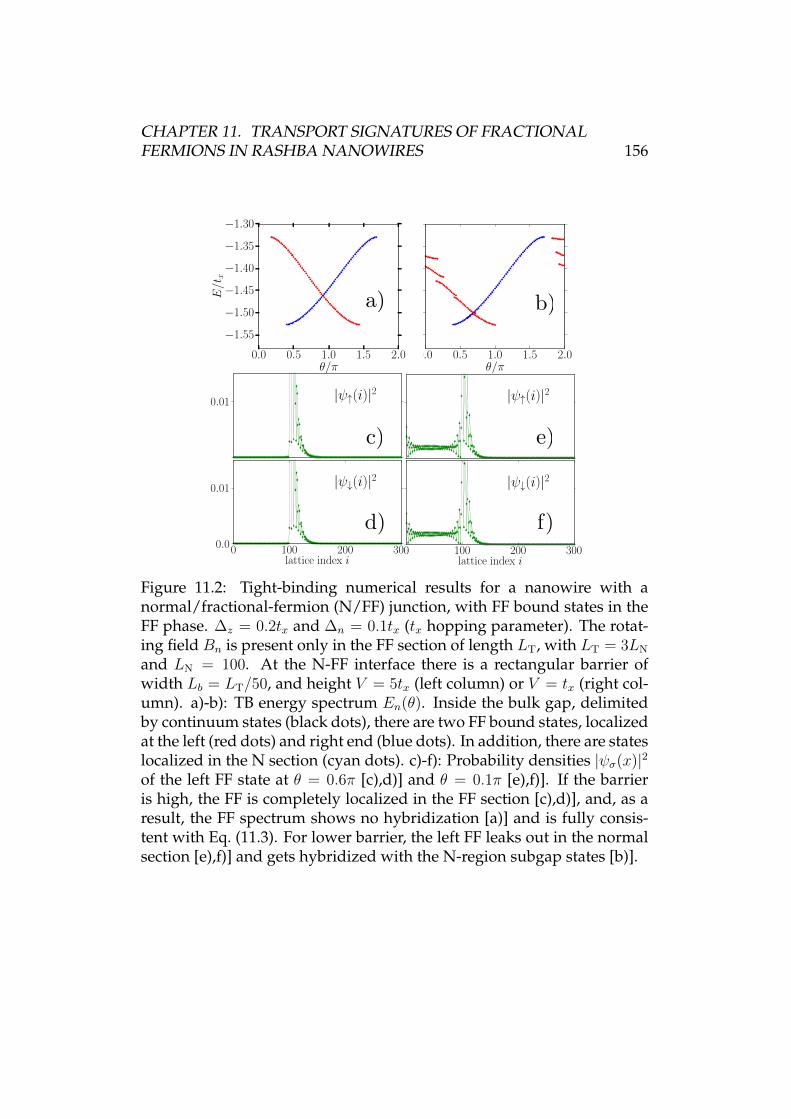
CHAPTER 11. TRANSPORT SIGNATURES OF FRACTIONALFERMIONS IN RASHBA NANOWIRES 156
0.0 0.5 1.0 1.5 2.0θ/π
−1.55
−1.50
−1.45
−1.40
−1.35
−1.30E
/tx
0.0 0.5 1.0 1.5 2.0θ/π
−1.55
−1.50
−1.45
−1.40
−1.35
−1.30
/t x
0.01|ψ↑(i)|2 0.01
|ψ↑(i)|2
0 100 200 300lattice index i
0.0
0.01|ψ↓(i)|2
0 100 200 300lattice index i
0.0
0.01|ψ↓(i)|2
Figure 11.2: Tight-binding numerical results for a nanowire with anormal/fractional-fermion (N/FF) junction, with FF bound states in theFF phase. ∆z = 0.2tx and ∆n = 0.1tx (tx hopping parameter). The rotat-ing field Bn is present only in the FF section of length LT, with LT = 3LN
and LN = 100. At the N-FF interface there is a rectangular barrier ofwidth Lb = LT/50, and height V = 5tx (left column) or V = tx (right col-umn). a)-b): TB energy spectrum En(θ). Inside the bulk gap, delimitedby continuum states (black dots), there are two FF bound states, localizedat the left (red dots) and right end (blue dots). In addition, there are stateslocalized in the N section (cyan dots). c)-f): Probability densities |ψσ(x)|2of the left FF state at θ = 0.6π [c),d)] and θ = 0.1π [e),f)]. If the barrieris high, the FF is completely localized in the FF section [c),d)], and, as aresult, the FF spectrum shows no hybridization [a)] and is fully consis-tent with Eq. (11.3). For lower barrier, the left FF leaks out in the normalsection [e),f)] and gets hybridized with the N-region subgap states [b)].
CHAPTER 11. TRANSPORT SIGNATURES OF FRACTIONALFERMIONS IN RASHBA NANOWIRES 157
and associated probability currents [215, 216, 217] at each wire/lead in-terface to find the differential conductance and the shot noise in the pres-ence of the FFs state. Depending on the choice of the spin-polarizationaxis in the leads, one observes different types of behavior in the spin-resolved transport coefficients Sσσ′ . With the given configuration of SOIand magnetic fields, the most natural choice (provided by the eigen-basis of t†t) is to work with y-polarized electrons. We then consider in-coming plane-wave WFs with wave vector kl =
√2m(µl + E)/~2, and a
nanowire WF that in the strong-imit reads ψNW = aψ+i +bψ−i +cψ+
e +dψ−e ,where ψ±i/e are the four solutions (internal/external branches, right/leftmovers) at energy E, given by
ψ±i (x) =
[E ±
√E2 −∆2
z
]
∆z
, 1
e±ikzx, (11.4)
ψ±e (x) =
eiθ[E ∓
√E2 −∆2
n
]
∆n
e−2iksox, e2iksox
e±iknx,
where ~kz =√E2 −∆2
z/α and ~kn =√E2 −∆2
n/α are the momentaat energy E associated to internal and external branches [34]. The def-initions for kz and kn apply both above and below the gap, where theybecome purely imaginary and describe evanescent modes, whose linearcombination gives rise to our FF bound states.
11.3 ResultsHere we present the results of our numerical analysis on transport throughthe SOI-coupled NW. For finite wire length, the two FF end states have afinite overlap, determined by their localization length(s)
ξz,n(E) ' ~α/√
∆2z,n − E2. (11.5)
For long wires, L ξz, ξn, the two FF states are well decoupled, andeach of them has an energy approximately given by the semi-infinite wireresult Eq. (11.3), see Fig. 11.1.
In Fig. 11.3, which contains the main result of this paper, we showthat the transport behavior in the long-wire regime nicely follows thespectrum EFF(θ), provided a suitable parameter configuration is chosen.
CHAPTER 11. TRANSPORT SIGNATURES OF FRACTIONALFERMIONS IN RASHBA NANOWIRES 158
More precisely, in order to probe in transport the unperturbed wire spec-trum one needs, as usual, to operate in the tunnel regime, i.e., to havesmall wire-leads coupling. This is usually implemented by adding astrong potential barrier at the N/NW interfaces. However, this methodhas the drawback of yielding bound state energies shifted to lower val-ues, proportionally to the wire-lead coupling, see Figs. 11.3a) and 11.3b).There is another method which allows one to make the bound state sig-nature visible, without the need of introducing a potential barrier at theinterfaces. It amounts to choosing very different Fermi energies (andhence different kF’s) in the wire and in the leads (or in different portionsof the wire). The momentum mismatch has then a filtering effect, and theintrinsic properties of the wire are probed without altering theE(θ) spec-tra (the level broadening is of course still present, decreasing for largermomentum mismatches), see Figs. 11.3c) and 11.3d). We stress that it isnecessary to tune µl in order to make the bound state signatures visiblein dI/dV . For a generic value of µl the momentum filtering acts eitherineffectively or too effectively, erasing also the signature of the FF boundstate.
In Fig. 11.3 we also show the behavior of the spin-flip reflection co-efficient R↑↓ as a function of energy and angle θ, in panels b) and d).One immediately notices that R↑↓ exhibits a striking and evident signa-ture of the left bound state, with a peak that almost perfectly traces itsspectrum EFF(θ). Quite intuitively, no influence of the right bound stateappears in the behavior of R↑↓, apart from at energies very close to thegap, where ξz,n increase significantly, and from the anticrossing at smallenergies, where the two branches hybridize and R↑↓ ' 0 (consistent withthe fact that at those points T↑ is enhanced to 1). Therefore, if one is ableto perform spin-polarized measurements yielding both R↑↑ and R↑↓, oneshould obtain a clear signature of the FF bound state when its energy(jointly set by ∆z,∆n, θ) is matched by the applied bias. The additionalpossibility of tuning θ (i.e. by shifting the FF section of the wire) wouldgrant the access to the full EFF(θ) behavior, an even stronger confirma-tion for the presence of the FF bound states.
Further experimental identification of the FFs is possible via noisemeasurements. We have calculated the shot noise S ∝ tr
(r†rt†t
)and
the Fano factor F ∝ S/I , both for spin-polarized and spin-unpolarizedtransport, and shown that they indeed carry signatures of the FFs, as ar-gued in the Supplementary Material.
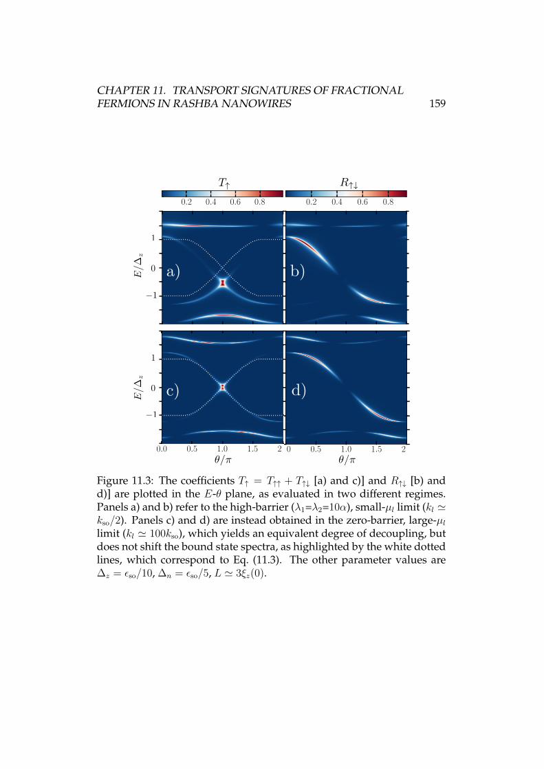
CHAPTER 11. TRANSPORT SIGNATURES OF FRACTIONALFERMIONS IN RASHBA NANOWIRES 159
0.0 0.5 1.0 1.5 2.0/
4
3
2
1
0
1
2
3
4
E
0.2 0.4 0.6 0.8
0.0 0.5 1.0 1.5 2.0/
4
3
2
1
0
1
2
3
4
E
0.2 0.4 0.6 0.8
0.0 0.5 1.0 1.5 2.0/
4
3
2
1
0
1
2
3
4
E
0.2 0.4 0.6 0.80.0 0.5 1.0 1.5 2.0
/
4
3
2
1
0
1
2
3
4
E
0.2 0.4 0.6 0.8
E/
zE
/
z
Figure 11.3: The coefficients T↑ = T↑↑ + T↑↓ [a) and c)] and R↑↓ [b) andd)] are plotted in the E-θ plane, as evaluated in two different regimes.Panels a) and b) refer to the high-barrier (λ1=λ2=10α), small-µl limit (kl 'kso/2). Panels c) and d) are instead obtained in the zero-barrier, large-µllimit (kl ' 100kso), which yields an equivalent degree of decoupling, butdoes not shift the bound state spectra, as highlighted by the white dottedlines, which correspond to Eq. (11.3). The other parameter values are∆z = εso/10, ∆n = εso/5, L ' 3ξz(0).
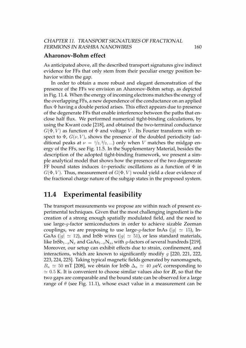
CHAPTER 11. TRANSPORT SIGNATURES OF FRACTIONALFERMIONS IN RASHBA NANOWIRES 160
Aharonov-Bohm effect
As anticipated above, all the described transport signatures give indirectevidence for FFs that only stem from their peculiar energy position be-havior within the gap.
In order to obtain a more robust and elegant demonstration of thepresence of the FFs we envision an Aharonov-Bohm setup, as depictedin Fig. 11.4. When the energy of incoming electrons matches the energy ofthe overlapping FFs, a new dependence of the conductance on an appliedflux Φ having a double period arises. This effect appears due to presenceof the degenerate FFs that enable interference between the paths that en-close half flux. We performed numerical tight-binding calculations, byusing the Kwant code [218], and obtained the two-terminal conductanceG(Φ, V ) as function of Φ and voltage V . Its Fourier transform with re-spect to Φ, G(ν, V ), shows the presence of the doubled periodicity (ad-ditional peaks at ν = 1/2, 3/2, ...) only when V matches the midgap en-ergy of the FFs, see Fig. 11.5. In the Supplementary Material, besides thedescription of the adopted tight-binding framework, we present a sim-ple analytical model that shows how the presence of the two degenerateFF bound states induces 4π-periodic oscillations as a function of Φ inG(Φ, V ). Thus, measurement of G(Φ, V ) would yield a clear evidence ofthe fractional charge nature of the subgap states in the proposed system.
11.4 Experimental feasibilityThe transport measurements we propose are within reach of present ex-perimental techniques. Given that the most challenging ingredient is thecreation of a strong enough spatially modulated field, and the need touse large-g-factor semiconductors in order to achieve sizable Zeemancouplings, we are proposing to use large-g-factor InAs (|g| ' 15), In-GaAs (|g| ' 12), and InSb wires (|g| ' 51), or less standard materials,like InSb1−xNx and GaAs1−xNx, with g-factors of several hundreds [219].Moreover, our setup can exhibit effects due to strain, confinement, andinteractions, which are known to significantly modify g [220, 221, 222,223, 224, 225]. Taking typical magnetic fields generated by nanomagnets,Bn ' 50 mT [208], we obtain for InSb ∆n ' 40 µeV, corresponding to' 0.5 K. It is convenient to choose similar values also for B, so that thetwo gaps are comparable and the bound state can be observed for a largerange of θ (see Fig. 11.1), whose exact value in a measurement can be
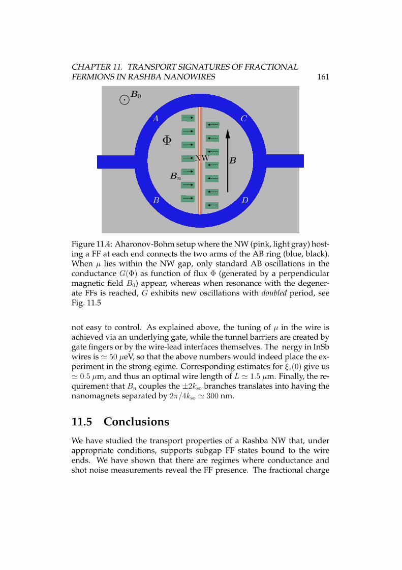
CHAPTER 11. TRANSPORT SIGNATURES OF FRACTIONALFERMIONS IN RASHBA NANOWIRES 161
Figure 11.4: Aharonov-Bohm setup where the NW (pink, light gray) host-ing a FF at each end connects the two arms of the AB ring (blue, black).When µ lies within the NW gap, only standard AB oscillations in theconductance G(Φ) as function of flux Φ (generated by a perpendicularmagnetic field B0) appear, whereas when resonance with the degener-ate FFs is reached, G exhibits new oscillations with doubled period, seeFig. 11.5
not easy to control. As explained above, the tuning of µ in the wire isachieved via an underlying gate, while the tunnel barriers are created bygate fingers or by the wire-lead interfaces themselves. The nergy in InSbwires is ' 50 µeV, so that the above numbers would indeed place the ex-periment in the strong-egime. Corresponding estimates for ξz(0) give us' 0.5 µm, and thus an optimal wire length of L ' 1.5 µm. Finally, the re-quirement that Bn couples the ±2kso branches translates into having thenanomagnets separated by 2π/4kso ' 300 nm.
11.5 ConclusionsWe have studied the transport properties of a Rashba NW that, underappropriate conditions, supports subgap FF states bound to the wireends. We have shown that there are regimes where conductance andshot noise measurements reveal the FF presence. The fractional charge
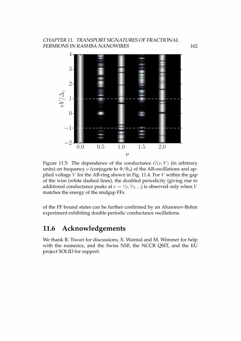
CHAPTER 11. TRANSPORT SIGNATURES OF FRACTIONALFERMIONS IN RASHBA NANOWIRES 162
0.0 0.5 1.0 1.5 2.0
2
1
0
1
2
3
4eV
/z
Figure 11.5: The dependence of the conductance G(ν, V ) (in arbitraryunits) on frequency ν (conjugate to Φ/Φ0) of the AB-oscillations and ap-plied voltage V for the AB-ring shown in Fig. 11.4. For V within the gapof the wire (white dashed lines), the doubled periodicity (giving rise toadditional conductance peaks at ν = 1/2, 3/2, ...) is observed only when Vmatches the energy of the midgap FFs.
of the FF bound states can be further confirmed by an Aharonov-Bohmexperiment exhibiting double-periodic conductance oscillations.
11.6 AcknowledgementsWe thank R. Tiwari for discussions, X. Waintal and M. Wimmer for helpwith the numerics, and the Swiss NSF, the NCCR QSIT, and the EUproject SOLID for support.
Bibliography
[1] D. Loss and D. DiVincenzo, “Quantum computation with quantumdots,” Phys. Rev. A, vol. 57, p. 120, Jan. 1998.
[2] L. P. Kouwenhoven, D. G. Austing, and S. Tarucha, “Few-electronquantum dots,” Rep. Prog. Phys., vol. 64, no. 6, p. 701, 2001.
[3] R. Hanson, L. P. Kouwenhoven, J. R. Petta, S. Tarucha, and L. M. K.Vandersypen, “Spins in few-electron quantum dots,” Rev. Mod.Phys., vol. 79, pp. 1217–1265, Oct 2007.
[4] C. Kloeffel and D. Loss, “Prospects for spin-based quantum com-puting in quantum dots,” Annual Review of Condensed MatterPhysics, vol. 4, no. 1, pp. 51–81, 2013.
[5] D. P. DiVincenzo, “Topics in Quantum Computers,” eprintarXiv:cond-mat/9612126, Dec. 1996.
[6] J. M. Elzerman, R. Hanson, L. H. Willems van Beveren, B. Witkamp,L. M. K. Vandersypen, and L. P. Kouwenhoven, “Single-shot read-out of an individual electron spin in a quantum dot,” Nature,vol. 430, no. 6998, pp. 431–435, 2004.
[7] J. Wrachtrup and F. Jelezko, “Processing quantum information indiamond,” Journal of Physics: Condensed Matter, vol. 18, no. 21,p. 807, 2006.
[8] P. Neumann, J. Beck, M. Steiner, F. Rempp, H. Fedder, P. R. Hem-mer, J. Wrachtrup, and F. Jelezko, “Single-shot readout of a singlenuclear spin,” Science, vol. 329, no. 5991, pp. 542–544, 2010.
[9] J.-P. Tetienne, L. Rondin, P. Spinicelli, M. Chipaux, T. Debuiss-chert, J.-F. Roch, and V. Jacques, “Magnetic-field-dependent photo-dynamics of single nv defects in diamond: an application to quali-
163
BIBLIOGRAPHY 164
tative all-optical magnetic imaging,” New J. of Phys., vol. 14, no. 10,p. 103033, 2012.
[10] A. Gruber, A. Drabenstedt, C. Tietz, L. Fleury, J. Wrachtrup, andC. v. Borczyskowski, “Scanning confocal optical microscopy andmagnetic resonance on single defect centers,” Science, vol. 276,no. 5321, pp. 2012–2014, 1997.
[11] G. Balasubramanian, P. Neumann, D. Twitchen, M. Markham,R. Kolesov, N. Mizuochi, J. Isoya, J. Achard, J. Beck, J. Tissler,V. Jacques, P. R. Hemmer, F. Jelezko, and J. Wrachtrup, “Ultra-long spin coherence time in isotopically engineered diamond,” NatMater, vol. 8, no. 5, pp. 383–387, 2009.
[12] T. Gaebel, M. Domhan, I. Popa, C. Wittmann, P. Neumann,F. Jelezko, J. R. Rabeau, N. Stavrias, A. D. Greentree, S. Prawer,J. Meijer, J. Twamley, P. R. Hemmer, and J. Wrachtrup, “Room-temperature coherent coupling of single spins in diamond,” NatPhys, vol. 2, no. 6, pp. 408–413, 2006.
[13] H. J. Mamin, M. Kim, M. H. Sherwood, C. T. Rettner, K. Ohno,D. D. Awschalom, and D. Rugar, “Nanoscale nuclear magneticresonance with a nitrogen-vacancy spin sensor,” Science, vol. 339,no. 6119, pp. 557–560, 2013.
[14] M. S. Grinolds, M. Warner, K. D. Greve, Y. Dovzhenko, L. Thiel,R. L. Walsworth, S. Hong, P. Maletinsky, and A. Yacoby, “Sub-nanometre resolution in three-dimensional magnetic resonanceimaging of individual dark spins,” Nat. Nano., vol. 9, pp. 279–284,Apr. 2014.
[15] T. Staudacher, F. Shi, S. Pezzagna, J. Meijer, J. Du, C. A. Meriles,F. Reinhard, and J. Wrachtrup Science, vol. 339, no. 6119, pp. 561–563, 2013.
[16] L. Rondin, J. P. Tetienne, T. Hingant, J. F. Roch, P. Maletinsky, andV. Jacques, “Magnetometry with nitrogen-vacancy defects in dia-mond,” Rep. Prog. Phys., vol. 77, no. 5, p. 056503, 2014.
[17] G. Waldherr, J. Beck, P. Neumann, R. S. Said, M. Nitsche, M. L.Markham, D. J. Twitchen, J. Twamley, F. Jelezko, and J. Wrachtrup,“High-dynamic-range magnetometry with a single nuclear spin indiamond,” Nat Nano, vol. 7, no. 2, pp. 105–108, 2012.
BIBLIOGRAPHY 165
[18] L. C. Bassett, F. J. Heremans, D. J. Christle, C. G. Yale, G. Burkard,B. B. Buckley, and D. D. Awschalom, “Ultrafast optical control oforbital and spin dynamics in a solid-state defect,” Science, 2014.
[19] P. Maletinsky, S. Hong, M. S. Grinolds, B. Hausmann, M. D. Lukin,R. L. Walsworth, M. Loncar, and A. Yacoby, “A robust scanning di-amond sensor for nanoscale imaging with single nitrogen-vacancycentres,” Nat. Nano, vol. 7, no. 5, pp. 320–324, 2012.
[20] D. S. Wang, A. G. Fowler, and L. C. L. Hollenberg, “Surfacecode quantum computing with error rates over 1%,” Phys. Rev. A,vol. 83, p. 020302, Feb 2011.
[21] R. Raussendorf and J. Harrington, “Fault-tolerant quantum com-putation with high threshold in two dimensions,” Phys. Rev. Lett.,vol. 98, p. 190504, May 2007.
[22] F. Wilczek, “Quantum mechanics of fractional-spin particles,”Phys. Rev. Lett., vol. 49, pp. 957–959, Oct 1982.
[23] R. Streater and I. Wilde, “Fermion states of a boson field,” NuclearPhysics B, vol. 24, no. 3, pp. 561 – 575, 1970.
[24] S. Fujimoto, “Topological order and non-abelian statistics in non-centrosymmetric s-wave superconductors,” Phys. Rev. B, vol. 77,no. 22, p. 220501, 2008.
[25] M. Sato, Y. Takahashi, and S. Fujimoto, “Non-abelian topologicalorder in s-wave superfluids of ultracold fermionic atoms,” Phys.Rev. Lett., vol. 103, no. 2, p. 020401, 2009.
[26] J. D. Sau et al., “Generic new platform for topological quantumcomputation using semiconductor heterostructures,” Phys. Rev.Lett., vol. 104, no. 4, p. 040502, 2010.
[27] M. Sato, Y. Takahashi, and S. Fujimoto, “Non-abelian topologicalorders and majorana fermions in spin-singlet superconductors,”Phys. Rev. B, vol. 82, no. 13, p. 134521, 2010.
[28] J. Alicea, “Majorana fermions in a tunable semiconductor device,”Phys. Rev. B, vol. 81, no. 12, p. 125318, 2010.
BIBLIOGRAPHY 166
[29] R. M. Lutchyn, J. D. Sau, and S. Das Sarma, “Majoranafermions and a topological phase transition in semiconductor-superconductor heterostructures,” Phys. Rev. Lett., vol. 105,p. 077001, 2010.
[30] Y. Oreg, G. Refael, and F. von Oppen, “Helical liquids and ma-jorana bound states in quantum wires,” Phys. Rev. Lett., vol. 105,p. 177002, 2010.
[31] V. Mourik et al., “Signatures of majorana fermions in hy-brid superconductor-semiconductor nanowire devices,” Science,vol. 336, p. 1003, 2012.
[32] M. T. Deng, C. L. Yu, G. Y. Huang, M. Larsson, P. Caroff, andH. Q. Xu, “Anomalous zero-bias conductance peak in a nb–insbnanowire–nb hybrid device,” Nano Letters, vol. 12, no. 12, pp. 6414–6419, 2012.
[33] A. Das, Y. Ronen, Y. Most, Y. Oreg, M. Heiblum, and H. Shtrikman,“Zero-bias peaks and splitting in an al-inas nanowire topologicalsuperconductor as a signature of majorana fermions,” Nat Phys,vol. 8, no. 12, pp. 887–895, 2012.
[34] J. Klinovaja, P. Stano, and D. Loss, “Transition from fractional tomajorana fermions in rashba nanowires,” Phys. Rev. Lett., vol. 109,p. 236801, 2012.
[35] J. Klinovaja and D. Loss, “Fractional fermions with non-abelianstatistics,” Phys. Rev. Lett., vol. 110, p. 126402, 2013.
[36] F. Jelezko, T. Gaebel, I. Popa, A. Gruber, and J. Wrachtrup, “Obser-vation of coherent oscillations in a single electron spin,” Phys. Rev.Lett., vol. 92, p. 076401, Feb 2004.
[37] F. Jelezko, T. Gaebel, I. Popa, M. Domhan, A. Gruber, andJ. Wrachtrup, “Observation of coherent oscillation of a single nu-clear spin and realization of a two-qubit conditional quantumgate,” Phys. Rev. Lett., vol. 93, p. 130501, Sep 2004.
[38] L. Childress, M. V. Gurudev Dutt, J. M. Taylor, A. S. Zibrov,F. Jelezko, J. Wrachtrup, P. R. Hemmer, and M. D. Lukin, “Coher-ent dynamics of coupled electron and nuclear spin qubits in dia-mond,” Science, vol. 314, no. 5797, pp. 281–285, 2006.
BIBLIOGRAPHY 167
[39] M. V. G. Dutt, L. Childress, L. Jiang, E. Togan, J. Maze, F. Jelezko,A. S. Zibrov, P. R. Hemmer, and M. D. Lukin, “Quantum regis-ter based on individual electronic and nuclear spin qubits in dia-mond,” Science, vol. 316, no. 5829, pp. 1312–1316, 2007.
[40] R. Hanson, V. V. Dobrovitski, A. E. Feiguin, O. Gywat, and D. D.Awschalom, “Coherent dynamics of a single spin interacting withan adjustable spin bath,” Science, vol. 320, no. 5874, pp. 352–355,2008.
[41] P. Neumann, N. Mizuochi, F. Rempp, P. Hemmer, H. Watanabe,S. Yamasaki, V. Jacques, T. Gaebel, F. Jelezko, and J. Wrachtrup,“Multipartite entanglement among single spins in diamond,” Sci-ence, vol. 320, no. 5881, pp. 1326–1329, 2008.
[42] L. Jiang, J. S. Hodges, J. R. Maze, P. Maurer, J. M. Taylor, D. G. Cory,P. R. Hemmer, R. L. Walsworth, A. Yacoby, A. S. Zibrov, and M. D.Lukin, “Repetitive readout of a single electronic spin via quan-tum logic with nuclear spin ancillae,” Science, vol. 326, no. 5950,pp. 267–272, 2009.
[43] G. D. Fuchs, V. V. Dobrovitski, D. M. Toyli, F. J. Heremans, andD. D. Awschalom, “Gigahertz dynamics of a strongly driven singlequantum spin,” Science, vol. 326, no. 5959, pp. 1520–1522, 2009.
[44] P. Neumann, J. Beck, M. Steiner, F. Rempp, H. Fedder, P. R. Hem-mer, J. Wrachtrup, and F. Jelezko, “Single-shot readout of a singlenuclear spin,” Science, vol. 329, no. 5991, pp. 542–544, 2010.
[45] B. B. Buckley, G. D. Fuchs, L. C. Bassett, and D. D. Awschalom,“Spin-light coherence for single-spin measurement and control indiamond,” Science, vol. 330, no. 6008, pp. 1212–1215, 2010.
[46] E. Togan, Y. Chu, A. Trifonov, L. Jiang, J. Maze, L. Childress,M. Dutt, A. Sorensen, P. Hemmer, A. Zibrov, and M. Lukin, “Quan-tum entanglement between an optical photon and a solid-state spinqubit,” Nature, vol. 466, no. 7307, pp. 730–734, 2010.
[47] L. Robledo, L. Childress, H. Bernien, B. Hensen, P. F. Alkemade,and R. Hanson, “High-fidelity projective read-out of a solid-statespin quantum register,” Nature, vol. 477, no. 7366, pp. 574–578,2011.
BIBLIOGRAPHY 168
[48] J. J. Pla, K. Y. Tan, J. P. Dehollain, W. H. Lim, J. J. L. Morton, F. A.Zwanenburg, D. N. Jamieson, A. S. Dzurak, and A. Morello, “High-fidelity readout and control of a nuclear spin qubit in silicon,”arXiv:1302.0047, Jan. 2013.
[49] J. J. Pla, K. Y. Tan, J. P. Dehollain, W. H. Lim, J. J. L. Morton, D. N.Jamieson, A. S. Dzurak, and A. Morello, “A single-atom electronspin qubit in silicon,” Nature, vol. 489, pp. 541–545, Sept. 2012.
[50] V. Dobrovitski, G. Fuchs, A. Falk, C. Santori, and D. Awschalom,“Quantum control over single spins in diamond,” Ann. Rev. Con-dens. Matter Phys., vol. 4, no. 1, pp. 23–50, 2013.
[51] M.-S. Choi, C. Bruder, and D. Loss, “Spin-dependent josephsoncurrent through double quantum dots and measurement of entan-gled electron states,” Phys. Rev. B, vol. 62, p. 13569, Nov. 2000.
[52] A. Wallraff, D. I. Schuster, A. Blais, L. Frunzio, R.-S. Huang, J. Ma-jer, S. Kumar, S. M. Girvin, and R. J. Schoelkopf, “Strong couplingof a single photon to a superconducting qubit using circuit quan-tum electrodynamics,” Nature, vol. 431, no. 7005, pp. 162–167, 2004.
[53] L. Childress, A. S. Sørensen, and M. D. Lukin, “Mesoscopic cav-ity quantum electrodynamics with quantum dots,” Phys. Rev. A,vol. 69, p. 042302, Apr 2004.
[54] Y. Rikitake and H. Imamura, “Decoherence of localized spins inter-acting via RKKY interaction,” Phys. Rev. B, vol. 72, p. 033308, July2005.
[55] G. Burkard and A. Imamoglu, “Ultra-long-distance interaction be-tween spin qubits,” Phys. Rev. B, vol. 74, p. 041307, Jul 2006.
[56] C. Flindt, A. S. Sørensen, and K. Flensberg, “Spin-orbit mediatedcontrol of spin qubits,” Phys. Rev. Lett., vol. 97, p. 240501, Dec. 2006.
[57] M. Trif, V. N. Golovach, and D. Loss, “Spin-spin coupling inelectrostatically coupled quantum dots,” Phys. Rev. B, vol. 75,p. 085307, Feb. 2007.
[58] M. Trif, V. N. Golovach, and D. Loss, “Spin dynamics in inasnanowire quantum dots coupled to a transmission line,” Phys. Rev.B, vol. 77, p. 045434, Jan 2008.
BIBLIOGRAPHY 169
[59] K. Flensberg and C. M. Marcus, “Bends in nanotubes allow electricspin control and coupling,” Phys. Rev. B, vol. 81, p. 195418, May2010.
[60] L. Trifunovic, O. Dial, M. Trif, J. R. Wootton, R. Abebe, A. Yacoby,and D. Loss, “Long-distance spin-spin coupling via floating gates,”Phys. Rev. X, vol. 2, p. 011006, Jan. 2012.
[61] M. D. Shulman, O. E. Dial, S. P. Harvey, H. Bluhm, V. Umansky,and A. Yacoby, “Demonstration of entanglement of electrostaticallycoupled singlet-triplet qubits,” Science, vol. 336, pp. 202–205, Apr.2012.
[62] M. Leijnse and K. Flensberg, “Coupling spin qubits via supercon-ductors,” Phys. Rev. Lett., vol. 111, p. 060501, Aug 2013.
[63] J. Levy, “Universal quantum computation with spin-1/2 pairs andheisenberg exchange,” Phys. Rev. Lett., vol. 89, no. 14, p. 147902,2002.
[64] S. Amasha, K. MacLean, I. P. Radu, D. M. Zumbuhl, M. A. Kastner,M. P. Hanson, and A. C. Gossard, “Electrical control of spin relax-ation in a quantum dot,” Phys. Rev. Lett., vol. 100, p. 046803, Jan.2008.
[65] H. Bluhm, S. Foletti, I. Neder, M. Rudner, D. Mahalu, V. Umansky,and A. Yacoby, “Dephasing time of gaas electron-spin qubits cou-pled to a nuclear bath exceeding 200µs,” Nat. Phys., vol. 7, no. 2,pp. 109–113, 2011.
[66] J. R. Petta, A. C. Johnson, J. M. Taylor, E. A. Laird, A. Yacoby, M. D.Lukin, C. M. Marcus, M. P. Hanson, and A. C. Gossard, “Coherentmanipulation of coupled electron spins in semiconductor quantumdots,” Science, vol. 309, no. 5744, pp. 2180–2184, 2005.
[67] F. H. L. Koppens, K. C. Nowack, and L. M. K. Vandersypen, “Spinecho of a single electron spin in a quantum dot,” Phys. Rev. Lett.,vol. 100, p. 236802, Jun 2008.
[68] R. Brunner, Y.-S. Shin, T. Obata, M. Pioro-Ladriere, T. Kubo,K. Yoshida, T. Taniyama, Y. Tokura, and S. Tarucha, “Two-qubitgate of combined single-spin rotation and interdot spin exchangein a double quantum dot,” Phys. Rev. Lett., vol. 107, p. 146801, 2011.
BIBLIOGRAPHY 170
[69] A. M. Childs, H. L. Haselgrove, and M. A. Nielsen, “Lower boundson the complexity of simulating quantum gates,” Phys. Rev. A,vol. 68, p. 052311, 2003.
[70] R. Raussendorf and J. Harrington, “Fault-tolerant quantum com-putation with high threshold in two dimensions,” Phys. Rev. Lett.,vol. 98, p. 190504, 2007.
[71] M. Trif, F. Troiani, D. Stepanenko, and D. Loss, “Spin-electric cou-pling in molecular magnets,” Phys. Rev. Lett., vol. 101, p. 217201,Nov 2008.
[72] I. H. Chan, R. M. Westervelt, K. D. Maranowski, and A. C. Gossard,“Strongly capacitively coupled quantum dots,” Appl. Phys. Lett.,vol. 80, no. 10, p. 1818, 2002.
[73] I. Chan, P. Fallahi, R. Westervelt, K. Maranowski, and A. Gossard,“Capacitively coupled quantum dots as a single-electron switch,”Physica E, vol. 17, no. 0, pp. 584 – 588, 2003.
[74] F. Kuemmeth, S. Ilani, D. C. Ralph, and P. L. McEuen, “Coupling ofspin and orbital motion of electrons in carbon nanotubes,” Nature,vol. 452, pp. 448–452, Mar. 2008.
[75] Y. Hu, H. O. H. Churchill, D. J. Reilly, J. Xiang, C. M. Lieber, andC. M. Marcus, “A ge/si heterostructure nanowire-based doublequantum dot with integrated charge sensor,” Nat. Nanotech., vol. 2,p. 622, 2007.
[76] D. Stepanenko and G. Burkard, “Quantum gates between capaci-tively coupled double quantum dot two-spin qubits,” Phys. Rev. B,vol. 75, p. 085324, Feb. 2007.
[77] A. C. Johnson, J. R. Petta, J. M. Taylor, A. Yacoby, M. D. Lukin, C. M.Marcus, M. P. Hanson, and A. C. Gossard, “Triplet-singlet spinrelaxation via nuclei in a double quantum dot,” Nature, vol. 435,no. 7044, pp. 925–928, 2005.
[78] J. Sten, “Ellipsoidal harmonics and their application in electrostat-ics,” J. Electrostatics, vol. 64, pp. 647–654, Sept. 2006.
[79] G. Burkard, D. Loss, and D. P. DiVincenzo, “Coupled quantumdots as quantum gates,” Phys. Rev. B, vol. 59, p. 2070, Jan. 1999.
BIBLIOGRAPHY 171
[80] J. H. Van Vleck, “Paramagnetic relaxation times for titanium andchrome alum,” Phys. Rev., vol. 57, pp. 426–447, Mar 1940.
[81] V. N. Golovach, A. Khaetskii, and D. Loss, “Phonon-induced de-cay of the electron spin in quantum dots,” Phys. Rev. Lett., vol. 93,p. 016601, Jun 2004.
[82] R. Hanson, L. P. Kouwenhoven, J. R. Petta, S. Tarucha, and L. M. K.Vandersypen, “Spins in few-electron quantum dots,” Rev. Mod.Phys., vol. 79, p. 1217, Oct. 2007.
[83] R. Zak, B. Rothlisberger, S. Chesi, and D. Loss, “Quantum com-puting with electron pins in quantum dots,” Riv. Nuovo Cimento,vol. 33, pp. 345–399, June 2010.
[84] D. Stepanenko, M. Rudner, B. I. Halperin, and D. Loss, “Singlet-triplet splitting in double quantum dots due to spin-orbit and hy-perfine interactions,” Phys. Rev. B, vol. 85, p. 075416, Feb 2012.
[85] D. P. DiVincenzo, “Fault-tolerant architectures for superconductingqubits,” Phys. Scr., vol. T137, p. 014020, 2009.
[86] F. H. L. Koppens, C. Buizert, K. J. Tielrooij, I. T. Vink, K. C.Nowack, T. Meunier, L. P. Kouwenhoven, and L. M. K. Vander-sypen, “Driven coherent oscillations of a single electron spin in aquantum dot,” Nature, vol. 442, p. 766, 2006.
[87] V. N. Golovach, M. Borhani, and D. Loss, “Electric-dipole-inducedspin resonance in quantum dots,” Phys. Rev. B, vol. 74, p. 165319,2006.
[88] K. C. Nowack, F. H. L. Koppens, Y. V. Nazarov, and L. M. K. Van-dersypen, “Coherent control of a single electron spin with electricfields,” Science, vol. 318, p. 1430, 2007.
[89] S. Nadj-Perge, S. M. Frolov, E. P. A. M. Bakkers, and L. P. Kouwen-hoven, “Spin-orbit qubit in a semiconductor nanowire,” Nature,vol. 468, p. 1084, 2011.
[90] C. Fasth, F. A., L. Samuleson, V. N. Golovach, and D. Loss, “Directmeasurement of the spin-orbit interaction in a two-electron inasnanowire quantum dot,” Phys. Rev. Lett., vol. 98, p. 266801, 2007.
BIBLIOGRAPHY 172
[91] C. Kloeffel, M. Trif, and D. Loss, “Strong spin-orbit interactionand helical hole states in ge/si nanowires,” Phys. Rev. B, vol. 84,p. 195314, Nov 2011.
[92] D. V. Bulaev, B. Trauzettel, and D. Loss, “Spin-orbit interactionand anomalous spin relaxation in carbon nanotube quantum dots,”Phys. Rev. B, vol. 77, p. 235301, 2008.
[93] H. O. H. Churchill, A. J. Bestwick, J. W. Harlow, J. Kuemmeth,D. Marcos, C. H. Stwertka, S. K. Watson, and C. M. Marcus, “Elec-tron–nuclear interaction in 13c nanotube double quantum dots,”Nat. Phys., vol. 5, p. 321, 2009.
[94] J. Klinovaja, M. J. Schmidt, B. Braunecker, and D. Loss, “Helicalmodes in carbon nanotubes generated by strong electric fields,”Phys. Rev. Lett., vol. 106, p. 156809, 2011.
[95] J. Fischer and D. Loss, “Dealing with decoherence,” Science,vol. 324, no. 5932, pp. 1277–1278, 2009.
[96] F. Marquardt and V. A. Abalmassov, “Spin relaxation in a quantumdot due to nyquist noise,” Phys. Rev. B, vol. 71, p. 165325, Apr. 2005.
[97] S. Bravyi, D. DiVincenzo, and D. Loss, “Schrieffer-wolff transfor-mation for quantum many-body systems,” Ann. Phys., vol. 326,no. 10, pp. 2793 – 2826, 2011.
[98] C. Kittel, “On the theory of ferromagnetic resonance absorption,”Phys. Rev., vol. 73, pp. 155–161, Jan 1948.
[99] H. Watanabe and H. Murayama, “Unified description of nambu-goldstone bosons without lorentz invariance,” Phys. Rev. Lett.,vol. 108, p. 251602, Jun 2012.
[100] M. Sparks, “Ferromagnetic resonance in thin films. i. theory ofnormal-mode frequencies,” Phys. Rev. B, vol. 1, pp. 3831–3856, May1970.
[101] I. Lee, Y. Obukhov, G. Xiang, A. Hauser, F. Yang, P. Banerjee,D. V. Pelekhov, and P. C. Hammel, “Nanoscale scanning probeferromagnetic resonance imaging using localized modes,” Nature,vol. 466, no. 7308, pp. 845–848, 2010.
BIBLIOGRAPHY 173
[102] M. A. Nielsen and I. L. Chuang, Quantum Computation and Quan-tum Information. Cambridge University Press, 1 ed., Jan. 2004.
[103] A. Imamoglu, D. D. Awschalom, G. Burkard, D. P. DiVincenzo,D. Loss, M. Sherwin, and A. Small, “Quantum information pro-cessing using quantum dot spins and cavity qed,” Phys. Rev. Lett.,vol. 83, pp. 4204–4207, Nov 1999.
[104] T. Tanamoto, K. Maruyama, Y. X. Liu, X. Hu, and F. Nori, “Efficientpurification protocols using iSWAP gates in solid-state qubits,”Phys. Rev. A, vol. 78, p. 062313, Dec 2008.
[105] D. P. DiVincenzo and D. Loss, “Rigorous born approximation andbeyond for the spin-boson model,” Phys. Rev. B, vol. 71, p. 035318,Jan. 2005.
[106] Y. Makhlin and A. Shnirman, “Dephasing of solid-state qubits atoptimal points,” Phys. Rev. Lett., vol. 92, p. 178301, Apr. 2004.
[107] A. A. Abrikosov, L. P. Gorkov, and I. E. Dzyaloshinski, Methods ofQuantum Field Theory in Statistical Physics. Dover, 1975.
[108] Y. Makhlin, G. Schon, and A. Shnirman, “Dissipative effects injosephson qubits,” Chem. Phys., vol. 296, pp. 315–324, Jan. 2004.
[109] W. Nolting and A. Ramakanth, Quantum Theory of Magnetism.Springer, 2009.
[110] J. Hauptmann, J. Paaske, and P. Lindelof, “Electric-field-controlledspin reversal in a quantum dot with ferromagnetic contacts,” Nat.Phys., vol. 4, no. 5, pp. 373–376, 2008.
[111] L. Hofstetter, A. Geresdi, M. Aagesen, J. Nygard, C. Schonenberger,and S. Csonka, “Ferromagnetic proximity effect in aferromagnet˘quantum-dot˘superconductor device,” Phys. Rev.Lett., vol. 104, p. 246804, Jun 2010.
[112] K. Khodjasteh and L. Viola, “Dynamically error-corrected gatesfor universal quantum computation,” Phys. Rev. Lett., vol. 102,p. 080501, Feb 2009.
[113] X. Xu, W. Yao, B. Sun, D. G. Steel, A. S. Bracker, D. Gammon,and L. J. Sham, “Optically controlled locking of the nuclear field
BIBLIOGRAPHY 174
via coherent dark-state spectroscopy,” Nature, vol. 459, no. 7250,pp. 1105–1109, 2009.
[114] I. T. Vink, K. C. Nowack, F. H. L. Koppens, J. Danon, Y. V. Nazarov,and L. M. K. Vandersypen, “Locking electron spins into magneticresonance by electron-nuclear feedback,” Nat. Phys., vol. 5, no. 10,pp. 764–768, 2009.
[115] H. Ohno, D. Chiba, F. Matsukura, T. Omiya, E. Abe, T. Dietl,Y. Ohno, and K. Ohtani, “Electric-field control of ferromagnetism,”Nature, vol. 408, no. 6815, pp. 944–946, 2000.
[116] J. Klinovaja, D. Stepanenko, B. I. Halperin, and D. Loss, “Exchange-based cnot gates for singlet-triplet qubits with spin-orbit interac-tion,” Phys. Rev. B, vol. 86, p. 085423, Aug 2012.
[117] R. Ernst, G. Bodenhausen, and A. Wokaun, Nuclear Magnetic Reso-nance in One and Two Dimensions. Oxford: Oxford Univ. Press, 1987.
[118] P. Hemmer, “Toward molecular-scale mri,” Science, vol. 339,no. 6119, pp. 529–530, 2013.
[119] J. A. Sidles, “Noninductive detection of singleproton magnetic res-onance,” Applied Physics Letters, vol. 58, no. 24, pp. 2854–2856, 1991.
[120] E. Ramsden, Hall-Effect Sensors, Second Edition: Theory and Applica-tion. Amsterdam ; Boston: Newnes, 2 edition ed., Mar. 2006.
[121] M. E. Huber, N. C. Koshnick, H. Bluhm, L. J. Archuleta, T. Azua,P. G. Bjornsson, B. W. Gardner, S. T. Halloran, E. A. Lucero, andK. A. Moler, “Gradiometric micro-squid susceptometer for scan-ning measurements of mesoscopic samples,” Rev. Sci. Instrum.,vol. 79, no. 5, 2008.
[122] C. L. Degen, M. Poggio, H. J. Mamin, C. T. Rettner, and D. Ru-gar, “Nanoscale magnetic resonance imaging,” Proc. Natl Acad. Sci.USA, vol. 106, no. 5, pp. 1313–1317, 2009.
[123] M. Poggio and C. L. Degen, “Force-detected nuclear magnetic res-onance: recent advances and future challenges,” Nanotechnology,vol. 21, no. 34, p. 342001, 2010.
BIBLIOGRAPHY 175
[124] P. Peddibhotla, F. Xue, H. I. T. Hauge, S. Assali, E. P. A. M. Bakkers,and M. Poggio, “Harnessing nuclear spin polarization fluctuationsin a semiconductor nanowire,” Nat Phys, vol. 9, no. 10, pp. 631–635,2013.
[125] M. Loretz, S. Pezzagna, J. Meijer, and C. L. Degen, “Nanoscalenuclear magnetic resonance with a 1.9-nm-deep nitrogen-vacancysensor,” App. Phys. Lett., vol. 104, no. 3, 2014.
[126] M. Schaffry, E. M. Gauger, J. J. L. Morton, and S. C. Benjamin, “Pro-posed spin amplification for magnetic sensors employing crystaldefects,” Phys. Rev. Lett., vol. 107, p. 207210, Nov. 2011.
[127] T. van der Sar, F. Casola, R. Walsworth, and A. Yacoby,“Nanometre-scale probing of spin waves using single electronspins,” arXiv:1410.6423, Oct. 2014.
[128] C. S. Wolfe, V. P. Bhallamudi, H. L. Wang, C. H. Du, S. Manuilov,R. M. Teeling-Smith, A. J. Berger, R. Adur, F. Y. Yang, and P. C.Hammel, “Off-resonant manipulation of spins in diamond via pre-cessing magnetization of a proximal ferromagnet,” Phys. Rev. B,vol. 89, p. 180406, May 2014.
[129] G. D. Fuchs, G. Burkard, P. V. Klimov, and D. D. Awschalom, “Aquantum memory intrinsic to single nitrogen-vacancy centres indiamond,” Nat. Phys, vol. 7, no. 10, pp. 789–793, 2011.
[130] E. C. Stoner and E. P. Wohlfarth, “A mechanism of magnetic hys-teresis in heterogeneous alloys,” Phil. Trans. R. Soc. A, vol. 240,no. 826, pp. 599–642, 1948.
[131] L. Trifunovic, F. L. Pedrocchi, and D. Loss, “Long-distance en-tanglement of spin qubits via ferromagnet,” Phys. Rev. X, vol. 3,p. 041023, Dec 2013.
[132] Cywinski, R. M. Lutchyn, C. P. Nave, and S. Das Sarma, “How toenhance dephasing time in superconducting qubits,” Phys. Rev. B,vol. 77, p. 174509, May 2008.
[133] G. de Lange, Z. H. Wang, D. Riste, V. V. Dobrovitski, and R. Han-son, “Universal dynamical decoupling of a single solid-state spinfrom a spin bath,” Science, vol. 330, no. 6000, pp. 60–63, 2010.
BIBLIOGRAPHY 176
[134] V. M. Acosta, E. Bauch, M. P. Ledbetter, C. Santori, K.-M. C. Fu,P. E. Barclay, R. G. Beausoleil, H. Linget, J. F. Roch, F. Treussart,S. Chemerisov, W. Gawlik, and D. Budker, “Diamonds with ahigh density of nitrogen-vacancy centers for magnetometry appli-cations,” Phys. Rev. B, vol. 80, p. 115202, Sep 2009.
[135] K. Ohno, F. Joseph Heremans, L. C. Bassett, B. A. Myers, D. M.Toyli, A. C. Bleszynski Jayich, C. J. Palmstrom, and D. D.Awschalom, “Engineering shallow spins in diamond with nitrogendelta-doping,” App. Phys. Lett., vol. 101, no. 8, p. 082413, 2012.
[136] B. A. Myers, A. Das, M. C. Dartiailh, K. Ohno, D. Awschalom, D.,and C. Bleszynski Jayich, A., “Probing surface noise with depth-calibrated spins in diamond,” Phys. Rev. Lett., vol. 113, p. 027602,Jul 2014.
[137] G. Puentes, G. Waldherr, P. Neumann, G. Balasubramanian, andJ. Wrachtrup, “Efficient route to high-bandwidth nanoscale mag-netometry using single spins in diamond,” Sci. Rep., vol. 4, 2014.
[138] P. London, P. Balasubramanian, B. Naydenov, L. P. McGuinness,and F. Jelezko, “Strong driving of a single spin using arbitrarilypolarized fields,” Phys. Rev. A, vol. 90, p. 012302, Jul 2014.
[139] G. D. Fuchs, V. V. Dobrovitski, D. M. Toyli, F. J. Heremans, andD. D. Awschalom, “Gigahertz dynamics of a strongly driven singlequantum spin,” Science, vol. 326, pp. 1520–1522, Nov. 2009.
[140] J. Yoneda, T. Otsuka, T. Nakajima, T. Takakura, T. Obata, M. Pioro-Ladriere, H. Lu, C. Palmstrøm, A. C. Gossard, and S. Tarucha, “FastElectrical Control of Single Electron Spins in Quantum Dots withVanishing Influence from Nuclear Spins,” arXiv:1411.6738, Nov.2014.
[141] N. L. Schryer and L. R. Walker, “The motion of 180 domain walls inuniform dc magnetic fields,” J. App. Phys., vol. 45, no. 12, p. 5406,1974.
[142] G. Balasubramanian, P. Neumann, D. Twitchen, M. Markham,R. Kolesov, N. Mizuochi, J. Isoya, J. Achard, J. Beck, J. Tissler,V. Jacques, P. R. Hemmer, F. Jelezko, and J. Wrachtrup, “Ultra-long spin coherence time in isotopically engineered diamond,”Nat. Mater, vol. 8, no. 5, pp. 383–387, 2009.
BIBLIOGRAPHY 177
[143] M. Loretz, T. Rosskopf, J. M. Boss, S. Pezzagna, J. Meijer, and C. L.Degen, “Single-proton spin detection by diamond magnetometry,”Science, 2014.
[144] A. O. Sushkov, I. Lovchinsky, N. Chisholm, R. L. Walsworth,H. Park, and M. D. Lukin, “Magnetic resonance detection of in-dividual proton spins using quantum reporters,” Phys. Rev. Lett.,vol. 113, p. 197601, Nov 2014.
[145] V. M. Acosta, E. Bauch, M. P. Ledbetter, C. Santori, K.-M. C. Fu,P. E. Barclay, R. G. Beausoleil, H. Linget, J. F. Roch, F. Treussart,S. Chemerisov, W. Gawlik, and D. Budker, “Diamonds with ahigh density of nitrogen-vacancy centers for magnetometry appli-cations,” Phys. Rev. B, vol. 80, p. 115202, Sep 2009.
[146] E. Schafer-Nolte, L. Schlipf, M. Ternes, F. Reinhard, K. Kern, andJ. Wrachtrup, “Tracking Temperature Dependent Relaxation Timesof Individual Ferritin Nanomagnets with a Wide-band QuantumSpectrometer,” ArXiv e-prints, June 2014.
[147] E. Schafer-Nolte, L. Schlipf, M. Ternes, F. Reinhard, K. Kern, andJ. Wrachtrup, “Tracking temperature-dependent relaxation timesof ferritin nanomagnets with a wideband quantum spectrometer,”Phys. Rev. Lett., vol. 113, p. 217204, Nov 2014.
[148] D. O. Smith, “Static and dynamic behavior of thin permalloyfilms,” J. App. Phys., vol. 29, no. 3, pp. 264–273, 1958.
[149] J. Lotze, H. Huebl, R. Gross, and S. T. B. Goennenwein, “Spin hallmagnetoimpedance,” Phys. Rev. B, vol. 90, p. 174419, Nov 2014.
[150] M. Julliere, “Tunneling between ferromagnetic films,” Phys. Lett. A,vol. 54, no. 3, pp. 225 – 226, 1975.
[151] K.-J. Lee, A. Deac, O. Redon, J.-P. Nozieres, and B. Dieny, “Excita-tions of incoherent spin-waves due to spin-transfer torque,” Nat.Mater, vol. 3, pp. 877–881, Dec 2004.
[152] J. Teissier, A. Barfuss, P. Appel, E. Neu, and P. Maletinsky, “Straincoupling of a nitrogen-vacancy center spin to a diamond mechani-cal oscillator,” Phys. Rev. Lett., vol. 113, p. 020503, Jul 2014.
[153] A. Aharoni, Introduction to the Theory of Ferromagnetism. Oxford ;New York: Oxford University Press, 2 edition ed., Mar. 2001.
BIBLIOGRAPHY 178
[154] V. N. Samofalov, D. P. Belozorov, and A. G. Ravlik, “Strong strayfields in systems of giant magnetic anisotropy magnets,” Physics-Uspekhi, vol. 56, p. 269, Mar. 2013.
[155] J. Norpoth, S. Dreyer, and C. Jooss, “Straightforward field calcula-tions for uniaxial hard magnetic prisms: stray field distributionsand dipolar coupling in regular arrays,” J. Phys. D: Appl. Phys.,vol. 41, p. 025001, 2008.
[156] R. Engel-Herbert and T. Hesjedal, “Calculation of the magneticstray field of a uniaxial magnetic domain,” J. Appl. Phys., vol. 97,p. 074504, 2005.
[157] H. Bluhm, S. Foletti, I. Neder, M. Rudner, D. Mahalu, V. Uman-sky, and A. Yacoby, “Dephasing time of gaas electron-spin qubitscoupled to a nuclear bath exceeding 200[thinsp][mu]s,” Nat Phys,vol. 7, no. 2, pp. 109–113, 2011.
[158] M. Malard, I. Grusha, G. I. Japaridze, and H. Johannesson, “Mod-ulated rashba interaction in a quantum wire: Spin and charge dy-namics,” Phys. Rev. B, vol. 84, p. 075466, Aug 2011.
[159] G. Thorgilsson, J. C. Egues, D. Loss, and S. I. Erlingsson, “Rashbaspin orbit interaction in a quantum wire superlattice,” Phys. Rev. B,vol. 85, p. 045306, Jan 2012.
[160] I. Tamm Phys. Z. Soviet Union, vol. 1, pp. 733–733, 1932.
[161] W. Shockley, “On the surface states associated with a periodic po-tential,” Phys. Rev., vol. 56, pp. 317–323, Aug 1939.
[162] R. Jackiw and C. Rebbi, “Solitons with fermion number 1/2,” Phys.Rev. D, vol. 13, pp. 3398–3409, Jun 1976.
[163] K. Sengupta et al., “Midgap edge states and pairing symmetryof quasi-one-dimensional organic superconductors,” Phys. Rev. B,vol. 63, no. 14, p. 144531, 2001.
[164] J. Sau et al., “Non-abelian quantum order in spin-orbit-coupledsemiconductors: Search for topological majorana particles in solid-state systems,” Phys. Rev. B, vol. 82, p. 214509, 2010.
[165] S. Sasaki et al., “Kondo effect in an integer-spin quantum dot,” Na-ture, vol. 405, p. 764, 2000.
BIBLIOGRAPHY 179
[166] M. Zareyan, W. Belzig, and Y. V. Nazarov, “Superconducting prox-imity effect in clean ferromagnetic layers,” Phys. Rev. B, vol. 65,p. 184505, 2002.
[167] B. J. van Wees et al., “Excess conductance of superconductor-semiconductor interfaces due to phase conjugation between elec-trons and holes,” Phys. Rev. Lett., vol. 69, p. 510, 1992.
[168] C. Lambert and R. Raimondi, “Phase-coherent transport in hybridsuperconducting nanostructures,” J. Phys.: Condens. Matter, vol. 10,p. 901, 1998.
[169] A. MacKinnon, “The calculation of transport properties and den-sity of states of disordered solids,” Z. Phys. B, vol. 59, p. 385, 1985.
[170] M. Anatram and S. Datta, “Current fluctuations in mesoscopic sys-tems with andreev scattering,” Phys. Rev. B, vol. 53, p. 16390, 1996.
[171] A. Y. Kitaev, “Unpaired majorana fermions in quantum wires,”Phys.-Usp., vol. 44, p. 131, 2001.
[172] O. Motrunich, K. Damle, and D. A. Huse, “Dynamics and trans-port in random quantum systems governed by strong-randomnessfixed points,” Phys. Rev. B, vol. 63, p. 134424, Mar 2001.
[173] J. D. Sau, S. Tewari, R. M. Lutchyn, T. D. Stanescu, andS. Das Sarma, “Non-abelian quantum order in spin-orbit-coupledsemiconductors: Search for topological majorana particles in solid-state systems,” Phys. Rev. B, vol. 82, p. 214509, Dec 2010.
[174] Y. Oreg, G. Refael, and F. von Oppen, “Helical liquids and ma-jorana bound states in quantum wires,” Phys. Rev. Lett., vol. 105,p. 177002, Oct 2010.
[175] F. Hassler, A. R. Akhmerov, C.-Y. Hou, and C. W. J. Beenakker,“Anyonic interferometry without anyons: how a flux qubit canread out a topological qubit,” New J. Phys., vol. 12, no. 12, p. 125002,2010.
[176] A. C. Potter and P. A. Lee, “Multichannel generalization of kitaev’smajorana end states and a practical route to realize them in thinfilms,” Phys. Rev. Lett., vol. 105, p. 227003, Nov 2010.
BIBLIOGRAPHY 180
[177] J. Alicea, Y. Oreg, G. Refael, F. von Oppen, and M. Fisher, “Non-abelian statistics and topological quantum information processingin 1d wire networks,” Nature Phys., vol. 7, pp. 412–412, 2011.
[178] S. Gangadharaiah, B. Braunecker, P. Simon, and D. Loss, “Majo-rana edge states in interacting one-dimensional systems,” Phys.Rev. Lett., vol. 107, p. 036801, Jul 2011.
[179] M. Duckheim and P. W. Brouwer, “Andreev reflection fromnoncentrosymmetric superconductors and majorana bound-stategeneration in half-metallic ferromagnets,” Phys. Rev. B, vol. 83,p. 054513, Feb 2011.
[180] E. M. Stoudenmire, J. Alicea, O. A. Starykh, and M. P. Fisher, “In-teraction effects in topological superconducting wires supportingmajorana fermions,” Phys. Rev. B, vol. 84, p. 014503, Jul 2011.
[181] D. Sticlet, C. Bena, and P. Simon, “Spin and majorana polarizationin topological superconducting wires,” Phys. Rev. Lett., vol. 108,p. 096802, Mar 2012.
[182] X. Wan, A. M. Turner, A. Vishwanath, and S. Y. Savrasov, “Topolog-ical semimetal and fermi-arc surface states in the electronic struc-ture of pyrochlore iridates,” Phys. Rev. B, vol. 83, p. 205101, May2011.
[183] A. A. Burkov and L. Balents, “Weyl semimetal in a topological in-sulator multilayer,” Phys. Rev. Lett., vol. 107, p. 127205, Sep 2011.
[184] M. Fabrizio and A. O. Gogolin, “Interacting one-dimensional elec-tron gas with open boundaries,” Phys. Rev. B, vol. 51, pp. 17827–17841, Jun 1995.
[185] S. Eggert and I. Affleck, “Magnetic impurities in half-integer-spin heisenberg antiferromagnetic chains,” Phys. Rev. B, vol. 46,pp. 10866–10883, Nov 1992.
[186] A. P. Schnyder, S. Ryu, A. Furusaki, and A. W. W. Ludwig, “Classi-fication of topological insulators and superconductors in three spa-tial dimensions,” Phys. Rev. B, vol. 78, p. 195125, Nov 2008.
[187] A. A. N. A. O. Gogolin and A. M. Tsvelik, Bosonization and StronglyCorrelated Systems. University Press, Cambridge, 1998.
BIBLIOGRAPHY 181
[188] T. Giamarchi, Quantum Physics in One Dimension. Oxford: Univer-sity Press, 2004.
[189] D. Loss, “Parity effects in a luttinger liquid: Diamagnetic and para-magnetic ground states,” Phys. Rev. Lett., vol. 69, pp. 343–346, Jul1992.
[190] D. Mailly, C. Chapelier, and A. Benoit, “Experimental observationof persistent currents in gaas-algaas single loop,” Phys. Rev. Lett.,vol. 70, pp. 2020–2023, Mar 1993.
[191] H. Bluhm, N. C. Koshnick, J. A. Bert, M. E. Huber, and K. A.Moler, “Persistent currents in normal metal rings,” Phys. Rev. Lett.,vol. 102, p. 136802, Mar 2009.
[192] O. Auslaender, A. Yacoby, R. de Picciotto, K. Baldwin, L. Pfeif-fer, and K. West, “Tunneling spectroscopy of the elementary ex-citations in a one-dimensional wire,” Science, vol. 295, pp. 825–825,2002.
[193] D. Chevallier, D. Sticlet, P. Simon, and C. Bena, “Mutation of an-dreev into majorana bound states in long ns and sns junctions,”Phys. Rev. B, vol. 85, p. 235307, 2012.
[194] E. Prada, P. San-Jose, and R. Aguado, “Transport spectroscopyof ns nanowire junctions with majorana fermions,” Phys. Rev. B,vol. 86, p. 180503, Nov 2012.
[195] C.-H. Lin, J. D. Sau, and S. Das Sarma, “Zero-bias conductancepeak in majorana wires made of semiconductor/superconductorhybrid structures,” Phys. Rev. B, vol. 86, p. 224511, Dec 2012.
[196] T. D. Stanescu, S. Tewari, J. D. Sau, and S. Das Sarma, “To close ornot to close: The fate of the superconducting gap across the topo-logical quantum phase transition in majorana-carrying semicon-ductor nanowires,” Phys. Rev. Lett., vol. 109, p. 266402, Dec 2012.
[197] F. Pientka, G. Kells, A. Romito, P. W. Brouwer, and F. vonOppen, “Enhanced zero-bias majorana peak in the differentialtunneling conductance of disordered multisubband quantum-wire/superconductor junctions,” Phys. Rev. Lett., vol. 109,p. 227006, Nov 2012.
BIBLIOGRAPHY 182
[198] D. Bagrets and A. Altland, “Class d spectral peak in majoranaquantum wires,” Phys. Rev. Lett., vol. 109, p. 227005, Nov 2012.
[199] D. I. Pikulin, J. P. Dahlhaus, M. Wimmer, H. Schomerus, and C. W. J.Beenakker, “A zero-voltage conductance peak from weak antilo-calization in a majorana nanowire,” New Journal of Physics, vol. 14,no. 12, p. 125011, 2012.
[200] D. Chevallier, D. Sticlet, P. Simon, and C. Bena, “Effects of fi-nite superconducting coherence lengths and of phase gradients intopological sn and sns junctions and rings,” Phys. Rev. B, vol. 87,p. 165414, Apr 2013.
[201] J. Liu, A. C. Potter, K. T. Law, and P. A. Lee, “Zero-bias peaksin the tunneling conductance of spin-orbit-coupled superconduct-ing wires with and without majorana end-states,” Phys. Rev. Lett.,vol. 109, p. 267002, Dec 2012.
[202] J. Klinovaja and D. Loss, “Composite majorana fermion wave func-tions in nanowires,” Phys. Rev. B, vol. 86, p. 085408, 2012.
[203] M. Cheng, R. M. Lutchyn, V. Galitski, and S. Das Sarma, “Splittingof majorana-fermion modes due to intervortex tunneling in a px +ipy superconductor,” Phys. Rev. Lett., vol. 103, p. 107001, Aug 2009.
[204] J. M. Rowell and W. L. McMillan, “Electron interference in a nor-mal metal induced by superconducting contracts,” Phys. Rev. Lett.,vol. 16, pp. 453–456, Mar 1966.
[205] E. J. H. Lee, X. Jiang, R. Aguado, G. Katsaros, C. M. Lieber, andS. De Franceschi, “Zero-bias anomaly in a nanowire quantum dotcoupled to superconductors,” Phys. Rev. Lett., vol. 109, p. 186802,Oct 2012.
[206] M. Kjaergaard, K. Wolms, and K. Flensberg, “Majorana fermionsin superconducting nanowires without spin-orbit coupling,” Phys.Rev. B, vol. 85, p. 020503, 2012.
[207] J. Klinovaja and D. Loss, “Giant spin-orbit interaction due to rotat-ing magnetic fields in graphene nanoribbons,” Phys. Rev. X, vol. 3,p. 011008, 2013.
[208] B. Karmakar et al., “Controlled coupling of spin-resolved quantumhall edge states,” Phys. Rev. Lett., vol. 107, p. 236804, 2011.
BIBLIOGRAPHY 183
[209] B. Braunecker, P. Simon, and D. Loss, “Nuclear magnetism andelectron order in interacting one-dimensional conductors,” Phys.Rev. B, vol. 80, p. 165119, 2009.
[210] B. Braunecker, G. I. Japaridze, J. Klinovaja, and D. Loss, “Spin-selective peierls transition in interacting one-dimensional conduc-tors with spin-orbit interaction,” Phys. Rev. B, vol. 82, p. 045127,2010.
[211] C. J. Lambert, “Generalized landauer formulae for quasi-particletransport in disordered superconductors,” J. Phys.: Condens. Mat-ter, vol. 3, no. 34, p. 6579, 1991.
[212] C. J. Lambert, V. C. Hui, and S. J. Robinson, “Multi-probe conduc-tance formulae for mesoscopic superconductors,” J. Phys.: Condens.Matter, vol. 5, no. 25, p. 4187, 1993.
[213] C. J. Lambert and R. Raimondi, “Phase-coherent transport in hy-brid superconducting nanostructures,” J. Phys.: Condens. Matter,vol. 10, no. 5, p. 901, 1998.
[214] Y. M. Blanter and M. Buttiker, “Shot noise in mesoscopic conduc-tors,” Phys. Rep., vol. 336, pp. 1–166, 2000.
[215] L. W. Molenkamp, G. Schmidt, and G. E. W. Bauer, “Rashba hamil-tonian and electron transport,” Phys. Rev. B (R), vol. 64, p. 121202,2001.
[216] V. A. Sablikov, A. A. Sukhanov, and Y. Y. Tkach, “Equilibrium edgespin currents in two-dimensional electron systems with spin-orbitinteraction,” Phys. Rev. B, vol. 78, p. 153302, 2008.
[217] V. A. Sablikov and Y. Y. Tkach, “Evanescent states in two-dimensional electron systems with spin-orbit interaction and spin-dependent transmission through a barrier,” Phys. Rev. B, vol. 76,p. 245321, 2007.
[218] C. Groth, M. Wimmer, A. Akhmerov, and X. Waintal, “Kwant:a software package for quantum transport,” arXiv:1309.2926,.http://kwant-project.org/.
[219] X. W. Zhang, W. J. Fan, S. S. Li, and J. B. Xia, “Giant and zero elec-tron g factors of dilute nitride semiconductor nanowires,” Appl.Phys. Lett., vol. 90, no. 19, p. 193111, 2007.
BIBLIOGRAPHY 184
[220] A. A. Kiselev, E. L. Ivchenko, and U. Rossler, “Electron g factor inone- and zero-dimensional semiconductor nanostructures,” Phys.Rev. B, vol. 58, pp. 16353–16359, 1998.
[221] T. Nakaoka, T. Saito, J. Tatebayashi, and Y. Arakawa, “Size, shape,and strain dependence of the g factor in self-assembled in(ga)asquantum dots,” Phys. Rev. B, vol. 70, p. 235337, 2004.
[222] Y. Lin, J. Nitta, T. Koga, and T. Akazaki, “Electron g factor in agated ingaas channel with double inas-inserted wells,” Physica E,vol. 21, pp. 656 – 660, 2004.
[223] C. E. Pryor and M. E. Flatte, “Lande g factors and orbital momen-tum quenching in semiconductor quantum dots,” Phys. Rev. Lett.,vol. 96, p. 026804, 2006.
[224] S. Csonka et al., “Giant fluctuations and gate control of the g-factorin inas nanowire quantum dots,” Nano Lett., vol. 8, no. 11, pp. 3932–3935, 2008.
[225] H. A. Nilsson et al., “Giant, level-dependent g factors in insbnanowire quantum dots,” Nano Lett., vol. 9, no. 9, pp. 3151–3156,2009.


![Spin waves in coupled YIG/Co heterostructuresexcitation of exchange spin waves by microwave magnetic fields requires nanolithographically defined microwave an-tennas [11] that have](https://img.pdfslide.org/doc/110x75/6068fa3a8fa72b2c5a423f16/spin-waves-in-coupled-yigco-heterostructures-excitation-of-exchange-spin-waves.jpg)