Embed Size (px)
Citation preview
MAGISTERARBEIT
Titel der Magisterarbeit
“Unlimited Labor Supply Analysis in Seven South-
American Countries in the Arthur Lewis Theory“
Verfasser
Jorge Luis Costa Vigil
angestrebter akademischer Grad
Magister der Sozial- und Wirtschaftswissenschaften
(Mag.rer.soc.oec.)
Wien, 2012
Studienkennzahl lt. Studienblatt : A 066913
Studienrichtung lt. Studienblatt : Magisterstudium Volkswirtschaftslehre
Betreuer : Mag. Dr. Robert Stehrer

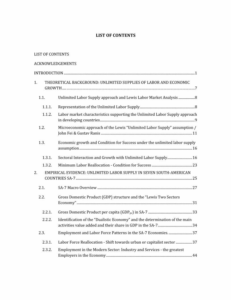
LIST OF CONTENTS
LIST OF CONTENTS
ACKNOWLEDGEMENTS
INTRODUCTION ........................................................................................................................................................ 1
1. THEORETICAL BACKGROUND: UNLIMITED SUPPLIES OF LABOR AND ECONOMIC
GROWTH ..... ……………………………………………………………………………………………………………7
1.1. Unlimited Labor Supply approach and Lewis Labor Market Analysis ................... 8
1.1.1. Representation of the Unlimited Labor Supply ................................................................ 8
1.1.2. Labor market characteristics supporting the Unlimited Labor Supply approach
in developing countries .............................................................................................................. 9
1.2. Microeconomic approach of the Lewis “Unlimited Labor Supply” assumption /
John Fei & Gustav Ranis .......................................................................................................... 11
1.3. Economic growth and Condition for Success under the unlimited labor supply
assumption ................................................................................................................................... 16
1.3.1. Sectoral Interaction and Growth with Unlimited Labor Supply............................. 16
1.3.2. Minimum Labor Reallocation - Condition for Success ............................................... 23
2. EMPIRICAL EVIDENCE: UNLIMITED LABOR SUPPLY IN SEVEN SOUTH-AMERICAN
COUNTRIES SA-7 ....................................................................................................................................... 25
2.1. SA-7 Macro Overview .............................................................................................................. 27
2.2. Gross Domestic Product (GDP) structure and the “Lewis Two Sectors
Economy” ...................................................................................................................................... 31
2.2.1. Gross Domestic Product per capita (GDPpc) in SA-7 ................................................... 33
2.2.2. Identification of the “Dualistic Economy” and the determination of the main
activities value added and their share in GDP in the SA-7........................................ 34
2.3. Employment and Labor Force Patterns in the SA-7 Economies. ........................... 37
2.3.1. Labor Force Reallocation - Shift towards urban or capitalist sector ................... 37
2.3.2. Employment in the Modern Sector: Industry and Services - the greatest
Employers in the Economy .................................................................................................... 44
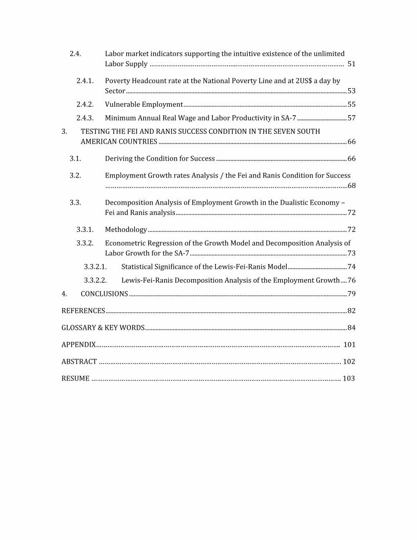
2.4. Labor market indicators supporting the intuitive existence of the unlimited
Labor Supply ………………………………………..………………………………………………… 51
2.4.1. Poverty Headcount rate at the National Poverty Line and at 2US$ a day by
Sector .............................................................................................................................................. 53
2.4.2. Vulnerable Employment ......................................................................................................... 55
2.4.3. Minimum Annual Real Wage and Labor Productivity in SA-7 ................................ 57
3. TESTING THE FEI AND RANIS SUCCESS CONDITION IN THE SEVEN SOUTH
AMERICAN COUNTRIES ......................................................................................................................... 66
3.1. Deriving the Condition for Success .................................................................................... 66
3.2. Employment Growth rates Analysis / the Fei and Ranis Condition for Success
…………………………………………………………………………………………………………………68
3.3. Decomposition Analysis of Employment Growth in the Dualistic Economy –
Fei and Ranis analysis .............................................................................................................. 72
3.3.1. Methodology ................................................................................................................................ 72
3.3.2. Econometric Regression of the Growth Model and Decomposition Analysis of
Labor Growth for the SA-7 ..................................................................................................... 73
3.3.2.1. Statistical Significance of the Lewis-Fei-Ranis Model ...................................... 74
3.3.2.2. Lewis-Fei-Ranis Decomposition Analysis of the Employment Growth .... 76
4. CONCLUSIONS ............................................................................................................................................ 79
REFERENCES ........................................................................................................................................................... 82
GLOSSARY & KEY WORDS .................................................................................................................................. 84
APPENDIX…………………………………………………………………………………………………………………. 101
ABSTRACT ………………………………………………………………………………………………………………… 102
RESUME ……………………………………………………………………………………………………………………. 103
ACKNOWLEDGEMENTS
The topic of this Master Thesis was recommended by Professor Dr. Robert Stehrer at the
beginning of my Master program in Economics at the University of Vienna. After studying
the concerning literature, it became clear to me that the “unlimited labor supply” in
developing economies is still a relevant topic. This Thesis is based on the paper “Economic
Development with Unlimited Supplies of Labor” written in 1954 by economist and
Professor, William Arthur Lewis. The purpose of this study is to identify the relevant and
current characteristics of the labor supply in seven South-American economies and match
them with those from the Lewis framework. The Lewis paper is basically theoretical and
intuitive and has been formalized by further researchers such as John Fei & Gustav Ranis
(1964). Professors John Fei and Gustav Ranis developed a growth Model and determined
the necessary condition for success in economies with particular characteristics in their
labor markets. After reviewing the theory, my empirical research focuses on the analysis of
labor market and macroeconomic indicators that support the existence of unlimited
supplies of labor in seven South-American countries (SA-7). In order to determine some of
the conclusions concerning the labor market situation and growth path in these economies,
I test the condition for success of the Lewis-Fei-Ranis growth model to prove statically the
significance of the model for these SA-7 economies.

Introduction
1
INTRODUCTION
Why is the Arthur Lewis paper – published 58 years ago - still important? Arthur Lewis
analysis and perception marked an important change in the labor market analysis in
developing countries and further in theories of growth. Before the publication of the Arthur
Lewis paper, “Economic Development with Unlimited Supplies of Labor” (1954), the labor
market analysis, practiced in the main international organizations such as Comisión
Económica para América Latina y el Caribe (CEPAL) and the national institutes of statistics1
in each country in Latin America, was related to the neoclassic vision, framed in an economy
context of one productive market in the economy where labor was re-allocated. After
publishing his paper in 1954, which was focused on the Asian economy situation, Arthur
Lewis marked an important turning point in the labor market analysis for developing
countries including the South-American countries, recognizing that labor force is allocated
from one sector of the economy to another much more productive sector.
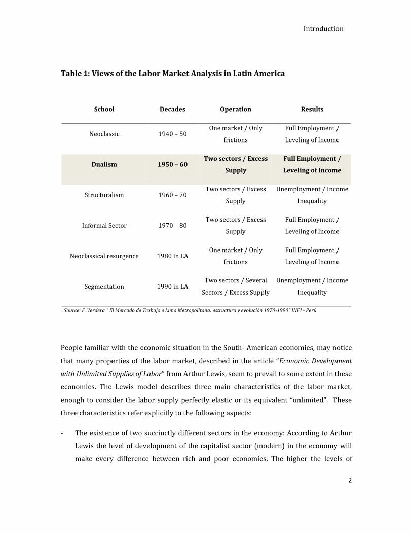
Table 1 shows chronologically the trends of the labor market analysis in South- American
countries since 1940. The new labor market analysis inspired by the Lewis model has been
used by different economic schools.
1 The national institutes of statistics in each country are agencies of the executive (government) in
charge of supervising all public statistics and organizing and managing the national statistic system.
Source: www.indec.gov.ar
Introduction
2
Table 1: Views of the Labor Market Analysis in Latin America
School Decades Operation Results
Neoclassic 1940 – 50 One market / Only
frictions
Full Employment /
Leveling of Income
Dualism 1950 – 60 Two sectors / Excess
Supply
Full Employment /
Leveling of Income
Structuralism 1960 – 70 Two sectors / Excess
Supply
Unemployment / Income
Inequality
Informal Sector 1970 – 80 Two sectors / Excess
Supply
Full Employment /
Leveling of Income
Neoclassical resurgence 1980 in LA One market / Only
frictions
Full Employment /
Leveling of Income
Segmentation 1990 in LA Two sectors / Several
Sectors / Excess Supply
Unemployment / Income
Inequality
Source: F. Verdera " El Mercado de Trabajo e Lima Metropolitana: estructura y evolución 1970-1990" INEI - Perú
People familiar with the economic situation in the South- American economies, may notice
that many properties of the labor market, described in the article “Economic Development
with Unlimited Supplies of Labor” from Arthur Lewis, seem to prevail to some extent in these
economies. The Lewis model describes three main characteristics of the labor market,
enough to consider the labor supply perfectly elastic or its equivalent “unlimited”. These
three characteristics refer explicitly to the following aspects:
- The existence of two succinctly different sectors in the economy: According to Arthur
Lewis the level of development of the capitalist sector (modern) in the economy will
make every difference between rich and poor economies. The higher the levels of
Introduction
3
development of the capitalist sector in comparison to the agriculture sector, the richer
the economy. Lewis considers that in the traditional or agricultural sector the main
output are goods of first necessity. Goods of first necessity are normal goods until a
point or quantity, where they become an inferior good; which means that the individual
or household will not spend more than a fixed quota of food. Thus any additional dollar
of income will be used for buying other kinds of goods or to save. This traditional sector
has as its constraints land and labor as factors of production. In the capitalist sector
instead, labor force is involved in activities where the output is normal goods and do
not become inferior.
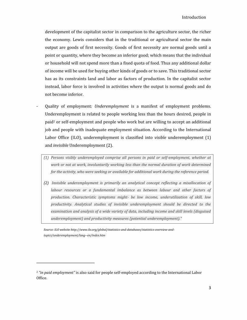
- Quality of employment: Underemployment is a manifest of employment problems.
Underemployment is related to people working less than the hours desired, people in
paid2 or self-employment and people who work but are willing to accept an additional
job and people with inadequate employment situation. According to the International
Labor Office (ILO), underemployment is classified into visible underemployment (1)
and invisible Underemployment (2).
(1) Persons visibly underemployed comprise all persons in paid or self-employment, whether at
work or not at work, involuntarily working less than the normal duration of work determined
for the activity, who were seeking or available for additional work during the reference period.
(2) Invisible underemployment is primarily an analytical concept reflecting a misallocation of
labour resources or a fundamental imbalance as between labour and other factors of
production. Characteristic symptoms might- be low income, underutilisation of skill, low
productivity. Analytical studies of invisible underemployment should be directed to the
examination and analysis of a wide variety of data, including income and skill levels (disguised
underemployment) and productivity measures (potential underemployment).”
Source: ILO website http://www.ilo.org/global/statistics-and-databases/statistics-overview-and-
topics/underemployment/lang--en/index.htm
2 “in paid employment” is also said for people self-employed according to the International Labor
Office.
Introduction
4
- The third characteristic is referred to as the labor force willing to work unlimitedly for
a minimum salary or wage, referred to as “subsistence wage”, by Lewis and further on
named “institutional wage” by some other authors.
Observing these characteristics of the labor market, Arthur Lewis declared situation as
evidence for the “existence” of an excess of labor in these economies.
Excess labor is thus related to overpopulation and labor force not well employed that earn a
wage equivalent to the minimum level of subsistence and thus vulnerable to poverty.
Unemployment and poverty are linked together as an effect of the excess labor. The surplus
of labor tends to start developing some unproductive activities with small revenues only. In
these economies, there is also another part of the society that works “formally” and gets
higher loans or salaries. The group of labor force under low quality of labor is mainly
allocated in the so-called “non capitalist sector” or “subsistence sector” (Lewis, 1954:4-5).
The magnitude of this subsistence sector is the most important component of the so-called
unlimited labor supply situation.
In this analysis I selected a group of seven South-American countries (SA-7): Argentina,
Brazil, Chile, Colombia, Peru, Uruguay and Venezuela. In these economies, at first glance the
characteristics such as high rates of underemployment and huge portions of the labor force
working at very low wages levels, match almost perfectly with the assumptions proposed in
the Lewis Model.
Therefore, my analysis is comprised of three core chapters. In the first chapter I review the
concept of unlimited labor supply in an economy (Lewis approach), remarking the most
important characteristics of an economy with unlimited labor supply according to his paper
“Economic Development with Unlimited Supplies of Labor” published in 1954. This
unlimited labor supply assumption will be the base for professors John Fei and Gustav Ranis
to develop and present the growth theory for the two sector or dualistic economies with
unlimited labor supply in the book titled “Development of the Labor Surplus Economy:
Theory and Policy”. Following the theory by Fei & Ranis, I explain briefly its view and theory
of growth and the success condition for a further empirical analysis in the second chapter of
this study.
Introduction
5
In the second chapter I provide a descriptive analysis in order to show and identify the
characteristics that give supportive evidence of unlimited labor supplies in these countries.
The third chapter provides tests of the condition for success under an economy facing
unlimited labor supplies and the determination of growth factor, following the
decomposition analysis of Fei & Ranis growth model.
Finally, in the fourth chapter, I provide my conclusions for those countries within the SA-7,
which have had successful results in all steps of my analysis.
The analysis answers the following research questions:
1. Can we find evidence for an excess of labor supply in the seven South American
countries considered?
2. According to Lewis framework, do we have relevant empirical evidence exerting
pressure on wages and supporting unlimited labor supply?
3. Did the seven South- American countries show some improvements on labor
productivity on their economic sectors in the last 40 years? To which extent is that in
accordance to the Arthur Lewis theory?
4. Which are the most productive sectors in the economies? Which sector is the most
labor intensive? Do the patterns match with Lewis framework of development?
5. Do the SA-7 economies fit in the Lewis-Fei-Ranis growth Model proposed in 1954 and
1964? To which activities is the poor part of the society related?
6. In the framework of the Lewis-Fei-Ranis model, what are the factors of the economy
that have been crucial to offset the labor force growth?
7. Considering the growth path of the dualistic economy, in which stage of development
are these economies located?
The data for the study was compiled from the World Bank online database, Oxford
University - Department of International Development Studies Data Base, UNIDO data base,
CEPAL online database and ILO database available on the respective websites (see
references and survey). Some recent data was also compiled from each country’s statistics
Introduction
6
government institute. I considered transcendental the politic and economic policy changes
from 2001 in the seven South-American countries in analysis. Due to data availability, the
period of analysis in the empirical part will be from 1991 through 2007 in order to skip the
current financial crisis.
Argentina and Brazil are the biggest industrialized economies in Latin America with 48%
and 37% of industry value added (IVA) as share of their respective GDP. Argentina and
Uruguay have the highest GDP per capita/year in 2009 in the South American region
(10,682 US$ and 9,284US$ respectively). Uruguay is geographically a small commercial
country between the giant Brazil and the big Argentina. Venezuela is a powerful country
which is one of the biggest industrialized countries and the fourth highest GDP per
capita/year in Latin America (IVA 41% of GDP and 5,425 US$ per capita/year) after
Argentina, Uruguay and Chile. Venezuela´s economy depends on oil revenues which account
for roughly 95% of export earnings, about 40% of federal budget revenues, and around
12% of GDP3. Chile is an important economy due to its export potential worldwide, mainly
in agro-industry and has the third highest GDP per capita/year in the region. Peru is an
economy with significant GDP growth rates in the last 10 years. Peru is considered a
primary export Economy. Peruvian Mining and industrial sector have led the Peruvian
economy to important economic changes since 2000 where successful policies reduced
poverty around 10% in the last decade (from 45% in 2000 to 35% in 2009). Colombia was
chosen for its interesting macro indicators that reveal a match with the Lewis approach,
such as 64% of the population living with an income over the national poverty line and high
rates of underemployment.
3 Economy overview at http://www.indexmundi.com/venezuela/economy_profile.html
1. Theoretical Background
7
1. THEORETICAL BACKGROUND: UNLIMITED SUPPLIES OF LABOR AND
ECONOMIC GROWTH
In 1954, William Arthur Lewis based his analysis on the roots of the classical growth model,
focusing on the labor supply in the expansion process.
Textbook contributions assume an upward-sloped labor supply curve, putting aside the
possibility of an unlimited labor supply. This approach is justified with respect to
developed economies, e.g. the Western European countries, which do not suffer from an
unlimited labor supply. With respect to developing economies, however, Lewis argued, “...
on the other hand over the greater part of Asia labor is unlimited in supply, and economic
expansion certainly cannot be taken for granted.” (Lewis, 1954: 4)
Arthur Lewis identified some relevant characteristics of the labor market in developing
countries such as the high rate of underemployment, overpopulated sectors relative to
capital or labor opportunities, largest groups of society working by their own perceiving
minimum compensations or low wages and also one sector of the economy well developed
with higher standards of living. This is what the next section is about.
In Section 1.2, the microeconomic approach developed by John Fei and Gustav Ranis (1964)
that supports the unlimited labor supply assumption is explained. This approach follows the
structure of the authors in their book “Development of the Labor Surplus Economy” written
in 1964 arguing that the first order condition of the classical model that refers that the
marginal product of labor equals the real wage is not satisfied, i.e. where Y =
is a textbook production function, i.e. output Y is a function of capital K and labor L.
This result which holds when labor is of unlimited supply, that, , becomes the
cornerstone of John Fei and Gustav Ranis contribution, which supports the Lewis approach
with respect to the existence of an unlimited supply of labor in these economies.
1. Theoretical Background
8
In Section 1.3 I briefly explain and illustrate the economic expansion concept and depict the
conditions for success in the Lewis model framework. Section 1.3.1 is basically the
explanation of the accumulation process in the two sectors economy with unlimited labor
supply. In section 1.3.2 I depict the conditions for success proposed by professors John Fei
and Gustav Ranis, related to the labor absorption process.
1.1. Unlimited Labor Supply approach and Lewis Labor Market
Analysis In this section I present the Arthur Lewis arguments of unlimited labor supply in a graphical
manner and explain the main labor market characteristics that support the idea of
unlimited supplies of labor in less developed economies. The unlimited labor supply is a
critical and crucially departing assumption for further growth theories for less developed
economies.
1.1.1. Representation of the Unlimited Labor Supply
Arthur Lewis proposed the scenario of a labor market with unlimited labor supplies. Lewis,
in his essay, remarked the necessity and set the feasibility to consider the assumption of an
unlimited labor supply in economies in countries such as Egypt, India or Jamaica, which
present high rates of underemployment, extreme low wages and low standards of living
that will be listed in section 1.1.2 of this chapter.
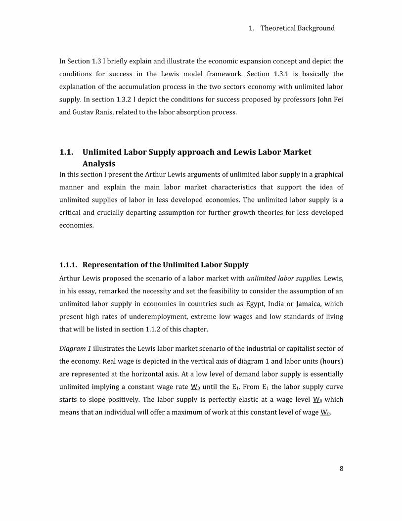
Diagram 1 illustrates the Lewis labor market scenario of the industrial or capitalist sector of
the economy. Real wage is depicted in the vertical axis of diagram 1 and labor units (hours)
are represented at the horizontal axis. At a low level of demand labor supply is essentially
unlimited implying a constant wage rate W0 until the E1. From E1 the labor supply curve
starts to slope positively. The labor supply is perfectly elastic at a wage level W0 which
means that an individual will offer a maximum of work at this constant level of wage W0.
1. Theoretical Background
9
Diagram 1: Representation of the Unlimited Labor Supply Approach
Author´s graph
Two important issues can be derived from this unlimited labor supply labor market
scenario, which are explained in Section 1.3.1:
- The feasibility of an unchanged or constant wage level W0
- Capitalist profits are higher when capitalist faces constant real wages W0
Considering a negative classic labor demand curve, in diagram 1.1 any shift of the labor
demand between W0 – L0 will be at a constant real wage. Capitalist can freely decide its level
of production. Lewis proposes that Capitalists will make profits from this cheap labor force
cost.
1.1.2. Labor market characteristics supporting the Unlimited Labor Supply approach
in developing countries
The questions arising are therefore to which extent the unlimited labor supply exists and
what are the determinants? Unlimited labor supply is said to exist in those countries with
1. Theoretical Background
10
high rates of underemployment and where population is large relative to capital and/or
natural resources (Lewis, 1954:5). Under these circumstances a negligible marginal
productivity of labor occurs. This is what capitalist income can profit from; but how far can
they go? The overpopulated agriculture sector will supply the manpower to fuel the
development process (Fei & Ranis, 1964:8). Therefore, below I describe the characteristics
of the labor supply with labor surplus.
i. Underemployment and Occasional jobs domain
“Occasional jobs” are activities developed by the unemployed or underemployed labor force.
These are jobs, where an individual tries to get some monetary compensation or tips from
doing some occasional short service. Some examples of occasional jobs are such as carrying
bags at the train station, jobbing gardener, etc (Lewis, 1954:2). The occasional job was one
of the main characteristics of the Asian labor market at that time and Lewis determined it as
something very important to be added to the classical labor market and growth path. The
existence of an “occasional sector” conformed by the “occasional jobbers” can also be
observed in South American countries in a generalized way which has developed over time.
The “occasional sector” is considered in the statistics as part of the “underemployment
sector”. According to Lewis the “occasional sector” can be also related to the unskilled labor
force and represents in overpopulated economies an enormous possibility of an industrial
expansion without shortage of unskilled labor (Lewis, 1954:4).
ii. Labor surplus and redundant labor in the Agriculture sector
Arthur Lewis identified two sectors in these developing economies, with one sector being
much more productive than the other. The less productive sector is the agriculture sector
located in rural areas with a large rate of underemployed population with low wages and
low standards of living. Due to the over-populated situation with respect to capital in this
sector of the economy, a large portion of the labor force is “redundant” in terms of
productivity. “Redundant labor force” is a situation where the position of employment of an
employee is or will become surplus to the requirements of the employer's business (Fei &
Ranis, 1964:13).
1. Theoretical Background
11
On the other hand, in this economy a much more productive sector (industrial or capital
sector) exists, where labor force is needed. Due to the free mobility of labor within one
economy, a transfer of labor force from the agriculture sector to the capital sector is feasible
and will reduce the “redundant” labor force in the traditional sector. The portion of the
redundant labor force transferred from one sector to the other becomes part of the
industrial labor force.
iii. Negligible Marginal productivity of Labor & Subsistence wage
Negligible marginal productivity prevails in economies with redundant labor force where
the minimum wage rate is institutionally determined. In these economies, the minimum
wage level will be fixed at a “subsistence level” (Lewis, 1954:6), comparable with the
national poverty line. In this scenario, we can intuitively deduce that the minimum wage
rate does not equal the marginal productivity of labor.
Now it is time to relate and enclose the idea related to “subsistence wage level” and
“negligible marginal productivity” into the idea of labor surplus and the consequence of an
“unlimited labor supply”. The supply of labor is said to be “unlimited” as long as there is
labor force willing to work for this “subsistence wage”.
The identification of two interconnected sectors in the economy (agriculture and industrial
sector) will let us think of two groups of labor force that freely allocate themselves in any of
these two sectors of the economy. That is one of the main issues emphasized by Lewis in his
article, to argue that this labor reallocation from agriculture sector to the industrial sector
will generate a pressure on wages in the industrial sector.
1.2. Microeconomic approach of the Lewis “Unlimited Labor Supply”
assumption / John Fei & Gustav Ranis According to Arthur Lewis, an economy with unlimited labor supply has two important
characteristics. The first one is related to the marginal productivity of labor that is in some
cases negligible; and the second one, is about the existence of an institutional wage at the
subsistence level (minimum wage). This subsistence wage level appears to be constant in
1. Theoretical Background
12
real terms due to the abundant unskilled rural labor that transfer to the cities and pressure
the wage in the capitalist sector over a minimum level of wage.
When we talk about unlimited labor supply, labor surplus intuitively comes to mind. The
classical economists consider the notion of “surplus labor” as the presence of disguised
unemployment with wages determined in a bargaining context; and the neoclassical
economists accept labor market clearance and labor supply decisions supported on
individual solution of its utility maximization problem based on the labor/leisure trade off
(Fei & Ranis, 1997:146).
According to Lewis’ model, in the traditional sector of the economy there is no labor market
clearance, thus labor surplus. The traditional sector with labor surplus is characterized by
the following issues:
- Redundant labor force: There is a large labor supply relative to fixed supply productive
available land.
- Output is concentrated on first necessity goods with a limit on demand.
In this framework, the neoclassical wage that equals the marginal product is not achieved.
Thus, there is an institutional minimum wage that is greater than the marginal productivity
of labor; hence, there is no equilibrium or competitive wage reached. These issues do not
allow the classical and neoclassical economists to derive analytically the institutional wage
(Fei & Ranis 1997:147).
On the other hand, the capitalist sector is tied to the traditional or agriculture sectors
institutional wage, of course, as long as the surplus labor persists. The way to erase the
labor surplus is through the labor reallocation, in which traditional sector labor force
becomes labor force in the capitalist sector. This labor reallocation is going to be achieved
with both sector effort and investment following the classic or neoclassic growth model.
Dualism disappears as the traditional or agriculture sector loses its characteristic labor
surplus and verges to the one-sector neoclassical model.
Clearing wages are obtained in the capitalist sector with the unskilled real wage tied to the
traditional sectors institutional real wage at some premium reflecting the necessary
1. Theoretical Background
13
inducement to move, possibly including an additional gap due to other government
interventions in the organized labor market (Fei & Ranis 1997: 148).
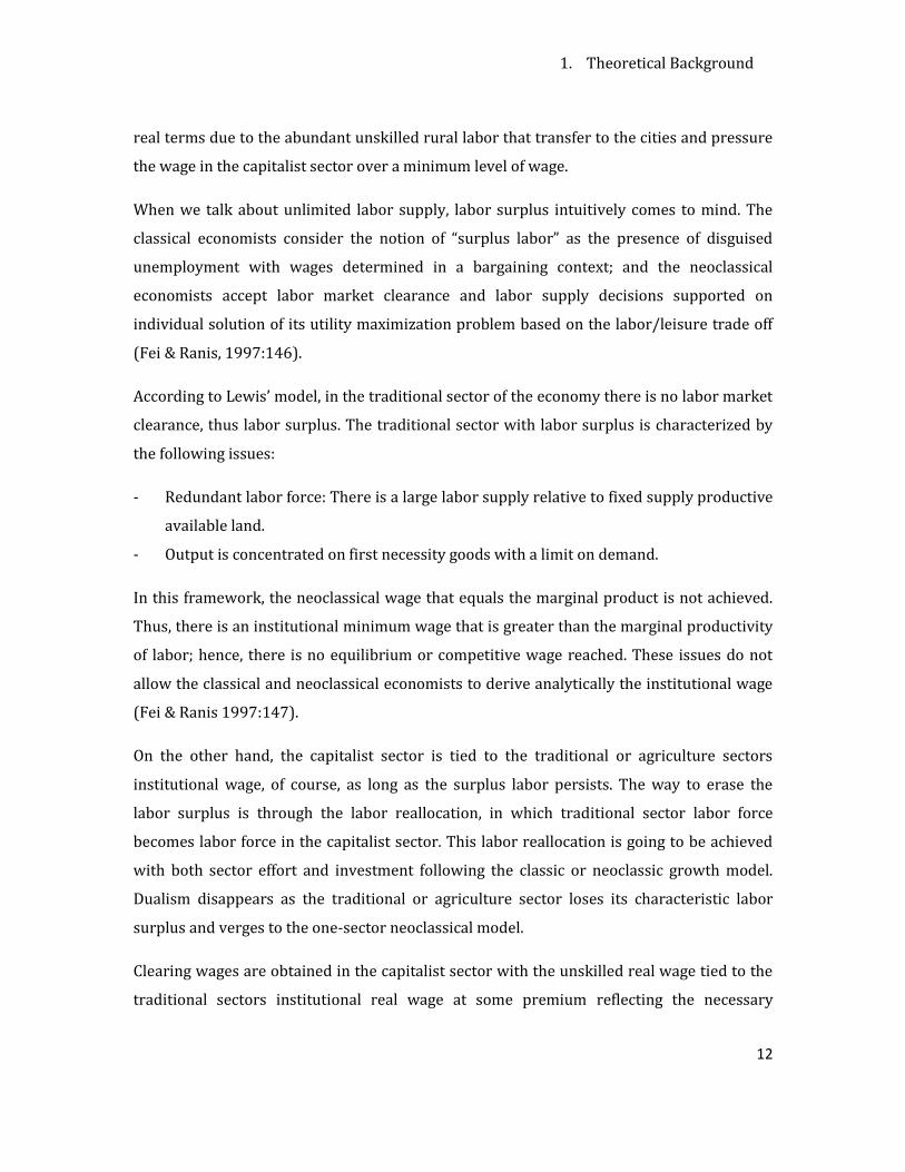
Diagram 2 illustrates the transition process from the traditional market view. Labor is
represented on the horizontal axis with an initial endowment L´. The vertical axis shows the
output and wage where w represents the constant institutional wage and MPL are the
correspondent marginal productivity of labor in the agriculture sector. (L´´ - L´) represents
the portion of the labor whose marginal product is under the institutional marginal wage
and is related to the underemployed or unemployed portion of the labor force.
Diagram 2: Transition Process
Source: Fei & Ranis, 1997:149. “Growth and Development from an Evolutionary Perspective”.
As the capitalist sector demands more labor force, the marginal productivity of the
remaining labor force in the traditional sector rises, hence MPL shifts to the right (MPL -MPL1
-MPL2), reducing the portion of agricultural labor force who is paid under the institutional
wage. Labor force reallocation in the capitalist sector reduces the endowment of labor force
in the traditional sector and ALS shifts to the left (ALS-ALS1-ALS2). As long as the labor
1. Theoretical Background
14
demand in the capitalist sector increases, this scenario will continue until the
underemployment or disguised unemployment totally disappears. This process ends at
point A when the marginal productivity of labor equals the wage at a given labor force
endowment.
In the Lewis model framework, John Fei and Arthur Ranis conclude that during the first
stage, the institutional wage does not equal the marginal productivity of labor until point A
is reached. The institutional wage is determined by each government and could also be
considered the legal minimum wage.
Following the Lewis model, John Fei and Gustav Ranis support the unlimited labor supply
assumption based on empirical results where they show that there is an institutional wage
above the very low marginal product of labor and that this wage rises only slowly via
institutional wage (CIW) adjustment and lags substantially behind the agricultural
productivity increases (Fei & Ranis 1997: 156).
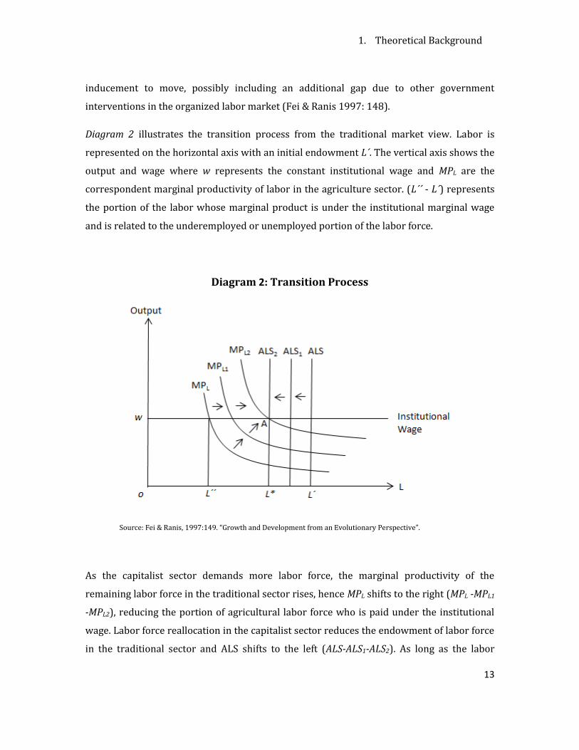
The indifference map plotted in diagram 3 shows the dynamics of the industrial real wage
according to Fei and Ranis, supporting the constant behavior of the real wage. Diagram 3
describes the consumer preferences of an industrial worker who perceives a real wage in
terms of industrial goods. Agricultural goods are plotted in the vertical axis and the
industrial goods in the horizontal one. The indifference curves are represented in curves C0,
C1, C2 and C3. The vector VV´ represents the caloric minimum of any individual and a
consequent location of all indifference curves is to be considered above this caloric
minimum. When the indifference curves become flat asymptotically above the caloric
minimum, it means that the industrial goods become poor substitutes of the agricultural
goods. Below the caloric minimum the individual begins to starve.
Now, the main topic is to understand the behavior of the industrial real wage. In diagram 3
the industrial wage w0, represented in the horizontal axis, is measured in terms of a basket
of industrial goods. On the other hand, in the agriculture sector exist a “reservoir” of
disguised unemployment (Fei and Ranis 1964: 156) with a negligible marginal productivity
and nevertheless perceives a positive institutional real wage (CIW) measure in terms of
agricultural goods.
1. Theoretical Background
15
Diagram 3: The Industrial Real Wage is determined by Agricultural Surplus
Source: Fei & Ranis, 1964: 155 C.4, S. 2 “Agricultural Surplus and the Industrial Real Wage”.
Since the agricultural goods are goods of first necessity, these are going to be part of the
consumption bundle of the industrial worker. The CIW in the agriculture sector governs the
value in exchange of the industrial real wage w. As long as there is disguised labor force in
the agriculture ready to transfer to the industrial sector, the real wage in the industrial
sector is not going to change even if there is an increase on the employment in the industrial
sector. The industrial real wage is to be tied to the CIW at wa.
To understand the dynamics, let’s consider a total agricultural surplus (TAS) that will all be
consumed by the industrial sector. Thus, an agricultural surplus per industrial worker (AAS)
is plotted in diagram 3 by A2, A1 and Am. The magnitude of AAS, given the CIW, determines
the terms of trade and industrial real wage. Suppose an initial AAS level A2 with
consumption level and the terms of trade G1 (price consumption line). The industrial real
wage w14 is determined from the terms of trade level waG1. Since the real industrial wage is
4 “The industrial real wage is indicated by the point w1 on the horizontal axis, due to the fact that only
at this level of industrial wage w1 and at this terms of trade level (slope of waw1) will the industrial
1. Theoretical Background
16
tied to the CIW, or has the same exchange value as the CIW, it implies that any tendency for
the real wage to increase substantially and thus create wage differential between
agriculture and industry will be “thwarted” by the flow of agriculture workers to industry
(Fei & Ranis, 1964:157).
Notice that if AAS is reduced, reduction in the consumption of agricultural goods cannot fall
under the minimum caloric level Am, where at point Em the price-consumption curve PCwa
starts to increase. Em is the point where the industrial good become to be no more a perfect
substitute of the first necessity agricultural good and the price of food begins to rise.
1.3. Economic growth and Condition for Success under the unlimited labor
supply assumption
Following the Arthur Lewis approach about the unlimited labor supply and two sectors in
the economy, in 1965 John Fei & Gustav Ranis developed a growth theory for those
countries with labor surplus. Fei & Ranis remark that for the development of their growth
theory, the intuitive notion of labor surplus is translated into an analytical condition, which
becomes an integral part of the framework. (Fei & Ranis 1964:4, Introduction: an Approach to
the Problem, “Development of the labor surplus Economy”)
The core theme of Fei & Ranis research was the continuous reallocation of labor from the
agricultural sector to the industrial sector. The rate of labor reallocation is crucial and
defines the success, stagnation or failure in the development effort of these economies.
1.3.1. Sectoral Interaction and Growth with Unlimited Labor Supply
Based on the theoretical background in the previous sections, Lewis provides a way to
consider a growing economy:
real wage command the same exchange value as CIW and will the commodity market be cleared (the
typical industrial worker will buy all the AAS available)“ Fei & Ranis 1964: Development of the labor
surplus Economy. Page 158.
1. Theoretical Background
17
“…the key to the process is the use which is made of the capitalist surplus in so far as this is
reinvested in creating new capital; the capitalist sector expands, taking more people into the
capitalist employment out of the subsistence sector. The surplus is then larger, still, capital
formation is still greater and so the process continues until the labor is surplus labor” (Lewis,
1954:11).
The process of success is going to be represented in two stages: The first one is when the
economy faces a surplus of labor represented by the unlimited labor supply. This first stage
is a representation of the two sectors economy. The second stage will be after the break
point where the labor supply is positive and wages will be bargained.
When talking about interaction, we may all think about this phenomenon in two different
locations (or regions). From Arthur Lewis’ approach, Fei and Ranis identified two locations
in the economy such as the agriculture sector located in rural areas and the industrial or
capitalist sector located in the cities or urban areas. The transcendental phenomenon in Fei
and Ranis is the role of redundant labor force in the production of agricultural goods, the
industrial production and employment and the labor reallocation process.
i. Redundant Labor force and agricultural production
The main characteristic of the agriculture sector is the overpopulation and the persistence
pressure of population on the scarce natural resources. The first assumption in these
economies is the initial and worsening bad endowment ratio land-labor, leading to rapidly
diminishing increments in agricultural output. Labor and land are the factors of production
in the agriculture sector and are represented in Diagram 4a. The respective contour lines
are depicted by M, M´, M´´ assuming constant returns to scale. The region of factor
substitutability is marked off by two ridge lines 0v* and 0u*; which means that under the
line 0u* the contour lines M, M´, M´´ became completely horizontal, indicating that with the
factor land held constant, labor becomes redundant as output cannot be raised. In the
theory it is assumed that the land available for cultivation is given. In Diagram 4a, for
example, the production factors in the agriculture sector are depicted, where the given land
available is established by the line 0t, and the line ts indicates the labor force employed
productively. This productively employed part of the labor force is called the “labor
utilization ratio” by Fei and Ranis, and denoted by R
1. Theoretical Background
18
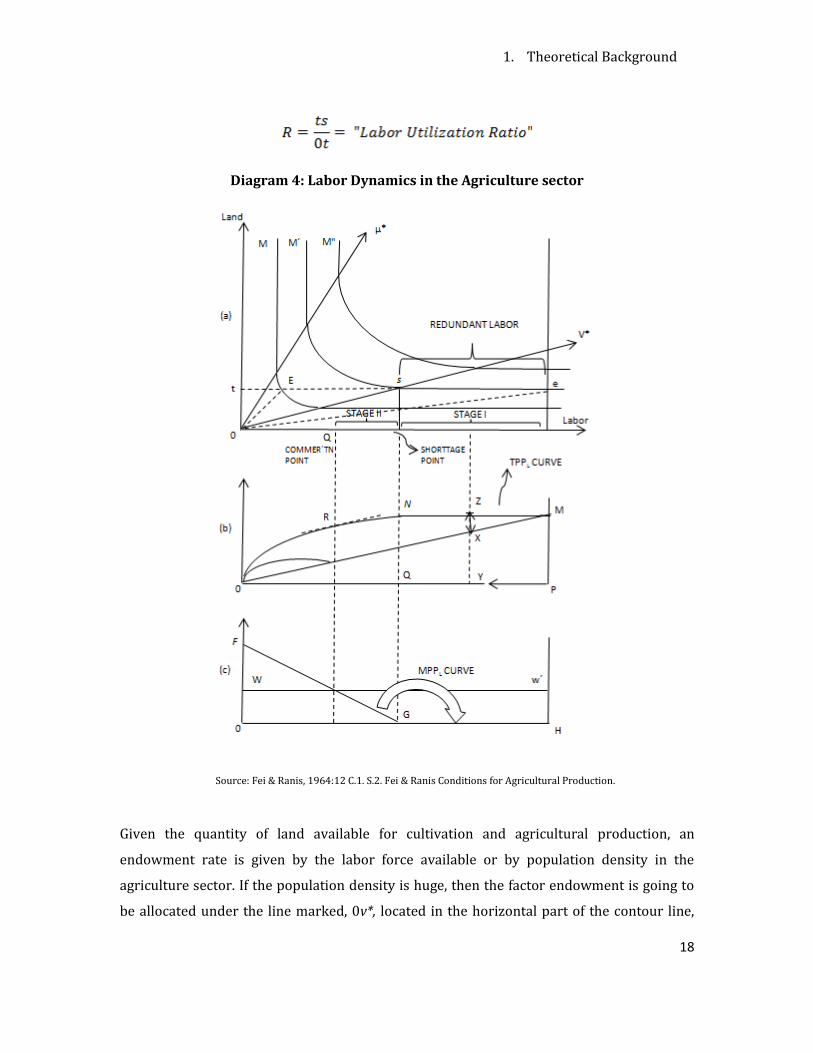
Diagram 4: Labor Dynamics in the Agriculture sector
Source: Fei & Ranis, 1964:12 C.1. S.2. Fei & Ranis Conditions for Agricultural Production.
Given the quantity of land available for cultivation and agricultural production, an
endowment rate is given by the labor force available or by population density in the
agriculture sector. If the population density is huge, then the factor endowment is going to
be allocated under the line marked, 0v*, located in the horizontal part of the contour line,
1. Theoretical Background
19
which means that there is redundant labor. The endowment ratio S in this case with
redundant labor is going to be strictly greater than the labor utilization rate R (S > R). The
endowment ratio is going to be given by
; where E is any point that indicates the magnitude of labor. Non-redundant labor
is going to be given as long as the labor utilization rate R equals or exceed the endowment
rate S is (R ≥ S).
Now there is a point s that represents the point at which the endowment ratio S equals the
labor utilization ratio R. At this point a non-redundancy labor ratio or coefficient T can be
calculated just by dividing T = ts/te (Fei & Ranis, 1997:14). This ratio T refers to the labor
utilization ratio R = ts/t0 and the endowment ratio S = te/t0; which dividing both by t0 we
get that:
The non-redundancy ratio is directly proportional to the labor utilization ratio and
inversely proportional to the endowment ratio or density proportion.
Diagram 4(b) depicts the total physical productivity of labor TPPL given the assumption that
land available is given; and Diagram 4(c) depicts the TPPL lined up with the corresponding
marginal productivity of labor MPPL. Diagrams 4(b) and (c) are vertically lined up with
Diagram 4(a).
Assuming that land is fixed, the TPPL represented in Diagram 4(b) increases at a decreasing
rate until the point N, where the MPPL becomes horizontal where TPPL cannot increase
anymore by adding more labor force. At this point N lined up with point G on the Diagram
4(c) the MPPL becomes zero.
Thus, in Diagrams 4 (a), (b) and (c) the non-redundancy ratio T will be given as:
.
In the Lewis, Fei and Ranis analysis, the development track in the long run will be strictly
related to the increase on productivity. For the analysis, area of land available for
1. Theoretical Background
20
cultivation will be given. It does not block the possibility of any further expansion of
cultivating land through forest clearing, drainage and other programs.
In this context, as a redundant labor force exists with marginal productivity of labor zero,
and following a profit-maximizing pattern of behavior in a competitive market, the wage
perceived by this redundant labor force is supposed to be zero. As a zero real wage level is
not possible, the wage perceived by this redundant labor force is going to be institutionally
determined by the government, based on minimum and necessary levels of subsistence
(minimum wage) and called by Fei and Ranis, the “Constant Institutional Wage” (CIW)5. In
this sense, Fei and Ranis considered that CIW level is “more or less” related to the average
productivity of labor APPL = MP/OP (see diagram 4 (b)) (Fei and Ranis 1964:21). In that
sense, APPL equals the real wage and be represented by the vector OM in diagram 4(b) and
by the vector ww´ in diagram 4(c).
An important dynamic issue that is shown in Diagram 4(b), is the reallocation and further
reduction of agricultural redundant labor force. Suppose a reallocation of agricultural labor
force to the industrial sector that reduces the redundant labor force from point P to Y, and
the agricultural production level M remains constant. As the agricultural production
remains constant and population in the agriculture sector has been reduced, then an
agricultural surplus is available to be transferred to the industrial sector. This production
surplus is called the Total Agriculture Sector or TAS and is represented on diagram 4(b) by
the vector XZ that is the difference between the agricultural output YZ and the wage income
of agricultural labor force XY.
ii. Industrial production and employment
Following the Fei & Ranis growth theory with unlimited labor supply, I explain briefly the
role of the industrial sector. As stated earlier, the industrial or capitalist sector has the role
of creating jobs and employment opportunities through capital formation. The creation of
employment opportunities is required for the absorption of the labor surplus released by
the agriculture sector that transfers to the cities. The inputs in the industrial sector will be
5 Fei and Ranis called to this the „Real institutional wage hypothesis“recognized in the development
literature. P. 22 “Development of the Labor Surplus Economy”.
1. Theoretical Background
21
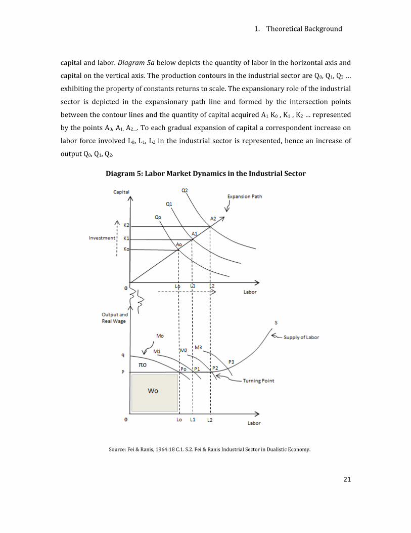
capital and labor. Diagram 5a below depicts the quantity of labor in the horizontal axis and
capital on the vertical axis. The production contours in the industrial sector are Q0, Q1, Q2 …
exhibiting the property of constants returns to scale. The expansionary role of the industrial
sector is depicted in the expansionary path line and formed by the intersection points
between the contour lines and the quantity of capital acquired A1 K0 , K1 , K2 … represented
by the points A0, A1, A2…. To each gradual expansion of capital a correspondent increase on
labor force involved L0, L1, L2 in the industrial sector is represented, hence an increase of
output Q0, Q1, Q2.
Diagram 5: Labor Market Dynamics in the Industrial Sector
Source: Fei & Ranis, 1964:18 C.1. S.2. Fei & Ranis Industrial Sector in Dualistic Economy.
1. Theoretical Background
22
The analysis in the long run is depicted in Diagram 5b, representing the phenomena that the
industrial sector can hire labor at a given supply curve, determined by the forces in the
agriculture sector. The labor supply curve S is determined by the curve P0, P1, P2, P3. In
Diagram 5b the vertical axis measures the wage of the labor force in the industrial sector in
terms of industrial goods. The horizontal part of the labor supply depicted in Diagram 5b
represents the postulation of Arthur Lewis assuming the release of labor from the
agriculture sector without affecting the agricultural production. The agriculture sector
provides a pool of redundant labor that will be the source of the labor supply in the
industrial sector after reallocation. For each amount of capital K0, K1, K2 the respective
marginal productivity of labor curves MPPL are depicted in Diagram 5b (M0, M1, M2)
determining the amount of labor in equilibrium and correspondent level of production or
output. Notice that for example at the level of capital K0 the correspondent amount of labor
L0 is hired and a correspondent level of production is reached. The whole area under the
marginal productivity of labor curve M0 encloses the magnitude of the benefit π of the
capitalist and the magnitude of wages paid (labor costs). In that sense, notice that with
horizontal supplies of labor the benefits of capitalist are much higher than would be with a
positive supply of labor. Hence, the investment rate will be high, including the so-called
hidden savings from workers, and is formalized by John Fei and Gustav Ranis as follows:
where:
K0 = Capital Stock in period 0
K1 = Capital Stock in period 1
π0 = Benefits of capitalist
S0 = Hidden saving from agriculture sector and labor force
The following process tends to be a continuing expansion process, where output and
growth is viewed as a continuing shifting of the marginal productivity of labor curves MPPL
to the right through time. An imminent reinvestment process and increase of labor demand
in the industrial sector is assumed to happen.
1. Theoretical Background
23
iii. Labor reallocation Process
According to Lewis, Fei and Ranis, there is the necessity of labor reallocation in the
successfully development process of a dualistic economy with unlimited labor.
A dualistic economy in the Arthur Lewis framework with an unlimited labor supply can
obtain three possible scenarios through time, with all of them determined by the labor
reallocation of its labor force θ and consequently labor absorption capability of the
capitalist or industrial sector.
- Failure of the capitalist economy: In the case of failure, the proportion of the labor
force absorbed by the capitalist or industrial sector is falling as the rate of population
growth overwhelms labor reallocation efforts. This results in insufficient demand in the
capitalist or industrial sector or an explosion in population and consequently labor
force growth
- Stagnation of the capitalist economy: In this case, a stand-off situation emerges
represented by a constant reallocation.
- Success of the capitalist economy: In this case, the labor reallocation is increasing,
signifying and increase in the fraction of the labor force engaged in commercialized
activities. (page 250 Fei & Ranis 1997)
The goal of a developing economy is, therefore, that the labor reallocation shall increase at a
rate exceeding the population or labor force growth rate.
1.3.2. Minimum labor reallocation - condition for success
Ranis and Fei defined the growth rate of the industrial labor force exceeding the growth
rate of the total population or labor force as the necessary condition for development. The
1. Theoretical Background
24
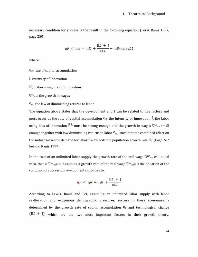
necessary condition for success is the result in the following equation (Fei & Ranis 1997,
page 250):
where:
K: rate of capital accumulation
: Intensity of Innovation
L: Labor using Bias of Innovation
na,: the growth in wages
LL: the law of diminishing returns to labor
The equation above states that the development effort can be related to five factors and
must occur at the rate of capital accumulation K, the intensity of innovation , the labor
using bias of innovation must be strong enough and the growth in wages na small
enough together with low diminishing returns to labor LL, such that the combined effect on
the industrial sector demand for labor W exceeds the population growth rate P. (Page 262
Fei and Ranis 1997)
In the case of an unlimited labor supply the growth rate of the real wage na, will equal
zero, that is na= 0. Assuming a growth rate of the real wage na= 0 the equation of the
condition of successful development simplifies to:
According to Lewis, Ranis and Fei, assuming an unlimited labor supply with labor
reallocation and exogenous demographic pressures, success in these economies is
determined by the growth rate of capital accumulation K and technological change
, which are the two most important factors in their growth theory.
2. Empirical Evidence of Unlimited Labor Supplies in SA-7
25
2. EMPIRICAL EVIDENCE: UNLIMITED LABOR SUPPLY IN SEVEN SOUTH-
AMERICAN COUNTRIES SA-7
“…Rosenzweig´s empirical findings are inherently
reasonable given the normal neoclassical machinery,
especially when the individual family´s leisure/work
trade off is viewed in its proper LDC perspective. But they
are not applicable to our view of an Institutional real
wage as part of the dynamic transition growth of the
dualistic economy.”
John Fei & Gustav Ranis6
Thus, the most important departing point to support the Lewis Model and, hence, the Fei
and Ranis growth theory, is to find evidence for the assumption of the existence of an
unlimited labor supply in the capitalist sector due to redundant labor force in the
agricultural or traditional sectors.
The Lewis model assumes that the real wage curve in the modern sector is flat until the
labor surplus on the traditional sector is absorbed by the capitalist sector promoted by the
labor reallocation process. At this point the real wage curve starts moving up, which -
according to Lewis - is represented by the “turning point”.
6 “Growth and Development from an evolutionary perspective“, 1997, Gustav Ranis & John Fei Page
160.
2. Empirical Evidence of Unlimited Labor Supplies in SA-7
26
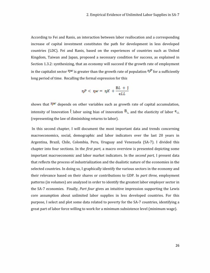
According to Fei and Ranis, an interaction between labor reallocation and a corresponding
increase of capital investment constitutes the path for development in less developed
countries (LDC). Fei and Ranis, based on the experiences of countries such as United
Kingdom, Taiwan and Japan, proposed a necessary condition for success, as explained in
Section 1.3.2: synthesizing, that an economy will succeed if the growth rate of employment
in the capitalist sector is greater than the growth rate of population for a sufficiently
long period of time. Recalling the formal expression for this
shows that depends on other variables such as growth rate of capital accumulation,
intensity of Innovation , labor using bias of innovation L, and the elasticity of labor LL
(representing the law of diminishing returns to labor).
In this second chapter, I will document the most important data and trends concerning
macroeconomics, social, demographic and labor indicators over the last 20 years in
Argentina, Brazil, Chile, Colombia, Peru, Uruguay and Venezuela (SA-7). I divided this
chapter into four sections. In the first part, a macro overview is presented depicting some
important macroeconomic and labor market indicators. In the second part, I present data
that reflects the process of industrialization and the dualistic nature of the economies in the
selected countries. In doing so, I graphically identify the various sectors in the economy and
their relevance based on their shares or contributions to GDP. In part three, employment
patterns (in volumes) are analyzed in order to identify the greatest labor employer sector in
the SA-7 economies. Finally, Part four gives an intuitive impression supporting the Lewis
core assumption about unlimited labor supplies in less developed countries. For this
purpose, I select and plot some data related to poverty for the SA-7 countries, identifying a
great part of labor force willing to work for a minimum subsistence level (minimum wage).
2. Empirical Evidence of Unlimited Labor Supplies in SA-7
27
2.1. SA-7 Macro Overview
I begin the analysis by examining the data at the aggregate level. According to the theory
explained in the previous chapter I show some relevant data in order to determine in an
intuitive way how these seven countries in South-America are compatible with the dualistic
model presented by Lewis. The seven countries chosen for the analysis are as follows:
Argentina, Brazil, Chile, Colombia, Uruguay, Peru and Venezuela. These countries provide
the most relevant contributions to South-American region development.
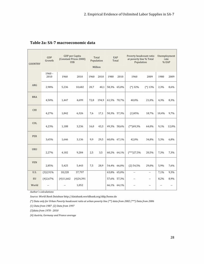
From Table 2.a it becomes evident that the fastest growing countries in the region between
1960 and 2010 were Brazil (4,50%), Chile (4,27%), Colombia (4,23%) and Peru (3,65%).
Contrary, the richest economies - Argentina, Uruguay and Venezuela - have had a GDP
growth of around 2,95%, 2,27% and 2,85%, respectively, from 1960 to 2010 on average.
In terms of GDP per capita we can determine that Argentina, Uruguay, Chile and Venezuela
are the richest countries within the SA-7. Argentina has experienced an enormous change in
GDP per capita in the last 50 years. Brazil and Chile have indeed had a relevant rate of
improvement in terms of GDP per capita. Venezuela instead, has had a marginal change in
the last 50 years in terms of GDP per capita. Uruguay, Peru and Colombia present a
considerable change in GDP per capita as well but lower as compared to Chile.
The economically active population (EAP) has increased in all countries at almost the same
proportion in the last 50 years. This is explained in part due to the economically active
women share, in which their participation in the total EAP over 15 years old has increased.
For example, in countries such as Argentina, Brazil, Chile and Colombia the share of women
in the EAP rose from 39,4%, 38,1%, 28,8%, 22,8% to 52%, 60%, 41,8% and 40,7%
respectively.
2. Empirical Evidence of Unlimited Labor Supplies in SA-7
28
Table 2a: SA-7 macroeconomic data
COUNTRY
GDP Growth
GDP per Capita (Constant Prices 2000)
US$
Total Population
Million
EAP Total
Poverty headcount ratio at poverty line % Total
Population
Unemployment rate
% EAP
1960 – 2010 1960 2010 1960 2010 1980 2010 1960 2009 1980 2009
ARG 2,98% 5,236 10,682 20,7 40,1 58,3% 65,0% (*) 32% (*) 13% 2,3% 8,6%
BRA 4,50% 1,447 4,699
72,8
194,9 61,5% 70,7% 40,0% 21,0% 4,3% 8,3%
CHI 4,27% 1,842 6,326
7,6
17,1 50,3% 57,3% (1)45% 18,7% 10,4% 9,7%
COL 4,23% 1,188 3,236
16,0
43,3 49,3% 58,6% (**)69,3% 64,0% 9,1% 12,0%
PER 3,65% 1,646 3,136
9,9
29,5 60,0% 67,1% 42,0% 34,8% 5,3% 6,8%
URU 2,27% 4,182 9,284
2,5
3,5 60,2% 64,1% (***)27,5% 20,5% 7,3% 7,3%
VEN 2,85% 5,425 5,443
7,5
28,9 54,4% 66,0% (2) 54,5% 29,0% 5,9% 7,6%
U.S. (3)2,91% 18,228 37,797 63,8% 65,0% -- -- 7,1% 9,3%
EU (4)2,67% (4)11,662 (4)24,391 57,6% 57,3% -- -- 8,2% 8,9%
World -- -- 1,052 66,1% 64,1% -- -- -- --
Author´s calculations
Source: World Bank Database http://databank.worldbank.org/ddp/home.do
(*) Data only for Urban Poverty headcount ratio at urban poverty line (**) data from 2002 (***) Data from 2006
(1) Data from 1987 (2) Data from 1997
(3)data from 1970 - 2010
(4) Austria, Germany and France average
2. Empirical Evidence of Unlimited Labor Supplies in SA-7
29
Table 2b: SA-7 Sectoral overview
COUNTRY
Agriculture Value Added %GDP
Industrial Value Added %GDP
Services Value Added %GDP
1960 2009 1960 2009 1960 2009
ARG 12,9% 7,5% 48,4% 31,7% 38,0% 60,0%
BRA 20,0% 6,8% 37,0% 25,4% 42,0% 68,0%
CHI 9,4% 3,3% 35,4% 42,1% 55,0% 54,6%
COL 29,3% 7,5% 26,9% 34,4% 43,8% 58,2%
PER 20,8% 7,3% 30,8% 34,1% 48,4% 58,6%
URU 13,4% 9,8% 33,1% 25,8% 53,5% 64,4%
VEN 4,7% 4,2% 41,3% 57,8% 52,0% 38,0%
US 3,5% 1,2% 35,2% 21,4% 61,2% 77,4%
EU 6,6% 1,5% 40,8% 23,9% (4)52,9% (4)73,74%
World 9,0% 3,0% 32,2% 27,0% -- --
Author´s calculations
Source: World Bank Database http://databank.worldbank.org/ddp/home.do
(1) Data from 1987 (2) Data from 1997
(3)data from 1970 - 2010
(4) Austria, Germany and France average
2. Empirical Evidence of Unlimited Labor Supplies in SA-7
30
Also, in Table 2a, we can observe the poverty headcount ratio at the national poverty line,
which is the ratio that gives the percent of the urban and rural population that lives under
the poverty line as defined by the income level and some standard of living indicators. As of
2009 the poorest country within SA-7 is Colombia with 64% of the total population living
under this poverty line. Over the last 50 years Colombia has improved this ratio to 5,3%.
The biggest success in this respect within the SA-7 countries is Chile, which has reduced this
incidence of poverty ratio from 45% in 1987 to 18,7% in 2009. Brazil has an important
success rate at reducing the respective ratio from 40% in 1981 to 21% in 2009.
Considerable reduction is found for Peru and Venezuela from 42% and 54,5% in 1993 and
1997, to 34,8% and 29% respectively in 2009. For Uruguay there is only data for the period
2006 – 2008, in which the ratio of population living under the poverty line has been
reduced from 27% to 20%, according to the World Bank Data Base. Argentina has reduced
its poverty headcount rate at the national poverty line of the urban population7, from 32%
in 1990 to 13,2% in 2009.
Since 1980, unemployment rates in the SA-7 have worsened in general, but not so in Chile.
In 1980 Chile experienced an unemployment rate of 10,4% and has been reduced to 9,68%
of the active population.
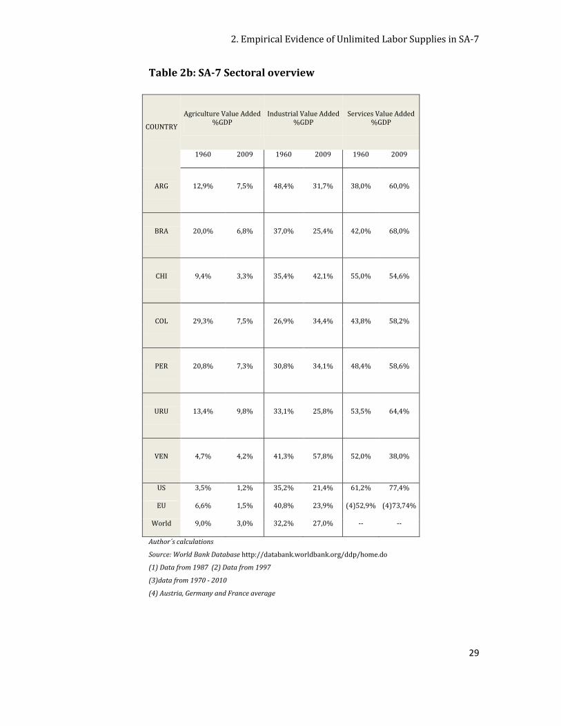
In table 2.b, value added by sector tells us that in 1960 agriculture had an important share
in the GDP of more than 20% and has suffered a relative reduction in the last 50 years
approaching levels of only 6% to 7% of GDP. This is the result of the development of other
new productive activities in the economies. This could be related directly to the rising
importance of industry and services (e.g. banks, financial services, tourism, etc). On the
contrary, in countries such as Argentina, Uruguay, Venezuela and Chile, the share of
agricultural value added (AVA) decreased, but less than in Brazil, Colombia and Peru.
The industrial value added share of GDP in Chile was determined by a related substitution
and development of industry productivity. AVA was replaced by industrial value added
(IVA) as a share of total GDP. Services value added (SVA) remained unchanged and has even
been reduced from 55% in 1960 to 54,6% in 2009. A similar trend is found in Venezuela,
7 See appendix 1
2. Empirical Evidence of Unlimited Labor Supplies in SA-7
31
where a reduction of the shares of SVA to GDP and an increase in the share of IVA has been
almost unchanged. This is definitely a phenomenon of the ongoing industrialization of the
economies. On the other hand, in countries such as Argentina, Brazil, and Uruguay, the IVA
has been reduced and compensated with an enormous increase on the SVA. A mixed
tendency is found for Peru and Colombia, which have gradually increased their industries
accompanied with a considerable and quite interesting increase in SVA.
2.2. Gross Domestic Product (GDP) structure and the “Lewis Two Sectors
Economy”
The gross domestic product (GDP) of an economy represents the total market value of all
final goods and services produced in a given period. GDP equals the total value of
consumption, the total investment and the government spending plus the net value of
exports and imports. GDP growth is what matters in economics and it is what has been
considered in growth theory.
Gross Domestic Product (GDP) can be distinguished by three broad sectors of the economy
such as Agriculture8, Industry9 and Services10 and measured in terms of value added11.
According to the classification of the International Labor Office (ILO), the value added in the
agriculture sector includes forestry, hunting, fishing, cultivation of crops and livestock
production.
8 According to the International Standard Industry Classification division (ISIC) agriculture
corresponds to divisions 1-5. http://search.worldbank.org
9 According to the ISIC divisions Industry corresponds to divisions 10-45.
http://search.worldbank.org
10 According to the ISIC divisions Services correspond to divisions 50-99.
http://search.worldbank.org
11 Value Added is the net output of a sector after adding up all outputs and substracting intermediate
inputs. It is calculated without making deductions for depreciations of fabricated assets or depletion
and degradation of natural resources. The origin of value added is determined by the International
Standard Industrial Classification (ISIC), revision 3. http://search.worldbank.org/
2. Empirical Evidence of Unlimited Labor Supplies in SA-7
32
The industrial value added, according to the International Standard of Industrial
classification (ISIC), comprises the value added in mining, manufacturing, construction,
electricity, water and gas. Data is given in US dollars (US$) at constant prices in 2000.
Services value added includes value added in wholesale and retail trade including hotels
and restaurants, transport, and government, financial, professional and personal services
charges, import duties, and any statistical discrepancies noted by national compilers as well
as discrepancies arising from rescaling.
Using the framework of the Lewis model and the notion of a dualistic economy, the
agriculture sector corresponds to the traditional sector of Lewis model. On the other hand,
industry and services are to be considered to correspond to the modern or capitalist sector
of the economy.
Lewis identified the characteristics of the dualistic economy as:
- The traditional sector produces first necessity goods and is located in rural areas and
faces the pressure of a vast labor force looking for job, that result in redundant labor.
- The modern or capitalist sector (industry and services related to industry and trade),
located in urban areas that demand labor force and better labor conditions. The
modern sector is the only productive sector able to use the redundant labor force in an
efficient and productive way released by the agriculture sector located in rural areas.
2. Empirical Evidence of Unlimited Labor Supplies in SA-7
33
2.2.1. Gross Domestic Product per capita (GDPpc) in SA-7
Lewis proposed the growth analysis based on the Gross National Income (GNI)12. The
difference between GDP and GNI is that profits of a firm in country A operating in country B
will only count for country A GNI but for country “B” GDP. Debts and interest payments of
services will decrease the GNI but not the GDP. If country A sells off its resources to entities
outside their country this will also be reflected over time in decreased GNI, but not
decreased GDP. I consider that an analysis of GDP seems to be more appropriate for
countries such as the SA-7, with increasing national debt and decreasing assets. For
methodology I will analyze the GDP conditions in SA-7.
There is a relevant increase of production in all SA-7 countries, especially for Chile, which
has an increasing trend without any stops since 1982 due to the new political changes in
that country based on the industrialization. In the 90´s, however, the creation of the
Mercosur, as the free-trading agreement between Brazil, Argentina, Uruguay and Mexico,
implied positive results in terms of GDPpc growth in only some member countries.
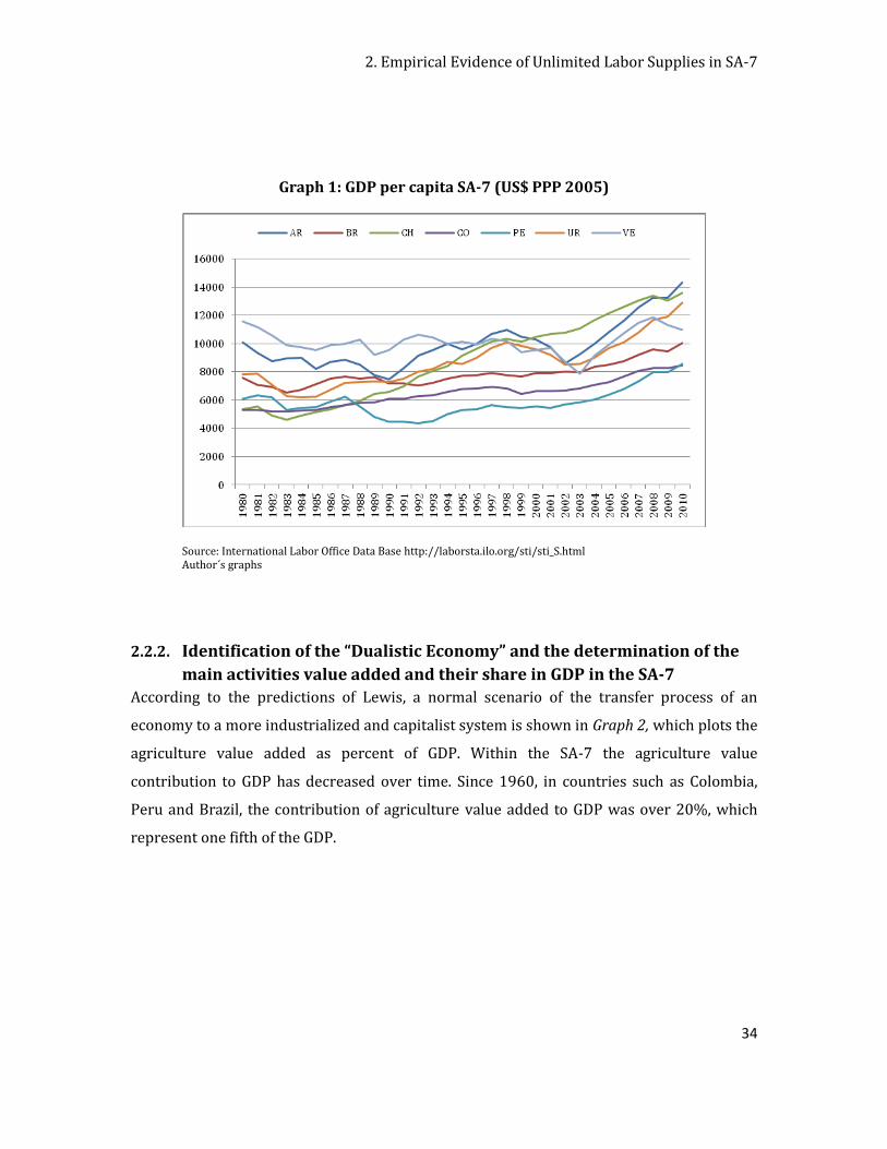
In Graph 1, the respective GDPpc at constant price in 2005 are plotted. Brazil shows an
interesting growth in GDP per capita from 1982 with a slight slowdown during the 90´s and
a recovery in the new century. Starting from the beginning of the 90´s, most of the countries
of the SA-7 started to show an increasing GDPpc growth rate. Peru is the only country that
has experienced remarkable changes in GDPpc since 2003. From 1980 until 1989, the SA-7
in common presented a decrease in GDPpc. For countries such as Argentina, Brazil and
Uruguay there is a turning point in the 1990s, since the GDPpc has increased steady. Chile
instead, shows a permanent growth of GDPpc from the period 1980 – 2010. Colombia and
Peru´s GDPpc follow similar trend with a remarkable acceleration since 2001.
12 Gross national income (GNI) comprises the value of all products and services generated within a
country in one year, together with its net income received from other countries. The GNI consists of:
the personal consumption expenditures, the gross private investment, the government consumption
expenditures, the net income from assets abroad (net income receipts), and the gross exports of
goods and services, after deducting two components: the gross imports of goods and services, and
the indirect business taxes. The GNI is similar to the gross national product (GNP), except that in
measuring the GNP one does not deduct the indirect business taxes. http://www.ilo.org/global/lang-
-en/index.htm.
2. Empirical Evidence of Unlimited Labor Supplies in SA-7
34
Graph 1: GDP per capita SA-7 (US$ PPP 2005)
Source: International Labor Office Data Base http://laborsta.ilo.org/sti/sti_S.html Author´s graphs
2.2.2. Identification of the “Dualistic Economy” and the determination of the
main activities value added and their share in GDP in the SA-7
According to the predictions of Lewis, a normal scenario of the transfer process of an
economy to a more industrialized and capitalist system is shown in Graph 2, which plots the
agriculture value added as percent of GDP. Within the SA-7 the agriculture value
contribution to GDP has decreased over time. Since 1960, in countries such as Colombia,
Peru and Brazil, the contribution of agriculture value added to GDP was over 20%, which
represent one fifth of the GDP.
2. Empirical Evidence of Unlimited Labor Supplies in SA-7
35
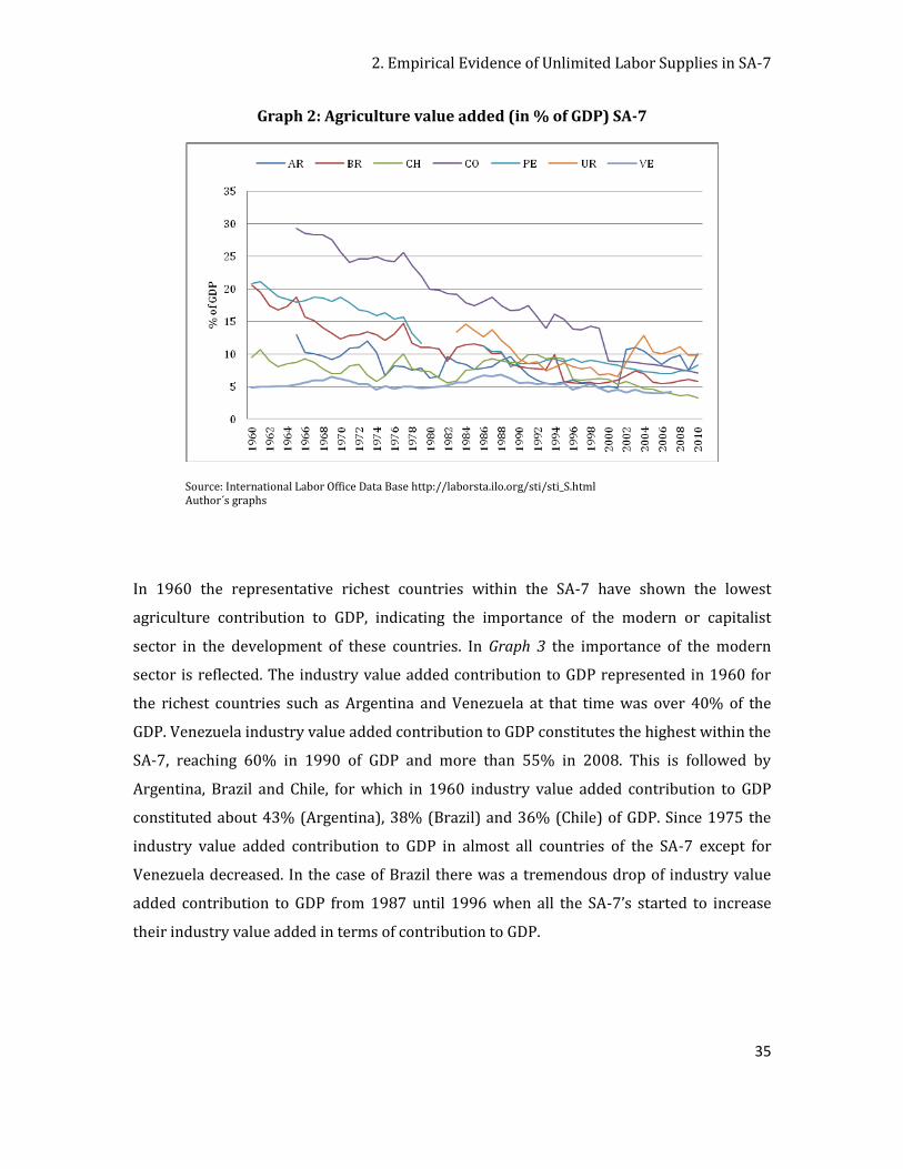
Graph 2: Agriculture value added (in % of GDP) SA-7
Source: International Labor Office Data Base http://laborsta.ilo.org/sti/sti_S.html Author´s graphs
In 1960 the representative richest countries within the SA-7 have shown the lowest
agriculture contribution to GDP, indicating the importance of the modern or capitalist
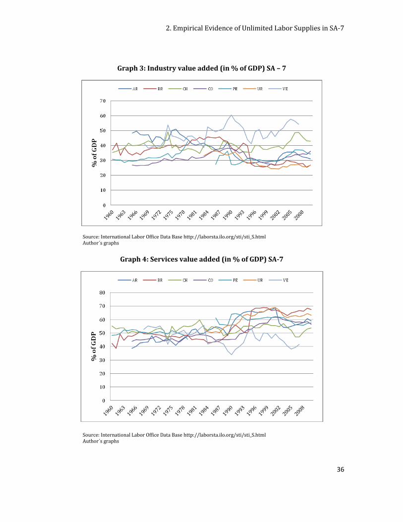
sector in the development of these countries. In Graph 3 the importance of the modern
sector is reflected. The industry value added contribution to GDP represented in 1960 for
the richest countries such as Argentina and Venezuela at that time was over 40% of the
GDP. Venezuela industry value added contribution to GDP constitutes the highest within the
SA-7, reaching 60% in 1990 of GDP and more than 55% in 2008. This is followed by
Argentina, Brazil and Chile, for which in 1960 industry value added contribution to GDP
constituted about 43% (Argentina), 38% (Brazil) and 36% (Chile) of GDP. Since 1975 the
industry value added contribution to GDP in almost all countries of the SA-7 except for
Venezuela decreased. In the case of Brazil there was a tremendous drop of industry value
added contribution to GDP from 1987 until 1996 when all the SA-7’s started to increase
their industry value added in terms of contribution to GDP.
2. Empirical Evidence of Unlimited Labor Supplies in SA-7
36
Graph 3: Industry value added (in % of GDP) SA – 7
Source: International Labor Office Data Base http://laborsta.ilo.org/sti/sti_S.html Author´s graphs
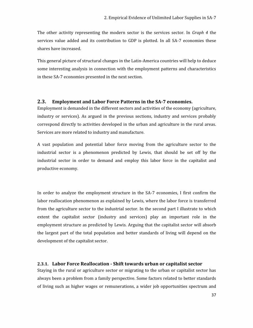
Graph 4: Services value added (in % of GDP) SA-7
Source: International Labor Office Data Base http://laborsta.ilo.org/sti/sti_S.html Author´s graphs
2. Empirical Evidence of Unlimited Labor Supplies in SA-7
37
The other activity representing the modern sector is the services sector. In Graph 4 the
services value added and its contribution to GDP is plotted. In all SA-7 economies these
shares have increased.
This general picture of structural changes in the Latin-America countries will help to deduce
some interesting analysis in connection with the employment patterns and characteristics
in these SA-7 economies presented in the next section.
2.3. Employment and Labor Force Patterns in the SA-7 economies. Employment is demanded in the different sectors and activities of the economy (agriculture,
industry or services). As argued in the previous sections, industry and services probably
correspond directly to activities developed in the urban and agriculture in the rural areas.
Services are more related to industry and manufacture.
A vast population and potential labor force moving from the agriculture sector to the
industrial sector is a phenomenon predicted by Lewis, that should be set off by the
industrial sector in order to demand and employ this labor force in the capitalist and
productive economy.
In order to analyze the employment structure in the SA-7 economies, I first confirm the
labor reallocation phenomenon as explained by Lewis, where the labor force is transferred
from the agriculture sector to the industrial sector. In the second part I illustrate to which
extent the capitalist sector (industry and services) play an important role in the
employment structure as predicted by Lewis. Arguing that the capitalist sector will absorb
the largest part of the total population and better standards of living will depend on the
development of the capitalist sector.
2.3.1. Labor Force Reallocation - Shift towards urban or capitalist sector
Staying in the rural or agriculture sector or migrating to the urban or capitalist sector has
always been a problem from a family perspective. Some factors related to better standards
of living such as higher wages or remunerations, a wider job opportunities spectrum and
2. Empirical Evidence of Unlimited Labor Supplies in SA-7
38
less chances of starving make the decision of migration towards urban areas easier. I will
plot the data provided by the World Bank and UNIDO in a way that allows empirically the
ability to observe a shift towards capitalist sector.
In this section I plot and analyze the growth rate of rural and urban population and their
share to total population. According to Lewis assumptions, rural population is related to the
labor force available for agriculture outside the cities. The cities and urban areas represent
the industrialization of a country and its activities are related mostly to the manufacture
and services. Urban population can also be employed in the productive activities and new
kinds of services, such as tourism, financial advisors, financial services on banks, transport
and expeditions, etc.
The main demographic phenomenon predicted by Arthur Lewis that happens in dualistic
economies with labor surplus is related to the migration of the rural population to cities or
urban societies that work in industry and services.
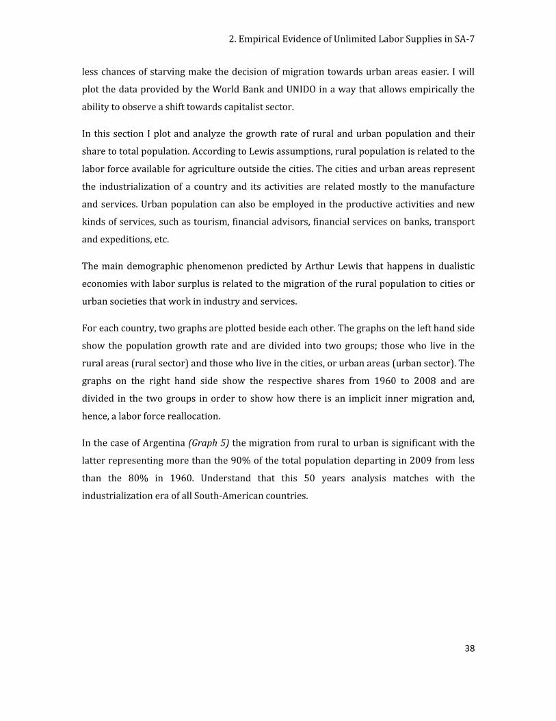
For each country, two graphs are plotted beside each other. The graphs on the left hand side
show the population growth rate and are divided into two groups; those who live in the
rural areas (rural sector) and those who live in the cities, or urban areas (urban sector). The
graphs on the right hand side show the respective shares from 1960 to 2008 and are
divided in the two groups in order to show how there is an implicit inner migration and,
hence, a labor force reallocation.
In the case of Argentina (Graph 5) the migration from rural to urban is significant with the
latter representing more than the 90% of the total population departing in 2009 from less
than the 80% in 1960. Understand that this 50 years analysis matches with the
industrialization era of all South-American countries.
2. Empirical Evidence of Unlimited Labor Supplies in SA-7
39
Graph 5: Argentina urban and rural population
Source: International Labor Office Data Base http://laborsta.ilo.org/sti/sti_S.html Author´s graphs
Brazil (Graph 6) presents an interesting behavior with a very pronounced trend of
decreasing both urban and rural population growth, accompanied by a high increasing
trend showing the increase of the Brazilian urban population as a share of total population.
Until 1960, the urban population represented only little more than 40% of the total
population. Fifty years later urban population is more than the 80% of the total population.
The particular topic for Brazil nowadays is the higher level of total population growth in
1960 and the almost parallel behavior of urban, rural and total growth rate along the fifty
years series.
Chile (Graph 7) and the other countries show a typical case of growth, with the urban
population growth being higher total population growth. In the last 25 years in Chile, both
growth rates of population are almost at the same level with urban population growth being
slightly above the total population growth rate. In the 1980s strong political changes
occurred in the economy, which caused a considerable increase on rural population growth
rate for 10 years.
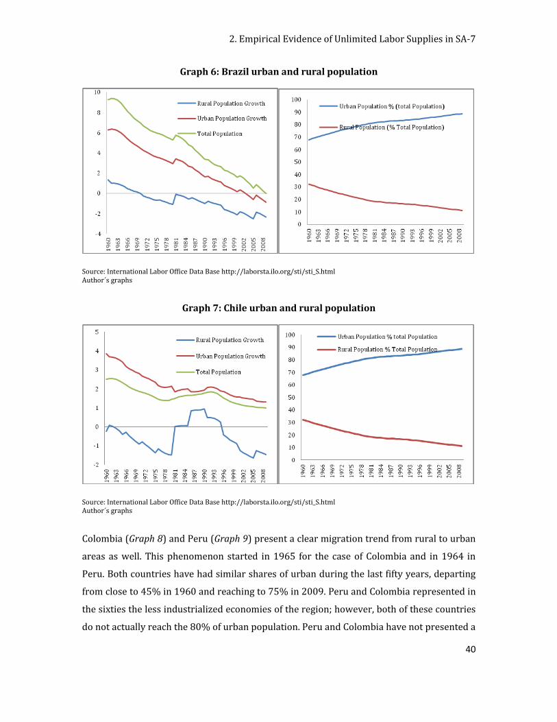
2. Empirical Evidence of Unlimited Labor Supplies in SA-7
40
Graph 6: Brazil urban and rural population
Source: International Labor Office Data Base http://laborsta.ilo.org/sti/sti_S.html Author´s graphs
Graph 7: Chile urban and rural population
Source: International Labor Office Data Base http://laborsta.ilo.org/sti/sti_S.html Author´s graphs
Colombia (Graph 8) and Peru (Graph 9) present a clear migration trend from rural to urban
areas as well. This phenomenon started in 1965 for the case of Colombia and in 1964 in
Peru. Both countries have had similar shares of urban during the last fifty years, departing
from close to 45% in 1960 and reaching to 75% in 2009. Peru and Colombia represented in
the sixties the less industrialized economies of the region; however, both of these countries
do not actually reach the 80% of urban population. Peru and Colombia have not presented a
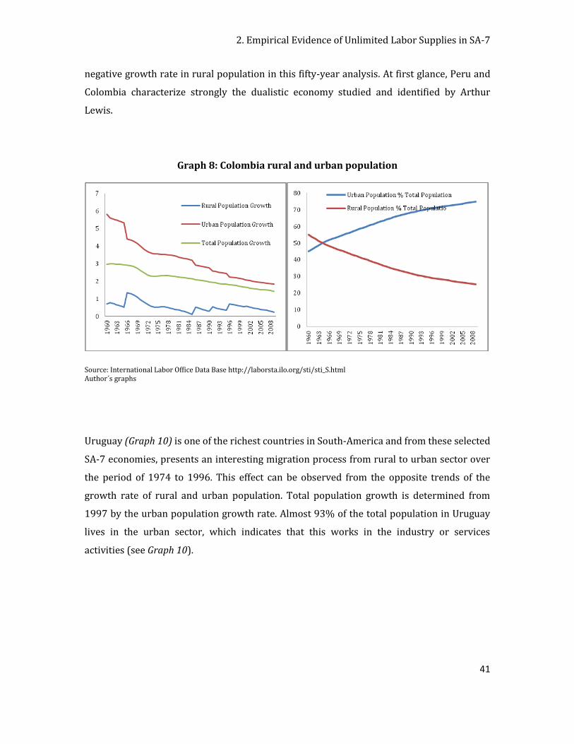
2. Empirical Evidence of Unlimited Labor Supplies in SA-7
41
negative growth rate in rural population in this fifty-year analysis. At first glance, Peru and
Colombia characterize strongly the dualistic economy studied and identified by Arthur
Lewis.
Graph 8: Colombia rural and urban population
Source: International Labor Office Data Base http://laborsta.ilo.org/sti/sti_S.html Author´s graphs
Uruguay (Graph 10) is one of the richest countries in South-America and from these selected
SA-7 economies, presents an interesting migration process from rural to urban sector over
the period of 1974 to 1996. This effect can be observed from the opposite trends of the
growth rate of rural and urban population. Total population growth is determined from
1997 by the urban population growth rate. Almost 93% of the total population in Uruguay
lives in the urban sector, which indicates that this works in the industry or services
activities (see Graph 10).
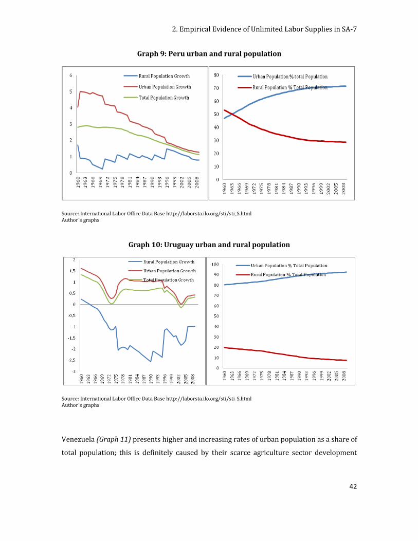
2. Empirical Evidence of Unlimited Labor Supplies in SA-7
42
Graph 9: Peru urban and rural population
Source: International Labor Office Data Base http://laborsta.ilo.org/sti/sti_S.html Author´s graphs
Graph 10: Uruguay urban and rural population
Source: International Labor Office Data Base http://laborsta.ilo.org/sti/sti_S.html Author´s graphs
Venezuela (Graph 11) presents higher and increasing rates of urban population as a share of
total population; this is definitely caused by their scarce agriculture sector development
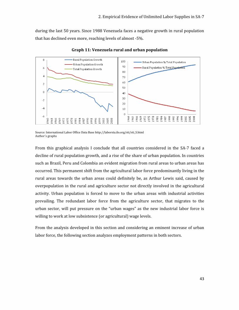
2. Empirical Evidence of Unlimited Labor Supplies in SA-7
43
during the last 50 years. Since 1988 Venezuela faces a negative growth in rural population
that has declined even more, reaching levels of almost -5%.
Graph 11: Venezuela rural and urban population
Source: International Labor Office Data Base http://laborsta.ilo.org/sti/sti_S.html Author´s graphs
From this graphical analysis I conclude that all countries considered in the SA-7 faced a
decline of rural population growth, and a rise of the share of urban population. In countries
such as Brazil, Peru and Colombia an evident migration from rural areas to urban areas has
occurred. This permanent shift from the agricultural labor force predominantly living in the
rural areas towards the urban areas could definitely be, as Arthur Lewis said, caused by
overpopulation in the rural and agriculture sector not directly involved in the agricultural
activity. Urban population is forced to move to the urban areas with industrial activities
prevailing. The redundant labor force from the agriculture sector, that migrates to the
urban sector, will put pressure on the “urban wages” as the new industrial labor force is
willing to work at low subsistence (or agricultural) wage levels.
From the analysis developed in this section and considering an eminent increase of urban
labor force, the following section analyzes employment patterns in both sectors.
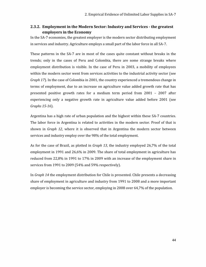
2. Empirical Evidence of Unlimited Labor Supplies in SA-7
44
2.3.2. Employment in the Modern Sector: Industry and Services - the greatest
employers in the Economy
In the SA-7 economies, the greatest employer is the modern sector distributing employment
in services and industry. Agriculture employs a small part of the labor force in all SA-7.
These patterns in the SA-7 are in most of the cases quite constant without breaks in the
trends; only in the cases of Peru and Colombia, there are some strange breaks where
employment distribution is visible. In the case of Peru in 2003, a mobility of employees
within the modern sector went from services activities to the industrial activity sector (see
Graph 17). In the case of Colombia in 2001, the country experienced a tremendous change in
terms of employment, due to an increase on agriculture value added growth rate that has
presented positive growth rates for a medium term period from 2001 – 2007 after
experiencing only a negative growth rate in agriculture value added before 2001 (see
Graphs 15-16).
Argentina has a high rate of urban population and the highest within these SA-7 countries.
The labor force in Argentina is related to activities in the modern sector. Proof of that is
shown in Graph 12, where it is observed that in Argentina the modern sector between
services and industry employ over the 98% of the total employment.
As for the case of Brazil, as plotted in Graph 13, the industry employed 26,7% of the total
employment in 1991 and 26,6% in 2009. The share of total employment in agriculture has
reduced from 22,8% in 1991 to 17% in 2009 with an increase of the employment share in
services from 1991 to 2009 (54% and 59% respectively).
In Graph 14 the employment distribution for Chile is presented. Chile presents a decreasing
share of employment in agriculture and industry from 1991 to 2008 and a more important
employer is becoming the service sector, employing in 2008 over 64,7% of the population.
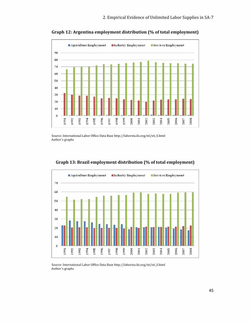
2. Empirical Evidence of Unlimited Labor Supplies in SA-7
45
Graph 12: Argentina employment distribution (% of total employment)
Source: International Labor Office Data Base http://laborsta.ilo.org/sti/sti_S.html Author´s graphs
Graph 13: Brazil employment distribution (% of total employment)
Source: International Labor Office Data Base http://laborsta.ilo.org/sti/sti_S.html Author´s graphs
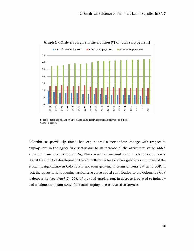
2. Empirical Evidence of Unlimited Labor Supplies in SA-7
46
Graph 14: Chile employment distribution (% of total employment)
Source: International Labor Office Data Base http://laborsta.ilo.org/sti/sti_S.html Author´s graphs
Colombia, as previously stated, had experienced a tremendous change with respect to
employment in the agriculture sector due to an increase of the agriculture value added
growth rate increase (see Graph 16). This is a non-normal and non predicted effect of Lewis,
that at this point of development, the agriculture sector becomes greater as employer of the
economy. Agriculture in Colombia is not even growing in terms of contribution to GDP, in
fact, the opposite is happening: agriculture value added contribution to the Colombian GDP
is decreasing (see Graph 2). 20% of the total employment in average is related to industry
and an almost constant 60% of the total employment is related to services.
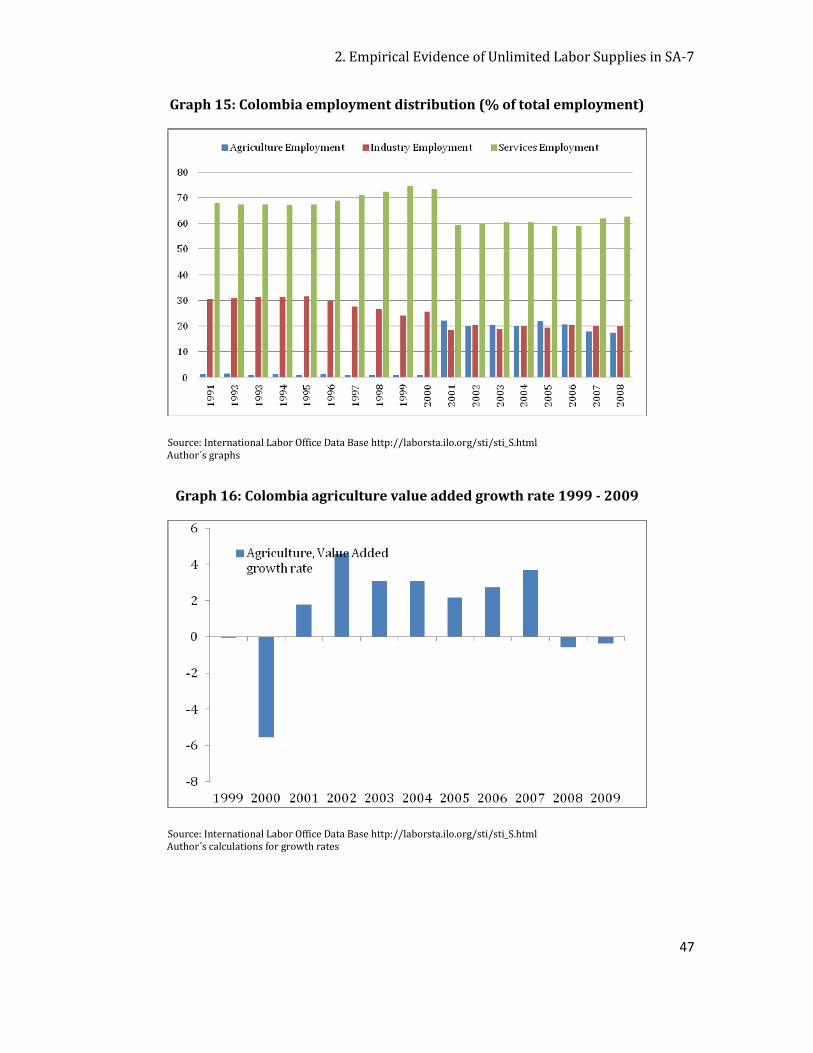
2. Empirical Evidence of Unlimited Labor Supplies in SA-7
47
Graph 15: Colombia employment distribution (% of total employment)
Source: International Labor Office Data Base http://laborsta.ilo.org/sti/sti_S.html Author´s graphs
Graph 16: Colombia agriculture value added growth rate 1999 - 2009
Source: International Labor Office Data Base http://laborsta.ilo.org/sti/sti_S.html Author´s calculations for growth rates
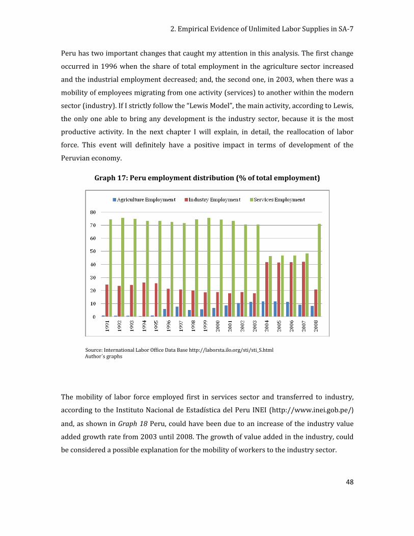
2. Empirical Evidence of Unlimited Labor Supplies in SA-7
48
Peru has two important changes that caught my attention in this analysis. The first change
occurred in 1996 when the share of total employment in the agriculture sector increased
and the industrial employment decreased; and, the second one, in 2003, when there was a
mobility of employees migrating from one activity (services) to another within the modern
sector (industry). If I strictly follow the “Lewis Model”, the main activity, according to Lewis,
the only one able to bring any development is the industry sector, because it is the most
productive activity. In the next chapter I will explain, in detail, the reallocation of labor
force. This event will definitely have a positive impact in terms of development of the
Peruvian economy.
Graph 17: Peru employment distribution (% of total employment)
Source: International Labor Office Data Base http://laborsta.ilo.org/sti/sti_S.html Author´s graphs
The mobility of labor force employed first in services sector and transferred to industry,
according to the Instituto Nacional de Estadística del Peru INEI (http://www.inei.gob.pe/)
and, as shown in Graph 18 Peru, could have been due to an increase of the industry value
added growth rate from 2003 until 2008. The growth of value added in the industry, could
be considered a possible explanation for the mobility of workers to the industry sector.
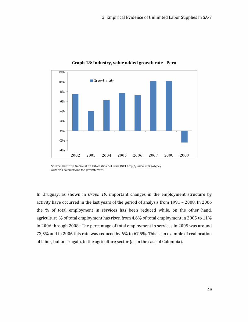
2. Empirical Evidence of Unlimited Labor Supplies in SA-7
49
Graph 18: Industry, value added growth rate - Peru
Source: Instituto Nacional de Estadística del Peru INEI http://www.inei.gob.pe/ Author´s calculations for growth rates
In Uruguay, as shown in Graph 19, important changes in the employment structure by
activity have occurred in the last years of the period of analysis from 1991 – 2008. In 2006
the % of total employment in services has been reduced while, on the other hand,
agriculture % of total employment has risen from 4,6% of total employment in 2005 to 11%
in 2006 through 2008. The percentage of total employment in services in 2005 was around
73,5% and in 2006 this rate was reduced by 6% to 67,5%. This is an example of reallocation
of labor, but once again, to the agriculture sector (as in the case of Colombia).
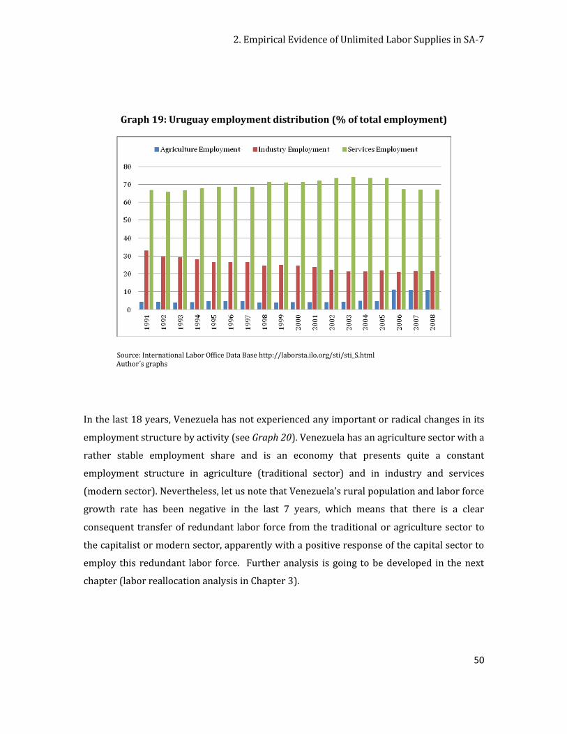
2. Empirical Evidence of Unlimited Labor Supplies in SA-7
50
Graph 19: Uruguay employment distribution (% of total employment)
Source: International Labor Office Data Base http://laborsta.ilo.org/sti/sti_S.html Author´s graphs
In the last 18 years, Venezuela has not experienced any important or radical changes in its
employment structure by activity (see Graph 20). Venezuela has an agriculture sector with a
rather stable employment share and is an economy that presents quite a constant
employment structure in agriculture (traditional sector) and in industry and services
(modern sector). Nevertheless, let us note that Venezuela’s rural population and labor force
growth rate has been negative in the last 7 years, which means that there is a clear
consequent transfer of redundant labor force from the traditional or agriculture sector to
the capitalist or modern sector, apparently with a positive response of the capital sector to
employ this redundant labor force. Further analysis is going to be developed in the next
chapter (labor reallocation analysis in Chapter 3).
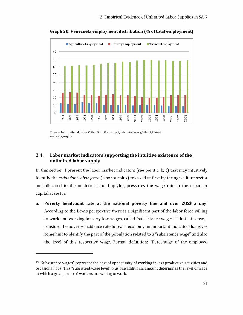
2. Empirical Evidence of Unlimited Labor Supplies in SA-7
51
Graph 20: Venezuela employment distribution (% of total employment)
Source: International Labor Office Data Base http://laborsta.ilo.org/sti/sti_S.html Author´s graphs
2.4. Labor market indicators supporting the intuitive existence of the unlimited labor supply
In this section, I present the labor market indicators (see point a, b, c) that may intuitively
identify the redundant labor force (labor surplus) released at first by the agriculture sector
and allocated to the modern sector implying pressures the wage rate in the urban or
capitalist sector.
a. Poverty headcount rate at the national poverty line and over 2US$ a day:
According to the Lewis perspective there is a significant part of the labor force willing
to work and working for very low wages, called “subsistence wages”13. In that sense, I
consider the poverty incidence rate for each economy an important indicator that gives
some hint to identify the part of the population related to a “subsistence wage” and also
the level of this respective wage. Formal definition: “Percentage of the employed
13 “Subsistence wages” represent the cost of opportunity of working in less productive activities and
occasional jobs. This “subsistent wage level” plus one additional amount determines the level of wage
at which a great group of workers are willing to work.
2. Empirical Evidence of Unlimited Labor Supplies in SA-7
52
population whose average per capita income is below the poverty and extreme poverty
line.” (CEPAL http://websie.eclac.cl/).
b. Vulnerable Employment phenomena: In SA-7 the unemployment rate is on average
around 9% of the participation rate. Thus, the unemployment rate is not that relevant
anymore for these economies and the international institutions such as CEPAL and ILO
pay more attention now to the quality of employment. Vulnerable employment is part
of the “employed” labor force with less favorable labor conditions, underpaid and
sporadic jobs, and represents a part of the labor force that pressures real wages.
c. Real Minimum Wage growth rate and Labor Productivity: The real minimum wage
data was compiled from the CEPAL database available on the internet14. For
methodological reasons, the Labor productivity is to be calculated as the average
productivity of labor. According to Lewis, the real wage does not equal the productivity
of labor in economies with labor surplus. The real wage is constant until there is no
more labor surplus left. The comparison allowed me to get some intuition about the
pressure from the “subsistence sector”, reflected on the almost zero growth rates of the
minimum wages for each country.
Lewis considered that a permanent allocation of the redundant labor force from the
agriculture or traditional sector to the capitalist sector of the economy induces a pressure
on wages and hence the existence of an unlimited labor supply. Lewis established the
existence of this so called “institutional wage” to be the minimum level of wage that a group
of “redundant” labor force is willing to get paid for its work.
The former and legal “minimum real wage” in the correspondent SA-7 economies is plotted
in Section 2.4.3 and is compared to the marginal productivity of labor in Section 2.4.4, in
order to determine in which countries within the SA-7 present unlimited labor supplies. Let
it be known that the Lewis “institutional wage or CIW” is to be represented by the legal
minimum wage of the country.
14 “Minimum wages (monthly or daily) coming from official sources are deflated with the consumer
price index (CPI), calculating a monthly real index. The average of these indexes represents the
annual index published” CEPAL
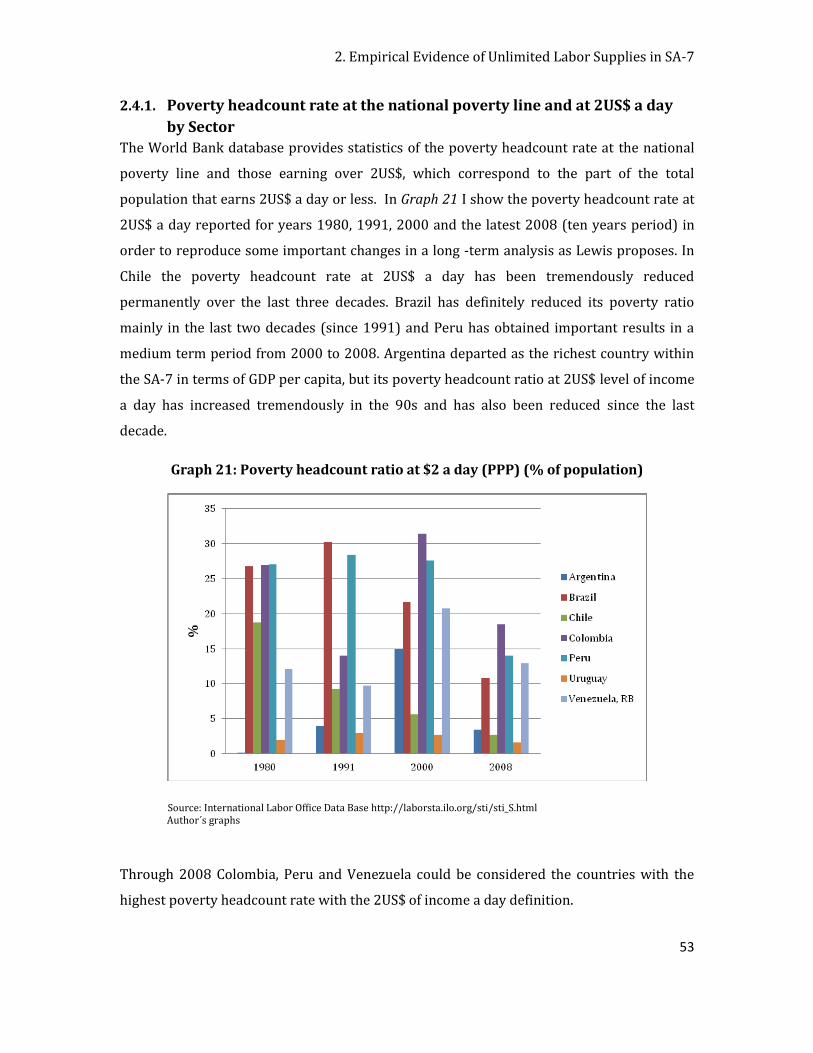
2. Empirical Evidence of Unlimited Labor Supplies in SA-7
53
2.4.1. Poverty headcount rate at the national poverty line and at 2US$ a day
by Sector
The World Bank database provides statistics of the poverty headcount rate at the national
poverty line and those earning over 2US$, which correspond to the part of the total
population that earns 2US$ a day or less. In Graph 21 I show the poverty headcount rate at
2US$ a day reported for years 1980, 1991, 2000 and the latest 2008 (ten years period) in
order to reproduce some important changes in a long -term analysis as Lewis proposes. In
Chile the poverty headcount rate at 2US$ a day has been tremendously reduced
permanently over the last three decades. Brazil has definitely reduced its poverty ratio
mainly in the last two decades (since 1991) and Peru has obtained important results in a
medium term period from 2000 to 2008. Argentina departed as the richest country within
the SA-7 in terms of GDP per capita, but its poverty headcount ratio at 2US$ level of income
a day has increased tremendously in the 90s and has also been reduced since the last
decade.
Graph 21: Poverty headcount ratio at $2 a day (PPP) (% of population)
Source: International Labor Office Data Base http://laborsta.ilo.org/sti/sti_S.html Author´s graphs
Through 2008 Colombia, Peru and Venezuela could be considered the countries with the
highest poverty headcount rate with the 2US$ of income a day definition.
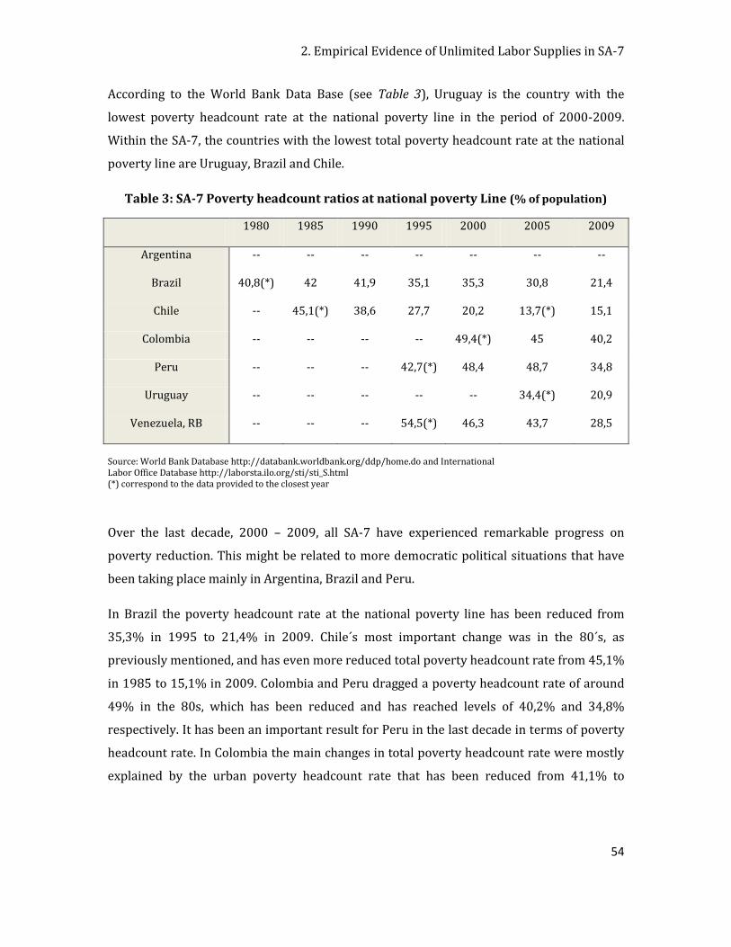
2. Empirical Evidence of Unlimited Labor Supplies in SA-7
54
According to the World Bank Data Base (see Table 3), Uruguay is the country with the
lowest poverty headcount rate at the national poverty line in the period of 2000-2009.
Within the SA-7, the countries with the lowest total poverty headcount rate at the national
poverty line are Uruguay, Brazil and Chile.
Table 3: SA-7 Poverty headcount ratios at national poverty Line (% of population)
1980 1985 1990 1995 2000 2005 2009
Argentina -- -- -- -- -- -- --
Brazil 40,8(*) 42 41,9 35,1 35,3 30,8 21,4
Chile -- 45,1(*) 38,6 27,7 20,2 13,7(*) 15,1
Colombia -- -- -- -- 49,4(*) 45 40,2
Peru -- -- -- 42,7(*) 48,4 48,7 34,8
Uruguay -- -- -- -- -- 34,4(*) 20,9
Venezuela, RB -- -- -- 54,5(*) 46,3 43,7 28,5
Source: World Bank Database http://databank.worldbank.org/ddp/home.do and International Labor Office Database http://laborsta.ilo.org/sti/sti_S.html (*) correspond to the data provided to the closest year
Over the last decade, 2000 – 2009, all SA-7 have experienced remarkable progress on
poverty reduction. This might be related to more democratic political situations that have
been taking place mainly in Argentina, Brazil and Peru.
In Brazil the poverty headcount rate at the national poverty line has been reduced from
35,3% in 1995 to 21,4% in 2009. Chile´s most important change was in the 80´s, as
previously mentioned, and has even more reduced total poverty headcount rate from 45,1%
in 1985 to 15,1% in 2009. Colombia and Peru dragged a poverty headcount rate of around
49% in the 80s, which has been reduced and has reached levels of 40,2% and 34,8%
respectively. It has been an important result for Peru in the last decade in terms of poverty
headcount rate. In Colombia the main changes in total poverty headcount rate were mostly
explained by the urban poverty headcount rate that has been reduced from 41,1% to
2. Empirical Evidence of Unlimited Labor Supplies in SA-7
55
35,8%15, maintaining its rural poverty headcount rates at levels over 54% of the total rural
population. The poverty headcount rate at the national poverty line diminution process in
Chile happened in the 80´s, as explained by both rural and urban poverty headcount rate
reduction, which have fallen from 51,5% in 1997 to 30,3% in 1995 and 43,6% to 22%,
respectively. Uruguay has reduced its poverty headcount rate at the national poverty line
also with a considerable percentage from 34,4% in 2005 to 20,9% in 2009. Venezuela
shows a remarkable result in poverty headcount rate at the national poverty line reduction.
Venezuela dragged a 54,5% total poverty headcount rate at the national poverty line level
before 2000 and has been reduced, reaching levels of 20,5% in 2009.
2.4.2. Vulnerable Employment
In developing countries there are different and separated categories of employment.
Therefore it is necessary to separate employees with less favorable labor conditions,
underpaid and sporadic jobs. In developed economies there are already strong social
protection measures, where workers who lose their jobs can move into unemployment. In
many developing economies on the other hand, workers who lose their jobs do not have
access to social protection schemes, for example. Rather than becoming unemployed, these
workers often take up various forms of employment, working on their own accounts, or
contributing to family businesses. This, in turn, results in an increase in the number of
workers in vulnerable employment.
According to Lawrence Jeff Johnson, chief of the International Labor Office (ILO):
“…While monitoring unemployment provides a good starting point to assess the health of
labor markets in developed economies, particularly in developing economies it is essential to
consider decent work deficits among the employed. Before the onset of the current economic
15 See appendix 1: Urban Poverty headcount rate is also released in the Database of the World Bank
with the correspondent link http://laborsta.ilo.org/sti/sti_S.html.
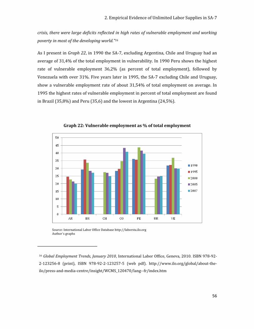
2. Empirical Evidence of Unlimited Labor Supplies in SA-7
56
crisis, there were large deficits reflected in high rates of vulnerable employment and working
poverty in most of the developing world.”16
As I present in Graph 22, in 1990 the SA-7, excluding Argentina, Chile and Uruguay had an
average of 31,4% of the total employment in vulnerability. In 1990 Peru shows the highest
rate of vulnerable employment 36,2% (as percent of total employment), followed by
Venezuela with over 31%. Five years later in 1995, the SA-7 excluding Chile and Uruguay,
show a vulnerable employment rate of about 31,54% of total employment on average. In
1995 the highest rates of vulnerable employment in percent of total employment are found
in Brazil (35,8%) and Peru (35,6) and the lowest in Argentina (24,5%).
Graph 22: Vulnerable employment as % of total employment
Source: International Labor Office Database http://laborsta.ilo.org Author´s graphs
16 Global Employment Trends, January 2010, International Labor Office, Geneva, 2010. ISBN 978-92-
2-123256-8 (print), ISBN 978-92-2-123257-5 (web pdf). http://www.ilo.org/global/about-the-
ilo/press-and-media-centre/insight/WCMS_120470/lang--fr/index.htm
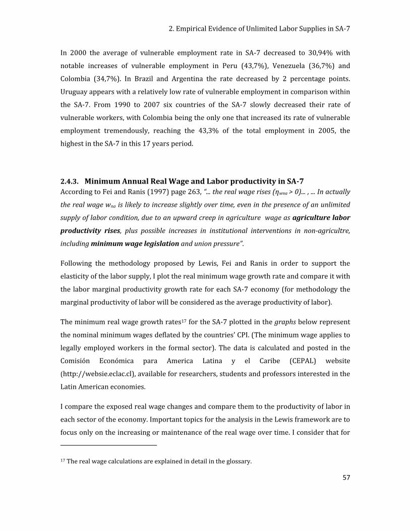
2. Empirical Evidence of Unlimited Labor Supplies in SA-7
57
In 2000 the average of vulnerable employment rate in SA-7 decreased to 30,94% with
notable increases of vulnerable employment in Peru (43,7%), Venezuela (36,7%) and
Colombia (34,7%). In Brazil and Argentina the rate decreased by 2 percentage points.
Uruguay appears with a relatively low rate of vulnerable employment in comparison within
the SA-7. From 1990 to 2007 six countries of the SA-7 slowly decreased their rate of
vulnerable workers, with Colombia being the only one that increased its rate of vulnerable
employment tremendously, reaching the 43,3% of the total employment in 2005, the
highest in the SA-7 in this 17 years period.
2.4.3. Minimum Annual Real Wage and Labor productivity in SA-7
According to Fei and Ranis (1997) page 263, “... the real wage rises (ƞwna > 0)... , ... In actually
the real wage wna is likely to increase slightly over time, even in the presence of an unlimited
supply of labor condition, due to an upward creep in agriculture wage as agriculture labor
productivity rises, plus possible increases in institutional interventions in non-agricultre,
including minimum wage legislation and union pressure”.
Following the methodology proposed by Lewis, Fei and Ranis in order to support the
elasticity of the labor supply, I plot the real minimum wage growth rate and compare it with
the labor marginal productivity growth rate for each SA-7 economy (for methodology the
marginal productivity of labor will be considered as the average productivity of labor).
The minimum real wage growth rates17 for the SA-7 plotted in the graphs below represent
the nominal minimum wages deflated by the countries’ CPI. (The minimum wage applies to
legally employed workers in the formal sector). The data is calculated and posted in the
Comisión Económica para America Latina y el Caribe (CEPAL) website
(http://websie.eclac.cl), available for researchers, students and professors interested in the
Latin American economies.
I compare the exposed real wage changes and compare them to the productivity of labor in
each sector of the economy. Important topics for the analysis in the Lewis framework are to
focus only on the increasing or maintenance of the real wage over time. I consider that for
17 The real wage calculations are explained in detail in the glossary.
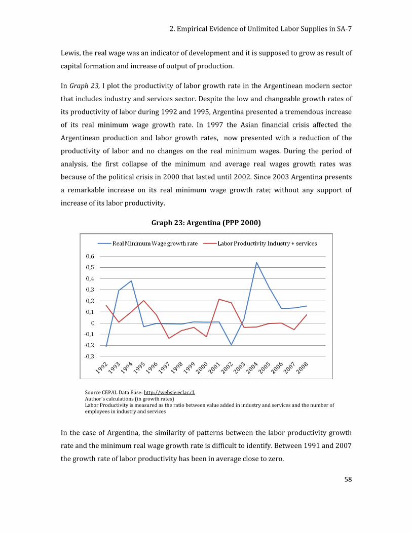
2. Empirical Evidence of Unlimited Labor Supplies in SA-7
58
Lewis, the real wage was an indicator of development and it is supposed to grow as result of
capital formation and increase of output of production.
In Graph 23, I plot the productivity of labor growth rate in the Argentinean modern sector
that includes industry and services sector. Despite the low and changeable growth rates of
its productivity of labor during 1992 and 1995, Argentina presented a tremendous increase
of its real minimum wage growth rate. In 1997 the Asian financial crisis affected the
Argentinean production and labor growth rates, now presented with a reduction of the
productivity of labor and no changes on the real minimum wages. During the period of
analysis, the first collapse of the minimum and average real wages growth rates was
because of the political crisis in 2000 that lasted until 2002. Since 2003 Argentina presents
a remarkable increase on its real minimum wage growth rate; without any support of
increase of its labor productivity.
Graph 23: Argentina (PPP 2000)
Source CEPAL Data Base: http://websie.eclac.cl. Author´s calculations (in growth rates) Labor Productivity is measured as the ratio between value added in industry and services and the number of employees in industry and services
In the case of Argentina, the similarity of patterns between the labor productivity growth
rate and the minimum real wage growth rate is difficult to identify. Between 1991 and 2007
the growth rate of labor productivity has been in average close to zero.
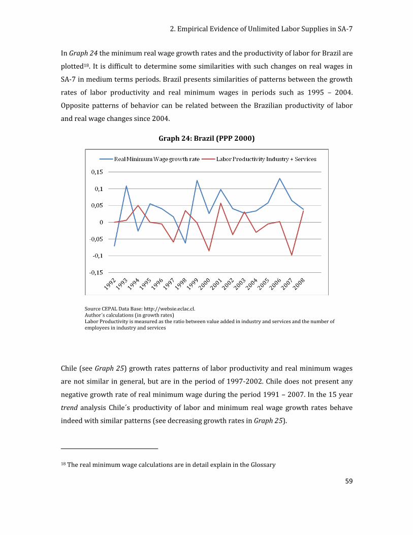
2. Empirical Evidence of Unlimited Labor Supplies in SA-7
59
In Graph 24 the minimum real wage growth rates and the productivity of labor for Brazil are
plotted18. It is difficult to determine some similarities with such changes on real wages in
SA-7 in medium terms periods. Brazil presents similarities of patterns between the growth
rates of labor productivity and real minimum wages in periods such as 1995 – 2004.
Opposite patterns of behavior can be related between the Brazilian productivity of labor
and real wage changes since 2004.
Graph 24: Brazil (PPP 2000)
Source CEPAL Data Base: http://websie.eclac.cl. Author´s calculations (in growth rates) Labor Productivity is measured as the ratio between value added in industry and services and the number of employees in industry and services
Chile (see Graph 25) growth rates patterns of labor productivity and real minimum wages
are not similar in general, but are in the period of 1997-2002. Chile does not present any
negative growth rate of real minimum wage during the period 1991 – 2007. In the 15 year
trend analysis Chile´s productivity of labor and minimum real wage growth rates behave
indeed with similar patterns (see decreasing growth rates in Graph 25).
18 The real minimum wage calculations are in detail explain in the Glossary
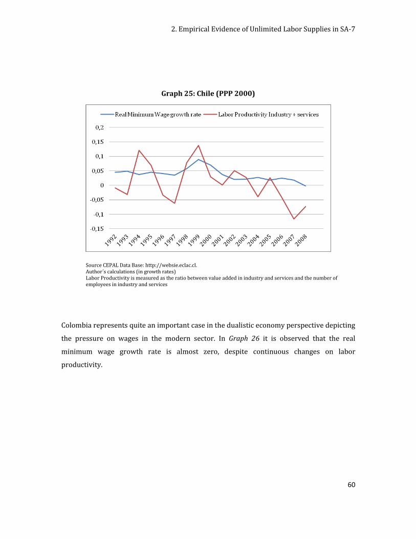
2. Empirical Evidence of Unlimited Labor Supplies in SA-7
60
Graph 25: Chile (PPP 2000)
Source CEPAL Data Base: http://websie.eclac.cl. Author´s calculations (in growth rates) Labor Productivity is measured as the ratio between value added in industry and services and the number of employees in industry and services
Colombia represents quite an important case in the dualistic economy perspective depicting
the pressure on wages in the modern sector. In Graph 26 it is observed that the real
minimum wage growth rate is almost zero, despite continuous changes on labor
productivity.
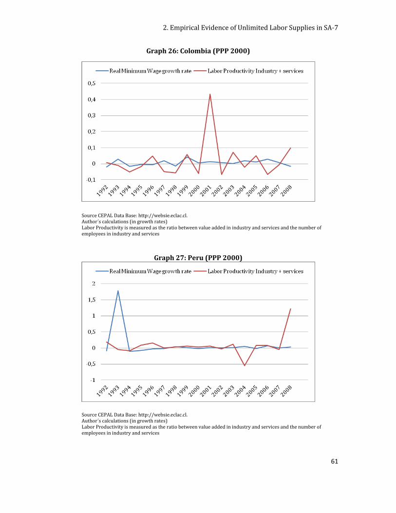
2. Empirical Evidence of Unlimited Labor Supplies in SA-7
61
Graph 26: Colombia (PPP 2000)
Source CEPAL Data Base: http://websie.eclac.cl. Author´s calculations (in growth rates) Labor Productivity is measured as the ratio between value added in industry and services and the number of employees in industry and services
Graph 27: Peru (PPP 2000)
Source CEPAL Data Base: http://websie.eclac.cl. Author´s calculations (in growth rates) Labor Productivity is measured as the ratio between value added in industry and services and the number of employees in industry and services
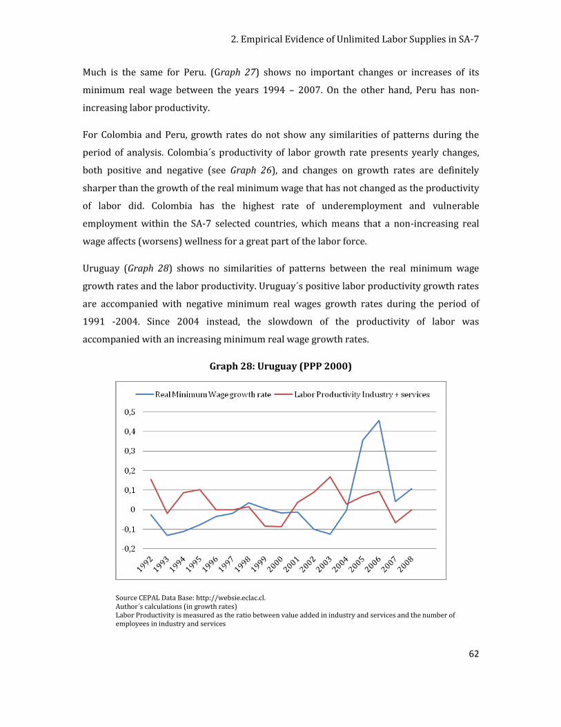
2. Empirical Evidence of Unlimited Labor Supplies in SA-7
62
Much is the same for Peru. (Graph 27) shows no important changes or increases of its
minimum real wage between the years 1994 – 2007. On the other hand, Peru has non-
increasing labor productivity.
For Colombia and Peru, growth rates do not show any similarities of patterns during the
period of analysis. Colombia´s productivity of labor growth rate presents yearly changes,
both positive and negative (see Graph 26), and changes on growth rates are definitely
sharper than the growth of the real minimum wage that has not changed as the productivity
of labor did. Colombia has the highest rate of underemployment and vulnerable
employment within the SA-7 selected countries, which means that a non-increasing real
wage affects (worsens) wellness for a great part of the labor force.
Uruguay (Graph 28) shows no similarities of patterns between the real minimum wage
growth rates and the labor productivity. Uruguay´s positive labor productivity growth rates
are accompanied with negative minimum real wages growth rates during the period of
1991 -2004. Since 2004 instead, the slowdown of the productivity of labor was
accompanied with an increasing minimum real wage growth rates.
Graph 28: Uruguay (PPP 2000)
Source CEPAL Data Base: http://websie.eclac.cl. Author´s calculations (in growth rates) Labor Productivity is measured as the ratio between value added in industry and services and the number of employees in industry and services
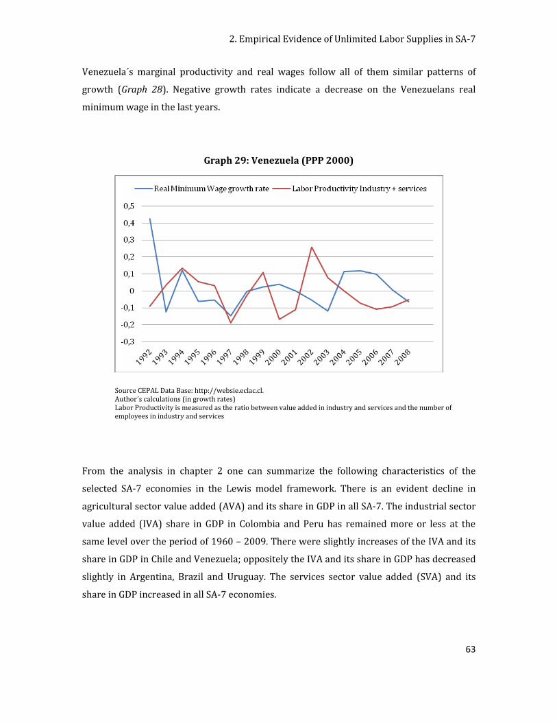
2. Empirical Evidence of Unlimited Labor Supplies in SA-7
63
Venezuela´s marginal productivity and real wages follow all of them similar patterns of
growth (Graph 28). Negative growth rates indicate a decrease on the Venezuelans real
minimum wage in the last years.
Graph 29: Venezuela (PPP 2000)
Source CEPAL Data Base: http://websie.eclac.cl. Author´s calculations (in growth rates) Labor Productivity is measured as the ratio between value added in industry and services and the number of employees in industry and services
From the analysis in chapter 2 one can summarize the following characteristics of the
selected SA-7 economies in the Lewis model framework. There is an evident decline in
agricultural sector value added (AVA) and its share in GDP in all SA-7. The industrial sector
value added (IVA) share in GDP in Colombia and Peru has remained more or less at the
same level over the period of 1960 – 2009. There were slightly increases of the IVA and its
share in GDP in Chile and Venezuela; oppositely the IVA and its share in GDP has decreased
slightly in Argentina, Brazil and Uruguay. The services sector value added (SVA) and its
share in GDP increased in all SA-7 economies.
2. Empirical Evidence of Unlimited Labor Supplies in SA-7
64
To some extent, the data provides the trends of the value added for each sector and its share
in GDP in these SA-7 economies. These trends seem to be similar to those predicted by
Lewis; such as the decreasing importance of the agriculture sector in value added terms and
a much more important role of the modern sector (industrial and services sector). Not only
are these activities important in volumes, but also in terms of employment. The industry
and services sector employs on average 80% of the total labor force and in Argentina’s case,
it employs even more than 98% of the labor force. Specifying the employment in the
industrial sector, the portion of labor force employed in the industrial sector in Argentina
and Uruguay tends to decrease. In contrast, in Brazil, Colombia and Peru, the share of labor
force employed in the industry tends to increase; and it is roughly unchanged in Chile and
Venezuela.
The predictions of the Lewis model with respect to demographic changes, such as the
transfer of labor force from the traditional sector to the modern sector seem be fulfilled in
the selected SA-7 economies. In some cases (Brazil, Colombia and Peru) the initial scenario
shows that the portion of population in the rural sector was greater than the portion of
population in the modern sector; this situation has been reversed in the last 50 years.
Part of the new labor force in the modern (urban) sector is released from the rural
(traditional or agriculture) sector, which represents the redundant labor force that causes
pressure on wages (Lewis, 1954). The assumption about a flat real wage is empirically
supported with the indicators given in section 2.4 such as high rates of vulnerable
employment, the high poverty headcount rates and the close to zero growth rates of the real
wage. Poverty headcount rate seems to be better off in some economies such as those of
Brazil, Colombia, Chile and Peru as compared to 30 years ago, however seems to have
worsened in countries such as Argentina, Venezuela and Uruguay. Vulnerable employment
rate is often related to bad labor conditions. In this respect, the situation seems to be better
in Argentina, Brazil and Chile, however, not in Colombia, Uruguay, Peru and Venezuela
where labor conditions haven’t improved at all.
All the characteristics and predictions of Lewis described above relates to the final and main
idea of pressure on wages. In section 2.4.3 the depicted growth of real wages seem to be flat
though slightly positive (growth rate close to zero) in all SA-7 economies and seem not to
follow similar patterns in comparison with the labor productive growth rates. This
2. Empirical Evidence of Unlimited Labor Supplies in SA-7
65
descriptive empirical analysis for these SA-7 economies encompasses the idea of the
presence of a dualist economy, which are in a slow transfer process towards an
industrialized economy.
The selected SA-7 economies seem to fulfill the Lewis assumptions and predictions such as
the initial traditional economy and the demographic changes but without the essential
response from the capitalist sector at all. In the next section some of main variables in the
Lewis model are presented graphically together with an analysis of the condition for
success, in order to determine the causes of the slow development in these SA-7 economies.
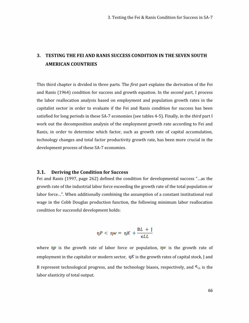
3. Testing the Fei & Ranis Condition for Success in SA-7
66
3. TESTING THE FEI AND RANIS SUCCESS CONDITION IN THE SEVEN SOUTH
AMERICAN COUNTRIES
This third chapter is divided in three parts. The first part explains the derivation of the Fei
and Ranis (1964) condition for success and growth equation. In the second part, I process
the labor reallocation analysis based on employment and population growth rates in the
capitalist sector in order to evaluate if the Fei and Ranis condition for success has been
satisfied for long periods in these SA-7 economies (see tables 4-5). Finally, in the third part I
work out the decomposition analysis of the employment growth rate according to Fei and
Ranis, in order to determine which factor, such as growth rate of capital accumulation,
technology changes and total factor productivity growth rate, has been more crucial in the
development process of these SA-7 economies.
3.1. Deriving the Condition for Success Fei and Ranis (1997, page 262) defined the condition for developmental success “…as the
growth rate of the industrial labor force exceeding the growth rate of the total population or
labor force…”. When additionally combining the assumption of a constant institutional real
wage in the Cobb Douglas production function, the following minimum labor reallocation
condition for successful development holds:
where is the growth rate of labor force or population, is the growth rate of
employment in the capitalist or modern sector, is the growth rates of capital stock, J and
B represent technological progress, and the technology biases, respectively, and LL is the
labor elasticity of total output.
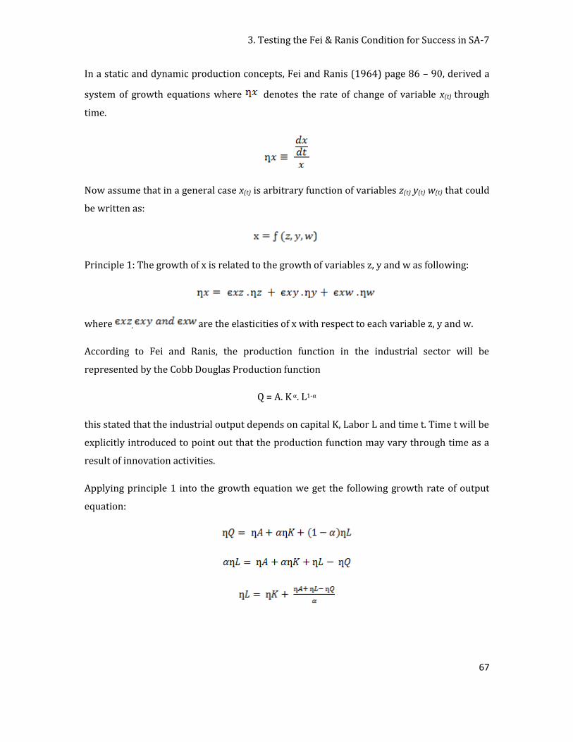
3. Testing the Fei & Ranis Condition for Success in SA-7
67
In a static and dynamic production concepts, Fei and Ranis (1964) page 86 – 90, derived a
system of growth equations where denotes the rate of change of variable x(t) through
time.
Now assume that in a general case x(t) is arbitrary function of variables z(t) y(t) w(t) that could
be written as:
Principle 1: The growth of x is related to the growth of variables z, y and w as following:
where , are the elasticities of x with respect to each variable z, y and w.
According to Fei and Ranis, the production function in the industrial sector will be
represented by the Cobb Douglas Production function
Q = A. K α. L1-α
this stated that the industrial output depends on capital K, Labor L and time t. Time t will be
explicitly introduced to point out that the production function may vary through time as a
result of innovation activities.
Applying principle 1 into the growth equation we get the following growth rate of output
equation:
3. Testing the Fei & Ranis Condition for Success in SA-7
68
Where = growth rate of industrial employment, = growth rate of industrial capital
accumulation, = J = intensity of innovation and ( - ) = = labor using bias of
innovation (Fei & Ranis, 1997:263) and α = є = elasticity of marginal productivity of labor.
Defining the necessary condition for developmental success as the growth rate of the
industrial employment = exceeding the growth rate of labor force , (Fei & Ranis
1997:262) we can arrange the previous equation as:
3.2. Employment Growth rates Analysis / the Fei and Ranis condition for
Success According to Lewis model, the “turning point” is going to be reached after periods of time
where the growth rate of employment in the modern sector exceeds the labor force or
population growth rate. is the growth rate of employment in the industrial sector and
the growth rate of employment in the service sector; let both conform the “Modern
Sector”, and let be the growth rate of the total labor force of the Economy.
I divided the Analysis of the Fei and Ranis “Condition for success”19 in two different
scenarios. The first one (extended analysis) is represented in Table 4 in which I consider the
growth rate of employment in the industry and services sectors together, i.e.
. Table 5 presents results for what I called the “strict analysis”, that considers only
what Lewis argued to be the most important and the most productive activity - which has to
be developed in order to grow- that is, employment growth in the “Industry” .
19 Details of conditions for success in Appendix 4
3. Testing the Fei & Ranis Condition for Success in SA-7
69
In tables 4 and 5 these two employment growth rates in the modern sector ( extended
analysis and strict analysis) together with the growth rate of the total labor force in the
economy are presented in a long term analysis, as the growth rate of employment in the
modern sector is greater than the growth rate of the labor force > , the economy is
following a development path and could be considered to reach the “Lewis turning point”.
As for the extended analysis (see table 4), the condition > over the period 1991 –
2000 is satisfied only in Chile, Colombia, Peru and Venezuela, with an average growth rate
difference of +1,2% for Chile, Colombia +1,1%, Peru +0,5% and Venezuela +0,4%. On the
other hand, Argentina, Brazil and Uruguay have not satisfied the condition, showing
negative annual average growth rate differences. This negative impact could be in some way
related to the Asiatic financial crisis in 1998 that has affected terms of trade in the biggest
Latin-American economies including Argentina and Brazil within the SA-7.
For the period 2000 -2007, the condition of success is satisfied in Argentina, Brazil, Chile,
Peru and Venezuela, being the most remarkable results in Venezuela with a annual average
growth rate difference of +1,7%, Argentina +1,6%, Brazil + 1,5%, Chile +1,2 and Peru
+0,1%; negative results are seen in Colombia -1,3% and Uruguay -0,1%.
Thus, in the 17 years analysis corresponding to the period 1991 – 2007, the Fei & Ranis
condition for success in an extended version has been satisfied for Chile, Peru and
Venezuela. Only Uruguay and Colombia have not satisfied the Fei and Ranis condition for
success. Colombia experienced a devastating blow < from 2000 to 2001, caused by
a tremendous reduction on the employment growth rate; in part, due to the recession
observed in these years with a respective GDP growth of 0,57% (1998) and -4,2% (1999)20.
Colombian industry value added decreased tremendously between 1999 and 2001,
especially in 1999 that decreased in -7,3% and -5,3% in 2000. Latin America suffered a
recession in 1998 – 1999, particularly in Argentina, Brazil, Chile and Colombia, attributable
to the Asian financial crisis (Thailand, March 1997).
20 See Section 2.2
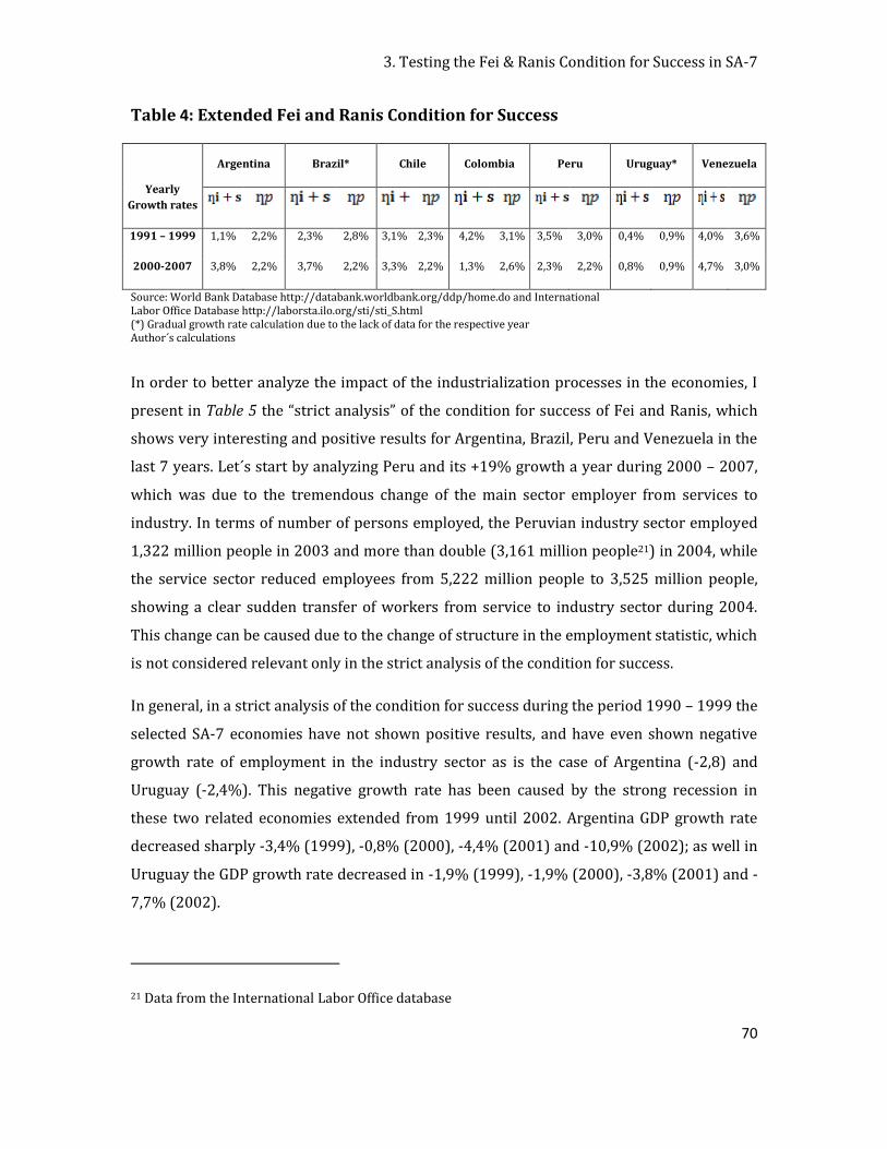
3. Testing the Fei & Ranis Condition for Success in SA-7
70
Table 4: Extended Fei and Ranis Condition for Success
Yearly
Growth rates
Argentina Brazil* Chile Colombia Peru Uruguay* Venezuela
1991 – 1999 1,1% 2,2% 2,3% 2,8% 3,1% 2,3% 4,2% 3,1% 3,5% 3,0% 0,4% 0,9% 4,0% 3,6%
2000-2007 3,8% 2,2% 3,7% 2,2% 3,3% 2,2% 1,3% 2,6% 2,3% 2,2% 0,8% 0,9% 4,7% 3,0%
Source: World Bank Database http://databank.worldbank.org/ddp/home.do and International Labor Office Database http://laborsta.ilo.org/sti/sti_S.html (*) Gradual growth rate calculation due to the lack of data for the respective year Author´s calculations
In order to better analyze the impact of the industrialization processes in the economies, I
present in Table 5 the “strict analysis” of the condition for success of Fei and Ranis, which
shows very interesting and positive results for Argentina, Brazil, Peru and Venezuela in the
last 7 years. Let´s start by analyzing Peru and its +19% growth a year during 2000 – 2007,
which was due to the tremendous change of the main sector employer from services to
industry. In terms of number of persons employed, the Peruvian industry sector employed
1,322 million people in 2003 and more than double (3,161 million people21) in 2004, while
the service sector reduced employees from 5,222 million people to 3,525 million people,
showing a clear sudden transfer of workers from service to industry sector during 2004.
This change can be caused due to the change of structure in the employment statistic, which
is not considered relevant only in the strict analysis of the condition for success.
In general, in a strict analysis of the condition for success during the period 1990 – 1999 the
selected SA-7 economies have not shown positive results, and have even shown negative
growth rate of employment in the industry sector as is the case of Argentina (-2,8) and
Uruguay (-2,4%). This negative growth rate has been caused by the strong recession in
these two related economies extended from 1999 until 2002. Argentina GDP growth rate
decreased sharply -3,4% (1999), -0,8% (2000), -4,4% (2001) and -10,9% (2002); as well in
Uruguay the GDP growth rate decreased in -1,9% (1999), -1,9% (2000), -3,8% (2001) and -
7,7% (2002).
21 Data from the International Labor Office database
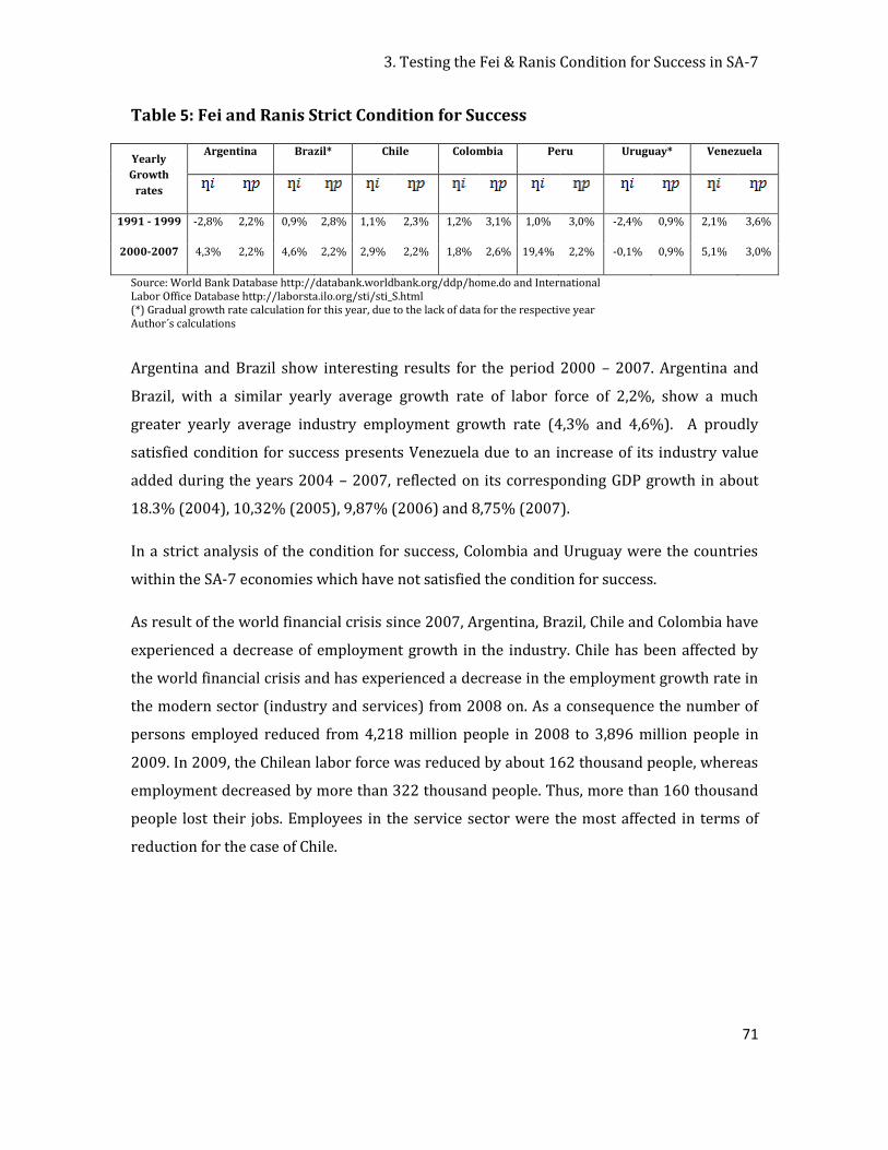
3. Testing the Fei & Ranis Condition for Success in SA-7
71
Table 5: Fei and Ranis Strict Condition for Success
Yearly
Growth
rates
Argentina Brazil* Chile Colombia Peru Uruguay* Venezuela
1991 - 1999 -2,8% 2,2% 0,9% 2,8% 1,1% 2,3% 1,2% 3,1% 1,0% 3,0% -2,4% 0,9% 2,1% 3,6%
2000-2007 4,3% 2,2% 4,6% 2,2% 2,9% 2,2% 1,8% 2,6% 19,4% 2,2% -0,1% 0,9% 5,1% 3,0%
Source: World Bank Database http://databank.worldbank.org/ddp/home.do and International Labor Office Database http://laborsta.ilo.org/sti/sti_S.html (*) Gradual growth rate calculation for this year, due to the lack of data for the respective year Author´s calculations
Argentina and Brazil show interesting results for the period 2000 – 2007. Argentina and
Brazil, with a similar yearly average growth rate of labor force of 2,2%, show a much
greater yearly average industry employment growth rate (4,3% and 4,6%). A proudly
satisfied condition for success presents Venezuela due to an increase of its industry value
added during the years 2004 – 2007, reflected on its corresponding GDP growth in about
18.3% (2004), 10,32% (2005), 9,87% (2006) and 8,75% (2007).
In a strict analysis of the condition for success, Colombia and Uruguay were the countries
within the SA-7 economies which have not satisfied the condition for success.
As result of the world financial crisis since 2007, Argentina, Brazil, Chile and Colombia have
experienced a decrease of employment growth in the industry. Chile has been affected by
the world financial crisis and has experienced a decrease in the employment growth rate in
the modern sector (industry and services) from 2008 on. As a consequence the number of
persons employed reduced from 4,218 million people in 2008 to 3,896 million people in
2009. In 2009, the Chilean labor force was reduced by about 162 thousand people, whereas
employment decreased by more than 322 thousand people. Thus, more than 160 thousand
people lost their jobs. Employees in the service sector were the most affected in terms of
reduction for the case of Chile.
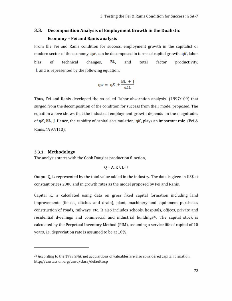
3. Testing the Fei & Ranis Condition for Success in SA-7
72
3.3. Decomposition Analysis of Employment Growth in the Dualistic
Economy – Fei and Ranis analysis
From the Fei and Ranis condition for success, employment growth in the capitalist or
modern sector of the economy, , can be decomposed in terms of capital growth, , labor
bias of technical changes, , and total factor productivity,
, and is represented by the following equation:
Thus, Fei and Ranis developed the so called “labor absorption analysis” (1997:109) that
surged from the decomposition of the condition for success from their model proposed. The
equation above shows that the industrial employment growth depends on the magnitudes
of , , . Hence, the rapidity of capital accumulation, , plays an important role (Fei &
Ranis, 1997:113).
3.3.1. Methodology
The analysis starts with the Cobb Douglas production function,
Q = A. K α. L1-α
Output Q, is represented by the total value added in the industry. The data is given in US$ at
constant prices 2000 and in growth rates as the model proposed by Fei and Ranis.
Capital K, is calculated using data on gross fixed capital formation including land
improvements (fences, ditches and drain), plant, machinery and equipment purchases
construction of roads, railways, etc. It also includes schools, hospitals, offices, private and
residential dwellings and commercial and industrial buildings22. The capital stock is
calculated by the Perpetual Inventory Method (PIM), assuming a service life of capital of 10
years, i.e. depreciation rate is assumed to be at 10%
22 According to the 1993 SNA, net acquisitions of valuables are also considered capital formation.
http://unstats.un.org/unsd/class/default.asp
3. Testing the Fei & Ranis Condition for Success in SA-7
73
Labor L, is represented by the headcount of employment in the modern sector (industry
services), according to the source provided by the national institutes of statistics of each
country and the ILO database (http://laborsta.ilo.org/STP). The decomposition analysis was
possible for Colombia only for a 6 years period, due to the lack of information on the gross
fixed capital formation for the period 1991 – 2001.
Given the growth equation above one can derive the model in growth terms for econometric
analysis,
Let´s denote that the “constant coefficient”, A, represents in our model the intensity of
innovation J and the coefficient of the gross fixed capital formation growth rate, α,
represents the elasticity of labor productivity LL (representing the law of diminishing
returns to labor); and let´s be e the error term.
From the condition for success presented in part 3.1 we can deduce that the labor biased of
technical changes BL equals the elasticity of labor productivity α times the difference
between the growth rate of employment in the modern sector and the growth rate of capital
accumulation ( – ) minus the intensity of innovation J.
The Fei and Ranis Model suggests that the more technological change biased towards the
factor –labor, BL, the better for the development of the dualistic economy.
My aim is to determine the significance of the Lewis, Fei and Ranis model for each economy
and, therefore, consider the decomposition analysis of labor growth to determine the main
sources that increase employment in the respective economy.
3.3.2. Econometric Regression of the growth Model and Decomposition
Analysis of labor growth for the SA-7
I analyze the statically significance of the Lewis – Fei - Ranis Model for each economy in the
two previous scenarios of the capitalist sector including only industry and a second scenario
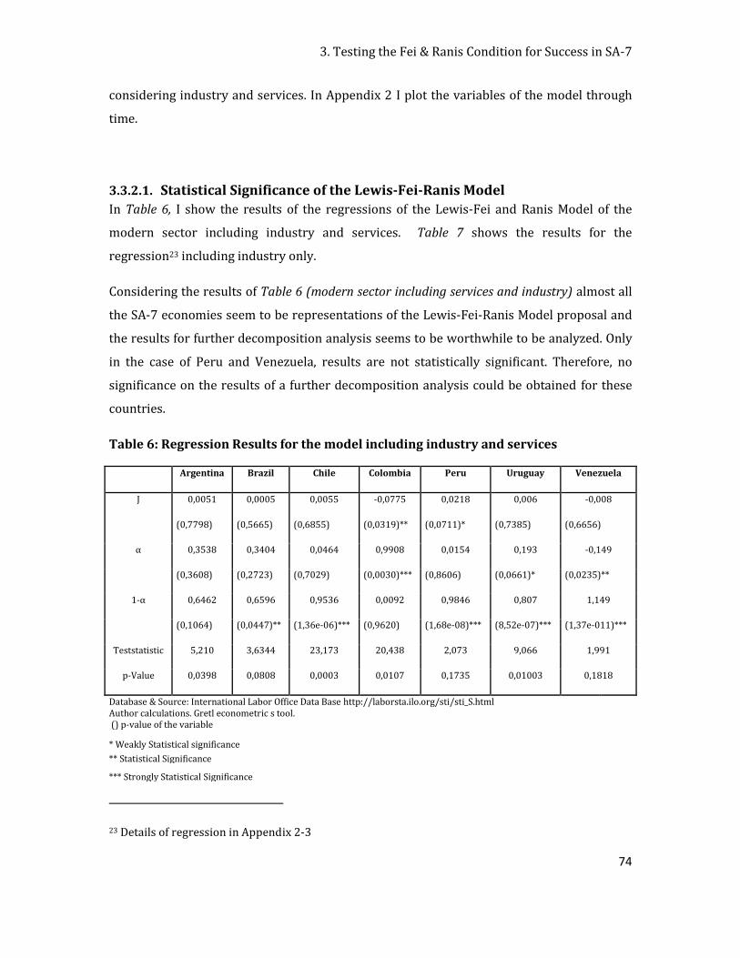
3. Testing the Fei & Ranis Condition for Success in SA-7
74
considering industry and services. In Appendix 2 I plot the variables of the model through
time.
3.3.2.1. Statistical Significance of the Lewis-Fei-Ranis Model
In Table 6, I show the results of the regressions of the Lewis-Fei and Ranis Model of the
modern sector including industry and services. Table 7 shows the results for the
regression23 including industry only.
Considering the results of Table 6 (modern sector including services and industry) almost all
the SA-7 economies seem to be representations of the Lewis-Fei-Ranis Model proposal and
the results for further decomposition analysis seems to be worthwhile to be analyzed. Only
in the case of Peru and Venezuela, results are not statistically significant. Therefore, no
significance on the results of a further decomposition analysis could be obtained for these
countries.
Table 6: Regression Results for the model including industry and services
Argentina Brazil Chile Colombia Peru Uruguay Venezuela
J 0,0051 0,0005 0,0055 -0,0775 0,0218 0,006 -0,008
(0,7798) (0,5665) (0,6855) (0,0319)** (0,0711)* (0,7385) (0,6656)
α 0,3538 0,3404 0,0464 0,9908 0,0154 0,193 -0,149
(0,3608) (0,2723) (0,7029) (0,0030)*** (0,8606) (0,0661)* (0,0235)**
1-α 0,6462 0,6596 0,9536 0,0092 0,9846 0,807 1,149
(0,1064) (0,0447)** (1,36e-06)*** (0,9620) (1,68e-08)*** (8,52e-07)*** (1,37e-011)***
Teststatistic 5,210 3,6344 23,173 20,438 2,073 9,066 1,991
p-Value 0,0398 0,0808 0,0003 0,0107 0,1735 0,01003 0,1818
Database & Source: International Labor Office Data Base http://laborsta.ilo.org/sti/sti_S.html Author calculations. Gretl econometric s tool. () p-value of the variable
* Weakly Statistical significance
** Statistical Significance
*** Strongly Statistical Significance
23 Details of regression in Appendix 2-3
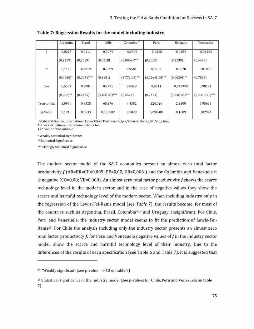
3. Testing the Fei & Ranis Condition for Success in SA-7
75
Table 7: Regression Results for the model including industry
Argentina Brazil Chile Colombia * Peru Uruguay Venezuela
J 0,0215 0,0111 0,0074 -0,0769 -0,0240 0,0154 -0,01262
(0,2459) (0,2539) (0,6218) (0,0009)*** (0,2858) (0,2130) (0,4446)
α 0,4446 0,7019 0,2209 0,9581 0,9259 0,2570 0,01809
(0,0680)* (0,0031)*** (0,1101) (2,77e-05)*** (4,72e-010)*** (0,0029)*** (0,7517)
1-α 0,5554 0,2981 0,7791 0,0419 0,0741 0,742959 0,98191
(0,027)** (0,1475) (3,16e-05)*** (0,5524) (0,2471) (5,73e-08)*** (6,43e-011)***
Teststatistic 1,8980 0,9325 65,276 4,4382 124,026 2,2108 5,95631
p-Value 0,1915 0,3533 0,000002 0,1029 5,09E-08 0,1609 0,02974
Database & Source: International Labor Office Data Base http://laborsta.ilo.org/sti/sti_S.html Author calculations. Gretl econometric s tool. () p-value of the variable
* Weakly Statistical significance
** Statistical Significance
*** Strongly Statistical Significance
The modern sector model of the SA-7 economies present an almost zero total factor
productivity J (AR=BR=CH=0,005; PE=0,02, UR=0,006 ) and for Colombia and Venezuela it
is negative (CO=0,08; VE=0,008). An almost zero total factor productivity J shows the scarce
technology level in the modern sector and in the case of negative values they show the
scarce and harmful technology level of the modern sector. When including industry only in
the regression of the Lewis-Fei-Ranis model (see Table 7), the results become, for most of
the countries such as Argentina, Brazil, Colombia*24 and Uruguay, insignificant. For Chile,
Peru and Venezuela, the industry sector model seems to fit the prediction of Lewis-Fei-
Ranis25. For Chile the analysis including only the industry sector presents an almost zero
total factor productivity J; for Peru and Venezuela negative values of J in the industry sector
model, show the scarce and harmful technology level of their industry. Due to the
differences of the results of each specification (see Table 6 and Table 7), it is suggested that
24 *Weakly significant (see p-value = 0,10 on table 7)
25 Statistical significance of the Industry model (see p-values for Chile, Peru and Venezuela on table
7)
3. Testing the Fei & Ranis Condition for Success in SA-7
76
the industrial and services sectors follow quite different development paths (mostly in
Argentina, Colombia, Uruguay and Venezuela). The econometric regression for Brazil, Chile
and Peru suggests that the model follows different patterns depending on the scenario (1.
Scenario: includes Industry + services; 2. Scenario: includes only Industry). Proof of this, are
the coefficient values that change tremendously.
3.3.2.2. Lewis-Fei-Ranis Decomposition Analysis of the Employment Growth
Considering the Fei-Ranis condition for success, we have that employment growth rate, ,
can be represented as follows:
The decomposition analysis of employment growth according to Fei and Ranis, consists on
determining the values of the variables of the condition for success, in order to identify the
main variables that contribute positive or negatively to the employment growth, , such
as, capital growth or capital accumulation, , labor bias of technical changes, , and total
factor productivity, .
In Table 8 the corresponding calculations regarding the decomposition of the employment
growth rate for Argentina, Brazil, Chile, Colombia and Uruguay is depicted. For economies
such as Peru and Venezuela, where the Lewis-Fei-Ranis model is non-statistically significant
the decomposition analysis has not been calculated.
Argentina’s decomposition of employment growth shows that capital formation or capital
accumulation ( ) plays an important role in the creation of employment and occasionally
negative values of the labor biased technology B, indicate that the bias of technical change
are likely to save labor in the production process (against labor). Fei and Ranis suggest that
the more technical progress labor biased the better it is for the development of the dualistic
economy. Argentina has in the 16 years from 1991 – 2007 an accumulative negative value of
labor biased technology factor B, on the other hand capital accumulation growth rate
has been the most important factor towards employment for this period. In Argentina
3. Testing the Fei & Ranis Condition for Success in SA-7
77
from years 2002 to 2004 the labor biased technology factor has been positive and towards
labor.
According to Fei and Ranis the corresponding calculus of the decomposition of the growth
rate of employment for Brazil shows a positive factor biased toward labor B which has
played an important role in employment. Capital accumulation has played a less
important role in employment creation over this period. The positive values of the labor
biased technology factor B indicate that the bias of technical change is more likely to use
labor in the production process (towards labor). Results for Chile indicate that capital
accumulation has played a strong important role in employment creation in the last 15
years. On the other hand, negative values of the factor bias indicate that the technical
change bias is much more likely to save labor. Also in Colombia´s capital accumulation, ,
has played a strong and important role in employment creation in this 7 years analysis.
There is also evidence for the factor biased to be against labor. Finally, capital formation or
capital accumulation in Uruguay also plays an important role in employment creation
and occasionally negative values of the labor biased technology B, indicates that technical
change bias is more likely to save labor in the production process (against labor).
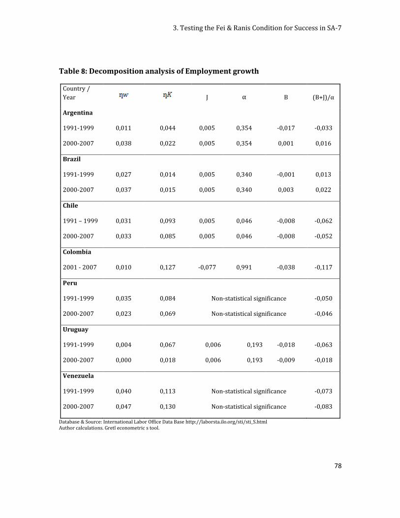
3. Testing the Fei & Ranis Condition for Success in SA-7
78
Table 8: Decomposition analysis of Employment growth
Country /
Year J α B (B+J)/α
Argentina
1991-1999 0,011 0,044 0,005 0,354 -0,017 -0,033
2000-2007 0,038 0,022 0,005 0,354 0,001 0,016
Brazil
1991-1999 0,027 0,014 0,005 0,340 -0,001 0,013
2000-2007 0,037 0,015 0,005 0,340 0,003 0,022
Chile
1991 – 1999 0,031 0,093 0,005 0,046 -0,008 -0,062
2000-2007 0,033 0,085 0,005 0,046 -0,008 -0,052
Colombia
2001 - 2007 0,010 0,127 -0,077 0,991 -0,038 -0,117
Peru
1991-1999 0,035 0,084 Non-statistical significance -0,050
2000-2007 0,023 0,069 Non-statistical significance -0,046
Uruguay
1991-1999 0,004 0,067 0,006 0,193 -0,018 -0,063
2000-2007 0,000 0,018 0,006 0,193 -0,009 -0,018
Venezuela
1991-1999 0,040 0,113 Non-statistical significance -0,073
2000-2007 0,047 0,130 Non-statistical significance -0,083
Database & Source: International Labor Office Data Base http://laborsta.ilo.org/sti/sti_S.html Author calculations. Gretl econometric s tool.
Conclusions
79
4. CONCLUSIONS
The trends and results that stand out from the selected SA-7 economies analysis above match
the trends expected by Lewis fairly well. First of all, from section 2 a shift of the redundant
agriculture labor force towards the urban or modern industrial sector can be clearly identified in
these SA-7 economies. The empirical evidence for this is that the agriculture share of GDP has
been maintained despite the decrease and lower growth rate of rural or agricultural labor force
that has even been negative in the last decades. This is particularly the case for countries such as
Brazil, Colombia and Peru, which presented a strong reduction of their labor force in agriculture.
Hence, this suggests the presence of redundant labor force in the agriculture sector in these
selected SA-7 economies.
The Lewis model argues that the modern sector plays an important role in employment (Lewis
1954:21). The redundant labor force from the agriculture sector is transferred towards the
capitalist sector with people searching for jobs opportunities and better standards of living. The
modern sector in these SA-7 economies indeed employs the greatest part of the labor force
distributed in the industry and services sector. According to Valpy FitzGerald26 this suggests that
“…tertiary sector or services act as “labor sponges” with a large part of their workforce
effectively underemployed.” (FitzGerald, 2004: 13). Nevertheless, Lewis considers the modern
sector (industry and services) as the core of the economic growth and development. In terms of
employment in these SA-7 economies, the agriculture activity has lost importance as an
employer with the industry27 and services28 becoming much more relevant.
Once the redundant labor is identified, it is necessary to identify the pressure on wages in the
modern sector, as a consequence of the transfer of redundant labor from the agriculture sector
of the economy. For this purpose three aspects have been analyzed: (i) poverty headcount rate
(ii) vulnerable employment and (iii) real minimum wage growth rate and labor productivity.
Vulnerable employment ratio embodies the employees with less favorable labor conditions such
26 Valpy FitzGerald on his paper in July 2004 “the Lewis Model in Practice: Economic Development in Latin America during the Twentieth Century”.
27 Industry employs up to 26% of the total labor force for the case of Brazil (see section 2.3.2)
28 Services employs up to 79% of the labor force for the case of Argentina (see section 2.3.2)
Conclusions
80
as underpaid and sporadic jobs, less social protection and no social benefits. In 2007, at least
19%29 of the employment in SA-7 was in a situation of vulnerable employment. Critical ratios are
shown for Colombia (41%) and Peru (39%). Growth rates of minimum real wages and labor
productivity in the SA-7 do not follow similar patterns with the exception of short periods of
time, where similar patterns were presented in Brazil, Chile, Uruguay and Venezuela (see 2.4.3).
Growth rates of the real minimum wage are almost zero, without any steady increase despite
sharp changes on the productivity of labor in the corresponding modern sector.
Following the Fei-Ranis growth model (section 3.1), the condition for success analysis has
revealed interesting results30 for the period 2000-2007 in countries such as Argentina, Brazil,
Chile, Peru and Venezuela. The condition for success has been tested and analyzed considering
two scenarios31. The condition for success needs to be satisfied for long periods of time in order
to reach economic development and thus better standards of living. From the analysis above
then, one can conclude that, as in the SA-7 economies condition for success is continuously
interrupted; hence, there is no evidence over a long-term that the Lewis-Fei-Ranis condition of
success is satisfied. Therefore, according to Lewis the economies have not reached the end of
the 1st stage and the labor markets do not face a significantly positively sloped labor supply
curve at all. Relatively flat real wages in these SA-7 economies are explained with the Lewis
Model. The Lewis-Fei-Ranis growth model including industry and services sectors shows
statistical significance in Argentina, Brazil, Chile, Colombia32 and Uruguay. For Peru and
Venezuela no statistical significance was found33. After determining the significance of the model
and locating the SA-7 into the capitalist Lewis-Fei-Ranis economic model, the decomposition
analysis of employment growth rate confirms that capital accumulation has been the main factor
towards employment in all the SA-7 economies. Low and in some cases negative values of factor
productivity enlighten the low level and lack of technology innovation in SA-7 economies, hence,
against employment. The factor bias of technology is in most of these cases demonstrating that
technology is most likely to save labor.
29 Argentina: 19% Brazil: 26% Chile24% Colombia: 41% Peru: 39% Uruguay: 24% Venezuela: 29%
30 See table 4 section 3.2
31 First scenario for the condition for success test includes industry and services / second scenario considers only industry
32 Due to the lack of data about the employment rate for Colombia was only possible the analysis for 7 years.
33 See table 6, section 3.3.2.1
Conclusions
81
Finally, the main Lewis-Fei-Ranis prediction about the almost flat real wages growth rates in the
modern sector – caused by the release of redundant labor force from the traditional sector
which disappears when the labor surplus coming from the traditional sector has been exhausted
- has been identified and confronted to empirical data. A great part of the SA-7 labor force
perceives low wages at a subsistence level and seem to prevail in the long-term. These SA-7
economies fit statistically in the neo-classical Lewis-Fei-Ranis growth model. According to the
empirical results, these economies could not satisfy the conditions of success for long-periods of
time as often being interrupted or affected by e.g. international crisis, political changes, etc.
Medium-term growth in the industry and services are directly and positive related to
employment. Some economies such as Brazil and Chile have increased tremendously in terms of
income per capita due to investment and increase of its industry. In the new century, the poorest
countries within the SA-7 such as Peru and Colombia have presented opposite results in terms of
poverty reduction. Peru has outstandingly reduced its poverty headcount rate in the last 7 years
as its economy has satisfied during 7 years the Lew-Fei-Ranis condition for success. Oppositely,
Colombia has not satisfied the condition for success at all and has not achieved positive results in
poverty reduction.
Through the analysis presented, I can conclude that these selected SA-7 economies fit in the
context and framework of the proposed Lewis Model. Thereby, some disruptions in the extent of
the Lewis growth path can be identified; one is related to the short-term satisfaction of the
condition for success and the second one is about the low level of technology and productivity in
the modern economy in this SA-7.
References
82
REFERENCES
TEXT SURVEY
W.A. Lewis, 1954, “Economic Development with Unlimited Supplies of Labour”, Ed. Oxford
University, pp 1 – 39.
Michael Todaro 1977, „Economic Development in the third world – Growth Theory“, pp 41
- 159.
W.A. Lewis, 1956, „Die Theorie des Wirtschaflichen Wachstums“, pp 1- 36.
John C. H. FEI & Gustav Ranis, 1964, “Growth and Development from an Evolutionary
Perspective”, pp 1 – 250.
John C. H. FEI & Gustav Ranis, 1997, “Growth and Development from an Evolutionary
Perspective”, pp 1 - 246.
Gustav Ranis, 2004, “Arthur Lewis Contribution to development thinking and Policy“, Yale
University, pp 01 – 78.
Valpy Fitzgerald, 2004 “ The Lewis Model in Practice: Economic Development in Latin
America during the Twentieth Century”, Oxford University.
Wazrul Islam and Ka Zuhiko Yokota, 2006, “At initial look at China´s industrialization in
light of the Lewis growth Model”, International Centre for Study of East Asian
Development (ICSEAD), Kita Kyoshu, Japan.
Karl Marx, 1946, “Lohnarbeit und Capital” (1946) , pp 15 – 40.
Bhatia, Kul B. (2002). Specific and mobile capital, migration and unemployment in a
Harris-Todaro model. Journal of International Trade and Economic Development.
Tim Ruffer (Oxford Policy Management) & John Knight (University of Oxford), February,
2007, “Informal Sector Labor Markets in Developing Countries” Oxford University.
ILO – Bouletin, 2010, ISBN 978-92-2-123256-8 (print), ISBN 978-92-2-123257-5 (web
pdf) Global Employment Trends, January 2010, International Labour Office, Geneva.
Gary S. Fields, July 2004 „Dualism in the Labor Market: A Perspective on the Lewis Model
After Half a Century“, Cornell University.
Kehoe, T. J. and Serra-Puche, J. 1983, “A computational general equilibrium model with
endogenous unemployment” Journal of Public Economics, pp 1-26..
Patricia Escobar, 2004, “Los límites del desarrollo capitalista: Vision Keynesiana”. Santiago
de Chile, pp 1 – 57.
Taylor, J. E.; May 2002. Trade integration and rural economies in less developed countries:
References
83
lessons from micro economy-wide models with particular attention to Mexico and Central
America. Report to the Latin America and Caribbean regional office of the World Bank.
Fischer, Manfred M, : Some major issues in regional Labour Markets Analysis / Manfred M
and Peter Nijkamp.- Wien- (WSG-discussion paper; 4)
DATABASE SURVEY
United Nation Statistics UNO http://unstats.un.org/unsd/snaama/selbasicFast.asp
International Labor Office online database for research:
http://www.ilo.org/global/statistics-and-databases/lang--en/index.htm
http://laborsta.ilo.org
http://www.ilo.org/dyn/normlex/en
http://www.ilo.org/dyn/natlex/natlex_browse.home?p_lang=en
http://www.ilo.org/ipec/ChildlabourstatisticsSIMPOC/lang--en/index.htm
Comisión Económica para América Latina CEPAL Online data base http://www.eclac.org
Instituto Nacional de estadística de Argentina http:/www.indec.mecon.ar/
Instituto Brasileiro de Geografia e Estadistica http:/www.ibge.gov.br/
Instituto Nacional de Estadísticas de Chile http://www.ine.cl/
Instituto Nacional de Estadística del Peru http://www.inei.gob.pe/
Instituto Nacional de administración y Estadística de Colombia http://www.dane.gov.co/
Instituto Nacional de Estadística de Uruguay http://www.ine.gub.uy/
Instituto Nacional de Estadística República Bolivariana de Venezuela
http://www.ine.gov.ve/
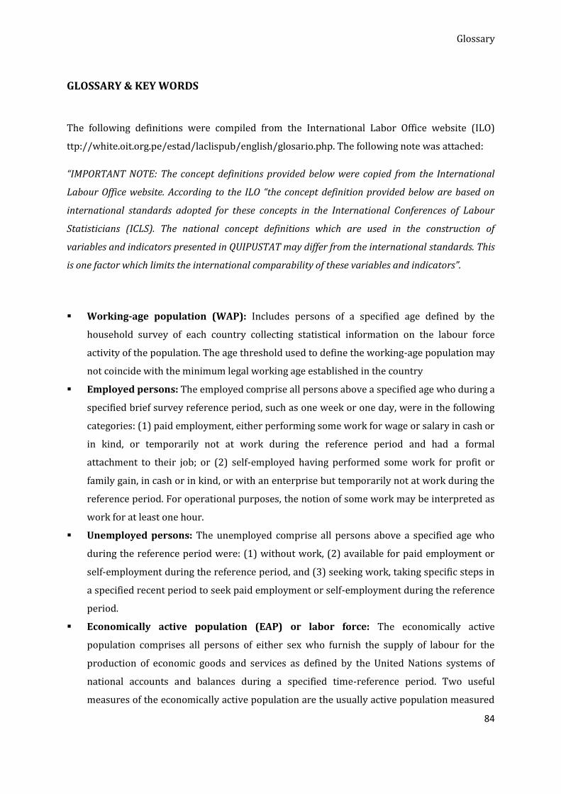
Glossary
84
GLOSSARY & KEY WORDS
The following definitions were compiled from the International Labor Office website (ILO)
ttp://white.oit.org.pe/estad/laclispub/english/glosario.php. The following note was attached:
“IMPORTANT NOTE: The concept definitions provided below were copied from the International
Labour Office website. According to the ILO “the concept definition provided below are based on
international standards adopted for these concepts in the International Conferences of Labour
Statisticians (ICLS). The national concept definitions which are used in the construction of
variables and indicators presented in QUIPUSTAT may differ from the international standards. This
is one factor which limits the international comparability of these variables and indicators”.
Working-age population (WAP): Includes persons of a specified age defined by the
household survey of each country collecting statistical information on the labour force
activity of the population. The age threshold used to define the working-age population may
not coincide with the minimum legal working age established in the country
Employed persons: The employed comprise all persons above a specified age who during a
specified brief survey reference period, such as one week or one day, were in the following
categories: (1) paid employment, either performing some work for wage or salary in cash or
in kind, or temporarily not at work during the reference period and had a formal
attachment to their job; or (2) self-employed having performed some work for profit or
family gain, in cash or in kind, or with an enterprise but temporarily not at work during the
reference period. For operational purposes, the notion of some work may be interpreted as
work for at least one hour.
Unemployed persons: The unemployed comprise all persons above a specified age who
during the reference period were: (1) without work, (2) available for paid employment or
self-employment during the reference period, and (3) seeking work, taking specific steps in
a specified recent period to seek paid employment or self-employment during the reference
period.
Economically active population (EAP) or labor force: The economically active
population comprises all persons of either sex who furnish the supply of labour for the
production of economic goods and services as defined by the United Nations systems of
national accounts and balances during a specified time-reference period. Two useful
measures of the economically active population are the usually active population measured
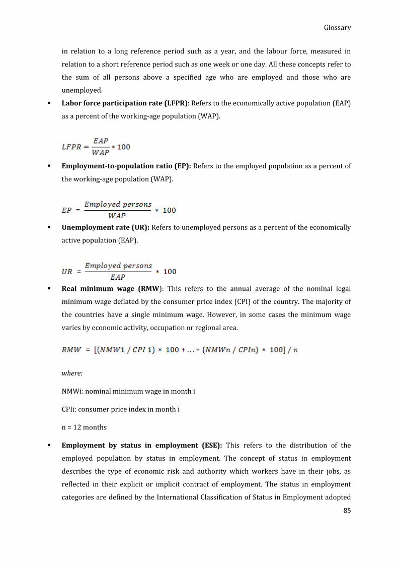
Glossary
85
in relation to a long reference period such as a year, and the labour force, measured in
relation to a short reference period such as one week or one day. All these concepts refer to
the sum of all persons above a specified age who are employed and those who are
unemployed.
Labor force participation rate (LFPR): Refers to the economically active population (EAP)
as a percent of the working-age population (WAP).
Employment-to-population ratio (EP): Refers to the employed population as a percent of
the working-age population (WAP).
Unemployment rate (UR): Refers to unemployed persons as a percent of the economically
active population (EAP).
Real minimum wage (RMW): This refers to the annual average of the nominal legal
minimum wage deflated by the consumer price index (CPI) of the country. The majority of
the countries have a single minimum wage. However, in some cases the minimum wage
varies by economic activity, occupation or regional area.
where:
NMWi: nominal minimum wage in month i
CPIi: consumer price index in month i
n = 12 months
Employment by status in employment (ESE): This refers to the distribution of the
employed population by status in employment. The concept of status in employment
describes the type of economic risk and authority which workers have in their jobs, as
reflected in their explicit or implicit contract of employment. The status in employment
categories are defined by the International Classification of Status in Employment adopted

Glossary
86
in the fourteenth International Conference of Labour Statisticians, known as ICSE-93.
1. Employees or wage and salaried workers, who get a basic remuneration not directly
dependent on the revenue of the employer and among whom countries may need and
be able to distinguish “employees with stable contracts” (including “regular
employees”) from other workers.
2. Employers, who are self-employed (i.e. whose remuneration depends directly on the
expectation of profits derived from the goods and services produced) and hire one or
more persons to work for them as ‘employees’, on a continuous basis.
3. Own-account workers, who are self-employed and do not hire ‘employees’ on a
continuous basis.
4. Members of producers’ cooperatives, who are self-employed in a cooperative producing
goods and services, where the members take part on an equal basis in making major
decisions concerning the cooperative.
5. Contributing family workers, who are self-employed in an establishment operated by a
related person, with too limited a degree of involvement in its operation to be
considered a partner.
6. Workers not classifiable by status, for whom insufficient relevant information is
available, and/or who cannot be included in any of the preceding categories.
ESEn = (Employed persons in status in employment category n / Total number of employed
persons) * 100
where:
n: employees, employers, own-account workers, . . . , workers not classifiable by status
Employment by economic activity (EEA): This refers to the distribution of the employed
population by economic activity, that is, the productive activity in which the employed are
engaged.
In order to standardize the classification of the economic activities, activities are grouped
based on the International Standard Industrial Classification of All Economic Activities
(ISIC), Second Revision. The economic activities are the following: Agriculture, hunting,
forestry and fishing, Mining and quarrying, Electricity, gas and water, Manufacturing,
Construction, Wholesale and retail trade and restaurants and hotels, Transport, storage and
communication, Financing, insurance, real estate and business services, Community, social
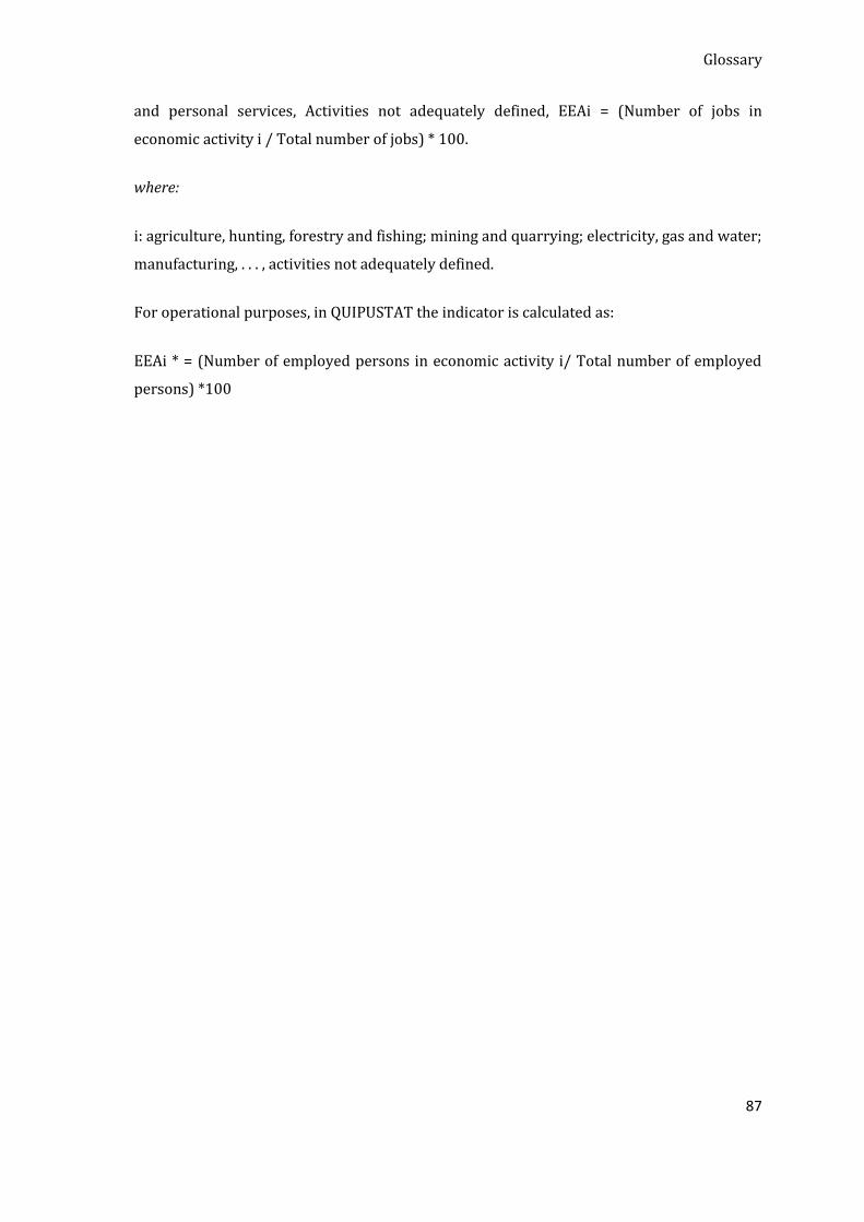
Glossary
87
and personal services, Activities not adequately defined, EEAi = (Number of jobs in
economic activity i / Total number of jobs) * 100.
where:
i: agriculture, hunting, forestry and fishing; mining and quarrying; electricity, gas and water;
manufacturing, . . . , activities not adequately defined.
For operational purposes, in QUIPUSTAT the indicator is calculated as:
EEAi * = (Number of employed persons in economic activity i/ Total number of employed
persons) *100
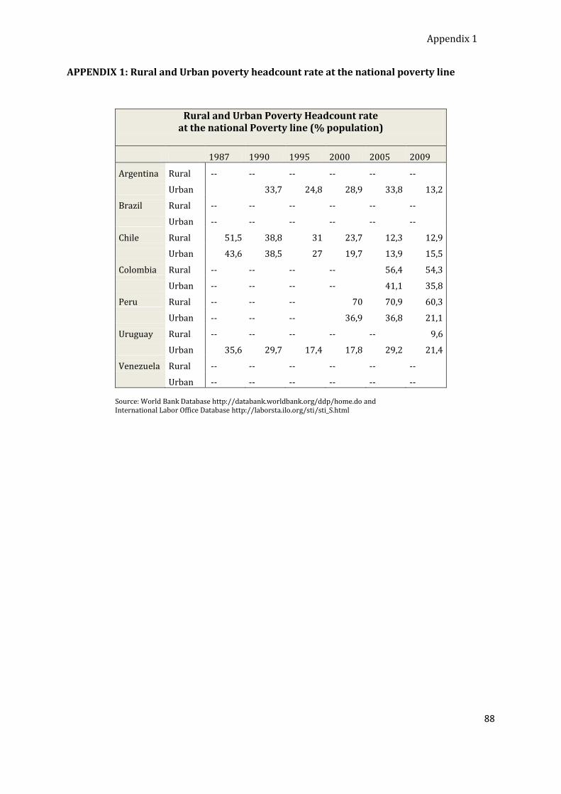
Appendix 1
88
APPENDIX 1: Rural and Urban poverty headcount rate at the national poverty line
Rural and Urban Poverty Headcount rate at the national Poverty line (% population)
1987 1990 1995 2000 2005 2009
Argentina Rural -- -- -- -- -- --
Urban 33,7 24,8 28,9 33,8 13,2
Brazil Rural -- -- -- -- -- --
Urban -- -- -- -- -- --
Chile Rural 51,5 38,8 31 23,7 12,3 12,9
Urban 43,6 38,5 27 19,7 13,9 15,5
Colombia Rural -- -- -- -- 56,4 54,3
Urban -- -- -- -- 41,1 35,8
Peru Rural -- -- -- 70 70,9 60,3
Urban -- -- -- 36,9 36,8 21,1
Uruguay Rural -- -- -- -- -- 9,6
Urban 35,6 29,7 17,4 17,8 29,2 21,4
Venezuela Rural -- -- -- -- -- --
Urban -- -- -- -- -- --
Source: World Bank Database http://databank.worldbank.org/ddp/home.do and International Labor Office Database http://laborsta.ilo.org/sti/sti_S.html
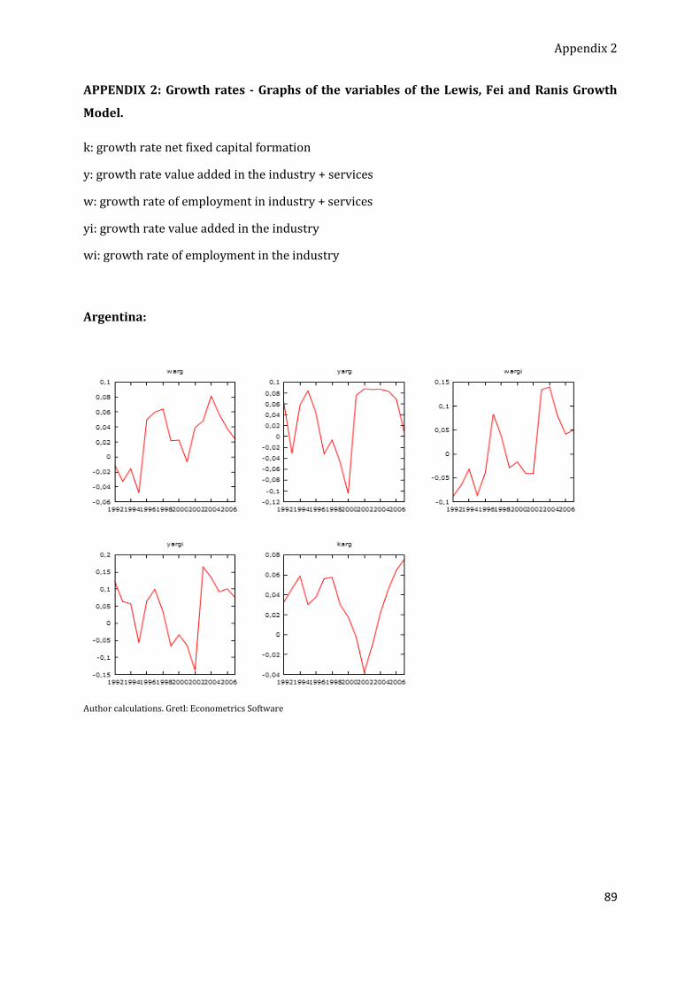
Appendix 2
89
APPENDIX 2: Growth rates - Graphs of the variables of the Lewis, Fei and Ranis Growth
Model.
k: growth rate net fixed capital formation
y: growth rate value added in the industry + services
w: growth rate of employment in industry + services
yi: growth rate value added in the industry
wi: growth rate of employment in the industry
Argentina:
Author calculations. Gretl: Econometrics Software
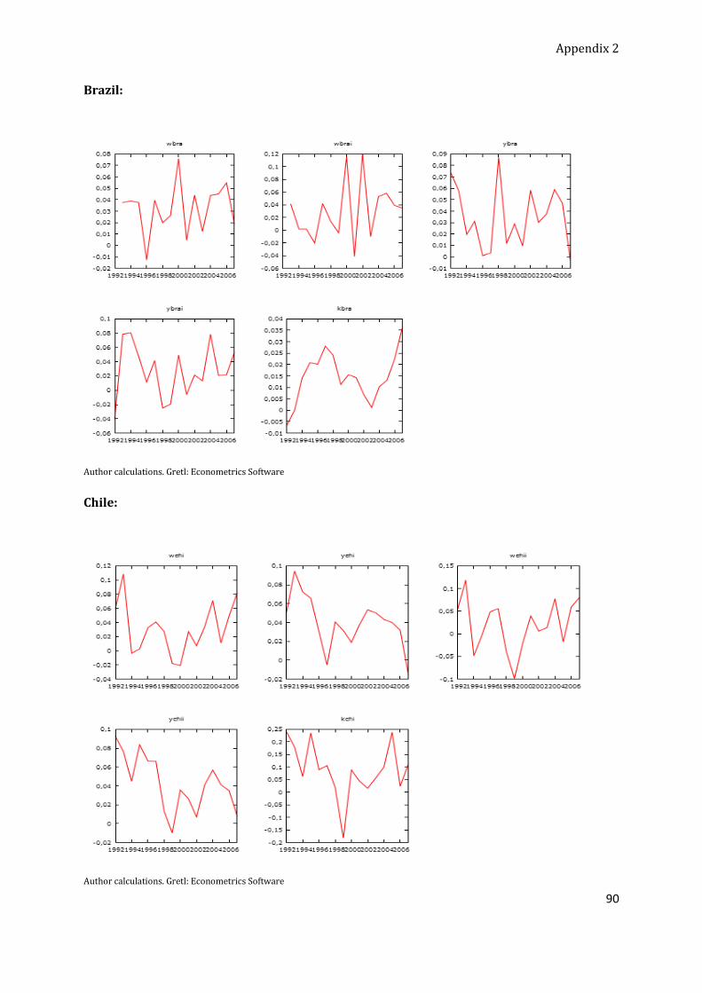
Appendix 2
90
Brazil:
Author calculations. Gretl: Econometrics Software
Chile:
Author calculations. Gretl: Econometrics Software
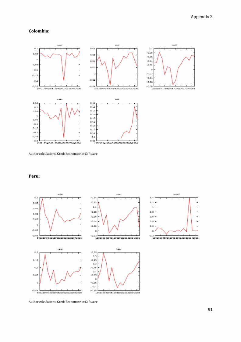
Appendix 2
91
Colombia:
Author calculations. Gretl: Econometrics Software
Peru:
Author calculations. Gretl: Econometrics Software
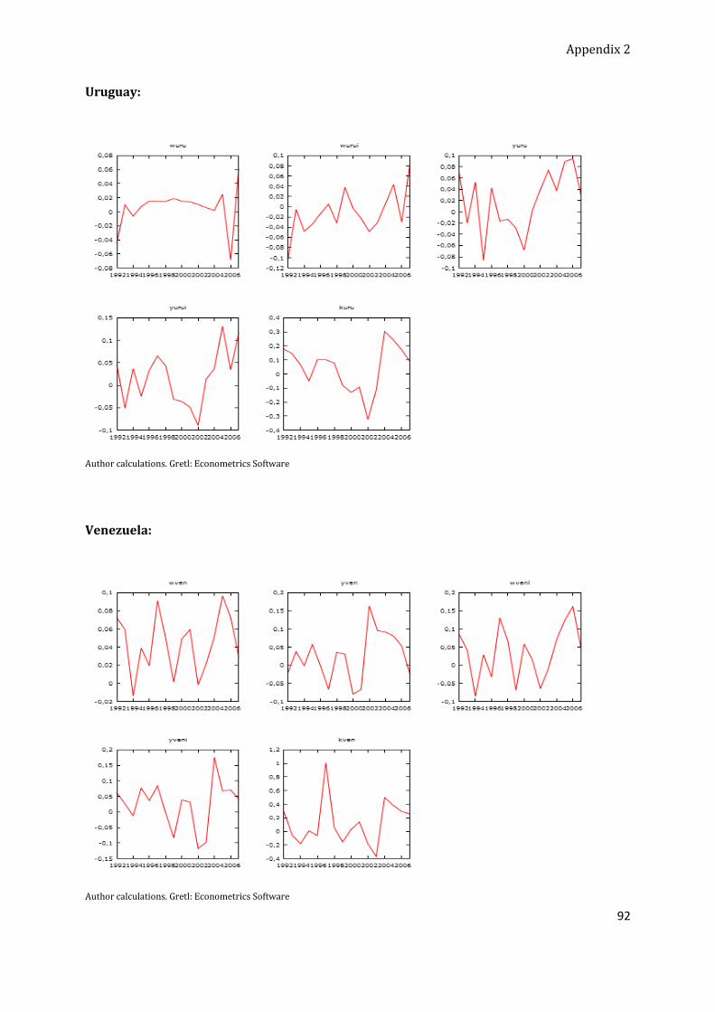
Appendix 2
92
Uruguay:
Author calculations. Gretl: Econometrics Software
Venezuela:
Author calculations. Gretl: Econometrics Software
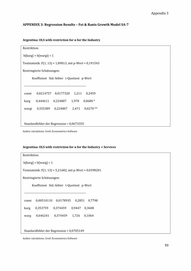
Appendix 3
93
APPENDIX 3: Regression Results – Fei & Ranis Growth Model SA-7
Argentina: OLS with restriction for α for the Industry
Restriktion:
b[karg] + b[wargi] = 1
Teststatistik: F(1, 13) = 1,89813, mit p-Wert = 0,191543
Restringierte Schätzungen:
Koeffizient Std.-fehler t-Quotient p-Wert
----------------------------------------------------------
const 0,0214757 0,0177320 1,211 0,2459
karg 0,444611 0,224807 1,978 0,0680 *
wargi 0,555389 0,224807 2,471 0,0270 **
Standardfehler der Regression = 0,0673355
Author calculations. Gretl: Econometrics Software
Argentina: OLS with restriction for α for the Industry + Services
Restriktion:
b[karg] + b[warg] = 1
Teststatistik: F(1, 13) = 5,21682, mit p-Wert = 0,0398201
Restringierte Schätzungen:
Koeffizient Std.-fehler t-Quotient p-Wert
----------------------------------------------------------
const 0,00510110 0,0178935 0,2851 0,7798
karg 0,353759 0,374459 0,9447 0,3608
warg 0,646241 0,374459 1,726 0,1064
Standardfehler der Regression = 0,0705149
Author calculations. Gretl: Econometrics Software
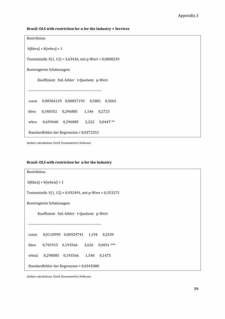
Appendix 3
94
Brazil: OLS with restriction for α for the Industry + Services
Restriktion:
b[kbra] + b[wbra] = 1
Teststatistik: F(1, 12) = 3,63436, mit p-Wert = 0,0808239
Restringierte Schätzungen:
Koeffizient Std.-fehler t-Quotient p-Wert
----------------------------------------------------------
const 0,00504129 0,00857193 0,5881 0,5665
kbra 0,340352 0,296885 1,146 0,2723
wbra 0,659648 0,296885 2,222 0,0447 **
Standardfehler der Regression = 0,0272351
Author calculations. Gretl: Econometrics Software
Brazil: OLS with restriction for α for the Industry
Restriktion:
b[kbra] + b[wbrai] = 1
Teststatistik: F(1, 12) = 0,932491, mit p-Wert = 0,353275
Restringierte Schätzungen:
Koeffizient Std.-fehler t-Quotient p-Wert
----------------------------------------------------------
const 0,0110999 0,00929741 1,194 0,2539
kbra 0,701915 0,193566 3,626 0,0031 ***
wbrai 0,298085 0,193566 1,540 0,1475
Standardfehler der Regression = 0,0345088
Author calculations. Gretl: Econometrics Software
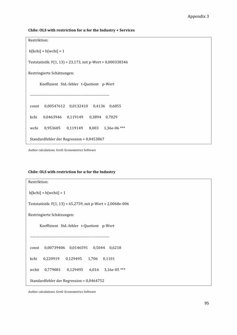
Appendix 3
95
Chile: OLS with restriction for α for the Industry + Services
Restriktion:
b[kchi] + b[wchi] = 1
Teststatistik: F(1, 13) = 23,173, mit p-Wert = 0,000338346
Restringierte Schätzungen:
Koeffizient Std.-fehler t-Quotient p-Wert
------------------------------------------------------------
const 0,00547612 0,0132410 0,4136 0,6855
kchi 0,0463946 0,119149 0,3894 0,7029
wchi 0,953605 0,119149 8,003 1,36e-06 ***
Standardfehler der Regression = 0,0453867
Author calculations. Gretl: Econometrics Software
Chile: OLS with restriction for α for the Industry
Restriktion:
b[kchi] + b[wchii] = 1
Teststatistik: F(1, 13) = 65,2759, mit p-Wert = 2,0068e-006
Restringierte Schätzungen:
Koeffizient Std.-fehler t-Quotient p-Wert
------------------------------------------------------------
const 0,00739406 0,0146591 0,5044 0,6218
kchi 0,220919 0,129495 1,706 0,1101
wchii 0,779081 0,129495 6,016 3,16e-05 ***
Standardfehler der Regression = 0,0464752
Author calculations. Gretl: Econometrics Software
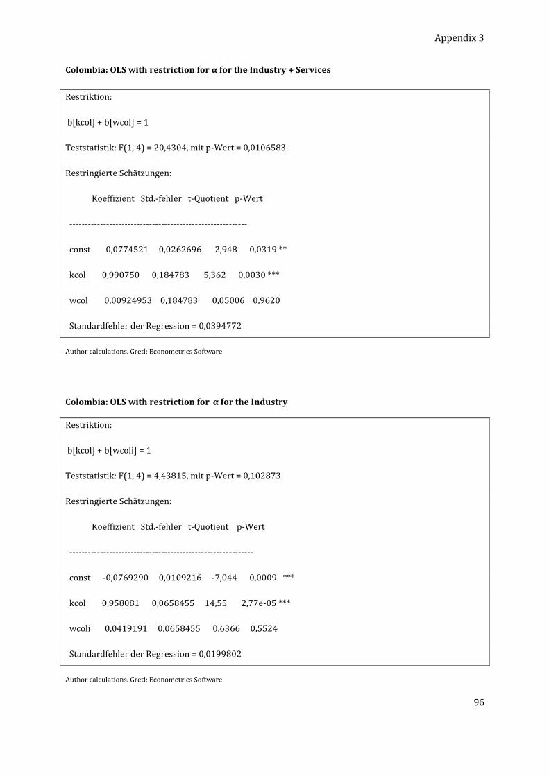
Appendix 3
96
Colombia: OLS with restriction for α for the Industry + Services
Restriktion:
b[kcol] + b[wcol] = 1
Teststatistik: F(1, 4) = 20,4304, mit p-Wert = 0,0106583
Restringierte Schätzungen:
Koeffizient Std.-fehler t-Quotient p-Wert
----------------------------------------------------------
const -0,0774521 0,0262696 -2,948 0,0319 **
kcol 0,990750 0,184783 5,362 0,0030 ***
wcol 0,00924953 0,184783 0,05006 0,9620
Standardfehler der Regression = 0,0394772
Author calculations. Gretl: Econometrics Software
Colombia: OLS with restriction for α for the Industry
Restriktion:
b[kcol] + b[wcoli] = 1
Teststatistik: F(1, 4) = 4,43815, mit p-Wert = 0,102873
Restringierte Schätzungen:
Koeffizient Std.-fehler t-Quotient p-Wert
------------------------------------------------------------
const -0,0769290 0,0109216 -7,044 0,0009 ***
kcol 0,958081 0,0658455 14,55 2,77e-05 ***
wcoli 0,0419191 0,0658455 0,6366 0,5524
Standardfehler der Regression = 0,0199802
Author calculations. Gretl: Econometrics Software
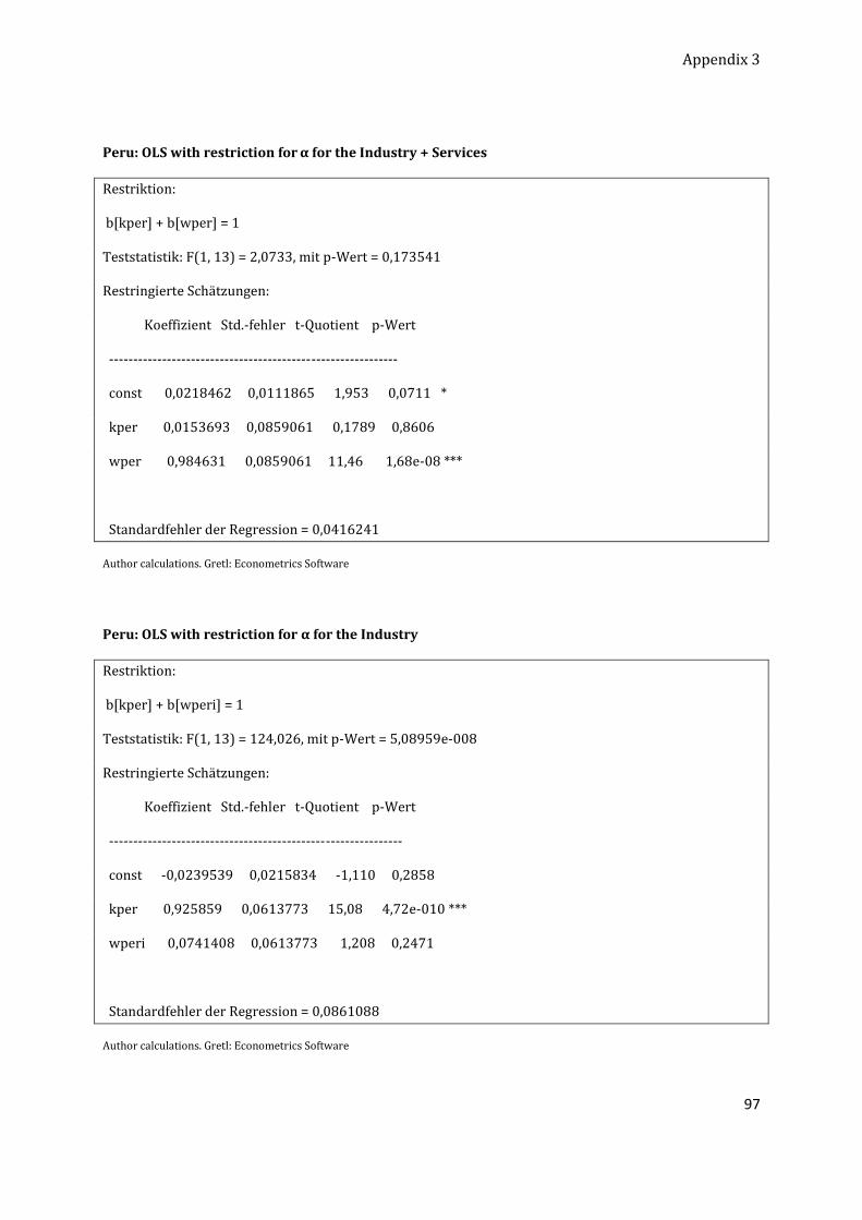
Appendix 3
97
Peru: OLS with restriction for α for the Industry + Services
Restriktion:
b[kper] + b[wper] = 1
Teststatistik: F(1, 13) = 2,0733, mit p-Wert = 0,173541
Restringierte Schätzungen:
Koeffizient Std.-fehler t-Quotient p-Wert
------------------------------------------------------------
const 0,0218462 0,0111865 1,953 0,0711 *
kper 0,0153693 0,0859061 0,1789 0,8606
wper 0,984631 0,0859061 11,46 1,68e-08 ***
Standardfehler der Regression = 0,0416241
Author calculations. Gretl: Econometrics Software
Peru: OLS with restriction for α for the Industry
Restriktion:
b[kper] + b[wperi] = 1
Teststatistik: F(1, 13) = 124,026, mit p-Wert = 5,08959e-008
Restringierte Schätzungen:
Koeffizient Std.-fehler t-Quotient p-Wert
-------------------------------------------------------------
const -0,0239539 0,0215834 -1,110 0,2858
kper 0,925859 0,0613773 15,08 4,72e-010 ***
wperi 0,0741408 0,0613773 1,208 0,2471
Standardfehler der Regression = 0,0861088
Author calculations. Gretl: Econometrics Software
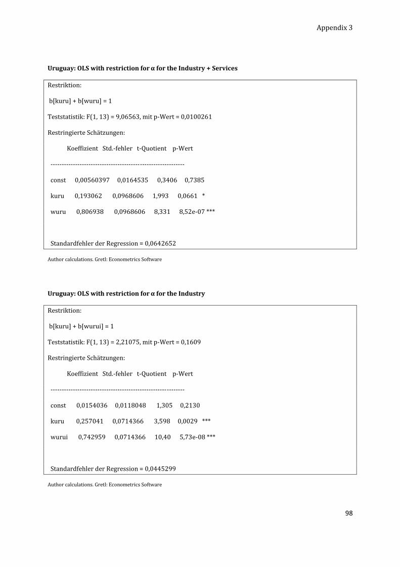
Appendix 3
98
Uruguay: OLS with restriction for α for the Industry + Services
Restriktion:
b[kuru] + b[wuru] = 1
Teststatistik: F(1, 13) = 9,06563, mit p-Wert = 0,0100261
Restringierte Schätzungen:
Koeffizient Std.-fehler t-Quotient p-Wert
------------------------------------------------------------
const 0,00560397 0,0164535 0,3406 0,7385
kuru 0,193062 0,0968606 1,993 0,0661 *
wuru 0,806938 0,0968606 8,331 8,52e-07 ***
Standardfehler der Regression = 0,0642652
Author calculations. Gretl: Econometrics Software
Uruguay: OLS with restriction for α for the Industry
Restriktion:
b[kuru] + b[wurui] = 1
Teststatistik: F(1, 13) = 2,21075, mit p-Wert = 0,1609
Restringierte Schätzungen:
Koeffizient Std.-fehler t-Quotient p-Wert
------------------------------------------------------------
const 0,0154036 0,0118048 1,305 0,2130
kuru 0,257041 0,0714366 3,598 0,0029 ***
wurui 0,742959 0,0714366 10,40 5,73e-08 ***
Standardfehler der Regression = 0,0445299
Author calculations. Gretl: Econometrics Software
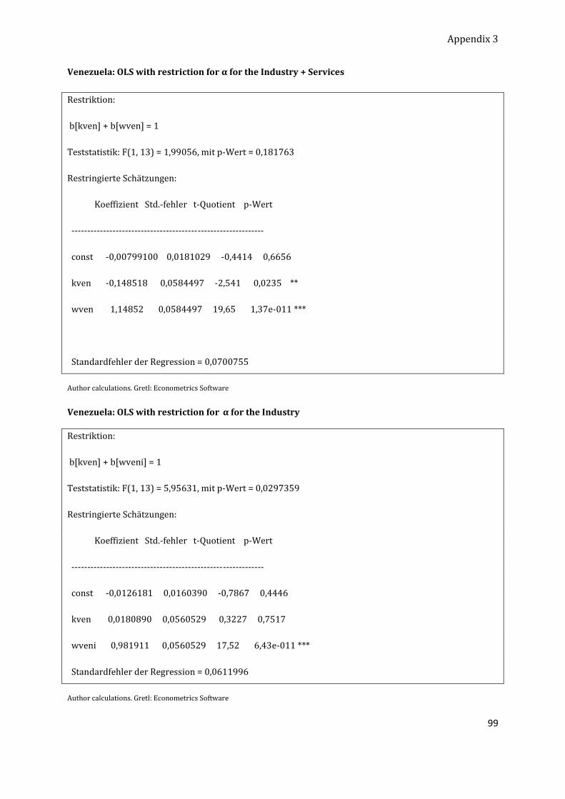
Appendix 3
99
Venezuela: OLS with restriction for α for the Industry + Services
Restriktion:
b[kven] + b[wven] = 1
Teststatistik: F(1, 13) = 1,99056, mit p-Wert = 0,181763
Restringierte Schätzungen:
Koeffizient Std.-fehler t-Quotient p-Wert
-------------------------------------------------------------
const -0,00799100 0,0181029 -0,4414 0,6656
kven -0,148518 0,0584497 -2,541 0,0235 **
wven 1,14852 0,0584497 19,65 1,37e-011 ***
Standardfehler der Regression = 0,0700755
Author calculations. Gretl: Econometrics Software
Venezuela: OLS with restriction for α for the Industry
Restriktion:
b[kven] + b[wveni] = 1
Teststatistik: F(1, 13) = 5,95631, mit p-Wert = 0,0297359
Restringierte Schätzungen:
Koeffizient Std.-fehler t-Quotient p-Wert
-------------------------------------------------------------
const -0,0126181 0,0160390 -0,7867 0,4446
kven 0,0180890 0,0560529 0,3227 0,7517
wveni 0,981911 0,0560529 17,52 6,43e-011 ***
Standardfehler der Regression = 0,0611996
Author calculations. Gretl: Econometrics Software
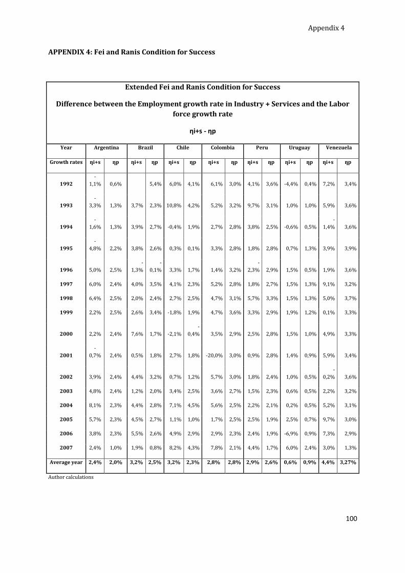
Appendix 4
100
APPENDIX 4: Fei and Ranis Condition for Success
Extended Fei and Ranis Condition for Success
Difference between the Employment growth rate in Industry + Services and the Labor
force growth rate
ƞi+s - ƞp
Year Argentina Brazil Chile Colombia Peru Uruguay Venezuela
Growth rates ƞi+s ƞp ƞi+s ƞp ƞi+s ƞp ƞi+s ƞp ƞi+s ƞp ƞi+s ƞp ƞi+s ƞp
1992
-
1,1% 0,6% 5,4% 6,0% 4,1% 6,1% 3,0% 4,1% 3,6% -4,4% 0,4% 7,2% 3,4%
1993
-
3,3% 1,3% 3,7% 2,3% 10,8% 4,2% 5,2% 3,2% 9,7% 3,1% 1,0% 1,0% 5,9% 3,6%
1994
-
1,6% 1,3% 3,9% 2,7% -0,4% 1,9% 2,7% 2,8% 3,8% 2,5% -0,6% 0,5%
-
1,4% 3,6%
1995
-
4,8% 2,2% 3,8% 2,6% 0,3% 0,1% 3,3% 2,8% 1,8% 2,8% 0,7% 1,3% 3,9% 3,9%
1996 5,0% 2,5%
-
1,3%
-
0,1% 3,3% 1,7% 1,4% 3,2%
-
2,3% 2,9% 1,5% 0,5% 1,9% 3,6%
1997 6,0% 2,4% 4,0% 3,5% 4,1% 2,3% 5,2% 2,8% 1,8% 2,7% 1,5% 1,3% 9,1% 3,2%
1998 6,4% 2,5% 2,0% 2,4% 2,7% 2,5% 4,7% 3,1% 5,7% 3,3% 1,5% 1,3% 5,0% 3,7%
1999 2,2% 2,5% 2,6% 3,4% -1,8% 1,9% 4,7% 3,6% 3,3% 2,9% 1,9% 1,2% 0,1% 3,3%
2000 2,2% 2,4% 7,6% 1,7% -2,1%
-
0,4% 3,5% 2,9% 2,5% 2,8% 1,5% 1,0% 4,9% 3,3%
2001
-
0,7% 2,4% 0,5% 1,8% 2,7% 1,8% -20,0% 3,0% 0,9% 2,8% 1,4% 0,9% 5,9% 3,4%
2002 3,9% 2,4% 4,4% 3,2% 0,7% 1,2% 5,7% 3,0% 1,8% 2,4% 1,0% 0,5%
-
0,2% 3,6%
2003 4,8% 2,4% 1,2% 2,0% 3,4% 2,5% 3,6% 2,7% 1,5% 2,3% 0,6% 0,5% 2,2% 3,2%
2004 8,1% 2,3% 4,4% 2,8% 7,1% 4,5% 5,6% 2,5% 2,2% 2,1% 0,2% 0,5% 5,2% 3,1%
2005 5,7% 2,3% 4,5% 2,7% 1,1% 1,0% 1,7% 2,5% 2,5% 1,9% 2,5% 0,7% 9,7% 3,0%
2006 3,8% 2,3% 5,5% 2,6% 4,9% 2,9% 2,9% 2,3% 2,4% 1,9% -6,9% 0,9% 7,3% 2,9%
2007 2,4% 1,0% 1,9% 0,8% 8,2% 4,3% 7,8% 2,1% 4,4% 1,7% 6,0% 2,4% 3,0% 1,3%
Average year 2,4% 2,0% 3,2% 2,5% 3,2% 2,3% 2,8% 2,8% 2,9% 2,6% 0,6% 0,9% 4,4% 3,27%
Author calculations
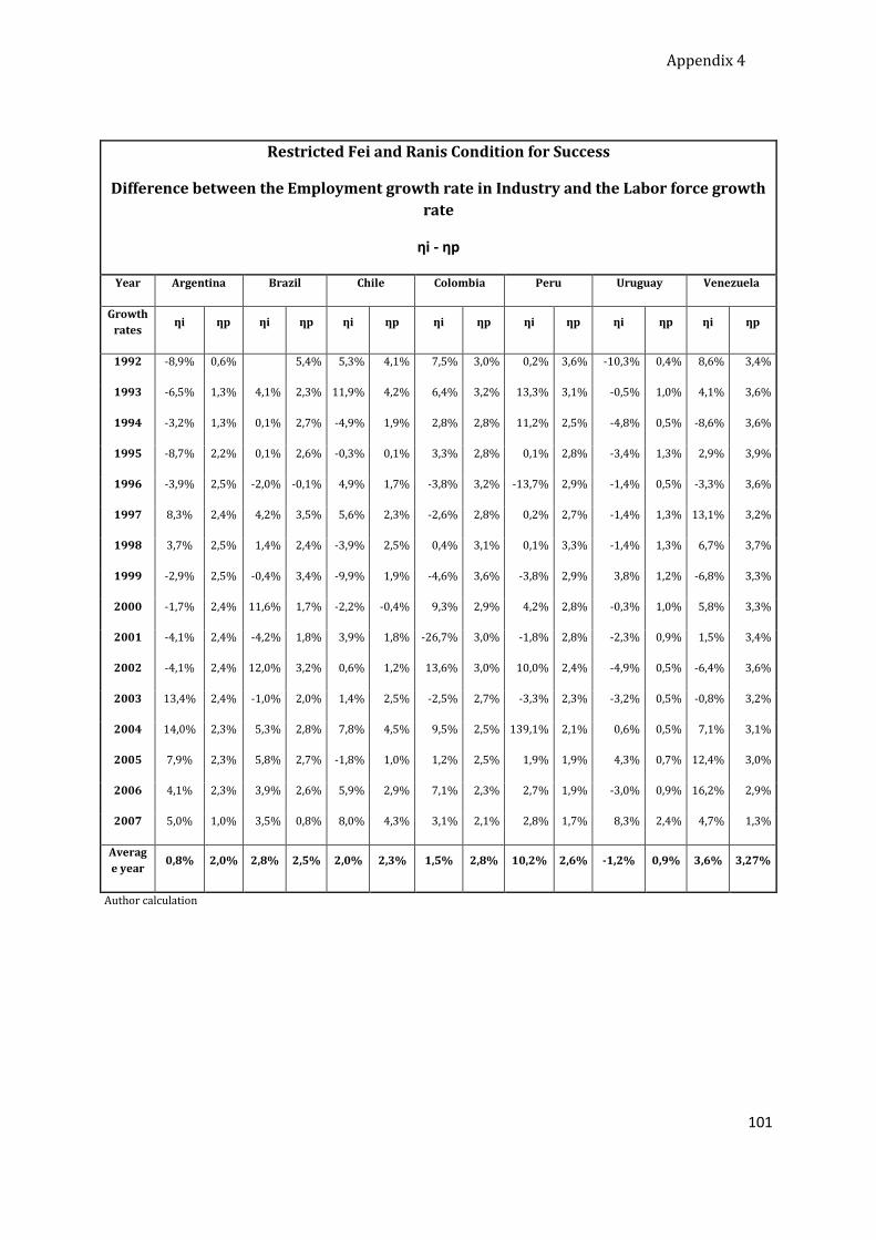
Appendix 4
101
Restricted Fei and Ranis Condition for Success
Difference between the Employment growth rate in Industry and the Labor force growth
rate
ƞi - ƞp
Year Argentina Brazil Chile Colombia Peru Uruguay Venezuela
Growth
rates ƞi ƞp ƞi ƞp ƞi ƞp ƞi ƞp ƞi ƞp ƞi ƞp ƞi ƞp
1992 -8,9% 0,6% 5,4% 5,3% 4,1% 7,5% 3,0% 0,2% 3,6% -10,3% 0,4% 8,6% 3,4%
1993 -6,5% 1,3% 4,1% 2,3% 11,9% 4,2% 6,4% 3,2% 13,3% 3,1% -0,5% 1,0% 4,1% 3,6%
1994 -3,2% 1,3% 0,1% 2,7% -4,9% 1,9% 2,8% 2,8% 11,2% 2,5% -4,8% 0,5% -8,6% 3,6%
1995 -8,7% 2,2% 0,1% 2,6% -0,3% 0,1% 3,3% 2,8% 0,1% 2,8% -3,4% 1,3% 2,9% 3,9%
1996 -3,9% 2,5% -2,0% -0,1% 4,9% 1,7% -3,8% 3,2% -13,7% 2,9% -1,4% 0,5% -3,3% 3,6%
1997 8,3% 2,4% 4,2% 3,5% 5,6% 2,3% -2,6% 2,8% 0,2% 2,7% -1,4% 1,3% 13,1% 3,2%
1998 3,7% 2,5% 1,4% 2,4% -3,9% 2,5% 0,4% 3,1% 0,1% 3,3% -1,4% 1,3% 6,7% 3,7%
1999 -2,9% 2,5% -0,4% 3,4% -9,9% 1,9% -4,6% 3,6% -3,8% 2,9% 3,8% 1,2% -6,8% 3,3%
2000 -1,7% 2,4% 11,6% 1,7% -2,2% -0,4% 9,3% 2,9% 4,2% 2,8% -0,3% 1,0% 5,8% 3,3%
2001 -4,1% 2,4% -4,2% 1,8% 3,9% 1,8% -26,7% 3,0% -1,8% 2,8% -2,3% 0,9% 1,5% 3,4%
2002 -4,1% 2,4% 12,0% 3,2% 0,6% 1,2% 13,6% 3,0% 10,0% 2,4% -4,9% 0,5% -6,4% 3,6%
2003 13,4% 2,4% -1,0% 2,0% 1,4% 2,5% -2,5% 2,7% -3,3% 2,3% -3,2% 0,5% -0,8% 3,2%
2004 14,0% 2,3% 5,3% 2,8% 7,8% 4,5% 9,5% 2,5% 139,1% 2,1% 0,6% 0,5% 7,1% 3,1%
2005 7,9% 2,3% 5,8% 2,7% -1,8% 1,0% 1,2% 2,5% 1,9% 1,9% 4,3% 0,7% 12,4% 3,0%
2006 4,1% 2,3% 3,9% 2,6% 5,9% 2,9% 7,1% 2,3% 2,7% 1,9% -3,0% 0,9% 16,2% 2,9%
2007 5,0% 1,0% 3,5% 0,8% 8,0% 4,3% 3,1% 2,1% 2,8% 1,7% 8,3% 2,4% 4,7% 1,3%
Averag
e year 0,8% 2,0% 2,8% 2,5% 2,0% 2,3% 1,5% 2,8% 10,2% 2,6% -1,2% 0,9% 3,6% 3,27%
Author calculation
Abstract
102
Abstract
Diese Arbeit analysiert die aktuellen Arbeitsmarktsituationen in sieben ausgewählten
südamerikanischen Ländern (SA-7) basieren auf dem Modell von Lewis (1954). Die Arbeit fasst
zunächst die wichtigsten Annahmen und Eigenschaften des Lewis-Modells zusammen, diskutiert
darauf aufbauend die Erweiterung im Rahmen des Wachstumsmodells von Fei und Ranis (1964)
und identifiziert somit die relevanten Prognosen des Lewis-Modells. Für die empirische
Überprüfung des Modeels wurden aktuelle und vertrauenswürdige Makroindikatoren, die auf
Websiten internationaler Organisationen veröffentlicht werden gesammelt, wobei die
wichtigsten Quellen von der Weltbank- und der International Labor Office-Datenbank kommen.
Die empirischen Ergebnisse bestätigen die Annahmen und Vorhersagen des Lewis-Modells für
die ausgewählten sieben Wirtschaften wodurch sich die Entwicklungsphasen im Rahmen des
Lewis-Fei-Ranis-Wachstumsmodells identifizieren lassen. Diese Forschung versteht sich
grundsätzlich als eine wirtschaftliche positive Analyse und vermeidet eine politische Kritik oder
Bewertung im normativen Sinne.
This research analyzes the current labor market situation in a selected group of seven South
American countries (SA-7) in the framework of the Lewis model (Lewis, 1954). It summarizes
the main assumptions and characteristics of the Lewis model in the SA-7 economies and the
extensions as put forward the Lewis-Fei-Ranis growth model (1964). In doing so it identifies the
main predictions of the Lewis model. The research is based on actual and authenticated
economic indicators published by international organizations websites, the World Bank and the
International Labor Office database being the main sources. Lewis assumption regarding the
long term shape of the real wage curve is related to better labor conditions and thus, better
standards of living for an economy. The final findings support the assumptions and predictions
of the Lewis model for these selected seven economies and therefore they let determine the
stages of development as argued in the framework of the Lewis-Fei-Ranis growth model. This
research is strictly an economic analysis and avoids any evaluation or critics on politics.
Jorge Luis Costa Vigil
Keywords: Unlimited Labor Supply, South-America, Lewis Theory.
Resume – Jorge Luis Costa Vigil
103
JORGE LUIS COSTA VIGIL
Borned on the 11th November 1981 in Lima, Peru
Julius-Meinl-gasse 15/5, 1170 Vienna, Austria
Telf: +43-699-1038 3804
A C A D E M I C B A C K G R O U N D
Advanced Game Theory – University of Vienna, Vienna, Austria 10/2008 – 01/2009
Bachelor in Economics – Universidad San Marcos, Lima, Peru 03/2000 – 02/2004
Economics in Mining, Oil and Energy Sector 03/2004 – 06/2004
Banking Seminar 03/2004 – 06/2004
Public Project Monitoring 03/2004 – 06/2004
W O R K E X P E R I E N C E ( ≥ 5 years):
Business Analyst - Subsidiary Network Department of the State Bank of Peru “Banco de la Nacion” (Peru)
Proffesional Field: Inner control 08/2006 - 02/2007
Business Analyst - State Bank of Peru “Banco de la Nacion” (Peru)
Proffesional Field: Risk analysis, Budget set up, Financial Restructure process prosecution
and Control. 07/2005 – 07/2006
Internship at the Organization of Consumer Development Department “INDECOPI” (Peru)
Proffesional Field: Business development 07/2005 – 07/2006
L A N G U A G E S :
Spanish – Native
English - Advanced Level
Italian - Advanced Level
German - Advanced Level