Embed Size (px)
Citation preview
Universitat Stuttgart - Institut fur Wasser- undUmweltsystemmodellierung
Lehrstuhl fur Hydromechanik und HydrosystemmodellierungProf. Dr.-Ing. Rainer Helmig
Master Thesis
Three Phase (Water, Air and NAPL)
Modeling of Bail-Down Test
Submitted by
Waqas Ahmed
Matriculation number 2708711
Stuttgart, 7 March,2014
Examiner: apl. Prof. Dr.-Ing. Holger Class
Supervisors: Olivier Atteia and Cedric Palmier

Author’s Statement
I hereby certify that I have prepared this master’s thesis independently, and that only
those sources, aids and advisors that are duly noted herein have been used and / or
consulted.
Signature: Date:

Acknowledgements
Throughout the entire thesis I was lucky enough to receive full support both intellec-
tually and emotionally by my adviser Holger Class, for that I am greatly indebted and
thankful. I am also thankful for the time and technical support by my supervisors
Cedric Palmier and Olivier Atteia without their help it would be impossible to com-
plete the thesis. I would also like to thank my family, especially my mother and father
for always believing in me, for their continuous love and their support in my decisions,
without whom I could not have made it here.
Abstract
Bail-down tests are commonly used to determine the LNAPL transmissivity, volume
and initial recovery rate for LNAPL contamination in the soil. In this work a non-
compositional 3p (three phase) LNAPL/water/air bail-down test model was simulated
on multiphase simulator DUMUX (Sec. 2.4). Model includes a radial flow of Light
Non Aqueous Phase Liquid (LNAPL) to well through the filter pack. Initially the
contaminated soil with LNAPL was allowed to reach equilibrium under capillary forces
using Van Genuchten (1980) [9] capillary relation. The applied model accurately de-
scribes the physical process during the bail-down test and shows the consistency with
the field data. The response of LNAPL recovery in the well to different soil and fluid
parameters was investigated. The results showed that LNAPL recovery time and ini-
tial recovery rates are dependent on soil capillary characteristics, permeability, initial
LNAPL thickness and fluid properties. In this work two analytical approaches were
used for analysis of the bail-down test model results to determine the LNAPL trans-
missivity. The First approach is based on a modified Bouwer and Rice analysis for slug
test (Huntley, 2000) [11]. The second approach is based on measured well thickness for
multi-layered soil (Jeong, 2014) [14]. The modified Bouwer and Rice method (Huntley,
2000) [11] showed good estimates, if the bail-down test is conducted such that poten-
tiometric head (total head in terms of water column) remains constant throughout the
test. A comparison for both approaches for multi-layered soil showed consistency with
the estimated LNAPL transmissivity.
Contents
1 Introduction 1
1.1 Motivation . . . . . . . . . . . . . . . . . . . . . . . . . . . . . . . . . . 1
1.2 Bail-Down Test . . . . . . . . . . . . . . . . . . . . . . . . . . . . . . . 3
1.2.1 Semi-Analytical Solution for Bail-Down Test Interpretation . . . 3
1.3 Scope of this Work . . . . . . . . . . . . . . . . . . . . . . . . . . . . . 7
1.4 Structure of Report . . . . . . . . . . . . . . . . . . . . . . . . . . . . 8
2 Fundamentals of Multiphase (Three Phase) Porous Media Model 9
2.1 General terms . . . . . . . . . . . . . . . . . . . . . . . . . . . . . . . . 9
2.1.1 Phases and Components . . . . . . . . . . . . . . . . . . . . . . 9
2.1.2 Wettability . . . . . . . . . . . . . . . . . . . . . . . . . . . . . 9
2.1.3 Saturation . . . . . . . . . . . . . . . . . . . . . . . . . . . . . . 10
2.1.4 Capillary Pressure . . . . . . . . . . . . . . . . . . . . . . . . . 10
2.1.5 Capillary Pressure Saturation Relationship . . . . . . . . . . . . 10
2.1.6 Relative Permeability and Extended Darcy’s Law . . . . . . . . 11
2.1.7 Saturation-Relative Permeability Relationship . . . . . . . . . . 12
2.2 Mathematical Formulation . . . . . . . . . . . . . . . . . . . . . . . . . 12
2.2.1 Mass Balance . . . . . . . . . . . . . . . . . . . . . . . . . . . . 13
2.3 Three Phase Model Concept . . . . . . . . . . . . . . . . . . . . . . . . 13
2.4 DUMUX Numerical Simulator . . . . . . . . . . . . . . . . . . . . . . . 15
3 Light Non Aqueous Phase Liquids (LNAPL) 16
3.1 Introduction . . . . . . . . . . . . . . . . . . . . . . . . . . . . . . . . . 16
3.2 Fate and Transport of LNAPL in Subsurface . . . . . . . . . . . . . . . 17
3.2.1 Parameters Effecting LNAPL Transport During Bail-Down test 17
3.3 Bail-Down Test Applied Problem . . . . . . . . . . . . . . . . . . . . . 19
3.3.1 Boundary and Initial Condition . . . . . . . . . . . . . . . . . . 19
3.4 Different Simulation Cases . . . . . . . . . . . . . . . . . . . . . . . . . 20
3.4.1 CASE I: Model Validation . . . . . . . . . . . . . . . . . . . . . 20
3.4.2 CASE II: Effect of Different Parameter to LNAPL Recovery in
Well . . . . . . . . . . . . . . . . . . . . . . . . . . . . . . . . . 22
3.4.3 CASE III: Effect of Multi-Layered Soil . . . . . . . . . . . . . . 22
I
CONTENTS II
4 Results and Discussion 24
4.1 CASE I: Model Validation . . . . . . . . . . . . . . . . . . . . . . . . . 24
4.2 CASE II: Effect of Different Parameter to LNAPL Recovery in Well . . 27
4.2.1 CASE II-A: Effect of Different Permeability . . . . . . . . . . . 28
4.2.2 CASE II-B: Effect of Different Van Genuchten α . . . . . . . . 29
4.2.3 CASE II-C: Effect of Different Initial Oil Thickness . . . . . . . 30
4.2.4 Case II-D: Effect of Different LNAPL Viscosity . . . . . . . . . 31
4.3 CASE III: Effect of Multi-Layered Soil . . . . . . . . . . . . . . . . . . 32
4.3.1 CASE III-A: 2m Fine Layer Between Silt and Coarse Layer
(LNAPL in Fine Layer) . . . . . . . . . . . . . . . . . . . . . . 32
4.3.2 CASE III-B: 1m Fine Layer Between Silt and Coarse Layer
(LNAPL in Fine and Coarse Layer) . . . . . . . . . . . . . . . . 33
5 Summary and Outlook 34
5.1 Summary . . . . . . . . . . . . . . . . . . . . . . . . . . . . . . . . . . 34
5.2 Conclusion . . . . . . . . . . . . . . . . . . . . . . . . . . . . . . . . . . 35
5.3 Outlook . . . . . . . . . . . . . . . . . . . . . . . . . . . . . . . . . . . 35
List of Figures
1.1 Transport and migration process of LNAPL (Newell, 1995) [18] . . . . . 1
1.2 Concept of LNAPL thickness in well and distribution in domain . . . . 3
1.3 Graphical interpretation of bail-down test data using Bouwer and Rice
method(Bouwer and Rice, 1976) [4] . . . . . . . . . . . . . . . . . . . . 6
2.1 Fluid distribution in pores (Helmig, 1997) [10] . . . . . . . . . . . . . . 10
2.2 Three phase three component model (Flemisch, 2007) [8] . . . . . . . . 14
2.3 Model concept bail-down test . . . . . . . . . . . . . . . . . . . . . . . 14
3.1 Applied model for bail-down simulation . . . . . . . . . . . . . . . . . . 19
3.2 Initial condition case I . . . . . . . . . . . . . . . . . . . . . . . . . . . 21
3.3 Case III: Schematic of layered soil . . . . . . . . . . . . . . . . . . . . . 23
4.1 Case I: Model validation . . . . . . . . . . . . . . . . . . . . . . . . . . 25
4.2 Case I: Profiles along radial direction . . . . . . . . . . . . . . . . . . . 26
4.3 Case II-A: Effect of different permeability . . . . . . . . . . . . . . . . . 28
4.4 Case II-B: Effect of different Van Genuchten α . . . . . . . . . . . . . . 29
4.5 Case II-C: Effect of different initial oil thickness . . . . . . . . . . . . . 30
4.6 Case II-D: Effect of different LNAPL viscosity . . . . . . . . . . . . . . 31
4.7 Case III-A: 2m fine layer (LNAPL in fine layer) . . . . . . . . . . . . . 32
4.8 Case III-B: 1m fine layer (LNAPL in fine and coarse layer) . . . . . . . 33
III
List of Tables
3.1 Fluid and porous media properties case I . . . . . . . . . . . . . . . . . 21
3.2 Case II: Variable parameters . . . . . . . . . . . . . . . . . . . . . . . . 22
3.3 Fluid and porous media properties for case III (Huntley 2002) [13] . . . 23
4.1 Case I: Analytical solution using modified Bouwer and Rice approach . 24
4.2 Case II-A: Analytical solution using modified Bouwer and Rice approach 28
4.3 Case II-B: Analytical solution using modified Bouwer and Rice approach 29
4.4 Case II-C: Analytical solution using modified Bouwer and Rice approach 30
4.5 Case II-D: Analytical solution using modified Bouwer and Rice approach 31
4.6 Case III-A: Analytical solution . . . . . . . . . . . . . . . . . . . . . . . 32
4.7 Case III-B: Analytical solution . . . . . . . . . . . . . . . . . . . . . . 33
IV
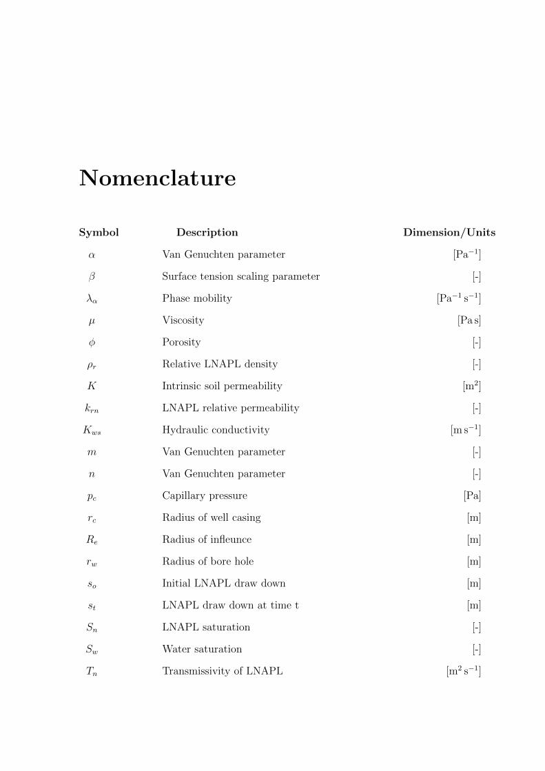
Nomenclature
Symbol Description Dimension/Units
α Van Genuchten parameter [Pa−1]
β Surface tension scaling parameter [-]
λα Phase mobility [Pa−1 s−1]
µ Viscosity [Pa s]
φ Porosity [-]
ρr Relative LNAPL density [-]
K Intrinsic soil permeability [m2]
krn LNAPL relative permeability [-]
Kws Hydraulic conductivity [m s−1]
m Van Genuchten parameter [-]
n Van Genuchten parameter [-]
pc Capillary pressure [Pa]
rc Radius of well casing [m]
Re Radius of infleunce [m]
rw Radius of bore hole [m]
so Initial LNAPL draw down [m]
st LNAPL draw down at time t [m]
Sn LNAPL saturation [-]
Sw Water saturation [-]
Tn Transmissivity of LNAPL [m2 s−1]
Chapter 1
Introduction
1.1 Motivation
Leakage from industrial sites is one of the major sources of ground water contamina-
tion. Once the contamination i.e. Non Aqueous Phase Liquids (NAPL) is released
from the site it migrates into the ground under the forces of gravity. NAPL moves
through the unsaturated zones where it is trapped by capillary forces, and if the
amount is sufficient it then moves until it reaches the water table. If it is a Light Non
Aqueous Phase Liquid (LNAPL) it lies above the water table and does not enter the
water saturated zone. When the capillary fringe is fully developed the LNAPL moves
laterally as a continuous, free phase layer along the upper boundary of the water
saturated zone due to gravity and capillary forces (Newell, 1995) [18]. After some time
when the infiltration of LNAPL is stopped, the hydro-static pressure is lowered and
water tends to rise, this water then comes in contact with LNAPL making an aqueous
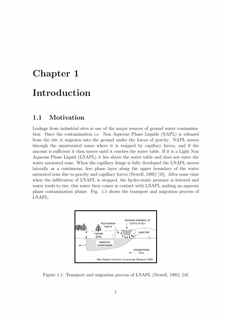
phase contamination plume. Fig. 1.1 shows the transport and migration process of
LNAPL.
Figure 1.1: Transport and migration process of LNAPL (Newell, 1995) [18]
1
1.1 Motivation 2
These industrial sites are prone to contaminate the groundwater, and as such there is
strong emphasis by federal and local governments for remediation of LNAPL from these
sites (Testa, 1989) [24]. To efficiently design remedial options for LNAPL removal it is
necessary to determine the LNAPL distribution, composition, volume, transmissivity
and initial recovery rate. To obtain this information different methods are used such
as excavations and test pits, soil borings, and monitoring wells.
If monitoring wells are properly installed, they can be used to estimate the volume,
transmissivity and initial recovery rate of contaminate. Bail-down test and aquifer
pumping test are commonly used methods to determined this information by con-
structing monitoring well. Both methods have their advantages and disadvantages.
Aquifer pumping test are time consuming and expensive to conduct, as pumping and
observation wells are required. Moreover in some case the extracted water is contam-
inated and need to be treated or the low permeable material do not allow these tests
to determine the information. A better alternative to aquifer pumping is a bail-down
test, where one well is used to determine all the information.
In this work the focus is on evaluating the process and estimates of transmissivity and
initial recovery rate obtain by the bail-down test. Further sections in this report will
give an understanding of the bail-down test.
1.2 Bail-Down Test 3
1.2 Bail-Down Test
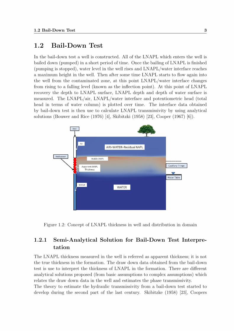
In the bail-down test a well is constructed. All of the LNAPL which enters the well is
bailed down (pumped) in a short period of time. Once the bailing of LNAPL is finished
(pumping is stopped), water level in the well rises and LNAPL/water interface reaches
a maximum height in the well. Then after some time LNAPL starts to flow again into
the well from the contaminated zone, at this point LNAPL/water interface changes
from rising to a falling level (known as the inflection point). At this point of LNAPL
recovery the depth to LNAPL surface, LNAPL depth and depth of water surface is
measured. The LNAPL/air, LNAPL/water interface and potentiometric head (total
head in terms of water column) is plotted over time. The interface data obtained
by bail-down test is then use to calculate LNAPL transmissivity by using analytical
solutions (Bouwer and Rice (1976) [4], Skibitzki (1958) [23], Cooper (1967) [6]).
Figure 1.2: Concept of LNAPL thickness in well and distribution in domain
1.2.1 Semi-Analytical Solution for Bail-Down Test Interpre-
tation
The LNAPL thickness measured in the well is referred as apparent thickness; it is not
the true thickness in the formation. The draw down data obtained from the bail-down
test is use to interpret the thickness of LNAPL in the formation. There are different
analytical solutions proposed (from basic assumptions to complex assumptions) which
relates the draw down data in the well and estimates the phase transmissivity.
The theory to estimate the hydraulic transmissivity from a bail-down test started to
develop during the second part of the last century. Skibitzke (1958) [23], Coopers
1.2 Bail-Down Test 4
(1967) [6], Lohman (1972) [15], Bouwer and Rice (1976) [4] and others developed
theories based on completely different assumptions. As an example, Cooper’s (1967) [6]
approach considers a fully penetrated well in a homogeneous isotropic artesian confined
aquifer. His solution used the differential equation governing non-steady radial flow
of confined groundwater. On the other hand, Bouwer and Rice (1976) [4] considered
a partially or fully penetrated well in an unconfined aquifers. The solution is based
on Thiem’s equation developed for steady flow with equilibrium condition in an
unconfined aquifer. Even if the Bouwer and Rice (1976) [4] solution is developed for
an unconfined aquifer, one can use this solution for a confined aquifer.
For an LNAPL/water system, the bail-down test analytical solutions to assess the
LNAPL transmissivity were developed around 2000. The commonly used solutions
are the modified Bouwer and Rice approaches (Lundy and Zimmerman (1996) [16],
Huntley (2000) [11]) and the modified Cooper solution (Beckett and Lyverse, 2002) [3].
The Lundy and Zimmerman (1996) [16] method assumes that no water enters the well
after the free LNAPL is removed. This assumption implies that the LNAPL/water
interface is not moving during the test which is quite uncommon and not expected.
Huntley (2000) [11] makes the assumption that the water transmissivity is for a
majority of the time much higher than the LNAPL transmissivity and so the total
potentiometric surface remains almost constant during the test.
In this work two analytical approaches are used for analysis of bail-down test model re-
sults to determine the LNAPL transmissivity. The first approach is based on modified
Bouwer and Rice analysis for the slug test (Huntley, 2000) [11]. The second approach
is based on measured LNAPL thickness in well for multi-layered soil (Jeong, 2014) [14].
1.2.1.1 Modified Bouwer and Rice Analysis for the Slug Test
The modified solution given by Huntley (2000) [11] is based on the work of Bouwer and
Rice (1976) [4], where they gave a solution for the slug test for water. To obtain the
LNAPL phase transmissivity (Tn) using the modified solution, it is required that the
(Tn) values be corrected by the reciprocal of the difference between the density of the
water and the density of the LNAPL ( 11−ρn ). This correction is required because unlike
water, as the LNAPL draw down changes, the volume change in the well is greater by
this density factor because water is being depressed in the well bore as LNAPL recovers
(Beckett and Lyverse, 2002) [3].
Huntley (2000) [11] states that if the total potentiometric surface remains relatively
constant during the test, the LNAPL transmissivity is given by:
Tn =2.3rc
2(1/1− ρr)2t
ln(Re
rw) log(
sost
) (1.1)
where Tn is the LNAPL transmissivity, rc is the radius of the casing, t is the elapsed
time, Re is the radius of influence, rw is radius of the well, so is the drawdown at t = 0,
1.2 Bail-Down Test 5
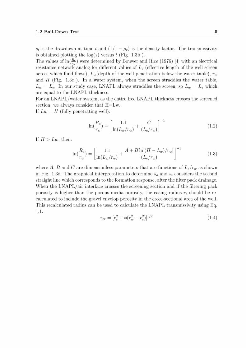
st is the drawdown at time t and (1/1 − ρr) is the density factor. The transmissivity
is obtained plotting the log(s) versus t (Fig. 1.3b ).
The values of ln(Rerw
) were determined by Bouwer and Rice (1976) [4] with an electrical
resistance network analog for different values of Le (effective length of the well screen
across which fluid flows), Lw(depth of the well penetration below the water table), rwand H (Fig. 1.3c ). In a water system, when the screen straddles the water table,
Lw = Le. In our study case, LNAPL always straddles the screen, so Lw = Le which
are equal to the LNAPL thickness.
For an LNAPL/water system, as the entire free LNAPL thickness crosses the screened
section, we always consider that H=Lw.
If Lw = H (fully penetrating well):
ln(Re
rw) =
[1.1
ln(Lw/rw)+
C
(Le/rw)
]−1
(1.2)
If H > Lw, then:
ln(Re
rw) =
[1.1
ln(Lw/rw)+A+B ln[(H − Lw)/rw]
(Le/rw)
]−1
(1.3)
where A, B and C are dimensionless parameters that are functions of Le/rw as shown
in Fig. 1.3d. The graphical interpretation to determine so and st considers the second
straight line which corresponds to the formation response, after the filter pack drainage.
When the LNAPL/air interface crosses the screening section and if the filtering pack
porosity is higher than the porous media porosity, the casing radius rc should be re-
calculated to include the gravel envelop porosity in the cross-sectional area of the well.
This recalculated radius can be used to calculate the LNAPL transmissivity using Eq.
1.1.
rcr = [r2c + φ(r2
w − r2c )]
1/2 (1.4)
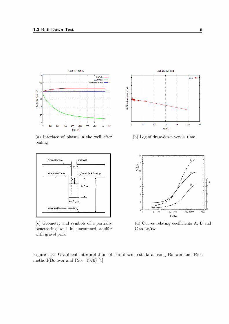
1.2 Bail-Down Test 6
(a) Interface of phases in the well after
bailing
(b) Log of draw-down versus time
(c) Geometry and symbols of a partially
penetrating well in unconfined aquifer
with gravel pack
(d) Curves relating coefficients A, B and
C to Le/rw
Figure 1.3: Graphical interpretation of bail-down test data using Bouwer and Rice
method(Bouwer and Rice, 1976) [4]
1.3 Scope of this Work 7
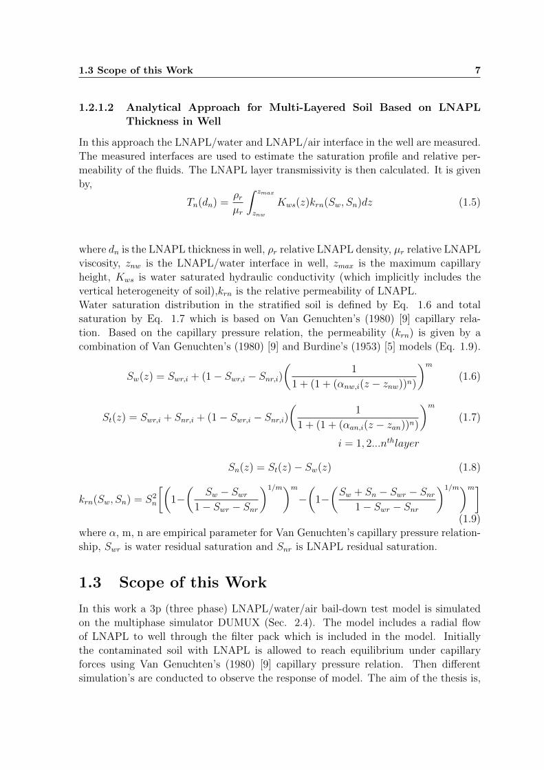
1.2.1.2 Analytical Approach for Multi-Layered Soil Based on LNAPL
Thickness in Well
In this approach the LNAPL/water and LNAPL/air interface in the well are measured.
The measured interfaces are used to estimate the saturation profile and relative per-
meability of the fluids. The LNAPL layer transmissivity is then calculated. It is given
by,
Tn(dn) =ρrµr
∫ zmax
znw
Kws(z)krn(Sw, Sn)dz (1.5)
where dn is the LNAPL thickness in well, ρr relative LNAPL density, µr relative LNAPL
viscosity, znw is the LNAPL/water interface in well, zmax is the maximum capillary
height, Kws is water saturated hydraulic conductivity (which implicitly includes the
vertical heterogeneity of soil),krn is the relative permeability of LNAPL.
Water saturation distribution in the stratified soil is defined by Eq. 1.6 and total
saturation by Eq. 1.7 which is based on Van Genuchten’s (1980) [9] capillary rela-
tion. Based on the capillary pressure relation, the permeability (krn) is given by a
combination of Van Genuchten’s (1980) [9] and Burdine’s (1953) [5] models (Eq. 1.9).
Sw(z) = Swr,i + (1− Swr,i − Snr,i)(
1
1 + (1 + (αnw,i(z − znw))n)
)m(1.6)
St(z) = Swr,i + Snr,i + (1− Swr,i − Snr,i)(
1
1 + (1 + (αan,i(z − zan))n)
)m(1.7)
i = 1, 2...nthlayer
Sn(z) = St(z)− Sw(z) (1.8)
krn(Sw, Sn) = S2n
[(1−(
Sw − Swr1− Swr − Snr
)1/m)m−(
1−(Sw + Sn − Swr − Snr
1− Swr − Snr
)1/m)m](1.9)
where α, m, n are empirical parameter for Van Genuchten’s capillary pressure relation-
ship, Swr is water residual saturation and Snr is LNAPL residual saturation.
1.3 Scope of this Work
In this work a 3p (three phase) LNAPL/water/air bail-down test model is simulated
on the multiphase simulator DUMUX (Sec. 2.4). The model includes a radial flow
of LNAPL to well through the filter pack which is included in the model. Initially
the contaminated soil with LNAPL is allowed to reach equilibrium under capillary
forces using Van Genuchten’s (1980) [9] capillary pressure relation. Then different
simulation’s are conducted to observe the response of model. The aim of the thesis is,
1.4 Structure of Report 8
1. To setup a 3p (LNAPL/water/air) model for bail-down test.
2. To check the reliability of an analytical solution.
3. To see the development of LNAPL in the well by changing the soil and fluid
parameters.
4. To check the performance of the model to multi-layered soil.
1.4 Structure of Report
The fundamentals of the applied multiphase (LNAPL, water and air ) model and the
implementation of the different relationships such as capillary pressure and relative
permeability in the three phase system are described in chapter 2. The description of
the contaminate NAPL (i.e LNAPL/DNAPL), LNAPL transport process in the sub-
surface, and its response to the soil parameters are summarized in chapter 3. Further,
in this chapter the applied problem setup and different simulation cases are defined.
Chapter 4 provides the results describing the draw-down response in the well to dif-
ferent cases and comparison of LNAPL transmissity calculated by analytical solution.
In the last chapter a summary of this work and recommendations for future work are
provided.
Chapter 2
Fundamentals of Multiphase (Three
Phase) Porous Media Model
2.1 General terms
To conduct a numerical simulation it is necessary to transfer the physical process in
the mathematical formulation based on assumptions which reduces the complexity but
adequately describes the physical process. In in this chapter a short description of
important terms in multiphase flow in porous media are given and conceptualization
of the LNAPL/water/air fluid distribution in porous media and monitoring well is
explained. It will give a brief understanding of how physical process are mathematically
modeled.
2.1.1 Phases and Components
Phase is described as a matter with homogeneous chemical properties which is sepa-
rated by a sharp interface and it is characterized by continuous fluid properties. Thus
it is possible for several fluid phases to exists in a porous media, while there is only one
gaseous phase present because there is no interface between the gasses . In the problem
of NAPL contamination, three possible phases can exist: water, air and LNAPL.
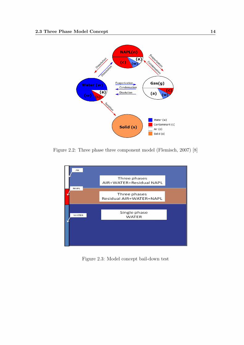
The term components can be define as constituents of a phase, which are associated
with unique chemical species (Flemisch, 2007) [8]. Example can be a dissolved NAPL
component in a water phase see Fig. 2.2.
2.1.2 Wettability
Wettability is defined as the overall tendency of one fluid to spread onto or adhere on
a solid in the presence of another fluid with which it is immiscible. This is used to
define the fluid distribution at the pore scale.
The wetting fluid will coat the solid surface and tend to occupy small pores, while the
9
2.1 General terms 10
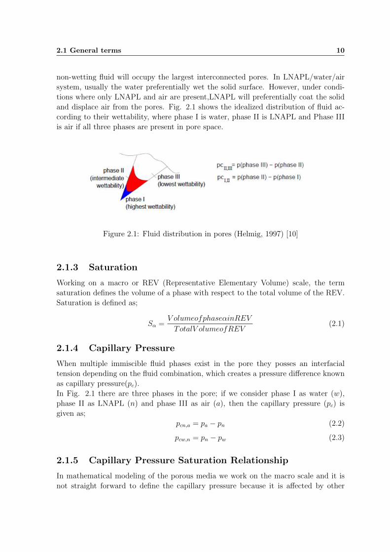
non-wetting fluid will occupy the largest interconnected pores. In LNAPL/water/air
system, usually the water preferentially wet the solid surface. However, under condi-
tions where only LNAPL and air are present,LNAPL will preferentially coat the solid
and displace air from the pores. Fig. 2.1 shows the idealized distribution of fluid ac-
cording to their wettability, where phase I is water, phase II is LNAPL and Phase III
is air if all three phases are present in pore space.
Figure 2.1: Fluid distribution in pores (Helmig, 1997) [10]
2.1.3 Saturation
Working on a macro or REV (Representative Elementary Volume) scale, the term
saturation defines the volume of a phase with respect to the total volume of the REV.
Saturation is defined as;
Sα =V olumeofphaseαinREV
TotalV olumeofREV(2.1)
2.1.4 Capillary Pressure
When multiple immiscible fluid phases exist in the pore they posses an interfacial
tension depending on the fluid combination, which creates a pressure difference known
as capillary pressure(pc).
In Fig. 2.1 there are three phases in the pore; if we consider phase I as water (w),
phase II as LNAPL (n) and phase III as air (a), then the capillary pressure (pc) is
given as;
pcn,a = pa − pn (2.2)
pcw,n = pn − pw (2.3)
2.1.5 Capillary Pressure Saturation Relationship
In mathematical modeling of the porous media we work on the macro scale and it is
not straight forward to define the capillary pressure because it is affected by other
2.1 General terms 11
parameters. The saturation of the phase (i.e wetting phase) has the strongest influence
on the capillary pressure, as describe in Sec. 2.1.2 that wetting phase occupies the
narrow pores and the non-wetting phase prefers the larger pores. If the wetting phase
saturation is low, the average radius of the meniscus is comparatively small and the
capillary pressure is accordingly high. There are different relationships which relates
the capillary pressure with saturation. The Van Genuchten (1980) [9] model is one of
the well known capillary pressure relationship where two phase exists.
pc =1
α(Sw
−1/m − 1)1/n (2.4)
Sw =Sw − Swr1− Swr
(2.5)
m = 1− 1
n(2.6)
Eq. 2.4 gives the general form Van Genuchten model for two phases, where Sw is the
effective saturation given by Eq. 2.5, Swr is the residual saturation (which describes
that the fluid is immobile below this saturation), α is the Van Genuchten pressure
scaling factor, m and n describes the soil uniformity.
For three phase system Parker (1987) [19] extended the Van Genuchten two phase
model by introducing new parameters (i.e βnw, βaw ). He considered the distribution
of phases in the pore based on their wettability as described in Sec. 2.1.2. Capillary
pressure at two interface pcn,a, pcw,n as describe by Eq. 2.3 are calculated. Parker
(1987) [19] gave the following capillary pressure-saturation relation for a three phase
system,
pcnw(Sw) =1
αβnw[(Sw)
n1−n − 1]1/n (2.7)
pcan(Sa) =1
αβan[(1− Sa)
n1−n − 1]1/n (2.8)
Where α, n,m and Sα(α = a, w) are the same parameters as that of Van Genuchten,
while β is the surface tension scaling parameter given as;
βan =σawσan
(2.9)
βnw =σawσnw
(2.10)
2.1.6 Relative Permeability and Extended Darcy’s Law
In a multiphase system, the pore space is occupied by more then one fluid, so the
fluids also experience the resistance in movement from each other. To account for this
resistance in a multiphase system, the permeability in Darcy’s law is multiplied by a
2.2 Mathematical Formulation 12
scalar nondimensional factor kr called relative permeability.
In multiphase flow in porous media, an extended version of Darcy’s law is used, given
by,
vα = −krαµα
K(5pα − ραg) (2.11)
where krα is the relative permeability of the phase α, µα is vicosity, K is intrinsic
permeability, pα pressure and g is the gravitational constant. The ratio krαµα
is called
the mobility λα of the phase.
2.1.7 Saturation-Relative Permeability Relationship
Relative permeability is dependent on the phase saturation. For fully saturated condi-
tions the krα = 1 and flow is considered as a single phase, while krα = 0 for saturation
below residual saturation and fluid is considered as immobile.
In a three phase system, fluid distribution is considered according to their wettability
as decribed in Sec. 2.1.2, so water is always considered as the wetting fluid occupying
small pores and gas as the non-wetting, thus the relative permeability for water and
gas(air) is only dependent on water and air saturation respectively. Their relationship
in a three phase system can be defined by two phase relationship,
krw =
√Sw[1− (1− S1/m
w )m]2 (2.12)
kra =3
√Sa[1− (1− Sa)1/m]2m (2.13)
The problem is with the NAPL, is that it is a intermediate wetting phase and its
distribution in the pores depends on the ratio of gas and water saturation. Parker’s
(1987) [20] approach based on Van Genuchten’s relationship is used here to give LNAPL
relative permeability,
krn =
√Sw
1− Swr
[(1− S
1mw )m − (1− S
1mt )m
]2
(2.14)
St =Sw + Sn − Swr
1− Swr(2.15)
2.2 Mathematical Formulation
The Reynold theorem is used to derive differential formulation of conserve quantity(as
mass). It states that,”the total rate of change of an extensive system property E equals
the rate of change of its corresponding intensive quantity e within a fixed control volume
(CV), plus the net rate change across its boundaries.” Mathematically it can be written
as,dE
dt=
∫Ω
∂(ρe)
∂tdΩ +
∫Γ
(ρe)(v.n)dΓ (2.16)
2.3 Three Phase Model Concept 13
2.2.1 Mass Balance
Considering that the change in mass in a closed system is zero, Reynold’s theorem
(Eq. 2.16) can be used to formulate a continuity equation by considering E in Eq. 2.16
equal to ”m”. In formulation we have to consider that the flow only occurs through
the pores, so porosity φ has to be taken in account. Secondly, this mass balance is
valid for all phases α. The formulation for continuity for each phase α can be given as,
∂(φSαρα)
∂t+5(ραvα) = 0 (2.17)
vα can be replaced by extended Darcy’s law Eq. 2.11, which gives the following form
of mass balance equation,
∂(φSαρα)
∂t︸ ︷︷ ︸accumulation term
−5(ραkrαµα
K(5pα − ραg)
)︸ ︷︷ ︸
advection term
− qc︸︷︷︸sink/source term
= 0 (2.18)
where φ is porosity, ρα is phase density, Sα is phase saturation, kr,α is relative per-
meability of phase α, µα dynamic viscosity, K intrinsic permeability and pα is phase
pressure.
2.3 Three Phase Model Concept
The general model concept for NAPL contamination can be described by the
Fig. 2.2, but in this work we assumed no dissolution of the NAPL. Model imple-
mented here only consists of three phases: LNAPL, air and water, without components.
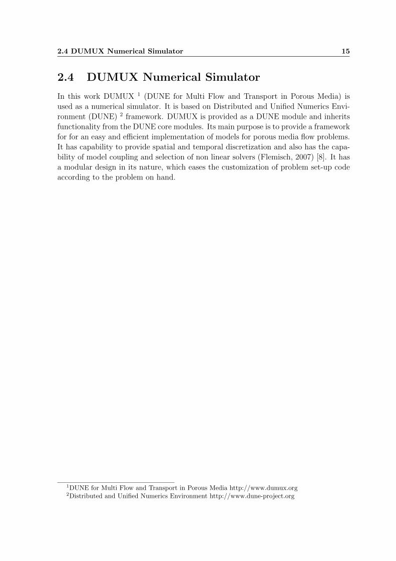
A more elaborate description of our model concept can be seen in the Fig. 2.3, where
three distinct zones can be seen; first one is in the unsaturated zone where the three
phases exists but LNAPL is considered as immobile, second is where also three phases
exists but air is considered as immobile and third zone is considered as fully saturated
with water.
We also conceptualized the well; in Fig. 2.3 at the extreme left is the well. There are
also three distinct zones visible. The first is where only air exists, then only LNAPL
and below that only water. The well is in cooperated in porous media domain as a
single phase with porosity and relative permeability of one (for futher details see Sec.
3.3).
2.3 Three Phase Model Concept 14
Figure 2.2: Three phase three component model (Flemisch, 2007) [8]
Figure 2.3: Model concept bail-down test
2.4 DUMUX Numerical Simulator 15
2.4 DUMUX Numerical Simulator
In this work DUMUX 1 (DUNE for Multi Flow and Transport in Porous Media) is
used as a numerical simulator. It is based on Distributed and Unified Numerics Envi-
ronment (DUNE) 2 framework. DUMUX is provided as a DUNE module and inherits
functionality from the DUNE core modules. Its main purpose is to provide a framework
for for an easy and efficient implementation of models for porous media flow problems.
It has capability to provide spatial and temporal discretization and also has the capa-
bility of model coupling and selection of non linear solvers (Flemisch, 2007) [8]. It has
a modular design in its nature, which eases the customization of problem set-up code
according to the problem on hand.
1DUNE for Multi Flow and Transport in Porous Media http://www.dumux.org2Distributed and Unified Numerics Environment http://www.dune-project.org
Chapter 3
Light Non Aqueous Phase Liquids
(LNAPL)
3.1 Introduction
Hydrocarbons that make an interface with water and exist as a separate, immisci-
ble phase when in contact with water or air are known as Nonaqueous Phase Liquids
(NAPLs) (Newell, 1995) [18]. Hydrocarbon having density more then water are clas-
sified as Dense Non Aqueous Phase Liquids (DNAPLs), whereas hydrocarbon having
density less then water are classified as Light Non Aqueous Phase Liquids (LNAPLs).
In our study the contaminant is LNAPL, thus the focus further in this section will be
on the transport process of LNAPL.
As discussed in Sec. 1.1, LNAPL are a source of contamination and to design their
remediation it is necessary to predict their volume and transmissivity. Research on
LNAPL in subsurface has been going on for years and so different conceptual mod-
els have been proposed. Early models (as Testa, 1989) [24] considered LNAPL as a
layer floating on the water table creating an oil saturated zone above the water table
known as ”oilpancakes”. Lenhard and Parker (1990) [22] showed that in the major-
ity of aquifers where uniform pore size distribution is not considered oil pancakes do
not exist. They showed that above the water table there is a effect of capillary and
LNAPL/water occurs in variable saturation above water saturated zones, thus consid-
ering the early conceptual models can lead to over estimation of in situ LNAPL and
can set unrealistic precedents for site closure goals (Beckett, 1994) [2].
Lenhard and Parker (1990) [22], Farr (1990) [7] and others considered multiphase theory
with three phases (LNAPL/water/air) to give a new concept of LNAPL estimation in
subsurface and their results were verified by Huntley (1994) [12] with field observations.
Multiphase theory shows that the LNAPL recovery is dependent upon the distribution
of contaminant, volume, its mobility and contaminant chemistry, which are controlled
by specific soil and fluid properties such as capillary pressure (Peargin, 1999) [21]. It is
necessary to understand the multiphase process involved in LNAPL migration in the
16
3.2 Fate and Transport of LNAPL in Subsurface 17
subsurface. In the following sections, a brief discussion is given about the processes
and parameter effecting LNAPL in the subsurface while considering multiphase theory.
3.2 Fate and Transport of LNAPL in Subsurface
A brief introduction regarding transport of LNAPL after release from the source was
given in the motivation (Sec. 1.1). This section will extend that discussion and focus
will be on parameters effecting that transport. If you are interested in reading more
about LNAPL transport in porous media, see Mercer (1990) [17] and Newell (1995) [18].
When there is a spill on the ground or leakage from a industrial site, LNAPL start
to migrate into the ground under the forces of gravity and spread laterally due to
the capillary forces. As LNAPL continues to moves through the unsaturated zones it
is trapped into the pores due to the effects of surface tension (it is known as residual
liquid, parameter representing it is residual saturation Snr), making a permanent source
for contamination (if there is recharge or fluctuation of water table). While moving
through the unsaturated zone some of the immiscible fluid may volatilize and form
vapors (In this work volatilization and biodegradation are neglected, so there will not
much discussion regarding these effects). If the amount is sufficient then it moves until
it reaches the water table; if it is LNAPL it will lie above the water table and will
not enter the water saturated zone. When the capillary fringe is fully developed the
LNAPL moves laterally as a continuous, free phase layer along the upper boundary
of the water saturated zone due to gravity and capillary forces (Newell, 1995) [18].
After some time when the infiltration of LNAPL is stopped, the hydro-static pressure
of LNAPL is reduced and water tends to rise. This water then comes in contact with
residual LNAPL making an aqueous phase contamination plume. Fig. 1.1 shows the
transport and migration process of LNAPL.
According to multiphase theory the fluid exists as different phases in the subsurface
as described in Sec. 2.1.1. When LNAPL enters the unsaturated zone it can exist in
four physical states as a gas, sorbed to solid, dissolved in water or as immiscible liquid.
Further when it migrates to the water saturated zone, LNAPL constituents may be
dissolved in the water where it can exist as a component. In this work the model
concept is only three phase, so no dissolved components are considered.
3.2.1 Parameters Effecting LNAPL Transport During Bail-
Down test
As described previously, in the bail-down test the LNAPL is bailed, after which the
LNAPL starts entering the well. It can be seen from the extended Darcy’s law (Eq.
2.11) that the movement of LNAPL depends on its mobility λ (which in turn depends
on relative permeability, saturation, viscosity, density and capillary pressure).
If the soil in the formation is fine, the Van Genuchten α (which is a capillary pressure
3.2 Fate and Transport of LNAPL in Subsurface 18
scaling factor) will be low, according to Van Genuchten’s model (Eq. 2.4) the capillary
fringe will be high making the maximum saturation low. According to the saturation-
relative permeability relationship (Sec. 2.1.7), low saturation will lead to a low value
of relative permeability and LNAPL will be less mobile, thus causing LNAPL recovery
in the well to slow down.
Capillary pressure developed in the formation depends on the pore size, moisture con-
tent and interfacial tension. If LNAPL and water exists in the system, due to the
density difference/interfacial tension, there will be a capillary pressure (Sec. 2.1.4)
which will lead water to enter the pores above the saturated zone making a capil-
lary fringe. Capillary condition also affects the distribution and magnitude of trapped
LNAPL in the formation.
As the mobility of LNAPL depends on viscosity, and the viscosity depends on tem-
perature, the movement of LNAPL can also be governed by the temperature. High
temperature leads to low viscosity and high movement of LNAPL, so in the case of
high temperature the LNAPL development in the well will be fast because low vis-
cosity leads to high mobility. In this work the temperature is constant, so there is no
variation in viscosity and density with respect to temperature.
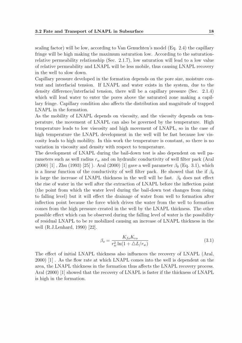
The development of LNAPL during the bail-down test is also dependent on well pa-
rameters such as well radius rw and on hydraulic conductivity of well filter pack (Aral
(2000) [1] , Zhu (1993) [25] ). Aral (2000) [1] gave a well parameter β0 (Eq. 3.1), which
is a linear function of the conductivity of well filter pack. He showed that the if β0
is large the increase of LNAPL thickness in the well will be fast. β0 does not effect
the rise of water in the well after the extraction of LNAPL before the inflection point
(the point from which the water level during the bail-down test changes from rising
to falling level) but it will effect the drainage of water from well to formation after
inflection point because the force which drives the water from the well to formation
comes from the high pressure created in the well by the LNAPL thickness. The other
possible effect which can be observed during the falling level of water is the possibility
of residual LNAPL to be re mobilized causing an increase of LNAPL thickness in the
well (R.J.Lenhard, 1990) [22].
βo =KfoKro
r2w ln(1 +4L/rw)
(3.1)
The effect of initial LNAPL thickness also influences the recovery of LNAPL (Aral,
2000) [1] . As the flow rate at which LNAPL comes into the well is dependent on the
area, the LNAPL thickness in the formation thus affects the LNAPL recovery process.
Aral (2000) [1] showed that the recovery of LNAPL is faster if the thickness of LNAPL
is high in the formation.
3.3 Bail-Down Test Applied Problem 19
3.3 Bail-Down Test Applied Problem
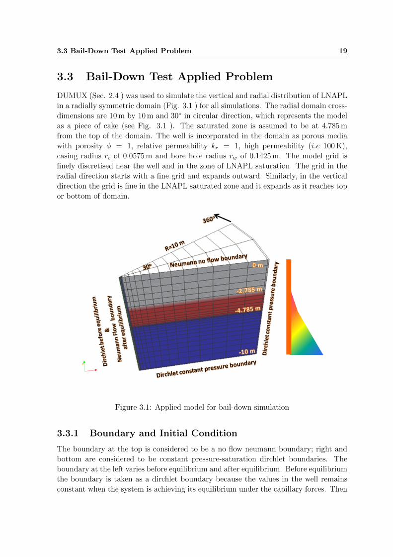
DUMUX (Sec. 2.4 ) was used to simulate the vertical and radial distribution of LNAPL
in a radially symmetric domain (Fig. 3.1 ) for all simulations. The radial domain cross-
dimensions are 10 m by 10 m and 30 in circular direction, which represents the model
as a piece of cake (see Fig. 3.1 ). The saturated zone is assumed to be at 4.785 m
from the top of the domain. The well is incorporated in the domain as porous media
with porosity φ = 1, relative permeability kr = 1, high permeability (i.e 100 K),
casing radius rc of 0.0575 m and bore hole radius rw of 0.1425 m. The model grid is
finely discretised near the well and in the zone of LNAPL saturation. The grid in the
radial direction starts with a fine grid and expands outward. Similarly, in the vertical
direction the grid is fine in the LNAPL saturated zone and it expands as it reaches top
or bottom of domain.
Figure 3.1: Applied model for bail-down simulation
3.3.1 Boundary and Initial Condition
The boundary at the top is considered to be a no flow neumann boundary; right and
bottom are considered to be constant pressure-saturation dirchlet boundaries. The
boundary at the left varies before equilibrium and after equilibrium. Before equilibrium
the boundary is taken as a dirchlet boundary because the values in the well remains
constant when the system is achieving its equilibrium under the capillary forces. Then
3.4 Different Simulation Cases 20
when equilibrium is achieved, a neumann flow boundary is applied to represent the
extraction of LNAPL.
The initial condition for the formation and the well varies according to the simulation
cases such as LNAPL thickness, viscosity, hydraulic conductivity and Van Genuchten
α (which are described for each simulation in Sec. 3.4 ) to quantify their effect on well
draw down, the general initial conditions which remain the same for all simulations
are,
• Saturated zone is assumed to be constant for all simulations, which is at 4.785 m
below from top of domain, where the saturation of water Sw = 0.99 in formation
and well.
• The initial reservoir pressure is given by hydro-static pressure distribution, using
p = patm + dwρwg + dnρng. With patm assumed to be 1.013 bar, dw (depth of
water) and dn (depth of LNAPL) varies according to the point where the pressure
is calculated.
• Temperature is assumed to be constant at T = 293 K.
• Density ( ρn = 882 kg/m3, ρw = 1000 kg/m3 ) is assumed to be constant.
3.4 Different Simulation Cases
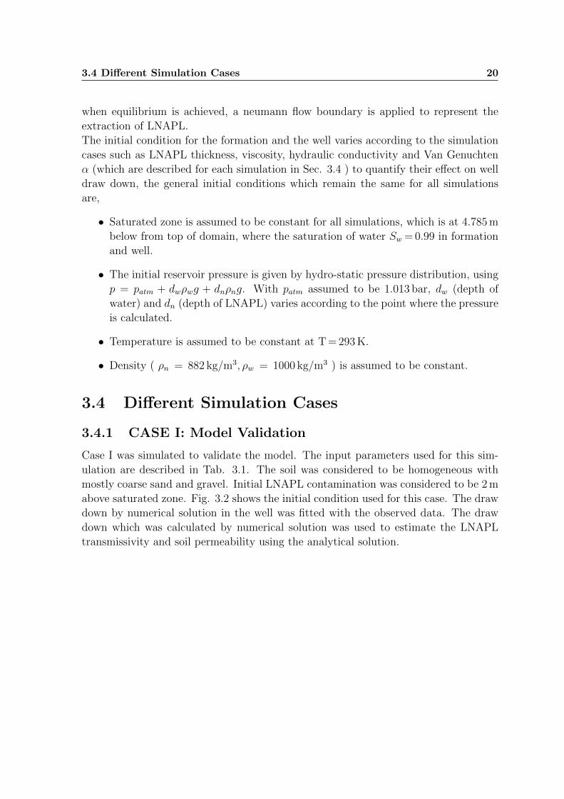
3.4.1 CASE I: Model Validation
Case I was simulated to validate the model. The input parameters used for this sim-
ulation are described in Tab. 3.1. The soil was considered to be homogeneous with
mostly coarse sand and gravel. Initial LNAPL contamination was considered to be 2 m
above saturated zone. Fig. 3.2 shows the initial condition used for this case. The draw
down by numerical solution in the well was fitted with the observed data. The draw
down which was calculated by numerical solution was used to estimate the LNAPL
transmissivity and soil permeability using the analytical solution.
3.4 Different Simulation Cases 21
Figure 3.2: Initial condition case I
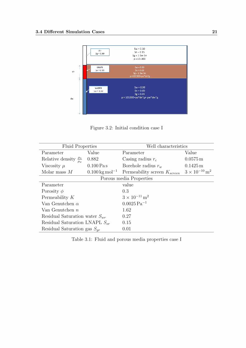
Fluid Properties Well characteristics
Parameter Value Parameter Value
Relative density ρnρw
0.882 Casing radius rc 0.0575 m
Viscosity µ 0.100 Pa s Borehole radius rw 0.1425 m
Molar mass M 0.100 kg mol−1 Permeability screen Kscreen 3× 10⁻¹⁰ m2
Porous media Properties
Parameter value
Porosity φ 0.3
Permeability K 3× 10⁻¹¹ m2
Van Genutchen α 0.0025 Pa−1
Van Genutchen n 1.62
Residual Saturation water Swr 0.27
Residual Saturation LNAPL Sor 0.15
Residual Saturation gas Sgr 0.01
Table 3.1: Fluid and porous media properties case I
3.4 Different Simulation Cases 22
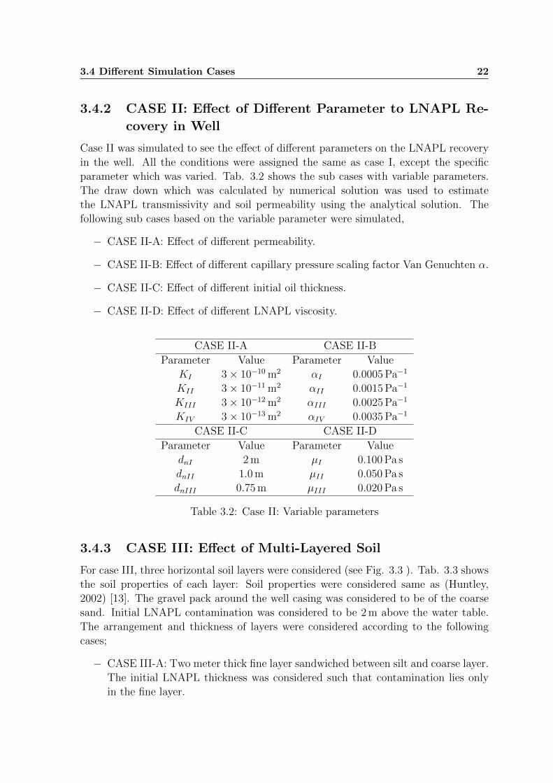
3.4.2 CASE II: Effect of Different Parameter to LNAPL Re-
covery in Well
Case II was simulated to see the effect of different parameters on the LNAPL recovery
in the well. All the conditions were assigned the same as case I, except the specific
parameter which was varied. Tab. 3.2 shows the sub cases with variable parameters.
The draw down which was calculated by numerical solution was used to estimate
the LNAPL transmissivity and soil permeability using the analytical solution. The
following sub cases based on the variable parameter were simulated,
− CASE II-A: Effect of different permeability.
− CASE II-B: Effect of different capillary pressure scaling factor Van Genuchten α.
− CASE II-C: Effect of different initial oil thickness.
− CASE II-D: Effect of different LNAPL viscosity.
CASE II-A CASE II-B
Parameter Value Parameter Value
KI 3× 10⁻¹⁰ m2 αI 0.0005 Pa−1
KII 3× 10⁻¹¹ m2 αII 0.0015 Pa−1
KIII 3× 10⁻¹² m2 αIII 0.0025 Pa−1
KIV 3× 10⁻¹³ m2 αIV 0.0035 Pa−1
CASE II-C CASE II-D
Parameter Value Parameter Value
dnI 2 m µI 0.100 Pa s
dnII 1.0 m µII 0.050 Pa s
dnIII 0.75 m µIII 0.020 Pa s
Table 3.2: Case II: Variable parameters
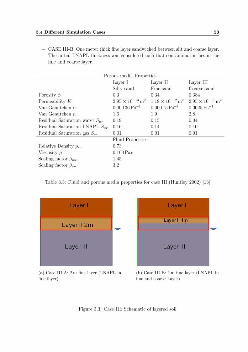
3.4.3 CASE III: Effect of Multi-Layered Soil
For case III, three horizontal soil layers were considered (see Fig. 3.3 ). Tab. 3.3 shows
the soil properties of each layer: Soil properties were considered same as (Huntley,
2002) [13]. The gravel pack around the well casing was considered to be of the coarse
sand. Initial LNAPL contamination was considered to be 2 m above the water table.
The arrangement and thickness of layers were considered according to the following
cases;
− CASE III-A: Two meter thick fine layer sandwiched between silt and coarse layer.
The initial LNAPL thickness was considered such that contamination lies only
in the fine layer.
3.4 Different Simulation Cases 23
− CASE III-B: One meter thick fine layer sandwiched between silt and coarse layer.
The initial LNAPL thickness was considered such that contamination lies in the
fine and coarse layer.
Porous media Properties
Layer I Layer II Layer III
Silty sand Fine sand Coarse sand
Porosity φ 0.3 0.34 0.384
Permeability K 2.95× 10⁻¹³ m2 1.18× 10⁻¹² m2 2.95× 10⁻¹¹ m2
Van Genutchen α 0.000 36 Pa−1 0.000 75 Pa−1 0.0025 Pa−1
Van Genutchen n 1.6 1.9 2.8
Residual Saturation water Swr 0.19 0.15 0.04
Residual Saturation LNAPL Snr 0.16 0.14 0.10
Residual Saturation gas Sgr 0.01 0.01 0.01
Fluid Properties
Relative Density ρrn 0.73
Viscosity µ 0.100 Pa s
Scaling factor βnw 1.45
Scaling factor βan 3.2
Table 3.3: Fluid and porous media properties for case III (Huntley 2002) [13]
(a) Case III-A: 2 m fine layer (LNAPL in
fine fayer)
(b) Case III-B: 1 m fine layer (LNAPL in
fine and coarse Layer)
Figure 3.3: Case III: Schematic of layered soil
Chapter 4
Results and Discussion
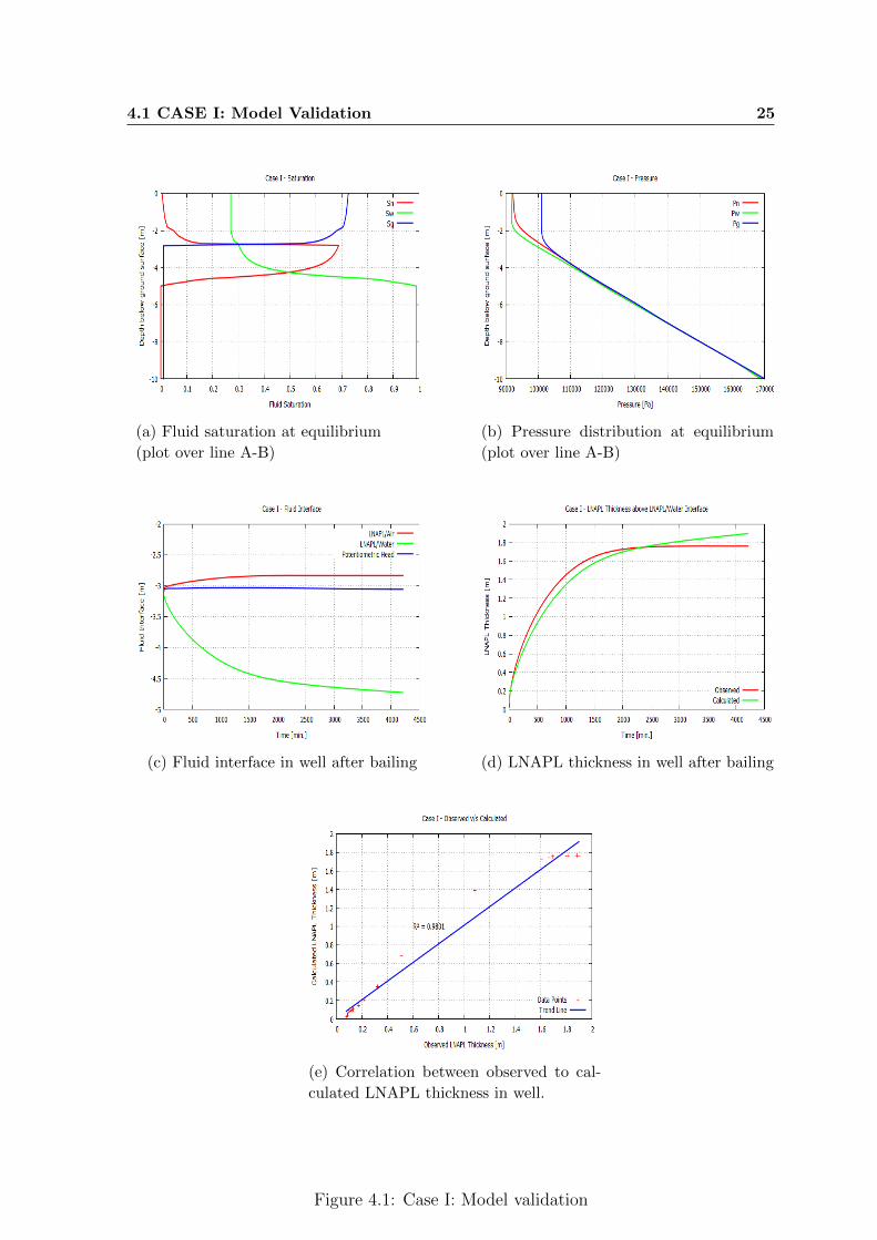
4.1 CASE I: Model Validation
Fig. 4.1a shows the saturation profile which was achieved at the equilibrium. Equilib-
rium condition was considered to have been reached when the capillary pressure in the
domain was minimized and the pressure profile in the system became linear (see Fig.
4.1b). At the equilibrium the maximum LNAPL saturation of 0.68 was achieved.
Fig. 4.1c shows the fluid interface and the potentiometric head (total head in term
of water height) achieved after the bailing of LNAPL in the well. It can be seen that
after the extraction of LNAPL from the well, water level rises in the well and after
certain time the LNAPL starts to enter the well from the formation until it achieves
an asymptotic height. The 80 % recovery time of LNPAL thickness in the well was
achieved at 1200 min which refer to 0.0225 gal/min estimated recovery rate (see Tab.
4.1).
This LNAPL draw down shows good correlation with observed data (Fig. 4.1d). A
good fit between calculated LNAPL thickness and observed values was achieved withR2
of 0.9831 (see Fig. 4.1e). Further validation was done by estimating the transmissivity
with a modified Bouwer and Rice analytical solution. LNAPL transmissivity estimated
by analytical solution was 2.52× 10⁻⁶ m2/s which corresponds to 1.45× 10⁻¹¹ m2 per-
meability for the soil which is in the same order of magnitude as the input to the
numerical solution.
KInput Tn Kanalytical 80 % Recovery time Estimated
m2 m2/s m2 min Recovery rate gal/min
3.00× 10⁻¹¹ 2.52× 10⁻⁶ 1.45× 10⁻¹¹ 1200 0.0225
Table 4.1: Case I: Analytical solution using modified Bouwer and Rice approach
24
4.1 CASE I: Model Validation 25
(a) Fluid saturation at equilibrium
(plot over line A-B)
(b) Pressure distribution at equilibrium
(plot over line A-B)
(c) Fluid interface in well after bailing (d) LNAPL thickness in well after bailing
(e) Correlation between observed to cal-
culated LNAPL thickness in well.
Figure 4.1: Case I: Model validation
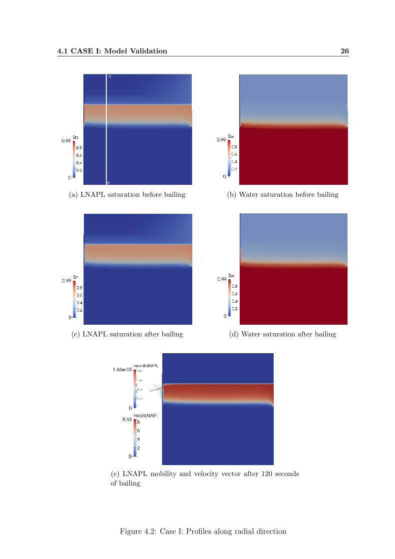
4.1 CASE I: Model Validation 26
(a) LNAPL saturation before bailing (b) Water saturation before bailing
(c) LNAPL saturation after bailing (d) Water saturation after bailing
(e) LNAPL mobility and velocity vector after 120 seconds
of bailing
Figure 4.2: Case I: Profiles along radial direction
4.2 CASE II: Effect of Different Parameter to LNAPL Recovery in Well 27
The simulation showed that the modified Bouwer and Rice method (Huntley, 2000) [11]
yields good results for the bail-down test simulations. The reason that it worked well
is due to the assumption that the draw down induced by the water removal is to be
much more lower than the saturated aquifer thickness and the LNAPL mobility only
depends on a thin part of the entire LNAPL layer where the Sn is maximal. From
Fig. 4.2e it can be seen that the maximum velocity vectors are at the top of LNAPL
contaminated layer where the LNAPL saturation is at a maximum.
4.2 CASE II: Effect of Different Parameter to
LNAPL Recovery in Well
The resulting LNAPL transmissivity for different sub cases demonstrates its depen-
dency on different input parameters. Tab. 4.2 shows result for different soil perme-
ability K; it can be seen that the values calculated from the analytical solution are in
the same order of magnitude as the input value to the model. The estimated values
comes closer when the input values of the soil permeability K is in the range of coarse
sand and gravel because other input parameters are for the coarse sand and gravel (as
Case-I). Similarly Tab. 4.3 shows the results for different Van Genuchten α. It can be
seen that when the value of α is smaller as 5 × 10⁻⁴ (as for sandy loam or silt), the
analytically calculated LNAPL transmissivity is lower and the value of permeability of
soil K does not corresponds to the input value.
Case II-C (Sec. 4.2.3 ) shows that the initial LNAPL thickness in the formation also
has significant influence on the estimation of LNAPL transmissivity. Larger thickness
yields higher maximum saturation, thus higher LNAPL recovery rate. Tab. 4.4 shows
that the larger thickness gives higher transmissivity of LNAPL.
Case II-D (Sec. 4.2.4 ) shows that the high viscosity of LNAPL leads to low trans-
missivity of LNAPL. Tab. 4.4 shows that the soil permeability recalculated from the
analytical solution does not corresponds to the input value for high viscous LNAPL
because the recovery of LNAPL is slow in this case. Additionally, the initial LNAPL
thickness in the formation is considered to be 1 m, which makes the LNAPL recovery
in the well slower then the 2 m LNAPL thickness as in Case I (Sec. 4.1 ).
4.2 CASE II: Effect of Different Parameter to LNAPL Recovery in Well 28
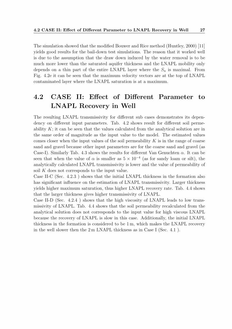
4.2.1 CASE II-A: Effect of Different Permeability
The saturation profile (Fig. 4.3a ) achieved at equilibrium for different permeability
cases is same because the capillary pressure scaling factors (as Van Genuchten α, n
and m) for all sub cases are the same. Maximum saturation achieved is 0.68, the same
as case I.
The response of LNAPL recovery for high permeable soil is faster then low permeable
soil (Fig. 4.3b), from Tab. 4.2 it can be seen that the 80% recovery of LNAPL height
in the well is quicker for high permeable soil and the estimated initial recovery rates
are also high.
(a) Fluid saturation at equilibrium (b) LNAPL thickness in well after bailing
Figure 4.3: Case II-A: Effect of different permeability
KInput Tn Kanalytical 80 % recovery time Estimated recovery rate
m2 m2/s m2 min gal/min
3.00× 10⁻¹⁰ 2.14× 10⁻⁵ 1.24× 10⁻¹⁰ 240 0.1124
3.00× 10⁻¹¹ 2.52× 10⁻⁶ 1.45× 10⁻¹¹ 1200 0.0225
3.00× 10⁻¹² 5.03× 10⁻⁷ 2.91× 10⁻¹² 10897 0.0025
3.00× 10⁻¹³ 3.77× 10⁻⁸ 2.18× 10⁻¹³ 40000 0.0007
Table 4.2: Case II-A: Analytical solution using modified Bouwer and Rice approach
4.2 CASE II: Effect of Different Parameter to LNAPL Recovery in Well 29
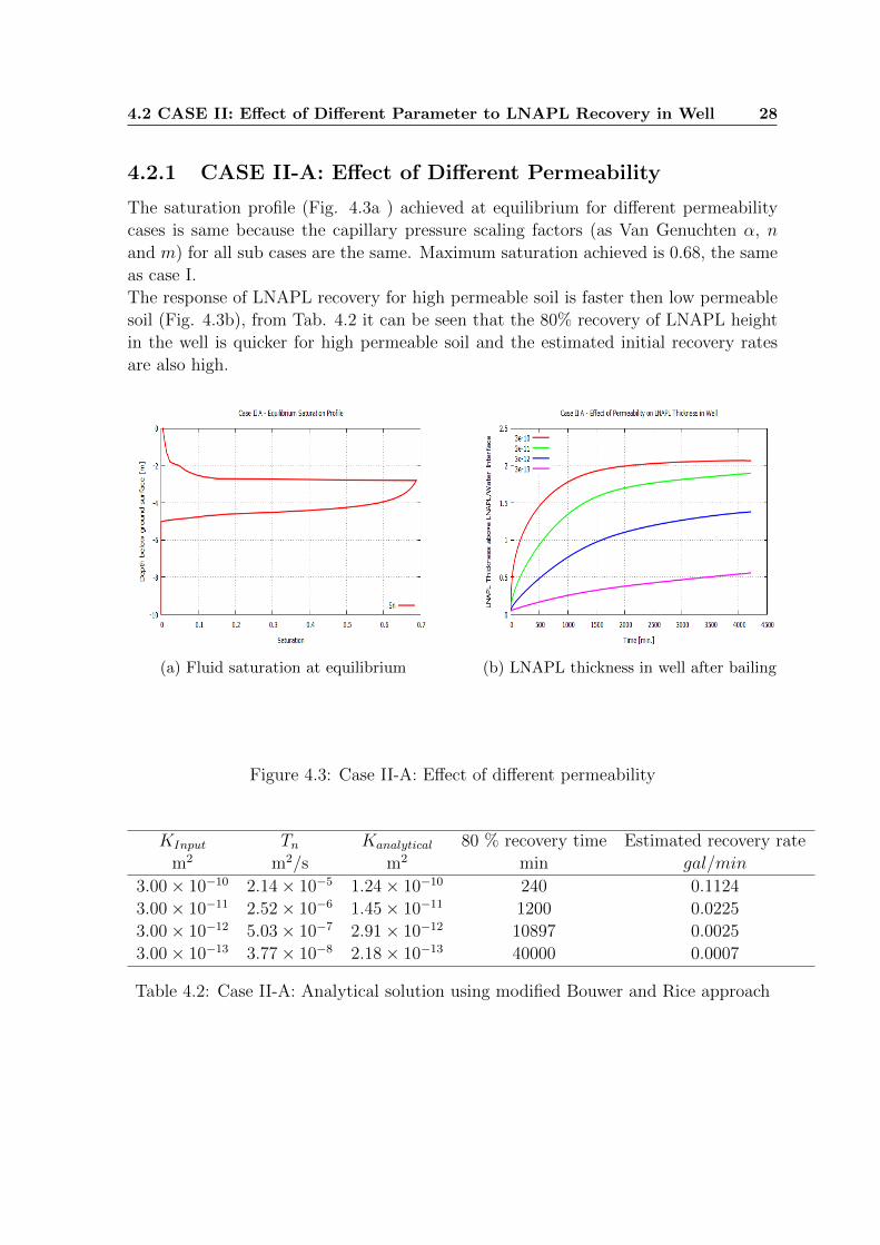
4.2.2 CASE II-B: Effect of Different Van Genuchten α
Van Genuchten α is the capillary pressure scaling factor and it effects the saturation
distribution in the soil (see Sec. 2.1.5). Fig. 4.4a shows the saturation profile achieved
at equilibrium for different Van Genuchten α: it can be seen that when the α is small
such as 5× 10⁻⁴ 1/Pa the maximum saturation achieved is low, which slows down the
LNAPL recovery process (Fig. 4.4b). The 80% recovery time of LNAPL height in the
well is high, which estimates a small initial LNAPL recovery rate (see Tab. 4.3). This
is because the relative permeability of LNAPL (which is saturation dependent) is low
for low saturation.
(a) Fluid saturation at equilibrium (b) LNAPL thickness in well after bailing
Figure 4.4: Case II-B: Effect of different Van Genuchten α
αInput Tn Kanalytical 80 % recovery time Estimated recovery rate
1/Pa m2/s m2 min gal/min
5× 10⁻⁴ 2.52× 10⁻⁷ 1.45× 10⁻¹² 2518 0.0107
15× 10−4 2.52× 10⁻⁶ 1.45× 10⁻¹¹ 1440 0.0187
25× 10−4 2.52× 10⁻⁶ 1.45× 10⁻¹¹ 1200 0.0225
35× 10−4 3.65× 10⁻⁶ 2.11× 10⁻¹¹ 1015 0.0266
Table 4.3: Case II-B: Analytical solution using modified Bouwer and Rice approach
4.2 CASE II: Effect of Different Parameter to LNAPL Recovery in Well 30
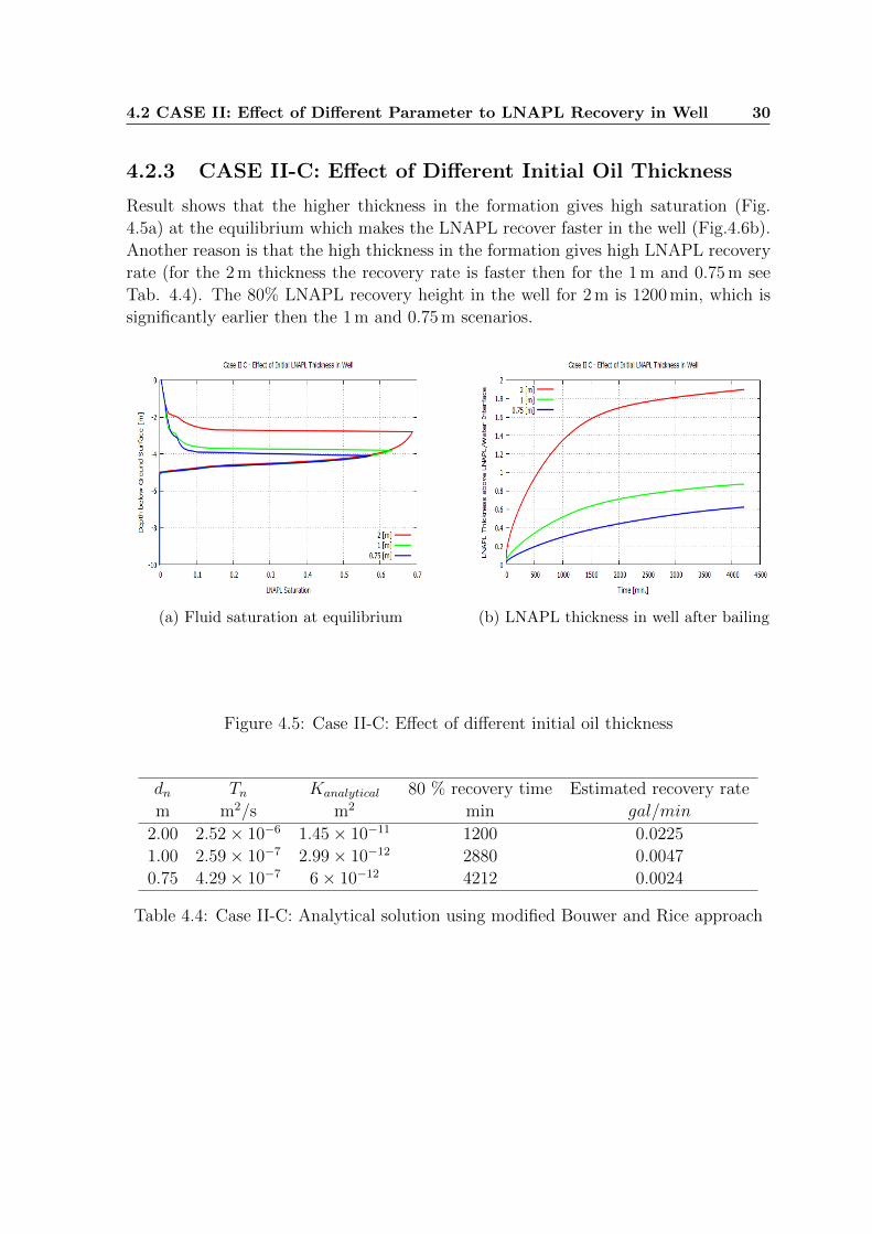
4.2.3 CASE II-C: Effect of Different Initial Oil Thickness
Result shows that the higher thickness in the formation gives high saturation (Fig.
4.5a) at the equilibrium which makes the LNAPL recover faster in the well (Fig.4.6b).
Another reason is that the high thickness in the formation gives high LNAPL recovery
rate (for the 2 m thickness the recovery rate is faster then for the 1 m and 0.75 m see
Tab. 4.4). The 80% LNAPL recovery height in the well for 2 m is 1200 min, which is
significantly earlier then the 1 m and 0.75 m scenarios.
(a) Fluid saturation at equilibrium (b) LNAPL thickness in well after bailing
Figure 4.5: Case II-C: Effect of different initial oil thickness
dn Tn Kanalytical 80 % recovery time Estimated recovery rate
m m2/s m2 min gal/min
2.00 2.52× 10⁻⁶ 1.45× 10⁻¹¹ 1200 0.0225
1.00 2.59× 10⁻⁷ 2.99× 10⁻¹² 2880 0.0047
0.75 4.29× 10⁻⁷ 6× 10⁻¹² 4212 0.0024
Table 4.4: Case II-C: Analytical solution using modified Bouwer and Rice approach
4.2 CASE II: Effect of Different Parameter to LNAPL Recovery in Well 31
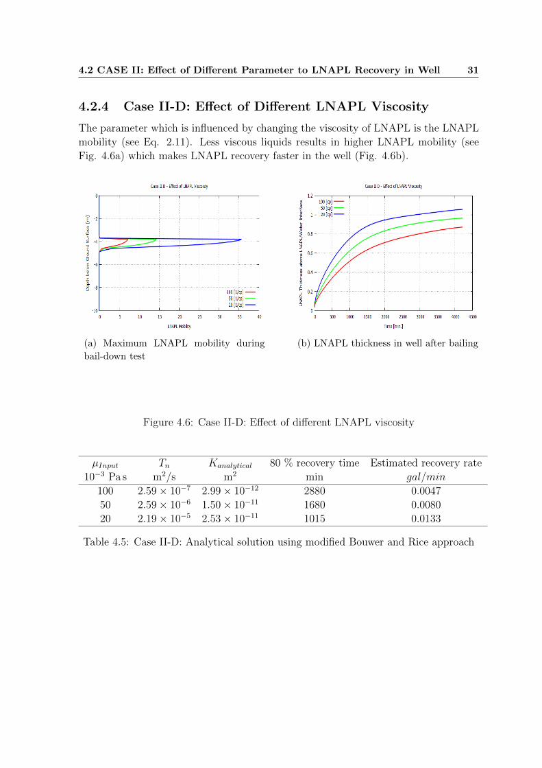
4.2.4 Case II-D: Effect of Different LNAPL Viscosity
The parameter which is influenced by changing the viscosity of LNAPL is the LNAPL
mobility (see Eq. 2.11). Less viscous liquids results in higher LNAPL mobility (see
Fig. 4.6a) which makes LNAPL recovery faster in the well (Fig. 4.6b).
(a) Maximum LNAPL mobility during
bail-down test
(b) LNAPL thickness in well after bailing
Figure 4.6: Case II-D: Effect of different LNAPL viscosity
µInput Tn Kanalytical 80 % recovery time Estimated recovery rate
10−3 Pa s m2/s m2 min gal/min
100 2.59× 10⁻⁷ 2.99× 10⁻¹² 2880 0.0047
50 2.59× 10⁻⁶ 1.50× 10⁻¹¹ 1680 0.0080
20 2.19× 10⁻⁵ 2.53× 10⁻¹¹ 1015 0.0133
Table 4.5: Case II-D: Analytical solution using modified Bouwer and Rice approach
4.3 CASE III: Effect of Multi-Layered Soil 32
4.3 CASE III: Effect of Multi-Layered Soil
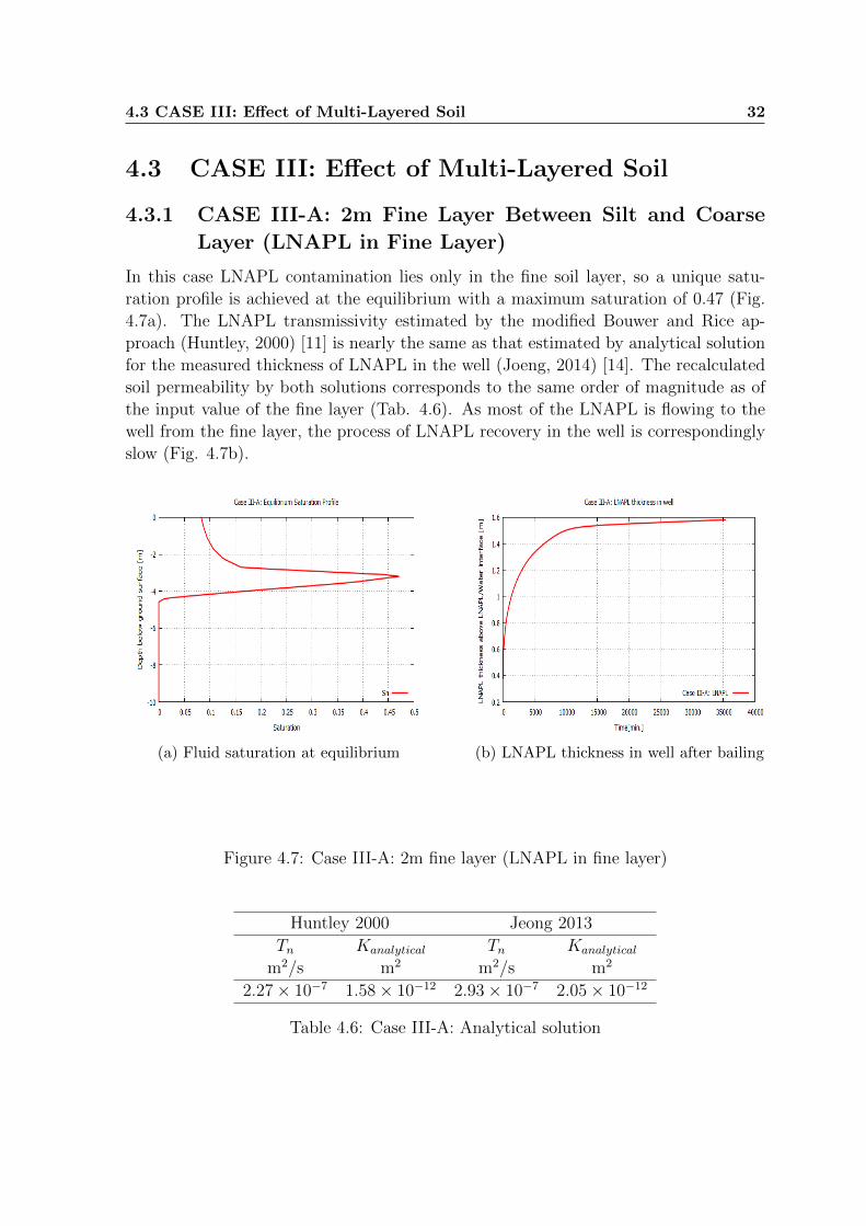
4.3.1 CASE III-A: 2m Fine Layer Between Silt and Coarse
Layer (LNAPL in Fine Layer)
In this case LNAPL contamination lies only in the fine soil layer, so a unique satu-
ration profile is achieved at the equilibrium with a maximum saturation of 0.47 (Fig.
4.7a). The LNAPL transmissivity estimated by the modified Bouwer and Rice ap-
proach (Huntley, 2000) [11] is nearly the same as that estimated by analytical solution
for the measured thickness of LNAPL in the well (Joeng, 2014) [14]. The recalculated
soil permeability by both solutions corresponds to the same order of magnitude as of
the input value of the fine layer (Tab. 4.6). As most of the LNAPL is flowing to the
well from the fine layer, the process of LNAPL recovery in the well is correspondingly
slow (Fig. 4.7b).
(a) Fluid saturation at equilibrium (b) LNAPL thickness in well after bailing
Figure 4.7: Case III-A: 2m fine layer (LNAPL in fine layer)
Huntley 2000 Jeong 2013
Tn Kanalytical Tn Kanalytical
m2/s m2 m2/s m2
2.27× 10⁻⁷ 1.58× 10⁻¹² 2.93× 10⁻⁷ 2.05× 10⁻¹²
Table 4.6: Case III-A: Analytical solution
4.3 CASE III: Effect of Multi-Layered Soil 33
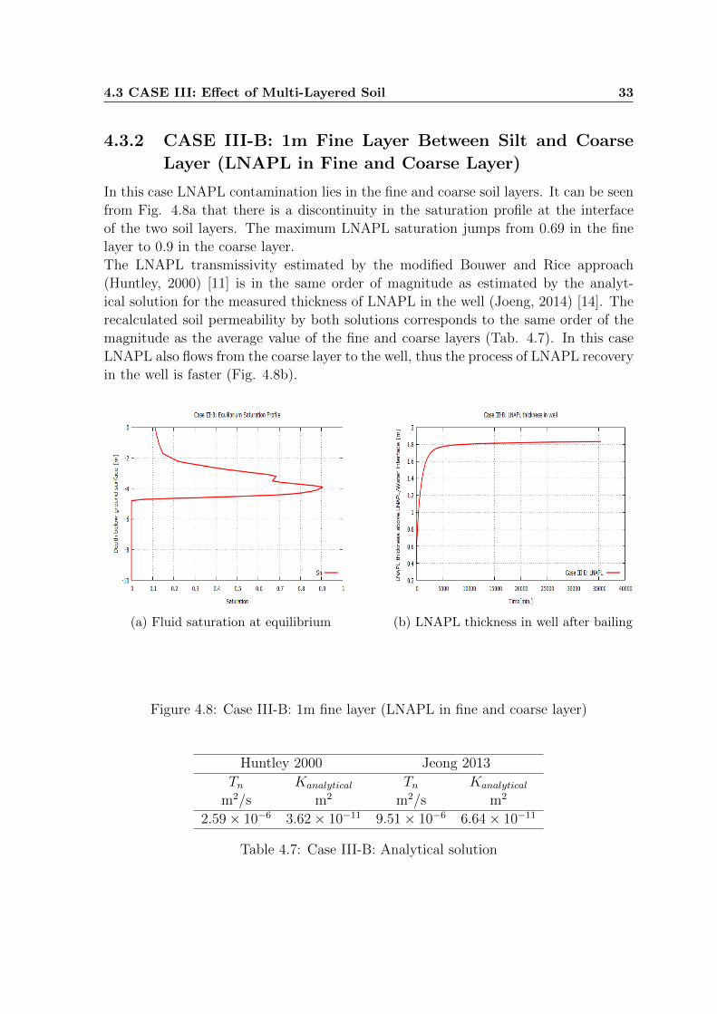
4.3.2 CASE III-B: 1m Fine Layer Between Silt and Coarse
Layer (LNAPL in Fine and Coarse Layer)
In this case LNAPL contamination lies in the fine and coarse soil layers. It can be seen
from Fig. 4.8a that there is a discontinuity in the saturation profile at the interface
of the two soil layers. The maximum LNAPL saturation jumps from 0.69 in the fine
layer to 0.9 in the coarse layer.
The LNAPL transmissivity estimated by the modified Bouwer and Rice approach
(Huntley, 2000) [11] is in the same order of magnitude as estimated by the analyt-
ical solution for the measured thickness of LNAPL in the well (Joeng, 2014) [14]. The
recalculated soil permeability by both solutions corresponds to the same order of the
magnitude as the average value of the fine and coarse layers (Tab. 4.7). In this case
LNAPL also flows from the coarse layer to the well, thus the process of LNAPL recovery
in the well is faster (Fig. 4.8b).
(a) Fluid saturation at equilibrium (b) LNAPL thickness in well after bailing
Figure 4.8: Case III-B: 1m fine layer (LNAPL in fine and coarse layer)
Huntley 2000 Jeong 2013
Tn Kanalytical Tn Kanalytical
m2/s m2 m2/s m2
2.59× 10⁻⁶ 3.62× 10⁻¹¹ 9.51× 10⁻⁶ 6.64× 10⁻¹¹
Table 4.7: Case III-B: Analytical solution
Chapter 5
Summary and Outlook
5.1 Summary
When there is a leakage from an industrial site it is necessary to remove the contami-
nate from the site. To design an efficient and effective recovery system information
regarding the type of contaminate, its chemical composition, transmissivity, volume
and recovery rate from an aquifer are required. There are different methods to get
this information, among which one of the commonly used methods is the bail-down
test. Data from the bail-down test can not be used directly to get all the information,
thus an analytical solution is required to get the information such as transmissivity,
volume and initial recovery rate. In this work two analytical approaches were used for
analysis of bail-down test model results to determine the LNAPL transmissivity. The
first approach is based on modified Bouwer and Rice analysis for slug test (Huntley,
2000) [11]. The second approach is based on measured well thickness for multi-layered
soil (Jeong, 2014) [14]. A comparison was done for multi-layered soil between the
results obtained by both analytical methods.
In this study the contaminate considered was a Light Non Aqueous Phase Liquid
(LNAPL) with fluid properties defined in Tab. 3.1 for the homogeneous cases and
Tab. 3.3 for the multi-layered soil. To observe the process during LNAPL recovery by
bail-down test a multiphase (i.e 3p LNAPL/water/air) non-compositional model was
simulated on Dumux numerical simulator. The effects of capillary pressure, saturation
and relative permeability were incorporated in the model via Van Genuchten’s
(1980) [9] and Parker’s (1987) [19] models.
A radial symmetric domain with radius of 10 m and depth of 10 m was setup. The
model was simulated for different cases to see the effect of LNAPL recovery in the
well by varying different parameters such as soil permeability K, Van Genuchten α,
initial oil thickness dn and viscosity. The model was also simulated for a multi-layered
soil configuration in the formation.
34
5.2 Conclusion 35
5.2 Conclusion
The applied multiphase (i.e 3p LNAPL/water/air) model replicates the physical pro-
cess observed during the bail-down test, thus the instantaneous extraction of LNAPL
from the well and its recovery in the well during baildown test can be described by
modeling three phase LNAPL/water/air flow in a radial domain. Results show that
the model is physically realistic and is capable of describing field data.
Numerical solution results show that if the bail-down test is done properly and water in
the well rises quickly enough, so that the potentiometric head remains constant during
the test, then the modified Bouwer and Rice method (Huntley, 2000) [11] can predict
good estimates of LNAPL transmissivity and initial recovery rates.
LNAPL recovery in the well and LNAPL transmissivty are highly dependent on the
input soil parameters and fluid properties. It was seen that when all the input param-
eters were in the proper range for a specific soil, the analytical solution estimated good
results. Reliable results from this model are only possible when the input parameters
are fitted with field data and sensitivity of parameters are done. In this work we only
showed the response of LNAPL recovery in a well by changing parameters, but no
sensitivity analysis was done.
LNAPL transmissivity for a mulit-layered soil predicted by the modified Bouwer and
Rice method (Huntley, 2000) [11] and the measured LNAPL thickness in the well (Jo-
eng, 2014) [14] was in the same order of magnitude. In the cases tested the arrangement
of the layers were idealized, the bottom layer in the two cases simulated were coarse
and the water rise in the well was quick that was the reason that modified Bouwer and
Rice method (Huntley, 2000) [11] performed well. The estimated LNAPL transmissiv-
ity can be erroneous if the bottom soil is considered to be silt then the water rise will
be slow, so further model validation for different soil arrangement has to done.
5.3 Outlook
The applied model in this work was tested for idealized conditions for a bail-down test.
Additional work is required to see the model’s response to other reservoir conditions,
well parameters and for random heterogeneity in the formation. In this work the
effects of different parameters were shown but the sensitivity analysis of parameters
was not done, so unknown parameters can be estimated by optimization algorithms
that minimize the difference between observed and field fluid elevations in the well.
The applied model for the bail-down test in this work is a three phase non compositional
model which neglects the dissolution, volatization and biodegradation of LNAPL. In
Dumux this bail-down problem can easily be extend to a compositional model where
these effects can be observed. The compostional model then can be tested to see the
efficiency of different LNAPL recovery options.
Bibliography
[1] Aral, M. and Liao, B. LNAPL Thickness Interpretation Based on Bail-Down
Tests. Ground Water, 2000.
[2] Beckett, G. and Huntley, D. The effect of soil characteristics on free-phase hydro-
carbon recovery rates. Proceedings of the 1994 Petroleum and . . . , 1994.
[3] Beckett, G. and Lyverse., M. A Protocol for Performing Field Tasks and Follow-up
Analytical Evaluation for LNAPL Transmissivity Using Well Baildown Procedures.
In API Interactive LNAPL Guide . API (American Petroleum Institute), 2002.
[4] Bouwer, H. and Rice, R. C. A slug test for determining hydraulic conductiv-
ity of unconfined aquifers with completely or partially penetrating wells. Water
Resources Research, 12(3):423–428, Juni 1976.
[5] Burdine, N. et al. Relative permeability calculations from pore size distribution
data. Journal of Petroleum Technology, 5(03):71–78, 1953.
[6] Cooper Jr, H. H., Bredehoeft, J. D., and Papadopulos, I. S. Response of a finite-
diameter well to an instantaneous charge of water. Water Resources Research,
3(1):263–269, 1967.
[7] Farr, A., Houghtalen, R., and McWhorter, D. Volume estimation of light non-
aqueous phase liquids in porous media. Groundwater, 1990.
[8] Flemisch, B., Fritz, J., and Helmig, R. DUMUX: a multi-scale multi-physics
toolbox for flow and transport processes in porous media. . . . on Multi-Scale . . . ,
S. 1–6, 2007.
[9] Genuchten, M. V. A closed-form equation for predicting the hydraulic conductivity
of unsaturated soils. Soil Science Society of America . . . , 1980.
[10] Helmig, R. et al. Multiphase flow and transport processes in the subsurface: a
contribution to the modeling of hydrosystems. Springer-Verlag, 1997.
[11] Huntley, D. Analytic determination of hydrocarbon transmissivity from baildown
tests. Groundwater, 2000.
36
BIBLIOGRAPHY 37
[12] Huntley, D., Wallace, J., and Hawk, R. Nonaqueous Phase Hydrocarbon in a
FineGrained Sandstone: 2. Effect of Local Sediment Variability on the Estimation
of Hydrocarbon Volumes. Ground Water, 1994.
[13] Huntley, D. and Beckett, G. D. Persistence of LNAPL sources: relationship be-
tween risk reduction and LNAPL recovery. Journal of contaminant hydrology,
59(1-2):3–26, November 2002.
[14] Jeong, J. and Charbeneau, R. J. An analytical model for predicting LNAPL dis-
tribution and recovery from multi-layered soils. Journal of contaminant hydrology,
156:52–61, Januar 2014.
[15] Lohman, S. W. and Bennett, R. Ground water hydraulics. US Government Print-
ing Office, 1972. 70 pp.
[16] Lundy, D. and Zimmerman, L. Assessing the recoverability of LNAPL plumes for
recovery system conceptual design. Proceedings of the 10th Annual National . . . ,
1996.
[17] Mercer, J. W. and Cohen, R. M. A review of immiscible fluids in the subsurface:
Properties, models, characterization and remediation. Journal of Contaminant
Hydrology, 6(2):107–163, 1990.
[18] Newell, C. J., Acree, S. D., Ross, R. R., & Huling, S. G. Ground Water Issue:
Light Nonaqueous Phase Liquids. EPA Ground Water Issue, S. 28, 1995.
[19] Parker, J. and Lenhard, R. A model for hysteretic constitutive relations govern-
ing multiphase flow: 1. saturation-pressure relations. Water Resources Research,
23(12):2187–2196, 1987.
[20] Parker, J., Lenhard, R., and Kuppusamy, T. A parametric model for constitutive
properties governing multiphase flow in porous media. Water Resources Research,
23(4):618–624, 1987.
[21] Peargin, T., Wickland, D., and Beckett, G. Evaluation of Short Term Multi-
phase Extraction Effectiveness for Removal of Non-Aqueous Phase Liquids from
Groundwater Monitoring Wells. . . . Chemical in Ground Water: . . . , 1999.
[22] R.J.Lenhard. Estimation of Free Hydrocarbon Volume From Fluid Levels in Mon-
itoring Well. Ground water, 28(1):57–67, 1990.
[23] Skibitzki, H. An equation for potential distribution about a well being bailed.
Forschungsbericht, U.S Geol.Survey, Washington, D.C, 1958.
[24] Testa, S. and Paczkowski, M. Volume determination and recoverability of free
hydrocarbon. Ground Water Monitoring & . . . , 1989.

BIBLIOGRAPHY 38
[25] Zhu, J. and Parker, J. Estimation of soil properties and free product volume from
baildown tests. . . . and Organic Chemicals . . . , 1993.