Embed Size (px)
Citation preview
DIPLOMARBEIT
Titel der Diplomarbeit
„Openness, Country Size and Economic Growth“
Verfasserin
Eva- Christine Hiller
Angestrebter akademischer Grad
Magistra der Sozial- und Wirtschaftswissenschaften (Mag. rer. soc. oec.)
Wien, im November 2009
Studienkennzahl lt. Studienblatt: 157 Studienrichtung lt. Studienblatt: Internationale Betriebswirtschaft Betreuer: a.o Lektor. Dr. Neil Foster
2
Table of contents 1. Introduction ......................................................................................................................... 4
2. General definitions .............................................................................................................. 5
2.1. What are openness / liberalization ............................................................................... 5
2.2. How do we measure it ................................................................................................. 5
2.3. How does it relate to growth ........................................................................................ 5
3. Literature on the topics ....................................................................................................... 5
4. Measures of trade openness and liberalisation .................................................................... 8
4.1. Measures of trade openness ......................................................................................... 8
4.2. Measures of trade liberalization ................................................................................ 13
5. The relation of trade, growth and the size of a country .................................................... 14
6. Factors of the size, openness and growth theory .............................................................. 15
6.1. Advantages and disadvantages of size ....................................................................... 15
6.1.1. Advantages of size ............................................................................................. 15
6.1.2. Disadvantages of size ......................................................................................... 18
7. Size, openness and growth: empirical evidence ............................................................... 19
7.1. Trade and growth: a review of the evidence .............................................................. 19
7.2. Country size and growth: a review of the evidence ................................................... 21
7.3. Openness and size ...................................................................................................... 23
7.3.1. Historical view of country size and trade ........................................................... 23
7.3.2. City-states in Europe as an example .................................................................. 23
7.3.3. The period of absolutism .................................................................................... 24
7.3.4. Upcoming of modern nation-states .................................................................... 25
7.3.5. The colonial empires .......................................................................................... 26
7.3.6. Borders in the period between the two world-wars ............................................ 27
7.3.7. Borders in the period after the second world war .............................................. 28
7.3.8. The European Union .......................................................................................... 32
8. Free trade as the best policy .............................................................................................. 33
9. Size, trade and growth reflected in a model ...................................................................... 33
9.1. Capital accumulation and growth .............................................................................. 36
10. Empirical analysis ............................................................................................................. 37
10.1. Propositions ............................................................................................................ 37
10.2. Model specifications and the estimated equation .................................................. 37
10.3. Information about the sources ................................................................................ 37
10.4. Initial results ........................................................................................................... 38
10.4.1. Interpretation of the variables ......................................................................... 38
3
10.5. Additional control variables ................................................................................... 40
10.5.1. Statement on the three additional control variables ........................................ 40
10.5.2. General interpretation of the additional control variables .............................. 41
10.6. Interactions with size ............................................................................................. 42
10.6.1. Interpretation of the parameter for the table interaction with size results ...... 42
10.7. Final results ............................................................................................................ 43
10.7.1. Proposition 1 ................................................................................................... 43
10.7.2. Proposition 2 ................................................................................................... 43
10.8. Conclusion ............................................................................................................. 43
11. Abstract ............................................................................................................................. 44
i. Summary in German ......................................................................................................... 45
ii. List of tables ...................................................................................................................... 46
iii. List of figures .................................................................................................................... 47
iv. List of references ............................................................................................................... 48
v. List of abbreviations ......................................................................................................... 51
vi. List of variables used ........................................................................................................ 52
vii. Curriculum vitae ............................................................................................................... 53
4
1. Introduction
In my thesis I am going to analyze the impact of trade on growth of economic success of
given countries and discuss various factors influencing the engagement in trade.
Economic experts like Ricardo talked of comparative advantage – countries should specialise
in producing those goods that they are best at producing (i.e. due to technological differences)
see [1]. By doing so, and by trading with other countries, world output can be increased.
Hecksher and Ohlin base their theory on differences in factor endowments. According to
them, countries should produce those goods that use intensively the factors of production that
are locally abundant (i.e. US should produce and export capital intensive goods and China
should produce and export labour intensive goods). These theories explain inter-industry trade
- trade in different products. Much trade however is intra.-industry - trade in similar products.
Theories have been developed to explain this kind of trade, usually based on increasing
returns to scale and/or product differentiation.
Consequently, if one country has more financial recourses than another given country but
only little labour resources while another country vice versa suffers from financial resources
and has on the other hand production factors like labour, land and machines it is advisable that
these two countries should enter into mutual trade to substitute their commodities. Both
enhance their revenues, the economy grows and everybody benefits from this cooperation see
[2].
I am now going to analyze the influencing factors relating to the connectivity between trade
and economic growth. Furthermore, hypotheses will be presented, which will be empirically
evaluated and discussed.
5
2. General definitions
2.1. What are openness / liberalization
Openness measures show how open an economy towards other economies is (in respect of
external trade and investments). Liberalization measures the change in openness.
2.2. How do we measure it
Openness: We divide our trade openness measures into two broad categories:
Measures of trade volumes and measures of trade restrictions see [3].
Liberalization measures such as policy accounts.
2.3. How does it relate to growth
More open countries show a greater tendency to receive technological advances created in
leading countries. Liberalization is preconditioned for growth.
3. Literature on the topics
Even though the relationship between growth and trade openness might have been one of the
most popular topics in the growth and development literature the evidence is still mixed, as
described in article [3]. Many growth models suggest that openness is good for growth, but
this often depends – in the new endogenous growth models – on the extent of international
spillovers and the comparative advantage of the country in question (i.e. it can lose from
openness if it has a comparative advantage in sectors that are not subject to increasing
returns). In my thesis I will concentrate on investigating the measure of trade liberalisation
and openness but also the negative influence of trade restrictions. Multifarious models
appeared in the endogenous growth literature in order to demonstrate an influence on the
worldwide growth rate through changing trade restrictions. However the theoretical growth
literature put a stronger emphasis on the relationship between trade policies and growth and
proposes that liberalisation should involve by all means a reduction of trade restrictions.
6
According to Rodriguez and Rodrik’s “Trade policy and economic growth: a skeptic’s guide
to the cross-national evidence” there are important factors that have an impact on a country’s
external sector for instance the size of a country, the income and geographical factors as well
as trade restrictions, see [3] and [4].
This means that there are certain factors that are able to influence the growth rate in different
ways. So you have to know everything about the effectiveness of these measures which we
will discuss in details later on. Even the new trade theory adds that benefits can be made by
considering different variables like comparative advantages for example.
However, there has been an increasing interest concerning trade policies on growth due to
large differences in growth rates; mainly in the less developed countries like Latin America,
East Asian and Sub-Saharan African ones. Most developing countries in the 1960s and 1970s
focused on import substitution industrialization (ISI) strategies. These strategies are based on
the assumption that a country should try to minimize its foreign dependency by encouraging
the domestic production of industrialized goods. Most developed countries were relatively
open presumably by adopting Export-Oriented policies. An Export-Oriented policy is one in
which the development strategy is based on the growth of domestic economic activity in
response to producer incentives that closely mirror international prices. Many developing
countries, particularly during the 60s and 70s adopted ISI policies, though this started to
change in the early 80s (following the debt crisis), see [5].
In contrast, East Asian countries did not follow this bias. They kept sticking to export-
promotion strategies (though this is contested in the literature) in order to outperform other
developing countries. This is maybe the reason why there has been an increasing interest in
the relationship between the economic performance of countries and trade liberalization,
which has advanced theoretical and empirical research since the late 1970’s. Nevertheless,
researchers are nowadays confronted with the absence of a clear termination of the words
“trade liberalization” and “openness”. Taking for the term “openness” as an example, the
meaning of this word changed consistently over time and is far from being well-defined now
so Yanikkaya [3] argued. This will lead to different results.
7
According to Krueger in 1978, trade liberalization can be achieved by applying “policies that
lower the biases against the export sector [3]”. She also claims that a successful exchange rate
policy can be achieved by employing an open economy towards the export sector. At the
same time Krueger considers that a country is able to shield its importing sector by using
trade barriers. On the contrary, Harrison (1996, p.420) assumes openness in conjunction with
trade policy fits to the idea of neutrality. In this sense neutrality describes status of being
neutral towards import substitution and exports. It is the disability to decide between earning
an entity of foreign exchange rate and saving an entity of foreign exchange rate. This
phenomena is not only adaptive on the whole regime, it is also possible to react neutral on an
average level which means that a regime can step in selected areas. Harrison also states that a
measure of trade policy should be able to cross out differences in export-promoting, inward-
oriented and neutral regimes. To summarize, Krueger identifies trade liberalisation as a step
that lowers any bias against the export sector, while Harrison (and others before her) consider
liberalisation to be any movement towards neutrality (i.e. that treats the export and import
substitution sector equally) – this could be a policy in the IS sector that need not affect
exports, see [3], [5] and [6].
“Recently, the meaning of “openness” has become similar to the notion of “free trade” that is
a trade system where all trade distortions are eliminated. Therefore, it is crucial to understand
this definition problem because various openness measures have different theoretical
implications for growth and different linkages with growth [3]."
In the past, empirical studies have not always been very successful in using specific
expressions for this issue. Especially when it comes to talk about the type of trade orientation
or terms for trade regimes that are employed by a specific country, obscurities start to appear.
However, this lack of clarity should not be the end of the story. As experts started to verify
endogenous growth theory and the importance of trade policies, they took different measures
into account to test the impact of trade openness on economic growth. This circumstances
lead, of course, to different results. But how is openness computed then? Yanikkaya states
that it would be the best solution to introduce an index implying all distracting factors that
bias scientific results like average tariff rates. In this context it should be mentioned that there
has an index been created by Anderson and Neary in 1992. They called it the “trade
restrictiveness index” which implies all barriers that adulterate the international trade [7].
8
Unfortunately it was only implemented for a small range of countries – because it is very
difficult to compute and is highly data intensive. Therefore some researchers took all
available data to measure trade openness while others like Leamer in 1988 tried to build up
indices to measure openness. The current used measures for openness of a given country can
be divided into five categories. Each category will be discussed successively in the following
section, see [3] and [8].
4. Measures of trade openness and liberalisation
4.1. Measures of trade openness
Openness measures show how open an economy is whereas liberalisation measures display
the change in openness (i.e. when a country liberalises its economy it increases its level of
openness). The first parameter to evaluate openness is basically to verify the trade shares.
They can be calculated by summing up imports and exports of a country divided by its GDP.
As extensive studies have proven, there is a strong and positive relation between trade shares,
GDP and growth as Yanikkaya [3] stated.
“More importantly, Rodrik et al. (2002) reported that neither geographical variables nor trade
shares hold their significances when entered growth regressions with institutional quality
variables measured by the rule of law and property rights [3].” Please see [9] for details.
This is only one result – but there are others that point differently. Furthermore, Yanikkaya
analyzed the impact of import and export shares in GDP on cross-country regressions. The
results confirmed a positive relationship, as previous studies have shown before. He also
admitted that implicating shares in growth regressions is a substantial progress for a better
understanding in connection with international trade. This point of view is also represented by
new trade theories unlike the earlier literature, which was focused on exports. Taking this
position of international theory as given, it is very hard to vindicate the importance of imports.
As an example we examine the theory of comparative advantage which indicates, that a
country’s resources are of more use if imports of goods and services are guaranteed, because
if they were produced in the country itself it would cost too much money. Thus, it would be
better to include imports as well as exports in a complementary way than choosing one of
these. Another way to estimate trade openness is to revise the population’s density. It can be
calculated by implicating the total area of a country in the ratio of the total population
9
comprising that higher ratios are determining economies that tend to be more open. Generally
speaking, literature thinks that countries with higher densities tend to be more open and can
revert to more international contacts. This conclusion is backed up by Yanikkaya’s results
which show that a country with lower density grows slower than a country with a high
density, see [3].
“The second category includes measures of trade barriers that include average tariff rates,
export taxes, total taxes on international trade, and indices of non-tariff barriers (NTBs) [3].”
NTB’s are measured by the so called Non-tariff barrier frequency (NFBF). “The coverage
ratio of NTBs for each is the import weighted percent of tariff code lines covered by various
types of NTBs (licenses, quotas, prohibitions) as a percentage of all tariff code lines within
the aggregate [10].”
Even though there might be certain errors in the mentioned trade restrictions, tariffs are
considered to be one of the most direct information of trade restrictions. However, the layout
of prevention by tariffs is not that obvious, as Pritchett and Sethi found out in 1994 as
described in [11]. In fact they detected an enormous difference between official tariff rates
and the collected ones. So they recommend employing the collected rates instead of taking the
“effective” tariffs into account since they are linked to factors that determine a gap between
the two tariff rates. Nevertheless the weak systematic dependency of collected and official
rates, seem to degrade collected rates to a suboptimal solution. Apart from that, several
researches were accomplished in the past years, which put their focus on growth and the
connection to average tariff rates. But the results were not consistent: while experts like
Harrison and Lee found a negative and significant relationship, Edwards, Clemens and
Williamson stated a weak one between growth and tariff rates. For further information please
see [6], [12], [13] and [14]. An enormous part of the empirical literature disregarded that there
has not been a definite argument on growth effects concerning trade restrictions.
Consequently a lot of studies assumed and checked whether trade restrictions have a negative
impact on growth all the time. Of course they kept ignoring facts like country size and the
development of a country. As this problem became obvious, Rodriguez and Rodrik started to
criticize it by means of Edwards’ paper in 1997 as [4] and [13] show. As they attempted to
reproduce Edwards’ results for the period 1980- 1990, they discovered a significant and
positive relationship between the average tariff rates and the total factor productivity of
10
growth. Nevertheless Rodrik and Rodriguez did not overlook at first sight that the time period
they hypothesized had been too short and the sample size, which they considered with 43
countries, had been not large enough. So they decided to extend their tests by including 66
instead of 43 countries and found out that import duties were not as important as supposed. As
opposed to that, Yanikkaya et al. tested for 80 countries the relationship between growth and
trade barriers for the period between 1970 and 1998. They found exactly the opposite of the
well-established opinion was true. In addition the results showed a feasible economic
advantage for growth. Although it seems to be a new kind of insight, the idea of a positive
relationship between tariffs and growth has already been appeared in the past. If we take a
look at some Post-War area studies for instance, we can find articles written by O’Rourke,
Irwin or Clemens and Williamson which show that different studies find different results
(even when using a similar measure) as described in [3], [14] and [15].
However growth literature disregarded other versions of taxes on trade. According to this,
Yanikkaya and his team analysed the influence of total taxes and export taxes on the
international trade. To size trade restrictiveness they put in the mentioned taxes disregarding
the fixed effects, and came to the conclusion of a positive relationship between growth and
trade barriers. Furthermore empirical studies tend to disregard the impact of non-tariff barriers
to trade on growth. Nevertheless Edwards used them to size trade restrictions and stated a
negligible relationship with growth. He inferred also from his study that non-tariff barriers to
trade (NTBs) are weak measures to classify trade tendency. This may be due to the fact that
NTBs do not necessary implying a strong change of rate. The next method for measuring
trade tendency contains bilateral payments arrangements (BPAs) and although little literature
states that BPAs are a good measure of openness, I think it should be mentioned for the sake
of completeness, as described in [3].
“A BPA in an agreement that describes the general method of settlement of trade balances
between two countries [3].”
BPAs were introduced to the market in the 1930s and became popular between the 1940’s and
1950’s. Especially after the Second World War, BPAs became very popular because a lot of
countries used BPAs to sponsor trade. This may be due to the lack of hard currency in the
non-dollar world at that time. Furthermore scientists like Auguste in 1997 and Triffin in 1976
regard BPAs as an important factor for decontrolling payment regimes and trade liberalisation
11
as restrictions on payments and trade were common since the post-war era. However, the
degree of esteem diminished after this period intensely, but nevertheless they remain present
today, like [3] and [17] show.
“Thus, it is probably safe to conclude that most countries have been using BPAs to expand or
maintain export markets by discriminatory trade policies [3].”
In this context, August explored in 1997 the BPAs impact on economic benefits in terms of
customs union theory as mentioned in [17]. He stated that BPAs can be advantageous for
economic welfare taken into account that misdirection of exchange rates or non convertibility
of currency can be possible. Even if BPAs disadvantage countries, who are not members of
bilateral agreements, positive returns are an achievement of the BPAs effects of trade
creation. But BPAs also enable two countries to benefit from trade between each other
because they face the same problem: they are confronted with limited foreign exchange on
trade on profit margin. Nevertheless, BPAs can cause inappropriate consequences for
countries by influencing trade orientation in a negative way. However, an enlargement of
credits empowers countries to augment shortcomings up to a certain margin even though
disequilibrium’s may occur seldom. Anyway there are other methods by which BPAs are able
to influence growth in a positive way. They can for example result in increased exploitation of
international reserves which are again able to cause advanced investment possibilities and
enhanced accumulation of capital. Even though there may a lack of studies which focused on
the relationship between growth differences on an international basis and BPAs, Mehrotra
supplied empirical testing which supports the theory. He inferred from studies dealing with
BPA effects on India in connection with the centrally planned economies between 1960 and
1970, that the BPA’s increased India’s volume of export and updated the terms of trade as
well. Yanikkaya and his crew confirmed a positive influence of BPAs on growth as well.
Aside from that, they employed a binary variable in their growth regressions analysis to show
whether there trade barriers have negative consequences on growth or not. Finally they came
to the conclusion of a slightly negative but insignificant relationship between the two factors;
see [3] and [19].
The next factor for analysing trade orientation is to take a closer look at the exchange rate.
One of the most popular factors in this category is the so called “black market premium”,
which demonstrates the profit of prices in the foreign exchange market. Commonly it has
12
been used in the growth literature to picture the seriousness of trade barriers. Harrison (1996)
and Edwards (1998) for example found a negative and significant impact of the black market
premium on growth, which approves the conventional wisdom of several studies as shown in
[6] and [13]. According to experts like Rodrik and Rodriguez in 2001, it is difficult to
consider the black market premium as a measure for policies as described in [4]. This is due
to the high correlation rate between policies and results that are seen as negative like a
decreasing trust in bureaucracy and increasing inflation rate or debt issues. As a consequence
of this insight, they came to the conclusion that using the black market premium leads to
misunderstanding trade barriers. In spite of certain doubts, Yanikkaya and his crew
implemented the black market premium in their regressions and discovered an intense
influence on war dummies, a rate for democracy, the statistical relevance for government
consumption, the rule of law and inflation. So we can infer from these results that it would be
better to consult the black market premium to sale the impact for a bundle of “bad“ policies
rather than utilize it to measure single policies such as trade policies. After all we come to the
final measure for scale trade orientation which is called indices of trade orientation. Indices
have been created in the past by some scientists, who wanted to find out more about the
impact of trade openness on growth. The need occurred because it stood out, that countries
with an outer-oriented strategy were permanently performing in a better way than economies
with inward-oriented strategies. The problem dealing with the relating studies was the lack of
an outstanding measure for openness which was dominating all other factors as stated in [3].
For example Sachs and Warner invented an index (which was criticised by Rodriguez and
Rodrik) based on a mixture of different factors that are associated with trade, in order to
classify openness. These factors are the black market premium as well as tariff rates, quotas,
the appearance of marketing boards and social organisation. As the index uses binary
statements to judge whether a country is open or not, the level of trade interference is left
behind. This means that countries with different degrees are interpreted as equally open.
Another problem for constructing the Sachs and Warner index is the availability of essential
information only at one point of time, see [5] and [20].
This is commented by Yanikkaya in the article “Trade openness and economic growth: a
cross-country empirical investigation” as follows: “Consequently, the emerging conclusion
form these studies is that these indices have crucial shortcomings in the measuring the trade
orientation of countries. Hence, the relationship between a number of openness measures and
13
growth is not as robust as previously suggested. Thus, we will not rely on these indices to
measure the effects of trade policies. Rather this study uses averages of import and export
taxes, total taxes on international trade, bilateral payments arrangements, current account
restrictions, and various measures of trade intensity ratios to measure the trade openness of
countries [3]”.
Finally he subsumed that these measures are a better choice for sizing trade policies, even if
they have to face their own issues like in [3].
4.2. Measures of trade liberalization
Even though information about comparative data is scare, we can identify certain factors to
measure liberalization. The most common method used to measure liberalization is to use
policy accounts. Unfortunately, there is a great difference between things that the government
or the World Bank promises to do and what is actually done in the end, which in consequence
causes problems with them. The next factor which is used to scale liberalization is the change
in relative price changes. Liberalization has an influence on relative changes in prices, which
means that it specifies the difference between local and world prices.
A not frequently used rating for liberalization is output based measures. They might include
trade sizing measures as well as macroeconomic factors. Summarizing, there is no direct
measure to judge liberalization. This is the reason why scientists used multiple criteria so
clarify liberalization actions. However the criteria they employed diversified from study to
study, see [21] and [22].
14
5. The relation of trade, growth and the size of a country
One question in connection with trade which appears consistently is whether the size of a
country affects the relationship between liberalisation and growth, i.e. is liberalisation better
for growth in larger or smaller countries. Among various economic factors the country size is
relevant for economic growth, i.e. larger countries grow faster in case of trade borders
whereas smaller counties grow faster in case of free trade. Now we will discuss how an
economy’s size interacts with other economic factors. The idea of analyzing the size of an
economy is very well known in the new growth literature. Therefore it is astonishing, that
variables like the size of a country and results of border designs have not been seriously taken
into account as determinants of growth. An explanation for this phenomenon might be that
factors of size, like land area or the population rate, have too little self-declaration when used
alone in a growth regression. We have to implicate size in other factors to discover the impact
of the country size on other economic factors. Unfortunately, researchers almost forgot to pay
attention to the regulation of border determination. Even experts that specialized in the
geography’s impact on growth did not devote to this important subject. In this context it
should be noted, that borders are built by human beings and are not an exogenous
geographical anomaly of a country. Even geographical features might be endogenous to some
extent. For example weather a land is landlocked or not is not up to mountains or rivers but is
a matter of local and international elements and is the achievement of constructing borders.
Compared to economists, philosophers like Montesquieu or Plato invested a lot of time to talk
about the size of a country. Even Aristotle wondered about political expenses of large polities;
see [20] and [23].
“Historians have studied the formation of states and their size and emphasized the role of wars
and military technology as an important determinant. In fact, rulers, especially nondemocratic
ones, have always seen size as a measure of power and tried to expand the size of the territory
under their rule. So, while throughout history country size seemed to be a constant
preoccupation of philosophers, political scientists and policymakers, economists have largely
ignored this subject [23].”
15
Some endogenous growth models would suggest that size (or a particular kind of size) should
increase growth – so called scale effects. However, the design of borders has been an
important topic in the international politics in the last decades. According to Alberto Alesina
et al. 76 countries were independent in 1946 and the number increased to 193 in 2002. The
exploding number of independent states might in general be due to the break- down of the
Soviet Union, decolonization and the separation of countries. Coming up on the next pages,
we will discuss the current literature which is specialized in country size and the influence on
growth. We will be confronted with questions like, why is size important for a country, is
there an influence and how does the whole system work? Then we will ask which features are
able to modify the construction of borders and what do we need for a development of a
country’s size. The latter is such a wide- ranging issue that we will concentrate on operational
criteria that have a strong impact on size. In the course of this we will take a closer look at
trade regimes like those mentioned in [23].
6. Factors of the size, openness and growth theory
6.1. Advantages and disadvantages of size
We will now focus on the basic terms for the ideal polity size and the equilibrium size as well.
6.1.1. Advantages of size
Regarding a country’s size we can find the following advantages for the habitants:
A) Scale effects can be found everywhere, especially in the production of goods for the
general welfare. As we are looking at the expenses of smaller countries, which are
manufacturing public commodities, higher costs per capita may not be seldom. The
reason for higher expenses in smaller countries is due to the lack of people “carrying” the
costs. When we are taking the judicial system, crime prevention, the health care system or
national parks for instance, we notice that a higher number of tax payers lower the costs
per capita. On the other hand there are expenses which are not hooked on the quantity of
taxpayers; see [23].
16
B) The smaller a polity (concerning the national product and habitants) the bigger is the
probability of getting attacked by another polity. Therefore it is safer to live in a bigger
country than in a smaller one. The argument of increasing returns to scale should be also
mentioned in this context because of the important role in defence expenses. Thus, a
smaller country has to invest more in military costs than bigger polities. Even if smaller
countries may join a military confederation with a bigger one, the bigger country is able
to allocate defence which may result from some kind of balance. Following this concept,
even for permitting an alliance being a bigger size country is an advantage like in [23].
C) Starting inter-regional externalities is for a large-scale country often easier than for a
smaller one. They usually do this by supplying common welfare goods that include from
outside coming factors as described in [23].
D) Large-scale polities have the possibility to distribute insurance to other polities that have
to face uncorrelated shocks. Let us take Catalonia for example. If this area faces an
economic slump which is under the Spanish average, the remaining party of the country
will send disposals and monetary aid. However the system work the other way round too.
Let us assume that Catalonia has an exceptional boom and is obviously in a better
economic condition than the rest of the regions. Consequently Catalonia can support the
other polities. However, it would be a different case if Catalonia was independent. In case
of a recession it would not be supported by the other Spanish regions and vice versa it
needs not to provide the others in times of a boom, see [23].
E) “Larger countries can build redistributive schemes from richer to poorer regions,
therefore achieving distributions of after tax income which would not be available to
individual regions acting independently. This is why poorer than average regions would
want from larger countries inclusive of richer regions, while the latter may prefer
independence [23].”
17
F) Now, we will discuss the importance of the market size.
“Adam Smith (1776) already had the intuition that the extent of the market creates a limit
on specialization. More recently, a well established literature from Romer (1986), Lucas
(1988) to Grossman and Helpman (1991) has emphasized the benefits of scale in light of
positive externalities in the accumulation of human capital and the transmission of
knowledge or in light of increasing returns to scale embedded in technology or
knowledge creation [23].” Please see also articles [24] and [25].
Other scientists like Murphy, Shleifer and Vishny for example, did not take the earnings
of size in their models into account, but kept concentrating on special growth structures.
The section where the models grew the most is basically displayed by rising benefits to
scale of technology and an endogenous growth rate. However, a lot of researchers point
out that size is an important factor to enhance the progression of competition of the
product market. In the context of economic models, size demonstrates revenues, spending
capacity and the amount of individuals that are going global on the market. In this case,
the market is not always equal to the political size of a polity; it relates more or less to the
economic dependence of a country. If country does not participate in the interchange of
goods and services for production with global market. In opposition to this, the size of a
country and its market does not matter in a system of overall free trade. So we infer from
this statement that in models with rising economies of scale the market size is always a
result of the combination between trade orientation and the size of a polity. Regarding the
theory, economic profit does not depend on the size a polity as long as the parameters of
production, concepts or commodities can be transferred without barriers- at least by using
methods of market size. Nevertheless studies have proven that crossing frontiers is
unfortunately very expensive, even though trade policy barriers may not occur. So it
seems to be a better solution to focus on interactions within one country, because crossing
borders would be too costly. This conclusion holds for the trade of commodities and
financial investments. Knowing all these facts about border effects, political and market
size, we would maybe estimate that trade orientation is determining the relationship
between economic profit and size. All in all we might come to the conclusion that
economic success is easier to achieve in a regime of trade barriers and being large for a
country is an advantage. On the other hand we could think that smaller regimes can
develop better in a regime without barriers widely known as free trade, see [23] and [26].
18
6.1.2. Disadvantages of size
If being large for a country equals economic gain, why does not only one polity exist? The
answer to this question is quite simple: because size entails a lot of extra costs, like admin
expenses, these costs overlie the advantages of size. Anyway, these expenses are only
problems of large scale countries, because this class of costs are only obligatory for them and
are not relevant for small polities. Apart from that, there are other restrictions on a country’s
size like the unity of personal preferences for example. Living in the same land includes the
joint use of public commodities and policies which means that individual preferences cannot
be assuaged sometimes. Even though policy privileges can be deputed to lower nation levels
of the government by not centralizing, a few exemplars are obliged to be national. Examples
for it would be legal framework, foreign affairs and monetary policy. In the past, the expenses
of individual preferences have been written down carefully, particularly cases in connection
with ethnological background have been utilized as a typical sample for the unity of
preferences. Scientists like Easterly and Levine showed 1997 that ethno linguistic splintering
are reciprocally linked with economic benefits and diverse degree of economic liberty,
democracy and the quality of the government. Especially these two scientists analyzed the
situation of ethnical fractionalization in Africa. They stated, that economic mistakes were
mainly made for the reason of designing ridiculous border which were made by colonizers as
Alesina et al. state. They admit in the article “Trade, growth and the size of a country” that the
borders in Africa are established in a very inefficient way. This statement does not depend on
the number of regions on the continent, but the route of borders slices lines without taking
care about ethnic lines. Taking a closer look at the openness of trade, we may assume that it’s
a balance between the advantages of size and its expenses. However, the advantages of size
start to diminish relatively to the expenses of preferences unity, as cross-country markets
initiate openness. In other words polities, which are small-sized and in a way more similar,
are able to develop easier in the world without borders. Compared to this, larger countries can
prosper better in a world with trade constraints. As a consequence bigger areas may prefer to
stay on their own while smaller regions prefer to benefit from redistributive flows of bigger
regions, see [23] and [27].
19
“There is a limit to how much poor regions can extract due to a nonsecession constraint,
which is binding for the richer regions. Empirically, often more racially fragmented countries
also have a more unequal distribution of income. That is, certain ethnic group are often much
poorer than others and economic success and opportunities are associated with belonging to
certain groups and not others. These are situations with the highest potential for political
instability and violence [23].”
7. Size, openness and growth: empirical evidence
Now we will analyze the empirical arguments on the trade openness of a country in
connection with growth and we will empirically find out more about the relation between the
growth and the country size. A. Alesina and his colleagues assume that both, the openness of
a country and its size, have a very strong impact on the size of a market. This is the reason
why they think that the two measures should only be pulled together with growth, see [23].
7.1. Trade and growth: a review of the evidence
As studies and surveys already analyzed more than adequate the empirical relationship
between growth and trade in the past. So now I am going to point out the most important
outcomes of studies that have been finished recently. The perception that trade openness is
linked with higher growth rates since the late 1950s, has created friction recently. To quantify
openness, different parameters of trade policies like barriers with or without tariffs as well as
the capacity of trade were used to analyse this relationship as described in [23] and [27].
“For example, Edwards (1998) showed that, out of nine indicators of trade policy openness,
eight were positively and significantly related to TFP growth in a sample of 93 countries.
Ben-David (1993) demonstrated that a sample of countries with open trade regimes displays
absolute convergence in per capita income, while a sample of closed countries did not.
Finally, in one of the most cited studies in this literature, Sachs and Warner (1995) classified
countries using a simple dichotomous indicator of openness, and argued that “closed”
countries experienced annual growth rates a full 2 percentage points below “open” countries
in the period 1970-1989. They also confirmed Ben-David’s result: open countries tend to
converge, not closed ones [23]”. See also [13], [20] and [28].
20
However, most studies concentrated on the relationship between growth and openness, taking
other growth parameters into account, leaving reverse causation behind. On the contrary,
Frankel and Romer researched into trade as a major parameter of income levels in 1999. The
method to measure openness does however attempt to deal with endogeneity / reverse
causality by using geographic instruments. They also valued that an increase of nearly 2
percent of the income level per capita is conditional upon an increase of 1 percent rise of the
trade to GDP ratio. Another scientist who put a focus on cases with endogeneity is Wacziarg.
He estimates a system of equations, with trade influencing growth indirectly through other
channels that basically considers a contemporaneous equation structure where openness has
an impact on certain variables which again influence growth, see [29].
“Walcziarg (2001) also addresses issues of endogeneity by estimating a simultaneous
equation system where openness affects a series of channel variables which in turn affect
growth. Results from this study suggest that a one standard deviation increase in the portion
of the trade to GDP ratio attributable to formal trade policy barriers (tariffs, nontariff barriers,
etc.) is associated with a 1 percentage point increase in annual growth across countries [23]”.
For further details please see [30].
However it is well known that international empirical analysis is very difficult to explore
because of data traps, detailed information and endogeneity problems. Nevertheless authors
understand the issue of finding detailed information where the measures of openness have a
negative influence on growth. This means that they infer from this conclusion that the zone of
potential effects are restricted by the lower bound of zero. Maybe we could think of it as a big
step forward in the international growth literature, because it determines an essential
constraint on the range of feasible approximations. Besides, Rodrik and Rodriguez stated in
2000 that the main issue of approximating influence of trade on growth seems to be the high
correlation rate of protectionism and growth-diminishing politics. An example for such a
policy would be the support of imbalances on a macroeconomic level. So we can derive that
trade limits belong in this sense to growth-decreasing policies. Soon after, Rodrik and
Rodriguez spread their information in 2000, growth and trade literature developed quickly.
For instance Alcalá and Ciccone applied a new indicator for measuring the trade volume and
revived the discussion about the relationship between growth and trade. Furthermore they
received results which were stable and significant which was the opposite of the common
21
findings. Even as they took geographical measures and consistent quality in their analysis, the
results did not change; see [4], [23] and [31].
“The difference stems for these authors’ use of a measure of “real openness” defined as a U.S.
dollar value of import plus export relative to GDP in PPP U.S. dollars, as further detailed
below. The same authors argue that their results are robust to controlling for institutional
quality, a point disputed by Rodrik, Subramanian and Trebbi (2004). In a within-country
context, Wacziarg and Welch (2003) show that episodes of trade liberalization are followed
by an average increase in growth on the order of 1-1,5 percentage points per annum [23].”
In order to get more information about Wacziarg and Welch see article [32]. A large deficit of
growth and trade literature is the decentralization on methods through which trade has an
impact on economic wealth. This is the reason why it is hard to say whether the market size
effects dynamic impact of trade orientation. Anyhow there are many ways to define a positive
significant coefficient when we are looking at a regression of trade openness dealing with
revenue levels or growth. Consequences like this could be a reason of an enhanced
cooperation of establishments, increased controlling of local policies, trade orientation that
enables technological transfer, augmented capital investment coming from foreign countries,
economies of scale or all effects together. Some researches try to distinguish between these
effects. The accepted opinion says that trade orientation augments the level of income and
growth. In doing so, this generates the assumption that the size of a market could be relevant.
Unfortunately there is no proof that it is the size of a market that is the major factors for
influencing growth, compared to other facets of openness, see [23] and [32].
7.2. Country size and growth: a review of the evidence
Now we are going to analyze the consequences for economic wealth focusing on the size of a
country. Looking at microeconomic literature, there are a lot of articles dealing with the
relationship between scale effects and the consequences on economic wealth. Furthermore in
connection with the company’s and industrial earning potentials, returns to scale are still
present in certain manufacturing areas. So it might be astonishing to know that returns to scale
are difficult to spot at an aggregate level. All in all, literature on a microeconomic level is
much bigger than the macroeconomic part. However the usual complaint is that the country
size is independent from growth and this holds for inter-country links as well as for
chronological orders in independent economies. Concerning the time-series aspect, Jones
22
stated in 1999 that a lot of growth models forecast that an economy’s long-run growth linear
proportional to the quantity of scientists. That is the reason why growth should have increased
with the number of researchers in the United States. While the quantity of scientists rose
disproportionately however, growth rates remained static in the developed countries since the
1870s. This circumstance generated serious problems for the first endogenous growth models
and was seen as a reason for the non-presence of scale effects in growth in the long-term; see
[23].
“In a cross-country context, some of the most systematic empirical tests of the scale
implications of endogenous growth models appeared in Backus, Kehoe and Kehoe (1992).
They showed empirically, in a specification where scale was defined as the size of total GDP,
that scale and aggregate growth were largely unrelated. In their baseline regression of growth
on the log of total GDP, the slope coefficient was positive but statistically insignificant [23].”
For more details see [33].
Furthermore scientists proved the existence of scale effects in data sets while they focused
their view on the production domain. They added that the results synonymous with the current
microeconomic analyzes, which tends to deals with manufacturing issues. However, the
regressions belonging to cumulative economy are frequently used as proof of the
nonexistence of scale effects on growth regarding the country section. A big issue concerning
this conclusion is that parameters which are added countrywide may be not the best solution
for representing the overall scale of an economy, the coverage of R&D actions or the role of
external human assets. Unfortunately scale effects cross country borders. In addition it should
be mentioned that larger countries inherit less open trade policies and they also do not import
as much technologies as smaller countries. So in a regression the coefficient of size tends to
zero as openness is left out of the function. Scientists’ picture, even empirically, that growth
may enhance as the import of production goods gets more specialized; see [23].
23
“They also mention that “by importing specialized inputs, a small country can grow as fast as
a larger one”. But they do not empirically examine variations in the degree of openness of an
economy and how it might impact the effect of size on growth. In other words, they examine
separately whether country size on the one hand, and imports of specialized inputs on the
other, affect growth [23].“
7.3. Openness and size
According to the Handbook of Economic Growth, openness and size have positive effects on
economic performance but it is less important for larger countries and size matters less in a
more open world; see [23].
7.3.1. Historical view of country size and trade
According to A. Alesina et al. there is a reason why economic wealth is derivable from
country size in the long run. Although they do not exclude the fact, that there is a system of
borders which depends on a lot of interdependent politic and economic factors. Furthermore I
am going to present the connection of trade orientation and the size of a country in a historical
sense; see [23].
7.3.2. City-states in Europe as an example
“The city-states of Italy and the Low Countries of the Renaissance in Europe represent a clear
example of a political entity that could prosper even if very small because they were taking
advantage of world markets. Free trade was the key to prosperity of these small states. A
contemporary observer describes Amsterdam as a place were “commerce is absolutely free,
absolutely nothing is forbidden to merchants, they have no rule to follow but their own
interest [23].”
As a consequence, the state pretended not to be aware of activities that were followed by
individuals even if the individuals did something against the state’s intention. Another factor
why city-states preferred to be tiny is that the state did not offer a lot of public commodities
which in turn causes no large losses concerning tax burden. Therefore, the connection
between the option of free trade and a small unity that offers only a few good to public leaded
small states to economic success that has never been there before, like mentioned in [3].
24
7.3.3. The period of absolutism
The development of centralized unities arose from feudal estates was initialized by three
major factors. The first power was the utilization of innovation technology on the defence
sector which augmented the amount of benefits during war times. Subsequently the demand
for rights of ownership grew and furthermore additional markets besides the maritime ones of
city-states were needed. The third and last one were militant lords’ required gigantic
populations to sideline tributes to support wars and extravagant possessions. Domestic
enlargement and monetary force accompanied each other which in fact started to “kill” city-
states in a transforming world. Even the city-states in Italy started to lose prevalence. In
contrary, Low Countries were still maintaining their basic par as Atlantic retailers, see [23].
“While the small city-states blossomed on trade, as Wilson (1967) writes regarding France by
the second half of sixteenth century primitive ideas about trade had already given rise to a
corpus of legislation...aimed at national self-sufficiency. Similarly, English policy turns quite
protectionist in the early seventeenth century. From the small and open city-states with low
taxation, the western world became organized in large countries pursuing inward looking
policies [23].” For more details see [34].
This was mainly the time when the system started to change from small-sized countries,
which had a relatively open trade system not providing much public goods to closed, large-
scale economies with effects of tax burden. However, systems developed differently outside
Europe. In India, China or the Ottoman Empire, to give some examples, regimes were
building up on a strong taxation without the system of city-states. As we take a closer look at
the Ottoman Empire, we notice that it basically subtracts rental payments from the habitants.
As we are analyzing India for instance, we can find that during this time has been generally
too demanding, for example see [23].
25
7.3.4. Upcoming of modern nation-states
In Europe as well as in North America, the nineteenth centenary can be classified as the
genesis of modern style of the nation-state. At this specific point, industrialization came up
and growth started to rise at the same time. This is maybe the factor that had a major impact
on both, economic wealth and country size and proofed in turn the significance of scale
effects. However, certain philosophers considered that nation-state’s ideal size consists of the
right mixture of the uniformity of speech, culture and the advantage of economic size. As we
can see in Adam Smith’s task, philosophers did know that an economy was able to boom
when free trade was allowed, not relying on a well centralized government. Anyway the
common perception was sure that an economy could only succeed if there was a minimum
size subsistent. Portugal, Belgium and Ireland were at that time regarded as being not large
enough to be viable. Nevertheless the option to do free trade was seen as a good chance to
prosper for countries that were not large-scaled. Giuseppe Mazzini, who was an Italian
architect, recommended for instance, the perfect number of states in Europe which in order
should not exceed 12. To establish his proposition he analyzed the relationship between the
possible economic size of a polity and certain national behaviour of different clusters. A well-
known political example of these times was the discussion about the independence of Portugal
and Belgium which states that both countries cannot be independent because they would not
be large enough to survive economically. The same holds for Germany in matters of the
German tariff union, which is also known as the “Zollverein”. In this case the nation-state was
regarded was essential in order to develop a market that was big enough. Merriman adds in
1996 that many German tradesmen and producers started to be aware of the negative
consequences of the custom union. That was mainly the reason why business people claimed
to terminate this union. On one hand side, the market size remained a problematic factor in
the formation of Germany. On the other hand a conflict with France another parameter, as
stated by Riker in 1964. However the creation of a free market without borders was a major
point for the genesis of the United States of America; please see [3], [5], [35] and [36].
26
7.3.5. The colonial empires
Regarding the time period of 1848 and 1870 international commerce effecting GDP started to
multiply by four in Europe. Furthermore Frantz, Taylor and Estevadeordal show off in 2003
that after 1870, bargaining augmented not dramatically, apart from slashing transportation
expenses, until the beginning of the First World War. As a matter of fact, the diminution was
due to the commerce between the European countries in the period between 1870 and 1915
and it has always been a case to disagree on between historians. In 1989, for instance, Bairoch
describes the implementation of new tariffs as the official end for trade without barriers for
Germany. Some scientists think that this perception is too extreme. Generally spoken it is not
disputed that cross-country trade would have been afflicted without dropping the expenses for
trading. This circumstance is usually connected with a rise of protectionism, as shown in [37]
and [38].
“The last two decades of the nineteenth century witnessed the expansion of European (and
North American) powers over much of the “less developed” world. One motivation of this
expansionary policy was certainly the opening of new markets. As reported Hobsbawm
(1987, p.67), in 1897 the British Prime Minister told the French ambassador to Britain that “if
you [the French] were not such persistent protectionists, you would not find us so keen to
annex new territories” [23].”
Of course there were no differences concerning protectionism between British and French.
The British marine was for instance still guarding their channels of trade. Analogical
contemplations can be made for the recording of the United Sates in the nineteenth century ad
early twenties. Simultaneous to Europe, the United States applied protectionism in this era;
see [23] and [39].
“In summary, from the point of view of the colonizers, Empires were a brilliant solution to the
trade-off between size and heterogeneity. Large empire guaranteed large markets, especially
necessary when protectionism was on the rise, but at the same time, by not granting
citizenship to the inhabitants of the colonies, the problem of having a heterogeneous
population with full political rights was reduced [23].”
27
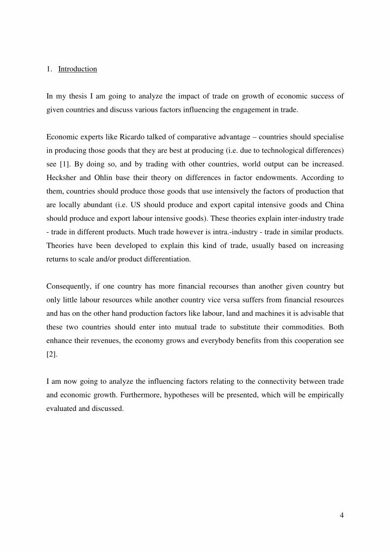
7.3.6. Borders in the period between the two world-wars
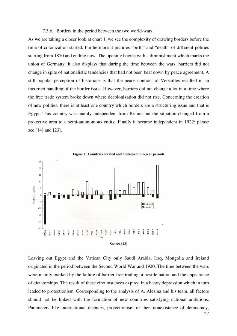
As we are taking a closer look at chart 1, we see the complexity of drawing borders before the
time of colonization started. Furthermore it pictures “birth” and “death” of different polities
starting from 1870 and ending now. The opening begins with a diminishment which marks the
union of Germany. It also displays that during the time between the wars, barriers did not
change in spite of nationalistic tendencies that had not been beat down by peace agreement. A
still popular perception of historians is that the peace contract of Versailles resulted in an
incorrect handling of the border issue. However, barriers did not change a lot in a time where
the free trade system broke down where decolonization did not rise. Concerning the creation
of new polities, there is at least one country which borders are a structuring issue and that is
Egypt. This country was mainly independent from Britain but the situation changed from a
protective area to a semi-autonomous entity. Finally it became independent in 1922; please
see [14] and [23].
Figure 1: Countries created and destroyed in 5-year periods
Source [23]
Leaving out Egypt and the Vatican City only Saudi Arabia, Iraq, Mongolia and Ireland
originated in the period between the Second World War and 1920. The time between the wars
were mainly marked by the failure of barrier-free trading, a hostile nation and the appearance
of dictatorships. The result of these circumstances expired in a heavy depression which in turn
leaded to protectionism. Corresponding to the analysis of A. Alesina and his team, all factors
should not be linked with the formation of new countries satisfying national ambitions.
Parameters like international disputes, protectionism or then nonexistence of democracy,
28
would in a sense support colonial forces in being linked to their realms and suppress
independent activities, see also [15].
7.3.7. Borders in the period after the second world war
“In the fifty years that followed the Second World War, the number of independent countries
increased dramatically. There were 74 countries in 1948, 89 in 1950, and 193 in 2001. The
world now comprises a large number of relatively small countries: in 1995, 87 of the
countries in the world had a population of less than 5 million, 58 had a population of less than
2,5 million, and 35 less than 500 thousands. In the same 50 years, the share of international
trade in world GDP increased dramatically [23].”
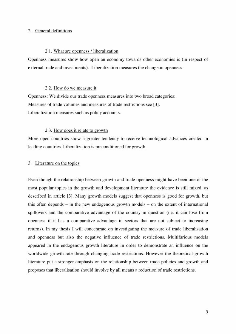
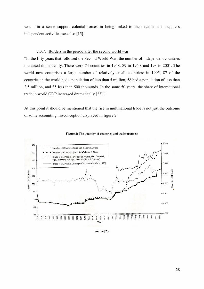
At this point it should be mentioned that the rise in multinational trade is not just the outcome
of some accounting misconception displayed in figure 2.
Figure 2: The quantity of countries and trade openness
Source [23]
29
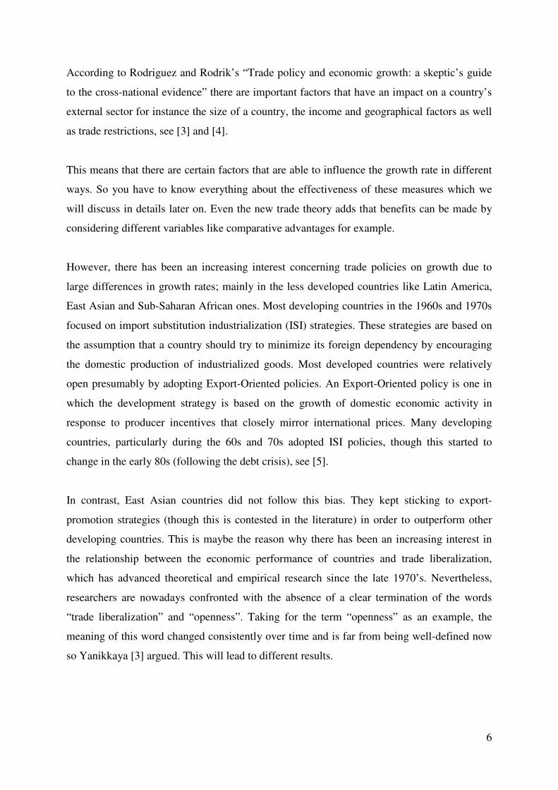
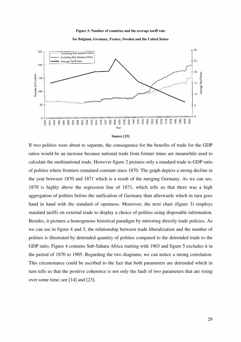
Figure 3: Number of countries and the average tariff rate
for Belgium, Germany, France, Sweden and the United States
Source [23]
If two polities were about to separate, the consequence for the benefits of trade for the GDP
ratios would be an increase because national trade from former times are meanwhile used to
calculate the multinational trade. However figure 2 pictures only a standard trade to GDP ratio
of polities where frontiers remained constant since 1870. The graph depicts a strong decline in
the year between 1870 and 1871 which is a result of the merging Germany. As we can see,
1870 is highly above the regression line of 1871, which tells us that there was a high
aggregation of polities before the unification of Germany than afterwards which in turn goes
hand in hand with the standard of openness. Moreover, the next chart (figure 3) employs
standard tariffs on external trade to display a choice of polities using disposable information.
Besides, it pictures a homogenous historical paradigm by mirroring directly trade policies. As
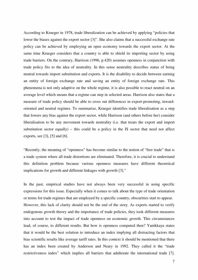
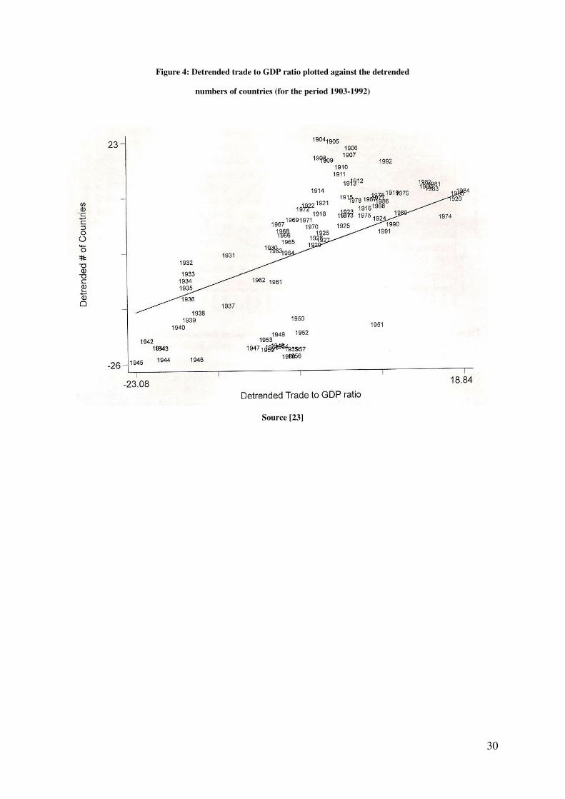
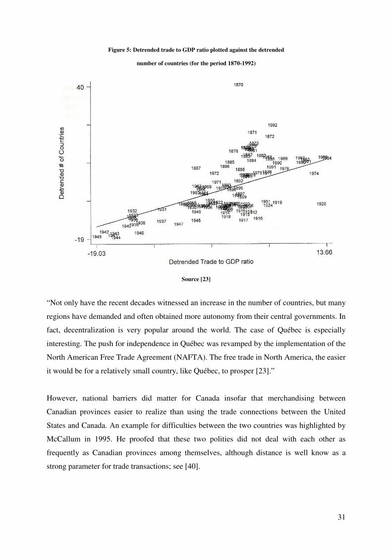
we can see in figure 4 and 5, the relationship between trade liberalization and the number of
polities is illustrated by detrended quantity of polities compared to the detrended trade to the
GDP ratio. Figure 4 contains Sub-Sahara Africa starting with 1903 and figure 5 excludes it in
the period of 1870 to 1905. Regarding the two diagrams, we can notice a strong correlation.
This circumstance could be ascribed to the fact that both parameters are detrended which in
turn tells us that the positive coherence is not only the fault of two parameters that are rising
over some time; see [14] and [23].
30
Figure 4: Detrended trade to GDP ratio plotted against the detrended
numbers of countries (for the period 1903-1992)
Source [23]
31
Figure 5: Detrended trade to GDP ratio plotted against the detrended
number of countries (for the period 1870-1992)
Source [23]
“Not only have the recent decades witnessed an increase in the number of countries, but many
regions have demanded and often obtained more autonomy from their central governments. In
fact, decentralization is very popular around the world. The case of Québec is especially
interesting. The push for independence in Québec was revamped by the implementation of the
North American Free Trade Agreement (NAFTA). The free trade in North America, the easier
it would be for a relatively small country, like Québec, to prosper [23].”
However, national barriers did matter for Canada insofar that merchandising between
Canadian provinces easier to realize than using the trade connections between the United
States and Canada. An example for difficulties between the two countries was highlighted by
McCallum in 1995. He proofed that these two polities did not deal with each other as
frequently as Canadian provinces among themselves, although distance is well know as a
strong parameter for trade transactions; see [40].
32
“This implies that there might be a cost for Québec in terms of trade flows if it was to become
independent and such arguments were made by the proponents of the “no” in the self-
determination referendum of 1996. As the perceived economic costs of secession fall with
greater North American economic integration, the likelihood of Québec gaining independence
can be expected in increase. In fact, the development of a true free-trade area in North
America might reduce these costs and make Québec separatism more attractive [23].”
7.3.8. The European Union
The European Union has been originally created by fifteen polities which decided to work
together as one. Thus they set up establishments through which the Union could take actions,
so that she could easier be responsible for all member states. These collective and
supranational institutions are for example a committee, a court of justice, a Parliament and a
Board of Ministers and provided them with specific policy privileges. As discussed before,
economic incorporation should result in political distance, so what does it mean for the
European Union? The first point is that the European Union is not an alliance because the
essential factor of a state is missing: she does not have the exclusive right for duress over its
national subjects. Hence, the European Union cannot satisfy the Weberian vision would
characterize a “sovereign state”. A recent recommended concept for the system of European
states clarifies definitely that the European Union is an agglomeration of autonomous
countries but, according to article two of the European Constitution, not a state. The second
point deals with the economic interdependence that is advancing in Europe compared to
domestic separatism which is getting more an issue of Union followers like Spain, France,
Italy and the United Kingdom; see [18] and [23].
“So much so, that many have argued that Europe will (and, perhaps should) become a
collection of regions (Brittany, the Basque Region, Scotland, Catalonia, Wales, Bavaria, etc.)
loosely connected within a European confederation of independent regions. In fact, ethic and
cultural minorities feel that they would be economically “viable” in the context of a truly
European common market, thus they could “safely” separate from the home country. This
argument is often mentioned in the press [23].”
We can see the EU as a supranational union of countries. In order to guarantee the functioning
of a common market and take advantage of economies of scale different tasks need to be
merged, as described in [18] and [23].
33
8. Free trade as the best policy
If free trade provides revenues, increases incomes and enhances the economic condition- is it
the best policy for every country? According to an article in “The Economist” this rule does
not hold for “countries that are big enough to exter an influence on the world prices of the
goods they trade”; see [41].
9. Size, trade and growth reflected in a model
Now I am going to demonstrate a simple model, which analyzes the relationship between
economic growth, the size of a country and international trade. The required information will
be based upon articles of Spolaore and Wacziarg in 2005, Alesina and Spolaore in 1997 and
2003 as well as a combination of these three scientists, which can be found in Alesina,
Spolaore and Wacziarg in 2000; see [23], [42] and [43].
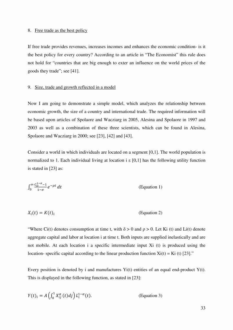
Consider a world in which individuals are located on a segment [0,1]. The world population is
normalized to 1. Each individual living at location i ε [0,1] has the following utility function
is stated in [23] as:
� ��������
�� ��� �� (Equation 1)
����� � ����� (Equation 2)
“Where Ci(t) denotes consumption at time t, with δ > 0 and ρ > 0. Let Ki (t) and Li(t) denote
aggregate capital and labor at location i at time t. Both inputs are supplied inelastically and are
not mobile. At each location i a specific intermediate input Xi (t) is produced using the
location- specific capital according to the linear production function Xi(t) = Ki (t) [23].”
Every position is denoted by i and manufactures Yi(t) entities of an equal end-product Y(t).
This is displayed in the following function, as stated in [23]:
����� � � �� ����
� ������ ������. (Equation 3)
34
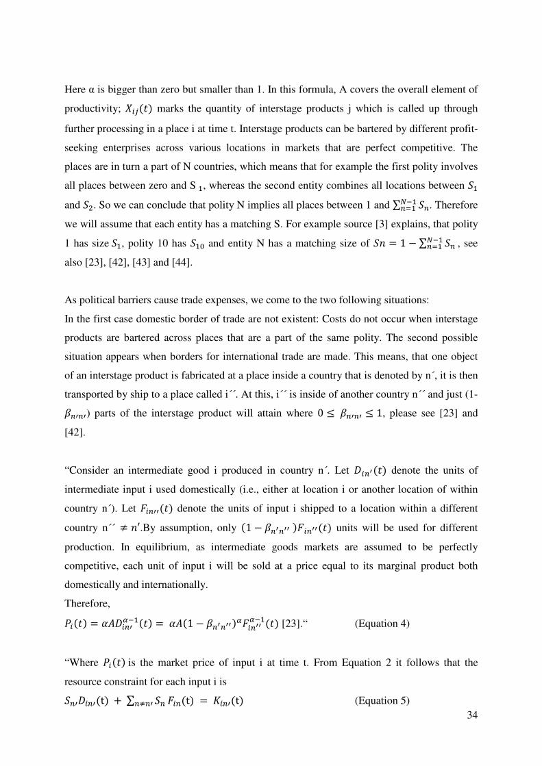
Here α is bigger than zero but smaller than 1. In this formula, A covers the overall element of
productivity; ������ marks the quantity of interstage products j which is called up through
further processing in a place i at time t. Interstage products can be bartered by different profit-
seeking enterprises across various locations in markets that are perfect competitive. The
places are in turn a part of N countries, which means that for example the first polity involves
all places between zero and S , whereas the second entity combines all locations between "
and "#. So we can conclude that polity N implies all places between 1 and ∑ "%&�%' . Therefore
we will assume that each entity has a matching S. For example source [3] explains, that polity
1 has size ", polity 10 has "� and entity N has a matching size of "( � 1 * ∑ "% &�%' , see
also [23], [42], [43] and [44].
As political barriers cause trade expenses, we come to the two following situations:
In the first case domestic border of trade are not existent: Costs do not occur when interstage
products are bartered across places that are a part of the same polity. The second possible
situation appears when borders for international trade are made. This means, that one object
of an interstage product is fabricated at a place inside a country that is denoted by n´, it is then
transported by ship to a place called i´´. At this, i´´ is inside of another country n´´ and just (1-
+%,%,) parts of the interstage product will attain where 0 . +%,%, . 1, please see [23] and
[42].
“Consider an intermediate good i produced in country n´. Let /�%0��� denote the units of
intermediate input i used domestically (i.e., either at location i or another location of within
country n´). Let 1�%,, ��� denote the units of input i shipped to a location within a different
country n´´ 2 (3.By assumption, only �1 * +%0%00 �1�%00��� units will be used for different
production. In equilibrium, as intermediate goods markets are assumed to be perfectly
competitive, each unit of input i will be sold at a price equal to its marginal product both
domestically and internationally.
Therefore,
4���� � 5�/�%,����� � 5��1 * +%0%00��1�%00
����� [23].“ (Equation 4)
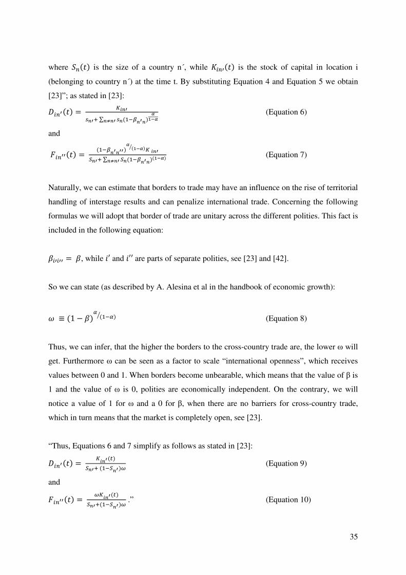
“Where 4���� is the market price of input i at time t. From Equation 2 it follows that the
resource constraint for each input i is
"%,/�%,�t� 7 ∑ "%%8%, 1�%�t� � ��%,�t� (Equation 5)
35
where "%��� is the size of a country n´, while ��%,��� is the stock of capital in location i
(belonging to country n´) at the time t. By substituting Equation 4 and Equation 5 we obtain
[23]”; as stated in [23]:
/�%0��� � 9�:0
;:0< ∑ ;:��=:0:�>
��>:?:0 (Equation 6)
and
1�%00��� � ��=:0:00�> ���>�@ 9 �:0
A:0< ∑ A::?:0 ��=:0:����>� (Equation 7)
Naturally, we can estimate that borders to trade may have an influence on the rise of territorial
handling of interstage results and can penalize international trade. Concerning the following
formulas we will adopt that border of trade are unitary across the different polities. This fact is
included in the following equation:
+�,�,, � +, while B3 and B33 are parts of separate polities, see [23] and [42].
So we can state (as described by A. Alesina et al in the handbook of economic growth):
C D �1 * +�� ����@ (Equation 8)
Thus, we can infer, that the higher the borders to the cross-country trade are, the lower ω will
get. Furthermore ω can be seen as a factor to scale “international openness”, which receives
values between 0 and 1. When borders become unbearable, which means that the value of β is
1 and the value of ω is 0, polities are economically independent. On the contrary, we will
notice a value of 1 for ω and a 0 for β, when there are no barriers for cross-country trade,
which in turn means that the market is completely open, see [23].
“Thus, Equations 6 and 7 simplify as follows as stated in [23]:
/�%0��� � 9�:0���A:0< ��A:0�E (Equation 9)
and
1�%00��� � E9�:0���A:0<��A:0�E .” (Equation 10)
36
9.1. Capital accumulation and growth
As stated in [23] it follows, that “in each location i costumers’ net household assets are
identical to the stock of capital ��%0���. Since each unit of capital yields one unit of
intermediate input I, the net return to capital is equal to the market price of intermediate input
4�� (for simplicity, we assume no depreciation). From intertemporal optimization we have the
following standard Euler equation
F���F�
����
G4���� * HI � J5�GC 7 �1 * C�"%,I����%0
����� * HK (Equation 11)
Hence, the steady-state level of capital at each location i of a country of size "% will be
��%;; � ��L
� �� ����@ GC 7 �1 * C�"%0I (Equation 12)
��;; � �
����@ ����
� ����@ GC 7 �1 * C�"%0I.“ (Equation 13)
Looking at Equation 13, we can conclude the following: Growth is rising in openness ω
which can be also written as the division of the derivative of ��;; by the derivation of ω and
then we obtain a result which is bigger than zero. Moreover we will find out that growth will
increase in the country size, which we obtain by relating ��;; to "%,. Finally we can state that
by putting the second derivative of ��;; in the nominator and the derivative of "%, times the
derivative of ω in the denominator, the result will be smaller than zero. So the smaller ω is
getting, the larger the country size effect will get, whereas the smaller the size of a country is,
the larger the effect of openness will be.
.
37
10. Empirical analysis
10.1. Propositions
To find out more about the relationship between country size, trade and economic growth, I
put up two propositions to find out more about these factors.
Proposition 1: Do size and openness of countries have positive effects on economic
performance?
Proposition 2: Is openness of a country is favorable for larger countries?
10.2. Model specifications and the estimated equation
To find out whether the openness of countries has positive effects on economic performance, I
estimated the following equation:
Estimated equation:
MNOP�Q�� � 5� 7 +RST�� 7 +#�U(VOV�� 7 +Wexp_gdp^_ 7 βalibdum^_ 7 βglib^_size^_
7 βjsize^_ 7 Y_ 7 ε^_
The equation includes country dummies (stated as B in 5�). Furthermore I put in the variables
gross capital formation (RST��), the growth rate of the population rate (�U(VOV��), the ratio of
exports to the gross domestic product (exp_gdp^_), liberalization dummies (libdum^_),
liberalization (UBm��), the size of a country (nBo ��) and year dummies (the � in Y_). When we
add all factors up in the end, we get the growth for a certain country and a specific time. The
element I wrote down as size consists of three basic elements: GDP, the population rate and
the area of a country. What we are trying to find out is the following: will growth increase
over time when size develops? The tables stated below will show the results to this equation.
10.3. Information about the sources
The tables mainly consist of two datasets: the Barro and Lee dataset and the Wacziarg and
Welch data records. The factor which belongs to the Barro and Lee dataset is syr15_60,
whereas growth, lninitgdppc, gcf, dlnpop and exp_gdp are counted among the WDI, the
World Development Indicator of Barro and Lee. The lib_dum was taken out of Wacziarg and
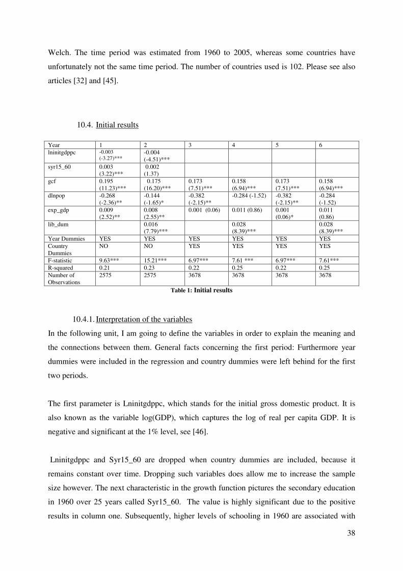
38
Welch. The time period was estimated from 1960 to 2005, whereas some countries have
unfortunately not the same time period. The number of countries used is 102. Please see also
articles [32] and [45].
10.4. Initial results
Year 1 2 3 4 5 6 lninitgdppc -0.003
(-3.27)*** -0.004 (-4.51)***
syr15_60 0.003 (3.22)***
0.002 (1.37)
gcf 0.195 (11.23)***
0.175 (16.20)***
0.173 (7.51)***
0.158 (6.94)***
0.173 (7.51)***
0.158 (6.94)***
dlnpop -0.268 (-2.36)**
-0.144 (-1.65)*
-0.382 (-2.15)**
-0.284 (-1.52) -0.382 (-2.15)**
-0.284 (-1.52)
exp_gdp 0.009 (2.52)**
0.008 (2.55)**
0.001 (0.06) 0.011 (0.86) 0.001 (0.06)*
0.011 (0.86)
lib_dum 0.016 (7.79)***
0.028 (8.39)***
0.028 (8.39)***
Year Dummies YES YES YES YES YES YES Country Dummies
NO NO YES YES YES YES
F-statistic 9.63*** 15.21*** 6.97*** 7.61 *** 6.97*** 7.61*** R-squared 0.21 0.23 0.22 0.25 0.22 0.25 Number of Observations
2575 2575 3678 3678 3678 3678
Table 1: Initial results
10.4.1. Interpretation of the variables
In the following unit, I am going to define the variables in order to explain the meaning and
the connections between them. General facts concerning the first period: Furthermore year
dummies were included in the regression and country dummies were left behind for the first
two periods.
The first parameter is Lninitgdppc, which stands for the initial gross domestic product. It is
also known as the variable log(GDP), which captures the log of real per capita GDP. It is
negative and significant at the 1% level, see [46].
Lninitgdppc and Syr15_60 are dropped when country dummies are included, because it
remains constant over time. Dropping such variables does allow me to increase the sample
size however. The next characteristic in the growth function pictures the secondary education
in 1960 over 25 years called Syr15_60. The value is highly significant due to the positive
results in column one. Subsequently, higher levels of schooling in 1960 are associated with
39
higher growth. The second column states the opposite: the coefficient is insignificant and
lower than in the first column. This means that there is no statistically significant relationship
between initial schooling and growth.
Coming to talk about Gcf, this stands for gross capital formation. For every year the results
are positive and significant. So, higher investment is associated with higher growth rates.
The following parameter is called Dlnpop and is the abbreviation for the difference in the log
of the population rate. Continuously, the numbers for Dlnpop remain negative and significant
over all years. As a matter of fact we can interpret that higher levels of population growth are
associated with lower growth of output per capita.
Taking a closer look at the export of Gdp, captured by Exp_gdp, we can recognize
coefficients that are all positive and tend to be significant. This indicates that there is a
positive relationship the level of openness and output growth.
The liberalization dummy, which is given by Lib_dum, is positive and significant all the time.
This circumstance tells us, that liberalizing a trade regime is associated with higher levels of
growth. Moreover, growth is associated with an increase in growth between 1.6% - 2.8%,
depending on the specification.
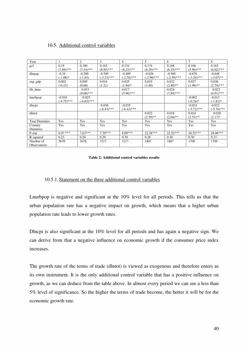
40
10.5. Additional control variables
Year 1 2 3 4 5 6 7 8 gcf 0.19
(7.69)*** 0.180 (7.54)***
0.165 (8.85)***
0.154 (8.23)***
0.174 (6.29)***
0.168 (6.19)***
0.166 (5.96)***
0.165 (6.02)***
dlnpop -0.34 (-1.88)*
-0.200 (-1.03)
-0.549 (-3.23)***
-0.489 (-2.76)***
-0.626 (-2.98)***
-0.560 (-2.59)***
-0.676 (-3.24)***
-0.648 (-3.07)**
exp_gdp 0.002 (-0.15)
0.009 (0.68)
0.016 (1.21)
0.025 (1.94)*
0.019 (1.40)
0.032 (2.40)**
0.027 (1.99)**
0.036 (2.74)***
lib_dum 0.033 (9.09)***
0.017 (5.98)***
0.024 (7.84)***
0.022 (6.91)***
lnurbpop -0.016 (-4.75)***
-0.025 (-6.63)***
-0.002 (-0.24)*
-0.013 (-1.83)*
dlncpi -0.036 (-6.43)***
-0.035 (-6.43)***
-0.024 (-5.72)***
-0.022 (-5.76)***
dlntot 0.022 (2.39)**
0.018 (2.04)**
0.024 (2.53)**
0.020 (2.17)*
Year Dummies Yes Yes Yes Yes Yes Yes Yes Yes Country Dummies
Yes Yes Yes Yes Yes Yes Yes Yes
F-stat 6.97 *** 7.63*** 7.39*** 8.09*** 22.38*** 22.52*** 26.52*** 28.06*** R-squared 0.23 0.26 0.29 0.30 0.28 0.30 0.30 0.33 Number of Observations
3678 3678 3217 3217 1807 1807 1709 1709
Table 2: Additional control variables results
10.5.1. Statement on the three additional control variables
Lnurbpop is negative and significant at the 10% level for all periods. This tells us that the
urban population rate has a negative impact on growth, which means that a higher urban
population rate leads to lower growth rates.
Dlncpi is also significant at the 10% level for all periods and has again a negative sign. We
can derive from that a negative influence on economic growth if the consumer price index
increases.
The growth rate of the terms of trade (dlntot) is viewed as exogenous and therefore enters as
its own instrument. It is the only additional control variable that has a positive influence on
growth, as we can deduce from the table above. In almost every period we can see a less than
5% level of significance. So the higher the terms of trade become, the better it will be for the
economic growth rate.
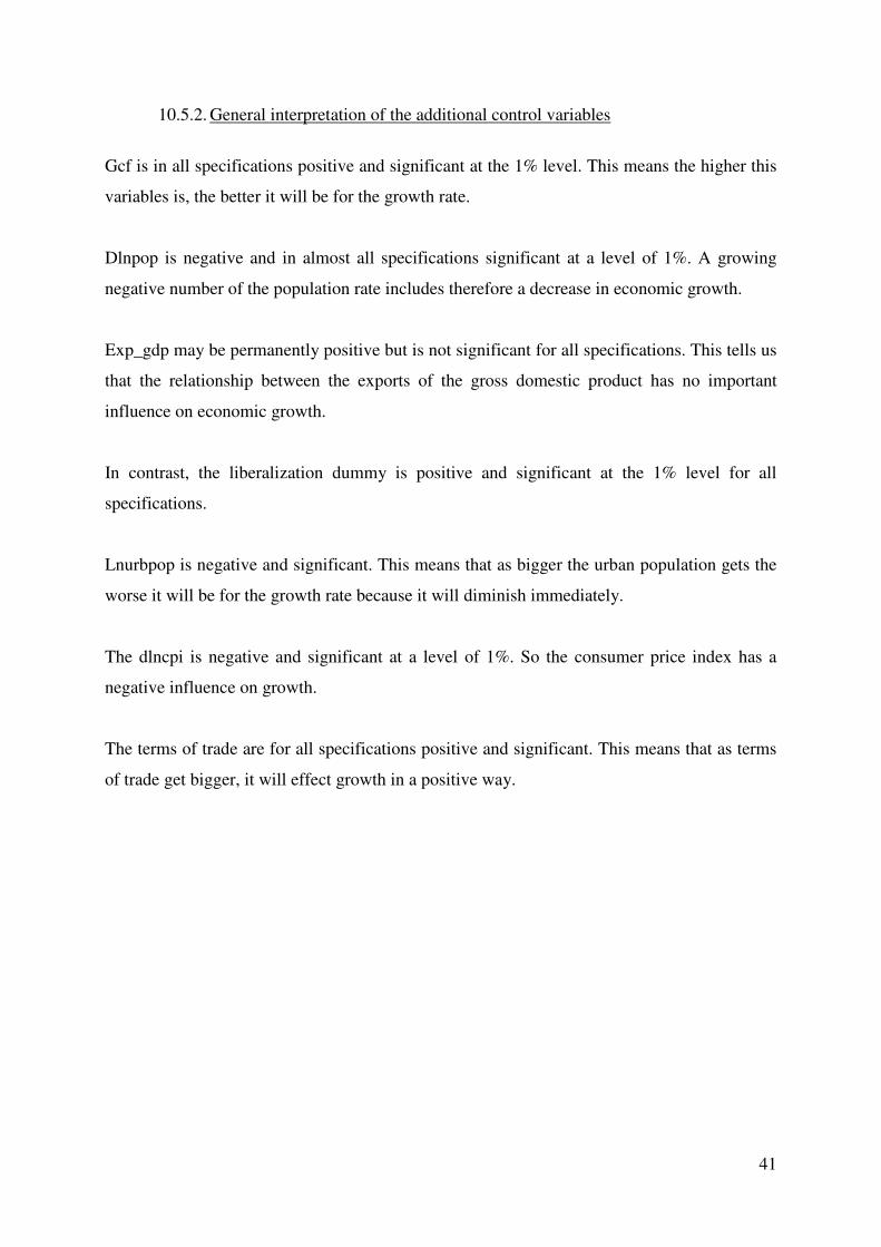
41
10.5.2. General interpretation of the additional control variables
Gcf is in all specifications positive and significant at the 1% level. This means the higher this
variables is, the better it will be for the growth rate.
Dlnpop is negative and in almost all specifications significant at a level of 1%. A growing
negative number of the population rate includes therefore a decrease in economic growth.
Exp_gdp may be permanently positive but is not significant for all specifications. This tells us
that the relationship between the exports of the gross domestic product has no important
influence on economic growth.
In contrast, the liberalization dummy is positive and significant at the 1% level for all
specifications.
Lnurbpop is negative and significant. This means that as bigger the urban population gets the
worse it will be for the growth rate because it will diminish immediately.
The dlncpi is negative and significant at a level of 1%. So the consumer price index has a
negative influence on growth.
The terms of trade are for all specifications positive and significant. This means that as terms
of trade get bigger, it will effect growth in a positive way.
42
10.6. Interactions with size
Year 1 2 3 4 5 6 gcf 0.156
(12.02)*** 0.161 (5.87)***
0.159 (12.25)***
0.181 (7.76)***
0.159 (12.16)***
0.158 (6.96)***
dlnpop -0.360 (-2.74)***
-0.584 (-2.77)***
-0.325 (-2.50)**
-0.323 (-1.77)*
-0.300 (-2.32)**
-0.292 (-1.61)
exp_gdp 0.013 (1.47)
0.031 (2.29)**
0.011 (1.19)
0.003 (0.22)
0.010 (1.17)
0.011 (0.84)
lib_dum 0.106 (4.44)***
0.025 (0.67)
0.104 (4.65)***
0.080 (3.19)***
0.070 (4.95)***
0.071 (3.95)***
lib_gdp -0.003 (-3.28)***
-0.000 (-0.05)
lngdp 0.021 (2.17)**
lib_pop -0.005 (-3.42)***
-0.063 (-1.84)*
lnpop -0.003 (-8.01)***
lib_area -0.003 (-3.00)***
-0.004 (-2.59)**
lnarea -0.292 (-1.08)
Year Dummies YES YES YES YES YES YES Country Dummies YES YES YES YES YES YES F-stat 7.76 21.23*** 7.77 7.63*** 7.76*** 7.56*** R-squared 0.25 0.30 0.25 0.27 0.25 0.25 Number of Observations
3678 3678 3678 3678 3677 3677
Table 3: Interactions with size results
10.6.1. Interpretation of the parameter for the table interaction with size results
Firstly, I should mention that the results on the other explanatory variables in the table are
largely as above, with investment (gcf) and the ratio of exports to GDP (exp_gdp) having a
positive impact on growth and population growth (dlnpop) a negative one.
Turning to the liberalization variable and its interaction with size, we find:
(i) in the first two columns we see that while the impact of liberalization on growth tends to
be positive, its impact is found to fall with increasing size (as measured by lngdp). This is
captured by the negative and significant coefficient on lib_gdp in column (1). When included
linearly the impact of the level of GDP is found to be positive and significant.
(ii) when using population as a measure of size (columns 3 and 4) I again find that the impact
of liberalization is decreasing in country size, that is, smaller countries benefit more in terms
of growth from trade liberalization. The coefficient on the level of population is found to be
negative and significant, unlike when GDP is used as a measure of size.
43
(iii) using area (columns 5 and 6) as a measure of size the results are qualitatively similar to
those for population.
Overall, the results robustly indicate that the benefits of liberalization are smaller in larger
countries.
10.7. Final results
10.7.1. Proposition 1
Summarizing it can be stated that these effects demonstrate a positive influence of openness
and size on economic performance, see [23] and [43].
10.7.2. Proposition 2
“Regarding the results above, we can detect, that this proposition is false because openness is
less important for larger countries. We can notice this by looking at the earnings of economic
success due to openness which start to diminish as size grows [23].”
10.8. Conclusion
Summarizing the above, openness (less important for larger countries), size (is measured by
GDP, population rate and area) and international trade have a positive influence on economic
success of countries and secure constant growth.
A) The relationship between growth and trade liberalization and the country size has been
analyzed.
I was looking for the inter-relationship between size and trade liberalization e.g. does
liberalization affect growth differently in larger countries than in smaller countries.
As a basis, I analyzed the panel data on a large number of countries over the period 1960
to 2005.
B) I found out that liberalization generally has a positive effect on growth.
The impact of size ambitions depends on the variables which are used.
Liberalization has a smaller influence on growth in larger countries compared to smaller
countries.
44
11. Abstract
The thesis shows that trade openness and liberalization are triggering factors for economic
growth. Despite the relationship between growth and trade openness, being one of the most
popular topics in the growth and development literature, the relationship between the two is
far from being fathomed as described in article [3].
In fact there is a dissent concerning basic definitions like liberalization and trade openness.
This circumstance does not only entail general confusion, it rather leads to different results
when trade openness and the size of countries are judged by their influence on economic
growth. A review delivers furthermore an insight into historical matters on this subject.
Finally, the empirical part analyzes why trade openness loses its relevance for larger
countries. In addition, a positive effect of openness, country size and international trade
concerning the economic success is investigated and empirical confirmed.
As far as the influence of country size (which are measured by the GDP, population rate and
area) is concerned, it is shown that openness is less important for larger countries but more
important for smaller countries. The reason is that smaller countries are not able to produce all
products on their own which are necessary for the coverage of the needs of their inhabitants.
In contrary bigger countries are not as dependent on imports because they are able to
manufacture the whole range of products without foreign support. Therefore they could more
easily reduce the trade openness. But also bigger countries will benefit from openness,
liberalization and international trade in order to reach constant economic growth.
45
i. Summary in German
Diese Diplomarbeit befasst sich mit den Determinanten des ökonomischen Wachstums.
Speziell auf die Auswirkungen von Offenheit gegenüber dem internationalen Handel und die
Größe von Ländern in Bezug auf das ökonomische Wachstum von Entwicklungs- sowie
Industrieländern wird näher eingegangen. Obwohl die Beziehung zwischen Wachstum und
Handelsfreiheit eines der wohl beliebtesten Themen der Wachstums- und
Entwicklungsliteratur ist, sind die Auswirkungen dieser Verbindung bis heute noch nicht
endgültig geklärt, siehe dazu Artikel [3]. Vielmehr besteht ein Dissens der Wissenschaftler
bei der Definition grundlegender Begriffe wie Liberalisierung und Handelsfreiheit. Dieser
Umstand bedingt allerdings nicht nur allgemeine Konfusion, er führt vielmehr zu
unterschiedlichen Resultaten bei der Analyse ob Handelsfreiheit und die Größe eines Landes
Einfluss auf das ökonomische Wachstum haben oder nicht. Ein historischer Überblick soll
zudem einen tieferen Einblick in die Materie liefern. Abschließend wird im empirischen Teil
untersucht, wieso Handelsfreiheit speziell für größere Länder immer mehr an Bedeutung
verliert. Zudem wird eine positive Wirkung von Freiheit, Landesgröße und internationalem
Handel bezüglich des ökonomischen Erfolgs hinterfragt und empirisch untermauert.
Allerdings sollte die Landesgröße nie als separate Determinante des Wachstums betrachtet
werden, sondern immer im Zusammenhang mit anderen ökonomischen Einflussgrößen.
46
ii. List of tables
Table 1: Initial results ............................................................................................................... 38
Table 2: Additional control variables results ........................................................................... 40
Table 3: Interactions with size results ...................................................................................... 42
47
iii. List of figures
Figure 1: Countries created and destroyed in 5-year periods ................................................... 27
Figure 2: The quantity of countries and trade openness ........................................................... 28
Figure 3: Number of countries and the average tariff rate ....................................................... 29
Figure 4: Detrended trade to GDP ratio plotted against the detrended .................................... 30
Figure 5: Detrended trade to GDP ratio plotted against the detrended .................................... 31
48
iv. List of references
[1] D. Ricardo, “On the Principles of Political Economy and Taxation”, reprinted as vol. 1. of P. Sraffa, P. (1951). The Works and Correspondence of David Ricardo, Cambridge University Press, 1817. [2] Bertil Ohlin, “Why Trade”, http://nobelprize.org, first published 28 February 2006, http://nobelprize.org/educational_games/economics/trade/ohlin.html, [accessed: 10.09.2009]. [3] Halit Yanikkaya, “Trade Openness and Economic Growth: A Cross-Country Empirical Investigation”, Journal of Development Economics 72, pp. 57-89, 2003. [4] D. Rodrik, F. Rodriguez, “Trade Policy and Economic Growth: A Skeptics Guide to the Cross-National Evidence, In: B. Bernanke, K. Rogoff, NBER Macroeconomics Annual, Vol. 15, pp 261-325, 2000. [5] Anne O. Krueger, “Why Trade Liberalisation is Good for Growth”, The Economic Journal, Vol. 108, No. 450, pp. 1513-1522, September 1998. [6] A. Harrison, “Openness and Growth: A Time Series, Cross-Country Analysis for Developing Countries”, Journal of Development Economics 48, pp 419-447, 1996. [7] J. E. Anderson, J. P. Neary, “Trade Reform with Quotas, Partial Rent Retention and Tariffs”, Econometrica 60, pp 57- 76, 1992. [8] E. E. Leamer, “Measures of Openness”, In: R. E. Baldwin, Trade Policy Issues and Empirical Analysis, The University of Chicago Press, pp. 147-204, 1988. [9] D. Rodrik, A. Subramanian, F. Trebbi, “Institutions Rule: The Primacy of Institutions over Geography and Integration in Economic Development”, Harvard University, Unpublished paper: www.ksghome.harvard.edu/~.drodrik.academic.ksg/institutionsrule,%205.0.pdf, [accessed 08.11.2009], 2002. [10] L. Pritchett, “Measuring Outward Orientation in LDCs: Can it be done”, Journal of Development Economics 49, pp. 307-335, 1996. [11] L. Pritchett, G. Sethi, “Tariff Rates, Tariff Revenue, and Tariff Reform: Some New Facts, The World Bank Economic Review 8 (1), pp. 1-16, 1994. [12] J.-W. Lee, “International Trade, Distortions and Long Run Economic Growth”, IMF Staff Papers 40 (2), pp. 299-328, 1993. [13] Sebastian Edwards, ”Openness, Productivity and Growth: What Do We Really Know”, NBER Working Paper No. 5978, International Finance and Macroeconomics and International Trade and Investment, pp. 383-398, March 1997. [14] M. A. Clemens, J. G. Williamson, “A Tariff-Growth Paradox? Protection’s Impact the World Around 1875-1997”, NBER Working Paper Series, No. 8549, 2001.
49
[15] K.H. O’ Rourke, “Tariffs and Growth in the late Nineteenth Century”, Economic Journal 110, pp. 456-483, 2000. [16] D.A. Irwin, “Interpreting the Tariff-Growth Correlation of the late Nineteenth Century” NBER Working Paper Series, No. 8739, 2002. [17] B. G. Auguste, “The Economies of International Payments Unions and Clearing Houses”, St. Martin’s Press, pp.1-224, 1997. [18] R. Triffin, “Europe and the Money Muddle”, Greenwood Press, Westport, pp. 1-351, 1976. [19] S. Mehrota, “India and the Soviet Union: Trade and Technology Transfer”, Cambridge University Press, pp.1-242, 1990. [20] D. Sachs, A. M. Warner, “Economic Reform and the Process of Global Integration”, Brookings Papers of Economic, pp.1-118, 1995. [21] David Greenaway, Wyn Morgan, Peter Wright, “Trade Reform, Adjustment and Growth: What does the evidence tell us”, Economic Journal 108, pp. 1547-1561, 1998. [22] David Greenaway, “Does Trade Liberalization Promote Economic Development”, Schottish Journal of Political Economy, Vol. 45, No. 5, pp. 491-511, November 1998. [23] Alberto Alesina, Enrico Spolaore, Romain Wacziarg, “Trade, growth and the size of countries”, Handbook of Economic Growth, Vol. 1B, pp. 1500-1522, 2005. [24] R. E. Lucas, “On the mechanics of economic development”, Journal of Monetary Economics 22, pp. 3-42, 1988. [25] G. M. Grossman, E. Helpman, “Quality ladders in the theory of growth”, Review of Economic Studies 58, pp. 43-61, 1991. [26] K. Murphy, A. Shleifer, R. Vishny, “Industrialization and the big push”, Journal of Political Economy 87 (5), pp. 1003-1026, 1989. [27] W. Easterly, “Life during growth”, Journal of Economic Growth 4, pp. 239-275, 1999. [28] D. Dollar, “Outward-oriented developing economies really do grow more rapidly: Evidence from 95 LDC’s 1976-1985”, Economic Development and Cultural Change 40, pp. 523-544, 1992. [29] J. A. Frankel, D. Romer, “Does Trade Cause Growth?”, American Economic Review 89 (3), pp. 379-399, 1999. [30] R. Wacziarg, “Measuring the Dynamic Gains from Trade”, World Bank Economic Review 15 (3), pp. 393-429, 2001. [31] F. Alcalá, A. Ciccone, “Trade and productivity”, Quarterly Journal of Economics 119 (2), pp. 613-646, 2004.
50
[32] R. Wacziarg, K. H. Welch, “Trade Liberalization and Growth: New evidence”, NBER Working Paper 10152, pp.1-91, 2003. [33] D. Backus, P. Kehoe, T. Kehoe, “In Search of Scale Effects in Trade and Growth”, Journal of Economic Theory 58 (2), pp. 377-409, 1992. [34] C. H. Wilson, “Trade society and the state”, In: E. E. Rich, C. H. Wilson, “The Cambridge Economic History of Europe from the Decline of the Roman Empire”, Vol.4, Cambridge University Press, pp. 487-575, 1967. [35] J. W. Merryman, “A History of Modern Europe: From the Renaissance to the Present”, W. W. Norton & Company, pp. 1-1376, 1996. [36] W. H. Riker, “Federalism: Origins, Operation, Significance”, Little Brown, 1964. [37] A. Estevadeordal, B. Franz, A. M. Taylor, „The Rise and Fall of World Trade 1870-1939“, Quarterly Journal of Economics 118 (2), pp. 359-407, 2003. [38] P. Bairoch, “European Trade Policy 1815-1914”, In: P. Mathias, S. Pollard, The Cambridge Economic History of Europe, Vol.8, Cambridge University Press, pp. 1-160, 1989. [39] E. Hobsbawm, “The Age of Empire”, Vintage Books, pp. 1-304, 1987. [40] J. McCallum, “National Borders Matter: Canada-US Regional Trade Patterns”, American Economic Review 85 (3), pp. 615-623, 1995. [41] “Why trade is good for you”, http://www.economist.com, published Oct 1st 1998, http://www.economist.com/displaystory.cfm?story_id=605144, [Accessed: 10.09.2009] [42] E. Spolare, R. Wacziarg, “Borders and Growth”, Journal of Economic Growth 10 (4), pp. 331-386, 2005. [43] A. Alesina, E. Spolare, “On the Number and Size of Nations”, Quarterly Journal of Economic 112 (4), pp. 1027-1056, 1997. [44] A. Alesina, E. Spolare, R. Wacziarg, “Economic Integration and Political Disintegration”, American Economic Review 90 (5), pp. 1276-1296, 2000. [45] R. J. Barro, J.- W. Lee, “Data Set for a Panel of 138 Countries”, available at
http://www.nber.org/data/ , [accessed: 07.11.2009], 1994.
[46] Robert J. Barro, Xavier Sala-i-Martin, Economic Growth, McGraw-Hill, Inc., p.431, 1995.
51
v. List of abbreviations
GDP Gross Domestic Product ISI Import Substitution Industrialization NTB Non-Tariff Barriers BPA Bilateral Payments Arrangements Et al. And Others TFP Total Factor Productivity R&D Research and Development NAFTA North American Free Trade Agreement Etc. Et Cetera
52
vi. List of variables used
Gcf Gross Capital Formation Dlnpop Rate of population growth Exp_Gdp Ratio of exports to Gross Domestic
Product Lngdp Log Gross Domestic Product Lib_dum Liberalization Dummy Lnurbpop Growth Rate of Urban Population Dlncpi Inflation rate (Consumer Price Index) Dlntot Growth in the Terms of Trade Lnpop Growth Rate of the Population Rate Lnarea Growth Rate of the Country Area Lninitgdppc Growth Rate of the Initial GDP per Capita Syr15_60 Average years of secondary schooling in
the population over age 15 in 1960
53
vii. Curriculum vitae
School 09/1987-07/1991 Elementary School Dominikanerinnen 09/1991-07/1997 Secondary School (AHS) Dominikanerinnen 09/1997-07/1999 Secondary School (AHS) Wenzgasse Education 09/1999- today Studies International Economics at the University of Vienna
Specialisations in Innovation and Technology Management and Financial Services
09/2005- 1/2006 Term abroad in the Netherlands (University van Tilburg) Professional Life 9/2004- 12/2004 Project employee for the experimental physics- University of Vienna 12/2004- 3/2005 Media Assistant Experimental physics-
University of Vienna 1/2008- 4/2008 Backup of the CEO assistant Skandia Austria Holding AG 4/2008- Today Assistance CFO/Assistance Accounting& Controlling Skandia Austria
Holding AG