Embed Size (px)
Citation preview

Mathematical Analysis and Modeling ofSignaling Networks
Dissertationzur
Erlangung des Doktorgrades (Dr. rer. nat.)der
Mathematisch-Naturwissenschaftlichen Fakultätder
Rheinischen Friedrich-Wilhelms-Universität Bonn
vonBenjamin Engelhardt
ausAnsbach
Bonn 2017

Angefertigt mit Genehmigung der Mathematisch-Naturwissenschaftlichen Fakultät derRheinischen Friedrich-Wilhelms-Universität Bonn
1. Gutachter: Dr. Holger Fröhlich2. Gutachter: Prof. Dr. Andreas Weber
Tag der Promotion: 10.10.2017Erscheinungsjahr: 2017

"Dimidium facti, qui coepit, habet:sapere aude, incipe."
Quintus Horatius Flaccus (65 v. Chr. – 8 v. Chr.)
iii


Acknowledgments
I would like to acknowledge all the people who continued to believe in my work and who sharedthis journey with me. First and foremost, I want to express my deepest gratitude to my principaladviser Dr. Holger Fröhlich for his guidance, support, and the immense amount of knowledgehe agreed to share. His continuous optimism for this work and his invaluable experience guidedme through all ups and downs during the last three years and allowed me to grow both as anindividual and as a research scientist. I could not imagine a better adviser.
I am greatly indebted to Prof. Dr. Andreas Weber for his strong support and valuable advice.Without his tireless effort and his believe in my work it would not have been possible to achievethe results presented in this thesis.
I sincerely thank Prof. em. Dr. med. Klaus Mohr for being part of my doctoral committee,for his insightful comments, encouragement and his continuous support and effort.
Furthermore, I would like to thank Prof. Dr. Thomas Schultz for agreeing to review thisthesis and to join the doctoral committee.
For the very close cooperation and all the outstanding and fruitful discussions we had over thepast years I owe special words of gratitude to Prof. Dr. Maik Kschischo. His brilliant commentsand suggestions greatly helped to enhance this thesis. He proved himself to be a genius mentor,colleague and – last but not least – a good friend.
I gratefully acknowledge the funding I received from the Deutsche Forschungsgemeinschaft(DFG) towards my PhD as part of the Research Training Group 1873. I also owe special thanksto Prof. Dr. med. Alexander Pfeifer for giving me the opportunity to visit the laboratory ofProf. Dr. George S. Baillie. I would like to express my gratitude to Prof. Dr. George S. Bailliefor establishing this successful cooperation. It was an honor for me to work with him, Jane E.Findlay and Dr. Christina Elliot in Glasgow. I will never forget this very intensive but highlyrewarding phase of my work. I would also like to thank all my group members at the B-IT, atProf. Mohr’s Lab and the Research Training Group 1873 for the warm working atmosphere andthe interesting discussions, which helped me in many ways.
This thesis is dedicated to my wife Anna and parents Hans and Monika who always supportedme and took my absence from many family gatherings with a smile.
v

Abstract
Motivation
Mathematical models are in focus of modern systems biology and increasingly important tounderstand and manipulate complex biological systems. At the same time, new and improvedtechniques in metabolomics and proteomics enhance the ability to measure cellular states andmolecular concentrations. In consequence, this leads to important biological insights and novelpotential drug targets. Model development in systems biology can be described as an iterativeprocess of model refinement to match the observed properties. The resulting research cycle isbased on a well-defined initial model and requires careful model revision in each step.
Accomplishments and Results
As an initial step, a stoichiometry-based mathematical model of the muscarinic acetylcholinereceptor subtype 2 (M2 receptor)-induced signaling in Chinese hamster ovary (CHO) cells wasderived. To validate the obtained initial model based on spatially accessible, not necessarilytime-resolved data, the novel constrained flux sampling (CFS) is proposed in this work. The thusverified static model was then translated into a dynamical system based on ordinary differentialequations (ODEs) by incorporating time-dependent experimental data.
To learn from the errors of systems biological models, the dynamic elastic-net (DEN), anovel approach based on optimal control theory, is proposed in this thesis. Next, the Bayesiandynamic elastic-net (BDEN), a systematic, fully algorithmic method based on the Markov chainMonte Carlo method was derived, which allows to detect hidden influences as well as missedreactions in ODE-based models. The BDEN allows for further validation of the developed M2
receptor-induced signaling pathway and thus provides evidence for the completeness of theobtained dynamical system.
Conclusion
This thesis introduces the first comprehensive model of the M2 receptor-induced signaling inCHO cells. Furthermore, this work presents several novel algorithms to validate and correctstatic and dynamic models of biological systems in a semi-automatic manner. These novelalgorithms are expected to simplify the development of further mathematical models in systemsbiology.
vii

Contents
1 Introduction 1
2 Modeling Biological Systems 72.1 Modeling Strategies . . . . . . . . . . . . . . . . . . . . . . . . . . . . . . . . 9
2.1.1 Top-down Strategies . . . . . . . . . . . . . . . . . . . . . . . . . . . 102.1.2 Bottom-up Strategies . . . . . . . . . . . . . . . . . . . . . . . . . . . 11
2.2 Research Cycle . . . . . . . . . . . . . . . . . . . . . . . . . . . . . . . . . . 122.3 Model Formalisms . . . . . . . . . . . . . . . . . . . . . . . . . . . . . . . . 15
2.3.1 Static and Dynamic Models . . . . . . . . . . . . . . . . . . . . . . . 152.3.2 Signaling and Metabolic Networks . . . . . . . . . . . . . . . . . . . . 172.3.3 Probabilistic Approaches . . . . . . . . . . . . . . . . . . . . . . . . . 182.3.4 Stoichiometric Matrices . . . . . . . . . . . . . . . . . . . . . . . . . 192.3.5 Differential Equations . . . . . . . . . . . . . . . . . . . . . . . . . . 22
2.4 Properties of Protein Interactions . . . . . . . . . . . . . . . . . . . . . . . . . 24
3 M2 Receptor-induced Signaling 313.1 Muscarinic Acetylcholine Receptors . . . . . . . . . . . . . . . . . . . . . . . 323.2 G Protein-mediated Signaling . . . . . . . . . . . . . . . . . . . . . . . . . . . 343.3 Experimental Tools . . . . . . . . . . . . . . . . . . . . . . . . . . . . . . . . 38
4 Methodology 414.1 Stoichiometric Network Analysis . . . . . . . . . . . . . . . . . . . . . . . . . 41
4.1.1 Left and Right Null Space . . . . . . . . . . . . . . . . . . . . . . . . 434.1.2 Constraint-based Modeling . . . . . . . . . . . . . . . . . . . . . . . . 45
4.2 Optimal Control Theory . . . . . . . . . . . . . . . . . . . . . . . . . . . . . 464.2.1 Derivation . . . . . . . . . . . . . . . . . . . . . . . . . . . . . . . . . 474.2.2 Numerical Solutions . . . . . . . . . . . . . . . . . . . . . . . . . . . 504.2.3 Objective Functions . . . . . . . . . . . . . . . . . . . . . . . . . . . 504.2.4 Properties . . . . . . . . . . . . . . . . . . . . . . . . . . . . . . . . . 52
4.3 Bayesian Inference . . . . . . . . . . . . . . . . . . . . . . . . . . . . . . . . 554.3.1 Markov Chain Monte Carlo Methods . . . . . . . . . . . . . . . . . . 594.3.2 Application: The Solution Space of Static CRNs . . . . . . . . . . . . 67
4.4 Parameter Estimation . . . . . . . . . . . . . . . . . . . . . . . . . . . . . . . 68
ix
5 Analysis of the M2 Receptor-dependent Signaling in CHO Cells 735.1 Introduction . . . . . . . . . . . . . . . . . . . . . . . . . . . . . . . . . . . . 735.2 Network Reconstruction . . . . . . . . . . . . . . . . . . . . . . . . . . . . . 745.3 Mathematical Modeling . . . . . . . . . . . . . . . . . . . . . . . . . . . . . . 755.4 Methods . . . . . . . . . . . . . . . . . . . . . . . . . . . . . . . . . . . . . . 78
5.4.1 Conservation Relationships . . . . . . . . . . . . . . . . . . . . . . . 785.4.2 Stimulation of the System . . . . . . . . . . . . . . . . . . . . . . . . 795.4.3 Sampling the Flux Polytope . . . . . . . . . . . . . . . . . . . . . . . 795.4.4 Constrained Flux Sampling . . . . . . . . . . . . . . . . . . . . . . . 805.4.5 Elementary Flux Modes . . . . . . . . . . . . . . . . . . . . . . . . . 81
5.5 Data . . . . . . . . . . . . . . . . . . . . . . . . . . . . . . . . . . . . . . . . 815.6 Results . . . . . . . . . . . . . . . . . . . . . . . . . . . . . . . . . . . . . . . 83
5.6.1 Resulting Conservation Relationships . . . . . . . . . . . . . . . . . . 835.6.2 Constraint Flux Sampling Correctly Predicts DMR Response under
Receptor Activation . . . . . . . . . . . . . . . . . . . . . . . . . . . 835.6.3 Knock-out Simulations . . . . . . . . . . . . . . . . . . . . . . . . . . 835.6.4 Combining EFMs and CFS Reveals Important Subnetworks and Regu-
latory Mechanisms . . . . . . . . . . . . . . . . . . . . . . . . . . . . 865.7 Conclusion . . . . . . . . . . . . . . . . . . . . . . . . . . . . . . . . . . . . 86
6 The Dynamic Elastic-Net 916.1 Introduction . . . . . . . . . . . . . . . . . . . . . . . . . . . . . . . . . . . . 916.2 Methods . . . . . . . . . . . . . . . . . . . . . . . . . . . . . . . . . . . . . . 93
6.2.1 The Nominal Model . . . . . . . . . . . . . . . . . . . . . . . . . . . 936.2.2 Representation of the Model Error . . . . . . . . . . . . . . . . . . . . 946.2.3 Estimating the Unmodeled Dynamics . . . . . . . . . . . . . . . . . . 94
6.3 Results . . . . . . . . . . . . . . . . . . . . . . . . . . . . . . . . . . . . . . . 966.3.1 JAK-STAT Signaling . . . . . . . . . . . . . . . . . . . . . . . . . . . 966.3.2 Photomorphogenic UV-B Signaling . . . . . . . . . . . . . . . . . . . 99
6.4 Conclusion . . . . . . . . . . . . . . . . . . . . . . . . . . . . . . . . . . . . 102
7 The Bayesian Dynamic Elastic-Net 1037.1 Introduction . . . . . . . . . . . . . . . . . . . . . . . . . . . . . . . . . . . . 1037.2 Methods . . . . . . . . . . . . . . . . . . . . . . . . . . . . . . . . . . . . . . 104
7.2.1 Motivation . . . . . . . . . . . . . . . . . . . . . . . . . . . . . . . . 1047.2.2 Approach . . . . . . . . . . . . . . . . . . . . . . . . . . . . . . . . . 1047.2.3 Marginal Likelihood of the Data . . . . . . . . . . . . . . . . . . . . . 1067.2.4 Smoothness and Sparsity via a Bayesian Elastic Net-Prior . . . . . . . 1077.2.5 Estimating Hidden Influences from Data . . . . . . . . . . . . . . . . . 1087.2.6 Estimating Endogenous Hidden Influences . . . . . . . . . . . . . . . 108
7.3 Results . . . . . . . . . . . . . . . . . . . . . . . . . . . . . . . . . . . . . . . 1107.3.1 Tested Mathematical Models . . . . . . . . . . . . . . . . . . . . . . . 1107.3.2 Simulation Study . . . . . . . . . . . . . . . . . . . . . . . . . . . . . 1117.3.3 Illustrative Examples With Real Data . . . . . . . . . . . . . . . . . . 113
x

7.3.4 Further Examples With Simulated Data . . . . . . . . . . . . . . . . . 1167.4 Conclusion . . . . . . . . . . . . . . . . . . . . . . . . . . . . . . . . . . . . 118
8 Refined Model of the M2 Receptor-dependent Signaling 1218.1 Introduction . . . . . . . . . . . . . . . . . . . . . . . . . . . . . . . . . . . . 1218.2 Experimental Procedures . . . . . . . . . . . . . . . . . . . . . . . . . . . . . 1218.3 Methods . . . . . . . . . . . . . . . . . . . . . . . . . . . . . . . . . . . . . . 1228.4 Results . . . . . . . . . . . . . . . . . . . . . . . . . . . . . . . . . . . . . . . 1248.5 Conclusion . . . . . . . . . . . . . . . . . . . . . . . . . . . . . . . . . . . . 125
9 Conclusions 129
Appendices 157
A List of Acronyms 159
B M2 Receptor-dependent Signaling in CHO Cells 163
C The Dynamic Elastic-Net 173
D The Bayesian Dynamic Elastic-Net 193
E Refined Model of the M2 Receptor-dependent Signaling 211
F List of Publications 217
xi

CHAPTER 1
Introduction
Even now, about 350 years after R. Hooke discovered empty contained spaces in cork and termedthem cells, many biological phenomena on a micro- and molecular level remain unclear (Hooke,1665). In contrast to the macroscopic properties of living systems, the view on molecular andeven microscopic events is still restricted (Noble, 2012; Azeloglu and Iyengar, 2015). Today,there is no doubt that macroscopic biological properties, and many diseases, are ultimatelycaused by molecular interactions (Noble, 2012; Bruggeman and Westerhoff, 2007; Zhao andIyengar, 2012). Although the continuous improvement of laboratory techniques has led toimportant insights into biological processes, there are still many unresolved questions. Theimprovement of laboratory techniques, however, has also sparked the emergence of various fieldsunder the umbrella of life sciences (Blankenburg et al., 2009; Robyt and White, 1987; Cravattet al., 2007). Starting with the form and structural features of organisms, the driving forcesof molecular interactions are now in the focus of research (Bruggeman and Westerhoff, 2007;Noble, 2012; Palsson, 2006). Thus, the fields of metabolics, proteomics and, finally, genomicshave become more and more important, with the overall aim to understand the molecular andthus non-observable mechanisms of life (Joyce and Palsson, 2006; Bruggeman and Westerhoff,2007; Noble, 2012; Palsson, 2006; Sauer et al., 2007).
All these branches of modern life sciences focus on biological properties caused by mo-lecular interactions, each at their own level of detail (Sauer et al., 2007; Noble, 2012; Aloyand Russell, 2006). One may think, for instance, of the interaction between the heartbeat andthe respiratory rate or the influence of drugs on the cellular response caused by drug-receptorinteractions (Yasuma and Hayano, 2004; Zhao and Iyengar, 2012). In the final analysis, thereare interactions between several regions of deoxyribonucleic acid (DNA) as the carrier of theindividuals’ genetic information (Alberts et al., 2014). But this is only one part of the story.There are multifarious interactions across all levels of an organism (Noble, 2012). When consid-ering the enormous number of cells in the human body, more than 1013 cells with about 30,000genes, it becomes very clear how complex these interactions must be (Alberts et al., 2014).Furthermore, there are still a lot of yet unknown phenomena, which can often only be treated asrandom events (Saarinen et al., 2008). All this serves to emphasize that our view on biological
1
Chapter 1 Introduction
systems, especially the human body and its cells, is restricted and only a certain part of thesesystems can be observed at the same time (Bruggeman and Westerhoff, 2007; Azeloglu andIyengar, 2015; Aloy and Russell, 2006).
Pharmacology investigates the impact of drugs on the cell and the human body as the basis ofpharmacy (Dale and Rang, 2011). Once the drug, a cocktail of specific molecules, enters thehuman body, e.g., by oral application, at some point it may be distributed throughout the wholebody via the blood stream (Dale and Rang, 2011). The drug ultimately binds to structures, i.e.,receptors, on the cell surface (Dale and Rang, 2011). This in turn initiates a flow of informationinvolving single cells or cellular compartments (Dale and Rang, 2011; Alberts et al., 2014).Such signaling pathways consist of various proteins which interact in different ways (Aloy andRussell, 2006; Meier-Schellersheim et al., 2009; Alberts et al., 2014). The involved interactionsand general protein structures are captured by the field of proteomics (Joyce and Palsson, 2006).In contrast, the field of metabolics focuses on chemical processes leading to intermediates andproducts of the metabolism (Joyce and Palsson, 2006). In turn, the distribution of proteins andthus the cellular structure is mainly determined by the genome (Sauer et al., 2007; Joyce andPalsson, 2006). Finally, genomics is the field of research dealing with the composition of thegenome and, in consequence, gene expression (Sauer et al., 2007; Joyce and Palsson, 2006;Alberts et al., 2014).
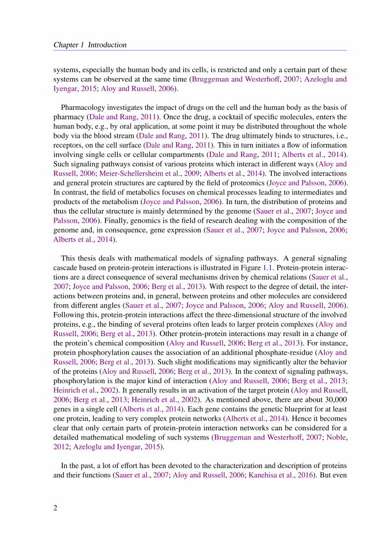
This thesis deals with mathematical models of signaling pathways. A general signalingcascade based on protein-protein interactions is illustrated in Figure 1.1. Protein-protein interac-tions are a direct consequence of several mechanisms driven by chemical relations (Sauer et al.,2007; Joyce and Palsson, 2006; Berg et al., 2013). With respect to the degree of detail, the inter-actions between proteins and, in general, between proteins and other molecules are consideredfrom different angles (Sauer et al., 2007; Joyce and Palsson, 2006; Aloy and Russell, 2006).Following this, protein-protein interactions affect the three-dimensional structure of the involvedproteins, e.g., the binding of several proteins often leads to larger protein complexes (Aloy andRussell, 2006; Berg et al., 2013). Other protein-protein interactions may result in a change ofthe protein’s chemical composition (Aloy and Russell, 2006; Berg et al., 2013). For instance,protein phosphorylation causes the association of an additional phosphate-residue (Aloy andRussell, 2006; Berg et al., 2013). Such slight modifications may significantly alter the behaviorof the proteins (Aloy and Russell, 2006; Berg et al., 2013). In the context of signaling pathways,phosphorylation is the major kind of interaction (Aloy and Russell, 2006; Berg et al., 2013;Heinrich et al., 2002). It generally results in an activation of the target protein (Aloy and Russell,2006; Berg et al., 2013; Heinrich et al., 2002). As mentioned above, there are about 30,000genes in a single cell (Alberts et al., 2014). Each gene contains the genetic blueprint for at leastone protein, leading to very complex protein networks (Alberts et al., 2014). Hence it becomesclear that only certain parts of protein-protein interaction networks can be considered for adetailed mathematical modeling of such systems (Bruggeman and Westerhoff, 2007; Noble,2012; Azeloglu and Iyengar, 2015).
In the past, a lot of effort has been devoted to the characterization and description of proteinsand their functions (Sauer et al., 2007; Aloy and Russell, 2006; Kanehisa et al., 2016). But even
2
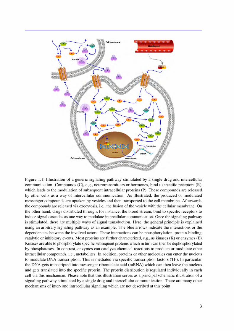
Figure 1.1: Illustration of a generic signaling pathway stimulated by a single drug and intercellularcommunication. Compounds (C), e.g., neurotransmitters or hormones, bind to specific receptors (R),which leads to the modulation of subsequent intracellular proteins (P). These compounds are releasedby other cells as a way of intercellular communication. As illustrated, the produced or modulatedmessenger compounds are uptaken by vesicles and then transported to the cell membrane. Afterwards,the compounds are released via exocytosis, i.e., the fusion of the vesicle with the cellular membrane. Onthe other hand, drugs distributed through, for instance, the blood stream, bind to specific receptors toinduce signal cascades as one way to modulate intercellular communication. Once the signaling pathwayis stimulated, there are multiple ways of signal transduction. Here, the general principle is explainedusing an arbitrary signaling pathway as an example. The blue arrows indicate the interactions or thedependencies between the involved actors. These interactions can be phosphorylation, protein-binding,catalytic or inhibitory events. Most proteins are further characterized, e.g., as kinases (K) or enzymes (E).Kinases are able to phosphorylate specific subsequent proteins which in turn can then be dephosphorylatedby phosphatases. In contrast, enzymes can catalyze chemical reactions to produce or modulate otherintracellular compounds, i.e., metabolites. In addition, proteins or other molecules can enter the nucleusto modulate DNA transcription. This is mediated via specific transcription factors (TF). In particular,the DNA gets transcripted into messenger ribonucleic acid (mRNA) which can then leave the nucleusand gets translated into the specific protein. The protein distribution is regulated individually in eachcell via this mechanism. Please note that this illustration serves as a principal schematic illustration of asignaling pathway stimulated by a single drug and intercellular communication. There are many othermechanisms of inter- and intracellular signaling which are not described at this point.
3
Chapter 1 Introduction
if all proteins including their various functions were fully characterized, it would still not bepossible to observe these structures and their interactions in sufficient detail in real-time (Brugge-man and Westerhoff, 2007; Noble, 2012; Azeloglu and Iyengar, 2015). However, today thereexist a lot of techniques to quantify the number of proteins and their composition at fixed timepoints (Blankenburg et al., 2009; Robyt and White, 1987; Cravatt et al., 2007). More oftenthan not the quantification is not possible in real-time for a huge number of proteins and thusthe processes have to be stopped and conserved in order to proceed with the actual quantifica-tion (Robyt and White, 1987; Schröder et al., 2010; Cravatt et al., 2007). Aggravated by thefact that it is not possible to observe these interactions with the human eye, in contrast to otherphenomena which occur on a microscopic level, this is where computational biology in gen-eral and systems biology in particular comes in (Meier-Schellersheim et al., 2009; Kitano, 2002).
Computational biology provides methods to capture otherwise unobservable compounds andmechanisms of such biological properties (Machado et al., 2011; Bruggeman and Westerhoff,2007; Kitano, 2002). It provides tools to analyze experimental data even if the underlyingcause is not observable or if the data is too complex for manual analysis (Bruggeman andWesterhoff, 2007; Meier-Schellersheim et al., 2009; Kitano, 2002). Determined by the natureof the accessible experimental data, the gained insights are often limited. When studyingprotein-protein interactions, often only the amount of active and inactive proteins is meas-urable (Bruggeman and Westerhoff, 2007; Meier-Schellersheim et al., 2009; Kitano, 2002).Therefore, direct assumptions regarding the underlying mechanisms are not possible. Never-theless, it is possible to make relative statements about correlations, e.g., whether an increasein one protein concentration affects the concentration of another protein or not, even thoughthe cause remains unclear (Machado et al., 2011; Bruggeman and Westerhoff, 2007; Kitano,2002). Here, computational biology provides multifunctional methods to further interpret theserelations (Bruggeman and Westerhoff, 2007; Meier-Schellersheim et al., 2009; Machado et al.,2011; Kitano, 2002).
This thesis aims for a detailed mechanistic modeling of protein-protein interaction networksto provide a physiological explanation for observed biological properties. In more detail amathematical model for the muscarinic acetylcholine receptor subtype 2 (M2 receptor)-inducedsignaling cascade is developed. Recent in vitro studies outlined an amplification of the drug-induced whole-cell response, as drafted in Figure 1.2 (Schrage et al., 2013). The variation of theoptical density of the cell caused by dynamic mass redistribution (DMR) is a common measurefor characterizing affinities and the efficiency of a given drug (Schrage et al., 2013; Schröderet al., 2011). So far, there is no explanation of the observed amplification, although it may leadto novel therapeutic approaches (Schrage et al., 2013; Schröder et al., 2011). The regulators ofG protein signaling (RGS) identified in this work are well known for their therapeutic potentialin the context of heart diseases (Kimple et al., 2011). Besides others, a lack of RGS4 results ina decrease of the heart rate in mice, which underlines the therapeutic potential of this class ofRGS (Kimple et al., 2011).
In addition to the developed M2 receptor-induced signaling pathway, several methodolo-gical innovations are presented that are of general interest for model development in systems
4
Figure 1.2: Ligand-induced whole-cell response in CHO cells. The cells were stimulated with differentiperoxo concentrations. The blue line indicates the 50% receptor binding level (pKD). The curve clearlysuggests a concentration-based signal-amplification. In addition, a time-dependent amplification of theligand-induced DMR response was observed (Engelhardt et al., 2017; Schrage et al., 2013).
biology (Engelhardt et al., 2017; Kitano, 2002; Azeloglu and Iyengar, 2015). Once the firstsketch of the assumed protein-protein interaction network has been derived, an experimentalvalidation of the model is required (Engelhardt et al., 2017; Kitano, 2002; Azeloglu and Iyengar,2015). Such data should ideally reflect all relevant components of the model in a time- andspace-resolved manner (Klipp and Liebermeister, 2006). In practice, this is often difficult toachieve due to technical, financial and time restrictions. Hence, it is desirable to first check theprincipal feasibility of the model to reproduce some expected key properties (Engelhardt et al.,2017; Kitano, 2002; Azeloglu and Iyengar, 2015). This way, the driving and thus importantproteins of the network can be localized and preferably measured, especially in cases wereresources are scarce and only a small number of the proteins are experimentally accessible (En-gelhardt et al., 2017; Kitano, 2002; Azeloglu and Iyengar, 2015). In order to address theseissues, I proposed a novel technique called constrained flux sampling (CFS) which allows for thegeneration of a first hypothesis and the ranking of the involved structures and players regardingtheir importance (Engelhardt et al., 2017). This allows for an improved experimental planningwith respect to the derived main actors (Engelhardt et al., 2017; Kitano, 2002; Azeloglu andIyengar, 2015).
The CFS analyzes the elementary flux modes (EFMs), the extreme pathways and the fluxsampling to reveal the principal behavior of the system (Engelhardt et al., 2017). In this work,this allowed to identify biologically important subnetworks, which have been described in detailin literature (Engelhardt et al., 2017). Moreover, CFS allowed to confirm that our developedmathematical model can reproduce the experimentally observable increase in cyclic adenosinemonophosphate (cAMP) production after receptor stimulation, which affects the cytoskeletonstructure and, in consequence, changes the optical density of the cells (Engelhardt et al., 2017).This demonstrates that mathematical tools developed for metabolic network analysis can also beapplied to mixed metabolic and signaling models (Engelhardt et al., 2017). This is very helpfulfor performing a priori model analyses with little effort and for the generation of hypotheses for
5
Chapter 1 Introduction
further research (Engelhardt et al., 2017; Kitano, 2002; Azeloglu and Iyengar, 2015).
For further validation and to achieve a better understanding of the temporal aspect of thesignaling process, a series of quantitative protein measurements were conducted. With thehelp of the gathered data, it was possible to extend and reformulate the original model. Therefined mathematical model (formulated as a system of ordinary differential equations (ODEs))reflected the observed temporal behavior of the M2 receptor-dependent signaling cascade.
In the context of ODE-based mathematical model development, a frequent concern is that,on the one hand, all relevant molecules and processes are included and, on the other hand,there are neither wrongly modeled nor missing molecular interactions. In order to addressthis general problem within this thesis, a novel algorithm called dynamic elastic-net (DEN) isproposed. The DEN uses both an initial ODE system and experimental measurements as inputand estimates which molecules in the ODE system are most likely influenced by factors that arenot captured in the model (Engelhardt et al., 2016). This allows to estimate hidden influences atspecific points in the system (Engelhardt et al., 2016). The methodology is based on optimalcontrol theory (OCT) and can be applied to any mathematical system of ODEs (Engelhardt et al.,2016). Therefore, the proposed approach could be applied to other fields of natural science aswell (Engelhardt et al., 2016). As it is common for deterministic approaches, the DEN doesnot include uncertainties of the estimates. To address this issue, a full Bayesian extension isdeveloped in this thesis. The Bayesian dynamic elastic-net (BDEN) takes the uncertainties of theobtained estimates into account and leads to more reliable solutions (?). Moreover, the BDENis principally able to detect wrong and missing reactions in ODE-based biological models (?).
Altogether, a first comprehensive molecular ODE-based model of the M2 receptor-inducedDMR in CHO cells is presented and analyzed in this work (Engelhardt et al., 2017). For thispurpose, I developed a novel approach to investigate signal transduction based on static mod-els (Engelhardt et al., 2017). Furthermore, a novel concept for detecting hidden influences aswell as missed and wrong interactions using measured dynamics of system internal variables ispresented (Engelhardt et al., 2016). Based on these ideas, a deterministic and Markov chainMonte Carlo (MCMC)-based algorithm was developed, which predicts unknown inputs ofhidden as well as observed variables (?).
In Chapter 2, this thesis first provides a general overview of the field of systems biology andrelated topics. Then, Chapter 3 introduces the motivating G protein (GP)-induced signaling andthe employed experimental techniques. Next, the fundamental methodology of the developedtechniques is explained in detail in Chapter 4. Starting with Chapter 5, the results and developedmethods are explained. In particular, Chapter 5 describes the developed CFS as a method toanalyze the static model of the GP-induced signaling in CHO cells. In addition, first conclusionsabout the signal amplification mechanism in CHO cells are drawn. Chapter 6 details the DEN asa novel approach to learn from the errors of dynamical biological systems. Following this, theBDEN is discussed in Chapter 7 as a Bayesian extension of the DEN. In Chapter 8, the dynamicmodel of the GP-induced signaling in CHO cells and the drawn conclusions are presented. Thefinal conclusions are then drawn in Chapter 9.
6

CHAPTER 2
Modeling Biological Systems
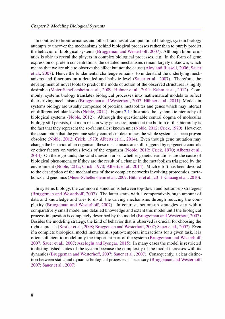
Biological processes are the result of a complex interplay of various components on differentlevels (Kestler et al., 2008; Bruggeman and Westerhoff, 2007; Noble, 2012). Consequently, asystematic interdisciplinary strategy is necessary to provide a global view on biological pro-cesses (Kestler et al., 2008; Bruggeman and Westerhoff, 2007; Noble, 2012). At the beginning,biological phenomena were largely considered separately and investigated by independentbranches of bioscience (Bruggeman and Westerhoff, 2007). Molecular biosciences, for instance,focused on the function of single molecules and did not consider the interplay between in-dividual molecules in a broader context (Bruggeman and Westerhoff, 2007). But with newand improved insights into biological systems, the involved processes were considered from amore global perspective and thus the focus shifted towards holistic approaches (Bruggeman andWesterhoff, 2007). This progress was facilitated by a dramatic improvement of measurementtechniques in metabolics, genomics and proteomics, such as mass spectrometry, quantitativewestern blotting (WB), DNA-sequencing and other high-throughput technologies (Blankenburget al., 2009; Robyt and White, 1987; Cravatt et al., 2007). The new interdisciplinary and holisticconcept led to the development of the field of systems biology (Kestler et al., 2008; Bruggemanand Westerhoff, 2007; Noble, 2012). Systems biology aims for a global view on biologicalprocesses in well-defined systems (Kestler et al., 2008; Bruggeman and Westerhoff, 2007; Noble,2012). Until 2004, when 99% of the euchromatic sequence of the human genome, includingabout 2.85 billion nucleotides, were successfully uncovered, systems biology mainly dealt withprotein-protein interactions and the metabolism on different cellular levels (Lander et al., 2001;Consortium, 2004; Hood and Galas, 2003). With the decoding of the human genome, gene regu-lation and gene expression became important topics in systems biology as well (Lander et al.,2001; Consortium, 2004; Eisenberg et al., 2000). The complexity and diversity of biologicalsystems requires an interdisciplinary and comprehensive approach (Aloy and Russell, 2006;Sauer et al., 2007). Thus, many concepts from physics and mathematics have been adaptedand applied to connect and uncover cellular mechanisms (Kestler et al., 2008; Bruggeman andWesterhoff, 2007; Noble, 2012; Sauer et al., 2007).
7
Chapter 2 Modeling Biological Systems
In contrast to bioinformatics and other branches of computational biology, system biologyattempts to uncover the mechanisms behind biological processes rather than to purely predictthe behavior of biological systems (Bruggeman and Westerhoff, 2007). Although bioinform-atics is able to reveal the players in complex biological processes, e.g., in the form of geneexpression or protein concentrations, the detailed mechanisms remain largely unknown, whichmeans that we are able to observe the effect but not the cause (Aloy and Russell, 2006; Saueret al., 2007). Hence the fundamental challenge remains: to understand the underlying mech-anisms and functions on a detailed and holistic level (Sauer et al., 2007). Therefore, thedevelopment of novel tools to predict the mode of action of the observed structures is highlydesirable (Meier-Schellersheim et al., 2009; Hübner et al., 2011; Kahm et al., 2012). Com-monly, systems biology translates biological processes into mathematical models to reflecttheir driving mechanisms (Bruggeman and Westerhoff, 2007; Hübner et al., 2011). Models insystems biology are usually composed of proteins, metabolites and genes which may interacton different cellular levels (Noble, 2012). Figure 2.1 illustrates the systematic hierarchy ofbiological systems (Noble, 2012). Although the questionable central dogma of molecularbiology still persists, the main reason why genes are located at the bottom of this hierarchy isthe fact that they represent the so-far smallest known unit (Noble, 2012; Crick, 1970). However,the assumption that the genome solely controls or determines the whole system has been provenobsolete (Noble, 2012; Crick, 1970; Alberts et al., 2014). Even though gene mutation maychange the behavior of an organism, these mechanisms are still triggered by epigenetic controlsor other factors on various levels of the organism (Noble, 2012; Crick, 1970; Alberts et al.,2014). On these grounds, the valid question arises whether genetic variations are the cause ofbiological phenomena or if they are the result of a change in the metabolism triggered by theenvironment (Noble, 2012; Crick, 1970; Alberts et al., 2014). Much effort has been devotedto the description of the mechanisms of these complex networks involving proteomics, meta-bolics and genomics (Meier-Schellersheim et al., 2009; Hübner et al., 2011; Chuang et al., 2010).
In systems biology, the common distinction is between top-down and bottom-up strategies(Bruggeman and Westerhoff, 2007). The latter starts with a comparatively huge amount ofdata and knowledge and tries to distill the driving mechanisms through reducing the com-plexity (Bruggeman and Westerhoff, 2007). In contrast, bottom-up strategies start with acomparatively small model and detailed knowledge and extent this model until the biologicalprocess in question is completely described by the model (Bruggeman and Westerhoff, 2007).Besides the modeling strategy, the kind of behavior that is observed is crucial for choosing theright approach (Kestler et al., 2008; Bruggeman and Westerhoff, 2007; Sauer et al., 2007). Evenif a complete biological model includes all spatio-temporal interactions for a given task, it isoften sufficient to model only the important part of the system (Bruggeman and Westerhoff,2007; Sauer et al., 2007; Azeloglu and Iyengar, 2015). In many cases the model is restrictedto distinguished states of the system because the complexity of the model increases with itsdynamics (Bruggeman and Westerhoff, 2007; Sauer et al., 2007). Consequently, a clear distinc-tion between static and dynamic biological processes is necessary (Bruggeman and Westerhoff,2007; Sauer et al., 2007).
8

2.1 Modeling Strategies
Figure 2.1: General hierarchy in systems biology. Protein-RNA networks, regulated by genes, are groupedin certain compartments or cell organelles which are the building blocks of cells. Interacting cells, suchas cardiomyocytes in the heart, build tissues, e.g., the cardiac muscle. Different types of tissues thenform certain organs such as the heart which is only a part of the entire organism. According to thisnatural hierarchy, initially, systems biology considered genes to be the main unilateral regulatory entity ofliving systems. Modern systems biology instead assumes that all components of the organism bilaterallyinteract on all levels. However, for modeling purposes, it makes sense to start either at the top or at thebottom of the illustrated hierarchy to successively reduce or increase the complexity of the system in ameaningful manner (Noble, 2012; Alberts et al., 2014; Crick, 1970).
This work focuses on static and dynamic mechanistic models of chemical reaction networks(CRNs), adopting a bottom-up approach. In contrast to, for instance, forecasting models,mechanistic models are not only capable to predict the behavior of biological systems butalso to reveal their underlying mechanisms (Meier-Schellersheim et al., 2009; Hübner et al.,2011; Chuang et al., 2010). Strictly speaking, solely predictive models are not systems biologymodels because they only forecast the behavior of the system rather than reveal emergentproperties (Kestler et al., 2008; Bruggeman and Westerhoff, 2007). However, the conceptualborders of systems biology are not clearly stated in literature (Aloy and Russell, 2006; Chuanget al., 2010; Hübner et al., 2011). Therefore, the term systems biology has different meaningsin different communities (Aloy and Russell, 2006). Because of its origin, systems biologyseeks to understand the mechanisms of living organic systems based on explanatory models andnot to build forecasting models with large predictive power but without the ability to supplydetailed mechanistic insights (Bruggeman and Westerhoff, 2007; Sauer et al., 2007; Noble,2012; Azeloglu and Iyengar, 2015).
2.1 Modeling Strategies
The sheer complexity of biological systems and their interaction requires a practical solutionstrategy to uncover the underlying mechanisms (Azeloglu and Iyengar, 2015). A trade-off
between complexity and reliability is essential to avoid oversimplification on the one hand
9
Chapter 2 Modeling Biological Systems
and overcomplication on the other (Azeloglu and Iyengar, 2015; Borkovich and Ebbole, 2010;Bruggeman and Westerhoff, 2007). Oversimplified models can deviate substantially fromreality by ignoring important details or involving abstracted and thus unquantifiable paramet-ers (Azeloglu and Iyengar, 2015). In contrast, the number of selectable variables in overcom-plicated models is higher than the number of data points and thus they can insufficiently bederived (Ashyraliyev et al., 2009). Both cases result in unrealistic and unreliable models (Azelo-glu and Iyengar, 2015). This can be addressed, at its extreme, from two different angles, i.e., thebottom-up and top-down perspective (Borkovich and Ebbole, 2010; Bruggeman and Westerhoff,2007). As discussed, bottom-up approaches start with comprehensive models which then getextended and, vice versa, top-down approaches start with large settings, often based on a hugeamount of data, which then get reduced (Borkovich and Ebbole, 2010; Bruggeman and West-erhoff, 2007). However, gene-regulatory networks are influenced by processes occurring at aproteomic level (Aloy and Russell, 2006). It is therefore important to have detailed knowledgeabout the mechanisms at the proteomic level to understand large-scale genomics data (Aloy andRussell, 2006). Mechanisms at the proteomic level are based on protein structures, and thusdetailed knowledge about the underlying three-dimensional structure of proteins is necessary tofully understand biological processes (Aloy and Russell, 2006).
Although top-down approaches are commonly referred to as phenomenological models, theconcept of reduction until the underlying mechanisms become clear can be transferred to puremechanistic models based on proteomics (Bruggeman and Westerhoff, 2007). Here, a similarquestion arises: whether to start with complete but complex or comprehensive but simplifiedmodels (Hübner et al., 2011; Bruggeman and Westerhoff, 2007).
2.1.1 Top-down Strategies
Since the basis of top-down modeling is mostly phenomenological, the underlying mechan-isms are unclear (Bruggeman and Westerhoff, 2007). The amount of prior knowledge is oftenvery restricted such that not even relationships between proteins are known (Borkovich andEbbole, 2010; Bruggeman and Westerhoff, 2007). However, large-scale mechanistic models orcorrelation-based models can be a starting point for top-down modeling (Borkovich and Ebbole,2010; Bruggeman and Westerhoff, 2007). The common principle of such modeling approachesis the idea that similar changes of components indicate a functional relation (Borkovich andEbbole, 2010). Thereby, system properties distilled from, for instance, proteom or transcriptomedata, are mapped to a mechanistic model with a certain complexity (Borkovich and Ebbole,2010; Bruggeman and Westerhoff, 2007). Top-down strategies take the entirety of large-scalenetworks into account and thus are able to predict completely unknown interactions (Hein-rich and Schuster, 1996; Choffnes et al., 2011; Bruggeman and Westerhoff, 2007). Yet thebasic mechanisms will remain hidden without further experimental observations (Heinrich andSchuster, 1996; Choffnes et al., 2011; Bruggeman and Westerhoff, 2007). In situations where theunderlying causality is completely unclear or just too complex for detailed modeling, top-downapproaches are often the method of choice (Heinrich and Schuster, 1996; Choffnes et al., 2011;Bruggeman and Westerhoff, 2007).
10
2.1 Modeling Strategies
Top-down approaches require a clear biological question to choose the right experimentaldesign in order to gain a large and information-rich data set (Borkovich and Ebbole, 2010).No prior knowledge regarding detailed interactions and the involved processes is necessary(Borkovich and Ebbole, 2010). The experimental data sets used for top-down approaches areusually very large and thus efficient statistical tools must be used to discover behavioral patternsand functional clusters (Bruggeman and Westerhoff, 2007). In consequence, the underlyingbiological process can be uncovered with increasing level of detail (Bruggeman and Westerhoff,2007). Starting with potentially complete, often genome-wide data, the biological processcan be successively revealed until the mechanistic details of the observed properties are fullyknown (Bruggeman and Westerhoff, 2007).
Besides their benefits, top-down approaches also have serious disadvantages, not the least be-cause causality of the data has to be assumed (Choffnes et al., 2011; Bruggeman and Westerhoff,2007). Hence, mechanisms which are well-described by correlations are often far away fromreality (Bruggeman and Westerhoff, 2007). Thus, the findings have to be verified experimentally.As recently demonstrated, it is very likely to arbitrarily find spurious structures in big data setsas long as the data set is sufficiently large (Calude and Longo, 2016). In order to successfullyuncover the functional and biochemical mechanisms of a biological system, it is essential todevelop a detailed model of the phenomena under investigation (Meier-Schellersheim et al.,2009; Azeloglu and Iyengar, 2015; Aloy and Russell, 2006).
2.1.2 Bottom-up Strategies
As an alternative to top-down strategies, bottom-up strategies start with restricted but detailedmechanistic, mostly biochemical networks, with the intention to eventually obtain a completemodel of the system (Bruggeman and Westerhoff, 2007). This requires prior knowledge andprior assumptions about the underlying mechanisms (Bruggeman and Westerhoff, 2007). Start-ing from a part of the entire model, e.g., a well-known subsystem, the model is iterativelyextended through the incorporation of more and more details (Bruggeman and Westerhoff,2007). In consequence, all components and mechanisms which are not or only partially knownare neglected in this approach (Borkovich and Ebbole, 2010). The question arises how to extendthe model at a certain level to avoid the inclusion of unnecessary details while at the same timeincluding all important mechanisms (Bruggeman and Westerhoff, 2007). This is in stark contrastto top-down approaches, where the main challenge is to keep all important mechanisms whileremoving unnecessary details (Borkovich and Ebbole, 2010; Bruggeman and Westerhoff, 2007).
In bottom-up approaches, the required information about the involved kinetics and physico-chemical properties of the components are composed in detailed models (Heinrich and Schuster,1996; Choffnes et al., 2011; Bruggeman and Westerhoff, 2007). Gathering meaningful datareflecting the properties of the system and the involved mechanisms is crucial for such detailedmodels (Hübner et al., 2011; Bruggeman and Westerhoff, 2007). Today, information aboutspecific mechanisms and interactions is stored in several databases which allows for the ad-aption of concrete models to the observed properties (Kanehisa et al., 2016; Juty et al., 2015).Information about the specific parameters is nevertheless rarely available because the conditions
11
Chapter 2 Modeling Biological Systems
under which the data was collected may vary from the conditions under which the parametersare estimated (Azeloglu and Iyengar, 2015). It is therefore important to reach a compromisebetween complexity and observability while at the same time avoiding the neglection of funda-mental biological mechanisms which might lead to wrong conclusions (Azeloglu and Iyengar,2015). On the other hand, it is also vital to avoid overcomplication and therefore weak predic-tions (Azeloglu and Iyengar, 2015). Parameter estimation is often the only way to determine theparameters of such models (Bruggeman and Westerhoff, 2007; Azeloglu and Iyengar, 2015).In consequence, bottom-up studies might show different levels of accuracy (Bruggeman andWesterhoff, 2007; Azeloglu and Iyengar, 2015). In this context, it is questionable if biologicallyexact kinetics, including thermodynamically feasible and accurate parameters, are essential for arealistic model (Bruggeman and Westerhoff, 2007; Azeloglu and Iyengar, 2015). An abstractionof the exact kinetics, including an approximation of the involved parameters, is often sufficientto describe the properties of the biological system and to uncover new mechanisms (Ashyraliyevet al., 2009; Azeloglu and Iyengar, 2015).
To balance the advantages and disadvantages of the discussed approaches, a combination ofboth strategies has been proposed (Meier-Schellersheim et al., 2009). This involves combininga large-scale network with both correlation-based interactions and a detailed mechanistic modelto end up with a holistic model of the whole organism (Meier-Schellersheim et al., 2009;Noble, 2012). Both the entire network and the driving mechanisms are considered whenadopting this strategy (Meier-Schellersheim et al., 2009). As an extension of this concept,multi-scale modeling unifies models of different levels and scales (Meier-Schellersheim et al.,2009; Noble, 2012). For the human pathogen Mycoplasma genitalium, an organism with one ofthe smallest genomes, a model including all components and interactions has been proposedin 2012 (Karr et al., 2012). The complex model contains different levels, starting with thegenome, and is able to simulate the whole life cycle of Mycoplasma genitalium (Karr et al.,2012). The idea behind the combination of both strategies is to combine different aspectsof an organism, such as genome information, protein interaction, inter-cellular signaling andorganelle mechanics, into one predictable detailed mechanistic model with maybe probabilisticcomponents (Meier-Schellersheim et al., 2009). Such models then allow for more realisticin silico knock-out experiments and drug-target prediction (Meier-Schellersheim et al., 2009;Kitano, 2002; Scheidel et al., 2016). In addition, an alternative promising strategy of increasingpopularity is the combined integration of various inherently different data sources, e.g., genomics,metabolics, proteomics and literature-based knowledge (Sauer et al., 2007; Praveen and Fröhlich,2013; Bruggeman and Westerhoff, 2007).
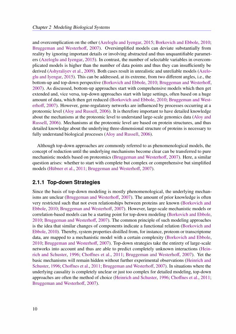
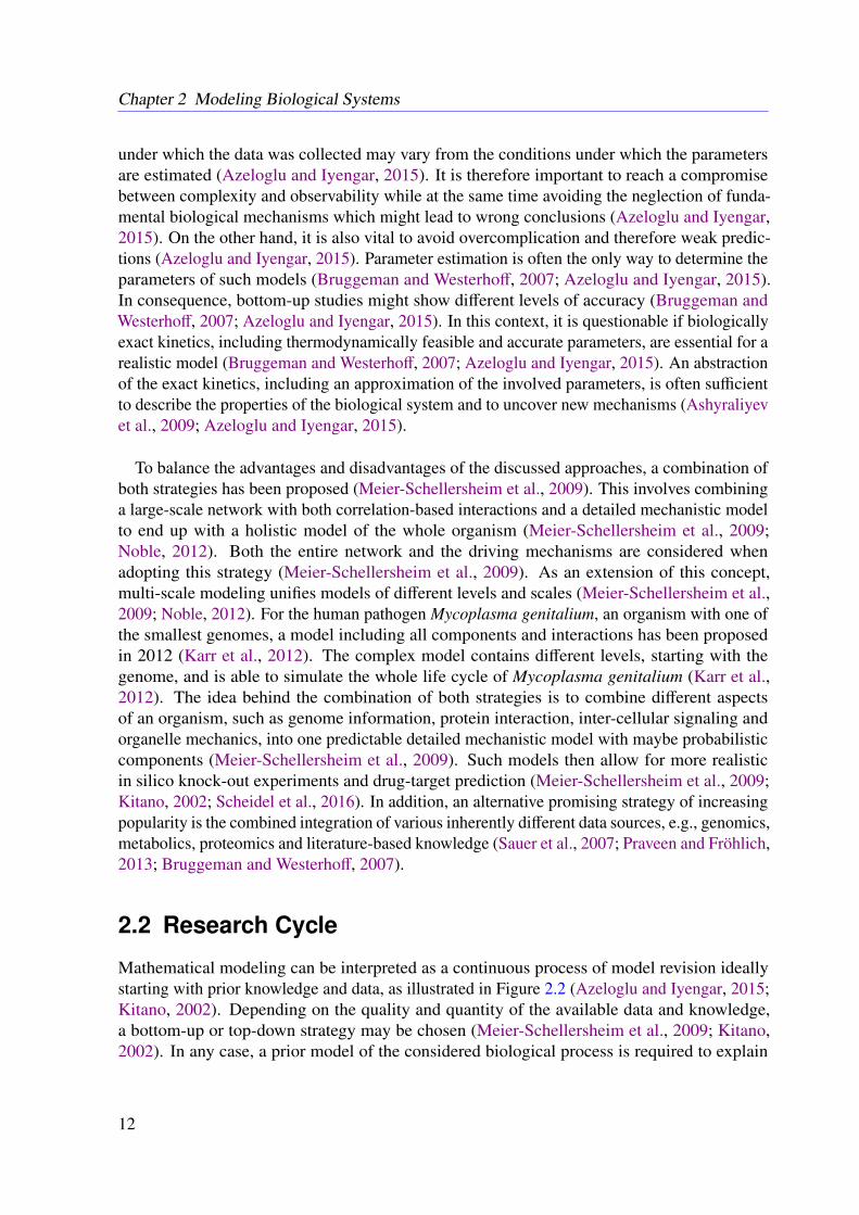
2.2 Research Cycle
Mathematical modeling can be interpreted as a continuous process of model revision ideallystarting with prior knowledge and data, as illustrated in Figure 2.2 (Azeloglu and Iyengar, 2015;Kitano, 2002). Depending on the quality and quantity of the available data and knowledge,a bottom-up or top-down strategy may be chosen (Meier-Schellersheim et al., 2009; Kitano,2002). In any case, a prior model of the considered biological process is required to explain
12
2.2 Research Cycle
the given observations (Kitano, 2002). This can be a detailed biochemical reaction network,which is often the case for bottom-up approaches, or a more general whole-cell model or patientmodel which allows for the identification of the involved subnetworks and components (Kitano,2002; Bruggeman and Westerhoff, 2007). The parameters of the model must then be adapted tothe given data in order to gain reliable model predictions (Azeloglu and Iyengar, 2015; Kitano,2002; Bruggeman and Westerhoff, 2007). The obtained in silico predictions are afterwardscompared with further experimental observations for verification and falsification (Kitano, 2002;Bruggeman and Westerhoff, 2007). In consequence, the inclusion and exclusion of components,subnetworks or a certain level of detail leads to a refined model (Kitano, 2002; Bruggeman andWesterhoff, 2007). The refined model has to be adapted again to the given data in order to gener-ate new in silico predictions (Kitano, 2002; Bruggeman and Westerhoff, 2007). This leads to acycle of testing and model refinement which continues until the in silico model is in sufficientagreement with the experimental observations (Kitano, 2002; Bruggeman and Westerhoff, 2007).
Several challenges have to be addressed during such a research cycle (Kitano, 2002; Brugge-man and Westerhoff, 2007). Depending on the complexity of the model and the quality of theunderlying data, for a given model, based on prior knowledge and a set of observations, the un-known parameters, e.g., the kinetic parameters or regression coefficients, of this model must beestimated (Jaqaman and Danuser, 2006; Kitano, 2002; Bruggeman and Westerhoff, 2007). Theadoption of model parameters is a difficult task because the information regarding the involvedactors is often limited, especially in case of top-down approaches (Azeloglu and Iyengar, 2015;Bruggeman and Westerhoff, 2007). Nevertheless, by comparing the model predictions withempirical data, the quality of the model can be evaluated (Azeloglu and Iyengar, 2015; Kitano,2002; Bruggeman and Westerhoff, 2007). The evaluation of the model may be difficult in caseswhere the features or components of interest are not directly accessible (Azeloglu and Iyengar,2015; Bruggeman and Westerhoff, 2007). In many situations, this requires the development ofnovel experimental in vivo or in vitro techniques, an adjustment of the research question or anadjustment of the experimental design (Azeloglu and Iyengar, 2015; Kitano, 2002; Borkovichand Ebbole, 2010).
Figure 2.2 illustrates the research cycle for bottom-up models (Azeloglu and Iyengar, 2015;Kitano, 2002). In contrast, for predictive modeling, large data-sets are used to train the algorithm,which is then able to predict a certain behavior based on fresh but similar data, as illustrated inFigure 2.2b (Bishop, 2007; Sauer et al., 2007; Gelman et al., 2013). Here, the initial data setis split into a training and a validation data set (Bishop, 2007). The latter is used to validatethe predictive power of the model trained by the training data set (Bishop, 2007). Nowadays,machine learning methods such as support vector machines are able to identify potential drugtargets and predict correlations between cellular processes (Bishop, 2007; Chuang et al., 2010;Murphy, 2011). This fundamentally differs from the understanding of systems biology asdefined in this work (Bishop, 2007; Bruggeman and Westerhoff, 2007; Hübner et al., 2011).Unfortunately, for bottom-up approaches, the model of the related protein-protein interactionnetwork, i.e., the biochemical reaction network, very frequently does not match the observationsat first glance (Azeloglu and Iyengar, 2015; Kitano, 2002). Even after adaptation of the involvedkinetic parameters, there sometimes remains a significant difference between observations and
13
Chapter 2 Modeling Biological Systems
model predictions (Azeloglu and Iyengar, 2015). Consequently, the model must be improvedby incorporating additional knowledge or further assumptions (Azeloglu and Iyengar, 2015).In these cases, the original model is replaced with a revised version and has to be evaluatedagain (Azeloglu and Iyengar, 2015). This process is repeated until the model is able to reproducethe given empirical data, as shown in Figure 2.2a (Azeloglu and Iyengar, 2015). A picture similarto the one in Figure 2.2 can be drawn for top-down approaches, but here the model is refined byreduction rather than extension (Azeloglu and Iyengar, 2015; Kitano, 2002; Bruggeman andWesterhoff, 2007).
Figure 2.2: General principles of computational biology. (a) In systems biology, bottom-up modelingstarts with an initial model based on literature or expert-based prior knowledge. By incorporating dataobtained from wet lab experiments or extracted from databases, the model parameters can be estimated.The model then allows for predictions and comparison with real observations. These observations arenot necessarily on the same level as the obtained data. An insufficient fit to the observed data indicatesa mistake in the model and thus the model needs to be revised and the parameters must be fitted again.This process results in a predictive model with regard to the underlying mechanisms. (b) In contrast,machine learning approaches focus on correlations within the given data set based on a restricted amountof prior knowledge. The given data can be split into two individual and isolated data sets. One is used totrain the model and the other to validate the findings. The aim of this approach is to derive a predictivemodel which allows to make accurate predictions and uncover the inherent features without knowledgeof the underlying mechanisms.
14
2.3 Model Formalisms
2.3 Model Formalisms
As a holistic and interdisciplinary approach, modern systems biology utilizes mathematicaltheories and experimental tools from different branches of modern life sciences (Machadoet al., 2011). Cellular components previously studied independently are nowadays analyzed inan integrated manner (Machado et al., 2011). The characterization of miscellaneous aspectsof the methods used in systems biology can be done from different angles (Machado et al.,2011; Kitano, 2002; Bruggeman and Westerhoff, 2007). From a conceptual point of view,models in systems biology are divided into static and dynamic models, as illustrated in Fig-ure 2.3 (Bruggeman and Westerhoff, 2007; Palsson, 2006). Both types of models are usefulto describe biological processes, which are classically defined as metabolic and signaling net-works (Klipp and Liebermeister, 2006; Palsson, 2006). Some authors consider gene regulatorynetworks as a special kind of biological model. However, because gene regulatory networks arebilaterally interacting with metabolic and signaling pathways, they are rather a part of these typesthan independent and autonomous (Machado et al., 2011; Noble, 2012). From a methodologicalpoint of view, a distinction can be made between deterministic and probabilistic approaches,while deterministic models still dominating current research in systems biology (Chuang et al.,2010; Murphy, 2011; Hübner et al., 2011).
2.3.1 Static and Dynamic Models
Static models reflect the topology of a biological system at a certain steady state and thusthey can be considered as a special or simplified case of dynamic models (Palsson, 2006). Aprominent static and hence structure-based approach is the so-called constraint-based model-ing (Bordbar et al., 2014; Jerby et al., 2010; Lewis et al., 2010). Most structural models imposeconstraints on the biological system to predict the rate of turnover of metabolites in biologicalprocesses (Bordbar et al., 2014). The essential physico-chemical constraints of static modelsare often represented by stoichiometric matrices, composed of the stoichiometric coefficientsof the involved reactions (Lewis et al., 2012). In contrast to dynamic systems, no kineticinformation is required for structural modeling and thus predictions about the inherent dynamicsor time-dependent regulations are not possible (Lewis et al., 2012; Klipp and Liebermeister,2006). Particularly with regard to signaling pathways, time-dependent behavior is of importancebecause signal amplification is often caused by a change in enzyme activity (Klipp and Lieber-meister, 2006; Heinrich et al., 2002). As stoichiometry-based models only deal with steadystates, these phenomena are difficult to capture with this approach (Lewis et al., 2012). Understeady state conditions, all state variables are assumed to be constant (Palsson, 2006; Heinrichet al., 2002). However, this holds true only before and after stimulation but not for the transitionbetween both states (Klipp and Liebermeister, 2006; Heinrich et al., 2002).
Studies of the detailed behavior of signaling processes or time-dependent metabolic phe-nomena require dynamic models (Klipp and Liebermeister, 2006; Klamt et al., 2006; Heinrichet al., 2002). Here, in contrast to top-down strategies, the comparatively small size of bottom-upmodels allows for dynamic and hence kinetic models (Bruggeman and Westerhoff, 2007). Be-
15
Chapter 2 Modeling Biological Systems
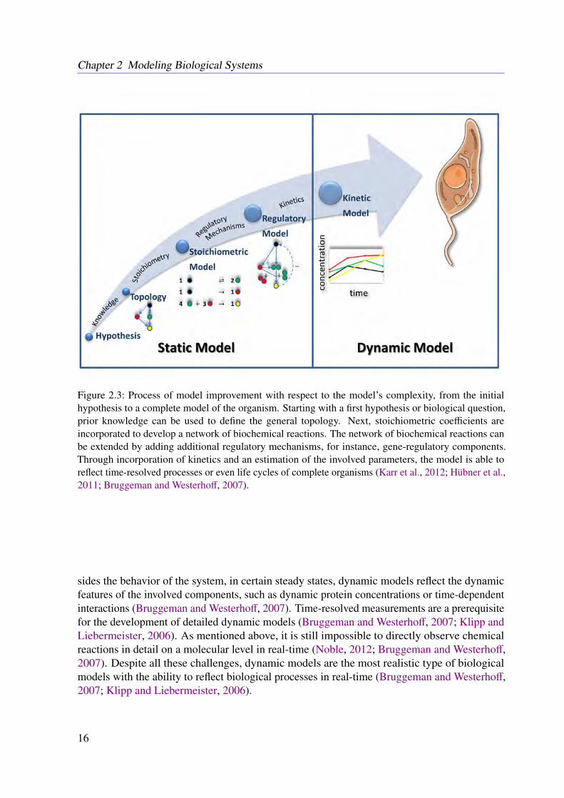
Figure 2.3: Process of model improvement with respect to the model’s complexity, from the initialhypothesis to a complete model of the organism. Starting with a first hypothesis or biological question,prior knowledge can be used to define the general topology. Next, stoichiometric coefficients areincorporated to develop a network of biochemical reactions. The network of biochemical reactions canbe extended by adding additional regulatory mechanisms, for instance, gene-regulatory components.Through incorporation of kinetics and an estimation of the involved parameters, the model is able toreflect time-resolved processes or even life cycles of complete organisms (Karr et al., 2012; Hübner et al.,2011; Bruggeman and Westerhoff, 2007).
sides the behavior of the system, in certain steady states, dynamic models reflect the dynamicfeatures of the involved components, such as dynamic protein concentrations or time-dependentinteractions (Bruggeman and Westerhoff, 2007). Time-resolved measurements are a prerequisitefor the development of detailed dynamic models (Bruggeman and Westerhoff, 2007; Klipp andLiebermeister, 2006). As mentioned above, it is still impossible to directly observe chemicalreactions in detail on a molecular level in real-time (Noble, 2012; Bruggeman and Westerhoff,2007). Despite all these challenges, dynamic models are the most realistic type of biologicalmodels with the ability to reflect biological processes in real-time (Bruggeman and Westerhoff,2007; Klipp and Liebermeister, 2006).
16
2.3 Model Formalisms
2.3.2 Signaling and Metabolic Networks
In literature, biological models are mainly divided into metabolic and signaling networks basedon the fact that metabolic pathways are characterized by a flow of matter and signaling pathwaysare characterized by a flow of information (Klipp and Liebermeister, 2006; Palsson, 2006).Nevertheless, it is obvious that metabolic and signaling networks are connected (Klipp andLiebermeister, 2006). Therefore, attempts have been made to combine both types of net-works (Engelhardt et al., 2017; Klamt et al., 2006; Behre and Schuster, 2009). Ultimately,both networks are based on the same fundamental mechanisms; only the point of view isdifferent (Klamt et al., 2006; Behre and Schuster, 2009).
Metabolic systems can be described as the interplay between anabolic and catabolic pro-cesses within the cell and are mostly based on enzyme conversions of one chemical entity intoanother (Dale and Rang, 2011; Berg et al., 2013). Today, metabolic systems biology mainlyfocuses on the reconstruction of metabolic networks for a target organism on a genome-scalelevel (Choffnes et al., 2011). In this context, enzyme-catalyzed protein cascades and constrainedsteady state models are of high relevance (Lehninger et al., 2005; Palsson, 2006). To allow forthe reconstruction of the metabolic system, the underlying network has to fulfill a number ofassumptions, which were summarized by Bernhard Palsson (Choffnes et al., 2011). Followingthis, all cellular functions can be explained through chemistry and the cell always behaves ina context-specific manner (Choffnes et al., 2011). The sugar metabolism in Saccharomycescerevisiae under aerobic and aerobic conditions might serve as an example (Rodrigues et al.,2006). It has been shown that Saccharomyces cerevisiae is able to switch its glucose catabolismbetween respiration and fermentation depending on the availability of receptive oxygen inthe environment (Rodrigues et al., 2006). In addition, mass and energy must be conserved inmetabolic systems (Choffnes et al., 2011). This intrinsic physical law enables the mathematicalanalysis of metabolic systems (Palsson, 2006).
Constraint-based modeling can be used to gain information on the turnover rates in metabolicnetworks (Bordbar et al., 2014; Jerby et al., 2010; Lewis et al., 2010). Most of these techniquesimpose constraints on the system and on the analysis method to predict the rate of turnoverof metabolites in a reaction (Bordbar et al., 2014). Constrained-based models assume themetabolism as a system of biochemical reactions (Lewis et al., 2012). Therefore, substratesand enzymes must be present in or produced by the system and the system is considered tobe approximately in-balance regarding to all transfers of matter and energy (Bordbar et al.,2014). The overall mass of the system thus remains constant over time and the direction of theinvolved reactions is under constraint of thermodynamic principles (Volkenshtein, 2009; Lewiset al., 2012). Nowadays, most of the required prior knowledge can be obtained from metabolicreconstruction databases (Lewis et al., 2012).
Signal transduction is often reduced to linear cascades involving protein-protein interactionsand the interaction with second messengers, e.g., cAMP or Ca2++ (Kestler et al., 2008). Althoughlinear systems are not able to reflect the real dynamics of signaling pathways, they are frequentlyemployed because meaningful readouts of the pathway activation are available when time-
17
Chapter 2 Modeling Biological Systems
resolved measurements of the involved components are not accessible (Kestler et al., 2008;Klipp and Liebermeister, 2006; Heinrich et al., 2002). An important improvement of linearsignaling cascade models was the inclusion of positive and negative feedback loops (Kestler et al.,2008). It is well known that most signaling pathways contain several feedback loops to controlthe amplitude of the transduced signal (Kestler et al., 2008). Here, signal amplification allows fora fast adaptation to the environment (Kestler et al., 2008; Heinrich et al., 2002). The topology ofsignaling pathways and linear approximations enable significant insights into signaling pathways,for instance regarding the maximum amplitude or the stability of signals (Kestler et al., 2008;Heinrich et al., 2002). But in order to reflect the detailed mechanisms of the signaling pathwaysand their interaction, detailed models are required, including detailed knowledge of the kineticsand turnover rates (Kestler et al., 2008; Klipp and Liebermeister, 2006; Heinrich et al., 2002).
2.3.3 Probabilistic Approaches
Over the past decade, dynamic modeling has become a leading topic in systems biology (Chuanget al., 2010; Hübner et al., 2011). The majority of modeling approaches in systems biologyapplied to biochemistry are based on ODEs and partial differential equations followed bystoichiometry-based approaches (Machado et al., 2011; Hübner et al., 2011). ODE-based mod-els are most suitable to describe small and medium-scale networks but often fail on a whole-celllevel (Meier-Schellersheim et al., 2009; Hübner et al., 2011; Chuang et al., 2010). This is one ofthe main reasons why probabilistic methods become more and more important, in addition todeterministic, e.g., stoichiometry- and ODE-based methods (Chuang et al., 2010; Hübner et al.,2011; Klipp and Liebermeister, 2006). Besides other Boolean networks, Bayesian networksand Petri nets are also frequently used in systems biology (Machado et al., 2011; Chuang et al.,2010; Hübner et al., 2011; Klipp and Liebermeister, 2006).
Although Boolean networks are mostly used to model the regulation of genes based on logicrules, protein-protein interactions can be expressed via Boolean networks as well (Machadoet al., 2011; Hübner et al., 2011). The components of Boolean networks are encoded as Booleanvariables which can either be active or inactive (Machado et al., 2011). In that manner, at eachdiscrete time point, the state of each Boolean variable is given by a function composed of thestates of all related regulators, e.g., enzymes or transcription factors (Machado et al., 2011). Thestate of all components changes synchronously (Machado et al., 2011). Thus, for large-scalenetworks, the determination of all possible states is a cost-intensive process (Machado et al.,2011). However, it can be used to find attracted steady states and to analyze the robustness ofthe network (Machado et al., 2011). Probabilistic Boolean networks have been established toincorporate uncertainties (Machado et al., 2011).
In contrast to Boolean networks, Bayesian networks allow for more detailed dependenciesand different states of the modeled components (Bishop, 2007; Machado et al., 2011). Bayesiannetworks are probabilistic graphs whereby their components are represented by random discreteor continuous variables with conditional dependencies, as mentioned in Section 4.3 (Bishop,2007; Machado et al., 2011). This can be considered as a directed graph, and each component,i.e., node, contains a probabilistic function which depends on the values of all related influencing
18

2.3 Model Formalisms
nodes (Bishop, 2007; Machado et al., 2011). Many different methods have been developedto infer the network structure and the corresponding probability parameters (Bishop, 2007;Machado et al., 2011). Due to the probabilistic nature of Bayesian networks, they allow towork with incomplete data sets and are frequently used for the modeling of gene-regulatory net-works (Bishop, 2007; Machado et al., 2011; Chuang et al., 2010). Dynamic Bayesian networksare a common extension to simulate time-dependent biological systems (Machado et al., 2011).
Whereas Boolean and Bayesian networks only allow for one type of node representing acluster of components or an individual component, Petri nets incorporate two different typesof nodes, i.e., places and transitions, and the dependencies between the nodes are representedby directed and weighted arcs (Scheidel et al., 2016; Junker and Schreiber, 2008; Machadoet al., 2011). The passive parts, i.e., components or clusters, are captured by the places andthe chemical reactions are represented through transitions (Scheidel et al., 2016; Junker andSchreiber, 2008; Machado et al., 2011). Commonly, places are represented as circles andtransitions as squares (Scheidel et al., 2016; Junker and Schreiber, 2008). Thereby the nodesof the resulting graph-structure represent either molecules or chemical reactions, whereas thedirected edges represent the relation between components and reactions (Scheidel et al., 2016;Junker and Schreiber, 2008; Machado et al., 2011). Usually the edges are weighted according totheir corresponding stoichiometric factor (Scheidel et al., 2016). This is in contrast to commongraphical representations of biochemical networks, where components are represented by nodesand the corresponding reactions via directed edges (Scheidel et al., 2016; Palsson, 2006). Theplaces are associated with tokens which can stand for the amount or concentration of a chemicalsubstance or a fulfilled precondition of a reaction (Scheidel et al., 2016; Junker and Schreiber,2008). Tokens are produced or consumed when the transitions fire (Machado et al., 2011). Thismeans that the transitions modulate the tokens in a similar way as biological processes wouldchange the state of the involved components (Scheidel et al., 2016; Junker and Schreiber, 2008;Machado et al., 2011). The state of the system is given by the distribution of the tokens, whichthus describes the dynamics of the system (Junker and Schreiber, 2008; Machado et al., 2011).
2.3.4 Stoichiometric Matrices
Given sufficient prior information, each biological process based on protein-protein interactionscan be described through a set of biochemical reactions (Heinrich et al., 2002; Palsson, 2006).These reaction processes are often an enzyme-catalyzed conversion of molecules or proteinbinding events (Berg et al., 2013).
19
Chapter 2 Modeling Biological Systems
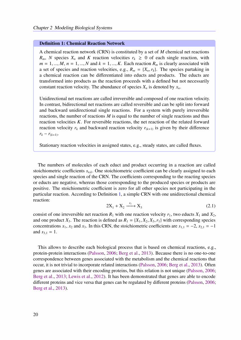
Definition 1: Chemical Reaction Network
A chemical reaction network (CRN) is constituted by a set of M chemical net reactionsRm, N species Xn and K reaction velocities rk ≥ 0 of each single reaction, withm = 1, ...,M, n = 1, ...,N and k = 1, ...,K. Each reaction Rm is clearly associated witha set of species and reaction velocities, e.g., Rm = Xn, rk. The species partaking ina chemical reaction can be differentiated into educts and products. The educts aretransformed into products as the reaction proceeds with a defined but not necessarilyconstant reaction velocity. The abundance of species Xn is denoted by xn.
Unidirectional net reactions are called irreversible and composed of one reaction velocity.In contrast, bidirectional net reactions are called reversible and can be split into forwardand backward unidirectional single reactions. For a system with purely irreversiblereactions, the number of reactions M is equal to the number of single reactions and thusreaction velocities K. For reversible reactions, the net reaction of the related forwardreaction velocity rk and backward reaction velocity r(k+1) is given by their differencerk − r(k+1).
Stationary reaction velocities in assigned states, e.g., steady states, are called fluxes.
The numbers of molecules of each educt and product occurring in a reaction are calledstoichiometric coefficients sn,k. One stoichiometric coefficient can be clearly assigned to eachspecies and single reaction of the CRN. The coefficients corresponding to the reacting speciesor educts are negative, whereas those corresponding to the produced species or products arepositive. The stoichiometric coefficient is zero for all other species not participating in theparticular reaction. According to Definition 1, a simple CRN with one unidirectional chemicalreaction:
2X1 + X2r1−−−→ X3 (2.1)
consist of one irreversible net reaction R1 with one reaction velocity r1, two educts X1 and X2,and one product X3. The reaction is defined as R1 = X1, X2, X3, r1 with corresponding speciesconcentrations x1, x2 and x3. In this CRN, the stoichiometric coefficients are s1,1 = −2, s2,1 = −1and s3,1 = 1.
This allows to describe each biological process that is based on chemical reactions, e.g.,protein-protein interactions (Palsson, 2006; Berg et al., 2013). Because there is no one-to-onecorrespondence between genes associated with the metabolism and the chemical reactions thatoccur, it is not trivial to incorporate related interactions (Palsson, 2006; Berg et al., 2013). Oftengenes are associated with their encoding proteins, but this relation is not unique (Palsson, 2006;Berg et al., 2013; Lewis et al., 2012). It has been demonstrated that genes are able to encodedifferent proteins and vice versa that genes can be regulated by different proteins (Palsson, 2006;Berg et al., 2013).
20
2.3 Model Formalisms
Definition 2: Stoichiometric Matrix
Let the vector u be the turnover rate of molecules through the system. Then, we canclearly define a linear transformation S ∈ RN×K which transforms the flux vector u intothe derivative of a concentration vector x as follows:
dxdt
= S u.
For a CRN with K single reactions and N species, the dimension of S is N × K. Eachelement sn,k represents the stoichiometric coefficient corresponding to species n in reactionk.
Every CRN can be split into external, exchange and internal reactions with respect to theboundaries of the network. In most situations, both exchange and internal reactions are con-sidered whereas external reactions are frequently neglected, but, depending on the context,it may be useful to only consider internal reactions (Palsson, 2006). In general, the reactionvelocities rk are functions of the related species concentrations and a set of rate constants rk:
rk = fk (x, rk) , (2.2)
with a general continuous and time-dependent function fk. In general, the derivative of aconcentration vector x is depend on the related reaction velocities and the correspondingstoichiometric coefficients, and the entities can be calculated through
dxn
dt=
K∑k=1
sn,k fk (x, rk), (2.3)
where sn,k is the stoichiometric coefficient of species n partaking in the single reaction k. Atfixed time points e.g., under steady state conditions, fk (x, rk) = vk is obtained and Equation (2.3)yields
dxn
dt=
K∑k=1
sn,kvk. (2.4)
The number of elements of the flux vector u is equal to the number of single-reaction velocitiesin the CRN. In most situations, the number of reactions in a CRNs is larger than the number ofspecies and therefore K > N, implying that S may not be of full rank (Palsson, 2006).
The stoichiometric matrix S is commonly considered as a connectivity matrix or a networkrepresented by a map (Palsson, 2006). The nodes in the map then correspond to the rows and thelinks to the columns of S , respectively (Palsson, 2006). Thus, S represents the general topologyof the system and is typically used to investigate time-independent features of the CRN (Palsson,2006).
These stoichiometry-based approaches have to rely on several assumptions (Palsson, 2006).First, the reaction component of interest is assumed to be uniformly distributed in the sys-
21
Chapter 2 Modeling Biological Systems
tem (Palsson, 2006). Second, the concentration is assumed to be sufficiently high to define areal number (Palsson, 2006). In addition, the reaction velocities are considered to not explicitlydepend on time (Palsson, 2006).
2.3.5 Differential Equations
In contrast to time-independent stoichiometry-based approaches, ODEs allow to capture theinherent dynamics of CRNs (Palsson, 2006; Azeloglu and Iyengar, 2015). Because the reactiondynamics are a key aspect of signaling processes, ODE-based approaches are frequently used tomodel this type of system (Hübner et al., 2011; Klipp and Liebermeister, 2006). ODEs are awidely discussed common topic in mathematics and interdisciplinary research (Mattheij andMolenaar, 2002).
Definition 3: Ordinary Differential Equation
Let F (t) be a real-valued function F : I×Ω→ Rwith Ω ⊂ Rd+1, I ⊂ R, x (t) a real-valuedfunction with x : I → R and x(d) (t) the derivative of x (t) to the order of d given by dd x(t)
ddtwith t ∈ R. Then, the implicit ordinary differential equation to the order of d is given by
F(t, x (t) , x(1) (t) , ..., x(d) (t)
)= 0.
In contrast, the explicit ordinary differential equation f with f : I × Ω→ R with Ω ⊂ Rd
is a special case of F and given by
x(d) (t) = f(t, x (t) , x(1) (t) , ..., x(d−1) (t)
).
The function Φ : I → R is named solution of the implicit ODE in the interval I ⊂ R ifΦ
(t, x (t) , x(1) (t) , ..., x(d) (t)
)= 0 and Φ is d times differentiable.
Accordingly, Φ : I → R, d − 1 times differentiable, is named solution of the explicit ODEin the interval I ⊂ R if Φ
(t, x (t) , x(1) (t) , ..., x(d−1) (t)
)= x(d).
For example, the first-order ODE
x (t) = −2x (t) ⇐⇒ x (t) + 2x (t) = 0, (2.5)
with x (t) = x(1) (t) has the solution x (t) = c exp (−2t) with c ∈ R.
The above definition can be extended to a system of coupled ODEs incorporating severaldependent variables (Walter, 2000). For systems biology, first-order systems of explicit ODEsare of interest.
22
2.3 Model Formalisms
Definition 4: First-Order System of Ordinary Differential Equations
Given n explicit ordinary differential equations fn : I × Ω → R with Ω ⊂ (Rn)1, I ⊂ R,x : I → Rn and t ∈ R the system
x(1) (t) = f (t, x (t))
is called system of ordinary differential equations of the order one. The system is said tobe autonomous if f is not directly dependent on t.
In general, due to the fact that ODE systems are basically solved via integration, they do notnecessarily have a unique solution, unless further constraints or initial conditions are given (Wal-ter, 2000). For biological systems, however, the initial conditions are frequently known andhence in many cases the arising initial value problem (IVP) has a unique solution (Palsson,2006; Kremling, 2012; Walter, 2000).
Definition 5: Initial Value Problem
Given a vector-valued function f : I × Ω → Rn with Ω ⊂ (Rn)d, I ⊂ R, x : I → Rn andt ∈ R, the system
x(d) (t) = f(t, x (t) , x(1) (t) , ..., x(d−1) (t)
)x (0) = x0,
with a vector of initial conditions x0 ∈ Rn is called initial value problem.
The Picard-Lindelöf theorem guarantees a unique solution of the IVP given by Definition 5 forLipschitz-continuous functions (Teschl, 2012). Lipschitz continuity is a stricter form of continu-ity ensuring that a given continuous function is limited in the rate of change over time (Teschl,2012). For most high-dimensional IVPs, an analytical solution does not exist (Teschl, 2012;Walter, 2000). Instead, the IVP can be solved numerically for discrete time points and restricteddue to its complexity (Hanke-Bourgeois, 2008).
Complex processes, e.g., those involving dynamics in time and space, have more than oneindependent variable (Kholodenko, 2006). These phenomena are usually addressed via partialdifferential equations (Kholodenko, 2006). Hybrid models in cancer research, where cell growthis often described through growth-consumption dynamics and cell dynamics on a lattice, arebased on partial differential equations (Altrock et al., 2015). In contrast, some biologicalprocesses are of random nature, such as the synaptic activity of neurotransmitters released fromsynaptic vesicles (Saarinen et al., 2008). Here, stochastic differential equations incorporatingrandom processes are commonly used (Saarinen et al., 2008). Unlike ODEs or partial differentialequations, stochastic differential equations are defined via integrals (Bauer, 2002, 1992). This isequivalent to the derivative-based formulation but circumvents the lack of differentiability ofstochastic processes, for instance, in case of Brownian motion (Bauer, 2002, 1992).
23
Chapter 2 Modeling Biological Systems
2.4 Properties of Protein Interactions
Biological processes are based on biochemical reactions which themselves are driven by chem-ical interactions (Berg et al., 2013; Choffnes et al., 2011). For general biological phenomena, itis not possible to postulate special laws of nature as in physics (Berg et al., 2013). However,all living organisms share a large number of biochemical features (Berg et al., 2013). Like allchemical reactions, biological processes are driven by the laws of thermodynamics (Berg et al.,2013). Besides the underlying chemical principles, the structure of the involved macromoleculesis also important (Alberts et al., 2014; Berg et al., 2013). This becomes particularly clear incase of DNA, which stores all genetic information (Alberts et al., 2014; Berg et al., 2013).In general, two DNA strands form a double helix via hydrogen bridge linkages between twocorresponding bases (Berg et al., 2013). In the DNA double helix, not the chemical interactionsbut the sequence of base pairs encode the genetic information (Berg et al., 2013). This verycomplex mechanism helps to ensure a stable storage of genetic information because even ifone DNA strand is damaged it can be rebuild by the corresponding strand (Berg et al., 2013).As illustrated, both mechanisms are rather closely interlinked than independent (Berg et al.,2013). The structure has a strong impact on the binding behavior of proteins which, in turn,influences the binding capacity and therefore the structure itself (Berg et al., 2013; Palsson,2006). However, the dominant driving force of protein-protein interactions are the laws ofthermodynamics (Berg et al., 2013; Palsson, 2006).
As stated in the first law of thermodynamics, energy can neither be consumed nor produced,it can only be converted from one form into another (Kremling, 2012; Berg et al., 2013). Forspontaneous processes, the disorder of the system, called entropy, increases (Kremling, 2012;Berg et al., 2013). The entropy denotes the ratio between the reversible heat and the system’sabsolute temperature (Kremling, 2012; Berg et al., 2013). The change in entropy can be directlymeasured by the so-called Gibbs free energy ∆G (Berg et al., 2013). In addition, ∆G is ameasure for the work which can be performed by reversible chemical reactions under constantconditions (Berg et al., 2013). Consequently, the Gibbs free energy is a measure for the drivingforce of a reaction and thus enables a differentiation between exergonic spontaneous processesand endergonic processes requiring an absorption of energy from the surroundings (Berg et al.,2013). Biochemical reactions proceed spontaneous only if the entropy increases, i.e., if ∆Gis negative (Berg et al., 2013). In thermodynamic equilibrium, the Gibbs free energy is equalto zero (Berg et al., 2013). ∆G is always negative for exergonic spontaneous processes andalways positive for endergonic processes (Berg et al., 2013). In other words, the overall entropyincreases in exergonic processes and decreases in endergonic processes (Berg et al., 2013). Onlyreactions increasing the entropy with ∆G < 0 occur spontaneously and therefore the chemicalequilibrium is shifted towards this direction (Berg et al., 2013). The reaction which decreasesthe entropy with ∆G > 0 proceeds more slowly and the reaction rate inclines towards zero (Berget al., 2013). Please note that ∆G alone provides no information regarding the reaction rateof the involved reactions (Berg et al., 2013). In practice, reactions are often accelerated byenzymes (Berg et al., 2013).
24
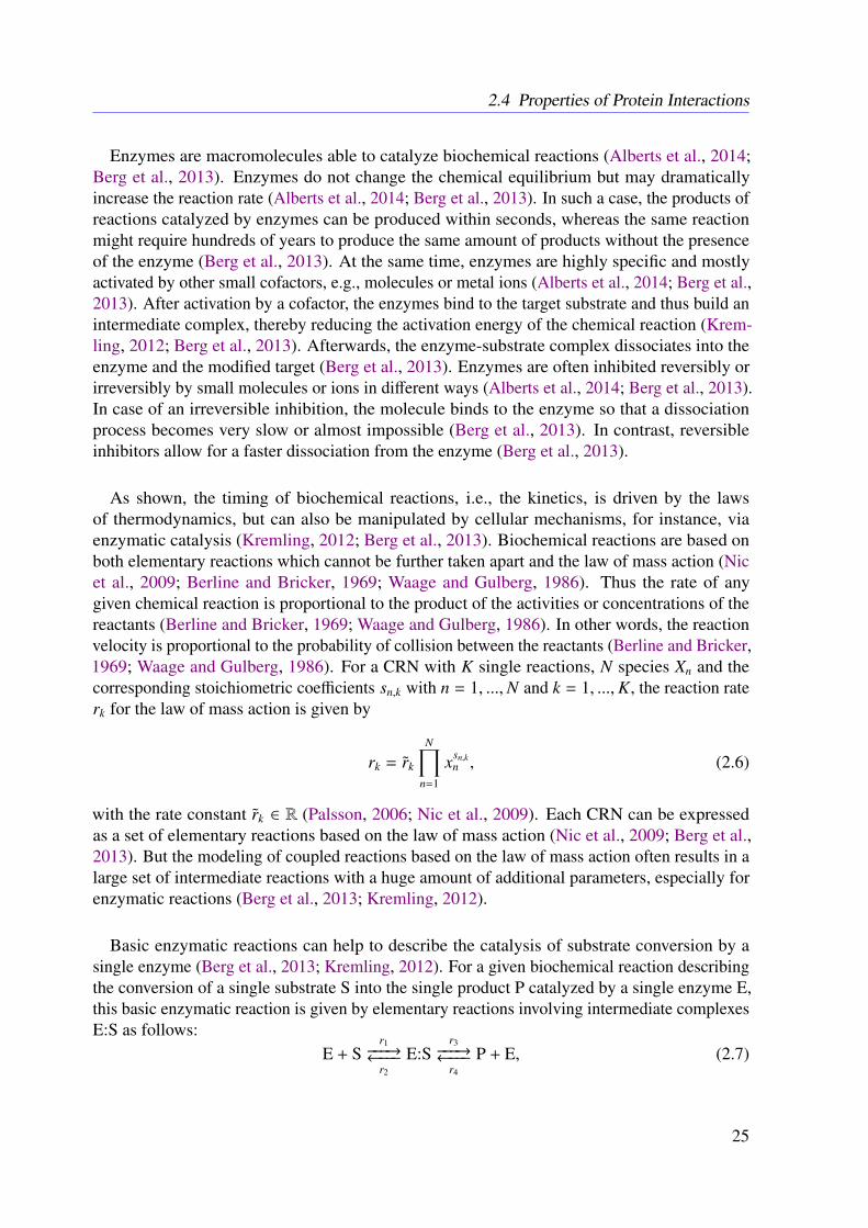
2.4 Properties of Protein Interactions
Enzymes are macromolecules able to catalyze biochemical reactions (Alberts et al., 2014;Berg et al., 2013). Enzymes do not change the chemical equilibrium but may dramaticallyincrease the reaction rate (Alberts et al., 2014; Berg et al., 2013). In such a case, the products ofreactions catalyzed by enzymes can be produced within seconds, whereas the same reactionmight require hundreds of years to produce the same amount of products without the presenceof the enzyme (Berg et al., 2013). At the same time, enzymes are highly specific and mostlyactivated by other small cofactors, e.g., molecules or metal ions (Alberts et al., 2014; Berg et al.,2013). After activation by a cofactor, the enzymes bind to the target substrate and thus build anintermediate complex, thereby reducing the activation energy of the chemical reaction (Krem-ling, 2012; Berg et al., 2013). Afterwards, the enzyme-substrate complex dissociates into theenzyme and the modified target (Berg et al., 2013). Enzymes are often inhibited reversibly orirreversibly by small molecules or ions in different ways (Alberts et al., 2014; Berg et al., 2013).In case of an irreversible inhibition, the molecule binds to the enzyme so that a dissociationprocess becomes very slow or almost impossible (Berg et al., 2013). In contrast, reversibleinhibitors allow for a faster dissociation from the enzyme (Berg et al., 2013).
As shown, the timing of biochemical reactions, i.e., the kinetics, is driven by the lawsof thermodynamics, but can also be manipulated by cellular mechanisms, for instance, viaenzymatic catalysis (Kremling, 2012; Berg et al., 2013). Biochemical reactions are based onboth elementary reactions which cannot be further taken apart and the law of mass action (Nicet al., 2009; Berline and Bricker, 1969; Waage and Gulberg, 1986). Thus the rate of anygiven chemical reaction is proportional to the product of the activities or concentrations of thereactants (Berline and Bricker, 1969; Waage and Gulberg, 1986). In other words, the reactionvelocity is proportional to the probability of collision between the reactants (Berline and Bricker,1969; Waage and Gulberg, 1986). For a CRN with K single reactions, N species Xn and thecorresponding stoichiometric coefficients sn,k with n = 1, ...,N and k = 1, ...,K, the reaction raterk for the law of mass action is given by
rk = rk
N∏n=1
xsn,kn , (2.6)
with the rate constant rk ∈ R (Palsson, 2006; Nic et al., 2009). Each CRN can be expressedas a set of elementary reactions based on the law of mass action (Nic et al., 2009; Berg et al.,2013). But the modeling of coupled reactions based on the law of mass action often results in alarge set of intermediate reactions with a huge amount of additional parameters, especially forenzymatic reactions (Berg et al., 2013; Kremling, 2012).
Basic enzymatic reactions can help to describe the catalysis of substrate conversion by asingle enzyme (Berg et al., 2013; Kremling, 2012). For a given biochemical reaction describingthe conversion of a single substrate S into the single product P catalyzed by a single enzyme E,this basic enzymatic reaction is given by elementary reactions involving intermediate complexesE:S as follows:
E + Sr1−−−→←−−−
r2
E:Sr3−−−→←−−−
r4
P + E, (2.7)
25
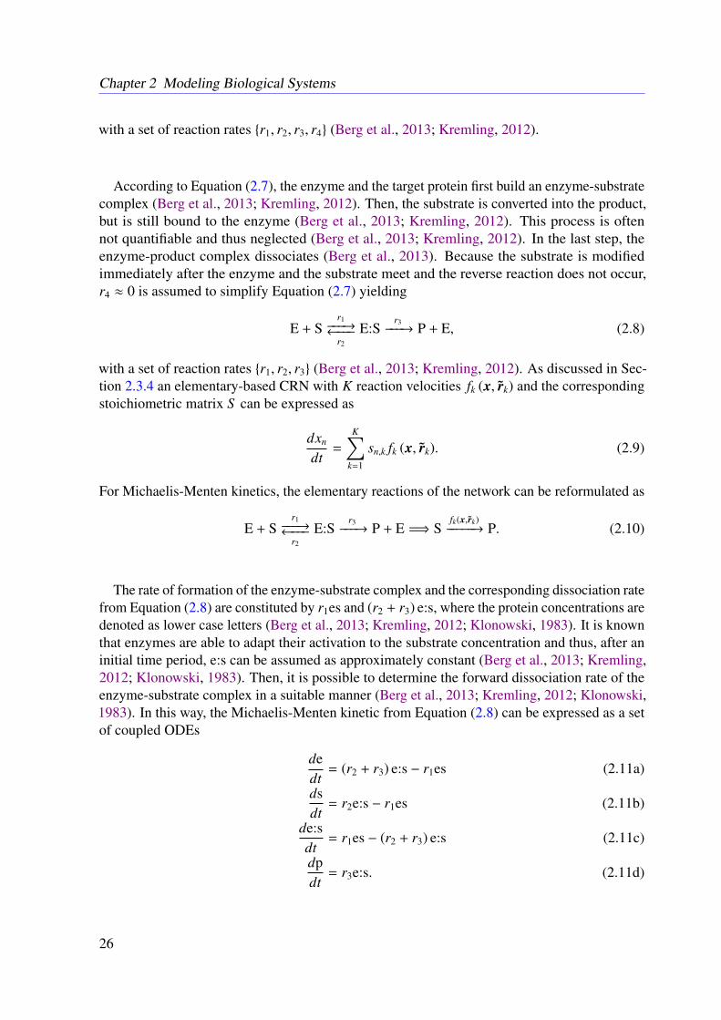
Chapter 2 Modeling Biological Systems
with a set of reaction rates r1, r2, r3, r4 (Berg et al., 2013; Kremling, 2012).
According to Equation (2.7), the enzyme and the target protein first build an enzyme-substratecomplex (Berg et al., 2013; Kremling, 2012). Then, the substrate is converted into the product,but is still bound to the enzyme (Berg et al., 2013; Kremling, 2012). This process is oftennot quantifiable and thus neglected (Berg et al., 2013; Kremling, 2012). In the last step, theenzyme-product complex dissociates (Berg et al., 2013). Because the substrate is modifiedimmediately after the enzyme and the substrate meet and the reverse reaction does not occur,r4 ≈ 0 is assumed to simplify Equation (2.7) yielding
E + Sr1−−−→←−−−
r2
E:Sr3−−−→ P + E, (2.8)
with a set of reaction rates r1, r2, r3 (Berg et al., 2013; Kremling, 2012). As discussed in Sec-tion 2.3.4 an elementary-based CRN with K reaction velocities fk (x, rk) and the correspondingstoichiometric matrix S can be expressed as
dxn
dt=
K∑k=1
sn,k fk (x, rk). (2.9)
For Michaelis-Menten kinetics, the elementary reactions of the network can be reformulated as
E + Sr1−−−→←−−−
r2
E:Sr3−−−→ P + E =⇒ S
fk(x,rk)−−−−−→ P. (2.10)
The rate of formation of the enzyme-substrate complex and the corresponding dissociation ratefrom Equation (2.8) are constituted by r1es and (r2 + r3) e:s, where the protein concentrations aredenoted as lower case letters (Berg et al., 2013; Kremling, 2012; Klonowski, 1983). It is knownthat enzymes are able to adapt their activation to the substrate concentration and thus, after aninitial time period, e:s can be assumed as approximately constant (Berg et al., 2013; Kremling,2012; Klonowski, 1983). Then, it is possible to determine the forward dissociation rate of theenzyme-substrate complex in a suitable manner (Berg et al., 2013; Kremling, 2012; Klonowski,1983). In this way, the Michaelis-Menten kinetic from Equation (2.8) can be expressed as a setof coupled ODEs
dedt
= (r2 + r3) e:s − r1es (2.11a)
dsdt
= r2e:s − r1es (2.11b)
de:sdt
= r1es − (r2 + r3) e:s (2.11c)
dpdt
= r3e:s. (2.11d)
26
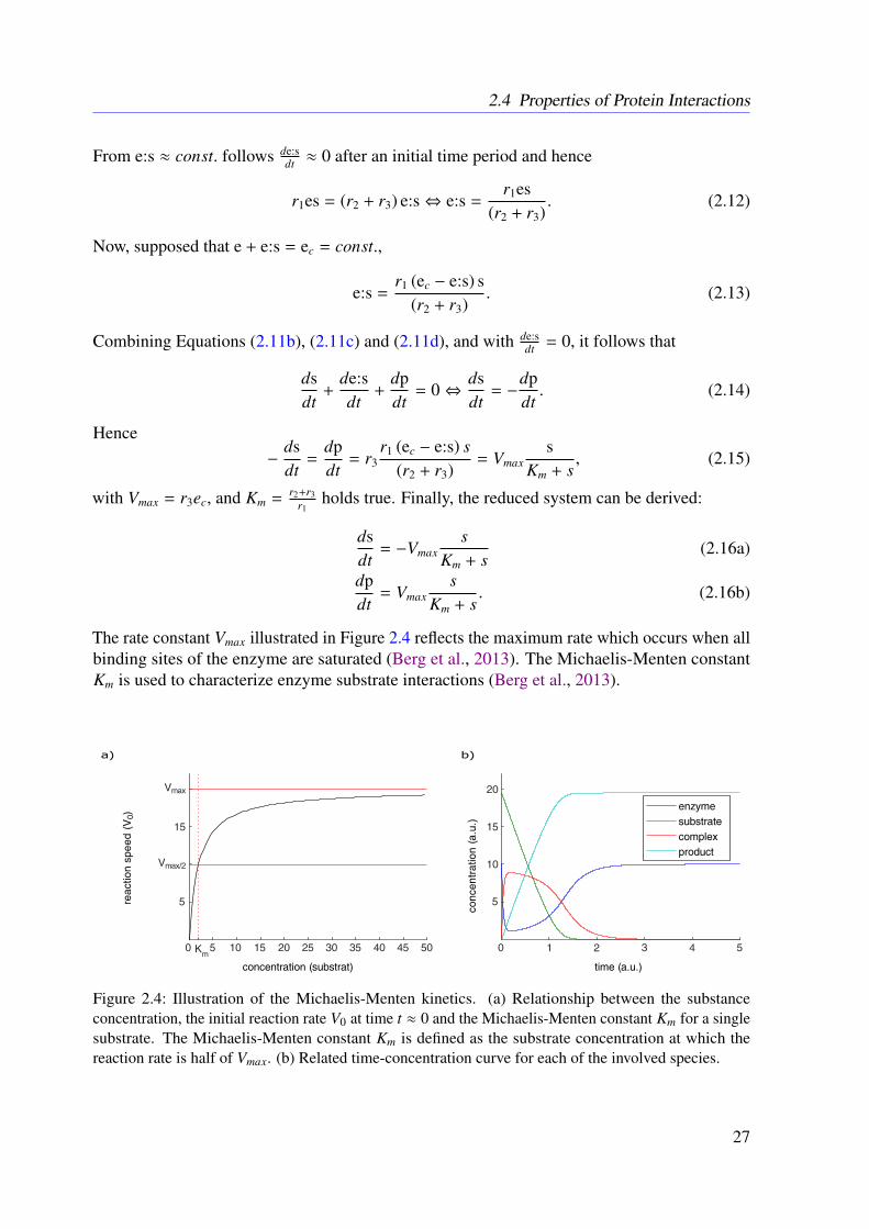
2.4 Properties of Protein Interactions
From e:s ≈ const. follows de:sdt ≈ 0 after an initial time period and hence
r1es = (r2 + r3) e:s⇔ e:s =r1es
(r2 + r3). (2.12)
Now, supposed that e + e:s = ec = const.,
e:s =r1 (ec − e:s) s
(r2 + r3). (2.13)
Combining Equations (2.11b), (2.11c) and (2.11d), and with de:sdt = 0, it follows that
dsdt
+de:sdt
+dpdt
= 0⇔dsdt
= −dpdt. (2.14)
Hence−
dsdt
=dpdt
= r3r1 (ec − e:s) s
(r2 + r3)= Vmax
sKm + s
, (2.15)
with Vmax = r3ec, and Km = r2+r3r1
holds true. Finally, the reduced system can be derived:
dsdt
= −Vmaxs
Km + s(2.16a)
dpdt
= Vmaxs
Km + s. (2.16b)
The rate constant Vmax illustrated in Figure 2.4 reflects the maximum rate which occurs when allbinding sites of the enzyme are saturated (Berg et al., 2013). The Michaelis-Menten constantKm is used to characterize enzyme substrate interactions (Berg et al., 2013).
Figure 2.4: Illustration of the Michaelis-Menten kinetics. (a) Relationship between the substanceconcentration, the initial reaction rate V0 at time t ≈ 0 and the Michaelis-Menten constant Km for a singlesubstrate. The Michaelis-Menten constant Km is defined as the substrate concentration at which thereaction rate is half of Vmax. (b) Related time-concentration curve for each of the involved species.
27
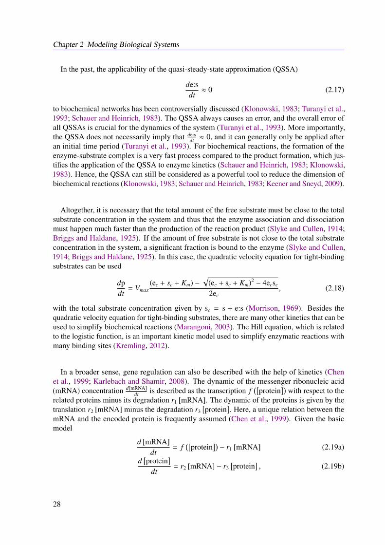
Chapter 2 Modeling Biological Systems
In the past, the applicability of the quasi-steady-state approximation (QSSA)
de:sdt≈ 0 (2.17)
to biochemical networks has been controversially discussed (Klonowski, 1983; Turanyi et al.,1993; Schauer and Heinrich, 1983). The QSSA always causes an error, and the overall error ofall QSSAs is crucial for the dynamics of the system (Turanyi et al., 1993). More importantly,the QSSA does not necessarily imply that de:s
dt ≈ 0, and it can generally only be applied afteran initial time period (Turanyi et al., 1993). For biochemical reactions, the formation of theenzyme-substrate complex is a very fast process compared to the product formation, which jus-tifies the application of the QSSA to enzyme kinetics (Schauer and Heinrich, 1983; Klonowski,1983). Hence, the QSSA can still be considered as a powerful tool to reduce the dimension ofbiochemical reactions (Klonowski, 1983; Schauer and Heinrich, 1983; Keener and Sneyd, 2009).
Altogether, it is necessary that the total amount of the free substrate must be close to the totalsubstrate concentration in the system and thus that the enzyme association and dissociationmust happen much faster than the production of the reaction product (Slyke and Cullen, 1914;Briggs and Haldane, 1925). If the amount of free substrate is not close to the total substrateconcentration in the system, a significant fraction is bound to the enzyme (Slyke and Cullen,1914; Briggs and Haldane, 1925). In this case, the quadratic velocity equation for tight-bindingsubstrates can be used
dpdt
= Vmax(ec + sc + Km) −
√(ec + sc + Km)2
− 4ecsc
2ec, (2.18)
with the total substrate concentration given by sc = s + e:s (Morrison, 1969). Besides thequadratic velocity equation for tight-binding substrates, there are many other kinetics that can beused to simplify biochemical reactions (Marangoni, 2003). The Hill equation, which is relatedto the logistic function, is an important kinetic model used to simplify enzymatic reactions withmany binding sites (Kremling, 2012).
In a broader sense, gene regulation can also be described with the help of kinetics (Chenet al., 1999; Karlebach and Shamir, 2008). The dynamic of the messenger ribonucleic acid(mRNA) concentration d[mRNA]
dt is described as the transcription f([
protein])
with respect to therelated proteins minus its degradation r1 [mRNA]. The dynamic of the proteins is given by thetranslation r2 [mRNA] minus the degradation r3
[protein
]. Here, a unique relation between the
mRNA and the encoded protein is frequently assumed (Chen et al., 1999). Given the basicmodel
d [mRNA]dt
= f([
protein])− r1 [mRNA] (2.19a)
d[protein
]dt
= r2 [mRNA] − r3[protein
], (2.19b)
28

2.4 Properties of Protein Interactions
the transcription function f([
protein])
can be modeled by a linear function
f([
protein])
=
N∑n=1
rn[proteinn
](2.20)
describing a combined effect of activators and inhibitors (Chen et al., 1999). In more complexsituations, f
([protein
])can be derived via a first order Taylor approximation (Chen et al., 1999).
Overall, ODEs allow for detailed models of biological processes but require a huge amount ofprior knowledge regarding the general network topology, as well as high-quality experimentaldata to estimate the involved species concentrations (Azeloglu and Iyengar, 2015; Sauer et al.,2007).
29

CHAPTER 3
M2 Receptor-induced Signaling
Mechanisms of drug action at various levels and from various points of view are of commonpharmacological interest (Dale and Rang, 2011). For more than 60 years, pharmacologists havesuccessfully discovered new drugs and therapies for many complex diseases, even though thecosts of drug development have increased dramatically (Zhao and Iyengar, 2012). Often theuse of correlations as starting points for drug discovery does not lead to desirable results (Zhaoand Iyengar, 2012). Correlation-based and also other black box models are often not able toreflect the complex relation of interactions on a molecular level and their effects on an organlevel (Zhao and Iyengar, 2012). As a consequence, processes discovered in silico, in vitro oreven in model organisms differ significantly from the human metabolism (Zhao and Iyengar,2012). Besides other pitfalls in drug development, the uncertainty of black box models isreflected by the high fraction of drugs which nowadays fail testing on patients to appraisetheir efficacy, effectiveness and safety (Wein, 2016; Zhao and Iyengar, 2012). This led to thedevelopment of a new promising field of systems pharmacology (Zhao and Iyengar, 2012). Sys-tems pharmacology investigates drug actions on a genome-wide level and combines networksof different size and level (Zhao and Iyengar, 2012). In addition to genomics, well-defineddrug-induced signaling pathways are also of interest (Zhao and Iyengar, 2012). In this spirit, thiswork aims to investigate the M2 receptor-mediated ligand-induced change of the cell’s opticaldensity.
Drugs such as ligands are substances with measurable biological effects which often targetreceptors (Dale and Rang, 2011). Ligands are molecules forming complexes with specific targetswithout getting converted (Dale and Rang, 2011). Reversible binding to a target, e.g., a receptor,causes cellular responses mediated by signaling cascades (Dale and Rang, 2011). Due to theireffect on receptors, ligands are distinguished into antagonists and agonists (Dale and Rang,2011). Agonists are able to stimulate receptors whereas antagonists have inhibitory effects (Daleand Rang, 2011). Falsely, antagonists are often called inverse agonists (Dale and Rang, 2011).However, inverse agonists are ligands which reduce the receptor activity of their targets and thusinduce a response opposite to the agonist (Dale and Rang, 2011). In case of the M2 receptor,the ligand moves to the ligand-binding pocket of the receptor, which is deeply buried within the
31
Chapter 3 M2 Receptor-induced Signaling
membrane, and engages in extensive hydrophobic contact with the receptor (Kruse et al., 2014).An elicited change of the three-dimensional shape orientation of the receptor then induces asignal transduction (Kruse et al., 2014).
3.1 Muscarinic Acetylcholine Receptors
Nowadays up to 50% of available drugs are related to G protein–coupled receptors (GPCRs),one of the largest protein families encoded in the human genome, approximately containing865 receptors (Fang et al., 2015; Bylund, 2007; Lander et al., 2001). Unsurprisingly, the GPCRfamily has become one of the most important target classes of proteins for drug discovery(Zheng, 2006; Fang et al., 2015; Dale and Rang, 2011). Most drugs for cardiovascular diseasesare targeting GPCRs, and nowadays GPCRs are also potent therapeutic targets for Alzheimer’sdisease (Salazar et al., 2007; Zhao et al., 2016). Due to its structure, GPCRs are also called7-transmembrane receptors (Dale and Rang, 2011). This integral membrane proteins consist ofseven transmembrane helices connected through three intra- and three extracellular loops (Daleand Rang, 2011). Interestingly enough, the five major families have only a few identical se-quences in common (Katritch et al., 2013).
Members of the GPCR family vary widely in their function and distribution (Dale and Rang,2011). The GPCR family includes receptors for many hormones and slow transmitters, suchas adrenergic receptors or chemokine receptors, which are involved in the pathogenesis ofmany important diseases, e.g., Alzheimer’s disease, asthma, cancer and acquired immunode-ficiency syndrome (Russo-Neustadt and Cotman, 1997; Vela et al., 2015; Sears and Lötvall,2005). Adrenergic receptors are one of the longest known group of GPCRs (Strosberg, 1993).They include nine subtypes and mediate (no-)adrenaline signaling (Strosberg, 1993). A prom-inent member of this group is the β2-adrenergic receptor, which is the main drug target forasthma (Sears and Lötvall, 2005). In addition, it is strongly related to chronic heart failures andaging (Brodde et al., 2006; Dale and Rang, 2011).
As another important and widely studied class of GPCRs, muscarinic acetylcholine recept-ors (mACHRs) are divided into five subtypes regarding to their distribution and physiologicalfunction (see Table 3.1) (Dale and Rang, 2011; Bonner et al., 1987; Brodde and Michel,1999). The M2 receptor, an important subtype of acetylcholine receptors, is among otherlocations mainly expressed in presynaptic terminals of peripheral, central neurons and cardi-omyocytes (Dale and Rang, 2011; Hernandez and Rathinavelu, 2006). Since the M2 receptorinfluences the heart beat frequency, it is related to negative dromotropic and negative chro-notropic events (Dale and Rang, 2011; Brodde and Michel, 1999). Its malfunctioning hasbeen associated with a number of diseases, such as cardiomyopathies (Brodde and Michel,1999). Like all mACHRs, the M2 receptor has an allosteric and a classical orthosteric bindingsite (Kruse et al., 2014). Ligands bound to the allosteric binding site are able to modulatethe receptor by changing its conformation (Kruse et al., 2014). Thereby either the activityof the classical orthosteric binding site gets modified or the binding affinity of the receptoris changed (Berg et al., 2013; Dale and Rang, 2011). A prominent allosteric modulator of
32
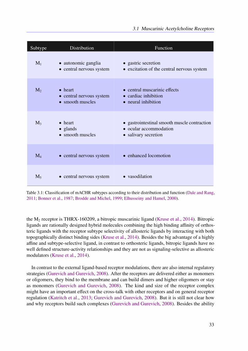
3.1 Muscarinic Acetylcholine Receptors
Subtype Distribution Function
M1 • autonomic ganglia• central nervous system
• gastric secretion• excitation of the central nervous system
M2 • heart• central nervous system• smooth muscles
• central muscarinic effects• cardiac inhibition• neural inhibition
M3 • heart• glands• smooth muscles
• gastrointestinal smooth muscle contraction• ocular accommodation• salivary secretion
M4 • central nervous system • enhanced locomotion
M5 • central nervous system • vasodilation
Table 3.1: Classification of mACHR subtypes according to their distribution and function (Dale and Rang,2011; Bonner et al., 1987; Brodde and Michel, 1999; Elhusseiny and Hamel, 2000).
the M2 receptor is THRX-160209, a bitropic muscarinic ligand (Kruse et al., 2014). Bitropicligands are rationally designed hybrid molecules combining the high binding affinity of orthos-teric ligands with the receptor subtype selectivity of allosteric ligands by interacting with bothtopographically distinct binding sides (Kruse et al., 2014). Besides the big advantage of a highlyaffine and subtype-selective ligand, in contrast to orthosteric ligands, bitropic ligands have nowell defined structure-activity relationships and they are not as signaling-selective as allostericmodulators (Kruse et al., 2014).
In contrast to the external ligand-based receptor modulations, there are also internal regulatorystrategies (Gurevich and Gurevich, 2008). After the receptors are delivered either as monomersor oligomers, they bind to the membrane and can build dimers and higher oligomers or stayas monomers (Gurevich and Gurevich, 2008). The kind and size of the receptor complexmight have an important effect on the cross-talk with other receptors and on general receptorregulation (Katritch et al., 2013; Gurevich and Gurevich, 2008). But it is still not clear howand why receptors build such complexes (Gurevich and Gurevich, 2008). Besides the ability
33
Chapter 3 M2 Receptor-induced Signaling
of the receptors to build complexes or clusters on the cell surface, there are second messenger-mediated mechanisms that decrease the signaling via receptor phosphorylation, which are calleddesensitization (Pierce et al., 2002). There are several proteins that are able to directly down-regulate the receptor activity, such as protein kinase A (PKA) and protein kinase C (PKC) (Pierceet al., 2002). Afterwards the phosphorylated receptor directly dissociates from the boundGP (Pierce et al., 2002). A more agonist-specific regulation is mediated by G protein-coupledreceptor kinases (GRK) only targeting the agonist-occupied receptor conformation controlledby several factors (Pierce et al., 2002). There are a lot of other mechanisms of receptordesensitization, such as the receptor degradation or regulation of the gene transcription, whichconsequentially all lead to a temporary decrease of the signal (Pierce et al., 2002). But thereare also mechanisms leading to a redistribution of the receptor via internalization (Pierce et al.,2002). Receptor internalization can either lead to the degradation or the dephosphorylation ofthe receptor (Pierce et al., 2002). Hence a positive or negative feedback might occur where thereceptor is internalized and transported to the endosome, e.g., via vesicles (Pierce et al., 2002).The vesicle-based transport is mediated via β-arrestin (Pierce et al., 2002). After the ligandhas bound to the dephosphorylated receptor and hence the receptor got activated, the signalis transduced by heterotrimeric GPs (Oldham and Hamm, 2008; Dale and Rang, 2011; Kruseet al., 2014).
3.2 G Protein-mediated Signaling
Once activated, GPCRs bind to a small number of GPs (Oldham and Hamm, 2008; Dale andRang, 2011). GPs are composed of α, βand γ subunits which are bound in the inactive state ofthe GP (Oldham and Hamm, 2008). There are 21 different α, 6 different β and 12 different γsubunits, as shown in Table 3.2 (Oldham and Hamm, 2008). All α subunits feature a GTPasebinding side and a helical domain (Oldham and Hamm, 2008). GTPase represents a family ofenzymes which hydrolyze guanosine-5’-triphosphate (GTP) (Alberts et al., 2014). The GTPasebinding side is typical for all members of the GP superfamily allowing them to bind to the β\γ
complex and is part of the domain responsible for binding and hydrolyzing GTP (Oldham andHamm, 2008). The second domain of the α subunit is to regulate membrane localization andinteraction with other proteins involved in the signaling (Oldham and Hamm, 2008). In contrast,the β and γ subunit build a functional complex which can only be dissociated under denaturingconditions (Oldham and Hamm, 2008). The interaction of the α subunit with the β\γ complexand the binding of the β subunit to the γ subunit is, in general, non-specific, but there is alsoevidence for a direct interaction of the α subunit with the γ subunit (Oldham and Hamm, 2008).
The β\γ-bound α subunit is not able to interact with other molecules (Oldham and Hamm,2008). Hence, in the bound state, neither the β\γ subunit nor the α subunit are able to transmitany signal (Oldham and Hamm, 2008). As illustrated in Figure 3.1, in this inactive state,guanosine-5’-diphosphate (GDP) is bound to the α subunit (Dale and Rang, 2011). This causesa high binding affinity with the receptor (Oldham and Hamm, 2008). The binding of the ligandto the receptor leads to a structural change within the α subunit (Oldham and Hamm, 2008).This inter-domain movement then results in a release of GDP, and GTP can bind to the α
34
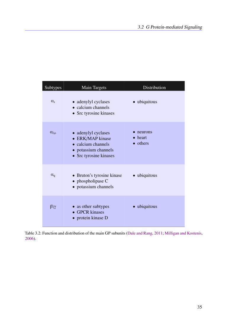
3.2 G Protein-mediated Signaling
Subtypes Main Targets Distribution
αs • adenylyl cyclases• calcium channels• Src tyrosine kinases
• ubiquitous
αi\o • adenylyl cyclases• ERK/MAP kinase• calcium channels• potassium channels• Src tyrosine kinases
• neurons• heart• others
αq • Bruton’s tyrosine kinase• phospholipase C• potassium channels
• ubiquitous
β\γ • as other subtypes• GPCR kinases• protein kinase D
• ubiquitous
Table 3.2: Function and distribution of the main GP subunits (Dale and Rang, 2011; Milligan and Kostenis,2006).
35
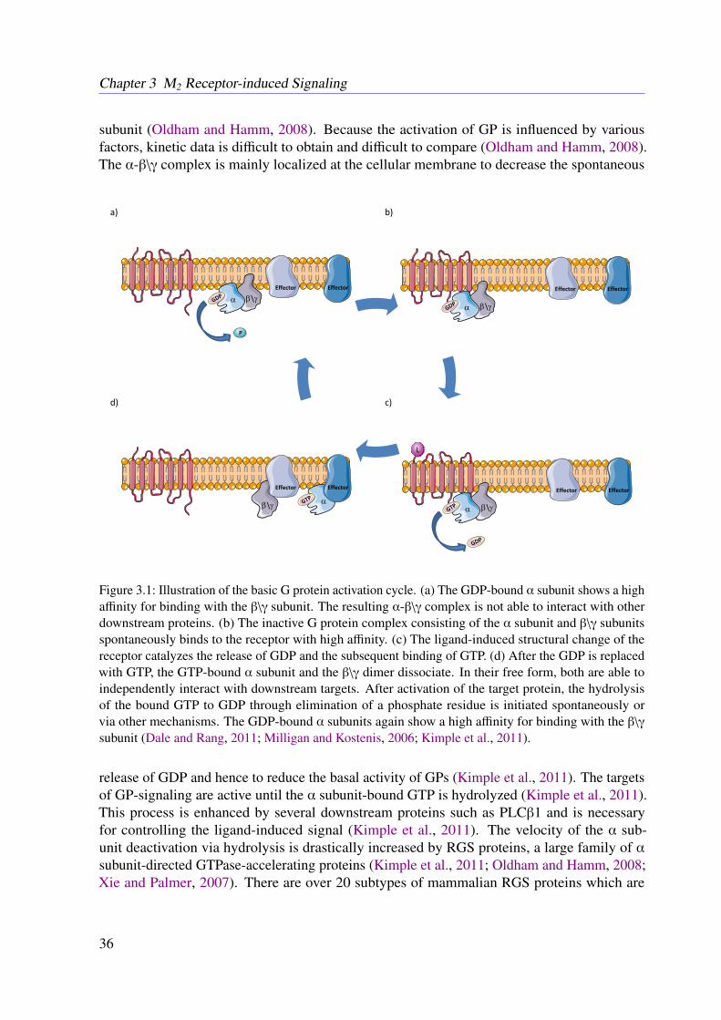
Chapter 3 M2 Receptor-induced Signaling
subunit (Oldham and Hamm, 2008). Because the activation of GP is influenced by variousfactors, kinetic data is difficult to obtain and difficult to compare (Oldham and Hamm, 2008).The α-β\γ complex is mainly localized at the cellular membrane to decrease the spontaneous
Effector Effector
Effector Effector Effector Effector
Effector Effector
P
a
a a
a
b\g b\g
b\g b\g
L
a) b)
d) c)
Figure 3.1: Illustration of the basic G protein activation cycle. (a) The GDP-bound α subunit shows a highaffinity for binding with the β\γ subunit. The resulting α-β\γ complex is not able to interact with otherdownstream proteins. (b) The inactive G protein complex consisting of the α subunit and β\γ subunitsspontaneously binds to the receptor with high affinity. (c) The ligand-induced structural change of thereceptor catalyzes the release of GDP and the subsequent binding of GTP. (d) After the GDP is replacedwith GTP, the GTP-bound α subunit and the β\γ dimer dissociate. In their free form, both are able toindependently interact with downstream targets. After activation of the target protein, the hydrolysisof the bound GTP to GDP through elimination of a phosphate residue is initiated spontaneously orvia other mechanisms. The GDP-bound α subunits again show a high affinity for binding with the β\γ
subunit (Dale and Rang, 2011; Milligan and Kostenis, 2006; Kimple et al., 2011).
release of GDP and hence to reduce the basal activity of GPs (Kimple et al., 2011). The targetsof GP-signaling are active until the α subunit-bound GTP is hydrolyzed (Kimple et al., 2011).This process is enhanced by several downstream proteins such as PLCβ1 and is necessaryfor controlling the ligand-induced signal (Kimple et al., 2011). The velocity of the α sub-unit deactivation via hydrolysis is drastically increased by RGS proteins, a large family of αsubunit-directed GTPase-accelerating proteins (Kimple et al., 2011; Oldham and Hamm, 2008;Xie and Palmer, 2007). There are over 20 subtypes of mammalian RGS proteins which are
36
3.2 G Protein-mediated Signaling
able to regulate GPCRs and other proteins very specifically and selectively but with varyingeffectiveness (Kimple et al., 2011; Xie and Palmer, 2007). Recent studies demonstrated that theselectivity of RGS proteins can be explained by their co-expression with the target at the righttime and location (Xie and Palmer, 2007).
Once activated, GP subunits transduce the ligand-mediated signal to several downstreamproteins (Dale and Rang, 2011). One of the most important targets for GP-induced signal-ing are various subtypes of adenylyl cyclase (AC) (Sunahara and Taussig, 2002; Pierce et al.,2002). For mammals, nine membrane-bound and one soluble isoform are known (Sunahara andTaussig, 2002; Pierce et al., 2002). The membrane-bound isoforms can be structured into twotransmembrane clusters and two cytoplasmic loops (Cooper, 2003; Hurley, 1999). With thehelp of metal ions, AC catalyzes the conversion of adenosine triphosphate (ATP) to cAMP andpyrophosphate (Sunahara and Taussig, 2002; Pierce et al., 2002; Hurley, 1999). The AC activityis mainly regulated by α subunits, depending on the isoform and the GP subunit (Sunaharaand Taussig, 2002). In general, αs subunits have stimulatory and αi subunits have inhibitoryeffects (Sunahara and Taussig, 2002). But there are also other regulators of the AC activity,e.g., the β\γ subunits, PKA and Ca2+ ions (Sunahara and Taussig, 2002). Since GDP-bound α
subunits have a tenfold lower affinity for AC, the GP-mediated catalysis is timed by the hydro-lysis of GTP, which terminates the GP-mediated signaling (Sunahara and Taussig, 2002). Thehydrolysis and therefore the termination of the signal is enhanced by RGS proteins (Sunaharaand Taussig, 2002). Besides the PKA-mediated inhibition of AC by phosphorylation, forskolinis a very potent stimulator which is widely used for in vitro experiments (Sunahara and Taussig,2002; Pierce et al., 2002; Hurley, 1999).
As a consequence of the production of cAMP catalyzed by AC, the concentration of thesecond messenger cAMP within the cytoplasma increases (Sunahara and Taussig, 2002; Pierceet al., 2002). It is known that cAMP is not uniformly distributed in the cytoplasm, i.e., the con-centration of cAMP next to AC and PKA differs from the overall cytosol concentration, whichmay lead to a compartmentalization of the cAMP concentration (Cooper, 2003; Kholodenko,2006). The second messenger molecule cAMP directly activates the enzyme PKA (Sunaharaand Taussig, 2002; Pierce et al., 2002). In the inactive state, PKA builds a complex com-prised of two catalytic subunits and one regulatory subunit dimer (Taylor et al., 2012). Thereare four known isoforms of the regulatory subunit and three known isoforms of the catalyticsubunits (Taylor et al., 2012). PKA downstream signaling is the main pathway induced byGPs (Taylor et al., 2012). The PKA activity is directly controlled by the cAMP level (Tayloret al., 2012). In the inactive state, the regulatory dimer blocks the binding sites of the catalyticsubunits making a binding to other substrates impossible (Taylor et al., 2012). Hence the level ofPKA activity depends on the local cAMP concentration, and the hydrolysis of cAMP catalyzedby 3’,5’-cyclonukleotid-phosphodiesterase (PDE) decreases the activity of PKA (Maurice et al.,2014). There are eleven mammalian PDE families which widely differ in their function (Mauriceet al., 2014). Hence, when PDE gets activated by PKA, it directly regulates the downstreamcAMP-induced signaling and can be considered as a negative feedback loop (Omori and Kotera,2007). PKA is then able to activate a large number of enzymes such as RGS proteins orGRKs (Alberts et al., 2014).
37
Chapter 3 M2 Receptor-induced Signaling
3.3 Experimental Tools
A wide range of techniques to measure responses mediated by external stimuli at cellular levelsis coupled to very specific cellular events (Dale and Rang, 2011). Most of them are invasive andmight cause significant changes in the cellular physiology (Fang et al., 2006). The second mes-senger cAMP is a prominent target for this kind of readouts (Engelhardt et al., 2017). However,measuring the concentration of cAMP only allows for conclusions about the receptor-mediateddownstream cascade from the receptor above the production of cAMP (Dale and Rang, 2011).The limited transferability to native systems and the restricted conclusions are a drawbackfor drug discovery and development (Fang et al., 2006). To ensure medical applicability, it isimportant to understand the functions of cellular targets under native conditions (Fang et al.,2006). Today, several types of optical biosensors allow to monitor cellular signaling processesnon-invasively in real time and thus lead to an improved understanding of cell biology andphysiology (Schröder et al., 2010; Schröder et al., 2011; Fang et al., 2006). Over the lastdecades, the number and range of biosensors have drastically increased (Fang et al., 2006). Inthe past, several optical principles were used to investigate ligand-induced receptor responses inmembrane homogenates (Fang et al., 2006). The resonant waveguide grating (RWG) techniquehas lead to the development of novel mass redistribution cell assay technologies (Fang et al.,2006). It allows to screen the DMR within the bottom portion of living cells (Schröder et al.,2010; Schröder et al., 2011; Fang et al., 2006).
As illustrated in Figure 3.2, broadband light enters the waveguide resonant grating (Rosenblattet al., 1997; Fang et al., 2006). The intensity of the reflected light can be considered to be afunction of the resonant wavelength (Rosenblatt et al., 1997; Fang et al., 2006). The nativecell can be placed on the grating to measure the optical density. The waveguide resonantgrating basically consists of a substrate layer and a waveguide film with an embedded gratingstructure (Rosenblatt et al., 1997; Fang et al., 2006). Because the height of the cells is mostlybeyond the wavelength of the incident light and larger than the penetration depth, the sensingvolume is restricted to the bottom of the cell not necessarily attached to the waveguide (Schröderet al., 2010; Schröder et al., 2011; Fang et al., 2006). In contemporary devices, the broadbandlight beam illuminates the whole waveguide, which allows for instantaneous measurements,whereas previously the beam only illuminated the waveguide punctually, resulting in delayedmeasurements (Fang et al., 2006). As demonstrated in several studies, the mass reorganizationwithin the sensing volume changes the incident angle of the incoupled light and hence leads toa shift of the wavelength of the outcoupled light (Schröder et al., 2010; Schröder et al., 2011;Fang et al., 2006).
Although the underlying details of the DMR are not yet known, it allows for dividingthe complex GPCR-mediated signal patterns into its separated subsequent GP downstreampathways (Schröder et al., 2010; Schröder et al., 2011). Through inhibition of concurrent GP-mediated downstream pathways with several inhibitors, a unique fingerprint of the concurrentpathways was found (Schröder et al., 2010; Schröder et al., 2011). Common inhibitors forGP signaling are pertussis toxin (PTX), YM-254890 (YM) and cholera toxin (CTX) (Schröderet al., 2010; Schröder et al., 2011). It is important to note that PTX, YM and CTX induce
38
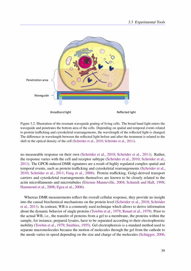
3.3 Experimental Tools
Figure 3.2: Illustration of the resonant waveguide grating of living cells. The broad band light enters thewaveguide and penetrates the bottom area of the cells. Depending on spatial and temporal events relatedto protein trafficking and cytoskeletal rearrangements, the wavelength of the reflected light is changed.The difference in wavelength between the reflected light before and after the treatment is related to theshift in the optical density of the cell (Schröder et al., 2010; Schröder et al., 2011).
no measurable response on their own (Schröder et al., 2010; Schröder et al., 2011). Rather,the response varies with the cell and receptor subtype (Schröder et al., 2010; Schröder et al.,2011). The GPCR-induced DMR signatures are a result of highly regulated complex spatial andtemporal events, such as protein trafficking and cytoskeletal rearrangements (Schröder et al.,2010; Schröder et al., 2011; Fang et al., 2006). Protein trafficking, Golgi-derived transportcarriers and cytoskeletal rearrangements themselves are known to be closely related to theactin microfilaments and microtubules (Etienne-Manneville, 2004; Schmidt and Hall, 1998;Hammond et al., 2008; Egea et al., 2006).
Whereas DMR measurements reflect the overall cellular response, they provide no insightinto the causal biochemical mechanisms on the protein level (Schröder et al., 2010; Schröderet al., 2011). In contrast, WB is a commonly used technique which allows to derive informationabout the dynamic behavior of single proteins (Towbin et al., 1979; Renart et al., 1979). Prior tothe actual WB, i.e., the transfer of proteins from a gel to a membrane, the proteins within thesample, for instance, prepared lysates, have to be separated according to their electrophoreticmobility (Towbin et al., 1979; Smithies, 1955). Gel electrophoresis is a standard method used toseparate macromolecules because the motion of molecules through the gel from the cathode tothe anode varies in speed depending on the size and charge of the molecules (Schägger, 2006;
39

Chapter 3 M2 Receptor-induced Signaling
Robyt and White, 1987; Smithies, 1955). The gel used in sodium dodecyl sulfate polyacrylamideelectrophoresis has a filter structure leading to a slow motion of big molecules and a separationof molecules relative to their size (Schägger, 2006; Robyt and White, 1987). The gel-trappedmolecules can be transferred to a membrane via WB (Robyt and White, 1987; Renart et al.,1979). Therefore, a membrane is placed over the gel and, under application of an electric field,the molecules move towards the anode from the gel to the membrane (Robyt and White, 1987;Renart et al., 1979).
After transfer, the membrane-bound molecules are still separated and do not change theirlocation compared to their absolute position on the gel (Towbin et al., 1979; Renart et al., 1979).Once the molecules, e.g., proteins, are transferred to the membrane, they can be marked andthus highlighted via specific antibodies (Robyt and White, 1987). The marked proteins are nowready for quantification with the help of a special camera systems (Robyt and White, 1987).Because gel electrophoresis and WB are highly sensitive techniques, it is possible to determinethe protein concentration based on the intensity of the markers (Robyt and White, 1987). Thelight intensity of the marker and the protein concentration are related because the light intensityof the marker increases with the number of marked molecules (Robyt and White, 1987). Theunderlying idea is to wash the membrane after adding the antibodies so that only markedantibodies bound to the specific antigen, i.e., protein, will remain on the membrane (Robyt andWhite, 1987).
40
CHAPTER 4
Methodology
In order to reconstruct the M2 receptor-induced signaling in CHO cells and thus the inherentsignal amplification, well-known methods from metabolic pathway reconstruction are extendedto signaling cascades in this work. The stoichiometric matrix provides information about therelevance of the involved species and subpathways (Engelhardt et al., 2017). As mentioned inChapter 2, signaling is encoded in the dynamic behavior of a system and hence, in addition tosteady state analyzes, a dynamic model is necessary for further investigations (Hübner et al.,2011; Klipp and Liebermeister, 2006).
Stoichiometric analyses of biological systems mainly based on algebraic tools have beenemployed for a long time (Wei and Prater, 1962; Palsson, 2006). As illustrated in Chapter 2, formodel development, it is reasonable to start with the analysis of the network topology and thebehavior of the system under steady state conditions based on elementary reactions (Wei andPrater, 1962; Palsson, 2006). Afterwards, the model should be complemented with advancedkinetics to incorporate the dynamic behavior (Azeloglu and Iyengar, 2015; Hübner et al., 2011).Here this strategy, which is similar to the bottom-up approach discussed in Section 2.1, isrequired because the amount of reliable knowledge and data is restricted (Bruggeman andWesterhoff, 2007; Azeloglu and Iyengar, 2015; Engelhardt et al., 2017).
4.1 Stoichiometric Network Analysis
A reconstruction of biochemical networks involves both the network topology and the kineticrates (Azeloglu and Iyengar, 2015; Palsson, 2006). In case of small- or medium-sized networks,ODE-based dynamical systems are often employed. However, topology-based approaches canalso yield valuable insights into the mechanisms and basic features of biochemical networks (Weiand Prater, 1962; Heinrich et al., 2002). Especially metabolic networks are frequently analyzedbased on their stoichiometry (Palsson, 2006; Bordbar et al., 2014). Metabolic networks can besufficiently characterized by certain steady states (Palsson, 2006). This assumption is justifiedby the high relaxation time of metabolic systems, which is typically in the order of minutesor seconds (Palsson, 2006). In contrast, a transient behavior is often observable for signaling
41
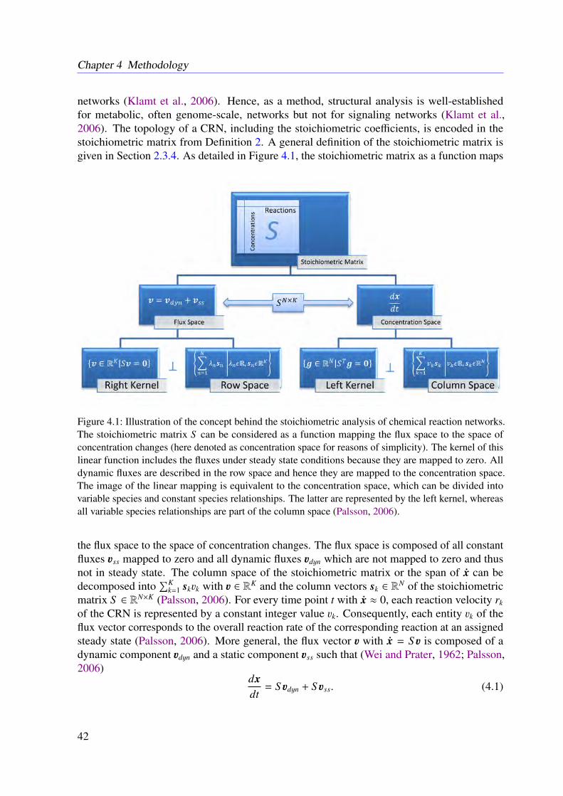
Chapter 4 Methodology
networks (Klamt et al., 2006). Hence, as a method, structural analysis is well-establishedfor metabolic, often genome-scale, networks but not for signaling networks (Klamt et al.,2006). The topology of a CRN, including the stoichiometric coefficients, is encoded in thestoichiometric matrix from Definition 2. A general definition of the stoichiometric matrix isgiven in Section 2.3.4. As detailed in Figure 4.1, the stoichiometric matrix as a function maps
Figure 4.1: Illustration of the concept behind the stoichiometric analysis of chemical reaction networks.The stoichiometric matrix S can be considered as a function mapping the flux space to the space ofconcentration changes (here denoted as concentration space for reasons of simplicity). The kernel of thislinear function includes the fluxes under steady state conditions because they are mapped to zero. Alldynamic fluxes are described in the row space and hence they are mapped to the concentration space.The image of the linear mapping is equivalent to the concentration space, which can be divided intovariable species and constant species relationships. The latter are represented by the left kernel, whereasall variable species relationships are part of the column space (Palsson, 2006).
the flux space to the space of concentration changes. The flux space is composed of all constantfluxes uss mapped to zero and all dynamic fluxes udyn which are not mapped to zero and thusnot in steady state. The column space of the stoichiometric matrix or the span of x can bedecomposed into
∑Kk=1 skvk with u ∈ RK and the column vectors sk ∈ R
N of the stoichiometricmatrix S ∈ RN×K (Palsson, 2006). For every time point t with x ≈ 0, each reaction velocity rk
of the CRN is represented by a constant integer value vk. Consequently, each entity vk of theflux vector corresponds to the overall reaction rate of the corresponding reaction at an assignedsteady state (Palsson, 2006). More general, the flux vector u with x = S u is composed of adynamic component udyn and a static component uss such that (Wei and Prater, 1962; Palsson,2006)
dxdt
= S udyn + S uss. (4.1)
42
4.1 Stoichiometric Network Analysis
Due to the fast time-scale of metabolic systems, the right and left null space, and hence
dxdt
= 0, (4.2)
are in focus of the analysis. In the steady state, i.e., x = 0, the whole system is approximately inbalance, though there is a continuous flow of the component materials (Wei and Prater, 1962;von Bertalanffy, 1950). Even if the whole system is not in a steady state, a subsystem withS uss ≈ 0 may exist (Wei and Prater, 1962; Palsson, 2006). This work demonstrates that thesteady state analysis can also be extended to complex signaling networks (Engelhardt et al.,2017).
4.1.1 Left and Right Null Space
Since every column of the stoichiometric matrix corresponds to a reaction and every row corres-ponds to a species, investigating the left and right null space of the stoichiometric matrix allowsto gain insights into the reaction and species dependencies, as illustrated in Figure 4.1 (Wei andPrater, 1962; Palsson, 2006).
Definition 6: Left and Right Null Space
Given a CRN with a stoichiometric matrix S ∈ RN×K , the right null space or kernel ker (S )is given by
ker (S ) =u ∈ RK |S u = 0
.
Accordingly, the left null space ker(S T
)is given by
ker(S T
)=
g ∈ RN
∣∣∣S Tg = 0.
For a CRN with K single reactions and N species, using common definitions from linearalgebra, the number of reactions K is equal to dim (ker (S )) + dim (im (S )) (Palsson, 2006). Inaddition, the image of the mapping S is defined as
im (S ) =x ∈ RN
∣∣∣x = S u u ∈ RK. (4.3)
Therefore, the dimension of ker (S ) is equivalent to the number of independent fluxes and thedimension of im (S ) is equivalent to the number of dependent fluxes (Palsson, 2006). In contrast,the number of species N depends on dim
(ker
(S T
))and dim
(im
(S T
)). The column space of S
is orthogonal to the kernel of S T and hence the space of concentration changes can be partitionedinto the column space and the left null space (Palsson, 2006).
Right Null Space
The behavior of the system under steady state conditions is characterized by the right nullspace (Palsson, 2006). It is always possible to find a set of basis vectors b ∈ RK for the right
43
Chapter 4 Methodology
null space such that
u =
(K−dim(im(S )))∑j=1
α jb j ∀u : S u = 0, (4.4)
with αi ∈ R (Llaneras and Picó, 2010). The basis vectors b j are not necessarily positive andcan therefore not be directly interpreted as fluxes in a biological manner (Wei and Prater, 1962;Palsson, 2006). In contrast, a convex representation of the kernel can often be directly mappedto pathways of the CRN (Llaneras and Picó, 2010). This is due to the fact that a flux, i.e., therate of turnover of molecules, through a biological system is unidirectional and thus always non-negative (Llaneras and Picó, 2010). A set of non-negative basis vectors leads to concepts basedon convex analysis (Palsson, 2006; Clarke, 1980). All possible steady state fluxes are enclosedby a polytope spanned by a set of conically independent generating vectors, where the numberof generating vectors in this set can exceed the dimension of the right null space (Palsson, 2006;Clarke, 1980). In contrast to Equation (4.4), the space of feasible steady states is in generalgiven by
P =u ∈ RK |S u = 0,Du ≥ 0
, (4.5)
with a diagonal matrix D ∈ RK×K , where Dii = 1 if the flux is irreversible and Dii = 0 oth-erwise (Llaneras and Picó, 2010). This is important because often two opposed irreversiblereactions are combined to one reversible reaction in order to reduce the dimension of the stoi-chiometric matrix. The composition of the related polytope is commonly addressed by extremecurrents or EFMs (Palsson, 2006; Clarke, 1980).
Left Null Space
Whereas ker (S ) and the row space help to explain the flux distribution, the left kernel ker(S T
)helps to explain species dependencies (Wei and Prater, 1962; Palsson, 2006). The left kerneladds all time derivatives up to zero (Wei and Prater, 1962; Palsson, 2006). Hence, for a convexbasis, the time-invariant quantities lead to conservation relationships (Wei and Prater, 1962;Palsson, 2006). Conservation relationships are all those vectors g with
g ∈y ∈ RN : S Ty = 0
. (4.6)
This implies
gT x = gT S u =(S Tg
)Tu = 0 (4.7a)
⇒ddt
N∑n=1
gnxn
= 0 (4.7b)
⇒ gT x =
N∑n=1
gnxn = const. (4.7c)
44
4.1 Stoichiometric Network Analysis
Each conservation relationship g represents a linear combination of constant species (Wei andPrater, 1962; Palsson, 2006). They can be interpreted as a cycle of mass conservation, e.g., theconservation of phosphate groups within a certain subpathway (Wei and Prater, 1962; Palsson,2006). A convex representation of ker
(S T
)seems natural because the involved quantities are
related to species concentrations which are always greater or equal to zero (Wei and Prater,1962; Palsson, 2006). The conservation relationships hold true for all network states and thus
gT x = gT xre f = const. (4.8)
orgT
(x − xre f
)= 0. (4.9)
In contrast to the original affine hyperspace resulting from the inhomogeneous linear systemgT x = const., the introduced reference vector xre f transforms the concentration space into anon-affine hyperspace. Consequently, the basis of this system is equivalent to ker
(S T
)(Palsson,
2006).
4.1.2 Constraint-based Modeling
In addition to the left kernel, the image of the linear mapping related to the stoichiometricmatrix is spanned by the column space of S . The decomposition x =
∑Kk=1 skvk and the fact
that the fluxes vk are constrained by finite values α ≤ u ≤ β lead to a constrained equationsystem (Palsson, 2006; Bordbar et al., 2014). The conservation relationships introduce additionalconstraints, resulting in a linear equation system
dxdt
= S u = b (4.10a)
α ≤ u ≤ β (4.10b)dgT x
dt= 0, (4.10c)
with real-valued vectors α ≤ β (Orth et al., 2010; Bordbar et al., 2014). The interval[α,β
]is
often used to define core reactions which are forced to be active and hence 0 <[αi, βi
]. For some
biological problems, this leads to an optimization task when including an objective function,e.g., max
(cTu
)(Becker and Palsson, 2008). The objective function mostly describes the growth
rate or the ATP production, which are optimized in some biological settings (Nam et al., 2014).For instance, in cancer cells, cell proliferation and ATP production are often assumed to bemaximized (Nam et al., 2014). An example from biotechnology is the regulation of the yeastmetabolism such that defined metabolites are optimized (Brochado et al., 2010; Vargas et al.,2011). These phenomena are typically addressed via a flux balance analysis (FBA) (Orth et al.,
45
Chapter 4 Methodology
2010). Here, the system given through Equation (4.10) is optimized through
max(cTu
)(4.11a)
dxdt
= 0 = S u (4.11b)
α ≤ u ≤ β, (4.11c)
with an objective cTu encoded by a real-valued vector c with ck , 0 for all fluxes which areassumed to be maximized. Vice versa cTu can also be minimized if necessary.
The solution space of the system described through Equations (4.10) is large and of irregularshape (Schellenberger and Palsson, 2009; Palsson, 2006). In consequence, it can have an infinitenumber of solutions (Palsson, 2006; Fischer, 2013). A promising approach to address this issueis to describe the constraints a system has to satisfy rather than computing an explicit solutionx = b (Schellenberger and Palsson, 2009; Palsson, 2006). Therefore, the solution space isreduced to feasible solutions (Schellenberger and Palsson, 2009; Palsson, 2006). As for the FBA,an important case described through Equations (4.10) is given by x = 0 (Palsson, 2006). Thesteady state is of polyhedral shape and therefore not as irregular as the general solution spacefor constraint-based models (Schellenberger and Palsson, 2009; Palsson, 2006). However, thecalculation of the solution space for x = 0 and the left kernel are non-trivial tasks and commonlyaddressed by MCMC algorithms (Schellenberger and Palsson, 2009; Megchelenbrink et al.,2014). A brief description of the latter is provided in Section 4.3.2. MCMC methods allow todetermine the size and shape of the steady state solution space and provide information aboutthe probabilities of feasible solutions (Wiback et al., 2004). The aim of a steady state analysis isto explore all possible and biologically relevant paths through the system in the steady state andcalculate their probabilities (Wiback et al., 2004; Schellenberger and Palsson, 2009; Palsson,2006).
4.2 Optimal Control Theory
OCT is very well known in engineering and also frequently applied to biological systems,especially to optimize bioprocesses in biotechnology and bioengineering (Paiewonsky, 1965;Crassidis and Junkins, 2011; Banga et al., 2005). The main intention is to control the trajectoriesof the variables in a dynamical system (Luenberger, 1979). In contrast to control theory, wherethe dynamic behavior and the modification via feedback loops are in focus, OCT asks for anoptimal modification with respect to a certain objective (Sontag, 2005). Thus OCT is closelyrelated to optimization and the calculus of variations (Luenberger, 1979).
In more general terms, a dynamical system and a set of initial values is given accordingto Definition 5. For the purpose of optimal control, it is necessary to explicitly distinguishbetween the states, i.e., dynamic model variables x (t) and additional inputs u (t) (Luenberger,1979; Martinelli, 2015). The desired objective functional J (x (t) ,u (t)), gives rise to a generalfirst-order optimal control problem (OCP), as described below (Luenberger, 1979).
46
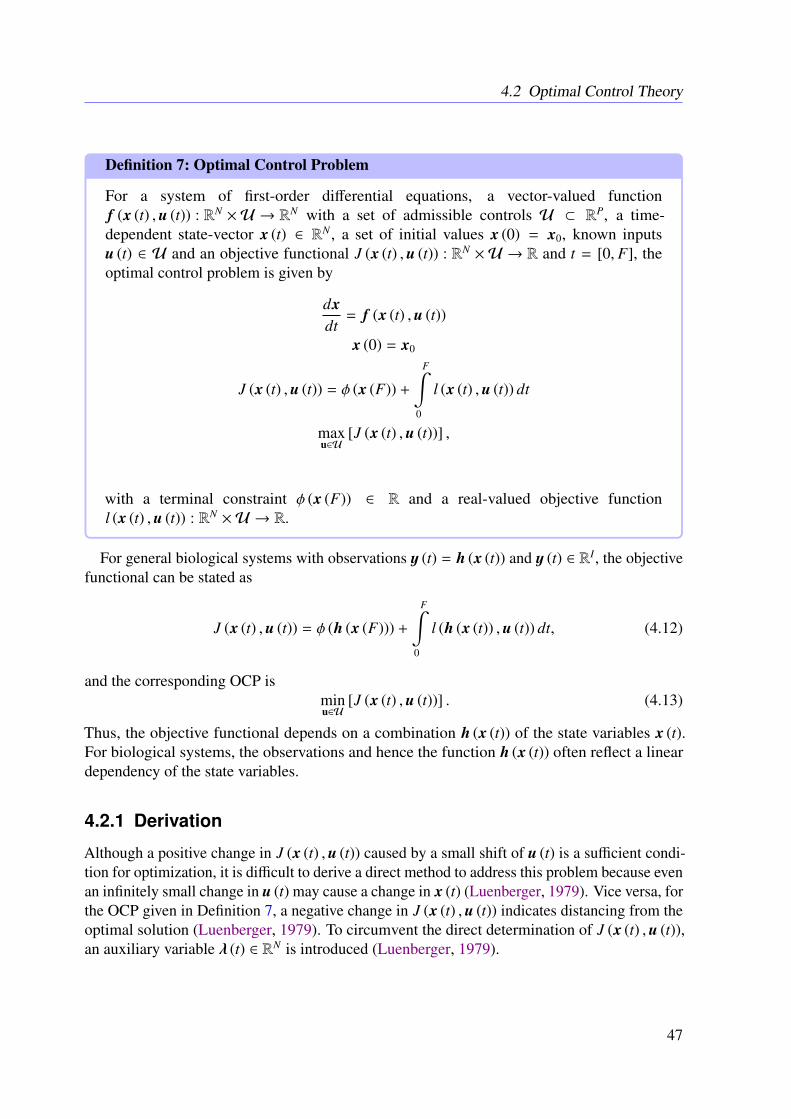
4.2 Optimal Control Theory
Definition 7: Optimal Control Problem
For a system of first-order differential equations, a vector-valued functionf (x (t) ,u (t)) : RN ×U → RN with a set of admissible controls U ⊂ RP, a time-dependent state-vector x (t) ∈ RN , a set of initial values x (0) = x0, known inputsu (t) ∈ U and an objective functional J (x (t) ,u (t)) : RN ×U → R and t = [0, F], theoptimal control problem is given by
dxdt
= f (x (t) ,u (t))
x (0) = x0
J (x (t) ,u (t)) = φ (x (F)) +
F∫0
l (x (t) ,u (t)) dt
maxu∈U
[J (x (t) ,u (t))] ,
with a terminal constraint φ (x (F)) ∈ R and a real-valued objective functionl (x (t) ,u (t)) : RN ×U → R.
For general biological systems with observations y (t) = h (x (t)) and y (t) ∈ RI , the objectivefunctional can be stated as
J (x (t) ,u (t)) = φ (h (x (F))) +
F∫0
l (h (x (t)) ,u (t)) dt, (4.12)
and the corresponding OCP isminu∈U
[J (x (t) ,u (t))] . (4.13)
Thus, the objective functional depends on a combination h (x (t)) of the state variables x (t).For biological systems, the observations and hence the function h (x (t)) often reflect a lineardependency of the state variables.
4.2.1 Derivation
Although a positive change in J (x (t) ,u (t)) caused by a small shift of u (t) is a sufficient condi-tion for optimization, it is difficult to derive a direct method to address this problem because evenan infinitely small change in u (t) may cause a change in x (t) (Luenberger, 1979). Vice versa, forthe OCP given in Definition 7, a negative change in J (x (t) ,u (t)) indicates distancing from theoptimal solution (Luenberger, 1979). To circumvent the direct determination of J (x (t) ,u (t)),an auxiliary variable λ (t) ∈ RN is introduced (Luenberger, 1979).
47
Chapter 4 Methodology
The auxiliary variable leads to the Hamiltonian function H (λ (t) , x (t) ,u (t)) : RN×RN×U → RwithU ⊂ RP given by (Luenberger, 1979)
H (λ (t) , x (t) ,u (t)) = λT (t) f (x (t) ,u (t)) + l (x (t) ,u (t)) . (4.14)
Applying Equation (4.14), the functional J (x (t) ,u (t)) can be reformulated by adding zero insuch a way that the modified functional
J (x (t) ,u (t) , λ (t)) = φ (x (F)) +
F∫0
[H (λ (t) , x (t) ,u (t)) − λT (t)
dx (t)dt
]dt (4.15)
becomes equivalent to J (x (t) ,u (t)) for each trajectory, but the freedom in the choice of λ (t)can be used to reduce the complexity of the OCP (Luenberger, 1979). For each trajectory, theidentity x − f (x (t) ,u (t)) = 0 holds true and hence it directly follows that
J (x (t) ,u (t)) = J (x (t) ,u (t) , λ (t)) ∀λ (t) ∈ RN . (4.16)
The obtained difference
∆J = J (x (t) , u (t) , λ (t)) − J (x (t) ,u (t) , λ (t)) , (4.17)
where u (t) = u (t) + ∆u (t) and x (t) = x (t) + ∆x (t), serves as a measurement for the change inthe objective functional caused by ∆u (t). Trivially, ∆u (t) = 0 leads to ∆J = 0. It is importantto see that a change in u (t) causes a change in the states of the system, but even a large changeof the input over a short interval of time may lead to a comparatively small change of thestates for each time point (Luenberger, 1979). This is caused by the direct dependency on theintegration of the objective function l (x (t) ,u (t)) (Luenberger, 1979). Please note that, whenintroducing additional state or control constraints, the explained variation is no longer directlysolvable (Crassidis and Junkins, 2011; Luenberger, 1979).
In consequence, through Taylor approximation and considering the fact that the input has noinfluence on the initial values, i.e., ∆x (0) = 0, ∆J can be reformulated as
∆J =
(∂φ (x (F))
∂x− λT (F)
)∆x (F)
+
F∫0
[∂H (λ (t) , x (t) ,u (t))
∂x+
dλT (t)dt
]∆x (t) dt
+
F∫0
(H (λ (t) , x (t) , u (t)) − H (λ (t) , x (t) ,u (t))) dt + o (∆x) ,
(4.18)
with the gradient ∂∂x and an additional error of the order o (∆x), following the Bachmann–Landau
notation, caused by the Taylor approximation and the application of the first-order differential
48
4.2 Optimal Control Theory
quotient (Luenberger, 1979; Hanke-Bourgeois, 2008). The reformulated Equation (4.18) is stilldifficult to calculate because it depends on the final values of x (t) and λ (t) which change with∆u (t). The fact that λ (t) can be chosen arbitrarily can be used to eliminate all terms except forthe last integral and thus to reduce the complexity of the system (Luenberger, 1979). Altogether,this leads to the adjoint differential equation
−
[dλ (t)
dt
]T
=∂H (λ (t) , x (t) ,u (t))
∂x(4.19a)[
dλ (F)dt
]T
=∂φ (x (F))
∂x, (4.19b)
which reduces Equation (4.18) to
∆J =
F∫0
(H (λ (t) , x (t) , u (t)) − H (λ (t) , x (t) ,u (t))) dt + o (∆x) . (4.20)
Equation (4.20) allows to establish a direct criterion for the improvement of ∆J because forany fixed u ∈ U for H (λ (t) , x (t) , u (t)) ≥ H (λ (t) , x (t) ,u) the integral in Equation (4.20) isgreater than or equal to zero and hence ∆J
∣∣∣u(t) ≥ ∆J |u due to the linearity of integrals and
H (λ (t) , x (t) , u (t)) ≥ H (λ (t) , x (t) ,u (t)) ∀t ∈ [0, F] (4.21a)
⇒
F∫0
H (λ (t) , x (t) , u (t)) dt ≥
F∫0
H (λ (t) , x (t) ,u) dt. (4.21b)
In consequence, u (t) is optimal with respect to any fixed u ∈ U (Luenberger, 1979). Accordingto this, the optimal control u (t) can be determined at each time point to satisfy ∆J
∣∣∣u(t) ≥ ∆J |uwith respect to all admissible control functions (Crassidis and Junkins, 2011). This givesrise to Pontryagin’s maximum (or minimum) principle which provides necessary optimalityconditions and thus is the basis of many numerical algorithms (Luenberger, 1979). Nevertheless,optimizing ∆J remains a difficult task. Several numerical methods have been developed toprovide a non-improvable solution by circumventing Pontryagin’s maximum principle (Bangaet al., 2005; Gong et al., 2008). However, the uniqueness of the solution with respect to allpossible trajectories is not always guaranteed (Banga et al., 2005; Gong et al., 2008).
49
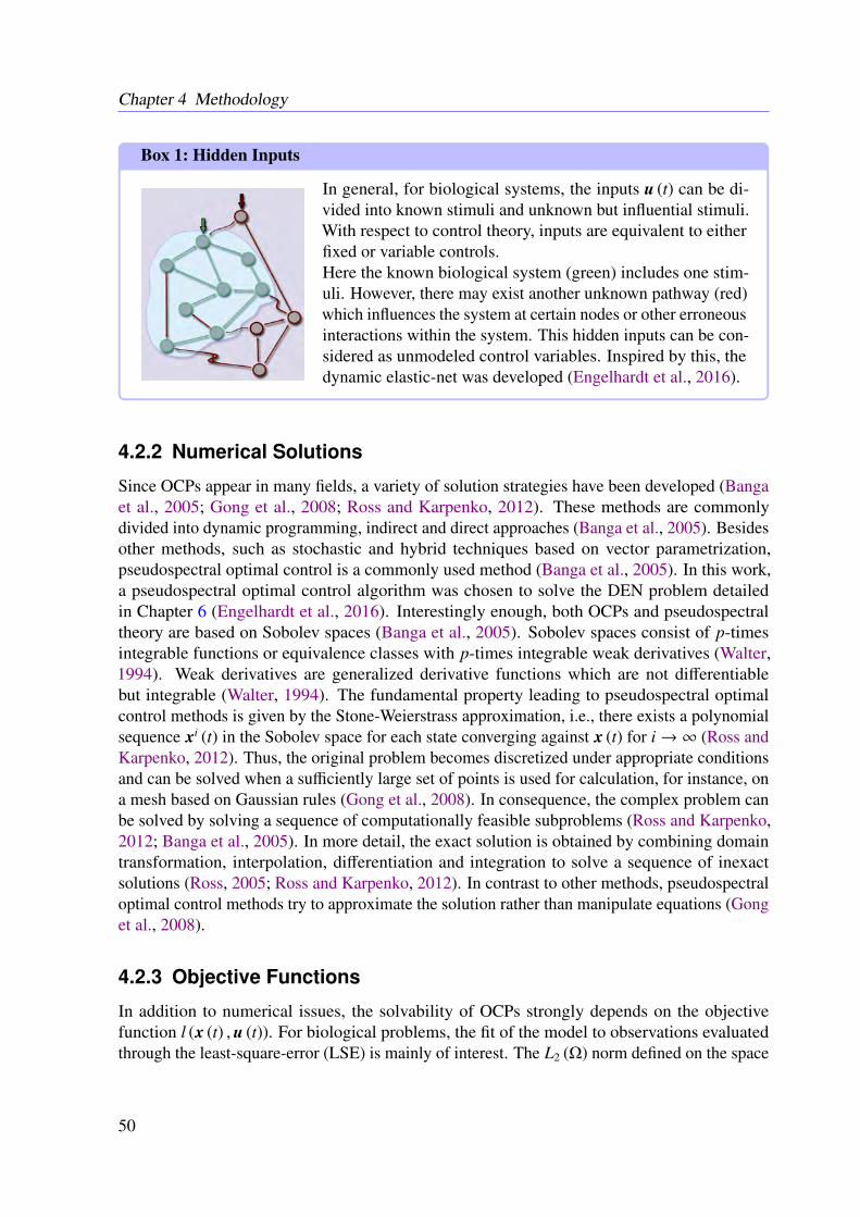
Chapter 4 Methodology
Box 1: Hidden Inputs
In general, for biological systems, the inputs u (t) can be di-vided into known stimuli and unknown but influential stimuli.With respect to control theory, inputs are equivalent to eitherfixed or variable controls.Here the known biological system (green) includes one stim-uli. However, there may exist another unknown pathway (red)which influences the system at certain nodes or other erroneousinteractions within the system. This hidden inputs can be con-sidered as unmodeled control variables. Inspired by this, thedynamic elastic-net was developed (Engelhardt et al., 2016).
4.2.2 Numerical Solutions
Since OCPs appear in many fields, a variety of solution strategies have been developed (Bangaet al., 2005; Gong et al., 2008; Ross and Karpenko, 2012). These methods are commonlydivided into dynamic programming, indirect and direct approaches (Banga et al., 2005). Besidesother methods, such as stochastic and hybrid techniques based on vector parametrization,pseudospectral optimal control is a commonly used method (Banga et al., 2005). In this work,a pseudospectral optimal control algorithm was chosen to solve the DEN problem detailedin Chapter 6 (Engelhardt et al., 2016). Interestingly enough, both OCPs and pseudospectraltheory are based on Sobolev spaces (Banga et al., 2005). Sobolev spaces consist of p-timesintegrable functions or equivalence classes with p-times integrable weak derivatives (Walter,1994). Weak derivatives are generalized derivative functions which are not differentiablebut integrable (Walter, 1994). The fundamental property leading to pseudospectral optimalcontrol methods is given by the Stone-Weierstrass approximation, i.e., there exists a polynomialsequence xi (t) in the Sobolev space for each state converging against x (t) for i→ ∞ (Ross andKarpenko, 2012). Thus, the original problem becomes discretized under appropriate conditionsand can be solved when a sufficiently large set of points is used for calculation, for instance, ona mesh based on Gaussian rules (Gong et al., 2008). In consequence, the complex problem canbe solved by solving a sequence of computationally feasible subproblems (Ross and Karpenko,2012; Banga et al., 2005). In more detail, the exact solution is obtained by combining domaintransformation, interpolation, differentiation and integration to solve a sequence of inexactsolutions (Ross, 2005; Ross and Karpenko, 2012). In contrast to other methods, pseudospectraloptimal control methods try to approximate the solution rather than manipulate equations (Gonget al., 2008).
4.2.3 Objective Functions
In addition to numerical issues, the solvability of OCPs strongly depends on the objectivefunction l (x (t) ,u (t)). For biological problems, the fit of the model to observations evaluatedthrough the least-square-error (LSE) is mainly of interest. The L2 (Ω) norm defined on the space
50
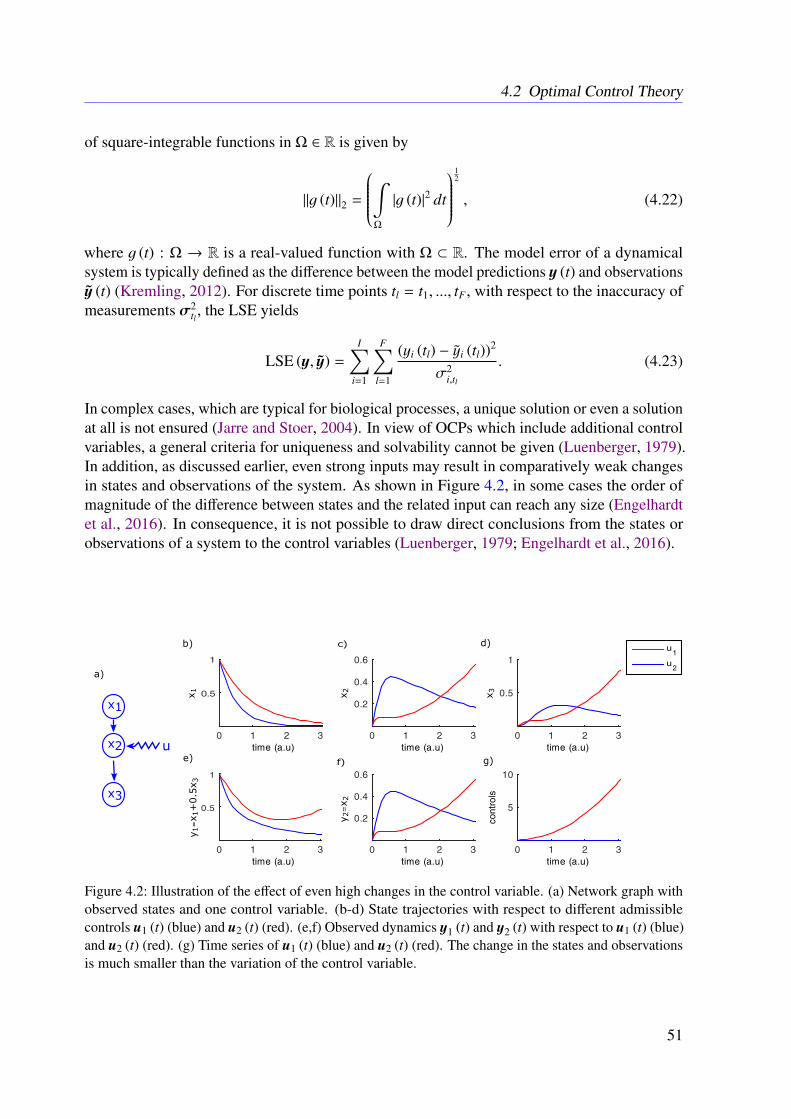
4.2 Optimal Control Theory
of square-integrable functions in Ω ∈ R is given by
‖g (t)‖2 =
∫Ω
|g (t)|2 dt
12
, (4.22)
where g (t) : Ω → R is a real-valued function with Ω ⊂ R. The model error of a dynamicalsystem is typically defined as the difference between the model predictions y (t) and observationsy (t) (Kremling, 2012). For discrete time points tl = t1, ..., tF , with respect to the inaccuracy ofmeasurements σ2
tl , the LSE yields
LSE (y, y) =
I∑i=1
F∑l=1
(yi (tl) − yi (tl))2
σ2i,tl
. (4.23)
In complex cases, which are typical for biological processes, a unique solution or even a solutionat all is not ensured (Jarre and Stoer, 2004). In view of OCPs which include additional controlvariables, a general criteria for uniqueness and solvability cannot be given (Luenberger, 1979).In addition, as discussed earlier, even strong inputs may result in comparatively weak changesin states and observations of the system. As shown in Figure 4.2, in some cases the order ofmagnitude of the difference between states and the related input can reach any size (Engelhardtet al., 2016). In consequence, it is not possible to draw direct conclusions from the states orobservations of a system to the control variables (Luenberger, 1979; Engelhardt et al., 2016).
Figure 4.2: Illustration of the effect of even high changes in the control variable. (a) Network graph withobserved states and one control variable. (b-d) State trajectories with respect to different admissiblecontrols u1 (t) (blue) and u2 (t) (red). (e,f) Observed dynamics y1 (t) and y2 (t) with respect to u1 (t) (blue)and u2 (t) (red). (g) Time series of u1 (t) (blue) and u2 (t) (red). The change in the states and observationsis much smaller than the variation of the control variable.
51
Chapter 4 Methodology
For some purposes, especially in cases where sparsity is required, the L1 (Ω) norm
‖g (t)‖1 =
∫Ω
|g (t)| dt
(4.24)
is used, but this leads to a non-smooth objective functional (Vossen and Maurer, 2006). Inmany applications, also in other fields of research, e.g., robotics, the L1 norm is a more realisticobjective because it weighs all function values equally (Vossen and Maurer, 2006). It has beenshown that the L1 norm must be treated numerically different, in contrast to so-called smoothOCPs based on LSEs (Vossen and Maurer, 2006). In practice, non-smooth OCPs with addedcontrol variables are often solved via regularization and augmentation approaches (Vossen andMaurer, 2006). Regularization approaches solve the problem for general Lp (Ω) norms definedthrough
‖g (t)‖p =
∫Ω
|g (t)|p dt
1p
, (4.25)
with p ≥ 1. The OCP can then be solved by determining the limit
limε→0
∫Ω
I∑i=1
|gi (t)|(p+ε)dt
1
p+ε
(4.26)
for p = 1 (Vossen and Maurer, 2006). Alternatively, an augmentation approach has beenproposed where the control variable is split into its positive and negative fraction (Vossenand Maurer, 2006). This approach doubles the number of involved control variables. In bothapproaches, the control variables tend to behave like step functions taking only zero, the definedmaximum and the defined minimum as values (Vossen and Maurer, 2006).
4.2.4 Properties
In practice, it is important to know whether the system can be clearly reconstructed basedon the given data or if there are non-distinguishable parts. This is directly related to thequestion of observability (Luenberger, 1979). In contrast to non-linear systems, observability iswell-investigated for linear dynamical systems given by
dx (t)dt
= Ax (t) + Bu (t) (4.27a)
y (t) = Cx (t) (4.27b)x (0) = x0, (4.27c)
where x0 ∈ RN is the initial value (Luenberger, 1979; Adamy, 2014). The lack of observability
is imputable to the linear mapping C caused by the fact that usually only parts of the system andcombinations of species are experimentally accessible.
52
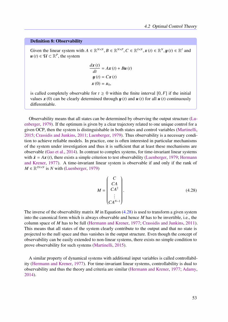
4.2 Optimal Control Theory
Definition 8: Observability
Given the linear system with A ∈ RN×N , B ∈ RN×P,C ∈ RI×N , x (t) ∈ RN , y (t) ∈ RI andu (t) ∈ U ⊂ RP, the system
dx (t)dt
= Ax (t) + Bu (t)
y (t) = Cx (t)x (0) = x0,
is called completely observable for t ≥ 0 within the finite interval [0, F] if the initialvalues x (0) can be clearly determined through y (t) and u (t) for all u (t) continuouslydifferentiable.
Observability means that all states can be determined by observing the output structure (Lu-enberger, 1979). If the optimum is given by a clear trajectory related to one unique control for agiven OCP, then the system is distinguishable in both states and control variables (Martinelli,2015; Crassidis and Junkins, 2011; Luenberger, 1979). Thus observability is a necessary condi-tion to achieve reliable models. In practice, one is often interested in particular mechanismsof the system under investigation and thus it is sufficient that at least these mechanisms areobservable (Gao et al., 2014). In contrast to complex systems, for time-invariant linear systemswith x = Ax (t), there exists a simple criterion to test observability (Luenberger, 1979; Hermannand Krener, 1977). A time-invariant linear system is observable if and only if the rank ofM ∈ RIN×N is N with (Luenberger, 1979)
M =
C
CACA2
...CAN−1
. (4.28)
The inverse of the observability matrix M in Equation (4.28) is used to transform a given systeminto the canonical form which is always observable and hence M has to be invertible, i.e., thecolumn space of M has to be full (Hermann and Krener, 1977; Crassidis and Junkins, 2011).This means that all states of the system clearly contribute to the output and that no state isprojected to the null space and thus vanishes in the output structure. Even though the concept ofobservability can be easily extended to non-linear systems, there exists no simple condition toprove observability for such systems (Martinelli, 2015).
A similar property of dynamical systems with additional input variables is called controllabil-ity (Hermann and Krener, 1977). For time-invariant linear systems, controllability is dual toobservability and thus the theory and criteria are similar (Hermann and Krener, 1977; Adamy,2014).
53
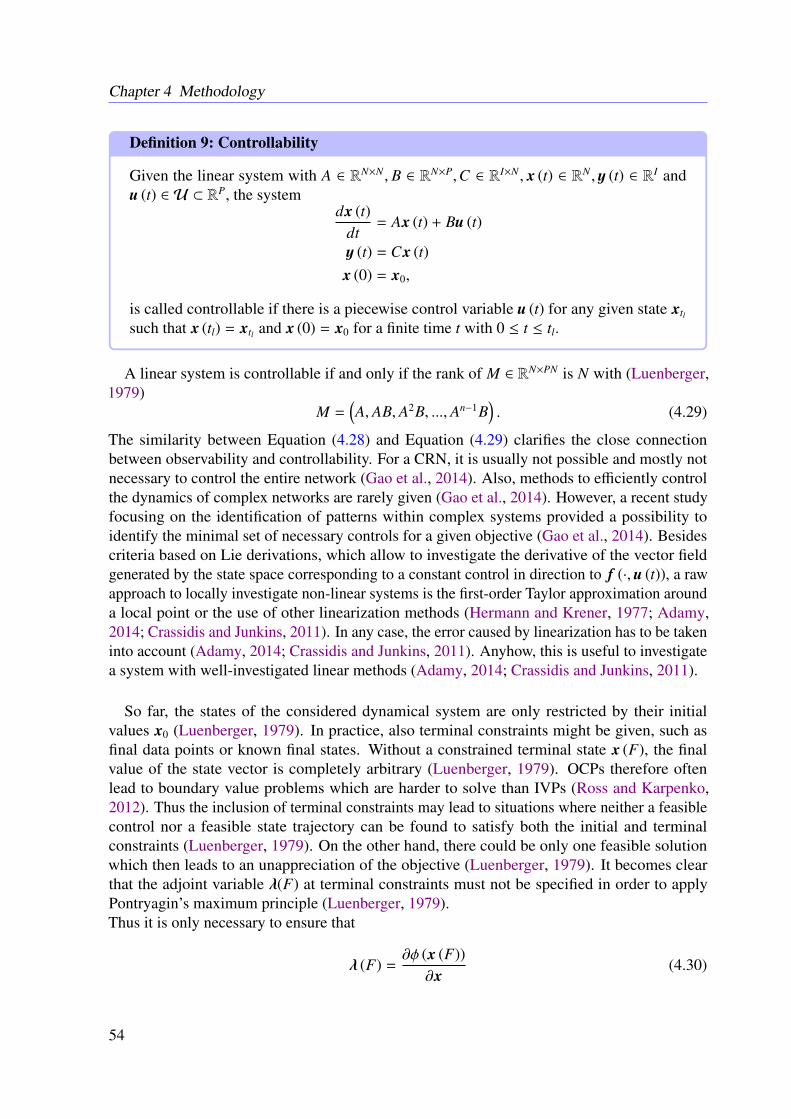
Chapter 4 Methodology
Definition 9: Controllability
Given the linear system with A ∈ RN×N , B ∈ RN×P,C ∈ RI×N , x (t) ∈ RN , y (t) ∈ RI andu (t) ∈ U ⊂ RP, the system
dx (t)dt
= Ax (t) + Bu (t)
y (t) = Cx (t)x (0) = x0,
is called controllable if there is a piecewise control variable u (t) for any given state xtlsuch that x (tl) = xtl and x (0) = x0 for a finite time t with 0 ≤ t ≤ tl.
A linear system is controllable if and only if the rank of M ∈ RN×PN is N with (Luenberger,1979)
M =(A, AB, A2B, ..., An−1B
). (4.29)
The similarity between Equation (4.28) and Equation (4.29) clarifies the close connectionbetween observability and controllability. For a CRN, it is usually not possible and mostly notnecessary to control the entire network (Gao et al., 2014). Also, methods to efficiently controlthe dynamics of complex networks are rarely given (Gao et al., 2014). However, a recent studyfocusing on the identification of patterns within complex systems provided a possibility toidentify the minimal set of necessary controls for a given objective (Gao et al., 2014). Besidescriteria based on Lie derivations, which allow to investigate the derivative of the vector fieldgenerated by the state space corresponding to a constant control in direction to f (·,u (t)), a rawapproach to locally investigate non-linear systems is the first-order Taylor approximation arounda local point or the use of other linearization methods (Hermann and Krener, 1977; Adamy,2014; Crassidis and Junkins, 2011). In any case, the error caused by linearization has to be takeninto account (Adamy, 2014; Crassidis and Junkins, 2011). Anyhow, this is useful to investigatea system with well-investigated linear methods (Adamy, 2014; Crassidis and Junkins, 2011).
So far, the states of the considered dynamical system are only restricted by their initialvalues x0 (Luenberger, 1979). In practice, also terminal constraints might be given, such asfinal data points or known final states. Without a constrained terminal state x (F), the finalvalue of the state vector is completely arbitrary (Luenberger, 1979). OCPs therefore oftenlead to boundary value problems which are harder to solve than IVPs (Ross and Karpenko,2012). Thus the inclusion of terminal constraints may lead to situations where neither a feasiblecontrol nor a feasible state trajectory can be found to satisfy both the initial and terminalconstraints (Luenberger, 1979). On the other hand, there could be only one feasible solutionwhich then leads to an unappreciation of the objective (Luenberger, 1979). It becomes clearthat the adjoint variable λ(F) at terminal constraints must not be specified in order to applyPontryagin’s maximum principle (Luenberger, 1979).Thus it is only necessary to ensure that
λ (F) =∂φ (x (F))
∂x(4.30)
54
4.3 Bayesian Inference
for all components of x (F) with ∆xi (F) , 0 (Luenberger, 1979). Consequently, for biologicalsystems, it can be favorable to restrict the final state to a defined interval rather than settingfixed terminal constraints or removing final data points and thus terminal constraints from thesystem (Luenberger, 1979). This may help to satisfy the objective function in cases where itis not possible to find feasible control variables and state trajectories with feasible initial andterminal constraints (Luenberger, 1979). In contrast, in some experimental frameworks it mightmake sense to consider the last time point as an additional variable leading to free terminal timeproblems (Luenberger, 1979).
4.3 Bayesian Inference
In contrast to purely deterministic approaches, statistical methods allow for an intuitive handlingof measurement noise, estimates of uncertain quantities and the analysis of random phenomenain general (Bishop, 2007; Gelman et al., 2013; Hoff, 2010). Such methods are often based onthe inherent correlations in data (Bishop, 2007; Gelman et al., 2013; Hoff, 2010). It is clear thatthe necessity of introducing probabilities is caused by a lack of knowledge and that there aredifferent ways to look at probabilities (Tschirk, 2014). The classical frequentism point of view,as the standard interpretation of probability, considers random variables as flexible values whichchange by multiple conduction of assigned random experiments (Tschirk, 2014). Consequently,probability is the relative frequency of an event (Tschirk, 2014). From the Bayesian point ofview, variables with unknown values are random, too, but the probability is considered as thereasonable expectation of an event (Tschirk, 2014; Hoff, 2010).
Frequentism only allows knowledge described by relative frequencies whereas in Bayesianstatistics there is no general restriction to a certain type of knowledge (Tschirk, 2014; Hoff,2010). This is why frequentism is often considered a special case of Bayesianism (Tschirk,2014). Besides theoretical aspects, this has practical consequences for the use of probabilit-ies (Tschirk, 2014). From the classical frequentist point of view, it is not clear if there is anyrelation between the estimated parameter and the true parameter since the estimates are justbased on random samples (Tschirk, 2014). Anyhow, there are some measurement variables,e.g., the efficiency, to characterize the relation between estimates and true values (Tschirk,2014). In contrast, Bayesian statistics estimates parameter distributions by incorporating priorknowledge (Tschirk, 2014; Hoff, 2010). If there is only little prior knowledge, the results willbe similar or equivalent to those obtained through frequentist approaches, with the deviationincreasing with the amount of prior knowledge (Tschirk, 2014).
Since Bayesian analysis uses prior knowledge to determine the probability of certain events,its advantage over classical statistical methods increases with the amount of prior knowledgefrequently given in biological problems (Tschirk, 2014; Hoff, 2010). In particular, Bayesianlearning makes it possible to perform optimal updates of beliefs given new information (Hoff,2010). Bayes’ law, as detailed in Box 2, is the fundamental concept of Bayesian statisticsand allows to deduce a posterior distribution based on the prior distribution and a samplingmodel (Hoff, 2010).
55
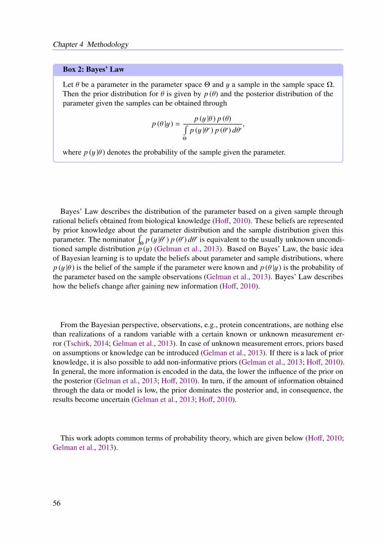
Chapter 4 Methodology
Box 2: Bayes’ Law
Let θ be a parameter in the parameter space Θ and y a sample in the sample space Ω.Then the prior distribution for θ is given by p (θ) and the posterior distribution of theparameter given the samples can be obtained through
p (θ |y ) =p (y |θ ) p (θ)∫
Θ
p (y |θ′ ) p (θ′) dθ′,
where p (y |θ ) denotes the probability of the sample given the parameter.
Bayes’ Law describes the distribution of the parameter based on a given sample throughrational beliefs obtained from biological knowledge (Hoff, 2010). These beliefs are representedby prior knowledge about the parameter distribution and the sample distribution given thisparameter. The nominator
∫Θ
p (y |θ′ ) p (θ′) dθ′ is equivalent to the usually unknown uncondi-tioned sample distribution p (y) (Gelman et al., 2013). Based on Bayes’ Law, the basic ideaof Bayesian learning is to update the beliefs about parameter and sample distributions, wherep (y |θ ) is the belief of the sample if the parameter were known and p (θ |y ) is the probability ofthe parameter based on the sample observations (Gelman et al., 2013). Bayes’ Law describeshow the beliefs change after gaining new information (Hoff, 2010).
From the Bayesian perspective, observations, e.g., protein concentrations, are nothing elsethan realizations of a random variable with a certain known or unknown measurement er-ror (Tschirk, 2014; Gelman et al., 2013). In case of unknown measurement errors, priors basedon assumptions or knowledge can be introduced (Gelman et al., 2013). If there is a lack of priorknowledge, it is also possible to add non-informative priors (Gelman et al., 2013; Hoff, 2010).In general, the more information is encoded in the data, the lower the influence of the prior onthe posterior (Gelman et al., 2013; Hoff, 2010). In turn, if the amount of information obtainedthrough the data or model is low, the prior dominates the posterior and, in consequence, theresults become uncertain (Gelman et al., 2013; Hoff, 2010).
This work adopts common terms of probability theory, which are given below (Hoff, 2010;Gelman et al., 2013).
56
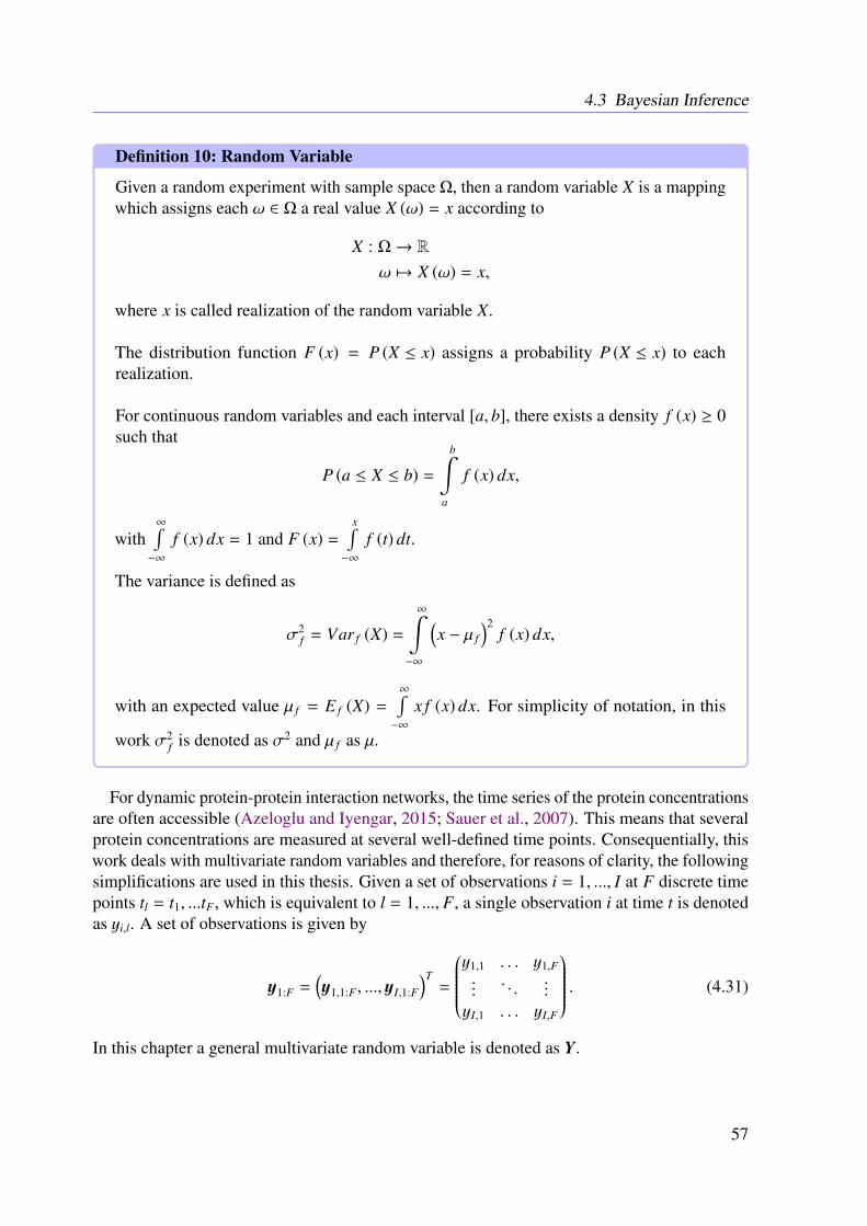
4.3 Bayesian Inference
Definition 10: Random Variable
Given a random experiment with sample space Ω, then a random variable X is a mappingwhich assigns each ω ∈ Ω a real value X (ω) = x according to
X : Ω→ R
ω 7→ X (ω) = x,
where x is called realization of the random variable X.
The distribution function F (x) = P (X ≤ x) assigns a probability P (X ≤ x) to eachrealization.
For continuous random variables and each interval [a, b], there exists a density f (x) ≥ 0such that
P (a ≤ X ≤ b) =
b∫a
f (x) dx,
with∞∫−∞
f (x) dx = 1 and F (x) =x∫−∞
f (t) dt.
The variance is defined as
σ2f = Var f (X) =
∞∫−∞
(x − µ f
)2f (x) dx,
with an expected value µ f = E f (X) =∞∫−∞
x f (x) dx. For simplicity of notation, in this
work σ2f is denoted as σ2 and µ f as µ.
For dynamic protein-protein interaction networks, the time series of the protein concentrationsare often accessible (Azeloglu and Iyengar, 2015; Sauer et al., 2007). This means that severalprotein concentrations are measured at several well-defined time points. Consequentially, thiswork deals with multivariate random variables and therefore, for reasons of clarity, the followingsimplifications are used in this thesis. Given a set of observations i = 1, ..., I at F discrete timepoints tl = t1, ...tF , which is equivalent to l = 1, ..., F, a single observation i at time t is denotedas yi,l. A set of observations is given by
y1:F =(y1,1:F , ..., yI,1:F
)T=
y1,1 . . . y1,F...
. . ....
yI,1 . . . yI,F
. (4.31)
In this chapter a general multivariate random variable is denoted as Y.
57
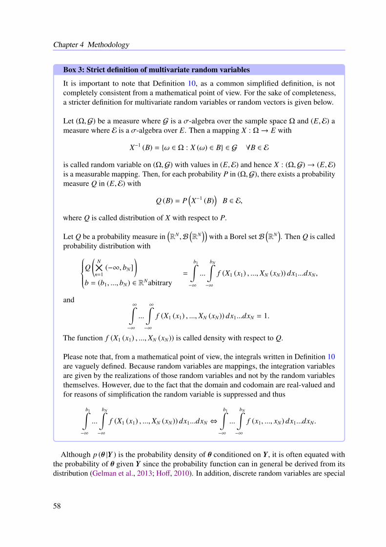
Chapter 4 Methodology
Box 3: Strict definition of multivariate random variables
It is important to note that Definition 10, as a common simplified definition, is notcompletely consistent from a mathematical point of view. For the sake of completeness,a stricter definition for multivariate random variables or random vectors is given below.
Let (Ω,G) be a measure where G is a σ-algebra over the sample space Ω and (E,E) ameasure where E is a σ-algebra over E. Then a mapping X : Ω→ E with
X−1 (B) = ω ∈ Ω : X (ω) ∈ B ∈ G ∀B ∈ E
is called random variable on (Ω,G) with values in (E,E) and hence X : (Ω,G)→ (E,E)is a measurable mapping. Then, for each probability P in (Ω,G), there exists a probabilitymeasure Q in (E,E) with
Q (B) = P(X−1 (B)
)B ∈ E,
where Q is called distribution of X with respect to P.
Let Q be a probability measure in(RN ,B
(RN
))with a Borel set B
(RN
). Then Q is called
probability distribution withQ(
N
×n=1
(−∞, bN])
b = (b1, ..., bN) ∈ RNabitrary=
b1∫−∞
...
bN∫−∞
f (X1 (x1) , ..., XN (xN)) dx1...dxN ,
and∞∫
−∞
...
∞∫−∞
f (X1 (x1) , ..., XN (xN)) dx1...dxN = 1.
The function f (X1 (x1) , ..., XN (xN)) is called density with respect to Q.
Please note that, from a mathematical point of view, the integrals written in Definition 10are vaguely defined. Because random variables are mappings, the integration variablesare given by the realizations of those random variables and not by the random variablesthemselves. However, due to the fact that the domain and codomain are real-valued andfor reasons of simplification the random variable is suppressed and thus
b1∫−∞
...
bN∫−∞
f (X1 (x1) , ..., XN (xN)) dx1...dxN ⇔
b1∫−∞
...
bN∫−∞
f (x1, ..., xN) dx1...dxN .
Although p (θ |Y ) is the probability density of θ conditioned on Y, it is often equated withthe probability of θ given Y since the probability function can in general be derived from itsdistribution (Gelman et al., 2013; Hoff, 2010). In addition, discrete random variables are special
58
4.3 Bayesian Inference
cases of continuous random variables (Gelman et al., 2013; Hoff, 2010).
4.3.1 Markov Chain Monte Carlo Methods
The probability of the estimated parameter set given the sample is an important measure for itsreliability (Brooks, 1998; Gelman et al., 2013; Hoff, 2010). As a direct consequence of Bayes’law (Box 2), the conditional posterior density of the parameter set can be approximated as
p (θ |Y ) ∝ p (Y |θ ) p (θ) , (4.32)
where the constant proportion is given by∫
Θ(Y |θ′ ) p (θ′) dθ′ (Hoff, 2010). In most cases this
integral is hard to solve and numerical integration or analytic approximation techniques mustbe used (Gelman et al., 2013; Hoff, 2010). Thus, neither the full posterior density nor themarginal posterior density are directly accessible (Hoff, 2010). MCMC methods allow forsampling directly from the posterior while avoiding analytical integration (Hoff, 2010). Thisway, sampling from the posterior based on prior knowledge about θ and the distribution of thedata Y given θ is possible (Hoff, 2010). Although the parameter distribution for the given datais not available, information about θ and the data given θ can often be derived (Gelman et al.,2013; Hoff, 2010).
The fundamental concept of MCMC methods is based on the fact that the posterior distributionis known up to a certain multiplicative constant (Gelman et al., 2013; Hoff, 2010). Here, it isoften possible to generate a chain of samples which converge against random samples from theposterior distribution (Brooks, 1998). More precisely, given a Markov chain
θ(s) : s = 1, ..., S
of realizations θ(s), then for any real-valued function g (θ) the state distribution of the Markovchain converges against the posterior distribution with (Brooks, 1998)
P
limS→∞
1S
S∑s=1
g(θ(s)
)=
∞∫−∞
g(θ′
)f(θ′ |Y
)dθ′
= 1. (4.33)
Markov chains are sequences of random variables θ(s) with
P(θ(s+1)
∣∣∣θ(s), ..., θ(1))
= P(θ(s+1)
∣∣∣θ(s))∀s. (4.34)
The most important properties of Markov chains for MCMC transitions are irreducibility, recur-rency and aperiodicity (Brooks, 1998). Irreducibility means that there exists a certain probabilitythat a state can be transitioned into another state within one or more steps (Brooks, 1998;Gelman et al., 2013; Hoff, 2010). Recurrency guarantees convergence in a finite time, whereasaperiodicity means that a return to a certain state can occur at irregular times (Brooks, 1998;Gelman et al., 2013; Hoff, 2010).
It can be shown that an irreducible and aperiodic Markov chain converges to a uniquestationary distribution (Brooks, 1998). This means that once the process behaves like a certain
59
Chapter 4 Methodology
distribution, it will stay there and, in consequence, all samples are drawn from this uniquestationary distribution (Brooks, 1998). In fact, a transition kernel K can be generated forMarkov chains which describes the transition between two states (Brooks, 1998). Dependingon the situation and the given amount of data and knowledge, different kernels have beendeveloped in the past (Brooks, 1998). This thesis focuses on Metropolis-Hastings (MH) andGibbs sampling. However, there are also other MCMC methods, such as approximate Bayesiancomputation (Toni et al., 2009).
Metropolis-Hastings Sampling
As discussed above, in situations where information about p (Y |θ ) and p (θ) is available but theposterior p (θ |Y ) is impossible to calculate, it is not possible to directly draw samples from theposterior and thus to characterize this distribution (Gelman et al., 2013). Consequently, by draw-ing samples from the posterior, it would be possible to achieve the expected value using Equa-tion (4.33) (Gelman et al., 2013). A very general approach is to collect a large number of samplesΘ =
θ(1), ..., θ(S )
whose distribution approximates the prior and satisfies Equation (4.33) by
drawing values from a sensitively chosen proposal distribution π(θ(∗)
∣∣∣θ(s))
(Brooks, 1998). Atfirst glance, a new sample θ(∗) of the collection already including s samples should ideally satisfyp(θ(∗) |Y
)≥ p
(θ(s)|Y
)(Brooks, 1998). This means, because θ(s) is already in the collection, θ(∗)
has to be included as well (Hoff, 2010). This concept can be quantified through a ratio, whichyields
r(θ(s), θ(∗)
)=
p(θ(∗) |Y
)p(θ(s)|Y
) . (4.35)
Now, two situations are possible: either r(θ(s), θ(∗)
)< 1 or r
(θ(s), θ(∗)
)≥ 1 (Hoff, 2010). In
the latter case, p(θ(∗) |Y
)≥ p
(θ(s)|Y
)and thus the new sample has to be included in the
collection (Hoff, 2010). However, if r(θ(s), θ(∗)
)< 1, there should be only a fraction of samples
θ(∗) with p(θ(∗) |Y
)< p
(θ(s)|Y
)for each member θ(s)
∈ Θ of the collection (Hoff, 2010). Let
r(θ(s), θ(∗)
)= min
1, p(θ(∗) |Y
)p(θ(∗)
)p(θ(s)|Y
)p(θ(s)
) × p(θ(s)
∣∣∣θ(∗))
p(θ(∗)
∣∣∣θ(s)) (4.36)
be the acceptance ratio, p(θ(s)|Y
)the posterior distribution with respect to θ(s) and p
(θ(∗)
∣∣∣θ(s))
the density used for the generation of the candidate θ(∗) (Gelman et al., 2013).
Then the corresponding transition kernel K(θ(s),Θ
)of the MH algorithm, ensuring that the next
60
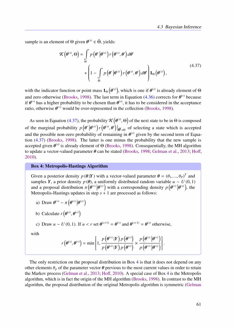
4.3 Bayesian Inference
sample is an element of Θ given θ(s)∈ Θ, yields:
K(θ(s),Θ
)=
∫Θ
p(θ′
∣∣∣θ(s))
r(θ(s), θ′
)dθ′
+
1 −∫Θ
p(θ′
∣∣∣θ(s))
r(θ(s), θ′
)dθ′
1Θ
(θ(s)
),
(4.37)
with the indicator function or point mass 1Θ
(θ(s)
), which is one if θ(s) is already element of Θ
and zero otherwise (Brooks, 1998). The last term in Equation (4.36) corrects for θ(∗) becauseif θ(∗) has a higher probability to be chosen than θ(s), it has to be considered in the acceptanceratio, otherwise θ(∗) would be over-represented in the collection (Brooks, 1998).
As seen in Equation (4.37), the probabilityK(θ(s),Θ
)of the next state to be in Θ is composed
of the marginal probability p(θ′
∣∣∣θ(s))
r(θ(s), θ′
) ∣∣∣θ′∈Θ of selecting a state which is acceptedand the possible non-zero probability of remaining in θ(s) given by the second term of Equa-tion (4.37) (Brooks, 1998). The latter is one minus the probability that the new sample isaccepted given θ(s) is already element of Θ (Brooks, 1998). Consequentially, the MH algorithmto update a vector-valued parameter θ can be stated (Brooks, 1998; Gelman et al., 2013; Hoff,2010).
Box 4: Metropolis-Hastings Algorithm
Given a posterior density p (θ |Y ) with a vector-valued parameter θ = (θ1, ..., θP)T andsamples Y, a prior density p (θ), a uniformly distributed random variable u ∼ U (0, 1)and a proposal distribution π
(θ(∗)
∣∣∣θ(s))
with a corresponding density p(θ(∗)
∣∣∣θ(s)), the
Metropolis-Hastings updates in step s + 1 are processed as follows:
a) Draw θ(∗) ∼ π(θ(∗)
∣∣∣θ(s))
b) Calculate r(θ(s), θ(∗)
)c) Draw u ∼ U (0, 1). If u < r set θ(s+1) = θ(∗) and θ(s+1) = θ(s) otherwise,
with
r(θ(s), θ(∗)
)= min
1, p(θ(∗) |Y
)p(θ(∗)
)p(θ(s)|Y
)p(θ(s)
) × p(θ(s)
∣∣∣θ(∗))
p(θ(∗)
∣∣∣θ(s)) .
The only restriction on the proposal distribution in Box 4 is that it does not depend on anyother elements θp of the parameter vector θ previous to the most current values in order to retainthe Markov process (Gelman et al., 2013; Hoff, 2010). A special case of Box 4 is the Metropolisalgorithm, which is in fact the origin of the MH algorithm (Brooks, 1998). In contrast to the MHalgorithm, the proposal distribution of the original Metropolis algorithm is symmetric (Gelman
61
Chapter 4 Methodology
et al., 2013; Hoff, 2010). This means that p(θ(∗)
∣∣∣θ(s))
= p(θ(s)
∣∣∣θ(∗))
and hence the correctionterm in Equation (4.36) vanishes (Gelman et al., 2013). A commonly used and more specialcase is the random walk Metropolis algorithm where the proposal density is generally given asa symmetric arbitrary density f
(θ(∗) − θ(s)
), i.e., a uniform or Gaussian distribution (Gelman
et al., 2013). Another commonly used option is the independent proposal distribution whichis independent of the current state θ(s) (Gelman et al., 2013; Hoff, 2010). This illustrates theuniversality of the MH algorithm and highlights the importance of the proposal distribution.
In fact, the behavior of the Markov chain heavily depends on the proposal distribution andthus an inadequate choice may result in a poor performance of the estimates (Andrieu andThoms, 2008). Major drawbacks of such methods are the correlation of nearby samples andthe fact that the initial samples have a different distribution than the target distribution (Gelmanet al., 2013; Hoff, 2010). The latter can be circumvented by introducing a burn-in phase, i.e., bysimply removing the first samples up to a certain number from the collection (Gelman et al.,2013). A convenient and conservative amount of omitted samples is half of the samples (Gelmanet al., 2013). In contrast, the correlation of samples within the collection is much harder to avoidsince the correlation corresponds to the distance between two successive samples (Gelman et al.,2013). An increase of the distance reduces the correlation but also increases the frequency ofsample rejection, which in turn reduces the efficiency (Gelman et al., 2013). On the other hand,serial correlation is not necessarily an issue (Gelman et al., 2013). Hence, once convergenceis reached, the samples are identically distributed and drawn from the posterior distributionanyway (Gelman et al., 2013). However, this still reduces the efficiency of the algorithm (Gel-man et al., 2013). Here, thinning is a commonly used technique to reduce autocorrelation byonly keeping every j-th sample (Brooks et al., 2011; Gelman et al., 2013). For more difficulttasks it is useful to monitor the convergence of samples and to estimate an effective sample sizeespecially to include a good stopping criteria (Gelman et al., 2013).
Since the performance of MCMC algorithms depends on the proposal distribution, a lot ofeffort has been devoted towards the optimization of the step size of the proposal (Andrieu andThoms, 2008; Gelman et al., 2013). Clearly, the variance of the proposal directly influencesthe estimations (Andrieu and Thoms, 2008). In addition, optimal estimations are supposed tohave a small variance (Andrieu and Thoms, 2008; Gelman et al., 2013). But proposal variancesthat are too small or too large lead to inaccurate estimations (Andrieu and Thoms, 2008). Thus,it is often important to design optimal proposal variances to achieve efficient and reliableprocedures (Andrieu and Thoms, 2008). Controlled MCMC methods address this issue withsequential updates of the proposal variance (Andrieu and Thoms, 2008). A major drawback ofsuch algorithms is that they tend to loose the ability to pass from one state to another withinfinite time which is a minimum requirement for consistent estimators (Andrieu and Thoms,2008). Accordingly, it is necessary to ensure that the algorithm does not produce poor proposaldistributions and becomes unstable (Andrieu and Thoms, 2008). An automatic choice of theproposal variance and thus the step size between two successive samples is therefore highlydesirable (Andrieu and Thoms, 2008). This leads to adaptive MCMC and MH procedures wherethe proposal distribution is automatically adapted and chosen (Andrieu and Thoms, 2008). Forvector-valued parameters, these algorithms update and scale the parameters and the related
62
4.3 Bayesian Inference
proposal distributions either component-wise or globally (Andrieu and Thoms, 2008). However,in practice, standard algorithms, such as random walk Metropolis or normal MH algorithms, areoften sufficient to explore the parameter space (Andrieu and Thoms, 2008; Gelman et al., 2013;Hoff, 2010).
Gibbs Sampling
Gibbs sampling can be viewed as a special case of MH sampling which makes the estimationmore feasible and efficient especially for multidimensional problems (Casella, 2001; Brooks,1998). In contrast to MH sampling, for Gibbs transitions, e.g., with two unknown parameters,namely θ1 ∈ θ and θ2 ∈ θ, the proposal distributions p
(θ(∗)
2
∣∣∣θ(s)1 , θ
(s)2
)and p
(θ(∗)
1
∣∣∣θ(s)1 , θ
(s)2
),
respectively, are set as the so-called full conditional distributions of θ1 given θ2 and viceversa (Gelman et al., 2013; Hoff, 2010). This means that
p(θ(∗)
1
∣∣∣θ(s)1 , θ
(s)2
)= p
(θ(∗)
1
∣∣∣θ(s)2 ,Y
)(4.38)
andp(θ(∗)
2
∣∣∣θ(s)1 , θ
(s)2
)= p
(θ(∗)
2
∣∣∣θ(s)1 ,Y
). (4.39)
Gibbs samplers are often based on conjugate priors which ideally allow to deduce a closed formof the posterior distribution (Casella, 2001; Hoff, 2010). As a consequence, it is possible to drawsamples directly from this closed form (Casella, 2001; Gelman et al., 2013). A prior distributionis conjugate to the posterior distribution and hence in the same family P if
p (θ) ∈ P ⇒ p (θ |Y ) ∈ P (4.40)
holds true (Hoff, 2010). For Gibbs sampling-based algorithms, conditional conjugate priordistributions are often sufficient (Hoff, 2010). Similar to Equation (4.40), the conditional con-jugate prior p
(θp
∣∣∣θ−p
)with θ−p =
(θ1, ..., θp−1, θp+1, ..., θP
)is assumed to be conjugate to the
posterior p (θ |Y ) (Gelman et al., 2013). This allows to draw iteratively from a set of unknownparameters (Gelman et al., 2013).
MH algorithms are also able to deal with models where more than one parameter has to beupdated iteratively (Gelman et al., 2013; Hoff, 2010; Brooks, 1998). But for Gibbs transitionsthe acceptance ratio always becomes one (Gelman et al., 2013; Hoff, 2010). Accordingly, allproduced samples are accepted, which leads to an optimal efficiency of the algorithm (Brooks,1998; Gelman et al., 2013; Hoff, 2010). The fact that the acceptance ratio for updating θp equalsone for each update follows from
p(θ(∗)
p , θ(s)−p
∣∣∣ Y)p(θ(s)
p
∣∣∣θ(∗)p , θ
(s)−p
)= p
(θ(∗)
p , θ(s)−p
∣∣∣ Y)p(θ(s)
p
∣∣∣θ(s)−p,Y
)(4.41a)
= p(θ(∗)
p
∣∣∣ θ(s)−p,Y
)p(θ(s)−p |Y
)p(θ(s)
p
∣∣∣θ(s)−p,Y
), (4.41b)
with the identity p (x, y |z ) = p (x |y, z ) p (y |z ) used in Equation (4.41b) (Hoff, 2010). For Gibbssampling algorithms, it is again possible that the samples are located in the same region for manyiterations which means that, once θ(s) is in a local pattern, the probability of θ(s+1) being again
63
Chapter 4 Methodology
in the same local pattern is high (Gelman et al., 2013; Hoff, 2010). This is supported by thefact that Gibbs samplers tend to sample θ(s+1) nearby θ(s) and thus samples may remain in suchregions for a long time, which increases the number of samples required for a sufficient posteriorapproximation (Hoff, 2010). Additionally, in many situations, it is not possible to derive a closedform of the prior distribution due to a lack of conjugate priors (Casella, 2001; Gelman et al.,2013; Hoff, 2010). In general, distributions belonging to the exponential family have naturalconjugate priors, whereas conjugate distributions are rarely given for other families (Gelmanet al., 2013).
Further Aspects
The superiority of Gibbs sampling becomes more clear for component-wise updates of parametervectors and hierarchical models (Gelman et al., 2013; Hoff, 2010). In contrast to MH-basedalgorithms, Gibbs transitions guarantee acceptance in each draw and hence the components canbe drawn successively (Gelman et al., 2013; Hoff, 2010). It is not necessary that each componentis updated in each iteration; it is only important to update them periodically (Gelman et al.,2013; Hoff, 2010). On the contrary, MH transitions do not guarantee acceptance for each drawand thus it is not ensured that the whole parameter space can be covered within a reasonabletime (Gelman et al., 2013; Hoff, 2010).
If the conditional posterior depends on additional hyperparameters, often the subset of theseadditional unknowns are estimated and their estimators are used to calculate the posterior basedon Gibbs transitions (Casella, 2001). But this is not an analysis in a Bayesian sense since theposterior distribution still depends on all the estimated hyperparameters (Casella, 2001). In a fullBayesian framework, this leads to hierarchical or multi-level models where the hyperparametersare treated as additional random variables, as described in Definition 11 (Gelman et al., 2013;Hoff, 2010). In contrast to parameters which are part of the underlying model, hyperparametersare additional unknowns influencing the prior distribution. The distribution of a hyperparameteris called hyperdistribution.
64
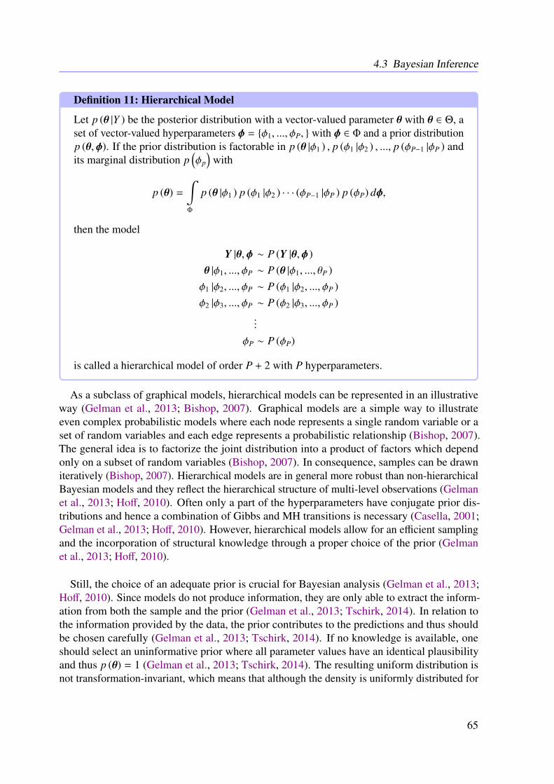
4.3 Bayesian Inference
Definition 11: Hierarchical Model
Let p (θ |Y ) be the posterior distribution with a vector-valued parameter θ with θ ∈ Θ, aset of vector-valued hyperparameters φ = φ1, ..., φP, with φ ∈ Φ and a prior distributionp (θ,φ). If the prior distribution is factorable in p (θ |φ1 ) , p (φ1 |φ2 ) , ..., p (φP−1 |φP ) andits marginal distribution p
(φp
)with
p (θ) =
∫Φ
p (θ |φ1 ) p (φ1 |φ2 ) · · · (φP−1 |φP ) p (φP) dφ,
then the model
Y |θ,φ ∼ P (Y |θ,φ )θ |φ1, ..., φP ∼ P (θ |φ1, ..., θP )φ1 |φ2, ..., φP ∼ P (φ1 |φ2, ..., φP )φ2 |φ3, ..., φP ∼ P (φ2 |φ3, ..., φP )
...
φP ∼ P (φP)
is called a hierarchical model of order P + 2 with P hyperparameters.
As a subclass of graphical models, hierarchical models can be represented in an illustrativeway (Gelman et al., 2013; Bishop, 2007). Graphical models are a simple way to illustrateeven complex probabilistic models where each node represents a single random variable or aset of random variables and each edge represents a probabilistic relationship (Bishop, 2007).The general idea is to factorize the joint distribution into a product of factors which dependonly on a subset of random variables (Bishop, 2007). In consequence, samples can be drawniteratively (Bishop, 2007). Hierarchical models are in general more robust than non-hierarchicalBayesian models and they reflect the hierarchical structure of multi-level observations (Gelmanet al., 2013; Hoff, 2010). Often only a part of the hyperparameters have conjugate prior dis-tributions and hence a combination of Gibbs and MH transitions is necessary (Casella, 2001;Gelman et al., 2013; Hoff, 2010). However, hierarchical models allow for an efficient samplingand the incorporation of structural knowledge through a proper choice of the prior (Gelmanet al., 2013; Hoff, 2010).
Still, the choice of an adequate prior is crucial for Bayesian analysis (Gelman et al., 2013;Hoff, 2010). Since models do not produce information, they are only able to extract the inform-ation from both the sample and the prior (Gelman et al., 2013; Tschirk, 2014). In relation tothe information provided by the data, the prior contributes to the predictions and thus shouldbe chosen carefully (Gelman et al., 2013; Tschirk, 2014). If no knowledge is available, oneshould select an uninformative prior where all parameter values have an identical plausibilityand thus p (θ) = 1 (Gelman et al., 2013; Tschirk, 2014). The resulting uniform distribution isnot transformation-invariant, which means that although the density is uniformly distributed for
65
Chapter 4 Methodology
a certain parametrization, it may not be for another (Gelman et al., 2013; Tschirk, 2014). Thisleads to the so-called Jeffrey’s prior which is in fact invariant against monotonous transforma-tions (Gelman et al., 2013; Tschirk, 2014).
To gain some confidence regarding the convergence of the samples MCMC diagnostics arenecessary (Gelman et al., 2013; Hoff, 2010). Mostly, it is more easy to determine whether thesamples are not converging than to ensure convergence (Hoff, 2010; Brooks et al., 2011). Manydifferent MCMC diagnostic tools and view-points can be found in literature, however, there isno perfect MCMC diagnostic tool due to the fact that the state space is usually poorly connec-ted (Brooks et al., 2011). Poorly connected state spaces result in a huge number of iterationsuntil the samples jump from one region to another (Hoff, 2010; Brooks et al., 2011). In thosesituations, the convergence is conditioned on the part where the chain was started (Hoff, 2010;Brooks et al., 2011). Although this is related to multimodality, i.e., the posterior distribution hasmultiple peaks, multimodality does not necessarily cause conditional convergence (Brooks et al.,2011). This all gives rise to several questions including, e.g., the number of MCMC runs, thesample size, the determination of the starting point or the introduction of additional variables toincrease convergence (Gelman et al., 2013; Brooks et al., 2011). It is important that the samplesize is large enough to avoid that the samples remain in a region with low probability and toenable transitions between all regions with high probability (Gelman et al., 2013; Hoff, 2010).The latter phenomena is called mixing, whereas the first is referred to as stationarity (Gelmanet al., 2013; Hoff, 2010). A perfect Markov chain does not stick and is able to jump betweendifferent regions in one step (Hoff, 2010). A direct measurement for stickiness is autocorrelation,which measures the correlation between samples depending on their distance (Gelman et al.,2013; Hoff, 2010). In general, the higher the autocorrelation, the larger the sample size has tobe in order to achieve a good precision (Gelman et al., 2013; Hoff, 2010).
The Hamiltonian Monte Carlo algorithm is a further improvement of MCMC methods and al-lows to explore the state space more quickly (Gelman et al., 2013). For high-dimensionalparameter spaces, even after re-parametrization and adjusted jump rules, Gibbs and MHtransition-based models retain their random walk behavior (Gelman et al., 2013). In contrast,the Hamiltonian Monte Carlo algorithm combines MCMC methods with deterministic aspectsby introducing an additional variable (Gelman et al., 2013). This variable is correlated to theproposal distribution and hence its trajectory allows for efficient parameter proposals (Gelmanet al., 2013). Even though the Hamiltonian Monte Carlo algorithm is very efficient, in practice,it is often not applicable since the gradient of the log posterior density must be analyticallyaccessible (Gelman et al., 2013). A numerical approximation of the gradients is considered toocostly since it has at least as many components as the dimension of the related parameters (Gel-man et al., 2013).
In addition to the discussed MCMC algorithms particle filters are often used as an alternat-ive (Särkkä, 2013; Gelman et al., 2013). This class of Bayesian filters is useful in the case ofmultimodal or partly discrete posterior distributions, where the commonly used Gaussian pro-cesses are not applicable (Särkkä, 2013; Gelman et al., 2013). Several such algorithms have beenreported in literature, e.g., importance sampling or sequential importance re-sampling (Särkkä,
66
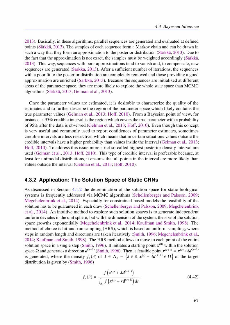
4.3 Bayesian Inference
2013). Basically, in these algorithms, parallel sequences are generated and evaluated at definedpoints (Särkkä, 2013). The samples of each sequence form a Markov chain and can be drawn insuch a way that they form an approximation to the posterior distribution (Särkkä, 2013). Due tothe fact that the approximation is not exact, the samples must be weighted accordingly (Särkkä,2013). This way, sequences with poor approximations tend to vanish and, to compensate, newsequences are generated (Särkkä, 2013). After a sufficient number of iterations, the sequenceswith a poor fit to the posterior distribution are completely removed and those providing a goodapproximation are enriched (Särkkä, 2013). Because the sequences are initialized at differentareas of the parameter space, they are more likely to explore the whole state space than MCMCalgorithms (Särkkä, 2013; Gelman et al., 2013).
Once the parameter values are estimated, it is desirable to characterize the quality of theestimates and to further describe the region of the parameter space which likely contains thetrue parameter values (Gelman et al., 2013; Hoff, 2010). From a Bayesian point of view, forinstance, a 95% credible interval is the region which covers the true parameter with a probabilityof 95% after the data is observed (Gelman et al., 2013; Hoff, 2010). Even though this conceptis very useful and commonly used to report confidences of parameter estimates, sometimescredible intervals are less restrictive, which means that in certain situations values outside thecredible intervals have a higher probability than values inside the interval (Gelman et al., 2013;Hoff, 2010). To address this issue more strict so-called highest posterior density interval areused (Gelman et al., 2013; Hoff, 2010). This type of credible interval is preferable because, atleast for unimodal distributions, it ensures that all points in the interval are more likely thanvalues outside the interval (Gelman et al., 2013; Hoff, 2010).
4.3.2 Application: The Solution Space of Static CRNs
As discussed in Section 4.1.2 the determination of the solution space for static biologicalsystems is frequently addressed via MCMC algorithms (Schellenberger and Palsson, 2009;Megchelenbrink et al., 2014). Especially for constrained-based models the feasibility of thesolution has to be guaranteed in each draw (Schellenberger and Palsson, 2009; Megchelenbrinket al., 2014). An intuitive method to explore such solution spaces is to generate independentuniform deviates in the unit sphere; but with the dimension of the system, the size of the solutionspace growths exponentially (Megchelenbrink et al., 2014; Kaufman and Smith, 1998). Themethod of choice is hit-and-run sampling (HRS), which is based on uniform sampling, wheresteps in random length and directions are taken iteratively (Smith, 1996; Megchelenbrink et al.,2014; Kaufman and Smith, 1998). The HRS method allows to move to each point of the entiresolution space in a single step (Smith, 1996). It initiates a starting point x(0) within the solutionspace Ω and generates a direction d(s+1) (Smith, 1996). Then, a feasible point x(s+1) = x(s)+λd(s+1)
is generated, where the density fs (λ) of λ ∈ Λs =λ ∈ R
∣∣∣x(s) + λd(s+1)∈ Ω
of the target
distribution is given by (Smith, 1996)
fs (λ) =f(x(s) + λd(s+1)
)∫
Λsf(x(s) + rd(s+1)
)dr. (4.42)
67
Chapter 4 Methodology
For stoichiometric analyses as detailed in Section 4.1, acquiring a uniform target distributionfs (λ) is sufficient (Megchelenbrink et al., 2014). Therefore, λ and d(s+1) can be chosen such thatthey are uniformly distributed within the solution space (Smith, 1996; Megchelenbrink et al.,2014). Consequently, the samples x(s) are also uniformly distributed and build a Markov chainin Ω (Smith, 1996; Megchelenbrink et al., 2014). In practice, this leads to an accumulationof sample points close to the boundaries of the solution space because the sampler tends todraw successive samples which are close to each other (Smith, 1996; Megchelenbrink et al.,2014). This drawback is addressed by the artificial centering hit-and-run (ACHR) method,which basically normalizes the chosen direction with respect to an approximate center to theprevious iterates (Megchelenbrink et al., 2014; Kaufman and Smith, 1998). In most cases,this leads to a faster convergence and makes larger steps possible (Megchelenbrink et al.,2014). On the other hand, due to the normalization based on the approximate center, eachsample depends on prior iterations and directions (Megchelenbrink et al., 2014). Hence thesampled sequence is no Markov chain and thus the convergence to the target distribution is notguaranteed (Megchelenbrink et al., 2014). Nonetheless, as an heuristic approach, the ACHR iscommonly used to sample the solution space of CRNs due to its capability to explore the wholesolution space (Schellenberger and Palsson, 2009; Megchelenbrink et al., 2014; Kaufman andSmith, 1998).
4.4 Parameter Estimation
As discussed in Chapter 2, developing ODE-based mathematical models in biology is an in-teractive process with the overall aim to match the given experimental data (Azeloglu andIyengar, 2015; Jaqaman and Danuser, 2006; Ashyraliyev et al., 2009). The inverse problem isthe estimation of the model parameters (Jaqaman and Danuser, 2006; Ashyraliyev et al., 2009).ODE-based models of biological systems are composed of reactions and thus kinetic rate laws.Dependent on the complexity of the system and the number of involved reactions and kinetic ratelaws, the number of unknown or partially known parameters can be very large. Hence, estimat-ing all parameters of a biological model is usually impossible due to the complexity of biologicalprocesses (Azeloglu and Iyengar, 2015; Ashyraliyev et al., 2009). Even if error free data isassumed, the structure of biological models may lead to non-identifiable parameters becausein order to estimate a certain number of unknowns at least the same number of data points isrequired (Jaqaman and Danuser, 2006; Ashyraliyev et al., 2009). Such structural non-identifiablemodels have multiple solutions and thus are not observable (cp. Section 4.2.4) (Ashyraliyevet al., 2009). However, it is often possible to detect the non-identifiable parameters and subnet-works of such models (Ashyraliyev et al., 2009; Raue et al., 2009). Consequently, methods formodel reduction can be used to reduce the fraction of non-identifiable parameters (Raue et al.,2009).
Although all parameters are structurally identifiable, there may be parameters with low con-fidence, i.e., parameters which are practically non-identifiable (Ashyraliyev et al., 2009; Raueet al., 2009). In recent literature there exist different definitions of identifiability (Ashyraliyevet al., 2009). Commonly, a parameter is called non-identifiable if its confidence interval is
68
4.4 Parameter Estimation
infinite (Raue et al., 2009). Roughly speaking, this means that there is an infinite number ofalternative parameter values which match the observations as well. A simple way to proofstructural identifiability of non-linear systems is based on Taylor approximations at measuredtime points (Ashyraliyev et al., 2009). A unique solution of the resulting system in terms ofparameters implies structural identifiability and thus a distinguishable model structure (Ashyrali-yev et al., 2009). Hence, structural identifiability is strongly related to the observability ofdynamical systems, which can also be assessed via local Taylor approximations, as explained inSection 4.2.4.
Due to a lack of data and the non-identifiability of the parameters, models in systems biologyare frequently build from incomplete datasets with mainly unknown parameters, and the directdetermination of the parameters from experimental data is often not possible (Azeloglu andIyengar, 2015; Jaqaman and Danuser, 2006; Ashyraliyev et al., 2009). Although nowadays largedatabases of measured parameters, e.g., kinetic constants, are accessible, in practice, they areof little value for mathematical modeling (Azeloglu and Iyengar, 2015). One major drawbackof such databases and in general of combining data from different sources and systems is thevariety of conditions under which they were measured (Azeloglu and Iyengar, 2015). Theseconditions, e.g., the pH-value or temperature, often disagree with the experimental data, whichthe modeler wants to fit and are thus biased (Azeloglu and Iyengar, 2015). However, they areuseful starting points for parameter estimation (Azeloglu and Iyengar, 2015; Ashyraliyev et al.,2009). Ideally, parameters are estimated based on absolute protein concentrations. But, in mostcases, only variations in the protein abundance and thus relative protein concentrations areaccessible (Azeloglu and Iyengar, 2015).
To address the above issues, different strategies for data-based parameter estimation on awhole system-level have been developed (Jaqaman and Danuser, 2006; Ashyraliyev et al., 2009).Basically, approaches for parameter estimation aim to optimize a well-defined objective functionwhich represents the discrepancy between experimental data and model predictions (Jaqamanand Danuser, 2006; Ashyraliyev et al., 2009). To avoid getting stuck in local extrema, globalsearch algorithms, such as simulated annealing or evolutionary algorithms, are mainly prob-abilistic methods with the theoretical ability to explore the whole parameter space (Jaqamanand Danuser, 2006; Ashyraliyev et al., 2009). The genetic algorithm is a common evolutionaryalgorithm used for parameter estimation which adapts the survival-of-the-fittest principle fromnature (Ashyraliyev et al., 2009; Raol et al., 2004). Similar to a population of individuals, aset of randomly chosen parameter vectors is initialized to explore the parameter space (Raolet al., 2004). As in evolutionary processes, individuals are then basically selected, recombinedand mutated based on their fitness or, in this context, feasibility (Ashyraliyev et al., 2009; Raolet al., 2004). This means those individuals which are close to the optimal solutions pass throughthis process and survive or are combined with other individuals close to the optimum, andindividuals far away from the optimum vanish (Ashyraliyev et al., 2009; Raol et al., 2004).Although global search strategies are capable to explore the whole parameter space, convergenceis not guaranteed (Ashyraliyev et al., 2009; Raol et al., 2004).
69
Chapter 4 Methodology
The second class of methods are local search algorithms (Ashyraliyev et al., 2009). Localsearch algorithms guarantee solutions with a certain accuracy based on theoretical proofs ofconvergence provided that the initial guess is sufficiently close to the optimum (Ashyraliyevet al., 2009). Gradient-based methods, which require first derivatives or their approximationswith respect to the parameters, are frequently used in systems biology (Karr et al., 2015; vanRiel, 2006). Although derivative-based methods are very efficient for a couple of systems, theyare often trapped in local extrema (Ashyraliyev et al., 2009; Karr et al., 2015). In addition,gradient-based methods are sensitive to measurement errors and starting points due to theirdeterministic nature (Ashyraliyev et al., 2009; Karr et al., 2015).
Although global search algorithms are able to explore the whole parameter space, theyhardly converge towards the exact optimum of the objective (Ashyraliyev et al., 2009). Onthe other hand, local search algorithms converge faster towards the optimum but tend to getstuck in local extrema if they start far away from the optimum (Ashyraliyev et al., 2009).Therefore, it makes sense to combine both approaches, i.e., to use the global exploration ofthe parameter space and increase the convergence speed in areas close to the optimum vialocal search algorithms (Ashyraliyev et al., 2009). Today, these hybrid methods are frequentlyused (Ashyraliyev et al., 2009; Karr et al., 2015).
Bayesian inference, as discussed in Section 4.3, is another frequently used approach to estim-ate parameters in biological systems (Jaqaman and Danuser, 2006; Coleman and Block, 2006).Here, the quantity of interest such as credible intervals of parameters or expected parametervalues are estimated by the use of prior knowledge via MCMC methods (Jaqaman and Danuser,2006; Coleman and Block, 2006). Bayesian methods provide reliability measurements such ascorrelations and variances (Jaqaman and Danuser, 2006; Coleman and Block, 2006). Accordingto Section 4.3, the prior distribution p (θ) reflecting the prior knowledge about the parameterstogether with the density of data given parameters p (Y |θ ) allows to draw samples from theparameter distribution p (θ |Y ) based on Bayes’ Law (Jaqaman and Danuser, 2006; Colemanand Block, 2006). The probability P (Y |θ ) reflects the discrepancy between predictions anddata with respect to the measurement noise σ2 and the linear combination of the observablestates h (x) of the given model. Hence, P (Y |θ ) is often given by P (Y |θ ) ∼ N
(h (x) ,σ2
)or
similar distributions (Jaqaman and Danuser, 2006; Hug et al., 2013; Coleman and Block, 2006).Bayesian inference is especially suitable for high-dimensional systems where other methodsfail due to the underlying complex parameter space (Jaqaman and Danuser, 2006; Coleman andBlock, 2006).
A well-chosen objective function is highly important for parameter estimation (Ashyraliyevet al., 2009; Karr et al., 2015; Kreutz et al., 2013). As discussed in Section 4.2.3, the LSE isan intuitive measurement for discrepancies between data and model predictions given a set ofmodel parameters yi (tl)
∣∣∣θ (Ashyraliyev et al., 2009; Kreutz et al., 2013). Under the assumption
70
4.4 Parameter Estimation
of Gaussian-distributed measurement errors, the LSE estimator
θ = arg minθ
I∑i=1
F∑l=1
(yi (tl) − yi (tl)
∣∣∣θ )2
σ2i,tl
, (4.43)
is equivalent to the maximum likelihood estimator (MLE) (Kreutz et al., 2013). With theprobability of the observations y given a set of model parameters θ, the MLE
θ = arg maxθ
I∏i=1
p(yi,1:F |θ
) (4.44)
maximizes the overall probability of the data given the estimated set of parameters (Kreutzet al., 2013; Raue et al., 2009). One advantage of the MLE is the derivable profile likelihoodas a direct measure for the impact of each model parameter and thus the identifiability ofthose parameters (Kreutz et al., 2013; Raue et al., 2009; Swameye et al., 2003). The profilelikelihood reflects the dependency of the probability of the data given the optimal parameterset conditioned on a single parameter and allows for accurate confidence or credible intervals,respectively (Kreutz et al., 2013; Raue et al., 2009).
Altogether, estimates based on a single set of experimental data do not imply reliable es-timations (Ashyraliyev et al., 2009; Azeloglu and Iyengar, 2015). Identifiability checks, val-idation based on perturbed data or other procedures can help to proof the credibility of themodel (Ashyraliyev et al., 2009; Azeloglu and Iyengar, 2015). Perturbed data and other val-idation data are often hardly accessible, and thus a parameter identifiability analysis remainsthe only option to gain confidence about the estimates (Ashyraliyev et al., 2009; Azelogluand Iyengar, 2015). On the other hand, one may argue that exact parameter estimates are notrequired to draw meaningful biological conclusions (Azeloglu and Iyengar, 2015).
71

CHAPTER 5
Analysis of the M2 Receptor-dependentSignaling in CHO Cells
In this chapter, a time-independent model of the M2 receptor-dependent signaling in CHO cellsis developed and analyzed on the basis of the novel CFS. The thus obtained insights into theamplification processes serve as a first attempt to describe the DMR-related signaling. To gain aclearer picture about the involved time-dependent amplification processes the model proposedin this chapter is further extended in Chapter 8 by including time-resolved kinetics. This workis accepted in a peer-reviewed journal (cp. Appendix F).
5.1 Introduction
As discussed in Chapter 3, the M2 receptor (encoded by the CHRM2 gene) belongs to thefamily of GPCRs and is related to negative dromotropic and negative chronotropic events.Since GPCRs represent one of the most important target classes of proteins for drug discovery,the development of specific agonists and antagonists for muscarinic receptors, including theM2 receptor, is still of high interest (Zheng, 2006). Iperoxo is a highly affine and efficaciousmuscarinic agonist that has recently served to elucidate the crystal structure of the active state ofthe M2 receptor (Schrage et al., 2013, 2014; Kruse et al., 2013; Hu et al., 2010). In traditionalpharmacology the ligand-binding event, second messenger concentrations, ion channel function,as well as tissue, organ or body responses are recorded. As discussed in Chapter 3, whole celltechniques nowadays are used to dissect the signaling of intact cells into different components(Schröder et al., 2011). In addition, iperoxo and its derivatives turned out to be valuable toolsfor gaining deeper insight into structure-signal relationships (Bock et al., 2014; Antony et al.,2009).
Recent experimental work explored the cellular response to iperoxo-induced M2 receptorstimulation in CHO cells (Schrage et al., 2013; Kruse et al., 2013; Schrage et al., 2016). Thecellular response was measured by DMR (Schröder et al., 2011). Since the DMR responsecan be assumed to be dependent on the M2 receptor-induced signaling our aim was to model
73
Chapter 5 Analysis of the M2 Receptor-dependent Signaling in CHO Cells
and study the corresponding reaction system. The pathway consists of proteins as well as thesecondary messenger cAMP. The respective biochemical reactions are principally well known(Pierce et al., 2002; Linderman, 2009; Sunahara and Taussig, 2002; Taylor et al., 2012), butto the best of our knowledge no effort has been taken so far to derive a mathematical model,especially for CHO cells, which are very important in pharmaceutical research and for theindustrial production of recombinant protein therapeutics (De Jesus and Wurm, 2011; Walsh,2010).
In this work we developed a mass action based mathematical description of the M2 receptor-dependent signaling network. Our developed model consists of 79 reactions, altogether involving64 relevant proteins and secondary messenger molecules described in literature. In our jointsignaling and secondary messenger model, all binding and (de-)phosphorylation events areexplicitly taken into account in order to enable subsequent stoichiometric matrix and fluxdistribution analysis (Wiback et al., 2004). Although this kind of analysis is usually onlyemployed for metabolic networks, as detailed in Section 4.1, our explicit modeling of bindingand phosphorylation events enables the adaption of these techniques to a mixed signalingand secondary messenger system. The usefulness of applying stoichiometric matrix analysistechniques to signaling pathways has for example been demonstrated by Behre and Schuster(2009), who adapted EFM analysis to this situation. This work demonstrates, how the known fluxsampling technique can be extended to incorporate partially available experimental information(here: cAMP production, PDE4 activation) (Smith, 1996). We tested our combined modelingand data driven sampling method by predicting key signaling mechanisms known from literature,but not explicitly encoded into the model. Our proposed CFS technique allows for qualitativepredictions of downstream stimulation effects on actin and tubulin levels, which here serve asour markers for the mass redistribution effect. These qualitative predictions are in agreementwith the experimental observations, which suggests CFS as a technique for model checking.This is further underlined by the possibility to combine CFS and EFM analysis yielding astatistical ranking of EFMs according to their expected biological relevance.
5.2 Network Reconstruction
GPCR-induced signaling is well-known in common literature (Pierce et al., 2002; Linderman,2009; Taylor et al., 2012; Sunahara and Taussig, 2002). Specifically the link to the cAMP-induced signaling is in the focus of current pharmaceutical research (Milligan and Kostenis,2006; Hu et al., 2010). Figure 5.1 depicts a schematic representation of the whole set of relevantmolecules and their interplay, which are considered in our model. In particular the process ofreceptor-induced GP activation is well studied, where the ligand-bound receptor changes itsphysical structure and the inactive associated GP interacts with the receptor and dissociatesinto its subunits (Pierce et al., 2002). Thereby the αi, αs and β\γ subunits are activated andare able to interact independently with other proteins like AC (Sunahara and Taussig, 2002;Milligan and Kostenis, 2006). The GP subunit αo has no significant influence on AC but ithas an influence on the DMR (Milligan and Kostenis, 2006). AC is one of the most importantproteins within the GP-mediated pathway and responsible for the secondary messenger pro-
74
5.3 Mathematical Modeling
duction. The large number of AC and GP subtypes causes a highly complex subnetwork withmany cross-reactions (Milligan and Kostenis, 2006; Sunahara and Taussig, 2002). Also thereceptor activation cycle itself is not trivial. This first step in the signaling cascade is highlyinteresting for pharmaceutical research and led to well developed models for receptor activationand inhibition (Woodroffe et al., 2009; Chen et al., 2003; Strange, 2008; Bornheimer et al., 2004).
Besides this completely membrane bound subnetwork the PKA-induced phosphorylationcascade, and the feedback loop causing cAMP degradation, is well studied (Taylor et al., 2012).cAMP binds to PKA and causes its activation. But an increase in PKA activity also leadsto an increase in PDE activity, which inactivates cAMP by degrading it to adenosine mono-phosphate (AMP) (Boswell-Smith et al., 2006). Through this mechanism the cell prevents acontinuous overstimulation by excessive cAMP levels. Stimulation of the receptor populationvia the muscarinic agonist iperoxo induced a cellular DMR response at concentrations that arefar lower than the corresponding concentration-binding relationships (Schrage et al., 2013).The same authors reported this amplification phenomenon also for other ligands, including thenatural ligand ACh (Schrage et al., 2013). The exact nature of the amplification process is not un-derstood so far, but may at least be partially attributed to intracellular signaling events (Schrageet al., 2016). According to common literature we suppose RGSs and GRKs to be of relevance.These proteins are closely related to the deactivation of the receptor and the GP subunits (Pierceet al., 2002; De Vries et al., 2000; Hollinger et al., 2003). In this work, we chose RGS14, GRK6and GRK2 as important representatives for each group.
The DMR, as an optical biosensor-based procedure, measures the shift in wavelength res-ulting from intracellular mass movement caused by the rearrangement of cell organelles andtransportation processes (Strange, 2008). In this work we chose actin and tubulin as DMRmarkers. Actin and tubulin are closely related to the cellular movement and we assume a strongcorrelation between changes in both protein and secondary messenger concentrations and therelative wavelength shifts measured by DMR (Hammond et al., 2008; Schmidt and Hall, 1998).Therefore, we took all proteins directly linked to actin and tubulin into account and assumedtheir activation to be correlated with the wavelength shift (cp. Figure 5.1). Maximal DMRresponse induced by iperoxo occurs typically after approximately 10 minutes (Schrage et al.,2013). According to the timescale and common literature we did not consider transcriptionaldownstream responses (Mayr and Montminy, 2001; Shaywitz and Greenberg, 1999). Furtherreferences are given in Appendix B.
5.3 Mathematical Modeling
All interactions shown in Figure 5.1 are explicitly formalized as mass action based elementaryreactions and all known proteins and their occurring complexes are included (Horn and Jackson,1972). Hence biological information from the available biochemical knowledge is preserved.Let x1, . . . , xN denote the concentrations of all molecules in the system. Then, according to
75
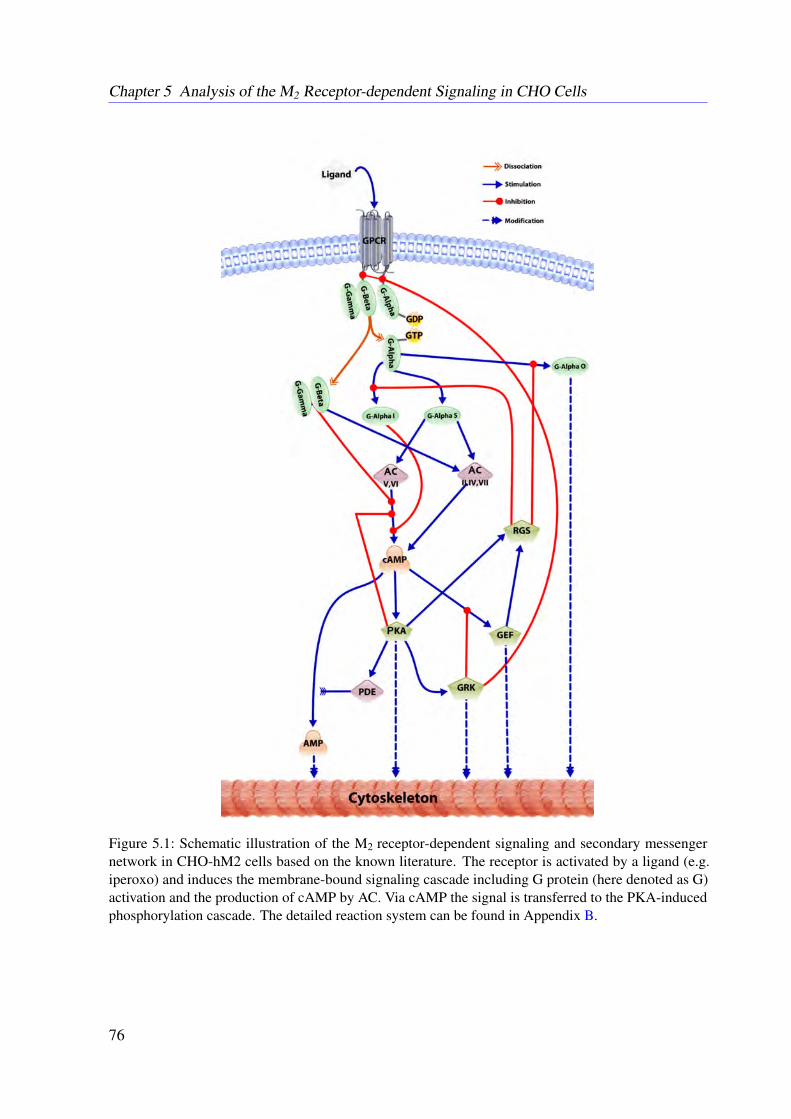
Chapter 5 Analysis of the M2 Receptor-dependent Signaling in CHO Cells
Figure 5.1: Schematic illustration of the M2 receptor-dependent signaling and secondary messengernetwork in CHO-hM2 cells based on the known literature. The receptor is activated by a ligand (e.g.iperoxo) and induces the membrane-bound signaling cascade including G protein (here denoted as G)activation and the production of cAMP by AC. Via cAMP the signal is transferred to the PKA-inducedphosphorylation cascade. The detailed reaction system can be found in Appendix B.
76
5.3 Mathematical Modeling
Section 2.3.4, the change of the concentration of molecule n can be written as
dxn
dt=
K∑k=1
sn,krk, (5.1)
where sn,k is the stoichiometric coefficient of molecule n in reaction k and rk denotes the corres-ponding reaction velocity. As an example, here the PKA activation by cAMP is shown (Corbinet al., 1988):
PKA→ PKA (5.2a)
PKA + 2cAMP→ PKA. (5.2b)
Here, PKA denotes the inactive form of PKA. Let us denote the rate of both reactions by r1
and r2, respectively. The stoichiometric coefficients are s1,1 = s2,2 = −1, s1,2 = s2,1 = 1 ands3,2 = −2. We then obtain
d[PKA]dt
= s1,1r1 + s1,2r2 (5.3a)
d[PKA]dt
= s2,1r1 + s2,2r2 (5.3b)
d[cAMP]dt
= s3,2r2. (5.3c)
Altogether the modeled system contains 79 elementary reactions, which can be found in Ap-pendix B. The full reaction system can be represented via a stoichiometric matrix S ∈ RN×K
with entries sn,k. In this matrix every molecule is represented by one row and every reaction isrepresented by one column.
The modeled system consists of several biochemical reaction types, namely binding, stim-ulation and inhibition. These biochemical events need to be represented appropriately in thereaction system and the stoichiometric matrix, respectively. This was done as follows: Theprotein activation via phosphorylation was modeled with the help of an intermediate moleculewhich represents the complex of the substrate and the related kinase. The kinase binds reversiblyto the substrate and forms an intermediate complex which then dissociates irreversibly into thekinase and the modified substrate. For instance, GRK2 is phosphorylated by PKA (Cong et al.,2001). For this purpose we introduce the intermediate complex PKA : GRK2 and write thereaction system as
PKA + GRK2 PKA : GRK2 (5.4a)PKA : GRK2→ GRK2 + PKA. (5.4b)
For every phosphorylation step we assumed a backward reaction P∗ → P, which dephos-phorylates the phosphoprotein P∗ with the help of an unknown phosphatase. In this example
77
Chapter 5 Analysis of the M2 Receptor-dependent Signaling in CHO Cells
GRK2 is dephosphorylated into GRK2
GRK2→ GRK2. (5.5)
Protein inhibition by kinases is modeled in a similar manner. A kinase binds reversibly to thetarget protein and forms an intermediate complex which then dissociates irreversibly into thekinase and the inactive protein. The inactive protein is now able to be activated again by anotherkinase. This process is illustrated using the inhibition of the guanine nucleotide exchangefactor (GEF) by GRK2 (Eijkelkamp et al., 2010)
GRK2 + GEF GRK2 : GEF (5.6a)
GRK2 : GEF → GRK2 + GEF. (5.6b)
As shown above, these reactions can be represented in the stoichiometric matrix S . The dimen-sion of the stoichiometric matrix can be decreased by expressing the forward and backwarddirection of the same reversible reaction by one row where reaction rates can be both positiveand negative. This is in contrast to strictly irreversible reactions where only positive reactionrates are allowed.
We also used the stoichiometric model to derive a system of ODEs based on the assumptionof mass action kinetics, as shown in Appendix B.
5.4 Methods
5.4.1 Conservation Relationships
Since signaling events are relatively fast, we can assume that for each protein the overall totalamount of phosphorylated, bound and unphosphorylated proteins is approximately constant,provided that the biological system is in steady state and the model was correct. Hence, checkingconservation relationships is a means to check the consistency of our model.
According to Palsson (2006), conservation relationships under steady state conditions aremathematically identifiable from the null space of S T . As detailed in Section 4.1.1, conservationrelationships are all those vectors g for which
S T g = 0. (5.7)
Each entry in g corresponds to exactly one molecule. The analysis of the entries of vectors gprovides thus a means to verify whether the expected constant total concentration of each proteinis fulfilled in reality. Moreover, we can also obtain insights into possibly existing constantprotein concentrations within whole reaction cascades.
78
5.4 Methods
5.4.2 Stimulation of the System
We are interested in qualitative changes upon receptor stimulation. For the unstimulated systemwe assume a steady state characterized by constant concentrations of all molecules. Receptorstimulation causes a perturbation of this steady state resulting in dynamic changes of molecularconcentrations. However, we assume that after some relaxation time the system will attain a –supposingly different – steady state, which is characterized by the molecular concentrations inthe stimulated state. In reality, the stimulated state does not need to be a dynamic equilibriumin the strict sense, but we believe it to be a useful approximation for a situation of maximumresponse, where all concentrations are nearly constant over time. We believe that this workinghypothesis is useful to analyze qualitative changes between the unstimulated and stimulatedstates, which is also supported by the fast – usually milliseconds – time scale of the signalingevents in comparison to the observable duration of responses to receptor stimulation.
The unstimulated and the stimulated state correspond to different solutions of system understeady state conditions. i.e., S v = 0. Our strategy will be to constrain the solution space of thissystem using experimental data. We will then use Monte Carlo sampling to compare possiblestationary reaction rates u in the simulated and unstimulated state.
For a qualitative comparison we suppose the DMR response to be given as the sum of allfluxes with known influence on the wavelength shift
Response =
K∑k=1
vk. (5.8)
Here vk denotes the activating flux related to molecule n with influence on the wavelength shift.The sum runs over all K in-fluxes into tubulin and actin, which are considered as markers of theDMR response (Hammond et al., 2008; Schmidt and Hall, 1998; Schröder et al., 2011).
5.4.3 Sampling the Flux Polytope
Since we are interested in the general behavior of the system without the incorporation ofadditional rate parameters, steady state solutions of the system can in principle be found throughMCMC HRS, as discussed in Section 4.3.2 (Smith, 1996; Brooks, 1998; Price et al., 2004). Asingle move in the HRS is performed by making a randomly chosen move within the unit spherefrom a given feasible solution. Afterwards the step size is adjusted such that the new solution isalso feasible (Smith, 1996; Megchelenbrink et al., 2014). A solution v∗ is called feasible, if itsatisfies
S v∗ = 0 (5.9a)αk ≤ v
∗k ≤ βk, ∀k = 1, . . . ,K (5.9b)
with bounds αk, βk. Note that, without further constraints, fluxes could take any real value,but in reality fluxes are bounded. Hence, for all reversible reactions, we set αk = −1000 and
79
Chapter 5 Analysis of the M2 Receptor-dependent Signaling in CHO Cells
βk = 1000 as loose bounds. For irreversible reactions, we set αk = 0. The flux bounds canin principle be used to incorporate experimental data. We will modify the flux bounds toqualitatively incorporate fold changes between stimulated and unstimulated cells, as explainedin the following section.
5.4.4 Constrained Flux Sampling
We incorporate partially available data of experimentally measured relative (steady state) molecu-lar concentrations into the above described flux sampling scheme in order to make qualitativepredictions about flux changes upon stimulation. The approach thus does not require detailedknowledge of the kinetic rate constants.
Let vk denote the steady state flux of the k-th reaction in the case of an unstimulated receptor.According to the law of mass action (see Section 2.4) with rate parameters rk we have
vk = rk
N∏n=1
xsn,kn , (5.10)
where xn is the set of molecules taking part in the particular reaction and xn their concentrations.Note that at this point we suppose the involved reversible reactions to be split into two irreversibleones. The flux vk for the same reaction under stimulation can be defined accordingly now withconcentrations xn. Usually, in experiments, relative concentration changes (fold changes) fn = xn
xn
are determined. Obviously,
vk
vk=
N∏n=1
f sn,kn (5.11)
which implies
vk = vk
N∏n=1
f sn,kn . (5.12)
Note that the stoichiometric coefficients sn,k in most cases are 1. The equation suggests aprincipal two-step procedure:
1. Perform conventional flux sampling for the unstimulated situation. This yields a set vk.
2. Perform flux sampling for the stimulated situation by plugging the observed fold changesinto Equation (5.12) in order to constrain the sampled fluxes.
In reality it may be more appropriate to consider confidence intervals [ f Minn , f Max
n ] for fn becausefold changes are subject to uncertainty. This can be addressed straightforwardly by replacingEquation (5.12) by an inequality
vk
N∏n=1
(f Minn
)sn,k≤ vk ≤ vk
N∏n=1
(f Maxn
)sn,k. (5.13)
80
5.5 Data
The quantity vk in practice needs to be estimated from the empirical flux distribution understeady state conditions. A reasonable choice is to take the mean or median of the sampledistribution plus/minus the standard deviation for that purpose.
5.4.5 Elementary Flux Modes
According to Section 4.1.1, Schuster and Hilgetag (1994) introduced EFM analysis for charac-terizing the geometry of the solution polytope of the equation system S v = 0 in a biologicallyinterpretable manner. All solution vectors occur as linear combinations of EFMs. This leads tothe polyhedral flux cone P(S )
P (S ) =
v ∈ RK
∣∣∣∣∣∣∣v =
Ke∑k=1
wkek wk ≥ 0
. (5.14)
EFMs are then defined as the extreme rays or edges of the flux cone P(S ) (Schuster and Hilgetag,1994; Llaneras and Picó, 2010). A formal assumption made in this equation is that reversiblereactions are split into irreversible ones. Each EFM can be characterized as the minimal set ofreactions which are required for a subsystem to exist as a functional unit (Papin et al., 2004).These subsystems either reflect fluxes through the whole reaction system or functional cycleswithin the system. Thus, the analysis of EFMs allows to identify biologically functional andinterpretable “building blocks” of the biological reaction system. In case of signaling, this alsoimplies that, without stimulation, there exists no EFM representing the whole network and noEFM describing the signaling flow through it.
In this work EFM analysis is combined with CFS: After having determined the flux distri-butions of the overall system under stimulated and unstimulated conditions we map the fluxesto each of the calculated EFMs. This is possible because each flux corresponds uniquely toone reaction. We then compute the median of all fluxes related to a specific EFM. Since wegenerated a large (here: 100, 000) sample of flux vectors we obtained an empirical distributionof these medians for each EFM. The significance of the difference in these distributions betweenstimulated and unstimulated conditions can be assessed via a Wilcoxon rank test, yielding ap-value. Because we do not only compare one but several EFMs, multiple testing correction ofp-values is performed via control of the false discovery rate (FDR) (Benjamini and Hochberg,1995). Moreover, we estimated the median fold change between stimulated and unstimulatedconditions.
5.5 Data
Parts of the experimental data (i.e., the dose-response relationships) were taken from Schrageet al. (2013): In that paper, the DMR was measured at 13 different concentrations of theM2 receptor-specific activator iperoxo, giving rise to dose-response curves (cp. Figure 5.2a).
81
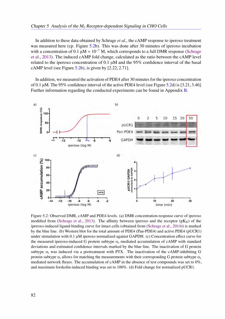
Chapter 5 Analysis of the M2 Receptor-dependent Signaling in CHO Cells
In addition to these data obtained by Schrage et al., the cAMP response to iperoxo treatmentwas measured here (cp. Figure 5.2b). This was done after 30 minutes of iperoxo incubationwith a concentration of 0.1 µM = 10−7 M, which corresponds to a full DMR response (Schrageet al., 2013). The induced cAMP fold change, calculated as the ratio between the cAMP levelrelated to the iperoxo concentration of 0.1 µM and the 95% confidence interval of the basalcAMP level (see Figure 5.2b), is given by [2.22, 2.71].
In addition, we measured the activation of PDE4 after 30 minutes for the iperoxo concentrationof 0.1 µM. The 95% confidence interval of the active PDE4 level (see Figure 5.2d) is [3.21, 3.46].Further information regarding the conducted experiments can be found in Appendix B.
Figure 5.2: Observed DMR, cAMP and PDE4 levels. (a) DMR concentration-response curve of iperoxomodified from (Schrage et al., 2013). The affinity between iperoxo and the receptor (pKD) of theiperoxo-induced ligand-binding curve for intact cells (obtained from (Schrage et al., 2014)) is markedby the blue line. (b) Western blot for the total amount of PDE4 (Pan-PDE4) and active PDE4 (pUCR1)under stimulation with 0.1 µM iperoxo normalized against GAPDH. (c) Concentration effect curve forthe measured iperoxo-induced G protein subtype αs mediated accumulation of cAMP with standarddeviations and estimated confidence intervals marked by the blue line. The inactivation of G proteinsubtype αi was induced via a pretreatment with PTX. The inactivation of the cAMP-inhibiting Gprotein subtype αi allows for matching the measurements with their corresponding G protein subtype αsmediated network fluxes. The accumulation of cAMP in the absence of test compounds was set to 0%,and maximum forskolin-induced binding was set to 100%. (d) Fold change for normalized pUCR1.
82
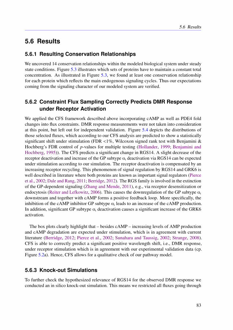
5.6 Results
5.6 Results
5.6.1 Resulting Conservation Relationships
We uncovered 14 conservation relationships within the modeled biological system under steadystate conditions. Figure 5.3 illustrates which sets of proteins have to maintain a constant totalconcentration. As illustrated in Figure 5.3, we found at least one conservation relationshipfor each protein which reflects the main endogenous signaling cycles. Thus our expectationscoming from the signaling character of our modeled system are verified.
5.6.2 Constraint Flux Sampling Correctly Predicts DMR Responseunder Receptor Activation
We applied the CFS framework described above incorporating cAMP as well as PDE4 foldchanges into flux constraints. DMR response measurements were not taken into considerationat this point, but left out for independent validation. Figure 5.4 depicts the distributions ofthose selected fluxes, which according to our CFS analysis are predicted to show a statisticallysignificant shift under stimulation (FDR <1%, Wilcoxon signed rank test with Benjamini &Hochberg’s FDR control of p-values for multiple testing (Hollander, 1999; Benjamini andHochberg, 1995)). The CFS predicts a significant change in RGS14. A slight decrease of thereceptor deactivation and increase of the GP subtype αi deactivation via RGS14 can be expectedunder stimulation according to our simulation. The receptor deactivation is compensated by anincreasing receptor recycling. This phenomenon of signal regulation by RGS14 and GRK6 iswell described in literature where both proteins are known as important signal regulators (Pierceet al., 2002; Dale and Rang, 2011; Berridge, 2012). The RGS family is involved in the extinctionof the GP-dependent signaling (Zhang and Mende, 2011), e.g., via receptor desensitization orendocytosis (Reiter and Lefkowitz, 2006). This causes the downregulation of the GP subtype αi
downstream and together with cAMP forms a positive feedback loop. More specifically, theinhibition of the cAMP inhibitor GP subtype αi leads to an increase of the cAMP production.In addition, significant GP subtype αi deactivation causes a significant increase of the GRK6activation.
The box plots clearly highlight that – besides cAMP – increasing levels of AMP productionand cAMP degradation are expected under stimulation, which is in agreement with currentliterature (Berridge, 2012; Pierce et al., 2002; Sunahara and Taussig, 2002; Strange, 2008).CFS is able to correctly predict a significant positive wavelength shift, i.e., DMR response,under receptor stimulation which is in agreement with our experimental validation data (cp.Figure 5.2a). Hence, CFS allows for a qualitative check of our pathway model.
5.6.3 Knock-out Simulations
To further check the hypothesized relevance of RGS14 for the observed DMR response weconducted an in silico knock-out simulation. This means we restricted all fluxes going through
83
Chapter 5 Analysis of the M2 Receptor-dependent Signaling in CHO Cells
Figure 5.3: Calculated conservation relationships: Each column represents one conservation relationshipand each row a protein. Red cells indicate proteins involved in a concentration relationship. The sum overall marked protein concentrations per column is constant. The inactive form of each protein is indicatedby the subscript "in".
84
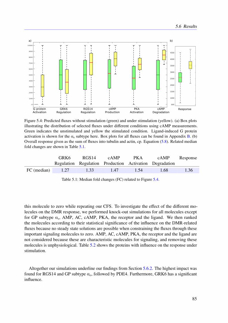
5.6 Results
Figure 5.4: Predicted fluxes without stimulation (green) and under stimulation (yellow). (a) Box plotsillustrating the distribution of selected fluxes under different conditions using cAMP measurements.Green indicates the unstimulated and yellow the stimulated condition. Ligand-induced G proteinactivation is shown for the αs subtype here. Box plots for all fluxes can be found in Appendix B. (b)Overall response given as the sum of fluxes into tubulin and actin, cp. Equation (5.8). Related medianfold changes are shown in Table 5.1.
GRK6 RGS14 cAMP PKA cAMP ResponseRegulation Regulation Production Activation Degradation
FC (median) 1.27 1.33 1.47 1.54 1.68 1.36
Table 5.1: Median fold changes (FC) related to Figure 5.4.
this molecule to zero while repeating our CFS. To investigate the effect of the different mo-lecules on the DMR response, we performed knock-out simulations for all molecules exceptfor GP subtype αs, AMP, AC, cAMP, PKA, the receptor and the ligand. We then rankedthe molecules according to their statistical significance of the influence on the DMR-relatedfluxes because no steady state solutions are possible when constraining the fluxes through theseimportant signaling molecules to zero. AMP, AC, cAMP, PKA, the receptor and the ligand arenot considered because these are characteristic molecules for signaling, and removing thesemolecules is unphysiological. Table 5.2 shows the proteins with influence on the response understimulation.
Altogether our simulations underline our findings from Section 5.6.2. The highest impact wasfound for RGS14 and GP subtype αo, followed by PDE4. Furthermore, GRK6 has a significantinfluence.
85
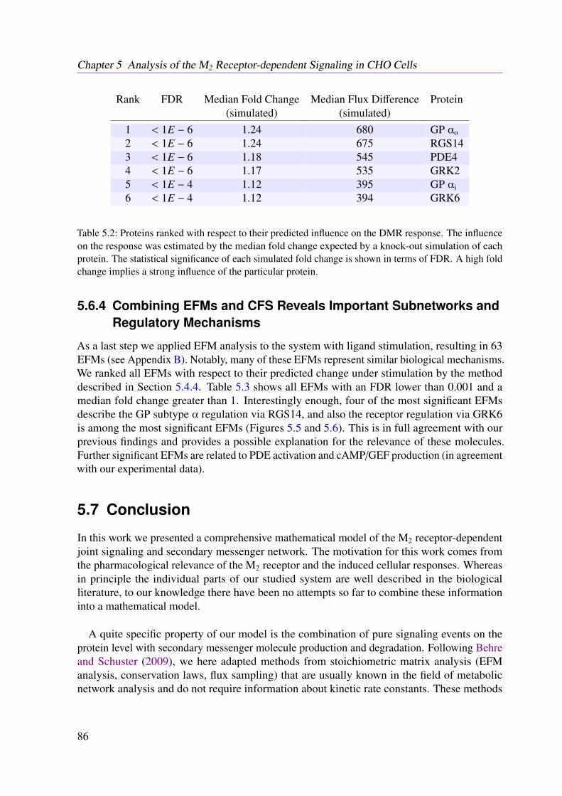
Chapter 5 Analysis of the M2 Receptor-dependent Signaling in CHO Cells
Rank FDR Median Fold Change Median Flux Difference Protein(simulated) (simulated)
1 < 1E − 6 1.24 680 GP αo
2 < 1E − 6 1.24 675 RGS143 < 1E − 6 1.18 545 PDE44 < 1E − 6 1.17 535 GRK25 < 1E − 4 1.12 395 GP αi
6 < 1E − 4 1.12 394 GRK6
Table 5.2: Proteins ranked with respect to their predicted influence on the DMR response. The influenceon the response was estimated by the median fold change expected by a knock-out simulation of eachprotein. The statistical significance of each simulated fold change is shown in terms of FDR. A high foldchange implies a strong influence of the particular protein.
5.6.4 Combining EFMs and CFS Reveals Important Subnetworks andRegulatory Mechanisms
As a last step we applied EFM analysis to the system with ligand stimulation, resulting in 63EFMs (see Appendix B). Notably, many of these EFMs represent similar biological mechanisms.We ranked all EFMs with respect to their predicted change under stimulation by the methoddescribed in Section 5.4.4. Table 5.3 shows all EFMs with an FDR lower than 0.001 and amedian fold change greater than 1. Interestingly enough, four of the most significant EFMsdescribe the GP subtype α regulation via RGS14, and also the receptor regulation via GRK6is among the most significant EFMs (Figures 5.5 and 5.6). This is in full agreement with ourprevious findings and provides a possible explanation for the relevance of these molecules.Further significant EFMs are related to PDE activation and cAMP/GEF production (in agreementwith our experimental data).
5.7 Conclusion
In this work we presented a comprehensive mathematical model of the M2 receptor-dependentjoint signaling and secondary messenger network. The motivation for this work comes fromthe pharmacological relevance of the M2 receptor and the induced cellular responses. Whereasin principle the individual parts of our studied system are well described in the biologicalliterature, to our knowledge there have been no attempts so far to combine these informationinto a mathematical model.
A quite specific property of our model is the combination of pure signaling events on theprotein level with secondary messenger molecule production and degradation. Following Behreand Schuster (2009), we here adapted methods from stoichiometric matrix analysis (EFManalysis, conservation laws, flux sampling) that are usually known in the field of metabolicnetwork analysis and do not require information about kinetic rate constants. These methods
86
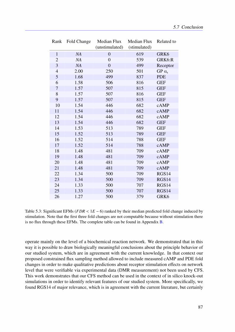
5.7 Conclusion
Rank Fold Change Median Flux Median Flux Related to(unstimulated) (stimulated)
1 NA 0 619 GRK62 NA 0 539 GRK6:R3 NA 0 499 Receptor4 2.00 250 501 GP αs
5 1.68 499 837 PDE6 1.58 506 816 GEF7 1.57 507 815 GEF8 1.57 507 816 GEF9 1.57 507 815 GEF10 1.54 446 682 cAMP11 1.54 446 682 cAMP12 1.54 446 682 cAMP13 1.54 446 682 GEF14 1.53 513 789 GEF15 1.52 513 789 GEF16 1.52 514 788 GEF17 1.52 514 788 cAMP18 1.48 481 709 cAMP19 1.48 481 709 cAMP20 1.48 481 709 cAMP21 1.48 481 709 cAMP22 1.34 500 709 RGS1423 1.34 500 709 RGS1424 1.33 500 707 RGS1425 1.33 500 707 RGS1426 1.27 500 379 GRK6
Table 5.3: Significant EFMs (FDR < 1E − 6) ranked by their median predicted fold change induced bystimulation. Note that the first three fold changes are not computable because without stimulation thereis no flux through these EFMs. The complete table can be found in Appendix B.
operate mainly on the level of a biochemical reaction network. We demonstrated that in thisway it is possible to draw biologically meaningful conclusions about the principle behavior ofour studied system, which are in agreement with the current knowledge. In that context ourproposed constrained flux sampling method allowed to include measured cAMP and PDE foldchanges in order to make qualitative predictions about receptor stimulation effects on networklevel that were verifiable via experimental data (DMR measurement) not been used by CFS.This work demonstrates that our CFS method can be used in the context of in silico knock-outsimulations in order to identify relevant features of our studied system. More specifically, wefound RGS14 of major relevance, which is in agreement with the current literature, but certainly
87
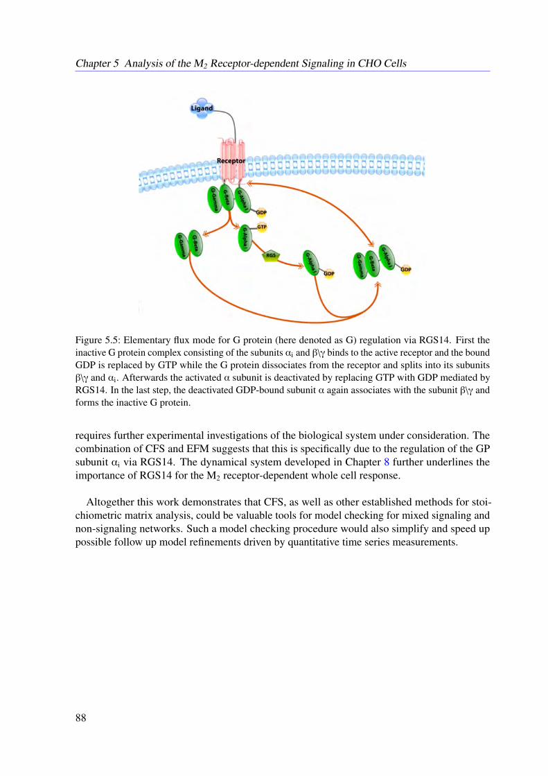
Chapter 5 Analysis of the M2 Receptor-dependent Signaling in CHO Cells
Figure 5.5: Elementary flux mode for G protein (here denoted as G) regulation via RGS14. First theinactive G protein complex consisting of the subunits αi and β\γ binds to the active receptor and the boundGDP is replaced by GTP while the G protein dissociates from the receptor and splits into its subunitsβ\γ and αi. Afterwards the activated α subunit is deactivated by replacing GTP with GDP mediated byRGS14. In the last step, the deactivated GDP-bound subunit α again associates with the subunit β\γ andforms the inactive G protein.
requires further experimental investigations of the biological system under consideration. Thecombination of CFS and EFM suggests that this is specifically due to the regulation of the GPsubunit αi via RGS14. The dynamical system developed in Chapter 8 further underlines theimportance of RGS14 for the M2 receptor-dependent whole cell response.
Altogether this work demonstrates that CFS, as well as other established methods for stoi-chiometric matrix analysis, could be valuable tools for model checking for mixed signaling andnon-signaling networks. Such a model checking procedure would also simplify and speed uppossible follow up model refinements driven by quantitative time series measurements.
88
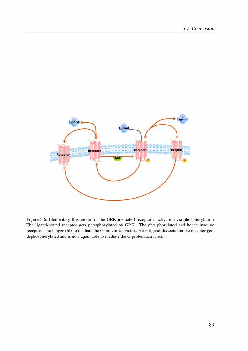
5.7 Conclusion
Figure 5.6: Elementary flux mode for the GRK-mediated receptor inactivation via phosphorylation.The ligand-bound receptor gets phosphorylated by GRK. The phosphorylated and hence inactivereceptor is no longer able to mediate the G protein activation. After ligand-dissociation the receptor getsdephosphorylated and is now again able to mediate the G protein activation.
89

CHAPTER 6
The Dynamic Elastic-Net
Even though general ability of the derived M2 receptor-dependent signaling pathway to reflectthe observed properties has been demonstrated in Chapter 5, it is not fully ensured that alldriving mechanisms are included in a refined time-resolved system. As discussed in Chapter 2,dynamical systems are more complex than static systems and thus a method to detect and correcterroneous models is highly desirable. The DEN is a deterministic approach based on OCT toaddress this issue, and a first attempt to towards automatic model correction (Engelhardt et al.,2016). This is important in order to refine the developed model for the M2 receptor-dependentsignaling in CHO cells in a reliable manner. This work has been published in a peer-reviewedjournal (cp. Appendix F).
6.1 Introduction
Ideally, a good model covers the essential features of the system whilst still being simple enoughfor interpretation and mechanistic understanding. Developing a good model is usually a labor-intensive manual effort. As discussed in Chapter 2, in biology the system to be modeled is oftenonly partially known and the distinction of relevant and irrelevant features and variables can bedifficult (Swameye et al., 2003; Sunnåker et al., 2013; Kahm et al., 2012). But, even if the majorcomponents of a biological system are well known, the sheer complexity of the system mightprevent the development of an accurate mathematical model, either because the quantitative datanecessary for modeling is not available or because the model is itself too complex to be useful.Thus, researchers in systems biology are frequently confronted with a paradoxical situation: Amodel is needed to better understand the system and to design informative experiments, butthe system is too large and complex for mathematical modeling given the limited amount ofknowledge, data and time.
One strategy, similar to bottom-up approaches (see Chapter 2), for modeling is to start witha simple model, which incorporates the most interesting variables and interactions as well asthe known input stimuli to the system (Figure 6.1a). For example, to model a CRN, we mightincorporate the concentrations of a few interesting proteins as dynamic state variables and
91
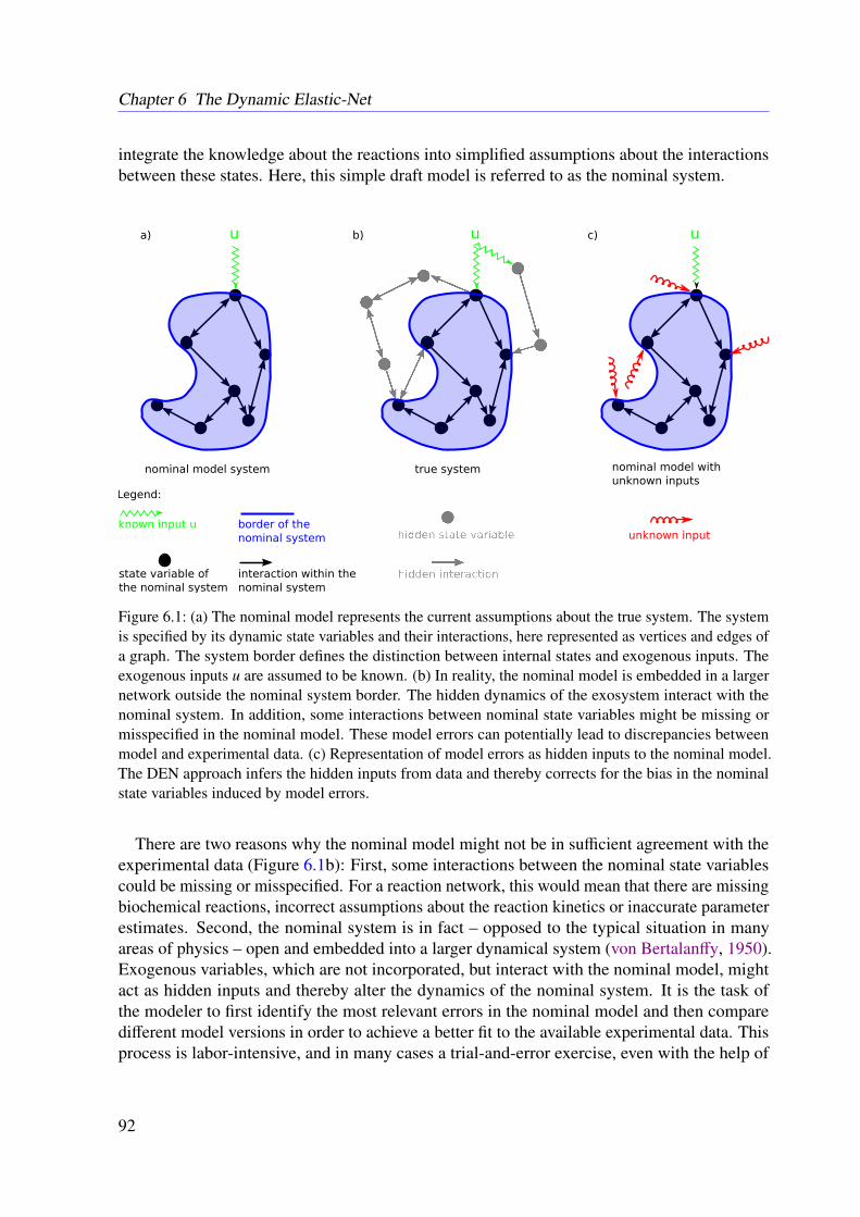
Chapter 6 The Dynamic Elastic-Net
integrate the knowledge about the reactions into simplified assumptions about the interactionsbetween these states. Here, this simple draft model is referred to as the nominal system.
Figure 6.1: (a) The nominal model represents the current assumptions about the true system. The systemis specified by its dynamic state variables and their interactions, here represented as vertices and edges ofa graph. The system border defines the distinction between internal states and exogenous inputs. Theexogenous inputs u are assumed to be known. (b) In reality, the nominal model is embedded in a largernetwork outside the nominal system border. The hidden dynamics of the exosystem interact with thenominal system. In addition, some interactions between nominal state variables might be missing ormisspecified in the nominal model. These model errors can potentially lead to discrepancies betweenmodel and experimental data. (c) Representation of model errors as hidden inputs to the nominal model.The DEN approach infers the hidden inputs from data and thereby corrects for the bias in the nominalstate variables induced by model errors.
There are two reasons why the nominal model might not be in sufficient agreement with theexperimental data (Figure 6.1b): First, some interactions between the nominal state variablescould be missing or misspecified. For a reaction network, this would mean that there are missingbiochemical reactions, incorrect assumptions about the reaction kinetics or inaccurate parameterestimates. Second, the nominal system is in fact – opposed to the typical situation in manyareas of physics – open and embedded into a larger dynamical system (von Bertalanffy, 1950).Exogenous variables, which are not incorporated, but interact with the nominal model, mightact as hidden inputs and thereby alter the dynamics of the nominal system. It is the task ofthe modeler to first identify the most relevant errors in the nominal model and then comparedifferent model versions in order to achieve a better fit to the available experimental data. Thisprocess is labor-intensive, and in many cases a trial-and-error exercise, even with the help of
92
6.2 Methods
innovative software and algorithms assisting modeling and model comparison (Sunnåker et al.,2013; Rodriguez-Fernandez et al., 2013; Babtie et al., 2014).
We introduced a computational method for ODEs, which automatically estimates the model er-ror from the data. As discussed, ODEs are frequently used in different areas of biology includingbiochemical reaction networks, pharmacokinetics, pharmacodynamics and population dynamics.
The basic idea of the method is to represent errors in the nominal model as hidden inputs tothe state variables (Figure 6.1c) and to estimate these inputs from the experimental data (Mookand Junkins, 1988; Kolodziej and Mook, 2005; Kahm et al., 2012). Since this is an inverseproblem with potentially many different solutions, we proposed a regularized method whichprovides parsimonious error estimates. Due to its formal similarity to the elastic-net regressionapproach (Zou and Hastie, 2005), we termed our algorithm the dynamic elastic-net (DEN).
The dynamic elastic-net provides important information about the variables in the nominalmodel, which are targeted by model errors. In addition, the DEN removes the bias in the nominalstate variables induced by the model error. This is important for the frequent situation wherenot all nominal states (e.g. protein concentrations) can directly be measured. The utility of theDEN is demonstrated here for two established models of the erythropoietin receptor (EpoR)and of the photomorphogenic ultraviolet B (UV-B) signaling network (Swameye et al., 2003;Ouyang et al., 2014). Further examples, including a model for G protein signaling and modelsfor several network motifs as well as some technical details, are given in Appendix C.
6.2 Methods
6.2.1 The Nominal Model
We assume that a nominal ODE model
˙x(t) = f (x(t),u(t)) (6.1a)y(t) = h(x(t)) (6.1b)x(0) = x0 (6.1c)
has been proposed to describe the dynamics of the system under consideration. The state vectorx(t) = (x1(t), . . . , xN(t))T contains the N dynamic variables xn (t), and ˙x(t) is the derivativewith respect to time t. The initial value of the state vector is x0. For a biochemical reactionnetwork, xn is often the concentration or abundance of the n-th species. The function u(t) =
(u1(t), . . . , uP(t))T represents a known external input to the system. The dynamics of the statevariables is determined by the function f = ( f1, . . . , fN)T and encodes the model assumptionsmade in the nominal model. This can be represented as a graph, where each node correspondsto one variable and a directed edge from n to j indicates that the time-derivative of xn dependson x j (Figure 6.1a) (Liu et al., 2013). A green zigzag arrow illustrates that ˙xn is directlyinfluenced by a known input. Typically, not all state variables x can directly be measured. The
93
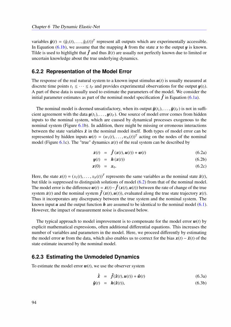
Chapter 6 The Dynamic Elastic-Net
variables y(t) = (y1(t), . . . , yI(t))T represent all outputs which are experimentally accessible.In Equation (6.1b), we assume that the mapping h from the state x to the output y is known.Tilde is used to highlight that f and thus x(t) are usually not perfectly known due to limited oruncertain knowledge about the true underlying dynamics.
6.2.2 Representation of the Model Error
The response of the real natural system to a known input stimulus u(t) is usually measured atdiscrete time points t1 ≤ · · · ≤ tF and provides experimental observations for the output y(tl).A part of these data is usually used to estimate the parameters of the model. We consider theinitial parameter estimates as part of the nominal model specification f in Equation (6.1a).
The nominal model is deemed unsatisfactory, when its output y(t1), . . . , y(tF) is not in suffi-cient agreement with the data y(t1), . . . , y(tF). One source of model error comes from hiddeninputs to the nominal system, which are caused by dynamical processes exogenous to thenominal system (Figure 6.1b). In addition, there might be missing or erroneous interactionsbetween the state variables x in the nominal model itself. Both types of model error can berepresented by hidden inputs w(t) = (w1(t), . . . , wN(t))T acting on the nodes of the nominalmodel (Figure 6.1c). The "true" dynamics x(t) of the real system can be described by
x(t) = f (x(t),u(t)) + w(t) (6.2a)y(t) = h (x(t)) (6.2b)x(0) = x0. (6.2c)
Here, the state x(t) = (x1(t), . . . , xN(t))T represents the same variables as the nominal state x(t),but tilde is suppressed to distinguish solutions of model (6.2) from that of the nominal model.The model error is the difference w(t) = x(t)− f (x(t),u(t)) between the rate of change of the truesystem x(t) and the nominal system f (x(t),u(t)), evaluated along the true state trajectory x(t).Thus it incorporates any discrepancy between the true system and the nominal system. Theknown input u and the output function h are assumed to be identical to the nominal model (6.1).However, the impact of measurement noise is discussed below.
The typical approach to model improvement is to compensate for the model error w(t) byexplicit mathematical expressions, often additional differential equations. This increases thenumber of variables and parameters in the model. Here, we proceed differently by estimatingthe model error w from the data, which also enables us to correct for the bias x(t) − x(t) of thestate estimate incurred by the nominal model.
6.2.3 Estimating the Unmodeled Dynamics
To estimate the model error w(t), we use the observer system
˙x = f (x(t),u(t)) + w(t) (6.3a)y(t) = h(x(t)), (6.3b)
94
6.2 Methods
which is a copy of Equations (6.2a) and (6.2b). The hat marks estimates of the state x(t), of theoutput y(t) and of the model error w(t). The latter is obtained by minimizing the error functional
J (x (t) , w (t)) =
F∑l=1
‖y(tl) − y(tl)‖2Q(tl) + R[w] . (6.4)
The first term in Equation (6.4) is the weighted mean square error between the measured outputsy(tl) and the outputs y(tl) of the observer system in Equations (6.3a) and (6.3b). The weightedsquare norm
‖y(tl) − y(tl)‖2Q(tl) = (y(tl) − y(tl))T Q(tl) (y(tl) − y(tl)) (6.5)
contains the symmetric weighting matrix Q(tl), which is often chosen to be diagonal and canbe used to transform outputs of very different magnitude to a common scale or to incorporateprecision estimates of the measurements at the different time points tl. The regularization term
R[w] = α1‖w‖1 +α2
2‖w‖22 (6.6a)
‖w‖1 =
∫ tF
t1
N∑n=1
|wn(t)|dt (6.6b)
‖w‖22 =
∫ tF
t1
N∑n=1
|wn(t)|2 dt. (6.6c)
is necessary to avoid overfitting of the data y(tl) by overly complex estimates w(t). The nonneg-ative parameters α1 and α2 determine the relative contributions of the L1 norm in Equation (6.6b)and of the L2 norm in Equation (6.6c). Minimization of Equation (6.4) under the constraintsin Equations (6.3a) and (6.3b) is an OCP, which needs to be solved numerically (see Ap-pendix C) (Pontryagin et al., 1986; Fleming and Rishel, 1975; Gerdts, 2012). As detailedin Section 4.2, in contrast to common OCPs, the controls are split into known and unknownvariables.
The combined L1 - L2 regularization in Equation (6.6a) is reminiscent of the elastic-netpenalty used in regression (Zou and Hastie, 2005). Therefore, we termed our approach thedynamic elastic-net. In analogy to regression, the L1 term causes some components wn(t) ofthe estimated model error to shrink to zero (cp. Appendix C). The amount of shrinkage isdetermined by α1, which can be chosen to suppress small error signals or noise distributed overmany components of the estimate w. The resulting sparse estimate is useful because it providesinformation about the states of the system which are targeted by systematic model errors, asrepresented by hidden inputs.
In contrast to regression, a pure L1 or least absolute shrinkage and selection operator (LASSO)type regularization is not useful in the dynamic setting because the solution for α2 = 0 can resultin unbounded estimates of w(t) (Tibshirani, 2011). Even when additional constraints on w(t)are imposed, the resulting solution is not smooth and either zero or at the boundaries of theconstraints (Vossen and Maurer, 2006). These insights about the OCP can be obtained from
95
Chapter 6 The Dynamic Elastic-Net
Pontryagin’s minimum principle, as detailed in Appendix C together with some strategies tochose suitable regularization parameters α1 and α2 (Pontryagin et al., 1986; Fleming and Rishel,1975). In addition to sparse but smooth estimates of the model error, the DEN automaticallyprovides a state estimate x(t). Often this is very interesting information, especially when not allstate variables are experimentally accessible.
The OCP in Equations (6.4) and (6.3) for w(t) requires the specification of an initial con-dition x(0) = x0, which is often not known or uncertain. Alternatively and according toSection 4.2.4, one can add the additional constraint
‖y(t1) − y(t1)‖Q(t1) ≤ ∆t1 (6.7)
to the OCP, where ∆t1 is a preset tolerance given for the fit of y(t1) to y(t1) at time t1. Similarly,a tolerance ∆1 can be prescribed to the fit at the last data point through
‖y(tF) − y(tF)‖Q(tF ) ≤ ∆tF . (6.8)
The tolerance parameters ∆t1 and ∆tF of these optional constraints can often be obtained fromthe error bars of the measurements.
6.3 Results
6.3.1 JAK-STAT Signaling
To illustrate the DEN estimator for a small and comprehensible model we used establishedexperimental data for the JAK-STAT signal transduction pathway (Swameye et al., 2003). Thefour state variables of the system represent the unphosphorylated cytoplasmic signal transducerand activator of transcription 5 (STAT5) (x1), the phosphorylated monomeric STAT5 (x2), thephosphorylated dimeric STAT5 (x3) and the nuclear dimeric STAT5 (x4). The nominal model
˙x1˙x2˙x3˙x4
=
−θ1 x1u
θ1 x1u − 2θ2 x22
θ2 x22 − θ3 x3
θ3 x3
︸ ︷︷ ︸f (x,u)
(6.9a)
(y1
y2
)=
(θ4(x2 + 2x3)
θ5(x1 + x2 + 2x3)
)︸ ︷︷ ︸
h(x)
(6.9b)
describes the phosphorylation of cytoplasmic STAT5 upon activation of the EpoR (the knowninput u), the dimerization of phosphorylated STAT5 and the export to the nucleus (Fig-ure 6.2) (Swameye et al., 2003). Time course data for the amount of cytoplasmic phos-
96
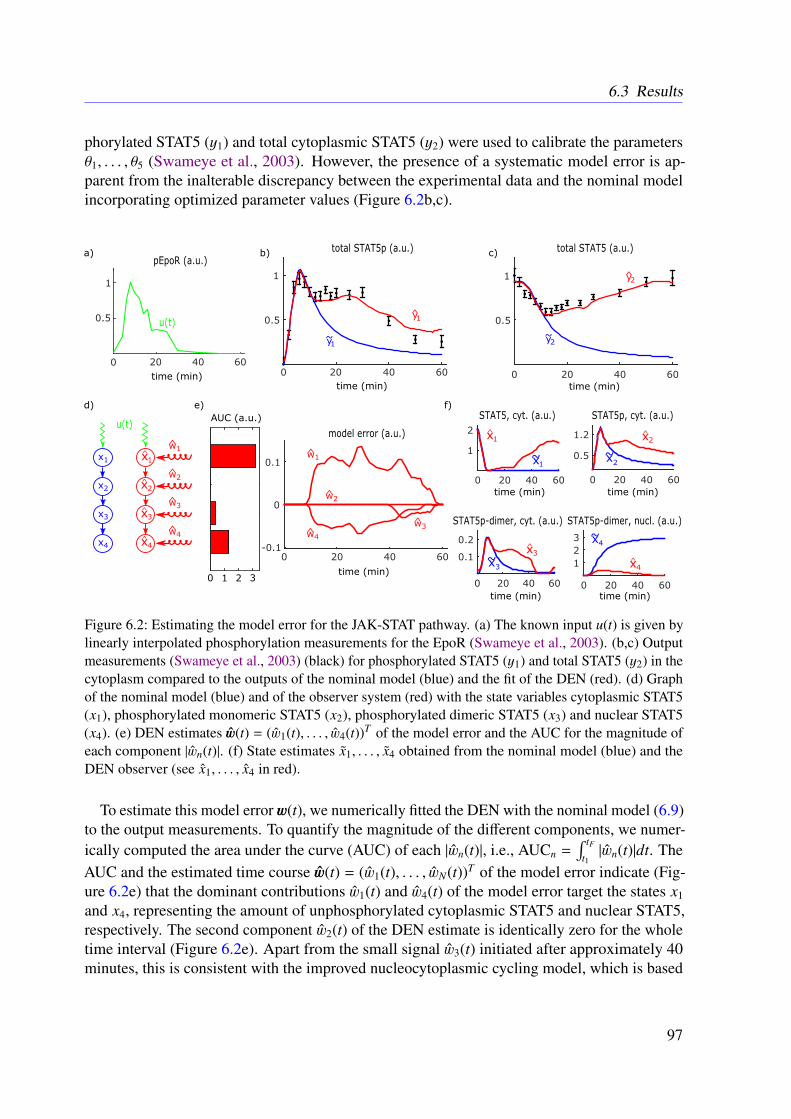
6.3 Results
phorylated STAT5 (y1) and total cytoplasmic STAT5 (y2) were used to calibrate the parametersθ1, . . . , θ5 (Swameye et al., 2003). However, the presence of a systematic model error is ap-parent from the inalterable discrepancy between the experimental data and the nominal modelincorporating optimized parameter values (Figure 6.2b,c).
Figure 6.2: Estimating the model error for the JAK-STAT pathway. (a) The known input u(t) is given bylinearly interpolated phosphorylation measurements for the EpoR (Swameye et al., 2003). (b,c) Outputmeasurements (Swameye et al., 2003) (black) for phosphorylated STAT5 (y1) and total STAT5 (y2) in thecytoplasm compared to the outputs of the nominal model (blue) and the fit of the DEN (red). (d) Graphof the nominal model (blue) and of the observer system (red) with the state variables cytoplasmic STAT5(x1), phosphorylated monomeric STAT5 (x2), phosphorylated dimeric STAT5 (x3) and nuclear STAT5(x4). (e) DEN estimates w(t) = (w1(t), . . . , w4(t))T of the model error and the AUC for the magnitude ofeach component |wn(t)|. (f) State estimates x1, . . . , x4 obtained from the nominal model (blue) and theDEN observer (see x1, . . . , x4 in red).
To estimate this model error w(t), we numerically fitted the DEN with the nominal model (6.9)to the output measurements. To quantify the magnitude of the different components, we numer-ically computed the area under the curve (AUC) of each |wn(t)|, i.e., AUCn =
∫ tFt1|wn(t)|dt. The
AUC and the estimated time course w(t) = (w1(t), . . . , wN(t))T of the model error indicate (Fig-ure 6.2e) that the dominant contributions w1(t) and w4(t) of the model error target the states x1
and x4, representing the amount of unphosphorylated cytoplasmic STAT5 and nuclear STAT5,respectively. The second component w2(t) of the DEN estimate is identically zero for the wholetime interval (Figure 6.2e). Apart from the small signal w3(t) initiated after approximately 40minutes, this is consistent with the improved nucleocytoplasmic cycling model, which is based
97
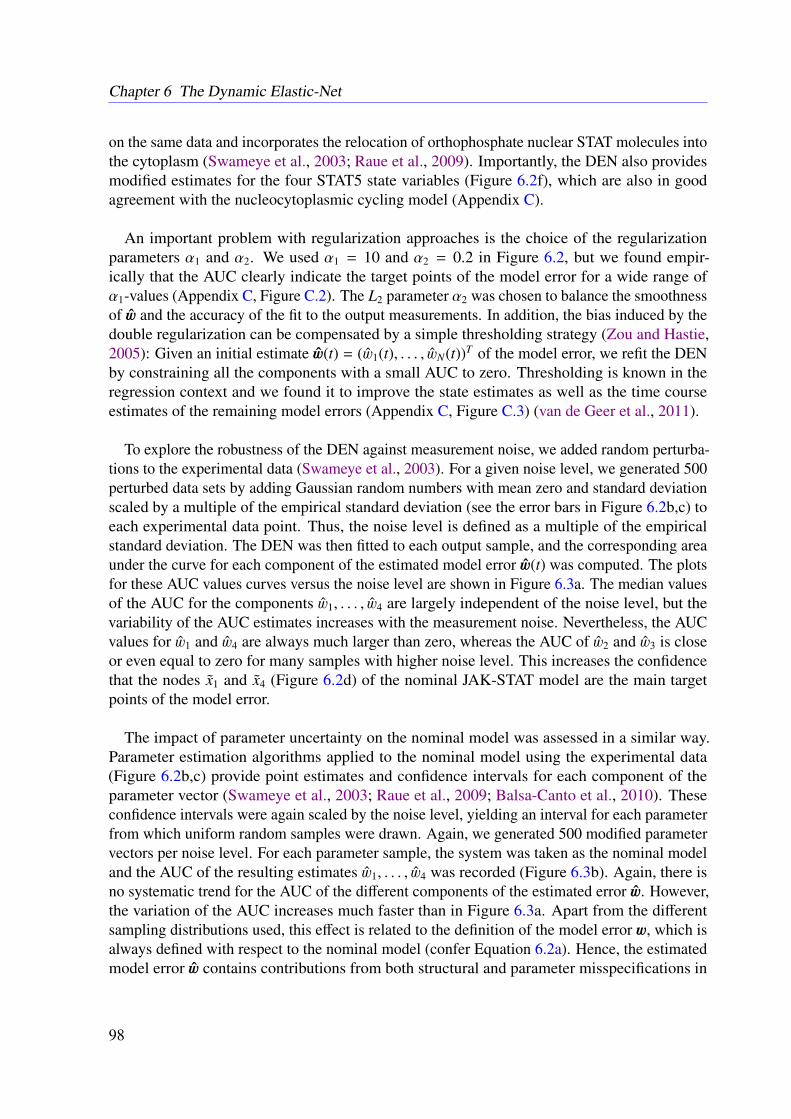
Chapter 6 The Dynamic Elastic-Net
on the same data and incorporates the relocation of orthophosphate nuclear STAT molecules intothe cytoplasm (Swameye et al., 2003; Raue et al., 2009). Importantly, the DEN also providesmodified estimates for the four STAT5 state variables (Figure 6.2f), which are also in goodagreement with the nucleocytoplasmic cycling model (Appendix C).
An important problem with regularization approaches is the choice of the regularizationparameters α1 and α2. We used α1 = 10 and α2 = 0.2 in Figure 6.2, but we found empir-ically that the AUC clearly indicate the target points of the model error for a wide range ofα1-values (Appendix C, Figure C.2). The L2 parameter α2 was chosen to balance the smoothnessof w and the accuracy of the fit to the output measurements. In addition, the bias induced by thedouble regularization can be compensated by a simple thresholding strategy (Zou and Hastie,2005): Given an initial estimate w(t) = (w1(t), . . . , wN(t))T of the model error, we refit the DENby constraining all the components with a small AUC to zero. Thresholding is known in theregression context and we found it to improve the state estimates as well as the time courseestimates of the remaining model errors (Appendix C, Figure C.3) (van de Geer et al., 2011).
To explore the robustness of the DEN against measurement noise, we added random perturba-tions to the experimental data (Swameye et al., 2003). For a given noise level, we generated 500perturbed data sets by adding Gaussian random numbers with mean zero and standard deviationscaled by a multiple of the empirical standard deviation (see the error bars in Figure 6.2b,c) toeach experimental data point. Thus, the noise level is defined as a multiple of the empiricalstandard deviation. The DEN was then fitted to each output sample, and the corresponding areaunder the curve for each component of the estimated model error w(t) was computed. The plotsfor these AUC values curves versus the noise level are shown in Figure 6.3a. The median valuesof the AUC for the components w1, . . . , w4 are largely independent of the noise level, but thevariability of the AUC estimates increases with the measurement noise. Nevertheless, the AUCvalues for w1 and w4 are always much larger than zero, whereas the AUC of w2 and w3 is closeor even equal to zero for many samples with higher noise level. This increases the confidencethat the nodes x1 and x4 (Figure 6.2d) of the nominal JAK-STAT model are the main targetpoints of the model error.
The impact of parameter uncertainty on the nominal model was assessed in a similar way.Parameter estimation algorithms applied to the nominal model using the experimental data(Figure 6.2b,c) provide point estimates and confidence intervals for each component of theparameter vector (Swameye et al., 2003; Raue et al., 2009; Balsa-Canto et al., 2010). Theseconfidence intervals were again scaled by the noise level, yielding an interval for each parameterfrom which uniform random samples were drawn. Again, we generated 500 modified parametervectors per noise level. For each parameter sample, the system was taken as the nominal modeland the AUC of the resulting estimates w1, . . . , w4 was recorded (Figure 6.3b). Again, there isno systematic trend for the AUC of the different components of the estimated error w. However,the variation of the AUC increases much faster than in Figure 6.3a. Apart from the differentsampling distributions used, this effect is related to the definition of the model error w, which isalways defined with respect to the nominal model (confer Equation 6.2a). Hence, the estimatedmodel error w contains contributions from both structural and parameter misspecifications in
98
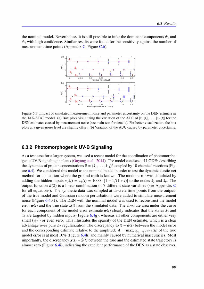
6.3 Results
the nominal model. Nevertheless, it is still possible to infer the dominant components w1 andw4 with high confidence. Similar results were found for the sensitivity against the number ofmeasurement time points (Appendix C, Figure C.6).
Figure 6.3: Impact of simulated measurement noise and parameter uncertainty on the DEN estimate inthe JAK-STAT model. (a) Box plots visualizing the variation of the AUC of |w1(t)|, . . . , |w4(t)| for theDEN estimates caused by measurement noise (see main text for details). For better visualization, the boxplots at a given noise level are slightly offset. (b) Variation of the AUC caused by parameter uncertainty.
6.3.2 Photomorphogenic UV-B Signaling
As a test case for a larger system, we used a recent model for the coordination of photomorpho-genic UV-B signaling in plants (Ouyang et al., 2014). The model consists of 11 ODEs describingthe dynamics of protein concentrations x = (x1, . . . , x11)T coupled by 10 chemical reactions (Fig-ure 6.4). We considered this model as the nominal model in order to test the dynamic elastic-netmethod for a situation where the ground truth is known. The model error was simulated byadding the hidden inputs w3(t) = w9(t) = 1000 · [1 − 1/(1 + t)] to the nodes x3 and x9. Theoutput function h(x) is a linear combination of 7 different state variables (see Appendix Cfor all equations). The synthetic data was sampled at discrete time points from the outputsof the true model and Gaussian random perturbations were added to simulate measurementnoise (Figure 6.4b-f). The DEN with the nominal model was used to reconstruct the modelerror w(t) and the true state x(t) from the simulated data. The absolute area under the curvefor each component of the model error estimate w(t) clearly indicates that the states x3 andx9 are targeted by hidden inputs (Figure 6.4g), whereas all other components are either verysmall (|w6|) or even zero. This illustrates the sparsity of the DEN estimate, which is a clearadvantage over pure L2 regularization The discrepancy w(t) − w(t) between the model errorand the corresponding estimate relative to the amplitude A = maxtl∈(t1,...,tF ) w3,9(tl) of the truemodel error is at most 10% (Figure 6.4h) and mainly caused by numerical inaccuracies. Mostimportantly, the discrepancy x(t) − x(t) between the true and the estimated state trajectory isalmost zero (Figure 6.4i), indicating the excellent performance of the DEN as a state observer.
99
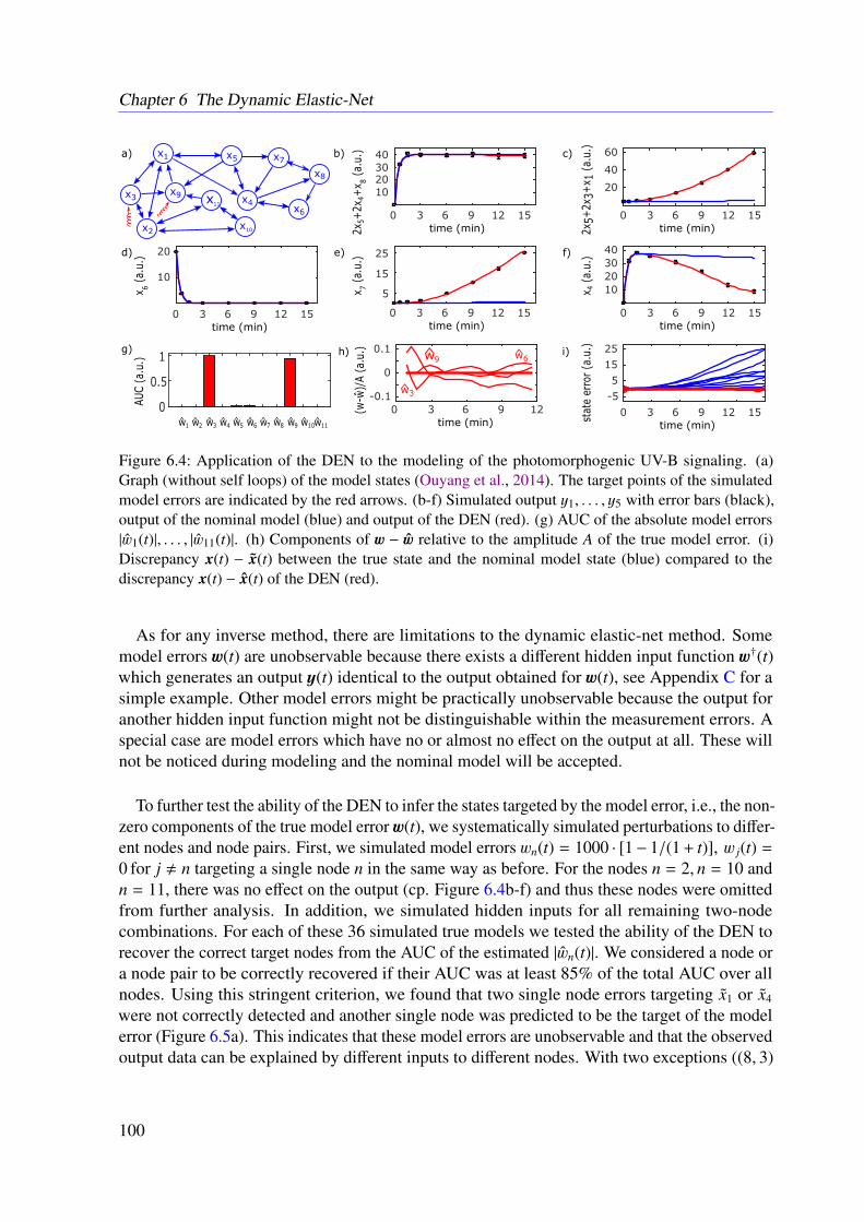
Chapter 6 The Dynamic Elastic-Net
Figure 6.4: Application of the DEN to the modeling of the photomorphogenic UV-B signaling. (a)Graph (without self loops) of the model states (Ouyang et al., 2014). The target points of the simulatedmodel errors are indicated by the red arrows. (b-f) Simulated output y1, . . . , y5 with error bars (black),output of the nominal model (blue) and output of the DEN (red). (g) AUC of the absolute model errors|w1(t)|, . . . , |w11(t)|. (h) Components of w − w relative to the amplitude A of the true model error. (i)Discrepancy x(t) − x(t) between the true state and the nominal model state (blue) compared to thediscrepancy x(t) − x(t) of the DEN (red).
As for any inverse method, there are limitations to the dynamic elastic-net method. Somemodel errors w(t) are unobservable because there exists a different hidden input function w†(t)which generates an output y(t) identical to the output obtained for w(t), see Appendix C for asimple example. Other model errors might be practically unobservable because the output foranother hidden input function might not be distinguishable within the measurement errors. Aspecial case are model errors which have no or almost no effect on the output at all. These willnot be noticed during modeling and the nominal model will be accepted.
To further test the ability of the DEN to infer the states targeted by the model error, i.e., the non-zero components of the true model error w(t), we systematically simulated perturbations to differ-ent nodes and node pairs. First, we simulated model errors wn(t) = 1000 · [1− 1/(1 + t)], w j(t) =
0 for j , n targeting a single node n in the same way as before. For the nodes n = 2, n = 10 andn = 11, there was no effect on the output (cp. Figure 6.4b-f) and thus these nodes were omittedfrom further analysis. In addition, we simulated hidden inputs for all remaining two-nodecombinations. For each of these 36 simulated true models we tested the ability of the DEN torecover the correct target nodes from the AUC of the estimated |wn(t)|. We considered a node ora node pair to be correctly recovered if their AUC was at least 85% of the total AUC over allnodes. Using this stringent criterion, we found that two single node errors targeting x1 or x4
were not correctly detected and another single node was predicted to be the target of the modelerror (Figure 6.5a). This indicates that these model errors are unobservable and that the observedoutput data can be explained by different inputs to different nodes. With two exceptions ((8, 3)
100
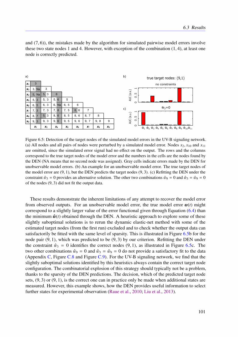
6.3 Results
and (7, 6)), the mistakes made by the algorithm for simulated pairwise model errors involvethese two state nodes 1 and 4. However, with exception of the combination (1, 4), at least onenode is correctly predicted.
Figure 6.5: Detection of the target nodes of the simulated model errors in the UV-B signaling network.(a) All nodes and all pairs of nodes were perturbed by a simulated model error. Nodes x2, x10 and x11are omitted, since the simulated error signal had no effect on the output. The rows and the columnscorrespond to the true target nodes of the model error and the numbers in the cells are the nodes found bythe DEN (NA means that no second node was assigned). Gray cells indicate errors made by the DEN forunobservable model errors. (b) An example for an unobservable model error. The true target nodes ofthe model error are (9, 1), but the DEN predicts the target nodes (9, 3). (c) Refitting the DEN under theconstraint w3 = 0 provides an alternative solution. The other two combinations w9 = 0 and w3 = w9 = 0of the nodes (9, 3) did not fit the output data.
These results demonstrate the inherent limitations of any attempt to recover the model errorfrom observed outputs. For an unobservable model error, the true model error w(t) mightcorrespond to a slightly larger value of the error functional given through Equation (6.4) thanthe minimum w(t) obtained through the DEN. A heuristic approach to explore some of theseslightly suboptimal solutions is to rerun the dynamic elastic-net method with some of theestimated target nodes (from the first run) excluded and to check whether the output data cansatisfactorily be fitted with the same level of sparsity. This is illustrated in Figure 6.5b for thenode pair (9, 1), which was predicted to be (9, 3) by our criterion. Refitting the DEN underthe constraint w3 = 0 identifies the correct nodes (9, 1), as illustrated in Figure 6.5c. Thetwo other combinations w9 = 0 and w3 = w9 = 0 do not provide a satisfactory fit to the data(Appendix C, Figure C.8 and Figure C.9). For the UV-B signaling network, we find that theslightly suboptimal solutions identified by this heuristics always contain the correct target nodeconfiguration. The combinatorial explosion of this strategy should typically not be a problem,thanks to the sparsity of the DEN predictions. The decision, which of the predicted target nodesets, (9, 3) or (9, 1), is the correct one can in practice only be made when additional states aremeasured. However, this example shows, how the DEN provides useful information to selectfurther states for experimental observation (Raue et al., 2010; Liu et al., 2013).
101
Chapter 6 The Dynamic Elastic-Net
6.4 Conclusion
Efficient computational methods to learn from incomplete model drafts and to direct modelimprovement are urgently needed. The proposed dynamic elastic-net approach provides sug-gestions for the location of these model errors in the network and estimates their dynamic timecourses from measured output data. The sparsity of the proposed target points for the model errorpromotes model improvements in the most parsimonious way. Even for an incomplete nominalmodel the algorithm can provide estimates for the system states which are not experimentallyaccessible. This is in stark contrast to many other state estimators including the Kalman filterfor linear systems and its various extensions for nonlinear systems, which usually require acorrectly specified model (Kalman, 1960; Julier and Uhlmann, 1997; Crassidis and Junkins,2011).
Not all model errors can uniquely be determined from the output. For such unobservablemodel errors, our strategy to explore alternative, slightly suboptimal solutions might indicatealternative explanations for observed discrepancies between the data and the nominal model.In addition, this approach can also be informative for selecting additional nodes required forobserving the state from output measurements (Raue et al., 2010; Liu et al., 2013). Furtherresearch is needed to establish the relationship between the network topology and the observab-ility of a model error.
Model errors arising in kinetic reaction systems can originate from erroneous rate equations orlacking reactions. The DEN can detect both types of errors as hidden inputs to the correspondingnodes of the network, but it can not discriminate between these errors. However, knowingthe nodes affected by a model error might already be very informative for systematic modelimprovement. This work raises fundamental questions regarding successful modeling strategies.The approach to manually include more and more details into the model to compensate forthe initial model errors is often not practical or at least very time consuming. The dynamicelastic-net hence paves the way towards a more principled and systematic way, in which modelscould be adapted based on experimental data.
102
CHAPTER 7
The Bayesian Dynamic Elastic-Net
In Chapter 6 I proposed the DEN as a promising approach to make ODE-based biological models,e.g., the developed model of the M2 receptor-induced signaling, complete and consistent. TheBDEN, as a Bayesian extension of the DEN, incorporates measurement uncertainties and allowsfor automatic correction of the nominal model by adding or removing single interactions. Thisresults in more robust and reliable estimations of the involved hidden influences. This work isunder review in a peer-reviewed journal (cp. Appendix F).
7.1 Introduction
The proposed DEN aims for estimating the dynamics of exogenous hidden influences, i.e.,exogenous hidden inputs, and misspecified molecular interactions, i.e., endogenous hiddeninputs to the nominal model via a penalized estimation procedure resembling elastic-net re-gression (Zou and Hastie, 2005; Engelhardt et al., 2016). This is strongly required since inmost situations researchers have partial knowledge and preliminary hypotheses about theirsystem, which needs to be integrated into a restricted but still predictive and experimentallyvalidatable model (Swameye et al., 2003). Even, if the biological system is partially known andthe data is given for almost all molecular species it is not clear how to deal with insufficientpredictions (Azeloglu and Iyengar, 2015).
As discussed in Chapter 6, the DEN addresses these issues in a suitable manner. Although themethod was tested successfully on several applications, such as the EpoR-dependent signalingnetwork (Swameye et al., 2003), it has still several shortcomings, which are addressed in thischapter. More specifically, the DEN is not a probabilistic approach and thus does not fullyaddress the unavoidable uncertainty about estimates. Moreover, the DEN does not answer thequestion whether estimated hidden inputs could be attributed to missed or wrongly modeledinteractions among the known molecular species. Hence, here the Bayesian DEN (BDEN) isintroduced as a new and fully probabilistic approach, which deals with all these aspects.
103
Chapter 7 The Bayesian Dynamic Elastic-Net
In contrast to the DEN, the BDEN method does not require prespecified hyperparameters.The predictive power of the BDEN compared to the DEN is illustrated in several real biologicalmodels and test cases. The BDEN thus provides a systematic Bayesian computational methodto identify target nodes and reconstruct the corresponding error signal including detection ofmissing and wrong molecular interactions within the assumed model. The method works forODE-based systems even with uncertain knowledge and noisy data. In contrast to approachesbased on point estimates the Bayesian framework incorporates the given uncertainty andcircumvents numerical pitfalls which frequently arise from optimization methods (Betts, 2009;Rao, 2010).
7.2 Methods
7.2.1 Motivation
The modeling process is assumed to start with an initial, potentially incomplete or partiallymisspecified nominal model including all known but not necessarily observable molecules (Liuet al., 2013). Figure 7.1 illustrates the general idea of automatic model correction. As discussedin Chapter 6, in most situations the real system differs from the initially modeled nominalsystem, which is reflected by an insufficient fit to the given data caused by (i) hidden influencesand (ii) erroneous molecular interactions. Exogenous hidden influences could, for example,be stimulatory (e.g., phosphorylation) or inhibitory (e.g., dephosphorylation) events affectingthe modeled system from outside. In addition, there could exist stimulatory or inhibitory in-fluences within the system, which are not included in the model due to lack of knowledge,i.e., missing molecular interactions. Similarly, wrongly included molecular interactions couldexist. In biochemical systems molecular interactions are based on biochemical reactions, e.g.,phosphorylation and binding events.
Due to the fact that biological systems are open the number of potential erroneous nodes (e.g.,proteins or other molecules) within the nominal model is huge (Babtie et al., 2014). Withoutfurther knowledge, independent error terms have to be assigned to each node. If the respectivenode is in reality not directly targeted by a hidden influence, the hidden input takes the valuezero. Only nodes directly affected by hidden influences have non-zero errors. Wrongly modeledor missing interactions between two nodes can be represented by two error terms, one for eachof the respective nodes, which will be correlated over time. This idea is exploited to detectmissing or erroneous interactions in a given ODE-based nominal model.
7.2.2 Approach
The assumed dynamical model is given by
x (t) = f (x (t) ,u (t)) + w (t) (7.1a)y (t) = h (x (t)) + ε (t) (7.1b)x (0) = η, (7.1c)
104
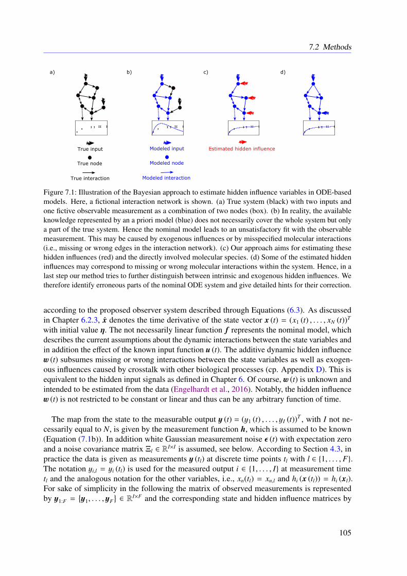
7.2 Methods
Figure 7.1: Illustration of the Bayesian approach to estimate hidden influence variables in ODE-basedmodels. Here, a fictional interaction network is shown. (a) True system (black) with two inputs andone fictive observable measurement as a combination of two nodes (box). (b) In reality, the availableknowledge represented by an a priori model (blue) does not necessarily cover the whole system but onlya part of the true system. Hence the nominal model leads to an unsatisfactory fit with the observablemeasurement. This may be caused by exogenous influences or by misspecified molecular interactions(i.e., missing or wrong edges in the interaction network). (c) Our approach aims for estimating thesehidden influences (red) and the directly involved molecular species. (d) Some of the estimated hiddeninfluences may correspond to missing or wrong molecular interactions within the system. Hence, in alast step our method tries to further distinguish between intrinsic and exogenous hidden influences. Wetherefore identify erroneous parts of the nominal ODE system and give detailed hints for their correction.
according to the proposed observer system described through Equations (6.3). As discussedin Chapter 6.2.3, x denotes the time derivative of the state vector x (t) = (x1 (t) , . . . , xN (t))T
with initial value η. The not necessarily linear function f represents the nominal model, whichdescribes the current assumptions about the dynamic interactions between the state variables andin addition the effect of the known input function u (t). The additive dynamic hidden influencew (t) subsumes missing or wrong interactions between the state variables as well as exogen-ous influences caused by crosstalk with other biological processes (cp. Appendix D). This isequivalent to the hidden input signals as defined in Chapter 6. Of course, w (t) is unknown andintended to be estimated from the data (Engelhardt et al., 2016). Notably, the hidden influencew (t) is not restricted to be constant or linear and thus can be any arbitrary function of time.
The map from the state to the measurable output y (t) = (y1 (t) , . . . , yI (t))T , with I not ne-cessarily equal to N, is given by the measurement function h, which is assumed to be known(Equation (7.1b)). In addition white Gaussian measurement noise ε (t) with expectation zeroand a noise covariance matrix Ξl ∈ R
I×I is assumed, see below. According to Section 4.3, inpractice the data is given as measurements y (tl) at discrete time points tl with l ∈ 1, . . . , F.The notation yi,l = yi (tl) is used for the measured output i ∈ 1, . . . , I at measurement timetl and the analogous notation for the other variables, i.e., xn(tl) = xn,l and hi (x (tl)) = hi (xl).For sake of simplicity in the following the matrix of observed measurements is representedby y1:F =
y1, . . . , yF
∈ RI×F and the corresponding state and hidden influence matrices by
105
Chapter 7 The Bayesian Dynamic Elastic-Net
x1:F ∈ RN×F and w1:F ∈ R
N×F with initial values x0 = η and w0 = 0.
From now on we are interested in hidden influences at discrete time points. Under thisassumption Equations (7.1) can be rewritten as:
xl = xl−1 +
∫ tl
tl−1
f (x(t),u
(t)) + w
(t)
dt (7.2a)
yl = N (h (xl) , Ξl) (7.2b)x0 = η. (7.2c)
Consequently, we obtain a first order Markov process over the state variables x. The functionw (t) is obtained by fitting a cubic smoothing spline through each of the N discrete time seriesof hidden influence signals wF with an initial value w0 (Fritsch and Carlson, 1980). Theassumption of Gaussian measurement noise can, if necessary, approximately be fulfilled aftera variance-stabilizing transformation (Atkinson, 1987). In addition, Ξl = diag
(ξ2
1,l, . . . , ξ2I,l
)is
supposed.
7.2.3 Marginal Likelihood of the Data
The likelihood of the observed data
p(y1:F |x0:F ,w0:F ,Ξ1:F
)=
F∏l=1
I∏i=1
p(yi,l
∣∣∣xl, ξ2i,l
)× p (xl |xl−1,wl−1:l ) . (7.3)
can be factorized due to the independence of the measurement noise with respect to time andobservables. Note that p (xl |xl−1,wl−1:l ) is defined by Equation (7.2a). In addition xl−1:l and wl−1:l
are conditionally independent from Ξ1:F . Since typically the number of replicate measurementsper time point is small, the empirical variance is not a reliable estimator of the true measurementnoise. Therefore, we impose an inverse gamma prior on the variance of the measurement noise
ξ2i,l ∼ IG (α, β) . (7.4)
The marginal likelihood of the data is obtained by marginalizing over the variance of themeasurement noise variable
p(y1:F |x0:F ,w0:F , α, β
)∝
F∏l=1
I∏i=1
∫p(yi,l
∣∣∣xl, ξ2i,l
)× p
(ξ2
i,l
∣∣∣α, β)dξ2i,l × p (xl |xl−1,wl−1:l ) . (7.5)
This integral can analytically be calculated to yield (Zacher et al., 2012)
p(y1:F |x0:F ,w0:F , α, β
)∝
F∏l=1
I∏i=1
Γ(α + 1
2
)Γ (α) (2πβ)
12
1(1 + 1
2β
(yi,l − hi (xl)
)2)α+ 1
2︸ ︷︷ ︸p(yl |xl,α,β )×p(xl |xl−1,wl−1:l )
. (7.6)
106
7.2 Methods
A detailed derivation of Equation (7.6) is provided in Appendix D.
According to Bayes’ theorem the posterior density over the hidden input signals w1:F is givenby:
p(w1:F
∣∣∣x0:F , y1:F ,Ξ1:F
)∝ p
(y1:F |x0:F ,w0:F ,Ξ1:F
)× p (w1:F) . (7.7)
Using Equation (7.6) we can directly draw samples from the posterior density of the hiddeninfluence. For this purpose we propose a Bayesian elastic-net prior as detailed in the followingsections.
7.2.4 Smoothness and Sparsity via a Bayesian Elastic Net-Prior
The hidden input signals wl−1:l can be understood as the statistical residuals of the nominalsystem, and every deviation of observations from the nominal system could thus be explained bynon-zero components in wl−1:l. However, we are only interested in hidden input signals, whichare far stronger than measurement noise. Therefore, we assume that the hidden input signal issmooth and sparse. Sparsity corresponds to the a priori belief that only a small subset of statevariables is truly affected by unknown external or internal input signals. In addition we assumethe hidden input signal to be smooth over time. Smoothness and sparsity are encoded by aprior distribution inspired by the Bayesian elastic-net, which is here combined with a first-orderMarkov process over w1:F (Li and Lin, 2010; Friedman et al., 1998). Overall our proposedapproach is thus a hierarchical graphical model shown in Figure 7.2. Details can be found inAppendix D.
Figure 7.2: Representation of the proposed Bayesian Dynamic Elastic-Net approach as a probabilisticgraphical model. The hidden influences wl form a Markov chain over all time points l = 1, . . . , F andare directly dependent on the shared parameters λ1 and λ2. Since the outcome of one integration steprepresents the initial value for the next integration step the system state variables x1, . . . , xF are alsosuccessively dependent.
107
Chapter 7 The Bayesian Dynamic Elastic-Net
Briefly, the Bayesian elastic-net defines a conditional Gaussian prior over each wn,l
∣∣∣wn,l−1
(n = 1, . . . ,N, l = 1, . . . , F). The scale of the variance of the Gaussian prior is a stronglydecaying and smooth distribution peaking at zero, which depends on parameters λ2, τ2 andσ2. The parameter τ2 is itself given an by exponential distribution (one for each component ofvector wn) with parameters λ1. In consequence, sparsity is dependent on the parameter vectorλ1, whereas smoothness is mainly controlled by λ2 (Zou and Zhang, 2009; Li and Lin, 2010).These parameters are drawn from hyperpriors, which can be set in a non-informative manner orwith respect to prior knowledge about the degree of shrinkage and smoothness of the hiddeninfluences (Kyung et al., 2010). Further details are given in Appendix D.
7.2.5 Estimating Hidden Influences from Data
To estimate the hidden input and the parameters in the hierarchical model, we devised aMetropolis-Hastings algorithm with Gibbs updates of the Bayesian elastic-net hyperparameters.The algorithm proceeds sequentially between the different time points 1, . . . , F by drawingdifferent samples at each supporting point. At sampling step s + 1 and time point l a randomcomponent wn,l is selected of the hidden input vector (a node in the network) at the previous timepoint, which is modified by a sample from a univariate Gaussian transition kernel π (Brooks,1998). The resulting vector w∗l is accepted with probability
r(w(s)
l
∣∣∣w∗l ) = min
1,p(yl |xl, α, β
)p(yl |xl, α, β
) × p(xl
∣∣∣xl−1,w∗l ,wl−1
)p(xl
∣∣∣xl−1,wsl ,wl−1
) × p(w∗l |θ
)p(ws
l |θ) , (7.8)
where p (wl |θ ) is the Bayesian elastic-net prior over the hidden influences conditioned by hyper-parameters θ =
λ1, λ2, τ
2, σ2. Because of the Gaussian measurement errors, the discrepancy
between data component yi,l and the corresponding model output hi(xl) in Equation (7.6) isgiven by the quadratic error
(yi,l − hi(xl)
)2. Note that xl is obtained by numerically integratingthe ODE system from time point tl−1 using xl−1 as initial value according to Equation (7.2a). Thecode for the sampling algorithm and further details are provided in Appendix D.
7.2.6 Estimating Endogenous Hidden Influences
After having estimated the hidden influences on the state components in the nominal ODEsystem, the question arises whether these hidden variables could in fact correspond to missing orwrongly specified interactions within the nominal system. A simple strategy which we followedhere, is to rank all state variables in the nominal system by their temporal correlation with theestimated hidden influences. The essential idea is that in case of a wrong or missing reactionthe estimated hidden time courses should "compensate" erroneous predictions by the nominalsystem (Figure 7.3). In general, wrong or missing interactions can either have an increasing("stimulatory") or decreasing ("inhibitory") influence on the target nodes. This results in anegative hidden influence with wn,1:F < 0 in the case of inhibition and a positive hidden influencewith wn,1:F > 0 in the case of stimulatory events. In general, wrong or missing interactions caneither have an increasing ("stimulatory") or decreasing ("inhibitory") influences on the target
108
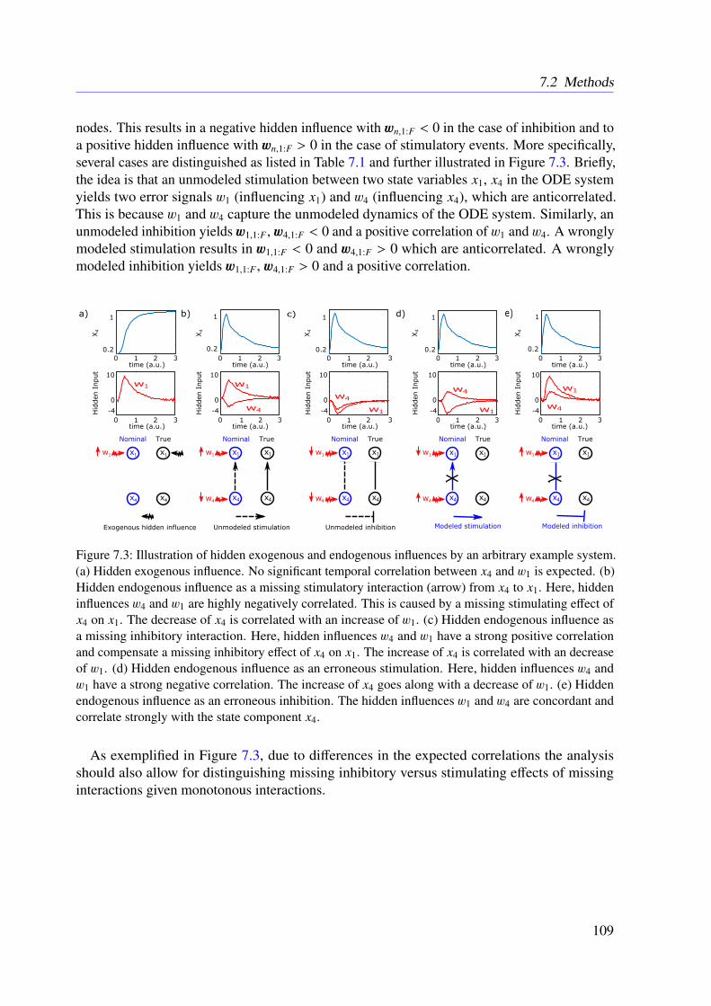
7.2 Methods
nodes. This results in a negative hidden influence with wn,1:F < 0 in the case of inhibition and toa positive hidden influence with wn,1:F > 0 in the case of stimulatory events. More specifically,several cases are distinguished as listed in Table 7.1 and further illustrated in Figure 7.3. Briefly,the idea is that an unmodeled stimulation between two state variables x1, x4 in the ODE systemyields two error signals w1 (influencing x1) and w4 (influencing x4), which are anticorrelated.This is because w1 and w4 capture the unmodeled dynamics of the ODE system. Similarly, anunmodeled inhibition yields w1,1:F , w4,1:F < 0 and a positive correlation of w1 and w4. A wronglymodeled stimulation results in w1,1:F < 0 and w4,1:F > 0 which are anticorrelated. A wronglymodeled inhibition yields w1,1:F , w4,1:F > 0 and a positive correlation.
Figure 7.3: Illustration of hidden exogenous and endogenous influences by an arbitrary example system.(a) Hidden exogenous influence. No significant temporal correlation between x4 and w1 is expected. (b)Hidden endogenous influence as a missing stimulatory interaction (arrow) from x4 to x1. Here, hiddeninfluences w4 and w1 are highly negatively correlated. This is caused by a missing stimulating effect ofx4 on x1. The decrease of x4 is correlated with an increase of w1. (c) Hidden endogenous influence asa missing inhibitory interaction. Here, hidden influences w4 and w1 have a strong positive correlationand compensate a missing inhibitory effect of x4 on x1. The increase of x4 is correlated with an decreaseof w1. (d) Hidden endogenous influence as an erroneous stimulation. Here, hidden influences w4 andw1 have a strong negative correlation. The increase of x4 goes along with a decrease of w1. (e) Hiddenendogenous influence as an erroneous inhibition. The hidden influences w1 and w4 are concordant andcorrelate strongly with the state component x4.
As exemplified in Figure 7.3, due to differences in the expected correlations the analysisshould also allow for distinguishing missing inhibitory versus stimulating effects of missinginteractions given monotonous interactions.
109
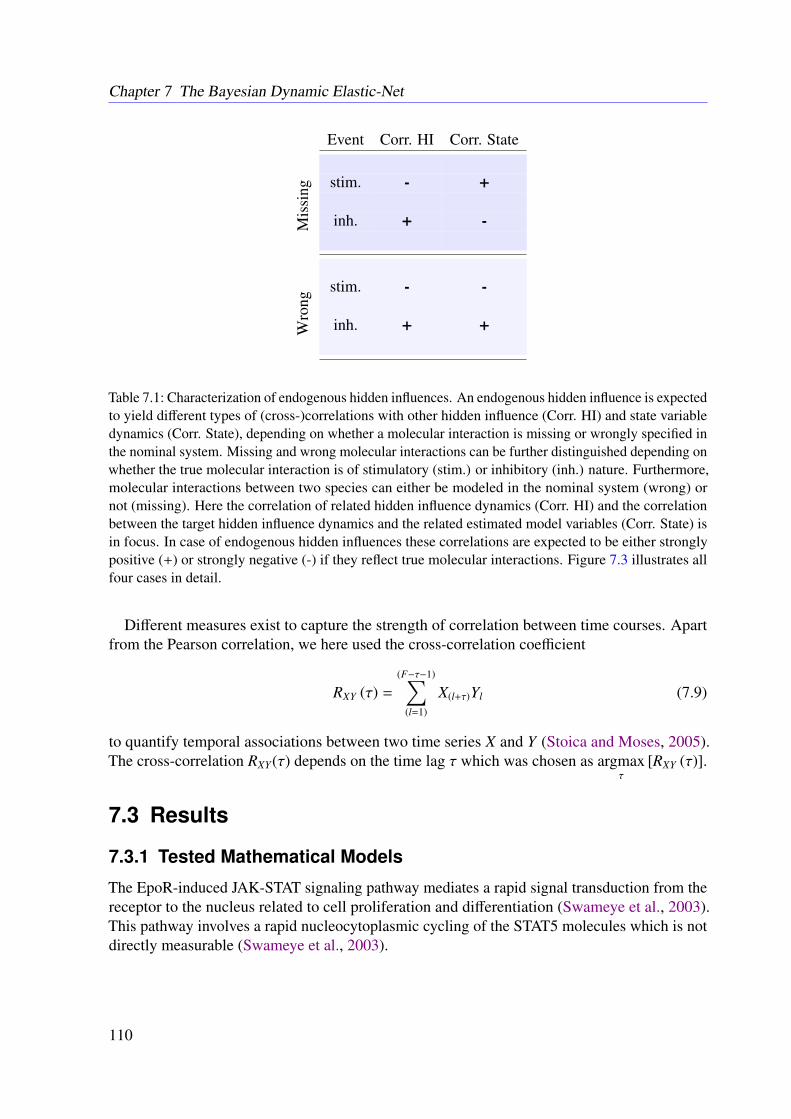
Chapter 7 The Bayesian Dynamic Elastic-Net
Event Corr. HI Corr. State
stim. - +
inh. + -Mis
sing
stim. - -
inh. + +Wro
ng
Table 7.1: Characterization of endogenous hidden influences. An endogenous hidden influence is expectedto yield different types of (cross-)correlations with other hidden influence (Corr. HI) and state variabledynamics (Corr. State), depending on whether a molecular interaction is missing or wrongly specified inthe nominal system. Missing and wrong molecular interactions can be further distinguished depending onwhether the true molecular interaction is of stimulatory (stim.) or inhibitory (inh.) nature. Furthermore,molecular interactions between two species can either be modeled in the nominal system (wrong) ornot (missing). Here the correlation of related hidden influence dynamics (Corr. HI) and the correlationbetween the target hidden influence dynamics and the related estimated model variables (Corr. State) isin focus. In case of endogenous hidden influences these correlations are expected to be either stronglypositive (+) or strongly negative (-) if they reflect true molecular interactions. Figure 7.3 illustrates allfour cases in detail.
Different measures exist to capture the strength of correlation between time courses. Apartfrom the Pearson correlation, we here used the cross-correlation coefficient
RXY (τ) =
(F−τ−1)∑(l=1)
X(l+τ)Yl (7.9)
to quantify temporal associations between two time series X and Y (Stoica and Moses, 2005).The cross-correlation RXY(τ) depends on the time lag τ which was chosen as argmax
τ
[RXY (τ)].
7.3 Results
7.3.1 Tested Mathematical Models
The EpoR-induced JAK-STAT signaling pathway mediates a rapid signal transduction from thereceptor to the nucleus related to cell proliferation and differentiation (Swameye et al., 2003).This pathway involves a rapid nucleocytoplasmic cycling of the STAT5 molecules which is notdirectly measurable (Swameye et al., 2003).
110
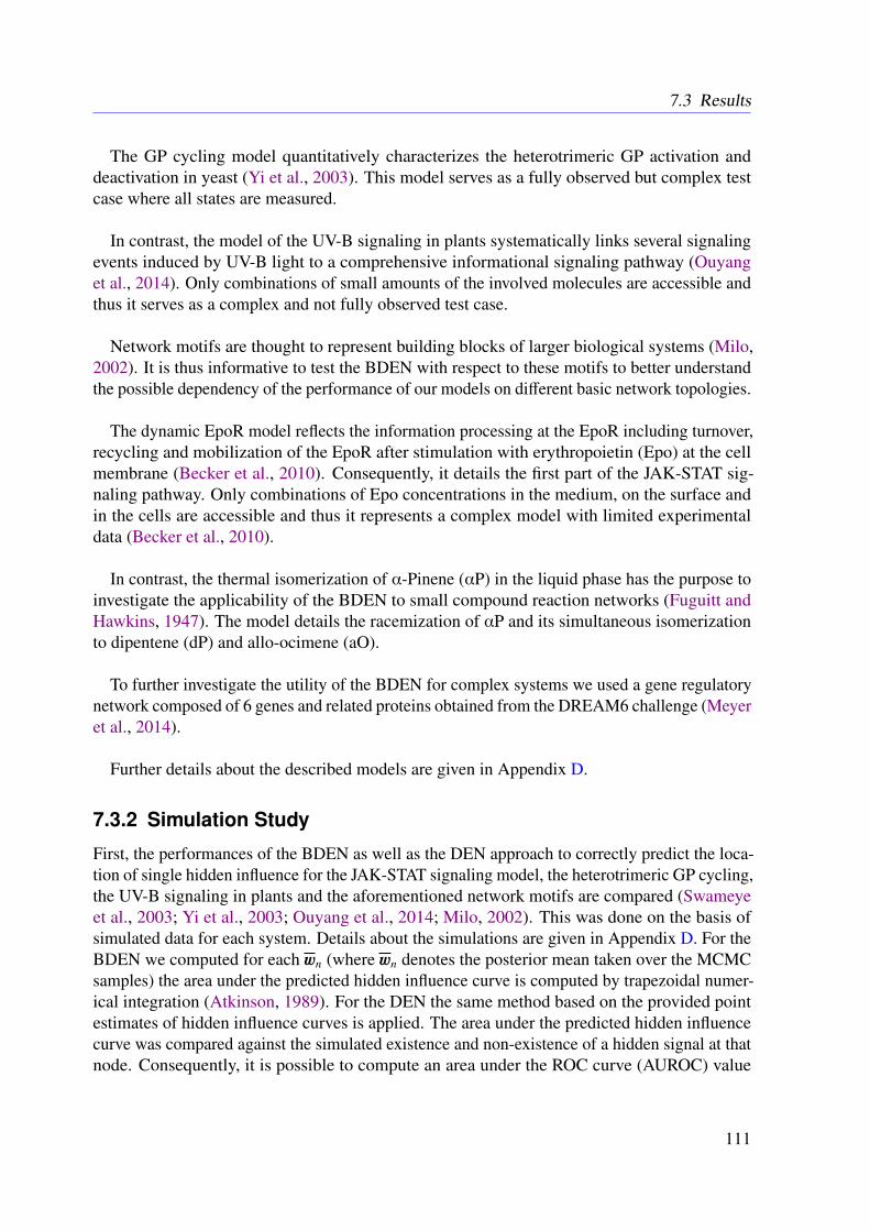
7.3 Results
The GP cycling model quantitatively characterizes the heterotrimeric GP activation anddeactivation in yeast (Yi et al., 2003). This model serves as a fully observed but complex testcase where all states are measured.
In contrast, the model of the UV-B signaling in plants systematically links several signalingevents induced by UV-B light to a comprehensive informational signaling pathway (Ouyanget al., 2014). Only combinations of small amounts of the involved molecules are accessible andthus it serves as a complex and not fully observed test case.
Network motifs are thought to represent building blocks of larger biological systems (Milo,2002). It is thus informative to test the BDEN with respect to these motifs to better understandthe possible dependency of the performance of our models on different basic network topologies.
The dynamic EpoR model reflects the information processing at the EpoR including turnover,recycling and mobilization of the EpoR after stimulation with erythropoietin (Epo) at the cellmembrane (Becker et al., 2010). Consequently, it details the first part of the JAK-STAT sig-naling pathway. Only combinations of Epo concentrations in the medium, on the surface andin the cells are accessible and thus it represents a complex model with limited experimentaldata (Becker et al., 2010).
In contrast, the thermal isomerization of α-Pinene (αP) in the liquid phase has the purpose toinvestigate the applicability of the BDEN to small compound reaction networks (Fuguitt andHawkins, 1947). The model details the racemization of αP and its simultaneous isomerizationto dipentene (dP) and allo-ocimene (aO).
To further investigate the utility of the BDEN for complex systems we used a gene regulatorynetwork composed of 6 genes and related proteins obtained from the DREAM6 challenge (Meyeret al., 2014).
Further details about the described models are given in Appendix D.
7.3.2 Simulation Study
First, the performances of the BDEN as well as the DEN approach to correctly predict the loca-tion of single hidden influence for the JAK-STAT signaling model, the heterotrimeric GP cycling,the UV-B signaling in plants and the aforementioned network motifs are compared (Swameyeet al., 2003; Yi et al., 2003; Ouyang et al., 2014; Milo, 2002). This was done on the basis ofsimulated data for each system. Details about the simulations are given in Appendix D. For theBDEN we computed for each wn (where wn denotes the posterior mean taken over the MCMCsamples) the area under the predicted hidden influence curve is computed by trapezoidal numer-ical integration (Atkinson, 1989). For the DEN the same method based on the provided pointestimates of hidden influence curves is applied. The area under the predicted hidden influencecurve was compared against the simulated existence and non-existence of a hidden signal at thatnode. Consequently, it is possible to compute an area under the ROC curve (AUROC) value
111
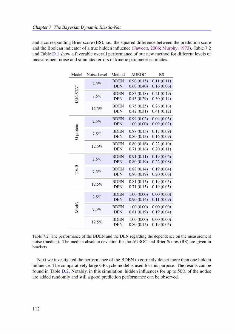
Chapter 7 The Bayesian Dynamic Elastic-Net
and a corresponding Brier score (BS), i.e., the squared difference between the prediction scoreand the Boolean indicator of a true hidden influence (Fawcett, 2006; Murphy, 1973). Table 7.2and Table D.1 show a favorable overall performance of our new method for different levels ofmeasurement noise and simulated errors of kinetic parameter estimates.
Model Noise Level Method AUROC BSJA
K-S
TAT
BDEN 0.90 (0.15) 0.11 (0.11)2.5%
DEN 0.60 (0.40) 0.16 (0.06)
BDEN 0.83 (0.18) 0.21 (0.19)7.5%
DEN 0.43 (0.29) 0.30 (0.14)
BDEN 0.75 (0.25) 0.26 (0.16)12.5%
DEN 0.42 (0.31) 0.41 (0.12)
Gpr
otei
n
BDEN 0.99 (0.02) 0.04 (0.03)2.5%
DEN 1.00 (0.00) 0.09 (0.02)
BDEN 0.88 (0.13) 0.17 (0.09)7.5%
DEN 0.80 (0.13) 0.16 (0.09)
BDEN 0.80 (0.16) 0.22 (0.10)12.5%
DEN 0.71 (0.16) 0.20 (0.11)
UV
-B
BDEN 0.91 (0.11) 0.19 (0.06)2.5%
DEN 0.80 (0.19) 0.22 (0.08)
BDEN 0.88 (0.14) 0.19 (0.04)7.5%
DEN 0.80 (0.19) 0.20 (0.06)
BDEN 0.81 (0.15) 0.19 (0.05)12.5%
DEN 0.71 (0.15) 0.19 (0.05)
Mot
ifs
BDEN 1.00 (0.00) 0.00 (0.00)2.5%
DEN 0.90 (0.14) 0.11 (0.09)
BDEN 1.00 (0.00) 0.00 (0.00)7.5%
DEN 0.81 (0.19) 0.19 (0.04)
BDEN 1.00 (0.00) 0.00 (0.00)12.5%
DEN 0.80 (0.15) 0.19 (0.05)
Table 7.2: The performance of the BDEN and the DEN regarding the dependence on the measurementnoise (median). The median absolute deviation for the AUROC and Brier Scores (BS) are given inbrackets.
Next we investigated the performance of the BDEN to correctly detect more than one hiddeninfluence. The comparatively large GP cycle model is used for this purpose. The results can befound in Table D.2. Notably, in this simulation, hidden influences for up to 50% of the nodesare added randomly and still a good prediction performance can be observed.
112
7.3 Results
In a similar manner the performance of the BDEN to detect wrong and missing interactionsis investigated (Table 7.3). Therefore wrong model specifications of the heterotrimeric GPcycling, the U-VB signaling in plants and the synthetic JAK-STAT signaling are simulated byrandomly removing and adding interactions. As described above, the quantitative predictions ofthe BDEN are given in terms of (cross-)correlations. By comparing these correlation valuesagainst the true existence and non-existence of a particular interaction, it is possible to computean AUROC value. Notably, missing and wrong interaction detection is only possible withthe BDEN approach. Again a very good performance for all systems under investigation isarchived. On average, 80% of the missing interactions are correctly detected by the BDEN.Among the correctly identified missing interactions, on average 90% were correctly classified as"stimulating" and "inhibiting", respectively (cp. Appendix D). Details regarding the dependencyon the measurement noise are given in Table 7.3 and results in dependency of deviance of theparameter estimates are given in Tables D.4 and D.5.
Model Noise Level AUROC2.5% 1.00 (0.00)7.5% 0.83 (0.28)JS
12.5% 0.80 (0.32)
2.5% 0.81 (0.19)7.5% 0.78 (0.22)G
P
12.5% 0.62 (0.47)
2.5% 1.00 (0.00)7.5% 0.91 (0.11)M
issi
ngIn
tera
ctio
n
UV
-B
12.5% 0.76 (0.16)
Model Noise Level AUROC2.5% 1.00 (0.00)7.5% 0.87 (0.32)JS
12.5% 0.80 (0.23)
2.5% 1.00 (0.00)7.5% 0.81 (0.32)G
P
12.5% 0.73 (0.40)
2.5% 0.81 (0.20)7.5% 0.70 (0.24)
Wro
ngIn
tera
ctio
n
UV
-B
12.5% 0.68 (0.30)
Table 7.3: Performance of the BDEN to detect wrong and missing interactions depending on the measure-ment noise (median) evaluated for the JAK-STAT (JS), G protein (GP) and UV-B network. The medianabsolute deviation for the AUROC is given in brackets.
7.3.3 Illustrative Examples With Real Data
In the following we further illustrate the results obtained with the BDEN for the JAK-STATsignaling model, the information processing at EpoR and the isomerization of αP using experi-mental data.
JAK-STAT Signaling
The JAK-STAT signaling pathway model (cp. Section 6.3.1) consists of four molecular species:Unbound STAT5 molecules become phosphorylated (STAT5p) catalyzed by the erythropoietinreceptor. Two STAT5p molecules can form a dimer (STAT5di) and thus are able to enter thenucleus (STAT5n). Only the amount of phosphorylated STAT5 molecules, the total amount ofSTAT5 and the erythropoietin receptor are directly accessible. Experimental measurements areavailable at 16 time points (Swameye et al., 2003).
113
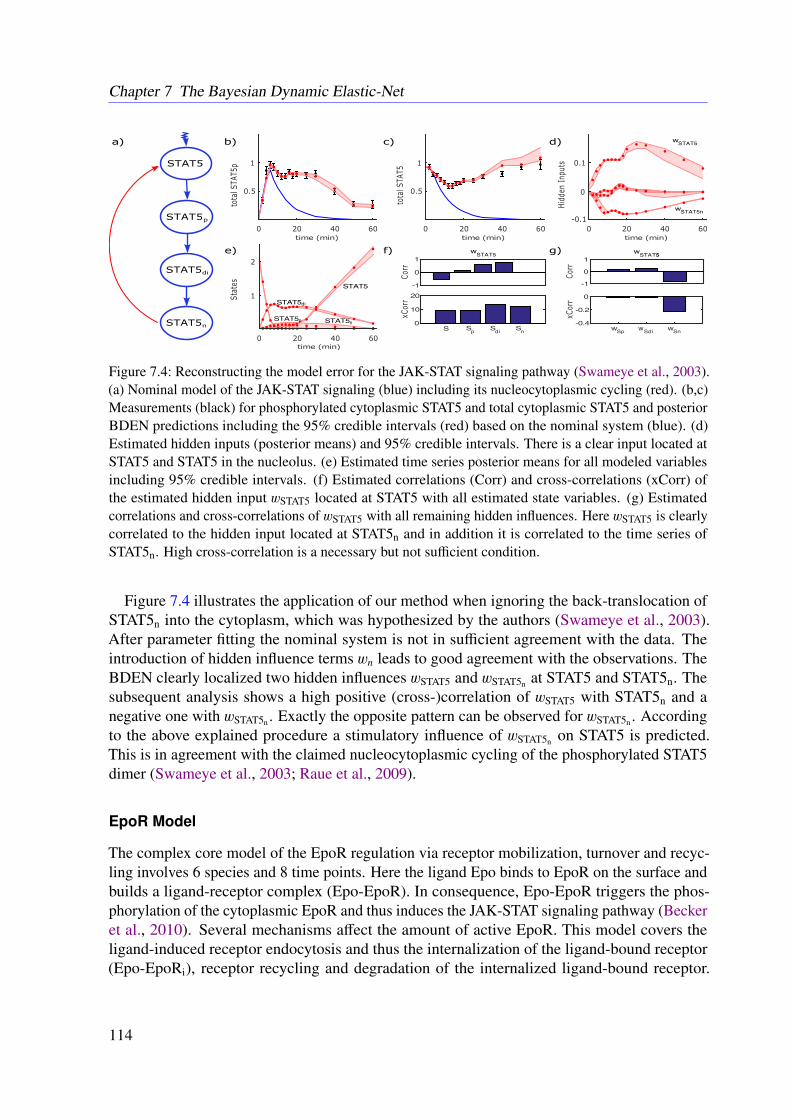
Chapter 7 The Bayesian Dynamic Elastic-Net
Figure 7.4: Reconstructing the model error for the JAK-STAT signaling pathway (Swameye et al., 2003).(a) Nominal model of the JAK-STAT signaling (blue) including its nucleocytoplasmic cycling (red). (b,c)Measurements (black) for phosphorylated cytoplasmic STAT5 and total cytoplasmic STAT5 and posteriorBDEN predictions including the 95% credible intervals (red) based on the nominal system (blue). (d)Estimated hidden inputs (posterior means) and 95% credible intervals. There is a clear input located atSTAT5 and STAT5 in the nucleolus. (e) Estimated time series posterior means for all modeled variablesincluding 95% credible intervals. (f) Estimated correlations (Corr) and cross-correlations (xCorr) ofthe estimated hidden input wSTAT5 located at STAT5 with all estimated state variables. (g) Estimatedcorrelations and cross-correlations of wSTAT5 with all remaining hidden influences. Here wSTAT5 is clearlycorrelated to the hidden input located at STAT5n and in addition it is correlated to the time series ofSTAT5n. High cross-correlation is a necessary but not sufficient condition.
Figure 7.4 illustrates the application of our method when ignoring the back-translocation ofSTAT5n into the cytoplasm, which was hypothesized by the authors (Swameye et al., 2003).After parameter fitting the nominal system is not in sufficient agreement with the data. Theintroduction of hidden influence terms wn leads to good agreement with the observations. TheBDEN clearly localized two hidden influences wSTAT5 and wSTAT5n at STAT5 and STAT5n. Thesubsequent analysis shows a high positive (cross-)correlation of wSTAT5 with STAT5n and anegative one with wSTAT5n . Exactly the opposite pattern can be observed for wSTAT5n . Accordingto the above explained procedure a stimulatory influence of wSTAT5n on STAT5 is predicted.This is in agreement with the claimed nucleocytoplasmic cycling of the phosphorylated STAT5dimer (Swameye et al., 2003; Raue et al., 2009).
EpoR Model
The complex core model of the EpoR regulation via receptor mobilization, turnover and recyc-ling involves 6 species and 8 time points. Here the ligand Epo binds to EpoR on the surface andbuilds a ligand-receptor complex (Epo-EpoR). In consequence, Epo-EpoR triggers the phos-phorylation of the cytoplasmic EpoR and thus induces the JAK-STAT signaling pathway (Beckeret al., 2010). Several mechanisms affect the amount of active EpoR. This model covers theligand-induced receptor endocytosis and thus the internalization of the ligand-bound receptor(Epo-EpoRi), receptor recycling and degradation of the internalized ligand-bound receptor.
114
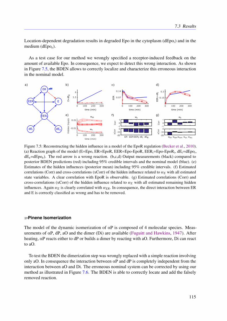
7.3 Results
Location-dependent degradation results in degraded Epo in the cytoplasm (dEpoi) and in themedium (dEpoe).
As a test case for our method we wrongly specified a receptor-induced feedback on theamount of available Epo. In consequence, we expect to detect this wrong interaction. As shownin Figure 7.5, the BDEN allows to correctly localize and characterize this erroneous interactionin the nominal model.
Figure 7.5: Reconstructing the hidden influence in a model of the EpoR regulation (Becker et al., 2010).(a) Reaction graph of the model (E=Epo, ER=EpoR, EER=Epo-EpoR, EERi=Epo-EpoRi, dEi=dEpoi,dEe=dEpoe). The red arrow is a wrong reaction. (b,c,d) Output measurements (black) compared toposterior BDEN predictions (red) including 95% credible intervals and the nominal model (blue). (e)Estimates of the hidden influences (posterior mean) including 95% credible intervals. (f) Estimatedcorrelations (Corr) and cross-correlations (xCorr) of the hidden influence related to wE with all estimatedstate variables. A clear correlation with EpoR is observable. (g) Estimated correlations (Corr) andcross-correlations (xCorr) of the hidden influence related to wE with all estimated remaining hiddeninfluences. Again wE is clearly correlated with wER. In consequence, the direct interaction between ERand E is correctly classified as wrong and has to be removed.
α-Pinene Isomerization
The model of the dynamic isomerization of αP is composed of 4 molecular species. Meas-urements of αP, dP, aO and the dimer (Di) are available (Fuguitt and Hawkins, 1947). Afterheating, αP reacts either to dP or builds a dimer by reacting with aO. Furthermore, Di can reactto aO.
To test the BDEN the dimerization step was wrongly replaced with a simple reaction involvingonly aO. In consequence the interaction between αP and dP is completely independent from theinteraction between aO and Di. The erroneous nominal system can be corrected by using ourmethod as illustrated in Figure 7.6. The BDEN is able to correctly locate and add the falselyremoved reaction.
115
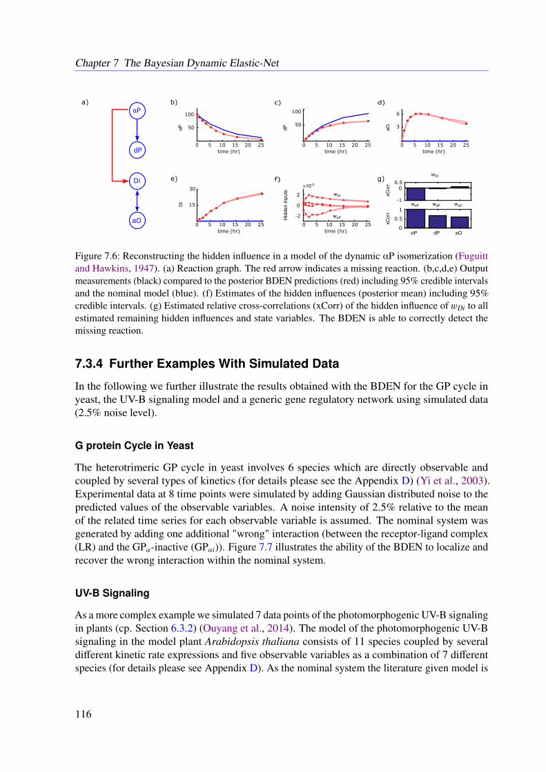
Chapter 7 The Bayesian Dynamic Elastic-Net
Figure 7.6: Reconstructing the hidden influence in a model of the dynamic αP isomerization (Fuguittand Hawkins, 1947). (a) Reaction graph. The red arrow indicates a missing reaction. (b,c,d,e) Outputmeasurements (black) compared to the posterior BDEN predictions (red) including 95% credible intervalsand the nominal model (blue). (f) Estimates of the hidden influences (posterior mean) including 95%credible intervals. (g) Estimated relative cross-correlations (xCorr) of the hidden influence of wDi to allestimated remaining hidden influences and state variables. The BDEN is able to correctly detect themissing reaction.
7.3.4 Further Examples With Simulated Data
In the following we further illustrate the results obtained with the BDEN for the GP cycle inyeast, the UV-B signaling model and a generic gene regulatory network using simulated data(2.5% noise level).
G protein Cycle in Yeast
The heterotrimeric GP cycle in yeast involves 6 species which are directly observable andcoupled by several types of kinetics (for details please see the Appendix D) (Yi et al., 2003).Experimental data at 8 time points were simulated by adding Gaussian distributed noise to thepredicted values of the observable variables. A noise intensity of 2.5% relative to the meanof the related time series for each observable variable is assumed. The nominal system wasgenerated by adding one additional "wrong" interaction (between the receptor-ligand complex(LR) and the GPα-inactive (GPαi)). Figure 7.7 illustrates the ability of the BDEN to localize andrecover the wrong interaction within the nominal system.
UV-B Signaling
As a more complex example we simulated 7 data points of the photomorphogenic UV-B signalingin plants (cp. Section 6.3.2) (Ouyang et al., 2014). The model of the photomorphogenic UV-Bsignaling in the model plant Arabidopsis thaliana consists of 11 species coupled by severaldifferent kinetic rate expressions and five observable variables as a combination of 7 differentspecies (for details please see Appendix D). As the nominal system the literature given model is
116
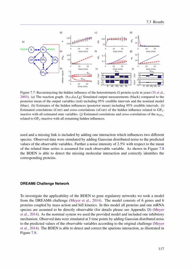
7.3 Results
Figure 7.7: Reconstructing the hidden influence of the heterotrimeric G protein cycle in yeast (Yi et al.,2003). (a) The reaction graph. (b,c,d,e,f,g) Simulated output measurements (black) compared to theposterior mean of the output variables (red) including 95% credible intervals and the nominal model(blue). (h) Estimates of the hidden influences (posterior mean) including 95% credible intervals. (i)Estimated correlations (Corr) and cross-correlations (xCorr) of the hidden influence related to GPα-inactive with all estimated state variables. (j) Estimated correlations and cross-correlations of the wGPαi
related to GPα-inactive with all remaining hidden influences.
used and a missing link is included by adding one interaction which influences two differentspecies. Observed data were simulated by adding Gaussian distributed noise to the predictedvalues of the observable variables. Further a noise intensity of 2.5% with respect to the meanof the related time series is assumed for each observable variable. As shown in Figure 7.8the BDEN is able to detect the missing molecular interaction and correctly identifies thecorresponding proteins.
DREAM6 Challenge Network
To investigate the applicability of the BDEN to gene regulatory networks we took a modelfrom the DREAM6 challenge (Meyer et al., 2014). The model consists of 6 genes and 6proteins coupled by mass action and hill kinetics. In this model all proteins and one mRNAspecies are assumed to be directly observable (for details please see Appendix D) (Meyeret al., 2014). As the nominal system we used the provided model and included one inhibitorymechanism. Observed data were simulated at 5 time points by adding Gaussian distributed noiseto the predicted values of the observable variables according to the original challenge (Meyeret al., 2014). The BDEN is able to detect and correct the spurious interaction, as illustrated inFigure 7.9.
117
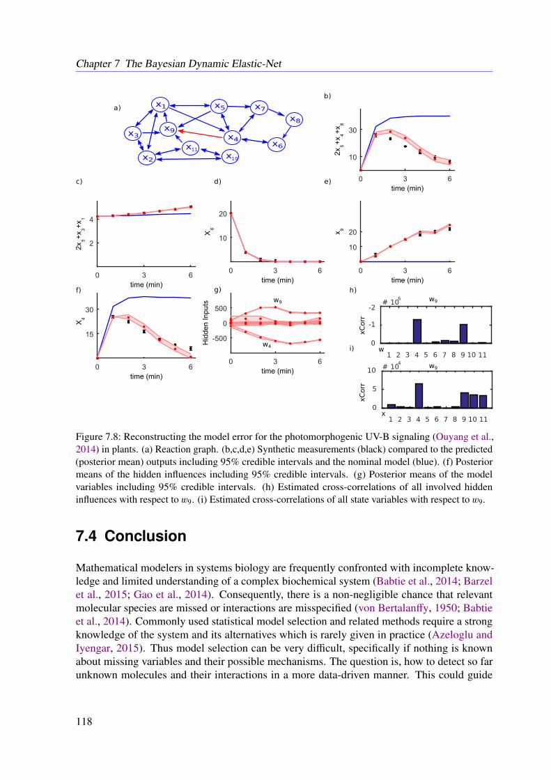
Chapter 7 The Bayesian Dynamic Elastic-Net
Figure 7.8: Reconstructing the model error for the photomorphogenic UV-B signaling (Ouyang et al.,2014) in plants. (a) Reaction graph. (b,c,d,e) Synthetic measurements (black) compared to the predicted(posterior mean) outputs including 95% credible intervals and the nominal model (blue). (f) Posteriormeans of the hidden influences including 95% credible intervals. (g) Posterior means of the modelvariables including 95% credible intervals. (h) Estimated cross-correlations of all involved hiddeninfluences with respect to w9. (i) Estimated cross-correlations of all state variables with respect to w9.
7.4 Conclusion
Mathematical modelers in systems biology are frequently confronted with incomplete know-ledge and limited understanding of a complex biochemical system (Babtie et al., 2014; Barzelet al., 2015; Gao et al., 2014). Consequently, there is a non-negligible chance that relevantmolecular species are missed or interactions are misspecified (von Bertalanffy, 1950; Babtieet al., 2014). Commonly used statistical model selection and related methods require a strongknowledge of the system and its alternatives which is rarely given in practice (Azeloglu andIyengar, 2015). Thus model selection can be very difficult, specifically if nothing is knownabout missing variables and their possible mechanisms. The question is, how to detect so farunknown molecules and their interactions in a more data-driven manner. This could guide
118
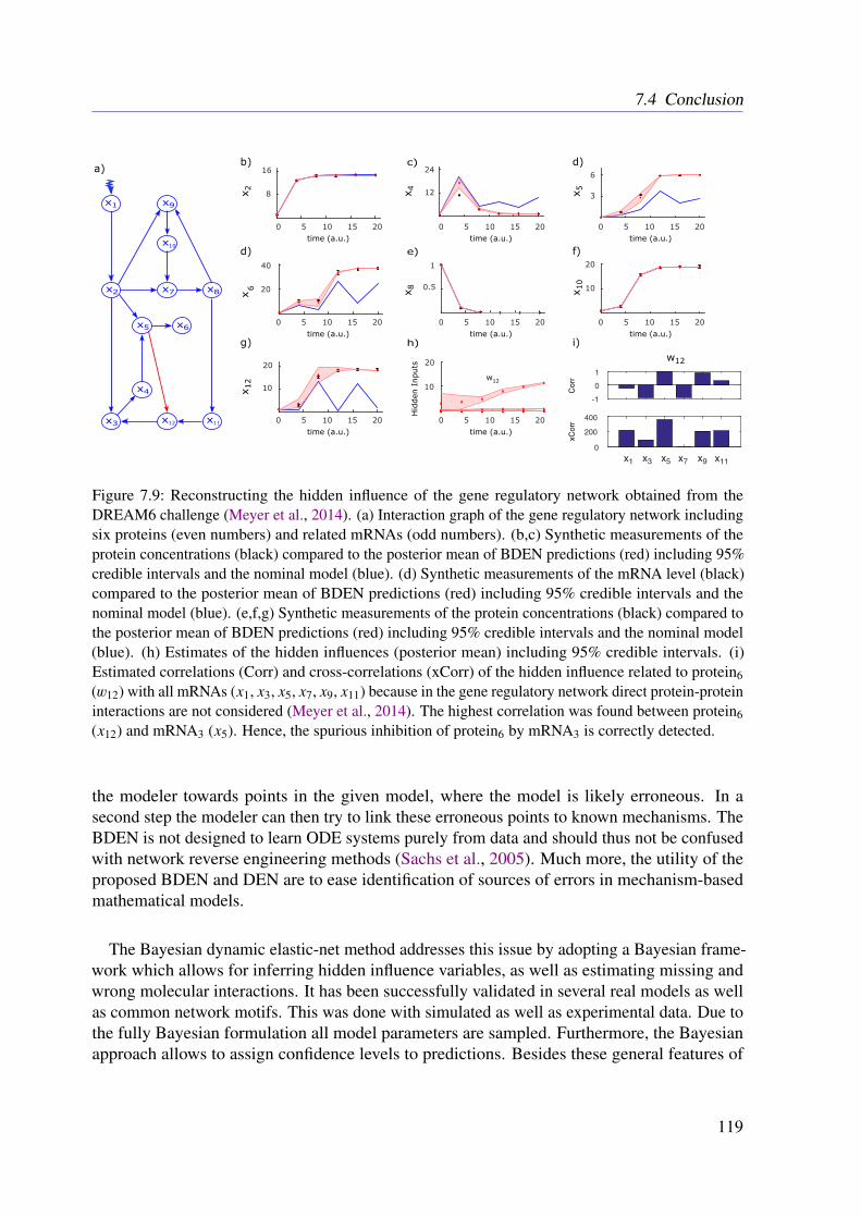
7.4 Conclusion
Figure 7.9: Reconstructing the hidden influence of the gene regulatory network obtained from theDREAM6 challenge (Meyer et al., 2014). (a) Interaction graph of the gene regulatory network includingsix proteins (even numbers) and related mRNAs (odd numbers). (b,c) Synthetic measurements of theprotein concentrations (black) compared to the posterior mean of BDEN predictions (red) including 95%credible intervals and the nominal model (blue). (d) Synthetic measurements of the mRNA level (black)compared to the posterior mean of BDEN predictions (red) including 95% credible intervals and thenominal model (blue). (e,f,g) Synthetic measurements of the protein concentrations (black) compared tothe posterior mean of BDEN predictions (red) including 95% credible intervals and the nominal model(blue). (h) Estimates of the hidden influences (posterior mean) including 95% credible intervals. (i)Estimated correlations (Corr) and cross-correlations (xCorr) of the hidden influence related to protein6(w12) with all mRNAs (x1, x3, x5, x7, x9, x11) because in the gene regulatory network direct protein-proteininteractions are not considered (Meyer et al., 2014). The highest correlation was found between protein6(x12) and mRNA3 (x5). Hence, the spurious inhibition of protein6 by mRNA3 is correctly detected.
the modeler towards points in the given model, where the model is likely erroneous. In asecond step the modeler can then try to link these erroneous points to known mechanisms. TheBDEN is not designed to learn ODE systems purely from data and should thus not be confusedwith network reverse engineering methods (Sachs et al., 2005). Much more, the utility of theproposed BDEN and DEN are to ease identification of sources of errors in mechanism-basedmathematical models.
The Bayesian dynamic elastic-net method addresses this issue by adopting a Bayesian frame-work which allows for inferring hidden influence variables, as well as estimating missing andwrong molecular interactions. It has been successfully validated in several real models as wellas common network motifs. This was done with simulated as well as experimental data. Due tothe fully Bayesian formulation all model parameters are sampled. Furthermore, the Bayesianapproach allows to assign confidence levels to predictions. Besides these general features of
119

Chapter 7 The Bayesian Dynamic Elastic-Net
a fully probabilistic framework, the BDEN method seems to be more stable and more robustbecause within the Bayesian framework over a large number of parameters is averaged and theBDEN does not rely on stiff integration methods.
A unique feature of our new approach is the distinction between exogenous and endogenoushidden influences in the biological system, allowing for the detection of missing and misspe-cified equations in the ODE system. Altogether, the BDEN is a further step towards a betterautomated and more objective revision of ODE-based models in systems biology. In view ofthe rapid progress of technologies to monitor biological dynamics, our approach could haveimplications for many fields including metabolic engineering, synthetic biology and pharma-cokinetics/pharmacodynamics. As the DEN and the BDEN are designed for generic ODEmodels, they can also be applied to challenging modeling tasks in engineering, robotics and inthe earth sciences (Engelhardt et al., 2016; Abarbanel, 2013).
120
CHAPTER 8
Refined Model of the M2Receptor-dependent Signaling
8.1 Introduction
As a further improvement, the structural model derived in Chapter 5 has been extended toinclude dynamic rate laws. The thus obtained time-resolved system allows to gain furtherinsights into the behavior of the M2 receptor-dependent signaling in CHO cells. The modifiedmodel now reflects the dynamic properties of the underlying signaling cascade. The involvedkinetic parameters were estimated based on quantitative measurements of the related proteinactivities reflected by the amount of phosphorylated or associated protein structures. Therefore,the amount of phosphorylated proteins and thus active proteins can be obtained by performingrepeated quantitative WB at defined time points. As discussed in Section 3.3, quantitative WBsare a common technique to measure protein concentrations. For this purpose the concentrationof the phosphorylated form and the overall protein concentration are measured for each protein.As a result, the obtained phosphorylated protein concentrations are normalized with respect tothe initial time point and the related amount of overall protein concentrations. This serves as ameasure for the relative protein activation and reduces the measurement error typically arisingfrom WBs.
8.2 Experimental Procedures
The protocols and techniques used in this study allow for an exact protein quantification, evenif the protein concentration is low. Further experimental details can be found in Appendix E.The stable expression of the M2 receptor was cross-checked through exposure to hygromycin.Successful and stable transfected CHO-Flip-In-hM2 cells include an additional gene whichmakes them resistant to hygromycin and thus populations with low expression levels can besorted out. Furthermore, all antibodies were checked regarding their specificity and affinity toCHO-Flip-In-hM2 cells to ensure the correct targeting of all proteins. In contrast to all other
121
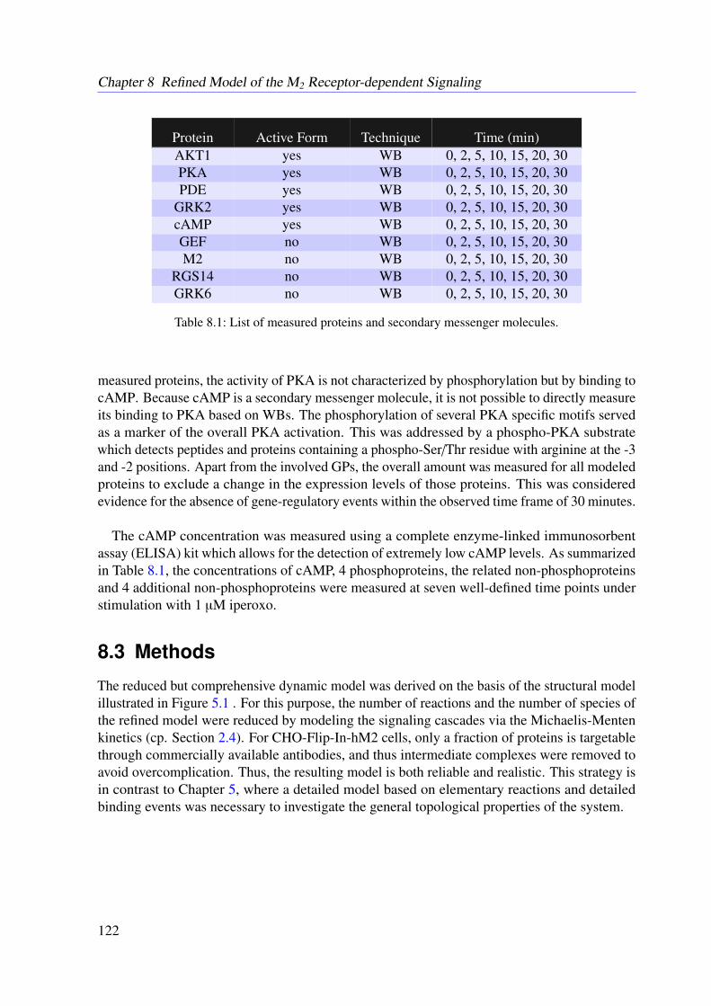
Chapter 8 Refined Model of the M2 Receptor-dependent Signaling
Protein Active Form Technique Time (min)AKT1 yes WB 0, 2, 5, 10, 15, 20, 30PKA yes WB 0, 2, 5, 10, 15, 20, 30PDE yes WB 0, 2, 5, 10, 15, 20, 30
GRK2 yes WB 0, 2, 5, 10, 15, 20, 30cAMP yes WB 0, 2, 5, 10, 15, 20, 30GEF no WB 0, 2, 5, 10, 15, 20, 30M2 no WB 0, 2, 5, 10, 15, 20, 30
RGS14 no WB 0, 2, 5, 10, 15, 20, 30GRK6 no WB 0, 2, 5, 10, 15, 20, 30
Table 8.1: List of measured proteins and secondary messenger molecules.
measured proteins, the activity of PKA is not characterized by phosphorylation but by binding tocAMP. Because cAMP is a secondary messenger molecule, it is not possible to directly measureits binding to PKA based on WBs. The phosphorylation of several PKA specific motifs servedas a marker of the overall PKA activation. This was addressed by a phospho-PKA substratewhich detects peptides and proteins containing a phospho-Ser/Thr residue with arginine at the -3and -2 positions. Apart from the involved GPs, the overall amount was measured for all modeledproteins to exclude a change in the expression levels of those proteins. This was consideredevidence for the absence of gene-regulatory events within the observed time frame of 30 minutes.
The cAMP concentration was measured using a complete enzyme-linked immunosorbentassay (ELISA) kit which allows for the detection of extremely low cAMP levels. As summarizedin Table 8.1, the concentrations of cAMP, 4 phosphoproteins, the related non-phosphoproteinsand 4 additional non-phosphoproteins were measured at seven well-defined time points understimulation with 1 µM iperoxo.
8.3 Methods
The reduced but comprehensive dynamic model was derived on the basis of the structural modelillustrated in Figure 5.1 . For this purpose, the number of reactions and the number of species ofthe refined model were reduced by modeling the signaling cascades via the Michaelis-Mentenkinetics (cp. Section 2.4). For CHO-Flip-In-hM2 cells, only a fraction of proteins is targetablethrough commercially available antibodies, and thus intermediate complexes were removed toavoid overcomplication. Thus, the resulting model is both reliable and realistic. This strategy isin contrast to Chapter 5, where a detailed model based on elementary reactions and detailedbinding events was necessary to investigate the general topological properties of the system.
122
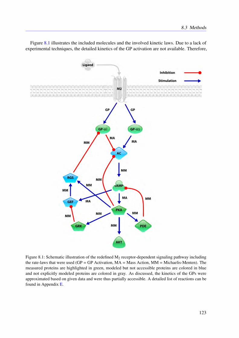
8.3 Methods
Figure 8.1 illustrates the included molecules and the involved kinetic laws. Due to a lack ofexperimental techniques, the detailed kinetics of the GP activation are not available. Therefore,
Figure 8.1: Schematic illustration of the redefined M2 receptor-dependent signaling pathway includingthe rate-laws that were used (GP = GP Activation, MA = Mass Action, MM = Michaelis-Menten). Themeasured proteins are highlighted in green, modeled but not accessible proteins are colored in blueand not explicitly modeled proteins are colored in gray. As discussed, the kinetics of the GPs wereapproximated based on given data and were thus partially accessible. A detailed list of reactions can befound in Appendix E.
123
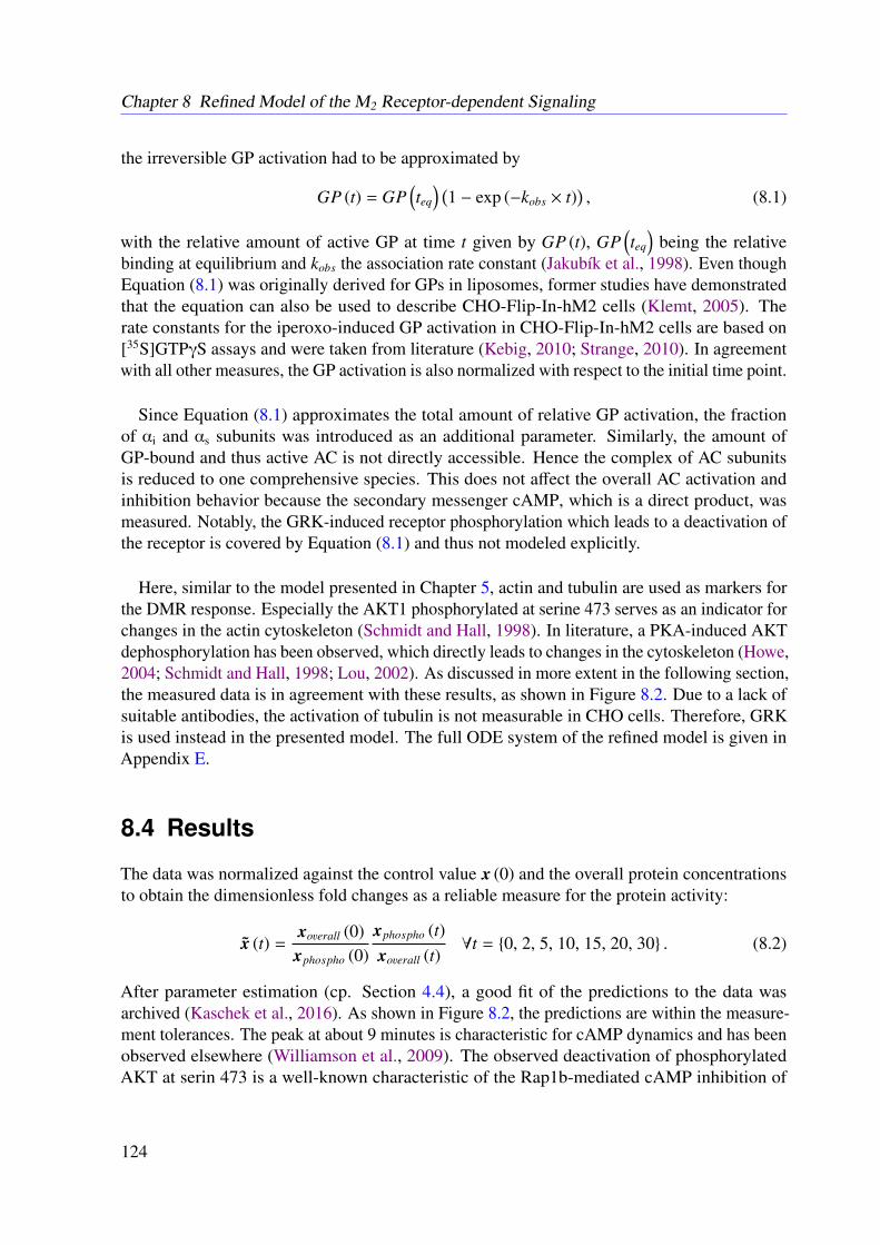
Chapter 8 Refined Model of the M2 Receptor-dependent Signaling
the irreversible GP activation had to be approximated by
GP (t) = GP(teq
) (1 − exp (−kobs × t)
), (8.1)
with the relative amount of active GP at time t given by GP (t), GP(teq
)being the relative
binding at equilibrium and kobs the association rate constant (Jakubík et al., 1998). Even thoughEquation (8.1) was originally derived for GPs in liposomes, former studies have demonstratedthat the equation can also be used to describe CHO-Flip-In-hM2 cells (Klemt, 2005). Therate constants for the iperoxo-induced GP activation in CHO-Flip-In-hM2 cells are based on[35S]GTPγS assays and were taken from literature (Kebig, 2010; Strange, 2010). In agreementwith all other measures, the GP activation is also normalized with respect to the initial time point.
Since Equation (8.1) approximates the total amount of relative GP activation, the fractionof αi and αs subunits was introduced as an additional parameter. Similarly, the amount ofGP-bound and thus active AC is not directly accessible. Hence the complex of AC subunitsis reduced to one comprehensive species. This does not affect the overall AC activation andinhibition behavior because the secondary messenger cAMP, which is a direct product, wasmeasured. Notably, the GRK-induced receptor phosphorylation which leads to a deactivation ofthe receptor is covered by Equation (8.1) and thus not modeled explicitly.
Here, similar to the model presented in Chapter 5, actin and tubulin are used as markers forthe DMR response. Especially the AKT1 phosphorylated at serine 473 serves as an indicator forchanges in the actin cytoskeleton (Schmidt and Hall, 1998). In literature, a PKA-induced AKTdephosphorylation has been observed, which directly leads to changes in the cytoskeleton (Howe,2004; Schmidt and Hall, 1998; Lou, 2002). As discussed in more extent in the following section,the measured data is in agreement with these results, as shown in Figure 8.2. Due to a lack ofsuitable antibodies, the activation of tubulin is not measurable in CHO cells. Therefore, GRKis used instead in the presented model. The full ODE system of the refined model is given inAppendix E.
8.4 Results
The data was normalized against the control value x (0) and the overall protein concentrationsto obtain the dimensionless fold changes as a reliable measure for the protein activity:
x (t) =xoverall (0)
xphospho (0)xphospho (t)xoverall (t)
∀t = 0, 2, 5, 10, 15, 20, 30 . (8.2)
After parameter estimation (cp. Section 4.4), a good fit of the predictions to the data wasarchived (Kaschek et al., 2016). As shown in Figure 8.2, the predictions are within the measure-ment tolerances. The peak at about 9 minutes is characteristic for cAMP dynamics and has beenobserved elsewhere (Williamson et al., 2009). The observed deactivation of phosphorylatedAKT at serin 473 is a well-known characteristic of the Rap1b-mediated cAMP inhibition of
124

8.5 Conclusion
AKT and has also been previously reported in literature (Lou, 2002; Howe, 2004).
Figure 8.2: Model output. (a) Predictions (lines) and measured values including measurement errors(dots). All predictions are within the measurement tolerances. RGS was not measurable, and thus onlythe predicted dynamics are shown. (b) Achieved sets of parameter estimates for different runs (index)sorted by increasing objective values (y-axis). Low values indicate small errors and thus a good matchwith the data. The fits with the lowest values clearly separate from the second plateau. The complete plotincluding all modeled proteins can be found in Appendix E.
In addition, the clear increase of RGS is in agreement with the initial hypothesis stated inChapter 5. To further investigate the role of RGS as an important regulator of the M2 receptor-dependent signaling dynamics, in silico knock-out experiments were performed, as shownin Figure 8.3. For the experiments, the concentration of RGS and all RGS-related reactionswere set to be constant zero. This mimics the absence of RGS from the system and thusallows to investigate the influence of RGS on the modeled signaling pathway. Accordingly, forverification, the concentration of cAMP and all cAMP-related reactions were set to zero as well.A clear decrease of the signaling strength was observed after RGS knock-out. In agreement withrecent literature, a clear change in AKT was observed (Zhang and Mende, 2011; Dale and Rang,2011; Howe, 2004; Pierce et al., 2002). This underlines the importance of the RGS-relatedfeedback for the DMR response. The tubulin-related change of the DMR response also dependson the RGS regulation. The completeness and consistency of the refined model was tested bothwith the DEN and the BDEN. As shown in Figures 8.4 and 8.5, no clear model error was found.This underlines that the model predictions and the experimental data are in good agreement.Taken together, this provides evidence for the reliability of the obtained dynamic model.
8.5 Conclusion
A careful model revision and the incorporation of kinetics, e.g., Michaelis-Menten kinetics andGP activation, allowed for a time-resolved model of the M2 receptor-dependent signaling inCHO cells. As shown in Figure 8.2, the model is in full agreement with the measurement dataand common literature. It is also in agreement with the former derived static model described
125
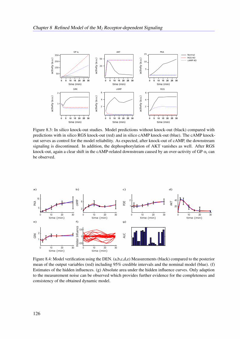
Chapter 8 Refined Model of the M2 Receptor-dependent Signaling
Figure 8.3: In silico knock-out studies. Model predictions without knock-out (black) compared withpredictions with in silico RGS knock-out (red) and in silico cAMP knock-out (blue). The cAMP knock-out serves as control for the model reliability. As expected, after knock-out of cAMP, the downstreamsignaling is discontinued. In addition, the dephosphorylation of AKT vanishes as well. After RGSknock-out, again a clear shift in the cAMP-related downstream caused by an over-activity of GP αi canbe observed.
Figure 8.4: Model verification using the DEN. (a,b,c,d,e) Measurements (black) compared to the posteriormean of the output variables (red) including 95% credible intervals and the nominal model (blue). (f)Estimates of the hidden influences. (g) Absolute area under the hidden influence curves. Only adaptionto the measurement noise can be observed which provides further evidence for the completeness andconsistency of the obtained dynamic model.
126
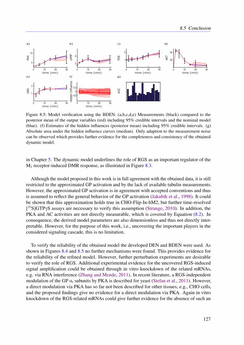
8.5 Conclusion
Figure 8.5: Model verification using the BDEN. (a,b,c,d,e) Measurements (black) compared to theposterior mean of the output variables (red) including 95% credible intervals and the nominal model(blue). (f) Estimates of the hidden influences (posterior mean) including 95% credible intervals. (g)Absolute area under the hidden influence curves (median). Only adaption to the measurement noisecan be observed which provides further evidence for the completeness and consistency of the obtaineddynamic model.
in Chapter 5. The dynamic model underlines the role of RGS as an important regulator of theM2 receptor-induced DMR response, as illustrated in Figure 8.3.
Although the model proposed in this work is in full agreement with the obtained data, it is stillrestricted to the approximated GP activation and by the lack of available tubulin measurements.However, the approximated GP activation is in agreement with accepted conventions and thusis assumed to reflect the general behavior of the GP activation (Jakubík et al., 1998). It couldbe shown that this approximation holds true in CHO-Flip-In-hM2, but further time-resolved[35S]GTPγS assays are necessary to verify this assumption (Strange, 2010). In addition, thePKA and AC activities are not directly measurable, which is covered by Equation (8.2). Inconsequence, the derived model parameters are also dimensionless and thus not directly inter-pretable. However, for the purpose of this work, i.e., uncovering the important players in theconsidered signaling cascade, this is no limitation.
To verify the reliability of the obtained model the developed DEN and BDEN were used. Asshown in Figures 8.4 and 8.5 no further mechanisms were found. This provides evidence forthe reliability of the refined model. However, further perturbation experiments are desirableto verify the role of RGS. Additional experimental evidence for the uncovered RGS-inducedsignal amplification could be obtained through in vitro knockdown of the related mRNAs,e.g. via RNA interference (Zhang and Mende, 2011). In recent literature, a RGS-independentmodulation of the GP αi subunits by PKA is described for yeast (Stefan et al., 2011). However,a direct modulation via PKA has so far not been described for other tissues, e.g., CHO cells,and the proposed findings give no evidence for a direct modulation via PKA. Again in vitroknockdown of the RGS-related mRNAs could give further evidence for the absence of such an
127
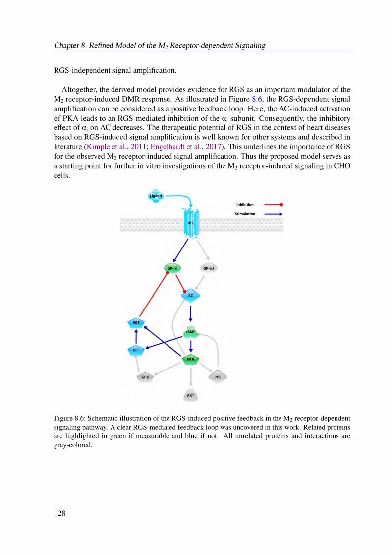
Chapter 8 Refined Model of the M2 Receptor-dependent Signaling
RGS-independent signal amplification.
Altogether, the derived model provides evidence for RGS as an important modulator of theM2 receptor-induced DMR response. As illustrated in Figure 8.6, the RGS-dependent signalamplification can be considered as a positive feedback loop. Here, the AC-induced activationof PKA leads to an RGS-mediated inhibition of the αi subunit. Consequently, the inhibitoryeffect of αi on AC decreases. The therapeutic potential of RGS in the context of heart diseasesbased on RGS-induced signal amplification is well known for other systems and described inliterature (Kimple et al., 2011; Engelhardt et al., 2017). This underlines the importance of RGSfor the observed M2 receptor-induced signal amplification. Thus the proposed model serves asa starting point for further in vitro investigations of the M2 receptor-induced signaling in CHOcells.
Figure 8.6: Schematic illustration of the RGS-induced positive feedback in the M2 receptor-dependentsignaling pathway. A clear RGS-mediated feedback loop was uncovered in this work. Related proteinsare highlighted in green if measurable and blue if not. All unrelated proteins and interactions aregray-colored.
128
CHAPTER 9
Conclusions
This work demonstrates the importance of theoretical mathematical methods as a tool for solvingconcrete biological research tasks. Although there is already a huge range of mathematical andphysical approaches in the field of life sciences, the present thesis underlines the significanceof individually tailored methods. It is motivated by the strong signal amplification of theM2 receptor-induced whole-cell response in CHO cells (Schrage et al., 2013). To address thisphenomena in static models, the novel CFS is proposed in this work (Engelhardt et al., 2017).As part of the model development process, in addition, a novel and promising approach to learnfrom the errors of systems biological models was developed. This approach is not restricted tobiological systems but can be applied to any ODE-based erroneous model (Engelhardt et al.,2016).
The proposed methods are inspired by modern systems biology. Thus the intention was todevelop a mechanistic model of the underlying biological properties. However, this is just onepossible approach to deal with such tasks in the field of mathematical biology and bioinformat-ics (Machado et al., 2011; Kitano, 2002). Hence, besides the algorithms developed in this work,there are also other possible routes (Machado et al., 2011; Kitano, 2002). For instance, a fullyprobabilistic strategy based on machine learning could help to uncover correlations between themodeled molecules and structures (Machado et al., 2011; Kitano, 2002; Bishop, 2007). In afurther step, a predictive model of the M2 receptor-induced whole-cell response could be estab-lished. This approach is preferable if the underlying detailed mechanisms are not completelyunderstood. In contrast, in the present case, the aim was to derive a detailed explanation of theunderlying mechanisms in the light of comparably rich and detailed mechanistic insights fromliterature. This is of essential interest because the whole signaling pathway has yet to be fullyinvestigated, even though the M2 receptor-dependent signaling in CHO cells is of high relevancefor pharmacological research (Engelhardt et al., 2016; Schröder et al., 2011; Schrage et al.,2013). More precisely, the system investigated in this work could serve as a pharmacologicalmodel for the evaluation of drug affinities and effectiveness (Engelhardt et al., 2016; Schröderet al., 2011; Schrage et al., 2013). Other methods designed for the analysis of signaling cascadesmore strongly focus on signal duration and signal strength (Klipp and Liebermeister, 2006;
129
Chapter 9 Conclusions
Heinrich et al., 2002). Therefore, this work provides the foundation for future investigations ofthe system (Engelhardt et al., 2017).
Starting with a static model of the M2 receptor-dependent signaling cascade, this work servesas an example for integrating methods from different areas. In literature, metabolic modelsand signaling cascades are clearly separated (Palsson, 2006; Klamt et al., 2006). Often thisdistinction holds true because the points of view are quite different. Whereas network analysisis mainly interested in the turnover of well-defined molecules and the subsequent optimizationof these processes (e.g., in biotechnology), the analysis of signaling cascades deals with thetemporal and quantitative aspects of protein pathways. However, apart from the velocity ofmetabolic processes (extremely fast) vs. signaling (slower), the underling biological mechan-isms are equivalent and the biological properties are identical (Klipp and Liebermeister, 2006).Thus it seems obvious to combine both areas to develop more comprehensive approaches. Theproposed CFS adopts and extends methods known from metabolic network analysis to addressthe amplification mechanism in signaling cascades (Engelhardt et al., 2017). CFS provides firstinsights into the behavior of static systems and allows for an initial verification of the modelstructure (Engelhardt et al., 2017). This may help to speed up the research cycle (cp. Sec-tion 2.2) and allows for ranking the modeled molecules and functional subnetworks with respectto their importance for signaling (Engelhardt et al., 2017). In addition, this method can be op-tionally enhanced through the incorporation of (partially) available data (Engelhardt et al., 2017).
RGS was localized as the main driver of the investigated signaling cascade in CHO cells (En-gelhardt et al., 2017). If signaling is considered as a directed flow of information from thestimulus downstream to the whole-cell response, RGS together with GP constitute a feedbackloop. Such positive feedback loops are known to function as signal amplifiers (Alon, 2007). Asdiscussed in Chapter 8, further mRNA knockdown experiments would be needed to provide fullexperimental evidence for the hypotheses presented in this work. Despite the gained insights,CFS is still restricted to topology-based phenomena. As demonstrated, this is a good startingpoint, especially for bottom-up strategies, but in general biological phenomena are also time-dependent. Thus a realistic dynamic model of the observed biological system was establishedand time-resolved protein measurements via WBs were conducted. Based on the obtained data,the fully dynamic model was fitted and validated.
The data was normalized to reduce measurement uncertainties and thus served as a measure ofthe relative protein activities. For the given task, this is a sufficient way of modeling. However,one drawback is the non-interpretability of the parameter estimates. This issue can be addressedby more detailed measurements of the involved parameters. For instance, mass spectrometryor specific assays could be used for more precise measurements. On the other hand, suchexperiments are very costly and time-intensive in cases where the experimental pipeline has tobe established with respect to the underlying system, e.g., the CHO cell.
Fitting models to data is still a challenging issue because parameter estimation remainsan ill-conditioned inverse problem. In consequence, even after parameter estimation hiddenconfounders may cause significant model errors (Engelhardt et al., 2016). The novel DEN and
130
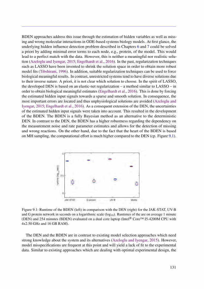
BDEN approaches address this issue through the estimation of hidden variables as well as miss-ing and wrong molecular interactions in ODE-based systems biology models. At first glance, theunderlying hidden influence detection problem described in Chapters 6 and 7 could be solveda priori by adding minimal error terms to each node, e.g., protein, of the model. This wouldlead to a perfect match with the data. However, this is neither a meaningful nor realistic solu-tion (Azeloglu and Iyengar, 2015; Engelhardt et al., 2016). In the past, regularization techniquessuch as LASSO have been invented to shrink the solution space in order to obtain more robustmodel fits (Tibshirani, 1996). In addition, suitable regularization techniques can be used to forcebiological meaningful results. In contrast, unrestricted systems tend to have diverse solutions dueto their inverse nature. A priori, it is not clear which solution to choose. In the spirit of LASSO,the developed DEN is based on an elastic-net regularization – a method similar to LASSO – inorder to obtain biological meaningful estimates (Engelhardt et al., 2016). This is done by forcingthe estimated hidden input signals towards a sparse and smooth solution. In consequence, themost important errors are located and thus unphysiological solutions are avoided (Azeloglu andIyengar, 2015; Engelhardt et al., 2016). As a consequent extension of the DEN, the uncertaintiesof the estimated hidden input signals were taken into account. This resulted in the developmentof the BDEN. The BDEN is a fully Bayesian method as an alternative to the deterministicDEN. In contrast to the DEN, the BDEN has a higher robustness regarding the dependency onthe measurement noise and rate parameter estimates and allows for the detection of missingand wrong reactions. On the other hand, due to the fact that the heart of the BDEN is basedon MH sampling, the computational effort is much higher compared to the DEN (cp. Figure 9.1).
Figure 9.1: Runtime of the BDEN (left) in comparison with the DEN (right) for the JAK-STAT, UV-Band G protein network in seconds on a logarithmic scale (log10). Runtimes of the are on average 1 minute(DEN) and 254 minutes (BDEN) evaluated on a dual core laptop (Intel® Core™ I5-4200M CPU with4x2.50 GHz and 16 GB RAM).
The DEN and the BDEN are in contrast to existing model selection approaches which needstrong knowledge about the system and its alternatives (Azeloglu and Iyengar, 2015). However,model misspecifications are frequent at this point and will yield a lack of fit to the experimentaldata. Similar to existing approaches which are dealing with optimal experimental design, the
131
Chapter 9 Conclusions
proposed methods guide towards points in the given model, where the model is likely erroneous.These erroneous points can then be linked to known mechanisms and thus lead to follow-upexperiments. Taking into account information about the accessibility of the involved moleculesand their combinations, the proposed methods could be extended towards a full automaticranking algorithm for optimal follow-up experiments.
As demonstrated in Chapters 6 and 7, both the DEN and the BDEN have limitations. These aredue to structurally and practical unidentifiable structures in dynamical systems, as discussed inSections 4.2 and 4.4. Linearization techniques or model reduction are a common starting point toaddress these issues with the final goal to determine the targetable hidden influences in the givenbiological system (Gao et al., 2014). Due to the fact that linear controllability and observabilityis a prerequisite of nonlinear control and observability, linearization of dynamical systems iscommonly used for this purpose (Gao et al., 2014). Furthermore, the controllability of nonlinearsystems is often structurally similar to linearized systems (Gao et al., 2014). As a deterministicapproach, the DEN may also suffer from multiple solutions caused by non-identifiable hiddeninput signals. The BDEN addresses this issue by estimating distributions rather than point estim-ates. In case of the DEN, this can be addressed by the adaption of multiple shooting approaches.In terms of optimization, the proposed objective function may lead to several minima which arealmost equivalent and thus the DEN may get stuck in one of those extrema. In consequence, itis not clear whether the solution represents a unique global minimum. In addition, the DENis sensitive to the regularization parameters for smoothness and sparsity. In contrast, due toits full Bayesian nature, the BDEN also optimizes the involved regularization parameters. Ingeneral, a statement about the convexity of the problem cannot be given. However, convexitywould imply the existence of a global minimum. To circumvent these issues, similar to multipleshooting approaches, the DEN could be initialized with different starting values. Here, severalminima would lead to different solutions. In the final analysis, this could serve as an indicatorfor multiple solutions and in consequence to rank possible hidden influences with respect to op-timality. Here the fit to the data, i.e., the LSE, can be used as an adequate measure for optimality.
Ultimately, an holistic approach of parameter estimation with respect to model correction inthe flavor of respectful modeling is desirable. In contrast to existing state-of-the-art methods,overcomplicated models and thus excessive parameter fitting could be circumvented in that way.Although the BDEN, as well as the DEN, are robust against a certain level of errors of kineticparameter estimates, parameters and the estimated hidden input signals are strongly dependent.Together with the task of avoiding structurally unidentifiable parameters, this is a non-trivialand mathematically complex issue and thus further research is required. In that context it isimportant to emphasize again that BDEN is not designed to learn ODE systems purely fromdata and should thus not be confused with network reverse engineering methods. However,one possible approach could be a combination of the BDEN and parameter re-estimation. Buta priori it is not clear how to choose a regularization term in order to prefer either additionalhidden influences or parameter re-estimation.
In Chapters 6 and 7, further applications of the DEN and the BDEN to other fields of researchare already discussed. In addition, the proposed DEN, as well as the BDEN, are highly related
132

to data assimilation approaches (Leeuwen et al., 2015). Data assimilation is commonly usedin meteorology to archive reliable weather forecasts (Abarbanel, 2013). It aims for makingforecasts based on given observations and mostly ODE-based model structures (Leeuwen et al.,2015). To obtain the current state of the system, a given model with several uncertainties has tobe integrated (Leeuwen et al., 2015). Similar to the methods presented in this work, this yields aninverse problem because typically only a fraction of the current states are observable (Leeuwenet al., 2015). In consequence, the system is divided into known and unknown parts (Leeuwenet al., 2015). This could be a further promising application of the presented methods. Basically,one would try to determine the dynamics of the unknown part of these models to finally modelthem explicitly. The explicit modeling of the unknown system dynamics allows for a moreeffective integration of the system as a first step towards a holistic investigation of the involvedblack box models.
Altogether, this work represents a further step towards the knowledge- and data-drivenmodeling of realistic biological systems. CFS serves as a method for dealing with static modelsin cases were data is only partially available. In contrast, both the DEN and the BDEN arepromising mathematical approaches with strong theoretical background to support the data-driven reliable modeling of dynamical systems. The intention of this work was to presentsupporting methods for practical research rather than pure in silico modeling tools. Especiallythe aspect of learning from the errors of models of biological systems is an alternative to existingapproaches for model development and correction across a wide range of scientific areas.
133


Bibliography
H. D. I. Abarbanel. Predicting the future: completing models of observed complex systems.Understanding complex systems. Springer, New York; Heidelberg; Dordrecht; London, 1stedition, 2013. ISBN 978-1-4614-7217-9 978-1-4614-7218-6.
Jürgen Adamy. Nichtlineare Systeme und Regelungen. Springer, Berlin; Heidelberg, 2nd edition,July 2014. ISBN 978-3-642-45012-9.
Bruce Alberts, Alexander Johnson, Julian Lewis, David Morgan, Martin Raff, Keith Roberts,and Peter Walter. Molecular Biology of the Cell. Garland Pub, New York, 6th edition,November 2014. ISBN 978-0-8153-4524-4.
Uri Alon. An introduction to systems biology: design principles of biological circuits. Number 10in Chapman & Hall/CRC mathematical and computational biology series. Chapman &Hall/CRC, Boca Raton, FL, 1st edition, 2007. ISBN 978-1-58488-642-6.
Patrick Aloy and Robert B. Russell. Structural systems biology: modelling protein interactions.Nature Reviews Molecular Cell Biology, 7(3):188–197, March 2006. doi: 10.1038/nrm1859.
Philipp M. Altrock, Lin L. Liu, and Franziska Michor. The mathematics of cancer: integratingquantitative models. Nature Reviews Cancer, 15(12):730–745, November 2015. doi: 10.1038/nrc4029.
Christophe Andrieu and Johannes Thoms. A tutorial on adaptive mcmc. Statistics and Comput-ing, 18(4):343–373, December 2008. doi: 10.1007/s11222-008-9110-y.
Johannes Antony, Kerstin Kellershohn, Marion Mohr-Andrä, Anna Kebig, Stefanie Prilla,Mathias Muth, Eberhard Heller, Teresa Disingrini, Clelia Dallanoce, Simona Bertoni, JasminSchrobang, Christian Tränkle, Evi Kostenis, Arthur Christopoulos, Hans Dieter Höltje,Elisabetta Barocelli, Marco De Amici, Ulrike Holzgrabe, and Klaus Mohr. Dualsteric gpcrtargeting: a novel route to binding and signaling pathway selectivity. FASEB J, 23(2):442–450,February 2009. doi: 10.1096/fj.08-114751.
Maksat Ashyraliyev, Yves Fomekong-Nanfack, Jaap A. Kaandorp, and Joke G. Blom. Systemsbiology: parameter estimation for biochemical models. FEBS Journal, 276(4):886–902,February 2009. doi: 10.1111/j.1742-4658.2008.06844.x.
135
Bibliography
A. C. Atkinson. Plots, Transformations, And Regression: An Introduction to Graphical Methodsof Diagnostic Regression Analysis. Oxford Statistical Science Series, 1. Oxford UniversityPress, New York, 1st edition, 1987. ISBN 978-0198533719.
Kendall E. Atkinson. An introduction to numerical analysis. Wiley, New York, 2nd edition,1989. ISBN 978-0-471-62489-9.
Evren U. Azeloglu and Ravi Iyengar. Good practices for building dynamical models in systemsbiology. Science Signaling, 8(371):fs8, April 2015. doi: 10.1126/scisignal.aab0880.
Ann C. Babtie, Paul Kirk, and Michael P. H. Stumpf. Topological sensitivity analysis forsystems biology. Proceedings of the National Academy of Sciences, 111(52):18507–18512,December 2014. doi: 10.1073/pnas.1414026112.
Eva Balsa-Canto, Antonio A. Alonso, and Julio R. Banga. An iterative identification procedurefor dynamic modeling of biochemical networks. BMC Systems Biology, 4(11):1–18, February2010. doi: 10.1186/1752-0509-4-11.
Julio R. Banga, Eva Balsa-Canto, Carmen G. Moles, and Antonio A. Alonso. Dynamic optimiz-ation of bioprocesses: Efficient and robust numerical strategies. Journal of Biotechnology,117(4):407–419, June 2005. doi: 10.1016/j.jbiotec.2005.02.013.
Baruch Barzel, Yang Yu Liu, and Albert Lászlá Barabási. Constructing minimal modelsfor complex system dynamics. Nature Communications, 6(7186):1–8, May 2015. doi:10.1038/ncomms8186.
Heinz Bauer. Maß- und Integrationstheorie. de Gruyter, Berlin; New York, 2nd edition, January1992. ISBN 978-3-11-087173-9.
Heinz Bauer. Wahrscheinlichkeitstheorie. de Gruyter, Berlin; New York, 5th edition, 2002.ISBN 978-3-11-017236-2.
Scott A. Becker and Bernhard Ø. Palsson. Context-specific metabolic networks are consistentwith experiments. PLoS Computational Biology, 4(5):1–10, May 2008. doi: 10.1371/journal.pcbi.1000082.
V. Becker, M. Schilling, J. Bachmann, U. Baumann, A. Raue, T. Maiwald, J. Timmer, andU. Klingmüller. Covering a broad dynamic range: Information processing at the erythropoietinreceptor. Science, 328(5984):1404–1408, June 2010. doi: 10.1126/science.1184913.
Jörn Behre and Stefan Schuster. Modeling signal transduction in enzyme cascades with theconcept of elementary flux modes. Journal of Computational Biology, 16(6):829–844, June2009. doi: 10.1089/cmb.2008.0177.
Yoav Benjamini and Yosef Hochberg. Controlling the false discovery rate: A practical andpowerful approach to multiple testing. Journal of the Royal Statistical Society Series B, 57(1):289–300, March 1995.
136

Bibliography
Jeremy M. Berg, John L. Tymoczko, Lubert Stryer, and Gregory J. Gatto. Biochemie. SpringerSpektrum, Heidelberg, 7th edition, 2013. ISBN 978-3-8274-2988-9 3-8274-2988-9.
Steven Berline and Clark Bricker. The law of mass action. Journal of Chemical Education, 46(8):499–501, August 1969. doi: 10.1021/ed046p499.
Michael J. Berridge. Module 2: Cell signalling pathway. Cell Signalling Biology, 2:csb0001002,April 2012. doi: 10.1042/csb0001002.
John T. Betts. Practical Methods for Optimal Control and Estimation Using Nonlinear Pro-gramming. Society for Industrial and Applied Mathematics, Philadelphia, 2nd edition, 2009.ISBN 978-0-89871-688-7.
Christopher Bishop. Pattern Recognition and Machine Learning. Springer, New York, 1stedition, 2007. ISBN 978-0-387-31073-2.
M. Blankenburg, L. Haberland, H. D. Elvers, C. Tannert, and B. Jandrig. High-throughputomics technologies: Potential tools for the investigation of influences of emf on biologicalsystems. Current Genomics, 10(2):86–92, April 2009. doi: 10.2174/138920209787847050.
Andreas Bock, Brian Chirinda, Fabian Krebs, Regina Messerer, Julia Bätz, Mathias Muth, CleliaDallanoce, Dominika Klingenthal, Christian Tränkle, Carsten Hoffmann, Marco De Amici,Ulrike Holzgrabe, Evi Kostenis, and Klaus Mohr. Dynamic ligand binding dictates partialagonism at a g protein-coupled receptor. Nature Chemical Biology, 10(1):18–20, January2014. doi: 10.1038/nchembio.1384.
T. I. Bonner, N. J. Buckley, A. C. Young, and M. R. Brann. Identification of a family ofmuscarinic acetylcholine receptor genes. Science, 237(4814):527–532, July 1987. doi:10.1126/science.3037705.
Aarash Bordbar, Jonathan M. Monk, Zachary A. King, and Bernhard Ø. Palsson. Constraint-based models predict metabolic and associated cellular functions. Nature Reviews Genetics,15(2):107–120, January 2014. doi: 10.1038/nrg3643.
Katherine Borkovich and Daniel Ebbole. Cellular and Molecular Biology of Filamentous Fungi.ASM Press, Washington, DC, 1st edition, July 2010. ISBN 978-1-55581-473-1.
S. J. Bornheimer, M. R. Maurya, M. G. Farquhar, and S. Subramaniam. Computationalmodeling reveals how interplay between components of a gtpase-cycle module regulatessignal transduction. Proceedings of the National Academy of Sciences, 101(45):15899–15904,November 2004. doi: 10.1073/pnas.0407009101.
Victoria Boswell-Smith, Domenico Spina, and Clive P. Page. Phosphodiesterase inhibitors.British Journal of Clinical Pharmacology, 147(Suppl 1):S252–S257, January 2006. doi:10.1038/sj.bjp.0706495.
George Edward Briggs and John Burdon Sanderson Haldane. A note on the kinetics of enzymeaction. Biochemical Journal, 19(2):338–339, January 1925. doi: 10.1042/bj0190338.
137
Bibliography
Ana Rita Brochado, Claudia Matos, Birger L. Møller, Jørgen Hansen, Uffe H. Mortensen, andKiran Raosaheb Patil. Improved vanillin production in baker’s yeast through in silico design.Microbial Cell Factories, 9(84):1–15, November 2010. doi: 10.1186/1475-2859-9-84.
Otto Erich Brodde and Martin C. Michel. Adrenergic and muscarinic receptors in the humanheart. Pharmacological reviews, 51(4):651–690, December 1999.
Otto Erich Brodde, Heike Bruck, and Kirsten Leineweber. Cardiac adrenoceptors: physiologicaland pathophysiological relevance. Journal of Pharmacological Sciences, 100(5):323–337,April 2006. doi: 10.1254/jphs.CRJ06001X.
Stephen Brooks. Markov chain monte carlo method and its application. Journal of the RoyalStatistical Society: Series D, 47(1):69–100, March 1998. doi: 10.1111/1467-9884.00117.
Steve Brooks, Andrew Gelman, Galin Jones, and Xiao Li Meng. Handbook of Markov ChainMonte Carlo. Chapman & Hall/CRC, Boca Raton; London; New York, 1st edition, 2011.ISBN 978-1-4200-7941-8.
Frank J. Bruggeman and Hans V. Westerhoff. The nature of systems biology. Trends inMicrobiology, 15(1):45–50, January 2007. doi: 10.1016/j.tim.2006.11.003.
David B. Bylund. 7-transmembrane receptors. In xPharm: The Comprehensive PharmacologyReference, pages 1–4. Elsevier, New York, 2007. ISBN 978-0-08-055232-3.
Cristian S. Calude and Giuseppe Longo. The deluge of spurious correlations in big data.Foundations of Science, pages 1–18, March 2016. doi: 10.1007/s10699-016-9489-4.
G. Casella. Empirical bayes gibbs sampling. Biostatistics, 2(4):485–500, December 2001. doi:10.1093/biostatistics/2.4.485.
C. Chen, Y. Cordeaux, S. J. Hill, and J. R. King. Modelling of signalling via g-protein coupledreceptors: pathway-dependent agonist potency and efficacy. Bulletin of Mathematical Biology,65(5):933–958, September 2003. doi: 10.1016/S0092-8240(03)00055-7.
T. Chen, H. L. He, and G. M. Church. Modeling gene expression with differential equations.Pacific Symposium on Biocomputing. Pacific Symposium on Biocomputing, pages 29–40,1999.
Eileen R. Choffnes, David A. Relman, Leslie A. Pray, and Institute of Medicine (U.S.), editors.The science and applications of synthetic and systems biology: workshop summary. NationalAcademies Press, Washington, 2011. ISBN 978-0-309-21939-6.
Han Yu Chuang, Matan Hofree, and Trey Ideker. A decade of systems biology. Annual Reviewof Cell and Developmental Biology, 26:721–744, November 2010. doi: 10.1146/annurev-cellbio-100109-104122.
Bruce L. Clarke. Stability of complex reaction networks. In I. Prigogine and Stuart A. Rice,editors, Advances in Chemical Physics, volume 43, pages 1–215. John Wiley & Sons, Inc.,Hoboken, January 1980. ISBN 978-0-470-14262-2 978-0-471-05741-3.
138
Bibliography
Matthew C. Coleman and David E. Block. Bayesian parameter estimation with informativepriors for nonlinear systems. AIChE Journal, 52(2):651–667, February 2006. doi: 10.1002/
aic.10667.
M. Cong, S. J. Perry, F. T. Lin, I. D. Fraser, L. A. Hu, W. Chen, J. A. Pitcher, J. D. Scott, andR. J. Lefkowitz. Regulation of membrane targeting of the g protein-coupled receptor kinase 2by protein kinase a and its anchoring protein akap79. The Journal of Biological Chemistry,276(18):15192–15199, May 2001. doi: 10.1074/jbc.M009130200.
International Human Genome Sequencing Consortium. Finishing the euchromatic sequence ofthe human genome. Nature, 431(7011):931–945, October 2004. doi: 10.1038/nature03001.
Dermot M. F. Cooper. Regulation and organization of adenylyl cyclases and camp. BiochemicalJournal, 375(Pt 3):517–529, November 2003. doi: 10.1042/BJ20031061.
J. D. Corbin, C. E. Cobb, S. J. Beebe, D. K. Granner, S. R. Koch, T. W. Gettys, P. F. Blackmore,S. H. Francis, and J. N. Wells. Mechanism and function of camp - and cgmp-dependentprotein kinases. Advances in Second Messenger and Phosphoprotein Research, 21:75–86,1988. ISSN 1040-7952.
John L. Crassidis and John L. Junkins. Optimal Estimation of Dynamic Systems. Chapman &Hall/CRC, Boca Raton; London; New York, 2nd edition, 2011. ISBN 978-1-4398-3985-0.
Benjamin F. Cravatt, Gabriel M. Simon, and John R. Yates III. The biological impact ofmass-spectrometry-based proteomics. Nature, 450(7172):991–1000, December 2007. doi:10.1038/nature06525.
Francis Crick. Central dogma of molecular biology. Nature, 227(5258):561–563, August 1970.doi: 10.1038/227561a0.
Maureen M. Dale and Humphrey P. Rang. Rang and Dale’s pharmacology. Elsevier, ChurchillLivingstone, Edinburgh, 7th edition, 2011. ISBN 978-0-7020-3471-8 0-7020-3471-1.
Maria De Jesus and Florian M. Wurm. Manufacturing recombinant proteins in kg-ton quantitiesusing animal cells in bioreactors. European Journal of Pharmaceutics and Biopharmaceutics,78(2):184–188, June 2011. doi: 10.1016/j.ejpb.2011.01.005.
L. De Vries, B. Zheng, T. Fischer, E. Elenko, and M. G. Farquhar. The regulator of g proteinsignaling family. Annual Review of Pharmacology and Toxicology, 40:235–271, April 2000.doi: 10.1146/annurev.pharmtox.40.1.235.
Gustavo Egea, Francisco Lázaro-Diéguez, and Montserrat Vilella. Actin dynamics at the golgicomplex in mammalian cells. Current Opinion in Cell Biology, 18(2):168–178, April 2006.doi: 10.1016/j.ceb.2006.02.007.
Niels Eijkelkamp, Huijing Wang, Anibal Garza-Carbajal, Hanneke L. D. M. Willemen, Fried J.Zwartkruis, John N. Wood, Robert Dantzer, Keith W. Kelley, Cobi J. Heijnen, and AnnemiekeKavelaars. Low nociceptor grk2 prolongs prostaglandin e2 hyperalgesia via biased camp
139
Bibliography
signaling to epac\rap1, protein kinase cepsilon, and mek \erk. Journal of Neuroscience, 30(38):12806–12815, September 2010. doi: 10.1523/JNEUROSCI.3142-10.2010.
D. Eisenberg, E. M. Marcotte, I. Xenarios, and T. O. Yeates. Protein function in the post-genomicera. Nature, 405(6788):823–826, June 2000. doi: 10.1038/35015694.
Ahmed Elhusseiny and Edith Hamel. Muscarinic-but not nicotinic-acetylcholine receptorsmediate a nitric oxide-dependent dilation in brain cortical arterioles: A possible role forthe m5 receptor subtype. Journal of Cerebral Blood Flow & Metabolism, 20(2):298–305,February 2000. doi: 10.1097/00004647-200002000-00011.
Benjamin Engelhardt, Holger Fröhlich, and Maik Kschischo. Learning (from) the errors ofa systems biology model. Natur3 Scientific Reports, 6(20772):1–9, February 2016. doi:10.1038/srep20772.
Benjamin Engelhardt, Janine Holze, Christina Elliott, George S. Baillie, Maik Kschischo, andHolger Fröhlich. Modeling and mathematical analysis of the m2 receptor-dependent jointsignaling and secondary messenger network in cho cells. Mathematics Applied in Medicineand Biology, accepted, 2017.
Sandrine Etienne-Manneville. Actin and microtubules in cell motility: Which one is in control?Traffic, 5(7):470–477, July 2004. doi: 10.1111/j.1600-0854.2004.00196.x.
Ye Fang, Ann M. Ferrie, Norman H. Fontaine, John Mauro, and Jitendra Balakrishnan. Resonantwaveguide grating biosensor for living cell sensing. Biophysical Journal, 91(5):1925–1940,September 2006. doi: 10.1529/biophysj.105.077818.
Ye Fang, Terry Kenakin, and Changlu Liu. Editorial: Orphan gpcrs as emerging drug targets.Frontiers in Pharmacology, 6(295):1–2, December 2015. doi: 10.3389/fphar.2015.00295.
T. Fawcett. An introduction to roc analysis. Pattern Recognition Letters, 27(8):861–874,February 2006. doi: 10.1016/j.patrec.2005.10.010.
Gerd Fischer. Lineare Algebra: Eine Einführung für Studienanfänger. Springer Spektrum,Wiesbaden, 18th edition, 2013. ISBN 978-3-658-03944-8.
Wendell H. Fleming and Raymond W. Rishel. Deterministic and stochastic optimal control.Applications of mathematics; 1. Springer-Verlag, Berlin; New York, 1st edition, 1975. ISBN978-0-387-90155-8.
Nir Friedman, Kevin Murphy, and Stuart Russell. Learning the structure of dynamic probab-ilistic networks. In Proceedings of the Fourteenth Conference on Uncertainty in ArtificialIntelligence, UAI’98, pages 139–147, San Francisco, 1998. Morgan Kaufmann PublishersInc. ISBN 1-55860-555-X.
F. N. Fritsch and R. E. Carlson. Monotone piecewise cubic interpolation. SIAM Journal onNumerical Analysis, 17(2):238–246, April 1980. doi: 10.1137/0717021.
140
Bibliography
Robert E. Fuguitt and J. Erskine Hawkins. Rate of the Thermal Isomerization of α-pinene in theliquid phase. Journal of the American Chemical Society, 69(2):319–322, February 1947. doi:10.1021/ja01194a047.
Jianxi Gao, Yang Yu Liu, Raissa M. D’Souza, and Albert László Barabási. Target control ofcomplex networks. Nature Communications, 5(5415):1–8, November 2014. doi: 10.1038/
ncomms6415.
Andrew Gelman, John B. Carlin, Hal S. Stern, David B. Dunson, Aki Vehtari, and Donald B.Rubin. Bayesian Data Analysis. Chapman & Hall/CRC, Boca Raton; London; New York,3rd edition, November 2013. ISBN 978-1-4398-4095-5.
Matthias Gerdts. Optimal control of ODEs and DAEs. De Gruyter textbook. De Gruyter, Berlin;Boston, 1st edition, 2012. ISBN 978-3-11-024995-8.
Qi Gong, Fariba Fahroo, and I. Michael Ross. Spectral algorithm for pseudospectral methods inoptimal control. Journal of Guidance, Control, and Dynamics, 31(3):460–471, May 2008.doi: 10.2514/1.32908.
Vsevolod V. Gurevich and Eugenia V. Gurevich. Gpcr monomers and oligomers: it takes allkinds. Trends in Neurosciences, 31(2):74–81, February 2008. doi: 10.1016/j.tins.2007.11.007.
Jennetta W. Hammond, Dawen Cai, and Kristen J. Verhey. Tubulin modifications and theircellular functions. Current Opinion in Cell Biology, 20(1):71–76, February 2008. doi:10.1016/j.ceb.2007.11.010.
Martin Hanke-Bourgeois. Grundlagen der Numerischen Mathematik und des WissenschaftlichenRechnens. Vieweg+Teubner Verlag, Wiesbaden, 3rd edition, 2008. ISBN 978-3-8348-0708-3.
R. Heinrich and S. Schuster. The Regulation of Cellular System. Chapman & Hall, New York,1st edition, 1996. ISBN 978-0412032615.
Reinhart Heinrich, Benjamin G. Neel, and Tom A. Rapoport. Mathematical models of proteinkinase signal transduction. Molecular Cell, 9(5):957–970, May 2002. doi: 10.1016/S1097-2765(02)00528-2.
R. Hermann and A. Krener. Nonlinear controllability and observability. IEEE Transactions onAutomatic Control, 22(5):728–740, October 1977. doi: 10.1109/TAC.1977.1101601.
Maria A. Hernandez and Appu Rathinavelu. Basic Pharmacology: Understanding Drug Actionsand Reactions. CRC Press, Boca Raton; London; New York, 1st edition, February 2006.ISBN 978-1-58716-160-5.
Peter D. Hoff. A First Course in Bayesian Statistical Methods. Springer, Heidelberg; London;New York, 1st edition, 2010. ISBN 978-0-387-92299-7.
Myles Hollander. Nonparametric statistical methods. Wiley series in probability and statistics.Wiley-Interscience, New York, 2nd edition, 1999. ISBN 978-0471190455.
141

Bibliography
Susanne Hollinger, Suneela Ramineni, and John R. Hepler. Phosphorylation of rgs14 by proteinkinase a potentiates its activity toward g alpha i. Biochemistry, 42(3):811–819, January 2003.
Josef Honerkamp and Björn Olaf Schelter. Statistical physics: an advanced approach withapplications. Graduate texts in physics. Springer, Berlin, 3rd edition, 2014. ISBN 978-3-642-28684-1.
Leroy Hood and David Galas. The digital code of dna. Nature, 421(6921):444–448, January2003. doi: 10.1038/nature01410.
Robert Hooke. Micrographia, or, Some physiological descriptions of minute bodies made bymagnifying glasses. Martyn, J. and Allestry, J., London, 1st edition, 1665. doi: 10.5962/bhl.title.904.
F. Horn and R. Jackson. General mass action kinetics. Archive for Rational Mechanics andAnalysis, 47(2):81–116, January 1972. doi: 10.1007/BF00251225.
Alan K. Howe. Regulation of actin-based cell migration by camp/pka. Biochimica et BiophysicaActa (BBA) - Molecular Cell Research, 1692(2-3):159–174, July 2004. doi: 10.1016/j.bbamcr.2004.03.005.
Jianxin Hu, Yan Wang, Xiaohong Zhang, John R. Lloyd, Jian Hua Li, Joel Karpiak, Stefano Cost-anzi, and Jürgen Wess. Structural basis of g protein-coupled receptor-g protein interactions.Nature Chemical Biology, 6(7):541–548, July 2010. doi: 10.1038/nchembio.385.
Katrin Hübner, Sven Sahle, and Ursula Kummer. Applications and trends in systems biology inbiochemistry: Systems biology in biochemical research. FEBS Journal, 278(16):2767–2857,August 2011. doi: 10.1111/j.1742-4658.2011.08217.x.
S. Hug, A. Raue, J. Hasenauer, J. Bachmann, U. Klingmüller, J. Timmer, and F.J. Theis. High-dimensional bayesian parameter estimation: Case study for a model of jak2/stat5 signaling.Mathematical Biosciences, 246(2):293–304, December 2013. doi: 10.1016/j.mbs.2013.04.002.
James H. Hurley. Structure, mechanism, and regulation of mammalian adenylyl cyclase. Journalof Biological Chemistry, 274(12):7599–7602, March 1999. doi: 10.1074/jbc.274.12.7599.
J. Jakubík, T. Haga, and S. Tucek. Effects of an agonist, allosteric modulator, and antagoniston guanosine-gamma-[35s]thiotriphosphate binding to liposomes with varying muscarinicreceptor/go protein stoichiometry. Molecular Pharmacology, 54(5):899–906, November1998. doi: 10.1124/mol.54.5.899.
Khuloud Jaqaman and Gaudenz Danuser. Linking data to models: data regression. NatureReviews Molecular Cell Biology, 7(11):813–819, November 2006. doi: 10.1038/nrm2030.
Florian Jarre and Josef Stoer. Optimierung. Springer-Lehrbuch. Springer, Berlin; Heidelberg;New York, 1st edition, 2004. ISBN 978-3-540-43575-4.
142
Bibliography
Livnat Jerby, Tomer Shlomi, and Eytan Ruppin. Computational reconstruction of tissue-specificmetabolic models: application to human liver metabolism. Molecular Systems Biology, 6(401):1–9, September 2010. doi: 10.1038/msb.2010.56.
Andrew R. Joyce and Bernhard Ø. Palsson. The model organism as a system: integrating’omics’ data sets. Nature Reviews Molecular Cell Biology, 7(3):198–210, March 2006. doi:10.1038/nrm1857.
Simon J. Julier and Jeffrey K. Uhlmann. New extension of the kalman filter to nonlinearsystems. In Signal Processing, Sensor Fusion, and Target Recognition VI, volume 3068,pages 182–193, July 1997. doi: 10.1117/12.280797.
Björn H. Junker and Falk Schreiber. Analysis of Biological Networks. Wiley-Interscience,Hoboken, 1st edition, March 2008. ISBN 978-0-470-04144-4.
N. Juty, R. Ali, M. Glont, S. Keating, N. Rodriguez, M. J. Swat, Sm Wimalaratne, H. Hermjakob,N. Le Novère, C. Laibe, and V. Chelliah. Biomodels: Content, features, functionality, anduse. CPT: Pharmacometrics & Systems Pharmacology, 4(2):55–68, February 2015. doi:10.1002/psp4.3.
Matthias Kahm, Clara Navarrete, Vicent Llopis-Torregrosa, Rito Herrera, Lina Barreto, LynneYenush, Joaquin Ariño, Jose Ramos, and Maik Kschischo. Potassium starvation in yeast:Mechanisms of homeostasis revealed by mathematical modeling. PLoS ComputationalBiology, 8(6):1–11, June 2012. doi: 10.1371/journal.pcbi.1002548.
R. E. Kalman. A new approach to linear filtering and prediction problems. Transactions of theAMSE, Part D, Journal of Basic Engineering, 82(1):35–45, March 1960.
Minoru Kanehisa, Yoko Sato, Masayuki Kawashima, Miho Furumichi, and Mao Tanabe. Keggas a reference resource for gene and protein annotation. Nucleic Acids Research, 44(D1):D457–D462, January 2016. doi: 10.1093/nar/gkv1070.
Guy Karlebach and Ron Shamir. Modelling and analysis of gene regulatory networks. NatureReviews Molecular Cell Biology, 9(10):770–780, October 2008. doi: 10.1038/nrm2503.
Jonathan R. Karr, Jayodita C. Sanghvi, Derek N. Macklin, Miriam V. Gutschow, Jared M.Jacobs, Benjamin Bolival, Nacyra Assad-Garcia, John I. Glass, and Markus W. Covert. Awhole-cell computational model predicts phenotype from genotype. Cell, 150(2):389–401,July 2012. doi: 10.1016/j.cell.2012.05.044.
Jonathan R. Karr, Alex H. Williams, Jeremy D. Zucker, Andreas Raue, Bernhard Steiert,Jens Timmer, Clemens Kreutz, DREAM8 Parameter Estimation Challenge Consortium,Simon Wilkinson, Brandon A. Allgood, Brian M. Bot, Bruce R. Hoff, Michael R. Kellen,Markus W. Covert, Gustavo A. Stolovitzky, and Pablo Meyer. Summary of the dream8parameter estimation challenge: Toward parameter identification for whole-cell models.PLOS Computational Biology, 11(5):1–21, May 2015. doi: 10.1371/journal.pcbi.1004096.
143
Bibliography
Daniel Kaschek, Wolfgang Mader, Mirjam Fehling-Kaschek, Marcus Rosenblatt, and JensTimmer. Dynamic modeling, parameter estimation and uncertainty analysis in r. bioRxiv,pages 1–31, November 2016. doi: 10.1101/085001.
Vsevolod Katritch, Vadim Cherezov, and Raymond C. Stevens. Structure-function of the g-protein-coupled receptor superfamily. Annual Review of Pharmacology and Toxicology, 53(1):531–556, January 2013. doi: 10.1146/annurev-pharmtox-032112-135923.
David E. Kaufman and Robert L. Smith. Direction choice for accelerated convergence in hit-and-run sampling. Operations Research, 46(1):84–95, February 1998. doi: 10.1287/opre.46.1.84.
Anna Elisabeth Kebig. Signalwegsaktivierung an muskarinischen M2-Rezeptoren: Einfluss derallosterischen Bindungsstelle. PhD thesis, Rheinische Friedrich-Wilhelms-Universität Bonn,2010.
James P. Keener and James Sneyd. Mathematical physiology. Number 8 in Interdisciplinaryapplied mathematics. Springer, New York, 2nd edition, 2009. ISBN 978-0-387-09419-9.
Hans A. Kestler, Christian Wawra, Barbara Kracher, and Michael Kühl. Network modelingof signal transduction: establishing the global view. BioEssays, 30(11-12):1110–1125,November 2008. doi: 10.1002/bies.20834.
Boris N. Kholodenko. Cell-signalling dynamics in time and space. Nature Reviews MolecularCell Biology, 7(3):165–176, February 2006. doi: 10.1038/nrm1838.
Adam J. Kimple, Dustin E. Bosch, Patrick M. Giguòre, and David P. Siderovski. Regulatorsof g-protein signaling and their gαsubstrates: Promises and challenges in their use as drugdiscovery targets. Pharmacological Reviews, 63(3):728–749, September 2011. doi: 10.1124/
pr.110.003038.
Hiroaki Kitano. Computational systems biology. Nature, 420(6912):206–210, November 2002.doi: 10.1038/nature01254.
Steffen Klamt, Julio Saez-Rodriguez, Jonathan A. Lindquist, Luca Simeoni, and Ernst D. Gilles.A methodology for the structural and functional analysis of signaling and regulatory networks.BMC Bioinformatics, 7(56):1–26, February 2006. doi: 10.1186/1471-2105-7-56.
Dorothea Klemt. Allosterische Modulation der Pilocarpin-induzierten G Protein-Aktivierungam muskarinischen M2- und M4-Acetylcholin-Rezeptor. PhD thesis, Rheinische Friedrich-Wilhelms-Universität Bonn, 2005.
Edda Klipp and Wolfram Liebermeister. Mathematical modeling of intracellular signalingpathways. BMC Neuroscience, 7(Suppl 1):1–16, October 2006. doi: 10.1186/1471-2202-7-S1-S10.
Wlodzimierz Klonowski. Simplifying principles for chemical and enzyme reaction kinetics.Biophysical Chemistry, 18(2):73–87, September 1983. doi: 10.1016/0301-4622(83)85001-7.
144

Bibliography
Jason R. Kolodziej and Joseph D. Mook. A novel approach to model determination using theminimum model error estimation. In Proceedings of the American Control Conference, 2005,volume 7, Portland, June 2005. IEEE Service Center. doi: 10.1109/ACC.2005.1470812.
Andreas Kremling. Kompendium Systembiologie: mathematische Modellierung und Modellana-lyse. Studium. Vieweg + Teubner, Wiesbaden, 1st edition, 2012. ISBN 978-3-8348-1907-9.
Clemens Kreutz, Andreas Raue, Daniel Kaschek, and Jens Timmer. Profile likelihood in systemsbiology. FEBS Journal, 280(11):2564–2571, June 2013. doi: 10.1111/febs.12276.
Andrew C. Kruse, Aaron M. Ring, Aashish Manglik, Jianxin Hu, Kelly Hu, Katrin Eitel, HaraldHübner, Els Pardon, Celine Valant, Patrick M. Sexton, Arthur Christopoulos, Christian C.Felder, Peter Gmeiner, Jan Steyaert, William I. Weis, K. Christopher Garcia, Jürgen Wess,and Brian K. Kobilka. Activation and allosteric modulation of a muscarinic acetylcholinereceptor. Nature, 507(7478):101 – 106, November 2013. doi: 10.1038/nature12735.
Andrew C. Kruse, Brian K. Kobilka, Dinesh Gautam, Patrick M. Sexton, Arthur Christopoulos,and Jürgen Wess. Muscarinic acetylcholine receptors: novel opportunities for drug develop-ment. Nature Reviews Drug Discovery, 13(7):549–560, June 2014. doi: 10.1038/nrd4295.
Minjung Kyung, Jeff Gill, Malay Ghosh, and George Casella. Penalized regression, standarderrors, and bayesian lassos. Bayesian Analysis, 5(2):369–411, June 2010. doi: 10.1214/10-BA607.
Eric S. Lander et al. Initial sequencing and analysis of the human genome. Nature, 409(6822):860–921, February 2001. doi: 10.1038/35057062.
Peter Jan Van Leeuwen, Yuan Cheng, and Sebastian Reich. Nonlinear Data Assimilation.Springer, Heidelberg; New York; London, 1st edition, July 2015. ISBN 978-3-319-18346-6.
Albert L. Lehninger, David L. Nelson, and Michael M. Cox. Principles of biochemistry. W. H.Freeman, New York, 4th edition, 2005. ISBN 978-0-7167-4339-2.
Nathan E. Lewis, Gunnar Schramm, Aarash Bordbar, Jan Schellenberger, Michael P. Andersen,Jeffrey K. Cheng, Nilam Patel, Alex Yee, Randall A. Lewis, Roland Eils, Rainer König, andBernhard Ø. Palsson. Large-scale in silico modeling of metabolic interactions between celltypes in the human brain. Nature Biotechnology, 28(12):1279–1285, December 2010. doi:10.1038/nbt.1711.
Nathan E. Lewis, Harish Nagarajan, and Bernhard Ø. Palsson. Constraining the metabolicgenotype-phenotype relationship using a phylogeny of in silico methods. Nature ReviewsMicrobiology, 10(4):291–305, February 2012. doi: 10.1038/nrmicro2737.
Chen Li, Marco Donizelli, Nicolas Rodriguez, Harish Dharuri, Lukas Endler, VijayalakshmiChelliah, Lu Li, Enuo He, Arnaud Henry, Melanie I Stefan, Jacky L Snoep, Michael Hucka,Nicolas Le Novère, and Camille Laibe. Biomodels database: An enhanced, curated andannotated resource for published quantitative kinetic models. BMC Systems Biology, 4(92):1–14, June 2010. doi: 10.1186/1752-0509-4-92.
145
Bibliography
Qing Li and Nan Lin. The bayesian elastic net. Bayesian Analysis, 5(1):151–170, March 2010.doi: 10.1214/10-BA506.
J. J. Linderman. Modeling of g-protein-coupled receptor signaling pathways. Journal ofBiological Chemistry, 284(9):5427–5431, February 2009. doi: 10.1074/jbc.R800028200.
Y. Y. Liu, J. J. Slotine, and Albert Lászlá Barabási. Observability of complex systems. Pro-ceedings of the National Academy of Sciences, 110(7):2460–2465, February 2013. doi:10.1073/pnas.1215508110.
Francisco Llaneras and Jesús Picó. Which metabolic pathways generate and characterize the fluxspace? a comparison among elementary modes, extreme pathways and minimal generators.BioMed Research International, 2010(753904):1–14, May 2010. doi: 10.1155/2010/753904.
L. Lou. camp inhibition of akt is mediated by activated and phosphorylated rap1b. Journal ofBiological Chemistry, 277(36):32799–32806, August 2002. doi: 10.1074/jbc.M201491200.
David G. Luenberger. Introduction to Dynamic Systems: Theory, Models, and Applications.Wiley, New York, 1st edition, May 1979. ISBN 978-0-471-02594-8.
Daniel Machado, Rafael S. Costa, Miguel Rocha, Eugénio C. Ferreira, Bruce Tidor, and IsabelRocha. Modeling formalisms in systems biology. AMB Express, 1(1):45, December 2011.doi: 10.1186/2191-0855-1-45.
Alejandro G. Marangoni. Enzyme kinetics: a modern approach. Wiley-Interscience, Hoboken,1st edition, 2003. ISBN 978-0-471-15985-8.
Agostino Martinelli. Nonlinear unknown input observability: Analytical expression of theobservable codistribution in the case of a single unknown input. In 2015 Proceedings of theConference on Control and its Applications, pages 9–15. Society for Industrial and AppliedMathematics, Philadelphia, PA, July 2015. ISBN 978-1-61197-407-2.
Robert Mattheij and Jaap Molenaar. Ordinary differential equations in theory and practice.Number 43 in Classics in applied mathematics. SIAM, c2002, Philadelphia, 1st edition, 2002.ISBN 978-0-89871-531-6.
Donald H. Maurice, Hengming Ke, Faiyaz Ahmad, Yousheng Wang, Jay Chung, and Vincent C.Manganiello. Advances in targeting cyclic nucleotide phosphodiesterases. Nature ReviewsDrug Discovery, 13(4):290–314, April 2014. doi: 10.1038/nrd4228.
Bernhard Mayr and Marc Montminy. Transcriptional regulation by the phosphorylation-dependent factor creb. Nature Reviews Molecular Cell Biology, 2(8):599–609, August2001. doi: 10.1038/35085068.
Wout Megchelenbrink, Martijn Huynen, and Elena Marchiori. optgpsampler: An improved toolfor uniformly sampling the solution-space of genome-scale metabolic networks. PLOS ONE,9(2):1–8, February 2014. doi: 10.1371/journal.pone.0086587.
146

Bibliography
Martin Meier-Schellersheim, Iain D. C. Fraser, and Frederick Klauschen. Multiscale modelingfor biologists. Wiley Interdisciplinary Reviews. Systems Biology and Medicine, 1(1):4–14,August 2009. doi: 10.1002/wsbm.33.
Pablo Meyer, Thomas Cokelaer, Deepak Chandran, Kyung Kim, Po-Ru Loh, George Tucker,Mark Lipson, Bonnie Berger, Clemens Kreutz, Andreas Raue, Bernhard Steiert, Jens Timmer,Erhan Bilal, DREAMVI-VII Parameter Estimation Consortium, Herbert M. Sauro, GustavoStolovitzky, and Julio Saez-Rodriguez. Network topology and parameter estimation: fromexperimental design methods to gene regulatory network kinetics using a community basedapproach. BMC Systems Biology, 8(13):1–18, February 2014. doi: 10.1186/1752-0509-8-13.
Graeme Milligan and Evi Kostenis. Heterotrimeric g-proteins: a short history. British Journalof Pharmacology, 147(Suppl 1):S46–S55, January 2006. doi: 10.1038/sj.bjp.0706405.
R. Milo. Network motifs: Simple building blocks of complex networks. Science, 298(5594):824–827, October 2002. doi: 10.1126/science.298.5594.824.
D. Joseph Mook and John L. Junkins. Minimum model error estimation for poorly modeleddynamic systems. Journal of Guidance, Control, and Dynamics, 11(3):256–261, April 1988.doi: 10.2514/3.20302.
J. F. Morrison. Kinetics of the reversible inhibition of enzyme-catalysed reactions by tight-binding inhibitors. Biochimica et Biophysica Acta (BBA) - Enzymology, 185(2):269–286,August 1969. doi: 10.1016/0005-2744(69)90420-3.
Allan H. Murphy. A new vector partition of the probability score. Journal of Applied Meteoro-logy, 12(4):595–600, June 1973. doi: 10.1175/1520-0450(1973)012<0595:ANVPOT>2.0.CO;2.
Robert F. Murphy. An active role for machine learning in drug development. Nature ChemicalBiology, 7(6):327–330, June 2011. doi: 10.1038/nchembio.576.
Hojung Nam, Miguel Campodonico, Aarash Bordbar, Daniel R. Hyduke, Sangwoo Kim,Daniel C. Zielinski, and Bernhard Ø. Palsson. A systems approach to predict oncometabolitesvia context-specific genome-scale metabolic networks. PLoS Computational Biology, 10(9):1–13, September 2014. doi: 10.1371/journal.pcbi.1003837.
Miloslav Nic, Jirí Jirat, Bedrich Kosata, Aubrey Jenkins, and Alan McNaught. Elementaryreaction. In IUPAC Compendium of Chemical Terminology. IUPAC, Research Triagle Park,NC, 2.1.0 edition, June 2009.
D. Noble. A theory of biological relativity: no privileged level of causation. Interface Focus, 2(1):55–64, February 2012. doi: 10.1098/rsfs.2011.0067.
William M. Oldham and Heidi E. Hamm. Heterotrimeric g protein activation by g protein-coupled receptors. Nature Reviews Molecular Cell Biology, 9(1):60–71, January 2008. doi:10.1038/nrm2299.
147
Bibliography
Kenji Omori and Jun Kotera. Overview of pdes and their regulation. Circulation Research, 100(3):309–327, February 2007. doi: 10.1161/01.RES.0000256354.95791.f1.
Jeffrey D. Orth, Ines Thiele, and Bernhard Ø. Palsson. What is flux balance analysis? NatureBiotechnology, 28(3):245–248, March 2010. doi: 10.1038/nbt.1614.
X. Ouyang, X. Huang, X. Jin, Z. Chen, P. Yang, H. Ge, S. Li, and X. W. Deng. Coordinatedphotomorphogenic uv-b signaling network captured by mathematical modeling. Proceedingsof the National Academy of Sciences of the United States of America, 111(31):11539–11544,August 2014. doi: 10.1073/pnas.1412050111.
B. Paiewonsky. Optimal control - a review of theory and practice. AIAA Journal, 3(11):1985–2006, November 1965. doi: 10.2514/3.3307.
Bernhard Ø. Palsson. Systems biology: properties of reconstructed networks. CambridgeUniversity Press, Cambridge; New York, 1st edition, 2006. ISBN 978-0-521-85903-5.
Jason A. Papin, Joerg Stelling, Nathan D. Price, Steffen Klamt, Stefan Schuster, and Bernhard Ø.Palsson. Comparison of network-based pathway analysis methods. Trends in Biotechnology,22(8):400–405, August 2004. doi: 10.1016/j.tibtech.2004.06.010.
Trevor Park and George Casella. The bayesian lasso. Journal of the American StatisticalAssociation, 103(482):681–686, June 2008. doi: 10.1198/016214508000000337.
Kristen L. Pierce, Richard T. Premont, and Robert J. Lefkowitz. Seven-transmembrane receptors.Nature Reviews Molecular Cell Biology, 3(9):639–650, September 2002. doi: 10.1038/
nrm908.
L. S. Pontryagin, V. G Boltyanskii, R. V. Gamkrelidze, and E. F. Mishchenko. The mathematicaltheory of optimal processes. Classics of Soviet mathematics. Gordon and Breach SciencePublishers, New York, 1st edition, 1986.
Paurush Praveen and Holger Fröhlich. Boosting probabilistic graphical model inference byincorporating prior knowledge from multiple sources. PLoS ONE, 8(6):1–10, June 2013. doi:10.1371/journal.pone.0067410.
Nathan D. Price, Jennifer L. Reed, and Bernhard Ø. Palsson. Genome-scale models of microbialcells: evaluating the consequences of constraints. Nature Reviews Microbiology, 2(11):886–897, November 2004. doi: 10.1038/nrmicro1023.
Anil V. Rao. A survey of numerical methods for optimal control. Advances in the AstronauticalSciences, 135(1), January 2010.
J. R. Raol, G. Girija, and J. Singh. Modelling and parameter estimation of dynamic systems,volume 65 of IEE control engineering series. Institution of Electrical Engineers, London, 1stedition, 2004. ISBN 978-0-86341-363-6.
148
Bibliography
A. Raue, C. Kreutz, T. Maiwald, J. Bachmann, M. Schilling, U. Klingmüller, and J. Timmer.Structural and practical identifiability analysis of partially observed dynamical models byexploiting the profile likelihood. Bioinformatics, 25(15):1923–1929, August 2009. doi:10.1093/bioinformatics/btp358.
A. Raue, V. Becker, U. Klingmüller, and J. Timmer. Identifiability and observability analysisfor experimental design in nonlinear dynamical models. Chaos, 20(4):1–8, December 2010.doi: 10.1063/1.3528102.
Eric Reiter and Robert J. Lefkowitz. Grks and β-arrestins: roles in receptor silencing, traffickingand signaling. Trends in Endocrinology and Metabolism, 17(4):159–165, May 2006. doi:10.1016/j.tem.2006.03.008.
J. Renart, J. Reiser, and G. R. Stark. Transfer of proteins from gels to diazobenzyloxymethyl-paper and detection with antisera: a method for studying antibody specificity and antigenstructure. Proceedings of the National Academy of Sciences, 76(7):3116–3120, July 1979.doi: 10.1073/pnas.76.7.3116.
John F. Robyt and Bernard J. White. Biochemical techniques: theory and practice. WavelandPress, Prospect Heights, 1st edition, 1987. ISBN 978-0-88133-556-9.
Fernando Rodrigues, Paula Ludovico, and Cecilia Leão. Sugar metabolism in yeasts: an over-view of aerobic and anaerobic glucose catabolism. In Gabor Peter and Carlos Rosa, editors,Biodiversity and Ecophysiology of Yeasts, pages 101–121. Springer, Berlin; Heidelberg, 2006.ISBN 978-3-540-30985-7.
Maria Rodriguez-Fernandez, Markus Rehberg, Andreas Kremling, and Julio R. Banga. Sim-ultaneous model discrimination and parameter estimation in dynamic models of cellularsystems. BMC Systems Biology, 7(76):1–14, August 2013. doi: 10.1186/1752-0509-7-76.
D. Rosenblatt, A. Sharon, and A. A. Friesem. Resonant grating waveguide structures. IEEEJournal of Quantum Electronics, 33(11):2038 –2059, November 1997. doi: 10.1109/3.641320.
I. Michael Ross. A historical introduction to the convector mapping principle. In Proceedingsof Astrodynamics Specialists Conference. Calhoun, the NPS Institutional Archive, 2005.
I. Michael Ross and Mark Karpenko. A review of pseudospectral optimal control: Fromtheory to flight. Annual Reviews in Control, 36(2):182–197, December 2012. doi: 10.1016/j.arcontrol.2012.09.002.
Amelia Russo-Neustadt and Carl W. Cotman. Adrenergic receptors in alzheimer’s disease brain:Selective increases in the cerebella of aggressive patients. Journal of Neuroscience, 17(14):5573–5580, July 1997.
Antti Saarinen, Marja Leena Linne, and Olli Yli-Harja. Stochastic differential equation modelfor cerebellar granule cell excitability. PLoS Computational Biology, 4(2):1–11, February2008. doi: 10.1371/journal.pcbi.1000004.
149
Bibliography
K. Sachs, O. Perez, Pe’er D., D. A. Lauffenburger, and G. P. Nolan. Causal protein-signalingnetworks derived from multiparameter single-cell data. Science, 308(5721):523–529, April2005. doi: 10.1126/science.1105809.
Natasha C. Salazar, Juhsien Chen, and Howard A. Rockman. Cardiac gpcrs: Gpcr signaling inhealthy and failing hearts. Biochimica et biophysica acta, 1768(4):1006–1018, April 2007.doi: 10.1016/j.bbamem.2007.02.010.
Simo Särkkä. Bayesian Filtering and Smoothing. Cambridge University Press, Cambridge;New York, 1st edition, September 2013. ISBN 978-1-107-61928-9.
U. Sauer, M. Heinemann, and N. Zamboni. Genetics: Getting closer to the whole picture.Science, 316(5824):550–551, April 2007. doi: 10.1126/science.1142502.
Hermann Schägger. Tricine-sds-page. Nature Protocols, 1(1):16–22, June 2006. doi: 10.1038/
nprot.2006.4.
M. Schauer and R. Heinrich. Quasi-steady-state approximation in the mathematical modelingof biochemical reaction networks. Mathematical Biosciences, 65(2):155–170, August 1983.doi: 10.1016/0025-5564(83)90058-5.
Jennifer Scheidel, Leonie Amstein, Jörg Ackermann, Ivan Dikic, and Ina Koch. In silicoknockout studies of xenophagic capturing of salmonella. PLOS Computational Biology, 12(12):1–18, December 2016. doi: 10.1371/journal.pcbi.1005200.
J. Schellenberger and Bernhard Ø. Palsson. Use of randomized sampling for analysis ofmetabolic networks. Journal of Biological Chemistry, 284(9):5457–5461, February 2009.doi: 10.1074/jbc.R800048200.
Anja Schmidt and Michael N. Hall. Signaling to the actin cytoskeleton. Annual Review of Celland Developmental Biology, 14(1):305–338, November 1998. doi: 10.1146/annurev.cellbio.14.1.305.
R. Schrage, W. K. Seemann, J. Klöckner, C. Dallanoce, K. Racké, E. Kostenis, M. De Amici,U. Holzgrabe, and K. Mohr. Agonists with supraphysiological efficacy at the muscarinic m2ach receptor: Supraphysiological m2 receptor activation. British Journal of Pharmacology,169(2):357–370, May 2013. doi: 10.1111/bph.12003.
R. Schrage, A. De Min, K. Hochheiser, E. Kostenis, and K. Mohr. Superagonism at g protein-coupled receptors and beyond. British Journal of Pharmacology, 173(20):3018–3027, October2016. doi: 10.1111/bph.13278.
Ramona Schrage, Janine Holze, Jessica Klöckner, Aileen Balkow, Anne S. Klause, Anna-LenaSchmitz, Marco De Amici, Evi Kostenis, Christian Tränkle, Ulrike Holzgrabe, and KlausMohr. New insight into active muscarinic receptors with the novel radioagonist [3h]iperoxo.Biochemical Pharmacology, 90(3):307–319, August 2014. doi: 10.1016/j.bcp.2014.05.012.
150

Bibliography
Ralf Schröder, Nicole Merten, Jesper Mosolff Mathiesen, Lene Martini, Anamarija Kruljac-Letunic, Friederike Krop, Andree Blaukat, Ye Fang, Elizabeth Tran, Trond Ulven, ChristelDrewke, Jennifer Whistler, Leonardo Pardo, Jesús Gomeza, and Evi Kostenis. The c-terminaltail of crth2 is a key molecular determinant that constrains gαi and downstream signalingcascade activation. Journal of Biological Chemistry, 284(2):1324–1336, September 2009.doi: 10.1074/jbc.M806867200.
Ralf Schröder, Johannes Schmidt, Stefanie Blättermann, Lucas Peters, Nicole Janssen, ManuelGrundmann, Wiebke Seemann, Dorina Kaufel, Nicole Merten, Christel Drewke, JesúsGomeza, Graeme Milligan, Klaus Mohr, and Evi Kostenis. Applying label-free dynamic massredistribution technology to frame signaling of g protein-coupled receptors noninvasively inliving cells. Nature Protocols, 6(11):1748–1760, October 2011. doi: 10.1038/nprot.2011.386.
Ralf Schröder, Nicole Janssen, Johannes Schmidt, Anna Kebig, Nicole Merten, StephanieHennen, Anke Müller, Stefanie Blättermann, Marion Mohr-Andrä, Sabine Zahn, Jörg Wenzel,Nicola J Smith, Jesús Gomeza, Christel Drewke, Graeme Milligan, Klaus Mohr, and EviKostenis. Deconvolution of complex g protein-coupled receptor signaling in live cellsusing dynamic mass redistribution measurements. Nature Biotechnology, 28(9):943–949,September 2010. doi: 10.1038/nbt.1671.
Stefan Schuster and Claus Hilgetag. On elementary flux modes in biochemical reaction systemsat steady state. Journal of Biological Systems, 2(2):165–182, June 1994. doi: 10.1142/
S0218339094000131.
Malcolm R. Sears and Jan Lötvall. Past, present and future–2-adrenoceptor agonists in asthmamanagement. Respiratory Medicine, 99(2):152–170, February 2005. doi: 10.1016/j.rmed.2004.07.003.
Adam J. Shaywitz and Michael E. Greenberg. Creb: A stimulus-induced transcription factoractivated by a diverse array of extracellular signals. Annual Review of Biochemistry, 68(1):821–861, July 1999. doi: 10.1146/annurev.biochem.68.1.821.
Donald D. Van Slyke and Glenn E. Cullen. The mode of action of urease and of enzymes ingeneral. Journal of Biological Chemistry, 19(2):141–180, January 1914.
Robert L. Smith. The hit-and-run sampler: a globally reaching markov chain sampler forgenerating arbitrary multivariate distributions. In Winter Simulation Conference, pages260–264. ACM Press, December 1996. doi: 10.1145/256562.256619.
O. Smithies. Zone electrophoresis in starch gels: group variations in the serum proteins ofnormal human adults. The Biochemical Journal, 61(4):629–641, December 1955. doi:10.1042/bj0610629.
Eduardo D. Sontag. Molecular systems biology and control. European Journal of Control, 11(4-5):396–435, January 2005. doi: 10.3166/ejc.11.396-435.
151

Bibliography
Eduard Stefan, Mohan K. Malleshaiah, Billy Breton, Po Hien Ear, Verena Bachmann, MichaelBeyermann, Michel Bouvier, and Stephen W. Michnick. Pka regulatory subunits mediatesynergy among conserved g-protein-coupled receptor cascades. Nature Communications, 2(598):1–10, December 2011. doi: 10.1038/ncomms1605.
Petre Stoica and Randolph L. Moses. Spectral analysis of signals. Pearson, Prentice Hall, UpperSaddle River, 1st edition, 2005. ISBN 978-0-13-113956-5.
P. G. Strange. Agonist binding, agonist affinity and agonist efficacy at g protein-coupledreceptors: Agonist binding, affinity and efficacy. British Journal of Pharmacology, 153(7):1353–1363, April 2008. doi: 10.1038/sj.bjp.0707672.
Philip G. Strange. Use of the gtpγs ([35s]gtpγs and eu-gtpγs) binding assay for analysis of ligandpotency and efficacy at g protein-coupled receptors: Gtpγs binding assays. British Journal ofPharmacology, 161(6):1238–1249, November 2010. doi: 10.1111/j.1476-5381.2010.00963.x.
A. Donny Strosberg. Structure, function, and regulation of adrenergic receptors. Protein Science,2(8):1198–1209, August 1993. doi: 10.1002/pro.5560020802.
Roger K Sunahara and Ron Taussig. Isoforms of mammalian adenylyl cyclase: multiplicities ofsignaling. Molecular interventions, 2(3):168–184, June 2002. doi: 10.1124/mi.2.3.168.
M. Sunnåker, E. Zamora-Sillero, R. Dechant, C. Ludwig, A. G. Busetto, A. Wagner, andJ. Stelling. Automatic generation of predictive dynamic models reveals nuclear phosphoryla-tion as the key msn2 control mechanism. Science Signaling, 6(277):1–15, May 2013. doi:10.1126/scisignal.2003621.
I. Swameye, T. G. Müller, J. Timmer, O. Sandra, and U. Klingmüller. Identification of nuc-leocytoplasmic cycling as a remote sensor in cellular signaling by databased modeling.Proceedings of the National Academy of Sciences, 100(3):1028–1033, April 2003. doi:10.1073/pnas.0237333100.
Susan S. Taylor, Ronit Ilouz, Ping Zhang, and Alexandr P. Kornev. Assembly of allostericmacromolecular switches: lessons from pka. Nature Reviews Molecular Cell Biology, 13(10):646–658, October 2012. doi: 10.1038/nrm3432.
Gerald Teschl. Ordinary differential equations and dynamical systems. Number v. 140 inGraduate studies in mathematics. American Mathematical Society, Providence, 1st edition,2012. ISBN 978-0-8218-8328-0.
Robert Tibshirani. Regression shrinkage and selection via the lasso. Journal of the RoyalStatistical Society, Series B, 58(1):267–288, February 1996. doi: 10.1.1.35.7574.
Robert Tibshirani. Regression shrinkage and selection via the lasso: a retrospective. Journalof the Royal Statistical Society: Series B, 73(3):273–282, June 2011. doi: 10.1111/j.1467-9868.2011.00771.x.
152
Bibliography
T. Toni, D. Welch, N. Strelkowa, A. Ipsen, and M. P. H. Stumpf. Approximate bayesiancomputation scheme for parameter inference and model selection in dynamical systems.Journal of The Royal Society Interface, 6(31):187–202, February 2009. doi: 10.1098/rsif.2008.0172.
H. Towbin, T. Staehelin, and J. Gordon. Electrophoretic transfer of proteins from polyacrylamidegels to nitrocellulose sheets: procedure and some applications. Proceedings of the NationalAcademy of Sciences, 76(9):4350–4354, September 1979.
Wolfgang Tschirk. Statistik: Klassisch oder Bayes. Springer-Lehrbuch. Springer, Berlin;Heidelberg, 1st edition, 2014. ISBN 978-3-642-54384-5 978-3-642-54385-2.
T. Turanyi, A. S. Tomlin, and M. J. Pilling. On the error of the quasi-steady-state approximation.The Journal of Physical Chemistry, 97(1):163–172, January 1993. doi: 10.1021/j100103a028.
Sara van de Geer, Peter Bühlmann, and Shuheng Zhou. The adaptive and the thresholded Lassofor potentially misspecified models (and a lower bound for the lasso). Electronic Journal ofStatistics, 5:688–749, July 2011. doi: 10.1214/11-EJS624.
Natal A. W. van Riel. Dynamic modelling and analysis of biochemical networks: mechanism-based models and model-based experiments. Briefings in Bioinformatics, 7(4):364–374,September 2006. doi: 10.1093/bib/bbl040.
Felipe A. Vargas, Francisco Pizarro, J. Ricardo Pérez-Correa, and Eduardo Agosin. Expandinga dynamic flux balance model of yeast fermentation to genome-scale. BMC Systems Biology,5(75):1–12, May 2011. doi: 10.1186/1752-0509-5-75.
Maria Vela, Mariana Aris, Mercedes Llorente, Jose A. Garcia-Sanz, and Leonor Kremer.Chemokine receptor-specific antibodies in cancer immunotherapy: Achievements and chal-lenges. Frontiers in Immunology, 6(12):1–15, January 2015. doi: 10.3389/fimmu.2015.00012.
Mikhail V. Volkenshtein. Entropy and information. Birkhäuser Verlag AG, Basel; Boston, 1stedition, 2009. ISBN 978-3-0346-0078-1.
Ludwig von Bertalanffy. The theory of open systems in physics and biology. Science, 111(2872):23–29, January 1950. doi: 10.1126/science.111.2872.23.
G. Vossen and H. Maurer. On l1-minimization in optimal control and applications to robotics.Optimal Control Applications and Methods, 27(6):301–321, November 2006. doi: 10.1002/
oca.781.
P. Waage and Cato M. Gulberg. Studies concerning affinity. Journal of Chemical Education, 63(12):1044–1047, December 1986. doi: 10.1021/ed063p1044.
Gary Walsh. Biopharmaceutical benchmarks 2010. Nature Biotechnology, 28(9):917–924,September 2010. doi: doi:10.1038/nbt0910-917.
153
Bibliography
Wolfgang Walter. Einführung in die Theorie der Distributionen. B I Wissenschaftsverlag,Mannheim; Leipzig; Wien; Zürich, 3rd edition, 1994. ISBN 978-3-86025-472-1.
Wolfgang Walter. Gewöhnliche Differentialgleichungen: eine Einführung. Springer-Lehrbuch.Springer, Berlin, 7th edition, 2000. ISBN 978-3-540-67642-3.
James Wei and Charles D. Prater. The structure and analysis of complex reaction systems. InAdvances in Catalysis, volume 13, pages 203–392. Elsevier, 1962.
Wolfgang Wein. Drug development: successes, problems and pitfalls-the industry perspective.ESMO Open, 1(1):1–3, January 2016. doi: 10.1136/esmoopen-2016-000033.
Sharon J. Wiback, Iman Famili, Harvey J. Greenberg, and Bernhard Ø. Palsson. Monte carlosampling can be used to determine the size and shape of the steady-state flux space. Journalof Theoretical Biology, 228(4):437–447, June 2004. doi: 10.1016/j.jtbi.2004.02.006.
Thomas Williamson, Jean-Marc Schwartz, Douglas B. Kell, and Lubomira Stateva. Determin-istic mathematical models of the camp pathway in saccharomyces cerevisiae. BMC SystemsBiology, 3(1):1–15, July 2009. doi: 10.1186/1752-0509-3-70.
P. J. Woodroffe, L. J. Bridge, J. R. King, and S. J. Hill. Modelling the activation of g-proteincoupled receptors by a single drug. Mathematical Biosciences, 219(1):32–55, May 2009. doi:10.1016/j.mbs.2009.02.003.
Guo-xi Xie and Pamela Pierce Palmer. How regulators of g protein signaling achieve selectiveregulation. Journal of Molecular Biology, 366(2):349–365, February 2007. doi: 10.1016/j.jmb.2006.11.045.
Fumihiko Yasuma and Jun Ichiro Hayano. Respiratory sinus arrhythmia: why does the heartbeatsynchronize with respiratory rhythm? Chest, 125(2):683–690, February 2004. doi: 10.1378/
chest.125.2.683.
T. M. Yi, H. Kitano, and M. I. Simon. A quantitative characterization of the yeast heterotrimericg protein cycle. Proceedings of the National Academy of Sciences, 100(19):10764–10769,September 2003. doi: 10.1073/pnas.1834247100.
Benedikt Zacher, Khalid Abnaof, Stephan Gade, Erfan Younesi, Achim Tresch, and HolgerFröhlich. Joint bayesian inference of condition-specific mirna and transcription factor activit-ies from combined gene and microrna expression data. Bioinformatics, 28(13):1714–1720,July 2012. doi: 10.1093/bioinformatics/bts257.
P. Zhang and U. Mende. Regulators of g-protein signaling in the heart and their potentialas therapeutic targets. Circulation Research, 109(3):320–333, July 2011. doi: 10.1161/
CIRCRESAHA.110.231423.
Juan Zhao, Yulin Deng, Zhaotan Jiang, and Hong Qing. G protein-coupled receptors gpcrs inalzheimer’s disease: A focus on bace1 related gpcrs. Frontiers in Aging Neuroscience, 8(58):1–15, March 2016. doi: 10.3389/fnagi.2016.00058.
154
Bibliography
Shan Zhao and Ravi Iyengar. Systems pharmacology: Network analysis to identify multiscalemechanisms of drug action. Annual Review of Pharmacology and Toxicology, 52(1):505–521,February 2012. doi: 10.1146/annurev-pharmtox-010611-134520.
C. J. Zheng. Therapeutic targets: Progress of their exploration and investigation of theircharacteristics. Pharmacological Reviews, 58(2):259–279, June 2006. doi: 10.1124/pr.58.2.4.
Hui Zou and Trevor Hastie. Regularization and variable selection via the elastic net. Journalof the Royal Statistical Society: Series B, 67(2):301–320, April 2005. doi: 10.1111/j.1467-9868.2005.00503.x.
Hui Zou and Hao Helen Zhang. On the adaptive elastic-net with a diverging number ofparameters. The Annals of Statistics, 37(4):1733–1751, August 2009. doi: 10.1214/08-AOS625.
155


Appendices
157


APPENDIX A
List of Acronyms
AC adenylyl cyclase
ACHR artificial centering hit-and-run
AMP adenosine monophosphate
aO allo-ocimene
αP α-Pinene
ATP adenosine triphosphate
AUC area under the curve
AUROC area under the ROC curve
BDEN Bayesian dynamic elastic-net
cAMP cyclic adenosine monophosphate
CFS constrained flux sampling
CHO Chinese hamster ovary
CRN chemical reaction network
CTX cholera toxin
DEN dynamic elastic-net
DMR dynamic mass redistribution
DNA deoxyribonucleic acid
dP dipentene
159
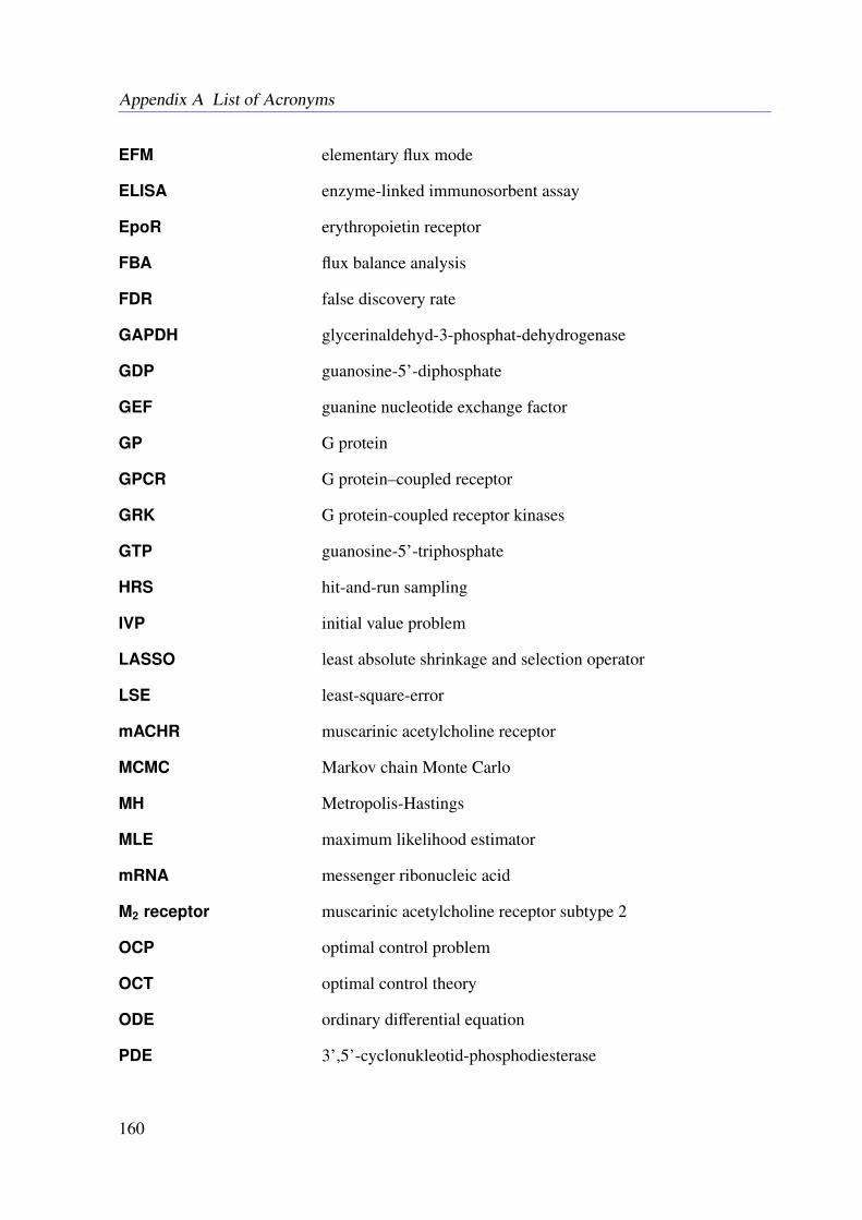
Appendix A List of Acronyms
EFM elementary flux mode
ELISA enzyme-linked immunosorbent assay
EpoR erythropoietin receptor
FBA flux balance analysis
FDR false discovery rate
GAPDH glycerinaldehyd-3-phosphat-dehydrogenase
GDP guanosine-5’-diphosphate
GEF guanine nucleotide exchange factor
GP G protein
GPCR G protein–coupled receptor
GRK G protein-coupled receptor kinases
GTP guanosine-5’-triphosphate
HRS hit-and-run sampling
IVP initial value problem
LASSO least absolute shrinkage and selection operator
LSE least-square-error
mACHR muscarinic acetylcholine receptor
MCMC Markov chain Monte Carlo
MH Metropolis-Hastings
MLE maximum likelihood estimator
mRNA messenger ribonucleic acid
M2 receptor muscarinic acetylcholine receptor subtype 2
OCP optimal control problem
OCT optimal control theory
ODE ordinary differential equation
PDE 3’,5’-cyclonukleotid-phosphodiesterase
160

PKA protein kinase A
PKC protein kinase C
PTX pertussis toxin
pUCR1 phosphorylated upstream conserved region 1
QSSA quasi-steady-state approximation
RGS regulators of G protein signaling
RWG resonant waveguide grating
STAT5 signal transducer and activator of transcription 5
UV-B ultraviolet B
WB western blotting
YM YM-254890
161


APPENDIX B
M2 Receptor-dependent Signaling inCHO Cells
Material and Methods
Cell Culture
Flp-In™-CHO cells stably expressing the hM2 receptor (CHO-hM2 cells) were cultured asdescribed previously in Ham’s nutrient mixture F-12 (Ham’s F-12) supplemented with 10%(v/v) fetal calf serum (FCS), 100 U mL-1 penicillin, 100 mg mL-1 streptomycin and 2 mMl-glutamine (Sigma Aldrich, UK) (Schrage et al., 2013) . The cells were grown in a humidifiedincubator at 37 °C and 5% CO2, and passaged by trypsinization at nearly confluence.
cAMP Assay
The quantification of the agonist-induced rise of the intracellular cAMP was performed usingCHO-hM2 cells pretreated with 50 ng/ml-1 PTX for 16-22 h as described previously using theHTRF-cAMP dynamic kit (Cisbio, Bagnols-sur-Cèze, France) according to the manufacturer’sintroductions (Schröder et al., 2009). The cells were incubated for 30 minutes with iperoxo. Thefluorescence was quantified on a Mithras LB 940 reader (Berthold Technologies, Bad Wildbad,Germany).
Western Blots
Cells were seeded into 6 well plates and stimulated with 0.1 µM iperoxo for 2, 5, 10, 15, 20,30 minutes. After specified treatments, cellular lysates were prepared in lysis buffer [25 mMHepes, 2.5 mM EDTA, 50 mM NaCl, 50 mM NaF, 30 mM sodium pyrophosphate, 10% (v/v)glycerol, 1% (v/v) Triton X-100, pH 7.5, containing Complete™ EDTA-free protease inhibitorcocktail tablets (Roche)].
163
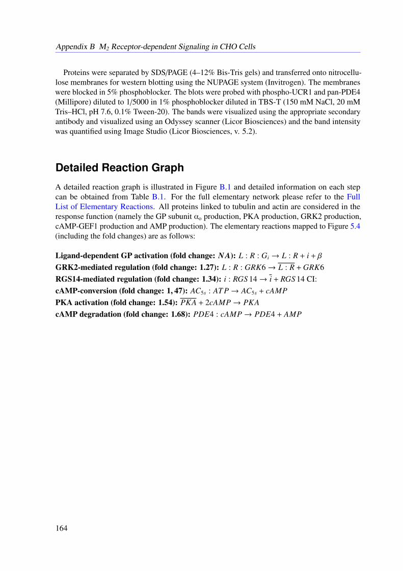
Appendix B M2 Receptor-dependent Signaling in CHO Cells
Proteins were separated by SDS/PAGE (4–12% Bis-Tris gels) and transferred onto nitrocellu-lose membranes for western blotting using the NUPAGE system (Invitrogen). The membraneswere blocked in 5% phosphoblocker. The blots were probed with phospho-UCR1 and pan-PDE4(Millipore) diluted to 1/5000 in 1% phosphoblocker diluted in TBS-T (150 mM NaCl, 20 mMTris–HCl, pH 7.6, 0.1% Tween-20). The bands were visualized using the appropriate secondaryantibody and visualized using an Odyssey scanner (Licor Biosciences) and the band intensitywas quantified using Image Studio (Licor Biosciences, v. 5.2).
Detailed Reaction Graph
A detailed reaction graph is illustrated in Figure B.1 and detailed information on each stepcan be obtained from Table B.1. For the full elementary network please refer to the FullList of Elementary Reactions. All proteins linked to tubulin and actin are considered in theresponse function (namely the GP subunit αo production, PKA production, GRK2 production,cAMP-GEF1 production and AMP production). The elementary reactions mapped to Figure 5.4(including the fold changes) are as follows:
Ligand-dependent GP activation (fold change: N A): L : R : Gi → L : R + i + β
GRK2-mediated regulation (fold change: 1.27): L : R : GRK6→ L : R + GRK6RGS14-mediated regulation (fold change: 1.34): i : RGS 14→ i + RGS 14 CI:cAMP-conversion (fold change: 1, 47): AC5s : AT P→ AC5s + cAMPPKA activation (fold change: 1.54): PKA + 2cAMP→ PKAcAMP degradation (fold change: 1.68): PDE4 : cAMP→ PDE4 + AMP
164
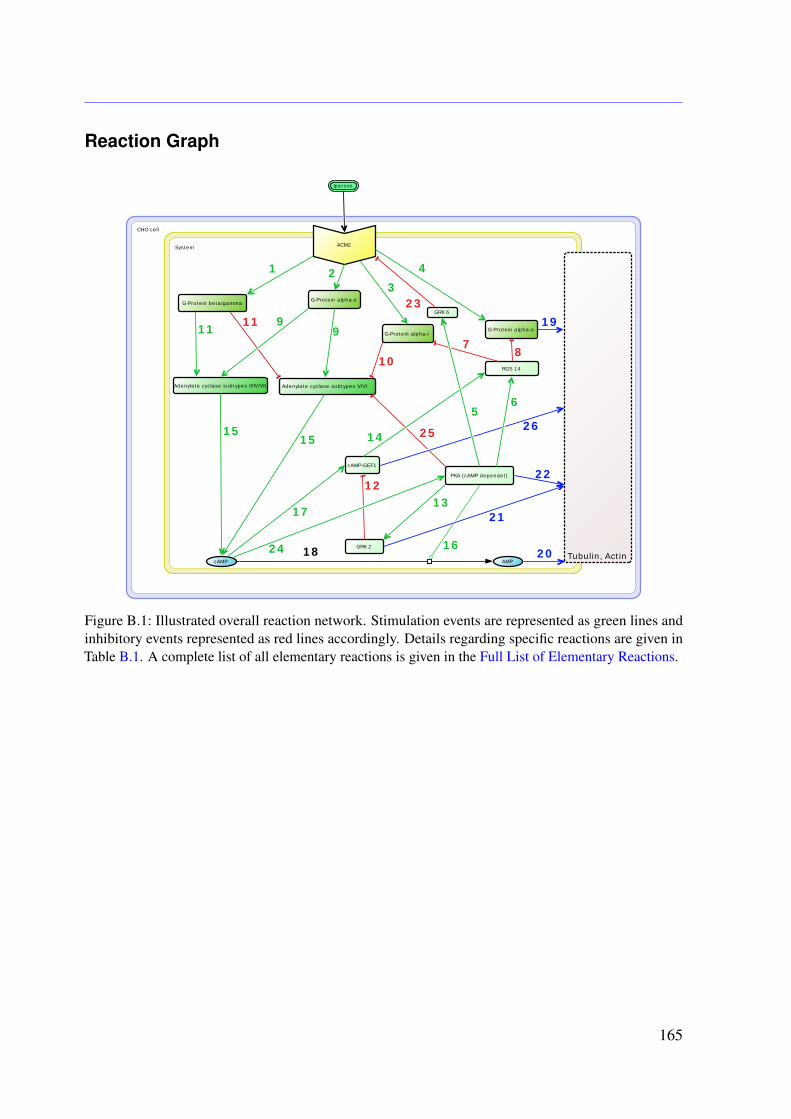
Reaction Graph
System
CHO cell
Tubulin, Actin
ACM2
cAMP
G-Protein alpha-sG-Protein beta/gamma
PKA (cAMP dependet)
Adenylate cyclase subtypes II/IV/VII
cAMP-GEF1
GRK 2
GRK 6
G-Protein alpha-i
RGS 14
AMP
Adenylate cyclase subtypes V/VI
Iperoxo
G-Protein alpha-o
1 23
4
56
78
99
10
1111
1213
141515
16
17
1824
23
19
20
21
22
25 26
Figure B.1: Illustrated overall reaction network. Stimulation events are represented as green lines andinhibitory events represented as red lines accordingly. Details regarding specific reactions are given inTable B.1. A complete list of all elementary reactions is given in the Full List of Elementary Reactions.
165

Appendix B M2 Receptor-dependent Signaling in CHO Cells
Table B.1: Basic reactions in the modeled biological system: Species shown in the column “From” arebiochemically converted into those shown in the column “To”. The underlying biological mechanismand its effect on the species in column “To” are shown in the fourth and fifth columns, respectively. Wedistinguish between binding, phosporylation, transformation, catalysis and unspecific chemical reactions.The effect of unspecific chemical reactions is denoted as “technical” because they are neither activatingnor inhibiting. The derived elementary reactions can be found in the Full List of Elementary Reactions.
Nr. From To Mechanism Effect Lead Author, Year, Journal[Impact]
1 ACM2 G-Protein beta/gamma binding activation Wettschurek N, 2005, Physiol Rev.[30.2]2 ACM2 G-Protein alpha-s transformation activation Cao J, 2003, Bioinformatics.[5.3]3 ACM2 G-Protein alpha-i family transformation activation Wettschurek N, 2005, Physiol Rev.[30.2]4 ACM2 G-Protein alpha-o transformation activation Azpiazu I, 2004, J Biol Chem.[4.56]5 PKA-cat (cAMP-dependent) GRK6 phosphorylation inhibition Rapacciulolo A, 2003, J Biol Chem.[4.56]6 PKA-cat (cAMP-dependent) RGS14 phosphorylation activation Riddle EL, 2005, Circ Res.[11.86]7 RGS14 G-Protein alpha-i family transformation inhibition Kimple RJ, 2002, Nature.[38.58]8 RGS14 G-Protein alpha-o transformation inhibition Rual JF, 2005, Nature.[38.58]9 G-Protein alpha-s Adenylate cyclase binding activation Pourquie O, 2005, Nature[38.58]10 G-Protein alpha-i Adenylate cyclase subtype 5 binding inhibition Taussig R, 1993, Science.[31.03]10 G-Protein alpha-i Adenylate cyclase subtype 6 binding inhibition Taussig R, 1993, Science.[31,03]11 G-Protein beta/gamma Adenylate cyclase subtype 2 binding activation Sunahara RK, 2002, Mol Interv[6.48]11 G-Protein beta/gamma Adenylate cyclase subtype 4 binding activation Sunahara RK, 2002, Mol Interv[6.48]11 G-Protein beta/gamma Adenylate cyclase subtype 5 binding inhibition Sunahara RK, 2002, Mol Interv[6.48]11 G-Protein beta/gamma Adenylate cyclase subtype 6 binding inhibition Sunahara RK, 2002, Mol Interv[6.48]11 G-Protein beta/gamma Adenylate cyclase subtype 7 binding activation Sunahara RK, 2002, Mol Interv[6.48]12 GRK2 cAMP-GEFI binding inhibition Eijkelkamp N, 2010, J Neurosci.[7.3]13 PKA-cat (cAMP-dependent) GRK2 phosphorylation activation Cong M, 2001, J Biol Chem.[4.65]14 cAMP-GEFI RAP-2A transformation activation Ohba Y, 2000, Mol Cell Biol.[5.37]14 RAP-2A RGS14 binding activation Bandyopadhyay S, 2010, Nat Methods.[23.57]15 Adenylate cyclase ATP = cyclic AMP + Pyrophosphate catalysis activation Wong ST, 2000, Neuron.[15.77]16 PKA-cat (cAMP-dependent) PDE4B phosphorylation activation Ghigo A, 2012, Circulation.[15.20]16 PDE4B cyclic AMP + H(,2)O = AMP catalysis activation Huston E, 1997, Biochem J.[5.37]17 cyclic AMP intracellular cAMP-GEFI binding activation Do Rooij Z, 1998, Nature.[38.58]18 ATP in cytoplasm ATP = cyclic AMP + Pyrophosphate reaction technical18 ATP = cyclic AMP + Pyrophosphate cyclic AMP intracellular reaction technical18 cyclic AMP intracellular cyclic AMP + H(,2)O = AMP reaction technical18 cyclic AMP + H(,2)O = AMP AMP in cytoplasm reaction technical19 G-Protein alpha-o Tubulin (in microtubules) transformation inhibition Roychowdhury S, 1999, J Biol Chem.[4.65]20 AMP Tubulin (in microtubules) transformation inhibition Lee JH, 2007, Nat. [41.46]21 GRK2 Tubulin (in microtubules) phosphorylation activation Storti B, 2012, J Biol Chem.[4.65]22 PKA-cat (cAMP-dependent) Actin cytoskeletal phosphorylation inhibition Howe AK, 2004 Biochim Biophys Acta.[5.54]23 GRK6 ACM2 phosphorylation inhibition Loudon RP, 1994, J Biol Chem.[4.65]24 cyclic AMP intracellular PKA-reg (cAMP-dependent) binding activation Lin JY, 2007, Nat.[38.58]24 PKA-reg (cAMP-dependent) PKA-cat (cAMP-dependent) binding activation Ghigo A, 2012, Circulation.[15.20]25 PKA-cat (cAMP-dependent) Adenylate cyclase subtype 5 phosphorylation inhibition Iwami G, 1995, J Biol Chem.[4.65]25 PKA-cat (cAMP-dependent) Adenylate cyclase subtype 6 phosphorylation inhibition Defer N, 2000, Am J Physiol Renal Physiol.[9.73]26 cAMP-GEFI AKT1 binding activation Misra UK, 2005, J Biol Chem.[4.65]
A ACM2 ACM2 several regulation Pierce KL, 2002, Nat Rev Mol Cell Biol.[37.16]B ACM2 G protein spontaneous activation Trzaskowski B, 2012, Curr Med Chem.[3.85].
166

Full List of Elementary Reactions
The first number (red) counts the reaction, the second number is linked to Table B.1. Fluxesinvolved in the cellular response as defined in Section 5.4.2 are marked by “*“.
L + R L : R (1|A)
R→ R (2|A)
L : R→ L : R (3|A)
R + GRK6 GRK6 : R (4|23)
GRK6 : R→ R + GRK6 (5|23)
L : R + GRK6 L : R : GRK6 (6|23)
L : R : GRK6→ L : R + GRK6 (7|23)
L : R R + L (8|A)
R + Gs R : Gs (9|1; 2; B)
R : Gs → R + s + β/γ (10|1; 2; B)
R + Gi R : Gi (11|1; 3; B)
R : Gi → R + i + β/γ (12|1; 3; B)
R + Go R : Go (13|1; 4; B)
R : Go → R + o + β/γ * (14|1; 4; B)
L : R + Gs L : R : Gs (15|1; 2)
L : R : Gs → L : R + s + β/γ (16|1; 2)
s→ s (17|2)
L : R + Gi LR : Gi (18|1; 3)
L : R : Gi → L : R + i + β/γ (19|1; 3)
i + RGS 14 i : RGS 14 (20|7)
i : RGS 14→ i + RGS 14 (21|7)
β/γ + i Gi (22|1; 3)
β/γ + s Gs (23|2; 3)
L : R + Go L : R : Go (24|1; 4)
L : R : Go → L : R + o + β/γ * (25|1; 4)
β/γ + o Go (26|1; 4)
o + RGS 14 o : RGS 14 (27|8)
o : RGS 14→ o + RGS 14 (28|8)
β/γ + AC4 AC4β (29|11)
s + AC4 AC4s (30|9)
s + AC4β AC4β/γs (31|9; 11)
β/γ + AC4s AC4β/γs (32|9; 11)
i + AC5 AC5i (33|10)
s + AC5 AC5s (34|9)
β/γ + AC5 AC5β/γ (35|11)
β/γ + AC5s AC5β/γs (36|9)
s + AC5β/γ AC5β/γs (37|9; 11)
i + AC5s AC5si (38|9; 10)
s + AC5i AC5si (39|9; 10)
AC4s AC4s : AT P (40|15)
AC4s : AT P→ AC4s + cAMP (41|15)
AC4βs AC4β/γs : AT P (42|15)
AC4β/γs : AT P→ AC4β/γs + cAMP (43|15)
β/γ + s + AC4 AC4β/γs (44|9; 11)
AC5 + i + s AC5is (45|10; 11)
AC5 + β/γ + s AC5β/γs (46|9; 11)
AC5s AC5s : AT P (47|15)
AC5s : AT P→ AC5s + cAMP (48|15)
ACp5 + s ACp
5s (49|9)
ACp5s ACp
5s : AT P (50|15)
ACp5s : AT P→ ACp
5s + cAMP (51|15)
AC5 + PKA AC5 : PKA (52|25)
AC5 : PKA→ ACp5 + PKA (53|25)
ACp5 → AC5 (54|25)
AC5s + PKA AC5s : PKA (55|25)
AC5s : PKA→ ACp5s + PKA (56|25)
PKA→ PKA (57|24)
PKA + 2cAMP→ PKA * (58|24)
PKA + RGS 14 PKA : RGS 14 (59|6)
PKA : RGS 14→ RGS 14 + PKA (60|6)
RGS 14→ RGS 14 (61|6)
PKA + GRK2 PKA : GRK2 (62|13)
PKA : GRK2→ GRK2 + PKA * (63|13)
GRK2→ GRK2 (64|13)
PKA + GRK6 PKA : GRK6 (65|5)
PKA : GRK6→ GRK6 + PKA (66|5)
GRK6→ GRK6 (67|5)
PKA + PDE4 PKA : PDE4 (68|16)
PKA : PDE4→ PDE4 + PKA (69|16)
PDE4→ PDE4 (70|16)
PDE4 + cAMP PDE4 : cAMP (71|16)
PDE4 : cAMP→ PDE4 + AMP (72|16)
AMP→ ∅ (73|18)
GEF + RGS 14 GEF : RGS 14 (74|14)
GEF : RGS 14→ RGS 14 + GEF (75|14)
GRK2 + GEF GRK2 : GEF (76|12)
GRK2 : GEF → GRK2 + GEF (77|12)
GEF → GEF (78|17, 12)
cAMP + GEF GEF * (79|17)
X : Y = Complex of X and Y
X = Inactive form of protein X
Xp = Phosphorylated protein
167
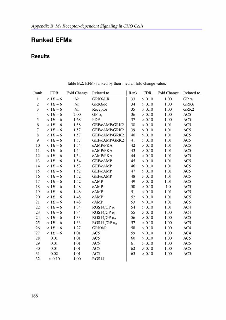
Appendix B M2 Receptor-dependent Signaling in CHO Cells
Ranked EFMs
Results
Table B.2: EFMs ranked by their median fold change value.
Rank FDR Fold Change Related to Rank FDR Fold Change Related to1 < 1E − 6 Na GRK6/LR 33 > 0.10 1.00 GP αs2 < 1E − 6 Na GRK6/R 34 > 0.10 1.00 GRK63 < 1E − 6 Na Receptor 35 > 0.10 1.00 GRK24 < 1E − 6 2.00 GP αs 36 > 0.10 1.00 AC55 < 1E − 6 1.68 PDE 37 > 0.10 1.00 AC56 < 1E − 6 1.58 GEF/cAMP/GRK2 38 > 0.10 1.01 AC57 < 1E − 6 1.57 GEF/cAMP/GRK2 39 > 0.10 1.01 AC58 < 1E − 6 1.57 GEF/cAMP/GRK2 40 > 0.10 1.01 AC59 < 1E − 6 1.57 GEF/cAMP/GRK2 41 > 0.10 1.01 AC5
10 < 1E − 6 1.54 cAMP/PKA 42 > 0.10 1.01 AC511 < 1E − 6 1.54 cAMP/PKA 43 > 0.10 1.01 AC512 < 1E − 6 1.54 cAMP/PKA 44 > 0.10 1.01 AC513 < 1E − 6 1.54 GEF/cAMP 45 > 0.10 1.01 AC514 < 1E − 6 1.53 GEF/cAMP 46 > 0.10 1.01 AC515 < 1E − 6 1.52 GEF/cAMP 47 > 0.10 1.01 AC516 < 1E − 6 1.52 GEF/cAMP 48 > 0.10 1.01 AC517 < 1E − 6 1.52 cAMP 49 > 0.10 1.01 AC518 < 1E − 6 1.48 cAMP 50 > 0.10 1.0 AC519 < 1E − 6 1.48 cAMP 51 > 0.10 1.01 AC520 < 1E − 6 1.48 cAMP 52 > 0.10 1.01 AC521 < 1E − 6 1.48 cAMP 53 > 0.10 1.01 AC522 < 1E − 6 1.34 RGS14/GP αi 54 > 0.10 1.01 AC423 < 1E − 6 1.34 RGS14/GP αi 55 > 0.10 1.00 AC424 < 1E − 6 1.33 RGS14/GP αo 56 > 0.10 1.00 AC525 < 1E − 6 1.33 RGS14 /GP αo 57 > 0.10 1.00 AC526 < 1E − 6 1.27 GRK6/R 58 > 0.10 1.00 AC427 < 1E − 6 1.01 AC5 59 > 0.10 1.00 AC428 0.01 1.01 AC5 60 > 0.10 1.00 AC529 0.01 1.01 AC5 61 > 0.10 1.00 AC530 0.01 1.01 AC5 62 > 0.10 1.00 AC531 0.02 1.01 AC5 63 > 0.10 1.00 AC532 > 0.10 1.00 RGS14
168
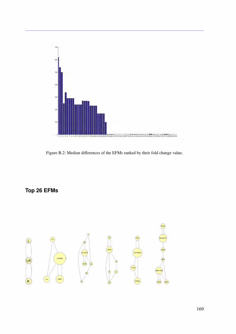
Figure B.2: Median differences of the EFMs ranked by their fold change value.
Top 26 EFMs
169
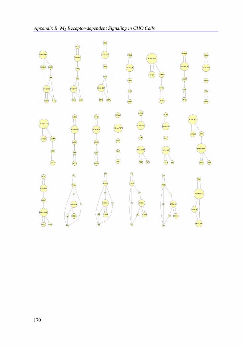
Appendix B M2 Receptor-dependent Signaling in CHO Cells
170
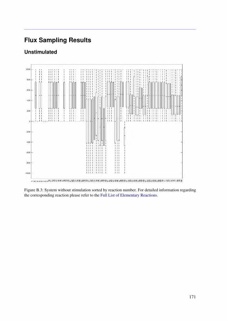
Flux Sampling Results
Unstimulated
Figure B.3: System without stimulation sorted by reaction number. For detailed information regardingthe corresponding reaction please refer to the Full List of Elementary Reactions.
171
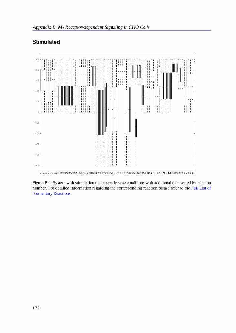
Appendix B M2 Receptor-dependent Signaling in CHO Cells
Stimulated
Figure B.4: System with stimulation under steady state conditions with additional data sorted by reactionnumber. For detailed information regarding the corresponding reaction please refer to the Full List ofElementary Reactions.
172
APPENDIX C
The Dynamic Elastic-Net
Software
The simulations were performed in MATLAB (R2014a, The MathWorks, Inc.) using TOMLABv8.0 with SQOPT 7.2-5 QP and SNOPT 7.2-5 NLP (Tomlab Optimization AB) for solvingthe optimal control problems. The computing time for a single run of the DEN on a laptop(Intel® CoreTM i5-4200M CPU with 4× 2.50GHz and 16 GB RAM) was on average 1 min.
Analysis of the Dynamic Elastic-Net Optimal ControlProblem
To gain a deeper understanding of the DEN we assume that the output y(t) of the underlyingtrue system
x(t) = f (x(t),u(t)) + w(t) (C.1a)y(t) = h(x(t)) (C.1b)
with initial conditions x(0) = x0 can be measured for all time points t in the interval [0, F].Accordingly, the error functional (Equation (6.4)) is replaced by the continuous time errorfunctional
J (x (t) , w (t)) =
∫ F
0‖y(t) − y(t)‖2Q(t) + α1‖w(t)‖1 +
α2
2‖w(t)‖22dt (C.2a)
=
∫ F
0
I∑i=1
I∑j=1
[qi j(t) (yi(t) − yi(t))
(y j(t) − y j(t)
)]+
N∑n=1
[α1|wn(t)| +
α2
2w2
n(t)]
dt (C.2b)
173
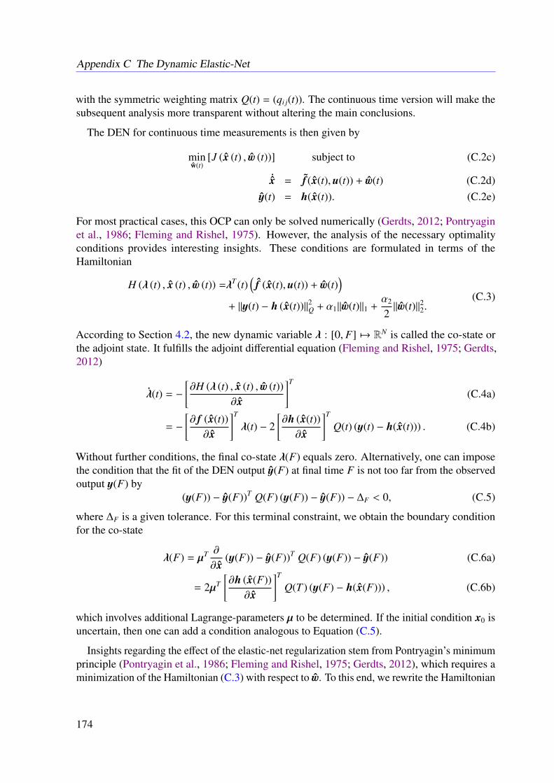
Appendix C The Dynamic Elastic-Net
with the symmetric weighting matrix Q(t) = (qi j(t)). The continuous time version will make thesubsequent analysis more transparent without altering the main conclusions.
The DEN for continuous time measurements is then given by
minw(t)
[J (x (t) , w (t))] subject to (C.2c)
˙x = f (x(t),u(t)) + w(t) (C.2d)y(t) = h(x(t)). (C.2e)
For most practical cases, this OCP can only be solved numerically (Gerdts, 2012; Pontryaginet al., 1986; Fleming and Rishel, 1975). However, the analysis of the necessary optimalityconditions provides interesting insights. These conditions are formulated in terms of theHamiltonian
H (λ (t) , x (t) , w (t)) =λT (t)(
f (x(t),u(t)) + w(t))
+ ‖y(t) − h (x(t))‖2Q + α1‖w(t)‖1 +α2
2‖w(t)‖22.
(C.3)
According to Section 4.2, the new dynamic variable λ : [0, F] 7→ RN is called the co-state orthe adjoint state. It fulfills the adjoint differential equation (Fleming and Rishel, 1975; Gerdts,2012)
λ(t) = −
[∂H (λ (t) , x (t) , w (t))
∂x
]T
(C.4a)
= −
[∂ f (x(t))∂x
]T
λ(t) − 2[∂h (x(t))∂x
]T
Q(t) (y(t) − h(x(t))) . (C.4b)
Without further conditions, the final co-state λ(F) equals zero. Alternatively, one can imposethe condition that the fit of the DEN output y(F) at final time F is not too far from the observedoutput y(F) by
(y(F)) − y(F))T Q(F) (y(F)) − y(F)) − ∆F < 0, (C.5)
where ∆F is a given tolerance. For this terminal constraint, we obtain the boundary conditionfor the co-state
λ(F) = µT ∂
∂x(y(F)) − y(F))T Q(F) (y(F)) − y(F)) (C.6a)
= 2µT
[∂h (x(F))
∂x
]T
Q(T ) (y(F) − h(x(F))) , (C.6b)
which involves additional Lagrange-parameters µ to be determined. If the initial condition x0 isuncertain, then one can add a condition analogous to Equation (C.5).
Insights regarding the effect of the elastic-net regularization stem from Pontryagin’s minimumprinciple (Pontryagin et al., 1986; Fleming and Rishel, 1975; Gerdts, 2012), which requires aminimization of the Hamiltonian (C.3) with respect to w. To this end, we rewrite the Hamiltonian
174
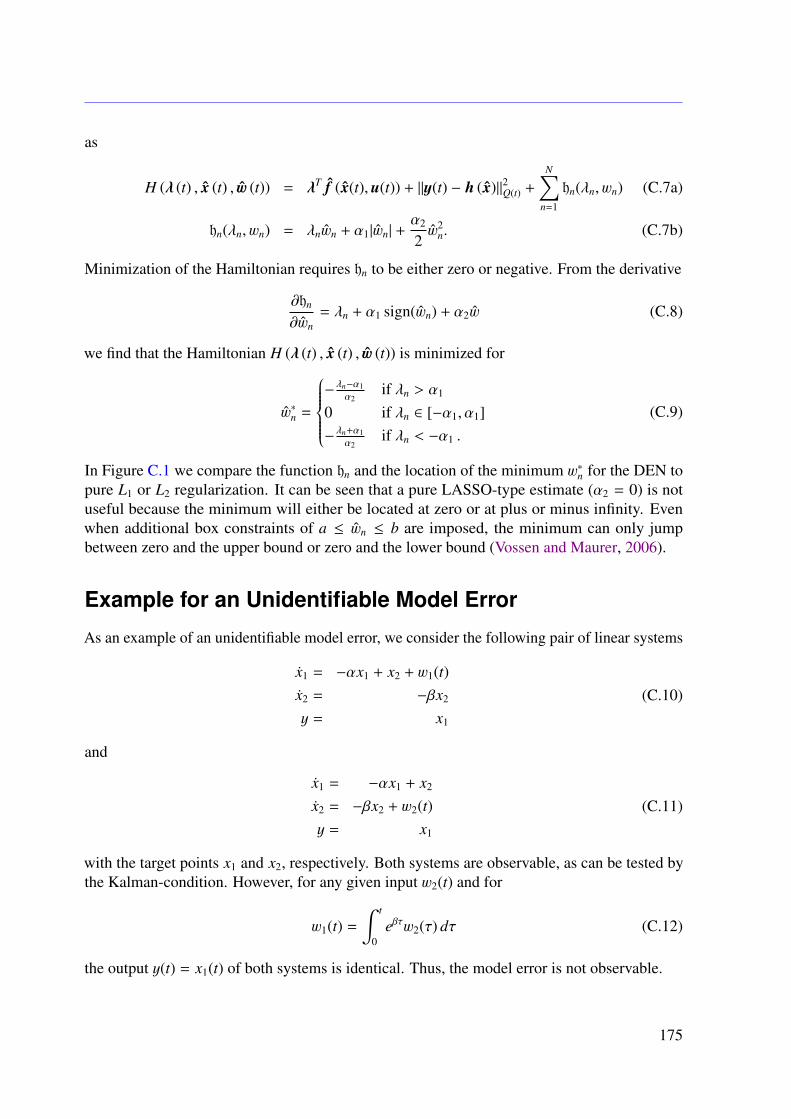
as
H (λ (t) , x (t) , w (t)) = λT f (x(t),u(t)) + ‖y(t) − h (x)‖2Q(t) +
N∑n=1
hn(λn, wn) (C.7a)
hn(λn, wn) = λnwn + α1|wn| +α2
2w2
n. (C.7b)
Minimization of the Hamiltonian requires hn to be either zero or negative. From the derivative
∂hn∂wn
= λn + α1 sign(wn) + α2w (C.8)
we find that the Hamiltonian H (λ (t) , x (t) , w (t)) is minimized for
w∗n =
−λn−α1α2
if λn > α1
0 if λn ∈ [−α1, α1]−λn+α1α2
if λn < −α1 .
(C.9)
In Figure C.1 we compare the function hn and the location of the minimum w∗n for the DEN topure L1 or L2 regularization. It can be seen that a pure LASSO-type estimate (α2 = 0) is notuseful because the minimum will either be located at zero or at plus or minus infinity. Evenwhen additional box constraints of a ≤ wn ≤ b are imposed, the minimum can only jumpbetween zero and the upper bound or zero and the lower bound (Vossen and Maurer, 2006).
Example for an Unidentifiable Model Error
As an example of an unidentifiable model error, we consider the following pair of linear systems
x1 = −αx1 + x2 + w1(t)x2 = −βx2
y = x1
(C.10)
and
x1 = −αx1 + x2
x2 = −βx2 + w2(t)y = x1
(C.11)
with the target points x1 and x2, respectively. Both systems are observable, as can be tested bythe Kalman-condition. However, for any given input w2(t) and for
w1(t) =
∫ t
0eβτw2(τ) dτ (C.12)
the output y(t) = x1(t) of both systems is identical. Thus, the model error is not observable.
175
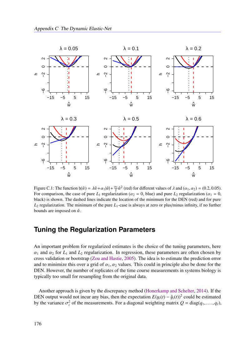
Appendix C The Dynamic Elastic-Net
−15 −5 5 15
−6
−2
02
w
h
λ = 0.05
−15 −5 5 15
−6
−2
02
w
h
λ = 0.1
−15 −5 5 15
−6
−2
02
w
h
λ = 0.2
−15 −5 5 15
−6
−2
02
w
h
λ = 0.3
−15 −5 5 15
−6
−2
02
w
h
λ = 0.5
−15 −5 5 15−
6−
20
2
w
h
λ = 0.6
Figure C.1: The function h(w) = λw+α1|w|+α22 w
2 (red) for different values of λ and (α1, α2) = (0.2, 0.05).For comparison, the case of pure L1 regularization (α2 = 0, blue) and pure L2 regularization (α1 = 0,black) is shown. The dashed lines indicate the location of the minimum for the DEN (red) and for pureL2 regularization. The minimum of the pure L1-case is always at zero or plus/minus infinity, if no furtherbounds are imposed on w.
Tuning the Regularization Parameters
An important problem for regularized estimates is the choice of the tuning parameters, hereα1 and α2 for L1 and L2 regularization. In regression, these parameters are often chosen bycross validation or bootstrap (Zou and Hastie, 2005). The idea is to estimate the prediction errorand to minimize this over a grid of α1, α2 values. This could in principle also be done for theDEN. However, the number of replicates of the time course measurements in systems biology istypically too small for resampling from the original data.
Another approach is given by the discrepancy method (Honerkamp and Schelter, 2014). If theDEN output would not incur any bias, then the expectation E(yi(t) − yi(t))2 could be estimatedby the variance σ2
i of the measurements. For a diagonal weighting matrix Q = diag(q1, . . . , qI),
176
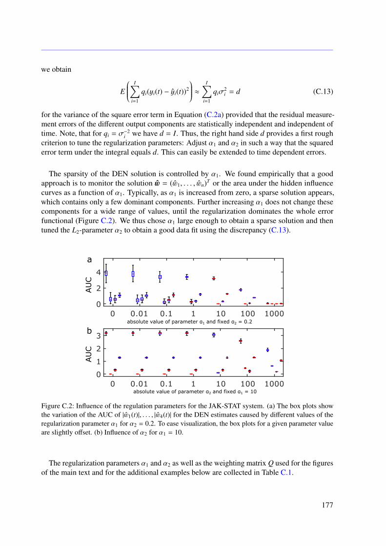
we obtain
E
I∑i=1
qi(yi(t) − yi(t))2
≈ I∑i=1
qiσ2i = d (C.13)
for the variance of the square error term in Equation (C.2a) provided that the residual measure-ment errors of the different output components are statistically independent and independent oftime. Note, that for qi = σ−2
i we have d = I. Thus, the right hand side d provides a first roughcriterion to tune the regularization parameters: Adjust α1 and α2 in such a way that the squarederror term under the integral equals d. This can easily be extended to time dependent errors.
The sparsity of the DEN solution is controlled by α1. We found empirically that a goodapproach is to monitor the solution w = (w1, . . . , wn)T or the area under the hidden influencecurves as a function of α1. Typically, as α1 is increased from zero, a sparse solution appears,which contains only a few dominant components. Further increasing α1 does not change thesecomponents for a wide range of values, until the regularization dominates the whole errorfunctional (Figure C.2). We thus chose α1 large enough to obtain a sparse solution and thentuned the L2-parameter α2 to obtain a good data fit using the discrepancy (C.13).
Figure C.2: Influence of the regulation parameters for the JAK-STAT system. (a) The box plots showthe variation of the AUC of |w1(t)|, . . . , |w4(t)| for the DEN estimates caused by different values of theregularization parameter α1 for α2 = 0.2. To ease visualization, the box plots for a given parameter valueare slightly offset. (b) Influence of α2 for α1 = 10.
The regularization parameters α1 and α2 as well as the weighting matrix Q used for the figuresof the main text and for the additional examples below are collected in Table C.1.
177
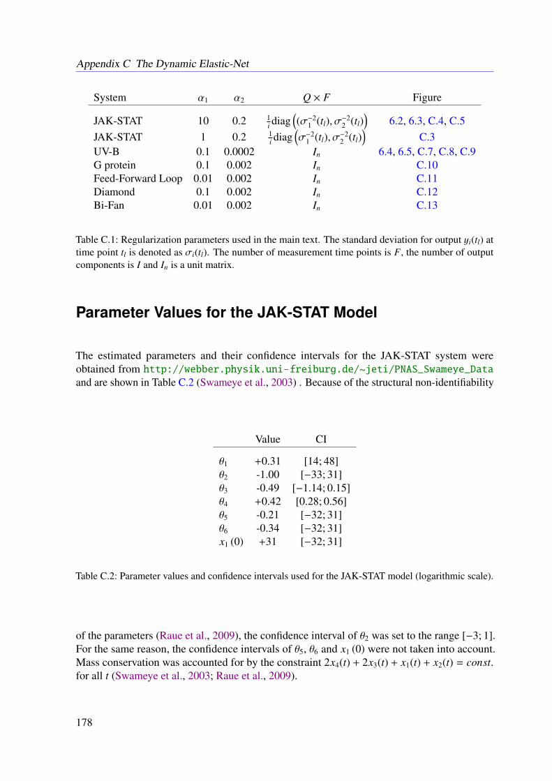
Appendix C The Dynamic Elastic-Net
System α1 α2 Q × F Figure
JAK-STAT 10 0.2 1i diag
((σ−2
1 (tl), σ−22 (tl)
)6.2, 6.3, C.4, C.5
JAK-STAT 1 0.2 1i diag
(σ−2
1 (tl), σ−22 (tl)
)C.3
UV-B 0.1 0.0002 In 6.4, 6.5, C.7, C.8, C.9G protein 0.1 0.002 In C.10Feed-Forward Loop 0.01 0.002 In C.11Diamond 0.1 0.002 In C.12Bi-Fan 0.01 0.002 In C.13
Table C.1: Regularization parameters used in the main text. The standard deviation for output yi(tl) attime point tl is denoted as σi(tl). The number of measurement time points is F, the number of outputcomponents is I and In is a unit matrix.
Parameter Values for the JAK-STAT Model
The estimated parameters and their confidence intervals for the JAK-STAT system wereobtained from http://webber.physik.uni-freiburg.de/~jeti/PNAS_Swameye_Dataand are shown in Table C.2 (Swameye et al., 2003) . Because of the structural non-identifiability
Value CI
θ1 +0.31 [14; 48]θ2 -1.00 [−33; 31]θ3 -0.49 [−1.14; 0.15]θ4 +0.42 [0.28; 0.56]θ5 -0.21 [−32; 31]θ6 -0.34 [−32; 31]x1 (0) +31 [−32; 31]
Table C.2: Parameter values and confidence intervals used for the JAK-STAT model (logarithmic scale).
of the parameters (Raue et al., 2009), the confidence interval of θ2 was set to the range [−3; 1].For the same reason, the confidence intervals of θ5, θ6 and x1 (0) were not taken into account.Mass conservation was accounted for by the constraint 2x4(t) + 2x3(t) + x1(t) + x2(t) = const.for all t (Swameye et al., 2003; Raue et al., 2009).
178
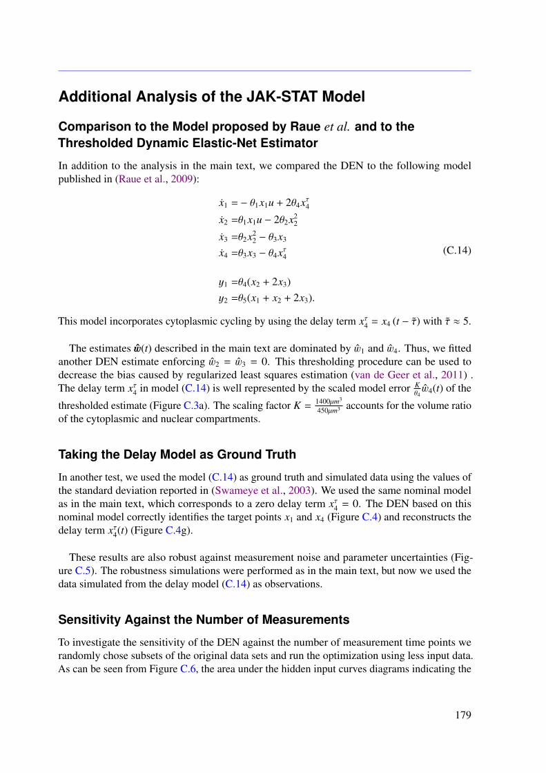
Additional Analysis of the JAK-STAT Model
Comparison to the Model proposed by Raue et al. and to theThresholded Dynamic Elastic-Net Estimator
In addition to the analysis in the main text, we compared the DEN to the following modelpublished in (Raue et al., 2009):
x1 = − θ1x1u + 2θ4xτ4x2 =θ1x1u − 2θ2x2
2
x3 =θ2x22 − θ3x3
x4 =θ3x3 − θ4xτ4
y1 =θ4(x2 + 2x3)y2 =θ5(x1 + x2 + 2x3).
(C.14)
This model incorporates cytoplasmic cycling by using the delay term xτ4 = x4 (t − τ) with τ ≈ 5.
The estimates w(t) described in the main text are dominated by w1 and w4. Thus, we fittedanother DEN estimate enforcing w2 = w3 = 0. This thresholding procedure can be used todecrease the bias caused by regularized least squares estimation (van de Geer et al., 2011) .The delay term xτ4 in model (C.14) is well represented by the scaled model error K
θ4w4(t) of the
thresholded estimate (Figure C.3a). The scaling factor K =1400µm3
450µm3 accounts for the volume ratioof the cytoplasmic and nuclear compartments.
Taking the Delay Model as Ground Truth
In another test, we used the model (C.14) as ground truth and simulated data using the values ofthe standard deviation reported in (Swameye et al., 2003). We used the same nominal modelas in the main text, which corresponds to a zero delay term xτ4 = 0. The DEN based on thisnominal model correctly identifies the target points x1 and x4 (Figure C.4) and reconstructs thedelay term xτ4(t) (Figure C.4g).
These results are also robust against measurement noise and parameter uncertainties (Fig-ure C.5). The robustness simulations were performed as in the main text, but now we used thedata simulated from the delay model (C.14) as observations.
Sensitivity Against the Number of Measurements
To investigate the sensitivity of the DEN against the number of measurement time points werandomly chose subsets of the original data sets and run the optimization using less input data.As can be seen from Figure C.6, the area under the hidden input curves diagrams indicating the
179
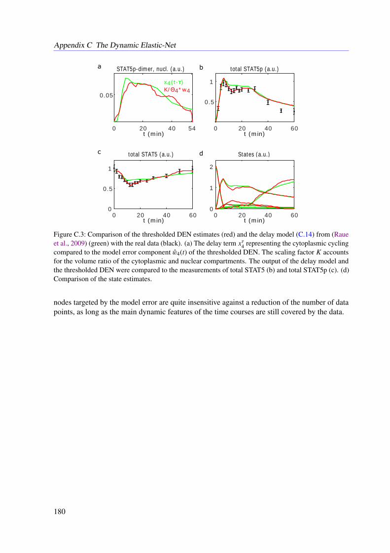
Appendix C The Dynamic Elastic-Net
0 20 40 600
0.5
1
0 20 40 60
0.5
1
0 20 40 54
0.05
STAT5p-dimer, nucl. (a.u.)
total STAT5 (a.u.)
total STAT5p (a.u.)
States (a.u.)
t (min) t (min)
t (min) t (min)
x4(t-τ)K/Θ4*w4
0 20 40 600
1
2
Figure C.3: Comparison of the thresholded DEN estimates (red) and the delay model (C.14) from (Raueet al., 2009) (green) with the real data (black). (a) The delay term xτ4 representing the cytoplasmic cyclingcompared to the model error component w4(t) of the thresholded DEN. The scaling factor K accountsfor the volume ratio of the cytoplasmic and nuclear compartments. The output of the delay model andthe thresholded DEN were compared to the measurements of total STAT5 (b) and total STAT5p (c). (d)Comparison of the state estimates.
nodes targeted by the model error are quite insensitive against a reduction of the number of datapoints, as long as the main dynamic features of the time courses are still covered by the data.
180
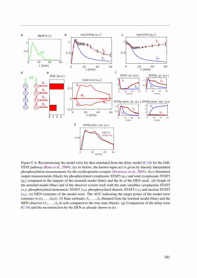
0 20 40 60
1
2
3
0 20 40 60
0.1
0.2
0 20 40 60
0.5
1.2
0 20 40 60
1
2
0 20 40 60-0.1
0
0.1
0 20 40 60
0.5
1
0 20 40 60
0.5
1
u(t)
x1
x2
x3
x4
w1
w2
w3
w4
a
c1
0.5
0 20 40 60
pEpoR (a.u.) total STAT5p (a.u.)
u(t) y 1
y 2
~y 2
w1
w4
w2
w3
model error (a.u.)STAT5, cyt. (a.u.)AUC (a.u.)
0 31 2
total STAT5 (a.u.)
STAT5p, cyt. (a.u.)
STAT5p-dimer, cyt. (a.u.) STAT5p-dimer, nucl. (a.u)
t (min)
t (min)t (min)
t (min)
t (min)
x^1 x^2
x^3
x^4
x~1 x~2
x~3
x~4
d
b
e
c
f
x^1
x^2
x^3
x^4
~y1
t (min)
t (min) t (min)
0 20 40 54
0.05
t(min)
STAT5p-dimer, nucl. (a.u.)
x4(t-τ)K/Θ4*w4
g
Figure C.4: Reconstructing the model error for data simulated from the delay model (C.14) for the JAK-STAT pathway (Raue et al., 2009). (a) As before, the known input u(t) is given by linearly interpolatedphosphorylation measurements for the erythropoietin receptor (Swameye et al., 2003). (b,c) Simulatedoutput measurements (black) for phosphorylated cytoplasmic STAT5 (y1) and total cytoplasmic STAT5(y2) compared to the outputs of the nominal model (blue) and the fit of the DEN (red). (d) Graph ofthe nominal model (blue) and of the observer system (red) with the state variables cytoplasmic STAT5(x1), phosphorylated monomeric STAT5 (x2), phosphorylated dimeric STAT5 (x3) and nuclear STAT5(x4). (e) DEN estimates of the model error. The AUC indicating the target points of the model errorestimates w1(t), . . . , w4(t). (f) State estimates x1, . . . , x4 obtained from the nominal model (blue) and theDEN observer (x1, . . . , x4 in red) compared to the true state (black). (g) Comparison of the delay term(C.14) and the reconstruction by the DEN as already shown in (e).
181
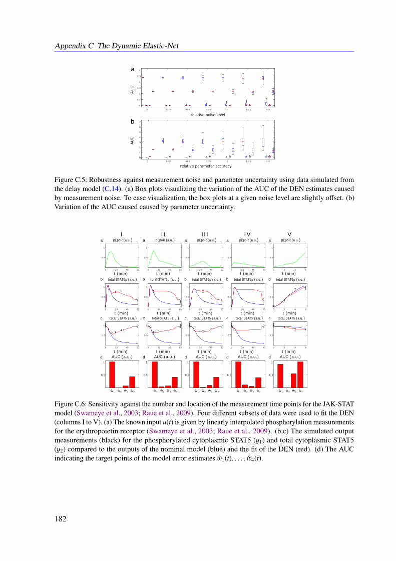
Appendix C The Dynamic Elastic-Net
Figure C.5: Robustness against measurement noise and parameter uncertainty using data simulated fromthe delay model (C.14). (a) Box plots visualizing the variation of the AUC of the DEN estimates causedby measurement noise. To ease visualization, the box plots at a given noise level are slightly offset. (b)Variation of the AUC caused caused by parameter uncertainty.
a
b total STAT5p (a.u.)
c
d
a
b total STAT5p (a.u.)
c
d
pEpoR (a.u.)
t (min)
t (min)
t (min)AUC (a.u.)
total STAT5 (a.u.)
IIIa
b total STAT5p (a.u.)
c
d
pEpoR (a.u.)
t (min)
t (min)
t (min)AUC (a.u.)
total STAT5 (a.u.)
IVa
b total STAT5p (a.u.)
c
d
pEpoR (a.u.)
t (min)
t (min)
t (min)AUC (a.u.)
total STAT5 (a.u.)
V
0 20 40 60
0.5
1
0 20 40 60
0.5
1
0 20 40 60
0.5
1
0 20 40 60
0.5
1
0.5
1
0 20 40 60
0.5
1
0 20 40 60
0.5
1
0 20 40 60
0.5
1
0.5
1
0 20 40 60
0.5
1
0 20 40 60
0.5
1
0 20 40 60
0.5
1
0.5
1
0 2 4 6
0.5
1
0 2 4 6
0.5
1
0 2 4 6
0.5
1
0.5
1
w1^ w2
^ w3^ w4
^ w1^ w2
^ w3^ w4
^ w1^ w2
^ w3^ w4
^
pEpoR (a.u.)
t (min)
t (min)
t (min)AUC (a.u.)
total STAT5 (a.u.)
Ia
b total STAT5p (a.u.)
c
d
pEpoR (a.u.)
t (min)
t (min)
t (min)AUC (a.u.)
total STAT5 (a.u.)
II
0 20 40 60
0.5
1
0 20 40 60
0.5
1
0.5
1
w1^ w2
^ w3^ w4
^ w1^ w2
^ w3^ w4
^
Figure C.6: Sensitivity against the number and location of the measurement time points for the JAK-STATmodel (Swameye et al., 2003; Raue et al., 2009). Four different subsets of data were used to fit the DEN(columns I to V). (a) The known input u(t) is given by linearly interpolated phosphorylation measurementsfor the erythropoietin receptor (Swameye et al., 2003; Raue et al., 2009). (b,c) The simulated outputmeasurements (black) for the phosphorylated cytoplasmic STAT5 (y1) and total cytoplasmic STAT5(y2) compared to the outputs of the nominal model (blue) and the fit of the DEN (red). (d) The AUCindicating the target points of the model error estimates w1(t), . . . , w4(t).
182
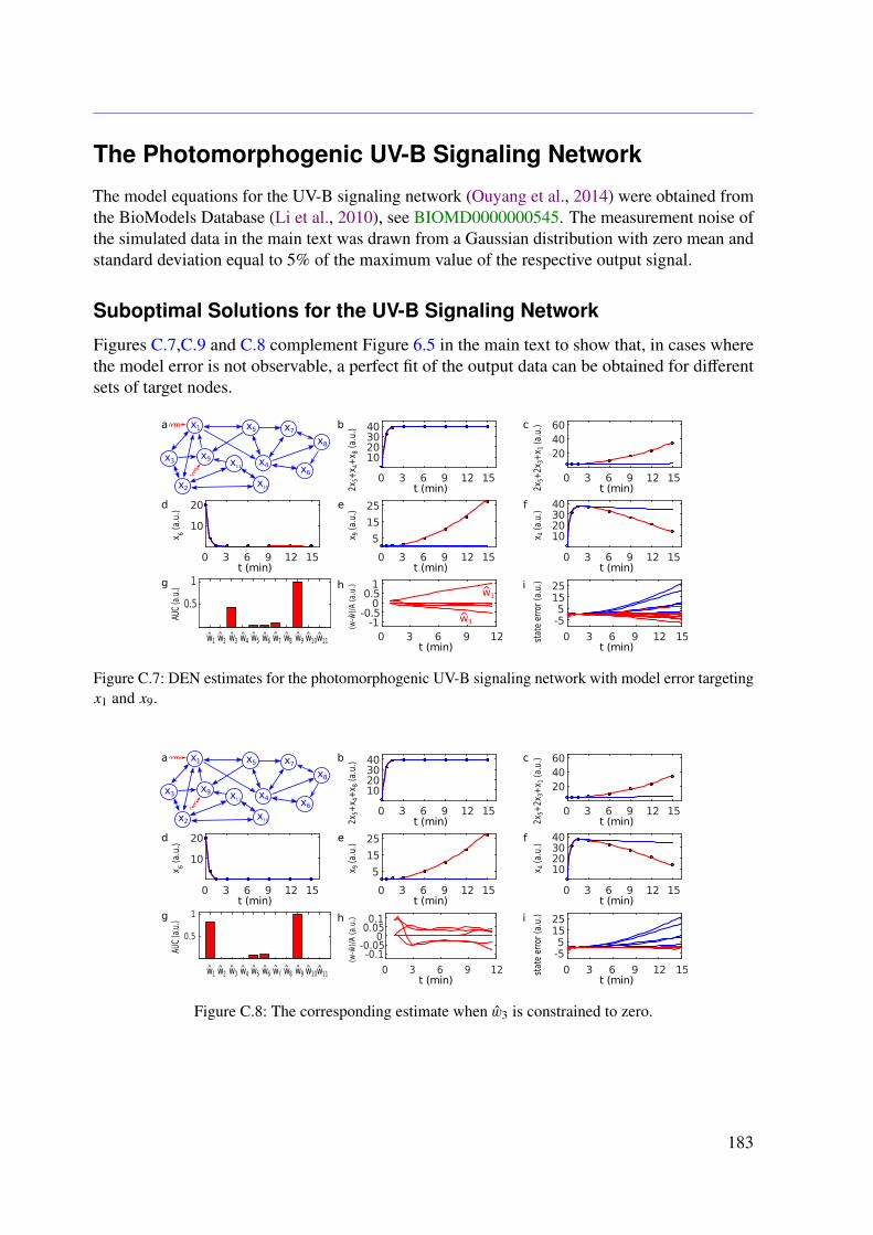
The Photomorphogenic UV-B Signaling Network
The model equations for the UV-B signaling network (Ouyang et al., 2014) were obtained fromthe BioModels Database (Li et al., 2010), see BIOMD0000000545. The measurement noise ofthe simulated data in the main text was drawn from a Gaussian distribution with zero mean andstandard deviation equal to 5% of the maximum value of the respective output signal.
Suboptimal Solutions for the UV-B Signaling Network
Figures C.7,C.9 and C.8 complement Figure 6.5 in the main text to show that, in cases wherethe model error is not observable, a perfect fit of the output data can be obtained for differentsets of target nodes.
Figure C.7: DEN estimates for the photomorphogenic UV-B signaling network with model error targetingx1 and x9.
Figure C.8: The corresponding estimate when w3 is constrained to zero.
183
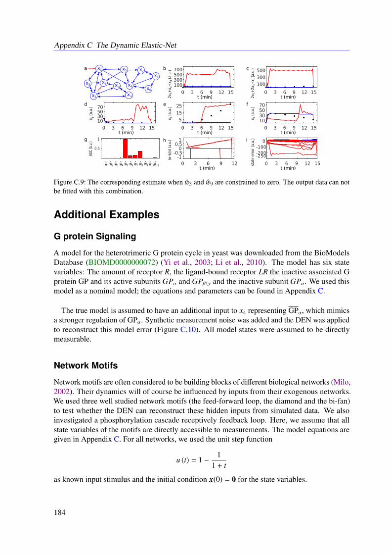
Appendix C The Dynamic Elastic-Net
Figure C.9: The corresponding estimate when w3 and w9 are constrained to zero. The output data can notbe fitted with this combination.
Additional Examples
G protein Signaling
A model for the heterotrimeric G protein cycle in yeast was downloaded from the BioModelsDatabase (BIOMD0000000072) (Yi et al., 2003; Li et al., 2010). The model has six statevariables: The amount of receptor R, the ligand-bound receptor LR the inactive associated Gprotein GP and its active subunits GPα and GPβ\γ and the inactive subunit GPα. We used thismodel as a nominal model; the equations and parameters can be found in Appendix C.
The true model is assumed to have an additional input to x4 representing GPα, which mimicsa stronger regulation of GPα. Synthetic measurement noise was added and the DEN was appliedto reconstruct this model error (Figure C.10). All model states were assumed to be directlymeasurable.
Network Motifs
Network motifs are often considered to be building blocks of different biological networks (Milo,2002). Their dynamics will of course be influenced by inputs from their exogenous networks.We used three well studied network motifs (the feed-forward loop, the diamond and the bi-fan)to test whether the DEN can reconstruct these hidden inputs from simulated data. We alsoinvestigated a phosphorylation cascade receptively feedback loop. Here, we assume that allstate variables of the motifs are directly accessible to measurements. The model equations aregiven in Appendix C. For all networks, we used the unit step function
u (t) = 1 −1
1 + t
as known input stimulus and the initial condition x(0) = 0 for the state variables.
184
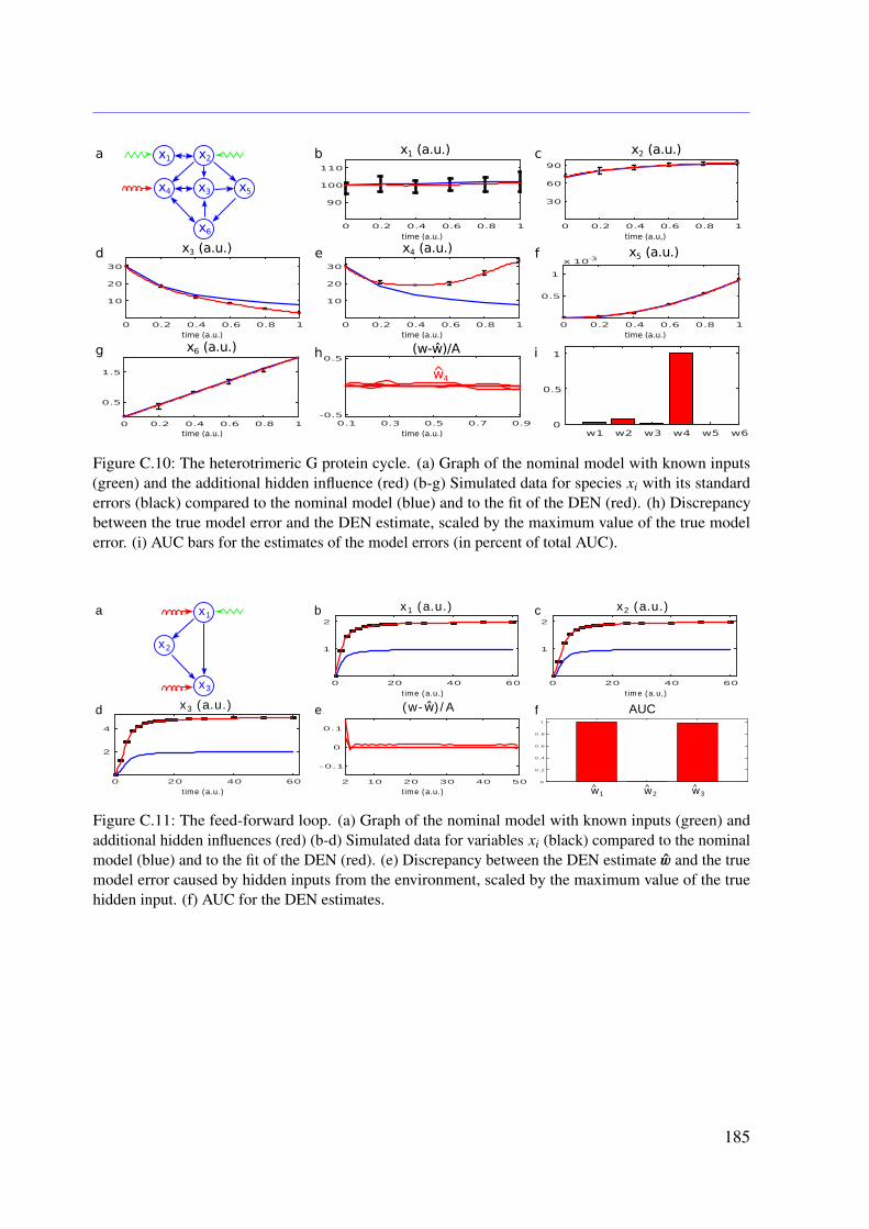
Figure C.10: The heterotrimeric G protein cycle. (a) Graph of the nominal model with known inputs(green) and the additional hidden influence (red) (b-g) Simulated data for species xi with its standarderrors (black) compared to the nominal model (blue) and to the fit of the DEN (red). (h) Discrepancybetween the true model error and the DEN estimate, scaled by the maximum value of the true modelerror. (i) AUC bars for the estimates of the model errors (in percent of total AUC).
0 20 40 60
1
2
0 20 40 60
1
2
0 20 40 60
2
4
time (a.u.) time (a.u,)
time (a.u.)time (a.u.)
x1 (a.u.) x2 (a.u.)
x3 (a.u.) (w-ŵ)/A AUC
x2
x3
x1
2 10 20 30 40 50
-0.1
0
0.1
w1^ w2
^ w3^
0
0.2
0.4
0.6
0.8
1
a b c
d e f
Figure C.11: The feed-forward loop. (a) Graph of the nominal model with known inputs (green) andadditional hidden influences (red) (b-d) Simulated data for variables xi (black) compared to the nominalmodel (blue) and to the fit of the DEN (red). (e) Discrepancy between the DEN estimate w and the truemodel error caused by hidden inputs from the environment, scaled by the maximum value of the truehidden input. (f) AUC for the DEN estimates.
185
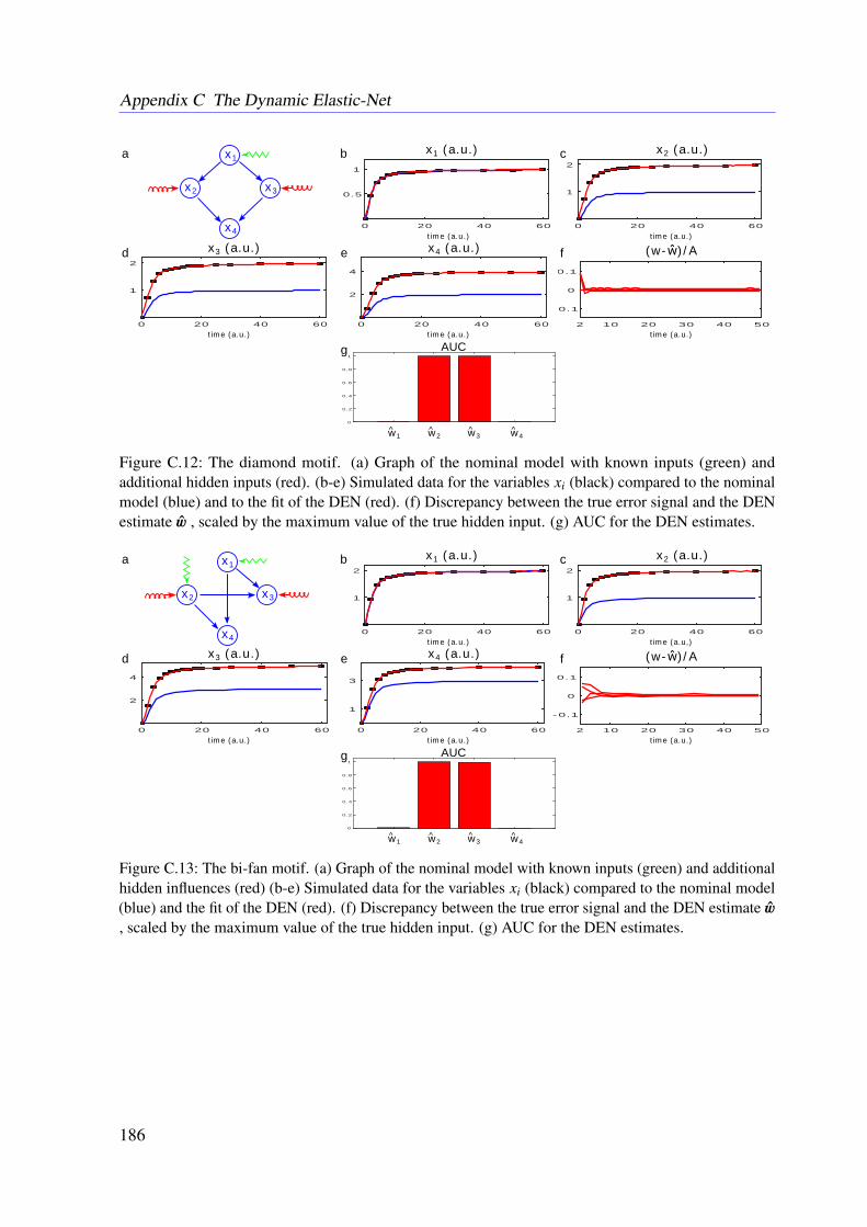
Appendix C The Dynamic Elastic-Net
0
0.2
0.4
0.6
0.8
1
2 10 20 30 40 50
-0.1
0
0.1
0 20 40 60
2
4
0 20 40 60
1
2
0 20 40 60
0.5
1
0 20 40 60
1
2
time (a.u.) time (a.u.)
time (a.u.)time (a.u.)time (a.u.)
x1 (a.u.) x2 (a.u.)
x3 (a.u.) x4 (a.u.) (w-ŵ)/A
x2 x3
x4
x1
AUC
w1^ w2
^ w3^ w4
^
a b c
d e f
g
Figure C.12: The diamond motif. (a) Graph of the nominal model with known inputs (green) andadditional hidden inputs (red). (b-e) Simulated data for the variables xi (black) compared to the nominalmodel (blue) and to the fit of the DEN (red). (f) Discrepancy between the true error signal and the DENestimate w , scaled by the maximum value of the true hidden input. (g) AUC for the DEN estimates.
0
0.2
0.4
0.6
0.8
1
0 20 40 60
1
3
0 20 40 60
2
4
0 20 40 60
1
2
0 20 40 60
1
2
time (a.u.) time (a.u,)
time (a.u.)time (a.u.)time (a.u.)
x1 (a.u.) x2 (a.u.)
x3 (a.u.) x4 (a.u.) (w-ŵ)/A
AUC
x2 x3
x4
x1
2 10 20 30 40 50
-0.1
0
0.1
w1^ w2
^ w3^ w4
^
a b c
d e f
g
Figure C.13: The bi-fan motif. (a) Graph of the nominal model with known inputs (green) and additionalhidden influences (red) (b-e) Simulated data for the variables xi (black) compared to the nominal model(blue) and the fit of the DEN (red). (f) Discrepancy between the true error signal and the DEN estimate w, scaled by the maximum value of the true hidden input. (g) AUC for the DEN estimates.
186
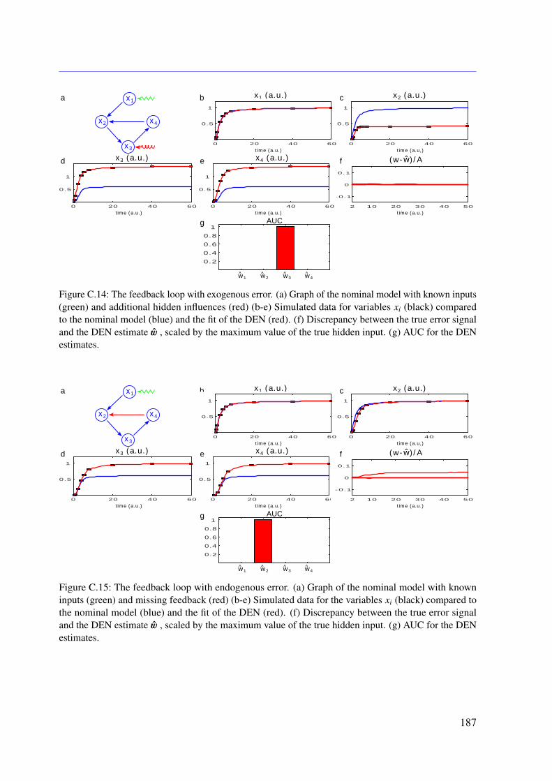
0.2
0.4
0.6
0.8
1
2 10 20 30 40 50
-0.1
0
0.1
0 20 40 60
0.5
1
0 20 40 60
0.5
1
0 20 40 60
0.5
1
time (a.u.) time (a.u,)
time (a.u.)time (a.u.)time (a.u.)
x1 (a.u.) x2 (a.u.)
x3 (a.u.) x4 (a.u.) (w-ŵ)/A
AUC
x2
x3
x4
x1
0 20 40 60
0.5
1
w1^ w2
^ w3^ w4
^
a b c
d e f
g
Figure C.14: The feedback loop with exogenous error. (a) Graph of the nominal model with known inputs(green) and additional hidden influences (red) (b-e) Simulated data for variables xi (black) comparedto the nominal model (blue) and the fit of the DEN (red). (f) Discrepancy between the true error signaland the DEN estimate w , scaled by the maximum value of the true hidden input. (g) AUC for the DENestimates.
0 20 40 60
0.5
1
0.2
0.4
0.6
0.8
1
0 20 40 60
0.5
1
0 20 40 60
0.5
1
a b c
d e f
g
time (a.u.) time (a.u,)
time (a.u.)time (a.u.)time (a.u.)
x1 (a.u.) x2 (a.u.)
x3 (a.u.) x4 (a.u.) (w-ŵ)/A
AUC
x2
x3
x4
x1
0 20 40 60
0.5
1
2 10 20 30 40 50
-0.1
0
0.1
w1^ w2
^ w3^ w4
^
Figure C.15: The feedback loop with endogenous error. (a) Graph of the nominal model with knowninputs (green) and missing feedback (red) (b-e) Simulated data for the variables xi (black) compared tothe nominal model (blue) and the fit of the DEN (red). (f) Discrepancy between the true error signaland the DEN estimate w , scaled by the maximum value of the true hidden input. (g) AUC for the DENestimates.
187

Appendix C The Dynamic Elastic-Net
Further Model Equations
Feed-forward Loop
True System
x1 (t) = u (t) − x1 (t) +
(1 −
11 + t
)x2 (t) = x1 (t) − x2 (t)
x3 (t) = x2 (t) + x1 (t) − x3 (t) +
(1 −
11 + t
)Nominal System
˙x1 (t) = u (t) − x1 (t)˙x2 (t) = x1 (t) − x2 (t)˙x3 (t) = x2 (t) + x1 (t) − x3 (t)
Diamond
True Systemx1 (t) = u (t) − x1 (t)
x2 (t) = x1 (t) − x2 (t) +
(1 −
11 + t
)x3 (t) = x1 (t) − x3 (t) +
(1 −
11 + t
)x4 (t) = x2 (t) + x3 (t) − x4 (t)
Nominal System˙x1 (t) = u (t) − x1 (t)˙x2 (t) = x1 (t) − x2 (t)˙x3 (t) = x1 (t) − x3 (t)˙x4 (t) = x2 (t) + x3 (t) − x4 (t)
Bi-fan
True Systemx1 (t) = u (t) − x1 (t)
x2 (t) = u (t) − x2 (t) +
(1 −
11 + t
)x3 (t) = x2 (t) + x1 (t) − x3 (t) −
(1 −
11 + t
)x4 (t) = x2 (t) + x1 (t) − x4 (t)
188

Nominal System˙x1 (t) = u (t) − x1 (t)˙x2 (t) = u (t) − x2 (t)˙x3 (t) = x2 (t) + x1 (t) − x3 (t)˙x4 (t) = x2 (t) + x1 (t) − x4 (t)
Feedback Loop 1
True System˙x1 (t) = u (t) − x1 (t)
˙x2 (t) =x1 (t)
1 + x4− x2 (t)
˙x3 (t) = x2 (t) − x3 (t) +
(1 −
11 + t
)˙x4 (t) = x3 (t) − x4 (t)
Nominal System˙x1 (t) = u (t) − x1 (t)
˙x2 (t) =x1 (t)
1 + x4− x2 (t)
˙x3 (t) = x2 (t) − x3 (t)˙x4 (t) = x3 (t) − x4 (t)
Feedback Loop 2
True Systemx1 (t) = u (t) − x1 (t)x2 (t) = x1 − x2 (t)x3 (t) = x2 (t) − x3 (t)˙x4 (t) = x3 (t) − x4 (t)
Nominal System˙x1 (t) = u (t) − x1 (t)
˙x2 (t) =x1 (t)
1 + x4− x2 (t)
˙x3 (t) = x2 (t) − x3 (t)˙x4 (t) = x3 (t) − x4 (t)
G protein Signaling Model
The model for the heterotrimeric G protein cycle in yeast was downloaded from the BioModelsDatabase (BIOMD0000000072) (Yi et al., 2003; Li et al., 2010). This model was used as a
189
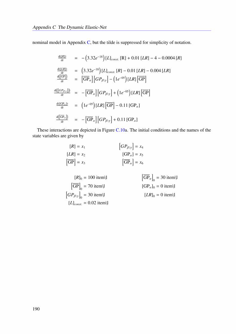
Appendix C The Dynamic Elastic-Net
nominal model in Appendix C, but the tilde is suppressed for simplicity of notation.
d([R])dt = −
(3.32e−18
)[L]const. [R] + 0.01 [LR] − 4 − 0.0004 [R]
d([LR])dt =
(3.32e−18
)[L]const. [R] − 0.01 [LR] − 0.004 [LR]
d([
GP])
dt =[GPα
] [GPβ\γ
]−
(1e−05
)[LR]
[GP
]d([GPβ\γ])
dt = −[GPα
] [GPβ\γ
]+
(1e−05
)[LR]
[GP
]d([GPα])
dt =(1e−05
)[LR]
[GP
]− 0.11 [GPα]
d([
GPα])
dt = −[GPα
] [GPβ\γ
]+ 0.11 [GPα]
These interactions are depicted in Figure C.10a. The initial conditions and the names of thestate variables are given by
[R] = x1
[GPβ\γ
]= x4
[LR] = x2 [GPα] = x5[GP
]= x3
[GPα
]= x6
[R]0 = 100 item\l[GPα
]0
= 30 item\l[GP
]0
= 70 item\l [GPα]0 = 0 item\l[GPβ\γ
]0
= 30 item\l [LR]0 = 0 item\l
[L]const. = 0.02 item\l
190
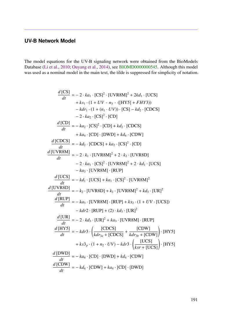
UV-B Network Model
The model equations for the UV-B signaling network were obtained from the BioModelsDatabase (Li et al., 2010; Ouyang et al., 2014), see BIOMD0000000545. Although this modelwas used as a nominal model in the main text, the tilde is suppressed for simplicity of notation.
d [CS]dt
= − 2 · ka1 · [CS]2· [UVR8M]2 + 2kd1 · [UCS]
+ ks1 · (1 + UV · n3 · ([HY5] + FHY3))− kdr1 · (1 + (n1 · UV)) · [CS] − kd2 · [CDCS]
− 2 · ka2 · [CS]2· [CD]
d [CD]dt
= − ka2 · [CS]2· [CD] + kd2 · [CDCS]
+ ka4 · [CD] · [DWD] + kd4 · [CDW]d [CDCS]
dt= − kd2 · [CDCS] + ka2 · [CS]2
· [CD]
d [UVR8M]dt
= − 2 · k1 · [UVR8M]2 + 2 · k2 · [UVR8D]
− 2 · ka1 · [CS]2· [UVR8M]2 + 2 · kd1 · [UCS]
− ka3 · [UVR8M] · [RUP]d [UCS]
dt= − kd1 · [UCS] + ka1 · [CS]2
· [UVR8M]2
d [UVR8D]dt
= − k2 · [UVR8D] + k1 · [UVR8M]2 + kd3 · [UR]2
d [RUP]dt
= − ka3 · [UVR8M] · [RUP] + ks2 · (1 + UV · [UCS])
− kdr2 · [RUP] + (2) · kd3 · [UR]2
d [UR]dt
= − 2 · kd3 · [UR]2 + ka3 · [UVR8M] · [RUP]
d [HY5]dt
= − kdr3 ·(
[CDCS]kdr3a + [CDCS]
+[CDW]
kdr3b + [CDW]
)· [HY5]
+ ks3p · (1 + n2 · UV) − kdr3 ·(
[UCS]ksr + [UCS]
)· [HY5]
d [DWD]dt
= − ka4 · [CD] · [DWD] + kd4 · [CDW]
d [CDW]dt
= − kd4 · [CDW] + ka4 · [CD] · [DWD]
191
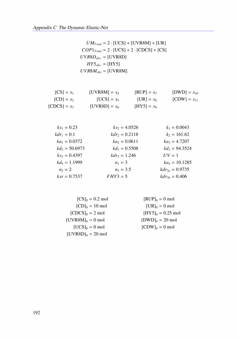
Appendix C The Dynamic Elastic-Net
UMTotal = 2 · [UCS] + [UVR8M] + [UR]COP1Total = 2 · [UCS] + 2 · [CDCS] + [CS]
UVR8Dobs. = [UVR8D]HY5obs. = [HY5]
UVR8Mobs = [UVR8M]
[CS] = x1 [UVR8M] = x4 [RUP] = x7 [DWD] = x10
[CD] = x2 [UCS] = x5 [UR] = x8 [CDW] = x11
[CDCS] = x3 [UVR8D] = x6 [HY5] = x9
ks1 = 0.23 ks2 = 4.0526 k1 = 0.0043kdr1 = 0.1 kdr2 = 0.2118 k2 = 161.62ka1 = 0.0372 ka2 = 0.0611 ka3 = 4.7207kd2 = 50.6973 kd3 = 0.5508 kd1 = 94.3524ks3 = 0.4397 kdr3 = 1.246 UV = 1kd4 = 1.1999 n1 = 3 ka4 = 10.1285n2 = 2 n3 = 3.5 kdr3a = 0.9735
ksr = 0.7537 FHY3 = 5 kdr3b = 0.406
[CS]0 = 0.2 mol [RUP]0 = 0 mol[CD]0 = 10 mol [UR]0 = 0 mol
[CDCS]0 = 2 mol [HY5]0 = 0.25 mol[UVR8M]0 = 0 mol [DWD]0 = 20 mol
[UCS]0 = 0 mol [CDW]0 = 0 mol[UVR8D]0 = 20 mol
192
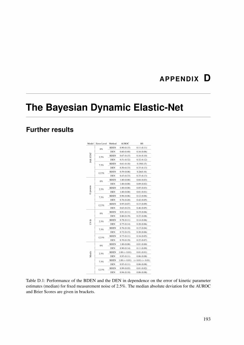
APPENDIX D
The Bayesian Dynamic Elastic-Net
Further results
Model Error Level Method AUROC BS
JAK
-STA
T
0%BDEN 0.90 (0.15) 0.11 (0.11)
DEN 0.60 (0.40) 0.16 (0.06)
2.5%BDEN 0.67 (0.15) 0.16 (0.10)
DEN 0.51 (0.32) 0.32 (0.12)
7.5%BDEN 0.61 (0.18) 0.19(0.15)
DEN 0.50 (0.33) 0.33 (0.13)
12.5%BDEN 0.59 (0.08) 0.26(0.16)
DEN 0.43 (0.33) 0.33 (0.13)
Gpr
otei
n
0%BDEN 1.00 (0.00) 0.04 (0.03)
DEN 1.00 (0.00) 0.09 (0.02)
2.5%BDEN 1.00 (0.00) 0.05 (0.03)
DEN 1.00 (0.00) 0.01 (0.01)
7.5%BDEN 0.96 (0.06) 0.12 (0.06)
DEN 0.76 (0.20) 0.42 (0.05)
12.5%BDEN 0.95 (0.07) 0.15 (0.09)
DEN 0.63 (0.23) 0.46 (0.05)
UV
-B
0%BDEN 0.91 (0.11) 0.19 (0.06)
DEN 0.80 (0.19) 0.22 (0.08)
2.5%BDEN 0.78 (0.11) 0.14 (0.06)
DEN 0.75 (0.14) 0.20 (0.06)
7.5%BDEN 0.76 (0.10) 0.15 (0.04)
DEN 0.72 (0.15) 0.20 (0.06)
12.5%BDEN 0.73 (0.11) 0.16 (0.05)
DEN 0.70 (0.19) 0.22 (0.07)
Mot
ifs
0%BDEN 1.00 (0.00) 0.01 (0.00)
DEN 0.90 (0.14) 0.11 (0.09)
2.5%BDEN 1.00 (< 0.01) 0.01 (0.01)
DEN 0.93 (0.11) 0.06 (0.08)
7.5%BDEN 1.00 (< 0.01) (< 0.01) (< 0.01)
DEN 0.93 (0.11) 0.06 (0.08)
12.5%BDEN 0.99 (0.03) 0.01 (0.02)
DEN 0.94 (0.10) 0.06 (0.08)
Table D.1: Performance of the BDEN and the DEN in dependence on the error of kinetic parameterestimates (median) for fixed measurement noise of 2.5%. The median absolute deviation for the AUROCand Brier Scores are given in brackets.
193
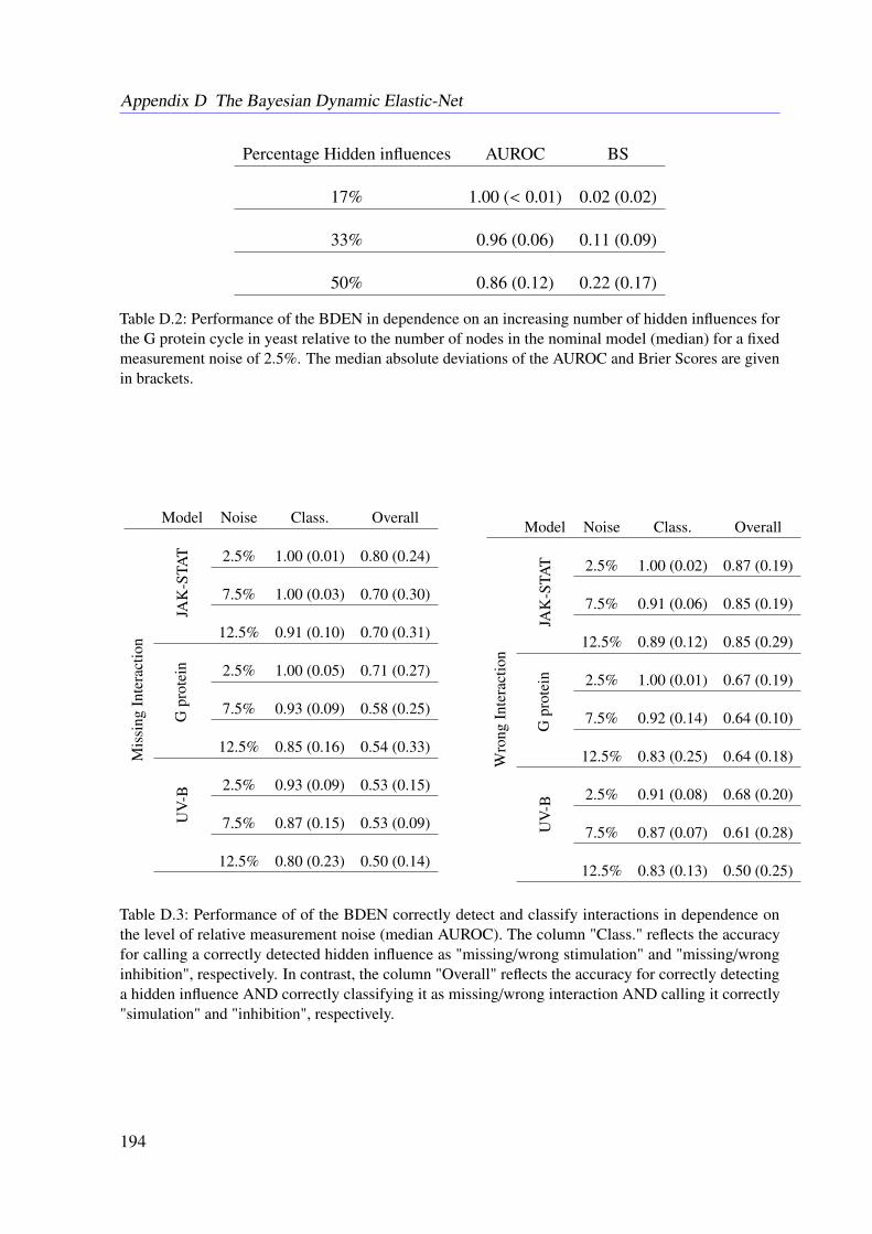
Appendix D The Bayesian Dynamic Elastic-Net
Percentage Hidden influences AUROC BS
17% 1.00 (< 0.01) 0.02 (0.02)
33% 0.96 (0.06) 0.11 (0.09)
50% 0.86 (0.12) 0.22 (0.17)
Table D.2: Performance of the BDEN in dependence on an increasing number of hidden influences forthe G protein cycle in yeast relative to the number of nodes in the nominal model (median) for a fixedmeasurement noise of 2.5%. The median absolute deviations of the AUROC and Brier Scores are givenin brackets.
Model Noise Class. Overall
Mis
sing
Inte
ract
ion
JAK
-STA
T 2.5% 1.00 (0.01) 0.80 (0.24)
7.5% 1.00 (0.03) 0.70 (0.30)
12.5% 0.91 (0.10) 0.70 (0.31)
Gpr
otei
n 2.5% 1.00 (0.05) 0.71 (0.27)
7.5% 0.93 (0.09) 0.58 (0.25)
12.5% 0.85 (0.16) 0.54 (0.33)
UV
-B
2.5% 0.93 (0.09) 0.53 (0.15)
7.5% 0.87 (0.15) 0.53 (0.09)
12.5% 0.80 (0.23) 0.50 (0.14)
Model Noise Class. Overall
Wro
ngIn
tera
ctio
n
JAK
-STA
T 2.5% 1.00 (0.02) 0.87 (0.19)
7.5% 0.91 (0.06) 0.85 (0.19)
12.5% 0.89 (0.12) 0.85 (0.29)
Gpr
otei
n 2.5% 1.00 (0.01) 0.67 (0.19)
7.5% 0.92 (0.14) 0.64 (0.10)
12.5% 0.83 (0.25) 0.64 (0.18)
UV
-B
2.5% 0.91 (0.08) 0.68 (0.20)
7.5% 0.87 (0.07) 0.61 (0.28)
12.5% 0.83 (0.13) 0.50 (0.25)
Table D.3: Performance of of the BDEN correctly detect and classify interactions in dependence onthe level of relative measurement noise (median AUROC). The column "Class." reflects the accuracyfor calling a correctly detected hidden influence as "missing/wrong stimulation" and "missing/wronginhibition", respectively. In contrast, the column "Overall" reflects the accuracy for correctly detectinga hidden influence AND correctly classifying it as missing/wrong interaction AND calling it correctly"simulation" and "inhibition", respectively.
194
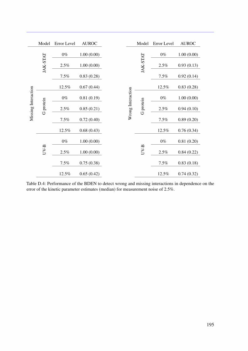
Model Error Level AUROC
Mis
sing
Inte
ract
ion
JAK
-ST A
T 0% 1.00 (0.00)
2.5% 1.00 (0.00)
7.5% 0.83 (0.28)
12.5% 0.67 (0.44)
Gpr
otei
n 0% 0.81 (0.19)
2.5% 0.85 (0.21)
7.5% 0.72 (0.40)
12.5% 0.68 (0.43)
UV
-B
0% 1.00 (0.00)
2.5% 1.00 (0.00)
7.5% 0.75 (0.38)
12.5% 0.65 (0.42)
Model Error Level AUROC
Wro
ngIn
tera
ctio
n
JAK
-ST A
T 0% 1.00 (0.00)
2.5% 0.93 (0.13)
7.5% 0.92 (0.14)
12.5% 0.83 (0.28)
Gpr
otei
n 0% 1.00 (0.00)
2.5% 0.94 (0.10)
7.5% 0.89 (0.20)
12.5% 0.76 (0.34)
UV
-B0% 0.81 (0.20)
2.5% 0.84 (0.22)
7.5% 0.83 (0.18)
12.5% 0.74 (0.32)
Table D.4: Performance of the BDEN to detect wrong and missing interactions in dependence on theerror of the kinetic parameter estimates (median) for measurement noise of 2.5%.
195
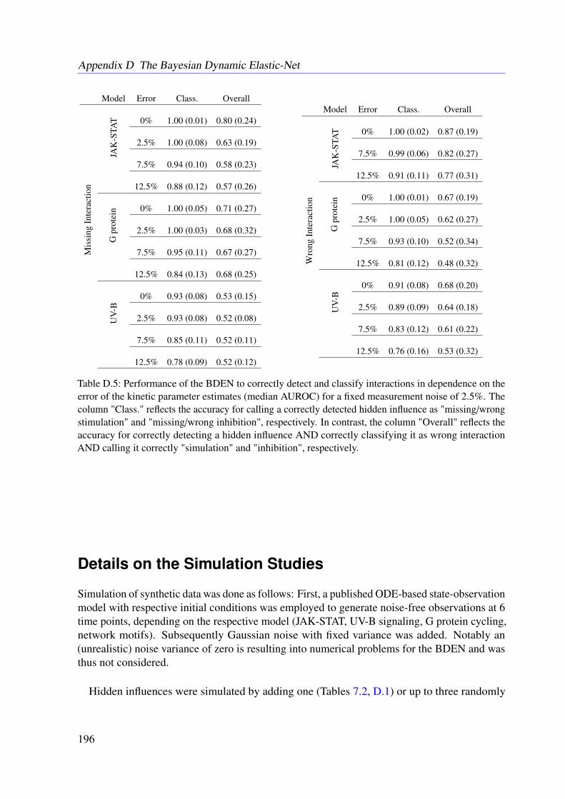
Appendix D The Bayesian Dynamic Elastic-Net
Model Error Class. OverallM
issi
ngIn
tera
ctio
n
JAK
-STA
T 0% 1.00 (0.01) 0.80 (0.24)
2.5% 1.00 (0.08) 0.63 (0.19)
7.5% 0.94 (0.10) 0.58 (0.23)
12.5% 0.88 (0.12) 0.57 (0.26)
Gpr
otei
n 0% 1.00 (0.05) 0.71 (0.27)
2.5% 1.00 (0.03) 0.68 (0.32)
7.5% 0.95 (0.11) 0.67 (0.27)
12.5% 0.84 (0.13) 0.68 (0.25)
UV
-B
0% 0.93 (0.08) 0.53 (0.15)
2.5% 0.93 (0.08) 0.52 (0.08)
7.5% 0.85 (0.11) 0.52 (0.11)
12.5% 0.78 (0.09) 0.52 (0.12)
Model Error Class. Overall
Wro
ngIn
tera
ctio
n
JAK
-STA
T 0% 1.00 (0.02) 0.87 (0.19)
7.5% 0.99 (0.06) 0.82 (0.27)
12.5% 0.91 (0.11) 0.77 (0.31)
Gpr
otei
n 0% 1.00 (0.01) 0.67 (0.19)
2.5% 1.00 (0.05) 0.62 (0.27)
7.5% 0.93 (0.10) 0.52 (0.34)
12.5% 0.81 (0.12) 0.48 (0.32)
UV
-B
0% 0.91 (0.08) 0.68 (0.20)
2.5% 0.89 (0.09) 0.64 (0.18)
7.5% 0.83 (0.12) 0.61 (0.22)
12.5% 0.76 (0.16) 0.53 (0.32)
Table D.5: Performance of the BDEN to correctly detect and classify interactions in dependence on theerror of the kinetic parameter estimates (median AUROC) for a fixed measurement noise of 2.5%. Thecolumn "Class." reflects the accuracy for calling a correctly detected hidden influence as "missing/wrongstimulation" and "missing/wrong inhibition", respectively. In contrast, the column "Overall" reflects theaccuracy for correctly detecting a hidden influence AND correctly classifying it as wrong interactionAND calling it correctly "simulation" and "inhibition", respectively.
Details on the Simulation Studies
Simulation of synthetic data was done as follows: First, a published ODE-based state-observationmodel with respective initial conditions was employed to generate noise-free observations at 6time points, depending on the respective model (JAK-STAT, UV-B signaling, G protein cycling,network motifs). Subsequently Gaussian noise with fixed variance was added. Notably an(unrealistic) noise variance of zero is resulting into numerical problems for the BDEN and wasthus not considered.
Hidden influences were simulated by adding one (Tables 7.2, D.1) or up to three randomly
196
picked (Table D.2) state variables on the right hand side of the ODE system, yielding a wrongnominal ODE system. Likewise, wrong interactions were simulated by randomly adding oneinteraction on the right hand side of the ODE system (Tables 7.3, D.3, D.4, D.5). Missinginteractions were simulated by randomly removing one of the existing interactions (Tables 7.3,D.3, D.4, D.5).
Due to the randomness of the process described above we repeated all simulations a numberof times (Table D.6). The exact number of repeats varies slightly to take into account thedifferent number of combination possibilities. ODE systems with more state variables or allowfor a larger number of possible combinations of hidden influence signals.
Table Repeats
7.2 4507.3 400D.1 450D.2 400D.3 350D.4 400D.5 350
Table D.6: Number of independent simulation repeats for each of the presented results.
Additive Hidden Inputs and Model Error
The assumption of a hidden input signal incorporates many different types of model errorsincluding parameter errors, hidden or misspecified interactions as well as inputs from exosystems.This can be seen as follows. Assume that the true system generating the data has the form(
x (t)z (t)
)=
(φ (x (t) , z (t) ,u (t))ψ (x (t) , z (t) ,u (t))
)(D.1a)
y (t) = h (x (t)) . (D.1b)
Here, x (t) = (x1 (t) , . . . , xN (t))T∈ RN is the state vector also included in the nominal model
x (t) = f (x (t) ,u (t)) (D.2a)y (t) = h (x (t)) , (D.2b)
which represents our current knowledge or assumptions about the true system. The outputmap h is assumed to be exactly known and depends only on x, so (D.2b) and (D.1b) have thesame form. The exostate z (t) = (z1 (t) , . . . , zP (t)) T in the true system (D.1) represents dynamic
197

Appendix D The Bayesian Dynamic Elastic-Net
variables ignored in the nominal model. Let us denote the solution of the true system (D.1a) as
ν(t) =
(x(t)z(t)
)with initial condition ν(t0) =
(x(t0)z(t0)
). (D.3)
Now the functions φ and f are compared along the true state trajectory (D.3) and define
w(t = x(t) − f (x(t),u(t)) = φ (x(t), z(t),u(t)) − f (x(t),u(t)) . (D.4)
Thus,x(t) = f (x(t),u(t)) + w(t). (D.5)
represents the true dynamics x(t) through the nominal system f and the hidden input w(t). Notethat the dependence on parameters is suppressed in the notation. However, this can be seen aspart of the systems specification, i.e., as defining the properties of f , φ and ψ, respectively.Thus, model errors can be represented by hidden (unknown) inputs.
Full Derivation of Equation (7.6)
According to (Zacher et al., 2012), Equation (7.6) can be derived as follows:Given yi,l
∣∣∣xl, ξ2i,l ∼ N
(yi,l
∣∣∣xl, 1/τi,l
)with unknown τ = 1
ξ2i,l
and τ ∼ G (α, β), we obtain
p(yi,l |xl, α, β
)∝
∫p(yi,l
∣∣∣xl, ξ2i,l
)× p
(ξ2
i,l
∣∣∣α, β)dξ2i,l
=
∫N
(yi,l
∣∣∣xl, τi,l
)×G
(τi,l
∣∣∣α, β)dτi,l
=
∫βα
Γ (α)τα−1 exp (−τβ)
(τ
2π
) 12
exp(−τ
2(yi,l − hi (xl)
)2)dτi,l
=βα
Γ (α)1√
2π
∫τα+ 1
2−1 exp
−τ(2β +
(yi,l − hi (xl)
)2)
2
dτi,l
=βα
Γ (α)1√
2π
Γ(α + 1
2
)(β + 1
2
(yi,l − hi (xl)
)2)α+ 1
2
=Γ(α + 1
2
)Γ (α)
1
(2πβ)12
1(1 + 1
2β
(yi,l − hi (xl)
)2)α+ 1
2
.
198
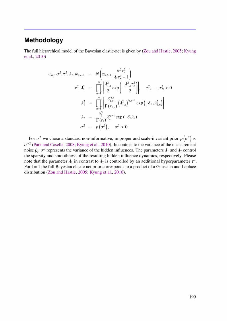
Methodology
The full hierarchical model of the Bayesian elastic-net is given by (Zou and Hastie, 2005; Kyunget al., 2010)
wn,l
∣∣∣σ2, τ2, λ2, wn,l−1 ∼ N(wn,l−1,
σ2τ2n
λ2τ2n + 1
)τ2
∣∣∣λ21 ∼
N∏n=1
λ21,n
2exp
−λ21,nτ
2n
2
, τ21, . . . , τ
2N > 0
λ21 ∼
N∏n=1
δr1,n1,n
Γ(r1,n
) (λ2
1,n
)r1,n−1exp
(−δ1,nλ
21,n
)λ2 ∼
δr22
Γ (r2)λr2−1
2 exp (−δ2λ2)
σ2 ∼ p(σ2
), σ2 > 0.
For σ2 we chose a standard non-informative, improper and scale-invariant prior p(σ2
)∝
σ−2 (Park and Casella, 2008; Kyung et al., 2010). In contrast to the variance of the measurementnoise ξl, σ
2 represents the variance of the hidden influences. The parameters λ1 and λ2 controlthe sparsity and smoothness of the resulting hidden influence dynamics, respectively. Pleasenote that the parameter λ1 in contrast to λ2 is controlled by an additional hyperparameter τ2.For l = 1 the full Bayesian elastic net prior corresponds to a product of a Gaussian and Laplacedistribution (Zou and Hastie, 2005; Kyung et al., 2010).
199
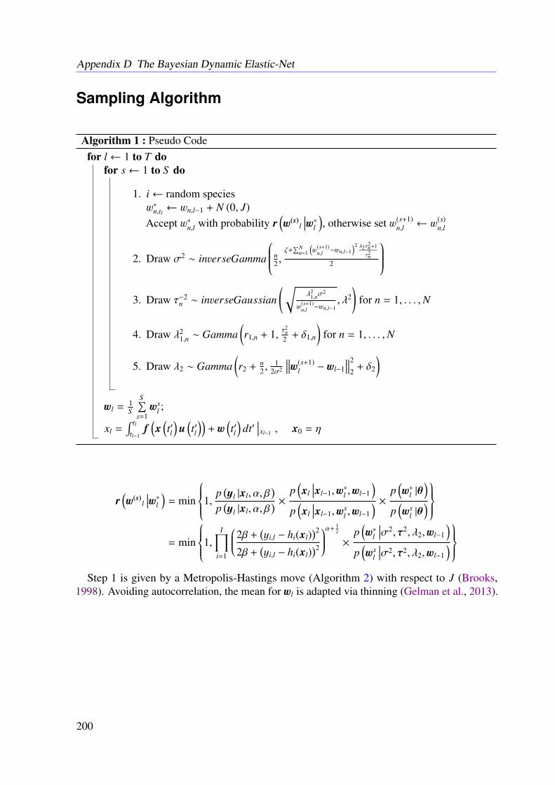
Appendix D The Bayesian Dynamic Elastic-Net
Sampling Algorithm
Algorithm 1 : Pseudo Codefor l← 1 to T do
for s← 1 to S do
1. i← random speciesw∗n,tl ← wn,l−1 + N (0, J)Accept w∗n,l with probability r
(w(s)
l
∣∣∣w∗l ), otherwise set w(s+1)n,l ← w(s)
n,l
2. Draw σ2 ∼ inverseGamma
n2 ,
ζ+∑N
n=1
(w(s+1)
n,l −wn,l−1)2 λ2τ
2n+1
τ2n
2
3. Draw τ−2
n ∼ inverseGaussian(√
λ21,nσ
2
w(s+1)n,l −wn,l−1
, λ2
)for n = 1, . . . ,N
4. Draw λ21,n ∼ Gamma
(r1,n + 1, τ
2n
2 + δ1,n
)for n = 1, . . . ,N
5. Draw λ2 ∼ Gamma(r2 + n
2 ,1
2σ2
∥∥∥w(s+1)l − wl−1
∥∥∥2
2+ δ2
)
wl = 1S
S∑s=1ws
l ;
xl =∫ tl
tl−1f(x(t′l)
u(t′l))
+ w(t′l)
dt′∣∣∣xl−1 , x0 = η
r(w(s)
l
∣∣∣w∗l ) = min
1,p(yl |xl, α, β
)p(yl |xl, α, β
) × p(xl
∣∣∣xl−1,w∗l ,wl−1
)p(xl
∣∣∣xl−1,wsl ,wl−1
) × p(w∗l |θ
)p(ws
l |θ)
= min
1,I∏
i=1
2β +(yi,l − hi(xl)
)2
2β +(yi,l − hi(xl)
)2
α+ 12
×p(w∗l
∣∣∣σ2, τ2, λ2,wl−1
)p(ws
l
∣∣∣σ2, τ2, λ2,wl−1
)
Step 1 is given by a Metropolis-Hastings move (Algorithm 2) with respect to J (Brooks,1998). Avoiding autocorrelation, the mean for wl is adapted via thinning (Gelman et al., 2013).
200
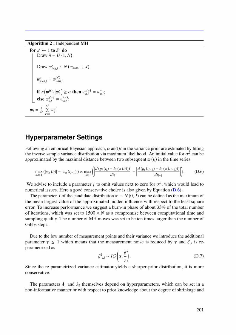
Algorithm 2 : Independent MHfor s′ ← 1 to S ′ do
Draw n ∼ U 1,N
Draw w∗i=n,l ∼ N(wn=n,l−1, J
)w∗n,n,l = w(s′)
n,n,l
if r(w(s)
l
∣∣∣w∗l ) ≥ α then ws′+1n,l = w∗n,l;
else ws′+1n,l = w(s′)
n,l ;
wl = 1S ′
S ′∑s′=1
ws′l
Hyperparameter Settings
Following an empirical Bayesian approach, α and β in the variance prior are estimated by fittingthe inverse sample variance distribution via maximum likelihood. An initial value for σ2 can beapproximated by the maximal distance between two subsequent w (tl) in the time series
maxn,l>1
(|wn (tl)| − |wn (tl−1)|) ∝ maxi,l>1
(∣∣∣∣∣d (yi (tl) − hi (x (tl)))dtl
∣∣∣∣∣ − ∣∣∣∣∣d (yi (tl−1) − hi (x (tl−1)))dtl−1
∣∣∣∣∣) . (D.6)
We advise to include a parameter ζ to omit values next to zero for σ2, which would lead tonumerical issues. Here a good conservative choice is also given by Equation (D.6).
The parameter J of the candidate distribution π ∼ N (0, J) can be defined as the maximum ofthe mean largest value of the approximated hidden influence with respect to the least squareerror. To increase performance we suggest a burn-in phase of about 33% of the total numberof iterations, which was set to 1500 × N as a compromise between computational time andsampling quality. The number of MH moves was set to be ten times larger than the number ofGibbs steps.
Due to the low number of measurement points and their variance we introduce the additionalparameter γ ≤ 1 which means that the measurement noise is reduced by γ and ξi,l is re-parametrized as
ξ2i,l ∼ IG
(α,β
γ
). (D.7)
Since the re-parametrized variance estimator yields a sharper prior distribution, it is moreconservative.
The parameters λ1 and λ2 themselves depend on hyperparameters, which can be set in anon-informative manner or with respect to prior knowledge about the degree of shrinkage and
201
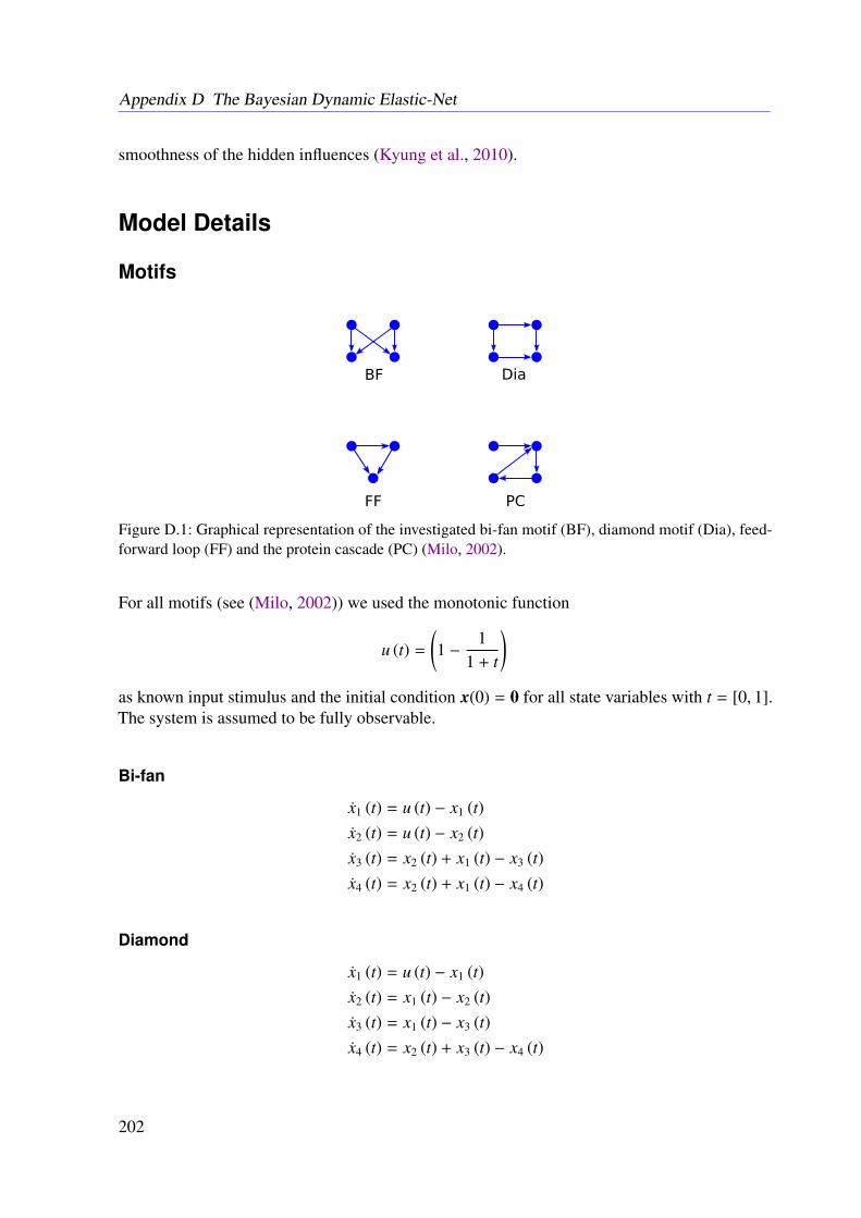
Appendix D The Bayesian Dynamic Elastic-Net
smoothness of the hidden influences (Kyung et al., 2010).
Model Details
Motifs
Figure D.1: Graphical representation of the investigated bi-fan motif (BF), diamond motif (Dia), feed-forward loop (FF) and the protein cascade (PC) (Milo, 2002).
For all motifs (see (Milo, 2002)) we used the monotonic function
u (t) =
(1 −
11 + t
)as known input stimulus and the initial condition x(0) = 0 for all state variables with t = [0, 1].The system is assumed to be fully observable.
Bi-fan
x1 (t) = u (t) − x1 (t)x2 (t) = u (t) − x2 (t)x3 (t) = x2 (t) + x1 (t) − x3 (t)x4 (t) = x2 (t) + x1 (t) − x4 (t)
Diamond
x1 (t) = u (t) − x1 (t)x2 (t) = x1 (t) − x2 (t)x3 (t) = x1 (t) − x3 (t)x4 (t) = x2 (t) + x3 (t) − x4 (t)
202
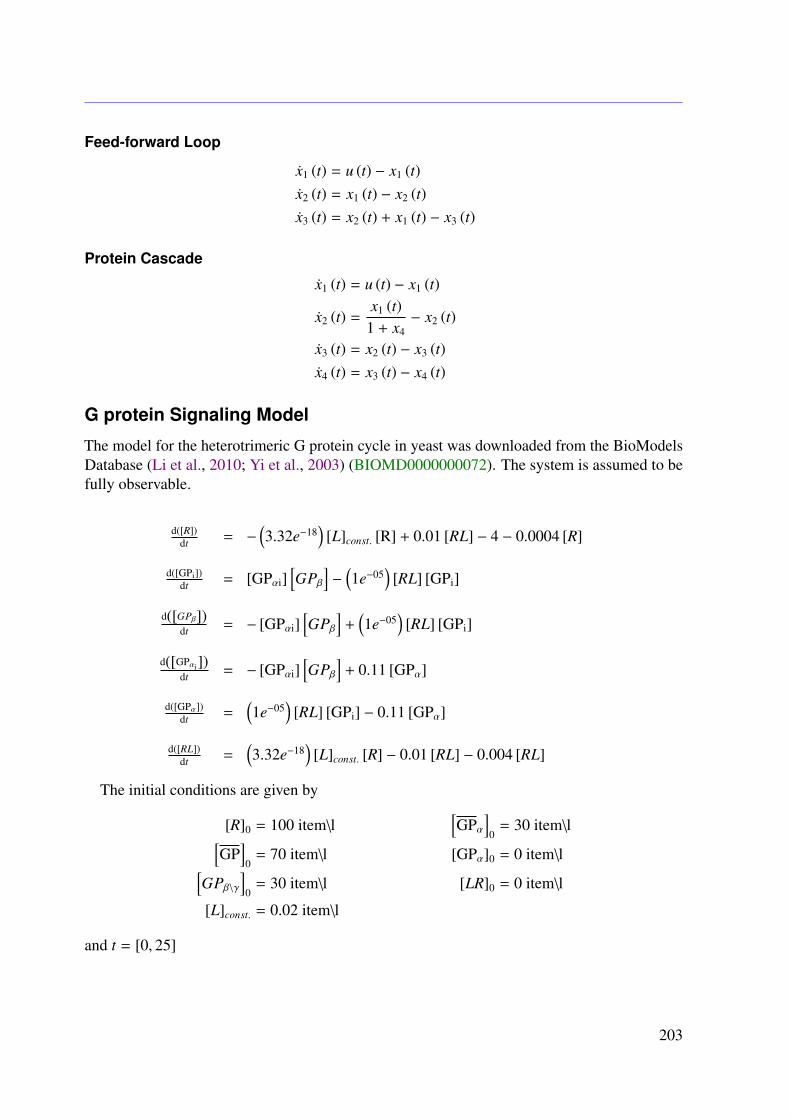
Feed-forward Loop
x1 (t) = u (t) − x1 (t)x2 (t) = x1 (t) − x2 (t)x3 (t) = x2 (t) + x1 (t) − x3 (t)
Protein Cascade
x1 (t) = u (t) − x1 (t)
x2 (t) =x1 (t)
1 + x4− x2 (t)
x3 (t) = x2 (t) − x3 (t)x4 (t) = x3 (t) − x4 (t)
G protein Signaling Model
The model for the heterotrimeric G protein cycle in yeast was downloaded from the BioModelsDatabase (Li et al., 2010; Yi et al., 2003) (BIOMD0000000072). The system is assumed to befully observable.
d([R])dt = −
(3.32e−18
)[L]const. [R] + 0.01 [RL] − 4 − 0.0004 [R]
d([GPi])dt = [GPαi]
[GPβ
]−
(1e−05
)[RL] [GPi]
d([GPβ])dt = − [GPαi]
[GPβ
]+
(1e−05
)[RL] [GPi]
d([GPαi])dt = − [GPαi]
[GPβ
]+ 0.11 [GPα]
d([GPα])dt =
(1e−05
)[RL] [GPi] − 0.11 [GPα]
d([RL])dt =
(3.32e−18
)[L]const. [R] − 0.01 [RL] − 0.004 [RL]
The initial conditions are given by
[R]0 = 100 item\l[GPα
]0
= 30 item\l[GP
]0
= 70 item\l [GPα]0 = 0 item\l[GPβ\γ
]0
= 30 item\l [LR]0 = 0 item\l
[L]const. = 0.02 item\l
and t = [0, 25]
203
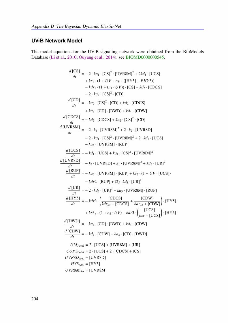
Appendix D The Bayesian Dynamic Elastic-Net
UV-B Network Model
The model equations for the UV-B signaling network were obtained from the BioModelsDatabase (Li et al., 2010; Ouyang et al., 2014), see BIOMD0000000545.
d [CS]dt
= − 2 · ka1 · [CS]2 · [UVR8M]2 + 2kd1 · [UCS]
+ ks1 · (1 + UV · n3 · ([HY5] + FHY3))
− kdr1 · (1 + (n1 · UV)) · [CS] − kd2 · [CDCS]
− 2 · ka2 · [CS]2 · [CD]d [CD]
dt= − ka2 · [CS]2 · [CD] + kd2 · [CDCS]
+ ka4 · [CD] · [DWD] + kd4 · [CDW]d [CDCS]
dt= − kd2 · [CDCS] + ka2 · [CS]2 · [CD]
d [UVR8M]dt
= − 2 · k1 · [UVR8M]2 + 2 · k2 · [UVR8D]
− 2 · ka1 · [CS]2 · [UVR8M]2 + 2 · kd1 · [UCS]
− ka3 · [UVR8M] · [RUP]d [UCS]
dt= − kd1 · [UCS] + ka1 · [CS]2 · [UVR8M]2
d [UVR8D]dt
= − k2 · [UVR8D] + k1 · [UVR8M]2 + kd3 · [UR]2
d [RUP]dt
= − ka3 · [UVR8M] · [RUP] + ks2 · (1 + UV · [UCS])
− kdr2 · [RUP] + (2) · kd3 · [UR]2
d [UR]dt
= − 2 · kd3 · [UR]2 + ka3 · [UVR8M] · [RUP]
d [HY5]dt
= − kdr3 ·(
[CDCS]kdr3a + [CDCS]
+[CDW]
kdr3b + [CDW]
)· [HY5]
+ ks3p · (1 + n2 · UV) − kdr3 ·(
[UCS]ksr + [UCS]
)· [HY5]
d [DWD]dt
= − ka4 · [CD] · [DWD] + kd4 · [CDW]
d [CDW]dt
= − kd4 · [CDW] + ka4 · [CD] · [DWD]
UMTotal = 2 · [UCS] + [UVR8M] + [UR]
COP1Total = 2 · [UCS] + 2 · [CDCS] + [CS]
UVR8Dobs. = [UVR8D]
HY5obs. = [HY5]
UVR8Mobs = [UVR8M]
204

[CS] = x1; [UVR8M] = x4; [RUP] = x7; [DWD] = x10;
[CD] = x2; [UCS] = x5; [UR] = x8; [CDW] = x11;
[CDCS] = x3; [UVR8D] = x6; [HY5] = x9
The initial conditions are given by
[CS]0 = 0.2 mol [RUP]0 = 0 mol
[CD]0 = 10 mol [UR]0 = 0 mol
[CDCS]0 = 2 mol [HY5]0 = 0.25 mol
[UVR8M]0 = 0 mol [DWD]0 = 20 mol
[UCS]0 = 0 mol [CDW]0 = 0 mol
[UVR8D]0 = 20 mol
and t = [0, 6].
JAK-STAT Model
The measurements for the JAK-STAT system were obtained from http://webber.physik.uni-freiburg.de/ ~jeti/PNAS_Swameye_Data. Mass conservation was accounted for by the con-straint 2x4(t) + 2x3(t) + x1(t) + x2(t) = const. for all t (Swameye et al., 2003; Raue et al., 2009).The nominal model is given by (Swameye et al., 2003):
x1 = −ψ1x1ux2 = ψ1x1u − 2ψ2x2
2
x3 = ψ2x22 − ψ3x3
x4 = ψ3x3
y2 = ψ5 (x1 + x2 + 2x3)y1 = ψ4 (x2 + 2x3) .
u = Erythropoietin Receptorx1 = STAT5x2 = STAT5p
x3 = STAT5di
x4 = STAT5n
y1 = total STAT5y2 = total STAT5p
and t = [0, 60].
205

Appendix D The Bayesian Dynamic Elastic-Net
Model of Information Processing at EpoR
The Model of the information processing at EpoR was obtained from (Becker et al., 2010). Datawas obtained from dMod.
x1 =kt · Bmax − kt · x1 − kon · x1 · x2 + ko f f · x3 + kex · x4
x2 = − kon · x1 · x2 + ko f f · x3 + kex · x4
x3 =kon · x1 · x2 − ko f f · x3 − ke · x3
x4 =ke · x3 − kex · x4 − kdi · x4 − kde · x4
x5 =kdi · x4
x6 =kde · x4
y2 =ψ1 (x2 + 2x6)y1 =ψ2 (x3)y3 =ψ3 (x4 + x5)
x1 = EpoRx2 = Epox3 = Epo-EpoRx4 = Epo-EpoRi
x5 = dEpoi
x6 = dEpoe
y1 = Epo concentration in the mediumy2 = Epo concentration on the surfacey3 = Epo concentration in the cells,
and t = [0, 300].
206

Model of α-Pinene Isomerization
The model of the thermal isomerization of αP in the liquid phase was obtained from (Fuguittand Hawkins, 1947).
x1 = − (p1 + p2) · x1
x2 =p1 · x1
x3 =p2 · x1 − (p3 + p4) · x3 + p5 · x4
x4 =p4 · x3 − p5 · x4
x1 = α-Pinenex2 = Dipentenex3 = Dimerx4 = allo-ocimene,
and t = [0, 25].
207

Appendix D The Bayesian Dynamic Elastic-Net
Gene Regulatory Network
The gene regulatory network was obtained from DREAM6 Challenge (Meyer et al., 2014). Forfurther information about this challenge we refer the reader to the DREAM6 Challenge.
x1 =pro1strength − mrna1degradation−rate · x1
x2 =rbs1strength · x1 − pdegradation−rate · x2
x3 =pro2strength ·
(x1v2Kd
)v2h
1 +(
x2v2Kd
)v2h·
1
1 +(
x6v5Kd
)v5h− mrna2degradation−rate · x3
x4 =rbs2strength · x3 − pdegradation−rate · x4
x5 =pro3strength ·
(x1v3Kd
)v3h
1 +(
x2v3Kd
)v3h·
1
1 +(
x2v4Kd
)v4h− mrna3degradation−rate · x5
x6 =rbs3strength · x5 − pdegradation−rate · x6
x7 =pro4strength ·
(x1v1Kd
)v1h
1 +(
x2v1Kd
)v1h·
1
1 +(
x5v8Kd
)v8h− mrna4degradation−rate · x7
x8 =rbs4strength · x7 − pdegradation−rate · x8
x9 =pro5strength ·1
1 +(
x4v6Kd
)v6h− mrna5degradation−rate · x9
x10 =rbs5strength · x9 − pdegradation−rate · x10
x11 =pro6strength ·1
1 +(
x4v7Kd
)v7h− mrna6degradation−rate ∗ x11
x12 =rbs6strength · x11 − pdegradation−rate · x12
y1 = pp1mrna
y2 = p1y3 = p2y4 = p3y5 = p4y6 = p5y7 = p6
208

x1 = pp1mrna
x2 = p1x3 = pp2mrna
x4 = p2x5 = pp3mrna
x6 = p3x7 = pp4mrna
x8 = p4x9 = pp5mrna
x10 = p5x11 = pp6mrna
x12 = p6
The initial conditions for the proteins p1 to p6 were set to 1 and, for all mRNA species,pp1mrna to pp6mrna were set to 0. The observation period is given by t = [0, 20].
209

APPENDIX E
Refined Model of the M2Receptor-dependent Signaling
Material and Methods
Cell Culture
Flp-In™-CHO cells stably expressing the hM2 receptor (CHO-hM2 cells) were cultured asdescribed previously in Ham’s nutrient mixture F-12 (Ham’s F-12) supplemented with 10%(v/v) fetal calf serum (FCS), 100 U mL-1 penicillin, 100 mg mL-1 streptomycin and 2 mMl-glutamine (Sigma Aldrich, UK) (Schrage et al., 2013). The cells were grown in a humidifiedincubator at 37 °C and 5% CO2, and passaged by trypsinization at nearly confluence.
cAMP Assay
Quantification of the agonist-induced rise of the intracellular cAMP was performed using cAMPComplete ELISA kit (ADI-900-163, Enzo Life Sciences, Inc) according to the manufacturer’sintroductions. Cells were incubated for 30 minutes with iperoxo.
Western Blots
Cells were seeded into 6 well plates and stimulated with 0.1 µM iperoxo for 2, 5, 10, 15, 20,30 minutes. After specified treatments, cellular lysates were prepared in lysis buffer [25 mMHepes, 2.5 mM EDTA, 50 mM NaCl, 50 mM NaF, 30 mM sodium pyrophosphate, 10% (v/v)glycerol, 1% (v/v) Triton X-100, pH 7.5, containing Complete™ EDTA-free protease inhibitorcocktail tablets (Roche)].
Proteins were separated by SDS/PAGE (4–12% Bis-Tris gels) and transferred onto nitrocellu-lose membranes for western blotting using the NUPAGE system (Invitrogen). The membraneswere blocked in 5% phosphoblocker. The blots were probed with the related antibodies (see
211
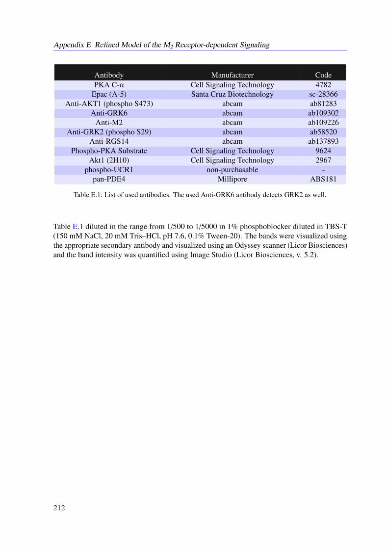
Appendix E Refined Model of the M2 Receptor-dependent Signaling
Antibody Manufacturer CodePKA C-α Cell Signaling Technology 4782
Epac (A-5) Santa Cruz Biotechnology sc-28366Anti-AKT1 (phospho S473) abcam ab81283
Anti-GRK6 abcam ab109302Anti-M2 abcam ab109226
Anti-GRK2 (phospho S29) abcam ab58520Anti-RGS14 abcam ab137893
Phospho-PKA Substrate Cell Signaling Technology 9624Akt1 (2H10) Cell Signaling Technology 2967
phospho-UCR1 non-purchasable -pan-PDE4 Millipore ABS181
Table E.1: List of used antibodies. The used Anti-GRK6 antibody detects GRK2 as well.
Table E.1 diluted in the range from 1/500 to 1/5000 in 1% phosphoblocker diluted in TBS-T(150 mM NaCl, 20 mM Tris–HCl, pH 7.6, 0.1% Tween-20). The bands were visualized usingthe appropriate secondary antibody and visualized using an Odyssey scanner (Licor Biosciences)and the band intensity was quantified using Image Studio (Licor Biosciences, v. 5.2).
212
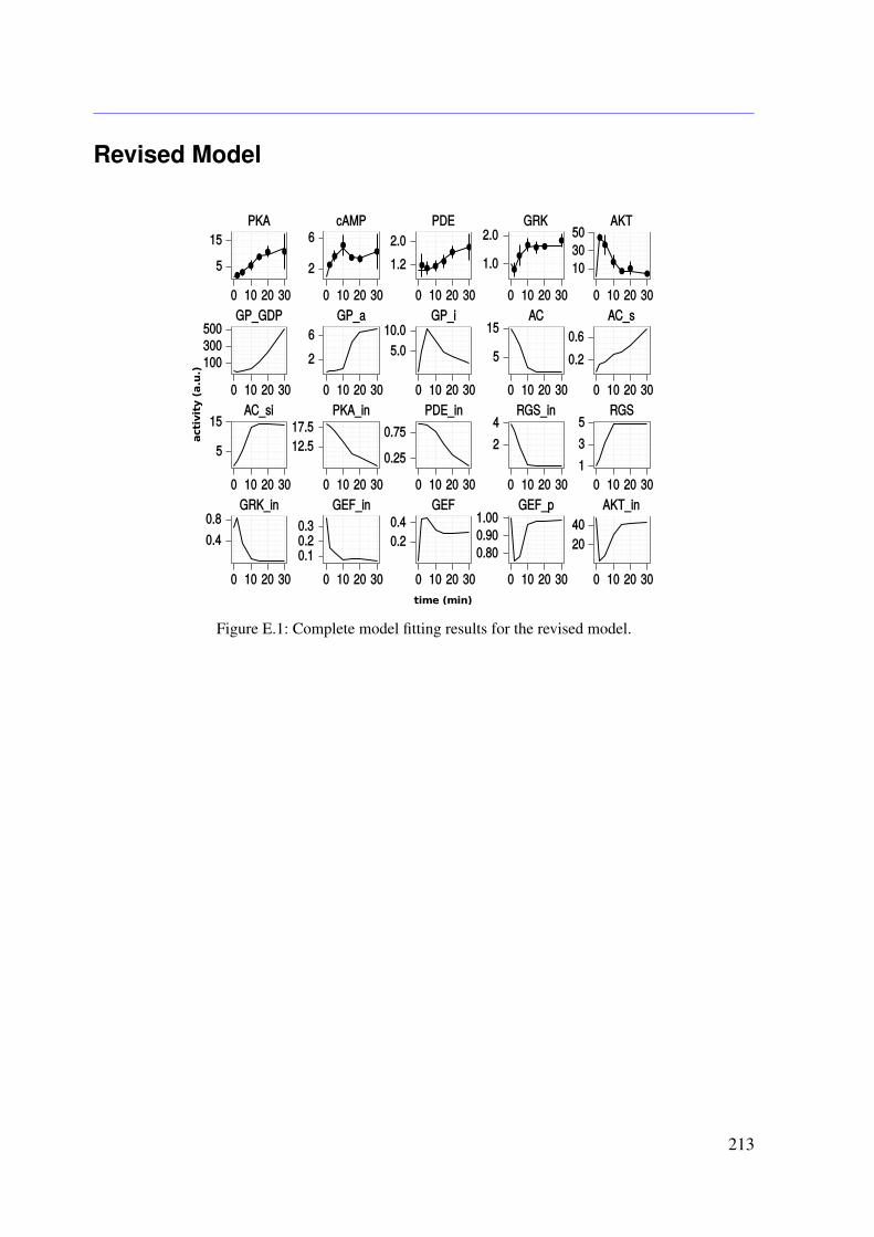
Revised Model
Figure E.1: Complete model fitting results for the revised model.
213
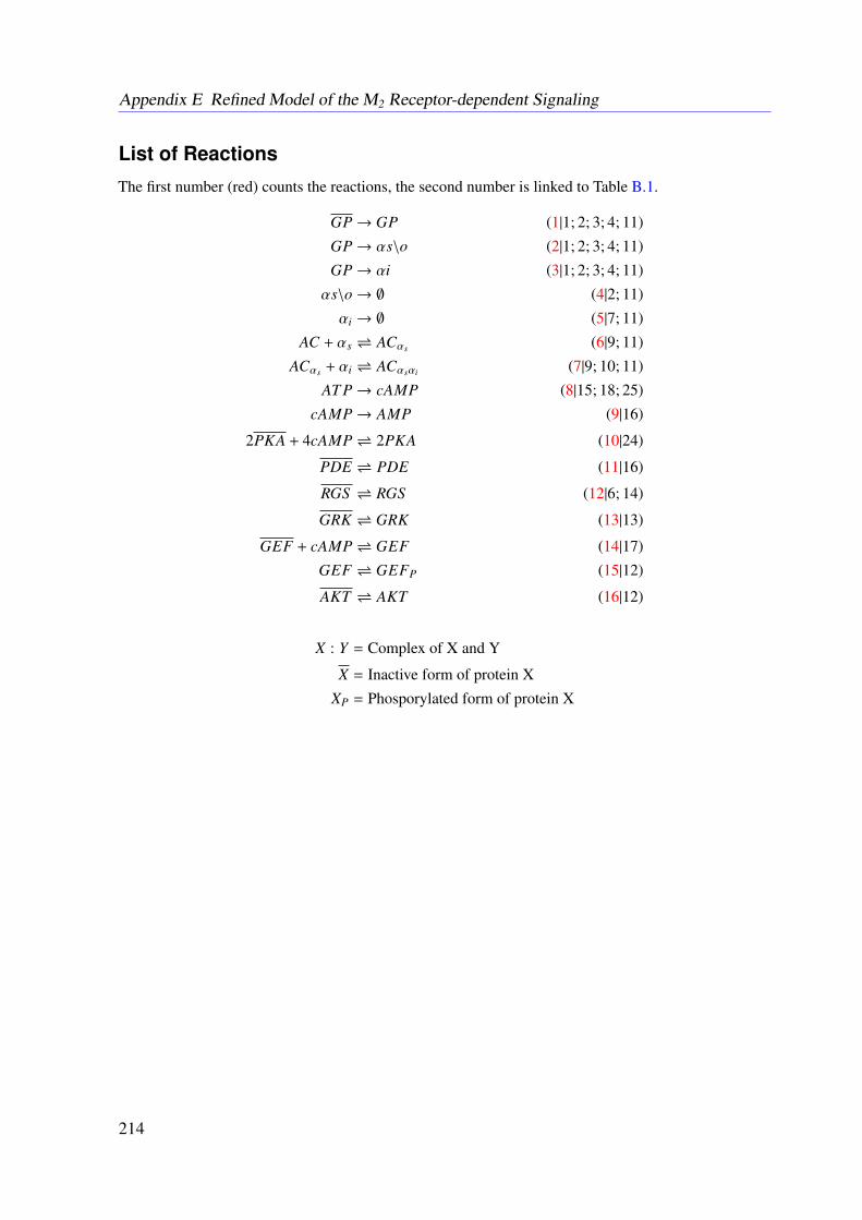
Appendix E Refined Model of the M2 Receptor-dependent Signaling
List of Reactions
The first number (red) counts the reactions, the second number is linked to Table B.1.
GP→ GP (1|1; 2; 3; 4; 11)
GP→ αs\o (2|1; 2; 3; 4; 11)
GP→ αi (3|1; 2; 3; 4; 11)
αs\o→ ∅ (4|2; 11)
αi → ∅ (5|7; 11)
AC + αs ACαs (6|9; 11)
ACαs + αi ACαsαi (7|9; 10; 11)
AT P→ cAMP (8|15; 18; 25)
cAMP→ AMP (9|16)
2PKA + 4cAMP 2PKA (10|24)
PDE PDE (11|16)
RGS RGS (12|6; 14)
GRK GRK (13|13)
GEF + cAMP GEF (14|17)
GEF GEFP (15|12)
AKT AKT (16|12)
X : Y = Complex of X and Y
X = Inactive form of protein X
XP = Phosporylated form of protein X
214

List of Rate Laws
Detailed list of rate laws including the parameter estimates. Numbers count the reactions linkedto the List of Reactions.
Rate-LawNr. Forward Backward Parameter Estimates
(1) keq(1 − exp
(−kobs × t
))keq = 50.5 kobs = 0.076
(2) (1 − Frac) ×V1×[GP]
Km1+[GP] Frac = 0.881 V1 = 14.994 Km1 = 0.247
(3) Frac ×V1[GP]
Km1+[GP] Frac = 0.881 V1 = 14.994 Km1 = 0.247
(4) V2 × [αs\o] V2 = 0.245
(5)V3×[RGS ]×[αi]
Km3+[αi] V3 = 2.790 Km3 = 0.066
(6) k1 × [AC] × [αs\o] k2 × [ACs] k1 = 2.240 k2 = 0.318
(7) k3 × [ACs] × [αi] k4 ×[ACsi
]k3 = 1.521 k4 = 0.176
(8) V4×[ACs ](Km4+[ACs ]
)(1+
[PKA]Ki4
) V4 = 47.223 Km4 = 0.658 Ki4 = 12.880
(9)V5×[cAMP]×[PDE]
Km5+[cAMP] V5 = 6.953 Km5 = 0.167
(10) k5 ×[PKA
]× [cAMP]4 k6 × [PKA]2 k5 = 8e − 05 k6 = 4e − 04
(11)V6×[PKA]×
[PDE
]Km6+
[PDE
] V7 × [PDE] V6 = 0.018 Km6 = 0.516 V7 = 0.010
(12)V8×[PKA]×
[RGS
]Km8+
[RGS
] +V12×[GEF]×
[RGS
]Km12+
[RGS
] V9 × [RGS ] V8 = 0.382 Km8 = 0.201 V12 = 0.312 Km12 = 0.354 V9 = 0.166
(13)V10×[PKA]×
[GRK
]Km10+
[GRK
] V11 × [GRK] V10 = 0.575 Km10 = 0.057 V11 = 0.961
(14) k7 ×[GEF
]× [cAMP] k8 × [GEF] k7 = 0.369 k8 = 0.363
(15)V13×[GEF]×[GRK]
Km13+[GEF] k9 ×[GEFp
]V13 = 0.423 Km13 = 0.351 k9 = 0.317
(16)V14×
[AKT
]Km14+
[AKT
] V15×[PKA]×[AKT ]Km15+[AKT ]) V14 = 55.452 Km14 = 5.054 V15 = 19.580 Km15 = 18.4603
215


APPENDIX F
List of Publications
Publications
• Engelhardt B, Fröhlich H, Kschischo M, Learning (from) the errors of a systems biologymodel, Nature Scientific Reports, 6, 20772, 2016.
• Engelhardt B, Kschischo M, Fröhlich H, A Bayesian Approach to Estimating HiddenVariables as well as Missing and Wrong Molecular Interactions in ODE Based Mathemat-ical Models, Journal of the Royal Society Interface, under review.
• Engelhardt B, Holze J, Elliott C, Baillie GS, Kschischo M, Fröhlich H, Modeling andMathematical Analysis of the M2-Receptor Dependent Joint Signaling and SecondaryMessenger Network in CHO Cells, Mathematical Medicine and Biology, accepted.
• Engelhardt B, König J, Blettner M, Wild P, Münzel T, Lackner K, Blankenberg S,Pfeiffer N, Beutel M, Zwiener I, Combining Cross-sectional Data on Prevalence with RiskEstimates from a Prediction Model, Methods of Information in Medicine, 5, 371 - 379,2014
Conference Presentations
• Engelhardt B, Fröhlich H, Kschischo M, Inferring model errors and unmeasured systemstates with incomplete models: The dynamic elastic net, presented at the Meeting of theInternational Study Group for Systems Biology 2016 in Jena (poster).
• Engelhardt B, Fröhlich H, Kschischo M, Learning (from) the errors of a systems biologymodel, presented at the International Symposium 2016 in Bonn (paper presentation andposter).
• Engelhardt B, Kschischo M, Fröhlich H, A New Computational Method to Make Dy-namic Mathematical Models Complete and Consistent, presented at the European Confer-ence on Mathematical and Theoretical Biology 2016 in Göttingen (poster).
217

Appendix F List of Publications
• Engelhardt B, Kschischo M, Fröhlich H, A Bayesian Approach for estimating hiddenvariables in ODE based systems biology models, presented at the European Conference onMathematical and Theoretical Biology 2016 in Notthingham (contributed talk and poster).
• Engelhardt B, Schrage R, Tränkle C, Mohr K, Kschischo M, Fröhlich H, G Protein-dependent Signaling in CHO Cells: Dynamic Systems and Beyond, presented at theSummer Academy Pharmacology 2015 in Bonn (contributed talk and poster).
• Engelhardt B, Kschischo M, Fröhlich H, Detection of Hidden Influences and MissedReactions in Quantitative Models of Biological Systems, presented at the Basel Computa-tional Biology Conference 2015 (contributed talk).
• Engelhardt B, Schrage R, Tränkle C, Mohr K, Kschischo M, Fröhlich H, MathematicalAnalysis and Joint Modeling of the M2 Receptor - dependent Signaling And SecondaryMessenger Network in CHO Cells, presented at the European Conference on Mathematicaland Theoretical Biology 2014 in Gothenburg (contributed talk).
218
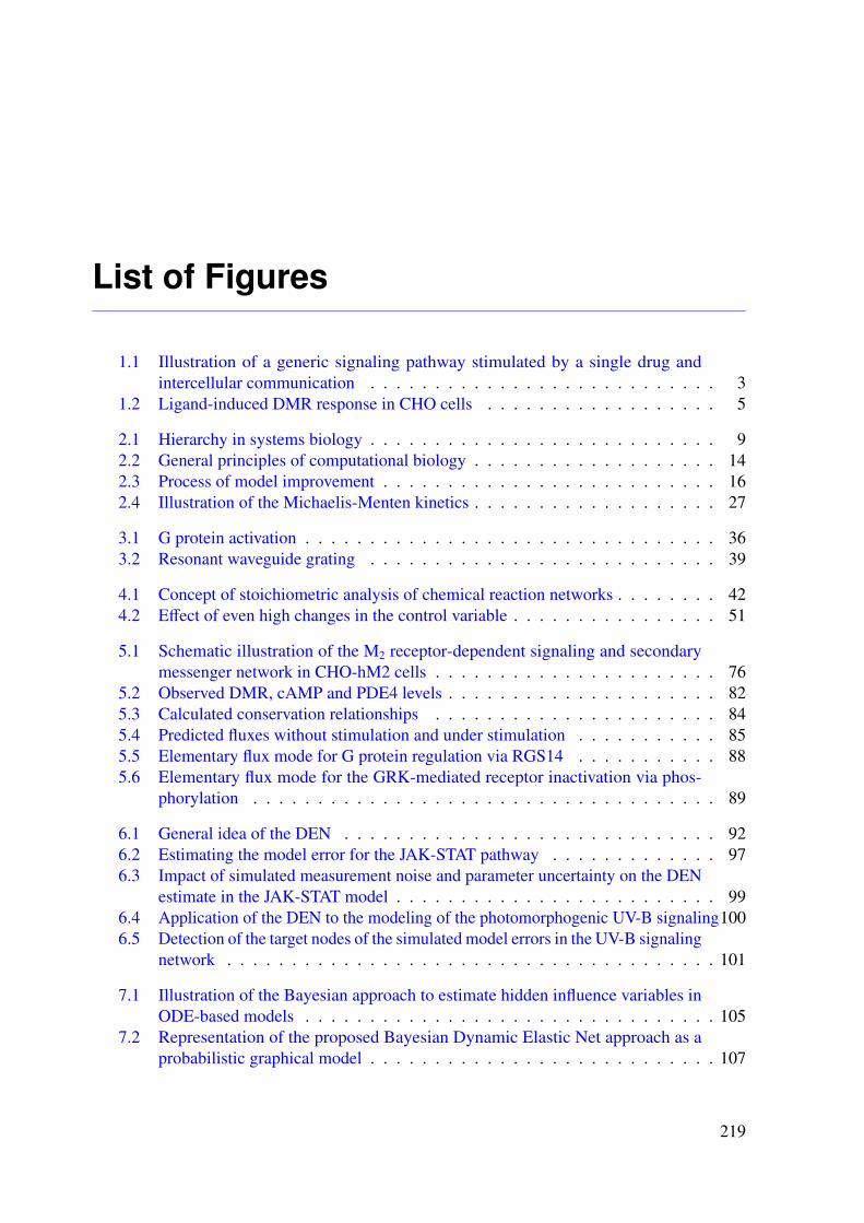
List of Figures
1.1 Illustration of a generic signaling pathway stimulated by a single drug andintercellular communication . . . . . . . . . . . . . . . . . . . . . . . . . . . 3
1.2 Ligand-induced DMR response in CHO cells . . . . . . . . . . . . . . . . . . 5
2.1 Hierarchy in systems biology . . . . . . . . . . . . . . . . . . . . . . . . . . . 92.2 General principles of computational biology . . . . . . . . . . . . . . . . . . . 142.3 Process of model improvement . . . . . . . . . . . . . . . . . . . . . . . . . . 162.4 Illustration of the Michaelis-Menten kinetics . . . . . . . . . . . . . . . . . . . 27
3.1 G protein activation . . . . . . . . . . . . . . . . . . . . . . . . . . . . . . . . 363.2 Resonant waveguide grating . . . . . . . . . . . . . . . . . . . . . . . . . . . 39
4.1 Concept of stoichiometric analysis of chemical reaction networks . . . . . . . . 424.2 Effect of even high changes in the control variable . . . . . . . . . . . . . . . . 51
5.1 Schematic illustration of the M2 receptor-dependent signaling and secondarymessenger network in CHO-hM2 cells . . . . . . . . . . . . . . . . . . . . . . 76
5.2 Observed DMR, cAMP and PDE4 levels . . . . . . . . . . . . . . . . . . . . . 825.3 Calculated conservation relationships . . . . . . . . . . . . . . . . . . . . . . 845.4 Predicted fluxes without stimulation and under stimulation . . . . . . . . . . . 855.5 Elementary flux mode for G protein regulation via RGS14 . . . . . . . . . . . 885.6 Elementary flux mode for the GRK-mediated receptor inactivation via phos-
phorylation . . . . . . . . . . . . . . . . . . . . . . . . . . . . . . . . . . . . 89
6.1 General idea of the DEN . . . . . . . . . . . . . . . . . . . . . . . . . . . . . 926.2 Estimating the model error for the JAK-STAT pathway . . . . . . . . . . . . . 976.3 Impact of simulated measurement noise and parameter uncertainty on the DEN
estimate in the JAK-STAT model . . . . . . . . . . . . . . . . . . . . . . . . . 996.4 Application of the DEN to the modeling of the photomorphogenic UV-B signaling1006.5 Detection of the target nodes of the simulated model errors in the UV-B signaling
network . . . . . . . . . . . . . . . . . . . . . . . . . . . . . . . . . . . . . . 101
7.1 Illustration of the Bayesian approach to estimate hidden influence variables inODE-based models . . . . . . . . . . . . . . . . . . . . . . . . . . . . . . . . 105
7.2 Representation of the proposed Bayesian Dynamic Elastic Net approach as aprobabilistic graphical model . . . . . . . . . . . . . . . . . . . . . . . . . . . 107
219
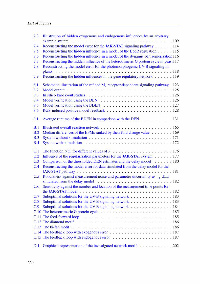
List of Figures
7.3 Illustration of hidden exogenous and endogenous influences by an arbitraryexample system . . . . . . . . . . . . . . . . . . . . . . . . . . . . . . . . . . 109
7.4 Reconstructing the model error for the JAK-STAT signaling pathway . . . . . . 1147.5 Reconstructing the hidden influence in a model of the EpoR regulation . . . . . 1157.6 Reconstructing the hidden influence in a model of the dynamic αP isomerization1167.7 Reconstructing the hidden influence of the heterotrimeric G protein cycle in yeast1177.8 Reconstructing the model error for the photomorphogenic UV-B signaling in
plants . . . . . . . . . . . . . . . . . . . . . . . . . . . . . . . . . . . . . . . 1187.9 Reconstructing the hidden influences in the gene regulatory network . . . . . . 119
8.1 Schematic illustration of the refined M2 receptor-dependent signaling pathway . 1238.2 Model output . . . . . . . . . . . . . . . . . . . . . . . . . . . . . . . . . . . 1258.3 In silico knock-out studies . . . . . . . . . . . . . . . . . . . . . . . . . . . . 1268.4 Model verification using the DEN . . . . . . . . . . . . . . . . . . . . . . . . 1268.5 Model verification using the BDEN . . . . . . . . . . . . . . . . . . . . . . . 1278.6 RGS-induced positive model feedback . . . . . . . . . . . . . . . . . . . . . . 128
9.1 Average runtime of the BDEN in comparison with the DEN . . . . . . . . . . . 131
B.1 Illustrated overall reaction network . . . . . . . . . . . . . . . . . . . . . . . . 165B.2 Median differences of the EFMs ranked by their fold change value . . . . . . . 169B.3 System without stimulation . . . . . . . . . . . . . . . . . . . . . . . . . . . . 171B.4 System with stimulation . . . . . . . . . . . . . . . . . . . . . . . . . . . . . 172
C.1 The function h(w) for different values of λ . . . . . . . . . . . . . . . . . . . . 176C.2 Influence of the regularization parameters for the JAK-STAT system . . . . . . 177C.3 Comparison of the thresholded DEN estimates and the delay model . . . . . . 180C.4 Reconstructing the model error for data simulated from the delay model for the
JAK-STAT pathway . . . . . . . . . . . . . . . . . . . . . . . . . . . . . . . . 181C.5 Robustness against measurement noise and parameter uncertainty using data
simulated from the delay model . . . . . . . . . . . . . . . . . . . . . . . . . 182C.6 Sensitivity against the number and location of the measurement time points for
the JAK-STAT model . . . . . . . . . . . . . . . . . . . . . . . . . . . . . . . 182C.7 Suboptimal solutions for the UV-B signaling network . . . . . . . . . . . . . . 183C.8 Suboptimal solutions for the UV-B signaling network . . . . . . . . . . . . . . 183C.9 Suboptimal solutions for the UV-B signaling network . . . . . . . . . . . . . . 184C.10 The heterotrimeric G protein cycle . . . . . . . . . . . . . . . . . . . . . . . . 185C.11 The feed-forward loop . . . . . . . . . . . . . . . . . . . . . . . . . . . . . . 185C.12 The diamond motif . . . . . . . . . . . . . . . . . . . . . . . . . . . . . . . . 186C.13 The bi-fan motif . . . . . . . . . . . . . . . . . . . . . . . . . . . . . . . . . . 186C.14 The feedback loop with exogenous error . . . . . . . . . . . . . . . . . . . . . 187C.15 The feedback loop with endogenous error . . . . . . . . . . . . . . . . . . . . 187
D.1 Graphical representation of the investigated network motifs . . . . . . . . . . . 202
220

List of Figures
E.1 Complete model fitting results for the revised model . . . . . . . . . . . . . . . 213
Elements in Figures 2.1, 2.3, 3.1 and 3.2 are adapted from Servier Medical Art; used under CC-BY.
221

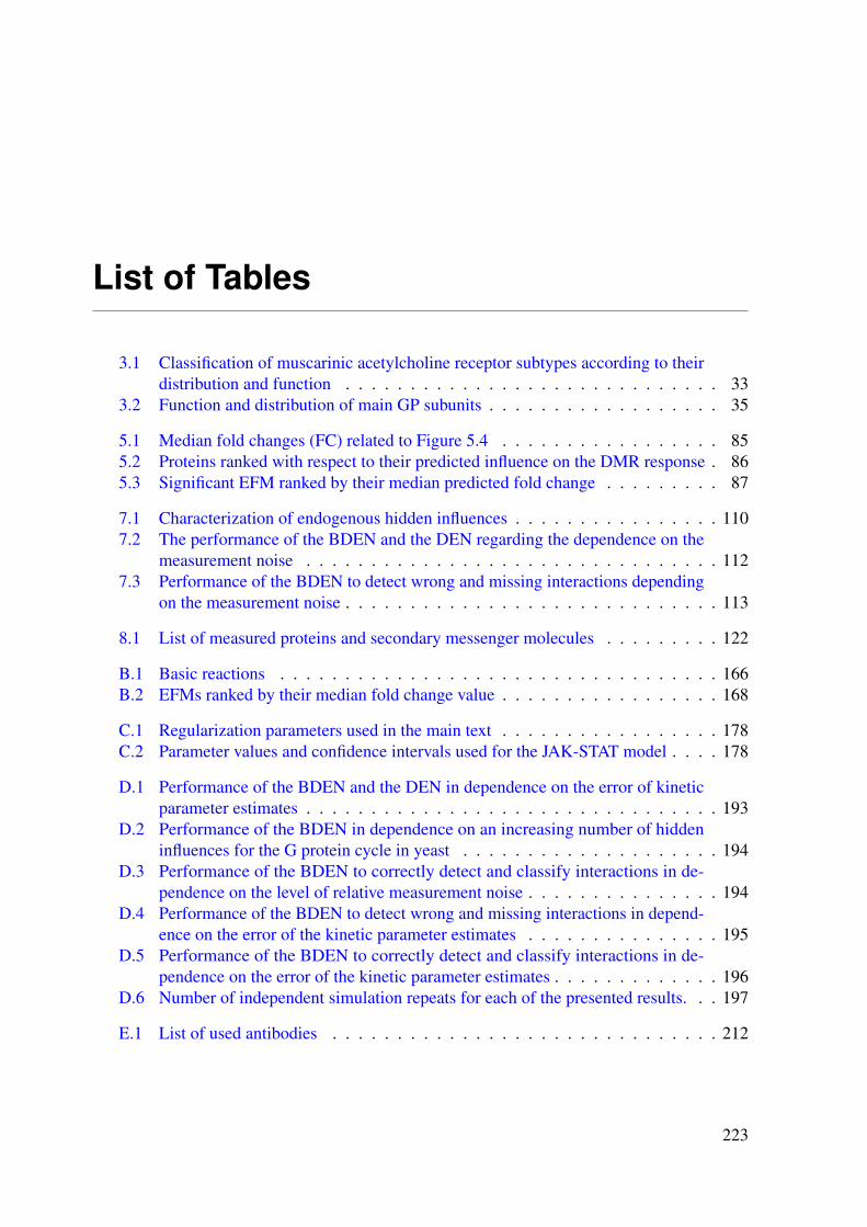
List of Tables
3.1 Classification of muscarinic acetylcholine receptor subtypes according to theirdistribution and function . . . . . . . . . . . . . . . . . . . . . . . . . . . . . 33
3.2 Function and distribution of main GP subunits . . . . . . . . . . . . . . . . . . 35
5.1 Median fold changes (FC) related to Figure 5.4 . . . . . . . . . . . . . . . . . 855.2 Proteins ranked with respect to their predicted influence on the DMR response . 865.3 Significant EFM ranked by their median predicted fold change . . . . . . . . . 87
7.1 Characterization of endogenous hidden influences . . . . . . . . . . . . . . . . 1107.2 The performance of the BDEN and the DEN regarding the dependence on the
measurement noise . . . . . . . . . . . . . . . . . . . . . . . . . . . . . . . . 1127.3 Performance of the BDEN to detect wrong and missing interactions depending
on the measurement noise . . . . . . . . . . . . . . . . . . . . . . . . . . . . . 113
8.1 List of measured proteins and secondary messenger molecules . . . . . . . . . 122
B.1 Basic reactions . . . . . . . . . . . . . . . . . . . . . . . . . . . . . . . . . . 166B.2 EFMs ranked by their median fold change value . . . . . . . . . . . . . . . . . 168
C.1 Regularization parameters used in the main text . . . . . . . . . . . . . . . . . 178C.2 Parameter values and confidence intervals used for the JAK-STAT model . . . . 178
D.1 Performance of the BDEN and the DEN in dependence on the error of kineticparameter estimates . . . . . . . . . . . . . . . . . . . . . . . . . . . . . . . . 193
D.2 Performance of the BDEN in dependence on an increasing number of hiddeninfluences for the G protein cycle in yeast . . . . . . . . . . . . . . . . . . . . 194
D.3 Performance of the BDEN to correctly detect and classify interactions in de-pendence on the level of relative measurement noise . . . . . . . . . . . . . . . 194
D.4 Performance of the BDEN to detect wrong and missing interactions in depend-ence on the error of the kinetic parameter estimates . . . . . . . . . . . . . . . 195
D.5 Performance of the BDEN to correctly detect and classify interactions in de-pendence on the error of the kinetic parameter estimates . . . . . . . . . . . . . 196
D.6 Number of independent simulation repeats for each of the presented results. . . 197
E.1 List of used antibodies . . . . . . . . . . . . . . . . . . . . . . . . . . . . . . 212
223