Mathematical Modelsfor Financial Bubbles

Sorin Nedelcu

Dissertation an der Fakultät für Mathematik,Informatik und Statistik der

Ludwig-Maximilians-Universität München

München 2014

Mathematical Models forFinancial Bubbles

Sorin Nedelcu

Dissertation an der Fakultät für Mathematik,Informatik und Statistik der

Ludwig-Maximilians-Universität München

vorgelegt am 01.12.2014

Erstgutachterin: Prof. Dr. Francesca BiaginiLudwig-Maximilians-Universität München

Zweitgutachter: Prof. Dr. Philip ProtterColumbia University, New York

Tag der Disputation: 22.12.2014

Eidesstattliche Versicherung(Siehe Promotionsordnung vom 12.07.11, § 8, Abs. 2 Pkt.5)

Hiermit erkläre ich an Eidesstatt, dass die Dissertation von mir selbstständing,ohne unerlaubte Beihilfe angeferteigt ist.

Nedelcu, Sorin

Ort, Datum Unterschrift Doktorand

Acknowledgements

This thesis has been written in partial fulfillment of the requirements for theDegree of Doctor of Natural Sciences at the Department of Mathematics,Informatics and Statistics at the University of Munich (Ludwig-Maximilians-Universität München).

First and foremost, I would like to express my deep gratitude to my ad-visor, Professor Francesca Biagini, for her constant support and guidancethrough every stage of my PhD. I’m very grateful for her availability eachtime her suggestions and mathematical expertise were needed, and for herconstant help and encouragement. The numerous mathematical discussionswith her helped me overcome the difficulties I faced during the writing ofthis thesis and her comments and suggestions substantially improved boththe contents and the presentation of this work. Last but not least, I wouldlike to thank her for her patience and trust throughout these years. I amforever indebted for the great opportunity to work with her.

I am especially grateful to Professor Hans Föllmer for his advice and con-tribution. His wide mathematical culture, inspiring ideas and his expertisewere crucial in completing important parts of this thesis. It has been a greathonour and a pleasure to work with him.

I am thankful to Professor Franz Merkl and Professor Philip Protter foraccepting to be members of my thesis defense committee.

I am very grateful to Professor Philip Protter for his interest in my thesisand for his visit to Munich in May 2013. His fascinating work on financialbubbles provided me with great insights into this topic and with a more pro-found understanding of financial mathematics.

I would like to thank to Professor Thilo Meyer-Brandis and ProfessorGregor Svindland and the Financial Mathematics Workgroup for their helpand support throughout these years and for providing a friendly and creativeenvironment.

Finally, I would like to express all my gratitude and appreciation to myparents for their unconditional love and support. I would like to thank myfather, who guided my first steps through mathematics. Without his con-stant encouragement and genuine passion for mathematics I would not havechosen this path in life.

Abstract

Financial bubbles have been present in the history of financial markets fromthe early days up to the modern age. An asset is said to exhibit a bub-ble when its market value exceeds its fundamental valuation. Although thisphenomenon has been thoroughly studied in the economic literature, a math-ematical martingale theory of bubbles, based on an absence of arbitrage hasonly recently been developed. In this dissertation, we aim to further con-tribute to the developement of this theory.In the first part we construct a model that allows us to capture the birth ofa financial bubble and to describe its behavior as an initial submartingale inthe build-up phase, which then turns into a supermartingale in the collapsephase. To this purpose we construct a flow in the space of equivalent martin-gale measures and we study the shifting perception of the fundamental valueof a given asset.In the second part of the dissertation, we study the formation of financialbubbles in the valuation of defaultable claims in a reduced-form setting. Inour model a bubble is born due to investor heterogeneity. Furthermore, ourstudy shows how changes in the dynamics of the defaultable claim’s marketprice may lead to a different selection of the martingale measure used forpricing. In this way we are able to unify the classical martingale theory ofbubbles with a constructive approach to the study of bubbles, based on theinteractions between investors.

Zusammenfassung

Finanz-Blasen sind seit der Entstehung der Finanzmärkte bis zur heutigenZeit gegenwärtig. Es gilt, dass ein Vermögenswert eine Finanzblase aufweist,sobald dessen Marktwert die fundamentale Bewertung übersteigt. Obwohldieses Phänomen in der Wirtschaftsliteratur ausgiebig behandelt wurde, isteine mathematische Martingaltheorie von Blasen, die auf der Abwesenheitvon Arbitragemöglichkeiten beruht, erst in letzter Zeit entwickelt worden.Das Ziel dieser Dissertation ist es einen Beitrag zur Weiterentwicklung dieserTheorie zu leisten.Im ersten Abschnitt konstruieren wir ein Model mit Hilfe dessen man dieEntstehung einer Finanz-Blase erfassen und deren Verhalten anfänglich alsSubmartingal in der build-up phase beschrieben werden kann, welches dannin der collapse phase zu einem Supermartingal wird. Zu diesem Zweck en-twickeln wir einen Zahlungsstrom im Raum der äquivalenten MartingalmaÃeund wir untersuchen die zu dem Vermögenswert passende Verschiebung desfundamentalen Werts.Der zweite Teil der Dissertation beschäftigt sich mit der Bildung von Finanz-Blasen bei der Bewertung von Forderungen, die mit Ausfallrisiken behaftetsind, in einer reduzierten Marktumgebung. In unserem Model ist die Entste-hung einer Blase die Folge der Heterogenität der Investoren. Des Weiterenzeigen unsere Untersuchungen, inwieweit Veränderungen der Dynamik desMarktpreises einer risikobehafteten Forderung zu einer Veränderung des zurBewertung verwendeten Martingalmaßes führen kann. Dadurch sind wir inder Lage die klassische Martingaltheorie von Finanz-Blasen mit einem kon-struktivem Ansatz zur Untersuchung von Finanz-Blasen zu vereinigen, derauf den Interaktionen zwischen Marktteilnehmern basiert.

ii

iii

Contents

Contents 1

1 Introduction 31.1 Motivation . . . . . . . . . . . . . . . . . . . . . . . . . . . . . 31.2 Contributing Manuscripts . . . . . . . . . . . . . . . . . . . . 7

2 Shifting martingale measures 102.1 Motivation . . . . . . . . . . . . . . . . . . . . . . . . . . . . . 102.2 The Setting . . . . . . . . . . . . . . . . . . . . . . . . . . . . 152.3 The birth of a bubble as a submartingale . . . . . . . . . . . . 202.4 The Delbaen-Schachermayer example . . . . . . . . . . . . . . 292.5 The behavior of the R-bubble under Q . . . . . . . . . . . . . 32

3 Stochastic volatility models 403.1 Stochastic model with independent Brownian motions . . . . . 403.2 Stochastic model with correlated Brownian motions . . . . . . 51

4 The formation of financial bubbles in defaultable markets 624.1 Introduction . . . . . . . . . . . . . . . . . . . . . . . . . . . . 624.2 The Setting . . . . . . . . . . . . . . . . . . . . . . . . . . . . 664.3 Bubbles in defaultable claim valuation . . . . . . . . . . . . . 714.4 The case of CIR default intensity . . . . . . . . . . . . . . . . 74

4.4.1 Reduced Information Setting . . . . . . . . . . . . . . . 934.5 Characterization ofMloc(W ) by measure pasting . . . . . . . 96

A Strict local martingales 103

Bibliography 105

1

Chapter 1

Introduction

1.1 MotivationBubbles and financial crises have been recorded throughout modern history,with probably the earliest documented events going back to the 17th and18th century: the Dutch tulipmania of 1634-1637, the Mississippi bubble of1719-1720 and the South Sea bubble of 1720, see Garber [28], [29]. All ofthese historical events exhibit two phases: a run-up phase characterized bya sharp increase in the price of an asset(price of tulips, shares of the Com-pagnie des Indes, shares of the South Sea company respectively), followed bya decline phase -the collapse of the price. Let us illustrate this fact with ashort expose of the last two historical events mentioned above.

The Mississippi bubble was created by the rise and fall of the Compag-nie des Indes, vehicle through which John Law, France’s Controller Generalof Finance tried to refinance France’s debt. The share prices of Compagnied’Indes rose from 1800 livres in July 1719, to 3000 livres in October 1719 andreached a peak value of 10000 livres at the end of the year. The rise in theprice was partly motivated by large-scale takeovers of other commercial com-panies (acquisition of the East India Company and China Company in May1719, acquisition of the Senegalese Company in September 1719) which leadto a monolopy over all French trade outside Europe, together with a takeoverof government functions (such as the mint and the collection of taxes). Law’sidea was to establish a “fund of credit” which, when leveraged, could financeand help expand the commercial enterprise: “finance of the operation camefirst; expanded commercial activity would result naturally once the finan-cial structure was in place”(Garber [28]). In January 1720, due to increasingattempts of shareholders to convert capital gains into gold form, the shareprices began to fall below 10000 livres. Despite Law’s attempts to prevent

3

the stock price’s decline, the price fell to 2000 livres in September 1720 andto 500 livres in September 1721, the same value the stock had in May 1719.

The South Sea bubble was caused by a similar plan, though much sim-pler, of the South Sea Company to acquire British government debt. TheCompany’s share price experienced a sharp increase from about 120 poundsin January 1720 to 775 pounds in August 1720. The speculation around theCompany’s shares lead to an increase in the prices of other Companies andto the creation of numerous, mostly fraudulent, “bubble companies”. TheSouth Sea Company’s share prices fell from its peak value of 775 poundsto 290 pounds in October 1720. The collapse is generally attributed to aliquidity crisis caused by the “Bubble Act” passed by the Parliament in June1720, and by the collapse of Law’s Compagnie d’Indes in September 1720,see Garber [28], Neal [47], Neal and Schubert [48].

More recent examples of bubbles include the ones that occured aroundthe US banking crises of 1837, 1873 and 1907, The Great Crash of 1929, theJapanese housing bubble of 1970-1989, the Dot-Com bubble of 1997-2002 andthe recent US housing bubble. For an overwiew of the causes that triggeredthese events, see Brunnermeier and Oehmke [11] and Protter [50], [51].

Several characteristics of financial bubbles have been pointed out as rec-curent in the economical literature. Asset price bubbles usually occur inperiods of technological and financial innovation, which leads to increasingexpectations of economic growth and profit among investors, see for exampleBrunnermeier and Oehmke [11], Protter [51], Scheinkman [54]. The devel-opement of trade between Europe and its colonies can be seen as a possibletrigger for the Mississippi and South Sea Bubbles, the advent of railroads,the internet, and of sophisticated financial instruments and hedging tech-niques can be seen as triggers for the Panic of 1873, the Dot-Com Bubbleand the recent credit bubble, respectively. Bubbles arise simultaneously withan increasing trading volume of the asset, and bubbles burst once the asset’ssupply is increased or a liquidity crisis appears, see for example Brunnermeier[10]. Furthermore, in an environment with several risky assets, asset pricebubbles can implode due to contagion, if the assets are held by the sameinvestors and are exposed to the same funding liquidity constraint.

An asset price bubble is defined to be the difference between the asset’smarket price and the lowest superreplicating price of its future dividents.From the economic perspective, one has to connect the appearance and dis-appearance of an asset price bubble at the microeconomic level with theinteractions between the market participants. In the economic literature,investor heterogeneity and limits to arbitrage are often indicated as possiblefactors behing the creation of asset price bubbles. Limits to arbitrage canresult from short-selling constraints, see Miller [46], or shocks to funding liq-

4

uidity, see e.g. Schleifer and Vishny [56]).Since most financial investments are exposed to risk and knightian uncer-

tainty, this can originate divergence of opinions among investors, or investorheterogeneity (investors agree to disagree). Harrison and Kreps [30] point outthat agents may disagree on the value of future dividends. In Scheinkmanand Xiong [55], each investor has a set of signals and observations on whichhe bases his estimation of the asset’s fundamental value. Overconfidence,or the agents’ tendency to exaggerate the importance of certain signals, canalso lead to investor heterogeneity. In a similar way, in the model proposedin Föllmer et. al.[25], investors may use different predictors when forecastingfuture prices and this may create heterogeneous beliefs in the market. Forother interesting references on the topic of bubble formation, see for instanceTirole [60], DeLong, Shleifer, Summers and Waldmann [21], Abreu and Brun-nermeier [1], and the references therein.

In mathematical finance, the characterization of price bubbles in termsmartingales/strict local martingales, in the setting of a market satisfying the“no free lunch with vanishing risk hypothesis (NFLV R)” was first introducedby Loewenstein and Willard [44]. In Cox and Hobson [18], an asset containsa bubble within its price process, if the discounted price process follows underthe risk neutral measure used for pricing a strict local martingale, that is, alocal martingale that is not a martingale. For a set of examples of strict localmartingales and references to additional literature on the topic, see AppendixA.

This approach to the study of financial bubbles, referred to as the mar-tingale theory of bubbles, was fundamented in the complete and incompletemarket settings in the seminal works of Jarrow, Protter and Shimbo [39],[40].In Jarrow et .al [40], [36], the authors also provide a study of derivativeswritten on assets exhibiting price bubbles, such as European call and putoptions, American options, forward and future contracts. An interestingproperty that has been highlighted in the above works is that the put-callparity usually does not hold when the asset’s price process is driven by astrict local martingale. The presence of bubbles in foreign exchange rateshas been studied in Jarrow and Protter [37] and Carr, Fisher and Ruf [13].In the model constructed in [37], exchange rate bubbles are caused by theexistence of a bubble in the price of either or both the domestic and foreignmarket currencies. Furthermore, in contrast to asset price bubbles that arealways positive, exchange rate bubbles can be negative. More precisely, if aforeign currency exhange rate is positive, then its inverse exchange rate isnegative. Carr, Fisher and Ruf [13] use the Föllmer measure [24] to constructa pricing operator for complete models where the exhange rate is driven bya strict local martingale. This construction allows to preserve the put-call

5

parity and also provides the minimal joint replication price for a contingentclaim.

Further connections between bubbles and the prices of derivatives writtenon assets whose price process is driven by a strict local martingale have beenstudied in Pal and Protter [49]. Karatzas, Kreher and Nikeghbali [42] extendthe results of [49], by providing the decomposition of the price of certainclases of path-dependent options (modified call-options and chooser options)and barrier options into a “non-bubble” term and a default term. Since themartingale theory of financial bubbles does not allow for bubbles in the priceof bounded asset prices, in Bilina-Falafala, Jarrow and Protter [8] the novelconcept of a relative asset bubble is introduced, which allows the study ofrisky assets with bounded payoffs within the current theory. With the helpof the volatility-based criteria developed by Carr et.al [12] for identifyingstrict local martingales, in Jarrow, Kchia and Protter[34] a methodology foridentifying bubbles (in real time) has been developed. In a recent article,Herdegen and Herrmann [31] discuss the stochastic investment opportunitiesin market model with bubbles. For a comprehensive survey of the recentmathematical literature on financial bubbles we refer to Protter [51].

The present thesis can be divided into two parts. In the first part, whichcovers Chapter 2 and Chapter 3, we construct a model that allows for theslow birth of an asset price bubble starting at zero, in the sense that itsinitial behavior is described by a submartingale. To this purpose we fix twolocal martingale measures Q and R, under which the asset’s wealth processfollows a uniformly integrable martingale and a strict local martingale, re-spectively. In Section 2.3 of Chapter 2, we construct a flow R = (Rt)t≥0

in the space of martingale measures which moves from the initial measureQ to the measure R, via convex combinations of the two. We provide suf-ficient conditions under which the resulting R-bubble perceived under theflow R is a local R-submartingale. Thus, we are able to capture in a re-alistic way the birth and subsequent behavior of the R-bubble under thereference measure R as follows: the R- bubble starts from its initial value asa submartingale and then turns into a supermartingale before it finally fallsback to zero. In Section 2.4, we examine in the setting of a slight extensionof the Delbaen-Schachermayer example, the behavior of the bubble processconstructed above. We show that the sufficient conditions under which thebubble process is a submartingale are satisfied. In the final Section 2.5 ofChapter 2, we change our point of view and instead of using R as referencemeasure, we take Q as reference. Here again, the birth of the bubble can bedescribed as a initial submartingale. However, its behavior is more delicateto examine, as illustrated in the context of the Delbaen-Schachermayer ex-ample.

6

Chapter 3 is dedicated to the study of the R-bubble in stochastic volatil-ity models. We verify that the sufficient conditions for our R-bubble processto be a local R-submartingale hold for a variant of the stochastic volatilitymodel discussed by Sin [57]. Moreover, our model can be modified in sucha way that the condition no longer holds. A similar analysis of the bubbleprocess is done in Section 3.2 in a modified variant of the Andersen-Piterbargvolatility model [3].

In Chapter 4 we examine the formation of financial bubbles in the valua-tion of defaultable claims in a reduced form credit risk model. The birth ofa bubble is generated by the impact of the heterogeneous beliefs of investorson the defaultable claim’s market wealth. A large group of investors whosetrades can influence the asset price may consider the claim to be a safe in-vestment under certain circumstances. Their trading actions create changesin the dynamics of the asset’s market wealth process, and these lead to sub-sequent shifts in the selection of the martingale measures used for pricing.Therefore, our model also provides an explanation how microeconomic inter-actions between agents may at an aggregate level determine a shift in themartingale measure, via a change in the dynamics of the market wealth pro-cess. In this way we establish a connection between the impact of differentviews within the groups of investors on asset prices and the classical resultsof the martingale theory of bubbles, see Biagini, Föllmer and Nedelcu [4] andJarrow and Protter [40]. The Chapter concludes with a characterization ofthe space of equivalent local martingale measures with the help of measurepasting, characterization which allows to rigurously capture how changes inthe dynamics of the asset price process lead to different selections of localmartingale measures used for pricing.

1.2 Contributing ManuscriptsThis thesis is based on the following manuscripts, which were developed bythe thesis’ author S. Nedelcu, in cooperation with coauthors:

1. F. Biagini, H. Föllmer, and S. Nedelcu [4]: Shifting martingale measuresand the birth of a bubble as a submartingale. Finance and Stochastics,18(2): 297-326, 2014.The results of this paper are the product of a joint work of S. Nedelcuwith two coauthors, Prof. F. Biagini and Prof. H. Föllmer. Most of thework was developed at the LMU Munich. Certain parts where final-ized during S. Nedelcu’s visits to Humboldt University and University

7

of Luxembourg (at the invitation of Prof. H. Föllmer). After a sugges-tion of H. Föllmer, S. Nedelcu and F. Biagini started to study a convexflow on the space of equivalent martingale measures and proved mostof the results in Section 3, in particular Theorem 2.3.9 and Corollary2.3.10. The argumentation concerning the economical significance ofthe model which is contained in Section 2, and Section 4 which containsthe Delbaen-Schachermayer example, was developed by S. Nedelcu to-gether with his 2 coauthors. Section 5 was developed independently byS. Nedelcu. Section 6 was developed by S. Nedelcu together with Prof.H. Föllmer. However, the final version of this part is mainly due to S.Nedelcu.

2. F. Biagini and S. Nedelcu [5]: The formation of financial bubbles in de-faultable markets. Preprint, Available at http://www.fm.mathematik.uni-muenchen.de/download/publications, 2014.The construction of the reduced-form credit risk framework in whichthe formation of bubbles is studied, was developed by S. Nedelcu to-gether with Prof. F. Biagini. Thus, Section 2, in which the model’sframework is constructed, Section 3, which contains the connectionwith the classical martingale theory of bubbles, and Section 5, whichcontains a case study, are the result of this joint work. A significantpart of the computations contained in the proofs of these Chapters wasdeveloped by S. Nedelcu. Furthermore S. Nedelcu suggested the useof the predictable version of Girsanov’s theorem in the proofs concern-ing measure changes and the existence of equivalent local martingalemeasures. The main idea of Section 4, the use of the concept of mea-sure pasting to the study of asset price bubbles, was developed by S.Nedelcu. This plays a fundamental role in unifying a constructive ap-proach to the study of asset price bubbles with the martingale theoryof bubbles.

The following list indicates in which way the two publications contributeto each Chapter of the Thesis and which sections represent unpublishedmanuscripts. The formulation of the statements of the Propositions, Lem-mas, Theorems, etc. is the same as in the two manuscripts. However, theauthor, who has been involved in the developement of all the results con-tained in the two publications, provides in the present thesis a more detailedversion for most of the proofs.

1. Chapter 1 provides a presentation of the existing mathematical liter-ature on financial bubbles. The summary of each article was written

8

independently by S. Nedelcu. The Chapter concludes with a summaryof the Thesis.

2. Chapter 2 is based the Sections 2, 3, 4 and 6 of Biagini, Föllmer andNedelcu [4].

3. Section 3.1 of Chapter 3 is based on Section 5 of Biagini, Föllmer andNedelcu [4]. Section 3.2 of Chapter 3 was developed independently byS. Nedelcu, and is based on a manuscript which is not yet published.

4. Chapter 4 is based on Biagini and Nedelcu [5]. Section 4.4.1, devel-oped independently by S. Nedelcu as part of an earlier draft version ofBiagini and Nedelcu [4], and is based on a manuscript which is not yetpublished.

Chapter 2

Shifting martingale measures

The contents of this Chapter are based on the author’s joint work with F. Bi-agini and H. Föllmer, which is contained in the article F. Biagini, H. Föllmerand S. Nedelcu [4]. More precisely, the present Chapter is based on Sec-tions 2, 3, 4 and 6 of [4]. The detailed description of the author’s personalcontribution is presented in Section 1.2.

2.1 MotivationAn asset price bubble is defined as the difference between two components:the observed market price of a given financial asset, which represents theamount that the marginal buyer is willing to pay, and the asset’s intrinsicor fundamental value, which is defined as the expected sum of future dis-counted dividends. As a result, Knightian/model uncertainty may arise dueto the fact that the asset’s fundamental value definition is made in termsof a conditional expectation. The fundamental component may be differ-ently perceived by investors according to their choice of the pricing measure.Thus, some agents may consider that a bubble exists in the asset price iftheir choice of the pricing measure does not lead to an equality between thecorresponding fundamental value and the asset’s market value. However, asshown in experimental economics, see Smith, Suchanek and Williams [58],bubbles may arise even if the probabilistic structure is perfectly known andthe economic agents are kept informed across all times about the fundamen-tal values of the assets.

In the present chapter we examine the perception of the fundamentalvalue. A first study on how this perception is connected to bubbles is donein a complete market setting in [39], by Jarrow, Protter, and Shimbo, whohowever point out the following inconvenient of the model: due to the unique-

10

ness of the martingale measure, bubbles cannot be born in this setting. Theyeither exist from the start of the model (and may disappear in time), or not.In order to overcome this difficulty, Jarrow, Protter, and Shimbo considerin their paper on Asset price bubbles in incomplete financial markets [40] anincomplete market model, i.e. a setting where there exist an infinite numberof local martingale measures. Hence the possible martingale measure thatcan be used for pricing is not unique anymore and each measure provides amarket consistent view of the future.

In our setting the discounted price process of a liquid financial asset fol-lows a semimartingale S under the real-world measure and D denotes theassociated cumulative discounted dividend process. We assume the existenceof an equivalent local martingale measure which turns the wealth processW = S + D into a local martingale. By following an argument of Harrisonand Kreps [30] we prove that any martingale measure can be seen as a pre-diction scheme that is consistent with the observed price process S from aspeculative point of view which takes into account future dividends and thepossibility of selling the asset at some future time.

However, different choices of the martingale measures may give differentassessments of the fundamental value, which is defined as the conditionalexpectation of future discounted dividends under the chosen equivalent localmartingale measure. Hence, if we denote SR to be the instrinsic value pro-cess under a martingale measure R, the bubble is defined as the differenceβR = S − SR, and this will be a non-negative local martingale under R.Nevertheless, in this incomplete model, if the bubble is defined in terms ofone fixed martingale measure R, then it either exists from the start of themodel (if R allows the existence of bubble) or it is zero all the time. In orderto allow the birth of a bubble in this framework after the model starts, weeliminate the time-consistency assumption.

We consider the definition of time consistency as provided in Föllmer andSchied [26]. Time consistency amounts to the requirement that all condi-tional probability distributions Rt(·|Ft), where Rt is an equivalent martin-gale measure for all t > 0 belong to the same martingale measure R. HereRt(·|Ft) represents the market’s view at time t. In particular, a completemarket model is automaticaly time-consistent, due to the uniqueness of themartingale measure. While time consistency is taked for granted in the math-ematical literature, in the real financial world various interactions betweeninvestors at the microeconomic level, like herding behavior of heterogeneousagents with interacting preferences and expectations, actions of large traders(see Chapter 4), or regime changes in the economy, may cause a shift of themartingale measure. This in turn leads to a dynamics in the space of equiva-lent local martingale measures and corresponding shifting perceptions of the

11

fundamental value.In [40], Jarrow, Protter and Shimbo consider a market model where

regime shifts occur in the underlying economy (due to risk aversion, institu-tional structures, technological innovations etc.) at different random times.This allows for the construction of a dynamic market model where a bubblesuddenly appears in the price of an asset at a stopping time and disappearsagain at a later stopping time.

The main objective of this chapter is to provide a realistic mathematicalmodel which captures the two stages of a financial bubble: the build-up stage,when the market price process diverges from the fundamental value and thecollapse phase when the market price drops and returns to the fundamentalvalue. To this purpose we wish to capture in the proposed setting the slowbirth of a perceived bubble starting at zero and to describe it as an initialsubmartingale, which then turns into a supermartingale before it falls backto the initial value zero. We consider two martingale measures Q and R rep-resenting the views of two (groups of) agents. A martingale measure is ofteninterpreted as a price equilibrium corresponding to the subjective preferencesand expectations of some representative agent; see for example Föllmer andSchied [27], Section 3.1. In the case of the martingale measure Q, the wealthprocess W is a uniformly integrable martingale, we have S = SQ. Hence,this subjective view can be interpreted as “optimistic” or “exuberant", sincethe market price is seen to coincide with the asset’s perceived intrinsic valuecomputed under the pricing measure Q. In particular, under the measure Qthere is no perception of a bubble contained in the asset’s price. Under themeasure R, the market wealth process W is no longer uniformly integrableand we have S > SR. Hence, under this view that can be characterized as“pessimistic” or “sober”, the market price is not justified from a fundamentalpoint of view and is affected by a bubble.

We provide examples of incomplete financial market models where suchmartingale measures Q and R coexist, see Section 2.4 of the present Chapterand Chapter 3 for examples which concern stochastic volatility models. Fur-thermore, we prove in the Delbaen-Schachermayer example, see Section 2.4as well as in the stochastic volatility model of Section 3.1, that the followingcondition is satisfied: The fundamental wealth WR = SR +D perceived un-der the “sober” measure R behaves as a submartingale under the “optimistic”measure Q. In terms of the agents’ perspectives, this behavior of WR underthe optimistic view represented by Q suggests that the pessimistic assess-ment WR is expected to be corrected through an upward trend.

In Section 2.3, we study a flow R = (Rt)t≥0 in the space of martingalemeasures that moves from the initial uniformly integrable martingale mea-sure Q to the non-uniformly integrable martingale measure R via convex

12

combinations of Q and R by putting an increasing weight on R. At eachtime t, the fundamental value process is computed with respect to the mar-tingale measure Rt. Consequently, the asset’s fundamental value is describedby the process SR. A further consequence of this construction is a shiftingperception of the asset’s fundamental value. We denote by βR = S−SR theresulting R-bubble perceived under the flow R. In Theorem 2.3.9, we pro-vide a crucial condition under which the birth and the subsequent behaviorof the R-bubble under the reference measure R can be described as follows:The R-bubble starts from its initial value as a submartingale (the build-upstage) and then turns into a supermartingale before it finally falls back tozero (the collapse phase). In Remark 2.3.3, we provide a possible economicintepretation for the shifting perception of the asset’s fundamental value byrefering to a microeconomic model of interacting agents described in Föllmeret al. [25].

In Section 2.4, we consider a slight extension of the classical Delbaen-Schachermayer setting. Instead of defining the price process along with themeasures Q and R in terms of two independent geometric Brownian motions,we consider a more general case where the price process S and the Radon-Nikodym density process of Q with respect to R are defined in terms of twoindependent continuous martingales. We are able to explicitly compute theprocesses WR and βR and show that the necessary condition for WR to bea local submartingale under Q is satisfied.

Section 2.5 provides a study of our model from the Q-perspective. To thispurpose we compute the canonical decomposition of the R-bubble under themeasure Q and provide conditions when the the birth of the bubble can be de-scribed as an initial submartingale with respect to the measure Q. However,as we show in the context of our extension of the Delbaen-Schachermayerexample, the modelling of the R-bubble’s behavior is not straighforward andrequires more technical effort.

The present chapter complements the study of successive regime switch-ing of Jarrow et al.[40] by allowing the capture of a submartingale behaviourin the birth of a perceived bubble and also provides a framework that allowsfor shifting martingale measures. This setting can be used as basis for a studyof the space of equivalent local martingale measures where the topologicalcharacterization of this space can be related to the size of a bubble. Fur-thermore, these contributions allow us to provide an interesting model alsofrom a practitioner point of view, since a dynamic in the space of martingalemeasures can be connected with the interactions of the market participantsat the microeconomic level. We illustrate this in Chapter 4, by showinghow possible changes in the dynamics of the asset price process can lead todifferent selections of the martingale measures used for pricing. Moreover,

13

Chapter 4 provides an example of an incomplete market setting where time-consistency fails and an asset price bubble can be born after the start of themodel.

14

2.2 The SettingLet (Ω,F , (Ft)t≥0, P ) be a filtered probability space satisfying the usual con-ditions: F0 contains all the P -null sets of F and the filtration (Ft)t≥0 isright-continuous i.e. Ft = ∩u>tFu for all t ≥ 0. We consider a market modelthat contains a risky asset and a money market account. We take the moneymarket accout as numéraire and consider directly a discounted setting, i.e. itis supposed to be constantly equal to 1. Let D = (Dt)t≥0 be a non-negativeincreasing and adapted right-continuous process representing the uncertaincumulative cash flow generated by the risky asset. We assume that the fil-tration is such that all martingales have continuous paths.

If ζ is a stopping time representing the maturity date or default time ofthe risky asset and the process D is seen as a cumulative dividend process,one can recover the setting of Jarrow et al. [40] by setting Dt := Dζ onζ ≤ t and defining the terminal payoff or liquidation value of the asset asXζ := (Dζ −Dζ−)1ζ<∞.

Let S = (St)t≥0 be a non-negative, adapted càdlàg process representingthe market price of the risky asset and denote by W = (Wt)t≥0 the corre-sponding wealth process defined by

Wt = St +Dt, t ≥ 0.

Definition 2.2.1. A probability measure Q equivalent to P under which thewealth process W is a Q-local martingale is called an equivalent local mar-tingale measure.

We denote byMloc(W ) the class of all probability measures Q ≈ P suchthat W is a local martingale under Q, and we asssume that

Mloc(W ) 6= ∅. (2.2.1)

The existence of an equivalent local martingale measure implies, via theFirst Fundamental Theorem, that S satisfies the No Free Lunch with Van-ishing Risk (NFLV R) condition. The converse implication is also true, seeDelbaen and Schachermayer [19]. In economic terms, NFLV R amounts tothe exclusion of all self-financing trading strategies that start with zero ini-tial investment and generate a non-negative cash flow for sure and a strictlypositive cash flow with positive probability (arbitrage opportunities). Weprovide examples of markets satisfying the NFLV R condition in Section2.4, Chapter 3 and Section 4.4 in Chapter 4.

Furthermore, the existence of an equivalent local martingale measure im-plies that the process W follows a semimartingale under the real world mea-sure P , i.e. W can be written as the sum between a càdlàg local martingaleand a càdlàg finite variation process.

15

Although the cumulative cash flow D associated to the risky asset isexogenously given, the price St can be justified at any time t from the per-spective of any probability measure Q ∈ Mloc(W ) in the following way: theinvestors determine the value St at time t by taking into account the expec-tation of the future cumulative cash-flows together with the option to sellthe asset at some future time τ . As explained in Harrison and Kreps [30],this quantity represents the maximum amount that the risky asset is worthfor any investor pricing under the measure Q at time t. This reasoning is ex-pressed in rigorous mathematical way in the following Lemma, more preciselyin equation (2.2.2) below.

Lemma 2.2.2. For any Q ∈Mloc(W ), the limits S∞ := limt→∞ St,W∞ := limt→∞Wt and D∞ := limt→∞Dt exist a.s. and in L1(Q), and

St = ess supτ≥tEQ[Dτ −Dt + Sτ |Ft]= ess supτ≥tEQ[Dτ −Dt + Sτ1τ<∞|Ft],

(2.2.2)

where the essential supremum is taken over all stopping times τ ≥ t.

Proof. Since W is a non-negative local martingale, it follows from Fatou’slemma that W is a supermartingale under Q since

EQ[Wt|Fs] = EQ[ limn→∞

Wt∧σn|Fs] ≤ lim infn→∞

EQ[Wt∧σn|Fs]

= lim infn→∞

Ws∧σn = Ws,

for any s ≤ t, where (σn)n≥0 represents a localizing sequence for the localmartingale W . By following the same reasoning we have

supt≥0

EQ[|Wt|] ≤ EQ[W0] <∞.

Therefore an application of the Martingale Convergence Theorem yields theexistence of the limit W∞ := limt→∞Wt Q-a.s. and in L1(Q). So doesS∞ := limt→∞ St, since the limit D∞ := limt→∞Dt exists by monotonicity.Thus the right side of equation (2.2.2) is well defined. Moreover, it followsfrom the optional sampling theorem that

Wt ≥ EQ[Wτ |Ft] (2.2.3)

for any stopping time τ ≥ t, due to the fact that W is a right-continuousclosed supermartingale. Since Wt = St + Dt for all t ≥ 0, (2.2.3) translatesinto

St ≥ EQ[Dτ −Dt + Sτ |Ft] ≥ EQ[Dτ −Dt + Sτ1τ<∞|Ft], (2.2.4)

16

for any stopping time τ ≥ t. Let now ζ = (ζn)n≥0 be a localizing sequencefor the Q-local martingale W . Then we get equality in (2.2.3), and hence in(2.2.4), for n > t and τ = ζ ∧ n.So we have proved (2.2.2).

LetSQt := EQ[D∞ −Dt|Ft], t ≥ 0, (2.2.5)

be the potential generated by the increasing process D under the measure Q.For the sake of convenience we remind the reader the definition of a potential.

Definition 2.2.3. An adapted càdlàg process X = (Xt)t≥0 is called a poten-tial if it is a non-negative supermartingale satisfying limt→∞ E[Xt] = 0.

An important consequence of Lemma 2.2.2 is that

St ≥ SQt = EQ[D∞ −Dt|Ft], (2.2.6)

Now we can define precisely the fundamental price of an asset as the ex-pected future cumulative cash-flow under a given equivalent local martingalemeasure.

Definition 2.2.4. For Q ∈Mloc(W ) the potential SQ defined in (2.2.5) willbe called the fundamental price of the asset perceived under the measure Q.

For any martingale measure Q ∈ Mloc(W ) and given the possibility ofselling the asset at some future time, Lemma 2.2.2 shows that the given priceof an asset can be justified from a speculative point of view. In this sensedifferent martingale measures provide the same assessment of the price S.However, if one considers each martingale measure Q to represent the viewsof a certain class of investors, then members of different classes may disagreeon the asset’s fundamental value SQ. In order to illustrate this point wewrite the setMloc(W ) as the following reunion:

Mloc(W ) =MUI(W ) ∪MNUI(W ),

whereMUI(W ) is the space of measures Q ≈ P under which W a uniformlyintegrable martingale and MNUI(W ) = Mloc(W ) \ MUI(W ). There existframeworks where the classesMUI(W ) andMNUI(W ) can be simultaneouslynon-empty, see the examples of Section 2.4 and Chapter 3. From now on weassume that this is the case:

Assumption 2.2.5. MUI(W ) 6= ∅ andMNUI(W ) 6= ∅.

Lemma 2.2.6. A measure Q ∈Mloc(W ) belongs toMUI(W ) if and only if

St = EQ[D∞ −Dt + S∞|Ft], t ≥ 0. (2.2.7)

17

Proof. If Q ∈MUI(W ) then W is a Q-uniformly integrable martingale and

Wt = EQ[W∞|Ft], (2.2.8)

for all t ≥ 0. and this gives

St +Dt = EQ[S∞ +D∞|Ft], t ≥ 0.

which is equivalent to (2.2.7). Conversely, condition (2.2.7) implies (2.2.8),and so W is a uniformly integrable martingale under Q.

The following Assumption guarantees that the given market price S isjustified also from a fundamental point of view i.e. there exists an equivalentlocal martingale measure under which S is perceived as a fundamental price.

Assumption 2.2.7. There exists Q ∈Mloc(W ) such that

S = SQ, (2.2.9)

where SQ is the fundamental price perceived under Q as defined in (2.2.6).

Lemma 2.2.8. Assumption 2.2.7 holds if and only if S∞ = 0 a.s., and inthis case equation (2.2.9) is satisfied if and only if Q ∈MUI(W ).

Proof. By (2.2.2) the equality S = SQ implies S∞ = 0 a.s. Conversely,if S∞ = 0 a.s. then (2.2.7) shows that S = SQ holds if and only if Q ∈MUI(W ), which by Assumption 2.2.5 contains at least one element.

From now on we assume that Assumption 2.2.7 is satisfied, and so wehave W∞ = D∞ a.s.

Definition 2.2.9. Let Q ∈ MUI(W ). The process WQ = SQ + D, definedby

WQt := EQ[D∞|Ft], t ≥ 0, (2.2.10)

will be called the fundamental wealth of the asset perceived under Q.

The above results lead to the following definition of a bubble.

Definition 2.2.10. For any Q ∈Mloc(W ) the non-negative adapted processβQ defined by

βQ = S − SQ = W −WQ ≥ 0 (2.2.11)

will be called the bubble perceived under Q or the Q-bubble.

The following result summarizes our findings and provides a characteri-zation of the Q-bubble.

18

Corollary 2.2.11. A measure Q ∈Mloc(W ) belongs toMUI(W ) if and onlyif the Q-bubble reduces to the trivial case βQ = 0. For Q ∈ MNUI(W ) theQ-bubble βQ is a non-negative local martingale such that βQ0 > 0 and

limt→∞

βQt = 0, a.s. and in L1(Q). (2.2.12)

Proof. Since βQ = W − WQ, then it is easy to see that βQ is a Q-localmartingale as the difference between the Q-local martingale W and the Q-uniformly integrable martingale WQ given by WQ

t = EQ[D∞|Ft], t ≥ 0. ByLemma 2.2.2 and Lemma 2.2.8 we have that S and SQ converge to 0 almostsurely and in L1(Q), we obtain (2.2.12).

For Q ∈ MNUI(W ) the Q-bubble βQ appears immediately at time 0and follows the dynamic of a non-negative local martingale. It follows fromFatou’s lemma that βQ is a Q-supermartingale and therefore

EQ[βQ0 ] ≥ EQ[βQt ],

for all t ≥ 0. In order to overcome this model drawback, in the followingsection we consider a flow in the spaceMloc(W ) that begins inMUI(W ) andthen enters the classMNUI(W ). This allows us to describe the slow birth ofa bubble starting from an initial value 0 and which follows the dynamics ofa submartingale process in the first phase.

19

2.3 The birth of a bubble as a submartingaleIn this section we consider a flow R = (Rt)t≥0 in the space of equivalent localmartingale measures, i.e. Rt ∈ Mloc(W ) for any t ≥ 0. The market’s viewof the future at each time t will be expressed as the conditional expectationunder the measure Rt of the future cumulative cash flows. We assume thatR is càdlàg in the simple sense that the adapted process WR defined by

WRt := ERt [D∞|Ft], t ≥ 0, (2.3.1)

admits a càdlàg version. This implies that the adapted process SR definedby

SRt = WRt −Dt = ERt [D∞|Ft] = ERt [D∞ −Dt|Ft], t ≥ 0.

has also a càdlàg version. This property is for example satisfied in the dy-namic market setting described in Jarrow et al.[40], and holds if the flow con-sists in switching from one martingale measure to another at certain stoppingtimes.

Definition 2.3.1. For a càdlàg flow R = (Rt)t≥0 we define the R-bubble asthe non-negative, adapted, càdlàg process

βR := W −WR = S − SR ≥ 0.

It is easy to see that the definitions of the processes WR, SR and of the asso-ciated bubble process βR depend on the conditional probability distributions

Rt[·|Ft], t ≥ 0. (2.3.2)

In the classical mathematical literature, these conditional probability distri-butions which quantify the market’s view of the future at each time t areassumed to be time consistent. This amounts to the requirement that theconditional probability distributions Rt[·|Ft]; t ≥ 0 belong to the samemartingale measure R0 ∈Mloc(W ). From an economic perspective, if

πt(H) =

∫HdRt[·|Ft] = ERt [H|Ft], t ≥ 0

represents the prediction of the value of a bounded contingent claim H attime t, then time consistency requires

πs(πt(H)) = πs(H) (2.3.3)

or equivalentlyERs [ERt [H|Ft]|Fs] = ERs [H|Fs].

for any s ≤ t. It is easy to see that (2.3.3) is satisfied if all the conditional dis-tributions in (2.3.2) belong to the same martingale measure R0 ∈Mloc(W ).The converse holds as well, as shown by the following proposition.

20

Proposition 2.3.2. If Rt[·|Ft] 6= R0[·|Ft] for some t > 0 then time consis-tency fails.

Proof. If Rt[·|Ft] 6= R0[·|Ft], then for some A ∈ F and some t > 0, the event

Bt = Rt[A|Ft] > R0[A|Ft]

has positive probability R0[Bt] > 0. In particular

1Bt(Rt[A|Ft]−R0[A|Ft]) ≥ 0.

We consider the bounded contingent claim H := IA∩Bt . Then H satisfies

πt(H) = ERt [H|Ft] ≥ ER0 [H|Ft],

and the inequality is strict on Bt. Thus we get

π0(H) = ER0 [H|F0] = ER0 [H] = ER0 [ER0 [H|Ft]]< ER0 [ERt [H|Ft]] = ER0 [πt(H)] = π0(πt(H)),

which contradicts the time consistency condition (2.3.3).

In the time consistent case when the conditional probability distributionsRt[·|Ft] belong to the same local martingale measure R0 ∈Mloc(W ), we arein the setting described by Corollary 2.2.11. More precisely, if the pricingmeasure R0 belongs to the setMUI(W ), then the asset price does not containa bubble, or a bubble already exists at time t = 0 if R0 ∈MNUI(W ).

As soon as the flow R is not constant, it describes a shifting system ofpredictions (Rt[·|Ft])t≥0 that is not time consistent. Let us focus now on thetime inconsistent case. As pointed in Lemma 2.2.8, the R-bubble reducesto the trivial case at time t if the market’s forward looking view given by ameasure Rt ∈MUI(W ) and it will be positive when the flow passes throughMNUI(W ). Our objective is to allow the flow to move from some initialmeasure Q inMUI(W ) to some measure R inMNUI(W ) via adapted convexcombinations. We consider

Q ∈MUI(W ) and R ∈MNUI(W ) (2.3.4)

and let ξ = (ξt)t≥0 be an adapted càdlàg process with values in [0, 1] startingin ξ0 = 0. On the space of equivalent local martingale measures Mloc(W )we define the flow R = (Rt)t≥0 such that at each time t ≥ 0, we have

Rt[·|Ft] := ξtR[·|Ft] + (1− ξt)Q[·|Ft]. (2.3.5)

21

Remark 2.3.3. A possible economic interpretation of our model is providedin Föllmer et al. [25]: there are two financial “gurus”, one optimistic whoseviews are captured by the measure Q, and one pessimistic whose view is cap-tured by the measure R. The agents are divided into two groups, each groupfollowing the predictions indicated by one of the gurus. Based on these pre-dictions, they forecast the future prices of the asset. However, the agents maychange their affiliation from one group to another, according to the accuracyof the predictions indicated by each guru. In consequence, the size of thetwo groups will shift in time, as agents become “chartists” or “trend-chasers”.Therefore, at any time t, the temporary price equilibrium is given by somemartingale measure Rt, which can be regarded as weighted average of Q andR, with the size of each weight depending on the size of the correspondinggroup of agents.

Lemma 2.3.4. For the flow R = (Rt)t≥0 defined by (2.3.5), the R-bubbleβR = S − SR is given by

βRt = ξt(St − SRt ) = ξtβRt , t ≥ 0. (2.3.6)

The R-bubble starts at βR0 = 0, and it dies out in the long run:

limt→∞

βRt = 0 a.s. and in L1(R).

Proof. At time t = 0, since ξ0 = 0 we have R0 = Q ∈ MUI(W ). Thereforethe R-bubble starts at the initial value 0, since

βR0 = W0 −WQ0 = W0 − EQ[D∞] = W0 − EQ[W∞] = 0.

Since

WRt = ξtER[W∞|Ft] + (1− ξt)EQ[W∞|Ft]

= ξtWRt + (1− ξt)Wt,

(2.3.7)

we obtain

βRt = Wt −WRt = Wt − ξtWR

t − (1− ξt)Wt

= ξt(Wt −WRt ) = ξt(St − SRt ) = ξtβ

Rt .

(2.3.8)

Hence limt→∞ βRt = 0 a.s. and in L1(R), since βR converges to 0 by Corollary

2.2.11 and ξ is bounded.

By allowing the placement of an increasing weight ξt on the predictionprovided by R in (2.3.5), we are able to describe the initial behavior of theR-bubble βR as an local R-submartingale starting from the initial value 0.

22

Proposition 2.3.5. If the process ξ is increasing then the R-bubble βR is alocal submartingale under R. If ξ remains constant after some stopping timeτ1, then βR is a local martingale under R, and hence an R-supermartingale,after time τ1.

Proof. By Corollary 2.2.11, the R-bubble βR = W−WR is a local martingaleunder R. Let σ be a localizing stopping time for βR under R, i.e. thestopped process (βR)σt := βRt∧σ is an R-martingale. Then the stopped process(βR)σ = (ξβR)σ is an R-submartingale since

(ξβR)σs = ξs∧σβRs∧σ = ξs∧σER[βRt∧σ|Fs] = ER[ξs∧σβ

Rt∧σ|Fs]

≤ ER[ξt∧σβRt∧σ|Fs] = ER[(ξβR)σt |Fs]

for s ≤ t. To show that βR is a local R-martingale after time τ1, we provethat the stopped process (βR)σ satisfies

ER[(βR)στ ] = ER[(βR)στ1 ]

for any stopping time τ ≥ τ1. By (2.3.6) we obtain

ER[βRτ∧σ] = ER[ξτ∧σβRτ∧σ] = ER[ξτ1∧σER[βRτ∧σ|Fτ1∧σ]]

= ER[ξτ1∧σβRτ1∧σ] = ER[βRτ1∧σ],

since ξτ∧σ = ξτ1∧σ.

Let us consider now the general case when the process ξ is a specialsemimartingale under R taking values in [0, 1]. Therefore ξ admits the uniquedecomposition

ξ = M ξ + Aξ, (2.3.9)

where M ξ represents the local R-martingale part and Aξ is a predictableprocess with paths of bounded variation. We want to find conditions underwhich initial behavior of theR-bubble βR is described by an R-submartingalestarting from 0. As in (2.3.8), the bubble βR is given by

βRt = ξt(St − SRt ) = ξtβRt .

Remember that βR is an local R-martingale. By applying the integration byparts formula, we obtain the canonical decomposition of βR

dβRt = d(ξtβRt ) = ξtdβ

Rt + βRt dξt + d[ξ, βR]t

= (ξtdβRt + βRt dM

ξt ) + βRt dA

ξt + d[ξ, βR]t

= (ξtdβRt + βRt dM

ξt ) + dARt ,

(2.3.10)

23

where we have denoted by AR the predictable process with paths of boundedvariation

ARt =

∫ t

0

βRs dAξs + [ξ, βR]t, t ≥ 0. (2.3.11)

The following proposition provides necessary and sufficient conditions underwhich βR is a local R-submartingale.

Proposition 2.3.6. The R-bubble βR is a local R-submartingale if and onlyif AR is an increasing process. If ξ is a submartingale, then the local R-submartingale property for βR holds whenever the process [ξ, βR] is increas-ing.

Proof. The first part is a direct consequence of (2.3.10). If ξ is a submartin-gale then Aξ is an increasing process. Hence also∫ t

0

βRs dAξs, t ≥ 0,

is increasing, because βR ≥ 0. Thus AR increases whenever [ξ, βR] is increas-ing.

From now on we specify the form of the flow R = (Rt)t≥0 and assume

Rt = (1− λt)Q+ λtR, (2.3.12)

where (λt)t≥0 is a deterministic càdlàg process of bounded variation thattakes values in [0, 1] with λ0 = 0. Let us denote by M = (Mt)t≥0 the Radon-Nikodym density process of Q with respect to R

Mt = ER[dQ

dR|Ft], t ≥ 0. (2.3.13)

Lemma 2.3.7. The conditional distributions Rt[·|Ft] are of the form (2.3.5)where the adapted process ξ is given by

ξt =λt

λt + (1− λt)Mt

, t ≥ 0. (2.3.14)

Proof. For any F -measurable Z ≥ 0 and any At ∈ Ft we have

ERt [Z;At] = ER[dRt

dRZ;At

]= ER[(λt + (1− λt)M∞)Z;At]

= ER[λtER[Z|Ft];At] + ER[(1− λt)ER[M∞Z|Ft];At]

= ER[λtER[Z|Ft];At] + ER[(1− λt)Mt

1

ER[M∞|Ft]ER[M∞Z|Ft];At

]= ER[λtER[Z|Ft] + (1− λt)MtEQ[Z|Ft];At].

24

SincedRt

dR|Ft = λt + (1− λt)Mt,

we haveλtdR

dRt

|Ft =λt

λt + (1− λt)Mt

= ξt

and

(1− λt)MtdR

dRt

|Ft =(1− λt)Mt

λt + (1− λt)Mt

= 1− λtλt + (1− λt)Mt

= 1− ξt.

Thus we can write

ERt [Z;At] = ER[λtER[Z|Ft] + (1− λt)MtEQ[Z|Ft];At]

= ER[dRt

dR(ξtER[Z|Ft] + (1− ξt)EQ[Z|Ft]);At

]= ERt [ξtER[Z|Ft] + (1− ξt)EQ[Z|Ft];At],

and this amounts to the representation (2.3.5) of the conditional distributionRt[·|Ft].

Lemma 2.3.8. If λ is increasing, then the process (ξt)t≥0 defined in (2.3.14)is an R-submartingale with values in [0, 1], and its Doob-Meyer decomposition(2.3.9) is given by

M ξt = −

∫ t

0

λs(1− λs)(λs + (1− λs)Ms)2

dMs (2.3.15)

and

Aξt =

∫ t

0

Ms

(λs + (1− λs)Ms)2dλs +

∫ t

0

λs(1− λs)2

(λs + (1− λs)Ms)3d[M,M ]s (2.3.16)

Proof. We have that ξt = g(Mt, λt), where the function g on (0,∞) × [0, 1]defined by

g(x, y) =y

y + (1− y)x(2.3.17)

is convex in x and increasing in y since

gxx(x, y) =2y(1− y)2

(y + (1− y)x)3≥ 0,

25

andgy(x, y) =

x

(y + (1− y)x)2≥ 0.

By applying Jensen’s inequality, we obtain

ξs = g(Ms, λs) = g(ER[Mt|Fs], λs) ≤ ER[g(Mt, λs)|Fs]≤ ER[g(Mt, λt)|Fs] = ER[ξt|Ft],

for any s ≤ t. Hence ξ is an R-submartingale. We apply the Itô’s formula toξt = g(Mt, λt) in order to obtain the Doob-Meyer decomposition (2.3.9) of ξ.We have

ξt = ξ0 +

∫ t

0

gx(Ms, λs)dMs +

∫ t

0

gy(Ms, λs)dλs +1

2

∫ t

0

gxx(Ms, λs)d[M,M ]s

= −∫ t

0

λs(1− λs)(λs + (1− λs)Ms)2

dMs +

∫ t

0

Ms

(λs + (1− λs)Ms)2dλs

+

∫ t

0

λs(1− λs)2

(λs + (1− λs)Ms)3d[M,M ]s

Therefore the local martingale part M ξ is given by

M ξt =

∫ t

0

gx(Ms, λs)dMs, t ≥ 0,

and the finite variation part Aξ is given by

Aξt =

∫ t

0

1

2gxx(Ms, λs)d[M,M ]s +

∫ t

0

gy(Ms, λs)dλs, t ≥ 0

and this proves (2.3.15) and (2.3.16).

Theorem 2.3.9. Consider a flow R = (Rt)t≥0 of the form (2.3.12), whereλ is an increasing, right-continuous function on [0,∞) with values in [0, 1]and initial value λ0 = 0. Assume that

WR is a local submartingale under Q (2.3.18)

or, equivalently, that

[WR,M ] is an increasing process. (2.3.19)

Then the R-bubble βR is a local submartingale under R with initial valueβR0 = 0. After time t1 = inft;λt = 1, βR is a local martingale under R,and hence an R-supermartingale.

26

Proof. Remember that WR and M are both martingales under R. An ap-plication of Itô’s product formula provides us with the following canonicaldecomposition of the semimartingale WRM under R

d(WRM) = WRdM +MdWR + d[WR,M ]

Therefore the quadratic covariation [WR,M ], which represents the predictableprocess of bounded variation in the canonical decomposition of WRM , is anincreasing process if and only if WRM is a local submartingale under R. Itfollows from Girsanov’s theorem that this is equivalent to WR being a localsubmartingale under Q.SinceW is a martingale under Q, this implies thatWM is an R-local martin-gale. Due to the fact thatW andM are both continuous R-local martingales,and in particular locally square integrable local martingales, Corollary II.2in [52] implies that the unique process [W,M ] that compensates WM mustbe equal to zero. However, note that this result holds also is we assumecontinuity for just one of the processes W and M . Since W is an R-localmartingale, the semimartingale decomposition of W under Q is given by

W =(W − 1

Md[M,Z]

)+

1

Md[M,Z]. (2.3.20)

By (2.3.20) and the fact that W is a Q-martingale, we obtain [W,M ] ≡ 0.Therefore

[βR,M ] = [W −WR,M ] = −[WR,M ] (2.3.21)

is a decreasing process. Let us compute the quadratic covariation between ξand βR. It follows from Lemma 2.3.7 that

d[ξ, βR] = d[M ξ, βR] + d[Aξ, βR] = gx(M,λ)d[M,βR].

Since g(x, y) is decreasing in x, we have gx(M,λ) ≤ 0. Therefore [ξ, βR] is anincreasing process. The local submartingale property of βR under R followsfrom Proposition 2.3.6. The rest follows as in Proposition 2.3.5 since ξt = 1for t ≥ t1.

Suppose that the wealth process W is strictly positive. Then there existsa unique semimartingale L such that W is the solution of the equation

Wt = W0 +

∫ t

0

WsdLs, t ≥ 0,

or equivalently, W can be written as the Doléans exponential

W = E (L) = exp(L− 1

2[L,L]). (2.3.22)

27

The process L is called the stochastic logarithm and is given by

Lt =

∫ t

0

1

Ws

dWs, t ≥ 0.

It is easy to see that L is a local martingale under R. Using the representation(2.3.22) of W , we factorize the fundamental wealth process WR perceivedunder R as follows

WRt = ER[WR

∞|Ft] = ER[W∞|Ft] = WtER[W∞Wt

|Ft]

= WtER[exp(L∞ −1

2[L,L]∞) exp(−Lt +

1

2[L,L]t)|Ft].

ThereforeWRt = WtCt, t ≥ 0, (2.3.23)

where C = (Ct)t≥0 is a semimartingale given by

Ct := ER[expL∞ − Lt −1

2([L,L]∞ − [L,L]t)|Ft], t ≥ 0. (2.3.24)

The martingale property of W under Q implies [W,M ] ≡ 0, and so thefactorization 2.3.23 yields:

d[WR,M ] = Wd[C,M ] + Cd[W,M ] = Wd[C,M ]. (2.3.25)

Since W is strictly positive, the criterion in Theorem 2.3.9 now takes thefollowing form:

Corollary 2.3.10. The R-bubble βR is a local R-submartingale if [C,M ] isan increasing process, where C is defined by the factorization WR = WC in(2.3.23) and (2.3.24).

28

2.4 The Delbaen-Schachermayer exampleIn the present section we provide an example of an incomplete financial mar-ket model where Assumption (2.2.5) is satisfied and where the R-bubble βRexhibits a local martingale behavior under R. More precisely, we show thatCondition (2.3.19) of Theorem 2.3.9 is satisfied.

Our model is a slight extension of the classical Delbaen-Schachermayersetting, see [20]. Instead of defining the price process along with the mea-sures Q and R in terms of two independent geometric Brownian motions,we consider a more general case where the price process S and the Radon-Nikodym density process of Q with respect to R are defined in terms of twoindependent continuous martingales.

Let (Ω,F , (Ft)t≥0, P ) be a filtered probability space satisfying the usualconditions and let X(1) and let X(2) be two independent and strictly positivecontinuous martingales such that X(1)

0 = X(2)0 = 1 and

limt↑∞

X(1)t = lim

t↑∞X

(2)t = 0, P − a.s.

We fix constants a ∈ (0, 1) and b ∈ (1,∞) and define the stopping times

τ1 := inft > 0;X(1)t = a, τ2 := inft > 0;X

(2)t = b (2.4.1)

and τ := τ1 ∧ τ2. Note that τ1 <∞ P -a.s. We fix N ∈ N. An application ofDoob’s stopping time theorem to the martingale X(2) yields

EP [X(2)τ2∧N |Ft] = X

(2)t∧τ2∧N .

By passing to the limit with the help of the Lebesgue’s dominated conver-gence theorem we obtain

EP [X(2)τ2|Ft] = EP [ lim

n→∞X

(2)τ2∧N |Ft] = lim

n→∞EP [X

(2)τ2∧N |Ft]

= limn→∞

X(2)t∧τ2∧N = X

(2)t∧τ2 .

ThereforeP [τ2 <∞|Ft] =

1

bX

(2)t∧τ2 . (2.4.2)

Now consider an asset that generates a single payment X(1)τ at time τ , and

whose price process S is given by St = X1t 1τ>t, t ≥ 0. Therefore the

cumulative dividend process D is given by

Dt = X(1)τ 1τ≤t, t ≥ 0,

29

and the corresponding wealth processW is given by the process X(1) stoppedat τ :

Wt = St +Dt = X(1)τ∧t, t ≥ 0.

Hence W is a P -martingale lower bounded by a since

Wt = X(1)t∧τ = X(1)

τ11τ1≤τ2∧t +X

(1)τ2∧t1τ2∧t<τ1

> a1τ1≤τ2∧t + a1τ2∧t<τ1 = a.

However, W it is not uniformly integrable, as shown in [20]. More precisely:

Lemma 2.4.1. We have

EP [W∞|Ft] = a(1− 1

bX

(2)t∧τ ) +

1

bX

(1)t∧τX

(2)t∧τ , (2.4.3)

and this is strictly smaller than Wt = X(1)t on the set τ > t.

Proof. Equation (2.4.3) is satisfied on the set τ ≤ t, since

a(1− 1

bX

(2)t∧τ ) +

1

bX

(1)t∧τX

(2)t∧τ = a(1− 1

bX(2)τ ) +

1

bX(1)τ X(2)

τ

= a(1− 1

bX(2)τ1

1τ1<τ2 −1

bX(2)τ2

1τ2≤τ1)

+1

bX(1)τ1X(2)τ1

1τ1<τ2 +1

bX(1)τ2X(2)τ2

1τ2≤τ1

= a− a

bX(2)τ1

1τ1<τ2 −a

bb1τ2≤τ1

+a

bX(2)τ1

1τ1<τ2 +X(1)τ2

1τ2≤τ1

= a− a1τ2≤τ1 +X(1)τ2

1τ2≤τ1

= X(1)τ1

1τ2>τ1 +X(1)τ2

1τ2≤τ1

= X(1)τ

and W∞ coincide with X(1)τ . On the set τ > t we have

EP [W∞|Ft] = EP [X(1)τ |Ft]

= EP [X(1)τ1

1τ2=∞|Ft] + EP [X(1)τ 1τ2<∞|Ft]

= aP [τ2 =∞|Ft] + EP [EP [X(1)τ1∧τ2 |Ft ∨ σ(τ2)]1τ2<∞|Ft].

(2.4.4)

Since τ2 is independent of X(1), the last term reduces to

X(1)t P [τ2 <∞|Ft],

30

and by (2.4.2) we obtain (2.4.3). It follows from definition (2.4.1) of τ1 andτ2 that X(1)

t > a and X(2)t < b on on τ > t. Therefore ER[W∞|Ft] < Wt =

X(1)t on τ > t.

Consider the bounded martingale M defined by

Mt := X(2)t∧τ , t ≥ 0,

and denote by Q ≈ P the probability measure with the Radon-Nikodymdensity process

dQ

dP= M∞ = X(2)

τ > 0.

We now show thatW is a uniformly integrable martingale under Q. It followsfrom Corollary II.2 and Exercise III.21 in Protter [52] that W is a Q-localmartingale since [W,M ] ≡ 0. Furthermore EP [X

(1)τ |τ2] = 1 on τ2 <∞ and

X(2)τ = EP [X

(2)τ2 1τ2<∞|Fτ ], hence

EQ[W∞] = EP [X(1)τ X(2)

τ ] = EP [X(1)τ X(2)

τ21τ2<∞]

= bEP [EP [X(1)τ |τ2]1τ2<∞] = bP (τ2 <∞)

= b1

bEP [X

(2)t∧τ2 ] = 1 = W0,

(2.4.5)

and this implies uniform integrability of W under Q.Set R := P . Then

R ∈MNUI(W ) and Q ∈MUI(W ).

As in Section 3 we now consider a flow R = (Rt)t≥0 of the form (2.3.12). By(2.4.3), the fundamental wealth process WR perceived under R is given by

WRt = ER[W∞|Ft] = a(1− 1

bMt) +

1

bWtMt, t ≥ 0. (2.4.6)

Condition (2.3.19) of Theorem 2.3.9 is satisfied in our present case asshown below.

Proposition 2.4.2. WR is a local submartingale under Q.

Proof. Since [W,M ] = 0, we obtain

d[WR,M ] =1

bd[(W − a)M,M ] =

1

b(W − a)d[M,M ].

This implies that [WR,M ] is an increasing process, i.e. WR is a local sub-martingale under Q.

31

We now consider the R-bubble βR. By (2.4.6), the R-bubble takes theform

βR = W −WR = (W − a)(1− 1

bM), (2.4.7)

and so the R-bubble is given by

βR = ξβR = ξ(W −WR) = ξ(W − a)(1− 1

bM).

In particular the R-bubble vanishes at time τ , that is, βRt = 0 for t ≥ τ .Since condition (2.3.18) is satisfied, the R-bubble starts from its initial value0 as a R-submartingale, which then turns into a supermartingale before itfinally returns to 0. More precisely:

Corollary 2.4.3. The behavior of the R-bubble under the measure R is de-scribed by Theorem 2.3.9.

2.5 The behavior of the R-bubble under QWe consider the setting of Section 2.3, where the flow R consists in movingfrom a measure Q ∈ MUI(W ) to a measure R ∈ MNUI(W ) such that, atany time t > 0, the market’s forward-looking view is given by the conditionaldistribution

Rt[·|Ft] = ξtR[·|Ft] + (1− ξt)Q[·|Ft],where ξ = (ξt)t≥0 is an adapted, càdlàg process with values in [0, 1] startingfrom ξ0 = 0. It follows from Lemma 2.3.4 that the R-bubble is of the form

βR = W −WR = ξβR.

The aim of this section is to examine the R-bubble under the measure Q.We first examine the R-bubble βR = W − WR = S − SR. We considerthat Condition (2.3.18) is satisfied i.e. WR is a local submartingale under Q.Therefore WR admits the following Doob-Meyer decomposition

WR = MQ + AQ, (2.5.1)

whereMQ is a Q-local martingale and AQ is an increasing continuous processof bounded variation.

Proposition 2.5.1. Under condition (2.3.18) the R-bubble βR is a uniformlyintegrable supermartingale under Q. More precisely, βR is the Q-potentialgenerated by the increasing process AQ, that is,

βRt = ER[AQ∞ − AQt |Ft], t ≥ 0. (2.5.2)

32

Proof. Since W is uniformly integrable under Q such that W > MQ andW > βR, the R-bubble

βR = W −WR = (W −MQ)− AQ

is a uniformly integrable Q-supermartingale. Since

EQ[MQ∞|Ft] = EQ[W∞ − A∞|Ft] = Wt − EQ[AR∞|Ft], (2.5.3)

we obtain (2.5.2).

We denote by M = (Mt)t≥0 the Radon-Nikodym density process of Rwith respect to Q i.e.

Mt :=dR

dQ|Ft =

1

Mt

, t ≥ 0,

where M is defined in (2.3.13). We know that M is a Q-martingale. More-over, the R-bubble can be written under the form

βR = ξβR,

where ξ := ξM and βR := βRM .

Lemma 2.5.2. The process βR = βRM is a local martingale under Q. Undercondition (2.3.18), the processes [βR, M ] and [βR, M ] are both increasing.

Proof. Since βR is a local R-martingale, it follows from Exercise III.21 inProtter [52] that βR is a local martingale under Q. Under condition (2.3.18)the process [βR,M ] is decreasing, see (2.3.21). Applying Itô’s formula to-gether with the integration by parts formula to βR = βRM and M = M−1

we have

d[βR, M ] = d[βRM, M ] = βRd[M, M ] + Md[βR, M ]

= − 1

M3d[βR,M ] +

1

M4βRd[M,M ]

and so [βR, M ] is increasing. Moreover an application of Itô’s formula yields

d[βR, M ] = − 1

M2d[βR,M ].

Hence also [βR, M ] is increasing.

33

Let (λt)t≥0 be an increasing càdlàg function that takes values in [0, 1] andstarts in λ0 = 0. In the following, we focus on the special case where the flowR = (Rt)t≥0 is of the form (2.3.12), i.e.

Rt = (1− λt)Q+ λtR,

In particular, the process ξ is now given by

ξt =λt

λt + (1− λt)Mt

, t ≥ 0, (2.5.4)

as shown in Lemma 2.3.7.

Proposition 2.5.3. The process ξ = ξM is a submartingale under Q. Moreprecisely, the Doob-Meyer decomposition of ξ under Q is given by

ξt = M ξ + Aξ (2.5.5)

withdM ξ = − λ2

(λM + (1− λ))2dM

and

dAξ =1

(λM + (1− λ))2dλ+

λ3

(λM + (1− λ))3d[M, M ]. (2.5.6)

Proof. Note thatξt = g(Mt, λt),

where the function g(x, y) is defined by

g(x, y) :=y

xy + (1− y)

and has the following partial derivatives

gx(x, y) = − y2

(xy + (1− y))2, gy(x, y) =

1

(xy + (1− y))2(2.5.7)

andgxx(x, y) =

2y3

(xy + (1− y))3. (2.5.8)

Therefore g(x, y) is convex in x ∈ (0,∞) and increasing in y ∈ [0, 1].

34

As in the proof of Lemma 2.3.8, it follows that ξ is a Q-submartingale.An application of Itô’s formula yields the Doob-Meyer decomposition of ξ

ξt = g(Mt, λt) =

∫ t

0

gy(Ms, λs)dλs +

∫ t

0

gx(Ms, λs)dMs

+1

2

∫ t

0

gxx(Ms, λs)d[M, M ]s

=

∫ t

0

1

(λsMs + (1− λs))2dλs −

∫ t

0

λ2s

(λsMs + (1− λs))2dMs

+

∫ t

0

λ3s

(λsMs + (1− λs))3d[M, M ]s.

We investigate the behavior of the R-bubble βR = ξβR = ξβR under themeasure Q.

Proposition 2.5.4. Under Q the R-bubble has the canonical decomposition

βR = MR + AR,

where the local martingale MR is given by

dMR = ξdβR + βRdM ξ.

The process AR takes the form

dAR =M

λM + (1− λ)(βRdλ− dD), (2.5.9)

where D denotes the increasing process given by

dD =λ2(1− λ)βR

M(λM + (1− λ))d[M, M ] + λ2d[βR, M ].

Proof. Applying integration by parts to βR = ξβR and using the Doob-Meyerdecomposition (2.5.5) of ξ, we obtain

dβR = ξdβR + βRdξ + d[βR, ξ]

= (ξdβR + βRdM ξ) + (βRdAξ + d[βR, ξ])

=: dMR + dAR,

35

where we have denoted

dMR = ξdβR + βRdM ξ,

anddAR = βRdAξ + d[βR, ξ].

Since βR is a Q-local martingale by Lemma 2.5.2 and M ξ is the Q-localmartingale part of ξ, it follows that MR is a local martingale under Q. Thefinite-variation part is given by AR and the decomposition is unique sinceβR is a special semimartingale due its continuity. Since ξ = g(M, λ) andβR = βRM , we obtain

d[βR, ξ] = d[g(M, λ), βR] = gx(M, λ)d[βR, M ]

= gx(M, λ)d[βRM, M ]

= gx(M, λ)(βRd[M, M ] + M [βR, M ]).

By (2.5.7) and (2.5.6), we obtain

dAR =βRM

(λM + (1− λ))2dλ+

βRMλ3

(λM + (1− λ))3d[M, M ]

− βRλ2

(λM + (1− λ))2d[M, M ]− λ2M

(λM + (1− λ))2d[βR, M ]

=βRM

(λM + (1− λ))2dλ− βRλ2(1− λ)

(λM + (1− λ))3d[M, M ]

− λ2M

(λM + (1− λ))2d[βR, M ]

=M

(λM + (1− λ))2(βRdλ− dD).

It follows from Lemma 2.5.2 that the process D is increasing.

Therefore the R-bubble βR can exhibit a supermartingale behavior un-der Q in periods when the process λ stays constant and βR is a strict Q-submartingale, if the increase in λ is strong enough to compensate for theincrease in D, as it may happen in the build-up phase of the bubble.

Definition 2.5.5. We say that the R-bubble βR behaves locally as a strictQ-submartingale in a given random period if AR is strictly increasing in thatperiod.

36

We conclude this section by examining in the setting of Section 2.4 thequalitative behavior of the R-bubble βR from the measure Q-perspective.According to (2.4.7), the R-bubble now takes the form

βR = (W − a)(1− 1

bM). (2.5.10)

We have d[W, M ] = −M−2d[W,M ] = 0 and d[M, M ] = −M−2d[M, M ].Therefore the increasing process [βR, M ] is given by

d[βR, M ] = d[(W − a)(1− 1

bM), M ]

= −1

b(W − a)d[M, M ] + (1− 1

bM)d[W, M ]

=1

b(W − a)M−2d[M, M ].

(2.5.11)

Letφ :=

dλ

d[M, M ]

be the density of the absolute continuous part of λ with respect to [M, M ].

Corollary 2.5.6. The R-bubble behaves locally as a strict Q-submartingalein periods where

φt > λ2t (1− λt(1−

1

b))(Mt −

1

b)−1(λtMt + (1− λt))−1. (2.5.12)

Proof. In this setting, by using (2.5.9), (2.5.10) and (2.5.11), the finite vari-

37

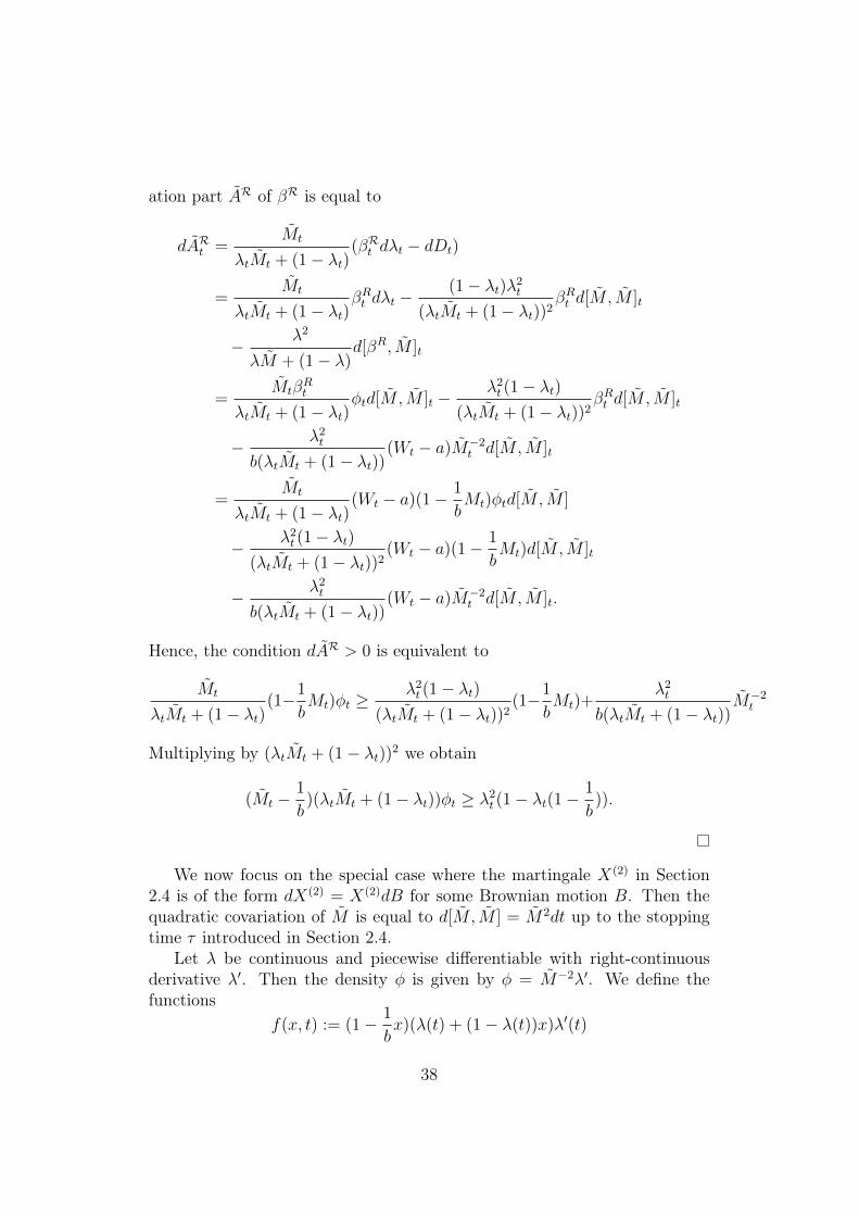
ation part AR of βR is equal to

dARt =Mt

λtMt + (1− λt)(βRt dλt − dDt)

=Mt

λtMt + (1− λt)βRt dλt −

(1− λt)λ2t

(λtMt + (1− λt))2βRt d[M, M ]t

− λ2

λM + (1− λ)d[βR, M ]t

=Mtβ

Rt

λtMt + (1− λt)φtd[M, M ]t −

λ2t (1− λt)

(λtMt + (1− λt))2βRt d[M, M ]t

− λ2t

b(λtMt + (1− λt))(Wt − a)M−2

t d[M, M ]t

=Mt

λtMt + (1− λt)(Wt − a)(1− 1

bMt)φtd[M, M ]

− λ2t (1− λt)

(λtMt + (1− λt))2(Wt − a)(1− 1

bMt)d[M, M ]t

− λ2t

b(λtMt + (1− λt))(Wt − a)M−2

t d[M, M ]t.

Hence, the condition dAR > 0 is equivalent to

Mt

λtMt + (1− λt)(1−1

bMt)φt ≥

λ2t (1− λt)

(λtMt + (1− λt))2(1−1

bMt)+

λ2t

b(λtMt + (1− λt))M−2

t

Multiplying by (λtMt + (1− λt))2 we obtain

(Mt −1

b)(λtMt + (1− λt))φt ≥ λ2

t (1− λt(1−1

b)).

We now focus on the special case where the martingale X(2) in Section2.4 is of the form dX(2) = X(2)dB for some Brownian motion B. Then thequadratic covariation of M is equal to d[M, M ] = M2dt up to the stoppingtime τ introduced in Section 2.4.

Let λ be continuous and piecewise differentiable with right-continuousderivative λ′. Then the density φ is given by φ = M−2λ′. We define thefunctions

f(x, t) := (1− 1

bx)(λ(t) + (1− λ(t))x)λ′(t)

38

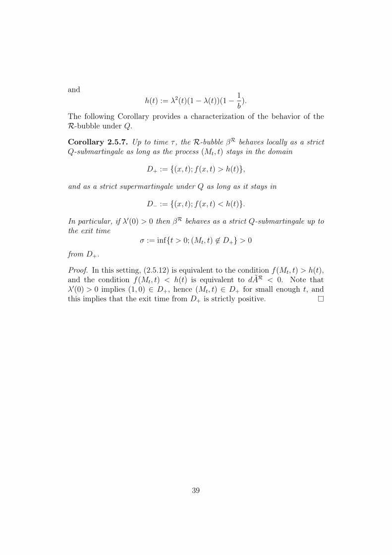
andh(t) := λ2(t)(1− λ(t))(1− 1

b).

The following Corollary provides a characterization of the behavior of theR-bubble under Q.

Corollary 2.5.7. Up to time τ , the R-bubble βR behaves locally as a strictQ-submartingale as long as the process (Mt, t) stays in the domain

D+ := (x, t); f(x, t) > h(t),

and as a strict supermartingale under Q as long as it stays in

D− := (x, t); f(x, t) < h(t).

In particular, if λ′(0) > 0 then βR behaves as a strict Q-submartingale up tothe exit time

σ := inft > 0; (Mt, t) 6∈ D+ > 0

from D+.

Proof. In this setting, (2.5.12) is equivalent to the condition f(Mt, t) > h(t),and the condition f(Mt, t) < h(t) is equivalent to dAR < 0. Note thatλ′(0) > 0 implies (1, 0) ∈ D+, hence (Mt, t) ∈ D+ for small enough t, andthis implies that the exit time from D+ is strictly positive.

39

Chapter 3

Stochastic volatility models

The contents of Section 3.1 of this Chapter are based on Section 5 of Bi-agini, Föllmer and S. Nedelcu [4], which was developed independently bythe author. Also Section 3.2 of the present Chapter was developed indepen-dently by the author and is based on a manuscript which is not yet published.

In the present chapter, we provide two examples within the framework ofstochastic volatility models, where we can compute explicitly the processesWR and βR and verify our condition on the submartingale behavior of WR

under Q. In Section 3.1 we present a version of the stochastic volatility modelintroduced by Sin [57]. We also show that the model can be modified in sucha way the condition no longer holds. In Section 3.2 we show that βR follows alocal R-submartingale in a modification of the Andersen-Piterbarg stochasticvolatility model. The Andersen-Piterbarg model represents a generalisationof the model of Sin [57] by allowing correlation between the Brownian motionsdriving the asset price process and the volatility, respectively.

3.1 Stochastic model with independent Brow-nian motions

Let B = (B1, B2, B3) be a 3-dimensional Brownian motion on a filteredprobability space (Ω,F , (Ft)t≥0, P ). We consider the stochastic volatilitymodel

dXt = σ1vtXtdB1t + σ2vtXtdB

2t , X0 = x,

dvt = a1vtdB1t + a2vtdB

2t + a3vtdB

3t , v0 = 1,

(3.1.1)

where the vectors a = (a1, a2) and σ = (σ1, σ2) are not parallel and satisfy(a · σ) > 0, and that a3 ∈ 0, 1.

40

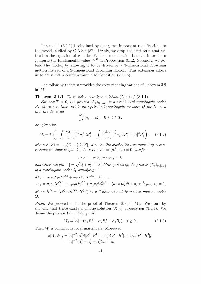
The model (3.1.1) is obtained by doing two important modifications tothe model studied by C.A.Sin [57]. Firstly, we drop the drift term that ex-isted in the equation of v under P . This modification is made in order tocompute the fundamental value WR in Proposition 3.1.2. Secondly, we ex-tend the model, by allowing it to be driven by a 3-dimensional Brownianmotion instead of a 2-dimensional Brownian motion. This extension allowsus to construct a counterexample to Condition (2.3.18).

The following theorem provides the corresponding variant of Theorem 3.9in [57].

Theorem 3.1.1. There exists a unique solution (X, v) of (3.1.1).For any T > 0, the process (Xt)t∈[0,T ] is a strict local martingale under

P . Moreover, there exists an equivalent martingale measure Q for X suchthat the densities

dQ

dP|Ft = Mt, 0 ≤ t ≤ T,

are given by

Mt = E(−∫ ·

0

vs(a · σ)

a · σ⊥σ⊥1 dB

1s −

∫ ·0

vs(a · σ)

a · σ⊥σ⊥2 dB

2s + |α|2B3

t

)t

, (3.1.2)

where E (Z) = exp(Z − 12[Z,Z]) denotes the stochastic exponential of a con-

tinuous semimartingale Z, the vector σ⊥ = (σ⊥1 , σ⊥2 ) 6= 0 satisfies

σ · σ⊥ = σ1σ⊥1 + σ2σ

⊥2 = 0,

and where we put |α| =√a2

1 + a22 + a2

3. More precisely, the process (Xt)t∈[0,T ]

is a martingale under Q satisfying

dXt = σ1vtXtdBQ,1t + σ2vtXtdB

Q,2t , X0 = x,

dvt = a1vtdBQ,1t + a2vtdB

Q,2t + a3vtdB

Q,3t − (a · σ)v2

t dt+ a3|α|2vtdt, v0 = 1,

where BQ = (BQ,1, BQ,2, BQ,3) is a 3-dimensional Brownian motion underQ.

Proof. We proceed as in the proof of Theorem 3.3 in [57]. We start byshowing that there exists a unique solution (X, v) of equation (3.1.1). Wedefine the process W = (Wt)t≥0 by

Wt = |α|−1(α1B1t + α2B

2t + α3B

3t ), t ≥ 0. (3.1.3)

Then W is continuous local martingale. Moreover

d[W,W ]t = |α|−2(α21d[B1, B1]t + α2

2d[B2, B2]t + α3td[B3, B3]t)

= |α|−2(α21 + α2

2 + α23)dt = dt.

41

Therefore it follows from Levy’s Theorem, see Theorem II.39 in [52], thatW is a Brownian motion under P . The process v satisfies the 1-dimensionalstochastic differential equation

dvt = |α|vtdWt, 0 ≤ t ≤ T. (3.1.4)

Due to the linearity of the coefficients, equation (3.1.4) admits a uniquesolution v = E (|α|W ). Therefore X is uniquely determined as the Doléansexponential of the square integrable process∫ t

0

σ1vsdB1s +

∫ t

0

σ2vsdB2s .

We prove that (Xt)t∈[0,T ] is a strict local martingale under P . To this purpose,it is sufficient to prove that EP [XT ] < X0. It follows from Lemma 4.2 of [57]that the expectation of the local martingale X under P is equal to

EP [XT ] = X0P (wt does not explode on [0, T ]),

where the auxiliary process (wt)t∈[0,T ] is given by

dwt = a1wtdB1t + a2wtdB

2t + a3wtdB

3t + (a · σ)w2

t dt, w0 = 1.

Moreover, w is the solution of the 1-dimensional stochastic differential equa-tion

dwt = |α|wtdWt + (a · σ)w2t dt, t ∈ [0, T ], (3.1.5)

where W is a P -Brownian motion defined in (3.1.3). It follows from Lemma4.3 of [57] that the unique solution of equation (3.1.5) explodes to +∞ infinite time with positive probability. This implies that EP [XT ] < X0.Let us show that the process M = (Mt)t∈[0,T ] is a well defined Radon-Nikodym density process, i.e. is a true martingale under the measure P .It follows from Lemma 4.2. of [57] that the expectation under P of MT canbe written as

EP [MT ] = M0P (vt does not explode on [0, T ]) (3.1.6)

where v = (vt)t∈[0,T ] satisfies

dvt = a1vtdB1t + a2vtdB

2t + a3vtdB

3t − (a · σ)(vt)

2dt+ a3|α|2vtdt,

for all t ∈ [0, T ]. The process v solves the 1-dimensional stochastic differentialequation

dvt = |α|vtdWt − (a · σ)(vt)2dt+ a3|α|2vtdt t ∈ [0, T ].

42

The explosion time of the process v, where by explosion we mean that theprocess v escapes the interval (0,∞) on which is defined, is given by

τ∞ = inft ≥ 0; vt 6∈ (0,∞).

We apply Feller’s test to v (see Chapter 5, section 5.5 of Karatzas and Shreve[41]) in order to prove that

P (τ∞ = +∞) = P (vt does not explode on [0, T ]) = 1.

As explained in Chapter 5, section 5.5 of Karatzas and Shreve [41], the Feller’stest goes as follows: in order to determine whether a process v explodes ornot in finite time, one has first to examine the behavior of the scale functionp(x) by computing the limits limx→0 p(x) and limx→∞ p(x). If

limx→0

p(x) = −∞ and limx→∞

p(x) = +∞, (3.1.7)

Then Proposition 5.22 in [41] implies that P (τ∞ = +∞) = 1. If at least oneof the equalities in is not satisfied, then we proceed to compute the functionu(x) defined in Problem 5.28 of [41] ad to examine the limits

limx→∞

u(x) and limx→0

u(x).

Theorem 5.29 in [41] states that P (τ∞ = +∞) = 1 or P (τ∞ = +∞) < 1according to whether the equality

limx→0

u(x) = limx→∞

u(x) = +∞.

is satisfied or not.The scale function is equal in our case to

p(x) =

∫ x

1

exp(−2

∫ y

1

−(a · σ)z2 + a3|α|2z|α|2z2

dz)dy,

and examine the limits limx↓0 p(x) and limx↑∞ p(x). Here we distinguish be-tween two cases:

Case 1: a3 = 0. We have

p(x) =

∫ x

1

exp(2(a · σ)

|α|2

∫ y

1

dz)dy

= k

∫ x

1

exp(2(a · σ)y

|α|2)dy

= k1|α|2

2(a · σ)exp(

2(a · σ)x

|α|2)− k2

43

with k, k1, k2 ∈ R+. Since a · σ > 0, we have

limx↑∞

p(x) = +∞,

By Problem 5.27 of [41] we obtain that

u(∞) = +∞,

whereu(x) =

∫ x

1

p′(y)

∫ y

1

2

p′(z)|α|2z2dzdy.

Moreover

limx→0+

p(x) = k1|α|2

2(a · σ)− k2 > −∞

As required by Feller’s test, we now compute

limx→0+

u(x) = limx→0+

∫ x

1

p′(y)

∫ y

1

2

|α|2z2p′(z)dzdy

= limx→0+

∫ x

1

2

|α|2z2p′(z)

∫ x

z

p′(y)dydz

= limx→0+

∫ x

1

2

|α|2z2exp(−2(a · σ)z

|α|2)

∫ x

z

exp(2(a · σ)y

|α|2)dydz

≥ limx→0+

e− 2(a·σ)|α|2

∫ x

1

2

|α|2z2

∫ x

z

dydz

= limx→0+

(e− 2(a·σ)|α|2

2

|α|2

∫ x

1

1

z2(x− z)dz

)= e

− 2(a·σ)|α|2

2

|α|2limx→0+

(− log x− x+ 1) = +∞

It follows from Feller’s Test for Explosions, see Theorem 5.29 of [41], that

P (τ∞ = +∞) = 1.

Hence v does not explode on [0, T ] and

EP [MT ] = M0P (vt does not explode on [0, T ]) = M0.

This implies that the positive local martingale M has constant expectationand therefore is a true P -martingale. We denote byQ the probability measurehaving the Radon-Nikodym density process with respect to P given by M .

44

It follows from Girsanov’s theorem that the process (BQ,it )t∈[0,T ], i = 1, 2

given by

BQ,it = Bi

t −∫ t

0

1

Ms

d[M,Bi]s = Bit +

∫ t

0

vs(a · σ)

(a · σ⊥)σ⊥i ds,

for all t ∈ [0, T ] is a Brownian motion under Q Hence the canonical semi-martingale decomposition of v under Q can be written in the following way

dvt =(a1vtdB

1t + a2vtdB

2t −

1

Mt

d[M, v]t)

+1

Mt

d[M, v]t

=(a1vtdB

1t + a2vtdB

2t + a1

v2t (a · σ)

a · σ⊥σ⊥1 dt+ a2

v2t (a · σ)

a · σ⊥σ⊥2 dt

)− v2

t (a · σ)dt

= a1vtdBQ,1t + a2vtdB

Q,2t − v2

t (a · σ)dt.

Analogously, one can obtain the canonical decomposition of X with respectto Q

dXt =(σ1vtXtdB

1t + σ2vtXtdB

2t −

1

Mt

d[M,X]t)

+1

Mt

d[M,X]t

=(σ1vtXtdB

1t + σ2vtXtdB

2t + σ1

v2t (a · t)

(a · σ⊥)σ⊥1 Xtdt

+ σ2v2t (a · t)

(a · σ⊥)σ⊥2 Xtdt

)+v2t (a · σ)

(a · σ⊥)(σσ⊥)Xtdt

= σ1vtXtdBQ,1t + σ2vtXtdB

Q,2t .

Hence, under the measure Q the bivariate process (X, v) satisfies

dXt = σ1vtXtdBQ,1t + σ2vtXtdB

Q,2t , X0 = x,

dvt = a1vtdBQ,1t + a2vtdB

Q,2t − (a · σ)v2

t dt, v0 = 1.

It is easy to see thatX is a positive localQ-martingale, hence aQ-supermartingale.To show that is a true Q-martingale it is enough to show that it has constantexpectation, i.e. EQ[XT ] = X0. It follows from Lemma 4.2 from [57] that

EQ[XT ] = X0Q(vt does not explode on [0, T ]),

where the auxiliary process (vt)t∈[0,T ] satisfies the stochastic differential equa-tion

dvt = a1vtdB1t + a2vtdB

2t . (3.1.8)

Since the equation (3.1.8) has linear coefficients, it follows from Remark5.19 [41] that it has a non-exploding solution. Therefore (Xt)t∈[0,T ] is a Q-martingale.

45

Case 2: a3 = 1. We follow the same steps as in Case 1. The scale functionis in this case equal to:

p(x) =

∫ x

0

exp(−2

∫ y

1

−(a · σ)z2 + |α|23z|α|2z2

dz)dy

= k

∫ x

1

exp(2(a · σ)y

|α|2)y−2dy,

where k ∈ R+. We examine the limits limx↓0 p(x) and limx↑∞ p(x). We havethat

limx↓0

p(x) = limx↓0

k

∫ x

1

exp(2(a · σ)y

|α|2)y−2dy = −∞

By Problem 5.27 of [41] we have that

u(0+) = +∞,

whereu(x) =

∫ x

1

p′(y)

∫ y

1

2

p′(z)|α|2z2dzdy.

Moreover, we have that

limx↑∞

p(x) = limx↑∞

k

∫ x

1

exp(2(a · σ)y

|α|2)y−2dy

= +∞.

Then it follows from Problem 5.27 of [41] that

u(∞) = +∞.

It follows from Feller’s Test for Explosions, see Theorem 5.29 of [41], that

P (τ∞ = +∞) = 1.

Therefore v does not explode on [0, T ] and

EP [MT ] = M0P (vt does not explode on [0, T ]) = M0.

Thus the positive local martingaleM has constant expectation and thereforeis a true P -martingale.

It follows from Girsanov’s Theorem that the Brownian motion (Bit)t∈[0,T ],

i = 1, 2 admits the following canonical decomposition under Q

dBit =

(dBi

t −1

Mt

d[M,Bi]t

)+

1

Mt

d[M,Bi]t

=(Bit +

vt(a · σ)

a · σ⊥σ⊥1 dt

)− vt(a · σ)

a · σ⊥σ⊥1 dt

= BQ,it −

vt(a · σ)

a · σ⊥σ⊥1 dt,

46

where (BQ,it )t∈[0,T ] is a Q-Brownian motion,for i = 1, 2. Analogously, one

obtains that the canonical semimartingale decomposition of B3 under Q isgiven by

dB3t =

(dB3

t −1

Mt

d[M,B3]t

)+

1

Mt

d[M,B3]t

= (dB3t − |α|2dt) + |α|2dt = dBQ,3

t + |α|2dt,

where (BQ,3t )t∈[0,T ] is a Q-Brownian motion. We see that X follows under Q

the dynamics

dXt = σ1vtXtdB1t + σ2vtXtdB

2t + σ1

(a · σ)v2t

a · σ⊥σ⊥1 Xtdt

+ σ2(a · σ)v2

t

a · σ⊥σ⊥2 Xtdt−

v2t (a · σ)

a · σ⊥(σ · σ⊥)Xtdt

= σ1vtXtdB1,Qt + σ2vtXtdB

2,Qt ,

and v has the following dynamics under Q

dvt =(a1vtdB

1t + a2vtdB

2t + vtdB

3t −

1

Mt

d[M, v]t)

+1

Mt

d[M, v]t

= a1vtdB1t + a2vtdB

2t + vtdB

3t +

1

Mt

vt(a · σ)

a · σ⊥σ⊥1 a1vtMtdt

+1

Mt

vt(a · σ)

a · σ⊥σ⊥2 a2vtMtdt−

1

Mt

|α|2vtMtdt− (a · σ)v2t dt+ |α|2vtdt

=(a1vtdB

Q,1t + a2vtdB

Q,2t + vtdB

Q,3t

)− (a · σ)v2

t dt+ |α|2vtdt.

Under the measure Q, the bivariate process (X, v) satisfies

dXt = σ1vtXtdB1,Qt + σ2vtXtdB

2,Qt , t ∈ [0, T ],

dvt = a1vtdB1,Qt + a2vtdB

2,Qt + vtdB

3,Qt − (a · σ)v2

t dt+ |α|2vtdt.

Thus X is a positive local Q-martingale. As in the previous case, in oderto show that is a true martingale it is enough to show that it has constantexpectation. By applying Lemma 4.2 from [57] we obtain

EQ[XT ] = X0Q(wt does not explode on [0, T ]),

where

dwt = a1wtdB1,Qt + a2wtdB

2,Qt + wtdB

3,Qt + |α|2wtdt. (3.1.9)

Due to the linearity of the coefficients, it follows from Remark 5.19 in [41]that equation (3.1.9) has a non-exploding solution. Therefore (Xt)t∈[0,T ] is aQ-martingale.

47

In the setting of Chapter 2, we now consider a financial market modelwith a financial asset that generates a single payment XT at time T andwhose price process S is given by St := Xt for t < T and ST = 0. Thenthe wealth process is given by W = X. Theorem 3.1.1 shows that W is auniformly integrable martingale under Q, and so we have

Q ∈MUI(W ).

Moreover, it follows from Theorem 3.1.1 that the wealth processW is a strictlocal martingale under P . We put

R := P ∈MNUI(W ).

The fundamental value WR perceived under R is given by

WRt = ER[WT |Ft] = ER[XT |Ft], t ∈ [0, T ].

Proposition 3.1.2. The process WR admits the factorization WR = W ·C,where the semimartingale C is of the form

Ct = 1 + (σ1c1(t) + σ2c2(t))vt, t ∈ [0, T ].

The time-dependent coefficients are given by

c1(t) = ER

[1

vt

∫ T−t

0

eXuvu+tdB1u

],

c2(t) = ER

[1

vt

∫ T−t

0

eXuvu+tdB2u

],

(3.1.10)

and satisfyσ1c1(t) + σ2c2(t) < 0 (3.1.11)

for any t ∈ [0, T ).

Proof. Since process X is given by the Doléans exponential

Xt = E(∫ ·

0

σ1vsdB1s +

∫ ·0

σ2vsdB2s

)t

, t ∈ [0, T ].

we have

XT

Xt

= exp

(∫ T

t

σ1vsdB1s +

∫ T

t

σ2vsdB2s −

1

2

∫ T

t

(σ21 + σ2

2)v2sds

)

= exp

(vt

∫ T

t

σ1vsvtdB1

s + vt

∫ T

t

σ2vsvtdB2

s −1

2v2t

∫ T

t

(σ21 + σ2

2)(vsvt

)2ds

).

48

We write W under the following factorial form

WRt = ER[XT |Ft] = XtER[

XT

Xt

|Ft] = WtCt,

where the semimartingale C is given by

Ct := ER[XT

Xt

|Ft] (3.1.12)

for t ∈ [0, T ]. The fact that the Brownian motion has increments independentof the past implies that

vuvt

= exp(a1(B1u −B1

t ) + a2(B2u −B2

t ) + a3(B3u −B3

t )−1

2|α|2(t− u))

is independent of Ft for T ≥ u ≥ t. We fix y := vt and define

Yu = σ1y

∫ t+u

t

vsvtdB1

s + σ2y

∫ t+u

t

vsvtdB2

s −1

2(σ2

1 + σ22)y2

∫ t+u

t

(vsvt

)2

ds,

for u ≥ 0. In particular, we have Y0 = 0 and

YT−t = σ1y

∫ T

t

vsvtdB1

s + σ2y

∫ T

t

vsvtdB2

s −1

2(σ2

1 + σ22)y2

∫ T

t

(vsvt

)2

ds.

An application of Itô’s formula for the function f(x) = ex yields

eYT−t = eY0 +

∫ T−t

0

eYudYu +1

2

∫ T−t

0

eYud[Y, Y ]u

= eY0 + σ1y

∫ T−t

0

vu+t

vteYudB1

u + σ2y

∫ T−t

0

vu+t

vteYudB2

u,

(3.1.13)

where the Brownian motion B = (B1, B2) defined by Biu := Bi

t+u − Bit,

i = 1, 2, is independent of Ft. For fixed vt = y, we have

Ct = ER[XT

Xt

|Ft] = ER[eYT−t ] = 1 + (σ1c1(t) + σ2c2(t))y, (3.1.14)

where c1(t) and c2(t) are given by (3.1.10). It follows from an applicationof Feller’s Test for Explosions, see [57], that WR

t < Wt for any t ∈ [0, T ).Therefore

Wt(1 + (σ1c1(t) + σ2c2(t))vt) < Wt, t ∈ [0, T ),

and this implies (3.1.11).

49

We consider the flow of equivalent local martingale measures R = (Rt)t≥0

defined by (2.3.12). Lemma 2.3.4 implies that the resulting bubble βR is ofthe form

βR = W −WR = ξ(W −WR).

Corollary 3.1.3. If a3 = 0, the process WR is a submartingale under themeasure Q, and so the behavior of the bubble βR is again described by Theo-rem 2.3.9.

Proof. We verify the sufficient condition in Corollary 2.3.10. Since

dCt = (σ1c1(t) + σ2c2(t))dvt + σ1vtdc1(t) + σ2vtdc2(t)

= (σ1c1(t) + σ2c2(t))a1vtdB1t + (σ1c1(t) + σ2c2(t))a2vtdB

2t

+ σ1vtdc1(t) + σ2vtdc2(t).

(3.1.15)

the local martingale part of the semimartingale C is given by

MCt =

∫ t

0

a1(σ1c1(s) + σ2c2(s))vsdB1s +

∫ t

0

a2(σ1c1(s) + σ2c2(s))vsdB2s .

Since M is the stochastic exponential defined in (3.1.2), M satisfies thestochastic differential equation

Mt = −∫ t

0

vs(a.σ)

(a.σ⊥)σ⊥1 MsdB

1s −

∫ t

0

vs(a.σ)

(a.σ⊥)σ⊥2 MsdB

2s .

Therefore the quadratic covariation [M,C] is equal to

[M,C]t = [M,M c]t =

∫ t

0

−(σ1c1(s) + σ2c2(s))(a.σ)v2sMsds.

It follows from (3.1.11) that the integrand is strictly positive, and therefore[M,C] is an increasing process. Thus βR is a local submartingale under R,as a consequence of Corollary 2.3.10.

We now provide a modification of the model in such a way that Condition(2.3.19) is no longer satisfied. To this aim we choose the parameters suchthat

|α|2

(a · σ)> 1,

and introduce the stopping time

τ := inft > 0; vt =|α|2

(a · σ). (3.1.16)

Consider a financial asset that generates a single payment Xτ0 at timeτ0 := T ∧ τ and whose price process S is given again by St := Xt for t < τ0

and St := 0 for t ≥ τ0. The wealth process is then given again by W = X.

50

Proposition 3.1.4. If a3 = 1, the quadratic covariation [M,C] is a decreas-ing process, and so condition (2.3.19) is no longer satisfied.

Proof. By using the same computations as in the proof of Proposition 3.1.2we obtain

dCt = (σ1c1(t) + σ2c2(t))dvt + σ1vtdc1(t) + σ2vtdc2(t)

= (σ1c1(t) + σ2c2(t))(a1vtdB1t + a2vtdB

2t + vtdB

3t )

+ σ1vtdc1(t) + σ2vtdc2(t),

where c1(t) and c2(t) are given by (3.1.10). It follows that the local martingalepart of C is given by

dMCt = (σ1c1(t) + σ2c2(t))(a1vtdB

1t + a2vtdB

2t + vtdB

3t ).

and

d[MC ,M ]t = −(σ1c1(t) + σ2c2(t))(a · σ)v2tMtdt

+ (σ1c1(t) + σ2c2(t))|a|2vtMtdt

= −(σ1c1(t) + σ2c2(t))(−|α|2 + (a · σ)vt)vtMtdt.

In view of (3.1.11) the process is decreasing on [0, τ0], since (a ·σ)vt−|α|2 ≤ 0on [0, τ0] by the definition of τ in (3.1.16) and since v0 = 1.

3.2 Stochastic model with correlated Brownianmotions

The following example is derived from the Anderson-Piterbarg model [3],which is generalisation of the previous case, by allowing correlation betweenthe Brownian motions driving the processes. Our example consists of a pro-cess driven by a 3-dimensional Brownian motion, instead of a 2-dimensionalBrownian motion, as is the case in [3].Let B = (B1, B2, B3) be a 3-dimensional Brownian motion defined on a fil-tered probability space (Ω,F , (Ft)t≥0, P ) and let ρ ∈ (−1, 1). We assumethat (Ft)t≥0 is the canonical filtration generated by B = (B1, B2, B3). Wedefine the following Brownian motions:

dW 1t = ρdB3

t +√

1− ρ2dB1t = ρdB3

t + ρdB1t ,

dW 2t = ρdB3

t +√

1− ρ2dB2t = ρdB3

t + ρdB2t

51

where we have denoted ρ =√

1− ρ2.We consider the following stochastic volatility model

dXt = λ1Xt

√vtdW

1t + λ2Xt

√vtdW

2t , X0 = 1

dvt = −kvtdt+ εvtdB3t ,

(3.2.1)

where λ1, λ2 ∈ R and k, ε are positive constants.

Theorem 3.2.1. If ρ > 0 and λ2 < 0 < λ1 ≤ −2−ρ2ρ2λ2, satisfying λ1+λ2 > 0,

there exists a unique solution (X, v) of (3.2.1) and for any T > 0, the processX = (Xt)t∈[0,T ] is a strict local martingale under P . Moreover there existsan equivalent martingale measure Q for X with the Radon-Nikodym densityprocess

dQ

dP|Ft = Mt, 0 ≤ t ≤ T,

given by

Mt = E(∫ ·

0

α1

√vsdW

1s +

∫ ·0

α2

√vsdW

2s

)t

,

where the coefficieints α1 and α2 are equal to

α1 = λ2 + ρ2λ1

α2 = −λ1 − ρ2λ2

(3.2.2)

Then the process X is a martingale under Q satisfying

dXt = λ1

√vtXtdW

1,Qt + λ1

√vtXtdW

2,Qt

dvt = (−kvt + ερ(α1 + α2)v32t )dt+ εvtdB

3,Qt .

where the W 1,Q, W 2,Q and B3,Q are Brownian motions under Q given by

W 1,Qt = W 1

t −∫ t

0

(α1

√vs + α2

√vsρ

2)ds,

W 2,Qt = W 2

t −∫ t

0

(α1

√vsρ

2 + α2

√vs)ds,

B3,Qt = B3

t −∫ t

0

(α1 + α2)ρ√vsds,

for all t ∈ [0, T ].

Theorem 3.2.1 is a consequence of the following Lemma. The tech-niques used in Lemma 3.2.2 are derived from Piterbarg and Anderson [2]and adapted to our case.

52

Lemma 3.2.2. If λ1, λ2 ∈ R fullfil the assumptions of Theorem 3.2.1, then(3.2.1) admits a unique solution and

EP [XT ] = P (τ v∞ > T ), (3.2.3)

where P is a probability measure such that the process v satisfies under P theequation

dvt = εvtdB3t − kvtdt+ (λ1 + λ2)ερv

32t dt

where (B3t )t∈[0,T ] is a P -Brownian motion and τ v∞ represents the explosion

time of the process v, i.e. the first time v exits the interval (0,∞) at +∞.More precisely τ v∞ = limn→∞ τn, where

τn = inft ≥ 0; |vt| ≥ n, n ∈ N. (3.2.4)

Proof. First we show the uniqueness of the solutions. The process v is ageometric Brownian motion having the form

vt = exp(εB3t − (k +

1

2ε2)t), 0 ≤ t ≤ T.

Therefore X is uniquely determined as the stochastic exponential of the pro-cess ∫ t

0

λ1

√vsdW

1s +

∫ t

0

λ2

√VsdW

2s .

Then the solution of (3.2.1) is given by

Xt = exp(

∫ t

0

λ1

√vsdW

1s +

∫ t

0

λ2

√vsdW

2s −

1

2(λ2

1 + λ22 + 2λ1λ2ρ

2)vsds)

= exp(∫ t

0

(λ1 + λ2)ρ√vsdB

3s +

∫ t

0

λ1ρ√vsdB

1s +

∫ t

0

λ2ρ√vsdB

2s

− 1

2

∫ t

0

(λ21 + λ2

2 + 2λ1λ2ρ2)vsds

).

Let F3T = σ(B3

s ; s ≤ T ). We compute EP [XT1τn>T], where τn is defined in

53

(3.2.4):

EP [XT1τn>T] = EP [EP [XT1τn>T|F3T ]] = EP [1τn>TEP [XT |F3

T ]]

= EP[1τn>T exp

(∫ T

0

(λ1 + λ2)ρ√vsdB

3s −

1

2

∫ T

0

(λ21 + λ2

2

+ 2λ1λ2ρ2)vsds

)EP[

exp(∫ T

0

λ1ρ√vsdB

1s +

∫ T

0

λ2ρ√vsdB

2s

)|F3

T

]]= EP

[1τn>T exp

(∫ T

0

(λ1 + λ2)ρ√vsdB

3s −

1

2

∫ T

0

(λ21 + λ2

2 + 2λ1λ2ρ2)ds

)EP[

exp(∫ T

0

λ1ρ√vsdB

1s

)exp

(∫ T

0

λ2ρ√vsdB

2s

)|F3

T

]]= EP

[1τn>T exp

(∫ T

0

(λ1 + λ2)ρ√vsdB

3s −

1

2

∫ T

0

(λ21 + λ2

2 + 2λ1λ2ρ2)vsds

)exp

(1

2

∫ T

0

(λ21 + λ2

2)ρ2vsds)]

= EP[1τn>T exp

(∫ T

0

(λ1 + λ2)ρ√vsdB

3s −

1

2

∫ T

0

(λ1 + λ2)2ρ2vsds)].

We consider the local martingale

ξt := exp(∫ t

0

(λ1 + λ2)ρ√vsdB

3s −

1

2

∫ T

0

(λ1 + λ2)2ρ2vsds), t ∈ [0, T ].

By replacing ξT in the above computations, we obtain

EP [XT1τn>T] = EP[1τn>TξT

]= EP

[1τn>TξT∧τn

]. (3.2.5)

Let ξn := (ξτnt )t∈[0,T ]. Then ξn is a true P -martingale and we can define ameasure P n with Radon-Nikodym density with respect to P given by

dP n

dP|Ft = ξnt , t ∈ [0, T ].

Therefore (3.2.5) becomes

EP [XT1τn>T] = EPn [1τn>T].

By applying the monotone convergence theorem and using the fact P (τ v∞ =+∞) = 1 we have

EP [XT ] = EP [XT1τv∞>T] = limn→∞

EP [XT1τn>T]

= limn→∞

EPn [1τn>T] = limn→∞

EP [1τn>T]

= EP [1τv∞>T].

54

The third equality follows from the fact that v follows the same law underPn as under P up to the explosion time τ v∞, see also Lemma 4.2 in Sin [57].We now examine the behavior of the process v under P . We apply Feller’stest to v (see Ch.5 in Karatzas and Shreve [41]) in order to show

P (τ v∞ > T ) < 1,

which implies EP [XT ] < 1, or equivalently, X is a strict P -local martingale.We compute the scale function

p1(x) =

∫ x

1

exp(− 2

∫ y

1

−kz + ρε(λ1 + λ2)z32

ε2z2dz)dy

=

∫ x

1

exp(2k

ε2

∫ y

1

1

zdz − 2ρ(λ1 + λ2)

ε

∫ y

1

z−12dz)dy

= K1

∫ x

1

y2kε2 e−

4ρ(λ1+λ2)ε

y12 dy,

where K1 > 0 is some positive constant. For simplicity we denote

α :=2k

ε2> 0 and β :=

4ρ(λ1 + λ2)

ε> 0

Let n be the smallest positive integer such that n ≥ α.Then ∫ ∞

1

yαe−βy12 dy ≤

∫ ∞1

yne−βy12 dy.

Since∫∞

1yne−βy

12 dy is convergent this implies

p1(+∞) = limx→∞

K1

∫ x

1

yαe−βy12 dy < +∞.

We consider the function

u1(x) =

∫ x

1

p′1(y)

∫ y

1

2

p′1(z)ε2z2dzdy.

and we examine the limit limx→∞ u1(x). By applying Fubini’s theorem weobtain

u1(x) =

∫ x

1

2

p′1(z)ε2z2

∫ x

z

p′1(y)dydz =2K2

ε2

∫ x

1

z−2−αeβz12

∫ x

z

yαe−βy12 dydz,

55

where K2 > 0 is a positive constant. We examine first the inner integral. Bydoing the substitution w = y

12 we get∫ x

z

yαe−βy12 dy =

∫ x12

z12

w2αe−βw2wdw = 2

∫ x12

z12

w2α+1e−βwdw

≤ 2

∫ ∞z12

w2α+1e−βwdw.

Let n0 ∈ N be the smallest positive integer satisfying n0 ≥ 2α + 1. Inparticular 2α + 2 > n0 ≥ 2α + 1. Then for z > 1

2

∫ ∞z12

w2α+1e−βwdw ≤ 2

∫ ∞z12

wn0e−βwdw =2

βzn02 e−βz

12 +

2n0

β

∫ ∞z12

wn0−1e−βwdw

=2

βzn02 e−βz

12 +

2n0

β2e−βz

12 z

n0−12

+2n0(n0 − 1)

β2

∫ ∞z12

wn0−2e−βwdw

=2

βzn02 e−βz

12 +

2n0

β2zn0−1

2 e−βz12

+ ...+2n0(n0 − 1)...(n0 − (n0 − 2))

β(n0−2)+1

∫ ∞z12

wn0−(n0−1)e−βwdw

=2

βzn02 e−βz

12 +

2n0

β2zn0−1

2 e−βz12

+ ...+2n0(n0 − 1)...(n0 − (n0 − 2))

β(n0−2)+1

1

βzn0−(n0−1)

2 e−βz12

+2n0(n0 − 1)...(n0 − (n0 − 1))

β(n0−2)+2

∫ ∞z12

e−βwdw

=2

βe−βz

12 z

n02 +

n0−1∑k=0

2n0(n0 − 1)...(n0 − k)

βk+1zn0−k−1e−βz

12 .

Therefore

u1(x) =2K2

ε2

∫ x

1

z−2−αeβz12

( 2

βzn02 e−βz

12 +

n0−1∑k=0

2n0(n0 − 1)...(n0 − k)

βk+1zn0−k−1

2 e−βz12

)dz

=4K2

ε2β

∫ x

1

zn02−2−αdz +

4K2

ε2

n0−1∑k=0

n0(n0 − 1)...(n0 − k)

βk+1

∫ x

1

zn0−k−1

2−α−2dz

=4K2

ε2β

1n0

2− α− 1

xn02−α−1

+4K2

ε2

n0−1∑k=0

n0(n0 − 1)...(n0 − k)

βk+1

1n0

2− α− 1− k+1

2

xn02−α−1− k+1

2 −K3

56

Therefore,u1(+∞) = limx→∞ u1(x) < ∞, since n0

2− α − 1 < 0. Hence, via

Theorem 5.29 in Karatzas and Shreve [41] we have that P (τ = +∞) < 1,where τ = inft ≥ 0; vt 6∈ (0,∞). In order to conclude that P (τ v∞ =∞) < 1,we show that the process v doesn’t reach 0 in finite time. To this purpose weemploy a comparison result, namely Proposition 2.18 of Karatzas and Shreve[41]. We consider the process v = (v)t∈[0,T ] satisfying under P the equation

dvt = −kvtdt+ εvtdB3t .

We know that P (τ0 =∞) = 1, where τ0 is the first time v exits the interval(0,∞). It follows from Proposition 2.18 of Karatzas and Shreve [41] that

vt ≤ vt P − a.s.

for all t ∈ [0, T ]. Hence v doesn’t reach 0 in finite time.Therefore X is a strict P -local martingale and this concludes our proof.

We now proceed with the proof of Theorem 3.2.1

Proof. We start by showing that the process M is a well defined Radon-Nikodym density process i.e. a true martingale under the measure P . Byusing the same reasoning as in Lemma 3.2.2 we obtain

EP [MT1τn>T] = EP [1τn>TEP [MT |F3T ]] = EP

[1τn>T exp

(∫ T

0

(α1 + α2)ρ√vsdB

3s

− 1

2

∫ T

0

(α1 + α2)2ρ2vsds)].

We define the local martingale (ξ)t∈[0,T ] by

ξt := exp(∫ t

0

(α1 + α2)ρ√vsdB

3s −

1

2

∫ t

0

(α1 + α2)2ρ2vsds),

for all t ∈ [0, T ]. As in Lemma 3.2.2, we can define the measures P n withthe Radon-Nikodym density processes with respect to P given by

dP n

dP|Ft = ξnt , t ∈ [0, T ].

where ξnt := ξt∧τn for all t ∈ [0, T ]. By passing to the limit and using thearguments Lemma 4.2 in [57], we obtain

EP [MT ] = P (τ v∞ > T ). (3.2.6)

57

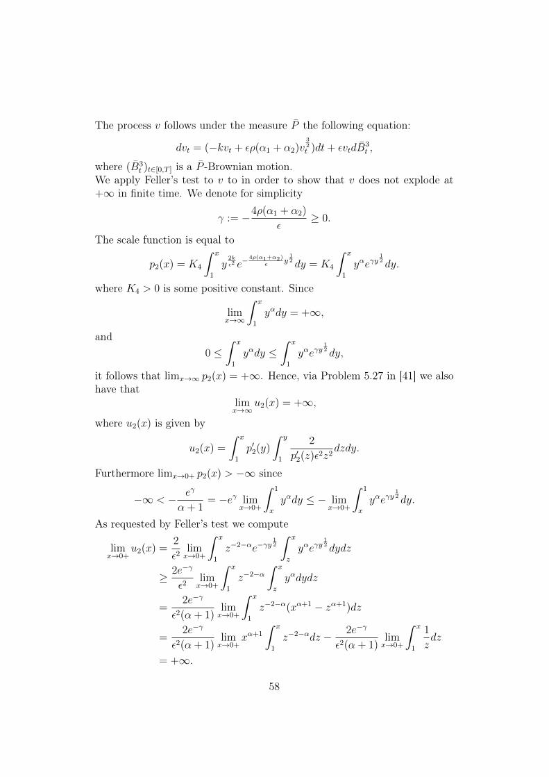
The process v follows under the measure P the following equation:

dvt = (−kvt + ερ(α1 + α2)v32t )dt+ εvtdB

3t ,

where (B3t )t∈[0,T ] is a P -Brownian motion.

We apply Feller’s test to v to in order to show that v does not explode at+∞ in finite time. We denote for simplicity

γ := −4ρ(α1 + α2)

ε≥ 0.

The scale function is equal to

p2(x) = K4

∫ x

1

y2kε2 e−

4ρ(α1+α2)ε

y12 dy = K4

∫ x

1

yαeγy12 dy.

where K4 > 0 is some positive constant. Since

limx→∞

∫ x

1

yαdy = +∞,

and0 ≤

∫ x

1

yαdy ≤∫ x

1

yαeγy12 dy,

it follows that limx→∞ p2(x) = +∞. Hence, via Problem 5.27 in [41] we alsohave that

limx→∞

u2(x) = +∞,

where u2(x) is given by

u2(x) =

∫ x

1

p′2(y)

∫ y

1

2

p′2(z)ε2z2dzdy.

Furthermore limx→0+ p2(x) > −∞ since

−∞ < − eγ

α + 1= −eγ lim

x→0+

∫ 1

x

yαdy ≤ − limx→0+

∫ 1

x

yαeγy12 dy.

As requested by Feller’s test we compute

limx→0+

u2(x) =2

ε2limx→0+

∫ x

1

z−2−αe−γy12

∫ x

z

yαeγy12 dydz

≥ 2e−γ

ε2limx→0+

∫ x

1

z−2−α∫ x

z

yαdydz

=2e−γ

ε2(α + 1)limx→0+

∫ x

1

z−2−α(xα+1 − zα+1)dz

=2e−γ

ε2(α + 1)limx→0+

xα+1

∫ x

1

z−2−αdz − 2e−γ

ε2(α + 1)limx→0+

∫ x

1

1

zdz

= +∞.

58

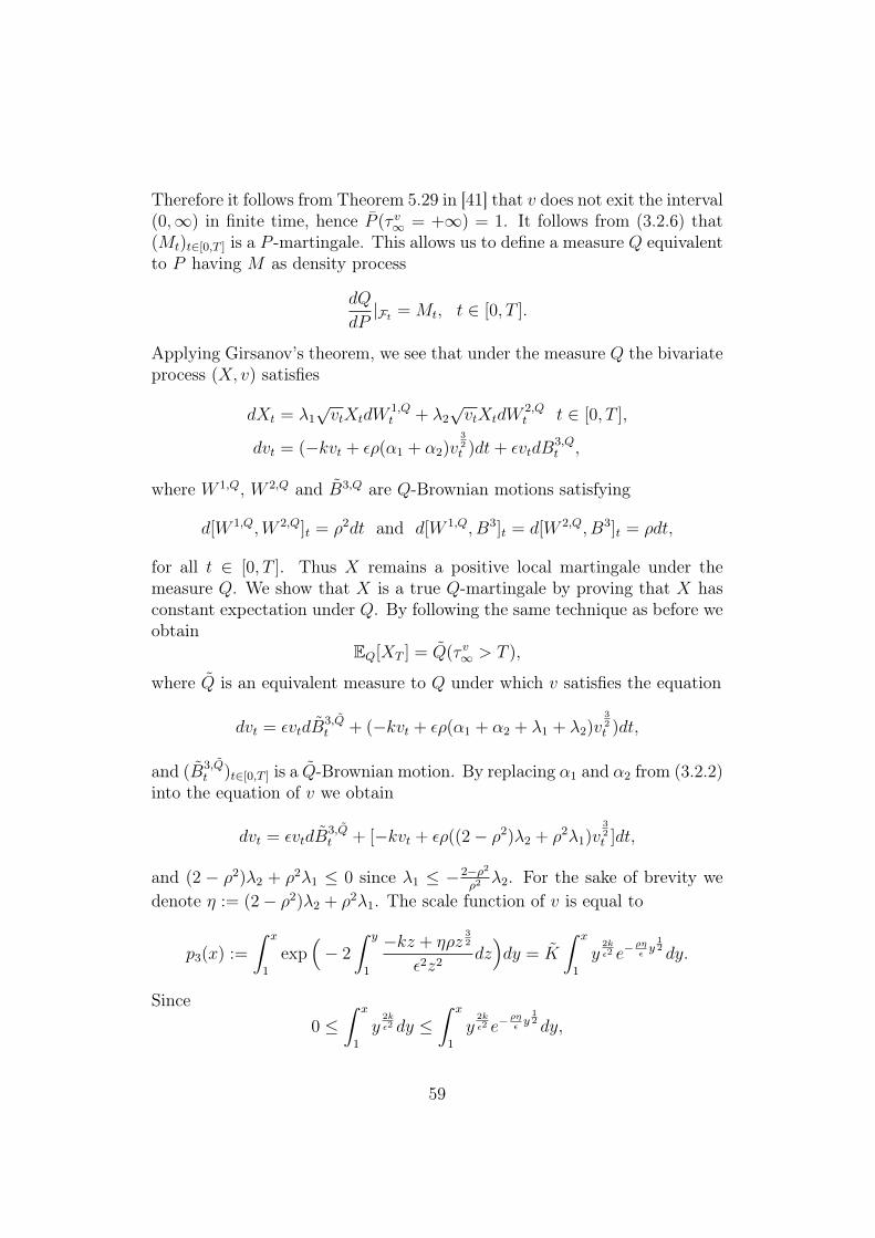
Therefore it follows from Theorem 5.29 in [41] that v does not exit the interval(0,∞) in finite time, hence P (τ v∞ = +∞) = 1. It follows from (3.2.6) that(Mt)t∈[0,T ] is a P -martingale. This allows us to define a measure Q equivalentto P having M as density process

dQ

dP|Ft = Mt, t ∈ [0, T ].

Applying Girsanov’s theorem, we see that under the measure Q the bivariateprocess (X, v) satisfies

dXt = λ1

√vtXtdW

1,Qt + λ2

√vtXtdW

2,Qt t ∈ [0, T ],

dvt = (−kvt + ερ(α1 + α2)v32t )dt+ εvtdB

3,Qt ,

where W 1,Q, W 2,Q and B3,Q are Q-Brownian motions satisfying

d[W 1,Q,W 2,Q]t = ρ2dt and d[W 1,Q, B3]t = d[W 2,Q, B3]t = ρdt,

for all t ∈ [0, T ]. Thus X remains a positive local martingale under themeasure Q. We show that X is a true Q-martingale by proving that X hasconstant expectation under Q. By following the same technique as before weobtain

EQ[XT ] = Q(τ v∞ > T ),

where Q is an equivalent measure to Q under which v satisfies the equation

dvt = εvtdB3,Qt + (−kvt + ερ(α1 + α2 + λ1 + λ2)v

32t )dt,

and (B3,Qt )t∈[0,T ] is a Q-Brownian motion. By replacing α1 and α2 from (3.2.2)

into the equation of v we obtain

dvt = εvtdB3,Qt + [−kvt + ερ((2− ρ2)λ2 + ρ2λ1)v

32t ]dt,

and (2 − ρ2)λ2 + ρ2λ1 ≤ 0 since λ1 ≤ −2−ρ2ρ2λ2. For the sake of brevity we

denote η := (2− ρ2)λ2 + ρ2λ1. The scale function of v is equal to

p3(x) :=

∫ x

1

exp(− 2

∫ y

1

−kz + ηρz32

ε2z2dz)dy = K

∫ x

1

y2kε2 e−

ρηεy12 dy.

Since0 ≤

∫ x

1

y2kε2 dy ≤

∫ x

1

y2kε2 e−

ρηεy12 dy,

59

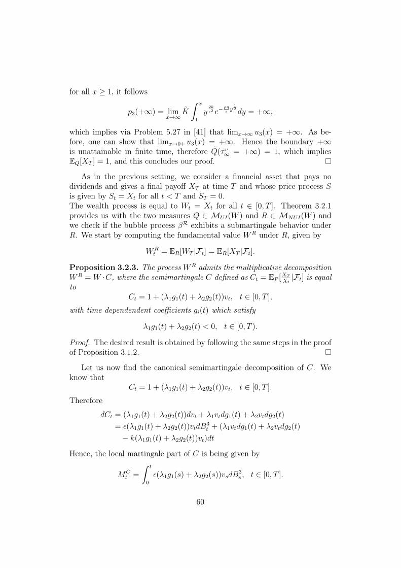
for all x ≥ 1, it follows

p3(+∞) = limx→∞

K

∫ x

1

y2kε2 e−

ρηεy12 dy = +∞,

which implies via Problem 5.27 in [41] that limx→∞ u3(x) = +∞. As be-fore, one can show that limx→0+ u3(x) = +∞. Hence the boundary +∞is unattainable in finite time, therefore Q(τ v∞ = +∞) = 1, which impliesEQ[XT ] = 1, and this concludes our proof.

As in the previous setting, we consider a financial asset that pays nodividends and gives a final payoff XT at time T and whose price process Sis given by St = Xt for all t < T and ST = 0.The wealth process is equal to Wt = Xt for all t ∈ [0, T ]. Theorem 3.2.1provides us with the two measures Q ∈ MUI(W ) and R ∈ MNUI(W ) andwe check if the bubble process βR exhibits a submartingale behavior underR. We start by computing the fundamental value WR under R, given by

WRt = ER[WT |Ft] = ER[XT |Ft].

Proposition 3.2.3. The processWR admits the multiplicative decompositionWR = W ·C, where the semimartingale C defined as Ct = EP [XT

Xt|Ft] is equal

toCt = 1 + (λ1g1(t) + λ2g2(t))vt, t ∈ [0, T ],

with time dependendent coefficients gi(t) which satisfy

λ1g1(t) + λ2g2(t) < 0, t ∈ [0, T ).

Proof. The desired result is obtained by following the same steps in the proofof Proposition 3.1.2.

Let us now find the canonical semimartingale decomposition of C. Weknow that

Ct = 1 + (λ1g1(t) + λ2g2(t))vt, t ∈ [0, T ].

Therefore

dCt = (λ1g1(t) + λ2g2(t))dvt + λ1vtdg1(t) + λ2vtdg2(t)

= ε(λ1g1(t) + λ2g2(t))vtdB3t + (λ1vtdg1(t) + λ2vtdg2(t)

− k(λ1g1(t) + λ2g2(t))vt)dt

Hence, the local martingale part of C is being given by

MCt =

∫ t

0

ε(λ1g1(s) + λ2g2(s))vsdB3s , t ∈ [0, T ].

60

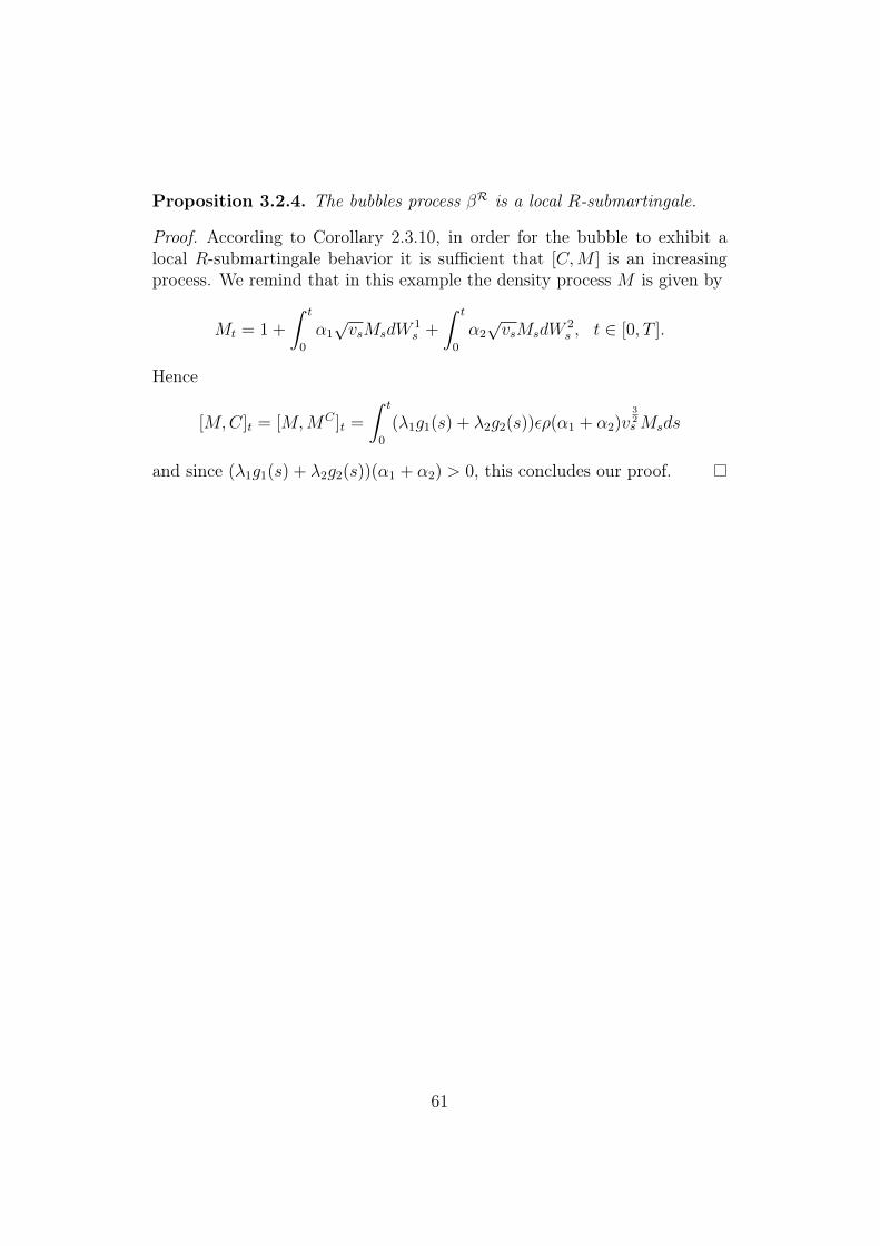
Proposition 3.2.4. The bubbles process βR is a local R-submartingale.

Proof. According to Corollary 2.3.10, in order for the bubble to exhibit alocal R-submartingale behavior it is sufficient that [C,M ] is an increasingprocess. We remind that in this example the density process M is given by

Mt = 1 +

∫ t

0

α1

√vsMsdW

1s +

∫ t

0

α2

√vsMsdW

2s , t ∈ [0, T ].

Hence

[M,C]t = [M,MC ]t =

∫ t

0

(λ1g1(s) + λ2g2(s))ερ(α1 + α2)v32sMsds

and since (λ1g1(s) + λ2g2(s))(α1 + α2) > 0, this concludes our proof.

61

Chapter 4

The formation of financialbubbles in defaultable markets

The contents of Sections 4.2, 4.3 and 4.4 of this Chapter are based on theauthor’s joint work with F. Biagini, and are contained in the manuscript F.Biagini and S. Nedelcu [5]. The detailed description of the author’s personalcontribution is presented in Section 1.2. Section 4.4.1 of the present Chapterwas developed independently by the author and is based on a manuscriptwhich is not yet published.

4.1 IntroductionAim of this Chaper is to construct a mathematical model that allows forthe formation of bubbles in the valuation of defaultable contingent claimsin a reduced form credit risk model. Furthermore, we establish a connec-tion between the classical martingale theory of bubbles and the constructiveapproach to the modelling of asset price bubbles which we propose in thisChapter.

Credit risk models have been introduced to describe financial marketsaffected by default risk, see Bielecki and Rutkowski [7] for an overview ofall the main approaches. A default risk represents the possibility that acounterparty is not able to fullfill its obligations that are stated in a financialcontract. An example of financial intruments that are affected by default riskare corporate bonds. These are financial products issued by a firm,that, inexchange of a fee for this commitment, take the obligation to make specificpayments at future dates to the buyers of the corporate bonds. The firmmay be forced to default on its commitment due to different circumstances(for example bankruptcy). This event causes losses for the bondholders if it

62

occurs during the lifetime of the bond i.e. the period between the momentwhen it is issued and its maturity. A corporate bond represents an exampleof defaultable claim.

In a reduced form setting, see for example Bielecki and Rutkowski [7], thefirm default time is represented by a totally inaccessible stopping time, whichimplies that the market cannot predict the time of the default. However, thedefault time may not be a stopping time with respect to the restricted filtra-tion. The distinction between the information that is available to the marketand information that is known within the firm (where the moment of defaultis an accessible stopping time) has been studied and pointed out in the liter-ature. Duffie and Lando [22] consider that the bond investors do not observethe bond issuer’s assets directly, but receive instead only periodic account-ing reports. Thus, investors draw their information from delayed financialreports and from other publicly available data. In this way the market ob-serves the values of the firm’s assets plus additional noise, due to the lack ofperfect information.

Cetin et al. [14] provide a different approach, where they construct areduced form model starting from a structural model. They consider two in-formation sets. In their approach the firm’s management can anticipate thedefault model by examining the firm’s cash flows. In constrast, the marketobserves only a partition of the manager’s information set. This structurehas the default time as being an accessible stopping time with respect to thefiltration representing the information available for the firm’s manager anda totally inaccesible stopping time with respect to the filtration representingthe information available to the market.

We consider here a classical reduced form setting, as discussed in Chapter8 of Bielecki and Rutkowski [7], and consider a market model with constantmoney market accout and the possibility of investing in defaultable claims,i.e. contracts traded over the counter between default-prone parties.

Our objective is to provide an explanation for the mechanism that leads toa change of the martingale measure used for pricing. We do this by modellingthe market price, which is influenced by the asset’s probability of default asperceived by the investor. As we point out in Chapter 2, the study of assetprice bubbles in the mathematical literature has been done in the frameworkof the martingale approach, see Jarrow, Protter et.al [39], [40], [36], [34],[37] and Biagini, Föllmer and Nedelcu [4]. In an incomplete financial marketmodel a bubble is generated after the start of the model if a switch froma uniformly integrable martingale measure Q to a non-uniformly integrablemartingale measure R occurs. Thus the dynamics of the discounted wealthprocess is described by a uniformly integrable martingale under Q and after-wards by a non-uniformly integrable martingale/strict local martingale under

63

R.As pointed out in Chapter 1, in the microeconomic theory of bubble for-

mation, factors such as limits of arbitrage and investor heterogeneity areoften seen as triggering the formation of asset price bubbles. Here we focuson the investor heterogeneity concept as possible explanation for the cre-ation of bubbles in our setting. Divergence of opinions may arise due to thefact that investors have different estimations of the value of future dividends(see e.g.Harrison and Kreps [30]), overconfidence (see Scheinkman and Xiong[55]), or due to their use of different economical indicators to forecast the fu-ture price of the asset ( see Föllmer et al.[25]).

A first attempt to explain the formation of asset price bubbles with aconstructive approach in the arbitrage-free pricing methodology is presentedin Jarrow, Protter and Roch [38]. Here a bubble is generated in the price ofa liquid financial asset traded through a limit order book via market trad-ing activity (volume of market orders, liquidity, etc). However, unlike inthe classical martingale theory of bubbles, in [38] the asset’s intrinsic valueis exogenously determined while the asset’s price bubble (and thus also theasset’s market price) is endogenously determined by the impact of liquidityrisk. The aim of the present Chapter is to costruct a mathematical modelthat can identify possible triggers generating a bubble in the price of default-able claims. Therefore, our setting and methods are completely differentfrom the ones in [38]. For the first time bubble generation is examined inthe context of defaultable markets. Furthermore, we are also able to showhow microeconomic factors may at an aggregate level determine a shift ofthe martingale measure by characterizing the set of equivalent martingalemeasures with the help of measure pasting, see Theorem 4.5.6. Moreover,our model allows for the succesive creation and dissappearance of bubbleswithin the price of the asset until the time of maturity.

The present Chapter has the following outline. In Section 4.2 we describethe setting. We place ourselves in a reduced form setting credit risk model,see Bielecki and Rutkowski [7]. Our model includes the possibility of invest-ing in defaultable claims, i.e. contingent agreements traded over-the-counterbetween default-prone parties. A defaultable contingent claim is a tripletH = (X,R, τ), where X is the promised claim, R is the recovery process andτ is the default time. For the sake of simplicity, the money market accountis supposed to be constantly equal to one.

We model the impact of investors’ heterogeneous beliefs on the marketwealth of a defaultable claim in the following way: at the starting moment ofour model, a given defaultable contingent claim H = (X,R, τ) is evaluatedby using the underlying pricing measure, as it is usual in the reduced formsetting, see Definition 8.1.2 in [7]. After a certain time, the claim will be to

64

be considered a safe investment, if the conditional probability of default inthe remaining time interval goes below a certain threshold p ∈ (0, 1), withp < P (0 < τ ≤ T ). The trading activity of the investors willing to buy theclaim determines a deviation from the initially estimated wealth via a factorf , which is a function of time and of the credibility process introduced inDefinition 4.2.4. This construction also allows us to define the novel conceptof observed asset price bubble, which represents the difference between themodified wealth process (called market wealth process) and the initially es-timated wealth process.

Section 4.3 integrates our model in the classical martingale theory of bub-bles. We provide conditions when an increase in the market wealth, due toinvestors’ trading activity can lead to an increase in the asset’s fundamentalvalue, computed with respect to a corresponding martingale measure.

In Section 4.4, we construct a reduced -form model where the stochasticintensity associated to the default time τ is driven by a Cox-Ingersoll-Rossmodel. Within this model we illustrate the results of the previous sections.

Section 4.5 establishes a connection between our approach and the mar-tingale theory of bubbles, as described by Cox and Hobson [18], Jarrow,Protter and Shimbo [40] and Biagini, Föllmer and Nedelcu [4]. To this pur-pose we characterize the set of equivalent martingale measures for the marketwealth process W of a defaultable claim via measure pasting, see Definition4.5.2. This concept, as introduced in Section 6.4 of Föllmer and Schied [27],allows us to provide a characterization of the equivalent martingale measuresforW in the following way: if σ1 denotes the starting moment of the influenceof the credibility process on the contract value, Theorem 4.5.6 shows thatall equivalent martingale measures for W are given by the pasting in σ1 ofan equivalent martingale measure for the initially estimated wealth up to σ1

with an equivalent martingale measure for (W −Wσ1)1·≥σ1, if 0 < σ1 < T .This result justifies in a rigorous mathematical way how a shift in the under-lying equivalent martingale measure is determined by a change in the wealthprocess due to the impact of microeconomic factors.

65

4.2 The SettingLet (Ω,G,F, P ) be a filtered probability space where the filtration F =(Ft)t∈[0,T ] satisfies the usual conditions of right-continuity and completeness.Let T > 0 be a fixed time horizon. We consider a market model that con-tains a defaultable asset with maturity date T and a money market account.We will use the money market account as numéraire, and so we may assumethat it is constantly equal to 1. The default time of the asset is representedby a non-negative G-measurable random variable τ : Ω → [0,+∞], withP (τ = 0) = 0 and P (τ > t) > 0, for each t ∈ [0, T ]. Note that the randomtime τ may not be an F-stopping time.

For the default time τ , we introduce the associated jump process H =(Ht)t∈[0,T ] given by Ht = 1τ≤t, t ∈ [0, T ]. We refer to H as the default pro-cess associated to the default time τ . It is obvious that H is right-continuous.We denote by H = (Ht)0≤t≤T the filtration generated by the process H, i.e.Ht = σ(Hu;u ≤ t) for any t ∈ [0, T ].

Let G = (Gt)t∈[0,T ] be the filtration obtained by progressively enlargingthe filtration F with the random time τ , i.e. G = F ∨ H. For the sake ofsimplicity we assume G0 = F0 = H0 = ∅,Ω and G = GT = FT ∨ HT . Thefiltration G is the smallest filtration satisfying the usual conditions contain-ing the original filtration F and for which τ is a stopping time. In the creditrisk literature G is the filtration containing the information relevant to themarket and is used for the pricing and hedging of defaultable claims.We denote by Z = (Zt)t∈[0,T ] the F-survival process of τ with respect to thefiltration F defined by

Zt = P (τ > t|Ft), t ∈ [0, T ],

and chosen to be càdlàg. The process Z is a bounded, non-negative F-supermartingale under P . In the credit risk literature the process Z is alsoreferred to as the Azéma F-supermartingale, see Coculescu et al.[16]. Weassume that Zt > 0 for all t ∈ [0, T ].

Definition 4.2.1. The process Γ = (Γt)t∈[0,T ] defined by

Γt = − lnZt = − lnP (τ > t|Ft), t ∈ [0, T ]

is called the F-hazard process of τ under P .

Since Zt > 0 this implies that Γ is well defined for every t ∈ [0, T ]. Wemake the following Assumptions for the rest of the Chapter:

Assumption 4.2.2. We consider that:

66

i) The immersion property holds under the measure P , i.e. all (F, P )-martingales are also (G, P )-martingales.

ii) The hazard process Γ admits the representation

Γt =

∫ t

0

µsds, t ∈ [0, T ],

where µ = (µt)t∈[0,T ] is an F-adapted process such that∫ t

0µsds < ∞

a.s. for all t ∈ [0, T ]. The process µ is called the stochastic intensityor hazard rate of τ

Note that the existence of the intensity implies that τ is a totally inacces-sible G-stopping time. If the immersion property holds, by Corollary 3.9 ofCoculescu et al.[16] we obtain that the Azéma supermartingale Z is a de-creasing process. Hence Γ is increasing, which implies that (µt)t∈[0,T ] is anon-negative process. Furthermore, since the Azéma supermartingale Z iscontinuous and decreasing, by Corollary 3.4 of Coculescu and Nikeghbali [17]we have that τ avoids all F-stopping times.The fact that Z is continuous and decreasing also implies that the process(Γt∧τ )t≥0 represents the P -compensator for the default process H, see Propo-sition 5.1.3 of Bielecki and Rutkowski [7] and Section 1.3 of Coculescu andNikeghbali [17]. Therefore the compensated process M = (Mt)t∈[0,T ] definedby

Mt := Ht −∫ t∧τ

0

µsds = Ht −∫ t

0

µsds, t ∈ [0, T ].

is a G-martingale, see Proposition 5.1.3 of Bielecki and Rutkowski [7]. Noticethat for the sake of brevity we put µt := µt1τ≥t.

Definition 4.2.3. A defaultable claim is given by a triplet H = (X,R, τ),where:

1. the promised contingent claim X ∈ L1(FT ) represents the non-negativepayoff received by the owner of the claim at time T , if there was nodefault prior to or at time T .

2. the recovery process R represents the recovery payoff at time τ of de-fault if default occurs prior to or at the maturity date T , and it isassumed to be a strictly positive, continuous, F-adapted process thatsatisfies

EP[

supt∈[0,T ]

Rt

]<∞. (4.2.1)

67

3. the G-stopping time τ represents the default time.

We assume that the underlying probability measure P is a martingale mea-sure. The existence of P implies that there is no free-lunch with vanish-ing risk, see [19]. We consider an intensity-based model for the valuationof defaultable contingent claims, as described in Chapter 8 of Bielecki andRutkowski [7]. By using Definition 8.1.2 of [7] we set

W et = EP [X1τ>T +Rτ1τ≤T|Gt], t ∈ [0, T ],

to be the estimated wealth process associated to a defaultable claim H =(X,R, τ) under P . Given

Λt := EP [X1τ>T +Rτ1τ≤T|Gt]1τ>t, t ∈ [0, T ]. (4.2.2)

then we can rewrite W e as

W et = Λt +Rτ1τ≤t, t ∈ [0, T ].

In the sequel, we model the impact of the trading activity of heterogeneousinvestors on the initial estimated wealth process of the asset. The investorsmay consider the defaultable claim to be a safe investment if some circum-stances are verified, as we explain more in detail below. To this aim we firstintroduce the following notion of credibility process which will play a crucialrole in our discussion.

Definition 4.2.4. For any t ≤ T the credibility process F = (Ft)t∈[0,T ] isdefined as

Ft = P (t < τ ≤ T |Gt),for all t ∈ [0, T ].

It is easy to see that credibility process has the following dynamics:

Lemma 4.2.5. The process F = (Ft)t∈[0,T ] is a (G, P )-supermartingale.

Proof. This immediately follows since F can be written in the form

Ft = EP [1τ≤T|Gt]− 1τ≤t.

Letf : [0, T ]× (0, 1]→ [1,∞) (4.2.3)

be a deterministic function in C1,2([0, T ] × (0, 1]). Fix p ∈ (0, 1) with p <P (0 < τ ≤ T ). We assume that

68

i) For all t ∈ [0, T ], f(t, x) = 1 for all x ≥ p and f(t, x) > 1 for x < p,

ii) f is strictly decreasing in both arguments for x < p.

Definition 4.2.6. The market wealth process W = (Wt)t∈[0,T ] of the de-faultable asset is defined as

Wt = f(t, Ft)Λt +Rτ1τ≤t, (4.2.4)

for all t ∈ [0, T ].

The process Λ represents the defaultable claims’ initial price estimation madeby the investors. However, if at time t, the claim’s conditional probabilityof default Ft goes below the threshold p ∈ (0, 1), then the asset is perceivedas a safe investment (i.e. the asset becomes “credible” enough). The credi-bility process F can be seen as an indicator capturing the views of a largeinvestor who purchases the claim when F goes below the threshold p andwhose trades can affect the stock price. Everyone in the market will followthe large investor, thus generating a possible bubble.

The impact of the fluctuations of the credibility process F on the ini-tial value estimation Λ is quantified by the function f(t, Ft). Note that inour model, Λ is also influenced at a time t when Ft < p, by the length ofthe remaining time interval [t, T ] to maturity. Since the investors are awareof the supermartingale property of F , see Proposition 4.2.5, the perceptionof the asset as being safe at an earlier date impacts the price in a moresignificant way than at a later date, i.e. if Ft1 = Ft2 for t1 < t2, thenf(t1, Ft1) > f(t2, Ft2).

Hence, our model is able to capture the fact that the views of opti-mistic investors are expressed more fully than the ones of pessimists andthat prices are biased upwards, see Scheinkman [54]. Of course, other expla-nations for this model are of course possible, see for example Brunnermeyerand Oehmke[11], Hugonnier [32], Scheinkman [54].

An important consequence of this construction is the fact that the changesin the dynamics of the underlying price process may lead to a different selec-tion of the martingale measure used for pricing, as we point out in Section4.3.

Remark 4.2.7. The impact of the credibility affects the value of the default-able asset only strictly prior to the default time τ . If τ occurs before or atT , the recovery payment Rτ will be paid, because this is settled a priori inthe contractual agreement underlying the claim. Hence R is not influencedby the credibility process. Furthermore, at the time of maturity T , when the

69

promised claim X must be delivered according to previously agreed contractualobligations if no default occurs, we have

WT = X1τ>T +Rτ1τ≤T = W eT ,

i.e . at time t = T there will be no difference between the asset’s marketwealth and its initial estimated wealth.

Remark 4.2.8. The martingale theory of bubbles does not allow for theexistence of bubbles in the price of assets with bounded payoffs. Therefore,in our setting, the payoff of the defaultable claim (and of the correspondingwealth process associated to the claim) must not be upper bounded. A possibleway of avoiding this model limitation in order to include the treament ofdefaultable bonds is by introducing the concept of relative asset price bubble,see Bilina-Falafala, Jarrow and Protter [8].

In the sequel we denote by σ1 the starting moment of the influence of F onΛ, i.e.

σ1 := inft ∈ [0, T ];Ft < p. (4.2.5)

Note that σ1 ≤ τ , see also Proposition 4.3.4.

70

4.3 Bubbles in defaultable claim valuationAs in Chapter 2, we denote by Mloc(W ) the space of probability measuresQ ≈ P defined on (Ω,G), under which the market wealth process W is a(G, Q)-local martingale and consider

Mloc(W ) =MUI(W ) ∪MNUI(W ),

where MUI(W ) denotes the collection of measures Q ≈ P that render Wa uniformly integrable martingale and MNUI(W ) = Mloc(W ) \ MUI(W ).Typically, there exist frameworks where the classesMUI(W ) andMNUI(W )can be simultaneously non-empty, see Section 2.4 and the examples in Chap-ter 3.

Remark 4.3.1. Here Mloc(W ) ∩Mloc(We) = ∅ if 0 < σ1 < T . By contra-

diction we assume that there exists Q ∈ Mloc(W ) ∩Mloc(We). Then, since

WT = W eT and W e

0 = W0, this would imply

0 = EQ[WT −W eT ] < EQ[Wσ1+ε −W e

σ1+ε] ≤ EQ[W0 −W e0 ] = 0,

for any ε > 0 such that σ1 + ε < T , which is of course not possible.

In particular the measure P is an equivalent local martingale measureonly for the process W e and not for the process W .

Definition 4.3.2. Let Q ∈Mloc(W ). The process WQ defined by

WQt = EQ[X1τ>T +Rτ1τ≤T|Gt], t ∈ [0, T ],

is called the fundamental wealth process of the defaultable claim perceivedunder the measure Q.

Note thatWt ≥ EQ[WT |Gt] = EQ[WQ

T |GT ] = WQt

for any Q ∈Mloc(W ), with strict inequality if W is a strict local martingaleunder Q. We introduce the definition of a Q-bubble, which coincides withDefinition 2.2.11, see also Jarrow et al.[40].

Definition 4.3.3. For any Q ∈ Mloc(W ), the non-negative adapted processβQ = (βQt )t∈[0,T ] defined by

βQt = Wt −WQt ≥ 0,

is called the bubble perceived under the measure Q or Q-bubble.

71

As in Chapter 2, the existence and the size of the Q-bubble βQ dependson the choice of the martingale measure. If Q ∈ MUI(W ), then βQ = 0.For Q ∈ MNUI(W ), the Q-bubble is a non-negative local martingale withβQT = 0. Furthermore it is also clear that there is no bubble at time T , sinceat time of maturity the asset X must be delivered according to contractualobligations, see also Remark 4.2.7. The following Proposition shows that themarket wealth process exhibits no bubbles after the time of defaults default.

Proposition 4.3.4. Let τ < T a.s. Then for any Q ∈Mloc(W )

βQt = Wt −WQt = 0, t ∈ [τ, T ].

Proof. Let Q ∈Mloc(W ). Then

WQt 1τ≤t = EQ[X1τ>T +Rτ1τ≤T|Gt]1τ≤t

= EQ[X1τ>T|Gt]1τ≤t + EQ[Rτ1τ≤T|Gt]1τ≤t= EQ[Rτ1τ≤t|Gt] = Rτ1τ≤t = Wt1τ≤t.

(4.3.1)

Definition 4.3.3 introduces the concept of bubble as in the approach of Jar-row et al.[40]. We now propose an alternative way of defining a bubble fordefaultable claims, which captures the market wealth’s divergence from theinitial estimation W e.

Definition 4.3.5. For any t ∈ [0, T ], we define the observed bubble βo =(βot )t∈[0,T ] by

βot = Wt −W et = (f(t, Ft)− 1)Λt1τ>t, t ∈ [0, T ]. (4.3.2)

The observed bubble represents the difference between the market wealth Wand the estimated wealth W e, which is induced by the trading behavior ofa large and influential group of investors. This behavior is triggered by thesentiment of safe investment due to the perception of a low default risk as-sociated to the claim.

Remark 4.3.6. The choice of the function f is arbitrary. It could be alsochosen to include the appearance of negative observed bubbles. It may hap-pen that for some reason a particular asset is not seen as trustworthy by aconsistent number of investors. In this case there could be a decrease in theasset’s market value that may not be motivated by the underlying economicand financial conditions.

72

In the following, we examine the connection between the observed bubbleβo and a Q-bubble for a given Q ∈ Mloc(W ). By using Definition 4.3.3, werewrite (4.3.2) as the following sum

βot = Wt −W et = (Wt −WQ

t ) + (WQt −W e

t )

= βQt + (WQt −W e

t ) ≥ 0.

In particular if Q ∈MUI(W ), then βQt = 0 and

βot = WQt −W e

t = Wt −W et ≥ 0, t ∈ [0, T ].

A change in the dynamics of the market wealth from its initial dynamicsrepresented by W e leads to the creation of an observed bubble. However,this may not create a bubble in the martingale sense if the market selects aspricing measure corresponding to the wealth process W , a measure from thesetMUI(W ).The observed bubble can be regarded as the sum of two components: thepossible bubble generated by a choice of a martingale measure belongingto the set MNUI(W ) and the difference between the intrinsic value of theasset and its initial estimated value. Under certain conditions, an increase inthe asset’s market wealth can lead to an increase of its’ fundamental valuemaking the second component of the bubble non-negative. The followingproposition provides a sufficient condition under which the estimated valueof the asset will be surpassed by its fundamental value.

Proposition 4.3.7. Let Q ∈ Mloc(W ) with Radon-Nikodym density pro-cess Z = (Zt)t∈[0,T ] i.e Zt = dQ

dP|Gt, t ∈ [0, T ]. If the process W eZ is a

P -submartingale, thenWQt ≥ W e

t , (4.3.3)

for all t ∈ [0, T ].

Proof. By applying Bayes’ theorem we obtain

WQt −W e

t = EQ[X1τ>T +Rτ1τ≤T|Gt]− EP [X1τ>T +Rτ1τ≤T|Gt]

=1

ZtEP [(X1τ>T +Rτ1τ≤T)ZT |Gt]

− EP [X1τ>T +Rτ1τ≤T|Gt]

=1

Zt(EP [W e

TZT |Gt]−W et Zt).

Therefore it is sufficient that W eZ is a (G, P )-submartingale for (4.3.3) tohold.

73

4.4 The case of CIR default intensityWe now illustrate the concepts presented in Sections 4.2 and Section 4.3 byconsidering a specific setting.

Let (Ω,G,F, P ) be a filtered probability space endowed with a 2-dimensionalF-Brownian motion B = (B1, B2) and we assume that F = F1 ∨ F2, whereF1 and F2 are the natural filtrations associated to B1 and B2 respectively.As in the previous section, let the random time of default be representedby a non-negative G-measurable random variable τ : Ω → [0,+∞], withP (τ = 0) = 0 and P (τ > t) > 0, for each t ∈ [0, T ]. We introduce theright-continuous process (Ht)t∈[0,T ] by setting Ht = 1τ≤t and we denote byH = (Ht)0≤t≤T the associated filtration. Let G = (Gt)t∈[0,T ] be the filtrationobtained by progressively enlarging the filtration F with the random time τ ,i.e. G = F∨H. For the sake of simplicity we assume G0 = F0 = H0 = ∅,Ωand G = GT = FT ∨HT .

Since the immersion property holds, the process (Bit)t≥0 is a continuous

G-martingale, for i = 1, 2. Furthermore, an application of Levy’s charac-terization theorem (see Theorem II.39 in Protter [52]) yields that (Bi

t)t≥0

is a G-Brownian motion, for i = 1, 2. Therefore B = (B1, B2) remains a2-dimensional Brownian motion in the enlarged filtration G.

Let X = (Xt)t∈[0,T ] be a process satisfying the following dynamics

dXt = σXtdB2t , X0 = x0, (4.4.1)

with x0 ∈ R+. It is easy to obtain the closed-form expression of X. The(unique) process X satisfying (4.4.1) is the Doléans-Dade exponential

Xt = x0 exp(σB2t −

1

2σ2t), t ∈ [0, T ].

We consider the defaultable contingent claim given by the triplet (X,R, τ),where the promised contingent claim is given by X = XT and the recoveryprocess R = (Rt)t∈[0,T ] is defined by setting Rt = cXt for all t ∈ [0, T ] andsome c ∈ (0, 1). By applying Doob’s maximal inequality to the martingaleX we obtainEP [ sup

t∈[0,T ]

Rt] ≤ cγP ( supt∈[0,T ]

Xt ≤ γ) + cEP [ supt∈[0,T ]

Xt1supt∈[0,T ]Xt>γ]

≤ cγ(1− P ( supt∈[0,T ]

Xt > γ)) + cEP [ supt∈[0,T ]

X2t ]

12P ( sup

t∈[0,T ]

Xt > γ)12

≤ cγ(1− 1

γ2x0e

σ2T)

+4c

γ2x0e

σ2T <∞.

for some γ > 0. Hence the recovery process R satisfies (4.2.1). All throughthis section we assume that 0 < σ1 < T , P -a.s.

74

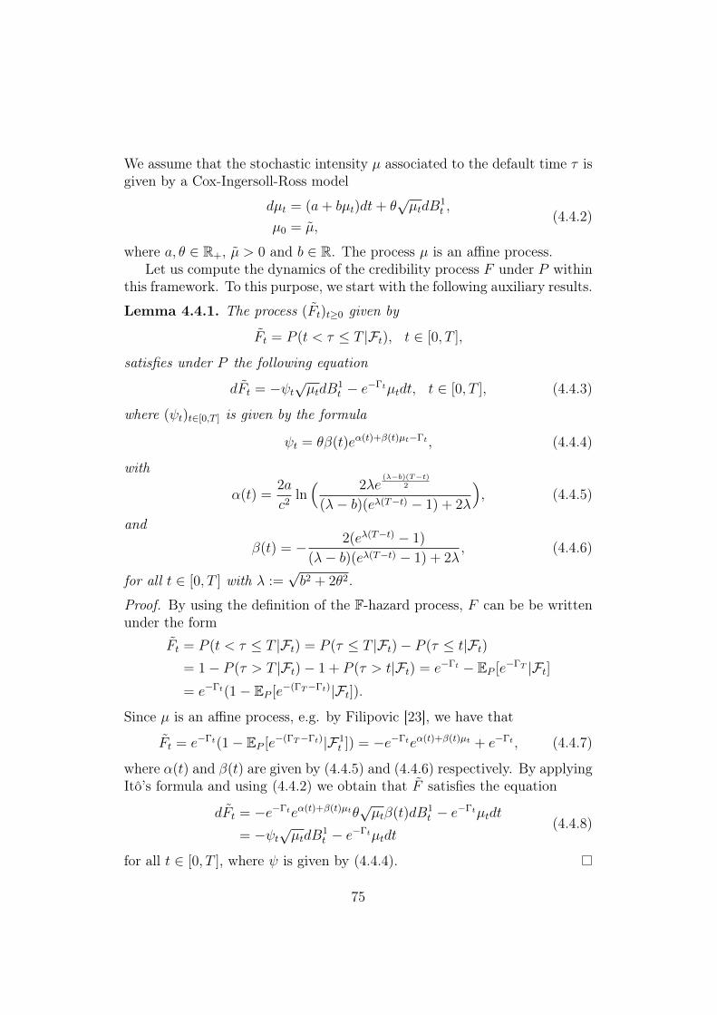
We assume that the stochastic intensity µ associated to the default time τ isgiven by a Cox-Ingersoll-Ross model

dµt = (a+ bµt)dt+ θ√µtdB

1t ,

µ0 = µ,(4.4.2)

where a, θ ∈ R+, µ > 0 and b ∈ R. The process µ is an affine process.Let us compute the dynamics of the credibility process F under P within

this framework. To this purpose, we start with the following auxiliary results.

Lemma 4.4.1. The process (Ft)t≥0 given by

Ft = P (t < τ ≤ T |Ft), t ∈ [0, T ],

satisfies under P the following equation

dFt = −ψt√µtdB

1t − e−Γtµtdt, t ∈ [0, T ], (4.4.3)

where (ψt)t∈[0,T ] is given by the formula

ψt = θβ(t)eα(t)+β(t)µt−Γt , (4.4.4)

with

α(t) =2a

c2ln( 2λe

(λ−b)(T−t)2

(λ− b)(eλ(T−t) − 1) + 2λ

), (4.4.5)

and

β(t) = − 2(eλ(T−t) − 1)

(λ− b)(eλ(T−t) − 1) + 2λ, (4.4.6)

for all t ∈ [0, T ] with λ :=√b2 + 2θ2.

Proof. By using the definition of the F-hazard process, F can be be writtenunder the form

Ft = P (t < τ ≤ T |Ft) = P (τ ≤ T |Ft)− P (τ ≤ t|Ft)= 1− P (τ > T |Ft)− 1 + P (τ > t|Ft) = e−Γt − EP [e−ΓT |Ft]= e−Γt(1− EP [e−(ΓT−Γt)|Ft]).

Since µ is an affine process, e.g. by Filipovic [23], we have that

Ft = e−Γt(1− EP [e−(ΓT−Γt)|F1t ]) = −e−Γteα(t)+β(t)µt + e−Γt , (4.4.7)

where α(t) and β(t) are given by (4.4.5) and (4.4.6) respectively. By applyingItô’s formula and using (4.4.2) we obtain that F satisfies the equation

dFt = −e−Γteα(t)+β(t)µtθ√µtβ(t)dB1

t − e−Γtµtdt

= −ψt√µtdB

1t − e−Γtµtdt

(4.4.8)

for all t ∈ [0, T ], where ψ is given by (4.4.4).

75

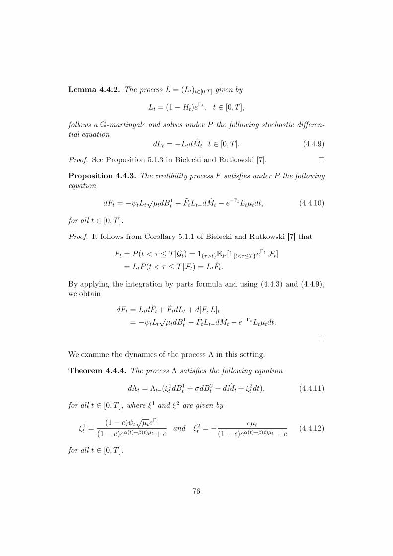
Lemma 4.4.2. The process L = (Lt)t∈[0,T ] given by

Lt = (1−Ht)eΓt , t ∈ [0, T ],

follows a G-martingale and solves under P the following stochastic differen-tial equation

dLt = −LtdMt t ∈ [0, T ]. (4.4.9)

Proof. See Proposition 5.1.3 in Bielecki and Rutkowski [7].

Proposition 4.4.3. The credibility process F satisfies under P the followingequation

dFt = −ψtLt√µtdB

1t − FtLt−dMt − e−ΓtLtµtdt, (4.4.10)

for all t ∈ [0, T ].

Proof. It follows from Corollary 5.1.1 of Bielecki and Rutkowski [7] that

Ft = P (t < τ ≤ T |Gt) = 1τ>tEP [1t<τ≤TeΓt |Ft]

= LtP (t < τ ≤ T |Ft) = LtFt.

By applying the integration by parts formula and using (4.4.3) and (4.4.9),we obtain

dFt = LtdFt + FtdLt + d[F,L]t

= −ψtLt√µtdB

1t − FtLt−dMt − e−ΓtLtµtdt.

We examine the dynamics of the process Λ in this setting.

Theorem 4.4.4. The process Λ satisfies the following equation

dΛt = Λt−(ξ1t dB

1t + σdB2

t − dMt + ξ2t dt), (4.4.11)

for all t ∈ [0, T ], where ξ1 and ξ2 are given by

ξ1t =

(1− c)ψt√µte

Γt

(1− c)eα(t)+β(t)µt + cand ξ2

t = − cµt(1− c)eα(t)+β(t)µt + c

(4.4.12)

for all t ∈ [0, T ].

76

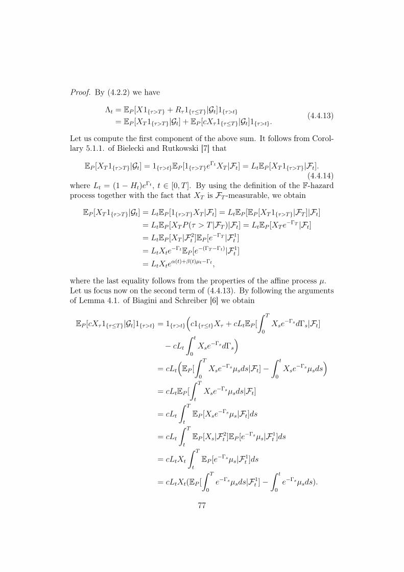
Proof. By (4.2.2) we have

Λt = EP [X1τ>T +Rτ1τ≤T|Gt]1τ>t= EP [XT1τ>T|Gt] + EP [cXτ1τ≤T|Gt]1τ>t.

(4.4.13)

Let us compute the first component of the above sum. It follows from Corol-lary 5.1.1. of Bielecki and Rutkowski [7] that

EP [XT1τ>T|Gt] = 1τ>tEP [1τ>TeΓtXT |Ft] = LtEP [XT1τ>T|Ft].

(4.4.14)where Lt = (1 − Ht)e

Γt , t ∈ [0, T ]. By using the definition of the F-hazardprocess together with the fact that XT is FT -measurable, we obtain

EP [XT1τ>T|Gt] = LtEP [1τ>TXT |Ft] = LtEP [EP [XT1τ>T|FT ]|Ft]= LtEP [XTP (τ > T |FT )|Ft] = LtEP [XT e

−ΓT |Ft]= LtEP [XT |F2

t ]EP [e−ΓT |F1t ]

= LtXte−ΓtEP [e−(ΓT−Γt)|F1

t ]

= LtXteα(t)+β(t)µt−Γt ,

where the last equality follows from the properties of the affine process µ.Let us focus now on the second term of (4.4.13). By following the argumentsof Lemma 4.1. of Biagini and Schreiber [6] we obtain

EP [cXτ1τ≤T|Gt]1τ>t = 1τ>t

(c1τ≤tXτ + cLtEP [

∫ T

0

Xse−ΓsdΓs|Ft]

− cLt∫ t

0

Xse−ΓsdΓs

)= cLt

(EP [

∫ T

0

Xse−Γsµsds|Ft]−

∫ t

0

Xse−Γsµsds

)= cLtEP [

∫ T

t

Xse−Γsµsds|Ft]

= cLt

∫ T

t

EP [Xse−Γsµs|Ft]ds

= cLt

∫ T

t

EP [Xs|F2t ]EP [e−Γsµs|F1

t ]ds

= cLtXt

∫ T

t

EP [e−Γsµs|F1t ]ds

= cLtXt(EP [

∫ T

0

e−Γsµsds|F1t ]−

∫ t

0

e−Γsµsds).

77

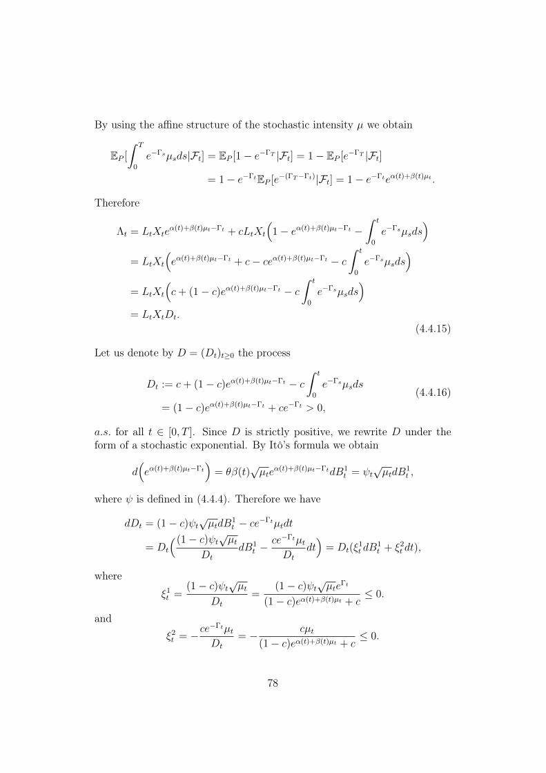
By using the affine structure of the stochastic intensity µ we obtain

EP [

∫ T

0

e−Γsµsds|Ft] = EP [1− e−ΓT |Ft] = 1− EP [e−ΓT |Ft]

= 1− e−ΓtEP [e−(ΓT−Γt)|Ft] = 1− e−Γteα(t)+β(t)µt .

Therefore

Λt = LtXteα(t)+β(t)µt−Γt + cLtXt

(1− eα(t)+β(t)µt−Γt −

∫ t

0

e−Γsµsds)

= LtXt

(eα(t)+β(t)µt−Γt + c− ceα(t)+β(t)µt−Γt − c

∫ t

0

e−Γsµsds)

= LtXt

(c+ (1− c)eα(t)+β(t)µt−Γt − c

∫ t

0

e−Γsµsds)

= LtXtDt.

(4.4.15)

Let us denote by D = (Dt)t≥0 the process

Dt := c+ (1− c)eα(t)+β(t)µt−Γt − c∫ t

0

e−Γsµsds

= (1− c)eα(t)+β(t)µt−Γt + ce−Γt > 0,

(4.4.16)

a.s. for all t ∈ [0, T ]. Since D is strictly positive, we rewrite D under theform of a stochastic exponential. By Itô’s formula we obtain

d(eα(t)+β(t)µt−Γt

)= θβ(t)

õte

α(t)+β(t)µt−ΓtdB1t = ψt

õtdB

1t ,

where ψ is defined in (4.4.4). Therefore we have

dDt = (1− c)ψt√µtdB

1t − ce−Γtµtdt

= Dt

((1− c)ψt√µt

Dt

dB1t −

ce−ΓtµtDt

dt)

= Dt(ξ1t dB

1t + ξ2

t dt),

where

ξ1t =

(1− c)ψt√µt

Dt

=(1− c)ψt

õte

Γt

(1− c)eα(t)+β(t)µt + c≤ 0.

and

ξ2t = −ce

−ΓtµtDt

= − cµt(1− c)eα(t)+β(t)µt + c

≤ 0.

78

An application of Itô’s product formula yields

dΛt = Ltd(XD)t +XtDtdLt + d[XD,L]t

= LtXtdDt + LtDtdXt + Ltd[D,X]t +XtDtdLt +Xtd[D,L]t +Dtd[X,L]t

= LtXtdDt + LtDtdXt +XtDtdLt

= LtXtDt(ξ1t dB

1t + ξ2

t dt) + LtDtσXtdB2t −XtDtLtdMt

= Λt−(ξ1t dB

1t + σdB2

t − dMt + ξ2t dt),

and this concludes the proof.

The following Theorem provides us with the dynamics of the market wealthprocess W . We remind that in our setting the immersion property holdsunder the measure P , i.e. all F-martingales are also G-martingales.

Theorem 4.4.5. The market wealth process W is a (G, P )-semimartingalethat admits the canonical decomposition

Wt = Mt + At,

for all t ∈ [0, T ], where the local martingale part M is given by

dMt = (f(t, Ft)ξ1t − fx(t, Ft)Ltψt

√µt)ΛtdB

1t + σf(t, Ft)ΛtdB

2t

+ (cXt − f(t, Ft)Λt−)dMt,(4.4.17)

and the finite variation part A is given by

dAt =

[f(t, Ft)ξ2t + ft(t, Ft)− fx(t, Ft)Lte−Γtµt +

1

2fxx(t, Ft)L

2tψ

2tµt

+ fx(t, Ft)LtFtµt − fx(t, Ft)Ltψt√µtξ

1t ]Λt + cXtµt

dt.

(4.4.18)

Proof. By applying the integration by parts formula we obtain

dWt = f(t, Ft)dΛt + Λtdf(t, Ft) + d[Λ, f(·, F )]t + cXtdHt. (4.4.19)

First we compute the dynamics of f(t, Ft). Using Itô’s formula (see Theorem

79

II.32 in Protter [52]) and (4.4.10) we have

f(t, Ft) = f(0, F0) +

∫ t

0

fs(s, Fs)ds+

∫ t

0

fx(s, Fs−)dFs +1

2

∫ t

0

fxx(s, Fs−)d[F, F ]cs

+∑

0<s≤t

f(s, Fs)− f(s, Fs−)− fx(s, Fs−)∆Fs)

= f(0, F0) +

∫ t

0

fs(s, Fs)ds−∫ t

0

fx(s, Fs)Lsψs√µsdB

1s

−∫ t

0

fx(s, Fs−)Fs−Ls−dMs −∫ t

0

fx(s, Fs)Lse−Γsµsds

+1

2

∫ t

0

fxx(s, Fs)L2sψ

2sµsd[B1, B1]s

+∑

0<s≤t

f(s, Fs)− f(s, Fs−)− fx(s, Fs−)∆Fs)

= f(0, F0) +

∫ t

0

fs(s, Fs)ds−∫ t

0

fx(s, Fs)Lsψs√µsdB

1s

−∫ t

0

fx(s, Fs−)Fs−Ls−dMs −∫ t

0

fx(s, Fs)Lse−Γsµsds

+1

2

∫ t

0

fxx(s, Fs)L2sψ

2sµsds

+

∫ t

0

f(s, Fs)− f(s, Fs−) + fx(s, Fs−)Fs−Ls−dMs

+

∫ t

0

fx(s, Fs)FsLsµsds,

where we wrote the sum of jumps as a stochastic integral as shown below∑0<s≤t

f(s, Fs)− f(s, Fs−)− fx(s, Fs−)∆Fs

=∑

0<s≤t

f(s, Fs)− f(s, Fs−) + fx(s, Fs−)FsLs−∆Hs

=∑

0<s≤t

f(s, Fs)− f(s, Fs−)∆Hs +∑

0<s≤t

fx(s, Fs−)FsLs−∆Hs

=

∫ t

0

(f(s, Fs)− f(s, Fs−))dHs +

∫ t

0

fx(s, Fs−)FsLs−dHs

=

∫ t

0

f(s, Fs)− f(s, Fs−) + fx(s, Fs−)FsLs−dMs +

∫ t

0

fx(s, Fs−)FsLs−µsds.

80

Therefore

f(t, Ft) = f(0, F0)−∫ t

0

fx(s, Fs)Lsψs√µsdB

1s +

∫ t

0

(f(s, Fs)− f(s, Fs−)

)dMs

+

∫ t

0

(fs(s, Fs)− fx(s, Fs)Lse−Γsµs +

1

2fxx(s, Fs)L

2sψ

2sµs

+ fx(s, Fs)FsLsµs

)ds.

(4.4.20)

Hence by Theorem 4.4.4 and (4.4.20) we have that the quadratic covariation[Λ, f(·, F )] is given by

d[Λ, f(·, F )]t = −fx(t, Ft)Ltψtξ1t

√µtΛtd[B1, B1]t

− (f(t, Ft)− f(t, Ft−))Λt−d[M, M ]t

= −(f(t, Ft)− f(t, Ft−))Λt−dHt − fx(t, Ft)Ltψtξ1t

√µtΛtdt

= −(f(t, Ft)− f(t, Ft−))Λt−dMt − fx(t, Ft)Ltψtξ1t

√µtΛtdt.

By replacing the expressions of [Λ, f(·, F )] and f(t, Ft) in (4.4.19) and byusing (4.4.11) we obtain

dWt = f(t, Ft)ξ1t ΛtdB

1t + σf(t, Ft)ΛtdB

2t − f(t, Ft−)Λt−dMt

+ f(t, Ft)ξ2t Λtdt− fx(t, Ft)Ltψt

√µtΛtdB

1t

+ (f(t, Ft)− f(t, Ft−))Λt−dMt +(ft(t, Ft)− fx(t, Ft)Lte−Γtµt

+1

2fxx(t, Ft)L

2tψ

2tµt + fx(t, Ft)FtLtµt

)Λtdt

− fx(t, Ft)Ltψt√µtξ

1t Λtdt− (f(t, Ft)− f(t, Ft−))Λt−dMt

+ cXtdMt + cXtµtdt

=(f(t, Ft)ξ

1t − fx(t, Ft)Ltψt

õt

)ΛtdB

1t + σf(t, Ft)ΛtdB

2t

+ (cXt − f(t, Ft−)Λt−)dMt

+(f(t, Ft)ξ

2t + ft(t, Ft)− fx(t, Ft)Lte−Γtµt

+1

2fxx(t, Ft)L

2tψ

2tµt + fx(t, Ft)LtFtµt

− fx(t, Ft)Ltψtξ1t

õt

)Λt + cXtµt

dt.

This concludes the proof.

81

Let us assume Mloc(W ) 6= ∅. We are interested in deriving a general formfor the Radon-Nikodym density process of a measure Q ∈ Mloc(W ) withrespect to the measure P . To this purpose, we consider a setting where thepredictable version of Girsanov’s theorem can be applied. This allows us touse the conditional quadratic covariation in the computation of the canonicalsemimartingale decomposition of W with respect to Q, see Theorem III.40in Protter [52].

Proposition 4.4.6. Let Q ∈Mloc(W ) with Radon-Nikodym density processZ = (Zt)t∈[0,T ] i.e. Zt = dQ

dP|Gt, t ∈ [0, T ]. We assume that the quadratic

covariation [Z,M ] is locally integrable. Then Z admits the representation

dZt = Zt−(b(1)t dB1

t + b(2)t dB2

t + b(3)t−dMt), t ∈ [0, T ], (4.4.21)

where (b(i)t )t∈[0,T ] are G-predictable processes for all i = 1, 2, 3, satisfying

0 = dAt +[(b

(1)t (ξ1

t f(t, Ft)− fx(t, Ft)Ltψt√µt)

+ σb(2)t f(t, Ft)

)Λt + b

(3)t (cXt − f(t, Ft)Λt−)µt

]dt

(4.4.22)

dt⊗ dP -almost surely on [0, T ]× Ω.

Proof. Since the process Z = (Zt)t∈[0,T ] is a G-martingale and the hazardprocess Γ admits the representation

Γt =

∫ t

0

µsds, t ∈ [0, T ],

it follows from Corollary 5.2.4. of Bielecki and Rutkowski [7] that Z can bewritten under the form

Zt = Z0 +

∫ t

0

ζ(1)s dB1

s +

∫ t

0

ζ(2)s dB2

s +

∫ t

0

ζ(3)s dMs,

for all t ∈ [0, T ], where the processes (ζ(i)t )t∈[0,T ] are G-predictable. Fur-

thermore, since Z is a stricly positive martingale, Z can be written as thestochastic exponential

Zt = E (K)t , t ∈ [0, T ],

where K = (Kt)t∈[0,T ] is a local martingale given by

Kt = K0 +

∫ t

0

b(1)s dB1

s +

∫ t

0

b(2)s dB2

s +

∫ t

0

b(3)s dMs, t ∈ [0, T ],

82

with

b(i)t =

ζ(i)t

Zt, t ∈ [0, T ].

Hence representation (4.4.21) follows.Since the quadratic covariation [Z,M ] is locally integrable, it follows from

Chapter III in Protter [52], that the conditional quadratic covariation process〈Z,M〉 exists and is defined as the compensator of [Z,M ]. Therefore, we canapply the predictable version of Girsanov’s Theorem. The local P -martingaleprocess (Mt)t∈[0,T ] given by (4.4.17) admits under Q the following canonicalsemimartingale decomposition

Mt =(Mt −

∫ t

0

1

Zs−d〈Z,M〉s

)+

∫ t

0

1

Zs−d〈Z,M〉s, t ∈ [0, T ].

Since the process (MQt )t∈[0,T ] given by

MQt = Mt −

∫ t

0

1

Zs−d〈Z,M〉s, t ∈ [0, T ].

is a local Q-martingale, it follows that W admits under Q the canonicalsemimartingale decomposition

Wt = MQt +

∫ t

0

1

Zs−d〈Z,M〉s + At, t ∈ [0, T ].

Since Q ∈Mloc(W ), this implies that

At +

∫ t

0

1

Zs−d〈Z,M〉s = 0

dt⊗ dP -a.s. Therefore (4.4.22) follows from the fact that

At +

∫ t

0

1

Zs−d〈Z,M〉s = At +

∫ t

0

1

ZsZsb

(1)s (ξ1

t f(t, Ft)− fx(t, Ft)Ltψt√µt)Λtd[B1, B1]s

+

∫ t

0

1

ZsZsb

(2)s σf(s, Fs)Λsd[B2, B2]s

+

∫ t

0

1

Zs−Zs−(cXs − f(s, Fs)Λs−)d〈M, M〉s

= At +

∫ t

0

[(b(1)s (ξ1

sf(s, Fs)− fx(s, Fs)Lsψs√µs)

+ σb(2)s f(s, Fs)

)Λs + b(3)

s (cXs − f(s, Fs)Λs−)µs

]ds.

83

We now state the following auxiliary result, that will be used later in theproofs.

Lemma 4.4.7. On the set τ > t we have

Rt < Λt. (4.4.23)

Proof. Since the recovery process (Rt)t≥0 is given by Rt = cXt for all t ≥ 0,with c ∈ (0, 1), we obtain

Rt1τ>t = cXt1τ>t = cEP [XT |Gt]1τ>t= c1τ>tEP [XT1τ>T +XT1τ≤T|Gt]= c(1τ>tEP [XT1τ>T|Gt] + 1τ>tEP [EP [XT1t<τ≤T|Gτ ]|Gt])= c1τ>tEP [XT1τ>T +Xτ1t<τ≤T|Gt] < Λt1τ>t.

We consider the following form for the function f(t, x). Let

f(t, x) :=

1 + k(T − t)(1− x

p) if x ≤ p, t ∈ [0, T ],

1 if x > p, t ∈ [0, T ],

where k > 0 is a positive constant. The partial derivatives of f(t, x) will beequal to

ft(t, x) :=

−k(1− x

p) if x ≤ p, t ∈ [0, T ],

0 if x > p, t ∈ [0, T ].

and

fx(t, x) :=

−kp(T − t) if x ≤ p, t ∈ [0, T ],

0 if x > p, t ∈ [0, T ].

Note that f(t, x) has bounded first and second order partial derivatives.Furthermore the impact of the credibility process F on the wealth processWis bounded. However the wealth process W is not bounded. For a commenton price bubbles in the case of assets with a bounded wealth process, we referto Remark 4.2.8.

For this specific example of f(t, x) we show that there exist a measureQ ∈ Mloc(W ) and compute its associated Radon-Nikodym density processwith respect to P .

Theorem 4.4.8. Suppose that the intensity process (µt)t∈[0,T ] satisfies thecondition

EP[

exp(1

σ2

∫ T

0

µ2sds)

]<∞. (4.4.24)

ThenMloc(W ) 6= ∅.

84

Proof. We start by bringing the expression of the finite variation part A ofW , as given in (4.4.18), to a simpler form. Note that fxx(t, x) = 0. From(4.4.4), (4.4.7) and (4.4.12) we obtain

dAt =

[f(t, Ft)ξ2t + ft(t, Ft)− fx(t, Ft)Lte−Γtµt +

1

2fxx(t, Ft)L

2tψ

2tµt

+ fx(t, Ft)LtFtµt − fx(t, Ft)Ltψt√µtξ

1t ]Λt + cXtµt

dt

=

[f(t, Ft)ξ2t + ft(t, Ft)− fx(t, Ft)µt + fx(t, Ft)(1− eα(t)+β(t)µt)µt

− fx(t, Ft)(1− c)ψt

õte

Γt

(1− c)eα(t)+β(t)µt + cLtψt√µt]Λt

+ cXtµt

dt

=f(t, Ft)ξ

2t + ft(t, Ft)

Λtdt+

[−fx(t, Ft)µt − fx(t, Ft)eα(t)+β(t)µtµt

+ fx(t, Ft)µt − fx(t, Ft)1− c

(1− c)eα(t)+β(t)µt + cθ2β2(t)e2α(t)+2β(t)µtµt]Λt

+ cXt

µtdt

=f(t, Ft)ξ

2t + ft(t, Ft)

Λtdt+

− fx(t, Ft)eα(t)+β(t)µt

·(

1 +1− c

(1− c)eα(t)+β(t)µt + cθ2β2(t)eα(t)+β(t)µt

)Λt + cXt

µtdt.

We denote

δt := −fx(t, Ft)eα(t)+β(t)µt(

1 +(1− c)eα(t)+β(t)µt

(1− c)eα(t)+β(t)µt + cθ2β2(t)

)(4.4.25)

for all t ∈ [0, T ]. It is easy to see that 0 ≤ δt < Cδ for some constant Cδ > 0a.s. for all t ∈ [0, T ]. Therefore

dAt =f(t, Ft)ξ

2t + ft(t, Ft)

Λtdt+

(δtΛt + cXt

)µtdt.

We define the measure Q1 by

dQ1

dP|GT = Z

(1)T , (4.4.26)

with the Radon-Nikodym density process Z(1) = (Z(1)t )t∈[0,T ] given by

dZ(1)t = b

(1)t Z

(1)t dB2

t ,

85

and

b(1)t = −

f(t, Ft)ξ2t + ft(t, Ft) + cXt

2Λtµt1τ>t

σf(t, Ft)

= − 1

σξ2t −

ft(t, Ft)

σf(t, Ft)− cXt

2σf(t, Ft)Λt

µt1τ>t

=1

σ

c

(1− c)eα(t)+β(t)µt + cµt + k(1− Ft

p)

1

σf(t, Ft)1σ1≤t

− 1

2σf(t, Ft)

cµt(1− c)eα(t)+β(t)µt + c

1τ>t

=1

σ

cµt(1− c)eα(t)+β(t)µt + c

(1− 1

2f(t, Ft)1τ>t

)+ k(1− Ft

p)

1

σf(t, Ft)1σ1≤t,

where we have used the fact that Λt = XtLtDt with Dt defined in (4.4.16).We prove that Z(1) is a true P -martingale. To this purpose we show thatNovikov’s condition is satisfied i.e.

EP[

exp(1

2

∫ T

0

(b(1)t )2d[B2, B2]t

)]<∞, P − a.s..

We have

EP[

exp(1

2

∫ T

0

(b(1)t )2dt)

]≤ EP

[exp

(∫ T

0

k2

σ2f(t, Ft)2

(1− Ft

p

)2

1σ1≤tdt

+

∫ T

0

c2µ2t

σ2(c+ (1− c)eα(t)+β(t)µt)2

(1− 1

2f(t, Ft)1τ>t

)2

dt)]

≤ CEP[

exp(∫ T

0

c2µ2t

σ2(c+ (1− c)eα(t)+β(t)µt)2dt)]

≤ CEP[

exp( 1

σ2

∫ T

0

µ2tdt)]

<∞,

where C = C(T ) > 0 is some positive constant depending on T and the lastinequality follows from (4.4.24). Therefore Z(1) is indeed a Radon-Nikodymdensity process. It follows from Girsanov’s theorem that the process

B2t = B2

t −∫ t

0

1

Z(1)s

d[Z(1), B2] = B2t −

∫ t

0

b(1)s ds, t ∈ [0, T ],

is a Q1-local martingale for all t ∈ [0, T ]. It follows from Levy’s charac-terization theorem that (B2

t )t∈[0,T ] is a Q1-Brownian motion with respect tothe filtration G. By applying Girsanov’s theorem we obtain the canonicalsemimartingale decomposition of W under Q1:

Wt = M1t + A1

t , t ∈ [0, T ],

86

where the local martingale part (M1t )t∈[0,T ] is equal to

M1t = Mt −

∫ t

0

1

Z(1)s

d[Z(1),M ]s

= M0 +

∫ t

0

(f(s, Fs)ξ1s − fx(s, Fs)Lsψs

√µs)ΛsdB

1s +

∫ t

0

σf(s, Fs)ΛsdB2s

+

∫ t

0

(cXs − f(s, Fs)Λs−)dMs −∫ t

0

σf(s, Fs)Λsb(2)s ds

= M0 +

∫ t

0

(f(s, Fs)ξ

1s − fx(s, Fs)Lsψs

õs

)ΛsdB

1s +

∫ t

0

σf(s, Fs)ΛsdB2s

+

∫ t

0

(cXs − f(s, Fs)Λs)dMs,

and the finite variation part (A1t )t∈[0,T ] is equal by

A1t = At +

∫ t

0

1

Z(1)s

d[Z(1), B2]s

=

∫ t

0

(f(s, Fs)ξ2s + fs(s, Fs))Λsds+

∫ t

0

(δsΛs + cXs)µsds

+

∫ t

0

σf(s, Fs)b(1)s Λsds

=

∫ t

0

(c

2Xs + δsΛs)µsds.

We define the process Z(2) = (Z(2))t∈[0,T ] as the stochastic exponential satis-fying the equation

dZ(2)t = btZ

(2)t dMt, t ∈ [0, T ], (4.4.27)

withbt =

c2Xt + δtΛt

f(t, Ft)Λt − cXt

, t ∈ [0, T ]. (4.4.28)

We prove that Z(2) is a Q1-martingale. First we show that the Q1-localmartingale Z(2) is positive. For this it is sufficient to show that ∆(b.M)t > −1for all t ∈ [0, T ], where b.M denotes the stochastic integral of b with respectto M . We start by showing that (bt)t∈[0,T ] defined in (4.4.28) satisfies bt > −1for all t ∈ [0, T ]. We have

bt =c2Xt + δtΛt

f(t, Ft)Λt − cXt

1τ≤t +c2Xt + δtΛt

f(t, Ft)Λt − cXt

1τ>t

= −1

21τ≤t +

c2Xt + δtΛt

f(t, Ft)Λt − cXt

1τ>t.

(4.4.29)

87

On the set τ > t we have by Lemma 4.4.7, (4.2.3) and (4.4.25) that

cXt < Λt ≤ f(t, Ft)Λt, (4.4.30)

sobt ≥ 0 on τ > t. (4.4.31)

Moreover bt > −1 for all t ∈ [0, T ]. Therefore the Q1-local martingale Z(2) ispositive since

∆(b.M)t = bt∆Mt = bt∆Ht > −1,

for all t ∈ [0, T ]. Since Z(2) is defined as the unique solution of (4.4.27), itfollows from Theorem II.37 in Protter [52] that Z(2) is given by

Z(2)t = exp

(∫ t

0

bsdMs

)Πs≤t(1 + bs∆Hs) exp(−bs∆Hs),

for all t ∈ [0, T ]. We have by (4.4.29) and (4.4.31) that

Z(2)t = exp

(∫ t

0

bsdHs −∫ t∧τ

0

bsµsds)

(1 + bτ1τ≤t) exp(−bτ1τ≤t)

= 1τ>t exp(−∫ t∧τ

0

bsµsds)

+1

21τ≤t exp

(−∫ t∧τ

0

bsµsds)

≤ 1τ>t +1

21τ≤t <

3

2,

for all t ∈ [0, T ]. Therefore the positive Q1-local martingale Z(2) is also upperbounded, hence Z(2) is a Q1-uniformly integrable martingale, see TheoremI.51 in Protter [52]. Analogously, we obtain that

|∆Z(2)t | = |Z

(2)t − Z

(2)t− | ≤ K∆,

for some K∆ > 0. Hence Z(2) has bounded jumps. It follows from Lemma3.14 in [33] that [Z(2),M1] has locally integrable variation. Therefore its Q1-compensator 〈Z(2),M1〉 exists and is well defined.

Since Z(2) is a Q1-martingale, we can define the measure Q2 with theRadon-Nikodym density process w.r.t. Q1 given by

dQ2

dQ1|GT = Z

(2)T . (4.4.32)

It follows from Proposition 5.3.1 in Bielecki and Rutkowski [7] that the pro-cess

Mt = Mt −∫ t

0

bsµsds, t ∈ [0, T ]

88

is a G-martingale under Q2. Since the conditional quadratic covariation〈Z(2),M1〉 exists underQ1, we can apply the predictable version of Girsanov’stheorem (see Theorem III.40 in [52]) in order to compute the canonical semi-martingale decomposition of W under Q2. We have

Wt = M2t + A2

t , t ∈ [0, T ],

Q2-a.s., where the local martingale part (M2t )t∈[0,T ] is given by

M2t = M1

t −∫ t

0

1

Z(2)s−d〈Z(2),M1〉s

= M0 +

∫ t

0

(f(s, Fs)ξ

1s − fx(s, Fs)Lsψs

õs

)ΛsdB

1s +

∫ t

0

σf(s, Fs)ΛsdB2s

+

∫ t

0

(cXs − f(s, Fs)Λs)dMs −∫ t

0

(cXs − f(s, Fs)Λs)bsµsds

= M0 +

∫ t

0

(f(s, Fs)ξ

1s − fx(s, Fs)Lsψs

õs

)ΛsdB

1s +

∫ t

0

σf(s, Fs)ΛsdB2s

+

∫ t

0

(cXs − f(s, Fs)Λs)dMs

and the finite variation part (A2t )t∈[0,T ] is given by by

A2t = A1

t +

∫ t

0

1

Z(2)s−d〈Z(2),M1〉s

=

∫ t

0

(c

2Xs + δsΛs)µsds+

∫ t

0

bsd〈M,M1〉s

=

∫ t

0

(c

2Xs + δsΛs)µsds+

∫ t

0

bs(cXs − f(s, Fs)Λs)µsds

= 0,

where we have used (4.4.28). Hence W is a local martingale under Q2. Thenthe equivalent probability measure Q ≈ P defined by

dQ

dP=dQ1

dP

dQ2

dQ1(4.4.33)

where Q1 and Q2 are defined in (4.4.26) and (4.4.32) respectively, belongs toMloc(W ), i.eMloc(W ) 6= ∅.

The following proposition provides us with a sufficient condition under whichan equivalent local martingale measure Q ∈ Mloc(W ) belongs to the subsetMNUI(W ).

89

Proposition 4.4.9. Let Q ∈ Mloc(W ) and we assume that 0 < σ1 < T . Ifthe estimated wealth process (W e

t )t∈[0,T ] is a Q-supermartingale with respectto the filtration G, then Q ∈MNUI(W ).

Proof. Let Q ∈ Mloc(W ) such that (W et )t∈[0,T ] is a (G, Q)-supermartingale.

Let ε > 0 such that σ1 + ε ≤ T . We have

EQ[WT ] = EQ[W eT ] = EQ[EQ[W e

T |Gσ1+ε]] ≤ EQ[W eσ1+ε]

< EQ[Wσ1+ε] ≤ EQ[W0].

Therefore W is a Q-strict local martingale on [0, T ].

We now provide sufficient conditions under which Proposition 4.3.7 holds inthis framework.

Proposition 4.4.10. Let Q ∈Mloc(W ) whose Radon-Nikodym density pro-cess with respect to P , Z = (Zt)t∈[0,T ] i.e. Zt = dQ

dP|Gt for all t ∈ [0, T ],

satisfies

i) EP [supt∈[0,T ] Z2t ] < +∞.

ii) The quadratic covariation process [W e, Z] is increasing.

Then W eZ is a P -submartingale.

Proof. By applying the integration by parts formula we obtain the semi-martingale decomposition of W eZ

d(W eZ)t = W edZt + ZtdWet + d[W e, Z] = dmt + dat, t ∈ [0, T ],

where the local martingale part (mt)t∈[0,T ] is given by

dmt = Zt−dWet +W e

t−dZt,

and the finite variation part (at)t∈[0,T ] is equal to

dat = d[W e, Z]t.

Hence the process W eZ is a local P -submartingale. In order to show thatW eZ is a P -submartingale, we prove

EP [ sups∈[0,T ]

|ms|] <∞.

Then it follows from Theorem I.51 in Protter [52] that (mt)t∈[0,T ] is a P -martingale. We have

0 < W et = EP [XT1τ>T + cXτ1τ≤T|Gt] < Xt∧τ ,

90

for all t ∈ [0, T ], since c < 1. Hence

EP [(W et )2] ≤ EP [X2

t∧τ ] <∞. (4.4.34)

for all t ∈ [0, T ]. Therefore W e is a square integrable P -martingale andsatisfies EP [(W e

T )2] = EP [[W e,W e]T ]. Let

mt = m+t −m−t , t ∈ [0, T ],

be the decomposition of the local martingale m into its positive part m+ andits negative part m−. Since

(W eZ)t = mt + at = m+t −m−t + at ≥ 0,

for all t ∈ [0, T ], we have m−t ≤ at, for all t ∈ [0, T ]. Moreover

m+t −m−t + at ≤ Xt∧τZt.

Therefore m+t ≤ Xt∧τZt for all t ∈ [0, T ] and

|mt| = m+t +m−t ≤ Xt∧τZt + at.

Hence

EP [ supt∈[0,T ]

|mt|] = EP [ supt∈[0,T ]

|Xt∧τZt + at|]

≤ EP [ supt∈[0,T ]

|Xt∧τZt|] + EP [ supt∈[0,T ]

[W e, Z]t]

= 2EP [ supt∈[0,T ]

(X2t∧τ + Z2

t )] + EP [[W e, Z]T ]

≤ 2EP [ supt∈[0,T ]

X2t ] + 2EP [ sup

t∈[0,T ]

Z2t ] + EP [[W e, Z]T ].

By the Kunita-Watanabe inequality, see Theorem II.25 in [52], we have

EP [[W e, Z]T ] ≤ EP [[W e,W e]T ]12EP [[Z,Z]T ]

12 = EP [(W e

T )2]12EP [Z2

T ]12 .

Therefore by (4.4.34) and by Doob’s maximal inequality it follows

EP [ supt∈[0,T ]

|mt|] ≤ 8EP [X2T ] + 2EP [ sup

t∈[0,T ]

Z2t ] + EP [X2

T ]12EP [Z2

T ]12 <∞.

We can conclude that (mt)t∈[0,T ] is a P -martingale.

Corollary 4.4.11. If Q ∈Mloc(W ) satisfies the assumptions of Proposition4.4.10, then

WQt −W e

t ≥ 0,

for all t ∈ [0, T ]

91

Proof. It is a consequence of Propositions 4.3.7 and 4.4.10.

We now obtain sufficient conditions under which the process W e is a R-supermartingale on the whole interval [0, T ] for a measure R ∈Mloc(W ).

Proposition 4.4.12. Let R ∈Mloc(W ) with Radon-Nikodym density processZ = (Zt)t∈[0,T ], where Zt = dR

dP|Gt, for t ∈ [0, T ]. We assume that the quadratic

covariation process [Z,M ] is locally integrable.If the processes b(i), i = 1, 2, 3, in the representation (4.4.21) of Z satisfy theinequality

(ξ1t b

(1)t + σb

(2)t )(

1 +c

1− ce−α(t)−β(t)µt

)≤ b

(3)t µt, (4.4.35)

on the set τ > t, then W e is a R-supermartingale on [0, T ]. In particularR ∈MNUI(W ).

Proof. By Theorem 4.4.4 it follows that W e satisfies under P the equation

dW et = dΛt +RtdHt

= Λt−(ξ1t dB

1t + σdB2

t − dMt + ξ2t dt) +Rt−dMt +Rtµtdt

= Λt(ξ1t dB

1t + σdB2

t ) + (cXt − Λt−)dMt + (ξ2t Λt + cXtµt)dt

= Λt(ξ1t dB

1t + σdB2

t ) + (cXt − Λt−)dMt + (cXtµt −ce−ΓtµtDt

LtXtDt)dt

= Λt(ξ1t dB

1t + σdB2

t ) + (cXt − Λt−)dMt + (cXtµt − ce−Γtµt(1−Ht)eΓtXt)dt

= Λt(ξ1t dB

1t + σdB2

t ) + (cXt − Λt−)dMt + (cXtµt − cµtXt)dt

= Λt(ξ1t dB

1t + σdB2

t ) + (cXt − Λt−)dMt,

where we have used (4.4.12) and (4.4.15). Since [Z,M ] is locally integrable,its P -compensator process 〈Z,M〉 exists and it is well defined. Therefore onecan apply the predictable version of Girsanov’s theorem in order to determinethe canonical semimartingale decomposition of W e under R. We have

W et = Nt +At, t ∈ [0, T ],

where the local martingale part N = (Nt)t∈[0,T ] is given by

Nt = W et −

∫ t

0

1

Zsd〈Z,W e〉, t ∈ [0, T ],

and the finite variation part A = (At)t∈[0,T ] is equal to

At =

∫ t

0

1

Zsd〈Z,W e〉

=

∫ t

0

1

Zs

((ξ1sb

(1)s + σb(2)

s )Λs + (cXs − Λs)b(3)s µs

)ds.

92

Therefore A is decreasing if

(ξ1t b

(1)t + σb

(2)t )Λt + (cXt − Λt)b

(3)t µt ≤ 0, t ∈ [0, T ].

This can be reformulated as follows on τ > t

(ξ1t b

(1)t + σb

(2)t )Λt ≤ (Λt − cXt)b

(3)t µt (4.4.36)

By replacing Λt = LtDtXt, where (Dt)t∈[0,T ] is defined in (4.4.16), (4.4.36)becomes

(ξ1t b

(1)t + σb

(2)t )LtDt ≤ (LtDt − c)b(3)

t µt

on τ > t, or

(ξ1t b

(1)t + σb

(2)t )(

1 +c

1− ce−α(t)−β(t)µt

)≤ b

(3)t µt,

on the set τ > t. Hence W e is a local R-supermartingale. Since W et =

Nt + At ≥ 0, this implies Nt ≥ −At, for all t ∈ [0, T ]. Therefore N is apositive local R-martingale. The fact that A is a decreasing process togetherwith the supermartingale property of N imply

ER[W et |Gs] = ER[Nt|Gs] + ER[At|Gs] ≤ Ns +As,

for any s, t ∈ [0, T ], with s ≤ t, i.e. W e is an R-supermartingale. ByProposition 4.4.9 we also obtain that R ∈MNUI(W ).

4.4.1 Reduced Information Setting

The credibility process F can be alternatively defined in a reduced infor-mation setting, by conditioning the probability of default on the remainingtime interval (t, T ] with respect to the smaller filtration F. Thus F is definedunder the form

Ft = P(t < τ ≤ T |Ft), (4.4.37)

for all t ∈ [0, T ]. This would correspond to a model where the investorscannot estimate the time of default using the larger information set Gt. Thedynamics of F are given by

Proposition 4.4.13. The credibility process F satisfies under P the follow-ing equation

dFt = −ψt√µtdB

1t − e−Γtµtdt,

whereψt = θβ(t)eα(t)+β(t)µt−Γt , (4.4.38)

93

with

α(t) =2a

c2ln( 2λe

(λ−b)(T−t)2

(λ− b)(eλ(T−t) − 1) + 2λ

), (4.4.39)

and

β(t) = − 2(eλ(T−t) − 1)

(λ− b)(eλ(T−t) − 1) + 2λ, (4.4.40)

for all t ∈ [0, T ] with λ :=√b2 + 2θ2.

Proof. See the proof of Proposition 4.4.3.

We can compute the canonical decomposition of the market wealth pro-cess W in the new setting. Note that the structure of the process Λ, ascomputed in Theorem 4.4.4, remains unchanged.

Theorem 4.4.14. The market wealth process W is a (G, P )-semimartingalethat admits the canonical decomposition

Wt = Mt + At,

for all t ∈ [0, T ], where the local martingale part M is given by

dMt = (f(t, Ft)ξ1t − fx(t, Ft)ψt

√µt)ΛtdB

1t + σf(t, Ft)ΛtdB

2t

+ (cXt − f(t, Ft)Λt−)dMt,(4.4.41)

and the finite variation part A is given by

dAt =

[ft(t, Ft) + f(t, Ft)ξ

2t − fx(t, Ft)ψtξ1

t

√µt]Λt

+ [(1

2fxx(t, Ft)ψ

2t − fx(t, Ft)e−Γt)Λt + cXt]µt

dt.

(4.4.42)

Proof. By applying the integration by parts formula and using Theorem 4.4.4we obtain

dWt = f(t, Ft)dΛt + Λtdf(t, Ft) + d[Λ, f(·, F )]t +RtdHt

= f(t, Ft)dΛt + Λtdf(t, Ft) + d[Λ, f(·, F )]t + cXtdMt + cXtµtdt

= f(t, Ft)Λt−(ξ1t dB

1t + σdB2

t − dMt + ξ2t dt)

+ Λt(ft(t, Ft)dt− fx(t, Ft)ψt√µtdB

1t − fx(t, Ft)e−Γtµtdt+

1

2fxx(t, Ft)ψ

2tµtdt)

− fx(t, Ft)Λtψtξ1t

√µtdt+ cXtdMt + cXtµtdt

By rearranging the terms, equations (4.4.41) and (4.4.42) follow.

94

We now assume that Mloc(W ) 6= ∅ and derive first a general form for theRadon-Nikodym density process associated to a measure Q ∈Mloc(W ).

Proposition 4.4.15. Let Q ∈Mloc(W ) with Radon-Nikodym density processZ = (Zt)t∈[0,T ] i.e. Zt = dQ

dP|Gt, t ∈ [0, T ]. Furthermore, we assume that

the quadratic covariation [Z,M ] is locally integrable. Then Z admits therepresentation

dZt = Zt(b(1)t dB1

t + b(2)t dB2

t + b(3)t dMt), t ∈ [0, T ], (4.4.43)

where (b(i)t )t∈[0,T ] are G-predictable processes for all i = 1, 2, 3, satisfying

0 = dAt +[(b

(1)t (ξ1

t f(t, Ft)− fx(t, Ft)ψt√µt)

+ σb(2)t f(t, Ft)

)Λt + b

(3)t (cXt − f(t, Ft)Λt−)µt

]dt

(4.4.44)

dt⊗ dP -almost surely on [0, T ]× Ω.

Proof. Since the process Z is strictly positive, representation (4.4.43) followsby the martingale representation theorem with respect to (G, P ), see [7].From the predictable version of Girsanov’s Theorem we obtain thatW admitsunder Q the following decomposition

Wt = Mt −∫ t

0

1

Zs−d〈Z,M〉s + At +

∫ t

0

1

Zs−d〈Z,M〉s, t ∈ [0, T ].

Since Q ∈Mloc(W ), this implies that

At +

∫ t

0

1

Zs−d〈Z,M〉s = 0

dt⊗ dP -a.s. which is equivalent to (4.4.44).

One can obtain within this setting the analogous results of Theorem 4.4.8and Propositions 4.4.10 and 4.4.12 by following similar steps to the ones intheir proofs, Section 4.4.

95

4.5 Characterization ofMloc(W ) by measure past-ing

In this section we characteriseMloc(W ), by using the pasting of measures , aconcept which plays an important role in mathematical finance in the studyof American options, in particular in the construction of the Upper and LowerSnell envelopes, as presented in Section 6.4 of Föllmer and Schied [27].

This technique allows us to connect the classical martingale theory ofbubbles with a constructive approach to the study of bubbles. The changesthat occur in the dynamics of the asset’s wealth process are captured throughpasting and lead to changes of dynamics in the space of equivalent localmartingale measures. Furthermore, pasting allows for a construction of anequivalent local martingale measure for W on the whole interval [0, T ], seeTheorem 4.5.6. To this purpose we decompose the market wealth process Was the following sum:

Wt = W σ1t + (Wt −Wσ1)1t≥σ1

= W(1)t +W

(2)t ,

(4.5.1)

where we denote W (1)t := W σ1

t and W (2)t := (Wt −Wσ1)1t≥σ1 for t ∈ [0, T ].

Note that before the optimistic investors start to influence the price, i.e.before the credibility process goes below the threshold p, the asset’s marketwealth coincides with the estimated wealth, and in particular,W (1)

t = W σ1t =

W et on σ1 > t. We start our study with a model where there will be only

one shift in the dynamics of the asset’s market price at time σ1 < T .

Assumption 4.5.1. The following assumptions hold:

i) We have 0 < σ1 < T .

ii) For i = 1, 2,Mloc(W(i)) 6= ∅.

We wish to describe the structure of the equivalent local martingale mea-sures Q ∈ Mloc(W ). The market wealth process W coincides with the es-timated wealth W e until the starting time σ1 of the bubble. After σ1 theunderlying price process is affected by the impact of the credibility and startsto change, producing also an alteration of the total wealth process W thatdeviates from W e. Hence an equivalent measure Q ∈ Mloc(W ) must takeinto account the change in the market wealth’s dynamics that occurs afterσ1. We can interpret this as a switch of measures created by the investors’heterogeneity or overconfidence. The endogenous construction of the asset’swealth process W allows us to provide a possible explanation to the dynamic

96

in the space of equivalent martingale measures as in the approach of Biaginiet al. [4] and Jarrow et al. [40]. Moreover, we show that an equivalent lo-cal martingale measure Q for W on the whole interval [0, T ] can be obtainedthrough the pasting in σ1 of two equivalent local martingale measures Q1 andQ2 corresponding to the processes W σ1 and (W −Wσ1)1·≥σ1 respectively.

We start by recalling some results concerning measure pasting. In thesequel let Q1 and Q2 be two equivalent measures on (Ω,GT ) and η be aG-stopping time with 0 ≤ η ≤ T .

Definition 4.5.2. The probability measure Q

Q(A) := EQ1 [Q2(A|Gη)], A ∈ GT ,

is called the pasting of Q1 and Q2 in η.

We remind the reader of the following result which relates the conditionalexpectation with respect to the measure Q with the conditional expectationswith respect to the initial measures Q1 and Q2.

Lemma 4.5.3. If Q is the pasting of Q1 and Q2 in η, then for all stoppingtimes ξ and all GT -measurable random variables Y ≥ 0 it holds that

EQ[Y |Gξ] = EQ1 [EQ2 [Y |Gη∨ξ]|Gξ].

Proof. See Lemma 6.40 in [27].

The following series of technical results will be used to obtain the desiredrepresentation of the elements in the set Mloc(W ). For i = 1, 2 let Z(i) :=

(Z(i)t )t∈[0,T ] be the corresponding Radon-Nikodym density process

Z(i)t =

dQi

dP|Gt , t ∈ [0, T ]. (4.5.2)

We put

Ut =dQ2

dQ1

|Gt , t ∈ [0, T ]. (4.5.3)

Lemma 4.5.4. The pasting Q of Q1 and Q2 in η is equivalent to Q1 andsatisfies

dQ

dQ1

|Gt =UtUη∧t

, t ∈ [0, T ], (4.5.4)

where U is introduced in (4.5.3).

97

Proof. By Lemma 6.39 in [27] we havedQ

dQ1

=UTUη.

Furthermore

EQ1 [dQ

dQ1

|Gt] = EQ1 [UTUη

1η≤t|Gt] + EQ1 [UTUη

1t<η|Gt]

=1

UηUt1η≤t + EQ1 [EQ1 [

UTUη

1t<η|Gη]|Gt]

=1

UηUt1η≤t + EQ1 [1t<η

1

UηEQ1 [UT |Gη]|Gt]

=1

UηUt1η≤t + EQ1 [1t<η|Gt]

=UtUt∧η

1η≤t +UtUt∧η

1t<η

=UtUt∧η

,

(4.5.5)

where the third equality follows from an application of Doob’s optional stop-ping time theorem and the fourth equality follows from fact that η > t ∈ Gt,since η is a G-stopping time.

This allows us to obtain the Radon-Nykodim density process Z = (Zt)t∈[0,T ]

of the measure Q obtained through pasting, i.e. Zt = dQdP|Gt , t ∈ [0, T ].

Corollary 4.5.5. The process Z = (Zt)t∈[0,T ] given by

Zt = Z(1)t

UtUt∧η

, t ∈ [0, T ], (4.5.6)

is a P -martingale with respect to the filtration G and dQdP|Gt = Zt, t ∈ [0, T ].

Furthermore

Zt = Z(1)t∧η

Z(2)t

Z(2)t∧η, t ∈ [0, T ],

where Z(1), Z(2) are given in (4.5.2).

Proof. By Lemma 4.5.4 and by applying Bayes formula we obtain

Zt = Z(1)t

UtUt∧η

= Z(1)t

EP [dQ2

dP|Gt]

EP [dQ1

dP|Gt]

EP [dQ1

dP|Gt∧η]

EP [dQ2

dP|Gt∧η]

= Z(1)t

Z(2)t

Z(1)t

Z(1)t∧η

Z(2)t∧η

= Z(1)t∧η

Z(2)t

Z(2)t∧η, t ∈ [0, T ].

98

The following result represents the central theorem of this section and pro-vides a way of constructing a local martingale measure Q for the processW on the whole interval [0, T ], under Assumption 4.5.1. This new measuretakes into account the possible changes that occur in the dynamics of W .Furthermore we can determine whether the resulting measure Q belongs toone of the setsMUI(W ) orMNUI(W ).

Theorem 4.5.6. We assume that Assumption 4.5.1 holds.

i) Let Qi ∈Mloc(Wi), i = 1, 2, and let Q ≈ P be the measure obtained by

the pasting of Q1 and Q2 in σ1, with Radon-Nikodym density processZt = dQ

dP|Gt, t ∈ [0, T ]. Then Q ∈Mloc(W ).

In addition, if Q1 ∈ MNUI(W(1)) or Q2 ∈ MNUI(W

(2)), then Q ∈MNUI(W ).

ii) On the other hand, let Q ∈Mloc(W ) with Radon-Nikodym density Z =(Zt)t∈[0,T ], i.e. Zt = dQ

dP|Gt, t ∈ [0, T ]. There exist Qi ∈Mloc(W

(i)), i =

1, 2, with corresponding Radon-Nikodym density processes Z(i)t = dQi

dP|Gt

given by Z(1)t = Zt∧σ1 and Z(2)

t = ZtZt∧σ1

for all t ∈ [0, T ], such that Zcan be written in the form

Zt = Z(1)t Z

(2)t , t ∈ [0, T ],

and Q is the pasting of Q1 and Q2 in σ1.

Proof. i) Let (τ in)n≥0 be a localizing sequence such that W (i),τ in is a Qi-martingale on [0, T ] for i = 1, 2. We now construct a sequence of G-stoppingtimes (τn)n≥0 such that W τn is a Q-martingale on [0, T ], where Q is the past-ing of Q1 and Q2 in σ1. We define the sequence of stopping times (τn)n≥0 by

99

τn := τ 1n ∧ τ 2

n, n ≥ 0. For any s ≤ t, it follows from Lemma 4.5.3 that

EQ[Wt∧τn|Gs] = EQ1 [EQ2 [Wt∧τn|Gs∨σ1 ]|Gs]= EQ1 [EQ2 [Wt∧τn∧σ1 +W

(2)t∧τn|Gs∨σ1 ]|Gs]

= EQ1 [Wt∧τn∧σ1 +W(2)(t∧τn)∧(s∨σ1)|Gs]

= Ws∧τn∧σ1 + EQ1 [W(2)(t∧τn)∧(s∨σ1)|Gs]

= Ws∧τn∧σ1 + EQ1 [1s∧τn<σ1W(2)(t∧τn∧σ1)∨(s∧τn)|Gs]

+ EQ1 [1s∧τn≥σ1W(2)(t∧τn∧σ1)∨(s∧τn)|Gs]

= Ws∧τn∧σ1 + EQ1 [1s∧τn<σ1W(2)t∧τn∧σ1 |Gs]

+ EQ1 [1s∧τn≥σ1W(2)s∧τn|Gs]

= Ws∧τn∧σ1 +W(2)s∧τn1s∧τn≥σ1

= W(1)s∧τn +W

(2)s∧τn = Ws∧τn ,

(4.5.7)

since W (2)t∧τn∧σ1 = (Wt∧τn∧σ1 − Wσ1)1t∧τn∧σ1≥σ1 = 0. The second and last

equality in (4.5.7) follow from (4.5.1). In these computations, we have usedthe measurability properties of the stopping times and Doob’s optional stop-ping time theorem.Hence Q ∈ Mloc(W ). For the second part of i) we use the fact that ifQ ∈MNUI(W ), then there exists t ∈ [0, T ] such that

Wt > EQ[WT |Gt].

This is a consequence of the fact that W is a positive local martingale andhence a supermartingale. Therefore, the supermartingale inequality holds

Wt ≥ EQ[WT |Gt], t ∈ [0, T ].

for all Q ∈ Mloc(W ), with equality for all Q ∈ Mloc(W ). If W is not auniformly integrable martingale, then the inequality must be strict at leastfor some t ∈ [0, T ].By applying Lemma 4.5.3 we obtain

EQ[WT |Gt] = EQ1 [EQ2 [WT |Gσ1∨t]|Gt]≤ EQ1 [Wσ1∨t|Gt] ≤ Wt,

(4.5.8)

where one of the inequalities is strict for some t if Q1 or Q2 belong to the setMNUI(W ).ii) Consider the set

Z(W ) := Z;ZW is a P − local martingale.

100

Then the Radon-Nikodym density process Z belongs to Z(W ). By Lemma2.3. of Stricker and Yan [59], since σ1 < T , we have that Z ∈ Z(W σ1) i.e.ZW σ1 is a P -local martingale on [0, T ]. We define the measure Q1 ≈ P by

dQ1

dP= Zσ1 .

and prove that ZtZt∧σ1

is a Radon-Nikodym density process for a measureQ2 ≈ P such that W (2) is a Q2-local martingale on [0, T ]. Let (τn)n∈N be alocalizing sequence for the Q-local martingale W . Then

EP[ ZtZt∧σ1

W(2)t∧τn|Gs

]= EP

[ ZtZt∧σ1

(Wt∧τn −Wσ1)1t∧τn≥σ1|Gs]

= EP[ ZtZt∧σ1

(Wt∧τn −Wσ1)1t∧τn≥σ1(1s∧τn≥σ1

+ 1s∧τn<σ1≤t∧τn + 1t∧τn<σ1)|Gs]

= EP[ ZtZt∧σ1

(Wt∧τn −Wσ1)1s∧τn≥σ1|Gs]

+ EP[ ZtZt∧σ1

(Wt∧τn −Wσ1)1s∧τn<σ1≤t∧τn|Gs]

= 1s∧τn≥σ11

Zσ1(EP [ZtWt∧τn|Gs]− EP [ZtWσ1|Gs])

+ EP[EP[ ZtZt∧σ1

(Wt∧τn −Wσ1)1s∧τn<σ1≤t∧τn|Gs∨σ1]|Gs]

=ZsZσ1∧s

(Ws∧τn −Wσ1)1s∧τn≥σ1

+ EP[1s∧τn<σ1≤t∧τn

1

Zσ1(EP [ZtWt∧τn|Gs∨σ1 ]

− EP [Wσ1Zt|Gs∨σ1 ])|Gs]

=ZsZσ1∧s

W(2)s∧τn + EP

[1s∧τn<σ1≤t∧τn

1

Zσ1(Zt∧(σ1∨s)W(t∧τn)∧(σ1∨s)

−Wσ1Zt∧(σ1∨s))|Gs]

=ZsZσ1∧s

W(2)s∧τn + EP

[1s∧τn<σ1≤t∧τn

Zt∧(σ1∨s)

Zσ1(Wt∧τn∧σ1 −Wσ1)|Gs

]=

ZsZσ1∧s

W(2)s∧τn .

These computations are a consequence of the definition of W (2), see 4.5.1, ofthe stopping times’ measurability properties, as well as of Doob’s optional

101

stopping time theorem. Hence ( 1Zσ1∧t

ZtW(2)t )t∈[0,T ] is a P -local martingale.

Thus we can definedQ2

dP|Gt :=

ZtZσ1∧t

, t ∈ [0, T ],

and by Corollary 4.5.5 it follows that Q is the pasting of Q1 and Q2 in σ1.

Theorem 4.5.6 shows how the selection as pricing measure of a martingalemeasure belonging to MNUI(W ) on a stochastic time interval leads to theformation of a bubble in the sense of Definition 4.3.3. This is made clear bythe fact that the pricing measure corresponding to the time interval [0, T ],and which is obtained through pasting, preserves the strict local martingaleproperty of the wealth process W . Reciprocally, one can decompose such ameasure into two pricing measures corresponding to smaller time intervals.

Remark 4.5.7. Note however that this model can be extended to include suc-cesive changes in the dynamics of the market wealth process W . Let (σn)n∈Nbe a sequence of stopping times marking the moment when the process Wis influenced by diverse microeconomic factors (risk-aversion, liquidity etc.).Then one can consider successive measure pastings in order to construct ameasure Q belonging toMloc(W ) on the whole interval [0, T ].

102

Appendix A

Strict local martingales

This section is intended to provide the reader an introduction to strict localmartingales and a (very) short list of references to the mathematical literatureon this topic. The question whether a local martingale process is a truemartingale or a strict local martingale has generated growing interest forstochastic analysis and also mathematical finance, especially due to theirimportance in the modelling of financial bubbles.

A strict local martingale is a local martingale which is not a martingale.One of the most known examples of strict local martingales is the inverse3-dimensional Bessel process.

Example A.0.8. Let (Ω,F , (Ft)t≥0, P ) be a filtered probability space and(Wt)t≥0 is a 3-dimensional Brownian motion starting in x0 6= 0, we definethe process

Xt = ‖Wt‖−1, t ≥ 0.

One can show that (Xt)t≥0 a local martingale with the corresponding localizingsequence τn = inft ≥ 0; ‖Wt‖ ≤ 1

n. Moreover, we have that

EP [X0] =1

‖x0‖

while limt→∞ EP [Xt] = 0. Hence X cannot be a martingale, since it doesnot have constant expectation. For a detailed proof we refer to Chung andWilliams [15].

We now provide an easy intuitive example of strict local martingale, takenfrom Kazamaki [43]. For the sake of completeness, we also present the cor-responding proof.

Lemma A.0.9. [43] Let (Ω,F , (Ft)t≥0, P ) be a filtered probability space and(Bt)t≥0 be a 1-dimensional Brownian motion with B0 = 0. We define the

103

stopping time τ = inft ≥ 0;Bt ≤ t− 1. The process (Lt)t≥0 given by

Lt = E (αBτ )t , t ≥ 0

is a strict P -local martingale, for any α > 1.

Proof. It follows from the continuity of B that

E (Bτ )∞ = exp(τ

2− 1),

since τ <∞. Therefore EP [exp( τ2)] ≤ e, which implies by Novikov’s criterion

that EP [E (Bτ )] = 1 and in particular EP [exp( τ2)] = e. We have that

EP [L∞] = EP [E (αBτ )∞] = EP [exp(ατ − α− 1

2α2τ)]

≤ e−αEP [exp(τ

2)] = e−α+1 < 1.

Therefore L is a strict local martingale.

We conclude this section by presenting the reader a list of recent resultsconcerning strict local martingales.

Stochastic exponentials of continuous local martingales, often used asdensity processes for absolutely continuous measure changes, have been ex-tensively studied and several criterias for determining whether a process is astrict local martingale or a true martingale have been developed, see Carr etal.[12], Mijatovic and Urusov [45].

A more general approach (which doesn’t require the continuity propertyof the process) for the study of right-continuous positive local martingales in-volves the use of the Föllmer measure [24]. For each positive right-continuouslocal martingale X one can associate a measure PX such that

EP [Xt] = PX(τX > t),

where τX = limn→∞(inft ≥ 0;Xt > n ∧ n). The interested reader mayconsult Jarrow and Larsson [35], Carr et al.[13], Kardaras et al.[42] for aseries of interesting results concerning this method. For an alternative wayof constructing strict local martingales with jumps and other examples, seeProtter [53].

104

Bibliography

[1] D. Abreu and M.K. Brunnermeier. Bubbles and crashes. Econometrica,71(1):173–204, 2003.

[2] L. Andersen and V. Piterbarg. Moment explosions in stochastic volatilitymodels:supplement. Supplemental Note, Bank of America and BarclaysCapital, http://dx.doi.org/DOI10.1007/s00780-0060011-7, 2006.

[3] L. Andersen and V. Piterbarg. Moment explosions in stochastic volatilitymodels. Finance and Stochastics, 22(2):29–50, 2007.

[4] F. Biagini, H. Föllmer, and S. Nedelcu. Shifting martingale measuresand the birth of a bubble as a submartingale. Finance and Stochastics,18(2):297–326, 2014.

[5] F. Biagini and S. Nedelcu. The formation of financial bubbles in default-able markets. Preprint, Available at: http://www.fm.mathematik.uni-muenchen.de/download/publications, 2014.

[6] F. Biagini and I. Schreiber. Risk-minimization for life insurance liabili-ties. SIAM Journal on Financial Mathematics, 4(1):243–264, 2013.

[7] T. Bielecki and M. Rutkowski. Credit Risk: Modeling, Valuation andHedging. Springer, 2002.

[8] Jarrow R. Bilina Falafala, R. and P. Protter. Changeof numeraires and relative asset price bubbles. Preprint,Available at SSRN: http://ssrn.com/abstract=2265465 orhttp://dx.doi.org/10.2139/ssrn.2265465, 2014.

[9] B. Bouchard and M. Nutz. Arbitrage and duality in non-dominateddiscrete-time models. Preprint, Available at ArXiv:1305.6008v1, 2013.

[10] M.K. Brunnermeier. Deciphering the liquidity and credit crunch 2007-2008. The Journal of Economic Perspectives, 23:77–100, 2009.

105

[11] M.K. Brunnermeier and M. Oehmke. Bubbles, financial crashes andsystemic risk. In E.N. White, editor, Handbook Of The Economics OfFinance. Elsevier, 2013.

[12] P. Carr and M. Cherny, A. Urusov. On the martingale property oftime-homogenuous diffusions. preprint.

[13] P. Carr, T. Fischer, and J. Ruf. On the hedging of options on explodingexchange rates. Finance and Stochastics, 18(1):115–144, 2014.

[14] U. Cetin, R. Jarrow, P. Protter, and Y. Yildirim. Modeling credit riskwith partial information. Annals of Applied Probability, 14(3):1167–1178, 2004.

[15] K.L. Chung and R.J. Williams. Introduction to Stochastic Integration.Probability and Its Applications. Birkhäuser, 2nd edition, 1990.

[16] D. Coculescu, M. Jeanblanc, and A. Nikeghbali. Default times, no-arbitrage conditions and changes of probability measures. Finance andStochastics, 16(3):513–535, 2012.

[17] D. Coculescu and A. Nikeghbali. Hazard processes and martingale haz-ard processes. Mathematical Finance, 22(3):519–537, 2012.

[18] A.M.G. Cox and D.G. Hobson. Local martingales, bubbles and optionprices. Finance and Stochastics, 9(4):477–492, 2005.

[19] F. Delbaen and W. Schachermayer. A general version of the fundamentaltheorem of asset pricing. Mathematische Annalen, 300:463–520, 1994.

[20] F. Delbaen and W. Schachermayer. A simple counter-example to severalproblems in the theory of asset pricing. Mathematical Finance, 8:1–12,1998.

[21] J.B. DeLong, A. Shleifer, L. Summers, and R. Waldmann. Noise traderrisk in financial markets. Journal of Political Economy, 98(4):703–738,1990.

[22] Lando D. Duffie, D. Term structures of credit spreads with incompleteaccounting information. Econometrica, 69(3):633–664, 2001.

[23] D. Filipovic. Term Structure Models: A Graduate Course. SpringerFinance, 2009.

106

[24] H. Föllmer. The exit measure of a supermartingale. Zeitschrift fürWahrscheinlichkeitstheorie und Verwandte Gebiete, 21(2):154–166, 1972.

[25] H. Föllmer, U. Horst, and A. Kirman. Equilibria in financial mar-kets with heterogeneous agents: A probabilistic perspective. Journalof Mathematical Economics, 41(1-2):123–155, 2005.

[26] H. Föllmer and A. Schied. Probabilistic aspects of finance. Bernoulli,19(4):1306–1326, 2013.

[27] H. Föllmer and A. Schied. Stochastic Finance: An introduction in dis-crete time. De Gruyter Graduate. Walter De Gruyter, 3rd edition, 2010.

[28] P.M. Garber. Famous first bubbles. the journal of Economic Perspec-tives, 4(2):35–54, 1990.

[29] P.M. Garber. Famous First Bubbles: The Fundamentals of Early Ma-nias. The MIT Press, 2001.

[30] J.M. Harrison and D.M. Kreps. Speculative investor behavior in a stockmarket with heterogeneous expectations. The Quarterly Journal of Eco-nomics, 92(2):323–336, 1978.

[31] M. Herdegen and S. Herrmann. Optimal investmentin a black-scholes model with a bubble. Preprint,Available at SSRN: http://ssrn.com/abstract=2354997 orhttp://dx.doi.org/10.2139/ssrn.2354997, 2013.

[32] J Hugonnier. Rational asset pricing bubbles and portfolio constraints.Journal of Economic Theory, 147:2260–2302, 2011.

[33] J. Jacod and A. Shiryaev. Limit Theorems for Stochastic Processes. ASeries of Comprehensive Studies in Mathematics. Springer, 2nd edition,2003.

[34] R. Jarrow, Y. Kchia, and P. Protter. How to detect an asset bubble.SIAM Journal on Financial Mathematics, 2:839–865, 2011.

[35] R. Jarrow and M. Larsson. Informational efficiency under short saleconstraints. Preprint, Available at arXiv:1401.1851, 2014.

[36] R. Jarrow and P. Protter. Forward and futures prices with bubbles.International Journal of Theoretical and Applied Finance, 12(7):901–924, 2009.

107

[37] R. Jarrow and P. Protter. Foreign currency bubbles. Review of Deriva-tives Research, 14(1):67–83, 2011.

[38] R. Jarrow, P. Protter, and A Roch. A liquidity based model for assetprice bubbles. Quantitative Finance, 12(9):1339–1349, 2012.

[39] R. Jarrow, P. Protter, and K. Shimbo. Asset price bubbles in com-plete markets. Advances in Mathematical Finance,, In Honor of DilipB. Madan:105–130, 2007.

[40] R. Jarrow, P. Protter, and K. Shimbo. Asset price bubbles in incompletemarkets. Mathematical Finance, 20(2):145–185, 2010.

[41] I. Karatzas and S. Shreve. Brownian Motion and Stochastic Calculus.Graduate Texts in Mathematics. Springer-Verlag Berlin Heidelberg NewYork, 2nd edition, 2008.

[42] C. Kardaras, D. Kreher, and A. Nikeghbali. Strict local martingales andbubbles. Preprint, Available at arXiv:1108.4177, 2011.

[43] N. Kazamaki. Continuous Exponential Martingales and BMO. LectureNotes in Mathematics. Springer, 1994.

[44] M. Loewenstein and G.A. Willard. Rational equilibrium asset-pricingbubbles in continuous trading models. Journal of Economic Theory,91(1):17–58, 2000.

[45] A. Mijatovic and M. Urusov. On the martingale property of certain localmartingales. Probability Theory and Related Fields, 152(1):1–30., 2012.

[46] E.M. Miller. Risk, uncertainty and divergence of opinion. The Journalof Finance, 32(4):1151–1168, 1977.

[47] L. Neal. How the south sea bubble was blown up and burst. In E.N.White, editor, Stock Market Crashes and Speculative Manias. EdwardElgar Publishing Limited, 1996.

[48] L. Neal and E. Schubert. The first rational bubbles: A new look at themississippi and south sea schemes. BEBR Working Paper 1188, U. ofIlinois, Urbana-Champaign, 1985.

[49] S. Pal and P. Protter. Analysis of continuous strict local martingales viah-transforms. Stochastic Processes and their Applications, 120(8):1424–1443, 2010.

108

[50] P. Protter. The financial meltdown. Matapli, 87:61?68, 2008.

[51] P. Protter. A mathematical theory of financial bubbles. In V. Hender-son and R. Sincar, editors, Paris-Princeton Lectures on MathematicalFinance, volume 2081 of Lecture Notes in Mathematics. Springer, 2013.

[52] P. Protter. A mathematical theory of financial bubbles. In V. Hender-son and R. Sincar, editors, Paris-Princeton Lectures on MathematicalFinance, volume 2081 of Lecture Notes in Mathematics. Springer, 2013.

[53] P. Protter. Strict local martingales with jumps. Preprint, Available atarXiv:1307.2436, 2014.

[54] J. Scheinkman. Speculation, Trading and Bubbles. Kenneth J. ArrowLecture Series. Columbia University Press, 2014.

[55] J. Scheinkmann and W Xiong. Overconfidence and speculative bubbles.Journal of Polical Economy, 111(6):1183–1219, 2003.

[56] A. Schleifer and R.W. Vischny. The limits of arbitrage. The Journal ofFinance, 52(1):35–55, 1997.

[57] C.A. Sin. Complications with stochastic volatility models. Advances inApplied Probability, 30(1):256–268, 1998.

[58] V. L. Smith, G.L. Suchanek, and A.W. Williams. Bubbles, crashes andendogenous expectations in experimental spot asset markets. Economet-rica, 56(5):1119–1151, 1988.

[59] C. Stricker and J.A. Yan. Some remarks on the optional decompositiontheorem. Seminaire de probabilites(Strasbourg), 32:56–66., 1998.

[60] J. Tirole. On the possibility of speculation under rational expectations.Econometrica, 53(6):1163–1182, 1982.

109