Embed Size (px)
Citation preview
MIMO Radar DOD/DOA Estimation and PerformanceAnalysis in the Presence of SIRP Clutter
Vom Fachbereich 18
Elektrotechnik und Informationstechnik
der Technischen Universität Darmstadt
zur Erlangung der Würde eines
Doktor-Ingenieurs (Dr.-Ing.)
genehmigte Dissertation
von
Xin Zhang, M.Sc.
Geboren am 19. 11. 1987 in Henan, China
Referent: Prof. Dr. Marius Pesavento
Korreferent: Prof. Dr. Mohammed Nabil El Korso
Tag der Einreichung: 31. 05. 2016
Tag der mündlichen Prüfung: 17. 08. 2016
D17
Darmstädter Dissertation
2016


Declaration
I, the undersigned, hereby declare that this dissertation is my original work and has not been
submitted or accepted for the award of any other degree in any institution.
Erklärung laut §9 der Promotionsordnung
Ich versichere hiermit dass ich die vorliegende Dissertation allein und nur unter Verwen-
dung der angegebenen Literatur verfasst habe. Die Arbeit hat bisher noch nicht zu Prü-
fungszwecken gedient.
Signature/Unterschrift: . . . . . . . . . . . . . . . . . . . . . . . . . . . . . . . . . . . . . . . . . .
Your name here
Place/Ort: . . . . . . . . . . . . . . . . . . . . . . . . . . . . . . . . . . . . . . . . . .
Date/Datum: . . . . . . . . . . . . . . . . . . . . . . . . . . . . . . . . . . . . . . . . . .


VXORI MEAE FIDELI
OPVSCVLVM DEDICATVM EST

AcknowledgementsI herewith express my deepest and sincerest gratitude to my supervisors
Prof. Dr. Marius Pesavento,
and
Prof. Dr. Mohammed Nabil El Korso,
who are to me not only the best academic mentors, but examples to follow as human beings;
and to my colleague
Dr. Ying Liu,
whose help with the numerical integration problems encountered in this work was indispens-
able; and to
Christian Steffens,
who contributed valuably to the German translation of this work’s abstract; and to all my
other previous and current colleagues in Communication Systems Group at TU Darmstadt,
among whom are (in alphabetical order of last names):
Dr. Samer Alabed, Florian Bahlke, Dr. Nils Bornhorst,
Martin Brossard, Dr. Yong Cheng, Dr. Dana Ciochina,
Ganapati Hegde, Dr. Ka Lung Law, Dr. Liang Li,
Fabio Nikolay, Dr. Pouyan Parvazi, Oscar Dario Ramos Cantor,
Dr. Adrian Schad, Wassim Suleiman, Dima Taleb,
Dr. Xin Wen, Dr. Florian Xaver, Dr. Yang Yang,
not merely for their generous and willing help both in work and in daily life, but also for
their company itself; and beg for forgiveness from all of the many who have contributed in
various ways to the completion of this tiny piece of work but whose name I fail to mention
above.
Xin Zhang
Darmstadt, Nov 15, 2016


圖難於其易,為大於其細。
(See simplicity in the complicated.
Achieve greatness in little things.)
——老子《道德經·為無為章第六十三》
(Lao-Tzu, Tao Te Ching, Ch. LXIII,
trans. G.-F. Feng and J. English)

Abstract i
AbstractThis thesis investigates the problem of target parameter estimation and performance analy-
sis of multiple-input multiple-output (MIMO) radar in the presence of non-Gaussian clutter.
During the past decades, multiple-input multiple-output (MIMO) radar has become a re-
search subject of growing interest, due to its superior performance in many aspects over the
traditional phased-array radar. Conventionally, MIMO radar clutter is modeled as Gaussian-
distributed. This modeling, however, becomes unrealistic and inadequate in certain specific
scenarios, where the clutter shows distinct non-Gaussianity. In the radar literature, one of
the most notable and popular models for such non-Gaussian clutter is the so-called spher-
ically invariant random process (SIRP) model. A SIRP is a complex, compound Gaussian
process with random power and can be represented as the product of two components: a
complex Gaussian process, called the speckle, and the square root of a positive scalar ran-
dom process, called the texture. The goal of this thesis is to devise estimation algorithms
for target parameters, more specifically, for direction-of-departures/arrivals (DODs/DOAs)
of the targets, in a MIMO radar context in the presence of SIRP clutter, and to evaluate the
ultimate performance of this estimation problem, in terms of performance bounds and of
target resolvability. First, three DOD/DOA estimation algorithms are proposed, which differ
from one another in the modeling of the texture, as well as in the respective likelihood func-
tions that they are based on, but have in common that all three algorithms employ the same
concept of the stepwise numerical concentration approach and thus have similar iterative
procedures. Performance properties like convergence of iterations and computational com-
plexity of the three proposed algorithms are then examined. Next, various Cramér-Rao-type
bounds (CRTBs) for the DOD/DOA parameters in this context are derived for performance
assessment and their relationships between one another are determined. The respective im-
pacts of the texture parameters on the CRTBs are investigated to illustrate the effect of the
clutter spikiness on the same. Then, the estimation performance achievable in the presence
of SIRP clutter is studied from another point of view, namely, that of the target resolvabil-
ity, which is quantified by the concept of the resolution limit (RL). As a result, an analytical,
closed-form expression of the RL with respect to (w.r.t.) the angular parameters between two

ii Abstract
closely spaced targets in this context is derived based on Smith’s criterion. For this aim, non-
matrix, closed-form expressions for several of the aforementioned CRTBs w.r.t. the angular
spacing between the targets are also obtained as byproducts. Moreover, an alternative, more
concrete expression for the RL is propsed for asymptotic scenarios. Like for the CRTBs, the
respective impacts of the texture parameters on the RL are also determined. Finally, numer-
ical simulations are provided to assess the performance of the proposed algorithms, to show
the validity of the derived RL expressions, as well as to reveal the CRTBs’ and the RL’s
insightful properties.

Zusammenfassung iii
ZusammenfassungDie vorliegende Dissertation untersucht das Problem der Zielparameterschätzung und der
zugehörigen Genauigkeitsanalyse in einem Multiple-Input Multiple-Output (MIMO)-Radarsystem
in Gegenwart von nicht Gaußschen Störechos (eng. clutter). Aufgrund seiner in vielen As-
pekten dem traditionellen Phased-Array-Radar überlegenen Leistungsfähigkeit sind MIMO-
Radarsysteme in den letzten Jahrzehnten ein Forschungsgegenstand von wachsendem In-
teresse geworden. In herkömmlichen Modellen wird das MIMO-Radar-Clutter gewöhnlich
als gaußverteilt modelliert. Jedoch wird diese Modellierung in bestimmten Szenarien, in
denen das Clutter von einer Gaußverteilung abweicht, unrealistisch und unzureichend. In
der Literatur zur Radartechnik ist eines der weitest verbreiteten Modelle für solch nicht
Gaußsches Clutter das Modell des sogenannten sphärisch invarianten Zufallsprozesses (eng.
spherically invariant random process, kurz SIRP). Ein SIRP ist ein komplexwertiger Ver-
bundgaußprozess mit zufälliger Leistung und kann als das Produkt von zwei Komponen-
ten dargestellt werden: ein komplexwertiger Gaußprozess, im Englischen als “Speckle”
bezeichnet, und die Quadratwurzel eines positiven Skalar-Zufallsprozess, im Englischen
als “Texture” bezeichnet. Das Ziel dieser Arbeit ist es, Schätzalgorithmen für Zielparam-
eter, genauer gesagt für Aus-/Einfallsrichtungen (eng. direction-of-departures/arrivals, kurz
DODs/DOAs) der Ziele, in einem MIMO-Radarsystem in Gegenwart von SIRP-Clutter zu
entwickeln, und die Leistungsfähigkeit dieser Schätzungsaufgabe in Bezug auf die Güte der
Zielparameterschätzung sowie das Zielauflösungsvermögen zu bewerten. Zunächst werden
drei DOD/DOA-Schätzalgorithmen vorgestellt, die sich voneinander in der Modellierung
des Textures sowie in den jeweilig zugrundeliegenden Wahrscheinlichkeitsfunktionen un-
terscheiden. Gleichzeitig ist allen drei Algorithmen gemeinsam, den gleichen Ansatz der
sukzessiven numerischen Konzentration zu verwenden und somit ähnliche iterative Ver-
fahrensweisen zu besitzen. Daraufhin werden Eigenschaften wie die Konvergenz der Iter-
ationen und die Rechenkomplexität der drei vorgeschlagenen Algorithmen untersucht. Für
die Analyse der Schätzgüte werden verschiedene Cramér-Rao-artige Grenzen (eng. Cramér-
Rao-type bounds, kurz CRTBs) für die DOD/DOA-Parameter abgeleitet und ihre Beziehun-
gen untereinander bestimmt, und die jeweiligen Auswirkungen der Textureparameter auf
iv Zusammenfassung
die CRTBs werden untersucht. Anschließend wird die erreichbare Schätzgüte in Gegenwart
von SIRP-Clutter unter dem Gesichtspunkt des Zielauflösungsvermögens betrachtet, welches
sich durch die sogenannte Auflösungsgrenze (eng. resolution limit, kurz RL) quantifizieren
lässt. Basierend auf dem Smithschen Kriterium wird als Ergebnis dieser Betrachtung ein
analytisch geschlossener Ausdruck des RLs mit Bezug auf die Winkelparameter zwischen
zwei eng aneinanderliegenden Zielen hergeleitet. Als Nebenprodukte der Herleitung werden
analytisch geschlossene Ausdrücke für mehrere der genannten CRTBs bezüglich des Winke-
labstands zwischen den Zielen erhalten. Darüber hinaus wird ein alternativer, konkreterer
Ausdruck für die RL für asymptotische Szenarien vorgestellt. Wie bereits für die CRTBs
werden die Auswirkungen der Textureparameter auf das RL bestimmt. Abschließend werden
numerische Ergebnisse dargestellt, um die Güte der vorgestellten Algorithmen zu demonstri-
eren, die Gültigkeit der abgeleiteten RL-Ausdrücke aufzuweisen sowie die aufschlussreichen
Eigenschaften der CRTBs und des RLs aufzuzeigen.

List of Abbreviations
Alg. algorithm
ARL angular resolution limit
BCD block coordinate descent
Ch. chapter
CM covariance matrix
CMLE conventional maximum likelihood estimator
cont’d continued
CPI coherent processing interval
CRB Cramér-Rao bound
CRLB Cramér-Rao lower bound
CRTB Cramér-Rao-type bound
DML deterministic maximum likelihood
DOA direction-of-arrival
DOD direction-of-departure
EMCB extended Miller-Chang bound
Eq. equation
ESPRIT estimation of signal parameters via rotational invariance technique
Fig. figure
FIM Fisher information matrix
GLRT generalized likelihood ratio test
v
vi List of abbreviations
GMANOVA generalized multivariate analysis of variance
HCRB hybrid Cramér-Rao bound
IEMLE iterative exact maximum likelihood estimator
i.i.d. independent and identically distributed
KKT Karush–Kuhn–Tucker
LF likelihood function
IMAPE iterative maximum a posteriori estimator
IMLE iterative maximum likelihood estimator
LLF log-likelihood function
MAP maximum a posteriori
MCB Miller-Chang bound
MCRB modified Cramér-Rao bound
MIMO multiple-input multiple-output
ML maximum likelihood
MSE mean squared error
MUSIC multiple signal classification
PDF probability density function
PX-EM parameter-expanded expectation-maximization
RCS radar cross-section
RL resolution limit
SCR signal-to-clutter ratio
Sec. section
Subsec. subsection
SIRP spherically invariant random process
SIRV spherically invariant random vector
SML stochastic maximum likelihood
SNR signal-to-noise ratio

List of abbreviations vii
SRL statistical resolution limit
STAP space-time adaptive processing
w.r.t. with respect to

viii List of abbreviations

List of Symbols
Z set of integers∧logical conjunction∨logical disjunction
∼ distributed as
∝ direct proportionality
⊗ Kronecker product
Hadamard product
(·) estimate of a parameter
(·)(i)
estimate of a parameter at the ith iteration
(·)T transpose of a matrix
(·)H conjugate transpose of a matrix
(·)∗ conjugate of a matrix
[·]i ith element of a vector
[·]i,j (i, j)th entry of a matrix
‖·‖ Euclidean norm
E· expectation
Ey · expectation w.r.t. the parameter y
Re· real part
Im· imaginary part
tr· trace of a matrix
ix
x List of Symbols
vec· vectorization of a matrix
A B A−B is a positive semidefinite matrix
Γ(·) gamma function
Ψ(·) digamma function
Kn(·) modified Bessel function of the second kind of order n
δij Kronecker delta
Bi ith Bernoulli number
imax maximum number of iterations
xoi abscissa of the generalized Gauss-Laguerre quadrature
woi weight of the generalized Gauss-Laguerre quadrature
O(·)1 order of the generalized Gauss-Laguerre quadrature; the number in
its subscript denotes the parameter of the corresponding abscissa and
weight
arg minxf(x) value of x that minimizes f(x)
P⊥(·) orthogonal projection matrix onto the null space spanned by the
columns of a matrix
K number of radar targets
L number of radar pulses per CPI
T number of snapshots per pulse
M number of sensors at the transmitter
N number of sensors at the receiver
λ carrier wavelength
d(T)i distance between the ith sensor and the reference sensor at the transmit-
ter
d(R)i distance between the ith sensor and the reference sensor at the receiver
IM M ×M identity matrix
0M×N M ×N zero matrix
JM M ×M all-ones matrix
1M all-ones column vector of dimension M

List of Symbols xi
el+1L L× 1 vector whose (l + 1)th element is one and others are zero
S signal source waveform matrix
s(t) signal source waveform vector at the tth snapshot (Ch. 7)
Y (l) radar output matrix at the lth pulse before matched filtering
Y radar output matrix before matched filtering in the one pulse per CPI case (Ch. 7)
y(t) radar output vector at the tth snapshot before matched filtering in the one pulse
per CPI case (Ch. 7)
M (l) clutter matrix at the lth pulse before matched filtering
M clutter matrix before matched filtering in the one pulse per CPI case (Ch. 7)
m(t) clutter vector at the tth snapshot before matched filtering in the one pulse per CPI
case (Ch. 7)
Z(l) radar output matrix at the lth pulse after matched filtering
N (l) clutter matrix at the lth pulse after matched filtering
z(l) vectorized radar output at the lth pulse after matched filtering
z(l) vectorized radar output at the lth pulse after matched filtering, spatially whitened
by the square root of the speckle CM inverse
z full observation vector after matched filtering
n(l) vectorized clutter at the lth pulse after matched filtering
τ(l) texture of the clutter vector n(l)
τ(t) texture of the clutter vectorm(t) in the one pulse per CPI case (Ch. 7)
τ vector containing the texture realizations at all L pulses
τMAP MAP estimate of the texture realization parameter vector τ
x(l) speckle of the clutter vector n(l)
x(t) speckle of the clutter vectorm(t) in the one pulse per CPI case (Ch. 7)
v(l) vector containing RCS coefficients and normalized Doppler frequency shifts of
the targets at the lth pulse
v parameter vector containing the real and imaginary parts of v(l) at all L pulses
xii List of Symbols
H(l) a diagonal matrix composed of the elements of v(l)
P a matrix composed of functions of v(l) at all L pulses
Q a matrix composed of functions of τ(l) and v(l) at all L pulses
αk(l) RCS coefficient of the kth target
αk RCS coefficient of the kth target in the one pulse per CPI case (Ch. 7)
α complex parameter vector including the RCS coefficients of all K targets
fk(l) normalized Doppler frequency shift of the kth target
f parameter vector containing the normalized Doppler frequency shifts of
all K targets
θ(T)k DOD of the kth target
θ(R)k DOA of the kth target
a(T)
(θ
(T)k
)transmit steering vector for the kth target
a(R)
(θ
(R)k
)receive steering vector for the kth target
θ parameter vector containing DODs and DOAs of all K targets
θCMLE estimate of θ by the CMLE
θIMLE estimate of θ by the IMLE
θIMAPE estimate of θ by the IMAPE
εθ convergence threshold w.r.t. θ
a(θ
(T)k , θ
(R)k
)steering vector after matched filtering
D(T) a matrix composed of the partial derivatives of the steering vector
a(θ
(T)k , θ
(R)k
)w.r.t. the DODs
D(R) a matrix composed of the partial derivatives of the steering vector
a(θ
(T)k , θ
(R)k
)w.r.t. the DOAs
D matrix composed ofD(T) andD(R)
D matrixD spatially whitened by the square root of the speckle CM inverse
A (θ) steering matrix after matched filtering
A (θ) steering matrix after matched filtering, spatially whitened by the square
root of the speckle CM inverse
List of Symbols xiii
b (θ, l) signal part of the observation at lth pulse
γ vector composed of the concatenation of b (θ, l) at all L pulses
a shape parameter of the clutter texture
b scale parameter of the clutter texture
Gamma(a, b) gamma distribution with shape parameter a and scale parameter b
Inv-Gamma(a, b) inverse-gamma distribution with shape parameter a and scale pa-
rameter b
Σ CM of the clutter speckle
σ2 a factor to adjust speckle power
Σn normalized clutter speckle CM
trΣa an alternatively assumed trace value for the speckle CM other than
the one in Eq. (2.17
r ratio between the alternatively and the originally assumed speckle
CM trace and the one assumed in Eq. (2.17)
(·)′
counterpart of a parameter resulting from the alternative assump-
tion on the speckle CM trace
ρ(l) clutter realization at the lth pulse with its speckle spatially whitened
by the square root of the speckle CM inverse
gMN
(‖ρ(l)‖2 , a, b
)characteristic function of SIRP clutter
hMN
(‖ρ(l)‖2 , a, b
)a function based the clutter characteristic function and its partial
derivative w.r.t. its first argument ‖ρ(l)‖2
kMN
(‖ρ(l)‖2 , a, b
)partial derivative of the clutter characteristic function w.r.t. its sec-
ond argument (the shape parameter a)
lMN
(‖ρ(l)‖2 , a, b
)partial derivative of the clutter characteristic function w.r.t. its third
argument (the scale parameter b)
ζ parameter vector containing the real and imaginary parts of the en-
tries of the lower triangular part of the speckle CM
xiv List of Symbols
χ original unknown parameter vector
ξ transformed unknown parameter vector
ξdet transformed unknown parameter vector in the deterministic texture case
ξhyb transformed hybrid unknown parameter vector
µ signal parameter vector containing θ and v
$ clutter parameter vector containing ζ, a and b
$det clutter parameter vector in the deterministic texture case
$hyb augmented hybrid clutter parameter vector
ξ unknown parameter vector for the simplified model (Ch. 7)
ψ transformed unknown parameter vector that does not contain the texture
parameters
p(τ(l); a, b) PDF of the clutter texture with parameters a and b
p(τ ; a, b) PDF of the texture realization parameter vector with parameters a and b
p (z |τ ;ψ ) conditional PDF of z conditioned on τ with parameter vector ψ
p (z, τ ; ξ) joint PDF between z and τ with parameter vector ξ
p (z; ξ) marginal PDF of z with parameter vector ξ
ΛC conditional LLF
ΛJ joint LLF
ΛM marginal LLF
CRB (θ) CRB w.r.t. the parameter vector θ
EMCB (θ) EMCB w.r.t. the parameter vector θ
MCB (θ) MCB w.r.t. the parameter vector θ
MCRB (θ) MCRB w.r.t. the parameter vector θ
HCRB (θ) HCRB w.r.t. the parameter vector θ
F FIM for the CRB
FEMC FIM for the EMCB
List of Symbols xv
FMC FIM for the MCB
FM FIM for the MCRB
FH FIM for the HCRB
Φ block of F w.r.t. the signal parameter vector µ
Φ FIM block w.r.t. the signal parameters for the simplified model (Ch. 7)
ς 4× 1 lower left block of Φ (Ch. 7)
Ω 4× 4 lower right block of Φ (Ch. 7)
Ωi i = 1, 2, 3 submatrices of Ω (Ch. 7)
Θi i = 1, . . . , 4 2× 2 submatrices of the inverse of Ω (Ch. 7)
Φθθ block of Φ w.r.t. the parameter vector θ
Φθv block of Φ w.r.t. the parameter vectors θ and v
ΦEMC block of FEMC w.r.t. the signal parameter vector µ
ΦMC block of FMC w.r.t. the signal parameter vector µ
ΦM block of FM w.r.t. the signal parameter vector µ
ΦH block of FH w.r.t. the signal parameter vector µ
φij entries of Φ
ϕij entries of Φ (Ch. 7)
φEMCij entries of ΦEMC
φMij entries of ΦM
κ(MN, a, b) a factor in the expression of the CRB that contains information from the
texture distribution
ν(a, b) a factor in the expression of the MCRB that contains information from
the texture distribution
ω1 electrical angle of the first target (Ch. 7)
ω2 electrical angle of the second target (Ch. 7)
∆ spacing between the two targets w.r.t. the electrical angles (Ch. 7)
σ∆ standard deviation of the estimate of ∆ (Ch. 7)
xvi List of Symbols
δ ARL of the two targets .r.t. the electrical angles (Ch. 7)
η a vector containing the unknown parameters after model linearization
(Ch. 7)
C(t) a matrix containing the known angular parameter ω1 after model lin-
earization (Ch. 7)
Ri, i = 1, 2, 3 matrices based on transformations of the steering vectors w.r.t. the
known angular parameter ω1 after model linearization (Ch. 7)
Υ block-diagonal matrix composed of the speckle CM inverse (Ch. 7)
βi(t), i = 1, 2, 3 columns of C(t), obtains as the respective products of Ri and s(t)
(Ch. 7)
βi, i = 1, 2, 3 vectors composed of the concatenation of βi(t), i = 1, 2, 3, respec-
tively, for all T snapshots (Ch. 7)
βi βi spatially whitened by the square root of Υ (Ch. 7)
y full observation vector (Ch. 7)
γij, i, j = 1, 2, 3 quadratic forms βHi Υβj (Ch. 7)
Q a factor in the analytical expression of the CRB based on the lin-
earized model (Ch. 7)
A, B, C coefficients of the quartic equation (transformed Smith’s equation) in
Eq. (7.42) (Ch. 7)
Γ a 3× 3 Gramian matrix whose entries are γij (Ch. 7)
U a matrix containing the singular vectors of Σ−1n (Ch. 7)
λn, n = 1, . . . , N eigenvalues of Σ−1n (Ch. 7)
Table of Contents
Abstract i
Zusammenfassung iii
List of Abbreviations v
List of Symbols ix
1 Introduction 1
1.1 Background . . . . . . . . . . . . . . . . . . . . . . . . . . . . . . . . . . 1
1.1.1 Multiple-Input Multiple-Output Radar . . . . . . . . . . . . . . . . 1
1.1.2 Spherically Invariant Random Process Clutter . . . . . . . . . . . . 3
1.1.3 Array Signal Processing . . . . . . . . . . . . . . . . . . . . . . . 5
1.1.4 The Cramér-Rao-Type Bounds . . . . . . . . . . . . . . . . . . . . 6
1.1.5 The Resolution Limit . . . . . . . . . . . . . . . . . . . . . . . . . 8
1.2 Thesis Overview . . . . . . . . . . . . . . . . . . . . . . . . . . . . . . . 10
1.2.1 Thesis Motivation . . . . . . . . . . . . . . . . . . . . . . . . . . 10
1.2.2 Thesis Objectives, Contributions and Structure . . . . . . . . . . . 12
2 MIMO Radar Model Setup 15
2.1 Observation Model . . . . . . . . . . . . . . . . . . . . . . . . . . . . . . 15
2.2 Observation Statistics . . . . . . . . . . . . . . . . . . . . . . . . . . . . . 19
2.3 Unknown Parameter Vector . . . . . . . . . . . . . . . . . . . . . . . . . . 23
2.4 Likelihood Functions . . . . . . . . . . . . . . . . . . . . . . . . . . . . . 26
xvii
xviii Table of Contents
3 Iterative Maximum Likelihood DOD and DOA Estimation 29
3.1 Estimates of the Unknown Parameters . . . . . . . . . . . . . . . . . . . . 30
3.2 Stepwise Numerical Concentration Approach . . . . . . . . . . . . . . . . 31
3.3 Algorithmic Procedure . . . . . . . . . . . . . . . . . . . . . . . . . . . . 33
3.4 Performance Analysis . . . . . . . . . . . . . . . . . . . . . . . . . . . . . 36
3.4.1 Convergence and Computational Cost . . . . . . . . . . . . . . . . 36
3.4.2 Invariance of the IMLE to Different Speckle CM Trace Assumptions 37
4 Iterative Maximum A Posteriori DOD and DOA Estimation 39
4.1 Estimates of the Unknown Parameters . . . . . . . . . . . . . . . . . . . . 40
4.2 Existence and Uniqueness of the Solution for the Shape Parameter . . . . . 43
4.2.1 K-Distributed Clutter Case . . . . . . . . . . . . . . . . . . . . . . 43
4.2.2 Student’s t-Distributed Clutter Case . . . . . . . . . . . . . . . . . 45
4.3 Algorithmic Procedure . . . . . . . . . . . . . . . . . . . . . . . . . . . . 45
4.4 Performance Analysis . . . . . . . . . . . . . . . . . . . . . . . . . . . . . 49
4.4.1 Convergence and Computational Cost . . . . . . . . . . . . . . . . 49
4.4.2 Invariance of the IMAPE to Different Speckle CM Trace Assumptions 50
5 Iterative Exact Maximum Likelihood DOD and DOA Estimation 51
5.1 Estimates of the Unknown Parameters . . . . . . . . . . . . . . . . . . . . 52
5.2 Comparison and Interpretation of the Objective Functions for θ . . . . . . . 55
5.3 Existence and Uniqueness of the Solutions for the Texture Parameters for
Student’s t-Distributed Clutter . . . . . . . . . . . . . . . . . . . . . . . . 56
5.4 Algorithmic Procedure . . . . . . . . . . . . . . . . . . . . . . . . . . . . 58
5.5 Performance Analysis . . . . . . . . . . . . . . . . . . . . . . . . . . . . . 61
5.5.1 Convergence and Computational Cost . . . . . . . . . . . . . . . . 61
5.5.2 Invariance of the IEMLE to Different Speckle CM Trace Assumptions 62
6 Cramér-Rao-Type Bounds 65
6.1 The Cramér-Rao Bound . . . . . . . . . . . . . . . . . . . . . . . . . . . . 65
6.1.1 The Score Functions . . . . . . . . . . . . . . . . . . . . . . . . . 66
Table of Contents xix
6.1.2 Calculation of the FIM Entries w.r.t. the Signal Parameters . . . . . 67
6.1.3 The Expression of κ(MN, a, b) . . . . . . . . . . . . . . . . . . . 71
6.1.4 The Expression of the CRB . . . . . . . . . . . . . . . . . . . . . 72
6.2 The Remaining Cramér-Rao-Type Bounds . . . . . . . . . . . . . . . . . . 74
6.2.1 The Extended Miller-Chang Bound . . . . . . . . . . . . . . . . . 74
6.2.2 The Miller-Chang Bound . . . . . . . . . . . . . . . . . . . . . . . 75
6.2.3 The Modified Cramér-Rao Bound . . . . . . . . . . . . . . . . . . 76
6.2.4 The Hybrid Cramér-Rao Bound . . . . . . . . . . . . . . . . . . . 78
6.3 The Relationships between the CRTBs . . . . . . . . . . . . . . . . . . . . 79
6.3.1 The CRB vs. the MCRB/HCRB . . . . . . . . . . . . . . . . . . . 79
6.3.2 The EMCB/MCB vs. the MCRB/HCRB . . . . . . . . . . . . . . . 80
6.3.3 The CRB vs. the EMCB/MCB . . . . . . . . . . . . . . . . . . . . 81
6.4 The CRTBs and the Texture Parameters . . . . . . . . . . . . . . . . . . . 81
6.4.1 CRTBs vs. the Shape Parameter a . . . . . . . . . . . . . . . . . . 82
6.4.2 CRTBs vs. the Scale Parameter b . . . . . . . . . . . . . . . . . . . 85
6.5 The Blockwise Expressions for the CRTBs . . . . . . . . . . . . . . . . . . 86
7 The Angular Resolution Limit 91
7.1 Model Setup . . . . . . . . . . . . . . . . . . . . . . . . . . . . . . . . . . 91
7.2 Model Linearization . . . . . . . . . . . . . . . . . . . . . . . . . . . . . . 93
7.3 The Analytical Expression of CRB(∆) . . . . . . . . . . . . . . . . . . . . 95
7.4 The Expression of the ARL . . . . . . . . . . . . . . . . . . . . . . . . . . 98
7.5 The Existence of the Valid Root . . . . . . . . . . . . . . . . . . . . . . . 100
7.6 The Asymptotic Expression of the ARL . . . . . . . . . . . . . . . . . . . 101
7.7 The ARL and the Texture Parameters . . . . . . . . . . . . . . . . . . . . . 102
7.8 The ARL Based on the Other CRTBs . . . . . . . . . . . . . . . . . . . . . 103
8 Numerical Simulations 105
8.1 The Three Proposed Estimators and the CRTBs . . . . . . . . . . . . . . . 105
8.1.1 Simulation Context . . . . . . . . . . . . . . . . . . . . . . . . . . 105
xx Table of Contents
8.1.2 Simulation Results on the Proposed Estimators . . . . . . . . . . . 106
8.1.3 Simulation Results on the CRTBs . . . . . . . . . . . . . . . . . . 109
8.2 The ARL . . . . . . . . . . . . . . . . . . . . . . . . . . . . . . . . . . . 112
8.2.1 Simulation Context . . . . . . . . . . . . . . . . . . . . . . . . . . 112
8.2.2 Simulation Results on the ARL . . . . . . . . . . . . . . . . . . . 112
9 Conclusions and Outlook 117
9.1 Conclusions . . . . . . . . . . . . . . . . . . . . . . . . . . . . . . . . . . 117
9.2 Outlook . . . . . . . . . . . . . . . . . . . . . . . . . . . . . . . . . . . . 119
Bibliography 120
Publications 137
Curriculum Vitae 139
Chapter 1
Introduction
1.1 Background
1.1.1 Multiple-Input Multiple-Output Radar
During the past decade, multiple-input multiple-output (MIMO) radar has been attracting an
increasing academic interest [1–5] due to its potential to significantly improve radar perfor-
mance as compared with the conventional, phased-array radar. MIMO radar, whose concept
was first introduced in [6, 7], can be generally defined as a radar that uses multiple antennas
to simultaneously transmit diverse (possibly linearly independent, or orthogonal) waveforms
and by utilizing multiple antennas to receive the reflected signals [3].
Based on their antenna configurations, MIMO radar systems generally fall into two
classes:
I. MIMO radar with widely separated antennas (also known as the statistical MIMO
radar, distributed MIMO radar, MIMO radar with large aperture arrays, etc.) [4, 5],
where the transmit (or both the transmit and the receive) antennas are separated widely
enough such that the observed aspect of the target is different for each pair of the trans-
mit/receive antennas. As a result, the total received signal is a superposition of signals
from multiple independent fading paths, i.e., paths with statistically independent re-
flection coefficients. Thus the signal-to-noise ratio (SNR) of the received signal are
1
2 Chapter 1. Introduction
relatively constant. This spatial diversity makes the MIMO radar with widely sepa-
rated antennas more robust against performance deteriorations arising from target scin-
tillations and glint, thereby improves the stability of statistical hypothesis tests, and
enhances the resolution and accuracy of target localization [1, 4, 8, 9].
II. MIMO radar with co-located antennas (also known as the co-located MIMO radar,
coherent MIMO radar, MIMO radar with small aperture arrays, etc.) [2, 3], which has
its antennas close to each other both at the transmitter and receiver. Consequently, all
the transmit/receive antenna pairs observe the identical radar cross-section (RCS) of
the target, which is a measure of power scattered in a given direction when a target is
illuminated by an incident wave [10]. By exploiting the waveform diversity, MIMO
radar with co-located antenna can utilize virtual sensors to extend its array aperture,
thus has the advantages of improved parameter identifiability and estimation accuracy,
higher resolution, more flexible beam-pattern design, direct applicability of space-time
adaptive processing (STAP) techniques, etc., [3, 11, 12]. Furthermore, MIMO radar
with co-located antennas can largely mitigate the time/phase synchronization problem
which MIMO radar with widely separated antennas is prone to.
It should be noted that MIMO radar with co-located antennas (with which this thesis is
concerned) can either be monostatic radar [2, 3, 13, 14] or bistatic radar [15–18], whereas
MIMO radar with widely separated antennas can be viewed as a type of multistatic radar [4].
A monostatic radar is a radar whose transmitter and receiver are co-located, while a bistatic
radar is one whose transmitter and receiver are separated by a distance that is comparable
to the expected target distance. A multistatic radar, on the other hand, consists of multiple
monostatic/bistatic radar components that are spatially diverse. Also note that the concepts of
“monostatic” and “bistatic” are concerned with the locations of the transmitter and receiver,
instead of the locations of the antennas constituting them, and should not be confused with
the concepts of MIMO radars with widely separated and co-located antennas.
1.1. Background 3
1.1.2 Spherically Invariant Random Process Clutter
The term “clutter” in the radar context refers to any unwanted echoes that are caused by
scattering objects (e.g., sea, ground, buildings, rain, birds, etc.) other than the targets of
interest. Clutter can generally be categorized as either surface or volume clutter, depending
on whether the related scatterer forms a surface or fills a volume. Surface clutter includes
ground and sea clutter, etc., while weather and chaff clutter are typical examples of volume
clutter. Similar to thermal noise, clutter is random due to the random phases and amplitudes
of the scatterers. Since in many scenarios the clutter level is much higher than the thermal
noise level at the radar receiver, the radar’s detection performance depends on the Signal-to-
Clutter Ratio (SCR) instead of the SNR in these cases [19].
In the larger part of the radar literature, the clutter is simply assumed to be a Gaussian
stochastic process. Such assumption is generally a good approximation in many cases and
has the central limit theorem as its theoretical basis, which requires that the received clutter
results from a large number of independent and identically distributed (i.i.d.) elementary
scatterers. However, in certain specific scenarios where this requirement is not fulfilled,
the radar clutter can have an extended tail in the distribution and thus cannot be correctly
described by the Gaussian model anymore. As an example, experimental measurements
reveal that the ground clutter data heavily deviate from the Gaussian model [20]. This is also
true, e.g., for the sea clutter in a high-resolution and low-grazing-angle radar context, where
the scatter number is random and the clutter shows nonstationarity [21].
To account for such problems where the clutter is a non-Gaussian process, numerous
clutter models have been developed. Among them, the so-called spherically invariant random
process (SIRP) model has become the most notable and popular one in radar clutter modeling
[20–24]. The concept of SIRPs was first proposed in [25] as a generalization to Gaussian
processes, in which a random process is called a SIRP if all the random variables having
the same variance in the subspace that is the closed linear span of all the random variables
sampled from that process, have the same distribution function. Accordingly, a random
vector obtained by sampling a SIRP is called a spherically invariant random vector (SIRV).
A SIRP is a two-scale, complex, compound Gaussian process with random power and
4 Chapter 1. Introduction
can be represented as the product of two components: a complex Gaussian process with zero
mean and unknown covariance matrix (CM), and the square root of a positive scalar random
process [22,23]. In the radar context, the former describes the local scattering and is usually
referred to as speckle, while the latter, modeling the local power changing, is called texture.
Till now, the SIRP model has gained widespread use to treat the heavy-tailed, non-
Gaussian distributions of radar clutters [21, 26–29], due to the many advantages that it has,
among which are:
I. A SIRP modeling is capable of describing different scales of the clutter roughness.
II. It encompasses a wide variety of non-Gaussian distributions (K-distribution, Student’s
t-distribution, Laplace, Cauchy and Weibull distribution, etc.).
III. It is mathematically tractable because a SIRP preserves many important properties of a
Gaussian process, such as [30]:
(i) The probability density function (PDF) of a SIRV sampled from a SIRP is uniquely
determined by the specification of its mean vector (often assumed as zero vector
in practice), its speckle CM, and its speckle PDF (called the characteristic PDF
of the SIRV).
(ii) A SIRV is invariant (closed) under a linear transformation, and does not change
its characteristic PDF by such a transformation. This property allows a SIRV to
be whitened without any penalty.
This thesis deals mainly with two clutter distributions belonging to the SIRP family that
are most common in literature and in practical applications, namely:
I. K-distributed clutter, in which the texture follows a gamma distribution.
II. Student’s t-distributed clutter, in which the texture follows a inverse-gamma distribu-
tion.
For clutter of both distributions the texture is characterised by two parameters: the shape
parameter and the scale parameter.
1.1. Background 5
1.1.3 Array Signal Processing
Array signal processing is a branch of signal processing that employs the outputs of an array
of sensors to detect signals and to determine signal parameters. Being a topic of growing
interest over the past few decades, array signal processing has found wide application in
many fields, such as radar, sonar, seismology, radio astronomy, wireless communication,
etc. [31, 32].
The quintessential goal of array signal processing in the estimation of parameters by
jointly exploiting temporal and spatial information obtained from an array of antenna sensors
with specific geometric configurations to sample a wavefield that contains information about
the parameters characterizing the signal sources (emitters) [31]. Such signal parameters
generally include the source number (the estimation of which is also known as detection
or signal enumeration), the directions-of-departure/arrival (DODs/DOAs), the ranges, the
velocities, etc., of the signal sources. In order to estimate the unknown parameters of interest,
one must firstly set up the observation model and then, based on the model specified, employ
a specific estimation algorithm. All of the estimation algorithms fall into two main categories
[31]:
I. Spectral-based methods, which find the highest peaks of a certain spectrum-like func-
tion of the signal parameters as their estimates. These methods can be further classified
into:
(i) Beamforming techniques, which steer the antennas to different directions and find
those with maximum power as the DOA estimates. Examples of this kind are the
conventional (Bartlett) beamformer, Carpon’s beamformer, etc. [31, 33].
(ii) Subspace-based techniques, which exploit properties of the eigenstructure of a
certain CM to carry out the analysis. These methods include the multiple signal
classification (MUSIC) algorithms and its various extensions [34–38], the estima-
tion of signal parameters via rotational invariance technique (ESPRIT) [39–43],
ect.
II. Parametric methods, which capitalize, in contrast to the spectral-based methods, more
6 Chapter 1. Introduction
fully on the underlying data model, and generally require a multidimensional search for
the estimates. The so-called maximum likelihood (ML) technique, the idea of which
consists in finding the values of the parameters that maximize the likelihood function
(LF) as their estimates [44], is arguably the most commonly used one of such parametric
methods. Based on two different assumptions about the statistics of the source signals,
the ML methods can be further divided into:
(i) Deterministic ML (DML) approach, which models the signal waveforms as deter-
ministic and unknown [45, 46].
(ii) Stochastic ML (SML) approach, which models the signal waveforms as a Gaus-
sian random process [47, 48].
Another estimation approach commonly used in practice and closely related to the ML
technique is the so-called maximum a posteriori (MAP) technique. Belonging to the
family of Bayesian estimators, the MAP approach incorporates a prior distribution fol-
lowed by the parameter(s) to be estimated into the LF for the ML approach, and max-
imizes the resulting posteriori LF [44]. The MAP technique can thus be seen as a
generalization of the ML technique to the case of unknown random parameters.
The spectral-based methods are computationally more efficient than the parametric meth-
ods by avoiding the exhaustive searches for parameter estimates that the latter typically re-
quire. The parametric methods, notwithstanding their intrinsic computational complexity,
generally provide more accurate results than the spectral-based ones, especially in contexts
where highly correlated or coherent signals are involved.
1.1.4 The Cramér-Rao-Type Bounds
The Cramér-Rao bound (CRB), also known as the Cramér-Rao lower bound (CRLB), is one
of the most fundamental tools for performance evaluation of estimation problems. Obtained
as the inverse of the Fisher information matrix (FIM), the CRB is proved to lower-bound
the variance of any unbiased estimator [44] (an estimator is called unbiased if the expected
value of the estimate it yields of a parameter is equal to the parameter’s true value). Thus the
1.1. Background 7
CRB not only offers a benchmark against which the performance of any unbiased estimator
can be tested in terms of the mean squared error (MSE) it achieves, but enables to rule out
impossible estimators.
An unbiased estimator that attains the CRB is called efficient. The SML estimator intro-
duced above in Sec. 1.1.3 is known to be asymptotically efficient with respect to (w.r.t.) the
number of snapshots, meaning that it achieves in the case of large number of snapshots the
CRB calculated under the corresponding model of Gaussian signal waveforms (the stochastic
CRB) [31, 44, 49], whereas the DML estimator cannot achieve in this case its corresponding
(i.e., the deterministic) CRB calculated by modeling the signal waveforms as deterministic,
because the number of unknown parameters increase with the number of snapshots [31]. On
the other hand, in the asymptotic case w.r.t. the SNR, and with a fixed number of snapshots,
the SML cannot achieve the stochastic CRB [50], while the DML achieves the deterministic
CRB [51].
In real-life applications there arises sometimes the task to estimate certain parameter(s)
of interest in the presence of unknown random nuisance parameters. This is, for instance,
precisely the case for MIMO radar DOD/DOA estimation problems in the presence of SIRP
clutter, which this thesis addresses, since the clutter texture is random and unknown. In such
cases, the CRB is often difficult or impossible to calculate, because the expressions of the
marginal PDF of the observation, with the random nuisance parameters integrated out, are
often complicated (sometimes without closed forms) and mathematically intractable. To deal
with such difficulties, a number of other lower bounds have been proposed in the literature
as alternatives to the CRB [52–57]. All these bounds are similar to the CRB in spirit, but
consider, instead of the PDF marginalized w.r.t. the observation, either the joint PDF of the
observation and the random nuisance parameters, or the PDF of the former conditioned on
the latter, and generally make specific assumptions about or impose certain restrictions on
the random nuisance parameters. As a result, these bounds are either looser (lower) than the
CRB or apply to a more strict class of estimators, but are easier to calculate as compared
with the CRB [52]. Notable examples of these bounds are:
I. Miller-Chang bound (MCB) [53], which is obtained by first assuming the random

8 Chapter 1. Introduction
nuisance parameters as deterministic and known, calculating the FIM based on the PDF
of the observation conditioned on the nuisance parameters, and finally averaging the
inverse of the FIM over the random nuisance parameters.
II. Extended Miller-Chang bound (EMCB) [52], which is an extension of the MCB, and
differs from it in that the EMCB assumes the random nuisance parameters as determin-
istic but unknown in calculating the FIM.
III. Modified Cramér-Rao bound (MCRB) [56, 57], which is the same as the MCB in
assuming the random nuisance parameters as deterministic and known, but averages
over the random nuisance parameters before the FIM inversion.
IV. Hybrid Cramér-Rao bound (HCRB) [54, 55], which considers the joint PDF of the
observation and the random nuisance parameters for the calculation of its FIM (the
word “hybrid” in its name signifies that it considers both deterministic and random
unknown parameters).
The bounds summarized above were classified in [52] under the name Cramér-Rao-like
bounds. Since this name has the same acronym as the Cramér-Rao lower bound, which is
more common in the literature, these bounds will be called in this thesis the Cramér-Rao-type
bounds (CRTBs) instead, to avoid confusion in nomenclature.
1.1.5 The Resolution Limit
The statistical resolution limit (SRL), or simply the resolution limit (RL), is another com-
mon tool to quantify the performance of estimation problems. The RL characterizes the
problem of signal resolvability, and is generally defined as the minimum distance w.r.t. the
parameters of interest (e.g., the DODs/DOAs, frequencies, electrical angles, etc.) that allows
distinguishing between two closely spaced signals [58–60].
Till now various methods have been devised to account for the RL, which can be classi-
fied, in view of the respective theories they rest on, into the following three approaches:
I. Mean null spectrum approach [61, 62], which is based on the mean null spectrum
1.1. Background 9
analysis of the signals, and is always related to a specific high-resolution algorithm.
There are two commonly used criteria belonging to this approach:
(i) Cox’s criterion [61], according to which two signals are resolvable if the mean
null spectrum at each of the two signals’ parameters of interest is lower than the
mean null spectrum at the midpoint of the two parameters.
(ii) Sharman and Durrani’s criterion [62], stating that two signals are resolvable if
the second derivative of the mean of the null spectrum at the midpoint of the two
signals’ parameters of interest is negative.
II. Detection theory approach [59, 63–67], which employs a hypothesis test, e.g., the
generalized likelihood ratio test (GLRT) or its asymptotic equivalent, the Bayesian hy-
pothesis test, etc., to decide if one signal or two closely spaced signals are present in the
set of the observations. Its idea is to link the minimum separation w.r.t. the parameters
of interest between two signals that is detectable at a given SNR, to the probability of
false alarm and/or of detection, thereby transforms the problem of resolvability is into
that of detectability.
III. Estimation theory approach [58, 68–71], which capitalizes on the CRB to describe
the RL. This is because the CRB is, as mentioned in Sec. 1.1.4, a lower bound for any
unbiased estimator, and therefore expresses ultimate estimation accuracy. Two major
criteria for the RL based on the CRB have been proposed, namely:
(i) Lee’s criterion [68,72], which states that two signals are resolvable if the larger of
the standard deviations of the estimation of the two signals’ parameters of interest
is less than twice the separation between these two parameters. In practice, the
standard deviation can be approximated by the square root of the CRB under mild
conditions [73]. One should note that Lee’s criterion ignores the coupling effect
between the two parameters of interest.
(ii) Smith’s criterion [58], which states that two signals are resolvable if the standard
deviation of the estimation of the two signals’ separation (w.r.t. the parameters of

10 Chapter 1. Introduction
interest) is less than this separation itself. The standard deviation is also approxi-
mated by the CRB. It can be readily seen that Smith’s criterion is an extension of
Lee’s by taking into account the coupling effect between the parameters.
In addressing the resolvability problem in a MIMO radar context in the presence of SIRP
clutter, the thesis will adopt the concept of the RL based on Smith’s criterion, in view of the
following advantages it enjoys:
I. It enjoys generality in contrast to the RL based on the mean null spectrum approach,
as the latter is always designed for a specific high-resolution algorithm, but not for a
specific signal model itself [74].
II. It is preferable to other criteria derived from the estimation theory, e.g., the one pro-
posed in [68, 72, 75], because it takes the coupling effect between the parameters of
interest into account.
III. It is closely related, as revealed in [60], to the RL based on the detection theory ap-
proach, meaning that these two approaches can in fact be unified.
1.2 Thesis Overview
This section provides and overview of this thesis. It begins with a brief discussion of the
state-of-the-art research progress in each of the field introduced above, and points out the
research gaps in the current literature, which make for the motivation and main foci of this
thesis. Then, based thereupon, the objectives of the thesis are listed, together with the con-
tributions corresponding to each of them made by this thesis. Finally, an outline of the thesis
structure is given by summarizing the content of each of its following chapters.
1.2.1 Thesis Motivation
Till now, abounding works have been dedicated to the research of MIMO radar, either to in-
vestigate detection/estimation algorithms or to evaluate radar performance in terms of lower
bounds or resolvability [2–4, 11, 12, 15, 18, 76–81]. Specifically, on the topic of DOD/DOA
1.2. Thesis Overview 11
estimation in a MIMO radar context, not few algorithms, either parametric [11, 17, 82–86]
or spectral-based [13–16, 87–95], have been developed, all of which, however, exclusively
model the radar clutter as Gaussian-distributed. On the other hand, as for estimation prob-
lems associated with non-Gaussian, particularly, with SIRP clutter, most of the related works
deal solely with the estimation of clutter parameters, in which the texture parameter(s) and/or
the speckle CM are estimated by assuming the presence of secondary data (known clutter-
only realizations) [28, 96–100], instead of considering unknown clutter realizations embed-
ded in and contaminating the transmitted/received signal. On the contrary, in order to es-
timate radar signal parameters under SIRP clutter, the authors of [98] and [101] devised
parameter-expanded expectation-maximization (PX-EM) algorithms, for phased-array and
MIMO radar, respectively. Nevertheless, their proposed algorithms are restricted to a special,
linear signal model, called the generalized multivariate analysis of variance (GMANOVA)
model [102], thus cannot be directly applied to general MIMO radar models, nor to the
DOD/DOA estimation problems, which are highly nonlinear [103]. To sum up, there ex-
ists no available algorithm in the current literature that addresses the DOD/DOA estimation
problem, indeed, that addresses target estimation problems in general in a comprehensive
manner, in a MIMO radar context in the presence of SIRP clutter.
As an ultimate tool for performance evaluation of estimation problems, the (both stochas-
tic and deterministic) CRB w.r.t. DOA parameters have been derived under a general array
signal processing model, respectively in the presence of white Gaussian noise [35,104,105],
nonuniform Gaussian noise [106], and colored Gaussian noise [107, 108]. On the other
hand, notable works investigating the CRB related to SIRP clutter or its certain specific kind
(e.g., K-distributed clutter) include, among others, [98, 109, 110]. None of these works,
however, provides expressions for the CRB w.r.t. DOD/DOA parameters for a general ob-
servation/SIRP clutter model in a systematic, comprehensive manner, as in parallel to the
results in [35, 104–108] for Gaussian noise. Furthermore, the expressions and properties of
the various CRTBs explored in [52] have not yet been investigated under SIRP clutter, either
(except for the HCRB derived elementwise under the specific GMANOVA model in [98]
with only one clutter texture parameter).

12 Chapter 1. Introduction
The concept of the other of the aforementioned performance tools, namely, the target
resolvability, in terms of the RL, was only recently introduced to the MIMO radar context.
Notable results of its investigation in this context can be found in [76–78]. In [76, 77], how-
ever, the clutter is modeled as Gaussian-distributed. In [78] the clutter is modeled as a SIRP,
but its texture is treated as deterministic and thus the information on the texture distribution
is not exploited. Furthermore, the approach in [78] is based on the GLRT (detection theory).
No work in the literature has been dedicated to the RL based on the estimation theory (more
precisely, on Smith’s criterion) in a MIMO radar context under SIRP clutter.
1.2.2 Thesis Objectives, Contributions and Structure
Based on the survey above of the existing gaps in the literature, this thesis undertakes the
following tasks as its objectives:
I. Design of DOD/DOA estimation algorithms that are both performant and computation-
ally efficient for co-located MIMO radar targets in the presence of SIRP clutter.
II. Calculation of and comparison between the various CRTBs w.r.t. DOD/DOA parame-
ters in the same context, and investigation of their properties.
III. Derivation of analytical expressions for the RL w.r.t. the angular parameters, namely,
the angular RL (ARL), of two closely spaced targets in this context based on Smith’s
criterion, and exploration into the RL’s properties.
The important, original contributions, corresponding to the objectives set above, can be
summarized as follows:
I. Three interrelated iterative DOD/DOA estimation algorithms are proposed in a co-
located MIMO radar context under SIRP clutter, which differ from one another in the
modeling of the clutter texture (as deterministic or stochastic) and in the respective LFs
(conditional, joint, or marginal) on which they rest. Performance analysis in terms of
convergence and computational complexity are carried out for the proposed algorithms,
and in terms of their respective advantages and disadvantages. The three proposed al-
gorithms are:
1.2. Thesis Overview 13
(i) Iterative maximum likelihood estimator (IMLE) (Ch. 3),
(ii) Iterative maximum a posteriori estimator (IMAPE) (Ch. 4),
(iii) Iterative exact maximum likelihood estimator (IEMLE) (Ch. 5),
all of which have significantly superior performance to that of the conventional ML
estimator (CMLE); the latter corresponds to the case where the clutter is assumed to be
uniform white Gaussian.
II. Both elementwise and blockwise expressions for the various CRTBs are derived in
the same context. Extensive examinations of their relationships and the relationships
between them and the texture parameters are provided.
III. An analytical expression for the ARL in this context is derived in Smith’s sense based
on the CRB, as well as an alternative, more concise expression for it in asymptotic
cases. Various properties of the RL revealed by the proposed expressions are carefully
inspected. The expressions for the ARL based on other CRTBs are also discussed. In
addition, non-matrix, closed-form expressions for certain of the CRTBs are derived as
byproducts.
The remaining part of this thesis is organized as follows. Ch. 2 introduces the observation
model of the co-located MIMO radar system and specifies the observation statistics. Chs. 3,
4 and 5 are dedicated to the derivation and performance assessment of the IMLE, IMAPE
and IEMLE, respectively. Ch. 6 presents the derivation of the expressions for the CRTBs and
provides analytical results on their respective properties. Ch. 7 addresses the derivation of
analytical expressions for the ARL. Ch. 8 provides the simulation results and discusses the
properties that are unmasked by the figures, of the proposed estimators, the CRTBs and the
ARL. Finally, Ch. 9 summarizes this thesis and gives an outlook for possible future works.

14 Chapter 1. Introduction
Chapter 2
MIMO Radar Model Setup
2.1 Observation Model
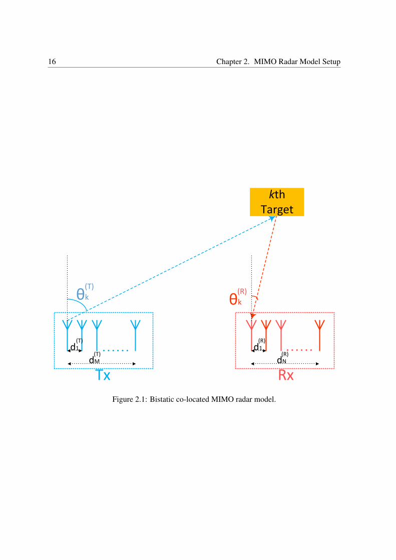
Consider a bistatic co-located MIMO radar system, illustrated by Fig. 2.1, with linear and
possibly nonuniform arrays both at the transmitter and the receiver. Further, assume that
K targets are illuminated by the MIMO radar, all modeled as far-field, narrowband, point
sources [3]. The radar output at the lth pulse in a coherent processing interval (CPI) is given
by [15]:
Y (l) =K∑k=1
αk(l)e2jπfk(l)la(R)
(θ
(R)k
)aT(T)
(θ
(T)k
)S
+M (l), l = 0, . . . , L− 1,
(2.1)
where L denotes the number of radar pulses per CPI; αk(l) and fk(l) denote a complex
coefficient proportional to the RCS and the normalized Doppler frequency shift of the kth
target, respectively; θ(T)k and θ(R)
k represent the DOD and DOA of the kth target, respectively
(cf. Fig. 2.1 for how these angles are measured); the transmit and receive steering vectors
are defined as:
a(T)
(θ
(T)k
)=
[ej
2π sin(θ(T)k )
λd(T)1 , . . . , ej
2π sin(θ(T)k )
λd(T)M
]T, (2.2)
15
16 Chapter 2. MIMO Radar Model Setup
kth Target
Tx Rx
θk θk
(T)(R)
d1
dM
d1
dN
(T)
(T)
(R)
(R)
Figure 2.1: Bistatic co-located MIMO radar model.
2.1. Observation Model 17
and
a(R)
(θ
(R)k
)=
[ej
2π sin(θ(R)k )
λd(R)1 , . . . , ej
2π sin(θ(R)k )
λd(R)N
]T, (2.3)
in whichM andN represent the number of sensors at the transmitter and the receiver, respec-
tively; d(T)i and d(R)
i denote the distance between the ith sensor and the reference sensor at
the transmitter and the receiver, respectively; λ stands for the carrier wavelength; the M ×T
matrix S and the N × T matrix M (l) denote the signal source waveform matrix and the
received clutter matrix at the lth pulse, respectively, where T is the number of snapshots per
pulse; and (·)T denotes the transpose of a matrix.
Since the MIMO radar diversity in terms of waveform coding enables the transmission
of orthogonal waveforms [4], such that
SSH = S∗ST = TIM , (2.4)
in which (·)H and (·)∗ represent the conjugate transpose and the conjugate of a matrix, re-
spectively, and IM denotes the M ×M identity matrix, the radar output after the matched
filtering [111] can be rewritten as:
Z(l) =1√TY (l)SH
=K∑k=1
√Tαk(l)e
2jπfk(l)la(R)
(θ
(R)k
)aT(T)
(θ
(T)k
)+N (l),
l = 0, . . . , L− 1,
(2.5)
where
N (l) =1√TM (l)SH (2.6)
denotes the clutter matrix at the lth pulse after matched filtering.
By stacking the output in Eq. (2.5) into an MN × 1 vector denoted by z(l), one further
has:z(l) =vec Z(l)
=A (θ)v(l) + n(l), l = 0, . . . , L− 1,(2.7)
18 Chapter 2. MIMO Radar Model Setup
in which vec· stands for the vectorization of a matrix, the K × 1 vector
v(l) =[√
Tα1(l)e2jπf1(l)l, . . . ,√TαK(l)e2jπfK(l)l
]T, l = 0, . . . , L− 1, (2.8)
contains the complex-valued RCS coefficients and the normalized Doppler shifts,
n(l) = vec N (l) , l = 0, . . . , L− 1, (2.9)
denotes the clutter vector after matched filtering at the lth pulse, and
A (θ) =[a(θ
(T)1 , θ
(R)1
), . . . ,a
(θ
(T)K , θ
(R)K
)](2.10)
denotes the steering matrix after matched filtering, where
θ =[θ
(T)1 , . . . , θ
(T)K , θ
(R)1 , . . . , θ
(R)K
]T(2.11)
is a 2K × 1 parameter vector introduced to incorporate the unknown DODs and DOAs of all
K targets, and
a(θ
(T)k , θ
(R)k
)=vec
a(R)
(θ
(R)k
)aT(T)
(θ
(T)k
)=(IM ⊗ a(R)
(θ
(R)k
))a(T)
(θ
(T)k
), k = 1, . . . , K,
(2.12)
in which ⊗ denotes the Kronecker product.
It is noteworthy that, after the matched filtering and mathematical transformations de-
scribed above, the co-located MIMO radar model in Eq. (2.7) attains the same expres-
sion as the general model for passive array signal processing applications considered in,
e.g., [35, 106, 112]. Also note that the considered co-located MIMO radar model can be
either bistatic or monostatic. In the latter case one simply has:
θ(T)k = θ
(R)k = θk, k = 1, . . . , K, (2.13)
2.2. Observation Statistics 19
and the direction parameter vector
θ = [θ1, . . . , θK ] (2.14)
has the size of K.
2.2 Observation Statistics
The clutter vectors n(l), l = 0, . . . , L − 1, is modeled as i.i.d. SIRVs [22], which can be
formulated as the product of two components statistically independent of each other:
n(l) =√τ(l)x(l), l = 0, . . . , L− 1, (2.15)
in which the texture terms τ(l), l = 0, . . . , L − 1, are i.i.d. positive random variables; the
speckle terms x(l), l = 0, . . . , L− 1, are i.i.d. MN -dimensional circular complex Gaussian
vectors with zero mean and second-order moments:Ex(i)xH(j)
= δijΣ
Ex(i)xT (j)
= 0MN×MN , i, j = 0, . . . , L− 1,
(2.16)
where Σ denotes the speckle CM, E· is the expectation operator, δij is the Kronecker delta,
and 0MN×MN denotes the MN ×MN zero matrix.
To avoid the ambiguity in the model arising from the scaling effect between the texture
and the speckle, thus to make the clutter parameters uniquely identifiable, assume that:
trΣ = MN, (2.17)
in which tr· denotes the trace.
As mentioned in Ch. 1, this thesis mainly focuses on two kinds of SIRP clutters that are
prevalent in the literature, namely, the K-distributed and the Student’s t-distributed clutters.
In both cases the texture is characterized by two parameters, the shape parameter a and the
20 Chapter 2. MIMO Radar Model Setup
scale parameter b (both a and b are positive numbers). Thus, the texture PDF is denoted by
p(τ(l); a, b) for the following clutter models:
• K-distributed clutter, in which τ(l) follows a gamma distribution [21,113–115] (de-
noted by τ(l) ∼ Gamma(a, b)), with
p(τ(l); a, b) =1
Γ(a)baτ(l)a−1e−
τ(l)b , (2.18)
where Γ(·) denotes the gamma function, defined as:
Γ(a) =
∫ +∞
0
xa−1e−xdx. (2.19)
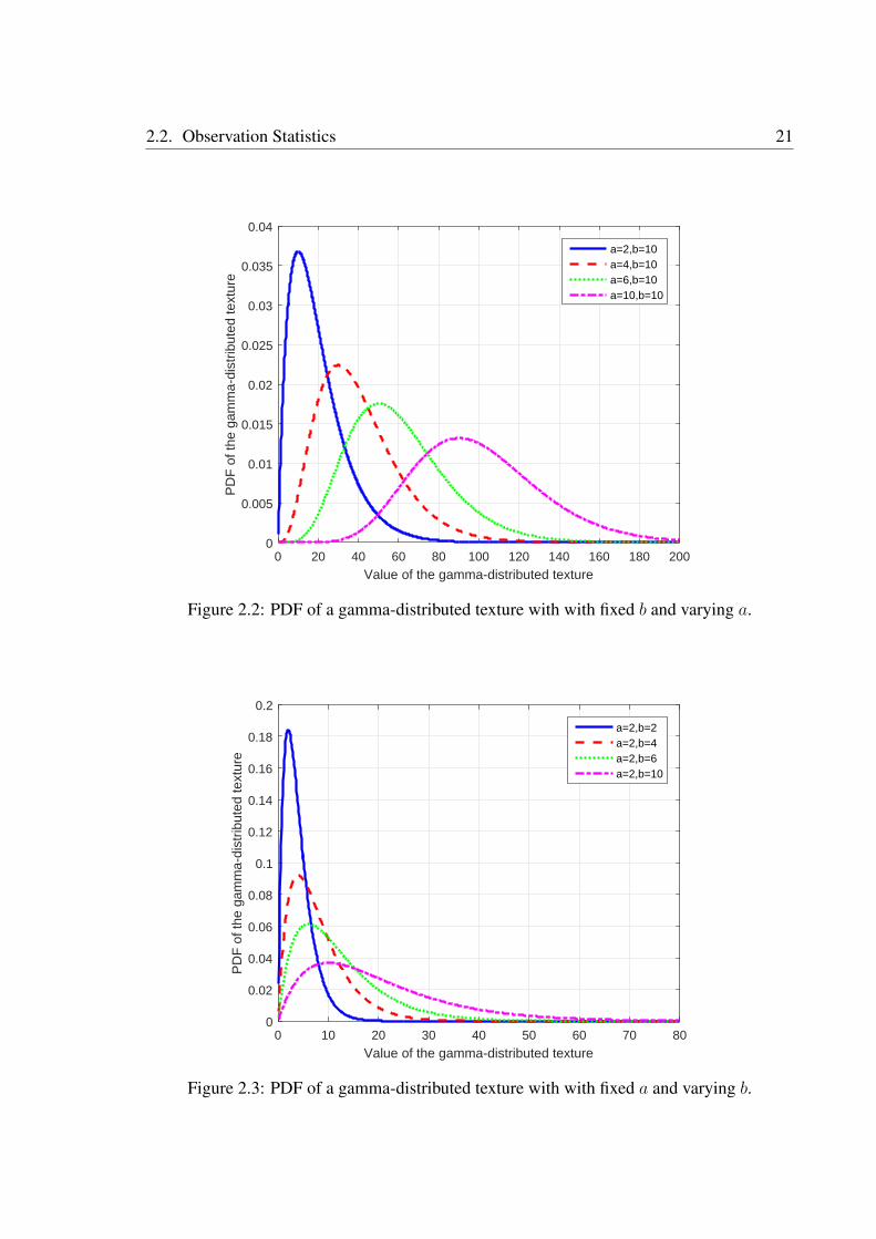
Figs. 2.2 and 2.3 illustrate the PDF of a gamma-distributed texture τ(l) with various
texture parameters, in Fig. 2.2 with fixed b and varying a, and in Fig. 2.3 with fixed
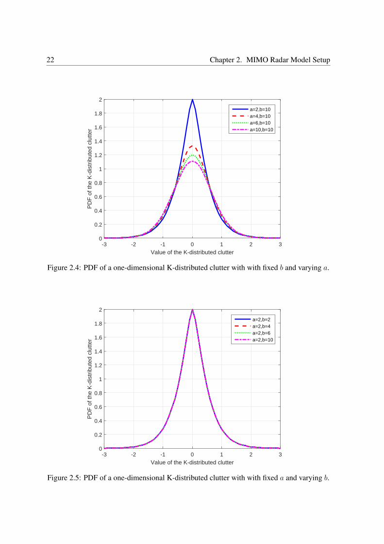
a and varying b. In Figs. 2.4 and 2.5, the PDF of a one-dimensional K-distributed
clutter (with the clutter power fixed to be 1) is shown with its texture parameters a and
b varying in a way corresponding to Figs. 2.2 and 2.3, respectively. Figs. 2.2 and 2.3
show that, either when the shape parameter a or the scale parameter b increases, the
gamma-distributed texture becomes more heavy-tailed. The K-distributed clutter as a
whole, with fixed clutter power, also becomes more heavy-tailed when a increases, but
does not change its distribution with the change of b, as can be seen from Figs. 2.4 and
2.5.
• Student’s t-distributed clutter, in which τ(l) follows an inverse-gamma distribution
[96, 116–118] (denoted by τ(l) ∼ Inv-Gamma(a, b)1), thus:
p(τ(l); a, b) =ba
Γ(a)τ(l)−a−1e−
bτ(l) . (2.20)
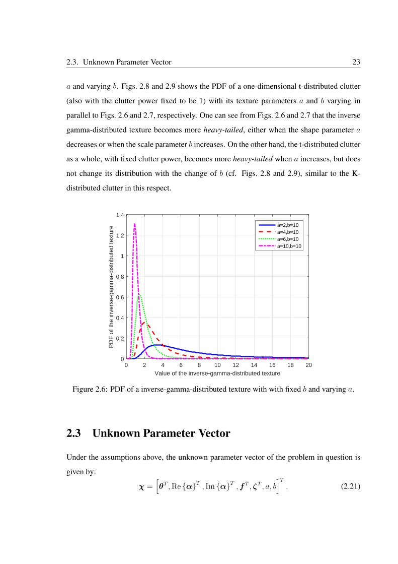
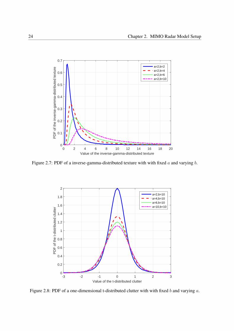
In Figs. 2.6 and 2.7 the PDF of a inverse-gamma-distributed texture τ(l) is plotted with
various texture parameters, in Fig. 2.6 with fixed b and varying a, and in Fig. 2.7 with fixed
1Equivalently, 1/τ(l) follows a gamma distribution such that 1/τ(l) ∼ Gamma(a, 1/b).
2.2. Observation Statistics 21
0 20 40 60 80 100 120 140 160 180 200
Value of the gamma-distributed texture
0
0.005
0.01
0.015
0.02
0.025
0.03
0.035
0.04P
DF
of t
he g
amm
a-di
strib
uted
text
ure
a=2,b=10a=4,b=10a=6,b=10a=10,b=10
Figure 2.2: PDF of a gamma-distributed texture with with fixed b and varying a.
0 10 20 30 40 50 60 70 80
Value of the gamma-distributed texture
0
0.02
0.04
0.06
0.08
0.1
0.12
0.14
0.16
0.18
0.2
PD
F o
f the
gam
ma-
dist
ribut
ed te
xtur
e
a=2,b=2a=2,b=4a=2,b=6a=2,b=10
Figure 2.3: PDF of a gamma-distributed texture with with fixed a and varying b.
22 Chapter 2. MIMO Radar Model Setup
-3 -2 -1 0 1 2 3
Value of the K-distributed clutter
0
0.2
0.4
0.6
0.8
1
1.2
1.4
1.6
1.8
2
PD
F o
f the
K-d
istr
ibut
ed c
lutte
r
a=2,b=10a=4,b=10a=6,b=10a=10,b=10
Figure 2.4: PDF of a one-dimensional K-distributed clutter with with fixed b and varying a.
-3 -2 -1 0 1 2 3
Value of the K-distributed clutter
0
0.2
0.4
0.6
0.8
1
1.2
1.4
1.6
1.8
2
PD
F o
f the
K-d
istr
ibut
ed c
lutte
r
a=2,b=2a=2,b=4a=2,b=6a=2,b=10
Figure 2.5: PDF of a one-dimensional K-distributed clutter with with fixed a and varying b.
2.3. Unknown Parameter Vector 23
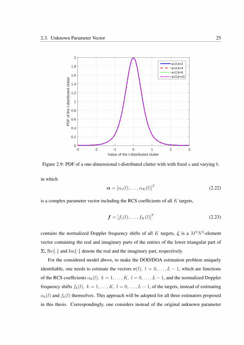
a and varying b. Figs. 2.8 and 2.9 shows the PDF of a one-dimensional t-distributed clutter
(also with the clutter power fixed to be 1) with its texture parameters a and b varying in
parallel to Figs. 2.6 and 2.7, respectively. One can see from Figs. 2.6 and 2.7 that the inverse
gamma-distributed texture becomes more heavy-tailed, either when the shape parameter a
decreases or when the scale parameter b increases. On the other hand, the t-distributed clutter
as a whole, with fixed clutter power, becomes more heavy-tailed when a increases, but does
not change its distribution with the change of b (cf. Figs. 2.8 and 2.9), similar to the K-
distributed clutter in this respect.
0 2 4 6 8 10 12 14 16 18 20
Value of the inverse-gamma-distributed texture
0
0.2
0.4
0.6
0.8
1
1.2
1.4
PD
F o
f the
inve
rse-
gam
ma-
dist
ribut
ed te
xtur
e a=2,b=10a=4,b=10a=6,b=10a=10,b=10
Figure 2.6: PDF of a inverse-gamma-distributed texture with with fixed b and varying a.
2.3 Unknown Parameter Vector
Under the assumptions above, the unknown parameter vector of the problem in question is
given by:
χ =[θT ,Re αT , Im αT ,fT , ζT , a, b
]T, (2.21)
24 Chapter 2. MIMO Radar Model Setup
0 2 4 6 8 10 12 14 16 18 20
Value of the inverse-gamma-distributed texture
0
0.1
0.2
0.3
0.4
0.5
0.6
0.7
PD
F o
f the
inve
rse-
gam
ma-
dist
ribut
ed te
xtur
e a=2,b=2a=2,b=4a=2,b=6a=2,b=10
Figure 2.7: PDF of a inverse-gamma-distributed texture with with fixed a and varying b.
-3 -2 -1 0 1 2 3
Value of the t-distributed clutter
0
0.2
0.4
0.6
0.8
1
1.2
1.4
1.6
1.8
2
PD
F o
f the
t-di
strib
uted
clu
tter
a=2,b=10a=4,b=10a=6,b=10a=10,b=10
Figure 2.8: PDF of a one-dimensional t-distributed clutter with with fixed b and varying a.
2.3. Unknown Parameter Vector 25
-3 -2 -1 0 1 2 3
Value of the t-distributed clutter
0
0.2
0.4
0.6
0.8
1
1.2
1.4
1.6
1.8
2
PD
F o
f the
t-di
strib
uted
clu
tter
a=2,b=2a=2,b=4a=2,b=6a=2,b=10
Figure 2.9: PDF of a one-dimensional t-distributed clutter with with fixed a and varying b.
in which
α = [α1(l), . . . , αK(l)]T (2.22)
is a complex parameter vector including the RCS coefficients of all K targets,
f = [f1(l), . . . , fK(l)]T (2.23)
contains the normalized Doppler frequency shifts of all K targets, ζ is a M2N2-element
vector containing the real and imaginary parts of the entries of the lower triangular part of
Σ, Re· and Im· denote the real and the imaginary part, respectively.
For the considered model above, to make the DOD/DOA estimation problem uniquely
identifiable, one needs to estimate the vectors v(l), l = 0, . . . , L − 1, which are functions
of the RCS coefficients αk(l), k = 1, . . . , K, l = 0, . . . , L− 1, and the normalized Doppler
frequency shifts fk(l), k = 1, . . . , K, l = 0, . . . , L− 1, of the targets, instead of estimating
αk(l) and fk(l) themselves. This approach will be adopted for all three estimators proposed
in this thesis. Correspondingly, one considers instead of the original unknown parameter

26 Chapter 2. MIMO Radar Model Setup
vector χ in Eq. (2.21), the transformed new unknown parameter vector:
ξ =[θT ,vT , ζT , a, b
]T, (2.24)
in which the 2KL× 1 vector
v =[Re v(0)T , Im v(0)T , . . . ,Re v(L− 1)T , Im v(L− 1)T
]T, (2.25)
is a parameter vector containing the real and imaginary parts of v(l) at all L pulses.
2.4 Likelihood Functions
Let
z =[zT (0), ...,zT (L− 1)
]T(2.26)
denote the full observation vector after matched filtering, further let
τ = [τ(0), . . . , τ(L− 1)]T (2.27)
represent the vector containing the texture realizations at all L pulses. Accordingly, the full
observation conditional likelihood (conditioned on τ ) can be written as:
p (z |τ ;ψ ) =L−1∏l=0
1
|πΣ| τMN(l)exp
(−‖ρ(l)‖2
τ(l)
); (2.28)
in which
ψ =[θT ,vT , ζT
]T(2.29)
is the unknown parameter vector that does not contain the texture parameters a and b, ‖·‖
denotes the Euclidean norm, and
ρ(l) = Σ−12 (z(l)−A (θ)v(l)) , (2.30)
2.4. Likelihood Functions 27
represents the clutter realization at the lth pulse with its speckle spatially whitened by the
square root of the speckle CM inverse.
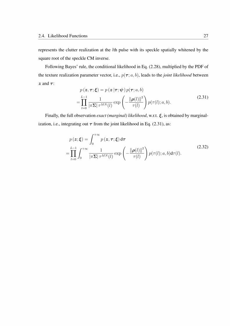
Following Bayes’ rule, the conditional likelihood in Eq. (2.28), multiplied by the PDF of
the texture realization parameter vector, i.e., p(τ ; a, b), leads to the joint likelihood between
z and τ :p (z, τ ; ξ) = p (z |τ ;ψ ) p(τ ; a, b)
=L−1∏l=0
1
|πΣ| τMN(l)exp
(−‖ρ(l)‖2
τ(l)
)p(τ(l); a, b).
(2.31)
Finally, the full observation exact (marginal) likelihood, w.r.t. ξ, is obtained by marginal-
ization, i.e., integrating out τ from the joint likelihood in Eq. (2.31), as:
p (z; ξ) =
∫ +∞
0
p (z, τ ; ξ) dτ
=L−1∏l=0
∫ +∞
0
1
|πΣ| τMN(l)exp
(−‖ρ(l)‖2
τ(l)
)p(τ(l); a, b)dτ(l).
(2.32)

28 Chapter 2. MIMO Radar Model Setup
Chapter 3
Iterative Maximum Likelihood DOD and
DOA Estimation
The marginal LF in Eq. (2.32) has an integral form and is mathematically difficult to handle.
To avoid maximizing the intractable Eq. (2.32), various estimation procedures in the SIRP
context have either proposed to use the joint LF in Eq. (2.31) [98] as a tool to achieve the
maximization of the marginal LF, or to maximize the conditional LF in Eq. (2.28) [119].
The latter approach treats τ as deterministic, i.e., as one realization from the texture process
rather than the process itself. Correspondingly, it takes this realization τ as one of its un-
known parameters to be estimated, while ignores the statistical distribution of the texture as
characterized by the texture parameters a and b. In deriving the proposed IMLE, this idea is
adopted and the usage of the term “ML” is with regard to this kind of deterministic texture
modeling.
Let ΛC denote the conditional log-likelihood function (LLF), which arises from Eq. (2.28),
as:ΛC = ln p (z |τ ;ψ )
=− LMN lnπ − L ln |Σ|
−MN
L−1∑l=0
ln τ(l)−L−1∑l=0
1
τ(l)ρH(l)ρ(l).
(3.1)
29

30 Chapter 3. Iterative Maximum Likelihood DOD and DOA Estimation
3.1 Estimates of the Unknown Parameters
To begin with, let ∂ΛC/∂τ(l) = 0, the solution of which provides an estimate of the param-
eter τ(l) when the parameters θ, v(l) and Σ are fixed. Using (·) to denote the estimate of a
parameter, τ(l) has the following closed-form expression:
τ(l) =1
MNρH(l)ρ(l)
=1
MNnH(l)Σ−1n(l),
(3.2)
in which the clutter vector at the lth pulse n(l) has, according to Eq. (2.7), the following
expression:
n(l) = z(l)−A (θ)v(l). (3.3)
Note that the expression of τ(l) in Eq. (3.2) is unique if the matrix Σ is invertible, i.e., if the
number of pulses per CPI L ≥MN .
On the other hand, the estimate of Σ, when θ, v(l) and τ(l) are fixed, can be found by
applying Lemma 3.2.2. in [120] to Eq. (3.1), as:
Σ =1
L
L−1∑l=0
1
τ(l)n(l)nH(l), (3.4)
which is unique, and in which replacing τ(l) by the expression of τ(t) in Eq. (3.2) leads to
the following expression of Σ:
Σ =MN
L
L−1∑l=0
n(l)nH(l)
nH(l)Σ−1n(l). (3.5)
One can calculate Eq. (3.5) iteratively by transforming it into:
Σ(i+1) =MN
L
L−1∑l=0
n(l)nH(l)
nH(l)(Σ(i)
)−1
n(l), (3.6)
in which (·)(i)
(i ≥ 0, and i ∈ Z) stands for the estimate of a parameter at the ith iteration,
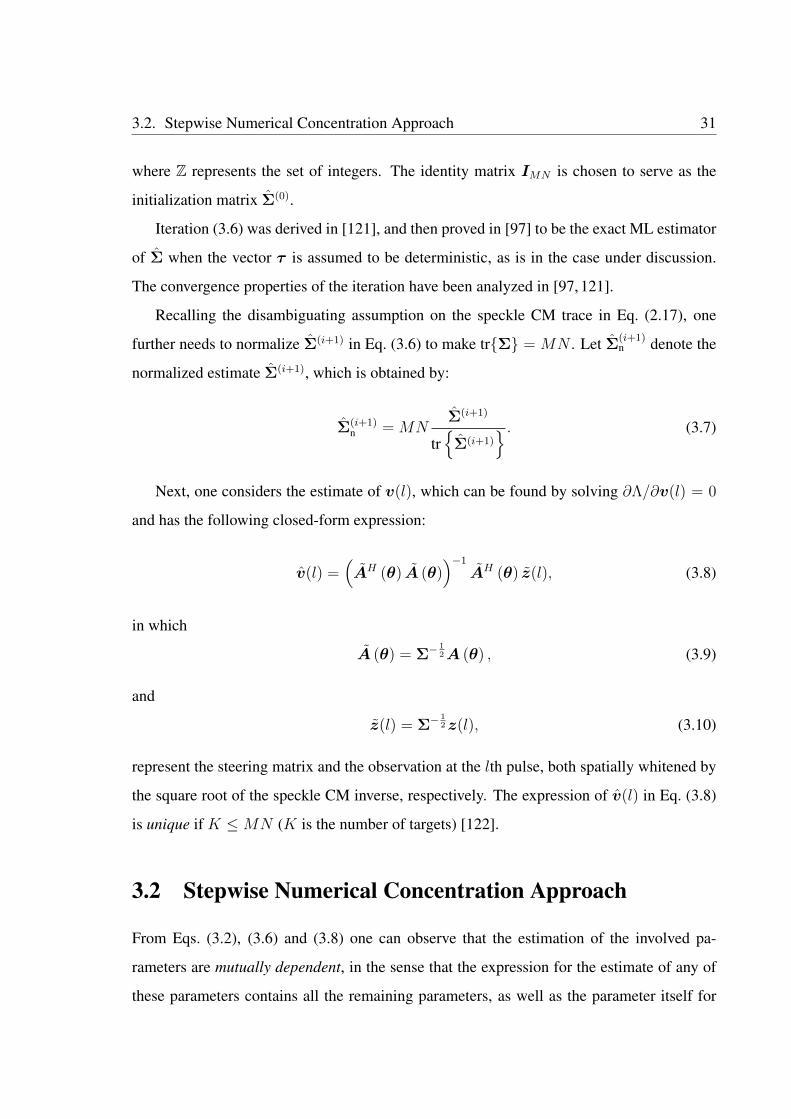
3.2. Stepwise Numerical Concentration Approach 31
where Z represents the set of integers. The identity matrix IMN is chosen to serve as the
initialization matrix Σ(0).
Iteration (3.6) was derived in [121], and then proved in [97] to be the exact ML estimator
of Σ when the vector τ is assumed to be deterministic, as is in the case under discussion.
The convergence properties of the iteration have been analyzed in [97, 121].
Recalling the disambiguating assumption on the speckle CM trace in Eq. (2.17), one
further needs to normalize Σ(i+1) in Eq. (3.6) to make trΣ = MN . Let Σ(i+1)n denote the
normalized estimate Σ(i+1), which is obtained by:
Σ(i+1)n = MN
Σ(i+1)
tr
Σ(i+1) . (3.7)
Next, one considers the estimate of v(l), which can be found by solving ∂Λ/∂v(l) = 0
and has the following closed-form expression:
v(l) =(AH (θ) A (θ)
)−1
AH (θ) z(l), (3.8)
in which
A (θ) = Σ−12A (θ) , (3.9)
and
z(l) = Σ−12z(l), (3.10)
represent the steering matrix and the observation at the lth pulse, both spatially whitened by
the square root of the speckle CM inverse, respectively. The expression of v(l) in Eq. (3.8)
is unique if K ≤MN (K is the number of targets) [122].
3.2 Stepwise Numerical Concentration Approach
From Eqs. (3.2), (3.6) and (3.8) one can observe that the estimation of the involved pa-
rameters are mutually dependent, in the sense that the expression for the estimate of any of
these parameters contains all the remaining parameters, as well as the parameter itself for
32 Chapter 3. Iterative Maximum Likelihood DOD and DOA Estimation
the case of Σ (cf. Eq. (3.5)). In [98] and [101], the authors overcame the similar difficulty
by exploiting the special structure of their GMANOVA model and obtained an expression
of Σ independent of their unknown signal parameters. However, such analytical concentra-
tion approach is inapplicable to the estimation problem under consideration. Therefore, the
estimation algorithms proposed in this thesis adopts the so-called stepwise numerical con-
centration method, of which the concept was introduced and employed, in the context of
nonuniform white Gaussian noise in [106], and of colored Gaussian noise in [123].
The idea of the stepwise concentration consists in the concentration of the LLF w.r.t.
certain unknown parameters in an iterative manner. For the problem under discussion, the
proposed procedure is to assume, for each iteration, that Σ and τ are fixed and known, and to
use their values to compute the estimate of v(l), which is then used, in its turn, to update the
values of Σ and τ for the next iteration. This sequential updating procedure is then continued
until convergence of the parameters of interest, which can be defined, e.g., by the criterion
that the difference between the values of estimates obtained from consecutive iterations falls
below a certain predefined small threshold.
This general procedure borne in mind, one finally returns to the LLF in Eq. (3.1) for the
estimation of θ, the parameter of interest in the problem under discussion, by considering the
values of Σ and τ as fixed and known estimates obtained from the previous iteration. Thus,
by neglecting the constant terms, the conditional LLF in Eq. (3.1) can be reformulated as:
ΛC = −L−1∑l=0
1
τ(l)ρH(l)ρ(l). (3.11)
By inserting Eq. (3.8) into Eq. (3.11) and maximizing the resulting expression w.r.t. θ,
one obtains the estimate of θ for each iteration, as:
θ = arg minθ
L−1∑l=0
1
τ(l)
∥∥∥P⊥A(θ)(t)z(l)
∥∥∥2, (3.12)
in which arg minθf (θ) denotes the value of θ that minimizes f (θ) (a function of θ), and
P⊥A(θ)
= IMN − A(θ)(AH(θ)A(θ)
)−1
AH(θ) (3.13)

3.3. Algorithmic Procedure 33
is the orthogonal projection matrix onto the null space spanned by the columns of the matrix
A(θ). Here, one makes the assumption regarding Eq. (3.12) that it is a unique optimum,
which for the array Khatri-Rao of Vandermonde manifold structure in Eq. (2.12) holds true
almost surely if K ≤MN [122].
3.3 Algorithmic Procedure
The whole procedure of the proposed IMLE, consisting of iterations between two steps, is
summarized in Alg. 3.1. Note that at the initialization step of the IMLE, the texture realiza-
tions are initialized as all ones, corresponding to a Gaussian-distributed clutter.
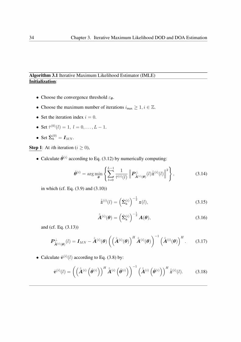
34 Chapter 3. Iterative Maximum Likelihood DOD and DOA Estimation
Algorithm 3.1 Iterative Maximum Likelihood Estimator (IMLE)Initialization:
• Choose the convergence threshold εθ.
• Choose the maximum number of iterations imax ≥ 1, i ∈ Z.
• Set the iteration index i = 0.
• Set τ (0)(l) = 1, l = 0, . . . , L− 1.
• Set Σ(0)n = IMN .
Step 1: At ith iteration (i ≥ 0),
• Calculate θ(i) according to Eq. (3.12) by numerically computing:
θ(i) = arg minθ
L−1∑l=0
1
τ (i)(l)
∥∥∥P⊥ˆA(i)(θ)(l)ˆz(i)(l)
∥∥∥2, (3.14)
in which (cf. Eq. (3.9) and (3.10))
ˆz(i)(l) =(Σ(i)
n
)− 12z(l), (3.15)
ˆA(i)(θ) =(Σ(i)
n
)− 12A(θ), (3.16)
and (cf. Eq. (3.13))
P⊥ˆA(i)(θ)(l) = IMN − ˆA(i)(θ)
((ˆA(i)(θ)
)H ˆA(i)(θ)
)−1 (ˆA(i)(θ)
)H. (3.17)
• Calculate v(i)(l) according to Eq. (3.8) by:
v(i)(l) =
((ˆA(i)
(θ(i)))H ˆA(i)
(θ(i)))−1 (
ˆA(i)(θ(i)))H
ˆz(i)(l). (3.18)
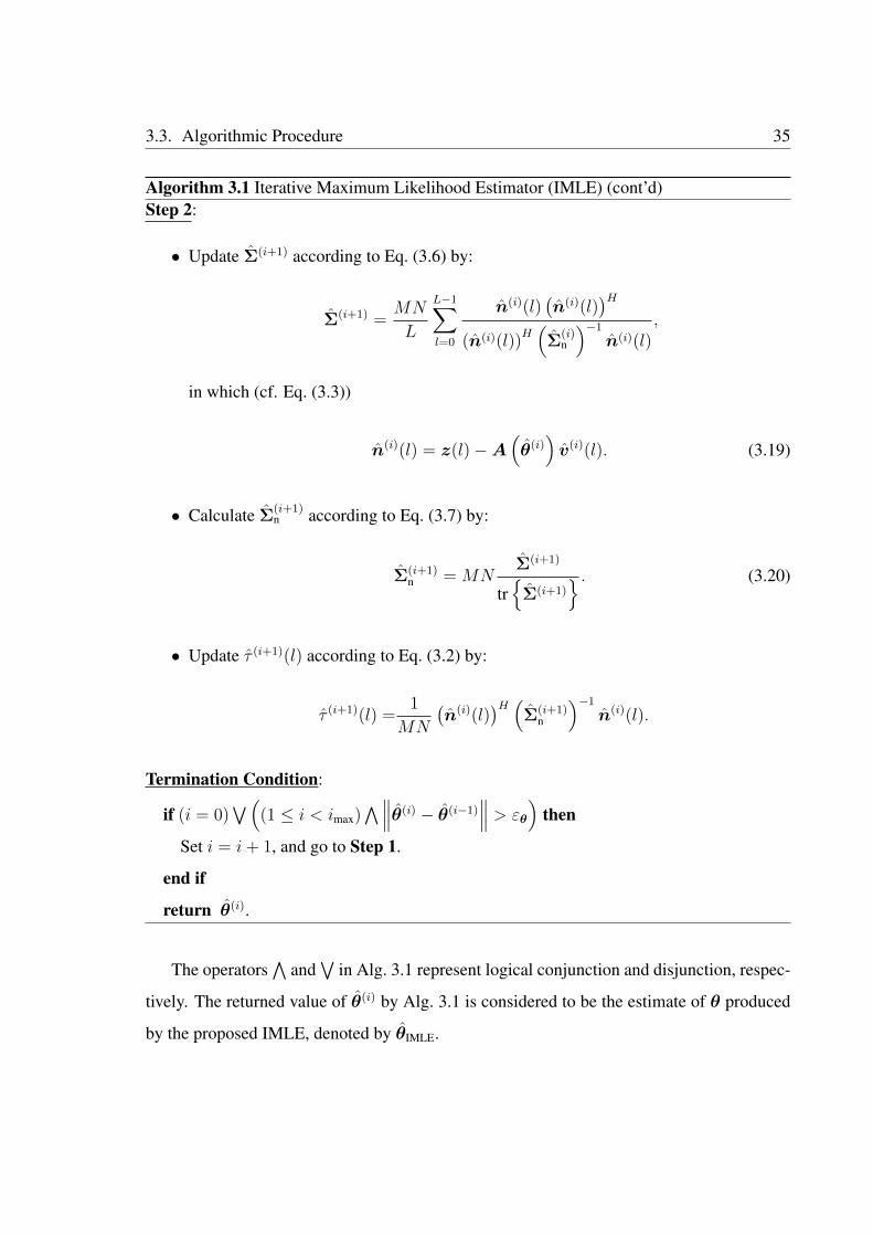
3.3. Algorithmic Procedure 35
Algorithm 3.1 Iterative Maximum Likelihood Estimator (IMLE) (cont’d)Step 2:
• Update Σ(i+1) according to Eq. (3.6) by:
Σ(i+1) =MN
L
L−1∑l=0
n(i)(l)(n(i)(l)
)H(n(i)(l))
H(Σ
(i)n
)−1
n(i)(l),
in which (cf. Eq. (3.3))
n(i)(l) = z(l)−A(θ(i))v(i)(l). (3.19)
• Calculate Σ(i+1)n according to Eq. (3.7) by:
Σ(i+1)n = MN
Σ(i+1)
tr
Σ(i+1) . (3.20)
• Update τ (i+1)(l) according to Eq. (3.2) by:
τ (i+1)(l) =1
MN
(n(i)(l)
)H (Σ(i+1)
n
)−1
n(i)(l).
Termination Condition:
if (i = 0)∨(
(1 ≤ i < imax)∧∥∥∥θ(i) − θ(i−1)
∥∥∥ > εθ
)then
Set i = i+ 1, and go to Step 1.
end if
return θ(i).
The operators∧
and∨
in Alg. 3.1 represent logical conjunction and disjunction, respec-
tively. The returned value of θ(i) by Alg. 3.1 is considered to be the estimate of θ produced
by the proposed IMLE, denoted by θIMLE.
36 Chapter 3. Iterative Maximum Likelihood DOD and DOA Estimation
3.4 Performance Analysis
3.4.1 Convergence and Computational Cost
The proposed IMLE algorithm can be viewed as an application of the block coordinate de-
scent (BCD) method [124, 125]. According to Proposition 2.7.1 (together with the text after
its proof) in [125], the BCD method converges to a stationary point (namely, a Karush–Kuhn–Tucker
(KKT) point) if:
i) The objective function is continuously differentiable;
ii) The constraint set of the parameters is compact;
iii) The function of the ith block-component attains a unique minimum over the constraint
set.
The first two conditions above hold true for the case of the proposed IMLE; so does the
third, under the mild conditions specified respectively below Eqs. (3.2), (3.4), (3.8) and
(3.12) to guarantee the uniqueness of the involved parameter estimates. The convergence of
the proposed IMLE algorithm to a stationary point is thus proved. In fact, as simulations
in Ch. 8 will show, the convergence of the estimate of the unknown parameter θ can be
observed, and is generally attainable with as few as two iterations, a result in accordance
with those in [106] and [123].
Based on the observation above, one can conclude that the computational cost of the pro-
posed IMLE, which lies mainly in the numerical solution of the highly nonlinear optimiza-
tion problem in Eq. (3.14), is only a few times of that of the CMLE. The latter corresponds
to the case where the clutter is assumed to be uniform white Gaussian, such that Eq. (3.12)
degenerate into [35]:
θCMLE = arg minθ
L−1∑l=0
∥∥P⊥A(θ)z(l)∥∥2
. (3.21)
3.4. Performance Analysis 37
3.4.2 Invariance of the IMLE to Different Speckle CM Trace Assump-
tions
To deal with the ambiguity arising from the scaling effect between the texture and the speckle
in the clutter model Eq. (2.15), an assumption has to be made about the value of the speckle
CM trace. In Eq. (2.17) it has been assumed that trΣ = MN . The proposed IMLE
algorithm, however, is invariant to the different choice of values for the assumed speckle
CM trace, as will be demonstrated in this subsection.
Let trΣa stand for an alternatively assumed trace value for the speckle CM other than
the one in Eq. (2.17), and in introduce a variable:
r =trΣa
trΣ, (3.22)
which represents the ratio between the alternatively and the originally (i.e., the one made in
Eq. (2.17)) assumed speckle CM trace. Consider the case that
r 6= 1. (3.23)
Further, let (·)′
denote the “counterpart” of a parameter resulting from this alternative
assumption on the speckle CM trace value. It then follows that:
Σ′ = rΣ, (3.24)
based on which one has from the speckle covariance expression in Eq. (2.16) that:
x′(l) =√rx(l), l = 0, . . . , L− 1, (3.25)
and accordingly, from Eq. (2.15), that:
τ ′(l) =1
rτ(l), l = 0, . . . , L− 1, (3.26)
38 Chapter 3. Iterative Maximum Likelihood DOD and DOA Estimation
such that: √τ ′(l)x′(l) =
√τ(l)x(l), l = 0, . . . , L− 1. (3.27)
Alternatively, Eq. (3.26) can be obtained by inserting Eq. (3.24) into Eq. (3.2).
Moreover, by inserting Eq. (3.24) into Eq. (2.30) one has:
ρ′(l) =1√rρ(l), l = 0, . . . , L− 1. (3.28)
Finally, by noticing that the objective function in Eq. (3.12) is in essence the search for
θ by:
θ = arg minθ
L−1∑l=0
1
τ(l)ρH(l)ρ(l)
, (3.29)
and by substituting Eqs. (3.26) and (3.28) into Eq. (3.29), one obtains:
θ′ = arg minθ
L−1∑l=0
1
τ ′(l)ρ′H(l)ρ′(l)
= arg minθ
L−1∑l=0
1
τ(l)ρH(l)ρ(l)
= θ,
(3.30)
which means that, for the IMLE, the estimate of the parameter θ under the alternative as-
sumption of trΣ is equal to that under the original assumption, i.e., that the value of θ
is independent of the assumed value of trΣ. One can thus conclude that the IMLE is
invariant to different speckle CM trace assumptions.
Chapter 4
Iterative Maximum A Posteriori DOD
and DOA Estimation
The IMLE proposed above, in which one models the texture as deterministic, has the advan-
tage of easier and faster implementation. It is also a natural approach when the texture does
not have a closed-form expression of distribution (e.g., in the case of Weibull clutter) or its
distribution is unknown. In general cases, however, such approach is suboptimal not only in
the sense that it is not based on the exact (marginal) likelihood, but that it ignores informa-
tion regarding the statistical properties (prior distribution) of the texture. As mentioned at
the beginning of Sec. 3, another way to avoid the mathematical complexity in maximizing
the marginal likelihood in Eq. (2.32) is to maximize the joint likelihood Eq. (2.31) instead.
This is, for instance, the approach adopted in [98], where the proposed PX-EM algorithm is
based on a “complete data likelihood" that is equivalent to the joint likelihood. Estimators
based on the joint likelihood are in essence MAP estimators, as can be readily seen from:
τMAP = arg maxτ
p (τ |z; ξ )
= arg maxτ
p (z |τ ;ψ ) p(τ ; a, b)
p (z; ξ)
= arg maxτ
p (z, τ ; ξ) ,
(4.1)
in which τMAP denotes the MAP estimate of τ .
39
40 Chapter 4. Iterative Maximum A Posteriori DOD and DOA Estimation
For this reason, the second estimator to be proposed in this chapter, which is based on the
joint likelihood and also employs a numerical concentration approach, is justifiably called
the IMAPE. By modeling the texture as stochastic and exploiting the its prior distribution,
the IMAPE, of which the derivation is presented below, leads to superior performance over
the IMLE.
4.1 Estimates of the Unknown Parameters
Let ΛJ denote the joint LLF, which is equal to:
ΛJ = ln p (z, τ ; ξ) = ln (p (z |τ ;ψ ) p(τ ; a, b))
= ΛC +L−1∑l=0
ln p(τ(l); a, b)
=
ΛC − L ln Γ(a)− La ln b+ (a− 1)L−1∑l=0
ln τ(l)
−∑L−1
l=0 τ(l)
b, K-distributed clutter,
ΛC − L ln Γ(a) + La ln b− (a+ 1)L−1∑l=0
ln τ(l)
− bL−1∑l=0
1
τ(l), Student’s t-distributed clutter.
(4.2)
The expression of τ(l), when all the remaining unknown parameters are fixed, can be
found by solving ∂ΛJ/∂τ(l) = 0, as:
τ(l) =
1
2
((a−MN − 1) b+
√(a−MN − 1)2 b2 + 4bnH(l)Σ−1n(l)
),
K-distributed clutter,
nH(l)Σ−1n(l) + b
a+MN + 1, Student’s t-distributed clutter,
(4.3)
in which n(l) has the same expression as in Eq. (3.3). The expression of τ(l) in Eq. (4.3), in
agreement with that in Eq. (3.2) for the IMLE, is unique if the matrix Σ is invertible, i.e., if
4.1. Estimates of the Unknown Parameters 41
the number of pulses per CPI L ≥MN .
A comparison between the expressions of τ(l) in Eq. (3.2) and in Eq. (4.3) reveals that
the latter takes into account the statistical properties of the texture. In these expressions, the
parameters a and b play the roles of scale/translation factors to enhance the estimation of
τ(l). This is more easily perceptible in the case of a Student’s t-distributed clutter, where the
expressions for τ(l) in Eq. (3.2) and (4.3) have a similar form. For example, the case of large
b and small a corresponds to a more heavily-tailed distribution of the texture and leads to an
increased probability of the realization of τ(l) with large values. In this case, the estimator
in Eq. (4.3), in contrast to that in Eq. (3.2), adjusts τ(l) in a way that prevents the occurrence
of small values and encourages that of larger ones.
For the next step, one considers the estimates of the texture parameters a and b. The latter
can be obtained by solving ∂ΛJ/∂b = 0, as:
b =
∑L−1
l=0 τ(l)
La, K-distributed clutter,
La∑L−1l=0
1τ(l)
, Student’s t-distributed clutter,(4.4)
which is unique for both clutter distributions.
On the other hand, calculating ∂ΛJ/∂a yields:
∂ΛJ
∂a=
− LΨ(a)− L ln b+
L−1∑l=0
ln τ(l), K-distributed clutter,
− LΨ(a) + L ln b−L−1∑l=0
ln τ(l), Student’s t-distributed clutter,
(4.5)
in which Ψ(·) stands for the digamma function, defined as the logarithmic derivative of the
gamma function in Eq. (2.19), namely:
Ψ(a) =d
daln Γ(a). (4.6)
From Eq. (4.5) it turns out that ∂ΛJ/∂a = 0 does not allow an analytical expression of
42 Chapter 4. Iterative Maximum A Posteriori DOD and DOA Estimation
the root. By inserting Eq. (4.4) into Eq. (4.5), one obtains:
∂ΛJ
∂a=
− LΨ(a)− L ln
(∑L−1l=0 τ(l)
La
)+
L−1∑l=0
ln τ(l),
K-distributed clutter,
− LΨ(a) + L ln
(La∑L−1l=0
1τ(l)
)−
L−1∑l=0
ln τ(l),
Student’s t-distributed clutter.
(4.7)
Thus the expression of a can be found by numerically solving Eq. (4.7). As will be demon-
strated below in Sec. 4.2, this expression of a is also unique.
Next, it is to approach the estimation of the parameters v(l) and the speckle CM Σ. By
noticing that ∂ΛJ/∂Σ = ∂ΛC/∂Σ, and ∂ΛJ/∂v(l) = ∂ΛC/∂v(l), it follows immediately
that the same expressions of Σ and v(l) in Eqs. (3.4) and (3.8), which were obtained for
the IMLE algorithm, are also valid in the case of the IMAPE algorithm. Substituting into
Eq. (3.4) the new expression of τ(l) in Eq. (4.3) and interpreting the resulting equation also
in an iterative form leads to the following expression for Σ:
Σ(i+1) =
2
L
L−1∑l=0
n(l)nH(l)
/((a−MN − 1) b
+
(4bnH(l)
(Σ(i)
)−1
n(l) + (a−MN − 1)2 b2
) 12
),
K-distributed clutter,
a+MN + 1
L
L−1∑l=0
n(l)nH(l)
b+ nH(l)(Σ(i)
)−1
n(l),
Student’s t-distributed clutter.
(4.8)
for which the initialization matrix is also chosen to be Σ(0) = IMN . Similar to the expression
of Σ(i+1) in Eq. (3.6) for the IMLE algorithm, Eq. (4.8) needs also to be substituted into
Eq. (3.7) to obtain the normalized estimate of the CM, Σ(i+1)n , to fulfill the assumption on
the CM trace made in Eq. (2.17).
4.2. Existence and Uniqueness of the Solution for the Shape Parameter 43
Finally, one addresses the estimation of θ. By adopting the numerical concentration
method similar to that in Sec. 3.2, one also assumes here that Σ and τ are known from the
previous iteration of the algorithm. Their values are then used to compute the estimate of
v(l) (like for the IMLE), and of, distinctively for the IMAPE, a and b. These estimates are
then jointly used, in their turn, to update the values of Σ and τ for the next iteration.
Since the estimates of a and b are only dependent on τ , these are also fixed for each
iteration. This allows one to drop those terms in the expression of the joint LLF ΛJ in
Eq. (4.2) that contain only these unknown parameters, and thereby to transform it into the
same expression as in Eq. (3.11). This means that θ can be obtained, also for the IMAPE
algorithm, from Eq. (3.12).
4.2 Existence and Uniqueness of the Solution for the Shape
Parameter
In contrast to the IMLE proposed in Ch. 3, the IMAPE models the texture as stochastic and
therefore needs to estimate the shape parameter a (by Eq. (4.5)) and the scale parameter b (by
Eq. (4.4)) of the texture distribution. As mentioned below Eq. (4.5), the estimate of a does
not allow an analytic expression, but can only be numerically found by solving the equation
∂ΛJ/∂a = 0. A theoretical proof of the existence of its unique solution is thus of concern to
ensure the validity and feasibility of the proposed algorithm, which is the aim of this section.
4.2.1 K-Distributed Clutter Case
One first considers the case of K-distributed clutter, for which Eq. (4.7) can be transformed,
by replacing Ψ(a) by the full series of its asymptotic series expansion:
Ψ(a) = ln(a)− 1
2a−∞∑n=1
B2n
2na2n, (4.9)
44 Chapter 4. Iterative Maximum A Posteriori DOD and DOA Estimation
where B2n denotes the 2nth Bernoulli number, into:
∂ΛJ
∂a= L
1
2a+∞∑n=1
B2n
2na2n+ ln
L∑L−1l=0 τ(l)
L
√√√√L−1∏l=0
τ(l)
. (4.10)
From the expression of Eq. (4.10), it follows readily that:
lima→0+
∂ΛJ
∂a= +∞,
lima→+∞
∂ΛJ
∂a= ln
L∑L−1l=0 τ(l)
L
√√√√L−1∏l=0
τ(l)
≤ ln(1) = 0.
(4.11)
The second to last step in the expression above is obtained by applying the inequality of
arithmetic and geometric means, which states that:
∑L−1l=0 τ(l)
L≥ L
√√√√L−1∏l=0
τ(l), (4.12)
where the equality holds only in the extreme case where
τ(0) = τ(1) = · · · = τ(L− 1), (4.13)
which corresponds to the Gaussian clutter case. For the K-distributed clutter under discus-
sion, this is a zero probability occurrence and thus is trivial in reality.
Furthermore, one can also see from Eq. (4.10) that ∂ΛJ/∂a is a continuous, strictly de-
creasing function of a in the interval (0,+∞), meaning that there exists exactly one value
of a in the interval (0,+∞) that leads to ∂Λ/∂a = 0, which corresponds to the global
maximum point of ΛJ w.r.t. a in the K-distributed clutter case.
4.3. Algorithmic Procedure 45
4.2.2 Student’s t-Distributed Clutter Case
Similarly, when the clutter follows a Student’s t-distribution, substituting Eqs. (4.4) and
Eq. (4.9) into Eq. (4.5) yields:
∂ΛJ
∂a= L
1
2a+∞∑n=1
B2n
2na2n+ ln
L∑L−1l=0
1τ(l)
L
√∏L−1l=0 τ(l)
, (4.14)
which is also a continuous, strictly decreasing function of a in the interval (0,+∞).
Applying the inequality of harmonic and geometric means:
L∑L−1l=0
1τ(l)
≤ L
√√√√L−1∏l=0
τ(l), (4.15)
to Eq. (4.14), one further has:
lima→0+
∂ΛJ
∂a= +∞,
lima→+∞
∂ΛJ
∂a= ln
L∑L−1l=0
1τ(l)
L
√∏L−1l=0 τ(l)
≤ ln(1) = 0,(4.16)
where, similarly, the equality in the second line holds only in the trivial case of Eq. (4.13).
Thus, one can conclude that, for Student’s t-distributed clutter, there also exists exactly
one root of the equation ∂Λ/∂a = 0 w.r.t. a in the interval (0,+∞), which corresponds to
the global maximum point of ΛJ w.r.t. a in this case.
4.3 Algorithmic Procedure
The whole procedure of the proposed IMAPE, which also consists of iterations between two
steps, is presented in Alg. 4.1. Note that the initialization of the IMAPE does not imply any
prior on the texture parameters. Like the IMLE in Alg. 3.1, the IMAPE also initializes the
clutter as Gaussian-distributed (with all texture realizations equal to one). Furthermore, at the
first iteration (when the iteration index i = 0), the IMAPE carries out the same estimation

46 Chapter 4. Iterative Maximum A Posteriori DOD and DOA Estimation
procedure as the IMLE in Alg. 3.1. Then, based on the obtained estimates from the first
iteration, the texture parameters are estimated according to Eqs. (4.7) and (4.4), and are used
for the estimation of Σ and τ(l) (according to Eqs. (4.8) and (4.3), respectively) for the
second iteration.
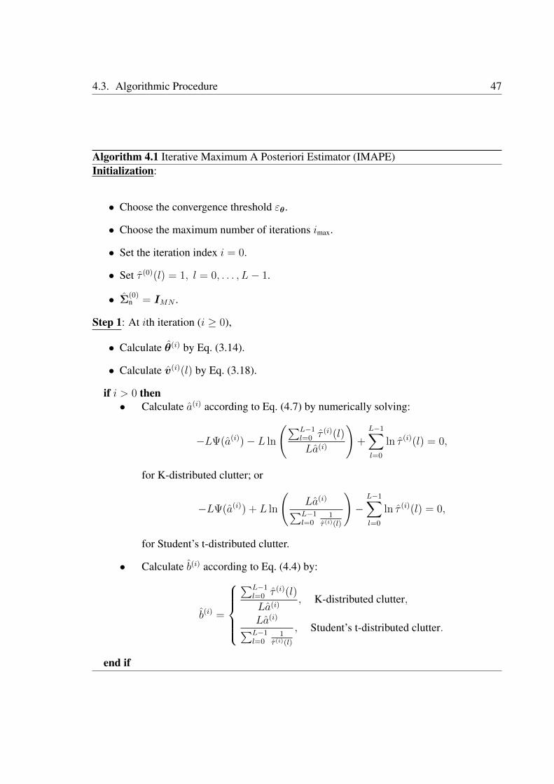
4.3. Algorithmic Procedure 47
Algorithm 4.1 Iterative Maximum A Posteriori Estimator (IMAPE)Initialization:
• Choose the convergence threshold εθ.
• Choose the maximum number of iterations imax.
• Set the iteration index i = 0.
• Set τ (0)(l) = 1, l = 0, . . . , L− 1.
• Σ(0)n = IMN .
Step 1: At ith iteration (i ≥ 0),
• Calculate θ(i) by Eq. (3.14).
• Calculate v(i)(l) by Eq. (3.18).
if i > 0 then• Calculate a(i) according to Eq. (4.7) by numerically solving:
−LΨ(a(i))− L ln
(∑L−1l=0 τ
(i)(l)
La(i)
)+
L−1∑l=0
ln τ (i)(l) = 0,
for K-distributed clutter; or
−LΨ(a(i)) + L ln
(La(i)∑L−1l=0
1τ (i)(l)
)−
L−1∑l=0
ln τ (i)(l) = 0,
for Student’s t-distributed clutter.
• Calculate b(i) according to Eq. (4.4) by:
b(i) =
∑L−1
l=0 τ(i)(l)
La(i), K-distributed clutter,
La(i)∑L−1l=0
1τ (i)(l)
, Student’s t-distributed clutter.
end if
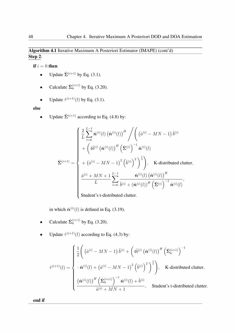
48 Chapter 4. Iterative Maximum A Posteriori DOD and DOA Estimation
Algorithm 4.1 Iterative Maximum A Posteriori Estimator (IMAPE) (cont’d)Step 2:
if i = 0 then
• Update Σ(i+1) by Eq. (3.1).
• Calculate Σ(i+1)n by Eq. (3.20).
• Update τ (i+1)(l) by Eq. (3.1).
else
• Update Σ(i+1) according to Eq. (4.8) by:
Σ(i+1) =
2
L
L−1∑l=0
n(i)(l)(n(i)(l)
)H /((a(i) −MN − 1
)b(i)
+
(4b(i)
(n(i)(l)
)H (Σ(i)
)−1
n(i)(l)
+(a(i) −MN − 1
)2(b(i))2) 1
2
), K-distributed clutter,
a(i) +MN + 1
L
L−1∑l=0
n(i)(l)(n(i)(l)
)Hb(i) + (n(i)(l))
H(Σ(i)
)−1
n(i)(l),
Student’s t-distributed clutter.
in which n(i)(l) is defined in Eq. (3.19).
• Calculate Σ(i+1)n by Eq. (3.20).
• Update τ (i+1)(l) according to Eq. (4.3) by:
τ (i+1)(l) =
1
2
((a(i) −MN − 1
)b(i) +
(4b(i)
(n(i)(l)
)H (Σ(i+1)
n
)−1
· n(i)(l) +(a(i) −MN − 1
)2(b(i))2) 1
2
), K-distributed clutter,
(n(i)(l)
)H (Σ
(i+1)n
)−1
n(i)(l) + b(i)
a(i) +MN + 1, Student’s t-distributed clutter.
end if
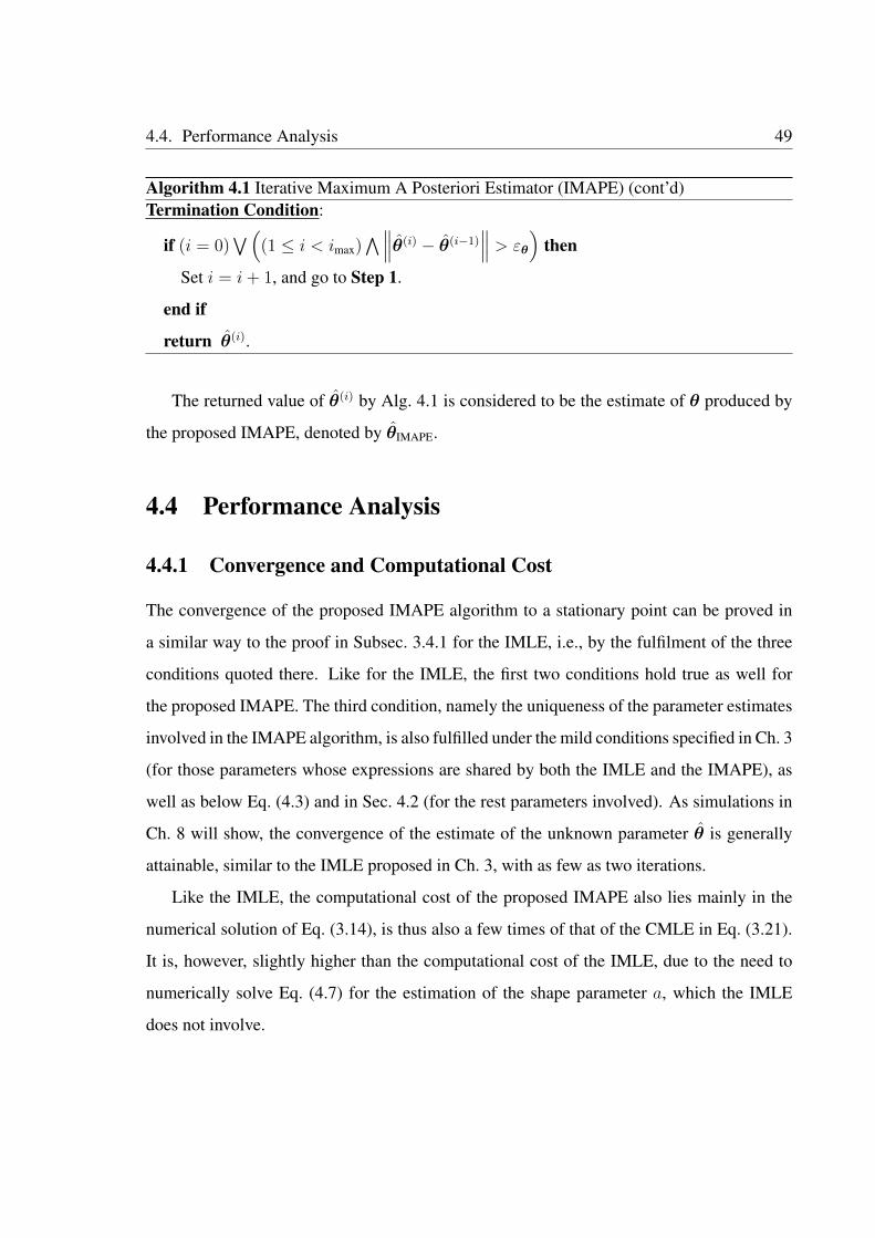
4.4. Performance Analysis 49
Algorithm 4.1 Iterative Maximum A Posteriori Estimator (IMAPE) (cont’d)Termination Condition:
if (i = 0)∨(
(1 ≤ i < imax)∧∥∥∥θ(i) − θ(i−1)
∥∥∥ > εθ
)then
Set i = i+ 1, and go to Step 1.
end if
return θ(i).
The returned value of θ(i) by Alg. 4.1 is considered to be the estimate of θ produced by
the proposed IMAPE, denoted by θIMAPE.
4.4 Performance Analysis
4.4.1 Convergence and Computational Cost
The convergence of the proposed IMAPE algorithm to a stationary point can be proved in
a similar way to the proof in Subsec. 3.4.1 for the IMLE, i.e., by the fulfilment of the three
conditions quoted there. Like for the IMLE, the first two conditions hold true as well for
the proposed IMAPE. The third condition, namely the uniqueness of the parameter estimates
involved in the IMAPE algorithm, is also fulfilled under the mild conditions specified in Ch. 3
(for those parameters whose expressions are shared by both the IMLE and the IMAPE), as
well as below Eq. (4.3) and in Sec. 4.2 (for the rest parameters involved). As simulations in
Ch. 8 will show, the convergence of the estimate of the unknown parameter θ is generally
attainable, similar to the IMLE proposed in Ch. 3, with as few as two iterations.
Like the IMLE, the computational cost of the proposed IMAPE also lies mainly in the
numerical solution of Eq. (3.14), is thus also a few times of that of the CMLE in Eq. (3.21).
It is, however, slightly higher than the computational cost of the IMLE, due to the need to
numerically solve Eq. (4.7) for the estimation of the shape parameter a, which the IMLE
does not involve.
50 Chapter 4. Iterative Maximum A Posteriori DOD and DOA Estimation
4.4.2 Invariance of the IMAPE to Different Speckle CM Trace Assump-
tions
The invariance of the IMAPE to different speckle CM trace assumptions can be easily ascer-
tained for the IMAPE. Recall the representation (·)′
defined in Sec. 3.4.2 that signifies the
“counterpart” of a parameter based on an alternatively assumed (i.e., other than the one in
Eq. (2.17)) speckle CM trace. It is clear that the relations revealed for the IMLE between
τ ′(l) and τ(l) by Eq. (3.26), and between ρ′(l) and ρ(l) by Eq. (3.28), also directly apply
to the IMAPE. Since, additionally, the IMAPE has the same objective function to search for
θ as the IMLE, which can be rewritten in the form of Eq. (3.29), the expression of ρ′(l) for
the IMAPE can be obtained just in the same way as for the IMLE, namely, by substituting
Eqs. (3.26) and (3.28) into Eq. (3.29), and is equal to θ, as shown in Eq. (5.29). This shows
that θ for the IMAPE is, just like for the IMLE, independent of the value of the assumed
speckle CM trace. Thus the IMAPE is, like the IMLE, invariant to different speckle CM
trace assumptions.
Chapter 5
Iterative Exact Maximum Likelihood
DOD and DOA Estimation
The IMLE proposed in Ch. 3 and the IMAPE in Ch. 4 are based on the conditional (in
Eq. (2.28)) and the joint (in Eq. (2.31)) likelihood respectively. In this sense both are sub-
optimal, and are alternatives to an estimator based on the marginal (exact) likelihood of the
observation (in Eq. (2.32)) with the texture integrated out. Such an estimator is mathemati-
cally intractable and computationally expensive, as it entails the computation of complicated
(and numerical, for the K-distributed clutter) integrals and the solution of nonlinear equa-
tions containing such integrals. Notwithstanding this drawback, its investigation is still of
significant technical interest, in consideration of the following aspects. First, it is not only
theoretically the optimum estimator, but in praxi it will indeed lead to superior performance
over both the IMLE and the IMAPE. Especially, this superiority becomes substantially ev-
ident in adverse scenarios where one has small SCRs, snapshot numbers, ect. Secondly,
it requires fewer iteration numbers than both the other two estimators. In the Student’s t-
distributed clutter case, where numerical integrals are not involved, this actually indicates
faster implementation.
This chapter is dedicated to the derivation of this optimum estimator, which, like the
IMLE, also employs the ML technique, but unlike it, models the texture as stochastic. It
contrasts with the IMLE also by the fact that it considers only the texture parameters in-
51
52 Chapter 5. Iterative Exact Maximum Likelihood DOD and DOA Estimation
stead of the texture itself (which is integrated out and thus absent in the marginal likelihood),
whereas the IMLE considers only the texture realization but ignores its distribution (the tex-
ture parameters). As mentioned in Ch. 1, this new estimator, which also adopts the numerical
concentration approach and takes an iterative form, is given the name IEMLE, in which the
first “E” in the acronym represents the word “exact”, for the purpose of differentiating it
from the IMLE and emphasizing the exact likelihood as its basis.
5.1 Estimates of the Unknown Parameters
Let ΛM denote the marginal (exact) LLF, which is obtained from Eq. (2.32), as:
ΛM = ln p (z; ξ)
=− LMN ln π − L ln |Σ|+L−1∑l=0
ln gMN
(‖ρ(l)‖2 , a, b
),
(5.1)
in which
gMN
(‖ρ(l)‖2 , a, b
)=
∫ +∞
0
exp(−‖ρ(l)‖2
τ(l)
)τMN(l)
p(τ(l); a, b)dτ(l)
=
2 ‖ρ(l)‖a−MN Ka−MN
(2 ‖ρ(l)‖ /b 1
2
)bMN+a
2 Γ(a),
K-distributed clutter,
baΓ(MN + a)
Γ(a)(‖ρ(l)‖2 + b
)MN+a, Student’s t-distributed clutter,
(5.2)
is called the characteristic function of SIRP clutter, where Kn(·) is the modified Bessel
function of the second kind of order n.
To begin with, one looks for the estimates of the clutter parameters, i.e., of the speckle
CM Σ, and the texture parameters a and b. The expression of Σ when other unknown
5.1. Estimates of the Unknown Parameters 53
parameters are fixed can be obtained by solving the equation: ∂ΛM/∂Σ = 0, as [121]:
Σ =1
L
L−1∑l=0
hMN
(‖ρ(l)‖2 , a, b
)n(l)nH(l), (5.3)
in whichhMN
(‖ρ(l)‖2 , a, b
)=−
(∂gMN
(‖ρ(l)‖2 , a, b
)∂ ‖ρ(l)‖2
)/gMN
(‖ρ(l)‖2 , a, b
)
=
Ka−MN−1
(2 ‖ρ(l)‖ /b 1
2
)b
12 ‖ρ(l)‖Ka−MN
(2 ‖ρ(l)‖ /b 1
2
) ,K-distributed clutter,
MN + a
‖ρ(l)‖2 + b, Student’s t-distributed clutter.
(5.4)
Note that, similar to Σ for the IMLE in Eq. (3.6) and for the IMAPE in Eq. (4.8), Σ in
Eq. (5.3) for the IEMLE also has an (albeit inexplicit) iterative nature, as can be seen from
the expression of ρ(l) in Eq. (2.30), which is a function of Σ. Thus Σ in Eq. (5.3) is unique
if the matrix Σ is invertible, i.e., if the number of pulses per CPI L ≥ MN . Furthermore,
due to the assumption on the CM trace in Eq. (2.17), Σ in Eq. (5.3) has also to be normalized
by Eq. (3.7) to obtain Σ(i+1)n .
Meanwhile, the estimates of a and b, when other unknown parameters are fixed, can be
found by equating ∂ΛM/∂a and ∂ΛM/∂b to zero, respectively, i,e, by solving:
∂ΛM
∂a=
L−1∑l=0
kMN
(‖ρ(l)‖2 , a, b
)gMN
(‖ρ(l)‖2 , a, b
) = 0, (5.5)
w.r.t. a, and∂ΛM
∂b=
L−1∑l=0
lMN
(‖ρ(l)‖2 , a, b
)gMN
(‖ρ(l)‖2 , a, b
) = 0, (5.6)
54 Chapter 5. Iterative Exact Maximum Likelihood DOD and DOA Estimation
w.r.t. b, in which
kMN
(‖ρ(l)‖2 , a, b
)=∂gMN
(‖ρ(l)‖2 , a, b
)∂a
=
− 1
baΓ(a)
∫ +∞
0
exp
(−‖ρ(l)‖2
τ(l)− τ(l)
b
)τ(l)−MN+a−1
·(
ln
(b
τ(l)
)+ Ψ(a)
)dτ(l), K-distributed clutter,
−baΓ(MN + a)
(ln(‖ρ(l)‖2
b+ 1)−Ψ(MN + a) + Ψ(a)
)Γ(MN)
(‖ρ(l)‖2 + b
)MN+a,
Student’s t-distributed clutter,
(5.7)
andlMN
(‖ρ(l)‖2 , a, b
)=∂gMN
(‖ρ(l)‖2 , a, b
)∂b
=
1
ba+2Γ(a)
∫ +∞
0
exp
(−‖ρ(l)‖2
τ(l)− τ(l)
b
)· τ(l)−MN+a−1 (τ(l)− ab) dτ(l),
K-distributed clutter,
−aba−1Γ(MN + a)
(−a ‖ρ(l)‖2 +MNb
)Γ(a+ 1)
(‖ρ(l)‖2 + b
)MN+a+1,
Student’s t-distributed clutter.
(5.8)
Both Eq. (5.5) and Eq. (5.6) can only be numerically solved. A theoretical proof of the
existence and uniqueness of their solutions for Student’s t-distributed clutter will be given
later in Sec. 5.3. For K-distributed clutter, which involves integrals that have no closed-form
expressions, a similar, analytical approach of proof seems impossible. The property of the
solutions in this case can nevertheless be determined by numerical means.
On the other hand, the estimate of v(l) can be found by solving ∂ΛM/∂v(l) = 0, and has
the same expression as v(l) in Eq. (3.8).
Next, one turns to the estimation of θ. As the expressions in Eqs. (5.3), (5.5), (5.6) and
5.2. Comparison and Interpretation of the Objective Functions for θ 55
(3.8) suggest, the estimation of each of the parameters a, b, Σ and v(l) requires the knowl-
edge of all the other. To deal with this mutual dependence of the parameter estimation, the
numerical concentration approach, which has been employed in Chs. (3) and (4) respectively
for the IMLE and the IMAPE, shall also be adopted here. More precisely, for the IEMLE,
one assumes that Σ, a, b θ are known at each iteration, and uses them to compute v(l), which
is then used in turn to update the values of Σ and a and b to be used in the next iteration.
This allows us to drop all the constant terms in the LLF, including those terms that contain
only Σ, a and b as unknown parameters, as they are fixed at each iteration. Furthermore, by
inserting the expression of v(l) in Eq. (3.8) into what remains in the LLF, the estimate of θ
is obtained as:
θ =
arg minθ
L−1∑l=0
((MN − a) ln
(∥∥∥P⊥A(θ)z(l)
∥∥∥)− lnKa−MN
(2∥∥∥P⊥A(θ)
z(l)∥∥∥/b 1
2
)),
K-distributed clutter,
arg minθ
L−1∑l=0
ln
(∥∥∥P⊥A(θ)z(l)
∥∥∥2
+ b
),
Student’s t-distributed clutter.
(5.9)
in which P⊥A(θ)
is defined in Eq. (3.13). One makes the assumption regarding Eq. (5.9) that
it is a unique optimum, implying that K ≤MN [122].
5.2 Comparison and Interpretation of the Objective Func-
tions for θ
At this point one may recall the expression of θ for the CMLE in Eq. (3.21), as well as that
for the IMLE and the IMAPE in Eq. (3.12), and compare them with Eq. (5.9).
Eq. (3.21) shows that the CMLE considers simply the sum of∥∥∥P⊥A(θ)z(l)
∥∥∥2
(the square
of the norm of the projection of the observation at pulse l onto the null space of the steering
56 Chapter 5. Iterative Exact Maximum Likelihood DOD and DOA Estimation
matrix), while the IMLE and IMAPE, as Eq. (3.12) shows, consider the modified sum of
these terms (pre-whitened by the speckle CM, and weighted by the inverse of the texture
realization at each pulse). It is precisely because of this modification that the IMLE and
IMAPE gain their advantages in performance over the CMLE.
On the other hand, one can see from Eq. (3.12) that the IEMLE considers neither the
direct nor the modified sum of the projections, but the sum of their logarithms (modified
by some algebraic operations), which is equivalent to the product of them. Since a sum is
small only if all its terms are small, while a product can be small even if only very few of its
terms are small enough, one can conclude that underlying this contrast between summation
and multiplication is an essential difference, namely, that the CMLE, IMLE and IMAPE
treat all the pulses “equally”, whereas the IEMLE focus only on the “best” pulses, i.e., those
corresponding to the texture realizations of small values. In fact, as the simulations in Ch. 8
will show, this difference leads to superior performance of the IEMLE not only hugely over
the CMLE, but also over the IMLE and IMAPE, especially in adverse scenarios of small
SCR or snapshot numbers.
5.3 Existence and Uniqueness of the Solutions for the Tex-
ture Parameters for Student’s t-Distributed Clutter
One first considers ∂ΛM/∂a, which can, by applying the following difference equation of the
digamma function:
Ψ(x+N)−Ψ(x) =N−1∑i=0
1
x+ i, N ≥ 1, N ∈ Z, (5.10)
be transformed into:
∂ΛM
∂a=L (Ψ(MN + a)−Ψ(a))−
L−1∑l=0
ln
(‖ρ(l)‖2
b+ 1
)
=MN−1∑i=0
L
a+ i−
L−1∑l=0
ln
(‖ρ(l)‖2
b+ 1
),
(5.11)
5.3. Existence and Uniqueness of the Solutions for the Texture Parameters for Student’st-Distributed Clutter 57
which is a continuous, strictly decreasing function of a in the interval (0,+∞) for any b ∈
(0,+∞). Furthermore, we have
lima→0+
∂ΛM
∂a= +∞,
lima→+∞
∂ΛM
∂a= −
L−1∑l=0
ln
(‖ρ(l)‖2
b+ 1
)< 0,
(5.12)
meaning that for any b ∈ (0,+∞), there exists exactly one value of a in the interval (0,+∞)
that leads to ∂ΛM/∂a = 0, which corresponds to the global maximum point of ΛM w.r.t. a.
On the other hand, the expression of ∂ΛM/∂b for Student’s t-distributed clutter is:
∂ΛM
∂b=La
b−
L−1∑l=0
MN + a
‖ρ(l)‖2 + b=ν(b)
δ(b), (5.13)
in which
δ(b) = bL−1∏l=0
(‖ρ(l)‖2 + b
)> 0 (5.14)
over the range of b, and
ν(b) =L∑i=0
cibi, (5.15)
is a polynomial w.r.t. b, whose coefficients are:
c0 = w0
L−1∏j=0
‖ρ(j)‖2 , (5.16a)
c1 = w1
∑0≤j0<···<jL−1≤L−1
jL−1∏j=j0
‖ρ(j)‖2 , (5.16b)
. . . (5.16c)
ci = wi∑
0≤j0<···<jL−i≤L−1
jL−i∏j=j0
‖ρ(j)‖2 , (5.16d)
. . . (5.16e)
cL−1 = wL−1
L−1∑j=0
‖ρ(j)‖2 , (5.16f)
cL = wL. (5.16g)
58 Chapter 5. Iterative Exact Maximum Likelihood DOD and DOA Estimation
in which
wi = (L− i)a− iMN, i = 0, . . . , L. (5.17)
The coefficients c0, . . . , cL can either be positive, zero, or negative, and their respective
signs depend of the values of a and N . Upon closer inspection, however, one can observe
that, irrespective of the relationship between the value of a andN , there is always at most one
sign change between consecutive nonzero coefficients within the entire sequence c0, . . . , cL.
For example, if(i− 1)MN
L− i+ 1< a <
iMN
L− i, (5.18)
then one has: cj > 0, j ≤ i− 1,
cj < 0, j ≥ i.(5.19)
Thus, it arises from Descartes’ rule of signs [126] that there is always one positive root of
ν(b). Furthermore, since δ(b) > 0 always holds, one arrives at the conclusion that ∂ΛM/∂b =
0 has exactly one root w.r.t. b over the range (0,+∞) for any a ∈ (0,+∞).
5.4 Algorithmic Procedure
Similar to the procedures of the IMLE in Alg. 3.1 and the IMAPE in Algs. 4.1, the whole
procedure of the proposed IEMLE also comprises iterations between two steps, as presented
in Alg. 5.1. The initialization approach for the IEMLE, however, is different from that for the
IMLE and the IMAPE. Both the latter two algorithms initialize the texture realizations as all-
one-valued, thereby initialize the clutter as Gaussian-distributed. The IEMLE, on the other
hand, does not consider the texture realizations as unknown parameters, but only considers
the texture parameters a and b. Accordingly, the IEMLE initializes a and b at the beginning
of the algorithm, instead of the texture realizations.
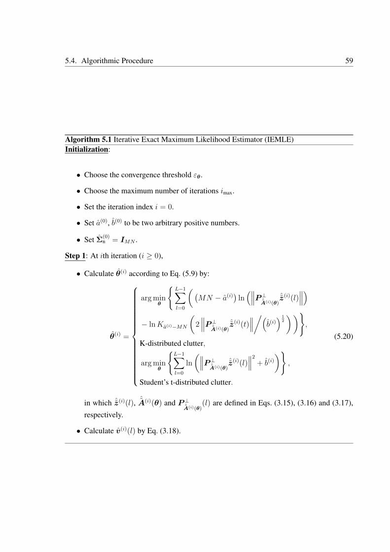
5.4. Algorithmic Procedure 59
Algorithm 5.1 Iterative Exact Maximum Likelihood Estimator (IEMLE)Initialization:
• Choose the convergence threshold εθ.
• Choose the maximum number of iterations imax.
• Set the iteration index i = 0.
• Set a(0), b(0) to be two arbitrary positive numbers.
• Set Σ(0)n = IMN .
Step 1: At ith iteration (i ≥ 0),
• Calculate θ(i) according to Eq. (5.9) by:
θ(i) =
arg minθ
L−1∑l=0
((MN − a(i)
)ln(∥∥∥P⊥ˆA(i)(θ)
ˆz(i)(l)∥∥∥)
− lnKa(i)−MN
(2∥∥∥P⊥ˆA(i)(θ)
ˆz(i)(t)∥∥∥/(b(i)
) 12
)),
K-distributed clutter,
arg minθ
L−1∑l=0
ln
(∥∥∥P⊥ˆA(i)(θ)ˆz(i)(l)
∥∥∥2
+ b(i)
),
Student’s t-distributed clutter.
(5.20)
in which ˆz(i)(l), ˆA(i)(θ) and P⊥ˆA(i)(θ)(l) are defined in Eqs. (3.15), (3.16) and (3.17),
respectively.
• Calculate v(i)(l) by Eq. (3.18).
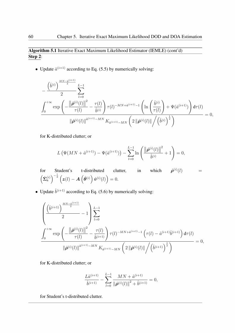
60 Chapter 5. Iterative Exact Maximum Likelihood DOD and DOA Estimation
Algorithm 5.1 Iterative Exact Maximum Likelihood Estimator (IEMLE) (cont’d)Step 2:
• Update a(i+1) according to Eq. (5.5) by numerically solving:
−
(b(i))MN−a(i+1)
2
2
L−1∑l=0∫ +∞
0
exp
(−∥∥ρ(i)(l)
∥∥2
τ(l)− τ(l)
b(i)
)τ(l)−MN+a(i+1)−1
(ln
(b(i)
τ(l)
)+ Ψ(a(i+1))
)dτ(l)
‖ρ(i)(l)‖a(i+1)−MN
Ka(i+1)−MN
(2 ‖ρ(i)(l)‖
/(b(i)) 1
2
) = 0,
for K-distributed clutter; or
L(Ψ(MN + a(i+1))−Ψ(a(i+1))
)−
L−1∑l=0
ln
(∥∥ρ(i)(l)∥∥2
b(i)+ 1
)= 0,
for Student’s t-distributed clutter, in which ρ(i)(l) =(Σ
(i)n
)− 12(z(l)−A
(θ(i))v(i)(l)
)= 0.
• Update b(i+1) according to Eq. (5.6) by numerically solving:
(b(i+1)
)MN−a(i+1)
2
2− 1
L−1∑l=0∫ +∞
0
exp
(−∥∥ρ(i)(l)
∥∥2
τ(l)− τ(l)
b(i+1)
)τ(l)−MN+a(i+1)−1
(τ(l)− a(i+1)b(i+1)
)dτ(l)
‖ρ(i)(l)‖a(i+1)−MN
Ka(i+1)−MN
(2 ‖ρ(i)(l)‖
/(b(i+1)
) 12
) = 0,
for K-distributed clutter; or
La(i+1)
b(i+1)−
L−1∑l=0
MN + a(i+1)
‖ρ(i)(l)‖2+ b(i+1)
= 0,
for Student’s t-distributed clutter.
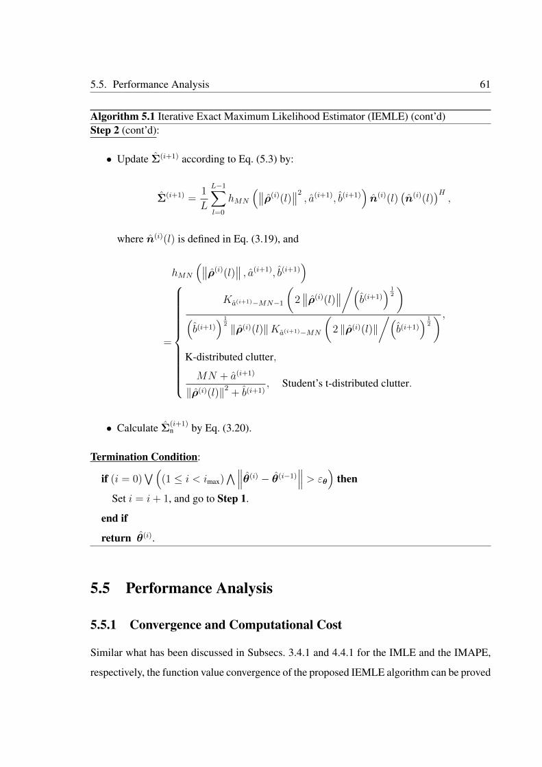
5.5. Performance Analysis 61
Algorithm 5.1 Iterative Exact Maximum Likelihood Estimator (IEMLE) (cont’d)Step 2 (cont’d):
• Update Σ(i+1) according to Eq. (5.3) by:
Σ(i+1) =1
L
L−1∑l=0
hMN
(∥∥ρ(i)(l)∥∥2, a(i+1), b(i+1)
)n(i)(l)
(n(i)(l)
)H,
where n(i)(l) is defined in Eq. (3.19), and
hMN
(∥∥ρ(i)(l)∥∥ , a(i+1), b(i+1)
)
=
Ka(i+1)−MN−1
(2∥∥ρ(i)(l)
∥∥/(b(i+1)) 1
2
)(b(i+1)
) 12 ‖ρ(i)(l)‖Ka(i+1)−MN
(2 ‖ρ(i)(l)‖
/(b(i+1)
) 12
) ,K-distributed clutter,
MN + a(i+1)
‖ρ(i)(l)‖2+ b(i+1)
, Student’s t-distributed clutter.
• Calculate Σ(i+1)n by Eq. (3.20).
Termination Condition:
if (i = 0)∨(
(1 ≤ i < imax)∧∥∥∥θ(i) − θ(i−1)
∥∥∥ > εθ
)then
Set i = i+ 1, and go to Step 1.
end if
return θ(i).
5.5 Performance Analysis
5.5.1 Convergence and Computational Cost
Similar what has been discussed in Subsecs. 3.4.1 and 4.4.1 for the IMLE and the IMAPE,
respectively, the function value convergence of the proposed IEMLE algorithm can be proved
62 Chapter 5. Iterative Exact Maximum Likelihood DOD and DOA Estimation
by showing the fulfillment of the three conditions listed in Subsec. 3.4.1 by the IEMLE. The
first two conditions are obviously valid. The third condition, i.e., the uniqueness of the
parameter estimates, is also fulfilled under the mild conditions specified below Eqs. (5.3),
(5.9) and those in Ch. 3 and Sec. 5.3 (for Student’s t-distributed clutter). Simulation results
in Ch. 8 will show that, to attain the convergence of the estimate of the unknown parameter
θ, the IEMLE requires still fewer iterations than the IMLE and the IMAPE. Generally one
iteration is enough for this purpose.
For t-distributed clutter case, the computational cost of the IEMLE lies mainly in the
numerical solution of Eq. (5.20). As the IEMLE requires fewer iterations than the IMLE and
the IMAPE, its computational cost is also smaller than them in this case. For K-distributed
clutter case, however, since the IEMLE involves numerically solving the nonlinear equations
in Eqs. (5.1) and (5.1) that contain numerical integrals, which is computationally highly
expensive, it turns out that the computational cost for the IEMLE in this case is much greater
than the IMLE and the IMAPE.
5.5.2 Invariance of the IEMLE to Different Speckle CM Trace Assump-
tions
Introduce the variables trΣa, r and the representation (·)′as defined in Sec. 3.4.2, to stand
for the alternatively assumed speckle CM trace, the ratio between this alternatively and the
originally (namely, in Eq. (2.17)) assumed speckle CM trace, and the “counterpart” of a pa-
rameter corresponding to the alternative assumption of trΣa, respectively. The expressions
of τ ′(l) in Eq. (3.26) and ρ′(l) in Eq. (3.28) also hold for the IEMLE.
Additionally, it is known from the scaling property of the gamma and the inverse-gamma
distributions that, if
τ(l) ∼ Gamma(a, b), (5.21)
then1
rτ(l) ∼ Gamma(a,
1
rb), (5.22)
5.5. Performance Analysis 63
and similarly, if
τ(l) ∼ Inv-Gamma(a, b), (5.23)
then1
rτ(l) ∼ Inv-Gamma(a,
1
rb). (5.24)
Hence
a′ = a, (5.25)
and
b′ =1
rb, (5.26)
for both texture distributions.
By substituting Eqs. (5.25), (5.26) and (3.28) into Eq. (5.2) one obtains that:
gMN
(‖ρ′(l)‖2
, a′, b′)
= rMNgMN
(‖ρ(l)‖2 , a, b
), l = 0, . . . , L− 1. (5.27)
for both clutter distributions.
Furthermore, by noticing that the objective function in Eq. (5.9) is in essence the search
for θ by:
θ = arg maxθ
L−1∑l=0
ln gMN
(‖ρ(l)‖2 , a, b
), (5.28)
and by applying Eq. (5.27), it can be shown that:
θ′ = arg maxθ
L−1∑l=0
ln gMN
(‖ρ′(l)‖2
, a′, b′)
= arg maxθ
L−1∑l=0
ln gMN
(‖ρ(l)‖2 , a, b
)+ LMN ln r
= arg maxθ
L−1∑l=0
ln gMN
(‖ρ(l)‖2 , a, b
)= θ,
(5.29)
which shows that the IEMLE is invariant to different speckle CM trace assumptions, as, like

64 Chapter 5. Iterative Exact Maximum Likelihood DOD and DOA Estimation
for the IMLE and the IMAPE, the estimated θ for the IEMLE is also independent of the
assumed value of trΣ.
Chapter 6
Cramér-Rao-Type Bounds
The task of this section is to derive the expressions for various CRTBs, including the CRB,
the MCB, the EMCB, the MCRB and the HCRB, w.r.t. the DOD and DOA parameters of
the MIMO radar in the presence of SIRP clutter, based on the estimation model given by
Eq. (2.7) in Ch. 2. The expressions of these CRTBs are derived first in the elementwise form
of the FIM matrices, then the relations between them are determined, as well as the respective
impacts of the texture parameters on each of them. Finally, to make their expressions more
compact and their calculation more convenient, a blockwise expression is then derived for
each of the CRTBs.
To be consistent with the proposed estimators in Chs. 3-5, and for the purpose of pa-
rameter identifiability, one considers for the derivation of the CRTBs also the transformed
unknown parameter vector in Eq. (2.24), instead of the original one in Eq. (2.21). Namely,
one takes v(l), l = 0, . . . , L− 1 defined in Eq. (2.8) as part of unknown parameters instead
of the RCS coefficients αk(l), k = 1, . . . , K, and the normalized Doppler frequency shifts
fk(l), k = 1, . . . , K, of the targets.
6.1 The Cramér-Rao Bound
Let CRB (θ) denotes the CRB w.r.t. the DODs and DOAs of the signal, which, like the
IEMLE proposed in Ch. 5, considers exactly the parameter vector ξ, and is obtained as the
65
66 Chapter 6. Cramér-Rao-Type Bounds
upper-leftmost elements (those corresponding to θ) of the inverse of the Fisher Information
Matrix (FIM). The latter, denoted by F , is calculated from the marginal (exact) LLF ΛM
defined in Eq. (5.1).
The elements of F are given by:
[F ]i,j = Ey
∂ΛM
∂ [ξ]i
∂ΛM
∂ [ξ]j
, i, j = 1, . . . , 2K(L+ 1) +M2N2 + 2, (6.1)
in which Ey · represents the expectation w.r.t. the parameter y, [·]i,j denotes the (i, j)th
entry of a matrix, and [·]i denotes the ith element of a vector.
6.1.1 The Score Functions
The computation of Eq. (6.1) requires, in the first place, the expressions of the partial deriva-
tives of ΛM w.r.t. all the elements of ξ (also known as the score functions).
First, introduce the 2K(L+ 1)× 1 signal parameter vector:
µ =[θT ,vT
]T, (6.2)
in which θ and v are defined in Eq. (2.11) and (2.25), respectively. The score functions w.r.t.
[µ]i , i = 1, . . . , 2K(L + 1), and [ζ]i , i = 1, . . . ,M2N2 (the parameter vector ζ is defined
in Sec. 2.3 and contains the real and imaginary parts of the entries of the lower triangular
part of the speckle CM Σ), can be calculated as:
∂ΛM
∂ [µ]i=−
L−1∑l=0
hMN
(‖ρ(l)‖2 , a, b
)·(ρH(l)Σ−
12∂b (θ, l)
∂ [µ]i+∂bH (θ, l)
∂ [µ]iΣ−
12ρ(l)
),
i = 1, . . . , 2K(L+ 1), (6.3a)
∂Λ
∂ [ζ]i= −
L−1∑l=0
hMN
(‖ρ(l)‖2 , a, b
)(ρH(l)Σ−
12∂Σ
∂ [ζ]iΣ−
12ρ(l)
)−Ltr
Σ−1 ∂Σ
∂ [ζ]i
, i = 1, . . . ,M2N2, (6.3b)
(6.3c)
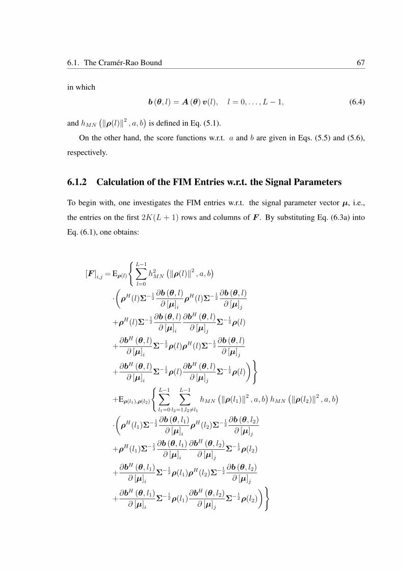
6.1. The Cramér-Rao Bound 67
in which
b (θ, l) = A (θ)v(l), l = 0, . . . , L− 1, (6.4)
and hMN
(‖ρ(l)‖2 , a, b
)is defined in Eq. (5.1).
On the other hand, the score functions w.r.t. a and b are given in Eqs. (5.5) and (5.6),
respectively.
6.1.2 Calculation of the FIM Entries w.r.t. the Signal Parameters
To begin with, one investigates the FIM entries w.r.t. the signal parameter vector µ, i.e.,
the entries on the first 2K(L + 1) rows and columns of F . By substituting Eq. (6.3a) into
Eq. (6.1), one obtains:
[F ]i,j = Eρ(l)
L−1∑l=0
h2MN
(‖ρ(l)‖2 , a, b
)·(ρH(l)Σ−
12∂b (θ, l)
∂ [µ]iρH(l)Σ−
12∂b (θ, l)
∂ [µ]j
+ρH(l)Σ−12∂b (θ, l)
∂ [µ]i
∂bH (θ, l)
∂ [µ]jΣ−
12ρ(l)
+∂bH (θ, l)
∂ [µ]iΣ−
12ρ(l)ρH(l)Σ−
12∂b (θ, l)
∂ [µ]j
+∂bH (θ, l)
∂ [µ]iΣ−
12ρ(l)
∂bH (θ, l)
∂ [µ]jΣ−
12ρ(l)
)
+Eρ(l1),ρ(l2)
L−1∑l1=0
L−1∑l2=1,l2 6=l1
hMN
(‖ρ(l1)‖2 , a, b
)hMN
(‖ρ(l2)‖2 , a, b
)·(ρH(l1)Σ−
12∂b (θ, l1)
∂ [µ]iρH(l2)Σ−
12∂b (θ, l2)
∂ [µ]j
+ρH(l1)Σ−12∂b (θ, l1)
∂ [µ]i
∂bH (θ, l2)
∂ [µ]jΣ−
12ρ(l2)
+∂bH (θ, l1)
∂ [µ]iΣ−
12ρ(l1)ρH(l2)Σ−
12∂b (θ, l2)
∂ [µ]j
+∂bH (θ, l1)
∂ [µ]iΣ−
12ρ(l1)
∂bH (θ, l2)
∂ [µ]jΣ−
12ρ(l2)
)
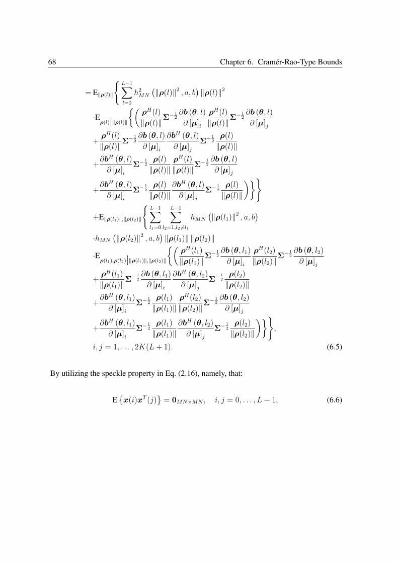
68 Chapter 6. Cramér-Rao-Type Bounds
= E‖ρ(l)‖
L−1∑l=0
h2MN
(‖ρ(l)‖2 , a, b
)‖ρ(l)‖2
·Eρ(l)
∣∣‖ρ(l)‖
(ρH(l)
‖ρ(l)‖Σ−
12∂b (θ, l)
∂ [µ]i
ρH(l)
‖ρ(l)‖Σ−
12∂b (θ, l)
∂ [µ]j
+ρH(l)
‖ρ(l)‖Σ−
12∂b (θ, l)
∂ [µ]i
∂bH (θ, l)
∂ [µ]jΣ−
12ρ(l)
‖ρ(l)‖
+∂bH (θ, l)
∂ [µ]iΣ−
12ρ(l)
‖ρ(l)‖ρH(l)
‖ρ(l)‖Σ−
12∂b (θ, l)
∂ [µ]j
+∂bH (θ, l)
∂ [µ]iΣ−
12ρ(l)
‖ρ(l)‖∂bH (θ, l)
∂ [µ]jΣ−
12ρ(l)
‖ρ(l)‖
)
+E‖ρ(l1)‖,‖ρ(l2)‖
L−1∑l1=0
L−1∑l2=1,l2 6=l1
hMN
(‖ρ(l1)‖2 , a, b
)·hMN
(‖ρ(l2)‖2 , a, b
)‖ρ(l1)‖ ‖ρ(l2)‖
·Eρ(l1),ρ(l2)
∣∣‖ρ(l1)‖,‖ρ(l2)‖
(ρH(l1)
‖ρ(l1)‖Σ−
12∂b (θ, l1)
∂ [µ]i
ρH(l2)
‖ρ(l2)‖Σ−
12∂b (θ, l2)
∂ [µ]j
+ρH(l1)
‖ρ(l1)‖Σ−
12∂b (θ, l1)
∂ [µ]i
∂bH (θ, l2)
∂ [µ]jΣ−
12ρ(l2)
‖ρ(l2)‖
+∂bH (θ, l1)
∂ [µ]iΣ−
12ρ(l1)
‖ρ(l1)‖ρH(l2)
‖ρ(l2)‖Σ−
12∂b (θ, l2)
∂ [µ]j
+∂bH (θ, l1)
∂ [µ]iΣ−
12ρ(l1)
‖ρ(l1)‖∂bH (θ, l2)
∂ [µ]jΣ−
12ρ(l2)
‖ρ(l2)‖
),
i, j = 1, . . . , 2K(L+ 1). (6.5)
By utilizing the speckle property in Eq. (2.16), namely, that:
Ex(i)xT (j)
= 0MN×MN , i, j = 0, . . . , L− 1, (6.6)
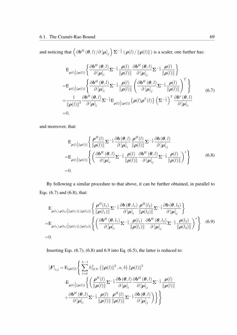
6.1. The Cramér-Rao Bound 69
and noticing that(∂bH (θ, l)/∂ [µ]j
)Σ−
12 (ρ(l)/ ‖ρ(l)‖) is a scaler, one further has:
Eρ(l)
∣∣‖ρ(l)‖
∂bH (θ, l)
∂ [µ]iΣ−
12ρ(l)
‖ρ(l)‖∂bH (θ, l)
∂ [µ]jΣ−
12ρ(l)
‖ρ(l)‖
=Eρ(l)
∣∣‖ρ(l)‖
∂bH (θ, l)
∂ [µ]iΣ−
12ρ(l)
‖ρ(l)‖
(∂bH (θ, l)
∂ [µ]jΣ−
12ρ(l)
‖ρ(l)‖
)T
=1
‖ρ(l)‖2
∂bH (θ, l)
∂ [µ]iΣ−
12 Eρ(l)
∣∣‖ρ(l)‖
ρ(l)ρT (l)
(Σ−
12
)T ∂b∗ (θ, l)
∂ [µ]i
=0,
(6.7)
and moreover, that:
Eρ(l)
∣∣‖ρ(l)‖
ρH(l)
‖ρ(l)‖Σ−
12∂b (θ, l)
∂ [µ]i
ρH(l)
‖ρ(l)‖Σ−
12∂b (θ, l)
∂ [µ]j
=Eρ(l)
∣∣‖ρ(l)‖
(∂bH (θ, l)
∂ [µ]iΣ−
12ρ(l)
‖ρ(l)‖∂bH (θ, l)
∂ [µ]jΣ−
12ρ(l)
‖ρ(l)‖
)∗=0.
(6.8)
By following a similar procedure to that above, it can be further obtained, in parallel to
Eqs. (6.7) and (6.8), that:
Eρ(l1),ρ(l2)
∣∣‖ρ(l1)‖,‖ρ(l2)‖
ρH(l1)
‖ρ(l1)‖Σ−
12∂b (θ, l1)
∂ [µ]i
ρH(l2)
‖ρ(l2)‖Σ−
12∂b (θ, l2)
∂ [µ]j
=E
ρ(l1),ρ(l2)
∣∣‖ρ(l1)‖,‖ρ(l2)‖
(∂bH (θ, l1)
∂ [µ]iΣ−
12ρ(l1)
‖ρ(l1)‖∂bH (θ, l2)
∂ [µ]jΣ−
12ρ(l2)
‖ρ(l2)‖
)∗=0.
(6.9)
Inserting Eqs. (6.7), (6.8) and 6.9 into Eq. (6.5), the latter is reduced to:
[F ]i,j = E‖ρ(l)‖
L−1∑l=0
h2MN
(‖ρ(l)‖2 , a, b
)‖ρ(l)‖2
·Eρ(l)
∣∣‖ρ(l)‖
(ρH(l)
‖ρ(l)‖Σ−
12∂b (θ, l)
∂ [µ]i
∂bH (θ, l)
∂ [µ]jΣ−
12ρ(l)
‖ρ(l)‖
+∂bH (θ, l)
∂ [µ]iΣ−
12ρ(l)
‖ρ(l)‖ρH(l)
‖ρ(l)‖Σ−
12∂b (θ, l)
∂ [µ]j
)
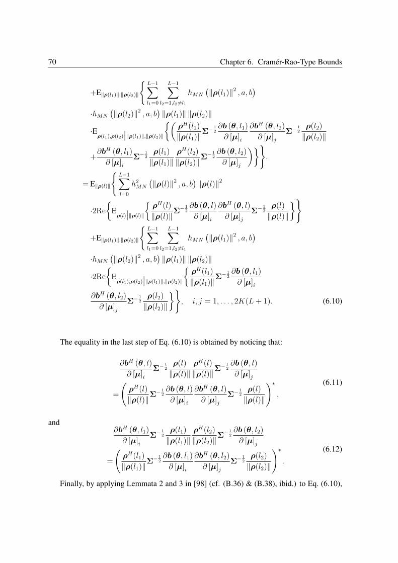
70 Chapter 6. Cramér-Rao-Type Bounds
+E‖ρ(l1)‖,‖ρ(l2)‖
L−1∑l1=0
L−1∑l2=1,l2 6=l1
hMN
(‖ρ(l1)‖2 , a, b
)·hMN
(‖ρ(l2)‖2 , a, b
)‖ρ(l1)‖ ‖ρ(l2)‖
·Eρ(l1),ρ(l2)
∣∣‖ρ(l1)‖,‖ρ(l2)‖
(ρH(l1)
‖ρ(l1)‖Σ−
12∂b (θ, l1)
∂ [µ]i
∂bH (θ, l2)
∂ [µ]jΣ−
12ρ(l2)
‖ρ(l2)‖
+∂bH (θ, l1)
∂ [µ]iΣ−
12ρ(l1)
‖ρ(l1)‖ρH(l2)
‖ρ(l2)‖Σ−
12∂b (θ, l2)
∂ [µ]j
).
= E‖ρ(l)‖
L−1∑l=0
h2MN
(‖ρ(l)‖2 , a, b
)‖ρ(l)‖2
·2Re
Eρ(l)
∣∣‖ρ(l)‖
ρH(l)
‖ρ(l)‖Σ−
12∂b (θ, l)
∂ [µ]i
∂bH (θ, l)
∂ [µ]jΣ−
12ρ(l)
‖ρ(l)‖
+E‖ρ(l1)‖,‖ρ(l2)‖
L−1∑l1=0
L−1∑l2=1,l2 6=l1
hMN
(‖ρ(l1)‖2 , a, b
)·hMN
(‖ρ(l2)‖2 , a, b
)‖ρ(l1)‖ ‖ρ(l2)‖
·2Re
Eρ(l1),ρ(l2)
∣∣‖ρ(l1)‖,‖ρ(l2)‖
ρH(l1)
‖ρ(l1)‖Σ−
12∂b (θ, l1)
∂ [µ]i
∂bH (θ, l2)
∂ [µ]jΣ−
12ρ(l2)
‖ρ(l2)‖
, i, j = 1, . . . , 2K(L+ 1). (6.10)
The equality in the last step of Eq. (6.10) is obtained by noticing that:
∂bH (θ, l)
∂ [µ]iΣ−
12ρ(l)
‖ρ(l)‖ρH(l)
‖ρ(l)‖Σ−
12∂b (θ, l)
∂ [µ]j
=
(ρH(l)
‖ρ(l)‖Σ−
12∂b (θ, l)
∂ [µ]i
∂bH (θ, l)
∂ [µ]jΣ−
12ρ(l)
‖ρ(l)‖
)∗,
(6.11)
and∂bH (θ, l1)
∂ [µ]iΣ−
12ρ(l1)
‖ρ(l1)‖ρH(l2)
‖ρ(l2)‖Σ−
12∂b (θ, l2)
∂ [µ]j
=
(ρH(l1)
‖ρ(l1)‖Σ−
12∂b (θ, l1)
∂ [µ]i
∂bH (θ, l2)
∂ [µ]jΣ−
12ρ(l2)
‖ρ(l2)‖
)∗.
(6.12)
Finally, by applying Lemmata 2 and 3 in [98] (cf. (B.36) & (B.38), ibid.) to Eq. (6.10),
6.1. The Cramér-Rao Bound 71
the latter can be further transformed into:
[F ]i,j =E‖ρ(l)‖
L−1∑l=0
h2MN
(‖ρ(l)‖2 , a, b
)‖ρ(l)‖2
· 2Re
tr
Σ−12∂b (θ, l)
∂ [µ]i
∂bH (θ, l)
∂ [µ]jΣ−
12
=2κ(MN, a, b)
LRe
tr
∂bH (θ, l)
∂ [µ]iΣ−1∂b (θ, l)
∂ [µ]j
, i, j = 1, . . . , 2K(L+ 1).
(6.13)
in which
κ(MN, a, b) = E‖ρ(l)‖
L−1∑l=0
h2MN
(‖ρ(l)‖2 , a, b
)‖ρ(l)‖2
. (6.14)
6.1.3 The Expression of κ(MN, a, b)
The expression of the factor κ(MN, a, b) can be obtained by applying Eqs. (C.48) and (C.49)
in [98] to Eq. (6.14) and transforming the latter into:
κ(MN, a, b) =
∫ +∞0
h2MN
(‖ρ(l)‖2 , a, b
)gMN
(‖ρ(l)‖2 , a, b
)‖ρ(l)‖2MN+1 d ‖ρ(l)‖∫ +∞
0gMN
(‖ρ(l)‖2 , a, b
)‖ρ(l)‖2MN−1 d ‖ρ(l)‖
,
(6.15)
into which one then substitutes the expressions of hMN
(‖ρ(l)‖2 , a, b
)and gMN
(‖ρ(l)‖2 , a, b
)in Eqs. (5.2), and (5.1), respectively, leading to:
κ(MN, a, b) =
∫ +∞
0xMN+a−1K
2a−MN−1(x)
Ka−MN (x)dx
2MN+a−2bΓ(MN)Γ(a), K-distributed clutter,
MNa(a+MN)
b(a+MN + 1), Student’s t-distributed clutter.
(6.16)
in which Kn(x) is the modified Bessel functions of the second kind of order n.
Note that, for Student’s t-distributed clutter, Eq. (6.16) is a generalization of the result
in [98] to the two texture parameter case. For K-distributed clutter, Eq. (6.16) offers a more
compact expression of κ(MN, a, b) than [98].
From Eq. (6.16) it is clear that the factor κ(MN, a, b) for K-distributed clutter, which
takes the form of integration of Bessel functions, has no close-form expression, and can only
72 Chapter 6. Cramér-Rao-Type Bounds
be evaluated numerically. One approach to its calculation is to use the generalized Gauss-
Laguerre quadrature [98,127,128], transforming its expression for K-distributed clutter into:
κ(MN, a, b) =
∑O(2MN+1)1
o1=1
(∑O(a−1)2
o2=1 exp
(−x2o1xo2 b
)1bx−(MN+1)o2
wo2
)2
∑O(a−1)3
o3=1 exp
(−x2o1xo3 b
)x−MNo3
wo3
exo1wo1
∑O(2MN−1)4
o4=1
(∑O(a−1)5
o5=1 exp(− x2o4xo5b
)x−MNo5
wo5
)exo4wo4
, (6.17)
where xoi , i = 1, . . . , 5, and woi , i = 1, . . . , 5, represent the abscissae and the weights
of the generalized Gauss-Laguerre quadrature, respectively; O(2MN+1)1 , O(a−1)
2 , etc., denote
the quadrature orders; with the subscript of each representing the respective parameter of the
corresponding abscissa and weight (e.g.,O(2MN+1)1 means that xo1 and wo1 have 2MN+1 as
their parameter). The values of these quadrature orders can be empirically chosen. Generally
speaking, a value around 160 for all of them is enough for the calculation.
6.1.4 The Expression of the CRB
To obtain the final expression of CRB (θ), one has further to determine the expression of the
remaining entries of F . For succinct documentation, introduce the (M2N2 + 2) × 1 clutter
parameter vector:
$ =[ζT , a, b
]T. (6.18)
First, one explores the values of the FIM cross-term entries between the signal parameter
vector µ and clutter parameter vector$.
It is clear from Eq. (6.3a) that, for any l = 0, . . . , L− 1, and with a fixed ‖ρ(l)‖,
∂ΛM
∂ [µ]i, i = 1, . . . , 2K(L+ 1), (6.19)
are odd functions of ρ(l), whereas
∂ΛM
∂ [$]j, j = 1, . . . ,M2N2 + 2, (6.20)
6.1. The Cramér-Rao Bound 73
are, as can be observed from Eqs. (6.3b), (5.5) and (5.6), even functions of ρ(l).
As a result,∂ΛM
∂ [µ]i
∂ΛM
∂ [$]j,
i = 1, . . . , 2K(L+ 1), j = 1, . . . ,M2N2 + 2,
(6.21)
are even functions of ρ(l), hence:
E
∂ΛM
∂ [µ]i
∂ΛM
∂ [$]j
=E‖ρ(l)‖
Eρ(l)
∣∣‖ρ(l)‖
∂ΛM
∂ [µ]i
∂ΛM
∂ [$]j
=0,
(6.22)
which reveals that F has the following block-diagonal structure:
F =
Φ 02K(L+1)×(M2N2+2)
02K(L+1)×(M2N2+2) Ξ
, (6.23)
in which Φ denotes the 2K(L+1)×2K(L+1) FIM block w.r.t. the signal parameter vector
µ, whose entries, denoted by φij , are given by:
φij =2κ(MN, a, b)
MN
L−1∑l=0
Re
∂bH (θ, l)
∂ [µ]iΣ−1∂b (θ, l)
∂ [µ]j
,
i, j = 1, . . . , 2K(L+ 1).
(6.24)
The matrix Ξ in Eq. (6.23) represents the FIM block w.r.t. the clutter parameter vector$.
Since the FIM blocks Φ and Ξ are decoupled from each other (meaning that the achievable
performance for the estimation of Ξ and of$ and independent from each other), the concrete
expressions for the entries of $ is not required for the purpose of obtain CRB (θ), and one
simply has:
[CRB (θ)]i,j =[Φ−1
]i,j, i, j = 1, . . . , 2K. (6.25)
as the elementwise expression of CRB (θ).
74 Chapter 6. Cramér-Rao-Type Bounds
6.2 The Remaining Cramér-Rao-Type Bounds
In parallel to the derivation for CRB (θ) in Sec. 6.1, this section discusses the expressions for
the remaining aforementioned CRTBs, including the EMCB, the MCB, the MCRB and the
HCRB, for the DOD/DOA parameter vector θ, denoted by EMCB (θ), MCB (θ) MCRB (θ)
and HCRB (θ), respectively.
6.2.1 The Extended Miller-Chang Bound
The EMCB was first proposed in [52] as an extension of the Miller-Chang Bound (MCB)
[53]. Its general motivation is to first treat the random nuisance parameters (the texture τ , in
the case under discussion) as deterministic but unknown, and to derive the CRB calculated
from the conditional LL ΛC in Eq. (3.1). Then in the next step, the assumption of determin-
istic τ is relaxed and the previously obtained CRB is averaged over different realizations of
τ drawn from the corresponding random distribution.
This approach has in common with the proposed IMLE in Ch. 3 that the latter also treats
τ to be deterministic. The performance of this algorithm, in terms of the averaged MSE re-
sulting from many independent Monte-Carlo trials, can be evaluated by averaging the CRBs
calculated for each of the trials. It is clear that such an averaged CRB, when the trial number
becomes large, approaches the EMCB.
Calculation of the EMCB considers the (2K(L+1)+M2N2+L)×1 unknown parameter
vector in the deterministic texture case:
ξdet =[ψT , τ T
]T, (6.26)
which incorporates the texture realization parameter vector τ but leaves out the texture pa-
rameters a and b. The entries of the corresponding FIM, denoted by FEMC, are calculated
by:
[FEMC]i,j =Ey|τ
∂ΛC
∂ [ξdet]i
∂ΛC
∂ [ξdet]j
,
i, j = 1, . . . , 2K(L+ 1) +M2N2 + L.
(6.27)
6.2. The Remaining Cramér-Rao-Type Bounds 75
Among the score functions involved in Eq. (6.27), those w.r.t. [µ]i , i = 1, . . . , 2K(L +
1), and [ζ]i , i = 1, . . . ,M2N2, are given above in Eqs. (6.3a) and (6.3b), respectively. The
score functions w.r.t. [τ ]i , i = 1, . . . , L, i.e., those w.r.t. τ(l), l = 0, . . . , L − 1, can be
calculated as:∂ΛC
∂τ(l)= −MN
τ(l)+
1
τ 2(l)‖ρ(l)‖2 , l = 0, . . . , L− 1. (6.28)
Inserting Eqs. (6.3a), (6.3b) and (6.28) into Eq. (6.27), and noticing that Eq. (6.28) is also
an even function of ρ(l), one arrives at the conclusion that, similar to the expression of F in
Eq. (6.23), FEMC also exhibits a block-diagonal structure, where the block w.r.t. the signal
parameter vector µ is decoupled from the block w.r.t. the clutter parameter vector (in the
deterministic texture case):
$det =[ζT , τ T
]T. (6.29)
Let ΦEMC denote the block of FEMC w.r.t. µ, The entries of ΦEMC, represented by φEMCij ,
have the following expressions:
φEMCij =2
L−1∑l=0
1
τ(l)Re
∂bH (θ, l)
∂ [µ]iΣ−1∂b (θ, l)
∂ [µ]j
,
i, j = 1, . . . , 2K(L+ 1).
(6.30)
Consequently, EMCB (θ) is given by:
[EMCB (θ)]i,j =[EτΦ−1
EMC
]i,j, i, j = 1, . . . , 2K. (6.31)
for which no closed-form expression exists.
6.2.2 The Miller-Chang Bound
The MCB proposed in [53], like its generalized version, the EMCB, also consists in calcu-
lating the CRB based on the LL conditioned on the nuisance parameters modeled as deter-
ministic, and then averaging the so obtained CRB over the nuisance parameters. It differs
from the EMCB only in that it treats the nuisance parameter not only as deterministic but
76 Chapter 6. Cramér-Rao-Type Bounds
also as known. Thus, the MCB considers the unknown parameters vector as ψ, and its FIM,
denoted by FMC, is calculated as:
[FMC]i,j =Ey|τ
∂ΛC
∂ [ψ]i
∂ΛC
∂ [ψ]j
,
i, j = 1, . . . , 2K(L+ 1) +M2N2.
(6.32)
From Eq. (6.32) it is easily seen that FMC is equal to the (2K(L+1)+M2N2)×(2K(L+
1) +M2N2) upper left-most block of the FIM for the EMCB, i.e.,:
FMC =
[FEMC]1,1 . . . [FEMC]1,2K(L+1)+M2N2
... . . . ...
[FEMC]2K(L+1)+M2N2,1 . . . [FEMC]2K(L+1)+M2N2,2K(L+1)+M2N2
. (6.33)
Thus, FMC also has a block-diagonal structure, and its block w.r.t. the signal parameter vector
µ, denoted by ΦMC, is equal to ΦEMC.
Generally speaking, it is proved in [52] that the EMCB is greater than or equal to the
MCB. However, for the problem under discussion, due to the block-diagonal structure of the
FIMs, it follows that:
[MCB (θ)]i,j =[EτF−1
MC
]i,j
=[EτΦ−1
MC
]i,j
=[EτΦ−1
EMC
]i,j
= [EMCB (θ)]i,j , i, j = 1, . . . , 2K,(6.34)
namely, the two are equal w.r.t. the DOD/DOA parameter vector θ.
6.2.3 The Modified Cramér-Rao Bound
The MCRB [56, 57], like the MCB, also considers the unknown parameter vector as ψ,
namely, it models τ as deterministic and known. Its corresponding FIM, denoted by FM, is
likewise calculated from the conditional LL in Eq. (3.1). The MCRB differs from the MCB
6.2. The Remaining Cramér-Rao-Type Bounds 77
only in that it averages over the random parameters before the FIM inversion, namely:
[FM]i,j =Ey,τ
∂ΛC
∂ [ψ]i
∂ΛC
∂ [ψ]j
=Eτ
Ey|τ
∂ΛC
∂ [ψ]i
∂ΛC
∂ [ψ]j
=Eτ
[FMC]i,j
,
i, j = 1, . . . , 2K(L+ 1) +M2N2.
(6.35)
Similar to F , FEMC and FMC, the FIM FM in Eq. (6.35) also has a block-diagonal structure,
whose block w.r.t. the signal parameter vector µ, denoted by ΦM, contains, according to
Eq. (6.35), the following entries φMij :
φMij =Eτ
φEMCij
=2ν(a, b)
L−1∑l=0
Re
∂bH (θ, l)
∂ [µ]iΣ−1∂b (θ, l)
∂ [µ]j
,
i, j = 1, . . . , 2K(L+ 1),
(6.36)
in which
ν(a, b) = E
1
τ(l)
=
1
b(a− 1), K-distributed clutter, for a > 1,
a
b, Student’s t-distributed clutter.
(6.37)
Thus MCRB (θ) is given by:
[MCRB (θ)]i,j =[Φ−1
M
]i,j, i, j = 1, . . . , 2K. (6.38)
78 Chapter 6. Cramér-Rao-Type Bounds
6.2.4 The Hybrid Cramér-Rao Bound
The HCRB as defined in [54], on the other hand, models the texture as random and considers
the (2K(L+ 1) +M2N2 + L+ 2)× 1 hybrid unknown parameter vector:
ξhyb = [ξT , τ T ]T , (6.39)
where τ is treated here as a random parameter vector that contains the i.i.d. random parame-
ter τ(l) at all snapshots. ξhyb is called “hybrid” as it contains both deterministic and random
parameters. Furthermore, the HCRB uses the joint LL in Eq. (4.2) to obtain its FIM, instead
of the conditional LL in Eq. (3.1) that is used in the derivation of the EMCB, MCB and
MCRB. It can be easily seen from the description above that the HCRB has the same spirit
as the proposed IMAPE in Ch. 4.
Let FH denote the FIM for the HCRB, of which the entries are calculated by:
[FH]i,j =Ey,τ
∂ΛJ
∂ [ξhyb]i
∂ΛJ
∂ [ξhyb]j
,
i, j = 1, . . . , 2K(L+ 1) +M2N2 + L+ 2.
(6.40)
By substituting Eqs. (6.3a), (6.3b), (5.5), (5.6) and (6.28) into Eq. (6.40), one can find
that FH also has a block-diagonal structure, namely, its block w.r.t. µ, denoted by ΦH, is
decoupled from the block w.r.t. the augmented hybrid clutter parameter vector:
$hyb =[$T , τ T
]T. (6.41)
Furthermore, since:
∂ΛJ
∂ [µ]i=
∂ΛC
∂ [µ]i, i = 1, . . . , 2K(L+ 1), (6.42)
it holds that:
ΦH = ΦM. (6.43)
6.3. The Relationships between the CRTBs 79
As a result, one has:
[HCRB (θ)]i,j = [MCRB (θ)]i,j =[Φ−1
M
]i,j, i, j = 1, . . . , 2K. (6.44)
6.3 The Relationships between the CRTBs
At this point, an analytical comparison between the CRTBs derived above is of interest,
which is also conducive to the determination of certain asymptotic properties of them, as
will be presented in this section.
6.3.1 The CRB vs. the MCRB/HCRB
It is theoretically proved, in [54] for the scaler and in [57] for the vector parameter case, that
the CRB is always larger than the HCRB. Since, according to Eq. (6.44), one also has the
equal MCRB and HCRB for the problem under discussion, it follows that:
CRB (θ) HCRB (θ) = MCRB (θ) , (6.45)
in which CRB (θ) HCRB (θ) means that CRB (θ)−HCRB (θ) is positive semidefinite.
This relationship becomes apparent when the clutter follows a Student’s t-distribution,
where CRB (θ) has a closed-form expression. By comparison of Eqs. (6.24) - (6.16) with
Eqs. (6.25), (6.36) and (6.44), one has:
CRB (θ) =a+MN + 1
a+MNMCRB (θ) =
a+MN + 1
a+MNHCRB (θ) . (6.46)
Consequently,
CRB (θ)−MCRB (θ) = CRB (θ)−HCRB (θ)
=1
a+MNMCRB (θ) =
1
a+MNHCRB (θ)
02K×2K ,
(6.47)
in which the inequality holds because the MCRB and HCRB matrices are per definitionem
positive semidefinite.
80 Chapter 6. Cramér-Rao-Type Bounds
Moreover, since
limMN→+∞
a+MN + 1
a+MN= 1, (6.48)
it follows from Eq. (6.46) that:
limMN→+∞
CRB (θ) = MCRB (θ) = HCRB (θ) , (6.49)
which shows that, for Student’s t-distributed clutter, the CRB approaches the MCRB/HCRB
in asymptotic cases w.r.t. the number of sensors either at the transmitter or the receiver.
One should note that this asymptotic property of the CRB, as will be demonstrated by
simulations, also holds for K-distributed clutter, despite the fact that, for this case, this prop-
erty seems impossible to be determined in an analytical way similar to that shown above,
due to the lack of a closed-form expression for κ(MN, a, b), as one can see from Eq. (6.16).
6.3.2 The EMCB/MCB vs. the MCRB/HCRB
The relationship between EMCB (θ) (or MCB (θ)) and MCRB (θ) (or HCRB (θ)) can be
revealed by noticing, according to Eqs. (6.35) and (6.38), that:
[MCRB (θ)]i,j =[Φ−1
M
]i,j
=[(Eτ ΦMC)−1]
i,j, i, j = 1, . . . , 2K. (6.50)
Since the quadratic form in Φ−1MC is a convex function of the entries of ΦMC, by Jensen’s
inequality, one has [129]:
EτΦ−1
MC
− (Eτ ΦMC)−1 0. (6.51)
Combining Eqs. (6.34), (6.50) and (6.51) leads to:
EMCB (θ) = MCB (θ) MCRB (θ) = HCRB (θ) . (6.52)
6.4. The CRTBs and the Texture Parameters 81
Furthermore, since, for both clutter distributions,
limL→+∞
∑L−1l=0
1τ(l)
L= E
1
τ(l)
, (6.53)
it follows that:
limL→+∞
ΦEMC = limL→+∞
ΦMC = ΦM = ΦH, (6.54)
and, as a consequence, that:
limL→+∞
EMCB (θ) = limL→+∞
MCB (θ) = MCRB (θ) = HCRB (θ) , (6.55)
viz., the EMCB/MCB approaches the MCRB/HCRB in asymptotic cases w.r.t. the number
of pulses.
6.3.3 The CRB vs. the EMCB/MCB
The relationship between CRB (θ) and EMCB (θ) (or EMCB (θ)), on the other hand, is
indefinite. More specifically, depending on the values of L and MN , the EMCB can either
be a tighter (larger in value) or looser (lower) bound than the CRB, as will be illustrated by
numerical simulations in Ch. 8.
6.4 The CRTBs and the Texture Parameters
This section investigates the respective impacts of the clutter’s texture parameters, a and b,
on the CRTBs. First, defined the SCR expression as [98, 101]:
SCR =1
L
∑L−1l=0 (A (θ)v(l))H (A (θ)v(l))
Eτ(l)tr Σ, (6.56)
in which Eτ(l) is equal to ab for K-distributed clutter and b/(a−1) for t-distributed clutter
(for a > 1) [130].
82 Chapter 6. Cramér-Rao-Type Bounds
It then turns out from Eq. (6.56) that, for a fixed SCR, one has:
1
trΣ∝
a, K-distributed clutter,
1
a− 1, Student’s t-distributed clutter, for a > 1,
(6.57)
and1
trΣ∝ b, K-distributed and Student’s t-distributed clutters, (6.58)
in which ∝ denotes direct proportionality. Note the relationships in Eq. (6.57) and (6.57)
hold irrespective of specific assumptions about the value of the speckle CM trace (e.g., the
one in Eq. (2.17)).
Furthermore, from Eq. (6.16), it can be found that:
κ(MN, a, b) ∝
∫ +∞
0xMN+a−1K
2a−MN−1(x)
Ka−MN (x)dx
2MN+a−2Γ(a), K-distributed clutter,
a(a+MN)
(a+MN + 1), Student’s t-distributed clutter, for a > 1,
(6.59)
and
κ(MN, a, b) ∝ 1
b, K-distributed and Student’s t-distributed clutters. (6.60)
6.4.1 CRTBs vs. the Shape Parameter a
One begins with the CRB. The expression in Eq. (6.24) can be converted to:
φij =2κ(MN, a, b)
trΣ
L−1∑l=0
Re
∂bH (θ, l)
∂ [µ]iΣ−1
n∂b (θ, l)
∂ [µ]j
,
i, j = 1, . . . , 2K(L+ 1),
(6.61)
where Σn is the normalized Σ defined in Eq. (3.7).
Eq. (6.61) shows that:
φij ∝κ(MN, a, b)
trΣ, (6.62)
6.4. The CRTBs and the Texture Parameters 83
to which one applies Eqs. (6.59) and (6.57) and has straightforwardly:
φij ∝
a∫ +∞
0xMN+a−1K
2a−MN−1(x)
Ka−MN (x)dx
2MN+a−2Γ(a), K-distributed clutter,
a(a+MN)
(a+MN + 1)(a− 1), Student’s t-distributed clutter, for a > 1,
(6.63)
meaning that for both clutter distributions, φij decreases as a increases1.
As a result, [CRB (θ)]i,j i, j = 1, . . . , 2K(L+ 1), increase with a for both clutter distri-
butions, i.e., the CRB is positively correlated with the shape parameter a, meaning that the
achievable estimation accuracy for the estimation of θ diminishes as a increases. This can
be intuitively explained by Figs. 2.4 and 2.8, which show that, for both clutter distributions
with a fixed clutter power, the clutter becomes more heavy-tailed as a increases, signifying
a larger portion of clutter power being decentralized.
Similarly, one can deduce from Eqs. (6.37) and (6.57) that:
φMij = φH
ij ∝a
a− 1, K-distributed and Student’s t-distributed clutters, (6.64)
which indicates a positive correlation also between the MCRB/HCRB and a, also mean-
ing that an increase in the value of a causes a diminished estimation accuracy that can be
achieved for the estimation of θ.
Notice that, as opposed to the CRB, which has different proportionalities to a for K-
distributed and for Student’s t-distributed clutters respectively, the MCRB/HCRB have the
same proportionality for both clutter distributions.
1This relationship is obvious for Student’s t-distributed clutter, for K-distributed clutter, however, for whichφij does not enjoy a closed-form expression, can only be determined numerically.
84 Chapter 6. Cramér-Rao-Type Bounds
Finally, for the EMCB/MCB, one has from Eq. (6.30) and (3.7) that:
φEMCij =
2MN
trΣ
L−1∑l=0
1
τ(l)Re
∂bH (θ, l)
∂ [µ]iΣ−1
n∂b (θ, l)
∂ [µ]j
∝ 1
trΣ
L−1∑l=0
1
τ(l),
i, j = 1, . . . , 2K(L+ 1).
(6.65)
Consequently, it follows from Eq. (6.31) and (6.34) that:
[EMCB (θ)]i,j = [MCB (θ)]i,j ∝ trΣEτ
1∑L−1
l=01τ(l)
,
i, j = 1, . . . , 2K(L+ 1).
(6.66)
It is known for Student’s t-distributed clutter that, if
τ(l) ∼ Inv-Gamma(a, b), (6.67)
then1
τ(l)∼ Gamma(a,
1
b). (6.68)
Thus, since τ(l), l = 0, . . . , L − 1, are i.i.d. variables, it from the property of the gamma
distribution that:1∑L−1
l=01τ(l)
∼ Gamma(La,1
b), (6.69)
and consequently, that:
Eτ
1∑L−1
l=01τ(l)
=La
b, Student’s t-distributed clutter, (6.70)
which, combined with Eqs. (6.57) and (6.66), results in:
[EMCB (θ)]i,j = [MCB (θ)]i,j ∝ a(a− 1), i, j = 1, . . . , 2K(L+ 1). (6.71)
6.4. The CRTBs and the Texture Parameters 85
indicating a positive correlation also between the EMCB/MCB and a.
For K-distributed clutter, an analogous deduction regarding the impact of a on the EMCB/MCB
seems, however, impossible or at least complicated, due to the presence of the sum of inverse
gamma variables, of which the precise distribution is unknown. The relationship between the
EMCB/MCB and a for K-distributed clutter can nevertheless be numerically ascertained, as
will be shown in Ch. 8.
6.4.2 CRTBs vs. the Scale Parameter b
Associating Eq. (6.60) with Eq. (6.61), yields:
φij ∝1
btrΣ, K-distributed and Student’s t-distributed clutters. (6.72)
which, combined with Eq. (6.58), shows that φij is thus independent of b for both clutter
distributions, which means that under a fixed SCR, changing b does not give rise to any
variation in the value of CRB (θ), meaning that the achievable estimation accuracy for the
estimation of θ is independent of the value of the scale parameter b. This is simply because,
as shown in Figs. 2.5 and 2.9, changing b does not result in any change in the PDF of the
clutter, for both clutter distributions with fixed clutter power.
The same also holds true for the MCRB/HCRB for both clutter distributions, and can be
established by transforming Eq. (6.36) into:
φMij =
2ν(a, b)MN
trΣ
L−1∑l=0
Re
∂bH (θ, l)
∂ [µ]iΣ−1
n∂b (θ, l)
∂ [µ]j
∝ν(a, b)
trΣ,
i, j = 1, . . . , 2K(L+ 1).
(6.73)
Furthermore, since it arises from Eq. (6.37) that:
ν(a, b) ∝ 1
b, K-distributed and Student’s t-distributed clutters, (6.74)
86 Chapter 6. Cramér-Rao-Type Bounds
which, inserted together with Eq. (6.58) into Eq. (6.73), demonstrates the independence of
the MCRB (thus also of the HCRB) of b, for both clutter distributions.
The independence of the EMCB/MCB of b under Student’s t-distributed clutter is straight-
forwardly confirmable by combining Eqs. (6.58), (6.66) and (6.70). However, under K-
distributed clutter, the relationship between the EMCB/MCB and b can only be determined
numerically.
In summary, the performance of the estimation, in terms of the lowest achievable CRTBs,
is only related to the shape parameter a of the clutter, and decreases as a becomes larger, and
is independent of the scale parameter b. This will also be verified by numerical simulations.
6.5 The Blockwise Expressions for the CRTBs
The CRTB expressions derived in Secs. 6.1 and 6.2 are given as the inverses of their respec-
tive FIM blocks w.r.t. the signal parameter vector µ, which are calculated elementwise by
Eqs. (6.24), (6.30), (6.36), ect. As alternatives to this elementwise approach, this section
presents the derivation for the blockwise expressions for the CRTBs, by reorganizing the
elementwise results in Secs. 6.1 and transforming them into matrix-block forms, which are
more compact and simpler for calculation, and are especially preferable to the former ones
when the size of µ, 2K(L+ 1), is large.
To begin with, one first approaches the CRB. The expression of φij in Eq. (6.24) can be
transformed into:
φij =2κ(MN, a, b)
MNRe
∂γH
∂ [µ]i
(IL ⊗Σ−1
) ∂γ
∂ [µ]j
, (6.75)
in which the LMN × 1 vector
γ =[bT (θ, 0) , . . . , bT (θ, L− 1)
]T=[vT (0)AT (θ) , . . . ,vT (L− 1)AT (θ)
]T.
(6.76)
6.5. The Blockwise Expressions for the CRTBs 87
Furthermore, by straightforward calculations one obtains:
∂γH
∂θ=[HH(0)DH , . . . ,HH(L− 1)DH
], (6.77a)
∂γH
∂Re v (l)=(el+1L ⊗A (θ)
)H, (6.77b)
∂γH
∂Im v (l)= −j
(el+1L ⊗A (θ)
)H, (6.77c)
in which
H(l) = I2 ⊗ diag [v(l)]1 , . . . , [v(l)]K , (6.78)
el+1L represents the L× 1 vector whose (l + 1)th element is one and others are zero, and
D =[D(T),D(R)
], (6.79)
where
D(T) =
[∂a(θ(T), θ(R)
)∂θ(T)
∣∣∣∣∣θ(T)=θ
(T)1 ,θ(R)=θ
(R)1
, . . . ,
∂a(θ(T), θ(R)
)∂θ(T)
∣∣∣∣∣θ(T)=θ
(T)K ,θ(R)=θ
(R)K
],
(6.80)
D(R) =
[∂a(θ(T), θ(R)
)∂θ(R)
∣∣∣∣∣θ(T)=θ
(T)1 ,θ(R)=θ
(R)1
, . . . ,
∂a(θ(T), θ(R)
)∂θ(R)
∣∣∣∣∣θ(T)=θ
(T)K ,θ(R)=θ
(R)K
].
(6.81)
Now, using Eq. (6.75) and Eqs. (6.77a) - (6.77c) to calculate the submatrices of Φ in
Eq. (6.23), one obtains:
Φ =
Φθθ Φθv
Φvθ Φvv
, (6.82)
in which Φθθ denotes the block of Φ w.r.t. the parameter vector θ, Φθv denotes the block
of Φ w.r.t. the parameter vectors θ and v, and so on. These submatrices have the following
88 Chapter 6. Cramér-Rao-Type Bounds
expressions:
Φθθ =2κ(MN, a, b)
MN
L−1∑l=0
ReHH(l)DHDH(l)
, (6.83)
where
D = Σ−12D; (6.84)
Φθv =[Φθv(0), . . . ,Φθv(L−1)
], (6.85)
Φvθ =[Φv(0)θ, . . . ,Φv(L−1)θ
], (6.86)
whereΦθv(l) =
[ΦθRev(l),ΦθImv(l)
]=
2κ(MN, a, b)
MN
[ReHH(l)DHA (θ)
,
ImHH(l)DHA (θ)
],
(6.87)
Φv(l)θ =[ΦθRev(l),ΦθImv(l)
]=
2κ(MN, a, b)
MN
[ReHH(l)DHA (θ)
T,
− ImHH(l)DHA (θ)
T ];
(6.88)
Φvv has the following block-diagonal form (meaning that the achievable performance for
the estimation of v(l), = 0, . . . , L− 1, and independent from one another):
Φvv =
Φv(0)v(0) 0
. . .
0 Φv(L−1)v(L−1)
, (6.89)
where
Φv(l)v(l) =
ΦRev(l)Rev(l) ΦRev(l)Imv(l)
ΦImv(l)Rev(l) ΦImv(l)Imv(l)
=
2κ(MN, a, b)
MN
ReAH (θ) A (θ)
ImAH (θ) A (θ)
−Im
AH (θ) A (θ)
ReAH (θ) A (θ)
.
(6.90)
6.5. The Blockwise Expressions for the CRTBs 89
By applying the blockwise matrix inversion formula [131] to Eq. (6.82) and exploiting
the submatrices’ structures in Eqs. (6.85), (6.86) and (6.89), one has:
CRB (θ) =(Φθθ −ΦθvΦ
−1vvΦvθ
)−1
=
(Φθθ −
L−1∑l=0
Φθv(l)Φ−1v(l)v(l)Φv(l)θ
)−1
.(6.91)
Finally, by inserting Eqs. (6.83), (6.87), 6.88 and (6.90), one can obtain, after some
manipulations, the following expression for CRB (θ):
CRB (θ) =
(2κ(MN, a, b)
MNRe
L−1∑l=0
HH(l)DHP⊥A(θ)
DH(l)
)−1
=MN
2κ(MN, a, b)L
(Re(DHP⊥
A(θ)D) P T
)−1
,
(6.92)
in which stands for the Hadamard product, and
P =1
LJ2 ⊗
L−1∑l=0
v(l)vH(l), (6.93)
where J2 is the 2× 2 all-ones matrix.
Following a similar procedure, one can also obtain:
MCRB (θ) = HCRB (θ)
=
(2ν(a, b)Re
L−1∑l=0
HH(l)DHP⊥A(θ)
DH(l)
)−1
=1
2ν(a, b)L
(Re(DHP⊥
A(θ)D) P T
)−1
,
(6.94)
andEMCB (θ) = MCB (θ)
=Eτ
(
2Re
L−1∑l=0
HH(l)DHP⊥A(θ)
DH(l)
)−1
=1
2LEτ
(Re(DHP⊥
A(θ)D) QT
)−1,
(6.95)

90 Chapter 6. Cramér-Rao-Type Bounds
where
Q =1
LJ2 ⊗
L−1∑l=0
1
τ(l)v(l)vH(l). (6.96)
Eqs. (6.92), (6.94) and (6.95) are the proposed blockwise expressions for the CRTBs.
Chapter 7
The Angular Resolution Limit
This chapter is dedicated to the question of the target resolvability, in terms of an analyt-
ical expression for the ARL of two closely spaced MIMO radar targets. For simplicity of
description and mathematical manipulation, several restrictions have to be imposed on the
co-located MIMO radar model introduced in Ch. 2, leading to a new model, which retains
the intrinsic characteristics of the original one, and on which the derivation of the ARL in
chapter rests.
7.1 Model Setup
The co-located MIMO radar model specified in Eq. (7.5), before matched filtering, when the
following assumptions are further made:
• The MIMO radar is monostatic, namely, the DODs of the targets are equal to the
DOAs.
• The MIMO radar has one radar pulse per CPI, i.e., L = 1;
• The MIMO radar illuminates two closely spaced far-field, narrowband, point sources;
• The steering vectors of the transmitter and the receiver are characterized by, instead
of the DODs/DOAs, the electrical angles of the two targets, denoted by ω1 and ω2,
91
92 Chapter 7. The Angular Resolution Limit
respectively. Furthermore, let
∆ = ω2 − ω1 (7.1)
denote the angular spacing between the two targets.
is transformed into:
Y =2∑
k=1
αka(R) (ωk)aT(T) (ωk)S +M . (7.2)
in which
a(T)(ωk) = [ejωkd((T))1 , . . . , ejωkd
((T))M ]T , (7.3)
and
a(R)(ωk) = [ejωkd((R))1 , . . . , ejωkd
((R))N ]T , (7.4)
Y , αk and M are the equivalents in the one pulse per CPI case to Y (l), αk(l) and M (l) in
Eq. (7.5), and the definitions of the other variables in Eq. (7.2) are the same as in Eq. (7.5).
Reformulate Eq. (7.2) in the vector form, into:
y(t) =2∑
k=1
αka(R) (ωk)aT(T) (ωk) s(t) +m(t), t = 1, . . . , T, (7.5)
where y(t) is the tth column of Y and represents the observation vector at the tth snapshot.
The same relationship holds true between s(t) and S, and betweenm(t) andM .
For the derivation in this chapter, the signal target source vectors s(t), t = 1, . . . , T in
Eq. (7.5) are viewed as deterministic, and the received clutter vectors m(t), t = 1, . . . , T
before matched filtering are assumed to be i.i.d. SIRVs [22], such that:
m(t) =√τ(t)x(t), t = 1, . . . , T. (7.6)
in which the statistical properties of the texture τ(t) and the speckle x(t)1 resemble, respec-
tively, those of τ(l) and x(l) introduced below Eq. (2.15); the CM matrix Σ in Eq. (2.16)
represents here for the new model the CM matrix of x(t) and has the size of N .
1The modifier (·) is used in the symbols τ(t) and x(t) to distinguish them from τ(l) and x(l) used in theprevious chapters, thus to avoid notational confusion.
7.2. Model Linearization 93
Furthermore, consider the electric angle ω1 to be known while ω2 is unknown, which
assumption makes good sense in many scenarios, e.g., in those where ω1 is considered a co-
operative target whose position is known and ω2 represents the unknown position of another,
non-cooperative target. Under all the assumptions above, the full unknown parameter vector
of the current problem, denoted by ξ so as to be distinguished from ξ in Eq. (2.24) for the
original model, is given by:
ξ =[∆,Reα1, Imα1,Reα2, Imα2, ζ
T , a, b]T, (7.7)
in which the target spacing ∆ is the parameter of interest.
7.2 Model Linearization
In order to obtain an analytical expression for the ARL in Smith’s sense (as is defined
in Sec. 1.1.5), a closed-form (non-matrix) expression for the CRB w.r.t. ∆, denoted by
CRB(∆), is required, which, however, cannot be directly obtained based on the model
in Eq. (7.5), due to its nonlinearity w.r.t. ∆. One thus has first to linearize the model
[59, 65, 76–78], and then derive the FIM expression based on the linearized model that is
feasible for analytical inversion. The ARL obtained from the linearized model approximates
the exact ARL obtained from the original one.
To linearize the model, one resorts to the second order Taylor expansion around ∆ = 0 in
Eq. (7.5). This step of approximation is justified by considering the fact that, in asymptotic
cases, e.g., those of large SCR or sample size, in which the CRB is a tight bound, the ARL is
always very small, i.e., the value of ∆ corresponding to the ARL approaches zero (∆ 1)
[59, 63–65, 132]. This is also supported by the fact that the ML estimator, and generally all
super-resolution estimators, have asymptotically an infinite resolution capability, leading to
the ARL asymptotically approaching to 0 [35, 74]. The second order Taylor expansions of
a(T) (ω2) and a(R) (ω2) are respectively given by:
a(T) (ω2) ≈ a(T) (ω1) + j∆a(T) (ω1)− ∆2
2a(T) (ω1) , (7.8a)
94 Chapter 7. The Angular Resolution Limit
a(R) (ω2) ≈ a(R) (ω1) + j∆a(R) (ω1)− ∆2
2a(R) (ω1) , (7.8b)
in which
a(T) (·) = a(T) (·) d(T), (7.9)
a(R) (·) = a(R) (·) d(R), (7.10)
a(T) (·) , a(T) (·) d(T) d(T), (7.11)
a(R) (·) , a(R) (·) d(R) d(R), (7.12)
where
d(T) = [0, d(T), . . . , (M − 1)d(T)]T , (7.13)
d(R) = [0, d(R), . . . , (N − 1)d(R)]T . (7.14)
One can then approximate Eq. (7.5) as (omitting all terms containing ∆n, n > 2):
y(t) ≈ C(t)η +m(t), t = 1, . . . , T, (7.15)
in which
η =[α1 + α2, jα2∆,−α2∆2
]T, (7.16)
and
C(t) = [β1(t),β2(t),β3(t)] , (7.17)
in which
βi(t) = Ris(t), i, j = 1, 2, 3, (7.18)
where
R1 = a(R) (ω1)aT(T) (ω1) , (7.19a)
R2 = a(R) (ω1)aT(T) (ω1) + a(R) (ω1) aT(T) (ω1) , (7.19b)
R3 = a(R) (ω1) aT(T) (ω1) +1
2a(R) (ω1)aT(T) (ω1)
7.3. The Analytical Expression of CRB(∆) 95
+1
2a(R) (ω1) aT(T) (ω1) . (7.19c)
7.3 The Analytical Expression of CRB(∆)
Let y =[yT (1), ...,yT (T )
]T denote the full observation vector. The marginal (exact) PDF
(marginalized w.r.t. the full observation) based on the linearized model in Eq. (7.15) is,
according to Eq. (2.32), given by:
p(y; ξ
)=
T∏t=1
1
|πΣ|
∫ +∞
0
exp(− 1τ(t)
(y(t)−C(t)η)H Σ−1 (y(t)−C(t)η))
τN(t)
· p(τ(t); a, b)dτ(t).
(7.20)
The FIM based on linearized model in Eq. (7.15) can be obtained by following the same
procedure as in Sec. 6.1 and using p(y; ξ
)in Eq. (7.20) for the calculation. The FIM has a
similar block-diagonal structure as in Eq. (6.23). Namely, its 5 × 5 block w.r.t. the signal
parameters (∆, Reα1, Imα1, Reα2 and Imα2), denoted by Φ in order to make
a distinction between it and Φ in Eq. (6.23), is decoupled from the FIM block w.r.t. the
other parameters (clutter parameters) in the unknown parameter vector ξ. Furthermore, the
calculation shows that the entries of Φ, denoted by ϕij, i, j = 1, . . . , 5 (to be distinguished
from φij in Eq. (6.24)), have the following expressions:
ϕ11 =2κ(N, a, b)|α2|2
N
(γ22 − 4∆Imγ23+ 4∆2γ33
)(7.21a)
ϕ22 = ϕ33 =2κ(N, a, b)
Nγ11, (7.21b)
ϕ44 = ϕ55 =2κ(N, a, b)
N
(γ11 − 2∆Imγ12+ ∆2γ22
−2∆2Reγ13 − 2∆3Imγ23+ ∆4γ33
), (7.21c)
ϕ12 = ϕ21 =2κ(N, a, b)
N
(− Reα2Imγ12 − Imα2Reγ12 − 2∆Reα2Reγ13
+2∆Imα2Imγ13), (7.21d)
ϕ13 = ϕ31 =2κ(N, a, b)
N
(Reα2Reγ12 − Imα2Imγ12 − 2∆Reα2Imγ13
−2∆Imα2Reγ13), (7.21e)
96 Chapter 7. The Angular Resolution Limit
ϕ14 = ϕ41 =2κ(N, a, b)
N
(− Reα2Imγ12 − Imα2Reγ12+ ∆Reα2γ22
−2∆Reα2Reγ13+ 2∆Imα2Imγ13 −∆2Imα2Reγ23
−3∆2Reα2Imγ23+ 2∆3Reα2γ33
), (7.21f)
ϕ15 = ϕ51 =2κ(N, a, b)
N
(Reα2Reγ12 − Imα2Imγ12+ ∆Imα2γ22
−2∆Reα2Imγ13 − 2∆Imα2Reγ13+ ∆2Reα2Reγ23
−3∆2Imα2Imγ23+ 2∆3Imα2γ33
), (7.21g)
ϕ23 = ϕ32 = ϕ45 = ϕ54 = 0, (7.21h)
ϕ24 = ϕ42 = ϕ35 = ϕ53
=2κ(N, a, b)
N
(γ11 −∆Imγ12 −∆2Reγ13
), (7.21i)
ϕ25 = ϕ52 = −ϕ34 = −ϕ43
=2κ(N, a, b)
N
(−∆Reγ12+ ∆2Imγ13
), (7.21j)
in which
γij = βHi Υβj, i, j = 1, 2, 3, (7.22)
where
Υ = IT ⊗Σ−1, (7.23)
βi = [βTi (1), . . . ,βTi (T )]T , i = 1, 2, 3, (7.24)
and
βj = [βTj (1), . . . ,βTj (T )]T , j = 1, 2, 3. (7.25)
Reformulate Φ into the following expression in terms of submatrices:
Φ =
ϕ11 ςT
ς Ω
, (7.26)
in which
ς = [ϕ12, ϕ13, ϕ14, ϕ15]T , (7.27)
7.3. The Analytical Expression of CRB(∆) 97
and
Ω =
Ω1 Ω2
ΩT2 Ω3
, (7.28)
where
Ω1 = ϕ22I2, (7.29)
Ω3 = ϕ44I2, (7.30)
and
Ω2 =
ϕ24 ϕ25
−ϕ25 ϕ24
. (7.31)
By employing the Block Matrix Inversion Lemma [131] on Φ and on Ω consecutively,
one obtains:
CRB (∆) =[Φ−1
]1,1
=ϕ11
1− ϕ11ςTΩ−1ς, (7.32)
in which
Ω−1 =
Θ1 Θ2
Θ3 Θ4
, (7.33)
where
Θ1 =(Ω1 −Ω2Ω
−13 ΩT
2
)−1, (7.34a)
Θ2 =−Ω−11 Ω2
(Ω3 −ΩT
2 Ω−11 Ω2
)−1, (7.34b)
Θ3 =−Ω−13 ΩT
2
(Ω1 −Ω2Ω
−13 ΩT
2
)−1, (7.34c)
Θ4 =(Ω3 −ΩT
2 Ω−11 Ω2
)−1; (7.34d)
are 2× 2 matrices.
Inserting Eqs. (7.21a) - (7.21j) into Eq. (7.32) gives rise to the analytical expression for
CRB (∆) as:
CRB (∆) =1
ϕ11 +Q, (7.35)
98 Chapter 7. The Angular Resolution Limit
in which
Q =(ϕ44ϕ212 + ϕ44ϕ
213 + ϕ22ϕ
214 + ϕ22ϕ
215
− 2ϕ24ϕ12ϕ14 − 2ϕ25ϕ12ϕ15 + 2ϕ25ϕ13ϕ15 − 2ϕ24ϕ13ϕ15)
/(ϕ224 + ϕ2
25 − ϕ22ϕ44).
(7.36)
Note that, by a similar derivation procedure to that above, one can also obtain an ana-
lytical expression for the MCRB/HCRB w.r.t. ∆, denoted by MCRB (∆) and HCRB (∆),
based on the linearized model in Eq. (7.15). The resulting MCRB and HCRB retain the
same expression as Eq. (7.35), yet with ϕij in Eqs. (7.21a) - (7.21j) calculated by replacing
κ(N, a, b)/N with ν in Eq. (6.37). The analytical expression for the EMCB/MCB w.r.t. ∆,
however, cannot be attained in an analogous way.
7.4 The Expression of the ARL
Let δ denote the ARL of the two targets in the model under discussion. Assume, without loss
of generality, that the spacing between the two targets
∆ > 0. (7.37)
In light of Smith’s criterion [58], these two targets can be resolved w.r.t. their electrical angles
if ∆ is greater than the standard deviation of the estimate of ∆ (denoted by σ∆). Hence, the
ARL δ, being per definitionem the lower limit of ∆ that fulfills the above criterion, is identical
to the value of ∆ for which
∆2 = σ2∆ (7.38)
holds.
In addition, it is known that under mild conditions [73]:
σ∆ ≈√
CRB(∆), (7.39)
7.4. The Expression of the ARL 99
therefore the value of δ can computed as the solution to the following equation:
∆2 = CRB(∆), (7.40)
which is referred to, conventionally, as Smith’s equation.
The solution of Smith’s equation in Eq. (7.40) is given by substituting the analytical
expression of CRB (∆), given in Eq. (7.35), into Eq. (7.40). In doing so, all the terms
containing ∆n, n > 4 are omitted to make the equation easier to solve analytically. Besides,
it is known from the parameter transformation property of the CRB [44] that:
CRB(∆) = CRB(−∆), (7.41)
meaning if ∆ is a root of (7.40), then −∆ will also be a root thereof. Thus one can remove
those terms in the equation that contain ∆n, n = 1, 3 (odd powers of ∆) without changing
its roots.
As a result of the procedure above, one obtains the following quartic equation of ∆:
A∆4 −B∆2 − C = 0, (7.42)
where
A =2κ(N, a, b)|α2|2
N
(γ11γ22γ33 + 2Re γ13γ
∗12γ∗23
−γ11|γ23|2 − γ22|γ13|2 − γ33|γ12|2), (7.43a)
B = γ11γ33 − |γ13|2, (7.43b)
C = γ11γ22 − |γ12|2. (7.43c)
The ARL δ is taken as the positive real root of Eq. (7.42), namely:
δ =
√B +
√B2 + 4AC
2A, (7.44)
100 Chapter 7. The Angular Resolution Limit
while the other roots are trivial and rejected.
7.5 The Existence of the Valid Root
The existence of δ in Eq. (7.44) needs to be proved, which is equivalent to prove that the
equation in Eq. (7.42) has one and only one positive real root w.r.t. δ. This can be achieved
by transforming Eq. (7.43a) into:
A =2κ(N, a, b)|α2|2
N|Γ| , (7.45)
in which Γ is a 3× 3 Gramian matrix whose entries are:
[Γ]i,j = γij = βHi βj, i, j = 1, 2, 3, (7.46)
where
βi = Υ12βi. (7.47)
From Eqs. (7.19a) - (7.19c) it is clear that βi, i, j = 1, 2, 3, are linearly independent from
one another, unless when
d(T) = p1M (7.48)
and
d(R) = q1N , (7.49)
both hold, where 1M and 1N represent the all-ones column vectors of dimension M and
N , respectively, and p and q are constants not both zero. The case that p = q = 0 occurs
only when the inter-sensor spacings at both the transmitter and the receiver all become zero,
which is an invalid condition in practice. Thus the Gramian matrix Γ is positive definite, and
it is always true that:
A > 0. (7.50)
7.6. The Asymptotic Expression of the ARL 101
Meanwhile, one can show that:
B > 0, (7.51)
and
C > 0, (7.52)
by employing the Cauchy-Schwarz inequality to Eqs. (7.43b) and (7.43c), where the equality
also holds only under the invalid condition explained above.
It thus follows from Eqs. (7.50), (7.51) and (7.52) that:
B2 + 4AC > 0, (7.53)
signifying that Eq. (7.42), when viewed as a quadratic equation w.r.t. δ2, has two real roots,
of which one and only one is positive. Equivalently, Eq. (7.42) as a quartic equation w.r.t. δ,
has also one and only one positive root, which has the expression in Eq. (7.44)
7.6 The Asymptotic Expression of the ARL
The expression in Eq. (7.44) has room for further simplification. Consider the structure of
γij in Eq. (7.22):
γij = βHi Υβj
=N
tr Σ
T∑t=1
sH(t)RHi Σ−1
n Rjs(t)
=N
tr Σ
T∑t=1
N∑n=1
λn [URis(t)]H [URjs(t)] , i, j = 1, 2, 3.
(7.54)
in which Σn is the normalized version of the speckle CM Σ for the model under discussion,
whose trace is N , U is a matrix containing the singular vectors of Σ−1n , with corresponding
eigenvalues denoted as λn, n = 1, . . . , N .
From Eq. (7.54), it is obvious that in the asymptotic cases, e.g., large T , N , or high SCR
102 Chapter 7. The Angular Resolution Limit
(which signifies large∑T
t=1 ‖s(t)‖2 or small tr Σ), one has:
γij 0, i, j = 1, 2, 3. (7.55)
Furthermore, since from Eqs. (7.43a) - (7.43c) it holds asymptotically that:
A = O(γ3ij), (7.56a)
B = O(γ2ij), (7.56b)
C = O(γ2ij), (7.56c)
thus, (B
2A
)2
= O(γ−2ij )
(C
A
)= O(γ−1
ij ), (7.57)
which, applied consecutively to Eq. (7.44), results in:
δ =
√√√√ B
2A+
√(B
2A
)2
+C
A≈ 4
√C
A, (7.58)
which is the proposed asymptotic expression for the ARL δ.
7.7 The ARL and the Texture Parameters
Eq. (7.58) is not only more concise in form, but facilitates one’s determining the relationship
between the ARL and the texture parameters of the clutter. The derivation follows similar
steps as in Sec. 6.4.
First of all, it arises from Eq. (7.22) that:
γij ∝1
tr Σ, (7.59)
7.8. The ARL Based on the Other CRTBs 103
which, applied to Eqs. (7.43a) and (7.43c), leads to
A ∝ κ(N, a, b)
(1
tr Σ
)3
, (7.60)
and
C ∝(
1
tr Σ
)2
. (7.61)
It follows, by substituting Eqs. (7.60) and (7.61) into Eq. (7.58), that:
δ ∝ 4
√tr Σ
κ(N, a, b), (7.62)
and moreover, by invoking Eqs. (6.57) and (6.59), that:
δ ∝
4
√√√√ 2N+a−2Γ(a)
a∫ +∞
0xN+a−1K
2a−N−1(x)
Ka−N (x)dx, K-distributed clutter,
4
√(a+N + 1)(a− 1)
a(a+N), Student’s t-distributed clutter, for a > 1,
(7.63)
which shows that, in both cases, δ decreases as a increases (though, again, this relation-
ship for K-distributed clutter can only be determined numerically), meaning that the ARL is
positively correlated with a.
Furthermore, by combining Eqs. (7.62), (6.58) and (6.60), the independence of the ARL
of the scale parameter b for both clutter distributions can be easily observed.
The analysis above shows that the respective impacts of the texture parameters on the
ARL are in accordance with that on the CRTBs, as will be certified by simulations.
7.8 The ARL Based on the Other CRTBs
Apart from the ARL based on the standard CRB, one can also obtain its variants based on
each of the other CRTBs, by equating ∆2 to the specific CRTB and finding its valid root.
For the ARL based on the EMCB, no closed-form expression seems attainable, and its value

104 Chapter 7. The Angular Resolution Limit
can be numerically evaluated by the procedure we used in [128]. For the ARL based on the
MCRB/HCRB, on the other hand, one can use the analytical expression of MCRB (∆) or
HCRB (∆) proposed at the end of Subsec. 7.3 and obtain an analytical expression for δ by
following the same procedure as that in Subsec. 7.4. In this case, δ retains the expression
as Eqs. (7.44) and (7.58), with only the difference that in the expression of A in Eq. (7.43a)
κ(N, a, b)/N is replaced by ν(a, b).
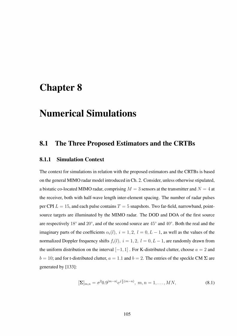
Chapter 8
Numerical Simulations
8.1 The Three Proposed Estimators and the CRTBs
8.1.1 Simulation Context
The context for simulations in relation with the proposed estimators and the CRTBs is based
on the general MIMO radar model introduced in Ch. 2. Consider, unless otherwise stipulated,
a bistatic co-located MIMO radar, comprisingM = 3 sensors at the transmitter andN = 4 at
the receiver, both with half-wave length inter-element spacing. The number of radar pulses
per CPI L = 15, and each pulse contains T = 5 snapshots. Two far-field, narrowband, point-
source targets are illuminated by the MIMO radar. The DOD and DOA of the first source
are respectively 18 and 20, and of the second source are 45 and 40. Both the real and the
imaginary parts of the coefficients αi(l), i = 1, 2, l = 0, L− 1, as well as the values of the
normalized Doppler frequency shifts fi(l), i = 1, 2, l = 0, L− 1, are randomly drawn from
the uniform distribution on the interval [−1, 1] . For K-distributed clutter, choose a = 2 and
b = 10; and for t-distributed clutter, a = 1.1 and b = 2. The entries of the speckle CM Σ are
generated by [133]:
[Σ]m,n = σ20.9|m−n|ejπ2
(m−n), m, n = 1, . . . ,MN, (8.1)
105
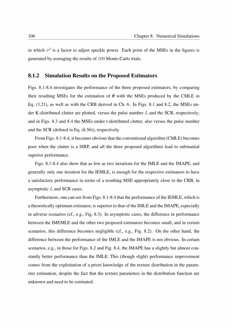
106 Chapter 8. Numerical Simulations
in which σ2 is a factor to adjust speckle power. Each point of the MSEs in the figures is
generated by averaging the results of 100 Monte-Carlo trials.
8.1.2 Simulation Results on the Proposed Estimators
Figs. 8.1-8.4 investigates the performance of the three proposed estimators, by comparing
their resulting MSEs for the estimation of θ with the MSEs produced by the CMLE in
Eq. (3.21), as well as with the CRB derived in Ch. 6. In Figs. 8.1 and 8.2, the MSEs un-
der K-distributed clutter are plotted, versus the pulse number L and the SCR, respectively;
and in Figs. 8.3 and 8.4 the MSEs under t-distributed clutter, also versus the pulse number
and the SCR (defined in Eq. (6.56)), respectively.
From Figs. 8.1-8.4, it becomes obvious that the conventional algorithm (CMLE) becomes
poor when the clutter is a SIRP, and all the three proposed algorithms lead to substantial
superior performance.
Figs. 8.1-8.4 also show that as few as two iterations for the IMLE and the IMAPE, and
generally only one iteration for the IEMLE, is enough for the respective estimators to have
a satisfactory performance in terms of a resulting MSE appropriately close to the CRB, in
asymptotic L and SCR cases.
Furthermore, one can see from Figs. 8.1-8.4 that the performance of the IEMLE, which is
a theoretically optimum estimator, is superior to that of the IMLE and the IMAPE, especially
in adverse scenarios (cf., e.g., Fig. 8.3). In asymptotic cases, the difference in performance
between the IMEMLE and the other two proposed estimators becomes small, and in certain
scenarios, this difference becomes negligible (cf., e.g., Fig. 8.2). On the other hand, the
difference between the performance of the IMLE and the IMAPE is not obvious. In certain
scenarios, e.g., in those for Figs. 8.2 and Fig. 8.4, the IMAPE has a slightly but almost con-
stantly better performance than the IMLE. This (though slight) performance improvement
comes from the exploitation of a priori knowledge of the texture distribution in the param-
eter estimation, despite the fact that the texture parameters in the distribution function are
unknown and need to be estimated.
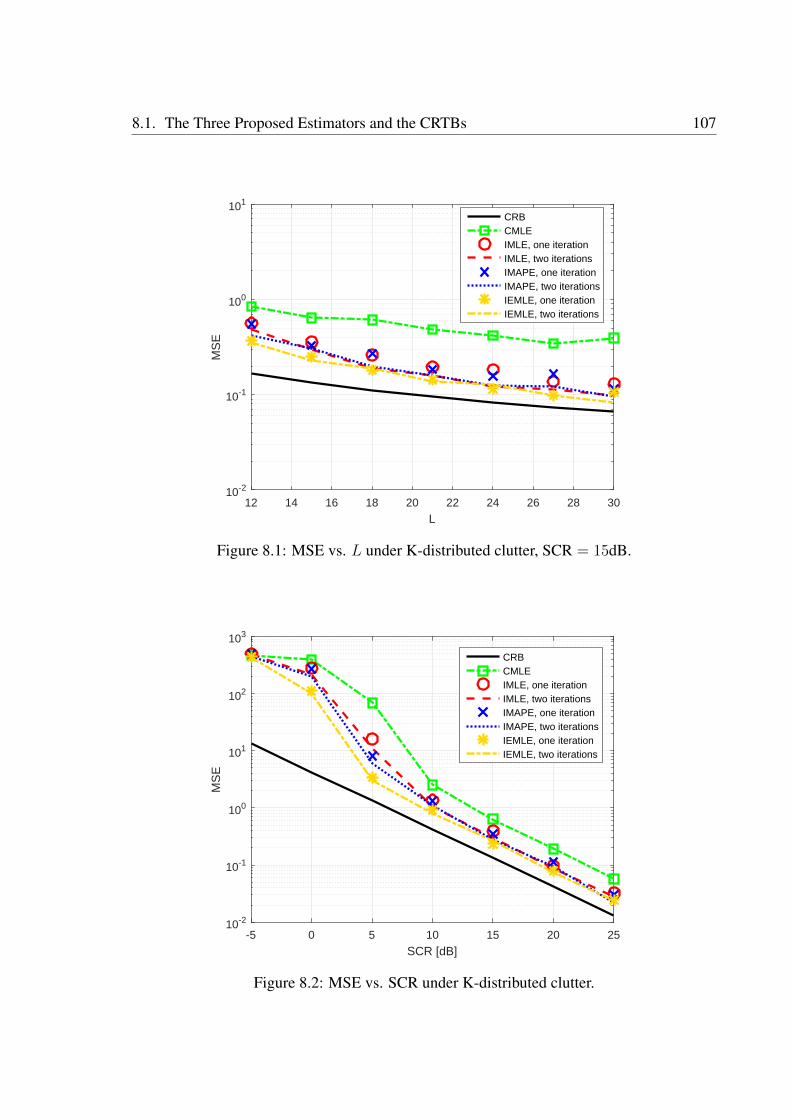
8.1. The Three Proposed Estimators and the CRTBs 107
12 14 16 18 20 22 24 26 28 30
L
10-2
10-1
100
101
MS
ECRBCMLEIMLE, one iterationIMLE, two iterationsIMAPE, one iterationIMAPE, two iterationsIEMLE, one iterationIEMLE, two iterations
Figure 8.1: MSE vs. L under K-distributed clutter, SCR = 15dB.
-5 0 5 10 15 20 25
SCR [dB]
10-2
10-1
100
101
102
103
MS
E
CRBCMLEIMLE, one iterationIMLE, two iterationsIMAPE, one iterationIMAPE, two iterationsIEMLE, one iterationIEMLE, two iterations
Figure 8.2: MSE vs. SCR under K-distributed clutter.
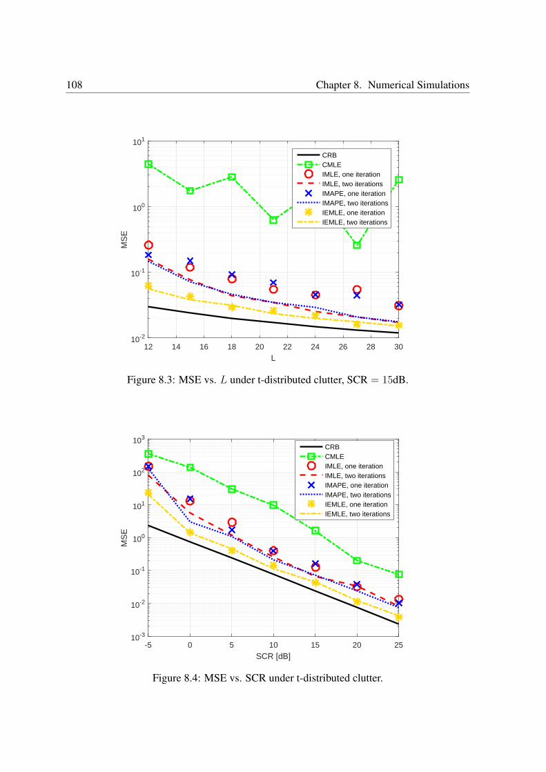
108 Chapter 8. Numerical Simulations
12 14 16 18 20 22 24 26 28 30
L
10-2
10-1
100
101
MS
E
CRBCMLEIMLE, one iterationIMLE, two iterationsIMAPE, one iterationIMAPE, two iterationsIEMLE, one iterationIEMLE, two iterations
Figure 8.3: MSE vs. L under t-distributed clutter, SCR = 15dB.
-5 0 5 10 15 20 25
SCR [dB]
10-3
10-2
10-1
100
101
102
103
MS
E
CRBCMLEIMLE, one iterationIMLE, two iterationsIMAPE, one iterationIMAPE, two iterationsIEMLE, one iterationIEMLE, two iterations
Figure 8.4: MSE vs. SCR under t-distributed clutter.
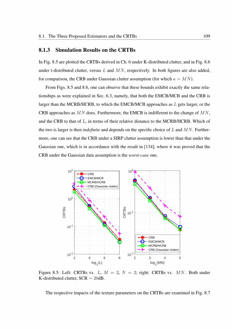
8.1. The Three Proposed Estimators and the CRTBs 109
8.1.3 Simulation Results on the CRTBs
In Fig. 8.5 are plotted the CRTBs derived in Ch. 6 under K-distributed clutter, and in Fig. 8.6
under t-distributed clutter, versus L and MN , respectively. In both figures are also added,
for comparison, the CRB under Gaussian clutter assumption (for which κ = MN ).
From Figs. 8.5 and 8.6, one can observe that these bounds exhibit exactly the same rela-
tionships as were explained in Sec. 6.3, namely, that both the EMCB/MCB and the CRB is
larger than the MCRB/HCRB, to which the EMCB/MCB approaches as L gets larger, or the
CRB approaches as MN does. Furthermore, the EMCB is indifferent to the change of MN ,
and the CRB to that of L, in terms of their relative distance to the MCRB/HCRB. Which of
the two is larger is then indefinite and depends on the specific choice of L and MN . Further-
more, one can see that the CRB under a SIRP clutter assumption is lower than that under the
Gaussian one, which is in accordance with the result in [134], where it was proved that the
CRB under the Gaussian data assumption is the worst-case one.
2 3 4 5log
2(MN)
10-2
10-1
100
CR
TB
s
CRBEMCB/MCBMCRB/HCRBCRB (Gaussian clutter)
2 4 6 8log
2(L)
10-2
10-1
100
101
CR
TB
s
CRBEMCB/MCBMCRB/HCRBCRB (Gaussian clutter)
Figure 8.5: Left: CRTBs vs. L, M = 2, N = 2; right: CRTBs vs. MN . Both underK-distributed clutter, SCR = 20dB.
The respective impacts of the texture parameters on the CRTBs are examined in Fig. 8.7
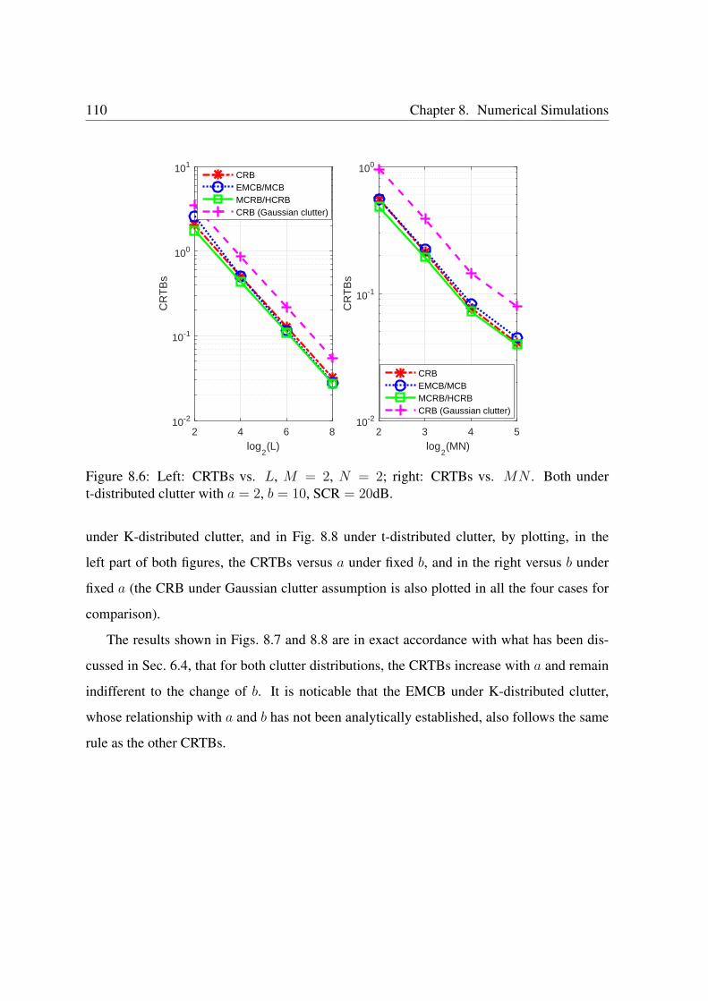
110 Chapter 8. Numerical Simulations
2 3 4 5log
2(MN)
10-2
10-1
100
CR
TB
s
CRBEMCB/MCBMCRB/HCRBCRB (Gaussian clutter)
2 4 6 8log
2(L)
10-2
10-1
100
101C
RT
Bs
CRBEMCB/MCBMCRB/HCRBCRB (Gaussian clutter)
Figure 8.6: Left: CRTBs vs. L, M = 2, N = 2; right: CRTBs vs. MN . Both undert-distributed clutter with a = 2, b = 10, SCR = 20dB.
under K-distributed clutter, and in Fig. 8.8 under t-distributed clutter, by plotting, in the
left part of both figures, the CRTBs versus a under fixed b, and in the right versus b under
fixed a (the CRB under Gaussian clutter assumption is also plotted in all the four cases for
comparison).
The results shown in Figs. 8.7 and 8.8 are in exact accordance with what has been dis-
cussed in Sec. 6.4, that for both clutter distributions, the CRTBs increase with a and remain
indifferent to the change of b. It is noticable that the EMCB under K-distributed clutter,
whose relationship with a and b has not been analytically established, also follows the same
rule as the other CRTBs.
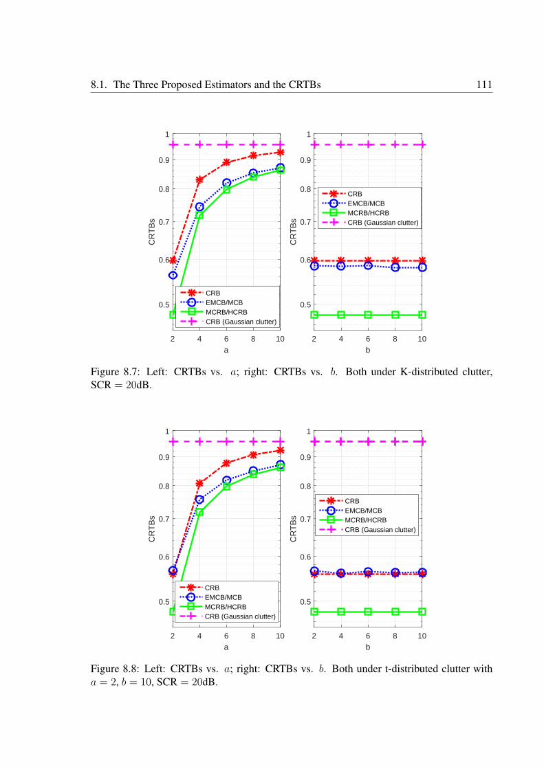
8.1. The Three Proposed Estimators and the CRTBs 111
2 4 6 8 10
a
0.5
0.6
0.7
0.8
0.9
1
CR
TB
s
CRBEMCB/MCBMCRB/HCRBCRB (Gaussian clutter)
2 4 6 8 10
b
0.5
0.6
0.7
0.8
0.9
1
CR
TB
s
CRBEMCB/MCBMCRB/HCRBCRB (Gaussian clutter)
Figure 8.7: Left: CRTBs vs. a; right: CRTBs vs. b. Both under K-distributed clutter,SCR = 20dB.
2 4 6 8 10
b
0.5
0.6
0.7
0.8
0.9
1
CR
TB
s
CRBEMCB/MCBMCRB/HCRBCRB (Gaussian clutter)
2 4 6 8 10
a
0.5
0.6
0.7
0.8
0.9
1
CR
TB
s
CRBEMCB/MCBMCRB/HCRBCRB (Gaussian clutter)
Figure 8.8: Left: CRTBs vs. a; right: CRTBs vs. b. Both under t-distributed clutter witha = 2, b = 10, SCR = 20dB.
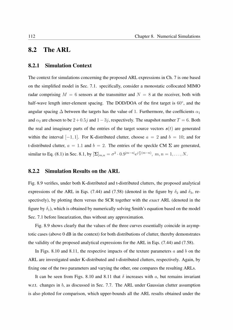
112 Chapter 8. Numerical Simulations
8.2 The ARL
8.2.1 Simulation Context
The context for simulations concerning the proposed ARL expressions in Ch. 7 is one based
on the simplified model in Sec. 7.1. specifically, consider a monostatic collocated MIMO
radar comprising M = 6 sensors at the transmitter and N = 8 at the receiver, both with
half-wave length inter-element spacing. The DOD/DOA of the first target is 60, and the
angular spacing ∆ between the targets has the value of 1. Furthermore, the coefficients α1
and α2 are chosen to be 2 + 0.5j and 1−3j, respectively. The snapshot number T = 6. Both
the real and imaginary parts of the entries of the target source vectors s(t) are generated
within the interval [−1, 1]. For K-distributed clutter, choose a = 2 and b = 10; and for
t-distributed clutter, a = 1.1 and b = 2. The entries of the speckle CM Σ are generated,
similar to Eq. (8.1) in Sec. 8.1, by [Σ]m,n = σ2 · 0.9|m−n|ej π2 (m−n), m, n = 1, . . . , N .
8.2.2 Simulation Results on the ARL
Fig. 8.9 verifies, under both K-distributed and t-distributed clutters, the proposed analytical
expressions of the ARL in Eqs. (7.44) and (7.58) (denoted in the figure by δ2 and δ3, re-
spectively), by plotting them versus the SCR together with the exact ARL (denoted in the
figure by δ1), which is obtained by numerically solving Smith’s equation based on the model
Sec. 7.1 before linearization, thus without any approximation.
Fig. 8.9 shows clearly that the values of the three curves essentially coincide in asymp-
totic cases (above 0 dB in the context) for both distributions of clutter, thereby demonstrates
the validity of the proposed analytical expressions for the ARL in Eqs. (7.44) and (7.58).
In Figs. 8.10 and 8.11, the respective impacts of the texture parameters a and b on the
ARL are investigated under K-distributed and t-distributed clutters, respectively. Again, by
fixing one of the two parameters and varying the other, one compares the resulting ARLs.
It can be seen from Figs. 8.10 and 8.11 that δ increases with a, but remains invariant
w.r.t. changes in b, as discussed in Sec. 7.7. The ARL under Gaussian clutter assumption
is also plotted for comparison, which upper-bounds all the ARL results obtained under the
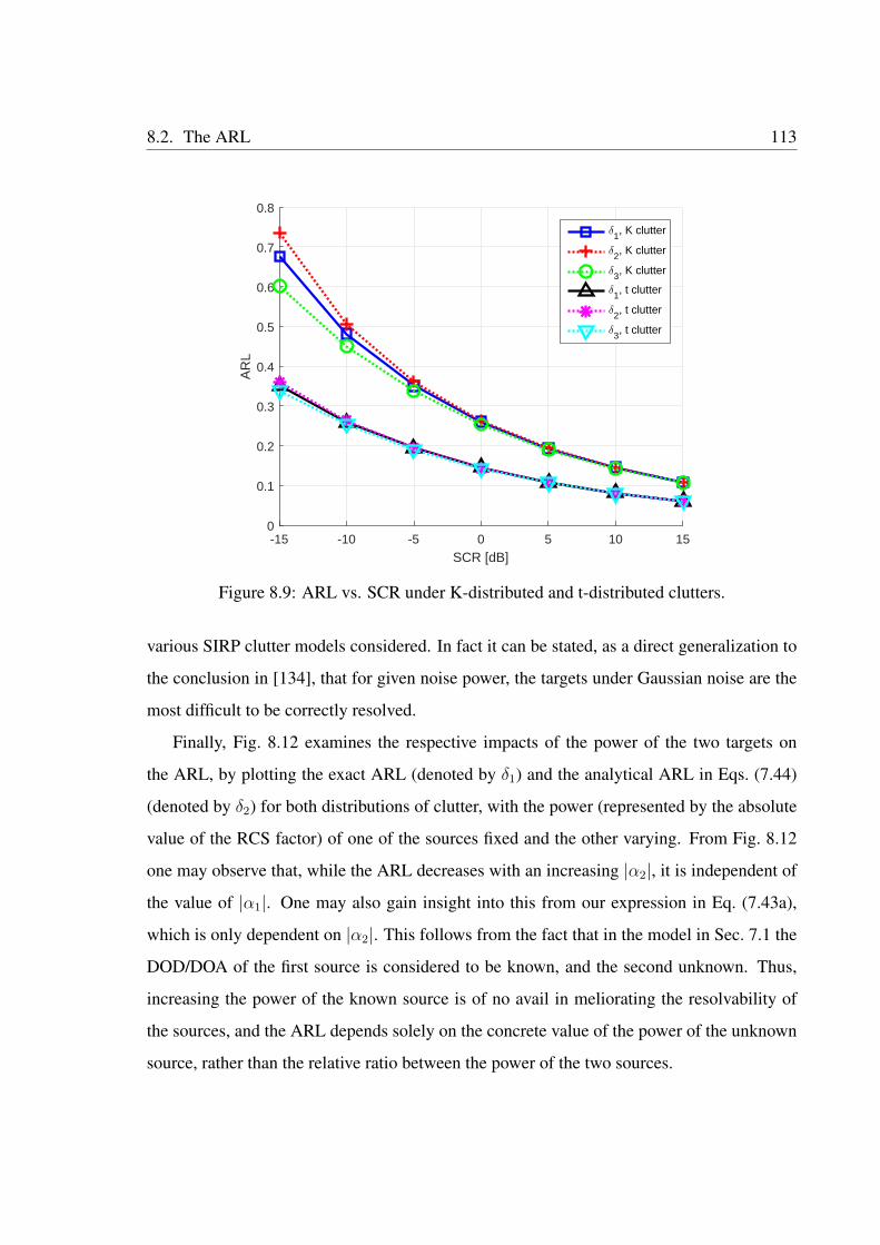
8.2. The ARL 113
-15 -10 -5 0 5 10 15
SCR [dB]
0
0.1
0.2
0.3
0.4
0.5
0.6
0.7
0.8
AR
Lδ
1, K clutter
δ2, K clutter
δ3, K clutter
δ1, t clutter
δ2, t clutter
δ3, t clutter
Figure 8.9: ARL vs. SCR under K-distributed and t-distributed clutters.
various SIRP clutter models considered. In fact it can be stated, as a direct generalization to
the conclusion in [134], that for given noise power, the targets under Gaussian noise are the
most difficult to be correctly resolved.
Finally, Fig. 8.12 examines the respective impacts of the power of the two targets on
the ARL, by plotting the exact ARL (denoted by δ1) and the analytical ARL in Eqs. (7.44)
(denoted by δ2) for both distributions of clutter, with the power (represented by the absolute
value of the RCS factor) of one of the sources fixed and the other varying. From Fig. 8.12
one may observe that, while the ARL decreases with an increasing |α2|, it is independent of
the value of |α1|. One may also gain insight into this from our expression in Eq. (7.43a),
which is only dependent on |α2|. This follows from the fact that in the model in Sec. 7.1 the
DOD/DOA of the first source is considered to be known, and the second unknown. Thus,
increasing the power of the known source is of no avail in meliorating the resolvability of
the sources, and the ARL depends solely on the concrete value of the power of the unknown
source, rather than the relative ratio between the power of the two sources.
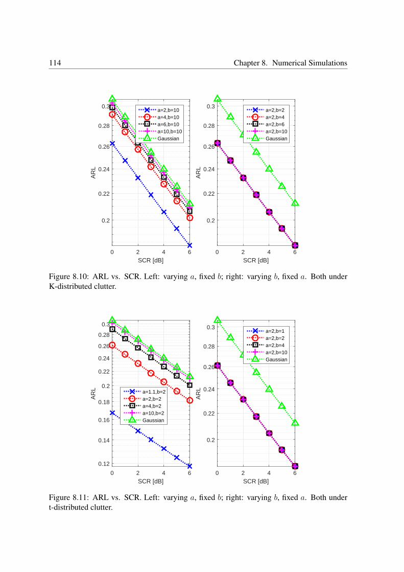
114 Chapter 8. Numerical Simulations
0 2 4 6
SCR [dB]
0.2
0.22
0.24
0.26
0.28
0.3
AR
L
a=2,b=10a=4,b=10a=6,b=10a=10,b=10Gaussian
0 2 4 6
SCR [dB]
0.2
0.22
0.24
0.26
0.28
0.3
AR
L
a=2,b=2a=2,b=4a=2,b=6a=2,b=10Gaussian
Figure 8.10: ARL vs. SCR. Left: varying a, fixed b; right: varying b, fixed a. Both underK-distributed clutter.
0 2 4 6
SCR [dB]
0.12
0.14
0.16
0.18
0.2
0.22
0.24
0.26
0.28
0.3
AR
L a=1.1,b=2a=2,b=2a=4,b=2a=10,b=2Gaussian
0 2 4 6
SCR [dB]
0.2
0.22
0.24
0.26
0.28
0.3
AR
L
a=2,b=1a=2,b=2a=2,b=4a=2,b=10Gaussian
Figure 8.11: ARL vs. SCR. Left: varying a, fixed b; right: varying b, fixed a. Both undert-distributed clutter.
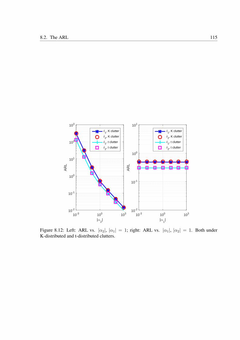
8.2. The ARL 115
10-3 100 103
|α2|
10-2
10-1
100
101
102
103
AR
L
δ1, K clutter
δ2, K clutter
δ1, t clutter
δ2, t clutter
10-3 100 103
|α1|
10-2
10-1
100
101
AR
Lδ
1, K clutter
δ2, K clutter
δ1, t clutter
δ2, t clutter
Figure 8.12: Left: ARL vs. |α2|, |α1| = 1; right: ARL vs. |α1|, |α2| = 1. Both underK-distributed and t-distributed clutters.

116 Chapter 8. Numerical Simulations
Chapter 9
Conclusions and Outlook
9.1 Conclusions
This thesis is dedicated to a systematic and comprehensive investigation into the DOD/DOA
estimation problem for MIMO radar targets in the presence of SIRP clutter, both in respect of
algorithm design and of performance analysis. The three proposed independent but intercon-
nected estimators in Chs. 3, 4 and 5, which employ the stepwise numerical concentration ap-
proach, are proved by the simulation results in Ch. 8 to be both performant and considerably
computationally efficient, as all of them require only a few iterations to attain convergence,
and lead to significantly superior performance than the conventional ML approach.
The IMLE proposed in Chs. 3 considers the texture realizations as unknown parameters
and ignores the statistical distribution of the texture. Thus it is the most robust among the
three proposed estimators, as it does not require any knowledge of the texture distribution.
By using the estimated texture realizations as weighting factors in its objective function, it
achieves significantly better performance than the conventional ML estimator. Furthermore,
it is the computationally simplest among the three proposed estimators, because it does not
entail any numerical calculation of integrals, nor does it need to numerically solve nonlinear
equations to obtain the estimates of the texture parameters.
The IMAPE proposed in Chs. 4, on the other hand, can be seen as a generalization of
the IMLE from a Bayesian point of view. It also considers texture realizations, but exploits
117
118 Chapter 9. Conclusions and Outlook
at the same time the information from the texture distribution to improve the estimation
accuracy. Furthermore, unlike the IMLE, the IMAPE can also be used to estimate the texture
parameters if this is a task.
The IEMLE proposed in Chs. 5, by considering the exact LLF, is a theoretically optimum
estimator. The IEMLE does not consider the texture realizations, but only the texture distri-
bution (in terms of the texture parameters). The objective function of the IEMLE, by taking
the form of multiplication other than summation, is essentially different from the one of the
IMLE and the IMAPE. In such a way, it can focus on the best pulses, while the IMLE and
the IMAPE treat all pulses equally. Thus, it has the superior performance among the three
proposed estimators, especially in adverse scenarios.
As measures of performance for the proposed algorithms, expressions for various CRTBs
w.r.t. DOD/DOA parameters are derived in Ch. 6, and their relationships are analytically
compared. Furthermore, inspection of the texture parameters’ respective effects on the
CRTBs reveals that all of the CRTBs have a positive correlation with the shape parame-
ter, but are all independent of the scale parameter. Thus the achievable estimation accuracy
diminishes as the shape parameter increases, but is not affected by the change of the scale
parameter. The reason for this is that, with fixed clutter power, an increase in the value of
the shape parameter causes the clutter to become more heavy-tailed, signifying a larger por-
tion of clutter power being decentralized; on the other hand, changing the scale parameter’s
value does not result in any change in the PDF of the clutter. Moreover, the CRTBs under a
SIRP clutter model are upper-bounded by those under a Gaussian one (with the same clutter
power), meaning that the achievable performance for estimation problems in the presence of
the SIRP clutter is always better than that in the presence of the Gaussian clutter.
Apart from the CRTBs, this thesis also studies another important performance measure
of estimation problems, namely, the target resolvability quantified by the RL. Based on the
non-matrix form expression for the CRB w.r.t. the target spacing, which is derived as a by-
product, two analytical expressions for the ARL are obtained in Ch. 7. The effects of the
texture parameters on the ARL are then explored, which are analogous to their effect on the
CRTBs. Furthermore, the proposed ARL expressions reveal that increasing the power of
9.2. Outlook 119
the known source cannot meliorate the resolvability of the sources, and the ARL depends
solely on the concrete value of the power of the unknown source, rather than the relative
ratio between the power of the two sources.
The analytical findings on the CRTBs and the ARL are also numerically corroborated by
simulations in Ch. 8.
9.2 Outlook
Proceeding from the contributions of this thesis summarized above, possible future works
may include, first of all, finding appropriate, more competent numerical analysis methods
for the calculation of numerical integrals involved in the IEMLE for K-distributed clutter
case, as well as for the numerical nonlinear equation solving problems involved both in the
IMAPE and the IEMLE. These numerical calculations constitute a major factor that adds
to the computational costs of the proposed algorithms (though they are generally already
substantially more computationally efficient as compared with some other iterative, e.g.,
PX-EM-based algorithms).
The proposed algorithms can also be applied to MIMO radar detection problems with
unknown target DOD/DOA parameters and other research topics based on such detection
problems, e.g., the RL based on the GLRT.
Furthermore, as generalizations of the DOA estimation algorithms in [106] and [123] to
the SIRP clutter case, the proposed algorithms in this thesis also have the potential to be
generalized, in their turn, to more complicated clutter cases. One such possibility is the case
where the whole radar noise is modeled as a mixture of SIRP and Gaussian clutter/noise.
This modeling not only becomes necessary in scenarios where the thermal noise (modeled
as Gaussian) cannot be ignored compared with the clutter (modeled as a SIRP) [135, 136],
but can also be used to describe contemporaneous backscattering by ground/clouds (whose
clutter is modeled as Gaussian) and sea (whose clutter is modeled as a SIRP) [28, 137]. A
main challenge of the generalization of the proposed algorithms to such a SIRP-Gaussian
mixture clutter context is that, under this model, the expressions of the LLFs become more
complicated, therefore many of the unknown parameter estimates that have closed-form ex-
120 Chapter 9. Conclusions and Outlook
pressions under SIRP clutter model can no longer have them, if no approximation is made to
the LLFs. However, at least for certain special cases, e.g., the case of white Gaussian speckle,
this problem disappears, and the generalization in question becomes rather straightforward.
Besides the SIRP-Gaussian mixture clutter model above, there are also two important
non-Gaussian clutter models related to the SIRP model, to which the proposed algorithms
have the potential to be generalized. One of them is the so-called generalized Bessel K
(GBK) distributed clutter, proposed in [138], the class of which partially overlaps that of
the SIRPs, but covers a wider variety of distributions. The other is the so-called complex
elliptically symmetric (CES) distributed clutter [139], which constitutes a broader class to
which SIRPs belong. Both models have till now attracted considerable research interest
concerning radar detection/estimation problems [138, 140–145], and the generalization of
the proposed algorithms to these more general non-Gaussian clutter models is of significant
practical value.
In parallel to the proposed algorithms, the expressions for the CRTBs w.r.t. DOD/DOA
paramters and for the ARL are also worth investigation under the framework of the SIRP-
Gaussian mixture, the GBK and the CES clutter models.
Bibliography
[1] E. Fishler, “MIMO radar: an idea whose time has come,” in Proc. IEEE Radar Con-
ference, Philadelphia, PA, Apr. 2004, pp. 71–78.
[2] J. Li and P. Stoica, “MIMO radar with colocated antennas,” IEEE Signal Processing
Mag., vol. 24, no. 5, pp. 106–114, Sep. 2007.
[3] ——, MIMO radar Signal Processing. New York: Wiley-Interscience, Oct. 2008.
[4] A. Haimovich, R. Blum, and L. Cimini, “MIMO radar with widely separated anten-
nas,” IEEE Signal Processing Mag., vol. 25, pp. 116–129, Jan. 2008.
[5] E. Fishier, A. Haimovich, R. Blum, L. Cimini, D. Chizhik, and R. Valenzuela, “Sta-
tistical MIMO radar,” in Proc. Adaptive Sensor Array Processing (ASAP) Workshop,
Lexington, MA, Mar. 2004.
[6] D. W. Bliss and K. W. Forsythe, “Multiple-input multiple-output (MIMO) radar and
imaging: Degrees of freedom and resolution,” in Proc. 37th Asilomar Conf. Signals,
Syst. Comput., vol. 1, Pacifc Grove, CA, Nov. 2003, pp. 54–59.
[7] D. J. Rabideau and P. Parker, “Ubiquitous MIMO multifunction digital array radar,”
in Proc. 37th Asilomar Conf. Signals, Syst. Comput., vol. 1, Pacifc Grove, CA, Nov.
2003, p. 1057–1064.
[8] E. Fishler, A. M. Haimovich, R. S. Blum, J. L. J. Cimini, D. Chizhik, and R. A. Valen-
zuela, “Spatial diversity in radars-models and detection performance,” IEEE Trans.
Signal Processing, vol. 54, no. 3, p. 823–838, Mar. 2006.
121
122 Bibliography
[9] N. H. Lehmann, A. M. Haimovich, R. S. Blum, and L. J. Cimini, “High resolution
capabilities of MIMO radar,” in Proc. 40th Asilomar Conf. Signals, Syst. Comput.,
Pacifc Grove, CA, Nov. 2006, pp. 25–30.
[10] E. F. Knott, J. F. Schaeffer, and M. T. Tulley, Radar Cross Section, 2nd ed. Boston:
Artech House, 1993.
[11] I. Bekkerman and J. Tabrikian, “Target detection and localization using MIMO radars
and sonars,” IEEE Trans. Signal Processing, vol. 54, no. 10, pp. 3873–3883, Oct.
2006.
[12] C.-Y. Chen and P. P. Vaidyanathan, “MIMO radar space-time adaptive processing us-
ing prolate spheroidal wave functions,” IEEE Trans. Signal Processing, vol. 56, no. 2,
pp. 623–635, Feb. 2008.
[13] X. Wang, W. Wang, J. Liu, X. Li, and J. Wang, “A sparse representation scheme for
angle estimation in monostatic MIMO radar,” Signal Processing, vol. 104, pp. 258–
263, Nov. 2014.
[14] W. Wang, X. Wang, H. Song, and Y. Ma, “Conjugate ESPRIT for DOA estimation in
monostatic MIMO radar,” Signal Processing, vol. 93, no. 7, p. 2070–2075, Jul. 2013.
[15] M. Jin, G. Liao, and J. Li, “Joint DOD and DOA estimation for bistatic MIMO radar,”
Signal Processing, vol. 89, no. 2, pp. 244–251, Feb. 2009.
[16] J. Chen, H. Gu, and W. Su, “A new method for joint DOD and DOA estimation in
bistatic MIMO radar,” Signal Processing, vol. 2, pp. 714–718, Feb. 2010.
[17] H. W. Chen, D. Yang, H.-Q. Wang, X. Li, and Z. Zhuang, “Direction finding for
bistatic MIMO radar using EM maximum likelihood algorithm,” Progress In Electro-
magnetics Research, vol. 141, pp. 99–116, Jul. 2013.
[18] T.-Q. Xia, “Joint diagonalization based DOD and DOA estimation for bistatic MIMO
radar,” Signal Processing, vol. 108, pp. 159–166, Mar. 2015.
Bibliography 123
[19] B. R. Mahafza, Radar Systems Analysis and Design Using MATLAB, 3rd ed. CRC
Press, 2013.
[20] J. B. Billingsley, “Ground clutter measurements for surface-sited radar,” Mas-
sachusetts Inst. Technol., Cambridge, MA, Tech. Rep. 780, Feb. 1993.
[21] F. Gini, M. V. Greco, M. Diani, and L. Verrazzani, “Performance analysis of two adap-
tive radar detectors against non-Gaussian real sea clutter data,” IEEE Trans. Aerosp.
Electron. Syst., vol. 36, no. 4, pp. 1429–1439, Oct. 2000.
[22] K. Yao, “Spherically invariant random processes: Theory and applications,” in Com-
munications, Information and Network Security, V. K. B. et al., Ed., 2002, pp. 315–
332.
[23] ——, “A representation theorem and its applications to spherically invariant random
processes,” IEEE Trans. Inf. Theory, vol. 19, no. 5, pp. 600–608, Sep. 1973.
[24] M. Rangaswamy, D. D. Weiner, and A. Ozturk, “Non-Gaussian vector identification
using spherically invariant random processes,” IEEE Trans. Aerosp. Electron. Syst.,
vol. 29, no. 1, pp. 111–124, Jan. 1993.
[25] A. M. Vershik, “Some characteristic properties of Gaussian stochastic processes,”
Theory Probab. Appl., vol. 9, no. 2, pp. 353–356, 1964.
[26] E. Jakeman and P. N. Pusey, “A model for non-Rayleigh sea echo,” IEEE Trans. An-
tennas Propag., vol. 24, no. 6, pp. 806–814, Nov. 1976.
[27] E. Conte and G. Ricci, “Performance prediction in compound-Gaussian clutter,” IEEE
Trans. Aerosp. Electron. Syst., vol. 30, no. 2, pp. 611–616, Apr. 1994.
[28] F. Gini, “Sub-optimum coherent radar detection in a mixture of K-distributed and
Gaussian clutter,” IEE Proceedings - Radar, Sonar and Navigation, vol. 114, no. 1,
pp. 39–48, Feb. 1997.
[29] M. Greco, F. Bordoni, and F. Gini, “X-band see-clutter nonstationarity: Influence of
long waves,” IEEE J. Ocean. Eng., vol. 29, no. 2, pp. 269–283, Apr. 2004.
124 Bibliography
[30] M. Rangaswamy, “Spherically invariant random processes for modeling non-Gaussian
radar clutter,” in Proc. 27th Asilomar Conf. Signals, Syst. Comput., vol. 2, Pacifc
Grove, CA, Nov. 1993, pp. 1106–1110.
[31] H. Krim and M. Viberg, “Two decades of array signal processing research: the para-
metric approach,” IEEE Signal Processing Mag., vol. 13, no. 4, pp. 67–94, 1996.
[32] D. H. Johnson and D. E. Dudgeon, Array Signal Processing: Concepts and Tech-
niques, 1st ed. Prentice-Hall, 1993.
[33] P. Stoica and R. L. Moses, Spectral Analysis of Signals. NJ: Prentice Hall, 2005.
[34] R. Schmidt, “Multiple emitter location and signal parameter estimation,” IEEE Trans.
Antennas Propagat., vol. 34, no. 3, pp. 276–280, Mar. 1986.
[35] P. Stoica and A. Nehorai, “MUSIC, maximum likelihood and Cramer-Rao bound,”
IEEE Trans. Acoust., Speech, Signal Processing, vol. 37, no. 5, pp. 720–741, May
1989.
[36] H. Krim, P. Forster, and J. G. Proakis, “Operator approach to performance analysis of
root-MUSIC and root-min-norm,” IEEE Trans. Signal Processing, vol. 40, no. 7, pp.
1687–1696, Jul. 1992.
[37] B. Rao and K. Hari, “Performance analysis of root-MUSIC,” IEEE Trans. Acoust.,
Speech, Signal Processing, vol. 37, no. 12, pp. 1939–1949, Dec. 1989.
[38] J. Mosher and R. Leahy, “Source localization using recursivaly applied and projected
(rap) music,” IEEE Trans. Signal Processing, vol. 47, pp. 332–340, Feb. 1999.
[39] R. Roy, A. Paulraj, and T. Kailath, “ESPRIT a subspace rotation approach to estima-
tion of parameters of cisoids in noise,” IEEE Trans. Acoust., Speech, Signal Process-
ing, vol. 34, pp. 1340–1342, 1986.
[40] N. Yuen and B. Friedlander, “Performance analysis of higher order ESPRIT for local-
ization of near-field sources,” IEEE Trans. Signal Processing, vol. 46, pp. 709–719,
Mar. 1998.
Bibliography 125
[41] K. Wong and M. Zoltowski, “Uni-vector-sensor ESPRIT for multisource azimuth, ele-
vation, andpolarization estimation,” IEEE Trans. Antennas Propagat., vol. 45, no. 10,
pp. 1467–1474, Oct. 1997.
[42] J. Li and R. Compton, “Angle and polarization estimation using esprit with a polariza-
tionsensitive array,” IEEE Trans. Antennas Propagat., vol. 39, no. 9, pp. 1376–1383,
Sep. 1991.
[43] M. Haardt and J. Nossek, “3-D unitary ESPRIT for joint 2-D angle and carrier estima-
tion,” in Proc. of IEEE Int. Conf. Acoust., Speech, Signal Processing (ICASSP), vol. 1,
Munich, Germany, 1997, pp. 255–258.
[44] S. M. Kay, Fundamentals of Statistical Signal Processing : Estimation Theory. NJ:
Prentice Hall, 1993, vol. 1.
[45] J. F. Böhme, “Estimation of source parameters by maximum likelihood and non linear
regression,” in Proc. of IEEE Int. Conf. Acoust., Speech, Signal Processing (ICASSP),
1984, pp. 731–734.
[46] M. Wax, “Detection and localization of multiple sources in noise with unknown co-
variance,” IEEE Trans. Signal Processing, vol. 40, no. 1, pp. 245–249, Jan. 1992.
[47] A. G. Jaffer, “Maximum likelihood direction finding of stochastic sources: a separable
solution,” in Proc. of IEEE Int. Conf. Acoust., Speech, Signal Processing (ICASSP),
New York, 1988.
[48] J. F. Böhme, “Estimation of spectral parameters of correlated signals in wavefields,”
Signal Processing, vol. 10, pp. 329–337, 1986.
[49] H. L. VanTrees, Detection, Estimation and Modulation Theory. New York: Wiley,
1968, vol. 1.
[50] A. Renaux, P. Forster, E. Chaumette, and P. Larzabal, “On the high SNR conditional
maximum-likelihood estimator full statistical characterization,” IEEE Trans. Signal
Processing, vol. 12, no. 54, pp. 4840–4843, Dec. 2006.
126 Bibliography
[51] B. Ottersten, M. Viberg, P. Stoica, and A. Nehorai, “Exact and large sample maximum
likelihood techniques for parameter estimation and detection in array processing,”
in Radar Array Processing, S. Haykin, J. Litva, and T. J. Shepherd, Eds. Berlin:
Springer-Verlag, 1993, ch. 4, pp. 99–151.
[52] F. Gini and R. Reggiannini, “On the use of Cramér-Rao-like bounds in the presence of
random nuisance parameters,” IEEE Trans. Commun., vol. 48, no. 12, pp. 2120–2126,
Dec. 2000.
[53] R. W. Miller and C. B. Chang, “A modified Cramér-Rao bound and its applications,”
IEEE Trans. Inform. Theory, vol. 24, no. 3, pp. 398–400, May 1978.
[54] I. Reuven and H. Messer, “A Barankin-type lower bound on the estimation error of a
hybrid parameter vector,” IEEE Trans. Inform. Theory, vol. 43, no. 3, pp. 1084–1093,
May 1997.
[55] S. Narasimhan and J. Krolik, “Fundamental limits on acoustic source range estimation
performance in uncertain ocean channels,” J. Acoust. Soc. Am., vol. 97, no. 1, pp. 215–
226, Jan. 1995.
[56] A. N. D’Andrea, U. Mengali, and R. Reggiannini, “The modified Cramér-Rao bound
and its application to synchronization problems,” IEEE Trans. Commun., vol. 42, no.
2/3/4, pp. 1391–1399, Feb./Mar./Apr. 1994.
[57] F. Gini, R. Reggiannini, and U. Mengali, “The modified Cramér-Rao bound in vector
parameter estimation,” IEEE Trans. Commun., vol. 46, no. 1, pp. 52–60, Jan. 1998.
[58] S. T. Smith, “Statistical resolution limits and the complexified Cramér Rao bound,”
IEEE Trans. Signal Processing, vol. 53, no. 5, pp. 1597–1609, May 2005.
[59] M. Shahram and P. Milanfar, “On the resolvability of sinusoids with nearby frequen-
cies in the presence of noise,” IEEE Trans. Signal Processing, vol. 53, no. 7, pp.
2579–2588, Jul. 2005.
Bibliography 127
[60] M. N. El Korso, R. Boyer, A. Renaux, and S. Marcos, “Statistical resolution limit for
multiple parameters of interest and for multiple signals,” in Proc. of IEEE Int. Conf.
Acoust., Speech, Signal Processing (ICASSP), Dallas, TX, Mar. 2010, pp. 3602–3605.
[61] H. Cox, “Resolving power and sensitivity to mismatch of optimum array processors,”
J. Acoust. Soc., vol. 54, no. 3, pp. 771–785, Mar. 1973.
[62] K. Sharman and T. Durrani, “Resolving power of signal subspace methods for fnite
data lengths,” in ICASSP, Florida, USA, 1995, pp. 1501–1504.
[63] M. Shahram and P. Milanfar, “Imaging below the diffraction limit: A statistical anal-
ysis,” IEEE Trans. Image Processing, vol. 13, no. 5, pp. 677–689, May 2004.
[64] Z. Liu and A. Nehorai, “Statistical angular resolution limit for point sources,” IEEE
Trans. Signal Processing, vol. 55, no. 11, pp. 5521–5527, Nov. 2007.
[65] A. Amar and A. Weiss, “Fundamental limitations on the resolution of deterministic
signals,” IEEE Trans. Signal Processing, vol. 56, no. 11, pp. 5309–5318, Nov. 2008.
[66] M. N. El Korso, R. Boyer, A. Renaux, and S. Marcos, “Statistical analysis of achiev-
able resolution limit in the near field source localization context,” Signal Processing,
vol. 92, no. 2, pp. 547–552, Feb. 2012.
[67] ——, “On the asymptotic resolvability of two point sources in known subspace in-
terference using a GLRT-based framework,” Signal Processing, vol. 92, no. 10, pp.
2471–2483, Oct. 2012.
[68] H. B. Lee, “The Cramér-Rao bound on frequency estimates of signals closely spaced
in frequency,” IEEE Trans. Signal Processing, vol. 40, no. 6, pp. 1507–1517, Jun.
1992.
[69] M. N. El Korso, R. Boyer, A. Renaux, and S. Marcos, “Statistical resolution limit of
the uniform linear cocentered orthogonal loop and dipole array,” IEEE Trans. Signal
Processing, vol. 59, no. 1, pp. 425–431, Jan. 2011.
128 Bibliography
[70] X. Zhang, M. N. El Korso, and M. Pesavento, “On the asymptotic resolvability of
far-field stochastic sources,” in Proc. EUSIPCO, Bucharest, Romania, Aug. 2012, pp.
889–893.
[71] ——, “Angular resolution limit for deterministic correlated sources,” in Proc. of IEEE
Int. Conf. Acoust., Speech, Signal Processing (ICASSP), Vancouver, Canada, May
2013, pp. 5539–5543.
[72] H. B. Lee, “The Cramér-Rao bound on frequency estimates of signals closely spaced
in frequency (unconditional case),” IEEE Trans. Signal Processing, vol. 42, no. 6, pp.
1569–1572, Jun. 1994.
[73] E. L. Lehmann, Theory of Point Estimation. New York: Wiley, 1983.
[74] M. Kaveh and A. J. Barabell, “The statistical performance of the MUSIC and the
minimum-norm algorithms in resolving plane waves in noise,” IEEE Trans. Acoust.,
Speech, Signal Processing, vol. 34, no. 2, pp. 331–341, Apr. 1986.
[75] E. Dilaveroglu, “Nonmatrix Cramér-Rao bound expressions for high-resolution fre-
quency estimators,” IEEE Trans. Signal Processing, vol. 46, no. 2, pp. 463–474, Feb.
1998.
[76] R. Boyer, “Performance bounds and angular resolution limit for the moving co-located
MIMO radar,” IEEE Trans. Signal Processing, vol. 59, no. 4, pp. 1539–1552, Apr.
2011.
[77] M. N. El Korso, R. Boyer, A. Renaux, and S. Marcos, “Statistical resolution limit for
source localization with clutter interference in a MIMO radar context,” IEEE Trans.
Signal Processing, vol. 60, no. 5, pp. 987–992, Feb. 2012.
[78] M. N. El Korso, F. Pascal, and M. Pesavento, “On the resolvability of closely spaced
targets using a colocated MIMO radar,” in Proc. 46th Asilomar Conference on Signals,
Systems and Computers, Pacific Grove, Nov. 2012, invited paper.
Bibliography 129
[79] M. Einemo and H. C. So, “Weighted least squares algorithm for target localization in
distributed MIMO radar,” Signal Processing, vol. 115, pp. 144–150, Oct. 2015.
[80] S. Hong, X. Wan, and H. Ke, “Spatial difference smoothing for coherent sources
location in MIMO radar,” Signal Processing, vol. 109, pp. 69–83, Apr. 2015.
[81] Y.-H. Tang, X.-F. Ma, W.-X. Sheng, and Y. Han, “Transmit beamforming for DOA
estimation based on Cramer-Rao bound optimization in subarray MIMO radar,” Signal
Processing, vol. 101, pp. 42–51, Aug. 2014.
[82] L. Xu, J. Li, , and P. Stoica, “Target detection and parameter estimation for MIMO
radar systems,” IEEE Trans. Aeronaut. Navig. Electron., vol. 44, no. 3, p. 927–939,
Jul. 2008.
[83] L. Xu and J. Li, “Iterative generalized-likelihood ratio test for MIMO radar,” IEEE
Trans. Signal Processing, vol. 55, no. 6, pp. 2375–2385, Jun. 2007.
[84] Y. Jin, J. Huang, and J. M, “Least square DOA estimator fast algorithm by MIMO
sonar,” Acta Electronica Sinica, vol. 37, no. 9, pp. 2041–2045, Sep. 2009.
[85] W. Shi, J. Huang, and C. He, “Fast algorithm for maximum likelihood DOA estimation
in MIMO array,” in Proc. World Congress on Engineering and Computer Science
(WCECS), San Francisco, USA, Oct. 2011.
[86] W. Shi, J. Huang, and Y. Hou, “Fast DOA estimation algorithm for MIMO sonar based
on ant colony optimization,” J. Syst. Eng. Electron., vol. 23, no. 2, pp. 173–178, Apr.
2012.
[87] C. Duofang, C. Baixiao, and Q. Guodong, “Angle estimation using ESPRIT in MIMO
radar,” Electron. Lett., vol. 44, no. 12, p. 770–771, Jun. 2008.
[88] C. Jinli, G. Hong, and S. Weimin, “Angle estimation using ESPRIT without pairing in
MIMO radar,” Electron. Lett., vol. 44, no. 24, p. 1422–1423, Nov. 2008.
130 Bibliography
[89] D. Nion and N. D. Sidiropoulos, “A PARAFAC-based technique for detection and
localization of multiple targets in a MIMO radar system,” in Proc. of IEEE Int.
Conf. Acoust., Speech, Signal Processing (ICASSP), Taipei, Taiwan, R.O.C., 2009,
pp. 2077–2080.
[90] A. Hassanien and S. A. Vorobyov, “Transmit energy focusing for DOA estimation in
MIMO radar with colocated antennas,” IEEE Trans. Signal Processing, vol. 59, no. 6,
pp. 2669–2682, Jul. 2011.
[91] C. Wen and G. Shi, “A unitary ESPRIT scheme of joint angle estimation for MOTS
MIMO radar,” Sensors (Basel), vol. 14, pp. 14 411–14 422, Aug. 2014.
[92] J. Li, X. Zhang, and T. Hu, “Compressive sensing-based angle estimation for MIMO
radar with multiple snapshots,” in Proc. Int. Conf. Comp. Sci. Electron. Eng. (ICC-
SEE), Hangzhou, China, Mar. 2013, pp. 2344–2347.
[93] X. Zhang, L. Xu, L. Xu, and D. Xu, “Direction of departure (DOD) and direction
of arrival (DOA) estimation in MIMO radar with reduced-dimension MUSIC,” IEEE
Commun. Lett., vol. 14, no. 12, pp. 1161–1163, Dec. 2010.
[94] X. Zhang and D. Xu, “Angle estimation in MIMO radar using reduced-dimension
Capon,” Electron. Lett., vol. 46, no. 12, pp. 860–861, Jul. 2010.
[95] J. Li, X. Zhang, and W. Chen, “Root-MUSIC based angle estimation for MIMO radar
with unknown mutual coupling,” Int. J. Antennas Propagat., vol. 2014, no. 1, pp. 1–8,
Jan. 2014.
[96] C. Liu and D. B. Rubin, “ML estimation of the t distribution using EM and its exten-
sions, ECM and ECME,” Statistica Sinica, vol. 5, pp. 19–39, 1995.
[97] F. Pascal, Y. Chitour, J.-P. Ovarlez, and P. Forster, “Covariance structure maximum-
likelihood estimates in compound Gaussian noise: Existence and algorithm analysis,”
IEEE Trans. Signal Processing, vol. 56, no. 1, pp. 34–48, Jan. 2008.
Bibliography 131
[98] J. Wang, A. Dogandžic, and A. Nehorai, “Maximum likelihood estimation of com-
pound Gaussian clutter and taget parameters,” IEEE Trans. Signal Processing, vol. 54,
no. 10, pp. 3884–3897, Oct. 2006.
[99] Y. Chitour and F. Pascal, “Exact maximum-likelihood estimates for SIRV covariance
matrix: Existence and algorithm analysis,” IEEE Trans. Signal Processing, vol. 56,
no. 10, pp. 4563–4573, Oct. 2008.
[100] P. Lombardo and C. J. Oliver, “Estimation of texture parameters in K-distributed clut-
ter,” IEE Proceedings - Radar, Sonar and Navigation, vol. 141, no. 4, pp. 196–204,
Aug. 1994.
[101] M. Akcakaya and A. Nehorai, “Adaptive MIMO radar design and detection in
compound-Gaussian clutter,” IEEE Trans. Aerosp. Electron. Syst., vol. 47, no. 3, pp.
2200–2207, Jul. 2011.
[102] A. Dogandžic and A. Nehorai, “Generalized multivariate analysis of variance: A uni-
fied framework for signal processing in correlated noise,” IEEE Signal Processing
Mag., vol. 20, no. 5, pp. 39–54, Sep. 2003.
[103] M. Haardt, M. Pesavento, F. Röemer, and M. N. El Korso, Subspace Methods and
Exploitation of Special Array Structures, Electronic Reference in Signal Processing:
Array and Statistical Signal Processing (M. Viberg, ed.). Academic Press Library in
Signal Processing, Elsevier Ltd., 2014, vol. 3.
[104] P. Stoica and A. Nehorai, “Performance study of conditional and unconditional direc-
tion of arrival estimation,” IEEE Trans. Acoust., Speech, Signal Processing, vol. 38,
pp. 1783–1795, Oct. 1990.
[105] A. J. Weiss and B. Friedlander, “On the Cramér-Rao bound for direction finding of
correlated sources,” IEEE Trans. Signal Processing, vol. 41, no. 1, pp. 495–499, Jan.
1993.
132 Bibliography
[106] M. Pesavento and A. B. Gershman, “Maximum-likelihood direction-of-arrival estima-
tion in the presence of unknown nonuniform noise,” IEEE Trans. Signal Processing,
vol. 49, no. 7, pp. 1310–1324, Jul. 2001.
[107] H. Ye and R. D. DeGroat, “Maximum likelihood DOA estimation and asymptotic
Cramér-Rao bounds for additive unknown colored noise,” IEEE Trans. Signal Pro-
cessing, vol. 43, no. 4, pp. 938–949, Apr. 1995.
[108] A. B. Gershman, P. Stoica, M. Pesavento, and E. Larsson, “Stochastic Cramér-Rao
bound for direction estimation in unknown noise fields,” IEE Proceedings-Radar,
Sonar and Navigation, vol. 149, pp. 2–8, Jan. 2002.
[109] Y. Abramovich, O. Besson, and B. Johnson, “Bounds for maximum likelihood regular
and non-regular DoA estimation in K-distributed noise,” IEEE Trans. Signal Process-
ing, vol. 63, no. 21, pp. 5746–5757, Nov. 2015.
[110] M. N. El Korso, A. Renaux, and P. Forster, “CRTB under K-distributed observation
with parameterized mean,” in Proc. IEEE International Sensor Array and Multichan-
nel Signal Processing Workshop (SAM), A Coruña, Spain, May 2014, pp. 461–464.
[111] P. Woodward, Probability and Information Theory with Applications to Radar. MA
: Artech House: Norwood, 1980.
[112] X. Zhang, M. N. El Korso, and M. Pesavento, “Maximum likelihood and maximum
a posteriori direction-of-arrival estimation in the presence of SIRP noise,” in Proc. of
IEEE Int. Conf. Acoust., Speech, Signal Processing (ICASSP), Shanghai, China, Mar.
2016.
[113] S. Watts, “Radar detection prediction in sea clutter using the compound K-distribution
model,” Proc. Inst. Electr. Eng. F, vol. 132, no. 7, pp. 613–620, Dec. 1985.
[114] T. Nohara and S. Haykin, “Canada east coast trials and the K-distribution,” Proc. Inst.
Electr. Eng. F, vol. 138, no. 2, pp. 82–88, Apr. 1991.
Bibliography 133
[115] K. J. Sangston and K. R. Gerlach, “Coherent detection of radar targets in a non-
Gaussian background,” IEEE Trans. Aerosp. Electron. Syst., vol. 30, no. 2, pp. 330–
340, Apr. 1994.
[116] K. L. Lange, R. J. A. Little, and J. M. G. Taylor, “Robust statistical modeling using
the t distribution,” J. Amer. Stat. Assoc., vol. 84, no. 408, pp. 881–896, Dec. 1989.
[117] E. Jay, J.-P. Ovarlez, D. Declercq, and P. Duvaut, “Bayesian optimum radar detector in
non-Gaussian noise,” in Proc. of IEEE Int. Conf. Acoust., Speech, Signal Processing
(ICASSP), Orlando, FL, May 2002, pp. 1289–1292.
[118] ——, “BORD: Bayesian optimum radar detector,” Signal Processing, vol. 83, no. 6,
pp. 1151–1162, Jun. 2003.
[119] E. Conte, A. D. Maio, and G. Ricci, “Recursive estimation of the covariance matrix of
a compound-Gaussian process and its application to adaptive CFAR detection,” IEEE
Trans. Signal Processing, vol. 50, no. 8, pp. 1908–1915, Aug. 2002.
[120] T. W. Anderson, An Introduction to Multivariate Statistical Analysis, 3rd ed. New
York: Wiley-Interscience, 2003.
[121] F. Gini and M. Greco, “Covariance matrix estimation for CFAR detection in correlated
heavy tailed clutter,” Signal Processing, vol. 82, no. 12, pp. 1847–1859, Dec. 2002.
[122] T. Jiang, N. D. Sidiropoulos, and J. M. F. ten Berge, “Almost-sure identifiability of
multidimensional harmonic retrieval,” IEEE Trans. Signal Processing, vol. 49, no. 9,
pp. 1849–1859, Sep. 2001.
[123] S. A. Vorobyov, A. B. Gershman, and K. M. Wong, “Maximum likelihood direction-
of-arrival estimation in unknown noise fields using sparse sensor arrays,” IEEE Trans.
Signal Processing, vol. 53, no. 1, pp. 34–43, Jan. 2005.
[124] P. Tseng, “Convergence of a block coordinate descent method for nondifferentiable
minimization,” Journal of Optimization Theory and Applications, vol. 109, no. 3, pp.
475–494, Jun. 2001.
134 Bibliography
[125] D. P. Bertsekas, Nonlinear Programming, 2nd ed. Nashua: Athena Scientific, 1999.
[126] B. Anderson, J. Jackson, and M. Sitharam, “Descartes’ rule of signs revisited,” Amer.
Math. Monthly, vol. 105, pp. 447–451, 1998.
[127] R. A. Thisted, Elements of Statistical Computing: Numerical Computation. New
York: Chapman & Hall, 1988.
[128] X. Zhang, M. N. El Korso, and M. Pesavento, “MIMO radar performance analysis
under K-distributed clutter,” in Proc. of IEEE Int. Conf. Acoust., Speech, Signal Pro-
cessing (ICASSP), Florence, Italy, May 2014, pp. 5287–5291.
[129] T. Groves and T. Rothenberg, “A note on the expected value of an inverse matrix,”
Biometrika, vol. 56, no. 3, pp. 690–691, Dec. 1969.
[130] A. Papoulis and S. U. Pillai, Probability, random variables, and stochastic processes.
New York: McGraw-Hill, 1965.
[131] K. Petersen and M. Pedersen, “The matrix cookbook,” Citeseer, 2006.
[132] H. L. V. Trees, Optimum Array Processing: Part IV of Detection, Estimation, and
Modulation Theory. New York: John Wiley & Sons Inc., 2002.
[133] M. Viberg, P. Stoica, and B. Ottersten, “Maximum likelihood array processing in spa-
tially correlated noise fields using parameterized signals,” IEEE Trans. Signal Pro-
cessing, vol. 45, no. 4, pp. 996–1004, Apr. 1997.
[134] P. Stoica and P. Babu, “The Gaussian data assumption leads to the largest Cramér-Rao
bound [lecture notes],” IEEE Signal Processing Mag., vol. 28, no. 3, pp. 132–133,
May 2011.
[135] Y. Abramovich and O. Besson, “Fluctuating target detection in fluctuating K-
distributed clutter,” IEEE Signal Processing Lett., vol. 22, no. 10, p. 1791–1795, Oct.
2015.
Bibliography 135
[136] O. Besson and Y. Abramovich, “Sensitivity analysis of likelihood ratio test in K dis-
tributed and/or Gaussian noise,” IEEE Signal Processing Lett., vol. 22, no. 12, pp.
2329–2333, Dec. 2015.
[137] A. Farina, F. Gini, M. V. Greco, and P. Lombardo, “Coherent radar detection of targets
against a combination of K-distributed and Gaussian clutter,” in Proc. IEEE National
Radar Conference, Piscataway, NJ, 1995, pp. 83–88.
[138] D. R. Iskander and A. M. Zoubir, “Estimating the parameters of the K-distribution
using the ML/MoM approach,” in Proc. TENCON. Digital Signal Processing Appli-
cations, Perth, Australia, Nov. 1996, pp. 769–774.
[139] E. Ollila, D. E. Tyler, V. Koivunen, and H. V. Poor, “Complex elliptically symmetric
distributions: Survey, new results and applications,” IEEE Trans. Signal Processing,
vol. 60, pp. 5597–5625, Nov. 2012.
[140] D. R. Iskander, “The generalised Bessel function K distribution and its application
to the detection of signals in the presence of non-Gaussian interference,” Ph.D. dis-
sertation, Queensland University of Technology, Signal Processing Research Centre,
Brisbane, Australia, Feb. 1997.
[141] D. R. Iskander, A. M. Zoubir, and B. Boashash, “A method for estimating the pa-
rameters of the K distribution,” IEEE Trans. Signal Processing, vol. 47, no. 4, pp.
1147–1151, Apr. 1999.
[142] E. Ollila and D. E. Tyler, “Distribution-free detection under complex elliptically sym-
metric clutter distribution,” in Proc. IEEE International Sensor Array and Multichan-
nel Signal Processing Workshop (SAM), Hoboken, NJ, Jun. 2012, pp. 413–416.
[143] M. Greco, S. Fortunati, and F. Gini, “Maximum likelihood covariance matrix estima-
tion for complex elliptically symmetric distributions under mismatched conditions,”
Signal Processing, vol. 104, pp. 381–386, Nov. 2014.
136 Bibliography
[144] Y. Abramovich and O. Besson, “Regularized covariance matrix estimation in complex
elliptically symmetric distributions using the expected likelihood approach — Part 1:
The over-sampled case,” IEEE Trans. Signal Processing, vol. 61, no. 23, pp. 5807–
5818, Jul. 2013.
[145] O. Besson and Y. Abramovich, “Regularized covariance matrix estimation in complex
elliptically symmetric distributions using the expected likelihood approach — Part 2:
The under-sampled case,” IEEE Trans. Signal Processing, vol. 61, no. 23, pp. 5819–
5829, Oct. 2013.

Publications
Internationally Refereed Journal Articles
• X. Zhang, M. N. El Korso, and M. Pesavento, “MIMO radar target localization and
performance evaluation under SIRP clutter,” Signal Processing, January 2017, pp.
217-232.
Internationally Refereed Conference Papers
• X. Zhang, M. N. El Korso, and M. Pesavento, “Maximum Likelihood and Maxi-
mum A Posteriori Direction-of-Arrival Estimation in the Presence of SIRP Noise,”
in Proc. 41th IEEE International Conference on Acoustics, Speech, and Signal Pro-
cessing (ICASSP 2016), Shanghai, China, March 2016, pp. 3081-3085.
• X. Zhang, M. N. El Korso, and M. Pesavento, “MIMO Radar Performance Analysis
under K-Distributed Clutter,” in Proc. 39th IEEE International Conference on Acous-
tics, Speech, and Signal Processing (ICASSP 2014), Florence, Italy, May 2014, pp.
5287-5291.
• X. Zhang, M. N. El Korso, and M. Pesavento, “Angular Resolution Limit for Determin-
istic Correlated Sources,” in Proc. 38th IEEE International Conference on Acoustics,
Speech, and Signal Processing (ICASSP 2013), Vancouver, Canada, May 2013, pp.
5539-5543.
• X. Zhang, M. N. El Korso, and M. Pesavento, “On the Asymptotic Resolvability of
137

138 Publications
Far-Field Stochastic Sources,” in Proc. 20th European Signal Processing Conference
(EUSIPCO 2012), Bucharest, Romania, August 2012, pp. 889-993.
Curriculum Vitae
Name: Xin ZHANG
Date of birth: 19.11.1987
Place of birth: Henan, China
Family status: married
Education
09/2009 - 10/2012 Technische Universität Darmstadt, Germany
Information and Communication Engineering (ICE), M.Sc.
Master thesis: “On the Asymptotic Resolvability of Far-Field Targets
in Gaussian and Non-Gaussian Clutter”
08/2005 - 07/2009 Tsinghua University, Beijing, China
Electronic Engineering, B.Sc.
Bachelor thesis: “Software Development on Mobile Terminal Oper-
ating System”
09/2002 - 06/2005 Xuchang High School, Xuchang, China
High school degree (Abitur)
Work Experience
11/2012 - 05/2016 Research associate at Communication Systems Group, Technische
Universität Darmstadt, Germany
10/2010 - 08/2011 Student research assistant at Fraunhofer Institute SIT, Darmstadt,
Germany
139